The CDS-bond Basis: Negativity Persistence and Limits to ...

1

The CDS-bond Basis: Negativity Persistence and Limits to Arbitrage*

Sahar Guesmi1 Ramzi Ben-Abdallah2

Michèle Breton3 Georges Dionne4

4 November 2019

Abstract

We reinvestigate the CDS-bond basis negativity puzzle after the financial crisis. This puzzle is defined as the unexpected persistence of the dislocation between bond and derivative credit markets. We show that the first two moments of the basis are described by three distinct Markov regimes identified with periods related to the 2008 financial crisis. We observe that the post-crisis regime differs significantly from the crisis and the pre-crisis regimes. We then explore the cross-sectional variation of the CDS-bond basis in each regime. Using a model with several limit-to-arbitrage factors, we validate that the negative basis can be explained by liquidity risk in both the bond and CDS markets, together with counterparty risk, collateral quality, and funding constraints. Finally, we propose a model to empirically affirm that the basis negativity persistence during the post-crisis period is mainly related to a significant decrease in basis arbitrage activity, which is partly explained by the post-crisis regulatory reforms.

JEL Classification: G12; G13; G14; G18; G28.

Keywords: CDS-bond basis, Markov regime, arbitrage, liquidity, financial crisis, Basel regulation, Dodd-Frank Act.

* Research supported by NSERC Canada, SSHRC Canada and the Canadian Derivatives Institute. It has been presented to the FMA 2009 conference.

1 HEC Montréal, Canada. [email protected]. 2 UQAM School of Management, Canada. [email protected]. 3 HEC Montréal, Canada. [email protected]. 4 Canada Research Chair in Risk Management, HEC Montréal, Canada. [email protected].

2

1. Introduction

In recent decades, credit default swaps (CDS) have become a significant component of financial markets.

CDSs are among the most liquid derivatives traded during this period. A CDS and its protected corporate

bond are considered reliable gauges of a given obligor’s default risk. Consequently, a strong statistical

relationship exists between the valuation of these two financial instruments. The CDS-bond basis is the

common way to quantify this relationship. It is defined as the difference between the CDS premium and

the default spread of a corporate bond with the same maturity.

In a frictionless market, a corporate bond and its CDS protection are expected to be priced equally for

bond default risk, such that the basis should not differ significantly from zero. However, market conditions

may cause the CDS-bond link to deviate from parity and the basis to become non-null, raising the

possibility of profits from arbitrage activities. Before the financial crisis, arbitrageurs took advantage of

this pricing mismatch, which made the spread difference between the bond (cash) and derivative markets

quickly return to its equilibrium value at zero.

When financial markets were hit by the financial crisis of 2008, the well-established connection between

the CDS premium and the bond spread broke down significantly, and the basis became strongly negative.

This departure from equilibrium persisted over several months and across several firms belonging to

different industries and rating classes. The consequences of this situation were severe for many market

participants, such as Citadel, Deutsche Bank, and Merrill Lynch, which wrongly assumed that the observed

negative CDS-bond basis was a regular, short-lived and riskless arbitrage opportunity. Although the basis

tightened after the financial crisis, it did not return to its pre-crisis level, and has remained persistently

and conspicuously negative (Adrian, Fleming and Shachar, 2017). Given the puzzling basis fluctuations

observed during the last decade, the link between the corporate bond and the CDS has become an

intriguing research subject that has been little investigated in the literature.

The aim of this paper is to explain the persistent negativity of the CDS-bond basis after the financial crisis.

We contend that this persistence is due to a dysfunction in the habitual arbitrage mechanism, accentuated

by market regulation. Our argumentation follows three steps. First we show that the evolution of the basis

during the period 01-2006 to 09-2014 exhibits three distinct Markov regimes, and that the post-crisis

regime differs from the regimes that prevailed before and during the onset of the financial crisis. We then

explore the cross-sectional variations of the CDS-bond basis in each regime, affirming that the price

inconsistencies largely reflect the various risks and costs associated with the basis arbitrage activity. We

3

show that these risks and costs changed significantly during and after the financial crisis. The main

empirical factors are bond and CDS illiquidity, CDS counterparty risk, deterioration of bond-collateral

quality, and funding constraints during the two periods. For robustness, we also consider three distinct

calendar periods (before, during, and after the recent financial crisis) and confirm that the impact of risk

and cost factors on basis trading is most pronounced during the crisis subperiod (01/07/2007-31/03/2009)

but is also observed after this period. In the third step, we provide empirical evidence of the decrease in

arbitrage activity following changes in the regulatory framework after the 2007-2009 financial crisis and

relate the decrease to the Basel III and Dodd-Franck Act post-crisis regulatory reforms. This is done by

tracing, through different periods, the effect of arbitrage on two major aspects of the corporate bond

market: transaction volume and pricing.

Despite the abundant literature on CDS-bond basis fluctuations (Bai and Collin-Dufresne, 2019; Kim, 2017;

Arakelyan and Serrano, 2016), our paper is the only contribution explaining these variations in an

endogenous risk-return framework. Our first contribution is to test that the data studied come from

possible distinct states. Given that these states are not observable, we estimate a Hidden Markov Model

(HMM) to endogenously identify negative basis regimes from normal or zero-basis regimes.

Our second contribution to the literature is to model differently how liquidity risk factors affect the basis

in the detected regimes. We are the first to consider both bond and CDS relative illiquidity as potential

determinants of the basis. Recently, it was shown that the CDS-bond basis is not limited to default risk,

but rather can integrate an illiquidity basis component (Kim 2017). Moreover, bond liquidity risk was

mostly reduced to a single dimension. We opt for an aggregate measure to capture the multidimensional

aspect of liquidity risk, consistent with Dick-Nielsen, Feldhutter and Lando (2012), and Dionne and

Maalaoui (2013). Moreover, while most of the literature considers bond illiquidity as a sufficient indicator

of liquidity risk in this market (Kryukova and Copeland, 2015; Longstaff et al., 2005), recent empirical

evidence (Arakelyan and Serrano, 2016) shows that CDS spreads may also contain a relevant liquidity

premium. We incorporate all these liquidity risks in the factors that may explain the negative persistence

of the basis.

The third and most innovative contribution is our detailed analysis of basis negative persistence in the

post-crisis period. Our paper is the first to explicitly isolate, from a regression analysis, the factors

explaining why the basis did not return to its pre-crisis level after the financial markets recovered. We

show that this phenomenon is explained by a significant deterioration in investors' involvement in basis

4

arbitrage activity. This result supports the growing body of literature on the adverse impact of the new

post-crisis regulatory framework on financial markets and on their major participants, including primary

dealers (Anderson and Stulz, 2017; Dick-Nielsen and Rossi, 2017; Bao, O'Hara and Zhou, 2018;

Boyarchenko, Gupta, Steele and Yen, 2016). More specifically, Boyarchenko et al. (2016) argue that the

new leverage ratio constraint on banks makes their basis trading more expensive. Our empirical results

suggest a decrease in arbitrage activity after the financial crisis. They further contribute to limits-to-

arbitrage research by providing two new proxies for non-observable arbitrage activity using a

methodology to infer arbitrage.

Our results compare favorably to those in the literature, and notably to those of the seminal paper of Bai

and Collin-Dufresne (2019), in explaining the variation of the basis across several calendar periods. Our

contribution differs by offering an endogenous division of the basis variation during the 2006-2014 period

by using a Markov switching model. We show that the explanatory factors of the basis variation during

the three detected regimes remain highly effective. We propose a formal test of the limit to arbitrage

explanation related to the persistent negative basis during the post-crisis period. Finally, we show

empirically how the post-crisis changes in financial market regulations dampened arbitrage activities.

The rest of the paper is organized as follows. Section 2 reviews the literature pertaining to the CDS-bond

basis. Section 3 reviews the link between the CDS and bond markets and describes the risks inherent to

negative basis trading. Section 4 provides details on the empirical methodology used to explore the basis

cross-sectional variation and to explain negativity persistence during the post-crisis period. Our dataset is

presented in Section 5, and our empirical results are discussed in Section 6. Section 7 concludes the paper.

2. Literature review

Our research is mainly related to the literature on the empirical interplay between the bond and CDS

markets. Contributions to this topic and research interests can be classified according to three consecutive

periods: before, during and after the 2008 financial crisis. Initially, research focused on finding empirical

evidence for the theoretical parity relationship and on explaining the fact that the basis was generally

slightly positive. During the crisis, the link between the CDS and bond markets was clearly violated, which

made researchers shift their interest to exploring the determinants of a negative basis. Despite a

remarkable change in the basis levels compared with the pre-crisis period, research on the post-crisis

period is rather scant.

5

Long before the financial crisis, Duffie (1999) argued that, under reasonable assumptions, there is a

theoretical equivalence between the CDS premium and the floating-rate spread of a corporate bond with

similar maturity, issued by the same entity. This theoretical link was empirically verified by Blanco,

Brennan and Marsh (2005), who document a stable equilibrium equating credit prices on cash and

synthetic markets for most of the entities considered. However, these authors find that this relationship

does not hold in the short run, for a limited number of companies where the CDS spread is an upper bound

for the credit-risk price, corresponding to a slightly positive basis. This is partly explained by the cheapest-

to-deliver (CTD) option in CDS contracts, which, in case of a credit event, allows the CDS holder to deliver

the cheapest among all traded bonds to the protection seller. The value of this option is expected to raise

the CDS’ price, so that it should trade at a higher premium than the corresponding bond spread. This

argument is also supported by De Wit (2006), who shows that technical constraints related to the difficulty

of shorting corporate bonds can explain positive deviations in the basis. By studying co-integration of bond

and CDS time series, De Wit (2006) affirms that prices may deviate slightly from fundamental values in

the short run, but generally move in unison and converge to a long-run equilibrium.

The first thorough study of CDS-bond basis drivers is provided by Trapp (2009), who establishes a co-

movement between CDS prices and asset swap spreads using a vector error correction analysis. Trapp

(2009) demonstrates that factors related to general market conditions and to firm liquidity and credit risk

have a significant impact on basis levels. Nashikkar, Subrahmanyam and Mahanti (2011) propose a

corporate bond liquidity measure that overcomes the problem of infrequent transaction prices and

volumes in the bond market. They find that this liquidity measure has important explanatory power for

the CDS-bond basis, exceeding that of other bond characteristics and traditional liquidity metrics such as

observed trading volume. They also find that liquid bonds are more expensive than their corresponding

CDS when compared with less liquid bonds.

The onset of the financial crisis challenged these earlier results. During the crisis, the basis reached

unexpected and substantially negative levels that lasted several months, which is inconsistent with the

cointegration feature observed during the previous period. Many researchers focused on this

phenomenon in order to determine factors that explain these unusual levels. Fontana (2011) concentrates

on the role of funding cost variables and argues that, during the financial crisis, the lack of funding sources,

combined with a capital shortage due to huge losses incurred by market participants, impeded basis

trading and, consequently, made convergence to equilibrium levels more difficult. Moreover, the increase

in funding costs may have prevented basis traders from funding and maintaining their arbitrage positions

6

and may have compelled them to close these positions by selling corporate bonds at a discount, which

pulled the basis further down.

Similarly, Mitchell and Pulvino (2012) suggest that debt financing risk is one of the main causes of basis

negativity. Hedge funds, which were among the most important players in the CDS-bond arbitrage

operation, typically funded their activities through primary dealers. During the financial crisis, this activity

was constrained by the inability of primary dealers to provide the needed capital and, as a result, the

operation mechanism broke down. Garleanu and Pederson (2011) develop a theoretical general-

equilibrium asset-pricing model that takes margin constraints into account. Applying their model to the

CDS-bond basis, they conclude that deviations from equilibrium are caused by a difference in margin

requirements of funded assets (such as corporate bonds) with respect to their unfunded derivatives (CDS).

Bhanot and Guo (2012) examine the role of liquidity as a potential factor of basis deviation from parity.

They distinguish two types of liquidity: arbitrageurs’ funding liquidity and asset-specific liquidity. They find

that the latter form of liquidity accounted for a considerable part of basis variability during the crisis.

Augustin (2012) also emphasizes the importance of considering idiosyncratic, market, and funding

liquidity risks separately. He concludes that, while all liquidity types have an impact on the magnitude of

the basis variations, funding liquidity is the most relevant. In a more recent study, Bai and Collin-Dufresne

(2019) explain the decline in the basis level by limits-to-arbitrage factors. They attribute the cross-

sectional variation of the basis during and after the financial crisis to risks and costs that were inherent to

the arbitrage operation during that period. However, the authors do not provide a formal model to

empirically isolate their arbitrage explanation. We complement their analysis of this issue.

Despite the puzzling fact that basis negativity persists long after the end of the financial crisis, very few

studies focus on the post-crisis period. Kim, Li and Zhang (2017) do not study the basis determinants, but

rather analyze the CDS-bond basis from a different angle, exploring the implications of arbitrage trades

on corporate bonds' future returns. Using a regression model of the basis on the risk factors inherent to

arbitrage activity, they split the basis into two parts. The first part is called the predicted basis and its

variation is explained by risk factors, while the variations in the second residual part are not explained by

variation in risk factors. These authors provide evidence that the residual part, which is exempt from all

arbitrage risks, is a strong predictor of bond excess returns. Our main contribution is to extend their

methodology to show explicitly how the limits to arbitrage explain the negative persistence of the CDS-

bond basis during the post-crisis period and to link this negative persistence to changes in the regulation

of the financial markets.

7

In conclusion, to the best of our knowledge, no empirical explanation has been provided for the lasting

departure from equilibrium between the CDS and bond markets after the financial crisis. In that sense,

our study complements the literature by focusing on a period spanning January 2006 to September 2014.

In addition, we test an explanation for the persistence of a negative CDS-bond basis in the post-crisis era,

starting in 2009. The role of post-crisis financial market regulation is also analyzed in detail.

3. The CDS-Bond basis

3.1 Bond and CDS markets

When buying a bond, an investor is exposed to the risk that the issuing corporation is unable to fulfill its

legal commitment to pay the interest and/or the principal of the borrowed amount. A Credit Default Swap

(CDS) is an instrument designed to short this credit risk. While related on several levels, the markets for

CDSs and for their underlying bonds have different characteristics, specifically with respect to liquidity,

investor types, and efficiency.

Unlike in the corporate bond market, where investors need to finance their position, CDS transactions do

not involve much funding. Shorting credit risk is usually difficult in the bond market. The secondary bond

market is not very liquid; investors generally hold bonds until maturity. This makes the CDS market

interesting for investors who want to trade the credit risk of a reference entity, and explains the

tremendous success of the CDS, which appeared as a liquid substitute to bonds for managing corporate

credit risk. Over the last 20 years, the CDS market has become investors' preferred instrument to trade

default risk, while the bond market remained less liquid and less popular. Some empirical studies provide

evidence that CDS spreads have lower liquidity premium than corporate bonds (Cossin and Lu, 2005; Zhu,

2006; Kim, 2017). This difference should have affected the equilibrium basis during and after the financial

crisis when liquidity risk became important.

The higher liquidity and lower funding costs associated with the CDS market, compared with the bond

market, have a significant impact in the price discovery process. Indeed, informed traders prefer to trade

on the more liquid and less costly CDS market, so that new market information is incorporated into CDS

prices before bond prices (Blanco, Brennan and Marsh, 2005). As a result, the bond market's efficiency

has been adversely affected by the introduction of the CDS instrument. The difference in efficiency and

price discovery between the bond and CDS markets is also caused by a difference in their participants.

8

Financial institutions, which are likely to be well informed, trade on both CDS and corporate bond markets,

while uninformed retail investors are mainly active on the cash market.

The introduction of the CDS also had an impact on the bond-pricing mechanism. The CDS market allows

investors to trade the CDS-bond basis. A negative basis trade consists of buying a CDS and holding a long

position in the bond, which raises the bond price. In case of an economic downturn or of funding or

liquidity difficulties, arbitrageurs may be unable to hold their portfolios and be forced to liquidate their

position in both instruments, which may put downward pressure on bond prices. Kim, Li and Zhang (2017)

provide empirical evidence that CDS-bond basis arbitrageurs' activity introduces sources of risk in the

bond market, affecting bond returns.

3.2 CDS-bond basis computation

Duffie (1999) shows that the spread of a floating-rate note over a risk-free rate is equivalent to the price

of a corresponding CDS with the same maturity. Accordingly, to accurately measure the CDS-bond basis,

one would need to pick a floating-rate bond from among the firm's debt securities. Unfortunately,

floating-rate bonds are much less commonly traded than fixed-rate bonds. While CDS prices are readily

available, the way the bond spread is computed distinguishes various methods used to compute the basis,

the three most common being the Z-spread, the Par Asset Swap Spread (ASW) and the Par Equivalent CDS

Spread (PECDS).

The PECDS is the only method that explicitly considers default-risk factors, that is, the term structure of

default probabilities and the recovery rate (Elizalde, Doctor and Saltuk, 2009; Nashikkar, Subrahmanyam

and Mahanti, 2011). The PECDS is the premium of a synthetic CDS. Its default probability term structure

allows the bond's discounted cash flows to be as close as possible to its observed price. The computation

of the PECDS involves extracting the firm's default probability term structure from its corresponding CDS

curve. This term structure is then shifted by a value minimizing the distance between the market price

and the theoretical price of the bond. The last step consists of reversing the process by transforming the

shifted default term structure into the premium of a synthetic CDS. The CDS-bond basis (Basis) is then the

difference between the observed CDS premium (CDS) and the synthetic CDS premium (PECDS), so that

( ) ( ) ( )= −i i iBasis T CDS T PECDS T (1)

9

where i and T index the reference entity and the maturity, respectively. Besides incorporating default

characteristics, another advantage of the PECDS method is that it allows the comparison of different CDS

values.

3.3 Arbitrage

Limits to arbitrage

In the specific case of credit derivatives, arbitrage opportunities arise when the prices in the CDS and bond

markets diverge, so that the basis becomes positive or negative. The basis is positive when the bond

spread is lower than its CDS premium. An appropriate arbitrage strategy is to short-sell the bond through

a reverse repo and to sell the corresponding CDS contract. Conversely, a negative basis indicates that the

bond spread is too high compared with its CDS premium. An arbitrageur can initiate a theoretically risk-

free position by holding the bond and buying protection against its default. The arbitrageur thus hedges

away the reference entity's default risk and simultaneously realizes a positive return equal to the basis

value. Given that short selling a bond is generally more difficult than purchasing it, negative-basis trading

is by far more popular among arbitrageurs than positive-basis trading.

Arbitrage is often defined as free money on the table. This perspective is challenged by Shleifer and Vishny

(1997), who point out that noise traders can cause price deviations to widen, so that arbitrageurs may

need to invest additional funds to maintain their positions. Given that keeping this capital flow for a long

period is costly, especially for highly levered arbitrageurs, such a situation may cause their collapse. A

well-known example is the collapse of the Long Term Capital Management (LTCM) hedge fund in 1998,

where the managers were unable to fund their position and saw their capital destroyed in a few days,

confirming that arbitrage activity indeed involves risks (Jorion, 2000; Dionne, 2019).

Since the LTCM demise, a growing body of literature has addressed limits to arbitrage that may deter

arbitrageurs from correcting mispricing (Mitchell and Pulvino, 2012; Gromb and Vayanos, 2010;

Brunnermeier and Pedersen, 2009). In practice, arbitraging away price distortions can be difficult, risky

and costly; implementation costs and capital availability have been identified as the main issues hindering

the ability to exploit price deviations. When funding is constrained and access to debt is limited,

arbitrageurs may be unable to raise capital to implement or maintain an arbitrage position. Borrowing

and transactions costs may also be so high that they exceed potential benefits, making arbitrage activity

less attractive. In a nutshell, arbitrageurs are crucial for the effective functioning of financial markets, but

10

various risks and costs weaken their ability and willingness to take advantage of price distortions, which

allows these anomalies to persist.

Negative-basis trading risks and costs

In this section, we describe the negative CDS-bond basis trading steps thoroughly in order to identify the

various limitations that may preclude this arbitrage activity and consequently hinder the price correction

mechanism (Elizalde, Doctor and Saltuk, 2009).

As mentioned, a negative-basis arbitrage strategy involves purchasing a bond and buying protection on

the CDS market. The bond purchase is often funded with borrowed money through the repo market,

where the bond must be posted as collateral. The interest rate applied to this transaction is the repo rate,

which varies across assets and may differ significantly from the risk-free rate, resulting in arbitrage costs.

Repo transactions generally have short maturities, and extending the holding period requires rolling over

the position, which may be executed at a higher repo rate. The rollover risk depends on both asset quality

and capital availability. Typically, the bond's market value cannot be entirely borrowed through the repo

market; the remaining haircut needs to be funded by other means. The size of the haircut depends on the

credit and liquidity risks of the collateral: when the borrower’s ability to sell the collateral is adversely

affected, or when the bond is less valuable, the haircut increases. Accordingly, lower collateral quality on

the repo market results in a higher haircut, which may reduce the profitability of the trade.

In contrast, taking a position on the CDS market requires an initial margin that is subject to margin calls,

which are triggered when the credit quality of one of the two parties, i.e. the CDS seller or buyer, changes.

Like haircuts, margin calls are typically financed at high interest rates. Thus, the ability of arbitrageurs to

fund their position depends not only on the bond's quality, but also on funding liquidity, capital

availability, and cost, which are subject to market conditions. Any worsening in funding conditions may

reduce the arbitrageurs' return considerably. Even worse, during the financial crisis, the funding cost not

only reached critical values, but funding itself became unavailable.

Empirical evidence shows that corporate bonds (Longstaff, Mithal and Neis, 2005) and their protections

(Arakelyan and Serrano, 2016) are both subject to liquidity frictions that may hinder transactions and

increase their cost. Moreover, arbitrageurs may need to unwind their position for some reason, such as

the need for cash or to stop the loss caused by depreciation of their portfolio. The arbitrageurs then need

to find investors eager to take the opposite position. This could be a particularly difficult, expensive and

11

long process for an illiquid bond or CDS. This challenge can accentuate even further during a crisis period,

when liquidity constraints are binding. Thus, arbitrageurs may find themselves stuck with a portfolio that

is losing value every day, without being able to limit the damage and get rid of it. Therefore, liquidity

specific to either a bond and/or a CDS can highly affect arbitrageurs' willingness to exploit price

distortions.

Finally, the negative-basis arbitrage strategy is based on the assumption that, by holding both bond and

CDS instruments, arbitrageurs are perfectly hedged against the reference entity's default risk, meaning

that, in case of default, the CDS seller will undoubtedly compensate bond holders for their loss. However,

this premise ignores counterparty risk in the CDS market, leaving arbitrageurs' long credit position

uncovered. Simultaneous default of the instrument and of its protection can happen, and these two

events can even exhibit positive correlation (wrong-way risk), particularly during financial crises.

These observations indicate that negative-basis trading is not a riskless operation. In practice, basis traders

are subject to significant risks and costs, namely, funding costs, illiquidity on both the bond and CDS

markets, protection sellers' counterparty risk, and bond collateral quality deterioration. Even if the

arbitrageur can hedge the default risk through CDS protection, it is difficult, if not impossible, to eliminate

all risks and costs inherent to negative-basis trading, which can therefore be considered to have its own

risks and returns, like all other investment strategies.

3.4 The post-crisis regulatory environment

During the global financial crisis of 2007-2009, many financial institutions experienced liquidity, funding

and solvency difficulties, causing significant losses and severely distressing the financial system. The crisis

unveiled many shortcomings of the financial system's regulatory framework, and important changes in

regulations and laws were introduced and gradually adopted during the post-crisis period.

A centerpiece of the regulatory reforms is the Basel III Accord, which aims at improving the liquidity and

solvency of the banking system. This reform involves increased capital requirements for banks. Banks are

required to hold more capital of higher quality against both their risky assets and their total exposure.

Moreover, the Basel III reforms require banks to hold an adequate stock of liquid instruments and to limit

funding risk by relying on stable, long-term sources of funding. Each of these restrictive reforms increases

banks’ capital cost and limits their role of providing liquidity to markets.

12

Another important regulatory reform is the Volcker rule of the Dodd-Frank Wall Street Reform and

Consumer Protection Act, which prohibits depository institutions from engaging in proprietary trading,

except for market-making activities, and forbids banks from owning, investing in or sponsoring hedge

funds and private equity funds.

While the aim of these regulatory reforms was to strengthen the health and resilience of the financial

system, many market participants and researchers argue that these new regulations may have caused

more harm than good (Bao, O'Hara and Zhou, 2018; Bessembinder, Jacobsen, Maxwell and

Venkataraman, 2018). In fact, the higher capital and liquidity requirements, combined with new leverage

ratios, reduced dealers' willingness to hold risky positions and, more importantly, increased their cost of

capital. In particular, these requirements made funding through the repo market much more expensive.

Duffie (2012) explains that market making is inherently a form of proprietary trading. The Volcker rule is

thus blamed for reducing banks' market-making capacity and, consequently, for deteriorating liquidity

provision in the corporate bond market (Dick-Nielsen and Rossi, 2017; Bao, O'Hara and Zhou, 2018).

The new regulatory framework therefore seems to be a hostile environment for CDS-bond basis

arbitrageurs, who find it more difficult and costly to hedge their risks and manage their positions. To

perform a negative-basis trade, arbitrageurs need to finance both bond and CDS purchases. To avoid huge

losses, they must also be able to close their arbitrage position as soon as the basis starts to deteriorate.

However, in an environment where market-making activity is hindered, liquidity is constrained, and

capital cost is high, entering, holding or exiting the basis trade becomes difficult and expensive. This may

dissuade market participants from engaging in basis arbitrage.

4. Methodology and variables

4.1 Regime analysis

One of our working hypotheses is that changes in the financial market environment may have altered the

behavior of the CDS-bond basis. To better analyze the observation of an incomplete recovery from the

non-zero basis anomaly after the crisis for all rating categories, we propose to investigate the evolution

of the basis variable in a Markov switching-regime framework. We propose that changes in the basis level

and variability are described by a Hidden Markov-switching Model (HMM) (Hamilton, 1990). We assume

there are n different regimes during our period of analysis. We apply the HMM model to the averaged

13

basis monthly data and obtain the regime transition matrix along with the mean and variance of the basis

variable in each of the n regimes. We then check the robustness of the n-regime assumption by performing

the same analysis with a n+1-regime model.

4.2 Basis cross-sectional variation

Further, we evaluate the impact of various frictions and constraints related to the negative-basis trade on

the basis cross-sectional variations. Specifically, for each reference entity in our database we quantify

arbitrage-risk variables, namely CDS and bond illiquidity, counterparty risk, collateral quality, and funding

cost. We perform a multivariate Fama-Macbeth regression of the basis on these various sources of risk

and cost according to the following equation:

it t 1t it 2t ILB,i 3t it 4t CNT,i 5t LIB,i 6t REP,i 7t it itB ILB ILC RAT=α + γ + γ β + γ + γ β + γ β + γ β + γ + ε (2)

where i and t index the reference entity and the date respectively, and itB is a basis value observation.

This regression is performed for each of the distinct Markov switching regimes identified by our HMM

analysis. These periods are analyzed separately because of the considerable difference in market

conditions during the different basis regimes. In addition, for robustness we also examine the impact of

the risk factors on the basis within calendar periods of our sample with respect to the financial market

crisis of 2008. Equation (2) differs from that of Bai and Collin-Dufresne (2019) in some respects. First, our

periods of analysis are determined endogenously from the HMM model. Second, our definitions of some

variables differ: in particular, we consider an illiquidity index for bonds (ILB) instead of three illiquidity

variables, and we add an illiquidity variable for CDS (ILC).

These regressions are used to test, in each subperiod, whether variations in arbitrage risk and cost

variables can explain the basis cross-sectional variation. If this were the case, that would indicate that

negative-basis trading is risky, such that arbitrage risk and cost may prevent the CDS-bond basis of the

more constrained arbitrage trades from converging to their fundamental levels.

Indeed, if risk-averse arbitrageurs had to choose between two trades on two different reference entities

that have the same return but not the same exposure to funding risk, for example, they would choose the

less risky trade. All risk-averse arbitrageurs would do the same, gradually reducing the return of the less

risky trade and its basis until equilibrium is reached, while this correction mechanism would be absent for

14

riskier arbitrage operations. We now define the variables used in Equation (2) and we concentrate our

interpretation of their effect on the negative basis assumption.

4.2.1 Bond illiquidity

In a negative-basis trade, bond liquidity affects the market value of the arbitrage position and its variation,

and, depending on market conditions, may affect trade attractiveness. In particular, liquidity constraints

may prevent an arbitrageur from exiting a position. Two variables are used to describe bond illiquidity

risk: ILB, which is a bond-illiquidity index based on eight different illiquidity measures, and ILB ,β which

represents the co-movement of specific and market illiquidity.

Bond illiquidity risk

Bond illiquidity risk is a multidimensional concept. There is no consensus on how to characterize it using

a single measure. Consistent with Dick-Nielsen, Feldhutter and Lando (2012), we opt for a multi-

dimensional methodology that consists of computing various illiquidity measures and performing a

principal component analysis (PCA) in order to choose a single variable summarizing the pertinent

information contained in these measures, which serves to construct our illiquidity index ILB. We use the

eight distinct bond illiquidity measures described in the appendix. We indicate by J the number of

illiquidity measures retained from the PCA analysis. We then create the illiquidity index ILB using these J

measures. This index is defined by

J j

itit jj 1

ILB V=

= ω∑ (3)

where jitV is the normalized value of illiquidity measure j and ωj is its loading obtained from the PCA.

A bond's poor liquidity implies a higher illiquidity premium, which increases the bond spread and

consequently pushes the basis toward negative values. Moreover, additional costs are borne by

arbitrageurs when bond transactions are complicated by liquidity issues. Bond illiquidity should have an

adverse impact on the negative-basis trade, and we therefore expect the coefficient of ILB to be negative

in (2).

15

Bond illiquidity beta

The bond illiquidity beta βILB contextualizes bond illiquidity by describing the dependence between the

bond and market illiquidity (Acharya and Pedersen, 2005). In our application, market illiquidity, denoted

by ILBM, is measured as the mean of the illiquidity variable ILB over the whole sample. βILB is then defined

as

( )( )

β = iILB,i

cov ILB ,ILBMvar ILBM

. (4)

When market conditions are poor and liquidity decreases, an arbitrageur intending to perform a negative-

basis trade would choose the bond with illiquidity risk that is less correlated with market illiquidity. We

expect that an increase in specific and market illiquidity dependence dissuades arbitrageurs from

investing in a bond, which has an adverse impact on the negative-basis trade.

4.2.2 CDS-liquidity risk

To measure CDS illiquidity, we opt for one of the most used proxies in the literature (Coro, Dufour and

Varotto, 2013), that is the bid-ask spread, denoted by ILC. Since negative-basis trading requires the

arbitrageur to hold a long position in the CDS, illiquidity in this instrument should have an adverse impact

on the investor's position and reduce the arbitrage return. In addition, CDS illiquidity can increase the cost

and difficulty of closing the arbitrage position. All other things being equal, an arbitrageur choosing

between two negative-basis trades would select the trade with the more liquid CDS, pushing its basis

toward zero. Given that a more liquid CDS should be associated with a less negative basis, we expect the

sign of the coefficient of ILC to be negative in (2).

4.2.3 Counterparty risk

Counterparty risk entails the possibility that both the bond and its protection seller default

simultaneously. To characterize counterparty risk we evaluate the correlation between the reference

entity and the CDS seller’s stock returns. However, because the CDS market is over-the-counter (OTC), it

is very difficult to accurately identify protection sellers. Accordingly, we identify CDS sellers by using the

primary dealer market. The counterparty-risk variable is then defined by

( )( )

β = iCNT,i

cov R ,RDvar RD

(5)

16

where iR is the stock return of the reference entity and RD is the excess return of market primary dealers.

Through a CDS purchase, the arbitrageur seeks to partly eliminate negative basis trade risks, namely the

firm's default risk. However, the worst scenario is when the protection provider becomes insolvent at

nearly the same time as the bond's default. The CDS contract turns out to be worthless, which may deter

the arbitrageur from investing in this trade and may consequently lower the basis. Therefore, the higher

the counterparty risk, the less eager the market participants are to engage in basis trading, and the lower

the negative basis level. We thus expect the coefficient of this variable to be negative in (2).

4.2.4 Funding

One of the major issues for any investor is funding. Arbitrageurs, which use borrowed money to finance

their basis trades, are exposed to funding risk. One of the worst scenarios for arbitrageurs is when the

basis is decreasing, which implies additional costs, simultaneously with a deterioration of funding

conditions. Funding risk refers to the risk that the cost of borrowing to finance a negative-basis trade

increases simultaneously with a decrease in the basis. Two variables, LIBOR beta ( )LIB ,β and Repo spread

beta ( )REPβ are used to characterize this risk.

LIBOR beta

This variable uses the difference between the LIBOR and OIS rates (LIB) as a proxy for the funding cost on

the uncollateralized debt market. The variable βLIB quantifies the dependence between the basis and

uncollateralized funding cost variations, and is computed by

( )( )

β = iLIB,i

cov basis ,LIBvar LIB

. (6)

Repo spread beta

This variable uses the Repo spread, REP, that is the difference between the General Collateral repo rate

and the Treasury Bill (T-Bill) rate. T-Bills are considered the safest bonds on the market. In case of adverse

market conditions, investors prefer less risky investments, namely T-Bills, which would decrease their

return compared with the repo rate. The variable REP is then a good indicator of the flight-to-quality

17

phenomenon. The variable βREP captures the link between the basis and collateralized debt cost

variations, and is computed by

( )( )

β = iREP,i

cov basis ,REPvar REP

. (7)

When basis variations are highly correlated with funding conditions, arbitrageurs could be subject to a

sudden and important increase in trading costs, which they would have to fund at a higher price. Higher

correlations thus deter arbitrageurs from investing in basis trades, which results in basis deterioration.

Thus, the two funding variables are expected to have negative coefficients in (2).

4.2.5 Collateral quality

Similar to Bai and Collin-Dufresne (2019), we use Moody's ratings, which we convert into numbers where

Aaa =1, AA =2 and so on, as a proxy of collateral quality denoted by RAT.1 While using ratings as a measure

of bond creditworthiness can be criticized, in our case we are interested in the market's willingness to

accept the bond as collateral and the resulting haircut, which is known to depend heavily on the bond's

rating. On the repo market, a decrease in collateral quality results in a higher haircut and repo rate, which

can reduce the arbitrage return significantly. All things being equal, arbitrageurs would then be more

attracted by a basis trade with better collateral quality, resulting in a basis improvement. A negative sign

is expected in (2).

Table 1 provides a list of the variables described above along with their symbol, definition and expected

sign in regression (2).

[Table 1 about here]

4.3 Residual and predicted basis analysis

Prior to the financial crisis of 2008, a period with very little market frictions and few risks, arbitrageurs

could lean against the negative basis until they made it disappear. Figure 1 clearly indicates that before

the financial crisis, the CDS-bond basis was very close to zero, or slightly positive for high yield firms.

1 In fact, Bai and Collin-Dufresne (2019) used CCC=1, CC-=2, … which explains the difference in the sign prediction for the parameter of RAT.

18

[Figure 1 about here]

With the advent of the crisis, market conditions became difficult, as funding became rare and expensive

and markets became illiquid. Consequently, arbitrage activities became difficult to execute, and the basis

reached very negative values in the two bond categories, for a period of more than a year.

After the end of the turmoil, given the considerable improvement in financial market conditions, one

would expect arbitrageurs to regain their ability to perform correcting trades, and consequently that the

basis should return to its pre-crisis levels. However, contrary to expectations, CDS and bond spreads did

not fully converge, as illustrated in Figure 1. Our main assumption is that the mechanism responsible for

bringing the basis back to its fundamental value, i.e., negative-basis arbitrage, was not fully functional

during the post-crisis period.

This assumption is motivated by growing concerns about the unintended negative impacts of the post-

crisis regulations on financial markets, especially on liquidity provision, market making and cost of capital.

Using a stylized example, Boyarchenko, Gupta, Steele and Yen (2016) show that the new capital

regulations, in particular the supplementary leverage ratio, increased the cost of basis trading

considerably. This results in a decrease in arbitrage profitability, which adversely affects arbitrageurs'

incentives to initiate this type of trade. These arguments hint at lesser arbitrage activity, which would

explain the persistence of basis negativity after the end of the crisis. In fact, at the current basis levels,

arbitrageurs would have performed negative-basis trading in the pre-crisis period and would

consequently have closed the existing gap between the two markets.

To show that the arbitrage mechanism is defective in the post-crisis period, causing the basis to constantly

depart from equilibrium, we need a reliable measure for this activity. However, this is a challenging task

because the identity of arbitrageurs is unknown, and arbitrage is not observable (Lou and Polk 2012).

To circumvent this problem, we opt for a methodology based on the separation of a variable into its

predicted and residual components (Chen, Hribar and Melessa 2018). To do so, we exploit the results of

regression (2). This regression aimed to show that CDS-bond basis arbitrage is not free money on the table,

and that arbitrageurs face a wide range of constraints. If this were the case, then it is not realistic to

consider that the entire basis is a pure gain for arbitrageurs. On the contrary, part of the basis would be

compensation for arbitrage risks and costs, and only the portion that remains unexplained by the arbitrage

19

risk and cost factors would represent the price discrepancy that arbitrageurs can correct through their

arbitrage activity.

Accordingly, we divide the observed basis into two parts:

▪ The predicted basis, denoted PB, is the part of the basis explained by the arbitrage factors, namely

funding, counterparty, value of collateral, and liquidity risks. This portion evaluates the reduction in

return due to all the difficulties and frictions related to the basis trade.

▪ The residual basis, denoted RB, is the part of the basis exempt from the described risks and costs. This

portion represents the real mispricing or, in other words, the real pure gain of an arbitrage trade.

Although the residual basis may not be fully devoid of market frictions or risk factors that are not

specified in our empirical model, it is expected to be less noisy in capturing mispricing after removing

well-known risks and measurable market frictions (Kim, Li and Zhang 2016).

To show a decrease in the potency of arbitrage, we estimate, through different periods, the effect of this

activity on two major aspects of the corporate bond market: purchase volume and pricing mechanism.

4.4 Impact of basis arbitrage activity on bond purchase volume

Assumption 1 The sensitivity of the bond purchase volume to the potential arbitrage gain decreased

after the crisis.

Given that a negative-basis arbitrage strategy involves purchasing a bond and its CDS, then a larger

potential profit, which is more appealing to arbitrageurs, will result in a larger amount of purchased bonds.

In other words, extensive basis trading activity should influence transaction volumes significantly. This

suggests that a regression of the amount of purchased bonds on the potential arbitrage gain, proxied by

the residual basis, would have a positive coefficient.

In each period, we run multivariate cross-sectional regressions of the bond's purchase volume on the

residual basis, controlling for the usual factors (Woodley 2010):

=

= α + γ + γ + ε∑K

it t 1t it kt kit itk 2

BV RB C , (8)

where i and t index the reference entity and date respectively, BV is the bond purchased volume, and the

variables kC are control variables. We use the coefficient γ1 , reflecting the sensitivity of bonds' trade

volume to the potential pure arbitrage profit, as a proxy of the intensity of the negative-basis arbitrage

20

activity. We expect the regression coefficient γ₁, an indicator of the strength of the negative-basis trade

activity, to be significantly positive before the crisis, reflecting a prevailing and efficient practice, while we

expect γ₁ to be insignificant or small after the crisis, reflecting a dysfunction in the correction mechanism.

The regressors used as control variables are the bond's one-day lagged purchased volume, age, amount

outstanding, illiquidity measure, and rating on date t.

We focus our study on the bond market, instead of the CDS market, for three reasons. First, detailed daily

data with buy/sell marks are available for bond transactions only. Second, before the CDS introduction

and the initiation of basis arbitrage activity, the bond market was dominated by buy-and-hold investors,

who were not very active. Third, given that basis deviations are generally small, arbitrageurs usually invest

large amounts of money. Consequently, we believe that large transactions driven by arbitrage incentives

should be easier to detect in the passive bond market than in the larger and more liquid CDS market.

4.5 Impact of basis arbitrage activity on bond returns

Assumption 2 The impact of arbitrage risks on bond returns decreased after the crisis.

During the financial crisis, difficult funding conditions compelled arbitrageurs to close their positions. This

deleveraging phenomenon impacted the bond market by putting unusual pressure on bond prices, driving

them down. Moreover, a decrease in negative-arbitrage activity reduces the demand for bonds. It is then

logical to assume that the negative-basis arbitrage activity and, more specifically, risks related to this

trade, may influence the bond-pricing mechanism. In fact, before the negative-basis trade became a

popular activity, most of the bond market transactions were performed by passive buy-and-hold

investors, who care about the risks described in Section 3.3 less than arbitrageurs do.

The predicted basis variable PB can be used as a proxy of the global risk involved in the negative-basis

arbitrage trade, as in the study by Kim, Li and Zhang (2017). These authors use the predicted basis as the

main explanatory variable to analyze the impact of negative-basis arbitrage on the price of corporate

bonds. Using data from the pre-crisis period, they affirm an arbitraging channel through which the risks

involved in negative-basis trades are transferred to bond returns and find that this channel exists only for

investment-grade bonds. The authors explain this result by the fact that high yield bonds are rarely traded

by arbitrageurs, so that negative-basis trade risks are not transferred to these bonds' returns. The

arbitraging channel is thus nonexistent for this category of bonds.

21

In the same way as for bond purchase volume, we study the relationship between arbitrage risks and bond

returns in the post-crisis period in order to check whether it is still relevant. The goal is to support our

assumption that arbitrage-trading activity decreased significantly after the crisis. If we show that risks

linked to the basis trade, proxied by the predicted basis, are not affecting bond pricing as they did in the

pre-crisis period, this means that the so-called arbitraging channel is destroyed or at least weakened,

indicating a decrease in the basis-arbitrage force. To confirm this, we regress the bond excess returns

during a 20-day holding period on the predicted basis:

K

it t 2t it kt kit itk 2

BR PB C ,=

= α + γ + γ + ε∑ (9)

where i and t index the reference entity and the date respectively, BR is the bond's 20-day holding period

excess return and PB is the predicted basis. The additional regressors kC used as control variables, are the

bond's age, credit rating, coupon, illiquidity and issuance amount, defined as the par value of the debt

initially issued.

A significant negative coefficient 2γ indicates that the arbitrage risks, proxied by the predicted basis PB,

negatively affect the bond returns BR, and that the arbitrage activity is functioning well. Conversely, a

non-significant coefficient 2γ indicates weak or nonexistent arbitrage activity. We expect the coefficient

2γ to be a non-significant coefficient during the post-crisis period.

4.6 Impact of basis arbitrage activity on the bond market during the post-crisis regulation period

As mentioned in Section 3.4, there are serious suspicions that the new post-crisis regulations hampered

arbitrageurs' activity and prevented them from bringing CDS and bond markets back to equilibrium

(Boyarchenko, Gupta, Steele and Yen, 2016). However, directly relating the changes in arbitrageurs'

behavior to the new regulatory framework is not an easy task (Dick-Nielsen, Feldhutter and Lando, 2012;

Bessembinder, Jacobsen, Maxwell and Venkataraman, 2018; Bao, O'Hara and Zhou, 2018). We choose to

approach this problem by comparing the impact of arbitrage trades on the bond market before and after

each reform.

The two main regulatory changes we consider are the Dodd-Frank Act, which took effect in July 2010, and

the implementation of the Basel III Accord in July 2013. We therefore divide the post-crisis period into

three subperiods, according to the dates of the advent of these regulations, to check whether the impact

22

of arbitrage activity on bonds’ transaction volume and/or return was altered. We test the two following

assumptions.

Assumption 3 The sensitivity of bond purchase volume to the potential arbitrage gain decreased after

the introduction of the two new regulations.

Assumption 4 The impact of arbitrage risks on bond returns decreased after the introduction of the two

new regulations.

5. Data

Our empirical investigation of the CDS-bond basis is based on a data sample that contains observations of

447 reference entities over the period 02/01/2006 to 30/09/2014, further divided into three sub-samples

pertaining to three calendar subperiods related to the financial crisis (Saunders and Allen, 2016): pre-crisis

(02/01/2006 to 30/06/2007), crisis (01/07/2007 to 31/03/2009) and post-crisis (01/04/2009 to

30/09/2014). These dates differ slightly from those of Bai and Collin-Dufresne (2019) regarding the end-

date of the financial crisis (04/2009 instead of 09/2009). As we will see, this difference does not affect the

results between the two studies. The analysis of our three calendar periods will be compared with that of

the estimated Markov regime periods. Later, we will use these calendar periods to analyze the effects of

regulation.

5.1 CDS-bond basis

Data sources

The first step in the construction of our database is the computation of the CDS-bond basis. We start by

collecting CDS data from Markit Company, a reliable information provider for credit derivative

instruments, which collects and aggregates quotes from principal market participants. We choose single

name, senior CDS contracts with a Modified Structuring (MR) documentation clause and US dollar price.

CDS premiums are quoted in basis points. We use CDS contracts with maturities ranging from 1 to 10 years

for the construction of the default probability term structure of a given reference entity.

The next step is to match a 5-year-maturity CDS with its underlying bond, in order to be able to compare

their spreads and compute the basis. Each reference entity has a set of issued bonds and only one CDS.

Ideally, the CDS should be matched with the bond that appears on the protection contract, but this is not

23

possible when dealing with a large sample. We choose instead the most classical bond with a maturity

providing the best fit with the CDS MR clause.

Our first selection criterion is based on bond characteristics. We keep straight bonds only. We exclude

securities denominated in foreign currencies or that have foreign issuer, variable coupons, or any special

features such as put, call, conversion and exchange embedded options. We also exclude floating-rate

bonds and bonds with sinking funds, in order to compute the bonds' discounted cash flows accurately.

Our second criterion is maturity: since we need to compare the bond spread to a 5-year CDS premium,

we select bonds with between 3 and 7.5 years left to maturity. The information on the criteria for selecting

the bonds is obtained from the FISD (Fixed Investment Security Database).

Detailed bond transaction data are obtained from TRACE (Trade Reporting and Compliance Engine). For

each selected bond, we extract the price, date, time and volume of every transaction. We use the Dick-

Nielson (2009) code to clean the TRACE database by removing transaction reporting errors.

Matching Trace and FISD data is relatively easy because bonds are identified by their CUSIP (Committee

on Uniform Securities Identification) in both databases. This is not the case for Markit, where CDSs are

identified by their RedCode, which needs to be matched with CUSIPs. To do so, we use two additional

tables from Markit: the Entities XML file and the Obligations XML file. We use the LIBOR-swap curve

downloaded from the Federal Reserve Board website for the risk-free rate used to discount cash flows in

the PECDS computation.

Summary statistics and preliminary analysis

Table 2 provides summary statistics on the daily CDS-bond basis values, averaged across each calendar

subperiod of the sample and across different rating categories. We observe that, prior to the financial

market crisis, the theoretical well-established relationship between CDS and bond spreads is confirmed

by the basis observed average level, which is close to zero. During the crisis, the average basis drops to -

111 bps, with a significant increase in volatility. The average basis level during the post-crisis period is

higher than during the crisis; post-crisis values are, however, still far from the pre-crisis level and volatility.

Another striking observation is the pronounced cross-sectional differences in basis values between rating

classes.


24

Figure 1 depicts the evolution of the average CDS-bond basis of investment grade (IG) and high yield (HY)

issuers over the three subperiods of the study. We observe that the dynamics of the basis for IG and HY

bonds differ significantly over the entire period. Before the crisis, while the HY basis is slightly above zero,

that of IG bonds is null; at the onset of the financial crisis, the decline in the basis is much more

pronounced for HY than for IG bonds, with a minimum value of -800 bps for HY bonds at the height of the

crisis, while the IG basis does not fall beyond -250 bps. Figure 1 also shows that the serious departure

from equilibrium in credit risk markets for HY and IG firms becomes striking with the Lehman Brothers

bankruptcy in September 2008. In the post-crisis period, the HY basis remains significantly lower than that

of IG bonds, and significantly lower than the pre-crisis level. Basis volatility also differs across ratings: the

basis of HY firms is much more volatile than that of IG firms, especially during the crisis period.

5.2 Arbitrage risk and cost factors

Risk factors are measured using a wide variety of data sources. Bond illiquidity proxies are computed using

bond transaction data from TRACE. Correlation values for these proxies are presented in Table 3. As

expected, some of the eight illiquidity measures are highly correlated. The results of the PCA used to

construct the bond illiquidity variable are provided in Table 4. Based on these results, the first five

illiquidity measures (Amihud, IRC, their variability, and Roll) and their loadings are retained to compute

the bond illiquidity index.



The CDS illiquidity variable is computed from the bid-ask spread measure provided by two different data

sources: CMA Datastream covers the period from 2006 to 2010, while the remaining values are obtained

from Markit liquidity reports. To compute the counterparty risk variable, we use the value-weighted stock

market returns, market capitalizations and equity returns obtained from CRSP. The list of primary dealers

is downloaded from the Federal Reserve Bank of New York website.

The funding risk variables are computed using the Overnight Index Swap (OIS) and the 3-month general

collateral repo rate, both obtained from Bloomberg. The correlation matrix of the variables used to

measure the negative-basis arbitrage risk factors is presented in Table 5.


25

6. Empirical results

6.1 Regime analysis of the basis

Table 6 reports the estimation results obtained using a three-regime Markov switching model for the

monthly series of the average CDS-bond basis.2 We report the mean and standard deviation of the basis

in each regime, along with the conditional probabilities of switching from one regime to another. All

estimated values are highly significant. Figure 2 shows the monthly evolution of the basis over time,

simultaneously with the endogenously defined basis Markov switching regimes, the subperiods used in

our robustness analysis, and the Lehman bankruptcy date.


[Figure 2 about here]

According to our results, the third regime, where the basis variability and mean (in absolute value) are the

highest, starts in the middle of the period that is commonly associated with the financial crisis. It is worth

noting that this regime starts a few months before the peak of the crisis, corresponding to the Lehman

Brothers bankruptcy, and lasts until almost one year after the official date associated with the end of the

financial crisis, indicating the presence of a persistence aspect in basis regimes. In fact, our crisis period

almost corresponds to the Crisis II period described by Bai and Collin-Dufresne (2019).

The first regime, identified with a slightly negative mean (-5.24 bps) and a low standard deviation (0.21

bps), covers the pre-crisis period and lasts until the first months of the financial crisis.

A second regime is identified by a significantly negative basis mean of -33.09 bps with a relatively low

standard deviation of 1.52 bps. Surprisingly, the post-crisis regime, instead of showing a return to the

normal (pre-crisis) period, shares the same second regime as the tumultuous first months of the financial

crisis.

According to these observations, the period commonly identified with the financial crisis does not

correspond to a single regime in the basis evolution, but rather to two distinct regimes, the second one

persisting well beyond the recognized end of the financial crisis period. The persistent departure from

2 We did reject the four-regime Markov model. Detailed results are available.

26

equilibrium in the post-crisis period is thus confirmed by the endogenous basis dynamics. In the following

sections, we will identify the second regime as a post-crisis regime, even though it contains months during

and after the financial crisis.

6.2 Basis cross-sectional variation

Results of the multivariate Fama-Macbeth regression of the basis on arbitrage risk and cost measures,

during the three Markov regimes, are summarized in Table 7.


The first factor of interest is bond illiquidity. As expected, the coefficient of the bond illiquidity variable

ILB is significantly negative across the three subperiods. The highest impact of ILB on the basis is observed

during the crisis subperiod (Regime 3), where the liquidity constraints in the corporate bond market were

particularly severe (Dick-Nielsen, Feldhutter and Lando, 2012). Note that the impact of the ILB decreases

after the crisis but remains significantly higher than in the pre-crisis subperiod. There is a growing and

controversial body of literature that argues that regulatory changes following the financial crisis had an

adverse impact on bond market liquidity (Anderson and Stulz, 2017; Bao et al., 2018), which, according to

our results, further affects the negativity of the basis.

Second, we find that CDS illiquidity, as measured by the variable ILC, also plays an important role in

explaining variations in the negative basis. The coefficient of ILC is significantly negative in all subperiods,

indicating that the difficulty of executing negative-basis arbitrage trades when the CDS market is not liquid

enough is a significant arbitrage-risk factor.

Our counterparty risk variable CNTβ reflects the risk of a simultaneous default of a reference entity and its

protection seller. The coefficient of CNTβ has the expected negative sign in all subperiods. Interestingly,

the impact of this variable is significantly lesser in the pre-crisis period. CDS sellers are large financial

institutions with well-established reputations. Before the crisis, there was a general belief that these

institutions were too solid to default. Arbitrageurs trusted them and, consequently, did not attribute much

importance to their default risk, which was perceived to be low. This could explain the value of the

coefficient of CNTβ in the pre-crisis period. However, during the crisis, firms that were believed to be too

big to fail (e.g., Lehman Brothers) went bankrupt. Investors then became more aware of the importance

of counterparty-default risk even when large institutions are involved. This is reflected in a considerable

27

increase in the coefficient of CNTβ during the crisis period. Our results indicate that this loss of confidence

persists during the post-crisis period (Regime 2), as reflected by a significantly negative coefficient, which

is not as high as for the crisis period sample (Regime 3), but higher than its pre-crisis level.

Funding risk is captured by two variables, LIBβ and REPβ . They are related to the co-movements of the

basis with funding conditions on the interbank and repo markets respectively. When the basis diverges,

arbitrageurs face additional costs (marking to market, margin calls, etc.), which they finance with

borrowed money. If this basis deterioration occurs simultaneously with a restriction on funding, arbitrage

return decreases significantly. As a consequence, when basis variations are highly correlated with funding

conditions, arbitrage trade becomes riskier, which may discourage arbitrageurs from investing in this

activity. Our results indicate that interbank funding risk ( LIBβ ) has a negative impact on the basis during

the post-crisis period while repo funding risk ( REPβ ) has a negative impact during the crisis period, that is

when capital became scarce and expensive (Gorton and Metrick, 2012).

Finally, the variable RAT, used as a proxy for bond collateral quality, has the expected significantly negative

impact in all subperiods. The cost and the possibility to fund an arbitrage trade are closely related to the

bond's collateral worthiness in the repo market, which is directly related to the repo rate, haircut and

trade costs. Like for most variables, the impact of RAT on the negative basis is highest during the crisis

period. Moreover, Gorton and Metrick (2012) document that repo haircuts increased dramatically during

the financial crisis, to reach 50% in late 2008, where many assets were no longer accepted as collateral.

In conclusion, our multivariate regressions explain much of the negative basis cross-sectional variation,

with an R² reaching 55% during the first regime. During the third regime, the explanatory power is 51%

and almost all variables are significant and have the expected impact in this period. Moreover, our model

also performs well during the second regime, with an R² of 38% and many variables significant and having

the intended impact.

As a robustness check, Table 8 reports the results of the multivariate Fama-Macbeth regression performed

on three sub-samples constructed on the basis of the financial crisis calendar data often used in the

literature to define the financial crisis period.


28

Examination of Table 8 shows that the regression results are very similar to those obtained in Table 7.

Indeed, during the various calendar periods, all the main risk factor coefficients are significant and have

the expected sign. More importantly, we find that the impact of these factors on the basis is most

pronounced during the tumultuous episode corresponding to the crisis regime. During the post-crisis

regime, risk factors’ effects decreased but remain highly significant and very different from those in the

pre-crisis period.

To sum up, in the two tables, the bond (ILB) and CDS (ILC) illiquidity variables are highly negatively

significant, as are the counterparty risk ( CNTβ ) and collateral quality (RAT) variables. These results strongly

confirm our predictions and are consistent with those of Bai and Collin-Dufresne (2019). We now test why

the equilibrium basis has not returned to zero after the financial crisis. We use the calendar periods of

Table 8 for the analysis of the effect of regulatory changes on basis arbitrage activity during the post-crisis

period.

6.3 Residual and predicted basis analysis

We now divide the basis variable observations into two components. From Equation (2), the residual basis

(RB) is identified with pure arbitrage profit, while the predicted basis (PB) estimates the negative-arbitrage

risks and costs. Table 9 reports the summary statistics pertaining to variables RB and PB over the entire

study period. These statistics show that a large portion of the basis variation is explained by the various

arbitrage-risk factors, such that the standard deviation of the residual basis is very small. Below we report

the analyses of these two variables (RB and PB) in order to test the assumptions supporting the argument

that the persistence of a negative basis after the crisis is caused by a defect of the arbitrage mechanism.


6.3.1 Impact of basis arbitrage activity on bond purchase volume

Our first empirical analysis focuses on the impact that arbitrage activity should have on bond transaction

volumes with respect to the passive buy-and-hold bond market. We want to show that after the crisis, an

increase in the arbitrage pure potential gain, proxied by the residual basis, does not lead to an increase in

the volume of bond trades, which is equivalent to saying that the coefficient γ₁ in regression (8) is not

significant during the post-crisis period.

29

The results of regression (8) performed to formally test Assumption 1 are presented in Table 11. We find

that the coefficient γ₁ in Equation (8) is positive and significant in the pre-crisis period: a larger potential

gain encourages arbitrageurs to invest and leads to an increase in bond purchases. This result confirms a

well-established relationship between arbitrage trades and the bond market before the crisis, in the sense

that arbitrage activity is well reflected in bond positions, and that more appealing negative basis trade

results in an increase in traded bond amounts.

However, we find that coefficient γ₁ in Equation (8) is not significantly different from 0 during the crisis.

Indeed, during this period, market conditions were difficult, with rare and expensive funding sources,

liquidity problems and high counterparty risk, which prevented arbitrageurs from investing in negative-

basis trades. This disruption in basis arbitraging activity is well captured by our regression.

We conclude this analysis by discussing the post-crisis period and compare the results with those of the

pre-crisis period. Given that market conditions improved after the crisis, we expect arbitrage activity to

resume and results to be comparable to those obtained for the pre-crisis period. This is, however, not the

case, and the coefficient γ₁ is not significant in the post-crisis sample: an increase in potential profit,

proxied by the residual basis, does not result in an increase in bond traded volume and in arbitrage

activity.


6.3.2 Impact of basis arbitrage activity on bond returns

Our second argument is that arbitrage risk factors, which previously influenced bond prices through an

arbitrage channel (Kim, Li and Zhang 2017), are no longer relevant during the post-crisis period. The results

of regression (9) used to formally test Assumption 2 are summarized in Table 12.


We find that the impact of the predicted basis is significantly negative in the pre-crisis period. This result

matches that of Kim, Li and Zhang (2017) and confirms their conclusion that arbitrage risk, as measured

by the predicted basis, can predict future bond returns. A negative impact means that a more negative

predicted basis, indicating riskier arbitrage trading, leads to higher compensation through higher future

bond returns. These results show that arbitrage risks indeed affect the bond market, and that part of the

arbitrage-risk premium is transferred to bond prices.

30

However, this is no longer the case during the post-crisis period. The predicted basis coefficient 2γ in

Equation 9 is not significant. This means that risks involved in arbitrage trading do not affect bond returns

during the post-crisis period. Therefore, arbitrage activity is not as important as it was in the pre-crisis

period. If it were, the arbitraging channel would transmit basis risks into bond prices and the coefficient

would be significant.

Empirical evidence supports our hypothesis of a decrease in arbitrage activity following the financial crisis

of 2008 by showing that arbitrage forces no longer affect transaction volumes and the pricing mechanism

in the corporate bond market. Consequently, when investors are no longer present in negative-basis

trading, it is not surprising that the negative basis does not revert to its fundamental value.

6.3.3 Impact of basis arbitrage activity on the bond market during the regulation era

As seen in the two preceding sections, empirical results point to a defective arbitrage mechanism during

the post-crisis period. We now investigate whether this defect can be attributed to changes in the

regulatory environment, namely to the reforms advocated in the Dodd-Frank Act and in the Basel III

Accord. We test assumptions 3 and 4 by examining the impact of the residual basis and of the predicted

basis on bond purchase volumes and on bond returns in the post-crisis period, which we divide into three

subperiods: before the regulatory reforms, after the passing of the Dodd-Frank Act, and after the

implementation of Basel III.

Tables 13 and 14 report the regression results. Not surprising, the coefficients of the residual and of the

predicted basis are both significant with the expected sign in the pre-regulation period. This result

indicates that the relationship between arbitrage trading and corporate bond market trading volume and

returns rebounded after the end of the financial crisis, suggesting that arbitrage activity resumed and

impacted the cash market. However, this relationship is no longer detectable in the post-Dodd Frank Act

period or in the post-Basel III period. One plausible conclusion is that, following a relative return to normal

at the end of the financial crisis, the arbitrage mechanism became dysfunctional starting from the Dodd

Frank Act reform date.



31

7. Conclusion

This paper analyzes the behavior of the CDS-bond basis over a time period encompassing three distinct

epochs, namely before, during, and after the recent global financial crisis, in order to explain the post-

crisis persistent negativity of the basis.

We first show that the evolution of the basis over time allows us to identify three distinct Markov regimes.

We find that the post-crisis level and the variability of the basis differ significantly from their

corresponding values before the financial crisis, and that the regime for the post-crisis basis is similar to

the regime prevailing during the first months of the financial crisis.

We then explore the cross-sectional variation of the CDS bond basis, with the aim of identifying the

portion of the basis that represents pure arbitrage profit. To do so, we consider as explanatory variables

the different risk and cost factors to which arbitrageurs involved in negative-basis trading are exposed.

The way we express risk sources allows our model to explain much of the basis cross-sectional variation.

We show that, over our entire period of study and not only during the financial crisis, a significant portion

of the basis consists of compensation for the exposure to arbitrage risks and costs. We also verify that

bond and CDS liquidity risk, bond collateral and CDS counterparty risk have significant power to explain

the variations in the basis, particularly during the crisis and post-crisis periods.

Finally, we test that the puzzling persistence of a negative basis after the crisis is caused by a dysfunction

in the correction mechanism of the market, namely, arbitrage activity. We use an indirect approach to

empirically document the decrease in arbitrage activity by tracing its impact on the bond market. We find

that the relationship between arbitrage profitability and bond purchases, and between arbitrage risk and

bond prices, is no longer significant in the post-crisis period, pointing to dysfunctional arbitrage activity

that causes a constant disequilibrium situation between CDS and bond spreads. We also find that the

deterioration in arbitrage activity is concurrent with the post-crisis regulatory reforms.

32

References

Acharya, V., Pedersen, L.H. (2005). Asset pricing and liquidity risk. Journal of Financial Economics, 77, 375-410.

Adrian, T., Fleming, M.J., Shachar, O. (2017). Market liquidity after the financial crisis. Federal Reserve Bank of New York, Liberty Street Economics. https://libertystreeteconomics.newyorkfed.org/2017/ 06/market-liquidity-after-the-financial-crisis.html.

Alexander, G., Sharpe, W. (1990). Investments. Englewood Cliffs, NJ: Prentice Hall. Anderson, M., Stulz, R.M. (2017). Is post-crisis bond liquidity lower? Working paper 23317, NBER, Boston. Arakelyan, A., Serrano, P. (2016). Credit spread changes within switching regimes. Journal of Multinational

Financial Management, 37-38, 139-157. Augustin, P. (2012). Squeezed everywhere: Can we learn something new from the CDS-Bond Basis?

Working paper, McGill University. Bai, J., Collin-Dufresne, P. (2019). The CDS-Bond basis. Financial Management, 48, 417-439. Bao, J., O'Hara, M., Zhou, XA. (2018). The Volcker rule and market-making in times of stress. Journal of

Financial Economics, 1-19. Bessembinder, H., Jacobsen, S., Maxwell, W., Venkataraman, K. (2018). Capital commitment and illiquidity

in corporate bonds. Journal of Finance, LXXIII, 4, 1615-1661. Bhanot, K., Guo, L. (2012). Types of liquidity and limits to arbitrage-the case of credit default swaps.

Journal of Futures Markets, 32, 4, 301-329. Blanco, R., Brennan, S., Marsh, I. (2005). An empirical analysis of the dynamic relation between

investment-grade bonds and Credit Default Swaps. Journal of Finance, 60, 2255-2281. Boyarchenko, P., Gupta, P., Steele, N., Yen, Y. (2016). Trends in credit market arbitrage. Federal Reserve

Bank of New York Staff Reports, 784. Brunnermeier, M., Pederson, LH. (2009). Market liquidity and funding liquidity. Review of Financial

Studies, 22,6, 2201-2238. Chen, W., Hribar, P., Melessa, S. (2018). Incorrect inferences when using residuals as dependent variables.

Journal of Accounting Research, 56,3, 751-796. Coro, F., Dufour, A., Varotto, S. (2013). Credit and liquidity components of corporate CDS spreads. Journal

of Banking and Finance, 37, 5511-5525. Cossin, D., Lu, H. (2005). Are European corporate bonds and default swap markets segmented? Working

Paper, International Center for Financial Asset Management and Engineering. De Wit, J. (2006). Exploring the CDS-bond basis. Working Paper 104, National Bank of Belgium. Dick-Nielsen, J. (2009). Liquidity biases in TRACE. Journal of Fixed Income, 19, 2, 43-55. Dick-Nielsen, J., Feldhutter, P., Lando, D. (2012). Corporate bond liquidity before and after the onset of

the subprime crisis. Journal of Financial Economics, 103, 3, 471-492. Dick-Nielsen, J., Rossi, M. (2017). The cost of immediacy for corporate bonds. Working paper, Texas A&M

University. Dimson, E., Mussavian, M. (2000). Three centuries of asset pricing. Journal of Banking and Finance, 23,

12, 1745-1769. Dionne, G. (2019). Corporate Risk Management: Theories and Applications. Wiley Finance Series, 404

pages.

33

Dionne, G., Maalaoui Chun, O. (2013). Default and liquidity regimes in the bond market during the 2002-2012 period. Canadian Journal Economics, 46, 4, 1160-1195.

Duffie, D. (1999). Credit swap valuation. Financial Analysts Journal, 55,1, 73-87. Duffie, D. (2012). Market-making under the proposed Volcker rule. Working Paper, Stanford University. Elizalde, A., Doctor, S., Saltuk, Y. (2009). Bond-CDS basis handbook. J.P.Morgan Credit Derivatives

Research. Fama, E.F. (1970). Efficient capital markets: A review of theory and empirical work. Journal of Finance, 25,

2, 383-417. Feldhütter, P. (2012). The same bond at different prices: Identifying search frictions and selling pressures.

Review of Financial Studies, 25, 4, 1155-1206. Fontana, A. (2011). The negative CDS-bond basis and convergence trading during the 2007/09 financial

crisis. Swiss Finance Institute Research paper no 11-41. Garleanu, N., Pedersen, LH. (2011) Margin-based asset pricing and deviations from the law of one price.

Review of Financial Studies, 24, 6, 1980-2022. Gorton, G., Metrick, A. (2012). Securitized banking and the run on repo. Journal of Financial Economics,

104, 425-451. Gromb, D., Vayanos, D. (2010). Limits of arbitrage. Annual Review of Financial Economics, 2, 251-275. Grossman, S.J., Stiglitz, J.E. (1980). Types of liquidity and limits to arbitrage-the case of credit default

swaps. The American Economic Review, 70, 3, 393-408. Hamilton, JD. (1990). Analysis of time series subject to changes in regime. Journal of Econometrics, 45, 1-

2, 39-70. Jorion, P. (2000). Risk management lessons from long-term capital management. European Financial

Management, 6, 277-300. Kim, G.H., Li, H., Zhang, W. (2016). CDS-bond basis and bond return predictability. Journal of Empirical

Finance, 38, 307-337. Kim, G.H., Li, H., Zhang, W. (2017). The CDS-bond basis arbitrage and the cross section of corporate bond

returns. Journal of Future Markets, 37, 8, 836-861. Kim, K. (2017). Liquidity basis between credit default swap and corporate bonds markets. International

Review of Economics and Finance, 48, 98-115. Kryukova, M., Copeland, L. (2015). The CDS-bond basis puzzle in the financial sector. Cardiff Economics,

Working paper. Longstaff, F.A., Mithal, S., Neis, E. (2005). Corporate yield spreads: Default risk or liquidity? New evidence

from the Credit Default Swap market. Journal of Finance, 60, 5, 2213-2254. Lou, D., Polk, C. (2012). Comomentum: Inferring arbitrage activity from return correlations. Working

paper, London School of Economics. Mitchell, M.L., Pulvino, T.C. (2012). Arbitrage crashes and the speed of capital. Journal of Financial

Economics, 104, 3, 469-490. Nashikkar, A., Subrahmanyam, M.G., Mahanti, S. (2011). Liquidity and arbitrage in the market for credit

risk. Journal of Financial and Quantitative Analysis, 88, 272-298. Roll, R. (1984). A simple implicit measure of the effective bid-ask spread in an efficient market. Journal of

Finance, 39, 1127-1139. Saunders, A., Allen, L. (2010). Credit Risk: Measurement In and Out of the Financial Crisis. Wiley Finance,

380 pages.

34

Shleifer, A., Vishny, R.W. (1997). The limits of arbitrage. Journal of Finance, 52, 35-55. Trapp, M. (2009). Trading the bond-CDS basis - The role of credit risk and liquidity. Working Paper 09-16,

Center for Financial Research, University of Cologne. Woodley, M. (2010). The cross section of trading activity in the over-the-counter market for corporate

bonds. Journal of Trading, 5, 2, 78-91. Zhu, H. (2006). An empirical comparison of credit spreads between the bond market and the credit default

swap market. Journal of Financial Services Research, 29, 211--235.

35

8. Appendix: Illiquidity measures

1. Amihud measure (AMI): Defined as the ratio of the absolute average daily return over the daily trading

volume, this measure characterizes the daily price impact of trades, that is, how much prices move

following a given trade volume. The Amihud measure increases with the sensitivity of prices to

transaction volumes, and indicates illiquidity. The Amihud measure for a reference entity i at date t is

computed by

it

i iNjt j 1,t

it i ij 1it jt j 1,t

P P1 1AMI ,N Q P

−

= −

− =

∑

where itN is the number of transactions on date t and ijtQ and i

jtP are, respectively, the volume and

price of transaction j=1,..., itN . Liquidity increases with transaction numbers and volumes and

decreases with price differentials.

2. Imputed Roudtrip Cost (IRC): This measure, proposed by Feldhütter (2012), is computed by

Max Min

Max

P PIRC ,P−

=

where MaxP and MinP are the maximum and minimum prices of an Imputed Roundtrip Trade, observed

when, on a given day, a bond trades n times with the same volume. This is likely to be a trade between

a buyer, a seller and a dealer, so that the difference between the minimum and maximum prices

reflects the bid-ask spread retained by the dealer.

3. Amihud variability ( AMIσ ): the standard deviation of a daily Amihud illiquidity measure over a 21-day

moving window. The variability of a bond illiquidity measure indicates the range of its possible future

levels.

4. IRC variability ( IRCσ ): the standard deviation of daily IRC over a 21-day moving window.

5. Roll measure (ROL): As shown by Roll (1984), under certain assumptions it is possible to infer bonds’

bid-ask spread from consecutive transaction prices, according to the following formula:

( )it it i,t 1ROL 2 cov , ,−= − ∆ ∆

36

where it∆ is a series of differences between transaction prices. The Roll measure is computed on a

daily basis using a 21-day moving window, with at least four transactions in each window. The

rationale behind this measure is that transaction prices alternate between bid and ask levels, so that

a higher bid-ask spread leads to a higher (negative) covariance between successive prices.

6. Bond holding time (BHT): The average holding time of a bond can be expressed as the inverse of

turnover, that is, the ratio of the amount outstanding over total trading volume. The higher the bond

holding time, the more illiquid the bond.

7. Bond zero-trading days (B0): This variable measures the proportion of days where the bond is not

traded during a given period; it is computed over a rolling window of 21 days. A higher ratio reflects

a more illiquid bond.

8. Firm zero-trading days (F0): This variable measures the proportion of days where none of the bonds

issued by the firm are traded during a period of 21 days.

37

Table 1: List of variables

This table provides the list of variables, symbols, definitions, data sources along with the predicted sign for the regression coefficient.

Variable Symbol Definition Data source Predicted sign for the regression coefficient

Bond illiquidity ILB Linear combination of bond illiquidity proxies obtained from a PCA analysis

Trace Negative

Bond illiquidity beta ILBβ Dependence between the bond and

market illiquidity Trace Negative

CDS illiquidity ILC CDS bid-ask spread Markit Negative

Counterparty risk CNTβ Dependence between the reference

entity and the primary dealers’ stock return

CRSP, Federal Reserve Bank of New York Negative

LIBOR beta LIBβ Dependence between the basis and the

LIBOR-OIS Federal Reserve Bank of New York, Bloomberg

Negative

Repo spread beta REPβ Dependence between the basis and the

Repo spread Federal Reserve Bank of New York, Bloomberg

Negative

Collateral quality RAT Reference entity’s rating FISD Negative

38

Table 2: Basis summary statistics

This table provides summary statistics for the CDS-bond basis in basis points for different Moody’s rating categories during three periods: pre-crisis period (02/01/2006 to 30/06/2007), financial crisis period (01/07/2007 to 31/03/2009) and post-crisis period (01/04/2009 to 30/09/2014).

Pre-crisis Crisis Post-crisis Mean S.D. Min Max Mean S.D. Min Max Mean S.D. Min Max All -5.56 3.17 -15.53 1.79 -110.82 113.65 -372.66 3.53 -45.04 38.20 -233.94 3.98 IG -6.71 2.19 -15.53 -2.12 -78.26 70.67 -231.46 -0.61 -29.39 24.14 -146.40 3.98 HY -0.44 10.51 -32.62 32.92 -202.70 248.54 -792.61 31.50 -93.61 83.74 -535.29 -16.99 AAA/AA -3.23 1.93 -11.51 0.67 -20.20 30.80 -115.19 28.74 -5.06 7.18 -24.31 29.36 A -4.87 2.07 -14.08 -0.85 -56.72 50.33 -184.28 8.62 -18.29 17.86 -105.49 3.98 BBB -11.53 3.34 -29.41 -4.36 -143.75 111.31 -365.65 -4.55 -42.90 37.23 -234.53 -9.04 BB -8.84 8.96 -36.43 22.38 -171.20 178.28 -633.00 24.52 -81.89 55.38 -355.10 -5.50 B 4.75 16.04 -29.76 43.28 -161.14 246.60 -641.64 58.46 -62.92 54.52 -387.85 4.32 CCC -8.52 57.11 -186.49 66.30 -272.94 242.89 -761.49 37.60 -166.10 146.15 -680.47 4.15

39

Table 3: Correlation matrix of the illiquidity variables

This table provides correlation values for the eight corporate bond liquidity measures. These measures are computed daily for the period 02/01/2006 to 30/09/2014. Bond transaction data are obtained from TRACE and bond information is obtained from FISD. The definitions of the variables are in the appendix.

AMI AMIσ IRC IRCσ ROL BHT B0 F0 AMI 1

AMIσ 0.54 1 IRC 0.49 0.26 1

IRCσ 0.37 0.45 0.50 1 ROL 0.30 0.37 0.38 0.44 1 BHT 0.26 0.16 0.02 0.05 0.05 1 B0 -0.19 -0.11 -0.13 -0.06 0.08 0.14 1 F0 -0.16 -0.10 -0.13 -0.07 0.05 0.13 0.85 1

Table 4: Results of the Principal Component Analysis (PCA) for the liquidity measures

This table provides the CPA loadings for each of the eight corporate bond liquidity measures and the cumulative explanatory contribution of the components. The measures are computed daily for the period 02/01/2006 to 30/09/2014. The bond transaction data are obtained from TRACE and bond information from FISD. The definitions of the variables are in the appendix. PCi is for principal component i.

PC1 PC2 PC3 PC4 PC5 PC6 PC7 PC8 AMI 0.41 0.09 0.41 0.24 0.49 0.27 -0.51 0.02

AMIσ 0.42 0.17 -0.02 -0.46 0.50 -0.12 0.55 0.12 IRC 0.37 0.01 0.03 0.75 -0.18 -0.13 0.46 0.01

IRCσ 0.44 0.19 -0.28 -0.11 -0.23 -0.63 -0.45 -0.01 ROL 0.37 0.26 -0.36 -0.16 -0.38 0.69 -0.02 -0.03 BHT 0.08 0.21 0.78 -0.28 -0.49 -0.06 0.09 -0.01 B0 -0.26 0.63 -0.05 0.09 0.07 -0.01 -0.01 0.70 F0 -0.27 0.63 -0.02 0.11 0.12 -0.04 -0.01 -0.70 Cum. explained 30% 51% 64% 75% 84% 91% 97% 100%

40

Table 5: Correlation matrix of the negative basis arbitrage risk factors

This table provides the correlation matrix of arbitrage risk factor variables for three distinct calendar subperiods. Panel A pertains to the pre-crisis period (02/01/2006 to 30/06/2007), Panel B to the crisis period (01/07/2007 to 31/03/2009), and Panel C to the post-crisis period (01/04/2009 to 30/09/2014). Definitions of the variables are in Table 1.

Panel A: Pre-Crisis ILB ILBβ ILC CNTβ LIBβ REPβ RAT ILB 1.0000

ILBβ 0.1478 1.0000 ILC 0.0494 0.0558 1.000

CNTβ -0.0095 -0.1254 -0.3562 1.0000 LIBβ 0.1121 -0.0039 0.1133 -0.0035 1.0000 REPβ -0.0934 0.0353 -0.1459 0.0205 -0.8784 1.0000

RAT 0.0225 0.0963 0.6228 -0.5554 0.2140 -0.2135 1.0000 Panel B: Crisis ILB ILBβ ILC CNTβ LIBβ REPβ RAT

ILB 1.0000 ILBβ 0.3245 1.0000

ILC 0.1139 0.0478 1.0000 CNTβ 0.2172 0.3776 -0.0138 1.0000 LIBβ -0.1296 -0.1716 -0.1120 -0.1582 1.0000 REPβ 0.0596 0.0825 0.0607 0.0311 -0.8710 1.0000

RAT 0.0627 -0.0841 0.2014 -0.4027 -0.1719 0.1371 1.0000 Panel C: Post-Crisis ILB ILBβ ILC CNTβ LIBβ REPβ RAT ILB 1.0000

ILBβ 0.2735 1.0000 ILC 0.0352 -0.0099 1.0000

CNTβ 0.0817 0.2241 -0.0152 1.0000 LIBβ -0.1433 -0.1185 -0.0042 -0.0482 1.0000 REPβ -0.2449 -0.2216 -0.0212 -0.1410 0.2973 1.0000

RAT 0.1712 0.0190 0.0743 -0.0557 -0.0811 -0.2097 1.0000

41

Table 6: Basis Markov switching-regime parameters

Panel A provides the basis switching-regime model parameters. We report the mean and standard deviation of the basis, along with their p-values in each regime. Panel B provides the conditional probabilities ijp of the switching process from Regime iR to Regime jR .

Panel A

R1 R2 R3 Mean -5.24 -33.09 -219.39 p-value 0.00 0.00 0.00 Standard_dev 0.21 1.52 123.79 p-value 0.00 0.00 0.00 Panel B R1 R2 R3 R1 0.84 0.01 0.16 R2 0.16 0.96 0.00 R3 0.00 0.03 0.84 Log_Likelihood -446.71

42

Table 7: Multivariate Fama-MacBeth regressions for the whole sample during basis endogenous regimes

This table provides the results of the multivariate cross-sectional Fama-Macbeth regressions of the negative CDS-bond basis on bond and CDS illiquidity, counterparty risk, collateral quality, and funding risk factors. We report the mean coefficients, standard errors, and R-squared values. Results are provided for three periods that correspond to the three endogenous basis regimes: Regime 1 (02/01/2006 to 31/10/2007), Regime 2 (01/11/2007 to 31/07/2008 and 16/12/2009 to 30/09/2014), and Regime 3 (01/08/2008 to 15/12/2009). The cross-sectional regressions run at daily frequency. *, **, and *** denote significance at the 10%, 5%, and 1% levels, respectively. Definitions of the variables are in Table 1.

Variable Regime 1 (pre-crisis) 02/01/2006 to 31/10/2007

Regime 2 (post-crisis) 01/11/2007 to 31/07/2008 &

16/12/2009 to 30/09/2014

Regime 3 (crisis) 01/08/2008 to 15/12/2009

Bond illiquidity (ILB)

-1.48*** (0.11)

-1.63*** (0.07)

-9.82*** (0.51)

Bond illiquidity beta ( ILBβ )

-0.42** (0.20)

2.88*** (0.26)

-1.35 (2.09)

CDS illiquidity (ILC)

-0.10*** (0.02)

-0.08*** (0.01)

-0.07*** (0.01)

Counterparty risk ( CNTβ )

-3.90*** (0.63)

-6.91*** (0.57)

-98.38*** (5.12)

Libor beta ( LIBβ )

0.19*** (0.06)

-0.01*** (0.01)

0.06*** (0.01)

Repo spread beta ( REPβ )

0.16*** (0.04)

0.002*** (0.01)

-0.13** (0.02)

Collateral quality (RAT)

-1.54*** (0.16)

-7.20*** (0.09)

-25.78*** (1.04)

Constant 3.54** (1.44)

23.08*** (0.71)

169.41*** (9.39)

R2 0.55 0.38 0.51

43

Table 8: Multivariate Fama-MacBeth regressions for the whole sample during pre-crisis, crisis and post-crisis periods

This table provides the results of the multivariate cross-sectional Fama-Macbeth regressions of the negative CDS-bond basis on bond and CDS illiquidity, counterparty risk, collateral quality and funding risk factors. We report the mean coefficients, standard errors, and R-squared values. Results are provided for three periods that correspond to the three calendar periods: pre-crisis (02/01/2006 to 30/06/2007), crisis (01/07/2007 to 31/03/2009), and post-crisis (01/04/2009 to 30/09/2014). The cross-sectional regressions run at daily frequency. *, **, and *** denote significance at the 10%, 5%, and 1% levels, respectively. Definitions of the variables are in Table 1.

Variable Pre-crisis 02/01/2006 to 30/06/2007

Crisis (01/07/2007 to 31/03/2009)

Post-crisis 01/04/2009 to 30/09/2014

Bond illiquidity (ILB)

-1.38*** (0.12)

-6.12*** (0.92)

-2.27*** (0.26)

Bond illiquidity beta ( ILBβ )

-0.55*** (0.20)

-0.68 (1.81)

2.80*** (0.70)

CDS illiquidity (ILC)

-0.12*** (0.02)

-0.05*** (0.02)

-0.08*** (0.01)

Counterparty risk ( CNTβ )

-4.10*** (0.74)

-68.90*** (12.55)

-9.83*** (2.02)

Libor beta ( LIBβ )

0.24*** (0.07)

0.08*** (0.03)

-0.02*** (0.01)

Repo spread beta ( REPβ )

0.20*** (0.05)

0.10** (0.05)

0.01*** (0.01)

Collateral quality (RAT)

-1.23*** (0.14)

-14.60*** (2.20)

-9.24*** (0.67)

Constant 4.20** (0.14)

90.72*** (18.19)

36.78*** (5.32)

R2 0.55 0.48 0.38

44

Table 9: Summary statistics of predicted and residual basis

This table provides summary statistics for the CDS-bond basis, predicted basis and residual basis in basis points for the period 02/01/2006 to 30/09/2014. The predicted basis PB is the portion of the basis explained by the arbitrage risk factors using regression (2). The residual basis RB is the remaining portion of the basis.

Mean Std. dev. Min Max Basis -82.52 80.93 -780.90 -7.21 PB -82.52 80.93 -780.91 -7.21 RB 0.00 0.01 -0.14 0.53

Table 10: Bond purchase volume grouped according to the value of the residual basis

This table provides the mean volume of purchased bonds for each of four observations sets. Portfolios 1 to 4 pool the bonds according to the value of the residual basis. Results are provided for the three periods: pre-crisis (02/01/2006 to 30/06/2007), crisis (01/07/2007 to 31/03/2009), and post-crisis (01/04/2009 to 30/09/2014). Transaction data are obtained from TRACE.


Crisis (01/07/2007 to 31/03/2009)

Post-crisis 01/04/2009 to 30/09/2014

Portfolio1 (lowest RB)

1,384,410 1,906,511 1,415,079

Portfolio2 1,648,443 1,664,319 1,374,388

Portfolio3 1,730,442 1,440,176 1,389,248

Portfolio4 (Highest RB) 1,810,907 1,482,073 1,556,415

45

Table 11: Multivariate Fama-MacBeth regressions of the purchased bond volume on the residual basis

This table reports the results of the daily cross-sectional regression of the bond purchase volume on the residual basis and a set of control variables. The residual basis is the portion that is unexplained by the arbitrage risk factors in Equation (1). Control variables are: the bond’s lagged volume, age, amount outstanding, Moody’s rating (RAT) and illiquidity factor (ILB). Results are provided for the three periods: pre-crisis (02/01/2006 to 30/06/2007), crisis (01/07/2007 to 31/03/2009), and post-crisis (01/04/2009 to 30/09/2014). *, **, and *** denote significance at the 10%, 5%, and 1% levels, respectively.


Crisis (01/07/2007 to 31/03/2009)

Post-crisis 01/04/2009 to 30/09/2014

Residual basis 0.60**

(0.23) -0.10 (0.08)

-0.00 (0.01)

Lagged volume 0.10*** (0.02)

0.12*** (0.01)

0.14*** (0.00)

Age -0.31*** (0.04)

-0.34*** (0.03)

-0.20*** (0.01)

Amount outstanding

0.93*** (0.07)

1.37*** (0.07)

1.12*** (0.02)

ILB -0.11*** (0.01)

-0.08*** (0.00)

-0.10*** (0.00)

RAT 0.16*** (0.01)

0.14*** (0.00)

0.15*** (0.00)

Constant -0.15 (0.16)

-0.30 (0.12)

-0.94 (0.04)

R2 0.19 0.16 0.15

46

Table 12: Multivariate Fama-MacBeth regressions of bond returns on predicted basis

This table reports the results of the daily cross-sectional regression of the future bond returns over a 20-day horizon, on the predicted basis and a set of control variables. The predicted basis is the portion of the basis explained by the arbitrage risk factors in Equation (1). Control variables are the bond’s Moody’s rating (RAT), age, annual coupon, issuance amount and illiquidity factor (ILB). Results are provided for the three periods: pre-crisis (02/01/2006 to 30/06/2007), crisis (01/07/2007 to 31/03/2009), and post-crisis (01/04/2009 to 30/09/2014). *, **, and *** denote significance at the 10%, 5%, and 1% levels, respectively.


Crisis (01/07/2007 to 31/03/2009)

Post-crisis 01/04/2009 to 30/09/2014

Predicted basis -0.96**

(0.26) 0.34

(0.29) -0.09 (0.16)

RAT 0.08 (0.85)

-3.56 (2.94)

5.71*** (0.85)

Age 0.02 (0.03)

-0.09** (0.04)

-0.00 (0.00)

Coupon -0.33 (0.21)

1.2*** (0.43)

-0.20*** (0.08)

Issuance_amount -0.02 (0.02)

-0.08* (0.04)

-0.06*** (0.01)

ILB 3.72*** (1.08)

4.09*** (1.49)

4.90*** (0.43)

Constant 0.78 (0.11)

0.35 (0.27)

0.23*** (0.07)

R2 0.27 0.24 0.16

47

Table 13: Multivariate Fama-MacBeth regressions of bond purchase volume on the residual basis during the post-crisis period

This table reports the results of the daily cross-sectional regression of bond purchase volume on the residual basis and a set of control variables. The residual basis is the portion that is unexplained by the arbitrage risk factors in Equation (1). Control variables are: the bond’s lagged volume, age, amount outstanding, Moody’s rating (RAT) and illiquidity factor (ILB). Results are provided for three periods: after the crisis but before the Dodd-Frank Act (01/04/2009 to 20/07/2010), after the Dodd-Frank Act (21/07/2010 to 30/06/2014), and after the Basel III reform (01/07/2013 to 30/09/2014). *, **, and *** denote significance at the 10%, 5%, and 1% levels, respectively.

Variable Before Dodd-Frank 02/01/2006 to 30/06/2007

After Dodd -Frank (01/07/2007 to 31/03/2009)

After Basel III 01/04/2009 to 30/09/2014

Residual basis 0.10** (0.03)

0.05 (0.03)

-0.02 (0.05)

Lagged volume 0.15*** (0.01)

0.13*** (0.01)

0.13*** (0.01)

Age -0.19*** (0.01)

-0.21*** (0.02)

-0.21*** (0.14)

Amount outstanding

1.53*** (0.06)

1.02*** (0.04)

0.94*** (0.04)

ILB -0.11*** (0.01)

-0.11*** (0.00)

-0.09*** (0.00)

RAT 0.19*** (0.09)

0.14*** (0.00)

0.12*** (0.00)

Constant -1.24*** (0.16)

-0.89*** (0.12)

-0.71*** (0.08)

R2 0.17 0.14 0.12

48

Table 14: Multivariate Fama-MacBeth regressions of bond returns on predicted basis during the post-crisis period

This table reports the results of the daily cross-sectional regression of the future bond returns over a 20-day horizon, on the predicted basis and a set of control variables. The predicted basis is the portion of the basis explained by the arbitrage risk factors in Equation (1). Control variables are the bond’s Moody’s rating (RAT), age, annual coupon, issuance amount and illiquidity factor (ILB). Results are provided for three periods: after the crisis but before the Dodd-Frank act (01/04/2009 to 20/07/2010), after the Dodd-Frank act was passed (21/07/2010 to 30/06/2014), and after the Basel III reform (01/07/2013 to 30/09/2014). *, **, and *** denote significance at the 10%, 5%, and 1% levels, respectively.


Crisis (01/07/2007 to 31/03/2009)

Post-crisis 01/04/2009 to 30/09/2014

Predicted basis -0.71***

(0.13) 0.20

(0.17) -0.07 (1.26)

RAT 5.53** (2.70)

-7.32*** (1.69)

1.50 (0.95)

Age 0.03 (0.02)

-0.02 (0.01)

-0.01 (1.17)

Coupon -0.51* (0.27)

0.09 (0.11)

-0.08 (0.05)

Issuance_amount -0.09 (0.03)

-0.06* (0.04)

-0.02*** (0.01)

ILB 5.12*** (1.14)

4.46*** (0.90)

6.03*** (0.56)

Constant 0.44*** (0.21)

0.06 (0.15)

0.39*** (0.07)

R2 0.21 0.15 0.12

49

Figure 1: The CDS-bond basis of IG and HY firms

This figure plots the two-week time series of the CDS-bond basis’ mean value for two groups of firms according to their Moody’s rating: investment grade (IG) and high yield (HY), from 02-01-2006 to 30-09-2014.

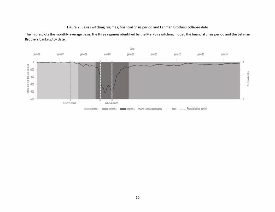
50

Figure 2: Basis switching regimes, financial crisis period and Lehman Brothers collapse date

The figure plots the monthly average basis, the three regimes identified by the Markov switching model, the financial crisis period and the Lehman Brothers bankruptcy date.

The CDS-bond Basis: Negativity Persistence and Limits to ...

Documents

Transcript of The CDS-bond Basis: Negativity Persistence and Limits to ...