The Casimir effect: Recent controversies and progress - arXiv

arX

iv:h

ep-t

h/04

0602

4v1

2 J

un 2

004

REVIEW ARTICLE

The Casimir effect: Recent controversies and

progress

Kimball A. Milton

Oklahoma Center for High Energy Physics and Department of Physics and

Astronomy, The University of Oklahoma, Norman, OK 73019 USA

E-mail: [email protected]

Abstract. The phenomena implied by the existence of quantum vacuum fluctuations,

grouped under the title of the Casimir effect, are reviewed, with emphasis on new

results discovered in the past four years. The Casimir force between parallel plates is

rederived as the strong-coupling limit of δ-function potential planes. The role of surface

divergences is clarified. A summary of effects relevant to measurements of the Casimir

force between real materials is given, starting from a geometrical optics derivation of

the Lifshitz formula, and including a rederivation of the Casimir-Polder forces. A great

deal of attention is given to the recent controversy concerning temperature corrections

to the Casimir force between real metal surfaces. A summary of new improvements

to the proximity force approximation is given, followed by a synopsis of the current

experimental situation. New results on Casimir self-stress are reported, again based

on δ-function potentials. Progress in understanding divergences in the self-stress of

dielectric bodies is described, in particular the status of a continuing calculation of the

self-stress of a dielectric cylinder. Casimir effects for solitons, and the status of the

so-called dynamical Casimir effect, are summarized. The possibilities of understanding

dark energy, strongly constrained by both cosmological and terrestrial experiments, in

terms of quantum fluctuations are discussed. Throughout, the centrality of quantum

vacuum energy in fundamental physics in emphasized.

PACS numbers: 11.10.Gh, 11.10.Wx, 42.50.Pq, 78.20.Ci

http://arxiv.org/abs/hep-th/0406024v1

The Casimir Effect 2

1. Introduction

The essence of quantum physics is fluctuations. That is, knowing the position of a

particle precisely means losing all knowledge about its momentum, and vice versa, and

generally the product of uncertainties of a generalized coordinate q and its corresponding

momentum p is bounded below:

∆q∆p ≥ ~

2, (1.1)

which reflects the fundamental commutation relation

[q, p] = i~. (1.2)

The Hamiltonian commutes with neither q nor p in general; this means that in an energy

eigenstate the fluctuations in q and p are both nonzero:

∆q > 0, ∆p > 0. (1.3)

Moreover, a harmonic oscillator has correspondingly a ground-state energy which is

nonzero:

Eho,n = ~ω

(

n +1

2

)

. (1.4)

The apparent implication of this is that a crystal, which may be thought of, roughly, as

a collection of atoms held in harmonic potentials, should have a large zero-point energy

at zero temperature:

EZP =∑

atoms

1

2~ω, (1.5)

ω being the characteristic frequency of each potential.

The vacuum of quantum field theory may similarly be regarded as an enormously

large collection of harmonic oscillators, representing the fluctuations of, for quantum

electrodynamics, the electric and magnetic fields at each point in space. (Canonically,

the momentum-coordinate pair correspond to the electric field and the vector potential.)

Put otherwise, the QED vacuum is a sea of virtual photons. Thus the zero-point energy

density of the vacuum is

U =∑ 1

2~ω = 2

∫

(dk)

(2π)31

2~c|k|, (1.6)

where k is the wavevector of the photon, and the factor of 2 reflects the two polarization

states of the photon.

This is an enormously large quantity. If we say that the largest wavevector

appearing in the integral is K, say ~cK ∼ 1019 GeV, the Planck scale, then U ∼ 10115

GeV/cm3. So it is no surprise that Dirac suggested that this zero-point energy be simply

discarded, as some irrelevant constant [1] (yet he became increasingly concerned about

the inconsistency of doing so throughout his life [2]). Pauli recognized that this energy

surely coupled to gravity, and it would then give rise to a large cosmological constant,

so large that the size of the universe could not even reach the distance to the moon


[3, 4]. This cosmological constant problem is with us to the present [5, 6]. But this was

not the most perplexing issue confronting quantum electrodynamics in the 1930s.

Renormalization theory, that is, a consistent theory of quantum electrodynamics,

was invented first by Schwinger [7] and then Feynman [8] in 1948; yet remarkably,

across the Atlantic, Casimir in the same year predicted the direct macroscopically

observable consequence of vacuum fluctuations that now bears his name [9]. This is the

attraction between parallel uncharged conducting plates that has been so convincingly

demonstrated by many experiments in the last few years [10]. Lifshitz and his group

generalized the theory to include dielectric materials in the 1950s [11, 12, 13, 14]. There

were many experiments to detect the effect in the 1950s and 1960s, but most were

inconclusive, because the forces were so small, and it was very difficult to keep various

interfering phenomena from washing out the effect [15]. However, there could be very

little doubt of the reality of the phenomenon, since it was intimately tied to the theory of

van der Waals forces between molecules, the retarded version of which had been worked

out by Casimir [16] just before he discovered (with a nudge from Bohr [17]) the force

between plates. Finally, in 1973, the Lifshitz theory was vindicated by an experiment

by Sabisky and Anderson [18].

But by and large field theorists were unaware of the effect until Glashow’s student

Boyer carried out a remarkable calculation of the Casimir self-energy of a perfectly

conducting spherical shell in 1968 [19]. Glashow was aware of Casimir’s proposal [20]

that a classical electron could be stablized by zero-point attraction, and thought the

calculation made a suitable thesis project. Boyer’s result was a surprise: The zero-

point force was repulsive for the case of a sphere. Davies improved on the calculation

[21]; then a decade later there were two independent reconfirmations of Boyer’s result,

one based on multiple scattering techniques [22] (now undergoing a renaissance, for

example, see [23]) and one on Green’s functions techniques [24] (dubbed source theory

[25]). Applications to hadronic physics followed in the next few years [26, 27, 28], and

in the last two decades, there has been something of an explosion of interest in the field,

with many different calculations being carried out [29, 10].

However, fundamental understanding has been very slow in coming. Why is the

cosmological constant neither large nor zero? Why is the Casimir force on a sphere

repulsive, when it is attractive between two plates? And is it possible to make sense of

Casimir force calculations between two bodies, or of the Casimir self-energy of a single

body, in terms of supposedly better understood techniques of perturbative quantum

field theory [30]? As we will see, none of these questions yet has a definitive answer, yet

progress has been coming. Even the temperature corrections to the Casimir effect, which

were considered by Sauer [31], Mehra [32], and Lifshitz [11] in the 1950s and 1960s, have

become controversial [33, 34, 35, 36, 37, 38, 39, 40, 41, 42, 43, 44, 45, 46, 47]. Thus

recent conferences on the Casimir effect have been quite exciting events [48, 49]. It is

the aim of the present review to bring the various issues into focus, and suggest paths

toward the solutions of the difficulties. It is a mark of the vitality and even centrality

of this field that such a review is desirable on the heels of two significant meetings on


the subject, and less than three years after the appearance of two major monographs

[10, 29] on Casimir phenomena. There are in addition a number of earlier, excellent

reviews [50, 51, 52], as well as more specialized treatments [53, 54, 55, 56]. Throughout

this review Gaussian units are employed.

This review is organized in the following manner. In section 2 we compute Casimir

energies and pressures between parallel δ function planes, which in the limit of large

coupling reproduce the results for a scalar field satisfying Dirichlet boundary conditions

on those surfaces. Although these results have been described before, clarification of the

nature of surface energy and divergences is provided. TM modes are also discussed here

for the first time. Then, in section 3 we rederive the Lifshitz formula for the Casimir

force between parallel dielectric slabs using a multiple reflection technique. The Casimir-

Polder forces between two atoms, and between an atom and a plate, are rederived.

After reviewing roughness and conductivity corrections, a detailed discussion of the

temperature controversy is given, with the conclusion that the TE zero-mode absence

must be taken seriously, which will imply that large temperature corrections should be

seen experimentally. New approaches to moving beyond the proximity approximation

in computing forces between nonparallel plane surface are reviewed. A discussion of the

remarkable progress experimentally since 1997 is provided. In section 4 after a review

of the general situation with respect to surface divergences, TE and TM forces on δ-

function spheres are described in detail, which in the limit of strong coupling reduce

to the corresponding finite electromagnetic contributions. For weak coupling, Casimir

energies are finite in second order in the coupling strength, but divergent in third order,

a fact which has been known for several years. This mirrors the corresponding result

for a dilute dielectric sphere, which diverges in third order in the deviation of the

permittivity from its vacuum value. Self-stresses on cylinders are also treated, with a

detailed discussion of the status of a new calculation for a dielectric cylinder, which

should give a vanishing self-stress in second order in the relative permittivity. Section 5

briefly summarizes recent work on quantum fluctuation phenomena in solitonic physics,

which has provided the underlying basis for much of the interest in Casimir phenomena

over the years. Dynamical Casimir effects, ranging from sonoluminescence through the

Unruh effect, are the subject of section 6. The presumed basis for understanding the

cosmological dark energy in terms of the Casimir fluctuations is treated in section 7,

where there may be a tight constraint emerging between terrestrial measurements of

deviations from Newtonian gravity and the size of extra dimensions. The review ends

with a summary of perspectives for the future of the field.

2. Casimir Effect Between Parallel Plates: A δ-Potential Derivation

In this section, we will rederive the classic Casimir result for the force between parallel

conducting plates [9]. Since the usual Green’s function derivation may be found in

monographs [29], and was recently reviewed in connection with current controversies

over finiteness of Casimir energies [57], we will here present a different approach, based


on δ-function potentials, which in the limit of strong coupling reduce to the appropriate

Dirichlet or Robin boundary conditions of a perfectly conducting surface, as appropriate

to TE and TM modes, respectively. Such potentials were first considered by the Leipzig

group [58, 59], but recently have been the focus of the program of the MIT group

[60, 61, 30]. The discussion here is based on a recent paper by the author [62]. We first

consider two δ-function potentials in 1 + 1 dimensions.

2.1. 1 + 1 dimensions

We consider a massive scalar field (mass µ) interacting with two δ-function potentials,

one at x = 0 and one at x = a, which has an interaction Lagrange density

Lint = −1

2

λ

aδ(x)φ2(x)− 1

2

λ′

aδ(x− a)φ2(x), (2.1)

where we have chosen the coupling constants λ and λ′ to be dimensionless. (But see

the following.) In the limit as both couplings become infinite, these potentials enforce

Dirichlet boundary conditions at the two points:

λ, λ′ →∞ : φ(0), φ(a)→ 0. (2.2)

The Casimir energy for this situation may be computed in terms of the Green’s

function G,

G(x, x′) = i〈Tφ(x)φ(x′)〉, (2.3)

which has a time Fourier transform,

G(x, x′) =

∫

dω

2πe−iω(t−t′)g(x, x′;ω). (2.4)

Actually, this is a somewhat symbolic expression, for the Feynman Green’s function (2.3)

implies that the frequency contour of integration here must pass below the singularities

in ω on the negative real axis, and above those on the positive real axis [63, 64]. The

reduced Green’s function in (2.4) in turn satisfies[

− ∂2

∂x2+ κ2 +

λ

aδ(x) +

λ′

aδ(x− a)

]

g(x, x′) = δ(x− x′). (2.5)

Here κ2 = µ2 − ω2. This equation is easily solved, with the result

g(x, x′) =1

2κe−κ|x−x′| +

1

2κ∆

[

λλ′

(2κa)22 cosh κ|x− x′|

− λ

2κa

(

1 +λ′

2κa

)

e2κae−κ(x+x′) − λ′

2κa

(

1 +λ

2κa

)

eκ(x+x′)

]

(2.6a)

for both fields inside, 0 < x, x′ < a, while if both field points are outside, a < x, x′,

g(x, x′) =1

2κe−κ|x−x′| +

1

2κ∆e−κ(x+x′−2a)

[

− λ

2κa

(

1− λ′

2κa

)

− λ′

2κa

(

1 +λ

2κa

)

e2κa]

.

(2.6b)


For x, x′ < 0,

g(x, x′) =1

2κe−κ|x−x′| +

1

2κ∆eκ(x+x′)

[

− λ′

2κa

(

1− λ

2κa

)

− λ

2κa

(

1 +λ′

2κa

)

e2κa]

.

(2.6c)

Here, the denominator is

∆ =

(

1 +λ

2κa

)(

1 +λ′

2κa

)

e2κa − λλ′

(2κa)2. (2.7)

Note that in the strong coupling limit we recover the familiar results, for example, inside

λ, λ′ →∞ : g(x, x′)→ −sinh κx< sinh κ(x> − a)

κ sinh κa. (2.8)

Evidently, this Green’s function vanishes at x = 0 and at x = a.

We can now calculate the force on one of the δ-function points by calculating the

discontinuity of the stress tensor, obtained from the Green’s function (2.3) by

〈T µν〉 =(

∂µ∂ν′ − 1

2gµν∂λ∂′

λ

)

1

iG(x, x′)

∣

∣

∣

x=x′

. (2.9)

Writing a reduced stress tensor by

〈T µν〉 =∫

dω

2πtµν , (2.10)

we find inside

txx =1

2i(ω2 + ∂x∂x′)g(x, x′)

∣

∣

∣

x=x′

=1

4iκ∆

(2ω2 − µ2)

[(

1 +λ

2κa

)(

1 +λ′

2κa

)

e2κa +λλ′

(2κa)2

]

− µ2

[

λ

2κa

(

1 +λ′

2κa

)

e−2κ(x−a) +λ′

2κa

(

1 +λ

2κa

)

e2κx]

. (2.11)

Let us henceforth simplify the considerations by taking the massless limit, µ = 0. Then

the stress tensor just to the left of the point x = a is

txx

∣

∣

∣

x=a−= − κ

2i

1 + 2

[(

2κa

λ+ 1

)(

2κa

λ′+ 1

)

e2κa − 1

]−1

. (2.12a)

From this we must subtract the stress just to the right of the point at x = a, obtained

from (2.6b), which turns out to be in the massless limit

txx

∣

∣

∣

x=a+= − κ

2i, (2.12b)

which just cancels the 1 in braces in (2.12a). Thus the force on the point x = a due to

the quantum fluctuations in the scalar field is given by the simple, finite expression

F = 〈Txx〉∣

∣

∣

x=a−− 〈Txx〉

∣

∣

∣

x=a+= − 1

4πa2

∫ ∞

0

dy y1

(y/λ+ 1)(y/λ′ + 1)ey − 1. (2.13)

This reduces to the well-known, Luscher result [65, 66] in the limit λ, λ′ →∞,

limλ=λ′→∞

F = − π

24a2, (2.14)


0.0 5.0 10.0 15.0 20.0λ

-0.15

-0.10

-0.05

Fa2

Figure 1. Casimir force (2.13) between two δ-function points having strength λ and

separated by a distance a.

and for λ = λ′ is plotted in Fig. 1.

Recently, Sundberg and Jaffe [67] have used their background field method to

calculate the Casimir force due to fermion fields between two δ-function spikes in 1 + 1

dimension. Apart from quibbles about infinite energies, in the limit λ→∞ they recover

the same result as for scalar, (2.14), which is as expected [68], since in the ideal limit the

relative factor between scalar and spinor energies is 2(1−2−D) in D spatial dimensions,

i.e., 7/4 for three dimensions and 1 for one.

We can also compute the energy density. In this simple massless case, the

calculation appears identical, because txx = t00 (reflecting the conformal invariance

of the free theory). The energy density is constant [(2.11) with µ = 0] and subtracting

from it the a-independent part that would be present if no potential were present, we

immediate see that the total energy is E = Fa, so F = −∂E/∂a. This result differs

significantly from that given in Refs. [61, 60, 69], which is a divergent expression in

the massless limit, not transformable into the expression found by this naive procedure.

However, that result may be easily derived from the following expression for the total

energy,

E =

∫

(dr) 〈T 00〉 = 1

2i

∫

(dr)(∂0∂′0 −∇2)G(x, x′)∣

∣

∣

x=x′

=1

2i

∫

(dr)

∫

dω

2π2ω2G(r, r), (2.15)

if we integrate by parts and omit the surface term. Integrating over the Green’s functions

in the three regions, given by (2.6a), (2.6b), and (2.6c), we obtain for λ = λ′,

E =1

2πa

∫ ∞

0

dy1

1 + y/λ− 1

4πa

∫ ∞

0

dy y1 + 2/(y + λ)

(y/λ+ 1)2ey − 1, (2.16)


where the first term is regarded as an irrelevant constant (λ/a is constant), and the

second is the same as that given by equation (70) of Ref. [60] upon integration by parts.

The origin of this discrepancy with the naive energy is the existence of a surface

contribution to the energy. Because ∂µTµν = 0, we have, for a region V bounded by a

surface S,

0 =d

dt

∫

V

(dr)T 00 +

∮

S

dSiT0i. (2.17)

Here T 0i = ∂0φ∂iφ, so we conclude that there is an additional contribution to the energy,

Es = −1

2i

∫

dS ·∇G(x, x′)∣

∣

∣

x′=x(2.18a)

= − 1

2i

∫ ∞

−∞

dω

2π

∑ d

dxg(x, x′)

∣

∣

∣

x′=x, (2.18b)

where the derivative is taken at the boundaries (here x = 0, a) in the sense of the outward

normal from the region in question. When this surface term is taken into account the

extra terms in (2.16) are supplied. The integrated formula (2.15) automatically builds in

this surface contribution, as the implicit surface term in the integration by parts. (These

terms are slightly unfamiliar because they do not arise in cases of Neumann or Dirichlet

boundary conditions.) See Fulling [70] for further discussion. That the surface energy

of an interface arises from the volume energy of a smoothed interface is demonstrated

in Ref. [62], and elaborated in section 2.4.

It is interesting to consider the behavior of the force or energy for small coupling

λ. It is clear that, in fact, (2.13) is not analytic at λ = 0. (This reflects an infrared

divergence in the Feynman diagram calculation.) If we expand out the leading λ2 term

we are left with a divergent integral. A correct asymptotic evaluation leads to the

behavior

F ∼ λ2

4πa2(ln 2λ+ γ) , E ∼ − λ2

4πa(ln 2λ+ γ − 1), λ→ 0. (2.19)

This behavior indeed was anticipated in earlier perturbative analyses. In Ref. [57] the

general result was given for the Casimir energy for a D dimensional spherical δ-function

potential (a factor of 1/4π was inadvertently omitted)

E = −λ2

πa

Γ(

D−12

)

Γ(D − 3/2)Γ(1−D/2)

21+2D[Γ(D/2)]2. (2.20)

This possesses an infrared divergence as D → 1:

E(D=1) =λ2

4πaΓ(0), (2.21)

which is consistent with the nonanalytic behavior seen in (2.19).

2.2. Parallel Planes in 3 + 1 Dimensions

It is trivial to extract the expression for the Casimir pressure between two δ function

planes in three spatial dimensions, where the background lies at x = 0 and x = a. We


merely have to insert into the above a transverse momentum transform,

G(x, x′) =

∫

dω

2πe−iω(t−t′)

∫

(dk)

(2π)2eik·(r−r′)⊥g(x, x′; κ), (2.22)

where now κ2 = µ2 + k2 − ω2. Then g has exactly the same form as in (2.6a)–(2.6c).

The reduced stress tensor is given by, for the massless case,

txx =1

2(∂x∂x′ − κ2)

1

ig(x, x′)

∣

∣

∣

x=x′

, (2.23)

so we immediately see that the attractive pressure on the planes is given by (λ = λ′)

P = − 1

32π2a4

∫ ∞

0

dy y31

(y/λ+ 1)2ey − 1, (2.24)

which coincides with the result given in Refs. [30, 71]. The leading behavior for small λ

is

PTE ∼ − λ2

32π2a4, λ≪ 1, (2.25a)

while for large λ it approaches half of Casimir’s result [9] for perfectly conducting parallel

plates,

PTE ∼ − π2

480a4, λ≫ 1. (2.25b)

The Casimir energy per unit area again might be expected to be

E = − 1

96π2a3

∫ ∞

0

dyy3

(y/λ+ 1)2ey − 1=

1

3

P

a, (2.26)

because then P = − ∂∂aE . In fact, however, it is straightforward to compute the energy

density 〈T 00〉 is the three regions, x < 0, 0 < x < a, and a < x, and then integrate it

over x to obtain the energy/area, which differs from (2.26) because, now, there exists

transverse momentum. We also must include the surface term (2.18a), which is of

opposite sign, and of double magnitude, to the k2 term. The net extra term is

E ′ = 1

48π2a3

∫ ∞

0

dy y21

1 + y/λ

[

1− y/λ

(y/λ+ 1)2ey − 1

]

. (2.27)

If we regard λ/a as constant (so that the strength of the coupling is independent of the

separation between the planes) we may drop the first, divergent term here as irrelevant,

being independent of a, because y = 2κa, and then the total energy is

E = − 1

96π2a3

∫ ∞

0

dy y31 + 2/(λ+ y)

(y/λ+ 1)2ey − 1, (2.28)

which coincides with the massless limit of the energy first found by Bordag et al [58],

and given in Refs. [30, 71]. As noted in section 2.1, this result may also readily be

derived through use of (2.15). When differentiated with respect to a, (2.28), with λ/a

fixed, yields the pressure (2.24).

In the limit of strong coupling, we obtain

limλ→∞E = − π2

1440a3, (2.29)

which is exactly one-half the energy found by Casimir for perfectly conducting plates [9].

Evidently, in this case, the TE modes (calculated here) and the TM modes (calculated

in the following subsection) give equal contributions.


2.3. TM Modes

To verify this claim, we solve a similar problem with boundary conditions that the

derivative of g is continuous at x = 0 and a,

∂

∂xg(x, x′)

∣

∣

∣

x=0,ais continuous, (2.30a)

but the function itself is discontinuous,

g(x, x′)∣

∣

∣

x=a+

x=a−= λa

∂

∂xg(x, x′)

∣

∣

∣

x=a, (2.30b)

and similarly at x = 0. These boundary conditions reduce, in the limit of

strong coupling, to Neumann boundary conditions on the planes, appropriate to

electromagnetic TM modes:

λ→∞ :∂

∂xg(x, x′)

∣

∣

∣

x=0,a= 0. (2.30c)

It is completely straightforward to work out the reduced Green’s function in this

case. When both points are between the planes, 0 < x, x′ < a,

g(x, x′) =1

2κe−κ|x−x′| +

1

2κ∆

(

λκa

2

)2

2 cosh κ(x− x′)

+λκa

2

(

1 +λκa

2

)

[

eκ(x+x′) + e−κ(x+x′−2a)]

, (2.31a)

while if both points are outside the planes, a < x, x′,

g(x, x′) =1

2κe−κ|x−x′|

+1

2κ∆

λκa

2e−κ(x+x′−2a)

[(

1− λκa

2

)

+

(

1 +λκa

2

)

e2κa]

, (2.31b)

where the denominator is

∆ =

(

1 +λκa

2

)2

e2κa −(

λκa

2

)2

. (2.32)

It is easy to check that in the strong-coupling limit, the appropriate Neumann

boundary condition (2.30c) is recovered. For example, in the interior region, 0 < x, x′ <

a,

limλ→∞

g(x, x′) =cosh κx< cosh κ(x> − a)

κ sinh κa. (2.33)

Now we can compute the pressure on the plane by computing the xx component of

the stress tensor, which is given by (2.23),

txx =1

2i(−κ2 + ∂x∂

′x)g(x, x

′)∣

∣

∣

x=x′

. (2.34)

The action of derivatives on exponentials is very simple, so we find

txx

∣

∣

∣

x=a−=

1

2i

[

−κ− 2κ

∆

(

λκa

2

)2]

, (2.35a)

txx

∣

∣

∣

x=a+= − 1

2iκ, (2.35b)


0.0 20.0 40.0 60.0 80.0 100.0λ

-0.020

-0.015

-0.010

-0.005

0.000

P a

4

P TE

P TM

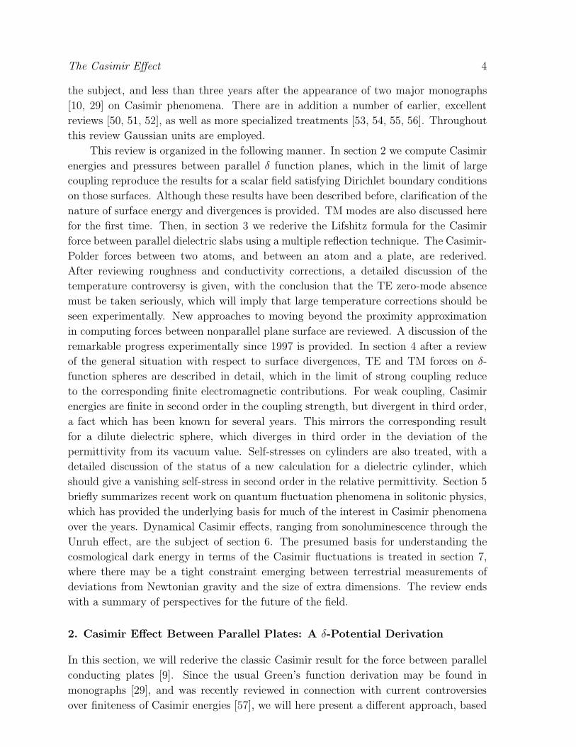
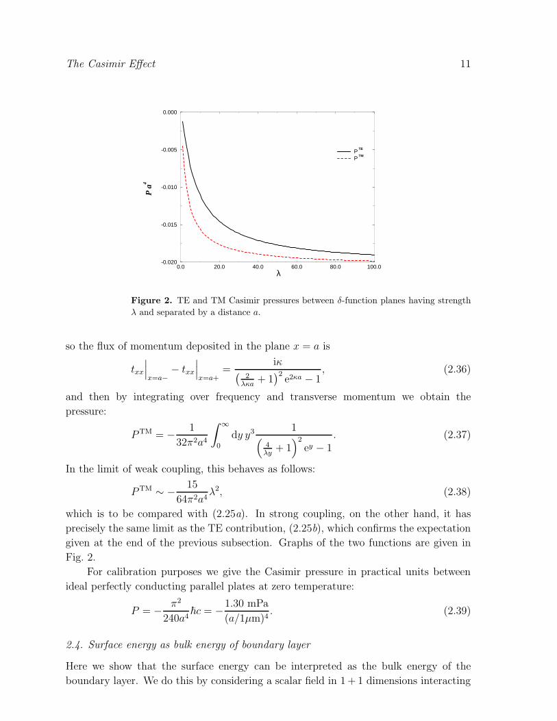
Figure 2. TE and TM Casimir pressures between δ-function planes having strength

λ and separated by a distance a.

so the flux of momentum deposited in the plane x = a is

txx

∣

∣

∣

x=a−− txx

∣

∣

∣

x=a+=

iκ(

2λκa

+ 1)2

e2κa − 1, (2.36)

and then by integrating over frequency and transverse momentum we obtain the

pressure:

PTM = − 1

32π2a4

∫ ∞

0

dy y31

(

4λy

+ 1)2

ey − 1. (2.37)

In the limit of weak coupling, this behaves as follows:

PTM ∼ − 15

64π2a4λ2, (2.38)

which is to be compared with (2.25a). In strong coupling, on the other hand, it has

precisely the same limit as the TE contribution, (2.25b), which confirms the expectation

given at the end of the previous subsection. Graphs of the two functions are given in

Fig. 2.

For calibration purposes we give the Casimir pressure in practical units between

ideal perfectly conducting parallel plates at zero temperature:

P = − π2

240a4~c = −1.30 mPa

(a/1µm)4. (2.39)

2.4. Surface energy as bulk energy of boundary layer

Here we show that the surface energy can be interpreted as the bulk energy of the

boundary layer. We do this by considering a scalar field in 1+ 1 dimensions interacting


with the background

Lint = −λ

2φ2σ, (2.40)

where

σ(x) =

h, − δ2< x < δ

2,

0, otherwise,(2.41)

with the property that hδ = 1. The reduced Green’s function satisfies[

− ∂2

∂x2+ κ2 + λσ(x)

]

g(x, x′) = δ(x− x′). (2.42)

This may be easily solved in the region of the slab, − δ2< x < δ

2,

g(x, x′) =1

2κ′

e−κ′|x−x′| +1

∆

[

(κ′2 − κ2) cosh κ′(x+ x′)

+ (κ′ − κ)2e−κ′δ cosh κ′(x− x′)]

. (2.43)

Here κ′ =√κ2 + λh, and

∆ = 2κκ′ cosh κ′δ + (κ2 + κ′2) sinh κ′δ. (2.44)

This result may also easily be derived from the multiple reflection formulas given in

section 3.1, and agrees with that given by Graham and Olum [72]. The energy of the

slab now is obtained by integrating the energy density

t00 =1

2i(ω2 + ∂x∂x′ + λh)g

∣

∣

∣

x=x′

(2.45)

over frequency and the width of the slab. This gives the vacuum energy of the slab

Es =1

2

∫ ∞

−∞

dκ

2π

1

2κ′∆

[

(κ′ − κ)2(−κ2 − κ′2 + λh)e−κ′δδ

+ (κ′2 − κ2)(−κ2 + κ′2 + λh )sinh κ′δ

δ

]

. (2.46)

If we now take the limit δ → 0 and h→∞ so that hδ = 1, we immediately obtain

Es =1

2π

∫ ∞

0

dκλ

λ+ 2κ, (2.47)

which precisely coincides with one-half the constant term in (2.16), with λ there replaced

by λa here.

There is no surface term in the total Casimir energy as long as the slab is of finite

width, because we may easily check that ddxg|x=x′ is continuous at the boundaries ± δ

2.

However, if we only consider the energy internal to the slab we encounter not only the

energy (2.15) but a surface term from the integration by parts. It is only this boundary

term that gives rise to Es, (2.47), in this way of proceeding.

Further insight is provided by examining the local energy density. In this we

follow the work of Graham and Olum [72, 73]. However, let us proceed here with

more generality, and consider the stress tensor with an arbitrary conformal term,

T µν = ∂µφ∂νφ− 1

2gµν(∂λφ∂

λφ+ λhφ2)− α(∂µ∂ν − gµν∂2)φ2, (2.48)


in d + 2 dimensions, d being the number of transverse dimensions. Applying the

corresponding differential operator to the Green’s function (2.43), introducing polar

coordinates in the (ζ, k) plane, with ζ = κ cos θ, k = κ sin θ, and

〈sin2 θ〉 = d

d+ 1, (2.49)

we get the following form for the energy density within the slab,

T 00 =2−d−2π−(d+1)/2

Γ((d+ 3)/2)

∫ ∞

0

dκ κd

κ′∆

(κ′2 − κ2)[

(1− 4α)(1 + d)κ′2 − κ2]

cosh 2κ′x

− (κ′ − κ)2e−κ′δκ2

. (2.50)

From this we can calculate the behavior of the energy density as the boundary is

approached from the inside:

T 00 ∼ Γ(d+ 1)λh

2d+4π(d+1)/2Γ((d+ 3)/2)

1− 4α(d+ 1)/d

(δ − 2|x|)d , |x| → δ/2. (2.51)

For d = 2 for example, this agrees with the result found in Ref. [72] for α = 0:

T 00 ∼ λh

96π2

(1− 6α)

(δ/2− |x|)d , |x| → δ

2. (2.52)

Note that, as we expect, this surface divergence vanishes for the conformal stress tensor

[74], where α = d/4(d+ 1). (There will be subleading divergences if d > 2.)

We can also calculate the energy density on the other side of the boundary, from

the Green’s function for x, x′ < −δ/2,

g(x, x′) =1

2κ

[

e−κ|x−x′| − eκ(x+x′+δ)(κ′2 − κ2)sinh κ′δ

∆

]

, (2.53)

and the corresponding energy density is given by

T 00 = − d(1− 4α(d+ 1)/d)

2d+2π(d+1)/2Γ((d+ 3)/2)

∫ ∞

0

dκ κd+1 1

∆(κ′2 − κ2)e2κ(x+δ/2) sinh κ′δ, (2.54)

which vanishes if the conformal value of α is used. The divergent term, as x → −δ/2,is just the negative of that found in (2.51). This is why, when the total energy is

computed by integrating the energy density, it is finite for d < 2, and independent of

α. The divergence encountered for d = 2 may be handled by renormalization of the

interaction potential [72]. In the limit as h → ∞, hδ = 1, we recover the divergent

expression (2.47) for d = 0, or in general

limh→∞

Es =1

2d+2π(d+1)/2Γ((d+ 3)/2)

∫ ∞

0

dκ κd λ

λ+ 2κ. (2.55)

Therefore, surface divergences have an illusory character.

For further discussion on surface divergences, see section 4.1.


3. Casimir Effect Between Real Materials

3.1. The Lifshitz Formula Revisited

As a prolegomena to the derivation of the Lifshitz formula for the Casimir force between

parallel dielectric slabs, let us note that the results in the previous section may be easily

derived geometrically, in terms of multiple reflections. Suppose we have translational

invariance in the y and z directions, so in terms of reduced Green’s functions, everything

is one-dimensional. Suppose at x = 0 and x = a we have discontinuities giving rise to

reflection and transmission coefficients. That is, if we only had the x = 0 interface, the

reduced Green’s function would have the form

g(x, x′) =1

2κ

(

e−κ|x−x′| + re−κ(x+x′))

, (3.1a)

for x, x′ > 0, while for x′ > 0 > x,

g(x, x′) =1

2κte−κ(x′−x). (3.1b)

Similarly, if we only had the interface at x = a, we would have similarly defined reflection

and transmission coefficients r′ and t′. Transmission and reflection coefficients defined

for a wave incident from the left instead of the right will be denoted with tildes. If both

interfaces are present, we can calculate the Green’s function in the region to the right

of the rightmost interface x, x′ > a in the form

g(x, x′) =1

2κ

(

e−κ|x−x′| +Re−κ(x+x′−2a))

, (3.2a)

where R may be easily computed by summing multiple reflections:

R = r′ + t′e−κare−κat′ + t′e−κare−κar′e−κare−κat′ + . . .

= r′ +rt′t′

e2κa − rr′. (3.2b)

For the TE δ-function potential (2.1), r = r = −(1+2κa/λ)−1, and t = t = 1+r, and we

immediately recover the result (2.6b). But the same formula applies to electromagnetic

modes in a dielectric medium with two parallel interfaces, where the permittivity is

ε(x) =

ε1, x < 0,

ε3, 0 < x < a,

ε2, a < x.

. (3.3)

In that case [75]

r =κ3 − κ1

κ3 + κ1, r′ =

κ2 − κ3

κ2 + κ3, r′ = −r′, (3.4a)

and

t′ = 1 + r′, t′ = 1− r′, (3.4b)

where κ2i = k2 − ω2ǫi. Substituting these expressions into (3.2b) we obtain

R =κ2 − κ3

κ2 + κ3+

4κ2κ3

κ23 − κ2

2

1κ3+κ1

κ3−κ1

κ3+κ2

κ3−κ2

e2κ3a − 1, (3.5)


which coincides with the formula (3.16) given in Ref. [29].

However, to calculate most readily the force between the slabs, we need the

corresponding formula for the reduced Green’s function between the interfaces. This

may also be readily derived by multiple reflections:

g(x, x′) =1

2κ

[

e−κ|x−x′| + r′e−κ(2a−x−x′) + rr′e−κ(2a−x′+x) + rr′2e−κ(4a−x−x′)

+ r2r′2e−κ(4a+x−x′) + . . .

+ re−κ(x′+x) + rr′e−κ(2a+x′−x) + r2r′e−κ(2a+x′+x) + r2r′2e−κ(4a+x′−x) + . . .]

=1

2κ

e−κ|x−x′| +1

e2κa − rr′

[

2rr′ cosh κ(x− x′) + r′eκ(x+x′) + re−κ(x+x′−2a)]

.

(3.6)

Indeed, this reduces to (2.6a) when the appropriate reflection coefficients are inserted.

The pressure on the planes may be computed from the discontinuity in the stress tensor,

or

txx

∣

∣

∣

x=a−− txx

∣

∣

∣

x=a+=

1

2i(−κ2 + ∂x∂x′)g(x, x′)

∣

∣

∣

x=x′=a−

x=x′=a+=

iκ1r1r′e2κa − 1

, (3.7)

from which the δ-potential results (2.12a) and (2.12b) follow immediately. For the case

of parallel dielectric slabs the TE modes therefore contribute the following expression

for the pressure‡:

PTE =

∫ ∞

−∞

dω

2π

∫

(dk)

(2π)2iκ3

κ3+κ2

κ3−κ2

κ3+κ1

κ3−κ1

e2κ3a − 1. (3.8)

The contribution from the TM modes are obtained by the replacement

κ→ κ′ =κ

ε, (3.9)

except in the exponentials [75]. This gives for the force per unit area at zero temperature

P T=0Casimir = −

1

4π2

∫ ∞

0

dζ

∫ ∞

0

dk2 κ3

(

d−1 + d′−1)

, (3.10)

with the denominators here being [κi =√

k2 + ζ2εi(iζ)]

d =κ3 + κ1

κ3 − κ1

κ3 + κ2

κ3 − κ2e2κ3a − 1, d′ =

κ′3 + κ′

1

κ′3 − κ′

1

κ′3 + κ′

2

κ′3 − κ′

2

e2κ3a − 1, (3.11)

which correspond to the TE and TM Green’s functions, respectively. This is the

celebrated Lifshitz formula [11, 12, 13, 14], which we shall discuss further in the following

subsections. We merely note here that if we take the limit ε1,2 →∞, and set ε3 = 1, we

recover Casimir’s result for the attractive force between parallel, perfectly conducting

plates (2.39).

Henkel et al [76] have computed the Casimir force at short distances (∼ 1 nm) from

interactions between polaritons. Their result agrees with the Lifshitz formula with the

plasma formula (3.33) employed, see Ref. [77, 78].

‡ For the case of dielectric slabs, the propagation constant κ is different on the two sides; we omit the

term corresponding to the free propagator, however. In the energy, the omitted terms are proportional

to the volume of each slab, and therefore correspond to the volume or bulk energy of the material.


3.2. The Relation to van der Waals Forces

Now suppose the central slab consists of a tenuous medium and the surrounding medium

is vacuum, so that the dielectric constant in the slab differs only slightly from unity,

ǫ− 1≪ 1. (3.12)

Then, with a simple change of variable,

κ = ζp, (3.13)

we can recast the Lifshitz formula (3.10) into the form

P ≈ − 1

32π2

∫ ∞

0

dζ ζ3[ε(ζ)− 1]2∫ ∞

1

dp

p2[(2p2 − 1)2 + 1]e−2ζpa. (3.14)

If the separation of the surfaces is large compared to the wavelength characterizing ε,

aζc ≫ 1, we can disregard the frequency dependence of the dielectric constant, and we

find

P ≈ −23(ε− 1)2

640π2a4. (3.15)

For short distances, aζc ≪ 1, the approximation is

P ≈ − 1

32π2

1

a3

∫ ∞

0

dζ(ε(ζ)− 1)2. (3.16)

These formulas are identical with the well-known forces found for the complementary

geometry in Ref. [79].

Now we wish to obtain these results from the sum of van der Waals forces, derivable

from a potential of the form

V = −B

rγ. (3.17)

We do this by computing the energy (N = density of molecules)

E = −12BN 2

∫ a

0

dz

∫ a

0

dz′∫

(dr⊥)(dr′⊥)

1

[(r⊥ − r′⊥)2 + (z − z′)2]γ/2

.(3.18)

If we disregard the infinite self-interaction terms (analogous to dropping the volume

energy terms in the Casimir calculation), we get [79, 80]

P = − ∂

∂a

E

A= − 2πBN 2

(2− γ)(3− γ)

1

aγ−3. (3.19)

So then, upon comparison with (3.15), we set γ = 7 and in terms of the polarizability,

α =ε− 1

4πN , (3.20)

we find

B =23

4πα2, (3.21)

or, equivalently, we recover the retarded dispersion potential of Casimir and Polder [16],

V = −23

4π

α2

r7, (3.22)


whereas for short distances we recover from (3.16) the London potential [81],

V = −3

π

1

r6

∫ ∞

0

dζ α(ζ)2. (3.23)

Recent, nonperturbative approaches to Casimir-Polder forces include that of

Buhmann et al [82].

3.2.1. Force Between a Molecule and a Plate One can also calculate the force between

a polarizable molecule, with electric polarizability α(ω), and a dielectric slab. A simple,

gauge-invariant way of doing this starts from the variational form [79, 29]

δW = −∫ ∞

−∞

dt δE = − i

2

∫

(dx)δε(x)Γkk(x, x), (3.24)

where δε(r) = 4πα(ω)δ(r −R), R denoting the position of the molecule. Here Γ is the

electromagnetic Green’s dyadic, defined by

Γ(r, r′) = i〈E(r)E(r′)〉. (3.25)

In terms of the reduced Green’s function, defined by (2.22), then

δE =i

24π

∫

dω

2π

d2k

(2π)2α(ω)gkk(x, x;ω,k). (3.26)

It is easily seen how the trace of the reduced Green’s function can be expressed in terms

of the reduced TE and TM Green’s functions,

gkk =

(

ω2gTE +k2

εε′gTM +

1

ε

∂

∂x

1

ε′∂

∂x′gTM

) ∣

∣

∣

∣

x=x′

. (3.27)

For a single interface, the Green’s functions to the right of a dielectric slab situated in

the half-space x < 0 are given by (3.1a) with the reflection coefficients in the vacuum

rTE =κ− κ1

κ+ κ1, rTM =

κ− κ1/ε1κ+ κ1/ε1

, (3.28)

where κ2 = k2 + ζ2 and κ21 = k2 + ζ2ε1. In this way, we immediately obtain the energy

between a dielectric slab (permittivity ε1) and a polarizable molecule a distance Z from

it:

Eslab,mol = −1

16π2

∫ ∞

0

dζ4πα(ζ)

∫ ∞

0

dk2 1

κe−2κZ

[

−ζ2κ− κ1

κ+ κ1+ (2k2 + ζ2)

ε1κ− κ1

ε1κ+ κ1

]

.

(3.29)

If the separation between the plate and the molecule is large, we expect that we may

neglect the frequency dependence of the polarizability, α(ζ) → α(0). There are then

two simple limits. If we take ε1 →∞ we are describing a perfectly conducting plane, in

which case we immediately obtain the result first given by Casimir and Polder [16]

Emetal,mol = −3α(0)

8πZ4. (3.30)

On the other hand, we could consider a tenuous medium, (ε1 − 1)≪ 1, in which case

Edilute,mol = −23

160π

α(0)(ε1 − 1)

Z4. (3.31)


The latter should be, as in the previous subsection, interpretable as the sum of

pairwise van der Waals interactions between the external molecule and the molecules

which make up the slab, given by the Casimir-Polder interaction (3.22). The net energy

then is

− 23

4παN

∫ ∞

Z

dz

∫ ∞

0

dρ ρ

∫ 2π

0

dφα(0)

(z2 + ρ2)7/2= −23

4παN 2π

20

α(0)

Z4, (3.32)

which coincides with (3.31) when (3.20) is used.

The force between a molecule and a plate has been measured by Sukenik et al. [83],

who actually verified the force between a molecule and two plates [84] at the roughly 10%

level. Recently, this result has been questioned (at about the same level of accuracy) by

Bordag [85], who argued that a subtle error involving the quantization of gauge fields in

the presence of boundaries was made by Casimir and Polder [16] and subsequent workers.

The fact that the result can be given an unambiguous gauge-invariant derivation, and

that it is closely related to the Lifshitz formula and the retarded dispersion van der

Waals force suggests that this critique is invalid. (Bordag now concedes that the usual

result is valid for “thick” plates, where the normal component of E is given by the

surface charge density.)

For a recent rederivation of (3.30) see Hu et al [86]. A very recent paper by Babb,

Klimchitskaya, and Mostepanenko [87] gives a rederivation of the Casimir-Polder energy

(3.30) in the retarded limit, and finds no support for Bordag’s modification. They then

go on to discuss the dynamical polarizability and thermal corrections for real materials,

and find substantial (35%) corrections at short distances ∼ 100 nm.

In this connection we might also mention the work of Noguez and Roman-

Velazquez [88], who calculate the force between a sphere and a plate made of dissimilar

materials in the non-retarded limit (see also van Kampen [89] and Gerlach [90]) in

terms of multipolar interactions. They find significant deviations from the proximity

approximation (section 3.5), which says that there is no difference between the force

between a sphere made of material A and a plate made of material B and the reversed

situation, when the separation is comparable or large compared to the radius of the

sphere, and that under the above-mentioned A-B interchange the forces change by up

to 6%. See also Ref. [91, 92].

Ford and Sopova [93, 94] consider Casimir forces between small metal spheres and

dielectric (and conducting) plates, modeled by a plasma dispersion relation

ε(ω) = 1− ω2p

ω2. (3.33)

The electric dipole approximation used requires aωp ≪ 1, that is, the radius of the

sphere a must be in the 10–100 nm range. The force is oscillatory, being alternatively

attractive and repulsive as a function of the height Z of the atom above the plate. Thus

levitation in the earth’s gravitational field might be possible, for Z ∼ 1 µm.


3.3. Roughness and Conductivity Corrections

3.3.1. Roughness Corrections No real material surface is completely smooth. Even

beyond the atomic level, there will be regions of higher and lower elevations. Insofar

as these are plateaus large compared to the separation between the disjoint surfaces,

the corrections can be easily incorporated by use of the proximity approximation (see

section 3.5 below). This is nothing other than the naively obvious statement that if

P (a) is the force per unit area between two parallel plates separated by a distance a,

the average force per area between rough surfaces made up of large plateaus and valleys,

with the perpendicular distance between two adjacent points on the two surfaces in terms

of transverse coordinates (x, y) being a(x, y), is

P =1

A

∫

dx dy P (a(x, y)). (3.34)

In Ref. [95], for example, an equivalent expression is used directly with data obtained by

topography of the surfaces using an atomic force microscope. Traditionally, a stochastic

estimate has been used. Let the separations a be distributed around the mean a0according to a Gaussian, with the probability of finding separation a being given by

p(a) =1√πδa

e−(a−a0)2/(δa)2 . (3.35)

We will assume δa≪ a0. Then, 〈a〉 = a0, 〈(a− a0)2〉 = 1

2(δa)2, and in general

〈aα〉 =∫ ∞

0

da aαp(a) =1√πδa

∫ ∞

−∞

da e−a2/(δa)2(a+ a0)α

= aα0

[

1 +α(α− 1)

2

1

2

(δa)2

a20+

α(α− 1)(α− 2)(α− 3)

4!

3

4

(δa)4

a40+ . . .

]

, (3.36)

The force between a sphere and a plate depends on the closest distance d between them

like d−3, see (3.78) below, so the stochastic estimate for the roughness correction in that

case, in terms of the mean-square fluctuation amplitude A = δa/√2, is

Fsph−pl,rough = Fsph−pl

[

1 + 6

(

A

d

)2

+ 45

(

A

d

)4

+ . . .

]

. (3.37)

A much more detailed discussion may be found in Ref. [10]. It must be appreciated that

the approximate treatment based on the proximity approximation is invalid for short

wavelength deformations [96].

3.3.2. Finite Conductivity Another interesting result, important for the recent

experiments [97, 98, 99, 100], is the correction for an imperfect conductor, where for

frequencies above the infrared, an adequate representation for the dielectric constant is

[75] that given by the plasma model (3.33) where the plasma frequency is, in Gaussian

units

ω2p =

4πe2N

m, (3.38)


where e and m are the charge and mass of the electron, and N is the number density

of free electrons in the conductor. A simple calculation shows, at zero temperature

[101, 79],

P ≈ − π2

240a4

[

1− 8

3√π

1

ea

(m

N

)1/2]

. (3.39)

If we define a penetration parameter, or skin depth, by δ = 1/ωp, we can write the force

per area for parallel plates out to fourth order as [102, 50, 103, 10]

P ≈ − π2

240a4

[

1− 16

3

δ

a+ 24

δ2

a2− 640

7

(

1− π2

210

)

δ3

a3+

2800

9

(

1− 163π2

7350

)

δ4

a4

]

, (3.40)

while using the proximity force theorem (see section 3.5), to convert pressures between

parallel plates to forces between a lens of radius R and a plate,

Fn−1 =2πR

n− 1aPn, (3.41)

for a term in the pressure going like Pn ∝ a−n, the force between a spherical surface

and a plate separated by a distance d is

F ≈ − π3R

360d3

[

1− 4δ

d+

72

5

δ2

d2− 320

7

(

1− π2

210

)

δ3

d3+

400

3

(

1− 163π2

7350

)

δ4

d4

]

. (3.42)

Lambrecht, Jaekel, and Reynaud [104] analyzed the Casimir force between mirrors

with arbitrary frequency-dependent reflectivity, and found that it is always smaller than

that between perfect reflectors.

We might also mention here the interesting suggestion that repulsive Casimir forces

might exist [105] between parallel plates. This harks back to an old suggestion of Boyer

[106], that repulsion will occur between two plates, one of which is a perfect electrical

conductor, ε→∞, and the other a perfect magnetic conductor, µ→∞,

P =7

8

π2

240

1

a4. (3.43)

However, it appears that it will prove very difficult to observe such effects in the

laboratory [107]. Klich [108] now seems to agree with this assessment.

3.4. Thermal Corrections

The discussion in this subsection is adapted from that in Refs. [109, 110]. We begin

by reviewing how temperature effects are incorporated into the expression for the

force between parallel dielectric (or conducting) plates separated by a distance a. To

obtain the finite temperature Casimir force from the zero-temperature expression, one

conventionally makes the following substitution in the imaginary frequency,

ζ → ζm =2πm

β, (3.44a)

and replaces the integral over frequencies by a sum,∫ ∞

−∞

dζ

2π→ 1

β

∞∑

m=−∞

. (3.44b)


This reflects the requirement that thermal Green’s functions be periodic in imaginary

time with period β [111]. Suppose we write the finite-temperature pressure as [for the

explicit form, see (3.10) and (3.58) below]

P T =

∞∑

m=0

′fm, (3.45)

where the prime on the summation sign means that the m = 0 term is counted with

half weight. To get the low temperature limit, one can use the Euler-Maclaurin (EM)

sum formula,∞∑

k=0

f(k) =

∫ ∞

0

f(k) dk +1

2f(0)−

∞∑

q=1

B2q

(2q)!f (2q−1)(0), (3.46)

where Bn is the nth Bernoulli number. This means here, with half-weight for the m = 0

term,

P T =

∫ ∞

0

f(m) dm−∞∑

k=1

B2k

(2k)!f (2k−1)(0). (3.47)

It is noteworthy that the terms involving f(0) cancel in (3.47). The reason for this is

that the EM formula equates an integral to its trapezoidal-rule approximation plus a

series of corrections; thus the 1/2 for m = 0 in (3.45) is built in automatically. For

perfectly conducting plates separated by vacuum [see the λ → ∞ limit of (2.24) or

(2.37), or the ε1,2 →∞ limit of (3.10) with ε3 = 1]

f(x) = − 2

πβ

∫ ∞

2πx/β

κ2 dκ1

e2κa − 1. (3.48)

Of course, the integral in (3.47) is just the inverse of the finite-temperature prescription

(3.44b), and gives the zero-temperature result. The only nonzero odd derivative

occurring is

f ′′′(0) = −16π2

β4, (3.49)

which gives a Stefan’s law type of term, seen in (3.53) below.

The problem is that the EM formula only applies if f(m) is continuous. If we follow

the argument of Ref. [35, 36, 44, 112], and take the ǫ1,2 →∞ limit of (3.10) at the end§(ǫ1,2 are the permittivities of the two parallel dielectric slabs), this is not the case, and

for the TE mode

f0 = 0, (3.50a)

fm = − ζ(3)

4πβa3, 0 <

2πam

β≪ 1. (3.50b)

Then we have to modify the argument as follows:

P T =

∞∑

m=0

′fm =

∞∑

m=1

fm =

∞∑

m=0

′fm −1

2f0, (3.51)

§ This is contrary to the “Schwinger” prescription advocated in Refs. [79, 29], in which the perfect-

conductor limit is taken before the zero-mode is extracted.


where fm is defined by continuity,

fm =

fm, m > 0,

limm→0 fm, m = 0.(3.52)

Then by using the EM formula,

P T =β

2π

∫ ∞

0

dζ f(ζ) +ζ(3)

8πβa3− π2

45

1

β4

= − π2

240a4

[

1 +16

3

(

a

β

)4]

+ζ(3)

8πa3T, aT ≪ 1. (3.53)

The same result for the low-temperature limit is extracted through use of the Poisson

sum formula, as, for example, discussed in Ref. [29]. Let us refer to these results, with

the TE zero mode excluded, as the modified ideal metal model (MIM). The conventional

result for an ideal metal (IM), obtained first by Lifshitz [11, 13] and by Sauer [31] and

Mehra [32], is given by (3.53) with the linear term in T omitted.

Exclusion of the TE zero mode will reduce the linear dependence at high

temperature by a factor of two,

P TIM ∼ −

ζ(3)

4πa3T, P T

MIM ∼ −ζ(3)

8πa3T, aT ≫ 1, (3.54)

but this is not observable by present experiments. The observable consequence, however,

is that it adds a linear term at low temperature, which is given in (3.53), up to

exponentially small corrections [29].

There are apparently two serious problems with the result (3.53):

• It would seem to be ruled out by experiment. The ratio of the linear term to the

T = 0 term is

∆ =30ζ(3)

π3aT = 1.16aT, (3.55a)

or putting in the numbers (300 K = (38.7)−1 eV, ~c = 197 MeV fm)

∆ = 0.15

(

T

300 K

)(

a

1µm

)

, (3.55b)

or as Klimchitskaya observed [113], there is a 15% effect at room temperature at

a separation of one micron. One would have expected this to have been been seen

by Lamoreaux [114]; his experiment was reported to be in agreement with the

conventional theoretical prediction at the level of 5%. (Lamoreaux [115] is now

proposing a new experiment to resolve this issue.)

• Another serious problem is the apparent thermodynamic inconsistency. A linear

term in the force implies a linear term in the free energy (per unit area),

F = F0 +ζ(3)

16πa2T, aT ≪ 1, (3.56)

which implies a nonzero contribution to the entropy/area at zero temperature:

S = −(

∂F

∂T

)

V

= − ζ(3)

16πa2. (3.57)


Taken at face value, this statement appears to be incorrect. We will discuss this problem

more closely in section 3.4.3, and will find that although a linear temperature dependence

will occur in the free energy at room temperature, the entropy will go to zero as the

temperature goes to zero. The point is that the free energy F for a finite ε always will

have a zero slope at T = 0, thus ensuring that S = 0 at T = 0. The apparent conflict

with (3.57) or (3.53) is due to the fact that the curvature of F (T ) near T = 0 becomes

infinite when ε → ∞. So (3.56) and (3.57), corresponding to the modified ideal metal

model, describe real metals approximately only for low, but not zero temperature – See

the following.

3.4.1. Lifshitz formula at nonzero temperature The Casimir surface pressure at finite

temperature P T between two dielectric plates separated by a distance a can be obtained

from the Lifshitz formula (3.10) by the prescription (3.44b)‖

P T = − 1

πβ

∞∑

m=0

′

∫ ∞

ζm

κ2dκ[

(

A−1m e2κa − 1

)−1+(

B−1m e2κa − 1

)−1]

. (3.58)

The relation between κ and the transverse wave vector k⊥ is κ2 = k2⊥ + ζ2m, where

ζm = 2πm/β. Furthermore, the squared reflection coefficients are

Am =

(

εp− s

εp+ s

)2

, Bm =

(

s− p

s+ p

)2

, (3.59a)

s2 = ε− 1 + p2, p =κ

ζm, (3.59b)

with ε(iζm) being the permittivity. Here, the first term in the square brackets in (3.58)

corresponds to TM modes, the second to TE modes. Note that whenever ε is constant,

Am and Bm depend on m and κ only in the combination p,

Am(κ) = A(p), Bm(κ) = B(p). (3.60)

The free energy F per unit area can be obtained from (3.58) by integration with

respect to a since P T = −∂F/∂a. We get [117]

βF =1

2π

∞∑

m=0

′

∫ ∞

ζm

κ dκ [ln(1− λTM) + ln(1− λTE)], (3.61a)

where

λTM = Ame−2κa, λTE = Bme

−2κa. (3.61b)

From thermodynamics the entropy S and internal energy U (both per unit area)

are related to F by F = U − TS, implying

S = −∂F∂T

, and thus U =∂(βF )

∂β. (3.62)

‖ A rederivation of the Casimir force between dissipative metallic mirrors at nonzero temperature has

been given by Reynaud, Lambrecht, and Genet [47]. They obtain formulas, generalizing those at zero

temperature [116], for the force valid even if the smoothness condition necessary for the derivation of

the Lifshitz formula is not satisfied due to the failure of the Poisson summation formula.


As mentioned above the behaviour of S as T → 0 has been disputed, especially for

metals where ε→∞. We now see the mathematical root of the problem: The quantities

Am = Bm → 1 in the ε→∞ limit except that B0 = 0 for any finite ε. So the question

has been whether B0 = 0 or B0 = 1 or something in between should be used in this

limit as results will differ for finite T , producing, as we saw above, a difference in the

force linear in T . The corresponding difference in entropy will thus be nonzero. Such

a difference would lead to a violation of the third law of thermodynamics, which states

that the entropy of a system with a nondegenerate ground state should be zero at T = 0.

Inclusion of the interaction between the plates at different separations cannot change

this general property. We will show that this discrepancy vanishes when the limit ε→∞is considered carefully.

3.4.2. Gold as a numerical example Let us go back to (3.58) for the surface pressure,

making use of the best available experimental results for ε(iζ) as input when calculating

the coefficients Am and Bm. We choose gold as an example. Useful information about

the real and imaginary parts, n′ and n′′, of the complex permittivity n = n′+in′′, versus

the real frequency ω, is given in Palik’s book [118] and similar sources. The range of

photon energies given in Ref. [118] is from 0.1 eV to 104 eV. (The conversion factor

1 eV = 1.519× 1015 rad/s (3.63)

is useful to have in mind.) When n′ and n′′ are known the permittivity ε(iζ) along the

positive imaginary frequency axis, which is a real quantity, can be calculated by means

of the Kramers-Kronig relations.

Figure 3 shows how ε(iζ) varies with ζ over seven decades, ζ ∈ [1011, 1018] rad/s.

The curve was given in Refs. [77, 119], and is reproduced here for convenience. (We

are grateful to A. Lambrecht and S. Reynaud for having given us the results of their

accurate calculations.) At low photon energies, below about 1 eV, the data are well

described by the Drude model,

ε(iζ) = 1 +ω2p

ζ(ζ + ν), (3.64)

where ωp is the plasma frequency (3.38) and ν the relaxation frequency. (Usually, ν is

taken to be a constant, equal to its room-temperature value, but see below.) The values

appropriate for gold at room temperature are [77, 119]

ωp = 9.0 eV, ν = 35 meV. (3.65)

The curve in Fig. 3 shows a monotonic decrease of ε(iζ) with increasing ζ , as

any permittivity as a function of imaginary frequency has to follow according to

thermodynamical requirements. The two dashed curves in the figure show, for

comparison, how ε(iζ, T ) varies with frequency if we accept the Drude model for all

frequencies, and include the temperature dependence of the relaxation frequency with

T as a parameter. (The latter is given in Fig. 4, according to the Bloch-Gruneisen

formula [120], which, however, does not take into account the physical fact that because


1011

1012

1013

1014

1015

1016

1017

1018

1019

100

101

102

103

104

105

106

107

108

109

1010

ζ (rad/s)

ε (iζ

)

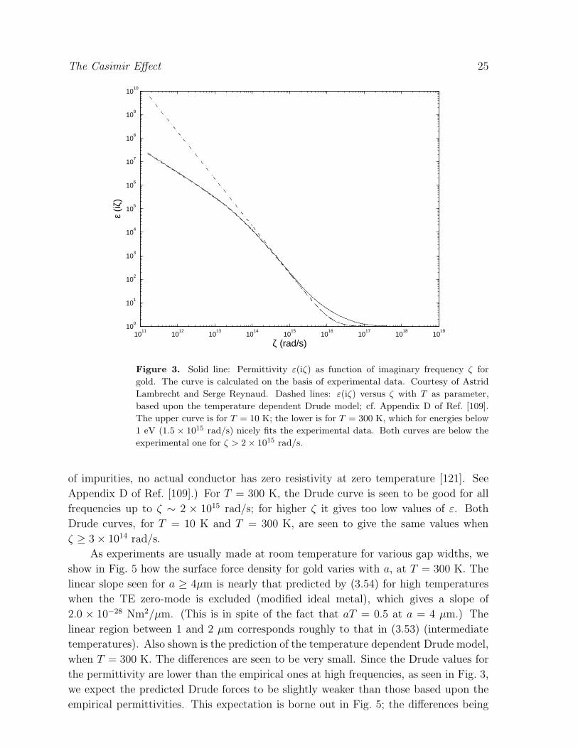
Figure 3. Solid line: Permittivity ε(iζ) as function of imaginary frequency ζ for

gold. The curve is calculated on the basis of experimental data. Courtesy of Astrid

Lambrecht and Serge Reynaud. Dashed lines: ε(iζ) versus ζ with T as parameter,

based upon the temperature dependent Drude model; cf. Appendix D of Ref. [109].

The upper curve is for T = 10 K; the lower is for T = 300 K, which for energies below

1 eV (1.5 × 1015 rad/s) nicely fits the experimental data. Both curves are below the

experimental one for ζ > 2× 1015 rad/s.

of impurities, no actual conductor has zero resistivity at zero temperature [121]. See

Appendix D of Ref. [109].) For T = 300 K, the Drude curve is seen to be good for all

frequencies up to ζ ∼ 2 × 1015 rad/s; for higher ζ it gives too low values of ε. Both

Drude curves, for T = 10 K and T = 300 K, are seen to give the same values when

ζ ≥ 3× 1014 rad/s.

As experiments are usually made at room temperature for various gap widths, we

show in Fig. 5 how the surface force density for gold varies with a, at T = 300 K. The

linear slope seen for a ≥ 4µm is nearly that predicted by (3.54) for high temperatures

when the TE zero-mode is excluded (modified ideal metal), which gives a slope of

2.0 × 10−28 Nm2/µm. (This is in spite of the fact that aT = 0.5 at a = 4 µm.) The

linear region between 1 and 2 µm corresponds roughly to that in (3.53) (intermediate

temperatures). Also shown is the prediction of the temperature dependent Drude model,

when T = 300 K. The differences are seen to be very small. Since the Drude values for

the permittivity are lower than the empirical ones at high frequencies, as seen in Fig. 3,

we expect the predicted Drude forces to be slightly weaker than those based upon the

empirical permittivities. This expectation is borne out in Fig. 5; the differences being


0 50 100 150 200 250 3000

5

10

15

20

25

30

35

40

T (K)

ν (m

eV)

Figure 4. Temperature dependence of the relaxation frequency for gold based on the

Bloch-Gruneisen formula [120].

large enough to be slightly visible at short distances, as we would expect since the plasma

nature of the material becomes more pronounced for small distances. Note that the

temperature dependence of the permittivity is irrelevant here because the temperature

is fixed.

It is of interest to check the magnitude of the dispersive effect in these cases.

We have therefore made a separate calculation of the expression (3.58) when ε is

taken to be constant. Figure 6 shows how the force varies with aT in cases when

ε ∈ 100, 1000, 10000,∞ are inserted in the expressions for Am and Bm in (3.59a).

It is seen from the figure that the first three curves asymptotically approach the

ε = ∞ curve, when ε increases, as we would expect. Again, we emphasize that the

dispersive curve for gold is calculated using the available room-temperature data for ε(iζ)

from Fig. 3. In the nondispersive case, there is of course no permittivity temperature

problem since ε is taken to be the same for all T .

There are several points worth noticing from Fig. 6:

(i) The curves have a horizontal slope at T = 0. For finite ε this property is clearly

visible on the curves. This has to be so on physical grounds: If the pressure had

a linear dependence on T for small T so would the free energy F , in contradiction

with the requirement that the entropy S = −∂F/∂T has to go to zero as T → 0.

For the gold data the initial horizontal slope is not resolvable on the scale of this

graph, but see the discussion in section 3.4.3.


0 1 2 3 4 5 6 7 8 90.4

0.6

0.8

1

1.2

1.4

1.6

1.8

a (µm)

−a4 F

T(1

0−27 N

m2 )

T = 300 K

Figure 5. Surface pressure for gold, multiplied with a4, versus a when T = 300 K.

Input data for ε(iζ) are taken from Fig. 3.

(ii) The curves show that the magnitude of the force diminishes with increasing

T (for a fixed a), in a certain temperature interval up to aT ≃ 0.3. This

perhaps counterintuitive effect is thus clear from the nondispersive curves. This is

qualitatively similar to the behavior seen in Fig. 5 for fixed T , where the minimum

occurs for aT ∼ 0.4.

(iii) It is seen that the curve for ε = const. = 1000 gives a reasonably good

approximation to the real dispersive curve for gold when a = 1 µm; the deviations

are less than about 5% except for the lowest values of aT (aT < 0.1). This

fact makes our neglect of the temperature dependence of ε(iζ) appear physically

reasonable; the various curves turn out to be rather insensitive with respect to

variations in the input values of ε(iζ).

(iv) Also, it can be remarked that B0 = 0 is required when ε is finite. Otherwise the

curves in Fig. 6, and thus the free energy, would have a finite slope at T = 0 which

again would imply a finite entropy contribution at T = 0 in violation with the third

law of thermodynamics.

3.4.3. Behavior of the Free Energy at Low Temperature The low temperature

correction is dominated by low frequencies,¶ where the Drude formula is extremely

¶ This statement is in the context of using of the Euler-Maclaurin summation formula to evaluate

(3.58), for example.


0 0.1 0.2 0.3 0.4 0.5 0.6 0.70.7

0.8

0.9

1

1.1

1.2

1.3

aT

−FT(m

Pa)

a = 1 µm

ε = 102

ε = 104

ε = 103

Au

ε = ∞

Figure 6. Nondispersive theory: Surface pressure for ε ∈ 100, 1000, 10000,∞.For low values of aT the latter coincides with the expression (3.53). Also shown for

comparison is the dispersive result for gold, where experimental input data for ε(iζ)

are taken from Fig. 3. Gap width is a = 1µm. The constraint a = 1µm applies only

to the dispersive case, since otherwise a4PT is a function of aT only. Note that room

temperature (300 K) corresponds to aT = 0.13.

accurate. Using this fact, we have performed analytic and numerical calculations which

show that the free energy has a quadratic low-temperature dependence, independent of

the plate separation:

F (T ) = F0 + T 2ω2p

48ν(2 ln 2− 1) = F0 + T 2(19 eV), T ≪ ν

ω2pa

2≈ 20 mK , (3.66)

where we have put in the numbers for gold, (3.65), (the temperature restriction refers

to a 1 µm plate separation) rather than the naive extrapolation (3.56)

F = F0 + Tζ(3)

16πa2= F0 +

T

4πa20.30. (3.67)

We see from Fig. 7 that the value in (3.67) indeed results if one extrapolates the

approximately linear curve there for ζa > 0.25 to zero, following the argument given in

(3.51). However, we see that the free energy smoothly changes to the quadratic behavior

exhibited in (3.66). Of course, the turn-over will be much sharper if we replace the room-

temperature relaxation frequency ν(300 K) by the positive value at zero temperature,

due to elastic scattering from defects or impurities.

Results consistent with these have been reported by Sernelius and Bostrom [122].

In particular they show that one cannot ignore the constant value ν(0 K), so there is


0.0 0.2 0.4 0.6 0.8 1.0ζa

-0.30

-0.25

-0.20

-0.15

f(ζ)

Figure 7. The behavior of the free energy for low frequencies, in the Drude model,

with parameters suitable for gold, and a plate separation of a = 1 µm. Here

FTE = T2πa2

∑∞

m=0′f(ζm). Here, we have used the room temperature value of the

relaxation parameter.

no relevant temperature dependence of the relaxation parameter. Although there is a

region of negative entropy, the Nernst heat theorem is not violated, but rather S → 0

as T → 0 if one goes to sufficiently low temperature, in contradiction to Refs. [123, 45].

3.4.4. Surface impedance form of reflection coefficient It has been proposed that

the resolution to the temperature problem for the Casimir effect is that the surface

impedance form of the reflection coefficients should be used in the Lifshitz formula

[124, 125, 126, 127], rather than that based on the bulk permittivity. Here we show that

the two approaches are in fact equivalent, and that the former must include transverse

momentum dependence.

For the TE modes, the reflection coefficient is given by (3.4a) [75]

rTE = −k1z − k2zk1z + k2z

, (3.68)

where

kaz =√

ω2ε− k2⊥ → i

√

ζ2[ε(iζ)− 1] + κ2 = iκa, (3.69)

with κ2 = κ22 = k2

⊥ + ζ2, and the subscripts 1 and 2 refer to the metal and the vacuum

regions, respectively. Now from Maxwell’s equations outside sources we easily derive

just inside the metal (the tangential components, designated by ⊥, of E and B are

continuous across the interface)

− ik1zk⊥ ·B⊥ − iωε

(

1− k2⊥

ω2ε

)

k⊥ · (n×E⊥) = 0, (3.70a)


−ik1zk⊥ · (n×E⊥)− iωk⊥ ·B⊥ = 0. (3.70b)

Here n is the normal to the interface. Now the surface impedance is defined by

E⊥ = Z(ω,k⊥)B⊥ × n, n×E⊥ = Z(ω,k⊥)B⊥. (3.71)

So eliminating B⊥ using this definition we find two equations:

k1z = −ω

Z, (3.72)

k21z = ω2ε− k2

⊥, (3.73)

the latter being the expected dispersion relation (3.69). Substituting this into the

expression for the reflection coefficient (3.68) we find

rTE = −ζ + Zκ

ζ − Zκ= −1 + Zp

1 − Zp, p =

κ

ζ, (3.74)

which apart from (relative) signs (presumably just a different convention choice)

coincides with that given in Geyer et al [124] or Bezerra et al [128]. See also

Refs. [129, 130]. The first discussion of the Lifshitz formula in this approach was given

in Ref. [102].

However, it is crucial to note that the “surface impedance” so defined depends on

the transverse momentum,

Z = − ζ√

ζ2[ε(iζ)− 1] + κ2, (3.75)

and so rTE → 0 as ζ → 0 just as in the dielectric constant formulation. Of course, we

have exactly the same result for the energy as before, since this is nothing but a slight

change of notation, as noted in Ref. [131, 36].

It is therefore incorrect to assume that Z is only a function of frequency, not of

transverse momentum, and to use the normal and anomalous skin effect formulas derived

for real waves impinging on imperfect conductors.+ In the above-cited references, this

necessary dependence was not included. (For further comments on the insufficiency of

the argument in Ref. [124] see Ref. [132].

How does the usual argument go? The normal component of the wavevector in a

conductor is given by

kz =

[

ω2

(

ε+ i4πσ

ω

)

− k2⊥

]1/2

→√i4πωσ, ω → 0, (3.76)

from which the usual normal skin effect formula follows immediately,

Z(ω) = −(1− i)

√

ω

8πσ. (3.77)

However, the limit in (3.76) here consists in omitting two “small” terms: ω2ε (which is

legitimate) and k2⊥ ≤ ω2. Here this last is not valid because in going to finite temperature

+ Of course, in general, the permittivity will be a function both of the frequency and the transverse

momentum, ε(ω,k⊥), but we believe the latter dependence is not significant for separations larger than

~c/ωp = 0.02 µm.


we have severed the connection between ω → iζ and k⊥; the latter is in no sense ignorable

as we take ζ → 0 to determine the low temperature dependence. This is the same error

to which we refer in Ref. [109]. (This k⊥ dependence still seems to be ignored in a

recent reanalysis by Torgerson and Lamoreaux [133] (see also Ref. [134]) who argue

that low frequencies of order of the inverse transverse size of the plates dominate the

low temperature behavior so that a linear term in the temperature does not appear.

This seems unlikely since the zero-temperature dependence is extracted by an analytic

continuation procedure.)

Not only do Mostepanenko, Klimchitskaya, et al [129, 124] ignore transverse

momentum dependence, but they apparently do not use the correct values of the

frequency in their evaluation of the surface impedance. They use the impedance

appropriate to the domain of infrared optics, thereby extrapolating the surface

impedance at what they consider a characteristic frequency ∼ 1/2a rather than using the

actual zero frequency value [126]. This seems to be a completely ad hoc prescription,

as opposed to the procedure advocated in Brevik et al [109], which uses the actual

electrical properties of the materials.

A beginning of a general discussion of nonlocal effects, including the anomalous

skin effect, in Casimir phenomena has recently been given by Esquivel and Svetovoy

[135]. There they argue that the Leontovich approach [136, 137] advocated by [129, 124]

only applies to normal incidence, which is why the surface impedances only depend on

frequency. In fact, this is incorrect in general, and if only local functions are used for the

permittivity, that is ε = ε(ω), the dependence for the TE surface impedance given above

is reproduced. For propagating waves the Leontovich approximation is appropriate, but

not for the evanescent fields relevant to the Casimir effect, where k⊥/ω > 1 occur. They

do not calculate temperature effects; the nonlocal anomalous skin effect for ω < ωp that

they compute gives a correction to the Casimir force of order 0.5%, but other nonlocal

effects, such as plasmon excitations, could be more significant [138, 139].

3.5. Beyond the Proximity Approximation

As we will discuss in the next section, to avoid problems of parallelism, most recent

experiments to measure the force between conductors have not been made between

parallel plates, but between a plate and a spherical surface, or between crossed cylinders.

The Lifshitz and Casimir formulas do not apply to these situations. However, in the

1930s, it was recognized that if the separation between the sphere and the plate is very

small compared to the radius of curvature of the sphere, the latter force may be derived

from the force for the parallel plate configuration. This result is usually called the

Proximity Force Theorem [140], which here says that the attractive force F between a

sphere of radius R and a flat surface is simply the circumference of the sphere times the

energy per unit area for parallel plates, or, from (2.29),

F = 2πR E(d) = − π3

360

R

d

~c

d2, R≫ d, (3.78)


where d is the distance between the plate and the sphere at the point of closest approach,

and R is the radius of curvature of the sphere at that point. (The exact shape of the

“sphere” is not relevant in the strict approximation R≫ d.) The proof of (3.78) is quite

simple. If R≫ d, each element of the sphere may be regarded as parallel to the plane,

so the potential energy of the sphere is

V (d) =

∫ π

0

2πR sin θR dθ E(d+R(1− cos θ)) = 2πR

∫ R

−R

dx E(d+R− x). (3.79)

To obtain the force between the sphere and the plate, we differentiate with respect to

d:

F = − ∂V

∂d= 2πR

∫ R

−R

dx∂

∂xE(d+R− x)

= 2πR[E(d)− E(d+ 2R)] ≈ 2πR E(d), d≪ R, (3.80)

provided that E(a) falls off with a. This result was already given in Refs. [141, 142, 143].

The proximity theorem itself dates back to a paper by Derjaguin in 1934 [144, 145].

Let us apply this theorem to the MIM model (3.53) for the force between parallel

plates at low temperature. The corresponding free energy is

F = − π2

720a3+

π2

45aT 4 − ζ(3)

2πT 3 +

ζ(3)

16πa2T, (3.81)

where the term constant in a is determined by the high-temperature limit (3.54) – see

Ref. [29], p. 56. This free energy is to be used in the proximity force theorem, with the

result for the force between a sphere and a plate [39, 114, 146, 10]

F = − π3

360

R

d3

[

1− 16(Td)4 +360ζ(3)

π3(Td)3 − 45ζ(3)

π3Td

]

. (3.82)

The terms linear in T would not be present in the IM model. At room temperature, 300

K, and at 1 µm separation, the successive terms correspond to corrections of −0.46%,

+3.1%, and −23%, respectively. This model, of course, does not begin to reflect the true

temperature dependence, discussed for parallel plates above. A full discussion of the

temperature dependence for the force between a spherical lens and a plate will appear

elsewhere.

Emig has recently presented exact results for Casimir forces between periodically

deformed surfaces [147, 148, 149]. In the latest paper, the authors calculate the force

between a flat plate and one with a rectangular (square) corrugation, of amplitude ∆a.

This was probed experimentally by Roy and Mohideen [150], with clear deviations from

the proximity approximation. (See also Refs. [151, 152] for measurements of the so-

called “lateral Casimir effect.”) For short wavelength corrugations for either TE or TM

modes one gets

P = − π2

480

1

(a−∆a)4≈ − π2

480a4

(

1 +4∆a

a

)

, (3.83)

while for long wavelength corrugations

P = − π2

480

1

2

(

1

(a−∆a)4+

1

(a+∆a)4

)

, (3.84)


which is as expected from the proximity approximation. For intermediate wavelength

corrugations numerical results are given. The force approaches that given by the

proximity approximation for large λ like ∆a/λ, as compared to (∆a/λ)2 for sinusoidal

corrugations, due to the sharp edges. These behaviors can be understood from the ray

optics approach of Jaffe and Scardicchio [23] discussed in the following subsection. The

relative contributions of the TE and TM modes vary with the wavelength and the shape

of the corrugation, the ratio of the modes approaching unity as a/∆a tends to 1 or ∞.

Insofar as first approximations to these interactions were extracted through use of the

proximity force theorem, these results shed valuable light on how to move beyond that

approximation.

3.5.1. Optical Paths A very interesting strategy for moving beyond the proximity

approximation has been suggested by Jaffe and Scardicchio [23]. This is related to the

semiclassical closed orbit approach advocated by Schaden and Spruch [153, 154, 155]

and earlier by Gutzweiler [156, 157], and also to that of Balian and Bloch [158, 159, 160].

Fulling has also recently proposed similar ideas [161, 162].

In the simplest context, that of parallel plates, the approach is, of course, exact,

and is precisely what we wrote down in (3.6). We simply compute the energy using

(2.15) with

G(r, r) =∫

(dk⊥)

(2π)2g(x, x), (3.85)

where g(x, x′) is given by (3.6). Rather than carry out the sum as given there, let us

sum the terms with even and odd numbers of reflections separately. The former give,

when the zero reflection term is omitted,

geven(x, x) =1

2κ2[

r′re−2κa + (r′r)2e−4κa + . . .]

=1

2κ(coth κa− 1), (3.86)

where in the last step we have inserted the values for the reflection amplitudes

appropriate to Dirichlet boundaries, r = r′ = −1. When this is inserted into the

expression for the energy we obtain rather immediately the usual result for the Casimir

energy between Dirichlet plates:

E = − 1

96π2a3

∫ ∞

0

duu3

eu − 1= − π2

1440a3. (3.87)

Keeping only the first term in the sum (2 reflections) gives

E (2) = − 1

16π2a3, (3.88)

which is in magnitude only 7.6% low, while keeping 2 plus 4 reflections give an error of

1.8%:

E (2) + E (4) = − 1

16π2a3

(

1 +1

16

)

. (3.89)

The odd reflections give a term in g(x, x) which depends on x:

godd(x, x) = −1

2κ

(

e−2κx + e2κ(x−a)) 1

1− e−2κa. (3.90)


when this is integrated over x, the a dependence of this term disappears, so this gives

rise to an irrelevant constant in the energy. Keeping it and the zero-reflection term gives

the expression for the total energy as obtained directly from (3.6)

E0 + Eeven + Eodd = − 1

12π2

1

a3

∫ ∞

0

dy y3(

coth y − 1

y

)

. (3.91)

Jaffe and Scardicchio [23] use this method to estimate the force between a sphere

an a plate. The results disagree with the proximity approximation when d/R is bigger

than a few percent, but agrees with an exact numerical calculation [163], described in

the following subsection, up to d/R ≈ 0.1, where the proximity theorem fails badly.

3.5.2. Worldline Approach to the Casimir Energy Gies, Moyaerts, and Langfeld

[163, 164] have developed a numerical technique for extracting Casimir energies in

nontrivial geometries, such as between a sphere and a plate. It is based on the string-

inspired worldline approach. They consider, like Graham et al [165, 61, 30] a scalar

field in a smooth background potential like (2.40). The worldline representation of

the effective action is obtained by introducing a proper time representation of the

functional logarithm with ultraviolet regularization, doing the trace in configuration

space, and interpreting the matrix element there as a Feynman path integral over all

worldlines x(τ). Field theoretic divergences can thus be handled. Other divergences

arise from the potential itself, when it approaches some idealized limit, which may not

be removed in a physically meaningful way and may or may not contribute to physical

observables. The expectation value is evaluated by the “loop-cloud” method, using

techniques from statistical mechanics. Although in the “sharp” and “strong” limits in

the sense of Graham et al [165, 61, 30] divergences occur in the theory, a finite force

between rigid bodies can be obtained. The general result for δ-function planes, discussed

in section 2.2, is reproduced numerically, and then the sphere-plate system is considered.

The numerical results, for d/R from 10−3 to 10, agree closely with the geometric mean∗of the plate-based and the sphere-based proximity force approximation (deviation from

either becomes sizable for d/R > 0.02). Note that electromagnetic fluctuations (e.g.,

TM modes) have not been considered in this approach.

3.6. Status of the Experimental Measurements on Casimir Forces

Attempts to measure the Casimir effect between solid bodies date back to the

middle 1950s. The early measurements were, not surprisingly, somewhat inconclusive

[142, 143, 168, 169, 170, 171, 172, 173, 174, 175]. The Lifshitz theory (3.10), for zero

temperature, was, however, confirmed accurately in the experiment of Sabisky and

∗ The geometric mean version of the proximity force approximation, which coincides with the

semiclassical periodic orbit method of Schaden and Spruch [153, 154, 155], has been found to be

the most accurate also for concentric cylindrical shells, the Casimir energy for which was calculated by

Mazzitelli et al [166, 167].


Anderson in 1973 [18]. So there could be no serious doubt of the reality of zero-point

fluctuation forces. For a review of the earlier experiments, see Refs. [15, 176].

New technological developments allowed for dramatic improvements in experimen-

tal techniques in recent years, and thereby permitted nearly direct confirmation of the

Casimir force between parallel conductors. First, in 1997 Lamoreaux used a electrome-

chanical system based on a torsion pendulum to measure the force between a conducting

plate and a sphere [114, 146], as given by the proximity force theorem (3.78). Lamore-

aux [114, 146] claimed agreement with this theoretical value at the 5% level, although it

seems that finite conductivity was not included correctly, nor were roughness corrections

incorporated [177]. Further, Lambrecht and Reynaud [77] analyzed the effect of conduc-

tivity and found discrepancies with Lamoreaux [178], and therefore stated that it was

too early to claim agreement between theory and experiment. See also Refs. [119, 179].

An improved experimental measurement was reported in 1998 by Mohideen

and Roy [97], based on the use of an atomic force microscope. They included

finite conductivity, roughness, and conventional temperature corrections, although no

evidence for latter has been claimed. Spectacular agreement with theory at the 1%

level was attained. Improvements were subsequently reported [98, 99]. (The nontrivial

effects of corrugations in the surface were examined in Ref. [150, 151, 152].) Erdeth

[180] measured the Casimir forces between crossed cylinders at separations of 20–100

nm. The highest precision was achieved with very smooth, gold-plated surfaces. Rather

complete analyses of the roughness, conductivity, and temperature corrections to the

Lamoreaux and Mohideen experiments have been published [181, 182, 39].

More recently, a new measurement of the Casimir force (3.78) was presented by

a group at Bell Labs [183, 184], using a micromachined torsional device, a micro-

electromechanical system or MEMS, by which they measured the attraction between

a polysilicon plate and a spherical metallic surface. Both surfaces were plated

with a 200 nm film of gold. The authors included finite conductivity [77, 185]

and surface roughness corrections [186, 187], and obtained agreement with theory at

better than 0.5% at the smallest separations of about 75 nm. However, potential

corrections of greater than 1% exist, so that limits the level of verification of the

theory. Their experimental work, which now continues at Harvard, suggests novel

nanoelectromechanical applications.

There is only one experiment with a parallel-plate geometry [188], which is of

limited accuracy (∼ 15%) due to the difficulty of maintaining parallelism. It is, however,

of considerable interest because the interpretation does not depend on the proximity

theorem, corrections to which are problematic [148, 23]; see section 3.5. The importance

of improving the accuracy of the parallel-plate configuration has been emphasized by

Onofrio [189].

The most precise experiment to date, using a MEMS, makes use of both static

and dynamical procedures and yields a claimed accuracy of about 0.25% [100, 190],

but this accuracy has been disputed [191], due to difficulty in controlling roughness

and the concomittant uncertainty in the ability to determine the separation distance.


It has been asserted [190] that this experiment rules out the temperature dependence

claimed in Ref. [109] (see section 3.4.2), but this is problematic at this point, especially

as comparison is only made with the MIM model (3.53), rather than with the detailed

calculation given there.

Very recently, the Harvard group has performed a very interesting Casimir force

measurement between a gold-covered plate and a sphere coated with a hydrogen-

switchable mirror [192]. Although the mirror becomes transparent in the visible upon

hydrogenation, no effect was observed on the Casimir force when the mirror was switched

on and off. This shows that, in contradiction to the claims of Mostepanenko et al

, for example in Ref. [127], the Casimir force is responsive to a very wide range of

frequencies, in accordance with the Lifshitz formula and the general dispersion relation

for the permittivity.♯ (See also Ref. [193, 194].) In particular, their results show that

wavelengths much larger than the separation between the surfaces play a crucial role.

Because all the recent experiments measure forces between relatively thin films,

rather than between bulk metals, significant deviations from the Lifshitz formula (∼ 2%)

may be expected [195]. This may also be relevant to the claimed accuracy of the first

Mohideen experiment [97], which uses a thin metallic coating, regarded as completely

transparent.

This may be an appropriate point to comment on the recent paper of Chen et al

[95]. This is based on a reanalysis of experimental data obtained four years ago in

Ref. [99]. Experimental precision of 1.75% and theoretical accuracy of 1.69% is claimed

at the shortest distances, 62 nm. However, their analysis seems flawed. They obtain

average experimental forces by averaging many measurements, which is only permissible

if the averaging is carried out at exactly the same separation between the surfaces. Of

course they have no way of knowing this. Furthermore, they apparently use the mean

separation parameter d0 as a free variable in their fit, which essentially negates the

possibility of testing the theory, which is most sensitive at the shortest separations [180].

Iannuzzi asserts that at distance of order 100 nm, errors of a few Angstroms preclude

a 1% measurement. Therefore this analysis cannot be used as a serious constraint for

either new forces or for setting limits on temperature corrections.††A difference force experiment has been proposed by Mohideen and collaborators

[196, 197]. The idea is to measure the difference in the force between a lens and a plate

at room temperature, before and after both surfaces have been heated 50 K by a laser

pulse. The measurements are not yet good enough to distinguish between the plasma

and the Drude modes of the permittivity, or between the simplified impedance model

versus the measured bulk permittivity approach, as discussed in section 3.4.

A proposal has been made to measure the force between eccentric cylinders, in which

the axes are parallel but slightly offset [167]. The net force on the inner cylinder is zero,

♯ Iannuzzi quotes Klimchitskaya as now agreeing with this statement. This, however, is hard to

reconcile with statements made in Ref. [126] that one should use the extrapolated surface impedance

value at ωc = 1/2a rather than the actual zero-frequency value.†† I thank Davide Iannuzzi for discussion of these points.


of course, when the cylinders are concentric, but this equilibrium point is unstable. The

idea is to look for a shift in the mechanical resonant frequency of the outer cylinder due

to the Casimir force exerted by the inner one. The chief difficulty may be in maintaining

parallelism.

Another active area of experimental effort involving Casimir measurements is the

search for new forces at the submicron level. These are based on looking for a discrepancy

between the measured and predicted Casimir forces. The most recent limits are given

in Krause, Decca, et al [198, 100]. Unfortunately, the limits, for an assumed potential

of the form

V (r) = −Gm1m2

r

(

1 + αe−r/λ)

, (3.92)

for λ < 10−7 m are only for absurdly large strengths, α ≤ 1014, and as λ decreases

the upper limit on α increases. The Purdue group has also proposed iso-electronic

experiments to look at the force between a sphere and two different plates, composed

of material with similar electronic properties (and hence similar Casimir forces) but

different nuclear properties (and hence presumably different new forces). See Ref. [199]

for a brief description of their experiment and the detection of a small, but probably

not significant, residual force.

Very recently, there has been a report [200] of an experiment [201] of dropping

ultracold neutrons onto a surface. They are trapped between the mirror and the earth’s

gravitational potential. These gravitational bound states would be modified by any

deviation from Newtonian gravity. No such deviations from Newton’s law is found down

to the 1–10 nm range. See also Nesvizhevsky and Protasov [202] who obtain limits on

non-Newtonian forces inferior to those of Casimir measurements, that is, α < 1021 at

λ = 10−7 m, although it is relatively better that the Casimir limits in the nanometer

range, but the limits are extremely weak there, α < 1026.

It is clear that as micro engineering comes into its own, Casimir forces will have

to be taken into account and utilized. A recent interesting paper by Chumak, Milonni,

and Berman [203] suggests that the noncontact friction observed by Stipe et al [204] on

a cantilever near a surface is due in major part to Casimir forces. The Casimir force

is responsible for the frequency shift observed of about 4.5% for a gold sample at a

separation of 2 nm.

For another example along these lines, Lin et al [205] have shown that Casimir-

Polder forces between atoms and the surface can provide fundamental limitations on

stability of a Bose-Einstein condensate near a microfabricated silicon chip, a system

which holds great promise for technological applications.

The recent intense experimental activity is very encouraging to the development of

the field. Coming years, therefore, promise ever increasing experimental input into a

field that has been dominated by theory for five decades.


4. Self-Stress

4.1. Surface and Volume Divergences

It is well known that in general the Casimir energy density diverges in the neighborhood

of a surface. For flat surfaces and conformal theories (such as the conformal scalar theory

considered in Ref. [57], or electromagnetism) those divergences are not present.‡ We

saw hints of this in section 2.4. In particular, Brown and Maclay [209] calculated the

local stress tensor for two ideal plates separated by a distance a along the z axis, with

the result for a conformal scalar

〈T µν〉 = − π2

1440a4[4zµzν − gµν ]. (4.1)

This result was given recent rederivations in [210, 57]. Dowker and Kennedy [211] and

Deutsch and Candelas [212] considered the local stress tensor between planes inclined

at an angle α, with the result, in cylindrical coordinates (t, r, θ, z),

〈T µν〉 = − f(α)

720π2r4

1 0 0 0

0 −1 0 0

0 0 3 0

0 0 0 −1

, (4.2)

where for a conformal scalar, with Dirichlet boundary conditions,

f(α) =π2

2α2

(

π2

α2− α2

π2

)

, (4.3)

and for electromagnetism, with perfect conductor boundary conditions,

f(α) =

(

π2

α2+ 11

)(

π2

α2− 1

)

. (4.4)

For α → 0 we recover the pressures and energies for parallel plates, (2.25b), (2.39) and

(3.87). (These results were later discussed in Ref. [213].)

Although for perfectly conducting flat surfaces, the energy density is finite, for

electromagnetism the individual electric and magnetic fields have divergent RMS values,

〈E2〉 ∼ −〈B2〉 ∼ 1

ǫ4, ǫ→ 0, (4.5)

a distance ǫ above a conducting surface. However, if the surface is a dielectric,

characterized by a plasma dispersion relation (3.33), these divergences are softened

〈E2〉 ∼ 1

ǫ3, −〈B2〉 ∼ 1

ǫ2, ǫ→ 0, (4.6)

so that the energy density also diverges [214]

〈T 00〉 ∼ 1

ǫ3, ǫ→ 0. (4.7)

‡ In general, this need not be the case. For example, Romeo and Saharian [206] show that with

mixed boundary conditions the surface divergences need not vanish for parallel plates. For additional

work on local effects with mixed (Robin) boundary conditions, applied to spheres and cylinders, and

corresponding global effects, see Refs. [207, 208, 70]. See also section 2.4 and Ref. [72, 73].


The null energy condition (nµnµ = 0)

T µνnµnν ≥ 0 (4.8)

is satisfied, so that gravity still focuses light.

Graham [215] examined the general relativistic energy conditions required by

causality. In the neighborhood of a smooth domain wall, given by a hyperbolic tangent,

the energy is always negative at large enough distances. Thus the weak energy condition

is violated, as is the null energy condition (4.8). However, when (4.8) is integrated over

a complete geodesic, positivity is satisfied. It is not clear if this last condition, the

Averaged Null Energy Condition, is always obeyed in flat space. Certainly it is violated

in curved space, but the effects always seem small, so that exotic effects such as time

travel are prohibited.

However, as Deutsch and Candelas [212] showed many years ago, in the

neighborhood of a curved surface for conformally invariant theories, 〈Tµν〉 diverges as

ǫ−3, where ǫ is the distance from the surface, with a coefficient proportional to the sum

of the principal curvatures of the surface. In particular they obtain the result, in the

vicinity of the surface,

〈Tµν〉 ∼ ǫ−3T (3)µν + ǫ−2T (2)

µν + ǫ−1T (1)µν , (4.9)

and obtain explicit expressions for the coefficient tensors T(3)µν and T

(2)µν in terms of the

extrinsic curvature of the boundary.

For example, for the case of a sphere, the leading surface divergence has the form,

for conformal fields, for r = a + ǫ, ǫ→ 0

〈Tµν〉 =A

ǫ3

2/a 0 0 0

0 0 0 0

0 0 1 0

0 0 0 sin θ

, (4.10)

in spherical polar coordinates, where the constant is A = 1/1440π2 for a scalar, or

A = 1/120π2 for the electromagnetic field. Note that (4.10) is properly traceless. The

cubic divergence in the energy density near the surface translates into the quadratic

divergence in the energy found for a conducting ball [216]. The corresponding quadratic

divergence in the stress corresponds to the absence of the cubic divergence in 〈Trr〉.This is all completely sensible. However, in their paper Deutsch and Candelas

[212] expressed a certain skepticism about the validity of the result of Ref. [24] for

the spherical shell case (described in part in section 4.4) where the divergences cancel.

That skepticism was reinforced in a later paper by Candelas [217], who criticized the

authors of Ref. [24] for omitting δ function terms, and constants in the energy. These

objections seem utterly without merit. In a later critical paper by the same author [218],

it was asserted that errors were made, rather than a conscious removal of unphysical

divergences.


Of course, surface curvature divergences are present. As Candelas noted [217, 218],

they have the form

E = ES

∫

dS + EC

∫

dS (κ1 + κ2) + ECI

∫

dS (κ1 − κ2)2 + EC

II

∫

dSκ1κ2 + . . . ,(4.11)

where κ1 and κ2 are the principal curvatures of the surface. The question is to what

extent are they observable. After all, as has been shown in Ref. [29, 57] and in section 2.4,

we can drastically change the local structure of the vacuum expectation value of the

energy-momentum tensor in the neighborhood of flat plates by merely exploiting the

ambiguity in the definition of that tensor, yet each yields the same finite, observable

(and observed!) energy of interaction between the plates. For curved boundaries, much

the same is true. A priori, we do not know which energy-momentum tensor to employ,

and the local vacuum-fluctuation energy density is to a large extent meaningless. It

is the global energy, or the force between distinct bodies, that has an unambiguous

value. It is the belief of the author that divergences in the energy which go like a power

of the cutoff are probably unobservable, being subsumed in the properties of matter.

Moreover, the coefficients of the divergent terms depend on the regularization scheme.

Logarithmic divergences, of course, are of another class [59].

Dramatic cancellations of these curvature terms can occur. It might be thought

that the reason a finite result was found for the Casimir energy of a perfectly conducting

spherical shell [19, 22, 24] is that the term involving the squared difference of curvatures

in (4.11) is zero only in that case. However, for reasons not yet apparent to the

present author, it has been shown that at least for the case of electromagnetism the

corresponding term is not present (or has a vanishing coefficient) for an arbitrary smooth

cavity [219], and so the Casimir energy for a perfectly conducting ellipsoid of revolution,

for example, is finite. This finiteness of the Casimir energy (usually referred to as the

vanishing of the second heat-kernel coefficient [10]) for an ideal smooth closed surface

was anticipated already in Ref. [22], but contradicted by Ref. [212]. More specifically,

although odd curvature terms cancel inside and outside for any thin shell, it would be

anticipated that the squared-curvature term, which is present as a surface divergence in

the energy density, would be reflected as an unremovable divergence in the energy.

For a closed surface the last term in (4.11) is a topological invariant, so gives an

irrelevant constant, while no term of the type of the penultimate term can appear

due to the structure of the traced cylinder expansion [70]. It would be extraordinarily

interesting if this Casimir energy could be computed for an ellipsoidal boundary, but the

calculation appears extremely difficult because the Helmholtz equation is not separable

in the exterior region.

4.2. Casimir Forces on Spheres via δ-Function Potentials

This section is an adaptation and an extension of calculations presented in Ref. [62].

This investigation was carried out in response to the program of the MIT group

[165, 60, 61, 71, 30]. They rediscovered irremovable divergences in the Casimir energy for


a circle in 2+1 dimensions first discovered by Sen [220, 221], but then found divergences

in the case of a spherical surface, thereby casting doubt on the validity of the Boyer

calculation [19]. Some of their results, as we shall see, are spurious, and the rest are

well known [59]. However, their work has been valuable in sparking new investigations

of the problems of surface energies and divergences.

We now carry out the calculation we presented in section 2 in three spatial

dimensions, with a radially symmetric background

Lint = −1

2

λ

aδ(r − a)φ2(x), (4.12)

which would correspond to a Dirichlet shell in the limit λ → ∞. The time-Fourier

transformed Green’s function satisfies the equation (κ2 = −ω2)[

−∇2 + κ2 +λ

aδ(r − a)

]

G(r, r′) = δ(r − r′). (4.13)

We write G in terms of a reduced Green’s function

G(r, r′) =∑

lm

gl(r, r′)Ylm(Ω)Y

∗lm(Ω

′), (4.14)

where gl satisfies[

− 1

r2d

drr2

d

dr+

l(l + 1)

r2+ κ2 +

λ

aδ(r − a)

]

gl(r, r′) =

1

r2δ(r − r′). (4.15)

We solve this in terms of modified Bessel functions, Iν(x), Kν(x), where ν = l + 1/2,

which satisfy the Wronskian condition

I ′ν(x)Kν(x)−K ′ν(x)Iν(x) =

1

x. (4.16)

The solution to (4.15) is obtained by requiring continuity of gl at each singularity, r′

and a, and the appropriate discontinuity of the derivative. Inside the sphere we then

find (0 < r, r′ < a)

gl(r, r′) =

1

κrr′

[

el(κr>)sl(κr<)−λ

κasl(κr)sl(κr

′)e2l (κa)

1 + λκasl(κa)el(κa)

]

. (4.17)

Here we have introduced the modified Riccati-Bessel functions,

sl(x) =

√

πx

2Il+1/2(x), el(x) =

√

2x

πKl+1/2(x). (4.18)

Note that (4.17) reduces to the expected result, vanishing as r → a, in the limit of

strong coupling:

limλ→∞

gl(r, r′) =

1

κrr′

[

el(κr>)sl(κr<)−el(κa)

sl(κa)sl(κr)sl(κr

′)

]

. (4.19)

When both points are outside the sphere, r, r′ > a, we obtain a similar result:

gl(r, r′) =

1

κrr′

[

el(κr>)sl(κr<)−λ

κael(κr)el(κr

′)s2l (κa)

1 + λκasl(κa)el(κa)

]

. (4.20)

which similarly reduces to the expected result as λ→∞.


Now we want to get the radial-radial component of the stress tensor to extract the

pressure on the sphere, which is obtained by applying the operator

∂r∂r′ −1

2(−∂0∂′0 +∇ ·∇′)→ 1

2

[

∂r∂r′ − κ2 − l(l + 1)

r2

]

(4.21)

to the Green’s function, where in the last term we have averaged over the surface of the

sphere. In this way we find, from the discontinuity of 〈Trr〉 across the r = a surface, the

net stress

S =λ

2πa2

∞∑

l=0

(2l + 1)

∫ ∞

0

dx(el(x)sl(x))

′ − 2el(x)sl(x)x

1 + λel(x)sl(x)x

. (4.22)

The same result can be deduced by computing the total energy (2.15). The free

Green’s function, the first term in (4.17) or (4.20), evidently makes no significant

contribution to the energy, for it gives a term independent of the radius of the sphere,

a, so we omit it. The remaining radial integrals are simply∫ x

0

dy s2l (y) =1

2x

[(

x2 + l(l + 1))

s2l + xsls′l − x2s′2l

]

, (4.23a)

∫ ∞

x

dy e2l (y) = −1

2x

[(

x2 + l(l + 1))

e2l + xele′l − x2e′2l

]

, (4.23b)

where all the Bessel functions on the right-hand-sides of these equations are evaluated

at x. Then using the Wronskian, we find that the Casimir energy is

E = − 1

2πa

∞∑

l=0

(2l + 1)

∫ ∞

0

dxxd

dxln [1 + λIν(x)Kν(x)] . (4.24)

If we differentiate with respect to a, with λ/a fixed, we immediately recover the force

(4.22). This expression, upon integration by parts, coincides with that given by Barton

[222], and was first analyzed in detail by Scandurra [223]. For strong coupling, it reduces

to the well-known expression for the Casimir energy of a massless scalar field inside and

outside a sphere upon which Dirichlet boundary conditions are imposed, that is, that

the field must vanish at r = a:

limλ→∞

E = − 1

2πa

∞∑

l=0

(2l + 1)

∫ ∞

0

dxxd

dxln [Iν(x)Kν(x)] , (4.25)

because multiplying the argument of the logarithm by a power of x is without effect,

corresponding to a contact term. Details of the evaluation of Eq. (4.25) are given in

Ref. [57], and will be considered in section 4.4 below. (See also Refs. [224, 225, 226].)

The opposite limit is of interest here. The expansion of the logarithm is immediate

for small λ. The first term, of order λ, is evidently divergent, but irrelevant, since that

may be removed by renormalization of the tadpole graph. In contradistinction to the

claim of Refs. [61, 60, 30, 71], the order λ2 term is finite, as established in Ref. [57].

That term is

E(λ2) =λ2

4πa

∞∑

l=0

(2l + 1)

∫ ∞

0

dxxd

dx[Il+1/2(x)Kl+1/2(x)]

2. (4.26)


The sum on l can be carried out using a trick due to Klich [227]: The sum rule∞∑

l=0

(2l + 1)el(x)sl(y)Pl(cos θ) =xy

ρe−ρ, (4.27)

where ρ =√

x2 + y2 − 2xy cos θ, is squared, and then integrated over θ, according to∫ 1

−1

d(cos θ)Pl(cos θ)Pl′(cos θ) = δll′2

2l + 1. (4.28)

In this way we learn that∞∑

l=0

(2l + 1)e2l (x)s2l (x) =

x2

2

∫ 4x

0

dw

we−w. (4.29)

Although this integral is divergent, because we did not integrate by parts in (4.26), that

divergence does not contribute:

E(λ2) =λ2

4πa

∫ ∞

0

dx1

2x

d

dx

∫ 4x

0

dw

we−w =

λ2

32πa, (4.30)

which is exactly the result (4.25) of Ref. [57], which also follows from (2.20) here.

However, before we wax too euphoric, we recognize that the order λ3 term appears

logarithmically divergent, just as Refs. [30] and [71] claim. This does not signal a

breakdown in perturbation theory, as the divergence (2.21) in the D = 1 calculation

did. Suppose we subtract off the two leading terms,

E = − 1

2πa

∞∑

l=0

(2l+1)

∫ ∞

0

dxxd

dx

[

ln (1 + λIνKν)− λIνKν +λ2

2(IνKν)

2

]

+λ2

32πa.(4.31)

To study the behavior of the sum for large values of l, we can use the uniform asymptotic

expansion (Debye expansion),

ν ≫ 1 : Iν(x)Kν(x) ∼t

2ν

[

1 +A(t)

ν2+

B(t)

ν4+ . . .

]

. (4.32)

Here x = νz, and t = 1/√1 + z2. The functions A and B, etc., are polynomials in t.

We now insert this into (4.31) and expand not in λ but in ν; the leading term is

E(λ3) ∼ λ3

24πa

∞∑

l=0

1

ν

∫ ∞

0

dz

(1 + z2)3/2=

λ3

24πaζ(1). (4.33)

Although the frequency integral is finite, the angular momentum sum is divergent. The

appearance here of the divergent ζ(1) seems to signal an insuperable barrier to extraction

of a finite Casimir energy for finite λ. The situation is different in the limit λ → ∞ –

See section 4.4.

This divergence has been known for many years, and was first calculated explicitly

in 1998 by Bordag et al [59], where the second heat kernel coefficient gave an equivalent

result,

E ∼ λ3

48πa

1

s, s→ 0. (4.34)


A possible way of dealing with this divergence was advocated in Ref. [223]. Very

recently, Bordag and Vassilevich [228] have reanalyzed such problems from the heat

kernel approach. They show that this O(λ3) divergence corresponds to a surface tension

counterterm, an idea proposed by me in 1980 [27, 229] in connection with the zero-

point energy contribution to the bag model. Such a surface term corresponds to λ/a

fixed, which then necessarily implies a divergence of order λ3. Bordag argues that it

is perfectly appropriate to insert a surface tension counterterm so that this divergence

may be rendered finite by renormalization.

4.3. TM Spherical Potential

Of course, the scalar model considered in the previous subsection is merely a toy model,

and something analogous to electrodynamics is of far more physical relevance. There are

good reasons for believing that cancellations occur in general between TE (Dirichlet) and

TM (Robin) modes. Certainly they do occur in the classic Boyer energy of a perfectly

conducting spherical shell [19, 22, 24], and the indications are that such cancellations

occur even with imperfect boundary conditions [222]. Following the latter reference, let

us consider the potential

Lint =1

2λa

1

r

∂

∂rδ(r − a)φ2(x). (4.35)

In the limit λ→∞ this corresponds to TM boundary conditions. The reduced Green’s

function is thus taken to satisfy[

− 1

r2d

drr2

d

dr+

l(l + 1)

r2+ κ2 − λa

r

∂

∂rδ(r − a)

]

gl(r, r′) =

1

r2δ(r−r′).(4.36)

At r = r′ we have the usual boundary conditions, that gl be continuous, but that its

derivative be discontinuous,

r2∂

∂rgl

∣

∣

∣

r=r′+

r=r′−= −1, (4.37)

while at the surface of the sphere the derivative is continuous,

∂

∂rrgl

∣

∣

∣

r=a+

r=a−= 0, (4.38a)

while the function is discontinuous,

gl

∣

∣

∣

r=a+

r=a−= −λ ∂

∂rrgl

∣

∣

∣

r=a. (4.38b)

Equations (4.38a) and (4.38b) are the analogues of the boundary conditions (2.30a),

(2.30b) treated in section 2.3.

It is then easy to find the Green’s function. When both points are inside the sphere,

r, r′ < a : gl(r, r′) =

1

κrr′

[

sl(κr<)el(κr>)−λκa[e′l(κa)]

2sl(κr)sl(κr′)

1 + λκae′l(κa)s′l(κa)

]

, (4.39a)

and when both points are outside the sphere,

r, r′ > a : gl(r, r′) =

1

κrr′

[

sl(κr<)el(κr>)−λκa[s′l(κa)]

2el(κr)el(κr′)

1 + λκae′l(κa)s′l(κa)

]

. (4.39b)


It is immediate that these supply the appropriate Robin boundary conditions in the

λ→∞ limit:

limλ→0

∂

∂rrgl

∣

∣

∣

r=a= 0. (4.40)

The Casimir energy may be readily obtained from (2.15), and we find, using the

integrals (4.23a), (4.23b)

E = − 1

2πa

∞∑

l=0

(2l + 1)

∫ ∞

0

dxxd

dxln [1 + λxe′l(x)s

′l(x)] . (4.41)

The stress may be obtained from this by applying −∂/∂a, and regarding λa as constant

[see (4.35)], or directly, from the Green’s function by applying the operator,

trr =1

2i

[

∇r∇r′ − κ2 − l(l + 1)

r2

]

gl

∣

∣

∣

r′=r, (4.42)

which is the same as that in (4.21), except that

∇r =1

r∂rr, (4.43)

appropriate to TM boundary conditions (see Ref. [230], for example). Either way, the

total stress on the sphere is

S = − λ

2πa2

∞∑

l=0

(2l + 1)

∫ ∞

0

dx x2 [e′l(x)s′l(x)]

′

1 + λxe′l(x)s′l(x)

. (4.44)

The result for the energy (4.41) is similar, but not identical, to that given by Barton

[222].

Suppose we now combine the TE and TM Casimir energies, (4.24) and (4.41):

ETE + ETM = − 1

2πa

∞∑

l=0

(2l + 1)

∫ ∞

0

dxxd

dxln[(

1 + λelslx

)

(1 + λxe′ls′l)]

. (4.45)

In the limit λ→∞ this reduces to the familiar expression for the perfectly conducting

spherical shell [24]:

limλ→∞

E = − 1

2πa

∞∑

l=1

(2l + 1)

∫ ∞

0

dxx

(

e′lel

+e′′le′l

+s′lsl

+s′′ls′l

)

. (4.46)

Here we have, as appropriate to the electrodynamic situation, omitted the l = 0 mode.

This expression yields a finite Casimir energy, as we will see in section 4.4. What about

finite λ? In general, it appears that there is no chance that the divergence found in the

previous section in order λ3 can be cancelled. But suppose the coupling for the TE and

TM modes are different. If λTEλTM = 4, a cancellation appears possible.

Let us illustrate this by retaining only the leading terms in the uniform asymptotic

expansions: (x = νz)

el(x)sl(x)

x∼ t

2ν, xe′l(x)s

′l(x) ∼ −

ν

2t, ν →∞. (4.47)


Then the logarithm appearing in the integral for the energy (4.45) is approximately

ln ∼ ln

(

−λTMν

2t

)

+ ln

(

1 +λTEt

2ν

)

+ ln

(

1− 2t

λTMν

)

. (4.48)

The first term here presumably gives no contribution to the energy, because it is

independent of λ upon differentiation, and further we may interpret∑∞

l=0 ν2 = 0 [see

(4.52)]. Now if we make the above identification of the couplings,

λ =λTE

2=

2

λTM, (4.49)

all the odd powers of ν cancel out, and

E ∼ − 1

2πa

∞∑

l=0

(2l + 1)

∫ ∞

0

dxxd

dxln

(

1− λ2t2

ν2

)

. (4.50)

The divergence encountered for the TE mode is thus removed, and the power series is

simply twice the sum of the even terms there. This will be finite. Presumably, the same

is true if the subleading terms in the uniform asymptotic expansion are retained.

It is interesting to approximately evaluate (4.50). The integral over z may be easily

evaluated as a contour integral, leaving

E ∼ −1

a

∞∑

l=0

ν2

1−

√

1− λ2

ν2

. (4.51)

This l sum appears to be divergent, an artifact of the asymptotic expansion, since we

know the λ2 term is finite. However, if we expand the square root for small λ2/ν2, we

see that the O(λ2) term vanishes if we interpret the sum as∞∑

l=0

ν−s = (2s − 1)ζ(s), (4.52)

in terms of the Riemann zeta function. The leading term is O(λ4):

E ∼ − λ4

8a

∞∑

l=0

1

ν2= − λ

4π2

16a. (4.53)

To recover the correct leading λ behavior in (4.30) requires the inclusion of the

subleading ν−2n terms displayed in (4.32).

Much faster convergence is achieved if we consider the results with the l = 0 term

removed, as appropriate for electromagnetic modes. Let’s illustrate this for the order

λ2 TE mode (now, for simplicity, write λ = λTE) Then, in place of the energy (4.30) we

have

E(λ2) =λ2

32πa+

λ2

4πa

∫ ∞

0

dx

x2sinh2 x e−2x =

λ2

a

(

1

32π+

ln 2

4π

)

=λ2

a(0.065 106 1). (4.54)

Now the leading term in the uniform asymptotic expansion is no longer zero:

E(0) = − 1

2πa

∞∑

l=1

(2l + 1)

∫ ∞

0

dxxd

dx

(

−λ2t2

8ν2

)

=λ2

8πa

∞∑

l=1

ν0(

−π2

)

=λ2

16a=

λ2

a(0.0625), (4.55)


which is 4% lower than the exact answer (4.54). The next term in the uniform asymptotic

expansion is

E(2) = − λ2

4πa[3ζ(2)− 4]

∫ ∞

0

dz t2t2 − 6t4 + 5t6

8

=λ2

a

(

3π2

2048− 3

256

)

=λ2

a(0.002 736 8), (4.56)

which reduces the estimate to

E(0) + E(2) =λ2

a(0.065 236 8), (4.57)

which is now 0.2% high. Going out one more term gives

E(4) = − λ2

8πa[15ζ(4)− 16]

∫ ∞

0

dz t2t4

16(7− 148t2 + 554t4 − 708t6 + 295t8)

= − λ2

a

(

59π4

524288− 177

16328

)

= −λ2

a(0.000 158 570), (4.58)

and the estimate for the energy is now only 0.04% low:

E(0) + E(2) + E(4) =λ2

a(0.065 078 23). (4.59)

We could also make similar remarks about the TM contributions.

4.4. Perfectly Conducting Spherical Shell

Now we consider a massless scalar in three space dimensions, with a spherical boundary

on which the field vanishes. This corresponds to the TE modes for the electrodynamic

situation first solved by Boyer [19, 22, 24]. The purpose of this section (adapted from

Ref. [57]) is to emphasize anew that, contrary to the implication of Ref. [60, 61, 30, 71],

the corresponding Casimir energy is also finite for this configuration.

The general calculation in D spatial dimensions was given in Ref. [224]; the pressure

is given by the formula

P = −∞∑

l=0

(2l +D − 2)Γ(l +D − 2)

l!2Dπ(D+1)/2Γ(D−12

)aD+1

∫ ∞

0

dxxd

dxln[

Iν(x)Kν(x)x2−D]

. (4.60)

Here ν = l − 1 +D/2. For D = 3 this expression reduces to

P = − 1

8π2a4

∞∑

l=0

(2l + 1)

∫ ∞

0

dxxd

dxln[

Il+1/2(x)Kl+1/2(x)/x]

. (4.61)

This precisely corresponds to the strong limit λ → ∞ given in (4.25), if we recall the

comment made about contact terms there. In Ref. [224] we evaluated expression (4.60)

by continuing in D from a region where both the sum and integrals existed. In that

way, a completely finite result was found for all positive D not equal to an even integer.

Here we will adopt a perhaps more physical approach, that of allowing the time-

coordinates in the underlying Green’s function to approach each other, as described in


Ref. [24]. That is, we recognize that the x integration above is actually a (dimensionless)

imaginary frequency integral, and therefore we should replace∫ ∞

0

dx f(x) =1

2

∫ ∞

−∞

dy eiyδf(|y|), (4.62)

where at the end we are to take δ → 0. Immediately, we can replace the x−1 inside the

logarithm in (4.61) by x, which makes the integrals converge, because the difference is

proportional to a delta function in the time separation, a contact term without physical

significance.

To proceed, we use the uniform asymptotic expansions for the modified Bessel

functions, (4.32). This is an expansion in inverse powers of ν = l + 1/2, low terms in

which turn out to be remarkably accurate even for modest l. The leading terms in this

expansion are

ln[

xIl+1/2(x)Kl+1/2(x)]

∼ lnzt

2+

1

ν2g(t) +

1

ν4h(t) + . . . , (4.63)

where x = νz and t = (1 + z2)−1/2. Here

g(t) =1

8(t2 − 6t4 + 5t6), (4.64a)

h(t) =1

64(13t4 − 284t6 + 1062t8 − 1356t10 + 565t12). (4.64b)

The leading term in the pressure is therefore

P0 = −1

8π2a4

∞∑

l=0

(2l + 1)ν

∫ ∞

0

dz t2 = − 1

8πa4

∞∑

l=0

ν2 =3

32πa4ζ(−2) = 0. (4.65)

where in the last step we have used the formal zeta function evaluation (4.52).§ Here

the rigorous way to argue is to recall the presence of the point-splitting factor eiνzδ and

to carry out the sum on l using∞∑

l=0

eiνzδ = − 1

2i

1

sin zδ/2, (4.66)

so∞∑

l=0

ν2eiνzδ = − d2

d(zδ)2i

2 sin zδ/2=

i

8

(

− 2

sin3 zδ/2+

1

sin zδ/2

)

. (4.67)

Then P0 is given by the divergent expression

P0 =i

π2a4δ3

∫ ∞

−∞

dz

z31

1 + z2, (4.68)

which we argue is zero because the integrand is odd, as justified by averaging over

contours passing above and below the pole at z = 0.

The next term in the uniform asymptotic expansion (4.63), that involving g, likewise

gives zero pressure, as intimated by the formal zeta function identity (4.52), which

§ Note that the corresponding TE contribution for the electromagnetic Casimir pressure would not be

zero, for there the sum starts from l = 1.


vanishes at s = 0. The same conclusion follows from point splitting, using (4.66) and

arguing that the resulting integrand ∼ z2t3g′(t)/zδ is odd in z. Again, this cancellation

does not occur in the electromagnetic case because there the sum starts at l = 1.

So here the leading term which survives is that of order ν−4 in (4.63), namely

P2 =1

4π2a4

∞∑

l=0

1

ν2

∫ ∞

0

dz h(t), (4.69)

where we have now dropped the point-splitting factor because this expression is

completely convergent. The integral over z is∫ ∞

0

dz h(t) =35π

32768(4.70)

and the sum over l is 3ζ(2) = π2/2, so the leading contribution to the stress on the

sphere is

S2 = 4πa2P2 =35π2

65536a2=

0.00527094

a2. (4.71)

Numerically this is a terrible approximation.

What we must do now is return to the full expression and add and subtract the

leading asymptotic terms. This gives

S = S2 −1

2πa2

∞∑

l=0

(2l + 1)Rl, (4.72)

where

Rl = Ql +

∫ ∞

0

dx

[

ln zt +1

ν2g(t) +

1

ν4h(t)

]

, (4.73)

where the integral

Ql = −∫ ∞

0

dx ln[2xIν(x)Kν(x)] (4.74)

was given the asymptotic form in Ref. [224, 29] (l ≫ 1):

Ql ∼νπ

2+

π

128ν− 35π

32768ν3+

565π

1048577ν5− 1208767π

2147483648ν7+

138008357π

137438953472ν9. (4.75)

The first two terms in (4.75) cancel the second and third terms in (4.73), of course.

The third term in (4.75) corresponds to h(t), so the last three terms displayed in (4.75)

give the asymptotic behavior of the remainder, which we call w(ν). Then we have,

approximately,

S ≈ S2 −1

πa2

n∑

l=0

νRl −1

πa2

∞∑

l=n+1

νw(ν). (4.76)

For n = 1 this gives S ≈ 0.002 852 78/a2, and for larger n this rapidly approaches the

value first given in Ref. [224], and rederived in [225, 226, 231]

STE = 0.002817/a2, (4.77)


a value much smaller than the famous electromagnetic result [19, 21, 24, 22],

SEM =0.04618

a2, (4.78)

because of the cancellation of the leading terms noted above. Indeed, the TM

contribution was calculated separately in Ref. [230], with the result

STM = −0.02204 1

a2, (4.79)

and then subtracting the l = 0 modes from both contributions we obtain (4.78)

SEM = STE + STM +π

48a2=

0.0462

a2. (4.80)

4.5. Dielectric Spheres

The Casimir self-stress on a uniform dielectric sphere was first worked out in 1979

[216]. It was generalized to the case when both electric permittivity and magnetic

permeability are present in 1997 [232]. Since this calculation is summarized in my

monograph [29], we content ourselves here with simply stating the result for the pressure,

(x =√εµ|y|, x′ =

√ε′µ′|y| where ε′, µ′ are the interior, and ε, µ are the exterior, values

of the permittivity and the permeability)

P = − 1

2a4

∫ ∞

−∞

dy

2πeiyδ

∞∑

l=1

2l + 1

4π

xd

dxlnDl

+ 2x′[s′l(x′)e′l(x

′)− el(x′)s′′l (x

′)]− 2x[s′l(x)e′l(x)− el(x)s

′′l (x)]

, (4.81)

where the “bulk” pressure has been subtracted, and

Dl = [sl(x′)e′l(x)− s′l(x

′)el(x)]2 − ξ2[sl(x

′)e′l(x) + s′l(x′)el(x)]

2, (4.82)

with the parameter ξ being

ξ =

√

ε′

ǫµµ′ − 1

√

ǫ′

ǫµµ′ + 1

, (4.83)

and δ is the temporal regulator introduced in (4.62). This result is obtained either by

computing the radial-radial component of the stress tensor, or from the total energy.

In general, this result is divergent. However, consider the special case√ǫµ =

√ǫ′µ′,

that is, when the speed of light is the same in both media. Then x = x′ and the Casimir

energy derived from (4.81) reduces to

E = 4πa3P = − 1

4πa

∫ ∞

−∞

dy eiyδ∞∑

l=1

(2l + 1)xd

dxln[1− ξ2((slel)

′)2], (4.84)

where

ξ =µ− µ′

µ+ µ′= −ε− ε′

ε+ ε′. (4.85)


If ξ = 1 we recover the case of a perfectly conducting spherical shell, treated in section 4.4

[cf. (4.46)], for which E is finite. In fact (4.84) is finite for all ξ.

Of particular interest is the dilute limit, where [227]

E ≈ 5ξ2

32πa=

0.099 4718ξ2

2a, ξ ≪ 1. (4.86)

[This evaluation is carried out in the same manner as that of (4.26).] It is remarkable

that the value for a spherical conducting shell (4.78), for which ξ = 1, is only 7% lower,

which as Klich remarks, is accounted for nearly entirely by the next term in the small

ξ expansion.

There is another dilute limit which is also quite surprising. For a purely dielectric

sphere (µ = 1) the leading term in an expansion in powers of ε − 1 is finite

[233, 234, 59, 235]:

E =23

1536π

(ε− 1)2

a= (ε− 1)2

0.004 767

a. (4.87)

This result coincides with the sum of van der Waals energies of the material making up

the ball [80]. The term of order (ε−1)3 is divergent [59]. The establishment of the result

(4.87) was the death knell for the Casimir energy explanation of sonoluminescence [236]

– See section 6.

The temperature correction to this result was first worked out by Nesterenko,

Lambiase, and Scapetta [237, 238]. See also Ref. [239].

4.6. Cylinders

It is much more difficult to carry out Casimir calculations for cylindrical geometries.

We restrict our attention here to cylinders of circular cross section and infinite

length. Although calculations have been carried out for parallelopiped geometries

[240, 241, 242, 243, 244, 245, 246, 247, 248, 249, 250, 251], the effects included refer

only to the interior modes of oscillation. This is because the wave equation is not

separable outside a cube or a rectangular solid. As a result, divergences occur which

cannot be legitimately removed, which nevertheless are artificially removed by zeta-

function methods. It is the view of the author that such finite results are without

meaning.

But even though circular-cylinder calculations are possible, they are considerably

more complex than the corresponding spherical calculations. This is not merely

because spherical Bessel functions are simpler than cylinder functions. The fundamental

difficulty in these geometries is that there is in general no decoupling between TE and

TM modes [252]. Progress in understanding has therefore been much slower in this

regime. It was only in 1981 that it was found that the electromagnetic Casimir energy

of a perfectly conducting cylinder was attractive, the energy per unit length being [253]

Eem,cyl = −0.01356

a2, (4.88)


for a circular cylinder of radius a. The corresponding result for a scalar field satisfying

Dirichlet boundary conditions of the cylinder is repulsive [254],

ED,cyl =0.000606

a2. (4.89)

These ideal limits are finite, but, as with the spherical geometry, less ideal

configurations have unremovable divergences. For example, a cylindrical δ-shell

potential, as described earlier, has divergences (in third order) [255]. And it is expected

that a dielectric cylinder will have a divergent Casimir energy, although the coefficient

of (ε − 1)2 will be finite for a dilute dielectric cylinder [256], corresponding to a finite

van der Waals energy between the molecules that make up the material [257]. Recent

progress in understanding these points will be described below.

4.6.1. Dielectric cylinders The following calculation represents work in progress with

Ines Cavero-Pelaez. Although the calculation remains incomplete, we offer it here as

a detailed example of how a complicated electromagnetic calculation is formulated in

the Green’s function approach. We start from the equations satisfied by the Green’s

dyadics for Maxwell’s equations in a medium characterized by a permittivity ε and a

permeability µ (see Ref. [216]):

∇× Γ′ − iωµΦ =1

ε∇× 1, (4.90a)

−∇×Φ− iωεΓ′ = 0, (4.90b)

where

Γ′(r, r′, ω) = Γ(r, r′;ω) +1

ε(ω), (4.91)

and where the unit dyadic 1 includes a three-dimensional δ function,

1 = 1δ(r − r′). (4.92)

The two dyadics are solenoidal,

∇ ·Φ = 0, (4.93a)

∇ · Γ′ = 0. (4.93b)

The corresponding second-order equations are

(∇2 + ω2εµ)Γ′ = −1ε∇× (∇× 1), (4.94a)

(∇2 + ω2εµ)Φ = iω∇× 1. (4.94b)

Classically, these Green’s dyadic equations are equivalent to Maxwell’s equations,

and give the solution thereto when a polarization source P is present,

E(x) =

∫

(dx′)Γ(x, x′) · P (x′). (4.95)


Quantum mechanically, they give the one-loop vacuum expectation values of the product

of fields (at a given frequency ω)

〈E(r)E(r′)〉 =~

iΓ(r, r′), (4.96a)

〈H(r)H(r′)〉 = −~i

1

ω2µ2∇× Γ(r, r′)×←−∇′

. (4.96b)

Thus, from knowledge of the classical Green’s dyadics, we can calculate the one-loop

vacuum energy or stress.

We now introduce the appropriate partial wave decomposition for a cylinder, a

slight modification of that given for a conducting cylindrical shell [253]‖:

Γ′(r, r′;ω) =

∞∑

m=−∞

∫ ∞

−∞

dk

2π

(∇× z)fm(r; k, ω)χmk(θ, z)

+i

ωε∇× (∇× z)gm(r; k, ω)χmk(θ, z)

, (4.97a)

Φ(r, r′;ω) =∞∑

m=−∞

∫ ∞

−∞

dk

2π

(∇× z)gm(r; k, ω)χmk(θ, z)

− iε

ωµ∇× (∇× z)fm(r; k, ω)χmk(θ, z)

, (4.97b)

where the cylindrical harmonics are

χmk(θ, z) =1√2π

eimθeikz, (4.98)

and the dependence of fm etc. on r′ is implicit (they are further vectors in the second

tensor index). Because of the presence of these harmonics, we have

∇× z → rim

r− θ

∂

∂r≡M, (4.99a)

∇× (∇× z)→ rik∂

∂r− θ

mk

r− zdm ≡N , (4.99b)

in terms of the cylinder operator

dm =1

r

∂

∂rr∂

∂r− m2

r2. (4.100)

Now if we use the Maxwell equation (4.90b) we conclude¶gm = gm, (4.101a)

(dm − k2)fm = −ω2µfm. (4.101b)

From the other Maxwell equation (4.90a) we deduce (we now make the second,

previously suppressed, position arguments explicit) (the prime on the differential

‖ It might be thought that we could immediately use the general waveguide decomposition of modes

into those of TE and TM type, for example as given in Ref. [258]. However, this is here impossible

because the TE and TM modes do not separate. See Ref. [252].¶ The ambiguity in solving for these equations is absorbed in the definition of subsequent constants of

integration.


operator signifies action on the second, primed argument)

dmDmfm(r; r′, θ′, z′) =

ω2µ

εχ∗mk(θ

′, z′)M∗′1

rδ(r − r′), (4.102a)

dmDmgm(r; r′, θ′, z′) = −iωχ∗

mk(θ′, z′)N ∗′ 1

rδ(r − r′), (4.102b)

where the Bessel operator appears,

Dm = dm + λ2, λ2 = ω2εµ− k2. (4.103)

Now we do the separation of variables on the second argument,

fm(r, r′) =

[

M∗′Fm(r, r′; k, ω) +N ∗′Fm(r, r

′; k, ω)]

χ∗mk(θ

′, z′), (4.104a)

gm(r, r′) = − i

ω

[

N ∗′Gm(r, r′; k, ω) +M∗′Gm(r, r

′; k, ω)]

χ∗mk(θ

′, z′), (4.104b)

where we have now introduced the two scalar Green’s functions Fm, Gm, which satisfy

dmDmFm(r, r′) =

ω2µ

ε

1

rδ(r − r′), (4.105a)

dmDmGm(r, r′) = ω21

rδ(r − r′), (4.105b)

while Fm and Gm are annihilated by the operator dmDm.

In the following we will apply these equations to a dielectric-diamagnetic cylinder

of radius a, where the interior of the cylinder is characterized by a permittivity ε and

a permeability µ, while the outside is vacuum, so ε = µ = 1 there. Let us compute the

Green’s dyadics for the case that the source point is outside, r′ > a. If the field point is

also outside, r, r′ > a, the Green’s dyadics have the form (µ = ε = 1)

Γ′ =∞∑

m=−∞

∫ ∞

−∞

dk

2π

M

(

−dm − k2

ω2

)

[

M∗′Fm(r, r′; k, ω) +N ∗′Fm(r, r

′; k, ω)]

+1

ω2N

[

N ∗′Gm(r, r′; k, ω) +M∗′Gm(r, r

′; k, ω)]

χmk(θ, z)χ∗mk(θ

′, z′), (4.106a)

Φ =∞∑

m=−∞

∫ ∞

−∞

dk

2π

i

ωM

[

N ∗′Gm(r, r′; k, ω) +M∗′Gm(r, r

′; k, ω)]

− i

ωN

[

M∗′Fm(r, r′; k, ω) +N ∗′Fm(r, r

′; k, ω)]

χmk(θ, z)χ∗mk(θ

′, z′). (4.106b)

From the differential equation (4.105a) we see that the Green’s function F has the form

(m 6= 0)

Fm = −ω2

λ2

[

1

2|m|

(

r<r>

)|m|

+π

2iJm(kr<)Hm(kr>)

]

+ amHm(λr)Hm(λr′) + bmr

−|m|Hm(λr′) + cmr

′−|m|Hm(λr) + dmr−|m|r′−|m|, (4.107)

while Gm has the same form with the constants am, bm, cm, dm replaced by a′m, b′m, c

′m,

d′m, respectively. The homogeneous functions have the form

Fm = amHm(λr)Hm(λr′) + bmr

−|m|Hm(λr′) + cmr

′−|m|Hm(λr) + dmr−|m|r′−|m|, (4.108)


and Gm replaces a→ a′, etc.

When the source point is outside and the field point is inside, there are only

homogeneous solutions of the equations, so we may write for r < a, r′ > a

Fm = emr|m|r′−|m| + fmr

|m|Hm(λr′) + gmJm(λ

′r)r′−|m| + hmJm(λ′r)Hm(λr

′), (4.109)

and similarly for Gm, Fm, Gm, with the constants denoted by e′m, em, and e′m,

respectively. Here the outside and inside forms of λ are given by

λ2 = ω2 − k2, λ′2 = ω2µε− k2. (4.110)

The various constants are to be determined, as far as possible, by the boundary

conditions at r = a. The boundary conditions at the surface of the dielectric cylinder are

the continuity of the tangential components of the electric field, of the normal component

of the electric displacement, of the normal component of the magnetic induction, and

of the tangential components of the magnetic field:

Et is continuous, εEn is continuous,

Ht is continuous, µHn is continuous. (4.111)

These conditions are redundant, but we will impose all of them as a check of consistency.

In terms of the Green’s dyadics, the conditions read

θ · Γ′∣

∣

∣

r=ais continuous, (4.112a)

z · Γ′∣

∣

∣

r=ais continuous, (4.112b)

r · εΓ′∣

∣

∣

r=ais continuous, (4.112c)

r · µΦ∣

∣

∣

r=ais continuous, (4.112d)

θ ·Φ∣

∣

∣

r=ais continuous, (4.112e)

z ·Φ∣

∣

∣

r=ais continuous. (4.112f)

A fairly elaborate system of linear equations for the various constants results. However,

they are not quite sufficient to determine all the relevant physical combinations. We

also need to impose one of the Helmholtz equations, say (4.94b). From that equation

we learn

b′ − k sgnm b = 0, (4.113a)

b− sgnm

kb′ = 0, (4.113b)

d+ d′ = 0, (4.113c)

f +µ

ε

sgnm

kf ′ = 0, (4.113d)

f ′ +ε

µk sgnm f = 0, (4.113e)

e− µ

εe′ = 0, (4.113f)


where we have introduced the abbreviations for any constant K

K = K − k sgnmK, K ′ = K ′ − sgnm

kK ′. (4.114)

Then from the boundary conditions we can solve for the remaining constants: First,

c = c′ = 0, (4.115a)

g = g′ = 0, (4.115b)

and

h′m = −ε

2

µ(1− εµ)

ω2mk

λλ′DhmHm(λa)Jm(λ

′a), (4.116a)

a′m =λ′2

λ2

ε

µ(1− εµ)

ω2mk

λλ′DhmJm(λ

′a)2, (4.116b)

am =ω2

λ2

π

2i

Jm(λa)

Hm(λa)+

λ′2ε

λ2µhm

Jm(λ′a)

Hm(λa), (4.116c)

all in terms of

hm =µ

εω2λλ

′D

Ξ, (4.116d)

where the denominators occurring here are

D = ελaJ ′m(λ

′a)Hm(λa)− λ′aJm(λ′a)H ′

m(λa), (4.117a)

D = µλaJ ′m(λ

′a)Hm(λa)− λ′aJm(λ′a)H ′

m(λa), (4.117b)

Ξ = (λλ′)2DD − (εµ− 1)2k2m2ω2H2m(λa)J

2m(λ

′a). (4.117c)

The second set of constants is

hm = − µ

ε2(1− εµ)

mk

λλ′Dh′mHm(λa)Jm(λ

′a), (4.118a)

am = −λ′2

λ2

(1− εµ)

ε

mk

λλ′Dh′mJm(λ

′a)2, (4.118b)

a′m =ω2

λ2

π

2i

Jm(λa)

Hm(λa)+

λ′2

λ2εh′m

Jm(λ′a)

Hm(λa), (4.118c)

in terms of

h′m = εω2λλ

′D

Ξ. (4.118d)

It might be thought that m = 0 is a special case, and indeed

1

2|m|

(

r<r>

)|m|

→ 1

2ln

r<r>

, (4.119)

but just as the latter is correctly interpreted as the limit as |m| → 0, so the coefficients

in the Green’s functions turn out to be just the m = 0 limits of those given above, so

the m = 0 case is properly incorporated.

It is now easy to check that, as a result of the conditions (4.113a), (4.113b), (4.113c),

(4.113d), (4.113e), (4.113f), (4.115a) and (4.115b), the terms in the Green’s functions

that involve powers of r or r′ do not contribute to the electric or magnetic fields. As


we might well have anticipated, only the pure Bessel function terms contribute. (This

observation was not noted in Ref. [253].)

We are now in a position to calculate the pressure on the surface of the sphere from

the radial-radial component of the stress tensor,

Trr =1

2

[

ε(E2θ + E2

z −E2r ) + µ(H2

θ +H2z −H2

r )]

, (4.120)

so as a result of the boundary conditions (4.111), the pressure on the cylindrical walls

are given by the expectation value of the squares of field components just outside the

cylinder:

Trr

∣

∣

∣

r=a−− Trr

∣

∣

∣

∣

r=a+

=ε− 1

2

(

E2θ + E2

z +1

εE2

r

) ∣

∣

∣

∣

r=a+

+µ− 1

2

(

H2θ +H2

z +1

µH2

r

) ∣

∣

∣

∣

r=a+

. (4.121)

These expectation values are given by (4.96a) and (4.96b), where the latter may also be

written as

〈H(r)H(r′)〉 = − 1

ωµΦ(r, r′)×←−∇′

. (4.122)

It is quite straightforward to compute the vacuum expectation values in terms of the

coefficients given above. Further details will be supplied in a forthcoming publication.

The resulting expression for the pressure may then, in a standard manner, be expressed

after a Euclidean rotation,

ω → iζ, λ→ iκ, (4.123)

so that the Bessel functions are replaced by the modified Bessel functions,

Jm(x′)Hm(x)→

2

πiIm(y

′)Km(y), (4.124)

where y = κa, y′ = κ′a, as

P =ε− 1

16π3a4

∫

dζa dka∞∑

m=−∞

1

Ξ

k2a2 − ζ2a2µ

y2Im(y

′)y′I ′m(y′)[yK ′

m(y)]2

− µ

y′2(k2a2 − ζ2a2ε)[y′I ′m(y

′)]2yK ′m(y)Km(y)

−[

µy2 +m2

y2(µk2a2 − ζ2a2)

]

Im(y′)y′I ′m(y

′)[Km(y)]2

+

(

− εµ− 1

ε

m2k2a2ζ2a2

y4

[

εµ− 1

y′2+ 2(ε+ 1)

]

+ y′2[

1 +m2

y4

(

k2a2 − ζ2a2

ε

)])

[Im(y′)]2yK ′

m(y)Km(y)

, (4.125)

where

Ξ = ∆∆ + (εµ− 1)2m2k2a2ζ2a2

y2y′2I2m(y

′)K2m(y), (4.126a)

∆ = εyI ′m(y′)Km(y)− y′K ′

m(y)Im(y′), (4.126b)

∆ = µyI ′m(y′)Km(y)− y′K ′

m(y)Im(y′). (4.126c)


This result reduces to the well-known expression for the Casimir pressure when the

speed of light is the same inside and outside the cylinder, that is, when εµ = 1. Then,

it is easy to see that the denominator reduces to

Ξ = ∆∆ =(ε+ 1)2

4ε

[

1− ξ2y2[(ImKm)′]2]

, (4.127)

where ξ = (ε− 1)/(ε+ 1). In the numerator introduce polar coordinates,

y2 = k2a2 + ζ2a2, ka = y sin θ, ζa = y cos θ, (4.128)

and carry out the trivial integral over θ. The result is

P = − 1

8π2a4

∫ ∞

0

dy y2∞∑

m=−∞

d

dyln(

1− ξ2 [y(KmIm)′]2)

, (4.129)

which is exactly the finite result derived in Ref. [257], and analyzed in a number of

papers [259, 260, 261]. For ξ = 1 this is the formal result for a perfectly conducting

cylindrical shell first analyzed in Ref. [253]. On the other hand, if ξ is regarded as small,

and (4.129) is expanded in powers of ξ2, then the term of order ξ2 turns out to vanish,

for reasons not yet understood [257, 261, 29]. Recall that the corresponding coefficient

for a dilute dielectric-diamagnetic sphere (4.86) is not zero.

4.6.2. Bulk Casimir Stress The above expression is incomplete. It contains an

unobservable “bulk” energy contribution, which the formalism would give if either

medium, that of the interior with dielectric constant ε and permeability µ, or that

of the exterior with dielectric constant and permeability unity, fills all space. The

corresponding stresses are computed from the free Green’s functions,

F (0)m (r, r′) =

µ

εG(0)

m (r, r′) = −ω2µ

λ′2ε

[

1

2|m|

(

r<r>

)|m|

+π

2iJm(λ

′r<)Hm(λ′r>)

]

. (4.130)

It should be noted that such a Green’s function does not satisfy the appropriate

boundary conditions, and therefore we cannot use (4.121), but rather one must compute

the interior and exterior stresses individually. Because the two scalar Green’s functions

differ only by a factor of µ/ε in this case, these are

T (0)rr (a−) = 1

2πi

∞∑

m=−∞

∫ ∞

−∞

dω

2π

∫ ∞

−∞

dk

2π

λ′2

ω2

[

∂

∂r

∂

∂r′G(0)

m +

(

λ′2 − m2

a2

)

G(0)m

] ∣

∣

∣

∣

r=r′=a−

,

(4.131)

while the outside bulk stress is given by the same expression with λ′ → λ. When we

substitute the appropriate interior and exterior Green’s functions given in (4.130), and

perform the Euclidean rotation, ω → iζ we obtain the following rather simple formula

for the bulk contribution to the pressure:

P b = T (0)rr (a−)− T (0)

rr (a+)

=1

8π3a2

∞∑

m=−∞

∫ ∞

−∞

dk

∫ ∞

−∞

dζ[

y′2I ′m(y′)K ′

m(y′)− (y′2 +m2)Im(y

′)Km(y′)

− y2I ′m(y)K′m(y)− (y2 +m2)Im(y)Km(y)

]

. (4.132)


This term must be subtracted from the pressure given in (4.125). Note that this term

is the direct analog of that found in the case of a dielectric sphere in Ref. [216] – See

(4.81). Note also that P b = 0 in the special case εµ = 1.

In the following, we will be interested in dilute dielectric media, where µ = 1 and

ε− 1≪ 1. We easily find that when the integrand in (4.132) is expanded in powers of

ε− 1) the leading terms yield

P b ≈ − 1

4π2a4

∞∑

m=−∞

∫ ∞

0

dy y

∫ 2π

0

dθ

2π

[

(ε− 1)ζ2a2Im(y)Km(y)

+1

4(ε− 1)2

(ζa)4

y[Im(y)Km(y)]

′ +O(ε− 1)3]

= − ε− 1

8π2a4

∞∑

m=−∞

∫ ∞

0

dy y3[

Im(y)Km(y) +3(ε− 1)

16y[Im(y)Km(y)]

′ +O(

(ε− 1)3)

]

,

(4.133)

where we have introduced polar coordinates as in (4.128).

4.6.3. Dilute Dielectric Cylinder We now turn to the case of a dilute dielectric medium

filling the cylinder, that is, set µ = 1 and consider ε − 1 as small. The leading term in

the pressure, O[(ε − 1)1], is obtained from (4.125) by setting µ = ε = 1 everywhere in

the integrand. The denominator Ξ is then unity, and we get

P ≈ − ε− 1

8π2a4

∞∑

m=−∞

∫ ∞

0

dy y3 Im(y)Km(y), (4.134)

which is exactly what is obtained to leading order from the bulk stress (4.133):

P − P b = O[(ε− 1)2], (4.135)

which is consistent with the interpretation of the Casimir energy as arising from the

pairwise interaction of dilutely distributed molecules. In fact, from Ref. [257, 262], we

know that the van der Waals energy vanishes even in order (ε − 1)2, so we expect the

same to occur with the Casimir energy, although the latter should diverge in O[(ε−1)3]

[256].

We now obtain the expression for the O[(ε − 1)2] term. Because the general

expression (4.125) is proportional to ε − 1, we need only expand the integrand to first

order in this quantity. Let us write it as

P =ε− 1

16π3a4

∫ ∞

−∞

dζa

∫ ∞

−∞

dka∞∑

m=−∞

N

∆∆, (4.136)

where we have noted that the (ε− 1)2 in Ξ (4.126a) can be dropped. Then introducing

polar coordinates as in (4.128), and expanding the numerator and denominator

according to

N = N (0) + (ε− 1)N (1) + . . . , ∆∆ = 1 + (ε− 1)∆(1) + . . . , (4.137)


the second-order term in the unsubtracted Casimir pressure is given by

P (2) =(ε− 1)2

16π3a4

∫ ∞

0

dy y

∫ 2π

0

dθ(

N (1) −∆(1)N (0))

. (4.138)

Here the correction to the denominator is

∆(1) = yI ′m(y)Km(y)− y sin2 θ[Im(y)Km(y)]′ + sin2 θ

(

m2 + y2)

I ′m(y)K′m(y)

− y2 sin2 θI ′m(y)K′m(y), (4.139)

and the first two term in the numerator expansion are

N (0) = −[

y2 +m2(1− 2 sin2 θ)]

Im(y)Km(y)− y2(1− 2 sin2 θ)I ′m(y)K′m(y), (4.140a)

N (1) = −12

(

m2 + y2) [

y2 +m2(1− 2 sin2 θ)]

K2m(y)I

2m(y)

+ y sin2 θ[(

m2 + y2)

+m2(1− 2 sin2 θ)− 4m2 cos2 θ]

I2m(y)Km(y)K′m(y)

+1

2y2 sin2 θ(1− 2 sin2 θ)(m2 + y2)I2m(y)K

′2m(y)

− 1

2y2 sin2 θ

[

y2 +m2(1− 2 sin2 θ)]

K2m(y)I

′2m(y)

+ y4[

sin2 θ − sin2 θ(1− 2 sin2 θ)]

Im(y)I′m(y)Km(y)K

′m(y)

+ y3[

sin2 θ + sin2 θ(1− 2 sin2 θ)]

I ′2m(y)Km(y)K′m(y)

+1

2y4 sin2 θ(1− 2 sin2 θ)I ′2mK

′2m. (4.140b)

The angular integrals are trivially∫ 2π

0

dθ sin2 θ = π,

∫ 2π

0

dθ sin4 θ =3

4π, (4.141)

and then the straightforward reduction of (4.138) is

P (2) =(ε− 1)2

64π2a4

∞∑

m=−∞

∫ ∞

0

dy

y(y2 +m2)(2y2 −m2)I2m(y)K2m(y)

+ 2y2(2y2 +m2)K2m(y)Im(y)I

′m(y)

− y3(y2 +m2)I2m(y)K′2m(y)− y3(2y2 −m2)K2

m(y)I′2m(y)

+ 4y4Km(y)K′m(y)I

′2m(y) + 2y4Im(y)I

′m(y)K

′2m(y) + y5 [I ′m(y)K

′m(y)]

2

. (4.142)

Our challenge now is to evaluate this quantity.

4.7. Perspective

I have been working on this problem, on and off, since 1998, when I learned of Romeo’s

proof [262] that the renormalized van der Waals energy for a dilute dielectric cylinder

was zero. Unfortunately, I had labored under a misconception concerning the form of the

Green’s dyadic, which was not in a sufficiently general form until I started re-examining

this problem with my graduate student Ines Cavero-Pelaez this past year. We now have

a consistent formal result, which only requires some delicate analysis to extract the

answer. The results, and further details, will follow in a paper to appear later this year.


This promises to add another bit of understanding to our knowledge of Casimir forces,

knowledge that seems to grow only incrementally based on specific calculations, since a

general understanding is still not at hand.

5. Casimir Effects for Solitons

Our discussion throughout this article so far has been confined to idealized boundaries,

although we alluded to a dynamical basis in the sections referring to the delta-function

potentials. Of course, from the beginning of the subject, it has always been the goal

to describe the interactions due to real interfaces, be they constituted of atoms and

molecules, or due to solutions of the quantum field equations themselves. The most

natural thing to consider is a solitonic background, where the soliton is a classical field

configuration which minimizes the energy, and then consider the effect of quantum

fluctuations around this background field. Perhaps the first physical ideas along this

direction were presented in the context of the bag model [263, 264, 265, 266, 68, 267, 268].

The bag is supposed to represent, semiclassically, the notions of confinement, in which

within the bag particles carrying color charge (quarks and gluons) are free to move

subject to perturbative QCD interactions, whereas outside the bag, no colored objects

can exist. Such a bag picture has never actually been derived from QCD, but it forms

an enormously fruitful phenomenological framework. Similar pictures can be derived

from truncated models [269, 270, 271, 272, 273, 274, 275].

Casimir energies have been discussed in connection with the bag model since 1980

[27, 229, 26]. (Actually, a zero-point energy parameter was put in the model from

the beginning.) Unfortunately, no reliable result could be derived because interior

contributions alone are inherently divergent. Efforts, however, more or less successful,

were made to extract finite parts [276], and a summary of some of the phenomenological

results can be found in Ref. [29]. Progress toward understanding the divergences promise

to lead to more reliable predictions in the near future.

However, for kink and soliton solutions, reliable Casimir effects have been found

in a number of cases. The reviews given at QFEXT03 [49] by van Nieuwenhuizen,

Bordag, and Jaffe are a useful starting point. For example, Refs. [277, 278, 279] show

that quantum corrections to the mass and central charge of supersymmetric solitons are

nonvanishing even though zero-point energies of bosons and fermions seem to cancel.

The Bogomolnyi bound is saturated because there is only one fermionic zero mode.

Very interesting methods have been presented in the past few years by the group

led by Jaffe [280, 165, 281], based on subtraction from the local spectral density (related

to derivatives of the phase shift) the first few Born terms, which correspond to low-

order Feynman diagrams, which may be renormalized in the standard manner. For any

smooth background a finite renormalized vacuum energy is obtained. These methods

have been used, as noted in section 2 and 4, to critically discuss energies and self

energies of idealized boundaries. In solitonic physics Fahri et al [282] have used these

methods to compute quantum fluctuations around static classical solitons in Euclidean


electroweak theory, which are unstable, in an attempt to find stable quantum solitons.

(See also Ref. [283].) No solutions have yet been found, yet some promising nonspherical

candidates exist.

Bordag [284] considers the vacuum energy of a fermion in the background of a

Nielsen-Olesen vortex (string) [285]. The vacuum energy is defined by zeta-function

regularization, and is expressed in terms of the Jost function, evaluated by using the

Abel-Plana formula. The quantum correction found in this way, however, is very small.

It may be that in other cases, such as electroweak strings, the quantum vacuum energy

might have more physical relevance, even leading to the stability of the string.

We should also mention that Casimir energies play an important role in lattice

simulations of QCD. For its role in QCD string formation see, for example, Juge, Kuti,

and Morningstar [286, 287] and Luscher and Weisz [288].

6. Dynamical Casimir Effects

Everything discussed above referred to static configurations. In such a case the concept

of energy is well-defined, but even then, as we have seen, it is not easy or noncontroversial

to extract a physically observable effect. When the boundaries are moving, the situation

is far more difficult.

In one dimension, the problem seems tractable. We can consider a point undergoing

harmonic oscillations, and ask what are the consequences for a scalar field which must

vanish at that point. We expect that the result is the production of real quanta of the

field. This is the dynamical Casimir effect. However the only reliable results seem to be

for motions which can be treated perturbatively, or in the opposite extreme, where the

adiabatic (instantaneous) approximation applies for very rapid changes.

In three dimensions, the situation is still more challenging. Here we should mention

the suggestion of Schwinger [289, 290], followed up by Eberlein [291, 292], Chodos

[293, 294], Carlson [295, 296], Visser [297, 298, 299, 300, 301, 301], and others, that the

copious production of light in sonoluminescence [302, 236] was due to the dynamical

Casimir effect, due to the rapid expansion and contraction of a micron-sized air bubbles

in water. The original estimation that there was sufficient energy available for this

mechanism was based on a naive use of the cutoff value of 12

∑

~ω. An actual calculation

showed that the energy was insufficient by 10 orders of magnitude [232]. Dynamically,

photons indeed should be produced by QED by a rapidly oscillating bubble, but to

produce the requisite number (106 per flash) necessitated, if not superluminal velocities

at least macroscopic collapse time scales of order 10−15 s, rather than the observed 10−11

s scale [80].

6.1. Fulling/Unruh/Hawking Radiation

One regime where definitive results exist for quantum particle production is in the

general relativistic context. The Moore-Fulling-Davies Effect is the production of


photons by a mirror undergoing uniform acceleration [303, 304, 305]. The photon

spectrum is thermal, with the temperature proportional to the acceleration of the mirror.

The Unruh effect is very similar [306]. If the free equations of quantum field theory are

examined in the frame of an accelerated observer, with acceleration a, it is found that

such an observer sees a heat-bath of photons, again with T = a/2π. (For a precise

description of these phenomena see the classic book by Birrell and Davies [307].)

These phenomena naturally are mirrored in gravitational phenomena. The

celebrated Hawking radiation [308] is the production of quanta by a black hole. Energy

is extracted from the black hole by particle-antiparticle production outside the horizon.

One particle escapes, while the other falls into the black hole. The resulting thermal

radiation has a temperature, in accordance with the expectation from the above,

proportional to the surface gravity of the black hole, or inversely proportional to its

mass M :

T = 1.2× 1026K

(

1 gm

M

)

. (6.1)

(Again, see Ref. [307].)

Scully and collaborators [309] have proposed an experiment to measure the Unruh

effect by injecting atoms into a microwave or optical cavity, which atoms then undergo

acceleration. Hu et al [86, 310] persuasively argue that this experiment will not detect

the Unruh effect, because the latter does not refer to the radiation produced by the

accelerated detector (which is nil), Lorentz invariance, crucial to the Unruh effect, is

broken by the cavity, the thermal distribution of photons in the cavity is not that of the

Unruh effect, and finally that the injection mechanism will produce cavity excitation so

that acceleration no longer plays a crucial role.

For recent work on moving charges, detectors, and mirrors by Hu’s group, see

Ref. [311].

6.2. Terrestrial Applications

Most of the calculations of the dynamical Casimir effect have considered scalar fields.

For example, Crocce et al [312] consider a cavity bifurcated by a semiconducting film

whose properties can be changed in time by laser pulses, modeled by a time-dependent

potential

Lint = −1

2V (t)δ(x)φ2. (6.2)

The inhomogeneous wave equation is solved with the time-dependence given as a first-

order perturbation, with the result that if the film is driven parametrically, that is,

in resonance with one of the modes of the cavity, particle (photon) production grows

exponentially. This is in line with the expectations from the 1 + 1 dimensional cavity,

where if the length undergoes periodic oscillations at a multiple of the fundamental

frequency ω0 = π/L of the cavity

L(t) = L+∆L sin kω0t, (6.3)


for large times the energy produced is [313, 314, 315, 316, 10]

E(t) = −k2ω0

24+

(k2 − 1)ω0

24cosh kω0

∆L

Lt, k = 1, 2, 3, . . . . (6.4)

The k = 0 value is the Casimir energy corresponding to (2.14). A numerical simulation

method for calculating particle production in both cosmological and terrestrial settings

is given in Ref. [317].

One of the few treatments of the 3 + 1 dimensional situation for electromagnetic

fields is that of Uhlmann et al [318], who consider a rectangular cavity of length L

with perfectly conducting walls, with a narrow dielectric slab of width a at one end

possessing a time-dependent permittivity ε(t). The time dependence is still treated

perturbatively. Only TM modes are effective in producing photons, the number of

which increase exponentially on resonance, just as in Ref. [312]:

〈N〉(t) = sinh2

(

k2⊥

ω

χ

ε0

a

Lt

)

, (6.5)

where k2⊥ is the square of the transverse wave vector, ω is the resonant frequency, and

χ is the amplitude of the sinusoidal time-varying permittivity,ε0ε(t)

= constant + χ sinωt. (6.6)

The challenge will be to devise a practical experiment where this effect can be observed

in the microwave regime.

7. Casimir Effect and the Cosmological Constant

7.1. Cosmological Constant Problem and Recent Observations

It has been appreciated for many years that there is an apparently fundamental

conflict between quantum field theory and the smallness of the cosmological constant

[5, 6, 319, 320]. This is because the zero-point energy of the quantum fields (including

gravity) in the universe should give rise to an observable cosmological vacuum energy

density,

ucosmo ∼1

L4Pl

, (7.1)

where the Planck length is

LPl =√

GN = 1.6× 10−33 cm. (7.2)

(We use natural units with ~ = c = 1. The conversion factor is ~c ≃ 2×10−14GeVcm.)

This means that the cosmic vacuum energy density would be

ucosmo ∼ 10118 GeVcm−3, (7.3)

which is 123 orders of magnitude larger than the critical mass density required to close

the universe:

ρc =3H2

0

8πGN

= 1.05× 10−5h20GeVcm−3, (7.4)


in terms of the dimensionless Hubble constant, h0 = H0/100 km s−1Mpc−1 ≈ 0.7.

From relativistic covariance the cosmological vacuum energy density must be the 00

component of the expectation value of the energy-momentum tensor, which we can

identify with the cosmological constant:

〈T µν〉 = −ugµν = − Λ

8πGgµν . (7.5)

[We use the metric with signature (−1, 1, 1, 1).] Of course this is absurd with u given

by Eq. (7.3), which would have caused the universe to expand to zero density long ago.

For most of the past century, it was the prejudice of theoreticians that the

cosmological constant was exactly zero, although no one could give a convincing

argument. In the last few years, however, with the new data gathered on the

brightness-redshift relation for very distant type Ia supernovæ [321, 322, 323, 324, 325],

corroborated by observations of the anisotropy in the cosmic microwave background

[326], observations of large-scale structure [327], and of the Sachs-Wolf effect [328].

Thus, it seems clear that the cosmological constant is near the critical value, and in fact

makes up the majority of the energy in the universe,

ΩΛ = Λ/8πGρc ≃ 0.75. (7.6)

Dark matter makes up most of the rest. Data are consistent with the value for the ratio of

pressure to energy predicted by the cosmological constant interpretation, w = p/ρ = −1[329, 330]. For reviews of the observational situation, see Ref. [331, 332]. It is very hard

to understand how the cosmological constant can be nonzero but small. (For a recent

example of how difficult this problem is to solve, see Dolgov [333].)

7.2. Quantum Fluctuations

In Ref. [334, 335] we have presented a plausible scenario for understanding this puzzle. It

seems quite clear that vacuum fluctuations in the gravitational and matter fields in flat

Minkowski space give a zero cosmological constant. On the other hand, since the work

of Kaluza and Klein [336, 337, 338] it has been an exciting possibility that there exist

extra dimensions beyond those of Minkowski space-time. Why do we not experience

those dimensions? The simplest possibility seems to be that those extra dimensions are

curled up in a space S of size a, smaller than some observable limit.

Of course, in recent years, the idea of extra dimensions has become much more

compelling. Superstring theory requires at least 10 dimensions, six of which must be

compactified, and the putative M theory, supergravity, is an 11 dimensional theory.

Perhaps, if only gravity experiences the extra dimensions, they could be of macroscopic

size. Various scenarios have been suggested [339, 340, 341].

Macroscopic extra dimensions imply deviations from Newton’s law at such a scale.

Five years ago, millimeter scale deviations seemed plausible, and many theorists hoped

that the higher-dimensional world was on the brink of discovery. Experiments were

initiated [342, 343]. Recently, the results of definitive Cavendish-type experiments

have appeared [344, 345, 346, 347], which indicate no deviation from Newton’s law


down to 100 µm. (The experimental constraints on non-Newtonian gravity discussed in

section 3.6 are so weak as to be useless in this connection.)

This poses an extremely serious constraint for model-builders.

Earlier we had proposed [334] that a very tight constraint indeed emerges if we

recognize that compact dimensions of size a necessarily possess a quantum vacuum or

Casimir energy of order u(z) ∼ a−4. These can be calculated in simple cases. Appelquist

and Chodos [348, 349] found that the Casimir energy for the case of scalar field on a

circle, S = S1, was

uC = − 3ζ(5)

64π6a4= −5.056× 10−5

a4, (7.7)

which needs only to be multiplied by 5 for graviton fluctuations. The general case of

scalars on S = SN , N odd, was considered by Candelas and Weinberg [350], who found

that the Casimir energy was positive for 3 ≤ N ≤ 19, with a maximum at N = 13 of

uC = 1.374 × 10−3/a4. The even dimensional case was much more subtle, because it

was divergent. Kantowski and Milton [63] showed that the coefficient of the logarithmic

divergence was unique, and adopting the Planck length as the natural cutoff, found

SN , N even : uNC =

αN

a4ln

a

LPl, (7.8)

but αN was always negative for scalars. In a second paper [351] we extended the analysis

to vectors, tensors, fermions, and to massive particles, among which cases positive values

of the (divergent) Casimir energy could be found. In an unsuccessful attempt to find

stable configurations, the analysis was extended to cases where the internal space was

the product of spheres [352].

It is important to recognize that these Casimir energies correspond to a cosmological

constant in our 3 + 1 dimensional world, not in the extra compactified dimensions

or “bulk.” They constitute an effective source term in the 4-dimensional Einstein

equations. Note that because the scale a makes no reference to four-dimensional space,

the total free energy of the universe (of volume V ) arising from this source is F = V uc,

so as required for dark energy or a cosmological constant,

p = − ∂

∂VF = −uc T µν = −ucg

µν , i.e., w = −1. (7.9)

The goal, of course, in all these investigations was to include graviton

fluctuations. However, it immediately became apparent that the results were gauge-

and reparameterization-dependent unless the DeWitt-Vilkovisky formalism was adopted

[353, 354, 355, 356]. This was an extraordinarily difficult task. Among the earlier papers

in which the unique effective action is given in simple cases we cite Ref. [357]; see

references therein. Only in 2000 did the general analysis for gravity appear, with results

for a few special geometries [358]. Cho and Kantowski obtain the unique divergent part

of the effective action for S = S2, S4, and S6, as polynomials in Λa2. (Unfortunately,

once again, they are unable to find any stable configurations.)

The results for the coefficient αN in (7.8) are α2 = 1.70× 10−2, α4 = −0.489, andα6 = 5.10, for Λa2 ∼ G/a2 ≪ 1. Graviton fluctuations dominate matter fluctuations,


except in the case of a large number of matter fields in a small number of dimensions.

Of course, it would be very interesting to know the graviton fluctuation results for odd-

dimensional spaces, but that seems to be a more difficult calculation; it is far easier to

compute the divergent part, which appears as a heat kernel coefficient, than the finite

part, which is all there is in odd-dimensional spaces.

These generic results may be applied to recent popular scenarios. For example, in

the ADD scheme only gravity propagates in the bulk, while the RS approach has other

bulk fields in a single extra dimension.

Let us now perform some simple estimates of the cosmological constant in these

models. The data require a positive cosmological constant, so we can exclude those

cases where the Casimir energy is negative. If we use the divergent results for even

dimensions, merely requiring that this be less than the critical density ρc implies the

inequality (α > 0)

a > [α ln(a/LPl)]1/480µm, (7.10)

where we can approximate (ln a/LPl)1/4 ≈ 2.9. The absence of deviations from Newton’s

law above 100 µm rules out all but one of the gravity cases (S2) given by Cho and

Kantowski [358]. For matter fluctuations only, excluded are N > 14 for a single vector

field and N > 6 for a single tensor field. (Fermions always have a negative Casimir

energy in even dimensions.) Of course, it is possible to achieve cancellations by including

various matter fields and gravity. In general the Casimir energy is obtained by summing

over the species of field which propagate in the extra dimensions,

utot =1

a4

∑

i

[αi ln(a/LPl) + βi] ≈βeff

a4, (7.11)

which leads to a lower limit analogous to (7.10). Presumably, if exact supersymmetry

held in the extra dimensions (including supersymmetric boundary conditions), the

Casimir energy would vanish, but this would seem to be difficult to achieve with large

extra dimensions (1 mm corresponds to 2× 10−4 eV). (See, for example, Ref. [333].)

That there is a correlation between the currently favored value of the cosmological

constant and submillimeter-sized extra dimensions has been noted qualitatively before

[359, 360, 361, 362]. A first attempt to calculate the cosmological constant in terms of

Casimir energies in the context of deconstructed extra dimensions is given by Bauer,

Lindner, and Seidl [363].

In summary, we have proposed the following scenario to explain the predominance

of dark energy in the universe.

(i) Quantum fluctuations of gravity/matter fields in extra dimensions give rise to a

dark energy, or cosmological constant, ∝ 1/a4 where a is the size of the extra

dimensions.

(ii) The dark energy will be too large unless a > 10− 300 µm.

(iii) Laboratory (Cavendish) tests of Newton’s law require a < 100 µm.


(iv) Thus, extra dimensions may be on the verge of discovery. If serious limits on the

validity of Newtonian gravity can be extended down to 10 µm, then we would have

to conclude that

(v) Extra dimensions probably do not exist, and dark energy has another origin, for

example quintessence [364]. However, the fact that the rapidly improving data

favor the cosmological constant interpretation of dark energy [329, 330], makes

alternatives disfavored, since they would generally exhibit time-dependence.

8. Future Prospects and Perspectives

In this review we have attempted to present a personal perspective on the progress

in understanding quantum vacuum energy and its physical implication in the past

four years. The primary stimulus for the development of the subject has been the

tremendous progress on the experimental front. This has brought to the fore issues

that were regarded as arcane, such as the temperature dependence of the Casimir forces

between metal plates, the meaning of infinities encountered in calculations of quantum

vacuum energy, and the source of the cosmological dark energy, which it is hard to

believe does not have something to do with quantum fluctuations, yet is remarkably

small. At this point, no definitive resolution of any of these issues has been given;

yet, progress is rapid, and I hope that this status report may help sharpen issues and

contribute in some small way to the solution of outstanding problems.

The reader will have noted that this document is far from even-handed. I have

continued to focus on the use of Green’s function techniques as expounded in my earlier

monograph [29]. I do not mean to disparage in any way the valuable progress made

using other techniques, including use of zeta-function methods, Jost functions, worldline

approaches, and scattering phase-shift formalisms; although I do continue to believe that

the Green’s function approach is the most physical. I also have focused on topics that

are of personal interest, so if I have slighted important subjects and researchers, I beg

forbearance.

I want to close this review by briefly mentioning a few topics that do not seem to

fit in the sections above. For example, there has been important work in the subject

of the Casimir effect in critical systems by Krech and collaborators [365, 51], in which

they consider massless excitations caused by critical fluctuations of the order parameter

of a condensed-matter system about the critical temperature 1/βc. For d transverse

dimensions, that force is

βcF = (d− 1)∆

a, (8.1)

where ∆ is universal. For an application to thinning of superfluid helium films, see

Ref. [366]. Williams [367] shows that vortex excitations are the source of the critical

fluctuations that give rise to the critical Casimir force in this situation.

An acoustic analog of the Casimir effect has been discussed [368, 369, 370].


There have been many extremely interesting contributions to cosmological and

brane-world models. For example, Dowker [371] considers the Casimir effect in nontrivial

cosmological topologies. A condensate of the metric tensor may stabilize Euclidean

Einstein gravity in a manner not unrelated to the Casimir effect [372]. And Brevik

has questioned the meaning of the Cardy-Verlinde formula expressing a bound on the

entropy [373]. (See also Ref. [374].) Mazur and Mottola [375, 376] have suggested

that dark energy is quantum vacuum energy due to a causal boundary effect at the

cosmological horizon – namely, that instead of a black hole, there are three regions due

to a quantum phase transition (perhaps due to the trace anomaly) in spacetime itself:

exterior (Schwarzchild) where ρ = p = 0; interior (de Sitter) where ρ = −p; and a thin

boundary shell where ρ = p. Details of this proposal are still vague; without a detailed

calculation one cannot tell whether even the vacuum energy will emerge correctly.

There have been many contributions on Casimir effects in brane-world scenarios,

for example, Refs. [377, 378].

Finally, we note that everything we have considered in this review has been at the

one-loop level. Radiative corrections to the Casimir effect have, in fact, been considered

by several authors. Most of the calculations have been in situations in which there

is only one significant direction: For QED, see Ref. [379, 380], and for λφ4 theory, see

Ref. [381, 382] and references therein. There is an impressive calculation of the radiative

correction to the Casimir effect with a spherical shell boundary, perfectly conducting

as far as electromagnetism is concerned, but transparent to electrons by Bordag and

Lindig [383].

So we leave the subject of Casimir phenomena as a work in progress. It is

clear that quantum fluctuation forces are vitally important both in the very large

and the very small domains, and that they will play increasingly central roles in

engineering applications. Thus, the subject is an exciting interdisciplinary topic, with

both fundamental and technological spinoffs. Thus the uncertainty principle is not just

about atomic and subatomic physics, but it may control our future, in many senses.

Acknowledgments

I am grateful to the US Department of Energy for partial funding of the research

reported here. I thank many colleagues, particularly Carl Bender, Michael Bordag,

Iver Brevik, Ines Cavero-Pelaez, Steve Fulling, Johan Høye, Galina Klimchitskaya,

Vladimir Mostepanenko, Jack Ng, and Yun Wang for collaborations and many helpful

conversations over the years.

References

[1] P. A. M. Dirac. Proc. Camb. Phil. Soc., 30:150, 1934.

[2] P. A. M. Dirac. The Principles of Quantum Mechanics. Oxford University Press, fourth edition,

1958.


[3] N. Straumann. Invited talk at the XVIIIth IAP Colloquium: Observational and theoretical

results on the accelerating universe, July 1-5 2002, Paris. [arXiv:gr-qc/0208027].

[4] N. Straumann. Invited lecture at the first Seminaire Poincare, Paris, March 2002.

[arXiv:astro-ph/0203330].

[5] S. Weinberg. Rev. Mod. Phys., 61:1, 1989.

[6] S. Weinberg. In Dark Matter 2000, Marina del Rey, CA. [arXiv:astro-ph/0005265].

[7] J. Schwinger. Phys. Rev., 73:416, 1948.

[8] R. P. Feynman. Phys. Rev., 74:1430, 1948.

[9] H. B. G. Casimir. Proc. Kon. Ned. Akad. Wetensch., 51:793, 1948.

[10] M. Bordag, U. Mohideen, and V. M. Mostepanenko. Phys. Rept., 353:1, 2001.

[arXiv:quant-ph/0106045].

[11] E. M. Lifshitz. Zh. Eksp. Teor. Fiz., 29:94, 1956. [English transl.: Soviet Phys. JETP 2:73,

1956].

[12] I. D. Dzyaloshinskii, E. M. Lifshitz, and L. P. Pitaevskii. Zh. Eksp. Teor. Fiz., 37:229, 1959.

[English transl.: Soviet Phys. JETP 10:161, 1960].

[13] I. D. Dzyaloshinskii, E. M. Lifshitz, and L. P. Pitaevskii. Usp. Fiz. Nauk, 73:381, 1961. [English

transl.: Soviet Phys. Usp. 4:153, 1961].

[14] L. D. Landau and E. M. Lifshitz. Electrodynamics of Continuous Media. Pergamon, Oxford,

1960.

[15] M. J. Sparnaay. In A. Sarlemijn and M. J. Sparnaay, editors, Physics in the Making: Essays on

Developments in 20th Century Physics in Honour of H.B.G. Casimir on the Occasion of his

80th Birthday, page 235, Amsterdam, 1989. North-Holland.

[16] H. B. G. Casimir and D. Polder. Phys. Rev., 73:360, 1948.

[17] H. B. G. Casimir. In M. Bordag, editor, The Casimir Effect 50 Years Later: The Proceedings of

the Fourth Workshop on Quantum Field Theory Under the Influence of External Conditions,

Leipzig, 1998, page 3, Singapore, 1999. World Scientific.

[18] E. S. Sabisky and C. H. Anderson. Phys. Rev. A, 7:790, 1973.

[19] T. H. Boyer. Phys. Rev., 174:1764, 1968.

[20] H. B. G. Casimir. Physica, 19:846, 1956.

[21] B. Davies. J. Math. Phys., 13:1324, 1972.

[22] R. Balian and B. Duplantier. Ann. Phys. (N.Y.), 112:165, 1978.

[23] R. L. Jaffe and A. Scardicchio. Phys. Rev. Lett., 92:070402, 2004. [arXiv:quant-ph/0310194].

[24] K. A. Milton, L. L. DeRaad, Jr., and J. Schwinger. Ann. Phys. (N.Y.), 115:388, 1978.

[25] J. Schwinger. Lett. Math. Phys., 1:43, 1975.

[26] K. Johnson. In B. Margolis and D. G. Stairs, editors, Particles and Fields 1979, page 353, New

York, 1980. AIP.

[27] K. A. Milton. Phys. Rev. D, 22:1441, 1980.

[28] K. A. Milton. Phys. Lett. B, 104:49, 1981.

[29] K. A. Milton. The Casimir Effect: Physical Manifestations of Zero-Point Energy. World

Scientific, Singapore, 2001.

[30] N. Graham, R.L. Jaffe, V. Khemani, M. Quandt, O. Schroeder, and H. Weigel. Nucl. Phys. B,

677:379, 2004. [arXiv:hep-th/0309130].

[31] F. Sauer. PhD thesis, Gottingen, 1962.

[32] J. Mehra. Physica, 37:145, 1967.

[33] V. B. Svetovoy and M. V. Lokhanin. Mod. Phys. Lett. A, 15:1437, 2000.


[34] V. B. Svetovoy and M. V. Lokhanin. Phys. Lett. A, 280:177, 2001. [arXiv:quant-ph/0101124].

[35] M. Bostrom and Bo E. Sernelius. Phys. Rev. Lett., 84:4757, 2000.

[36] M. Bostrom and Bo E. Sernelius. Phys. Rev. A, 61:052703, 2000.

[37] B. E. Sernelius. Phys. Rev. Lett., 87:139102, 2001.

[38] B. E. Sernelius and M. Bostrom. Phys. Rev. Lett., 87:259101, 2001.

http://arxiv.org/abs/gr-qc/0208027

http://arxiv.org/abs/astro-ph/0203330


http://arxiv.org/abs/quant-ph/0106045


http://arxiv.org/abs/hep-th/0309130




[39] M. Bordag, B. Geyer, G. L. Klimchitskaya, and V. M. Mostepanenko. Phys. Rev. Lett., 85:503,

2000. [arXiv:quant-ph/0003021].

[40] M. Bordag, B. Geyer, G. L. Klimchitskaya, and V. M. Mostepanenko. Phys. Rev. Lett., 87:259102,

2001.

[41] C. Genet, A. Lambrecht, and S. Reynaud. Phys. Lett. A, 62:012110, 2000.


[42] S. Lamoreaux. Phys. Rev. Lett., 87:139101, 2001.

[43] G. L. Klimchitskaya and V. M. Mostepanenko. Phys. Rev. A, 63:062108, 2001.


[44] I. Brevik, J. B. Aarseth, and J. S. Høye. Phys. Rev. E, 66:026119, 2002.


[45] V. B. Bezerra, G. L. Klimchitskaya, and V. M. Mostepanenko. Phys. Rev. A, 66:062112, 2002.


[46] C. Genet, A. Lambrecht, and S. Reynaud. Int. J. Mod. Phys. A, 17:761, 2002.


[47] S. Reynaud, A. Lambrecht, and C. Genet. In K. A. Milton, editor, Proceedings of the 6th

Workshop on Quantum Field Theory Under the Influence of External Conditions, Paramus,

NJ, 2004. Rinton Press. [arXiv:quant-ph/0312224].

[48] ITAMP Workshop 2002: Casimir Forces: Recent Developments in Experiment and Theory.

http://itamp.harvard.edu/casimir.html.

[49] K. A. Milton, editor. Proceedings of the 6th Workshop on Quantum Field Theory Under the

Influence of External Conditions, Paramus, NJ, 2004. Rinton Press.

[50] V. M. Mostepanenko and N. N. Trunov. The Casimir Effect and its Applications. Oxford Science

Publications, Oxford, 1997.

[51] M. Krech. Casimir Effect in Critical Systems. World Scientific, Singapore, 1994.

[52] P. Milonni. The Quantum Vacuum: An Introduction to Quantum Electrodynamics. Academic

Press, Boston, 1994.

[53] E. Elizalde, S. D. Odintsov, A. Romeo, A. A. Bytsenko, and S. Zerbini. Zeta Regularization

Techniques with Applications. World Scientific, Singapore, 1994.

[54] E. Elizalde. Ten Physical Applications of Spectral Zeta Functions. Springer, Berlin, 1995.

[55] K. Kirsten. Spectral Functions in Mathematics and Physics. Chapman and Hall/CRC, Boca

Raton, 2002.

[56] D. V. Vassilevich. Phys. Rept., 388:279, 2003. [arXiv:hep-th/0306138].

[57] K. A. Milton. Phys. Rev. D, 68:065020, 2003. [arXiv:hep-th/0210081].

[58] M. Bordag, D. Hennig, and D. Robaschik. J. Phys. A, 25:4483, 1992.

[59] M. Bordag, K. Kirsten, and D. Vassilevich. Phys. Rev. D, 59:085011, 1999.

[arXiv:hep-th/9811015].

[60] N. Graham, R.L. Jaffe, V. Khemani, M. Quandt, M. Scandurra, and H. Weigel. Nucl. Phys. B,

645:49, 2002. [arXiv:hep-th/0207120].

[61] N. Graham, R.L. Jaffe, V. Khemani, M. Quandt, M. Scandurra, and H. Weigel. Phys. Lett.,

B572:196, 2003. [arXiv:hep-th/0207205].

[62] K. A. Milton. J. Phys. A, 2004. in press. [arXiv:hep-th/0401090].

[63] R. Kantowski and K. A. Milton. Phys. Rev. D, 35:549, 1987.

[64] I. Brevik, B. Jensen, and K. A. Milton. Phys. Rev. D, 64:088701, 2001. [arXiv:hep-th/0004041].

[65] M. Luscher, K. Symanzik, and P. Weisz. Nucl. Phys. B, 173:365, 1980.

[66] M. Luscher. Nucl. Phys. B, 180:317, 1981.

[67] P. Sundberg and R. L. Jaffe. Ann. Phys. (N.Y.), 309:442, 2004. [arXiv:hep-th/0308010].

[68] K. Johnson. Acta Phys. Pol., B6:865, 1975.

[69] R. L. Jaffe. AIP Conf. Proc., 687:3, 2003. [arXiv:hep-th/0307014].

[70] S. A. Fulling. J. Phys. A, 36:6529, 2003. [arXiv:quant-ph/0302117].

[71] H. Weigel. In K. A. Milton, editor, Proceedings of the 6th Workshop on Quantum Field








http://itamp.harvard.edu/casimir.html












Theory Under the Influence of External Conditions, Princeton, N.J., 2004. Rinton Press.


[72] N. Graham and K. D. Olum. Phys. Rev. D, 67:085014, 2003. [arXiv:hep-th/0211244].

[73] K. D. Olum and N. Graham. Phys. Lett. B, 554:175, 2003. [arXiv:gr-qc/0205134].

[74] C. G. Callan, Jr., S. Coleman, and R. Jackiw. Ann. Phys. (N.Y.), 59:42, 1970.

[75] J. Schwinger, L. L. DeRaad, Jr., K. A. Milton, andW.-y. Tsai. Classical Electrodynamics. Perseus

Books, Reading, Massachusetts, 1998.

[76] C. Henkel, K. Joulain, J.-Ph. Mulet, and J.-J. Greffet. Phys. Rev. A, 69:023808, 2004.

[arXiv:physics/0308095].

[77] A. Lambrecht and S. Reynaud. Eur. Phys. J. D, 8:309, 2000. [arXiv:quant-ph/9907105].

[78] C. Genet, F. Intravaia, A. Lambrecht, and S. Reynaud. Ann. Fond. L. de Broglie, 29:311, 2004.


[79] J. Schwinger, L. L. DeRaad, Jr., and K. A. Milton. Ann. Phys. (N.Y.), 115:1, 1978.

[80] K. A. Milton and Y. J. Ng. Phys. Rev. E, 57:5504, 1998. [arXiv:hep-th/9707122].

[81] F. London. Z. Physik, 63:245, 1930.

[82] S. Y. Buhmann, H. T. Dung, L. Knoll, and D. G. Walsh. [arXiv:quant-ph/0403128].

[83] C. I. Sukenik, M. G. Boshier, D. Cho, V. Sundoghar, and G. A. Hinds. Phys. Rev. Lett., 70:560,

1993.

[84] G. Barton. Proc. Roy. Soc. London, 410:175, 1987.

[85] M. Bordag. 2004. [arXiv:hep-th/0403222].

[86] B. L. Hu, A. Roura, and S. Shresta. [arXiv:quant-ph/0401188].

[87] J. F. Babb, G. L. Klimchitskaya, and V. M. Mostepanenko. [arXiv:quant-ph/0405163].

[88] C. Noguez and C. E. Roman-Velazquez. [arXiv:quant-ph/0312009].

[89] N. G. van Kampen, B. R. A. Nijboer, and K. Schram. Phys. Lett. A, 26:307, 1968.

[90] E. Gerlach. Phys. Rev. B, 4:393, 1971.

[91] C. Noguez and C. E. Roman-Velazquez. In K. A. Milton, editor, Proceedings of the 6th Workshop

on Quantum Field Theory Under the Influence of External Conditions, Paramus, NJ, 2004.

Rinton Press. [arXiv:quant-ph/0312090].

[92] C. Noguez, C. E. Roman-Velazquez, R. Esquivel-Sirvent, and C. Villareal.


[93] L. H. Ford and V. Sopova. In K. A. Milton, editor, Proceedings of the 6th Workshop on Quantum

Field Theory Under the Influence of External Conditions, Paramus, NJ, 2004. Rinton Press.


[94] L. Ford. Phys. Rev. A, 58:4279, 1998. [arXiv:quant-ph/9804055].

[95] F. Chen, G. L. Klimchitskaya, U. Mohideen, and V. M Mostepanenko. Phys. Rev. A, 69:022117,

2004. [arXiv:quant-ph/0401153].

[96] C. Genet, A. Lambrecht, P. M. Neto, and S. Reynaud. Europhys. Lett., 62:484, 2003.


[97] U. Mohideen and A. Roy. Phys. Rev. Lett., 81:4549, 1998. [arXiv:physics/9805038].

[98] A. Roy, C.-Y. Lin, and U. Mohideen. Phys. Rev. D, 60:R111101, 1999. [arXiv:quant-ph/9906062].

[99] B. W. Harris, F. Chen, and U. Mohideen. Phys. Rev. A, 62:052109, 2000.


[100] R. S. Decca, D. Lopez, E. Fischbach, and D. E. Krause. Phys. Rev. Lett., 91:050402, 2003.


[101] C. M. Hargreaves. Proc. Kon. Ned. Akad. Wetensch. B, 68:231, 1965.

[102] V. M. Mostepanenko and N. N. Trunov. Sov. J. Nucl. Phys., 42:812, 1985.



[104] A. Lambrecht, M.-T. Jaekel, and S. Reynaud. Phys. Lett. A, 225:188, 1997.


[105] O. Kenneth, I. Klich, A. Mann, and M. Revzen. Phys. Rev. Lett., 89:033001, 2002.




http://arxiv.org/abs/physics/0308095















http://arxiv.org/abs/physics/9805038








[106] T. H. Boyer. Phys. Rev. A, 9:2078, 1974.

[107] D. Iannuzzi and F. Capasso. Phys. Rev. Lett., 91:029101, 2003. [arXiv:quant-ph/0305065].

[108] I. Klich. In K. A. Milton, editor, Proceedings of the 6th Workshop on Quantum Field Theory

Under the Influence of External Conditions, Paramus, NJ, 2004. Rinton Press.

[109] J. S. Høye, I. Brevik, J. B. Aarseth, and K. A. Milton. Phys. Rev. E, 67:056116, 2003.


[110] I. Brevik, J. B. Aarseth, J. S. Høye, and K. A. Milton. In K. A. Milton, editor, Proceedings

of the 6th Workshop on Quantum Field Theory Under the Influence of External Conditions,

Paramus, NJ, 2004. Rinton Press. [arXiv:quant-ph/0311094].

[111] P. C. Martin and J. Schwinger. Phys. Rev., 115:1342, 1959.

[112] I. Brevik, J. B. Aarseth, and J. S. Høye. Int. J. Mod. Phys. A, 17:776, 2002.


[113] G. L. Klimchitskaya. Int. J. Mod. Phys. A, 17:751, 2002. [arXiv:quant-ph/0111023].

[114] S. K. Lamoreaux. Phys. Rev. Lett., 78:5, 1997.

[115] S. Lamoreaux. In K. A. Milton, editor, Proceedings of the 6th Workshop on Quantum Field

Theory Under the Influence of External Conditions, Paramus, NJ, 2004. Rinton Press.

[116] C. Genet, A. Lambrecht, and S. Reynaud. Phys. Rev. A, 67:043811, 2003.


[117] J. S. Høye, I. Brevik, and J. B. Aarseth. Phys. Rev. E, 63:051101, 2001.

[118] E. D. Palik, editor. Handbook of Optical Constants of Solids. Academic Press, New York, 1998.

[119] A. Lambrecht and S. Reynaud. Phys. Rev. Lett., 84:5672, 2000. [arXiv:quant-ph/9912085].

[120] E. U. Condon and H. Odishaw, editors. Handbook of Physics. McGraw-Hill, New York, 1967.

Eq. (6.12).

[121] M. Khoshenevisan, W. P. Pratt, Jr., P. A. Schroeder, and S. D. Steenwyk. Phys. Rev. B, 19:3873,

1979.

[122] Bo E. Sernelius and M. Bostrom. In K. A. Milton, editor, Proceedings of the 6th Workshop on

Quantum Field Theory Under the Influence of External Conditions, Paramus, NJ, 2004. Rinton

Press.



[124] B. Geyer, G. L. Klimchitskaya, and V. M. Mostepanenko. Phys. Rev. A, 67:062102, 2003.


[125] V. M. Mostepanenko. In K. A. Milton, editor, Proceedings of the 6th Workshop on Quantum


[126] G. L. Klimchitskaya. In K. A. Milton, editor, Proceedings of the 6th Workshop on Quantum Field


[127] V. B. Bezerra, G. L. Klimchitskaya, V. M. Mostepanenko, and C. Romero. Phys. Rev. A,

69:022119, 2004. [arXiv:quant-ph/0401138].

[128] V. B. Bezerra, G. L. Klimchitskaya, and V. M. Mostepanenko. 2003. [arXiv:quant-ph/0306050].

[129] V. B. Bezerra, G. L. Klimchitskaya, and C. Romero. Phys. Rev. A, 65:012111, 2002.

[arXi:quant-ph/0110128].

[130] V. B. Svetovoy and M. B. Lokhanin. Phys. Rev. A, 67:022113, 2003. [arXiv:quant-ph/0301035].

[131] W. L. Mochan, C. Villareal, and R. Esquivel-Sirvent. Rev. Mex. Fis., 48:339, 2002.


[132] V. B. Svetovoy. [arXiv:quant-ph/0306174].

[133] J. R. Torgerson and S. K. Lamoreaux. [arXiv:quant-ph/0309153].

[134] J. R. Torgerson and S. K. Lamoreaux. [arXiv:quant-ph/0208042].

[135] R. Esquivel and V. B. Svetovoy. [arXiv:quant-ph/0404073].

[136] E. M. Lifshitz and L. P. Pitaevskii. Physical Kinetics. Pergamon Press, Oxford, 1981.

[137] A. A. Abrikosov. Fundamentals of the Theory of Metals. North Holland, Amsterdam, 1988.





















[138] R. Esquivel, C. Villareal, and M. L. Mochan. Phys. Rev. A, 68:052103, 2003.


[139] R. Esquivel-Sirvent and M. L. Mochan. In K. A. Milton, editor, Proceedings of the 6th Workshop


Rinton Press.

[140] J. Blocki, J. Randrup, W. J. Swiatecki, and C. F. Tsang. Ann. Phys. (N.Y.), 105:427, 1977.

[141] I. I. Abrikosova and B. V. Deriagin (Derjaguin). Dokl. Akad. Nauk SSSR, 90:1055, 1953.

[142] B. V. Deriagin (Derjaguin) and I. I. Abrikosova. Zh. Eksp. Teor. Fiz., 30:993, 1956. [English

transl.: Soviet Phys. JETP 3:819, 1957].

[143] B. V. Derjaguin, I.I. Abrikosova, and E. M. Lifshitz. Quart. Rev., 10:295, 1956.

[144] B. V. Deryagin (Derjaguin). Kolloid Z., 69:155, 1934.

[145] B. V. Deryagin (Derjaguin) et al . J. Colloid. Interface Sci., 53:314, 1975.

[146] S. K. Lamoreaux. Phys. Rev. Lett., 81:5475(E), 1998.

[147] T. Emig. Europhys. Lett., 62:466–472, 2003. [arXiv:cond-mat/0206585].

[148] T. Emig. In K. A. Milton, editor, Quantum Field Theory Under the Influence of External

Conditions, Paramus, NJ, 2004. Rinton Press. [arXiv:cond-mat/0311465].

[149] R. Buscher and T. Emig. 2004. [arXiv:cond-mat/0401451].

[150] A. Roy and U. Mohideen. Phys. Rev. Lett., 82:4380, 1999.

[151] F. Chen, U. Mohideen, G. L. Klimchitskaya, and V. M. Mostepanenko. Phys. Rev. Lett.,

88:101801, 2002. [arXiv:quant-ph/0201087].

[152] F.Chen, U. Mohideen, G. L. Klimchitskaya, and V. M. Mostepanenko. Phys. Rev. A, 66:032113,

2002. [arXiv:quant-ph/0209167].

[153] M. Schaden, L. Spruch, and F. Zhou. Phys. Rev. A, 57:1108, 1998.

[154] M. Schaden and L. Spruch. Phys. Rev. A, 58:935, 1998.

[155] M. Schaden and L. Spruch. Phys. Rev. Lett., 84:459, 2000.

[156] M. C. Gutzweiler. J. Math. Phys., 12:343, 1971.

[157] M. C. Gutzweiler. Chaos in Classical and Quantum Mechanics. Springer, Berlin, 1990.

[158] R. Balian and C. Bloch. Ann. Phys. (N.Y.), 60:401, 1970.



[161] S. A. Fulling. J. Phys. A, 35:4049, 2002. [arXiv:quant-ph/0012070].

[162] S. A. Fulling. In K. A. Milton, editor, Proceedings of the 6th Workshop on Quantum Field Theory


[163] H. Gies, K. Langfeld, and L. Moyaerts. JHEP, 0306:018, 2003. [arXiv:hep-th/0303264].

[164] L. Moyaerts, K. Langeld, and H. Gies. In K. A. Milton, editor, Proceedings of the 6th Workshop


Rinton Press. [arXiv:hep-th/0311168].

[165] N. Graham, R. L. Jaffe, and H. Weigel. Int. J. Mod. Phys., A17:846, 2002.


[166] F. D. Mazzitelli, M. J. Sanchez, N. Scoccola, and J. Von Stecher. Phys. Rev. A, 67:013807, 2003.


[167] F. D. Mazzitelli. In K. A. Milton, editor, Proceedings of the 6th Workshop on Quantum Field


[168] A. Kitchener and A. P. Prosser. Proc. Roy. Soc. (London) A, 242:403, 1957.

[169] M. Y. Sparnaay. Physica, 24:751, 1958.

[170] W. Black, J. G. V. de Jongh, J. Th. G. Overbeck, and M. J. Sparnaay. Trans. Faraday Soc.,

56:1597, 1960.

[171] A. van Silfhout. Proc. Kon. Ned. Akad. Wetensch. B, 69:501, 1966.

[172] D. Tabor and R. H. S. Winterton. Nature, 219:1120, 1968.

[173] D. Tabor and R. H. S. Winterton. Proc. Roy. Soc. (London) A, 312:435, 1969.

[174] R. H. S. Winterton. Contemp. Phys., 11:559, 1970.


http://arxiv.org/abs/cond-mat/0206585











[175] J. N. Israelachivili and D. Tabor. Proc. Roy. Soc. (London) A, 331:19, 1972.

[176] J. N. Israelachivili. Intermolecular and Surface Forces. Academic, London, 1991.

[177] U. Mohideen and A. Roy. Phys. Rev. Lett., 83:3341, 1999.

[178] S. K. Lamoreaux. Phys. Rev. A, 59:R3149, 1999.

[179] S. K. Lamoreaux. Phys. Rev. Lett., 84:5673, 2000.

[180] T. Ederth. Phys. Rev. A, 62:062104, 2000. [arXiv:quant-ph/0008009].

[181] M. Bordag, B. Geyer, G. L. Klimchitskaya, and V. M. Mostepanenko. Phys. Rev. D, 58:075003,

1998. [arXiv:hep-ph/9804223].

[182] G. L. Klimchitskaya, A. Roy, U. Mohideen, and V. M. Mostepanenko. Phys. Rev. A, 60:3487,

1999. [arXiv:quant-ph/9906033].

[183] H. B. Chan, V. A. Aksyuk, R. N. Kleiman, D. J. Bishop, and F. Capasso. Science, 291:1941,

2001. (10.1126/science.1057984).

[184] H. B. Chan, V. A. Aksyuk, R. N. Kleiman, D. J. Bishop, and F. Capasso. Phys. Rev. Lett.,

87:211801, 2001. [arXiv:quant-ph/0109046].

[185] G. L. Klimchitskaya, U. Mohideen, and V. M. Mostepanenko. Phys. Rev. A, 61:062107, 2000.


[186] A. A. Maradudin and P. Mazur. Phys. Rev. B, 22:1677, 1980.

[187] V. B. Bezerra, G. L. Klimchitskaya, and C. Romero. Mod. Phys. Lett. A, 12:2613, 1997.

[188] G. Bressi, G. Carugno, R. Onofrio, and G. Ruoso. Phys. Rev. Lett., 88:041804, 2002.


[189] R. Onofrio. In K. A. Milton, editor, Proceedings of the 6th Workshop on Quantum Field Theory


[190] R. S. Decca, E. Fischbach, G. L. Klimchitskaya, D. E. Krause, D. Lopez, and V. M. Mostepanenko.

Phys. Rev. D, 68:116003, 2003. [arXiv:hep-ph/0310157].

[191] D. Iannuzzi. In K. A. Milton, editor, Quantum Field Theory Under the Influence of External

Conditions, New Jersey. Rinton Press. [arXiv:quant-ph/0312043].

[192] D. Iannuzzi, M. Lisanti, and F. Capasso. Proc. Nat. Acad. Sci. USA, 101:4019, 2004.


[193] M. Bostrom and Bo E. Sernelius. Phys. Rev. B, 61:2204, 1999.

[194] M. Bostrom and Bo E. Sernelius. Phys. Rev. A, 61:046101, 2000.

[195] V. B. Svetovoy. In K. A. Milton, editor, Quantum Field Theory Under the Influence of External

Conditions, Paramus, New Jersey, 2004. Rinton Press. [arXiv:cond-mat/0401562].

[196] F. Chen, U. Mohideen, and P. W. Milonni. In K. A. Milton, editor, Proceedings of the 6th


NJ, 2004. Rinton Press.

[197] F. Chen, G. L. Klimchitskaya, U. Mohideen, and V. M. Mostepanenko. Phys. Rev. Lett.,

90:160404, 2003. [arXiv:quant-ph/0302149].

[198] D. E. Krause et al . In K. A. Milton, editor, Proceedings of the 6th Workshop on Quantum Field


[199] R. S. Decca. In K. A. Milton, editor, Proceedings of the 6th Workshop on Quantum Field Theory


[200] S. Baessler. Invited talk given at DPF 2004, May 1, 2004, abstract B9.004.

[201] V. V. Nesvizhevsky et al . Phys. Rev. D, 67:102002, 2003. [arXiv:hep-ph/0306198].

[202] V. V. Nesvizhevsky and K. V. Protasov. 2004. [arXiv:hep-ph/0401179].

[203] A. A. Chumak, P. W. Milonni, and G. P. Berman. [arXiv:cond-mat/0310081].

[204] B. L. Stipe, H. J. Mamin, T. D. Stowe, T. W. Kenny, and D. Rugar. Phys. Rev. Lett., 87:096801,

2001.

[205] Y.-j. Lin, I. Teper, C. Chin, and V. Vuletic. Phys. Rev. Lett., 92:050404, 2004.

[arXiv:cond-mat/0308457].

[206] A. Romeo and A. A. Saharian. J. Phys. A, 35:1297, 2002. [arXiv:hep-th/0007242].

[207] A. A. Saharian. Phys. Rev. D, 63:125007, 2001. [arXiv:hep-th/0012185].


http://arxiv.org/abs/hep-ph/9804223

















[208] A. Romeo and A. A. Saharian. Phys. Rev. D, 63:105019, 2001. [arXiv:hep-th/0101155].

[209] L. S. Brown and G. J. Maclay. Phys. Rev., 184:1272, 1969.

[210] A. A. Actor and I. Bender. Fortsch. Phys., 44:281, 1996.

[211] J. S. Dowker and G. Kennedy. J. Phys. A, 11:895, 1978.

[212] D. Deutsch and P. Candelas. Phys. Rev. D, 20:3063, 1979.

[213] I. Brevik and M. Lygren. Ann. Phys. (N.Y.), 251:157, 1996.

[214] V. Sopova and L. H. Ford. In K. A. Milton, editor, Proceedings of the 6th Workshop on Quantum


[215] N. Graham. In K. A. Milton, editor, Proceedings of the 6th Workshop on Quantum Field Theory


[216] K. A. Milton. Ann. Phys. (N.Y.), 127:49, 1980.

[217] P. Candelas. Ann. Phys. (N.Y.), 143:241, 1982.

[218] P. Candelas. Ann. Phys. (N.Y.), 167:257, 1986.

[219] F. Bernasconi, G.M. Graf, and D. Hasler. Ann. Henri Poincare, 4:1001, 2003.

[arXiv:math-ph/0302035].

[220] S. Sen. Phys. Rev. D, 24:869, 1981.

[221] S. Sen. J. Math. Phys., 22:2968, 1981.

[222] G Barton. J. Phys. A, 37:1011, 2004.

[223] M. Scandurra. J. Phys. A, 32:5679, 1999. [arXiv:hep-th/9811164].

[224] C. M. Bender and K. A. Milton. Phys. Rev. D, 50:6547, 1994. [arXiv:hep-th/9406048].

[225] S. Leseduarte and A. Romeo. Europhys. Lett., 34:79, 1996.

[226] S. Leseduarte and A. Romeo. Ann. Phys. (N.Y.), 250:448, 1996. [arXiv:hep-th/9605022].

[227] I. Klich. Phys. Rev. D, 61:025004, 2000. [arXiv:hep-th/9908101].

[228] M. Bordag and D. V. Vassilevich. 2004. [arXiv:hep-th/0404069].


[230] K. A. Milton. Phys. Rev. D, 55:4940, 1997. [arXiv:hep-th/9611078].

[231] S. Leseduarte and A. Romeo. Commun. Math. Phys., 193:317, 1998. [arXiv:hep-th/9612116].

[232] K. A. Milton and Y. J. Ng. Phys. Rev. E, 55:4207, 1997. [arXiv:hep-th/9607186].

[233] I. Brevik, V. N. Marachevsky, and K. A. Milton. Phys. Rev. Lett., 82:3948, 1999.


[234] G. Barton. J. Phys. A, 32:525, 1999.

[235] J. S. Høye and I. Brevik. J. Stat. Phys., 100:223, 2000. [arXiv:quant-ph/9903086].

[236] M. P. Brenner, S. Hilgenfeldt, and D. Lohse. Rev. Mod. Phys., 74:425, 2002.

[237] V. V. Nesterenko and G. Lambiase and and G. Scarpetta. Phys. Rev.D, 64:025013, 2001.


[238] V. V. Nesterenko, G. Lambiase, and G. Scarpetta. Int. J. Mod. Phys. A, 17:790, 2002.


[239] V. V. Nesterenko. In Proceedings of the International Conference ‘I. Ya. Pomeranchuk and

Physics at the Turn of Centuries,’ Moscow, January 24–28, 2003, Singapore. World Scientific.


[240] W. Lukosz. Physica, 56:109, 1971.

[241] W. Lukosz. Z. Phys., 258:99, 1973.

[242] W. Lukosz. Z. Phys., 262:327, 1973.

[243] J. R. Ruggiero, A. H. Zimerman, and A. Villani. Rev. Bras. Fis., 7:663, 1977.

[244] J. R. Ruggiero, A. H. Zimerman, and A. Villani. J. Phys. A, 13:761, 1980.

[245] J. Ambjørn and S. Wolfram. Ann. Phys. (N.Y.), 147:1, 1983.

[246] F. Caruso and N. P. Neto and B. F. Svaiter and N. F. Svaiter. Phys. Rev. D, 43:1300, 1991.

[247] F. Caruso, R. De Paola, N. F. Svaiter. Int. J. Mod. Phys. A, 14:2077, 1999.


[248] A. A. Actor. Ann. Phys. (N.Y.), 230:303, 1994.

[249] A. A. Actor and I. Bender. Phys. Rev. D, 52:3581, 1995.


http://arxiv.org/abs/math-ph/0302035
















[250] X. Li, H. Cheng, and X. Zhai. Phys. Rev. D, 56:2155, 1997.

[251] H. Queiroz, J. C. da Silva, F.C. Khanna, M. Revzen, and A. E. Santana. [arXiv:hep-th/0311246].

[252] J. A. Stratton. Electromagnetic Theory. McGraw-Hill, New York, 1941.

[253] L. L. DeRaad, Jr. and K. A. Milton. Ann. Phys. (N.Y.), 136:229, 1981.

[254] V. V. Nesterenko and I. G. Pirozhenko. J. Math. Phys., 41:4521, 2000. [arXiv:hep-th/9910097].

[255] M. Scandurra. J. Phys. A, 33:5707, 2000. [arXiv:hep-th/0004051].

[256] M. Bordag and I. G. Pirozhenko. Phys. Rev. D, 64:025019, 2001. [arXiv:hep-th/0102193].

[257] K. A. Milton, A. V. Nesterenko, and V. V. Nesterenko. Phys. Rev. D, 59:105009, 1999.

[arXiv:hep-th/9711168, v3].

[258] J. Schwinger and K. A. Milton. Electromagnetic Radiation. Springer-Verlag, Berlin, 2004. in

preparation.

[259] I. Brevik and G. H. Nyland. Ann. Phys. (N.Y.), 230:321, 1994.

[260] P. Gosdzinsky and A. Romeo. Phys. Lett. B, 441:265, 1998. [arXiv:hep-th/9809199].

[261] I. Klich and A. Romeo. Phys. Lett. B, 476:369, 2000. [arXiv:hep-th/9912223].

[262] A. Romeo. private communication, 1998.

[263] A. Chodos, R. L. Jaffe, K. Johnson, C. B. Thorn, and V. Weisskopf. Phys. Rev. D, 9:3471, 1974.

[264] A. Chodos, R. L. Jaffe, K. Johnson, and C. B. Thorn. Phys. Rev. D, 10:2599, 1974.

[265] A. Chodos and C. B. Thorn. Phys. Rev. D, 12:2733, 1975.

[266] T. DeGrand, R. L. Jaffe, K. Johnson, and J. Kiskis. Phys. Rev. D, 12:2060, 1975.

[267] J. F. Donoghue, E. Golowich, and B. R. Holstein. Phys. Rev. D, 12:2875, 1975.

[268] R. E. Schrock and S. B. Treiman. Phys. Rev. D, 19:2148, 1979.

[269] S. L. Adler. Phys. Rev. D, 17:3212, 1978.

[270] S. L. Adler. Phys. Lett., B86:203, 1979.

[271] S. L. Adler. Phys. Rev., D21:550, 1980.

[272] S. L. Adler. Phys. Rev., D23:2905, 1981.

[273] S. L. Adler and T. Piran. Phys. Lett., B117:91, 1982.

[274] S. L. Adler and T. Piran. Phys. Lett., B113:405, 1982.

[275] G. K. Savvidy. Phys. Lett. B, 71:113, 1977.


[277] A. Rebhan, P. van Nieuwenhuizen, and R. Wimmer. In K. A. Milton, editor, Proceedings of the

6th Workshop on Quantum Field Theory Under the Influence of External Conditions, Paramus,

NJ, 2004. Rinton Press. [arXiv:hep-th/0401127].

[278] A. S. Goldhaber, A. Rebhan, P. van Nieuwenhuizen, and R. Wimmer. 2004.


[279] R. Wimmer A. Rebhan, P. van Nieuwenhuizen. [arXiv:hep-th/0404223].

[280] N. Graham, R. L. Jaffe, M. Quandt, and H. Weigel. Phys. Rev. Lett., 87:131601, 2001.


[281] M. Quandt. In K. A. Milton, editor, Proceedings of the 6th Workshop on Quantum Field



[282] E. Fahri, N. Graham, R. L. Jaffe, V. Khemani, and H. Weigel. Nucl. Phys. B, 665:623, 2003.


[283] V. Khemani. In K. A. Milton, editor, Proceedings of the 6th Workshop on Quantum Field Theory


[284] M. Bordag. In K. A. Milton, editor, Proceedings of the 6th Workshop on Quantum Field



[285] H. B. Nielsen and P. Olesen. Nucl. Phys. B, 61:45, 1973.

[286] K. J. Juge, J. Kuti, and C. Morningstar. In International Conference on Color

Confinement and Hadrons in Quantum Chromodynamics (Confinement 2003), Tokyo, 2003.

[arXiv:hep-lat/0401032].















http://arxiv.org/abs/hep-lat/0401032


[287] K. J. Juge, J. Kuti, and C. Morningstar. In International Conference on Color

Confinement and Hadrons in Quantum Chromodynamics (Confinement 2003), Tokyo, 2003.

[arXiv:hep-lat/0312019].

[288] M. Luscher and P. Weisz. JHEP, 07:049, 2002. [arXiv:hep-lat/0207003].

[289] J. Schwinger. Proc. Natl. Acad. Sci. USA, 90:958, 2105, 4505, 7285, 1993.

[290] J. Schwinger. Proc. Natl. Acad. Sci. USA, 91:6473, 1994.

[291] C. Eberlein. Phys. Rev. A, 53:2772, 1996. [arXiv:quant-ph/9506024].

[292] C. Eberlein. Phys. Rev. Lett., 76:3842, 1996. [arXiv:quant-ph/9506023].

[293] A. Chodos. In B. Kursonolglu, S. Mintz, and A. Perlmutter, editors, Orbis Scientiae 1996, Miami

Beach, New York, 1996. Plenum. [arXiv:hep-ph/9604368].

[294] A. Chodos and S. Groff. Phys. Rev. E, 59:3001, 1999. [arXiv:hep-ph/9807512].

[295] C. E. Carlson, C. Molina-Parıs, J. Perez-Mercader, and M. Visser. Phys. Lett. B, 395:76, 1997.


[296] C. E. Carlson, C. Molina-Parıs, J. Perez-Mercader, and M. Visser. Phys. Rev. D, 56:1262, 1997.


[297] C. Molina-Parıs and M. Visser. Phys. Rev. D, 56:6629, 1997. [arXiv:hep-th/9707073].

[298] M. Visser, S. Liberati, F. Belgiorno, and D. W. Sciama. Phys. Rev. Lett., 83:678, 1999.


[299] S. Liberati, M. Visser, F. Belgiorno, and D. W. Sciama. Phys. Rev. D, 61:085023, 2000.


[300] S. Liberati, M. Visser, F. Belgiorno, and D. W. Sciama. Phys. Rev. D, 61:085024, 2000.


[301] S. Liberati, F. Belgiorno, M. Visser, and D. W. Sciama. J. Phys. A, 33:2251, 2000.


[302] B. P. Barber, R. A. Hiller, R. Lofstedt, S. J. Putterman, and K. Weniger. Phys. Rep., 281:65,

1997.

[303] G. T. Moore. J. Math. Phys., 11:2679, 1970.

[304] S. A. Fulling and P. C. W. Davies. Proc. R. Soc. London, Ser. A, 348:393, 1976.

[305] P. C. W. Davies and S. A. Fulling. Proc. R. Soc. London, Ser. A, 356:237, 1977.

[306] W. G. Unruh. Phys. Rev. D, 14:870, 1976.

[307] N. D. Birrell and P. C. W. Davies. Quantum Fields in Curved Space. Cambridge University

Press, Cambridge, 1982.

[308] S. W. Hawking. Nature, 248:30, 1974.

[309] M. O. Scully, V. A. Kocharovsky, A. Belyanin, E. Fry, and F. Capasso. [arXiv:quant-ph/0305178].

[310] B. L. Hu and A. Roura. [arXiv:quant-ph/0402088].

[311] C. R. Galley, B. L. Hu, and P. R. Johnson. In K. A. Milton, editor, Proceedings of the 6th


NJ, 2004. Rinton Press. [arXiv:quant-ph/0402002].

[312] M. Crocce, D. A. R. Dalvit, F. C. Lombardo, and F. D. Mazzitelli. 2004.


[313] P. Wegrzyn. 2004. [arXiv:quant-ph/0312219].

[314] P. Wegrzyn. Mod. Phys. Lett. A, 19:769, 2004. [arXiv:quant-ph/0312220].

[315] V. V. Dodonov and A. B. Klimov. Phys. Lett. A, 167:309, 1992.

[316] V. V. Dodonov, A. B. Klimov, and D. E. Kikonov. J. Math. Phys., 34:2742, 1993.

[317] N. D. Antunes. [arXiv:hep-ph/0310131].

[318] M. Uhlmann, G. Plunien, R. Schutzhold, and G. Soff. 2004. [arXiv:quant-ph/0404157].

[319] S. Weinberg. Phys. Rev. D, 61:103505, 2000. [arXiv: astro-ph/0002387].

[320] Ya. B. Zeldovich. Uspekhi Fiz. Nauk, 95:209, 1968.

[321] A. G. Riess et al . Astron. J., 116:1009, 1998. [arXiv:astro-ph/9805201].

[322] S. Perlmutter et al . Astrophys. J., 517:565, 1999. [arXiv:astro-ph/9812133].

[323] R. A. Knop et al . Astrophys. J., 598:102, 2003. [arXiv:astro-ph/0309368].



























[324] J. L. Tonry et al . Astrophys. J., 594:1, 2003. [arXiv:astro-ph/0305008].

[325] A. G. Riess et al . 2004. [arXiv:astro-ph/0402512].

[326] D.N. Spergel et al (WMAP). Astrophys. J. Suppl., 148:175, 2003. [arXiv:astro-ph/0302209].

[327] M. Tegmark et al . Phys. Rev. D, 69:103501, 2003. [arXiv:astro-ph/0310723].

[328] S. P. Boughn and R. G. Crittenden. Nature, 427:45, 2004. [arXiv:astro-ph/0404470] and

references therein.

[329] Yun Wang. 2004. [arXiv:astro-ph/0404484].

[330] Yun Wang and M. Tegmark. 2004. [arXiv:astro-ph/0403292].

[331] T. Padmanabhan. Phys. Rep., 380:235, 2003. [arXiv:gr-qc/0311036].

[332] P. J. E. Peebles and B. Ratra. Rev. Mod. Phys., 75:559, 2003. [arXiv:astro-ph/0207347].

[333] A. D. Dolgov. [arXiv:hep-ph/0405089].

[334] K. A. Milton, R. Kantowski, C. Kao, and Y. Wang. Mod. Phys. Lett., A16:2281, 2001.

[arXiv:hep-ph/0105250].

[335] K. A. Milton. Grav. Cosmol., 9:66, 2003. [arXiv:hep-ph/0210170].

[336] T. Kaluza. Sitz. Preuss. Akad. Wiss. Phys. Math., K1:966, 1921.

[337] O. Klein. Nature, 118:516, 1926.

[338] O. Klein. Z. Phys., 37:895, 1926.

[339] N. Arkani-Hamed, S. Dimopoulos, and G. Dvali. Phys. Lett. B, 429:263, 1998.


[340] N. Arkani-Hamed, S. Dimopoulos, G. Dvali, and N. Kaloper. Phys. Rev. Lett., 84:586, 2000.


[341] L. Randall and R. Sundrum. Phys. Rev. Lett., 83:4690, 1999. [arXiv:hep-th/9906064].

[342] J. C. Long, H. W. Chan, and J. C. Price. Nucl. Phys. B, 539:23, 1999. [arXiv:hep-ph/9805217].

[343] J. C. Long, A. B. Churnside, and J. C. Price. In Proceedings of 9th Marcel Grossmann Meeting

on Recent Developments in Theoretical and Experimental General Relativity, Gravitation and

Relativistic Field Theories (MG 9), Rome, Italy, 2–9 July, 2000. [arXiv:hep-ph/0009062].

[344] C. D. Hoyle, U. Schmidt, B. R. Heckel, E. G. Adelberger, J. H. Gundlach, D. J. Kapner, and H.

E. Swanson. Phys. Rev. Lett., 86:1418, 2001. [arXiv:hep-ph/0011014].

[345] E. G. Adelberger, B. R. Heckel, and A. E. Nelson. Ann. Rev. Nucl. Part. Sci., 53:77, 2003.


[346] J. C. Long and J. C. Price. Comptes Rendus Physique, 4:337, 2003. [arXiv:hep-ph/0303057].

[347] J. C. Long, H. W. Chan, A. B. Churnside, E. A. Gulbis, M. C. M. Varney, and J. C. Price.

Nature, 421:922, 2003. [arXiv:hep-ph/0210004].

[348] T. Appelquist and A. Chodos. Phys. Rev. Lett., 50:141, 1983.

[349] T. Appelquist and A. Chodos. Phys. Rev. D, 28:772, 1983.

[350] P. Candelas and S. Weinberg. Nucl. Phys. B, 237:397, 1984.

[351] R. Kantowski and K. A. Milton. Phys. Rev. D, 36:3712, 1987.

[352] D. Birmingham, R. Kantowski, and K. A. Milton. Phys. Rev. D, 38:1809, 1988.

[353] G. A. Vilkovisky. Nucl. Phys. B, 234:125, 1984.

[354] G. A. Vilkovisky. In S. C. Christensen, editor, Quantum Theory of Gravity, Bristol, England,

1984. Hilger.

[355] A. O. Barvinsky and G. A. Vilkovisky. Phys. Rep., 119:1, 1985.

[356] B. S. DeWitt. In I. A. Batalin, C. J. Isham, and G. A. Vilkovisky, editors, Quantum Field Theory

and Quantum Statistics, Bristol, England, 1987. Hilger.

[357] S. D. Odintsov. Phys. Lett., B262:394–397, 1991.

[358] H. T. Cho and R. Kantowski. Phys. Rev. D, 62:124003, 2000. [hep-th/0004082].

[359] D. B. Kaplan and M. B. Wise. JHEP, 08:037, 2000. [arXiv:hep-ph/0008116].

[360] T. Banks. Nucl. Phys., B309:493, 1988.

[361] S. R. Beane. Phys. Lett., B358:203, 1995. [arXiv:hep-ph/9502226].

[362] S. R. Beane. Gen. Rel. Grav., 29:945–951, 1997. [arXiv:hep-ph/9702419].

[363] F. Bauer, M. Lindner, and G. Seidl. 2003. [arXiv:hep-th/0309200].




























[364] P. J. Steinhardt. Phil. Trans. Roy. Soc. Lond., A361:2497, 2003.

[365] D. Dantchev and M. Krech. [arXiv:cond-mat/0402238].

[366] R. Zandi, J. Rudnick, and M. Kardar. [arXiv:cond-mat/0404309].

[367] G. A. Williams. Phys. Rev. Lett., 92:197003, 2004. [arXiv:cond-mat/0307125].

[368] A. Larraza and B. Denardo. Phys. Lett. A, 248:151, 1998.

[369] A. Larraza, C. D. Holmes, R. T. Susbilla, and B. Denardo. J. Acoust. Soc. Am., 103:276, 1998.

[370] J. Barcenas, L. Reyes, and R. Esquivel-Sirvent. [arXiv:quant-ph/0405106].

[371] J. S. Dowker. [arXiv:hep-th/0404093].

[372] J. Polonyi and E. Regos. [arXiv:hep-th/0404185].

[373] I. Brevik. [arXiv:gr-qc/0404095].

[374] I. Brevik, K. A. Milton, and S. D. Odintsov. Ann. Phys. (N.Y.), 302:120, 2002.


[375] P. O. Mazur and E. Mottola. In K. A. Milton, editor, Proceedings of the 6th Workshop on

Quantum Field Theory Under the Influence of External Conditions, Paramus, NJ, 2004. Rinton

Press. [arXiv:gr-qc/0405111].

[376] P. O. Mazur and E. Mottola. [arXiv:gr-qc/0109035].

[377] I. Brevik, K. A. Milton, S. Nojiri, and S. D. Odintsov. Nucl. Phys. B, 599:305, 2001.


[378] S. Ichinose and A. Murayama. 2004. [arXiv:hep-th/0401015].

[379] M. Bordag, D. Robaschik, and E. Wieczorek. Ann. Phys. (N.Y.), 165:192, 1985.

[380] D. Robaschik, K Scharnhorst, and E. Wieczorek. Ann. Phys. (N.Y.), 174:401, 1987.

[381] F. A. Barone, R. M. Cavalcanti, and C. Farina. 2003. [arXiv:hep-th/0312169].

[382] F. A. Barone, R. M. Cavalcanti, and C. Farina. Nucl. Phys. Proc. Suppl., 127:118, 2004.


[383] M. Bordag and J. Lindig. Phys. Rev. D, 58:045003, 1998. [arXiv:hep-th/9801129].
















The Casimir effect: Recent controversies and progress - arXiv

Documents

Transcript of The Casimir effect: Recent controversies and progress - arXiv