The Augmented Solow Model with Mincerian Schooling and Externalities by Kai Carstensen, Erich Gundlach, and Susanne Hartmann

No. 1408| March, 2008

Kiel Institute for the World Economy, Düsternbrooker Weg 120, 24105 Kiel, Germany

Kiel Working Paper No. 1408| March, 2008

The Augmented Solow Model with Mincerian Schooling and Externalities *

Kai Carstensen, Erich Gundlach, and Susanne Hartmann

Abstract: We combine the augmented Solow model with the Mincer equation to derive a specification that identifies an education externality within a production function framework. The previous empirical literature has not reached a consensus about the size of the education externality, which is given by the difference between the microeconomic and the macroeconomic return to education. Relative to our benchmark value that is based on a parameterization of the derived specification, we find that the estimated education externality is too large when the empirical model is not properly restricted, and appears to be absent when all control variables of the empirical model are properly accounted for. We note that the absence of an education externality would be inconsistent with observed levels education subsidies.

Keywords: Augmented Solow model, education externalities, Mincer equation

JEL classification: O4

Kai Carstensen ifo Institut für Wirtschaftsforschung Postfach 86 04 60 81631 München Phone: +49 89 9224-1266 Fax: +49 89 985369 Email: carstensen@ifo.de Erich Gundlach Kiel Institute for the World Economy 24100 Kiel, Germany Telephone: +49 431 8814 284 E-mail: erich.gundlach@ifw-kiel.de

Susanne Hartmann Deutsche Gesellschaft für technische Zusammenarbeit (GTZ) P.O. Box 5180 65726 Eschborn email: susanne.hartmann@gtz.de

* We are grateful for comments on an earlier version to participants of a Kiel Institute-MPI Workshop, Werner Bönte, two anonymous referees, and Bjarne S. Jensen. ____________________________________ The responsibility for the contents of the working papers rests with the author, not the Institute. Since working papers are of a preliminary nature, it may be useful to contact the author of a particular working paper about results or caveats before referring to, or quoting, a paper. Any comments on working papers should be sent directly to the author. Coverphoto: uni_com on photocase.com

1. Introduction

Educational capital appears to be one of the factors that are closely related to long-run economic

development. For instance, a high level of education per worker may increase the productivity of other

production factors like physical capital and co-workers, or a high aggregate level of educational

capital may generate more ideas and hence faster technological change. Thus educational capital

accumulation may have macroeconomic returns that go beyond the individual private returns.

Presumed education externalities in turn appear to justify the prevailing public subsidization of

education in most if not all countries of the world.

Positive education externalities should show up as the difference between the macroeconomic

and the microeconomic return to education. Empirical work on this issue has not derived clear-cut

conclusions up to now. Some authors find evidence in favor of aggregate education externalities, but

others deny their empirical relevance, as summarized by Pritchett (2006). We think that part of the

inconclusive state of art has to do with the occasional comparison of returns that is inconsistent with a

simple production function framework, and with the neglect of important control variables such as the

quality of schooling in relation to the quantity of schooling.

We use the framework of the augmented Solow model (Mankiw et al. 1992) to derive a

specification that identifies an education externality within a production function framework. Our

discussion aims to clarify how a macroeconomic return to education can be related to a Mincerian

return (Mincer 1974), which has served in the literature as the standard benchmark for a

microeconomic return to education. We show how a number of restrictions can be imposed on the

specification in order to gain degrees of freedom for the estimation. Benchmark calculations based on

a parameterization of our derived specification then suggest a range of plausible estimates for the

education externality.

Based on these considerations, we argue that it will become difficult to estimate the exact size

of the education externality when the difference between the macroeconomic and the microeconomic

return to education is predicted to be in a narrow range of about 3 percentage points. Our empirical

2

results roughly confirm that the search for the size of the education externality comes close to the

proverbial search for the needle in the haystack.

2. The Augmented Solow Model, Mincerian Schooling, and Education Externalities

2.1 From the Mincer Equation to a Further Augmented Solow Model

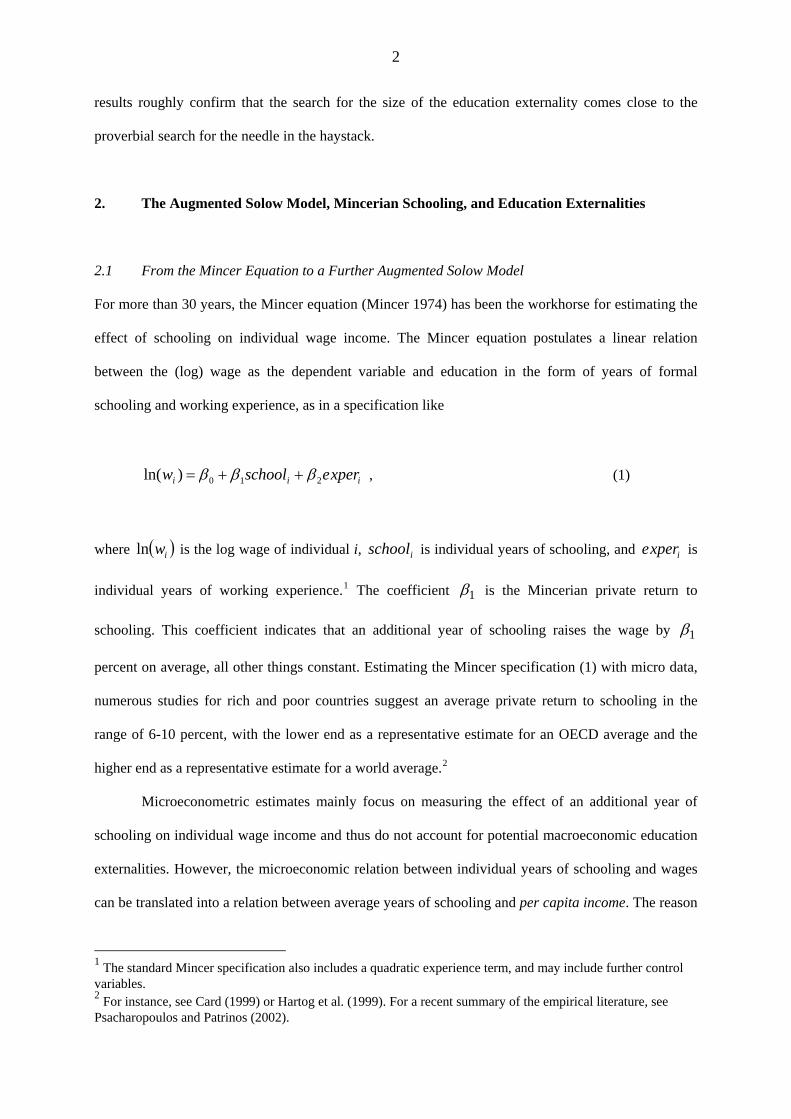
For more than 30 years, the Mincer equation (Mincer 1974) has been the workhorse for estimating the

effect of schooling on individual wage income. The Mincer equation postulates a linear relation

between the (log) wage as the dependent variable and education in the form of years of formal

schooling and working experience, as in a specification like

iii xpereschoolw 210)ln( βββ ++= , (1)

where is the log wage of individual i, is individual years of schooling, and is

individual years of working experience.

( )iwln ischool ixpere

1 The coefficient 1β is the Mincerian private return to

schooling. This coefficient indicates that an additional year of schooling raises the wage by 1β

percent on average, all other things constant. Estimating the Mincer specification (1) with micro data,

numerous studies for rich and poor countries suggest an average private return to schooling in the

range of 6-10 percent, with the lower end as a representative estimate for an OECD average and the

higher end as a representative estimate for a world average.2

Microeconometric estimates mainly focus on measuring the effect of an additional year of

schooling on individual wage income and thus do not account for potential macroeconomic education

externalities. However, the microeconomic relation between individual years of schooling and wages

can be translated into a relation between average years of schooling and per capita income. The reason

1 The standard Mincer specification also includes a quadratic experience term, and may include further control variables. 2 For instance, see Card (1999) or Hartog et al. (1999). For a recent summary of the empirical literature, see Psacharopoulos and Patrinos (2002).

3

is that the labor share (the share of total wages in GDP) does not follow a trend, neither over time

(Piketty and Saez 2003) nor across countries (Bernanke and Gurkaynak 2001; Gollien 2002). But if

labor shares are constant, wages are proportional to per-capita income. Hence the private return to

schooling has to be multiplied by the labor share to derive a benchmark for the macroeconomic return

to schooling that would be expected in the absence of an education externality. Put differently, a

positive difference between an observed macro return to schooling and the proportionally adjusted

private return to schooling would indicate the presence (and size) of an education externality.

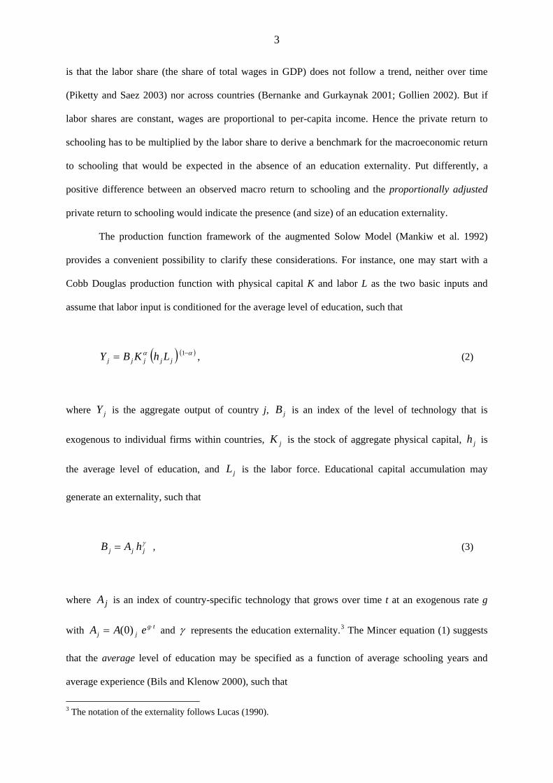
The production function framework of the augmented Solow Model (Mankiw et al. 1992)

provides a convenient possibility to clarify these considerations. For instance, one may start with a

Cobb Douglas production function with physical capital K and labor L as the two basic inputs and

assume that labor input is conditioned for the average level of education, such that

, (2) ( ) ( )αα −= 1jjjjj LhKBY

where is the aggregate output of country j, is an index of the level of technology that is

exogenous to individual firms within countries, is the stock of aggregate physical capital, is

the average level of education, and is the labor force. Educational capital accumulation may

generate an externality, such that

jY jB

jK jh

jL

, (3) γjjj hAB =

where is an index of country-specific technology that grows over time t at an exogenous rate g

with and

jA

tgjj eAA ⋅= )0( γ represents the education externality.3 The Mincer equation (1) suggests

that the average level of education may be specified as a function of average schooling years and

average experience (Bils and Klenow 2000), such that

3 The notation of the externality follows Lucas (1990).

4

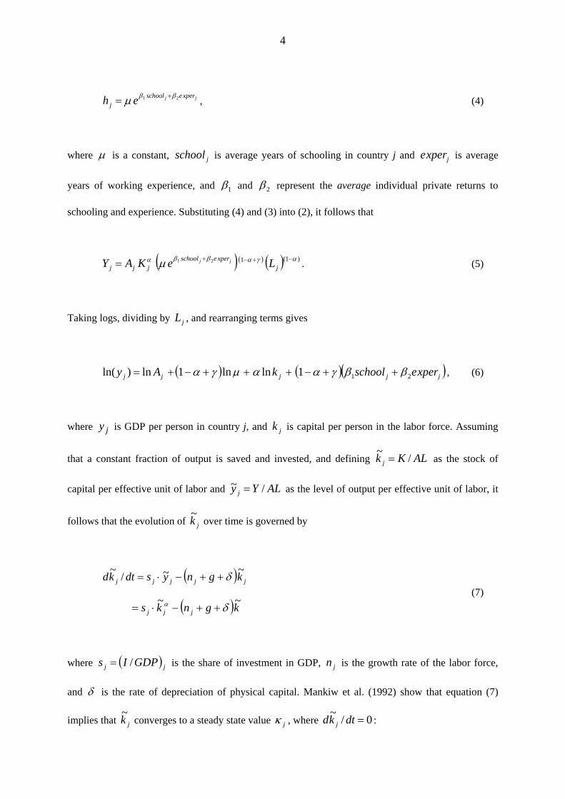
, (4) jj xpereschoolj eh 21 ββμ +=

where μ is a constant, is average years of schooling in country j and is average

years of working experience, and

jschool jxpere

1β and 2β represent the average individual private returns to

schooling and experience. Substituting (4) and (3) into (2), it follows that

( ) ( ) ( ) )1(121 αγαββα μ −+−+= jxpereschool

jjj LeKAY jj . (5)

Taking logs, dividing by , and rearranging terms gives jL

( ) ( )( )jjjjj xpereschoolkAy 211lnln1ln)ln( ββγααμγα ++−+++−+= , (6)

where is GDP per person in country j, and is capital per person in the labor force. Assuming

that a constant fraction of output is saved and invested, and defining

jy jk

ALKk j /~= as the stock of

capital per effective unit of labor and ALYy j /~ = as the level of output per effective unit of labor, it

follows that the evolution of jk~ over time is governed by

( )

( )kgnks

kgnysdtkd

jjj

jjjjj

~~

~~/~

δ

δ

α ++−⋅=

++−⋅= (7)

where is the share of investment in GDP, is the growth rate of the labor force,

and

( jj GDPIs /= ) jn

δ is the rate of depreciation of physical capital. Mankiw et al. (1992) show that equation (7)

implies that jk~ converges to a steady state value jκ , where 0/~=dtkd j :

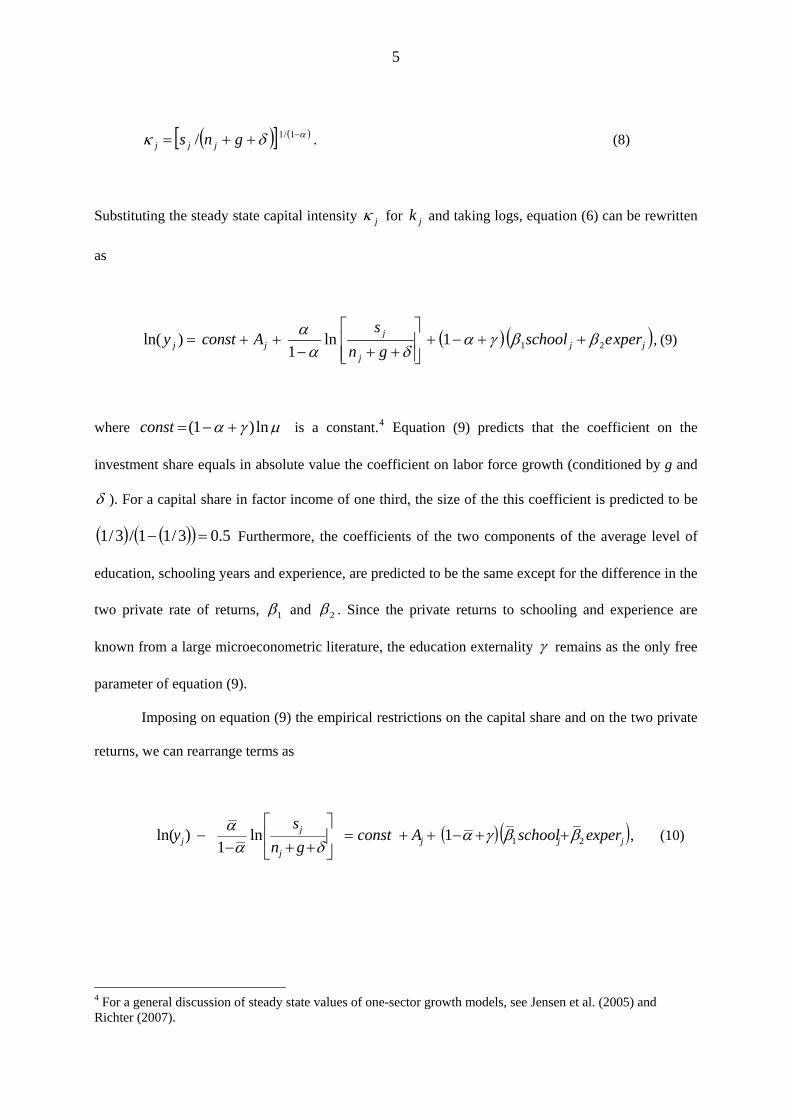
5

( )[ ] ( αδκ −++= 1/1/ gns jjj) . (8)

Substituting the steady state capital intensity jκ for and taking logs, equation (6) can be rewritten

as

jk

( ) ( )jjj

jjj xpereschool

gns

Aconsty 211ln1

)ln( ββγαδα

α++−+

⎥⎥⎦

⎤

⎢⎢⎣

⎡

++−++= , (9)

where μγα ln)1( +−=const is a constant.4 Equation (9) predicts that the coefficient on the

investment share equals in absolute value the coefficient on labor force growth (conditioned by g and

δ ). For a capital share in factor income of one third, the size of the this coefficient is predicted to be

Furthermore, the coefficients of the two components of the average level of

education, schooling years and experience, are predicted to be the same except for the difference in the

two private rate of returns,

( ) ( )( ) 5.03/11/3/1 =−

1β and 2β . Since the private returns to schooling and experience are

known from a large microeconometric literature, the education externality γ remains as the only free

parameter of equation (9).

Imposing on equation (9) the empirical restrictions on the capital share and on the two private

returns, we can rearrange terms as

( ) ( )jjjj

jj xpereschoolAconst

gns

y 211ln1

)ln( ββγαδα

α++−++=⎥

⎦

⎤⎢⎣

⎡

++−− , (10)

4 For a general discussion of steady state values of one-sector growth models, see Jensen et al. (2005) and Richter (2007).

6

where the restricted parameters are indicated by a bar. In this specification, the coefficient to be

estimated is ( )γα +−1 . In the absence of an education externality, the coefficient should equal two

thirds for a capital share of one third.

2.2. Macro Returns and the Size of the Education Externality: Benchmark Calculations

Equation (10) can be used to derive benchmark values for the macroeconomic returns to schooling

( schoolλ ) and experience ( xpereλ ):

( ) 11 βγαλ +−=school and (11a)

( ) 21 βγαλ +−=xpere . (11b)

Hence with a capital share in factor income of 3/1=α and with 1.01 =β as an upper bound for the

private return to schooling, we would expect to find a value of the macro-Mincer return to schooling

of 067.0=schoolλ if there is no education externality. Similarly, we would expect to find a value of

the macro return to experience of 02.0=xpereλ for an average private return of 3 percent )03.0( 2 =β

if there is no education externality. That is, a macro return to schooling of 10 percent or a macro return

to experience of 3 percent would indicate the presence of a large education externality.

Prevailing subsidies to public education are a major reason to expect empirical estimates of

schoolλ and xpereλ above the benchmark values of 6.7 percent and 2 percent. Given that the

instructional costs of schooling are mainly covered by public expenditures in most countries, the

question of interest is by how much the empirical estimates of schoolλ and xpereλ can be expected to

differ from the benchmark values. For instance in the United States, about 90 percent of the

instructional costs at public colleges are paid by federal and state governments. Based on US data,

Heckman and Klenow (1997) calculate that due to these subsidies, an individual will be indifferent

between additional schooling (college) and working if the private Mincerian return to schooling is

7

about 9 percent, which is in line with the typical micro-Mincer estimates. From the point of view of

the government, they calculate that the observed level of schooling subsidies is justified if the

macroeconomic return to schooling is about 3 percentage points higher than the benchmark value for

the private return. So based on our no-externality macro benchmark value of 6.7 percent, we would

expect to find a macro return to schooling of about 10 percent in order to justify present levels of

schooling subsidies.

A similar benchmark follows from a calculation that considers the macroeconomic return to

physical capital. If capital earns its marginal product (MPK), it can be measured as

( YKMPK // )α= . With a capital share of one third and a capital output ratio of 3, as discussed by

Mankiw et al. (1992) for the US, it follows that the implied macroeconomic return to physical capital

equals 11 percent. With a lower capital output ratio of 2, which represents an average value for rich

and poor countries, the implied macroeconomic return to capital would rise to about 17 percent. For a

lower bound of the capital share of 4/1=α , the macroeconomic return to capital would range from 8

percent to 13 percent, conditional on the applied capital output ratio. Since the macroeconomic returns

to physical and educational capital investments will tend to be equalized, we consider a macro return

to schooling of about 10 percent as a lower bound.

Given that the level of schooling subsidies reaches similar levels as in the US in most

countries around the world, an estimated macro return to schooling in the range of 10 percent would

imply that a large education externality is already internalized by the public subsidization of

schooling. For instance, equation (11a) suggests a benchmark value for the education externality γ of

one third for a macro return of 10 percent, a micro return of 10 percent, and a capital share of one

third.5

Equation (11a) also suggests that an estimate of an education externality that differs in a

statistically significant way from the benchmark estimate will be hard to come by. This is because

even small and statistically insignificant differences in macro returns to schooling imply large

differences in the size of the education externality. For all other parameters as before, an estimate of

5 Lucas (1990) derived a comparable education externality of 0.4 on the basis of US data for a capital share of 1/4 and the growth rates of per capita income and average years of schooling.

8

the macro return of 15 percent would already imply an education externality of 0.8, which looks

implausibly high within a production function framework.6 Thus a priori it seems that empirical

analyses can at best reveal whether there is a positive education externality at all, but not by how much

such an externality may differ from a benchmark value of one third that considers the prevailing level

of education subsidies.

3. Empirical Results

3.1 Main Variables and Measures of Schooling Quality

We begin our empirical analysis with a basic sample of 827 countries for which we have data on the

variables specified in equation (9), mainly for the base year 1995. Our data on GDP per worker (y),

investment ( ), and labor force growth (n) are taken from PWT 6.1 (Heston et al. 2002).

We assume a constant rate and a constant rate

GDPIs /=

02.0=g 05.0=δ , as is standard in the related

literature (see, e.g., Barro et al. 1995). Average years of schooling (school) are taken from Barro and

Lee (2001) and our measure of the average years of experience of the workforce (exper) is based on

data taken from UN (1997). The appendix A.1 includes detailed information on the definitions and

sources of all variables used in the empirical analysis.

Our preferred measure of schooling years takes into account that the quality of schooling is

not the same across countries. Recent comparative studies of international educational standards such

as the PISA study (OECD 2001) or previously the TIMS study (TIMSS 1996) have shown that there

are large international differences in the quality of schooling. We address this problem by correcting

the observed average years of schooling with a measure of schooling quality.

Hanushek and Kimko (2000) report standardized test scores in international comparisons of

student achievement in "percent correct" format. For countries not covered by Hanushek and Kimko

(2000) but included in our sample, we have imputed the missing values as averages of region- and

6 An education externality of 0.8 would imply that a doubling of all inputs would increase output by a factor of 3.5. 7 See appendix A.2.

9

income-based estimates, as reported in Gundlach et al. (2002). We then transform the "percent correct"

format into a format with an average of 500 and a standard deviation of 100 by solving for a and b in:

500*)( =+ abcorrectpercentaverage , and (12)

100*)( =bcorrectpercentstd . (13)

The format with an average of 500 and a standard deviation of 100 has been established as a standard

reporting format in recent international studies of student achievement (OECD 2001, TIMSS 1996).

According to these studies, a test score difference of about 50 points represents an average

performance difference of about one year of schooling (one grade). Regressing average years of

schooling on our transformed test score measure, we find that one year of schooling in the population

aged 15-65 is associated with a test score difference of about 60 points, close to the results reported for

TIMSS and PISA. We define our measure of quality-adjusted schooling as

( ) 60/500−+= jjj testschoolqschool , (14)

where is the transformed test score result for country j. That is, for countries with test score

results close to the international average of 500 points (like the United States), the quality adjustment

does not make an important difference, but a country with a test score result of about 380 points (like

Kenya) would have a quality-adjusted measure of schooling that is about two years below the average

years of schooling reported by Barro and Lee (2001).

jtest

3.2 Empirical Estimates of the Education Externality

Our empirical analysis mainly aims at estimating the sign of the presumed education externality, and

more ambitiously at estimating its size. As discussed in Section 2, we impose as restrictions a capital

share of 31=α , and private returns to schooling of 1.01 =β and to experience of 03.02 =β . By

imposing the empirical restrictions we can circumvent the problem that otherwise the parameters of

10

equation (9) cannot be estimated simultaneously because we have the four potentially unknown

parameters α , γ , 1β , and 2β , but only the three explanatory variables (conditional) investment

( )ln(ln δ++− gns jj ), average years of schooling with or without quality adjustment (qschool,

school), and experience (exper). So we estimate the education externality γ with the restricted

equation (10). However, equation (10) suggests that we should control for international differences in

the level of technology . jA

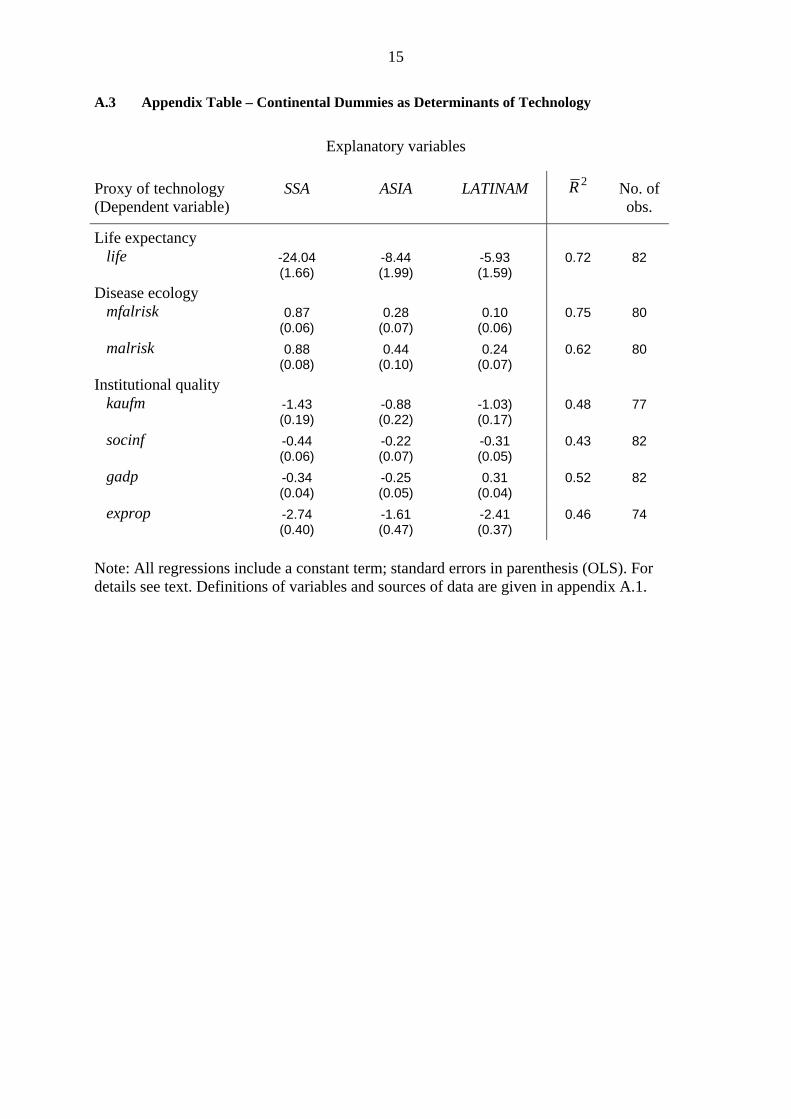
In appendix A.3 we document that a number of variables that have been suggested in the

literature as proxies for differences in technology across countries are closely correlated with a set of

continental dummies for Sub-Saharan Africa (SSA), Asia (ASIA), and Latin America (LATINAM). For

instance, we find that this set of three continental dummies can explain between 40 and 70 percent of

the variation of each of the following variables, which all may reflect certain aspects of international

differences in a broad concept of technology: a measure of life expectancy (Heckman and Klenow

1997), two alternative measures of the prevalence of malaria (Sachs 2003), and four alternative

measures of institutional quality (Hall and Jones 1999, Acemoglu et al. 2001, Rodrik et al. 2004).

These empirical results motivate our approach to control for international differences in a broad

concept of technology with three continental dummies.

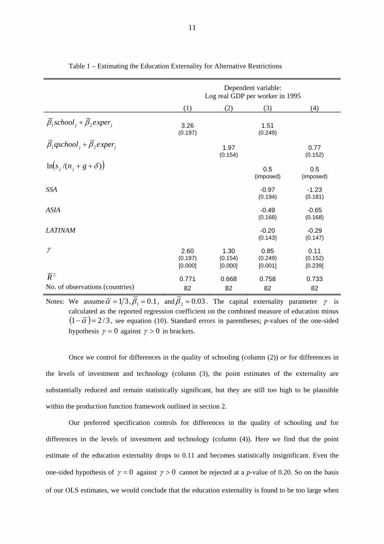
We get three basic results. We obtain a statistically significant education externality with a

large point estimate of 2.6 if we do not control for international differences in the quality of schooling

and in investment and technology (Table 1, column (1)). From an economic perspective, i.e., relative

to our benchmark value of 0.33 derived in section 2, an estimated externality of 2.6 appears to reflect

an omitted variables bias, since measures of education and experience are likely to be positively

correlated with the quality of schooling, the level of investment, and the level of technology. Hence

the estimated externality may be biased upwardly.

11

Table 1 – Estimating the Education Externality for Alternative Restrictions

Dependent variable: Log real GDP per worker in 1995

(1) (2) (3) (4)

jj xpereschool 21 ββ + 3.26 1.51 (0.197) (0.249)

jj xpereqschool 21 ββ + 1.97 0.77

(0.154) (0.152)

( ))/(ln δ++ gns jj 0.5 0.5

(imposed) (imposed)

SSA -0.97 -1.23 (0.194) (0.181)

ASIA -0.49 -0.65 (0.168) (0.168)

LATINAM -0.20 -0.29 (0.143) (0.147)

γ 2.60 1.30 0.85 0.11 (0.197) (0.154) (0.249) (0.152) [0.000] [0.000] [0.001] [0.239]

2R 0.771 0.668 0.758 0.733 No. of observations (countries) 82 82 82 82

Notes: We assume 31=α , 1.01 =β , and 03.02 =β . The capital externality parameter γ is calculated as the reported regression coefficient on the combined measure of education minus ( ) 3/21 =−α , see equation (10). Standard errors in parentheses; p-values of the one-sided hypothesis 0=γ against 0>γ in brackets.

Once we control for differences in the quality of schooling (column (2)) or for differences in

the levels of investment and technology (column (3), the point estimates of the externality are

substantially reduced and remain statistically significant, but they are still too high to be plausible

within the production function framework outlined in section 2.

Our preferred specification controls for differences in the quality of schooling and for

differences in the levels of investment and technology (column (4)). Here we find that the point

estimate of the education externality drops to 0.11 and becomes statistically insignificant. Even the

one-sided hypothesis of 0=γ against 0>γ cannot be rejected at a p-value of 0.20. So on the basis

of our OLS estimates, we would conclude that the education externality is found to be too large when

12

the empirical model is not properly restricted, and found to be absent when all presumed control

variables are included. Taken at face value, this result would suggest that the observed level of

subsidization of schooling is not justified for reasons of economic efficiency.

One caveat of our results is that they may be biased because of endogenous regressors and

especially because of measurement error. For instance, schooling and experience may be imperfect

proxies for a true measure of educational capital, with or without an adjustment for schooling quality.

To control for this potential sources of downward bias, one would have to consider instrumental

variables estimation (IVs). We leave a detailed discussion of IV estimation for further research.

4. Summary

Our paper shows how the augmented Solow model can be combined with the Mincer equation to

derive a simple production function specification that allows us to estimate an education externality.

With this framework, we can show how the well-known private rates of return to schooling and

experience relate to a macroeconomic rate of return that takes into account all external costs and

benefits of educational capital accumulation. For reasonable parameter values, we can also show that a

macroeconomic return that exceeds an (adjusted) private benchmark return by a few percentage points

implies a large difference for the education externality.

These considerations reveal why previous empirical studies have not succeeded in providing a

clear-cut picture. With cross-country data, even a five percentage point difference in macroeconomic

and private rates of return to schooling may not be large enough to allow for a statistically significant

estimate of the size of the education externality, and may often not even suffice to identify its sign.

Our OLS regression results confirm that what may appear as a statistically significant estimate of an

education externality disappears once the underlying specification is properly restricted. It remains to

be seen whether IV estimation results may provide a different answer.

13

Appendix

A 1. Definitions and Sources of Variables A Level of technology, approximated by continental dummies. ASIA Dummy variable for Asian countries; excludes Japan, includes Papua NG and

other Oceania. δ Depreciation rate (of physical capital); assumed to be 5 percent. exper Average years of experience of the working age population in 1990, calculated as

indicated in Heckman and Klenow (1997). Based on the age distribution of the population aged 5-64 years and on school enrollment rates, which can be combined to calculate the share of the population aged 5-64 years that is working (not in school). For each age group, work experience is calculated as age minus schooling attainment minus 6 years. Our measure is the working-population-weighted average of these experience levels. Source: UN (1997); Barro and Lee (2001); own calculations.

exprop Index of protection against expropriation, constructed by Political Risk Services.

Source: taken from McArthur and Sachs (2001). g Rate of technological change; assumed to be 2 percent. gadp Index of government anti-diversion policies; calculated as an unweighted

average of five variables: law and order, bureaucratic quality, corruption, risk of expropriation, and government repudiation of contracts. Source: Hall and Jones (1999).

kaufm Unweighted average governance indicator (1996), based on six aggregated survey

measures: voice and accountability, political stability, government effectiveness, regulatory quality, rule of law, and control of corruption. Source: Kaufmann et al. (2004).

LATINAM Dummy variable for Latin American countries. life Life expectancy at birth, 1990.

Source: World Bank (2005). malrisk Proportion of each country’s population at risk of malaria transmission, involving

three largely non-fatal species of the malaria pathogen (Plasmodium vivax, P. malariae, P. ovale) (1994); measured on a [0,1] scale; dataset as of 27 October 2003. Source: Sachs (2003), here taken from http://www.earth.columbia.edu/about/director/-malaria/index.html#datasets.

mfalrisk Proportion of a country’s population at risk of falciparum malaria transmission (1994);

measured on a [0,1] scale. Revised version, dataset as of 27 October 2003. Source: Sachs (2003), here taken from http://www.earth.columbia.edu/about/-director/malaria/index.html#datasets.

n Average growth rate of the workforce in 1960-1995. Source: Heston et al. (2002); own calculations.

14

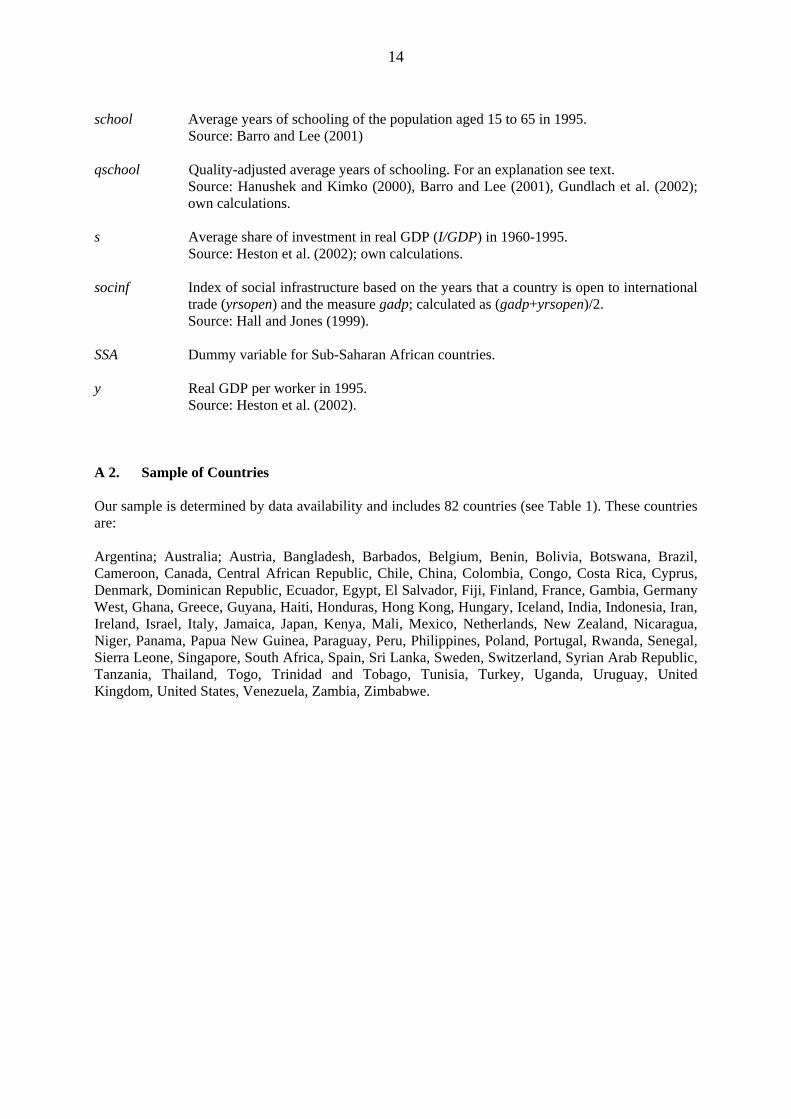
school Average years of schooling of the population aged 15 to 65 in 1995.

Source: Barro and Lee (2001) qschool Quality-adjusted average years of schooling. For an explanation see text.

Source: Hanushek and Kimko (2000), Barro and Lee (2001), Gundlach et al. (2002); own calculations.

s Average share of investment in real GDP (I/GDP) in 1960-1995. Source: Heston et al. (2002); own calculations. socinf Index of social infrastructure based on the years that a country is open to international

trade (yrsopen) and the measure gadp; calculated as (gadp+yrsopen)/2. Source: Hall and Jones (1999).

SSA Dummy variable for Sub-Saharan African countries. y Real GDP per worker in 1995.

Source: Heston et al. (2002). A 2. Sample of Countries Our sample is determined by data availability and includes 82 countries (see Table 1). These countries are: Argentina; Australia; Austria, Bangladesh, Barbados, Belgium, Benin, Bolivia, Botswana, Brazil, Cameroon, Canada, Central African Republic, Chile, China, Colombia, Congo, Costa Rica, Cyprus, Denmark, Dominican Republic, Ecuador, Egypt, El Salvador, Fiji, Finland, France, Gambia, Germany West, Ghana, Greece, Guyana, Haiti, Honduras, Hong Kong, Hungary, Iceland, India, Indonesia, Iran, Ireland, Israel, Italy, Jamaica, Japan, Kenya, Mali, Mexico, Netherlands, New Zealand, Nicaragua, Niger, Panama, Papua New Guinea, Paraguay, Peru, Philippines, Poland, Portugal, Rwanda, Senegal, Sierra Leone, Singapore, South Africa, Spain, Sri Lanka, Sweden, Switzerland, Syrian Arab Republic, Tanzania, Thailand, Togo, Trinidad and Tobago, Tunisia, Turkey, Uganda, Uruguay, United Kingdom, United States, Venezuela, Zambia, Zimbabwe.

15

A.3 Appendix Table – Continental Dummies as Determinants of Technology

Explanatory variables

Proxy of technology (Dependent variable)

SSA ASIA LATINAM 2R No. of obs.

Life expectancy life -24.04 -8.44 -5.93 0.72 82 (1.66) (1.99) (1.59) Disease ecology mfalrisk 0.87 0.28 0.10 0.75 80 (0.06) (0.07) (0.06) malrisk 0.88 0.44 0.24 0.62 80 (0.08) (0.10) (0.07) Institutional quality kaufm -1.43 -0.88 -1.03) 0.48 77 (0.19) (0.22) (0.17) socinf -0.44 -0.22 -0.31 0.43 82 (0.06) (0.07) (0.05) gadp -0.34 -0.25 0.31 0.52 82 (0.04) (0.05) (0.04) exprop -2.74 -1.61 -2.41 0.46 74 (0.40) (0.47) (0.37) Note: All regressions include a constant term; standard errors in parenthesis (OLS). For details see text. Definitions of variables and sources of data are given in appendix A.1.

16

References

Acemoglu, D., S. Johnson, J. A. Robinson (2001). The Colonial Origins of Comparative Development: An Empirical Investigation. American Economic Review 91 (5): 1369–1401.

Barro, R. J., J.-W. Lee (2001). International Data on Educational Attainment: Updates and Implications. Oxford Economic Papers 53 (3): 541–563.

Barro, R. J., N. G. Mankiw, X. Sala-i-Martin (1995). Capital Mobility in Neoclassical Models of Growth. American Economic Review 85 (1): 103-115.

Bernanke, B. S., R. S. Gürkaynak (2001). Is Growth Exogenous? Taking Mankiw, Romer, and Weil Seriously. NBER Macroeconomics Annual 16: 11–57.

Bils, M., P. J. Klenow (2000). Does Schooling Cause Growth? American Economic Review 90 (5): 1160-1183.

Card, D. E. (1999). The Causal Effect of Education on Earnings. In: O. Ashenfelter and D. Card (eds.), The Handbook of Labor Economics, Vol. 3A: 1801–1863. Amsterdam: Elsevier.

Gollin, D. (2002). Getting Income Shares Right: Accounting for the Self-Employed. Journal of Political Economy 110: 458–474.

Gundlach, E., D. Rudman, L. Wößmann (2002). Second Thoughts on Development Accounting. Applied Economics 34: 1359–1369.

Hall, R. E., C. I. Jones (1999). Why Do Some Countries Produce So Much More Output Per Worker Than Others? Quarterly Journal of Economics 114 (1): 83–116.

Hanushek, E. A., D. D. Kimko (2000). Schooling, Labor Force Quality, and the Growth of Nations. American Economic Review 90 (5): 1184–1208.

Hartog, J., J. Odink, J. Smits (1999). Private Returns to Education in the Netherlands: A Review of the Literature. In: R. Asplund and P. T. Pereira (eds.), Returns to Human Capital in Europe: A Literature Review. Helsinki: Research Institute of the Finnish Economy.

Heckman, J. J., P. J. Klenow (1997). Human Capital Policy. University of Chicago, mimeo.

Heston, A., R. Summers, B. Aten (2002). Penn World Table Version 6.1. Center for International Comparisons at the University of Pennsylvania (CICUP), October. http://datacentre2.chass.utoronto.ca/pwt/

Jensen, B. S., P. K. Alsholm, M. E. Larsen, J. M. Jensen (2005). Dynamic Structure, Exogeneity, Phase Portraits, Growths Paths, and Scale and Substitution Elasticities. Review of International Economics 13 (1): 59-89.

Jensen, B. S., M. Richter (2007). Stochastic One-Sector and Two-Sector Growth Models in Continous Time. In: B. S. Jensen, T. Palokangas (Eds.), Stochastic Economic Dynamics. Copenhagen Business School Press: 167-216.

Kaufmann, D., A. Kraay, M. Mastruzzi (2004). Governance Matters III. Governance Indicators for 1996-2002. World Bank Economic Review 18 (2): 253-287.

Lucas, R. E., Jr. (1990). Why Doesn't Capital Flow from Rich to Poor Countries? American Economic Review 80 (2): 92-96.

Mankiw, N. G., D. Romer, D. N. Weil (1992). A Contribution to the Empirics of Economic Growth. Quarterly Journal of Economics 107: 407–437.

McArthur, J. W., J. D. Sachs (2001). Institutions and Geography: A Comment on Acemoglu, Johnson, and Robinson (2000). NBER Working Paper, 8114, February.

Mincer, J. (1974). Schooling, Experience, and Earnings. New York: Columbia University Press.

17

OECD (2001). Knowledge and Skills for Life: First Results from the OECD Programme for International Student Assessment (PISA) 2000. Paris: OECD.

Piketty, Thomas, and Emmanuel Saez (2003). Income Inequality in The United States, 1913-1998. The Quarterly Journal of Economics 118 (1): 1-39.

Pritchett, L. (2006). Does Learning to Add up Add up? The Returns to Schooling in Aggregate Data. In: E. Hanushek, F. Welch (eds.), Handbook of the Economics of Education, Vol. 1: 635–695. Amsterdam: Elsevier.

Psacharopoulos, G., H. A. Patrinos (2002). Returns to Investment in Education: A Further Update. World Bank, Policy Research Working Paper, 2881, September.

Rodrik, D., A. Subramanian, F. Trebbi (2004). Institutions Rule: The Primacy of Institutions over Geography and Integration in Economic Development. Journal of Economic Growth 9 (2): 131-165.

Sachs, J. (2003). Institutions Don't Rule: Direct Effects of Geography on Per Capita Income. NBER Working Paper Series, 9490.

TIMSS International Study Center (1996). Highlights of Results from TIMSS. Third International Science and Mathematics Study. Boston College, November. http://wwwcsteep.bc.edu/TIMSS1/Achievement.html

United Nations (UN) (1997). The Sex and Age Distributions of the World Populations. New York: United Nations.

World Bank (2005). World Development Indicators. CD-ROM.