The causal effect of parents' schooling on children's schooling in Europe. A new IV approach

The causal effect of parents’ schooling on children’s

schooling in Europe. A new IV approach.

This version: December 2013.∗

Enkelejda HavariUniversity of Venice - Ca’ Foscari

Marco SavegnagoBank of Italy†

University of Rome “Tor Vergata”

Abstract

This paper estimates the causal effect of parental education on children’s educa-

tion in 13 European countries, using representative data from the Survey of Health,

Ageing and Retirement in Europe (SHARE). A novel instrumental variable approach

is used to solve the endogeneity issue. We combine two instruments: parental

birth order (indicator for being a first born) and Compulsory Schooling Laws (CSL).

While CSL have been widely used in applied work, our contribution is to introduce

parental birth order as instrument in the intergenerational mobility literature. We

find that parental education has a positive, large and significant causal effect on chil-

dren’s education. This finding is robust to the instrument chosen (birth order, CSL,

or both), to sample selection and to several robustness checks.

Keywords: intergenerational transmission, causality, birth order, education, Europe

JEL codes: J01, J6, I2, I24.

∗Corresponding author: Enkelejda Havari, [email protected]. We thank Josh Angrist, Erich Battistin,

Daniele Checchi, Mario Padula, Franco Peracchi, Andrea Pozzi, Kjell S.Salvanes, Daniela Vuri and an

anonymous referee for helpful comments. We also thank participants at: IRVAPP seminar (Trento, Decem-

ber 2013), 4th SHARE user conference (Liege, November 2013), Youth Workshop (Salerno, October 2013),

Royal Economic Society annual conference (London, April 2013), University of Venice “Ca’ Foscari” seminar

(April 2013), University of Rome “Tor Vergata” lunch seminar (October, 2012), Italian SHARE user confer-

ence (Venice, June 2012). All remaining errors are our responsibility. This paper uses data from SHARELIFE

release 1, as of November 24, 2010, and from SHARE release 2.5.0, as of May 24, 2011. The SHARE data

collection has been primarily funded by the European Commission. See www.share-project.org for

the full list of funding institutions.†Any views expressed in this paper are those of the authors and do not necessarily reflect those of the

Bank of Italy.

1 Introduction

It is widely known that more educated parents raise more educated children, al-

though it is difficult to identify the channels that contribute to this positive relation-

ship and their relative importance (Becker and Tomes 1979; Black and Devereux 2011;

D’Addio 2007). Inherited ability (nature) is a key driver in the transmission process of

human capital, as it reflects the underlying genetic endowment that is passed over gen-

erations. On the other hand, children’s probabilities of success in life are also influenced

by the environment in which an individual grows up (nurture), shaped by parental ed-

ucation and the amount of time and resources invested on them.

Disentangling the nature channel from the nurture one would help solving not only

an old controversy in the social sciences but also improve the design of more efficient

policies in the future. If the nurture channel prevails, then a well targeted policy inter-

vention (such as promoting the diffusion of student loans to mitigate family financial

constraints) can lead to positive spillovers for successive generations. Vice-versa, if abil-

ity dominates, policies can still be useful in helping more disadvantaged children, but

the achievements would come at a greater cost (Holmlund et al. 2011). Since parents not

only invest time and financial resources on children but also transmit part of their unob-

served ability, simply regressing children’s education on parental education is likely to

produce upward biased estimates of the parameter of interest, overstating educational

persistence across generations. Therefore, the objective of this paper is to propose a new

strategy to correct for the endogeneity issue.

Our contribution to the existing literature is twofold.

First, we introduce a new instrumental variable (IV) approach in the IGM literature:

exploiting the fact that first born individuals are on average better educated than later

born individuals (see sections 3.2 and 4.3 for details), we instrument parental educa-

tion with parental birth order. Importantly, this strategy does not require exogenous

shocks to be implemented (in the spirit of the quasi-experimental method), as informa-

tion on parental birth order is available in most household surveys.1 Then, we enrich

the instrument set considering also the compulsory schooling laws (CSL) introduced in

several European countries in different years, especially in the post-World War II period.

Although the two instruments target two different sub-populations (namely, first born

parents and parents exposed to the increase of the minimum schooling leaving age), re-

sults are similar using either one or the other instrument, or using both of them. Since

exogeneity of CSL reforms is generally accepted, we interpret this result as evidence in

favour of the exogeneity of parental birth order as instrument.

The second contribution we make points toward external validity: we extend the

1Such as the German Socio-Economic Panel, the Health and Retirement Survey, etc.

2

analysis of intergenerational causal effects in education to 13 European countries (Aus-

tria, Belgium, Czech Republic, Denmark, France, Germany, Greece, Italy, Netherlands,

Poland, Spain, Sweden, Switzerland). In this way we overcome the limitation of most of

the existing literature which relies on single-country analysis.

We draw on a new longitudinal household survey such as the Survey of Health,

Ageing and Retirement in Europe (SHARE), which is quickly reaching popularity among

researchers for many advantages it offers with respect to other data sources (see Section

4.1). For what concerns the analysis on CSL reforms, we supplement our data with

external information, relying on Brunello et al. (2009) and Brunello et al. (2012).

We find that parental education has a positive and significant causal effect on children

education. Using first born instrument only, a one-year increase in parental education

leads to an increase of 0.429 years in children’s schooling. When the sample is restricted

to those countries who have experienced changes in the compulsory schooling legisla-

tion (which reduces the sample size by two thirds), the causal effect increases to 0.6 using

first born alone and to 0.541 using as instruments both first born indicator and compul-

sory years of schooling. We acknowledge that the two instruments target two different

sub-populations and we address this issue by characterizing the compliers with respect

to some predetermined socio-economic variables. As expected we find that CSL reforms

mostly affect individuals at the bottom of the education distribution while the same can-

not be stated for first born compliers. Noteworthy, the causal effects are similar (in a

statistical sense) in apparently different sub-populations: a piece of evidence in favour

of the treatment homogeneity, although this conclusion must be taken with care. Finally,

we run a series of specification tests and robustness checks aimed to exclude the possi-

bility that our results are driven by a particular country or a particular characteristics of

parent’s family.

The paper is organized as follows: Section 2 describes the relevant literature regard-

ing intergenerational transmission of human capital in a causal framework. Section 3

outlines our identification strategy and provides background information on parental

birth order and CSL. Section 4 describes our data, what are our most important vari-

ables and sample choices, and provides some descriptive statistics. Section 5 presents

our results: OLS regressions, IV-2SLS regressions, the characterization of the compliers

sub-population and robustness checks. Finally, Section 6 concludes.

2 Background literature

The literature on intergenerational transmission of education from parents to chil-

dren is very rich and has traditionally followed a descriptive approach, documenting

education persistence across generations. However, in the last years there have been at-

3

tempts to unveil the causal mechanisms (if any) underlying such associations (Black and

Devereux 2011).

Empirical research accounts for endogeneity of parental education typically resort-

ing to three different strategies: twins studies (where the difference in schooling between

children of twin parents is regressed on the difference in schooling between the twin

parents themselves, so unobserved components are removed within twins),2 adoptees

(based on the idea that the genetic link between children and adoptive parents is ab-

sent),3 or instrumental variables (which exploit plausible exogenous shocks that in prin-

ciple should affect children’s schooling only through the education of the parents, com-

monly called the exclusion restriction).

None of these strategies is immune from pitfalls. Twins and adoptees strategies are

usually based on relatively small samples and they often neglect relevant unobserved

heterogeneity.4 On the other hand, instruments typically used to identify the parameter

of interest (such as CSL reform, or variation in college attendance rates) may be weak,

capture cohort variation if the policy shock is implemented nationwide, or cannot even

be available for the population of interest.

Our paper contributes to the IV strategy stream of literature. We instrument parental

education with parental birth order alone (in the first part of the analysis) and with birth

order and CSL reforms together (in the second part). We show that birth order as instru-

ment is relevant (it is highly predictive of parental education, ceteris paribus) and delivers

parameter estimates non statistically different from those obtained using the two instru-

ments together: we interpret this fact as indirect evidence in favour of the exogeneity of

parental birth order. The economic rationale of using these two instruments is developed

in sections 3.2 and 3.3.

Among others,5 our paper is mostly related to Oreopoulos et al. (2006), Chevalier

(2004), Black et al. (2005b), which exploit CSL reforms implemented after 1945 respec-

tively in US, UK and Norway. The intuition behind these papers is that a given cohort of

parents in a given county (or state, or municipality)6 was forced to stay in school an extra

year before they were legally allowed to drop out: this extra year of education does not

depend on parental unobserved ability or motivation and can be exploited as a source

of exogenous variation. Oreopoulos et al. (2006) find that increasing parental education

2Examples of twins strategy are Rosenzweig and Wolpin (1994), Behrman and Rosenzweig (2002), Pron-

zato (2012).3Examples of adoptees strategy are Sacerdote (2002, 2007), Bjorklund et al. (2006).4For instance, the fact that identical twins may not have identical abilities or that, as in the adoptees case,

the placement process can be related to the characteristics of the biological parents.5Such as Carneiro et al. (2013), Maurin and McNally (2008).6With the exception of Chevalier (2004), in which the 1972 CSL reform was applied nationwide in Eng-

land and Wales, in the other papers cited above there is variation in CSL implementation both in time and

in space.

4

significantly reduces children probability of grade repetition, and that mother’s and fa-

ther’s effects have similar magnitude. Chevalier (2004) finds a positive effect of maternal

education on the probability that a child receives a post-secondary degree; no significant

effect is found for fathers. Black et al. (2005b) show no evidence of a causal relation-

ship between parents’ and children years of education; when restricting the sample to

parents with less than 9 years of education (since the reform should not have impact on

more educated parents), they find no effect for fathers and small effects for mothers.

Our paper is also related to two recent works by Mazzonna (2013) and Stella (2013),

both of them using SHARE data. Mazzonna (2013) analyses the causal effect of education

on physical and mental health of the elderly population (SHARE respondents), instru-

menting education with birth order and CSL reforms. The most important differences

between our paper and Mazzonna (2013) are that: first, we focus on the intergenera-

tional persistence of education and not on the education-health relationship; second, in

our setting the statistical units are children of SHARE respondents and the endogenous

variable is parental education, thus leading to a different exclusion restriction (while in

Mazzonna 2013 both the dependent and independent variable is defined at the same

individual level). Stella (2013) adopts the CSL strategy in an IV regression of child’s on

parental education. There are important differences between our paper and Stella (2013).

First, we instrument parental education with birth order and CSL: this allows us to run an

over-identification test of restrictions for the instruments exogeneity and - within a het-

erogeneous effect framework - to study the characteristics of the sub-populations who

comply with our two instruments. Second, we consider up to 4 children for each parent

while Stella’s analysis is limited to first born children only: for the reasons explained in

section 3.2 we think that first born individuals are different from later borns, so results

obtained with a sample of first born children may not be generalized to other siblings.

3 Empirical strategy and descriptions of the instruments

3.1 Empirical model

Our analysis assumes a linear model linking child’s education to parents’ education,

unobserved child’s ability and other observed socio-demographic characteristics. This

model is standard in the economic literature when the dependent variable is given by

years of education and seems to fit very well our data (see the descriptive analysis in

section 4.3). The parameter of interest is the expected increase in children’s education

caused by a one-year increase in parental education, anything else being equal. Therefore,

our interest is in estimating β1 in the following equation:

5

ECij = β0 + β1 E

Pj + η hC

ij + εij , (1)

where ECij denotes years of the education of child i in family j, EP

j is parental edu-

cation (note that this variable does not have the index i, as we can have more children

for one parent), hCij represents child’s unobserved ability and εij is a random component

uncorrelated with any other variables included in the model. OLS estimation of (1) is

flawed since children’s ability is not observed. If innate ability is transmitted across gen-

erations (for example through a first order AR process)7 and if we assume η > 0, then

we have Cov(EPj , h

Cij) > 0: in this case, the OLS estimator of β1 is biased upward.

To estimate β1 consistently we rely on instrumental variables (IV). The underly-

ing idea is to exploit exogenous variation in parents’ education (that is, not related to

parental ability) to identify the causal effect on children’s education. The identifying as-

sumption is that the instruments affect child’s education only through parental education.

Accordingly, we estimate the following model by 2SLS, where equations (2) and (3)

are respectively the causal equation of interest and the first stage:

ECijtc = β0 + β1 E

Pjtc +Xijtc

′β2 + f(t, c) + (η hCijtc + εijtc) (2)

EPjtc = α0 + Zjtc

′α1 +Xijtc′α2 + f(t, c) + ξjtc. (3)

In equations (2) and (3), ECijtc denotes again years of the education of child i in family

j born in year t in country c, EPjtc is parental education, hC

ijtc is the omitted child ability,

and εijtc and ξjtc are random shocks affecting respectively child’s and parent’s education.

In the regressions we include a set of socio-demographic controls for both generations

Xijtc and a set of country and cohort fixed effects f(t, c). The matrix Zjtc represents our

set of instrumental variables: depending on the specifications we will use Zjtc ≡ [FBjtc]

or Zjtc ≡ [FBjtc, CSLjtc], where FBjtc is a binary variable taking value 1 when the parent

is first born and CSLjtc measures the minimum years of completed education mandated

by Compulsory Schooling Laws.

In the next two sections we provide more details on our instruments and discuss

their validity.

3.2 First instrument: Parental birth order

In the first part of the analysis we instrument parental education with parental birth

order (using first born status). It is well established in the economic literature that first7If, for example, equation (1) was estimated on a sample of adopted children and adoptive parents, then:

(i) child’s and parent’s innate ability would be orthogonal; (ii) child ability would be orthogonal to parent’s

education and ; (iii) its omission from equation (1) would not bias OLS estimates.

6

born individuals tend to have more years of education than the later born (Becker and

Lewis 1973, Black et al. 2005a, De Haan 2010). There are several possible (and non exclu-

sive) reasons behind this fact. First, credit constrained families may run out of financial

resources to support investment in human capital of later born children, especially in

larger families. This last consideration highlights the importance of appropriately ac-

counting for family size in the birth order analysis, since later born individuals are more

likely to belong to larger families (e.g. a birth order of 4 implies sibship size larger or

equal to 4). Second, there might exist cultural preferences that tend to favour investment

of resources and time towards first born children. Third, if the time spent with parents

during early childhood is more valuable (in terms of future educational achievement)

than the time spent when children are grown-up, then a first-born child is advantaged

since he/she does not have to share parental time with other siblings until a second child

is born. Fourth (but somehow related to the third reason), as emphasized by Zajonc

(1976) “confluence model”, the average intellectual environment within the family de-

clines as the number of children increases. In other words, a first child exploits the richest

intellectual environment composed by two cognitive mature adults, a second child lives

with two adults and one immature child and so on: the result is that later born children

face the most diluted intellectual environment, with negative consequences for their ed-

ucation. Finally, there might be strategic parenting, according to which the upbringing of

a first born child is stricter in order to deter bad behaviour in later born children, and this

strict upbringing contributes to first borns’ higher education (Hotz and Pantano 2013).

Determining which of these channels prevails, and how their relative importance

varies across countries and cohorts, would be indeed an interesting topic to explore but

this goes beyond the scope of the paper. Since we are using a sample of parents aged

more than 50 years old (with the median age be 64), we can only conjecture that cultural

preferences towards the first born individuals are driving most first born educational

advantage (our first stage effects that we will see in section 3.2). Whatever are the un-

derlying mechanisms that link birth order to education, a necessary condition for our

identification strategy is that our first-born instrument is exogenous.8

A key assumption is that the first-born instrument satisfies the exclusion restriction,

that is to say that parental education is the only channel through which the first-born

variable FBjtc affects children’s educationECijtc. The exclusion restriction may be violated

if first born parents have a better endowment of innate ability, which then is transmitted

to their children via the genetic link.

It is difficult though to imagine a credible reason why first born individuals should

possess more innate ability than later born individuals, except maybe for the fact that

later-born children are born to older mothers and are going to receive a presumably

8In our previous notation: Cov(FBjtc, η hCijtc + εijtc) = 0.

7

lower quality genetic endowment. The evidence on the relationship between birth order

and intelligence, as measured by IQ or by ah hoc designed cognitive tests, is controver-

sial (see discussions in Black et al. 2011 and in Kanazawa 2012). Most of this controversy

involves whether birth order has genuine within-family effect (with earlier born being

more intelligent then later born in the same family) or reflects spurious between-family

association (with earlier born in small families being more intelligent than later born in

large families). Rodgers et al. (2000) argue that almost all empirical studies have used

cross-sectional data, and the negative association between birth order and intelligence

found by those studies is a “methodological illusion”. More recently Black et al. (2011)

find large and significant birth order effects on IQ for a large sample of Norwegian young

men, using both cross-sectional and within-family methods; however, the authors them-

selves state that such IQ gap cannot be ascribed to either genetic or biological differences

resulting from different experiences in utero. Kanazawa (2012) studies the effect of birth

order an a series of ad hoc designed cognitive tests for a cohort of British children at ages

7, 11 and 16. Differently from Black et al. (2011), he finds that the correlation between

birth order and test scores is completely driven by family size and suggests that “birth

order has no genuine causal effect on general intelligence”. In light of the above dis-

cussion, we feel safe in considering parental birth order orthogonal to children’s innate

ability.

The exclusion restriction might also be violated if parental birth order is correlated

to some other determinants of children’s education, that go beyond father education.

Although instrument exogeneity is untestable, we tackle this issue in two ways. First,

evidence from the J-test of over-identifying restrictions never rejects the null hypothesis

of instruments exogeneity: since CSL reforms arguably satisfy the exclusion restriction

(see section 3.3), we interpret this evidence in favour of birth order exogeneity. Second,

we can exclude one potential mechanism through which parental birth order may affect

children’s education, other than parental education. If first born parents are more likely

to receive bequests from their parents, this can have a positive effect on children’s edu-

cation. Our data show that birth order is not associated with the probability of receiving

a property house as bequest. Finally, Mazzonna (2013) shows that parental birth order

does not affect biological characteristics (such as adult height) or psychological traits

(such as the level of religiosity) that in our case may drive both parental and children

education.9

9In Mazzonna (2013) the focus is on potential drivers of educational choices and old age health outcomes

for the same individual.

8

3.3 Second instrument: Compulsory Schooling Laws

As already stated in the previous section, we consider as a second instrument the

number of mandatory schooling years induced by the introduction of CSL in 10 Eu-

ropean countries in different years. The use of CSL as instrument for education is well

established in the literature and has been used in different contexts (Angrist and Keueger

1991; Oreopoulos et al. 2006; Chevalier 2004; Brunello et al. 2009, etc), showing a positive

and moderate effect of CSL on educational attainment in different countries.

For the use of mandatory schooling years as instrument we rely mostly on Brunello

et al. (2009), where they exploit plausibly exogenous variation in schooling induced by

CSL in Europe in the post-World War II period, using prevalently the SHARE survey.

The key assumption in this type of literature is that additional schooling is assigned to

each individual based on the date of birth and independently from their future choices

or observable characteristics. In our paper this translates into saying that mandatory

schooling is assigned to parents based on their year of birth without influencing directly

the future education of their children (exclusion restriction). The identification of CSL

effects on parental education comes from the variation of the schooling reforms across

countries and over cohorts. One raised issue is that educational reforms could poten-

tially improve school quality (e.g leading to spillover effects) which is in most cases an

omitted variable. Brunello et al. (2013) test this assumption using external data and find

that the internal validity of this popular identification strategy is intact.

4 Data and descriptive statistics

4.1 The Survey of Health, Ageing and Retirement in Europe

Our study draws on the Survey of Health, Ageing and Retirement in Europe (SHARE),

a multidisciplinary cross-country household panel survey, which collects detailed infor-

mation on individuals aged 50 or more (plus their spouses independent of age), who

speak the official language of the country in which they reside and do not live abroad

or in an institution. SHARE is to be considered a representative sample of old-age Eu-

ropeans and is conducted in many countries (13 of which form a longitudinal sample),

representing different areas of Europe: Northern Europe (Denmark and Sweden), Cen-

tral Europe (Austria, Belgium, France, Germany, the Netherlands, Switzerland), Eastern

Europe (Poland and Czech Republic), the Mediterranean countries (Greece, Italy, Spain),

Ireland and Israel. Four waves of SHARE are currently available, where in the last one

(released in November 2011) four new countries have joined the project (Estonia, Hun-

gary, Portugal and Slovenia). Greece has left the project in the last wave while Israel was

included in wave 1 and Ireland in wave 2. In our analysis we will consider 13 countries

9

participating both in wave 2 and Sharelife.

SHARE collects detailed information at the household and individual level cover-

ing different topics such as: household economics, education, health, social security

and income, financial investments, etc. An advantage of the survey is undoubtedly its

cross-country comparability due to the common questionnaire and the standardization

of fieldwork procedures in each country (Borsch-Supan and Jurges 2005). Further, it is

designed to be harmonized with other surveys such as the Health and Retirement Study

(HRS) in the US and the English Longitudinal Survey on Ageing (ELSA) in UK.

A second advantage of SHARE is the release of its third wave, named SHARELIFE,

which recollects retrospectively information on life-histories of each individual from age

10 onwards considering among others housing transitions (from first residence), em-

ployment transitions (from first job), complete fertility histories, changes in health and

health behaviour, and includes also a distinct module with detailed questions regarding

childhood circumstances (when respondents were about 10 years old). This is important

in the light of numerous findings that early life circumstances matter for long-term out-

comes (Almond and Currie 2011). In SHARELIFE the modules of questions are arranged

based on what is usually most important for the respondent and hence remembered most

accurately (e.g starting from children, partners and then accommodation). Further, the

interview is supported by a multidimensional life grid, a computerized version of the

life-calendar interview - that allow respondent to view important events on a computer

screen and at the same time allows the interviewer to link questions to parallel events.

See Havari and Mazzonna (2011) for the analysis of recall bias problems in the SHARE-

LIFE data. In particular they show that information related to the childhood period is

very little affected by problems of recall bias or coloring.

4.2 Description of main variables

Parental and children education The main variables in our analysis are the educa-

tional attainment of parents and children. We measure education by the number of years

spent in full time education. While for parents (SHARE respondents) we know both the

years of completed schooling and the highest degree obtained (ISCED level), for chil-

dren we know only the latter: for this reason we convert the ISCED level into years of

schooling by exploiting information on the educational system of each country.10 Since

the questionnaire is common and the questions related to educational attainment are al-

ready expressed in a comparable format (using ISCED classification), we expect errors

to be very limited.

10SHARE provides details in the release guide (see SHARE release guide wave2, 2-5-0, 2011).

10

Parental birth order and family size Information on parental birth order is gathered

from wave 2. Each respondent is asked to provide his birth order, specifically whether

he is the oldest child, the youngest one or somewhere in between. Further, he is asked

to count the number of siblings still alive at the time of the interview. To better infer

respondent’s sibship size we also rely on questions contained in the childhood module

(SHARELIFE). In particular, knowing the number of persons living in the house at the

age of 10 and the presence of each family component (mother, father, etc) we compute the

number of siblings at the age of 10. We combine information on sibship size from both

wave 2 and SHARELIFE and in absence of information from wave 2 we use siblings size

defined at the age of 10.

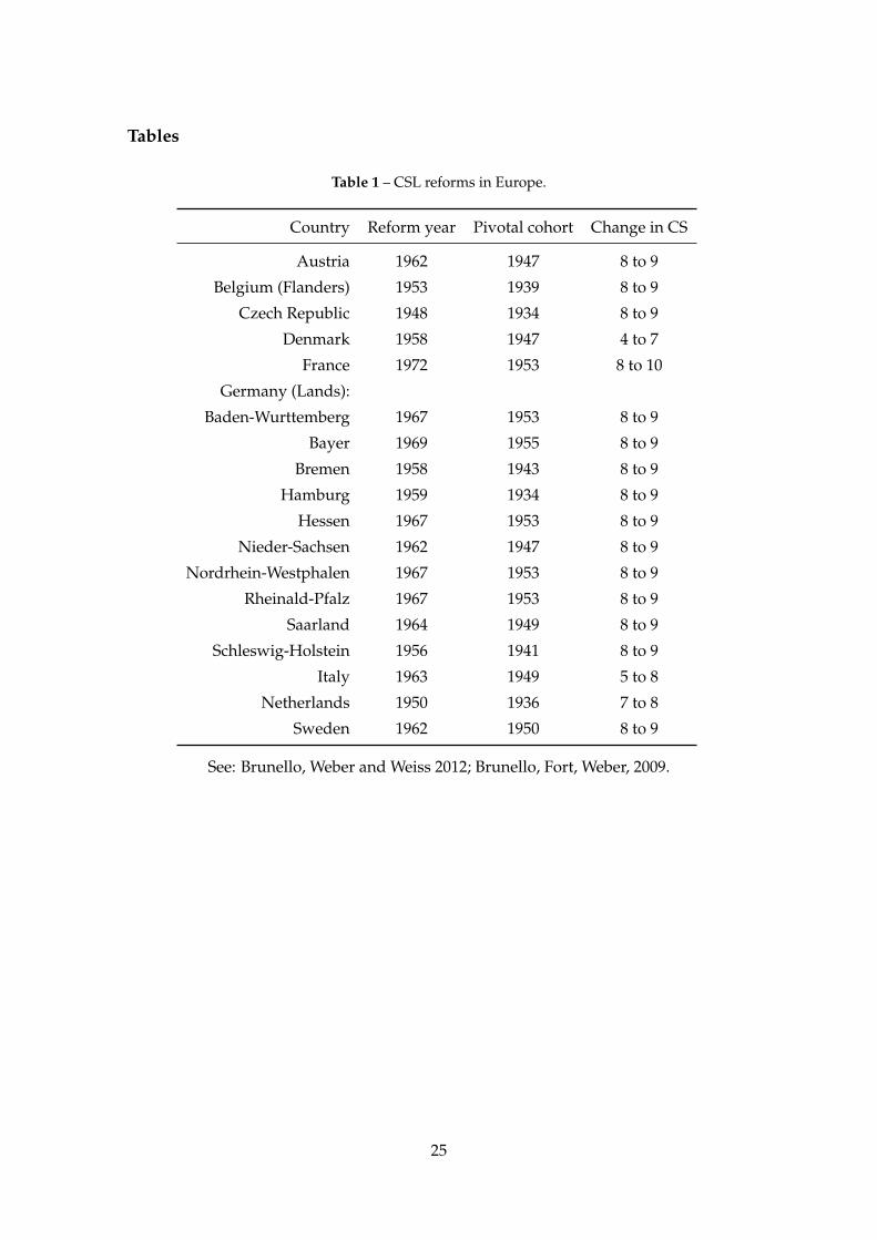
Compulsory schooling laws. Information on CSL is taken from the papers by Brunello

et al. (2009) and Brunello et al. (2012). We restrict our sample to include the following

countries: Austria, Belgium (only Flanders), Czech Republic, Denmark, France, Ger-

many (only Western part), Italy, the Netherlands and Sweden (See Table 1).11 As in

previous papers we select one reform for each country to avoid blurring the differences

between the pre-treatment and post-treatment cohorts. It is important to underline that

generally the compulsory schooling laws have contributed to an increase of parental

schooling by one extra year, affecting especially those at the ISCED 2 or 3 level depend-

ing on the country under consideration. To make the comparison between post-treated

and pre-treated cohorts as credible as possible, we restrict our sample to parents born

up to 10 years before/after the pivotal cohort, who have biological children aged 25 or

more (see Section 4.3).

Other control variables We also control for children’s birth order and sibship size (as

we do for parents). Information on children can be found in wave 2 in a specific module,

where one of the parents (the family respondent) provides details for children’s edu-

cation, birth year, marital status etc. Further, we include an indicator for parent ever

being unemployed during lifetime. This indicator is constructed looking at employment

transitions of SHARE respondents (parents) in SHARELIFE.

4.3 Samples selection and descriptive statistics

In the regression analysis we use two samples, depending on the adopted set of in-

struments. When parental first born indicator is used alone, we consider the full sample.

We select parents present in both wave 2 and 3 of SHARE and aged more than 50 years

old (more than 16.000 parents). For each respondent, we know the schooling level of up

11For more details we remind to the paper by Brunello et al. (2009).

11

to 4 selected children. We end up with a sample of almost 37.000 children, born before

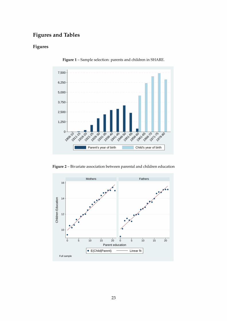
1981. From now on, we refer to this sample as the Full sample. Figure 1 gives a graphical

description of birth year for parents and children in the full sample.

When parental first born indicator and CSL reforms are used together, our sample is

restricted to those countries that actually experienced a CSL reform: in this way we lose

Greece, Poland, Spain and Switzerland. Moreover, to isolate the CSL reform effect, for

each country we consider parents born up to 10 years before and 10 years after the first

cohort potentially affected by the reform (so called pivotal cohort). With these restric-

tions we are left with about 6400 parents and 13500 children. For simplicity we refer to

this sub-sample as the CSL sample.

Table 2 shows descriptive statistics for parents and children in both the full and CSL

samples. We learn that parents have on average 10.3 years of education, are female

(57%, reflecting differential mortality at old ages), aged 66, first born (39%), with 2.39

children and prevalently live with the spouse or partner (69%). The picture is similar in

both samples, with the exception that the average level of education is higher in the CSL

sample (11.2 years), because some countries characterized by low levels of education

(such as Spain and Greece) are excluded due to absence of CSL reforms. Children have

on average 13 years of education in both samples, are equally shared among males and

females, aged 40, first born (45%) and prevalently live with the spouse or partner (64%).

Since we are interested in the relation between parental and children education, in

Figure 2 we show the bivariate association between the two variables. Each point in the

graphs represents the conditional sample mean of children education for any given level

of parental education. These graphs provides support for the use of a linear model for

our data.

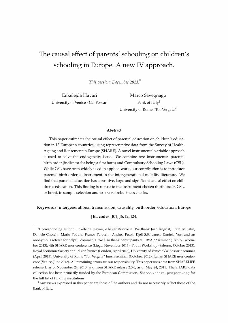
In the next figures we show graphically the intuition behind our first born instru-

ment. The left panel of Figure 3 shows the “first stage” when using birth order, con-

trolling for family size. In particular, first born parents have approximately 0.5 years of

education more than non-first borns. This advantage is roughly constant for any level

of sibship size, although it slightly declines in larger families. The right panel shows

the “reduced form” effect. Children of first born parents have approximately 0.25 years

of education more than children of non-first born parents: even in this case the gap is

roughly constant controlling for sibship size and slightly reduces for larger family. From

this simple analysis we would expect a 2SLS effect not far from 0.5.

12

5 Results

5.1 OLS results

Because the sample size associated to each instrument is different,12 to make sensi-

tive comparisons across estimation methods we report: the OLS results for both the full

sample and the CSL sample (Table 3); IV results using only parental birth order as in-

strument for both samples as well (Tables 4 and 5); IV results using only CSL reforms

as instrument for the CSL sample (Table 6); 2SLS results using both instruments for the

CSL sample (Table 7); a synthetic view of results is given in Table 8.

We start discussing the OLS estimates for equation (2) in Table 3. Two different spec-

ifications are used. In the baseline regression (columns 1 and 3) we control for parental

education, indicators for the dyads father-daughter, mother-daughter and mother-son

(excluded category: father-son) aimed to capture fixed effect for parent’s and children

gender. We also add country fixed effects, parental birth year fixed effects and child

3-years cohort fixed effects: these fixed effects are meant to absorb time-invariant coun-

try characteristics and capture the historical evolution of education for both parents and

children generations. In columns 2 and 4 we add a series of indicators for child’s birth

order (excluded category: first born) and a continuous variable for the total number of

children in the family.13 Since parental employment history could be relevant for chil-

dren’s achievement, we add an indicator for parent being ever unemployed. We cluster

standard errors at the household level as we have multiple children for each parent.

As expected we find a positive and significant relationship between parents’ and

children’s years of education. An increase in parental education of one year leads to an

increase in children’s schooling of 0.27–0.25 of a year (about three months), depending

on the specification.14 Interestingly, the estimated coefficients for parental education are

very similar across the two samples. In general, daughters are more educated than sons

(irrespectively whether the respondent parent is male or female), and sons with respon-

dent parent being the mother are more educated than sons with respondent parent being

father.

The estimated coefficients of other control variables have the expected sign. Second

born children, third born, fourth born, fifth or later born have respectively 0.32, 0.54,

0.87, 1.29 fewer years of education than first born children:15 this evidence suggests that

12Full sample when using first born as instrument; CSL sample when using compulsory schooling laws,

restricting the number of countries to those enacting reforms.13We also experimented using a series of dummies for number of children instead of the continuous vari-

able: estimated coefficients are very similar both for the parameter of interest and for the control variables.14Our estimates are consistent with the general findings in the literature. Intergenerational elasticities in

education vary between 0.20 and 0.45 (Black et al. 2005b).15The magnitude and the significance of these last four estimates is little affected if the number of children

13

the advantage of earlier born individuals persists even in the most recent generations.

Moreover, increasing the number of children in the house decreases the expected years

of schooling of all children by 0.18 years of education; finally, education is reduced by 0.3

years if parent has ever experienced an unemployment spell in his/her labour history.

5.2 2SLS results

We now discuss estimates from the IV/2SLS regression, which represents the core of

our results. We start considering only parental birth order as instrument. Table 4 shows

the estimates from the first stage, where parental education is regressed on a dummy for

parent being first born, a set of dummy variables capturing parental sibship size (where

the excluded category is a parent with no siblings) and all the other controls included in

the OLS regressions.16

Like in Figure 3, we notice a positive effect of parental birth order on educational

achievement, even when the largest set of controls is added. Being a first born parent

increases parental schooling by 0.415 of a year (approximately 5 months of extra school-

ing) with respect to a later born; when we use the CSL sample the first stage estimate

increases to 0.48. First born instruments exhibit a high predictive power on parental

education: even when adding the full set of controls, the F statistic on the excluded in-

strument is 38.4 in the full sample and 21.2 in the CSL sample. Differently from what we

have seen in Table 3 for the children generation, females are less educated than males:

the mother-daughter and mother-son coefficients are negative and significant. The detri-

mental effect of parental sibship size is large and significant when sibship size is at least 3

(so parent with two brothers/sisters) in the full sample, and at least 4 in the CSL sample.

The IV estimates using first born as instrument are reported in Table 5. The results

point towards a positive causal effect of parent’s schooling: a one-year increase leads

children schooling to increase by 0.43 of a year (around 5 months) using the full sample

and to 0.6 of a year (around 7 months) using the CSL sample. Being the first (to our

knowledge) to use such an instrument in the intergenerational mobility literature, we

cannot compare this estimate with existing studies.

Moreover, most of the above cited papers focus on different dependent variables

rather than years of education (such as the probability of attending post-secondary edu-

cation or the probability to repeat a grade).17

is entered in a set of fourteen mutually exclusive dummies.16Obviously, children characteristics are not determinants of parental education: these controls are in-

cluded because they enter as exogenous variables in the IV regression, whose estimates are shown in Ta-

ble 5.17Also for this lack of comparability we enriched the instrument set with CSL, even at the cost of reducing

the sample size from more than 35,000 to less than 13,000 children.

14

Notably, the 2SLS estimates are higher than the OLS estimates by a factor of 1.7 and

2.4 respectively in the full and CSL sample. Although this does not meet the a priori be-

lieves about the source of endogeneity, this evidence is quite common in the empirical

applications. One common explanation is that the IV corrects both for classical measure-

ment error (which biases downwards the OLS estimates) and for the endogeneity of the

dependent variable, and that the first effect prevails on the second one. Another expla-

nation (in the context of IGM literature see discussion in Oreopoulos et al. 2006) suggests

that IV can be larger than OLS because the IV estimates approximate the average effect

for a small group of the population (the one targeted by the instrument), whereas the

OLS estimates provide an average effect among everyone. A detailed analysis on the

characteristics of the subgroup mostly affected by the instrument (birth order) is pre-

sented in Section 5.3.

Table 6 show results for IV regression when using as instrument CSL solely. Since

we select only countries where some educational reforms took place and cohorts born

10 years before or after the pivotal cohort, we lose about two-thirds of the full sample.

From now on, our discussion will be based on the CSL sample only.

In the first two columns we show results from the first stage (column 1 is the baseline

and in column 2 we add other controls). An increase of 1 year in compulsory schooling

increases parental education by 0.25.18 The F-statistic is higher than 11, so the instrument

should not be weak, although it is lower than the F-statistics when using first born.

With CSL, we find again a positive effect of parental schooling on children’s school-

ing (columns 3 and 4), although in the last specification it is significant at a 10% level.

The estimated marginal effect is 0.42 or 0.38 according to the specification.19

We are now ready to discuss our last set of estimates: Table 7 shows 2SLS regression

results with both instruments used together. As in table Table 7, columns 1 and 2 report

first stage estimates. Being a first born parent increases education by 0.47 years (slightly

less than when first born was used alone; see column 4 in Table 4) and one extra year of

compulsory schooling yields 0.217 years of actual schooling (slightly less than when CSL

was used alone; see column 2 in Table 6). Using the two instruments together does not

jeopardize their predictive power: both first stage coefficients are significant at the 1%

level and the combined F statistic is 14.5. In columns 3 and 4 we report 2SLS estimates.

All control variable coefficients have the expected sign. Parental family size is irrelevant

to children education; being second born children, third, fourth and more than fifth re-

duces education by respectively 0.237, 0.421, 0.57 and 1.212 years; an extra child in the

family reduces education of 0.1 years. The causal effect in this over-identified model

is 0.541 years of education: the effect is large in magnitude and significant at 1% level.

18The result from the first stage when using CSL is similar to that reported by Brunello et al. (2009).19Both the magnitude and the precision of estimates are comparable to those reported in Stella (2013).

15

This estimate is closer to the one found when using first born instrument alone (0.6): this

reflects the fact that the first stage when using first born is stronger than the first stage

when using CSL reforms. Columns 3 and 4 also report the statistic and the p-value of

the J-test of over-identifying restrictions: in both specifications the null hypothesis that

the instruments are correctly excluded from the main equation is not rejected. Assuming

the exogeneity of CSL, this - coupled with the robustness checks in Section 5.4 - might be

interpreted as evidence in favour of the first born exogeneity.

In Table 8 we summarize all our main results. We found that the OLS estimates

of parental education to be around 0.25, a value in line with other empirical studies.

The IV estimates using first born ranged between 0.415 and 0.6 (always significant at

1%) depending on specifications and sample used; in all cases, first stage were very

strong. The IV estimates using CSL reforms are 0.375 (significant at 10%) or 0.421 (5%)

depending on the specification; F-statistics on the excluded instruments were smaller

than in the first born case but above the often used rule of thumb of 10. Finally, full 2SLS

specifications delivered estimates of 0.541 and led to a non rejection of the J-test.

One further question needs to be explored further: why the two IV estimates are

different (although not as much as to reject the J-test) and why they are larger than OLS.

This question is addressed within a heterogeneous treatment effect model. A priori we

expect the two instruments to affect different subgroups of the population. The CSL

affects those who in absence of the reforms wouldn’t have taken further education: this

is represented by those in low socio-economic status. First born instrument affect those

individuals who wouldn’t have taken further education if they had not been first born: in

principle this might happen not only at the bottom of the socio-economic distribution but

even - and probably more - in the middle class. Some socio-demographic characteristics

of the individuals affected by the instruments are studied in Section 5.3.

5.3 Heterogeneous treatment and compliers characterization

Where does the difference between the two IV estimates (with first born delivering

higher estimates than CSL) come from? Within a homogeneous treatment effect frame-

work it just reflects sample variability (if both instruments are valid), whereas if we allow

the treatment effect to vary across individuals it may be the case that the two instruments

target two different sub-populations and thus deliver two different IV estimates. In this

section we interpret our estimates as Local Average Treatment Effect, i.e. the effect on

children education for those parents who changed their education in response to one or

the other instrument (so called compliers).20 Although the compliers cannot be listed from

observed data, by exploiting Bayes theorem the compliers population can be easily char-

20Imbens and Angrist (1994), Angrist and Pischke (2008).

16

acterized when both the endogenous variable and the instrument are binary.21 Therefore

we recode our endogenous variable as a dummy taking value 1 if parent has more than

10 years of education. Regarding our instruments, first-born is already binary and CSL

has been recoded such that it takes value 1 if the individual belongs to the cohorts poten-

tially affected by the reform. We characterize the sub-population of compliers according

to the following set of pre-treatment dummy variables, mostly related to parent’s in-

fancy: books (=1 if there were less than 25 books in the house), large household (=1 if the

number of people living with the respondent is higher than the country-cohort median),

room per capita (=1 if the number of rooms per capita was smaller than the country-cohort

median), breadwinner main activity (=1 if he/she was a blue collar or with an elementary

occupation), rural (=1 if the household used to live in a rural area during childhood).

The analysis for a sample of 6400 parents (CSL sample) is shown in Table 9, where we

report the unconditional mean of the pre-treatment dummy X , the conditional mean for

the compliers’ population and the relative likelihood (respect to the whole sample) that

a complier has X = 1.

With respect to the whole sample, CSL compliers are equally likely to have had fewer

than 25 books at home when ten, 11% more likely to have lived in a larger family, 19-20%

more likely to have had fewer rooms per capita and have lived in a rural area and 27%

more likely that their main breadwinner had an elementary occupation. All in all, this

characterization confirms that CSL compliers have a poorer socio-economic background

than the average parent in the sample. Tracing a precise picture of first born compliers

is more difficult. With respect to the sample, they are 36% more likely to have had few

rooms per capita, but they are 28% less likely to have had few books at home, 19% less

likely to have lived in a larger family and about 5% less likely to have lived in a rural

area and that their main breadwinner had an elementary occupation.

Compliers characterization for both instruments shows that CSL compliers have a

socio-economic background poorer than average, which presumably places compliers

parents’ at the bottom of the education distribution. Differently, first born compliers

have not a poorer background (if any, their socio-economic status is slightly higher than

the average).22 The fact that two such different instruments (targeting two qualitatively

different sub-populations) deliver similar causal effects23 can be interpreted as evidence

in favour of a homogeneous treatment effect model.24

21See Angrist (2004) and Angrist and Pischke (2008) for the methodology and Fort et al. (2011) for an

application.22A caveat applies here: remember that we have not used the original variables but we recoded our en-

dogenous variable and our CSL instrument in dummy indicators, in order to make the analysis feasible.23At least in the sense of the J-test of over-identifying restrictions.24Naturally this conclusion must be taken with care, as in principal other valid instruments may affect

other sub-populations with different causal effects.

17

5.4 Robustness checks

A fundamental assumption behind our empirical strategy is that the first born instru-

ment satisfies the exclusion restriction. For example, it could be that first born parents

are more likely to inherit their parents’ house: if this is the case, children’s education

will be affected through a channel which is distinct from that of parental education, thus

violating the exclusion restriction. Instrument exogeneity is intrinsically untestable, but

we can rule out this hypothesis looking at results from a linear probability model in Ta-

ble 10: the dependent variable is a dummy taking value 1 if the parent has ever received

a property house as a bequest. The relation is interesting per se: for example we see that

this probability decreases as parental sibship size increases. The most important aspect

is that first born does not affect the probability of receiving a property as a bequest.

A second concern is that first born results may be driven by a particular type of family

size (for example, parent with one brother/sister). In Table 11 we run IV regressions by

sibship size (2, 3, more than 4). We see that the IV estimates of parental education are

quite consistent with each other: the only non significant estimate is for family size of 3

(so parent plus 2 siblings).

Since we are exploiting cross-country data, it could be that results are driven pri-

marily by one specific country in the sample. We repeat our 2SLS regression with both

instruments leaving one country out at each time. Results25 look very robust: estimates

for parental education range from 0.481∗∗∗ (leaving Denmark out) to 0.613 ∗∗∗ (leaving

Netherlands out). All in all, we are confident that our estimates are robust to the specifi-

cation used and to the sample choice.

6 Conclusions

It is well known that parental and children’s schooling achievements are correlated,

but there is no consensus whether association describes a genuine causal effect or merely

reflects the fact that more able parents tend to raise more able children. This nurture

versus nature debate has important public policy implications: policies aimed at increas-

ing the schooling level of the most disadvantaged individuals will have very different

long-term effects depending on whether environmental factors (nurture) or unobserved

characteristics (nature) prevail.

In this paper we propose to use parental birth order as an instrument for parental

education in the IGM literature. The main advantage of this strategy is that it does not

require external or exogenous shocks to identify the causal effect for the population of

interest. Birth order has a strong predictive power for parental education and it is rea-

25Available upon request.

18

sonably uncorrelated to unobserved children’s innate ability. We apply this estimation

strategy to a large and representative sample of old age parents taken from the Survey

of Health, Ageing and Retirement in Europe (SHARE). We find that parental education

has a positive and significant causal effect on children education: our preferred estimate

suggest an intergenerational causal effect of 0.429 years of education for the full sample

and 0.6 for the CSL sample (see below).

In the second part of the analysis we moved away from the just-identified model:

we enrich the instrument set with information on Compulsory Schooling Laws (CSL)

reforms that have been introduced in several European countries after World War II.

These reforms increased the minimum schooling leaving age for the same cohorts, thus

requiring parents to stay an extra year in school. However, because reforms have taken

place in fewer countries, we had to reduce our sample when using CSL compared to

first born. The 2SLS estimate with both instruments shows that the coefficient of inter-

generational persistence amounts to 0.541 and it is significant at the 1% level; the J-test

of over-identifying restriction never lead us to reject the null hypothesis that the instru-

ments are correctly excluded from the equation of interest.

The evidence presented in this paper suggests that parental education causally affects

children’s education. These results are robust to different sample selections and to the

choice of the instrument set (first born alone, CSL alone, both of them).

19

References

ALMOND, D. AND J. CURRIE (2011): “Human capital development before age five,”

Handbook of labor economics, 4, 1315–1486.

ANGRIST, J. D. (2004): “Treatment effect heterogeneity in theory and practice,” The Eco-

nomic Journal, 114, C52–C83.

ANGRIST, J. D. AND A. B. KEUEGER (1991): “Does compulsory school attendance affect

schooling and earnings?” The Quarterly Journal of Economics, 106, 979–1014.

ANGRIST, J. D. AND J.-S. PISCHKE (2008): Mostly harmless econometrics: An empiricist’s

companion, Princeton university press.

BECKER, G. S. AND H. G. LEWIS (1973): “On the Interaction between the Quantity and

Quality of Children,” Journal of Political Economy, 81, S279–88.

BECKER, G. S. AND N. TOMES (1979): “An equilibrium theory of the distribution of

income and intergenerational mobility,” The Journal of Political Economy, 1153–1189.

BEHRMAN, J. R. AND M. R. ROSENZWEIG (2002): “Does increasing women’s schooling

raise the schooling of the next generation?” American Economic Review, 323–334.

BJORKLUND, A., M. LINDAHL, AND E. PLUG (2006): “The origins of intergenerational

associations: Lessons from Swedish adoption data,” The Quarterly Journal of Economics,

121, 999–1028.

BLACK, S. E. AND P. J. DEVEREUX (2011): “Recent developments in intergenerational

mobility,” Handbook of labor economics, 4, 1487–1541.

BLACK, S. E., P. J. DEVEREUX, AND K. G. SALVANES (2005a): “The more the merrier?

The effect of family size and birth order on children’s education,” The Quarterly Journal

of Economics, 120, 669–700.

——— (2005b): “Why the Apple Doesn’t Fall Far: Understanding Intergenerational

Transmission of Human Capital,” American Economic Review, 95, 437–449.

——— (2011): “Older and wiser? Birth order and IQ of young men,” CESifo Economic

Studies, 57, 103–120.

BORSCH-SUPAN, A. AND H. JURGES (2005): “The Survey of Health, Aging, and Retire-

ment in Europe. Methodology,” Mannheim Research Institute for the Economics of Aging

(MEA).

20

BRUNELLO, G., M. FORT, AND G. WEBER (2009): “Changes in compulsory schooling,

education and the distribution of wages in Europe*,” The Economic Journal, 119, 516–

539.

BRUNELLO, G., M. FORT, G. WEBER, AND C. T. WEISS (2013): “Testing the Internal

Validity of Compulsory School Reforms as Instrument for Years of Schooling,” IZA

Discussion Paper, 7533.

BRUNELLO, G., G. WEBER, AND C. T. WEISS (2012): “Books Are Forever: Early Life

Conditions, Education and Lifetime Income,” IZA Discussion Papers, 6386.

CARNEIRO, P., C. MEGHIR, AND M. PAREY (2013): “Maternal education, home envi-

ronments, and the development of children and adolescents,” Journal of the European

Economic Association, 11, 123–160.

CHEVALIER, A. (2004): “Parental Education and Child’s Education: A Natural Experi-

ment,” IZA Discussion Papers, 1153.

D’ADDIO, A. C. (2007): “Intergenerational Transmission of Disadvantage: Mobility or

Immobility Across Generations?” OECD Social, Employment and Migration Working Pa-

pers, 52.

DE HAAN, M. (2010): “Birth order, family size and educational attainment,” Economics

of Education Review, 29, 576–588.

FORT, M., N. SCHNEEWEIS, AND R. WINTER-EBMER (2011): “More schooling, more chil-

dren: Compulsory schooling reforms and fertility in Europe,” IZA Discussion Papers,

6015.

HAVARI, E. AND F. MAZZONNA (2011): “Can we trust older people’s statements on their

childhood circumstances? Evidence from SHARELIFE,” SHARE Working Paper Series,

5.

HOLMLUND, H., M. LINDAHL, AND E. PLUG (2011): “The causal effect of parents’

schooling on children’s schooling: A comparison of estimation methods,” Journal of

Economic Literature, 49, 615–651.

HOTZ, V. J. AND J. PANTANO (2013): “Strategic Parenting, Birth Order and School Per-

formance,” NBER Working Paper, 19542.

IMBENS, G. W. AND J. D. ANGRIST (1994): “Identification and estimation of local aver-

age treatment effects,” Econometrica: Journal of the Econometric Society, 467–475.

KANAZAWA, S. (2012): “Intelligence, birth order, and family size,” Personality and social

psychology bulletin, 38, 1157–1164.

21

MAURIN, E. AND S. MCNALLY (2008): “Vive la Revolution! Long-Term Educational

Returns of 1968 to the Angry Students,” Journal of Labor Economics, 26, 1–33.

MAZZONNA, F. (2013): “The effect of education on old age health and cognitive abilities-

does the instrument matter?” MEA at the Max-Planck Institute for Social Law and

Social Policy.

OREOPOULOS, P., M. E. PAGE, AND A. H. STEVENS (2006): “The intergenerational ef-

fects of compulsory schooling,” Journal of Labor Economics, 24, 729–760.

PRONZATO, C. (2012): “An examination of paternal and maternal intergenerational

transmission of schooling,” Journal of Population Economics, 25, 591–608.

RODGERS, J. L., H. H. CLEVELAND, E. VAN DEN OORD, AND D. C. ROWE (2000): “Re-

solving the debate over birth order, family size, and intelligence.” American Psycholo-

gist, 55, 599.

ROSENZWEIG, M. R. AND K. I. WOLPIN (1994): “Are There Increasing Returns to the

Intergenerational Production of Human Capital? Maternal Schooling and Child Intel-

lectual Achievement.” Journal of Human Resources, 29.

SACERDOTE, B. (2002): “The Nature and Nurture of Economic Outcomes,” American

Economic Review, 344–348.

——— (2007): “How large are the effects from changes in family environment? A study

of Korean American adoptees,” The Quarterly Journal of Economics, 122, 119–157.

STELLA, L. (2013): “Intergenerational transmission of human capital in Europe: evidence

from SHARE,” IZA Journal of European Labor Studies, 2, 13.

ZAJONC, R. B. (1976): “Family configuration and intelligence: Variations in scholastic

aptitude scores parallel trends in family size and the spacing of children,” Science.

22

Figures and Tables

Figures

Figure 1 – Sample selection: parents and children in SHARE.

0

1,250

2,500

3,750

5,000

6,250

7,500

1906

-10

1911

-15

1916

-20

1921

-25

1926

-30

1931

-35

1936

-40

1941

-45

1946

-50

1951

-55

1956

-60

1961

-65

1966

-70

1971

-75

1976

-80

Parent's year of birth Child's year of birth

Figure 2 – Bivariate association between parental and children education

10

12

14

16

0 5 10 15 20 0 5 10 15 20

Mothers Fathers

E(Child|Parent) Linear fit

Chi

ldre

n E

duca

tion

Parent education

Full sample

23

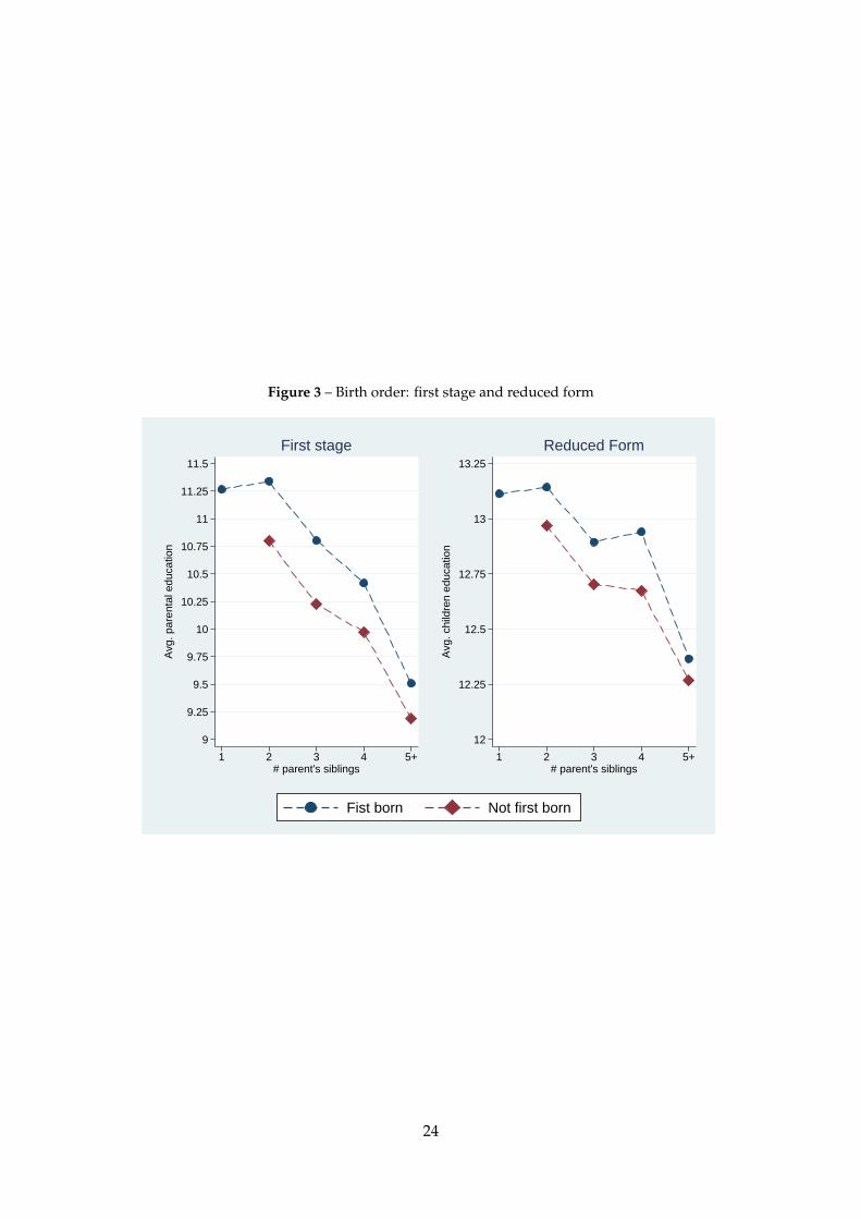
Figure 3 – Birth order: first stage and reduced form

9

9.25

9.5

9.75

10

10.25

10.5

10.75

11

11.25

11.5

Avg

. par

enta

l edu

catio

n

1 2 3 4 5+# parent's siblings

First stage

12

12.25

12.5

12.75

13

13.25

Avg

. chi

ldre

n ed

ucat

ion

1 2 3 4 5+# parent's siblings

Reduced Form

Fist born Not first born

24

Tables

Table 1 – CSL reforms in Europe.

Country Reform year Pivotal cohort Change in CS

Austria 1962 1947 8 to 9

Belgium (Flanders) 1953 1939 8 to 9

Czech Republic 1948 1934 8 to 9

Denmark 1958 1947 4 to 7

France 1972 1953 8 to 10

Germany (Lands):

Baden-Wurttemberg 1967 1953 8 to 9

Bayer 1969 1955 8 to 9

Bremen 1958 1943 8 to 9

Hamburg 1959 1934 8 to 9

Hessen 1967 1953 8 to 9

Nieder-Sachsen 1962 1947 8 to 9

Nordrhein-Westphalen 1967 1953 8 to 9

Rheinald-Pfalz 1967 1953 8 to 9

Saarland 1964 1949 8 to 9

Schleswig-Holstein 1956 1941 8 to 9

Italy 1963 1949 5 to 8

Netherlands 1950 1936 7 to 8

Sweden 1962 1950 8 to 9

See: Brunello, Weber and Weiss 2012; Brunello, Fort, Weber, 2009.

25

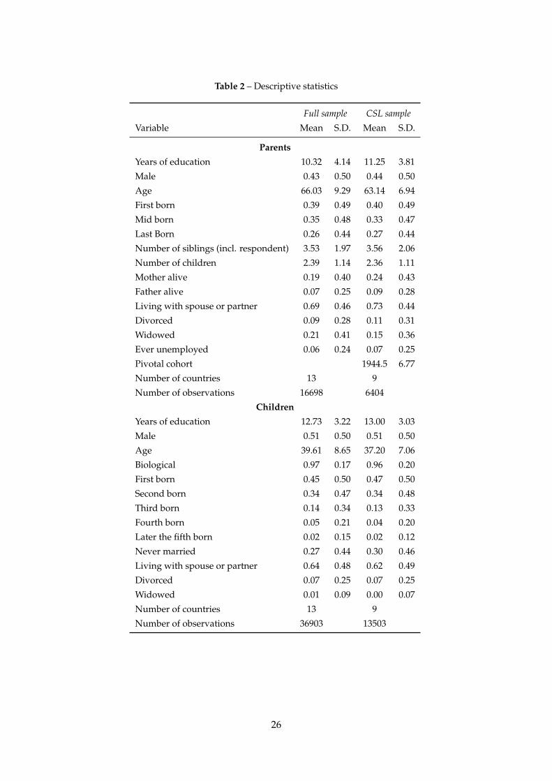
Table 2 – Descriptive statistics

Full sample CSL sample

Variable Mean S.D. Mean S.D.

Parents

Years of education 10.32 4.14 11.25 3.81

Male 0.43 0.50 0.44 0.50

Age 66.03 9.29 63.14 6.94

First born 0.39 0.49 0.40 0.49

Mid born 0.35 0.48 0.33 0.47

Last Born 0.26 0.44 0.27 0.44

Number of siblings (incl. respondent) 3.53 1.97 3.56 2.06

Number of children 2.39 1.14 2.36 1.11

Mother alive 0.19 0.40 0.24 0.43

Father alive 0.07 0.25 0.09 0.28

Living with spouse or partner 0.69 0.46 0.73 0.44

Divorced 0.09 0.28 0.11 0.31

Widowed 0.21 0.41 0.15 0.36

Ever unemployed 0.06 0.24 0.07 0.25

Pivotal cohort 1944.5 6.77

Number of countries 13 9

Number of observations 16698 6404

Children

Years of education 12.73 3.22 13.00 3.03

Male 0.51 0.50 0.51 0.50

Age 39.61 8.65 37.20 7.06

Biological 0.97 0.17 0.96 0.20

First born 0.45 0.50 0.47 0.50

Second born 0.34 0.47 0.34 0.48

Third born 0.14 0.34 0.13 0.33

Fourth born 0.05 0.21 0.04 0.20

Later the fifth born 0.02 0.15 0.02 0.12

Never married 0.27 0.44 0.30 0.46

Living with spouse or partner 0.64 0.48 0.62 0.49

Divorced 0.07 0.25 0.07 0.25

Widowed 0.01 0.09 0.00 0.07

Number of countries 13 9

Number of observations 36903 13503

26

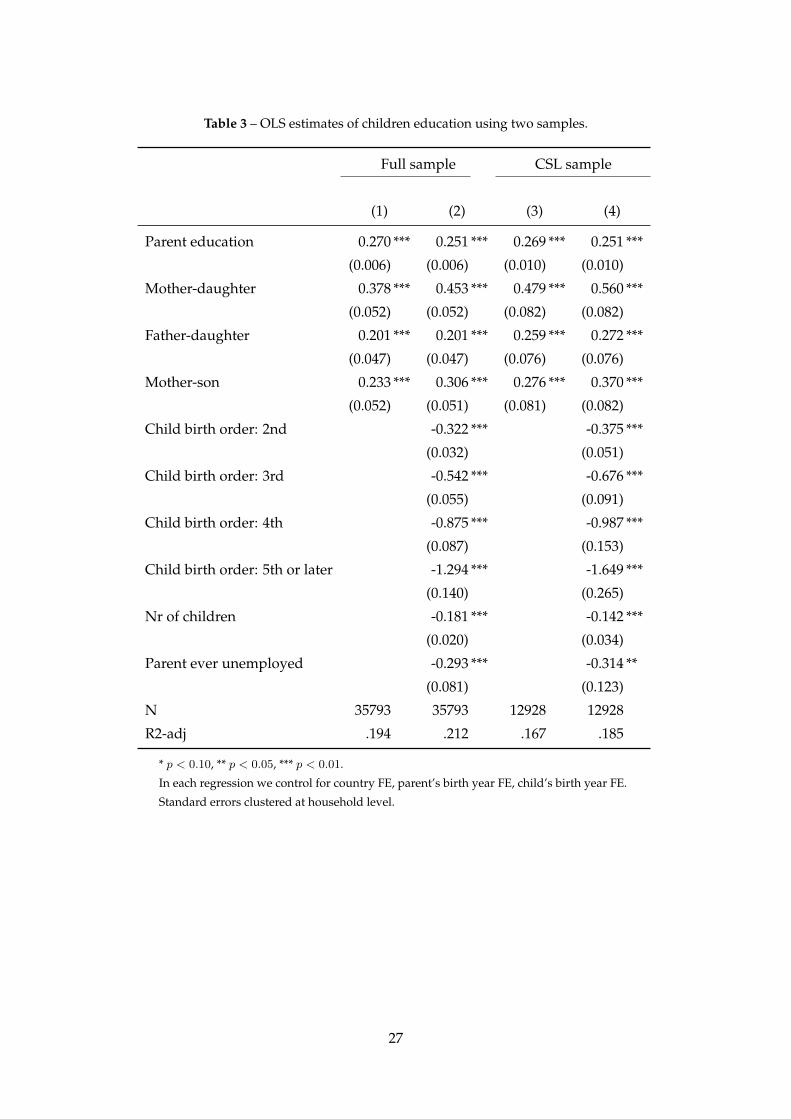
Table 3 – OLS estimates of children education using two samples.


(1) (2) (3) (4)

Parent education 0.270 *** 0.251 *** 0.269 *** 0.251 ***

(0.006) (0.006) (0.010) (0.010)

Mother-daughter 0.378 *** 0.453 *** 0.479 *** 0.560 ***

(0.052) (0.052) (0.082) (0.082)

Father-daughter 0.201 *** 0.201 *** 0.259 *** 0.272 ***

(0.047) (0.047) (0.076) (0.076)

Mother-son 0.233 *** 0.306 *** 0.276 *** 0.370 ***

(0.052) (0.051) (0.081) (0.082)

Child birth order: 2nd -0.322 *** -0.375 ***

(0.032) (0.051)

Child birth order: 3rd -0.542 *** -0.676 ***

(0.055) (0.091)

Child birth order: 4th -0.875 *** -0.987 ***

(0.087) (0.153)

Child birth order: 5th or later -1.294 *** -1.649 ***

(0.140) (0.265)

Nr of children -0.181 *** -0.142 ***

(0.020) (0.034)

Parent ever unemployed -0.293 *** -0.314 **

(0.081) (0.123)

N 35793 35793 12928 12928

R2-adj .194 .212 .167 .185

* p < 0.10, ** p < 0.05, *** p < 0.01.

In each regression we control for country FE, parent’s birth year FE, child’s birth year FE.

Standard errors clustered at household level.

27

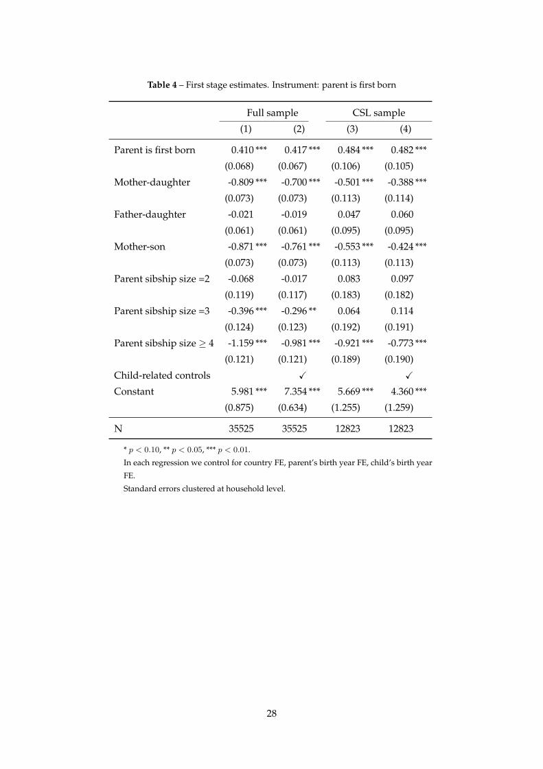
Table 4 – First stage estimates. Instrument: parent is first born


(1) (2) (3) (4)

Parent is first born 0.410 *** 0.417 *** 0.484 *** 0.482 ***

(0.068) (0.067) (0.106) (0.105)

Mother-daughter -0.809 *** -0.700 *** -0.501 *** -0.388 ***

(0.073) (0.073) (0.113) (0.114)

Father-daughter -0.021 -0.019 0.047 0.060

(0.061) (0.061) (0.095) (0.095)

Mother-son -0.871 *** -0.761 *** -0.553 *** -0.424 ***

(0.073) (0.073) (0.113) (0.113)

Parent sibship size =2 -0.068 -0.017 0.083 0.097

(0.119) (0.117) (0.183) (0.182)

Parent sibship size =3 -0.396 *** -0.296 ** 0.064 0.114

(0.124) (0.123) (0.192) (0.191)

Parent sibship size ≥ 4 -1.159 *** -0.981 *** -0.921 *** -0.773 ***

(0.121) (0.121) (0.189) (0.190)

Child-related controls X X

Constant 5.981 *** 7.354 *** 5.669 *** 4.360 ***

(0.875) (0.634) (1.255) (1.259)

N 35525 35525 12823 12823

* p < 0.10, ** p < 0.05, *** p < 0.01.

In each regression we control for country FE, parent’s birth year FE, child’s birth year

FE.


28

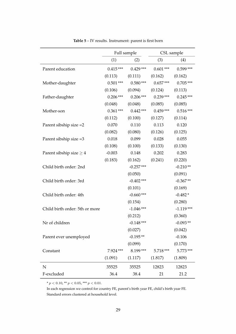
Table 5 – IV results. Instrument: parent is first born


(1) (2) (3) (4)

Parent education 0.415 *** 0.429 *** 0.601 *** 0.599 ***

(0.113) (0.111) (0.162) (0.162)

Mother-daughter 0.501 *** 0.580 *** 0.657 *** 0.705 ***

(0.106) (0.094) (0.124) (0.113)

Father-daughter 0.206 *** 0.206 *** 0.239 *** 0.245 ***

(0.048) (0.048) (0.085) (0.085)

Mother-son 0.361 *** 0.442 *** 0.459 *** 0.516 ***

(0.112) (0.100) (0.127) (0.114)

Parent sibship size =2 0.070 0.110 0.113 0.120

(0.082) (0.080) (0.126) (0.125)


(0.108) (0.100) (0.133) (0.130)

Parent sibship size ≥ 4 -0.003 0.148 0.202 0.283

(0.183) (0.162) (0.241) (0.220)

Child birth order: 2nd -0.257 *** -0.210 **

(0.050) (0.091)

Child birth order: 3rd -0.402 *** -0.367 **

(0.101) (0.169)

Child birth order: 4th -0.660 *** -0.482 *

(0.154) (0.280)

Child birth order: 5th or more -1.046 *** -1.119 ***

(0.212) (0.360)

Nr of children -0.148 *** -0.093 **

(0.027) (0.042)

Parent ever unemployed -0.195 ** -0.106

(0.099) (0.170)

Constant 7.924 *** 8.199 *** 5.718 *** 5.773 ***

(1.091) (1.117) (1.817) (1.809)

N 35525 35525 12823 12823

F-excluded 36.4 38.4 21 21.2

* p < 0.10, ** p < 0.05, *** p < 0.01.



29

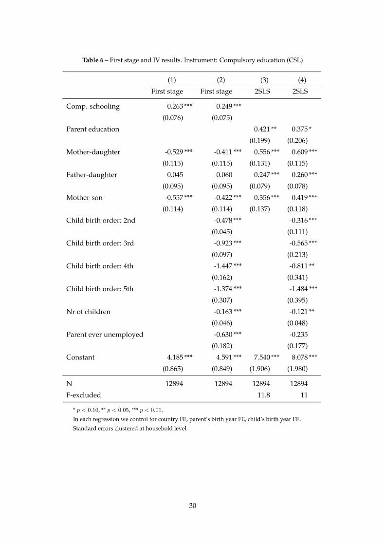
Table 6 – First stage and IV results. Instrument: Compulsory education (CSL)

(1) (2) (3) (4)

First stage First stage 2SLS 2SLS

Comp. schooling 0.263 *** 0.249 ***

(0.076) (0.075)

Parent education 0.421 ** 0.375 *

(0.199) (0.206)

Mother-daughter -0.529 *** -0.411 *** 0.556 *** 0.609 ***

(0.115) (0.115) (0.131) (0.115)

Father-daughter 0.045 0.060 0.247 *** 0.260 ***

(0.095) (0.095) (0.079) (0.078)

Mother-son -0.557 *** -0.422 *** 0.356 *** 0.419 ***

(0.114) (0.114) (0.137) (0.118)


(0.045) (0.111)


(0.097) (0.213)

Child birth order: 4th -1.447 *** -0.811 **

(0.162) (0.341)

Child birth order: 5th -1.374 *** -1.484 ***

(0.307) (0.395)

Nr of children -0.163 *** -0.121 **

(0.046) (0.048)

Parent ever unemployed -0.630 *** -0.235

(0.182) (0.177)

Constant 4.185 *** 4.591 *** 7.540 *** 8.078 ***

(0.865) (0.849) (1.906) (1.980)

N 12894 12894 12894 12894

F-excluded 11.8 11

* p < 0.10, ** p < 0.05, *** p < 0.01.



30

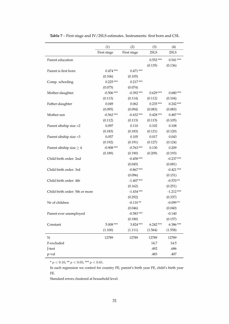
Table 7 – First stage and IV/2SLS estimates. Instruments: first born and CSL

(1) (2) (3) (4)

First stage First stage 2SLS 2SLS

Parent education 0.552 *** 0.541 ***

(0.135) (0.136)

Parent is first born 0.474 *** 0.471 ***

(0.106) (0.105)

Comp. schooling 0.225 *** 0.217 ***

(0.075) (0.074)

Mother-daughter -0.506 *** -0.392 *** 0.629 *** 0.680 ***

(0.113) (0.114) (0.112) (0.104)

Father-daughter 0.049 0.062 0.235 *** 0.242 ***

(0.095) (0.094) (0.083) (0.083)

Mother-son -0.562 *** -0.432 *** 0.428 *** 0.487 ***

(0.112) (0.113) (0.115) (0.105)


(0.183) (0.183) (0.121) (0.120)


(0.192) (0.191) (0.127) (0.124)

Parent sibship size ≥ 4 -0.908 *** -0.763 *** 0.130 0.209

(0.189) (0.190) (0.209) (0.193)


(0.045) (0.081)


(0.096) (0.151)

Child birth order: 4th -1.407 *** -0.570 **

(0.162) (0.251)

Child birth order: 5th or more -1.434 *** -1.212 ***

(0.292) (0.337)

Nr of children -0.110 ** -0.099 **

(0.046) (0.040)

Parent ever unemployed -0.583 *** -0.140

(0.180) (0.157)

Constant 5.008 *** 3.824 *** 6.242 *** 6.386 ***

(1.100) (1.111) (1.564) (1.558)

N 12789 12789 12789 12789

F-excluded 14.7 14.5

J-test .492 .686

p-val .483 .407

* p < 0.10, ** p < 0.05, *** p < 0.01.

In each regression we control for country FE, parent’s birth year FE, child’s birth year

FE.


31

Tabl

e8

–Sy

nthe

sis

ofes

tim

ates

:OLS

and

IV-2

SLS.

Full

and

CSL

sam

ple.

OLS

IV(fi

rstb

orn)

IV(C

SL)

2SLS

(Fir

stbo

rn,C

SL)

Full

sam

ple

CSL

sam

ple

Full

sam

ple

CSL

sam

ple

CSL

sam

ple

CSL

sam

ple

Pare

nted

ucat

ion

(sec

ond

stag

e)0.

251*

**0.

251*

**0.

429*

**0.

599*

**0.

375*

0.54

1***

Firs

tbor

n(fi

rsts

tage

)0.

417*

**0.

482*

**0.

471*

**

CSL

(firs

tsta

ge)

0.24

9***

0.21

7***

F-ex

clud

ed38

.421

.211

14.5

J-te

stst

atis

tic

0.68

6

J-te

stp-

valu

e0.

407

N35

793

1292

835

525

1282

312

894

1278

9

32

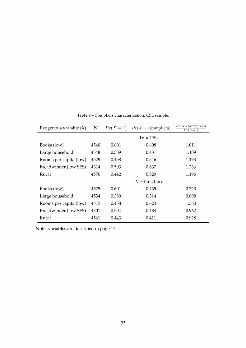
Table 9 – Compliers characterization. CSL sample.

Exogenous variable (X) N Pr(X = 1) Pr(X = 1|compliers) Pr(X=1|compliers)Pr(X=1)

IV = CSL

Books (low) 4540 0.601 0.608 1.011

Large household 4548 0.389 0.431 1.109

Rooms per capita (low) 4529 0.458 0.546 1.193

Breadwinner (low SES) 4314 0.503 0.637 1.266

Rural 4576 0.442 0.529 1.196

IV = First born

Books (low) 4525 0.601 0.435 0.723

Large household 4534 0.389 0.314 0.808

Rooms per capita (low) 4515 0.458 0.623 1.360

Breadwinner (low SES) 4301 0.504 0.484 0.962

Rural 4561 0.443 0.411 0.928

Note: variables are described in page 17.

33

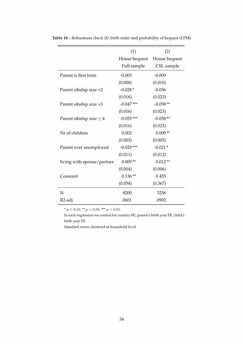
Table 10 – Robustness check (I): birth order and probability of bequest (LPM)

(1) (2)

House bequest House bequest


Parent is first born -0.003 -0.009

(0.008) (0.010)

Parent sibship size =2 -0.028 * -0.036

(0.016) (0.023)

Parent sibship size =3 -0.047 *** -0.058 **

(0.016) (0.023)

Parent sibship size ≥ 4 -0.055 *** -0.058 **

(0.016) (0.023)

Nr of children 0.002 0.009 **

(0.003) (0.005)

Parent ever unemployed -0.029 *** -0.021 *

(0.011) (0.012)

living with spouse/partner 0.009 ** 0.012 **

(0.004) (0.006)

Constant 0.136 ** 0.455

(0.054) (0.367)

N 8200 3236

R2-adj .0601 .0902

* p < 0.10, ** p < 0.05, *** p < 0.01.

In each regression we control for country FE, parent’s birth year FE, child’s

birth year FE.


34

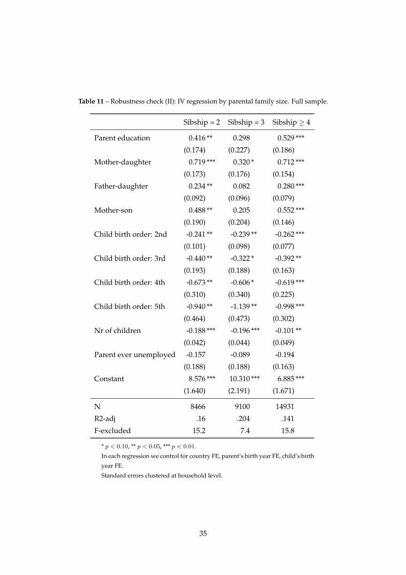
Table 11 – Robustness check (II): IV regression by parental family size. Full sample.

Sibship = 2 Sibship = 3 Sibship ≥ 4

Parent education 0.416 ** 0.298 0.529 ***

(0.174) (0.227) (0.186)

Mother-daughter 0.719 *** 0.320 * 0.712 ***

(0.173) (0.176) (0.154)

Father-daughter 0.234 ** 0.082 0.280 ***

(0.092) (0.096) (0.079)

Mother-son 0.488 ** 0.205 0.552 ***

(0.190) (0.204) (0.146)

Child birth order: 2nd -0.241 ** -0.239 ** -0.262 ***

(0.101) (0.098) (0.077)

Child birth order: 3rd -0.440 ** -0.322 * -0.392 **

(0.193) (0.188) (0.163)

Child birth order: 4th -0.673 ** -0.606 * -0.619 ***

(0.310) (0.340) (0.225)

Child birth order: 5th -0.940 ** -1.139 ** -0.998 ***

(0.464) (0.473) (0.302)

Nr of children -0.188 *** -0.196 *** -0.101 **

(0.042) (0.044) (0.049)

Parent ever unemployed -0.157 -0.089 -0.194

(0.188) (0.188) (0.163)

Constant 8.576 *** 10.310 *** 6.885 ***

(1.640) (2.191) (1.671)

N 8466 9100 14931

R2-adj .16 .204 .141

F-excluded 15.2 7.4 15.8

* p < 0.10, ** p < 0.05, *** p < 0.01.

In each regression we control for country FE, parent’s birth year FE, child’s birth

year FE.


35

The causal effect of parents' schooling on children's schooling in Europe. A new IV approach

Documents

Transcript of The causal effect of parents' schooling on children's schooling in Europe. A new IV approach