arX

iv:0

811.

0004

v2 [

astr

o-ph

] 1

Dec

200

8Accepted to the Astrophysical Journal, October 31, 2008Preprint typeset using LATEX style emulateapj v. 10/09/06

THE ATOMIC TO MOLECULAR TRANSITION IN GALAXIES.II: HI AND H2 COLUMN DENSITIES

Mark R. Krumholz1

Department of Astrophysical Sciences, Princeton University, Peyton Hall, Princeton, NJ 08544 and Department of Astronomy &Astrophysics, University of California, Santa Cruz, Interdisciplinary Sciences Building, Santa Cruz, CA 95060

Christopher F. McKeeDepartments of Physics and Astronomy, University of California, Berkeley, Campbell Hall, Berkeley, CA 94720-7304

Jason TumlinsonSpace Telescope Science Institute, 3700 San Martin Dr., Baltimore, MD 21218

Accepted to the Astrophysical Journal, October 31, 2008

ABSTRACT

Gas in galactic disks is collected by gravitational instabilities into giant atomic-molecular complexes,but only the inner, molecular parts of these structures are able to collapse to form stars. Determiningwhat controls the ratio of atomic to molecular hydrogen in complexes is therefore a significant problemin star formation and galactic evolution. In this paper we use the model of H2 formation, dissociation,and shielding developed in the previous paper in this series to make theoretical predictions for atomicto molecular ratios as a function of galactic properties. We find that the molecular fraction in agalaxy is determined primarily by its column density and secondarily by its metallicity, and is to goodapproximation independent of the strength of the interstellar radiation field. We show that the columnof atomic hydrogen required to shield a molecular region against dissociation is ∼ 10 M⊙ pc−2 atsolar metallicity. We compare our model to data from recent surveys of the Milky Way and of nearbygalaxies, and show that the both the primary dependence of molecular fraction on column densityand the secondary dependence on metallicity that we predict are in good agreement with observedgalaxy properties.

Subject headings: galaxies: ISM — ISM: clouds — ISM: molecules — ISM: structure — molecularprocesses

1. INTRODUCTION

The formation of molecular hydrogen is a critical stepin the transformation of interstellar gas into new stars.The neutral atomic interstellar medium (ISM) in galax-ies is generally segregated into cold clouds embeddedin a warm inter-cloud medium (McKee & Ostriker 1977;Wolfire et al. 2003), and the inner parts of some of thesecold atomic clouds harbor regions where the gas is well-shielded against dissociation by the interstellar radiationfield (ISRF). In these regions molecules form, and oncethey do star formation follows.

A full theory of star formation requires as one of itscomponents a method for expressing in terms of observ-ables the fraction of a galaxy’s ISM that is in the molec-ular phase (e.g. Krumholz & McKee 2005). No modelspublished to date satisfy this requirement, but observa-tions have yielded a number of empirical rules for galax-ies’ molecular content. Based on Hi and CO mappingof nearby galaxies Wong & Blitz (2002, hereafter WB02)and Blitz & Rosolowsky (2004, 2006, hereafter BR04 andBR06) infer that the molecular to atomic surface densityratio RH2

= ΣH2/ΣHI in a galaxy varies with the inter-

stellar pressure P needed for hydrostatic balance in theISM as RH2

∝ P 0.92, and that the atomic surface density

Electronic address: krumholz@ucolick.orgElectronic address: cmckee@astro.berkeley.eduElectronic address: tumlinson@stsci.edu

1 Hubble Fellow

saturates at a maximum value of ∼ 10M⊙ pc−2. The ob-served saturation and a similar dependence of molecularfraction on pressure are also seen in newer surveys such asthe HERA CO-Line Extragalactic Survey (HERACLES)that cover a broader range of galaxy properties at higherspatial resolution (Walter et al. 2008; Bigiel et al. 2008;Leroy et al. 2008, hereafter L08). However the physicalorigin of these patterns is unclear. The samples on whichthey are based are composed solely of nearby galaxieswith a limited range of properties, and in the absence ofa physical model it is uncertain how far they can safelybe extrapolated to regimes of metallicity, surface density,or other properties not represented in samples of nearbygalaxies.

Theoretical treatments of the problem to date do notyet make such an extrapolation possible. A number ofauthors have considered the microphysics of H2 forma-tion and the structure of photodissociation regions invarying levels of detail (e.g. van Dishoeck & Black 1986;Black & van Dishoeck 1987; Sternberg 1988; Elmegreen1989; Draine & Bertoldi 1996; Neufeld & Spaans 1996;Spaans & Neufeld 1997; Hollenbach & Tielens 1999;Liszt & Lucas 2000; Liszt 2002; Browning et al. 2003;Allen et al. 2004), but none of these treatments addressthe problem of atomic to molecular ratios on galacticscales. Wyse (1986) and Wang (1990a,b) present mod-els for cloud formation in galactic disks, but these bothrely on prescriptions for the rate of conversion of atomic

2

to molecular gas that are based either on rates of cloudcollisions or on Schmidt laws, not on physical models ofH2 formation and dissociation. Elmegreen (1993) gives atheory of the molecular fraction in galaxies that does in-clude a treatment of the H2 formation and self-shielding.However, his model neglects dust shielding, an orderunity effect, and it also requires knowledge of a galaxy’sISRF strength, which cannot easily be determined obser-vationally, and its interstellar pressure, which can onlybe inferred indirectly based on arguments about hydro-static balance. This makes the model difficult to testor to apply as part of a larger theory of star forma-tion. Schaye (2004) considers the conditions necessaryto form a cold atomic phase of the ISM. The existence ofsuch a phase is a necessary but not sufficient conditionfor molecule formation, so while Schaye’s model providesa minimum condition for star formation, in makes nostatements about what fraction of the ISM goes into themolecular phase able to form stars, and thus no state-ment on the star formation rate that is achieved oncethe minimum condition is met.

Numerical models are in a similar situation.Hidaka & Sofue (2002) and Pelupessy et al. (2006)simulate galaxies using subgrid models for H2 formationsimilar to those presented by Elmegreen (1993), andshow that they can reproduce some qualitative featuresof the H2 distribution in galaxies. Robertson & Kravtsov(2008) show that a simulation of a galaxy’s ISM thatincludes radiative heating and cooling in the ionizedand atomic phases, coupled with an approximatetreatment of H2 formation on grains and dissociationby the ISRF, can reproduce the observed molecularcontent of galaxies. This suggests that the simulationscontain the necessary physical ingredients to explain theobservations, but the simulations do not by themselvesreveal how these ingredients fit together to produce theobserved result. Moreover, like the observed empiricalrules, the simulations are based on a very limited rangeof galaxy properties, and in the absence of a modelwe can use to understand the origin of the simulationresults, it is unclear how to extrapolate. Extending thesimulations to cover the full range of galaxy parametersin which we are interested would be prohibitivelyexpensive in terms of both computational and humantime.

Our goal in this paper is to remedy this lack of theo-retical understanding by providing a first-principles the-oretical calculation of the molecular content of a galacticdisk in terms of direct observables. In Krumholz et al.(2008, hereafter Paper I), we lay the groundwork for thistreatment by solving the idealized problem of determin-ing the location of the atomic to molecular transitionin a uniform spherical gas cloud bathed in a uniform,isotropic dissociating radiation field. In this paper we ap-ply our idealized model to atomic-molecular complexes ingalaxies as a way of elucidating the underlying physicalprocesses and parameters that determine the molecularcontent. We refer readers to Paper I for a full descriptionof our solution to the idealized problem, but here we re-peat a central point: for a spherical cloud exposed to anisotropic dissociating radiation field, if we approximatethe transition from atomic to molecular as occurring inan infinitely thin shell separating gas that is fully molec-ular from gas of negligible molecular content, the fraction

of a cloud’s radius at which this transition occurs is solelya function of two dimensionless numbers:

χ=fdissσdcE

∗0

nR(1)

τR =nσdR. (2)

Here fdiss ≈ 0.1 is the fraction of absorptions of a Lyman-Werner (LW) band photons that produce H2 dissociationrather than simply excitation and radiative decay to abound state, σd is the dust absorption (not extinction)cross-section per hydrogen nucleus in the LW band, E∗

0is the free-space number density of LW photons (i.e. faroutside our cloud), n is the number density of hydrogennuclei in the atomic shielding layer, R is the H2 formationrate coefficient on dust grain surfaces, and R is the cloudradius.

The quantity τR is simply a measure of the size of thecloud. It is the dust optical depth that a cloud wouldhave if its density throughout were equal to its densityin the atomic region. We may think of χ as a dimension-less measure of the intensity of the dissociating radiation;formally it is equal to the ratio of the rate at which LWphotons are absorbed by dust grains to the rate at whichthey are absorbed by hydrogen molecules in a parcel ofpredominantly atomic gas in dissociation equilibrium infree-space. This is a measure of the strength of the ra-diation field because in strong radiation fields the gascontains very few molecules, so most LW photons are ab-sorbed by dust and χ is large. In weak radiation fields thegas contains more molecules, which due to their large res-onant cross-section dominate the absorption rate, mak-ing χ small.

Over the remainder of this paper we apply the modelof Paper I to atomic-molecular complexes in galaxies. In§ 2 we begin by considering giant clouds, which we mayapproximate as slabs, and in § 3 we extend our treatmentto clouds of finite size. In § 4 we compare the modelpredictions of the previous two sections to observationsof atomic and molecular gas. Finally in § 5 we summarizeand discuss conclusions.

2. THE ATOMIC ENVELOPES OF GIANT CLOUDS

In this section we specialize to the case of giant clouds,which we define as those for which eτR ≫ 1. For theseclouds we show in Paper I that the dust optical depthfrom the cloud surface to the atomic-molecuar transition,τHI, is a function of χ alone. We therefore begin ouranalysis with an estimate of χ.

2.1. The Normalized Radiation Field

Of the quantities that enter into the normalized ra-diation field χ, fdiss is the most certain, because it isonly a very weak function of the spectrum of the dis-sociating radiation. We therefore take it to have aconstant value fdiss ≈ 0.1 independent of environment(Draine & Bertoldi 1996; Browning et al. 2003; Paper I).Similarly, σd and R are functions of the properties ofdust grains. These are both measures of the total sur-face area of dust grains mixed in the atomic shieldingenvelope around a molecular cloud; the former measuresthe area available for absorbing photons, while the lat-ter measures the area available for catalyzing H2 forma-tion. There will of course be an additional dependence

3

of these quantities on the optical and chemical proper-ties of grains, but these effects likely provide only a smallfraction of the total variation. To first order, therefore,we expect the ratio σd/R to vary little with galactic en-vironment, and we can simply adopt the value from thesolar neighborhood. This is

σd

R= 3.2 × 10−5 σd,−21

R−16.5s cm−1 (3)

where σd,−21 = σd/10−21 cm2, R−16.5 = R/10−16.5

cm3 s−1, and our best estimates for the solar neighbor-hood give σd,−21 ≈ R−16.5 ≈ 1 (Draine & Bertoldi 1996;Wolfire et al. 2008).

Unfortunately, n and E∗0 are considerably harder to

determine, since we cannot easily make direct measure-ments of the atomic density around a molecular cloud orthe dissociating radiation field to which it is subjected,particularly for clouds in extragalactic space. (It is pos-sible to determine these quantities for PDRs being pro-duced by individual star clusters – see Smith et al. 2000and Heiner et al. 2008a,b – but these methods are gener-ally not able to determine mean radiation fields aroundgiant clouds.) However, we can still gain considerable in-sight into the ratio E∗

0/n that enters into χ if we realizethat n is not free to assume any value for a given E∗

0 .The atomic gas in a galaxy generally comprises regionsof both cold and warm gas (cold neutral medium andwarm neutral medium, or CNM and WNM, respectively)in approximate pressure balance (e.g. McKee & Ostriker1977; Wolfire et al. 2003). Molecular clouds form in re-gions where the gas is primarily cold. This is becausethe the effective opacity to LW photons provided by thesmall population of molecules found in a given element ofpredominantly atomic gas varies as n2, so the cold phase,due to its higher density, is far more effective at shieldingfrom LW photons than the warm phase. Thus the n weare concerned with is not the mean density of a galaxy’satomic ISM, it is the density in the cold phase only. Inthe presumably dense gas in the vicinity of a molecularcloud, most of the mass is likely in the cold rather thanthe warm phase in any event.

We can estimate the CNM density by using the con-dition of pressure balance between the cold and warmphases. Wolfire et al. (2003) show that, for a given am-bient FUV radiation intensity G0 (given in units of theHabing 1968 field, corresponding to a number densityE∗

0 ≈ 4.4 × 10−4 LW photons cm−3), ionization ratefrom EUV radiation and x-rays ζt, abundance of dustand polycyclic aromatic hydrocarbons Zd, and gas phasemetal abundance Zg, the minimum number density nmin

at which CNM can exist in pressure balance with WNMis well-approximated by

nmin ≈ 31G′0

Z ′d/Z

′g

1 + 3.1(G′0Z

′d/ζ

′t)

0.365cm−3, (4)

where the primes denote quantities normalized to theirvalues in the solar neighborhood. Wolfire et al. (2003)obtain this expression by constructing a temperature-density relation, determined by balancing the rate ofgrain photoelectric heating against cooling by the finestructure lines of Cii and Oi. Once they have con-structed the T − n curve, they identify the temperatureat which the pressure is minimized. This is the warmest

temperature at which the CNM can be in pressure bal-ance, and thus the corresponding density is the lowestpossible CNM density. The primary uncertainty in thisexpression arises from the abundance, size distribution,and reaction properties of polycyclic aromatic hydrocar-bons (PAHs), but changes in PAH properties generallychange nmin only at the factor of ∼ 2 level (cf. Figure 8of Wolfire et al. 2003).

In a galaxy where young stars provide the dominantsource of radiation and the IMF is constant, the FUVheating rate and the EUV/x-ray ionization rate are likelyto be proportional to the star formation rate, and there-fore to each other. We therefore assume that ζ′t = G′

0.Furthermore, if the physics of dust formation does notvary strongly from galaxy to galaxy, then the dust andgas phase metal abundances are likely proportional tothe total metallicity Z, so we adopt Z ′

d = Z ′g = Z ′.

With these approximations the minimum CNM densitybecomes

nmin ≈ 31G′

0

1 + 3.1Z ′0.365cm−3. (5)

We caution at this point that both the assumptions thatζ′t = G′

0 and Z ′d = Z ′

g = Z ′ are unlikely to hold in el-liptical galaxies, where young stars are not the dominantsources of EUV or x-ray radiation, and where the amountof dust per unit metallicity is known to be different thanin spirals. Thus, equation (5) is unlikely to hold in ellip-ticals.

The CNM can exist in pressure balance at densitieshigher than nmin, so we take the typical CNM density tobe

nCNM = φCNMnmin. (6)

We adopt φCNM ≈ 3 as our fiducial value, whichgives a CNM density of nCNM = 22 cm−3 and (usingWolfire et al.’s T −n relation, equation 18 of this paper)a temperature of TCNM = 105 K, consistent with obser-vations of typical CNM properties in the solar neighbor-hood. (Near a GMC, we expect G′

0 ∼ 10 rather thanG′

0 = 1, due to the proximity of sites of star formation –Wolfire, Hollenbach, & McKee 2008, in preparation – butthis does not affect our results, since we only care aboutthe ratioG′

0/n.) In practice φCNM cannot be much largerthan this, because pressure balance between the CNMand WNM is possible only over a limited range of CNMdensities. If the CNM densities exceeds nmin by morethan a factor of ∼ 10 the CNM and WNM again cannotbe in pressure balance because it is impossible for thewarm phase to have a high enough pressure.

Using equation (3) for σd/R and equation (6) for n,and noting that the LW photon number density in thesolar neighborhood is roughly 7.5 × 10−4 cm−3 (Draine1978; Paper I), we find a total estimate for the dimen-sionless radiation field strength

χ = 2.3

(

σd,−21

R−16.5

)

1 + 3.1Z ′0.365

φCNM. (7)

Note that all explicit dependence on the dust proper-ties, the radiation field, and the atomic gas density havecancelled out of this expression.

Dependence on the dust properties has dropped out forthe simple reason explained above: σd and R are bothmeasures of the dust surface area, so their ratio is nearly

4

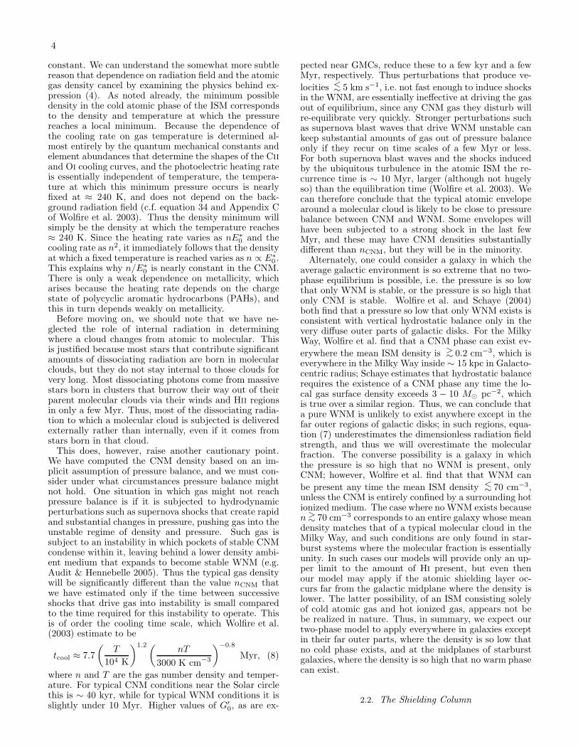
constant. We can understand the somewhat more subtlereason that dependence on radiation field and the atomicgas density cancel by examining the physics behind ex-pression (4). As noted already, the minimum possibledensity in the cold atomic phase of the ISM correspondsto the density and temperature at which the pressurereaches a local minimum. Because the dependence ofthe cooling rate on gas temperature is determined al-most entirely by the quantum mechanical constants andelement abundances that determine the shapes of the Ciiand Oi cooling curves, and the photoelectric heating rateis essentially independent of temperature, the tempera-ture at which this minimum pressure occurs is nearlyfixed at ≈ 240 K, and does not depend on the back-ground radiation field (c.f. equation 34 and Appendix Cof Wolfire et al. 2003). Thus the density minimum willsimply be the density at which the temperature reaches≈ 240 K. Since the heating rate varies as nE∗

0 and thecooling rate as n2, it immediately follows that the densityat which a fixed temperature is reached varies as n ∝ E∗

0 .This explains why n/E∗

0 is nearly constant in the CNM.There is only a weak dependence on metallicity, whicharises because the heating rate depends on the chargestate of polycyclic aromatic hydrocarbons (PAHs), andthis in turn depends weakly on metallicity.

Before moving on, we should note that we have ne-glected the role of internal radiation in determiningwhere a cloud changes from atomic to molecular. Thisis justified because most stars that contribute significantamounts of dissociating radiation are born in molecularclouds, but they do not stay internal to those clouds forvery long. Most dissociating photons come from massivestars born in clusters that burrow their way out of theirparent molecular clouds via their winds and Hii regionsin only a few Myr. Thus, most of the dissociating radia-tion to which a molecular cloud is subjected is deliveredexternally rather than internally, even if it comes fromstars born in that cloud.

This does, however, raise another cautionary point.We have computed the CNM density based on an im-plicit assumption of pressure balance, and we must con-sider under what circumstances pressure balance mightnot hold. One situation in which gas might not reachpressure balance is if it is subjected to hydrodynamicperturbations such as supernova shocks that create rapidand substantial changes in pressure, pushing gas into theunstable regime of density and pressure. Such gas issubject to an instability in which pockets of stable CNMcondense within it, leaving behind a lower density ambi-ent medium that expands to become stable WNM (e.g.Audit & Hennebelle 2005). Thus the typical gas densitywill be significantly different than the value nCNM thatwe have estimated only if the time between successiveshocks that drive gas into instability is small comparedto the time required for this instability to operate. Thisis of order the cooling time scale, which Wolfire et al.(2003) estimate to be

tcool ≈ 7.7

(

T

104 K

)1.2 (

nT

3000 K cm−3

)−0.8

Myr, (8)

where n and T are the gas number density and temper-ature. For typical CNM conditions near the Solar circlethis is ∼ 40 kyr, while for typical WNM conditions it isslightly under 10 Myr. Higher values of G′

0, as are ex-

pected near GMCs, reduce these to a few kyr and a fewMyr, respectively. Thus perturbations that produce ve-

locities <∼ 5 km s−1, i.e. not fast enough to induce shocksin the WNM, are essentially ineffective at driving the gasout of equilibrium, since any CNM gas they disturb willre-equilibrate very quickly. Stronger perturbations suchas supernova blast waves that drive WNM unstable cankeep substantial amounts of gas out of pressure balanceonly if they recur on time scales of a few Myr or less.For both supernova blast waves and the shocks inducedby the ubiquitous turbulence in the atomic ISM the re-currence time is ∼ 10 Myr, larger (although not hugelyso) than the equilibration time (Wolfire et al. 2003). Wecan therefore conclude that the typical atomic envelopearound a molecular cloud is likely to be close to pressurebalance between CNM and WNM. Some envelopes willhave been subjected to a strong shock in the last fewMyr, and these may have CNM densities substantiallydifferent than nCNM, but they will be in the minority.

Alternately, one could consider a galaxy in which theaverage galactic environment is so extreme that no two-phase equilibrium is possible, i.e. the pressure is so lowthat only WNM is stable, or the pressure is so high thatonly CNM is stable. Wolfire et al. and Schaye (2004)both find that a pressure so low that only WNM exists isconsistent with vertical hydrostatic balance only in thevery diffuse outer parts of galactic disks. For the MilkyWay, Wolfire et al. find that a CNM phase can exist ev-

erywhere the mean ISM density is >∼ 0.2 cm−3, which is

everywhere in the Milky Way inside ∼ 15 kpc in Galacto-centric radius; Schaye estimates that hydrostatic balancerequires the existence of a CNM phase any time the lo-cal gas surface density exceeds 3 − 10 M⊙ pc−2, whichis true over a similar region. Thus, we can conclude thata pure WNM is unlikely to exist anywhere except in thefar outer regions of galactic disks; in such regions, equa-tion (7) underestimates the dimensionless radiation fieldstrength, and thus we will overestimate the molecularfraction. The converse possibility is a galaxy in whichthe pressure is so high that no WNM is present, onlyCNM; however, Wolfire et al. find that that WNM can

be present any time the mean ISM density <∼ 70 cm−3,

unless the CNM is entirely confined by a surrounding hotionized medium. The case where no WNM exists becausen >∼ 70 cm−3 corresponds to an entire galaxy whose meandensity matches that of a typical molecular cloud in theMilky Way, and such conditions are only found in star-burst systems where the molecular fraction is essentiallyunity. In such cases our models will provide only an up-per limit to the amount of Hi present, but even thenour model may apply if the atomic shielding layer oc-curs far from the galactic midplane where the density islower. The latter possibility, of an ISM consisting solelyof cold atomic gas and hot ionized gas, appears not bebe realized in nature. Thus, in summary, we expect ourtwo-phase model to apply everywhere in galaxies exceptin their far outer parts, where the density is so low thatno cold phase exists, and at the midplanes of starburstgalaxies, where the density is so high that no warm phasecan exist.

2.2. The Shielding Column

5

The normalized radiation field χ is the primary fac-tor controlling the size of the atomic gas column thatis needed to shield a molecular cloud against dissocia-tion, and thus in determining fraction of the gas in agalaxy is molecular. This quantity in turn determineswhat fraction of a galaxy’s ISM is molecular, and there-fore available for star formation, and what fraction isatomic, and thus without star formation. The invari-ance of χ across galactic environments has importantconsequences for atomic-molecular complexes. First, χmeasures the relative importance of dust shielding andH2 self-shielding, so our results that χ ∼ 1 across galax-ies implies that dust- and self-shielding contribute nearlyequally in essentially all galactic environments. We donot expect to find clouds where either dust- or molecular-shielding completely dominate except near strong sourcesof dissociating radiation where the atomic ISM is not inpressure balance or in regions of such low or high densitythat the atomic ISM does not have two phases.

Second, the dust optical depth through the Hi shieldinglayer, τHI, is primarily a function of χ; the dependence onτR arises from geometric effects, and is greater than orderunity only if the molecular region inside a cloud is a smallfraction of its size. (Strictly speaking this is the opticaldepth of the CNM, not of all the atomic gas. As notedabove most of the atomic gas around a molecular cloud isprobably CNM, but there could be significant amounts ofWNM along the line of sight that is not associated withthat cloud, and which does not contribute to shieldingit.) This implies that the dust optical depth through theatomic envelopes of molecular clouds should be roughlyconstant across galactic environments, at least as long asthis optical depth is not close to that of the entire atomic-molecular complex. The only significant variation will bea weak increase in τHI with metallicity. Correspondingly,the total Hi gas column will decrease with metallicityto a power less than unity, since τHI increases slightlywith metallicity, but the column of Hi required to achievethis dust optical depth decreases with metallicity. Toillustrate for these effects we solve for τHI as a functionof Z in the limit τR → ∞ using the formalism of Paper I,and plot the result in Figure 1.

As the plot shows, four our fiducial model φCNM = 3,we predict that the Hi layer around a molecular cloud inthe Milky Way, Z ′ = 1, should have an absorption op-tical depth of τHI = 0.40 to LW photons, correspondingto an Hi column NHi = 4.0 × 1020 cm−2 (mass columndensity Σ = 4.5 M⊙ pc−2), assuming a dust absorptioncross section per H nucleus of σd = 10−21 cm−2. It isimportant to note that all of these values represent theabsorption column on one side of a giant cloud. A 21-cmobservation would detect the shielding column on bothsides for a cloud exposed to the ISRF on both sides, sothe detected Hi column would be double the values givenin Figure 1. As a shall see in § 3, the column is somewhatlarger for a cloud of finite size.

It is important to note that the shielding column wehave calculated is somewhat different than the atomic-to-molecular transition column density reported for theMilky Way by Savage et al. (1977, logN(H) = 20.7)and for the LMC and SMC by Tumlinson et al. (2002,logN(H) ≥ 21.3 and ≥ 22, respectively). These valuesare the total column densities along pencil-beam lines ofsight at which the fraction of the gas column in the form

Fig. 1.— The dust optical depth of the Hi shielding layer τHI

(upper panel), and the corresponding Hi column NHi (lower panel)for very large clouds, τR → ∞. We show these results computed forφCNM = 3 (thick lines) and for φCNM = 1 and 10 (upper and lowerthin lines, respectively). The circles indicate our values for theMilky Way, Z′ = 1, for our fiducial φCNM = 3: τHI = 0.40, NHI =4.0×1020. To compute NHI from τHI, we assume a dust absorptioncross section per H nucleus in the LW band of σd = 10−21Z/Z⊙.We also show the visual extinction AV corresponding to our τHI

and the mass column density Σ corresponding to NHi. For theformer we have assumed AV /τHI = 0.48, following the models ofDraine (2003a,b,c) as explained in the text. To compute the latterwe assume a mean particle mass per H nucleus of 2.34 × 10−24 gcm−2, corresponding to a standard cosmic mixture of H and He.

of H2 reaches about 10% of the total. In contrast, inthe two-zone approximation we adopt in Paper I, we as-sume that the atomic-to-molecular transition is infinitelysharp, and under this approximation the shielding col-umn we report is the column at which the gas goes fromfully atomic to fully molecular. Were the transition trulyinfinitely sharp as we have approximated it to be, theratio of H2 to total column density would be zero atour computed shielding column. Comparing our theoret-ical shielding columns to the detailed numerical radiativetransfer models we present in Paper I shows that in re-ality, for conditions typical of the Milky Way, the ratioof H2 column to total column at our calculated transi-tion column NHI is roughly 20%. Since this is a factor of2 larger than the 10% ratio used in the observationally-defined transition column, and in our simple model theH2 fraction increases linearly with total column densityonce we pass our predicted transition point, we expectour shielding column to be a factor of ∼ 2 larger thanthe values reported by Savage et al. and Tumlinson et al.We compare our model predictions to these data sets inmore detail in § 4.2.

Using the extinction and absorption curves of Draine(2003a,b,c), the ratio of visual extinction to 1000 A ab-sorption is AV /τHI = 0.48 for Draine’s RV = 4.0 model,so the visual extinction corresponding to τHI = 0.40 isAV = 0.19. Adopting the RV = 5.5 curve instead,appropriate for denser clouds, gives AV = 0.28, whileRV = 3.1, for diffuse regions, gives AV = 0.13. Ourestimates for the LW dust optical depth and visual ex-tinction vary little with metallicity, changing by only a

6

factor of 2.7 for a metallicity ranging from 10−2Z⊙ to100.5Z⊙.

The variation between the curves with φCNM = 1, 3, 10show the full plausible range of variation in shielding col-umn arising from our uncertainty about the true den-sity in the atomic envelopes of molecular clouds. TheφCNM = 1 and 10 curves are both within a factor of 2.6of the fiducial model, so this is an upper bound on ouruncertainty. The actual error is likely to be smaller thanthis, since φCNM = 1 and 10 correspond to the extremeassumptions that the CNM assumes is minimum or max-imum possible equilibrium densities.

We can obtain a quick approximation to the resultsshown in Figure 1 simply by noting that at solar metallic-ity our fiducial normalized radiation field is χ = 3.1, andwe show in Paper I that for a giant cloud with χ < 4.1(corresponding to Z ′ < 2.5 for our fiducial parameters)the LW dust optical depth through the atomic shieldinglayer is

τHI =ψ

4, (9)

where

ψ = χ2.5 + χ

2.5 + χe. (10)

The dust-adjusted radiation field ψ is a function only ofmetallicity; for our fiducial parameters φCNM = 3 andσd,−21/R−16.5 = 1, and Milky Way metallicity, Z ′ =1, we obtain ψ = 1.6. Moreover, the dependence onmetallicity is weak: at Z ′ = 1/10, ψ = 1.0, while at Z ′ =1/100, ψ = 0.77. Because ψ depends only on metallicity,we can also express the characteristic Hi shielding columnon one side of a giant cloud solely as a function of Z ′:

ΣHi =µH

σdτHI(Z

′, φχ) (11)

=4.5M⊙ pc−2 f(Z ′, φχ)

σ0,−21Z ′(12)

where µH = 2.34×10−24 g is the mean mass per hydrogennucleus and σ0,−21 is the dust absorption cross-section atMilky Way metallicity (logZ ′ = 0) in units of 10−21 cm2.The function f(Z ′, φχ) is given by

f(Z ′, φχ)=0.54(

0.32 + Z ′0.385)

φ−1χ ·

(

1.05φχ + 0.42 + Z ′0.385

0.39φχ + 0.42 + Z ′0.385

)

, (13)

where

φχ ≡

(

φCNM

3

) (

R−16.5

σd,−21

)

, (14)

f(1, 1) = 1, and for our fiducial parameters φχ = 1. Thenumerical factors that appear in f(Z ′, φχ) are derivedsimply by substituting equation (7) for χ into equation(10) and thence into equation (11). These equations,and therefore the numerical values in the function f , de-pend solely on microphysical constants that describe theproperties of molecular hydrogen and the chemistry of itsformation on grain surfaces (which set fdiss and σd/R)and the shapes of the Cii and Oi cooling curves (whichset the ratio E∗

0/n). We have therefore calculated theshielding column to good approximation solely in termsof microphysical constants.

3. THE ATOMIC ENVELOPES OF FINITE CLOUDS

3.1. Formulation of the Problem

To account for the fact that clouds have finite sizesand column densities, and that these can be quite smallin dwarf galaxies or other low-pressure environments,we must examine the second dimensionless number thatcharacterizes H2 formation and shielding: τR = nσdR.Consider a cloud of known, fixed column density Σcomp.If atomic-molecular complexes were of uniform densitythen we could find τR simply by multiplying Σcomp

by the dust cross section per unit mass σd/µH, whereµH ≈ 2.34 × 10−24 g is the mean mass per H nucleus.However, the atomic region is warmer and has a lowermean mass per particle than the molecular one, and thushas a correspondingly lower density. This reduces thedust optical depth through it. Since it is the density anddust optical depth through the atomic shielding layerthat matters, we must estimate τR using the value ofn appropriate for the atomic gas rather than the meandensity in the complex. In other words, the quantity wewant is

τR = nCNMσdR, (15)

and we defineφmol ≡

nmol

nCNM(16)

as the ratio of densities. Here nmol and nCNM are thenumber densities of hydrogen nuclei in the molecular andCNM phases of the ISM, respectively.

In the Milky Way, typical molecular cloud densitiesare nmol ≈ 100 cm−3 (McKee & Ostriker 2007), whileobservations of the giant Hi clouds around these molec-ular regions find typical densities nCNM ≈ 10 cm−3

(Elmegreen & Elmegreen 1987), suggesting φmol ≈ 10.We do not expect this ratio to vary strongly betweengalaxies, so we should generally find φmol ≈ 10.

We can can make an independent argument for φmol ≈10 by considering thermal pressure balance across theatomic-molecular interface. This argument only appliesto gas near an atomic-molecular transition surface, whichmay or may not include the bulk of the gas in a cloud,but it does provide an estimate for the density ratio nearthe interface. Pressure balance requires that

φmol = 1.8TCNM

Tmol, (17)

where Tmol and TCNM are the temperatures in the molec-ular and cold neutral atomic media, respectively, and thefactor of 1.8 accounts for the difference in mean numberof particles per H nucleus in the two phases. Across avery wide range of galactic environments the tempera-ture in the molecular phase of the ISM is Tmol ≈ 10− 20K, as a result of the balance between grain photoelectricheating and CO cooling. Since are interested in gas atthe edge of the molecular region, we adopt Tmol = 20 Kas typical. (Temperatures are somewhat higher in star-burst systems, but in these galaxies the molecular frac-tion is essentially unity in any event.) Using the model ofWolfire et al. (2003) for the atomic medium, and makingthe approximations Z ′

d = Z ′g = Z ′ and ζ′t = G′

0 as in§ 2.1, the density-temperature relation in the atomic gasis

nCNM ≈20G′

0T−0.2CNM,2e

1.5/TCNM,2

1 + 2.6(T1/2CNM,2Z

′)0.365, (18)

7

where TCNM,2 = TCNM/(100 K). Combining this withequations (5) and (6) enables us to write an implicitequation for the CNM temperature in terms of φCNM

and Z ′:

20T−0.2CNM,2e

1.5/TCNM,2

1 + 2.6(T1/2CNM,2Z

′)0.365= φCNM

31

1 + 3.1Z ′0.365. (19)

Substituting the solution to this equation in equation(17) immediately gives us φmol, the ratio of the numberdensities of H nuclei in the molecular and CNM gas. Forour fiducial φCNM = 3, we find φmol = 9.6 at Z ′ = 1,varying by only a few percent for metallicities in therange Z ′ = 10−2−101. Given the encouraging agreementbetween this and the value φmol ≈ 10 we find observa-tionally, we adopt the value of φmol given by equations(17) and (19) as our standard value for the remainder ofthis work.

A spherical cloud that consists of a molecular core ofnumber density nmol and an outer atomic envelope ofnumber density nCNM has a mean column density

Σcomp =4

3µHnCNMR

[

1 + (φmol − 1)x3H2

]

, (20)

where xH2is the fraction of the cloud radius at which it

transitions from molecular to atomic, i.e. xH2= 1 cor-

responds to a cloud that is molecular throughout andxH2

= 0 to one that is atomic throughout (see PaperI). It is convenient to rewrite this in terms of an opticaldepth

τc ≡3

4

(

Σcompσd

µH

)

(21)

→ 0.067Z ′Σcomp,0, (22)

where Σcomp,0 = Σcomp/(1M⊙ pc−2) and the arrow inthe second step indicates that we have used our fiducialσd = 10−21Z ′ cm2. Equations (20) and (21) imply

τc = τR[

1 + (φmol − 1)x3H2

]

. (23)

Note that neither τR nor τc is the true center-to-edge dustoptical depth of the complex; τR is the optical depth thecomplex would have if its density were nCNM throughout,and τc is the optical depth it would have if its atomic andmolecular gas were mixed uniformly rather than spatiallysegregated.

We are now in a position to compute the shieldingcolumn and the atomic and molecular fractions in fi-nite clouds. If we consider a complex of a given columndensity Σcomp and metallicity Z ′, and we take the dustopacity to be given by its Milky Way value adjusted formetallicity, σd = σd,MWZ

′ with σd,MW = 10−21 cm−2,then equations (21) and (23) give one constraint on theunknowns τR and xH2

from pressure balance betweenthe atomic and molecular phases. Dissociation-formationequilibrium, as computed in Paper I, gives a second con-straint. We show in Paper I how to compute the valueof xH2

for a given τR and χ: its value is given implicitlyby the solution to equations (33) and (37), or (43) and(44), of that paper. Since we have already computed χ interms of the metallicity (equation 7), a choice of Σcomp

and Z ′ fully determine the two unknowns τR and xH2.

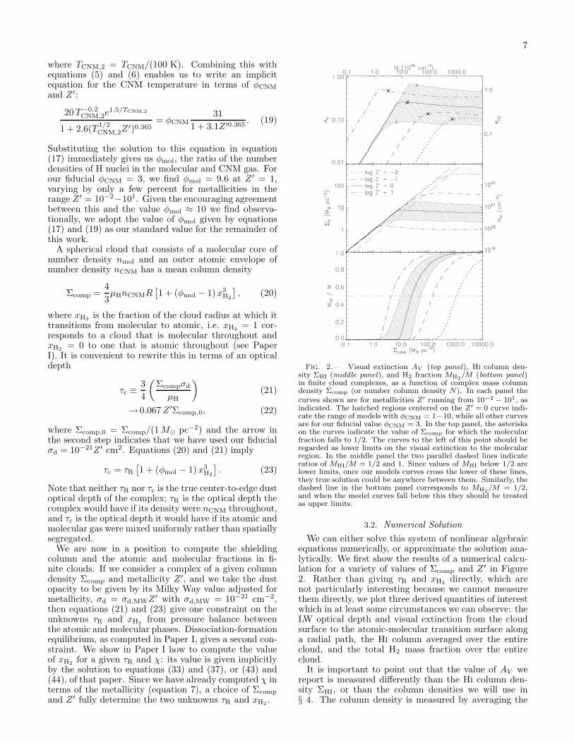
Fig. 2.— Visual extinction AV (top panel), Hi column den-sity ΣHI (middle panel), and H2 fraction MH2

/M (bottom panel)in finite cloud complexes, as a function of complex mass columndensity Σcomp (or number column density N). In each panel thecurves shown are for metallicities Z′ running from 10−2 − 101, asindicated. The hatched regions centered on the Z′ = 0 curve indi-cate the range of models with φCNM = 1−10, while all other curvesare for our fiducial value φCNM = 3. In the top panel, the asteriskson the curves indicate the value of Σcomp for which the molecularfraction falls to 1/2. The curves to the left of this point should beregarded as lower limits on the visual extinction to the molecularregion. In the middle panel the two parallel dashed lines indicateratios of MHI/M = 1/2 and 1. Since values of MHI below 1/2 arelower limits, once our models curves cross the lower of these lines,they true solution could be anywhere between them. Similarly, thedashed line in the bottom panel corresponds to MH2

/M = 1/2,and when the model curves fall below this they should be treatedas upper limits.

3.2. Numerical Solution

We can either solve this system of nonlinear algebraicequations numerically, or approximate the solution ana-lytically. We first show the results of a numerical calcu-lation for a variety of values of Σcomp and Z ′ in Figure2. Rather than giving τR and xH2

directly, which arenot particularly interesting because we cannot measurethem directly, we plot three derived quantities of interestwhich in at least some circumstances we can observe: theLW optical depth and visual extinction from the cloudsurface to the atomic-molecular transition surface alonga radial path, the Hi column averaged over the entirecloud, and the total H2 mass fraction over the entirecloud.

It is important to point out that the value of AV wereport is measured differently than the Hi column den-sity ΣHI, or than the column densities we will use in§ 4. The column density is measured by averaging the

8

mass per unit area over the entire complex, while AV

is measured along a single pencil beam from the surfaceof the cloud to the atomic-molecular transition along aradial trajectory. The former quantity is more analogousto what is measured in an observation using a telescopebeam that only marginally resolves or does not resolvea complex, while the latter is more closely analogous toa measurement of the extinction of a background pointsource through a cloud. We also caution that, for reasonswe discuss in § 3.3, our predictions are only accurate formolecular mass fractions > 1/2. (This is in the worstcase of very low metallicity and intermediate φCNM; ouraccuracy range expands as metallicity increases towardsolar and as φCNM gets smaller or larger than 3.) Belowthis limit our calculations yield only upper limits on themolecular fraction, not firm predictions. This confidencelimit is shown in the Figure 2.

The plots immediately yield a number of interestingresults. First, our prediction of nearly constant AV

through the atomic shielding layers around molecularclouds continues to hold whenever there is a significantmolecular fraction, even for finite clouds. Our predictionof a characteristic AV ≈ 0.2 through atomic shielding en-velopes of molecular clouds therefore continues to apply.

We also find that there is a saturation in the Hi columndensity at roughly 6 M⊙ pc−2 for solar metallicity, whichrises by a factor of a somewhat less then ten for everydecade by which the metallicity declines. The Hi columnsaturates simply because once Σcomp is large enough, thecloud column densities become so large that they are ef-fectively in the infinite cloud limit. At this point theshielding column is geometry-independent, and is deter-mined solely by the normalized strength of the radiationfield, χ, a value that does not vary much from galaxy togalaxy. Once Σcomp is sufficiently large to put a complexin the large cloud limit, adding additional mass simplyincreases the size of the shielded molecular layer, so theH2 fraction just rises smoothly. The saturation value of6 M⊙ pc−2 at solar metallicity is set by a combination ofthe fundamental constants describing H2 formation anddissociation, the shape of the Cii and Oi cooling curves(which determine the CNM density and temperature),and the properties of interstellar dust grains, which setthe ratio σd/R.

3.3. Geometric Uncertainties for Finite Clouds

In § 4.7 of Paper I we show that our method for deter-mining the molecular abundance in finite clouds suffersfrom a systematic uncertainty arising from our imperfectknowledge of the opacity along rays that pass through theatomic envelope of a cloud. For our fiducial model wetake the opacity along these rays due to molecules mixedinto the atomic gas to be set by the value of the disso-ciation radiation field at the surface of the zone wheremolecules dominate the opacity. Our results depend onthis approximation very little except at low molecular

volume fraction, x3H2

<∼ 0.2; in that case the uncertainty

about this approximation means that our model enablesus to predict only an upper limit on the molecular frac-tion, not an exact value.

In this paper we are concerned with molecular massrather than volume fractions, so we must quantify thatuncertainty. To do so, we proceed as in § 4.7 of Paper I:we adopt the opposite assumption, that opacity along

Fig. 3.— Ratio of minimum to maximum predicted H2 massfraction versus maximum predicted H2 mass fraction, for a varietyof values of Z′ and φCNM, as indicated. Curves for log Z′ < −1are not shown because they are indistinguishable from those forlog Z′ = −1.

rays passing through the region of the cloud wheremolecules dominate the opacity but still constitute asmall fraction of all H nuclei is infinite. We then re-peat the calculations of § 3 following this assumption:for a given Σcomp and Z ′, rather than solve the systemof equations formed by equation (23) of this paper andequations (33) and (37) or (43) and (44) of Paper I, weinstead solve equation (23) together with equations (69)and (70) or (71) of Paper I. Doing so gives a lower boundon the molecular content for a given Σcomp and Z ′. Bycomparing the results in this case to our fiducial calcu-lations as presented in § 3, we obtain an estimate of theuncertainty of our results.

In Figure 3 we show the results of this exercise. Onthe y-axis we show the ratio of the H2 mass fraction pre-dicted using our maximum opacity assumption, whichrepresents the minimum possible molecular content, di-vided by the value produced by our fiducial model, whichrepresents the maximum. This gives an estimate of ouruncertainty. The x-axis indicates the H2 mass fractionpredicted using the fiducial assumption we make else-where in the paper. As the plot shows, the two calcula-tions differ most at low Z ′ and intermediate φCNM. Inthis case the calculations differ by a factor of a few forH2 mass fractions below ∼ 0.5. If we adopt a factor of3 as an accuracy goal, this means that for cases wherewe predict an H2 mass fraction below 0.5, and at lowmetallicity, our predictions should be taken only as up-per limits. For solar metallicity or higher our confidencerange extends down to molecular mass fractions around0.4, and we attain upper limits below this.

3.4. Analytic Approximation

We can gain additional insight into the behavior of thesolution by constructing an analytic approximation. Theratio of the molecular mass MH2

to the total complexmass M is

fH2≡MH2

M=

φmolx3H2

1 + (φmol − 1)x3H2

. (24)

We wish to obtain an approximation for this in terms ofthe known quantities ψ (given in terms of metallicity byequations 7 and 10) and τc (given in terms of complexcolumn density by equation 21). We show in Paper I that

9

for ψ <∼ 3 and molecular volume fractions x3H2

>∼ 0.15, a

range in parameter space that includes most of our mod-els for realistic cloud parameters, the molecular volumeis well-approximated by

x3H2

≈ 1 −3ψ

4τR∆, (25)

where for convenience we have defined

τR∆ ≡ τR + aψ, (26)

and a = 0.2 is a numerical parameter that is optimizedfor agreement between the approximate and numericalsolutions. Substituting this approximation into the con-dition for pressure balance, equation (23), gives

τc = τR

[

φmol +3ψ

4τR∆(1 − φmol)

]

. (27)

As in Paper I, our approach to obtaining an analytic so-lution is to perform a series expansion in a. We thereforedefine

τc∆ ≡ τc

(

1 +aψ

τR

)

, (28)

so that τc∆/τc = τR∆/τR. Using this definition of τc∆together with equation (27) for τc implies that

τc∆ = φmol

(

τR∆ −3

4ψ

)

+3

4ψ. (29)

If we now use our approximation (25) and rewrite theresult in terms of τc∆ using equation (29), we obtain

fH2= 1 −

3ψ

4τc∆. (30)

We must now express τc∆ in terms of ψ, τc, and a alone.Thus

τc∆ = τc + aψ

(

τcτR

)

(31)

= τc + aψ

(

τc∆τR∆

)

. (32)

The second term on the RHS still involves the unknownsτc∆ and τR∆, but because they are already multiplied bya we now need only determine them to zeroth order ina. Solviing equation (29) for τR∆ gives

τR∆

τc∆=

1

φmol+

(

1 −1

φmol

)

3ψ

4τc∆(33)

≈1

φmol+

(

1 −1

φmol

)

3ψ

4τc, (34)

where in the second step we have dropped a term of ordera to obtain an expression that is accurate to zeroth orderin a. Substituting this into equation (32), and thence intoequation (30), gives our final expression for the molecularmass fraction, accurate to first order in a:

fH2= 1 −

3ψ

4τc

[

1 +4aψφmol

4τc + 3(φmol − 1)ψ

]−1

. (35)

Comparison of this approximate expression with the nu-merical solution illustrated in Figure 2 shows that for ourfiducial φCNM = 3 and metallicities from Z ′ = 10−2−10,

it is accurate to better than 30% whenever the approx-imation analytic solution gives fH2

> 0.25, but that itgoes to zero too sharply at low molecular fraction. Wecan improve the approximation by forcing the H2 frac-tion to approach zero smoothly rather than sharply atlow column density. Experimentation shows that the ex-pression

f−3HI = 1 +

{(

4τc3ψ

)[

1 +4aψφmol

4τc + 3(φmol − 1)ψ

]}3

(36)

matches the numerical result for fHI ≡ MHI/M forφCNM = 3 to better than 20% for all Z ′ < 10 regardlessof the value of fHI. (However note that, as we show in

§ 3.3, for fH2

<∼ 1/2 our estimate of the molecular content

is only an upper limit, and this is true of equation 36 aswell.) Using equation (21) to replace τc with Σcomp, andsubstituting in our fiducial values φCNM = 5, a = 0.2,and σd = 10−21Z ′ cm−2, equation (36) becomes

fHI →

[

1 +( s

11

)3(

125 + s

96 + s

)3]−1/3

(37)

where

s ≡Σcomp,0Z

′

ψ(38)

and Σcomp,0 = Σcomp/(1M⊙ pc−2). Note that our resultindicates that to good approximation the molecular con-tent of an atomic-molecular complex depends only on thecombination of input parameters Z ′Σcomp,0/ψ; the nu-merator Z ′Σcomp,0 is simply the dust column density ofthe complex up to a scaling factor, while the denomina-tor ψ is the dimensionless radiation field, which equations(7) and (10) give solely as a function of metallicity.

From (37), it also immediately follows that the H2 toHi ratio RH2

≡ fH2/fHI is

RH2≈

[

1 +( s

11

)3(

125 + s

96 + s

)3]1/3

− 1. (39)

For RH2> 1, which is the regime for which our models

apply with high confidence, we can use an even simplerexpression

RH2≈ 0.08s = 0.08

Σcomp,0Z′

ψ, (40)

where is accurate to ∼ 30%.Similarly, we show in Paper I that the dust absorption

optical depth through the atomic layer for a finite cloudis well-approximated by

τHI ≈ψ

4

[

1

1 − (a′/4)(ψ/τR)

]

, (41)

where a′ = 32 − 4a = 0.7. If we treat a′/4 as a small

parameter and perform a series expansion around it, thenwe need only approximate τR to zeroth order in a. Wecan do this simply by using equation (34) with a = 0,which allows us to set τR = τR∆ and τc = τc∆. Thus tozeroth order in a we have

τR = τR∆

[

1

φmol+

(

1 −1

φmol

)

3ψ

4τc

]

, (42)

10

and to first order in a or a′ we have

τHI =ψ

4

[

1 −a′ψφmol

4τc + 3(φmol − 1)ψ

]−1

. (43)

As with approximation (35) for the molecular mass frac-tion, this expression works well whenever the molecularfraction is not too low, and may be improved by forc-ing the optical depth to approach the total cloud opticaldepth smoothly when the column density becomes low.The expression

τ−2HI = τ−2

c +16

ψ2

[

1 −a′ψφmol

4τc + 3(φmol − 1)ψ

]2

(44)

is accurate to better than 35% for all Z ′ < 10, and tobetter than 25% for Z ′ < 1.

It is also convenient to invert our analytic expressionsto determine column density as a function of molecularcontent and metallicity. The term (125 + s)/(96 + s) inequation (37) is generally close to unity except at ex-tremely high column densities, so if we neglect second-order corrections to the difference between this term andunity, we can solve equation (37) for fHI to obtain

Σcomp,0Z′

ψ→ 11

(

f−3HI − 1

)1/3 8.7 +(

f−3HI − 1

)1/3

11 +(

f−3HI − 1

)1/3(45)

This expression matches the numerical solution at the∼ 20% level for fHI < 0.75. Note that this result im-plies that the column density Σcomp at which a given Hifraction is reached depends on metallicity both explic-itly through the Z ′ term in the numerator, representingthe effect of metallicity on dust content, and implicitlythrough ψ (equations 7 and 10), representing the effectof metallicity on the ratio of radiation intensity to CNMdensity. Since ψ is an increasing function of metallicity,for a given molecular fraction Σcomp has a weaker thanlinear dependence on metallicity. For example, evalu-ating (45) with fHI = 0.5 at solar metallicity Z ′ = 1indicates that we expect the gas to be half molecularfor complexes with Σcomp = 27 M⊙ pc−2. (The exactnumerical solution is Σcomp = 25.5 M⊙ pc−2.) At one-third solar metallicity, Z ′ = 1/3, half molecular contentis reached at Σcomp = 67 M⊙ pc−2 (using equation 45;numerically Σcomp = 55.3M⊙ pc−2), somewhat less thana factor of 3 higher.

4. COMPARISON TO OBSERVATIONS

Our model makes strong predictions for the relativefractions of Hi and H2 as a function of total surface den-sity and metallicity, and in this section we compare theseresults to a variety of galactic and extragalactic observa-tions.

4.1. Extragalactic Observations

4.1.1. Data Sets

We use three extragalactic data sets for comparison toour models. Two are recent surveys that have mappednearby galaxies in 21 cm Hi and 2.6 mm CO(1 → 0)emission at overlapping positions, and therefore providean ideal laboratory in which to test our model. The firstof these is the work of WB02, BR04, and BR06, who re-port Hi and H2 surface densities on a pixel-by-pixel basis

TABLE 1Galaxy metallicities

Galaxy log(O/H) + 12a Sampleb Reference

Solar (Milky Way) 8.76 B 7DDO154 7.67 L 3HOI 7.54 L 6HOII 7.68 L 6IC10 8.26 B 1IC2574 7.94 L 6NGC0598 8.49 B 5NGC0628 8.51 L 5NGC0925 8.32 L 5NGC2403 8.39 L 5NGC2841 8.81 L 5NGC2976 8.30 L 8NGC3077 8.64 L 8NGC3184 8.72 L 5NGC3198 8.42 L 5NGC3351 8.80 L 5NGC3521 8.49 BL 5NGC3627 9.25 BL 4NGC4214 8.22 L 2NGC4321 8.71 B 5NGC4414 ... B ...NGC4449 8.31 L 2NGC4501 8.78 B 5NGC4736 8.50 BL 5NGC5033 8.68 B 5NGC5055 8.68 BL 5NGC5194 8.75 BL 5NGC5457 8.44 B 5NGC6946 8.53 L 5NGC7331 8.48 BL 5NGC7793 8.34 L 5

References. — 1 – Garnett (1990), 2 – Martin(1997), 3 – van Zee et al. (1997), 4 – Ferrarese et al. (2000),5 – Pilyugin et al. (2004), 6 – Walter et al. (2007), 7 –Caffau et al. (2008), 8 – Walter et al. (2008). An entry ... in-dicates that there is no gas-phase metallicity is reported in theliterature.a We take the metallicity relative to solar to be proportionalto the O/H ratio, i.e. log Z′ = [log(O/H) + 12] − 8.76.b B =galaxy is in BR06 sample, L = galaxy is in L08 sample

in 14 nearby galaxies (including the Milky Way). TheH2 surface densities are inferred from CO observationstaken as part of the BIMA SONG survey (Regan et al.2001; Helfer et al. 2003), while the Hi observations arefrom the VLA. WB02 and BR06 supplement these datawith stellar surface density measurements from 2MASS(Jarrett et al. 2003), which together with the equationsgiven in BR06 can be used to derive a pressure in eachpixel if one assumes that the gas in in hydrostatic bal-ance, that the stellar scale height greatly exceeds the gasscale height, and that the gas velocity dispersion has aknown value. The galaxies in the sample are all molecule-rich spirals with metallicities within 0.5 dex of solar.

The second extragalactic data set we use is compiled byL08, who a combine Hi measurements from the THINGSsurvey with CO data partly taken from BIMA SONG andpartly from the ongoing HERACLES survey. The au-thors also include 2MASS stellar surface densities in theircompilation, and give mean pressures. Unlike the BR06sample the data reported are averages over galactocen-tric rings rather than individual pixels, although point-by-point maps at sub-kpc resolution are in preparation(F. Walter, 2008, private communication). The sampleincludes 23 galaxies, of which roughly half are large spi-rals and roughly half are low-mass, Hi-dominated dwarfs.

11

The galaxies in the data set partly overlap with those inthe sample of BR06, but extend over a wider range ofmetallicities and molecule fractions.

We summarize the galaxies in the samples in Table1. We also report metallicities for each galaxy wherethese are available in the literature. We do not includeNGC4414 in the analysis, because no gas phase metal-licity is available for it. In the comparison that follows,we neglect the presence of metallicity gradients withinthese galaxies, because gradients are only available forsome of them. On top of this, we note that the metal-licities themselves are probably uncertain at levels fromhundreths to tenths of a dex, depending on the galaxyand the analysis technique used, which adds additionalscatter on top of that already introduced by our neglectof metallicity gradients.

In both data sets the uncertainty in the Hi columndensities is generally ∼ 10%. In the CO data the formaluncertainties are generally ∼ 20 − 30%, but the dom-inant uncertainty is probably systematic: the X factorused to convert observed CO luminosities into H2 col-umn densities. This is uncertain at the factor of ∼ 2level (Blitz et al. 2007), and almost certainly varies withmetallicity (e.g. Bolatto et al. 2008). Thus, although forclarity we will suppress error bars in the plots that fol-low, recall that the molecular data is uncertain at thefactor of ∼ 2 level.

The third data set we use, in § 4.1.4, is theSpitzer Survey of the Small Magellanic Cloud (S3MC)(Bolatto et al. 2007; Leroy et al. 2007). This survey dif-fers from the SONG and THINGS data sets in that thosesurveys infer the presence of H2 via CO emission, whereasS3MC measures molecular hydrogen using measurementsof dust from Spitzer combined with Hi measurements byStanimirovic et al. (1999) and Stanimirovic et al. (2004).The basic idea behind the technique is that one deter-mines the dust-to-gas ratio in a low-column density re-gion where molecules are thought to contribute negli-gibly to the total column. Then by comparing the Hiand dust column density maps, one can infer the pres-ence of H2 in pixels where the total dust column ex-ceeds what one would expect for the observed Hi col-umn and a fixed dust-to-gas ratio. The reason for usingthis technique is that, at the low metallicity of the SMC(log[O/H] + 12 = 8.0, Dufour 1984, i.e. 0.76 dex belowSolar), CO may cease to be a reliable tracer of moleculargas. The SMC represents the lowest metallicity galaxyfor which we have H2 detections rather than upper lim-its; the BR06 sample does not contain any galaxies withmetallicities as low as the SMC, and no CO was detectedin any of the L08 galaxies with metallicities comparableto or lower than the SMC. Thus, the SMC represents aunique opportunity to test our models at very low metal-licity.

Before comparing to these data sets, it is worth com-menting briefly on one additional extragalactic data setto which we will not compare our models: observationsof H2 column densities along sightlines in the LMC andSMC using FUSE (Tumlinson et al. 2002). We do notuse this data set for comparison because it includes onlysightlines with low column densities that are stronglydominated by atomic gas; the highest reported H2 frac-tion is below 10%. Sightlines with significantly highermolecular content than this absorb too much background

starlight to allow FUSE to make a reliable measurementof the H2 column. The low column densities of the cloudsthat FUSE can observe in these galaxies place almost allof them into the regime where our theory yields only up-per limits. Those limits are generally consistent with thedata, but the comparison is not particularly illuminating.

4.1.2. Column Density and Metallicity Dependence

In this section we compare our models predictions ofthe Hi and H2 mass fractions as a function of totalcolumn density and metallicity to our two extragalac-tic data sets. To perform this comparison, for conve-nience we first break the sample into four metallicitybins: −1.25 < logZ ′ < −0.5, −0.5 < logZ ′ < −0.25,−0.25 < logZ ′ < 0, and 0 < logZ ′ < 0.5, whereZ ′ = Z/Z⊙ and we adopt log(O/H) + 12 = 8.76 asthe value corresponding to solar metallicity (Caffau et al.2008). These bins roughly evenly divide the data; we donot include the galaxies for which metallicities are notavailable in the literature.

Next we must consider how finite spatial resolution willaffect our comparison. Given the beam sizes in the ob-served data, which range from ∼ 0.3 kpc for the nearestgalaxies to a few kpc for the most distant, each pixel(for BR06) or ring (for L08) in the observed data set islikely to contain multiple atomic-molecular complexes.The atomic and molecular observations are convolved tothe same resolution, so this does not bias the measure-ment of the atomic to molecular ratio, although it doesmean that this ratio is measured over an averaging scaleset by the beam size. Since individual atomic molecu-lar complexes presumably represent peaks of the galacticcolumn density, however, the total (Hi + H2) observedgas surface density Σobs reported for each pixel or ringrepresents only a lower limit on Σcomp, the total sur-face density of individual complexes. In our model thefraction of the cloud in molecular form is a strictly in-creasing function of Σcomp (and of metallicity Z), whilethe atomic fraction is a strictly decreasing function. Be-cause we have only the observed column density Σobs

available, not the column density of an individual com-plex Σcomp, we have no choice but to take Σcomp = Σobs

as our best estimate. The error in this approximationprobably ranges from tens of percent for nearby galax-ies where the beam size is not much larger than the sizeof a complex up to an order of magnitude or more forring-averages in distant galaxies. As a result, though, weexpect to overestimate the atomic fraction and underes-timate the molecular fraction. Physically we may thinkof this as a clumping effect: the clumpier the gas is, thebetter able it is to shield itself against dissociating radi-ation. Since our observations smooth over scales largerthan the characteristic gas clumping scale, we will missthis effect.

There are also two effects which go in the other di-rection, however. First, as noted above, shielding comesprimarily from cold atomic gas, not warm gas. Althoughmost of the gas in the immediate vicinity of a singlemolecular region is probably cold, observations that av-erage over many molecular cloud complexes are likely toinclude a fair amount of WNM gas as well. Since wehave only the total Hi column densities including bothphases, we are prone to overestimate Σcomp and thereforethe molecular fraction, because the WNM raises the Hi

12

column but does not provide much shielding. This effectis not important at moderate to high column densities,where the atomic gas does not dominate the total massbudget, but it could be significant at lower densities.

Second, there may be gas along our line of sightthrough a galaxy that is not associated with an atomic-molecular complex along that line of sight. This effectwill increase in severity as the galaxy comes close to edge-on, since this will increase the path length of our line ofsight through the galaxy. As with WNM gas, this ex-tra material contributes to Σobs but not to the complexsurface density Σcomp, and it therefore leads us to over-estimate the molecular fraction. We can perform a verysimple calculation to estimate the size of this effect. Con-sider a simple self-gravitating gas disk characterized bythe standard vertical density profile n ∝ sech2(0.88z/h),where h is the half-height of the gas. At some pointin this disk is an atomic-molecular complex, centered atthe midplane. Since complexes are found preferentiallyat the midplane, unless the galaxy is very close to edge-on then we need not consider the possibility of our line ofsight intersecting multiple independent complexes. Sincethe complex formed from a large-scale gravitational in-stability in the disk, its characteristic size is ∼ h, and wetherefore consider gas to be “associated” with the com-plex if it is within a distance h of it in the plane of thedisk. Suppose this galaxy has an inclination i. Mak-ing the worst-case assumption, that there is no densityenhancement due to the presence of the self-gravitatingcomplex, we can then compute what the fraction of thegas we see along our line of sight is not associated withit. This is simply

∫ ∞

h cot i sech2(0.88z/h) dz∫ ∞

0sech2(0.88z/h) dz

= 1 − tanh(1.13 cot i). (46)

This is less than 0.5 for all inclinations less than 64◦.Only a handful of the galaxies in the SONG and THINGSsurveys have inclinations larger than this, so even in theworst case scenario where complexes do not represent anyenhancement of the gas density, we expect non-associatedgas to produce an error smaller than a factor of ∼ 2for the great majority of the galaxies to which we arecomparing.

Given the limitations imposed by finite resolution, weproceed as follows. Using the method described in § 3,we compute the molecular mass fraction

fH2(Σcomp, Z) ≡

MH2

M, (47)

as a function of complex column density Σcomp andmetallicity Z. (For these and all subsequent predictionswe use our fiducial value of φCNM = 3.) We then generatepredicted Hi and H2 column densities for each metallicitybin and each observed column density Σ via

ΣH2,predicted = fH2(Σobs, Zmin)Σobs (48)

ΣHI,predicted =[1 − fH2(Σobs, Zmin)]Σobs, (49)

where Zmin is the minimum metallicity for that bin.Since fH2

(Σcomp, Z) is a strictly increasing function ofΣcomp and Z, and we know that Σobs < Σcomp andZmin < Z, we expect fH2

(Σobs, Zmin) to be a lowerlimit on the true molecular fraction. We therefore expectΣH2,predicted to be a lower limit on the observed data, and

Fig. 4.— Hi column density ΣHi versus total column densityΣ for galaxies in metallicity bins −1.25 < log Z′ < −0.5, −0.5 <log Z′ < −0.25, −0.25 < log Z′ < 0, and 0 < log Z′ < 0.5, asindicated. In each panel we plot the values of ΣHi and Σ fromthe samples of BR06 (squares) and L08 (diamonds) and show ourmodel predictions of ΣHi as a function of Σ for log Z′ = −1.25,−0.5, −0.25, and 0 (lines, highest to lowest). The curve for thevalue of log Z′ equal to the minimum log Z′ for each bin, whichshould represent the upper envelope of the data, is shown as asolid line. The rest are shown as dotted lines. The four linesare the same in each panel. To maximize readability we omit theerror bars on the data points. The parallel slanted dashed lines,ΣHI = Σobs/2 and ΣHI = Σobs, show the range of value of ΣHI

for which our predictions should be treated as upper limits for thereasons discussed in § 3.3. Parts of our model curves above theΣHI = Σobs/2 line could be as high as the ΣHI = Σobs line.

ΣHI,predicted to be an upper limit. The possible exceptionto this statement is at low column densities, where a sig-nificant fraction of the Hi column may be in the form ofWNM.

We plot the data against our theoretical prediction forthe upper envelope of ΣHI in Figure 4, and we showthe corresponding predicted lower envelopes for ΣH2

andRH2

≡ ΣH2/ΣHI in Figures 5 and 6. For the BR06 data

set, rather than plotting the tens of thousands of individ-ual pixels it contains, for each galaxy we show the dataaveraged over 20 logarithmically-spaced column densitybins running from the minimum to the maximum valueof Σobs reported for that galaxy. As the plots show, ourmodel predictions for the upper envelope of the Hi sur-face density and the corresponding lower envelope of theH2 surface density as a function of total surface densityand metallicity agree very well with the data. The datafill the space up to our predicted envelopes but for themost part do not cross them, even when the predicted Hi

envelope becomes flat for Σobs>∼ 10 M⊙ pc−2. Moreover,

13

Fig. 5.— Same as Figure 4, except that we show H2 rather thanHi column densities. For clarity we do not show non-detections.Note that NH2

is the column density of H nuclei in molecular form,which is twice the column density of H2 molecules. The slanteddashed line is ΣH2

= Σobs/2; as discussed in § 3.3, above this lineour model curves may be taken as predictions, while below it theyshould be taken as upper limits.

our model recovers not only the primary dependence ofΣHI on the total observed column density Σobs, but alsothe secondary dependence on metallicity. For example,rings in the lowest metallicity bin in the L08 data setreach total mean column densities of almost 20 M⊙ pc−2,but still show no detectable molecular component. Onthe other hand, in the highest metallicity bin the molec-ular fraction is close to 70% in rings with Σobs ≈ 20 M⊙

pc−2. Our models reproduce this effect: at a metallicityof logZ ′ = −0.5, we predict that the gas will be 94%atomic even at a surface density of 20 M⊙ pc−2, whereasfor logZ ′ = 0.5 we predict an atomic fraction of only30% at that column density, in agreement with the data.

We caution that we can only predict upper limits onthe molecular content in regions of parameter space whenour predicted molecular fraction falls below ∼ 1/2, forthe reasons discussed in § 3.3. We have indicated theregions where our model predictions convert to upperlimits in Figures 4 – 6. Alternately, one can expressthis uncertainty as giving a minimum column density atwhich we can predict a value rather than an upper limitfor molecular content. For reference, at the metallicitiesof logZ ′ = −1.25, −0.5, −0.25, 0, and 0.5 which definethe edges of our metallicity bins, the minimum columndensities for which we can predict numerical values tobetter than factor of few confidence are 250, 58, 38, 25,and 11 M⊙ pc−2, respectively.

Fig. 6.— Same as Figures 4 and 5, except that we show RH2≡

ΣH2/ΣHI rather than column densities. For clarity we do not show

non-detections. The horizontal dashed line corresponds to RH2=

1; as discussed in § 3.3, above this line our model curves may betaken as predictions, while below it they should be taken as upperlimits.

Finally, we note that the future HERACLES /THINGS data set represents an opportunity to performan even stronger test of our model. In Figure 4 a signif-icant fraction of the data points fall below our predictedupper limits, and correspondingly these points are aboveour lower limits in Figures 5 and 6. We hypothesize thatthese data points represent rings or pixels within whichthe gas is significantly clumped, so that the averagedcolumn density Σobs seen in the observation is signifi-cantly lower than the column density at which most ofthe molecular gas in that beam or ring is found, and ourcalculation for a complex with Σcomp = Σobs overesti-mates the Hi column. In reality these regions probablyconsist of patches of high column density where most ofthe molecules reside, embedded in a lower density ambi-ent medium that has a lower molecular fraction than wedetermine by averaging over large scales. If we could ob-serve these regions at higher resolution, in Figure 4 thehigh column, high molecular content points will lie to theright of and slightly above the low resolution points, sinceboth the total and Hi column densities will be higherthan for the lower resolution observation, but the in-crease in the total column will be larger than in theHi column. Conversely, the low column, low moleculepatches will lie to the left and slightly downward fromthe low resolution points, since both the total and Hicolumns will decline, but the Hi by less, since the atomicfraction rises. These changes will bring the data points

14

Fig. 7.— Same as Figure 4, except that we show only datafrom BR06, and we have divided this data set into “near” galaxies,those for which the survey resolution is < 1 kpc, and “far” galaxies,those for which the resolution is > 1 kpc.

closer to our model curves. Indeed, the existing dataalready hint that such an effect is present: the singlebeam-averaged observations of the BR06 data set scat-ter away from our limit lines noticeably less than thering-averaged observations from L08. Similarly, we candivide the point-by-point data from BR06 into a “near”sample, consisting of galaxies for which the resolutionis smaller than 1 kpc, and a “far” sample, consisting ofgalaxies with larger resolutions. We plot a version ofFigure 4 using only this divided data set from BR06 inFigure 7. The comparison is quite noisy, but the data inthat bin do at least seem consistent with the hypothesisthat the near data fall closer to the model lines than thefar data.

The full HERACLES survey, currently underway, willreport measurements of the molecular surface density forindividual patches ∼ 0.5 kpc in size, generally smallerthan the beam patches the BIMA / SONG survey. While

this is still considerably larger than the <∼ 0.1 kpc-size of

a typical atomic-molecular complex in the Milky Way, atthe higher spatial resolution of the full HERACLES dataset beam-smearing effects should be reduced and the col-umn densities reported for each patch should be closer tothe true column densities Σcomp of the individual atomic-molecular complexes. We therefore predict that in thefull HERACLES data set the ΣHi −Σobs relation shouldbe closer to our theoretical upper and lower limit curvesthan the lower resolution or azimuthally-averaged datashown in Figures 4 – 6.

4.1.3. Pressure Dependence

BR04 and BR06 find that the molecular fraction in agalaxy correlates with the mid-plane gas pressure as

RH2≡

ΣH2

ΣHI=

(

P/kB

3.5 ± 0.6 × 104 K cm−3

)0.92±0.07

,

(50)while L08 find

RH2=

(

P/kB

2.0 × 104 K cm−3

)0.8

(51)

for their sample. Although our model does not directlygive a prediction for the dependence of the molecularfraction on pressure, and we argue that surface densityand metallicity are the physical variables that directlycontrol the molecular fraction, we wish to check whetherour model is consistent with the observed correlation.

To avoid introducing any bias in performing this check,we must determine pressures from observable quantitiesin the same way that BR06 and L08 do, following an ap-proximation introduced by BR04.2 The BR04 approxi-mation treats the galaxy as an infinite thin disk of uni-form gas and stars in vertical hydrostatic balance. Forsuch a disk the pressure is related to surface density by

P =π

2GΣg

(

Σg + Σ∗

vgv∗

)

, (52)

where Σg is the total (Hi plus H2) gas surface density, Σ∗

is the stellar surface density, and vg and v∗ are the verti-cal velocity dispersions of the gas and stellar components,respectively. The gas velocity dispersion is roughly con-stant, vg ≈ 8 km s−1, for the galaxies in the BR06 andL08 samples. The term Σ∗/v∗ presents more difficulty,however. It varies by orders of magnitude from galaxycenters to edges, and between galaxies, so we cannot picka single value for it. Since in our model the molecularfraction is a function only of metallicity and Σg, thismeans that we do not predict a single-valued relation-ship between RH2

and P that we can directly compareto the empirical fits.

However, we can still compare our model to the data intwo ways. First, we can pick a range of values of Σ∗/v∗consistent with the range in the observed sample, anddemonstrate that the resulting range of predictions forRH2

covered by our model is consistent with the observa-tional data. For this purpose we follow BR06 in adoptinga constant value vg = 8 km s−1 and using simplified ver-sion of equation (52), which follows from assuming thatboth the surface density and scale height of the stars aremuch greater than those of the gas:

P

kB=272 cm−3 K

(

Σobs

M⊙ pc−2

) (

Σ∗

M⊙ pc−2

)0.5

×

(

vg

km s−1

) (

h∗pc

)−0.5

, (53)

2 It is important to note that the midplane pressure which theobservers attempt to estimate is not the same as the pressure inthe molecular gas or the CNM which we balanced in § 2.1; thetotal midplane pressure includes contributions from all phases ofthe ISM rather than just the CNM or molecular clouds, as well ascontributions from magnetic fields, cosmic rays, and bulk motions.The pressure we use in § 2.1 includes thermal pressure in the CNMor molecular gas only.

15

Fig. 8.— Molecular to atomic ratio RH2versus pressure P . We

show the data sets of BR06 (squares) and L08 (diamonds), andpredictions for models with log ρ∗ = −2.5, −1.5, −0.5, 0.5, and1.5 in units of M⊙ pc−3 (highest to lowest lines, as indicated),and with metallicities log Z′ = −0.5 and 0 (dashed and solid lines,respectively). In the upper panel for clarity we show only a singlegalaxy from each data set (NGC4736 from BR06 and HOII fromL08), while in the lower panel we show the data for all galaxies;the model curves in each panel are identical. For BR06 the datawe show are averaged over 0.1 dex-wide bins in pressure, as inBR06’s Figure 3. For the L08 data, we only plot rings for whichboth molecular and atomic gas are detected. The dotted horizontallines show RH2

= 1; below this line our predictions should be takenas upper limits only.

where Σobs is the observed value of the total gas surfacedensity Σg, h∗ is the stellar scale height, and for con-venience we define ρ∗ = Σ∗/h∗. We consider values oflog ρ∗ from −2.5 to 1.5 in units of M⊙ pc−3, a range thatcovers almost all of the samples of BR06 and L08. For agiven value of ρ∗, equation (53) gives a single-valued re-lationship between P and Σg, so for each P and a choiceof metallicity we can use our model to make a predic-tion for ΣHI and thus for RH2

. As with our calculationsin § 4.1.2, we expect to systematically underpredict RH2

because the observed column density Σobs is an under-estimate of the true column density of atomic-molecularcomplexes that are not resolved by the telescope beam.

We show the results of this computation in Figure 8.As expected, the model covers an area consistent withthe observed data. First note that there is a systematicoffset between the results from BR06 and L08; this islikely because some of the structural parameters that areused in equation (53) are quite uncertain, particularlyh∗, and the values adopted by the two surveys are notnecessarily the same. We should keep this uncertainty inmind as we proceed, since it suggests an upper limit onthe level of agreement we can expect.

Nonetheless, the correlation between RH2and P shown

in both observational surveys, RH2∝ P 0.8−0.9, is some-

what flatter than any of our model curves for a particularchoice of ρ∗, which all approach RH2

∝ P 1 at large P .However this is to be expected: low pressures and gas col-

umn densities are found preferentially in the outer partsof galaxies where ρ∗ is small, so at low P we expect tobe closer to the higher model curves, which have low ρ∗.Conversely, high pressures and values of Σg are foundpreferentially in regions with higher stellar densities ρ∗,so high P values should be closer to the lower modelcurves, which have larger ρ∗. This covariance betweenP and ρ∗ results in a flattening of the RH2

∝ P relationthat we would predict if all galaxies had fixed ρ∗.

We can eliminate this covariance effect and produce astronger test than that shown in Figure 8 by using ourmodel to generate predictions for molecular content di-rectly, and plotting those against the inferred pressure.To do this, for each galactocentric ring in the L08 dataset we take the observed total gas surface density Σobs

and the metallicity given in Table 1 (which we treat asconstant in each the galaxy) and use our model to predictRH2

. Similarly, for the BR06 data set we take the ob-served gas surface density Σobs in each pixel and use ourmodel to generate a prediction for RH2

. Since the pres-sure in each ring or pixel is known, by this procedure wegenerate a synthetic set of data points (P,RH2

) which wecan compare to the observations, and from which we cangenerate a fit for RH2

as a function of P .Before making the comparison, however, we must also

model the effects of finite telescope sensitivity, whichmake it impossible to detect molecules below a certainminimum column density. Since, as Figure 8 shows, ourmodel predicts that the slope of RH2

versus P varies withP , this can affect the fit we generate from our syntheticdata. We include this effect using a procedure nearlyidentical to that of BR06. These authors first estimatethe minimum value of RH2

as a function of pressure thatthey could detect in each galaxy based on their telescopenoise limits. For our synthetic data we adopt a minimumRH2,min = 0.05 for all galaxies, slightly below the lowestaverage RH2

that BR06 report for any of the galaxiesthey analyze. For each galaxy we then identify the low-est pressure Pmin for which all the pixels / rings haveRH2

> RH2,min. At pressures above Pmin, the sampleshould be nearly complete, in the sense that no pixelsor rings will have molecular non-detections that couldbias a fit of RH2

versus P . At pressures below Pmin

the data are incomplete, and we therefore drop all pix-els or rings whose pressures are below Pmin. This pro-duces a sensitivity-corrected set of synthetic data. Fi-nally, following BR06 we then bin the pixels by pressure,using bins 0.1 dex wide, and for each pressure bin in eachgalaxy we compute an average value of RH2

. We do notbin the rings in the L08 sample.

We overplot the synthetic and real data in Figure 9.Fitting our synthetic data to a powerlaw function forRH2

versus P gives

RH2=

(

P/kB

9.0 × 103 K cm−3

)0.81

, (54)

if we include our models for both the BR06 and L08 datasets. Using only one or the other gives

RH2=

(

P/kB

2.2×102 K cm−3

)0.74

, (BR06)(

P/kB

2.8×105 K cm−3

)0.85

, (L08). (55)

As expected, we obtain a slope shallower than unity asa result of the systematic increase of ρ∗ with P . The

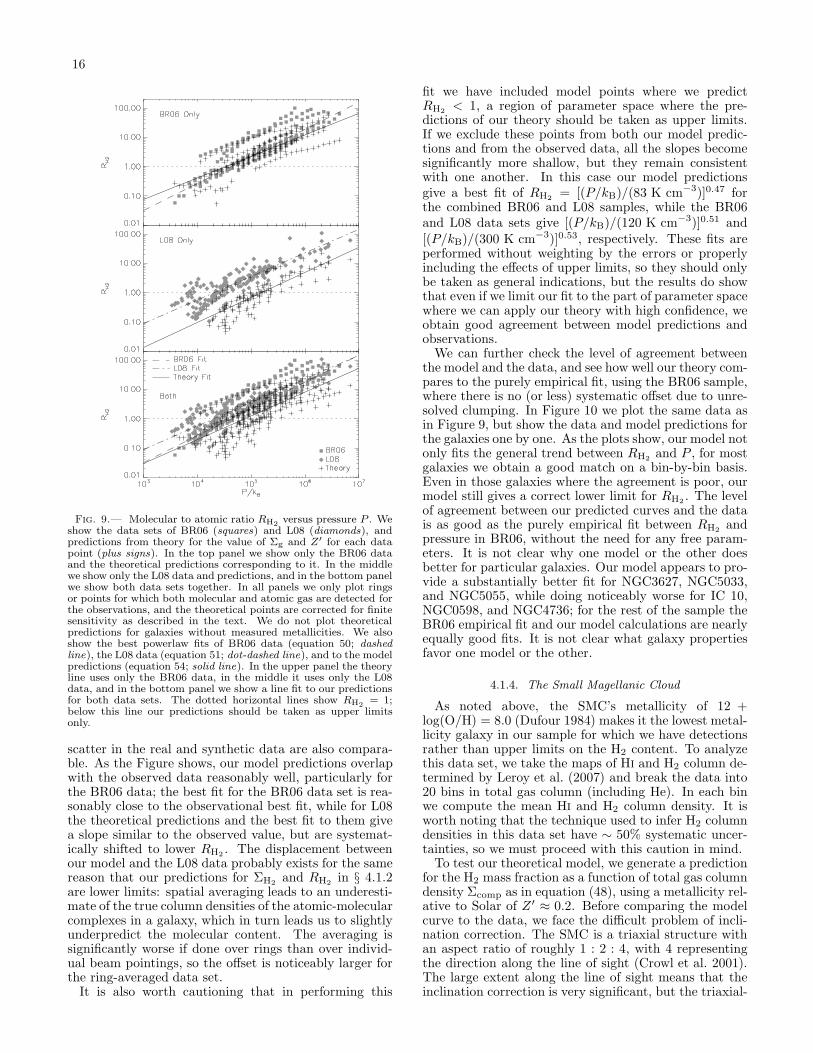
16

Fig. 9.— Molecular to atomic ratio RH2versus pressure P . We

show the data sets of BR06 (squares) and L08 (diamonds), andpredictions from theory for the value of Σg and Z′ for each datapoint (plus signs). In the top panel we show only the BR06 dataand the theoretical predictions corresponding to it. In the middlewe show only the L08 data and predictions, and in the bottom panelwe show both data sets together. In all panels we only plot ringsor points for which both molecular and atomic gas are detected forthe observations, and the theoretical points are corrected for finitesensitivity as described in the text. We do not plot theoreticalpredictions for galaxies without measured metallicities. We alsoshow the best powerlaw fits of BR06 data (equation 50; dashedline), the L08 data (equation 51; dot-dashed line), and to the modelpredictions (equation 54; solid line). In the upper panel the theoryline uses only the BR06 data, in the middle it uses only the L08data, and in the bottom panel we show a line fit to our predictionsfor both data sets. The dotted horizontal lines show RH2

= 1;below this line our predictions should be taken as upper limitsonly.

scatter in the real and synthetic data are also compara-ble. As the Figure shows, our model predictions overlapwith the observed data reasonably well, particularly forthe BR06 data; the best fit for the BR06 data set is rea-sonably close to the observational best fit, while for L08the theoretical predictions and the best fit to them givea slope similar to the observed value, but are systemat-ically shifted to lower RH2

. The displacement betweenour model and the L08 data probably exists for the samereason that our predictions for ΣH2

and RH2in § 4.1.2

are lower limits: spatial averaging leads to an underesti-mate of the true column densities of the atomic-molecularcomplexes in a galaxy, which in turn leads us to slightlyunderpredict the molecular content. The averaging issignificantly worse if done over rings than over individ-ual beam pointings, so the offset is noticeably larger forthe ring-averaged data set.

It is also worth cautioning that in performing this

fit we have included model points where we predictRH2

< 1, a region of parameter space where the pre-dictions of our theory should be taken as upper limits.If we exclude these points from both our model predic-tions and from the observed data, all the slopes becomesignificantly more shallow, but they remain consistentwith one another. In this case our model predictionsgive a best fit of RH2

= [(P/kB)/(83 K cm−3)]0.47 forthe combined BR06 and L08 samples, while the BR06and L08 data sets give [(P/kB)/(120 K cm−3)]0.51 and[(P/kB)/(300 K cm−3)]0.53, respectively. These fits areperformed without weighting by the errors or properlyincluding the effects of upper limits, so they should onlybe taken as general indications, but the results do showthat even if we limit our fit to the part of parameter spacewhere we can apply our theory with high confidence, weobtain good agreement between model predictions andobservations.

We can further check the level of agreement betweenthe model and the data, and see how well our theory com-pares to the purely empirical fit, using the BR06 sample,where there is no (or less) systematic offset due to unre-solved clumping. In Figure 10 we plot the same data asin Figure 9, but show the data and model predictions forthe galaxies one by one. As the plots show, our model notonly fits the general trend between RH2

and P , for mostgalaxies we obtain a good match on a bin-by-bin basis.Even in those galaxies where the agreement is poor, ourmodel still gives a correct lower limit for RH2

. The levelof agreement between our predicted curves and the datais as good as the purely empirical fit between RH2

andpressure in BR06, without the need for any free param-eters. It is not clear why one model or the other doesbetter for particular galaxies. Our model appears to pro-vide a substantially better fit for NGC3627, NGC5033,and NGC5055, while doing noticeably worse for IC 10,NGC0598, and NGC4736; for the rest of the sample theBR06 empirical fit and our model calculations are nearlyequally good fits. It is not clear what galaxy propertiesfavor one model or the other.

4.1.4. The Small Magellanic Cloud

As noted above, the SMC’s metallicity of 12 +log(O/H) = 8.0 (Dufour 1984) makes it the lowest metal-licity galaxy in our sample for which we have detectionsrather than upper limits on the H2 content. To analyzethis data set, we take the maps of Hi and H2 column de-termined by Leroy et al. (2007) and break the data into20 bins in total gas column (including He). In each binwe compute the mean Hi and H2 column density. It isworth noting that the technique used to infer H2 columndensities in this data set have ∼ 50% systematic uncer-tainties, so we must proceed with this caution in mind.

To test our theoretical model, we generate a predictionfor the H2 mass fraction as a function of total gas columndensity Σcomp as in equation (48), using a metallicity rel-ative to Solar of Z ′ ≈ 0.2. Before comparing the modelcurve to the data, we face the difficult problem of incli-nation correction. The SMC is a triaxial structure withan aspect ratio of roughly 1 : 2 : 4, with 4 representingthe direction along the line of sight (Crowl et al. 2001).The large extent along the line of sight means that theinclination correction is very significant, but the triaxial-

17

Fig. 10.— Same as Figure 9, except that we show only the BR06, and we plot only two galaxies per panel, as indicated, so that we cancompare on a galaxy-by-galaxy basis. In each panel the black open points are the observed data, while the gray filled points are our modelpredictions. The dashed line shows the BR06 empirical fit.

ity of the galaxy means that no single number describesthe inclination, as is the case for a disk. We thereforecompare the model and the data using two different in-clination corrections, one assuming an inclination i = 76◦

(corresponding to a 1 : 4 aspect ratio) and one assumingan inclination i = 63◦ (corresponding to a 1 : 2 aspectratio). These should bracket the true inclination cor-rection. Another caution we should make here is that,due to these large inclinations, there may be significantamounts of gas along a given line of sight that are notassociated with whatever atomic-molecular complex itintersects, so the Hi column densities may be overesti-mates (see § 4.1.2).

Figure 11 shows a comparison of the data and themodel curve. As expected, the data for the two differ-ent inclination corrections bracket the model curve quitewell. We should be cautious about reading too much into

the agreement at low Σobs (<∼ 30 M⊙ pc−2), where boththe data and our model are quite uncertain. Indeed, RH2

is such a sharp function of Σobs at low column that the

factor of 2 variation in the total column introduced bythe uncertainty in the inclination translates to a factorof ∼ 50 difference in the value of RH2

at a fixed Σobs.Thus, our model need only be correct within a factor of50 to lie in between the two curves for the different incli-nation corrections. At higher Σobs (>∼ 80 M⊙ pc−2), onthe other hand, the inclination correction only producesa factor of ∼ 2 uncertainty in RH2

, and the ability of ourmodel to match the data here is significant. It shows thatwe are capable of predicting the total column at whichRH2

∼ 1 to better than a factor of 2 accuracy even in agalaxy with metallicity ∼ 1/10 Solar.

4.2. Galactic Observations

4.2.1. Data Sets

We next compare our model to observations of themolecular content of clouds in the Milky Way, asmeasured by the Copernicus (Spitzer & Jenkins 1975)and the Far Ultraviolet Spectroscopic Explorer (FUSE)(Moos et al. 2000; Sahnow et al. 2000) missions. These

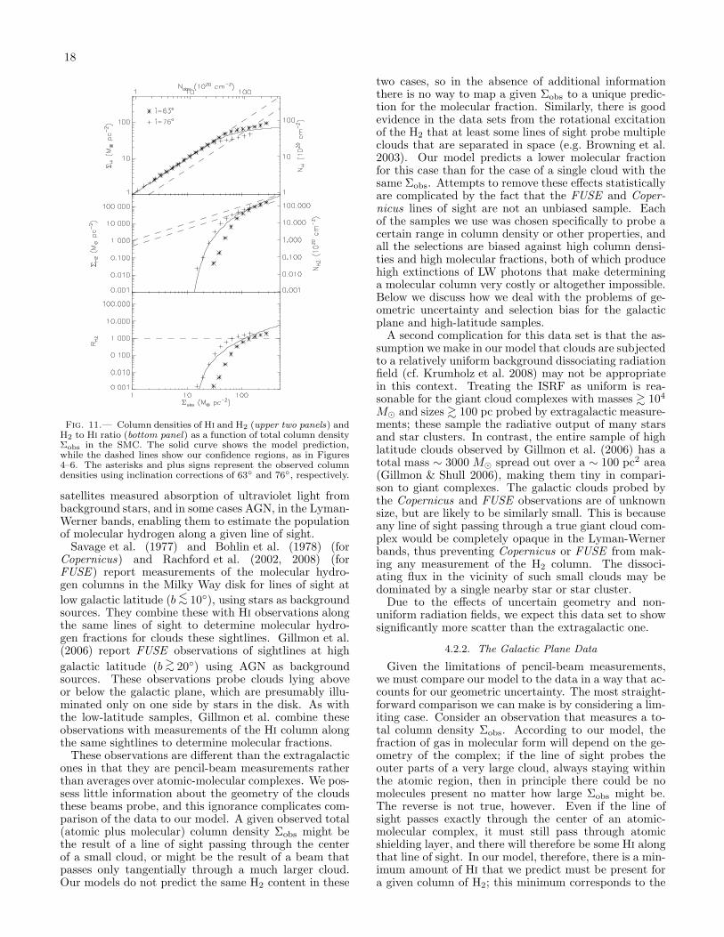
18

Fig. 11.— Column densities of Hi and H2 (upper two panels) andH2 to Hi ratio (bottom panel) as a function of total column densityΣobs in the SMC. The solid curve shows the model prediction,while the dashed lines show our confidence regions, as in Figures4–6. The asterisks and plus signs represent the observed columndensities using inclination corrections of 63◦ and 76◦, respectively.

satellites measured absorption of ultraviolet light frombackground stars, and in some cases AGN, in the Lyman-Werner bands, enabling them to estimate the populationof molecular hydrogen along a given line of sight.

Savage et al. (1977) and Bohlin et al. (1978) (forCopernicus) and Rachford et al. (2002, 2008) (forFUSE ) report measurements of the molecular hydro-gen columns in the Milky Way disk for lines of sight at

low galactic latitude (b <∼ 10◦), using stars as backgroundsources. They combine these with Hi observations alongthe same lines of sight to determine molecular hydro-gen fractions for clouds these sightlines. Gillmon et al.(2006) report FUSE observations of sightlines at high

galactic latitude (b >∼ 20◦) using AGN as backgroundsources. These observations probe clouds lying aboveor below the galactic plane, which are presumably illu-minated only on one side by stars in the disk. As withthe low-latitude samples, Gillmon et al. combine theseobservations with measurements of the Hi column alongthe same sightlines to determine molecular fractions.

These observations are different than the extragalacticones in that they are pencil-beam measurements ratherthan averages over atomic-molecular complexes. We pos-sess little information about the geometry of the cloudsthese beams probe, and this ignorance complicates com-parison of the data to our model. A given observed total(atomic plus molecular) column density Σobs might bethe result of a line of sight passing through the centerof a small cloud, or might be the result of a beam thatpasses only tangentially through a much larger cloud.Our models do not predict the same H2 content in these

two cases, so in the absence of additional informationthere is no way to map a given Σobs to a unique predic-tion for the molecular fraction. Similarly, there is goodevidence in the data sets from the rotational excitationof the H2 that at least some lines of sight probe multipleclouds that are separated in space (e.g. Browning et al.2003). Our model predicts a lower molecular fractionfor this case than for the case of a single cloud with thesame Σobs. Attempts to remove these effects statisticallyare complicated by the fact that the FUSE and Coper-nicus lines of sight are not an unbiased sample. Eachof the samples we use was chosen specifically to probe acertain range in column density or other properties, andall the selections are biased against high column densi-ties and high molecular fractions, both of which producehigh extinctions of LW photons that make determininga molecular column very costly or altogether impossible.Below we discuss how we deal with the problems of ge-ometric uncertainty and selection bias for the galacticplane and high-latitude samples.

A second complication for this data set is that the as-sumption we make in our model that clouds are subjectedto a relatively uniform background dissociating radiationfield (cf. Krumholz et al. 2008) may not be appropriatein this context. Treating the ISRF as uniform is rea-sonable for the giant cloud complexes with masses & 104

M⊙ and sizes & 100 pc probed by extragalactic measure-ments; these sample the radiative output of many starsand star clusters. In contrast, the entire sample of highlatitude clouds observed by Gillmon et al. (2006) has atotal mass ∼ 3000 M⊙ spread out over a ∼ 100 pc2 area(Gillmon & Shull 2006), making them tiny in compari-son to giant complexes. The galactic clouds probed bythe Copernicus and FUSE observations are of unknownsize, but are likely to be similarly small. This is becauseany line of sight passing through a true giant cloud com-plex would be completely opaque in the Lyman-Wernerbands, thus preventing Copernicus or FUSE from mak-ing any measurement of the H2 column. The dissoci-ating flux in the vicinity of such small clouds may bedominated by a single nearby star or star cluster.

Due to the effects of uncertain geometry and non-uniform radiation fields, we expect this data set to showsignificantly more scatter than the extragalactic one.

4.2.2. The Galactic Plane Data

Given the limitations of pencil-beam measurements,we must compare our model to the data in a way that ac-counts for our geometric uncertainty. The most straight-forward comparison we can make is by considering a lim-iting case. Consider an observation that measures a to-tal column density Σobs. According to our model, thefraction of gas in molecular form will depend on the ge-ometry of the complex; if the line of sight probes theouter parts of a very large cloud, always staying withinthe atomic region, then in principle there could be nomolecules present no matter how large Σobs might be.The reverse is not true, however. Even if the line ofsight passes exactly through the center of an atomic-molecular complex, it must still pass through atomicshielding layer, and there will therefore be some Hi alongthat line of sight. In our model, therefore, there is a min-imum amount of Hi that we predict must be present fora given column of H2; this minimum corresponds to the

19

Fig. 12.— Column density of H2 (upper panel) and Hi (lowerpanel) versus total column density for the Copernicus (diamonds)and FUSE (squares) data, and for the limits (dashed line) andtypical values (solid line) we compute from our model. The dashedline is an upper limit in the upper panel, and a lower limit in thelower one. For the data, we only plot points with measured Hicolumns. Arrows indicate lines of sight for which the Hi column ismeasured but only an upper limit is available for the H2 column.In the upper panel the dotted lines show ΣH2

= Σ and ΣH2=

Σ/3 (the edge of our region of confident prediction), while in thelower panel they show ΣHI = Σ and ΣHI = 2Σ/3. Note that NH2

represents the column of H nuclei in molecular form; the numberof H2 molecules is half this.

case of a line of sight that passes directly through thecenter of a complex. This implies that we can make aprediction as follows: we consider a complex of meancolumn density Σcomp, and use our model to predict theatomic, molecular, and total column densities, ΣHI,cen,ΣH2,cen, and Σcen, that one would see along a line of sightpassing through the center of the complex. The curvesΣHI,cen versus Σcen and ΣH2,cen versus Σcen that we gen-erate through this procedure should then be lower andupper limits, respectively, on the observed distributionsof ΣHI versus Σobs and ΣH2

versus Σobs.Instead of computing a limit, we can also make an esti-

mate for the “typical” atomic and molecular fractions weshould see at a given Σobs. If we knew the true distribu-tion of column densities for atomic-molecular complexesin the Milky Way, we could do this by integrating alllines of sight through that distribution and computingthe mean atomic and molecular columns at a given totalcolumn. However, we do not know the true distribution,and even if we did this procedure would not address ef-fects of observational bias in selecting sightlines. Instead,we make a much rougher calculation. Using our model wecan compute the radius xH2

(Σcomp) at which the cloudwhose true mean column density is Σcomp transitionsfrom atomic to molecular for solar metallicity (Z = 1).The atomic and molecular columns along a sightline thatstrikes the cloud of radius R at a distance βR from itscenter are

ΣHI =2τRσd

{

√

1 − β2 −√

x2H2

− β2, β < xH2

√

1 − β2, β > xH2

(56)

Fig. 13.— RH2versus column density for the FUSE high-latitude

sample (squares; Gillmon et al. 2006) and for our model (line). Ar-rows indicate lines of sight for which only an upper limit is availablefor the H2 column. Note that Nobs represents the total column ofH nuclei in either atomic or molecular form.

ΣH2=

2τRφmol

σd

{√

x2H2

− β2, β < xH2

0, β > xH2

, (57)

and the H2 fraction averaged over all pencil beams pass-ing through the cloud is,

fH2,beams(Σcomp) = 2

∫ 1

0

βΣH2

ΣH2+ ΣHI

dβ. (58)

To estimate a “typical” atomic or molecular contentfor a given observed total gas column Σobs, we cansimply take ΣHI,obs ≈ [1 − fH2,beams(Σobs)]Σobs andΣH2,obs ≈ fH2,beams(Σobs)Σobs. This is equivalent tosaying that our sightlines do indeed probe random im-pact parameters on cloud complexes, and that whenwe observe a sightline of column density Σobs, most ofthe time we are observing a complex whose mean col-umn density is also about Σobs. This assumption couldfail if low column density clouds were rare compared tohigh column density ones, so that most of the sightlinesthat produce a given Σobs were really tangential pathsthrough high column clouds rather than beams passingclose to the the centers of low column clouds. However,there is no evidence that high-column density atomic-molecular complexes outnumber low-column ones, andin general in the ISM more mass tends to be in diffusethan dense structures, so we proceed with our assump-tion that Σcomp ≈ Σobs.

We plot both our limits on the Hi and H2 columns andour estimates for their typical values against the Coper-nicus and FUSE data sets in Figure 12. As the plotshows, both our limits and our typical columns matchthe observed data reasonably well. As with the extra-galactic case, we recover the overall trend that the gas ismostly Hi until a total column of a few M⊙ pc−2, andthen mostly molecular thereafter.

4.2.3. The High-Latitude Data

The comparison to the high-latitude data set is some-what less straightforward, because the clouds at highlatitude are only illuminated from one side. Indeed,Gillmon et al. (2006) find that these clouds becomemolecular at column densities a factor of ∼ 2 lower thando clouds in the galactic plane, probably as a result ofthis one-sided illumination. We have not considered the

20

case of clouds of finite size illuminated over only halftheir surfaces. However, we can obtain a reasonable ap-proximation to this configuration using the case of semi-infinite clouds subjected to an isotropic, uniform disso-ciation radiation field, which we considered in § 2. Asemi-infinite cloud blocks dissociating radiation over 2πsr, and thus the depth of the atomic shielding layer at itssurface is determined only by photons that arrive fromthe “front side”. This is therefore a close analogy to thecase of a high-latitude cloud, although it differs in thecloud geometry.

In Paper I we show that using a semi-infinite slab inplace of a finite cloud tends to produce errors in esti-mating the exact location of a transition from atomicto molecular in a finite cloud, but that the semi-infinitecalculation does give a good estimate of the column atwhich clouds transition from mostly atomic to mostlymolecular. We therefore expect to obtain roughly theright transition column and thus the right column of Hifor clouds that are mostly molecular, but not particularlyaccurate predictions for the exact molecular column. Fora semi-infinite cloud of solar metallicity, as we show in§ 2 we predict a molecular to atomic ratio of

RH2=

{

0, Σ < 4.5M⊙ pc−2

(Σ − 4.5M⊙ pc−2)/Σ, Σ > 4.5M⊙ pc−2 ,

(59)where Σ is the total column density. In other words,for a semi-infinite cloud of solar metallicity, the first 4.5M⊙ pc−2 are atomic, and the rest are molecular. Weshow this prediction overplotted with the FUSE high-latititude data in Figure 13. As the plot shows, we indeeddo not get very accurate predictions for the exact ratio ofHi to H2, but our calculation agrees quite well with thegeneral value of Σ for which the transition from molecu-lar to atomic occurs. In particular, our one-sided modelrecovers the observational result that a cloud illuminatedfrom one side shows a lower atomic-to-molecular transi-tion column than an isotropically-illuminated cloud.

5. SUMMARY AND CONCLUSIONS

We present a first-principles calculation of the molec-ular gas content of galactic disks in terms of the observ-able properties of those galaxies. Our calculations buildon the simple model for photodissociation fronts in finiteclouds presented in Paper I, in which we show that theamount of atomic material required to shield a molecu-lar cloud against dissociation by the interstellar radiationfield (ISRF) can be characterized by two parameters: χ,a radiation field strength normalized by the gas densityand the properties of dust grains, and τR, a measure ofthe dust optical depth of a cloud. We show that, due tothe way the density in the cold phase of the atomic ISMvaries with ISRF, the normalized radiation field strengthtakes a characteristic value χ ≈ 1 in all galaxies wherea two-phase atomic ISM is present, with only a weakdependence on metallicity.

The existence of a characteristic normalized radiationfield strength, and its weak dependence on metallicity,has a number of important consequences. First, it en-ables us to give a simple analytic approximation (equa-tions 36 or 37) for the fraction of mass in an atomic-molecular complex that will be in the atomic or molec-ular phases solely in terms of the column density of the

complex and the metallicity of the gas. This makes iteasy to test our calculations against observations. Sec-ond, we show that as a consequence of χ assuming anearly fixed value, the atomic envelopes of molecularclouds have a characteristic visual extinction AV ≈ 0.2at solar metallicity. Similarly, the transition from atomicto molecular gas occurs at a characteristic shielding col-umn of ΣHI ≈ 10 M⊙ pc−2. These quantities both varysub-linearly metallicity, with AV declining and ΣHI in-creasing as metallicity does. We calculate these valuesand their metallicity-dependence solely in terms of themicrophysical constants that describe the properties ofH2 formation and dissociation, the cooling curves of Ciiand Oi, and the properties of interstellar dust grains.Our model does not depend on unobservable parameterssuch as the gas volume density or the ISRF strength ina galaxy.

Our model compares favorably with observations ofthe atomic and molecular content of clouds both in theMilky Way and in nearby galaxies. We are able to re-produce both the characteristic column density at whichclouds transition from being primarily atomic to primar-ily molecular, and the way that this characteristic columndepends on metallicity and on whether clouds are illumi-nated on one side or on both sides. We are also ableto reproduce the observed correlation between molecularcontent and interstellar pressure.

The development of a predictive model for the molecu-lar content of galaxies that does not rely on unknown andgenerally unobservable quantities such as the radiationfields or gas volume densities in those galaxies opens upnew possibilities to advance our understanding of galacticevolution. In low-density dwarfs or high-redshift galaxiescontaining few metals, the formation of molecular cloudsmay be the rate limiting step in star formation. On theother hand, previous work has shown that, once molec-ular gas forms, it converts itself into stars at a rate ofa few percent of the mass per free-fall time independentof its density or environment (Krumholz & McKee 2005;Krumholz & Tan 2007; McKee & Ostriker 2007). Thusa theory of molecule formation creates the possibility ofdeveloping a theory of the star formation rate capable ofmaking predictions that can be applied not only in therelatively molecule-rich nearby galaxies for which em-pirical star formation laws have been determined (e.g.Kennicutt 1998), but also in the more distant and lowermetallicity universe where these laws are known to breakdown (e.g. Wolfe & Chen 2006). We plan to explore sucha theory in future work.

We thank B. Rachford and A. Leroy for providingcopies of their data, and F. Bigiel, S. Faber, N. Gnedin,A. Leroy, A. Sternberg, and F. Walter for helpful dis-cussions and comments on the manuscript. We thankthe referee, E. Rosolowsky, for providing comments thatimproved the quality of the paper. Support for thiswork was provided by: NASA through Hubble Fellow-ship grant #HSF-HF-01186 awarded by the Space Tele-scope Science Institute, which is operated by the Asso-ciation of Universities for Research in Astronomy, Inc.,for NASA, under contract NAS 5-26555 (MRK); NASA,as part of the Spitzer Space Telescope Theoretical Re-search Program, through a contract issued by the Jet

21

Propulsion Laboratory, California Institute of Technol-ogy (MRK); and by the National Science Foundationthrough grants AST-0807739 (to MRK), AST-0606831

(to CFM), and PHY05-51164 (to the Kavli Institute forTheoretical Physics, where MRK, CFM, and JT collab-orated on this work).

REFERENCES

Allen, R. J., Heaton, H. I., & Kaufman, M. J. 2004, ApJ, 608, 314Audit, E. & Hennebelle, P. 2005, A&A, 433, 1Bigiel, F., Leroy, A., Walter, F., Brinks, E., de Blok, W. J. G.,

Madore, B., & Thornley, M. D. 2008, AJ, in press,arXiv:0810.2541

Black, J. H. & van Dishoeck, E. F. 1987, ApJ, 322, 412Blitz, L., Fukui, Y., Kawamura, A., Leroy, A., Mizuno, N.,

& Rosolowsky, E. 2007, in Protostars and Planets V, ed.B. Reipurth, D. Jewitt, & K. Keil, 81–96

Blitz, L. & Rosolowsky, E. 2004, ApJ, 612, L29—. 2006, ApJ, 650, 933Bohlin, R. C., Savage, B. D., & Drake, J. F. 1978, ApJ, 224, 132Bolatto, A. D., Leroy, A. K., Rosolowsky, E., Walter, F., & Blitz,

L. 2008, ApJ, arXiv:0807.0009Bolatto, A. D., Simon, J. D., Stanimirovic, S., van Loon, J. T.,

Shah, R. Y., Venn, K., Leroy, A. K., Sandstrom, K., Jackson,J. M., Israel, F. P., Li, A., Staveley-Smith, L., Bot, C., Boulanger,F., & Rubio, M. 2007, ApJ, 655, 212

Browning, M. K., Tumlinson, J., & Shull, J. M. 2003, ApJ, 582,810

Caffau, E., Ludwig, H.-G., Steffen, M., Ayres, T. R., Bonifacio, P.,Cayrel, R., Freytag, B., & Plez, B. 2008, ArXiv e-prints, 805

Crowl, H. H., Sarajedini, A., Piatti, A. E., Geisler, D., Bica, E.,Claria, J. J., & Santos, Jr., J. F. C. 2001, AJ, 122, 220

Draine, B. T. 1978, ApJS, 36, 595—. 2003a, ARA&A, 41, 241—. 2003b, ApJ, 598, 1017—. 2003c, ApJ, 598, 1026Draine, B. T. & Bertoldi, F. 1996, ApJ, 468, 269Dufour, R. J. 1984, in IAU Symposium, Vol. 108, Structure and

Evolution of the Magellanic Clouds, ed. S. van den Bergh &K. S. D. Boer, 353–360

Elmegreen, B. G. 1989, ApJ, 338, 178—. 1993, ApJ, 411, 170Elmegreen, B. G. & Elmegreen, D. M. 1987, ApJ, 320, 182Ferrarese, L., Ford, H. C., Huchra, J., Kennicutt, Jr., R. C., Mould,

J. R., Sakai, S., Freedman, W. L., Stetson, P. B., Madore, B. F.,Gibson, B. K., Graham, J. A., Hughes, S. M., Illingworth, G. D.,Kelson, D. D., Macri, L., Sebo, K., & Silbermann, N. A. 2000,ApJS, 128, 431

Garnett, D. R. 1990, ApJ, 363, 142Gillmon, K. & Shull, J. M. 2006, ApJ, 636, 908Gillmon, K., Shull, J. M., Tumlinson, J., & Danforth, C. 2006, ApJ,

636, 891Habing, H. J. 1968, Bull. Astron. Inst. Netherlands, 19, 421Heiner, J. S., Allen, R. J., Emonts, B. H. C., & van der Kruit, P. C.

2008a, ApJ, 673, 798Heiner, J. S., Allen, R. J., Wong, O. I., & van der Kruit, P. C.

2008b, ArXiv e-prints, 808Helfer, T. T., Thornley, M. D., Regan, M. W., Wong, T., Sheth,

K., Vogel, S. N., Blitz, L., & Bock, D. C.-J. 2003, ApJS, 145, 259Hidaka, M. & Sofue, Y. 2002, PASJ, 54, 223Hollenbach, D. J. & Tielens, A. G. G. M. 1999, Reviews of Modern

Physics, 71, 173Jarrett, T. H., Chester, T., Cutri, R., Schneider, S. E., & Huchra,

J. P. 2003, AJ, 125, 525Kennicutt, R. C. 1998, ApJ, 498, 541Krumholz, M. R. & McKee, C. F. 2005, ApJ, 630, 250Krumholz, M. R., McKee, C. F., & Tumlinson, J. 2008, ApJ, in

press, arXiv:0805.2947Krumholz, M. R. & Tan, J. C. 2007, ApJ, 654, 304Leroy, A., Bolatto, A., Stanimirovic, S., Mizuno, N., Israel, F., &

Bot, C. 2007, ApJ, 658, 1027Leroy, A., Walter, F., Bigiel, F., Brinks, E., de Blok, W. J. G., &

Madore, B. 2008, AJ, in press, arXiv:0810.2556Liszt, H. 2002, A&A, 389, 393Liszt, H. & Lucas, R. 2000, A&A, 355, 333Martin, C. L. 1997, ApJ, 491, 561McKee, C. F. & Ostriker, E. C. 2007, ARA&A, 45, 565McKee, C. F. & Ostriker, J. P. 1977, ApJ, 218, 148

Moos, H. W., Cash, W. C., Cowie, L. L., Davidsen, A. F., Dupree,A. K., Feldman, P. D., Friedman, S. D., Green, J. C., Green,R. F., Gry, C., Hutchings, J. B., Jenkins, E. B., Linsky, J. L.,Malina, R. F., Michalitsianos, A. G., Savage, B. D., Shull, J. M.,Siegmund, O. H. W., Snow, T. P., Sonneborn, G., Vidal-Madjar,A., Willis, A. J., Woodgate, B. E., York, D. G., Ake, T. B.,Andersson, B.-G., Andrews, J. P., Barkhouser, R. H., Bianchi,L., Blair, W. P., Brownsberger, K. R., Cha, A. N., Chayer, P.,Conard, S. J., Fullerton, A. W., Gaines, G. A., Grange, R.,Gummin, M. A., Hebrard, G., Kriss, G. A., Kruk, J. W., Mark,D., McCarthy, D. K., Morbey, C. L., Murowinski, R., Murphy,E. M., Oegerle, W. R., Ohl, R. G., Oliveira, C., Osterman, S. N.,Sahnow, D. J., Saisse, M., Sembach, K. R., Weaver, H. A., Welsh,B. Y., Wilkinson, E., & Zheng, W. 2000, ApJ, 538, L1

Neufeld, D. A. & Spaans, M. 1996, ApJ, 473, 894Pelupessy, F. I., Papadopoulos, P. P., & van der Werf, P. 2006,

ApJ, 645, 1024Pilyugin, L. S., Vılchez, J. M., & Contini, T. 2004, A&A, 425, 849Rachford, B. L., Snow, T. P., Destree, J. D., Ross, T. L., Ferlet, R.,

Friedman, S. D., Gry, C., Jenkins, E. B., Morton, D. C., Savage,B. D., Shull, J. M., Sonnentrucker, P., Tumlinson, J., Vidal-Madjar, A., Welty, D. E., & York, D. G. 2008, ApJ, submitted

Rachford, B. L., Snow, T. P., Tumlinson, J., Shull, J. M., Blair,W. P., Ferlet, R., Friedman, S. D., Gry, C., Jenkins, E. B.,Morton, D. C., Savage, B. D., Sonnentrucker, P., Vidal-Madjar,A., Welty, D. E., & York, D. G. 2002, ApJ, 577, 221

Regan, M. W., Thornley, M. D., Helfer, T. T., Sheth, K., Wong,T., Vogel, S. N., Blitz, L., & Bock, D. C.-J. 2001, ApJ, 561, 218

Robertson, B. E. & Kravtsov, A. V. 2008, ApJ, 680, 1083Sahnow, D. J., Moos, H. W., Ake, T. B., Andersen, J., Andersson,

B.-G., Andre, M., Artis, D., Berman, A. F., Blair, W. P.,Brownsberger, K. R., Calvani, H. M., Chayer, P., Conard, S. J.,Feldman, P. D., Friedman, S. D., Fullerton, A. W., Gaines, G. A.,Gawne, W. C., Green, J. C., Gummin, M. A., Jennings, T. B.,Joyce, J. B., Kaiser, M. E., Kruk, J. W., Lindler, D. J., Massa,D., Murphy, E. M., Oegerle, W. R., Ohl, R. G., Roberts, B. A.,Romelfanger, M. L., Roth, K. C., Sankrit, R., Sembach, K. R.,Shelton, R. L., Siegmund, O. H. W., Silva, C. J., Sonneborn, G.,Vaclavik, S. R., Weaver, H. A., & Wilkinson, E. 2000, ApJ, 538,L7

Savage, B. D., Bohlin, R. C., Drake, J. F., & Budich, W. 1977,ApJ, 216, 291

Schaye, J. 2004, ApJ, 609, 667Smith, D. A., Allen, R. J., Bohlin, R. C., Nicholson, N., & Stecher,

T. P. 2000, ApJ, 538, 608Spaans, M. & Neufeld, D. A. 1997, ApJ, 484, 785Spitzer, Jr., L. & Jenkins, E. B. 1975, ARA&A, 13, 133Stanimirovic, S., Staveley-Smith, L., Dickey, J. M., Sault, R. J., &

Snowden, S. L. 1999, MNRAS, 302, 417Stanimirovic, S., Staveley-Smith, L., & Jones, P. A. 2004, ApJ, 604,

176Sternberg, A. 1988, ApJ, 332, 400Tumlinson, J., Shull, J. M., Rachford, B. L., Browning, M. K.,

Snow, T. P., Fullerton, A. W., Jenkins, E. B., Savage, B. D.,Crowther, P. A., Moos, H. W., Sembach, K. R., Sonneborn, G.,& York, D. G. 2002, ApJ, 566, 857

van Dishoeck, E. F. & Black, J. H. 1986, ApJS, 62, 109van Zee, L., Haynes, M. P., & Salzer, J. J. 1997, AJ, 114, 2479Walter, F., Brinks, E., de Blok, W. J. G., Bigiel, F., Kennicutt,

R. C., Jr., Thornley, M. D., & Leroy, A. K. 2008, AJ, in press,arXiv:0810.2125

Walter, F., Cannon, J. M., Roussel, H., Bendo, G. J., Calzetti,D., Dale, D. A., Draine, B. T., Helou, G., Kennicutt, Jr., R. C.,Moustakas, J., Rieke, G. H., Armus, L., Engelbracht, C. W.,Gordon, K., Hollenbach, D. J., Lee, J., Li, A., Meyer, M. J.,Murphy, E. J., Regan, M. W., Smith, J.-D. T., Brinks, E., deBlok, W. J. G., Bigiel, F., & Thornley, M. D. 2007, ApJ, 661,102

Wang, Z. 1990a, ApJ, 360, 529—. 1990b, ApJ, 360, 543Wolfe, A. M. & Chen, H.-W. 2006, ApJ, 652, 981

22

Wolfire, M. G., McKee, C. F., Hollenbach, D., & Tielens,A. G. G. M. 2003, ApJ, 587, 278

Wolfire, M. G., Tielens, A. G. G. M., Hollenbach, D., & Kaufman,M. J. 2008, ApJ

Wong, T. & Blitz, L. 2002, ApJ, 569, 157Wyse, R. F. G. 1986, ApJ, 311, L41