Artificial Intelligence through Prolog by Neil C. Rowe - The ...
Upload
khangminh22Category
view
1download
0

The Art of Prolog


Leon SterlingEhud Shapirowith a foreword by David H. D. Warren
The Art of PrologAdvanced Programming TechniquesSecond Edition
The MIT PressCambridge, MassachusettsLondon, England

© 1986, 1994 Massachusetts Institute of Technology
All rights reserved. No part of this book may be reproduced in any form byany electronic or mechanical means (including photocopying, recording, orinformation storage and retrieval) without permission in writing from thepublisher.
This book was composed and typeset by Paul C. Anagnostopoulos and JoeSnowden using ZzTEX. The typeface is Lucida Bright and Lucida New Mathcreated by Charles Bigelow and Kris Holmes specifically for scientific andelectronic publishing. The Lucida letterforms have the large x-heights andopen interiors that aid legibility in modern printing technology, but also echosome of the rhythms and calligraphic details of lively Renaissance handwrit-ing. Developed in the 1980s and 1990s, the extensive Lucida typeface familyincludes a wide variety of mathematical and technical symbols designed toharmonize with the text faces.
This book was printed and bound in the United States of America.
Library of Congress Cataloging-in-Publication DataSterling, Leon
The art of Prolog : advanced programming techniques / LeonSterling, Ehud Shapiro ; with a foreword by David H. D. Warren.
p. cm. - (MIT Press series in logic programming)Includes bibliographical references and index.ISBN 978-O-262-19338-2 (hardcover: alk. paper), 978-O-262-69163-5 (paperback)1. Prolog (Computer program language) I. Shapiro, Ehud Y.
II. Title. III. Series.QA76.73.P76S74 1994OOS.13'3dc2O 93-49494
lo CIP

To Ruth, Miriam, Micha!, Dan ya, and Sara


Contents
Figures xiii
Programs xvii
Series Foreword xxv
Foreword xxvii
Preface xxxi
Preface to First Edition
I Logic Programs 9
Introduction i
Basic Constructs 11
Li Facts 11
1.2 Queries 12
1.3 The Logical Variable, Substitutions, and Instances 13
1.4 Existential Queries 14
1.5 UniversalFacts 15
1.6 Conjunctive Queries and Shared Variables 16
1.7 Rules 18

viii Contents
1.8 A Simple Abstract Interpreter 22
1.9 The Meaning of a Logic Program 25
1.10 Summary 27
2 Database Programming 29
2.1 Simple Databases 29
2.2 Structured Data and Data Abstraction 35
2.3 Recursive Rules 39
2.4 Logic Programs and the Relational Database Model 42
2.5 Background 44
3 Recursive Programming 45
3.1 Arithmetic 45
3.2 Lists 56
3.3 Composing Recursive Programs 65
3.4 Binary Trees 72
3.5 Manipulating Symbolic Expressions 78
3.6 Background 84
4 The Computation Model of Logic Programs 87
4.1 Unification 87
4.2 An Abstract Interpreter for Logic Programs 91
4.3 Background 98
S Theory of Logic Programs 101
5.1 Semantics 101
5.2 Program Correctness 105
5.3 Complexity 108
5.4 Search Trees 110
5.5 Negation in Logic Programming 113
5.6 Background 115

ix Contents
II The Prolog Language 117
6 Pure Prolog 119
6.1 The Execution Model of Prolog 119
6.2 Comparison to Conventional Programming Languages 124
6.3 Background 127
7 Programming in Pure Prolog 129
7.1 Rule Order 129
7.2 Termination 131
7.3 Goal Order 133
7.4 Redundant Solutions 136
7.5 Recursive Programming in Pure Prolog 139
7.6 Background 147
8 Arithmetic 149
8.1 System Predicates for Arithmetic 149
8.2 Arithmetic Logic Programs Revisited 152
8.3 Transforming Recursion into Iteration 154
8.4 Background 162
9 Structure Inspection 163
9.1 Type Predicates 163
9.2 Accessing Compound Terms 167
9.3 Background 174
10 Meta-Logical Predicates 175
10.1 Meta-Logical Type Predicates 176
10.2 Comparing Nonground Terms 180
10.3 Variables as Objects 182
10.4 The Meta-Variable Facility 185
10.5 Background 186

x Contents
11 Cuts and Negation 189
11.1 Green Cuts: Expressing Determinism 189
11.2 Tail Recursion Optimization 195
11.3 Negation 198
11.4 Red Cuts: Omitting Explicit Conditions 202
11.5 Default Rules 206
11.6 Cuts for Efficiency 208
11.7 Background 212
12 Extra-Logical Predicates 215
12.1 Input/Output 215
12.2 Program Access and Manipulation 219
12.3 Memo-Functions 221
12.4 Interactive Programs 223
12.5 Failure-Driven Loops 229
12.6 Background 231
13 Program Development 233
13.1 Programming Style and Layout 233
13.2 Reflections on Program Development 235
13.3 Systematizing Program Construction 238
13.4 Background 244
HI Advanced Prolog Programming Techniques 247
14 Nondeterministic Programming 24914.1 Generate-and-Test 249
14.2 Don't-Care and Don't-Know Nondeterminism 263
14.3 Artificial Intelligence Classics: ANALOGY, ELIZA, andMcSAM 270
14.4 Background 280
15 Incomplete Data Structures 283
15.1 Difference-Lists 283

xi Contents
15.2 Difference-Structures 291
15.3 Dictionaries 293
15.4 Queues 297
15.5 Background 300
16 Second-Order Programming 301
16.1 All-Solutions Predicates 301
16.2 Applications of Set Predicates 305
16.3 Other Second-Order Predicates 314
16.4 Background 317
17 Interpreters 319
17.1 Interpreters for Finite State Machines 319
17.2 Meta-Interpreters 323
17.3 Enhanced Meta-Interpreters for Debugging 331
17.4 An Explanation Shell for Rule-Based Systems 341
17.5 Background 354
18 Program Transfoutiation 357
18.1 Unfold/Fold Transformations 357
18.2 Partial Reduction 360
18.3 Code Walking 366
18.4 Background 373
19 Logic Grammars 375
19.1 Definite Clause Grammars 375
19.2 A Grammar Interpreter 380
19.3 Application to Natural Language Understanding 382
19.4 Background 388
20 Search Techniques 389
20.1 Searching State-Space Graphs 389
20.2 Searching Game Trees 401
20.3 Background 407
xii Contents
IV Applications 409
21 Game-Playing Programs 411
21.1 Mastermind 411
21.2 Nim 415
21.3 Kalah 420
21.4 Background 423
22 A Credit Evaluation Expert System 429
22.1 Developing the System 429
22.2 Background 438
23 An Equation Solver 439
23.1 An Overview of Equation Solving 439
23.2 Factorization 448
23.3 Isolation 449
23.4 Polynomial 452
23.5 Homogenization 454
23.6 Background 457
24 A Compiler 43924.1 Overview of the Compiler 459
24.2 The Parser 466
24.3 The Code Generator 470
24.4 The Assembler 475
24.5 Background 478
A Operators 479
References 483
Index 497

Figure s
1.1 An abstract interpreter to answer ground queries with respectto logic programs 22
1.2 Tracing the interpreter 23
1.3 A simple proof tree 25
2.1 Defining inequality 31
2.2 A logical circuit 32
2.3 Still-life objects 34
2.4 A simple graph 41
3.1 Proof trees establishing completeness of programs 47
3.2 Equivalent forms of lists 57
3.3 Proof tree verifying a list 58
3.4 Proof tree for appending two lists 61
3.5 Proof trees for reversing a list 63
3.6 Comparing trees for isomorphism 74
3.7 A binary tree and a heap that preserves the tree's shape 77
4.1 A unification algorithm 90
4.2 An abstract interpreter for logic programs 93
4.3 Tracing the appending of two lists 94
4.4 Different traces of the same solution 95
4.5 Solving the Towers of Hanoi 97
4.6 A nonterminating computation 97

xiv Figures
5.1 A nonterminating computation 107
5.2 Two search trees 111
5.3 Search tree with multiple success nodes 112
5.4 Search tree with an infinite branch 113
6.1 Tracing a simple Prolog computation 121
6.2 Multiple solutions for splitting a list 122
6.3 Tracing a quicksort computation 123
7.1 A nonterminating computation 132
7.2 Variant search trees 139
7.3 Tracing a reverse computation 146
8.1 Computing factorials iteratively 155
9.1 Basic system type predicates 164
9.2 Tracing the substitute predicate 171
11.1 Theeffectofcut 191
13.1 Template for a specification 243
14.1 A solution to the 4 queens problem 253
14.2 A map requiring four colors 255
14.3 Directed graphs 265
14.4 Initial and final states of a blocks world problem 267
14.5 A geometric analogy problem 271
14.6 Sample conversation with ELIZA 273
14.7 AstoryfilledinbyMcSAM 276
14.8 Three analogy problems 279
15.1 Concatenating difference-lists 285
15.2 Tracing a computation using difference-lists 287
15.3 Unnormalized and normalized sums 292
16.1 Power of Prolog for various searching tasks 307
16.2 The problem of Lee routing for VLSI circuits 308
16.3 Input and output for keyword in context (KWIC) problem 312
16.4 Second-order predicates 315
17.1 A simple automaton 321

xv Figures
17.2 Tracing the meta-interpreter 325
17.3 Fragment of a table of builtin predicates 327
17.4 Explaining a computation 351
18.1 A context-free grammar for the language a*b*c* 371
20.1 The water jugs problem 393
20.2 A simple game tree 405
21.1 A starting position for Nim 415
21.2 Computing nim-sums 419
21.3 Board positions for Kalah 421
23.1 Test equations 440
23.2 Position of subterms in terms 449
24.1 A PL program for computing factorials 460
24.2 Target language instructions 460
24.3 Assembly code version of a factorial program 461
24.4 The stages of compilation 461
24.5 Output from parsing 470
24.6 The generated code 475
24.7 The compiled object code 477


Programs
1.1 A biblical family database 12
1.2 Biblical family relationships 23
2.1 Defining family relationships 31
2.2 A circuit for a logical and-gate 33
2.3 The circuit database with names 36
2.4 Course rules 37
2.5 The ancestor relationship 39
2.6 A directed graph 41
2.7 The transitive closure of the edge relation 41
3.1 Defining the natural numbers 46
3.2 The less than or equal relation 48
3.3 Addition 49
3.4 Multiplication as repeated addition 51
3.5 Exponentiation as repeated multiplication 51
3.6 Computing factorials 52
3.7 The minimum of two numbers 52
3.8a A nonrecursive definition of modulus 53
3.8b A recursive definition of modulus 53
3.9 Ackermann's function 54
3.10 The Euclidean algorithm 54
3.11 Defining a list 57

xviii Programs
3.12
3.13
3.14
3.15
3.16
3.17
3.18
3.19
3.20
3.21
3.22
3.23
3.24
3.25
3.26
3.27
3.28
3.29
3.30
3.31
3.32
5.1
7.1
7.2
7.3
7.4
7.5
7.6
7.7
7.8
7.9
Membership of a list 58
Prefixes and suffixes of a list 59
Determining sublists of lists 60
Appending two lists 60
Reversing a list 62
Determining the length of a list 64
Deleting all occurrences of an element from a list 67
Selecting an element from a list 67
Permutation sort 69
Insertion sort 70
Quicksort 70
Defining binary trees 73
Testing tree membership 73
Determining when trees are isomorphic 74
Substituting for a term in a tree 75
Traversals ofabinary tree 76
Adjusting a binary tree to satisfy the heap propertyRecognizing polynomials 79
Derivative rules 80
Towers of Hanoi 82
Satisfiability of Boolean formulae 83
Yet another family example 102
Yet another family example 130
Merging ordered lists 138
Checking for list membership 139
Selecting the first occurrence of an element from a listNonmembership of a list 141
77
140
Testing for a subset 142
Testing for a subset 142
Translating word for word 143
Removing duplicates from a list 145

xix Programs
710 Reversing with no duplicates 146
8.1 Computing the greatest common divisor of two integers 152
8.2 Computing the factorial of a number 153
8.3 An iterative factorial 155
8.4 Another iterative factorial 156
8.5 Generating a range of integers 157
8.6a Summing a list of integers 157
8.6b Iterative version of summing a list of integers using an accumu-lator 157
8.7a Computing inner products of vectors 158
8.7b Computing inner products of vectors iteratively 158
8.8 Computing the area of polygons 159
8.9 Finding the maximum of a list of integers 160
8.10 Checking the length of a list 160
811 Finding the length of a list 161
8.12 Generating a list of integers in a given range 161
9.la Flattening a list with double recursion 165
9,lb Flattening a list using a stack 166
9.2 Finding subterms of a term 168
9.3 A program for substituting in a term 170
9.4 Subtermdefinedusinguniv 172
9,5a Constructing a list corresponding to a term 173
9.5b Constructing a term corresponding to a list 174
10.1 Multiple uses for plus 176
10.2 A multipurpose length program 177
10.3 A more efficient version of grandparent 178
10.4 Testing if a term is ground 178
10.5 Unification algorithm 180
10.6 Unification with the occurs check 181
10.7 Occurs in 182
10.8 Numbering the variables in a term 185

xx Programs
10.9 Logical disjunction 186
11.1 Merging ordered lists 190
11.2 Merging with cuts 192
11.3 ininimuinwith cuts 193
11.4 Recognizing polynomials 193
11.5 Interchange sort 195
11.6 Negation as failure 198
11.7 Testing if terms are variants 200
11.8 Implementing 201
11.9a Deleting elements from a list 204
i 1.9b Deleting elements from a list 204
11.10 If-then-else statement 205
11.1 la Determining welfare payments 207
ll.11b Determining welfare payments 207
12.1 Writing a list of terms 216
12.2 Reading in a list of words 217
12.3 Towers of Hanoi using a memo-function 222
12.4 Basic interactive loop 223
12.5 A line editor 224
12.6 An interactive shell 226
12.7 Logging a session 228
12.8 Basic interactive repeat loop 230
12.9 Consulting a file 230
13.1 Finding the union of two lists 241
13.2 Finding the intersection of two lists 241
13.3 Finding the union and intersection of two lists 241
14.1 Finding parts of speech in a sentence 251
14.2 Naive generate-and-test program solving N queens 253
14.3 Placing one queen at a time 255
14.4 Map colormg 256
14.5 Test data for map coloring 257

xxi Programs
14.6 A puzzle solver 259
14.7 A description of a puzzle 260
14.8 Connectivity in a finite DAG 265
14.9 Finding a path by depth-first search 266
14.10 Connectivity in a graph 266
14.11 A depth-first planner 268
14.12 Testing the depth-first planner 269
14.13 A program solving geometric analogies 272
14.14 Testing ANALOGY 273
14.15 ELIZA 275
14.16 McSAM 277
14.17 Testing McSAM 278
15.1 Concatenating difference-lists 285
15.2 Flattening a list of lists using difference-lists 286
15.3 Reverse with difference-lists 288
15.4 Quicksort using difference-lists 289
15.5 A solution to the Dutch flag problem 290
15.6 Dutch flag with difference-lists 291
15.7 Normalizing plus expressions 292
15.8 Dictionary lookup from a list of tuples 294
15.9 Dictionary lookup in a binary tree 295
15.10 Meltingaterm 296
15.11 Aqueueprocess 297
15.12 Flattening a list using a queue 298
16.1 Sample data 302
16.2 Applying set predicates 303
16.3 Implementing an all-solutions predicate using difference-lists,assert, and retract 304
16.4 Testing connectivity breadth-first in a DAG 306
16.5 Testing connectivity breadth-first in a graph 307
16.6 Lee routing 310
16.7 Producing a keyword in context (KWIC) index 313

xxii Programs
16.8 Second-order predicates in Prolog 316
17.1 An interpreter for a nondeterministic finite automaton (NDFA)320
17.2 An NDFA that accepts the language (ab)* 321
17.3 An interpreter for a nondetermimstic pushdown automaton(NPDA) 322
17.4 An NPDA for palindromes over a finite alphabet 322
17.5 A meta-interpreter for pure Prolog 324
17.6 A meta-interpreter for pure Prolog in continuation style 326
17.7 AtracerforProlog 328
17.8 A meta-interpreter for building a proof tree 329
17.9 A meta-interpreter for reasoning with uncertainty 330
17.10 Reasoning with uncertainty with threshold cutoff 331
17.11 A meta-interpreter detecting a stack overflow 333
17.12 A nonterminating insertion sort 334
17.13 An incorrect and incomplete insertion sort 335
17.14 Bottom-up diagnosis of a false solution 336
17.15 Top-down diagnosis of a false solution 338
17.16 Diagnosing missing solution 340
17.17 Oven placement rule-based system 342
17.18 A skeleton two-level rule interpreter 343
17.19 An interactive rule interpreter 345
17.20 A two-level rule interpreter carrying rules 347
17.21 A two-level rule interpreter with proof trees 348
17.22 Explaining aproof 350
17.23 An explanation shell 352
18.1 A program accepting palindromes 359
18.2 A meta-interpreter for determining a residue 361
18.3 A simple partial reduction system 362
18.4 Specializing an NPDA 363
18.5 Specializing a rule interpreter 364
18.6 Composing two enhancements of a skeleton 368

xxiii Programs
18.7 Testing program composition 370
18.8 A Prolog program parsing the language a*b*c* 371
18.9 Translating grammar rules to Prolog clauses 372
19.1 Enhancing the language a*b*c* 377
19.2 Recognizing the language dt1cN 377
19.3 Parsing the declarative part of a Pascal block 378
19.4 A definite clause grammar (DCG) interpreter 381
19.5 A DCG interpreter that counts words 382
19.6 A DCG context-free grammar 383
19.7 A DCG computing a parse tree 384
19.8 A DCG with subject/object number agreement 385
19.9 A DCG for recognizing numbers 387
20.1 A depth-first state-transition framework for problem solving390
20.2 Solving the wolf, goat, and cabbage problem 392
20.3 Solving the water jugs problem 394
20.4 Hill climbing framework for problem solving 397
20.5 Test data 398
20.6 Best-first framework for problem solving 399
20.7 Concise best-first framework for problem solving 40020.8 Framework for playing games 402
20.9 Choosing the best move 403
20.10 Choosing the best move with the minimax algorithm 406
20.11 Choosing a move using minimax with alpha-beta pruning 407
21.1 Playing mastermind 413
21.2 A program for playing a winning game of Nim 417
21.3 A complete program for playing Kalah 424
22.1 A credit evaluation system 432
22.2 Test data for the credit evaluation system 437
23.1 A program for solving equations 442
24.1 A compiler from PL to machine language 462
24.2 Test data 465


Series Foreword
The logic programming approach to computing investigates the use oflogic as a programming language and explores computational modelsbased on controlled deduction.
The field of logic programming has seen a tremendous growth in thelast several years, both in depth and in scope. This growth is reflected inthe number of articles, journals, theses, books, workshops, and confer-ences devoted to the subject. The MIT Press series in logic programmingwas created to accommodate this development and to nurture it. lt isdedicated to the publication of high-quality textbooks, monographs, col-lections, and proceedings in logic programming.
Ehud ShapiroThe Weizmann Institute of ScienceRehovot, Israel


Foreword
Programming in Prolog opens the mind to a new way of looking at com-puting. There is a change of perspective which every Prolog programmerexperiences when first getting to know the language.
I shall never forget my first Prolog program. The time was early 1974.I had learned about the abstract idea of logic programming from BobKowaiski at dinburgh, although the name "logic programming" had notyet been coined. The main idea was that deduction could be viewed as aform of computation, and that a declarative statement of the form
P if Q and R and S.
could also be interpreted procedurally as
To solve P, solve Q and R and S.
Now I had been invited to Marseilles. Here, Alain Colmerauer and his col-leagues had devised the language Prolog based on the logic programmingconcept. Somehow, this realization of the concept seemed to me, at firstsight, too simpleminded. However, Gerard Battani and Henri Meloni hadimplemented a Prolog interpreter in Fortran (their first major exercise inprogramming, incidentally). Why not give Prolog a try?
I sat at a clattering teletype connected down an ordinary telephone lineto an IBM machine far away in Grenoble. I typed in some rules defininghow plans could be constructed as sequences of actions. There was oneimportant rule, modeled on the SRI planner Strips, which described howa plan could be elaborated by adding an action at the end. Another rule,necessary for completeness, described how to elaborate a plan by insert-ing an action in the middle of the plan. As an example for the planner to

xxviii Foreword
work on, I typed in facts about some simple actions in a "blocks world"and an initial state of this world. I entered a description of a goal state tobe achieved. Prolog spat back at me:
7
meaning it couldn't find a solution. Could it be that a solution was notdeducible from the axioms I had supplied? Ah, yes, I had forgotten toenter some crucial facts. I tried again. Prolog was quiet for a long timeand then responded:
DEBORDEMENT DE PILE
Stack overflow! I had run into a loop. Now a loop was conceivable sincethe space of potential plans to be considered was infinite. However, I hadtaken advantage of Prolog's procedural semantics to organize the axiomsso that shorter plans ought to be generated first. Could something elsebe wrong? After a lot of head scratching, I finally realized that I hadmistyped the names of some variables. I corrected the mistakes, andtried again.
Lo and behold, Prolog responded almost instantly with a correct planto achieve the goal state. Magic! Declaratively correct axioms had assureda correct result. Deduction was being harnessed before my very eyesto produce effective computation. Declarative programming was trulyprogramming on a higher plane! I had dimly seen the advantages intheory. Now Prolog had made them vividly real in practice. Never had Iexperienced such ease in getting a complex program coded and running.
Of course, I had taken care to formulate the axioms and organize themin such a way that Prolog could use them effectively. I had a generalidea of how the axioms would be used. Nevertheless it was a surpriseto see how the axioms got used in practice on particular examples. Itwas a delightful experience over the next few days to explore how Prologactually created these plans, to correct one or two more bugs in my factsand rules, and to further refine the program.
Since that time, Prolog systems have improved significantly in terms ofdebugging environments, speed, and general robustness. The techniquesof using Prolog have been more fully explored and are now better un-derstood. And logic programming has blossomed, not least because ofits adoption by the Japanese as the central focus of the Fifth Generationproject.

xxix Foreword
After more than a decade of growth of interest in Prolog, it is a greatpleasure to see the appearance of this book. Hitherto, knowledge of howto use Prolog for serious programming has largely been communicatedby word of mouth. This textbook sets down and explains for the firsttime in an accessible form the deeper principles and techniques of Prologprogramming
The book is excellent for not only conveying what Prolog is but also ex-plaining how it should be used. The key to understanding how to useProlog is to properly understand the relationship between Prolog andlogic programming. This book takes great care to elucidate the relation-ship.
Above all, the book conveys the excitement of using Prologthe thrillof declarative programming As the authors put it, "Declarative program-ming clears the mind" Declarative programming enables one to concen-trate on the essentials of a problem without gettmg bogged down intoo much operational detail. Programming should be an intellectuallyrewarding activity. Prolog helps to make it so. Prolog is indeed, as theauthors contend, a tool for thinking.
David H. D. WarrenManchester, England, September 1986


Preface
Seven years have passed since the first edition of The Art of Prolog waspublished. In that time, the perception of Prolog has changed markedly.While not as widely used as the language C, Prolog is no longer regardedas an exotic language. An abundance of books on Prolog have appeared.Prolog is now accepted by many as interesting and useful for certainapplications. Articles on Prolog regularly appear in popular magazines.Prolog and logic programming are part of most computer science andengineering programs, although perhaps in a minor role in an artificialintelligence or programming languages class. The first conference onPractical Applications of Prolog was held in London in April 1992. Astandard for the language is likely to be in place in 1994. A future forProlog among the programming languages of the world seems assured.
In preparing for a second edition, we had to address the question ofhow much to change. I decided to listen to a request not to make the newedition into a new book. This second edition is much like the first, al-though a number of changes are to be expected in a second edition. Thetypography of the book has been improved: Program code is now in a dis-tinctive font rather than in italics. Figures such as proof trees and searchtrees are drawn more consistently. We have taken the opportunity to bemore precise with language usage and to remove minor inconsistencieswith hyphenation of words and similar details. All known typographi-cal errors have been fixed. The background sections at the end of mostchapters have been updated to take into account recent, important re-search results. The list of references has been expanded considerably.Extra, more advanced exercises, which have been used successfully in myProlog classes, have been added.

xxxii Preface
Let us take an overview of the specific changes to each part in turn.Part IV, Applications, is unchanged apart from minor corrections andtidying. Part I, Logic Programs, is essentially unchanged. New programshave been added to Chapter 3 on tree manipulation, including heapifyinga binary tree. Extra exercises are also present.
Part II, The Prolog Langauge, is primarily affected by the imminence ofa Prolog standard. We have removed all references to Wisdom Prolog inthe text in preparation for Standard Prolog. It has proved impossible toguarantee that this book is consistent with the standard. Reaching a stan-dard has been a long, difficult process for the members of the committee.Certain predicates come into favor and then disappear, making it difficultfor the authors of a text to know what to write. Furthermore, some of theproposed I/O predicates are not available in current Prologs, so it is im-possible to run all the code! Most of the difficulties in reaching a Prologstandard agreeable to all interested parties have been with builtin or sys-tem predicates. This book raises some of the issues involved in addingbuiltins to Prolog but largely avoids the concerns by using pure Prolog asmuch as possible. We tend not to give detailed explanations of the con-troversial nonlogical behaviors of some of the system predicates, and wecertainly do not use odd features in our code.
Part III, Advanced Programming Tecimiques, is the most altered in thissecond edition, which perhaps should be expected. A new chapter hasbeen added on program transformation, and many of the other chaptershave been reordered. The chapters on Interpreters and Logic Grammarshave extensive additions.
Many people provided us feedback on the first edition, almost all ofit very positive. I thank you all. Three people deserve special thanksfor taking the trouble to provide long lists of suggestions for improve-ments and to point out embarrassingly long lists of typos in the firstedition: Norbert Fuchs, Harald Søndergaard, and Stanley Selkow. Thefollowing deserve mention for pointing out mistakes and typos in thevarious printings of the first edition or making constructive commentsabout the book that led to improvements in later printings of the firstedition and for this second edition. The list is long, my memory some-times short, so please forgive me if I forget to mention anyone. Thanksto Ham Assiryani, Tim Boemker, Jim Brand, Bill Braun, Pu Chen, YvesDeville, George Ernst, Claudia Günther, Ann Halbran, Sundar Iyengar,Gary Kacmarcik, Mansoor Khan, Sundeep Kumar, Arun Lakhotia, Jean-

xxxiii Preface
Louis Lassez, Charlie Linville, Per Ljung, David Maier, Fred Mailey, MartinMarshall, Andre Mesarovic, Dan Oldham, Scott Pierce, Lynn Pierce, DavidPedder, S. S. Ramakrishnan, Chet Ramey, Marty Silverstein, Bill Sloan, RonTaylor, Rodney Topor, R. J. Wengert, Ted Wright, and Nan Yang. For theformer students of CMPS41Ì, I hope the extra marks were sufficient re-ward.
Thanks to Sarah Fliegelmann and Venkatesh Srinivasan for help withentering changes to the second edition and TeXing numerous drafts.Thanks to Phil Gannon and Zoë Sterling for helpful discussions about thefigures, and to Joe Geiles for drawing the new figures. For proofreadingthe second edition, thanks to Kathy Kovacic, David Schwartz, Ashish Jam,and Venkatesh Srinivasan. Finally, a warm thanks to my editor, TerryEhling, who has always been very helpful and very responsive to queries.
Needless to say, the support of my family and friends is the mostimportant and most appreciated.
Leon SterlingCleveland, January 1993


Preface to First Edition
The origins of this book lie in graduate student courses aimed at teach-ing advanced Prolog programming A wealth of techniques has emergedin the fifteen years since the inception of Prolog as a programming lan-guage. Our intention in this book has been to make accessible the pro-grammmg techniques that kindled our own excitement, imagination, andinvolvement in this area.
The book fills a general need. Prolog, and more generally logic pro-gramming, has received wide publicity in recent years. Currently avail-able books and accounts, however, typically describe only the basics. Allbut the simplest examples of the use of Prolog have remained essentiallyinaccessible to people outside the Prolog community.
We emphasize throughout the book the distinction between logic pro-gramming and Prolog programming Logic programs can be understoodand studied, using two abstract, machine-independent concepts: truthand logical deduction. One can ask whether an axiom in a program istrue, under some interpretation of the program symbols; or whether alogical statement is a consequence of the program. These questions canbe answered independently of any concrete execution mechanism.
On the contrary, Prolog is a programming language, borrowing its basicconstructs from logic. Prolog programs have precise operational mean-ing: they are instructions for execution on a computera Prolog ma-chine. Prolog programs in good style can almost always be read as log-ical statements, thus inheriting some of the abstract properties of logicprograms. Most important, the result of a computation of such a Pro-log program is a logical consequence of the axioms in it. Effective Prolog

xxxvi Preface to First Edition
progranmiing requires an understanding of the theory of logic program-ming.
The book consists of four parts: logic programming, the Prolog lan-guage, advanced techniques, and applications. The first part is a self-contained introduction to logic programming. It consists of five chapters.The first chapter introduces the basic constructs of logic programs. Ouraccount differs from other introductions to logic programming by ex-plaining the basics in terms of logical deduction. Other accounts explainthe basics from the background of resolution from which logic program-ming originated. We have found the former to be a more effective meansof teaching the material, which students find intuitive and easy to under-stand.
The second and third chapters of Part I introduce the two basic stylesof logic programming: database programming and recursive program-ming. The fourth chapter discusses the computation model of logic pro-gramming, introducing unification, while the fifth chapter presents sometheoretical results without proofs. In developing this part to enable theclear explanation of advanced techniques, we have introduced new con-cepts and reorganized others, in particular, in the discussion of typesand termination. Other issues such as complexity and correctness areconcepts whose consequences have not yet been fully developed in thelogic programming research community.
The second part is an introduction to Prolog. It consists of Chapters 6through 13. Chapter 6 discusses the computation model of Prolog incontrast to logic programming, and gives a comparison between Prologand conventional programming languages such as Pascal. Chapter 7 dis-cusses the differences between composing Prolog programs and logicprograms. Examples are given of basic programming techniques.
The next five chapters introduce system-provided predicates that areessential to make Prolog a practical programming language. We clas-sify Prolog system predicates into four categories: those concernedwith efficient arithmetic, structure inspection, meta-logical predicatesthat discuss the state of the computation, and extra-logical predicatesthat achieve side effects outside the computation model of logic pro-gramming. One chapter is devoted to the most notorious of Prologextra-logical predicates, the cut. Basic techniques using these systempredicates are explained. The final chapter of the section gives assortedpragmatic programming tips.

xxxvii Preface to First Edition
The main part of the book is Part III. We describe advanced Prologprogramming techniques that have evolved in the Prolog programmingcommunity, illustrating each with small yet powerful example programs.The examples typify the applications for which the technique is useful.The six chapters cover nondeterministic programming, incomplete datastructures, parsing with DCGs, second-order programming, search tech-.niques, and the use of meta-interpreters.
The final part consists of four chapters that show how the material inthe rest of the book can be combined to build application programs. Acommon request of Prolog newcomers is to see larger applications. Theyunderstand how to write elegant short programs but have difficulty inbuilding a major program. The applications covered are game-playingprograms, a prototype expert system for evaluating requests for credit, asymbolic equation solver, and a compiler.
During the development of the book, it has been necessary to reorga-nize the foundations and basic examples existing in the folklore of thelogic programming community. Our structure constitutes a novel frame-work for the teaching of Prolog.
Material from this book has been used successfully for several courseson logic programming and Prolog: in Israel, the United States, and Scot-land. The material more than suffices for a one-semester course to first-year graduate students or advanced undergraduates. There is consider-able scope for instructors to particularize a course to suit a special areaof interest.
A recommended division of the book for a 13-week course to senior un-dergraduates or first-year graduates is as follows: 4 weeks on logic pro-gramming, encouraging students to develop a declarative style of writingprograms, 4 weeks on basic Prolog programming, 3 weeks on advancedtechniques, and 2 weeks on applications. The advanced techniquesshould include some discussion of nondeterminism, incomplete datastructures, basic second-order predicates, and basic meta-interpreters.Other sections can be covered instead of applications. Application areasthat can be stressed are search techniques in artificial intellígence, build-ing expert systems, writing compilers and parsers, symbol manipulation,and natural language proces sing.
There is considerable flexibility in the order of presentation. The ma-terial from Part I should be covered first. The material in Parts III and IVcan be interspersed with the material in Part lito show the student how

xxxviii Preface to First Edition
larger Prolog programs using more advanced techniques are composedin the same style as smaller examples.
Our assessment of students has usually been 50 percent by homeworkassignments throughout the course, and 50 percent by project. Our expe-rience has been that students are capable of a significant progranimingtask for their project. Examples of projects are prototype expert systems,assemblers, game-playing programs, partial evaluators, and implementa-tions of graph theory algorithms.
For the student who is studying the material on her own, we stronglyadvise reading through the more abstract material iii Part I. A good Pro-log progranirning style develops from thinking declaratively about thelogic of a situation. The theory in Chapter 5, however, can be skippeduntil a later reading.
The exercises in the book range from very easy and well defined todifficult and open-ended. Most of them are suitable for homework exer-cises. Some of the more open-ended exercises were submitted as courseprojects.
The code in this book is essentially in Edinburgh Prolog. The course hasbeen given where students used several different variants of EdinburghProlog, and no problems were encountered. All the examples run onWisdom Prolog, which is discussed in the appendixes.
We acknowledge and thank the people who contributed directly to thebook. We also thank, collectively and anonymously, all those who indi-rectly contributed by influencing our programming styles in Prolog. Im-provements were suggested by Lawrence Byrd, Oded Maler, Jack Minker,Richard O'Keefe, Fernando Pereira, and several anonymous referees.
We appreciate the contribution of the students who sat throughcourses as material from the book was being debugged. The first authoracknowledges students at the University of Edinburgh, the WeizmannInstitute of Science, Tel Aviv University, and Case Western Reserve Uni-versity. The second author taught courses at the Weizmanri Institute andHebrew University of Jerusalem, and in industry.
We are grateful to many people for assisting in the technical aspectsof producing a book. We especially thank Sarah Fliegelmann, who pro-duced the various drafts and camera-ready copy, above and beyond thecall of duty. This book might not have appeared without her tremendousefforts. Arvind Bansal prepared the index and helped with the references.Yehuda Barbut drew most of the figures. Max Goldberg and Shmuel Safra

xxxix Preface to First Edition
prepared the appendix. The publishers, MIT Press, were helpful and sup-portive.
Finally, we acknowledge the support of family and friends, withoutwhich nothing would get done.
Leon Sterling1986


Introduction
The inception of logic is tied with that of scientific thinking. Logic pro-vides a precise language for the explicit expression of one's goals, knowl-edge, and assumptions. Logic provides the foundation for deducingconsequences from premises; for studying the truth or falsity of state-ments given the truth or falsity of other statements; for establishing theconsistency of one's claims; and for verifying the validity of one's argu-ments.
Computers are relatively new in our intellectual history. Similar tologic, they are the object of scientific study and a powerful tool forthe advancement of scientific endeavor. Like logic, computers requirea precise and explicit statement of one's goals and assumptions. Un-like logic, which has developed with the power of human thinking as theonly external consideration, the development of computers has been gov-erned from the start by severe technological and engineering constraints.Although computers were intended for use by humans, the difficul-ties in constructing them were so dominant that the language forexpressing problems to the computer and instructing it how to solvethem was designed from the perspective of the engineering of the com-puter alone.
Almost all modern computers are based on the early concepts of vonNeumann and his colleagues, which emerged during the 1940s. The vonNeumann machine is characterized by a large uniform store of memorycells and a processing unit with some local cells, called registers. Theprocessing unit can load data from memory to registers, perform arith-metic or logical operations on registers, and store values of registersback into memory. A program for a von Neumann machine consists of

2 Introduction
a sequence of instructions to perform such operations, and an additionalset of control instructions, which can affect the next instruction to beexecuted, possibly depending on the content of some register.
As the problems of building computers were gradually understood andsolved, the problems of using them mounted. The bottleneck ceased tobe the inability of the computer to perform the human's instructions butrather the inability of the human to instruct, or program, the computer.A search for programming languages convenient for humans to use be-gan. Starting from the language understood directly by the computer,the machine language, better notations and formalisms were developed.The main outcome of these efforts was languages that were easier forhumans to express themselves in but that still mapped rather directlyto the underlying machine language. Although increasingly abstract, thelanguages in the mainstream of development, starting from assemblylanguage through Fortran, Algol, Pascal, and Ada, all carried the markof the underlying machinethe von Neumann architecture.
To the uninitiated intelligent person who is not familiar with the en-gineering constraints that led to its design, the von Neumann machineseems an arbitrary, even bizarre, device. Thinking in terms of its con-strained set of operations is a nontrivial problem, which sometimesstretches the adaptiveness of the human mind to its limits.
These characteristic aspects of programming von Neumann computersled to a separation of work: there were those who thought how to solvethe problem, and designed the methods for its solution, and there werethe coders, who performed the mundane and tedious task of translatingthe instructions of the designers to instructions a computer can use.
Both logic and programming require the explicit expression of one'sknowledge and methods in an acceptable formalism. The task of makingone's knowledge explicit is tedious. However, formalizing one's knowl-edge in logic is often an intellectually rewarding activity and usuallyreflects back on or adds insight to the problem under consideration. Incontrast, formalizing one's problem and method of solution using thevon Neumann instruction set rarely has these beneficial effects.
We believe that programming can be, and should be, an intellectu-ally rewarding activity; that a good programming language is a powerfulconceptual toola tool for organizing, expressing, experimenting with,and even communicating one's thoughts; that treating programming as

Introduction
"coding," the last, mundane, intellectually trivial, time-consuming, andtedious phase of solving a problem using a computer system, is perhapsat the very root of what has been known as the "software crisis."
Rather, we think that programming can be, and should be, part ofthe problem-solving process itself; that thoughts should be organized asprograms, so that consequences of a complex set of assumptions can beinvestigated by "running" the assumptions; that a conceptual solution toa problem should be developed hand-in-hand with a working programthat demonstrates it and exposes its different aspects. Suggestions inthis direction have been made under the title "rapid prototyping."
To achieve this goal in its fullestto become true mates of the humanthinking processcomputers have still a long way to go. However, wefind it both appropriate and gratifying from a historical perspective thatlogic, a companion to the human thinking process since the early days ofhuman intellectual history, has been discovered as a suitable stepping-stone in this long journey.
Although logic has been used as a tool for designing computers and forreasoning about computers and computer programs since almost theirbeginning, the use of logic directly as a prograniming language, termedlogic programming, is quite recent.
Logic programming, as well as its sister approach, functional program-ming, departs radically from the mainstream of computer languages.Rather then being derived, by a series of abstractions and reorganiza-tions, from the von Neumann machine model and instruction set, it isderived from an abstract model, which has no direct relation to or de-pendence on to one machine model or another. It is based on the beliefthat instead of the human learning to think in terms of the operationsof a computer that which some scientists and engineers at some pointin history happened to find easy and cost-effective to build, the com-puter should perform instructions that are easy for humans to provide.In its ultimate and purest form, logic programming suggests that evenexplicit instructions for operation not be given but rather that the knowl-edge about the problem and assumptions sufficient to solve it be statedexplicitly, as logical axioms. Such a set of axioms constitutes an alterna-tive to the conventional program. The program can be executed by pro-viding it with a problem, formalized as a logical statement to be proved,called a goal statement. The execution is an attempt to solve the prob-

4 Introduction
lem, that is, to prove the goal statement, given the assumptions in thelogic program.
A distinguishing aspect of the logic used in logic programming is thata goal statement typically is existentially quantified: it states that thereexist some individuals with some property. An example of a goal state-ment is, "there exists a list X such that sorting the list 13, 1,21 gives X."The mechanism used to prove the goal statement is constructive. If suc-cessful, it provides the identity of the unknown individuals mentioned inthe goal statement, which constitutes the output of the computation. Inthe preceding example, assuming that the logic program contains appro-priate axioms defining the sort relation, the output of the computationwouldbeX= [1,2,3].
These ideas can be summarized in the following two metaphoricalequations:
program = set of axioms.
computation = constructive proof of a goal statement from the program.
The ideas behind these equations can be traced back as far as intuition-istic mathematics and proof theory of the early twentieth century. Theyare related to Hilbert's program, to base the entire body of mathemati-cal knowledge on logical foundations and to provide mechanical proofsfor its theories, starting from the axioms of logic and set theory alone.It is interesting to note that the failure of this program, from which en-sued the incompleteness and undecidability results of Gödel and Turing,marks the beginning of the modern age of computers.
The first use of this approach in practical computing is a sequel toRobinson's unification algorithm and resolution principle, published in1965. Several hesitant attempts were made to use this principle as a basisof a computation mechanism, but they did not gain any momentum.The beginning of logic programming can be attributed to Kowalski andColmerauer. Kowalski formulated the procedural interpretation of Hornclause logic. He showed that an axiom
A if B1 and B2 and... and B
can be read and executed as a procedure of a recursive programminglanguage, where A is the procedure head and the B are its body. In

Introduction
addition to the declarative reading of the clause, A is true if the B aretrue, it can be read as follows: To solve (execute) A, solve (execute) B1 andB2 and. . . and B. In this reading, the proof procedure of Horn clauselogic is the interpreter of the language, and the unification algorithm,which is at the heart of the resolution proof procedure, performs thebasic data manipulation operations of variable assignment, parameterpassing, data selection, and data construction.
At the same time, in the early 1970s, Colmerauer and his group atthe University of Marseilles-Aix developed a specialized theorem prover,written in Fortran, which they used to implement natural language pro-cessing systems. The theorem prover, called Prolog (for Programmationen Logique), embodied Kowaiski's procedural interpretation. Later, vanEmden and Kowalski developed a formal semantics for the language oflogic programs, showing that its operational, model-theoretic, and fix-point semantics are the same.
In spite of all the theoretical work and the exciting ideas, the logic pro-gramming approach seemed unrealistic. At the time of its inception, re-searchers in the United States began to recognize the failure of the "next-generation Al languages," such as Micro-Planner and Conniver, which de-veloped as a substitute for Lisp. The main claim against these languageswas that they were hopelessly inefficient, and very difficult to control.Given their bitter experience with logic-based high-level languages, it isno great surprise that U.S. artificial intelligence scientists, when hearingabout Prolog, thought that the Europeans were over-excited over whatthey, the Americans, had already suggested, tried, and discovered not towork.
In that atmosphere the Prolog-lo compiler was almost an imaginarybeing. Developed in the mid to late 1970s by David H. D. Warren andhis colleagues, this efficient implementation of Prolog dispelled all themyths about the impracticality of logic programming. That compiler, stillone of the finest implementations of Prolog around, delivered on purelist-processing programs a performance comparable to the best Lisp sys-tems available at the time. Furthermore, the compiler itself was writtenalmost entirely in Prolog, suggesting that classic programming tasks, notjust sophisticated AI applications, could benefit from the power of logicprogramming.

6 Introduction
The impact of this implementation cannot be overemphasized. Withoutit, the accumulated experience that has led to this book would not haveexisted.
In spite of the promise of the ideas, and the practicality of their im-plementation, most of the Western computer science and AI researchcommunity was ignorant, openly hostile, or, at best, indifferent to logicprogramming. By 1980 the number of researchers actively engaged inlogic programming were only a few dozen in the United States and aboutone hundred around the world.
No doubt, logic programming would have remained a fringe activityin computer science for quite a while longer hadit not been for the an-nouncement of the Japanese Fifth Generation Project, which took placein October 1981. Although the research program the Japanese presentedwas rather baggy, faithful to their tradition of achieving consensus atalmost any cost, the important role of logic programming in the nextgeneration of computer systems was made clear.
Since that time the Prolog language has undergone a rapid transitionfrom adolescence to maturity. There are numerous commercially avail-able Prolog implementations on most computers. A large number of Pro-log programming books are directed to different audiences and empha-size different aspects of the language. And the language itself has moreor less stabilized, having a de facto standard, the Edinburgh Prolog fam-ily.
The maturity of the language means that it is no longer a concept forscientists yet to shape and define but rather a given object, with vicesand virtues. lt is time to recognize that, on the one hand, Prolog fallsshort of the high goals of logic programming but, on the other hand, is apowerful, productive, and practical programming formalism. Given thestandard life cycle of computer programming languages, the next fewyears will reveal whether these properties show their merit only in theclassroom or prove useful also in the field, where people pay money tosolve problems they care about.
What are the current active subjects of research in logic programmingand Prolog? Answers to this question can be found in the regular sci-entific journals and conferences of the field; the Logic ProgrammingJournal, the Journal of New Generation Computing, the InternationalConference on Logic Programming, and the IEEE Symposium on Logic

7 Introduction
Programming as well as in the general computer science journals andconf erences.
Clearly, one of the dominant areas of interest is the relation betweenlogic programming, Prolog, and parallelism. The promise of parallel com-puters, combined with the parallelism that seems to be available in thelogic programming model, have led to numerous attempts, still ongoing,to execute Prolog in parallel and to devise novel concurrent program-ming languages based on the logic programming computation model.This, however, is a subject for another book.

r--&J 2è - L
Leonardo Da Vinci. Old Man thinking. Pen and ink (slightly enlarged). About1510. Windsor Castle, Royal Library.
i

I Logic Programs
A logic program is a set of axioms, or rules, defining relations betweenobjects. A computation of a logic program is a deduction of conse-quences of the program. A program defines a set of consequences, whichis its meaning The art of logic programming is constructing concise andelegant programs that have the desired meaning.


Li Facts
The simplest kind of statement is called a fact. Facts are a means ofstating that a relation holds between objects. An example is
father(abrahani,isaac).
This fact says that Abraham is the father of Isaac, or that the relation f a-ther holds between the individuals named abraham and isaac. Anothername for a relation is a predicate. Names of individuals are known asatoms. Similarly, plus(2,3,5) expresses the relation that 2 plus 3 is 5.The familiar plus relation can be realized via a set of facts that definesthe addition table. An initial segment of the table is
plus(O,O,O). plus(O,1,1). plus(O,2,2). plus(O,3,3).
Basic Constructs
The basic constructs of logic programming, terms and statements, areinherited from logic. There are three basic statements: facts, rules, andqueries. There is a single data structure: the logical term.
plus(1,O,1). plus(1,1,2). plus(1,2,3). plus(1,3,4).
A sufficiently large segment of this table, which happens to be also alegal logic program, will be assumed as the definition of the plus relationthroughout this chapter.
The syntactic conventions used throughout the book are introduced asneeded. The first is the case convention. It is significant that the names

12 Chapter 1
father(terach,abraham). male(terach).
father (terach,nachor). male (abraham).
father (terach,haran). male (nachor).
f ather(abraham,isaac). male (haran).
father (haran,lot). male(isaac).
father (haran,milcah). male (lot).
father(haran,yiscah).
female(sarah).
mother(sarah,isaac). female (milcah).
female(yiscah).
Program 1.1 A biblical family database
of both predicates and atoms in facts begin with a lowercase letter ratherthan an uppercase letter.
A finite set of facts constitutes a program. This is the simplest formof logic program. A set of facts is also a description of a situation. Thisinsight is the basis of database programming, to be discussed in the nextchapter. An example database of family relationships from the Bible isgiven as Program 1.1. The predicates father, mother, male, and female
express the obvious relationships.
1.2 Queries
The second form of statement in a logic program is a query. Queries area means of retrieving information from a logic program. A query askswhether a certain relation holds between objects. For example, the queryfather (abraham, isaac)? asks whether the father relationship holdsbetween abraham and isaac. Given the facts of Program 1.1, the answerto this query is yes.
Syntactically, queries and facts look the same, but they can be distin-guished by the context. When there is a possibility of confusion, a term!-nating period will indicate a fact, while a terminating question mark willindicate a query. We call the entity without the period or question marka goal. A fact P. states that the goal P is true. A query P? asks whetherthe goal P is true. A simple query consists of a single goal.
Answering a query with respect to a program is determining whetherthe query is a logical consequence of the program. We define logical

13 Basic Constructs
consequence incrementally through this chapter. Logical consequencesare obtained by applying deduction rules. The simplest rule of deductionis identity: from P deduce P. A query is a logical consequence of anidentical fact.
Operationally, answermg simple queries using a program containingfacts like Program 1.1 is straightforward. Search for a fact in the programthat implies the query. If a fact identical to the query is found, the answeris yes.
The answer no is given if a fact identical to the query is not found,because the fact is not a logical consequence of the program. This answerdoes not reflect on the truth of the query; it merely says that we failed toprove the query from the program. Both the queries f emale(abrahazn)?
and plus(1 ,1,2)? will be answered no with respect to Program 1.1.
1.3 The Logical Variable, Substitutions, and Instances
A logical variable stands for an unspecified individual and is used ac-cordingly. Consider its use in queries. Suppose we want to know ofwhom abraham is the father. One way is to ask a series of queries,father(abraham,lot)?, father(abraham,milcah)?, ..., father
(abraham,isaac)?,. . . until an answer yes is given. A variable allowsa better way of expressing the query as f ather(abraham,X)?, to whichthe answer is X=isaac. Used in this way, variables are a means of sum-marizing many queries. A query containing a variable asks whether thereis a value for the variable that makes the query a logical consequence ofthe program, as explained later.
Variables in logic programs behave differently from variables in con-ventional programming languages. They stand for an unspecified but sin-gle entity rather than for a store location in memory.
Having introduced variables, we can define a term, the single datastructure ¡ii logic programs. The definition is inductive. Constants andvariables are terms. Also compound terms, or structures, are terms.A compound term comprises a functor (called the principal functorof the term) and a sequence of one or more arguments, which areterms. A functor is characterized by its name, which is an atom, andits arity, or number of arguments. Syntactically, compound terms have

14 Chapter 1
the form f(t1,t2,. . .,t), where the functor has name f and is of arityn, and the t are the arguments. Examples of compound terms includes(0), hot(milk), name(john,doe), list(a,list(b,nil)), foo(X), andtree(tree(nil,3,nil) ,5,R).
Queries, goals, and more generally terms where variables do not occurare called ground. Where variables do occur, they are called nonground.For example, f oo (a, b) is ground, whereas bar (X) is nonground.
DefinitionA substitution is a finite set (possibly empty) of pairs of the form X = t,where X is a variable and t is a term, and X X1 for every i j, and Xdoes not occur in t1, for any i and j. .
An example of a substitution consisting of a single pair is {X=isaac}.
Substitutions can be applied to terms. The result of applying a substi-tution G to a term A, denoted by AO, is the term obtained by replacingevery occurrence of X by t in A, for every pair X = t in O.
The result of applying {X=isaac} to the term f ather(abraham,X) isthe term father(abrahani,isaac).
DefinitionA is an instance of B if there is a substitution O such that A = BO. .
The goal f ather(abraham,isaac) is an instance of father (abraham,X) by this definition. Similarly, mother(sarah, isaac) is an instance ofmother(X,Y) under the substitution {X=sarah,Y=isaac}.
1.4 Existential Queries
Logically speaking, variables in queries are existentially quantified, whichmeans, intuitively, that the query father (abraham, X)? reads: "Doesthere exist an X such that abraham is the father of X?" More generally,a query p(T1,T2,. . .,T)?, which contains the variables X1,X2,. . .,Xk reads:"Are there X1,X2,. . .,Xk such that p(T1,T2,. . .,T)?" For convenience, exis-tential quantification is usually omitted.
The next deduction rule we introduce is generalization. An existentialquery P is a logical consequence of an instance of it, PO, for any substi-tution 6. The fact f ather(abraham, isaac) implies that there exists an Xsuch that f ather(abraham,X) is true, namely, X=isaac.

15 Basic Constructs
Operationally, to answer a nonground query using a program of facts,search for a fact that is an instance of the query. If found, the answer,or solution, is that instance. A solution is represented in this chapter bythe substitution that, if applied to the query, results in the solution. Theanswer is no if there is no suitable fact in the program.
In general, an existential query may have several solutions. Program1.1 shows that Haran is the father of three children. Thus the queryfather (haran,X)? has the solutions (X=lot}, {X=milcah}, {X=yiscah}.
Another query with multiple solutions is plus (X, Y, 4)? for finding num-bers that add up to 4. Solutions are, for example, {X=O, Y=4} and {X=1,Y=3}. Note that the different variables X and Y correspond to (possibly)different objects.
An interesting variant of the last query is plus(X,X,4)?, which insiststhat the two numbers that add up to 4 be the same. It has a uniqueanswer {X=2}.
LS Universal Facts
Variables are also useful in facts. Suppose that all the biblical characterslike pomegranates. Instead of including in the program an appropriatefact for every individual,
likes(abraham,pomegranates).
likes(sarah,pomegranates).
a fact likes (X,pomegranates) can say it all. Used in this way, variablesare a means of summarizing many facts. The fact tirnes(O,X,O) summa-rizes all the facts stating that o times some number is O.
Variables in facts are implicitly universally quantified, which means,intuitively, that the fact likes(X,pomegranates) states that for all X,X likes pomegranates. In general, a fact p(T1,. . .,T) reads that for allX1,. . .,Xk, where the X1 are variables occurring in the fact, p(T1,. .is true. Logically, from a universally quantified fact one can deduceany instance of it. For example, from likes(X,poniegranates), deducelikes (abraham, pomegranates).

16 Chapter 1
This is the third deduction rule, called instantiation. From a universallyquantified statement P, deduce an instance of it, PO, for any substitution0.
As for queries, two unspecified objects, denoted by variables, can beconstrained to be the same by using the same variable name. The factplus (0, X, X) expresses that O is a left identity for addition. It reads thatfor all values of X, O plus X is X. A similar use occurs when translating theEnglish statement "Everybody likes himself" to likes (X, X).
Answering a ground query with a universally quantified fact is straight-forward. Search for a fact for which the query is an instance. For example,the answer to plus(0,2,2)? is yes, based on the fact plus(0,X,X). An-swering a nonground query using a nonground fact involves a new defi-nition: a common instance of two terms.
DefinitionC is a common instance of A and B if it is an instance of A and an instanceof B, in other words, if there are substitutions 0 and 02 such that C=A01is syntactically identical to BO2.
For example, the goals plus(0,3,Y) and plus(0,X,X) have a com-mon instance plus (0,3,3). When the substitution {Y=3} is applied toplus (0,3, Y) and the substitution {X=3} is applied to plus (0, X, X), bothyield plus(0,3,3).
In general, to answer a query using a fact, search for a common in-stance of the query and fact. The answer is the common instance, if oneexists. Otherwise the answer is no.
Answering an existential query with a universal fact using a commoninstance involves two logical deductions. The instance is deduced fromthe fact by the rule of instantiation, and the query is deduced from theinstance by the rule of generalization.
1.6 Conjunctive Queries and Shared Variables
An important extension to the queries discussed so far is conjunctivequeries. Conjunctive queries are a conjunction of goals posed as a query,for example, f ather(terach,X) ,father(X,Y)? or in general, Q,. .Simple queries are a special case of conjunctive queries when there is a

17 Basic Constructs
single goal. Logically, it asks whether a conjunction is deducible from theprogram. We use '," throughout to denote logical and. Do not confusethe comma that separates the arguments in a goal with commas used toseparate goals, denoting conjunction.
In the simplest conjunctive queries all the goals are ground, for exam-ple, f ather(abraham,isaac) ,male(lot)?. The answer to this query us-ing Program 1.1 is clearly yes because both goals in the query are facts inthe program. In general, the query Q,. .,Q,?, where each Q is a groundgoal, is answered yes with respect to a program P if each Q is implied byP. Hence ground conjunctive queries are not very interesting.
Conjunctive queries are interesting when there are one or more sharedvariables, variables that occur in two different goals of the query. An ex-ample is the query f ather(haran,X) ,male(X)?. The scope of a variablein a conjunctive query, as in a simple query, is the whole conjunction.Thus the query p(X),q(X)? reads: "Is there an X such that both p(X) and
Shared variables are used as a means of constraining a simple queryby restricting the range of a variable. We have already seen an examplewith the query plus (X , X, 4)?, where the solution of numbers addingup to 4 was restricted to the numbers being the same. Consider thequery f ather(harari,X) ,male(X)?. Here solutions to the query f a-
ther(haran,X)? are restricted to children that are male. Program 1.1shows there is only one solution, {X1ot}. Alternatively, this query canbe viewed as restricting solutions to the query male (X)? to individualswho have Haran for a father.
A slightly different use of a shared variable can be seen in the queryfather (terach,X) ,father(X,Y)?. On the one hand, it restricts the sonsof terach to those who are themselves fathers. On the other hand, it con-siders individuals Y, whose fathers are sons of terach. There are severalsolutions, for example, (Xabrahain, Y=isaac J and {X=haran, Y=lot J.
A conjunctive query is a logical consequence of a program P if all thegoals in the conjunction are consequences of P, where shared variablesare instantiated to the same values in different goals. A sufficient condi-tion is that there be a ground instance of the query that is a consequenceof P. This instance then deduces the conjuncts in the query via general-ization.
The restriction to ground instances is unnecessary and will be lifted inChapter 4 when we discuss the computation model of logic programs.

18 Chapter 1
We employ this restriction in the meantime to simplify the discussion inthe coming sections.
Operationally, to solve the conjunctive query A1,A2 ,...,A? using a pro-gram P, find a substitution O such that A10 and.. . and AO are groundinstances of facts in P. The same substitution applied to all the goals en-sures that instances of variables are common throughout the query. Forexample, consider the query f ather(haran,X) ,male(X)? with respectto Program 1.1. Applying the substitution {X=lot} to the query givesthe ground instance father (haran,lot) ,male (lot)?, which is a conse-quence of the program.
1.7 Rules
Interesting conjunctive queries are defining relationships in their ownright. The query father (haran,X) ,male(X)? is asking for a son of Ha-ran. The query father(terach,X) ,father(X,Y)? is asking about grand-children of Terach. This brings us to the third and most important state-ment in logic programming, a rule, which enables us to define new rela-tionships in terms of existing relationships.
Rules are statements of the form:
A - B1,B2,. .
where n O. The goal A is the head of the rule, and the conjunction ofgoals B1,. . .,B is the body of the rule. Rules, facts, and queries are alsocalled Horn clauses, or clauses for short. Note that a fact is just a specialcase of a rule when n = O. Facts are also called unit clauses. We alsohave a special name for clauses with one goal in the body, namely, whenn = 1. Such a clause is called an iterative clause. As for facts, variablesappearing in rules are universally quantified, and their scope is the wholerule.
A rule expressing the son relationship is
son(X,Y) - father(Y,X), male(X).
Similarly one can define a rule for the daughter relationship:
daughter(X,Y) - father(Y,X), female(X).

19 Basic Constructs
A rule for the grandfather relationship is
grandfather(X,Y) father(X,Z), father(Z,Y).
Rules can be viewed in two ways. First, they are a means of ex-pressing new or complex queries in terms of simple queries. A queryson(X,haran)? to the program that contains the preceding rule for sonis translated to the query f ather(haran,X) ,male(X)? according to therule, and solved as before. A new query about the son relationship hasbeen built from simple queries involving father and male relationships.Interpreting rules in this way is their procedural reading. The proceduralreading for the grandfather rule is: "To answer a query is X the grand-father of Y?, answer the conjunctive query Is X the father of Z and Z thefather of Y?."
The second view of rules comes from interpreting the rule as a logicalaxiom. The backward arrow is used to denote logical implication. Theson rule reads: "X is a son of Y if Y is the father of X and X is male."In this view, rules are a means of defining new or complex relationshipsusing other, simpler relationships. The predicate son has been defined interms of the predicates father and male. The associated reading of therule is known as the declarative reading. The declarative reading of thegrandfather rule is: "For all X, Y, and Z, X is the grandfather of Y if Xis the father of Z and Z is the father of Y."
Although formally all variables in a clause are universally quantified,we will sometimes refer to variables that occur in the body of the clause,but not in its head, as if they are existentially quantified inside the body.For example, the grandfather rule can be read: "For all X and Y, X is thegrandfather of Y if there exists a Z such that X is the father of Z and Zis the father of Y." The formal justification of this verbal transformationwill not be given, and we treat it just as a convenience. Whenever it is asource of confusion, the reader can resort back to the formal reading of aclause, in which all variables are universally quantified from the outside.
To incorporate rules into our framework of logical deduction, we needthe law of modus ponens. Modus ponens states that from B and A B
we can deduce A,
DefinitionThe law of universal modus ponens says that from the rule
R = (A - B1,B2,. .

20 Chapter 1
and the facts
B.B.
B.
A' can be deduced if
A' - B'1,B,. .
is an instance of R.
Universal modus ponens includes identity and instantiation as specialcases.
We are now in a position to give a complete definition of the conceptof a logic program and of its associated concept of logical consequence.
DefinitionA logic program is a finite set of rules.
DefinitionAn existentially quantified goal G is a logical consequence of a program Pif there is a clause in P with a ground instance A - B1,. . . ,B, n O suchthat B1.....B are logical consequences of P, and A is an instance of G. .
Note that the goal G is a logical consequence of a program P if and onlyif G can be deduced from P by a finite number of applications of the ruleof universal modus pollens.
Consider the query son (S, haran)? with respect to Program 1.1 aug-mented by the rule for son. The substitution {X=lot , Y=haran} appliedto the rule gives the instance son(lot,haran) f ather(haran,lot),male(lot). Both the goals in the body of this rule are facts in Pro-gram 1.1. Thus universal modus ponens implies the query with answer{S=lot}.
Operationally, answering queries reflects the definition of logical con-sequence. Guess a ground instance of a goal, and a ground instance ofa rule, and recursively answer the conjunctive query corresponding tothe body of that rule. To solve a goal A with program P, choose a ruleA1 B1,B2,. . .,B in P, and guess substitution O such that A = A10, and

21 Basic Constructs
BO is ground for i í n. Then recursively solve each BLO. This pro-cedure can involve arbitrarily long chains of reasoning. lt is difficult ingeneral to guess the correct ground instance and to choose the right rule.We show in Chapter 4 how the guessing of an instance can be removed.
The rule given for son is correct but is an incomplete specification ofthe relationship. For example, we cannot conclude that Isaac is the sonof Sarah. What is missing is that a child can be the son of a mother aswell as the son of a father. A new rule expressing this relationship can beadded, namely,
son(X,Y) - niother(Y,X), male(X).
To define the relationship grandparent correctly would take four rulesto include both cases of father and mother:
grandparent (X, Y)
grandparent (X ,Y)
grandparent (X, Y)
grandparent (X ,Y)
- father(X,Z)
- father(X,Z)
- mother(X,Z)
- mother(X,Z)
father(Z,
mother (Z
father(Z,
mother (Z
Y).
Y).
Y).
Y).
There is a better, more compact, way of expressing these rules. We needto define the auxiliary relationship parent as being a father or a mother.Part of the art of logic programming is deciding on what intermediatepredicates to define to achieve a complete, elegant axiomatization of arelationship. The rules defining parent are straightforward, capturingthe definition of a parent being a father or a mother. Logic programscan incorporate alternative definitions, or more technically disjunction,by having alternative rules, as for parent:
parent(X,Y) - f ather(X,Y).
parent(X,Y) mother(X,Y).
Rules for son and grandparent are now, respectively,
son(X,Y) - parent(Y,X), male(X).
grandparent(X,Y) - parent(X,Z), parent(Z,Y).
A collection of rules with the same predicate in the head, such asthe pair of parent rules, is called a procedure. We shall see later thatunder the operational interpretation of these rules by Prolog, such acollection of rules is indeed the analogue of procedures or subroutinesin conventional programming languages,

22 Chapter 1
1.8 A Simple Abstract Interpreter
An operational procedure for answering queries has been informally de-scribed and progressively developed in the previous sections. In thissection, the details are fleshed out into an abstract interpreter for logicprograms. In keeping with the restriction of universal modus ponens toground goals, the interpreter only answers ground queries.
The abstract interpreter performs yes/no computations. It takes asinput a program and a goal, and answers yes if the goal is a logi-cal consequence of the program and no otherwise. The interpreter isgiven in Figure 1.1. Note that the interpreter may fail to terminate ifthe goal is not deducible from the program, in which case no answer isgiven.
The current, usually conjunctive, goal at any stage of the computationis called the resolvent. A trace of the interpreter is the sequence of resol-vents produced during the computation. Figure 1.2 is a trace of answer-ing the query son(1ot,harn)? with respect to Program 1.2, a subset ofthe facts of Program 1.1 together with rules defining son and daughter.For clarity, Figure 1.2 also explicitly states the choice of goal and clausemade at each iteration of the abstract interpreter.
Each iteration of the while loop of the abstract interpreter correspondsto a single application of modus ponens. This is called a reduction.
Input:
Output:
Algorithm
A ground goal G and a program P
yes if G is a logical consequence of P,no otherwise
Initialize the resolvent to G.while the resolvent is not empty do
choose a goal A from the resolventchoose a ground instance of a clause A' B1.....B,, from P
such that A and A' are identical(if no such goal and clause exist, exit the while loop)
replace A by B1.....B,, in the resolventIf the resolvent is empty, then output yes, else output no.
Figure 1.1 An abstract interpreter to answer ground queries with respect tologic programs

23 Basic Constructs
Input: sori(lot,haran)? and Program L2Resolvent is son(lot ,haran)
Resolvent is not emptychoose son(lot,haran) (the only choice)choose son(lot,haran) father(haran,lot), male(lot)
new resolvent is father(haran,lot), male(lot)
Resolvent is not emptychoose father (hamo ,lot)
choose father (haran,lot).
new resolvent is inale(lot)
Resolvent is not emptychoose male(lot)
choose male(lot)
new resolvent is empty
Output: yes
Figure 1.2 Tracing the interpreter
father(abraham,isaac) male(isaac)
father(haran,lot). male(lot).
father (haran,mïlcah). female (milcah).
father(haran,yiscah) female(yiscah).
son(X,Y) - father(Y,X), male(X).
daughter(X,Y) father(Y,X), female(X).
Program 1.2 Biblical family relationships
DefinitionA reduction of a goal G by a program P is the replacement of G by thebody of an instance of a clause in P, whose head is identical to the chosengoal.
A reduction is the basic computational step in logic programming. Thegoal replaced in a reduction is reduced, and the new goals are derived.In this chapter, we restrict ourselves to ground reductions, where thegoal and the instance of the clause are ground. Later, in Chapter 4, weconsider more general reductions where unification is used to choose theinstance of the clause and make the goal to be reduced and the head ofthe clause identical.
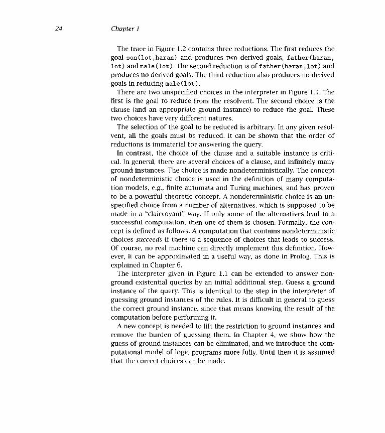
24 Chapter 1
The trace in Figure 1.2 contains three reductions. The first reduces thegoal son(lot,haran) and produces two derived goals, f ather(haran,
lot) and male (lot). The second reduction is of father (har,lot) andproduces no derived goals. The third reduction also produces no derivedgoals in reducing male (lot).
There are two unspecified choices in the interpreter in Figure 1.1. Thefirst is the goal to reduce from the resolvent. The second choice is theclause (and an appropriate ground instance) to reduce the goal. Thesetwo choices have very different natures.
The selection of the goal to be reduced is arbitrary. In any given resol-vent, all the goals must be reduced. It can be shown that the order ofreductions is immaterial for answering the query.
In contrast, the choice of the clause and a suitable instance is criti-cal. In general, there are several choices of a clause, and infinitely manyground instances. The choice is made nondeterministically. The conceptof nondeterministic choice is used in the definition of many computa-tion models, e.g., finite automata and Turing machines, and has provento be a powerful theoretic concept. A nondeterrninistic choice is an un-specified choice from a number of alternatives, which is supposed to bemade in a "clairvoyant" way. If only some of the alternatives lead to asuccessful computation, then one of them is chosen. Formally, the con-cept is defined as follows. A computation that contains nondeterministicchoices succeeds if there is a sequence of choices that leads to success.Of course, no real machine can directly implement this definition. How-ever, it can be approximated in a useful way, as done in Prolog. This isexplained in Chapter 6.
The interpreter given in Figure 1.1 can be extended to answer non-ground existential queries by an initial additional step. Guess a groundinstance of the query. This is identical to the step in the interpreter ofguessing ground instances of the rules. It is difficult in general to guessthe correct ground instance, since that means knowing the result of thecomputation before performing it.
A new concept is needed to lift the restriction to ground instances andremove the burden of guessing them. In Chapter 4, we show how theguess of ground instances can be eliminated, and we introduce the com-putational model of logic programs more fully. Until then it is assumedthat the correct choices can be made.

25 Basic Constructs
Figure 1.3 A simple proof tree
A trace of a query implicitly contains a proof that the query followsfrom the program. A more convenient representation of the proof is witha proof tree. A proof tree consists of nodes and edges that represent thegoals reduced during the computation. The root of the proof tree for asimple query is the query itself. The nodes of the tree are goals that arereduced during the computation. There is a directed edge from a nodeto each node corresponding to a derived goal of the reduced goal. Theproof tree for a conjunctive query is just the collection of proof trees forthe individual goals in the conjunction. Figure 1.3 gives a proof tree forthe program trace in Figure 1.2.
An important measure provided by proof trees is the number of nodesin the tree. lt indicates how many reduction steps are performed in acomputation. This measure is used as a basis of comparison betweendifferent programs in Chapter 3.
1.9 The Meaning of a Logic Program
How can we know if a logic program says what we wanted it to say? Ifit is correct, or incorrect? In order to answer such questions, we haveto define what is the meaning of a logic program. Once defined, we canexamine if the program means what we have intended it to mean.
DefinitionThe meaning of a logic program P, M(P), is the set of ground goalsdeducible from P. u
From this definition it follows that the meaning of a logic programcomposed just of ground facts, such as Program 1.1, is the program it-self. In other words, for simple programs, the program "means just what

26 Chapter 1
it says." Consider Program 1.1 augmented with the two rules definingthe parent relationship. What is its meaning? It contains, in additionto the facts about fathers and mothers, mentioned explicitly in the pro-gram, all goals of the form parent(X,Y) for every pair X and Y suchthat father (X, Y) or mother (X, Y) is in the program. This example showsthat the meaning of a program contains explicitly whatever the programstates implicitly.
Assuming that we define the intended meaning of a program also tobe a set of ground goals, we can ask what is the relation between theactual and the intended meanings of a program. We can check whethereverything the program says is correct, or whether the program sayseverything we wanted it to say.
Informally, we say that a program is correct with respect to someintended meaning M if the meaning of P, M(P), is a subset of M. That is,a correct program does not say things that were not intended. A programis complete with respect to M if M is a subset of M(P). That is, a completeprogram says everything that is intended. It follows that a program P iscorrect and complete with respect to an intended meaning M if M = M(P).
Throughout the book, when meaningful predicate and constant namesare used, the intended meaning of the program is assumed to be the oneintuitively implied by the choice of names.
For example, the program for the son relationship containing onlythe first axiom that uses father is incomplete with respect to the in-tuitively understood intended meaning of son, since it cannot deduceson(isaac,sarah). If we add to Program 1.1 the rule
son(X,Y) - rnother(X,Y), male(Y).
it would make the program incorrect with respect to the intended mean-mg, since it deduces son(sarah,isaac).
The notions of correctness and completeness of a logic program arestudied further in Chapter 5.
Although the notion of truth is not defined fully here, we will saythat a ground goal is true with respect to an intended meaning if it isa member of it, and false otherwise. We will say it is simply true if it is amember of the intended meaning implied by the names of the predicateand constant symbols appearing in the program.

27 Basic Constructs
1.10 Summary
We conclude this section with a summary of the constructs and conceptsintroduced, filling in the remaining necessary definitions.
The basic structure in logic programs is a term. A term is a constant,a variable, or a compound term. Constants denote particular individualssuch as integers and atoms, while variables denote a single but unspec-ified individual. The symbol for an atom can be any sequence of char-acters, which is quoted if there is possibility of confusion with othersymbols (such as variables or integers). Symbols for variables are distin-guished by beginning with ari uppercase letter.
A compound term comprises a functor (called the principal functorof the term) and a sequence of one or more terms called arguments. Afunctor is characterized by its name, which is an atom, and its arity ornumber of arguments. Constants are considered functors of arity O. Syn-tactically, compound terms have the form f(t1,t2.....t) where the functorhas name f and is of arity n, and the t are the arguments. A functorf of arity n is denoted f/n. Functors with the same name but differentarities are distinct. Terms are ground if they contain no variables; other-wise they are nonground. Goals are atoms or compound terms, and aregenerally nonground.
A substitution is a finite set (possibly empty) of pairs of the form X = t,where X is a variable and t is a term, with no variable on the left-handside of a pair appearing on the right-hand side of another pair, and notwo pairs having the same variable as left-hand side. For any substitutionO {X1 = ti,X2 t2,... ,X = t} and term s, the term sO denotes theresult of simultaneously replacing in s each occurrence of the variableX by t, i j <n; the term sO is called an instance of s. More will be saidon this restriction on substitutions in the background to Chapter 4.
A logic program is a finite set of clauses. A clause or rule is a univer-sally quantified logical sentence of the form
A - B1,B2,. . .,Bk. k O,
where A and the B are goals. Such a sentence is read declaratively: "A isimplied by the conjunction of the B1," and is interpreted procedurally "Toanswer query A, answer the conjunctive query B1,B2,. . .,Bk." A is called theclause's head and the conjunction of the B the clause's body. If k = O,

28 Chapter 1
the clause is known as a fact or unit clause and written A., meaning Ais true under the declarative reading, and goal A is satisfied under theprocedural interpretation. If k = 1, the clause is known as an iterativeclause.
A query is a conjunction of the form
A1,...,A? n>O,
where the A are goals. Variables in a query are understood to be existen-tially quantified.
A computation of a logic program P finds an instance of a given querylogically deducible from P. A goal G is deducible from a program P ifthere is an instance A of G where A B1,.. .,B, n O, is a ground instanceof a clause in P, and the B are deducible from P. Deduction of a goalfrom an identical fact is a special case.
The meaning of a program P is inductively defined using logical de-duction. The set of ground instances of facts in P are in the meaning Aground goal G is in the meaning if there is a ground instance G B1,. .
of a rule in P such that B1,. . .,B are in the meaning. The meaning consistsof the ground instances that are deducible from the program.
An intended meaning M of a program is also a set of ground unit goals.A program P is correct with respect to an intended meaning M if M(P) isa subset of M. It is complete with respect to M if M is a subset of M(P).Clearly, it is correct and complete with respect to its intended meaning,which is the desired situation, if M = M(P).
A ground goal is true with respect to an intended meaning if it is amember of it, and false otherwise.
Logical deduction is defined syntactically here, and hence also themeaning of logic programs. In Chapter 5, alternative ways of describingthe meaning of logic programs are presented, and their equivalence withthe current definition is discussed.

2 Database Programming
2.1 Simple Databases
We begin by revising Program 1.1, the biblical database, and its aug-mentation with rules expressing family relationships. The databaseitself had four basic predicates, f ather/2, mother/2, male/i, and f e-
male/i. We adopt a convention from database theory and give foreach relation a relation scheme that specifies the role that each po-sition in the relation (or argument in the goal) is intended to repre-sent. Relation schemes for the four predicates here are, respectively,f ather(Father,Chilcl), mother(Mother,Child), male(Person), andfemale (Person). The mnemonic names are intended to speak for them-selves.
Variables are given mnemonic names in rules, but usually X or Y whendiscussing queries. Multiword names are handled differently for vari-ables and predicates. Each new word ¡n a variable starts with an upper-case letter, for example, NieceOrNephew, while words are delimited by
There are two basic styles of using logic programs: defining a logicaldatabase, and manipulating data structures. This chapter discusses data-base programming. A logic database contains a set of facts and rules.We show how a set of facts can define relations, as in relational data-bases. We show how rules can define complex relational queries, as inrelational algebra. A logic program composed of a set of facts and rutesof a rather restricted format can express the functionalities associatedwith relational databases.

30 Chapter 2
underscores for predicate and function names, for example, schedule_
conf lict.
New relations are built from these basic relationships by defining suit-able rules. Appropriate relation schemes for the relationships introducedin the previous chapter are son(Son,Parent), daughter(Daughter,
Parent), parent (Parent ,Child), and grandparent(Grandparent,
Grandchild). From the logical viewpoint, it is unimportant which re-lationships are defined by facts and which by rules. For example, if theavailable database consisted of parent, male and female facts, the rulesdefining son and grandparent are still correct. New rules must be writ-ten for the relationships no longer defined by facts, namely, father andmother. Suitable rules are
father (Dad, Child) - parent(Dad, Child), male(Dad).
mother (Mum, Child) - parent(Mum, Child), f emale(Mum).
Interesting rules can be obtained by making relationships explicit thatare present in the database only implicitly. For example, since we knowthe father and mother of a child, we know which couples produced off-spring, or to use a Biblical term, procreated. This is not given explicitly inthe database, but a simple rule can be written recovering the information.The relation scheme is procreated(Man,Woman).
procreated(Man,Woman) -
father (Man,Child), mother(Woman,Child).
This reads: "Man and Woman procreated if there is a Child such that Manis the father of Child and Woman is the mother of Child."
Another example of information that can be recovered from the simpleinformation present is sibling relationships - brothers and sisters. Wegive a rule for brother (Brother,Sibling).
brother (Brother ,Sib) -
parent (Parent ,Brother), parent(Parent ,Sib), male(Brother).
This reads: "Brother is the brother of Sib if Parent is a parent of bothBrother and Sib, and Brother is male."
There is a problem with this definition of brother. The query brother
(X,X)? is satisfied for any male child X, which is not our understandingof the brother relationship.
In order to preclude such cases from the meaning of the program,

31 Database Programming
abraham isaac.
abraham milcah.
isaac lot.
liaran lot.
lot milcah.
Figure 2.1 Defining inequality
uncle (Uncle Person)
brother(Uncle,Parent), parent(Parent,Person).
sibling(Sibl,Sib2) -
parent(Parent,Sibl), parent(Parent,Sib2), Sibi Sib2.
cousin(Cousini ,Cousin2) -
parent (Parenti ,Cousini),
parent (Parent2 ,Cousin2),
sibling(Parentl,Parent2).
Program 2.1 Defining family relationships
we introduce a predicate (Termi , Term2). It is convenient to write thispredicate as an infix operator. Thus Termi Term2 is true if Terni andTerm2 are different. For the present it is restricted to constant terms.lt can be defined, in principle, by a table X Y for every two differentindividuals X and Y in the domain of interest. Figure 2.1 gives part ofthe appropriate table for Program 1.1.
The new brother rule is
brother (Brother,Sib)parent (Parent ,Brother),parent (Parent ,Sib),male (Brother)Brother Sib.
The more relationships that are present, the easier it is to define com-plicated relationships. Program 2.1 defines the relationshipsuncle(Uncle,Person), sibling(Sibl,Sib2), and cousin(Cousinl,Cousin2). The definition of uncle in Program 2.1 does not define thehusband of a sister of a parent to be an uncle. This may or may not bethe intended meaning. In general, different cultures define these familyrelationships differently. In any case, the logic makes clear exactly whatthe programmer means by these family relationships.
abraham haran.
abraham yiscah.
isaac milcah.
haran milcah.
lot yiscah.
abraham lot.
isaac liaran.
isaac yiscah.
haran 4 yiscah.
mïlcah yiscah.

32 Chapter 2
Another relationship implicit in the family database is whether awoman is a mother. This is determined by using the mother/2 relation-ship. The new relation scheme is mother (Woman), defined by the rule
mother(Woman) - mother(Woman,Child).
This reads: "Woman is a mother if she is the mother of some Child." Notethat we have used the same predicate name, mother, to describe twodifferent mother relationships. The mother predicate takes a differentnumber of arguments, i.e., has a different arity, in the two cases. Ingeneral, the same predicate name denotes a different relation when it hasa different arity.
We change examples, lest the example of family relationships becomeincestuous, and consider describing simple logical circuits. A circuit canbe viewed from two perspectives. The first is the topological layout ofthe physical components usually described in the circuit diagram. Thesecond is the interaction of functional units. Both views are easily ac-commodated in a logic program. The circuit diagram is represented bya collection of facts, while rules describe the functional components.
Program 2.2 is a database giving a simplified view of the logical and-gate drawn in Figure 2.2. The facts are the connections of the particularresistors and transistors comprising the circuit. The relation schemefor resistors is resistor(Endl,End2) and for transistors transis-
tor (Gate ,Source, Drain).
Power
Figure 2.2 A logical circuit
n3o
n5o

33 Database Programming
rosistor(power,nl).
resistor(power,n2).
transistor(n2,ground,nl).
transistor(n3,n4,ri2)
transistor(n5,ground,n4).
inverter(Input,Output) -Output is the inversion of Input.
inverter(Input ,Output) -
transistor(Input ,ground,Uutput),
resistor (power ,Output).
nand_gate(Inputl,Input2,Output) -Output is the logical nand of Inputi and Input2.
nand_gate(Inputl , Input2,Uutput)
transïstor(Inputl ,X,Output),
transistor(Input2 ,ground,X),
resistor (power ,Output).
and_gate(Inputl,Iriput2,Output) -Output is the logical and of Inputi and Iriput2.
and_gate(Inputl ,Input2,Output) -
nand_gate(Inputl ,Iriput2,X),
inverter (X ,Output).
Program 2.2 A circuit for a logical and-gate
The program demonstrates the style of commenting of logic programswe will follow throughout the book. Each interesting procedure is pre-ceded by a relation scheme for the procedure, shown in italic font, and byEnglish text defining the relation. We recommend this style of comment-ing, which emphasizes the declarative reading of programs, for Prologprograms as well.
Particular configurations of resistors and transistors fulfill roles cap-tured via rules defining the functional components of the circuit. Thecircuit describes an and-gate, which takes two input signals and pro-duces as output the logical and of these signals. One way of buildingan and-gate, and how this circuit is composed, is to connect a nand-gatewith an inverter. Relation schemes for these three components are and_
gate(Inputl,Input2,Output), nand_gate(Inputl,Input2,Output),
and inverter(Input ,Output).

34 Chapter 2
To appreciate Program 2.2, let us read the inverter rule. This states thatan inverter is built up from a transistor with the source connected to theground, and a resistor with one end connected to the power source. Thegate of the transistor is the input to the inverter, while the free end of theresistor must be connected to the dram of the transistor, which formsthe output of the inverter. Sharing of variables is used to insist on thecommon connection.
Consider the query and_gate(Inl , 1n2 ,Out)? to Program 2.2. It hasthe solution {Ini=n3, 1n2=n5 , Out=nl}. This solution confirms that thecircuit described by the facts is an and-gate, and indicates the inputs andoutput.
2.1.1 Exercises for Section 2.1
Modify the rule for brother on page 21 to give a rule for sister,
the rule for uncle in Program 2.1 to give a rule for niece, andthe rule for sibling in Program 2.1 so that it only recognizes fullsiblings, i.e., those that have the same mother and father.
Using a predicate married_couple(Wife,Husband), define the rela-tionships mother_in_law, brother_in_law, and son_in_law.
Describe the layout of objects in Figiire 2.3 with facts using thepredicates left_of(Objectl,Object2) and above(Objecti3Ob-
ject2). Define predicates right_of (Objectl,Object2) and below
(Obj ect 1. .Obj ect2) in terms of left_of and above, respectively.
Figure 2.3 Still-life objects

35 Database Programming
22 Structured Data and Data Abstraction
A limitation of Program 2.2 for describing the and-gate is the treatmentof the circuit as a black box. There is no indication of the structure of thecircuit in the answer to the and_gate query, even though the structurehas been implicitly used in finding the answer. The rules tell us thatthe circuit represents an and-gate, but the structure of the and-gate ispresent only implicitly. We remedy this by adding an extra argument toeach of the goals in the database. For uniformity, the extra argumentbecomes the first argument. The base facts simply acquire an identifier.Proceeding from left to right in the diagram of Figure 2.2, we label theresistors rl and r2, and the transistors ti, t2, and t3.
Names of the functional components should reflect their structure. Aninverter is composed of a transistor and a resistor. To represent this,we need structured data. The technique is to use a compound term,inv(T,R), where T and R are the respective names of the inverter's com-ponent transistor and resistor. Analogously, the name of a nand-gate willbe nand(T1,T2,R), where Ti, T2, and R name the two transistors and re-sistor that comprise a nand-gate. Finally, an and-gate can be named interms of an inverter and a nand-gate. The modified code containing thenames appears in Program 2.3.
The query and_gate(G,Inl,1n2,Out)? has solution {G=and(nand(t2,
t3,r2) ,inv(ti,rl)) ,In1=n3,In2n5,Out=n1}. Ini, 1n2, and Out havetheir previous values. The complicated structure for G reflects accuratelythe functional composition of the and-gate.
Structuring data is important in progranmìing in general and in logicprogramming in particular. It is used to organize data in a meaningfulway. Rules can be written more abstractly, ignoring irrelevant details.More modular programs can be achieved this way, because a change ofdata representation need not mean a change in the whole program, asshown by the following example.
Consider the following two ways of representing a fact about a lecturecourse on complexity given on Monday from 9 to 11 by David Harel inthe Feinberg building, room A:
course(complexity,monday,9,li,david,harel,feinberg,a).
and

36 Chapter 2
resistor (R,Nodel,Node2) -R is a resistor between Nodel and Node2.
resistor(rl,power,nl).
resistor(r2,power,n2).
transistor ( T,Gate,Source,D rain) *T is a transistor whose gate is Gate,source is Source, and drain is Drain.
transistor(tl,n2,ground,ni).
transistor(t2,n3,n4,n2).
transistor(t3,n5,ground,n4).
inverter(I,Input,Output) -I is an inverter that inverts In put to Output.
inverter(inv(T,R) ,Input,Output) -
transistor(T, Input ,ground,Output),
resistor(R,power,Output).
nand_g ate (Nand,Inputl ,Input2, Output) -Nand is a gate forming the logical nand, Output,of Inputi and Input2.
nand_gate(nand(Tl ,T2 ,R) ,Inputl ,Input2,Output) -
transistor(T1 ,Inputl,X,Output),
transistor (T2 , Input2 ,ground, X),
resistor(R,power,Output).
and_gate(And,Inputl,Input2,Output)And is a gate forming the logical and, Output,of Inputi and Input2.
and_gate(and(N,I),Inputi,Input2,Output) -
nan&gate(N, Input i, Input2 ,X),
inverter(I ,X,Output).
Program 2.3 The circuit database with names

37 Database Programming
course(complexity,time(monday,9,11) ,lecturer(david,harel),
location(feinberg,a)).The first fact represents course as a relation between eight items - acourse name, a day, a starting hour, a finishing hour, a lecturer's firstname, a lecturer's surname, a building, and a room. The second factmakes course a relation between four items - a name, a time, a lecturer,and a location with further qualification. The time is composed of a day,a starting time, and a finishing time; lecturers have a first name anda surname; and locations are specified by a building and a room. Thesecond fact reflects more elegantly the relations that hold.
The four-argument version of course enables more concise rules tobe written by abstracting the details that are irrelevant to the query.Program 2.4 contains examples. The occupied rule assumes a predicateless than or equal, represented as a binary infix operator .
Rules not using the particular values of a structured argument neednot "know" how the argument is structured. For example, the rules forduration and teaches represent time explicitly as time (Day »Start,Finish) because the Day or Start or Finish times of the course are de-sired. In contrast, the rule for lecturer does not. This leads to greatermodularity, because the representation of time can be changed withoutaffecting the rules that do not inspect it.
We offer no definitive advice on when to use structured data. Not usingstructured data allows a uniform representation where all the data aresimple. The advantages of structured data are compactness of represen-tation, which more accurately reflects our perspective of a situation, and
lecturer (Lecturer ,Course)
course (Course,Time,Lecturer,Location)
duration(Courso ,Length) -
course(Course,time(Day,Start,Finish),Lecturer,Location),
plus (Start, Length ,Finish).
teaches (Lecturer ,Day) -
course(Course,time(Day,Start,Finish) ,Lecturer,Locatïon).
occupied(Room,Day,Time) -
course(Course,time(Day,Start,Finish),Lecturer,Room),
Start Time, Time Finish.
Program 2.4 Course rules

38 Chapter2
modularity. We can relate the discussion to conventional programminglanguages. Facts are the counterpart of tables, while structured data cor-respond to records with aggregate fields.
We believe that the appearance of a program is important, particularlywhen attempting difficult problems. A good structuring of data can makea difference when programming complex problems.
Some of the rules in Program 2.4 are recovering relations between twoindividuals, binai-y relations, from the single, more complicated one.All the course information could have been written in terms of binaryrelations as follows:
day (complexity, monday).
start_time (complexity, 9).
f inish_time(cornplexity, 11).
lecturer(complexity,harel).
building(complexity,feinberg).
room(complexity, a).
Rules would then be expressed differently, reverting to the previous styleof making implicit connections explicit. For example,
teaches(Lecturer,Day) -
lecturer (Course ,Lecturer), day(Course ,Day).
2.2.1 Exercises for Section 2.2
Add rules defining the relations location(Course,Building),
busy (Lecturer ,Time), and cannot_meet (Lecturerl ,Lecturer2).
Test with your own course facts.
Possibly using relations from Exercise (i), define the relation sched-ule_conflict (Time ,Place ,Coursel ,Course2).
Write a program to check if a student has met the requirements fora college degree. Facts will be used to represent the courses that thestudent has taken and the grades obtained, and rules will be usedto enforce the college requirements.
Design a small database for an application of your own choice. Usea single predicate to express the information, and invent suitablerules.

39 Database Programming
2.3 Recursive Rules
The rules described so far define new relationships in terms of existingones. An interesting extension is recursive definitions of relationshipsthat define relationships in terms of themselves. One way of viewingrecursive rules is as generalization of a set of nonrecursive rules.
Consider a series of rules defining ancestors - grandparents, great-grandparents, etc:
grandparent (Ancestor, Descendant) -
parent (Ancestor,Person), parent(Person,Descendant).
greatgrandparent (Ancestor, Descendant) -
parent (Ancestor,Person), grandparent(Person,Descendant).
greatgreatgrandparent (Ancestor ,Descendant) -
parent (Ancestor,Person), greatgrandparent(Person,
Descendant).
A clear pattern can be seen, which can be expressed in a rule defining therelationship ancestor (Ancestor ,Descendant):
ancestor (Ancestor, Descendant) -
parent (Ancestor,Person), ancestor(Person,Descendant).
This rule is a generalization of the previous rules.A logic program for ancestor also requires a nonrecursive rule, the
choice of which affects the meaning of the program. If the fact ances-tor (X, X) is used, defining the ancestor relationship to be reflexive, peo-ple will be considered to be their own ancestors. This is not the intuitivemeaning of ancestor. Program 2.5 is a logic program defining the ances-
tor relationship, where parents are considered ancestors.
ancestor(Ancestor,Descendant)Ancestor is an ancestor of Descendant.
ancestor(Ancestor,Descendaxit) -parent (Ancestor , Descendant)
ancestor(Ancestor,Descendant) -parent(Ancestor,Person), ancestor(Person,Descendant).
Program 2.5 The ancestor relationship

40 Chapter 2
The ancestor relationship is the transitive closure of the parent re-lationship. In general, finìding the transitive closure of a relationship iseasily done in a logic program by using a recursive rule.
Program 2.5 defining ancestor is an example of a linear recursive pro-gram. A program is linear recursive if there is only one recursive goal inthe body of the recursive clause. The linearity can be easily seen fromconsidering the complexity of proof trees solving ancestor queries. Aproof tree establishing that two individuals are n generations apart givenProgram 2.5 and a collection of parent facts has 2 . n nodes.
There are many alternative ways of defining ancestors. The declarativecontent of the recursive rule in Program 2.5 is that Ancestor is an ances-tor of Descendant if Ancestor is a parent of an ancestor of Descendant.Another way of expressing the recursion is by observing that Ancestorwould be an ancestor of Descendant if Ancestor is an ancestor of a par-ent of Descendant. The relevant rule is
ancestor(Ancestor,Descendant) -
ancestor(Ancestor,Person), parent(Person,Descendant).
Another version of defining ancestors is not linear recursive. A pro-gram identical in meaning to Program 2.5 but with two recursive goals inthe recursive clause is
ancestor(Ancestor,Descendant) -
parent (Ancestor,Descendant).
ancestor(Ancestor,Descendant) -
ancestor(Ancestor,Person), ancestor(Person,Descendant).
Consider the problem of testing connectivity in a directed graph. Adirected graph can be represented as a logic program by a collectionof facts. A fact edge(Nodel,Node2) is present in the program if thereis an edge from Nodel to Node2 in the graph. Figure 2.4 shows a graph;Program 2.6 is its description as a logic program.
Two nodes are connected if there is a series of edges that can be tra-versed to get from the first node to the second. That is, the relation con-
nected(Nodel,Node2), which is true if Nodel and Node2 are connected,is the transitive closure of the edge relation. For example, a and e areconnected in the graph in Figure 2.4, but b and f are not. Program 2.7defines the relation. The meaning of the program is the set of goals con-

41 Database Programming
Figure 2.4 A simple graph
edge(a,b). edge(a,c), edge(b,d).
edge(c,d). edge(d,e). edge(f,g).
Program 2.6 A directed graph
connected(Nodel,Node2) -Nodel is connected to Node2 in thegraph defined by the edge/2 relation.
cormected(Node,Node).
connected(Nodel,Node2) - edge(Nodel,Link),
Program 2.7 The transitive closure of the edge relation
nected(X,Y), where X and Y are connected. Note that connected is atransitive reflexive relation because of the choice of base fact.
2.3.1 Exercises for Section 2.3
(i) A stack of blocks can be described by a collection of facts on
(Blockl,Block2), which is true if Blocki is on Block2. Define apredicate above(Blockl,Block2) that is true if Blocki is aboveBlock2 in the stack. (Hint: above is the transitive closure of on.)
connected(Link,Node2)

42 Chapter 2
Add recursive rules for left_of and above from Exercise 2.1(iii) onp. 34. Define higher(Objectl,Object2),whichis true if Objecti ison a line higher than Object2 in Figure 2.3. For example, the bicycleis higher than the fish in the figure.
How many nodes are there in the proof tree for connected(a,e)using Programs 2.6 and 2.7? In general, using Program 2.6 and acollection of edge/2 facts, how many nodes are there in a proof treeestablishing that two nodes are connected by a path containing nintermediate nodes?
2.4 Logic Programs and the Relational Database Model
Logic programs can be viewed as a powerful extension to the relationaldatabase model, the extra power coming from the ability to specify rules.Many of the concepts mtroduced have meaningful analogues in terms ofdatabases. The converse is also true. The basic operations of the rela-tional algebra are easily expressed within logic programming.
Procedures composed solely of facts correspond to relations, the arityof the relation being the arity of the procedure. Five basic operationsdefine the relational algebra: union, set difference, Cartesian product,projection, and selection. We show how each is translated into a logicprogram.
The union operation creates a relation of arity n from two relations rand s, both of arity n. The new relation, denoted here r_union_s, is theunion of r and s. It is defined directly as a logic program by two rules:
r_union_s(X1, . . . ,X) - r(Xi, . . .
r_union_s(X1, . . . ,X) - s(Xi, . . . ,X).
Set difference involves negation. We assume a predicate not. Intu-itively, a goal not G is true with respect to a program P if G is not alogical consequence of P. Negation in logic programs is discussed inChapter 5, where limitations of the intuitive definition are indicated. Thedefinition is correct, however, if we deal only with ground facts, as is thecase with relational databases.
The definition of r_diff_s of arity n, where r and s are of arity n, is

43 Database Programming
r_diff_s(Xi, . . ,X) - r(Xi, . . . ,X,), not s(Xi, . . ,X,).
Cartesian product can be defined in a single rule. If r is a relation ofarity m, and s is a relation of arity n, then r_x_s is a relation of aritym + n defined by
r_x_s(Xi, . . ,X,Xji, . . . ,Xm)r(Xi, . . . s(Xm+i, . . . ,Xmn).
Projection involves forming a new relation comprising'only some ofthe attributes of an existing relation. This is straightforward for anyparticular case. For example, the projection r13 selecting the first andthird arguments of a relation r of arity 3 is
r13(Xi,X3) - r(Xì1X2,X3).
Selection is similarly straightforward for any particular case. Considera relation consisting of tuples whose third components are greater thantheir second, and a relation where the first component is Smith or Jones.In both cases a relation r of arity 3 is used to illustrate. The first examplecreates a relation rl:
rl(X1,X2,X3) - r(Xj,X2,X3) ,X3 > X2.
The second example creates a relation r2, which requires a disjunctiverelationship, smith_or_j ones:
r2(Xi,X2,X3) - r(Xj,X2,X3), smith_or_jones(Xj).
smith_or_j ones (smith).
smith_or_j ones (jones).
Some of the derived operations of the relational algebra are moreclosely related to the constructs of logic programming We mention two,intersection and the natural join. If r and s are relations of arity n, theintersection, r_meet_s is also of arity n and is defined in a single rule.
r_meet_s(Xi, . . . ,X) - r(X1, . . . ,X), s(Xi, . . . ,X).
A natural join is precisely a conjunctive query with shared variables.

44 Chapter 2
2.5 Background
Readers interested in pursuing the connection between logic program-ming and database theory are referred to the many papers that havebeen written on the subject. A good starting place is the review paper byGallaire et al. (1984). There are earlier papers on logic and databases inGallaire and Minker (1978). Another interesting book is about the imple-mentation of a database query language in Prolog (Li, 1984). Our discus-sion of relational databases follows Uliman (1982). Another good accountof relational databases can be found in Maier (1983).
In the seven years between the appearance of the first edition and thesecond edition of this book, the database community has accepted logicprograms as extensions of relational databases. The term used for a data-base extended with logical rules is logic database or deductive database.There is now a wealth of material about logic databases. The rewrittenversion of Ullman's text (1989) discusses logic databases and gives point-ers to the important literature.
Perhaps the major difference between logic databases as taught froma database perspective and the view presented here is the way of evalu-ating queries. Here we implicitly assume that the interpreter from Figure4.2 will be used, a top-down approach. The database community prefersa bottom-up evaluation mechanism. Various bottom-up strategies for an-swering a query with respect to a logic database are given in Uliman(1989).
In general, an n-ary relation can be replaced by n + i binary relations,as shown by Kowalski (1979a). If one of the arguments forms a key forthe relation, as does the course name in the example in Section 2.2, nbinary relations suffice.
The addition of an extra argument to each predicate in the circuit,as discussed at the beginning of Section 2.2, is an example of an en-hancement of a logic program. The technique of developing programsby enhancement is of growing importance. More will be said about thisin Chapter 13.

3.1 Arithmetic
The simplest recursive data type, natural numbers, arises from the foun-dations of mathematics. Arithmetic is based on the natural numbers.This section gives logic programs for performing arithmetic.
In fact, Prolog programs for performing arithmetic differ considerablyfrom their logical counterparts, as we will see in later chapters. How-ever, it is useful to spend time discussing the logic programs. There are
Recursive Prograniniing
The programs of the previous chapter essentially retrieve informationfrom, and manipulate, finite data structures. In general, mathematicalpower is gained by considering infinite or potentially infinite structures.Finite instances then follow as special cases. Logic programs harness thispower by using recursive data types.
Logical terms can be classified into types. A type is a (possibly infinite)set of terms. Some types are conveniently defined by unary relations. Arelation p/i defines the type p to be the set of X's such that p(X).
For example, the male/i and female/i predicates used previously de-fine the male and female types.
More complex types can be defined by recursive logic programs. Suchtypes are called recursive types. Types defined by unary recursive pro-grams are called simple recursive types. A program defining a type iscalled a type definition.
In this chapter, we show logic programs defining relations over simplerecursive types, such as integers, lists, and binary trees, and also pro-grams over more complex types, such as polynomials.

46 Chapter 3
natural_number(X) -X is a natural number.
natural_nuniber(0).natural_number(s(X)) - natural_number(X).
Program 3.1 Defining the natural numbers
two main reasons. First, the operations of arithmetic are usually thoughtof functionally rather than relationally. Presenting examples for such afamiliar area emphasizes the change in thinking necessary for compos-ing logic programs. Second, it is more natural to discuss the underlyingmathematical issues, such as correctness and completeness of programs.
The natural numbers are built from two constructs, the constant sym-bol O and the successor function s of arity 1. All the natural numbers arethen recursively given as 0, s(0), s(s(0)), s(s(s(0))).....We adoptthe convention that s(0) denotes the integer n, that is, n applicationsof the successor function to O.
As in Chapter 2, we give a relation scheme for each predicate, togetherwith the intended meaning of the predicate. Recall that a program Pis correct with respect to an intended meaning M if the meaning ofP is a subset of M. It is complete if M is a subset of the meaning ofP. It is correct and complete if its meaning is identical to M. Provingcorrectness establishes that everything deducible from the program isintended. Proving completeness establishes that everything intended isdeducible from the program. Two correctness and completeness proofsare given in this section.
The simple type definition of natural numbers is neatly encapsulatedin the logic program, shown as Program 3.1. The relation scheme usedis natural_number (X), with intended meaning that X is a natural num-ber. The program consists of one unit clause and one iterative clause (aclause with a single goal in the body). Such a program is called minimalrecursive.
PropositionProgram 3.1 is correct and complete with respect to the set of goalsnatural_number(s'(0)), for i O.
Proof (1) Completeness. Let n be a natural number. We show that thegoal natural_number (n) is deducible from the program by giving anexplicit proof tree. Either n is O or of the form sa(0). The proof treefor the goal natural_nuniber(0) is trivial. The proof tree for the goal

47 Recursive Programming
uraI_number(s1 (0)
s(s(0),sm(0) ,sn*m(0))
s (0) ,sm(0) (O
js(s(0) ,sm(0),sm+l (0))
cpIus(0),sm(0),sm(0)
cturaJ_number(sm(O
Figure 3.1 Proof trees establishing completeness of programs
natural_number (s (. .s(0)...)) contains n reductions, using the rule inProgram 3.1, to reach the fact riatural_number(0), as shown in the lefthalf of Figure 3.1.
(2) Correctness. Suppose that natural_nuniber(X) is deducible fromProgram 3.1, in n deductions. We prove that natural_riuniber(X) is inthe intended meaning of the program by induction on n. If n = O, thenthe goal must have been proved using a unit clause, which implies that X= O. If n > o, then the goal must be of the form natural_number(s(X')),since it is deducible from the program, and further, natural_nuxnber(X')is deducible in n - i deductions. By the induction hypothesis, X' is in theintended meaning of the program, i e X'=&c (0) for some k O. u
The natural numbers have a natural order. Program 3.2 is a logic pro-gram defining the relation less than or equal to according to the order.We denote the relation with a binary infix symbol, or operator, , accord-ing to mathematical usage. The goal O < X has predicate symbol < ofarity 2, has arguments O and X, and is syntactically identical to '' (O,X).

48 Chapter 3
x Y -X and Y are natural numbers,such that X is less than or equal to Y.
O X - natural_number(X).s(X) < s(Y) - X Y.
natural_number(X) - See Program 3.1
Program 3.2 The less than or equal relation
The relation scheme is N1 N2. The intended meaning of Program 3.2is all ground facts X Y, where X and Y are natural numbers and X isless than or equal to Y. Exercise (ii) at the end of this section is to provethe correctness and completeness of Program 3.2.
The recursive definition of is not computationally efficient. The prooftree establishing that a particular N is less than a particular M has M + 2nodes. We usually think of testing whether one number is less thananother as a unit operation, independent of the size of the numbers.Indeed, Prolog does not define arithmetic according to the axioms pre-sented in this section but uses the underlying arithmetic capabilities ofthe computer directly.
Addition is a basic operation defining a relation between two naturalnumbers and their sum. In Section 1.1, a table of the plus relation wasassumed for all relevant natural numbers. A recursive program capturesthe relation elegantly and more compactly, and is given as Program 3.3.The intended meaning of Program 3.3 is the set of facts plus (X,Y,Z),where X, Y, and Z are natural numbers and X+Y=Z.
PropositionPrograms 3.1 and 3.3 constitute a correct and complete axiomatizationof addition with respect to the standard intended meaning of plus/3.
Proof (1) Completeness. Let X, Y, and Z be natural numbers such thatX+Y=Z. We give a proof tree for the goal plus (X,Y,Z). If X equals O, thenY equals Z. Since Program 3.1 is a complete axiomatization of the naturalnumbers, there is a proof tree for natural_number(Y), which is easilyextended to a proof tree for plus (O, Y, Y). Otherwise, X equals 5n(Q) forsome n. If Y equals m (0), then Z equals sm (0). The proof tree in theright half of Figure 3.1 establishes completeness.

49 Recursive Programming
plus(X,Y,Z)X, Y , and Z are natural numberssuch that Z is the sum of X and Y.
plus(O,X,X) natural_number(X).
plus(s(X),Y,s(Z)) plus(X,Y,Z).
natural_number(X) - See Program 3.1
Program 3.3 Addition
(2) Correctness. Let plus(X,Y,Z) be in the meaning. A simple induc-tive argument on the size of X, similar to the one used in the previousproposition, establishes that X+Y=Z. u
Addition is usually considered to be a function of two argumentsrather than a relation of arity 3. Generally, logic programs correspondingto functions of n arguments define relations of arity n + 1. Computingthe value of a function is achieved by posing a query with n argumentsinstantiated and the argument place corresponding to the value of thefunction uninstantiated. The solution to the query is the value of thefunction with the given arguments. To make the analogy clearer, we givea functional definition of addition corresponding to the logic program:
o+X = X.s(X)+Y = s(X+Y).
One advantage that relational programs have over functional programsis the multiple uses that can be made of the program. For example, thequery plus (s (0) ,s(0) ,s(s(0)))? means checking whether i + i = 2.(We feel free to use the more readable decimal notation when mentioningnumbers.) As for , the program for plus is not efficient. The proof treeconfirming that the sum of N and M is N + M has N + M + 2 nodes.
Posing the query plus(s(0) ,s(0) ,X)?, an example of the standarduse, calculates the sum of 1 and 1. However, the program can just as eas-ily be used for subtraction by posing a query such as plus (s (0) , X, s (s(s(0))))?. The computed value of Xis the difference between 3 and 1,namely, 2. Similarly, asking a query with the first argument uninstanti-ated, and the second and third instantiated, also performs subtraction.
A more novel use exploits the possibility of a query having multiple so-lutions. Consider the query plus(X,Y,s(s(s(0))))?. It reads: "Do there

50 Chapter 3
exist numbers X and Y that add up to 3." In other words, find a partitionof the number 3 into the sum of two numbers, X and Y. There are severalsolutions.
A query with multiple solutions becomes more interesting when theproperties of the variables in the query are restricted. There are twoforms of restriction: using extra conjuncts in the query, and instanti-ating variables in the query. We saw examples of this when querying adatabase. Exercise (ii) at the end of this section requires to define a pred-icate even(X), which is true if X is an even number. Assuming such apredicate, the query plus (X,Y,N) ,even(X) ,even(Y)? gives a partitionof N into two even numbers. The second type of restriction is exemplifiedby the query plus(s(s(X)),s(s(Y)),N)?, which insists that each of thenumbers adding up to N is strictly greater than 1.
Almost all logic programs have multiple uses. Consider Program 3.2for , for example. The query s (0) s (s (0))? checks whether i is lessthan or equal to 2. The query X s(s(0))? finds numbers X less thanor equal to 2. The query X Y? computes pairs of numbers less than orequal to each other.
Program 3.3 defining addition is not unique. For example, the logicprogram
plus(X,O,X) - natural_nuniber(X).
plus(X,s(Y),s(Z)) - plus(X,Y,Z).
has precisely the same meaning as Program 3.3 for plus. Two programsare to be expected because of the symmetry between the first two argu-ments. A proof of correctness and completeness given for Program 3.3applies to this program by reversing the roles of the symmetric argu-ments.
The meaning of the program for plus would not change even if itconsisted of the two programs combined. This composite program is un-desirable, however. There are several different proof trees for the samegoal. It is important both for runtime efficiency and for textual concise-ness that axiomatizations of logic programs be minimal.
We define a type condition to be a call to the predicate defining thetype. For natural numbers, a type condition is any goal of the formnatural_number (X).
In practice, both Programs 3.2 and 3.3 are simplified by omitting thebody of the base rule, natural_number (X). Without this test, facts such

51 Recursive Programming
times(X,Y,Z)X, Y, arid Z are natural numberssuch that Z is the product of X and Y.
times(O,X,O)
times(s(X) ,Y,Z) es(X,Y,XY), plus(XY,Y,Z).
plus(X,Y,Z) See Program 3.3
Program 3.4 Multiplication as repeated addition
exp(N,X,Y)N, X, and Y are natural numberssuch that Y equals X raised to the power N.
exp(s(X) 0,0).
exp(0,s(X) ,s(0))
exp(s(N),X,Y) .- exp(N,X,Z), times(Z,X,Y).
times(X,Y,Z) - See Program 3.4
Program 3.5 Exponentiation as repeated multiplication
as O a and plus(O,a,a), where a is an arbitrary constant, will bein the programs' meanings. Type conditions are necessary for correctprograms. However, type conditions distract from the simplicity of theprograms arid affect the size of the proof trees. Hence in the followingwe might omit explicit type conditions from the example programs, Pro-grams 3.4-3.7.
The basic programs shown are the building blocks for more compli-cated relations. A typical example is defining multiplication as repeatedaddition. Program 3.4 reflects this relation. The relation scheme istimes(X,Y,Z), meaning X times Y equals Z.
Exponentiation is defined as repeated multiplication. Program 3.5 forexp(N,X,Y) expresses the relation that XN=Y. It is analogous to Pro-gram 3.4 for times(X,Y,Z), with exp and times replacing times andplus, respectively. The base cases for exponentiation are X0=1 for all pos-itive values of X, and 0N=0 for positive values of N.
A definition of the factorial function uses the definition of multiplica-tion.RecallthatN! =NN i .....2 i.Thepredicatefactorial(N,F)relates a number N to its factorial F. Program 3.6 is its axiomatization.

52 Chapter 3
factoria!(N,F) -F equals N factorial.
Íactorial(O,s(0))factorial(s(N),F) - factorial(N,F1), times(s(N),F1,F).times(X,Y,Z) - SeeProgram3.4.
Program 3.6 Computing factorials
minimum(N1,N2,Min) -The minimum of the natural numbers Nl and N2 is Min.
minimum(N1,N2,N1) Nl 5 N2.
minimum(Nl,N2,N2) - N2 Nl.
Nl 52 - See Program 3.2
Program 3.7 The minimum of two numbers
Not all relations concerning natural numbers are defined recursively.Relations can also be defined in the style of programs in Chapter 2. Anexample is Program 3.7 determining the minimum of two numbers viathe relation minimum (Nl , N2 , Mm).
Composing a program to determine the remainder after integer divi-sion reveals an interesting phenomenondifferent mathematical defini-tions of the same concept are translated into different logic programs.Programs 3 .8a and 3 .8b give two definitions of the relation mod (X ,Y, Z),which is true if Z is the value of X modulo Y, or in other words, Z is the re-mainder of X divided by Y. The programs assume a relation < as specifiedin Exercise (i) at the end of this section.
Program 3.8a illustrates the direct translation of a mathematical defi-nition, which is a logical statement, into a logic program. The programcorresponds to an existential definition of the integer remainder: "Z isthe value of X mod Y if Z is strictly less than Y, and there exists a num-ber Q such that X = Q . Y + Z. In general, mathematical definitions areeasily translated to logic programs.
We can relate Program 3.8a to constructive mathematics. Althoughseemingly an existential definition, it is also constructive, because of theconstructive nature of <, plus, and times. The number Q, for example,proposed in the definition will be explicitly computed by times iii anyuse of mod.

53 Recursive Programming
mod(X,}Z) -Z is the remainder of the integer division of X by Y.
mod(X,Y,Z) - Z < Y, times(Y,Q,QY), plus(QY,Z,X).
Program 3.8a A nonrecursive definition of modulus
mod(X,Y,Z) -Z is the remainder of the integer division of X by Y.
mod(X,Y,X) .- X < Y.mod(X,Y,Z) plus(X1,Y,X), mod(X1,Y,Z).
Program 3.8b A recursive definition of modulus
In contrast to Program 3.8a, Program 3.8b is defined recursively. It con-stitutes an algorithm for finding the integer remainder based on repeatedsubtraction. The first rule says that X mod Y is X if X is strictly less thanY. The second rule says that the value of X mod Y is the same as X - Ymod Y. The effect of any computation to determine the modulus is to re-peatedly subtract Y from X until it becomes less than Y and hence is thecorrect value.
The mathematical function X mod Y is not defined when Y is zero. Nei-ther Program 3.8a nor Program 3.8b has goal mod(X,O,Z) in its meaningfor any values of X or Z. The test of < guarantees that.
The computational model gives a way of distinguishing between thetwo programs for mod. Given a particular X, Y, and Z satisfying mod,we can compare the sizes of their proof trees. In general, proof treesproduced with Program 3.8b will be smaller than those produced withProgram 3.8a. In that sense Program 3.8b is more efficient. We defer morerigorous discussions of efficiency till the discussions on lists, where theinsights gained will carry over to Prolog programs.
Another example of translating a mathematical definition directly intoa logic program is writing a program that defines Ackermann's function.Ackermann's function is the simplest example of a recursive functionthat is not primitive recursive. It is a function of two arguments, definedby three cases:
ackermann(O,N) = N + 1.
ackermann(M, O) = ackerrnann(M - 1, 1).
ackermann(M,N) = ackermann(M - 1,ackermann(M,N - 1)).

54 Chapter 3
ackermarìn(X,Y,A)A is the value of Ackermann'sfunction for the natural numbers X and Y.
ackermarm (O ,N , s (N) )
ackermann(s(M) ,O,Val) - ackermann(M,s(0) ,Val).
ackermann(s(M) ,s(N) ,Val)
ackermann(s(M),N,Vall), ackermann(M,Vall,Val).
Program 3.9 Ackermann's function
gcd(X,Y,Z) -Z is the greatest common divisor ofthe natural numbers X and Y.
gcd(X,Y,Gcd) - mod(X,Y,Z), gcd(Y,Z,Gcd).
gcd(X,O,X) X > O.
Program 3.10 The Euclidean algorithm
Program 3.9 is a translation of the functional definition into a logic pro-gram. The predicate ackermann(M,N,A) denotes that A=ackermann(M,N).The third rule involves two calls to Ackermann's function, one to com-pute the value of the second argument.
The functional definition of Ackermann's function is clearer than therelational one given in Program 3.9. In general, functional notation ismore readable for pure functional definitions, such as Ackermann'sfunction and the factorial function (Program 3.6). Expressing constraintscan also be awkward with relational logic programs. For example, Pro-gram 3.8a says less directly that X = Q . Y + Z.
The final example in this section is the Euclidean algorithm for findingthe greatest common divisor of two natural numbers, recast as a logicprogram. Like Program 3.8b, it is a recursive program not based on therecursive structure of numbers. The relation scheme is gcd(X,Y,Z), withintended meaning that Z is the greatest common divisor (or gcd) of twonatural numbers X and Y. It uses either of the two programs, 3.8a or 3.8b,for mod.
The first rule in Program 3.10 is the logical essence of the Euclideanalgorithm. The gcd of X and Y is the same as the gcd of Y and X modY. A proof that Program 3.10 is correct depends on the correctness

55 Recursive Programming
of the above mathematical statement about greatest common divisors.The proof that the Euclidean algorithm is correct similarly rests on thisresult.
The second fact in Program 3.10 is the base fact. It must be specifiedthat Xis greater than Oto preclude gcd(O,O,O) from being in the mean-ing. The gcd of O and O is not well defined.
3.1.1 Exercises for Section 3.1
Modify Program 3.2 for < to axiomatize the relations <, >, and .Discuss multiple uses of these programs.
Prove that Program 3.2 is a correct and complete axiomatization of<
Prove that a proof tree for the query s'(0) < tm(Q) using Pro-gram 3.2 has m + 2 nodes.
Define predicates even(X) and odd(X) for determining if a naturalnumber is even or odd. (Hint: Modify Program 3.1 for natural_nuniber.)
(y) Write a logic program defining the relation f ib(N,F) to determinethe Nth Fibonacci number F.
The predicate times can be used for computing exact quotientswith queries such as times(s(s(0)),X,s(s(s(s(0)))))? to find
the result of 4 divided by 2. The query times(s(s(0)),X,s(s(s(0))))? to find 3/2 has no solution. Many applications require theuse of integer division that would calculate 3/2 to be 1. Write aprogram to compute integer quotients. (Hint: Use repeated subtrac-tion.)
Modify Program 3.10 for finding the gcd of two integers so thatit performs repeated subtraction directly rather than use the modfunction. (Hint: The program repeatedly subtracts the smaller num-ber from the larger number until the two numbers are equal.)
Rewrite the logic programs in Section 3.1 using a different represen-tation of natural numbers, namely as a sum of l's. For example, themodified version of Program 3.1 would be

56 Chapter 3
natural_number (1).
natural_number(1+X) - natural_number(X).
Note that + is used as a binary operator, and O is not defined to bea natural number.
3.2 Lists
The basic structure for arithmetic is the unary successor functor. Al-though complicated recursive functions such as Ackermann's functioncan be defined, the use of a unary recursive structure is limited. This sec-tion discusses the binary structure, the list.
The first argument of a list holds an element, and the second argumentis recursively the rest of the list. Lists are sufficient for most computa-tions - attested to by the success of the programming language Lisp,which has lists as its basic compound data structure. Arbitrarily complexstructures can be represented with lists, though it is more convenient touse different structures when appropriate.
For lists, as for numbers, a constant symbol is necessary to terminaterecursion. This "empty list," referred to as nil, will be denoted here bythe symbol [1. We also need a functor of arity 2. Historically, the usualfunctor for lists is "" (pronounced dot), which overloads the use of theperiod. It is convenient to define a separate, special syntax. The term
(X,Y) is denoted [XJY]. Its components have special names: X is calledthe head and Y is called the tail.
The term [XIY] corresponds to a cons pair in Lisp. The correspondingwords for head and tail are, respectively, car and cdr.
Figure 3.2 illustrates the relation between lists written with differentsyntaxes. The first colunm writes lists with the dot functor, and is theway lists are considered as terms in logic programs. The second colunmgives the square bracket equivalent of the dot syntax. The third columnis an improvement upon the syntax of the second colunm, essentiallyhiding the recursive structure of lists. In this syntax, lists are writtenas a sequence of elements enclosed in square brackets and separatedby commas. The empty list used to terminate the recursive structure issuppressed. Note the use of "cons pair notation" in the third columnwhen the list has a variable tail.

57 Recursive Programming
Formal object Cons pair syntax Element syntax
(a,] 1) Fai F]] Fa]
.(a,(b,F J)) [aIFbIF J]] Fa,b]
.(a,.(b,.(c,F 1))) ]aiFbI]c I] J]]] Fa,b,c]
(aX) Faix] Faix]
Fai]biXl] Fa,biX]
Figure 3.2 Equivalent forms of lists
!ist(Xs)Xs is a list.
list([ ]).list([XiXs]) - list(Xs).
Program 3.11 Defining a list
Terms built with the dot functor are more general than lists. Program3.11 defines a list precisely. Declaratively it reads: "A list is either theempty list or a cons pair whose tail is a list." The program is analogous toProgram 3.1 defining natural numbers, and is the simple type definitionof lists.
Figure 3.3 gives a proof tree for the goal list ([a, b, cl). Implicit in theproof tree are ground instances of rules in Program 3.11, for example,list( [a,b , c]) - list( [b, c]). We specify the particular instance hereexplicitly, as instances of lists in cons pair notation can be confusing.[a, b, c] is an instance of [XIXs] under the substitution {X=a, Xs= [b, c]).
Because lists are richer data structures than numbers, a great variety ofinteresting relations can be specified with them. Perhaps the most basicoperation with lists is determining whether a particular element is ina list. The predicate expressing this relation is member (Element,List).Program 3.12 is a recursive definition of member/2.
Declaratively, the reading of Program 3.12 is straightforward. X is anelement of a list if it is the head of the list by the first clause, or if itis a member of the tail of the list by the second clause. The meaningof the program is the set of all ground instances member (X,Xs), where

58 Chapter 3
Figure 3.3 Proof tree verifying a list
member(Element,List) -Element is an element of the list List.
member(X, [XIXs]).member(X,[YIYs]) - member(X,Ys).
Program 3.12 Membership of a list
X is an element of Xs. We omit the type condition in the first clause.Alternatively, it would be written
rnember(X,[XIXs]) - list(Xs).
This program has many interesting applications, to be revealedthroughout the book. Its basic uses are checking whether an elementis in a list with a query such as member(b, [a,b,c])?, finding an ele-ment of a list with a query such as member (X, [a, b, c])?, and finding alist containing an element with a query such as member(b,X)?. This lastquery may seem strange, but there are programs that are based on thisuse of member.
We use the following conventions wherever possible when naming vari-ables in programs involving lists. If X is used to denote the head of alist, then Xs will denote its tail. More generally, plural variable names willdenote lists of elements, and singular names will denote individual ele-ments. Numerical suffixes will denote variants of lists. Relation schemeswill still contain nmemonic names.

59 Recursive Programming
prefix(Prefix,List) -Prefix is a prefix of List.
prefix([ ],Ys).
prefix([XIXs],[XJYs]) - prefix(Xs,Ys).
suffix(Suffix,List)Suffix is a suffix of List.
suffix(Xs,Xs)
suffix(Xs,[YIYs]) - suffix(Xs,Ys)
Program 3.13 Prefixes and suffixes of a list
Our next example is a predicate sublist(Sub,List) for determiningwhether Sub is a sublist of List. A sublist needs the elements to beconsecutive: [b, c] is a sublist of [a, b, c , d], whereas [a, c] is not.
It is convenient to define two special cases of sublists to make the defi-nition of sublist easier. lt is good style when composing logic programsto define meaningful relations as auxiliary predicates. The two cases con-sidered are initial sublists, or prefixes, of a list, and terminal sublists, orsuffixes, of a list. The programs are interesting in their own right.
The predicate prefix(Prefix,List) is true if Prefix is an initial sub-list of List, for example, prefix([a,b] , [a,b,c]) is true. The compan-ion predicate to prefix is suffix(Suffix,List), determining if Suffix
is a terminal sublist of List. For example, suffix( [b, c] , [a,b, ci) is
true. Both predicates are defined in Program 3.13. A type condition ex-pressing that the variables in the base facts are lists should be added tothe base fact in each predicate to give the correct meaning.
An arbitrary sublist can be specified in terms of prefixes and suffixes:namely, as a suffix of a prefix, or as a prefix of a suffix. Program 3.14aexpresses the logical rule that Xs is a sublist of Ys if there exists Ps suchthat Ps is a prefix of Ys and Xs is a suffix of Ps. Program 3.14b is the dualdefinition of a sublist as a prefix of a suffix.
The predicate prefix can also be used as the basis of a recursivedefinition of sublist. Thìs is given as Program 3.14c. The base rule readsthat a prefix of a list is a sublist of a list. The recursive rule reads that thesublist of a tail of a list is a sublist of the list itself.
The predicate member can be viewed as a special case of sublist de-
fined by the rule
member(X,Xs) - sublist([X],Xs).

60 Chapter 3
sublist (Sub,List) -Sub is a sublist of List.
Suffix of a prefix
sublist(Xs,Ys) - prefix(Ps,Ys), suffix(Xs,Ps).
Prefixofasuffixsublist(Xs,Ys) - prefix(Xs,Ss), suffix(Ss,Ys).
C: Recursive definition of a sublistsublist(Xs,Ys) - prefix(Xs,Ys).
sublist(Xs, [YIYs]) - sublist(Xs,Ys).
Prefix of a suffix, using append
sublist (Xs , AsXsBs) -
append(As,XsBs,AsXsBs), append(Xs,Bs,XsBs).
Suffix of a prefix, using append
sublist (Xs , AsXsBs) -
append(AsXs,Bs,AsXsBs), append(As,Xs,AsXs).
Program 3.14 Determining sublists of lists
append (Xs, Ys,XsYs) -XsYs is the result of concatenatingthe lists Xs and Ys.
append([ ],Ys,Ys).
append([XIXs],Ys,[XIZs]) - append(Xs,Ys,Zs).
Program 3.15 Appending two lists
The basic operation with lists is concatenating two lists to give a thirdlist. This defines a relation, append(Xs,Ys,Zs), between two lists Xs, Ysand the result Zs of joining them together. The code for append, Pro-gram 3.15, is identical in structure to the basic program for combiningtwo numbers, Program 3.3 for plus.
Figure 3.4 gives a proof tree for the goal append([a,b] , [c,d] , [a,b,c , d]). The tree structure suggests that its size is linear in the size ofthe first list. In general, if Xs is a list of n elements, the proof tree forappend(Xs,Ys,Zs) has n + 1 nodes.
There are multiple uses for append similar to the multiple uses forplus. The basic use is to concatenate two lists by posing a query such

61 Recursive Programming
[a,b],[c,d
rcpend([b],[c,d],[b,c,d]
ppend([ ],[c,d],[c,d])
Ftgure 3.4 Proof tree for appending two lists
as append([a,b,c] , [d,e] ,Xs)? with answer Xs=[a,b,c,d,e]. A querysuch as append(Xs,[c,d],[a,b,c,d])? finds the difference Xs=[a,b]
between the lists [c,d] and [a,b,c,d]. Unlike plus, append is not sym-metric in its first two arguments, and thus there are two distinct versionsof finding the difference between two lists.
The analogous process to partitioning a number is splitting a list. Thequery append(As,Bs, [a,b,c,d])?, for example, asks for lists As andBssuch that appending Bs to As gives the list [a,b,c,d]. Queries aboutsplitting lists are made more interesting by partially specifying the na-ture of the split lists. The predicates member, sublist, prefix, and suf-
fix, introduced previously, can all be defined in terms of append byviewing the process as splitting a list.
The most straightforward definitions are for prefix and suffix, whichjust specify which of the two split pieces are of interest:
prefix(Xs,Ys) - append(Xs,As,Ys).
suffix(Xs,Ys) - append(As,Xs,Ys).
Sublist can be written using two append goals. There are two distinctvariants, given as Programs 3.14d and 314e. These two programs areobtained from Programs 3.14a and 3.14b, respectively, where prefix andsuffix are replaced by append goals.Member can be defined using append, as follows:
member(X,Ys) - append(As, [XIXs] ,Ys).
This says that X is a member of Ys if Ys can be split into two lists whereX is the head of the second list.

62 Chapter 3
reverse(List, Tsil) -Tsil is the result of reversing the list List.
Naive reverse
reverse(f 1,1 1).reverse([XIXs] ,Zs) reverse(Xs,Ys), append(Ys, [X] ,Zs).
Reverse-accumulate
reverse(Xs,Ys) - reverse(Xs,[ ],Ys).
reverse([XIXs],Acc,Ys) - reverse(Xs,[XIAcc],Ys).
reverse([ ],Ys,Ys).
Program 3.16 Reversing a list
A similar rule can be written to express the relation adj acent (X, Y, Zs)
that two elements X and Y are adjacent in a list Zs:
adjacent(X,Y,Zs) - append(As, [X,YIYs] ,Zs).
Another relation easily expressed through append is determining thelast element of a list. The desired pattern of the second argument toappend, a list with one element, is built into the rule:
last(X,Xs) append(As,[X],Xs).
Repeated applications of append can be used to define a predicatereverse (Li st ,Tsil). The intended meaning of reverse is that Tsil is alist containing the elements in the list List in reverse order to how theyappear m List. An example of a goal in the meaning of the program isreverse ([a, b, c] , [c , b, a]). The naive version, given as Program 3.1 6a,is the logical equivalent of the recursive formulation in any language:recursively reverse the tail of the list, and then add the first element atthe back of the reversed tail.
There is an alternative way of defining reverse without calling append
directly. We define an auxiliary predicate reverse (Xs,Ys,Zs), which istrue if Zs is the result of appending Ys to the elements of Xs reversed.It is defined in Program 3.16b. The predicate reverse/3 is related toreverse/2 by the first clause in Program 3.16b.
Program 3.16b is more efficient than Program 3.16a. Consider Fig-ure 3.5, showing proof trees for the goal reverse( [a,b, cl , [c ,b , a]) us-ing both programs. In general, the size of the proof tree of Program 3.16a

63 Recursive Programming
reverse([b,c],[c,b])
reverse([ LE 1) append([ ],[c],[c]) append([ 1,[b],[b])
append([c,b],[a],[c,b,a])
append([b],[a] [ba])
append([ ],[a],[a])
cZTIerse([a,b,c],[c,b,aj
crse([a,b,c],[ ],[c,b,i
erse([c],[b,a],[c,b,a])
reverse([ ],[c,b,a],[c,b,a]
Figure 3.5 Proof trees for reversing a list

64 Chapter 3
!ength(Xs,N) -The list Xs has N elements.
length([ 1,0).length([XIXs],s(N)) - length(Xs,N).
Program 3.17 Determining the length of a list
is quadratic in the number of elements in the list to be reversed, whilethat of Program 3.16b is linear.
The insight in Program 3.16b is the use of a better data structure forrepresenting the sequence of elements, which we discuss in more detailin Chapters 7 and 15.
The final program in this section, Program 3.17, expresses a rela-tion between numbers and lists, using the recursive structure of each.The predicate length(Xs,N) is true if Xs is a list of length N, thatis, contains N elements, where N is a natural number. For example,length([a,b] ,s(s(0))), indicating that [a,b] has two elements, is inthe program's meaning.
Let us consider the multiple uses of Program 3.17. The query length([a,b] ,X)? computes the length, 2, of a list [a,b]. In this way, lengthis regarded as a function of a list, with the functional definition
length([ 1) = Olength([XIXs]) = s(length(Xs)).
The querylength([a,b] ,s(s(0)))? checks whetherthelist [a,b] haslength 2. The query length(Xs,s(s(0)))? generates a list of length 2with variables for elements.
3.2.1 Exercises for Section 3.2
(i) A variant of Program 3.14 for sublist is defined by the followingthree rules:
subsequence([XIXs] , [XIYs]) - subsequence(Xs,Ys).subsequence(Xs, [Y lYs]) - subsequence(Xs,Ys).subsequence([ ] ,Ys).
Explain why this program has a different meaning from Pro-gram 3.14.
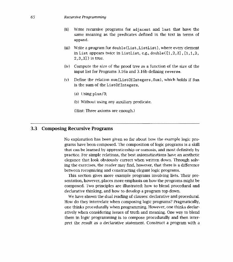
65 Recursive Programming
Write recursive programs for adjacent and last that have thesame meaning as the predicates defined in the text in terms ofappend.
Write a program for double (List,ListList), where every element[ri List appears twice in ListList, e.g., double([1,2,3] [1,1,2,
2,3,3]) is true.
Compute the size of the proof tree as a function of the size of theinput list for Programs 3.16a and 3.1Gb defining reverse.
(y) Define the relation suin(Listoflntegers,Sum), which holds if Sum
is the sum of the ListOf Integers,
Using plus/3;
Without using any auxiliary predicate.
(Hint: Three axioms are enough.)
3.3 Composing Recursive Programs
No explanation has been given so far about how the example logic pro-grams have been composed. The composition of logic programs is a skillthat can be learned by apprenticeship or osmosis, and most definitely bypractice. For simple relations, the best axiomatizations have an aestheticelegance that look obviously correct when written down. Through solv-ing the exercises, the reader may find, however, that there is a differencebetween recognizing and constructing elegant logic programs
This section gives more example programs involving lists. Their pre-sentation, however, places more emphasis on how the programs might becomposed. Two principles are illustrated: how to blend procedural anddeclarative thinking, and how to develop a program top-down.
We have shown the dual reading of clauses: declarative and procedural.How do they interrelate when composing logic programs? Pragmatically,one thinks procedurally when programming. However, one thinks declar-atively when considering issues of truth and meaning. One way to blendthem in logic programming is to compose procedurally and then niter-pret the result as a declarative statement. Construct a program with a

66 Chapter 3
given use in mind; then consider if the alternative uses make declarativesense. We apply this to a program for deleting elements from a list.
The first, and most important, step is to specify the intended meaningof the relation. Clearly, three arguments are involved when deleting ele-ments from a list: an element X to be deleted, a list Li that might haveoccurrences of X, and a list L2 with all occurrences of X deleted. An ap-propriate relation scheme is delete (Li , X, L2). The natural meaning isall ground instances where L2 is the list Li with all occurrences of X re-moved.
When composing the program, it is easiest to think of one specificuse. Consider the query delete([a,b,c,b] ,b,X)?, a typical example offinding the result of deleting an element from a list. The answer here isX= [a, c]. The program will be recursive on the first argument. Let's donour procedural thinking caps.
We begin with the recursive part. The usual form of the recursive ar-gument for lists is [XXs]. There are two possibilities to consider, onewhere X is the element to be deleted, and one where it is not. In the firstcase, the result of recursively deleting X from Xs is the desired answer tothe query. The appropriate rule is
delete([XIXs],X,Ys) - delete(Xs,X,Ys).Switching hats, the declarative reading of this rule is: "The deletion of
X from [XXs] is Ys if the deletion of X from Xs is Ys." The conditionthat the head of the list and the element to be deleted are the same isspecified by the shared variable in the head of the rule.
The second case where the element to be deleted is different from X,the head of the list, is similar. The result required is a list whose headis X and whose tail is the result of recursively deleting the element. Therule is
delete([XIXs],Z,[XIYs]) - X Z, delete(Xs,Z,Ys).
The rule's declarative reading is: "The deletion of Z from [XIXs] is[XYs] if Z is different from X and the deletion of Z from Xs is Ys." Incontrast to the previous rule, the condition that the head of the list andthe element to be deleted are different is made explicit in the body of therule.
The base case is straightforward. No elements can be deleted from theempty list, and the required result is also the empty list. This gives the

67 Recursive Programming
delete(List,X,HasNoXs) -The list HasNoXs is the result of removing alloccurrences of X from the list List.
delete([XIXs],X,Ys) - delete(Xs,X,Ys).
delete([XIXs],Z,[XIYs]) XZ, delete(Xs,Z,Ys).
delete([ ] ,X, E 1).
Program 3.18 Deleting all occurrences of an element from a list
select (X,HasXs,OneLessXs) -The list OneLessXs is the result of removingone occurrence of X from the list HasXs.
select (X, [XIXs] ,Xs)
select(X,[YIYs],[YIZs]) select(X,Ys,Zs).
Program 3.19 Selecting an element from a list
fact delete([ ] ,X, E J). The complete program is collected together asProgram 3.18.
Let us review the program we have written, and consider alternativeformulations. Omitting the condition XZ from the second rule in Pro-gram 3.18 gives a variant of delete. This variant has a less natural mean-ing, since any number of occurrences of an element may be deleted. Forexample, delete([a,b,c,b],b,[a,c]), delete([a,b,c,b],b,[a,c,b]), delete([a,b,c,b],b,[a,b,c]), and delete([a,b,c,b],b,[a,b,c , b]) are all in the meaning of the variant.
Both Program 3.18 and the variant include in their meaning instanceswhere the element to be deleted does not appear in either list, for ex-ample, delete([a] ,b, [a]) is true. There are applications where this isnot desired. Program 3.19 defines select(X,L1,L2), a relation that hasa different approach to elements not appearing in the list. The meaningof select (X,L1,L2) is all ground instances where L2 is the list Li whereexactly one occurrence of X has been removed. The declarative readingof Program 3.19 is: "X is selected from [XXs] to give Xs; or X is selectedfrom [YYs] to give [YZs] if X is selected from Ys to give Zs,"
A major thrust in programming has been the emphasis on a top-downdesign methodology, together with stepwise refinement. Loosely, the

68 Chapter 3
methodology is to state the general problem, break it down into subprob-lems, and then solve the pieces. A top-down programming style is onenatural way for composing logic programs. Our description of programsthroughout the book will be mostly top-down. The rest of this section de-scribes the composition of two programs for sorting a list: permutationsort and quicksort. Their top-down development is stressed.
A logical specification of sorting a list is finding an ordered permuta-tion of a list. This can be written down immediately as a logic program.The basic relation scheme is sort (Xs,Ys), where Ys is a list containingthe elements in Xs sorted in ascending order:
sort(Xs,Ys) - permutation(Xs,Ys), ordered(Ys).
The top-level goal of sorting has been decomposed. We must now definepermutation and ordered.
Testing whether a list is ordered ascendingly can be expressed in thetwo clauses that follow. The fact says that a list with a single elementis necessarily ordered. The rule says that a list is ordered if the firstelement is less than or equal to the second, and if the rest of the list,beginning from the second element, is ordered:
ordered([X]).
ordered([X,YIYs]) - X Y, ordered([YJYs]).
A program for permutation is more delicate. One view of the processof permuting a list is selecting an element nondeterrniriistically to be thefirst element of the permuted list, then recursively permuting the restof the list. We translate this view into a logic program for permutation,using Program 3.19 for select. The base fact says that the empty list isits own unique permutation:
permutation(Xs, [ZIZs]) - select(Z,Xs,Ys), permutation(Ys,Zs).
permutation([ ],[ 1).
Another procedural view of generating permutations of lists is recur-sively permuting the tail of the list and inserting the head in an arbitraryposition. This view also can be encoded immediately. The base part isidentical to the previous version:
permutation([XIXsI ,Zs) - permutation(Xs,Ys), insert(X,Ys,Zs).
permutation([ ],[ ]).

69 Recursive Programming
sort(Xs,Ys) -The list Ys is an ordered permutation of the list Xs.
sort(Xs,Ys) - permutation(Xs,Ys), ordered(Ys).
permutation(Xs, [ZIZs]) - select(Z,Xs,Ys), permutation(Ys,Zs).
perrnutation([ ],[ 1).ordered([ ]).
ordered([X])
ordered([X,YIYs]) X Y, ordered([YIYs]).
Program 3.20 Permutation sort
The predicate insert can be defined in terms of Program 3.19 for se-lect:
insert(X,Ys,Zs) '- select(X,Zs,Ys).
Both procedural versions of permutation have clear declarative read-ings.
The "naive" sorting program, which we call permutation sort, is col-lected together as Program 3.20. It is an example of the generate-and-testparadigm, discussed fully in Chapter 14. Note the addition of the extrabase case for ordered so that the program behaves correctly for emptylists.
The problem of sorting lists is well studied. Permutation sort is not agood method for sorting lists in practice. Much better algorithms comefrom applying a "divide and conquer" strategy to the task of sorting. Theinsight is to sort a list by dividing it into two pieces, recursively sortingthe pieces, and then joining the two pieces together to give the sortedlist. The methods for dividing and joining the lists must be specified.There are two extreme positions. The first is to make the dividing hard,and the joining easy. This approach is taken by the quicksort algorithmThe second position is making the joining hard, but the dividing easy.This is the approach of merge sort, which is posed as Exercise (y) at theend of this section, and insertion sort, shown in Program 3.21.
In insertion sort, one element (typically the first) is removed from thelist. The rest of the list is sorted recursively; then the element is inserted,preserving the orderedness of the list.
The insight in quicksort is to divide the list by choosing an arbitraryelement in it, and then to split the list into the elements smaller than the

70 Chapter 3
sort(Xs,Ys) -The list Ys is an ordered permutation of the list Xs.
sort([XIXs],Ys) - sort(Xs,Zs), insert(X,Zs,Ys).
sort([ ],[ ]).
insert(X,[ ],[X]).
insert(X,[YIYs],[YIZs]) - X> Y, insert(X,Ys,Zs).
insert(X, [YIYs] , [X,YIYs]) - X y.
Program 3.21 Insertion sort
quicksort (Xs, Ys) -The list Ys is an ordered permutation of the list Xs.
quicksort([XIXs] ,Ys) -
partition(Xs,X,Littles,Bigs),
quicksort(Littles,Ls),
quicksort(Bigs,Bs),
append(Ls, [X lBs] ,Ys).
quicksort([ ],[ 1).partition([XIXs] ,Y, [XILs] ,Bs) X Y, partition(Xs,Y,Ls,Bs).
partition([XIXs] ,Y,Ls, [XIBs]) - X > Y, partition(Xs,Y,Ls,Bs).
partition( E ] ,Y, E J , E i)
Program 3.22 Quicksort
chosen element and the elements larger than the chosen element. Thesorted list is composed of the smaller elements, followed by the chosenelement, and then the larger elements. The program we describe choosesthe first element of the list as the basis of partition.
Program 3.22 defines the quicksort algorithm. The recursive rule forquicksort reads: "Ys is a sorted version of [XIXs] if Littles and Bigsare a result of partitioning Xs according to X; Ls and Bs are the result ofsorting Littles and Bigs recursively; and Ys is the result of appending[XBs] to Ls."
Partitioning a list is straightforward, and is similar to the program fordeleting elements. There are two cases to consider: when the currenthead of the list is smaller than the element being used for the parti-tioning, and when the head is larger than the partitioning element. Thedeclarative reading of the first partition clause is: "Partitioning a listwhose head is X and whose tail is Xs according to an element Y gives the

71 Recursive Programming
lists [XLitt1es] and Bigs if X is less than or equal to Y, and partitioningXs according to Y gives the lists Littles and Bigs." The second clausefor partition has a similar reading. The base case is that the empty listis partitioned into two empty lists.
3.3.1 Exercises for Section 3.3
Write a program for substitute(X,Y,Li,L2), where L2 is theresult of substituting Y for all occurrences of X in Li, e.g., sub-stitute(a,x,[a,b,a,c],[x,b,x,c]) is true, whereas substi-tute (a, x, [a,b, a, cl , [a,b ,x, c] ) is false.
What is the meaning of the variant of select:
select (X, [XIXs] ,Xs).select(X, [YIYs] , [YIZs]) '- X Y,
select(X,Ys,Zs).
Write a program for no_doubles(L1 ,L2), where L2 is the result ofremoving all duplicate elements from Li, e.g., no_doubles ([a, b, c,b], [a,c,b]) is true. (Hint: Use member.)
Write programs for evenpermutation(Xs ,Ys) and oddpermuta-tion(Xs,Ys) that find Ys, the even and odd permutations, respec-tively, of a list Xs. For example, even_permutation([i »2,3] » [2,3,i]) andoddpeimutation([i,2,3],[2,i,3]) aretrue.
(y) Write a program for merge sort.
(vi) Write a logic program for kthlargest (Xs , K) that implements thelinear algorithm for finding the kth largest element K of a list Xs.The algorithm has the following steps:
Break the list into groups of five elements.Efficiently find the median of each of the groups, which can be donewith a fixed number of comparisons.Recursively find the median of the medians.Partition the original list with respect to the median of medians.Recursively find the kth largest element in the appropriate smallerlist.

72 Chapter 3
(vii) Write a program for the relation better_poker_hand(Handl,
Hand2,Hand) that succeeds if Hand is the better poker hand be-tween Handi and Hand2. For those unfamiliar with this card game,here are some rules of poker necessary for answering this exercise:
The order of cards is 2, 3, 4, 5, 6, 7, 8, 9, 10, jack, queen, king,ace.
Each hand consists of five cards.
The rank of hands in ascending order is no pairs < one pair <two pairs < three of a kind < flush < straight < full house <four of a kind < straight flush.
Where two cards have the same rank, the higher denominationwins, for example, a pair of kings beats a pair of 7's.
(Hints: (1) Represent a poker hand by a list of terms of the formcard(Suit,Value). For example a hand consisting of the 2 ofclubs, the 5 of spades, the queen of hearts, the queen of dia-monds, and the 7 of spades would be represented by the list [card
(clubs,2),card(spades,5),card(hearts,queen),card(diamonds,
queen),card(spades,7)1. (2)It maybe helpful to define relationssuch as has_f lush (Hand), which is true if all the cards in Hand areof the same suit; has_full_house (Hand), which is true if Hand hasthree cards with the same value but in different suits, and the othertwo cards have the same different value; and has_straight (Hand),
which is true if Hand has cards with consecutive values. (3) Thenumber of cases to consider is reduced if the hand is first sorted.)
3.4 Binary Trees
We next consider binary trees, another recursive data type. These struc-tures have an important place in many algorithms.
Binary trees are represented by the ternary functor tree (Element,
Leí t,Right), where Element is the element at the node, and Left andRight are the left and right subtrees respectively. The empty tree isrepresented by the atom void. For example, the tree

73 Recursive Programming
a
b C
would be represented as
tree(a,tree(b,void,void),tree(c,void,void)).
Logic programs manipulating binary trees are similar to those manip-ulating lists. As with natural numbers and lists, we start with the typedefinition of binary trees. lt is given as Program 3.23. Note that the pro-gram is doubly recursive; that is, there are two goals in the body of therecursive rule with the same predicate as the head of the rule. This re-suits from the doubly recursive nature of binary trees and will be seenalso in the rest of the programs of this section.
Let us write some tree-processing programs. Our first example testswhether an element appears in a tree. The relation scheme is tree_
member(Element,Tree). The relation is true if Element is one of thenodes in the tree. Program 3.24 contains the definition. The declarativereading of the program is: "X is a member of a tree if it is the element atthe node (by the fact) or if it is a member of the left or right subtree (bythe two recursive rules)."
The two branches of a binary tree are distinguishable, but for many ap-plications the distinction is not relevant. Consequently, a useful concept
binary_tree( Tree) -Tree is a binary tree.
binary_tree (void).
binary_tree (tree(Element ,Lef t ,Right)) -
binary_tree(Left), binarytree(Right).
Program 3.23 Defining binary trees
tree_member(Element,Tree) -Element is an element of the binary tree Tree.
tree_momber(X,tree(X,Left,Right)).
tree_member(X,tree(Y,Left ,Right)) - tree_rnember(X,Left).
tree_membor(X,tree(Y,Left ,Right)) '- tree_member(X ,Rïght).
Program 3.24 Testing tree membership

74 Chapter 3
a b
Figure 3.6 Comparing trees for isomorphism
isotree(Treel,Tree2) -Tree I and Tree2 are isomorphic binary trees.
isotree(void,void).
isotree(tree(X,Leftl,Rightl),tree(X,Left2,Right2))
isotree(Leftl,Left2), isotree(Rightl,Right2)
isotree(tree(X,Leftl,Rightl),tree(X,Left2,Right2))
isotree(Leftl ,Right2), isotree(Rightl ,Left2).
Program 3.25 Determining when trees are isomorphic
is isomorphism, which defines when unordered trees are essentially thesame. Two binary trees Ti and T2 are isomorphic if T2 can be obtainedby reordering the branches of the subtrees of Ti. Figure 3.6 shows threesimple binary trees. The first two are isomorphic; the first and third arenot.
Isomorphism is an equivalence relation with a simple recursive defini-tion. Two empty trees are isomorphic. Otherwise, two trees are isomor-phic if they have identical elements at the node and either both the leftsubtrees and the right subtrees are isomorphic; or the left subtree of oneis isomorphic with the right subtree of the other and the two other sub-trees are isomorphic.
Program 3.25 defines a predicate isotree(Treel,Tree2), which istrue if Tree i and Tree2 are isomorphic. The predicate is symmetric inits arguments.
Programs related to binary trees involve double recursion, one for eachbranch of the tree. The double recursion can be manifest in two ways.Programs can have two separate cases to consider, as in Program 3.24 fortree_member. In contrast, Program 3.12 testing membership of a list hasonly one recursive case. Alternatively, the body of the recursive clausehas two recursive calls, as in each of the recursive rules for isotree inProgram 3.25.

75 Recursive Programming
substitute (X, Y,TreeX,TreeY) -The binary tree Tree Y is the result of replacing alloccurrences of X in the binary tree TreeX by Y.
substïtute(X,Y,void,void)
substitute(X,Y,tree(Node,Left,Right),tree(Nodel,Leftl,Rightl))
replace (X,Y,Node,Nodel)
substitute (X,Y,Left,Leftl)
substitute(X,Y,Rigbt,Rightl).
replace(X,Y,X,Y).
replace(X,Y,Z,Z) - X Z.
Program 3.26 Substituting for a term in a tree
The task in Exercise 3.3(i) is to write a program for substituting for el-ements in lists. An analogous program can be written for substitutingelements in binary trees. The predicate substitute(X,Y,OldTree,
NewTree) is true if NewTree is the result of replacing all occurrencesof X by Y in OldTree. An axiomatization of substitute/4 is given asProgram 3.26.
Many applications involving trees require access to the elements ap-pearing as nodes. Central is the idea of a tree traversal, which is a se-quence of the nodes of the tree in some predefined order. There are threepossibilities for the linear order of traversal: preorder, where the value ofthe node is first, then the nodes in the left subtree, followed by the nodesin the right subtree; morder, where the left nodes come first followed bythe node itself and then the right nodes; and postorder, where the nodecomes after the left arid right subtrees.
A definition of each of the three traversals is given in Program 3.27.The recursive structure is identical; the ordy difference between the pro-grams is the order in which the elements are composed by the variousappend goals.
The final example in this section shows interesting manipulation oftrees. A binary tree satisfies the heap property if the value at each nodeis at least as large as the value at its children (if they exist). Heaps, a classof binary trees that satisfy the heap property, are a useful data structureand can be used to implement priority queues efficiently.
lt is possible to heapify any binary tree containing values for which anordering exists. That is, the values in the tree are moved around so that

76 Chapter 3
preorder ( Tree,Pre) -Pre is a preorder traversal of the binary tree Tree.
preorder(tree(X,L,R) ,Xs)
preorder(L,Ls), preorder(R,Rs), append([XJLsJ,Rs,Xs).
preorder(void, E 1).morder ( Tree,In) -
In is an morder traversal of the binary tree Tree.inorder(tree(X,L,R) ,Xs) -
inorder(L,Ls), inorder(R,Rs), append(Ls,EXIRs],Xs).
inorder(void, E 1).
postorder ( Tree,Post) -Post is a postorder traversal of the binary tree Tree.
postorder(tree(X,L,R) ,Xs) -
postorder(L,Ls),
postorder(R,Rs),
append(Rs, [X] ,Rsl),
append(Ls,Rsl,Xs).
postorder(void, E 1).
Program 3.27 Traversals of a binary tree
the shape of the tree is preserved and the heap property is satisfied. Anexample tree and its heapified equivalent are shown in Figure 3.7.
An algorithm for heapifying the elements of a binary tree so that theheap property is satisfied is easily stated recursively. Heapify the left andright subtrees so that they both satisfy the heap property and then ad-just the element at the root appropriately. Program 3.28 embodies thisalgorithm. The relation heapify/2 lays out the doubly recursive pro-gram structure, and adjust(X,HeapL,HeapR,Heap) produces the finaltree Heap satisfying the heap property from the root value X and the leftand right subtrees HeapL and HeapR satisfying the heap property.
There are three cases for adj ust/4 depending on the values. If the rootvalue is larger than the root values of the left and right subtrees, thenthe heap is tree(X,HeapL,HeapR). This is indicated in the first adjust
clause in Program 3.28. The second clause handles the case where theroot node in the left heap is larger than the root node and the root of theright heap. In that case, the adjustment proceeds recursively on the leftheap. The third clause handles the symmetric case where the root nodeof the right heap is the largest. The code is simplified by relegating theconcern whether the subtree is empty to the predicate greater/2.

77 Recursive Programming
Figure 3.7 A binary tree and a heap that preserves the tree's shape
heapify ( Tree,Heap)The elements of the complete binary tree Tree have been adjustedto form the binary tree Heap, which has the same shape as Tree andsatisfies the heap property that the value of each parent node isgreater than or equal to the values of its children.
heapify(void,void).heapify(tree(X,L,R) Heap)
heapify(L,HeapL), heapify(R,HeapR), adjust(X,HeapL,HeapR,Heap).
adj ust (X , HeapL , HeapR , tree (X , HeapL , HeapR)greater(X,HeapL), greater(X,HeapR).
adj ust(X,tree(X1,L,R),HeapR,tree(X1,HeapL,HeapR))X < Xl, greater(X1,HeapR), adjust(X,L,R,HeapL).
adjust(X,HeapL,tree(Xl,L,R),tree(Xl,HeapL,HeapR)) -
X < Xl, greater(Xl,HeapL), adjust(X,L,R,HeapR).
greater(X,void).
greater(X,tree(X1,L,R)) - X Xl.
Program 3.28 Adjusting a binary tree to satisfy the heap property
3.4.1 Exercises for Section 3.4
(i) Define a program for subtree(S ,T), where S is a subtree of T.
(II) Define the relation sum_tree(Treeoflntegers,Sum), which holdsif Sum is the sum of the integer elements in TreeOflntegers.
(IIi) Define the relation ordered(Treeof Integers), which holds if Treeis an ordered tree of integers, that is, for each node in the treethe elements in the left subtree are smaller than the element in

78 Chapter 3
the node, and the elements in the right subtree are larger thanthe element in the node. (Hint: Define two auxiliary relations,ordered_left(X,Tree) and ordered_right(X,Tree), which holdif both Tree is ordered and X is larger (respectively, smaller) thanthe largest (smallest) node of Tree.)
(iv) Define the relation tree_insert(X,Tree,Treel), which holds ifTreel is an ordered tree resulting from inserting X into the orderedtree Tree. If X already occurs in Tree, then Tree and Tree i are iden-tical. (Hint: Four axioms suffice.)
(y) Write a logic program for the relation path(X,Tree,Path), wherePath is the path from the root of the tree Tree to X.
3.5 Manipulating Symbolic Expressions
The logic programs illustrated so far in this chapter have manipulatednatural numbers, lists, and binary trees. The programming style is ap-plicable more generally. This section gives four examples of recursiveprogramming - a program for defining polynomials, a program for sym-bolic differentiation, a program for solving the Towers of Hanoi problem,and a program for testing the satisfiability of Boolean formulae.
The first example is a program for recognizing polynomials in someterm X. Polynomials are defined inductively. X itself is a polynomial inX, as is any constant. Sums, differences, and products of polynomials inX are polynomials in X. So too are polynomials raised to the power of anatural number, and the quotient of a polynomial by a constant.
An example of a polynomial in the term x is x2 - 3x + 2. This followsfrom its being the sum of the polynomials, x2 - 3x and 2, where x2 - 3xis recognized recursively.
A logic program for recognizing polynomials is obtained by expressingthe preceding informal rules in the correct form. Program 3.29 definesthe relation polynomial (Expression,X), which is true if Expression is
a polynomial in X. We give a declarative reading of two rules from theprogram.
The fact polynomial(X,X) says that a term X is a polynomial in itself.The rule

79 Recursive Programming
polynomial (Expression,X) -Expression is a polynomial ¡n X.
polynomial (X , X)
polynomial (Term, X) -
constant (Term)
polynomial (Termi +Term2 , X) -
polynomial (Terml,X), polynomial(Torm2,X).
polynomial (TermlTorm2 ,X)
polynomial(Terml,X), polynomial(Term2,X).
polynomial (Terml *Term2 , X)
polynomïal(Terml,X), polynomial(Term2,X).
polynomial (Terml/Term2 , X)
polynomial(Terml,X), constant(Term2).
polynomial(TermtN,X)
natural_number(N), polynomial(Term,X).
Program 3.29 Recognizing polynomials
polynomial(Terml+Terin2,X) -polyrioinial(Termi,X), polynomial(Term2,X).
says that the sum Terml+Term2 is a polynomial in X if both Tenni andTerm2 are polynomials in X.
Other conventions used in Program 3.29 are the use of the unary pred-icate constant for recognizing constants, and the binary functor T todenote exponentiation. The term XTY denotes x".
The next example is a program for taking derivatives. The relationscheme is derivative(Expression,X,DifferentiatedExpression).The intended meaning of derivative is that DifferentiatedExpres-sion is the derivative of Expression with respect to X.
As for Program 3.29 for recognizing polynomials, a logic program fordifferentiation is just a collection of the relevant differentiation rules,written in the correct syntax. For example, the fact
derivative(X,X,s(0)).
expresses that the derivative of X with respect to itself is 1. The fact
derivative(sin(X) ,X,cos(X)).

80 Chapter 3
derivative (Expression,X,DifferentiatedEx pression)DifferentiatedEx pression is the derivative ofExpression with respect to X.
derivative(X,X,s(0)).
derivative(XIs(N) ,X,s(N)*XIN)
derivative(sin(X) ,X,cos(X))
derivative(cos(X) ,X,-sin(X)).
derivative(elX,X,eX).
derivative(log(X),X,1/X).
derivat ive (F+G ,X ,DF+DG) -
derivative(F,X,DF), derivative(G,X,DG).
derivat ive (F-G ,X ,DF-DG) -
derivative(F,X,DF), derivative(G,X,DG).
derivat ive (F*G ,X ,F*DG+DF*G)
derivative(F,X,DF), derivative(G,X,DG).
derivative(1/F,X,-DF/(F*F)) -
derivative(F,X,DF).
derivative(F/G,X, (G*DF-F*DG)/(G*G)) -
derivative(F,X,DF), derivative(G,X,DG).
Program 3.30 Derivative rules
reads: "The derivative of sin(X) with respect to X is cos(X)." Naturalmathematical notation can be used. A representative sample of functionsand their derivatives is given in Program 3.30.
Sums and products of terms are differentiated using the sum rule andproduct rule, respectively. The sum rule states that the derivative of asum is the sum of derivatives. The appropriate clause is
derivative(F+G,X,DF+DG) -
derivative(F,X,DF), derivative(G,X,DG).
The product rule is a little more complicated, but the logical clause isjust the mathematical definition:
derivative(F*G,X,F*DG+DF*G) -
derivative(F,X,DF), derivative(G,X,DG).
Program 3.30 also contains the reciprocal and quotient rules.The chain rule is a little more delicate. It states that the derivative of
f(g(x)) with respect to x is the derivative of f(g(x)) with respect to g(x)times the derivative of g(x) with respect to x. As stated, it involves quan-

81 Recursive Programming
tification over functions, and is outside the scope of the logic programswe have presented.
Nonetheless, a version of the chain rule is possible for each particularfunction. For example, we give the rule for differentiating XN and sin(X):
derivative(Uls(N) ,X,s(N)*UTN*DU) -
derivative (U,X,DU).
derivative(sin(U),X,cos(U)*DU) - derivative(U,X,DU).
The difficulty of expressing the chain rule for differentiation arisesfrom our choice of representation of terms. Both Programs 3.29 and3.30 use the 'natural" representation from mathematics where termsrepresent themselves. A term such as sin(X) is represented using aunary structure sin. If a different representation were used, for example,unary_term(sin,X) where the name of the structure is made accessible,then the problem with the chain rule disappears. The chain rule can thenbe formulated as
derivative (unary_term(F,U) ,X,DF*DU) -
derivative(unary_term(F,U),U,DF), derivative(IJ,X,DU).
Note that all the rules in Program 3.30 would have to be reformulated interms of this new representation and would appear less natural.
People take for granted the automatic simplification of expressionswhen differentiating expressions. Simplification is missing from Program3.30. The answer to the query derivative (3*x+2,x,D)? is D(3*1+O*x)+O. We would immediately simplify D to 3, but it is not specified in thelogic program.
The next example is a solution to the Towers of Hanoi problem, astandard introductory example in the use of recursion. The problem isto move a tower of n disks from one peg to another with the help of anauxiliary peg. There are two rules. Only one disk can be moved at a time,and a larger disk can never be placed on top of a smaller disk.
There is a legend associated with the game. Somewhere hidden in thesurroundings of Hanoi, an obscure Far Eastern village when the legendwas first told, is a monastery. The monks there are performing a taskassigned to them by God when the world was created - solving thepreceding problem with three golden pegs and 64 golden disks. At themoment they complete their task, the world will collapse into dust. Sincethe optimal solution to the problem with n disks takes 2 - i moves, we

82 Chapter 3
hanoi (N,A,B,C,Moves) -Moves is a sequence of moves for solving the Towers ofHanoi puzzle with N disks and three pegs, A, B, and C.
hanoi(s(0),A,B,C,[A to B]).hanoi(s(N),A,B,C,Moves) -
hanoi(N,A,C,B,Msl),hanoi(N,C,B,A,Ms2)append(Msl,[A to BIMs2],Moves).
Program 3.31 Towers of Hanoi
need not lose any sleep over this possibility. The number 264 is comfort-ingly big.
The relation scheme for solving the problem is hanoi(N,A,B,C,
Moves). It is true if Moves is the sequence of moves for moving a towerof N disks from peg A to peg B using peg C as the auxiliary peg. This is anextension to usual solutions that do not calculate the sequence of movesbut rather perform them. The representation of the moves uses a binaryfunctor to, written as an infix operator. The term X to Y denotes thatthe top disk on peg X is moved to peg Y. The program for solving theproblem is given in Program3.31.
The declarative reading of the heart of the solution, the recursive rulein Program 3.31, is: "Move s is the sequence of moves of s (N) disks frompeg A to peg B using peg C as an auxiliary, if Msi is the solution formoving N disks from A to C using B, Ms2 is the solution for moving N disksfrom C to B using A, and Moves is the result of appending [A to BIMs2]
to Msi."
The recursion terminates with moving one disk. A slightly neater, butless intuitive, base for the recursion is moving no disks. The appropriatefact is
hanoi(O,A,B,C,[ ]).
The final example concerns Boolean formulae.A Boolean formula is a term defined as follows: The constants true and
false are Boolean formulae; if X and Y are Boolean formulae, so are Xv Y,XA Y, and -X, where y and A are binary infix operators for disjunctionand conjunction, respectively, and is a unary prefix operator for nega-tion.

83 Recursive Programming
saris fiable(Formula)There is a true instance of the Boolean formula Formula.
satisfiabie(true)
satisfiable(XAY) - satisfiable(X), satisfiable(Y).
satisfiabie(XVY) satisfïable(X).
satisfiable(XVY) - satisfiable(Y).
satisfiable(-X) - invalid(X).
invalid(Formula)There is a false instance of the Boolean formula Formula.
invalid (f aise)
invaiid(XVY) - invaiìd(X), invalid(Y).
invaiid(XAY) invaiid(X).
invalid(XAY) - invalid(Y).
invalid(-'-Y) - satisf jable (Y)
Program 3.32 Satisfiability of Boolean formulae
A Boolean formula F is true if
F 'true',F = XAY, and both X and Y are true.F = XvY, and either X or Y (or both) are true.F = X, and X is false.
A Boolean formula F is false if
F = 'false'.F = XAY, and either X or Y (or both) are false.F = XvY, and both X and Y are false.F = =X, and X is true.
Program 3.32 is a logic program for determining the truth or falsityof a Boolean formula. Since it can be applied to Boolean formulae withvariables, it is actually more powerful than it seems. A Boolean formulawith variables is satisfiable if it has a true instance. It is invalid if ithas a false instance. These are the relations computed by the program.

84 Chapter 3
3.5.1 Exercises for Section 3.5
Write a program to recognize if an arithmetic sum is normalized,that is, has the form A + B, where A is a constant and B is a normal-ized sum.
Write a type definition for Boolean formulae.
Write a program for recognizing whether a logical formula is inconjunctive normal form, namely, is a conjunction of disjunctionsof literals, where a literal is an atomic formula or its negation.
Write a program for the relation negation_inwards (Fi ,F2), whichis true if F2 is the logical formula resulting from moving all nega-tion operators occurring in the formula Fi inside conjunctions anddisjunctions.
(y) Write a program for converting a logical formula into conjunctivenormal form, that is, a conjunction of disjunctions.
(vi) Consider the following representation of a bag, that is, a list ofelements with multiplicities. The function symbol bag(Element,
Multiplicity,RestûfBag) should be used. The atom void canbe used as an empty bag. For example, the term bag (a, 3, bag (b, 2,
void)) represents a list of three copies of an element a, and twocopies of an element b. Write logic programs to
Take the union of two bags;
Take the intersection of two bags;
Substitute for an element in a bag;
Convert a list into a bag;
Convert a binary tree into a bag.
3.6 Background
Many of the programs in this chapter have been floating around the logicprogramming community, and their origins have become obscure. For

85 Recursive Programming
example, several appear in Clocksm and Mellish (1984) and in the unevencollection of short Prolog programs, How to Solve It in Prolog by Coelhoet al. (1980).
The latter book has been updated as Coelho and Cotta (1988) and isa source for other simple examples. The exercise on describing pokerhands is due to Ken Bowen.
The classic reference for binary trees is Knuth (1968) and for sortingKnuth (1973).
A discussion of the linear algorithm for the kth largest algorithms canbe found in most textbooks on algorithms, for example, Horowitz andSahni (1978). The discussion of the heap property is taken from Horowitzand Sahni (1978).
Many of the basic programs for arithmetic and list processing have asimple structure that allows many correctness theorems to be provedautomatically, see, for example, Boyer and Moore (1979) and Sterling andBundy (1982).
Ackermann's function is discussed by Peter (1967).


4 The Computation Model of LogicPrograms
The computation model used in the first three chapters of the book hasa severe restriction. All goals appearing in the proof trees are ground. Allrule instances used to derive the goals in the proof trees are also ground.The abstract interpreter described assumes that the substitutions givingthe desired ground instances can be guessed correctly. In fact, the cor-rect substitutions can be computed rather than guessed.
This chapter presents a general computation model of logic programs.The first section presents a unification algorithm that removes the guess-work in determining instances of terms. The second section presents anappropriately modified abstract interpreter and gives example computa-tions of logic programs.
The computation model of logic programming we present is especiallywell suited to sequential languages such as Prolog. Our model can beused to describe parallel logic programming languages. However, devel-opers of these languages have often used other models, such as statetransitions or dynamic tree creation and destruction (see Section 4.3).
4.1 Unification
The heart of our computation model of logic programs is unification.Unification is the basis of most work in automated deduction and of theuse of logical inference in artificial intelligence.
Necessary terminology for describing the algorithm is repeated fromChapter 1, and new definitions are introduced as needed.

88 Chapter 4
Recall that a term t is a common instance of two terms, t1 and t2, ifthere exist substitutions 9 and 92 such that t equals t191 and t202. Aterm s is more general than a term t 1f t is an instance of s but s is notan instance of t. A term s is an alphabetic variant of a term t if boths is an instance of t and t is an instance of s. Alphabetic variants arerelated by the renaming of variables that occur in the terms. For exam-ple, meinber(X,tree(Left,X,Right)) and member(Y,tree(Left,Y,Z))
are alphabetic variants.A unifier of two terms is a substitution making the terms identical. If
two terms have a unifier, we say they unify. There is a close relation be-tween unifiers and common instances. Any unifier determines a commoninstance, and conversely, any common instance determines a unifier.
For example, append([1,2,3] ,[3,4] ,List) and append([XXs] ,Ys,
[XIZs]) unify. A unifying substitution is {X"1,Xs[2,3], Ys=[3,4],
List=[1Zs] }. Their common instance, determined by this unifying sub-stitution, is append( [1,2,3] [3,4], [1Zs] ).
A most general unifier, or mgu, of two terms is a unifier such that theassociated common instance is most general. It can be shown that if twoterms unify, all mgus are equivalent. Making that statement precise isbeyond the scope of this book, but we give pointers in Section 4.3. Weproceed by giving an algorithm that computes a most general unifier oftwo terms if one exists.
The algorithm for unification presented here is based on solving equa-tions. The input for the algorithm is two terms, T1 and T2. The outputof the algorithm is an mgu of the two terms if they unify, or failure ifthe terms do not unify. The algorithm uses a pushdown stack for storingthe equations that need to be solved and a location, O, for collecting thesubstitution comprising the output.
The location O is initially empty, and the stack is initialized to containthe equation T1 = T2. The algorithm consists of a loop of popping anequation from the stack and processing it. The loop terminates whenthe stack becomes empty or if failure occurs in processing an invalidequation.
We consider the possible actions for dealing with a popped equationS = T. The simplest case is if S and T are identical constants or var-iables. This equation is correct, and nothing further needs to be done.The computation continues by popping the next equation from thestack.

89 The Computation Model of Logic Programs
If S is a variable, and T is a term not containing S, the following hap-pens. The stack is searched for all occurrences of S, which are replacedby T. Similarly, all occurrences of S in O are replaced by T. Then the sub-stitution S = T is added to O. It is significant that S does not occur in T.The test embodied by the phrase "not containing" is known as the occurscheck.
If T is a variable, and S is a term not containing T, i.e., T satisfiesthe occurs check with respect to S, the symmetric sequence of actionshappens.
Equations are added to the stack if S and T are compound terms withthe same principal functor and arity, f(S1,. . .,S,) and f(T1,.. say.For the terms to unify, each of the argument pairs must simultaneouslyunify. This is achieved by pushing the n equations, S = T, onto the stack.
In any other case, failure is reported, and the algorithm terminates. Ifthe stack is emptied, the terms unify, and the unifier can be found in¿9. The complete algorithm is given as Figure 4.1. The occurs check isembodied in the phrase "that does not occur in."
We do not prove the correctness of this algorithm, nor analyze its com-plexity. The interested reader is referred to the literature in Section 4.3.
Consider attempting to unify the terms append([a,b] , [c,d] ,Ls) andappend([XIXs] ,Ys, [XIZs]). The stack is initialized to the equation
append([a,b] , [c,d] ,Ls) append([XIXs] ,Ys, [XIZs]).
These two terms have the same functor, append, and arity, 3, so we addthe three equations relating the subterms of the two terms. These are{a,b]=[XIXs], [c,d]=Ys, and Ls=[XZs].
The next equation, [a, b] = [X Xs], is popped from the stack. These twocompound terms have the same functor, ".", and arity, 2, so two equa-tions, aX and [b] =X, are added to the stack. Continuing, the equationa=X is popped. This is covered by the second case in Figure 4.1. X is avariable not occurring in the constant, a. All occurrences of X in the stackare replaced by a. One equation is affected, namely Ls= [XIZs], whichbecomes Ls= [a Zs]. The equation X=a is added to the initially empty sub-stitution, and the algorithm continues.
The next equation to be popped is Lb] =Xs. Again this is covered by thesecond case. Xs= [b] is added to the set of substitutions, and the stack ischecked for occurrences of Xs. There are none, and the next equation ispopped.

90 Chapter 4
Input: Two terms T1 and T2 to be unified
Output: O, the mgu of T1 and T2, or failure
Algorithm: Initialize the substitution O to be empty,the stack to contam the equation T1 = T2,and failure to false.
while stack not empty and no failure do
pop X = Y from the stack
caseX is a variable that does not occur in Y:
substitute Y for X in the stack and in Oadd X = Y to O
Y is a variable that does not occur in X:substitute X for Y in the stack and in Oadd Y = X to O
X and Y are identical constants or variables:continue
Xisf(X1.....X)andYisf(Y1.....Y)for some functor f and n> O:push X, = Y,i = i n, on the stack
otherwise:failure is true
If failure, then output failure else output O.
Figure 4.1 A unification algorithm
The second case also covers [c,d]=Ys. Another substitution, Ys=[c,dl, is added to the collection, and the final equation, Ls=[aZs], is
popped. This is handled by the symmetric first case. Ls does notoccur in [aZs], so the equation is added as is to the unifier, andthe algorithm terminates successfully. The unifier is {X=a,Xs=[b]
Ys= Ec , d], Ls= [aZs] }. The common instance produced by the unifier isappend([a,bl , [c,d] , [als]). Note that in this unification, the substi-tutions were not updated.
The occurs check is necessary to prevent the unification of terms suchas s (X) and X. There is no finite common instance of these terms. How-

91 The Computation Mode! of Logic Programs
ever, most Prolog implementations omit the occurs check from the unifi-cation algorithm, for pragmatic reasons.
When implementing this unification algorithm for a particular logicprogramming language, the explicit substitution in both the equations onthe stack and the unifier is avoided. Instead, logical variables and otherterms are represented by memory cells with different values, and variablebinding is implemented by assigning to the memory cell representing alogical variable a reference to the cell containing the representation ofthe term the variable is bound to. Therefore,
Substitute Y for X in stack and in O.Add X = Y to substitutions.
is replaced by
Make X a reference to Y.
4.1.1 Exercises for Section 4.1
Use the algorithm in Figure 4.1 to compute an mgu of append([b],[c,d] ,L) and append([XIXs] ,Ys, [XIZs]).
Use the algorithm in Figure 4.1 to compute anmguofhnoi(s(N),A,B,C,Ms)andhanoi(s(s(0)),a,b,c,Xs).
4.2 An Abstract Interpreter for Logic Programs
We revise the abstract interpreter of Section 1.8 in the light of the unifi-cation algorithm. The result is our full computation model of logic pro-grams. Ail the concepts introduced previously, such as goal reductionsand computation traces, have their analogues in the full model.
A computation of a logic program can be described informally as fol-lows. It starts from some initial (possibly conjunctive) query G and, if itterminates, has one of two results: success or failure. If a computationsucceeds, the instance of G proved is conceived of as the output of thecomputation. A given query can have several successful computations,each resulting in a different output. In addition, it may have nontermi-nating computations, to which we associate no result.
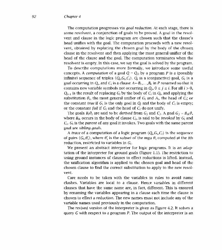
92 Chapter 4
The computation progresses via goal reduction. At each stage, there issome resolvent, a conjunction of goals to be proved. A goal in the resol-vent and clause in the logic program are chosen such that the clause'shead unifies with the goal. The computation proceeds with a new resol-vent, obtained by replacing the chosen goal by the body of the chosenclause in the resolvent and then applying the most general unifier of thehead of the clause and the goal. The computation terminates when theresolvent is empty. In this case, we say the goal is solved by the program.
To describe computations more formally, we introduce some usefulconcepts. A computation of a goal Q = Qo by a program P is a (possiblyinfinite) sequence of triples (Q,G1,C1). Q is a (conjunctive) goal, G is agoal occurring in Q, and C is a clause AB1,. . .,B in P renamed so that itcontains new variable symbols not occurring in O, O j i. For all i> O,Q is the result of replacing G by the body of C in Q, and applying thesubstitution 0, the most general unifier of G and A, the head of C; orthe constant true if G is the only goal in Q and the body of C is empty;or the constant fail if G and the head of C do not unify.
The goals B01 are said to be derived from G1 and C. A goal G = Bk0,where Bjk occurs in the body of clause C1, is said to be invoked by G andC. G is the parent of any goal it invokes. Two goals with the same parentgoal are sibling goals.
A trace of a computation of a logic program (Q,G1,C1) is the sequenceof pairs (G1,G), where 0 is the subset of the mgu 0 computed at the ithreduction, restricted to variables in G.
We present an abstract interpreter for logic programs. It is an adap-tation of the interpreter for ground goals (Figure 1.1). The restriction tousing ground instances of clauses to effect reductions is lifted. Instead,the unification algorithm is applied to the chosen goal and head of thechosen clause to find the correct substitution to apply to the new resol-vent.
Care needs to be taken with the variables in rules to avoid nameclashes. Variables are local to a clause. Hence variables in differentclauses that have the same name are, in fact, different. This is ensuredby renaming the variables appearing in a clause each time the clause ischosen to effect a reduction. The new names must not include any of thevariable names used previously in the computation.
The revised version of the interpreter is given as Figure 4.2. It solves aquery G with respect to a program P. The output of the interpreter is an

93 The Computation Model of Logic Programs
Input:
Output:
Algorithm:
A goal G and a program P
An instance of G that is a logical consequence of P,or no otherwise
lnitjalize the resolvent to G.while the resolvent is not empty do
choose a goal A from the resolventchoose a (renamed) clause A' B1 ..,B,1 from P
such that A and A' unify with mgu E)(if no such goal and clause exist, exit the while loop)
replace A by B1 ,...,B ¡n the resolventapply O to the resolvent and to G
If the resolvent is empty, then output G, else output rio.
Figure 4.2 An abstract interpreter for logic programs
instance of G if a proof of such an instance is found, or no if a failurehas occurred during the computation. Note that the interpreter may alsofail to terminate.
An instance of a query for which a proof is found is called a solution tothe query.
The policy for adding and removing goals from the resolvent is calledthe scheduling policy of the interpreter. The abstract interpreter leavesthe scheduling policy unspecified.
Consider solving the query append([a,b] , [c,d] ,Ls)? by Program3.15 for append using the abstract interpreter of Figure 4.2. The resol-vent is initialized to be append([a,bJ , [c,d] ,Ls). lt is chosen as thegoal to reduce, being the on'y one. The rule chosen from the program is
append([XIXs],Ys,[XIZs]) - append(Xn,Ys,Zs).
The unifier of the goal and the head of the rule is {X=a,Xs=[b],
Ys=[c,d] , Ls[aIZs]}. A detailed calculation of this unifier appearedin the previous section. The new resolvent is the instance of ap-
pend(Xn , Ys ,Zn) under the unifier, namely, append( [b] , [c , d] ,Zn). Thisgoal is chosen in the next iteration of the loop. The same clause forappend is chosen, but variables must be renamed to avoid a clash ofvariable names. The version chosen is
append([X1IXs1],Ysl,[X1IZs1]) - apperid(Xsl,Ysl,Zsl).

94 Chapter 4
append([a,b] , [c,d] ,Ls)append([b] , [c,d] ,Zs)
append([ j, [c,d] ,Zsl)true
Output: Ls= [a, b, c , d]
Ls= [aIZs]Zs[bIZsl]Zsl=[c,d]
Figure 4.3 Tracing the appending of two lists
The unifier of the head and goal is {X1=b, Xsl=[ ], Ys1[c,d],Zs=[bZs1]}. The new resolvent is append([ ], [c,d] ,Zsl). This timethe fact append( [ ] , Zs2 , Zs2) is chosen; we again rename variables asnecessary. The unifier this time is {Zs2=[c,d] , Zsl=[c,d]}. The newresolvent is empty and the computation terminates.
To compute the result of the computation, we apply the relevant partof the mgu's calculated during the computation. The first unificationinstantiated Ls to [aIZs]. Zs was instantiated to [bZs1] in the secondunification, and Zs i further became [c , d]. Putting it together, Ls has thevalue [a[b[c,d]]],ormore simply, [a,b,c,d].
The computation can be represented by a trace. The trace of the fore-going append computation is presented in Figure 4.3. To make the tracesclearer, goals are indented according to the indentation of their parent.A goal has an indentation depth of d+1 if its parent has indentationdepth d.
As another example, consider solving the query son(S,haran)? byProgram 1.2. It is reduced using the clause son(X,Y) - f ather(Y,X),male (X). A most general unifier is {X=S,Y=haran}. Applying the sub-stitution gives the new resolvent f ather(haran,S), male(S). This isa conjunctive goal. There are two choices for the next goal to reduce.Choosing the goal father (haran , S) leads to the following computation.The goal) unifies with the fact father (haran, lot) in the program, andthe computation continues with S instantiated to lot. The new resolventis male (lot), which is reduced by a fact in the program, and the compu-tation terminates. This is illustrated in the left trace in Figure 4.4.
The other possibility for computing S=haran is choosing to reducethe goal male (S) before father (haran,S). This goal is reduced by thefact male(lot) with S instantiated to lot. The new resolvent is f a-ther (haran, lot), which is reduced to the empty goal by the correspond-ing fact. This is the right trace in Figure 4.4.

95 The Computation Model of Logic Programs
son(S,haran) son(S,haran)father(haran,S) S1ot male(S) S=:]otmale(lot) father(haran,lot)
true true
Figure 4.4 Different traces of the same solution
Solutions to a query obtained using the abstract interpreter may con-tain variables. Consider the query mernber(a,Xs)? with respect to Pro-gram 3.12 for member. This can be interpreted as asking what list Xs hasthe element a as a member One solution computed by the abstract inter-preter is Xs= [a lYs], namely, a list with a as its head and an unspecifiedtail. Solutions that contain variables denote an infinity of solutionsalltheir ground instances.
There are two choices in the interpreter of Figure 4.2: choosing the goalto reduce, and choosing the clause to effect the reduction. These must beresolved in any realization of the computation model. The nature of thechoices is fundamentally different.
The choice of goal to reduce is arbitrary; it does not matter which ischosen for the computation to succeed. If there is a successful computa-tion by choosing a given goal, then there is a successful computation bychoosing any other goal. The two traces in Figure 4.4 illustrate two suc-cessful computations, where the choice of goal to reduce at the secondstep of the computation differs.
The choice of the clause to effect the reduction is nondeterministic.Not every choice will lead to a successful computation. For example, inboth traces in Figure 4.4, we could have gone wrong. If we had chosen toreduce the goal father (haran,S) with the fact father (haran,yiscah),we would not have been able to reduce the invoked goal male (yiscah).For the second computation, had we chosen to reduce male(S) withmale(isaac), the invoked goal f ather(haran,isaac) could not havebeen reduced.
For some computations, for example, the computation illustrated inFigure 4.3, there is only one clause from the program that can reduceeach goal. Such a computation is called deterministic. Deterministic com-putations mean that we do not have to exercise our nondeterministicimagination.
The alternative choices that can be made by the abstract interpreterwhen trying to prove a goal implicitly define a search tree, as described

96 Chapter 4
more fully in Section 5.4. The interpreter "guesses" a successful pathin this search tree, corresponding to a proof of the goal, if one exists.However, dumber interpreters, without guessing abilities, can also bebuilt, with the same power as our abstract interpreter. One possibilityis to search this tree breadth-first, that is, to explore all possible choicesin parallel. This will guarantee that if there is a finite proof of the goal(i.e., a finite successful path in the search tree), it will be found.
Another possibility would be to explore the abstract search tree depth-first. In contrast to the breadth-first search strategy, the depth-first onedoes not guarantee finding a proof even if one exists, since the searchtree may have infinite paths, corresponding to potentially infinite com-putations of the nondeterministic interpreter. A depth-first search of thetree might get lost in an infinite path, never finding a finite successfulpath, even if one exists.
In technical terms, the breadth-first search strategy defines a completeproof procedure for logic programs, whereas the depth-first one is in-complete. In spite of its incompleteness, depth-first search is the oneincorporated in Prolog, for practical reasons, as explained in Chapter 6.
Let us give a trace of a longer computation, solving the Towers ofHanoi problem with three disks, using Program 3.31. It is a deterministiccomputation, given as Figure 4.5. The final append goal is given withoutunifications. It is straightforward to fill them in.
Computations such as that in Figure 4.5 can be compared to compu-tations in more conventional languages. Unification can be seen to sub-sume many of the mechanisms of conventional languages: record alloca-tion, assignment of and access to fields in records, parameter passing,and more. We defer the subject until the computation model for Prologis introduced in Chapter 6.
A computation of G by P terminates if G = true or fail for some nO. Such a computation is finite and of length n. Successful computationscorrespond to terminating computations that end in true. Failing com-putations end in fail. All the traces given so far have been of successfulcomputations.
Recursive programs admit the possibility of nonterminating computa-tions. The query append(Xs, [c,d] ,Ys)? with respect to append can bereduced arbitrarily many times using the rule for append. In the process,Xs becomes a list of arbitrary length. This corresponds to solutions ofthe query appending [c , dl to an arbitrarily long list. The nonterminat-ing computation is illustrated in Figure 4.6.
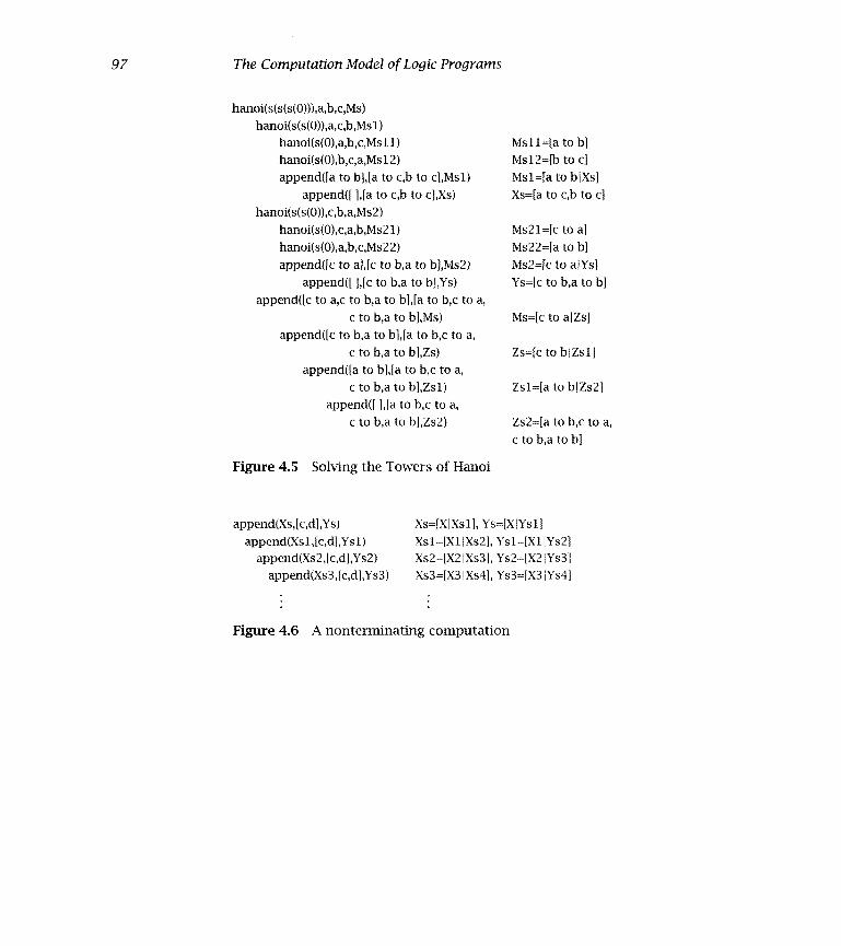
97 The Computation Mode! of Logic Programs
hanoi(s(s(s(0))),a,b,c,Ms)hanoi(s(s(0)),a,c,b,Msl)
hanoi(s(0),a,b,c,Msl 1)hanoi(s(0),b,c,a,Ms 12)append([a to bija to c,b to ciMsi)
appendU ]ja to c,b to c],Xs)hanoi(s(s(0)),c,b,a,Ms2)
hanoi(s(0),c,a,b,Ms2 1)hanoi(s(0),a,b,c,Ms22)append(]c to aJ,fc to b,a to b],Ms2)
appendU ],[c to ba to b],Ys)append([c to a,c to b,a to bila to b,c to a,
c to b,a to b],Ms)append(Lc to b,a to b],[a to b,c to a,
c to b,a to bJ,Zs)append([a to biLa to b,c to a,
c to b,a to biZsl)appendU ]Ja to b,c to a,
c to b,a to b],Zs2)
Figure 4.5 Solving the Towers of Hanoi
append(Xs,[c,dJ,Ys)append(Xsl ,]c,d],Ysl)
append(Xs2,[c,dI,Ys2)append(Xs 3 ,[c,d],Ys3)
Xs=[XIXs1], Ys=LXYs1l
Xsl=[X1 Xs2], Ysl=[X1 IYs2lXs2=[X2IXs3], Ys2=LX2JYs3]
Xs3=[X3IXs4I, Ys3=[X3IYs4]
Figure 4.6 A nonterminating computation
Msll=[a to b]Ms12=[b toc]Msl=[a to bIXsJXs=[a to c,b to cl
Ms21=Fc to a]
Ms22=[a to biMs2=[c to alYs]Ys=[c to b,a to b]
Ms=Lc to aIZsI
Zs=[c to bjZsli
Zsl=[a to bIZs2]
Zs2=[a to b,c to a,c to b,a to b]

98 Chapter 4
All the traces presented so far have an important feature in common.If two goals G and G1 are invoked from the same parent, and G appearsbefore G in the trace, then all goals invoked by G will appear beforeG in the trace. This scheduling policy makes traces easier to follow, bysolving queries depth-first.
The scheduling policy has another important effect: instantiating vari-ables before their values are needed for other parts of the computation.A good ordering can mean the difference between a computation beingdeterministic or not.
Consider the computation traced in Figure 4.5. The goal
hanoi(s(s(s(0))) ,a,b,c,Ms)
is reduced to the following conjunction
hanoi(s(s(0)) ,a,c,b,Msl),
hanoi(s(s(0)) ,c,b,a,Ms2)
append(Msl, [a to bIMs2] ,Ms).
If the append goal is now chosen, the append fact could be used (incor-rectly) to reduce the goal. By reducing the two hanoi goals first, and allthe goals they invoke, the append goal has the correct values for Ms i andMs2.
4.2.1 Exercises for Section 4.2
Trace the query sort([3,1,2] ,Xs)? using the permutation sort(3.20), insertion sort (3.21), and quicksort (3.22) programs in turn.
Give a trace for the goal derivative(3*sin(x)-4*cos(x),x,D)
using Program 3.30 for derivative.
Practice tracing your favorite computations.
4.3 Background
Unification plays a central role in automated deduction and in the useof logical inference in artificial intelligence. It was first described in thelandmark paper of Robinson (1965). Algorithms for unification have been

99 The Computation Model of Logic Programs
the subject of much investigation: see, for example, Martelli and Monta-nari (1982), Paterson and Wegman (1978), and Dwork et al. (1984). Typi-cal textbook descriptions appear in Bundy (1983) and Niisson (1980).
The definition of unification presented here is nonstandard. Readerswishing to learn more about unifiers are referred to the definitive dis-cussion on unification in Lassez, Maher, and Marriott (1988). This paperpoints out inconsistencies of the various definitions of unifiers that havebeen proposed in the literature, including the version in this book. Es-sentially, we have explained unifiers based on terms to avoid technicalissues of composition of substitutions, which are not needed for our de-scription of logic progranmiing computations.
The computation model we have presented has a sequential bias andis influenced by the computation model for Prolog given in Chapter 6.Nonetheless, the model has potential for parallelism by selecting severalgoals or several rules at a time, and for elaborate control by selectingcomplicated computation rules. References for reading about differentcomputation models for logic programming are given in Section 6.3.
Another bias of our computation model is the central place of unifi-cation. An exciting development within logic programming has been therealization that unification is just one instance of constraint solving. Newcomputation models have been presented where the solution of equal-fly constraints, i.e., unification, in the abstract interpreter of Figure 4.2is replaced by solving other constraints. Good starting places to readabout the new constraint-based models are Colmerauer (1990), Jaffar andLassez (1987), and Lassez (1991).
A proof that the choice of goal to reduce from the resolvent is arbitrarycan be found in Apt and van Emden (1982) or in the text of Lloyd (1987).
A method for replacing the runtime occurs check with compile-timeanalysis was suggested by Plaisted (1984).
Attempts have been made to make unification without the occurscheck more than a necessary expedient for practical implementations ofProlog. In particular, Colmerauer (1982b) proposes a theoretical modelfor such unifications that incorporates computing with infinite terms.
A novel use of unification without the occurs check appears in Eggertand Chow (1983), where Escher-like drawings that gracefully tend to in-finity are constructed.


5.1 Semantics
Semantics assigns meanings to programs. Discussing semantics allowsus to describe more formally the relation a program computes. Chap-ter 1 informally describes the meaning of a logic program P as the setof ground instances that are deducible from P via a finite number of ap-plications of the rule of universal modus ponens. This section considersmore formal approaches.
5 Theory of Logic Programs
A major underlying theme of this book, laid out in the introduction, isthat logic programming is attractive as a basis for computation becauseof its basis in mathematical logic, which has a well-understood, well-developed theory. In this chapter, we sketch some of the growing theoryof logic programming, which merges the theory inherited from mathe-matical logic with experience from computer science and engineering.Giving a complete account is way beyond the scope of this book. In thischapter, we present some results to direct the reader in important direc-tions. The first section, on semantics, gives definitions and suggests whythe model-theoretic and proof-theoretic semantics give the same result.The main issue in the second section, on program correctness, is termi-nation. Complexity of logic programs is discussed in the third section.The most important section for the rest of the book is Section 4, whichdiscusses search trees. Search trees are vital to understanding Prolog'sbehavior. Finally, we introduce negation in logic programming.

102 Chapter 5
parent(terach,abraham). parent(abrahani,isaac).parent(isaac ,jacob). parent(jacob,benjainin).ancestor(X,Y) - parent(X,Y).ancestor(X,Z) - parent(X,Y), ancestor(Y,Z).
Program 5.1 Yet another family example
The operational semantics is a way of describing procedurally themeaning of a program. The operational meaning of a logic program Pis the set of ground goals that are instances of queries solved by P usingthe abstract interpreter given in Figure 4.2. This is an alternative for-mulation of the previous semantics, which defined meaning in terms oflogical deduction.
The declarative semantics of logic programs is based on the standardmodel-theoretic semantics of first-order logic. In order to define it, somenew terminology is needed.
DefinitionLet P be a logic program. The Herbrand universe of P, denoted U(P), isthe set of all ground terms that can be formed from the constants andfunction symbols appearing in P. u
In this section, we use two running examplesyet another family data-base example, given as Program 5.1; and Program 3.1 defining the naturalnumbers, repeated here:
natural_number (0)
natural_number(s(X)) - natural_number(X).
The Herbrand universe of Program 5.1 is the set of all constants appear-ing in the program, namely, {terach, abraham, isaac ,jacob, benj amin}.
If there are no function symbols, the Herbrand universe is finite. In Pro-gram 3.1, there is one constant symbol, O, and one unary function sym-bol, s. The Herbrand universe of Program 3.1 is {O, s (0) , s (s (0)), . . .
If no constants appear in a program, one is arbitrarily chosen.
DefinitionThe Herbrand base, denoted B(P), is the set of all ground goals thatcan be formed from the predicates in P and the terms in the Herbranduniverse.

103 Theory of Logic Programs
There are two predicates, parent/2 and ancestor/2, in Program 5.1.The Herbrand base of Program 5.1 consists of 25 goals for each predi-cate, where each constant appears as each argument:
{parent(terach,terach), parent(terach,abraham),parerit(terach,isaac), parent(terach,jacob),parent(terach,benjanuin), parent(abraham,terach),parent (abraham, abraham), parent(abraham, isaac),parent(abraham,jacob), parent(abraham,benjanìin),parent(isaac,terach), parent(isaac,abrahain),parent(isaac,isaac), parent(isaac,jacob),parent(isaac,benjaniin), parent(jacob,terach),parent(jacob,abraham), parent(jacob,isaac),parent(jacob,jacob), parent(jacob,berijamin),parent(berijamin,terach), parent(benjainin,abraham),parent (benjamin,isaac), parent(benjamin,jacob),parent(benjamin,benjarniri), ancestor(terach,terach),ancestor(terach,abraham), ancestor(terach,isaac),ancestor(terach,jacob), ancestor(terach,benjamin),ancestor(abrahani,terach), ancestor(abraham,abrahani),ancestor(abraham,isaac), ancestor(abrahain,jacob),ancestor(abraham,benjamin), ancestor(isaac,terach),ancestor(isaac,abrahani), ncestor(isaac,isaac),ancestor(isaac,jacob), ancestor(isaac,benjaxnin),ancestor(jacob,terach), ancestor(jacob,abraham),ancestor(jacob,isaac), ancestor(jacob,jacob),ancestor(jacob,berijainin), ancestor(benjamin,terach),ancestor(benjamin,abrahain), ancestor(benjainin,isaac),ancestor (benjamin, jacob), ancestor (benj amin, benjamin) }.
The Herbrand base is infinite if the Herbrand universe is. For Pro-gram 3.1, there is one predicate, natural_number. The Herbrand baseequals tnatural_nuinber(0) ,natural_riumber(s(0)), . . . L
DefinitionAn interpretation for a logic program is a subset of the Herbrand base. u
An interpretation assigns truth and falsity to the elements of the Her-brand base. A goal in the Herbrand base is true with respect to an inter-pretation if it is a member of it, false otherwise.

104 Chapter 5
DefinitionAn interpretation I is a model for a logic program if for each groundinstance of a clause in the program AB1,. . .,B, A is in I if B1,. . .,B areinI.
Intuitively, models are interpretations that respect the declarativereading of the clauses of a program.
For Program 3.1, natural_number(0) must be in every model, andnatural_number(s(X)) is in the model if natural_number(X) is. Anymodel of Program 3.1 thus includes the whole Herbrand base.
For Program 5.1, the facts parent(terach,abraham), parent(abra-
ham,isaac), parent(isaac,jacob), and parent(jacob,benjamin)
must be in every model. A ground instance of the goal ancestor(X,Y) is
in the model if the corresponding instance of parent (X, Y) is, by the firstclause. So, for example, ancestor(terach,abrahain) is in every model.By the second clause, ancestor(X,Z) is in the model if parent(X,Y) andancestor(Y,Z) are.
It is easy to see that the intersection of two models for a logic programP is again a model. This property allows the definition of the intersectionof all models.
DefinitionThe model obtained as the intersection of all models is known as theminimal model and denoted M(P). The minimal model is the declarativemeaning of a logic program. .
The declarative meaning of the program for natural_number, its min-imal model, is the complete Herbrand base {natural_number(0) ,natu-
ral_number(s(0)),natural_number(s(s(0))), . ..
The declarative meaning of Program 5.1 is {parent(terach,abrahani),
parent(abrahain,isaac), parent(isaac,jacob), parent(jacob,
benjamin), ancestor(terach,abraham), ancestor(abraham,isaac),
ancestor(isaac,jacob), ancestor(jacob,benjamin), ancestor
(terach,isaac), ancestor(terach,jacob), ancestor(terach,
benjamin), ancestor(abraham,jacob), ancestor(abraham,ben-jamin), ancestor(isaac,benjamin)}.
Let us consider the declarative meaning of append, defined as Pro-gram 3.15 and repeated here:
append([XIXs],Ys,[XIZs]) - append(Xs,Ys,Zs).
append([ ] ,Ys,Ys).

105 Theory of Logic Programs
The Herbrand universe is F 1,1F ]],[[ 1,1 ]], . . , namely, all lists that can bebuilt using the constant 1]. The Herbrand base is all combinations oflists with the append predicate. The declarative meaning is all ground in-stances of append([ I ,Xs,Xs), that is, append([ i, [ J 1 i)append( E i , [L i] , [L i]), . . , together with goals such as append([E 1] , E i , [E ]]), which are logically implied by application(s) ofthe rule. This is only a subset of the Herbrand base. For example,append( E J , E ] , [E ]]) is not in the meaning of append but is in theHerbrand base.
Denotational semantics assigns meanings to programs based on asso-ciating with the program a function over the domain computed by theprogram. The meaning of the program is defined as the least fixpoint ofthe function, if it exists. The domain of computations of logic programsis interpretations.
DefinitionGiven a logic program P, there is a natural mapping Tp from interpreta-tions to interpretations, defined as follows:
Te(I) = [A in B(P):A B1,B2,.. .,B, n 0, is a ground instance ofa clause in P, and B1,.. .,B are in I}. i
The mapping is monotonic, since whenever an interpretation I is con-tained in an interpretation J, then Tp(I) is contained in Tp(J).
This mapping gives an alternative way of characterizing models. Aninterpretation I is a model if and only if Te(I) is contained in I.
Besides being monotonic, the transformation is also continuous, a no-tion that will not be defined here. These two properties ensure that forevery logic program P, the transformation Tp has a least fixpoint, whichis the meaning assigned to P by its denotational semantics.
Happily, all the different definitions of semantics are actually describ-ing the same object. The operational, denotational, and declarative se-mantics have been demonstrated to be equivalent. This allows us to de-fine the meaning of a logic program as its minimal model.
5.2 Program Correctness
Every logic program has a well-defined meaning, as discussed ¡n Sec-tion 5.1. This meaning is neither correct nor incorrect.

106 Chapter 5
The meaning of the program, however, may or may not be what wasintended by the programmer. Discussions of correctness must thereforetake mto consideration the intended meaning of the program. Our pre-vious discussion of proving correctness and completeness similarly waswith respect to an intended meanrng of a program.
We recall the definitions from Chapter 1. An intended meaning of aprogram P is a set of ground goals. We use intended meanings to denotethe set of goals intended by the programmer for the program to com-pute. A program P is correct with respect to an intended meaning M ifM(P) is contained in M. A program P is complete with respect to an in-tended meaning if M is contained in M(P). A program is thus correct andcomplete with respect to an intended meaning if the two meanings coin-cide exactly.
Another important aspect of a logic program is whether it terminates.
DefinitionA domain is a set of goals, not necessarily ground, closed under theinstance relation. That is, if A is in D and A' is an instance of A, thenA' is in D as well.
DefinitionA termination domain of a program P is a domain D such that everycomputation of P on every goal in D terminates.
Usually, a useful program should have a termination domain that in-cludes its intended meaning. However, since the computation model oflogic programs is liberal in the order in which goals in the resolvent canbe reduced, most interesting logic programs will not have interesting ter-mination domains. This situation will improve when we switch to Prolog.The restrictive model of Prolog allows the programmer to compose non-trivial programs that terminate over useful domains.
Consider Program 3.1 defining the natural numbers. This program isterminating over its Herbrand base. However, the program is nonter-minating over the domain {natural_number(X)}. This is caused by thepossibility of the nonterminating computation depicted in the trace inFigure 5.1.
For any logic program, it is useful to find domains over which it isterminating. This is usually difficult for recursive logic programs. We

107 Theory of Logic Programs
natural_riuinber(X) Xs(X1)natural_nuinber(X1) X1s(X2)
natural_number(X2) X2s(X3)
Figure 5.1 A nonterminating computation
need to describe recursive data types in a way that allows us to discusstermination.
Recall that a type, introduced in Chapter 3, is a set of terms.
DefinitionA type is complete if the set is closed under the instance relation. Withevery complete type T we can associate an incomplete type IT, which isthe set of terms that have instances in T and instances not in T. .
We illustrate the use of these definitions to find termination domainsfor the recursive programs using recursive data types in Chapter 3. Spe-cific instances of the definitions of complete and incomplete types aregiven for natural numbers and lists. A (complete) natural number is ei-ther the constant O, or a term of the form s(X). An incomplete naturalnumber is either a variable, X, or a term of the form s(0), where X isa variable. Program 3.2 for is terminating for the domain consistingof goals where the first and/or second argument is a complete naturalnumber.
DefinitionA list is complete if every instance satisfies the definition given in Pro-gram 3.11. A list is incomplete if there are instances that satisfy thisdefinition and instances that do not. .
For example, the list [a,b,c] is complete (proved in Figure 3.3), whilethe variable X is incomplete. Two more interesting examples: [a, X, c] isa complete list, although not ground, whereas [a,bXs] is incomplete.
A termination domain for append is the set of goals where the firstand/or the third argument is a complete list. We discuss domains forother list-processing programs in Section 7.2, on termination of Prologprograms.

108 Chapter 5
5.2.1 Exercises for Section 5.2
Give a domain over which Program 3.3 for plus is terminating.
Define complete and incomplete binary trees by analogy with thedefinitions for complete and incomplete lists.
5.3 Complexity
We have analyzed informally the complexity of several logic programs,for example, and plus (Programs 3.2 and 3.3) in the section on arith-metic, and append and the two versions of reverse in the section on lists(Programs 3.15 and 3.16). In this section, we briefly describe more formalcomplexity measures.
The multiple uses of logic programs slightly change the nature of com-plexity measures. Instead of looking at a particular use and specifyingcomplexity in terms of the sizes of the inputs, we look at goals in themeaning and see how they were derived. A natural measure of the com-plexity of a logic program is the length of the proofs it generates forgoals in its meaning.
DefinitionThe size of a term is the number of symbols in its textual representation.
.Constants and variables, consisting of a single symbol, have size 1.
The size of a compound term is i more than the sum of the sizes ofits arguments. For example, the list [b] has size 3, [a,b] has size 5,and the goal append([a,b] , [c,d] ,Xs) has size 12. In general, a list ofn elements has size 2 . n + 1.
DefinitionA program P is of length complexity L(n) if for any goal G in the meaningof P of size n there is a proof of G with respect to P of length less thanequal to L(n).
Length complexity is related to the usual complexity measures in com-puter science. For sequential realizations of the computation model, itcorresponds to time complexity. Program 3.15 for append has linear

109 Theory of Logic Programs
length complexity. This is demonstrated in Exercise (i) at the end of thissection.
The applicability of this measure to Prolog programs, as opposed tologic programs, depends on using a unification algorithm without an oc-curs check. Consider the runtime of the straightforward program for ap-pending two lists. Appending two lists, as shown in Figure 4.3, involvesseveral unifications of append goals with the head of the append ruleappend([XXs] ,Ys, [XIZs]). At least three unifications, matching vari-ables against (possibly incomplete) lists, will be necessary. If the occurscheck must be performed for each, the argument lists must be searched.This is directly proportional to the size of the input goal. However, if theoccurs check is omitted, the unification time will be bounded by a con-stant. The overall complexity of append becomes quadratic in the size ofthe input lists with the occurs check, but only linear without it.
We introduce other useful measures related to proofs. Let R be a proof.We define the depth of R to be the deepest invocation of a goal in theassociated reduction. The goal-size of R is the maximum size of any goalreduced.
DefinitionA logic program P is of goal-size complexity G(n) if for any goal A in themeaning of P of size n, there is a proof of A with respect to P of goal-sizeless than or equal to G(n). .
DefinitionA logic program P is of depth-complexity D(n) if for any goal A in themearnng of P of size n, there is a proof of G with respect to P of depthD(n).
Goal-size complexity relates to space. Depth-complexity relates tospace of what needs to be remembered for sequential realizations, andto space and time complexity for parallel realizations.
5.3.1 Exercises for Section 5.3
(i) Show that the size of a goal in the meaning of append joining alist of length n to one of length ni to give a list of length n + mis 4 . n + 4 m + 4. Show that a proof tree has rn + i nodes. Hence

110 Chapter 5
show that append has linear complexity. Would the complexity bealtered if the type condition were added?
Show that Program 3.3 for plus has linear complexity.
Discuss the complexity of other logic programs.
5.4 Search Trees
Computations of logic programs given so far resolve the issue of nonde-terminism by always making the correct choice. For example, the com-plexity measures, based on proof trees, assume that the correct clausecan be chosen from the program to effect the reduction. Another way ofcomputationally modeling nondetermrnism is by developing all possiblereductions in parallel. In this section, we discuss search trees, a formal-ism for considering all possible computation paths.
DefinitionA search tree of a goal G with respect to a program P is defined asfollows. The root of the tree is G. Nodes of the tree are (possibly con-junctive) goals with one goal selected. There is an edge leading from anode N for each clause in the program whose head unifies with the se-lected goal. Each branch in the tree from the root is a computation of Gby P. Leaves of the tree are success nodes, where the empty goal has beenreached, or failure nodes, where the selected goal at the node cannot befurther reduced. Success nodes correspond to solutions of the root of thetree. u
There are in general many search trees for a given goal with re-spect to a program. Figure 5.2 shows two search trees for the queryson(S,haran)? with respect to Program 1.2. The two possibilities cor-respond to the two choices of goal to reduce from the resolvent f a-
ther(haran,S) ,male(S). The trees are quite distinct, but both have asingle success branch corresponding to the solution of the query S=lot.
The respective success branches are given as traces in Figure 4.4.We adopt some conventions when drawing search trees. The leftmost
goal of a node is always the selected one. This implies that the goals inderived goals may be permuted so that the new goal to be selected for

111 Theory of Logic Programs
Figure 5.2 Two search trees
reduction is the first goal. The edges are labeled with substitutions thatare applied to the variables in the leftmost goal. These substitutions arecomputed as part of the unification algorithm.
Search trees correspond closely to traces for deterministic computa-tions. The traces for the append query and hanoi query given, respec-tively, in Figures 4.3 and 4.5 can be easily made into search trees. This isExercise (i) at the end of this section.
Search trees contain multiple success nodes if the query has mul-tiple solutions. Figure 5.3 contains the search tree for the query ap-pend(As , Bs, [a, b, ci)? with respect to Program 3.15 for append, askingto split the list [a, b, ci into two. The solutions for As and Bs are foundby collecting the labels of the edges in the branch leading to the successnode. For example, in the figure, following the leftmost branch gives thesolution {As=[a,b,c] ,Bs=[ J).
The number of success nodes is the same for any search tree of a givengoal with respect to a program.
Search trees can have infinite branches, which correspond to nonter-minating computations. Consider the goal append(Xs, [c,di ,Ys) withrespect to the standard program for append. The search tree is given inFigure 5.4. The infinite branch is the nonterminating computation givenin Figure 4.6.

112 Chapter 5
Figure 5.3 Search tree with multiple success nodes
Complexity measures can also be defined in terms of search trees. Pro-log programs perform a depth-first traversal of the search tree. There-fore, measures based on the size of the search tree will be a more real-istic measure of the complexity of Prolog programs than those based onthe complexity of the proof tree. However, the complexity of the searchtree is much harder to analyze.
There is a deeper point lurking. The relation between proof trees andsearch trees is the relation between nondeterministic computations anddeterministic computations. Whether the complexity classes defined viaproof trees are equivalent to complexity classes defined via search treesis a reformulation of the classic P=NP question in terms of logic program-ming.
5.4.1 Exercises for Section 5.4
Transform the traces of Figure 4.3 and 4.5 into search trees.
Draw a search tree for the query sort([2,4, 1] ,Xs)? using permu-tation sort.
],Bsa,c]}
{Asl =[ ],Bs=[b,c]}
C{As2=[ },Bs=lcJ}

113 Theory of Logic Programs
5.5 Negation in Logic Programming
Logic programs are collections of rules and facts describing what is true.Untrue facts are not expressed explicitly; they are omitted. When writingrules, it is often natural to include negative conditions. For example,defining a bachelor as an unmarried male could be written as
bachelor(X) - male(X), not married(X).
if negation were allowed. In this section, we describe an extension tothe logic programming computation model that allows a limited form ofnegation.
Researchers have investigated other extensions to logic programmingto allow disjunction, and indeed, arbitrary first-order formulae. Dis-cussing them is beyond the scope of this book. The most useful of theextensions is definitely negation.
We define a relation not G and give a semantics. The essence of logicprogranmiing is that there is an efficient procedural semantics. There isa natural way to adapt the procedural semantics to negation, namely bynegation as failure. A goal G fails, (not G succeeds), if G cannot be derivedby the procedural semantics.
{Xs=[X1 jXsl ],Ys=[X1 IYsl]}
aspen
{Xsl =[X2IXs2],Ysl =[X2IYs2J}
aspen
lXs2=[X3IXs3J,Ys2=[X3IYs3]}
Figure 5.4 Search tree with an infinite branch
4
.4
s

114 Chapter 5
The relation not G is only a partial form of negation from first-orderlogic. The relation not uses the negation as failure rule. A goal not G will
be assumed to be a consequence of a program P if G is not a consequenceof P.
Negation as failure can be characterized in terms of search trees.
DefinitionA search tree of a goal G with respect to a program P is finitely failed if ithas no success nodes or infinite branches. The finite failure set of a logicprogram P is the set of goals G such that G has a finitely failed searchtree with respect to P.
A goal not G is implied by a program P by the "negation as failure" ruleif G is in the finite failure set of P.
Let us see a simple example. Consider the program consisting of twofacts:
likes (abrahain,poinegranates).
likes(isaac,pomegranates).
The goal not likes (sarah, pomegranates) follows from the program bynegation as failure. The search tree for the goal likes (sarah, pomegran-ates) has a single failure node.
Using negation as failure allows easy definition of many relations. Forexample, a declarative definition of the relation disjoint(Xs,Ys) thattwo lists, Xs and Ys, have no elements in common is possible as follows.
disjoint(Xs,Ys) - not (member(X,Xs), member(X,Ys)).
This reads: "Xs is disjoint from Ys if there is no element X that is amember of both Xs and Ys."
An intuitive understanding of negation as failure is fine for the pro-grams in this book using negation. There are semantic problems, how-ever, especially when integrated with other issues such as completenessand termination. Pointers to the literature are given in Section 5.6, andProlog's implementation of negation as failure is discussed in Chap-ter 11.

115 Theory of Logic Programs
5.6 Background
The classic paper on the semantics of logic programs is of van Emdenand Kowaiski (1976). Important extensions were given by Apt and vanEmden (1982). In particular, they showed that the choice of goal to re-duce from the resolvent is arbitrary by showing that the number of suc-cess nodes is an invariant for the search trees. Textbook accounts ofthe theory of logic programming discussing the equivalence between thedeclarative and procedural semantics can be found in Apt (1990), Deville(1990), and Lloyd (1987).
In Shapiro (1984), complexity measures for logic programs are com-pared with the complexity of computations of alternating Turing ma-chines. It is shown that goal-size is linearly related to alternating space,the product of length and goal-size is linearly related to alternating tree-size, and the product of depth and goal-size is linearly related to alter-nating time.
The classic name for search trees in the literature is SLD trees. Thename SLD was coined by research in automatic theorem proving, whichpreceded the birth of logic programming. SLD resolution is a particu-lar refinement of the resolution principle introduced in Robinson (1965).Computations of logic programs can be interpreted as a series of reso-lution steps, and in fact, SLD resolution steps, and are still commonlydescribed thus in the literature. The acronym SLD stands for Selecting aliteral, using a Linear strategy, restricted to Definite clauses.
The first proof of the correctness and completeness of SLD resolution,albeit under the name LUSH-resolution, was given by Hill (1974).
The subject of negation has received a large amount of attention andinterest since the inception of logic programming. The fundamental workon the semantics of negation as failure is by Clark (1978). Clark's results,establishing soundness, were extended by Jaffar et al. (1983), who provedthe completeness of the rule.
The concept of negation as failure is a restricted version of the closedworld assumption as discussed in the database world. For more infor-mation see Reiter (1978). There has been extensive research on charac-terizing negation in logic programming that has not stabilized at thistime. The reader should look up the latest logic programming conferenceproceedings to find current thinking. A good place to start reading to un-derstand the issue is Kunen (1989).

Leonardo Da Vinci. Portrait of the Florentine poet Bernardo Bellincioni, en-gaged at the Court of Ludovico Sforza. Woodcut, based on a drawing byLeonardo. From Bellincioni's Rime. Milan 1493.

H The Prolog Language
In order to implement a practical programming language based on thecomputation model of logic programming, three issues need attention.The first concerns resolving the choices remaining in the abstract inter-preter for logic programs, defined in Chapter 4. The second concernsenhancing the expressiveness of the pure computation model of logicprograms by adding meta-logical and extra-logical facilities. Finally, ac-cess to some of the capabilities of the underlying computer, such as fastarithmetic and input/output, must be provided. This part discusses howProlog, the most developed language based on logic programming, han-dles each of these issues.


6 Pure Prolog
A pure Prolog program is a logic program, in which an order is definedboth for clauses in the program and for goals in the body of the clause.The abstract interpreter for logic programs is specialized to take advan-tage of this ordering information. This chapter discusses the executionmodel of Prolog programs in contrast to logic programs, and comparesProlog to more conventional languages.
The relation between logic programming and Prolog is reminiscent ofthe relation between the lambda-calculus and Lisp. Both are concrete re-alizations of abstract computation models. Logic programs that executewith Prolog's execution mechanism are referred to as pure Prolog. PureProlog is an approximate realization of the logic programming compu-tation model on a sequential machine. lt is certainly not the only possi-ble such realization. However, it is a realization with excellent practicalchoices, which balance preserving the properties of the abstract modelwith catering for efficient implementation.
6.1 The Execution Model of Prolog
Two major decisions must be taken to convert the abstract interpreterfor logic programs into a form suitable for a concrete programming lan-guage. First, the arbitrary choice of which goal in the resolvent to reduce,namely, the scheduling policy, must be specified. Second, the nondeter-ministic choice of the clause from the program to effect the reductionmust be implemented.

120 Chapter 6
Several logic programming languages exist, reflecting different choices.Prolog and its extensions (Prolog-II, IC-Prolog, and MU-Prolog, for exam-ple) are based on sequential execution. Other languages, such as PAR-LOG, Concurrent Prolog, GHC, Aurora-Prolog, and Andorra-Prolog, arebased on parallel execution. The treatment of nondeternunism distin-guishes between sequential and parallel languages. The distinction be-tween Prolog and its extensions is in the choice of goal to reduce.
Prolog's execution mechanism is obtained from the abstract interpreter bychoosing the leftmost goal instead of an arbitrary one and replacing the non-deterministic choice of a clause by sequential search for a unifiable clause andbacktracking.
In other words, Prolog adopts a stack scheduling policy. It maintainsthe resolvent as a stack: pops the top goal for reduction, and pushes thederived goals onto the resolvent stack.
In addition to the stack policy, Prolog simulates the nondeterministicchoice of reducing clause by sequential search and backtracking. Whenattempting to reduce a goal, the first clause whose head unifies with thegoal is chosen. If no unifiable clause is found for the popped goal, thecomputation is unwound to the last choice made, and the next unifiableclause is chosen.
A computation of a goal G with respect to a Prolog program P is thegeneration of all solutions of G with respect to P. In terms of logicprogramming concepts, a Prolog computation of a goal G is a completedepth-first traversal of the particular search tree of G obtained by alwayschoosing the leftmost goal.
Many different Prolog implementations exist with differing syntax andprogramming facilities. Recently, there has been an attempt to reach aProlog standard based on the Edinburgh dialect of Prolog. At the time ofwriting, the standard has not been finalized. However a complete draftexists, which we essentially follow. We refer to the Prolog described inthat document as Standard Prolog. The syntax of logic programs thatwe have been using fits within Standard Prolog except that we use somecharacters not available on a standard keyboard. We give the standardequivalent of our special characters. Thus :- should be used instead of- in Prolog programs to separate the head of a clause from its body.All the programs in this book run (possibly with minor changes) in allEdinburgh-compatible Prologs.
A trace of a Prolog computation is an extension of the trace of a com-putation of a logic program under the abstract interpreter as described

121 Pure Prolog
father(abraharn,isaac). male(isaac).father(haran,lot) male(lot).father (haran,milcah) female (yiscah)father(haran,yiscah). female (milcah).
son(X,Y) father(Y,X), male(X).daughter(X,Y) f ather(Y,X), f emale(X).
son (X, haran)?f ather (heran , X) X=lotmale ( lot)
trueOutput: X=lot
father (haran , X)male (milcah) ffather (heran, X)male(yiscah) f
no (more) solutions
Xmil cah
X=yi scah
Figure 6.1 Tracing a simple Prolog computation
in Section 4.2. We revise the computations of Chapters 4 and 5, indicat-ing the similarities and differences. Consider the query son(X,haran)?with respect to Program 1.2, biblical family relationships, repeated at thetop of Figure 6.1. The computation is given in the bulk of Figure 6.1. ltcorresponds to a depth-first traversal of the first of the search trees inFigure 5.2. It is an extension of the first trace in Figure 4.4, since thewhole search tree is searched.
The notation previously used for traces must be extended to handlefailure and backtracking. An f after a goal denotes that a goal fails, thatis there is no clause whose head unifies with the goal. The next goal af-ter a failed goal is where the computation continues on backtracking.It already appears as a previous goal in the trace at the same depth ofindentation and can be identified by the variable names. We adopt theEdinburgh Prolog convention that a ";" typed after a solution denotes acontinuation of the computation to search for more solutions. Unifica-tions are indicated as previously.
Trace facilities and answers provided by particular Prolog implementa-tions vary from our description. For example, some Prolog implementa-tions always give all solutions, while others wait for a user response aftereach solution.

122 Chapter 6
append([XIXs] ,Ys, [XIZs]) append(Xs,Ys,Zs).
append([ I ,Ys,Ys).
append(Xs,Ys, [a,b,c])
append(Xsl,Ys, [b,c])
append(Xs2,Ys, [cl)
append(Xs3,Ys, E I)true
Output: (Xs=[a,b,c],Ys=[ ])
append(Xs2,Ys, [cl)
trueOutput: (Xs=[a,b] ,Ys=[c]
append(Xsl,Ys, [b,c])
trueOutput: (Xs= [a] , Ys= [b, c])
append(Xs,Ys, [a,b,c])
trueOutput: (Xs=[ ],Ys=[a,b,c])
no (more) solutions
Figure 6.2 Multiple solutions for splitting a list
Xs=[aIXsl]
Xsl= [bi Xs2]
Xs2= [cl Xs3]
Xs3=[ ],Ys=[ I
Xs2=[ ] ,Ys[c]
Xsl=[ ],Ys=[b,c]
Xs=[ ],Ys=[a,b,c]
The trace of append([a,b], [c,d] ,Ls)? giving the answer Ls=[a,b,c,dl is precisely the trace given in Figure 4.3. Figure 4.5, giving the tracefor solving the Towers of Hanoi with three disks, is also a trace ofthe hanoi program considered as a Prolog program solving the queryhanoi(s(s(s(0))) ,a,b,c,Ms)?. The trace of a deterministic computa-tion is the same when considered as a logic program or a Prolog program,provided the order of goals is preserved.
The next example is answering the query append (Xs , Ys, [a, b, c])?
with respect to Program 3.15 for append. There are several solutions ofthe query. The search tree for this goal was given as Figure 5.3. Figure 6.2gives the Prolog trace.
Tracing computations is a good way to gain understanding of the ex-ecution model of Prolog. We give a slightly larger example, sorting alist with the quicksort program (Program 3.22, reproduced at the top ofFigure 6.3). Computations using quicksort are essentially deterministicand show the algorithmic behavior of a Prolog program. Figure 6.3 givesa trace of the query qui cksort ([2, 1,3] , Xs)?. Arithmetic comparisons

123 Pure Prolog
quicksort([XIXS] ,Ys) -
partition(Xs,X,Littles,Bigs),
quicksort(Littles,Ls),
quicksort(Bigs,Bs),
append(Ls, [X lBs] ,Ys).
quïcksort([ ],C ]).partition([XIXs] ,Y, EXILs] ,Bs)
X Y, partition(Xs,Y,Ls,Bs).
partitïon([XIXs] ,Y,Ls, [XIBs])
X > Y, partition(Xs,Y,Ls,Bs).
partition([ ],Y,[ LE J).quicksort([2,1,3] ,qs)
partition([1,3] ,2,Ls,Bs)12partition([3] ,2,Lsl,Bs)32 f
partition([3] ,2,Lsl,Bs)
3>2partition([ I ,2,Lsl,Bsl)
quicksort(E1] ,qsl)
partition([ ] ,1,Ls2,Bs2)
quicksort([ ] ,Qs2)
quicksort([ ] ,Qs3)
append([ I ji] ,Qsi)
quicksort([3] ,Qs4)
partition([ I ,3,Ls3,Bs3)
quicksort([ J ,Qs5)
quicksort([ ] ,Qs6)
appendU ] , [3] ,Qs4)
appendUl] ,[2,3] ,Qs)
appendU I ,[2,3] ,Ys)
trueOutput: (Qsti,2,3])
Figure 6.3 Tracing a quicksort computation
Ls= [1 I Lsi]
Lsi[3 Ls2]
Bs [31 Bsl]
Ls1[ ]Bsl
Ls2=[ ]Bs2
Qs2=[ J
Qs3=[ ]
Qsi=[1]
Ls3=[ ]=Bs3
s5=[ I
Qs6[ ]Qs4 [3]
Qs=EljYs]
Ys[2,3]

124 Chapter 6
are assumed to be unit operations, and the standard program for append
is used.We introduce a distinction between shallow and deep backtracking.
Shallow backtracking occurs when the unification of a goal and a clausefails, and an alternative clause is tried. Deep backtracking occurs whenthe unification of the last clause of a procedure with a goal fails, andcontrol returns to another goal in the computation tree.
It is sometimes convenient to include, for the purpose of this defini-tion, test predicates that occur first in the body of the clause as partof unification, and to classify the backtracking that occurs as a result oftheir failure as shallow. An example in Figure 6.3 is the choice of a newclause for the goal partition([3] ,2,Lsl,Bs).
6.1.1 Exercises for Section 6.1
Trace the execution of daughter(X,haran)? with respect to Pro-gram 1.2.
Trace the execution of sort([3, 1,2] ,Xs)? with respect to Pro-gram 3.21.
Trace the execution of sort([3, 1,2] ,Xs)? with respect to Pro-gram 3.20.
6.2 Comparison to Conventional Programming Languages
A programming language is characterized by its control and data ma-nipulation mechanisms. Prolog, as a general-purpose progranmiing lan-guage, can be discussed in these terms, as are conventional languages.In this section, we compare the control flow and data manipulation ofProlog to that of Algol-like languages.
The control in Prolog programs is like that in conventional procedurallanguages as long as the computation progresses forward. Goal invoca-tion corresponds to procedure invocation, and the ordering of goals inthe body of clauses corresponds to sequencing of statements. Specifi-cally, the clause A B1,. . .,B can be viewed as the definition of a pro-cedure A as follows:

125 Pure Prolog
procedure Acall B1,call B2,
call B,end.
Recursive goal invocation in Prolog is similar in behavior and imple-mentation to that of conventional recursive languages. The differencesshow when backtracking occurs. In a conventional language, if a compu-tation cannot proceed (e.g., all branches of a case statement are false), aruntime error occurs. In Prolog, the computation is simply undone to thelast choice made, and a different computation path is attempted.
The data structures manipulated by logic programs, terms, correspondto general record structures in conventional programming languages.The handling of data structures is very flexible in Prolog. Like Lisp, Prologis a declaration-free, typeless language.
The major differences between Prolog and conventional languages inthe use of data structures arise from the nature of logical variables. Log-ical variables refer to individuals rather than to memory locations. Con-sequently, having once beed specified to refer to a particular individual,a variable cannot be made to refer to another individual. In other words,logic programming does not support destructive assignment where thecontents of an initialized variable can change.
Data manipulation in logic programs is achieved entirely via the unifi-cation algorithm. Unification subsumes
Single assignment
Parameter passingRecord allocation
Read/write-once field-access in records
We discuss the trace of the quicksort program in Figure 6.3, point-ing out the various uses of unification. The unification of the initialgoal quicksort ([2, 1 3] , s) with the head of the procedure definitionquicksort ([XI Xs] , Ys) illustrates several features. The unification of[2, 1 3] with the term [X I Xs] achieves record access to the list and alsoselection of its two fields, the head and tail.

126 Chapter 6
The unification of [1 3] with Xs achieves parameter passing to thepartition procedure, because of the sharing of the variables. This givesthe first argument of partition. Similarly, the unification of 2 with Xpasses the value of the second parameter to partition.
Record creation can be seen with the unification of the goal parti-tion( [1,3] .2, Ls ,Bs) with the head of the partition procedure parti-
tion([XIXs] ,Z, [XILs1] ,Bsl). As a result, Ls is instantiatedto [li Ls 1]. Specifically, Ls is made into a list and its head is assignedthe value 1, namely, record creation and field assignment via unifica-tion.
The recursive algorithm embodied by the quicksort program canbe easily coded in a conventional programming language using linkedlists and pointer manipulation. As discussed, unification is achiev-ing the effect of the necessary pointer manipulations. Indeed, the ma-nipulation of logical variables via unification can be viewed as anabstraction of low-level manipulation of pointers to complex datastructures.
These analogies may provide hints on how to implement Prolog effi-ciently on a von Neumann machine. Indeed, the basic idea of compilationof Prolog is to translate special cases of unification to conventional mem-ory manipulation operations, as specified previously.
Conventional languages typically incorporate error-handling or excep-tion-handling mechanisms of various degrees of sophistication. Pure Pro-log does not have an error or exception mechanism built into its defi-nition. The pure Prolog counterparts of nonfatal errors in conventionalprograms, e.g., a missing case in a case statement, or dividing by zero,cause failure in pure Prolog.
Full Prolog, introduced in the following chapters, includes systempredicates, such as arithmetic and I/O, which may cause errors.Current Prolog implementations do not have sophisticated error-handling mechanisms. Typically, on an error condition, a system pred-icate prints an error message and either fails or aborts the computa-tion.
This brief discussion of Prolog's different way of manipulating datadoes not help with the more interesting question: How does program-ming in Prolog compare with programming in conventional program-ming languages? That is the major underlying topic of the rest of thisbook.
127 Pure Prolog
6.3 Background
The origins of Prolog are shrouded in mystery. All that is known is thatthe two founders, Robert Kowaiski, then at Edinburgh, and Alain Colmer-auer at Marseilles worked on similar ideas during the early 1970s, andeven worked together one summer The results were the formulation ofthe logic programming philosophy and computation model by Kowaiski(1974), and the design and implementation of the first logic program-ming language Prolog, by Colmerauer and his colleagues (1973). Threerecent articles giving many more details about the beginnings of Prologand logic programming are Cohen (1988), Kowalski (1988), and Colmer-auer and Roussel (1993).
A major force behind the realization that logic can be the basis of apractical programming language has been the development of efficientimplementation techniques, as pioneered by Warren (1977). Warren'scompiler identified special cases of unification and translated them intoefficient sequences of conventional memory operations. Good accountsof techniques for Prolog implementation, both interpretation and compi-lation, can be found in Maier and Warren (1988) and Ait-Kaci (1991).
Variations of Prolog with extra control features, such as IC-Prolog(Clark and McCabe, 1979), have been developed but have proved toocostly in runtirne overhead to be seriously considered as alternatives toProlog. We will refer to particular interesting variations that have beenproposed in the appropriate sections.
Another breed of logic programming languages, which indirectlyemerged from IC-Prolog, was concurrent logic languages. The first wasthe Relational Language (Clark and Gregory, 1981), followed by Concur-rent Prolog (Shapiro, 1983b), PARLOG (Clark and Gregory, 1984), GHC(Ueda, 1985), and a few other proposals.
References for the variations mentioned in the text are, for Prolog-Il (van Caneghem, 1982), IC-Prolog (Clark et al., 1982), and MU-Prolog(Naish, 1986). Aurora-Prolog is described in Disz et al. (1987), while astarting place for reading about AKL, a language emerging from Andorra-Prolog is Janson and Haridi (1991).
The syntax of Prolog stems from the clausal form of logic due toKowaiski (1974). The original Marseilles interpreter used the terminol-ogy of positive and negative literais from resolution theory. The clauseAB1,...,Bwaswritten +AB1.. . .

128 Chapter 6
David H. D. Warren adapted Marseilles Prolog for the DEC-10 at the Uni-versity of Edinburgh, with help from Fernando Pereira. Their decisionshave been very influential. Many systems adopted most of the conven-tions of Prolog-10 (Warren et al., 1979), which has become known moregenerically as Edinburgh Prolog. Its essential features are described inthe widespread primer on Prolog (Clocksin and Mellish, 1984). This bookfollows the description of Standard Prolog existing as Scowen (1991).
A paper by Cohen (1985) delves further into the relation between Pro-log and conventional languages.

7 Prograniming in Pure Prolog
7.1 Rule Order
Two syntactic issues, irrelevant for logic programs, are important to con-sider when composing Prolog programs The rule order, or clause order,of clauses in each procedure must be decided. Also the goal order ofgoals in the bodies of each clause must be determined The consequencesof these decisions can be immense. There can be orders of magnitudeof difference in efficiency in the performance of Prolog programs. In ex-treme though quite common cases, correct logic programs will fail to givesolutions because of nontermination.
A major aim of logic programming is to enable the programmer to pro-gram at a higher level. Ideally one should write axioms that define thedesired relations, maintaining ignorance of the way they are going tobe used by the execution mechanism. Current logic programming lan-guages, Prolog in particular, are still far away from allowing this ideal ofdeclarative programming The specific, well-defined choices of how theirexecution mechanisms approximate the abstract interpreter cannot be ig-nored. Effective logic programming requires knowing and utilizing thesechoices.
This chapter discusses the consequences of Prolog's execution modelfor the logic programmer New aspects of the programming task areintroduced. Not only must programmers come up with a correct andcomplete axiomatization of a relation but they must also consider itsexecution according to the model.

130 Chapter 7
parent(terach,abraham). parent(abraham,isaac).parent(isaac,jacob). parent(jacob,benjaxnin).ancestor(X,Y) - parent(X,Y).ancestor(X,Z) - parent(X,Y), ancestor(Y,Z).
Program 7.1 Yet another family example
The rule order determines the order in which solutions are found.
Changing the order of rules in a procedure permutes the branchesin any search tree for a goal using that procedure. The search tree istraversed depth-first. So permuting the branches causes a different orderof traversal of the search tree, and a different order of finding solutions.The effect is clearly seen when using facts to answer an existential query.With our biblical database and a query such as father (X, Y)?, changingthe order of facts will change the order of solutions found by Prolog.Deciding how to order facts is not very important.
The order of solutions of queries solved by recursive programs is alsodetermined by the clause order. Consider Program 5.1, a simple bibli-cal database together with a program for the relationship ancestor, re-peated here as Program 7.1.
For the query ancestor (terach,X)? with respect to Program 7.1, thesolutions will be given in the order, X=abraham, X=isaac, X=j acob, andX=benjamin. If the rules defining ancestor are swapped, the solutionswill appear in a different order, namely, X=benj amin, X=j acob, X=isaac,and X=abraham.
The different order of ancestor clauses changes the order of searchingthe implicit family tree. In one order, Prolog outputs solutions as it goesalong. With the other order, Prolog travels to the end of the family treeand gives solutions on the way back. The desired order of solutions isdetermined by the application, and the rule order of ancestor is chosenaccordingly.
Changing the order of clauses for the member predicate (Program 3.12)also changes the order of search. As written, the program searches thelist until the desired element is found. If the order of the clauses isreversed, the program always searches to the end of the list. The orderof solutions will also be affected, for example, responding to the querymember(X, [1,2,3])?. In the standard order, the order of solutions is

131 Programming in Pure Prolog
intuìtive X=1, X=2, X=3. With the rules swapped, the order is X=3, X=2,X=1. The order of Program 3.12 is more intuitive and hence preferable.
When the search tree for a given goal has an infinite branch, the or-der of clauses can determine if any solutions are given at all. Considerthe query append(Xs, [c,d] ,Ys) with respect to append. As can be seenfrom the search tree in Figure 5.4, no solutions would be given. If, how-ever, the append fact appeared before the append rule, an infinite numberof pairs Xs , Ys satisfying the query would be given.
There is no consensus as to how to order the clauses of a Prolog pro-cedure. Clearly, the standard dictated in more conventional languages,of testing for the termination condition before proceeding with the iter-ation or recursion is not mandatory in Prolog. This is demonstrated inProgram 3.15 for append as well as in other programs in this book. Thereason is that the recursive or iterative clause tests its applicability byunification. This test is done explicitly and independently of the otherclauses in the procedure.
Clause order is more important for general Prolog programs than itis for pure Prolog programs. Other control features, notably the cut tobe discussed in Chapter 11, depend significantly on the clause order.When such constructs are used, clauses lose their independence andmodularity, and clause order becomes significant.
In this chapter, for the most part, the convention that the recursiveclauses precede the base clauses is adopted.
7.1.1 Exercises for Section 7.1
Verify the order of solutions for the query ancestor(abraham,X)?with respect to Program 7.1, and its variant with different rule orderfor ancestor, claimed in the text.
What is the order of solutions for the query ancestor(X,benja-miri)? with respect to Program 7.1? What if the rule order forancestor were swapped?
7.2 Termination
Prolog's depth-first traversal of search trees has a serious problem. Ifthe search tree of a goal with respect to a program contains an infinite

132 Chapter 7
branch, the computation will not terminate. Prolog may fail to find asolution to a goal, even though the goal has a finite computation.
Nontermination arises with recursive rules. Consider adding a relation-ship marri ed (Male ,Female) to our database of family relationships. Asample fact from the biblical situation is married(abraham,sarah). Auser querying the married relationship should not care whether malesor females are first, as the relationship is commutative. The "obvious"way of overcoming the commutativity is adding a recursive rule mar-
ried(X,Y) - married(Y,X). If this is added to the program, no com-putation involving marriedwould ever terminate. For example, the traceof the query married(abraham, sarah)? is given in Figure 7.1.
Recursive rules that have the recursive goal as the first goal in thebody are known as left recursive rules. The problematic married axiomis an example. Left recursive rules are inherently troublesome in Prolog.They cause nonterminating computations if called with inappropriatearguments.
The best solution to the problem of left recursion is avoidance. Themarried relationship used a left recursive rule to express comrnutativìty.Commutative relationships are best handled differently, by defining anew predicate that has a clause for each permutation of the argumentsof the relationship. For the relationship married, a new predicate, are_married (Personi , Person2), say, would be defined using two rules:
are_married(X,Y) - married(X,Y).
are_married(X,Y) - married(Y,X).
Unfortunately, it is not generally possible to remove all occurrences ofleft recursion. All the elegant minimal recursive logic programs shownin Chapter 3 are left recursive, and can cause nontermination. However,
married(X,Y) - married(Y,X).married(abrahaxn, sarah).
married(abrahain, sarah)married(sarah, abraham)
married(abraham, sarah)married(sarah, abraham)
Figure 7.1 A nonterminating computation

133 Programming in Pure Prolog
the appropriate analysis, using the concepts of domains and completestructures introduced in Section 5.2, can determine which queries willterminate with respect to recursive programs.
Let us consider an example, Program 3.15 for appending two lists. Theprogram for append is everywhere terminating for the set of goals whosefirst and/or last argument is a complete list. Any append query whosefirst argument is a complete list will terminate. Similarly, all querieswhere the third argument is a complete list will terminate. The programwill also terminate if the first and/or third argument is a ground termthat is not a list. The behavior of append is best summed up by consid-ering the queries that do not terminate, namely, when both the first andthird arguments are incomplete lists that are unifiable.
The condition for when a query to Program 3.12 for member terminatesis also stated in terms of incomplete lists. A query does not terminate ifthe second argument is an incomplete list. If the second argument of aquery to member is a complete list, the query terminates.
Another guaranteed means of generating nonterminating computa-tions, easy to overlook, is circular definitions. Consider the pair of rules
parent(X,Y) - child(Y,X).
child(X,Y) - parent(Y,X).
Any computation involving parent or child, for example, parent
(haran,lot)?, will not terminate. The search tree necessarily containsan infinite branch, because of the circularity.
7.2.1 Exercises for Section 7.2
Discuss the termination behavior of both programs in Program 3.13determining prefixes and suffixes of lists.
Discuss the termination of Program 3.14c for sublist.
7.3 Goal Order
Goal order is more significant than clause order. lt is the principal meansof specifying sequential flow of control in Prolog programs. The pro-grams for sorting lists, e.g., Program 3.22 for quicksort, exploit goalorder to indicate the sequence of steps in the sorting algorithms.

134 Chapter 7
We first discuss goal order from the perspective of database program-ming. The order of goals can affect the order of solutions. Considerthe query daughter(X,haran)? with respect to a variant of Program1.2, where the order of the facts f emale(milcah) and f emale(yiscah)
is interchanged. The two solutions are given in the order X=milcah,
X=yiscah. If the goal order of the daughter rule were changed to bedaughter(X,Y) - f emale(X) ,father(Y,X) ., the order of the solutionsto the query, given the same database, would be X=yiscah, X=milcah.
The reason that the order of goals in the body of a clause affectsthe order of solutions to a query is different from the reason that theorder of rules in a procedure affects the solution order. Changing ruleorder does not change the search tree that must be traversed for a givenquery. The tree is just traversed in a different order. Changing goal orderchanges the search tree.
Goal order determines the search tree.
Goal order affects the amount of searching the program does in solv-ing a query by deternnning which search tree is traversed. Consider thetwo search trees for the query son(X,haran)?, given in Figure 5.2. Theyrepresent two different ways of finding a solution. In the first case, solu-tions are found by searching for children of haran and checking if theyare male. The second case corresponds to the rule for son being writtenwith the order of the goals in its body swapped, namely, son(X,Y) -
male (X), parent(Y,X). Now the query is solved by searching throughall the males in the program and checking if they are children of ha-
ran. If there were many male facts in the program, more search wouldbe involved. For other queries, for example, son(sarah,X)?, the reverseorder has advantages. Since sarah is not male, the query would fail morequickly.
The optimal goal order of Prolog programs varies with different uses.Consider the definition of grandparent. There are two possible rules:
grandparent(X,Z) - parent(X,Y), parent(Y,Z).
grandparent(X,Z) - parent(Y,Z), parent(X,Y).
If you wish to find someone's grandson with the grandfather relation-ship with a query such as grandparent (abraham, X)?, the first of therules searches more directly. If looking for someone's grandparent with

135 Programming in Pure Prolog
a query such as grandparent (X,isaac)?, the second rule finds the solu-tion more directly. If efficiency is important, then it is advisable to havetwo distinct relationships, grandparent and grandchild, to be used ap-propnately at the user's discretion.
In contrast to rule order, goal order can determine whether computa-tions terminate. Consider the recursive rule for ancestor:
a.ncestor(X,Y) - parent(X,Z), ancestor(Z,Y).
If the goals in the body are swapped, the ancestor program becomesleft recursive, and all Prolog computations with ancestor are nontermi-nating.
The goal order is also important in the recursive clause of the quicksortalgorithm in Program 322:
quicksort([XIXs] ,Ys) -
partition(Xs,X,Littles,Bigs),
quicksort(Littles,Ls),
quicksort(Bigs,Bs),
append(Ls, [X lBs] ,Ys).
The list should be partitioned into its two smaller pieces before recur-sively sorting the pieces. If, for example, the order of the partition goaland the recursive sorting goal is swapped, no computations terminate.
We next consider Program 3.16a for reversing a list:
reverse([ ],[ ]).
reverse([XIXs] ,Zs) - reverse(Xs,Ys), append(Ys, [X],Zs).
The goal order ìs significant. As written, the program terminates withgoals where the first argument is a complete list. Goals where the firstargument is an incomplete list give nonterminating computations. If thegoals in the recursive rule are swapped, the determining factor of the ter-mination of reverse goals is the second argument. Calls to reverse withthe second argument a complete list terminate. They do not terminate ifthe second argument is an incomplete list.
A subtler example comes from the definition of the predicate sub-list in terms of two append goals, specifying the sublist as a suf-fix of a prefix, as given in Program 3.14e. Consider the query sub-list ([2,3] , [1 2,3,4])? with respect to the program. The query isreduced to append(AsXs,Bs, [1,2,3,4]), append(As, [2,3] ,AsXs)?.

136 Chapter 7
This has a finite search tree, and the initial query succeeds. If Pro-gram 3.14e had its goals reversed, the initial query would be reducedto append(As,[2,31,AsXs),append(AsXs,Bs,[1,2,3,4])?. This leadsto a nonterminating computation because of the first goal, as illustratedin Figure 5.4.
A useful heuristic for goal order can be given for recursive programswith tests such as arithmetic comparisons, or determining whether twoconstants are different. The heuristic is to place the tests as early aspossible. An example comes in the program for partition, which is partof Program 3.22. The first recursive rule is
partition([XIXs] ,Y, EXILs] ,Bs) - X Y, partition(Xs,Y,Ls,Bs).
The test X < Y should go before the recursive call. This leads to asmaller search tree.
In Prolog progranmiing (in contrast, perhaps, to life in general) our goalis to fail as quickly as possible. Failing early prunes the search tree andbrings us to the right solution sooner.
7.3.1 Exercises for Section 7.3
Consider the goal order for Program 3.14e defining a sublist ofa list as a suffix of a prefix. Why is the order of the appendgoals in Program 3.14e preferable? (Hint: Consider the query sub-list(Xs, [a,b,c])?.)Discuss the clause order, goal order, and termination behavior forsubstitute, posed as Exercise 3.3(i).
7.4 Redundant Solutions
An important issue when composing Prolog programs, irrelevant forlogic programs, is the redundancy of solutions to queries. The mean-ing of a logic program is the set of ground goals deducible from it. Nodistinction is made between whether a goal in the meaning could bededuced uniquely from the program, or whether it could be deducedin several distinct ways. This distinction is important for Prolog whenconsidering the efficiency of searching for solutions. Each possible de-

137 Programming in Pure Prolog
duction means an extra branch in the search tree. The bigger the searchtree, the longer a computation will take. It is desirable in general to keepthe size of the search tree as small as possible.
Having a redundant program may cause, in an extreme case, exponen-tial increase in runtime, in the event of backtracking. If a conjunction ofn goals is solved, and each goal has one redundant solution, then in theevent of backtracking, the conjunction may generate 2" solutions, thuspossibly changing a polynomial-time program (or even a linear one) to beexponential.
One way for redundancy to occur in Prolog programs is by covering thesame case with several rules. Consider the following two clauses definingthe relation minimum.
minimum(X,Y,X) - X < Y.
minimum(X,Y,Y) - Y X.
The query minimuni(2,2,M)? with respect to these two clauses has aunique solution M=2, which is given twice; one is redundant.
Careful specification of the cases can avoid the problem. The secondclause can be changed to
minimuni(X,Y,Y) - Y < X.
Now only the first rule covers the case when the two numbers have equalvalues.
Similar care is necessary with the definition of partition as part ofProgram 3.22 for quicksort. The programmer must ensure that only oneof the recursive clauses for partition covers the case when the numberbeing compared is the same as the number being used to split the list.
Another way redundancy appears in programs is by having too manyspecial cases. Some of these can be motivated by efficiency. An extra factcan be added to Program 3.15 for append, namely, append(Xs, E J ,Xs),to save recursive computations when the second argument is an emptylist. In order to remove redundancy, each of the other clauses for appendwould have to cover only lists with at least one element as their secondargument.
We illustrate these points when composing Program 7.2 for the relationmerge (Xs , Ys , Ze), which is true if Xs and Ys are lists of integers sorted inascending order and Zs is the ordered list resulting from merging them.

138 Chapter 7
merge(Xs,Ys,Zs) -Zs is an ordered list of integers obtained frommerging the ordered lists of integers Xs and Ys.
merge([XIXs],[YIYs],[XIZs]) -
X < Y, merge(Xs,[YIYs],Zs).
merge([XIXs] ,[YIYs] , [X,XIZs]) -
X Y, merge(Xs,Ys,Zs).
merge([XIXs],[YIYs],[YIZs]) -
X > Y, merge([XIXs],Ys,Zs).
merge([ I, [XIXs] , [XIXs]).
merge(Xs, E I ,Xs).
Program 7.2 Merging ordered lists
There are three separate recursive clauses. They cover the three pos-sible cases: when the head of the first list is less than, equal to, orgreater than the head of the second list. We discuss the predicates <,=:=, and> in Chapter 8. Two cases are needed when the elements iii ei-ther list have been exhausted. Note that we have been careful that thegoal merge ( [ I , [ I , [ ]) is covered by only one fact, the bottom one.
Redundant computations occur when using member to find whethera particular element occurs in a particular list, and there are multipleoccurrences of the particular element being checked for in the list. Forexample, the search tree for the query member (a, [a, b, a, c]) would havetwo success nodes.
The redundancy of previous programs was removed by a careful con-sideration of the logic. In this case, the member program is correct. If wewant a different behavior, the solution is to compose a modified versionof member.
Program 7.3 defines the relation member_check(X,Xs) which checkswhether an element X is a member of a list Xs. The program is a vari-ant of Program 3.12 for member that adds a test to the recursive clause.It has the same meaning but, as a Prolog program, it behaves differ-ently. Figure 7.2 shows the difference between the search trees for theidentical query to the two programs. The left tree is for the goal mem-ber(a, [a,b,a,c]) with respect to Program 3.12. Note there are two suc-cess nodes. The right tree is for the goal member_check(a, [a,b,a,c])with respect to Program 7.3. It has only one success node.

139 Programming in Pure Prolog
member_check (X,Xs)X is a member of the list Xs.
rnember_check(X, [XIXs]).
member_check(X,[YIYs]) - X Y, member_check(X,Ys).
Program 7.3 Checking for list membership
Figure 7.2 Variant search trees
We restrict use of Program 7.3 to queries where both arguments areground. This is because of the way is implemented in Prolog, discussedin Section 11.3.
7.5 Recursive Programming in Pure Prolog
Lists are a very useful data structure for many applications written inProlog. In this section, we revise several logic programs of Sections 3.2and 3.3 concerned with list processing. The chosen clause and goal or-ders are explained, and their termination behavior presented. The sectionalso discusses some new examples. Their properties are analyzed, and areconstruction offered of how they are composed.
member check(aja,b,a,c
aa, member_check(a,[b,a,c

140 Chapter 7
select_first (X,Xs, Ys)Ys is the list obtained by removing thefirst occurrence of X from the list Xs.
selectfirst(X, [XIXs] ,Xs)
select_first(X, [YIYs] , [YIZs])
X Y, select_first(X,Ys,Zs).
Program 7.4 Selecting the first occurrence of an element from a list
Programs 3.12 and 3.15 for member and append, respectively, are cor-rect Prolog programs as written. They are both minimal recursive pro-grams, so there is no issue of goal order. They are in their preferredclause order, the reasons for which have been discussed earlier in thischapter. The termination of the programs was discussed in Section 7.2.
Program 3.19 for select is analogous to the program for member:
select (X, [XIXs] ,Xs).select(X,[YIYs],[YIZs]) - select(X,Ys,Zs).
The analysis of select is similar to the analysis of member. There is noissue of goal order because the program is minimal recursive. The clauseorder is chosen to reflect the intuitive order of solutions to queries suchas select(X,[a,b,c],Xs), namely, {X=a,Xs=[b,c]},{X=b,Xs=[a,c]},{X=c,Xs=[a,b]}. The first solution is the result of choosing the firstelement, and so forth. The program terminates unless both the secondand third arguments are incomplete lists.
A variant of select is obtained by adding the test X Y in the recur-sive clause. As before, we assume that is only defined for ground argu-ments. The variant is given as Program 7.4 defining the relation select_f irst(X,Xs,Ys). Programs 3.12 and 7.3 defining member and mnember_check have the same meaning. Program 7.4, in contrast, has a differentmeaningfromProgram3.19.Thegoalselect(a,[a,b,a,c],[a,b,c]) isin the meaning of select, whereas select_f irst (a, [a,b,a,c] , [a,b,c]) is not in the meaning of select_first.
The next program considered is Program 3.20 for permutation. Theorder of clauses, analogously to the clause order for append, reflects themore likely mode of use:
permutation(XsJXÌYs]) - select(X,Xs,Zs), permnutation(Zs,Ys).permutation( E J , E ]).

141 Progromming in Pure Prolog
nonmember(X,Xs) -X is not a member of the list Xs.
nonmember(X,[YIYs]) - X Y, nonmernber(X,Ys).
nonmember(X,[ I).
Program 7.5 Nonmembership of a list
The goal order and the termination behavior of permutation are closelyrelated. Computations of permutation goals where the first argumentis a complete list will terminate. The query calls select with its sec-ond argument a complete list, which terminates generating a completelist as its third argument. Thus there is a complete list for the recur-sive permutation goal. If the first argument is an incomplete list, thepermutation query will not terminate, because it calls a select goalthat will not terminate. 1f the order of the goals in the recursive rulefor permutation is swapped, the second argument of a permutation
query becomes the significant one for determining termination. If itis an incomplete list, the computation will not terminate; otherwise itwill.
A useful predicate using is nonmember(X,Ys) which is true if Xis nota member of a list Ys. Declaratively the definition is straightforward: Anelement is a norimember of a list if it is not the head and is a nonmemberof the tail. The base case is that any element is a nonmember of theempty list. This program is given as Program 7.5.
Because of the use of , nonmember is restricted to ground instances.This is sensible intuitively. There are arbitrarily many elements that arenot elements of a given list, and also arbitrarily many lists not containinga given element. Thus the behavior of Program 7.5 with respect to thesequeries is largely irrelevant.
The clause order of nonmember follows the convention of the recursiveclause preceding the fact. The goal order uses the heuristic of putting thetest before the recursive goal.
We reconstruct the composition of two programs concerned with thesubset relation. Program 7.6 defines a relation based on Program 3.12for member, and Program 7.7 defines a relation based on Program 3.19for select. Both consider the occurrences of the elements of one list ina second list.

142 Chapter 7
members(Xs,Ys)Each element of the list Xs is a member of the list Ys.
members([XIXs] ,Ys) - member(X,Ys), members(Xs,Ys).
members([ ],Ys).
Program 7.6 Testing for a subset
selects(Xs,Ys) -The list Xs is a subset of the list Ys.
selects([XIXs],Ys) - select(X,Ys,Ysl),
selects([ I ,Ys)
select(X,Ys,Zs) - See Program 3.19.
Program 7.7 Testing for a subset
selects(Xs,Ysl)
Program 7.6 defining members (Xs,Ys) ignores the multiplicity of ele-ments in the lists. For example, members ([b, b] , [a, b, cl) is in the mean-ing of the program. There are two occurrences of b in the first list, butonly one in the second.
Program 7.6 is also restrictive with respect to termination. If eitherthe first or the second argument of a members query is an incompletelist, the program will not terminate. The second argument must be acomplete list because of the call to member, while the first argumentmust also be complete, since that is providing the recursive control. Thequery members (Xs, [1 ,2,3])? asking for subsets of a given set does notterminate. Since multiple copies of elements are allowed in Xs, thereare an infinite number of solutions, and hence the query should notterminate.
Both these limitations are avoided by Program 7.7. The revised relationis selects (Xs,Ys). Goals in the meaning of Program 7.7 have at mostas many copies of an element in the first list as appear in the second.Related to this property, Program 7.7 terminates whenever the secondargument is a complete list. A query such as selects(Xs, [a,b,c]) hasas solution all the subsets of a given set.
We now consider a different example: translating a list of Englishwords, word for word, into a list of French words. The relation is trans-
late(Words,Mots), where Words is a list of English words and Mots thecorresponding list of French words. Program 7.8 performs the trans-

143 Programming in Pure Prolog
translate(Words,Mots) -Mots is a list of French words that is thetranslation of the list of English words Words.
tx-anslate([WordlWords] [Mot Mots]) -
dict(Word,Mot), translate(Words,Mots)
translate([ ],[ J).dïct(the,le) dict(dog,chien)
dïct(chases,chasso) dict(cat,chat)
Program 7.8 Translating word for word
lation. It assumes a dictionary of pairs of corresponding English andFrench words, the relation scheme being dict(Word,Mot). The trans-lation is very naive, ignoring issues of number, gender, subject-verbagreement, and so on. Its range is solving a query such as trans-late([the,dog,chases,the,cat]),X)? with solution X=[le,chien,
chasse , le , chat]. This program can be used in multiple ways. Englishsentences can be translated to French, French ones to English, or twosentences can be checked to see if they are correct mutual translations.
Program 7.8 is a typical program performing mapping, that is, convert-ing one list to another by applying some function to each element of thelist. The clause order has the recursive rule(s) first, and the goal ordercalls dict first, so as not to be left recursive.
We conclude this section with a discussion of the use of data structuresin Prolog programs. Data structures are handled somewhat differently inProlog than in conventional programming languages. Rather than havinga global structure, all parts of which are accessible, the programmerspecifies logical relations between various substructures of the data.
Taking a more procedural view, in order to build and modify struc-tures, the Prolog programmer must pass the necessary fields of the struc-ture to subprocedures. These fields are used and/or acquire values dur-ing the computation. Assignment of values to the structures happens viaunification.
Let us look more closely at a generic example - producing a singleoutput from some given input. Examples are the standard use of ap-
pend, joining two lists together to get a third, and using Program 7.8 totranslate a list of English words into French. The computation proceedsrecursively. The initial call instantiates the output to be an incomplete

144 Chapter 7
list [X I Xs]. The head X is instantiated by the call to the procedure, oftenin unification with the head of the clause. The tail Xs is progressively in-stantiated while solving the recursive call. The structure becomes fullyinstantiated with the solution of the base case and the termination of thecomputation.
Consider appending the list Ic, d] to the list [a, b], as illustratedin Figure 4.3. The output Ls=[a,b,c,d] is constructed in stages, asLs=[alZs], Zs=[bZs1], and finally Zsl=[c,d], when the base fact ofappend is used. Each recursive call partially instantiates the originally in-complete list. Note that the recursive calls to append do not have accessto the list being computed. This is a top-down construction of recursivestructures and is typical of programming in Prolog.
The top-down construction of recursive data structures has one limi-tation. Pieces of the global data structure cannot be referred to deeperin the computation. This is illustrated in a program for the relation no_
doubles (XXs,Xs), which is true if Xs is a list of all the elements appear-ing in the list XXs with all duplicates removed.
Consider trying to compose no_doubles top-down. The head of therecursive clause will be
no_doubles([XIXs], . . .) -
where we need to fill iii the blank. The blank is filled by calling no_
doubles recursively on Xs with output Ys and integrating Ys with X. IfX has not appeared in the output so far, then it should be added, and theblank will be [XYs]. If X has appeared, then it should not be added andthe blank is Ys. This cannot be easily said. There is no way of knowingwhat the output is so far.
A program for no_doubles can be composed by thinking differentlyabout the problem. Instead of deternrniing whether an element has al-ready appeared in the output, we can determine whether it will appear.Each element X is checked to see if it appears again in the tail of the listXs. If X appears, then the result is Ys, the output of the recursive call tono_doubles. If X does not appear, then it is added to the recursive result.This version of no_doubles is given as Program 7.9. It uses Program 7.5for nonmember.
A problem with Program 7.9 is that the list without duplicates may nothave the elements in the desired order. For example, no_doubles ([a, b,c , b] , Xs)? has the solution Xs= [a, c , b], where the solution Xs= [a, b, c]

145 Programming in Pure Prolog
no_doubles (Xs, Ys)Ys is the list obtained by removingduplicate elements from the list Xs.
no_doubles([XIXs] ,Ys) -
mernber(X,Xs), no_doubles(Xs,Ys).
no_doubles([XIXs] ,[XIYs]) -
nomnember(X,Xs), rio_doubles(Xs,Ys)
no_doubles([ 1,1 J).nonmember(X,Xs) - See Program 7.5.
Program 7.9 Removing duplicates from a list
may be preferred. This latter result is possible if the program is rewrit-ten. Each element is deleted from the remainder of the list as it is found.In terms of Program 7.9, this is done by replacing the two recursive callsby a rule
no_doubles([XIXs] , [XIYs]) -
delete(X,Xs,Xsl), no_doubles(Xsl,Ys).
The new program builds the output top-down. However, it is inefficientfor large lists, as will be discussed in Chapter 13. Briefly, each call todelete rebuilds the whole structure of the list.
The alternative to building structures top-down is building thembottom-up. A simple example of bottom-up construction of data struc-tures is Program 3.16b for reversing a list:
reverse(Xs,Ys) '- reverse(Xs,[ ],Ys).
reverse([XIXs] ,Revs,Ys) - reverse(Xs, [XIRevs] ,Ys).
reverse([ I ,Ys,Ys).
An extra argument is added to reverse/2 and used to accumulate thevalues of the reversed list as the computation proceeds. This procedurefor reverse builds the output list bottom-up rather than top-down. Inthe trace in Figure 7.3 solving the goal reverse([a,b,c] ,Xs), the suc-cessive values of the middle argument of the calls to reverse/3 E ],[a], [b, a], and [c , b, a] represent the structure being built.
A bottom-up construction of structures allows access to the partialresults of the structure during the computation. Consider a relation nd_
reverse(Xs ,Ys) combining the effects of no.doubles and reverse. The

146 Chapter 7
reverse([a,b,c] ,Xs)
reverse([a,b,c] , E I ,Xs)
reverse([b,c] , [a] ,Xs)
reverse([c] , [b,a] ,Xs)
reverse([ I, [c,b,a] ,Xs)
trueXs[c,b,a]
Figure 7.3 Tracing a reverse computation
nd_reverse(Xs, Ys)Ys is the reversal of the list obtained byremoving duplicate elements from the list Xs.
nd_reverse(Xs ,Ys) - nd_reverse(Xs, [ I ,Ys).
nd_reverse([XIXs] ,Revs,Ys) -
member(X,Revs), nd_reverse(Xs,Revs,Ys).
nd_reverse([XIXs] ,Revs,Ys) -
nonmember(X,Revs), nd_reverse(Xs, [XlRevs] ,Ys).
n&reverse([ I ,Ys,Ys).
nonmember(X,Xs) - See Program 7.5.
Program 7.10 Reversing with no duplicates
meaning of nd_reverse is that Ys is a list of elements in Xs in reverse or-der and with duplicates removed. Analogously to reverse, nd_reverse
calls nd_reverse/3 with an extra argument that builds the result bottom-up. This argument is checked to see whether a particular element ap-pears, rather than checking the tail of the list as in Program 7.9 forno_doubles. The program is given as Program 7.10.
We emphasize the characteristics of bottom-up construction illus-trated here. One argument behaves as an accumulator of the final datastructure. It is augmented in the recursive call, so that the more complexversion is in the body of the clause rather than in its head. This contrastswith top-down construction, where the more complex version of the datastructure being built is in the head of the clause. Another argument isused solely for returning the output, namely, the final value of the ac-cumulator. It is instantiated with the satisfaction of the base fact. Theargument is explicitly carried unchanged in the recursive call.
The tecimique of adding an accumulator to a program can be general-ized. It is used in Chapter 8 discussing Prolog programs for arithmetic.

147 Programming in Pure Prolog
Accumulators cari also be viewed as a special case of incomplete datastructures, as is discussed in Chapter 15.
7.5.1 Exercise for Section 7.5
(i) Write Program 7.9 for no_doubles, building the structure bottom-up
7.6 Background
Prolog was envisaged as a first approximation to logic programming,which would be superseded by further research. Its control has alwaysbeen acknowledged as being limited and naive. An oft-cited slogan, cred-ited to Kowaiski (1979b), is "Algorithm Logic + Control." The particularcontrol provided in pure Prolog was intended as just one solution on thepath to declarative prograniming and intelligent control. Time has shownotherwise. The control of Prolog has proven adequate for a large range ofapplications, and the language has not only endured but has blossomed.
Nonetheless, logic programming researchers have investigated otherforms of control. For example, LOGLISP (Robinson and Sibert, 1982) hasbreadth-first traversal of the search tree, and IC-Prolog (Clark and Mc-Cabe, 1979) has co-routining. MU-Prolog (Naish, 1986) allows suspensionto provide a correct implementation of negation and to prevent the com-putation from searching infinite branches in certain cases. Wait declara-tions are generated (Naish, 1985b) that are related to the conditions ontermination of Prolog programs given in Section 7.2.
A methodology for systematically constructing simple Prolog pro-grams is given in Deville (1990). Essential to Deville's methods arespecifications, a subject touched upon in Section 13.3.
Analysis of Prolog programs, and logic programs more generally, hasbecome a hot topic of research. Most analyses are based on some form ofabstract interpretation, a topic beyond the scope of this book. The initialwork in Prolog can be found in Mellish (1985), and a view of leadingresearch groups can be found in a special issue of the Journal of LogicProgramming (1993).
Extensive work has also appeared recently on analyzing termination ofProlog programs. A starting place for this topic is PlUmer (1990).


8 Arithmetic
The logic programs for performing arithmetic presented in Section 3.1are very elegant, but they are not practical. Any reasonable computerprovides very efficient arithmetic operations directly in hardware, andpractical logic programming languages cannot afford to ignore this fea-ture. Computations such as addition take unit time on most computersindependent of the size of the addends (as long as they are smaller thansome large constant). The recursive logic program for plus (Program 3.3)takes time proportional to the first of the numbers being added. Thiscould be improved by switching to binary or decimal notation but stillwon't compete with direct execution by dedicated hardware.
Every Prolog implementation reserves some predicate names forsystem-related procedures. Queries to these predicates, called systempredicates, are handled by special code in the implementation in contrastto calls to predicates defined by pure Prolog programs. A Prolog imple-mentor should build system predicates that complement pure Prolognaturally and elegantly. Other names for system predicates are evaluablepredicates, builtiri predicates, or bips, the latter two being referred to inthe draft for Standard Prolog.
8.1 System Predicates for Aiitkmetic
The role of the system predicates for arithmetic introduced in Prolog isto provide an interface to the underlying arithmetic capabilities of thecomputer in a straightforward way. The price paid for this efficiency is

150 Chapter 8
that some of the machine-oriented arithmetic operations are not as gen-eral as their logical counterparts. The interface provided is an arithmeticevaluator, which uses the underlying arithmetic facilities of the com-puter. Standard Prolog has a system predicate is (Value ,Expression)
for arithmetic evaluation. Goals with the predicate is are usually writtenin binary infix form, taking advantage of the operator facility of Prolog,about which we now digress.
Operators are used in order to make programs more readable. Peopleare very flexible and learn to adjust to strange surroundingsthey canbecome accustomed to reading Lisp and Fortran programs, for example.We believe nonetheless that syntax is important; the power of a goodnotation is well known from mathematics. Ari integral part of a goodsyntax for Prolog is the ability to specify and use operators.
Operators, for example and <, have already been used in earlierchapters. Standard Prolog provides several operators, which we intro-duce as they arise. Programmers can also define their own operatorsusing the built-in predicate op/3. An explanation of the mechanism foroperator declarations, together with a list of pre-defined operators andtheir precedences is given in Appendix B.
Queries using the arithmetic evaluator provided by Prolog have theform Value is Expression?. Queries to the evaluator are interpretedas follows. The arithmetic expression Expression is evaluated and theresult is unified with Value. Once arithmetic evaluation succeeds, thequery succeeds or fails depending on whether unification succeeds orfails.
Here are some examples of simple addition, illustrating the use andbehavior of the evaluator. The query (X is 3+5)? has the solution X=8.This is the standard use of the evaluator, instantiating a variable to thevalue of an arithmetic expression. The query (8 is 3+5)? succeeds. Hav-ing both arguments to is instantiated allows checking the value of anarithmetic expression. (3+5 is 3+5)? fails because the left-hand argu-ment, 3+5, does not unify with 8, the result of evaluating the expression.
Standard Prolog specifies a range of arithmetic operations that shouldbe supported by Prolog for both integers and reals represented asfloating-point numbers. In particular, the evaluator provides for addi-tion, subtraction, multiplication, and division (+, -, *, I) with their usualmathematical precedences. In this book, we restrict ourselves to integerarithmetic.

151 Arithmetic
What happens if the term to be evaluated is not a valid arithmetic ex-pression? An expression can be invalid for one of two reasons, whichshould be treated differently, at least conceptually. A term such as3+x for a constant x cannot be evaluated. In contrast, a term 3+Yfor a variable Y may or may not be evaluable, depending on the valueof Y.
The semantics of any logic program is completely defined, and, in thissense, logic programs cannot have runtime "errors." For example, thegoal X is 3+Y has solutions (X=3,Y=O}. However, when interfacing logicprograms to a computer, the limitations of the machine should be takeninto account. A runtime error occurs when the machine cannot determinethe result of the computation because of insufficient information, thatis, uninstantiated variables. This is distinct from goals that simply fail.Extensions to Prolog and other logic languages handle such "errors" bysuspending until the values of the concerned variables are known. Theexecution model of Prolog as introduced does not permit suspension.Instead of simply failure, we say an error condition occurs.
The query (X is 3+x)? fails because the right-hand argument cannotbe evaluated as an arithmetic expression. The query (X is 3Y)? is anexample of a query that would succeed if Y were instantiated to an arith-metic expression. Here an error condition should be reported.
A common misconception of beginning Prolog programmers is to re-gard is as taking the place of assignment as in conventional program-ming languages. It is tempting to write a goal such as (N is N+1). Thisis meaningless. The goal fails if N is instantiated, or causes an error if Nis a variable.
Further system predicates for arithmetic are the comparison operators.Instead of the logically defined <, (written =<), >, (written >),Prolog directly calls the underlying arithmetic operations. We describethe behavior of <; the others are virtually identical. To answer the query(A < B)?, A and B are evaluated as arithmetic expressions. The tworesultant numbers are compared, and the goal succeeds if the result ofevaluating A is less than the result of evaluating B. Again, if A or B is notan arithmetic expression, the goal will fail, and an error condition shouldresult if A or B are not ground.
Here are some simple examples. The query (1 < 2)? succeeds, asdoes the query (3-2 < 2*3+1)?. On the other hand, (2 < 1)? fails, and(N < 1)? generates an error when N is a variable.

152 Chapter 8
Tests for equality and inequality of values of arithmetic expressionsare implemented via the builtin predicates =: = and =1=, which evaluateboth of their arguments and compare the resulting values.
8.2 Arithmetic Logic Programs Revisited
Performing arithmetic via evaluation rather than logic demands a recon-sideration of the logic programs for arithmetic presented in Section 3.1.Calculations can certainly be done more efficiently. For example, findingthe minimum of two numbers can use the underlying arithmetic com-parison. The program syntactically need not change from Program 3.7.Similarly, the greatest common divisor of two integers can be computedefficiently using the usual Euclidean algorithm, given as Program 8.1.Note that the explicit condition .3 > O is necessary to avoid multiplesolutions when J equals O and errors from calling mod with a zero ar-gument.
Two features of logic programs for arithmetic are missing from theirProlog counterparts. First, multiple uses of programs are restricted. Sup-pose we wanted a predicate plus (X,Y,Z) that performed as before, builtusing is. The obvious definition is
plus(X,Y,Z) - Z is X+Y.
This works correctly if X and Y are instantiated to integers. However,we cannot use the same program for subtraction with a goal such asplus(3,X,8)?, which raises an error condition. Meta-logical tests areneeded if the same program is to be used for both addition and sub-traction. We defer this until meta-logical predicates are introduced inChapter 10.
Programs effectively become specialized for a single use, and it istricky to understand what happens when the program is used differently.
greatesLconimon_divisor (X, Y,Z) -Z is the greatest common divisor of the integers X and Y.
greatest_common_divisor(I,O,I).
greatest_common_divisor(I , .J,Gcd) -
J > O, B. is I mod J, greatest_common_divisor(J,R,Gcd).
Program 8.1 Computing the greatest common divisor of two integers

153 Arithmetic
factorial(N,F) -F is the integer N factorial.
factorial(N,F) -
N > 0, Nl is N-1, factorial(N1,F1), F is N*F1.
factorial (0,1).
Program 8.2 Computing the factorial of a number
Program 3.7 for minimum, for example, can be used reliably only for find-ing the minimum of two integers.
The other feature missing from Prolog programs for arithmetic is therecursive structure of numbers. In logic programs, the structure is usedto determine which rule applies, and to guarantee termination of compu-tations. Program 8.2 is a Prolog program for computing factorials closelycorresponding to Program 3.6. The recursive rule is more clumsy thanbefore. The first argument in the recursive call of factorial must be cal-culated explicitly rather than emerging as a result of unification. Further-more, the explicit condition determining the applicability of the recursiverule, N > O, must be given. This is to prevent nonterminating computa-tions with goals such as factorial(-1,N)? or even factorial(3,F)?.Previously, in the logic program, unification with the recursive structureprevented nonterminating computations.
Program 8.2 corresponds to the standard recursive definition of thefactorial function. Unlike Program 3.6, the program can be used only tocalculate the factorial of a given number. A factorial query where thefirst argument is a variable will cause an error condition.
We must modify the concept of correctness of a Prolog program toaccommodate behavior with respect to arithmetic tests. Other systempredicates that generate runtime "errors" are handled similarly. A Prologprogram is totally correct over a domani D of goals if for all goals in Dthe computation terminates, does not produce a runtime error, and hasthe correct meaning. Program 8.2 is totally correct over the domain ofgoals where the first argument is an integer.
8.2.1 Exercises for Section 8.2
(i) The Nth triangular number is the sum of the numbers up to and in-cluding N. Write a program for the relation triangle(N,T), whereT is the Nth triangular number. (Hint: Adapt Program 8.2.)

154 Chapter 8
(ii) Write a Prolog program for power(X,N,V), where V equals XN.
Which way can it be used? (Hint: Model it on Program 3.5 for exp.)
(ill) Write Prolog programs for other logic programs for arithmetic givenin the text and exercises in Section 3.1.
(iv) Write a Prolog program to generate a Huifman encoding tree from alist of symbols and their relative frequencies.
8.3 Transforming Recursion into Iteration
In Prolog there are no iterative constructs as such, and a more generalconcept, namely recursion, is used to specify both recursive and iterativealgorithms. The main advantage of iteration over recursion is efficiency,mostly space efficiency. In the implementation of recursion, a data struc-ture (called a stack frame) has to be maintained for every recursive callthat has not terminated yet. A recursive computation involving n recur-sive procedure calls would require, therefore, space linear in n. On theother hand, an iterative program typically uses only a constant amountof memory, independent of the number of iterations.
Nevertheless, there is a restricted class of recursive programs that cor-responds quite closely to conventional iterative programs. Under someconditions, explained further in Section 11.2 on tail recursion optimiza-tion, such Prolog programs can be implemented with almost the sameefficiency as iterative programs in conventional languages. For this rea-son, it is preferable to express a relation using an iterative program, ifpossible. In this section, we show how recursive programs can be madeiterative using accumulators.
Recall that a pure Prolog clause is iterative if it has one recursive callin the body. We extend this notion to full Prolog, and allow zero ormore calls to Prolog system predicates before the recursive call. A Prologprocedure is iterative if it contains only unit clauses and iterative clauses.
Most simple arithmetic calculations can be implemented by iterativeprograms.
Factorials can be computed, for example, in a loop where the numbersup to the desired factorial are multiplied together. A procedure in a

155 Arithmetic
factorial(N);
I is O; T is 1;
while I < N doI is I + 1; T is T * I end;
return T.
Figure 8.1 Computing factorials iteratively
factorial(N,F)F is the integer N factorial.
factorïal(N,F) - factorial(0,N,i,F).
factorial(I,N,T,F)
I < N, Ii is 1+1, Ti is T*I1, factorial(I1,N,T1,F).
factorial(N,N,F,F).
Program 8.3 An iterative factorial
Pascal-like language using a while loop is given in Figure 8.1. Its iterativebehavior can be encoded directly in Prolog with an iterative program.
Prolog does not have storage variables, which can hold intermediateresults of the computation and be modified as the computation pro-gresses. Therefore, to implement iterative algorithms, which require thestorage of intermediate results, Prolog procedures are augmented withadditional arguments, called accumWators. Typically, one of the interme-diate values constitutes the result of the computation upon terminationof the iteration. This value is unified with the result variable using theunit clause of the procedure.
This technique is demonstrated by Program 8.3, which is a Prolog del-initìon of factorial that mirrors the behavior of the while ioop in Fig-ure 8.1. It uses factorial(I ,N,T,F), which is true if F is the value of N
factorial, and I and T are the values of the corresponding loop variablesbefore the (i+1)th iteration of the loop.
The basic iterative loop is performed by the iterative procedure f acto-
rial/4. Each reduction of a goal using Íactorial/4 corresponds to aniteration of the while loop. The call of f actorial/4 by factorìal/2 cor-responds to the initialization stage. The first argument of factorial/4,the loop counter, is set to O.

156 Chapter 8
factorial(N,F) -F is the integer N factorial.
factorial(N,F) - factorial(N,1,F).
factorial(N,T,F) -
N > O, Ti is T*N, Nl is N-1, factorial(Nl,Ti,F).
factorial(O,F,F).
Program 8.4 Another iterative factorial
The third argument of f actorial/4 is used as an accumulator of therunning value of the product. It is initialized to 1 in the call to f ac-
torial/4 by factorial/2. The handling of both accumulators in Pro-gram 8.3 is a typical programming technique in Prolog. It is closely re-lated to the use of accumulators in Programs 3.16b and 7.10 for collect-ing elements in a list.
Accumulators are logical variables rather than locations in memory.The value is passed between iterations, not an address. Since logicalvariables are "write-once," the updated value, a new logical variable, ispassed each time. Stylistically, we use variable names with the suffix 1,for example, Ti and Il, to indicate updated values.
The computation terminates when the counter I equals N. The rule forf actorial/4 in Program 8.3 no longer applies, and the fact succeeds.With this successful reduction, the value of the factorial is returned.This happens as a result of the unification with the accumulator in thebase clause. Note that the logical variable representing the solution, thefinal argument of f actorial/4, had to be carried throughout the wholecomputation to be set on the final call of factorial. This passing ofvalues in arguments is characteristic of Prolog programs and might seemstrange to the newcomer.
Program 8.3 exactly mirrors the while loop for factorial given in Fig-ure 8.1. Another iterative version of factorial can be written by count-ing down from N to 0, rather than up from O to N. The basic programstructure remains the same and is given as Program 8.4. There is an ini-tialization call that sets the value of the accumulator, and recursive andbase clauses implementing the while loop.
Program 8.4 is marginally more efficient than Program 8.3. In general,the fewer arguments a procedure has, the more readable it becomes, andthe faster it runs.

157 Arithmetic
between(I,J,K) -K is an integer between the integers I and J inclusive.
betwoen(I,J,I) - I < J.between(I,J,K) I < J, Il is 1+1, between(I1,J,K).
Program 8.5 Generating a range of integers
sumlist(Is,Sum)Sum is the sum of the list of integers Is.
sunilist([IIIs],Sum) sun1list(Is,IsSum), Sum is I+IsSuni.sumlist([ ],O).
Program 8.6a Summing a list of integers
sumlist(Is,Sum) -Sum is the sum of the list of integers Is.
sumlist(Is,Sum) - sumlist(Is,O,Suin).sujnlist([IIIs] ,Temp,Suin) -
Tempi is Temp+I, sumlist(Is,Templ,Sum).suinlist([ ] ,Suxn,Suni).
Program 8.6b Iterative version of summing a list of integers using an accu-mulator
A useful iterative predicate is between (I , .3 , K), which is true if K is aninteger between I and J inclusive. lt can be used to generate nondeter-ministically integer values within a range (see Program 8.5). This is usefulin generate-and-test programs, explained in Section 14.1, and in failure-driven loops, explained in Section 12.5.
Iterative programs can be written for calculations over lists of integersas well. Consider the relation sumlist(IntegerList,Sum), where Sum isthe sum of the integers in the list IntegerList. We present two pro-grams for the relation. Program 8.6a is a recursive formulation. To suma list of integers, sum the tail, and then add the head. Program 8.6b usesan accumulator to compute the progressive sum precisely as Program 8.3for factorial uses an accumulator to compute a progressive product.An auxiliary predicate, sunilist/3, is introduced with an extra argumentfor the accumulator, whose starting value, O, is set in the initial call to

158 Chapter 8
inner_product (Xs, Ys, Value) -Value is the inner product of the vectorsrepresented by the lists of integers Xs and Ys.
inner_product ([XI Xs] , [Y I Ys] ,IP) -
inner_product(Xs,Ys,IP1), IP is X*Y+IP1.
inner_product([ ],[ ],O).
Program 8.7a Computing inner products of vectors
inner_product (Xs, Ys,Value) -Value is the limer product of the vectorsrepresented by the lists of integers Xs and Ys.
inner_product (XS,YS, IP) - inner_product(Xs ,Ys,O, IP)
inner_product([XIXs] , [Y lYs] ,Temp, IP) -
Tempi is X*Y+Temp, inner_product(Xs,Ys,Templ ,IP).
inner_product([ ],[ ],IP,IP).
Program 8.7b Computing inner products of vectors iteratively
sumlist/3. The sum is passed out in the final call by unification with thebase fact. The only difference between Program 8.6b and the iterative ver-sions of factorial is that the recursive structure of the list rather thana counter is used to control the iteration.
Let us consider another example. The inner product of two vec-tors is the sum X1 Y1 + + X Y. If we represent vectors aslists, it is straightforward to write a program for the relation inner_
product (Xs,Ys,IP), where IP is the inner product of Xs and Ys. Pro-grams 8.7a and 8.7b are recursive and iterative versions, respectively.The iterative version of inner_product bears the same relation to therecursive inner_product that Program 8.6b for suinlist bears to Pro-gram 8.6a.
Both Programs 8.7a and 8.7b are correct for goals inner_product (Xs,
Ys , Zs), where Xs and Ys are lists of integers of the same length. Thereis a built-in check that the vectors are of the same length. The programsfail if Xs and Ys are of different lengths.
The similarity of the relations between Programs 8.6a and 8.6b, andPrograms 8.7a and 8.7b, suggests that one may be automatically trans-formed to the other. The transformation of recursive programs to equiv-

159 Arithmetic
area(Chain,A rea)Area is the area of the polygon enclosed by the list of pointsChain, where the coordinates of each point are represented bya pair (X,Y) of integers.
area( [Tuple] 0).
area([(Xl,Yl),(X2,Y2)IXYs],Area)
area([(X2,Y2)IXYs] Areal),
Area is (Xl*Y2-Yl*X2)/2 + Areal.
Program 8.8 Computing the area of polygons
aient iterative programs is an interesting research question. Certainly itcan be done for the simple examples shown here.
The sophistication of a Prolog program depends on the underlyinglogical relation it axiomatizes. Here is a very elegant example of a simpleProlog program solving a complicated problem.
Consider the following problem: Given a closed planar polygon chain{P1,P2.....P}, compute the area of the enclosed polygon and the orienta-tion of the chain. The area is computed by the line integral
1/2 Jxdy-ydx,
where the integral is over the polygon chain.The solution is given in Program 8.8, which defines the relation
area(Chain,Area). Chain is given as a list of tuples, for example,[(4,6),(4,2), (0,8), (4,6)]. The magnitude of Area is the area of the poly-gon bounded by the chain. The sign of Area is positive if the orientationof the polygon is counterclockwise, and negative if it is clockwise.
The query area([(4,6),(4,2),(O,8),(4,6)],Area)? has the solu-tion Area = -8. The polygon gains opposite orientation by reversingthe order of the tuples. The solution of the query area([(4,6),(0,8),
(4,2) ,(4,6)] ,Area)? is Area = 8.
The program shown is not iterative. Converting it to be iterative is thesubject of Exercise (y) at the end of the section.
An iterative program can be written to find the maximum of a list ofintegers. The relation scheme is maxlist(Xs,Max), and the program isgiven as Program 8.9. An auxiliary predicate maxlist(Xs,X,Max) is usedfor the relation that Max is the maximum of X and the elements in thelist Xs. The second argument of maxlist/3 is initialized to be the first

160 Chapter 8
maxlist(Xs,N) -N is the maximum of the list of integers Xs.
maxlist([XIXs3,M) - maxlist(Xs,X,M).
rnaxlist([XIXs],Y,M) - maximuin(X,Y,Y1), rnaxlist(Xs,Y1,M).
maxlist([ ],M,M).
maximuni(X,Y,Y) - X Y.
maximum(X,Y,X) - X > Y.
Program 8.9 Finding the maximum of a list of integers
length(Xs,N) -Xs is a list of length N.
length([XIXs],N) - N > 0, Ni is N-1, length(Xs,N1).
length([ 1,0).
Program 8.10 Checking the length of a list
element of the list. Note that the maximum of an empty list is not definedby this program.
The standard recursive program for finding the maximum of a list ofintegers constitutes a slightly different algorithm. The recursive formula-tion finds the maximum of the tail of the list and compares it to the headof the list to find the maximum element. In contrast, Program 8.9 keepstrack of the rurming maximum as the list is traversed.
Program 3.17 for finding the length of a list is interesting, affordingseveral ways of translating a logic program into Prolog, each of which hasits separate features. One possibility is Program 8.10, which is iterative.Queries length (Xs , N)? are handled correctly if N is a natural number,testing if the length of a list is N, generating a list of N uninstantiatedelements, or failing. The program is unsuitable, however, for findingthe length of a list with a call such as length([1,2,3 ,N)?. This querygenerates an error.
The length of a list can be found using Program 8.11. This programcannot be used, however, to generate a list of N elements. In contrast toProgram 8.10, the computation does not terminate if the first argumentis an incomplete list. Different programs for length are needed for thedifferent uses.

161 Arithmetic
iength(Xs,N)N is the length of the list Xs.
length([XIXs],N) - length(Xs,N1), N is Ni-4-i.
length([ 1,0)
Program 8.11 Finding the length of a list
range(M,N,Ns) -Ns is the list of integers between M and N inclusive.
range(M,N,[MINs]) M < N, Ml is M+1, range(M1,N,Ns).
range(N,N, [N]).
Program 8.12 Generating a list of integers in a given range
Similar considerations about the intended use of a program occurwhen trying to define the relation range(M,N,Ns), where Ns is the listof integers between N and N inclusive. Program 8.12 has a specific use:generating a list of numbers in a desired range. The program is totallycorrect over all goals rarige(M,N,Ns) where M and N are instantiated. Theprogram cannot be used, however, to find the upper and lower limitsof a range of integers, because of the test M < N. Removing this testwould allow the program to answer a query range(M,N, [1,2,3])?, butthen it would not terminate for the intended use, solving queries such asrange (1,3, Ns) ?.
8.3.1 Exercises for Section 8.3
Write an iterative version for triangle(N,T), posed as Exer-cise 8.2(i).
Write an iterative version for power(X,N,V), posed as Exercise8.2(u).
Rewrite Program 8.5 so that the successive integers are generatedin descending order.
Write an iterative program for the relation timeslist (Integer-
List,Product) computing the product of a list of integers, anal-ogous to Program 8.6b for sumlist.

162 Chapter 8
(y) Rewrite Program 8.8 for finding the area enclosed by a polygon sothat it is iterative.
Write a program to find the minimum of a list of integers.
Rewrite Program 8.11 for finding the length of a list so that it isiterative. (Hint: Use a counter, as in Program 8.3.)
Rewrite Program 8.12 so that the range of integers is built bottom-up rather than top-down.
8.4 Background
The examples given in this chapter are small and do not especially ex-ploit Prolog's features. Algorithms that are fundamentally recursive aremore interesting in Prolog. A good example of such a program is the FastFourier Transform, for which efficient versions have been written in Pro-log.
A good place for reading about Huifman encoding trees for Exercise8.2(iv) is Abelson and Sussman (1985).
A program for transforming recursive programs to iterative ones,which handles the examples in the text, is described in Bloch (1984).
Program 8.8, computing the area of a polygon, was shown to us byMartin Nils son.

9 Structure Inspection
Standard Prolog has several predicates related to the structure of terms.These predicates are used to recognize the different types of terms, todecompose terms into their functor and arguments, and to create newterms. This chapter discusses the use of predicates related to term struc-ture.
9.1 Type Predicates
Type predicates are unary relations that distinguish between the differenttypes of terms. System predicates exist that test whether a given term isa structure or a constant, and further, whether a constant is an atom, aninteger or floating-point. Figure 9.1 gives the four basic type predicatesin Standard Prolog, together with their intended meanings.
Each of the basic predicates in Figure 9.1 can be regarded as an infi-nite table of facts. The predicate integer/i would consist of a table ofintegers:
integer(0). integer(i). integer(-1).
The predicate atom/i would consist of a table of atoms in the program:
atoin(foo). atom (bar). .
The predicate compound/i would consist of a table of the function sym-bols in the program with variable arguments, etc.
compound(father(X,Y)). compound(son(X,Y)).

164 Chapter 9
integer(X) - X is an integer.
atom(X) - X is an atom.
real(X) - X is a floating-point number.
compound(X) - X is a compound term.
Figure 9.1 Basic system type predicates
Other type predicates can be built from the basic type predicates. Forexample, that a number is either an integer or floating-point can be rep-resented by two clauses:
number(X) - integer(X).
number(X) - real(X).
Standard Prolog includes a predicate number/i effectively defined inthis way. It also includes a predicate atomic (X), which is true if X is anatom or a number. In this book, we prefer to call the predicate con-
stant/i. To run under Standard Prolog, the following clause may benecessary:
constant(X) - atomic(X).
To illustrate the use of type predicates, the query integer (3)? wouldsucceed, but the query atom(3)? would fail. One might expect that acall to a type predicate with a variable argument, such as integer (X) ?,
would generate different integers on backtracking. This is not practicalfor implementation, however, and we would prefer that such a call re-port an error condition. In fact, Standard Prolog specifies that the callinteger (X)? should fail.
The only terms not covered by the predicates in Figure 9.1 are vari-ables. Prolog does provide system predicates relating to variables. Theuse of such predicates, however, is conceptually very different from theuse of structure inspection predicates described in this chapter. Meta-logical predicates (theìr technical name) are the subject of Chapter 10.
We give an example of the use of a type predicate as part of a pro-gram for flattening a list of lists. The relation flatten(Xs,Ys) is true ifYs is the list of elements occurring in the list of lists Xs. The elementsof Xs can themselves be lists or elements, so elements can be arbitrarilydeeply nested. An example of a goal in the meaning of flatten is f lat-ten([[a] , [b, [c,d]] ,e] , [a,b,c,d,e]).

165 Structure Inspection
flatten(Xs,Ys)Ys is a list of the elements of Xs.
flatten([XIXs] ,Ys)
flatten(X,Ysl), flatten(Xs,Ys2), append(Ysl,Ys2,Ys).
flatten(X,[X])
constant(X), X[ 1.flatten([ ],[ 1).
Program 9.la Flattening a list with double recursion
The simplest program for flattening uses double recursion. To flattenan arbitrary list [XIXs], where X can itself be a list, flatten the head of thelist X, flatten the tail of the list Xs, and concatenate the results:
flatten([XIXs] ,Ys)
flatten(X,Ysl), flatten(Xs,Ys2), append(Ysl,Ys2,Ys).
What are the base cases? The empty list is flattened to itself: A typepredicate is necessary for the remaining case. The result of flattening aconstant is a list containing the constant:
flatten(X, [X]) - constant(X), Xl E ]
The condition constant (X) is necessary to prevent the rule being usedwhen X is a list. The complete program for f latten is given as Pro-gram 9.la.
Program 9.la, although very clear declaratively, is not the most effi-cient way of flattening a list. In the worst case, which is a left-linear tree,the program would require a number of reductions whose order is qua-dratic in the number of elements in the flattened list.
A program for flatten that constructs the flattened list top-down is alittle more involved than the doubly recursive version. lt uses an auxiliarypredicate flatten(Xs,Stack,Ys), where Ys is a flattened list containingthe elements in Xs and a stack Stack to keep track of what needs to beflattened. The stack is represented as a list.
The call of flatten/3 by f latten/2 initializes the stack to the emptylist. We discuss the cases covered by f latten/3. The general case isflattening a list [XXs], where X is itself a list. ¡ri this case Xs is pushedonto the stack, and X is recursively flattened. The predicate list(X) is
used to recognize a list. It is defined by the fact list ( [XIXs]):

166 Chapter 9
flatten(Xs,Ys) -Ys is a list of the elements of Xs.
flatten(Xs,Ys) - flatten(Xs,[ ],Ys).
flatten([XIXs] ,S,Ys) -
list (X), flatten(X, [XsIS] ,Ys)
flatten([XIXs],S,[XIYs]) -
constant(X), X E I , flatten(Xs,S,Ys).
flatten([ ],[XIS],Ys) -
flatten(X,S,Ys).
flatten([ 1,1 ],E I).list([XIXs]).
Program 9.lb Flattening a list using a stack
flatten([XIXs] ,S,Ys) - list(X), flatten(X, [XsIS] ,Ys).
When the head of the list is a constant other then the empty list, it isadded to the output, and the tail of the list is flattened recursively:
flatten([XIXs],S,[XIYs]) -
constant(X),X[ 1, flatten(Xs,S,Ys).
When the end of the list is reached, there are two possibilities, dependingon the state of the stack. If the stack is nonempty, the top element ispopped, and the flattening continues:
flatten([ ],[XIS],Ys) - flatten(X,S,Ys).
If the stack is empty, the computation terminates:
flatten([ ],[ ],[ 1).
The complete program is given as Program 9.lb.A general technique of using a stack is demonstrated in Program 9.lb.
The stack is managed by unification. Items are pushed onto the stackby recursive calls to a consed list. Items are popped by unifying withthe head of the list and recursive calls to the tail. Another applicationof stacks appears in Programs 17.3 and 17.4 simulating pushdown au-tomata.
Note that the stack parameter is an example of an accumulator.The reader can verify that the revised program requires a number of
reductions linear in the size of the flattened list.

167 Structure Inspection
9.1.1 Exercise for Section 9.1
(i) Rewrite Program 9.la for f latten(Xs,Ys) to use an accumulatorinstead of the call to append, keeping it doubly recursive.
9.2 Accessing Compound Terms
Recognizing a term as compound is one aspect of structure inspection.Another aspect is providing access to the furictor name, arity, and argu-ments of a compound term. One system predicate for delving into com-pound terms is functor (Term, F, Arity). This predicate is true if Term is
a term whose principal functor has name F and arity Arity. For example,functor(father(haran,lot),father,2)? succeeds.
The functor predicate can be defined, analogously to the type pred-icates, by a table of facts of the form functor(f(Xl,...,XN),f,N) foreach functor f of arity N, for example, functor(father(X,Y) father,
2), functor(son(X,Y) ,son,2).....StandardProlog considers constantsto be functors of arity O, with the appropriate extension to the functortable.
Calls to functor can fail for various reasons. A goal such as f unc-
tor(father(X,Y) ,son,2) does not unify with an appropriate fact inthe table. Also, there are type restrictions on the arguments of f uric-
tor goals. For example, the third argument of functor, the arity of theterm, cannot be an atom or a compound term. If these restrictions areviolated, the goal fails. A distinction can be made between calls that failand calls that should give an error because there are infinitely many so-lutions, such as functor(X,Y,2)?.
The predicate functor is commonly used in two ways, term decompo-sition and creation. The first use finds the functor name and arity of agiven term. For example, the query functor(father(haran,lot) ,X,Y)?
has the solution {X=father,Y"2}. The second use builds a term with aparticular functor name and arity. A sample query is functor (T ,father,
2)? with solution T=father(X,Y).
The companion system predicate to functor is arg(N,Term,Arg),
which accesses the arguments of a term rather than the functor name.

168 Chapter 9
subterm (Sub, Term)Sub is a subterm of the ground term Term.
subterm(Term,Term).
subterm(Sub,Term) -
compound(Term), functor(Term,F,N), subterm(N,Sub,Term).
subterm(N ,Sub,Term) -
N > 1, Nl is N-1, subterm(N1,Sub,Term).
subterm(N,Sub,Term) -
arg(N,Term,Arg), subterm(Sub,Arg).
Program 9.2 Fmdmg subterms of a term
The goal arg (N ,Term, Arg) is true if Arg is the Nth argument of Term. Forexample, arg(1,father(haran,lot) ,haran) is true.
Like functor/3, arg/3 is commonly used in two ways. The term de-composition use finds a particular argument of a compound term. Aquery exemplifying this use is arg(2,father(haran,lot) ,X)? with so-lution X=lot. The term creation use instantiates a variable argument of aterm. For example, the query arg(1,father(X,lot) ,haran)? succeeds,instantiating X to haran.
The predicate arg is also defined as if there is an infinite table of facts.A fragment of the table is
arg(i,father(X,Y) ,X). arg(2,father(X,Y) ,Y).
arg(i,son(X,Y) ,X).
Calls to arg fail if the goal does not unify with the appropriate fact in thetable, for example, arg(1,father(haran,lot) abraham). They also failif the type restrictions are violated, for example, if the first argument isan atom. An error is reported with a goal such as arg (1 , X, Y).
Let us consider an example of using functor and arg to inspect terms.Program 9.2 axiomatizes a relation subterm(T1 T2), which is true if Ti isa subterm of T2. For reasons that will become apparent later, we restrictTi and T2 to be ground.
The first clause of Program 9.2 defining subterm/2 states that any termis a subterm of itself. The second clause states that Sub is a subterm ofa compound term Term if it is a subterm of one of the arguments. Thenumber of arguments, i.e., the arity of the principal functor of the term,

169 Structure Inspection
is found and used as a ioop counter by the auxiliary subterm/3, whichiteratively tests all the arguments.
The first clause of subterm/3 decrements the counter and recursivelycalls subterm. The second clause covers the case when Sub is a subtermof the Nth argument of the term.
The subteim procedure can be used in two ways: to test whether thefirst argument is indeed a subterm of the second; and to generate sub-terms of a given term. Note that the clause order determines the orderin which subterms are generated. The order in Program 9.2 gives sub-terms of the first argument before subterms of the second argument,and so on. Swapping the order of the clauses changes the order of solu-tions.
Consider the query subterm (a, f (X , Y))?, where the second argumentis not ground. Eventually the subgoal subterrn(a,X) is reached. This suc-ceeds by the first subterm rule, instantiating X to a. The subgoal alsomatches the second subterm rule, invoking the goal compound(X), whichgenerates an error. This is undesirable behavior.
We defer the issues arising when performing structure inspection onnonground terms to Chapter 10, where meta-logical predicates with suit-able expressive power are introduced. For the rest of this chapter, allprograms are assumed to take only ground arguments unless otherwisestated.
Program 9.2 is typical code for programs that perform structure in-spection. We look at another example, substituting for a subterm in aterm.
The relation scheme for a general program for substituting subtermsis substitute (Old,New,OldTerm,Newlerm), where NewTerm is the resultof replacing all occurrences of Old in OldTeim by New. Program 9.3 imple-menting the relation generalizes substituting for elements in a list, posedas Exercise 3.3(i) and the logic program (Program 3.26) substituting forelements in binary trees.
Program 9.3 is a little more complicated than Program 9.2 for sub-term but conforms to the same basic pattern. The clauses for substi-tute/4 cover three different cases. The last, handling compound terms,calls an auxiliary predicate substitute/5, which iteratively substitutesin the subterms. The arity of the principal functor of the term is usedas the initial value of a loop counter that is successively decrementedto control the iteration. We present a particular example to illustrate

170 Chapter 9
substitute( Old,New,OldTerm,NewTerrn) -NewTenn is the result of replacing all occurrences of Oidin OldTerm by New.
substitute(Old,New, Dld,New).
substitute(Old,New,Term,Term) -
constant(Term), Term Old.
substitute(Old,New,Term,Termi) -
compound(Term),
f unctor (Term , F , N)
functor(Terml ,F,N),
substitute(N,Old,New,Term,Terml).
substitute(N,Old,New,Term,Terml) -
N > O,
arg (N , Term , Arg)
substitute(Old,New ,Arg,Argl),
arg(N,Terml ,Argl),
Nl is N-i,
substitute(Ni3Old,New,Term,Termi).
substitute(O,Old,New,Term,Termi).
Program 9.3 A program for substituting in a term
the interesting points lurking in the code. A trace of the query substi-
tute (cat ,dog, owns(j arie ,cat) , X)? is given in Figure 9.2.The query fails to unify with the fact in Program 9.3. The second rule
is also not applicable because owns(jane,cat) is not a constant.The third substitute rule is applicable to the query. The second call
of functor is interesting. Name and Arity have been instantiated to owns
and 2, respectively, in the previous call of furictor, so this call builds aterm that serves as the answer template to be filled in as the computationprogresses. This explicit term building has been achieved by implicit uni-fication in previous Prolog programs. The call to substitute/5 succes-sively instantiates the arguments of Termi. In our example, the secondargument of owns (Xi,X2) is instantiated to dog, and then Xl is mstanti-ated to jane.
The two calls to arg serve different tasks in substitute/5. The firstcall selects an argument, while the second call of arg instantiates anargument.
Substitution in a term is typically done by destructive assignment inconventional languages. Destructive assignment is not possible directly

171 Structure Inspection
substitute(cat,dog,owns(jane,cat) ,X)
constant(owns(jane,cat)) f
substitute (cat ,dog, owns(jane, cat) ,X)
coinpound(owns(jane ,cat))
functor(owns(jane,cat) ,F,N)
functor(X owns, 2)
substitute(2,cat,dog,owns(jane,cat),owns(X1,X2))
2>0arg(2,owns(jane,cat) Arg)
substitute(cat ,dog, cat ,Argl)
arg (2 , owns (Xl, X2) , dog)
Nl is 2-1
substitute(1,cat,dog,owns(jarie,cat), owns(X1
1>0arg(l,owns(jane,cat) ,Arg2)
substitute(cat ,dog,jane,Arg3)
constant (j ane)
jane cat
arg(1,owns(X1,dog) jane)
N2 is 1-1
substitute(0,cat,dog,owns(jane,cat),owns
0>0 f
substitute(0,cat,dog,owns(jane,cat) ,owns
trueOutput: (Xowns (j ane ,dog))
gure 9.2 Tracing the substitute predicate
in Prolog. Program 9.3 typifies how Prolog handles changing data struc-tures. The new term is recursively built as the old term is being traversed,by logically relating the corresponding subterms of the terms.
Note that the order of the second arg goal and the recursive call tosubstitute/5 can be swapped. The modified clause for substitute/5
is logically equivalent to the previous one and gives the same resultin the context of Program 9.3. Procedurally, however, they are radicallydifferent.
Another system predicate for structure inspection is a binary operatorcalled, for historical reasons, univ. The goal Term =.. List succeeds
if List is a list whose head is the functor name of the term Term andwhose tail is the list of arguments of Term. For example, the query (f a-ther(haran,lot) =. . [f ather,haran,lot])? succeeds.
Xowns (j ane,
cat)
F=owns , N2
Xowns(X1 ,X2)
ArgcatArgl=dog
X2dogN1=l
,dog))
Arg2j ane
Arg3=j ane
XljaneN2=0
(jane,dog))
(jane,dog))

172 Chapter 9
subterm(Sub,Term) -Sub is a subterm of the ground term Term.
subterm(Term,Term).
subterm(Sub,Term) -
compound(Term), Term =.. [FIArgs], subterm_list(Sub,Args).
subterm_list (Sub, [Arg I Args])
subterm (Sub Arg).
subterm_list (Sub, [Arg I Args]) -subterm_list (Sub Args).
Program 9.4 Subterm defined using univ
Like functor and arg, Univ has two uses. Either it builds a termgiven a list, for example, (X =. . [f ather,haran,lot])? with solutionX=father(haran,lot), or it builds a list given a term, for example, (f a-
ther(haran, lot) =.. Xs)? with solution Xs= [f ather,haran, lot].
In general, programs written using functor and arg can also be writtenwith Univ. Program 9.4 is an alternative definition of subterin, equivalentto Program 9.2. As in Program 9.2, an auxiliary predicate investigates thearguments; here it is subterm_list. Univ is used to access the list ofarguments, Args, of which subterms are recursively found by subterm_
list.
Programs using univ to inspect structures are usually simpler. How-ever, programs written with functor and arg are in general more effi-cient than those using univ, since they avoid building intermediate struc-tures.
A neat use of univ is formulating the chain rule for symbolic differ-entiation. The chain rule states that d/dx{f(g(x)} = d/dg(x){f(g(x)J xd/dx{g(x)}. In Section 3.5, we noted that this rule could not be expressedas a single clause of a logic program as part of Program 3.30. A Prologrule encapsulating the chain rule is
derivative (F_G_X,X ,DF*DG) -
F_G_X =.. [F,G_X],
derivative(F_G_X,G_X,DF),
derivative(G_X,X,DG).
The function F_G_X is split up by univ into its function F and argumentG_X, checking that F is a function of arity i at the same time. The deriva-

173 Structure Inspection
Term =.. List -List is a list containing the ftmctor of Term followedby the arguments of Term.
Term .. [FIArgsI
functor(Term,F,N), args(O,N,Term,Args).
args(I,N,Term,[krglArgs])
I < N, Il is 1+1, arg(I1,Term,Arg), args(I1,N,Term,Args).
args(N,N,Term,[ J).
Program 9.Sa Constructing a list corresponding to a term
tive of F with respect to its argument is recursively calculated, as is thederivative of G_X. These are combined to give the solution.Univ can be defined m terms of functor and arg. Two different def-
initions are necessary, however, to cover both building lists from termsand building terms from lists. One definition does not suffice, because oferrors caused by uninstantiated variables. Other system predicates aresimilarly precluded from flexible use.
Program 9.5a behaves correctly for building a list from a term. Thefunctor F is found by the call to functor, and the arguments are re-cursively found by the predicate args. The first argument of args is acounter that counts up, so that the arguments will appear in order in thefinal list. If Program 9.5a is called with Term uninstantiated, an error willbe generated because of an incorrect call of furictor.
Program 9.5b behaves correctly for constructing a term from a list. Thelength of the list is used to determine the number of arguments Theterm template is built by the call to functor, and a different variant ofargs is used to fill in the arguments. Program 9.5b results in an errorif used to build a list, because of the goal length(Args ,N) being calledwith uninstantiated arguments.
9.2.1 Exercises for Section 9.2
Define a predicate occurrences (Sub,Term,N), true if N is the num-ber of occurrences of subterm Sub in Term, Assume that Term isground.
Define a predicate position(Subterm,Term,Position), where Po-sition is a list of argument positions identifying Subterm withinTerm. For example, the position of X in 2'sin(X) is [2,1], since

174 Chapter 9
Term =..List -The functor of Term is the first element of the list List,and its arguments are the rest of List's elements.
Term =.. EFIArgs] -
length(Args,N), Î unctor(Term,F,N), args(Args,Term,i).
args([ArglArgs] ,Term,N) -
arg(N,Term,Arg), Nl is N+1, args(Args,Terin,Nl).
args([ ],Term,N).
length(Xs,N) - See Program 8.11.
Program 9.Sb Constructing a term corresponding to a list
sin(X) is the second argument of the binary operator "", and Xis the first argument of sin(X). (Hint: Add an extra argument forProgram 9.2 for subterni, and build the position list top-down.)
Rewrite Program 9.5a so that it counts down. (Hint: Use an accumu-lator.)
Define functor and arg in terms of univ. How can the programs beused?
(y) Rewrite Program 9.3 for substitute so that it uses univ.
9.3 Background
Prolog does not distinguish between object-level and meta-level typepredicates. We have taken a different approach, by defining the type testpredicates to work only on instantiated terms and by treating the meta-logical test predicates (e.g., var/i, discussed in Section 10.1) separately.The predicates for accessing and constructing terms, functor, arg, and
originate from the Edinburgh family The origin of =.. is in the oldProlog-10 syntax for lists, which used the operator ,. . instead of thecurrent in lists, e.g., [a,b,c,. .Xs] instead of [a,b,cXs]. The . . onthe right-hand side suggested or reminded that the right-hand side ofthe equality is a list.
Several of the examples in this section were adapted from O'Keefe(1983).
Exercises 9.2(1) and 9.2(u) are used in the equation solver in Chapter 23.

10 Meta-Logical Predicates
A useful extension to the expressive power of logic programs is providedby the meta-logical predicates. These predicates are outside the scope offirst-order logic, because they query the state of the proof, treat variables(rather than the terms they denote) as objects of the language, and allowthe conversion of data structures to goals.
Meta-logical predicates allow us to overcome two difficulties involvingthe use of variables encountered in previous chapters. The first difficultyis the behavior of variables in system predicates. For example, evaluatingan arithmetic expression with variables gives an error. So does callingtype predicates with variable arguments. A consequence of this behavioris to restrict Prolog programs to have a single use in contrast to themultiple uses of the equivalent logic programs.
The second difficulty is the accidental instantiation of variables duringstructure inspection. Variables need to be considered as specific objectsrather than standing for an arbitrary unspecified term. In Chapter 9 wehandled the difficulty by restricting inspection to ground terms only.
This chapter has four sections, each for a different class of meta-logicalpredicates. The first section discusses type predicates that determinewhether a term is a variable. The second section discusses term com-parison. The next sections describe predicates enabling variables to bemanipulated as objects. Finally, a facility is described for converting datainto executable goals.

176 Chapter 10
10.1 Meta-Logical Type Predicates
The basic meta-logical type predicate is var (Term), which tests whethera given term is at present an uninstantiated variable. Its behavior is simi-lar to the type predicates discussed in Section 9.1. The query var (Term)?
succeeds if Term is a variable and fails if Term is not a variable. For exam-ple, var(X)? succeeds, whereas both var(a)? and var([XXs])? fail.
The predicate var is an extension to pure Prolog programs. A tablecarmot be used to give all the variable names. A fact var (X) means thatall instances of X are variables rather than that the letter X denotes avariable. Being able to refer to a variable name is outside the scope offirst-order logic in general or pure Prolog in particular.
The predicate nonvar (Term) has the opposite behavior to var. Thequery nonvar (Term)? succeeds if Term is not a variable and fails if Term
is a variable.The meta-logical type predicates can be used to restore some flexibility
to programs using system predicates and also to control goal order. Wedemonstrate this by revising some programs from earlier chapters.
Consider the relation plus (X,Y,Z). Program 10.1 is a version of plusthat can be used for subtraction as well as addition. The idea is to checkwhich arguments are instantiated before calling the arithmetic evaluator.For example, the second rule says that if the first and third arguments,X and Z, are not variables, the second argument, Y, can be determined astheir difference. Note that if the arguments are not integers, the evalua-tion will fail, the desired behavior.
The behavior of Program 10.1 resembles that of Program 3.3, the logicprogram for plus. Further, it does not generate any errors. Nonetheless,it does not have the full flexibility of the recursive logic program: itcannot be used to partition a number mto two smaller numbers, for
plus(X,Y,Z) -The sum of the numbers X and Y is Z.
plus(X,Y,Z) -
plus(X,Y,Z) -plus(X,Y,Z) -
Program 10.1
nonvar(X),
nonvar(X),
nonvar(Y),
nonvar(Y), Z
nonvar(Z), Y
nonvar(Z), X
Multiple uses for plus
is X+Y.
is Z-X.
is Z-Y.

177 Meta-Logical Predicates
length(Xs,N) -The list Xs has length N.
length(Xs,N) nonvar(Xs), lengthl(Xs,N).length(Xs,N) - var(Xs), nonvar(N), lerigth2(Xs,N).lengthl(Xs,N) See Program 8.11.length2(Xs,N) .- See Program 8.10.
Program 10.2 A multipurpose length program
example. To partition a number involves generating numbers, for whicha different program is needed. This is posed as Exercise (ii) at the end ofthis section.
Meta-logical goals placed initially in the body of a clause to decidewhich clause in a procedure should be used are called meta-logical tests.Program 10.1 for plus is controlled by meta-logical tests. These tests re-fer to the current state of the computation. Knowledge of the operationalsemantics of Prolog is required to understand them.
Standard Prolog in fact endows the type predicates with a meta-logicalability. For example, if X is a variable the goal integer(X) fails, ratherthan giving an error. This enables the rules from Program 10.1 to be writ-ten using the system predicate integer rather than nonvar, for example,
plus(X,Y,Z) - integer(X), integer(Y), Z is X+Y.
We feel it is preferable to separate type checking, which is a perfectly le-gitimate first-order operation, from meta-logical tests, which are a muchstronger tool.
Another relation that can have multiple uses restored is length (Xs , N)
determining the length N of a list Xs. Separate Prolog programs (8.10 and8.11) are needed to find the length of a given list and to generate anarbitrary list of a given length, despite the fact that one logic program(3.17) performs both functions. Program 10.2 uses meta-logical tests todefine a single length relation. The program has an added virtue overPrograms 8.10 and 8.11. lt avoids the non-terminating behavior presentin both, when both arguments are uninstantiated.
Meta-logical tests can also be used to make the best choice of the goalorder of clauses in a program. Section 7.3 discusses the definition ofgrandparent:

178 Chapter lO
grandparent(X,Z) -X is the grandparent of Z.
grandparent(X,Z) - nonvar(X), parent(X,Y), parent(Y,Z).
grandparent(X,Z) - nonvar(Z), parent(Y,Z), parent(X,Y).
Program 10.3 A more efficient version of grandparent
ground(Term) -Term is a ground term.
ground(Term) -
nonvar (Term), constant(Term).
ground(Term) -
nonvar (Term),
compound (Term),
f unctor (Term , F , N)
ground (N , Term)
ground(N,Term) -
N > O,
arg (N , Term , Arg)
ground (Arg)
Nl is N-1,
ground(Nl ,Term).
ground(O,Term).
Program 10.4 Testing if a term is ground
grandparent(X,Z) - parent(X,Y), parent(Y,Z).
The optimum goal order changes depending on whether you are search-ing for the grandchildren of a given grandparent or the grandparents ofa given grandchild. Program 10.3 is a version of grandparent that willsearch more efficiently.
The basic meta-logical type predicates can be used to define more in-volved meta-logical procedures. Consider a relation ground (Term), whichis true if Term is ground. Program 10.4 gives a definition.
The program is in the style of the programs for structure inspectiongiven in Section 9.2, in particular Program 9.3 for substitute. The twoclauses for ground/i are straightforward. In both cases, a meta-logicaltest is used to ensure that no error is generated. The first clause saysthat constant terms are ground. The second clause deals with structures.

179 Me ta-Logical Predicates
It calls an auxiliary predicate ground/2, which iteratively checks that allthe arguments of the structure are ground.
We look at a more elaborate example of using meta-logical type predi-cates; writing a unification algorithm The necessity of Prolog to supportunification for matching goals with clause heads means that explicit uni-fication is readily available. Prolog's underlying unification can be usedto give a trivial definition
unify (X , X)
which is the definition of the system predicate =12, namely, X=X.Note that this definition depends on Prolog's underlying mechanism
for unification, and hence does not enforce the occurs check.A more explicit definition of Prolog's unification is possible using mcta-
logical type predicates. Although more cumbersome and less efficient,this definition is useful as a basis for more elaborate unification algo-rithms One example is unification with the occurs check, described inSection 10.2. Another example is unification ni other logic programminglanguages that can be embedded in Prolog, such as read-only unificationof Concurrent Prolog.
Program 10.5 is an explicit definition of unification. The relationunify(Ternil,Term2) is true if Termi unifies with Term2. The clausesof unify outline the possible cases. The first clause of the program saysthat two variables unify The next clause is an encapsulation of the rulefor unification that if X is a variable, then X unifies with Y.
The other case bearing discussion in Program 10.5 is unifying two com-pound terms, as given in the predicate term_unify(X,Y). This predicatechecks that the two terms X and Y have the same principal functor andarity, and then checks that all the arguments unify, using uriify_args, ina way similar to the structure inspection programs shown before.
10.1.1 Exercises for Section 10.1
Write a version of Program 8.12 for range that can be used in mul-tiple ways.
Write a version of Program 10.1 for plus that partitìons a numberas well as performing addition and subtraction. (Hint: Use between
to generate numbers.)

180 Chapter 10
unify(Terml,Term2) -Termi arLd Term2 are unified, ignoring the occurs check.
unify(X,Y) -
var(X), var(Y), XY.
unify(X,Y) -
var(X), nonvar(Y), X=Y.
unify(X,Y) -
var(Y), nonvar(X), YX.
unify(X,Y) -
nonvar(X), nonvar(Y), constant(X), constant(Y), X=Y.
unify(X,Y) -
nonvar(X), nonvar(Y), compound(X), compound(Y), term_unify(X,Y).
term_unify(X,Y) -
functor(X,F,N), functor(Y,F,N), unify_args(N,X,Y).
unify_args(N,X,Y) -
N > O, unify_arg(N,X,Y), Nl is N-1, unify_args(N1,X,Y).
unify_args(O,X,Y).
unify_arg(N,X,Y) -
arg(N,X,ArgX), arg(N,Y,ArgY), unify(ArgX,ArgY).
Program 10.5 Unification algorithm
10.2 Comparing Nonground Terms
Consider the problem of extending the explicit unification program, Pro-gram 10.5, to handle the occurs check. Recall that the occurs check ispart of the formal definition of unification, which requires that a variablenot be unified with a term containing this variable. In order to implementit in Prolog, we need to check whether two variables are identical (not justunifiable, as any two variables are). This is a meta-logical test.
Standard Prolog provides a system predicate, =/2, for this purpose.The query X == Y? succeeds if X and Y are identical constants, identicalvariables, or both structures whose principal functors have the samename and arity, and recursively X == Y1? succeeds for all correspondingarguments X and Y. of X and Y. The goal fails otherwise. For example, X== 5? fails (in contrast to X = 5?).
There is also a system predicate that has the opposite behavior to ==.The query X \== Y? succeeds unless X and Y are identical terms.

181 Meta-Logical Predicates
unify(Terml,Term2) -Term 1 and Term2 are unified with the occurs check.
uriify(X,Y)
var(X), var(Y), XY.
unify(X,Y)
var(X), nonvar(Y), not_occurs_in(X,Y), X=Y.
i.mify(X,Y) -
var(Y), nonvar(X), not_occurs_in(Y,X), YX.
unify(X,Y) -
nonvar(X), nonvar(Y), constant(X), constant(Y), X=Y.
unify(X,Y)
nonvar(X), nonvar(Y), compound(X), compound(Y), term_unify(X,Y).
noLoccursjn(X,Term) -The variable X does not occur in Term.
not_occurs_in(X,Y) -
var(Y), X \== Y.
not_occurs_in(X ,Y)
nonvar(Y), constant(Y).
not_occurs_in(X,Y)
nonvar(Y), compound(Y), functor(Y,F,N), not_occurs_in(N,X,Y).
not_occurs_in(N,X,Y)
N>O, arg(N,Y,Arg), not_occurs_in(X,Arg), Nl is N-1,
uot_occurs_in(N1 ,X ,Y).
not_occurs_in(O,X,Y).
term_unify(X,Y) .- See Program 10.5.
Program 10.6 Unification with the occurs check
The predicate \== can be used to define a predicate not_occurs_
in(Sub,Term), which is true if Sub does not occur in leIm, the relationthat is needed in the unification algorithm with the occurs check. not_
occurs_in (Sub, Term) is a meta-logical structure inspection predicate. ltis used in Program 10.6, a variant of Program 10.5, to implement unifica-tion with the occurs check.
Note that the definition of not_occurs_in is not restricted to groundterms. Lifting the restriction on Program 9.2 for subterm is not aseasy. Consider the query subterm(X,Y)?. This would succeed using Pro-gram 9.2, instantiating X to Y.
We define a meta-logical predicate occurs_in(Sub,Term) that has thedesired behavior.

182 Chapter 10
occurs_in(Sub,Terrn) -Sub is a subterm of the (possibly nonground) term Term.
Using ==
occurs_in(X,Term) -
subterm(Sub,Term), X == Sub.
Using freeze
occurs_in(X,Terni) -
freeze(X,Xf), freeze(Term,Termf), subterm(Xf,Termf).
subterm(X,Term) - See Program 9.2.
Program 10.7 Occurs in
The predicate == allows a definition of occurs_in based on Pro-gram 9.2 for subterm. All the subterms of the given term are generatedon backtracking and tested to see if they are identical to the variable.The code is given in Program 10.7a.
As defined, subterm works properly only for ground terms. However,by adding meta-logical type tests, as in the definition of not_occurs_inin Program 10.6, this problem is easily rectified.
10.3 Variables as Objects
The delicate handling of variables needed to define occurs_in in Sec-tion 10.2 highlights a deficiency in the expressive power of Prolog. Vari-ables are not easily manipulated. When trying to inspect, create, andreason about terms, variables can be unwittingly instantiated.
A similar concern occurs with Program 9.3 for substitute. Considerthe goal substitute(a,b,X,Y), substituting a for b in a variable X togive Y. There are two plausible behaviors for substitute in this case.Logically there is a solution when X is a and Y is b. This is the solutionactually given by Program 9.3, achieved by unification with the base factsubstitute (OLd ,New, Old ,New).
In practice, another behavior is usually preferred. The two terms X anda should be considered different, and Y should be instantiated to X. Theother base case from Program 9.3,
substitute(Old,New,Term,Term) - constant(Term), Term Old.
183 Meta-Logical Predicates
covers this behavior. However, the goal would fail because a variable isnot a constant.
We can prevent the first (logical) solution by using a meta-logical testto ensure that the term being substituted in is ground. The unificationimplicit in the head of the clause is then only performed if the testsucceeds, and so must be made explicit. The base fact becomes the rule
substitute(Old,New,Terni,New) - ground(Terni), Old = Term.
Treating a variable as different from a constant is handled by a specialrule, again relying on a meta-logical test:
substitute(Old,New,Var,Var) - var(Var).
Adding the two preceding clauses to Program 9.3 for substitute andadding other meta-logical tests allows the program to handle nongroundterms. However, the resultant program is inelegant. It is a mixture ofprocedural and declarative styles, and it demands of the reader an under-standing of Prolog's control flow. To make a medical analogy, the symp-toms have been treated (undesirable instantiation of variables), but notthe disease (inability to refer to variables as objects). Additional meta-logical primitives are necessary to cure the problem.
The difficulty of mixing object-level and meta-level manipulation ofterms stems from a theoretical problem. Strictly speaking, meta-levelprograms should view object-level variables as constants and be able torefer to them by name.
We suggest two system predicates, f reeze(Term,Frozen) and melt
(Frozen, Thawed), to allow explicit manipulation of variables. Freezing aterm Term makes a copy of the term, Frozen, where all the uninstantiatedvariables in the term become unique constants. A frozen term looks like,and can be manipulated as, a ground term.
Frozen variables are regarded as ground atoms during unification. Twofrozen variables unify if and only if they are identical Similarly, if afrozen term and an uninstantiated variable are unified, they become anidentical frozen term. The behavior of frozen variables in system predi-cates is the behavior of the constants. For example, arithmetic evaluationinvolving a frozen variable will fail.
The predicate freeze is meta-logical in a similar sense to var. It en-ables the state of a term during the computation to be manipulated di-rectly.

184 Chapter 10
The predicate freeze allows an alternative definition of occurs_in
from the one given m Section 10.2. The idea is to freeze the term so thatvariables become ground objects. This makes Program 9.2 for subterm,
which works correctly for ground terms, applicable. The definition isgiven as Program 10.7b.
Freezing gives the ability to tell whether two terms are identical. Twofrozen terms, X and Y, unify if and only if their unfrozen versions areidentical, that is, X == Y. This property is essential to the correct behav-ior of Program 10.7b.
The difference between a frozen term and a ground term is that thefrozen term can be "melted back" into a nonground term. The compan-ion predicate to freeze is melt(Frozen,Thawed). The goal melt(X,Y)produces a copy Y of the term X where frozen variables become regularProlog variables. Any instantiations to the variables in X during the timewhen X has been frozen are taken into account when melting Y.
The combination of freeze and melt allows us to write a variant ofsubstitute, non_ground_substitute, where variables are not acciden-tally instantiated. The procedural view of non_ground_substitute is asfollows. The term is frozen before substitution; the substitution is per-formed on the frozen term using the version of substitute, which workscorrectly on ground terms; and then the new term is melted:
non_ground_substitute(X,Y,Old,New) -
freeze(Dld,Oldl), substitute(X,Y,Oldl,01d2),
melt(01d2,New).
The frozen term can also be used as a template for making copies.The system predicate melt_new (Frozen,Term) makes a copy Term of theterm Frozen, where frozen variables are replaced by new variables.
One use of melt_new is to copy a term. The predicate copy(Term,Copy)
produces a new copy of a term. It can be defined in a single rule:
copy(Term,Copy) - f reeze(Term,Frozen), melt_new(Frozen, Copy).
Standard Prolog provides the predicate copy_term(Terml ,Term2) forcopying terms. It is true if and only if Term2 unifies with a term T that isa copy of Termi except that all the variables of Termi have been replacedby fresh variables.
Unfortunately, the predicates freeze/2, melt/2, and melt_new/2 asdescribed here are not present in existing Prolog implementations. They

185 Meta-Logical Predicates
numbervars(Term,N1,N2)The variables in Term are numbered from Nl to N2 - 1.
nuinbervars('$VAR' (N) ,N,N1) -Nl is N+1.
nunibervars (Term, N, N) -norivar(Term), constant(Temm).
nunibervars(Term,N1 ,N2) -norivar(Term), compound(Temm),f unctor (Term , Name , N)nuxnbervars (O ,N , Term , Nl, N2)
nuinbervars (N ,N Term, Nl, Nl)nuinbervars(I,N,Term,N1,N3)
I <NIl is 1+1,arg(Il,Term,Arg),nuinbervars(Arg,N1 ,N2),nuinbervars(I1,N,Term,N2,N3).
Program 10.8 Numbering the variables in a term
will be useful nonetheless in expressing and explaining the behavior ofextra-logical predicates, discussed in Chapter 12.
A useful approximation to freeze is the predicate nunbervars (Term,
Nl ,N2), which is provided in many Edinburgh Prolog libraries. A call tothe predicate is true if the variables appearing in Term can be numberedfrom Nl to N2-1. The effect of the call is to replace each variable in theterm by a term of the foriii '$VAR' (N) where N lies between Nl and N2.For example, the goal numbervars(append([XIXs] ,Ys, [XIZs] ,1,N) suc-ceeds with the substitution {X='$VAR(l)', Xs'$VAR' (2), Ys='$VAR'
(3), Zs='$VAR' (4), N=5}. Code implementing numbervars is given asProgram 10.8. lt is in the same style as the structure inspection utilitiesgiven in Chapter 9.
10.4 The Meta-Variable Facility
A feature of Prolog is the equivalence of programs and data - bothcan be represented as logical terms. In order for this to be exploited,programs need to be treated as data, and data must be transformed intoprograms. In this section, we mention a facility that allows a term to be

186 Chapter 10
X;Y -X or Y.
X Y - X.X Y - Y.
Program 10.9 Logical disjunction
converted into a goal. The predicate call(X) calls the goal X for Prologto solve.
In practice, most Prolog implementations relax the restriction we haveimposed on logic programs, that the goals in the body of a clause mustbe nonvariable terms. The me ta-variable facility allows a variable to ap-pear as a goal in a conjunctive goal or in the body of the clause. Duringthe computation, by the time it is called, the variable must be instan-tiated to a term. It will then be treated as usual. If the variable is notinstantiated when it comes to be called, an error is reported. The meta-variable facility is a syntactic convenience for the system predicate call.
The meta-variable facility greatly facilitates meta-prograrnrning, in par-ticular the construction of meta-interpreters and shells. Two importantexamples to be discussed in later chapters are Program 12.6, a simpleshell, and Program 17.5, a meta-interpreter. It is also essential for defin-ing negation (Program 11.6) and allowing the definition of higher-orderpredicates to be described in Section 16.3.
We give an example of using the meta-variable facility with a definitionof logical disjunction, denoted by the binary infix operator "; ". The goal(X;Y) is true if X or Y is true. The definition is given as Program 10.9.
10.5 Background
An excellent discussion of meta-logical system predicates in DEC-10 Pro-log, and how they are used, can be found in O'Keefe (1983).
The unification procedure for Concurrent Prolog, written in Prolog, isin Shapiro (1983b).
The difficulty in correctly manipulating object-level variables in Prologat the meta-level has been raised by several people. The discussion firstextensive discussion is in Nakashima et al. (1984), where the predicatesfreeze, melt, and melt_new are introduced. The name freeze was a little

187 Meta-Logica! Predicates
unfortunate, as it has been suggested for other additions to pure Prolog.Most notable is Colmerauer's geler (Colmerauer, 1982a), which allowsthe suspension of a goal and gives the programmer more control overgoal order. This predicate is provided by Sicstus Prolog as freeze. Thediscussion of Nakashima and colleagues, although publicized in the firstediton of this book, was largely ignored, to be revived by Barklund (1989)musing over "What is a variable in Prolog?" and by attempts to do meta-programming in constraint logic programming languages, for example,Heintze et aI. (1989) and [im and Stuckey (1990).
The Gödel project (Hill and Uoyd, 1993) has advocated replacing Pro-log by a language that facilitates explicit manipulation of variables at ameta-level. In Lloyd and Hill (1989), the terms ground and nongroundrepresentation are used. Prolog uses a nonground representation, andadding freeze and nuinbervars allows a ground representation.


11.1. Green Cuts: Expressing Determinism
Consider the program merge(Xs,Ys,Zs) (Program 11.1), which mergestwo sorted lists of numbers Xs and Ys into the combined sorted list Zs.
Merging two lists of sorted numbers is a deterministic operation. Onlyone of the five merge clauses applies for each nontrivial goal in a givencomputation. To be more specific, when comparing two numbers X andY, for example, only one of the three tests X < Y, X = : = Y, and X > Y canbe true. Once a test succeeds, there is no possibility that any other testwill succeed.
11 Cuts and Negation
Prolog provides a single system predicate, called cut, for affecting theprocedural behavior of programs. Its main function is to reduce thesearch space of Prolog computations by dynamically pruning the searchtree. The cut can be used to prevent Prolog from following fruitless com-putation paths that the programmer knows could not produce solutions.
The cut can also be used, inadvertently or purposefully, to pi-une com-putation paths that do contain solutions. By doing so, a weak form ofnegation can be effected.
The use of cut is controversial. Many of its uses can only be inter-preted procedurally, in contrast to the declarative style of programmingwe encourage. Used sparingly, however, it can improve the efficiency ofprograms without compromising their clarity.

190 Chapter 11
merge(Xs,Ys,Zs) -Zs is an ordered list of integers obtained from mergingthe ordered lists of integers Xs and Ys.
merge([XJXs], [YIYs] , [XIZs]) - X < Y, merge(Xs, [YIYs] ,Zs).
merge([XIXs], [YIYs] , [X,YZs]) - X=:=Y, merge(Xs,Ys,Zs).
merge([XXs], [YIYs] , [YIZs]) - X > Y, merge([XIXs] ,Ys,Zs).
merge(Xs, E ] ,Xs).
merge([ ],Ys,Ys).
Program 11.1 Merging ordered lists
The cut, denoted !, can be used to express the mutually exclusivenature of the tests. It is placed after the arithmetic tests. For example,the first merge clause is written
merge([XIXs],[YIYs],[XIZs]) x < Y, !, merge(Xs,[Y IYs],Zs).
Operationally, the cut is handled as follows.The goal succeeds and commits Prolog to all the choices made since the
parent goal was unified with the head of the clause the cut occurs in.Although this definition is complete and precise, its ramifications and
implications are not always intuitively clear or apparent.Misunderstandings concerning the effects of a cut are a major source
for bugs for experienced and inexperienced Prolog programmers alike.The misunderstandings fall into two categories: assuming that the cutprunes computation paths it does not, and assuming that it does notprune solutions where it actually does.
The following implications may help clarify the foregoing terse defini-tion:
First, a cut prunes all clauses below it. A goal p unified with a clausecontaining a cut that succeeded would not be able to produce solutionsusing clauses that occur below that clause.Second, a cut prunes all alternative solutions to the conjunction ofgoals that appear to its left in the clause. For example, a conjunctivegoal followed by a cut will produce at most one solution.On the other hand, the cut does not affect the goals to its right inthe clause. They can produce more than one solution in the event ofbacktracking. However, once this conjunction fails, the search proceeds

191 Cuts and Negation
i =:2,Imerge([3,5],[3],Xsi
Figure 11.1 The effect of cut
from the last alternative prior to the choice of the clause containing thecut.
Let us consider a fragment of the search tree of the query merge ([1 3,5] , [2,3] ,Xs)? with respect to Program 112, a version of merge withcuts added. The fragment is given as Figure 11.1. The query is first re-ducedtotheconjunctivequeryl 2,!,merge([3,5],[2,3],Xsl)?;thegoal i < 2 is successfully solved, reaching the node marked (*) in thesearch tree. The effect of executing the cut is to prune the branchesmarked (a) and (b).
Continuing discussion of Program 11.2, the placement of the cuts inthe three recursive clauses of merge is after the test.' The two base casesof merge are also deterministic. The correct clause is chosen by unifica-tion, and thus a cut is placed as the first goal (and in fact the only goal) inthe body of the rule. Note that the cuts eliminate the redundant solutionto the goal merge ( [ J , L J , Xs). Previously, this was accomplished moreawkwardly, by specifying that Xs (or Ys) had at least one element.
1. The cut after the third merge clause is unliecessary in any practica! sense. Proce-durally, it will not cause any reduction of search. But it makes the program moresymmetric, and like the old joke says about chicken soup, it doesn't hurt.

192 Chapter 11
merge(Xs,Ys,Zs) -Zs is an ordered list of integers obtained from mergingthe ordered lists of integers Xs and Ys.
merge([XIXs],[YIYs],[XIZs]) -X < Y, !, merge(Xs,[YIYs],Zs).
merge([XXs] ,[YIYs] , [X,YIZs]) -
X=:=Y, !, merge(Xs,Ys,Zs).
merge([XIXs] , [Y lYs], [YIZs]) -X > Y, !, merge([XIXs],Ys,Zs).
merge(Xs, E ] ,Xs) -
merge([ ],Ys,Ys) - L
Program 11.2 Merging with cuts
We restate the effect of a cut in a general clause C = A - B1,. . . ,Bk,!,
Bk+2, . . . ,B in a procedure defining A. If the current goal G unifies withthe head of C, and B1,. . .,B further succeed, the cut has the followingeffect. The program is committed to the choice of C for reducing G; anyalternative clauses for A that might unify with G are ignored. Further,should B fail for i> k + 1, backtracking goes back only as far as the LOther choices remaining in the computation of B, i k, are pruned fromthe search tree. If backtracking actually reaches the cut, then the cut fails,and the search proceeds from the last choice made before the choice ofG to reduce C.
The cuts used in the merge program express that merge is determinis-tic. That is, only one of the clauses can be used successfully for provingan applicable goal. The cut commits the computation to a single clause,once the computation has progressed enough to determine that this isthe only clause to be used.
The information conveyed by the cut prunes the search tree, and henceshortens the path traversed by Prolog, which reduces the computationtime. In practice, using cuts in a program is even more important forsaving space. Intuitively, knowing that a computation is deterministicmeans that less information needs to be kept for use in the event ofbacktracking. This can be exploited by Prolog implementations with tailrecursion optimization, discussed in Section 11.2.
Let us consider some other examples. Cuts can be added to the pro-gram for computing the minimum of two numbers (Program 3.7) in pre-cisely the same way as for merge. Once an arithmetic test succeeds, there

193 Cuts and Negation
minimum(X,Y,Min) -Min is the minimum of the numbers X and Y.
minimuin(X,Y,X) - XY, Lminimuin(X,Y,Y) - X > Y, L
Program 11.3 minimum with cuts
polynomial ( Term,X) -Term is a poiynornial in X.
polynomial(X,X) - L
polynomial(Term,X) -
constant (Term),
polynomial (Terml+Term2 , X)
polynomial (Terni, X), polynomial(Term2,X).
polynomial (Terml-Term2 , X)
!, polynomial(Terml,X), polynomial(Term2,X).
polynomial (Terml*Term2 ,X)
polynomial(Termi,X), polynomial (Term2,X).
polynomial (Terml/Term2 , X)
polynomial (Terml,X) constant (Term2)
polynomial(TermIN,X) -
!, integer(N), N > O, polynomial (Term,X).
Program 11.4 Recog zing polynomials
is no possibility for the other test succeeding. Program 11.3 is the appro-priately modified version of minimum.
A more substantial example where cuts can be added to indicate thata program is deterministic is provided by Program 3.29. The programdefines the relation polynomial(Term,X) for recognizing if Term is apolynomial in X. A typical rule is
polynomial (Ternil+Term2 , X) -
polynomial(Terml,X), polynomial(Term2,X).
Once the term being tested has been recognized as a sum (by unifyingwith the head of the rule), it is known that none of the other polynomialrules will be applicable. Program 11.4 gives the complete polynomialprogram with cuts added. The result is a deterministic program that hasa mixture of cuts after conditions and cuts after unification.

194 Chapter 11
When discussing the Prolog programs for arithmetic, which use the un-derlying arithmetic capabilities of the computer rather than a recursivelogic program, we argued that the increased efficiency is often achievedat the price of flexibility. The logic programs lost their multiple useswhen expressed as Prolog programs. Prolog programs with cuts also haveless flexibility than their cut-free equivalents. This is not a problem if theintended use of a program is one-way to begin with, as is often the case.
The examples so far have demonstrated pruning useless alternativesfor the parent goal. We give an example where cuts greatly aid efficiencyby removing redundant computations of sibling goals. Consider the re-cursive clause of an interchange sort program:
sort(Xs,Ys) -
append(As, [X,YIBs] ,Xs),
X > Y,
append(As, [Y,XIBs] ,Xsl),
sort (Xsl,Ys).
The program searches for a pair of adjacent elements that are outof order, swaps them, and continues until the list is ordered. The baseclause is
sort(Xs,Xs) - ordered(Xs).
Consider a goal sort([3,2, 1] ,Xs). This is sorted by swapping 3 and2, then 3 and 1, and finally 2 and i to produce the ordered list [1 ,2,3].
It could also be sorted by first swapping 2 and 1, then swapping 3 and1, and finally swapping 3 and 2, to arrive at the same solution. We knowthere is only one sorted list. Consequently there is no point in searchingfor another alternative once an interchange is made. This can be indi-cated by placing the cut after the test X > Y. This is the earliest it isknown that an interchange is necessary. The interchange sort programwith cut is given as Program 11.5.
The addition of cuts to the programs described in this section does notalter their declarative meaning; all solutions to a given query are found.Conversely, removing the cuts should similarly not affect the meaning ofthe program. Unfortunately, this is not always the case. A distinction hasbeen made in the literature between green cuts and red cuts. Green cutshave been considered in this section. The addition and removal of greencuts from a program do not affect the program's meaning. Green cuts

195 Cuts and Negation
sort(Xs,Ys)Ys is an ordered permutation of the list of integers Xs.
sort(Xs,Ys)
append(As, [X,YIBs] ,Xs),
X > Y,
append(As, [Y,XIBs] ,Xsl),
sort (Xsl,Ys)
sort(Xs,Xs) -
ordered(Xs)
ordered(Xs) See Program 3.20.
Program 11.5 Interchange sort
prune on'y computation paths that do not lead to new solutions. Cutsthat are not green are red.
The cut interacts with system predicates such as call and ;, intro-duced in Chapter 10, and with predicates such as riot, introduced later inthis chapter. The question is what scope should cut have, that is, whichchoice points should be affected. Since such tricky uses of cut are notpresented or advocated in this book, we defer discussion of the scope ofcut until Chapter 17 on interpreters,
Exercises for Section 11.1
Add cuts to the partition program from quicksort, Program 3.22.
Add cuts to the differentiation program, Program 3.30.
(il) Add cuts to the insertion sort program, Program 3.21.
11.2 Tail Recursion Optimization
As noted in Section 8.3, the main difference from a performance pointof view between recursion and iteration is that recursion requires, ingeneral, space linear in the number of recursive calls to execute, whereas

196 Chapter 11
iteration can be executed in constant space, independent of the numberof iterations performed.
Recursive programs defined free of side effects might be consideredmore elegant and pleasing than their iterative counterparts defined interms of iteration and local variables. However, an order of magnitudein space complexity seems an unacceptable price for such aesthetic plea-sures. Fortunately, there is a class of recursive programs, precisely thosethat can be translated directly into iterative ones, that can be executed inconstant space.
The implementation technique that achieves this space saving is calledtail recursion optimization, or more precisely, last call optimization. Intu-itively, the idea of tail recursion optimization is to execute a recursiveprogram as if it were an iterative one.
Consider the reduction of a goal A using the clause
A' - B1,B2, . . . ,B.
with most general unifier 9. The optimization is potentially applicable tothe last call in the body of a clause, B. It reuses the area allocated forthe parent goal A for the new goal B.
The key precondition for this optimization to apply is that there beno choice points left from the time the parent goal A reduced to thisclause to the time the last goal B is reduced. In other words, A has noalternative clauses for reduction left, and there are no choice points leftin the computation of goals to the left of B, namely, the computation ofthe conjunctive goal (B1,B2,. . .,B1)O, was deterministic.
Most implementations of tail recursion optimization can recognize toa limited extent at runtime whether this condition occurs, by comparingbacktracking-related information associated with the goals B and A. An-other implementation technique, clause indexing, also interacts closelywith tail recursion optimization and enhances the ability of the imple-mentation to detect that this precondition occurs. Indexing performssome analysis of the goal, to detect which clauses are applicable forreduction, before actually attempting to do the unifications. Typically,indexing is done on the type and value of the first argument of the goal.
Consider the append program:
append([XIXs] ,Ys, [XIZs]) - append(Xs,Ys,Zs).
append( [ J ,Ys ,Ys).

197 Cuts and Negation
If it is used to append two complete lists, then by the time the recursiveappend goal is executed, the preconditions for tail recursion optimiza-tion hold. No other clause is applicable to the parent goal (if the firstargument unifies with [XXs], it certainly won't unify with L], since weassumed that the first argument is a complete list). There are no othergoals in the body besides append, so the second precondition holds vac-uously.
However, for the implementation to know that the optimization ap-plies, it needs to know that the second clause, although not tried yet,is not applicable. Here indexing comes into play. By analyzing the firstargument of append, it is possible to know that the second clause wouldfail even before trying it, and to apply the optimization in the recursivecall to append.
Not all implementations provide indexing, and not all cases of deter-minism can be detected by the indexing mechanisms available. Thereforeit is in the interest of the programmer to help an implementation thatsupports tail recursion optimization to recognize that the preconditionsfor applying it hold.
There is a sledgehammer technique for doing so: Add a cut before thelast goal of a clause, in which tail recursion optimization should alwaysapply, as in
A1 - B1,B2, . . . ,!,B.
This cut prunes both alternative clauses left for the parent goal A, andany alternatives left for the computation of (B1,B2,. .
In general, it is not possible to answer if such a cut is green or red, andthe programmer's judgment should be applied.
It should be noted that the effect of tail recursion optimization is en-hanced greatly when accompanied with a good garbage collector. Statednegatively, the optimization is not very significant without garbage col-lection. The reason is that most tail recursive programs generate somedata structures on each iteration. Most of these structures are tempo-rary and can be reclaimed (see, for instance, the editor in Program 12.5).Together with a garbage collector, such programs can run, in principle,forever. Without it, although the stack space they consume would remainconstant, the space allocated to the uncollected temporary data struc-tures would overflow.

198 Chapter 11
notX -X is not provable.
not X - X, !, fail.not X.
Program 11.6 Negation as failure
11.3 Negation
The cut can be used to implement a version of negation as failure. Pro-gram 11.6 defines a predicate not (Goal), which succeeds if Goal fails. Aswell as using cut, the program uses the meta-variable facility described inChapter 10, and a system predicate fail that always fails.
Standard Prolog provides a predicate fail_if (Goal), which has thesame behavior as not/i. Other Prologs provide the same predicate underthe name \+/i. The rationale for not calling the system predicate notis that the predicate does not implement true logical negation, and itis misleading to label it as such. We believe that the user easily learnshow the predicate differs from true negation, as we will explain, andprogrammers are helped rather than misled by the name.
Let us consider the behavior of Program 11.6 in answering the querynot G? The first rule applies, and G is called using the meta-variablefacility. If G succeeds, the cut is encountered. The computation is thencommitted to the first rule, and not G fails. If the call to G fails, then thesecond rule of Program 11.6 is used, which succeeds. Thus not G fails ifG succeeds and succeeds if G fails.
The rule order is essential for Program 11.6 to behave as intended. Thisintroduces a new, not entirely desirable, dimension to Prolog programs.Previously, changing the rule order only changed the order of solutions.Now the meaning of the program can change. Procedures where the ruleorder is critical in this sense must be considered as a single unit ratherthan as a collection of individual clauses.
The termination of a goal not G depends on the termination of G. If G
terminates, so does not G. If G does not terminate, then not G may ormay not terminate depending on whether a success node is found in thesearch tree before an infinite branch. Consider the following nontermi-nating program:

199 Cuts and Negation
married(abraham, sarah).
married(X,Y) married(Y,X).
The query not married(abrahaxn,sarah)? terminates (with failure) eventhough married (abraham, sarah)? does not termrnate.
Program 11.6 is incomplete as an implementation of negation by fail-ure. The incompleteness arises from Prolog's incompleteness in realizingthe computation model of logic programs. The definition of negation asfailure for logic programs is in terms of a finitely failed search tree. AProlog computation is not guaranteed to find one, even if it exists. Thereare goals that could fail by negation as failure, that do not terminate un-der Prolog's computation rule. For example, the query not (p (X) ,q(X))?
does not terminate with respect to the program
p(s(X)) p(X).q(a).
The query would succeed if the q(X) goal were selected first, since thatgives a finitely failed search tree.
The incorrectness of Program 11.6 stems from the order of traver-sal of the search tree and arises when not is used in conjunction withother goals. Consider using not to define a relationship unniarried_
student(X) for someone who is both not married and a student, asin the following program:
unmarried_student(X) not married(X), student(X).
student (bill).
married(joe).
The query unmarried_student (X)? fails with respect to the precedingdata, ignoring that X=bill is a solution logically implied by the rule andtwo facts. The failure occurs in the goal not married(X), since there is asolution X=j 0e. The problem can be avoided here by swapping the orderof the goals in the body of the rule.
A similar example is the query not (X=1), X=2?, which fails althoughthere is a solution X=2.
The implementation of negation as failure is not guaranteed to workcorrectly for nonground goals, as the foregoing examples demonstrate.In most implementations of Prolog, it is the responsibility of the pro-grammer to ensure that negated goals are ground before they are solved.

200 Chapter ii
variants ( Termi , Term2) -Tenni and Term2 are variants.
variants(Terxnl ,Term2) -
verify ( (numbervars (Termi 0, N),
numbervars (Term2 0, N),
Term 1=Term2)).
verify(Goal) -Goal has a true instance. Verifying this is not doneconstructively, so variables are not instantiated in the process.
verify(Goal) - not(not Goal).
numbervars(Term,N,N1) - See Program 10.8.
Program 11.7 Testing if terms are variants
This can be done either by a static analysis of the program or by a run-time check, using the predicate ground defined in Program 10.4.
The predicate not is very useful. It allows us to define interesting con-cepts. For example, consider a predicate disjoint(Xs,Ys), true if twolists Xs and Ys have no elements in common. It can be defined as
disjoint(Xs,Ys) not (meniber(Z,Xs), member(Z,Ys)).
Many other examples of using not will appear in the programs through-out this book.
An interesting property of not (Goal) is that it never instantiates thearguments in Goal. This is because of the explicit failure after the callto Goal succeeds, which undoes any bindings made. This property canbe exploited to define a procedure verify(Goal), given as part of Pro-gram 11.7, which determines whether a goal is true without affectingthe current state of the variable bindings. Double negation provides themeans.
We note in passing that negation as implemented in Prolog shares afeature with negation in natural language. A doubly negated statement isnot the same as the equivalent affirmative statement.
The program for verify can be used in conjunction with Program 10.8for numbervars to define a notion of equality intermediate between uniti-ability provided by =/2 and syntactic equality provided by ==/2. Thepredicate variants(X,Y) defined in Program 11.7 is true if two termsX and Y are variants. Recall from Chapter 4 that two terms are variants

201 Cuts and Negation
x y -X and Y are not unifiable.
X X - ', fail.
X Y.
Program 11.8 Implementing
if they are instances of each other. This can be achieved with the follow-ing trick, implemented in Program 11.7. Instantiate the variables usingnumbervars, test whether the terms unify, and undo the instantiation.
The three forms of comparison =12, variant/2, arid ==/2 are pro-gressively stronger, with unifiability being the weakest and most general.Identical terms are variants, and variant terms are unifiable The distinc-tion between the different comparisons vanishes for ground terms; forground terms all three comparisons return the same results.
The conjunction of cut and fail used in the first clause of not in Pro-gram 11.6 is known as the cut-fail combination. The cut-fail combinationis a technique that can be used more generally. It allows early failure. Aclause with a cut-fail combination says that the search need not (and willnot) proceed.
Some cuts in a cut-fail combination are green cuts. That is, the programhas the same meaning if the clause containing the cut-fail combinationis removed. For example, consider Program 10.4 defining the predicateground. An extra clause can be added, which can reduce the search with-out affecting the meaning:
ground(Term) - var(Term), !, fail.
The use of cut in Program 11.6 implementing not is riot green, but red.The program does not behave as intended if the cut is removed.
The cut-fail combination is used to implement other system predi-cates involving negation. For example, the predicate (written as \= inStandard Prolog) can be simply implemented via unification and cut-fail,rather than via an infinite table, with Program 11.8. This program is alsoonly guaranteed to work correctly for ground goals.
With ingenuity, and a good understanding of unification and the ex-ecution mechanism of Prolog, interesting definitions can be found formany meta-logical predicates. A sense of the necessary contortions can

202 Chapter 11
be found in the program for same_var(X,Y), which succeeds if X and Yare the same variable and otherwise fails:
same_var(foo,Y) var(Y), , fail.
same_var(X,Y) var(X), var(Y).
The argument for its correctness follows: "If the arguments to samevarare the same variable, binding X to f oo will bind the second argumentas well, so the first clause will fail, and the second clause will succeed.If either of the arguments is not a variable, both clauses will fail. If thearguments are different variables, the first clause will fail, but the cutstops the second clause from being considered."
Exercises for Section 1L3
Define the system predicate \== using == and the cut-fail combina-tion.
Define nonvar using var and the cut-fail combination.
11.4 Red Cuts: Omitting Explicit Conditions
Prolog's sequential choice of rules and its behavior in executmg cut arethe key features necessary to compose the program for not. The pro-grammer can take into account that Prolog will only execute a part ofthe procedure if certain conditions hold. This suggests a new, and mis-guided, style of programming in Prolog, where the explicit conditionsgoverning the use of a rule are omitted.
The prototypical (bad) example in the literature is a modified versionof Program 11.3 for minimum. The comparison in the second clause ofthe program can be discarded to give the program
minimum(X,Y,X) XY,minimum(X,Y,Y).
The reasoning offered to justify the program is as follows: "If X is lessthan or equal to Y, then the minimum is X. Otherwise the minimumis Y, and another comparison between X and Y is unnecessary." Such acomparison is performed, however, by Program 11.3.

203 Cuts and Negation
There is a severe flaw with this reasoning. The modified program hasa different meaning from the standard program for minimum. It succeedson the goal miriimuxn(2,5,5). The modified program is a false logic pro-gram.
The incorrect minimum goal implied by the modified program can beavoided. It is necessary to make explicit the unification between the firstand third arguments, which is implicit in the first rule. The modified ruleis
minimum(X,Y,Z) - XY, !, Z=X.
This technique of using the cut to cornniit to a clause after part of theunification has been done is quite general. But for minimum the resultantcode is contrived. lt is far better to simply write the correct logic pro-gram, adding cuts if efficiency is important, as done in Program 11.3.
Using cut with the operational behavior of Prolog in mind is problem-atic. lt allows the writing of Prolog programs that are false when readas logic programs, that is, have false conclusions but behave correctlybecause Prolog is unable to prove the false conclusions. For example, ifminimum goals are of the form minimum (X, Y, Z), where X and Y are instan-tiated, but Z is not, the modified program behaves correctly.
The only effect of the green cuts presented in Section 11.1 is to prunefrom the search tree branches that are known to be useless. Cuts whosepresence in a program changes the meaning of that program are calledred cuts. The removal of a red cut from a program changes its meaning,i.e., the set of goals it can prove.
A standard Prolog programming technique using red cuts is the omis-sion of explicit conditions. Knowledge of the behavior of Prolog, specifi-cally the order in which rules are used in a program, is relied on to omitconditions that could be inferred to be true. This is sometimes essen-tial in practical Prolog programming, since explicit conditions, especiallynegative ones, are cumbersome to specify and inefficient to run. But mak-ing such omissions is error-prone.
Omitting an explicit condition is possible if the failure of the previousclauses implies the condition. For example, the failure of the comparisonXY in the minimum code implies that X is greater than Y. Thus the testX > Y can be omitted. In general, the explicit condition is effectively thenegation of the previous conditions. By using red cuts to omit conditions,negation is being expressed implicitly.

204 Chapter 11
delete(Xs,X,Ys) -Ys is the result of deleting all occurrences of X from the list Xs.
delete([XIXs],X,Ys) - !, delete(Xs,X,Ys).
delete([XIXs],Z,[XIYs]) - X Z, !, delete(Xs,Z,Ys).
delete([ ],X,[ 3).
Program 11.9a Deleting elements from a list
delete(Xs,X,Ys) -Ys is the result of deleting all occurrences of X from the list Xs.
delete([XIXs],X,Ys) , delete(Xs,X,Ys).
delete([XIXs],Z,[XIYs]) - delete(Xs,Z,Ys).
delete([ ],X,[ 3).
Program 11.9b Deleting elements from a list
Consider Program 11.5 for interchange sort. The first (recursive) ruleapplies whenever there is an adjacent pair of elements in the list thatare out of order. When the second sort rule is used, there are no suchpairs and the list must be sorted. Thus the condition ordered(Xs) canbe omitted, leaving the second rule as the fact sort(Xs,Xs). As withminimum, this is an incorrect logical statement.
Once the ordered condition is removed from the program, the cutchanges from green to red. Removing the cut from the variant withoutthe ordered condition leaves a program that gives false solutions.
Let us consider another example of omitting an explicit condition. Con-sider Program 3.18 for deleting elements in a list. The two recursiveclauses cover distinct cases, corresponding to whether or not the headof the list is the element to be deleted. The distinct nature of the casescan be indicated with cuts, as shown in Program 11.9a.
By reasoning that the failure of the first clause implies that the headof the list is not the same as the element to be deleted, the explicitinequality test can be omitted from the second clause. The modifiedprogram is given as Program 11.9b. The cuts in Program 11.9a are greenin comparison to the red cut in the first clause of Program 11 .9b.
In general, omitting simple tests as in Program 11.9b is inadvisable.The efficiency gain by their omission is minimal compared to the loss ofreadability and modifiability of the code.

205 Cuts and Negation
if_then_e!se(P,QR)Either P and Q or not P and R.
if_then_else(P,Q,R) P, , Q.
if_then_else(P,Q,R) - R.
Program 11.10 If-then-else statement
Let us investigate the use of cut to express the if-then-else controlstructure. Program 11.10 defines the relation if _then_else(P,Q,R).
Declaratively, the relation is true if P and Q are true, or not P and R aretrue. Operationally, we prove P and, if successful, prove Q, else prove R.
The utility of a red cut to implement this solution is self-evident. Thealternative to using a cut is to make explicit the condition under which Ris run. The second clause would read
if_then_else(P,Q,R) - not P, R.
This could be expensive computationally. The goal P will have to be com-puted a second time in the determination of not.
We have seen so far two kinds of red cuts. One küid is built into theprogram, as m the definitions of not and . A second kind was a greencut that became red when conditions in the programs were removed.However, there is a third kind of red cut. A cut that is introduced intoa program as a green cut that just improves efficiency can turn out to bea red cut that changes the program's meaning.
For example, consider trying to write an efficient version of member
that does not succeed several times when there are multiple copies ofan element in a list. Taking a procedural view, one might use a cut toavoid backtracking once an element is found to be a member of a list.The corresponding code is
member(X,[XIXs]) - I.member(X,[YIYs]) - member(X,Ys).
Adding the cut indeed changes the behavior of the program. However,it is now not an efficient variant of member, since, for example, thequery member(X, [1,2,3])? gives only one solution, X=1. It is a variantof member_check, given as Program 7.3, with the explicit condition XY omitted, and hence the cut is red.

206 Chapter 11
Exercises for Section 11.4
Discuss where cuts could be placed in Program 9.3 for substi-
tute. Consider whether a cut-fail combination would be useful, andwhether explicit conditions can be omitted.
Analyze the relation between Program 3.19 for select and the pro-gram obtained by adding a single cut:
select(X,[XIXs],Xs) - !.
select(X, [YIYs], [YIZs]) - select(X,Ys,Zs)
(Hint: Consider variants of select.)
115 Default Rules
Logic programs with red cuts essentially consist of a series of specialcases and a default rule. For example, Program 11.6 for not had a specialcase when the goal G succeeded and a default fact not G used otherwise.The second rule for if_then_else in Program 11.10 is
if_then_else(P,Q,R) - R.
It is used by default if P fails.Using cuts to achieve default behavior is in the logic progranmiing
folklore. We argue, using a simple example, that often it is better tocompose an alternative logical formulation than to use cuts for defaultbehavior.
Program 11.11 a is a naive program for determining social welfare pay-ments. The relation pension(Person,Pension) determines which pen-sion, Pension, a person, Person, is entitled to. The first pension rulesays that a person is entitled to an invalid's pension if he is an invalid.The second rule states that people over the age of 65 are entitled to anold age pension if they have contributed to a suitable pension schemelong enough, that is, they must be paid_up. People who are not paid upare still entitled to supplementary benefit if they are over 65.
Consider extending Program 11.11 a to include the rule that people re-ceive nothing if they do not qualify for one of the pensions. The proce-dural "solution" is to add cuts after each of the three rules, and an extradefault fact

207 Cuts and Negation
pension (X, nothing).
This version is given as Program 11.11b.Program liJib behaves correctly on queries to determine the pension
to which people are entitled, for example, pension(mc_tavish,X)?. Theprogram is not correct, though. The query pension(mc_tavish,noth-
ing)? succeeds, which mc_tavish wouldn't be too happy about, andpension(X,old_age_perision)? has the erroneous unique answer X=mc_tavish. The cuts prevent alternatives being found. Program 11.IIb onlyworks correctly to determine the pension to which a given person isentitled.
A better solution is to introduce a new relation erititlement(X,Y),
which is true if X is entitled to Y. lt is defined with two rules and usesProgram lilla for pension:
entitlement(X,Y) - pension(X,Y).
entitlement(X,nothing) - not pension(X,Y).
This program has all the advantages of Program 11.11b and neitherof the disadvantages mentioned before. It shows that making a person
pension(Person,Pension)Pension is the type of pension received by Person.
pension(X,invalid_pension) invalid(X).
pensiou(X,old_age_pension) over_65(X), paid_up(X).
pension(X,supplementary_benef it) over_65(X).
invalid(mc_tavish).
over_65(mc.tavish) . over_65(mc_donald) . over_65(mc_duff)
paid_up(mc_tavish). paid_up(mc.donald).
Program 11.11a Determining welfare payments
pension(Person,Pension) -Pension is the type of pension receìved by Person.
pension(X,invalid_pension) invalid(X),
pension(X,old_age_perision) over_65(X) , paid_up(X)
pension(X,supplementary_benefït) - over_65(X) , !
pension (X , nothing)
Program hub Determining welfare payments

208 Chapter 11
entitled to nothing as the default rule is really a new concept and shouldbe presented as such.
11.6 Cuts for Efficiency
Earlier in this chapter, we claimed that the efficiency of some Prologprograms could be improved through sparing use of the cut. This sec-tion explores the claim. Two issues are addressed. The first is the mean-ing of efficiency in the context of Prolog. The second is appropriate usesof cut.
Efficiency relates to utilization of resources. The resources used bycomputations are space and time. To understand Prolog's use of spaceand time, we need to consider Prolog implementation technology.
The two major areas of memory manipulated during a Prolog computa-tion are the stack and the heap. The stack, called the local stack in manyEdinburgh Prolog implementations, is used to govern control flow. Theheap, called the global stack in many Edinburgh Prolog implementations,is used to construct data structures that are needed throughout the com-putation.
Let us relate stack management to the computation model of Prolog.Each time a goal is chosen for reduction, a stack frame is placed on thestack. Pointers are used to specify subsequent flow of control once thegoal succeeds or fails. The pointers depend on whether other clauses canbe used to reduce the chosen goal. Handling the stack frame is simplifiedconsiderably if it is known that only one clause is applicable. Technically,a choice point needs to be put on the stack if more than one clause isapplicable.
Experience has shown that avoiding placing choice points on the stackhas a large impact on efficiency. Indeed, Prolog implementation tech-nology has advanced to the stage that deterministic code, i.e., withoutchoice points, can be made to run almost as efficiently as conventionallanguages.
Cuts are one way that Prolog implementations know that only oneclause is applicable. Another way is by the effective use of indexing.Whether a cut is needed to tell a particular Prolog implementation thatonly one clause is applicable depends on the particular indexing scheme.

209 Cuts and Negation
In this book, we often use the first argument to differentiate betweenclauses. Indexing on the first argument is the most common among Pro-log implementations. For effective use, consult your Prolog manual.
Efficient use of space is determined primarily by controlling the growthof the stack. Already we have discussed the advantages of iterative codeand last call optimization. Too many frames placed on the stack cancause computations to abort. In practice this is a major concern. Runningout of stack space is a common symptom of an infinite loop or running ahighly recursive program. For example, Program 3.9 implementing Ack-ermann's function, when adapted for Prolog arithmetic, quickly exhaustsan implementation's capacity.
Time complexity is approximated by number of reductions. Thus effi-cient use of time can be determined by analyzing the number of reduc-tions a program makes. In Part I, we analyzed different logic programs bythe size of proof trees. In Prolog, size of search tree is a better measure,but it becomes difficult to incorporate Prolog's nondeterminism.
Probably the most important approach to improving time performanceis better algorithms Although Prolog is a declarative language, the no-tion of an algorithm applies equally well to Prolog as to other languages.Examples of good and bad algorithms for the same problem, togetherwith their Prolog implementations, have been given in previous chap-ters. Linear reverse using accumulators (Program 3.16b) is clearly moreefficient than naive reverse (Program 3.16a). Quicksort (Program 3.22) isbetter than permutation sort (Program 3.20).
Besides coming up with better algorithms, several things can be doneto influence the performance of Prolog programs One is to choose a bet-ter implementation. An efficient implementation is characterized by itsraw speed, its indexing capabilities, support for tail recursion optimiza-tion, and garbage collection. The speed of logic programniing languagesis usually measured in LIPS, or logical inferences per second. A logicalinference corresponds to a reduction in a computation. Most Prolog im-plementations claim a LIPS rating. The standard benchmark, by no meansideal, is to time Program 3.16a, naive reverse, reversing a list. There are496 reductions for a list of 30 elements.
Once the implementation is fixed, the programs themselves can betuned by
u Good goal ordering, where the rule is "fail as early as possible"

210 Chapter 11
Exploitation of the indexing facility, by ordering arguments appropri-ately
Elimination of nondeterminism using explicit conditions and cuts
Let us elaborate on the third item and discuss guidelines for usingcut. As discussed, Prolog implementations will perform more efficientlyif they know a predicate is deterministic. The appropriate sparing useof cut is primarily for saying that predicates are deterministic, not forcontrolling backtracking.
The two basic principles for using a cut are
Make cuts as local as possible.
Place a cut as soon as it is known that the correct clause has beenchosen.
Let us illustrate the principles with the quicksort program, Program3.22. The recursive clause is as follows
quicksort([XIXsI ,Ys) -
partition(Xs,X,Littles,Bigs), quicksort(Littles,Ls),
quicksort(Bigs,Bs), append(Ls, [XIBs] ,Ys).
We know there is only one solution for the partition of the list. Ratherthan place a cut in the clause for quicksort, the partition predicateshould be made deterministic. This is in accordance with the first princi-ple.
One of the partition clauses is
partition([XIXs] ,Y, EXILs] ,Bs) -
X Y, partition(Xs,Y,Ls,Bs).
1f the clause succeeds, then no other will be applicable. But the cut
should be placed before the recursive call to partition rather than after,according to the second principle.
Where and whether to place cuts can depend on the Prolog implemen-tation being used. Cuts are needed only if Prolog does not know thedeterminism of a predicate. If, for example, indexing can determine thatonly one predicate is applicable, no cuts are needed. In a system withoutindexing, cuts would be needed for the same program.
Having discussed appropriate use of cuts, we stress that adding cutsto a program should typically be done after the program runs correctly.

211 Cuts and Negation
A common misconception is that a program can be fixed from givingextraneous answers and behaving incorrectly by adding cuts. This is notso. Prolog code should be debugged as declaratively as possible, a topicwe discuss in Chapter 13. Only when the logic is correct should efficiencybe addressed.
The final factor that we consider in evaluating the efficiency of Prologprograms is the creation of intermediate data structures, which primarilyaffects use of the heap. Minimizing the number of data structures beinggenerated is a subject that has not received much attention in the Prologliterature. We analyze two versions of the predicate sublist(Xs,Ys) toillustrate the type of reasoning possible.
The two versions of sublist that we consider involve Program 3.13for calculating prefixes and suffixes of lists. We must also specify thecomparison with respect to a particular use. The one chosen for theanalysis is whether a given list is a sublist of a second given list. Thefirst clause that follows denotes a sublìst as a prefix of a suffix, and thesecond clause defines a sublist as a suffix of a prefix:
sublist(Xs,AsXsBs) - suffix(XsBs,AsXsBs), prefix(Xs,XsBs)
sublist(Xs,AsXsBs) - prefix(AsXs,AsXsBs), suffix(Xs,AsXs)
Although both programs have the same meaning, there is a differencein the performance of the two programs. If the two arguments to sub-list are complete lists, the first clause simply goes down the second list,returning a suffix, then goes down the first list, checking if the suffix is aprefix of the first list. This execution does not generate any new interme-diate data structures. On the other hand, the second clause creates a newlist, which is a prefix of the second list, then checks ifthis list is a suffixof the first list. If the check fails, backtracking occurs, and a new prefixof the first list is created.
Even though, on the average, the number of reductions performed bythe two clauses is the same, they are different in their efficiency. The firstclause does not generate new structures (does not cons, in Lisp jargon).The second clause does. When analyzing Lisp programs, it is common toexamine the consing performance in great detail, and whether a programconses or not is an important efficiency consideration. We feel that theissue is important for Prolog programs, but perhaps the state of the artof studying the performance of large Prolog programs has not maturedenough to dictate such analyses.

212 Chapter 11
11.7 Background
The cut was introduced in Marseilles Prolog (Colmerauer et al., 1973)and was perhaps one of the most influential design decisions in Pro-log. Colmerauer experimented with several other constructs, which cor-responded to special cases of the cut, before coming up with its fulldefinition.
The terminology green cuts and red cuts was introduced by van Emden(1982), in order to try to distinguish between legitimate and illegitimateuses of cuts. Alternative control structures, which are more structuredthen the cut, are constantly being proposed, but the cut still remains theworkhorse of the Prolog programmer. Some of the extensions are if-then-else constructs (O'Keefe, 1985) and notations for declaring that a relationis functional, or deterministic, as well as "weak-cuts," "snips," remote-cuts (Chikayama, 1984), and not itself, which, as currently implemented,can be viewed as a structured application of the cut.
The controversial nature of cut has not been emphasized in this book.A good starting place to read about some of cut's problems, and thevariation in its implementation, is Moss (1986). Many of the difficultiesarise from the scope of the cut, and how cuts interact with the systempredicates for control such as conjunction, disjunction, and the meta-variable facility. For example, two versions of call have been suggested,one that blocks the cut and one that does not. Further discussion of cutcan be found in O'Keefe (1990), including an exposition on when cutshould be used.
Some Prologs provide if_then_else(P,Q,R) under the syntax P - Q;R and an abridged if-then form P - Q. Whether to include if-then-elsein Standard Prolog has been a controversial issue. The trade-off is con-venience for some programming tasks versus thorny semantic anoma-lies. This issue has been raised several times on the USENET newsgroupcomp.lang.prolog. Relevant comments were collected in the May 1991 is-sue of the Newsletter of the Association for Logic Progranmiing, Volume4, No. 2.
The cut is also the ancestor of the commit operator of concurrentlogic languages, which was first introduced by Clark and Gregory (1981)in their Relational Language. The commit cleans up one of the majordrawbacks of the cut, which is destroying the modularity of clauses.

213 Cuts and Negation
The cut is asymmetric, because it eliminates alternative clauses belowthe clause in which it appears, but not above. Hence a cut in one clauseaffects the meaning of other clauses. The commit, on the other hand, issymmetric and therefore cannot implement negation as failure; it doesnot destroy the modularity of clauses.
The pioneering work on Prolog implementation technology was inD.H.D. Warren's Ph.D. thesis (1977). Warren later added tail recursionoptimization to his original DEC-10 compiler (1986). Tail recursion op-timization was implemented concurrently by Bruynooghe (1982) in hisProlog system. A motley collection of papers on Prolog implementationscan be found in Campbell (1984).
Most current compilers and implementation technology are based onthe WAM (Warren Abstract Machine), published as a somewhat cryptictechnical report (Warren, 1983). Readers seriously interested in programefficiency need to understand the WAM. The best places to start readingabout the WAM are Maier and Warren (1988) and AIt-Kaci (1991).
References to negation in logic programming can be found in Sec-tion 5.6. Implementations of a sound negation as failure rule in dialectsof Prolog can be found in Prolog-II (van Caneghem, 1982) and MU-Prolog(Naish, 1985a).
The program for same_var and its argument for correctness are due toO'Keefe (1983).
Program hub for pension is a variant of an example due to SamSteel for a Prolog course at the University of Edinburgh - hence theScottish flavor. Needless to say, this is not intended as, nor is it anaccurate expression, of the Scottish or British social welfare system.

12 Extra-Logical Predicates
There is a class of predicates in Prolog that lie outside the logic program-mirig model, and are called extra-logical predicates. These predicatesachieve a side effect in the course of being satisfied as a logical goal.There are basically three types of extra-logical system predicates: pred-icates concerned with I/O, predicates for accessing and manipulating theprogram, and predicates for interfacing with the underlying operatingsystem. Prolog I/O and program manipulation predicates are discussedin this chapter. The interface to the operating system is too system-dependent to be discussed in this book.
12.1 Input/Output
A very important class of predicates that produces side effects is thatconcerned with I/O. Any practical programming language must have amechanism for both input and output. The execution model of Prolog,however, precludes the expression of I/O within the pure component ofthe language.
The basic predicate for input is read(X). This goal reads a term fromthe current input stream, usually from the terminal. The term that hasbeen read is unified with X, and read succeeds or fails depending on theresult of unification.
The basic predicate for output is write (X). This goal writes the termX on the current output stream, as defined by the underlying operatingsystem, usually to the terminal. Neither read nor write give alternativesolutions on backtracking.

216 Chapter 12
writeln([XIXs]) - write(X), writeln(Xs).
writeln(C J) - nl.
Program 12.1 Writing a list of terms
The normal use of read is with a variable argument X, which acquiresthe value of the first term in the current input stream. The instantiationof X to something outside the program lies outside the logical model,since each time the procedure is called, read(X) succeeds with a (pos-sibly) different value for X.Read attempts to parse the next term on the input stream. If it fails, it
prints an error message on the terminal.There is an asymmetry between the extra-logical nature of read and
write. If all calls to write were replaced with the goal true, which alwayssucceeded once, the semantics of the program would be unaffected. Thatis not true for read.
Early Prolog implementations did not concentrate on input and outputfacilities, providing the basic predicates read and write, or their equiva-lents, and little else. More recent Prolog implementations have a widerrange of formatted I/O options, some of which have been adopted inStandard Prolog. In this book, the emphasis is not on I/O, and so we re-.strict outselves to basic predicates and some simple utilities describedin the rest of this section. For more elaborate I/O, consult your particularProlog manual.
A useful utility is a predicate writeln(Xs), analogous to the Pascalcommand, which writes the list of terms Xs as a line of output on the cur-rent output stream. It is defined in Program 12.1. The predicate writein
uses the builtin predicate nl, which causes the next output character tobe on a new line. As an example of its use, executing the conjunctive goal(X=3, writeln(['The value of X is ',X]) produces the output
The value of X is 3.
Note the use of the quoted atom 'The value of X is '. Both read andwrite operate at the term level. A lower level for I/O is the characterlevel. Edinburgh Prolog assumed that characters were represented byASCII codes. Standard Prolog takes a broader perspective to support suchcharacter sets as Kanji. The basic output predicate is put_char (Char),

217 Extra-Logical Predicates
read_word_list (Words) -Words is a list of words read from the input stream via side effects.
read_word_list (Words) -
get_char(FirstChar),
road_words (FirstChar ,Words).
read_words (Char, [Word I Words]) -word_char (Char)
read_word (Char Word, NextChar),
read_words (NextChar ,Words).
read_words (Char ,Words) -
fill_char (Char),
get_char(NextCliar),
read_words (NextChar ,Words).
read_words(Char,[ ]) -erid_of_words_char(Char).
read_word(Char Word, NextChar) -
word_chars(Char,Chars ,NextChar),
atom_list(Word,Chars).
word_chars (Char, [Char I Chars] FinalChar)
word_char(Char), ,
get_char(NextChar),
word_chars (NextChar Chars ,FinalChar).
word_chars(Char,[ ],Char) -
not word_char(Char).
Program 12.2 Reading in a list of words
which outputs the character Char on the current output stream. Stan-dard Prolog allows you to specify the output stream, but we do not giveexamples here. The basic input predicate at the character level is get_
char(Char), which reads a character C from the current input streamand then unifies C with Char.
Program 12.2 defines read_word_list (Words), a utility predicate forreading in a list of words, Words, from the current input, terminatedby an end-of-words character, for example a period. Specific definitionsof the predicates word_char/i, fill_char/i, and end_of_words_char/i
need to be added. It can be used to allow freer form input. In Pro-gram 12.2, words can be separated by arbitrarily many fill characters.

218 Chapter 12
The predicate read_word_list reads a character, FirstChar, and callsread_words(FirstChar,Words). This predicate does one of three ac-tions, depending on what FirstChar is. If FirstChar is a word character,then the next word is found. Word characters in Standard Prolog are up-percase and lowercase letters, underscores, and digits. The second actionis to ignore filling characters, and so the next character is read, and theprogram continues recursively. Finally, if the character denoting the endof the words is reached, the program terminates and returns the list ofwords.
It is important that the program must always read a character aheadand then test what it should do. If the character is useful, for example, aword character, it must be passed down to be part of the word. Otherwisecharacters can get lost when backtracking. Consider the following readand process loop:
process([ ])
get_char (C), end_of_words_char(C).
process([WIWordsl) -
get_char(C), word_char(C), get_word(C,W), process(Words).
If the first character in a word is not an end_of_words_char, the firstclause will fail, and the second clause will cause the reading of the nextcharacter.
Returning to Program 12.2, the predicate read_word (Char ,Word,
NextChar) reads a word Word given the current character Char and re-turns the next character after the word, NextChar. The list of characterscomposing the word is found by word_chars/3 (with the same argu-ments as read_word). The word is created from the list of charactersusing the system predicate atom_list/2. In word_chars there is thesame property of looking ahead one character, so that no character islost.
Predicates such as fill_char/i and word_char/i exemplify data ab-straction in Prolog.
Exercise for Section 12.1
(i) Extend Program 12.2 to handle a wider range of inputs, for example,numbers.

219 Extra-Logical Predicates
12.2 Program Access and Manipulation
So far programs have been assumed to be resident in computer memory,without discussion of how they are represented or how they got there.Many applications depend on accessing the clauses in the program. Fur-thermore, if programs are to be modified at runtirne, there must be a wayof adding (and deleting) clauses.
The first Prologs, implemented as simple interpreted systems, classi-fied predicates as builtm and static or user-defined and dynamic. Thesubsequent development of compilers and libraries require a more so-phisticated classification.
Each user-defined predicate is either dynamic or static. The procedureof a dynamic predicate can be altered, whereas the procedure of a staticpredicate cannot. Builtin predicates are assumed to be static. The systempredicates introduced in this section apply only to dynamic predicatesand will probably cause error messages if applied to static predicates.In this book, we assume all predicates are dynamic unless otherwisespecified. In many Prologs, declarations are needed to make a predicatedynamic.
The system predicate for accessing a program is clause (Head,Body).
The goal clause (Head,Body) must be called with Head instantiated. Theprogram is searched for the first clause whose head unifies with Head.
The head and body of this clause are then unified with Head and Body.
On backtracking, the goal succeeds once for each unifiable clause in theprocedure. Note that clauses in the program cannot be accessed via theirbody.
Facts have the atom true as their body. Conjunctive goals are repre-sented using the binary furictor , . The actual representations can beeasily abstracted away, however.
Consider Program 3.12 for member:
member(X, [XJXs]).
member(X,[YIYs]) - member(X,Ys)
The goal clause (member (X,Ys) ,Body) has two solutions: tYs=[XXs]Body=true} and (Ys=[YYsl] ,Bodymember(X,Ysl)}. Note that a freshcopy of the variables appearing in the clause is made each time a unifi-cation is performed. In terms of the meta-logical primitives freeze and

220 Chapter 12
melt, the clause is stored in frozen form in the program. Each call toclause causes a new melt of the frozen clause. This is the logical coun-terpart of the classic notion of reentrant code.
System predicates are provided both to add clauses to the programand to remove clauses. The basic predicate for adding clauses is as-
sertz (Clause), which adds Clause as the last clause of the correspond-ing procedure. For example, assertz(father(haran,lot))? adds thefather fact to the program. When describing rules an extra level ofbrackets is needed for technical reasons concerning the precedence ofterms. For example, assertz((parent(X,Y) - f ather(X,Y))) is thecorrect syntax.
There is a variant of assertz, asserta, that adds the clause at thebeginning of a procedure.
If Clause is uninstantiated (or if Clause has the form HB with Huninstantiated), an error condition occurs.
The predicate retract (C) removes from the program the first clausein the program unifying with C. Note that to retract a clause such asa - b,c,d, you need to specify retract((a - C)). A call to retract
may only mark a clause for removal, rather than physically removing it,and the actual removal would occur only when Prolog's top-level query issolved. This is for implementation reasons, but may lead to anomalousbehavior in some Prologs.
Asserting a clause freezes the terms appearing in the clause. Retractingthe same clause melts a new copy of the terms. In many Prologs thisis exploited to be the easiest way of copying a term. Standard Prolog,however, provides a builtin predicate copy_term/2 for this purpose.
The predicates assert and retract introduce to Prolog the possibil-ity of programming with side effects. Code depending on side effects forits successful execution is hard to read, hard to debug, and hard to rea-son about formally. Hence these predicates are somewhat controversial,and using them is sometimes a result of intellectual laziness or incompe-tence. They should be used as little as possible when programming Manyof the programs to be given in this book can be written using assert andretract, but the results are less clean and less efficient. Further, as Pro-log compiler technology advances, the inefficiency in using assert andretract will become more apparent.
It is possible, however, to give logical justification for some limiteduses of assert and retract. Asserting a clause is justified, for exam-

221 Extra-Logical Predicates
pie, if the clause already logically follows from the program. In such acase, adding it will not affect the meaning of the program, since no newconsequences can be derived. Perhaps program efficiency will improve,as some consequences could be derived faster. This use is exemplified inthe lemma construct, introduced m Section 12.3.
Similarly, retracting a clause is justified if the clause is logically re-dundant. In this case, retracting constitutes a kind of logical garbagecollection, whose purpose is to reduce the size of the program.
12.3 Memo-Functions
Memo-functions save the results of subcomputations to be used later ina computation. Remembering partial results is impossible within pureProlog, so memo-functions are implemented using side effects to theprogram Programming in this way can be considered bottom-up pro-gramming.
The prototypical memo-function is lemma (Goal). Operationally, it at-tempts to prove the goal Goal and, if successful, stores the result of theproof as a lemma. It is implemented as
lemina(P) P, asserta((P - !)).
The next time the goal P is attempted, the new solution will be used,and there will be no unnecessary recomputation. The cut is present toprevent the more general program being used. Its use is justified only ifP does not have multiple solutions.
Using lemmas is demonstrated with Program 12.3 for solving the Tow-ers of Hanoi problem. The performance of Program 3.31 in solving theproblem is dramatically improved. It is well known that the solution ofthe Towers of Hanoi with N disks requires 2N moves. For example,ten disks require 1,023 moves, or in terms of Program 3.31, 1,023 callsof hanoi(1 ,A,B,C,Xs). The overall number of general calls of hanoi/5is significantly more.
The solution to the Towers of Hanoi repeatedly solves subproblemsmoving the identical number of disks. A memo-function can be used torecall the moves made in solving each subproblem of moving a smaller

222 Chapter 12
hanoi (N,A,B,C,Moves) -Moves is the sequence of moves required to move N disksfrom peg A to peg B using peg C as an intermediaryaccording to the rules of the Towers of Hanoi puzzle.
hanoi(1,A,B,C,[A to B]).
hanoi(N,A,B,C,Moves) -
N > 1,
Ni is N-1,
lemma(hanoi(N1,A,C,B,Msl)),
hanoi(N1,C,B,A,Ms2),
append(Msl,[A to BIMs2],Moves).
lemrna(P) - P, asserta((P - D).Testing
test_hanoi(N,Pegs,Moves)
hanoi(N,A,B,C,Moves), Pegs = [A,B,C].
Program 12.3 Towers of Hanoi using a memo-function
number of disks. Later attempts to solve the subproblem can use thecomputed sequence of moves rather than recomputing them.
The idea is seen with the recursive clause of hanoi in Program 12.3.The first call to solve hanoi with N - i disks is remembered, and can beused by the second call to hanoi with N - i disks.
The program is tested with the predicate test_hanoi (N,Pegs,Moves).
N is the number of disks, Pegs is a list of the three peg names, andMoves is the list of moves that must be made. Note that in order to takeadvantage of the memo-functions, a general problem is solved first. Onlywhen the solution is complete, and all memo-functions have recordedtheir results, are the peg names instantiated.
Exercise for Section 12.3
(i) Two players take turns to say a number between i and 3 inclusive.A sum is kept of the numbers, and the player who brings the sumto 20 wins. Write a program to play the game to win, using memo-functions.

223 Extra-Logical Predicates
12.4 Interactive Programs
A common form of a program requiring side effects is an interactive ioop.A command is read from the terminal, responded to, and the next com-mand read. Interactive loops are implemented typically by while loops inconventional languages. Program 12.4 gives the basic skeleton of suchprograms, where a command is read, then echoed by being written onthe screen.
The read/echo ioop is invoked by the goal echo. The heart of the pro-gram is the relation echo (X), where X is the term to be echoed. The pro-gram assumes a user-defined predicate last_input/i, which succeeds ifthe argument satisfies the termination condition for input. If the termi-nation condition is satisfied by the input, the loop terminates; otherwisethe term is written and a new term is read.
Note that the testing of the term is separate from its reading. Thisis necessary to avoid losing a term: terms cannot be reread. The samephenomenon occurred in Program 12.2 for processing characters. Thecharacter was read and then separately processed.
Program 12.4 is iterative and deterministic. lt can be run efficiently ona system with tail recursion optimization, always using the same smallamount of space.
We give two examples of programs using the basic cycle of readinga term, and then processing it. The first is a line editor. The secondinteractive program is a shell for Prolog commands, which is essentiallya top-level interpreter for Prolog in Prolog.
The first decision in writing a simple line editor in Prolog is how torepresent the file. Each line in the file must be accessible, together withthe cursor position, that is the current position within the file. We use astructure file (Bef ore,After), where Before is a list of lines before thecursor, and After is a list of lines after the cursor. The cursor position is
echo - read(X), echo(X).
echo(X) - last_input(X), !.
echo(X) - write(X), nl, read(Y), , echo(Y).
Program 12.4 Basic interactive ioop

224 Chapter 12
edit - edit(file([ ],[ D).edit(File) -
write_prompt, read(Command), edit (File,Command).
edit(File,exit) -
edit (File ,Comnand) -
apply(Command,File,Filel), , edit(Filel).
edit (File, Command) -
writeln([Command,' is not applicable']), !, edit(File).
apply(up,file([XIXs] ,Ys) ,file(Xs, [XIYs]))
apply(up(N) ,file(Xs,Ys) ,file(Xsl,Ysl)) -
N > O, up(N,Xs,Ys,Xsl,Ysl).apply(down,file(Xs,[YIYs]),file([YIXs],Ys)).apply(insert(Line),file(Xs,Ys),file(Xs, [LinelYs])).
apply(delete,file(Xs, [YIYs]) ,file(Xs,Ys)).
apply(print,file([XIXs],Ys),file([XIXs],Ys)) -
write(X), nl.
apply(print(*),file(Xs,Ys),file(Xs,Ys)) -
reverse(Xs,Xsl), write_file(Xsl) , write_file(Ys)
up(N,[ ],Ys,[ ],Ys).up(O,Xs,Ys,Xs,Ys).up(N, [XIXs] ,Ys,Xsl,Ysi) -
N > O, Nl is N-1, up(Nl,Xs,[XIYs],Xsl,Ysl).write_file([XIXs]) -
write(X), nl, write_file(Xs).
write_file([ 1).write_prompt - write('»'), nl.
Program 12.5 A line editor
restricted to be at the end of some line. The lines before the cursor willbe in reverse order to give easier access to the lines nearer the cursor.The basic loop accepts a command from the keyboard and applies it toproduce a new version of the file. Program 12.5 is the editor.
An editing session is invoked by edit, which initializes the file be-ing processed to the empty file, file ( [ ] , [ ])). The interactive loopis controlled by edit (File). It writes a prompt on the screen, usingwrite_prompt, then reads and processes a command. The process-ing uses the basic predicate edit(File,Command), which applies thecommand to the file. The application is performed by the goal ap-
ply(Command,File,Filel), where Fuel is the new version of the file

225 Extra-Logical Predicates
after the command has been applied. The editing continues by callingedit/i on Fuel. The third edit/2 clause handles the case when nocommand is applicable, indicated by the failure of apply. In this case,an appropriate message is printed on the screen and the editing contin-ues. The editing session is terminated by the command exit, which isseparately tested for by edit/2.
Let us look at a couple of apply clauses, to give the flavor of howcommands are specified. Particularly simple are commands for movingthe cursor. The riause
apply(up,file([XIXs] ,Ys) ,file(Xs, [XIYs]))
says that we move the cursor up by moving the line immediately abovethe cursor to be immediately below the cursor. The command fails if thecursor is at the top of the file. The command for moving the cursor down,also shown in Program 12.5, is analogous to moving the cursor up.
Moving the cursor up N lines rather than a single line involves using anauxiliary predicate up/5 to change the cursor position in the file. Issuesof robustness surface in its definition. Note that apply tests that theargument to up is sensible, i.e., a positive number of lines, before up
is invoked. The predicate up itself handles the case when the numberof lines to be moved up is greater than the number of lines in the file.The command succeeds with the cursor placed at the top of the file.Extending the editor program to move a cursor down N lines is posedas an exercise at the end of this section.
Other commands given in Program 12.5 insert and delete lines. Thecommand for insert, insert (Line), contains an argument, namely theline to be inserted. The command for delete is straightforward. It failsif the cursor is at the bottom of the screen. Also in the editor are com-mands for printing the line above the cursor, print, and for printing thewhole file, print(*).
The editor commands are mutually exclusive. Only one apply clause isapplicable for any command. As soon as an apply goal succeeds, thereare no other possible alternatives. Prolog implementations that supportindexing would find the correct clause immediately and leave no choicepoints. Imposing determinism via exploitation of indexing is a little dif-ferent than adding explicit cuts, as described in Section 11.1, where thecuts would have been applied directly to the apply facts themselves. Thedifference between the two approaches is merely cosmetic. Note that a

226 Chapter 12
shell -shell_prompt, read(Goal), shell(Goal).
shell(exit) -
shell(Goal) -
ground(Goal), !, shell_solve_ground(Goal), shell.
shell(Goal) -shell_solve (Goal), shell.
shell_solve(Goal) -
Goal, write(Goal), nl, fail.
shell_solve (Goal) -
write('No (more) solutions'), nl.
shell_solve_ground(Goal)
Goal, ! , write('Yes'), nl.
shell_solve_ground(Goal)
writeYNo'), nl.
shell_prompt - write('Next command? ').
Program 12.6 An interactive shell
cut is still needed in the second edit clause to indicate that successfulexecution of a command and reporting of an error message are mutuallyexclusive.
A possible extension to the editor is to allow each command to handleits own error message. For example, suppose you wanted a more helpfulmessage than "Command not applicable" when trying to move up whenat the top of the file. This would be handled by extending the applyclause for moving up in the file.
We shift from editors to shells. A shell accepts commands from aterminal and executes them. We illustrate with an example of a shell foranswering Prolog goals. This is presented as Program 12.6.
The shell is invoked by shell. The code is similar to the editor. Theshell gives a prompt, using shell_prompt, then reads a goal and triesto solve it using shell (Goal). A distmction is made between solvingground goals, where a yes/no answer is given, and solving nongroundgoals, where the answer is the appropriately instantiated goal. These twocases are handled by shell_solve_ground and shell_solve, respec-tively. The shell is terminated by the goal exit.

227 Extra-Logical Predicates
Both shell_solve_ground and shell_solve use the meta-variable fa-cility to call the goal to be solved. The success or failure of the goaldetermines the output message. These predicates are the simplest exam-ples of meta-interpreters, a subject discussed in Chapter 17.
The shell_solve procedure shows an interesting solve-write-fail com-bination, which is useful to elicit all solutions to a goal by forced back-tracking. Since we do not wish the shell to fail, an alternative clause isprovided, which succeeds when all solutions to the goal are exhausted. ltis interesting to note that it is not possible to collect all solutions to goalsin a straightforward way without using some sort of side effect. This isexplained further in Chapter 16 on second-order programming.
The shell can be used as a basis for a logging facility to keep a recordof a session with Prolog. Such a facility is given as Program 12.7. Thisnew shell is invoked by log, which calls the basic interactive predicateshell (Flag) with Flag initialized to log. The flag takes one of two val-ues, log or nolog, and indicates whether the output is currently beinglogged.
The logging facility is an extension of Program 12.6. The principalpredicates take an extra argument, which indicates the current state oflogging. Two extra commands are added, log and nolog, to turn loggingon and off.
The flag is used by the predicates concerned with I/O. Each messagewritten on the screen must also be written in the logging file. Also, eachgoal read is inserted in the log to increase the log's readability. Thus callsto read in Program 12.6 are replaced by a call to shell_read, and callsto write replaced by calls to shell_write.
The definition of shell_write specifies what must be done:
shell_write(X,nolog) - write(X).
shell_write(X,log) - write(X), file_write([X] , 'prolog.log').
If the flag is currently nolog, the output is written normally to the screen.If the flag is log, an extra copy is written to the file prolog.log. Thepredicate file_write (X,File) writes the line X to file File.
The remaining two predicates in Program 12.7, f ile_write/2 andclose_logging_file, involve interacting with the underlying file sys-tem. Appropriate commands from Standard Prolog are given, and thereader is referred to a Prolog manual for more information.

228 Chapter 12
log - shell(log).
shell(Flag) -
shell_prompt, shell_read(Goal,Flag), shell(Goal,Flag).
shell (exit ,Flag) -
close_logging_file.
shell(nolog,Flag) -
shell(nolog).
shell(log,Flag) -
shell (log).
shell (Goal Flag)
ground(Goal), , shell_solve_ground(Goal,Flag), shell(Flag).
shell (Goal ,Flag) -
shell_solve(Goal,Flag), shell(Flag).
shell_solve (Goal ,Flag)
Goal, shell_write(Goal,Flag), nl, fail.
shell_solve (Goal ,Flag) -
shell_writeYNo (more) solutions' Flag), nl.
shell_solve_ground(Goal Flag) -
Goal, ! , shell_write('Yes' Flag), nl.
shell_solve_ground(Goal ,Flag) -
shell_write('No' ,Flag), nl.
shell_prompt - write('Next command? ').
shell_read(X,log) - read(X),
file_write(['Next command? ',X) , 'prolog.log').
shell_read(X,nolog) - read(X).
shell_write(X,nolog) '- write(X).
shell_write(X,log) - write(X), file_write(X, 'prolog.log').
file_write(X,File) - write_term(File,Term,[ 1).close_logging_file - close('prolog.log').
Program 12.7 Logging a session

229 Extra-Logical Predicates
Exercises for Section 12.4
(i) Extend Program 125, the editor, to handle the following com-mands:
Move the cursor down N lines,
Delete N lines,
Move to a line containing a given term,
Replace one term by another,
Arty command of your choice.
(II) Modify the logging facility, Program 12.7, so that the user can spec-ify the destmation file of the logged output.
123 Failure-Driven Loops
The interactive programs in the previous section were all based on tail re-cursive loops. There is an alternative way of writing loops in Prolog thatare analogous to repeat loops in conventional languages. These loopsare driven by failure and are called failure-driven loops. These ioops areuseful only when used in conjunction with extra-logical predicates thatcause side effects. Their behavior can be understood only from an opera-tional point of view.
A simple example of a failure-driven ioop is a query Goal, write
(Goal), nl, fail?, which causes all solutions to a goal to be written onthe screen. Such a loop is used in the shells of Programs 12.6 and 12.7.
A failure-driven loop can be used to define the system predicatetab(N) for printing N blanks on the screen. It uses Program 8.5 for be-tween:
tab(N) - between(1,N,I), put.char(' '), fail.
Each of the interactive programs in the previous section can be rewrit-ten using a failure-driven loop. The new version of the basic interactiveloop is given as Program 12.8. lt is based on a nonterminating system

230 Chapter 12
echo - repeat, read(X), echo(X),
echo(X) last_input(X), !.
echo(X) write(X), nl, fail.
repeat.
repeat - repeat.
Program 12.8 Basic interactive repeat ioop
consult(File) -The clauses of the program in the ifie File are read and asserted.
consult(File) - openOEile,read,DD), consult_loop(DD), close(DD).
consult_loop(DD) - repeat, read(Clause), process(Clause,DD), !.
process(Clause,DD) - at_end_of_streani(DD).
process(Clause,DD) - assertz(Clause), fail.
Program 12.9 Consulting a file
predicate repeat, which can be defined by the minimal recursive proce-dure in Program 12.8. Unlike the Program 12.4 goal, the goal echo (X)
fails unless the termination condition is satisfied. The failure causesbacktracking to the repeat goal, which succeeds, and the next term isread and echoed. The cut in the definition of echo ensures that the repeatloop is not reentered later.
Failure-driven loops that use repeat are called repeat loops and arethe analogue of repeat loops from conventional languages. Repeat loopsare useful in Prolog for interacting with the outside system to repeatedlyread and/or write. Repeat loops require a predicate that is guaranteedto fail, causing the iteration to continue, unless the loop should be ter-minated. The goal echo(X) in Program 12.8 serves that function, onlysucceeding when the last input is reached. A useful heuristic for buildingrepeat loops is that there should be a cut in the body of the clause withthe repeat goal, which prevents a nonterminating computation were theioop to be reentered via backtracking.
We use a repeat loop to define the system predicate consult (File)
for reading in a file of clauses and asserting them. Program 12.9 containsits definition. The system predicates open/3 and close/i are used foropening and closing an input file, respectively.

231 Extra-Logical Predicates
Tail recursive loops are preferable to repeat loops because the latterhave no logical meaning. In practice, repeat loops are often necessaryto run large computations, especially on Prolog implementations withouttail recursion optimization or garbage collection. Explicit failure typicallyinitiates some implementation-dependent reclamation of space.
Exercise for Section 12.5
(i) Write your own version of the builtin predicate abolish(F,N) thatretracts all the clauses for the procedure F of arity N.
12.6 Background
I/O has never really blended well with the rest of the language of Pro-log. Its standard implementation, with side effects, relies solely on theprocedural semantics of Prolog and has no connection to the underlyinglogic programming model. For example, if an output is issued on a fail-ing branch of a computation, it is not undone upon backtracking. If aninput term is read, it is lost on backtracking, as the input stream is notbacktrackable.
Concurrent logic languages attempt to remedy the problem and to in-tegrate I/O better with the logic programming model by identifying theI/O streams of devices with the logical streams in the language (Shapiro,1986). Perpetual recursive processes can produce or consume incremen-tally those potentially unbounded streams.
Self-modifying programs are a bygone concept in computer science.Modern programming languages preclude this ability, and good assem-bly language practice also avoids such programming tricks. lt is ironicthat a programming language attempting to open a new era in computerprogramming opens the front door to such arcane techniques, using thepredicates assert and retract.
These program manipulation predicates of Prolog were devised ini-tially as a low-level mechanism for loading and reloading programs, im-plemented in DEC-10 Prolog by the consult and reconsult predicates.However, like any other feature of a language, they ended up being usedfor tasks that, we believe, were not intended by their original designers.

232 Chapter 12
Reluctantly, we must acknowledge that assert and retract are partof Prolog, and clarify the anomalies. Attempts have been made in thisdirection. Inconsistencies between different Prolog implementations arediscussed in Moss (1986). The best way of handling retracts seems to bethe logical update view presented in Lindholm and O'Keefe (1987).
The discussion of static and dynamic predicates comes from the Stan-dard Prolog draft (Scowen, 1991).
The program for the Towers of Hanoi was shown to us by Shmuel Safra.Memo-functions in the context of artificial intelligence were proposed byDonald Michie (1968).
The line editor is originally due to Warren (1982b).

13 Program Development
Software engineering considerations are as relevant for programmingin logic programming languages as in procedural languages. Prolog isno different from any other language in its need for a methodology tobuild and maintain large programs A good progranirning style is im-portant, as is a good program development methodology. This chapterdiscusses programming style and layout and program development, andintroduces a method called stepwise enhancement for systematic con-struction of Prolog programs.
13.1 Programming Style and Layout
One basic concern in composing the programs in this book has been tomake them as declarative as possible to increase program clarity andreadability. A program must be considered as a whole. Its readability isdetermined by its physical layout and by the choice of names appear-ing in it. This section discusses the guidelines we use when composingprograms.
An important influence in making programs easy to read is the namingof the various objects in the program. The choice of all predicate names,variable names, constants, and structures appearing in the program af-fect readability. The aim is to emphasize the declarative reading of theprogram.
We choose predicate names to be a word (or several words) that namesrelations between objects in the program rather than describing what the
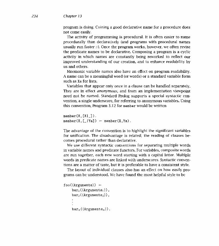
234 Chapter 13
program is doing. Coining a good declarative name for a procedure doesnot come easily.
The activity of programming is procedural. It is often easier to nameprocedurally than declaratively (and programs with procedural namesusually run faster :-). Once the program works, however, we often revisethe predicate names to be declarative. Composing a program is a cyclicactivity in which names are constantly being reworked to reflect ourimproved understanding of our creation, and to enhance readability byus and others.
Mnemonic variable names also have an effect on program readability.A name can be a meaningful word (or words) or a standard variable formsuch as Xs for lists.
Variables that appear only once in a clause can be handled separately.They are in effect anonymous, and from an implementation viewpointneed not be named. Standard Prolog supports a special syntactic con-vention, a single underscore, for referring to anonymous variables. Usingthis convention, Program 3.12 for member would be written
member(X, [XI_]).
member(X, 1_lYs]) member(X,Ys).
The advantage of the convention is to highlight the significant variablesfor unification. The disadvantage is related; the reading of clauses be-comes procedural rather than declarative.
We use different syntactic conventions for separating multiple wordsin variable names and predicate functors. For variables, composite wordsare run together, each new word starting with a capital letter. Multiplewords in predicate names are linked with underscores. Syntactic conven-tions are a matter of taste, but it is preferable to have a consistent style.
The layout of individual clauses also has an effect on how easily pro-grams can be understood. We have found the most helpful style to be
f oo((Arguments))
bari((Argumentsi)),
bar2 ((Arguments2)),
bar((Arguments)).

235 Program Development
The heads of all clauses are aligned, the goals in the body of a clauseare indented and occupy a separate line each. A blank line is insertedbetween procedures, but there is no space between individual clauses ofa procedure.
Layout in a book and the typography used are not entirely consistentwith actual programs. If all the goals in the body of a clause are short,then have them ori one line. Occasionally we have tables of facts withmore than one fact per line.
A program can be self-documenting if sufficient care is taken withthese two factors and the program is sufficiently simple. Given the nat-ural aversion of programmers to comments and documentation, this isvery desirable.
In practice, code is rarely self-documenting and comments are needed.One important part of the documentation is the relation scheme, whichcan be presented before the clauses defining that relation, augmentedwith further explanations if necessary. The explanations used in thisbook define the relation a procedure computes. It is not always easy tocome up with a precise, declarative, natural language description of arelation computed by a logic program. However, the inability to do sousually indicates that the programmer does not fu[ly understand thecreation, even if the creation actually works. Hence we encourage the useof the declarative documentation conventions adopted in this book. Theyare a good means of commurncating to others what a program defines aswell as a discipline of thought, enabling programmers to think about andreflect on their own creations.
13.2 Reflections on Program Development
Smce programming in pure Prolog is as close to writing specificationsas any practical programming language has gotten, one might hope thatpure Prolog programs would be bug-free. This, of course, is not the case.Even when axiomatizing one's concepts and algorithms, a wide spectrumof bugs, quite similar to ones found in conventional languages, can beencountered.
Stating it differently, for any formalism there are sufficiently com-plex problems for which there are no self-evidently correct formulations

236 Chapter 13
of solutions. The difference between low-level and high-level languages,then, is only the threshold after which simple examination of the pro-gram is insufficient to determine its correctness.
There are two schools of thought on what to do on such an occasion.The "verification" school suggests that such complex programs be ver-ified by proving that they behave correctly with respect to an abstractspecification. It is not clear how to apply this approach to logic programs,since the distance between the abstract specification and the program ismuch smaller then in other languages. If the Prolog axiomatization is notself-evident, there is very little hope that the specification, no matter inwhat language it is written, would be.
One might suggest using full first-order logic as a specification formal-ism for Prolog. It is the authors' experience that very rarely is a specifi-cation in full first-order logic shorter, simpler, or more readable then thesimplest Prolog program defining the relation.
Given this situation, there are weaker alternatives. One is to provethat one Prolog program, perhaps more efficient though more complex,is equivalent to a simpler Prolog program, which, though less efficient,could serve as a specification for the first. Another is to prove that a pro-gram satisfies some constraint, such as a "loop invariant," which, thoughnot guaranteeing the program's correctness, increases our confidence init.
In some sense, Prolog programs are executable specifications. The al-ternative to staring at them, trying to convince ourselves that they arecorrect, is to execute them, and see if they behave in the way we want.This is the standard testing and debugging activity, carried out in pro-gram development fri any other progranmiing language. All the classicalmethods, approaches, and common wisdom concerning program testingand debugging apply equally well to Prolog.
What is the difference, then, between program development in conven-tional, even symbolic languages and Prolog?
One answer is that although Prolog programming is "just" program-ming, there is some improvement in ease of expression and speed of de-bugging compared to other lower-level formalisms - we hope the readerhas already had a glimpse of it.
Another answer is that declarative programming clears your mind. Saidless dramatically, progranmiing one's ideas in general, and program-ming in a declarative and high-level language in particular, clarifies one's

237 Program Development
thoughts and concepts. For experienced Prolog programmers, Prolog isnot just a formalism for coding a computer, but also a formalism inwhich ideas can be expressed and evaluated - a tool for thinking.
A third answer is that the properties of the high-level formalism oflogic may eventually lead to practical program development tools thatare an order of magnitude more powerful then the tools used today.Examples of such tools are automatic program transformers, partial-evaluators, type inference programs, and algorithmic debuggers. The lat-ter are addressed in Section 17.3, where program diagnosis algorithmsand their implementation in Prolog are described.
Unfortunately, practical Prolog programming environments incorpo-rating these novel ideas are not yet widely available. In the meantime,a simple tracer, such as explained in Section 17.2, is most of what onecan expect. Nevertheless, large and sophisticated Prolog programs canbe developed even using the current Prolog environments, perhaps withgreater ease than ¡n other available languages.
The current tools and systems do not dictate or support a specificprogram development methodology. However, as with other symbolicprogramming languages, rapid prototyping is perhaps the most naturaldevelopment strategy. In this strategy, one has an evolving, usable pro-totype of the system in most stages of the development. Developmentproceeds by either rewriting the prototype program or extending it. An-other alternative, or complementary, approach to program developmentis "think top-down, implement bottom-up." Although the design of a sys-tem should be top-down and goal-driven, its implementation proceedsbest if done bottom-up. In bottom-up programming each piece of codewritten can be debugged immediately. Global decisions, such as repre-sentation, can be tested in practice on small sections of the system, andcleaned up and made more robust before most of the programming hasbeen done. Also, experience with one subsystem may lead to changes inthe design of other subsystems.
The size of the chunks of code that should be written and debugged asa whole varies and grows as the experience of the programmer grows. Ex-perienced Prolog programmers can write programs consisting of severalpages of code, knowing that what is left after writing is done is mostlysimple and mundane debugging. Less experienced programmers mightfind it hard to grasp the functionality and interaction of more then a fewprocedures at a time.

238 Chapter 13
We would like to conclude this section with a few moralistic state-ments. For every programming language, no matter how clean, elegant,and high-level, one can find programmers who will use it to write dirty,contorted, and unreadable programs. Prolog is no exception. However,we feel that for most problems that have an elegant solution, there is anelegant expression of that solution in Prolog. It is a goal of this book toconvey both this belief and the tools to realize it in concrete cases, byshowing that aesthetics and practicality are not necessarily opposed orconflicting goals. Put even more strongly, elegance is not optional.
13.3 Systematizing Program Construction
The pedagogic style of this book is to present well-constructed programsillustrating the important Prolog programming techniques. The examplesare explained in sufficient detail so that readers can apply the techniquesto construct similar programs to meet their own programming needs.Implicitly, we are saying that Prolog programming is a skill that can belearned by observing good examples and abstracting the principles.
Learning by apprenticeship, observing other programs, is not the onlyway. As experience with programming in Prolog accumulates, more sys-tematic methods of teaching Prolog programming are emerging. Theemergence of systematic methods is analogous to the emergence ofstructured programniing and stepwise refinement in the early 1970s af-ter sufficient experience had accumulated in writing programs in thecomputer languages of the 19 SOs and 1960s.
In this section, we sketch a method to develop Prolog programs. Thereader is invited to reconstruct for herself how this method could be ap-plied to develop the programs in Parts III and IV of this book. Underlyingthe method is a desire to provide more structure to Prolog programs sothat software components can be reused and large applications can beroutinely maintained and extended.
Central to the method is identifying the essential flow of control of aprogram. A program embodying a control flow is called a skeleton. Extragoals and arguments can be attached to a skeleton. The extra goals andarguments are entwined around the central flow of control and performadditional computations. The program containing the extra arguments

239 Program Development
and goals is called an enhancement of the skeleton. Building an enhance-ment from a skeleton will be called applying a technique.
For example, consider Program 8.6a for summing a list of numbers,reproduced here:
sumlist([XIXs],Sum) - sumlist(Xs,XsSum), Sum is X+XsSum.
sumlist([ 1,0).
The control flow embodied ni the suinlist program is traversing thelist of numbers. The skeleton is obtained by dropping the second ar-gument completely, restricting to a predicate with one argument, andremoving goals that only pertain to the second argument. This gives thefollowing program, which should be identifiable as Program 3.11 definrnga list.
list([XIXs]) - list(Xs).
list([ 1).
The extra argument of the sunilist program calculates the sum ofthe numbers in the list. This form of calculation is very common andappeared in several of the examples in Chapter 8.
Another enhancement of the list program is Program 8.11 calculatingthe length of a list. There is a clear similarity between the programsfor length and sumuist. Both use a similar technique for calculating anumber, in one case the sum of the numbers in the list, in the second thelength of the list.
length([XIXs],N) - length(Xs,N1), N is N1+1.
length([ 1,0).
Multiple techniques can be applied to a skeleton. For example, we canapply both sunirning elements and counting elements in one pass to getthe program sum_length:
suni_length([XIXs] ,Sum,N) -
suxnlist(Xs,XsSuni,N1), Sum is X+XsSum, N is N1+1.
sum_length([ 1,0,0).
Intuitively, it is straightforward to create the sum_length programfrom the programs for sumuist and length. The arguments are takendirectly and combined to give a new program. We call this operation com-position. In Chapter 18, a program for composition is presented.

240 Chapter 13
Another example of a technique is adding a pair of arguments as anaccumulator and a final result. The technique is informally described inSection 7.5. Applying the appropriate version of the technique to thelist skeleton can generate Program 8.6b for sumlist or the iterativeversion of length, which is the solution to Exercise 8.3(vii).
Identifying control flows of programs may seem contradictory to theideal of declarative progranmiing espoused in the previous section. How-ever, at some level programming is a procedural activity, and describ-ing well-written chunks of code is fine. It is our belief that recognizingpatterns of programs makes it easier for people to develop good style.Declarativeness is preserved by ensuring wherever possible that each en-hancement produced be given a declarative reading.
The progranuning method called stepwise enhancement consists ofthree steps:
Identify the skeleton program constituting the control flow.Create enhancements using standard programming techniques.Compose the separate enhancements to give the final program.
We illustrate stepwise enhancement for a simple example - calculat-ing the union and intersection of two lists of elements. For simplicity weassume that there are no duplicate elements in the two lists and that wedo not care about the order of elements in the answer.
A skeleton for this program follows. The appropriate control flow is totraverse the first list, checking whether each element is a member or notof the second list. There will be two cases:
skel([XIXs],Ys) - mernber(X,Ys), skel(Xs,Ys).
skel([XIXs],Ys) - nonmember(X,Ys), skel(Xs,Ys).
skel([ ],Ys).
To calculate the union, we need a third argument, which can be builttop-down in the style discussed in Section 7.5. We consider each clausein turn. When an element in the first list is a member of the second list,it is not included in the union. When an element in the first list is nota member of the second list, it is included in the union. When the firstlist is empty, the union is the second list. The enhancement for union isgiven as Program 13.1.

241 Program Development
union(Xs,Ys,Us)Us is the union of the elements ¡n Xs and Ys.
union([XIXs] ,Ys,Us) .- member(X,Ys), union(Xs,Ys,Us).union([XIXs],Ys,[XIUs]) nonmember(X,Ys), unïon(Xs,Ys,Us).union([ ],Ys,Ys).
Program 13.1 Finding the union of two lists
intersect (Xs, Ys,Is) -Is is the intersection of the elements in Xs and Ys.
intersect([XIX$],Ys,[XIIs]) - mernber(X,Ys), intersect(Xs,Ys,Is).intersect([XIXS],Ys,Is) - nonniember(X,Ys), intersect(Xs,Ys,Is).intersect([ 1,Ys,[ 1).
Program 13.2 Finding the intersection of two lists
union_intersect (Xs, Ys, Us,Is)Us and Is are the union and intersection, respectively, of theelements in Xs and Ys.
union_intersect([XIXs] ,Ys,Us, EXils]) -inernber(X,Ys) , union_intersect(Xs,Ys,Us,Is)
union_intersect([XIXs] ,Ys, [XIUs] ,Is)nonniember(X,Ys), union_intersect(Xs,Ys,Us,Is)
union_intersect([ ],Ys,Ys,[ 1)
Program 13.3 Finding the union and intersection of two lists
The intersection, given as Program 13.2, is determined with a similartechnique. We again consider each clause in turn. When an element in thefirst list is a member of the second list, it is included in the intersection.When an element in the first list is not a member of the second list, itis not included in the intersection. When the first list is empty, so is theintersection.
Calculating both the union and the intersection can be determined in asingle traversal of the first list by composing the two enhancements. Thisprogram is given as Program 13.3.
Developing a program is typically straightforward once the skeletonhas been decided. Knowing what skeleton to use is less straightforward

242 Chapter 13
and is learned by experience. Experience is necessary for any design task.By splitting up the program development into three steps, however, thedesign process is simplified and given structure.
A motivation behind giving programs structure, as is done by stepwiseenhancement, is to facilitate program maintenance. It is easy to extenda program by adding new techniques to a skeleton, and it is possible toimprove programs by changing skeletons while maintaining techniques.Further, the structure makes it easy to explain a program.
Skeletons and techniques can be considered as constituting reusablesoftware components. This will be illustrated in Chapter 17, where thesame skeleton meta-interpreter is useful both for program debuggingand for expert system shells.
Having raised software engineering issues such as maintainability andreusabiity, we conclude this chapter by examining two other issues thatmust be addressed if Prolog is to be routinely used for large softwareprojects. The place of specifications should be clarified, and modules arenecessary if code is to be developed in pieces.
It is clear from the previous section that we do not advocate usingfirst-order logic as a specification language. Still, it is necessary to havea specification, that is, a document explaining the behavior of a programsufficiently so that the program can be used without the code having tobe read. We believe that a specification should be the primary form ofdocumentation and be given for each procedure in a program.
A suggested form for a specification is given in Figure 13.1. It consistsof a procedure declaration, effectively giving the name and arity of thepredicate; a series of type declarations about the arguments; a relationscheme; and other important information such as modes of use of thepredicate and multiplicities of solutions in each mode of use. We discusseach component in turn.
Types are emerging as important in Prolog programs. An untyped lan-guage facilitates rapid prototyping and interactive development, but formore systematic projects, imposing types is probably worthwhile.
The relation scheme is a precise statement in English that explains therelation computed by the program. All the programs in this book havea relation scheme. It should be stressed that relation schemes must beprecise statements. We believe that proving properties of programs willproceed in the way of mathematics, where proofs are given by precisestatements in an informal language.

243 Program Development
procedure p(Tj,T2 .....T)Types: T1: type I
T2: type 2
T: type nRelation scheme:
Modes of use:
Multiplicities of' solution:
Figure 13.1 Template for a specification
Prolog programs inherit from logic programs the possibility of be-ing multi-use. In practice, multi-use is rare. A specification should statewhich uses are guaranteed to be correct. That is the purpose of themodes of use component in Figure 13.1. Modes of use are specified bythe instantiation state of arguments before and after calls to the predi-cate.
For example, the most common mode of use of Program 3.15 for ap-pend(Xs,Ys,Zs) for concatenating two lists Xs and Ys to produce a listZs is as follows. Xs and Ys are instantiated at the time of call, whereasZs is not, and all three arguments are instantiated after the goal suc-ceeds. Calling append/3 with all three arguments instantiated is a dif-ferent mode of use. A common convention, taken from DEC-10 Prologis to use + for an instantiated argument, - for an uninstantiated argu-ment, and? for either. The modes for the preceding use of append areappend(+, +, ) before the call and append(+, +, +) after the call.
More precise statements can be made by combining modes with types.The mode of use of the current example becomes the following: Beforethe call the first two arguments are complete lists and the third a vari-able; after the call all three arguments are complete lists.
Multiplicities are the number of solutions of the predicate, and shouldbe specified for each mode of use of the program. lt is useful to giveboth the minimum and maximum number of solutions of a predicate.The multiplicities can be used to reason about properties of the program.
Modules are primarily needed to allow several people to work on aproject. Several programmers should be able to develop separate compo-nents of a large system without worrying about undesirable interactions

244 Chapter 13
such as conflict of predicate names. What is needed is a mechanism forspecifying what is local to a module and which predicates are importedand exported.
Current Prolog systems provide primitive facilities for handling mod-ules. The current systems are either atom-based or predicate-based, de-pending on what is made local to the module. Directives are provided forspecifying imports and exports. Experience is growing in using existingmodule facilities, which will be translated into standards for modulesthat will ultimately be incorporated into Standard Prolog. The currentdraft on modules in Standard Prolog is in too much flux to describe here.The user needing modules should consult the relevant Prolog manual.
Exercises for Section 13.3
Enhance Program 13.3 to build the list of elements contained in thefirst list but not in the second list.
Write a program to solve the following problem. Given a binary treeT with positive integers as values, build a tree that has the samestructure as T but with every node replaced by the maximum valuein the tree. It can be accomplished with one traversal of the tree.(Hint: Use Program 3.23 as a skeleton.)
Write a program to calculate the mean and mode of an ordered listof numbers in one pass of the list.
13.4 Background
Commenting on Prolog programming style has become more prevalent inrecent Prolog textbooks. There are useful discussions in both Ross (1989)and O'Keefe (1990). The latter book also introduces program schemas,which have parallels with skeletons and techniques.
Stepwise enhancement has emerged from ongoing work at Case West-ern Reserve University, first in the COMPOSERS group and more recentlyin the ProSE group. Examples of decomposing Prolog programs intoskeletons and techniques are given in Sterling and Kirschenbaum (1993)and presented in tutorial form in Deville, Sterling, and Deransart (1991).

245 Program Development
Underlying theory is given in Power and Sterling (1990) and Kirschen-baum, Sterlmg, and fain (1993). An application of structuring Prologprograms using skeletons and techniques to the inductive inference ofProlog programs can be found in Kirschenbaum and Sterling (1991).
Automatic incorporation of techniques into skeletons via partial evalu-ation has been described in Lakhotia (1989).
The discussion on specifications for Prolog programs is strongly influ-enced by Deville (1990).
Exercise 13.3(11) was suggested by Giles Kahn. The example is orig-inally due to Bird. Exercise 13.3(iii) emerged through interaction withMarc Kirschenbaum. Solutions to both exercises are given in Deville, Ster-ling, and Deransart (1991).

Leonardo Da Vinci. Study of a Woman 's Hands folded over her Breast. Silver-point on pink prepared paper, heightened with white. About 1478. WindsorCastle, Royal Library.

1H Advanced Prolog Programming Techniques
The expressive power and high-level nature of logic programming canbe exploited to write programs that are not easily expressed in conven-tional programming languages. Different problem-solving paradigms canbe supported, and alternative data construction and access mechanismscan be used.
The simple Prolog programs of the previous part are examples of theuse of basic programming techniques, reinterpreted ni the context oflogic programming This part collects more advanced techniques thathave evolved ni the logic programming community and exploit the spe-cial features of logic programs. We show how they can be used to advan-tage.


14 Nondeterniinistic Prograniming
One feature of the logic programming computation model lacking in con-ventional programming models is nondetermiriism. Nondeterminism isa technical concept used to define, in a concise way, abstract computa-tion models. However, in addition to being a powerful theoretical con-cept, nondeterminism is also useful for defining and implementmg algo-rithms. This chapter shows how, by thinking nondeterministically, onecan construct concise and efficient programs.
Intuitively, a nondeterministic machine can choose its next operationcorrectly when faced with several alternatives. True nondeterministicmachines cannot be realized but can be simulated or approximated. Inparticular, the Prolog interpreter approximates the nondeterministic be-havior of the abstract interpreter of logic programs by sequential searchand backtracking, as explained in Chapter 6. However, the fact that non-determinism is only simulated without being "really present" can be ab-stracted away in many cases in favor of nondeterministic thinking inmuch the same way as pointer manipulation details involved in unifica-tion can be abstracted away in favor of symbolic thinking.
14.1 Generate-and-Test
Generate-and-test is a common technique in algorithm design and pro-gramming Here is how generate-and-test works for problem solving. Oneprocess or routine generates candidate solutions to the problem, and an-other process or routine tests the candidates, trying to find one or allcandidates that actually solve the problem.

250 Chapter 14
It is easy to write logic programs that, under the execution model ofProlog, implement the generate-and-test technique. Such programs typi-cally have a conjunction of two goals, in which one acts as the generatorand the other tests whether the solution is acceptable, as in the followingclause:
f ind(X) - generate(X), test(X).
This Prolog program would actually behave like a conventional, procedu-ral, generate-and-test program. When called with f ind(X)?, generate (X)
succeeds, returning some X, with which test (X) is called. If the test goalfails, execution backtracks to generate (X), which generates the nextelement. This continues iteratively until the tester successfully finds asolution with the distinguishing property or until the generator has ex-hausted all alternative solutions.
The programmer, however, need not be concerned with the generate-and-test cycle and can view this technique more abstractly, as an instanceof nondetermirilstic programming. In this nondeterministic program thegenerator guesses correctly an element in the domain of possible solu-tions, and the tester simply verifies that the guess of the generator iscorrect.
A good example of a program with multiple solutions and com-monly used as a generator is Program 3.12 for member. The query mem-
ber(X, [a,b,c])? will yield the solutions X=a, X=b, and X=c successivelyas required. Thus member can be used to nondeterministically choose thecorrect element of a list in a generate-and-test program.
Program 14.1 is a simple example of generate-and-test using mem-
ber as a generator. The program identifies parts of speech of a sen-tence. We assume that a sentence is represented as a list of wordsand that there is a database of facts giving the parts of speech ofparticular words. Each part of speech is a unary predicate whoseargument is a word, for example, noun (man) indicates that man is anoun. The relation verb(Sentence,Word) is true if Word is a verb insentence Sentence. The analogous meanings are intended for noun/2
and article/2. The query verb([a,man,loves,a,woman],V)? findsthe verb V'loves in the sentence using generate-and-test. Wordsin the sentence are generated by member and tested to see if they areverbs.

251 Nondeterministic Programming
verb(Sentence,Verb) -Verb is a verb in the list of words Sentence.
verb(Sentence ,Word) - mernber(Word,Sentence), verb(Word).
noun(Sentence,Word) - member(Word,Sentence), noun(Word).
article(Sentence,Word) - member(Word,Sentence) , article(Word)
Vocabulary
noun (man) . noun (woman)
article (a). verb(loves).
member(X,Xs) '- SeeProgram3.12.
Program 14.1 Finding parts of speech in a sentence
Another simple example is testing whether two lists have an elementin common. Consider the predicate intersect (Xs,Ys), which is true ifXs and Ys have an element in common:
intersect(Xs,Ys) - member(X,Xs), member(X,Ys).
The first member goal in the body of the clause generates membersof the first list, which are then tested to see whether they are in thesecond list by the second member goal Thinking nondeterrninistically, thefirst goal guesses an X in Xs, and the second verifies that the guess is amember of Ys.
Note that when executed as a Prolog program, this clause effectivelyimplements two nested loops, The outer ioop iterates over the elementsof the first list, and the irmer loop checks whether the chosen element isa member of the second list. Hence this nondetermiriistic logic programachieves, under the execution model of Prolog, a behavior very similar tothe standard solution one would compose for this problem in Fortran,Pascal, or Lisp.
The definition of member in terms of append,
member(X,Xs) - append(As, [X lBs] ,Xs).
is itself essentially a generate-and-test program. The two stages, how-ever, are amalgamated by the use of unification. The append goal gen-erates splits of the list, and immediately a test is made whether the firstelement of the second list is X.
Typically, generate-and-test programs are easier to construct than pro-grams that compute the solution directly, but they are also less efficient.

252 Chapter 14
A standard technique for optimizing generate-and-test programs is to"push" the tester inside the generator as deeply as possible. Ultimately,the tester is completely intertwined with the generator, and only correctsolutions are generated.
Let us consider optimizing generate-and-test programs by pushing thetester into the generator. Program 3.20 for permutation sort is anotherexample of a generate-and-test program. The top level is as follows:
sort(Xs,Ys) - permutation(Xs,Ys), ordered(Ys).
Abstractly, this program guesses nondeterministically the correct permu-tation via permutation(Xs,Ys), and ordered checks that the permuta-tion is actually ordered.
Operationally, the behavior is as follows. A query involving sort is re-duced to a query involving permutation and ordered. A failure-drivenloop ensues. A permutation of the list is generated by permutation andtested by ordered. If the permuted list is not ordered, the executionbacktracks to the permutation goal, which generates another permuta-tion to be tested. Eventually an ordered permutation is generated andthe computation terminates.
Permutation sort is a highly inefficient sorting algorithm, requiringtime super-exponential in the size of the list to be sorted. Pushing thetester into the generator, however, leads to a reasonable algorithm. Thegenerator for permutation sort, permutation, selects an arbitrary ele-ment and recursively permutes the rest of the list. The tester, ordered,verifies that the first two elements of the permutation are in order, thenrecursively checks the rest. If we view the combined recursive permuta-
tion and ordered goals as a recursive sorting process, we have the basisfor insertion sort, Program 3.21. To sort a list, sort the tail of the list andinsert the head of the list into its correct place in the order. The arbitraryselection of an element has been replaced by choosing the first element.
Another example of the advantage of intertwining generating and test-ing can be seen with programs solving the N queens problem.
The N queens problem requires the placement of N pieces on an N-by-N rectangular board so that no two pieces are on the same line: hori-zontal, vertical, or diagonal. The original formulation called for 8 queensto be placed on a chessboard, and the criterion of not being on the sameline corresponds to two queens not attacking each other under the rulesof chess. Hence the problem's name.

253 Nondeterministic Programming
QII Q
Q
Figure 14.1 A solution to the 4 queens problem
queens(N,Queens)Queens is a placement that solves the N queens problem,represented as a permutation of the list of numbers 11,2,... ,N1.
queens(N,Qs)rane(1,N,Ns), permutation(Ns,Qs), safe(Qs).
safe(Qs) -The placement Qs is safe.
safe([QIQs]) - safe(Qs), not attack(Q,Qs).safe([ ]).attack(X,Xs) - attack(X,1,Xs).attack(X,N,[YIYs]) - X is Y+N X is Y-N.attack(X,N,[YIYs]) Nl is N+l, attack(X,Nl,Ys).permutation(Xs,Ys) - See Program 3.20.rarige(M,N,Ns) - See Program 8.12.
Program 14.2 Naive generate-and-test program solving N queens
The program has been well studied in the recreational mathematics lit-erature. There is no solution for N = 2 and N 3, and a unique solutionup to reflection for N = 4, shown in Figure 14.1. There are 88 solutionsfor N = 8, or 92, depending on strictness with symmetries.
Program 14.2 is a simplistic program solving the N queens problem.The relation queen (N,Qs) is true if Qs is a solution to the N queens prob-lem. Solutions are specified as a permutation of the list of the numbers ito N. The first element of the lìst is the row number to place the queen inthe first column, the second element indicates the row number to placethe queen in the second column, etc. Figure 14.1 indicates the solution12,4,1,3] to the 4 queens problem. This specification of solutions, and

254 Chapter 14
the program generating them, has implicitly incorporated the observa-tion that any solution to the N queens problem will have a queen on each'row and a queen on each colunm.
The program behaves as follows. The predicate range creates a listNs of the numbers from i to N. Then a generate-and-test cycle begins.The permutation predicate generates a permutation Qs of Ns, which istested to see whether it is a solution to the problem with the predi-cate safe(Qs). This predicate is true if Qs is a correct placement of thequeens. Since two queens are not placed on the same row or colunm, thepredicate need only check whether two queens attack each other along adiagonal. Safe is defined recursively. A list of queens is safe if the queensrepresented by the tail of the list are safe and the queen represented bythe head of the list does not attack any of the other queens. The def-inition of attack(Q , Qs) uses a neat encapsulation of the interaction ofdiagonals. A queen is on the same diagonal as a second queen N columnsaway if the second queen's row number is N units greater than, or Nunits less than, the first queen's row number. This is expressed by thefirst clause of attack/3 in Program 14.2. The meaning of attack(Q,Qs)is that queen Q attacks some queen in Qs. The diagonals are tested itera-tively until the end of the board is reached.
Program 14.2 cannot recognize when solutions are symmetric. Theprogram gives two solutions to the query queens(4,Qs)?, namelyQs=[2,4,1,3] and Qs=[3,1,4,2].
Although it is a well-written logic program, Program 14.2 behaves inef-ficiently. Many permutations are generated that have no chance of beingsolutions. As with permutation sort, we improve the program by pushingthe tester, in this case safe, into the generator.
Instead of testing the complete permutation, that is, placing all thequeens, each queen can be checked as it is being placed. Program 14.3computes solutions to the N queens problem by placing the queens oneat a time. It also proceeds by generating and testing, in contrast to inser-tion sort, which became a deterministic algorithm by the transformation.The generator in the program is select and the tester is attack, or moreprecisely its negation.
The positions of the previously placed queens are necessary to testwhether a new queen is safe. Therefore the final solution is built upwardusing an accumulator. This is an application of the basic technique de-scribed in Section 7.5. A consequence of using an accumulator is that thequeens are placed on the right-hand edge of the board. The two solu-

255 Nondeterministic Programming
queens(N,Queens) -Queens is a placement that solves the N queens problem,represented as a permutation of the list of numbers [1,2.....NJ.
queens(N,Qs) - range(1,N,Ns), queeris(Ns,[ ],Qs).queens (UriplacedQs , SaÍeQs , Qs)
select (Q ,Unplacedqs ,UnplacedQsl),not attack(Q,SaÍeQs),queens (UnplacedQsl, [QISafeQs] ,Qs).
queens([ ],Qs,Qs).select(X,Xs,Ys) - SeeProgram3.19.attack(X,Xs) - See Program 14.2.
Program 14.3 Placing one queen at a time
Figure 14.2 A map requiring four colors
tions to the query queens(4,Qs)? are given in the opposite order to thesolutions given by Program 14.2.
The next problem is to color a planar map so that no two adjoining re-gions have the same color. A famous conjecture, an open question for ahundred years, was proved in 1976, showing that four colors are suffi-cient to color any planar map. Figure 14.2 gives a simple map requiringfour colors to be colored correctly. This can be proved by enumeration ofthe possibilities. Hence four colors are both necessary and sufficient.
Program 14.4, which solves the map-coloring problem, uses thegenerate-and-test programming technique extensively. The program im-plements the following nondeterministic iterative algorithm:
For each region of the map,choose a color,choose (or verify) colors for the neighboring regions from the
remaining colors.

256 Chapter 14
color_map (Map,Colors) -Map is colored with Colors so that no two neighbors have the same
color. The map is represented as an adjacency-list of regions
region(Name,Color,Neighbors), where Name is the name of the
region, Color is its color, and Neighbors are the colors of its
neighbors.
color_map([RegionlRegions] ,Colors) -
color_region(Region,Colors),
color_map(Regions Colors).
color_map( E I Colors).
color_region (Region, Colors) -Region and its neighbors are colored using Colors so that the
region's color is different from the color of any of its neighbors.
color_region(region(Name,Color,Neighbors) Colors) -
select (Color Colors ,Colorsl),
members (Neighbors ,Colorsi).
select(X,Xs,Ys) See Program 3.19.
members(Xs,Ys) See Program 7.6.
Program 14.4 Map coloring
A data structure is needed to support the algorithm. The map is repre-sented as a list of regions. Each region has a name, a color, and a list ofcolors of the adjoining regions. The map in Figure 14.2, for example, isrepresented as
[region(a,A, [B,C,D]) ,region(b,B, [A,C,E]),
region(c,C, [A,B,D,E,F]) ,region(d,D, [A,C,F]),
region(e,EJB,C,F]),region(f,F,[C,D,E])].
The sharing of variables is used to ensure that the same region is notcolored with two different colors by different iterations of the algorithm.
The top-level relation is color_map (Map,Colors), where Map is repre-sented as before, and Colors is a list of colors used to color the map.Our colors are red, yellow, blue, and white. The heart of the algorithm isthe definition of color_region(Region,Colors):
color_region(region(Nanie,Color,Neighbors) ,Colors) -
select (Color,Colors,Colorsl), members(Neighbors,Colorsl).

257 Nondeterministic Programming
Test datatest_color(Name,Map)
map (Name , Map)
colors (Naine,Colors)color_map (Map,Colors)
map(test, [region(a,A, [B,C,D]),region(b,B, [A,C,E]),region(c,C,[A,B,D,E,F]),region(d,D,[A,C,F]),region(e,E, [B,C,F]),region(f,F, [C,D,E])]).
map(west_europe, [region(portugal ,P, [E]), region(spain,E, [F,PI),region(fraiice,F,[E,I,S,B,WG,L]), region(belgiuxn,B,[F,H,L,WG]),regïon(holland,H,[B,WG]), region(west_germa.ny,WG,[F,A,S,H,B,L]),region(luxembourg,L,[F,B,WG]), region(italy,I,[F,A,S]),region(switzerland,S,[F,I,A,WG]), region(austria,A,[I,S,WG])]).
colors(X, [red,yellow,blue,white])
Program 14.3 Test data for map coloring
Both the select and members goals can act as generators or testers,depending on whether their arguments are instantiated.
Overall, the effect of the program is to instantiate a data structure, themap. The calls to select and members can be viewed as specifying localconstraints. The predicates either generate by instantiating arguments inthe structure or test whether instantiated values satisfy local constraints.Program 14.5 tests the map coloring solution.
Instantiating a data structure designed especially for a problem is aparticularly effective means of implementing generate-and-test solutions.Unification and failure to unify control the building of the final solutionstructure, avoiding creation of unnecessary intermediate data structures.Since unification is supported well by Prolog implementations, solutionsare found quickly. Exercise 14.1(iv) assigns the task of designing a datastructure that can be instantiated to solve the N queens problem. Theresulting program solves the N queens problem much more quickly thanProgram 14.3.
Our final example is solving a logic puzzle. The behavior of the pro-gram is similar to the map-coloring program. The logic puzzle consistsof some facts about some small number of objects that have various at-tributes. The minimum number of facts is given about the objects andattributes, to yield a unique way of assigning attributes to objects.

258 Chapter 14
Here is an example that we use to describe the technique of solvinglogic puzzles.
Three friends came first, second, and third iii a programming competi-tion. Each of the three has a different first name, likes a different sport,and has a different nationality.
Michael likes basketball and did better than the American. Simon, theIsraeli, did better than the tennis player. The cricket player came first.
Who is the Australian? What sport does Richard play?Logic puzzles such as this one are elegantly solved by instantiating
the values of a suitable data structure and extracting the solution val-ues. Each clue is translated into a fact about the data structure. This canbe done before the exact form of the data structure is determined usingdata abstraction. Let us analyze the first clue: "Michael likes basketballand did better than the American." Two distinct people are referred to.One is named Michael, whose sport is basketball, and the other is Amer-ican. Further, Michael did better than the American. If we assume thestructure to be instantiated is Friends, then the clue is expressed as theconjunction of goals
did_better(Nanl,Man2,Friends), f irst_name(Manl,michael),
sport(Manl,basketball), nationality(Man2,arnerican),
Similarly, the second clue can be translated to the conditions
did_better(Nani,Man2,Friends), f irst_name(Manl,sinion),
nationality(Manl,israeli), sport(Man2,tennis),
and the third clue to the conditions
f irst(Friends,Man), sport(Man,cricket).
A framework for solving puzzles is given as Program 14.6. The rela-tion computed is solve_puzzle(Puzzle,Solution), where Solution is
the solution to Puzzle. The puzzle is represented by the structure puz-zle(Clues,Queries,Solution), where the data structure being instan-tiated is incorporated into the clues and queries, and the values to beextracted are given by Solution.
The code for solve_puzzle is trivial. All it does is successively solveeach clue and query, which are expressed as Prolog goals and are exe-cuted with the meta-variable facility.
The clues and queries for our example puzzle are given in Program14.7. We describe the structure assumed by the clues to solve the puzzle.

259 Nondetermiriistic Programming
solve_puzzle(Puzzle,Solution) -Solution is a solution of Puzzle,where Puzzle is puzzle (Clues, Queries,Solution).
solve_puzzle (puzzle(Clues,Queries,Solution) ,Solution) -
solve (Clues)
solve (Queries)
solve([CluelClues]) -
Clue, solve(Clues).
solve([ I).
Program 14.6 A puzzle solver
Each person has three attributes and can be represented by the structurefriend(Name,Country,Sport). There are three friends whose order inthe progranmiing competition is significant. This suggests an orderedsequence of three elements as the structure for the problem, ì.e., the list
[friend(Nl,C1,S1),friend(N2,C2,S2),friend(N3,C3,S3)].
The programs defining the conditions did_better, first_name, na
tionality, sport, and first are straightforward, and are given inProgram 14.7.
The combination of Programs 14.6 and 14.7 works as a giant generate-and-test. Each of the did_better and member goals access people, andthe remaining goals access attributes of the people. Whether they aregenerators or testers depends on whether the arguments are instanti-ated or not. The answer to the complete puzzle, for the curious, is thatMichael is the Australian, and Richard plays tennis.
The puzzle given in Program 14.7 is simple An interesting question ishow well does the framework of Program 14.6 scale. A good example of alarger puzzle is given in Exercise 14.1(vi). Is the framework adequate forsuch a puzzle?
The short answer is yes. Prolog is an excellent language for solvinglogic puzzles. However, care must be taken when formulating the cluesand queries. For example, the predicate member is often essential to spec-ify inclivìduals, as is done to formulate the query in Program 14.7. lt maybe tempting to become systematic and begin the puzzle solution by spec-ifying all individuals by member goals. This can lead to very inefficientprograms because too many choice-points are set up. In general, implicitchecking of a condition is usually more efficient. Another observation is

260 Chapter 14
Test data
test_puzzle (Name ,Solution) -
structure (Name ,Structure),
clues (Name ,Structure, Clues)
queries (Name ,Structure, Queries ,Solution),
solve_puzzle (puzzle (Clues, Queries ,Solution) ,Solution).
structure(test, [friend(N1,C1,S1),friend(N2,C2,S2),friend(N3,C3,S3)]).
clues(test ,Friends,
[(did_better (ManiCluel ,Man2Cluel ,Friends), 'h Clue i
first_name (ManiCluel michael), sport(ManlCluei basketball),
nationality (Man2Cluel american)),
(did_better(ManlClue2,Man2Clue2,Friends), X Clue 2
first_name (ManlClue2, simon), nationality(ManlClue2, israeli),
sport (Man2Clue2 ,tennis)),
(first(Friends,ManClue3), sport(ManClue3,cricket)) X Clue 3
])
queries (test, Friends,
[ member(Qi,Friends),
first_name(Q1,Name),
nationality(Qi australian), 'h Query i
member(Q2,Friends),
first_naine(Q2,richard)
sport(Q2,Sport) X Query 2
[['The Australian is ', Name] ['Richard plays ', Sport]]
did_better(A,B, [A,B,C]).
did_better(A,C, [A,B,C]).
did_better(B,C,[A,B,C]).
first_name(friend(A,B,C) ,A).
nationality(friend(A,B,C) B).
sport (friend(A,B,C) ,C).
f irst ( [X IXs] , X)
Program 14.7 A description of a puzzle

261 Nondeterministic Programming
that the order of the goals in the queries can significantly affect run-ning time. It is best to worry about this once the problem formulationis correct. Determining appropriate goal order is a skill easily learned byexperience.
Another tip concerns negative clues, such as "John is not the tailor."These clues are best regarded as specifying two separate individuals,John and the tailor, rather than as setting up a negative condition aboutone individual. The predicate select can be used instead of member toguarantee that individuals are different.
Exercises for Section 14.1
(i) Write a program to compute the integer square root of a natu-ral number N defined to be the number I such that j2 < N, but(I + 1)2 > N. Use the predicate between/3, Program 85, to generatesuccessive natural numbers on backtracking.
(II) Write a program to solve the stable marriage problem (Sedgewick,1983), stated as follows:
Suppose there are N men and N women who want to get married. Eachman has a list of all the women in his preferred order, and each womanhas a list of all the men in her preferred order. The problem is to find aset of marriages that is stable.A pair of marriages is unstable if there are a man and woman whoprefer each other to their spouses. For example, consider the pair ofmarriages where David is married to Paula, and Jeremy is married toJudy. If David prefers Judy to Paula, and Judy prefers David to Jeremy,the pair of marriages is unstable. This pair would also be unstable ifJeremy preferred Paula to Judy, and Paula preferred Jeremy to David.A set of marriages is stable if there is no pair of unstable marriages.
Your program should have as input lists of preferences, and pro-duce as output a stable set of marriages. It is a theorem from graphtheory that this is always possible. Test the program on the follow-ing five men and five women with their associated preferences:
avraham: chana tamar zvia ruth sarahbinyamin: zvia chana ruth sarah tamarchaim: chana ruth tamar sarah zviadavid: zvia ruth chana sarah tamarelazar: tamar ruth chana zvia sarah

262 Chapter 14
zvia: elazar avraham david binyamin chaimchana: david elazar binyamin avraham chaimruth: avraham david binyamin chaim elazarsarah: chaim binyamin david avraham elazartamar: david binyamin chaim elazar avraham
Use Program 14.4 to color the map of Western Europe. The coun-tries are given in Program 14.5.
Design a data structure for solving the N queens problem by instan-tiation. Write a program that solves the problem by instantiatingthe structure.
(y) Explain why the following program solves the N queens problem:
queens (N, Qs)
gen_list(N,Qs), place_queens(N,Qs,Ups,Downs).
gen_list(O,[ 1).gen_list(N,[QIL]) - N > O, Nl is N-1, gen_list(N1,L).
place_queens (O,Qs ,Ups,Downs).
place_queens(I,Qs,Ups, [DlDowns]) -
I > O, Il is I-1,
place_queens(I1,Qs, [UlUps] ,Downs),
place_queen(I ,Qs,Ups,Downs).
place_queen(Q, [QIQs] , [QiUpsi , [QlDowns]).
place_queen(Q, [Q1IQs], [UlUps] , [DlDowns] -
place_queen(Q,Qs ,Ups,Downs).
(vi) Write a program to solve the following logic puzzle. There are fivehouses, each of a different color and inhabited by a man of a differ-ent nationality, with a different pet, drink, and brand of cigarettes.
The Englishman lives in the red house.
The Spaniard owns the dog.
Coffee is drunk in the green house.
The Ukrainian drinks tea.

263 Nondeterministic Programming
The green house is immediately to the right (your right) of theivory house.
The Winston smoker owns snails.
Kools are smoked in the yellow house.
Milk is drunk in the middle house.
The Norwegian lives in the first house on the left.
The man who smokes Chesterfields lives in the house next tothe man with the fox.
Kools are smoked in the house next to the house where thehorse is kept.
(1) The Lucky Strike smoker drinks orange juice.
The Japanese smokes Parliaments.
The Norwegian lives next to the blue house.
Who owns the Zebra? Who drinks water?
(vii) Write a program to test whether a graph is planar using the algo-rithm of Hoperoft and Tarjan (Deo, 1974; Even, 1979).
14.2 Don't-Care and Don't-Know Nondeterminism
Two forms of nondeterminism are distinguished in the logic program-ming literature. They differ in the nature of the choice that must be madeamong alternatives. For don't-care nondeterminism, the choice can bemade arbitrarily. In terms of the logic programming computation model,any goal reduction will lead to a solution, and it does not matter whichparticular solution is found. For don't-know nondeterminism, the choicematters but the correct one is not known at the time the choice is made.
Most examples of don't-care nondeterminism are not relevant for theProlog programmer. A prototypical example is the code for minimum.Program 3.7 is the standard, incorporating a limited amount of don't-carenondetermïriism, namely, when X and Y are the same:

264 Chapter 14
minimum(X,Y,X) - X Y.
minimum(X,Y,Y) - Y X.
In Section 7.4, we termed this redundancy and advised against its use.On the other hand, programs exhibiting don't-know nondeterminism
are common. Consider the program for testing whether two binary treesare isomorphic (Program 3.25, reproduced here). Each clause is indepen-dently correct, but given two isomorphic binary trees, we don't knowwhich of the two recursive clauses should be used to prove the isomor-phism. Operationally, only when the computation terminates success-fully do we know the correct choice:
isotree(void,void).
isotree(tree(X,L1,R1),tree(X,L2,R2))
isotree(L1,L2), isotree(R1,R2).
isotree(tree(X,L1,R1),tree(X,L2,R2)) -
isotree(L1,R2), isotree(L2,R1).
Composing Prolog programs exhibiting either form of nondeterminismcan be indistinguishable from composing deterministic programs. Eachclause is written independently. Whether inputs match only one clauseor several is irrelevant to the programmer. Indeed this is seen from themultiple uses that can be made of Prolog programs. With arguments in-stantiated in one way, the program is deterministic; with another patternof instantiation, the program is nondeterministic. For example, append/3is deterministic if called with its first two arguments instantiated, whileit is generally nondeterministic if called with the third argument instan-tiated and the first two arguments uninstantiated.
The behavior of Prolog programs seemingly having don't-know nonde-terminism such as isotree is known. A given logic program and a querydetermine a search tree, as discussed in Chapter 5, which is searcheddepth-first by Prolog. Writing a program possessing don't-know nonde-terminism is really specifying a depth-first search algorithm for solvingthe problem.
We consider this viewpoint in a little more detail with a particularexample: finding whether two nodes in a graph are connected. Figure14.3 contains two graphs that will be used to test our ideas. The left-hand one is a tree, while the right-hand one is not, containing a cycle.Trees, or more generally, directed acyclic graphs (DAGs), behave betterthan graphs with cycles, as we will see in our example programs.

265 Nondeterministic Programming
Figure 14.3 Directed graphs
connected(X,Y)Node X is connected to node Y,given an edge/2 relation describing a DAG.
connected(X,X)conriected(X,Y) - edge(X,N), connected(N,Y).Data
edge (a, b) edge (a , c) edge(a,d) edge (a, e) edge(d,j)edge(c,f) edge (c , g) edge(f,h). edge(e,k). edge (f , i)edge (z, y) edge (y, z) edge (z , x) edge (y, u) edge(z,v).
Program 14.8 Connectivity in a finite DAG
Our first program is a small modification of a logic program of Section2.3. Program 14.8 defines the relation connected(X,Y), which is true iftwo nodes in a graph, X and Y, are connected. Edges are directed; the factedge(X,Y) states that a directed edge exists from X to Y. Declarativelythe program is a concise, recursive specification of what it means fornodes in a graph to be connected. Interpreted operationally as a Prologprogram, it is the implementation of an algorithm to find whether twonodes are connected using depth-first search.
The solutions to the query connected(a,X)? using the data from theleft-hand graph in Figure 14.3 gives as values for X, a, b, c, f, h, i, g, d, j,
e, k. Their order constitutes a depth-first traversal of the tree.Program 14.9 is an extension of this simple program that finds a path
between two nodes. The predicate path(X,Y,Path) is true if Path is

266 Chapter 14
path(X,Y,Path) -Path is a path between two nodes X and Yin the DAG defined by the relation edge/2.
path(X,X, [X]).
path(X,Y,[XIP]) - edge(X,N), path(N,Y,P).
Program 14.9 Finding a path by depth-first search
connected(X,Y) -Node X is connected to node Y in the graph defined by edge/2.
connected(X,Y) - connected(X,Y, [X]).
connected(X,X,Visited).
connected(X,Y,Visited) -edge(X,N), not member(N,Visited), connected(N,Y, [NiVisited]).
Program 14.10 Connectivity in a graph
a path from the node X to the node Y in a graph. Both endpoints areincluded in the path. The path is built downward, which fits well with therecursive specification of the connected relation. The ease of computingthe path is a direct consequence of the depth-first traversal. Extendinga breadth-first traversal to find the path is much more difficult. Sections16.2 and 20.1 show how it can be done.
Depth-first search, dfs, correctly traverses any finite tree or DAG (di-rected acyclic graph). There is a problem, however, with traversing agraph with cycles. The computation can become lost in an infinite looparound one of the cycles. For example, the query connected(x,Node)?,
referring to the right-hand graph of Figure 14.3 gives solutions Node=y,
Node=z, and Node=x repeatedly without reaching u or y.The problem is overcome by modifying connected. An extra argument
is added that accumulates the nodes visited so far. A test is made toavoid visiting the same node twice. This is shown in Program 14.10.
Program 14.10 successfully traverses a finite directed graph depth-first. The pure Prolog program needed for searching finite DAGs must beextended by negation in order to work correctly. Adding an accumulatorof paths visited to avoid entering loops effectively breaks the cycles inthe graph by preventing traversal of an edge that would complete a cycle.

267 Nondeterrninistic Programming
q
Figure 14.4 Initial and final states of a blocks world problem
The program is not guaranteed to reach every node of an infinite graph.To do so, breadth-first search is necessary. This is discussed further inSection 16.2.
This section is completed with a program for building simple plansin the blocks world. The program is written nondeterministically, essen-tially performing a depth-first search. It combines the two extensionsmentioned before - keeping an accumulator of what has been traversed,and computing a path.
The problem is to form a plan in the blocks world, that is, to specifya sequence of actions for restacking blocks to achieve a particular con-figuration. Figure 14.4 gives the initial state and the desired final state ofa blocks world problem. There are three blocks, a, b, and c, and threeplaces, p, q, and r. The actions allowed are moving a block from the topof a block to a place and moving a block from one block to another. Foran action to succeed, the top of the moved block must be clear, and alsothe place or block to which it is being moved must be clear.
The top-level procedure of Program 14.11 solving the problem istransform(Statel,State2,Plaiì). A plan of actions, Plan, is producedthat transforms Statel into State2 when executed.
States are represented by a list of relations of the form on(X,Y),
where X is a block and Y is a block or place. They represent thefacts that are true in the state. For example, the initial and finalstates in Figure 14.4 are, respectively, [on(a,b) ,on(b,p) ,on(c,r)] and[on(a,b) ,on(b,c) ,on(c,r)]. The state descriptions are ordered in thesense that the on relation for a precedes that of b, which precedes theon relation for c. The state descriptions allow easy testing of whethera block or place X is clear in a given state by checking that there is norelation of the form on(A,X). The predicates clear/2 and on/3 in Pro-gram 14.11 take advantage of this representation.

268 Chapter 14
transform (State 1,State2,Plan)Plan is a plan of actions to transform Statel into State2.
transform(Statel,State2,Plan) -
transform(Statel,State2, [Statel] Plan).
transform(State,State,Visited,[ 1).transform(Statel,State2,Visited, [ActionlActions]) -
legal_action(Action,Statel),
update(Action,Statel ,State),
not member(State,Visited),
transform(State,State2, [State IVisited] ,Actions).
legal_action(to_place(Block,Y,Place) ,State)
on(Block,Y,State), clear(Block,State),
place (Place), clear(Place,State).
legal_action(to_block(Blockl,Y,Block2) State) -
on(Blockl,Y,State), clear(Blockl,State), block(Block2),
Blocki Block2, clear(Block2,State)
clear(X,State) - not member(on(A,X),State).
on(X,Y,State) - member(on(X,Y) ,State).
update(to_block(X,Y,Z) ,State,Statei) -
substitute(on(X,Y),on(X,Z),State,Statel).
update(to_place(X,Y,Z),State,Statel) -
substitute(on(X,Y),on(X,Z),State,Statel).
substitute(X,Y,Xs,Ys) - See Exercise 3.3(i).
Program 14.11 A depth-first planner
The nondeterministic algorithm used by the planner is given by therecursive clause of transforin/4 in the program:
While the desired state is not reached,find a legal action,update the current state,check that it has not been visited before.
There are two possible actions, moving to a block and moving to a place.For each, the conditions for which it is legal must be specified, and amethod given for updating the state as a result of performing the action.
Program 14.11 successfully solves the simple problem given as Pro-gram 14.12. The first plan it produces is horrendous, however:

269 Nondeterministic Programming
[to_place(a,b,q) ,to_block(a,q, c) ,to_place(b,p,q) ,to_place(a, c
to_block(a,p,b) ,to_place(c ,r,p) ,to_place(a,b,r) ,to_block(a,r, c),
to_place(b,q,r),to_place(a,c,q),to_block(a,q,b),to_place(c,p,q),
to_place(a,b,p),to_block(a,p,c),to_place(b,r,p),to_place(a,c,r),
to_block(b,p,a) ,to_place(c,q,p) ,to_block(b,a,c) ,to_place(a,r,q),
to_block(b,c,a),to_place(c,p,r),to_block(b,a,c),to_place(a,q,p),
to._block (a , p , b) ]
Block a is first moved to q, then to c. After that, block b is moved to q,block a is moved to p and b, and after 20 more random moves, the finalconfiguration is reached.
lt is easy to incorporate a little more intelligence by first trying toachieve one of the goal states. The predicate legal_action can be re-
placed by a predicate choose_action(Actiorj,Statel,State2). A sim-
pie definition suffices to produce intelligent behavior in our exampleproblem:
choose_action(Action,Statel,State2) -
suggest(Action,State2), legal_action(Action,Statel).
choose_action(ActionState1,State2) -
legal_action(Action,Statel).
suggest (to_place (X,Y,Z) ,State)
member(on(X,Z) State), place(Z).
suggest (to_block (X,Y,Z) ,State)
mernber(on(X,Z) ,State), block(Z).
The first plan now produced is [to_place(a,b,q),to_block(b,p,c),
to_block (a, q, b)]
Testing and data
test_plan(Narne,Plan) -initial_state(Name,I), fïnal_state(Narne,F), transform(I,F,Plan).
ïnitial_state(test,[on(a,b),on(b,p),on(c,r)]).final_state(test, [on(a,b) ,on(b,c) ,on(c,r)])block(a). block(b). block(c).place(p). place(q). place(r).
Program 14.12 Testing the depth-first planner

270 Chapter 14
Exercises for Section 14.2
Apply Program 14.11 to solve another simple blocks world prob-lem.
Modify Program 14.11 to solve the following planning problem.Consider a simplified computer consisting of a single accumula-
tor and a large number of general purpose registers. There are fourinstructions: load, store, add and subtract. From the initial statewhere the accumulator is empty, registerl contains the value cl,register2 contains c2, register3 contains c3 and register4 containsc4, achieve a final state where the accumulator contains
(cl - c2) + (c3 - c4)
(cl - c2) + (cl - c2)
cl, and registerl contains cl + (c2 - c3), and register2 containsc2 - c3.
14.3 Artificial Intelligence Classics: ANALOGY, EUZA, and McSAM
"The best way to learn a subject is to teach it" is a cliche commonlyrepeated to new teachers. An appropriate analogue for new programmersis that the best way to understand a program is to rewrite or extend it.In this spirit, we present logical reconstructions of three AI programs.Each is clear, understandable, and easily extended. The exercises at theend of the section encourage the reader to add new facts and rules to theprograms.
The three programs chosen are the ANALOGY program of Evans forsolving geometric analogy questions from intelligence tests; the ELIZAprogram of Weizenbaum, which simulates or rather parodies conversa-tion; and McSAM, a microversion of SAM, a program for "understanding"stories from the Yale language group. Each logical reconstruction is ex-pressed very simply. The nondeterminism of Prolog allows the program-mer to ignore the issues of search.
Consider the task of solving the geometric analogy problems typicallyused in intelligence tests. Several diagrams are presented in a prototypi-

271 Nondeterministic Programming
¡sto AB
as
Figure 14.5 A geometric analogy problem
cal problem. Diagrams A, B, and C are singled out from a list of possibleanswers and the following question is posed: "A is to B as C is to whichone of the 'answer' diagrams?" Figure 14.5 gives a simple problem of thistype.
Here is an intuitive algorithm for solving the problem, where termssuch as find, apply, and operation are left unspecified:
Find an operation that relates A to B.Apply the operation to C to give a diagram X.Find X, or its nearest equivalent, among the answers.
In the problem in Figure 14.5, the positions of the square and triangleare swapped (with appropriate scaling) between diagrams A and B. The"obvious" answer is to swap the square and the circle in diagram C. Theresultant diagram appears as no. 2 in the possible answers.
Program 14.13 is a simple program for solving analogy problems. Thebasic relation is analogy (Pain , Pair2 ,Answers), where each Pair is ofthe form X is_to Y. To parse the program, is_to must be declared asan infix operator. The two elements in Pair i bear the same relation asthe two elements in Pair2, and the second element in Pair2 appears inAnswers. The definition of analogy implements the intuitive algorithm:
A3
analogy(A is_to B,C is_to X,Answers) match(A,B,Dperation),
match(C,X,Operation), member(X,Answers).
o ¡sto
C

272 Chapter 14
analogy (Pairl,Pair2,Answers) -An analOgy holds between the pairs of figures Pain and Pair2.The second element of Pair2 is one of the possible Answers.
analogy(A is_to B,C is_to X,Answers) -
match(A,B4Operation),
match(C,X,Operation),
member (X,Answers).
match(inside(Figurei ,Figure2) , inside(Figure2,Figurel) ,invert).
match(above(Figurel ,Figure2) ,above(Figure2,Figurel) ,invert).
Program 14.13 A program solving geometric analogies
A fundamental decision is how the figures in the problem should berepresented. In Program 14.13, figures are represented as Prolog terms.Diagram A in Figure 14.5 is a square inside a triangle and is representedas the term inside(square,triangle).
The relation between two diagrams is found by the predicate match
(A,B4Operation). This relation is true if Operation matches A and B.The operation invert is used to solve our example problem. The behav-ior of invert is to swap its arguments.
The predicate match is used in two distinct ways in this program. Thefirst time it produces an operation matching two given diagrams Thesecond time it produces a second diagram given an operation and a di-agram. These details are, however, irrelevant from the nondeterministicviewpoint. Finding the answer is implemented simply, checking whethera given diagram appears in the list of answers. Note that the secondmatch goal and the member goal can be swapped. The behavior then be-comes guessing an answer using member as a generator, and verifyingthat the guess has the same relation to diagram C as A does to B. Pro-gram 14.14 tests the analogy program.
Exercise 14.3(i) poses three additional problems to be solved by anal-ogy, which can be expressed within the framework of Program 14.13. Therepresentation of pictures by terms, and the description of operationsbecomes increasingly ad hoc. Indeed, much of the "intelligence" of theprogram is embedded in the representation. The original ANALOGY pro-gram did not assume as much knowledge. It took a line drawing and triedto recognize the objects. Triangles, squares, and so on, were not assumedto be the primitives.

273 Nondeterministic Programming
Testing and data
test_analogy(Nanie,X)figures(Name,A,B,C)answers (Naine ,Answers),analogy(A is_to B,C is_to X,Answers).
figures(testl,inside(square,triangle),inside(triangle,square)inside (circle , square)
answers(testl, [inside(circle,triangle) ,inside(square,circle)inside (triangle ,square)])
Program 14.14 Testing ANALOGY
1 am unhappy.» How long have you been unhappy?Six months. Can you help me.
» What makes you think I help you?You remind me of my father and brother.
>> Please tell me more about father.I like teasing father.
>> Does anyone else in your family like teasing father?No, only me.
>> Please go on.
Figure 14.6 Sample conversation with ELIZA
The next Al classic considered is a simplified version of ELIZA. The pro-gram aims to simulate a conversation. A user types in a sentence, andELIZA responds with an appropriate question or comment. ELIZA doesnot understand in any real sense, responding to its input by recognizingword patterns and replying by using a corresponding response pattern.To make the patterns of responses more credible, a psychiatrist settingis adopted. A sample interaction with ELIZA is given in Figure 14.6. Com-puter responses are preceded by ».
The heart of ELIZA is a procedure for matching the input sentenceagainst a pattern. The resulting match is applied to another pattern to de-termine the program reply. The pair of patterns can be considered a stim-ulus/response pair, where the input is matched against the stimulus and

274 Chapter 14
the output generated from the response. A typical stimulus/responsepair is
I am (statement> How long have you been (statement>?
Using this pair, the response of the program to the input statement "I amunhappy" will be the question "How long have you been unhappy?" The(statement> can be viewed as a slot to be filled.
Program 14.15 is a simple version of ELIZA. It implements the follow-ing algorithm:
Read the input.While the input is not bye,
choose a stimulus/response pair,match the input to the stimulus,generate the reply from the response and the above match,output the response,read the next input.
The stimulus/response pairs are represented as facts of the form pat-tern(Stimulus,Response), where both Stimulus and Response are listsof words and slots. Slots in the patterns are represented by integers. Thepredicate match(Pattern,Table ,Words) is used for both the second andthird steps of the algorithm. It expresses a relation between a patternPattern, a list of words Words, and a table Table, where the table recordshow the slots in the pattern are filled. A central part of the match proce-dure is played by a nondeterministic use of append to break up a listof words. The table is represented by an incomplete data structure, dis-cussed in more detail in Chapter 15. The missing procedure lookup/3 isgiven in Section 15.3. The reply is generated by reply(Words). which is amodified version of Program 12.1 for writeln that leaves spaces betweenwords.
The final program presented in this section is Micro SAM or McSAM. Itis a simplified version of the SAM (Script Applier Mechanism) programdeveloped in the natural language group at Yale University. The aim ofMcSAM is to "understand" stories. Given a story, it finds a relevant scriptand matches the individual events of the story against the patterns in thescript. In the process, events in the script not explicitly mentioned in thestory are filled in.

275 Nondeterministic Programming
elizaSimulates a conversation via side effects.
eliza read_word_list(Input), eliza(Input), !.
eliza([bye])reply(['Goodbye. I hope I have helped you']).
eliza(Input) -pattern(Stirnulus ,Response)match(Stimulus,Dictionary,Input),match(Response,Dictionary,Output),reply(Output),read_word_list ( Input 1)
eliza(Inputl).match(Pattern,Dictionary,Words) -
Pattern matches the list of words Words, and matchings arerecorded in the Dictionary.
match([NlPattern] ,Dictionary,Target)integer(N), lookup(N,Dictionary,LeftTarget),append(Leftlarget ,RightTarget ,Target),match(Pattern,Dictionary,RightTarget).
match([WordlPattern] ,Dictionary, [Word Target]) -atom(Word) , match(Pattern,Dictionary,Target).
match([ ] ,Dictionary, E ])lookup(Key,Dictionary,Value) - See Program 15.8.pattern (Stimulus,Response)
Response is an applicable response pattern to the pattern Stimulus.pattern([ï,am,1],['How',long,have,you,been,l,?]).pattern([1,you,2,me],['What',makes,you,think,'I',2,you,?]).pattern([i,like,l],['Does',anyone,else,in,your,farnïly,like,l,?]).pattern(Ei,feel,l],E'Do',you,often,feel,that,way,?]).pattern([1,X,2],['Please',tell,me,rnore,about,X,.])
important (X)pattern ( [1] , E' Please ' , go , on ,
important (father). important (mother). important(son).important(sïster). important (brother). important (daughter).
reply([HeadlTail]) - write(Head), write(' '), reply(Tail).reply([ ]) - nl.read_word_list(Xs) - See Program 12.2.
Program 14.15 ELIZA

276 Chapter 14
Input: John went to Leones, ate a hamburger, and left.
Output: John went to Leones. He was shown from the door to a seat.A waiter brought Joim a hamburger, which John ate by mouth.The waiter brought Joim a check, and John left Leones foranother place.
Figure 14.7 A story filled in by McSAM
Both the story and the script are represented in terms of Schank'stheory of conceptual dependency. For example, consider the input storyin Figure 14.7, which is used as an example in our version of McSAM. TheEnglish version
"John went to Leones, ate a hamburger, and left"
is represented in the program as a list of lists:
E [ptrans, john, john, Xl, leones],
[ingest, X2, hamburger, X3],
[ptrans, Actor, Actor, X4, X5] ]
The first element in each list, ptrans and ingest, for example, is a termfrom conceptual dependency theory. The representation of the story as alist of lists is chosen as a tribute to the original Lisp version.
Programming McSAM in Prolog is a triviality, as demonstrated byProgram 14.16. The top-level relation is rncsain(Story,Script), whichexpands a Story into its "understood" equivalent according to a rele-vant Script. The script is found by the predicate f ind(Story,Script,
Defaults). The story is searched for a nonvariable argument that trig-gers the name of a script. In our example of John visiting Leones, theatom leones triggers the restaurant script, indicated by the fact trig-ger(leones,restaurant) in Program 14.17.
The matching of the story to the script is done by match(Script,
Story), which associates lines in the story with lines in the script. Re-maining slots in the script are filled in by name_defaults(Defaults).
The "output" is
[ptrans ,jo,john,place1,leones]
[ptrans , j ohn,john, door ,seat]
[mtrans,john ,waiter, hamburger]

277 Nondeterministic Programming
mcsam(Story,Script) -Script describes Story.
mcsaxnCStory,Script)find(Story,Script ,Defaults),match(Script ,Story)name_deau1ts(Defau1ts).
find(Story,Script ,Defaults) -f iliLer (Slot , Story)trigger(Slot.Name),script (Name,Script ,Defaults).
match(Script,Story) -Story is a subsequence of Script.
match(Script, E J)matcii([LinelScript] ,ELine Story]) - match(Script,Story)match([LinelScript],Story) match(Script,Story).filler (Slot,Story)
Slot is a word in Story.
filler(Slot ,Story)rnember([ActionlArgs] ,Story),member(Slot ,Args),nonvar(Slot)
name_defaults(De faults)Unifies default pairs in Defaults.
naine_defaults([ ]).name_defaults([[N,N]IL]) - name_defaults(L).name_defaults([[N1,N2]IL]) - Nl N2, na.me_defaults(L).
Program 14.16 McSAM
[ingest ,john,hamburger, [mouth,john]1
[atrans ,john, check, john,waiter]
[ptrans ,john, j ohn,leones, place2].
Its translation to English is given in Figure 14.7.The work done on the original McSAM was all in the searching and
pattern matching This is accomplished in Prolog by nondeterministicprogramming and unification.

278 Chapter 14
Testing and datatest_mcsam(Name ,TinderstoodStory) -
story(Name,Story), mcsam(Story,UnderstoodStory).
story(test, [[ptrans, john, john, Xl, leones]
[ingest, X2, hamburger, X3],
[ptrans, Actor, Actor, X4, X5] ]).
script (restaurant,
[ptrans, Actor, Actor, EarlierPlace, Restaurant]
[ptrans, Actor, Actor, Door, Seat],
[mtrans, Actor, Waiter, Food]
[ingest, Actor, Food, [mouth, Actor] ],
[atrans, Actor, Money, Actor, Waiter]
[ptrans, Actor, Actor, Restaurant, Gone] ],
[Actor, customer] , [EarlierPlace, placet]
[Restaurant, restaurant] , [Door, door]
[Seat, seat] , [Food, meal] , [Waiter, waiter]
[Money, check], [Gone, place2] ] ).
trigger(leones restaurant)
trigger(waiter,restaurant).
Program 14.17 Testing McSAM
Exercises for Section 14.3
Extend ANALOGY, Program 14.13, to solve the three problems inFigure 14.8.
Extend ELIZA, Program 14.15, by adding new stimulus/responsepatterns.
If the seventh statement in Figure 14.6 is changed to be "I liketeasing my father," ELIZA responds with "Does any one else in yourfamily like teasing my father." Modify Program 14.15 to "fix" thisbehavior, changing references such as I, my, to you, your, etc.
Rewrite McSAM to use structures.
(y) Reconstruct another AI classic. A good candidate is the generalproblem solver GPS.

279 Nondeterministic Programming
(iii) Given:
D
7OA
9 10
D D D
11 12 13 14 15
Figure 14.8 Three analogy problems
Given: L14 Lì
B
EÇDo1Given:

280 Chapter 14
14.4 Background
Applying Prolog to generate-and-test problems has been very common.Many researchers have discussed the behavior of Prolog in solving theN queens problem and map coloring. A good discussion of how Prologhandles the N queens problem can be found in Elcock (1983). The Nqueens program given in Exercise 14.1(v), the fastest of which we areaware, is due to Thomas Fruewirth. A classification of generate-and-testprograms in Prolog is given in Bansal and Sterling (1989).
Several researchers have used Prolog's behavior on generate-and-test problems as a reason to investigate alternative control of logicprograms. Suggestions for improvement include co-routining incorpo-rated in IC-Prolog (Clark and McCabe, 1979) and intelligent backtracking(Bruynooghe and Pereira, 1984). Neither have been widely adopted intoProlog.
Other examples of solving puzzles by instantiating structures are givenin a book by Evan Tick (1991) comparing Prolog program performancewith concurrent logic progranmiing languages.
The zebra puzzle, Exercise 14.1(iv) did the rounds on the Prolog Digestin the early 1980s. It was used as an unofficial benchmark to test boththe speed of Prolog implementations and the ability of Prolog program-mers to write clear code. The description of clues given in Program 14.7was influenced by one of the solutions. The framework of Program 14.6was tested extensively by Steven Kaminski in a course project at CaseWestern Reserve University. He took the first 20 puzzles of an avail-able puzzle book and solved them using the framework. Although verymuch a Prolog novice, he was able to use Prolog fairly easily to find so-lutions. His experience highlighted some interesting points, namely, howto handle negative information and the undesirability of too many choicepoints with redundant calls to select and member.
The definitive discussion of don't-care and don't-know nondetermin-ism in logic programming appears in Kowalski (1979a).
Program 14.11 for planning is a variant of an example from Kowalski(1979a). The original planning program in Prolog was WARPLAN (Warren,1976), reproduced in Coelho et al. (1980). Exercise 14.2(li) was adaptedfrom descriptions of WARPLAN's abilities in Coelho and Cotta (1988).

281 Nondeterministic Programming
ANALOGY constituted the Ph.D. thesis of Thomas Evans at MIT in thernid-1960s. A good description of the program appears in Semantic Infor-mation Processing (Minsky, 1968). Evans's program tackled many aspectsof the problem that are made trivial by our choice of representation, forexample, identifying that there are triangles, squares, and circles in thediagrams. Our version, Program 14.13, emerged from a discussion groupof Leon Sterling with a group of epistemics students at the University ofEdinburgh.
ELIZA was originally presented in Weizenbaum (1966). Its performanceled people to believe that a limited form of the Turing test had beenpassed. Weizenbaum, its author, was horrified by people's reactions tothe program and to Al more generally, and he wrote an impassioned pleaagainst taking the program too seriously (Weizenbaum, 1976). Our ver-sion, Program 14.15, is a slight variant of a teaching program attributedto Alan Bundy, Richard O'Keefe, and Henry Thompson, which was usedfor AI courses at the University of Edinburgh.
McSAM is a version of the SAM program, which was tailored forteaching AI programming (Schank and Riesbeck, 1981). Our version,Program 14.16, is due to Ernie Davis and Ehud Shapiro. More informa-tion about conceptual dependency can be found in Schank and Abelson(1977).
A rational reconstruction of GPS, suggested in Exercise 14.3(v), wasshown to us by George Ernst.


15.1 Difference-Lists
Consider the sequence of elements 1,2,3. It can be represented as thedifference between pairs of lists. It is the difference between the lists[1,2,3,4,5] and [4,51, the difference between the lists [1,2,3,8] and [8], andthe difference between [1,2,3] and [J. Each of these cases is an instanceof the difference between two incomplete lists [1,2,3 Xs] and Xs.
We denote the difference between two lists as a structure As\Bs, whichis called a difference-list. As is the head of the difference-list and Bs the
15 Incomplete Data Structures
The programs presented so far have been discussed in terms of relationsbetween complete data structures. Powerful programming techniquesemerge from extending the discussion to incomplete data structures, asdemonstrated in this chapter.
The first section discusses difference-lists, an alternative data struc-ture to lists for representing a sequence of elements. They can be usedto simplify and increase the efficiency of list-processing programs. Insome respects, difference-lists generalize the concept of accumulators.Data structures built from the difference of incomplete structures otherthan lists are discussed in the second section. The third section showshow tables and dictionaries, represented as incomplete structures, canbe built incrementally during a computation. The final section discussesqueues, an application of difference-lists.

284 Chapter 15
tail. In this example [1,2,3Xs]\Xs is the most general difference-list repre-senting the sequence 1,2,3, where [1,2,3Xs] is the head of the difference-list and Xs the tail.
Logical expressions are unified, not evaluated. Consequently the bi-nary functor used to denote difference-lists can be arbitrary. Of course,the user must be consistent in using the same functor in any one pro-gram. Another common choice of functor besides \ is -. The functor fordifference-lists can also be omitted entirely, the head and the tail of thedifference-list becoming separate arguments in a predicate. While thislast choice has advantages from a perspective of efficiency, we use thefunctor \ throughout for clarity.
Lists and difference-lists are closely related. Both are used to repre-sent sequences of elements. Any list L can be trivially represented as adifference-list L\[ J. The empty list is represented by any difference-listwhose head and tail are identical, the most general form being As\As.
Difference-lists are an established logic programming technique. Theuse of difference-lists rather than lists can lead to more concise andefficient programs. The improvement occurs because of the combiningproperty of difference-lists. Two incomplete difference-lists can be con-catenated to give a third difference-list in constant time. In contrast, listsare concatenated using the standard append program in time linear inthe length of the first list.
Consider Figure 15.1. The difference-list Xs\Zs is the result of append-ing the difference-list Ys\Zs to the difference-list Xs\Ys. This can beexpressed as a single fact. Program 15.1 defines a predicate append_
dl(As,Bs,Cs), which is true if the difference-list Cs is the result ofappending the difference-list Bs to the difference-list As. We use the suf-fix _dl to denote a variant of a predicate that uses difference-lists.
A necessary and sufficient condition characterizing when two differ-ence-lists As\Bs and Xs\Ys can be concatenated using Program 15.1 isthat Bs be unifiable with Xs. In that case, the two difference-lists are com-patible. If the tail of a difference-list is uninstantiated, it is compatiblewith any difference-list. Furthermore, in such a case Program 15.1 wouldconcatenate it in constant time. For example, the result of the queryappend_dl([a,b,cIXs]\Xs, [1,2]\[ J ,Ys)? is (Xs=[1,2] ,Ys=[a,b,c,
1,2]\[ ]).
Difference-lists are the logic prograniming counterpart of Lisp's rplacd,which is also used to concatenate lists in constant time and save consing

285 Incomplete Data Structures
Xs\Zs
Figure 15.1 Concatenating difference-lists
append_dI(As,Bs,Cs)The difference-list Cs is the result of appending Bs to As,where As and Bs are compatible difference-lists.
append_dl(Xs\Ys, Ys\Zs, Xs\Zs).
Program 15.1 Concatenating difference-lists
(allocating new list-cells). There is a difference between the two: the for-mer are free of side effects and can be discussed in terms of the abstractcomputation model, whereas rplaccl is a destructive operation, whichcan be described only by reference to the machine representation of S-expressions.
A good example of a program that can be improved by using differ-ence-lists is Program 9.la for flattening a list. It uses double recursion toflatten separately the head and tail of a list of lists, then concatenatesthe results. We adapt that program to compute the relation f latten_
dl(Xs,Ys), where Ys is a difference-list representing the elements thatappear in a list of lists Xs in correct order. The direct translation ofProgram 9.la to use difference-lists follows:
flatten_dl([XIXs] ,Ys\Zs) -
f latten_dl(X,As\Bs), f latten_dl(Xs,Cs\Ds),
append_dl (As\Bs , Cs\Ds , Ys\Zs).
flatten_dl(X, [XIXs]\Xs) -
conistant(X), X[ J.
flatten_dl([ ] ,Xs\Xs).
XsXs\Ys
YsYs\Zs
Zs

286 Chapter 15
flatten (Xs,Ys)Ys is a flattened list containing the elements in Xs.
flatten(Xs,Ys) - flatten_dl(Xs,Ys\[ 1).flatten_dl([XIXs] ,Ys\Zs) -
flatten_dl(X,Ys\Ysl), flatten_dl(Xs,Ysl\Zs)
flatten_dl(X, [XIXs]\Xs) -
constant(X), XL[ ].
flatten_diCE J ,Xs\Xs)
Program 15.2 Flattening a list of lists using difference-lists
The doubly recursive clause can be simplified by unfolding the append_
dl goal with respect to its definition in Program 15.1. Unfolding is dis-cussed in more detail in Chapter 18 on program transformation. Theresult is
flatten_dl([XIXs] ,As\Ds) -
flatten_dl(X,As\Bs), flatten_dl(Xs,Bs\Ds).
The program for flatten_cl! can be used to implement flatten by ex-pressing the connection between the desired flattened list and thedifference-list computed by f latt en_dl as follows:
flatten(Xs,Ys) - flatten_dl(Xs,Ys\[ 1).
Collecting the program and renaming variables yields Program 15.2.Declaratively Program 15.2 is straightforward. The explicit call to ap-
pend is made unnecessary by flattening the original list of lists into adifference-list rather than a list. The resultant program is more efficient,because the size of its proof tree is linear in the number of elements inthe list of lists rather than quadratic.
The operational behavior of programs using difference-lists, such asProgram 15.2, is harder to understand. The flattened list seems to bebuilt by magic.
Let us investigate the program in action. Figure 15.2 is a trace of thequery flatten([[a] , [b, [c]]] ,Xs)? with respect to Program 15.2.
The trace shows that the output, Xs, is built top-down (in the terminol-ogy of Section 7.5). The tail of the difference-list acts like a pointer to theend of the incomplete structure. The pomter gets set by unification. Byusing these "pointers" no intermediate structures are built, in contrastto Program 9.la.

287 Incomplete Data Structures
flatten([[a] , [b,[c]]] ,Xs)
flatten_dl([[a] , [b, [cl]] ,Xs\[ 1)flatten_dl([a] ,Xs\Xsl)
flatten_dl(a,Xs\Xs2) Xs [aIXs2]
constant (a)
a []flatten_dl([],Xs2\Xsl) Xs2 = Xsl
flatten_dl([[b,[c]]],Xsl\[ 1)flatten_dl([b, [cl] ,Xsl\Xs3)
flatten_dl(b,Xsl\Xs4) Xsl = [bIXs4]
constant (b)
b []flatten_dl([[c]] ,Xs4\Xs3)
flatten_dl([c] ,Xs4\Xs5)
flatten_dl(c,Xs4\Xs6) Xs4 [cIXs6]
constant (c)
c []flatten_dl([ ],Xs6\Xs5) Xs6 Xs5
flatten_dl([ 1 ,Xs5\Xs3) Xs5 Xs3
flatten_dl([ 1 ,Xs3\[ 1) Xs3 [ I
Output: Xs = [a,b,c]
Figure 15.2 Tracing a computation using difference-lists
The discrepancy between clear declarative understanding and difficultprocedural understanding stems from the power of the logical variable.We can specify logical relations implicitly and leave their enforcement toProlog. Here the concatenation of the difference-lists has been expressedimplicitly, and it is mysterious when it happens in the program.
Building structures with difference-lists is closely related to buildingstructures with accumulators. Loosely, difference-lists build structurestop-down, while accumulators build structures bottom-up. Exercise 9.1(i)asked for a doubly recursive version of flatten that avoided the call toappend by using accumulators. A solution is the following program:
flatten(Xs,Ys) - flatten(Xs,[ ],Ys).
flatten([XIXsJ,Zs,Ys) -
flatten(Xs,Zs,Ysl), flatten(X,Ysl,Ys).
flatten(X,Xs, [XIXs]) -
constant(X), X[ ].flatten([ I ,Xs,Xs).

288 Chapter 15
reverse(Xs,Ys) -Ys is the reversal of the list Xs.
reverse(Xs,Ys) - reverse_dl(Xs,Ys\[ 1).reverse_dl([XIXs] ,Ys\Zs) -
reverse_dl (Xs,Ys\ [XIZs]).
reverse_dl( E ] ,Xs\Xs).
Program 15.3 Reverse with difference-lists
The similarity of this program to Program 15.2 is striking. There are onlytwo differences between the programs. The first difference is syntactic.The difference-list is represented as two arguments, but in reverse order,the tail preceding the head. The second difference is the goal order inthe recursive clause of flatten. The net effect is that the flattened list isbuilt bottom-up from its tail rather than top-down from its head.
We give another example of the similarity between difference-listsand accumulators. Program 15.3 is a translation of naive reverse (Pro-gram 3.16a) where lists have been replaced by difference-lists, and theappend operation has been unfolded away.
When are difference-lists the appropriate data structure for Prolog pro-grams? Programs with explicit calls to append can usually gain in effi-ciency by using difference-lists rather than lists. A typical example is adoubly recursive program where the final result is obtained by append-ing the outputs of the two recursive calls. More generally, a program thatindependently builds different sections of a list to be later combined is agood candidate for using difference-lists.
The logic program for quicksort, Program 3.22, is an example of adoubly recursive program where the final result, a sorted list, is obtainedfrom concatenating two sorted sublists. It can be made more efficient byusing difference-lists. All the append operations involved in combiningpartial results can be performed implicitly, as shown in Program 15.4.
The call of quicksort_di by quicksort is an initializing call, as forflatten in Program 15.2. The recursive clause is the quicksort algorithminterpreted for difference-lists where the final result is pieced togetherimplicitly rather than explicitly. The base clause of quicksort_di statesthat the result of sorting an empty list is the empty difference-list. Notethe use of unification to place the partitioning element X after the smaller

289 Incomplete Data Structures
quicksort (List,SortedList) -SortedList is an ordered permutation of List.
quicksort(Xs,Ys) quicksortd1(Xs,Ys\[ 1).quicksort_dl([XIXs] ,Ys\Zs) -
partition(Xs,X,Littles,Bigs)
quicksort_dl(Littles , Ys\ [X lYsi])
quicksort_dl(fligs,Ysl\Zs)
quicksort_dl([ ] ,Xs\Xs)
partition(Xs,X,Ls,Bs) See Program 3.22.
Program 15.4 Quicksort using difference-lists
elements Ys and before the bigger elements Ysi in the call quicksort_
dl(Littles,Ys\[XYs1]).
Program 15.4 is derived from Program 3.22 in exactly the same wayas Program 15.2 is derived from Program 9.la. Lists are replaced bydifference-lists and the append_dl goal unfolded away. The initial call ofquicksort_dl by quicksort expresses the relation between the desiredsorted list and the computed sorted difference-list.
An outstanding example of using difference-lists to advantage is a solu-tion to a simplified version of Dijkstra's Dutch flag problem. The problemreads: "Given a list of elements colored red, white, or blue, reorder thelist so that all the red elements appear first, then all the white elements,followed by the blue elements. This reordering should preserve the orig-inal relative order of elements of the same color." For example, the list[red(1),white(2),blue(3),red(4),white(5)] should be reordered to[red(1) ,red(4) ,white(2) ,white(5) ,blue(3)].
Program 15.5 is a simple-minded solution to the problem that collectsthe elements in three separate lists, then concatenates the lists. The basicrelation is dut ch (Xs ,Ys), where Xs is the original list of colored elementsand Ys is the reordered list separated into colors.
The heart of the program is the procedure distribute, which con-structs three lists, one for each color. The lists are built top-down. Thetwo calls to append can be removed by having distribute build threedistinct difference-lists instead of three lists. Program 15.6 is an appro-priately modified version of the program.
The implicit concatenation of the difference-lists is done in the ini-tializing call to distribute_dls by dutch. The complete list is finally

290 Chapter 15
dutch (Xs,RedsWhitesBlues) -Reds WhitesBlues is a list of elements of Xs orderedby color: red, then white, then blue.
dutch(Xs ,RedsWhitesBlues) -
distribute(Xs,Reds,Whites,Blues),
append(Whites,Blues ,WhitesBlues),
append (Reds, WhitesBlues , RedsWhitesBlues).
distribute(Xs,Reds, Whites,Blues) -Reds, Whites, and Blues are the lists of the red, white,and blue elements in Xs, respectively.
distribute([red(X)IXs] ,[red(X) Reds] ,Whites,Blues) -
distribute(Xs,Reds,Whites,Blues).
distribute([white(X)IXs] ,Reds,[white(X)IWhites] Blues) -
distribute(Xs,Reds,Whites,Blues).
distribute([blue(X)IXs] ,Reds,Whites, [blue(X)jBlues]) -
distribute(Xs,Reds,Whites,Blues).
distribute([ l,E], E ] [1).append(Xs,Ys,Zs) - See Program 3.15.
Program 15.5 A solution to the Dutch flag problem
"assembled" from its parts with the satisfaction of the base clause ofdistribute_dis.
The Dutch flag example demonstrates a program that builds parts ofthe solution independently and pieces them together at the end. It is amore complex use of difference-lists than the earlier examples.
Although it makes the program easier to read, the use of an explicitconstructor such as \ for difference-lists incurs noticeable overheadin time and space. Using two separate arguments to represent thedifference-list is more efficient. When important, this efficiency can begained by straightforward manual or automatic transformation.
Exercises for Section lSd
Rewrite Program 15.2 so that the final list of elements is in thereverse order to how they appear in the list of lists.
Rewrite Programs 3.27 for preorder(Tree,List), inorder(Tree,
List) and postorder(Tree,List), which collect the elements oc-

291 Incomplete Data Structures
dutch (Xs,RedsWhitesBlues)Reds WhitesBlues is a list of elements of Xs orderedby color: red, then white, then blue.
dutch(Xs ,RedsWhitesBlues) -
distribute_dis (Xs , RedswhitesBlues\Whitesßlues,
WhitesBlues\Blues,Blues\[ 1).distribute_dis (Xs,Reds, Whites,Blues)
Reds, Whites, and Blues are the difference-lists of thered, white, and blue elements in Xs, respectively.
distribute_dls( [red(X) I Xs]
[red(X) IReds]\Redsl,Whìtes,Blues)
distribute_dls(Xs,Reds\Redsl,Whites,Blues).
distrïbute_dls([white(X) IXs]
Reds, [whïte(X)Iwhites]\Whitesl,Blues)
distribute_dls(Xs,Reds,Whites\Whitesl Blues)
distribute_dls( [blue (X) I Xs]
Reds,Whites, [blue(X) IBlues]\Bluesl) -
distribute_d1s(Xs,Reds,.ihites ,Blues\Bluesl)
distrïbute_dls([ ],Reds\Reds,Whites\Whites,Blues\Blues).
Program 15.6 Dutch flag with difference-lists
currmg in a binary tree, to use difference-lists and avoid an explicitcall to append.
(iii) Rewrite Program 12.3 for solving the Towers of Hanoi so that thelist of moves is created as a difference-list rather than a list.
i 5.2 Difference-Structures
The concept underlying difference-lists is the use of the difference be-tween incomplete data structures to represent partial results of a compu-tation. This can be applied to recursive data types other than lists. Thissection looks at a specific example, sum expressions.
Consider the task of normalizing sum expressions. Figure 15.3 con-tains two sums (u + b) + (C + ci) and (ci + (b + (c + cl))). Standard Prologsyntax brackets the term a + b + c as ((a + b) + c). We describe a pro-cedure converting a sum into a normalized one that is bracketed to theright. For example, the expression on the left in Figure 15.3 would be

292 Chapter 15
/\+ +/\ /\
a b cd
Figure 15.3 Unriormalized and normalized sums
normalize(Sum,NormalizedSum) -NormalizedSum is the result of normalizing the sum expression Sum.
normalize(Exp,Norm) normalize_ds(Exp,Norm++O).
normalize_ds (A+B , Norm++Space) -
normalize_ds (A, Norm++Normß), normalize_ds (B, NormB++Space).
normalize_ds(A, (A+Space)++Space)
constant (A)
Program 15.7 Normalizing plus expressions
converted to the one on the right. Such a procedure is useful for doingalgebraic simplification, facilitating writing programs to test whether twoexpressions are equivalent.
We introduce a difference-sum as a variant of a difference-list. Adifference-sum is represented as a structure El ++ F2, where El andF2 are incomplete normalized sums. lt is assumed that ++ is defined as abinary infix operator. It is convenient to use O to indicate an empty sum.
Program 15.7 is a program for normalizing sums. The relation schemeis normalize (Exp Norm), where Norm is an expression equivalent to Exp
that is bracketed to the right and preserves the order of the constantsappearing in Exp.
This program is similar in structure to Program 15.2 for flatteninglists using difference-lists. There is an initialization stage, where thedifference-structure is set up, typically calling a predicate with the samename but different arity or different argument pattern. The base casepasses out the tail of the incomplete structure, and the goals in the body

293 Incomplete Data Structures
of the recursive clause pass the tail of the first incomplete structure tobe the head of the second.
The program builds the normalized sum top-down. By analogy with theprograms usmg difference-lists, the program can be easily modified tobuild the structure bottom-up, which is Exercise (ii) at the end of thissection.
The declarative reading of these programs is straightforward. Opera-tionally the programs can be understood in terms of building a structureincrementally, where the "hole" for further results is referred to explic-itly. This is entirely analogous to difference-lists.
Exercises for Section 15.2
(i) Define the predicate normalized_sum(Expressiori), which is trueif Expression is a normalized sum.
(ii) Rewrite Program 15.7 so that
The normalized sum is built bottom-up;
The order of the elements is reversed.
(iii) Enhance Program 15.7 so that numbers appearing in the addendsare added together and returned as the first component of the nor-malized sum, For example, (3 + X) + 2 + (y + 4) should be normal-ized to 9 + (X + y).
(iv) Write a program to normalize products using difference-products,defined analogously to difference-sums.
15.3 Dictionaries
A different use of incomplete data structures enables the implementa-tion of dictionaries. Consider the task of creating, using, and maintaininga set of values indexed under keys. There are two main operations wewould like to perform: looking up a value stored under a certain key, andentering a new key and its associated value. These operations must en-sure consistency - for example, the same key should not appear twice

294 Chapter 15
lookup (Key,Dictionary, Value) -Dictionary contams Value mdexed under Key.Dictionary is represented as an incompletelist of pairs of the form (Key,Value).
lookup(Key, [(Key,Value) IDict] ,Value).
lookup(Key, [(Keyl,Valuel)IDict] ,Value) -
Key Keyl, lookup(Key,Dict,Value).
Program 15.8 Dictionary lookup from a list of tuples
with two different values. It is possible to perform both operations, look-ing up values of keys, and entering new keys, with a single simple proce-dure by exploiting incomplete data structures.
Consider a linear sequence of key-value pairs. Let us see the advan-tages of using an incomplete data structure for its representation. Pro-gram 15.8 defines the relation lookup(Key,Dictionary,Value) which istrue if the entry under Key in the dictionary Dictionary has value Value.
The dictionary is represented as an incomplete list of pairs of the form(Key,Value).
Let us consider an example where the dictionary is used to rememberphone extensions keyed under the names of people. Suppose that Dict isinitially instantiated to [(arnold, 8881) , (barry,4513) , (cathy, 5950)
Xs]. The query lookup(arnold,Dict,N)? has as answer N=8881 andis used for finding Arnold's phone number. The query lookup(barry,
Dict,4513)? succeeds, checking that Barry's phone number is 4513.The entry of new keys and values is demonstrated by the query
lookup(david,Dict,1199)?. Syntactically this appears to check David'sphone number. Its effect is different. The query succeeds, instantiatingDict to [(arnold,8881),(barry,4513),(cathy,5950),(david,1199)
Xsl]. Thus lookup has entered a new value.What happens if we check Cathy's number with the query lookup
(cathy,Dict,5951)?, where the number is incorrect? Rather than en-tering a second entry for Cathy, the query fails because of the test KeyKeyl.
The lookup procedure given in Program 15.8 completes Program 14.15,the simplified ELIZA. Note that when the program begins, the dictionaryis empty, indicated by its being a variable. The dictionary is built up

295 Incomplete Data Structures
lookup (Key,Dictionary, Value) -Dictionary contains Value indexed under Key.Dictionary is represented as an ordered binary tree.
lookup(Key,dict(Key,X,Left,Right),Value)
!, X Value.
lookup(Key,dict(Keyl,X,Left,Right),Value) -
Key < Keyl, lookup(Key,Left,Value).
lookup(Key,dict(Keyl,X,Left,Right),Value)
Key > Keyl, lookup(Key,Right,Value).
Program 1.9 Dictionary lookup in a binary tree
during the matching against the stimulus half of a stimulus-responsepair. The constructed dictionary is used to produce the correct response.Note that entries are placed in the dictionary without their values beingkrown: a striking example of the power of logical variables. Once aninteger is detected, it is put in the dictionary, and its value is determinedlater.
Searching linear lists is not very efficient for a large number of key-value pairs. Ordered binary trees allow more efficient retrieval of infor-mation than linear lists. The insight that an incomplete structure can beused to allow entry of new keys as well as to look up values carries overto binary trees.
The binary trees of Section 3.4 are modified to be a four-place structuredict(Key,Value,Left,Right), where Left and Right are, respectively,the left and right subdictionaries, and Key and Value are as before. Thefunctor dict is used to suggest a dictionary.
Looking up in the dictionary tree has a very elegant definition, simi-lar in spirit to Program 15.8. It performs recursion on binary trees ratherthan on lists, and relies on unification to instantiate variables to dictio-nary structures. Program 15.9 gives the procedure lookup(Key,Dictio-
nary,Value), which as before both looks up the value corresponding toa given key and enters new values.
At each stage, the key is compared with the key of the current node.If it is less, the left branch is recursively checked; if it is greater, theright branch is taken. If the key is non-numeric, the predicates < and >must be generalized. The cut is necessary in Program 15.9, in contrast to

296 Chapter 15
freeze(A,B) -Freeze term A into B.
freeze(A,B) -copy_term(A,B), numbervars(B4O,N).
me!t_new(A,B) -Melt the frozen term A into B.
melt_new(A,B) -melt(A,B,Dictionary),
melt('$VAR' (N) ,X,Dictionary)
lookup(N,Dictionary,X).
melt(X,X,Dictionary)
constant (X)
melt (X, Y ,Dictionary)
compound(X),
f unctor (X , F , N)
f unctor (Y ,F , N)
melt(N,X,Y,Dictionary).
melt(N,X,Y,Dictionary) -
N > O,
arg(N,X,ArgX),
melt(ArgX,ArgY,Dictionary),
arg(N,Y,ArgY),
Nl is N-1,
melt (Nl ,X,Y,Dictionary).
melt (O,X,Y,Dictionary).
numbervars(Term,Nl ,N2) '- See Program 10.8.
lookup(Key,Dictionary,Value) See Program 15.9.
Program 13.10 Meltmg a term
Program 15.8, because of the nonlogical nature of comparison operators,which will give errors if keys are not instantiated.
Given a number of pairs of keys and values, the dictionary they deter-mine is not unique. The shape of the dictionary depends on the order inwhich queries are posed to the dictionary.
The dictionary can be used to melt a term that has been frozen usingProgram 10.8 for numbervars. The code is given as Program 15.10. Eachmelted variable is entered into the dictionary, so that the correct sharedvariables will be assigned.

297 Incomplete Data Structures
15.4 Queues
An interesting application of difference-lists is to implement queues.A queue is a first-in, first-out store of information. The head of thedifference-list represents the beginning of the queue, the tail representsthe end of the queue, and the members of the difference-list are the ele-ments in the queue. A queue is empty if the difference-list is empty, thatis, if its head and tail are identical.
Maintaining a queue is different from maintaining a dictionary. Weconsider the relation queue(s), where a queue processes a stream ofcommands, represented as a list S. There are two basic operations on aqueueenqueuing an element and dequeuing an elementrepresented,respectively, by the structures enqueue (X) and dequeue (X), where X isthe element concerned.
Program 15.11 implements the operations abstractly. The predicatequeue(s) calls queue(S,Q), where Q is initialized to an empty queue.queue/2 is an interpreter for the stream of enqueue and dequeue com-mands, responding to each command and updating the state of thequeue accordingly. Enqueuing an element exploits the incompleteness ofthe tail of the queue, instantiating it to a new element and a new tail,which is passed as the updated tail of the queue. Clearly, the calls toenqueue and dequeue can be unfolded, resulting in a more concise andefficient, but perhaps less readable, program.
queue(S)S is a sequence of enqueue and dequeue operations,represented as a list of terms enqueue(X) and dequeue(X).
queue(s) queue(S,Q\Q).
queue([enqueue(X) XsJ ,Q)
eriqueue(X,Q,Q1), queue(Xs,Q1).
queue([dequeue(X)IXs] ,q)
dequeue(X,Q,Q1), queue(Xs,Q1).
queue([ ],Q).
enqueue(X,Qh\[XIQt] ,Qh\Qt).
dequeue(X, [XIQh]\Qt,Qh\Qt).
Program 1S.11 A queue process

298 Chapter 15
flatten(Xs,Ys) -Ys is a flattened list containing the elements in Xs.
flatten(Xs,Ys) - flatten_q(Xs,Qs\Qs,Ys).
flatten_q([XIXs) ,Ps\[XslQs] ,Ys) -
flatten_q(X,Ps\Qs,Ys).
flatten_q(X, [QIPs]\Qs, [XIYs]) -
constant(X), X[ I, flatten_q(Q,Ps\Qs,Ys).
flatten_q([ ],Q,Ys) -non_empty(Q), dequeue(X,Q,Q1), flatten_q(X,Q1,Ys).
flatten_q([ ],[ I\[ ],[ 1).non_empty([ ]\[ 1) - !, fail.
non_empty (Q)
dequeue(X, [XIQh]\Qt,Qh\Qt).
Program 15.12 Flattening a list using a queue
The program terminates when the stream of commands is exhausted.It can be extended to insist that the queue be empty at the end of thecommands by changing the base fact to
queue([ I,Q) empty(Q).
A queue is empty if both its head and tail can be instantiated to theempty list, expressed by the fact empty ( [ ] \ E ]). Logically, the clauseempty (Xs\Xs) would also be sufficient; however, because of the lackof the occurs check in Prolog, discussed in Chapter 4, it may succeederroneously on a nonempty queue, creating a cyclic data structure.
We demonstrate the use of queues in Program 15.12 for flattening alist. Although the example is somewhat contrived, it shows how queuescan be used. The program does not preserve the order of the elements inthe original list.
The basic relation is flatten_q(Ls,Q,Xs), where Ls is the list of liststo be flattened, Q is the queue of lists waiting to be flattened, and Xs isthe list of elements in Ls. The initial call of f latten_q/3 by f latten/2
initializes an empty queue. The basic operation is enqueuing the tail ofthe list and recursively flattening the head of the list:
flatten_q(EXIXs],Q,Ys)enqueue(Xs,Q,Q1), flatten._q(X,Q1,Ys).

299 Incomplete Data Structures
The explicit call to enqueue can be omitted and incorporated via unifica-tion as follows:
flatten_q([XIXs] ,Qh\[XsIQt] ,Ys) - flatten_q(X,Qh\Qt,Ys).
If the element being flattened is a constant, it is added to the outputstructure being built top-down, and an element is dequeued (by unifyingwith the head of the difference-list) to be flattened in the recursive call:
flatten_q(X, [QIQh]\Qt, [XIYs]) -
constant(X), X[ ] , flatten_q(Q,Qh\Qt,Ys).
When the empty list is being flattened, either the top element is de-queued
flatten_q([ ],Q,Ys)
non_empty(Q), dequeue(X,Q,Q1), flattenq(X,Q1,Ys).
or the queue is empty, and the computation terminates:
flatten_q([ ],[ ]\[ ],[ ]).
A previous version of Program 15.12 incorrectly expressed the casewhen the list was empty, and the top element was dequeued as
flatten_q([ ],[QIQh]\Qt,Ys) - flatten_q(Q,Qh\Qt,Ys).
This led to a nonterminating computation, since an empty queue Qs\Qs
unified with [QIQh] \Qt and so the base case was never reached.Let us reconsider Program 15.11 operationally. Under the expected use
of a queue, enqueue(X) messages are sent with X determined and de-
queue (X) with X undetermined. As long as more elements are enqueuedthan dequeued, the queue behaves as expected, with the difference be-tween the head of the queue and the tail of the queue being the elementsin the queue. However, if the number of dequeue messages received ex-ceeds that of enqueue messages, an interesting thing happens - thecontent of the queue becomes negative. The head runs ahead of the tail,resulting in a queue containing a negative sequence of undetermined el-ements, one for each excessive dequeue message.
It is interesting to observe that this behavior is consistent with the as-sociativity of appending of difference-lists. If a queue qs\[X1,X2,X3Qs]
that contains minus three undetermined elements has the queue [a, b,
c,d,ejXs]\Xs that contains five elements appended to it, then the result

300 Chapter 15
will be the queue [d, e Xs] \Xs with two elements, where the "negative"elements X1,X2,X3 are unified with a,b,c.
15.5 Background
Difference-lists have been in the logic programming folklore since itsinception. The fifst description of them in the literature is given by Clarkand Tarniund (1977).
The automatic transformation of simple programs without difference-lists to programs with difference-lists, for example, reverse and f lat-
ten, can be found in Bloch (1984).Section 15.1 implicitly contains an algorithm for converting from a
program with explicit calls to append to an equivalent, more efficientprogram that uses difference-lists to concatenate the elements and whichis much more efficient. Care is needed in application of the algorithm.There are excellent discussions of a correct algorithm and the dangersof using difference-lists without the occurs check in Sondergaard (1990)and Marriott and Søndergaard (1993).
There is an interesting discussion of the Dutch flag problem in O'Keefe(1990).
Automatic removal of a functor denoting difference-lists is describedin Gallagher and Bruynooghe (1990).
Maintaining dictionaries and queues can be given a theoretical basis asa perpetual process, as described by Warren (1982) and Lloyd (1987).
Queues are particularly important in concurrent logic programminglanguages, since their input need not be a list of requests but a stream,which is generated incrementally by the processes requesting the ser-vices of the queue.

16 Second-Order Programming
16.1 All-Solutions Predicates
Solving a Prolog query with a program entails finding an instance ofthe query that is implied by the program. What is involved in findingall instances of a query that are implied by a program? Declaratively,such a query lies outside the logic programming model presented inChapter 1. lt is a second-order question, since it asks for the set ofelements with a certain property. Operationally, it is also outside thepure Prolog computation model. In pure Prolog, all information about acertain branch of the computation is lost on backtracking. This prevents
Chapters 14 and 15 demonstrate Prolog programming techniques baseddirectly on logic programming. This chapter, in contrast, shows pro-grarnming techniques that are missing from the basic logic programmingmodel but can nonetheless be incorporated into Prolog by relying on lan-guage features outside of first-order logic. These techniques are calledsecond-order, since they talk about sets and their properties rather thanabout individuals.
The first section introduces predicates that produce sets as solutions.Computing with predicates that produce sets is particularly powerfulwhen combined with programming techniques presented in earlier chap-ters. The second section gives some applications. The third section looksat lambda expressions and predicate variables, which allow functionsand relations to be treated as "first-class" data objects.

302 Chapter 16
father(terach,abraham). f ather(haran,lot).
f ather(terach,nachor). f ather(haran,milcah).
f ather(terach,haran). father(haran,yiscah).
f ather(abraham,isaac).
male (abraham). male (haran). female (yiscah).
male (Isaac) male (nachor). female (milcah).
male (lot)
Program 16.1 Sample data
a simple way of using pure Prolog to find the set of all solutions to aquery, or even to find how many solutions there are to a given query.
This section discusses predicates that return all instances of a query.We call such predicates all-solutions predicates. Experience has shownthat all-solutions predicates are very useful for programming.
A basic all-solutions predicate is f indall(Terrn,Goal,Bag). The pred-icate is true if and only if Bag unifies with the list of values to which avariable X not occurring in Term or Goal would be bound by successiveresatisfaction of call (Goal), X=Term? after systematic replacement ofall variables in X by new variables.
Procedurally, f indall(Term,Goal,Bag) creates an empty list L, re-names Goal to a goal G, and executes G. If G succeeds, a copy of Termis appended to L, and G is reexecuted. For each successful reexecution, acopy of Term is appended to the list. Eventually, when G fails, Bag is um-fled with L. The success or failure of f Indall depends on the success orfailure of the unification.
We demonstrate the use of all-solutions predicates using part of thebiblical database of Program 1.1, repeated here as Program 16.1.
Consider the task of finding all the children of a particular father. It isnatural to envisage a predicate children(X,Kids), where Kids is a listof children of X. It is immediate to define using f indall, namely,
children(X,Kids) - f indall(Kid,father(X,Kid) ,Kids).
The query children(terach,Xs)? with respect to Program 16.1 pro-duces the answer Xs = [abraham,nachor,haran].
The query f indall(F,father(F,K),Fs)? with respect to Program16.1 produces the answer F = [terach,haran,terach,haran,terach,haran, abraham]. It would be useful to conceive of this query as asking

303 Second-Order Programming
for_all ( Goal,Condition)For all solutions of Goal, Condition is true.
for_all(Goal,Coudition) -
findall(Condition,Goal,Cases), check(Cases).
check([CaselCases]) Case, check(Cases)
check([ 1).
Program 16.2 Applying set predicates
who is a father and to receive as solution [terach,haran,abraham]. Thisanswer can be obtained by removing duplicate solutions.
Another interpretation can be made of the query f indali(F,father
(F,K) ,Fs)?. Instead of having a single solution, all fathers, there couldbe a solution for each child K. Thus one solution would be K=abrahain,
Fs = [terach]; another would be K=lot, Fs = [haran]; and so on.Standard Prolog provides two predicates that distinguish between
these two interpretations. The predicate bagof (Terni ,Goal ,Bag) is likef indall except that alternative solutions are found for the variables inGoal. The predicate setof(Terni,Goal,Bag) is a refinement of bagof
where the solutions in Bag are sorted corresponding to a standard orderof terms and duplicates removed. If we want to emphasize that the solu-tion should be conceived of as a set, we refer to all-solutions predicatesas set predicates.
Another all-solutions predicate checks whether all solutions to aquery satisfy a certain condition. Program 16.2 defines a predicate f or
ali (Goal,Condition), which succeeds when Condition is true for allvalues of Goal. It uses the meta-variable facility.
The query for_all(father(X,C),male(C))? checks which fathershave only male children. It produces two answers: X=terach and X=abra-hain.
A simpler, more efficient, but less general version of for_all can bewritten directly using a combination of nondeterminism and negation byfailure. The definition is
forall(Goal,Condition) - not (Goal, not Condition).
It successfully answers a query such as f orall(father(terach,X),
male (X))? but fails to give a solution to the query f orall(father(X,
C) ,male(C))?.

304 Chapter 16
find_alLdl (X, Goal,Instances) -Instances is the multiset ofinstances of X for which Goal is true. The multiplicityof an element is the number of different ways Goal can beproved with it as an instance of X.
f ind_all_di (X ,Goal, Xs) -
assertaY$instance'('$mark')), Goal,
asserta('$instance' (X)), fail.
f ind_all_dl (X ,Goal, Xs\Ys) -
retract('$instance'(X)), reap(X,Xs\Ys),
reap(X,Xs\Ys) -
X '$mark', retract('$instance'(Xl)), !,
reap (Xl, Xs\ [X lYs] )
reapY$mark' ,Xs\Xs).
Program 16.3 Implementing an all-solutions predicate using difference-lists, assert, and retract
We conclude this section by showing how to implement a simple vari-ant of f indall. The discussion serves a dual purpose. It illustratesthe style of implementation for all-solutions predicates and gives autility that will be used in the next section. The predicate f ind_all_
dl(X,Goal,Instances) is true if Instances is the bag (multiset) ofinstances of X, represented as a difference-list, where Goal is true.
The definition of f ind_all_dl is given as Program 16.3. The programcan only be understood operationally. There are two stages to the pro-cedure, as specified by the two clauses for f ind_all_dl. The explicitfailure in the first clause guarantees that the second will be executed.The first stage finds all solutions to Goal using a failure-driven loop, as-serting the associated X as it proceeds. The second stage retrieves thesolutions.
Asserting $niark is essential for nested all-solutions predicates to workcorrectly, lest one set should "steal" solutions produced by the other all-solutions predicate.
Exercise for Section 16.1
(i) Define the predicate intersect(Xs,Ys,Zs) using an all-solutionspredicate to compute the intersection Zs of two lists Xs and Ys.

305 Second-Order Programming
What should happen if the two lists do not intersect? Compare thecode with the recursive definition of intersect.
16.2 Applications of Set Predicates
Set predicates are a significant addition to Prolog. Clean solutions are ob-tained to many problems by using set predicates, especially when otherprogramming techniques, discussed in previous chapters, are incorpo-rated. This section presents three example programs: traversing a graphbreadth-first, using the Lee algorithm for finding routes in VLSI circuits,and producing a keyword in context (KWIC) index.
Section 14.2 presents three programs, 14.8, 14.9, and 14.10, fortraversing a graph depth-first. We discuss here the equivalent programsfor traversing a graph breadth-first.
The basic relation is comiected(X,Y), which is true if X and Y areconnected. Program 16.4 defines the relation. Breadth-first search is im-plemented by keeping a queue of nodes waiting to be expanded. Theconnected clause accordingly calls connected_bfs(Queue,Y), which istrue if Y is in the connected component of the graph represented by thenodes in the Queue.
Each call to connected_bf s removes the current node from the headof the queue, finds the edges connected to it, and adds them to the tailof the queue. The queue is represented as a difference-list, and the all-solutions predicate f ind_all_di is used. The program fails when thequeue is empty. Because difference-lists are an incomplete data struc-ture, the test that the queue is empty must be made explicitly. Otherwisethe program would not terminate.
Consider the edge clauses in Program 16.4, representing the left-handgraph in Figure 14.3. Using them, the query connected(a,X)? gives thevalues a, b, c, d, e, f, g, j, k, h, i for X on backtracking, which is a breadth-first traversal of the graph.
Like Program 14.8, Program 16.4 correctly traverses a finite tree or adirected acyclic graph (DAG). If there are cycles in the graph, the programwill not terminate. Program 16.5 is an improvement over Program 16.4 inwhich a list of the nodes visited in the graph is kept. Instead of addingall the successor nodes at the end of the queue, each is checked to see if
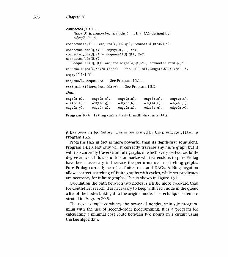
306 Chapter 16
connected(X,Y) -Node X is connected to node Y in the DAG defined byedge/2 facts.
connected(X,Y) - enqueue(X,Q\Q,Q1), connected_bfs(Q1,Y).
connected_bfs(Q,Y) - empty(Q), !, fail.
connected_bfs(Q,Y) - dequeue(X,Q,Q1), X=Y.
connected_bfs(Q,Y) -
dequeue(X,Q,Qi), enqueue_edges(X,Q1,Q2), connected_bfs(Q2,Y).
enqueue_edges(X,Xs\Ys,Xs\Zs) - find_all_dl(N,edge(X,N),Ys\Zs),
empty([ ]\[ 1).enqueue/3, dequeue/3 - See Program 15.11.
f ind_all_dl(Terrn,Goal ,DList) - See Program 16.3.
Dataedge (a, b) edge(a,c). edge(a,d). edge (a » e) edge (f , i)
edge(c,f). edge(c,g). edge (f , h) edge (e , k) edge(d,j).
edge(x,y). edge (y , z) edge (z , x) edge (y , u) edge (z , y)
Program 16.4 Testing connectivity breadth-first in a DAG
it has been visited before. This is performed by the predicate filter inProgram 16.5.
Program 16.5 in fact is more powerful than its depth-first equivalent,Program 14.10. Not only will it correctly traverse any finite graph but itwill also correctly traverse infinite graphs in which every vertex has finitedegree as well. It is useful to summarize what extensions to pure Prologhave been necessary to increase the performance in searching graphs.Pure Prolog correctly searches finite trees and DAGs. Adding negationallows correct searching of finite graphs with cycles, while set predicatesare necessary for infinite graphs. This is shown in Figure 16.1.
Calculating the path between two nodes is a little more awkward thanfor depth-first search. It is necessary to keep with each node in the queuea list of the nodes linking it to the original node. The technique is demon-strated in Program 20.6.
The next example combines the power of nondeterministic program-ming with the use of second-order programming. lt is a program forcalculating a minimal cost route between two points in a circuit usingthe Lee algorithm.

307 Second-Order Programming
connected(X,Y)Node X is connected to node Y in the graph defined byedge/2 facts.
connected (X Y)
enqueue(X,q\Q,Q1), connected_bfs(Q1,Y,[X]).
connected_bfs(Q,Y,Visited) '- ernpty(Q) , , fail.
connected_bfs(Q,Y,Visited) - dequeue(X,Q,Q1), XY.
connected_bfs(Q,Y,Visïted)
dequeue(X,Q,Q1)
findall(N,edge(X,N) ,Edges),
filter(Edges,Vïsited,Visitedl,Q1,Q2)
connected_bfs(Q2,Y,Visitedl)
filter([NINs] ,Visited,Visitedl,Q,Ql) -
member(N,Visited), ! , filter(Ns,Visited,Visitedl,Q,Q1).
filter([NINs] ,Visited,Visitedi,Q,Q2)
not member(N,Visited), ! , enqueue(N,Q,Q1),
filter(Ns, [NiVisited] ,Visitedl,Q1,Q2).
filter([ I ,Visited,Visited,q,Q)
empty([ ]\[ 1).enqueue/3, dequeue/3 See Program 15.11.
Program 16.5 Testing connectivity breadth-first in a graph
Finite trees and DAGsPure PrologFinite graphsPure Prolog + negationInfinite graphsPure Prolog -- second order + negation
Figure 16.1 Power of Prolog for various searching tasks

308 Chapter 16
Figure 16.2 The problem of Lee routing for VLSI circuits
The problem is formulated as follows. Given a grid that may haveobstacles, find a shortest path between two specified points. Figure 16.2shows a grid with obstacles. The heavy solid line represents a shortestpath between the two points A and B. The shaded rectangles representthe obstacles.
We first formulate the problem in a suitable form for programming.The VLSI circuit is modeled by a grid of points, conveniently assumed tobe the upper quadrant of the Cartesian plane. A route is a path betweentwo points in the grid, along horizontal and vertical lines only, subjectto the constraints of remaining in the grid and not passing through anyobstacles.
Points in the plane are represented by their Cartesian coordinates anddenoted X-Y. In Figure 16.2, A is 1-1 and B is 5-5. This representationis chosen for readability and utilizes the definition of - as an infix binary

309 Second-Order Programming
operator. Paths are calculated by the program as a list of points fromB to A, including both endpoints. In Figure 16.2 the route calculated is[5-5,5-4,5-3,5-2,4-2,3-2,2-2,1-2,1-11, and is marked by the heavy solidline.
The top-level relation computed by the program is lee_route (A, B,
Obstacles,Path), where Path is a route (of minimal distance) frompoint A to point B in the circuit. Obstacles are the obstacles in the grid.The program has two stages. First, successive waves of neighboring gridpoints are generated, starting from the initial point, until the final pointis reached. Second, the path is extracted from the accumulated waves.Let us examine the various components of Program 16.6, the overallprogram for Lee routing.
Waves are defined inductively. The initial wave is the list [A]. Succes-sive waves are sets of points that neighbor a point in the previous waveand that do not already appear in previous waves. They are illustrated bythe lighter solid lines in Figure 16.2.
Wave generation is performed by waves (B, WavesSoFar ,Obstacles,
Waves). The predicate waves/4 is true if Waves is a list of waves tothe destination B avoiding the obstacles represented by Obstacles andWavesSoFar is an accumulator containing the waves generated so far intraveling from the source. The predicate terminates when the destina-tion is in the current wave. The recursive clause calls next _wave/4, whichfinds all the appropriate grid points constituting the next wave using theall-solutions predicate f indal 1.
Obstacles are assumed to be rectangular blocks. They are representedby the term obstacle(L,R), where L is the coordinates of the lowerleft-hand corner and R the coordinates of the upper right-hand corner.Exercise (i) at the end of this section requires modifying the program tohandle other obstacles.
The predicate path (A,B,Waves,Path) finds the path Path back from B
to A through the Waves generated in the process. Path is built downward,which means the order of the points is from B to A. This order can bechanged by using an accumulator in path.
Program 16.6 produces no output while computing the Lee route. Inpractice, the user may like to see the computation in progress. This canbe easily done by adding appropriate write statements to the proceduresnext_wave and path.

310 Chapter 16
lee_route ( Source,Destination, Obstacles,Path)Path is a minimal length path from Source toDestination that does not cross Obstacles.
lee_route (A, B ,Obstacles, Path)
waves(B,[[A] 1 ]] ,Obstacles,Waves),
path (A ,B , Waves , Path)
waves (Destination, WavesSoFar, Obstacles, Waves) -Waves is a list of waves including WavesSoFar(except, perhaps, its last wave) that leads to Destinationwithout crossing Obstacles.
waves(B, [Wave Waves] ,Obstacles,Waves) - member(B,Wave), !.waves(B, [Wave ,LastWavelLastWaves] ,Obstacles,Waves) -
next_wave (Wave, LastWave ,Obstacles, NextWave),waves(B, [NextWave,Wave ,LastWave ILastWaves] ,Obstacles,Waves).
next_ wave ( Wave,Last Wave, Obstacles,NextWave) -Next Wave is the set of admissible points from Wave,that is, excluding points from Last Wave,Wave and points under Obstacles.
next_wave(Wave ,LastWave ,Obstacles ,NextWave) -
findall(X,admissible(X,Wave ,LastWave,Obstacles) ,NextWave).
admissible (X ,Wave, LastWave ,Obstacles) -
adjacent(X,Wave,Obstacles),
not member(X,LastWave),
not member(X,Wave).
adjacent (X,Wave ,Obstacles) -
member (Xl, Wave)neighbor(Xl ,X),
not obstructed(X,Obstacles).
neighbor(Xl-Y,X2-Y) - next_to(X1,X2).
neighbor(X-Yi,X-Y2) - next_to(Yl,Y2).
next_to(X,X1) - Xl is X+l.
next_to(X,X1) - X > O, Xl is Xl.
obstructed (Point ,Obstacles) -
menber(Obstacle,Obstacles), obstructs(Point,Obstacle).
obstructs(X-Y,obstacle(X-Yl,X2-Y2)) - Yl Y, Y Y2.
obstructs(X-Y,obstacle(XlYl,X-Y2)) - Yl Y, Y Y2.
obstructs(X-Y,obstacle(X1-Y,X2-Y2)) '- Xl X, X X2.
obstructs(X-Y,obstacle(Xl-Yl,X2-Y)) Xl X, X X2.
Program 16.6 Lee routing

311 Second-Order Programming
path ( Source,Destination, Waves,Path)Path is a path from Source to Destination going through Waves.
path(A,A,Waves,[A]) - L
path(A,B, [Wave IWaves] , [BiPath]) -
member(Bi ,Wave),
neighbor (B , Bi)
!, path(A,B1,Waves,Path).
Testing and data
test_lee (Naine , Path)
data(Name,A,B,Dbstacles), lee_route(A,B4Obstacles,Path).
data(test,i-1,5-5, [obstacle(2-3,4-5),obstacle(6-6,8-8)]).
Program 16.6 (Continued)
Our final example in this section concerns the keyword in context(KWIC) problem. Again, a simple Prolog program, combining nondeter-ministic and second-order programming, suffices to solve a complextask.
Finding keywords in context involves searching text for all occurrencesof a set of keywords, extracting the contexts in which they appear. Weconsider here the following variant of the general problem: "Given a listof titles, produce a sorted list of all occurrences of a set of keywords inthe titles, together with their context."
Sample input to a program is given in Figure 16.3 together with theexpected output. The context is described as a rotation of the title withthe end of the title indicated by -. In the example, the keywords arealgorithmic, debugging, logic, problem, program, programming, prolog,and solving, all the nontrivial words.
The relation we want to compute is kwic(Titles,Kwiclitles) whereTitles is the list of titles whose keywords are to be extracted, and Kwic-Titles is the sorted list of keywords in their contexts. Both the inputand output titles are assumed to be given as lists of words. A more gen-eral program, as a preliminary step, would convert freer-form input intolists of words and produce prettier output.
The program is presented in stages. The basis is a nondeterministicspecification of a rotation of a list of words. It has an elegant definitionin terms of append:

312 Chapter 16
Input: progranmiïng m prologlogic for problem solvinglogic programmingalgorithmic program debugging
Output: algorithmic program debugging -,debuggrrg - algorithmic program,logic for problem solving -,logic programming -,problem solving - logic for,program debugging - algorithmic,programming in prolog -,programming - logic,prolog - prograinnhing in,solving - logic for problem
Figure 16.3 Input and output for keyword in context (KWIC) problem
rotate(Xs,Ys) - append(As,Bs,Xs), append(Bs,As,Ys).
Declaratively, Ys is a rotation of Xs if Xs is composed of As followed byBs, and Ys is Bs followed by As.
The next stage of development involves identifying single words aspotential keywords. This is done by isolating the word in the first callto append. Note that the new rule is an instance of the previous one:
rotate(Xs,Ys) -
append(As,[KeyIBsJ,Xs), append([KeyIBs],As,Ys).
This definition also improves the previous attempt by removing the du-plicate solution when one of the split lists is empty and the other is theentire list.
The next improvement involves examining a potential keyword moreclosely. Suppose each keyword Word is identified by a fact of the formkeyword (Word). The solutions to the rotate procedure can be filteredso that only words identified as keywords are accepted. The appropriateversion is
rotate_and_f ilter(Xs,Ys) - append(As, [KeyIBs] ,Xs),
keyword(Key), append(rKeylBs] ,As,Ys).

313 Second-Order Programming
kwìc (Titles,KWTitles) -KWTitles is a KWIC index of the list of titles Titles.
kwic(Titles,KWTitles) -setof(Ys,XsI(rnember(Xs,Tit].es),rotate_and_f ilter(Xs,Ys)) ,KWTitles).
rot ate_and_fiiter(Xs, Ys) -Ys is a rotation of the list Xs such thatthe first word of Ys is significant and -is inserted after the last word of Xs.
rotate_and_filter(Xs,Ys) -append(As, [Key lBs] ,Xs),not insignificant(Key),append([KeylBs] [''lAs] ,Ys).
Vocabulary of insignificant words
insignificant(a). insignif ïcant (the).insignificant(iri) . insigriif icant (for).Testing arid data
test_kwic(Books,Kwic) -titles(Books,Titles) , kwic(Titles,Kwic)
titles(lp, [[logic,for,problem,solving][logic, programming][algorithmic, program ,debugging],[programming, in prolog]]).
Program 16.7 Producing a keyword in context (KWIC) index
Operationally rotate_and_filter considers all keys, filtering out theunwanted alternatives. The goal order is important here to maximizeprogram efficiency.
In Program 16.7, the final version, a complementary view to recogniz-ing keywords is taken. Any word Word is a keyword unless otherwisespecified by a fact of the form insignificant(Word). Further the proce-dure is augmented to insert the end-of-title mark -, providing the con-text information. This is done by adding the extra symbol in the secondappend call. Incorporating this discussion yields the clause for rotate_and_f ilter ni Program 16.7.
Finally, a set predicate is used to get all the solutions. Quantificationis necessary over all the possible titles. Advantage is derived from the

314 Chapter 16
behavior of setof in sorting the answers. The complete program is givenas Program 16.7, and is an elegant example of the expressive power ofProlog. The test predicate is test_kwic/2.
Exercises for Section 162
Modify Program 16.6 to handle other obstacles than rectangles.
Adapt Program 16.7 for KWIC so that it extracts keywords fromlines of text.
Modify rotation of a list so that it uses difference-lists.
Write a program to find a minimal spanning tree for a graph.
(y) Write a program to find the maximum flow in a network designusing the Ford-Fulkerson algorithm.
16.3 Other Second-Order Predicates
First-order logic allows quantification over individuals. Second-orderlogic further allows quantification over predicates. Incorporating thisextension into logic programming entails using rules with goals whosepredicate names are variables. Predicate names become "first-class" dataobjects to be manipulated and modified.
A simple example of a second-order relation is the determination ofwhether all members of a list have a certain property. For simplicitythe property is assumed to be described as a unary predicate. Let usdefine has_property(Xs,P), which is true if each element of Xs hassome property P. Extending Prolog syntax to allow variable predicatenames enables us to define has_property as in Figure 16.4. Because has_
property allows variable properties, it is a second-order predicate. Anexample of its use is testing whether a list of people Xs is all male with aquery has_property(Xs,male)?.
Another second-order predicate is rnap_list(Xs,P,Ys). Ys is the mapof the list Xs under the predicate P. That is, for each element X of Xs
there is a corresponding element Y of Ys such that P (X , Y) is true. The

315 Second-Order Programming
has_property([XIXsI,P) P(X), has_property(Xs,P).
has_property([ ] ,P).
map_1it([XIXs] ,P, [YIYsI) - P(X,Y) , map_list(Xs,P,Ys).
rnap_list( E I ,P, E I).
Figure 16.4 Second-order predicates
order of the elements in Xs is preserved in Ys. We can use map_list
to rewrite some of the programs of earlier chapters. For example, Pro-gram 7.8 mapping English to French words can be expressed as map_
list(Words,dict,Mots). Uke has_property, map_list is easily definedusing a variable predicate name. The definition is given in Figure 16.4.
Operationally, allowing variable predicate names implies dynamic con-struction of goals while answering a query. The relation to be computedis not fixed statically when the query is posed but is determined dynam-ically during the computation.
Some Prologs allow the programmer to use variables for predicatenames, and allow the syntax of Figure 16.4. lt is unnecessary to com-plicate the syntax however. The tools already exist for implementingsecond-order predicates. One basic relation is necessary, which we callapply; it constructs the goal with a variable functor. The predicate apply
is defined by a set of clauses, one for each functor name and arity. Forexample, for functor foo of ariry n, the clause is
apply(foo,X1, . . . ,Xn) - foo(X1, . . . ,Xn).
The two predicates in Figure 16.4 are transformed into Standard Prologin Program 16.8. Sample definitions of apply clauses are given for theexamples mentioned in the text.
The predicate apply performs structure inspection. The whole collec-tion of apply clauses can be generalized by using the structure inspec-tion primitive, univ. The general predicate apply(P,Xs) applies predi-cate P to a list of arguments Xs:
apply(F,Xs) - Goal =.. [FIXs], Goal.
We can generalize the function to be applied from a predicate name, i.e.,an atom, to a term parameterized by variables. An example is substitut-ing for a value in a list. The relation substitute/4 from Program 9.3

316 Chapter 16
has_property (Xs,P)Each element in the list Xs has property P.
has_property([XIXs] ,P) -
apply(P,X), has_property(Xs,P).
has_property( E I ,P).apply(male,X) male(X).
maplist (Xs,P, Ys)Each element in the list Xs stands in relationP to its corresponding element in the list Ys.
map_list([XIXs],P,[YIYs]) -
apply(P,X,Y), map_list(Xs,P,Ys).
map_list([ ],P,[ J).
apply(dict,X,Y) - dict(X,Y).
Program 16.8 Second-order predicates in Prolog
can be viewed as an instance of map_ list if parameterization is allowed.Namely, map_list(Xs,substitute(Old,New) ,Ys) has the same effect insubstituting the element New for the element Old in Xs to get Ys - exactlythe relation computed by Program 9.3. In order to handle this correctly,the definition of apply must be extended a little:
apply(P,Xs) -
P =.. Li, append(Li,Xs,L2), Goal .. L2, Goal.
Using apply as part of map_list leads to inefficient programs. For ex-ample, using substitute directly rather than through map_list resultsin far fewer intermediate structures being created, and eases the taskof compilation. Hence these second-order predicates are better used inconjunction with a program transformation system that can translatesecond-order calls to first-order calls at compile-time.
The predicate apply can also be used to implement lambda expres-sions. A lambda expression is one of the form lambda(X1,.. .,X).Expres-sion. If the set of lambda expressions to be used is known in advance,they can be named. For example, the above expression would be replacedby some unique identifier, f 00 say, and defined by an apply clause:
apply(foo,X1, . . - ,Xn) - Expression.

317 Second-Order Programming
Although possible both theoretically and pragmatically, the use oflambda expressions and second-order constructs such as has_property
and map_list is not as widespread in Prolog as in functional program-ming languages like Lisp. We conjecture that this is a combination ofcultural bias and the availability of a host of alternative programmingtechniques. It is possible that the ongoing work on extending the logicprograniniing model with higher-order constructs and integrating it withfunctional programming will change the picture.
In the meantime, all-solutions predicates seem to be the main and mostuseful higher-order construct in Prolog.
Exercise for Section 16.3
(i) Write a program performing beta reduction for lambda expressions.
16.4 Background
The discussion of f indall uses the description contained in the Stan-dard Prolog document (Scowen, 1991). An excellent discussion of theall-solutions predicates bagof and setof in Edinburgh Prolog are givenin Warren (1982a). Discussions of "rolling your own" set predicates canbe found in both O'Keefe (1990) and Ross (1989).
Set predicates are a powerful extension to Prolog. They can be used (in-efficiently) to implement negation as failure and meta-logical type pred-icates (Kahn, 1984). If a goal G has no solutions, which is determined bya predicate such as f indall, then not G is true. The predicate var(X)
is implemented by testing whether the goal X=1 ; X=2 has two solutions.Further discussion of such behavior of set predicates and a survey of dif-ferent implementations of set predicates can be found in Naish (1985a).
Further description of the Lee algorithm and the general routing prob-lem for VLSI circuits can be found in textbooks on VLSI, for example,Breuer and Carter (1983). A neat graphic version of Program 16.6 hasbeen written by Dave Broderick.

318 Chapter 16
Recent logic programming research has focused somewhat more onhigher-order logic programming. Approaches of note are Lambda-Prolog(Miller and Nadathur, 1986) and HiLog (Chen et al., 1989).
KWIC was posed as a benchmark for high-level programming languagesby Penis, and was used to compare several languages. We find the Prologimplementation of it perhaps the most elegant of all.
Our description of lambda expressions is modeled after Warren(1982a). Predicates such as apply and map_list were part of the utili-ties package at the University of Edinburgh. They were fashionable fora while but fell out of favor because they were not compiled efficiently,and no source-to-source transformation tools were available.

17 Interpreters
Meta-programs treat other programs as data. They analyze, transform,and interpret other programs. The writing of meta-programs, or meta-programming, is particularly easy in Prolog because of the equivalenceof programs and data: both are Prolog terms. We have already presentedsome examples of meta-programs, namely, the editor of Program 12.5and the shell process of Program 12.6. This chapter covers interpreters,an important and useful class of meta-programs, and Chapter 18 dis-cusses program transformation.
17.1 Interpreters for Finite State Machines
The sharp distinction between programs and data present in most com-puter languages is lacking in Prolog. The equivalence of programs anddata greatly facilitates the writing of interpreters. We demonstrate thefacility in this section by considering the basic computation models ofcomputer science. interpreters for the various classes of automata arevery easily written in Prolog.
lt is interesting to observe that the interpreters presented in this sec-tion are a good application of nondetermmistic progranmiing The pro-grams that are presented illustrate typical examples of don't-know non-determinism. The same interpreter can execute both deterministic andnondetermimstic automata because of the nondeterminism of Prolog.
DefinitionA (nondeterministic) finite automaton, abbreviated NDFA, is a 5-tuple(QX,Ö,I,F), where Q is a set of states, is a set of symbols, 6 is a

320 Chapter 17
accept(Xs) -The string represented by the list Xs is accepted bythe NDFA defined by initial/i, delta/3, and final/i.
accept(Xs) - initial(Q), accept(Xs,Q).
accept([XIXs],Q) - delta(Q,X,Q1), accept(Xs,Q1)
accept([ ],Q) - final(Q).
Program 17.1 An interpreter for a nondeterministic finite automaton(NDFA)
mapping from Q x to Q, I is an initial state, and F is a set of finalstates. If the mapping is a function, then an NDFA is deterministic.
A finite automaton can be specified as a Prolog program by three col-lections of facts. The predicate initial (Q) is true if Q is the initial state.The predicate final (Q) is true if Q is a final state. The most interesting isdelta(Q,X,Ql), which is true if the NDFA changes from state Q to stateQl on receipt of symbol X. Note that both the set of states and the setof symbols can be defined implicitly as the constants that appear in theinitial, final, and delta predicates.
An NDFA accepts a string of symbols from the alphabet if whenstarted in its initial state, and following the transitions specified by ô, theNDFA ends up in one of the final states. An interpreter for an NDFA mustdetermine whether it accepts given strings of symbols. Program 17.1 isan interpreter. The predicate accept (Xs) is true if the NDFA definedby the collection of initial, final, and delta facts accepts the stringrepresented as the list of symbols Xs.
Figure 17.1 shows a deterministic automaton that accepts the language(ab)*. There are two states, qO and ql. If in state qO an a is received, theautomaton moves to state ql. The automaton moves back from ql to qOif a b is received. The initial state is qO, and qO is also the single finalstate.
To use the interpreter, a specific automaton must be given. Program17.2 is the realization in Prolog of the automaton in Figure 17.1. Thecombination of Programs 17.1 and 17.2 correctly accepts strings of al-ternating a's and b's.
If an arc from qO to itself labeled a is added to the automaton in Fig-ure 17.1, we get a new automaton that recognizes the language (a(a*)b)*.

321 Interpreters
Figure 17.1 A simple automaton
initial(qO)
uinal(qO)
delta (qQ , a, qi)
cielta(ql,b,qO).
Program 17.2 An NDFA that accepts the language (ab)*
This automaton is nondeterministic because on receipt of an a in state qOit is not determined which path will be followed. Nondeterminism doesnot affect the interpreter in Program 17.1. All that is needed to producethe new automaton is to add the fact delta(qO,a,qO) and the combinedprogram will behave correctly.
Another simple computation model is a pushdown automaton that ac-cepts the class of context-free languages. Pushdown automata extendNDFAs by providing a single stack for memory in addition to the in-ternal state of the automaton. Formally, a (nondeterministic) pushdownautomaton, abbreviated NPDA, is a 7-tuple (Q,G,&LZ,F) where Q, , I,F are as before, G is the set of symbols that can be pushed onto the stack,Z is the start symbol on the stack, and 6 is changed to take the stack intoaccount.
Specifically, ô is a mapping from Q x x G* to Q x G*. The mappingcontrols the change of state of the NPDA and the pushing and poppingof elements onto and off the stack by the NPDA. In one operation, theNPDA can pop (push) one symbol off (onto) the stack.
Analogously to an NDFA, an NPDA accepts a string of symbols from thealphabet E*, if when started ¡n its initial state and with the starting sym-bol on the stack, and following the transitions specified by ô, the NPDAends up in one of the final states with the stack empty An interpreterfor an NPDA is given as Program 17.3. The predicate accept(Xs) is trueif the NDFA defined by the collection of initial, final, and delta facts

322 Chapter 17
accept(Xs) -The string represented by the list Xs is accepted bythe NPDA defined by initial/I, delta/5, and final/i.
accept(Xs) - initial(Q), accept(Xs,Q,[ 1).accept([XIXs],Q,S) - delta(Q,X,S,Q1,S1), accept(Xs,Q1,S1).
accept([ ],Q,[ 1) - final(Q).
Program 17.3 An interpreter for a nondeterministic pushdown automaton(NPDA)
initial(qO). final(ql).
delta(qO,X,S,qO, [XIS]).
delta(qO,X,S,ql, [XIS]).
delta (qO ,X, S, qi, S)
delta(ql,X, [XIS] ,ql,S).
Program 17.4 An NPDA for palindromes over a finite alphabet
accepts the string represented as the list of symbols Xs. The interpreteris very similar to the interpreter of an NDFA given as Program 17.1. Theonly change is the explicit manipulation of the stack by the delta predi-cate.
A particular example of an NPDA is given as Program 17.4. This au-tomaton accepts palindromes over a finite alphabet. A palindrome is anonempty string that reads the same backwards as forwards. Examplepalindromes are noon, madam, and gleneig. Again, the automaton isspecified by initial, final, and delta facts, and the sets of symbolsbeing defined implicitly. The automaton has two states: qO, the initialstate when symbols are pushed onto the stack, and qi, a final state whensymbols are popped off the stack and compared with the symbols in theinput stream. When to stop pushing and start popping is decided nonde-terministically. There are two delta facts that change the state from qOto ql to allow for palindromes of both odd and even lengths.
Programs 17.1 and 17.2 can be combined into a single program forrecognizing the language (ab)*. Similarly, Programs 17.3 and 17.4 can becombined into a single program for recognizing palindromes. A programthat can achieve this combination is given in Chapter 18.

323 Interpreters
It is straightforward to build an interpreter for a Turing machine writ-ten in a similar style to the interpreters in Programs 17.1 and 17.3. Thisis posed as Exercise (iii) at the end of this section. Building ari interpreterfor Turing machines shows that Prolog has the power of all other knowncomputation models.
Exercises for Section 17.1
Define an NDFA that accepts the language ab*c.
Define an NPDA that accepts the language ab1.
Write an interpreter for a Turing machine
17.2 Meta-Interpreters
We turn now to a class of especially useful interpreters. A meta-inter-preter for a language is an interpreter for the language written in thelanguage itself. Being able to write a meta-interpreter easily is a very pow-erful feature of a programming language. It gives access to the computa-tion process of the language and enables the building of an integratedprogramming environment. The examples in the rest of this chapterdemonstrate the potential of meta-interpreters arid the ease with whichthey can be written. In this section, we also examine issues in writingmeta-interpreters.
Throughout the remainder of this chapter, the predicate solve is usedfor a meta-interpreter. A suitable relation scheme is as follows. The re-lation solve(Goal) is true if Goal is true with respect to the programbeing interpreted.
The simplest meta-interpreter that can be written in Prolog exploits themeta-variable facility. Et is defined by a single clause:
solve(A) - A.
This trivial interpreter is only useful as part of a larger program. Forexample, a version of the trivial interpreter forms the basis for the in-teractive shell given as Program 12.6 arid the logging facility given asProgram 12.7. In general, as we suggest here and see in more detail in

324 Chapter 17
solve(Goal) -Goal is true given the pure Prolog program defined by clause/2.
solve (true)
solve((A,B)) - solve(A), solve(B).
salve(A) - clause(A,B), solve(B).
Program 17.5 A meta-interpreter for pure Prolog
Sections 17.3 and 17.4, meta-interpreters are useful and important be-cause of the easily constructed enhancements.
The best known and most widely used meta-interpreter models thecomputation model of logic programs as goal reduction. The threeclauses of Program 17.5 interpret pure Prolog programs. This meta-interpreter, called vanilla, together with its enhancements, is the basis ofthe rest of this section and Section 17.3.
The interpreter in Program 17.5 can be given a declarative reading. Thesolve fact states that the empty goal, represented by the constant true,is true. The first solve rule states that a conjunction (A,B) is true if A
is true and B is true. The second solve rule states that a goal A is true ifthere is a clause A - B in the interpreted program such that B is true.
We also give a procedural reading of the three clauses in Program17.5. The solve fact states that the empty goal, represented in Prolog bythe atom true, is solved. The next clause concerns conjunctive goals. Itreads: "To solve a conjunction (A,B), solve A and solve B." The generalcase of goal reduction is covered by the final clause. To solve a goal,choose a clause from the program whose head unifies with the goal, andrecursively solve the body of the clause.
The procedural reading of Prolog clauses is necessary to demonstratethat the meta-interpreter of Program 17.5 indeed reflects Prolog's choicesof implementing the abstract computation model of logic programming.The two choices are the selection of the leftmost goal as the goal toreduce, and sequential search and backtracking for the nondeterministicchoice of the clause to use to reduce the goal. The goal order of the bodyof the solve clause handling conjunctions guarantees that the leftmostgoal in the conjunction is solved first. Sequential search and backtrackingcomes from Prolog's behavior in satisfying the clause goal.
The hard work of the interpreter is borne by the third clause of Pro-gram 17.5. The call to clause performs the unification with the heads

325 Interpreters
solve(rnember(X, [a,b,c]))clause(inember(X, [a,b,c]) ,B)solve (true)
true Output: X=a
solve (true)clause(true,T) f
clause(member(X, [a,b,c] 6)solve(member(X, [b,c]))
clause(member(X, [b,c]) ,Bl)solve (true)true Output: Xb
solve (true)clause(true,T) f
clause(member(X, [b,c]),B1)solve (member(X, [cl))
clause (member(X, [cl ,B2)solve (true)true Output: X=c
solve (true)clause(true,T) f
clause(rnember(X, [cl ,B2))solve(member(X, C i))
clause(member(X, E ]),B3)no (more) solutions
Figure 17.2 Tracing the meta-interpreter
{Xa, 13=true
tBmember(X, [b,c])}
{x=b ,B1=true
(B1member(X, [c])}
{X=c ,B2=true}
{B2=member(X, C
of the clauses appearing in the program. It is also responsible for giv-ing different solutions on backtracking. Backtracking also occurs in theconjunctive rule reverting from B to A.
Tracing the meta-interpreter of Program 17.5 solving a goal is instruc-tive. The trace of answering the query solve (member (X, [a, b, c])) withrespect to Program 3.12 for member is given in Figure 17.2.
The vanilla meta-interpreter inherits Prolog's representation of clausesusing the system predicate clause. Alternative representations ofclauses are certainly possible, and indeed have been used by alter-native Prologs. lists are one possible representation. The clause A -B1,B2,...,B can be represented by the clause rule(A, [B1,...,Bn]). In

326 Chapter 17
solve(Goal) -Goal is true given the pure Prolog program defined by clause/2.
solve(Goal) solve(Goal,[ J).
solve([ ],[ 1).solve([ ],[GIGoals]) solve(G,Goals).
solve([AIB] ,Goals) append(B,Goals,Goalsl), solve(A,Goalsl).
solve(A,Goals) - rule(A,B), solve(B,Goals).
Program 17.6 A meta-interpreter for pure Prolog in continuation style
this representation, the empty list represents the empty goal and listconstruction represents conjunction. This representation is used in Pro-gram 17.6.
A different representation imposes a different form on the meta-interpreter, as illustrated in Program 17.6. Unlike Program 17.5, thisversion of the vanilla meta-interpreter makes explicit the remaining goalsin the resolvent. Enhancements can be written to exploit the fact that theresolvent is accessible during the computation, for example, allowing amore sophisticated computation rule. The behavior of Program 17.6 canbe considered as being in continuation style promoted by languages suchas Scheme.
Differences in meta-interpreters can be characterized in terms of theirgranularity, that is the chunks of the computation that are made acces-sible to the programmer. The granularity of the trivial one-clause meta-interpreter is too coarse. Consequently there is little scope for applyingthe meta-interpreter. It is possible, though not as easy, to write a meta-interpreter that models unification and backtracking. The granularity ofsuch a meta-interpreter is very fine. Working at this fine level is usuallynot worthwhile. The efficiency loss is too great to warrant the extra ap-plications. The meta-interpreter in Program 17.5, at the clause reductionlevel, has the granularity most suited for the widest range of applica-tions.
The vanilla meta-interpreter must be extended to handle language fea-tures outside pure Prolog. Builtin predicates are not defined by clausesin the program and need different treatment. The easiest way to incor-porate builtin predicates is to use the meta-variable facility to call themdirectly. A table of builtin predicates is necessary. In this chapter, weassume a table of facts of the form builtin(Predicate) for each builtin

327 Interpreters
builtin(A is ) builtin(A > B)
builtin(read(X)) buìltin(write(X)).
builtin(integer(X)). builtin(functor(T,F,N)).
builtin(clause(A,B)) builtin(builtin(X)).
Figure 17.3 Fragment of a table of builtin predicates
predicate. Figure 17.3 gives part of that table. A table of builtin predi-cates is provided in some Prologs by another name but is not present inStandard Prolog.
The clause solve(A) builtin(A), A. can be added to the meta-interpreter in Program 17.5 to correctly handle builtin predicates. Theresulting program handles four disjoint cases, one per clause, for solvinggoals: the empty goal, conjunctive goals, builtin goals, and user-definedgoals. For compatibility with a number of Prolog systems, the meta-interpreters in the rest of this section contain cuts to indicate that theclauses are mutually exclusive.
The extra solve clause makes the behavior of the builtin predicates in-visible to the meta-interpreter. User-defined predicates that one wants tomake invisible can be handled similarly with a single clause. Conversely,there are occasions when builtin predicates for negation and second-order programming should be made visible.
The vanilla meta-interpreter needs to be extended to handle cuts cor-rectly. A naive incorporation of cuts treats them as a builtin predicate,effectively adding a clause solve (!) !. This clause does not achievethe correct behavior of cut. The cut in the clause commits to the currentsolve clause rather than pruning the search tree.
To achieve correct behavior of cut in a meta-interpreter, one needs tounderstand scope, that is to which clause the cut commits. The scope ofcut, as described in Chapter 11, is the clause in which the cut is a goalin the body. The scope of cut when it is contained within a meta-logicalbuiltin predicate such as conjunction and disjunction is less distinct andvaries in different Prologs. If a cut is part of a disjunction, should ex-ecution of the cut commit to the current disjunct or to the clause inwhich the disjunction is embedded? Handling cut correctly in a mcta-interpreter is tricky and usually relies on technical details of the scope ofcut in a particular implementation of Prolog. Incorporating cuts within

328 Chapter 17
solve_trace( Goal) -Goal is true given the Prolog program defined by clause/2.The program traces the proof by side effects.
solve_trace(Goal) - solve_trace(Goal,O).
solve_trace(true,Depth) -
solve_trace((A,B) ,Depth) -
solve_trace(A,Depth), solve_trace(B,Depth).
solve_trace (A ,Depth) -
builtin(A), !, A, display(A,Depth), nl.
solve_trace (A ,Depth)
clause(A,B), display(A,Depth), nl, Depthl is Depth + 1,
solve_trace (B ,Depthl).
display(A,Depth) -
Spacing is 3*Depth, put_spaces(Spacing), write(A).
put_spaces(N) -
between(1,N,I), put_charY '), fail.
put_spaces (N)
between(i,N,I) - SeeProgram8.5.
Program 17.7 A tracer for Prolog
meta-interpreters has been widely studied, and references to solutionsare given in Section 17.5.
We apply meta-mterpreters to develop a simple tracer. Program 17.7handles success branches of computations and does not display failurenodes in the search tree. It is capable of generating the traces presentedin Chapter 6.
The basic predicate is solve_trace(Goal,Depth), where Goal is
solved at some depth. The starting depth is assumed to be O. The firstsolve_trace/2 clause in Program 17.7 states that the empty goal issolved at any depth. The second clause indicates that each goal in a con-junct is solved at the same depth. The third clause handles builtins. Thefinal solve_trace/2 clause matches the goal with the head of a programclause, displays the goal, increments the depth, and solves the body ofthe program clause at the new depth.
The predicate display(Goal,Depth) is an interface for printing thetraced goal. The second argument, Depth, controls the amount of inden-tation of the first argument, Goal. Level of indentation correlates withdepth in the proof tree.

329 Interpreters
solve(Goal,Tree) -Tree is a proof tree for Goal given the program definedby c!ause/2.
solve(true,true)
solve((A,B) , (ProofA,ProofB)) -
solve(A,ProoÍA), solve(B,ProofB)
solve(A,(Abuiltin)) - builtin(A), 1, A.
solve(A,(AProof)) clause(A,fl), solve(B,Proof).
Program 17.8 A meta-interpreter for building a proof tree
There is subtlety in the goal order of the clause
solve_trace (A ,Depth) -
clause(A,B), display(A,Depth), nl, Depthl is Depth + 1,
solve_trace(B,Depthl).
The display goal is between calls to clause and solve_trace, ensuringthat the goal is displayed each time Prolog backtracks to choose anotherclause. If the clause and display goals are swapped, only the initial callof the goal is displayed.
Using Program 17.7 for the query solve_trace (append(Xs,Ys, [a,b,
c]))? with Program 3.15 for append generates a trace like the one pre-sented in Section 6.1. The output messages and semicolons for alterna-tive solutions are provided by the underlying Prolog. There is only onedifference from the trace in Figure 6.2. The unifications are already per-formed. Separating out unifications requires explicit representation ofunification and is considerably harder.
A simple application of meta-interpreters constructs a proof tree whilesolving a goal. The proof tree is built top-down. A proof tree is essen-tial for the applications of debugging and explanation in the next twosections.
The basic relation is solve(Goal,Tree), where Tree is a proof treefor the goal Goal, Proof trees are represented by the structure Goal -
Proof. Program 17.8 implements solve/2 and is a straightforward en-hancement of the vanilla meta-interpreter. We leave as an exercise forthe reader giving a declarative reading of the program.
Here is an example of using Program 17.8 with Program 1.2. The querysolve(son(lot,haran) ,Proof)? has the solution
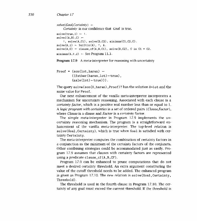
330 Chapter 17
solve( Goal,Certainty)Certainty is our confidence that Goal is true.
solve(true,1) -
solve((A,B),C) -
!, solve(A,C1), solve(B,C2), minimum(C1,C2,C).
solve(A,1) - builtin(A), !, A.
solve(A,C) - clause_cf(A,B,C1), solve(B,C2), C is Cl * C2.
minimum(X,Y,Z) - See Program 11.3.
Program 17.9 A meta-interpreter for reasoning with uncertainty
Proof = (son(lot,haran) -
((f ather(haran,lot)true),
(male(lot)true))).
The query solve (son (X,haran) ,Proof)? has the solution X=lot and thesame value for Proof.
Our next enhancement of the vanilla meta-interpreter incorporates amechanism for uncertainty reasoning. Associated with each clause is acertainty factor, which is a positive real number less than or equal to 1.A logic program with certainties is a set of ordered pairs (Clause,Factor),where Clause is a clause and Factor is a certainty factor.
The simple meta-interpreter in Program 17.9 implements the un-certainty reasoning mechanism. The program is a straightforward en-hancement of the vanilla meta-interpreter. The top-level relation issolve (Goal,Certainty), which is true when Goal is satisfied with cer-tainty Certainty.
The meta-interpreter computes the combination of certainty factors ina conjunction as the minimum of the certainty factors of the conjuncts.Other combining strategies could be accommodated just as easily. Pro-gram 17.9 assumes that clauses with certainty factors are representedusing a predicate clause_cf (A, B ,CF).
Program 17.9 can be enhanced to prune computations that do notmeet a desired certainty threshold. An extra argument constituting thevalue of the cutoff threshold needs to be added. The enhanced programis given as Program 17.10. The new relation is solve (Goal,Certainty,
Threshold).
The threshold is used in the fourth clause in Program 17.10. The cer-tainty of any goal must exceed the current threshold. If the threshold is

331 Interpreters
solve (Goal, Certainty, Threshold) -Certainty is our confidence, greater than Threshold, that Goal is true.
solve(true,1,T) -
solve( (A , B) ,C , T)
I, solve(A,Cl,T), solve(B,C2,T), minimuin(Ci,C2,C).
solve(A,1,T) .- builtin(A), !, A.
solve(A,C,T) -
clause_cf(A,B,C1), Cl > T, Ti is T/Cl,
solve(B,C2,Tl), C is Cl * C2.
minimuin(X,Y,Z) See Program 11.3.
Program 17.10 Reasoning with uncertainty with threshold cutoff
exceeded, the computation continues. The new threshold is the quotientof the previous threshold by the certainty of the clause.
Exercises for Section 17.2
Write a meta-interpreter to count the number of times a procedureis called in a successful computation.
Write a meta-interpreter to find the maximum depth reached in acomputation.
Extend Program 17.6 to give a tracer and build a proof tree.
Extend Program 17.7 for solve_trace/2 to print out failed goals.
(y) Modify Program 17.8 to use a different representation for a prooftree.
17.3 Enhanced Meta-Interpreters for Debugging
Debugging is an essential aspect of programming, even in Prolog. Thepromise of high-level programming languages is not so much iii theprospect for writing bug-free programs but in the power of the com-puterized tools for supportmg the process of program development. Forreasons of bootstrapping and elegance, these tools are best implemented

332 Chapter 17
in the language itself. Such tools are programs for manipulating, analyz-ing, and simulating other programs, or in other words, meta-programs.
This section shows meta-programs for supporting the debuggingprocess of pure Prolog programs. The reason for restricting ourselvesto the pure part is clear: the difficulties in handling the impure parts ofthe language.
To debug a program, we must assume that the programmer has someintended behavior of the program in mind, and an intended domain ofapplication on which the program should exhibit this behavior. Giventhose, debugging consists of finding discrepancies between the pro-gram's actual behavior and the behavior the programmer intended.Recall the definitions of an intended meaning and a domain from Sec-tion 5.2. An intended meaning M of a pure Prolog program is the setof ground goals on which the program should succeed. The intendeddomain D of a program is a domain on which the program should ter-minate. We require the intended meaning of a program to be a subset ofthe intended domain.
We say that A1 is a solution to a goal A if the program returns on a goalA its instance A1. We say that a solution A is true in an intended meaningM if every instance of A is in M. Otherwise it is false in M.
A pure Prolog program can exhibit only three types of bugs, given anintended meaning and an intended domain. When invoked on a goal A inthe intended domain, the program may do one of three things:
Fail to terminateReturn some false solution AOFail to return some true solution AO
We describe algorithms for supporting the detection and identification ofeach of these three types of bugs.
In general, it is not possible to detect if a Prolog program is nonter-minating; the question is undecidable. Second best is to assign some apriori bound on the running time or depth of recursion of the program,and abort the computation if the bound is exceeded. It is desirable tosave part of the computation to support the analysis of the reasons fornontermination. The enhanced meta-interpreter shown in Program 17.11achieves this. It is invoked with a call solve(A,D,Overf low), where A isan initial goal, and D an upper bound on the depth of recursion. The call

333 Interpreters
solve(A,D,Overflow) -A has a proof tree of depth less than D andOverflow equals no_overflow, or A has abranch in the computation tree longer than D, andOverflow contains a list of its first D elements.
solve(true,D,no_overflow) Lsolve(A,0,overflow([ J)) - L
solve((A,B) ,D,Overf low)
D >0, !,solve (A,D,Overf iowA)
solve_conjunction(OverflowA,B,D,Overflow).
solve(A,D,no_overflow) -
D > 0,
builtiri(A), !, A.
solve(A,D,Overflow)
D > 0,
clause (A ,B)
Dl is D-1,
soive(B,D1,OverflowB)
return_overflow(QverflowB ,A ,Overf low).
solve_conjunction(overfiow(S) ,B,D,overflow(S))
solveconjunctïon(nooverflow,B,D,Overfiow) -
solve (B,D,Overflow)
returnoverflow(no_overflow,A ,no_overf low).
return_overflow(overflow(S),A,overfiow([AIS])).
Program 17.11 A meta-interpreter detecting a stack overflow
succeeds if a solution is found without exceeding the predefined depthof recursion, with Overflow instantiated to no_overflow. The call alsosucceeds if the depth of recursion is exceeded, but in this case Over-
flow contains the stack of goals, i.e., the branch of the computation tree,which exceeded the depth-bound D.
Note that as soon as a stack overflow is detected, the computationreturns, without completing the proof. This is achieved by solve_
conjunction and return_overflow.
For example, consider Program 17.12 for insertion sort. When calledwith the goal solve(isort([2,2],Xs),6,Overf low), the solution re-turned is

334 Chapter 17
isort(Xs,Ys) -Ys is an ordered permutation of Xs. Nontermination program.
isort([XIXs],Ys) - isort(Xs,Zs), insert(X,Zs,Ys).
isort([ ],[ 1).
insert(X,[YIYs],[X,YIYs]) -
X < Y.
insert(X,[YIYs],[YIZs]) -X Y, insert(Y,[XIYs],Zs).
insert(X,[ ],[X]).
Program 17.12 A nonterminating insertion sort
The overflowed stack can be further analyzed, upon return, to diagnosethe reason for nontermination. This can be caused, for example, by aloop, i.e., by a sequence of goals G1,G2,. . .,G, on the stack, where G1 andG are called with the same input, or by a sequence of goals that callseach goal with increasingly larger inputs. The first situation occurs in thepreceding example. It is clearly a bug that should be fixed in the program.The second situation is not necessarily a bug, and knowing whether theprogram should be fixed or whether a larger machine should be boughtin order to execute it requires further program-dependent information.
The second type of bug is returning a false solution. A program canreturn a false solution only if it has a false clause. A clause C is falsewith respect to an intended meaning M if it has an instance whose bodyis true in M and whose head is false in M. Such an instance is called acounterexam pie to C.
Consider, for example, Program 17.13 for insertion sort. On the goalisort([3,2,1] ,Xs) it returns the solution isort([3,2,1] [3,2,1])
which is clearly false.
Xs = [2,2, 2,2,2,2],Overflow = overflow( [
isort( [2,2] [2,2,2,2,2,2]),
insert (2, [2] ,[2,2,2,2,2,2]),insert (2,[2] [2,2,2,2,2]),insert (2,[2] ,[2,2,2,2]),
insert (2, [2] ,[2,2,2]),
insert (2, [2] ,[2,2])])

335 Interpreters
isort(Xs,Ys) -Buggy insertion sort.
isort(EXIXs],Ys) isort(Xs,Zs), irisert(X,Zs,Ys).
isort([ I,[ I).inert(X, [YIY] , [X,YIYs]) -
X Y.
insert (X, [YIYsJ , [Y IZs]
X > Y, insert(X,Ys,Zs).
insert(X,[ I,EX]).
Program 17.13 An incorrect and incomplete insertion sort
The false clause in the program is
insert(X, [YIYs], [X,YIYs]) - X Y.
and a counterexample to it is
insert(2, [1] [2,1]) .- 2 1.
Given a ground proof tree corresponding to a false solution, one canfind a false instance of a clause as follows: Traverse the proof tree inpostorder. Check whether each node in the proof tree is true. If a falsenode is found, the clause whose head is the false node and whose bodyis the conjunction of its sons is a counterexample to a clause in theprogram. That clause is false and should be removed or modified.
The correctness of this algorithm follows from a simple inductiveproof. The algorithm is embedded in an enhanced meta-interpreter,shown as Program 17.14.
The algorithm and its implementation assume an oracle that can an-swer queries concerning the intended meaning of the program. The or-acle is some entity external to the diagnosis algorithm. It can be theprogrammer, who can respond to queries concerning the intended mean-ing of the program, or another program that has been shown to havethe same meaning as the intended meaning of the program under de-bugging. The second situation may occur in developing a new version ofa program while using the older version as an oracle. lt can also occurwhen developing an efficient program (e.g., quicksort), given an ineffi-cient executable specification of it (i.e., permutation sort), and using thespecification as an oracle.

336 Chapter 17
false_solution (A,Clause) -If A is a provable false instance, then Clause isa false clause in the program. Bottom-up algorithm.
false_solution(A,Clause)
solve(A,Proof)
false_clause (Proof ,Clause)
solve(Goal,Proof) - See Program 17.8.
false_clause(true,ok)
faise_clause((A,B) ,Clause) -
f aise_clause (A , ClauseA)
check_conjunction(CiauseA ,B ,Clause).
false_clause((AB) ,Clause) -f aise_clause (B , ClauseB)
check_clause (ClauseB , A, B ,Clause).
check_conjunction(ok ,B ,Clause)
f aise_clause (B , Clause)
check_conjunction((AB1) ,B, (ABl)).
check_clause(ok,A,B,Clause) -
query_goal (A ,Answer),
check_answer (Answer, A, B ,Clause).
check_clause((AlBl) ,A,B, (AlBl)).
check_answer(true,A,B,ok).check_answer(false,A,B, (ABl)) -
extract_body (B,Bl).
extract_body (true , true)
extract_body((AB) ,A).extract_body(((AB) ,Bs) , (A,As)) -
extract_body(Bs,As).
query_goal(A,true) -
built in (A)
query_goal (Goal ,Answer) -
not builtin(Goal),
writeln(['Is the goal ',Goal,' true?']),
read (Answer).
Program 17.14 Bottom-up diagnosis of a false solution

337 Interpreters
When invoked with the goal false_solution(isort([3,2,1] ,X) ,C)
the algorithm exhibits the following interactive behavior:
false_solution(isort([3,2,1],X),C)?
Is the goal isort([ ],[ ]) true?true.Is the goal insert(1, [ ] , [1]) true?true.Is the goal isort ([1] , [1] ) true?true.Is the goal insert (2, [1] , [2,1]) true?false.
X = [3,2,1],C = insert(2,[1],[2,1]) - 2 1.
This returns a counterexample to the false clause.The proof tree returned by solve/2 is not guaranteed to be ground,
in contrast to the assumption of the algorithm. However, a ground prooftree can be generated by either instantiating variables left in the prooftree to arbitrary constants before activating the algorithm, or by request-ing the oracle to instantiate the queried goal when it contains variables.Different instances might imply different answers. Since the goal of thisalgorithm is to find a counterexample as soon as possible, the oracleshould instantiate the goal to a false instance if it can.
One of the main concerns with diagnosis algorithms is improving theirquery complexity, i.e., reducing the number of queries they require todiagnose the bug. Given that the human programmer may have to answerthe queries, this desire is understandable. The query complexity of thepreceding diagnosis algorithm is linear in the size of the proof tree.There is a better strategy, whose query complexity is linear in the depthof the proof tree, not its size. In contrast to the previous algorithm,which is bottom-up, the second algorithm traverses the proof tree top-down. At each node it tries to find a false son. The algorithm recurseswith any false son found. If there is no false son, then the current nodeconstitutes a counterexample, as the goal at the node is false, and all itsSons are true.
The implementation of the algorithm is shown in Program 17.15. Notethe use of cut to implement ¡mplicit negation in the first clause of f alse_goal/2 and the use of query_goal/2 as a test predicate.

338 Chapter 17
false_solution (A, Clause)If A is a provable false instance, then Clauseis a false clause in the program. Top-down algorithm.
false_solution(A ,Clause) -
solve (A,Proof),
false_goal (Proof ,Clause).
solve(Goal,Proof) - See Program 17.8.
false_goal((A'B) ,Clause) -
f alse_conjunction (B, Clause)
false_goal((AB) ,(ABl)) -extract_body(B,Bl).
false_conjunction(((AB) ,Bs) ,Clause)
query_goal (A,false),
false_goal((AB) ,Clause).
false_conjunction((AB) ,Clause)
query_goal (A,false),
false_goal((AB) ,Clause).
false_conjunction((A,As) ,Clause)
false_conjunction(As ,Clause).
extract_body(Tree,Body) - See Program 17.14.
query_goal(A,Answer) - See Program 17.14.
Program 17.15 Top-down diagnosis of a false solution
Compare the behavior of the bottom-up algorithm with the followingtrace of the interactive behavior of Program 17.15:
false_solution(isort([3,2,1] ,X),C)?
Is the goal isort([2, 11,12,1]) true?false.Is the goal isort ([1] , [11) true?true.Is the goal insert (2, [1] [2,1]) true?false.
X = [3,2,1],C = insert(2, [11,12,1]) - 2 1.
There is a diagnosis algorithm for false solutions with an even betterquery complexity, called divide-and-query. The algorithm progresses bysplitting the proof tree into two approximately equal parts and querying

339 Interpreters
the node at the splitting point. 1f the node is false, the algorithm isapplied recursively to the subtree rooted by this node. If the node istrue, its subtree is removed from the tree and replaced by true, and anew middle point is computed. The algorithm can be shown to requirea number of queries logarithmic in the size of the proof tree. In case ofclose-to-linear proof trees, this constitutes an exponential improvementover both the top-down and the bottom-up diagnosis algorithms.
The third possible type of bug is a missing solution. Diagnosing amissing solution is more difficult than fixing the previous bugs. We saythat a clause covers a goal A with respect to an intended meaning M if ithas an instance whose head is an instance of A and whose body is in M.
For example, consider the goal insert (2, [1,3] ,Xs). lt is covered bythe clause
insert(X, [YIYs] , [X,YJYs]) X Y.
of Program 17.13 with respect to the intended meaning M of the pro-gram, since in the following instance of the clause
insert(2,[1,3],[1,2,3]) - 2 1.
the head is ari instance of A and the body is in M.It can be shown that if a program P has a missing solution with respect
to an intended meaning M, then there is a goal A in M that is not coveredby any clause in P. The proof of this claim is beyond the scope of thebook. lt is embedded in the diagnosis algorithm that follows.
Diagnosing a missing solution imposes a heavier burden on the oracle.Not only does it have to know whether a goal has a solution but it mustalso provide a solution, if it exists. Using such an oracle, an uncoveredgoal can be found as follows.
The algorithm is given a missing solution, i.e., a goal in the intendedmeaning M of the program P, for which P fails. The algorithm starts withthe initial missing solution. For every clause that unifies with it, it checks,using the oracle, if the body of the clause has an instance in M. If thereis no such clause, the goal is uncovered, and the algorithm terminates.Otherwise the algorithm finds a goal in the body that fails. At least oneof them should fail, or else the program would have solved the body, andhence the goal, in contrast to our assumption. The algorithm is appliedrecursively to this goal.

340 Chapter 17
missing_solution (A,Goal) -If A is a nonprovable true ground goal, then Goal is atrue ground goal that is uncovered by the program.
missing_solution((A,B),Goal) -
(not A, missing_solution(A,Goal)
A, missing_solution(B,Goal))
inissing_solution(A,Goal) -
clause (A, B)
query_clause((AB)),
missing_solution (B , Goal)
missing_solution(A,A) -
not system(A)
query_clause(Clause) -
writeln(['Enter a true ground instance of ',Clause,
'if there is such, or no' otherwise']),
read (Answer)
check_answer (Answer , Clause)
check_answer(no,Clause) - !, fail.
check_answer(Clause,Clause)
check_answer (Answer ,Clause) -
write ('Illegal answer'),
query_clause (Clause)
Program 17.16 Diagnosing missing solution
An implementation of this algorithm is shown in Program 17.16. Theprogram attempts to trace the failing path of the computation and to finda true goal which is uncovered. Following is a session with the program:
missing_solution(isort([2,1,3],[1,2,3]),C)?
Enter a true ground instance of(isort([2,1,3],[1,2,3]) -
isort([1,3],Xs),insert(2,Xs,[1,2,3]))
if there is such, or "no" otherwise
(isort([2,1,3],[1,2,3]) -
isort([1,3] ,[1,3]) ,insert(2, [1,3] [1,2,3])).
Enter a true ground instance of(isort([1,3] [1,3]) - isort([3] ,Ys) ,insert(1,Ys, [1,3]))
if there is such, or 'no' otherwise

341 Interpreters
(isort([1,3],[1,3]) - isort([3],[3]),insert(1,[3],[1,3])).
Enter a true ground instance of(insert(1, [3] ,[1,3]) - 1 3)
if there is such, or no' otherwise
no.
C insert(1, [3] [1,3])
The reader can verify that the goal insert(1, [3] [1,3]) is not coveredby Program 17.13.
The three algorithms shown can be incorporated in a high-quality in-teractive program development environment for Prolog.
17.4 An Explanation Shell for Rule-Based Systems
The final section of this chapter presents an application of interpretersto rule-based systems. An explanation shell is built that is capable of ex-plaining why goals succeed and fail and that allows interaction with theuser during a computation. The shell is developed with the methodologyof stepwise enhancement introduced in Section 13.3.
The skeleton interpreter in this section is written in the same style asthe vanilla meta-interpreter and has the same granularity. It differs intwo important respects. First, it interprets a rule language rather thanProlog clauses. Second, the interpreter has two levels to allow explana-tion of failed goals.
Before describing the interpreter, we give an example of a toy rule-based system written in the rule language. Program 17.17 contains somerules for placing a dish on the correct rack in an oven for baking. Factshave the form fact (Goal), For example, the first fact in Program 17.17states that dishl is of type bread.
Rules have the form rule(Head,Body,Naine), where Head is a goal,Body is (possibly) a conjunction of goals, and Naine is the name of therule. Individual goals in the body are placed inside a unary postfix func-tor is_true, for reasons to be explained shortly. Conjunctions in thebody are denoted by the binary infix operator &, which differs from Pro-log syntax. Operator declarations for & and is_true are given in Program17.17. To paraphrase a sample rule, rule place i in Program 17.17 states:

342 Chapter 17
Rule base for a simple expert system for placing dishes in an oven.The predicates used in the rules areplace_in_oven (Dish,Rack) -
Dish should be placed in the oven at level Rack for baking.pastry(Dish) - Dish is a pastry.main_meal(Dish) Dish is a main meal.slow_cooker(Dish) - Dish is a slow cooker.type(Dish,Type) - Dish is best described as Type.size(Dish,Size) - The size of Dish is Size.The rules have the form rule(Head,Body,Name).
:- op(40,xfy,&).
op(30,xf,is_true).
rule (place_in_oven (Dish , top)
pastry(Dish) is_true & size(Dish,small) is_true,placei).
rule (place_in_oven (Dish ,middle)
pastry(Dish) is_true & size(Dish,big) is_true,place2).
rule (place_in_oven(Dish,middle) ,main_meal(Dish) is_true,place3).
rule(place_in_oven(Dish,bottom) ,slow_cooker(Dish) is_true ,place4)
rule(pastry(Dish) ,type(Dish, cake) is_true,pastryi).
rule (pastry(Dish) ,type(Dish,bread) is_true,pastry2).
rule(main_meal(Dish) ,type(Dish,meat) is_true,main_meal).
rule(slow_cooker(Dish) ,type(Dish,milk_pudding) is_true,slow_cooker).
fact (type (dishl ,bread)).
fact(size(dishi,big)).
Program 17.17 Oven placement rule-based system
"A dish should be placed on the top rack of the oven if it is a pastry andits size is small."
Why use a separate rule language when the syntax is so close to Prolog?The first rule, place 1, could be written as follows.
place_in_oven(Dish,top) - pastry(Dish), size(Dish,sxnall).
There are two main reasons for the rule language. The first is pedagog-ical. The rule interpreter is neater, avoiding complicated details associ-ated with Prolog's impurities such as the behavior of builtin predicateswhen called by clause. Avoiding Prolog's impurities also makes it easierto partially evaluate the interpreter, as described in Chapter 18.

343 Interpreters
monitor(Goal) -Succeeds if a result of yes is returned from solving Goalat the solve level, or when the end of the computation is reached.
monitor(Goal) - solve(Goal,Result) , filter(Result)
monitor (Goal)
fïlter(yes)0/,
filter(no) .- fail.
solve(Goal,Result) -Given a set of rules of the form rule(A,B,Name), Goal hasResult yes if it follows from the rules and no if it does not.
solve(A,yes) fact(A).
solve(A,Result) '- rule(A,B,Naxne), solve_body(B,Result).
solve (A na)
solve_body(A&B,Result)
solve(A,ResultA), solve_and(ItesultA,B,Result)
solve_body(A ïs_true,Result) - salve(A,Result).
solve_and(no,A,no).
solve_and(yes,B,Result) solve(B,Result).
Program 17.18 A skeleton two-level rule interpreter
The second reason is to show by example that the best way to developa rule-based application in Prolog is to design a rule language on top ofProlog. Although the rule language is largely syntactic sugar, experiencehas shown that users of a rule-based system are happier working in acustomized rule language than in Prolog. Rule languages are straightfor-ward to provide on top of Prolog.
We now start our presentation of the explanation shell. According tothe method of stepwise enhancement, the skeleton constituting the basiccontrol flow of the final program is presented first. Program 17.18 con-tains the skeleton of the rule ìnterpreter. The principal requirement thatshaped the skeleton is the desire to handle both successful and failedcomputations in one interpreter.
The rule interpreter presented in Program 17.18 has two levels. The toplevel, or monitor level, consists of the predicates monitor and filter.
The bottom level, or solve level, consists of the predicates solve, solve_
body, and solve_and. Two levels are needed to correctly handle failedcomputations.

344 Chapter 17
Let us consider the bottom level first. The three predicates consti-tute an interpreter at the same level of granularity as the vanilla meta-interpreter. There is one major difference. There is a result variable thatsays whether a goal succeeds or fails. A goal that succeeds, with the re-sult variable indicating failure, instead of failing gives rise to a differentcontrol flow, compensated for by the top level.
The predicate solve(Goal,Result) solves a single goal. There arethree cases. The result is yes if the goal is a fact in the rule base. Theresult is no if no fact or head of a rule matches the goal. If there is arule that matches the goal, the result will be returned by the predicatesolve_body(Goal,Result). The order of the third clause is significantbecause we only want to report no for an individual goal if there is nosuitable fact or rule. Effectively, solve succeeds for each branch of thesearch tree, the result being yes for successful branches and no for failedbranches.
solve_body/2 has two clauses handling conjunctive goals and goals ofthe form A is_true. The functor is_true is a wrapper that allows uni-fication to distinguish between the two cases. A Prolog implementationwith indexing would produce efficient code. The clause handling con-junctions calls a predicate solve_and/3, which uses the result of solvingthe first conjunct to decide whether to continue. The code for solve_
and results in behavior similar to the behavior of solve_conjunction inProgram 17.11.
The monitor level is essentially a generate-and-test program. The solvelevel generates a branch of the search tree, and the test procedure fil-
ter accepts successful branches of the search tree, indicated by the re-sult being yes. Failed branches, i.e., ones with result no, are rejected. Notethat the second clause for filter could simply be omitted. We leave it inthe program, albeit commented out, to make clear the later enhancementstep for adding a proof tree.
The first enhancement of the rule interpreter makes it interactive. Theinteractive interpreter is given as Program 17.19. The user is given theopportunity to supply information at runtime for designated predicates.The designated predicates are given as a table of askable facts. Forexample, a fact askable(type(Dish,Type)). appearing in the tablewould indicate that the user could ask the type of the dish.
Interaction with the user is achieved by adding a new clause to thesolve level:

345 Interpreters
solve(Goal,Result) -Given a set of rules of the form rule(A,B,Narne), Goal hasResult yes if it follows from the rules and no if it does not.The user is prompted for missing information.
solve(A,yes) fact(A).
solve(A,Result) - rule(A,B,Name), solve_body(B,Result).
solve(A,Result) - askable(A), solve_askable(A,Result).
solve (Ano)
solve_body(A&B,Result)
solve_body(A,ResultA) , solve_and(ResultA,B,Result)
solve_body(A is_true,Result) solve(A,Result).
solve_and(no,A,no)
solve_and(yes,B,Result) - solve(B,Result)
solve_askable(A,Result) -
not known(A), ask(A,Response), respond(Response,A,Result).
The following predicates facilitate interaction with the user.ask(A,Response) - display_query(A) read(Response).
respond(yes,A,yes) - assert(known_to_be_true(A)).
respond(no,A,no) - assert(known_to_be_false(A)).
known(A) known_to_be_true(A).
known(A) known.to_be_false(A).
display_query(A) - write(A), write('? ').
Program 17.19 An interactive rule interpreter
solve(A,Result) - askable(A), solve_askable(A,Result).
An alternative method of making the rule interpreter interactive is todefine a new class of goals in the body. An additional solve_body clausecould be added, for example,
solve_body(A is_askable,Result) - solve_askable(A,Result).
We prefer adding a solve clause and having a table of askable factsto embedding in the rules the information about whether a predicateis askable. The rules become more uniform. Furthermore, the askableinformation is explicit meta-knowledge, which can be manipulated asneeded.
To complete the interactive component of the rule interpreter, codefor solve_askable needs to be specified. The essential components are

346 Chapter 17
displaying a query and accepting a response. Experience with users ofrule-based systems shows that it is essential not to ask the same ques-tion twice. Users get very irritated telling the computer information theyfeel it should know. Thus answers to queries are recorded using assert.
Program 17.19 contains appropriate code. Only the solve level is given.The monitor level would be identical to Program 17.18.
Program 17.19 queries the user. The interaction can be extended toallow the user also to query the program. The user may want to knowwhy a particular question is being asked. A facility for giving a why ex-planation is common in rule-based systems, the answer being the rulecontaining the queried goal in its body. In order to give this why explana-tion, we need to extend the rule interpreter to carry the rules that havebeen used so far.
Program 17.20 is an enhancement of Program 17.18 that carries the listof rules that have been used in solving the query. All the predicates carrythe rules as an extra argument. The rule list is initialized to be emptyin the first monitor clause. The rule list is updated in the second solve
clause when a new rule is invoked.We now describe how the list of rules can be used to provide a why
explanation. A new respond clause needs to be added to Program 17.19.The appropriate behavior is to display the rule, then prompt the useragain for the answer to the query.
respond(why,A, [Rule Rules]) - display_rule(Rule),
ask(A,Answer), respond(Answer,A,Rules).
Repeated responses of why can be handled by giving the rule thatinvoked the current rule. The correct behavior is achieved by havingthe recursive respond goal use the rest of the rules. Finally, when thereare no more rules to display, an appropriate response must be given. Asuitable respond clause is
respond(cthy,A,[ ]) -
writeln(['No more explanation possible']), ask(A,Answer),
respond(Answer,A, E ]).
Now let us consider generating explanations of goals that have suc-ceeded or failed. The explanations will be based on the proof tree forsuccessful goals and the search tree for failed goals. Note that a search

347 Interpreters
monitor(Goal) -Succeeds if a result of yes is returned from solving Goalat the solve level, or when the end of the computation is reached.
monitor(Goal) - solve(Goal,Result, [ 1), filter(Result).
monitor (Goal)
filter(yes)
V0 filter(no) - fail.
so!ve(Goal,Result,Rules) -Given a set of rules of the form rule(A,B,Name), Goal hasResult yes if it follows from the rules and no if it does not.Rules is the current list of rules that have been used.
solve(A,yes,Rules) - fact(A).
solve(A,Result,Rules) -
rule(A,B,Name), RulesB [Name Rules],
solve_body(B,Result ,RulesB).
solve(A,no,Rules).
solve_body(A&B,Result ,Rules) -
solve_body(A,ResultA,Rules),
solve_and(ResultA,B,Result ,Rules)
solve_body(A is_true,Result,Rules) - solve(A,Result,Rules)
solve_and(no,A,no,Rules)
solve_and(yes,B,Result,Rules) - solve(B,Result,Rules).
Program 17.20 A two-level rule interpreter carrying rules
tree is a sequence of branches. Each branch is either a proof tree or a fail-ure branch that is like a proof tree. Program 17.18 can be enhanced to in-corporate both cases. The enhanced program is given as Program 17.21.The solve level returns a branch of the search tree, and the monitor levelkeeps track of the failure branches since the last proof tree. The rela-tion between the predicate solve/3 in Program 17.21 and solve/2 inProgram 17.18 is analogous to the relation between Programs 17.8 and17.5.
Four predicates are added to the monitor level to record and removebranches of the search tree. The fact C search tree' (Proof) recordsthe current sequence of branches of the search tree since the last success. The predicate set_search_tree, called by the top-level monitor
goal, initializes the sequence of branches to the empty list. Similarly,

348 Chapter 17
monitor(Goal,Proof) -Succeeds if a result of yes is returned from solving Goal at thesolve level, in which case Proof is a proof tree representing thesuccessful computation, or when the end of the computation is reached,in which case Proof is a list of failure branches since the last success.
monitor (Goal ,Proof) -
set_search_tree, solve(Goal,Result,Proof),
filter(Result ,Proof).
monitor (Goal ,Proof) -
collect_proof (P), reverse(P, E ] ,P1),
Proof = failed(Goal,P1).
filter(yes,Proof) - reset_search_tree.
filter(no ,Proof) - store_proof (Proof), fail.
solve( Goal,Result,Proof) -Given a set of rules of the form rule(A,B,Name), Goal hasResult yes if it follows from the rules and no if it does not.Proof is a proof tree if the result is yes and a failure branchof the search tree if the result is no.
:- op(40,xfy,because).
op(30,xfy,with).
solve(A,yes,Tree) - fact(A), Tree = fact(A).
solve(A,Result,Tree) -
rule(A,B,Name), solve_body(B,Result ,Proof),
Tree = A because B with Proof.
solve(A,no,Tree) -
not fact(A), not rule(A,B,Name), Tree = no_match(A).
solve_body(A&B,Result ,Proof) -
solve_body (A, ResultA, ProofA),
solve_and (ResultA, B ,Result, ProofB),
Proof = Proof A & ProofB.
solve_body(A is_true,Result ,Proof) - solve(A,Result ,Proof).
solve_and (no, A ,no, unsearched).
solve_and(yes,B,Result,Tree) - solve(B,Result,Tree).
Program 17.21 A two-level rule interpreter with proof trees

349 Interpreters
The following predicates use side effects to record and removebranches of the search tree.collect_proof(Proof) - retractY search tree' (Proof)).
store_proof (Proof) -
retract ('search tree'(Tree)),
assert('search tree'([ProofTreeJ))
set_search_tree assertYsearch tree'([ D).reset_search_tree
retract('search tree' (Proof)),
assert('search tree'([ 1)).
reverse(Xs,Ys) SeeProgram3.16.
Program 17.21 (Continued)
reset_search_tree initializes the search tree but first removes the cur-rent set of branches. It is invoked by filter when a successful compu-tation is detected. The predicate store_proof updates the search tree,while collect_proof removes the search tree. The failure branches arereordered in the second clause for monitor/2.
Having generated an explanation, we now consider how to print it.The proof tree is a recursive data structure that must be traversed tobe explained. Traversing a recursive data structure is a straightforwardexercise. Appropriate code is given in Program 17.22, and a trace of acomputation given in Figure 17.4.
The explanation shell is obtained by combining the enhancements ofPrograms 17.19, 17.20, and 17.21. The final program is given as Pro-gram 17.23. Understanding the program is greatly facilitated by viewingit as a sum of the three components.
Exercises for Section 17.4
Add the ability to explain askable goals to the proof explainer inProgram 17.22.
Add the ability to execute Prolog builtin predicates to the explana-tion shell.
Write a two-level meta-interpreter to find the maximum depthreached in any computation of a goal.

350 Chapter 17
explain(Goal) -Explains how the goal Goal was proved.
explain(Goal) - monitor(Goal ,Proof), interpret(Proof).
monitor(Goal,Proof) - See Program 17.21.
interpret (Proof A&ProofB)
interpret(ProofA), interpret(ProofB).
interpret(failed(A,Branches))
nl, writeln([A,' has failed with the following failure
branches: ']),
interpret (Branches).
interpret ([Fail I Fails]) -interpret(Fail), nl, write('NEW BRANCH'), nl,
interpret (Fails).
interpret([ J).
interpret(fact(A)) -
nl, writeln([A,' is a fact in the database.']).
interpret(A because B with Proof)
nl, writeln([A,' is proved using the rule']),
display_rule(rule(A,B)), interpret(Proof).
interpret (no_match (A))
nl, writeln([A,' has no matching fact or rule in the rule base.']).
interpret (unsearched) -
nl, writeln(['The rest of the conjunct is unsearched.']).
display_rule (rule (A, B)) -
write('IF '), write_conjunction(B), writeln(['THEN ',A ]).
write_conjunction(A&B)
write_conjunction(A), write(' AND '),
write_conjunction(B).
write_conjunction(A is_true) - write(A).
writeln(Xs) - See Program 12.1.
Program 17.22 Explaining a proof

35J Interpreters
place_in_oven(dishl ,middle) is proved using the ruleIF pastry(dishl) AND size(dishl,big)
THEN place_in_oven(dishl ,rniddle)
pastry(dishl) is proved using the ruleIF type(dishl ,bread)
THEN pastry(dïshl)
type (dishi ,bread) is a fact in the database.size(dìshl,big) is a fact in the database.
Xmidd1e
place_in_oven(dishl ,x) has failed with the following failure branches:pltace_in_oven(dishl ,middle) is proved using the ruleIF maiu_rneal(dishl)
THEN place_iu_oven(dishl,middle)
main_meal(dishl) is proved using the ruleIF type(dishl,meat)
THEN maïn_meal(dishl)
type(dishl,meat) has no matching fact or rule in the rule base.NEW BRANCH
place_in_oven(dïshl,lov) is proved using the rule1F slow_cooker(djshl)
THEN place_in_oven(dishl ,low)
slow_cooker(dishl) is proved using the ruleIF type(dishl ,milk_pudding)
THEN slow_cooker(dishl)
type(dishl,milk_pudding) has no matching fact or rule in the rule base.
Figure 17.4 Explaining a computation

352 Chapter 17
monitor ( Goal,Proof) -Succeeds if a result of yes is returned from solving Goal at thesolve level, in which case Proof is a proof tree representing thesuccessful computation, or when the end of the computation is reached,in which case Proof is a list of failure branches since the last success.
monitor (Goal ,Proof) -set_search_tree, solve(Goal,Result, E ] ,Proof),filter(Result,Proof).
monitor (Goal ,Proof) -collect_proof (P), reverse(P, E ] ,P1)Proof = failed(Goal,P1).
filter(yes,Proof) - reset_search_tree.filter(no,Proof) store_proof (Proof), fail.solve( Goal,Result,Rules,Proof) -
Given a set of rules of the form rule(A,B,Name), Goal hasResult yes if it follows from the rules and no if it does not.Rules is the current list of rules that have been used.Proof is a proof tree if the result is yes and a failure branchof the search tree if the result is no.
:- op(40,xfy,because).: op(30,xfy,with).
solve(A,yes,Rules,Tree) - fact(A), Tree = fact(A).solve(A,Result,Rules,Tree) -
rule(A,B,Name), RulesB = [Naine IRules]solve_body(B,Result,RulesB,Proof),Tree = A because B with Proof.
solve(A,Result,Rules,Tree) -askable(A), solve_askable(A,Result,Rules), Tree = user(A).
solve(A,no,Rules,Tree)not fact(A), not rule(A,B,Narne), Tree = no_match(A).
solve_body(A&B,Result,Rules,Proof) -solve_body(A,ResultA,Rules,ProofA),solve_and (ResultA, B ,Result, Rules, ProofB),Proof = ProofA & ProofB.
solve_body(A is_true ,Result ,Rules ,Proof) -solve(A,Result,Rules,Proof).
solve_and (no, A ,no, Rules, unsearched).solve_and(yes,B,Result,Rules,Tree)
solve (B ,Result, Rules ,Tree).
Program 17.23 An explanation shell
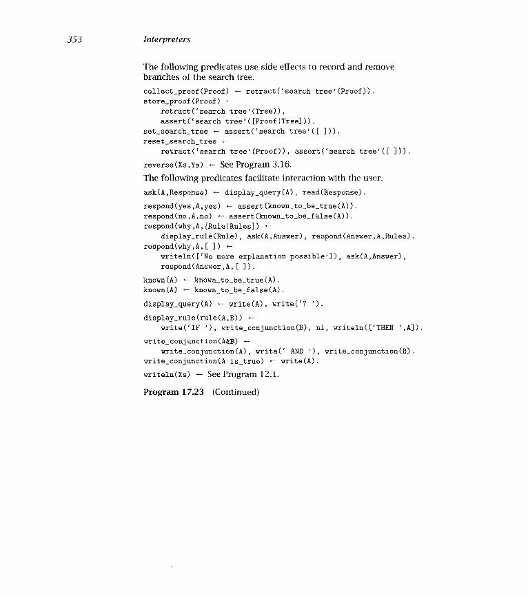
353 Interpreters
The following predicates use side effects to record and removebranches of the search tree.collect_proof(Proof) - retract('search tree' (Proof)).
store_proof (Proof)
retract ('search tree'(Tree)),
assert('search tree' ([Proof ITree]))
set_search_tree assert('search tree'([ 1)).
reset_search_tree
retract('search tree'(Proof)) , assertYsearch tree' ([ 1))
reverse(Xs,Ys) SeeProgram3.16.The followrng predicates facilitate interaction with the user.ask(A,Response) - display_query(A), read(Response).
respond(yes,A,yes) '- assert(known_to_be_true(A))
respond(no,A,no) - assert(known_to_be_false(A)).
respond(why,A, [Rule Rules]) -
display_rule(Rule), ask(A,Answer), respond(Answer,A,Rules).
respond(why,A,[ J)
writeln( ['No more explanation possible']), ask(A,Answer)
respond(Answer,A, [ 1).known(A) - known_to_be_true(A).
known(A) known_to_be_f aise (A)
display_query(A) write(A), write('? ').
display_rule(rule(A,B)) -
writeYlF '), write_conjunction(B), nl, writeln(['THEN ' ,A]).
write_conjunction(A&B) -
write_conjunction(A), write(' AND '), write_conjunction(B).
write_conjunction(A is_true) - write(A).
writein(Xs) - See Program 12.1.
Program 1723 (Continued)

354 Chapter 17
17.5 Background
Our notation for automata follows Hoperoft and Uliman (1979).There is considerable confusion in the literature about the term meta-
interpreterwhether it differs from the term meta-level interpreter,for example. The lack of clarity extends further to the topic of meta-programming. A good discussion of meta-programming can be found inYalçinalp (1991).
One dimension of the discussion is whether the interpreter is capableof interpreting itself. An ìnterpreter with that capability is also calledmeta-circular or self-applicable. An important early discussion of meta-circular interpreters can be found in Steele and Sussman (1978). Thatpaper claims that the ability of a language to specify itself is a funda-mental criterion for language design.
The vanilla meta-interpreter is rooted in Prolog folklore. A versionwas in the suite of programs attached to the first Prolog interpreterdeveloped by Colmerauer and colleagues, and was given in the earlycollection of Prolog programs (Coelho et al., 1980). Subsequently, meta-interpreters, and more generally meta-programs, have been written toaffect the control flow of Prolog programs. References are Gallaire andLasserre (1982), Pereira (1982), and Dincbas and Le Pape (1984). Usingenhanced meta-interpreters for handling uncertainties is described byShapiro (1983c).
There have been several papers on handling cuts in meta-interpreters.A variant of the vanilla meta-interpreter handling cuts correctly is de-scribed in Coelho et al. (1980) and attributed to Luis Pereira. One easymethod to treat cuts is via ancestor cut, which is only present in a fewPrologs like Waterloo Prolog on the IBM and Wisdom Prolog, describedin the first edition of this book. There is a good discussion of meta-interpreters in general, and cuts in particular, in O'Keefe (1990).
Shapiro suggested that enhanced meta-interpreters should be the basisof a progranmiing environment. The argument, along with the debuggingalgorithms of Section 17.3, can be found in Shapiro (1983a). Shapiro'sdebugging work has been extended by Dershowitz and Lee (1987) andDrabent et al. (1989).
Prolog is a natural language for building rule-based systems. The basicstatements are rules, and the Prolog interpreter can be viewed as a back-

355 Interpreters
ward chaining inference engine. Early advocates of Prolog for expert sys-tems were Clark and McCabe (1982), who discussed how explanation fa-cilities and uncertainty can be added to simple expert systems expressedas Prolog clauses by adding extra arguments to the predicates. Incorpo-rating interaction with the user in Prolog was proposed by Sergot (1983).An explanation facility incorporating Sergot's query_the_user was partof the APES expert system shell, described in Hammond (1984).
Using meta-interpreters as a basis for explanation facilities was pro-posed by Sterling (1984). Incorporating failure in a meta-interpreter hasbeen discussed by several researchers, including Hammond (1984), Ster-ling and Latee (1986), and Bruffaerts and Henin (1989). The first descrip-tion of ari integrated meta-interpreter for both success and failure is inYalçinalp and Sterling (1989). The rute interpreter given in Section 17.4is an adaptation of the last paper. The layered approach can be usedto explain cuts clearly, as in Sterling and Yalçinalp (1989), and also foruncertainty reasoning, as in Yalçinalp and Sterling (1991) and more com-pletely in Yalçinalp (1991).


18 Program Transformation
As stated in the introduction to Chapter 17, meta-prograniming, or thewriting of programs that treat other programs as data, is particularlyeasy in Prolog. This chapter gives examples of programs that transformand manipulate Prolog programs. The first section looks at fold/unfold,the operation that underlies most applications of program transfor-mation for Prolog programs. The transformations given in Chapter 15for using difference-lists to avoid explicit concatenation of lists can beunderstood as unfold operations, for example. The second section de-scribes a simple system for controlled unfolding and folding, which isespecially good for removing layers of interpretation. The final sectiongives two examples of source-to-source transformation by code walking
18.1 Unfold/Fold Transformations
Logic programming arose from research on resolution theorem proving.The basic step in the logic programming computation model, goal re-duction, corresponds to a single resolution between a query and a pro-gram clause. Unfold/fold operations correspond to resolution betweentwo Horn clauses. Loosely, unfolding corresponds to replacing a goal inthe body of a clause by its definition, while folding corresponds to recog-nizing that goal(s) in the body of a clause are an instance of a definition.These two operations, being so similar, are often discussed together.
We demonstrate unfolding and folding with a running example in thefirst part of this chapter. The example is specializing the interpreter fornondeterministic pushdown automata (Program 17.3) for the particular

358 Chapter 18
pushdown automaton for recognizing palindromes (Program 17.4). Ingeneral, specializing interpreters is a good application for unfold/foldoperations.
DefinitionUnfolding a goal B in a clause A - B1,.. .,B with respect to a clause B- C1,. . .,Cm where B and B unify with mgu O, produces a clause (A -B1,.. .,B1,C1,. . .,Cm,Bji.....B)O.
As an example of unfolding, we specialize the clause accept (Xs) -
initial(Q), accept(Xs,Q, [ ]) to a particular initial state by unfold-ing the initial (Q) goal with respect to a particular initial fact. Specif-ically, unfolding with respect to the fact initial (push) produces theclause accept(Xs) - accept(Xs,push, E ]). (Note that in our runningexample we use the states push and pop for qQ and qi, respectively, fromthe NPDA of Program 17.4.)
The effect of the unfolding is to instantiate the initial state for theNPDA to push. In general, the effect of unfolding is to propagate variablebindings to the right, as in this example, and also to the left, to goals inthe body of the clause and possibly also to the head.
There may be several clauses whose heads unify with a given goal inthe body of a clause. We extend the definition of unfolding accordingly.
DefinitionUnfolding a goal B in a clause A - B1,. . .,B with respect to a proceduredefining B is to unfold the goal with respect to each clause in the proce-dure whose head unifies with B. u
Unfolding the delta/5 goal in the clause accept([XIXs],Q,S)
delta(Q,X,S,Q1,S1), accept(Xs,Q1,S1) withrespect to the followingprocedure for delta adapted from Program 17.4
delta(push,X,S,push, [XIS]). delta(push,X,S,pop, [XIS]).
delta(push,X,S,pop,S). delta(pop,X,[XIS],pop,S).
produces four clauses, one for each fact.
accept([XIXs],push,S) - accept(Xs,push, [XIS]).
accept([XIXs],push,S) - accept(Xs,pop, [XIS]).
accept([XIXs],push,S) - accept(Xs,pop,S).
accept([XIXs] ,pop, [XIS]) - accept(Xs,pop,S).

359 Program Transformation
palindrome(Xs)The string represented by the list Xs is a palindrome.
palindrome(Xs) - palindrome(Xs,push, E 1).
palindrome([XIXs],push,S) - palïndrome(Xs,push, [XIS]).
palindrome([XIXs] ,push,S) palindrome(Xs,pop, [XIS]).
palindrome([XIXs] ,push,S) - palindrome(Xs,pop,S).
paliridrome([XIXs] pop, [XIS]) - palindrome(Xs,pop,S).
palindrome([ ],pop,[ 1).
Program 18.1 A program accepting palindromes
This example shows variable bhidings being propagated both to theright, and to the head of the clause left of the goal being unfolded.
Folding is the reverse of unfolding. The occurrence of a body of aclause is replaced by its head. It is easiest to show with an example.Folding the goal accept (Xs,push, L 1) m the clause accept(Xs) - ac-
cept(Xs,push, [ J) with respect to the clause palindrome(Xs,State,
Stack) - accept(Xs,State,Stack) produces the clause accept(Xs)
palindrome(Xs,push,[ J).Note that if we now unfold the goal palindrome (Xs ,push, E ]) in ac-
cept(Xs) - paliridrome(Xs,push, L J) with respect to the clause justused for folding, palindrome(Xs,State,Stack) - accept(Xs,State,
Stack), we arrive back at the original clause, accept (Xs) - accept (Xs,push, [ J). Ideally, fold/unfold are inverse operations.
Our example of folding used an iterative clause, i.e., one with a singlegoal in the body. Folding can be performed on a conjunction of goals,but there are technical difficulties arising from the scope of variables.Here we restrict ourselves to iterative clauses. The reader interested inthe more general case should study the references given at the end ofthe chapter.
Specialization of the interpreter of Program 17.3 is completed by un-folding the f irial(L) goal in the third clause of Program 17.3, folding alloccurrences of accept/3, and folding with respect to the clause palm-drome(Xs) - accept(Xs). Program 18.1 is then obtained.
Propagating bindings leftward in Prolog will not preserve correctnessin general. For example, consider unfolding the goal r (X) with respect tothe fact r(3) in the clause p(X) - var(X) , r(x). The resulting clause,

360 Chapter 18
p (3) - var(3), clearly always fails, in contrast with the original clause.Unfolding for Prolog can be performed correctly by not propagatingbindings leftward, and replacing the unfolded goal by the unifier. For thisexample, the result would be p(X) - var(X), X=3. This will not be anissue in the examples we consider.
Exercise for Section 18.1
(i) Specialize the interpreter of Program 17.1 to the NDFA of Pro-gram 17.2, or any other NDFA, by unfold/fold operations.
18.2 Partial Reduction
In this section we develop a simple system for controlled unfold/foldoperations according to prescribed user declarations. Systems for con-trolled unfolding are known in the logic programming literature as par-tial evaluators. This name reveals the influence of functional program-ming, where the basic computation model is evaluation. We prefer torefer to the system in terms of the computation model of logic program-ming, goal reduction. We thus, nonstandardly, say our system is doingpartial reduction, and call it a partial reducer.
Considerable research on applying partial reduction has shown thatpartial reduction is especially useful for removing levels of interpreta-tion. The sequence of unfold/fold operations given in Section 18.1 typifywhat is possible. The general NPDA interpreter was specialized to a spe-cific NPDA, removing interpreter overhead. The resulting program, Pro-gram 18.1, only recognizes palindromes but does so far more efficientlythan the combination of Programs 17.3 and 17.4.
Let us see how to build a system that can apply the unfold and foldoperations that were needed to produce the palindrome program. Themain idea is to recursively perform unfold/fold until no more "progress"can be achieved. A relation that replaces a goal by its equivalent underthese operations is needed. The resulting equivalent goal is known as aresidue. Let us call our basic relation preduce (Goal ,Residue), with in-tended meaning that Residue is a residue arising from partially reducingGoal by applying unfold and fold operations.

361 Program Transformation
preduce(Goal,Residue) -Partially reduce Goal to leave the residue Residue.
preduce(true,true) - L
preduce((A,B),(PA,PB)) , preduce(A,PA), preduce(B,PB).
preduce(A,B) - should_fold(A,B),
preduce(A,Residue)
should_unfold(A), ! , clause(A,B), preduce(B,Residue)
preduce(A,A).
Program 18.2 A meta-interpreter for determining a residue
Program 18.2 contains code for preduce. There are three possibilitiesfor handling a single goal. It can be folded, unfolded, or left alone. Thequestion immediately arises how to decide between the three possibil-ities. The easiest for a system is to rely on the user. Program 18.2 as-sumes that the user gives should_fold (Goal , FoldedGoal) declarationsthat say which goals should be folded and to what they should be folded,and also should_unfold(Goal) declarations that say which goals shouldbe unfolded. Unification against the program clauses determines to whatthey should be unfolded. Goals not covered by either declaration are leftalone. The remaining clauses in Program 18.2 handle the empty goal,true, and conjunctive goals, which are treated recursively in the obviousway.
Observe that Program 18.2 is essentially a meta-interpreter at the gran-ularity level of vanilla (Program 17.5). The meta-interpreter is enhancedto return the residue. Handling builtins is assigned to the exercises.
The query preduce((initial(Q), accept(Xs,Q,[ 1)), Residue)?
assuming appropriate should_fold and should_unfold declarations (tobe given shortly) has as solution Residue = (true,palindromo(Xs,
push, E ])). lt would be preferable to remove the superfluous call totrue. This can be done by modifying the clause handling conjunctivegoals to be more careful in computing the conjunctive resolvent. A suit-able modification is
preduce((A,B) ,Res) -
!, preduce(A,PA), preduce(B,PB), combine(PA,PB,Res),
The code for combine, removing superfluous empty goals, is given inProgram 18.3.

362 Chapter 18
process(Program, RedProgram) -Partially reduce each of the clauses in Program to produceRedProgram.
process(Prog,NewProg) -
findall(PC1, (member(C1 ,Prog) ,preduce(C1 ,PC1)) ,NewProg).
test (Name ,Program) -
program(Name,Clauses), process(Clauses,Prograxn).
preduce ( Goal,Residue) -Partially reduce Goal to leave the residue Residue.
preduce((A - B),(PA PB))
!, preduce(B,PB), preduce(A,PA).
preduce(true,true) -
preduce((A,B) ,Res) -
!, preduce(A,PA), preduce(B,PB), combine(PA,PB,Res).
preduce(A,B) - should_fold(A,B),
preduce(A,Residue) -
should_unf oid(A) , ! , ciause(A,B) preduce(B,Residue).
preduce(A,A).
combine(true,B,B) -
combine(A,true,A) -
combine(A,B,(A,B)).
Program 18.3 A simple partial reduction system
To extend Program 18.2 into a partial reducer, clauses must be han-dled as well as goals. We saw a need in the previous section to partiallyreduce the head and body of a clause. The only question is in which or-der. Typically, we will want to fold the head and unfold the body. Sinceunfolding propagates bindings, unfolding first will allow more specificfolding. Thus our proposed rule for handling clauses is
preduce((A - B),(PA - PB)) -!, preduce(B,PB), preduce(A,PA).
This goal order is advantageous for the example of the rule interpreterto be presented later in this section.
To partially reduce a program, we need to partially reduce each of itsclauses. For each clause, there may be several possibilities because ofnondeterrninism. For example, the recursive accept/3 clause led to fourrules because of the four possible ways of unfolding the delta goal. The

363 Program Transformation
prograin(npda,[(accept(Xsl) initial(Q1), accept(Xsl,Q1,[ 1),(accept([X2IXs2],Q2,S2) - delta(Q2,X2,S2,Q12,S12),
accept(Xs2,Q12,S12)), (accept([ ],Q3,[ J) true)]).
should_unf old C initial (Q))
should_unfold(final(Q))
should_unfold(delta(A,B,C,D,E)).
should_fold(accept(Q,Xs,Q1),palindrome(Q,Xs,Q1)).
should_fold (accept (Xs) ,palindrome (Xs)).
Program 18.4 Specializing an NPDA
cleanest way to get the whole collection of program clauses is to use theall-solutions predicate f indall. That gives
process (Prog, NewProg) -
f indall(PC1, (mernber(Cl,Prog), preduce(Cl,PC1)) ,NewProg).
Putting all the preceding actions together gives a simple system forpartial reduction. The code is presented as Program 18.3. The programalso contains a testing clause.
We now concentrate on how to specify should_fold and should_unfold declarations. Consider the NPDA example for recognizing palin-dromes. The initial, final, and delta goals should all be unfolded. Adeclaration is needed for each. The accept/i and accept/3 goals shouldbe folded into palindrome goals with the same argument. The declara-tion for accept/i is should_f old(accept(Xs),palindrome(Xs)). All
the necessary declarations are given in Program 18.4. Program 18.4 alsocontains the test program as data. Note the need to make all the vari-ables in the program distinct. Applying Program 18.3 to Program 18.4 byposing the query test(npda,P)? produces Program 18.1, with the onlydifference being an explicit empty body for the last palindrome fact.
We now give a more complicated example of applying partial reductionto remove a level of overhead. We consider a simpler variant of the ruleinterpreter given in Section 17.4. The variant is at the bottom level ofthe layered interpreter. The interpreter, whose relation is solve(A,N),
counts the number of reductions used in solving the goal A. The codefor solve and related predicate solve_body is given in Program 18.5.The rules that we will consider constitute Program 17.17 for determining

364 Chapter 18
Rule interpreter for counting reductionssolve(A,1) - fact(A).
solve(A,N) - rule(A,B,Name), solve_body(B,NB), N is NB+1.
solve_body (A&B , N)
solve_body(A,NA), solve_body(B,NB), N is NA+NB.
solve_body(A is_true,N) - solve(A,N).
Sample rule base
rule(oven(Dish,top) ,pastry(Dish) is_true
& size(Dish,small) is_true,placel)
rule(oven(Dish,middle) ,pastry(Dish) is_true
& size(Dish,big) is_true,place2).
rule (oven(Dish,middle) ,main_meal(Dish) is_true,place3).
rule (oven(Dish,bottom) , slow_cooker(Dish) is_true,place4)
rule(pastry(Dish),type(Dish,cake) is_true,pastryl).
rule (pastry(Dish) ,type(Dish,bread) is_true,pastry2).
rule(main_meal(Dish) ,type(Dish,meat) is_true ,main_meal).
rule(slow_cooker (Dish) ,type(Dish,milk_pudding)
is_true ,slow_cooker).
should_fold(solve(oven(D,P),N),oven(D,P,N)).
should_fold(solve(pastry(D),N),pastry(D,N)).
should_fold(solve(main_meal(D) ,N) ,main_meal(D,N)).
should_fold(solve(slow_cooker(D),N),slow_cooker(D,N)).
should_fold(solve(type(D,P),N),type(D,P,N)).
should_fold(solve(size(D,P),N),size(D,P,N)).
should_unfold(solve_body(G,N)).
should_unfold(rule(A,B,Name)).
program(rule_interpreter, [(solve(A1,l) - fact(A1)),
(solve(A2,N) - rule(A2,B,Name), solve_body(B,NB), N is NB+i)]).
Program 18.5 Specializing a rule interpreter

365 Program Transformation
where a dish should be placed in the oven. The rules are repeated inProgram 18.5 for convenience.
The effect of partial reduction in this case will be to "compile" therules into Prolog clauses where the arithmetic calculations are done. Theresulting Prolog clauses can in turn be compiled, in contrast to the com-bination of interpreter plus rules. Rule place i will be transformed to
oven(Dish,top,N)
pastry(Dish,N1), size(Dish,small,N2),
N3 is N1+N2, N is N3+1.
The idea is to unfold the calls to rule so that each rule can be handled,and also to unfold the component of the interpreter that handles syn-tactic structure, specifically solvebody. What gets folded are the indi-vidual calls to solve, such as solve (oven (D,P) ,N), which gets replacedby a predicate oven (D , P, N) The necessary declarations are given in Pro-gram 18.5. Program 18.3 applied to Program 18.5 produces the desiredeffect.
Specifying what goals should be folded and unfolded is in generalstraightforward in cases similar to what we have shown. Nevertheless,making such declarations is a burden on the programmer. In many cases,the declarations can be derived automatically. Discussing how is beyondthe scope of the chapter.
How useful partial reduction is for general Prolog programs is an openissue. As indicated, care must be taken when handling Prolog's impuri-ties not to change the meaning of the program. Further, interaction withProlog implementations can actually mean that programs that have beenpartially reduced can perform worse than the original program. lt will beinteresting to see how much partial reduction will be applied for Prologcompilation.
Exercises for Section 182
Extend Program 18.3 to handle builtins.
Apply Program 18.3 to the two-level rule interpreter with rulesgiven as Program 17.20.

366 Chapter 18
18.3 Code Walking
The examples of meta-prograrnniing given so far in Chapters 17 and 18are dynamic in the sense that they "execute" Prolog programs by per-forming reductions. Prolog is also a useful language for writing staticmeta-programs that perform syntactic transformations of Prolog pro-grams. In this section, we give two nontrivial examples in which pro-grams are explicitly manipulated syntactically.
The first example of explicit program manipulation is program com-position. In Section 13.3, stepwise enhancement for systematic construc-tion of Prolog programs was introduced. The third and final step in themethod is composition of separate enhancements of a common skele-ton. We now present a program to achieve composition that is capable ofcomposing Programs 13.1 and 13.2 to produce Program 13.3.
The running example we use to illustrate the program is a variant ofthe example in Chapter 13. The skeleton is the same, namely,
skel([XIXs],Ys) - member(X,Ys), skel(Xs,Ys).skel([XIXs],Ys) - nonmember(X,Ys), skel(Xs,Ys).skel([ ],Ys).The union program, Program 13.1, is also the same, namely,
union([XIXs],Ys,Us) - member(X,Ys), union(Xs,Ys,Us).union([XIXs] ,Ys, [XIUs]) - nonmember(X,Ys), union(Xs,Ys,Us).union([ ],Ys,Ys).The second program to be composed is different and represents whenadded goals are present. The relation to be used is common(Xs,Ys,N),which counts the number of common elements N in two lists Xs and Ys.The code is
coinmon([XIXs],Ys,N) -meinber(X,Ys), conimon(Xs,Ys,M), N is M+1.
coinmon([XIXs],Ys,N) - nonmember(X,Ys), coinmon(Xs,Ys,N).comnion([ J,Ys,O).
The program for composition makes some key assumptions that canbe justified by theory underlying stepwise enhancement. Describing thetheory is beyond the scope of this book. The most important assump-tion is that there is a one-to-one correspondence between the clauses of

367 Program Transformation
the two programs being composed, and one-to-one correspondences be-tween the clauses of each of the programs and the common skeleton.
Programs are represented as lists of clauses. The first clause in the firstprogram corresponds to the first clause in the second program and tothe first clause in the skeleton. Our assumption implies that the lists ofclauses of programs being composed have the same length. The threeprograms have been written with corresponding clauses in the same or-der. (That the lists of clauses do have the same length is not checkedexplicitly.)
In order to perform composition, a composition specification isneeded. It states how the arguments of the final program relate tothe two extensions. The relation that we will assume is composition_
specification(Programl,Program2,Skeleton,FinalProgram). An ex-
ample of the specification for our running example is composition_
specification(union(Xs,Ys,Us), conunon(Xs,Ys,N), skel(Xs,Ys),
uc(Xs,Ys,Us,N). The composition specification is given as part of Pro-gram 18.6.
The program for composition is given as Program 18.6. The top-levelrelation is compose/4, which composes the first two programs assumedto be enhancements of the third argument to produce the compositeprogram, which is the fourth argument.
The program proceeds clause by clause in the top ioop of Pro-gram 18.6, where compose_clause/4 does the clause composition. Thearguments correspond exactly to the arguments for compose. To com-pose two clauses, we have to compose the heads and the bodies. Com-position of the heads of clauses happens through unification with thecomposition specification. The predicate compose_bodies/4 is used tocompose the bodies. Note that the order of arguments has been changedso that we systematically traverse the skeleton. Each goal in the skeletonmust be represented in each of the enhancements so that it can be usedas a reference to align the goals in each of the enhancements.
The essence of compose_bodies is to traverse the body of the skeletongoal by goal and construct the appropriate output goal as we proceed.In order to produce tidy output and avoid superfluous empty goals, adifference-structure is used to build the output body. The first clausefor compose_bodies covers the case when the body of the skeleton isnonempty. The predicates first and rest, which access the body of theskeleton, are a good example of data abstraction.

368 Chapter 18
compose (Program 1 ,Program2,Skeleton,FinalProgram) -FinaiProgram is the result of composing Program i andProgram2, which are both enhancements of Skeleton.
compose([CllIClsl] , [Cl2ICis2] , [CiSkellCisSkei] ,[Cl Cisl) -compose_clause(Cll ,C12 ,ClSkel ,Cl),
compose (Cisl ,Cls2,CisSkei,Cls)
compose([ ]j ],[ ],[ 1).compose_clause((AlBl) , (A2B2) , (ASkelBSkel) ,(AB)) -
composition_specification(Al ,A2 ,ASkel ,A)
compose_bodies(BSkei,Bl ,B2,B\true).
compose_bodíes(SkeiBody,Bodyl ,Body2,B\BRest) -
first (SkelBody,G),
align(G,Bodyl Cl ,RestBodyl ,B\Bl),
align(G,Body2,G2,RestBody2,Bl\(Goal,B2)),
compose_goal(Gl ,G2,Goai),
rest(SkeiBody,Gs)
compose_bodies(Gs,RestBodyl ,RestBody2,B2\BRest).
compose_bodies (true, Bodyl , Body2 , B\BRest) -
rest_goals (Bodyl,B\Bl), rest_goals(Body2,Bl\BRest).
align(Goal,Body,G,RestBody,B\B) -
first(Body,G), correspond(G,Goai), , rest(Body,RestBody).
align(Goal,(G,Body),CorrespondingG,RestBody,(G,B)\Bl) -
align (Goal ,Body, CorrespondingG , RestBody , B\Bl).
first((G,Gs) ,G)
first(G,G) - G (A,B), G true.
rest((G,Gs) ,Gs)
rest(G,true) - G (A,B).
correspond (G , G)
correspond(G,B) map(G,B).
compose_goai(G,G,G) - !
compose_goai(Al ,A2,A) -
composition_specification(Al,A2,ASkei,A).
rest_goals(true,B\B) - !
rest_goals(Body, (G,B)\BRest) -
first(Body,G), , rest(Body,Bodyl), rest_goais(Bodyl,B\BRest).
Program 18.6 Composing two enhancements of a skeleton

369 Program Transformation
An important assumption made by Program 18.6 concerns finding thegoals in the bodies of the program that correspond to the goals in theskeleton. The assumption made, embedded in the predicate correspond,
is that a mapping will be given from goals in the enhancement to goalsin the skeleton. In our running example, the predicates member and non-
member map onto themselves, while both union and common map ontoskel. This information, provided by the predicate map/2, is needed tocorrectly align goals from the skeleton with goals of the program beingcomposed. The code for align as presented allows for additional goalsto be present between goals in the skeleton. The only extra goal in ourrunning example is the arithmetic calculation in common, which is afterthe goals corresponding to the skeleton goals.
The second clause for compose_bodies covers the case when the bodyis empty, either from dealing with a fact or because the skeleton has beentraversed. In this case, any additional goals need to be included in theresult. This is the function of rest_goals.
Program 18.7 contains a testing clause for Program 18.6, along with thespecific data for our running example. As with Program 18.4, variablesin the programs being composed must be named differently. Automaticgeneration of composition specifications for more complicated examplesis possible.
The second example of explicit manipulation of programs is the con-version of context-free grammar rules to equivalent Prolog clauses.Context-free grammars are defined over a language of symbols, dividedinto nonterminal symbols and terminal symbols. A context-free grammaris a set of rules of the form
(head) - (body)
where head is a nonterminal symbol and body is a sequence of oneor more items separated by commas. Each item can be a terminal ornonterminal symbol. Associated with each grammar is a starting symboland a language that is the set of sequences of terminal symbols obtainedby repeated (nondeterministic) application of the grammar rules startingfrom the starting symbol. For compatibility with Chapter 19, nonterminalsymbols are denoted as Prolog atoms, terminal symbols are enclosedwithin lists, and II denotes the empty operation.
The language a(bc)* can be defined by the following context-free gram-mar consisting of four rules:

370 Chapter 18
test_compose (X, Prog) -programl(X,Progl), program2(X,Prog2),skeleton(X,Skeleton), compose(Progl ,Prog2 ,Skeleton,Prog).
programi (test,(union([X1IXs1] ,Ysl,Zsl) -
member(X1,Ysi), union(Xsl,Ysi,Zsl)),(union([X2IXs2] ,Ys2, [X2IZs2]) -
nonmember(X2,Ys2), union(Xs2,Ys2,Zs2)),(union([ ],Ys3,Ys3) - true)]).
program2(test, E(common([X1IXs1] ,Ysl,Ni)
member(Xi,Ysl), comxnon(Xsl,Ysl,M1), Nl is M1+l),(common([X2IXs2] ,Ys2,N2) -
nonmember(X2,Ys2), common(Xs2,Ys2,N2)),(cominon([ ],Ys3,O) - true)]).
skeleton(test, I(skel([X1IXs1],Ysl) - member(Xl,Ysl), skel(Xsl,Ysl)),(skel([X2IXs2] ,Ys2) - nonmember(X2,Ys2), skel(Xs2,Ys2)),(skel([ ],Ys3) - true)]).
composition_specification(union(Xs,Ys,Us), common(Xs,Ys,N)skel(Xs,Ys) ,uc(Xs,Ys,Us,N))
rnap(union(Xs,Ys,Zs), skel(Xs,Ys))map(common(Xs,Ys,N), skel(Xs,Ys)).
Program 18.7 Testing program composition
s - [a], b.
b - [b], c.
b - [ ].
c - [c], b.
Another example of a context-free grammar is given in Figure 18.1.This grammar recognizes the language a*b*c*.
A context-free grammar can be immediately written as a Prolog pro-gram. Each nonterminal symbol becomes a unary predicate whose argu-ment is the sentence or phrase it identifies. The naive choice for repre-senting each phrase is as a list of terminal symbols. The first grammarrule in Figure 18.1 becomes
s(Xs) - a(As), b(Bs),
c(Cs), append(Bs,Cs,BsCs), append(As,BsCs,Xs).

371 Program Transformation
s -' a, b, c.a - [a], a.a -. [ ].b [b], b.b [J.c -. [c], c.C £ J.
Figure 18.1 A context-free grammar for the language a*b*c*
s(As\Xs) '- a(As\Bs), b(Bs\Cs), c(Cs\Xs).a(Xs\Ys) - connect([a] ,Xs\Xsl), a(Xsl\Ys).a(Xs\Ys) - connect([ ] ,Xs\Ys)b(Xs\Ys) '- connect([b] ,Xs\Xsl), b(Xsl\Ys).b(Xs\Ys) - connect([ ],Xs\Ys).c(Xs\Ys) - cormect([c],Xs\Xsl), c(Xsl\Ys).c(Xs\Ys) - cormect([ ],Xs\Ys).connect([ ] ,Xs\Xs).connect([WIWs] , [WIXs]\Ys) connect(Ws,Xs\Ys).
Program 18.8 A Prolog program parsing the language a*b*c*
Completing the grammar of Figure 18.1 in the style of the previousrule leads to a correct program for parsing, albeit an inefficient one.The calls to append suggest, correctly, that a difference-list might be amore appropriate structure for representing the sequence of terminalsin the context of parsing. Program 18.8 is a translation of Figure 18.1 toa Prolog program where difference-lists represent the phrases. The basicrelation scheme is s(Xs), which is true if Xs is a sequence of symbolsaccepted by the grammar.
The predicate connect (Xs,Ws) is true if the list Xs represents the samesequence of elements as Ws. The predicate is used to make explicit thetranslation of terminal symbols to Prolog programs.
As a parsing program, Program 18.8 is a top-down, left-to-right re-cursive parser that backtracks when it needs an alternative solution. Al-though easy to construct, backtracking parsers are in general inefficient.However, the efficiency of the underlying Prolog implementation in gen-eral more than compensates.

372 Chapter 18
translate( Grammar,Program) -Program is the Prolog equivalent of the context-freegrammar Grammar.
translate ([Rule Rules] , [Clause I Clauses]) -
translate_rule(Rule ,Clause),
translate (Rules , Clauses)
translate([ ],[ J).translate_rule ( GrammarRule,PrologClause) -
Prolog Clause is the Prolog equivalent of the grammarrule GrammarRule.
translate_rule((Lhs - Rhs),(Head - Body)) -
translate_head(Lhs,Head,Xs\Ys),
translate_body (Rhs ,Body, Xs\Ys).
translate_head(A,Al ,Xs) -
translate_goal(A,Al ,Xs).
translate_body(A,B) , (Al ,B1) ,Xs\Ys) -
translate_body(A,Al,Xs\Xsl), translate_body(B,Bl,Xsl\Ys).
translate_body (A,Al ,Xs)
translate_goal(A,Al ,Xs).
translate_goal (A,Al ,DList) -
nonterminal(A), functor(Al,A,l), arg(l,Al,DList).
translate_goal(Terms,coirnect(Terms,S) ,S)
terminals (Terms).
nonterminal(A) atom(A).
terminals(Xs) - list(Xs).
list(Xs) - seeProgram3.11.
Program 18.9 Translating grammar rules to Prolog clauses
We now present Program 18.9, which translates Figure 18.1 to Pro-gram 18.8. As for Program 18.6, the translation proceeds clause byclause. There is a one-to-one correspondence between grammar rulesand Prolog clauses. The basic relation is translate(Rules,Clauses).
Individual clauses are translated by translate.rule/2. To translate arule, both the head and body must be translated, with the appropriatecorrespondence of difference-lists, which will be added as additionalarguments.
Adding an argument is handled by the predicate translate_goal. Ifthe goal to be translated is a nonterminal symbol, a unary predicate with

373 Program Transformation
the same functor is created. If the goal is a list of terminal symbols, theappropriate connect goal is created. When executed, the connect goalconnects the two difference-lists. Code for connect is in Program 18.8.
Program 18.9 can be extended for automatic translation of definiteclause grammar rules. Definite clause grammars are the subject of Chap-ter 19. Most versions of Edinburgh Prolog provide such a translator.
Exercise for Section 18.3
(i) Apply Program 18.6 to one of the exercises posed at the end ofSection 13.3.
18.4 Background
Often research in logic programming has followed in the steps of relatedresearch in functional programming. This is true for unfold/fold and par-tial evaluation. Burstall and Darlington (1977) wrote the seminal paperon unfold/fold in the functional programming literature. Their work wasadapted for logic programming by Tamaki and Sato (1984).
The term partial evaluation may have been used first in a paper byLombardi and Raphael (1964), where a simple partial evaluator for Lispwas described. A seminal paper introducing partial evaluation to com-puter science is due to Futamura in 1971, who noted the possibilityof compiling away levels of interpretation. Komorowski described thefirst partial evaluator for pure Prolog in his thesis in 1981. He has sincepreferred the term partial deduction. Gallagher in 1983 was the first toadvocate using partial evaluation in Prolog for removing interpretationoverhead (Gallagher, 1986). Venken (1984) was the first to list some ofthe problems of extending partial evaluation to full Prolog. The paperthat sparked the most interest in partial evaluation in Prolog is dueto Takeuchi and Furukawa (1986). They discussed using partial evalua-tion for removing runtime overhead and showed an order of magnitudespeedup. Sterling and Beer (1989) particularize the work for expert sys-tems. Their paper introduces the issue of pushing down meta-arguments,which is subsumed in this chapter by should_fold declarations. SpecificProlog partial evaluation systems to read for more details are ProMiX

374 Chapter 18
(Lakhotia and Sterling, 1990) and Mixtus (Sahlin, 1991). An interestingapplication of partial evaluation is given by Smith (1991), where efficientstring-matching programs were developed.
Composition was first discussed in the context of Prolog meta-inter-preters in Sterling and Beer (1989) and an informal algorithm was givenin Sterling and Lakhotia (1988). A theory is found in Kirschenbaum, Ster-ling, and Jam (1993).

19 Logic Grammars
A very important application area of Prolog is parsing. In fact, Prologoriginated from attempts to use logic to express grammar rules and toformalize the process of parsing. In this chapter, we present the mostcommon logic grammar formalism, definite clause grammars. We showhow grammar rules can be considered as a language on top of Prolog,and we apply granirnar rules to parse simple English sentences. In Chap-ter 24, definite clause grammars are used as the parsing component of asimple compiler for a Pascal-like language.
19.1 Definite Clause Grammars
Definite clause grammars arise from adding features of Prolog tocontext-free grammars. In Section 18.3, we briefly sketched how context-free grammars could be immediately converted to Prolog programs,which parsed the language specified by the context-free grammar. Byadding the ability of Prolog to exploit the power of unification and theability to call builtin predicates, a very powerful parsing formalism isindeed achieved, as we now show.
Consider the context-free grammar for recognizing the languagea*b*c*, presented in Figure 18.1, with equivalent Prolog program Pro-gram 18.8. The Prolog program can be easily enhanced to count thenumber of symbols that appear in any recognized sequence of a's, b's,and c's. An argument would be added to each predicate constitutingthe number of symbols found. Arithmetic would be performed to addnumbers together. The first clause would become

376 Chapter 19
s(As\Xs,N) -a(As\Bs,NA), b(Bs\Cs,NB), c(Cs\Xs,NC), N is NA+NB+NC.
The extra argument counting the number of a's, b's, and c's can beadded to the grammar rule just as easily, yielding
s(N) - a(NA), b(NB), c(NC), N is NA+NB+NC.
Adding arguments to nonterminal symbols of context-free grammars,and the ability to call (arbitrary) Prolog predicates, increases their util-ity and expressive power. Grammars in this new class are called definiteclause grammars, or DCGs. Definite clause grammars are a generaliza-tion of context-free grammars that are executable, augmented by thelanguage features of Prolog.
Program 18.9, translating context-free grammars into Prolog programs,can be extended to translate DCGs into Prolog. The extension is posed asExercise (i) at the end of this section. Throughout this chapter we writeDCGs in grammar rule notation, being aware that they can be viewedas Prolog programs. Many Edinburgh Prolog implementations providesupport for grammar rules. The operator used for - is -->. Grammarrules are expanded automatically into Prolog clauses with two extra ar-guments added as the last two arguments of the predicate to representas a difference-list the sequence of tokens or words recognized by thepredicate. Braces are used to delimit goals to be called by Prolog di-rectly, which should not have extra arguments added during translation.Grammar rules are not part of Standard Prolog but will probably be in-corporated in the future.
Program 19.1 gives a DCG that recognizes the language a*b*c* andalso counts the number of letters in the recognized sequence. The en-hancement from Figure 18.1 is immediate. To query Program 19.1, con-sideration must be taken of the two extra arguments that will be added.Forexample,asuitablequeryiss(N,[a,a,b,b,b,c],1 ])?.
Counting the symbols could, of course, be accomplished by traversingthe difference-list of words. However, counting is a simple enhancementto understand, which effectively displays the essence of definite clausegrammars. Section 19.3 presents a wider variety of enhancements.
Our next example is a striking one of the increase in expressive powerpossible using extra arguments and unification. Consider recognizing thelanguage a"b"c", which is not possible with a context-free grammar

377 Logic Grammars
s(N) a(NA), b(NB), c(NC), (N is NA+NB+NC}.
a(N) - [a], a(N1), (N is Ni+i}.a(0) [1.b(N) [b], b(N1), (N is N1+1}.b(0) [ ].c(N) -' [c] , c(N1) , (N is N1+1}c(0) E].
Program 19.1 Enhancing the language a*b*c*
s - a(N), b(N), c(N).a(N) [a], a(N1), (N is N1+1}.a(0) - [ ].b(N) -. [b] , b(N1) , (N is N11-1}b(0) - [ ].c(N) -. [c] , c(N1) , {N is N1+1}c(0) -. E].
Program 19.2 Recognizing the language aN1cN
However, there is a straightforward modification to the grammar givenas Program 191. All that is necessary is to change the first rule and makethe number of a's, b's, and c's the same. The modified program is givenas Program 19.2.
In Program 19.2, unification has added context sensitivity and in-creased the expressive power of DCGs over context-free grammars. DCGsshould be regarded as Prolog programs. Indeed, parsing with DCGs is aperfect illustration of Prolog programming using nondeterrninistic pro-gramming and difference-lists. The top-down, left-to-right computationmodel of Prolog yields a top-down, left-to-right parser.
Definite clause grammars can be used to express general programs.For example, a version of Program 3.15 for append with its last twoarguments swapped can be written as follows.
append([ 1) - E].append([XIXs]) -. lix], append(Xs).
Using DCGs for tasks other than parsing is an acquired programmingtaste.

378 Chapter 19
The grammar for the declarative part of a Pascal program.
declarative_part -
const_declaration, type_declaration,
var_declaration, procedure_declaration.
Constant declarations
const_declaration - E J
const_declaration
[const] , const_definition, E;] , const_definitions.
const_definitions E J
const_def initions
const_definition, E;] , const_definitions.
const_definition - identifier, [=1, constant.
identifier - [X] , {atom(X) }.
constant - [X], {constant(X)}.
Type declarations
type_declaration -. E ].type_declaration
[type] , type_definition, [;] , type_definitions.
type_definitions E I
type_definitions - type_definition, E;] , type_definitions.
type_definition identifier, [=1 , type.
type -. ['INTEGER'].type ['REAL'].
type ['BOOLEAN'].type ['CHAR'].
Variable declarations
var_declaration - [ I.var_declaration
[var] , var_definition, E;] , var_definitions.
var_definitions -' E J
var_definitions - var_definition, E;] , var_definitions.
var_definition - identifiers, E:], type.
identifiers identifier.
identifiers - identifier, E,] , identifiers.
Program 19.3 Parsing the declarative part of a Pascal block

379 Logic Grammars
Procedure declarationsprocedure_declaration -. E
procedure_declaration -. procedure_heading, E;] , block.
procedure_heading
[procedure] , identifier, formal_parameter_part.
formal_parameter_part E ].formal_parameter_part [C] , f ormal_parameter_section, E)]
formal_parameter_section - formal_parameters.
formal_parameter_ection -.
formal_parameters, E;] , formal_parameter_section.
formal_parameters value_parameters.
formal_parameters -. variable_parameters.
value_parameters var_definition.
variable_parameters [var], var_definition.
Program 19.3 (Continued)
We conclude this section with a more substantial example. A DCG isgiven for parsing the declarative part of a block in a Pascal program. Thecode does not in fact cover all of Pascal - it is not complete in its defi-mtion of types or constants, for example. Extensions to the grammar areposed in the exercises at the end of this section. Parsing the statementpart of a Pascal program is illustrated in Chapter 24.
The grammar for the declarative part of a Pascal block is given as Pro-gram 19.3. Each grammar rule corresponds closely to the syntax diagramfor the corresponding Pascal statement. For example, the syntax diagramfor constant declarations is as follows:
---> const -----> Constant Definition > >
+ < +
The second grammar rule for const_declaration in Program 19.3says exactly the same. A constant declaration is the reserved wordconst followed by a constant definition, handled by the nontermrnalsymbol const_definition; followed by a semicolon; followed by therest of the constant definition, handled by the nonterminal symbolconst_def initions. The first rule for const_declaratìon effectivelystates that the constant declaration is optional. A constant definition is

380 Chapter 19
an identifier followed by =, followed by a constant. The definition forconst_def initions is recursive, being either empty or another constantdefinition; followed by a semicolon; followed by the rest of the constantdefinition.
The remainder of Program 19.3 is sirmiarly easy to understand. Itclearly shows the style of writing grammars in Prolog.
Exercises for Section 19.1
Extend Program 18.9 so that it translates definite clause grammarsto Prolog as well as context-free grammars.
Add to Program 19.3 the ability to correctly handle label declara-tions and function declarations.
Enhance Program 19.3 to return the list of variables declared in thedeclarative part.
Write a program to parse the language of your choice in the style ofProgram 19.3.
19.2 A Grammar Interpreter
Grammar rules are viewed in the previous section as syntactic sugar forProlog clauses. This view is supported by Prolog systems with automaticgrammar rule translation. There is a second way of viewing grammarrules, namely as a rule language.
This section takes the second view and considers grammar rules asan embedded language on top of Prolog. We consider applying the in-terpreter techniques of Chapter 17 to grammar rules.
Program 19.4 is an interpreter for grammar rules. The basic relationis parse (Symbol,Tokens), which is true ifa sequence of grammar rulescan be applied to Symbol to reach Tokens. The tokens are represented asa difference-list.
The granularity of the DCG interpreter is at the clause reduction level,the same as for the vanilla meta-interpreter, Program 17.5, and the expertsystem rule interpreter, Program 17.18. Indeed, the code ni Program 19.4is similar to those interpreters. There are four cases, handled by the

381 Logic Grammars
parse(Start,Tokens)The sequence of tokens Tokens represented as a difference-listcan be reached by applying the grammar rules defined by /2,starting from Start.
parse(A,Tokens) -nonterminal(A), A -. B, parse(B,Tokens).
parse((A,B) ,Tokens\Xs)parse(A,Tokens\Tokensl), parse(B,Tokensl\Xs).
parse(A,Tokens) terminais(A), cormect(A,Tokens).parse({A},Xs\Xs) - A.terminals(Xs) See Program 18.9.
connect(Xs,Tokens) - See Program 18.8.
Program 19.4 A definite clause grammar (DCG) interpreter
four clauses for parse in Program 19.4. The first rule handles the basicoperation of reducing a nonterminal symbol, and the second rule handlesconjunctions of symbols. The third rule handles terminal symbols, andthe fourth rule covers the ability to handle Prolog predicates by callingthem directly using the meta-variable facility.
Observe that the last argument in parse/2, the DCG interpreter, is adifference-list. This difference-list can be handled implicitly using gram-mar rule notation. In other words, Program 19.4 could itself be written asa DCG. This task is posed as Exercise 19.2(i).
Recall that the interpreters of Chapter 17 were enhanced. Similarly,the DCG interpreter, Program 19.4, can be enhanced. Program 19.5 givesa simple enhancement that counts the number of tokens used in pars-ing. As mentioned before, this particular enhancement could be accom-plished directly, but it illustrates how an interpreter can be enhanced.
Comparing Programs 19.1 and 19.5 raises an important issue. Is itbetter to enhance a grammar by modifying the rules, as in Program 19.1,or to add the extra functionality at the level of the interpreter? Thesecond approach is more modular, but suffers from a lack of efficiency,
Exercises for Section 19.2
(i) Write Program 19.4 as a DCG.

382 Chapter 19
parse(Start, Tokens,N)The sequence of tokens Tokens, represented as a difference-list,can be reached by applying the grammar rules defined by -./2,starting from Start, and N tokens are found.
parse(A,Tokens,N) -
nonterminal(A), A -. B, parse(B,Tokens,N).
parse((A,B) ,Tokens\Xs,N)
parse(A,Tokens\Tokensl ,NA), parse(B,Tokensl\Xs ,NB),
N is NA+NB.
parse(A,Tokens,N) -
terminais(A), connect(A,Tokens), length(A,N).
parse({A},Xs\Xs,O) - A.
terninals(Xs) - See Program 18.9.
connect(A,Tokens) - See Program 18.8.
length(Xs,N) - SeeProgram8.11.
Program 19.5 A DCG interpreter that counts words
Use the partial reducer, Program 18.3, to specialize the interpreterof Program 19.4 to a particular grammar For example, Figure 18.1should be transformed to Program 19.1.
Enhance Program 19.4 to build a parse tree.
19.3 Application to Natural Language Understanding
An important application area of logic programming has been under-standing natural languages. Indeed, the origins of Prolog lie within thisapplication. In this section, it is shown how Prolog, through definiteclause grammars, can be applied to natural language processing.
A simple context-free grammar for a small subset of English is givenin Program 19.6. The nonterminal symbols are grammatical categories,parts of speech and phrases, and the terminal symbols are English wordsthat can be thought of as the vocabulary. The first rule in Program 19.6says that a sentence is a noun phrase followed by a verb phrase. The lastrule says that surprise is a noun. A sample sentence recognized by thegrammar is: "The decorated pieplate contains a surprise."

383 Logic Grammars
Grammar Rules
sentence - noun_phrase, verb_phrase.
noun_phrase determiner, noun_phrase2.
noun_phrase - noun_phrase2.
noun_phrase2 adjective, noun_phrase2.
noun_phrase2 -, noun.
verb_phrase -. verb.
verb_phrase -' verb, noun_phrase.
Vocabulary
determiner [the] . adjective [decorated]
determiner - [a]
noun - [pieplate] . verb -' [contains]
noun -' [surprise]
Program 19.6 A DCG context-free grammar
Using the terminology of stepwise enhancement introduced in Chap-ter 13, we can view a grammar as a skeleton. We proceed to show howuseful grammatical features can be added by enhancement. The nexttwo programs are enhancements of Program 19.6. The enhancements,although simple, typify how DCGs can be used for natural language ap-plications. Both programs exploit the power of the logical variable.
The first enhancement is constructing a parse tree for the sentence asit is being parsed. The program is given as Program 19.7. Arguments rep-resenting (subparts of) the parse tree must be added to Program 19.6.The enhancement is similar to adding structured arguments to logic pro-grams, as discussed in Section 2.2. The program builds the parse treetop-down, exploiting the power of the logic variable.
The rules in Program 19.7 can be given a declarative reading. For exam-ple, consider the rule
sentence(sentence(NP,VP)) - noun_phrase (NP), verb_phrase(VP).
This states that the parse tree built in recognizing the sentence is a struc-ture sentence (NP,VP), where NP is the structure built while recognizingthe noun phrase and VP is the structure built while recognizing the verbphrase.

384 Chapter 19
sentence(sentence(NP,VP)) - noun_phrase(NP), verb_phrase(VP).
noun_phrase(np(D,N)) determiner(D), noun_phrase2(N).
noun_phrase(np(N)) noun_phrase2(N).
noun_phrase2(np2(A,N)) -. adjective(A), noun_phrase2(N).
noun_phrase2(np2(N)) noun(N).
verb_phrase(vp(V)) - verb(V).
verb_phrase(vp(V,N)) verb(V), noun_phrase (N).
Vocabulary
determiner(det(the)) - [the]
determiner(det(a)) [a]
noun(noun(pieplate)) -. [pieplate]
noun(noun(surprise)) -. [surprise]
adjective(adj(decorated)) - [decorated].
verb(verb(contains)) - [contains]
Program 19.7 A DCG computing a parse tree
The next enhancement concerns subject/object number agreement.Suppose we wanted our grammar also to parse the sentence "The dec-orated pieplates contain a surprise." A simplistic way of handling pluralforms of nouns and verbs, sufficient for the purposes of this book, is totreat different forms as separate words. We augment the vocabulary byadding the facts
noun(noun(pieplates)) -P [pieplates]
verb(verb(contain)) - [contain].
The new program would parse "The decorated pieplates contain a sur-prise" but unfortunately would also parse "The decorated pieplates con-tains a surprise." There is no insistence that noun and verb must both besingular, or both be plural.
Number agreement can be enforced by adding an argument to theparts of speech that must be the same. The argument indicates whetherthe part of speech is singular or plural. Consider the grammar rule
sentence (sentence (NP ,VP))
noun_phrase(NP,Num), verb_phrase(VP,Nuin).
The rule insists that both the noun phrase, which is the subject of thesentence, and the verb phrase, which is the object of the sentence, have

385 Logic Grammars
sent once ( sentence (NP VP)noun_phrase(NP,Num), verb_phrase(VP,Num).
noun_phrase(np(D,N) Nun)determiner(D,Nurn), noun_phrase2(N,Num).
noun_phrase(np(N) Nun) -. noun_phrase2(N,Nuxn).
noun_phrase2(np2(A,N) ,Nuzn) -.adjective(A), noun_phrase2(N,Nuzn).
noun_phrase2(np2(N) ,Nuin) -. noun(N,Num).
verb_phrase (vp(V) ,Nuis) - verb(V,Num)vorb_phrase(vp(V,N) ,Num)
verb(V,Nuni), nouri_phrase(N,Nunìl).
Vocabulary
determiner(det(the) Nun) [the]detertniner(det(a),singular) - [a].noun(noun(pieplate),singular) - [pieplate]noun(noun(pieplates) plural) -. [pieplates]noun(noun(surprïse) singular) -. [surprise]noun(noun(surprises) plural) [surprises]adjective(adj(decorated)) -. [decorated].verb(verb(contains) ,singular) [contains].verb(verb(contain) ,plural) [contain].
Program 19.8 A DCG with subject/object number agreement
the same number, singular or plural. The agreement is indicated by thesharing of the variable Nun. Expressing subject/object number agreementis context-dependent information, which is clearly beyond the scope ofcontext-free grammars.
Program 19.8 is an extension of Program 19.7 that handles numberagreement correctly. Noun phrases and verb phrases must have the samenumber, singular or plural. Similarly, the determiners and nouns in anoun phrase must agree in number. The vocabulary is extended to indi-cate which words are singular and which plural. Where number is unim-portant, for example, with adjectives, it can be ignored, and no extraargument is given. The determiner the can be either singular or plural.This is handled by leaving the argument indicating number uninstanti-ated.

386 Chapter 19
The next example of a DCG uses another Prolog feature, the abilityto refer to arbitrary Prolog goals in the body of a rule. Program 19.9 isa grammar for recognizing numbers written in English up to, but notincludmg, 1,000. The value of the number recognized is calculated usingthe arithmetic facilities of Prolog.
The basic relation is number (N), where N is the numerical value of thenumber being recognized. According to the grammar specified by theprogram, a number is zero or a number N of at most three digits, the rela-tion xxx (N) Similarly xx (N) represents a number N of at most two digits,and the predicates rest _xxx and rest_xx denote the rest of a number ofthree or two digits, respectively, after the leading digit has been removed.The predicates digit, teen, and tens recognize, respectively, single dig-its, the numbers 10 to 19 inclusive, and the multiples of ten from 20 to90 inclusive.
A sample rule from the grammar is
xxx(N) -
digit(D), [hundred], rest_xxx(N1), {N is D*100+N1}.
This says that a three-digit number N must first be a digit with valueD, followed by the word hundred followed by the rest of the number,which will have value Ni. The value for the whole number N is obtainedby multiplying D by 100 and adding Nl.
DCGs inherit another feature from logic programming, the ability tobe used backward. Program 19.9 can be used to generate the writtenrepresentation of a given number up to, but not including, 1,000. Intechnical terms, the grammar generates as well as accepts. The behaviorin so doing is classic generate-and-test. All the legal numbers of thegrammar are generated one by one and tested to see whether they havethe correct value, until the actual number posed is reached. This featureis a curiosity rather than an efficient means of writing numbers.
The generative feature of DCGs is not generally useful. Many grammarshave recursive rules. For example, the rule in Program 19.6 defining anoun_phrase2 as an adjective followed by a noun_phrase2 is recursive.Using recursively defined grammars for generation results in a nonter-minating computation. In the grammar of Program 19.7, noun phraseswith arbitrarily many adjectives are produced before the verb phrase isconsidered.

387 Logic Grammars
nuinber(0) -. [zero]
number(N) -. xxx(N).
xxx(N)
digit(D), [hundred], rest_xxx(N1), {N is D*100+N1}.
xxx(N) xx(N).
rest_xxx(0) -. E J.rest_xxx(N) [and] , xx(N).
xx(N) -, digit(N).
xx(N) -. teen(N).
xx(N) - tens(T), rest_xx(N1), {N is T+N1}.
rest_xx(0) -. E ]
rest_xx(N) digit(N).
digit(1) -. [one] . teen(1O) -. [ten]
digit(2) -. [two] . teen(11) - [eleven]
digit(3) -' [three]. teen(12) -. [twelve].
digit(4) -. [four]. teeri(13) -. [thirteen]
digit(5) -, [five] teen(14) -' [fourteen]
digit(6) [six] teen(15) [fifteen]
digit(7) [seven]. teen(16) - [sixteen]
digit(8) - [eight]. teen(17) - [seventeen]
digit(9) -. [nine] teen(18) [eighteen]
teen(19) [nineteen]
tens(20) -. [twenty]
tens(30) - [thirty]
tens(40) -. [forty]
tens(50) [fifty]
tens(60) -' [sixty].
tens(70) - [seventy]
tens(80) - [eighty].
tens(90) - [ninety].
Program 19.9 A DCG for recogmzing numbers

388 Chapter 19
Exercises for Section 19.3
Write a simple grammar for French that illustrates gender agree-ment.
Extend and modify Program 19.9 for parsing numbers so that it cov-ers all numbers less than i million. Don't forget to include thingslike "thirty-five hundred" and to not include "thirty hundred."
19.4 Background
Prolog was connected to parsing right from its very beginning. As men-tioned before, the Prolog language grew out of Colmerauer's interestin parsing, and his experience with developing Q-systems (Colmerauer,1973). The implementors of Edinburgh Prolog were also keen on natu-ral language processing and wrote one of the more detailed accounts ofdefinite clause grammars (Pereira and Warren, 1980). This paper gives agood discussion of the advantages of DCGs as a parsing formalism incomparison with augmented transition networks (ATN5).
The examples of using DCGs for parsing languages in Section 19.1 wereadapted from notes from a tutorial on natural language analysis givenby Lynette Hirschman at the Symposium on Logic Progranuning in SanFrancisco in 1987. The DCG interpreter of Section 19.2 is adapted fromPereira and Shieber (1987).
Even though the control structure of Prolog matches directly that ofrecursive-descent, top-down parsers, other parsing algorithms can alsobe implemented in it quite easily. For example, Matsumoto et al. (1986)describes a bottom-up parser in Prolog.
The grammar in Program 19.3 is taken from Appendix 1 of Findlayand Watt (1985). The grammar in Program 19.6 is taken from Winograd's(1983) book on computational linguistics.
For further reading on logic grammars, refer to Pereira and Shieber(1987) and Abramson and Daffi (1989).

20 Search Techniques
In this chapter, we show programs encapsulating classic AI search tech-niques. The first section discusses state-transition frameworks for solv-ing problems formulated in terms of a state-space graph. The seconddiscusses the minimax algorithm with alpha-beta pruning for searchinggame trees.
20.1 Searching State-Space Graphs
State-space graphs are used to represent problems. Nodes of the graphare states of the problem. An edge exists between nodes if there is atransition rule, also called a move, transforming one state into the next.Solving the problem means finding a path from a given initial state to adesired solution state by applying a sequence of transition rules.
Program 20.1 is a framework for solving problems by searching theirstate-space graphs, using depth-first search as described in Section 14.2.
No cornniitment has been made to the representation of states. Themoves are specified by a binary predicate move(State,Move), whereMove is a move applicable to State. The predicate update(State,Move,
Statel) finds the state Statel reached by applying the move Move tostate State. It is often easier to combine the move and update proce-dures. We keep them separate here to make knowledge more explicit andto retain flexibility and modularity, possibly at the expense of perfor-mance.
The validity of possible moves is checked by the predicate legal
(State), which checks if the problem state State satisfies the con-straints of the problem. The program keeps a history of the states visited

390 Chapter 20
solve_dfs (State,History,Moves) -Moves is a sequence of moves to reach adesired final state from the current State,where History contains the states visited previously.
solve_dfs(State,History,[ J) -
final_state (State).
solve_dfs(State,History, [Move Moves])
move (State,Move),
update (State,Move,Statei),
legal(Statel),
not member(Statel ,History),
solve_dfs(Statei, [Statelillistory] ,Moves).
Testing the framework
test_dfs(Problem,Moves) -
initial_state(Problem,State), solve_dfs(State,[State] Moves).
Program 20.1 A depth-first state-transition framework for problem solving
to prevent looping. Checking that looping does not occur is done by see-ing if the new state appears in the history of states. The sequence ofmoves leading from the initial state to the final state is built incremen-tally in the third argument of salve_df s/3.
To solve a problem using the framework, the programmer must decidehow states are to be represented, and axiomatize the move, update, andlegal procedures. A suitable representation has profound effect on thesuccess of this framework.
Let us use the framework to solve the wolf, goat, and cabbage problem.We state the problem informally. A farmer has a wolf, goat, and cabbageon the left side of a river. The farmer has a boat that can carry at mostone of the three, and he must transport this trio to the right bank. Theproblem is that he dare not leave the wolf with the goat (wolves loveto eat goats) or the goat with the cabbage (goats love to eat cabbages).He takes all his jobs very seriously and does not want to disturb theecological balance by losing a passenger.
States are represented by a triple, wgc(B,L,R), where B is the po-sition of the boat (left or right), L is the list of occupants of theleft bank, and R the list of occupants of the right bank. The ini-tial and final states are wgc(lef t, [wolf,goat,cabbage] , E ]) andwgc (right, [ I , [wolf ,goat , cabbage]), respectively. In fact, it is notstrictly necessary to note the occupants of both the left and right banks.

391 Search Techniques
The occupants of the left bank can be deduced from the occupants ofthe right bank, and vice versa. But having both makes specifying movesclearer.
lt is convenient for checking for loops to keep the lists of occupantssorted. Thus wolf will always be listed before goat, both of whom will bebefore cabbage if they are on the same bank.
Moves transport an occupant to the opposite bank and can thus bespecified by the particular occupant who is the Cargo. The case whennothing is taken is specified by the cargo alone. The nondeterministicbehavior of member allows a concise description of all the possible movesin three clauses as shown in Program 20.2: moving something from theleft bank, moving something from the right bank, or the farmer's rowingin either direction by himself.
For each of these moves, the updating procedure must be specified,namely, changing the position of the boat (by update_boat/2) and up-dating the banks (by update_banks). Using the predicate select allowsa compact description of the updating process. The insert procedureis necessary to keep the occupant list sorted, facilitating the check if astate has been visited before. It contains all the possible cases of addingan occupant to a bank.
Finally, the test for legality must be specified. The constraints are sim-ple. The wolf and goat cannot be on the same bank without the farmer,nor can the goat and cabbage.
Program 20.2, together with Program 20.1, solves the wolf, goat, andcabbage problem. The clarity of the program speaks for itself.
We use the state-transition framework for solving another classicsearch problem from recreational mathematicsthe water jugs prob-lem. There are two jugs of capacity 8 and 5 liters with no markings, andthe problem is to measure out exactly 4 liters from a vat containing 20liters (or some other large number). The possible operations are fillingup a jug from the vat, emptying a jug into the vat, and transferring thecontents of one jug to another until either the pouring jug is emptiedcompletely, or the other jug is filled to capacity. The problem is depictedin Figure 20.1.
The problem can be generalized to N jugs of capacity C1.....CN. Theproblem is to measure a volume V, different from all the C but lessthan the largest. There is a solution if V is a multiple of the greatestcommon divisor of the C. Our particular example is solvable because 4is a multiple of the greatest common divisor of 8 and 5.

392 Chapter 20
States for the wolf, goat and cabbage problem are a structurewgc(Boat,Left,Right), where Boat is the bank on which the boatcurrently is, Left is the list of occupants on the left bank ofthe river, and Right is the list of occupants on the right bank.
initial_state(wgc,wgc(left, [wolf ,goat,cabbagej 1 1)).final_state (wgc(right, E i , [wolf ,goat ,cabbage])).
move(wgc(lef t ,L,R) ,Cargo) - member(Cargo,L).
move(wgc(right ,L,R) ,Cargo) - member(Cargo,R).
move(wgc(B,L,R) ,alone).
update(wgc(B,L,R),Cargo,wgc(B1,L1,R1)) -
update_boat(B,B1), update_banks(Cargo,B,L,R,L1,R1).
update_boat (left ,right).
update_boat (right ,left).
update_banks(alone,B,L,R,L,R).
update_banks(Cargo,lef t ,L,R,Ll,R1)
select(Cargo,L,L1), insert(Cargo,R,R1).
update_banks(Cargo,right,L,R,L1,R1) -
select(Cargo,R,R1), insert(Cargo,L,L1).
insert(X,[YIYs],[X,YIYs]) -
precedes (X , Y)
insert(X,[YIYs],[YIZs]) -
precedes(Y,X) , insert(X,Ys,Zs)
insert(X,[ ],[X]).
precedes(wolf ,X).
precedes (X , cabbage)
legal(wgc(left,L,R)) - not illegal(R).
legal(wgc(right,L,R)) - not illegal(L).
illegal(Bank) - member(wolf Bank), menber(goat ,Bank).
illegal(Bank) - member(goat ,Bank), member(cabbage,Bank).
select(X,Xs,Ys) See Program 3.19.
Program 20.2 Solving the wolf, goat, and cabbage problem

393 Search Techniques
Jb8 litres 5 litres
Figure 20.1 The water jugs problem
The particular problem we solve is for two jugs of arbitrary capacity,but the approach is immediately generalizable to any number of jugs.The program assumes two facts in the database, capacity(I CI), forI equals i and 2. The natural representation of the state is a structurejugs(V1 ,V2), where Vi and V2 represent the volumes of liquid currentlyin the two jugs. The initial state is jugs (0,0) and the desired final stateeither jugs(0,X) or jugs(X,0), where X is the desired volume. In fact,the only final state that needs to be specified is that the desired volumebe in the larger jug. The volume can be transferred from the smallervolume, if it fits, by emptying the larger jug and pouring the contentsof the smaller jug into the larger one.
Data for solving the jugs problem in conjunction with Program 20.1are given in Program 20.3. There are six moves filling each jug, emptyingeach jug, and transferring the contents of one jug to another. A sam-pie fact for filling the first jug is ¡nove (jugs (Vi, V2) ,fili(i)). The jugs'state is given explicitly to allow the data to coexist with other problemsolving data such as in Program 20.2. The emptying moves are optimizedto prevent emptying an already empty jug. The updating procedure asso-ciated with the first four moves is simple, while the transferring opera-tion has two cases. If the total volume in the jugs is less than the capacityof the jug being filled, the pouring jug will be emptied and the otherjug will have the entire volume. Otherwise the other jug will be filled tocapacity and the difference between the total liquid volume and the ca-pacity of the filled jug will be left in the pouring jug. This is achieved bythe predicate adjust/4. Note that the test for legality is trivial becauseall reachable states are legal.
Most interesting problems have too large a search space to be searchedexhaustively by a program like 20.1. One possibility for improvement is
-u4 litres

394 Chapter 20
iriitial_state(jugs,jugs(O,O)).
final_state(jugs(4,V)).
final_state(jugs(V,4).
move(jugs(V1,V2) ,fill(1)).
niove(jugs(Vt,V2) ,fill(2)).
move(jugs(V1,V2),empty(1)) - Vi > O.
move(jugs(V1,V2),empty(2)) - V2 > O.
move(jugs(Vi,V2),transfer(2,1)).
move(jugs(V1,V2) ,transfer(1,2)).
update(jugs(Vi,V2),fill(1),jugs(C1,V2)) - capacity(i,C1).
update(jugs(V1,V2),fill(2),jugs(V1,C2)) capacity(2,C2).
update(jugs(V1,V2) ,empty(1) ,jugs(O,V2)).
update(jugs(V1,V2),empty(2),jugs(Vi3O)).
update(jugs(Vi,V2),transfer(2,i),jugs(W1,W2)) -
capacity(i,Ci),
Liquid is Vi + V2,
Excess is Liquid - Cl,
adjust (Liquid,Excess,Wl ,W2).
update(jugs(Vl,V2),transfer(i,2),jugs(Wl,W2)) -
capacity(2,C2),
Liquid is Vi + V2,
Excess is Liquid - C2,
adjust (Liquid,Excess,W2,Wi).
adjust(Liquid,Excess,Liquid,O) - Excess O.
adjust(Liquid,Excess,V,Excess) -
Excess > O, V is Liquid - Excess.
iegai(jugs(Vi,V2)).
capacity(i,8).
capacity(2,5).
Program 20.3 Solving the water jugs problem

395 Search Techniques
to put more knowledge into the moves allowed. Solutions to the jug prob-lem can be found by filling one of the jugs whenever possible, emptyingthe other whenever possible, and otherwise transferring the contents ofthe jug being filled to the jug being emptied. Thus instead of six movesonly three need be specified, and the search will be more direct, becauseonly one move will be applicable to any given state. This may not give anoptimal solution if the wrong jug to be constantly filled is chosen.
Developing this point further, the three moves can be coalesced intoa higher-level move, fill_and_transfer. This tactic fills one jug andtransfers all its contents to the other jug, emptying the other jug asnecessary. The code for transferring from the bigger to the smaller jugis
move(jugs(V1,V2) ,fill_and_transfer(1)).
update(jugs(V1,V2),fill_and_transfer(1),jugs(0,V))
capacity(1,C1),
capacity(2,C2),
Cl > C2,
V is (Cl+V2) mod C2.
Using this program, we need only three fill and transfer operations tosolve the problem in Figure 20.1.
Adding such domain knowledge means changing the problem descrip-tion entirely and constitutes programming, although at a different level.
Another possibility for improvement of the search performance, inves-tigated by early research in Al, is heuristic guidance. A general frame-work, based on a more explicit choice of the next state to search inthe state-space graph, is used. The choice depends on numeric scoresassigned to positions. The score, computed by an evaluation function,is a measure of the goodness of the position. Depth-first search canbe considered a special case of searching using an evaluation functionwhose value is the distance of the current state to the initial state, whilebreadth-first search uses an evaluation function which is the inverse ofthat distance.
We show two search techniques that use an evaluation function explic-itly: hill climbing and best-first search. In the following, the predicatevalue (State,Value) is an evaluation function. The techniques are de-scribed abstractly.

396 Chapter 20
Hill climbing is a generalization of depth-first search where the suc-cessor position with the highest score is chosen rather than the leftmostone chosen by Prolog. The problem-solving framework of Program 20.1 iseasily adapted. The hill climbing move generates all the states that can bereached from the current state in a single move, and then orders themin decreasing order with respect to the values computed by the evalu-ation function. The predicate evaluate_and_order(Moves ,State, MVs)
determines the relation that MVs is an ordered list of move-value tuplescorresponding to the list of moves Moves from a state State. The overallprogram is given as Program 20.4.
To demonstrate the behavior of the program we use the example treeof Program 14.8 augmented with a value for each move. This is given asProgram 20.5. Program 20.4, combined with Program 20.Sand appropri-ate definitions of update and legal searches the tree in the order a, d,
j. The program is easily tested on the wolf, goat, and cabbage problemusing as the evaluation function the number of occupants on the rightbank.
Program 20.4 contains a repeated computation. The state reached byMove is calculated in order to reach a value for the move and then re-calculated by update. This recalculation can be avoided by adding anextra argument to move and keeping the state along with the move andthe value as the moves are ordered. Another possibility if there will bemany calculations of the same move is using a memo-function. What isthe most efficient method depends on the particular problem. For prob-lems where the update procedure is simple, the program as presentedwill be best.
Hill climbing is a good technique when there is only one hill and theevaluation function is a good indication of progress. Essentially, it takesa local look at the state-space graph, making the decision on where nextto search on the basis of the current state alone.
An alternative search method, called best-first search, takes a globallook at the complete state-space. The best state from all those currentlyunsearched is chosen.
Program 20.6 for best-first search is a generalization of breadth-firstsearch given in Section 16.2. A frontier is kept as for breadth-first search,which is updated as the search progresses. At each stage, the next bestavailable move is made. We make the code as similar as possible toProgram 20.4 for hill climbing to allow comparison.

397 Search Techniques
solve_hill_climb (Sta te,History,Moves) -Moves is the sequence of moves to reach adesired final state from the current State,where History is a list of the states visited previously.
solve_hill_climb(State,History, [ ])
final_state (State).
solve_hill_climb(Sate,History,[MovePMoves]) -
hill_climb (State , Move)
update (State,Move,Statel),
legal(Statel)
not member(Statel,History),
solve_hill_climb(Statel, [Statel IHistory] Moves)
hill_climb(State,Move) -
findall(M,move(State,M) ,Moves)
evaluate_and_order(Moves,State, E ] ,MVs),
member((Move,Value) ,MVs).
evaluate_and_order (Moves,State,SoFar, Orde redMvs)All the Moves from the current Stateare evaluated and ordered as Orde redMvs.SoFar is an accumulator for partial computations.
evaluate_and_order([Move Moves] ,State ,MVs ,DrderedMVs)
update(State ,Move,Statel),
value (Statel, Value)
insert((Move,Value) ,MVs,MVs1),
evaluate_and_order (Moves ,State,MVs1 ,OrderedMVs).
evaluate_and_order([ I ,State,MVs,MVs).
insert(MV,[ ],[MV]).
insert((M,V),[(M1,V1)IMVs],[(M,V),(M1,V1)IMVs]) -
V Vi.
insert((M,V),[(Ml,Vi)JMVs]j(M1,V1)IMVs1]) -V < Vi, ïnsert((M,V),MVs,MVsi).
Testing the framework
test_hill_climb(Problem,Moves) -
initial_state (Problem,State),
solve_hill_climb(State, [State] ,Moves)
Program 20.4 Hill climbing framework for problem solving

398 Chapter 20
Program 20.5 Test data
At each stage of the search, there is a set of moves to consider ratherthan a single one. The plural predicate names, for example, updates
and legals, indicate this. Thus legals(States,Statesl) filters a set ofsuccessor states, checking which ones are allowed by the constraints ofthe problem. One disadvantage of breadth-first search (and hence best-first search) is that the path to take is not as conveniently calculated.Each state must store explicitly with it the path used to reach it. This isreflected in the code.
Program 20.6 tested on the data of Program 20.5 searches the tree inthe same order as for hill climbing.
Program 20.6 makes each step of the process explicit. In practice, itmay be more efficient to combine some of the steps. When filtering thegenerated states, for example, we can test that a state is new and also le-gal at the same time. This saves generating intermediate data structures.Program 20.7 illustrates the idea by combining all the checks into oneprocedure, update_frontier.
Exercises for Section 20.1
Redo the water jugs program based on the two fill-and-transferoperations.
Write a program to solve the missionaries and cannibals problem:
Three missionaries and three cannibals are standing on the left bank ofa river. There is a small boat to ferry them across with enough roomfor only one or two people. They wish to cross the river. If ever thereare more missionaries than cannibals on a particular bank of the river,the missionaries will convert the cannibals. Find a series of ferryingsto transport safely all the missionaries and cannibals across the riverwithout exposing any of the cannibals to conversion.
initial_state(tree,a). value(a,O). final_state(j).
move(a,b). value(b,1). move(c,g). value(g,6).
move(a,c). value(c,5). move(d,j). value(j,9).
move(a,d). value(d,7). move(e,k). value(k,1).
move(a,e). value(e,2). move(f,h). value(h,3).
move(c,f). value(f,4). move(f,i). value(i,2).

399 Search Techniques
solve_best (Frontier,History,Moves)Moves is a sequence of moves to reach a desired final state fromthe initial state, where Frontier contains the current states underconsideration, and History contains the states visited previously.
solve_best([state(State,Path,Value)IFrontior] ,History,Moves)'-final_state(State), reverse(Path,Moves).
solve_best([state(State,Path,Value)IFrontier] ,History,FinalPath)-findall(M,rnove(State,M) Moves),updates (Moves , Path, State , States)legals(States,Statesl)news(Statesl,History,States2),evaluates(States2,Values),inserts(Values,Frontier,Frontierl),solve_best (Frontierl, [State IHistory] ,FinalPath)
upda tes (Moves,Path,State,Sta tes)States is the list of possible states accessible from thecurrent State, according to the list of possible Moves,where Path is a path from the initial node to State.
updates([MIMs],Path,S,[(S1,[MIPath]flSs]) -update(S,M,S1), updates(Ms,Path,S,Ss).
updates([ ],Patb,State,[ 1).le gals (States,Statesl) -
Statesi is the subset of the list of States that are legal.legals( E (S , P) IStates] , [ (S , P) IStatesi] )
legal(S), legals(States,Statesl).legals( E (S, P) States] , St at esi)
not legal(s), legals(States,Statesl)legals(E ],[ 1).news (States,History,Statesl) -
Statesi is the list of states in States but not in History.news([(S,P)IStates] ,History,Statesl)
member(S,History), news(States,Hïstory,Statesl).news([(S,P)IStates],History,[(S,P)IStatesl])
not member(S,History), news(States,History,Statesl).news([ ],History,[ 1).evaluates(States,Values) -
Values is the list of tuples of States augmented by their value.
evaluates([(S,PflStates],[state(S,P,VflValues]) -value(S,V), evaluates(States,Values).
evaluates([ ],[ 1).
Program 20.6 Best-first framework for problem solving

400 Chapter 20
inserts (States,Frontier,Frontierl) -Fron tien is the result of inserting States into the current Frontier.
inserts([ValuelValues] ,Frontier,Frontierl) -
insert (Value ,Frontier, FrontierO),
inserts (Values, FrontierO , Frontierl).
inserts([ I ,Frontier,Frontier).
insert (State, C j , [State]).insert(State,[StatellStates] , [State,StatellStates] -
lesseq_value(State , Statel).
insert (State, [Statel IStates] , [State IStates]) -
equals(State,Statel).
insert(State, [StateliStates] , [StateliStatesi]) -
greater_value(State,Statel), insert(State,States,Statesl)
equals(state(S,P,V) ,state(S,P1,V)).
lesseq_value(state(Si,Pi,V1),state(52,P2,V2)) - Si S2, Vi V2.
greater_value(state(S1,P1,V1),state(S2,P2,V2)) - Vi > V2.
Program 20.6 (Continued)
solve_best (Frontier,History,Moves)Moves is a sequence of moves to reach a desired final statefrom the initial state. Frontier contains the current statesunder consideration. History contains the states visited previously.
solve_best([state(State,Path,Value) Frontier] ,History,Moves) -
final_state(State), reverse(Path, [ j ,Moves).
solve_best([state(State,Path,Value) Frontier] ,History,FinalPath)
findall(M,move(State,M) ,Moves),
update_frontier(Moves,State,Path,History,Frontier,Frontierl),
solve_best (Frontierl, [State I History] , FinalPath).
update_frontier([MIMs],State,Path,Hïstory,F,F1) -
update (State , M, Statel)
legal(Statel),
value (Statel,Value),
not member(Statel,History),
insert((Statel, [MiPath] ,Value) ,F,FO),
update_Írontier(Ms,State,Path,History,FO,F1).
update_frontier([ ],S,P,H,F,F).
insert(State,Frontier,Frontierl) - See Program 20.6.
Program 20.7 Concise best-first framework for problem solving

401 Search Techniques
Write a program to solve the five jealous husbands problem (Du-deney, 1917):
During a certain flood five married couples found themselves sur-rounded by water and had to escape from their unpleasant positionin a boat that would only hold three persons at a time. Every husbandwas so jealous that he would not allow his wife to be in the boat or oneither bank with another man (or with other men) unless he himself waspresent. Find a way of getting these five men and their wives across tosafety.
Compose a general problem-solving framework built aroundbreadth-first search analogous to Program 20.1, based on programsin Section 16.2.
(y) Express the 8-queens puzzle within the framework. Find an evalua-tion function.
20.2 Searching Game Trees
What happens when we play a game? Starting the game means setting upthe chess pieces, dealing out the cards, or setting out the matches, forexample. Once it is decided who plays first, the players take turns makinga move. After each move the game position is updated accordingly.
We develop the vague specification in the previous paragraph into asimple framework for playing games. The top-level statement is
play(Game)
initialize (Gaine, Position ,Player),
display_game (Position,Player),
play (Position, Player , Result)
The predicate initialize (Gaine ,Posit on,Player) determines the ini-tial game position Position for Game, and Player, the player to start.
A game is a sequence of turns, where each turn consists of a playerchoosing a move, the move being executed, and the next player beingdetermined. The neatest way of expressing this is as a tail recursiveprocedure, play, with three arguments: a game position, a player tomove, and the final result. It is convenient to separate the choice of themove by choose_move/3 from its execution by move/3. The remaining

402 Chapter 20
play(Game) -Play game with name Game.
play(Game) -
initialize(Game,Position,Player),
display_game (Position , Player)
play(Position,Player,Result).
play(Position,Player,Result) -
game_over (Position,Player,Result), ! , announce(Result).
play(Position,Player,Result) -
choose_move (Position, Player , Move)
move(Move,Position,Positionl),
display_game (Positioni ,Player),
next_player(Player,Playerl),
play(Positionl,Playeri,Result).
Program 20.8 Framework for playing games
predicates m the clause for play/3 display the state of the game anddetermine the next player:
play(Position,Player,Result) -
choose_move(Position,Player,Move),
move(Move,Position,Positionl),
display_game (Positioni ,Player),
next_player(Player ,Player 1),
!, play(Positionl,Playerl,Result)
Program 20.8 provides a logical framework for game-playing programs.Using it for writing a program for a particular game focuses attention onthe important issues for game playing: what data structures should beused to represent the game position, and how strategies for the gameshould be expressed. We demonstrate the process in Chapter 21 by writ-ing programs to play Nim and Kalah.
The problem-solving frameworks of Section 20.1 are readily adaptedto playing games. Given a particular game state, the problem is to find apath of moves to a winning position.
A game tree is similar to a state-space graph. It is the tree obtained byidentifying states with nodes and edges with players' moves. We do not,however, identify nodes on the tree, obtained by different sequences ofmoves, even if they repeat the same state. In a game tree, each layer iscalled a ply.

403 Search Techniques
evahiate_and_choose (Moves,Position,Record,BestMove) -Chooses the BestMove from the set of Moves from thecurrent Position. Record records the current best move.
evaluate_and_choose( [MovelMoves] ,Positïon,Record,BestMove)
inove(Move,Position,Positionl)
value(Positionl ,Value),
update (Move , Value , Record , Recordi)
evaluate_and_choose(Moves,Position,Recordl ,BestMove).
evaluate_and_choose([ j ,Position, (Move,Value) ,Move).
update(Move,Valu,(Move1,Value1),(Move1,Value1))
Value Valuel.
update(Move ,Value, (Movel ,Valuel) ,(Move ,Value)) -
Value > Valuel.
Program 20.9 Choosing the best move
Most game trees are far too large to be searched exhaustively. This sec-tion discusses the techniques that have been developed to cope with thelarge search space for two-person games. In particular, we concentrateon the minimax algorithm augmented by alpha-beta pruning. This strat-egy is used as the basis of a program we present for playing Kalah inChapter 21.
We describe the basic approach of searching game trees using evalua-tion functions. Again, in this section value(Position,Value) denotesan evaluation function computing the Value of Position, the currentstate of the game. Here is a simple algorithm for choosing the next move:
Find all possible game states that can be reached in one move.Compute the values of the states using the evaluation function.Choose the move that leads to the position with the highest score.
This algorithm is encoded as Program 20.9. It assumes a predicatemove (Move,Position,Positionl) that applies a Move to the current Po-
sition to reach Positioni. The interface to the game framework ofProgram 20.8 is provided by the clause
choose_move (Position, computer,Move) -
firidall(M,move(Position,M) ,Moves),
evaluate_and_choose (Moves,Position, (nil,-1000) ,Move).
The predicate move(Position,Move) is true if Move is a possible movefrom the current position.

404 Chapter 20
The basic relation is evaluate_and_choose (Noves ,Position,Record,
BestMove) which chooses the best move BestMove in the possible Moves
from a given Position. For each of the possible moves, the correspond-ing position is determined, its value is calculated, and the move withthe highest value is chosen. Record is a record of the current best moveso far. In Program 20.9, it is represented as a tuple (Move,Value). Thestructure of Record has been partially abstracted in the procedure up
date/4. How much data abstraction to use is a matter of style and atrade-off among readability, conciseness, and performance.
Looking ahead one move, the approach of Program 20.9, would besufficient if the evaluation function were perfect, that is, if the scorereflected which positions led to a win and which to a loss. Games becomeinteresting when a perfect evaluation function is not known. Choosing amove on the basis of looking ahead one move is generally not a goodstrategy. It is better to look several moves ahead and to infer from whatis found the best move to make.
The minimax algorithm is the standard method for determining thevalue of a position based on searching the game tree several ply ahead.
The algorithm assumes that, when confronted with several choices,the opponent would make the best choice for her, i.e., the worst choicefor me. My goal then is to make the move that maximizes for me thevalue of the position after the opponent has made her best move,i.e., that minimizes the value for her. Hence the name minimax Thisreasoning proceeds several ply ahead, depending on the resources thatcan be allocated to the search. At the last ply the evaluation function isused.
Assuming a reasonable evaluation function, the algorithm will producebetter results the more ply are searched. It will produce the best move ifthe entire tree is searched.
The minimax algorithm is justified by a zero-sum assumption, whichsays, informally, that what is good for me must be bad for my opponent,and vice versa.
Figure 20.2 depicts a simple game tree of depth 2 ply. The player hastwo moves in the current position, and the opponent has two replies.The values of the leaf nodes are the values for the player. The oppo-nent wants to minimize the score, so will choose the minimum values,making the positions be worth +1 and 1 at one level higher in the tree.The player wants to maximize the value and will choose the node withvalue +1.

405 Search Techniques
Figure 20.2 A simple game tree
Program 20.10 encodes the rninimax algorithm. The basic relation isminimax(D,Position,MaxMin,Move,Value), which is true if Move is themove with the highest Value from Position obtained by searching D ply
in the game tree. MaxMin is a flag that indicates if we are maximizing orminimizing. lt is i for maximizing and - i for minimizing, the particularvalues being chosen for ease of manipulation by simple arithmetic opera-tions. A generalization of Program 20.9 is used to choose from the set ofmoves. Two extra arguments must be added to evaluate_and_choose:
the number of ply D and the flag MaxMin. The last argument is general-ized to reflirn a record including both a move and a value rather thanjust a move. The minimax procedure does the bookkeeping, changing thenumber of moves being looked ahead and also the minimax flag. The ini-tial record is (nil,-1000), where nil represents an arbitrary move and
i000 is a score intended to be less than any possible score of the evalu-ation function.
The observation about efficiency that was made about combining themove generation and update procedures in the context of searchingstate-space graphs has an analogue when searching game trees. Whetherit is better to compute the set of positions rather than the set of moves(with the corresponding change in algorithm) will depend on the particu-lar application.
The minimax algorithm can be improved by keeping track of the re-sults of the search so far, using a technique known as alpha-beta pruning.The idea is to keep for each node the estimated minimum value found sofar, the alpha value, along with the estimated maximum value, beta. If,on evaluating a node, beta is exceeded, no more search on that branch isnecessary. In good cases, more than half the positions in the game treeneed not be evaluated.

406 Chapter 20
evaluate_and_choose (Moves,Position,Depth,Flag,Record,BestMove) -Choose the BestMove from the set of Moves from the currentPosition using the minimax algorithm searching Depth piy ahead.Flag indicates if we are currently minimizing or maximizing.Record records the current best move.
evaluate_and_choose( [MovelMoves] ,Position,D,MaxMin,Record,Best)
move (Move,Position,Positionl),
minimax(D,Positionl ,MaxMin,MoveX,Value),
update (Nove ,Value, Record, Recordi),
evaluate_and_choose(Moves,Position,D,MaxMin,Recordl Best).
evaluate_and_choose([ I ,Position,D,MaxMin,Record,Record).
minimax(O,Position,MaxMin,Move,Value) -
value (Position,V),
Value is V*MaxMin.
minimax (D Position, MaxMin Move, Value)
D > O,
findall(M,move(Position,M) ,Moves),
Dl is D 1,
MinMax is -MaxMin,
evaluate_and_choose(Moves,Position,Dl,MinMax, (nil,-1000),
(Nove,Value)).
update (Move,Value ,Record,Recordl) - See Program 20.9.
Program 20.10 Choosing the best move with the minimax algorithm
Program 20.11 is a modified version of Program 20.10 that incor-porates alpha-beta pruning. The new relation scheme is alpha_beta
(Depth,Position,Alpha,Beta,Move ,Value), which extends mirumaxby replacing the minimax flag with alpha and beta. The same relationholds with respect to evaluate_and_choose.
Unlike the one in Program 20.10, the version of evaluate_arid_choosein Program 20.11 does not need to search all possibilities. This isachieved by introducing a predicate cutoff, which either stops searchingthe current branch or continues the search, updating the value of alphaand the current best move as appropriate.
For example, the last node in the game tree in Figure 20.2 does notneed to be searched. Once a move with value 1 is found, which isless than the value of + 1 the player is guaranteed, no other nodes cancontribute to the final score.
The program can be generalized by replacing the base case of alpha_
beta by a test of whether the position is terminal. This is necessary inchess programs, for example, for handling incomplete piece exchanges.

407 Search Techniques
evaluate_and_choose (Moves,Position,Depth,Alpha,Beta,Record,BestMove)Chooses the BestMove from the set of Moves from the currentPosition using the minimax algorithm with alpha-beta cutoff searchingDepth piy ahead. Alpha and Beta are the parameters of the algorithm.Record records the current best move.
evaluate_and_choose([MovelMovesl ,Position,D,Alpha,Beta,Movel,
BestMove)
move(Move,Position,Positionl)
alpha_beta(D ,Positionl ,Alpha,Beta,MoveX,Value),
Valuel is -Value,
cutoff (Move,Valuel,D,Alpha,Beta,Moves,Positïon,Novel,BestMove)
evaluate_and_choose([ j ,Position,D,Alpha,Beta,Move,(Move,Alpha)).
alpha_beta(O ,Positïon,Alpha,Beta,Move ,Value) -
value (Position, Value)
alphabeta(D,Position,Alpha,Beta,Move ,Value)
findall(M,move(Position,M) ,Moves),
Alphal is -Beta,
Betal is -Alpha,
Dl is D-1,
evaluateand_choose(Moves,Position,D1,Alphal,Betal,nil,
i (Move,Value)).
cutoff (Move,Value,D,Alpha,Beta,Moves,Position,Movel, (Move,Value))
Value Beta.
cutoff (Move,Value,D,Alpha,Beta,Moves,Position,Movel,BestMove)
Alpha < Value, Value < Beta,
evaluateandchoose(Moves,Position,D,Value,Beta,Move,BestMove)cutoff (Move,Value,D,Alpha,Beta,Moves,Position,Movel,BestMove)
Value Alpha,
evaluateandchoose(Moves,Positiou,D,Alpha,Beta,Movel,BestMove).
Program 20.11 Choosing a move using minimax with alpha-beta pruning
20.3 Background
Search techniques for both planning and game playing are discussed inAl textbooks. For further details of search strategies or the minimax algo-rithm and its extension to alpha-beta pruning, see, for example, Nilsson(1971) or Winston (1977).
Walter Wilson originally showed us the alpha-beta algorithm in Prolog.

V.4M 1 ' lr
r'--4- ..-i..-; 4r Ti+ T T 4 4.1''-
L.J.U....._A_-_1-___¡ -
- r ___ -
r --' r'" .,. . 4_r. .Jws -.. -'1 ''r-f ,st.f,a4
4.w4.M -qe. ....» ..-''.1 . i.a .. L ' 'rà'. .... 1A4
Leonardo Da Vinci, The Proportions of the Human Figure, after Vitruvius. Penand ink. About 1492. Venice Academy.
IV Applications
Prolog has been used for a wide range of applications: expert systems,natural language understanding, symbolic algebra, compiler writing,building embedded languages, and architectural design, to name a few.In this part, we give a flavor of writing application programs in Prolog.
The first chapter looks at programs for playing three games: master-mind, Nim, and Kalah. The next chapter presents an expert system forevaluating requests for credit. The third chapter presents a program forsolving sI'mbolic equations, and the final chapter looks at a compiler fora Pascal-like language.
The emphasis in presentation in these chapters is on writing clearprograms. Knowledge embedded in the programs is made explicit. Minorefficiency gains are ignored if they obscure the declarative reading of theprogram.


21 Game-Playing Programs
21.1 Mastermind
Our first program guesses the secret code in the game of mastermind ltis a good example of what can be programmed in Prolog easily with justa little thought.
The version of mastermind we describe is what we played as kids. Itis a variant on the commercial version and needs less hardware (onlypencil and paper). Player A chooses a sequence of distinct decimal digitsas a secret codeusually four digits for beginners and five for advancedplayers. Player B makes guesses and queries player A for the number ofbulls (number of digits that appear in identical positions in the guess andin the code) and cows (number of digits that appear in both the guess andthe code, but in different positions).
There is a very simple algorithm for playing the game: Impose someorder on the set of legal guesses; then iterate, making the next guess thatis consistent with all the information you have so far until you find thesecret code.
Learning how to play a game is fun. As well as understanding the rulesof the game, we must constantly learn new strategies and tactics untilthe gaine is mastered. Writing a program to play games is also fun, anda good vehicle for showing bow to use Prolog for writing nontrivial pro-grams.

412 Chapter 21
Rather than defining the notion of consistency formally, we appeal tothe reader's intuition: A guess is consistent with a set of answers toqueries if the answers to the queries would have remained the same ifthe guess were the secret code.
The algorithm performs quite well compared with experienced players:an average of four to six guesses for a code with four digits with anobserved maximum of eight guesses. However, it is not an easy strategyfor humans to apply, because of the amount of bookkeeping needed. Onthe other hand, the control structure of Prolognondeterministic choice,simulated by backtrackingis ideal for implementing the algorithm.
We describe the program top-down. The entire program is given asProgram 21.1. The top-level procedure for playing the game is
mastermind(Code) -
cleanup, guess(Code), check(Code), announce.
The heart of the top level is a generate-and-test loop. The guessing pro-cedure guess (Code), which acts as a generator, uses the procedure se-
lects(Xs,Ys) (Program 7.7) to select nondeterrninistically a list Xs ofelements from a list Ys. According to the rules of the game, Xs is con-strained to contain four distinct elements, while Ys is the list of the tendecimal digits:
guess(Code) -
Code = [X1,X2,X3,X4],
selects(Code,[1,2,3,4,5,6,7,8,9,O]).
The procedure check(Guess) tests the proposed code Guess. It firstverifies that Guess is consistent with all (i.e., not inconsistent with any) ofthe answers to queries already made; then it asks the user for the numberof bulls and cows in Guess. The ask(Guess) procedure also controlsthe generate-and-test loop, succeeding only when the number of bulls isfour, indicating the correct code is found:
check(Guess) -
not inconsistent(Guess), ask(Guess).
Ask stores previous answers to queries in the relation query(X,B,C),
where X is the guess, B is the number of bulls in it, and C the numberof cows. A guess is inconsistent with a previous query if the number ofbulls and cows do not match:

413 Game-Playing Programs
mastermind(Code) -
cleanup, guess(Code), check(Code), announce.
guess(Code) -Code = [X1,X2,X3,X4J, selects(Code,[1,2,3,4,5,6,7,8,9,O]).
Verify the proposed guess
check (Guess)
not inconsistent(Guess) , ask(Guess)
inconsistent (Guess)
query(OldGuess,Bulls,Cows),
not bulls_and_cows_rnatch(DldGuess,Guess,Bulls,Cows).
bulls_and_cows_match(OldGuess,Guess,Bulls,Cows) -
exact_matches(OldGuess,Guess,N1),
Bulls =: Nl, 'f, Correct number of bulls
common_members (OldGuess Guess ,N2),
Cows =:= N2-Bulls. '/ Correct number of cows
exact_matches(Xs,Ys,N) -
size_of (A,saine_place(A,Xs,Ys) ,N)
common_members(Xs ,Ys ,N)
size_of (A, (member(A,Xs) ,member(A,Ys)) ,N).
sanie_place(X,[XIXs] , [XIYs]).
sane_place(A, [XIXs] , [YIYs]) - same_place(A,Xs,Ys)
Asking a guessask (Guess)
repeat,
writeln(['How many bulls and cows in ',Guess,'?']),
read((Bulls,Cows))
sensible (Bulls,Cows)
assert (query(Guess,Bulls,Cows)),
Bulls 4.
sensible(Bulls,Cows) -
integer(Bulls), integer(Cows), Bulls+Cows 4.
Bookkeeping
cleanup - abolish(query,3).
announce -
size_of (X,query(X,A,B) ,N)
writeln(['Found the answer after ',N,' queries']).
size_of(X,G,N) - findall(X,G,Xs), length(Xs,N).
length(Xs,N) - See Program 8.11.
selects(X,Xs) - See Program 7.7.
abolish(F,N) - See Exercise 12.5(i).
Program 21.1 Playing mastermind

414 Chapter 21
inconsistent(Guess) -query(Úld,Bulls,Cows),not bulls_and_cows_match(Old,Guess,Bulls,Cows).
The bulls match between a previous guess OldGuess and a conjecturedguess Guess if the number of digits in the same position in the twoguesses equals the number of Bulls in DidGuess. It is computed by thepredicate exact_matches(DldGuess,Guess,Bulls). The cows match ifthe number of common digits without respect to order corresponds tothe sum of Bulls and Cows; it is computed by the procedure bulls_and_cows_match. It is easy to count the number of matchtug digits andcommon digits in two queries, using an all-solutions predicate size_of/3.
The ask(Guess) procedure is a memo-function that records the answerto the query. It performs some limited consistency checks on the inputwith the procedure sensible/2 and succeeds only if four bulls are indi-cated. The expected syntax for the user's reply is a tuple (Bulls,Cows).
The remaining (top-level) predicates are for bookkeeping. The first,cleanup, removes unwanted information from previous games. Thepredicate announce tells how many guesses were needed, which is de-termined using size_of /3.
A more efficient implementation of the exact_matches and common_members procedures can be obtained by writing iterative versions:
exact_matches(Xs,Ys,N) - exact_matches(Xs,Ys,O,N).exact_matches([XIXs] , [XIYsI ,K,N) -
Kl is K+l, exact_matches(Xs,Ys,Kl,N).exact_matches([XIXs] , [YIYsI ,K,N) -
X Y, exact_matches(Xs,Ys,K,N).exact_matches([ ],[ ],N,N).common_members(Xs,Ys,N) - common_members(Xs,Ys,O,N).
comnaon_members([XIXs] ,Ys,K,N) -member(X,Ys), Kl is K+l, comnion_members(Xs,Ys,Kl,N).
comrnon_members([XIXs] ,Ys,K,N) -common_members (Xs , Ys , K, N).
comxnon_members([ I ,Ys,N,N).
Using the more efficient versions of exact_matches and common_members saves about 10%-30% of the execution time.

415 Game-Playing Programs
21.2 Ni
We turn our attention now from mastermind to Nim, also a game for twoplayers. There are several piles of matches, and the players take turnsremoving some of the matches (up to all) in a pile. The winner is theplayer who takes the last match. Figure 21.1 gives a common startingposition, with piles of 1, 3, 5 and 7 matches.
To implement the Nim-playing program, we use the game-playingframework of Program 20.8.
The first decision is the representation of the game position andthe moves. A natural choice for positions is a list of integers whereelements of the list correspond to piles of matches. A move is a tu-pie (N,M) for taking M matches from pile N. Writing the proceduremove(Move,Position,Positionl), where Position is updated to Posi-tioni by Move, is straightforward. The recursive rule counts down matchpiles until the desired pile is reached. The remaining piles of matchesrepresenting the new game position are computed routinely:
move((K,M) , [NINs] , [N1Ns1]) -
K > 1, Kl is K-1, move((K1,M),Ns,Nsl).
There are two possibilities for updating the specified pile of matches,the base case of the procedure. If all the matches are taken, the pile isremoved from the list. Otherwise the new number of matches in the pileis computed and checked to be legal:
move((1,N), [NINs] ,Ns).
move((l,M), [NINs] , [Nl INs]) - N > M, Nl is N-M.
The mechanics of turns for two-person games is specified by two facts.
s
Figure 21.1 A starting position for Nim
s I I

416 Chapter 21
The initial piles of matches and who moves first must be decided bythe two players. Assuming the computer moves second, the game ofFigure 21.1 is specified as
initialize(niin, [1,3,5,7] ,opponent).
The game is over when the last match is taken. This corresponds to thegame position being the empty list. The person having to move next isthe loser, and the output messages of announce are formulated accord-ingly. The details are in Program 21.2.
It remains to specify how to choose the moves. The opponent's movesare accepted from the keyboard; how much flexibility is allowed in inputis the responsibility of the programmer
choose_move (Pos ition,opponent, Move)
writeln(['Please make move']),
read (Move),
legal (Move,Position).
Choosing a move for the computer requires a strategy. A simple strat-egy to implement is taking all of the first pile of matches. It is recom-mended only for use against extremely poor players:
choose_move([NINs] ,computer, (1,N)).
A wirming strategy is known for Nim. It involves dividing game states,or positions, into two classes, safe and unsafe. To determine if a positionis safe or unsafe, the binary representation of the number of matchesin each pile is computed. The fErn-sum of these binary numbers is thencalculated as follows. Each column is summed independently modulo 2.If the total in each colunm is zero, the position is safe. Otherwise theposition is unsafe.
Figure 21.2 illustrates the process for the four piles of matches inFigure 21.1. The binary representations of 1, 3, 5, and 7 are 1, 11, 101,and 111 respectively. Calculating the mm-sum: there are four l's in theunits column, two l's in the 2's colunm and two l's in the 4's colunm;an even number of l's in each. The mm-sum is zero, making the position[1,3,5,7] safe. On the other hand the position [2,61 is unsafe. The binaryrepresentations are 10 and 110 Summing them gives one i in the 4'scolumn and two l's in the 2's colunm. The single i in the 4's columnmakes the position unsafe.

417 Game-Playing Programs
play(Game) '- See Program 20.8.Filling in the game-playing framework
initialize(nim, [1,3,5,7'] opponent).display_gaine(Position,X) write(Position), nl.ganie_over([ I ,Player,Player).anuounce(computer) - write('You won! Congratulations.'), nl.annol.mco(opponent) - write('I won.'), nl.Choosing moves
choose_move (Position,opponent Move)writeln(['Please make move']), read(Move), legal(Move,Position).
legal((K,N) Position) - nth_member(K,Position,M), N M.
nth_member(1, [XIXs] ,X).nth_rnember(N,[XIXs],Y) N > 1, Nl is N-1, nth_member(N1,Xs,Y).
choose_move (Position, computer,Move)evaluate (Position,Saf ety,Suxri)decide_move(Safety,Position,Sum,Move).
evaluate(Positïon,Safety,Suin) -nim_sum(Position, [ I ,Suxn) , sa±ety(Sum,Salety)
safety(Sum,safe) - zero(Sum), !.safety(Suxn,unsafe) - not zero(Suin),decide_move(safe Position,Sum, (1,1))
'h The computer's ''arbitrary nove''decide_move(unsaíe,Position,Sum,Move) -
saíe_move(Position,Sum,Move).
move(Move,Position,Positionl)Position i is the resi.ilt of executing the moveMove from the current Position.
move((K,M),[NIN5],[NINs1]) -K > 1, Kl is K-1, move((K1,M),Ns,Nsl).
move1,N) [N INs] Ns).move((1,M),[NINs],[N1INs]) -
N > M, Nl is N-M.
next_player(computer,opponent). next_player(opponent computer).
Program 21.2 A program for playing a winning game of Nim

418 Chapter 21
nim_sum(Position,SoFar,Sum) -Sum is the nim-sum of the current Position,and SoFar is an accumulated value.
nim_sum([NINs] ,Bs,Sum) -
binary(N,Ds), nim_add(Ds,Bs,Bsl), nim_sum(Ns,Bsl,Sum).
nim_sum([ ] ,Sum,Sum).
nim_add(Bs, E I ,Bs).nim_add([ ],Bs,Bs).
nim_add([BIBs] , [CICs] , [DIDs]) -
D is (Bi-C) mod 2, nim_add(Bs,Cs,Ds).
binary(l, [1]).
binary(N,[DIDs]) -
N > i, D is N mod 2, Nl is N/2, binary(Ni,Ds).
decimal(Ds,N) - decimal(Ds,O,l,N).
decimal([ ],N,T,N).
decimal([DIDs],A,T,N) -Al is A+D*T, Ti is T*2, decimal(Ds,A1,Ti,N).
zero([ J).
zero([OIZs]) - zero(Zs).
safe_move (Position,NimSum,Move) -Move is a move from the current Position withthe value NimSum that leaves a safe position.
safe_move(Piles,NimSum,Move) -
safe_move(Piles,NimSum, i ,Move).
safe_move([PileIPiles] ,NimSum,K,(K,M)) -
binary(Pile,Bs), can_zero(Bs,NimSum,Ds,O), decimal(Ds,M).
safe_move([PileIPiles] ,NimSum,K,Move)
Kl is K+l, safe_move(Piles,NimSum,Kl,Move).
can_zero([ ],NimSum,[ ],O) -
zero(NimSum).
can_zero([BIB5L[OlNimSuna],[CIDs],C) -can_zero (Es, NimSum , Ds , C).
can_zero([BIBs] , [ilNimSum] , [DIDs] ,C) -
D is i-B*C, Cl is l-B, can_zero(Bs,NimSuxn,Ds,Ci).
Program 21.2 (Continued)

419 Game-Playing Programs
000Figure 21.2 Computmg mm-sums
The winning strategy is to always leave the position safe. Any unsafeposition can be converted to a safe position (though not all moves do),while any move from a safe position creates an unsafe one. The beststrategy is to make an arbitrary move when confronted with a safe posi-tion, hoping the opponent will blunder, and to convert unsafe positionsto safe ones.
The current position is evaluated by the predicate evaluate/3, whichdetermines the safety of the current position. An algorithm is neededto compute the nim-sum of a position. The nim-sum is checked by thepredicate safety(Sum,Safety), which labels the position safe or unsafedepending on the value of Sum.
choose_move (Position,computer, Move) -
evaluate (Poition,Safety, Sum),
decide_move (Saf ety, Position , Sum , Move)
The move made by the computer computed by decide_move/4 de-pends on the safety of the position. If the position is safe, the computermakes the "arbitrary" move of one match from the first pile. If the posi-tion is unsafe, an algorithm is needed to compute a move that convertsan unsafe position into a safe one. This is done by safe_move/3.
In a prior version of the program evaluate did not return Sum. In thewriting of safe_move it transpired that the mm-sum was helpful, and itwas sensible to pass the already computed value rather than recomput-ing it.
The nim-sum is computed by nim_sum(Ns,SoFar,Suzn). The relationcomputed is that Sum is the mm-sum of the numbers Ns added to whathas been accumulated in SoFar. To perform the additions, the numbersmust first be converted to binary, done by biriary/2:
nìm_sum([N INs] ,Bs,Sum) -
binary(N,Ds), nim_add(Ds,Bs,Bsl), nim_sum(Ns,Bsl,Sum).

420 Chapter 21
The binary form of a number is represented here as a list of digits. Toovercome the difficulty of adding lists of unequal length, the least signif-icant digits are earliest in the list. Thus 2 (in binary 10) is representedas [0,1], while 6 is represented as [0,1,1]. The two numbers can then beadded from least significant digit to most significant digit, as is usual foraddition. This is done by nim_add/3 and is slightly simpler than regu-lar addition, since no carry needs to be propagated. The code for bothbinary and nim_add appears in Program 21.2.
The nim-sum Suni is used by the predicate safe_move (Ns ,Sum ,Move) tofind a winning move Move from the position described by Ns. The piles ofmatches are checked in turn by safe_move/4 to see if there is a numberof matches that can be taken from the pile to leave a safe position. Theinteresting clause is
safe_move([PileIPiles] ,NimSuni,K,(K,M)) -
binary(Pile,Bs), can_zero(Bs,NimSum,Ds,O), decimal(Ds,M).
The heart of the program is can_zero(Bs,NimSum,Ds,Carry). This re-lation is true if replacing the binary number Bs by the binary numberDs would make NimSum zero. The number Ds is computed digit by digit.Each digit is determined by the corresponding digit of Bs, NimSum, and acarry digit Carry initially set to 0. The number is converted to its decimalequivalent by decimal/2 in order to get the correct move.
Program 21.2 is a complete program for playing Nim interactively in-corporating the winning strategy. As well as being a program for playingthe game, it is also an axiomatization of what constitutes a winning strat-egy.
21.3 Kalah
We now present a program for playing the game of Kalah that uses alpha-beta pruning. Kalah fits well into the paradigm of game trees for tworeasons. First, the game has a simple, reasonably reliable evaluation func-tion, and second, its game tree is tractable, which is not true for gamessuch as chess and go. It has been claimed that some Kalah programs areunbeatable by human players. Certainly, the one presented here beats us.
Kalah is played on a board with two rows of six holes facing each other.Each player owns a row of six holes, plus a kalah to the right of the holes.

421 Game-Playing Programs::Ô Ô
Ô Ô
Figure 21.3 Board positions for Kalah
In the initial state there are six stones in each hole and the two kalahs areempty. This is pictured in the top half of Figure 21.3.
A player begins his move by picking up all the stones in one of hisholes. Proceeding counterclockwise around the board, he puts one ofthe picked-up stones in each hole and in his own kalah, skipping theopponent's kalah, until no stones remain to be distributed. There arethree possible outcomes. If the last stone lands on the kalah, the playerhas another move. If the last stone lands on an empty hole owned bythe player, and the opponent's hole directly across the board contains atleast one stone, the player takes all the stones in the hole plus his lastlanded stone and puts them all in his kalah. Otherwise the player's turnends, and his opponent moves.
The bottom kalah board in Figure 21.3 represents the following movefrom the top board by the owner of the top holes. He took the six stonesin the rightmost hole and distributed them, the last one ending in thekalah, allowing another move. The stones in the fourth hole from theright were then distributed.
If all the holes of a player become empty (even if it is not his turn toplay), the stones remaining in the holes of the opponent are put in theopponent's kalah and the game ends. The winner of the game is the firstplayer to get more than half the stones in his kalah.

422 Chapter 21
The difficulty for programming the game in Prolog is finding an effi-cient data structure to represent the board, to facilitate the calculationof moves. We use a four-argument structure board (Holes , Kalah, Opp-
Holes, OppKalah), where Holes is a list of the numbers of stones in yoursix holes, Kalah is the number of stones in your kalah, and OppHoles
and OppKalah are, respectively, the lists of the numbers of stones in theopponent's holes and the number of stones in his kalah. Lists were cho-sen rather than six-place structures to facilitate the writing of recursiveprograms for distributing the stones in the holes.
A move consists of choosing a hole and distributing the stones therein.A move is specified as a list of integers with values between 1 and 6inclusive, where the numbers refer to the holes. Hole i is farthest fromthe player's kalah, while hole 6 is closest. A list is necessary rather thana single integer because a move may continue. The move depicted inFigure 21.3 is [1,4].
The code gives all moves on backtracking. The predicate stones_in_
hole(M,Board,N) returns the number of stones N in hole M of the Board
if N is greater than O, failing if there are no stones in the hole. Thepredicate ext end_move (M ,Board, N, Ms) returns the continuation of themove Ms. The second clause for move handles the special case when allthe player's holes become empty during a move.
Testing whether the move continues is nontrivial, since it may involveall the procedures for making a move. If the last stone is not placed in thekalah, which can be determined by simple arithmetic, the move will end,and there is no need to distribute all the stones. Otherwise the stones aredistributed, and the move continues recursively.
The basic predicate for making a move is distribute_stones (Stones,
N ,Board, Board 1), which computes the relation that Board i is obtainedfrom Board by distributing the number of stones in Stones startingfrom hole number N. There are two stages to the distribution, puttingthe stones in the player's holes, distribute_my_holes, and putting thestones in the opponent's holes, distribute_your_holes.
The simpler case is distributing the stones in the opponent's holes.The holes are updated by distribute, and the distribution of stonescontinues recursively if there is an excess of stones. A check is madeto see if the player's board has become empty during the course of themove, and if so, the opponent's stones are added to his kalah.
Distributing the player's stones must take into account two possibili-ties, distributing from any particular hole, and continuing the distribu-

423 Game-Playing Programs
tion for a large number of stones. The pick_up_and_distribute pred-icate is the generalization of distribute to handle these cases. Thepredicate check_capture checks if a capture has occurred and updatesthe holes accordingly; update_kalah updates the number of stones inthe player's kalah. Some other necessary utilities such as ri_substitute
are also included in the program.The evaluation function is the difference between the number of stones
in the two kalahs:
value(board(H,K,Y,L),Value) - Value is K-L.
The central predicates have been described. A running program is nowobtained by filling in the details for I/O, for initializing and terminatingthe game, etc. Simple suggestions can be found in the complete programfor the game, given as Program 21.3.
[n order to optimize the performance of the program, cuts can beadded. Another tip is to rewrite the main loop of the program as a failure-driven ioop rather than a tail recursive program. This is sometimes nec-essary in implementations that do not incorporate tail recursion opti-mization and a good garbage collector.
21.4 Background
The mastermind program, slightly modified, originally appeared inSIGART (Shapiro, 1983d) in response to a program for playing master-mind in Pascal. The SIGART article provoked several reactions, bothof theoretical improvements to algorithms for playing mastermind andpractical improvements to the program. Most interesting was an analy-sis and discussion by Powers (1984) of how a Prolog program could brewritten to good benefit using the mastermind code as a case study.Eventually, speedup by a factor of 50 was achieved.
A proof of the correctness of the algorithm for playing Nim can befound in any textbook discussing games on graphs, for example, Berge(1962).
Kalah was an early AI target for game-playing programs (Slagle andDixon, 1969).

424 Chapter 21
Play framework
play(Game) See Program 20.8.
Choosing a move by minimax with alpha-beta cutoff
choose_move (Position,computer, Move)
lookahead(Depth),
alpha_beta(Depth,Position,-40,40,Move,Value),
nl, write(Move), nl.
choose_move (Position,opponent, Move)
nl, writeln(['please nake move']), read(Move), legal(Move).
alpha_beta(Depth,Position,Alpha,Beta,Move,Value)
See Program 20.11.
move(Board, [MIMs])
member(M, [1,2,3,4,5,6]),
stones_in_hole (M,Board,N),
extend_move (N ,M, Board, Ms)
nove(board([O,O,O,O,O,O],K,Ys,L),[]).
stones_in_hole(M,board(Hs,K,Ys,L),Stones)
nth_nember(M,Hs,Stones), Stones > O.
extend_move(Stones,M,Board,[ J)
Stones =\ (7-M) nod 13,
extend_move(Stones ,M,Board,Ms)
Stones (7-M) mod 13, !,
distribute_stones(Stones ,M,Board,Boardl),
move(Boardl,Ms).
Executing a move
move([N Nsj ,Board,FinalBoard)
stones_in_hole (N, Bod,Stones),
distribute_stones (Stones, N ,Board, Boardi),
move (Ns, Boardi , FinalBoard).
move([ ],Boardl,Board2)
swap(Eoardl ,Board2).
distribute_stones (Stones,Hole,Board,Boardl)Boardi is the result of distributing the number of stonesStones from Hole from the current Board.It consists of two stages: distributmg the stones in the player'sholes, distribute_my_holes, and distributing the stonesin the opponent's holes, distribute_your_holes.
Program 21.3 A complete program for playing Kalah

425 Garne-PlQying Progrcims
distribute_stones(Stones,Hole,Board,FinalBoard)distribute_my_holes(Stones,Hole,Board,Boardl,Stonesl),distribute_your_holes (Stonesi ,Boardl ,FinalBoard).
distribute_my_holes(Stones,N,board(Hs,K,Ys,L),board(Hsl,Kl,Ys,L),Stonesl) -
Stones > 7-N,pick_up_axid_distribute(N,Stones,Hs,Hsl),Kl is K+1, Stonesi is Stones-fN-7.
dïstribute_my_holes(Stones,N,board(Hs,K,Ys,L),Board,O) -Stones 7-N,pïckup_ancLdistribute(N,Stones,Hs,Hsl),check_capture(N,Stones,Hsl,Hs2,Ys,Ysi,Pieces),update_kalah(Pieces,N,Stones,K,Kl)checkïffinished(board(Hs2,Kl,Ysl,L),Board).
checkcapture(N,Stones,Hs,Hsl,Ys,Ysl,Pieces)Finishingllole is N+Stones,nth_rnernber(FinishingHole,Hs, 1),OppositeHole is 7-FinishingHole,ath_member (OppositeHole , Ys , Y),Y> O, I,n_substitute(OppositeHole,Ys ,O,Ysl)n_substitute (FinishingHole,Hs ,O,Hsl),Pieces is Y+l.
check_capture(N,Stones,Hs,Hs,Ys,Ys,O)
check.if_finished(board(Hs,K,Ys,L),board(Hs,K,Hs,Ll)) -zero(Hs) , ! , suinlist(Ys,YsSum) , Li is L-i-YsSum.
check_iLfinished(board(Hs,K,Ys,L),board(Ys,Kl,Ys,L)) -zero(Ys), !, sunilist(Hs,HsSun), Kl is K+HsSum.
check_if_f inished(Soard,Board)update_kalah(O,Stones,N,K,K) '- Stones < 7-N, !.update_kalah(O,Stones,N,K,Kl) - Stones 7-N, !, Kl is K+l.update_kalah(Pieces,Stones,N,K,Kl) - Pieces > O, , Kl is K+Pieces.distributeyour_holes(O,Board,Board) - !distributeyour_holes(Stones,board(Hs,K,Ys,L),bosrd(Hs,K,Ysl,L))
i Stones, Stones < 6,non_zero(Hs), !
distribute (Stones,Ys,Ysl)
Program 21.3 (Continued)

426 Chapter 21
distribute_your_holes (Stones ,board(Hs,K,Ys,L) ,Board) -
Stones > 6, !,
distribute(6,Ys,Ysl),
Stonesi is Stones-6,
distribute_stones(Stonesl ,O,board(Hs ,K,Ysi ,L) ,Board).
distribute_your_holes(Stones,board(Hs,K,Ys,L),board(Hs,K,Hs,Ll)) -
zero(Hs), !, sumlist(Ys,YsSuni), Li is Stones+YsSum+L.
Lower-level stone distribution
pick_up_and_distribute(O,N,Hs,Hsi) -
!, distribute(N,Hs,Hsl).
pick_up_and_distribute(l,N, [HIHs] ,[OIHsi]) -
distribute(N,Hs,Hsi).
pick_up_and_distribute(K,N,[HIHs] ,[HIHs1]) -
K > i, !, Kl is K-1, pick_up_and_distribute(Kl,N,Hs,Hsi).
distribute(O,Hs,Hs) -
distribute(N, [HIHs] , [HhIHsl]) -
N > O, !, Nl is N-i, Hl is H+l, distribute(Nl,Hs,Hsl).
distribute(N,[ ],[ ]) - L
Evaluation function
value(board(H,K,Y,L),Value) - Value is K-L.
Testing for the end of the gamegame_over(board(O,N,O,N) ,Player,draw) -
pieces(K), N 6*K,
game_over(board(H,K,Y,L) ,Player,Player) -
pieces(N), K > 6*N, !.
gameover(board(H,K,Y,L) ,Player,Opponent) -
pieces(N), L > 6*N, next_player(Player,Opponent).
announce(opponent) - writeln( ['You won! Congratulations.']).
announce(computer) - writeln(['I won.']).
announce(draw) - writeln(['The game is a draw']).
Miscellaneous game utilities
nthjnember(N, [HIHs] ,K) -
N > 1, !, Ni is N-1, nthmember(Nl,Hs,K).
nthmember(l, [HIHs] ,H).
n_substitute(l, [XIXs] ,Y, [YIXs]) - !
n_substitute(N, [XXs] ,Y, [XIXs1]) -
N > 1, !, Ni is N-1, n_substitute(Nl,Xs,Y,Xsi).
Program 21.3 (Continued)

427 Game-Playing Programs
next_player(computer opponent).
next_player (opponent ,computer).
legal([NINsJ) - O < N, N < 7, legal(Ns).
legal([ ]).
swap(board(Hs,K,Ys,L) ,board(Ys,L,Hs ,K)).
display_game (Position, computer)
show (Posit ion)
display_game (Position, opponent)
swap(Position,Positionl) , show(Positionl)
show(board(H,K,Y,L)) -
reverse(H,HFt), write_stones(HR),
write_kalahs(K,L) , write_stones(Y)
write_stones (H)
nl, tab(5), display_holes(H).
display_holes( [H IHs]) -
write_pile (H) , display_holes(Hs)
display_holes([ J) - nl.
write_pile(N) N < 10, write(N), tab(4)
write_pile(N) - N 10, write(N), tab(3)
write_kalahs(K,L)
write(K), tab(34), write(L), nl.
zero([O,O,0,0,O,O]).
non_zero(Hs) - Hs [0,0,0,0,0,0]
Initializinglookahead(2).
initialize(kalali,board([N,N,N,N,N,N],O,[N,N,N,N,N,N],O),opponent) -
pieces (N)
pieces (6).
Program 21.3 (Continued)


22 A Credit Evaluation Expert System
22.1 Developing the System
This chapter presents an account of developing a prototype expert sys-tem. The example comes from the world of banking: evaluating requestsfor credit from small business ventures. We give a fictionalized accountof the development of a simple expert system for evaluating client re-quests for credit from a bank. The account is from the point of view ofProlog programmers, or knowledge engineers, commissioned by the bankto write the system. It begins after the most difficult stage of building anexpert system, extracting the expert knowledge, has been under way forsome time. In accordance with received wisdom, the programmers havebeen consulting with a single bank expert, Chas E. Manhattan. Chas has
When the first edition of this book was published, there was a surge ofactivity in the application of artificial intelligence to industry. Of partic-ular interest were expert systemsprograms designed to perform taskspreviously allocated to highly paid human experts. One important fea-ture of expert systems is the explicit representation of knowledge.
This entire book is relevant for programming expert systems. The ex-ample programs typify code that might be written. For instance, theequation-solving program of Chapter 23 can be, and has been, viewed asan expert system. The knowledge of expert systems is often expressed asrules. Prolog whose basic statements are rules is thus a natural languagefor implementing expert systems.

430 Chapter 22
told us that three factors are of the utmost importance in considering arequest for credit from a client (a small business venture).
The most important factor is the collateral that can be offered by theclient in case the venture folds. The various types of collateral are di-vided into categories. Currency deposits, whether local or foreign, arefirst-class collateral. Stocks are examples of second-class collateral, andthe collateral provided by mortgages and the like is illiquid.
Also very important is the client's financial record. Experience in thebank has shown that the two most important factors are the client'snet worth per assets and the current gross profits on sales. The client'sshort-term debt per annual sales should be considered in evaluating therecord, and slightly less significant is last year's sales growth. For knowl-edge engineers with some understanding of banking, no further expla-nation of such concepts is necessary. In general, a knowledge engineermust understand the domain sufficiently to be able to communicate withthe domain expert.
The remaining factor to be considered is the expected yield to thebank. This is a problem that the bank has been working on for a while.Programs exist to give the yield of a particular client profile. The knowl-edge engineer can thus assume that the information will be available inthe desired form.
Chas uses qualitative terms in speaking about these three factors: "Theclient had an excellent financial rating, or a good form of collateral. Hisventure would provide a reasonable yield," and so on. Even concepts thatcould be determined quantitatively are discussed in qualitative terms.The financial world is too complicated to be expressed only with thenumbers and ratios constantly being calculated. In order to make judg-ments, experts in the financial domain tend to think in qualitative termswith which they are more comfortable. To echo expert reasoning and tobe able to interact with Chas further, qualitative reasoning must be mod-eled.
On talking to Chas, it became clear that a significant amount of theexpert knowledge he described could be naturally expressed as a mixtureof procedures and rules. On being pressed a little in the second and thirdinterviews, Chas gave rules for determining ratings for collateral andfinancial records. These involved considerable calculations, and in fact,Chas admitted that to save himself work in the long term, he did a quickinitial screening to see if the client was at all suitable.

431 A Credit Evaluation Expert System
This information is sufficient to build a prototype. We show how thesecomments and observations are translated into a system. The top-levelbasic relation is credit(Client,Answer), where Answer is the replygiven to the request by Client for credit. The code has three modules-collateral, financial_rating, and bank_yieldcorrespondirig to thethree factors the expert said were important. The initial screening todetermine that the client is worth considering in the first place is per-formed by the predicate ok_prof ile(Client). The answer Answer isthen determined with the predicate evaluate (Prof ile,Answer), whichevaluates the Profile built by the three modules.
Being proud knowledge engineers, we stress the features of the top-level formulation in credit/2. The modularity is apparent. Each of themodules can be developed independently without affecting the rest ofthe system. Further, there is no commitment to any particular data struc-ture, i.e., data abstraction is used. For this example, a structure prof ile(C,F,Y) represents the profile of collateral rating C, the financialrating F, and the yield Y of a client. However, nothing central dependson this decision, and it would be easy to change it. Let us consider someof the modular pieces.
Let us look at the essential features of the collateral evaluation module.The relation collateral_ratirig/2 determines a rating for a particu-lar client's collateral. The first step is to determine an appropriate pro-file. This is done with the predicate collateral_profile, which classi-fies the client's collateral as first_class, second_class, or illiquidand gives the percentage each covers of the amount of credit theclient requested. The relation uses facts in the database concerningboth the bank and the client. In practice, there may be separate data-bases for the bank and the client. Sample facts shown in Program22.1 indicate, for example, that local currency deposits are first-classcollateral.
The profile is evaluated to give a rating by collateral_evaluation. ltuses rules of thumb to give a qualitative rating of the collateral: excellent,good, etc. The first collateral_evaluation rule, for example, reads:"The rating is excellent if the coverage of the requested credit amountby first-class collateral is greater than or equal to loo percent."
Two features of the code bear comment. First, the terminology usedin the program is the terminology of Chas. This makes the program (al-most) self-documenting to the experts and means they can modify it with

432 Chapter 22
Credit Evaluation
credit (Client,Answer)Answer is the reply to a request by Client for credit.
credit (Client ,Answer) -
ok_profile (Client),
collateral_rating (Client ,Collateralhating),
financial_rating(Client ,FinancialRating),
bank_yield (Client ,Yield),
evaluate(profile(CollateralRating,FinancialRating,Yield) Answer).
The collateral rating module
collateraL rating ( Client,Rating) -Rating is a qualitative description assessing the collateraloffered by Client to cover the request for credit.
collateral_rating (Client Rating)
collateral_profile (Client, FirstClass , SecondClass , Illiquid),
collateral_evaluation (FirstClass ,SecondClass , Illiquid,Rating).
collateral_prof ile(Client ,FirstClass,SecondClass,Illiquid) -
requested_credit (Client ,Credit),
collateral_percent (f irst_class,Client ,Credit ,FirstClass),
collateral_percent(second_class,Clïent ,Credit,SecondClass),
collateral_percent(illiquid,Client,Credit ,Illiquid).
collateral_percent (Type ,Client Total ,Value) -
findall(X, (collateral(Collateral Type),
amount (Collateral,Client,X)) ,Xs)
sumlist(Xs,Suni),
Value is Sum*100/Total.
Evaluation rules
collateral_evaluation(FirstClass , SecondClass ,Illiquid ,excellent) -FirstClass loo.
collateral_evaluation(FirstClass,SecondClass ,Illiquid,excellent) -
FirstClass > 70, FirstClass + SecondClass 100.
collateral_evaluation(FirstClass ,SecondClass,Illiquid,good) -
FirstClass + SecondClass > 60,
FirstClass + SecondClass < 70,
FirstClass + SecondClass + Illiquid 100.
Bank data classification of collateral
collateral (local_currency_deposits ,first_class)
collateral (foreign_currency_deposits ,first_class)
collateral (negotiate_instruments ,second_class).
collateral (mortgage, illiquid).
Program 22.1 A credit evaluation system

433 A Credit Evaluation Expert System
Financial ratingfinancial_rating C Client,Rating)
Rating is a qualitative description assessing the financialrecord offered by Client to support the request for credit.
financial_rating(Client Rat ing)
financial_f actors (Factors)
score (Factors ,Client, 0, Score),
calibrate (Score , Rating)
Financial evaluation rules
calibrate(Score,bad) Score -500.calibrate(Score,mediuin) - -500 < Score, Score < 150.calibrate(Score,good) 150 Score, Score < 1000.
calibrate(Score,excellent) - Score 1000.
Bank data - weighting factors
financial_factors(E(net_worth_per_assets,5),(last_year_sales_growth, 1),(gross_prof its_on_sales,5),(short_term_debt_per_annual_sales, 2) 1).
score([(Factor,Weight)IFactorsl ,Client,Acc,Score) -
value (Factor,Client ,Value)
Acci is Acc + Weight*Value,
score (Factors,Client,Accl ,Score)
score([ I ,Client,Score,Score)
Final evaluation
evaluate (Pro file,Outcome)Outcome is the reply to the client's Profile.
evaluate(Profile Answer)
rule(Conditions,Answer), verify(Conditions,Profile).
verify([condition(Type,Test,Rating)IConditions] ,Profile) -
scale(Type,Scale),
select_value (Type Profile ,Fact)
compare(Test ,Scale Fact Rating),
verify(Conditions Profile).
verify([ I Profile)
compare('=',Scale,Rating,Rating).
compare('>' Scale,Ratingl,Rating2) -
precedes(Scale,Ratingl ,Rating2).
compare('' Scale,Ratingl,Rating2) -
precedes(Scale,Ratingl,Rating2) Ratingi Rating2.
Program 22.1 (Continued)

434 Chapter 22
compare('<' ,Scale,Ratingi,Rating2) -
precedes(Scale,Rating2,Ratingl).
compare('' ,Scale,Ratingl,Rating2) -
precedes(Scale,Rating2,Ratingl) ; Ratingi = Rating2.
precedes([R1IRs] ,R1,R2).
precedes([RIRs],Ri,R2) - R R2, precedes(Rs,Rl,R2).
select_value(collateral,profile(C,F,Y) ,C)
select_value(finances,profile(C,F,Y) ,F).
select_value(yield,profile(C,F,Y) ,Y).
Utilities
sumlist(Xs,Sum) - See Program 8.6b.
Bank data and rules
rule([condition(collateral, '' ,excellent),
condition(finances, '' ,good),
condition(yield, '' ,reasonable)] ,give_credit).
rule([condition(collateral, ,good) ,condition(finances, C ,good),
condition(yield, '' ,reasonable)] ,consult_superior).
rule ( [conditíon(collateral, '' ,moderate),
condition(finances, '' ,mediuin)]
refuse_credit)
scale(collateral, [excellent,good,moderate]).
scale(finances, [excellent ,good,medium,bad]).
scale (yield, [excellent ,reasonable, poor]).
Program 22.1 (Continued)
little help from the knowledge engineer. Allowing people to think in do-main concepts also facilitates debugging and assists in using a domain-independent explanation facility as discussed in Section 17.4. Second, theapparent naivete of the evaluation rules is deceptive. A lot of knowledgeand experience are hidden behind these simple numbers. Choosing poorvalues for these numbers may mean suffering severe losses.
The financial evaluation module evaluates the financial stability of theclient. It uses items taken mainly from the balance and profit/loss sheets.The financial rating is also qualitative. A weighted sum of financial fac-tors is calculated by score and used by calibrate to determine thequalitative class.
It should be noted that the modules giving the collateral rating and thefinancial rating both reflect the point of view and style of a particular

435 A Credit Evaluation Expert System
expert, Chas Manhattan, rather than a universal truth. Within the bankthere is no consensus about the subject. Some people tend to be conser-vative and some are prepared to take considered risks.
Programming the code for determining the collateral and financial rat-ings proceeded easily. The knowledge provided by the expert was moreor less directly translated into the program. The module for the overallevaluation of the client, however, was more challenging.
The major difficulty was formulating the relevant expert knowledge.Our expert was less forthcoming with general rules for overall evaluationthan for rating the financial record, for example. He happily discussedthe profiles of particular clients, and the outcome of their credit requestsand loans, but was reluctant to generalize. He preferred to react to sug-gestions rather than volunteer rules.
This forced a close reevaluation of the exact problem we were solving.There were three possible answers the system could give: approve therequest for credit, refuse the request, or ask for advice. There were threefactors to be considered. Each factor had a qualitative value that was oneof a small set of possibilities. For example, the financial rating couldbe bad, medium, good, or excellent. Further, the possible values wereranked on an ordinal scale.
Our system clearly faced an instance of a general problem: Find anoutcome from some ordinal scale based on the qualitative results ofseveral ordinal scales. Rules to solve the problem were thus to give aconclusion based on the outcome of the factors. We pressed Chas withthis formulation, and he rewarded us with several rules. Here is a typicalone: "If the client's collateral rating is excellent (or better), her financialrating good (or better), and her yield at least reasonable, then grant thecredit request."
An inirnediate translation of the rule is
evaluate (profile (excellent,good,reasonable) ,give_credit).
But this misses many cases covered by the rule, for example, when theclient's profile is (excellent,good,excellent). All the cases for a givenrule can be listed. lt seemed more sensible, however, to build a moregeneral tool to evaluate rules expressed in terms of qualitative valuesfrom ordinal scales.

436 Chapter 22
There is potentially a problem with using ordinal scales becauseof the large number of individual cases that may need to be speci-fied. If each of the N modules have M possible outcomes, there areNM cases to be considered. In general, it is infeasible to have a sep-arate rule for each possibility. Not only is space a problem for somany rules but the search involved in finding the correct rule maybe prohibitive. So instead we defined a small ad hoc set of rules. Wehoped the rules defined, which covered many possibilities at once,would be sufficient to cover the clients the bank usually dealt with.We chose the structure rule(Conditions,Conclusion) for our rules,where Conditions is a list of conditions under which the rule appliesand Conclusion is the rule's conclusion. A condition has the form con-dition(Factor,Relation,Rating), insisting that the rating from thefactor named by Factor bears the relation named by Relation to therating given by Rating.
The relation is represented by the standard relational operators: <, =,>, etc. The previously mentioned rule is represented as
rule([condition(collateral, '' ,excellent),
condition(finances, '' ,good),
condition(yield, '' ,reasonable)] ,give_credit).
Another rule given by Chas reads: "If both the collateral rating and fi-nancial rating are good, and the yield is at least reasonable, then consultyour superior." This is translated to
rule( [condition(collateral, ' ,good),
condition(finances, '=' ,good),condition(yield, '' ,reasonable)] ,consult_superior).
Factors can be mentioned twice to indicate they lie in a certain range ormight not be mentioned at all. For example, the rule
rule( [condition(collateral, '' ,moderate),
condition(finances, '' ,medium)]
refuse_credit).
states that a client should be refused credit if the collateral rating is nobetter than moderate and the financial rating is at best medium. Theyield is not relevant and so is not mentioned.

437 A Credit Evaluation Expert System
Client Data
bank_yield(clientl ,excellent)requested_credit (clienti 50000).amount (local_currency_deposits client i 30000).axnount(foreign_currencydeposits ,clienti ,20000).amount (bank_guarantees, clienti 3000).
axnount(negotiate_instruxnents,clientl,5000).amount(stocks,clientl,9000)amount (mortgage ,clienti , i2000).amount (do cuments client i, 14000).
value (net_worth_per_assets,clienti ,40).value(last_year_sales_growth,clientl 20).value (gross_prof its_on_sales,clienti 45).value(short_term_debt_per_annual_sales,clienti ,9).ok_profile(clienti).
Program 22.2 Test data for the credit evaluation system
The interpreter for the rules is written nondeterministically. The pro-cedure is: "Find a rule and verify that its conditions apply," as definedby evaluate. The predicate verify(Conditions,Profile) checks thatthe relation between the corresponding symbols in the rule and the onesthat are associated with the Profile of the client is as specified by Con-
ditions. For each Type that can appear, a scale is necessary to givethe order of values the scale can take. Examples of scale facts in thebank database are scale(collateral, [excellent,good,Inoderate])
and scale(finances, [excellent,good,mediuni,bad]). The predicateselect_value returns the appropriate symbol of the factor under the or-dinality test that is performed by compare. lt is an access predicate, andconsequently the only predicate dependent on the choice of data struc-ture for the profile.
At this stage, the prototype program is tested. Some data from realclients are necessary, and the answer the system gives on these individ-uals is tested against what the corresponding bank official would say.The data for clienti is given in Program 22.2. The reply to the querycredit(clientl,X) isX = give_credit.
Our prototype expert system is a composite of styles and methods -not just a backward chaining system. Heuristic rules of thumb are used

438 Chapter 22
to deterrnme the collateral rating; an algorithm, albeit a simple one, isused to deterrmne the financial rating; and there is a rule language, withan interpreter, for expressing outcomes in terms of values from discreteordinal scales. The rule interpreter proceeds forward from conditionsto conclusion rather than backward as in Prolog. Expert systems mustbecome such composites in order to exploit the different forms of knowl-edge already extant.
The development of the prototype was not the only activity of theknowledge engineers. Various other features of the expert system weredeveloped in parallel. An explanation facility was built as an extension ofProgram 17.22. A simulator for rules based on ordinal scales was builtto settle the argument among the knowledge engineers as to whether areasonable collection of rules would be sufficient to cover the range ofoutcomes in the general case.
Finally, a consistency checker for the rules was built. The followingmeta-rule is an obvious consistency principle: "If all of client A's factorsare better than or equal to client B's, then the outcome of client A mustbe better than or equal to that of client B."
22.2 Background
More details on the credit evaluation system can be found in Ben-Davidand Sterling (1986).

23 An Equation Solver
A very natural area for Prolog applications is symbolic manipulation. Forexample, a Prolog program for symbolic differentiation, a typical symbolmanipulation task, is just the rules of differentiation in different syntax,as shown in Program 3.30.
In this chapter, we present a program for solving symbolic equations. Itis a simplification of PRESS (PRolog Equation Solving System), developedin the mathematical reasoning group of the Department of Artificial In-telligence at the University of Edinburgh. PRESS performs at the level ofa mathematics student ni her final year of high school.
The first section gives an overview of equation solving with some exam-ple solutions. The remaining four sections cover the four major equation-solving methods implemented in the equation solver.
23.1 An Overview of Equation Solving
The task of equation solving can be described syntactically. Given anequation Lhs = Rhs in an unknown X, transform the equation into anequivalent equation X = Rhsl, where Rhsl does not contain X. This finalequation is the solution. Two equations are equivalent if one is trans-formed into the other by a finite number of applications of the axiomsand rules of algebra.
Successful mathematics students do not solve equations by blindlyapplying axioms of algebra. Instead they learn, develop, and use variousmethods and strategies. Our equation solver, modeling this behavior, isaccordingly a collection of methods to be applied to an equation to be

440 Chapter 23
cos(x) (1 2 sin(x)) = Ox2-3x+2=O
(lii) 22x - 5 2x+ + 16 = O
Figure 23.1 Test equations
solved. Each method transforms the equation by applying identities ofalgebra expressed as rewrite rules. The methods can and do take widelydifferent forms. They can be a collection of rules for solving the class ofequations to which the method is applicable, or algorithms implementinga decision procedure.
Abstractly, a method has two parts: a condition testing whether themethod is applicable, and the application of the method itself.
The type of equations our program can handle are indicated by thethree examples [n Figure 23.1. They consist of algebraic functions of theunknown, that is +, -, *, /, and exponentiation to an integer power, andalso trigonometric and exponential functions. The unknown is x in allthree equations.
We briefly show how each equation is solved.The first step in solving equation (i) in Figure 23.1 is factorization. The
problem to be solved is reduced to solving cos(x) = O and i - 2 sin(x) =O. A solution to either of these equations is a solution to the originalequation.
Both the equations cos(x) = O and 1 - 2 . sin(x) = O are solved by mak-ing x the subject of the equation. This is possible because x occurs oncein each equation.
The solution to cos(x) = O is arccos(0). The solution of 1 - 2 sin(x) =O takes the following steps:
i - 2 sin(x) = O,
2 . sín(x) = 1,
sin(x) = 1/2,x = arcsin(1/2).
In general, equations with a single occurrence of the unknown can besolved by an algorithmic method called isolation. The method repeatedlyapplies an appropriate inverse function to both sides of the equation

441 An Equation Solver
until the single occurrence of the unknown is isolated on the left-handside of the equation. Isolation solves i - 2 sin(x) = O by producing thepreceding sequence of equations.
Equation (ii) in Figure 23.1, x2 - 3 x + 2 = O, is a quadratic equation inx. We all learn in high school a formula for solving quadratic equations.The discriminant, b2 4 a c, is calculated, in this case (_3)2 4 . i 2,
which equals 1, and two solutions are given: x = ((-3) + \/T)/2, whichequals 2, and x = ((-3) - fÏ)/2, which equals 1.
The key to solving equation (iii) fri Figure 23.1 is to realize that theequation is really a quadratic equation in 2x. The equation 22'x - 52i+16=Ocanberewrittenas(2x)2_5.2.2x+16=O.Thiscanbesolved for 2, giving two solutions of the form 2X =Rhs, where Rhs isfree of x. Each of these equations are solved for x to give solutions toequation (iii).
PRESS was tested on equations taken from British A-level examinationsin mathematics. It seems that examiners liked posing questions suchas equation (in), which involved the student's manipulating logarithmic,exponential, or other transcendental functions into fortiis where theycould be solved as polynomials A method called homogenization evolvedto solve equations of these types.
The aim of homogenization is to transform the equation into a poly-nomial in some term containing the unknown. (We simplify the moregeneral homogenization of PRESS for didactic purposes.) The methodconsists of four steps, which we illustrate for equation (ili). The equa-tion is first parsed and all maximal nonpolynomial terms containing theunknown are collected with duplicates removed. This set is called the of-fenders set. In the example, it is 22), 2x+1}. The second step is finding aterm, known as the reduced term. The result of homogenization is a poly-nomial equation in the reduced term. The reduced term in our example is2V. The third step of homogenization is finding rewrite rules that expresseach of the elements of the offenders set as a polynomial in the reducedterm. Finding such a set guarantees that homogenization will succeed. Inour example the rewrite rules are 22x (2x)2 and 2x+1 = 2 . 2X Finally,
the rewrite rules are applied to produce the polynomial equation.We complete this section with a brief overview of the equation solver.
The basic predicate is solve_equation(Equation,X,Solution). The re-lation is true if Solution is a solution to Equation in the unknown X. Thecomplete code appears as Program 23.1.

442 Chapter 23
solve_equation (Equation, Unknown,Solution) -Solution is a solution to the equation Equationin the unknown Unknown.
solve_equation(A*B=O ,X ,Solution) -
factorize(A*B,X,Factors\[ J),
remove_duplicates (Factors ,Factorsl),
solve_factors(Factorsl ,X,Solution).
solve_equation(Equation,X,Solution)
single_occurrânce (X ,Equation),
position(X,Equation, [SidelPosition]),
maneuver_sides(Side ,Equation,Equationl),
isolate (Position,Equationl ,Solution).
solve_equation(Lhs=Rhs ,X Solution)
polynomial(Lhs,X),
polynomial (Rhs , X),
polynomial_normal_form (Lhs-Rhs , X, PolyForm),
solve_polynomial_equation(PolyForm,X,Solution).
solve_equation (Equation,X ,Solution) -
homogenize (Equation,X,Equationl ,X1),
solve_equation(Equationl Xl ,Solutionl),
solve_equation(Solutionl ,X,Solution).
The factorization methodfactorize (Expression,Subterm,Factors) -
Factors is a difference-list consisting of the factors ofthe multiplicative term Expression that contain the Subterm.
factorize(A*B,X,Factors\Rest) - ! , factorize(A,X,Factors\Factorsl),
factorize(B,X,Factorsl\Rest).
factorize(C,X, [ClFactors]\Factors) -
subterm(X,C), !.
factorize(C,X ,Factors\Factors).
solve_factors (Factors, Unknown,Solution) -Solution is a solution of the equation Factor = O in theUnknown for some Factor in the list of Factors.
solve_factors([FactorlFactors] ,X,Solution) -
solve_equation (Factor=O ,X,Solution).
solve_factors([FactortFactors] ,X,Solution)
solve_f actors (Factors ,X,Solution).
Program 23.1 A program for solving equations
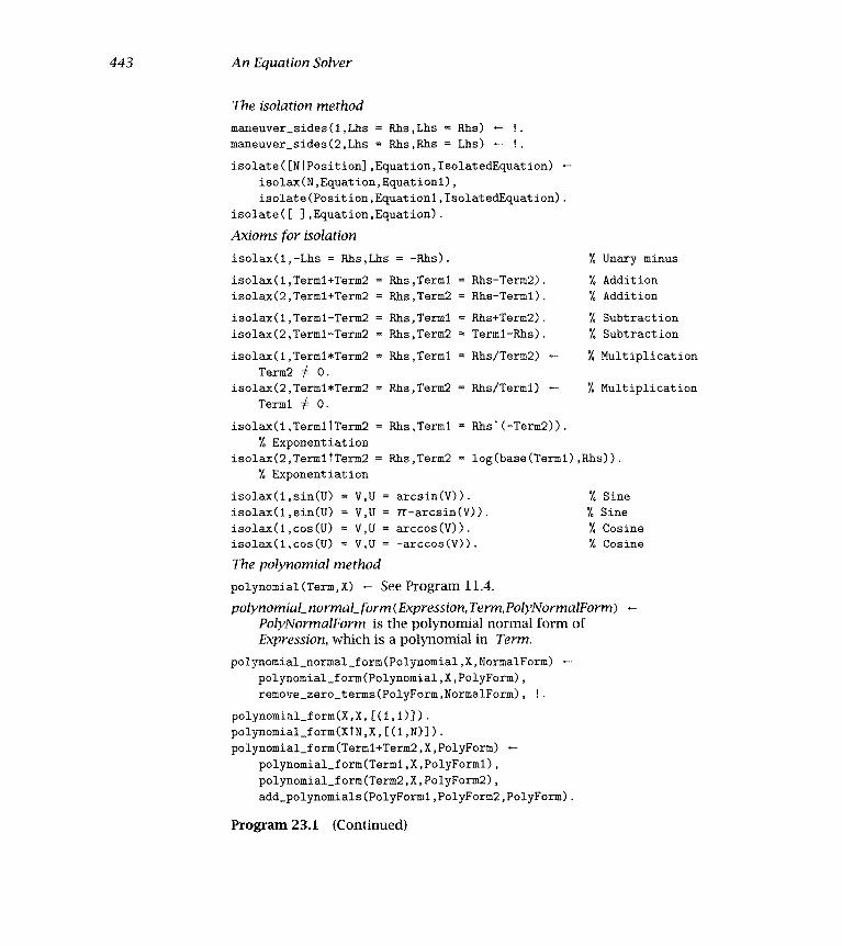
443 An Equation Solver
The isolation method
maneuver_sides(i,Lhs = Rhs,Lhs Rhs) -maneuver_sides(2,Lhs Rhs,Rhs Lhs) -isolate([NlPosition],Equation,IsolatedEquation) -
isolax(N,Equation,Equationl),isolate(Positíon,Equationi,IsolatedEquatïon).
isolate([ 1 ,Equation,Equatiori).Axioms for isolation
isolax(1,-Lhs = Rhs,Lhs -Rhs).
isolax(i,Terml+Term2 = Rhs,Termi = Rhs-Term2).isolax(2,Termi+Term2 Rhs,Term2 Rhs-Teruil).
isolax(1,Terml-Term2 Rhs,Tenni Rhs+Term2).isolax(2,Terml-Term2 Rhs,Term2 Terml-Rhs).
isolax(1,Terml*Term2 Rhs,Terml Rhs/Term2)Term2 O.
isolax(2,Termi'Term2 Rbs,Term2 Rhs/Terml) -Tenni O.
'h Unary minus
'I, AdditionX Addition
X SubtractionX Subtraction'I Multiplication
X Multiplication
isolax(1,TermllTerm2 = Rhs,Terml = RhsI(-Term2)).X Exponentiation
isolax(2,TerrniîTerm2 Rhs,Term2 log(base(Terml),Rhs)).'h Exponentiation
isolax(l,sin(U) = V,U = arcsin(V)). X Sineisolax(1,sin(U) V,U Tr-arcsin(V)). X Sineisolax(1,cos(U) V,IJ = arccos(V)). 'h Cosineisolax(i,cos(U) V,tJ = -arccos(V)). X Cosine
The polynomial method
polynomial(Term,X) See Program 11.4.
polynomiaL normal_form (Expression, Term ,PolyNormalForrn)PolyNormalForm is the polynomial normal form ofExpression, which is a polynomial ¡n Term.
polynomial_normal_f orm(Polynomial ,X,NormalForm) -polynomial_f orm(Polynomial , X, PolyForm),remove_zero_terms(PolyForm,NormalForm)
polynomial_form(X,X, C(i,i)]).polynomial_form(XIN,X,[(i,N)]).polynomial_f orm(Terml+Term2 ,X,PolyForin) -
polynomial_f orm(Termi ,X ,PolyForml),polynomial_f ors (Term2,X,PolyForm2),add_polynomials (PolyFormi , PolyForm2 , PolyForm).
Program 23.1 (Continued)

444 Chapter 23
polynomial_f orm(Terml-Term2 ,X,PolyForm) -polynomial_f orm(Termt ,X,PolyForml),polynomial_form (Term2 , X, PolyForm2),subtract_polynomials (PolyFormi , PolyForm2 , PolyForm).
polynomial_form(Terml*Term2,X PolyForm) -polynomial_f orn (Termi ,X,PolyForml),polynomial_f orni(Term2 ,X,PolyForm2),multiply_polynomials(PolyForml ,PolyForm2,PolyForm).
polynomial_form(TermtN,X,PolyForm) -polynomial_f orm(Term,X ,PolyForml),binomial (PolyFormi , N, PolyForm).
polynomial_f orin(Tern,X, [(Term,O)]) -free_of (X,Term),
remove_zero_terms([(O,N)IPoly] Polyl) -!, remove_zero_terms(Poly,Polyi).
remove_zero_terms([(C,N)IPoly] , [(C,N)JPolyl]) -C O, , remove_zero_terms(Poly,Polyl).
remove_zero_terms([ il,[ ]).Polynomial manipulation routinesadd_polynomials (Polyl,Poly2,Poly)
Poly is the sum of Polyl and Po!y2, where Polyl,PoIy2, and Poly are all in polynomial form.
add_polynomials([ ],Poly,Poly) -add_polynoinials(Poly, [ ] ,Poly) -add_polynomials([(Ai,Ni)lPolyl] , [(Aj ,Nj)Poly2] ,[(Ai,Ni)IPoly]) -
Ni > Nj, !, add_polynomials(Polyl, [(Aj,Nj)IPoly2l,Poly).add_polynomials([(Ai,Ni)tPolyl],[(Aj,Nj)jPoly2] ,[(A,Ni)IPolyl) -
Ni =:= Nj, !, A is Ai+Aj, add_polynomials(Polyl,Poly2,Poly).add_polynomials([(Ai,Ni)IPolyl] ,f(Aj ,Nj)Poly2],[(Aj,Nj)IPoly])
Ni < Nj, ! , add_polynomials([(Ai,Ni)IPolyl] ,Poly2,Poly).subtract_polynomials (Polyl,Poly2,Poly) -
Po/y is the difference of Polyl and Poly2, where Polyl,Poly2, and Poly are all in polynomial form.
subtract_polynomials (Polyl , Poly2 , Poly) -multiply_single (Poly2, (1,O) ,Poly3),add_polynomials(Polyl,Poly3,Poly),
multiply_single(Polyl,Monomial,Poly) -Poly is the product of Po/yl and Monomial, where Polyland Po/y are in polynomial form, and Monomial has theform (C,N) denoting the monomial C1XN.
multiply_single([(C1,N1)IPolyl],(C,N),[(C2,N2)IPoly]) -C2 is C1*C, N2 is N1+N, multiply_single(Polyl,(C,N),Poly).
multiply_single([ ],Factor,[ 1).
Program 23.1 (Continued)

445 Ari Equation Solver
multiply_polynomials (Polyl,Poly2,Poly) -Poly is the product of Polyl and Poly2, where Polyl,Poly2, and Poly are all in polynomial form.
multiply_polynomials([(C,N)lPolyl],Poly2,Poly) -multiply_single(Poly2, (C,N) ,Poly3),multiply_polynomials (Polyl , Poly2 , Poly4),add_polynomials (Poly3, Poly4 , Poly).
multiply_polynomials([ ],P,[ 1).binornial(Poly, i ,Poly).
Polynomial equation solver
solve_polynomial_equation (Equation, Unknown,Solution) -Solution is a solution to the polynomial Equation in the unknownUnknown.
solve_polynomial_equation(PolyEquation,X,X = -linear(PolyEquat ion), !,pad(PolyEquation, [(A,i) , (B4O)1).
solve_polyriomial_equation(PolyEquation,X, Solution) -quadratic(PolyEquation), !,pad(PolyEquation, [(A,2) , (B,1) , (C,O)])discrimïnarit(A,B,C,Discriminant),root(X,A,B,C,Discriminant,Solution).
discriminant(A,fl,C,D) D is B*B - 4*A*C.
root(X,A,B,C,O,X= -B/(2*A)).root(X,A,B,C,D,X (-B+sqrt(D))/(2*A)) .- D > O.root(X,A,B,C,D,X (-B-sqrt(D))/(2*A)) - D > O.pad([(C,N) IPoly] , [(C,N) IPolyl])
pad(Poly,Polyl).pad(Poly,[(O,N)lPolylI)
pad(Poly,Polyl).pad([ J,[ 1).linear([(Coeff 1) IPoly])quadratic( [(Coeff 2)1 Poly])The homogenization method
homogenize (Equation,X,Equation 1,X1) -The Equation in X is transfoi iiied to the polynomialEquation i in Xl where Xi contains X.
homogenïze(Equation,X,Equationl Xl) -offenders (Equation,X,Dffenders),reduced_term(X,Dffenders,Type Xl),rewrite(Offenders,Type,Xi ,Substitutions),substitute(Equation,Substitutions ,Equationl)
Program 23.1 (Continued)

446 Chapter 23
offenders(Equation, Unknown,Offenders)Offenders is the set of offenders of the Equation in the Unknown.
offenders(Equation,X,Offenders) -
parse(Equation,X,Offendersl\[ 1),remove_duplicates(Offendersl ,Offenders),
multiple(Offenders).
reduced_term(X,Offenders,Type,X1) -
classify(Offenders,X,Type),
candidate(Type,Dffenders,X,X1).
Heuristics for exponential equationsclassify(Offenders,X,exponential) -
exponential_offenders(Offenders ,X).
exponential_offenders([AIBIOffs] ,X) -
free_of(X,A), subterm(X,B), exponential_offenders(Offs ,X).
exponential_offenders([ ],X).
candidate(exponential,Offenders,X,AIX) -
base (Offenders,A), polynomial_exponents(Offenders,X).
base([AIBlOffs] ,A) - base(Offs,A)
base([ ],A).
polynomial_exponents([AIBIOffs] ,X) -
polynomial(B,X), polynomial_exponents(Dffs,X).
polynomial_exponents( E ] ,X).
Parsing the equation and making substitutionsparse (Expression, Term, Offenders) -
Expression is traversed to produce the set of Offenders in Term,that is, the nonalgebraic subterms of Expression containing Term.
parse(A+B,X,L1\L2) -1, parse(A,X,L1\L3), parse(B,X,L3\L2).
parse(A*B,X,Li\L2)
!, parse(A,X,L1\L3), parse(B,X,L3\L2).
parse(A-B,X,Li\L2) -
!, parse(A,X,L1\L3), parse(B,X,L3\L2).
parse(A=B,X,L1\L2) -
parse(A,X,L1\L3), parse(B,X,L3\L2).
parse(AIB,X,L) -
integer(B), !, parse(A,X,L).
parse(A,X,L\L) -
freeof(X,A), !.
parse(A,X,EAIL]\L) -
subterm(X,A), !.
Program 23.1 (Continued)

447 An Equation Solver
substitute (Expression,Substitutions,Expressionl) -The list of Substitutions is applied to Expression to produceExpression 1.
substitute (A+B ,Subs, NewA+NewB)', substitute(A,Subs,NewA), substitute(B,Subs,NewB).
substitute (A*B ,Subs, NewA*New) -substitute(A,Subs,NewA), substitute(B,Subs,NewB).
substitute (-B,Subs, NewA-NewB) -substitute(A,Subs,NewA), substitute(B,Subs,NewB).
substitute (A=B ,Subs, NewA=NewB) -substitute(A,Subs,NevA), substitute(B,Subs,NewB).
substituto(AIB,Subs,NewAIB) -iuteger(B), ! , substitute(A,Subs,NewA).
substitute(A,Subs,B) -member(A=B,Subs), L
substitute(A,Subs,A).Finding homogenization rewrite rules
rewrite([DffIOffs] ,Type,X1, [Off=TermlRewrites]) *homogenize_axiom(Type,Off ,X1 ,Terin),rewrite (Offs,Type,X1 ,Rewrites).
rewrite([ 1,Type,X,[ ]).Homogenization axioms
homogenize_axiom(exponential,A1(N*X) ,AIX, (AIX) TN)homogenize_axioin(exponeritial,At(-X),AIX,1/(AIX)).homogenize_axiom(exponential,A1(X+B),AIX,ATB*AIX).
Utilities
subterm(Sub,Term) See Program 9.2.
position(Term,Term,[ 1) - Lposition(Sub,Term,Path) -
compound(Term), functor(Term,F,N), position(N,Sub,Term,Path),positïon(N,Sub,Term, [NiPath]) -
arg(N,Terrn,Arg), position(Sub,Arg,Path)position(N,Sub,Terin,Path) -
N > 1, Nl is N-1, position(N1,Sub,Term,Path).
free_of(Subterm,Term) - occurrence(Subterm,Terrn,O).single_occurrerice(Subterm,Term) - occurrence(Subterm,Term,l).occurrence(Terin,Term,l) -occurrence(Sub,Term,N) -
cornpound(Terrn), ! , functor(Term,F,M), occurrence(M,Sub,Term,O,N).occurrence(Sub,Term,O) - Term Sub.
Program 23.1 (Continued)

448 Chapter 23
occurrence(M,Sub,Term,N1,N2) -M > O, !, arg(M,Term,Arg), occurrence(Sub,Arg,N), N3 is N+N1,
Ml is M-1, occurrence(M1,Sub,Term,N3,N2).
occurrence (O , Sub , Term ,N, N)
remove_duplicates(Xs,Ys) no_doubles(Xs,Ys).
no_doubles(Xs,Ys) - SeeProgram7.9.multiple([X1,X2IXs]).
Testing and datatest_press(X,Y) - equation(X,E,U), solve_equation(E,U,Y).
equation(1,cos(x)*(l-2*sin(x))=O,x).
equation(2,x12-3*x+20,x).
equation(3,21(2*x)-5*21(x+1)+16=O,x).
Program 23.1 (Continued)
Program 23.1 has four clauses for solve_equation, one for each ofthe four methods needed to solve the equations in Figure 23.1. Moregenerally, there is a clause for each equation-solving method. The fullPRESS system has several more methods.
Our equation solver ignores several features that might be expected.There is no simplification of expressions, no rational arithmetic, norecord of the last equation solved, no help facility, and so forth. PRESSdoes contain many of these facilities as discussed briefly in Section 23.6.
23.2 Factorization
Factorization is the first method attempted by the equation solver. Notethat the test whether factorization is applicable is trivial, being unifica-tion with the equation A * B = O. If the test succeeds, the simpler equa-tions are recursively solved. The top-level clause implementing factoriza-tion is
solve_equation(A*B=O,X,Solution) -
factorize(A*B,X,Factors\[ 1),remove_duplicates (Factors ,Factorsl),
solve_factors (Factors 1, X, Solution).

449 An Equation Solver
The top-level clause in Program 23.1 has a cut as the first goal in thebody. This is a green cut: none of the other methods depend on thesuccess or failure of factorization. In general, we omit green cuts fromclauses we describe in the text.
23.3 Isolation
A useful concept to locate and manipulate the single occurrence of theunknown is its position. The position of a subterm in a term is a list ofargument numbers specifying where it appears. Consider the equationcos(x) = O. The term cos(x) containing x is the first argument of theequation, and x is the first (and only) argument of cos(x). The positionof x in cos(x) = O is therefore [1,1]. This is indicated in the diagram inFigure 23.2. The figure also shows the position of x in i - 2 . sin(x) = Owhich is 11,2,2,1].
The clause defining the method of isolation is
solve_equation(Equation,X,Solution) -
single_occurrence (X, Equation)
position(X,Equation, [Side Position]),
maneuver_sides (Side , Equation, Equationi)
isolate (Position,Equationl ,Solution).
ZNcos O
Figure 23.2 Position of subterms in terms

450 Chapter 23
The condition characterizing when isolation is applicable is that therebe a single occurrence of the unknown X in the equation, checked bysingle_occurrence. The method calculates the position of X with thepredicate position. The isolation of X then proceeds in two stages. First,maneuver_sides ensures that X appears on the left-hand side of theequation, and second, isolate makes it the subject of the formula.
It is useful to define single_occurrence in terms of the more generalpredicate occurrence(Subterm,Term,N), which counts the number oftimes N that Subterm occurs in the term Term. Both occurrence andposition are typical structure inspection predicates. Both are posed asexercises at the end of Section 9.2. Code for them appears in the utilitiessection of Program 23.1.
The predicate maneuver_sides (N ,Equation, Equationi) consists oftwo facts:
maneuver_sides(1,Lhs = Rhs,Lhs = Rhs).
maneuver_sides(2,Lhs = Rhs,Rhs = Lhs).
Its effect is to ensure that the unknown appears on the left-hand side ofEquationi. The first argument N, the head of the position list, indicatesthe side of the equation in which the unknown appears. A i means theleft-hand side, and the equation is left intact. A 2 means the right-handside, and so the sides of the equation are swapped.
The transformation of the equation is done by isolate/3. It repeatedlyapplies rewrite rules until the position list is exhausted:
isolate([NlPosition] ,Equation,IsolatedEquation) -
isolax(N,Equation,Equationl),
isolate (Position,Equationl , IsolatedEquation).
isolate( [ J ,Equation,Equation).
The rewrite rules, or isolation axioms, are specified by the predicateisolax(N,Equation,Equationl). Let us consider an example used insolving i - 2 . sin(x) = O. An equivalence transformation on equationsis adding the same quantity to both sides of an equation. We show itstranslation into an isolax axiom for manipulating equations of the formu - y = w. Note that rules need only simplify the left-hand side of equa-tions, since the unknown is guaranteed to be on that side.
Two rules are necessary to cover the two cases whether the first orsecond argument of u - y contains the unknown. The term u - y = w
451 Ari Equotion Solver
can be rewritten to either u = w + i' or y = u - w. The first argument ofisolax specifies which argument of the sum contains the unknown. TheProlog equivalent of the two rewrite rules is then
isolax(1,Terinl-Term2 = Rhs,Terml Rhs+Term2).isolax(2,Terml-Term2 = Rhs,Term2 = Terml-Rhs).
Other isolation axioms are more complicated. Consider simplifying aproduct on the left-hand side of an equation. One of the expected ruleswould be
isolax(1,Terml*Term2 = Rhs,Terml = Rhs/Term2).
If Teiui2 equals zero, however, the rewriting is invalid. A test is thereforeadded that prevents the axioms for multiplication being applied if theterm by which it divides is O. For example,
isolax(1,Terinl*Term2 = Rhs,Terml = Rhs/Term2) - Terin2 O.
Isolation axioms for trigonometric functions illustrate another possi-bility that must be catered for - multiple solutions. An equation such assin(x) = 1/2 that is reached in our example has two solutions between Oand 2 . Tr. The alternative solutions are handled by having separate iso-lax axioms:
isolax(1,sin(U) = V,U = arcsin(V)).isolax(1,sin(U) V,U = Tr - arcsin(V)).
In fact, the equation has a more general solution. Integers of the form2 n iT can be added to either solution for arbitrary values of n. Thedecision whether a particular or general solution is desired depends oncontext and on semantic information independent of the equation solver.
Further examples of isolation axioms are given in the complete equa-tion solver, Program 23.1.
The code described so far is sufficient to solve the first equation in Fig-ure 23.1, cos(x) . (1 - 2 . sin(x)) = O. There are four answers arccos(0),- arccos(0), arcsin((1 - 0)/2), rr - arcsin((1 - 0)/2). Each can be simpii-fled, for example, arcsin((1 - O)/2) to rr/6, but will not be unless theexpression is explicitly evaluated.
The usefulness of an equation solver depends on how well it can per-form such simplification, even though simplification is not strictly part

452 Chapter 23
of the equation-solving task. Writing an expression simplifier is nontriv-ial, however. It is undecidable whether two expressions are equivalent ingeneral. Some simple identities of algebra can be easily incorporated, forexample, rewriting O + u to u. Choosing between other preferred forms,e.g., (1 + x)3 and i + 3 x + 3 x2 + x3, depends on context.
23.4 Polynomial
Polynomial equations are solved by a polynomial equation solver, apply-ing various polynomial methods. Both sides of the equation are checkedas to whether they are polynomials in the unknown. If the checks aresuccessful, the equation is converted to a polynomial normal form bypolynomial_normal_form, and the polynomial equation solver solve_
polynomial_equat ion is invoked:
solve_equation(Lhs=Rhs , X ,Solution)
polynomial(Lhs,X),
polynomial(Rhs,X),
polynomial_normal_form (Lhs-Rhs , X, PolyForm),
solve_polynomial_equation (PolyForm,X, Solution).
The polynomial normal form is a list of tuples of the form (A,N1),where A is the coefficient of which is necessarily nonzero. The tuplesare sorted into strictly decreasing order of N; for each degree there is atmost one tuple. For example, the list [(1,2), (-3, 1),(2,O)] is the normalform for x2 - 3 . x + 2. The leading term of the polynomial is the head ofthe list. The classic algorithms for handling polynomials are applicable toequations in normal form. Reduction to polynomial normal form occursin two stages:
polynomial_normal_form (Polynomial , X, NormalForm) -
polynomial_f orm (Polynomial, X, PolyForm),
remove_zero_terms (PolyForm NormalForm).
The predicate polynornial_form(X,Polynomial PolyForm) decom-poses the polynomial. PolyForm is a sorted list of coefficient-degreetuples, where tuples with zero coefficients may occur.
It is convenient for many of the polynomial methods to assume thatall the terms in the polynomial form have nonzero coefficients. There-

453 An Equation Solver
fore the final step of polynomial_normal_form is removing those terniswhose coefficients are zero. This is achieved by a simple recursive proce-dure remove_zero_terms.
The code for polynomial_form directly echoes the code for polyno-mial. For each clause used in the parsing process, there is a correspond-ing clause giving the resultant polynomial. For example, the polynomialform of a term x1 is [(1,n)], which is expressed in the clause
polynomial_form(XIN,X, [(1,N)J).
The recursive clauses for polynomial_form manipulate the polynomi-als in order to preserve the polynomial form. Consider the clause
polynomial_form(Polyl+Poly2,X,PolyForm) -
polynomial_f orm(Polyl ,X,PolyForml),
polynomial_f orm(Poly2 , X, PolyForm2),
add_polynomials (PolyFormi , PolyForm2 , PolyForm).
The procedure add_polynomials contains an algorithm for adding poly-nomials in normal form. The code is a straightforward list of the possi-bilities that can arise:
add_polynomials([ I ,Poly,Poly).add_polynomials (Poly, E I ,Poly).
add_polynomials([(Ai,Ni) IPolyl] , [(Aj,Nj)IPoly2], [(Ai,Ni)IPoly])
Ni > Nj, add_polynomials(Polyl, E(Aj , Nj) IPoly2] , Poly).
add_polynomials([(Ai,Ni)IPolyl] ,[(Aj,Nj)IPoly2] , [(A,Ni)Poly]) -
Ni =:= Nj, A is Ai+Aj, add_polynomials(Polyl,Poly2,Poly).
add_polynomials([(Ai,Ni)IPolyl],[(Aj,Nj)IPoly2],[(Aj,Nj)IPoly]) -Ni < Nj, add_polynomials([(Ai,Ni)IPolyl] ,Poly2,Poly).
Similarly, the procedures subtract_polynomials, mult iply_polyno-
mials, and binomial are algorithms for subtracting, multiplying, andbinomially expanding polynomials in normal form to produce results innormal form. The subsidiary predicate multiply_single(Polyl,Mono-
mial,Poly2) multiplies a polynomial by a monomial (C,N) to produce anew polynomial.
Once the polynomial is in normal form, the polynomial equation solveris invoked. The structure of the polynomial solver follows the structureof the overall equation solver. The solver is a collection of methods that

454 Chapter 23
are tried in order to see which is applicable and can be used to solve theequation. The predicate solve_polynomial_equation is the analogousrelation to solve_equation.
The second equation in Figure 23.1 is quadratic and can be solved withthe standard formula. The equation solver mirrors the human method.The polynomial is identified as being suitable for the quadratic methodby checking (with quadratic) if the leading term in the polynomial is ofsecond degree. Since zero terms have been removed in putting the poly-nomial into its normal form, pad puts them back if necessary. The nexttwo steps are familiar: calculating the discriminant, and returning theroots according to the value of the discriminant. Again multiple solutionsare indicated by having multiple possibilities:
solve_polynomial_equation(Poly,X,Solution) -
quadratic(Poly),
pad(Poly, [(A,2) , (B,1) , (C,O)])
discriminant(A,B,C,Discriminant),
root(X,A,B,C,Discriminant,Solution).
discriminant(A,B,C,D) - D is (B*B - 4*A*C).
root(X,A,B,C,O,X= -B/(2*A)).
root(X,A,B,C,D,X= (-B+sqrt(D))/(2*A)) - D > O.
root(X,A,B,C,D,X= (-B-sqrt(D))/(2*A)) - D > O.
Other clauses for solve_polynomial_equation constitute separatemethods for solving different polynomial equations. Linear equationsare solved with a simple formula. In PRESS, cubic equations are handledby guessing a root and then factoring, reducing the equation to a qua-dratic. Other tricks recognize obvious factors, or that quartic equationsmissing a cubic and a linear term are really disguised quadratics.
23.5 Homogenization
The top-level clause for homogenization reflects the transformation ofthe original equation into a new equation in a new unknown, which isrecursively solved; its solution is obtained for the original unknown:

455 An Equation Solver
solve_equation(Equation,X,Solution) -hornogenize(Equation,X,Equationl,X1),solve_equation(Equationl ,X1 ,Solutionl),solve_equation(Solutionl ,X, Solution).
The code for homogenize/4 implements the four stages of homoge-nization, described in Section 23.1. The offenders set is calculated byoffenders/3, which checks that there are multiple offenders. If there isoily a single offender, homogenization will not be useful:
hornbgenize(Equation,X,Equationl ,X1) -offenders (Equation, X,Offenders),reduced_terni(X,Offenders Type ,X1)rewrite(Offenders,Type,X1,Substitutions),substitute (Equation,Substitutions, Equatìonl).
The predicate reduced_term/4 finds a reduced term, that ìs, a candi-date for the new unknown. In order to structure the search for the re-duced term, the equation is classified into a type. This type is used in thenext stage to find rewrite rules expressing each element of the offendersset as an appropriate function of the reduced term. The type of the exam-ple equation is exponential. PRESS encodes a lot of heuristic knowledgeabout finding a suitable reduced term. The heuristics depend on the typeof the terms appearing in the offenders set. To aid the structuring (andretrieval) of knowledge, finding a reduced term proceeds in two stages -classifying the type of the offenders set, and finding a reduced term ofthat type:
reduced_terni(X ,Offenders, Type ,Xl) -classify(Offenders,X,Type),candidate(Type,Offenders,X,X1).
We look at the set of rules appropriate to our particular equation.The offenders set is of exponential type because all the elements in theoffenders set have the form A, where A does not contain the unknownbut B does. Standard recursive procedures check that this is true.
The heuristic used to select the reduced term in this example is that ifall the bases are the same, A, and each exponent is a polynomial in theunknown, X, then a suitable reduced term is Ax:

456 Chapter 23
candidate (exponential ,Offenders, X ,AIX) -
base(Offenders,A), polynomial_exponents(Offenders,X).
The straightforward code for base and polynomial_exponents is in thecomplete program. The heuristics in PRESS are better developed than theones shown here. For example, the greatest common divisor of all theleading terms of the polynomials is calculated and used to choose thereduced term.
The next step is checking whether each member of the offenders setcan be rewritten in terms of the reduced term candidate. This involvesfinding an appropriate rule. The collection of clauses for homogenize_
axiom constitute the possibly applicable rewrite rules. In other words,relevant rules must be specified in advance. The applicable rules in thiscase are
homogenize_axiom(exponential,AI (N*X) ,AIX, (AIX) IN).
homogenize_axiom(exponential,AI(X+B) ,AIX,AIB*AIX).
Substituting the term in the equation echoes the parsing process usedby offenders as each part of the equation is checked to see whether it isthe appropriate term to rewrite.
Exercises for Chapter 23
Add isolation axioms to Program 23.1 to handle quotients on theleft-hand side of the equation. Solve the equation x/2 = 5.
Add to the polynomial equation solver the ability to solve disguisedlinear and disguised quadratic equations. Solve the equations 2x3-8=x3, andx4 5 2 +6=0.
The equation cos(2 . x) - sin(x) = O can be solved as a quadraticequation in sin(x) by applying the rewrite rule cos(2 . X) = i - 2sin2(x). Add clauses to Program 23.1 to solve this equation. Youwill need to add rules for identifying terms of type trigonometric,heuristics for finding trigonometric reduced terms, and appropriatehomogenization axioms.
(iv) Rewrite the predicate free_of (Term,X) so that it fails as soon as itfinds an occurrence of X in Term.

457 An Equation Solver
(V) Modify Program 23.1 so that it solves simple simultaneous equa-tions.
23.6 Background
Symbolic manipulation was an early application area for Prolog. Earlyexamples are programs for symbolic integration (Bergman and Kanoui,1973) and for proving theorems in geometry (Welham, 1976).
The PRESS program, from which Program 23.1 is adapted, owes a debtto many people. The original version was written by Bob Weiham Manyof the researchers in the mathematical reasoning group working withAlan Bundy at the University of Edinburgh subsequently tinkered withthe code. Published descriptions of the program appear in Bundy andWeiham (1981), Sterling et al. (1982), and Silver (1986). The last referencehas a detailed discussion of homogenization.
PRESS includes various modules, not discussed in this chapter, thatare interesting ¡n their own right: for example, a package for inter-val arithmetic (Bundy, 1984), an infinite precision rational arithmeticpackage developed by Richard O'Keefe, and an expression simplifierbased on difference-structures as described in Section 15.2, developed byLawrence Byrd. The successful integration of all these modules is strongevidence for the practicality of Prolog for large programming projects.
The development of PRESS showed up classic points of software engi-neering. For example, at one stage the program was being tuned priorto publishing some statistics. Profiling was done on the program, whichshowed that the predicate most commonly called was free_of. Rewritingit as suggested in Exercise 23(iv) resulted in a speedup of 35 percent inthe performance of PRESS.
Program 23.1 is a considerably cleaned-up version of PRESS. Tidyingthe code enabled further research. Program 23.1 was easily translated toother logic programming laliguages, Concurrent Prolog and FCP (Sterlingand Codish, 1986). Making the conditions when methods were used moreexplicit enabled the writing of a program to learn new equation-solvingmethods from examples (Silver, 1986).


24.1 Overview of the Compiler
The source language for the compiler is PL, a simplified version of Pascaldesigned solely for the purposes of this chapter. lt contains an assign-ment statement, an if-then-else statement, a while statement, and simple1/O statements. The language is best illustrated with an example. Fig-ure 24.1 contains a program for computing factorials written in PL. Aformal definition of the syntax of the language is implicit in the parserin Program 24.1.
The target language is a machine language typical for a one-accumu-lator computer. Its instructions are given in Figure 24.2. Each instructionhas one (explicit) operand, which can be one of four things: an integerconstant, the address of a storage location, the address of a programinstruction, or a value to be ignored. Most of the instructions also have asecond implicit operand, which is either the accumulator or its contents.In addition, there is a pseudoinstruction block that reserves a number ofstorage locations as specified by its integer operand.
The scope of the compiler is clear from its behavior on our example.Figure 24.3 is the translation of the PL program in Figure 24.1 into ma-
24 A Compiler
Our final application is a compiler. The program is presented top-down.The first section outlines the scope of the compiler and gives its defim-tion. The next three sections describe the three major components: theparser, the code generator, and the assembler.

460 Chapter 24
program factorial;
begin
read value;
count 1;
result : 1;
while count < value do
begin
count count+1;
result := result*count
end
write result
end
Figure 24.1 A PL program for computing factorials
Figure 24.2 Target language instructions
chine language. The compiler produces the colunms labeled Instructionand Operand.
The task of compiling can be broken down into the five stages givenin Figure 24.4. The first stage transforms a source text into a list oftokens. The list of tokens is parsed in the second stage, syntax analysis,to give a source structure. The third and fourth stages transform thesource structure into relocatable code and assemble the relocatable codeinto absolute object code, respectively. The final stage outputs the objectprogram.
Our compiler implements the middle three stages. Both the first stageof lexical analysis and the final output stage are relatively uninterestingand are not considered here. The top level of the code handles syntaxanalysis, code generation, and assembly.
Arithmetic
Literals Menory Control
junpeq
I/O, etc.
read
addc add jumpne write
subc sub jumplt halt
mulc mul junpgt
divc div junple
loadc
store
load jumpge
jump

461
Figure 24.3 Assembiy code version of a factorial program
A Compiler
Symbol Address Instruction Operand Symbol
i READ 21 VALUE
2 LOADC i3 STORE 19 COUNT
4 LOADC 205 STORE 20 RESULT
LABEL1 6 LOAD 19 COUNT
7 SUB 21 VALUE
8 JUMPGE 16 LABEL2
9 LOAD 19 COUNT
10 ADDC 1
11 STORE 19 COUNT
12 LOAD 20 RESULT
13 MUL 19 COUNT
14 STORE 20 RESULT
15 JUMP 6 LABEL1
LABEL2 16 LOAD 20 RESULT
17 WRITE O
18 HALT O
COUNT 19 BLOCK 3
RESULT 20VALUE 21
Object Object
SourceText
TokenList
SourceStructure
Structure(relocat-
able)
Structu re(abso-
lute)
ObjectProgram
Lexical Syntax Code Assembly OutputAnalysis Analysis Generation
Figure 24.4 The stages of compilation
The basic predicate compile (Tokens,ObjectCode) relates a list of to-kens Tokens to the ObjectCode of the program the tokens represent.The compiler compiles correctly any legal PL program but does not han-dle errors; that is outside the scope of this chapter. The list of tokensis assumed to be input from some previous stage of lexical analysis.The parser performing the syntax analysis, implemented by the predi-cate parse, produces from the Tokens an internal parse tree Structure.

462 Chapter 24
compile(Tokens,ObjectCode)ObjectCode is the result of compilation ofa list of Tokens representing a PL program.
compile (Tokens ,ObjectCode)
parse (Tokens ,Structure),
encode (Structure ,Dictionary,Code),
assemble (Code ,Dictionary,ObjectCode).
The parserparse( Tokens,Structure) -
Structure represents the successfully parsed list of Tokens.parse (Source ,Structure)
pl_program(Structure,Source\[ j).
p1_program(S) - [program], identifier(X), E';'], statement(S).
statement((S;Ss)) -
[begin] , statement(S), rest_statements(Ss).
statement(assign(X,V))
identifier(X) , E' :'] , expression(V).
statement(if(T,Si,S2)) -
[if] , test(T), [then] , statement(S1), [else] , statement(S2)
statement(while(T,S)) -
[while] , test(T) , [do] , statement(S)
statement(read(X)) -.
[read] , identifier(X)
statement(write(X)) -.
[write] , expression(X).
rest_statements((S;Ss)) - [';'] , statement(S), rest_statements(Ss).
rest_statements(void) [end]
expression(X) -e pl_constant(X).
expression(expr(Op,X,Y))
pl_constant(X), arithmetic_op(Op), expression(Y).
arithmetic_op('+') -. ['+'j
arithmetic_op('-') - E'-'].
arithmetic_op('*') -. ['*'].
arithmetic_op('/') - E'!'].
pl_constant(name(X)) -. identifier(X).
pl_constant(number(X)) -' pl_integer(X).
identifier(X) -' [X], {atom(X)}.
pl_integer(X) -' EX], {integer(X)}.
test(compare(Op,X,Y)) -
expression(X), comparison_op(Op), expression(Y).
Program 24.1 A compiler from PL to machine language

463 A Compiler
comparison_opY=') -cornparison_op(') [''].comparison_opY>') . ['>'1.comparison_opY<') ['<'J.
comparison_op('') . ['>']
comparison_op('') [''].
The code generator
encode C Structure,Dictionary,RelocatableCode) -
Relocatable Code is generated from the parsed Structurebuilding a Dictioriry associating variables with addresses.
encode((X;Xs),D,(Y;Ys)) -
encode(X,D,Y), encode(Xs,D,Ys).
encode(void,D,no_op).
encode(assign(Name,E),D,(Code; instr(store,Address))) -
lookup(Name,D,Address) , encode_expression(E,D,Code)
encode(if(Test,Then,Else) ,D,
(TestCode; ThenCode; instr(jump,L2);
label (Li); ElseCode; label(L2))) -
encode_test (Test ,L1 ,D ,TestCode)
encode (Then,D ,ThenCode),
encode (Else,D,ElseCode)
encode (wliile(Test,Do) ,D,
(label(L1); TestCode; DoCode; instr(jump,L1); label(L2))) -
encode_test(Test,L2,D,TestCode), encode(Do,D,DoCode).
encode(read(X) ,D,instr(read,Address))
lookup(X,D,Address).
encode(write(E),D,(Code; instr(write,O)))
encode_expression(E,D,Code).
encode_expression (Expression,Dictionary, Code) -Code corresponds to an arithmetic Expression.
encode_expression(number(C) ,D,ïnstr(loadc,C)).
encode_expression(nanie(X),D,instr(load,Address))
lookup(X,D,Address)
encode_expression(expr(Op,E1,E2),D,(Load;Instruction))
single_instruction(Op,E2,D,Instruction),
encode_expression(E1 ,D,Load).
encode_expression(expr(Dp,Ei,E2) ,D,Code) -
not sïngle_instruction(Op,E2,D,Instructïon)
single_operation(Op,E1 ,D,E2Code,Code),
encode_expression(E2,D,E2Code).
Program 24.1 (Continued)

464 Chapter 24
single_instruction(Op,nuinber(C),D,instr(OpCode,C)) -
literal_operation(Op,OpCode).
single_instruction(Op,naine(X),D,instr(OpCode,A)) -
memory_operation(Op,OpCode), lookup(X,D,A).
single_operation(Op,E,D,Code, (Code; Instruction)) -
coinmutative(Op), single_instruction(Op,E,D,Instruction).
single_operation (Op. E, D ,Code,
(Code;instr(store,Address);Load;instr(OpCode,Addressfl) -
not commutative(Op),
lookupC$temp' ,D,Address),
encode_expression(E,D,Load),
op_code (E , Op , OpCode)
op_code(number(C) ,Op,OpCode) - literal_operation(Op,OpCode).
op_code(name(X) ,Op,OpCode) - niemory_operation(Op,OpCode).
literal_operation('+' ,addc). memory_operationY+' ,add).
literal_operation('-' ,subc). memory_operationY-' sub).
literal_operation('*' ,mulc). memory_operationY*' mul).
literal_operationY/' ,divc). memory_operationY/' div).
comlnutative('-*'). cominutative('*).
encode_test (compare(Op,E1 E2) Label,D,
(Code; instr(OpCode ,Label))) -
coniparison_opcode (Op OpCode)
encode_expression(exprY' ,Ei,E2) ,D,Code).
comparison_opcode('=' jumpne). comparison_opcode(' ' ,jumpeq).
comparison_opcodeY>' ,jumple). comparison_opcode('' ,jumplt).
comparison_opcodeY<' ,jumpge). comparison_opcode(' ' jumpgt).
lookup(Naine,Dictionary,Address) - See Program 15.9.
The assembler
assemble ( Code,Dictionary, TidyCode) -TidyCode is the result of assembling Code removingno_Ups and labels, and filling in the Dictionary.
assemble(Code Dictionary,TidyCode) -
tidy_and_count (Code, 1 N,TidyCode\(instr(halt 0) ;block(L)))
Ni is N+i,
allocate (Dictionary,Nl,N2),
L is N2-N1, L
tidy_and_count((Codei ;Code2) M,N,TCodel\TCode2) -
tidy_and_count(Codel,M,M1,TCodel\Rest),tidy_and_count(Code2,Mi N,Rest\TCode2).
tidy_and_count(instr(X,Y),N,Ni,(instr(X,Y);Code)\Code) -
Nl is N+l.
tidy_and_count (label (N) N N, Code\Code).
tidy_and_count (no_op ,N, N, Code\Code)
Program 24.1 (Continued)

465 A Compiler
allocate(void,N,N).
allocate(dict(Name,N1,Before,After),N0,N)
allocate (Bef ore ,NO , Nl)
N2 is Ni1,
allocate (After,N2,N)
Program 24.1 (Continued)
test_compiler(X,Y)
proram(X,P) , compile(P,Y)
program(testl, [program,testl,' ; ,begïn,write,
x + ' , y , - ' , z , ' / ' , 2 , end]prograxn(test2, [prograni,test2,' ;',
begin,if,a,'>' ,b,then,max, :' ,a,else,max, :' ,b,end])
prograni(factorial,
[prograin,factorial, ;'
,begin
,read,value,'
,count , :=' , 1,';',result, :=' ,1, (;)
,while,count,'<' ,value,do
,begin
,count, ,count, '+' 1,,result, := ,result, 't' ,count
end, '
,write, result
,end])
Program 24.2 Test data
The structure is used by the code generator encode to produce relocat-able code Code. A dictionary associating variable locations to memoryaddresses and keeping track of labels is needed to generate the code.This is the second argument of encode. Finally, the relocatable code isassembled into object code by assemble with the aid of the constructedDictionary.
The testing data and instructions for the program are given as Pro-gram 24.2. The program factorial is the PL program of Figure 24.1 trans-lated into a list of tokens. The two small programs consist of a singlestatement each, and test features of the language not covered by thefactorial example. The program testi tests compilation of a nontrivialarithmetic expression, and test2 checks the if-then-else statement.

466 Chapter 24
24.2 The Parser
The parser proper is written as a definite clause grammar, as describedin Chapter 19. The predicate parse as given in Program 24.1 is just aninterface to the DCG, whose top-level predicate is p1_program. The DCGhas a single argument, the structure corresponding to the statements, asdescribed later. A variant of Program 18.9 is assumed to translate theDCG into Prolog clauses. The convention of that program is that the lastargument of the predicates defined by the DCG is a difference-list:
parse (Source ,Structure) -
pl_program(Structure,Source\[ 1).
The first statement of any PL program must be a program statement. Aprogram statement consists of the word program followed by the nameof the program. We call words that must appear for rules of the grammarto apply standard identifiers, the word program being an example. Thename of the program is an identifier in the language. What constitutesidentifiers, and more generally constants, is discussed in the context ofarithmetic expressions. The program name is followed by a semicolon,another standard identifier, and then the program proper begins. Thebody of a PL program consists of statements or, more precisely, a sin-gle statement that may itself consist of several statements. All this issummed up in the top-level grammar rule:
p1_program(S) -
[program], identifier(X), [C;] , statement(S).
The structure returned as the output of the parsing is the statementconstituting the body of the program. For the purpose of code genera-tion, the top-level program statement has no significance and is ignoredin the structure built.
The first statement we describe is a compound statement. Its syntaxis the standard identifier begin followed by the first statement, S, say,in the compound statement, and then the remaining statements Ss. Thestructure returned for a compound statement is (S; Ss), where ; is usedas a two-place infix functor. Note that S, Ss, or both may be compoundstatements or contain them. The semicolon is chosen as functor to echoits use in PL for denoting sequencing of statements:

467 A Compiler
statement ( (S; Ss) )
[begin] , statement(S), rest_statements(Ss).
Statements in PL are delimited by semicolons. The rest of the state-ments are accordingly defined as a semicolon followed by a nonemptystatement, and recursively the remaining statements:
rest_statements((S;Ss)) -.
E';'], tatement(S), rest_statements(Ss).
The end of a sequence of statements is indicated by the standard iden-tifier end. The atom void is used to mark the end of a statement in theinternal structure. The base case of rest_statements is therefore
rest_statements(void) -. [end]
The above definition of statements precludes the possibility of emptystatements. Programs and compound statements in PL cannot be empty.
The next statement to discuss is the assignment statement. It has asimple syntactic definition - a left-hand side, followed by the standardidentifier is, followed by the right-hand side. The left-hand side is re-stricted to being a PL identifier, and the right-hand side is any arithmeticexpression whose definition is to be given:
statement(assign(X,E))
identifier(X), [':='], expression(E).
The structure returned by the successful recognition of an assignmentstatement has the form assign(X,E). The (Prolog) variable E representsthe structure of the arithmetic expression, and X is the name of the(PL) variable to be assigned the value of the expression. It is implicitlyassumed that X will be a PL identifier.
For simplicity of both code and explanation, we restrict ourselves toa subclass of arithmetic expressions. Two rules define the subclass. Anexpression is either a constant or a constant followed by an arithmeticoperator and recursively an arithmetic expression. Examples of expres-sions in the subclass are x, 3, 2 . t and x + y - z/2, the expression in thefirst test case in Program 24.2:
expression(X) -. pl_constant(X).
expression(expr(Op,X,Y)) -.
pl_constant(X), arithxnetic_op(Op), expression(Y).

468 Chapter 24
This subclass of expressions does not respect the standard precedenceof arithmetic operators. The expression x . 2 + y is parsed as x (2 + y).On the other hand, the expression x + y - z/2 is interpreted unambigu-ously as x + (y - (z/2)).
For this example, we restrict ourselves to two types of constants in PL:identifiers and integers. The specification of p1_constant duly consistsof two rules. Which of the two is found is reflected in the structurereturned. For identifiers X, the structure name (X) is returned, whereasnumber (X) is returned for the integer X:
pl_constant(name(X)) - identifier(X).
pl_constant(number(X)) -. pl_integer(X).
For simplicity we assume that PL integers and PL identifiers are Prologintegers and atoms, respectively. This allows the use of Prolog systempredicates to identify the PL identifiers and integers. Recall that the curlybraces notation of DCGs is used to specify Prolog goals:
identifier(X) [X], {atom(X)}.
pl_integer(X) - [X], {integer(X)}.
In fact, all grammar rules that use PL identifiers and constants couldbe modified to call the Prolog predicates directly if greater efficiency isneeded.
A list of arithmetic operators is necessary to complete the definitionof arithmetic expressions. The form of the statement for addition, repre-sented by +, follows. The grammar rules for subtraction, multiplication,and division are analogous, and appear in the full parser in Program 24.1:
arithmetic_op(+') [C]The next statement to be discussed is the conditional statement, or
if-then-else. The syntax for conditionals is the standard identifier if fol-lowed by a test (to be defined). After the test, the standard identifier then
is necessary, followed by a statement constituting the then part, the stan-dard identifier else and a statement constituting the else part, in thatorder. The structure built by the parser is if (T,Si , S2), where T is thetest, Si is the then part, and S2 is the else part:
statement(if(T,Si,S2))
[if], test(T), [then], statement(Si),
[else], statement(S2).

469 A Compiler
Tests are defined to be an expression followed by a comparison oper-ator and another expression. The structure returned has the form com-pare (Op , X, Y), where Op is the comparison operator, and X and Y are theleft-hand and right-hand expressions in the test, respectively:
test(compare(Op,X,Y)) -.expression(X), comparison_op(Op), expression(Y).
The definition of comparison operators using the predicate compari-son_op is analogous to the use of arithmetic_op to define arithmeticoperators. Program 24.1 contains definitions for =, , >, <,, and .
While statements consist of a test and the action to take if the test istrue. The structure returned is while(T,S), where T is the test and S is
the action. The syntax is defined by the following rule:
statement(while(T,S)) -.[while], test(T), [do], statement(S).
I/O is handled in PL with a simple read statement and a simple writestatement. The input statement consists of the standard identifier readfollowed by a PL identifier; it returns the structure read(X), where X isthe identifier. Write statements are similar:
statement(read(X)) -. [read], identifier(X).
statement(write(X)) - [write], expression(X).
Collecting the various pieces of the DCG just described gives a parser
for the language. Note that ignoring the arguments in the DCG gives aformal BNF grammar for PL.
Let us consider the behavior of the parser on the test data in Pro-gram 24.2. The parsed structures produced for the two single statementprograms have the form (structure) ;void, where (structure) repre-sents the parsed statement. The write statement is translated to
write(expr(+,name(x),expr(-,name(y),expr(/,name(z),
nuinber(2))))),
and the if-then-else statement is translated to
if (compare (> ,riame (a) ,name (b)) , assign(max name (a) )assign(max,name(b))).
The factorial program is parsed into a sequence of five statements fol-lowed by void. The output after parsing for all three test programs is

470 Chapter 24
Program testi:write(expr(+,nanie(x) ,expr(-,name(y),
expr(/,name(z) ,nuniber(2)flfl;voidProgram test2:
if(compare(>,name(a) ,name(b)),assign(max,naine(a)),assign(max,name(bfl) ;void
Program test3:
read(value);assign(count,number(lfl;assign(result,number(lfl;while(compare(< ,name(count) ,name(value)),(assign(count,expr(+,name(count),number(1)));assign(result,expr(*,name(result),nanie(count)fl;void));write(name(result)) ;void
Figure 24.5 Output from parsing
given in Figure 24.5. This is the input for the second stage of compila-tion, code generation.
24.3 The Code Generator
The basic relation of the code generator is encode (Structure,Dictio-
nary ,Code), which generates Code from the Structure produced by theparser. This section echoes the previous one. The generated code is de-scribed for each of the structures produced by the parser representingthe various PL statements.Dictionary relates PL variables to memory locations, and labels to
instruction addresses. The dictionary is used by the assembler to resolvelocations of labels and identifiers. Throughout this section D refers tothis dictionary. An incomplete ordered binary tree is used to implementit, as described in Section 15.3. The predicate lookup(Name,D,Value)
(Program 15.9) is used for accessing the incomplete binary tree.The structure corresponding to a compound statement is a sequence
of its constituent structures. This is translated into a sequence of blocksof code, recursively defined by encode. The functor ; is used to denotesequencing. The empty statement denoted by void is translated into anull operation, denoted no_op. When the relocatable code is traversedduring assembly this "pseudoinstruction" is removed.

471 A Compiler
The structure produced by the parser for the general PL assignmentstatement has the form assign(Name,Expression), where Expression
is the expression to be evaluated and assigned to the PL variable Name.
The correspondmg compiled form calculates the expression followedby a store instruction whose argument is the address correspondingto Name. The representation of individual instructions in the compiledcode is the structure instr(X,Y), where X is the instruction and Y is theoperand. The appropriate translation of the assign structure is there-fore (Code; instr(store,Address)), where Code is the compiled formof the expression, which, after execution, leaves the value of the ex-pression in the accumulator. It is generated by the predicate encode_
expression(Expression, D, ExpressionCode), Encoding the assignmentstatement is performed by the clause
ericode(assign(Name,Expression) ,D,(Code;instr(store,Address)))
- lookup(Name ,D,Address), encode....expression(Expression,
D,Code).
This clause is a good example of Prolog code that is easily understooddeclaratively but hides complicated procedural bookkeeping. Logically,relations have been specified between Name and Address, and betweenExpression and Code. From the programmer's point of view it is irrele-vant when the final structure is constructed, and in fact the order of thetwo goals in the body of this clause can be swapped without changingthe behavior of the overall program. Furthermore, the lookup goal, in re-lating Name with Address, could be making a new entry or retrieving aprevious one, where the final instantiation of the address happens in theassembly stage. None of this bookkeeping needs explicit mention by theprogrammer. It goes on correctly in the background.
There are several cases to be considered for compiling the expression.Constants are loaded directly; the appropriate machine instruction isloadc C, where C is the constant. Similarly identifiers are compiled intothe instruction load A, where A is the address of the identifier. The twocorresponding clauses of encode_expression are
encode_expression(nuniber(C) ,D,instr(loadc,C)).
encode_expression(name(X) ,D,instr(load,Address)) -
lookup(X,D,Address).
472 Chapter 24
The general expression is the structure expr (Op ,El , E2), where Op isthe operator, El is a PL constant, and E2 is an expression. The formof the compiled code depends on E2. If it is a PL constant, then thefinal code consists of two statements: an appropriate load instructiondetermined recursively by encode_expression and the single instructioncorresponding to Op. Again, it does not matter in which order the twoinstructions are determined. The clause of encode_expression is
encode_expression(expr(Op,El,E2),D, (Load;Instruction)) -single_instruction(Op,E2,D, Instruction),encode_expression(El ,D,Load).
The nature of the single instruction depends on the operator andwhether the PL constant is a number or an identifier. Numbers referto literal operations, and identifiers refer to memory operations:
single_instruction(Op,nuniber(C) ,D,instr(Opcode,C)) -literal_operation(Op , Opcode).
single_instruction(Op,name(X) ,D,instr(Opcode,A)) -meniory_operation(Op,Opcode), lookup(X,D,A).
A separate table of facts is needed for each sort of operation. Therespective form of the facts is illustrated for +:
literal_operation(+ , addc). mernory_operation(+ ,add).
A separate calculation is necessary when the second expression is nota constant and caimot be encoded in a single instruction. The form of thecompiled code is determined from the compiled code for calculating E2,and the single operation is determined by Op and El:
encode_expression(expr(Op,El,E2) ,D,Code) -not single_instruction(Op,E2,D,Instruction),single_operation(Op El, D, E2Code ,Code),encode_expression(E2,D,E2Code).
In general, the result of calculating E2 must be stored iii some tempo-rary location, called $telnp in the following code. The sequence of instruc-tions is then the code for E2, a store instruction, a load instruction forEl, and the appropriate memory operation addressing the stored con-tents. The predicates shown previously are used to construct the finalform of the code:

473 A Compiler
single_operation(Op, E, D ,Code,(Code;instr(store,Address);Load;instr (OpCode ,Address))
not cornmutative(Dp),lookup('$temp' ,D,Address),encode_expression (E,D,Load),op_code (E,Op,OpCode).
An optimization is possible if the operation is commutative, e.g., ad-dition or multiplication, which circumvents the need for a temporaryvariable. In this case, the memory or literal operation can be performedon El, assuming that the result of computing E2 is in the accumulator:
single_operation(Op,E,D,Code, (Code;Instruction)) -cominutative(Op), single_instruction(Op,E,D,Instruction).
The next statement is the conditional if-then-else parsed into the struc-ture if(Test,Then,Else). To compile the structure, we have to intro-duce labels to which instructions can jump. For the conditional we needtwo labels marking the beginning and end of the else part respectively.The labels have the form label (N), where N is the address of the instruc-tion. The value of N is filled in during the assembling stage, when thelabel statement itself is removed. The schematic of the code is given bythe third argument of the following encode clause:
encode(if(Test,Then,Else) ,D,(TestCode;ThenCode;instr(junip,L2);label (Li);ElseCode;label(L2))
encode_test (Test ,Li , D, TestCode),encode (Then,D ,ThenCode),encode (Else, D, ElseCode).

474 Chapter 24
In order to compare two arithmetic expressions, we subtract the sec-ond from the first and make the jump operation appropriate to the par-ticular comparison operator. For example, if the test is whether two ex-pressions are equal, we circumvent the code if the result of subtractingthe two is not equal to zero. Thus comparison_opcode(c= ,jumpne) is afact. Note that the label that is the second argument of encode_test is
the address of the code following the test.
encode_test(compare(Op,E1,E2) ,Label,D,
(Code; instr(OpCode,Label)))
comparison_opcode(Op,DpCode),
encode_expression(expr('-' ,E1,E2),D,Code).
The next statement to consider is the while statement. The statement isparsed into the structure while (Test, Statements). A label is necessarybefore the test, then the test code is given as for the if-then-else state-ment, then the body of code corresponding to Statements and a jumpto reperform the test. A label is necessary after the jump instruction forwhen the test fails.
encode (while (Test,Do) ,D,
(label (Li);
TestCode;
DoCode;
instr(jump,L1);
label(L2))
)
encode_test (Test ,L2,D,TestCode),
encode (Do, D, DoCode).
The I/O statements are straightforward. The parsed structure for in-put, read (X), is compiled into a single read instruction, and the table isused to get the correct address:
encode (read(X) ,D,instr(read,Address)) -
lookup(X,D,Address).
The output statement is translated into encoding an expression and thena write instruction:
encode(write(E) ,D, (Code; instr(write,O))) -
encode_expression(E,D,Code).

475 A Compiler
Program testi
((instr(load,Z);instr(divc,2fl;instr(store,Teuip);instr(load,Y);instr(sub,Ternp));instr(add,X));instr(write 0)); no_op
Program test2:
(((instr(load,A);instr(sub,B));ïnstr(jumple,Llfl;(instr(load,A);instr(store,Max));instr(juxnp,L2);label(L1);(instr(load,B);instr(store,Max));label(L2));no_op
Program factorial:instr(read,Value); (instr(loadc,1);ïnstr(store,Count));
(instr(loadc,i);instr(store,Result)); (label (Li);((instr(load,Count);instr(sub,Value));instr(jumpge,L2));(((instr(load,Count);instr(addc,i));instr(store,Count));((instr(load,Result);iritr(mul,Countfl;instr(store,Resultfl;no_op) ;instr(jwnp,Li);label(L2)) ;(instr(load,Result);instr(write,0));no_op
Figure 24.6 The generated code
Figure 24.6 contains the relocatable code after code generation and be-fore assembly for each of the three examples of Program 24.2. Mnemonicvariable names have been used for easy reading.
24.4 The Assembler
The final stage performed by the compiler is assembling the relocatablecode into absolute object code. The predicate assemble(Code,Dictio-
nary, ObjectCode) takes the. Code and Dictionary generated in the pre-vious stage and produces the object code. There are two stages in the as-sembly. During the first stage, the instructions in the code are counted, atthe same time computing the addresses of any labels created during codegeneration and removing unnecessary null operations. Tuis tidied codeis further augmented by a halt instruction, denoted by instr(halt,O),
and a block of L memory locations for the L PL variables and tempo-rary locations in the code. The space for memory locations is denotedby block (L). In the second stage, addresses are created for the PL andtemporary variables used in the program:
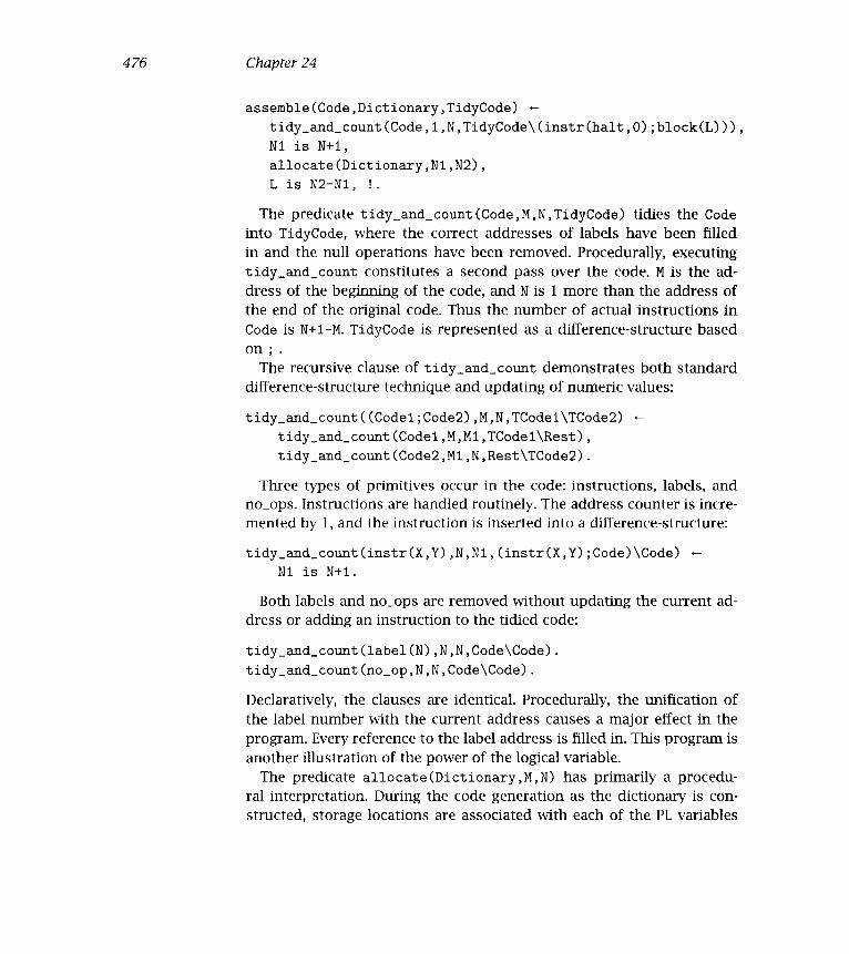
476 Chapter 24
assemble(Code,Dictionary,TidyCode) -
tidy_and_count(Code,1,N,TidyCode\(instr(halt,O) ;block(L))),
Nl is N+1,
allocate (Dictionary ,Nl, N2),
L is N2-N1, !.
The predicate tidy_and_count(Code,M,N,TidyCode) tidies the Code
into TidyCode, where the correct addresses of labels have been filledin and the null operations have been removed. Procedurally, executingtidy_and_count constitutes a second pass over the code. M is the ad-dress of the begimiing of the code, and N is i more than the address ofthe end of the original code. Thus the number of actual instructions inCode is N+1-M. TidyCode is represented as a difference-structure basedon;
The recursive clause of tidy_and_count demonstrates both standarddifference-structure technique and updating of numeric values:
tidy_and_count((Codel;Code2) ,M,N,TCodel\TCode2) -
tidy_and_count (Codel ,M,M1 ,TCodel\Rest),
tidy_and_count (Code2 ,Ml , N, Rest\TCode2).
Three types of primitives occur in the code: instructions, labels, andno_ops. Instructions are handled routinely. The address counter is incre-mented by 1, and the instruction is inserted into a difference-structure:
tidy_and_count(instr(X,Y),N,N1,(instr(X,Y);Code)\Code) -
Nl is N+1.
Both labels and no_ops are removed without updating the current ad-dress or adding an instruction to the tidied code:
tidy_and_count(label(N) ,N,N,Code\Code).
tidy_and_count(no_op,N,N,Code\Code).
Declaratively, the clauses are identical. Procedurally, the unification ofthe label number with the current address causes a major effect in theprogram. Every reference to the label address is filled in. This program isanother illustration of the power of the logical variable.
The predicate allocate(Dictionary,M,N) has primarily a procedu-ral interpretation. During the code generation as the dictionary is con-structed, storage locations are associated with each of the PL variables

477 A Compiler
Program testi:instr(load,11);instr(divc,2);instr(store,12);instr(load,1O);
instr(sub,12);instr(add,9);instr(write,O);instr(halt,O);block(4)
Program test2:instr(load,1O);instr(sub,11);instr(jumple,7);instr(load,1O);
instr(store, 12) ; iristr(jurnp,9) ïnstr(load, 11) instr(store, 12)
instr(halt 0) ;block(3)
Program factorial:instr(read,21);instr(loadc,1);instr(store,19);instx(loadc,1);
instr(store,20);instr(load,19);instr(sub,21);instr(jumpge,16);
instr(load,19);instr(addc,1);instr(store,19);instr(load,20);
instr(mul,19);instr(store,20);instr(junip,6);instr(load,20);
instr(write,0) instr(halt »0) ;block(3)
Figure 24.7 The compiled object code
in the program, plus any temporary variables needed for computing ex-pressions. The effect of allocate is to assign actual memory locationsfor the variables and to fill in the references to them in the program.
The variables are found by traversing the Dictionary. M is the addressof the memory location for the first variable, and N is i more than theaddress of the last. The order of variables is alphabetic corresponding totheir order in the dictionary. The code also completes the dictionary as adata structure.
allocate(void,N,N).
allocate(dict(Name,N1,Before,After) ,NO,N)
allocate (Bef ore,NO,N1),
N2 is N1+1,
allocate(After,N2,N).
Because the dictionary is an incomplete data structure, the predicateallocate can succeed many times. The variables at the end of the treematch both the fact and the recursive clause. For the compiler, the easi-est way to stop multiple solutions is to add a cut to the clause for assem-ble/3, which conmits to the first (and minimal) assignment of memorylocations for variables.
The compiled versions of the test programs given in Program 24.2appear in Figure 24.7.

478 Chapter 24
Exercises for Chapter 24
(i) Extend the compiler so that it handles repeat loops. The syntax isrepeat (statement) until (test). Extensions to both the parser andthe compiler need to be made. Test the program on the following:
program repeat;
begin
i : 1;
repeat
i begin
ii write(i);
ii i i+1
i end
until i = 11
end.
(ii) Extend the definition of arithmetic expressions to allow arbitraryones. In the encoder, you will have to cater for the possibility ofneeding several temporary variables.
24.5 Background
The compiler described is based on a delightful paper by Warren (1980).

A Operators
An operator is defined by its name, specifier, and priority. The name isusually an atom. The priority is an integer between i and 1200 inclusive.The specifier is a mnemonic that defines two things, class and asso-ciativity. There are three classes of operators: prefix, infix, and postfix.Associativity, which determines how to associate terms containing mul-tiple operators, can be one of three possibilities: left-associative, right-associative, and non-associative.
There are seven possible operator types, which are given in Table AJ.A left-associative prefix operator is not possible, nor is a right-associativepostfix operator. An operator specifier yfy does not make sense as itwould lead to ambiguity. Consequently Standard Prolog does not allowsuch a specifier.
To explain the associativity, consider a term a :: b :: c. If the infixoperator :: was left-associative, the term would be read as (a :: b) :: c. Ifthe operator :: was right-associative, the term would be read as a :: (b :: c).If the operator :: was non-associative, the term would be illegal.
If uncertain about priorities when using operators, terms can always bebracketed. If you prefer not to bracket terms, you must take into accountthe associativity of the operator(s) involved and the priorities of terms.For example, the following three rules apply.
An operand with the same priority as a non-associative operatormust be bracketed to avoid a syntax error by the Prolog reader.An operator with the same (or smaller) priority as a right-associativeoperator that follows that operator need not be bracketed.An operator with smaller priority than a left-associative operatorthat precedes that operator need not be bracketed.

480 Appendix A
Table A. iTypes of Operators in Standard Prolog
Specifier Class Associativity
fx prefix non-associativefy prefix right-associativexfx infix non-associativexfy infix right-associativeyfx infix left-associativexf postfix non-associativeyf postfix left-associative
Table A.2Predefined Operators in Standard Prolog
Priority Specifier Operator(s)
1200 xfx (:- -->)1200 fx1100 xfy1000 xfy
700 xfx = \=700 xfx == \==700 xfx700 xfx500 yfx +-400 yfx200 xfy200 fy
Standard Prolog specifies some predefined operators. The prioritiesand specifiers of the operators which have been used in the text are givenin Table A.2.
New operators are added with the directive
op (X ,Y, Z)
where X is the priority, Y is the operator specifier, and Z is the operatorname. These were used in Chapter 17 when defining a new rule language.

481 Operators
The system of operator declarations in Prolog is straightforward andcan be used effectively for applications. The reader should be aware,however, that there are some subtle semantic anomalies in how opera-tors are defined and handled. The anomalies, best discovered by trial anderror, should not cause problems and can be "programmed around"


References
Abelson, H. and Sussman, G. J., Structure and Interpretation of ComputerPrograms, MIT Press, Cambridge, Massachusetts, 1985.
Abramson, H. and Dahi, V., Logic Grammars, Springer-Verlag, New York,1989.
Abramson, H. and Rogers, M. (eds.), Meta-Programming in Logic Program-ming, MIT Press, Cambridge, Massachusetts, 1989.
Alt-Kaci, H., The WAM: A (Real) Tutorial, MIT Press, Cambridge, Massachu-setts, 1991.
Apt, K. R., Logic Programming, in Handbook of Theoretical Computer Science,J. van Leeuwen (ed.), pp. 493-574, North-Holland, Amsterdam, 1990.
Apt, K. R. and van Emden, M. H., Contributions to the Theory of Logic Pro-grarnming, J. ACM 29, pp. 841-862, 1982.
Bansal, A. and Sterling, L. S., Classifying Generate-and-Test Logic Programs,International J. of Parallel Processing 8(4), pp. 401-446, 1989.
Barkiund, J., What is a Variable in Prolog? in (Abramson and Rogers, 1989),pp. 383-398.
Ben-David, A. and Sterling, L., A Prototype Expert System for Credit Evalua-tion, in Artificial Intelligence in Economics and Management, L. F. Pau (ed.),pp. 121-128, North-Holland, Amsterdam, 1986.
Berge, C., The Theory of Graphs and its Applications, Methuen & Co., London,1962.
Bergman, M. and Kanoui, H., Application of Mechanical Theorem Provingto Symbolic Calculus, in Proc. Third International Symposium on AdvancedComputing Methods in Theoretical Physics, CNRS, Marseilles, 1973.

484 References
Bloch, C., Source-to-Source Transformations of Logic Programs, Tech. ReportCS-84-22, Department of Applied Mathematics, Weizmanri Institute of Sci-ence, Rehovot, Israel, 1984.
Bowen, D. L., Byrd, L., Pereira, L. M., Pereira, F. C. N., and Warren, D. H. D.,Prolog on the DECSystem-10, User's Manual, University of Edinburgh, 1981.
Bowen, K. and Kowaiski, R., Amalgamating Language and Meta-Language, in(Clark and Tarnlund, 1982), pp. 153-172.
Boyer, R. S. and Moore, J. S., A Computational Logic, Academic Press, ACMMonograph Series, 1979.
Breuer, G. and Carter, H. W., VLSI Routing, in Hardware and Software Con-cepts in VLSI, G. Rabbat (ed.), pp. 368-405, Van Nostrand Reinhold, 1983.
Bruffaerts, A. and Henin, E., Negation as Failure: Proofs, Inference Rules andMeta-interpreters, in (Abramson and Rogers, 1989), pp. 169-190.
Bruynooghe, M., The Memory Management of Prolog Implementations, in(Clark and Tarnlund, 1982), pp. 83-98.
Bruynooghe, M. and Pereira, L. M., Deductive Revision by Intelligent Back-tracking, in (Campbell, 1984), pp. 194-2 15.
Bundy, A., A Computer Model of Mathematical Reasoning, Academic Press,New York, 1983.
Bundy, A., A Generalized Interval Package and Its Use for Semantic Checking,ACM Transactions on Mathematical Software 10, pp. 392-407, 1984.
Bundy, A. and Weiham, R., Using Meta-level Inference for Selective Appli-cation of Multiple Rewrite Rules in Algebraic Manipulation, Artificial Intelli-gence 16, pp. 189-2 12, 1981.
Burstall, R. M. and Darlington, J., A Transformation System for DevelopingRecursive Programs, J. ACM 24, pp. 46-67, 1977.
Byrd, L., Understanding the Control Flow of Prolog Programs, in (Tarniund,1980).
Campbell, J. A. (ed.), Implementations of Prolog, Ellis Horwood Publication,Wiley, New York, 1984.
Chen, W., Kiefer, M., and Warren, D. S., HiLog: A First-Order Semantics forHigher-Order Logic Programming Constructs, in Proc. 1989 North AmericanConference on Logic Programming, E. Lusk, and R. Overbeek, (eds.), pp. 1090-1114, MIT Press, Cambridge, Massachusetts, 1989.

485 References
Chikayama, T., Unique Features of ESP, in Proc. International Conference oriFifth Generation Computer Systems, pp. 292-298, ICOT - Institute for NewGeneration Computer Technology, Tokyo, Japan, 1984.
Ciepielewski, A., Scheduling in OR-parallel Prolog Systems, Frameworks, Sur-vey, and Open Problems, Technical Report 91-02, University of Iowa, 1991.
Clark, K. L., Negation as Failure, in (Gallaire and Minker, 1978), pp. 293-322.
Clark, K. L. and Gregory, S., A Relational Language for Parallel Programming,in Proc. ACM Symposium on Functional Languages and Computer Architec-ture, pp. 171-178, 1981.
Clark, K. L. and Gregory, S., PARLOG: Parallel Programming in Logic, Re-search Report 84/4, Department of Computing, Imperial College of Scienceand Technology, England, 1984.
Clark, K. L. and McCabe, F. G., The Control Facilities of ¡C-Prolog, in ExpertSystems in the MicroelectronicAge, D. Michie (ed.), pp. 153-167, University ofEdinburgh Press, 1979.
Clark, K. L. and McCabe, F. G., PROLOG: A Language for Implementing ExpertSystems, in Machine Intelligence 10, J. Hayes, D. Michie and Y. H. Pao (eds.),pp. 45 5-470, Ellis Horwood Publication, Wiley, New York, 1982.
Clark, K. L, McCabe, F. G., and Gregory, S., IC-Prolog Language Features, in(Clark and Tarnlund, 1982).
Clark, K. L. and Tarniund, S.-A., A First Order Theory of Data and Programs,Information Processing 77, pp. 939-944, North-Holland, Amsterdam, 1977.
Clark, K. L. and Tarnlund, S-A. (eds.), Logic Programming, Academic Press,London, 1982.
Clocksin, W. F. and Mellish, C. S., Programming in Prolog, 2nd Edition,Springer-Verlag, New York, 1984.
Coelho, H. and Cotta, J., Prolog by Example, Springer-Verlag, New York, 1988.
Coelho, H., Cotta, J. C., and Pereira, L. M., How to Solve It in Prolog, 2ndEdition, Laboratorio Nacional de Engenharia Civil, Lisbon, Portugal, 1980.
Cohen, J., Describing Prolog by Its Interpretation and Compilation, Comm.ACM 28, pp. 1311-1324, 1985.
Cohen, J., A View of the Origins and Development of Prolog, Comm. ACM3 1(1), pp. 26-36, 1988.

486 References
Colmerauer, A., Les systemes-Q ou un Formalisme pour Analyser et Syn-thesizer des Phrases sur Ordinateur, Publication Interne No. 43, Dept.d'Informatique, Universite de Montreal, Canada, 1973.
Colmerauer, A., Prolog-II, Manuel de reference et modele theorique, Grouped'Intelligence Artificielle, Universite d'Aix-Marseille II, France, 1982a.
Colmerauer, A., Prolog And Infinite Trees, in (Clark and Tarniund, 1982)b, pp.231-251.
Colmerauer, A., An Introduction to Prolog-III, Comm. ACM 3 3(70), pp. 70-90,1990.
Colmerauer, A., Kanoui, H., Pasero, R., and Roussel, P., Un Systeme de Com-munication Homme-machine en Francais, Research Report, Groupe Intelli-gence Artificielle, Universite Aix-Marseille II, France, 1973.
Colmerauer, A. and Roussel, P., The Birth of Prolog, in ACM SIGPLAN Notices,28(3), pp. 37-52, 1993.
Deo, N., Graph Theory with Applications to Engineering and Computer Sci-ence, Prentice Hall, Englewood Cliffs, N. J., 1974.
Dershowitz, N. and Lee, Y. J., Deductive Debugging, in Proc. Third IEEE Sym-posium on Logic Programming, San Francisco, pp. 298-306, 1987.
Deville, Y., Logic ProgrammingSystematic Program Development, Addi-son-Wesley, Reading, Massachusetts, 1990.
Deville, Y., Sterling, L. S. and Deransart, P., Prolog for Software Engineering,Tutorial presented at Eighth International Conference on Logic Programming,Paris, France, 1991.
Dincbas, M. and Le Pape, J. P., Metacontrol or Logic Programs in METALOG,in Proc. International Conference on Fifth Generation Computer Systems, pp.361-370, ICOT - Institute for New Generation Computer Technology, Tokyo,Japan, 1984.
Disz, T., Lusk, E., and Overbeek, R., Experiments with OR-Parallel Logic Pro-grams, in Proc. Fourth International Conference on Logic Programming, J. L.Lassez (ed.), pp. 5 76-600, MIT Press, Cambridge, Massachusetts, 1987.
Drabent, W., Nadjm-Tehrani, S., and Maluszynski, J., Algorithmic Debuggingwith Assertions, in (Abramson and Rogers, 1989), pp. 501-521.
Dudeney, H. E., Amusements in Mathematics, Thomas Nelson and Sons, Lon-don, 1917.

487 References
Dwork, C., Kanellakis, P. C., and Mitchell, J. C., On the Sequential Nature ofUnification, J. Logic Programming 1, pp. 35-50, 1984.
Eggert, P. R. and Chow, K. P., Logic Programming Graphics with InfiniteTerms, Tech. Report University of California, Santa Barbara 83-02, 1983.
Elcock, E. W., The Pragmatics of Prolog: Some Comments, in Proc. Logic Pro-gramming Workshop '83, pp. 94-106, Algarve, Portugal, 1983.
Even, S., Graph Algorithms, Computer Science Press, 1979.
Findlay, W. and Watt, D. A., PASCAL: An Introduction to Methodical Program-ming, 2nd edition, Pitman, 1985.
Futarnura, Y., Partial Evaluation of Computation ProcessAn Approach to aCompiler-Compiler, Systems, Computers, Controls 2, pp. 45-50, 1971.
Gallagher, J., Transforming Logic Programs by Specializing Interpreters, inProc. Seventh European Conference on Artificial Intelligence, pp. 109-122,Brighton, England, 1986.
Gallagher, J. and Bruynooghe, M., Some Low-Level Source Transformationsfor Logic Programs, in Proc. Second Workshop on Meta-Programming in Logic,pp. 229-244, Leuven, Belgium, 1990.
Gallaire, H. and Lasserre, C., A Control Metalanguage for Logic Programming,in (Clark and Tarniund, 1982), pp. 173-185.
Gallaire, H. and Minker, J., Logic and Databases, Plenum Publishing Co., NewYork, 1978.
Gallaire, H., Minker, J., and Nicolas, J. M., Logic and Databases: A DeductiveApproach, Computing Surveys 16, pp. 153-185, 1984.
Gregory, S., Parallel Logic Programming in PARLOG, Addison-Wesley, Read-ing, Massachusetts, 1987.
Hammond, P., Micro-Prolog for Expert Systems, Chapter 11 in Micro-Prolog:Programming in Logic, K. Clark and F. McCabe (eds.), Prentice Hall, Engle-wood Cliffs, N. J., 1984.
Heintze, N., Michaylov, S., Stuckey, P. and Yap, R., On Meta-Programming inCLP(R), in Proc. 1989 North American Conference on Logic Programming, E.Lusk, and R. Overbeek, (eds.), pp. 52-66, MIT Press, Cambridge, Massachu-setts, 1989.
Hill, P. and Lloyd, J. W., Analysis of Meta-Programs, in (Abramson and Rogers,1989), pp. 23-51.

488 References
Hill, P. and Lloyd, J. W., The Gödel Progranming Language, MIT Press, Cam-bridge, Massachusetts, 1993.
Hill, R., LUSH-Resolution and Its Completeness, DCL Memo 78, Departmentof Artificial Intelligence, University of Edinburgh, Scotland, 1974.
Hoperoft, J. E. and Ullman, J. D., Introduction to Automata Theory, Languages,Computation, Addison-Wesley, Reading, Massachusetts, 1979.
Horowitz, E. and Salmi, S., Fundamentals of Computer Algorithms, ComputerScience Press, 1978.
Jaffar, J., Lassez, J. L., and Lloyd, J. W., Completeness of the Negation asFailure Rule, in Proc. of the International Join t Conference on Artificial Intelli-gence, pp. 500-506, Karlsruhe, Germany, 1983.
Jaffar, J. and Lassez, J. L., From Unification to Constraints, in Proc. of LogicProgramming '87, K. Furukawa, H. Tanaka, and T. Fujisaki, (eds.), pp. 1-18,Springer-Verlag LNCS 315, 1987.
Janson, S. and Haridi, S., Progranuning Paradigms of the Andorra KernelLanguage, in Proc. 1991 International Symposium on Logic Programming, V.Saraswat, and K. Ueda, (eds.), pp. 167-183, MIT Press, Cambridge, Massachu-setts, 1991.
Journal of Logic Programming, Special Issue on Abstract Interpretation, 15,1993.
Kahn, K. M., A Primitive for the Control of Logic Programs, in Proc. Inter-national IEEE Symposium on Logic Programming, Atlantic City, pp. 242-251,1984.
Kirschenbaum, M., Sterling, L., and Jam, A., Relating Logic Programs via Pro-gram Maps, Annals of Mathematics and Artificial Intelligence 8(3-4), 1993.
Knuth, D., The Art Of Computer Programming, Volume 1, Fundamental Algo-rithms, Addison-Wesley, Reading, Massachusetts, 1968.
Knuth, D., The Art Of Computer Programming, Volume 3, Sorting and Search-ing, Addison-Wesley, Reading, Massachusetts, 1973.
Komorowski, H. J., A Specification of an Abstract Prolog Machine and ItsApplication to Partial Evaluation, Ph. D. Thesis, available as Report No. 69,Software Systems Research Center, Linköping University, 1981.
Kowalski, R., Predicate Logic as a Progrannning Language, in Proc. IFIPCongress, J. Rosenfeld (ed.), pp. 569-574, North-Holland, Amsterdam, 1974.
Kowalski, R., Logic For Problem Solving, North-Holland, Amsterdam, 1979a.

489 References
Kowälski, R., Algorithm = Logic + Control, Comm. ACM 22, pp. 424-436,197gb.
Kowaiski, R., The Early Years of Logic Programming, Comm. ACM 3 1(1), pp.38-43, 1988.
Kunen, K., Logic for Logic Programmers, Tutorial Notes Ti, North AmericanConference on Logic Programming, Cleveland, October, 1989.
Lakhotia, A., Incorporating 'Programming Techniques' into Prolog programs,in Proc. 1989 North American Conference on Logic Programming, E. Lusk,and R. Overbeek, (eds.), pp. 426-440, MIT Press, Cambridge, Massachusetts,1989.
Lakhotia, A. and Sterling, L. S., ProMiX: A Prolog Partial Evaluation System, in(Sterling, 1990), pp. 137-179.
Lassez, J. L., From LP to LP: Programming with Constraints, UnpublishedTechnical Report, 1991.
Lassez, J. L., Maher, M., and Marriott, K., Unification Revisited, in FoundationsofDeductive Databases and Logic Programming, J. Minker, (ed.), pp. 587-625,Morgan Kaufmann, 1988.
Li, D., A Prolog Database System, Research Studies Press, Ltd., Wiley, England,1984.
Lim, P. and Stuckey, P., Meta-Programming as Constraint Programming, inProc. NACLP-90, S. Debray and M. Hermenegildo (eds.), pp. 406-420, MITPress, Cambridge, Massachusetts, 1990.
Lindholm, T. and O'Keefe, R., Efficient Implementation of a Defensible Se-mantics for Dynamic Prolog Code, in Proc. Fourth International Conferenceon Logic Programming, J. L. Lassez (ed.), pp. 2 1-39, MIT Press, Cambridge,Massachusetts, 1987.
Lloyd, J. W., Foundations OfLogic Programming, 2nd Edition, Springer-Verlag,New York, 1987.
Lombardi, L. A. and Raphael, B., Lisp as the Language for an IncrementalComputer, in The Programming Language LISP: Operation and Application,E. C. Berkeley and D. G. Bobrow (eds.), pp. 204-219, MIT Press, Cambridge,Massachusetts, 1964.
Maier, D., The Theory ofRelational Databases, Computer Science Press, 1983.
Maier, D. and Warren, D. S., Computing with Logic-Logic Programming withProlog, Benjamin-Cummings, 1988.

490 References
Marriott, K. and Sondergaard, H., Difference-List Transformation for Prolog,New Generation Computing 11(2), PP. 12 5-157, 1993.
Martelli, A. and Montanari, U., An Efficient Unification Algorithm, ACM Trans-actions on Programming Languages and Systems 4(2), pp. 2 58-282, 1982.
Matsumoto, Y., Tanaka, H., and Kiyono, M., BUP: A Bottom-Up Parsing Systemfor Natural Languages, in (van Caneghem and Warren, 1986), pp. 262-275.
Mellish, C. S., Some Global Optimizations for a Prolog Compiler, J. LogicProgramming 2, pp. 43-66, 1985.
Michie, D., "Memo" Functions and Machine Learning, Nature, 218, pp. 19-22,1968.
Miller, D. and Nadathur, G., Higher-Order Logic Programming, in Proc. ThirdInternational Conference on Logic Programming, E. Y. Shapiro, (ed.), Pp. 448-462, Springer-Verlag LNCS 225, 1986.
Minsky, M., Semantic In formation Processing, MIT Press, Cambridge, Massa-chusetts, 1968.
Moss, C., Cut and PasteDefining the Impure Primitives of Prolog, in Proc.Third International Conference on Logic Programming, E. Y. Shapiro, (ed.), pp.686-694, Springer-Verlag LNCS 225, 1986.
Naish, L., All Solutions Predicate in PROLOG, in Proc IEEE Symposium onLogic Programming, Boston, pp. 73-77, IEEE Computer Society Press, 1985a.
Naish, L., Automating Control for Logic Programs, J. Logic Programming 2,pp. 167-184, 1985b.
Naish, L., Negation and Control in Prolog, Springer-Verlag LNCS 238, 1986.
Nakashima, H., Tomura S. and Ueda, K., What Is a Variable in Prolog? in Proc.of the International Conference on Fifth Generation Computer Systems, pp.327-332, ICOT - Institute for New Generation Computer Technology, Tokyo,Japan, 1984.
Nilsson, N. J., Problem Solving Methods in Artificial Intelligence, McGraw-Hill,New York, 1971.
Niisson, N. J., Principles of Artificial Intelligence, Tioga Publishing Co., PaloAlto, California, 1980.
O'Keefe, R. A., Programming Meta-Logical Operations in Prolog, DAI WorkingPaper No. 142, University of Edinburgh, Scotland, 1983.

491 References
O'Keefe, R. A., On the Treatment of Cuts in Prolog Source-Level Tools, inProc. 1985 IEEE Symposium on Logic Programming, Boston, pp. 68-72, IEEEComputer Society Press, 1985.
O'Keefe, R. A., The Craft of Prolog, MIT Press, Cambridge, Massachusetts,1990.
Paterson, M. S. and Wegman, M. N., Linear Unification, J. Computer and Sys-tems Sciences 16, pp. 158-167, 1978.
Pereira, L. M., Logic Control with Logic, in Proc. First international Logic Pro-gramming Conference, pp. 9-18, Marseilles, France, 1982.
Pereira, F. C. N. and Shieber, S., Prolog and Natural Language Analysis, CSLILecture Notes No. 10, CSLI, Stanford University, Stanford, 1987.
Pereira, F. C. N. and Warren, D. H. D., Definite Clause Grammars for LanguageAnalysisA Survey of the Formalism and a Comparison with AugmentedTransition Networks, Artificial Intelligence 13, pp. 231-278, 1980.
Peter, R., Recursive Functions, Academic Press, New York, 1967.
Plaisted, D. A., The Occur-Check Problem in Prolog, New Generation Comput-ing 2, pp. 309-322, 1984.
Plümer, L., Termination Proofs for Logic Programs, Springer-Verlag, NewYork, 1990.
Power, A. J. and Sterling, L. S., A Notion of Map between Logic Programs, inProc. Seventh International Conference on Logic Programming, D. H. D. War-ren and P. Szeredi (eds.), pp. 390-404, MIT Press, Cambridge, Massachusetts,1990.
Powers, D., Playing Mastermind More Logically, SIGART Newsletter 89, pp.28-32, 1984.
Quintus Prolog Reference Manual, Quintus Computer Systems Ltd., 1985.
Reiter, R., On Closed World Databases, in (Gallaire and Minker, 1978), pp. 55-76. Also in Readings in Artificial Intelligence, Webber and Niisson (eds.), TiogaPublishing Co., Palo Alto, California, 1981.
Robinson, J. A., A Machine-Oriented Logic Based on the Resolution Principle,J. ACM 12, pp. 23-41, January 1965.
Robinson, J. A. and Sibert, E. E., LOGLISP: Motivation, Design and Implemen-tation, in (Clark and Tarnlund, 1982), pp. 299-3 13.
Ross, P., Advanced Prolog, Techniques and Examples, Addison-Wesley, Read-ing, Massachusetts, 1989.

492 References
Sahlin, D., An Automatic Partial Evaluator for Full Prolog, Ph. D. Thesis, avail-able as SICS Dissertation Series 4, Swedish Institute of Computer Science,1991.
Schank, R. C. and Abelson, R. P., Scripts, Plans, Goals, and Understanding,Lawrence Erlbaum, Hillsdale, N. J., 1977.
Schank, R. C. and Riesbeck, C., Inside Computer Understanding: Five Pro-grams Plus Miniatures, Lawrence Erlbaum, Hillsdale, N. J., 1981.
Scowen, R., Prolog: Working Draft 5.0, N72, 1991.
Sedgewick, R., Algorithms, Addison-Wesley, Reading, Massachusetts, 1983.
Sergot, M., A Query the User Facility for Logic Programming, in IntegratedInteractive Computer Systems, North-Holland, Amsterdam, 1983.
Shapiro, E., Algorithmic Program Debugging, MIT Press, Cambridge, Massa-chusetts, 1983a.
Shapiro, E., A Subset of Concurrent Prolog and Its Interpreter, Tech. ReportTR-003, ICOTInstitute for New Generation Computer Technology, Tokyo,Japan, 1983b.
Shapiro, E., Logic Programs with Uncertainties: A Tool for Implementing Rule-Based Systems, Proc. Eighth International Joint Conference on Artificial Intel-ligence, pp. 529-532, Karlsruhe, Germany, 1983c.
Shapiro, E., Playing Mastermind Logically, SIGART Newsletter 85, pp. 28-29,1983d.
Shapiro, E., Alternation and the Computational Complexity of Logic Pro-grams, J. Logic Programming 1, pp. 19-33, 1984.
Shapiro, E., Systems Programming in Concurrent Prolog, in (van Caneghemand Warren, 1986), pp. 5 0-74.
Shapiro, E. and Takeuchi, A., Object Oriented Programming in ConcurrentProlog, New Generation Computing 1, pp. 2 5-48, 1983.
Shortliffe, E. H., Computer Based Medical Consultation, MYCIN, North-Holland, New York, 1976.
Silver, B., Meta-level Inference, Elsevier Science, Amsterdam, Netherlands,1986.
Silverman, W., Hirsch, M., Houri, A. and Shapiro, E., The Logix System UserManual, Weizmann Institute of Science, Rehovot, Israel, 1986.

493 References
Slagle, J. and Dixon, J., Experiments with Some Programs That Search GameTrees, J. ACM 16, pp. 189-207, 1969.
Smith, D., Partial Evaluation of Pattern Matching in Constraint Logic Program-ming Languages, Proc. Symposium on Partial Evaluation and Semantics-BasedProgram Manipulation, SIGPLAN Notices 26, pp. 62-71, September 1991.
Sondergaard, H., Semantics-Based Analysis and Transformation of Logic Pro-grams, Ph. D. Thesis, also Tech. Report 89/2 1, University of Melbourne, 1989.
Steele, G. L., Jr. and Sussman, G. J., The Art of the Interpreter, or the Modu-larity Complex, Tech. Memorandum MM-453, MIT Al-Lab, May 1978.
Sterling, L. S., Expert System = Knowledge + Meta-Interpreter, Tech. ReportCS84-17, Weizmann Institute of Science, Rehovot, Israel, 1984.
Sterling, L. S. (ed.), The Practice of Prolog, MIT Press, Cambridge, Massachu-setts, 1990.
Sterling, L. S. and Beer, R. D., Meta-Interpreters for Expert System Construc-tion,J. Logic Programming 6(1-2), pp. 163-178, 1989.
Sterling, L. S. and Bundy, A., Meta-Level Inference and Program Verification, inProc. of the Sixth Conference on Automated Deduction, pp. 144-150, Springer-Verlag LNCS 138, 1982.
Sterling, L. S., Bundy, A., Byrd, L., O'Keefe, R., and Silver, B., Solving symbolicequations with PRESS, in Computer Algebra, pp. 109-116, Springer-VerlagLNCS 144, 1982.
Sterling, L. S. and Codish, M., PRESSing for Parallelism: A Prolog Pro-gram Made Concurrent, J. Logic Programming 3, pp. 75-92, 1986.
Sterling, L. S. and Kirschenbaum, M., Applying Techniques to Skeletons, inConstructing Logic Programs, J. M. J. Jacquet (ed.), pp.127-140. Wiley, NewYork, 1993.
Sterling, L. S. and Lalee, M., An Explanation Shell for Expert Systems, Compu-tational Intelligence 2, pp. 136-141, 1986.
Sterling, L. S. and Lakhotia, A., Composing Prolog Meta-Interpreters, in Proc.Fifth International Conference on Logic Programming, K. Bowen, and R.Kowatski, (eds.), pp. 386-403, MIT Press, Cambridge, Massachusetts, 1988.
Sterling, L. S. and Yalçinalp, L. U., Explaining Prolog Computations Using aLayered Meta-Interpreter, in Proc. IJCAI-89, pp. 66-7 1, Morgan Kaufmarm,1989.

494 References
Takeuchi, A. and Furukawa, K., Partial Evaluation of Prolog Programs and ItsApplication to Meta Programming, Information Processing 86, H. J. Kugler(ed.), pp. 415-420, Elsevier, New York, 1986.
Tamaki, H. and Sato, T., Unfold/Fold Transformations of Logic Programs,Proc. Second International Conference on Logic Programming, pp. 127-138,Uppsala, Sweden, 1984.
Tarnlund, S.-A. (ed.), Proc. of the Logic Programming Workshop, Debrecen,Hungary, 1980.
Tick, E., Parallel Logic Programming, MIT Press, Cambridge, Massachusetts,1991.
Ueda, K., Guarded Horn Clauses, ICOT Tech. Report 103, ICOT, Tokyo, Japan,1985.
Ullman, J. D., Principles of Database Systems, 2nd Edition, Computer SciencePress, 1982.
Ullman, J. D., Principles of Database and Knowledge-Base Symbols, Volume 1,Computer Science Press, 1989.
van Caneghem, M. (ed.), Prolog-H User's Manual, 1982.
van Caneghem, M. and Warren, D. H. D. (eds.), Logic Programming and itsApplications, Ablex Publishing Co., 1986.
van Emden, M., Warren's Doctrine on the Slash, Logic Programming Newslet-ter, December, 1982.
van Emden, M. and Kowalski, R., The Semantics of Predicate Logic as a Pro-gramming Language, Comm. ACM 23, pp. 733-742, 1976.
Venken, R., A Prolog Meta-Interpreter for Partial Evaluation and its Appli-cation to Source-to-Source Transformation and Query Optimization, in Proc.European Conference on Artificial Intelligence, pp. 9 1-100, Pisa, 1984.
Warren, D. H. D., Generating Conditional Plans and Programs, Proc. AISBSummer Conference, pp. 344-3 54, Edinburgh, Scotland, 1976.
Warren, D. H. D., Implementing PrologCompiling Logic Programs i and 2,DAI Research Reports 39 and 40, University of Edinburgh, Scotland, 1977.
Warren, D. H. D., Logic Progranmiing and Compiler Writing, Software-Practiceand Experience 10(2), pp. 97-125, 1980.
Warren, D. H. D., Higher-Order Extensions to Prolog: Are They Needed?, Ma-chine Intelligence 10, pp. 441-454, Hayes, Michie and Pao (eds.), Ellis Hor-wood Publications, Wiley, New York, 1982a.

495 References
Warren, D. H. D., Perpetual ProcessesAn Unexploited Prolog Technique, inProc. Prolog Programming Environments Workshop, Sweden, 1982b.
Warren, D. H. D., Ari Abstract Prolog Instruction Set, Tech. Note 309, SRIInternational, Menlo Park, California, 1983.
Warren, D. H. D., Optimizing Tail Recursion in Prolog, in (van Caneghem andWarren, 1986), pp. 77-90.
Warren, D. H. D., Pereira, F., and Pereira L. M., User's Guide to DECsystem-10Prolog, Occasional Paper 15, Department of Artificial Intelligence, Universityof Edinburgh, Scotland, 1979.
Weizenbaum, J., ELIZAA Computer Program for the Study of Natural Lan-guage Communication between Man and Machine, CACM 9, pp. 36-4 5, 1966.
Weizenbaum, J., Computer Power and Human Reason, W. H. Freeman & Co.,1976.
Welham, R., Geometry Problem Solving, Research Report 14, Department ofArtificial Intelligence, University of Edinburgh, Scotland, 1976.
Winograd, T., Language as a Cognitive Process, Volume I. Syntax, Addison-Wesley, Reading, Massachusetts, 1983.
Winston, P. H., Artificial Intelligence, Addison-Wesley, Reading, Massachu-setts, 1977.
Yalçìnalp, L. U., Meta-Programming for Knowledge-Based Systems in Prolog,Ph. D. Thesis, available as Tech. Report TR 91-141, Center for Automationand Intelligent Systems Research, Case Western Reserve University, Cleve-land, 1991.
Yalçinalp, L. U. and Sterling, L. S., An Integrated Interpreter for ExplainingProlog's Successes and Failures, in (Abramson and Rogers, 1989), pp. 191-203.
Yalçinalp, L. U. and Sterling, L. S., Uncertainty Reasoning in Prolog with Lay-ered Meta-Interpreters, in Proc. Seventh Conference on Artificial IntelligenceApplications, pp. 398-402, IEEE Computer Society Press, February 1991.


Index
Abstract interpretation, 147Abstract interpreter, 22-24, 91-96,
119-123Accumulator, 146-147, 155-157,
166, 240, 254, 266, 287-288,309
bottom-up construction of lists,14 5-146
definition, 155generalization to difference-list,
28 7-288Abramson, Harvey, 388Ackermann's function, 53-55, 85Ait-Kaci, Hassan, 127, 213All-solutions predicates, 302-304Alpha-beta pruning, 405-407Alphabetic variant, 88, 200Alternating Turing machine, 115ANALOGY, 270, 272, 281Ancestor cut, 354Anonymous variable, 234APES expert system shell, 355append, 60-62, 93-94, 104-105, 109,
122, 131, 133, 140, 196-197,288, 311
Appending. See ConcatenationApt, Krzystof, 99, 1056arg, 167-168, 173, 174Argument, 13, 27, 171Arithmetic
logic programs for, 45-55
Prolog programs for, 150-161Arithmetic evaluation, 150-151Arithnietic expression, 151, 467Arity, 13, 27, 32Askable goals for expert systems,
344-346Assembler, 475-477assert, 220-221, 231-232, 304Assignment, 125, 170Atom, 11, 27, 164atom, 163-164atomic, 164Automata, 3 19-323
Backtracking, 120-122, 125, 190,192, 218, 231, 249-250, 280,324
deep, 124intelligent, 280shallow, 124
bagof, 303, 317Bansal, Arvind, 280Barklund, Jonas, 187Beer, Randall, 373Benchmark, 209Ben-David, Arie, 438Berge, Claude, 423Bergman, Marc, 457Best-first search, 396-400Binary predicate, 38, 44Binary tree, 72-77, 85, 295

498 Index
Binding, 91Bips, 150Bird, R., 245Bloch, Charlene, 162Blocks world problem, 269-271Body of a clause, 18Boolean formula, 82-83Bottom-up construction, 145-146,
287Bottom-up evaluation, 44Bottom-up implementation, 237Bottom-up parser, 388Bowen, Dave, 127Bowen, Ken, 85Boyer, Robert, 85Breadth-first search, 266, 305-307,
396, 398Broderick, David, 317Bruffaerts, A., 355Bruynooghe, Maurice, 212, 282, 300Builtm predicates, 150, 326-32 7Bundy, Alan, 85, 99, 281, 457Burstall, Rod, 373Byrd, Lawrence, 457
call, 186car, 56Cartesian product, in relational
algebra, 43cdr, 56Certainty factor, 330Certainty threshold, 330-331Chain rule, for derivatives, 80-81Character I/O, 216-218Character strings, 216, 218Chen, Weidong, 318Chikayama, Takashi, 212Choice point, 208Chow, D., 99Circuit, logic program, 32-34Circular definition, 133Clark, Keith, 115, 127, 147, 212, 282,
300, 355Clause, 18, 24, 27-28, 95, 120, 219
body, 18definition, 18, 27head, 18Horn, 18indexing, 196-197, 209-2 10iterative, 18, 28nondeterministic choice, 24, 120order. See Rule orderreduction, 95, 120, 326unit, 18, 28
clause, 219, 324-325Clause reduction level, 326Clocksin, William, 85, 128Closed world assumption, 115Code generation (for PL), 470-475Codish, Michael, 457Coelho, Helder, 85, 282, 354Cohen, Jacques, 127, 128Colmerauer, Alain, 99, 127, 187, 212,
354, 388Coloring planar maps, 255-257Comments, 33, 235Common instance, 16, 88Commutative relation, 132Comparison of Prolog with conven-
tional languages, 124-126Comparison operator, 153Compiler for PL, 459-475Compiler for Prolog, 213Complete list, 107, 133Complete natural number, 107Complete structure, 133Complete type, 107Completeness
of program, 26, 28, 46, 48, 106of recursive data structure, 107
Complexity, 108-109depth, 109goal-size, 109length, 108time, 108, 209
COMPOSERS, 244Composition, 239, 366-368, 374Composition specification, 367

499 Index
compound, 163-164
Compound term, 13-14, 27, 35, 37,
108, 167-173
size of, 108
Computationdeterministic, 95, 112
goal, 92, 96, 120nondetermthistic, 112
nonterminating, 92, 106-107, 111,
132-133, 332, 386.
of logic program, 22, 28, 92
output, 91
parallel, 99of Prolog program, 120-12 3
redundant, 138Concatenation
of lists, 60-61of difference-lists, 284
Conceptual dependency, 276, 281
Concurrent logic language, 99, 231Concurrent Prolog, 120, 179, 186,
457Conjunctive goal, 92, 219Conjunctive query, 16-18
Cons pair, 58Consing, 211, 284Constant, 27, 108, 164
constant, 164
consult, 230-23 1
Context-dependent information, 385
Context, finding keywords in, 311-313
Context-free grammar, 369-371,
3 75-3 77
translation to Prolog program,3 72-3 73
Continuation-style meta-mterpreter,326
Control flow, 124, 133, 238-240
Conventional language, comparisonwith Prolog, 124-126
copy_term, 224
Co-routining, 147, 187, 280
Correctness of program, 26, 28,
46-49, 106, 153
Cotta, J., 85, 282
Counterexample, 334
Credit evaluation system, 439-457Cut, 189-2 13, 327, 449
definition, 190
effect of, 190-192, 202-205
effect on storage space, 192,
208-209in expressing mutually exclusive
test, 189
-fail combination. See Cut-failcombination
green. See Green cutin if-then-else statement, 205incompleteness in implementing
negation as failure, 199
loss of flexibility, 194, 204, 205
red, 195, 202-205
restriction on rule order, 198
rule order in negation as failure,198
scope, 195, 327
search tree pruning, 190-191
simulation in meta-interpreter,327
Cut-fail combination, 201-202implementing meta-logical
predicate, 201-202safe use, 201
DAG, 264, 305-306
Dahl, Veronica, 394Darlington, John, 373
Data abstraction, 35-38, 258Data manipulation, in Prolog, 125
Data structure, 125, 143-147, 171,
211, 274, 283-300
creation in Prolog, 125
cyclic, 298
incomplete, 146, 274, 283-300
in Prolog, 143-147

500 Index
Database,deductive, 44logical, 29relational, 42-44
Davis, Ernie, 281DCG. See Definite clause grammarDebugging, enhanced meta-
interpreter for, 33 1-340Declarative reading, 19, 57, 65-66,
324Declarative semantics, 104Deductive database, 44Deep backtracking, 124Default rule, 206-208Definite clause grammar, 375-388,
466generative feature, 386relationship with context-free
grammar, 376, 377Denotational semantics, 105Depth-bounded meta-interpreter,
3 3 2-3 3 3Depth-complexity, 109Depth-first graph traversal, 266Depth-first search, 112, 120, 130,
264-266, 389, 396Depth-first traversal of search tree,
112Derivative, 79-81, 172Dershowitz, Nachum, 354Destructive assignment, 125, 170Deterministic computation, 95,
111-112Deville, Yves, 115, 147, 244, 245Dictionary, 293-296, 300, 470, 477Difference-list, 283-292, 299-300,
304, 305, 371, 373compatibility of, 284concatenation, 284-285head, 283tail, 284
Difference-structure, 291-293, 457,476
Difference-sum, 291
Differentiation, 79-81, 172Dincbas, Mehmet, 354Directed acydic graph, 264, 305-306Directed graph, 40-4 1, 264Disjunction, 21, 186Disjunctive goal, 186Disjunctive relationship, 42Disz, Terry, 127Divide-and-conquer, 69Divide-and-query, 338Domain, 106, 133, 332
intended, 332termination, 106
Don't-care nondeterminism, 263,280
Don't-know nondeterminism, 263-264, 280
Double recursion, 73-74, 165, 287Drabent, w., 354Dudeney, H., 401Dutch flag problem, 289-290Dwork, Cynthia, 99Dynamic predicate, 232
Editor, 223-226Edinburgh Prolog, 120, 127, 208Eggert, Paul, 99Elcock, E., 280Eliza, 273-275, 281Empty difference-list, 284Empty list, 56Empty queue, 298Empty tree, 72Enhancement, 239-241, 326Equation solving, 439-457
definition, 440factorization, 440, 448-449homogenization, 441, 454-456isolation, 440-441, 449-452overview, 439-441polynomial, 452-454quadratic, 441simplification, 451-452
Ernst, George, 281

501 Index
Error condition, 126, 151, 164Error handling, 1 26, 151Error, runtime, 151, 153Euclidean algorithm, 54, 152Evaluable predicate. See Builtin
predicatesEvaluation of arithmetic expression,
150-151Evaluation function, 395, 403Evaluation, partial, 360-365Exception handling, 126, 151Execution mechanism, 120Execution model of Prolog, 119-122Existential quantification, 20Existential query, 14-15Expert system
for credit evaluation, 429-438enhanced interpreters for, 341-
354Evans, Thomas, 281Explanation shell for expert systems,
341-35 3Extra-logical predicate, 215-231
for i/o, 215-219for program access and manipula-
tion, 219-221types of, 215
Fact, 11-12, 15-16,27Factorial, 5 1-52, 155-156Factorization, 440, 448-449Failure-driven loops, 229-231, 423Failure node, 110False solution, 334-339FCP, 457findall, 302, 317Finite failure, 113-114Fixpoint of a logic program, 105Fixpoint semantics, 105Flattening a list, 164-166, 285-288,
298-299Fold/unfold, 357-360, 373Freezing terms, 183-185Früwïrth, Thom, 280
Functionalgebraic, 440relationship to relation, 49
Functional programming, 3Functor, 4, 13-14, 167functor, 167-174Furukawa, Koichi, 373Futamura, Y., 373
Gallagher, John, 300, 373Gallaire, Herve, 44, 354Game playing framework, 402Game tree, 402-403Garbage collection, 197, 231, 423Generalization, 14Generate-and-test, 69, 249-262, 280
in game playing, 412optimization, 252
Generator, 250, 252, 254get_char, 2 17-218GI-IC, 120, 127Goal
conjunctive, 22, 92computation of, 92, 120definition, 12derived, 23, 92disjunctive, 186dynamic construction of, 315ground, 25-26invocation, 92, 128parent, 92reduction, 22, 92, 95-96selection, 24sibling, 92size, 108
Goat order, 95, 129, 133, 136, 178,209, 324
and left recursion, 136and nonterminating computation,
13 5-136comparison with clause order,
135effect on termination, 135effect on trace, 95

502 Index
Grammar See Context-free grammar;Definite clause grammar
Grammar rule, 369-3 72Granularity, of a meta-interpreter,
326Graph, 40-4 1, 2 64-266, 305, 306
connectivity, 40-4 1, 266cyclic, 305-306directed, 40-41, 264-266directed acyclic, 264-266, 305-306
Greatest common divisor, 54, 152Green cut, 184-195, 212, 449
effect on declarative meaning, 194Gregory, Steve, 127, 198Ground
definition, 14goal, 2 5-26, 93instance, 24, 26object, 183-183reduction, 23representation, 187term, 27query, 14
Hammond, Peter, 355Haridi, Seif, 127Head of a clause, 18Head of a list, 58Heap, 208, 211Heapify a binary tree, 7 5-77Heap property, 75Heintze, Nevin, 187Hemn, Eric, 355Herbrand base, 102-105Herbrand universe, 102Heuristic search, 395Hill-climbing, 396-398Hill, Pat, 187Hill, R., 115HiLog, 324Hirschmann, Lynette, 388Homogenization, 441, 454-456Horn clause, 18
¡C-Prolog, 120, 127, 147, 280Identity, 13If-then-else statement, 205, 212Incomplete data structure, 146, 274,
283-300Incomplete list, 107, 133, 136, 141,
144, 283, 293Incomplete structure, 146, 287Incomplete type, 107Indexing, 196-197, 210Infinite graph, 266, 305Infinite search tree, 96, 111, 131morder traversal of binary tree, 75Input/output at the character level,
2 16-2 18Input/output for reading in a list of
words, 217-2 18Insertion sort, 69-70, 333Instance,
common, 16, 88definition, 14, 27, 88ground, 23, 26
Instantiation, 16Intelligent backtracking, 280Intended domain, 332Interactive
loop, 223program, 223-230prompting, 346
integer, 163-164Interchange sort, 194-195Interpretation of a logic program,
103-104Interpreter
abstract. See Abstract mterpreterof automata, 319-322meta-, 227, 323-341
Intersection in relational algebra, 43Isolation, 440-441, 449-452Isomorphism of binary trees, 74,
264Iteration, 154-159Iterative clause, 18, 28, 154

503 Index
Jaffar, Joxan, 99, 115Jam, Ashish, 245Janson, Sverker, 127Join in relational algebra, 43
Kahn, Ken, 317Kahn, Gilles, 245Kalah, 420-427Karninski, Steven, 280Kanoui, H., 457Key-value pairs, 294Kirschenbaum, Marc, 244, 245, 374Knuth, Donald, 85Komorowski, Jan, 373Kowaiski, Robert, 44, 115, 127, 147,
280Kunen, Ken, 115KWIC, 311-313, 318
Lakhotia, Arun, 245, 374Lambda calculus, 119Lambda expression, 316, 318Lambda Prolog, 324Lasserre, Claudine, 354Lassez, Jean-Louis, 99Last call optimization, 196-197, 209Lee algorithm, 306-311, 317Lee,Y., 354Left recursive rule, 132Lemma, 221Length complexity, 109Lengthof list, 64, 160-161, 177Le Pape, J., 354Lexical analysis, 461Li, Deyi, 44Um, Pierre, 187Undholm, Tim, 232Linear recursive, 40LIPS, 209Lisp, 119, 317, 373List, 56-64, 125-126, 133, 135,
137-146, 158complete, 107, 133defimtion, 57
empty, 56flattening, 164-166, 285-288,
298-299head, 56incomplete, 107, 133, 136, 141,
144, 283, 293length, 64, 160-161, 177merging, 137-138, 189-192splitting, 61tail, 56type definition, 57
Lloyd, John, 99, 115, 187, 300Logging facility, 227-228Logic program,
definition, 20, 27interpretation, 103-104meaning, 25-26, 28
Logic puzzles, 2 58-261, 280Logical consequence, 17, 20Logical deduction, 16, 20, 27Logical database, 29Logical disjunction, 186Logical implication, 13, 16Logical variable, 13, 91, 126, 156,
287, 383, 476LOGLISP, 147
Maier, David, 44, 213Maher, Michael, 99Maintenance, 242Mapping of list, 143, 314-315Marriott, Kim, 99, 300Marseilles Prolog, 127-128, 212Martelli, Alberto, 99Mastermind, 411-414, 423Matsumoto, Y., 388McCabe, Frank, 127, 147, 282, 355McSAM, 274, 276-278, 281Mellish, Chris, 85, 128, 147Meaning, 2 5-26, 28
declarative, 104definition, 25intended, 25, 28, 105-106, 332,
340

504 Index
Meaning (cont.)of logic program, 2 5-26
Melting frozen terms, 184, 296niember, 57-58, 59, 61, 130-131, 133,
138, 140, 205, 250, 251Memo-function, 221-222, 232, 396Merge sort, 69Merging sorted lists, 137-138, 189-
192Meta-arguments, 373Meta-interpreter, 227, 242, 323-341
for debugging, 33 1-340, 354definition, 323depth-bounded, 332-333enhanced, 324, 328-331,granularity, 326proof tree, 329-330, 337-338run-time overhead, 373
Meta-logical predicate, 175-186, 201,317
Meta-logical test, 152, 176-178Meta-prograrnrning, 186, 319, 354,
366Meta-variable facility, 155-156, 215,
304Mgu, 88Michie, Donald, 232Miller, Dale, 318Minimal model, 104Minimal recursive program, 46, 132,
140Minimax algorithm, 404-407Minker, Jack, 44Minsky, Marvin, 281Missing solution, 3 39-340Model of a logic program, 104Mode of use, 243Module, 244Monotomc mapping, 105Montanari, Ugo, 99Moore, J., 85Moss, Chris, 212, 232Most general unifier, 88MU-Prolog, 120, 127, 147
Multiple solutions, 49-50, 243, 302Multiple success node, 11
N queens problem, 252-25 5, 280Nadathur, Gopalan, 318Naish, Lee, 127, 147, 213, 317Nakashima,, H., 186-187Natural number, 46-5 1, 102, 104NDFA, 319-321Negation as failure, 113-115, 198-
200Negation in logic programs, 113-115,
199Nilsson, Martin, 162Nim, 415-420, 423Nonground representation, 187Nonterminal symbols in grammar,
369-3 70Nontermmating computation, 92,
111, 131-133, 153, 332-334, 386Nondeterminism, 24, 95-96, 112,
249-280combining with negation as failure,
303combining with second-order, 306definition, 24, 95-96don't-care, 263, 280don't-know, 263-264, 280in game playing, 412
Nondeterministic choice, 24, 95, 119Nondeterministic computation, 111-
112Nondeterministic finite automata,
3 19-32 1nonvar, 176, 178not, 198-200NPDA, 322Number, 46-51, 152
parsing, 386-387recursive structure, 152
Occurs check, 89, 90-91, 99, 109,179, 298
Offenders set, 441, 455

505 Index
O'Keefe, Richard, 174, 186, 212, 213,232, 244, 281, 300, 317, 354
Operational semantics, 102Operator, 31, 150, 479-481Oracle, 335
Palindrome, 322Parent goal, 92PARLOG, 120, 127Parser for PL, 466-469Parse tree, 383Parsing with DCGs, 375-388Partial evaluation, 360, 373-3 74Partial reduction, 360-365Pascal, 3 78-379, 459Pattern matching, 273-275, 278Pereira, Fernando, 128, 388Pereira, Luis, 280, 354Permutation sort, 68-69, 252Perpetual process, 231, 300PL, 459-460Plaisted, David, 99Plümer, Lutz, 147Poker, 74, 87Polynomial, 78-79, 452-454
coefficient representation, 452using cut, 193
Postorder traversal, 75, 335Power, John, 244Powers, David, 423Predicate
definition, 11dynamic, 232evaluable, 149extra-logical, 215-231names, 29, 233-234static, 232structure inspection, 163-174system, 149
Preorder traversal, 75PRESS, 439, 441, 457Priority of operators, 479-480Problem solving
depth-first framework, 390
best-first framework, 399-400bill-climbing framework, 397searching state space, 389-398
Procedural semantics, 102Procedure
definition, 21invocation, 124
Programaccess and manipulation, 219-221completeness, 26, 28, 46, 48, 105complexity, 108-109correctness, 26, 28, 46-49, 105-
106, 153definition, 12, 20, 27development, 235-238functional, 3, 49maintenance, 242relational, 3, 49termination, 106, 131-133, 147
Programmingwith side-effects, 220, 231, 237bottom-up, 237interactive, 223-230style and layout, 233-23 5
Projection in relational algebra, 43Prolog
comparison with conventionallanguages, 124-126
computation, 120-122execution mechanism, 120higher order extension, 314-3 18program efficiency, 208-211pure, 119, 235, 326, 332
Prolog!!, 120, 127Proof tree, 25, 47, 58, 60-61, 63, 112,
329-330, 337-338ProSE group, 244Prototyping, 237Pushdown automata, 32 1-322Puzzle solver, 258-261
Quantification, 15, 18-20Query, 12-18, 28
conjunctive, 16-18

506 Index
Query (cont.)definition, 12existential, 14-15simple, 12, 17
Queue, 297-300negative elements, 299
Quicksort, 69-71, 122-123, 135,288-289
read, 215-216real, 164Record structure, 126Recursion, 154-162, 195-198
tail, 154-162, 192, 209, 213Recursive computation, 154Recursive data structure, 107, 291
heuristics for goal order, 136Recursive rule, 39-42, 132-13 3, 386
left, 132linear, 40
Red cut, 195, 202-205Reduced term, 441, 455Reduction, 22-23, 92-95, 111Redundant computation, 138Redundant solution, 136-138, 192Redundancy, 264Reiter, Raymond, 115Relation
definition, 11, 30relationship to function, 49
Relational algebra, 42-44Relational database, 42-44Relational Language, 127Relation scheme, 29, 242Relocatable code, 461Renaming, 92repeat, 230Repeat loop, 230-231Resolvent, 22, 92, 96retract, 220-221, 23 1-232, 304Reusable code, 242,Reversing a list, 62-64, 136Robinson, Alan, 98, 115, 147Ross, Peter, 232, 244, 317
Rotating of list, 312Roussel, Phillipe, 127rplacd, 284-285Rule, 18-21, 39-41, 130
body, 18, 27default, 206-208definition, 18, 27head, 18, 27recursive, 39-4 1
Rule order, 129-131, 198effect on solution, 129-130
Runtime error, 151, 153
Safra, Shmuel, 232Sahlin, Dan, 374Sato, T., 373Scheduling policy, 93, 119Schemas, 244Scope of cut in meta-interpreter, 327Scope of variable, 17Script, 274, 276-2 78Search
best-first, 396-400breadth-first, 266, 305-307, 396,
398depth-first, 112, 120, 130, 264-
266, 389, 396state space, 389-398
Searching game tree, 401-407Searching state space, 284-294Search tree, 96, 110-112, 130-131,
191pruning using cut, 190-192
Second-order predicate, 314-318Second-order programming, 301-
318combining with nondeterministic
programming, 306Selection in relational algebra, 43Semantics, 101-105
declarative, 104denotational, 105fixpoint, 105operational, 102

507 Index
procedural, 102Sergot, Marek, 355Set difference, in relational algebra,
42setof, 303, 317Set predicate, 303, 315-314
implementation, 304S-expression, 285Shared variable, 15, 17, 43, 126, 199,
256in conjunctive query, 17, 43in negation as failure, 199instantiation, 17
Shapiro, Ehud, 115, 127, 186, 231,281, 354, 423
Shell, 226-228, 341-353, 355Sibert, Ernie, 147Sibling goal, 92Sicstus Prolog, 187Side effects, 215, 220, 227,
231Silver, Bernard, 457Simple query, 12-18Simplification of expression, 374Skeleton, 238, 240-242, 244-245,
366-368SLD tree. See Search treeSLD resolution, 115Smith, D., 374Snips, 212Software engineering, 242Sondergaard, Harald, 300Sort
insertion, 69-70, 333interchange, 194-195merge, 69permutation, 68-69, 252quick, 69-71, 122-123, 135, 288-
289Specification, 242-243Specification formalism, 236Stack, 89, 166, 208-209, 321-322
overflow, 333scheduling policy, 93, 119
Standard Prolog, 128, 150, 232, 244,317
State space graph, 389, 402State space search, 380-398Static predicate, 232Steel, Sam, 213Stepwise refinement, 67Stepwise enhancement, 240-242,
244, 366Sterling, Leon, 85, 244, 245, 280,
281, 355, 373, 374, 438, 457Stimulus/response pair, 273-274Stream, 231, 300String manipulation, 216Structure
incomplete, 146, 287incremental buildup, 292recursive, 291
Structured data, 3 5-38Structure inspection, 163-174, 178,
315Stuckey, Peter, 187Subject/object number agreement in
grammar, 384-385Substitution, 14, 27, 88
in a list, 71inaterm, 169-171, 182-183¡n a tree, 75
Successor function, 46Success node, 110Symbolic expression manipulation,
78-81, 439, 457System predicates, 149-152
Tail of a list, 58Tall recursion optimization, 192,
196-197, 209, 213, 231, 423Tait recursive loop, 231, 423Term, 11, 13-14, 27, 35, 88, 167-169,
180-18 5accessing, 167-168building given list, 173compound, 13-14, 27, 35, 37, 108,
16 7-173

508 Index
Term (cont.)copying, 183, 184definition, 13finding subterm, 168-169identity, 180reading, 215size, 108substitution, 169-171unification. See Unificationwriting, 215
Takeuchi, Akikazu, 373Tamaki, H., 373Tarniund, Sten-Ake, 300Techniques, 239-242, 244-245Tester, 250, 252, 254Thawing terms, 184,Thompson, Henry, 281Tick, Evan, 280Time complexity, 108, 209Top-down construction of struc-
tures, 144-145, 237, 286-288,293, 383
Top-down development, 65-67Top-down evaluation, 44Towers of Hanoi, 81-82, 97-98,
22 1-222Trace, 22-23, 92, 96-98, 120-123,
328, 287as meta-program, 328of meta-interpreter, 325of Prolog computation, 120-12 3
Transformation, of recursion toiteration, 154-159
Transitive closure of relation, 40-41Tree
binary, 72-77, 85, 295empty, 72game, 404-403isomorphism of, 74, 264parse, 383search, 96, 110-112, 130-131, 191traversal, 75, 335
Turing machine, 115, 323Type, 45, 242
complete, 107condition, 50-51, 58definition, 45incomplete, 107me ta-logical predicate, 176predicate, 163-164, 176recursive, 45
Ueda, Kazunori, 127Unary relation, type of a term,
163-164Uncertainty reasoning, 330-331,
3 54-3 5 5Unfolding, 286, 288, 3 57-360, 373Unification, 87-91, 98-99, 109, 125-
126, 127, 143, 179-180, 251,286
algorithm, 88-90, 179-180including occurs check, 179-180
Unifier, 88Union in relational algebra, 42Unit clause, 18, 28univ, 171-173Universal modus ponens, 19, 101Universal quantification, 15, 18-19Universally quantified fact, 15-16
Van Emden, Maarten, 99, 115, 212Vanilla meta-interpreter, 324var, 176, 317Variable
anonymous, 234binding, 91definition, 13difference in Prolog, 13identity testing, 180-182logical, 13, 91, 126, 156, 287, 383,
376mnemonics, 29as object, 182-185predicate names, 315renaming, 88, 92scope, 17shared, 15, 17, 43, 126, 256
509 Index
size, 108type, 126type checking, 256
Van Caneghem, Michel, 127, 213Venken, Raf, 373Verification, 236
WAM, 213Warren Abstract Machine, 213Warren, David H. D., 127, 128, 213,
232, 282, 300, 317, 318, 388,478
Warren, David Scott, 127, 213Weak cut, 212Weizenbaum, Joseph, 281Weiham, Bob, 457Why explanation, 346Wilson, Walter, 407Winograd, Terry, 388write, 215
Yalçinalp, Umit, 354, 355
Zebra puzzle, 262-263, 280Zero-sum game, 404


Logic ProgrammingEhud Shapiro, editorKoichi Furukawa, Jean-Louis Lassez, Fernando Pereira, andDavid H. D. Warren, associate editors
The Art of Prolog: Advanced Programming Techniques, Leon Sterling andEhud Shapiro, 1986
Logic Programming: Proceedings of the Fourth International Conference (vol-umes i and 2), edited by Jean-Louis Lassez, 1987
Concurrent Prolog: Collected Papers (volumes 1 and 2), edited by EhudShapiro, 1987
Logic Programming: Proceedings of the Fifth International Conference andSymposium (volumes i and 2), edited by Robert A. Kowaiski and Kenneth A.Bowen, 1988
Constraint Satisfaction in Logic Programming, Pascal Van Hentenryck, 1989
Logic-Based Knowledge Representation, edited by Peter Jackson, Han Re-ichgelt, and Frank van Harmelen, 1989
Logic Programming: Proceedings of the SiNth International Conference, editedby Giorgio Levi and Maurizio Martelli, 1989
Meta-Programming in Logic Programming, edited by Harvey Abramson andM. H. Rogers, 1989
Logic Programming: Proceedings of the North American Conference 1989(volumes 1 and 2), edited by Ewing L. Lusk and Ross A. Overbeek, 1989
Logic Programming: Proceedings of the 1990 North American Conference,edited by Saumya Debray and Manuel Hermenegildo, 1990
Logic Programming: Proceedings of the Seventh International Conference,edited by David H. D. Warren and Peter Szeredi, 1990
The Craft of Prolog, Richard A. O'Keefe, 1990
The Practice of Prolog, edited by Leon S. Sterling, 1990
Eco-Logic: Logic-Based Approaches to Ecological Modelling, David Robertson,Alan Bundy, Robert Muetzelfeldt, Mandy Haggith, and Michael Uschold, 1991
Warren's Abstract Machine: A Tutorial Reconstruction, Hassan Aït-Kaci, 1991
Parallel Logic Programming, Evan Tick, 1991

Logic Programming: Proceedings of the Eighth International Conference,edited by Koichi Furukawa, 1991
Logic Programming: Proceedings of the 1991 International Symposium, editedby Vijay Saraswat and Kazunori Ueda, 1991
Foundations of Disjunctive Logic Programming, Jorge Lobo, Jack Minker, andArcot Rajasekar, 1992
Types in Logic Programming, edited by Frank Pfenriing, 1992
Logic Programming: Proceedings of the Joint International Conference andSymposium on Logic Programming, edited by Krzysztof Apt, 1992
Concurrent Constraint Programming, Vijay A. Saraswat, 1993
Logic Programming Languages: Constraints, Functions, and Objects, edited byK. R. Apt, J. W. de Bakker, and J. J. M. M. Rutten, 1993
Logic Programming: Proceedings of the Tenth International Conference onLogic Programming, edited by David S. Warren, 1993
Constraint Logic Programming: Selected Research, edited by Frédéric Ben-hamou and Alain Colmerauer, 1993
A Grammatical View of Logic Programming, Pierre Deransart and JanMaluszyuiski, 1993
Logic Programming: Proceedings of the 1993 International Symposium, editedby Dale Miller, 1993
The Gödel Programming Language, Patricia Hill and John Lloyd, 1994
The Art of Prolog: Advanced Programming Techniques, second edition, LeonSterling and Ehud Shapiro, 1994
Copyright © 2022 FDOKUMEN