日本ソフトウェア科学会第31回大会(2014年度)講演論文集

Prolog再再再考考考: 急急急がががななないいいででで推推推測測測

オレッグ・キセリョーヴ　亀山 幸義 ∗†

古典Prologは、項代数、非決定性、単一化, 反例探索、論理と制御の分離 という最も基本的な概念を簡潔にまとめている素敵な言語である。プログ ラムが双方向に動くのは不思議だ。しかし、現実のPrologプログラムが 持つ問題-カットの多用、算術, FFI, committed choice, 頻繁な発散など -が古典Prologの利点を打消してしまう。古典Prologは、魅力的な問題だ。古典Prologの勉強をして、その問題から 教訓を学ぶ必要がある。その教訓として、非決定性は基本的だが、標準の 実行モードになるべきではない、そして、遅延推測を使わないと性能が悪 すぎる、ということがあげられる。古典Prologの利点は、普通の正格な関数型言語で実装できる。本研究では、 遅延推測をOCamlライブラリとして実現し、そのライブラリを使って Prologの典型的な例を記述する。加えて、双方向に動く型推論、 committed choice(maximal munch)を使って双方向に動くparser combinators を記述する。これらは古典Prologで表現できない。これらの実装から、 論理変数の独特な性質、エルブラン領域の列挙の最適化の立場から見た単一化、 WAMへのコンパイルなどが理解できる。

Classical Prolog is an elegant language that concisely represents the fundamental concepts of term algebra, non-determinism, unification, counter-example driven search, and the separation of logic and control. The ability to runa program forwards and backwards is uncanny. However, real Prolog programs are replete with cuts, FFI calls,committed choice and unexpected divergence – defiling the Classical purity.Classical Prolog is an enchanting misconception. It ought to be studied, for its ideas and lessons. One lesson is thatguessing – non-determinism – is fundamental, but should not be the default mode of execution. One should guess,but guess lazily.The strong points of Prolog can be brought into an ordinary functional programming language. Using OCamlas a representative, we implement lazy guessing as a library, with which we reproduce classical Prolog examples.Furthermore, we demonstrate parser combinators that use committed choice (maximal munch) and can still be runforwards and backwards. They cannot be expressed in Classical Prolog. Logic variables, unification, and its WAMcompilation strategy naturally emerge as a “mere optimization” of the Herbrand universe enumeration.

1 Introduction

Classical Prolog [2, 13] – the archetype and theeponym of logic programming – is a fascinatinglanguage, especially for natural language processing[1, 10] and knowledge representation, planning andreasoning [3, 8]. It is greatly appealing to declara-

∗Rethinking Prolog†Oleg Kiselyov, Yukiyoshi Kameyama, Tsukuba

tively state the properties of a problem and let thesystem find the solution. Most intriguing is the abil-ity to run programs ‘forwards’ and ‘backwards’. Werecall these irresistible features in §2.1.

The concise and declarative formulation of prob-lems is the gift of non-determinism and the reasonfor its invention [11]. Classical Prolog makes non-determinism the default computational mode. Takento such extreme, non-determinism turns from virtue

into vice. Quite many computations and models aremostly deterministic. Implementing them in Pro-log with any acceptable performance requires theextensive use of problematic features such as cut.Purity is also compromised when interfacing withmainstream language libraries, which are determin-istic and cannot run backwards. Divergence is theconstant threat, forcing the Prolog programmers toforsake the declarative specification and program di-rectly against the search strategy. All in all, ClassicalProlog is the exquisite square peg in the world withmostly round holes.

The case in point is the ubiquitous committedchoice [9], which is necessary to express the pervasive‘maximal munch’ parsing convention (§5) as well asthe ‘don’t care non-determinism’. For these reasons,committed choice is natively supported in Prolog, asthe ‘soft-cut’. However, Prolog programs with com-mitted choice can no longer be run backwards: see§5.1.

The history of Prolog [13], designed on the founda-tion of non-determinism and resolution, is adapting,restricting or overcoming these ideas to make the lan-guage general-purpose. An alternative is to start witha mature general-purpose, deterministic program-ming language, with a proven record of solving real-world problems – and add non-determinism. Is thisa good alternative? We explore this question in §3.We use Hansei – a probabilistic programming systemimplemented as a library in OCaml [6, 7] – to solve anumber of classic logic programming problems, fromzebra to scheduling, to parser combinators, to re-versible type checking. The complete code accompa-nying the paper is available at http://okmij.org/

ftp/kakuritu/logic-programming.html.Many mature functional languages easily let non-

determinism in, thanks to the features like Mon-adPlus in Haskell or delimited control libraries inScala, OCaml or Scheme. Alas, the cheaply addednon-determinism has a ridiculously poor performanceeven on toy problems. Making non-determinism us-able requires non-trivial insight: lazy sharing, see§3.2.

As a larger case study, §5.2 presents a parser com-binator library to build maximal-munch parsers thatare reversible: a parser may run forwards to parse a

given string, and backwards to generate all parseablestrings, the language of its grammar. Such reversibleparser combinators with the maximal munch cannotbe idiomatically implemented in Classical Prolog.

Our argument is the argument for functional logicprogramming [5] – however, realized not as a stan-dalone language such as Curry but as a library inthe ordinary programming language. We stress thatwe do not advocate the embedding of Prolog in ageneral-purpose language. Many such embeddingshave been done (in Scheme, Haskell, Scala, etc), allsharing the drawbacks of Classical Prolog. Rather,we advocate transcending Prolog: taking its best fea-tures – separation of the model specification from thesearch and non-determinism – and bringing them intothe conventional functional-programming language.Such bottom-up approach is not only practical butalso theoretically revealing. We see in §6 how logicvariables and unification naturally emerge as a “mereoptimization” of non-deterministic search.

2 Fascination and Disappoint-ment of Classical Prolog

In this section we recall how Classical Prolog contin-ues to hold our fascination. We also recall the dis-appointments and eventual realization that ClassicalProlog is in reality not a general-purpose program-ming language. This realization drives us to intro-duce the best Prolog features in the general purpose,functional languages, in §3.

2.1 The Append example

All the best features of Prolog can be illustrated inonly two lines of code: the append relation:

append([], L,L).append([H|T],L,[ H|R]) :− append(T,L,R).

The three-place predicate append establishes the re-lation between three lists l1, l2 and l3 such that l1is a prefix and l2 is the corresponding suffix of l3.The two lines declare that the empty list is a pre-fix of any list, a list is a suffix of itself, and a listprefix is the sequence of its initial elements. When

we ask a Prolog system if there is a list X suchthat append([t,t,t],[f,f],X) holds, Prolog answers ‘Yes’.Furthermore, it gives us that list X – as if append werea function to concatenate two lists.

?− append([t,t, t],[ f , f ], X).X = [t, t, t, f , f ].

Prolog’s append is however is not just a function: itis a relation. We may specify any two lists and queryfor the other one that makes the relation hold. Forexample, let us check if a given list has a given prefix,and if so, remove it (that is, obtain the correspondingsuffix).

?− append([t,t], X,[ t, t, t, f , f ]).X = [t, f , f ].

Likewise, we can check for, and remove, a given suf-fix. If the list concatenation was like running appendforwards, prefix removal is like running it backwards.

There are more ways to run append; for example:find all lists R with the given prefix [t,t,t] and anarbitrary suffix X.

?− append([t,t, t], X,R).R = [t, t, t |X].

The answer is given on one line, which, however,compactly represents an infinite number of solutions.Hence a question in Prolog may have more than oneanswer. We get the first hint of non-determinism.

If we ask for all lists with the [f,f] suffix, Prolog liststhe solutions, as an infinite stream. Non-determinismbecomes clear.

?− append( ,[f, f ], R).R = [f, f ] ;R = [ G328, f, f ] ;R = [ G328, G334, f, f ] ;R = [ G328, G334, G340, f, f ]....

Append can also split a given list in all possibleways, returning its prefixes and suffixes. If the list isfinite, we obtain the finite number of answers.

?− append(X,Y,[t,t, t, f , f ]).X = [], Y = [t, t, t, f , f ] ;X = [t], Y = [t, t, f , f ] ;X = [t, t], Y = [t, f , f ] ;

X = [t, t, t], Y = [f, f ] ;X = [t, t, t, f ], Y = [f] ;X = [t, t, t, f , f ], Y = [] ;false . % no more answers

2.2 Disappointments

The append relation is the best illustration of Pro-log – of its fascination, and, as we see in this section,of some of its disappointments. Recall our exampleof finding all lists R with the given prefix [t,t,t].

?− append([t,t, t], X,R).R = [t, t, t |X].

The given answer compactly represents the infiniteset of lists. Only some of them are boolean lists, thatis, made of elements t and f. We cannot enforce thetype of the list elements through a static type system:Classical Prolog is untyped. One may think the lackof a type system is a minor drawback. The easy-to-write specification for boolean lists:

bool(t). bool(f ).boollist ([]).boollist ([ H|T]) :− bool(H), boollist (T).

lets us declare that the lists R and X in the originalexample are in fact boolean:

?− append([t,t, t], X,R), boollist (X), boollist (R).X = [], R = [t, t, t] ;X = [t], R = [t, t, t, t] ;X = [t, t], R = [t, t, t, t, t] ;X = [t, t, t], R = [t, t, t, t, t, t] ;...

The result is disappointing. First, boolean lists withthe given prefix are no longer compactly represented.More worrisome, Prolog is stuck on t. For example,[t,t,t,f] is also a boolean list with the prefix [t,t,t],but we do not see it among the answers. The built-insearch strategy of Prolog is incomplete. If we changethe order of the predicates in the conjunction

?− boollist (X), boollist (R), append([t, t, t], X,R).

we find to our dismay that Prolog loops after givingthe first solution. Therefore, Classical Prolog pro-grams are not as declarative as one may think: the

order of predicates and clauses matters a great deal.One must be very familiar with the evaluation strat-egy to write programs that produce any result, letalone produce the result fast.

There are more problems, such as numerical cal-culations or interfacing with foreign functions. Theycan be dealt with various success in modern Prologsystems, via mode inference, tabing and constraint-solving systems – which take us beyond Classical Pro-log.

The biggest problem is non-determinism as the de-fault. Many real-life problems are mostly determin-istic, or involve long segments of deterministic com-putations (e.g., number crunching). Encoding suchproblems efficiently in Prolog is very difficult, oftenrequiring ‘cut’ and other impure features, which de-stroy the reversibility and do not play well with con-straint solving. §4 gives one example, of the needfor restricting non-determinism and the problem itcauses for Prolog.

When a problem suits Prolog, the answer is breath-takingly elegant. But most of the time it is not.

3 An alternative to Prolog

As an alternative to Classical Prolog we add non-determinism to an ordinary language, where deter-minism is default. An example is a library calledHansei1, which adds weighted non-determinism(probabilities) to the ordinary OCaml. (We will ig-nore the probabilities in this paper.) The techniquesillustrated in this section are not limited to Hanseior OCaml. One such technique is lazy generation,assuming the role of logic variables.

The primitives of the library, see Figure 1, are dist,to non-deterministically choose an element from alist, and fail. There is also a strange sounding func-tion reify0 that turns a program into a tree of choicesαpV, letting us program our own search strategies.The library has many convenient functions writtenin terms of the primitives, such as flip, flipping acoin, and the uniform selection; exact reify exhaus-tively searches through all the choices and producesthe flattened choice tree, or the probability table.

1http://okmij.org/ftp/kakuritu/

Basic functions

type prob = floatval dist : (prob ∗ α) list → αval fail : unit → αval reify0 : (unit → α) → α pVval letlazy : (unit → α) → (unit → α)

Convenient derived functions

val flip : prob → boolval uniformly : α array → α...val exact reify : (unit → α) → α pVval reify part : int option → (unit → α) →

(prob ∗ α) list...

Figure 1: Hansei interface

Hansei (and similar libraries for Scala or Haskell)show that just adding non-determinism to an estab-lished language is straightforward. With little effortwe can already write Prolog-like programs, and we doin §3.1. We also see that the cheap non-determinismis cheap indeed: it performs poorly and is prone todivergence. §3.2 presents a smart alternative. Ourrunning example is writing the classic append rela-tion of Prolog in Hansei.

3.1 Cheap non-determinism

At first blush, there is little to do. OCaml already hasa built-in operation @ to concatenate two lists. Ex-tending this function to a relation is also straightfor-ward, thanks to non-determinism. We demonstrateon the example of running append backwards: un-concatenating a given list and producing all its pos-sible prefixes and the corresponding suffixes. Thetask thus is to represent the following Prolog code inOCaml

?− append(X,Y,[t,t, t, f , f ]).

The key idea is that running backwards is tanta-mount to generate-and-test: in our case, generat-ing candidate prefixes and suffixes and then testingif they make up the given list. We merely need agenerator of lists, all boolean lists in our example.

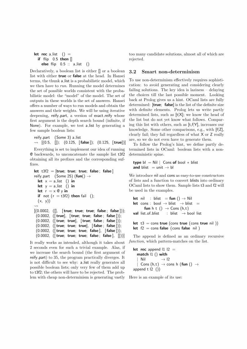
let rec a list () =if flip 0.5 then []else flip 0.5 :: a list ()

Declaratively, a boolean list is either [] or a booleanlist with either true or false at the head. In Hanseiterms, the thunk a list is a probabilistic model, whichwe then have to run. Running the model determinesthe set of possible worlds consistent with the proba-bilistic model: the “model” of the model. The set ofoutputs in these worlds is the set of answers. Hanseioffers a number of ways to run models and obtain theanswers and their weights. We will be using iterativedeepening, reify part, a version of exact reify whosefirst argument is the depth search bound (infinite, ifNone). For example, we test a list by generating afew sample boolean lists:

reify part (Some 3) a list [(0.5, []); (0.125, [ false ]); (0.125, [ true])]

Everything is set to implement our idea of running@ backwards, to unconcatenate the sample list t3f2obtaining all its prefixes and the corresponding suf-fixes.

let t3f2 = [true; true; true; false ; false ]reify part (Some 25) (fun() →let x = a list () inlet y = a list () inlet r = x @ y inif not (r = t3f2) then fail ();(x, y)) [(0.0002, ([], [ true; true; true; false ; false ]));(0.0002, ([ true], [ true; true; false ; false ]));(0.0002, ([ true; true], [ true; false ; false ]));(0.0002, ([ true; true; true], [ false ; false ]));(0.0002, ([ true; true; true; false ], [ false ]));(0.0002, ([ true; true; true; false ; false ], []))]

It really works as intended, although it takes about2 seconds even for such a trivial example. Alas, ifwe increase the search bound (the first argument ofreify part) to 35, the program practically diverges. Itis not difficult to see why: a list really generates allpossible boolean lists; only very few of them add upto t3f2; the others will have to be rejected. The prob-lem with cheap non-determinism is generating vastly

too many candidate solutions, almost all of which arerejected.

3.2 Smart non-determinism

To use non-determinism effectively requires sophisti-cation: to avoid generating and considering clearlyfailing solutions. The key idea is laziness – delayingthe choices till the last possible moment. Lookingback at Prolog gives us a hint. OCaml lists are fullydetermined: [true; false] is the list of the definite sizewith definite elements. Prolog lets us write partlydetermined lists, such as [t|X]; we know the head ofthe list but do not yet know what follows. Compar-ing this list with others, such as [t,f|Y], increases ourknowledge. Some other comparisons, e.g., with [f|Z],clearly fail; they fail regardless of what X or Z reallyare, so we do not even have to generate them.

To follow the Prolog’s hint, we define partly de-termined lists in OCaml: boolean lists with a non-deterministic spine.

type bl = Nil | Cons of bool ∗ blistand blist = unit → bl

We introduce nil and cons as easy-to-use constructorsof lists and a function to convert blists into ordinaryOCaml lists to show them. Sample lists t3 and f2 willbe used in the examples.

let nil : blist = fun () → Nillet cons : bool → blist → blist =

fun h t () → Cons (h,t)val list of blist : blist → bool list

let t3 = cons true (cons true (cons true nil ))let f2 = cons false (cons false nil )

The append is defined as an ordinary recursivefunction, which pattern-matches on the list.

let rec append l1 l2 =match l1 () with| Nil → l2| Cons (h,t) → cons h (fun () →

append t l2 ())

Here is an example of its use:

reify part None (fun () →list of blist (append t3 f2)) [(1., [ true; true; true; false ; false ])]

giving the expected result. We have defined append asa function, and can indeed run it as the concatenationfunction, ‘forwards’.

Prolog also lets us concatenate lists that are par-tially or wholly unknown, represented by logic vari-ables. For example, append([t,t,t],X,R) will enumer-ate all lists with [t,t,t] as the prefix, see §2.1. If we areinterested in only boolean lists, we had to complicatethe Prolog code

append([t, t, t], X,R), boollist (X), boollist (R).

and faced the problem of incomplete search: Prologcould not produce any lists that included f. In Han-sei, the role of logic variable as the representation forsome boolean list is played by a generator:

let rec a blist () : blist =letlazy (fun () →

uniformly [| Nil ;Cons(flip 0.5, a blist ()) |])

We need the magical function letlazy, which at firstblush looks like the identity function. It is anotherprimitive of Hansei, taking a thunk and returning athunk. When we force the resulting thunk, we forcethe original one, and remember the result. All fur-ther forcing return the same result. In functionallogic programming, this is called “call-time choice”.In quantum mechanics, it is called “wave-functioncollapse”. Before we observe a system, for example,a still spinning coin, there could indeed be severalchoices for the result. After we observed the system,all further observations give the same result. Like thequantum-mechanical entanglement, letlazy is a way toshare the non-deterministic state.

Passing a blist as the second argument of append,

reify part (Some 3) (fun() →let x = a blist () inlist of blist (append t3 x)) [(0.5, [ true; true; true]);(0.125, [ true; true; true; false ]);(0.125, [ true; true; true; true])]

lets us see, within the given search bound, all booleanlists whose first three elements are true. Unlike theProlog code, we are no longer stuck generating listswhose all elements are true.

The moment of truth is running append backwards.We have already explained the key idea of generate-and-test in §3.1. The code in that section is trivialto adapt to partially determined lists blist; we onlyneed the comparison function on blists:

let rec bl compare l1 l2 =match (l1 (), l2 ()) with| (Nil , Nil ) → true| (Cons (h1,t1), Cons (h2,t2)) →

h1 = h2 && bl compare t1 t2| → false

Applying the generate-and-test idea to reverse theappend2:

reify part None (fun() →let l = append t3 f2 inlet x = a blist () inlet y = a blist () inlet r = append x y inif not (bl compare r l ) then fail ();(list of blist x, list of blist y)

gives the same, expected result as in §3.1, but witha surprise. First, the result is produced 1000 timesfaster. Second, the program terminates with the ex-pected six answers even though we imposed no searchbound: the first argument of reify part is None. Al-though x and y in the code will generate any booleanlist, thanks to laziness, the search space is effectivelyfinite, and quite small. Thus the real speed-up dueto laziness is infinite.

The letlazy operation in the definition of a blist iscrucial:

let rec a blist () =letlazy (fun () →

uniformly [| Nil ;Cons(flip 0.5, a blist ()) |])

The operation uniformly guesses at the top construc-tor of the list: Nil or Cons; letlazy delays the guess,

2See the accompanying code for the examples of runningappend in other modes.

letting the program proceed until the result of theguess is truly needed. Hopefully the program rarelygets to that point because the search encountered acontradiction at some other place.

Laziness in non-deterministic computations ishence indispensable. Non-deterministic laziness how-ever is different from the familiar facility to delay thecomputation and memoize its result, such as OCaml’slazy, Scheme’s delay or Haskell’s lazy evaluation. Wemay think of a non-deterministic choice, flipping acoin, as splitting the current world. In one world,the coin came up ‘head’, in the other it came ‘tail’.If we are to cache the result, we should use differentmemo tables for different worlds, because differentworlds have different choices. Ordinary lazy evalua-tion is implemented by mutation of the ordinary, orglobal, or shared memory – shared across all possibleworlds. Non-deterministic laziness needs world-localmemory [4]3.

4 Parsing with committedchoice

Kleene star is an intrinsic operator in regular ex-pressions and is commonly used in EBNF and othergrammar formalisms. Just as common is the so-called “maximal munch” restriction on the Kleenestar, forcing the longest possible match. After re-minding why maximal munch is so prevalent, we de-scribe the grave problem it poses for parsers that aremeant to be run both forwards and backwards – thatis, to parse a given stream according to the grammarand to generate all parseable streams, the grammar’slanguage.

Maximal munch cuts shorter-match choices and re-duces non-determinism – hence making forward runsfaster. On the downside, when running the parserbackwards the cut choices mean lost solutions andthe (greatly) incomplete language generation. Hanseiremoves the downside. Parsers built with the Hanseiparser combinator library support maximal munchand can be run effectively backwards to generate the

3World-local memory is also necessary for unification andgeneral constraint accumulation and solving.

complete language, without omissions. Surprisingly,Hansei already had the necessary features, in partic-ular, the nested inference.

5 Maximal munch rule

The maximal munch convention is so common inparsing that it is hardly ever mentioned. For ex-ample, a programming language specification clichedefines the syntax of an identifier as a letter followedby a sequence of letters and digits, or, in the extendedBNF,

identifier :: = letter letter or digit ∗

where ∗, the Kleene star, denotes zero or more repe-titions of letter or digit. In the string ”var1 + var2”we commonly take var1 and var2 to be identifiers.However, according to the above grammar every pre-fix of an identifier is also an identifier. Therefore, weshould regard v, va and var as identifiers as well. Toavoid such conclusions and the need to complicatethe grammar, the maximal munch rule is assumed:letter or digit∗ denotes the longest sequence of lettersand digits. Without the maximal munch, we wouldhave to write

identifier :: = letter letter or digit ∗

[ look−ahead: not letter or digit ]

It is not only awkward, requiring the notation forlook-ahead, but also much less efficient. If ∗ meanszero or more occurrences, letter or digit∗ on input”var1 ” will match the empty string, ”a”, ”ar” and”ar1”. Only the last match leads to the successfulparse of the identifier, recognizing var1. Maximalmunch cuts the irrelevant choices. It has proved souseful that it is rarely explicitly stated when describ-ing grammars.

5.1 Maximal munch in Prolog: Re-versibility lost

Maximal munch however destroys the reversible pars-ing, the ability to run the parser forward (as a parseror recognizer) and backward (as a language genera-tor). We illustrate the problem in Prolog. A rec-ognizer in Prolog is a relation between two streams

(lists of characters) S and Srem such that Srem is thesuffix of S. In a functional language, we would saythat a recognizer recognizes the prefix in S, returningthe remaining stream as Srem. Here is the recognizerfor the character ’a’:

charA([a|Srem],Srem).

The Kleene-star combinator (typically calledmany) takes as an argument a recognizer and repeatsit zero or more times. Without the maximal munch,it looks as follows:

many0(P,S,S).many0(P,S,Rest) :−

call (P,S,Srem), many0(P,Srem,Rest).

where P is an arbitrary parser. Thusmany0(charA,S,R) will recognize or generate theprefix of S with zero or more ’a’ characters. (Re-call that call is the standard Prolog predicate tocall a goal indirectly: call(charA,S,R) is equivalentto the charA(S,R).) Thanks to the first clause,many0(P,S,R) always recognizes the empty string.Here is how we recognize a∗ in the sample inputstream [a,a,b]:

?− many0(charA,[a,a,b],R).R = [a, a, b] ;R = [a, b] ;R = [b]

and generate the language of a∗:

?− many0(charA,S,[]).S = [] ;S = [a] ;S = [a, a] ;S = [a, a, a] ; ...

To implement the maximal munch, many shouldcall the argument parser as long as it succeeds. Totell if the parser fails or succeeds we turn to soft-cut. Recall, soft-cut P ∗→Q; R is equivalent to theconjunction P, Q if P succeeds at least once. Soft-cutcommits to that choice and totally discards R in thatcase. R is evaluated only when P fails from the outset.Soft-cut lets us write many with maximal munch:

many(P,S,Rest) :−call (P,S,Srem) ∗→many(P,Srem,Rest) ;

S = Rest.

Now the the empty string is recognized (i.e.,S = Rest) only if the parser P fails. Recognizing a∗in the sample input

?− many(charA,[a,a,b],R).R = [b].

becomes quite more efficient. There is only onechoice, for the longest sequence of as. However, at-tempting to generate the language a∗:

?− many(charA,S,[]).<loops>

leads to an infinite loop. The argument recognizer,charA, when asked to generate, always succeeds.Therefore, the recursion in many never terminates.When running backwards, the recognizer tries to gen-erate the longest string of as – the infinite string. Al-though the empty string belongs to the language a∗,we fail to generate it.

5.2 Maximal munch in Hansei: Re-versibility regained

The Hansei parser combinator library, Figure 3, sup-ports many, which, unlike the one in Prolog, no longerforces the trade-off between efficient parsing and gen-eration. Hansei’s many obeys maximal munch andgenerates the complete language, with no omissions.Hansei lets us have it both ways. Before describingthe implementation, we show a few representative ex-amples, Figure 2.

Examples 5-7 show the argument parsers withchoices, even overlapping choices as in Example 7.The combinator many (actually, many1 defined asmany1 p = p <∗ many p) may nest. In Example 3,a∗a does not recognize ”aaa” since the a∗ munchesthe entire stream leaving nothing for the parser ofthe final a. This is the expected behavior under max-imal munch. Example 7 shows no parse for the samereason. Finally in the last example we generate thecomplete language for a∗, including the empty string.

To implement the maximal munch in Hansei weneed something like soft-cut, the ability to detecta failure and proceed. Hansei has exactly the righttools: reify0 and reflect:

Parser Stream Result1 many (p char ’a’) ”aaaa” unique2 many (p char ’a’) <∗> p char ’b’ ”b” unique3 many (p char ’a’) <∗ p char ’a’ ”aaa” no parse4 many (p char ’a’) <∗> many (p char ’a’)) ”aaa” unique5 many ((p char ’a’) <|> (p char ’b’)) ”ababb” unique6 many ((many1 (p char ’a’)) <|>

(many1 (p char ’b’))) ”aaabab” unique7 many ((p char ’a’ <∗ p char ’a’) <|> p char ’a’)

<∗ p char ’a’ ”aaa” no parse8 many (p char ’a’) random ””, ”a”, ”aa”, . . .

Figure 2: Examples of maximal munch parsing

A parser takes a stream and returns the parsing result,the result of a semantic action, and the remainder of thestream:

type stream v = Eof | Cons of char ∗ streamand stream = unit → stream vtype α parser = stream →α ∗ stream

Primitive parser

val let p char : char → char parser

checks the current element of the stream is the given char-acter, returning it.

Parsing combinators

val (<∗> ) : (α → β) parser → α parser → β parserval ( <∗ ) : α parser → β parser → α parserlet (<|> ) : αparser → α parser → α parser =fun p1 p2 st → uniformly [| p1;p2|] st

combine parsers and their semantic actions and expressthe rules of the grammar: (<∗> ) combines parsers sequen-tially and (<|> ) expresses the alternation. The combina-tor ( <∗ ) is the specializations of (<∗> ).

Figure 3: Hansei parser combinator library

type α vc = V of α| C of (unit → α pV)

and α pV = (prob ∗α vc) list

val reify0 : (unit → α) → α pVval reflect : α pV →α

The primitive reify0 converts a probabilistic com-putation to a lazy tree of choices αpV, whosenodes contain found solutions V x or not-yet-exploredbranches. The primitive reflect, the inverse of reify0,turns a tree of choices into a probabilistic programthat will make those choices. The primitive reify0is fundamental in Hansei: probabilistic inference isimplemented by first reifying a program (the genera-tive model) to the tree of choices and then exploringthe tree in various ways. For instance, the full treetraversal corresponds to exact inference.

Soft-cut can also be implemented as a choice-tree traversal, first success below, which explores thebranches looking for the first V leaf. It returns thetree resulting from the exploration, which could beempty if no V leaf was ever found. Soft-cut then issimply

val first success : α pV →α pV

let soft cut :(unit → α) → (α → ω) → (unit → ω) → ω =fun p q r →match first success (reify0 p) with| [] → r ()| t → q (reflect t)

We write many in terms of the soft-cut as we did inProlog:

let many : α parser → α list parser = fun p →let rec self st =

soft cut(* check if p succeeded *)

(fun () → p st )(* continue with p *)

(fun (v, st ) →let (vs, st ) = self st in

(v:: vs, st ))(fun () → ([], st )) (* if p failed *)

in self

The second question is avoiding losing solutionswhen running the parser “backwards”. Unlike Pro-log, Hansei parsers are functions rather than rela-tions. They take a stream, attempt to recognize itsprefix and return the rest of the stream on success.They cannot be run backwards. However, we achievethe same result – producing the set of parseablestreams – by generating all streams, feeding themto the parser and returning the streams that parsedcompletely. Since the number of possible streams isgenerally infinite, we have to generate them lazily, ondemand. To ensure completeness – to avoid losingany solutions – the parsers should have the property

many p (s1 ⊕ s2) = many p s1 ⊕ many p s2

where ⊕ stands for non-deterministic choice. Sur-prisingly, many p already satisfies it. The trick islaziness in the stream and Hansei’s support of nestedinference. The primitive reify0 may appear in prob-abilistic programs – in other words, a probabilisticmodel may itself perform inference, over an innermodel. In order for this to work correctly, we hadto ensure that

let x = letlazy (s1 ⊕ s2) inreify0 (fun () → model x)

≡let x = letlazy s1 in reify0 (fun () → model x)⊕let x = letlazy s2 in reify0 (fun () → model x)

where x is demanded in model. That is, reify0should reify only the choices made by the inner pro-gram, and let the outer choices take effect. The

stream generator has to be lazy, so it has the formletlazy (s1 ⊕ s2). Comparing the nested inferenceproperty with the code for many reveals that the keyproperty of many p (s1 ⊕ s2) is satisfied without usneeding to do anything. Our many has exactly theright semantics.

6 Conclusions

Classical logic programming all too often forces us tochoose between efficiency and expressiveness, on onehand, and completeness on the other hand. Nega-tion and committed choice make logic programs eas-ier to write and, in some modes, faster to run. Alas,some other modes (informally, running ‘backwards’)become unusable or impossible. Kleene star is a goodexample of the trade-off: maximal munch simplifiesthe grammar and makes parsing efficient, but de-stroys the ability to generate grammar’s language.Functional logic programming systems can removethe trade-off. Properly implemented encapsulatedsearch (nested inference, in Hansei) lets us distin-guish the choices of the parser from the choices ofthe stream and cut only the former. Perhaps sur-prisingly this distinction just falls out of the needfor non-deterministic stream to be lazy. Thus Kleenestar with maximal munch lets us parse and generatethe complete language. In Hansei, we can have itboth ways.

We have gone back to Herbrand: we build the Her-brand universe (the set of all ground terms) and ex-plore it to find a model of a program. We build theuniverse by modeling ‘logic variables’ as generatorsfor their domains. Since the Herbrand universe formost logic programs is infinite, non-strict evaluationis the necessity. Furthermore, since logic variablesmay occur several times, we must be able to corre-late the generators. Finally, we need a systematicway of exploring the search space, without gettingstuck in one infinite sub-region. Hansei, among othersimilar systems, satisfies all these requirements.

Logic variables and unification have been intro-duced by Robinson as a way to ‘lift’ ground reso-lution proofs of Herbrand, to avoid generating thevast number of ground terms [12]. Logic variables ef-

fectively delay the generation of ground terms to thelast possible moment and to the least extent. Doingcomputations only as far as needed is also the goalof lazy evaluation. It appears that lazy evaluationcan make up for logic variables, rendering Herbrand’soriginal approach practical. It remains a fascinatingtask to be able to systematically derive a unificationprocedure.

Acknowledgement We thank Tom Schrijvers forhelpful comments and discussions.

References

[1] P. Blackburn, J. Bos, and K. Stiegnitz. LearnProlog Now! College Publications, London,2006. ISBN 1904987176.

[2] W. F. Clocksin and C. S. Mellish. Programmingin Prolog. Springer, 5 edition, 2003.

[3] Committee for Development and Promotion ofBasic Computer Technology. Fifth generationcomputer systems project final evaluation re-port. ICOT Journal, (40):3–24, 1994.

[4] S. Fischer, O. Kiselyov, and C.-c. Shan. Purelyfunctional lazy nondeterministic programming.Journal of Functional Programming, 21(4–5):413–465, 2011.

[5] M. Hanus. Multi-paradigm declarative lan-guages. In Proceedings of the International Con-ference on Logic Programming (ICLP 2007),number 4670 in LNCS, pages 45–75. Springer,2007.

[6] O. Kiselyov and C.-c. Shan. Embedded prob-abilistic programming. In W. M. Taha, ed-itor, Proceedings of the Working Conferenceon Domain-Specific Languages, number 5658in LNCS, pages 360–384. Springer, 15–17 July2009. ISBN 3-642-03033-5.

[7] O. Kiselyov and C.-c. Shan. Monolingual prob-abilistic programming using generalized corou-tines. In Proceedings of the 25th Conference

on Uncertainty in Artificial Intelligence, pages285–292, Corvallis, Oregon, 19–21 June 2009.AUAI Press. URL http://uai.sis.pitt.edu/

displayArticleDetails.jsp?mmnu=1&smnu=

2&article_id=1601&proceeding_id=25.

[8] T. Moto-oka, editor. Fifth Generation ComputerSystems. North-Holland, New York, 1982.

[9] L. Naish. Pruning in logic programming. Techni-cal Report 95/16, Department of Computer Sci-ence, University of Melbourne, Melbourne, Aus-tralia, June 1995. URL http://www.cs.mu.oz.

au/~lee/papers/prune/.

[10] F. C. N. Pereira and S. N. Shieber. Prologand Natural-Language Analysis. Center for theStudy of Language and Information, Stanford,California, 1987.

[11] M. O. Rabin and D. Scott. Finite automataand their decision problems. IBM Journal ofResearch and Development, 3:114–125, 1959.

[12] J. A. Robinson. Computational logic: Memo-ries of the past and challenges for the future.In Proceedings of the First International Con-ference on Computational Logic, number 1861in LNAI, pages 1–24, 2000.

[13] P. V. Roy. 1983-1993: The wonder yearsof sequential prolog implementation. Techni-cal Report 36, Paris DEC Research Labora-tory, Dec. 1993. URL http://www.hpl.hp.com/

techreports/Compaq-DEC/PRL-RR-36.pdf.