Crystal structure • Interstitial atom • Grain size • Heat treatment • Specimen orientation
Upload
khangminh22Category
view
0download
0
The application of single specimen
foraminiferal isotope analyses to
investigate seasonality in the
Southern Ocean
Anna Dora Mikis
Thesis submitted for the Degree of Doctor of Philosophy
Cardiff University
September 2017

i
Summary
The Antarctic Peninsula and the surrounding Southern Ocean are some of the most climatically
sensitive regions on Earth. The West Antarctic Peninsula (WAP) experienced a ~3.4°C warming
during the 20th century which was accompanied by widespread glacial melting. In contrast, 21st
century air temperature records in the northern Antarctic Peninsula show a decreasing trend
indicating large scale natural decadal-scale climate variability at that location. Atmospheric and
oceanographic variability in the WAP have also been observed in Holocene climate records
showing variable meltwater discharge relating to the frequency of La Niña events and summer
insolation during the late Holocene.
Single specimen foraminiferal isotope analysis has been successfully used to study changes in
seasonal variability in the tropical regions relating to El Niño-Southern Oscillation (ENSO). In this
thesis, I investigate the applicability of this method to study seasonal changes in environmental
conditions in the high latitudes over a range of timescales.
In the Scotia Sea, a modern record of the polar foraminifera species, Neogloboquadrina
pachyderma, shows temperature related distribution and δ18O signature, the presence of multiple
morphotypes, as well as variable calcification depths and vital offsets related to biological
processes and as determined by the single specimen isotope analysis. A six-year long sediment
trap-derived Neogloboquadrina pachyderma record of abundance, morphology, and single
specimen δ18O showed that all these parameters are driven by seasonal changes in sea ice
concentration and food availability - relating to chlorophyll α concentration and sea surface
temperature - at the Antarctic Peninsula. The Neogloboquadrina pachyderma record highlights
inter-annual variability, relating to the teleconnections between ENSO/Southern Annular Mode
and the high latitude atmospheric setting, proving its suitability to investigate seasonality changes.
Finally, in the Scotia Sea, single specimen Globorotalia inflata δ18O record displayed variability
during the Holocene relating to changes in Antarctic Intermediate source waters in the Southern
Ocean.

ii
DECLARATION This work has not been submitted in substance for any other degree or award at this or any other university or place of learning, nor is being submitted concurrently in candidature for any degree or other award. Signed ………………………………………………….…… (candidate) Date …………………
STATEMENT 1
This thesis is being submitted in partial fulfillment of the requirements for the degree of Doctor of
Philosophy
Signed ………………………………………….…………… (candidate) Date …………………
STATEMENT 2
This thesis is the result of my own independent work/investigation, except where otherwise stated,
and the thesis has not been edited by a third party beyond what is permitted by Cardiff University’s
Policy on the Use of Third Party Editors by Research Degree Students. Other sources are
acknowledged by explicit references. The views expressed are my own.
Signed ………………………………………………………. (candidate) Date …………………
STATEMENT 3
I hereby give consent for my thesis, if accepted, to be available online in the University’s Open
Access repository and for inter-library loan, and for the title and summary to be made available to
outside organisations.
Signed ………………………………………………..……... (candidate) Date …………………
STATEMENT 4: PREVIOUSLY APPROVED BAR ON ACCESS
I hereby give consent for my thesis, if accepted, to be available online in the University’s Open
Access repository and for inter-library loans after expiry of a bar on access previously
approved by the Academic Standards & Quality Committee.
Signed ……………………………………………...…..…… (candidate) Date …………………

iii
“All we have to decide is what to do with the time
that is given to us.”
J. R. R. Tolkien

iv
Acknowledgements
I would begin by thanking my main supervisor, Jenny Pike for her continuous support, guidance,
and encouragement not only during the past four years of this PhD but during my undergraduate
degree as well. I would also like thank Vicky Peck and Kate Hendry for giving me the opportunity
to work on this project and for helping to find solutions whenever a problem arose. I am also very
grateful to Mike Meredith for all the time he has given, and to Melanie Leng for supporting my
isotope work.
I am very grateful to Hugh Ducklow, Deborah Steinberg, and Sharon Stammerjohn for sharing
their samples and their data, which ultimately allowed me to complete this thesis. I would also like
to thank Frank Peeters and Suzan Verdegaal – Warmerdam at VU, Amsterdam for the isotope
measurements, as well as Hilary Sloane at NERC Isotope Geoscience Laboratory for the
additional isotope measurements. My thanks also goes to the Antarctic Science International
Bursary for awarding me with a grant that enabled me to carry out most of the isotope analysis. I
am also grateful to Dani Schmidt at Bristol and Kirsty Edgar, now in Birmingham, for allowing and
helping me to work in their facilities to complete the morphometric analysis, and for extensive
discussions that led me to understand all that the data could reveal. I would also like to thank
Dani and Kirsty for fuelling my scientific curiosity and inspiring me to dig deeper into the science.
Additionally, I am also grateful to the British Antarctic Survey for enabling me to take part in the
BAS scientific cruise JR304 aboard the RRS James Clark Ross. I would like to thank the research
staff and the crew for helping me to collect vital samples as well as for making the cruise a truly
enjoyable once in a lifetime experience.
I am forever grateful to the paleoclimate group in Cardiff for all their support, in particular to Paola,
for all her guidance, advice, and scientific discussions. I would like to thank my past and present
office mates for providing endless discussions both about science and everyday life. Particularly,
thanks to Freya, Amy, Hennie, Micky, Elaine, Kim, Steph, and Rachel for all your support, for
being wonderful friends, and making these last four years so memorable. I would also like to thank
Emmanuela, Sophie, and Bethan for all their support too. Special thanks go to Kim and Steph
who helped me get through the most difficult times, for being amazing people, teaching me how
to unwind during stressful times, and for letting me crash with them whenever I was in Bristol.
I would like to thank Louise for being a great friend who has always been there to listen and have
some cake and tea when needed. Most of all, I am hugely grateful to Paul for his love and support,
and for always being ready with a cwtch. Finally, I would like to thank my family for teaching and
encouraging me to forever expand my knowledge.
v
Commonly used symbols and Abbreviations
ACC Antarctic Circumpolar Current
AAIW Antarctic Intermediate Water
AASW Antarctic Surface Water
AAWW Antarctic Winter Water
Chl α Chlorophyll α concentration
δ18Onp Neogloboquadrina pachyderma oxygen isotope
δ18Oeq Equilibrium δ18O
EH Early Holocene
ENSO El Niño-Southern Oscillation
G. inflata Globorotalia inflata
LCDW Lower Circumpolar Deep Water
LH Late Holocene
MD Maximum diameter
Np Neogloboquadrina pachyderma
PCA Principal Component Analysis
PF Polar Front
SACCF Southern ACC Front
SAF Subantarctic Front
SAM Southern Annular Mode
SAMW Subantarctic Mode Water
SB Southern Boundary Front of the ACC
SIC Sea Ice Concentration
SST Sea Surface Temperature
TZW Transition Zone Water
UCDW Upper Circumpolar Deep Water
WAP West Antarctic Peninsula

vi
Table of contents
1. Introduction ........................................................................................................... 1
1.1. Single Specimen Analysis ................................................................................ 1
1.2. Climate variability in the southern high latitudes ............................................... 2
1.3. Aims and Objectives ........................................................................................ 3
1.4. Outline of the Thesis ........................................................................................ 5
2. Regional Setting and Oceanography ................................................................... 7
2.1. Scotia Sea ................................................................................................ 7
2.1.1. Modern Oceanography ............................................................................................ 7
2.2. Western Antarctic Peninsula .................................................................. 11
2.2.1. Glacial setting......................................................................................................... 11
2.2.2. Oceanography ....................................................................................................... 12
2.2.3. Atmospheric setting ............................................................................................... 13
2.3. Atmospheric teleconnections between the southern high latitudes and
the tropics .............................................................................................. 14
2.3.1. El Niño-Southern Oscillation .................................................................................. 14
2.3.2. Southern Annular Mode ......................................................................................... 16
3. Background information on proxies .................................................................. 19
3.1. Planktonic foraminifera ........................................................................... 19
3.1.1. Foraminifera life cycle and ontogeny ..................................................................... 19
3.1.2. Neogloboquadrina pachyderma (Ehrenberg, 1861) .............................................. 20
3.1.3. Globorotalia inflate (d’Orbigny, 1839b) .................................................................. 23
3.2. Foraminifera morphology ............................................................................... 25
3.3. Stable isotopes ...................................................................................... 26
3.3.1. Seawater ................................................................................................................ 27
3.3.1.1. Oxygen isotopes ................................................................................... 27
3.3.1.2. Carbon isotopes .................................................................................... 28
3.3.2. Foraminifera ........................................................................................................... 29
3.3.2.1. Neogloboquadrina pachyderma ............................................................ 29
3.3.2.2. Globorotalia inflata ................................................................................ 30
4. Materials and Methods ....................................................................................... 33
4.1. JR304 cruise materials and methods ..................................................... 33
4.1.1. Sampling for foraminifera ....................................................................................... 34
4.1.2. Water column profiling .......................................................................................... 35
4.1.3. Seawater stable isotope analysis ......................................................................... 36

vii
4.1.4. Neogloboquadrina pachyderma stable isotope analysis ...................................... 37
4.1.5. Predicting equilibrium δ18O value of calcite ........................................................... 38
4.2. PAL-LTER Time series ........................................................................... 38
4.2.1. Neogloboquadrina pachyderma flux measurements ............................................. 39
4.2.2. Measurements of morphology .............................................................................. 44
4.2.2.1. Automated image acquisition ................................................................ 44
4.2.2.2. Manual image acquisition ..................................................................... 47
4.2.3. Stable isotope analysis ......................................................................................... 48
4.2.4. Predicting the equilibrium δ18O value of calcite ..................................................... 49
4.2.5. Environmental parameters ..................................................................................... 50
4.3. Falkland Plateau sediment core ............................................................. 51
4.3.1. Stable isotope analysis of Globorotalia inflata ....................................................... 52
5. Results and Discussion ...................................................................................... 55
5.1. Neogloboquadrina pachyderma abundance, vital effects, and calcification
depth variability in the Scotia Sea: results from vertical plankton hauls .. 55
5.1.1. Oceanographic setting ........................................................................................... 55
5.1.1.1. Temperature profiles ............................................................................. 56
5.1.1.2. Salinity profiles ...................................................................................... 59
5.1.1.3. Fluorescence and density profiles ........................................................ 59
5.1.2. Neogloboquadrina pachyderma abundance in the Scotia Sea ........................... 60
5.1.2.1. Neogloboquadrina pachyderma morphotypes ...................................... 63
5.1.3. Neogloboquadrina pachyderma stable isotopic signatures and
water column δ18O gradients ................................................................................. 66
5.1.3.1. Neogloboquadrina pachyderma oxygen isotopic ratios ........................ 66
5.1.3.2. Neogloboquadrina pachyderma carbon isotopic ratios......................... 68
5.1.3.3. Seawater δ18O trends .......................................................................... 70
5.1.4. Foraminiferal and seawater oxygen isotopes: equilibrium, vital effects, and
calcification depths ................................................................................................. 71
5.1.4.1. Relationships between δ18Osw and salinity in the Scotia Sea ............... 71
5.1.4.2. Neogloboquadrina pachyderma shell weight vs δ18Onp: impact
of size on oxygen isotope ratio ........................................................................ 71
5.1.4.3. Exploration of vital effects during isotope fractionation by
Neogloboquadrina pachyderma in the Scotia Sea .......................................... 74
5.1.5. Summary and Conclusion ...................................................................................... 79
5.2. Seasonal variability of Neogloboquadrina pachyderma abundance,
morphology, and stable isotope composition at the
West Antarctic Peninsula ............................................................... 81
5.2.1. Statistical methods for data analysis ..................................................................... 82
viii
5.2.1.1. Spearman’s rank correlation coefficient ................................................ 82
5.2.1.2. Interquartile range ................................................................................. 82
5.2.1.3. Mann-Whitney U-test ............................................................................ 83
5.2.1.4. Levene’s test for Equality of Variances ................................................. 83
5.2.1.5. Principal Component Analysis .............................................................. 83
5.2.1.6. Anderson-Darling test for normality ...................................................... 84
5.2.2. Assessment of Neogloboquadrina pachyderma flux, morphology, and stable
isotope chemistry from a six year-long time series ............................................... 84
5.2.2.1. Physical properties and seasonality at Palmer Deep ........................... 84
5.2.2.2. Neogloboquadrina pachyderma flux between 2006 and 2013 ............. 86
5.2.2.3. The morphological variability of Neogloboquadrina pachyderma
at Palmer Deep ................................................................................................ 92
5.2.2.4. Neogloboquadrina pachyderma stable isotopes ................................. 111
5.2.3. A typical year at Palmer Deep ............................................................................. 122
5.2.3.1. Phase 1 – Winter sea ice season ....................................................... 122
5.2.3.2. Phase 2 – Sea ice break up season ................................................... 124
5.2.3.3. Phase 3 – Summer season ................................................................. 124
5.2.3.4. Phase 4 – Late summer season ......................................................... 125
5.2.3.5. Phase 5 – Autumn season .................................................................. 125
5.2.3.6. Phase 6 – Early winter season ........................................................... 125
5.2.4. Annual flux patterns: What controls foraminiferal flux in the high latitudes? ....... 126
5.2.4.1. Inter-annual variability in Neogloboquadrina pachyderma
shell flux ......................................................................................................... 128
5.2.5. The role of environmental variability on Neogloboquadrina pachyderma
shell size and morphology ................................................................................... 128
5.2.5.1. Morphotypes of Neogloboquadrina pachyderma ................................ 128
5.2.5.2. Neogloboquadrina pachyderma morphological variability and the role of
environmental parameters ............................................................................. 129
5.2.6. Neogloboquadrina pachyderma calcification and stable isotope variability ........ 132
5.2.6.1. Depth and seasonality of calcification ................................................. 133
5.2.6.2. Intra-and inter-annual variability in Neogloboquadrina pachyderma δ18O
....................................................................................................................... 135
5.2.7. Seasonal variability of Neogloboquadrina pachyderma δ18O derived from
single specimen analysis ..................................................................................... 137
5.2.7.1. Relationship between Neogloboquadrina pachyderma size and single
specimen stable isotopes .............................................................................. 140
5.2.8. Exceptional Neogloboquadrina pachyderma flux event of 2010: What is the role of
the Southern Annular Mode and the El Niño-Southern Oscillation ...................... 143
5.2.8.1. Variability in sea ice advance and retreat due to Southern
Annular Mode and El Niño-Southern Oscillation ........................................... 144
5.2.8.2. Recent trends in wind-driven sea ice variability in the
Palmer region ................................................................................................. 145
5.2.9. Synthesis and Conclusion .................................................................................... 148

ix
5.3. Investigating intermediate water mass variability in the Southern Ocean during
the Holocene ................................................................................................ 153
5.3.1. Comparison of paired and single specimen Globorotalia inflata ......................... 153
5.3.2. Single specimen stable isotope record of the Holocene ...................................... 158
5.3.2.1. Single specimen oxygen isotope record ............................................. 158
5.3.2.2. Single specimen carbon isotope record .............................................. 161
5.3.3. Globorotalia inflata stable isotope variability during the Holocene ...................... 163
5.3.4. Globorotalia inflata as an Antarctic Intermediate Water proxy species ............... 164
5.3.5. Does Globorotalia inflata stable isotope variability reflect changes in local
or regional environmental conditions ................................................................... 167
5.3.6. Temperature- and size-dependency in single specimen Globorotalia inflata
δ18O measurements ............................................................................................. 169
5.3.7. The role of biological and chemical processes on Globorotalia inflata δ13C ....... 172
5.3.8. A changing regime of Antarctic Intermediate Water sources during
the Holocene ........................................................................................................ 173
5.3.8.1. SAMW variability and its impact on AAIW properties and Globorotalia
inflata δ18O due to Holocene climate variability in the Southeast Pacific ...... 175
5.3.8.2. AAWW variability and its impact on AAIW properties and Globorotalia
inflata δ18O due to Holocene climate variability at the Antarctic Peninsula
and South Atlantic .......................................................................................... 178
5.3.9. Summary and Conclusion .................................................................................... 179
6. Conclusions and Recommendations............................................................... 181
6.1. Neogloboquadrina pachyderma abundance, vital effects, and calcification
depth variability in the Scotia Sea: results from vertical plankton hauls 181
6.2. Seasonal variability of Neogloboquadrina pachyderma abundance,
morphology, and stable isotope composition at the
West Antarctic Peninsula ..................................................................... 183
6.3. Investigating intermediate water mass variability in the Southern Ocean
during
the Holocene ........................................................................................ 185
6.4. Recommendations to improve methods ............................................... 186
7. References ........................................................................................................ 189
Appendix ................................................................................................................. 207

1
1. Introduction
1.1 Single Specimen Analysis
Single specimen foraminiferal stable isotope analysis has been commonly used during
the past 20 to 30 years to study variability in oceanographic conditions on seasonal
timescales in the low latitude regions (e.g. Spero and Williams, 1990; Koutavas et al.,
2006; Wit et al., 2010; Ganssen et al., 2011; Feldmejier et al., 2013; Ford et al., 2015;
Metcalfe et al., 2015). Traditionally, a number of foraminifera tests (20-40) are combined
from a sediment sample to produce a single foraminifera sample for stable isotope
analysis. Each centimetre of a sediment core, and thus an assemblage of foraminifera
from which the 20-40 tests are picked, spans a large temporal range. As a result, the
single stable isotope value obtained from the amalgamation of the tests is an average of
the environmental conditions recorded by the foraminifera. Coincidentally, short duration
events (e.g. periodic meltwater input to coastal regions), as well as seasonal and
interannual variability are masked by the average environmental signal. With
improvements in technology it has become possible to analyse single specimens of
foraminifera for their stable isotope ratio to reveal past short-term events and changes in
seasonal and interannual configuration of oceanography.
One of the earliest single specimen studies (Spero and Williams, 1990) utilised Orbulina
universa, a large (>500 μm) and heavy (~30μg) planktonic foraminifera, that secretes a
terminal spherical chamber around the entire test during the last 3-5 days of its life cycle
making it suitable for studying short-term environmental events. Between 11 and 35
individual specimens were analysed for stable isotopes from sediment samples to study
episodic meltwater input to the Gulf of Mexico during the end of the last glacial period
(~11.8 ka BP) and during the end of the Younger Dryas (~9.5 ka BP) (Spero and
Williams, 1990).
So far, most of the single specimen studies have focused on variability in the El Niño-
Southern Oscillation during the Holocene (Koutavas et al., 2006; Leduc et al., 2009;
Khider et al., 2011; Koutavas and Joanides, 2012), or earlier time periods (Leduc et al.,
2009; Scroxton et al., 2011; Koutavas and Joanides, 2012; Ford et al., 2015). Other
studies have utilised the method to investigate more regional seasonal changes, such
as seasonal variability in the Central Mediterranean during prominent climate events of
the Holocene (Goudeau et al., 2015) and sea surface temperature ranges in the Arabian
Sea during the last 20 ka (Ganssen et al., 2011). Single specimen foraminiferal stable

Chapter 1: Introduction
2
isotopes have also been used to gain greater insight into the role of environmental
changes and hydrography on specific species’ habitat preferences and calcification
patterns (Metcalfe et al., 2015; Steinhardt et al., 2015).
1.2 Climate variability in the southern high latitudes
Antarctica and the surrounding Southern Ocean are one of the most climatically sensitive
regions on the planet, with certain areas experiencing some of the most rapid warming
observed globally in recent decades. The West Antarctic Peninsula experienced a
~3.4°C warming during the 20th century (Vaughan et al., 2003), which is approximately
five times the global average of 0.6 ± 0.2°C identified by the Intergovernmental Panel on
Climate Change for the same period (Houghton et al., 2001). A similar, higher rate of
warming was observed in West Antarctica, where the region around the Amundsen Sea
experienced a 2.4 ± 1.2°C warming between 1958 and 2010 (Bromwich et al., 2013).
The atmospheric warming was accompanied by increased glacier melting; 84% of 244
tidewater and marine glacier fronts experienced melting between 1945 and 2005 (Cook
et al., 2005). The flow rate of these melting glaciers has increased by approximately 12%
between 1992 and 2005 due to frontal thinning related to the increased oceanic
temperatures (Pritchard and Vaughan, 2007, Pritchard et al., 2012). The increased
glacial melting along the Antarctic Peninsula has been shown to be the result of warm
and warming Circumpolar Deep Water at mid-depths (Cook et al., 2016). Together, the
rate and extent of the recent glacial melting experienced along the WAP is unparalleled
for the past 120 years (Hendry and Rickaby, 2008).
In contrast to the 20th century warming, 1999-2014 surface air temperature records from
northern Antarctic Peninsula stations show decreasing trends (−0.47 ± 0.25°C per
decade), especially during austral summer, in response to a strengthening of the
midlatitude jet driving cold, southeasterly winds over the Peninsula more frequently
(Turner et al., 2016). The variability between the 20th and 21st centuries have been shown
to be within the boundaries of large natural decadal-scale climate variability at this
location.
The variability in atmospheric processes observed along the Antarctic Peninsula and
further afield can have considerable impact on the Antarctic marine ecosystem, from top
predators to phytoplankton (Clarke et al., 2007; Ducklow et al., 2012) and on
oceanographic processes (e.g. Matthews and Meredith, 2004; Meredith et al., 2008;
Stammerjohn et al., 2008b; Meredith et al., 2016). Long-term records show that the sea
ice season over the Antarctic Peninsula shelf area decreased by 30-40 days in 1992-
2004 compared to 1979-2001 in response to changing atmospheric processes

Chapter 1: Introduction
3
(Stammerjohn et al., 2008b). Additionally, lower number of sea ice days between 1998
and 2001 compared to the 1992-1997 period were associated with persistent northerly
winds deriving from sustained La Niña and positive Southern Annular Mode conditions
(Massom et al., 2006; Stammerjohn et al., 2008a). Variable sea ice melt and glacial
meltwater distribution along the West Antarctic Peninsula between 2011 and 2014 have
also been shown to be strongly linked to regional wind forcing related to the Southern
Annular Mode and the El Niño-Southern Oscillation (Meredith et al., 2016). A
multidecadal record of phytoplankton abundance has shown that a five-fold interannual
variability in annual peak chlorophyll concentrations are strongly related to wind forcing
(Ducklow et al., 2012), and that a factor of two decline between 1979 and 2006 in the
northern parts of the West Antarctic Peninsula is most likely due to an up to 60% increase
in surface winds in that time period (Montes-Hugo et al., 2009). Concurrently, the
southern regions of the West Antarctic Peninsula experienced increasing phytoplankton
biomass by up to 66%, driven by periods of low sea ice concentrations, wind, and cloud
cover (Montes-Hugo et al., 2009).
Variability in the atmospheric and oceanographic conditions in the southern polar regions
have been observed during the Holocene period, similarly to modern times. A record of
oxygen isotope composition of marine diatoms deriving from a sediment core at Palmer
Deep, West Antarctic Peninsula has identified variations in glacial meltwater fluxes
(Swann et al., 2013, Pike et al., 2013) relating to increasing frequency of La Niña events
and increasing summer insolation during the late Holocene, while ocean-driven frontal
melting of glaciers was linked to meltwater discharge during the mid to late Holocene
(Pike et al., 2013).
1.3 Aims and Objectives
The original aim of the study was to provide a top-down investigation of seasonality
changes using a single species’ (Neogloboquadrina pachyderma) single specimen
stable isotope analysis. Through this approach, constraints and region-specific
information would have been developed on the single specimen stable isotope method
by assessing living and recently alive specimens with co-located environmental
parameters. The information derived from this study would then have been used in an
assessment of seasonal and interannual variability over a longer timescale, made
possible by a time-series sediment trap. This would reveal how the surface water signal
travels through the water column, and provide a picture on how an annual signal might
get built up in the sediment. Finally, the lessons learnt in the two modern studies would
have been applied to data derived from a high resolution sediment core to provide a

Chapter 1: Introduction
4
rounded assessment of seasonal variability over long timescales (hundreds or
thousands of years). However, the sediment core specified for this study experienced
geochemical changes post-recovery which prevented the collection of foraminifera. An
alternate core was found, albeit, at a location under different environmental and climate
regimes. Additionally, the Neogloboquadrina pachyderma specimens identified in the
new core were not sufficient in size to be analysed individually, therefore an alternate
species, Globorotalia inflata, was used for the single specimen analysis. As a result, the
focus of the downcore study changed, moving from a surface water perspective to an
intermediate water one, and the findings of the modern studies did not apply to the
interpretation of the paleoceanography record. Furthermore, the changes in location and
species meant that the aims and objectives of the final part of the thesis needed to be
adapted.
The overall aim of this thesis is to investigate the applicability of single specimen stable
isotope analysis of foraminifera to study seasonal changes in environmental conditions
in the Southern Ocean on a range of timescales. In addition, emphasis is placed on the
relationship between environmental changes and biochemical variability of foraminifera
in the high latitudes.
The specific objectives of the thesis are:
To study modern Neogloboquarina pachyderma single specimen stable isotope
variability in the mid to high latitudes in order to create a region-specific record of
vital effects.
To create a modern record of seasonal and interannual variability of
Neogloboquarina pachyderma in relation to environmental changes at the West
Antarctic Peninsula. This investigation will include:
the assessment of foraminifera abundance and flux from a six-year long
sediment trap and its relationship to food availability, water temperatures,
and sea ice presence.
the detailed study of Neogloboquarina pachyderma morphology, the
identification of different morphospecies, and their dominance under
different environmental conditions.
the analysis and interpretation of single specimen Neogloboquarina
pachyderma stable isotopes in relation to morphological variability, as
well as to seasonal changes of temperatures, food availability, and sea
ice.
the assessment of the Neogloboquarina pachyderma record in light of
interannual atmospheric and oceanographic variability relating to

Chapter 1: Introduction
5
teleconnections with El Niño-Southern Oscillation and/or Southern
Annular Mode, and its impact on the potential use of Neogloboquarina
pachyderma stable isotopes in this region.
To investigate intermediate water variability in the Scotia Sea during the
Holocene period by utilising a single specimen Globorotalia inflata stable isotope
record from the Falkland Plateau. This will provide potential insight into the role
of the polar regions on intermediate water mass variability in the mid latitude
regions.
1.4 Outline of the Thesis
In Chapter 2, the regional setting and the associated oceanography of the two main
regions involved in the thesis (the Scotia Sea and the Antarctic Peninsula) are presented.
Additionally, the two main climate phenomena, impacting the Southern Ocean regions,
(El Niño-Southern Oscillation and Southern Annular Mode) are described and their
impact on high latitude atmospheric and oceanographic conditions is discussed.
In Chapter 3, the proxies used throughout the thesis are reviewed. The first part of the
chapter provides information on the life cycle of foraminifera and gives an assessment
about the two planktonic foraminifera species, Neogloboquadrina pachyderma and
Globorotalia inflata, utilised in the study. The second part of the chapter reviews
foraminiferal morphology and its use in paleoclimate studies. In the final part of the
chapter, stable isotope analysis of seawater and foraminifera is discussed.
In Chapter 4, a detailed description is provided on the materials and methods used in
the thesis. The chapter is divided into three main sections reflecting the three studies
that form the thesis. The first section covers the JR304 cruise materials and the
associated stable isotope analysis. The second section constitutes the time series
samples at Palmer Deep and the flux, morphological, and stable isotope analysis that
derive from those samples. Finally, in the third section, the sediment samples from the
Falkland Plateau are described together with the stable isotope analysis undertaken on
them.
The following chapter (Chapter 5) and its constituent three sections present and discuss
the results obtained during this study. Each of the three sections focuses on a different
application of the single specimen analysis in the southern mid to high latitudes and
provides a scientific assessment of the foraminifera species utilised.
Neogloboquadrina pachyderma is the most abundant planktonic foraminifera in the high
latitudes and is commonly used in studies that employ planktonic foraminifera to

Chapter 1: Introduction
6
investigate recent and past high latitude climatic variations. As a result, information about
species habitat, behaviour, environmental preferences, and response to environmental
changes are widely available. However, an assessment of past studies highlights the
species’ environment-specific nature. In Chapter 5.1, a detailed assessment of vertical
plankton tow-derived Neogloboquadrina pachyderma abundance, morphology, and
single specimen stable isotope signature is provided in relation to environmental
conditions. The first part of the results and discussion section describes the
oceanographic conditions during the sample collection in the austral spring of 2014 while
the rest of the results and discussion covers the distribution of Neogloboquadrina
pachyderma in the Scotia Sea and the relationship between Neogloboquadrina
pachyderma stable isotopes, shell weights, calcification depths, and isotope
fractionation-derived vital effects.
The West Antarctic Peninsula is one of the most climatically sensitive regions of the high
latitudes and particularly, of Antarctica. A high degree of intra- and interannual variability
has been observed in the regional climate and sea ice distribution around the WAP
impacting all levels of the food web and is modulated by teleconnections with El Niño-
Southern Oscillations and the Southern Annular Mode. The holistic assessment of
Neogloboquadrina pachyderma abundance, morphology, and single specimen stable
isotope variability over a period of six years (2006-2013) from a sediment trap at the
continental shelf off Palmer Deep is presented in Chapter 5.2. Detailed statistical
analysis is carried out on the Neogloboquadrina pachyderma data in relation to
environmental parameters to investigate the relationship between the two. The results
are discussed in terms of seasonal and environmental variability along the West Antarctic
Peninsula and the role Southern Annular Mode and El Niño-Southern Oscillation plays
on Neogloboquadrina pachyderma at the study site.
The Southern Ocean and the southern mid-latitude climate experienced variability during
the long-term gradual cooling of the Holocene period, with oscillations in Southern
Westerly Wind stress, changes in El Niño-Southern Oscillation frequency, and variability
in glacial meltwater flux from the Antarctic Peninsula. In chapter 5.3, single specimen
Globorotalia inflata stable isotope record from the Falkland Plateau is used to reconstruct
intermediate water variability during the Holocene. The biological factors behind
Globorotalia inflata stable isotope composition is fully explored before utilising it as a
proxy for oceanographic variability and is discussed in relation to existing records of
Holocene climate variability from the southern mid to high latitudes.
A summary of key findings in relation to the original aims and objectives is presented in
Chapter 6 together with improvements to methods.

7
2 Regional Setting and Oceanography
2.1 Scotia Sea
The Scotia Sea is an area of the Southern Ocean bounded to the west by the Drake
Passage and to the north, east, and south by the Scotia Arc (Figure 2.1). The Scotia Arc
was formed during the mid-Cretaceous (120-83 Ma) as a result of the westward
movement of the South American plate, which led to the uplift of the southern tip of the
Andes and the proto North Scotia Ridge (Dalziel et al., 2013). Due to the uplift of the
North Scotia Ridge the South Georgia microcontinent began moving eastward towards
its current position (Figure 2.1). The Antarctic and South American continental plates
began to spread apart around 55 Ma (early Eocene) beginning the development of the
Drake Passage, as well as the South Scotia Sea, the South Scotia Ridge, and the Scotia
Plate itself (Eagles, 2010). A deep water connection between South America and
Antarctica is thought to have developed by 34-40 Ma. The youngest part of the Scotia
Sea to experience spreading is the West Scotia Sea, where the last of the seafloor
spreading has been dated to 6.6-5.9 Ma (Livermore et al., 2005).
2.1.1 Modern Oceanography
The modern oceanography of the Drake Passage and the Scotia Sea region is well
known due to a long history of oceanographic research in the area. The main feature of
the Scotia Sea region, and of the Southern Ocean as a whole, is the
eastward/northeastward flow of the Antarctic Circumpolar Current (ACC) (Figure 2.1),
which is driven by the Southern Westerly Winds between 45°S and 55°S (Orsi et al.,
1995). The ACC is the largest current system in the global ocean, transporting 136.7±6.9
Sv of water (Meredith et al., 2011), together with heat, salt, nutrients, and other chemical
properties between the Atlantic, Indian and Pacific Oceans (Orsi et al., 1995). The flow
of the ACC is linked to the steep shoaling of isopycnals towards southern latitudes
through the entire water column (Figure 2.2), as well as to large geostrophic shear
(Deacon, 1937).
The ACC is defined by three frontal regions which are characterised by fast-flowing
currents and separated by calmer waters (Meredith et al., 2011). The position of the
frontal boundaries can be defined as areas of steep shoaling/deepening of isopycnal
surfaces (Orsi et al., 1995). The three fronts from north to south (Figure 2.2):
Subantarctic Front (SAF), Polar Front (PF) and Southern ACC Front (SACCF)
(Whitworth, 1980; Orsi et al., 1995). An additional front, the Southern Boundary of the

Chapter 2: Regional Setting and Oceanography
8
ACC (SB) is recognised south of the SACCF as the area where the Upper Circumpolar
Deep Water (UCDW) shoals to a shallow depth of ~200 m (Orsi et al., 1995). The SAF
separates the ACC from the influence of subtropical waters, while the SB separates the
ACC from the subpolar waters (Figure 2.1).
Within the Scotia Sea, bathymetry controls the paths of the currents and water masses
associated with the three fronts creating meanders and eddies leading to increased
water mixing through the water column and across the frontal boundaries (Peterson and
Whitworth, 1989). East of South America, the ACC turns northward due to the
bathymetry of the basin and the Scotia Arc (Figure 2.1). The SAF, the most northerly of
the main ACC fronts hugs the continental slope around the Falkland Islands, while the
water masses along the PF cross the West Scotia Sea and travel through the North
Scotia Ridge west of South Georgia (Figure 2.1; Garabato et al., 2003). In contrast, the
currents along the SACCF transport water out of the Scotia Sea through the gaps
between the South Georgia microcontinent and the East Scotia Ridge (Figure 2.1). The
northward movement of the water masses along the SAF allows for some of the water
to escape from the ACC, forming the Malvinas Current, that closely follows the South
Dep
th (
m)
Figure 2.1: Bathymetry and geological setup (after Dalziel et al., 2013) of the Scotia Sea region with the frontal systems of the Antarctic Circumpolar Current (after Garabato et al., 2003). Red lines denote plate boundaries, double red lines are spreading ridges, red arrows represent direction of transform fault, and teeth indicate direction of subduction zone (Dalziel et al., 2013). SG, South Georgia microcontinent; SAF: Subantarctic Front; PF: Polar Front; SACCF: Southern Antarctic Circumpolar Current Front; SB: Southern Boundary of the ACC. The SAF, PF, and SACCF are the three main fronts of the ACC transporting most of the water mass (Orsi et al., 1995).
Chapter 2: Regional Setting and Oceanography
9
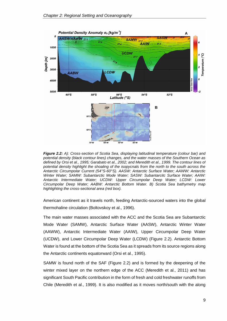
American continent as it travels north, feeding Antarctic-sourced waters into the global
thermohaline circulation (Boltovskoy et al., 1996).
The main water masses associated with the ACC and the Scotia Sea are Subantarctic
Mode Water (SAMW), Antarctic Surface Water (AASW), Antarctic Winter Water
(AAWW), Antarctic Intermediate Water (AAIW), Upper Circumpolar Deep Water
(UCDW), and Lower Circumpolar Deep Water (LCDW) (Figure 2.2). Antarctic Bottom
Water is found at the bottom of the Scotia Sea as it spreads from its source regions along
the Antarctic continents equatorward (Orsi et al., 1995).
SAMW is found north of the SAF (Figure 2.2) and is formed by the deepening of the
winter mixed layer on the northern edge of the ACC (Meredith et al., 2011) and has
significant South Pacific contribution in the form of fresh and cold freshwater runoffs from
Chile (Meredith et al., 1999). It is also modified as it moves north/south with the along
Figure 2.2: A): Cross-section of Scotia Sea, displaying latitudinal temperature (colour bar) and potential density (black contour lines) changes, and the water masses of the Southern Ocean as defined by Orsi et al., 1995; Garabato et al., 2002; and Meredith et al., 1999. The contour lines of potential density highlight the shoaling of the isopycnals from the north to the south across the Antarctic Circumpolar Current (54°S-60°S). AASW: Antarctic Surface Water; AAWW: Antarctic Winter Water; SAMW: Subantarctic Mode Water; SASW: Subantarcitc Surface Water; AAIW: Antarctic Intermediate Water; UCDW: Upper Circumpolar Deep Water; LCDW: Lower Circumpolar Deep Water; AABW: Antarctic Bottom Water. B) Scotia Sea bathymetry map highlighting the cross-sectional area (red box).
A
B

Chapter 2: Regional Setting and Oceanography
10
the SAF across the Southern Ocean. As a result, temperature and the salinity of this
water mass display a wide range across the three ocean basins, with temperature
(salinity) ranging from 4-5°C (34.2-34.3 PSU) in the eastern South Pacific to 14-15°
(35.4-35.5 PSU) in the western South Atlantic (McCartney et al., 1977).
AASW is found south of the PF (Figure 2.2) all the way to the continental margin of
Antarctica (Orsi et al., 1995). Its properties are determined by the air-sea interactions,
formation and melting of sea ice, and advection (Gordon and Huber, 1984), with
temperatures ranging on average from −1.0 to 1.0 °C, and salinities ranging from 34.0
PSU to 34.6 PSU (Emery et al., 2003). Due to its low salinity and temperature it readily
mixes with UCDW at the southern edge of the ACC where the UCDW shoals closer to
the surface (Smith and Klink, 2002). Once mixed with UCDW, AASW flows north towards
the Polar Front (Orsi et al., 1995).
AAWW is formed in the spring/summer when the melting sea ice and glacial ice along
the Antarctic Peninsula freshens the cold surface waters (Meredith et al., 1999) along
the continental margin leading to the isolation the cold winter mixed layer (Mosby, 1934).
This isolated cold mixed layer becomes AAWW with very low potential temperatures
(less than −1.0°C) and low salinity (~33.9 PSU) (Meredith et al., 1999) which then flows
equatorward, deepening south of the PF (Figure 2.2).
Towards the northern edge of the ACC, AAIW is found beneath SAMW, while south of
the PF it is located directly below AASW (Orsi et al., 1995) (Figure 2.2). AAIW can
originate from a number of sources. It can form from AASW that undergo subduction at
the Polar Front (Orsi et al., 1995), from AAWW, originating from the winter mixed layer
of the Bellingshausen Sea, that flowed north towards the Polar Front (Meredith et al.,
1999; Naveira Garabato et al., 2009), or from modified cold, fresh SAMW that flowed
eastwards from the South Pacific through the Drake Passage into the Scotia Sea
(McCartney, 1977). The source waters that make of the AAIW result in temperatures that
range between 2°C and 6°C, and salinities between 33.8 PSU and 34.8 PSU across the
Southern Ocean (Emery et al., 2003). The low salinity sources waters of the AAIW lead
to a very low salinity profile for the AAIW itself, resulting in a salinity minimum at
intermediate depths (Talley, 1996).
UCDW is found below AAIW in the northern part of the ACC, and below AASW in the
southern part of the ACC (Figure 2.2). It is easily recognised by its low-oxygen, high
nutrient concentration properties, as well as its high temperatures (>1.5°C) and high
salinity (34.65 PSU to 34.7 PSU) (Orsi and Whitworth III, 2005). UCDW shoals from

Chapter 2: Regional Setting and Oceanography
11
depths of up to 3500 m at the SACCF towards the surface at the SB where it mixes with
AASW (Orsi et al., 1995).
LCDW is the high salinity (~34.5 PSU), cold (0°C to −0.5°C) and thus dense branch of
the Circumpolar Deep Water that penetrates the southern regions of the Pacific, Indian,
and Atlantic Ocean basins (Sloyan and Rintoul, 2001) thanks to its density. It is formed
south of the ACC through brine rejections and direct mixing with shelf waters (Orsi et al.,
1995; Sloyan and Rintoul, 2001). Similarly to UCDW, it is found at shallower depths at
the southern edge of the ACC, and deepens equatorward (Figure 2.2).
2.2 Western Antarctic Peninsula
The Antarctic Peninsula (AP) is a narrow (<250 km wide), long (~1250 km) mountainous
body, rising to a height of 3500 m at its highest with only a few areas dropping below
2000 m (King and Turner, 1997). The northernmost point of AP reaches 63°S at Prime
Head, while the majority of the landmass lies between 63°S and 75°S (Figure 2.3) and
is subjected to subpolar climates with significantly contrasting meteorological and
oceanographic conditions on the opposing sides of the peninsula. The spine of the AP
is made up of Mesozoic-Tertiary igneous granitoids now capped by a permanent ice cap
(Domack et al., 2003), the AP Ice Sheet.
2.2.1 Glacial setting
Glaciation of the AP most likely started around 30 million years ago during the Eocene,
as recorded in the South Shetland Islands (Dingle and Lavelle, 1998), while large-scale
expansion of glaciation across the continental shelf during the Miocene and the Pliocene-
Pleistocene has also been identified (Barker and Camerlenghi; 2002). The present
physical setting is the result of the decline of the AP Ice Sheet, sea level rise and isostatic
adjustment following the Last Glacial Maximum. The contrasting glacial setting of the
eastern and western side of the peninsula is due to the different precipitation patterns
over the areas. The WAP is characterised by regular cyclonic activity related to the
prevailing southern Westerlies which carry large quantities of snow to the area. This
results in high accumulation rates and a markedly lower equilibrium line altitude despite
the higher average summer temperatures (Domack et al., 2003). The East Antarctic
Peninsula (EAP) is characterised by lower levels of snowfall, lower average annual
temperatures and higher equilibrium line altitude. This contrast results in marked
differences in the development and characteristics of glaciers and ice shelves on the two
sides of the peninsula. Ice shelves on the eastern side have low elevation surfaces
susceptible to rapid changes in meltwater production, while the tidewater and outlet

Chapter 2: Regional Setting and Oceanography
12
glaciers of the western side have significant snow pack and higher snow lines which are
less prone to changes in meltwater production (Skvarca and DeAngelis, 2003).
2.2.2 Oceanography
The Antarctic Circumpolar Current is driven by the Southern Westerly Winds (SWW) and
travels past the AP from west to east, entering the Atlantic sector of the Southern Ocean
through the Drake Passage (Figure 2.3). The western side of the peninsula is bathed by
Upper Circumpolar Deep Water (UCDW) (Figure 2.3) that upwells at the Southern
Boundary of the ACC and is carried to the WAP via the ACC (Orsi and Whitworth III,
2004). The UCDW acts as the most important source of heat and nutrients along the
WAP (Martinson and McKee, 2012) as it is significantly warmer than the surface waters
around the Peninsula. Above UCDW, Antarctic Surface Water readily mixes with UCDW
due to its density (Meredith et al., 1999). Vertical mixing between AASW and UCDW
creates a water mass that has surface temperatures above freezing during the winter
(Smith and Klinck, 2002). Characteristics of the surface waters along the AP vary with
the freezing and the melting of the sea ice, significantly affecting salinity and density.
The contrasting water masses and different atmospheric settings create different sea ice
regimes along the EAP and WAP. Sea ice is present all year round in most years in the
Weddell Sea (only the northernmost areas experience ice-free times). In contrast, the
Figure 2.3: Bathymetry map of the seas surrounding the Antarctic Peninsula showing frontal boundaries (white lines; after Naveira Garabato et al., 2002) and winter and summer sea ice extent (blue solid and dotted lines, respectively; after NASA, 2009). Black star denotes location of Palmer Deep. SSI: South Shetland Islands; SOI: South Orkney Islands.

Chapter 2: Regional Setting and Oceanography
13
sea surface along the WAP experiences large inter-annual variations in sea ice presence
(King et al., 2003). During the winter months sea ice extends to the northernmost regions
of the peninsula, however, by March it melts back all the way to the southern parts of the
Bellingshausen Sea (Figure 2.3).
2.2.3 Atmospheric setting
Due to the geography of the peninsula a strong marine influence exists over the area.
SWW have the main influence over the climate of the WAP, carrying moist,
comparatively warm air masses from the mid-latitudes over the peninsula (Bentley et al.,
2009). The EAP experiences significantly colder conditions as the cold continental air
masses from the interior of the continent descend into the Weddell Sea embayment
(Domack et al., 2003). Due to a large equator-to-pole atmospheric air temperature
difference the Southern Ocean and the coastal areas around the continent endure the
development of regular forceful weather systems. In the areas of climatic fronts (e.g.
Antarctic Polar Front – APF- and the increased thermal gradient along the coast of the
continent) strong horizontal temperature gradients exist together with frequent
cyclogenesis, cloud cover and strong wind activity (King and Turner, 1997).
The WAP experiences the largest interannual variability in surface air temperatures on
the Antarctic continent. This interannual atmospheric variability is controlled by the twice-
yearly poleward movement and intensification of the atmospheric low-pressure trough in
the spring and the autumn around the high latitudes, termed the semi-annual oscillation
(SAO) (van Loon, 1967). The interactions between sea ice and the atmosphere due to
the SAO drive the seasonal cycle of sea ice advance and retreat (e.g. Watkins and
Simmonds, 1999; Stammerjohn et al., 2003). Surface air temperature at Faraday station;
found at the northern half of the peninsula has a mean annual temperature range of
~11°C with a standard deviation of ~1.1°C (King, 1994). The variation derives from the
large temperature change observed during the winter months, between June and
September, which persist into the following year (King and Turner, 1997), suggesting
that the temperature change is related to changes in ocean circulation and in sea surface
temperature (SST). At Marguerite Bay (Figure 2.3), average annual temperature is
around −9°C and average precipitation is in excess of 300 mm/year (Allen et al., 2011).
Surface air temperatures along the WAP display sensitivity to the extent of sea ice cover
over the Bellingshausen Sea on a seasonal scale. During times of maximum sea ice
extent (winter and spring) surface air temperatures display a negative correlation with
sea ice (Jacobs and Comiso, 1997). The exact relationship between the two factors has
not been determined yet due to the diversity of processes effecting sea ice extent and

Chapter 2: Regional Setting and Oceanography
14
SST. The role of upwelling UCDW and the influence of the EL Niño-Southern Oscillation
on the development of the sea ice remains elusive (Domack, et al., 2003), thereby the
effect of the sea ice on the surface air temperature is difficult to decipher.
Larger scale atmospheric circulation is determined by the location of the peninsula itself
in relation to the circumpolar trough (CPT) of low sea level pressure. This in turn varies
as part of the larger-scale Southern Hemisphere circulation, in which pressure levels
across the atmosphere vary inversely between the mid and high latitudes (King and
Turner, 1997). This mode of variability of Southern Hemisphere circulation is called the
Southern Annular Mode (SAM). Part of the CPT is the Amundsen Low, an extensive area
of low pressure found over the Amundsen Sea and which drives mild, northwesterly
winds over the coast of the WAP (King et al., 2003). The high topography of the peninsula
prevents the transport of this warmer air mass from the WAP to the EAP, thereby creating
a significant surface temperature gradient (5-10°C) between the two sides (Bentley et
al., 2009).
2.3 Atmospheric teleconnections between the southern high
latitudes and the tropics
On inter-annual timescales, atmospheric variability around the south Pacific section of
the Southern Ocean, and thus variability in sea ice advance and retreat along the
Antarctic Peninsula are mostly controlled by the teleconnections between El Niño-
Southern Oscillation/Southern Annular Mode and the high latitudes as these modulate
the Semi-Annual Oscillation (Thompson and Wallace, 2000).
2.3.1 El Niño-Southern Oscillation
El Niño-Southern Oscillation (ENSO) is an interannual cycle in the atmospheric and
ocean circulation of the Pacific region (Figure 2.4) that has significant effect on the
climate of the rest of the globe. The Southern Oscillation (SO) is one of the largest
interannual climate variations on the planet (Rasmusson and Wallace, 1983). In the
tropical Pacific Ocean the SO is linked to large-scale fluctuations in SST, rainfall and in
the intensity of the trade winds, while in the subcontinent of India it is associated with
severe droughts. Over North America the SO has been correlated with severe winter
weather; while the Northern Hemisphere as a whole experiences large oscillations in
mean atmospheric temperatures during SO events (Horel and Wallace, 1981; Philander,
1983).
The SO refers to the variation in the atmospheric mass over the Pacific Ocean, with cold,
intermediate and warm conditions in the near-surface areas of the eastern Pacific Ocean

Chapter 2: Regional Setting and Oceanography
15
(King and Turner, 1997). During the cold periods, termed La Niña, the tropics are
characterised by stronger trade winds and a surface pressure difference between the
eastern and western Pacific. The eastern Pacific around South America experiences the
development of high pressure, while the western Pacific, around Indonesia and Australia,
experiences low pressure (Figure 2.4B; Horel and Wallace, 1981). The low pressure
system results in the development of active convective systems and prolonged heavy
rainfall over that area. During the less frequent El Niño periods, the atmospheric and
oceanic circulation undergoes a significant change (Philander, 1983). The strength of the
trade winds decreases during these periods along with the surface pressure gradient
between the east and west side of the Pacific Ocean, resulting in decreased convective
activity and precipitation in the western Pacific (Figure 2.4A), causing large-scale
droughts most prominently in Australia (Rasmusson and Wallace, 1983).
The SO also affects surface ocean currents, with the presence of increased upwelling of
nutrient-rich, cold waters off the coast of South America during La Niña (Figure 2.4B;
Philander, 1983). El Niño events are characterised by weaker surface ocean currents
and reduced upwelling off the coast of South America.
A B
C
Figure 2.4: Schematic representation of the atmospheric and oceanographic conditions in the tropical Pacific during El Niño (A), La Niña (B), and normal conditions (C) highlighting the changes in the depth of the thermocline, in the location of the warm pool, and in the position of the convective cell (Pacific Marine Environmental Laboratory, NOAA, [Accessed: August 2017]).
Chapter 2: Regional Setting and Oceanography
16
It has been well established that the variations in atmospheric and oceanic temperatures
and ocean circulation due to the ENSO events have an effect on the climate around the
AP (e.g. White and Peterson, 1998; Harangozo, 2000). Studies have shown that surface
air temperatures and atmospheric circulation displayed variability relating to ENSO
during the 1945-2005 period (White and Peterson, 1998; King et al., 2003; Meredith et
al., 2004b; Meredith and King, 2005).
ENSO is a tropical phenomenon that has a great impact on the southeast Pacific section
of the Southern Ocean through the development of Rossby waves over the Pacific
Ocean (Hoskins and Karoly, 1981; Harangozo, 2000; Kwok and Comiso, 2002; Turner,
2004). The Rossby waves develop over the mid-latitudes during El Niño events and
travel poleward weakening the polar front jet while strengthening the subtropical jet
(Hoskins and Karoly, 1981). As a result positive pressure anomalies develop along the
WAP region leading to a lack of cyclonic activity over the Amundsen/Bellingshausen
Seas (Renwick, 2005) and dominant cold, southerly winds blowing off from the AP
resulting in colder than average SST and increased sea ice cover and duration (Kwok
and Comiso, 2002; Turner, 2004). La Niña events are associated with the opposite
atmospheric and oceanic anomalies (Figure 2.5B), with the weakening of the subtropical
jet and the strengthening of the polar front jet (Kwok and Comiso, 2002) resulting in
greater cyclonic activity in the Bellingshausen Sea (Li, 2000) with warmer SST along the
WAP (Yuan, 2000) stemming from the increased northerly winds that carry warm, moist
air (Fogt and Bromwhich, 2006; Stammerjohn et al., 2008a, Clem and Fogt, 2013).
2.3.2 Southern Annular Mode
Southern Annular Mode, and the variability between its positive and negative phases is
associated with the development of zonally symmetrical atmospheric pressure
differences of opposing sings between the polar regions and the midlatitudes centered
around 45° latitude (Thompson and Wallace, 2000). Changes in the strength and mode
of the SAM determine variability in the strength and positioning of the circumpolar
westerly winds (Thompson and Wallace, 2000; Marshall et al., 2006; Marshall and
Bracegirdle, 2015). Along with the zonal variability, SAM also has a strong meridional
component, particularly around the Amundsen/Bellingshausen Sea and the Ross Sea
(Marshall et al., 2003) During positive SAM periods positive pressure anomalies exist in
the midlatitudes and negative anomalies are found in the high latitudes (Figure 2.5A)
supporting the development of warm southerly winds along the WAP region and cold
northerly winds in the Amundsen and Ross Seas (Kwok and Comiso, 2002; Lefebvre et
al., 2004). This pattern switches to the opposite during negative SAM (Lefebvre et al.,

Chapter 2: Regional Setting and Oceanography
17
2004). The warm northerly winds during +SAM create negative sea ice and positive SST
anomalies along the WAP (Figure 2.5A). Negative SAM creates the opposite anomalies
for both sea ice and SST (Kwok and Comiso, 2002; Lefebvre and Goose, 2005, Clem
and Fogt, 2013). SAM has become more positive during the past few decades due to
the combination of anthropogenic forcings and natural variability (Marshall et al., 2003).
During the past thirty years co-variability between ENSO and SAM has increased: La
Niña coincided with positive SAM, and El Niño with negative SAM (Kwok and Comiso,
2002; Stammerjohn et al., 2008a, Clem and Fogt, 2013). The impact of ENSO and SAM
on the strength of sea level pressure (SLP) anomalies and sea ice advance on the WAP
also intensified during the same period (Stammerjohn et al., 2003; Stammerjohn et al.,
2008a). As a result negative SLP anomalies during austral summer and autumn are
observed on the WAP during La Niña events and positive SAMs, and vice versa for
positive SLP. Concurrently variability in WAP sea ice trends has been closely linked to
Figure 2.5: Schematic representation of the atmospheric response across the Southern Pacific sector of the Southern Ocean and the Antarctic Peninsula to positive SAM (A) and La Niña (B) (Stammerjohn et al., 2008). A) Black arrows depict the westerly winds around Antarctica, while the blue and yellow areas show differences in atmospheric pressure. B) Base map represents sea surface temperature variability (red areas are higher temperatures).

Chapter 2: Regional Setting and Oceanography
18
the SLP anomalies. Earlier wind-driven sea ice retreat and later sea ice advance is
associated with the development of strong negative SLP anomalies along the WAP
supporting anomalously warm northerly winds in the Bellingshausen Sea as a result of
the increasingly positive SAM and strong La Niñas since the 1990s. Conversely, positive
SLP anomalies during the autumn months in the Amundsen Sea region are associated
with cold southerly winds over the WAP region resulting in early sea ice advance
(Stammerjohn et al., 2008a, b).
Similarly to the Antarctic Peninsula, ENSO and SAM has had an impact on the water
masses in the Scotia Sea. Interannual variability observed in the volume transport of the
ACC has been found to coincide with variability in the strength and phase of SAM,
suggesting that the long-term increase in SAM strength is accelerating the ACC volume
transport (Meredith et al., 2011). Additionally, interannual variability in the salinity and
potential temperature of AAIW (0.01-0.04 PSU; 0.1°C-0.5°C respectively) between 1965
and 2005 were found to be related to ENSO and SAM-driven variations in wintertime air-
sea heat fluxes and net evaporation, due to changes in the Southern Westerly Wind
(SWW) stress (Meredith et al., 2011). The salinity of AAIW decreased by ~0.05 PSU
between the 1970s and the early 2000s with almost no change in temperature, most
likely as a result of decreasing AAWW salinity in the Bellingshausen region (Naveira
Garabato, 2009). This was related to increased precipitation and sea ice melt linked to
interdecadal changes in the SWW, likely due to increased positive trend in SAM
(Meredith and King, 2005; Meredith et al., 2011).
19
3 Background information on proxies
3.1 Planktonic foraminifera
Two species of planktonic foraminifera were used in this project, Neogloboquadrina
pachyderma and Globorotalia inflata. Planktonic foraminfera are single celled surface
dwelling protozoa which excrete a calcite shell. They have long been used as a means
to study historical changes in oceanography and climate due to their excellent
preservation potential and ubiquity in marine sediments. The two species were chosen
based on their high abundances in the sediments and seawaters assessed.
Neogloboquadrina pachyderma (sinistral) specimens were collected from surface waters
of the Scotia Sea in 2014 and from sediment trap samples located offshore from Palmer
Deep, WAP, covering a six-year period between 2009 and 2013. Globorotalia inflata
specimens were collected from a marine sediment core recovered from the Falkland
Plateau.
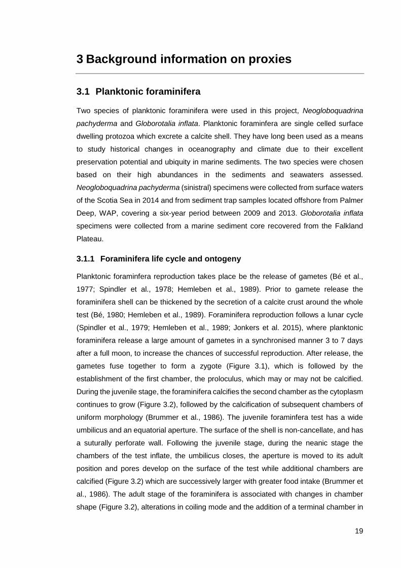
3.1.1 Foraminifera life cycle and ontogeny
Planktonic foraminfera reproduction takes place be the release of gametes (Bé et al.,
1977; Spindler et al., 1978; Hemleben et al., 1989). Prior to gamete release the
foraminifera shell can be thickened by the secretion of a calcite crust around the whole
test (Bé, 1980; Hemleben et al., 1989). Foraminifera reproduction follows a lunar cycle
(Spindler et al., 1979; Hemleben et al., 1989; Jonkers et al. 2015), where planktonic
foraminifera release a large amount of gametes in a synchronised manner 3 to 7 days
after a full moon, to increase the chances of successful reproduction. After release, the
gametes fuse together to form a zygote (Figure 3.1), which is followed by the
establishment of the first chamber, the proloculus, which may or may not be calcified.
During the juvenile stage, the foraminifera calcifies the second chamber as the cytoplasm
continues to grow (Figure 3.2), followed by the calcification of subsequent chambers of
uniform morphology (Brummer et al., 1986). The juvenile foraminfera test has a wide
umbilicus and an equatorial aperture. The surface of the shell is non-cancellate, and has
a suturally perforate wall. Following the juvenile stage, during the neanic stage the
chambers of the test inflate, the umbilicus closes, the aperture is moved to its adult
position and pores develop on the surface of the test while additional chambers are
calcified (Figure 3.2) which are successively larger with greater food intake (Brummer et
al., 1986). The adult stage of the foraminifera is associated with changes in chamber
shape (Figure 3.2), alterations in coiling mode and the addition of a terminal chamber in

Chapter 3: Background information on proxies
20
some species. The terminal stage of the foraminifera relates to reproduction, which can
be manifested in the ontogeny by the thickening of the entire shell by the addition of a
calcite crust that has a cancellate texture, the formation of spherical, kummerform, or
sac-form final chamber, or the shedding of the spines in spinose species (Brummer et
al., 1986; Hemleben et al., 1989).
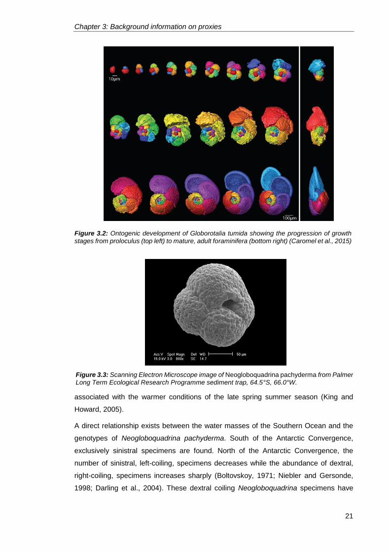
3.1.2 Neogloboquadrina pachyderma (Ehrenberg, 1861)
Neogloboquadrina pachyderma (Np) (Figure 3.3) is the dominant planktonic foraminifera
species south of the Polar Front on both hemispheres (Pflaumann et al., 1996; Niebler
and Gersonde, 1998). It has no symbionts, tolerates a wide range of SSTs, but has a
preference for lower sea surface salinities (about 34 psu) and small seasonal variations
(NOAA, 1996; Spindler, 1996). Greatest Np abundances are commonly found in
association with chlorophyll maxima (because of lack of symbiont), in areas of small
vertical temperature gradients and minimal seasonal stratification; however, it is also
found living in sea ice (Spindler, 1990; Mortyn and Charles, 2003). Np generally calcifies
at 50-200 m water depth in the polar seas (Kohfeld et al., 1996; Bauch et al., 1997),
however, the species can adjust its depth habitat in response to local hydrography (i.e.
eddy mixing or advection of water masses) (Mortyn and Charles, 2003; Jonkers et al.,
2013). Along the WAP, Np lives in the surface waters all year round, occupying the ice-
water interface during the austral winter (Hendry et al., 2009). Peak flux of Np is
Figure 3.1: Generalised representation of foraminiferal life cycle showing the transformation between gametes, zygotes, gamonts and sexual and asexual reproduction (http://www.ucl.ac.uk/GeolSci/micropal/foram.html).Planktonic foraminifera undergo only sexual reproduction (Schiebel and Hemleben, 2005).
Chapter 3: Background information on proxies
21
associated with the warmer conditions of the late spring summer season (King and
Howard, 2005).
A direct relationship exists between the water masses of the Southern Ocean and the
genotypes of Neogloboquadrina pachyderma. South of the Antarctic Convergence,
exclusively sinistral specimens are found. North of the Antarctic Convergence, the
number of sinistral, left-coiling, specimens decreases while the abundance of dextral,
right-coiling, specimens increases sharply (Boltovskoy, 1971; Niebler and Gersonde,
1998; Darling et al., 2004). These dextral coiling Neogloboquadrina specimens have
Figure 3.2: Ontogenic development of Globorotalia tumida showing the progression of growth stages from proloculus (top left) to mature, adult foraminifera (bottom right) (Caromel et al., 2015)
Figure 3.3: Scanning Electron Microscope image of Neogloboquadrina pachyderma from Palmer Long Term Ecological Research Programme sediment trap, 64.5°S, 66.0°W.
Chapter 3: Background information on proxies
22
been suggested to be designated their own species (Neogloboquadrina incompta) based
on their genetics (Darling et al., 2006). The sudden change between Neogloboquadrina
pachyderma and Neogloboquadrina incompta (N. incompta) marks the boundary
between the Polar Front and the Subantarctic waters. Another distinct boundary is found
between the northern edge of the Subantarctic Front and the southern edge of the
Subtropical front where Np virtually disappear and N. incompta dominates (Boltovskoy,
1996).
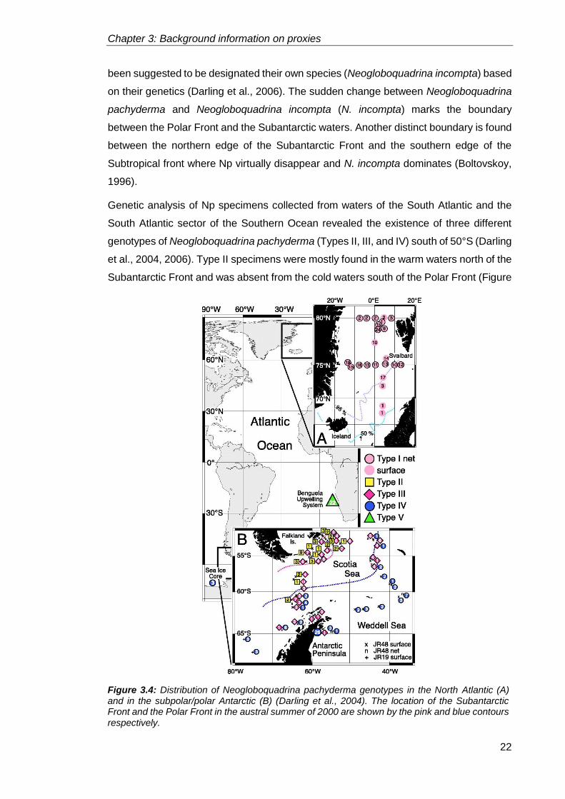
Genetic analysis of Np specimens collected from waters of the South Atlantic and the
South Atlantic sector of the Southern Ocean revealed the existence of three different
genotypes of Neogloboquadrina pachyderma (Types II, III, and IV) south of 50°S (Darling
et al., 2004, 2006). Type II specimens were mostly found in the warm waters north of the
Subantarctic Front and was absent from the cold waters south of the Polar Front (Figure
Figure 3.4: Distribution of Neogloboquadrina pachyderma genotypes in the North Atlantic (A) and in the subpolar/polar Antarctic (B) (Darling et al., 2004). The location of the Subantarctic Front and the Polar Front in the austral summer of 2000 are shown by the pink and blue contours respectively.

Chapter 3: Background information on proxies
23
3.4). Type III specimens were widely distributed across the Southern Ocean (Figure 3.4),
being most abundant north of the Polar Front. Type IV Np were only observed in the
coldest waters, south of the Polar Front (Figure 3.3) (Darling et al., 2006).
During its life cycle, Np migrates through the water column – juvenile forms proliferate in
the top 50 m of the surface waters and they migrate down as they mature, completing
gametogenesis in deeper surface waters (Kozdon et al., 2009). During this time, Np adds
new chambers and calcite layers to the test at varying temperature and salinity zones,
thereby each specimen records distinct environmental conditions (Schiebel and
Hemleben, 2005). As part of the final phase of the organism’s life cycle a thick calcite
layer might be added to the test (Kozdon et al., 2009). As this can take place at a much
deeper depth (with considerably different environmental conditions) than the original
calcification, the foraminifera test has two separate calcite layers. This secondary calcite
makes Np a highly resistant species against dissolution, as evidenced by low dissolution
indexes recorded in the Scotia Sea (Malmgren 1983).
Two distinct forms of Np have been identified in the Atlantic Ocean, one with heavy
encrustation of calcium carbonate on the outer surface, and one without encrustation
(Kohfeld et al., 1996; Kozdon et al., 2009). The encrustation results in average shell
weights which are 3-4 times that of those without a secondary calcite crust. The non-
encrusted Np has a shiny, smooth and translucent surface (Kohfeld et al., 1996) and is
found to live within the pycnocline in the Arctic, between 100 and 150 m water depth.
Living non-encrusted Np in the Arctic region (Kohfeld et al., 1996) are found in the top
80 m of the surface waters, in the cold, mixed layer of the water column. In the Southern
Ocean Np was found in water depths of up to 200 m (Mortyn and Charles, 2003). It
appears that the secondary calcite crust is only added to the shell once the organism
falls out of the main chlorophyll zone into the main pycnocline, possibly as part of its life
cycle. δ18O of Np in sediments, therefore, provide a record of temperature and salinity
near/slightly above the main pycnocline (Kuroyanagi et al., 2011) while variations of
δ18Ocalcite between different shell sizes reflect the strength of the pycnocline as well as
possible water column stratification, which allows for the reconstruction of past water
column structures.
3.1.3 Globorotalia inflata (d’Orbigny, 1839b)
Globorotalia inflata (G. inflata) (Figure 3.5) is a non-symbiotic deep-dwelling planktonic
foraminifera (Bé 1969, Fairbanks et al., 1980, Hemleben et al., 1989) calcifying mainly
within the mixed layer and the thermocline (Wilke et al., 2006).This species has been
identified as a transitional species which is present in waters between the subtropical
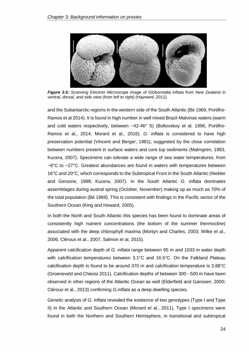
Chapter 3: Background information on proxies
24
and the Subantarctic regions in the western side of the South Atlantic (Bé 1969, Portilho-
Ramos et al 2014). It is found in high number in well mixed Brazil-Malvinas waters (warm
and cold waters respectively, between ~42-46° S) (Boltovskoy et al. 1996, Portilho-
Ramos et al., 2014, Morard et al., 2016). G. inflata is considered to have high
preservation potential (Vincent and Berger, 1981), suggested by the close correlation
between numbers present in surface waters and core top sediments (Malmgren, 1983,
Kucera, 2007). Specimens can tolerate a wide range of sea water temperatures, from
~8°C to ~27°C. Greatest abundances are found in waters with temperatures between
16°C and 20°C, which corresponds to the Subtropical Front in the South Atlantic (Niebler
and Gersone, 1998; Kucera, 2007). In the South Atlantic G. inflata dominates
assemblages during austral spring (October, November) making up as much as 70% of
the total population (Bé 1969). This is consistent with findings in the Pacific sector of the
Southern Ocean (King and Howard, 2005).
In both the North and South Atlantic this species has been found to dominate areas of
consistently high nutrient concentrations (the bottom of the summer thermocline)
associated with the deep chlorophyll maxima (Mortyn and Charles, 2003; Wilke et al.,
2006; Cléroux et al., 2007, Salmon et al, 2015).
Apparent calcification depth of G. inflata range between 95 m and 1033 m water depth
with calcification temperatures between 3.1°C and 16.5°C. On the Falkland Plateau
calcification depth is found to be around 370 m and calcification temperature is 3.88°C
(Groeneveld and Chiessi 2011). Calcification depths of between 300 - 500 m have been
observed in other regions of the Atlantic Ocean as well (Elderfield and Ganssen, 2000;
Cléroux et al., 2013) confirming G.inflata as a deep-dwelling species.
Genetic analysis of G. inflata revealed the existence of two genotypes (Type I and Type
II) in the Atlantic and Southern Ocean (Morard et al., 2011). Type I specimens were
found in both the Northern and Southern Hemisphere, in transitional and subtropical
Figure 3.5: Scanning Electron Microscope image of Globorotalia inflata from New Zealand in ventral, dorsal, and side view (from left to right) (Hayward, 2011).

Chapter 3: Background information on proxies
25
waters (Morard et al., 2011). In the South Atlantic, the Type I genotype dominates the
warm waters of the Brazil Current (Morard et al., 2016). The Type II genotype was only
found in the subpolar waters of the Southern Ocean (Morard et al., 2011), in the cold
waters of the Malvinas Current (Morard et al., 2016) and, within the Antarctic Circumpolar
Current (Morard et al., 2011).
3.2 Foraminifera morphology
Morphology of planktonic foraminifera has been utilised as a proxy for past climate
variability for over forty years (e.g. Bé, 1968; Malmgren and Kennett, 1972; Healy-
Williams et al., 1992; Kucera and Kennett, 2002; Moller et al., 2013). N. pachyderma was
one of the first planktonic foraminifera species chosen for morphological studies due to
its abundance in surface sediments in the mid to high latitudes and the affinity of different
morphologies for specific water masses and latitudinal positions (Malmgren and Kennett,
1972). The earliest morphology studies were carried out by splitting foraminifera samples
between numerous size fractions and by visual assessments (Kennett, 1968; Malmgren
and Kennett, 1972). These studies provided information on trends in maximum and
median diameters, on % fraction of the samples with four/four and a half/five chambers
in last whorl, and on the % fraction of sinistrally and dextrally coiling tests (early studies
did not differentiate the different coiling directions as separate species). These early
investigations highlighted the now well understood trend that Neogloboquadrina
pachyderma abundance and size increases with increasing latitude between the mid-
latitudes and the Polar Front.
With technological improvements it became possible to conduct more thorough
morphological studis by first digitising foraminifera specimens (e.g. Healy-Williams and
Williams, 1981; Williams et al, 1988) and then directly measuring aspects of the tests
using automated microscopes and image analysis (Kucera and Kennett, 2002; Schmidt
et al., 2004a; Moller et al., 2013). The morphology of Neogloboquadrina pachyderma
specimens from Southern Indian Ocean (Williams et al., 1988; Healy Williams, 1992)
and from North Atlantic core top samples (Healy Williams, 1992) were analysed by
Fourier shape analysis. This approach revealed the existence of multiple morphotypes
(six in the Southern Indian Ocean) each responding to different environmental conditions
and parameters, such as temperature and the zonal distribution of water masses and
frontal boundaries. These second-generation morphological studies integrated the stable
isotope analysis of Np, which revealed isotopic differences of up to 1.6‰ in the δ18O ratio
between morphotypes relating to environmental processes (Williams et al., 1988).
Smaller, 0.5‰ offset was found in the δ13C ratios of morphotypes which were attributed
Chapter 3: Background information on proxies
26
to biologically-controlled processes. Results also offered insight into Np calcification as
specimens from the South Indian Ocean showed that morphotypes with greater
pentagonality calcify with increasing disequilibrium from seawater (Healy-Williams
1992).
The morphological analysis of Neogloboquadrina pachyderma specimens by automated
microscopes and image acquisition was used by numerous studies to investigate the
evolutionary origins and improvements of Np (Huber et al., 2000; Kucera and Kennett,
2002) and other planktonic species (Schmidt et al., 2004a; Schmidt et al., 2004b). Mean
and maximum shell size records revealed consistent increase in Np size since the mid-
Pleistocene in both the North Atlantic (Huber et al., 2000) and in the North Pacific (Kucera
and Kennett, 2002) as the species improved its adaptation to cold environmental
conditions. The power of the automated morphological analysis is illustrated by the global
sedimentary record of 23 planktonic foraminiferal species whose size distribution was
analysed spatially and temporally (Schmidt et al., 2004a; Schmidt et al., 2004b). The
automated analysis allowed the identification of environmental optima for the different
planktonic foraminifera species based on the strong positive correlation between test
size, abundance and temperature. An optimum temperature ~0°C was identified for Np,
and 20-25°C for G. inflata (Schmidt et al., 2004b) by the relationship between
foraminifera size, abundance and temperature.
More recently, morphological studies are attempting to use Neogloboquadrina
pachyderma morphology as a means to study past SST and environmental variability in
climatically sensitive regions like the Arctic (Eynaud et al., 2009) and North Atlantic
(Moller et al., 2013). Five morphotypes of Np were identified in the central Arctic (Eynaud
et al., 2009), with 25% of the entire Np population (which make up the three largest
morphotype groups) explained by warm, North Atlantic water intrusion into the Arctic
Basin during the Quaternary. In one of the most recent Np morphology studies (Moller
et al., 2013) Np size records were used to create an empirical formula to reconstruct past
SST variability since the Last Glacial Maximum in the North Atlantic. The strong linear
correlation between Np size and temperature in this region allowed the development of
this empirical formula which can successfully be used in the polar regions where other
palaeotemperature proxies struggle.
3.3 Stable isotopes
Stable oxygen and carbon isotopes of foraminiferal calcite are used to decipher global
and regional climate change. Emiliani (1955) conducted one of the first research studies
into Pleistocene climate change in which stable isotopes of oxygen and carbon were

Chapter 3: Background information on proxies
27
used. Since then, a wide range of research has taken place to determine what drives
variation in these stable isotopes (e.g. Shackleton and Opdyke, 1973; Erez and Luz,
1983; Gonfiantini, 1986).
Three stable isotopes of oxygen exist: 16O, 17O and 18O. 16O and 18O are the most
abundant isotopes with relative fractions of 99.76% and 0.20% respectively, leaving only
0.04% of all oxygen on Earth as 17O (Rohling and Cook, 1999). There are two stable
isotopes of carbon, 12C and 13C with a relative abundance of 98.89% and 1.11%
respectively (Faure, 1986). Molecules which are made up of the lighter isotopes react
more easily than those with the heavy isotopes. Partitioning of these isotopes between
different substances is called fractionation (Rohling and Cook, 1999) and is a result of
reactions during isotope exchange and of kinetic effects (e.g. diffusion).
In order to accurately quantify the abundance of the rarer isotopes the ratio between the
less and more abundant isotope is determined (18O/16O and 13C/12C) then compared to
a known standard, using the following equations (Ravelo and Hillaire-Marcel, 2007),
expressed as a delta (δ) value and that have units of per mil (‰, per thousand) (Figure
3.6).
High δ values show the enrichment of the heavy isotope relative to the standard, while
low δ values show the enrichment of the lighter isotope relative to the standard. Analysis
of stable isotopes is done by using a mass spectrometer in which the mass ratios of CO2
(calculated by reacting carbonate with phosphoric acid) are determined with reference
to a standard CO2 with known isotopic composition, the Pee Dee Belemnite (PDB) and
later the Vienna PDB (VPDB) (Rohling and Cook, 1999). This will be explained in more
detail in section 4.
3.3.1 Seawater
3.3.1.1 Oxygen isotopes
A number of processes can affect the δ18O signature of seawater in which foraminifera
thrive. Seawater δ18O is closely linked to the all the processes of the hydrological cycle,
including evaporation, vapour transport, precipitation and iceberg melting (Hoffmann and
Figure 3.6: Equations to calculate the ratios of stable oxygen and carbon isotopes (Ravelo and Hillaire-Marcel,
2007):

Chapter 3: Background information on proxies
28
Heimann, 1997; Rohling and Cook, 1999). The long-term storage of water in ice sheets
and aquifers considerably affects δ18O, while seasonal sea-ice formation and melting
also affects the stable oxygen isotope composition of seawater, causing seasonal
variability (Fairbanks, 1989; Ravelo and Hillaire-Marcel, 2007). Advection and mixing of
water masses originating from different regions can also influence local δ18O (Frew et al.
1995). Oxygen isotope ratios in foraminiferal calcite are affected by a number of factors,
most importantly the equilibrium fractionation between seawater and the different
carbonate species (Kim and O’Neil, 1997), which defines a strong and important
temperature influence on the δ18O of foraminiferal calcite. Disequilibrium in δ18O is linked
to changes in carbonate ion concentration, respiration, symbiont photosynthesis,
ontogeny (changes in δ18O with shell development) and gametogenic calcite (secretion
of calcite, enriched in 18O, on the surface of the shell before gamete release) (Spero and
Lea, 1993; Rohling and Cook, 1999).
3.3.1.2 Carbon isotopes
The δ13C of seawater is very closely linked to the organic carbon cycle and to
sedimentary carbonate (Ravelo and Hillaire-Marcel, 2007). Photosynthesis, respiration
and the export of organic matter leaves the organic matter reservoir with a distinct δ13C
value of −25‰, compared to 0‰ for the carbonate reservoir (Hoefs, 1997). A significant
depth gradient exists in the δ13C profile in seawater. During photosynthesis, 12C is utilised
leaving the surface waters enriched in 13C. Remineralisation of organic matter in the
mixed layer releases the lighter carbon isotope and somewhat balances the offset
between 12C and 13C created by photosynthesis (Rohling and Cook, 1999). The export
production of organic matter to the deeper waters removes 12C to the deep water,
resulting in seawater at depth being enriched in 12C and depleted in 13C (Figure 3.7).
Increased export of organic matter creates a sharper gradient between the surface and
deep water. Surface water δ13C also depends on the air-water CO2 exchange and the
rate of carbon burial.
Foraminiferal calcite carbon isotope ratios reflect the δ13C of the seawater dissolved
inorganic carbon (DIC) in which the organism calcified, however, the δ13C of the
foraminiferal carbonate is in disequilibrium with the seawater due to kinetic fractionation
during comparatively rapid calcification and because of biological vital effects (Ravelo
and Hillaire-Marcel, 2007). δ13CDIC (stable carbon isotope ratio of DIC in seawater) varies
through time and it is not uniform around the world’s oceans or through the water column
(Kroopnick et al., 1972), therefore calcification depth and, in turn, temperature are key
factors that influence δ13C of calcite. Important processes and factors which also affect
the δ13C of calcite include (i) the incorporation of low metabolic CO2 into the calcite (vital

Chapter 3: Background information on proxies
29
effect) (Erez, 1978, Kohfeld et al., 1996; Ortiz et al., 1996); (ii) the photosynthetic activity
of symbionts (increased light intensity results in 13C enrichment in calcite shells of
symbiont-bearing foraminifera) (Spero and Lea, 1993); (iii) the rate of growth (increasing
shell size increases 13C enrichment) (Spero and Parker, 1985); and (iv) the concentration
of carbonate ion in the seawater (δ13C decreases with increasing [CO32-]) (Spero et al.,
1997).
3.3.2 Foraminifera
3.3.2.1 Neogloboquadrina pachyderma
Stable isotope ratios of Neogloboquadrina pachyderma calcite are useful
palaeoceanographic and palaeoclimatic proxies as they correlate with surface water
conditions in the polar regions (Kohfled et el., 1996) which, in turn, are extremely
sensitive to changes in climate. δ13C and δ18O of Np calcite have been used in the past
to determine variations in deep water circulation (Lehman and Keigwin, 1992), changes
in upwelling and surface water productivity among others (Charles and Fairbanks, 1990).
A fairly constant relationship exists between SST and δ18Ocalcite: an approximately 4°C
increase in SST (0-20 m depth) results in ~1‰ decrease in δ18Ocalcite (Epstein et al, 1953).
Figure 3.7: The schematic diagram displays the relationship between surface and deep water carbon isotope composition with relation to photosynthesis, export of organic matter through the water column and remineralisation at depth (Rohling and Cook, 1999).

Chapter 3: Background information on proxies
30
δ18O of Np in the Arctic region varies by 1.5‰ between 50 and 200 m water depth; δ13C
values do not vary significantly in the same depth zone, but remain within 0.50±0.14‰
(Kohfeld et al., 1996).
A consistent offset of ~1‰ exists in the δ18Ocalcite relative to the equilibrium calcite value,
which is attributed to vital effects (Bauch et al., 1997). To accurately determine δ18Ocalcite
these vital effects need to be accounted for. In polar regions, a correction factor of 0.73‰
±0.2 can be included into the calculations (Hendry et al., 2009). Size can affect δ18Ocalcite
as smaller (125-180 μm) specimens show on average a −0.79‰ difference compared to
larger specimens (180-250 μm) (Jonkers et al., 2013). This variation is due to different
calcification depth between large and small specimens, calcification rate and respiration.
Plankton tow samples from the Northern Pacific (Kuroyanagi et al., 2011) show that large
Neogloboquadrina pachyderma specimens secrete their shell more slowly and at
shallower depth with both higher δ18O and δ13C values than smaller ones.
Modern data suggests that a clear seasonal variation exists in δ18Oseawater in coastal
Antarctic waters, with high values found during the austral winter (up to 0.05‰), and low
values observed during the austral summer (approximately −0.9‰) (Meredith et al.,
2008b). This seasonal variation is most likely due to seasonal changes in glacial
meltwater input because sea ice processes alone would only affect the salinity of the
surface waters as it accounts for only 1% of the freshwater input during the summer. As
air temperature remains steadily below 0°C, the seasonal variation of seawater δ18O is
determined by the degree of glacial melting and SST during the austral summer
(Meredith et al., 2013).
Calculating δ13Ccalcite of the tests is simplified at high-latitude regions because
temperature is decoupled from other environmental factors in regions where seasonal
sea ice conditions dominate. Due to decreased gas exchange between the surface
waters and the atmosphere during the austral winter, δ13Ccalcite becomes 0.8‰ lower
(Meredith et al., 2013). This is reversed once sea-ice melts during the spring season
allowing the replenishment of CO2 with lower δ13C into the surface waters.
3.3.2.2 Globorotalia inflata
δ18O values of G. inflata calcite range between ~1.5‰ and 3.0‰ from 35°S to 50°S
respectively while δ13C values range from 0.8‰ to ~1.8‰ over the same latitudes
(Groeneveld and Chiessi, 2011, Morard et al., 2016). δ13Ccalcite values show a clear trend
towards more positive numbers with increasing latitudes, while the δ18Ocalcite values are
more variable (Chiessi et al. 2007). G. inflata moves deeper in the water column during
its life cycle, to depths of up to 800 m. As the organism sinks deeper it continues to add
Chapter 3: Background information on proxies
31
volume to its test by the addition of a secondary calcite crust which can account for as
much as 50% of the total shell weight (Lohmann, 1995, Wilke et al., 2006, Chiessi et al.
2007). Seasonal variability of the Brazil-Malvinas Confluence is recorded in the
variability of the δ18O value and the calcification depth of G.inflata (Chiessi et al. 2007).
This results in the δ18O values of deeper waters being incorporated into the calcite crust
hence making this species a useful indicator of changes taking place in deeper waters.
Carbon isotope ratio of G.inflata is mainly controlled by the δ13CDIC and [𝐶𝑂32−] of the
seawater as opposed to temperature) with a δ13C/[𝐶𝑂32−] slope of −0.013‰ to −0.015‰
(μmol kg−1) (Wilke et al., 2006). δ13C of this species becomes lighter with increased size
and weight - a ~ 1‰ change between 250μm and 500 μm - while a similar relationship
is not observed between δ18O and size/weight (Elderfield et al. 2002). This reflects the
downward migration of G.inflata during calcification and the incorporation of lighter
carbonate isotopes into the calcite crust at depth. Carbon isotope ratios of G. inflata show
a positive correlation with nutrient concentrations in the South Atlantic (Chiessi et al.
2007).

Chapter 3: Background information on proxies
32
33
4. Materials and Methods
The foraminifera used in my research were recovered from three different settings.
Specimens obtained from plankton tows were collected during the RRS James Clark
Ross cruise JR304 in November-December 2014, as part of the scientific component of
the cruise funded by the British Antarctic Survey (Watkins et al., 2016). I sailed as a
scientist on-board this cruise. The main goal of the cruise was to undertake the Western
Core Box survey – a yearly assessment of krill distribution and biomass- and to carry out
a series of 36 hour-long time stations across the Scotia Sea for collaborative biological
studies. Specimens obtained from sediment trap samples were recovered between 2006
and 2013 as part of the Palmer Station Antarctica Long Term Ecological Research
(Palmer LTER) Network funded by the United States National Science Foundation. The
main aim of the Palmer LTER study that began in 1990 at Palmer Station is to understand
how the seasonality and interannual variability of sea ice extent and duration influence
the ecosystems and biogeochemical cycle along the marginal sea ice zone (Smith et al.,
1995). The marine sediment core GC528 used in this study was collected during the
RRS James Clark Ross cruise JR244 between January and March 2011 as part of the
Quaternary Sediments Workpackage within the Chemistry and Past Climate Programme
funded the British Antarctic Survey. The main aim of the cruise was to gain new insight
into the glacial maxima around the South Orkney Islands and in the southern Weddell
Sea during the late Quaternary, to study past glacial retreats and to assess the changes
in paleoceanographic conditions in these areas (Larter et al., 2011). My project aims for
the three sample sets can be found in Chapter 1.3.
The aim of this chapter is to describe the regional setting of the localities the foraminifera
specimens were collected from and to provide information on the methodologies used
throughout my research.
4.1 JR304 cruise materials and methods
The JR304 cruise was a science and logistic leg of the 2014-15 passage of the RRS
James Clark Ross to Antarctica, which took place between 15th November and 17th
December 2014. The cruise combined base relief and replenishment work with research
activities in the Scotia Sea. The science aspect of the cruise covered a number of
objectives. These include the annual krill biomass survey (Western Core Box) in the
South Georgia region, four time station investigations to study diel changes in the
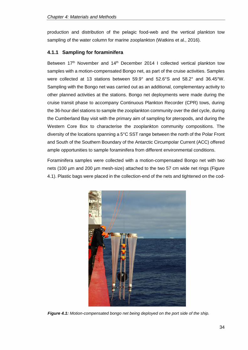
Chapter 4: Materials and Methods
34
production and distribution of the pelagic food-web and the vertical plankton tow
sampling of the water column for marine zooplankton (Watkins et al., 2016).
4.1.1 Sampling for foraminifera
Between 17th November and 14th December 2014 I collected vertical plankton tow
samples with a motion-compensated Bongo net, as part of the cruise activities. Samples
were collected at 13 stations between 59.9° and 52.6°S and 58.2° and 36.45°W.
Sampling with the Bongo net was carried out as an additional, complementary activity to
other planned activities at the stations. Bongo net deployments were made during the
cruise transit phase to accompany Continuous Plankton Recorder (CPR) tows, during
the 36-hour diel stations to sample the zooplankton community over the diel cycle, during
the Cumberland Bay visit with the primary aim of sampling for pteropods, and during the
Western Core Box to characterise the zooplankton community compositions. The
diversity of the locations spanning a 5°C SST range between the north of the Polar Front
and South of the Southern Boundary of the Antarctic Circumpolar Current (ACC) offered
ample opportunities to sample foraminifera from different environmental conditions.
Foraminifera samples were collected with a motion-compensated Bongo net with two
nets (100 µm and 200 µm mesh-size) attached to the two 57 cm wide net rings (Figure
4.1). Plastic bags were placed in the collection-end of the nets and tightened on the cod-
Figure 4.1: Motion-compensated bongo net being deployed on the port side of the ship.
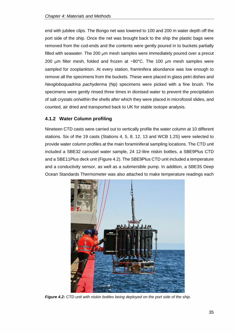
Chapter 4: Materials and Methods
35
end with jubilee clips. The Bongo net was lowered to 100 and 200 m water depth off the
port side of the ship. Once the net was brought back to the ship the plastic bags were
removed from the cod-ends and the contents were gently poured in to buckets partially
filled with seawater. The 200 µm mesh samples were immediately poured over a precut
200 µm filter mesh, folded and frozen at −80°C. The 100 µm mesh samples were
sampled for zooplankton. At every station, framinifera abundance was low enough to
remove all the specimens from the buckets. These were placed in glass petri dishes and
Neogloboquadrina pachyderma (Np) specimens were picked with a fine brush. The
specimens were gently rinsed three times in dionised water to prevent the precipitation
of salt crystals on/within the shells after which they were placed in microfossil slides, and
counted, air dried and transported back to UK for stable isotope analysis.
4.1.2 Water Column profiling
Nineteen CTD casts were carried out to vertically profile the water column at 10 different
stations. Six of the 19 casts (Stations 4, 5, 8, 12, 13 and WCB 1.2S) were selected to
provide water column profiles at the main foraminiferal sampling locations. The CTD unit
included a SBE32 carousel water sample, 24 12-litre niskin bottles, a SBE9Plus CTD
and a SBE11Plus deck unit (Figure 4.2). The SBE9Plus CTD unit included a temperature
and a conductivity sensor, as well as a submersible pump. In addition, a SBE35 Deep
Ocean Standards Thermometer was also attached to make temperature readings each
Figure 4.2: CTD unit with niskin bottles being deployed on the port side of the ship.

Chapter 4: Materials and Methods
36
time a niskin bottle was fired, allowing for the calibration of the SBE9Plus CTD unit. An
altimeter, a fluorometer, a photosynthetically active radiation (PAR) sensor, two oxygen
sensors and a transmissometer were also attached to the CTD unit to provide as much
information on the water properties as possible. The CTD data was collected at 24Hz
and logged to a PC. The Seasave 7.22.3 by Sea-Bird Electronics, Inc. software was used
to process the relayed data (Watkins et al., 2016).
4.1.3 Seawater stable isotope analysis
The 24 niskin bottles attached to the CTD unit were used to collect water samples from
discreet water depths simultaneously with the profiling. The niskin bottles were fired at
predetermined depths that covered the depth range of the Bongo nets with an additional
sample collected at 500 m water depth or the bottom of the cast, depending on which
was deeper. Once back on deck the niskin bottles were sampled immediately for
seawater stable oxygen isotope analysis. The samples for δ18O analysis were collected
as a priority to prevent any gas exchange between the niskin bottle and the air. The
seawater from the niskin bottles was transferred into 30 mL Nalgene bottles via a tygon
tube which was soaked in filtered seawater overnight to prevent bubble formation. The
Nalgene bottles were left to overflow approximately three times to limit air bubbles in the
bottle. The filled Nalgene bottles were capped, wrapped in parafilm and stored at 4°C
until analysis. Altogether, 41 water samples were collected for δ18O analysis. Water
samples were also collected for TA/DIC analysis, δ13C of Particulate Organic Carbon
(δ13CPOC) and δ13C of Dissolved Inorganic Carbon (δ13CDIC) analysis to provide a
complete dataset about surface water carbonate chemistry. Unfortunately, a third of the
precipitated inorganic carbon samples contained insufficient material for analysis. The
other two-third of the samples were analysed for δ13CDIC, however, the analysis yielded
measurements which were outside the expected δ13CDIC variation: average value of
−9.95‰ instead of the expected 0.4-1.0‰ range in the South Atlantic Ocean (Kroopnick,
1985). Therefore further analyses for carbonate and nutrients were abandoned.
The 30 mL water samples were analysed for stable oxygen isotope ratios at the Stable
Isotope Facility of the British Geological Survey in Keyworth, UK. The samples were
analysed using an IsoPrime 100 instrument equipped with an Aquaprep. The seawater
δ18O analysis followed the equilibrium method for oxygen (Epstein and Mayeda, 1953).
Every sample was run three times to establish precision, with an average of ±0.02‰
achieved. All isotopic measurements are reported as per mil deviation from the Vienna
Standard Mean Ocean Water2 (‰ VSMOW2).

Chapter 4: Materials and Methods
37
4.1.4 Neogloboquadrina pachyderma stable isotope analysis
Stable isotope measurements on the Np specimens from the plankton tows and from the
sediment trap were carried out at the Faculty of Earth and Life Sciences, Vrije University,
Amsterdam, which I visited between 15th January 2016 and 13th February 2016. The
laboratory was chosen based on the capability of the mass spectrometer, which can
measure carbonate material weighing as little as 6-7 µg reliably. Prior to analysis we
attempted to chemically clean the specimens to remove any organic or inorganic matter
present on/in the tests. As a test, 10 specimens were placed in a vial with a 3% H2O2
solution for 30 minutes followed by three dionised water rinses. After the final rinse,
methanol was added to the vial which was placed in a sonic bath for 15 seconds. The
specimens were rinsed again three times with dionised water and air-dried. At the end
of this test, the specimens were inspected under a microscope to assess potential
damage caused by the cleaning procedure. Out of the 10 specimens only four survived
the cleaning procedure in one piece. The rest of the tests broke into multiple pieces or
disintegrated entirely. As a result, the chemical cleaning step was abandoned. The
specimens were recovered live from surface waters hence it is unlikely that the tests
contained any other carbonate material (chiefly coccolithophores) which could alter the
stable isotope signal of the test and we are confident that the chemical cleaning step was
not a pre-requisite of the stable isotope analysis.
Np specimens were weighed individually on a Mettler Toledo XPR2U high precision
microbalance (d=0.1 μg) in pre-weighed aluminium foil boats in Amsterdam. The
specimens were placed into the foil boats with a dry-brush to prevent adding additional
moisture to the sample. The stable isotope measurements were carried out on a Finnigan
GasBench II preparation device interfaced with a Finnigan Delta mass spectrometer.
Each specimen was placed into a glass vial for analysis. Approximately 4-6 glass beads
were placed on top of the specimens to prevent them from flying around in the vial when
the acid is injected. The carbonate samples were acidified in helium flushed sample vials,
creating CO2. The resulting CO2-helium mixture was transferred to the isotope ratio mass
spectrometer to determine the δ18O and δ13C ratio of the gas. During this process, the
mass spectrometer measures the available gas in each vial eight times in succession.
As a result, at the first measurement, all the gas is available while for the last
measurement, only a fraction of the originally available gas remains. Each of the eight
measurements provide a δ18O and a δ13C value so the standard deviation for each
sample is derived from the variability between the eight measurements. The
spectrometer was calibrated through the international standard IAEA-CO1 and the
laboratory’s own in-house standard VICS. A range of weights of VICS standards were
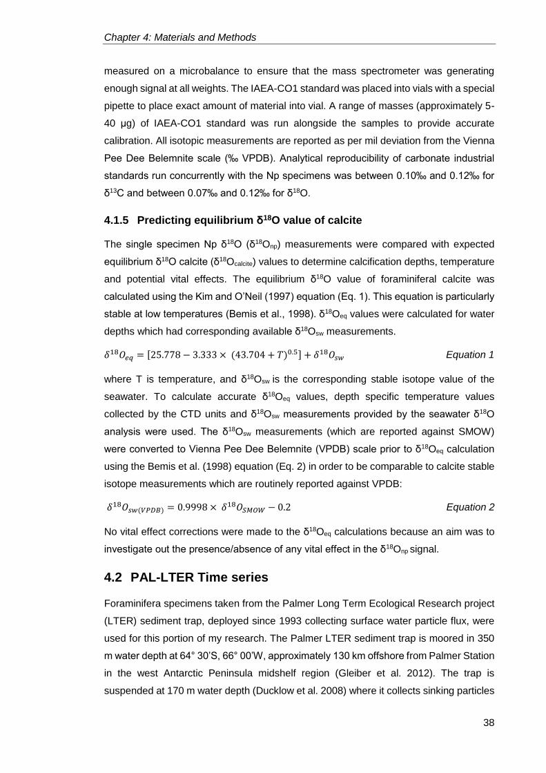
Chapter 4: Materials and Methods
38
measured on a microbalance to ensure that the mass spectrometer was generating
enough signal at all weights. The IAEA-CO1 standard was placed into vials with a special
pipette to place exact amount of material into vial. A range of masses (approximately 5-
40 μg) of IAEA-CO1 standard was run alongside the samples to provide accurate
calibration. All isotopic measurements are reported as per mil deviation from the Vienna
Pee Dee Belemnite scale (‰ VPDB). Analytical reproducibility of carbonate industrial
standards run concurrently with the Np specimens was between 0.10‰ and 0.12‰ for
δ13C and between 0.07‰ and 0.12‰ for δ18O.
4.1.5 Predicting equilibrium δ18O value of calcite
The single specimen Np δ18O (δ18Onp) measurements were compared with expected
equilibrium δ18O calcite (δ18Ocalcite) values to determine calcification depths, temperature
and potential vital effects. The equilibrium δ18O value of foraminiferal calcite was
calculated using the Kim and O’Neil (1997) equation (Eq. 1). This equation is particularly
stable at low temperatures (Bemis et al., 1998). δ18Oeq values were calculated for water
depths which had corresponding available δ18Osw measurements.
𝛿18𝑂𝑒𝑞 = [25.778 − 3.333 × (43.704 + 𝑇)0.5] + 𝛿18𝑂𝑠𝑤 Equation 1
where T is temperature, and δ18Osw is the corresponding stable isotope value of the
seawater. To calculate accurate δ18Oeq values, depth specific temperature values
collected by the CTD units and δ18Osw measurements provided by the seawater δ18O
analysis were used. The δ18Osw measurements (which are reported against SMOW)
were converted to Vienna Pee Dee Belemnite (VPDB) scale prior to δ18Oeq calculation
using the Bemis et al. (1998) equation (Eq. 2) in order to be comparable to calcite stable
isotope measurements which are routinely reported against VPDB:
𝛿18𝑂𝑠𝑤(𝑉𝑃𝐷𝐵) = 0.9998 × 𝛿18𝑂𝑆𝑀𝑂𝑊 − 0.2 Equation 2
No vital effect corrections were made to the δ18Oeq calculations because an aim was to
investigate out the presence/absence of any vital effect in the δ18Onp signal.
4.2 PAL-LTER Time series
Foraminifera specimens taken from the Palmer Long Term Ecological Research project
(LTER) sediment trap, deployed since 1993 collecting surface water particle flux, were
used for this portion of my research. The Palmer LTER sediment trap is moored in 350
m water depth at 64° 30’S, 66° 00’W, approximately 130 km offshore from Palmer Station
in the west Antarctic Peninsula midshelf region (Gleiber et al. 2012). The trap is
suspended at 170 m water depth (Ducklow et al. 2008) where it collects sinking particles

Chapter 4: Materials and Methods
39
through its 0.5 m2 surface area. The time series sediment trap is a PARFLUX Mark 78H
21-sample trap (by McLane Research Labs, Falmouth, MA) which collects particles in
500 ml bottles (Figure 4.3). The traps are recovered and redeployed during January of
each year. Sampling intervals vary according to expected sedimentation trends, resulting
in shorter sampling intervals (7 days) during strong flux periods and longer ones (up to
92 days) during periods of slower sedimentation (Table 4.1) (Ducklow et al. 2008). The
collected sediment trap samples were held at 5°C until arrival to the laboratory. The
samples were gently rinsed to separate out any larger swimmers present in the samples.
Zooplankton found within the trap samples were archived in 2% formaldehyde under cold
conditions. The processed samples were split until 2002 by employing a PARFLUX Wet
Sample Divider (by McLane Research), and since 2002 a plankton splitter has been
used. Sediment trap samples with exceptionally high sedimentation were split up to
1/512 for analysis. All the samples were first analysed for total mass dry weight, organic
carbon, particulate nitrogen and particulate phosphorus before any other analysis took
place. Archived samples collected after 2002 are stored at Virginia Institute of Marine
Sciences (VIMS), United States, in formalin. Any samples not archived are placed in 100
ml plastic cups, freeze-dried and stored at VIMS. More detailed information on the
sample processing can be found in Ducklow et al. (2008).
4.2.1 Neogloboquadrina pachyderma flux measurements
Ninety-three (from a total of 125) sediment trap samples covering the time period
between 18/01/2006 and 27/01/2013 were received from VIMS for the foraminifera flux
study. To determine the flux of foraminifera, specimens were examined using a Zeiss
optical microscope under 5-fold magnification.
Figure 4.3: McLane PARFLUX Mark 78H 21-sample trap of the type deployed at the Palmer LTER site (Poppe et al. 2000).

Chapter 4: Materials and Methods
40
Twenty-nine percent of the samples were whole, unsplit samples, while the rest (71%)
were split portions of larger samples, with the split factor varying between 0.05 and 0.5
(Table 4.1). Inspection of the samples using the microscope revealed diatom
concentrations of up to 90% in some cases. This can be attributed to the high-latitude
location of the sediment trap. High percentage of faecal pellets were observed in
samples with high sediment flux, relating to strong productivity. The majority of the
sediment in the samples were made up of marine snow (organic material derived from
dead plants and animals as well as from faecal matter) (Figure 4.4). This marine snow
became clumped during the freeze-drying process, resulting – in some cases – in
foraminifera becoming encased.
A number of different techniques were employed in order to break up the clumps of
marine snow and free any foraminifera trapped within the samples. First, samples were
gently rinsed through a sieve with di-ionised water to break up clumps. This proved
insufficient as not all clumps broke up and samples became static after the rinse. In order
to dissolve the organic material the samples were treated with a 3% solution of H2O2 for
30 minutes. Samples were sonicated in a sonic bath for 30 seconds to break up clumps.
After sonication the samples were rinsed with di-ionised water to remove any dissolved
or loosely clumped organic material. This approach was also unsuccessful because the
organic material did not break up or dissolve sufficiently to release the foraminifera tests.
Raising the sonication period to 1 minute resulted in the breakage of the foraminifera
specimens. Another approach was to introduce di-ionised water to the samples placed
in a petri dish. The aim was to collect foraminifera specimens with a pipette as the less
dense organic material would float to the surface while the foraminifera would collect on
the bottom of the petri dish. This approach was slightly more successful as it countered
Figure 4.4: Clumped marine snow in 22/02/2012 sediment trap sample.
500 µm

Chapter 4: Materials and Methods
41
Table 4.1: Palmer LTER sediment trap collection periods, sediment trap cup ID numbers and sample split factors. Samples highlighted blue were not received as these have been depleted by
other studies already.
Start Date End Date Duration Mid-Date Sediment Trap Cup # Split Factor
15/01/2006 22/01/2006 7 18/01/2006 1 0.50
22/01/2006 29/01/2006 7 25/01/2006 2 0.50
29/01/2006 12/02/2006 14 05/02/2006 3 0.10
12/02/2006 01/03/2006 17 20/02/2006 4 0.10
01/03/2006 01/04/2006 31 16/03/2006 5 0.10
01/04/2006 01/05/2006 30 16/04/2006 6 0.50
01/05/2006 01/06/2006 31 16/05/2006 7 0.50
01/06/2006 01/07/2006 30 16/06/2006 8 0.50
01/07/2006 01/09/2006 62 01/08/2006 9 0.50
01/09/2006 01/10/2006 30 16/09/2006 10 0.50
01/10/2006 01/11/2006 31 16/10/2006 11 0.50
01/11/2006 08/11/2006 7 04/11/2006 12 0.50
08/11/2006 15/11/2006 7 11/11/2006 13 0.50
15/11/2006 22/11/2006 7 18/11/2006 14 0.50
22/11/2006 29/11/2006 7 25/11/2006 15 0.50
29/11/2006 06/12/2006 7 02/12/2006 16 0.50
06/12/2006 13/12/2006 7 09/12/2006 17 0.50
13/12/2006 20/12/2006 7 16/12/2006 18 0.50
20/12/2006 27/12/2006 7 23/12/2006 19 0.50
27/12/2006 03/01/2007 7 30/12/2006 20 0.50
03/01/2007 10/01/2007 7 06/01/2007 21 0.50
15/01/2007 22/01/2007 7 18/01/2007 1 0.33
22/01/2007 29/01/2007 7 25/01/2007 2 0.33
29/01/2007 12/02/2007 14 05/02/2007 3 0.50
12/02/2007 01/03/2007 14 20/02/2007 4 0.50
01/03/2007 15/03/2007 14 08/03/2007 5 0.10
15/03/2007 01/04/2007 17 23/03/2007 6 0.10
01/04/2007 01/05/2007 30 16/04/2007 7 0.10
01/05/2007 01/06/2007 31 16/05/2007 8 0.33
01/06/2007 01/07/2007 30 16/06/2007 9 No Split
01/07/2007 01/09/2007 92 01/08/2007 10 No Split
01/09/2007 01/10/2007 31 16/09/2007 11 No Split
01/10/2007 01/11/2007 31 16/10/2007 12 No Split
01/11/2007 15/11/2007 14 08/11/2007 13 No Split
15/11/2007 22/11/2007 7 18/11/2007 14 No Split
22/11/2007 29/11/2007 7 25/11/2007 15 No Split
29/11/2007 06/12/2007 7 02/12/2007 16 No Split
06/12/2007 13/12/2007 7 09/12/2007 17 No Split
13/12/2007 20/12/2007 7 16/12/2007 18 No Split
20/12/2007 27/12/2007 7 23/12/2007 19 No Split
27/12/2007 03/01/2008 7 30/12/2007 20 No Split
03/01/2008 10/01/2008 7 06/01/2008 21 No Split

Chapter 4: Materials and Methods
42
Start Date End Date Duration Mid-Date Sediment Trap Cup # Split Factor
15/01/2008 22/01/2008 7 18/01/2008 1 0.40
22/01/2008 29/01/2008 7 25/01/2008 2 No Split
29/01/2008 12/02/2008 14 05/02/2008 3 0.40
12/02/2008 01/03/2008 18 21/02/2008 4 No Split
01/03/2008 15/03/2008 14 08/03/2008 5 0.30
15/03/2008 01/04/2008 17 23/03/2008 6 No Split
01/04/2008 01/05/2008 30 16/04/2008 7 0.50
01/05/2008 01/06/2008 31 16/05/2008 8 0.50
01/06/2008 01/07/2008 30 16/06/2008 9 No Split
01/07/2008 01/09/2008 62 01/08/2008 10 No Split
01/09/2008 01/10/2008 30 16/09/2008 11 No Split
01/10/2008 01/11/2008 31 16/10/2008 12 No Split
01/11/2008 15/11/2008 14 08/11/2008 13 0.50
15/11/2008 22/11/2008 7 18/11/2008 14 No Split
22/11/2008 29/11/2008 7 25/11/2008 15 0.10
29/11/2008 06/12/2008 7 02/12/2008 16 0.50
06/12/2008 13/12/2008 7 09/12/2008 17 No Split
13/12/2008 20/12/2008 7 16/12/2008 18 No Split
20/12/2008 27/12/2008 7 23/12/2008 19 No Split
27/12/2008 03/01/2009 7 30/12/2008 20 No Split
03/01/2009 10/01/2009 7 06/01/2009 21 No Split
03/03/2010 19/03/2010 16 11/03/2010 1 0.50
19/03/2010 02/04/2010 14 26/03/2010 2 0.50
02/04/2010 16/04/2010 14 09/04/2010 3 0.15
16/04/2010 30/04/2010 14 23/04/2010 4 0.50
30/04/2010 30/05/2010 30 15/05/2010 5 0.15
30/05/2010 30/06/2010 31 14/06/2010 6 0.50
30/06/2010 30/07/2010 30 15/07/2010 7 0.75
30/07/2010 30/08/2010 31 14/08/2010 8 0.50
30/08/2010 30/09/2010 31 14/09/2010 9 0.50
30/09/2010 15/10/2010 15 07/10/2010 10 0.50
15/10/2010 22/10/2010 7 18/10/2010 11 0.50
22/10/2010 03/11/2010 12 28/10/2010 12 0.50
03/11/2010 15/11/2010 12 09/11/2010 13 0.05
15/11/2010 23/11/2010 8 19/11/2010 14 0.05
23/11/2010 30/11/2010 7 26/11/2010 15 0.50
30/11/2010 07/12/2010 7 03/12/2010 16 No Split
07/12/2010 14/12/2010 7 10/12/2010 17 0.50
14/12/2010 21/12/2010 7 17/12/2010 18 0.50
21/12/2010 28/12/2010 7 24/12/2010 19 No Split
28/12/2010 04/01/2011 7 31/12/2010 20 0.50
04/01/2011 10/01/2011 6 07/01/2011 21 No Split
15/01/2011 22/01/2011 7 18/01/2011 1 0.15
22/01/2011 29/01/2011 7 25/01/2011 2 0.15
29/01/2011 12/02/2011 14 05/02/2011 3 0.05

Chapter 4: Materials and Methods
43
Start Date End Date Duration Mid-Date Sediment Trap Cup # Split Factor
12/02/2011 01/03/2011 17 20/02/2011 4 0.05
01/03/2011 15/03/2011 14 08/03/2011 5 0.05
15/03/2011 01/04/2011 17 23/03/2011 6 0.05
01/04/2011 01/05/2011 30 16/04/2011 7 0.10
01/05/2011 01/06/2011 31 16/05/2011 8 0.50
01/06/2011 01/07/2011 30 16/06/2011 9 0.50
01/07/2011 01/09/2011 62 01/08/2011 10 0.50
01/09/2011 01/10/2011 30 16/09/2011 11 0.50
01/10/2011 01/11/2011 31 16/10/2011 12 0.50
01/11/2011 15/11/2011 14 08/11/2011 13 No Split
15/11/2011 22/11/2011 7 18/11/2011 14 0.50
22/11/2011 29/11/2011 7 25/11/2011 15 0.50
29/11/2011 06/12/2011 7 02/12/2011 16 0.50
06/12/2011 13/12/2011 7 09/12/2011 17 0.50
13/12/2011 20/12/2011 7 16/12/2011 18 0.50
20/12/2011 27/12/2011 7 23/12/2011 19 0.50
27/12/2011 03/01/2012 7 30/12/2011 20 No Split
03/01/2012 01/02/2012 17 23/01/2012 1 0.10
15/01/2012 15/02/2012 14 08/02/2012 2 0.30
01/02/2012 01/03/2012 15 22/02/2012 3 0.10
15/02/2012 01/04/2012 31 16/03/2012 4 0.10
01/03/2012 01/05/2012 30 16/04/2012 5 0.30
01/04/2012 01/06/2012 31 16/05/2012 6 No Split
01/05/2012 01/09/2012 92 17/07/2012 7 No Split
01/06/2012 01/10/2012 30 16/09/2012 8 No Split
01/10/2012 01/11/2012 31 16/10/2012 9 No Split
01/11/2012 15/11/2012 14 08/11/2012 10 No Split
15/11/2012 22/11/2012 7 18/11/2012 11 No Split
22/11/2012 29/11/2012 7 25/11/2012 12 No Split
29/11/2012 06/12/2012 7 02/12/2012 13 0.30
06/12/2012 13/12/2012 7 09/12/2012 14 0.30
13/12/2012 20/12/2012 7 16/12/2012 15 No Split
20/12/2012 27/12/2012 7 23/12/2012 16 No Split
27/12/2012 03/01/2013 7 30/12/2012 17 No Split
03/01/2013 10/01/2013 7 06/01/2013 18 No Split
10/01/2013 17/01/2013 7 13/01/2013 19 No Split
17/01/2013 24/01/2013 7 20/01/2013 20 0.50
24/01/2013 31/01/2013 7 27/01/2013 21 0.75
problems with static behaviour (created by the freeze-drying process), however, it did
not aid the break-up of clumps. As none of these approaches helped with releasing the
foraminifera from the organic material, individual specimens were picked from samples
with a wet brush. Although this was time consuming it ensured that all specimens were

Chapter 4: Materials and Methods
44
removed from the trap samples. A soft fine brush was placed in di-ionised water for a
couple of seconds, then without drying, clumps of organic matter were gently separated
in a sampling tray. Every foraminifera specimen found within the samples was removed
and placed in holding trays.
Once all foraminifera specimens were removed from the sediment trap cups the
specimens were counted using a specimen tally counter. Results are presented as
number of specimens per m2 per day. Collection periods vary during the course of an
annual cycle therefore results were averaged to a one day period. To account for the
production and settling time the flux records were shifted by 1 week based on Np sinking
speeds of 0.189 to 0.431 cm/s reported by Von Gyldenfeldt et al (2000). This shift was
applied to all the foraminifera records in Chapter 5.2. The time-shifted Np flux and stable
isotope records were used to create average annual composite figures following
methods used by Jonkers et al (2010) in order to average out inter-annual variability in
Chapter 5.2. To create the average annual composite figures the calendar dates of the
Np flux records were converted to year days. I averaged the daily values of flux, organic
carbon, organic nitrogen and sea ice concentration over consecutive seven-day periods
in the six different years (2006, 2007, 2008, 2010, 2011, and 2012) to make a composited
year, described by weekly averages. Sea surface temperature and chlorophyll α
concentration values were already presented as weekly averages. These weekly
average values were used to create a synthetic sedimentary signal with the mid-dates of
the weekly averages used to present the records in Chapter 5.2.
4.2.2 Measurements of morphology
One of the aims of the sediment trap study was to assess the morphological variability
of N. pachyderma shells that lived under different environmental conditions.
Morphological parameters of the foraminfera specimens were collected by two different
method.
4.2.2.1 Automated image acquisition
Selected multi-specimen samples were measured using an automated microscope and
image analysis system (Bollmann et al., 2004) at the University of Bristol (Figure 4.5).
The system utilises an incident light microscope analyser to view samples placed in
glass/plexi trays. The glass trays are held in a plastic holder equipped with adjustable
feet for levelling the trays. Underneath the trays a sheet of black velvet is placed which
enhances the contrast of the calcite specimens (which are naturally white in colour) and
absorbs any reflected light. The system automatically scans the holding trays placed on

Chapter 4: Materials and Methods
45
a motorised stage and captures images via a CCD video camera attached to a Wild MZ3
incident light stereomicroscope. Foraminifera samples were carefully evenly distributed
on each of the six glass trays to prevent specimens clumping together. Once the image
acquisition is completed Analysis5.0 software is used to identify individual specimens on
the images. This is achieved by thresholding, whereby the differences in grey value
distribution are used to differentiate between objects in the foreground and the
background itself. To achieve high precision it is essential that light intensity is constant
throughout the image acquisition –which can take up to 4-6 hours- a high contrast is set
prior to acquisition, illumination of the trays is uniform and all the trays are level. To
achieve uniform and constant light illumination it is essential to only introduce known light
sources, therefore the system is set up in a dark room and only the fibre optic ring light
attached to the microscope should be illuminated. The glass/plexi trays have low light
reflectance properties which, together with the light absorbing black velvet, makes it
possible to detect the outline of bright objects correctly. Analysis5.0, the image analysis
software, provides morphological data on 21 different parameters derived from the
identified specimens. Out of the 21 parameters, I used the following 8 for statistical
analysis and assessment: area, perimeter, minimum diameter, maximum diameter,
aspect ratio, elongation, sphericity and mean grey value. A further four parameters are
derived using equations (Table 4.2; Mollar et al. 2013): circularity ratio, elongation ratio,
box ratio and compactness coefficient.
Figure 4.5: Automated microscope system set up at Bristol University. A: CCD video camera; B: Incident light microscope; C: Glass trays with adjustable feet for levelling; D: Tray for black velvet; E: Computer controlled motorised stage
A
B
C D
E

Chapter 4: Materials and Methods
46
Table 4.2: Definition of secondary morphological parameters derived from measured parameters (after Moller et al. 2013).
Primary parameters Secondary morphological parameters
p Perimeter Rc = A*4*π / p2 Circularity ratio
A Area Re = 2*√A / (Xmax *√π) Elongation ratio
Xmax Maximum diameter B = Xmin/Xmax Box ratio
Xmin Minimum diameter C = p / 2*√π*√A Compactness coefficient
Figure 4.6: Example of foraminifera specimens captured only in parts by the automated microscope system.
Figure 4.7: Slight halo is visible around the specimen encircled. This attests itself as a fuzzy edge around the boundary of the test.

Chapter 4: Materials and Methods
47
Although this approach is a relatively simple and quick way to acquire morphological
data it suffers from a number of drawbacks. In previous studies of morphological
parameters (Healy-Williwams et al., 1992; Moller et al., 2013) it was suggested that
foraminifera specimens should only be measured in umbilical view in order to provide
consistent and comparable data. As the foraminifera samples are gently poured onto the
trays it is possible that some specimens do not land in an umbilical position but on their
side. It is also possible that some specimens are not analysed as they are only captured
on the edges of images and, with only a small overlap between images (to prevent
duplication), specimens could be missed (Figure 4.6). These problems were considered
and steps were taken to reduce the effect of these before the analysis took place.
Samples were placed onto the trays carefully and were assessed under an optical
microscope to ensure that all specimens are positioned in the standard umbilical position.
Specimens were also placed sufficiently far apart from each other so that they did not
touch. It was hoped that these measures were sufficient to reduce the number of
incorrect data points produced by the scanning. Another drawback of this approach is
the automatic object recognition itself. The software uses a thresholding method utilising
differences in grey values between object and background. This is a successful approach
when dealing with relatively large objects (0.5-1 mm diameter), however, some of the
specimens studied here only measure ~100-120 µm in diameter. All specimens display
a slight halo around the perimeter of the test, due to slight light reflection, which can
make the tests appear larger and this becomes problematic in the case of small
specimens (Figure 4.7). This halo effect can be reduced by manually adjusting the
thresholding boundary in the image analysis software increasing the grey value
threshold. External reproducibility of the automated system was tested on the maximum
diameter dataset and was found to be ±1.70 µm (Couderc, personal communication).
The main advantage of the automated image acquisition is the possibility to analyse a
large number of specimens (maximum number of specimens analysed in one tray was
approximately 2000) in a short amount of time (one hour/tray), providing a reasonably
robust dataset.
4.2.2.2 Manual image acquisition
Samples with a large number of specimens (> 100) were split using a microsplitter until
only approximately 50 specimens remained in aliquot with the aim to maintain a
consistent sample size aiding statistical analysis. Average sample size was 42 (with a
range of 6-65). Prior to analysis, specimens were transferred onto a glass slide and
oriented in umbilical position. A weak water-based wallpaper glue solution was used to

Chapter 4: Materials and Methods
48
ensure the specimens stayed in place. The glue was water based and is commonly used
for combined morphology and stable isotope work as it does not affect the stable isotope
measurements. The glue did not hinder the imaging process as it was transparent, and
the solution was weak enough that it easily dissolved when a wet brush was used to
remove the specimens without any damage later on. The glass slides were placed over
standard sample slides which have a black paper base.
The fixed specimens were placed under Olympus SZX7 transmitted light microscope
equipped with a QImaging FAST 1394 camera. Images were taken under five-fold
magnification with the Q-Capture software. Prior to analysis a microscale was used to
create an accurate scale for the image. Light intensity, contrast and focus were all
adjusted prior to each image being captured to ensure clarity. Once captured, a scale
was attached to every image to aid further processing. Due to the presence of the
wallpaper glue some glare was present on the images which prohibited the correct
identification of the specimens in ImageProPlus 6.2, the software used for the analysis
of morphological parameters. To remove this glare the images were transferred into
Adobe PhotoshopCC 2015, where the background of each image was changed to black.
A smoothing factor of 5 was also applied to the outline of each specimen on the images
to prevent the pixels creating an artificially angular outline. This small smoothing factor
ensured that angular lines from pixels were rounded off without altering the natural
outline of the specimens. The images were then transferred into ImageProPlus 6.2 for
analysis where thresholding (using the differences in grey value distribution to
differentiate between objects in the foreground and the background) was used to identify
the specimens from the background. The scales attached to the images were used to
set up the correct scale for each measurement. The following parameters were
measured using the software: area, major axis, minor axis, maximum diameter, and
minimum diameter, mean diameter, perimeter, roundness, size (length) and size (width).
These primary parameters were used to calculate the secondary morphological
parameters - circularity ratio, elongation ratio, box ratio and compactness coefficient
(Table 4.2).
4.2.3 Stable Isotope Analysis
Stable isotope analysis was carried out on individual and multiple Np specimens at the
Faculty of Earth and Life Sciences, Vrije University, Amsterdam. The methods described
in Section 1.1.4 were followed for the single specimen analysis of the PAL-LTER
specimens. A multi-specimen stable isotope record was created in addition to the single
specimen record from the sediment trap samples. To create the multi-specimen record,

Chapter 4: Materials and Methods
49
foraminifera samples were used from sediment trap cups which either had no sufficient
number of specimens to allow for single specimen analysis or had an abundance of
specimens to allow for additional analysis. Twenty-seven multi-specimen analyses were
carried out in total. For each analysis Np specimens were placed in a pre-weighed foil
boat until each sample reached a minimum of 30 µg. Average sample mass for the 27
multi-specimen samples was 42.5 µg, with a minimum of 24.7 μg and maximum of 66.4
μg. The samples were placed in glass vials with 4-6 glass microbeads. Stable isotope
analysis was carried out using the same Finnigan GasBench II preparation device
interfaced with a Finnigan Delta mass spectrometer, as described in Section 1.1.4. The
spectrometer was calibrated through the international standard IAEA-CO1 and the
laboratory’s own in-house standard VICS. A range of weights of VICS standards were
measured on a microbalance to ensure that the mass spectrometer was generating
enough signal at all weights. The IAEA-CO1 standard was placed into vials with a special
pipette to place exact amount of material into vial. A range of masses (approximately 5-
40 μg) of IAEA-CO1 standard was run alongside the samples to provide accurate
calibration. All isotopic measurements are reported as per mil deviation from the Vienna
Pee Dee Belemnite scale (‰ VPDB). Analytical reproducibility of carbonate industrial
standards run concurrently with the Np specimens was between 0.08‰ and 0.24‰ for
δ13C and between 0.09‰ and 0.22‰ for δ18O.
4.2.4 Predicting the equilibrium δ18O value of calcite
One of the objectives of the sediment trap study was to investigate the calcification depth
of Np in this polar setting. To this end, the expected equilibrium δ18O calcite (δ18Ocalcite)
values were calculated following the same method described in Section 1.1.5. δ18Osw
values are not widely available along the Antarctic Peninsula. In order to calculate the
δ18Oeq values we calculated predicted δ18Osw values from salinity values derived from the
World Ocean Atlas 13 dataset. Two different equations were used to calculate the
predicted δ18Osw. The first one (Eq. 3) was based on the salinity - δ18Osw relationship
derived from measured δ18Osw (Meredith et al., 2017). The δ18Osw, seawater temperature
and salinity datasets were collected each January in 2011 and 2012 during the annual
PAL-LTER cruise. The dataset included measurements down to depths of 600 m
providing a robust salinity - δ18Osw relationship for the summer period. It is expected that
the salinity - δ18Osw relationship is stable when significant amount of freshwater is not
injected to the ocean. In a coastal position, such as the PAL-LTER sediment trap site,
the injection of freshwater during the melt-season causes the salinity - δ18Osw relationship
to break down (Meredith et al., 1999) therefore a second equation was needed to reflect
the change in water column structure. Equation 4 was based on salinity and δ18Osw

Chapter 4: Materials and Methods
50
measurements from off the coast of Palmer Station, Anvers Island. The drawback of this
dataset is the limited depth range (surface to 10 m) which means that no δ18Oeq values
could be calculated below the mixed layer where salinity values would deviate from
surface values. The following two equations were used to calculate the predicted δ18Osw
values:
𝑃𝑟𝑒𝑑𝑖𝑐𝑡𝑒𝑑 𝛿18𝑂𝑠𝑤 = (0.3387 × 𝑆) − 11.796 Equation 3
𝑃𝑟𝑒𝑑𝑖𝑐𝑡𝑒𝑑 𝛿18𝑂𝑠𝑤 = (0.0458 × 𝑆) − 1.8883 Equation 4
Where S is salinity. The predicted δ18Osw values were converted to VPDB scale using
Eq. 2 in Section 1.1.5. Predicted δ18Oeq values were calculated following Eq. 3 utilising
temperature values derived from the WOA13 dataset. Vital effect corrections were not
included in the δ18Oeq as one of the aims of the stable isotope analysis was to investigate
the presence/absence of any biological effects on isotope fractionation during
calcification.
No δ18Oeq values could be calculated for the winter sea ice season due to the lack of
δ18Osw values.
4.2.5 Environmental parameters
The environmental dataset, including the chlorophyll α concentration, sea surface
temperature and sea ice concentration, is generated as part of the PAL-LTER program
(Smith et al., 1995; Ducklow et al., 2007).
Water samples are collected off the coast of Palmer Station from discreet depth intervals
to determine chlorophyll α concentration, by hand from a zodiac. Samples are collected
once or twice per week between October and March each year and Chl α concentrations
are extracted by fluorescence analysis at Palmer Station and available on the Palmer
LTER Data System (www.pal.lternet.ed/data).
Weekly sea surface temperatures (SST) were provided by Sharon Stammerjohn (Co-
Principal Investigator at Palmer-LTER, Institute of Arctic and Alpine Research, University
of Colorado Boulder, USA) for the Palmer vicinity, centred on 64.5°S and 64.5°W. These
SST fields were blended from ship, buoy and satellite data on a 1 degree by 1 degree
grid (Reynolds and Smith, 1994; Reynolds et al., 2002). The dataset is available at
http://iridl.ldeo.columbia.edu/SOURCES/.NOAA/.NCEP/.EMC/.CMB/.GLOBAL/.Reyn_S
mithOIv2/.weekly/.sst/
Daily sea ice concentration dataset for the sediment trap site was also provided by
Sharon Stammerjohn. The dataset is from the NASA Goddard Space Flight Center’s
Scanning Multichannel Microwave Radiometer and the Defence Meteorological Satellite

Chapter 4: Materials and Methods
51
Program’s Special Sensor Microwave/Imager time series derived from the Bootstrap
algorithm (Stammerjohn et al., 2003) and is presented as % cover.
4.3 Falkland Plateau sediment core
Sediment core GC528 was collected during the JR244 British Antarctic Survey cruise of
the RRS James Clark Ross in March 2011. GC528 is a 7.9 m long gravity core which
was recovered from the South Falkland Slope Drift on the Southern Falkland Plateau
(53.00’.78 S, 58°02’43 W, 598 m water depth). The top 58 cm of the core consists of
carbonate-rich coarse sand with a high abundance of foraminifera (Figure 4.8). Below
58 cm the core abruptly changes to a finer-grained, darker sediment with more organic
material and less carbonate, hence foraminifera, than the overlying material. This unit
gradually changes into a coarser carbonate-poor unit below 108 cm. This unit makes up
the majority of the sediment core, finishing at 575 cm. More organic material-rich
sediment is found below 58 cm, which contains a greater amount of carbonate than the
unit above it but still less than the top 58 cm of the core. The sediment core was dated
by radiocarbon dating benthic foraminfera and the Bayesian statistical approach was
used to constrain the final age model (Table 4.3, Figure 4.9) (Roberts et al., 2016). A
detailed discussion on the construction of the age model can be found in Roberts, J.
(2016).
Figure 4.8: GC528 sediment core log representing the main sediment units and the Marine Isotope Stages (MIS) the core
encompasses (Roberts, 2016).

Chapter 4: Materials and Methods
52
4.3.1 Stable isotope analysis of Globorotalia inflata
A paleoceanographic record from core GC528 was generated using single specimen
Globorotalia inflata stable isotope analysis. The first 100 cm of the core was sampled at
5 cm intervals, the wet sediment was weighed, washed over a 63 μm sieve using a fine
water spray and then dried in the oven at 40°C for at least 24 hours. The fine (<63 μm)
and the coarse (>63 μm) fractions were weighed and then placed into vials and bags,
respectively. The coarse fraction was dry sieved into narrow size ranges (<125 μm, 125-
250 μm, 250-350 μm and >350 μm) and all the available G. inflata were picked out of the
samples. The number of G. inflata specimens in each sample varied between 19 and 95.
Prior to stable isotope analysis, the specimens were cleaned of organic matter by being
Core depth (cm) 14C AMS age (yr B.P) 1σ (yr) Reservoir age (yr) 1σ (yr) Laboratory
0 2540 30 967 110 Beta Analytic
5.5 2090 30 967 110 Beta Analytic
30 4972 45 967 110 Godwin/UB
41 6178 39 967 110 Godwin/UB
49 7150 30 967 110 Beta Analytic
58 9383 48 967 110 Godwin/UB
61 7876 51 967 110 Godwin/UB
61 9026 48 967 110 Godwin/UB
66 11925 48 987 110 Godwin/UB
72 12562 55 1031 110 Godwin/UB
78 12652 53 1040 110 Godwin/UB
82 12295 53 1077 110 Godwin/UB
88 12611 47 1077 110 Godwin/UB
98 13251 50 1084 110 Godwin/UB
109.5 12234 65 1150 110 Godwin/UB
111.5 13079 63 1175 110 Godwin/UB
119 13670 70 1298 110 Godwin/UB
124 14410 81 1325 110 Godwin/UB
139.5 14651 80 1330 110 Godwin/UB
149 16380 90 1364 110 Beta Analytic
199 17340 101 1364 110 Godwin/UB
229 17220 70 1364 110 Beta Analytic
289 18260 108 1364 110 Godwin/UB
350 20628 140 1364 110 Godwin/UB
416 29475 372 1364 110 Godwin/UB
448 33440 210 1364 110 Beta Analytic
Table 4.3: Radiocarbon dates for core GC528, Falkland Plateau, obtained from the benthic foraminifera Uvigerina bifurcate and used in the Bchron age model (Roberts, et al., 2016).

Chapter 4: Materials and Methods
53
placed into a glass vial with a 3% H2O2 solution for 30 minutes, after which the specimen
were rinsed with di-ionised water followed by a sonication with methanol in an ultrasonic
bath set at 20% power for 20 seconds. After the sonication the samples were rinsed with
di-ionised water and dried in the oven at 40°C. During this cleaning process
approximately a third of the total specimens in each sample were lost as a result of
breakage. The dried specimens were individually weighed on a Mettler Toledo XP6 high
precision microbalance (d=1 μg) in pre-weighed aluminium foil boats. Twelve sets of
single specimen stable isotope measurements on the G. inflata shells were carried out
on the Isoprime 100 with Multiprep at the Stable Isotope Facility, British Geological
Survey, Keyworth. The mass spectrometer is capable of analysing carbonate samples
weighing as little as 5-6 µm with precision. For the single specimen analysis 30
specimens were selected from each time horizon. Unfortunately, some specimens from
three different samples were lost during transportation and, as a result, samples
representing 7224 (49-50 cm), 8688.5 (55-56 cm) and 9601.25 yr BP (59-60 cm) have
less than 30 individual measurements. All isotopic measurements are reported as per
mil deviation from the Vienna Pee Dee Belemnite scale (‰ VPDB). The values were
normalised to the VPDB scale using a calcite laboratory standard (KCM) run concurrently
Figure 4.9: Age-depth model for top 450 cm section of core GC528, produced by Roberts et al. (2016). Bchron age model (black line) is used for core GC528.

Chapter 4: Materials and Methods
54
with the foraminfera specimens and calibrated against SRM19 NIST reference material.
Analytical reproducibility of the laboratory standards was between 0.03‰ and 0.07‰ for
δ13C and between 0.03‰ and 0.04‰ for δ18O. Due to a number of technical issues with
the Isoprime 100 mass spectrometer, 8 sets of samples were analysed using a GV
Isoprime mass spectrometer with Multiprep and VG Optima at the Stable Isotope Facility,
British Geological Survey, Keyworth. This mass spectrometer is capable of analysing
carbonate material weighing 20 µg or more. To achieve the required amount of carbonate
two G. inflata specimens were analysed together. This approach was necessary to
produce a dataset for the eight time horizons with acceptable precision; however, by
analysing two specimens in one vial the range of the isotope measurements in each time
horizon is potentially reduced. Due to the limited availability of G.inflata in the sediment
core the number of paired analysis per time horizon varied between 18 and 31. The
isotopic measurements are reported as %VPDB and were normalised to the VPDB scale
using the KCM standards ran concurrently with the G.inflata samples. Analytical
reproducibility of the KCM laboratory standard was 0.03‰ for δ13C and 0.05‰ for δ18O.

55
5 Results and Discussion
5.1 Neogloboquadrina pachyderma abundance, vital effects,
and calcification depth variability in the Scotia Sea: results
from vertical plankton hauls
Neogloboquadrina pachyderma is the most abundant planktonic foraminifera in the high
latitudes (Kipp, 1976; Hilbrecht, 1996). It has been widely used to assess recent and past
high latitude climatic changes (e.g. Kohfeld et al., 1996; Little et al., 1997; Ninnemann
and Charles, 1997; Multiza et al., 1997; Bauch et al., 2000; Hillaire-Marcel et al., 2004;
Eynaud et al., 2009; Hanslik et al., 2010; Hibbert et al., 2010; Smith et al., 2010; Moller
et al., 2013; Vautravers et al., 2013; Berben et al., 2017; Jennings et al., 2017). Studies
of modern Neogloboquadrina pachyderma from plankton tows and sediment traps have
shown significant variability in abundance, calcification depths, vital effects, and stable
isotope composition linked to local oceanographical conditions (e.g. Ortiz et al., 1996;
Bauch et al., 1997; Bauch et al., 2002; Mortyn and Charles, 2003; Kuroyanagi et al.,
2011; Jonkers et al., 2013; Asahi et al., 2015). Because of these regional variations it is
important to provide local calibrations for future paleoceanographic investigations. Here,
a detailed assessment of vertical plankton tow-derived Neogloboquadrina pachyderma
record of abundance, morphology, and single specimen stable isotope composition is
provided for the Scotia Sea. First, the oceanographic conditions during the sampling
period are assessed to determine the environmental controls on the foraminifera record.
This is followed by a detailed description of Neogloboquadrina pachyderma abundance,
morphology and stable isotope variability in the study area within the Scotia Sea. These
records are used to evaluate the relationship between Neogloboquadrina pachyderma
stable isotopes, shells weights, calcification depths, and isotope-fractionation-derived
vital effects.
5.1.1 Oceanographic setting
I assess the physical and chemical structure of the water column along the JR304 cruise
track in order to constrain controls on the spatial distribution of Neogloboquadrina
pachyderma (Np) in the modern Scotia Sea. A first order assessment can be made by
analysing World Ocean Atlas 2013 (WOA13) data for the period of October-December,
which gives oceanographic data that is averaged over decadal periods, in this case
between 2005 and 2012 with 0.25° latitudinal and longitudinal data coverage (Locarnini
et al., 2013; Zweng et al., 2013). The WOA13 temperature profile shows that average

Chapter 5.1: Np abundance, vital effects, and calcification depth in the Scotia Sea
56
surface temperature ranges from -1°C in the south to 1°C in the north, across the 8.5°
latitudinal span of the cruise transect (Figure 5.1A). The southern part of the transect is
characterised by a more defined density structure with cold and fresh Winter Water (WW,
a result of deep winter mixing (Meredith et al., 2010)) occupying the top 200-400 m of
the surface waters. WW overlays warmer and saltier Upper Circumpolar Deep Water
(UCDW) between ~58°S and ~56°S. This warmer water mass reaches ~1500 m water
depth and lies above the colder and less salty Lower Circumpolar Deep Water (LCDW).
UCDW is not detected south of 58°S; WW directly overlays LCDW which shoals towards
the surface along the 27.8 kg/m3 isopycnal (Orsi et al., 1995). At the deepest part (below
3000 m) of the Scotia Sea just north of the South Orkney shelf, cold (<0°C) and dense
(<27.85 kg/m3) Antarctic Bottom Water (AABW) is present (Orsi et al., 1995) (Figures
5.1A, B). In contrast, the surface waters at the northern end of the transect are warmer
and fresher than the WW to the south. This warmer water mass is the Antarctic Surface
Water (AASW) which becomes Antarctic Intermediate Water (AAIW) as it moves north
beyond the Polar Front and is subducted from surface waters to more intermediate depth
due to density differences (Orsi et al., 1995; Talley, 1996; Garabato et al., 2003; Evans
et al., 2014). The AASW reaches ~400 m water depth, below which lies the warmer and
saltier UCDW followed by the colder and denser LCDW (Figure 5.1A,B). Water column
profiles can be constructed from the CTD deployments undertaken at the sampling
localities (Figure 5.2) during the cruise. These CTD-derived profiles show similar patterns
to the WOA13 profiles in both temperature and salinity (Figure 5.3).
5.1.1.1 Temperature profiles
Sea surface temperature (SST) (based on CTD measurements taken during the JR304
cruise) is coldest at Station 4 which is located south of the Southern Boundary of the
Antarctic Circumpolar Current (SB, Figure 5.2). North of the SB, a 1.6°C SST
temperature gradient exists between the most southerly location (Station 5) and the
northern end of the transect (Station 12 and Station 13) where SSTs reach up to ~2.5°C
(Figure 5.3A). Station 5 is located south of the Southern Antarctic Circumpolar Current
Front (SACCF, Figure 5.2) and hence shows surface temperatures which are ~0.5°
colder (Figure 5.3A) than localities north of the SACCF (Station 8, WCB 1.2S, Station
12, 13). Between the SB and the Polar Front (PF) at Station 5, subsurface temperatures
converge below 200 m depth. At all localities water temperatures in the upper 25-50 m
remain close to the SST, defining the mixed layer, then decrease to a minimum from 90-
120 m depth (the thermocline) below which they increase within the UCDW . At the
southernmost station (Station 4) the water temperature minimum is reached at around
90 m water depth and, at the northern end of the transect (Station 13), the water

Chapter 5.1: Np abundance, vital effects, and calcification depth in the Scotia Sea
57
Figure 5.1: Temperature (A) and salinity (B) cross-section of the water column through JR304 cruise track (C). Black lines in temperature cross-section are isopycnals representing potential density. Black triangles depict the approximate location of two fronts, the Southern Boundary of Antarctic Circumpolar Current (SB) and the Southern Antarctic Circumpolar Current Front. Major water masses are identified based on temperature, salinity and potential density properties from Orsi et al. (1995) and Garabato et al. (2003). WW: Winter Water; AASW: Antarctic Surface Water; AAIW: Antarctic Intermediate Water; UCDW: Upper Circumpolar Deep Water; LCDW: Lower Circumpolar Deep Water; AABW: Antarctic Bottom Water. The cross section is highlighted by the red polygon in bottom right figure (C).

Chapter 5.1: Np abundance, vital effects, and calcification depth in the Scotia Sea
58
Figure 5.2: Surface temperature map of the Scotia Sea. Major oceanic fronts are annotated on the map. N-PF: Northern Boundary of Polar Front; S-PF: Southern Boundary of Polar Front; SACCF: Southern Antarctic Circumpolar Current Front; SB: Southern Boundary of Antarctic Circumpolar Current. Front positions based on dynamic heights in Venables et al. (2012). Vertical plankton tow sampling locations are identified by crosses. Red crosses represent locations of samples where water samples and foraminifera specimens were analysed for stable isotopes. Yellow cross represent Station 4 where only seawater oxygen isotope data is available. Stations identified as WCB indicate annual Western Core Box krill survey grid locations.

Chapter 5.1: Np abundance, vital effects, and calcification depth in the Scotia Sea
59
temperature minimum is reached around 120 m water depth. The two sampling locations
on the continental shelf (Station 8 and WCB 1.2S; Figure 5.2) show similar temperature
profiles to the other stations; however, water temperature minima are reached at 160 m
and 150 m respectively, close to the seafloor (Station 8: 250 m, WCB 1.2S: 201 m).
5.1.1.2 Salinity profiles:
Salinity shows a uniform pattern across the open ocean transect north of the SB (Station
5, 12, 13 and WCB 1.2S). Surface salinity is ~33.9 PSU at every station (apart from
coastal Station 8) and remains uniform to 100-120 m water depth, after which it increases
rapidly (halocline) between 120-175 m, followed by a more gradual increase with depth.
South of the SB (at Station 4) surface salinity is ~34.4 PSU and increases with depth
gradually. The salinity profile of Station 8, off the coast of South Georgia, is distinct from
the open ocean profiles north of the SB. Surface water salinity at Station 8 is lower (33.3
PSU) than at all other locations with a strong shallow halocline between 12 and 18 m
water depth. Between 18 and 100 m water depths at Station 8, salinity is similar to the
open ocean stations, but below 100 m it remains 0.5 PSU below the open ocean stations.
The anomalous salinity pattern at Station 8 can be attributed to its close proximity to the
glaciers terminating within Cumberland Bay and the reduced influence of UCDW.
5.1.1.3 Fluorescence and density profiles:
Phytoplankton are an important source of food for foraminifera and it has been shown
that the depth of maximum phytoplankton abundance is closely associated with
foraminiferal calcification depth (Kohfeld et al., 1995; Bauch et al., 1997). Fluorescence,
which is a measure of the amount of photosynthetic microorganisms (phytoplankton that
synthesise chlorophyll α) in the water column, is highest within the mixed layer at all
localities along the transect (Figure 5.3C). Surface concentrations range from 0.11
mg/m3 at Station 5 to 1.99 mg/m3 at Station 12. Apart from Station 8, maximum
concentrations of fluorescence are reached in the mixed layer above the pycnocline (the
depth of steepest density change; Fig 3C, 3D), at ~75 m water depth, which is consistent
with observations of Mortyn and Charles (2003). Although the absolute concentration of
maximum fluorescence varies between sites, the relative changes with depth are similar.
At Station 8 the shallow halocline controls the density structure of the water column and
fluorescence maximum is reached at the bottom of the pycnocline (~25 m), followed by
a decrease to surface concentrations (<0.3 mg/m3) by around 50 m water depth. The
density profile of Station 4, south of the SACCF, shows a consistent offset from the other
stations, with surface and deeper water (below 150 m) values ~0.5 and ~0.2 kg/m3
higher, respectively, than the average values of the open ocean locations (Figure 5.3D).
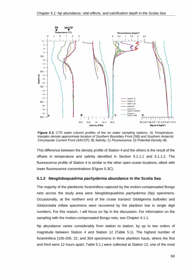
Chapter 5.1: Np abundance, vital effects, and calcification depth in the Scotia Sea
60
This difference between the density profile of Station 4 and the others is the result of the
offsets in temperature and salinity identified in Section 5.1.1.1 and 5.1.1.2. The
fluorescence profile of Station 4 is similar to the other open ocean locations, albeit with
lower fluorescence concentrations (Figure 5.3C).
5.1.2 Neogloboquadrina pachyderma abundance in the Scotia Sea
The majority of the planktonic foraminifera captured by the motion-compensated Bongo
nets across the study area were Neogloboquadrina pachyderma (Np) specimens.
Occasionally, at the northern end of the cruise transect Globigerina bulloides and
Globorotalia inflata specimens were recovered by the plankton tow in single digit
numbers. For this reason, I will focus on Np in the discussion. For information on the
sampling with the motion-compensated Bongo nets, see Chapter 4.1.1.
Np abundance varies considerably from station to station, by up to two orders of
magnitude between Station 4 and Station 12 (Table 5.1). The highest number of
foraminifera (100-200, 22, and 354 specimens in three plankton hauls, where the first
and third were 12 hours apart; Table 5.1.) were collected at Station 12, one of the most
Figure 5.3: CTD water column profiles of the six water sampling stations. A) Temperature, triangles denote approximate location of Southern Boundary Front (SB) and Southern Antarctic Circumpolar Current Front (SACCF); B) Salinity; C) Fluorescence; D) Potential Density (θ).
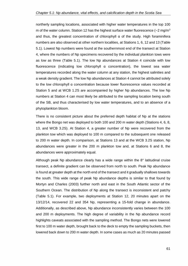
Chapter 5.1: Np abundance, vital effects, and calcification depth in the Scotia Sea
61
northerly sampling locations, associated with higher water temperatures in the top 100
m of the water column. Station 12 has the highest surface water fluorescence (~2 mg/m3
and thus, the greatest concentration of chlorophyll α of the study. High foraminifera
numbers are also observed at other northern localities, at Stations 1, 6, 12 and 13 (Table
5.1). Lowest Np numbers were found at the southernmost end of the transect at Station
4, where the numbers of Np specimens recovered by the individual plankton tows were
as low as three (Table 5.1). The low Np abundances at Station 4 coincide with low
fluorescence (indicating low chlorophyll α concentration), the lowest sea water
temperatures recorded along the water column at any station, the highest salinities and
a weak density gradient. The low Np abundances at Station 4 cannot be attributed solely
to the low chlorophyll α concentration because lower fluorescence values recorded at
Station 5 and at WCB 1.2S are accompanied by higher Np abundances. The low Np
numbers at Station 4 can most likely be attributed to the sampling location being south
of the SB, and thus characterised by low water temperatures, and to an absence of a
phytoplankton bloom.
There is no consistent picture about the preferred depth habitat of Np at the stations
where the Bongo net was deployed to both 100 and 200 m water depth (Stations 4, 6, 8,
13, and WCB 3.2S). At Station 4, a greater number of Np were recovered from the
plankton tow which was deployed to 100 m compared to the subsequent one released
to 200 m water depth. In comparison, at Stations 13 and at the WCB 3.2S station, Np
abundances were greater in the 200 m plankton tow and, at Stations 6 and 8, the
abundances were approximately equal.
Although peak Np abundance clearly has a wide range within the 8° latitudinal cruise
transect, a definite gradient can be observed from north to south. Peak Np abundance
is found at greater depth at the north end of the transect and it gradually shallows towards
the south. This wide range of peak Np abundance depths is similar to that found by
Mortyn and Charles (2003) further north and east in the South Atlantic sector of the
Southern Ocean. The distribution of Np along the transect is inconsistent and patchy
(Table 5.1). For example, two deployments at Station 12, 20 minutes apart on the
13/12/14, recovered 22 and 354 Np, representing a 15-fold change in abundance.
Additionally, as described above, Np abundance inconsistently varies between the 100
and 200 m deployments. The high degree of variability in the Np abundance record
highlights caveats associated with the sampling method. The Bongo nets were lowered
first to 100 m water depth, brought back to the deck to empty the sampling buckets, then
lowered back down to 200 m water depth. In some cases as much as 20 minutes passed

Chapter 5.1: Np abundance, vital effects, and calcification depth in the Scotia Sea
62
between the collection of the 100 and 200 m deployments. During that time, the water
mass underneath the ship constantly changed due to currents, allowing the lateral
transport of water masses away from, and to the sampling locality. This means, that in
the time period between the 100 m and 200 m deployments foraminifera could have been
transported away from the site, or could have been introduced to the location. This lateral
advection of foraminifera by the water currents impedes good reproducibility of net
Date Station
No./name Lat. (°) Long. (°)
Mesh size (μm)
Depth (m)
No. of Np
17/11/2014 18:38 Station 1 −56.67 −58.17 200 200 <200
17/11/2014 19:07 Station 1 −56.67 −58.17 100 200 90
18/11/2014 16:21 Station 2 −58.99 −51.8 100 200 100
19/11/2014 11:24 Station 3 −60.77 −46.48 100 115 50
25/11/2014 15:49 Station 4 −59.96 −46.16 100 100 40
25/11/2014 15:53 Station 4 −59.96 −46.16 100 200 6
25/11/2014 19:13 Station 4 −59.96 −46.16 100 100 25
25/11/2014 19:28 Station 4 −59.96 −46.16 100 200 3
26/11/2014 14:40 Station 4 −59.96 −46.16 100 100 7
27/11/2014 13:10 Station 5 - P2 −57.61 −43.67 100 200 59
28/11/2014 08:23 Station 6 −55.24 −41.26 100 200 <200
29/11/2014 15:17 Station 6 −55.25 −41.26 100 100 <200
29/11/2014 15:29 Station 6 −55.25 −41.26 100 200 <200
03/12/2014 15:38 Station 8 −54.2 −36.45 100 100 >50
03/12/2014 15:54 Station 8 - Cumberland Bay
−54.2 −36.45 200 200 >50
08/12/2014 23:12 WCB 1.2N Station −53.49 −39.25 100 200 31
09/12/2014 06:59 WCB 1.2S station - Western Core
Box −53.85 −39.14 100 200 94
10/12/2014 04:54 WCB 2.2N station −53.43 −38.7 100 200 18
10/12/2014 04:54 WCB 2.2N station −53.43 −38.7 200 200 <20
11/12/2014 05:40 WCB 3.2S station −53.71 −37.97 100 100 63
11/12/2014 05:40 WCB 3.2S station −53.71 −37.97 200 200 109
13/12/2014 06:26 Station 12 - P3 −52.81 −39.97 100 200 <200
13/12/2012 21:17 Station 12 −52.81 −39.97 200 200 22
13/12/2014 21:39 Station 12 −52.81 −39.97 200 100 354
14/12/2014 08:27 Station 13 −52.6 −39.2 100 100 <100
14/12/2014 08:46 Station 13 - Upwelling
−52.6 −39.2 100 200 <200
14/12/2014 15:57 Station 13 −52.6 −39.2 100 200 100
Table 5.1: Foraminifera sampling localities during JR304 cruise with date, station name and number, latitude and longitude of sampling, bongo net mesh size, bottom depth of bongo net deployment and the number of Np specimens captured in the plankton tow. Highlighted rows represent samples that underwent stable isotope analysis. At stations where precise numbers could not be provided, an upper or lower limit is given based on approximate recorded numbers.

Chapter 5.1: Np abundance, vital effects, and calcification depth in the Scotia Sea
63
catches at any one location. The limited number of Bongo net deployments hinders the
thorough assessment of Np abundance in the Scotia Sea. A more structured sampling
strategy, where Bongo nets are deployed at a regular distance from each other (for
example, a 0.5° gap could be applied between sampling localities) could improve the
spatial assessment of Np abundance. Sampling at either side of the frontal boundaries
(SB, SACCF, Northern and Southern boundary of PF, SAF) could also improve our
understanding of Np abundance in the Scotia Sea. In addition, the use of a depth-
integrated plankton tow (e.g. Multiple Opening/Closing Net and Environmental Sensing
System: MOCNESS), as opposed to the single-depth Bongo nets, would greatly enhance
our understanding of Np habitat and calcification depth by highlighting specific depth
intervals (e.g. 0-20 m, 20-50 m, 50-100 m, etc.) where Np is abundant .
5.1.2.1 Neogloboquadrina pachyderma morphotypes
Prior to stable isotope analysis specimens from five plankton tow hauls (Table 5.1) were
inspected under the light microscope to ensure that morphotype-related variability in the
stable isotope data is limited. It is recognised that high resolution SEM images would be
helpful in the determination of the different morphotypes; however, visual inspection
under a light microscope was the only means of morphotype separation for this study.
Overall, three different morphotypes are present in the samples.
A review of existing literature reveals that Neogloboquadrina pachyderma specimens
have been placed into different categories based on several different aspects of their
morphological features. To date, no consistent morphological group classification
method has been developed, leading to arbitrary determination of groups. Kennett (1968)
separated Np specimens in the South Pacific and in the Southern Ocean based on
chamber numbers in the final whorl, wall thickness and shape, and identified two groups.
Group one, located south of 54-55°S was dominated by 4-chambered, thick-walled and
compact specimens. In comparison, group two, located north of 54-55°S was dominated
by 4 ½-to 5-chambered, thinner-walled and more lobate specimens. Vautravers et al.
(2013) also used shape and size to identify two separate morphotypes (Morphotypes A
and B) in sediment samples from the Antarctic Peninsula. Specimens belonging to
Morphotype A were larger, quadrate and showed signs of a secondary crust, while
specimens in the Morphotype B group were smaller, more lobate and had thinner shells
than Morphotype A, and were considered to be juvenile forms of Morphotype A.
Morphological assessments carried out on northern hemisphere specimens were based
on similar characteristics to the southern hemisphere ones. Stehman (1972) identified
three different Neogloboquadrina pachyderma groups (Forms 1, 2, and 3) in the

Chapter 5.1: Np abundance, vital effects, and calcification depth in the Scotia Sea
64
Labrador Sea which were based on shape, calcification, and aperture. Specimens which
belonged to Form 1 had a compact, heavily calcified shell with a small aperture, 4
chambers in the final whorl, and were common in the coldest waters of the region. Form
2 specimens had a quadrate/square appearance, the shells were heavily calcified and
had 4 ½ to 5 chambers in the final whorl. Form 3 specimens were more elongated, less
square, were less encrusted, had an arched, sinuous lip around the aperture, had 5
chambers in the final whorl, and were found in warmer waters. Kohfeld et al. (1996) found
two groups of Np in the Northern North Atlantic, and used the shape and surface texture
of the shells to separate the groups. Np specimens that belonged to Group one were
heavily encrusted, opaque, quadrate, and had heavier shells with crystalline surfaces.
Group two specimens had smooth, reticulate surfaces, were nonencrusted, and more
elongated with a lower shell mass and were suggested to be juvenile (or pre-
encrustation) forms of Group one. A more recent study by Eynaud (2011) carried out on
Arctic Ocean samples has provided the most thorough assessment of Np morphology to
date and identified five different groups (Nps-1, 2, 3, 4, and 5) based on specimen size,
shape, number of chambers, aperture size, and encrustation. Of particular interest from
the five morphotypes, are the Nps-2, Nps-3 and Nps-5 groups. Nps-2 specimens were
quadrate, encrusted and had 4 globular chambers and a large aperture. Nps-3
specimens were more elongated, had 4 to 4 ½ chambers and a large aperture. In
contrast, Nps-5 specimens were smaller than the rest, lozenge-shaped and elongated,
and had 4, nonencrusted chambers with small, deep suture lines.
Genetic analysis of North and South Atlantic, and Southern Ocean Neogloboquadrina
pachyderma specimens revealed the existence of five different genotypes (Darling et al.,
2004). Only one genotype (Type I) was found in the North Atlantic, while four genotypes
(Type II, III, IV, and V) were identified in the Southern Hemisphere samples. Type V
specimens are only found in the Benguela Upwelling system, while the other three
genotypes dominate in different regions of the Southern Ocean. Type II is dominant north
of the Subantarctic Front, Type III is widespread north of the Polar Front, while Type IV
is only found south of the Polar Front.
Based on the above studies, I identified three different morphotypes (Np-A, B, and C) of
Neogloboquadrina pachyderma. Np-A specimens have compact, quadrate, cancellate
shells with 4 globular chambers in the final whorl, and a prominent, large aperture and
no clearly visible suture lines. Np-A specimens look similar in shape to the Nps-2
morphotype (Figure 5.4A) identified by Eynaud (2011), Group one of Kennett (1968) and
Kohfeld et al. (1996), Morphotype A of Vautravers et al. (2013), and Form 1 of Stehman
(1972). Np-A morphotype dominates the Station 5 and Station 8 samples, the most

Chapter 5.1: Np abundance, vital effects, and calcification depth in the Scotia Sea
65
southerly stations (Figure 5.2), and also makes up a greater portion of the Station 12,
and Station 13 assemblages than the other morphotypes. In contrast, at WCB 1.2S Np-
A only makes up a small portion of the population, as identified under a microscope.
Under the light microscope the specimens from Station 5 look smaller than the
specimens from the rest of the plankton tows.
Np-B specimens have more lobate, elongated, 4 to 4 ½ chambered cancellate shells
with signs of encrustation and not very clear suture lines. In this group, the final chamber
of the shell is more deflated, not globular and smaller than the other chambers. This
group, Np-B, looks similar to the Nps-3 (Figure 5.4B) morphotype identified by Eynaud
(2011) and Group two of Kennett (1968). Np-B morphotype is found in the Station 12
and Station 13 populations but altogether makes up a smaller portion than Np-A.
Np-C specimens have smaller (than Np-A and B) elongated, lobate shells with a shiny
surface and 4 ½ chambers with distinct suture lines. These specimens do not show signs
of encrustation and look similar to the Nps-5 morphotype (Figure 5.4C) identified by
Eynaud (2011), Morphotype B of Vautravers et al (2013), and Group two of Kohfeld et al
(1996). In some instances, the cytoplasm of the foraminifera was still intact at collection.
Based on the lack of encrustation, presence of cytoplasm, highly elongated shape and
similarity to the above morphotypes, Np-C specimens can be considered as juvenile,
pre-gametogenic specimens that have not gone through reproduction. Np-C morphotype
is found at all stations, making up a small portion of the population at Stations 5, 8, 12
and 13, and dominating the WCB 1.2S population. Np-C specimens in the Station 5, 8
and WCB 1.2S populations generally still contain their cytoplasm at collection, while
specimens belonging to the Station 12 and 13 population were missing the cytoplasm
when collected by the Bongo net plankton hauls.
Figure 5.4: Scanning Electron Microscope images of Nps-2 (A), Nps-3 (B), and Nps-5 (C) Neogloboquadrina pachyderma morphotypes in ventral view from Eynaud (2011). Specimens derive from Central Arctic sediments (IODP-ACEX Hole 4C) and show the diversity of morphology observable in this species.
A B C

Chapter 5.1: Np abundance, vital effects, and calcification depth in the Scotia Sea
66
Three right-coiling Neogloboquadrina pachyderma specimens were present in the
Station 12 samples (total of 112 specimens). As Darling et al. (2006) discussed, <3% of
Np is right coiling in Atlantic and Southern Ocean populations, and therefore we assume
that those present in the Station 12 sample are aberrant version of Np instead of
Neogloboquadrina incompta specimens.
Using the spatial distribution of Np genotypes as identified by Darling et al (2004) it can
be hypothesised that the Np-A morphotype (dominant at Station 5 and 8, south of the
SACCF) belongs to the Type IV genotype group, while Np-B morphotype (present at
Station 12 and 13, north of the SACCF, close to the PF) specimens most likely belong
to the Type III genotype group. As the Np-C morphotype represents pre-reproduction
specimens, this morphotype cannot be placed into either genotype group. Genetic
analysis, akin to the Darling et al (2004) study is required to confirm the genotypes of the
plankton tow samples. To reduce within-sample variability due to morphotype mixing, I
aimed to choose only the dominant morphotypes for stable isotope analysis from each
sample, i.e. Np-A specimens from the Station 5, 8, 12, and 13 samples; Np-C specimens
from the WCB 1.2S samples (Table 5.2).
5.1.3 Neogloboquadrina pachyderma stable isotopic signatures and water
column δ18O gradients
Single specimen stable isotope ratios were measured on Np from five different plankton
tow hauls, deployed to 200 m water depths. A minimum of 30 single specimens were
analysed from each station; however, only 20, 15 and 29 reliable data points could be
derived from Station 8, WCB 1.2S and Station 12, respectively. Variability between
specimens can be observed in both the oxygen and carbon isotopic records (Figure 5.5).
5.1.3.1 Neogloboquadrina pachyderma oxygen isotopic ratios
Average oxygen isotope values of Np (δ18Onp) vary from +2.22 ± 0.34‰ at WCB 1.2S to
+3.38 ± 0.22‰ at Station 5 (Figure 5.5A). The data show a maximum inter-station-station
spread of 2.22‰ across the stations - between the highest value, +3.77‰, at Station 5
and lowest value, +1.5‰, at WCB1.2S (Table 5.2). Largest variability of δ18Onp values
within a locality is recorded at WCB 1.2S with a 1.27‰ range and a 0.12 variance. The
smallest variability is recorded at Station 12, where δ18Onp values have a range of 0.62‰,
and a variance of 0.03. The range of δ18Onp values recorded at Station 13 (1.27‰) is as
high as at WCB 1.2S; however, this is skewed by a single data point (+1.81‰) outside
the 1.5xInterquartile range. This is also reflected by the smaller variance (0.05 vs 0.12
at WCB 1.2S) and by the smaller standard deviation (0.23‰ vs

Chapter 5.1: Np abundance, vital effects, and calcification depth in the Scotia Sea
67
0.34‰ at WCB 1.2S). Although the lowest oxygen isotope values are not observed at
the most northerly location, a clear latitudinal gradient exists in the record with values
decreasing from south to north (Figure 5.5A).
An Fmax test conducted on the δ18Onp dataset reveal statistically significant difference
(p=0.0001) between the δ18Onp-derived variances of the different localities. For further
statistical tests parametric analysis techniques need to be employed due to the
statistically significant differences between the variances. A Kruskal-Wallis test (non-
parametric equivalent of ANOVA) reveals statistically significant difference between any
of the medians of the five localities (p = 6.65x10⁻²²). Furthermore, Mann-Whitney
pairwise tests (non-parametric equivalent of t-test), highlight the existence of statistically
Figure 5.5: Single specimen N. pachyderma δ18O (A) and δ13C (B) boxplots arranged by latitude. Station 5 is the most southerly location, Station 13 is most northerly location. Black crosses represent outliers (data points outside 1.5 x IQR), numbers denote the number of single specimens analysed.
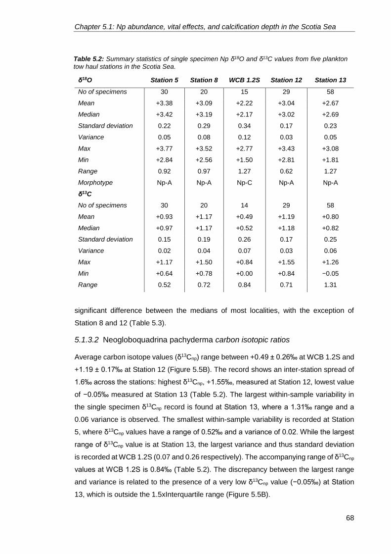
Chapter 5.1: Np abundance, vital effects, and calcification depth in the Scotia Sea
68
significant difference between the medians of most localities, with the exception of
Station 8 and 12 (Table 5.3).
5.1.3.2 Neogloboquadrina pachyderma carbon isotopic ratios
Average carbon isotope values (δ13Cnp) range between +0.49 ± 0.26‰ at WCB 1.2S and
+1.19 ± 0.17‰ at Station 12 (Figure 5.5B). The record shows an inter-station spread of
1.6‰ across the stations: highest δ13Cnp, +1.55‰, measured at Station 12, lowest value
of −0.05‰ measured at Station 13 (Table 5.2). The largest within-sample variability in
the single specimen δ13Cnp record is found at Station 13, where a 1.31‰ range and a
0.06 variance is observed. The smallest within-sample variability is recorded at Station
5, where δ13Cnp values have a range of 0.52‰ and a variance of 0.02. While the largest
range of δ13Cnp value is at Station 13, the largest variance and thus standard deviation
is recorded at WCB 1.2S (0.07 and 0.26 respectively). The accompanying range of δ13Cnp
values at WCB 1.2S is 0.84‰ (Table 5.2). The discrepancy between the largest range
and variance is related to the presence of a very low δ13Cnp value (−0.05‰) at Station
13, which is outside the 1.5xInterquartile range (Figure 5.5B).
δ18O Station 5 Station 8 WCB 1.2S Station 12 Station 13
No of specimens 30 20 15 29 58
Mean +3.38 +3.09 +2.22 +3.04 +2.67
Median +3.42 +3.19 +2.17 +3.02 +2.69
Standard deviation 0.22 0.29 0.34 0.17 0.23
Variance 0.05 0.08 0.12 0.03 0.05
Max +3.77 +3.52 +2.77 +3.43 +3.08
Min +2.84 +2.56 +1.50 +2.81 +1.81
Range 0.92 0.97 1.27 0.62 1.27
Morphotype Np-A Np-A Np-C Np-A Np-A
δ13C
No of specimens 30 20 14 29 58
Mean +0.93 +1.17 +0.49 +1.19 +0.80
Median +0.97 +1.17 +0.52 +1.18 +0.82
Standard deviation 0.15 0.19 0.26 0.17 0.25
Variance 0.02 0.04 0.07 0.03 0.06
Max +1.17 +1.50 +0.84 +1.55 +1.26
Min +0.64 +0.78 +0.00 +0.84 −0.05
Range 0.52 0.72 0.84 0.71 1.31
Table 5.2: Summary statistics of single specimen Np δ18O and δ13C values from five plankton
tow haul stations in the Scotia Sea.

Chapter 5.1: Np abundance, vital effects, and calcification depth in the Scotia Sea
69
The within-sample δ13Cnp variance reveal statistically significant difference between the
five stations when analysed through an Fmax test (p=0.01). Similarly to the δ18Onp record,
the δ13Cnp values display normal distribution at every station; however, due to the
significant difference between the variance of the different stations, non-parametric
statistical tests need to be employed for further analysis. A Kruskal-Wallis test shows
statistically significant difference between any of the medians of the different stations (p
= 2.03x10⁻¹⁶). Additionally, Mann-Whitney pairwise tests also show similar results to the
δ18O dataset (Table 5.3), with statistically significant difference recorded between the
medians of most stations (exception is the Station 8: Station 12 relationship). There is
no clear latitudinal gradient in the δ13Cnp measurements (Figure 5.5B).
Seawater samples were collected at every CTD station to determine the carbon isotope
variability of dissolved inorganic carbon (DIC), to help the interpretation of the δ13Cnp
dataset. However, the amount of DIC collected was not enough to provide accurate
figures. Therefore it is not possible to assess whether δ13CDIC or biological processes
(kinetic fractionation and vital effects) exert a greater influence on the δ13Cnp.
δ18O Station 5 Station 8 WCB 1.2S Station 12
Station 5
Station 8 3.90x10⁻⁴
WCB 1.2S 6.41x10⁻⁸ 1.70x10⁻⁶
Station 12 3.21x10⁻⁷ 0.502 7.72x10⁻⁸
Station 13 8.26x10⁻¹⁴ 1.92x10⁻⁶ 7.49x10⁻⁶ 4.87x10⁻¹⁰
δ13C
Station 5
Station 8 3.62x10⁻⁵
WCB 1.2S 2.74x10⁻⁶ 2.10x10⁻⁶
Station 12 3.33x10⁻⁷ 0.722 1.75x10⁻⁷
Station 13 0.013 1.97x10⁻⁷ 3.17x10⁻⁴ 3.45x10⁻¹⁰
Table 5.3: Bonferroni corrected p values of pairwise Mann-Whitney U tests conducted on the single specimen Np δ18O and δ13C dataset. Highlighted cells indicate statistically significant difference between samples (p<0.05).

Chapter 5.1: Np abundance, vital effects, and calcification depth in the Scotia Sea
70
5.1.3.3 Seawater δ18O trends
Seawater samples from a range of water depths, collected at the same locations as
foraminifera samples for stable isotope analysis (Figure 5.2) were analysed for their
oxygen isotope values. The δ18O of the seawater (δ18Osw) shows a consistent pattern
along the transect (Figure 5.6). The maximum surface water δ18Osw difference between
all stations is 0.34‰, while only a 0.04‰ difference exists between four of the northerly
locations (Stations 5, 12, 13 and WCB 1.2S). The lowest surface water δ18Osw value
(−0.43‰) is recorded at Station 8, proximal to Cumberland Bay, most likely as a result
of the low surface water salinity (Figure 5.3B). The highest surface water δ18O (−0.17‰)
is found at the most southerly location, Station 4, south of the SB. δ18Osw through the
water column is similar at each open ocean station, generally increasing with increasing
depth (Figure 5.6). The general consistency of the δ18Osw values between the stations
suggests that the same water masses were sampled across the study area and
differences in δ18Onp are most likely due to the effect of temperature.
Figure 5.6: Seawater δ18O profiles at the six sampling locations. Station 4 is south of the SB, Station 5 is located south of the SACCF. All other stations are north of the SACCF and south of the PF.
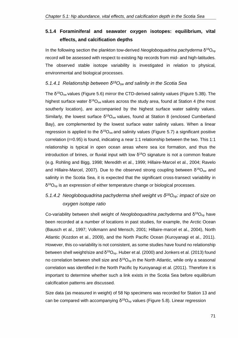
Chapter 5.1: Np abundance, vital effects, and calcification depth in the Scotia Sea
71
5.1.4 Foraminiferal and seawater oxygen isotopes: equilibrium, vital
effects, and calcification depths
In the following section the plankton tow-derived Neogloboquadrina pachyderma δ18Onp
record will be assessed with respect to existing Np records from mid- and high-latitudes.
The observed stable isotope variability is investigated in relation to physical,
environmental and biological processes.
5.1.4.1 Relationship between δ18Osw and salinity in the Scotia Sea
The δ18Osw values (Figure 5.6) mirror the CTD-derived salinity values (Figure 5.3B). The
highest surface water δ18Osw values across the study area, found at Station 4 (the most
southerly location), are accompanied by the highest surface water salinity values.
Similarly, the lowest surface δ18Osw values, found at Station 8 (enclosed Cumberland
Bay), are complemented by the lowest surface water salinity values. When a linear
regression is applied to the δ18Osw and salinity values (Figure 5.7) a significant positive
correlation (r=0.95) is found, indicating a near 1:1 relationship between the two. This 1:1
relationship is typical in open ocean areas where sea ice formation, and thus the
introduction of brines, or fluvial input with low δ18O signature is not a common feature
(e.g. Rohling and Bigg, 1998; Meredith et al., 1999; Hillaire-Marcel et al., 2004; Ravelo
and Hillaire-Marcel, 2007). Due to the observed strong coupling between δ18Osw and
salinity in the Scotia Sea, it is expected that the significant cross-transect variability in
δ18Onp is an expression of either temperature change or biological processes.
5.1.4.2 Neogloboquadrina pachyderma shell weight vs δ18Onp: impact of size on
oxygen isotope ratio
Co-variability between shell weight of Neogloboquadrina pachyderma and δ18Onp have
been recorded at a number of locations in past studies, for example, the Arctic Ocean
(Bausch et al., 1997; Volkmann and Mensch, 2001; Hillaire-marcel et al., 2004), North
Atlantic (Kozdon et al., 2009), and the North Pacific Ocean (Kuroyanagi et al., 2011).
However, this co-variability is not consistent, as some studies have found no relationship
between shell weight/size and δ18Onp. Huber et al. (2000) and Jonkers et al. (2013) found
no correlation between shell size and δ18Onp in the North Atlantic, while only a seasonal
correlation was identified in the North Pacific by Kuroyanagi et al. (2011). Therefore it is
important to determine whether such a link exists in the Scotia Sea before equilibrium
calcification patterns are discussed.
Size data (as measured in weight) of 58 Np specimens was recorded for Station 13 and
can be compared with accompanying δ18Onp values (Figure 5.8). Linear regression

Chapter 5.1: Np abundance, vital effects, and calcification depth in the Scotia Sea
72
Figure 5.7: δ18O-salinity relationship at six CTD stations across the Scotia Sea showing statistically significant correlation (r=0.95) indicating that salinity is the dominant factor on δ18Osw
values in the Scotia Sea.
Figure 5.8: Linear regression figures of shell weight:δ18Onp. Specimens originate from Station 13 plankton tow haul. Statistically significant correlation is found between shell weight and δ18Onp, as indicated by the r value (greater than 0.25 at 95% significance).

Chapter 5.1: Np abundance, vital effects, and calcification depth in the Scotia Sea
73
analysis reveals significant correlation between weight and δ18Onp, supporting previously
published size-dependent δ18O records (e.g. Bausch et al., 1997; Hillaire-Marcel et al.,
2004; Kuroyanagi et al., 2011). Heavier specimens have higher δ18Onp values, most likely
due to deeper calcification depths (in colder and more saline waters) and the addition of
secondary crust at those deeper depths. In contrast, smaller, and thus lighter specimens
have lower δ18Onp values, most likely as a result of shallower calcification depths (in
warmer and less saline waters) and possible lack of secondary calcite crust. This trend
is observable across the study area (Figure 5.9), with the highest average δ18Onp values
accompanying high shell weights (Station 5) and the lowest average δ18Onp values are
coupled with the lowest shell weights (WCB 1.2S). The combination of the lowest shell
weights and lowest δ18Onp measurements in the WCB 1.2S sample most likely reflects
the lack of secondary crust of the Np-C morphotype specimens, and a shallower
calcification depth than Np specimens elsewhere in the study region. This agrees well
with previous assessment of pre-gametogenic Np (Kohfeld et al., 1996; Kozdon et al.,
2009), where Np specimens with ontogenic calcite only have been recorded to have
lower shell mass and δ18Onp values (Kohfeld et al., 1995; Kozdon et al., 2009). However,
variabilities are present in this trend. Relatively low, average shell weight of 7.3 ± 0.97
μg at Station 8 is accompanied by relatively high δ18Onp values, centred on 3.09 ± 0.29‰.
The combination of such high δ18Onp values and low shell weight most likely relates to
the cold water temperatures (Figure 5.3A) present at calcification depth at the time of
sampling coupled with probable secondary calcification and morphological differences.
Station 8 is located closer to shore than the rest of the stations, in Cumberland Bay,
South Georgia (Figure 5.2). Glacial meltwater runoff from nearby South Georgia would
have introduced nutrients (e.g. nitrate and phosphate) to the waters of Cumberland Bay,
Figure 5.9: Average shell weight and δ18Onp (A) variability at five stations across the Scotia Sea. Error bars depict one standard deviation range.

Chapter 5.1: Np abundance, vital effects, and calcification depth in the Scotia Sea
74
allowing Np to complete its life cycle, reproduce and secrete a secondary calcite crust
more rapidly than if nutrients were more limited resulting in the calcification of smaller
shells compared to ones achieved during a longer calcification period. The overall
variability in the shell weight-δ18Onp relationship is most likely the result of the latitudinal
temperature increase between the most southerly and northerly sites (Figure 5.3A)
combined with the impact of morphological variability (as discussed in Section 5.1.2.1).
5.1.4.3 Exploration of vital effects during isotope fractionation by
Neogloboquadrina pachyderma in the Scotia Sea
The influence of temperature on the δ18Onp is reflected well in the predicted calcite
equilibrium values (δ18Oeq, Figure 5.10) which shows a ~0.4‰ difference at the surface
between Station 5 and Station 13 even when δ18Osw is identical at −0.27‰ (Figure 5.6).
Highest δ18Oeq values are observed at Station 5 (0-150 m water depth), as a result of the
lowest water temperature values of the five stations. δ18Oeq values are almost identical
at Station 12 and 13, showing consistently lower values between 40 m and 100 m than
the rest of the stations (Figure 5.10) as a result of similar temperature trends across the
water column (Figure 5.11D,E).
Previous plankton tow and sediment trap studies have identified the depth habitat of Np
as within or just below the mixed layer, the exact depth of which depends on local
hydrography and can range from 35 m to 150 m (Volkmann and Mensch, 2001; Jonkers
et al., 2010; Kuroyanagi et al., 2011; Asahi et al., 2015). The long held assumption in Np
ontogeny is that the development of the secondary calcite crust takes place in deeper
waters than the secretion of the ontogenic calcite shell (Hemleben and Spindler, 1983;
Kohfeld et al., 1996; Kozdon et al., 2009). The calcification of the secondary crust has
been linked to the pycnocline or just below the pycnocline (Ortiz et al., 1996; Mortyn and
Charles, 2003; Simstich et al., 2003; Hillaire-Marcel et al., 2004; Kozdon et al., 2009).
By using the depth of the mixed layer and that of the pycnocline as a guide, δ18O
equilibrium offsets of Np can be assessed across the Scotia Sea.
The depth of the mixed layer and of the pycnocline varies across the sites (Figure 5.11).
The shallowest mixed layer (surface to 12 m water depth) is found at Station 8 (Figure
5.11B) as the result of the low-salinity lens in the enclosed Cumberland Bay. Here,
average δ18Onp values (with ±1σ) follow the δ18Oeq without significant offset below the
mixed layer, within the thermocline. The average δ18Onp value (+3.09‰) converge onto
the δ18Oeq at ~100 m water depth.
At the rest of the stations the mixed layer is between 50 and 75 m deep (Figure 5.11A-
E) and thus both the pycnocline and the thermocline are found much deeper than at

Chapter 5.1: Np abundance, vital effects, and calcification depth in the Scotia Sea
75
Cumberland Bay. At Station 5 and 12, the relationship between the average δ18Onp and
δ18Oeq is similar to Station 8. At these stations Np-A morphotypes dominate and were
chosen for stable isotopic analysis. The average δ18Onp value (±1σ) follows the δ18Oeq
below the mixed layer without any significant offset and it converges onto the δ18Oeq
value at ~100 m water depth.
This equilibrium calcification below the mixed layer only agrees well with one other
plankton tow study conducted in the northern Pacific Ocean (Asahi et al., 2015). Most
plankton tow studies conducted in the Arctic Ocean (Bausch et al., 1997; Bausch et al.,
2002; Hillaire-Marcel et al., 2004), in the North Atlantic (Kohfeld et al., 1996; Volkmann
and Mensch, 2001; Kozdon et al., 2009) and in the Southern Ocean (Mortyn and Charles,
2003) have identified negative vital offsets up to 1‰. Lack of vital offsets in Np are
commonly identified in sediment trap studies across the oceans (Jonkers et al., 2010;
Jonkers et al., 2013; Sagawa et al., 2013; Asahi et al., 2015) and have been linked to
the dominance of the encrusted specimens in the sediment traps. However, it is
important to note that differences in vital offsets have been recorded in both plankton
tows and sediment traps conducted at the same location (e.g. ‒1‰ vital offset recorded
in sediment trap study of Kuroyanagi et al., 2011).
Figure 5.10: Calculated foraminiferal calcite equilibrium δ18O values against depth at Station 5, 8, 12, 13 and WCB 1.2S. These locations were chosen based on the availability of sufficient number of Np for stable isotope analysis.

Chapter 5.1: Np abundance, vital effects, and calcification depth in the Scotia Sea
76
Different dynamics in the δ18Onp:δ18Oeq relationship are observed at WCB 1.2S and
Station 13. WCB 1.2S, where the Np-C morphotype dominates, is the only station where
the range of single specimen δ18Onp falls outside the δ18Oeq profile (Figure 5.11C). At this
location δ18Oeq values across the entire water profile are higher than the maximum single
specimen δ18Onp. The bottom of the mixed layer is approximately at 50 m water depth.
The average δ18Onp value (+2.27 ± 0.35‰) at WCB 1.2S shows a negative offset of 0.6‰
from mixed layer δ18Oeq value (at 20 m) and a 0.65‰ negative offset from the δ18Oeq
value just below the mixed layer (60 m).
At Station 13, where Np-A morphotype dominates, 50% of the δ18Onp falls outside the
δ18Oeq profile (Figure 5.11E). The average δ18Onp follows the δ18Oeq profile in the mixed
layer (top 50 m) without any offset. However, the δ18Oeq values diverge from δ18Onp and
increase below the mixed layer in line with the increasing water temperature. As a result
only 50% of the single specimen δ18Onp values show no vital offset within the thermocline.
The rest of the specimens show negative fractionation of up to 0.46‰ compared to mixed
layer δ18Oeq values and a ‒0.78‰ offset compared to thermocline δ18Oeq value (at 100 m
water depth).
A common theme of all stations is the presence of single specimen δ18Onp values that
either exhibit a negative offset from or fall within mixed layer δ18Oeq values. The negative
offset from δ18Oeq across the entire water profile, coupled with the low δ18Onp (+1.5 to
+2.77‰) observed at WCB 1.2S are additional confirmation that these
Neogloboquadrina pachyderma specimens are nonencrusted, havening only secreted
ontogenic calcite and belong to the Np-C morphotype. At this station the specimens still
contained their cytoplasm when collected, with some showing signs of transitioning
between juvenile and adult stages, indicating that the specimens were most likely still
alive during collection. Ontogenic calcite exhibits a negative fractionation of minimum of
1‰ relative to δ18Oeq (Volkmann and Mensch, 2001; Kozdon et al., 2009) as a result of
faster calcification in the juvenile and pre-adult stages that require higher respiration
rates (Hemleben et al., 1989). As the δ18O of respired CO2 is significantly lower than the
δ18O of CO2 in equilibrium with seawater (Epstein et al., 1977; McConnaughey, 1989),
the faster calcification rate or smaller test size results in a significant negative
fractionation (Kozdon et al., 2009). The negative fractionation identified in the mixed layer
agrees well with previous studies conducted in the Atlantic sector of the Southern Ocean,
where vital offsets of up to −1.2‰ compared with δ18Oeq values above 100 m have been
recorded (Donner and Wefer, 1994; Mortyn and Charles, 2003).
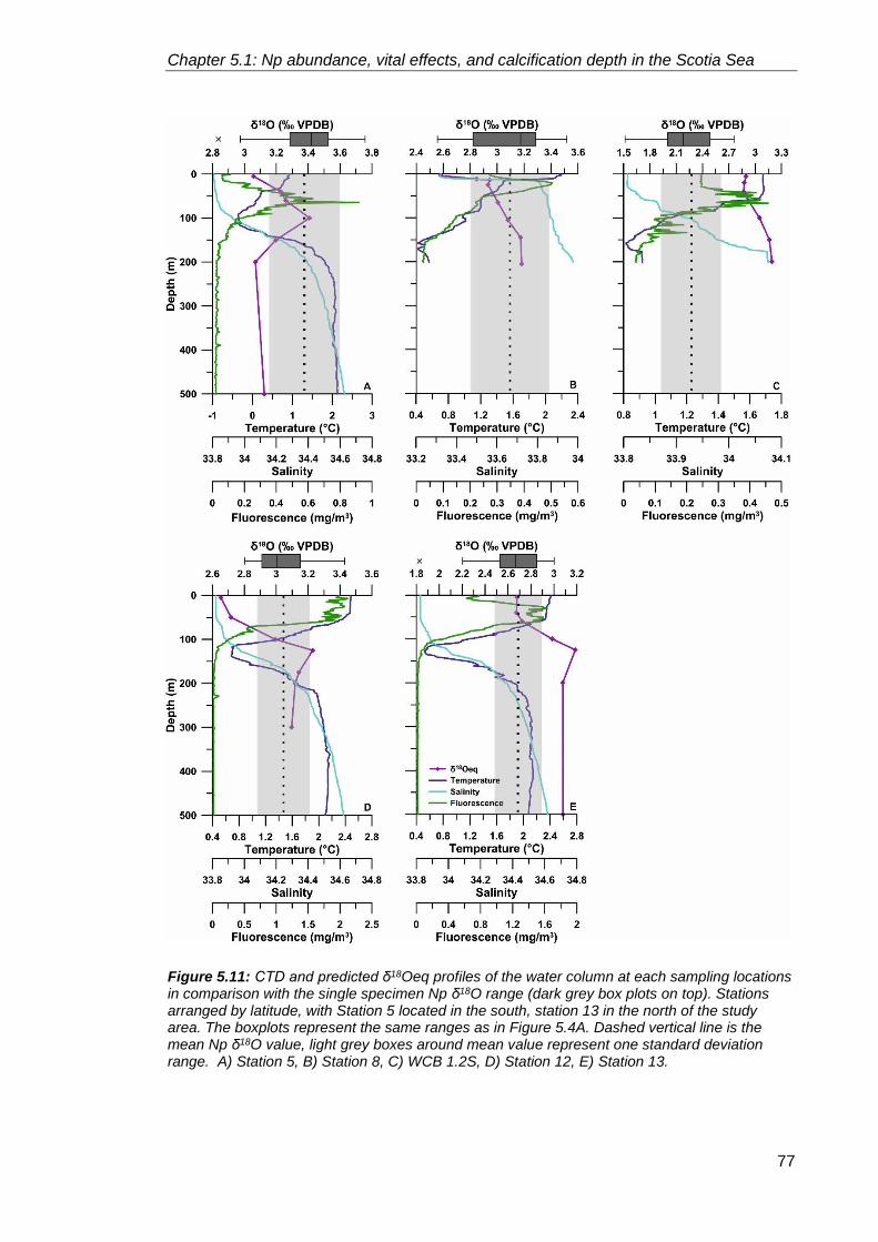
Chapter 5.1: Np abundance, vital effects, and calcification depth in the Scotia Sea
77
Figure 5.11: CTD and predicted δ18Oeq profiles of the water column at each sampling locations in comparison with the single specimen Np δ18O range (dark grey box plots on top). Stations arranged by latitude, with Station 5 located in the south, station 13 in the north of the study area. The boxplots represent the same ranges as in Figure 5.4A. Dashed vertical line is the mean Np δ18O value, light grey boxes around mean value represent one standard deviation range. A) Station 5, B) Station 8, C) WCB 1.2S, D) Station 12, E) Station 13.

Chapter 5.1: Np abundance, vital effects, and calcification depth in the Scotia Sea
78
The negative fractionation exhibited by 50% of the specimens at Station 13 and
equilibrium calcification within the mixed layer (instead of below it) exhibited by
specimens at Stations 5, 8, and 12 could be explained by a number of reasons. One
possibility, is that specimens were chosen incorrectly prior to stable isotope analysis and
they are not Np-A morphotypes, but Np-C morphotypes instead. Another explanation
could be the secretion of the secondary crust within the mixed layer. Np-C morphotypes
were identified in all Bongo net hauls (Section 5.1.2.1), and at Station 5 and 8 these
specimens contained their cytoplasm upon collection, indicating their pre-reproduction
status. No shell was chosen with a cytoplasm from the Station 5 and 8 samples, therefore
the picking of incorrect morphotype cannot explain equilibrium calcification within the
mixed layer at these stations. Specimens at Stations 12 and 13 were without their
cytoplasm, regardless of morphotype. Care was taken to avoid the picking of incorrect
morphotypes. Only specimens that displayed signs of the secondary crust (large
euhedral calcite crystals on surface and rough surface texture) were chosen, therefore
the incorrect identification of morphotype can be discounted. Instead, it is likely, that
specimens that show equilibrium calcification within the mixed layer or show negative
fractionation in the mixed layer (Station 13) have secreted the calcite crust within the
mixed layer.
The exact reasons and processes behind the secretion of the secondary crust of
Neogloboquadrina pachyderma are still not known. In some planktonic foraminifera
species the calcification of the secondary crust is related to gametogenesis (Bé, 1980).
In the case of Np, early studies suggested that the secondary crust forms in response to
declining water temperatures as the organism descends through the water column
(Hemleben and Spindler, 1983; Kohfeld et al., 1996). However, a more recent study on
North Atlantic Np from sediment traps found no indication that the secondary crust forms
at greater depth (Jonkers et al., 2016). Additionally, secretion of the secondary crust at
constant temperature has been observed in cultured specimens of Neogloboquadrina
incompta, a close relative of Np (C. Davis, personal communication). Instead of a
temperature control, it was suggested that crust formation is driven by tight biological
controls, during late ontogeny at relatively shallow depths (Jonkers et al., 2012; Jonkers
et al., 2016; Fehrenbacher et al., 2017). Therefore it is plausible that the large amplitude
in the single specimen δ18Onp data across the Scotia Sea stations is due to this
calcification within the mixed layer. The variability in vital offset within the Scotia Sea and
the lack of agreement on the processes behind the secondary crust formation highlight
the need for further studies of Neogloboquadrina pachyderma biology, morphology and
stable isotope variability.

Chapter 5.1: Np abundance, vital effects, and calcification depth in the Scotia Sea
79
5.1.5 Summary and Conclusion
In this chapter, the aim was to investigate the variability of Neogloboquadrina
pachyderma abundance, morphology, stable isotope composition and vital effects in the
Scotia Sea in order to be able to provide constraints for time series and paleoclimate
studies that utilise Np within the Southern Ocean.
Motion-compensated Bongo nets used to collect Np exhibit considerable variability in
abundance across the study area. Np abundance varies by up to two orders of
magnitude between a station south of the Southern Boundary of the Antarctic
Circumpolar Current and a station on the southern edge of the Polar Front. Highest
number of Np found in the most northerly location is associated with the highest surface
water fluorescence (expression of chlorophyll α concentration) and highest water
temperatures down to 100 m water depth. Lowest number of Np was recovered at the
southernmost station, and is associated with low fluorescence values and low water
temperatures across the water column. The equatorward increase in Np numbers is
accompanied by increasing depth of peak abundance. The Bongo net hauls across the
study area highlight the link between Np abundance, food availability and water
temperature in the polar waters of the Scotia Sea and support previously published South
Atlantic Np records (Mortyn and Charles, 2003).
Visual inspection of Neogloboquadrina pachyderma specimens under a light microscope
revealed the existence of three morphotypes, whose distribution varies across the study
area with latitude. The two adult morphotypes, Np-A and Np-B, are separated by the
Southern Antarctic Circumpolar Current Front (SACCF). Np-B is found only north of the
SACCF, while Np-A is present mostly in the colder waters south of it. The third
morphotype, Np-C, represents juvenile, pre-gametogenic specimens, and is found
across the study area, dominating one population west of South Georgia.
Stable isotope analysis of single specimens of Neogloboquadrina pachyderma reveals
a latitudinal gradient in δ18Onp, decreasing from south to north with decreasing δ18Osw
and increasing water temperatures. The δ18Onp record shows co-variability with size, with
heavier specimens showing higher δ18Onp. Highest δ18Onp is recorded in the Np-A
morphotypes at the southern stations, while the lowest δ18Onp is recorded in the pre-
gametogenic Np-C morphotypes at WCB 1.2S. Comparison of single specimen δ18Onp
with δ18Oeq across the study area reveals variable vital offsets. The δ18Onp of the Np-C
morphotype specimens, which calcify in the mixed layer, show negative offset of ~0.6‰
from mixed layer δ18Oeq. The Np-A morphotypes show equilibrium calcification below the
mixed layer and within the mixed layer as well. Negative fractionation within the mixed
Chapter 5.1: Np abundance, vital effects, and calcification depth in the Scotia Sea
80
layer is also recorded in this morphotype. The variable offset from δ18Oeq of the Np-A
morphotype specimens highlights the possibility for the calcification of the secondary
crust within the mixed layer as well as below it. This finding supports previous studies of
Np and closely related species that argued that the secretion of the secondary crust does
not require colder temperatures, such as those found in deeper waters, but is instead
biologically controlled, and can take place in shallower waters within the mixed layer
(Jonkers et al., 2012; Jonkers et al., 2016; Fehrenbacher et al., 2017). This variable
calcification of the secondary crust in the Np-A morphotype of Neogloboquadrina
pachyderma means that any future study of Np stable isotopes within the polar regions
should determine the morphotype as well as the calcification depths of the specimens
prior to any assessment of stable isotope records.

81
5.2 Seasonal variability of Neogloboquadrina pachyderma
abundance, morphology, and stable isotope composition at
the West Antarctic Peninsula
The West Antarctic Peninsula is one of the most climatically sensitive regions in the
world. It experienced a ~3.4°C warming during the 20th century (Vaughan et al., 2003),
five times the global average of 0.6 ± 0.2°C for the same period (Houghton et al., 2001).
One of the consequences of the increasing temperatures has been the increased melting
of tidewater and marine glacier fronts, with 84% of 244 has undergone melting between
1945 and 2005 (Cook et al., 2005). Long-term records of sea ice concentration along the
West Antarctic Peninsula show that the sea ice season shortened by 30-40 days in the
1992-2004 period compared to 1979-2001 as a result of the changes in atmospheric
processes (Stammerjohn et al., 2008b). Interannual variability in the number of sea ice
days over the Antarctic Peninsula shelf area has been linked to teleconnections between
El Niño-Southern Oscillation and the high latitude atmospheric settings. Sea ice records
show, that years with low number of sea ice days coincide with persistent northerly winds
deriving from sustained La Niña in the tropical Pacific and positive Southern Annular
Mode conditions in the high latitudes (Massom et al., 2006; Stammerjohn et al., 2008a).
Changes in the atmospheric and oceanic conditions impact the Antarctic ecosystem, as
seen by a factor of two decrease in annual peak chlorophyll concentration between 1979
and 2006 (Ducklow et al., 2012) relating to increased surface winds (Montes-Hugo et al.,
2009).
In this chapter, a six-year long record of Neogloboquadrina pachyderma abundance,
morphology, and single specimen stable isotope variability offshore of Palmer Station,
Antarctica (Figure 2.3), is presented in relation to environmental conditions. Detailed
statistical analysis is carried out on the all Neogloboquadrina pachyderma parameters in
order to provide a robust assessment on the response of this polar species to
environmental changes. The single specimen stable isotope record is used to assess
intra- and inter-annual variability in vital effects and to provide a local constraint for future
paleoceanographic investigations.
The first section provides information on the statistical analysis used throughout this
study. The second section describes the results of the flux, morphology, and single
specimen stable isotope analyses, while the rest of the chapter contains the discussion
of the results in the context of environmental variability along the West Antarctic
Peninsula.

Chapter 5.2: Seasonal variability of Np abundance, morph, and δ18O at the WAP
82
5.2.1 Statistical methods for data analysis
For data analysis the samples with the mid-date of collection period 9/12/2008,
16/05/2011, 22/02/2012 and 13/11/2013 were removed due to the very small specimen
number (12, 6, 13 and 11 respectively) within the samples being below the threshold
(n=15) identified through a rarefaction curve for statistical significance in statistical data
analysis (Appendix 1).
5.2.1.1 Spearman’s rank correlation coefficient
Spearman’s rank correlation is a nonparametric test used to identify the strength and
direction of a monotonic relationship between two series of data (Townend, 2002).
Monotonic relationship differs from linear in that when one variable increases (or
decreases) the other variable also increases (decreases) but not at the same time –
linear relationship is also monotonic (Lehman and Romano, 2005). The test was used to
assess the relationship between the Neogloboquadrina pachyderma (Np) flux record and
the environmental variables (5.2.2). Non-paired values from each variable were removed
prior to analysis. All remaining variables were ranked using the Excel function
“Rank.Avg” then sorted according to the ranking of the Np flux. Spearman’s correlation
test was carried out using PAST v.3.15 (Hammer et al., 2016).
5.2.1.2 Interquartile range
Interquartile range measures the statistical dispersion or spread of data (Townend,
2002). It indicates the extent to which the central 50% of the data points (between 25th
and 75th percentile) within a dataset are dispersed. It is a simple method to measure
variability, by dividing the dataset into quartiles, with the central value identified by the
median. The interquartile range is the difference between the upper (75th percentile, Q3)
and the lower (25th percentile, Q1) quartile (Townend, 2002). This descriptive statistical
method was used on the raw Np flux dataset to identify variability in the time-series, as
indicated by the presence of outliers. Outliers are defined as follows:
𝑂𝐿 = 𝑄1 − 1.5 × 𝐼𝑄𝑅
or
𝑂𝐿 = 𝑄3 + 1.5 × 𝐼𝑄𝑅
where OL is outlier, Q1 is lower quartile, Q3 is upper quartile and IQR is interquartile
range (Upton and Cook, 1996).
Equation 5
Equation 6

Chapter 5.2: Seasonal variability of Np abundance, morph, and δ18O at the WAP
83
5.2.1.3 Mann-Whitney U-test
The Mann-Whitney U test is a nonparametric alternative to the t-test and is used to
determine if two samples are likely to derive from the same population, utilising the value
of the median (Townend, 2002). The main requirements and assumptions for the tests
are: i) samples are not normally distributed; ii) samples should follow the same shape
(i.e. if one sample is skewed right, the other should be too); and iii) the two samples
should be independent (Hammer and Harper (2006). The Mann-Whitney U test was
carried out on the morphological datasets collected by the manual and automated
method (see section 4.2.2 in Methods). The number of samples analysed by the manual
method was smaller than the number analysed by the automated method, hence
samples (collected by the automated method) which did not make a pair were removed
prior to analysis. Additionally, raw measurements were normalised before analysis to
limit artificial results arising from large within-sample variances.
5.2.1.4 Levene’s test for Equality of Variances
Levene’s test is used to test if two or more samples have equal variances when the data
displays a non-normal distribution (Levene, 1960). It is a non-parametric alternative to
the Fmax test, which requires a normal distribution and prefers samples which have
equal number of data points (Hartley, 1950). Levene’s test is less sensitive test than
Fmax test as it neither requires a normal distribution or equal number of data points in
the samples. The original version of the test used the mean of the samples for the
statistical analysis; however, later developments explored the use of the medians (Brown
and Forsythe, 1974) and this proved more beneficial in samples which showed a skewed
distribution. In this chapter, I used the median values of the samples to run Levene’s test
as some samples showed a skewed distribution.
5.2.1.5 Principal Component Analysis
Principal Component Analysis (PCA) is a type of multivariate analysis that identifies
patterns in data, and highlights their similarities and differences through visual
representation (Townend, 2002). Multivariate statistical analysis techniques can be used
where several different types of measurements are made on each individual sample
(Smith, 2002). PCA has a linear response model, and identifies hypothetical variables
(components) that can explain most of the variance in the multidimensional dataset
(Hammer and Harper, 2006). It can achieve this by reducing the dimensionality of the
data while retaining most of the variation within the dataset (Jolliffe, 2002). At its most
basic, PCA uses a series of least-squares regressions to fit straight lines through the
data (Jongman et al., 1995). When represented visually, the first PCA axis embodies the

Chapter 5.2: Seasonal variability of Np abundance, morph, and δ18O at the WAP
84
first principal component (the hypothetical variable that explains the most variability
within the dataset), the second PCA axis, the second principal component, and so on.
The accompanying principal component scores corresponds to the slope of the fitted
linear regression line for the variable against the PCA axis, i.e. a positive score means
an increase in the variable, and a negative score means a decrease in the variable
(Jongman et al., 1995). Each principal component has an eigenvalue which is essentially
the variance of the scores (Townend, 2002). PCA was used to analyse the manually
collected morphometric dataset where the morphometric values were normalised, as
well as on the means of log-transformed maximum diameter values together with the
means of the size-invariant morphometric parameters.
5.2.1.6 Anderson-Darling test for normality
The Anderson-Darling test (A2) is used to test if a sample of data derives from a
population with a specified distribution (Stephens, 1974). It is related to the Kolmogorov-
Smirnov test and is most commonly used to test for normal distribution (Stephens, 1986).
The test calculates critical values based on a specific distribution (e.g. lognormal, normal,
and exponential) which allows it to be a more sensitive test than other statistical tests for
normality (Stephens, 1974). I have used the Anderson-Darling test to assess the
distribution within the manually collected morphometrics dataset. The test was run on
the log-transformed maximum diameter values of each sample. Additionally, the test was
also carried out on the first principal component scores belonging to the Principal
Component Analysis tests undertaken on the four size-invariant variables (see section
4.2.2 in Methods). Utilising the Anderson-Darling test on the first principal component
scores can identify continuity in the morphospace — the representation of the possible
shape, form and structure of an organism (Moller et al., 2013).
5.2.2 Assessment of Neogloboquadrina pachyderma flux, morphology,
and stable isotope chemistry from a six year-long time series
5.2.2.1 Physical properties and seasonality at Palmer Deep
The physical properties of the environment are described to provide a context for the
relationship of the abundance, morphology and geochemistry of Np to environmental
parameters. Sea surface temperature (SST), sea ice concentration (SIC), chlorophyll α
concentration (chl α) and organic carbon and nitrogen fluxes (OCF and ONF
respectively), recorded at the Palmer LTER site between Jan 2006 and Jan 2013 provide
the environmental context (Figure 5.12). Throughout this 7 year period SST generally
varies between 2°C and -1.5°C between summer and winter (Figure 5.12A). Inter-annual

Chapter 5.2: Seasonal variability of Np abundance, morph, and δ18O at the WAP
85
Figure 5.12: Time-series flux record in relation to environmental variables. A) Satellite-derived weekly sea surface temperature (purple line) and WOA13-derived monthly temperature at 100 m water depth (grey line) overlain onto the time-series interval. B) Satellite-derived sea ice concentration. C) Nps shell flux. D) Chlorophyll α concentration between 10-20 m. E) Organic carbon (red line) and organic nitrogen (green line) flux record. Seasonal variability is observed in all three flux records. AJO: April,July,October

Chapter 5.2: Seasonal variability of Np abundance, morph, and δ18O at the WAP
86
variability of up to ~1°C is observed in the maximum difference between winter and
summer SST values. Seawater temperatures at 100 m water depth display a smaller
seasonal variability (maximum inter-annual range of 2°C) and exhibit less inter-annual
variability than SST. We observe a strong seasonal stratification of the upper water
column between late-spring and early-autumn throughout the record (increased offset
between SST and 100 m temperature, Figure 5.12A). SIC and duration (Figure 5.12B)
shows a strong seasonal cycle with pronounced inter-annual variability. Peak SIC occurs
from July, and the exact timing and maximum values vary between years. Years where
SIC approaches 100%are associated with minimum SST of −1.5°C, close to the freezing
point of sea water. In 2010 and 2012, when SIC did not exceed 78.8% and 66.8%
respectively, minimum SST was -1.28°C and -1.02°C respectively.
The length of the sea ice season also shows strong inter-annual variability, between 46
days in 2008 and 108 days in 2011 (Figure 5.12B). After minimal values during the sea
ice season, chl α concentration peaks after the end of the sea ice season (Figure 5.12D)
when glacial meltwater introduces nutrients to the surface waters which together with the
stratified water column, promote primary productivity, especially the development of
diatom blooms (Smith et al., 1995; Pike et al., 2013; Peck et al., 2015). Peak chl α
concentrations oscillate between 9.6 mg/m3 and 35 mg/m3 between 2006 and 2013
showing a strong inter-annual variability (Figure 5.12D). Total organic carbon flux varies
from 0 to about 140 mg/m2/day and are lowest between April and October (Figure 5.12E)
when the water column is mixed (Figure 5.12A) and highest in the summer during times
of maximum stratification. Variability in the organic carbon flux is also observed between
the individual years throughout the record as well as within the years (Figure 5.12E). The
greatest total organic carbon flux is recorded in 2006 while the lowest is in 2008. Total
organic nitrogen flux follows the same trends as the organic carbon flux.
5.2.2.2 Neogloboquadrina pachyderma flux between 2006 and 2013
Foraminiferal flux will be described in the context of the annual and inter-annual changes
in the environmental conditions outlined above (Section 5.2.2.1). Neogloboquadrina
pachyderma (Np) was the only species found in the time series samples, which can be
attributed to the polar location of the trap. Hence, from here on foraminifera flux is
referred to as Np flux. Np fluxes generally range over two orders of magnitude from zero
in winter months to over 300 tests/m2/day in summer (Figure 5.12C). Exceptional fluxes
of 1100 - 9500 tests/m2/day were observed during the spring of 2010. Summer peak
fluxes are generally above 100 tests/m2/day with the exception of 2008 when summer
fluxes only reached ~5 tests/m2/day. Higher Np flux values of 13-26 tests/m2/day are

Chapter 5.2: Seasonal variability of Np abundance, morph, and δ18O at the WAP
87
Figure 5.13: Weekly averaged and time-shifted time series flux record (black lines: average values,of 2006-2012 period; colour dots: individual years). A) Annual satellite-derived weekly SST, average SST (black line) and WOA13 monthly temperature at 85 m and 100 m water depths (grey lines). B) WOA13 monthly salinity record at surface (black line), 85 m and 100 m (grey lines) water depths. C) Annual satellite-derived daily sea ice concentration, average SIC (black line). D) Chlorophyll α concentration (10-20 m), average Chl α concentration (black line). E) Average carbon flux (black line) and annual records. F) Nps flux record (extremely high flux of October 2010 removed from calculation of average). The low fluxes of early January and the sudden drop off at the end of December are due to the gaps in sampling periods.

Chapter 5.2: Seasonal variability of Np abundance, morph, and δ18O at the WAP
88
recorded during the early summer period that year. Two distinct pulses of Np flux are
recorded in the weekly-averaged annual flux record (Figure 5.13F). The first, broader
pulse begins in late spring (end of October) and lasts until mid-summer (January) while
the second, shorter-lived pulse arrives in late summer (mid-February) and dissipates by
early autumn (April). The start of the first pulse in October coincides with the early
chlorophyll bloom (Figure 5.13D) and takes place after the retreat of the seasonal sea
ice (Figure 5.13C) reaching average fluxes of ~45 tests/m2/day by the second half of
November (Figure 5.13F), and year on year ranging from 60 to 100 tests/m2/day.
Between the end of November and mid-January the shell flux of Np first drops slightly to
an average of ~35 tests/m2/day (although fluxes vary from zero to ~50 tests/m2/day
between the years). This decrease is followed by a peak in mid-January with average
flux above 100 tests/m2/day. Note that the low averages of 10 tests/m2/day between late
December and early January (Figure 5.13F) include gaps in the trap sampling hence, by
comparison with other trap studies (Jonkers et al., 2010; Kuroyanagi et al., 2011), it is
assumed that flux continues across this interval at the same rate as in early December.
Significant inter-annual variability is found in the Np flux during this first pulse (e.g. Np
flux of minimum of 1 tests/m2/day in 2006 December compared to maximum of 88
tests/m2/day in 2010 December, maximum of over 300 tests/m2/day in 2006 January
compared to a minimum of 11 tests/m2/day in 2007 January).
After mid-January Np flux decreases rapidly from its peak to an average of ~10
tests/m2/day (Figure 5.13F) coinciding with maximum water column stratification. The
second pulse of Np flux, an abrupt increase to ~50 tests/m2/day at the end of February,
coincides with the second chlorophyll bloom of the ice-free season (Figures 5.13D and
12B, respectively). By the end of March this second Np flux pulse dissipates and fluxes
drop to ~4-5 tests/m2/day by April (Figure 5.13F). Np flux falls to background levels (zero
to five Np tests/m2/day, Figure 5.13F) after March as SST and chl α decrease (Figures
5.13A and 13D) and the water column experiences greater mixing in the surface (Figure
5.13B). These low levels of Np flux remain the norm between April and late October
(Figure 5.13F) with the exception of 2010 October, when the highest Np flux of the entire
time series (1100 – 9550 tests/m2/day) was recorded (Figure 5.12C).
Seasonal and inter-annual variability in Neogloboquadrina pachyderma flux
To assess the foraminiferal flux variability through the time-series the interquartile range
(IQR) and the outliers of the dataset are defined. Fourteen of the 92 samples are
identified as outliers in the flux data set (Figure 5.14). These can be considered as data

Chapter 5.2: Seasonal variability of Np abundance, morph, and δ18O at the WAP
89
Table 5.4: Neogloboquadrina pachyderma flux data summary
Mean 286.76
Median 3.68
Standard deviation 1392.73
Variance 1939695.83
Minimum 0
Maximum 9586.29
Mean + 1σ 1679.49
Mean + 2σ 3072.22
Quartile 1 0
Quartile 2 3.68
Quartile 3 23.7
Top outliers (Q3+(1.5xIQR)) >59.3
Figure 5.14: Boxplot of Neogloboquadrina pachyderma flux range. Crosses represent outliers, thick black line is median, grey dashed line is mean. Low outliers are not present as flux number cannot be below zero.

Chapter 5.2: Seasonal variability of Np abundance, morph, and δ18O at the WAP
90
points that are outside the expected normal distribution and are different from the rest of
the population, and that there is statistically significant variability in the flux. The
significant variability is also indicated by the large difference between the average and
the median value (Table 5.4).
Statistically-determined high fluxes occur during January in 2006, January 2007,
October, November, and December in 2010, March in 2011, January and December in
2012 and in January 2013 (Figure 5.15). These higher Np flux values occur mostly during
times when carbon flux is high and/or chlorophyll α concentration is above or near 3
mg/m3. However, it is worth noting that while high fluxes of Np are always associated
with increased carbon flux or chlorophyll α concentration, these factors do not always
lead to higher Np flux, as highlighted in Figure 5.16.
To assess the relationship between the Np flux record and the environmental variables
a series of Spearman’s correlation tests were carried out. This test circumvents problems
arising from the non-normal distribution of the datasets by ranking the values. Prior to
analyses non-paired values were removed from the dataset and the rest of the dataset
was ranked and sorted according to the Np flux record. The Spearman’s Correlation tests
revealed significant correlations for Np flux only with organic carbon and organic nitrogen
flux, additionally, organic carbon and nitrogen flux are positively correlated with an r value
close to 1 (Table 5.5). Significant correlation was found between chlorophyll α
concentration and organic carbon and nitrogen flux. Significant correlation was also
found between carbon/nitrogen flux and sea ice cover and SST.
Figure 5.15: Neogloboquadrina pachyderma shell flux variability through the time-series. Black symbols represent statistically significant outliers in the data. AJO: April,July,October

Chapter 5.2: Seasonal variability of Np abundance, morph, and δ18O at the WAP
91
Table 5.5: Spearman’s correlation coefficient (r) values. Statistically significant (p<0.05) results are highlighted in bold
Variable Nps flux Carbon flux Nitrogen flux Sea Ice Conc. SST Chlorophyll α
conc.
Nps flux 1 0.229 0.219 -0.035 0.112 -0.005 Carbon flux 0.229 1 0.989 -0.493 0.790 0.312 Nitrogen flux 0.219 0.989 1 -0.480 0.770 0.309 Sea Ice Conc. -0.035 -0.493 -0.480 1 -0.610 0.160 SST 0.112 0.790 0.770 -0.610 1 0.077 Chlorophyll α conc. -0.005 0.312 0.309 0.160 0.077 1
Figure 5.16: Neogloboquadrina pachyderma flux (A), organic carbon flux (B) and Chlorophyll α (C) concentration through time. Highlighted areas show that some instances of increased organic carbon/chlorophyll concentration do not lead to higher Nps flux. AJO: April, July, October

Chapter 5.2: Seasonal variability of Np abundance, morph, and δ18O at the WAP
92
5.2.2.3 The morphological variability of Neogloboquadrina pachyderma at
Palmer Deep
In the next three sections the variability of Np morphology at Palmer Deep is analysed.
The two data collection methods employed in this study will be evaluated and followed
by an assessment of Np shape, size and translucency through the time series and,
finally, the morphological variability will be considered from a statistical perspective.
Comparison of data collection methods: automated vs manual
Morphological analysis of the Np specimens was carried out both manually and using
automated microscopy. A range of morphological parameters were analysed by both
methods, including maximum, minimum and mean diameter, area, perimeter and
sphericity. Mean grey values were analysed with the automated microscope. For a
detailed description on the data collection methods please see Chapter 4.
The morphological datasets collected manually and by automated microscopy can be
compared by carrying out a series of Mann-Whitney U-tests. In order to assess the
interchangeability of the datasets it was important to analyse how closely related the
results are from the two data collection methods. The maximum diameter (MD)
parameter was chosen as the basis of the comparison because it was analysed using
both methods and it is one of the parameters discussed most often in the literature
(Healy-Williams et al. 1992; Eynaud et al, 2009, Moller et al. 2013). First, the absolute
values were normalised to avoid any artificial results arising from the large range of
values within some of the sample. The MD measurements were normalised to values
ranging between 0 and 1 by using the following equation: Xmax,n = (n − nmin) / (nmax − nmin)
(Moller et al., 2013). By normalising the data, large differences in variance are also
reduced (Table 5.6), which is a prerequisite of the Mann-Whitney U-test.
Samples were chosen for Mann-Whitney U-tests on the basis that both of the data
collection methods were used for morphological analysis. Altogether MD values of 32
sets of samples were tested. The results of the tests showed that there is significant
difference between the medians of 11 pairs of samples out of the 32 (Table 5.7). The
results of the Mann-Whitney U-tests suggest that there is a significant difference between
the MD obtained from the two methods and that samples analysed by the different
methods cannot be combined into one dataset. The difference in the number of
measurments collected by the different methods did not affect the results of the Mann-
Whitney U-test. Some of the pairs of samples with large differences in the number of
measurements (e.g. 19/11/2010: 63 and 471 measurements collected by the manual
and automated method, respectively) showed no significant difference in mean MD,

Chapter 5.2: Seasonal variability of Np abundance, morph, and δ18O at the WAP
93
while others did (e.g. 25/01/2006: 62 (manual) and 435 (automated)). Although the
results of the two different techniques are not comparable overall, the 32 sets of data
show similar trends when the manually-derived and microscope-derived datasets are
visually displayed next to each other (Figure 5.17). This suggests that while the results
of the different methods should not be considered as a single dataset, the automated
microscopy method can be used just as effectively as the manual method when looking
Table 5.6: Comparison of the sample variances (σ2) of raw and normalised maximum diameter dataset measured by the manual and automated method. By normalising the maximum diameter
(Xmax) values (Xmax,n = (n − nmin) / (nmax − nmin) it is possible to reduce the large range in the between
sample variance (Moller et al., 2013).
Manual Automated
Date Raw data Normalised Raw data Normalised
25/01/2006 1106.015 0.052 1541.667 0.044
11/11/2006 1507.080 0.079 1805.995 0.091
25/11/2006 1396.773 0.078 1589.419 0.077
25/01/2007 461.877 0.050 964.885 0.033
16/05/2007 835.982 0.049 1714.285 0.058
16/09/2007 535.423 0.088 612.345 0.080
23/03/2008 1447.136 0.047 1564.296 0.071
16/06/2008 1202.753 0.037 508.883 0.029
01/08/2008 1308.768 0.046 2194.566 0.089
16/09/2008 2103.138 0.057 1252.068 0.080
18/11/2008 1529.784 0.053 2121.510 0.055
09/12/2008 2016.842 0.110 2787.791 0.087
06/01/2009 2121.196 0.090 2236.071 0.107
18/10/2010 675.414 0.058 762.928 0.047
28/10/2010 2167.502 0.019 1067.015 0.050
19/11/2010 2192.987 0.053 2862.933 0.035
17/12/2010 3172.922 0.048 3424.120 0.031
31/12/2010 2380.290 0.042 2979.673 0.050
08/03/2011 1328.747 0.043 2385.108 0.045
23/03/2011 1983.947 0.081 2272.193 0.045
16/05/2011 853.053 0.164 2439.452 0.081
22/02/2012 849.344 0.088 1228.326 0.145
16/05/2012 870.636 0.075 1043.833 0.066
17/07/2012 1864.943 0.071 1637.209 0.088
16/09/2012 709.146 0.057 921.671 0.037
08/11/2012 1900.198 0.040 2139.616 0.036
18/11/2012 2299.111 0.041 2948.182 0.038
02/12/2012 4092.891 0.023 3841.313 0.026
09/12/2012 4066.276 0.052 1101.263 0.068
23/12/2012 3233.613 0.064 2968.266 0.059
30/12/2012 3637.243 0.053 2643.694 0.037
27/01/2013 1717.861 0.053 2575.266 0.031

Chapter 5.2: Seasonal variability of Np abundance, morph, and δ18O at the WAP
94
Table 5.7: Results of Mann-Whitney U-tests (p values) and number of data points. Statistically significant (p<0.05) results are highlighted in bold
into broad-scale variability in the morphology of foraminifera. The automated method is
a faster way to collect data as it does not rely on manual orientation and placement of
individual specimens onto slides which can be time consuming when dealing with 1000s
of specimens. Steps were taken prior to data collection to ensure that the specimens are
orientated in the same way in order to create a dataset which is truly comparable with
the manual dataset. As shown by the results of the statistical analyses these steps did
not eliminate entirely the possibility that some specimens are measured in their side view
instead of their umbilical view. The manual placement, orientation, image acquisition and
analysis of each individual specimen took 3.5-4 hours per sample, depending on the
number of specimens within a sample. This is approximately 24 times longer than what
Date p values No. of data
points (manual) No. of data
points (automated)
25/01/2006 0.013 62 435
11/11/2006 1.000 17 11
25/11/2006 0.714 38 27
25/01/2007 0.532 63 129
16/05/2007 0.912 17 12
16/09/2007 0.625 18 15
23/03/2008 0.626 39 35
16/06/2008 < 0.0001 55 313
01/08/2008 0.004 48 10
16/09/2008 0.531 22 24
18/11/2008 0.018 49 36
09/12/2008 0.877 12 17
06/01/2009 0.506 18 14
18/10/2010 0.021 64 62
28/10/2010 < 0.0001 63 57
19/11/2010 0.117 63 471
17/12/2010 0.597 62 96
31/12/2010 0.494 62 103
08/03/2011 0.529 43 38
23/03/2011 0.203 23 48
16/05/2011 0.649 6 17
22/02/2012 0.947 13 9
16/05/2012 0.105 29 23
17/07/2012 0.346 24 11
16/09/2012 0.275 49 52
08/11/2012 0.018 56 59
18/11/2012 0.036 65 110
02/12/2012 < 0.0001 64 108
09/12/2012 0.414 50 35
23/12/2012 0.773 50 59
30/12/2012 0.005 64 136
27/01/2013 0.021 61 155

Chapter 5.2: Seasonal variability of Np abundance, morph, and δ18O at the WAP
95
Figure 5.17: Comparison of manual and automatic image acquisition and analysis using the maximum diameter record. Absolute range of values can be slightly different between manually derived values (A) and those produced by the automatic microscope and image analysis system (B). However, general trands are similar. Note the succesively increasing max. diameter between winter and summer 2012 (phase 1-phase 4) and the successively decreasing values between spring 2010 and autumn 2011 (phase 2-phase 5) observed by both methods.The width of the boxes varies in accordance with the length of time each cup was open in the sediment trap. Slimmest box represents 7 days, thickest box indicates 92 days.

Chapter 5.2: Seasonal variability of Np abundance, morph, and δ18O at the WAP
96
is required for the automated microscopy. The use of an automated microscope and
image analysis of the manually mounted individual specimens could, in a future study,
provide an ideal solution for acquiring high precision, high accuracy data in a time
efficient manner.
Variability of Neogloboquadrina pachyderma shape, size and translucency
To inspect the morphological variability of Np three parameters were used: MD,
sphericity and mean grey value – each measured using the automated microscopy
method. These parameters describe the overall morphology of the specimens well. MD
is variable with size while sphericity and mean grey value are not variable with size. MD
is a representation of the size of the test, with the assumption that older/less stressed
organisms would have a larger maximum diameter than younger/more stressed
organisms. Sphericity refers to the shape of the shell, i.e. how round/elongated the
foraminiferal test is and is a reflection of the ratio between the longest and shortest
distance measured on the shell, with the perfect sphere represented by the highest value
of 1. The mean grey values are the expression of translucency as the grey value
represents the brightness of a pixel. The brighter (whiter) the pixel the higher the grey
value with a maximum of 255 in an 8-bit image (Johnson, 2006). The brightness of the
pixels express the amount of calcification of the shell, with more heavily calcified
specimens displaying whiter, less translucent tests.
Np shell size, expressed as MD, displays intra-and inter-annual variability (Figure 5.18C).
Minimum, mean and maximum MD of the spring-summer months (October-April) are
consistently higher compared to the corresponding winter (June-September) values of
the same year. The highest maximum MDs were recorded during Nov-Jan 2010-11 and
Dec 2012. The maximum MD recorded in these two summers exceed the summer
maximum MD of 2006, 2007 and 2008 by as much as 200 µm (Figure 5.18C). Average
and minimum MD display similar trends to the maximum MD, but with smaller overall
variability. While Np shell size displays seasonal variability throughout the time series,
the sphericity of the shells remain relatively unchanged (Figure 5.18B). The variability in
the spread of the sphericity data remains similar to the MD dataset: largest ranges
recorded in the spring-summer (October-April) and smallest ones in the winter (May-
September) (Figure 5.18B). The translucency (hence calcification) of the shells,
expressed by the mean grey value (Figure 5.18A) shows clear intra-annual variability,
similar to that observed in the maximum diameter time series The maximum winter mean
grey values are lower than the corresponding year’s summer mean grey values (Figure
5.18A), i.e. there is greater calcification of specimens collected in the summer and less
calcification

Chapter 5.2: Seasonal variability of Np abundance, morph, and δ18O at the WAP
97
Figure 5.18: Time-series record of the foraminiferal morphological parameters (collected by automated method) and environmental variables. A) Mean grey values as a measure of translucency and calcification; B) Sphericity; C) Maximum diameter; D) Organic carbon flux; E) Chlorophyll α flux; F) Sea surface temperature; G) Sea ice concentration. AJO: April,July,October
Chapter 5.2: Seasonal variability of Np abundance, morph, and δ18O at the WAP
98
of those collected in the winter. The recorded range in mean grey value is typically
smallest during the winter months and largest during the summer. The data range of
each sample set can also be assessed by analysing the relative frequency distribution
of each parameter (Figure 5.19). The relative frequency distribution of each parameter
illustrates the same trends observed in Figure 5.18 and highlights the variability in shell
size and translucency (mean grey value). Shell size and translucency (Figure 5.19) show
high variability through the time series and show the relationship between shell size and
translucency (extent of calcification) (Figures 5.19A and 19C). There is a greater
proportion of whiter (less translucent, more calcified) shells during Dec 2006 - Jan 2007,
Oct 2010 - March 2011, and Nov 2012 - Jan 2013, concurrent with a greater percentage
of larger shell sizes (>300 μm). In contrast, a higher incidence of smaller shells (May
2007 - Jan 2008, Jan 2012 - Jul 2012) are accompanied by a higher incidence of lower
mean grey values, indicative of greater translucency (less calcification). The proportion
of the different sphericity groups is fairly stable through the record (Figure 5.19B),
especially when compared to the variability observed in the MD and mean grey values
datasets.
Statistical analysis of variability in Neogloboquadrina pachyderma morphology
To determine the main factors behind Np morphological variation a series of statistical
analyses was carried out on the morphological parameters and the environmental data.
For the morphological parameters, data collected by the manual method was used solely
due to the large variability present in the secondary morphological parameters (circularity
ratio and elongation ratio) calculated from surface area and maximum diameter (MD)
measurements (see Chapter 4, 4.2.2.1) collected by automated microscopy. Np shell
size was measured both as the MD and cross-sectional surface area (Figure 5.20).
Significant correlation (r value between 0.959 and 0.996; Table 5.8) was found between
MD and the square root of surface area in all 36 sets of samples collected by the manual
method. The relationship can also be expressed as the slope of the regression, which
varied between 0.760 and 0.918, with an average of 0.837 ± 0.04 for the time period
between 2006 and 2013 (Table 5.8). These calculations indicate that both cross sectional
area and MD can be used to represent shell size as the relationship between them is
relatively constant due to the small variations in sphericity. In my study MD was used as
a measure of shell size which allows comparison with previous studies (Moller et al.
2013, Kucera and Kennett, 2002).
In order to determine the distribution of the shell sizes across the whole time series as
represented by MD, Anderson-Darling tests were carried out on each of the 32 sets of
samples as listed in Table 5.8. The distribution of the shell sizes is shown in the

Chapter 5.2: Seasonal variability of Np abundance, morph, and δ18O at the WAP
99
A
B
C
Figure 5.19: Relative frequency of mean grey values (A), sphericity (B) and maximum diameter (C) of Nps through the time series.
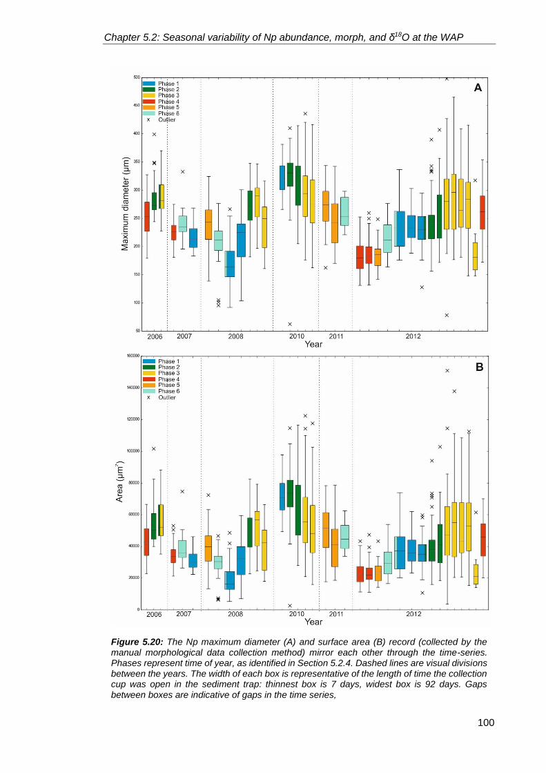
Chapter 5.2: Seasonal variability of Np abundance, morph, and δ18O at the WAP
100
Figure 5.20: The Np maximum diameter (A) and surface area (B) record (collected by the manual morphological data collection method) mirror each other through the time-series. Phases represent time of year, as identified in Section 5.2.4. Dashed lines are visual divisions between the years. The width of each box is representative of the length of time the collection cup was open in the sediment trap: thinnest box is 7 days, widest box is 92 days. Gaps between boxes are indicative of gaps in the time series,

Chapter 5.2: Seasonal variability of Np abundance, morph, and δ18O at the WAP
101
Table 5.8: Correlation (r) and slope of regression values between maximum diameter and surface area measurements (manual data collection method) 32 samples of the time series (four samples with less than 15 specimens/sample were removed following Section 5.2.2). Number of specimens in each sample and the r value at 95% statistical significance are also included in table.
Date Correlation r value at
0.05 significance
Count Slope of
regression
25/01/2006 0.980 0.250 62 0.804
11/11/2006 0.969 0.456 17 0.855
25/11/2006 0.982 0.304 38 0.819
25/01/2007 0.969 0.250 63 0.852
16/05/2007 0.968 0.456 17 0.877
16/09/2007 0.959 0.444 18 0.816
23/03/2008 0.988 0.304 39 0.86
16/06/2008 0.987 0.273 55 0.791
01/08/2008 0.988 0.288 48 0.868
16/09/2008 0.994 0.400 22 0.833
18/11/2008 0.977 0.273 49 0.833
06/01/2009 0.991 0.444 18 0.85
18/10/2010 0.981 0.250 64 0.803
28/10/2010 0.992 0.250 63 0.822
19/11/2010 0.983 0.250 63 0.903
17/12/2010 0.983 0.250 62 0.836
31/12/2010 0.982 0.250 62 0.866
08/03/2011 0.983 0.288 43 0.888
23/03/2011 0.995 0.400 23 0.904
23/01/2012 0.990 0.288 46 0.826
08/02/2012 0.983 0.304 42 0.807
16/05/2012 0.976 0.349 29 0.915
17/07/2012 0.990 0.381 24 0.828
16/09/2012 0.968 0.273 49 0.852
16/10/2012 0.980 0.304 38 0.863
08/11/2012 0.979 0.250 56 0.778
18/11/2012 0.985 0.250 65 0.76
02/12/2012 0.984 0.250 64 0.772
09/12/2012 0.986 0.273 50 0.78
23/12/2012 0.985 0.273 50 0.807
30/12/2012 0.989 0.250 64 0.819
27/01/2013 0.974 0.250 61 0.766

Chapter 5.2: Seasonal variability of Np abundance, morph, and δ18O at the WAP
102
histograms with the accompanying Anderson-Darling p-values in Figure 5.21 (as log-
transformed maximum diameter).
When the log-transformed MD data are plotted on a Normal Probability plot (normal Q-
Q plots in Appendix 2) and tested for normality, four out of the 36 sets of samples display
a non-normal distribution. This accounts for 11% of the entire dataset. The non-normally
distributed samples are highlighted in Figure 5.21. The dominance of a unimodal
distribution in 89% of the samples suggests that shell size can be represented by the
log-transformed maximum diameter with confidence. As discussed in Moller et al. (2013)
the log-transformed maximum diameter can be used as a measure of the mean MD of
the population because it is not affected by sample size, thereby avoiding the possibility
of skewed results deriving from small sample sizes. Levene’s test for Equality of
Variances was carried out on the log-transformed MD dataset covering the entire time-
series (2006-2013) to investigate the consistency of the variance (dispersion of data
points). The Levene’s test reveals statistically significant difference (p = <0.0001, at 0.05
significance) indicating inter-annual variability in the range of test size between 2006 and
2013. The presence/absence of intra-annual variability can be determined by applying a
Levene’s test to portion of the log-transformed MD dataset that belongs to 2012 (the
most complete trap record).The test reveals a significant difference (p = <0.0001, at 0.05
significance) indicating intra-annual variability in the range of test size.
p=0.34 p=0.03 p=0.51
p=0.26 p=0.25 p=0.52
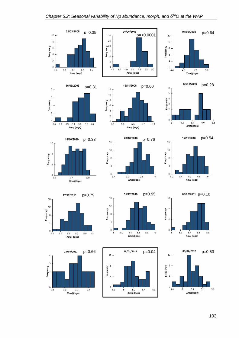
Chapter 5.2: Seasonal variability of Np abundance, morph, and δ18O at the WAP
103
p=0.35 p=<0.0001
p=0.64
p=0.31 p=0.60 p=0.28
p=0.33 p=0.76 p=0.54
p=0.79 p=0.95
p=0.66 p=0.04 p=0.53
p=0.10

Chapter 5.2: Seasonal variability of Np abundance, morph, and δ18O at the WAP
104
p=0.49 p=0.09 p=0.74
p=0.08 p=0.08 p=0.31
p=0.30 p=0.12 p=0.19
p=0.28 p=0.02
Figure 5.21: Histograms of the log-transformed maximum diameter values of each samples including the Anderson-Darling Normality test-derived p values.. Non-normally distributed datasets are highlighted with black outline.

Chapter 5.2: Seasonal variability of Np abundance, morph, and δ18O at the WAP
105
Results of Principal Component Analyses
The distributions of the four size-invariant morphological parameters (circularity ratio,
box ratio, elongation ratio and compactness coefficient, Table 5.9), which relate to body
shape, were analysed within each sample (manually collected dataset) using principal
component analysis (PCA) (representative sample shown in Figure 5.22). The visual
representation of the PCA can reveal statistically defined clusters of points that can be
attributed to different morphotypes (Figure 5.22). The presence of multiple clusters and
thus multiple morphotypes can also be supported by undertaking Anderson-Darling test
for normality on the first principle component site scores. A non-normal distribution of the
scores suggest multiple morphotypes within a sample, as seen for example in the
16/09/2007 sample (Figure 5.22). Fourteen of the 32 samples display a non-normal
distribution (Table 5.10) indicating that in those 14 samples multiple morphotypes are
Table 5.9: Definition of secondary morphological parameters, which relate to body shape as opposed to body size are derived from measured parameters (after Moller et al. 2013).
Primary parameters Secondary morphological parameters
p Perimeter Rc = A*4*π / p2 Circularity ratio
A Area Re = 2*√A / (Xmax *√π) Elongation ratio
Xmax Maximum diameter B = Xmin/Xmax Box ratio
Xmin Minimum diameter C = p / 2*√π*√A Compactness coefficient
Figure 5.22: PCA biplot of 16/09/2007 normalised size-invariant morphological variables showing clustering of data points (blue circles). F1 is the first principle component axis. F2 is the second principle component axis. Brackets show the proportion of the variance explained by each component axis.

Chapter 5.2: Seasonal variability of Np abundance, morph, and δ18O at the WAP
106
present. To assess the relationship between the body size and the body shape the log-
transformed maximum diameter of each specimen was plotted against the first principal
component scores (for example, Figure 5.23, rest in Appendix 3). The two parameters
correlated with each other in 12 of the 32 samples (Table 5.10) (four samples were
discounted from the total of 36 samples due to the number of specimens being less than
15, see Section 5.2.2). The linear correlation coefficients (r values) were between −0.48
and 0.51, which suggests variable relationship between shape and size, i.e. positive
correlation – as a specimen becomes larger it also becomes more rounded or in the case
of negative correlations the specimens were more rounded the smaller they were. The
result from the largest sample is shown in Figure 5.23.
To assess the relationship between the shape and the size parameters in each set of
samples, PCA was performed on the mean values of the log-transformed maximum
diameter and the mean values of each size-invariant morphological parameter of the 36
sets of data (Figure 5.24, Table 5.11). Three principal components explain 99.9% of the
variability in the dataset. The first principal component (F1) is strongly correlated with the
size-invariant variables (Table 5.11). It increases with increasing circularity, elongation
and box ratio and increases with decreasing compactness coefficient. This suggests that
these four criteria covary. F1 can therefore be viewed as a measure of circularity ratio,
elongation ratio, box ratio, and compactness coefficient. F1 correlates most strongly with
elongation ratio and box ratio with correlation coefficients of 0.819 and 0.792 (Table 5.11)
indicating that the first principal component is primarily a measure of these two
Figure 5.23: Relationship between log-transformed maximum diameter (ln Xmaj) and the first principle component scores of the PCA conducted on the normalised size-invariant morphological values. Figure shown is 18/11/2012 sample which contains the largest number of specimens analysed.

Chapter 5.2: Seasonal variability of Np abundance, morph, and δ18O at the WAP
107
Date Count Anderson-Darling
p value
Xmaj(ln)-Size-invariant PCA F1 r
value
25/01/2006 62 0.225 -0.118
11/11/2006 17 0.517 -0.110
25/11/2006 38 0.503 -0.213
25/01/2007 63 0.203 0.043
16/05/2007 17 0.308 -0.083
16/09/2007 18 0.045 -0.035
23/03/2008 39 0.358 -0.216
16/06/2008 55 0.030 -0.338
01/08/2008 48 0.001 0.442
16/09/2008 22 0.373 0.081
18/11/2008 49 0.390 0.037
06/01/2009 18 0.114 0.262
18/10/2010 64 0.527 -0.480
28/10/2010 63 0.009 -0.324
19/11/2010 63 0.009 0.323
17/12/2010 62 0.054 -0.025
31/12/2010 62 0.029 0.248
08/03/2011 43 <0.0001 0.124
23/03/2011 23 0.180 0.508
23/01/2012 46 0.000 0.046
08/02/2012 42 0.016 -0.214
16/05/2012 29 0.297 0.480
17/07/2012 24 0.006 0.136
16/09/2012 49 0.000 -0.033
16/10/2012 38 0.103 0.010
08/11/2012 56 0.051 -0.291
18/11/2012 65 <0.0001 -0.431
02/12/2012 64 0.151 -0.351
09/12/2012 50 0.539 -0.353
23/12/2012 50 0.051 -0.148
30/12/2012 64 0.011 -0.235
27/01/2013 61 0.004 -0.389
Table 5.10: Mid-date of collection period for sediment trap samples, number of data points per sample, Anderson-Darling p value of significance of the first principle component scores (F1) of the PCA conducted on the normalised size-invariant morphological dataset, and the correlation coefficient (r) calculated between the log-transformed maximum diameter (Xmaj) and the F1. Significant p-values and correlations highlighted in bold.

Chapter 5.2: Seasonal variability of Np abundance, morph, and δ18O at the WAP
108
variables and the observed variability in the dataset is related to changes in elongation
in two dimensions, i.e. how elongate or round the specimens are, which relates to the
ratio between the minor axis and major axis. The second principal component (F2) is
also correlated with circularity ratio, elongation ratio, box ratio, and compactness
coefficient, but to a lesser degree. Strongest correlation is recorded between circularity
ratio and F2 (-0.641) (Table 5.11), so this component (F2) can be viewed as a measure
of how close to a perfect sphere the specimens are. The third principal component
(Figure 5.25 – F1-F3 biplot) only makes up 17% of the total variability in the dataset in
comparison to the 49% and 33% of contribution of F1 and F2, respectively. However, it
does show a strong positive correlation with maximum diameter (r = 0.840, Table 5.11)
suggesting that this component is a measure of specimen size. The biplot of the PCA
results (Figure 5.26) reveal these strong correlations between the principal components
and the variables. PCA biplots are used mainly to determine groupings of observations
based on the positions of the variables with respect to the principle components. In
Figure 5.24 I find that the observations are scattered across both F1 and F2 and that
observations belonging to the same seasons do not cluster together.
The dataset used for the PCA analysis was separated out based on the
presence/absence of correlation between log-transformed MD and first principal
component scores of PCA on size-invariant morphological parameters (e.g. Figure 5.23)
within a given sample. Two PCAs were carried out on the datasets separated by the
presence/absence of correlation between log-transformed maximum diameter and F1 of
Figure 5.24: PCA biplot (F1-F2 scores) of the mean values of log-transformed maximum diameter and the man values of each size-invariant morphological parameters covering the time series (2006-2013). Seasons are identified as: green-spring, red-summer, orange-autumn, and blue-winter.

Chapter 5.2: Seasonal variability of Np abundance, morph, and δ18O at the WAP
109
the PCA conducted on the normalised size-invariant morphological dataset (Table
5.10). These showed similar results to PCA that was carried out on the dataset which
was not separated by the correlation (Table 5.10) was (Figure 5.26). Neither PCA
analysis show any clear clustering of points based on seasonal separation of the data
(Figure 5.26A, B). Differences arise when the impact of the morphological variables is
Eigenvalues
F1 F2 F3
Eigenvalue 2.469 1.675 0.852
Variability (%) 49.381 33.493 17.031
Cumulative % 49.381 82.874 99.905
Correlations between variables and factors
F1 F2 F3
Circularity ratio 0.753 -0.641 0.147
Elongation ratio 0.819 0.529 -0.220
Box ratio 0.792 0.565 -0.227
Compactness coefficient -0.762 0.628 -0.157
ln Xmaj (µm) 0.153 0.521 0.840
Table 5.11: Eigenvalues and correlation between variables and principle component factors of the PCA run on the mean values values of log-transformed maximum diameter and the mean values of each size invariant morphological parameters of the time series.
Figure 5.25: PCA biplot (F1-F3 scores) of the mean values of log-transformed maximum diameter and the mean values of each size-invariant morphological parameters covering the time series (2006-2013). Seasons are identified as: green-spring, red-summer, orange-autumn, and blue-winter.

Chapter 5.2: Seasonal variability of Np abundance, morph, and δ18O at the WAP
110
considered on the principle components. In the dataset where no correlation exits
between the log-transformed MD and the first principal component scores of PCA on
size-invariant morphological parameters 99% of the variability can be explained by three
principal components (Table 5.11, Figure 5.26A) which is similar to the results of the
PCA analysis conducted on the entire dataset together (Figure 5.24). Correlation
between the morphological variables and the principal components (Table 5.11, Figure
5.26A) is also similar to the relationships identified in the PCA run on the data from the
32 sediment trap samples (Figure 5.24): F1 and F2 correlate strongly with size-invariant
variables, F3 with log-transformed maximum diameter), but the directions of the
correlations are the opposite (Figure 5.26A). In Figure 5.26A (dataset where samples
show no relationship between shape and size) F1 is most strongly correlated with
compactness coefficient and circularity ratio (r = 0.867 and -0.864 respectively),
suggesting that it is a measure of how compact and perfectly spherical a specimen is.
F2 shows similarly strong correlations with elongation ratio and box ratio (r= 0.817 and
0.837), therefore we can consider F2 to be a measure of how elongated a specimen is
in two dimensions (box ratio is equal to the ratio between minimum diameter and
maximum diameter). In the dataset where samples show a significant relationship
between shape and size the first two principal components can explain over 90% of the
variability (Table 5.11). Here F1 is strongly correlated with the size-invariant variables
and F2 with the log-transformed maximum diameter (Figure 5.26B, Table 5.11). Similarly
to the results of the PCA conducted on the entire dataset prior to splitting it up (Figure
5.24) F1 is most strongly correlated with elongation ratio and box ratio (r=0.941 and
0.939, respectively), therefore it can be considered to be a measure of these two
Figure 5.26: PCA biplots of the mean values of of log-transformed maximum diameter and the mean values of each size-invariant morphological parameters belonging to samples where no correlation was found in Table 5.10 (A) and where correlation was identified (B).Seasons are identified as: green-spring, red-summer, orange-autumn, and blue-winter.

Chapter 5.2: Seasonal variability of Np abundance, morph, and δ18O at the WAP
111
variables. F2 is a measure of specimen size as it is only correlated with log-transformed
maximum diameter (r= 0.83). Hence, based on these findings, the results of the PCA
conducted on the original dataset of 36 observations is highly influenced by the samples
where a statistically significant relationship exists between the log-transformed MD
(indicative of specimen size) and the size-invariant morphological parameters (indicative
of shape). The lack of clustering into groups in any of the PCA biplots (Figures
5.24,25,26) indicates that the observed morphological variability (Figure 5.20, Section
5.2.2.3) is related to a combination of environmental parameters acting on the wellbeing
of the foraminifera.
To summarise the findings of this section:
Shell size (expressed as maximum diameter) displays intra-and inter-annual
variability. Mean grey values, an expression of translucency and extent of
calcification, shows intra-annual variability.
Statistical analysis supports the use of log-transformed maximum diameter as a
measure of Np size in a population.
Inter-and intra-annual variability of Np size is supported by statistical analysis.
Multiple morphotypes are identified in 14 out of 32 samples by PCA.
Positive and negative linear correlation between body shape and body size is found
in 12 out of 32 samples.
PCA revealed that size-invariant morphological parameters, particularly elongation
and box ratio exert the greatest influence on body shape.
The results of the PCA conducted on the entire dataset (36 samples) are strongly
influenced by samples where statistically significant correlation exists between body
shape and body size.
The PCA analyses revealed no clustering of data points related to the seasons the
samples derive from suggesting that the morphological variability is the result of a
combination of variable environmental parameters (food availability, temperature, sea
ice, etc).
5.2.2.4 Neogloboquadrina pachyderma stable isotopes
The original goal of the project was to carry out novel single specimen stable isotope
analysis on every sample (sediment trap cup) of the time series to provide a holistic
record of Np stable isotope variability in the polar region of the Antarctic Peninsula. The
variable collection period of the sediment cup and the single specimen analysis could
allow the study of Np stable isotope variability related to short-and longer term
environmental changes as well as the identification of inherent vital offsets (7 day

Chapter 5.2: Seasonal variability of Np abundance, morph, and δ18O at the WAP
112
collection periods).To carry out single specimen stable isotope analysis, a minimum of
15 Np specimens, each weighing a minimum of 5 μg, are needed in each sample (see
Chapter 4). However, some samples contained less than 15 specimens, and/or had
specimens where the majority weighed less than 5 μg each, which prohibited the creation
of a continuous stable isotope record. To overcome the problem, multi-specimen stable
isotope analysis was carried out on the samples where single specimen analysis was
not possible.
Multi-specimen stable isotope analysis
For the multi-specimen stable isotope analysis four to ten specimens were pooled
together from the specific sample to provide approximately 40 μg carbonate for each
analysis.
Approximately 1‰ variability is observed in both the Neogloboquadrina pachyderma
δ18O (δ18Onp) and the δ13C (δ13Cnp) records (Figure 5.27). The δ18Onp record (Figure
5.27A) varies between +2.77‰ (17/07/2012) and +3.71‰ (11/11/2006) and has an
average value of +3.29‰ ± 0.21‰ (one standard deviation) through the time series. The
δ13Cnp record (Figure 5.27B) varies between +0.167‰ (22/02/2012) and +1.02‰
(02/12/2012) with an average value of +0.56‰ ± 0.20‰ (one standard deviation) for the
2006-2013 time series. Anderson-Darling tests for normality reveals that the δ18Onp
dataset is normally distributed (p=0.333), while the δ13Cnp is not normally distributed
(p=0.032) (Figure 5.28) suggesting statistically greater variability within the δ13Cnp record
through time series compared to the δ18Onp record.
Single specimen stable isotope analysis
Single specimen stable isotope analysis was carried out on samples which had >20 Np
specimens. To assess the variability in the single specimen stable isotope records
Levene’s test for Equality of Variances was conducted separately on the oxygen and on
the carbon isotope datasets. The Levene’s test run on the δ18Onp record shows that at
least one of the variances is statistically different from another (p=0.005), which indicates
that there is significant difference between the samples in the dispersion of the δ18Onp
values. δ18Onp values show differences between the seasons (Figure 5.29A). Samples
collected through the austral winter (May-September) have much lower δ18Onp ratios
compared to ones collected during the summer (December-February) months. In
contrast to the δ18Onp record, the Levene’s test undertaken on the δ13Cnp dataset found
no significant difference (p=0.076) between variances, suggesting that the intra-sample
variance is consistent through the time series.

Chapter 5.2: Seasonal variability of Np abundance, morph, and δ18O at the WAP
113
Figure 5.27: Bulk Neogloboquadrina pachyderma stable isotope dataset (A: δ18O, B: δ13C). Error bars: ± 1 standard deviation. AJO: April, July, October.
A
B
A B
p=0.333 p=0.032
Figure 5.28: Relative frequency histogram of bulk δ18Onp (A) and δ13Cnp (B) data sets. Black line represents the expected normal distribution. Anderson-Darling test for normality (results as p-values) revealed a normal distribution for δ18Onp (A) and non-normal distribution for δ13Cnp (B). The latter dataset is skewed towards the lower values.

Chapter 5.2: Seasonal variability of Np abundance, morph, and δ18O at the WAP
114
The range of both stable isotopes vary between the bulk and single specimen analysis.
While the multi-specimen data displays only a 1‰ range in both isotope ratios, a 4‰
and a 2‰ range is recorded in the single specimen δ18Onp and δ13C, respectively (Figure
5.29).
Predicted δ18O calcite equilibrium
To constrain the approximate calcification depth of Neogloboquadrina pachyderma at
Palmer Deep, and to determine any apparent vital effects in the oxygen isotope record,
the equilibrium δ18O (δ18Oeq) values can be calculated (Figure 5.30) using the following
equation derived from Kim and O’Neil (1997) and Peeters et al., (2002):
𝛿18𝑂𝑒𝑞 = 25.778 − 3.333 × (43.704 + 𝑇)0.5 + 𝛿18𝑂𝑠𝑤(𝑃𝐷𝐵) Equation 7.
where T is the seawater temperature and the δ18Osw(PDB) is the δ18O of seawater
expressed with respect to the Pee Dee Belemnite (PDB) scale. A correction for vital
effects, which is related to temperature variability (Bausch et al., 1997), was not applied
in the δ18Oeq calculation as one of the objectives of the δ18Onp assessment was the
evaluation of vital effects. This can only be achieved if the δ18Onp and δ18Oeq
measurements are compared without any vital effect correction factor. δ18Osw is usually
expressed with respect to the Standard Mean Ocean Water (SMOW) scale and the
conversion to PDB is achieved through the following (Bemis et al., 1998):
𝛿18𝑂𝑠𝑤(𝑃𝐷𝐵) = 0.9998 × 𝛿18𝑂𝑆𝑀𝑂𝑊 − 0.2 Equation 8.
A number of factors need to be considered before the δ18Oeq values can be calculated.
In the polar regions, especially along the WAP, annual SST variability is small (~2°C)
compared to the midlatitudes, and temperatures are generally low (-1.5 to 1.5°C), which
means that temperature only has a small influence on the density and δ18O of the
seawater (δ18Osw) (Meredith et al., 1999). Instead, salinity drives the annual variability of
density and δ18Osw. At the WAP the input of glacial meltwater and sea ice formation/melt
determines the salinity-δ18Osw relationship. Glacial ice is isotopically very low (as low as
−50‰) (Weiss et al., 1979, Rozanski et al., 1993), hence relatively small glacial runoff
events can affect δ18Osw. Sea ice formation (and the accompanying brine rejection) and
sea ice melt (freshwater release) can alter the salinity of the seawater considerably, while
having little impact on the δ18Osw (Meredith et al., 1999) resulting in a non-linear salinity-
δ18Osw relationship in the high latitudes (Bausch et al., 1997). Therefore it is important,
that we use δ18Osw values which derive from the same locality as the Np specimens and
that the seasonal variability in δ18Osw is captured by actual measurements when
calculating δ18Oeq values. However, no δ18Osw values are available for the winter season
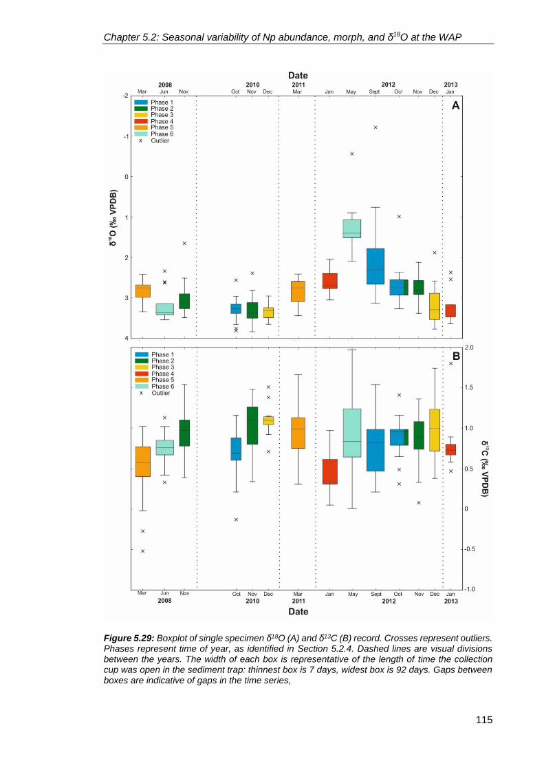
Chapter 5.2: Seasonal variability of Np abundance, morph, and δ18O at the WAP
115
Figure 5.29: Boxplot of single specimen δ18O (A) and δ13C (B) record. Crosses represent outliers. Phases represent time of year, as identified in Section 5.2.4. Dashed lines are visual divisions between the years. The width of each box is representative of the length of time the collection cup was open in the sediment trap: thinnest box is 7 days, widest box is 92 days. Gaps between boxes are indicative of gaps in the time series,

Chapter 5.2: Seasonal variability of Np abundance, morph, and δ18O at the WAP
116
at any depth, and only surface water data is available for the majority of the year. Depth-
integrated δ18Osw data (collected by CTD) are only available from annual PAL-LTER
cruises conducted in January of each year. To compensate for the lack of year-round
δ18Osw data World Ocean Atlas 13 Salinity (Zweng et al., 2013) data were used to
calculate expected δ18Osw values for the period between January and October using the
following equation:
𝛿18𝑂𝑠𝑤 = 0.3387 × 𝑆 − 11.796 Equation 9.
Where S is salinity and δ18Osw is the δ18O of seawater calculated with respect to SMOW.
The equation is determined from observed relationship between δ18Osw and salinity
(Meredith et al., 2017). An alternative δ18Osw equation (Equation 10) was used to
calculate δ18Osw for the period between October and December. This is due to the
introduction of glacial and sea ice melt into the surface water during the spring. Only
surface values (0-50 m) were calculated for the October-December period as only
surface water (0-50 m) δ18Osw measurements exist for this period.
𝛿18𝑂𝑠𝑤 = 0.0458 × 𝑆 − 1.8883 Equation 10.
The calculated δ18Osw values were used to calculate the δ18Oeq values together with
World Ocean Atlas 13 Temperature data (Locarnini et al., 2013) using Equation 7 and 8.
The existence of measured (as opposed to calculated) δ18Osw depth profile means that
summer conditions are represented well in the δ18Oeq calculations (Figure 5.30). Due to
the lack of winter δ18Osw data, and the lack of δ18Osw data below the surface between
October and January, no winter (at any depths) and below surface spring δ18Oeq values
are calculated (Figure 5.31C).
The predicted isotopic equilibrium of δ18O of calcite shows distinct seasonal variability at
the surface and at depth, ranging from +2.83‰ to +3.64‰ at 0 m, and from +3.16‰ to
+3.55‰ at 100 m water depth (Figure 5.30). The larger seasonal difference in the surface
compared to deeper water is expected due to the greater variability in water temperature
and salinity driven by the annual growth and melt of sea ice (Figures 5.31A, B). The
predicted δ18Oeq values at depth (50-100 m) show similar patterns to the measured
δ18Onp values between October and April (spring to early autumn). The δ18Oeq and δ18Onp
values diverge in late autumn and the dissimilarity continues during winter. Equilibrium
δ18O at surface and at depth converge in late autumn, following the temperature profile
indicative of the development of deeper mixing. This convergence of δ18Oeq between
surface and depth is accompanied by lower δ18Onp, which is up to 0.7‰ lower than δ18Oeq
values at 0 m and 50 m by the winter.

Chapter 5.2: Seasonal variability of Np abundance, morph, and δ18O at the WAP
117
Oxygen isotopes
The multi-specimen δ18Onp record shows a 1‰ seasonal amplitude with lowest values
between May and September (late autumn to winter) and highest values between
November and January (late-spring to mid-summer) (Figure 5.32A). The single specimen
δ18Onp values show a similar pattern; however, the amplitude of difference between
winter and summer values is larger, at ~2‰. Single specimen δ18Onp represents an
average δ18O value that is acquired through the life-span of the individual foraminifera
which can vary from several weeks to months depending on environmental conditions
(Kozdon et al., 2009). Therefore within a sediment cup each single specimen δ18Onp
measurement represents conditions specific to that individual resulting in a range of
values within a cup. Multi-specimen δ18Onp analysis averages out the within-sample
variance deriving from the probability that the specimens experienced different
environmental conditions. Comparison of the mean single specimen δ18Onp and the multi-
Figure 5.30: Equilibrium δ18O depth profiles calculated from direct δ18Osw observations from Meredith et al. (2016) (blue lines) and from calculated δ18Osw data based on WOA13 salinity measurements (grey lines). Depth range of Nps calcification indicated by grey box. Grey horizontal line represents depth of the sediment trap.

Chapter 5.2: Seasonal variability of Np abundance, morph, and δ18O at the WAP
118
Figure 5.31: Weekly
averaged and time
shifted time series
δ18O record (black
lines: average values
of 2006-2012 period;
colour dots: individual
years). A) Satellite-
derived weekly SST,
average SST (black
line) and WOA13
monthly temperature
at 50 m and 100 m
water depths (grey
dashed lines). B)
WOA13 monthly
salinity record at
surface (black line),
50 m and 100 m (grey
dashed lines) water
depths. C) Multi-
specimen Nps δ18O
record, δ18Oeq values
at surface, 50m and
at 100 m water
depths. D) Satellite-
derived weekly sea
ice concentration
(SIC) and average
SIC through the time
series. E) Measured
chlorophyll α
concentration at
64.78°S, 64.07°W. F)
Organic carbon flux
record. G) Nps flux
record (extremely
high flux of October
2010 removed from
calculation of
average).
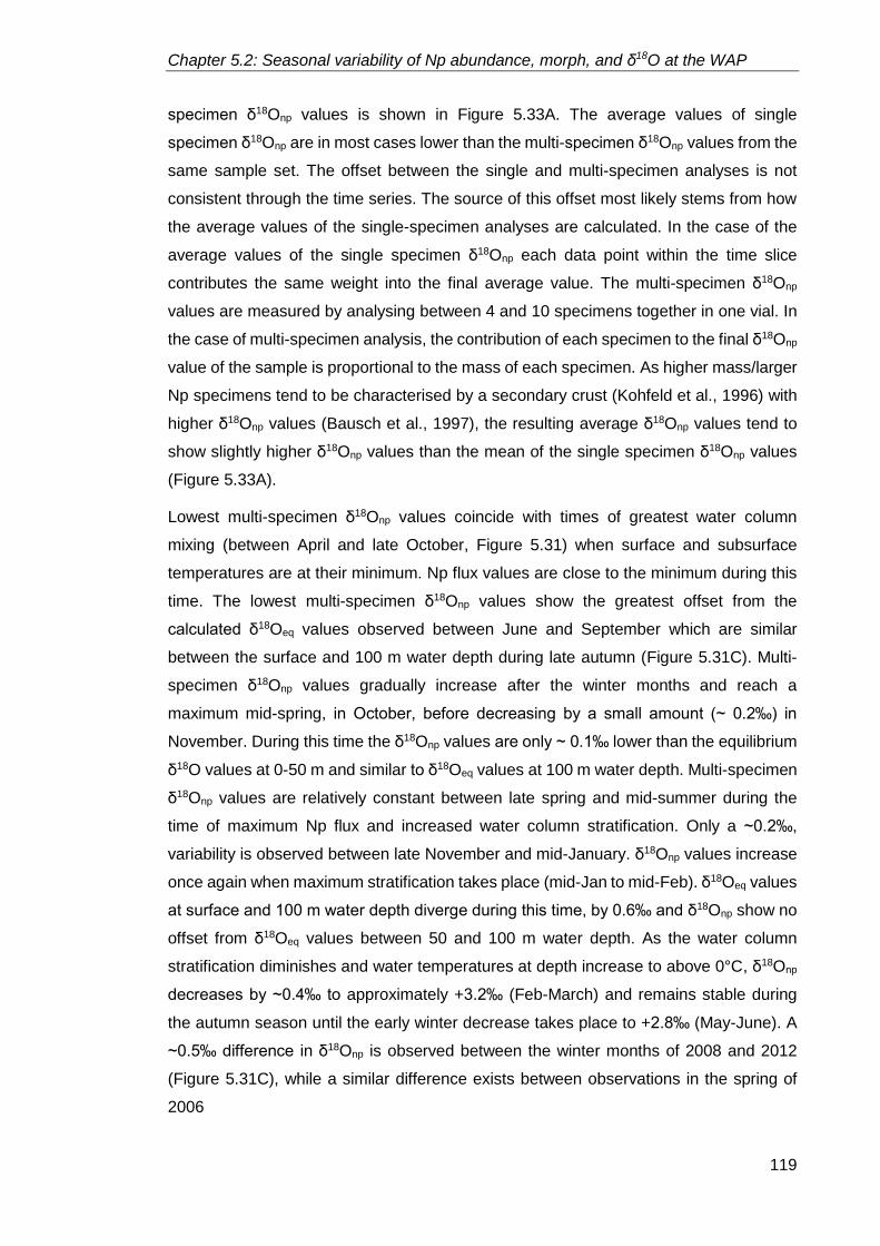
Chapter 5.2: Seasonal variability of Np abundance, morph, and δ18O at the WAP
119
specimen δ18Onp values is shown in Figure 5.33A. The average values of single
specimen δ18Onp are in most cases lower than the multi-specimen δ18Onp values from the
same sample set. The offset between the single and multi-specimen analyses is not
consistent through the time series. The source of this offset most likely stems from how
the average values of the single-specimen analyses are calculated. In the case of the
average values of the single specimen δ18Onp each data point within the time slice
contributes the same weight into the final average value. The multi-specimen δ18Onp
values are measured by analysing between 4 and 10 specimens together in one vial. In
the case of multi-specimen analysis, the contribution of each specimen to the final δ18Onp
value of the sample is proportional to the mass of each specimen. As higher mass/larger
Np specimens tend to be characterised by a secondary crust (Kohfeld et al., 1996) with
higher δ18Onp values (Bausch et al., 1997), the resulting average δ18Onp values tend to
show slightly higher δ18Onp values than the mean of the single specimen δ18Onp values
(Figure 5.33A).
Lowest multi-specimen δ18Onp values coincide with times of greatest water column
mixing (between April and late October, Figure 5.31) when surface and subsurface
temperatures are at their minimum. Np flux values are close to the minimum during this
time. The lowest multi-specimen δ18Onp values show the greatest offset from the
calculated δ18Oeq values observed between June and September which are similar
between the surface and 100 m water depth during late autumn (Figure 5.31C). Multi-
specimen δ18Onp values gradually increase after the winter months and reach a
maximum mid-spring, in October, before decreasing by a small amount (~ 0.2‰) in
November. During this time the δ18Onp values are only ~ 0.1‰ lower than the equilibrium
δ18O values at 0-50 m and similar to δ18Oeq values at 100 m water depth. Multi-specimen
δ18Onp values are relatively constant between late spring and mid-summer during the
time of maximum Np flux and increased water column stratification. Only a ~0.2‰,
variability is observed between late November and mid-January. δ18Onp values increase
once again when maximum stratification takes place (mid-Jan to mid-Feb). δ18Oeq values
at surface and 100 m water depth diverge during this time, by 0.6‰ and δ18Onp show no
offset from δ18Oeq values between 50 and 100 m water depth. As the water column
stratification diminishes and water temperatures at depth increase to above 0°C, δ18Onp
decreases by ~0.4‰ to approximately +3.2‰ (Feb-March) and remains stable during
the autumn season until the early winter decrease takes place to +2.8‰ (May-June). A
~0.5‰ difference in δ18Onp is observed between the winter months of 2008 and 2012
(Figure 5.31C), while a similar difference exists between observations in the spring of
2006
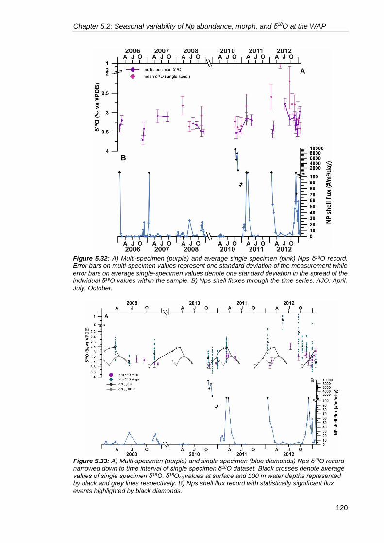
Chapter 5.2: Seasonal variability of Np abundance, morph, and δ18O at the WAP
120
Figure 5.32: A) Multi-specimen (purple) and average single specimen (pink) Nps δ18O record. Error bars on multi-specimen values represent one standard deviation of the measurement while error bars on average single-specimen values denote one standard deviation in the spread of the individual δ18O values within the sample. B) Nps shell fluxes through the time series. AJO: April, July, October.
Figure 5.33: A) Multi-specimen (purple) and single specimen (blue diamonds) Nps δ18O record narrowed down to time interval of single specimen δ18O dataset. Black crosses denote average values of single specimen δ18O. δ18Oeq values at surface and 100 m water depths represented by black and grey lines respectively. B) Nps shell flux record with statistically significant flux events highlighted by black diamonds.
A
B
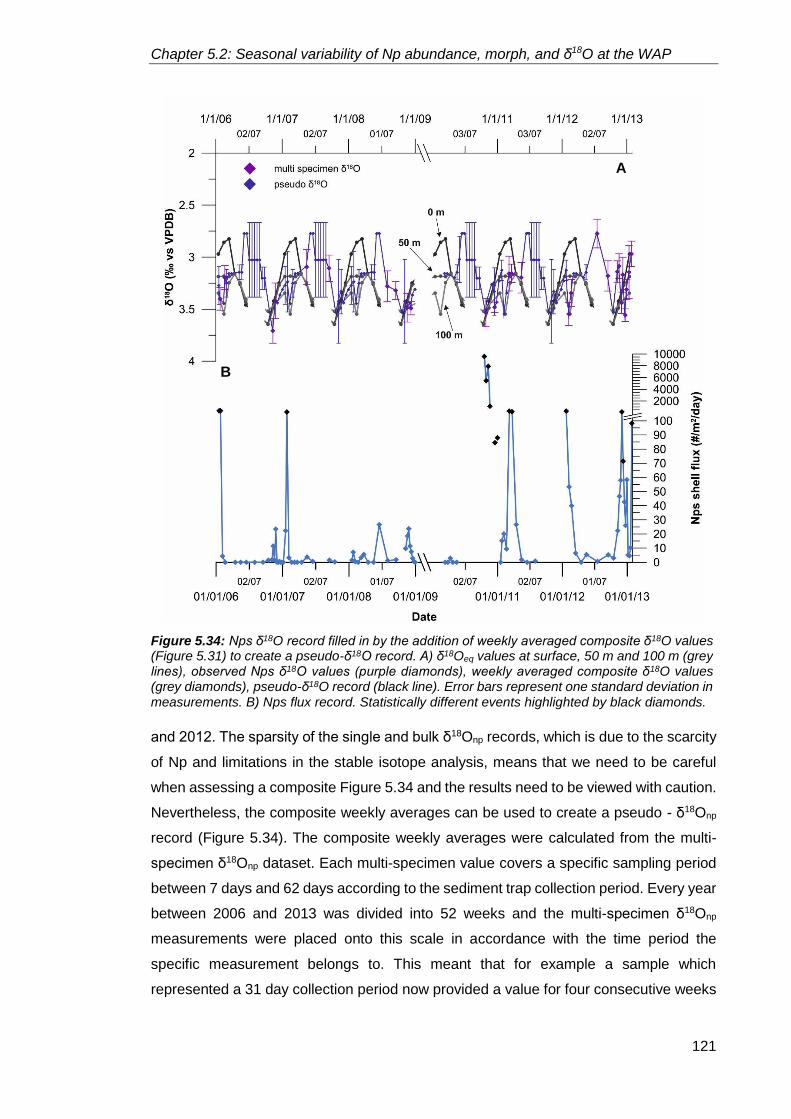
Chapter 5.2: Seasonal variability of Np abundance, morph, and δ18O at the WAP
121
and 2012. The sparsity of the single and bulk δ18Onp records, which is due to the scarcity
of Np and limitations in the stable isotope analysis, means that we need to be careful
when assessing a composite Figure 5.34 and the results need to be viewed with caution.
Nevertheless, the composite weekly averages can be used to create a pseudo - δ18Onp
record (Figure 5.34). The composite weekly averages were calculated from the multi-
specimen δ18Onp dataset. Each multi-specimen value covers a specific sampling period
between 7 days and 62 days according to the sediment trap collection period. Every year
between 2006 and 2013 was divided into 52 weeks and the multi-specimen δ18Onp
measurements were placed onto this scale in accordance with the time period the
specific measurement belongs to. This meant that for example a sample which
represented a 31 day collection period now provided a value for four consecutive weeks
Figure 5.34: Nps δ18O record filled in by the addition of weekly averaged composite δ18O values (Figure 5.31) to create a pseudo-δ18O record. A) δ18Oeq values at surface, 50 m and 100 m (grey lines), observed Nps δ18O values (purple diamonds), weekly averaged composite δ18O values (grey diamonds), pseudo-δ18O record (black line). Error bars represent one standard deviation in measurements. B) Nps flux record. Statistically different events highlighted by black diamonds.
A
B
Chapter 5.2: Seasonal variability of Np abundance, morph, and δ18O at the WAP
122
(see Figure 5.31C). When multiple data points are available for the same 7-day period
an average value is calculated. The spread of the δ18Onp values during each year and
the annual variability remains stable (Figure 5.33A) which means that by combining the
multi-specimen δ18Onp record with the weekly averaged composite δ18Onp values from
Figure 5.31C - which are placed into the time series where no multi-specimen δ18Onp is
available - it is possible to complete the existing δ18Onp time series (Figure 5.34A).
5.2.3 A typical year at Palmer Deep
In order to describe the environmental parameters and their relation to each other I
averaged the same weeks in the six different years (2006, 2007, 2008, 2010, 2011, and
2012) to make a composite year, described by weekly averages. The resulting model
can be divided into six distinct phases (Figure 5.35) based on the intra-annual trend of
the Neogloboquadrina pachyderma (Np) flux, as well as by the intra-annual trends shown
by the environmental variables. Note that this averaging across the six years masks the
inter-annual variation (e.g. timing of peak chlorophyll α concentrations varies year-on-
year, timing of sea ice retreat varies year-on-year).
5.2.3.1 Phase 1 – Winter sea ice season
Phase 1 is defined by the lowest Np values of the year (Figure 5.35F), the onset of winter
sea ice presence, peak Sea Ice Concentration (SIC), and subsequent reduction to ~20%
SIC (Figure 5.35C). Sea ice occurs between July and October every year between 2006
and 2013 (Figure 5.35C). On average SIC peaks at the end of winter, during September;
however, variability is found between the years. For example, maximum SIC is reached
in August in 2007 compared to late October in 2006. Peak SIC rarely reaches 100% in
the region, averaging around 70% between 2006 and 2013 (Figure 5.35C). Between July
and October a SST minimum (Figure 5.35A) is associated with sea ice. By the end of
the winter, sea water at 100 m water depth is warmer than at the surface due to the
upward heat flux from the modified UCDW which is present deeper than the sampling
depth (Smith and Klinck, 2002). At the same time, salinity at depth (100 m), is increased
(Figure 5.35B) due to brine rejection during sea ice formation (Meredith et al., 2004),
which also contributes to the deepening of the mixed layer and the erosion of the
stratification. This period of sea ice presence between July and October coincides with
the lowest organic carbon and nitrogen fluxes (close to zero mg/m2/day) (Figure 5.35E).

Chapter 5.2: Seasonal variability of Np abundance, morph, and δ18O at the WAP
123
A
B
C
D
E
F
Figure 5.35: Legend as in Figure 5.13 in Section 5.2.2.1. Dashed vertical lines represent the identified phases in section 5.23.

Chapter 5.2: Seasonal variability of Np abundance, morph, and δ18O at the WAP
124
5.2.3.2 Phase 2 - Sea ice break up season
The sea ice break up season is defined as a period of increasing Np flux (Figure 5.35F),
decreasing SIC, from ~20% to zero (Figure 5.35C), and concomitant increasing
Chlorophyll α (Chl α) concentration, from zero to ~3 mg/m3 (Figures5.35D). Towards the
end of October SIC decreases (Figure 5.35C) and becomes more intermittent (Figure
5.35C, section 5.2.2.1) relating to changes in wind patterns (Meredith et al., 2017).
Salinity at the surface and at 100 m water depth decreases by ~0.2 PSU following Phase
1 (Figure 5.35B), while SST and water temperature at 50 m increases in step with the
decreasing water temperature at 100 m water depth (Figure 5.35A). This change in the
water temperature across the 100 m water profile allows the mixed layer to begin to
dissipate. The start of the shallow stratification of the water column and the release of
nutrients from sea ice and glacial melt provides an ideal setting for diatom blooms. As a
result Chl α concentration steadily rises to during this phase (Figure 5.35D). An increase
in organic carbon flux from 0 to ~5 mg/m2/day (Figure 5.35E) is also observed during this
period. The timing of the development of this spring diatom bloom (November onwards)
is also documented by satellite-derived Chl α and pigment biomass records (Smith et al.,
2008).
5.2.3.3 Phase 3 – Summer season
The summer season is defined by high Np flux (Figure 5.35F) and, steadily increasing
SST (Figure 5.35A) and the complete disappearance of sea ice by the end of November
(Figure 5.35C). During this phase between late November and mid-January SST
continues to increase, reaching above 1°C, and water temperature at 100 m water depth
continues to decrease, eventually equalling temperatures at 50 m depth by the end of
December (Figure 5.35A). This increase in SST is accompanied by a steady decrease
in surface water salinity (Figure 5.35B) due to glacial melt as air and ocean both warm.
A result of the changes in temperature and salinity is the strengthening of the
stratification of the water column at shallow depths (0-50 m). The melt of the sea ice and
the development of the shallow stratification leads to increased primary productivity,
which is reflected in the Chl α concentration (Figure 5.35D). Chl α concentration reaches
its peak (~7 mg/m3 on average) during this phase and remains steadily high during the
summer months (Figure 5.35D). As a result of increased primary productivity organic
carbon flux also increases by the end of this period (mid-January), reaching ~21
mg/m2/day in January (Figure 5.35E). Inter-annual variability can be seen in both the Chl
α concentration and organic carbon flux record during this phase. Chl α values vary from
1 to 29 mg/m3 between 2006 and 2012 and show sudden, sharp increases even within

Chapter 5.2: Seasonal variability of Np abundance, morph, and δ18O at the WAP
125
individual years (Figure 5.35D), reflecting the rapid response of diatom blooms to
changes in environmental drivers. Organic carbon flux varies in a similar fashion to Chl
α, with values ranging from 2 to 65 mg/m2/day between November and January (Figure
5.35E), and sudden increases occur concomitantly with the Chl α concentration record.
5.2.3.4 Phase 4 - Late summer season
The late summer season is defined by decreasing Np flux (Figure 5.35F), increasing
organic carbon flux (Figure 5.35E) and continuously increasing SST (Figure 5.35A).
Between mid-January and mid-February SST reaches a maximum of ~1.5°C and
temperatures at 100 m water depth continue to decrease leading to maximum
stratification by mid-February (Figure 5.35A). This period of the year is characterised by
the lowest surface salinities (33.6 PSU) (Figure 5.35B) due to the input of glacial
meltwater from the coastal regions. Salinity at 50 m and 100 m water depth begins to
increase (Figure 5.35B) which further strengthens the water column stratification. Chl α
concentration remains steady on average between 4 and 6 mg/m3 although inter-annual
variability is prominent in the record (Figure 5.35D). Sustained primary productivity and
the increased SST lead to a steady increase in the organic carbon flux, reaching a peak
of ~ 40mg/m2/day (Figure 5.35E) by mid-February.
5.2.3.5 Phase 5 - Autumn season
Autumn is defined by increasing Np flux (Figure 5.35F), decreasing carbon flux (Figure
5.35E) and decreasing SST (Figure 5.35A). During the second half of February
stratification decreases as SST starts to cool and water temperature at 50 and 100 m
depths begins to increase (Figure 5.35A). The weakening of the water column
stratification during this time is further driven by the increase in surface salinity and
decrease in salinity at 100 m water depth (Figure 5.35B). The early part of this phase is
characterised by another peak in chlorophyll α concentration (to over 6 mg/m2) which is
then followed by a steady decrease reaching values close to 0 by the end of this phase
in April (Figure 5.35D). The early peak in Chl α concentration is accompanied by a high
organic carbon flux of ~30-40 mg/m2/day (Figure 5.35E). The organic carbon flux also
begins to decrease towards the end of the phase but in a more gradual manner than the
Chl α concentration values. These shifts in Chl α concentration and organic carbon flux
values coincide with the falling SST and dissipating stratification.
5.2.3.6 Phase 6 – Early winter season
The early winter season is defined by the second lowest Np flux values (Figure 5.35F),
further decreasing organic carbon flux (Figure 5.35E) and SST (Figure 5.35A) values.

Chapter 5.2: Seasonal variability of Np abundance, morph, and δ18O at the WAP
126
SST decreases as heat is lost to the atmosphere (Meredith et al., 2004) leading to the
erosion of the stratification of the previous summer and to the deepening of the mixed
layer. By the end of April, water column stratification completely disappears as SST in
the upper 100 m of the water column equals out at ~0.5°C (Figure 5.35A). Similarly,
surface salinity and salinity at 50 m and 100 m water depths become equal at ~ 34 PSU
(Figure 5.35B) as a result of greater and deeper vertical mixing during this time. During
this period organic carbon flux gradually reduces and reaches base levels close to zero
by May (Figure 5.35E). By the end of this phase conditions are suitable for sea ice
formation.
5.2.4 Annual flux patterns: What controls foraminiferal flux in the high
latitudes?
Fluxes of Np, organic carbon and organic nitrogen are highest between November and
February (phase 2-4, Figure 5.35E,F). Primary production and thus the marine
ecosystem (e.g. phytoplankton, krill, fish, and larger marine organisms) on the
continental shelf of the WAP is primarily driven by the seasonal cycle of sea ice, light
availability (insolation), and atmospheric and oceanographic circulation (Smith et al.,
1995; Prézelin et al, 2000; Prézelin et al., 2004, Ducklow et al., 2007). During November
to February, the Palmer Deep LTER sediment trap is located within the outer marginal
ice zone (the outer edge of the seasonal sea ice), which is an area of high primary
production (Smith and Nelson, 1985, Smiths et al., 2008), and where the availability of
nutrients and the physical properties of the water column vary both temporally and
spatially (Smith et al., 1995) in turn affecting biological communities. The extent of the
sea ice off the shore of the WAP (and thus the location of the MIZ) shows high inter-
annual variability (Figure 5.35C) which leads to the variation observed in the onset of
primary production (Ducklow et al., 2007). Np flux at the mooring site shows a close
relationship with Chl α concentrations (Figure 5.12, and 5.35), showing the importance
of food availability for the Np fluxes.
Neogloboquadrina pachyderma shell flux shows two peaks during the year (Figure
5.35F). The first peak coincides with the sea ice melt, increasing solar insolation, the
development of the spring chlorophyll bloom and the onset of water column stratification
(phases 2 and 3). The second peak occurs around the time of maximum annual SST
and surface salinity, when the water column is fully stratified (phase 5). Spearman’s
Correlation tests undertaken on the Np flux and the environmental variables (Section
5.2.2.2, Table 5.5) only identified statistically significant correlations between Np flux and

Chapter 5.2: Seasonal variability of Np abundance, morph, and δ18O at the WAP
127
organic carbon and organic nitrogen flux. However, statistically significant correlation
was also found between Chl α and organic carbon and nitrogen flux.
Chlorophyll α concentration reaches an early maximum between the end of November
and early December when sea ice has retreated sufficiently and the surface ocean has
begun to stratify (phases 2 and 3, Figure 5.35C, D). The development of the spring bloom
coincides with the increase of Np flux (Figure 5.35E). Chlorophyll α concentrations
remain above 5 mg/m3 between December and March (phases 3-5). The early part of
phase 3 coincides with Np flux levels which are reduced and Corg and Norg flux values
which are stable (Figure 5.35D,E). From January onwards (late phase 3), Corg and Norg
increases rapidly, while Np flux reaches peak levels. By phase 3 sea ice typically
disappears from the shelf area, and stratification is increased. The sustained presence
of Chl α during this time can be attributed to glacial melt as it carries nutrients from the
land and to micro-and macronutrients (iron, nitrate, and phosphate) from UCDW getting
mixed into surface waters (Smiths et al., 1995; Ducklow et al., 2007; Martinson et al.,
2008; Smith et al., 2008).
Although Chl α levels remain above 5 mg/m3 until the end of summer (phase 4), and Corg
and Norg values consistently increase from mid-January to mid-February, Np flux drops
off from its peak level to values similar those observed in spring (early phase 2). During
phase 4 stratification becomes stable and SST increases rapidly (Figure1A). The second
Np flux peak (Figure 5.35F) takes place after Chl α and Corg and Norg reach their
maximum and SST is at its peak (phase 5).
From those years in the record when the temporal coverage of water column
sedimentation is almost complete, it is evident that Np shell flux displays a bimodal
pattern, similar to that observed in the North Atlantic by Tolderlund and Bé (1971) and
Jonkers et al. (2010). This suggests that permanent stratification does not control shell
flux, rather the development of optimum growing conditions (food availability, timing of
sea ice retreat and maximum SST). This bimodal flux pattern contrasts with studies
conducted in the northern end of the AP, the Weddell Sea (Donner and Wefer, 1994)
and in the Arctic, where a single summer peak is observed (Kohfeld et al., 1996; Bausch
et al., 1997; Simstich et al., 2003).
Spearman’s Rank Correlation tests (section 5.2.2.2, Table 5.5) reveal that Np flux is only
significantly positively correlated with organic carbon and nitrogen flux values (Table
5.5). In turn, organic carbon and nitrogen flux values show positive correlation with SST
and chlorophyll concentration, and negative correlation with SIC, meaning that with
increasing SST and Chl α and decreasing sea ice, biological productivity is increased

Chapter 5.2: Seasonal variability of Np abundance, morph, and δ18O at the WAP
128
(thus the increased organic carbon and nitrogen produced by primary production). The
lack of significant correlation between Np flux values and environmental variables means
that one parameter alone cannot influence the flux pattern. Rather it is the effects of the
environmental variables on the food availability that determines Np flux, as the
combination of SST, Chl α and sea ice determines the strength of the biological
productivity, which is similar to the relationship observed in other high latitude regions
(Donner and Wefer, 1994; Kohfeld et al., 1996; Mortyn and Charles; 2003; Kuroyanagi
et al., 2011).
5.2.4.1 Inter-annual variability in Neogloboquadrina pachyderma shell flux
Triggers for increased Np flux are consistent each year (i.e. flux is always increased once
sea ice melts), however, inter-annual variability is observed in the timing and amplitude
of peak Np flux (Figure 5.12). The timing of the first flux peak occurs in November in
2006-07, 2008-09 and in 2012-13, while in 2011-12, the first peak takes place earlier, in
October. Flux is not available from 2007-08 and 2011-12. The timing of the second peak
also varies between the years. In 2005-2006, 2006-07, 2007-08, 2011-12 and 2012-13
this occurs in January, while in 2010-11 it is in late February-March. Flux is not available
for the 2009-10 season. The amplitude of the peak fluxes varies by three orders of
magnitude during the six year record (Figure 5.12C). Summer 2007-08 shows the lowest
peak fluxes (4 shells/m2/day in January), although samples from November and
December are missing from the record. The greatest abundance of foraminifera is
recorded in 2010-11 in October, with 9586 shells/m2/day. The timing of the greatest
fluxes of each year also varies between the years. In 2005-06, 2006-07, and 2011-12
highest abundances were reached in January, while in 2010-11 highest abundances
were observed in October-November. In summer 2012-13 the fluxes of the two peaks
are approximately equal (107 and 98 shells/m2/day). The differences in the timing and
amplitude of the peak flux is partially driven by the relatively early sea ice melt in 2010
and also by the timing of the chlorophyll blooms.
5.2.5 The role of environmental variability on Neogloboquadrina
pachyderma shell size and morphology
5.2.5.1 Morphotypes of Neogloboquadrina pachyderma
By assessing the shape and size of Np through the time series we can identify two main
morphotypes, Np-A and Np-C (Figure 5.36) following from Chapter 5.1. Np-A is quadrate,
rounded, and fairly spherical. It primarily has four visible chambers and a central
aperture. It is visibly encrusted with a secondary crust and it is rather large (Figure

Chapter 5.2: Seasonal variability of Np abundance, morph, and δ18O at the WAP
129
5.36A). These specimens are most abundant between September and February -austral
spring and summer (Figure 5.37). Np-C is smaller, has thinner walls, generally quite
lobate and elongated with four chambers and the aperture in an off-centre position
(Figure 5.36B). This morphotype does not have a secondary crust. It can be considered
that Np-C is the pre-adult form of Np-A as it contains all the signs of pre-reproduction
specimens, such as small, more translucent shell, elongated shape, position of aperture,
(Hemleben, 1989; Kozdon et al., 2009). Np-C specimens are most abundant between
March and August – austral autumn and winter (Figure 5.37). The presence of these two
morphotypes (pre- and post-reproduction) in the sediment trap samples agrees well with
sedimentary records from the region (Vautravers et al., 2013).
5.2.5.2 Neogloboquadrina pachyderma morphological variability and the role of
environmental parameters
The results of the principal component analyses in section 5.2.2.3 revealed that
seasonality alone cannot explain the morphological variability observed in the dataset.
To determine what drives the morphological variability, redundancy analysis (RDA) was
carried out on the means of the size-normalised, size-dependent, size-invariant
morphological data and the environmental parameters (Figure 5.38). This analysis
shows a single dominant trend in the joint space of morphological variables and
environmental parameters. The first canonical axis (F1) explains 84.9% of the joint
variation. This axis is dominated by the size-dependent morphological variables,
elongation ratio and circularity ratio and are linked to the concentration of sea ice,
showing a negative correlation. This suggests, that the presence of sea ice and its
increasing concentration has an adverse effect on the population, as smaller and less
A B
Figure 5.36: Scanning Electron Microscope images of Np-A (A) and Np-C (B) morphotypes of Neogloboquadrina pachyderma.

Chapter 5.2: Seasonal variability of Np abundance, morph, and δ18O at the WAP
130
Figure 5.37: Maximum diameter (A) and transparency (B) time series record derived by automatic microscope system showing the difference in morphology between winter samples (blue boxes) through the record.

Chapter 5.2: Seasonal variability of Np abundance, morph, and δ18O at the WAP
131
round specimens indicate the reduced chance of gametogenesis and development of a
secondary crust. The second canonical axis shows the effect of the opposing trends of
chlorophyll and SST on the compactness coefficient. Positive correlation can be
observed between SST and nitrogen and carbon fluxes (Figure 5.38). A negative
correlation is observed between the compactness coefficient and SST, nitrogen and
carbon fluxes, while a positive correlation is observed between chlorophyll concentration
and the compactness coefficient. This trend shows the impact of productivity changes
on the shape of the foraminifera, where greater chlorophyll α concentration (can be
considered as food availability) results in more compact shells potentially indicating
reproductive success and greater calcification (Kohfeld et al., 1996; Eynaud et al., 2009).
Similar observations have been made in the North Atlantic and in the Arctic Sea as well
(Eynaud et al., 2009; Moller et al., 2013), where nutrient concentrations and the
availability of phytoplankton influence Np shell shape as well as size. However, it is worth
noting, that F2 only explains 10% of the joint variance and therefore the observed
relationships can only be considered weak. Additionally, the constrained and
unconstrained variances of the RDA each account for 50% of the variability, thereby the
environmental parameters are only responsible for 50% of the morphological variability
meaning that other factors need to be considered to explain the total variability.
Figure 5.38: Redundancy Analysis biplot of the means of the normalised size-dependent and size-invariant morphological data (black) and the environmental parameters (red).

Chapter 5.2: Seasonal variability of Np abundance, morph, and δ18O at the WAP
132
In summary, the presence/absence of sea ice and availability of food are the most
important drivers behind Np proliferation. A nearby sediment core record of Np
abundance and morphology (Vautravers et al., 2013) supports this hypothesis.
Specimens resembling Np-C were found to be dominating the sedimentary record
between 26 and 72 ka BP, the last glacial period, suggesting the high mortality rate of
pre-adult (pre-reproduction) Np in response to increased sea-ice extent and
concentration. Therefore it can be considered that the prevalence of sea ice and the
decreased food availability (as a result of shorter and/or less frequent sea ice melt
episodes) create unfavourable conditions for Np to complete their life cycle. Mature,
more robust Np survive these conditions to reproduce once the sea ice dissipates and/or
food becomes plentiful but their relative abundance is reduced.
5.2.6 Neogloboquadrina pachyderma calcification and stable isotope
variability
The δ18O of foraminiferal calcite is determined by the equilibrium fractionation between
calcite and seawater (which is a function of temperature), and by ‘vital effects’ which may
create deviations from equilibrium (Niebler et al., 1999; Rohling and Cook, 1999; Section
4.1.5). Foraminifera secrete CaCO3 from the surrounding seawater (Ravelo and Hillaire-
Marcel, 2007) and the offset between δ18O of foraminiferal calcite and the δ18O of the
seawater depends on the temperature. Although some species show isotopic equilibrium
with seawater with very little deviation (e.g.: G. tumida, G. bulloides, G. crassaformis)
(Niebler et al., 1999), Neogloboquadrina pachyderma has been observed to calcify in
equilibrium (King and Howard, 2005; Jonkers et al., 2013; Sagawa et al., 2013; Asahi et
al., 2015, Chapter 5.1) as well as out of equilibrium with seawater (Kohfeld et al., 1996;
Ortis et al., 1996; Bauch et al., 1997; Volkmann and Mensch, 2001; Bauch et al., 2002;
Mortyn and Charles, 2003; Simstich et al., 2003; King and Howard, 2005; Kuroyanagi et
al., 2011, Chapter 5.1); in the latter case the offset can vary from −0.4‰ (King and
Howard, 2005) to −1.3‰ (Volkmann and Mensch, 2001). Additionally, offsets from
equilibrium calcite vary between the ontogenic calcite (secreted prior to reproduction)
and the secondary crust (precursor to gametogenesis) (Kozdon et al., 2009). A −0.5 to
−1‰ offset from equilibrium was observed in the ontogenic calcite of Np specimens in
the North Atlantic, while a positive vital offset of 0.8‰ was observed in the secondary
crust of Np specimens in the same location (Kozdon et al., 2009). As the development
of the secondary crust is a sign of reproduction and the final stage of the life cycle
(Kucera, 2007), and it is assumed that Np dies shortly after gametogenesis (due to the
break-up of the cytoplasm into isogametes (Hemleben et al., 1989), recovered tests that
do not have a secondary crust can be considered to have died prior to reproduction.

Chapter 5.2: Seasonal variability of Np abundance, morph, and δ18O at the WAP
133
Therefore differences in vital offsets could be expected between Morphotype A and B
(see above Section 5.2.5) relating to where in its life cycle the specimen died.
The lack of consensus on Np vital offset and variability between morphotypes show the
importance of identifying the presence/absence of vital offset at the study site prior to
further assessment of the foraminifera-derived stable isotope record. Once the vital offset
is assessed, the calcification depths of Np can be determined.
5.2.6.1 Depth and seasonality of calcification
As discussed in Bauch et al. (1997), the calcification depth is not necessarily the same
as depth of habitat as Np migrate through the water column while they build their shells
incorporating the signal of the water column along the way (Hemleben et al., 1989).
Additionally, Np secretes a secondary calcite crust after gametogenesis when the
organism sinks to deeper depths (Schiebel and Hemleben, 2005; Kozdon et al., 2009).
As the secondary calcite crust can make up as much as 80% the shell weight (Kohfeld
et al., 1996; Stangeew, 2001) the δ18O of the shell can be skewed towards deeper depths
(heavier δ18O). Therefore each specimen’s δ18O reflects a weighted average of δ18Osw
along the part of the water column the specimen inhabited and calcified in.
To determine the calcification depth, first we need to know of any offset from δ18Oeq
discuss what the vital effect is before assessing whether a correction is needed. By April,
stratification dissipates and the water column is well mixed between 0 and minimum of
100 m (Figure 5.39), meaning the δ18Oeq is uniform between these depths. During this
time Np δ18O follows the δ18Oeq closely without any apparent offset. When the water
column is stratified (December - March) an offset between surface δ18Oeq and Np δ18O
becomes evident (Figure 5.39C). At this time Np δ18O seems to follow the same pattern
as temperature below the surface mixed layer.
The depth at which Np calcifies can be constrained by the δ18Oeq depth profiles, which
are calculated from observed δ18Osw, CTD salinity and temperature values and the
modelled data from WOA13. We identify the Np calcification depth during the summer
months between 45 and 100 m, assuming no offset from δ18Oeq due to vital effects
(Figure 5.39). This depth is similar to previously published sediment trap record further
south along the Antarctic Peninsula (Hendry et al., 2009) and to sediment trap (Kohfeld
et al., 1996, Bauch et al., 1997) and plankton tow records (Carstens et al., 1997) in the
Arctic region and fall within the shallower end of calcification depths identified in the
South Atlantic sector of the Southern Ocean using plankton tows (Mortyn and Charles,
2003). Shallower calcification depths have been recorded in the northern Pacific regions
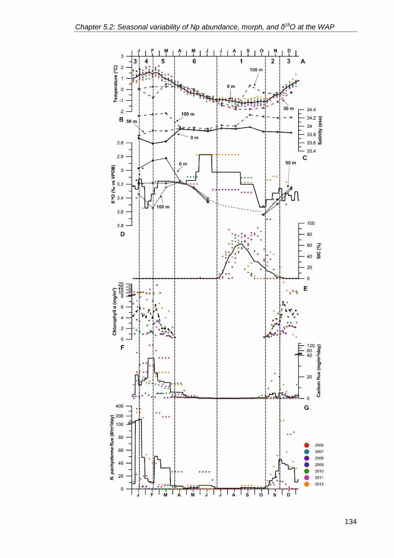
Chapter 5.2: Seasonal variability of Np abundance, morph, and δ18O at the WAP
134
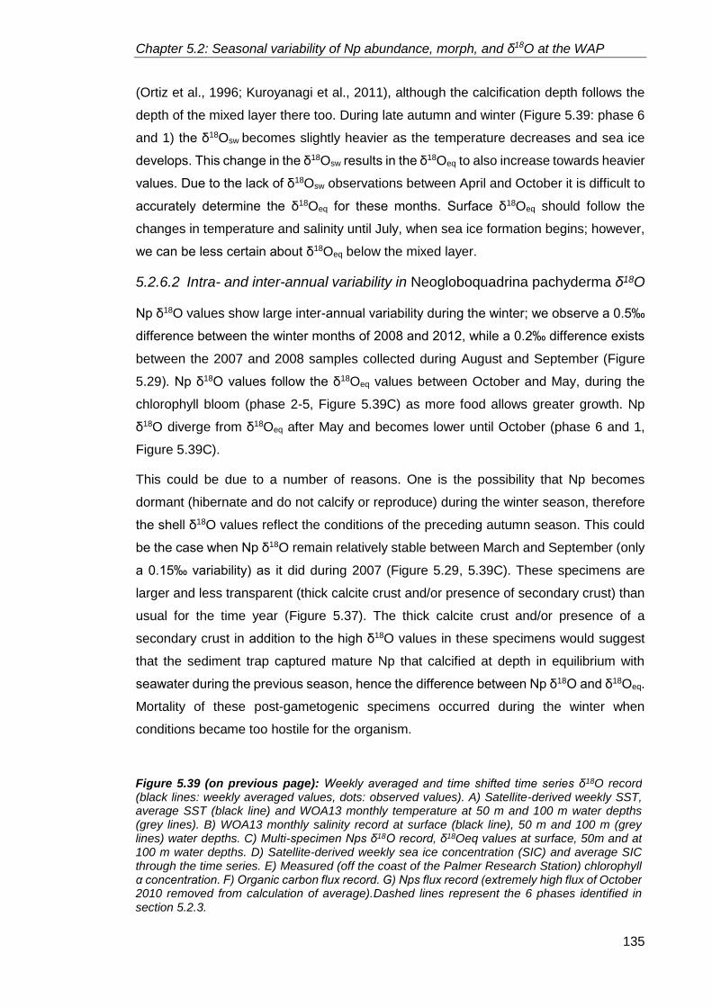
Chapter 5.2: Seasonal variability of Np abundance, morph, and δ18O at the WAP
135
(Ortiz et al., 1996; Kuroyanagi et al., 2011), although the calcification depth follows the
depth of the mixed layer there too. During late autumn and winter (Figure 5.39: phase 6
and 1) the δ18Osw becomes slightly heavier as the temperature decreases and sea ice
develops. This change in the δ18Osw results in the δ18Oeq to also increase towards heavier
values. Due to the lack of δ18Osw observations between April and October it is difficult to
accurately determine the δ18Oeq for these months. Surface δ18Oeq should follow the
changes in temperature and salinity until July, when sea ice formation begins; however,
we can be less certain about δ18Oeq below the mixed layer.
5.2.6.2 Intra- and inter-annual variability in Neogloboquadrina pachyderma δ18O
Np δ18O values show large inter-annual variability during the winter; we observe a 0.5‰
difference between the winter months of 2008 and 2012, while a 0.2‰ difference exists
between the 2007 and 2008 samples collected during August and September (Figure
5.29). Np δ18O values follow the δ18Oeq values between October and May, during the
chlorophyll bloom (phase 2-5, Figure 5.39C) as more food allows greater growth. Np
δ18O diverge from δ18Oeq after May and becomes lower until October (phase 6 and 1,
Figure 5.39C).
This could be due to a number of reasons. One is the possibility that Np becomes
dormant (hibernate and do not calcify or reproduce) during the winter season, therefore
the shell δ18O values reflect the conditions of the preceding autumn season. This could
be the case when Np δ18O remain relatively stable between March and September (only
a 0.15‰ variability) as it did during 2007 (Figure 5.29, 5.39C). These specimens are
larger and less transparent (thick calcite crust and/or presence of secondary crust) than
usual for the time year (Figure 5.37). The thick calcite crust and/or presence of a
secondary crust in addition to the high δ18O values in these specimens would suggest
that the sediment trap captured mature Np that calcified at depth in equilibrium with
seawater during the previous season, hence the difference between Np δ18O and δ18Oeq.
Mortality of these post-gametogenic specimens occurred during the winter when
conditions became too hostile for the organism.
Figure 5.39 (on previous page): Weekly averaged and time shifted time series δ18O record (black lines: weekly averaged values, dots: observed values). A) Satellite-derived weekly SST, average SST (black line) and WOA13 monthly temperature at 50 m and 100 m water depths (grey lines). B) WOA13 monthly salinity record at surface (black line), 50 m and 100 m (grey lines) water depths. C) Multi-specimen Nps δ18O record, δ18Oeq values at surface, 50m and at 100 m water depths. D) Satellite-derived weekly sea ice concentration (SIC) and average SIC through the time series. E) Measured (off the coast of the Palmer Research Station) chlorophyll α concentration. F) Organic carbon flux record. G) Nps flux record (extremely high flux of October 2010 removed from calculation of average).Dashed lines represent the 6 phases identified in section 5.2.3.

Chapter 5.2: Seasonal variability of Np abundance, morph, and δ18O at the WAP
136
Another possibility to account for the lighter shell δ18O with respect to δ18Oeq is that the
shell δ18O reflects ontogenic calcite. The secondary crust secreted post-gametogenesis
at deeper water depths then the original calcite layer typically has heavier δ18O signature
(Reiss, 1957; Hemleben et al., 1989; Kozdon et al., 2009). Np specimens that have not
secreted the secondary crust (due to mortality prior to the formation of the crust or to
unfavourable conditions), therefore have δ18O compositions that are lighter than those
with secondary crust (Kozdon et al., 2009). The relatively light Np δ18O values (2.7‰)
recorded between May and August of 2012 (Figure 5.29A) could reflect the lack of
secondary crust. Ion microprobe analysis of Np specimens collected by plankton tows in
the North Atlantic revealed that ontogenic calcite δ18O in a shell can range from 1.1‰ to
3.0‰ and that the average ontogenic δ18O values of the specimens do not reflect the
changes of δ18Oeq values with depth (Kozdon et al., 2009). Rather, the authors identified
a 0.5 to 1‰ negative fractionation relative to surface water δ18Oeq. The negative offset
of 0.8‰ identified by our study between the 2012 May-August Np δ18O and
corresponding δ18Oeq falls within this range of offset. Additionally, specimens with light
δ18Onp (winter 2012 specimens) are smaller in size and more translucent, than
specimens which calcified during the previous year and later on in the year too (Figure
5.37).
All of these data support the possibility that these specimens did not acquire a secondary
crust and that these are not fully mature specimens. Accordingly, δ18Onp values of these
immature specimens reflect ontogenic calcite only and the offset from equilibrium δ18O
values is due to the disequilibrium fractionation related to the early stages of the
foraminifera life cycle when calcification occurs rapidly requiring higher respiration rates
(Berger et al., 1978; Hemleben et al., 1989; Spero and Lea, 1996). Foraminifera
experience the greatest level of growth when food availability is high and δ18Osw is
relatively fixed (Hemleben et al., 1989). At the WAP these conditions are fulfilled during
the austral spring and summer, when nutrient Chl α concentrations are highest providing
ample food. The large intra-annual variability observed in the Np flux record (Figure
5.39), with higher fluxes the spring-summer, particularly in December and January, than
in the rest of the year combined could potentially bias the δ18Onp that would be derived
from core-top or sediment core samples to reflect spring-summer conditions and time of
year. This has important implications for the interpretation of foraminifera-based paleo
records.
SST begins to increase during phase 2, which is preceded by the divergence of salinity
between the surface and depth (Figure 5.39). The small changes in salinity, especially
the decrease in the surface, indicate the introduction of freshwater. This would suggest

Chapter 5.2: Seasonal variability of Np abundance, morph, and δ18O at the WAP
137
the beginning of the stratification of the water column, however, SST and temperature
below the surface do not begin to diverge until December. As discussed above, sea ice
melt does not have a significant influence on the δ18Osw, however, the influence of glacial
meltwater would commence in December/January (when surface water δ18Osw become
lighter due to the isotopically very light meltwater). Therefore δ18Osw and in turn δ18Oeq
values are expected to remain stable within the mixed layer during the spring and the
early summer months (October to December). This is reflected in the Np δ18O values
which on average show no significant offset from the δ18Oeq values at the surface or at
depth (Figure 5.39). Because of the deep mixed layer it is not possible to accurately
constrain the calcification depth during this time period beyond the fact that Np grow in
the mixed layer. Inter-annual variability is present in the Np δ18O specimens during
October and November resulting in some offset from δ18Oeq. This can be attributed to the
corresponding inter-annual variability in the sea ice cover. Higher than average sea ice
cover was recorded in 2012 during this time, which could result in the lighter Np δ18O
values observed.
5.2.7 Seasonal variability of Neogloboquadrina pachyderma δ18O derived
from single specimen analysis
Single specimen δ18O values show significant seasonal variability (Figure 5.29A, Figure
5.40, and Table 5.12) similar to that observed in the multi-specimen record. Np δ18O
values are heaviest during the summer months and are lighter during both the previous
and following seasons (Figure 29A). The heaviest δ18O values coincide with the largest
tests sizes (Figure 5.41B) and greater percentage of encrusted specimens (Figure
Figure 5.40: Variance of δ18O of single specimen Nps per sample. Error bars represent the standard error of the variance: σ2*√(2/(n-1)), where σ2 is the variance and n is the number of observations.
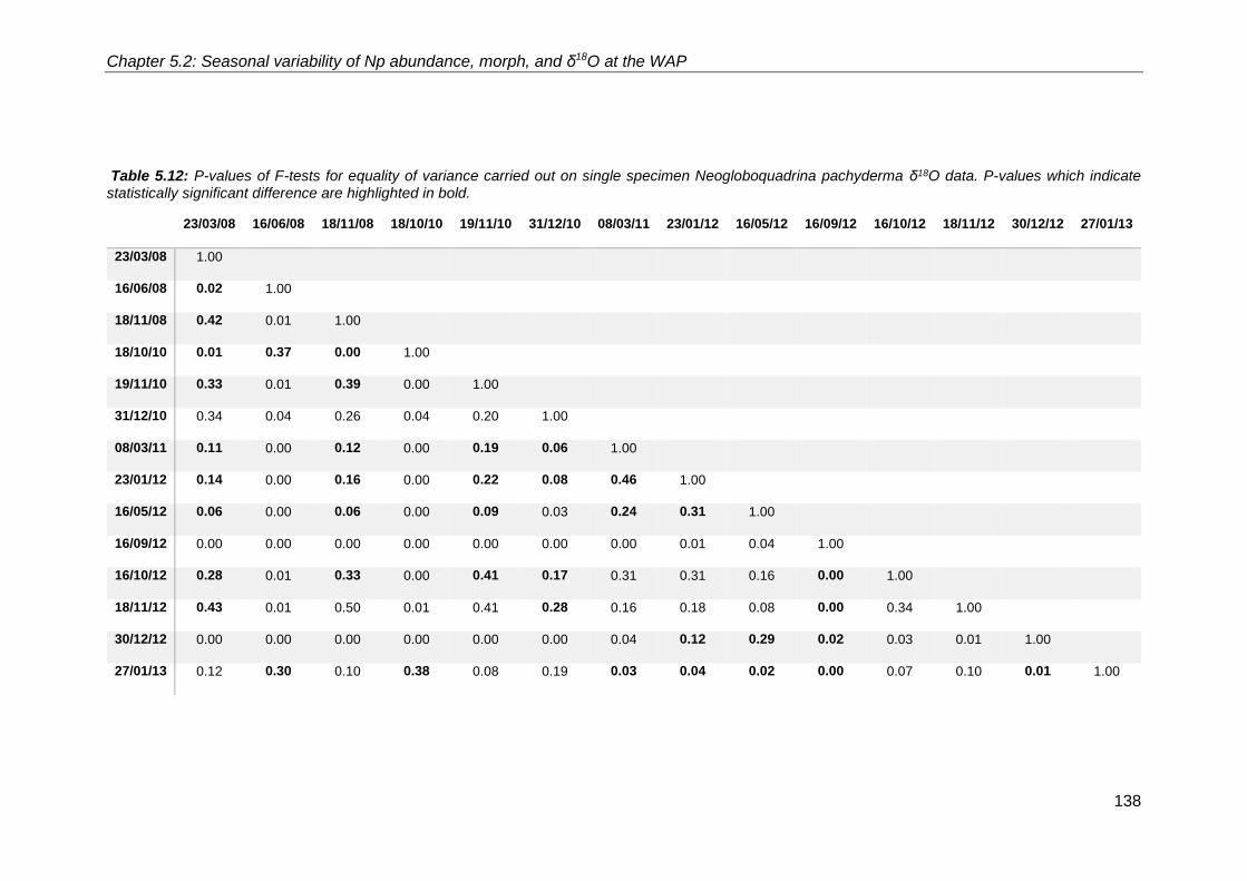
Chapter 5.2: Seasonal variability of Np abundance, morph, and δ18O at the WAP
138
Table 5.12: P-values of F-tests for equality of variance carried out on single specimen Neogloboquadrina pachyderma δ18O data. P-values which indicate statistically significant difference are highlighted in bold.
23/03/08 16/06/08 18/11/08 18/10/10 19/11/10 31/12/10 08/03/11 23/01/12 16/05/12 16/09/12 16/10/12 18/11/12 30/12/12 27/01/13
23/03/08 1.00
16/06/08 0.02 1.00
18/11/08 0.42 0.01 1.00
18/10/10 0.01 0.37 0.00 1.00
19/11/10 0.33 0.01 0.39 0.00 1.00
31/12/10 0.34 0.04 0.26 0.04 0.20 1.00
08/03/11 0.11 0.00 0.12 0.00 0.19 0.06 1.00
23/01/12 0.14 0.00 0.16 0.00 0.22 0.08 0.46 1.00
16/05/12 0.06 0.00 0.06 0.00 0.09 0.03 0.24 0.31 1.00
16/09/12 0.00 0.00 0.00 0.00 0.00 0.00 0.00 0.01 0.04 1.00
16/10/12 0.28 0.01 0.33 0.00 0.41 0.17 0.31 0.31 0.16 0.00 1.00
18/11/12 0.43 0.01 0.50 0.01 0.41 0.28 0.16 0.18 0.08 0.00 0.34 1.00
30/12/12 0.00 0.00 0.00 0.00 0.00 0.00 0.04 0.12 0.29 0.02 0.03 0.01 1.00
27/01/13 0.12 0.30 0.10 0.38 0.08 0.19 0.03 0.04 0.02 0.00 0.07 0.10 0.01 1.00

Chapter 5.2: Seasonal variability of Np abundance, morph, and δ18O at the WAP
139
Figure 5.41: Single specimen Nps δ18O (A), maximum diameter (B) and translucency (C) record. The morphometric dataset was created by the automatic microscope system. Black stars indicate the corresponding δ18O dataset. Boxes are coloured according to the phases identified in section 5.2.3.
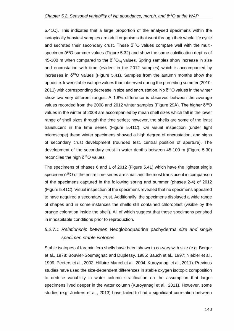
Chapter 5.2: Seasonal variability of Np abundance, morph, and δ18O at the WAP
140
5.41C). This indicates that a large proportion of the analysed specimens within the
isotopically heaviest samples are adult organisms that went through their whole life cycle
and secreted their secondary crust. These δ18O values compare well with the multi-
specimen δ18O summer values (Figure 5.32) and show the same calcification depths of
45-100 m when compared to the δ18Oeq values. Spring samples show increase in size
and encrustation with time (evident in the 2012 samples) which is accompanied by
increases in δ18O values (Figure 5.41). Samples from the autumn months show the
opposite: lower stable isotope values than observed during the preceding summer (2010-
2011) with corresponding decrease in size and encrustation. Np δ18O values in the winter
show two very different ranges. A 1.8‰ difference is observed between the average
values recorded from the 2008 and 2012 winter samples (Figure 29A). The higher δ18O
values in the winter of 2008 are accompanied by mean shell sizes which fall in the lower
range of shell sizes through the time series; however, the shells are some of the least
translucent in the time series (Figure 5.41C). On visual inspection (under light
microscope) these winter specimens showed a high degree of encrustation, and signs
of secondary crust development (rounded test, central position of aperture). The
development of the secondary crust in water depths between 45-100 m (Figure 5.30)
reconciles the high δ18O values.
The specimens of phases 6 and 1 of 2012 (Figure 5.41) which have the lightest single
specimen δ18O of the entire time series are small and the most translucent in comparison
of the specimens captured in the following spring and summer (phases 2-4) of 2012
(Figure 5.41C). Visual inspection of the specimens revealed that no specimens appeared
to have acquired a secondary crust. Additionally, the specimens displayed a wide range
of shapes and in some instances the shells still contained chloroplast (visible by the
orange coloration inside the shell). All of which suggest that these specimens perished
in inhospitable conditions prior to reproduction.
5.2.7.1 Relationship between Neogloboquadrina pachyderma size and single
specimen stable isotopes
Stable isotopes of foraminifera shells have been shown to co-vary with size (e.g. Berger
et al., 1978; Bouvier-Soumagnac and Duplessy, 1985; Bauch et al., 1997; Niebler et al.,
1999; Peeters et al., 2002; Hillaire-Marcel et al., 2004; Kuroyanagi et al., 2011). Previous
studies have used the size-dependent differences in stable oxygen isotopic composition
to deduce variability in water column stratification on the assumption that larger
specimens lived deeper in the water column (Kuroyanagi et al., 2011). However, some
studies (e.g. Jonkers et al., 2013) have failed to find a significant correlation between

Chapter 5.2: Seasonal variability of Np abundance, morph, and δ18O at the WAP
141
size and stable isotopes, which suggests that regional differences exist in this
relationship as a result of different environmental controls. A lack of relationship between
shell size and stable isotope would imply that between-sample and within-sample stable
isotope variability are both purely related to environmental variability (chiefly
temperature).
To investigate the existence of such size-dependent stable isotope variability in the WAP
region, the single specimen stable isotope record was separated based on the minimum
diameter of each shell. Due to the low shell flux the samples were not sieved into the
usual shell sizes of <150 µm, 150-250 µm and >250µm, but instead the size of each
specimen was determined through the morphometric analysis prior to isotopic analysis.
To make the results comparable to previous studies minimum diameter was employed
as an indicator of size.
The dataset shows consistent size effect on both the δ18O and δ13C of Np (Figure 5.42)
when the whole dataset is taken into consideration, although δ18O shows a stronger
correlation with size than δ13C, with a 0.52 and 0.23 r value respectively. When divided
into two size fractions (150-250 µm and >250µm) δ18O still shows correlation with size:
r=0.28 and r=0.32 for 150-250 μm and >250 μm, respectively (Figure 5.42A). In
comparison, the size effect disappears when the δ13C dataset is separated into the two
size fractions: r=0.007 (150-250 μm), r=0.06 (>250 μm) (Figure 5.42B). An average of
~0.15‰ offset is observed between the small and large Np δ18O throughout the record,
although this is not a consistent offset. The variability in the offset between the smaller
and larger size fraction suggests that the differences are largely related to variable
oceanographic conditions, instead of size-specific kinetic/metabolic effects.
150-250 µm R² = 0.076
>250 µmR² = 0.102
Whole size rangeR² = 0.27
0.50
1.00
1.50
2.00
2.50
3.00
3.50
4.00
4.50
100 200 300 400
Np
s δ
18O
(‰
vs V
PD
B)
Shell size (µm)
150-250 µmR² = 0.00005
>250 µmR² = 0.0032
Whole size rangeR² = 0.0523
0.00
0.40
0.80
1.20
1.60
2.00
100 200 300 400
Np
s δ
13C
(‰
vs V
PD
B)
Shell size (µm)
A B
Figure 5.42: Regression diagrams between Nps shell size (blue diamonds: 150-250 µm, purple dots: >250 µm) and δ18O (A) and δ13C (B). Significant correlations are detected between shell
size and both stable isotopes when the whole dataset is analysed together.

Chapter 5.2: Seasonal variability of Np abundance, morph, and δ18O at the WAP
142
A similar variable offset relating to environmental variability has been observed in the
North Pacific (Kuroyanagi et al., 2011). The offset varies between 0.01‰ (19/11/2010)
and 0.72‰ (16/09/2012), with no discernible seasonal variability. This 0.15‰ is
comparable to previously published records in the Northern Hemisphere (Bauch et al.,
1997 and Kuroyanagi et al., 2011). In comparison, the average offset between the small
and large Np δ13C is 0.04, with a minimum of 0.01‰ (31/12/2010) and maximum of
0.44‰ (30/12/2012).
Larger specimens of Np (which are likely to weigh more) are more likely to calcify deeper
in the water column, in colder and more saline waters giving rise to higher δ18Onp values.
In contrast, smaller specimens (smaller weight) are likely to calcify in shallower waters,
with higher temperatures and lower salinity, leading to lower δ18Onp values. Additionally,
specimens with a secondary crust are more likely to be larger in size and heavier in
weight – test weight can increase by up to 80% as a result of the secondary crust
(Kohfeld et al., 1996). As the secondary crust is added in deeper waters, below the
pycnocline (Kohfeld et al., 1996; Bauch et al., 1997; Kozdon et al., 2009) the δ18O of Np
with a thick secondary crust will have higher δ18O values, as observed by Kozdon et al.
(2009). Therefore the statistically significant differences between the δ18O of the two size
fractions of Np and the variable offset between the two size fractions can be attributed
to calcification depth differences (and thus temperature and salinity) the smaller and
larger specimens calcified in and to the presence/absence, as well as percent
contribution of secondary crust to the total shell.
The size-specific Np δ13C values (Figure 5.42B) (as identified by the statistically
significant correlation coefficient of 0.23) agree with previously published records of size-
specific Np δ13C (Donner and Wefer, 1994; Volkmann and Mensch, 2001; Hillaire-Marcel
et al., 2004). The correlation between size and δ13C can be attributed to a number of
factors: i) higher δ13C of Dissolved Inorganic Carbon (δ13CDIC), and [CO32−] in surface
waters (Spero et al., 1997; Bemis et al., 2000); ii) impact of biological and kinetic
fractionation on the δ13C of smaller and larger specimens (Hemleben et al., 1989).
δ13CDIC is higher in the surface waters as a result of primary production, and lower at
depth as a result of remineralisation (Broecker and Peng, 1982). Therefore smaller
specimens that calcify closer should have higher δ13C values. Carbonate ion
concentration acts in the opposite direction of the foraminiferal δ13C complicating the
interpretation of the stable carbon isotope record.
Foraminifera calcify (and respire) faster during the early part of their life cycle, and as a
result, smaller and younger specimens incorporate a greater amount of 12C leading to
lower shell δ13C (Hemleben et al., 1989), this is clearly evidenced by the lower δ13Cnp

Chapter 5.2: Seasonal variability of Np abundance, morph, and δ18O at the WAP
143
values in the smaller specimens (Figure 5.29B). Respiration and calcification rate
decrease after the early part of the life cycle which leads to the incorporation of a greater
amount of 13C into the shell increasing its δ13C signature. Additionally, the secondary
calcite crust is secreted in deeper waters with lower temperature, which would increase
the shell δ13C. Similarly to the δ18Onp record, the variable offset between the δ13C of the
small and large size fraction could be the result of differences between calcification
depths, presence/absence of secondary crust and the life stage the specimen achieved
prior to mortality.
5.2.8 Exceptional Neogloboquadrina pachyderma flux event of 2010: What
is the role of the Southern Annular Mode and the El Niño-Southern
Oscillation?
Neogloboquadrina pachyderma flux, morphology and stable isotope composition are all
closely linked to sea ice extent and food availability (see Sections 5.2.3, 5.2.4, and 5.2.5).
Np flux shows a close relationship with Chl α concentration (an indicator of primary
production and food availability), while variability in the timing of the onset of primary
production is driven by the inter-annual variability of sea ice extent (Smith et al., 1997).
My records show that differences in the timing and amplitude of peak Np flux between
2006 and 2012 are driven by the timing of the onset of sea ice melt. Additionally, the
presence of sea ice as well as its extent are shown to have adverse effects on Np
morphology, as the concentration of smaller sized specimens (that might not have gone
through reproduction) is higher during sea ice periods. In contrast, increased Chl α
concentration (and thus food availability) has a positive impact on Np morphology and
reproductive success. Periods of increased food availability (spring-summer period
and/or lower sea ice concentration) and greater reproductive success (evidenced by
presence of secondary crust) result in higher δ18O shell signature that also links Np δ18O
with the environmental variability.
Sea ice has a complex but important relationship with the climate phenomenon El Niño
Southern Oscillation (ENSO) and the Southern Annular Mode (SAM) (e.g. Turner et al.,
2004) with the implication that some of the interannual variability in the Np flux,
morphometric and stable isotope data may be driven by the impact of ENSO and the
SAM on the WAP climate and oceanographic conditions.

Chapter 5.2: Seasonal variability of Np abundance, morph, and δ18O at the WAP
144
5.2.8.1 Variability in sea ice advance and retreat due to Southern Annular Mode
and El Niño-Southern Oscillation
Atmospheric variability in the WAP region on annual timescales is controlled by the twice-
yearly poleward movement and intensification of the high latitude atmospheric low-
pressure trough in the spring and the autumn, termed the semi-annual oscillation (SAO)
(van Loon, 1967). The interactions between sea ice and the atmosphere due to the SAO
drive the seasonal cycle of sea ice advance and retreat (e.g. Watkins and Simmonds,
1999; Stammerjohn et al., 2003). On inter-annual timescales, atmospheric variability and
thus variability in sea ice advance and retreat are mostly controlled by the
teleconnections between SAM/ENSO and the high latitudes because SAM/ENSO
modulate the SAO (Watkins and Simmonds, 2000).
During the past thirty years co-variability between ENSO and SAM has increased (Kwok
and Comiso, 2002; Fogt and Bromwich, 2006; Stammerjohn et al., 2008, Fogt et al.,
2011; Clem and Fogt, 2013), meaning that the two processes change in-phase with each
other more often: La Niña (El Niño) events occur at the same time as positive (negative)
phases of SAM (Fogt et al., 2011). The impact of ENSO and SAM on the strength of sea
level pressure (SLP) anomalies and sea ice advance on the WAP also intensified during
the same period (Stammerjohn et al., 2003; Stammerjohn et al., 2008b). As a result,
negative SLP anomalies during austral summer and autumn are observed on the WAP
during La Niña events and positive SAM (Figure 2.5), while positive SLP anomalies
dominate when El Niño is in phase with negative SAM (Table 5.12). Concurrently,
variability in WAP sea ice trends has been closely linked to the SLP anomalies. Earlier
wind-driven sea ice retreat and later sea ice advance is associated with the development
of strong negative SLP anomalies along the WAP (Table 5.12) supporting anomalously
warm northerly winds in the Bellingshausen Sea as a result of the increasingly positive
SAM and strong La Niña events since the 1990s. Conversely, positive SLP anomalies
Table 5.12: Impact of co-varying El Niño-Southern Oscillation (ENSO) and Southern Annular Mode (SAM) on sea level pressure (SLP) anomaly over the West Antarctic Peninsula (WAP), wind direction over the WAP, and the length of the sea ice season along the WAP as a result of the interaction of the above (Stammerjohn et al., 2008a; Stammerjohn et al., 2008b; Meredith et al., 2017).
ENSO La Niña El Niño
SAM Positive Negative
SLP anomaly over WAP Negative Positive
Wind direction Northerly Southerly
Length of sea ice season Short Long

Chapter 5.2: Seasonal variability of Np abundance, morph, and δ18O at the WAP
145
during the autumn months in the Amundsen Sea region are associated with cold
southerly winds over the WAP region resulting in early sea ice advance (Table 5.12)
(Stammerjohn et al., 2008a).
5.2.8.2 Recent trends in wind-driven sea ice variability in the Palmer region
The long term trends described in Section 5.2.3 are still prevalent along the WAP today
(Meredith et al., 2017). Significant inter-annual variability in sea ice pattern was observed
between 2010 and 2014 along the WAP (Figure 5.43) and the strong link between SLP
anomalies, wind patterns and sea ice trends continued. Of particular relevance to the
Palmer LTER sediment trap Np flux record is the impact of both the strongest positive
SAM (Figure 5.44A) as well as the impact of a strong La Niña (Figure 5.44B) on sea ice
distribution in 2010, in comparison to weaker SAM/El Niño years. The strong positive
SAM and the strong La Niña gave rise to the development of very low SLP in the
Bellingshausen Sea creating strong north-northwesterly winds between September 2010
and February 2011 (Figure 5.43A). These winds blew warm, moist air into the region
reducing sea ice extent and duration with an early spring retreat (early October) and late
sea ice advance (Figure 5.12). The result of the low sea ice extent and short duration
during the winter of 2010 was the low sea ice melt in the Palmer region in the austral
spring-summer season of 2010-2011 (Meredith et al., 2017). The concentration of
meteoric waters in near-shore areas (driven by the amount of precipitation) was
increased as a result of the warm and moist northerly winds, which are more likely to
contribute significant amount of precipitation (Meredith et al., 2017).
Increased meteoric water concentration supports strong southward geostrophic flow
along the WAP that carries micronutrients (source of food for microorganisms) out of the
northern WAP region to more southerly locations quicker (Meredith et al., 2013). The
loss of micronutrients by the stronger geostrophic flow was most likely counteracted by
the enhanced upwelling and eddy-transport of warm, nutrient-rich UCDW waters onto
the continental shelf, which, created favourable conditions for phytoplankton (especially
diatom) growth in the outer to midshelf region (Prézelin et al., 2004). Increased UCDW
incursions onto the continental shelf of the WAP have become more common in recent
decades (Martinson et al., 2008) and previous studies (Martinson et al., 2008; Martinson
and McKee, 2012) have shown that enhanced upwelling is most likely to take place
during positive SAM and coinciding La Niña events. The combination of the above
processes created perfect conditions for the proliferation of Np, that resulted in the >1000
specimen/m2/day Np flux value observed in October and November 2010 (Figure 5.12C).
These specimens were larger (higher maximum diameter values: Figure 5.37A), rounder
(Figure 5.18B), and less translucent (mean grey value – Figure 5.37B) than Np from
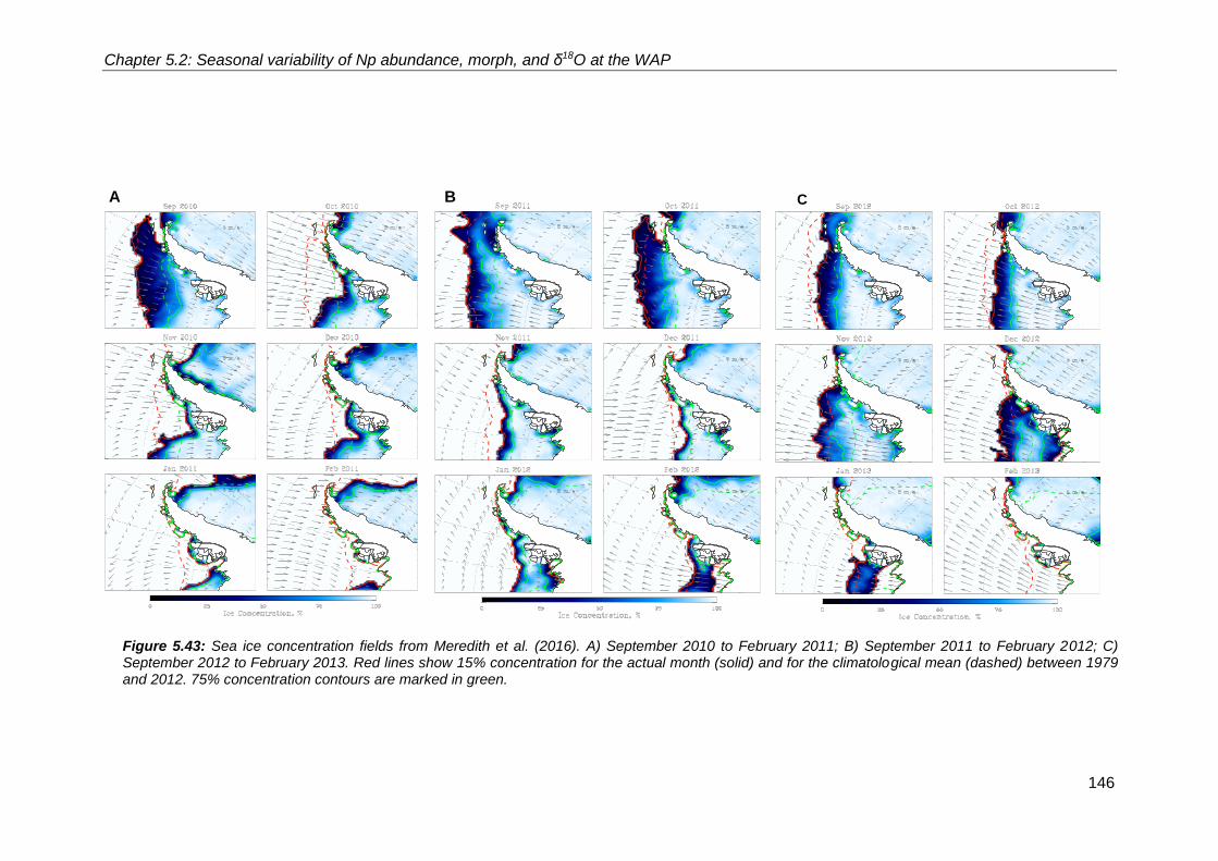
Chapter 5.2: Seasonal variability of Np abundance, morph, and δ18O at the WAP
146
A B C
Figure 5.43: Sea ice concentration fields from Meredith et al. (2016). A) September 2010 to February 2011; B) September 2011 to February 2012; C) September 2012 to February 2013. Red lines show 15% concentration for the actual month (solid) and for the climatological mean (dashed) between 1979 and 2012. 75% concentration contours are marked in green.

Chapter 5.2: Seasonal variability of Np abundance, morph, and δ18O at the WAP
147
other years indicating greater reproductive success (presence of secondary crust)
resulting in some of the highest δ18Onp measurements (3.53‰) between 2006 and 2013
(Figure 5.41A).
In comparison to 2010, 2012 was characterised by El Niño-like conditions over the
Pacific Ocean (Figure 5.44B) (Wolter and Timlin, 1998; Wolter, 2016). Concurrently,
SAM switched to a negative state after September 2012 (Figure 5.44A) (Marshall et al.,
2016). The combination of the El Niño and the negative SAM gave rise to the
development of a high SLP cell over the southern Bellingshausen/Amundsen Sea
creating strong and persistent southerly winds over the WAP between October and
December 2012 (Meredith et al., 2017). As a result of these winds, although 2012 had
the lowest overall sea ice cover of the sediment trap collection period (Figure 5.12B),
sea ice lingered in the region around the sediment trap until late November as the winds
carried cold air over the sea ice (Figure 5.43C) (Meredith et al., 2017). The strong, cold
southerly winds (arising from a dry region) limited the amount of precipitation over the
A
B
Figure 5.44: SAM (A) and ENSO (B) index. SAM index is based on the departure from the zonal means between 40°S and 65°S (Marshall, 2003). Red sections show positive SAM period, blue sections show negative SAM periods in the top figure. The ENSO index based on the departure from the 1950-1993 reference period (Wolter, 2016). Red sections show El Niño conditions, blue sections show La Niña conditions in bottom figure. Note the co-variability between positive SAM and La Niña and vice versa for negative SAM and El Niño.

Chapter 5.2: Seasonal variability of Np abundance, morph, and δ18O at the WAP
148
WAP and the sea decreasing the near-shore meteoric water concentration, which in turn
weakened the southward geostrophic flow (Meredith et al., 2013) limiting the amount of
micronutrients carried out of the northern WAP region. Thus, Np flux between
September and December 2012 was much lower than in 2010 (Figure 5.12), varying
between 5 and 142 shell/m2/day. The specimens that calcified during this period were
also on average smaller (lower maximum diameter: Figure 5.37A) than in 2010. The
roundness (sphericity, Figure 5.18B) and the translucency (mean grey values, Figure
5.37B) of the shells were similar to 2010, indicating that those specimens that grew under
these conditions still succeeded in completing their life cycles, completing
gametogenesis and secreting their secondary crust. This is also reflected in the δ18Onp
measurements, which are similar to the 2010 measurements (Figure 5.41A). This
reproductive success is most likely due to the high Chl α concentrations sustained by the
weakened geostrophic flow.
Due to the significance and unusual characteristic of the Np flux values during the austral
spring of 2010 we can attribute this event to the impact of the coinciding strong positive
SAM and La Niña on the WAP. It is expected that northerly winds will become more
persistent and stronger in the future as a response of a dominant positive SAM as
anthropogenic forcings persist (Van Wessem et al., 2015) creating the possibility of
shorter sea ice seasons and warmer SST. These processes will create more favourable
growing conditions for Np at the WAP, potentially increasing its abundance during the
spring-summer period. The warmer seas and the greater food availability will allow Np
to grow larger, and support greater reproductive success. This would have implications
for the stable isotope record, as larger shells which have a secondary crust will make up
more of the sediment that reaches the seafloor increasing the chances of preservation.
5.2.9 Synthesis and Conclusion
The main findings of the previous discussion sections are summarised in Figure 5.45.
Under normal circumstances Np abundance displays a peak during the late spring-early
summer (NDJ) period once the sea ice has completely retreated and chlorophyll
concentration is increasing. During this time the majority of the Np appear to have
completed their full life cycle prior to mortality on account of their large (>275 μm
maximum diameter) spherical tests indicative of secondary calcite crust formation
following reproduction/gametogenesis. Due to the presence of the secondary calcite
crust obtained at depth in the water column δ18Onp is the heaviest (~3.5‰) in these
specimens and therefore average sample values are heaviest at this time of the year.
Small, elongated, non-encrusted specimens are also captured by the sediment trap

Chapter 5.2: Seasonal variability of Np abundance, morph, and δ18O at the WAP
149
Figure 5.45: Synthesis figure of the seasonal average flux, morphology and stable isotope composition of Nps in the continental shelf region of the WAP.

Chapter 5.2: Seasonal variability of Np abundance, morph, and δ18O at the WAP
150
during late spring-early summer, albeit in small numbers. These small specimens have
lighter δ18Onp values obtained closer to the surface and can be considered to be
immature specimens that have not reproduced prior to mortality. As the phytoplankton
bloom and chlorophyll concentration increases and Np reaches deeper depths the flux
decreases from its initial peak but still maintains high values, similarly to previous
observations by Kohfeld et al. (1996) and Jonkers et al. (2013).
During the austral summer (phases 3 and 4) Np maintains a steady presence in the
surface waters (small, elongated, immature specimens) as well as further down in the
water column (large, spherical specimens with secondary crust) carrying lighter and
heavier individual stable isotopic signatures, respectively. As chlorophyll concentrations
and SSTs decrease and the water column stratification begins to break up during the
austral autumn (phase 5-early 6), Np flux values decrease significantly. The proportion
of encrusted to non-encrusted specimens in the sediment trap decreases during this
period indicating that conditions are less favourable for Np to complete its life cycle. By
the end of the austral autumn and the start of winter (phase 6), large encrusted
specimens become very rare in the trap. Overall flux values reach very low levels and
mostly small (<220 μm maximum diameter), elongated, thin-shelled pre-mature
specimens with the lightest δ18O values of the year reach the sediment trap. This time of
the year is characterised by low food availability due to the lack of micronutrients and
diminishing light, which together make it difficult for Np to reach the reproductive stage
in its life cycle. However, some specimens must be able to survive the conditions and
reproduce as Np remain present in the surface waters as shown by its more or less
continuous presence in the trap.
During the winter months (phase 1) when sea ice is present above the sediment trap Np
flux values remain close to zero (in some years it reaches zero). The specimens collected
at this time of the year are small, albeit larger than during late autumn-early winter (phase
6). It is difficult to decipher where exactly the organisms live when sea ice occupies the
surface waters. It is known that Np can survive and live within the brine channels of the
sea ice (Spindler et al., 1996). It might be possible that the organisms go into a
hibernation mode during this winter monrhs and stop calcifying until conditions become
suitable during early spring when sea ice begins to dissipate. This possibility is supported
by the presence of medium sized (>220μm) less elongated specimens which show a
secondary crust by early spring (September) as soon as sea ice coverage decreases
and SST increases. The presence of non-encrusted (most likely pre-gametogenic)
specimens in the surface waters in late autumn – early winter (phase 6) when chlorophyll
concentrations are close to zero, SSTs are very low, the water column is well mixed, and

Chapter 5.2: Seasonal variability of Np abundance, morph, and δ18O at the WAP
151
sea ice begins to form proves the fragility of Np in the high latitude regions. It supports
previous suggestions about increased mortality rate prior to reproduction in unfavourable
conditions during colder periods in the past 75 ka (Vautravers et al., 2013).
The above pattern of Np flux, morphology and stable isotope variability throughout the
year can be modulated by extreme SAM and ENSO conditions, specifically during times
of strong positive SAM coinciding with a strong La Niña as demonstrated by the austral
spring 2010 samples. Our findings have important palaeoceanographic implications.
Firstly, we suggest that when present non-encrusted Np specimens should not be mixed
up with encrusted specimens when geochemical analysis is undertaken as the two
different morphologies represent different depth habitats and seasons. Secondly, Np
proxy records that only utilise encrusted specimens risk the possibility of only
reconstructing austral spring and summer conditions and hence cannot draw
conclusions about year-round conditions. Finally, the average annual Np flux value in a
year not effected by strong SAM and ENSO is significantly lower than the annual flux
value during a strong +SAM/La Niña year. Deposition of calcareous material to the
seafloor is low in the high latitudes. Therefore it is possible that years with extreme flux
values -due to the impact of the strong teleconnections with SAM and La Niña- could
overwhelm average years in the sediment record. This would result in sediment cores
recording primarily the years with extreme seasonal variability as opposed to average
years with average conditions, skewing paleoreconstructions.

Chapter 5.2: Seasonal variability of Np abundance, morph, and δ18O at the WAP
152

153
5.3 Investigating intermediate water mass variability in the
Southern Ocean during the Holocene
The Southern Ocean and the southern mid-latitudes experienced wide scale climate
variability during the long-term gradual cooling of the Holocene period (Masson et al.,
2000). The Southern Westerly Winds oscillated between periods of weaker and stronger
strength (Lamy et al., 2010). Similarly, Antarctic Intermediate Waters experienced
variability between lower and higher flow speeds during the Holocene that accompanied
a gradual increase since the end of the deglacial period (Voigt et al., 2016). Along the
Antarctic Peninsula, the flux of glacial meltwater from the glaciers of the West Antarctic
Peninsula into the surrounding Bellingshausen Sea also showed periods of highs and
lows during the past 13,000 years (Pike et al., 2013). Since the mid-Holocene El Niño-
Southern Oscillation (ENSO) has intensified, with greater number of events occurring in
the tropical Pacific since ~5,500 yr BP (Moy et al., 2002). However, this intensification
has not been constant, and periods of high ENSO activity interrupted by quieter periods
in the tropical Pacific.
In this chapter, a single specimen Globorotalia inflata stable isotope record is utilised to
assess changes in the seasonality of oceanographic conditions in the mid-latitude
regions around the Falkland Plateau, Scotia Sea. As shown in the previous chapter,
single specimen foraminiferal stable isotopes are a useful proxy to assess changes in
seasonality, as they can highlight changes in the range of conditions within a time period.
The first two sections of this chapter describes the results of the Globorotalia inflata
stable isotope analysis, while the rest of the sections assess the results and aims to
provide a thorough discussion on Holocene oceanographic variability in the Scotia Sea.
5.3.1 Comparison of paired and single specimen Globorotalia inflata
The aim of producing the downcore foraminifera δ18O record at core site GC528 on the
Falkland Plateau is to investigate variability in the seasonality of oceanographic
conditions during the Holocene period. To achieve this, δ18O values outside normal, or
average, conditions need to be captured within a sample. The analysis of a number of
individual (single specimen) foraminifera allows us to find these outliers which represent
conditions experienced during the growing season of the individual organism. Although
single specimen analysis is the best to capture ranges in conditions, if single foraminifera
specimens are very small, with carbonate mass too low for analysis (<5 μg), it is possible
to analyse pairs of specimens to increase the carbonate mass. However, extreme/outlier
stable isotope values may be compromised as a result of the consolidation of each

Chapter 5.3: Intermediate water mass variability in the Southern Ocean - Holocene
154
specimen’s stable isotope signature, reducing the within-sample variability. As a result,
paired specimen analysis may not provide the true range of δ18O values. To determine
its suitability for capturing seasonality, paired specimen isotope data must be compared
to single specimen isotope data.
In this study, paired and single specimen Globototalia inflata δ18O analyses were carried
out and the statistical distribution of the datasets were compared (Table 5.13, 5.14
respectively). The eight samples of δ18O analyses (Table 5.13), comprising paired
analysis of G. inflata from sediment samples each covering one centimetre stratigraphic
thickness, were grouped together and an Anderson-Darling test for Normality was carried
out on the 213 data points. Similarly, the 12 samples of single specimen δ18O data (Table
5.14) were grouped together to test for normality using the Anderson-Darling test. The
results of both tests (p = 0.005 and p = <0.0001 for combined paired sample dataset and
combined single specimen sample dataset, respectively) show non-normal distributions
which could either be a result of outliers or widely different ranges in the samples that
make up the paired and single specimen dataset. Anderson-Darling tests were also
carried out on the δ13C datasets and revealed non-normal distribution of both the
Table 5.13: Summary statistics of paired specimen Globorotalia inflata δ18O and δ13C analyses from sediment core GC528 (Falkland Plateau). n: number of data points; σ: standard deviation;
σ2: variance; SE σ2: standard error of variance calculated as σ2*(2/(n−1)).
δ18O Sample depth (cm)
Age n Mean Median σ σ2 SE σ2
1-2 1100 18 +2.68 +2.69 0.092 0.008 0.001
3-4 1150 30 +2.73 +2.71 0.1 0.01 0.001
13-14 2550 30 +2.71 +2.70 0.116 0.013 0.001
19-20 3250 31 +2.64 +2.63 0.095 0.009 0.001
25-26 3900 31 +2.74 +2.73 0.089 0.008 0.001
35-36 5250 28 +2.66 +2.69 0.115 0.013 0.001
45-46 6600 24 +2.79 +2.78 0.116 0.013 0.001
51-52 7700 21 +2.76 +2.74 0.125 0.016 0.002
δ13C
1-2 1100 18 +1.54 +1.54 0.119 0.014 0.002
3-4 1150 30 +1.54 +1.56 0.132 0.017 0.001
13-14 2550 29 +1.53 +1.55 0.136 0.018 0.001
19-20 3250 31 +1.61 +1.62 0.154 0.024 0.002
25-26 3900 31 +1.63 +1.63 0.133 0.018 0.001
35-36 5250 28 +1.51 +1.53 0.141 0.02 0.001
45-46 6600 24 +1.55 +1.58 0.137 0.019 0.002
51-52 7700 21 +1.45 +1.48 0.17 0.029 0.003

Chapter 5.3: Intermediate water mass variability in the Southern Ocean - Holocene
155
combined paired sample (p = <0.0001) and the combined single specimen sample (p =
0.0002) datasets. As a result, only non-parametric statistical tests can be carried out on
the samples of paired and single specimen analyses.
To explore whether variability is reduced in the stable isotope data which derive from
pairs of specimens, compared to those which derive from single specimens, the variance
and the standard error of the variance of each sample is compared (Figure 5.46 and
5.47). The variance of single specimen δ18O samples displays greater variability than the
paired specimen δ18O samples throughout the time-series (Figure 5.46). The paired
specimen samples δ18O variance is relatively stable, oscillating between 0.008 and 0.016
(3900 yr BP and 7720 yr BP, respectively) (Table 5.13, Figure 5.46A). In comparison,
Table 5.14: Summary statistics of single specimen Globorotalia inflata δ18O and δ13C dataset from sediment core GC528. n: number of data points; σ: standard deviation; σ2: variance; SE σ2:
standard error of variance calculated as σ2*(2/(n−1)); A2: Anderson-Darling value; p: p-value of
Anderson-Darling test. P-values <0.05 are highlighted. These samples are not normally distributed.
δ18O Sample
Depth (cm) Age n Mean Median σ σ2 SE σ2 A2 p
7-8 1700
30 +2.61 +2.62 0.106 0.011 0.001 0.219 0.823
9-10 2000
30 +2.65 +2.67 0.086 0.007 0.001 0.295 0.573
12-13 2400
30 +2.62 +2.63 0.100 0.010 0.001 0.340 0.474
14-18 2800
30 +2.55 +2.52 0.113 0.012 0.001 0.422 0.303
21-22 3450
30 +2.59 +2.56 0.098 0.010 0.001 0.325 0.508
27-28 4100
30 +2.57 +2.56 0.074 0.006 0.000 0.631 0.091
31-32 4700
30 +2.63 +2.64 0.090 0.008 0.001 0.325 0.509
37-38 5500
00
30 +2.77 +2.75 0.137 0.019 0.001 1.490 0.001
41-42 6100
29 +2.62 +2.61 0.075 0.005 0.000 0.179 0.910
49-50 7200
24 +2.78 +2.77 0.104 0.011 0.001 0.384 0.367
55-56 8700
27 +2.85 +2.84 0.183 0.034 0.003 1.452 0.001
59-60 9600
8 +2.93 +2.97 0.141 0.020 0.006 0.295 0.511
δ13C
7-8 1700
30 +1.44 +1.48 0.167 0.028 0.002 0.640 0.086
9-10 2000
30 +1.51 +1.53 0.178 0.032 0.002 0.456 0.249
12-13 2400
30 +1.48 +1.52 0.176 0.031 0.002 0.493 0.201
14-18 2800
30 +1.43 +1.41 0.181 0.037 0.003 0.487 0.208
21-22 3450
30 +1.56 +1.57 0.164 0.027 0.002 0.400 0.341
27-28 4100
30 +1.48 +1.45 0.191 0.036 0.003 0.277 0.630
31-32 4700
30 +1.53 +1.56 0.121 0.015 0.001 0.392 0.356
37-38 5500
00
30 +1.54 +1.54 0.150 0.022 0.002 0.404 0.333
41-42 6100
29 +1.53 +1.49 0.143 0.020 0.001 0.862 0.023
49-50 7200
24 +1.57 +1.57 0.141 0.020 0.002 0.415 0.309
55-56 8700
27 +1.40 +1.46 0.250 0.062 0.005 0.799 0.033
59-60 9600
8 +1.53 +1.57 0.176 0.031 0.009 0.435 0.220

Chapter 5.3: Intermediate water mass variability in the Southern Ocean - Holocene
156
the single specimen samples δ18O variance ranges between 0.005 (6100 yr BP) and
0.034 (8700 yr BP) (Table 5.14, Figure 5.46B), a 2.5-fold increase in the variability
between the paired specimen samples. The total δ13C variance shows similar trends.
The paired specimen samples δ13C variance fluctuates between 0.018 (3900 yr BP) and
0.029 (7700 yr BP) (Table 5.13, Figure 5.47A), while the single specimen samples δ13C
variance varies between 0.015 (4700 yr BP) and 0.062 (8700 yr BP) (Table 5.14, Figure
5.47B), representing a greater than 3-fold increase in-between sample variances. These
findings suggest that the paired and single specimen samples should not be analysed
together as one time series because the paired specimen stable isotope analysis
artificially reduces the within-sample variability by averaging out the extreme isotope
Figure 5.46: Comparison of total δ18O variance between paired (A) and single specimen (B) Globoraotalia inflata dataset from sediment core GC528. Variance in the single specimen dataset displays greater degree of variability than in the paired specimen dataset. Error bars represent the standard error associated with the variance.
0.000
0.005
0.010
0.015
0.020
0.025
0.030
0.035
0.040
1100 1150 2550 3250 3900 5250 6600 7700
To
tal δ
18O
va
ria
nc
e (
σ2)
Age (yr BP)
Paired specimens A
0
0.005
0.01
0.015
0.02
0.025
0.03
0.035
0.04
1700 2000 2400 2800 3450 4100 4700 5500 6100 7200 8700 9600
Age (yr BP)
Single specimensB
To
tal
δ18O
va
ria
nc
e (
σ2)

Chapter 5.3: Intermediate water mass variability in the Southern Ocean - Holocene
157
measurements. The simplest statistical comparison of paired and single specimen
samples, each comprising multiple measurements, is carried out by analysing the
position of the means of the two normally distributed datasets through a Student’s t test.
This approach reveals whether the groups are comparable or are different. However, the
paired and single specimen sample stable isotope datasets are not normally distributed,
hence the non-parametric version of the t test - the Mann-Whitney U test - needs to be
applied. The Mann- Whitney U test uses the position of the median value as a summary
of the data, which requires the dataset to be ranked. The results of the U test show
0.000
0.010
0.020
0.030
0.040
0.050
0.060
0.070
0.080
1100 1150 2550 3250 3900 5250 6600 7700
To
tal δ
13C
va
ria
nc
e (
σ2)
Age (yr BP)
Paired specimensA
0
0.01
0.02
0.03
0.04
0.05
0.06
0.07
0.08
1700 2000 2400 2800 3450 4100 4700 5500 6100 7200 8700 9600
To
tal δ
13C
va
ria
nc
e (
σ2)
Age (yr BP)
Single specimens B
Figure 5.47: Comparison of total δ13C variance between paired (A) and single specimen (B) Globorotalia inflata dataset from sediment core GC528. Total variance of the paired specimen δ13C samples is consistently smaller than the variance in the single specimen samples indicating that seasonality is artificially reduced by the analysis of pairs of specimens. Error bars represent the standard error of associated with the variance.

Chapter 5.3: Intermediate water mass variability in the Southern Ocean - Holocene
158
statistically significant difference between the medians of the paired and single specimen
sample datasets, for both the δ18O (p = 0.0001) and δ13C (p = 0.0003) datasets. These
results support the analysis of variances, and suggest that the paired and the single
specimen dataset are significantly different and hence should not be grouped together
for further analysis. Based on this result, further analysis of the stable isotope data from
core GC528 will focus solely on the single specimen data.
5.3.2 Single specimen stable isotope record of the Holocene
Box-whisker plots were employed to visualise the single specimen stable isotope record
(Figure 5.48). These graphs illustrate the main trends in the record, by showing the
median, 25%, 75%, minimum and maximum values, as well as the outliers. The outliers
are determined based on the following (Eq.11):
𝑂𝐿 = 1.5 × 𝐼𝑄𝑅
where OL is the outlier and IQR is the inter-quartile range (the difference between the
upper-quartile (75% value) and the lower-quartile (25% value)). The outliers represent
data points which fall outside the normal variability, and can be treated as recording
extreme seasonality.
One of the main features of the Globorotalia inflata single specimen stable isotope time
series (Figure 5.48) is the difference in the within-sample range between the δ18O and
δ13C datasets. The average range (maximum – minimum) in the δ18O samples is 0.48‰,
while in the δ13C samples it is 0.68‰. This difference is even more evident when the
interquartile range is compared: the δ18O samples have an average interquartile range
of 0.13‰; and the δ13C samples have an average interquartile range of 0.23‰.
Additionally, the total δ18O within-sample variance fluctuates between 0.005 and 0.034
(Table 5.14), and the total δ13C within-sample variance varies between 0.015 and 0.062
(Table 5.14). These differences in the within-sample ranges and variances shows that
the δ18O time series displays less overall variability than the δ13C time series.
5.3.2.1 Single specimen oxygen isotope record
The total inter-sample variability in the median δ18O (Figure 5.48A) is 0.37‰ between
9600 yr BP and 5500 yr BP (Table 5.14). During this period, both the median and the
general trend of the data points decrease to lower δ18O values (Figure 5.48A). The δ18O
record is stable between 4700 year BP and 1700 year BP, with 0.08‰ inter-sample
variability between the median values (Table 5.14), which is outside the mass
spectrometer’s standard error of 0.05‰ associated with the analysis. The median δ18O
value decreases from +2.97‰ at 9600 yr BP to +2.66‰ at 2000 yr BP (Table 5.14). The
Equation 11
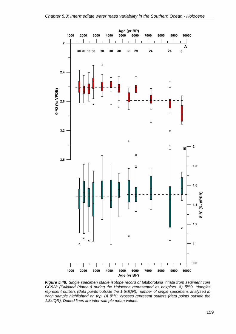
Chapter 5.3: Intermediate water mass variability in the Southern Ocean - Holocene
159
Figure 5.48: Single specimen stable isotope record of Globorotalia inflata from sediment core GC528 (Falkland Plateau) during the Holocene represented as boxplots. A) δ18O, triangles represent outliers (data points outside the 1.5xIQR); number of single specimens analysed in each sample highlighted on top. B) δ13C, crosses represent outliers (data points outside the 1.5xIQR). Dotted lines are inter-sample mean values.
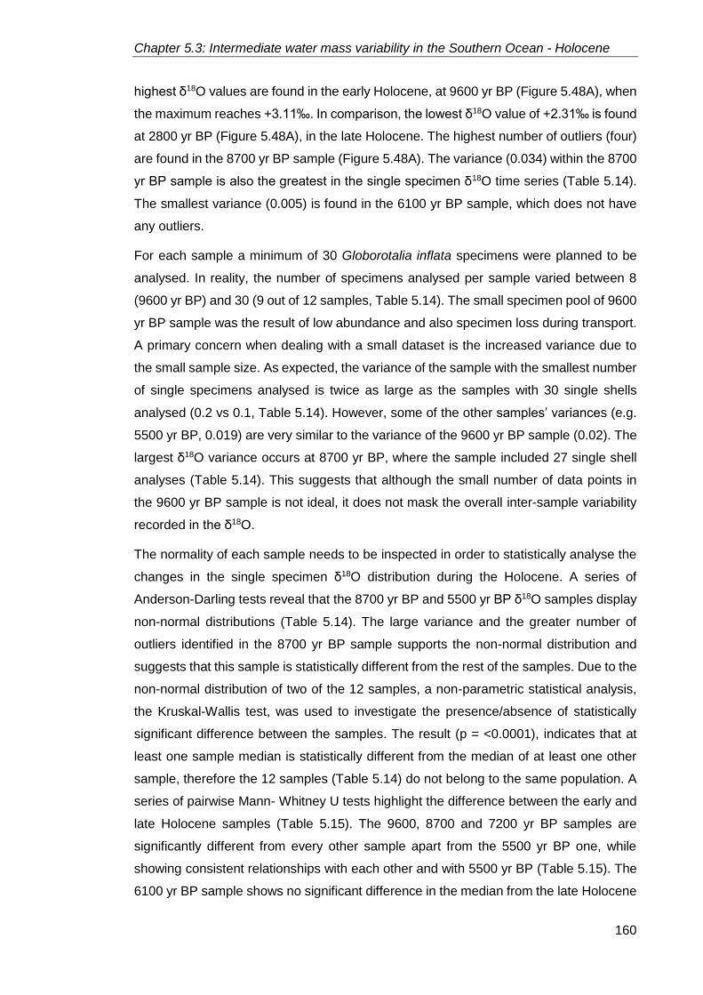
Chapter 5.3: Intermediate water mass variability in the Southern Ocean - Holocene
160
highest δ18O values are found in the early Holocene, at 9600 yr BP (Figure 5.48A), when
the maximum reaches +3.11‰. In comparison, the lowest δ18O value of +2.31‰ is found
at 2800 yr BP (Figure 5.48A), in the late Holocene. The highest number of outliers (four)
are found in the 8700 yr BP sample (Figure 5.48A). The variance (0.034) within the 8700
yr BP sample is also the greatest in the single specimen δ18O time series (Table 5.14).
The smallest variance (0.005) is found in the 6100 yr BP sample, which does not have
any outliers.
For each sample a minimum of 30 Globorotalia inflata specimens were planned to be
analysed. In reality, the number of specimens analysed per sample varied between 8
(9600 yr BP) and 30 (9 out of 12 samples, Table 5.14). The small specimen pool of 9600
yr BP sample was the result of low abundance and also specimen loss during transport.
A primary concern when dealing with a small dataset is the increased variance due to
the small sample size. As expected, the variance of the sample with the smallest number
of single specimens analysed is twice as large as the samples with 30 single shells
analysed (0.2 vs 0.1, Table 5.14). However, some of the other samples’ variances (e.g.
5500 yr BP, 0.019) are very similar to the variance of the 9600 yr BP sample (0.02). The
largest δ18O variance occurs at 8700 yr BP, where the sample included 27 single shell
analyses (Table 5.14). This suggests that although the small number of data points in
the 9600 yr BP sample is not ideal, it does not mask the overall inter-sample variability
recorded in the δ18O.
The normality of each sample needs to be inspected in order to statistically analyse the
changes in the single specimen δ18O distribution during the Holocene. A series of
Anderson-Darling tests reveal that the 8700 yr BP and 5500 yr BP δ18O samples display
non-normal distributions (Table 5.14). The large variance and the greater number of
outliers identified in the 8700 yr BP sample supports the non-normal distribution and
suggests that this sample is statistically different from the rest of the samples. Due to the
non-normal distribution of two of the 12 samples, a non-parametric statistical analysis,
the Kruskal-Wallis test, was used to investigate the presence/absence of statistically
significant difference between the samples. The result (p = <0.0001), indicates that at
least one sample median is statistically different from the median of at least one other
sample, therefore the 12 samples (Table 5.14) do not belong to the same population. A
series of pairwise Mann- Whitney U tests highlight the difference between the early and
late Holocene samples (Table 5.15). The 9600, 8700 and 7200 yr BP samples are
significantly different from every other sample apart from the 5500 yr BP one, while
showing consistent relationships with each other and with 5500 yr BP (Table 5.15). The
6100 yr BP sample shows no significant difference in the median from the late Holocene

Chapter 5.3: Intermediate water mass variability in the Southern Ocean - Holocene
161
samples of 1700, 2000, 2400, 2800, 3450, 4100 and 4700 yr BP (Table 5.15), while
statistically significant difference in the median is identified between 6100 yr BP and the
preceding three samples (Table 5.15). Significant difference is also recorded between
the 2800 and 2000 yr BP as well as the 4100 and 2000 yr BP samples (Table 5.15).
5.3.2.2 Single specimen carbon isotope record
There is no visually apparent trend in the single specimen sample δ13C time series
compared to the δ18O time series (Figure 5.48). The total inter-sample variability in the
sample median δ13C values during the Holocene is 0.16‰ (Figure 5.48B) (outside the
mass spectrometer’s standard error of 0.3‰ associated with the stable isotope analysis),
found between the 3450 yr BP (highest median value of +1.57‰) and 2800 yr BP (lowest
median value of +1.41‰) samples (Table 5.14). While the δ18O time series can be
divided into two parts (early and late Holocene), a division cannot be made in the δ13C
time series as the sample medians do not change significantly though time (Figure
5.48B). Outliers in δ13C are present in six of the 12 samples (Figure 5.48B). Only one
sample (6100 yr BP) has more than one outlier; however, the two outliers in this sample
do not correspond to the largest variance (Table 5.14). The largest variance (0.062)
occurs at 8700 yr BP, while the smallest variance (0.015) belongs to the 4700 yr BP
sample (Table 5.14). This total difference of 0.048 between the smallest and largest
within-sample variance is larger than that found in the δ18O time series as a whole
(Section 5.3.1).
The results of the Anderson-Darling normality tests on the combined single specimen
samples δ13C dataset reveal that the 6100 yr BP and 8700 yr BP δ13C samples have a
non-normal distribution (Table 5.14) most likely as a result of the large variance (in the
case of the 8700 yr BP sample, Table 5.14) and the greater number of outliers (6100 yr
BP sample). The ensuing non-parametric Kruskal-Wallis test carried out on the combined
single specimen samples δ13C dataset revealed that there is significant difference (p =
0.019) between the medians of the δ13C samples and that the samples do not belong to
the same population. Pairwise Mann-Whitney U tests (Table 5.15) did not reveal which
sample is significantly different from the others. This outcome suggests that although the
samples do not belong to the same population, and hence display significant difference
in their medians, the pairwise Mann-Whitney U test is not sensitive enough to detect the
exact relationship between the samples. This result highlights the limitation of non-
parametric statistical tests, which are known to be less sensitive than parametric tests
(Corder and Foreman, 2014).

Chapter 5.3: Intermediate water mass variability in the Southern Ocean - Holocene
162
Table 5.15: Bonferroni corrected p values of pairwise Mann-Whitney U tests conducted on sediment core GC528 single specimen Globorotalia inflata samples δ18O and δ13C. Highlighted cells indicate statistically significant difference between samples (p<0.05). δ18O Age 1700 2000 2400 2800 2450 4100 4700 5500 6100 7200 8700
1700
2000 1
2400 1 1
2800 1 0.047 0.908
3450 1 1 1 1
4100 1 0.041 1 1 1
4700 1 1 1 0.346 1 0.444
5500 2.58300E-04 5.60E-03 6.82E-04 3.38E-06 4.964E-06 1.952E-07 7.78E-04
6100 1 1 1 0.414 1 0.678 1 7.62E-05
7200 1.77E-04 1.464E-03 1.36E-04 3.97E-06 4.43E-06 8.92E-07 3.28E-04 1 3.173E-05
8700 7.94E-06 5.08E-05 9.90E-06 8.97E-07 1.26E-06 7.79E-07 2.98E-05 0.487 6.990E-06 1
9600 2.92E-03 0.004 0.003 0.002 0.002 0.002 0.004 0.382 0.002 0.916 1
δ13C
1700
2000 1
2400 1 1
2800 1 1 1
3450 0.873 1 1 0.99
4100 1 1 1 1 1
4700 1 1 1 1 1 1
5500 1 1 1 1 1 1 1
6100 1 1 1 1 1 1 1 1
7200 0.975 1 1 0.47 1 1 1 1 1
8700 1 1 1 1 0.576 1 1 1 1 0.774
9600
1 1 1 1 1 1 1 1 1 1 1

Chapter 5.3: Intermediate water mass variability in the Southern Ocean - Holocene
163
5.3.3 Globorotalia inflata stable isotope variability during the Holocene
The Globorotalia inflata single specimen sample δ18O time series has an average of
~0.2‰ difference in the mean values between samples from 9600-5500 yr BP and 4700-
1700 yr BP (Figure 5.48A), which is greater than the standard error of 0.05‰ associated
with the analysis.. The 9600-5500 yr BP period, here referred to as the Early Holocene
(EH), has average G. inflata δ18O values (between samples) of around +2.79 ± 0.13‰,
while the 4700-1700 yr BP period, here referred to as the Late Holocene (LH), has an
average G. inflata δ18O value of around +2.6 ± 0.1‰ (between samples). The variance
(range) of within-sample δ18O values also shows significant difference between the EH
and LH. Average EH within-sample variance is 0.018, and the average LH within-sample
variance is half that of the EH, at 0.09. These differences in sample δ18O averages and
within-sample variances suggest different environmental conditions existed between the
EH and LH intervals.
Contrary to the single specimen sample δ18O time series, the G. inflata single specimen
sample δ13C time series is consistent between the EH and LH (Figure 5.48B). The
between-sample average G. inflata δ13C value is +1.51± 0.17‰ in the EH, and the
between-sample average δ13C value is only 0.02‰ lower, at +1.49 ± 0.17‰, in the LH.
Additionally, the difference between the EH and LH δ13C within-specimen variance is
0.02. Differences are more prominent in the δ13C time series when the time period 4100-
1700 yr BP is compared with 9600-8600 yr BP and 7200-4700 yr BP. When the time-
series is grouped into these three time-slices a 0.06‰ difference exists between the
average δ13C values between 7200-4700 yr BP and 4100-1700 yr BP and a 0.08‰
difference in average δ13C exists between the 9600-8700 yr BP and 7200-4700 yr
periods. These differences are within the standard error associated with the mean values
of the three time period (0.21‰, 0.14‰, and 0.18‰ for the 9600-8700 yr BP. 7200-4700
yr BP, and 4100-1700 yr BP period respectively). Similarly, the within-sample variance
also displays greater offsets than the difference between the EH and LH variances when
the record is divided into these three time-slices, with 0.013 (between 7200-4700 yr BP
and 4100-1700 yr BP) and 0.027 (9600-8700 yr BP and 7200-4700 yr BP) difference
recorded between the average within-sample variances.
The different trends described in the last two paragraphs about the Globorotalia inflata
δ18O and δ13C suggest that the two records are driven by different processes that acted
at different times through the Holocene. Additionally, the statistically significant
differences identified between the single specimen samples in both the δ18O and δ13C
time series (Section 5.3.2.1, 5.3.2.2) indicate that environmental conditions changed
Chapter 5.3: Intermediate water mass variability in the Southern Ocean - Holocene
164
throughout the Holocene. The following section discusses the potential environmental
processes responsible for the isotope variability, and how the single specimen G. inflata
stable isotope time series compares with existing Southern Ocean Holocene records of
air temperatures, wind strength, Antarctic Intermediate Water strength, and glacial
meltwater discharge.
5.3.4 Globorotalia inflata as an Antarctic Intermediate Water proxy species
Globorotalia inflata is a deep-dwelling planktonic foraminifera (Bé, 1969) that mainly
calcifies in the thermocline during austral spring (Bé, 1969; King and Howard, 2005;
Wilke et al., 2006). A large-scale study of South Atlantic thermocline temperatures based
on G. inflata identified the calcification depth of this species to be between 350-400 m
(Groeneveld and Chiessi, 2011). Specimens recovered from the northern part of the
Falkland Plateau (48.91°S 57.88°W, north of Falkland Islands) were shown to have
calcified at 368 m water depth and at 3.88°C water temperature (Groeneveld and
Chiessi, 2011). This assessment puts G. inflata calcification within intermediate water
masses (Figure 5.49), specifically, within Antarctic Intermediate Water.
To constrain the approximate calcification depth of Globorotalia inflata in sediment core
GC528, and to determine any apparent vital effects in the oxygen isotope record, the
equilibrium δ18O (δ18Oeq) values were calculated. Monthly temperature and salinity data
for the sediment core location were obtained from World Ocean Atlas 13 (WOA13,
Locarnini et al., 2013; and Zweng et al., 2013; http://doi.org/10.7289/V5NZ85MT).
Seawater δ18O (δ18Osw) was estimated assuming a linear relationship (Eq. 1) between
salinity (S) and δ18Osw based on regional δ18Osw data covering the area between 55.07°S
58.29°W and 56.13°S 57.67°W, obtained from the Global Seawater Oxygen-18
Database (Schmidt et al., 1999; https://data.giss.nasa.gov/o18data/). The area (between
53.13°S 53.38°W and 53.13°S 56.38°W) selected for salinity values from the WOA13
(Zweng et al., 2013) experiences a small, 0.26 PSU, seasonal variability. The
relationship between salinity and δ18Osw is linear in the open ocean (Meredith et al.,
1999), therefore it is reasonable to enlist only one set of equations to calculate δ18Osw
(Eq. 12):
𝛿18𝑂𝑠𝑤 = 0.1698 × 𝑆 − 5.9533 Equation 12.
The calculated δ18Osw values were converted to the Pee Dee Belemnite (PDB) scale
following Bemis et al. (1998) (Eq. 13),
𝛿18𝑂𝑠𝑤(𝑃𝐷𝐵) = 0.9998 × 𝛿18𝑂𝑆𝑀𝑂𝑊 − 0.2 Equation 13.

Chapter 5.3: Intermediate water mass variability in the Southern Ocean - Holocene
165
A
B
Figure 5.49: A) Cross-sectional temperature profile of the Scotia Sea between 53°W and 56°W. The profile highlights the changing water mass structure across the 8° latitudinal section. Potential density is represented by isoclines in order to aid water mass identification. AAWW: Antarctic Winter Water; SAMW: Subantarctic Mode Water; AAAIW: Antarctic Intermediate Water; UCDW: Upper Circumpolar Deep Water; LCDW: Lower Circumpolar Deep Water. Black star represents the depth of the sediment core GC528. B) Surface water temperature map of the Scotia Sea and the Southwest Atlantic. Main frontal systems highlighted by black lines. SAF: Subantarctic Front; PF: Polar Front; SACCF: Southern Antarctic Circumpolar Current Front. Black cross represents sediment core location.

Chapter 5.3: Intermediate water mass variability in the Southern Ocean - Holocene
166
where δ18Osmow is the calculated δ18Osw value (Eq. 12) expressed on the Standard Mean
Ocean Water (SMOW) scale. The δ18Oeq values were calculated following Kim and O’Neil
(1997) and Peeters et al. (2002) temperature and δ18O relationship (Eq. 14):
𝛿18𝑂𝑒𝑞 = 25.778 − 3.333 × (43.704 + 𝑇)0.5 + 𝛿18𝑂𝑠𝑤(𝑃𝐷𝐵) Equation 14
where T is the seawater temperature and δ18Osw(PDB) is the calculated δ18Osw value (Eq.
13) expressed with respect to the PDB scale.
The δ18Oeq profile (Figure 5.50) of the austral spring months (September, October and
November) shows steadily increasing δ18O values with depth. Surface water (0-100 m)
values are lowest in November due to increasing SST. δ18Oeq values vary between
+2.29‰ and +2.67‰ in the spring months between 300 and 400 m water depths (Figure
Figure 5.50: A) Equilibrium δ18O, B) Temperature and C) Salinity at the location of sediment core GC528. δ18Oeq values for September (green), October (light blue) and November (dark blue) between the surface and 500 m water depth show the most likely calcification depth of between 150 and 500 m water depth for Globorotalia inflata. Surface values in November are highly skewed by the introduction of low salinity waters while temperature and salinity values for September show the lack of vertical stratification during that month. Published G. inflata δ18O values (with ±0.4‰ standard deviation; Niebler et al., 1999) fall on the δ18Oeq values corresponding to October supporting previous suggestions of spring-time calcification (King and Howard, 2005). δ18Oeq are based on δ18O-salinity relationship drawn from regional δ18Osw values from the Global Seawater Oxygen-18 database (Schmidt et al., 1999) and salinity and temperature values from WOA 13 (Loncarnini et al., 2013; Zweng et al., 2013).

Chapter 5.3: Intermediate water mass variability in the Southern Ocean - Holocene
167
5.50). Highest δ18Oeq values within this depth interval are found in October, increasing
from +2.61‰ at 300 m to +2.67‰ at 400 m (Figure 5.50). As the δ18Oeq values are based
on temperature and salinity values from the WOA13 (which reflect average climatologies
between 1955 and 2005) we can only make reasonable assumptions on Globorotalia
inflata calcification for the late Holocene (4700-1700 yr BP), when water temperatures
and salinities closely resembled those found today.
Late Holocene Globorotalia inflata single specimen δ18O values vary approximately
between +2.4‰ and +2.8‰ (Figure 5.48A), with an average of around +2.6‰. Deep-
dwelling planktonic foraminifera species, like G. inflata, calcify more or less in equilibrium
with the surrounding seawater, but with a significant standard deviation (±0.4‰)
(Fairbanks et al., 1982; Niebler et al., 1999; Wilke et al., 2006). Previous studies of G.
inflata placed its main calcification depth within the thermocline, however, calcification
does continue as the organism descends to deeper depths (Fairbanks et al., 1982; Wilke
et al., 2006). Based on the continuous calcification below the thermocline (Fairbanks et
al., 1982) and the δ18Oeq profile (Figure 5.50) we can place the LH G. inflata main
calcification depth between 150 m and 400 m, with calcification taking place mostly in
October. The timing and the depth of calcification agrees well with plankton tow (Mortyn
and Charles, 2003) and core top records from the South Atlantic (Chiessi et al., 2007;
Groeneveld and Chiessi, 2011). By comparing the identified calcification depth range
(150-400 m) with the WOA13 temperature and salinity data (Figure 5.49 and 5.50B, C)
it can be confirmed that G. inflata calcification takes place within the AAIW, which makes
the species suitable for the investigation of AAIW variability.
5.3.5 Does Globorotalia inflata stable isotope variability reflect changes in
local or regional environmental conditions?
The region of the Falkland Plateau, between 52°19’S and 53°21’S (Figure 5.51), is
characterised by the transition from a coastal environment dominated by Shelf Water to
an open ocean environment dominated by Transition Zone Water (TZW) (Sirota and
Sundakov, 2014). The TZW separates coastal Shelf Waters from AAIW carried by the
Falkland Current onto the Plateau (Figure 5.51). Long-term oceanography records from
the southern parts of the Falklands Plateau, spanning the time period between 2002 and
2014, reveal that seasonal temperature and salinity variability within the TZW penetrate
only to 130-140 m water depth, and warm temperature anomalies in the shelf region are
also restricted to this depth (Sirota and Sundakov, 2014). In contrast, negative
temperature anomalies of ~0.4°C were recorded within the whole depth transect (surface
to >330 m) in 2002 and 2010 (Sirota and Sundakov, 2014). The sediment core location

Chapter 5.3: Intermediate water mass variability in the Southern Ocean - Holocene
168
(53°S 58°W) is under the influence of TZW at the surface (0 to ~200 m, Figure 5.51) and
of the AAIW in the deeper layers (below 200 m) (Arkhipkin et al., 2004). The modern
oceanographic record of Sirota and Sundakov (2014) supports the findings that G. inflata
calcification takes place within AAIW. Seasonal temperature and salinity variability is
restricted to the top 130-140 m, and seasonal variability below 140 m is negligible (Sirota
and Sundakov, 2014), hence it is reasonable to suggest that the G. inflata (calcifying
below 150 m) stable isotope record does not reflect local seasonal surface or deeper
water variability. This suggestion is also supported by the fact that G. inflata
predominantly reproduces during the austral spring (e.g. King and Howards, 2005). Core
GC528 has an average sedimentation rate of 6.9 cm/kyr during the Holocene (Roberts,
2016), meaning that on average a 1 cm stratigraphic thickness contains ~145 years of
sediment and thus preserved foraminifera, hence, it is unlikely that intra-annual variability
will be preserved.
The stable isotope record might reflect local interannual variability, however, the ~0.4°C
temperature anomaly (equal to <0.1‰ change in δ18Oforam) between 2002 and 2003 was
linked to the increased influence of TZW closer to the coastal areas of the Falkland
Islands (Sirota and Sundakov, 2014). This temperature anomaly was negative in sign,
indicating the increased influence of colder water masses, and positive temperature
anomalies did not penetrate to G. inflata calcification depths. The G. inflata δ18O data
becomes lower during the Holocene indicating increasing water temperatures (if δ18O
reflects temperature instead of salinity and δ18Osw changes). However, the modern local
oceanography record indicates that only colder water masses penetrate to G. inflata
Figure 5.51: October temperature depth profile of Falkland Plateau between 52°19’S and 53°21’S (Sirota and Sundakov, 2014). Sediment core location is located between St.5 and St.6 which is bathed in AAIW at depths below 200 m.

Chapter 5.3: Intermediate water mass variability in the Southern Ocean - Holocene
169
calcification depths (Sirota and Sundakov, 2014). Hence, it is concluded that the G.
inflata δ18O does not record local oceanographic changes (including variable influence
of TZW), but records regional changes in environmental conditions. Holocene
paleoclimate records (e.g. Holmgren and Bjorck 2013; Lamy et al., 2011; Varma et al.,
2011) show a steady decline in oceanic and atmospheric temperatures between 9000 yr
BP and present day in response to declining solar insolation levels. If this temperature
decline was reflected in the G. inflata δ18O data, we could expect steadily increasing δ18O
values since 9000 yr BP. However, the G. inflata δ18O values decrease between the EH
and the LH (Figure 5.48A). This suggests, that instead of temperature, the G. inflata δ18O
record reflects changes in AAIW properties in response to source water variability.
5.3.6 Temperature- and size-dependency in single specimen Globorotalia
inflata δ18O measurements
Depth-integrated plankton tow records (Wilke et al., 2006) from the eastern South
Atlantic show that Globorotalia inflata δ18O data increase with depth following the
decreasing trend in temperature, however, there is also a 0.3‰ offset in δ18O between
smaller (150-250 µm) and larger (250-355 µm) size fractions showing higher δ18O in
larger specimens (Figure 5.52). These plankton tow findings suggest continued shell
growth and calcification with increasing depth mostly controlled by local hydrography, as
opposed to a limited and restricted calcification depth. A similar temperature-δ18O
relationship was identified in a number of other studies (e.g. Ganssen and Kroon, 2000;
King and Howard, 2005; Chiessi et al., 2007), as was the size-δ18O relationship (e.g.
Lončarić et al., 2006; Metcalfe et al., 2015) which supports the existence of size- and
temperature-related isotope variability in G. inflata.
Due to limited abundance, Globorotalia inflata specimens were not separated into
specific size fractions and, hence, size-related isotope variability cannot be discounted
from the stable isotope data. Tentative assumptions on the scale of the impact of size on
GC528 G. inflata δ18O can be made using visual observation. Specimens from the EH
period (particularly prior to 6100 yr BP) were less abundant and generally smaller than
specimens from LH samples. Based on the size-δ18O relationship it would be expected
that smaller shells would provide lower δ18O values, however, the GC528 G. inflata δ18O
results show higher average δ18O values in the EH and lower average values in the LH
(Figure 5.48A), which suggest that the long- term record is not a reflection of the size
variability of G. inflata across the Holocene but a genuine record of AAIW source-water
variability.
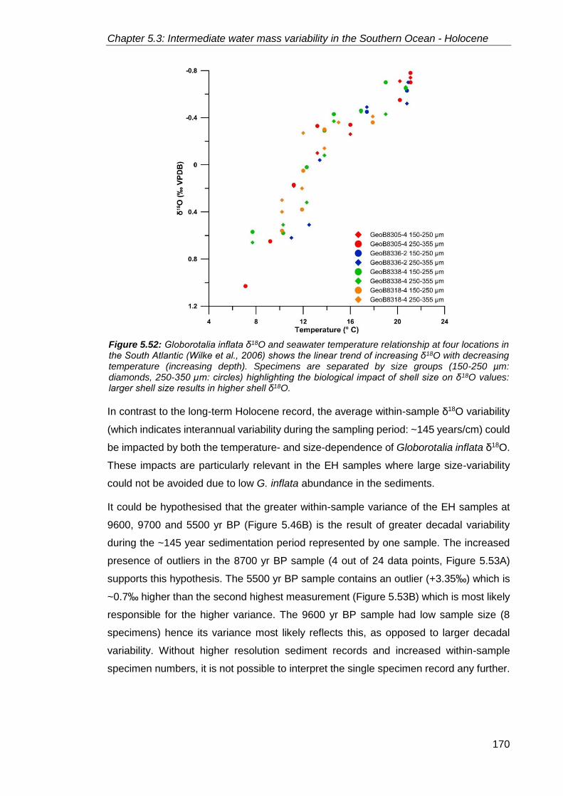
Chapter 5.3: Intermediate water mass variability in the Southern Ocean - Holocene
170
In contrast to the long-term Holocene record, the average within-sample δ18O variability
(which indicates interannual variability during the sampling period: ~145 years/cm) could
be impacted by both the temperature- and size-dependence of Globorotalia inflata δ18O.
These impacts are particularly relevant in the EH samples where large size-variability
could not be avoided due to low G. inflata abundance in the sediments.
It could be hypothesised that the greater within-sample variance of the EH samples at
9600, 9700 and 5500 yr BP (Figure 5.46B) is the result of greater decadal variability
during the ~145 year sedimentation period represented by one sample. The increased
presence of outliers in the 8700 yr BP sample (4 out of 24 data points, Figure 5.53A)
supports this hypothesis. The 5500 yr BP sample contains an outlier (+3.35‰) which is
~0.7‰ higher than the second highest measurement (Figure 5.53B) which is most likely
responsible for the higher variance. The 9600 yr BP sample had low sample size (8
specimens) hence its variance most likely reflects this, as opposed to larger decadal
variability. Without higher resolution sediment records and increased within-sample
specimen numbers, it is not possible to interpret the single specimen record any further.
Figure 5.52: Globorotalia inflata δ18O and seawater temperature relationship at four locations in the South Atlantic (Wilke et al., 2006) shows the linear trend of increasing δ18O with decreasing temperature (increasing depth). Specimens are separated by size groups (150-250 µm: diamonds, 250-350 µm: circles) highlighting the biological impact of shell size on δ18O values: larger shell size results in higher shell δ18O.
Figure 7: Globorotalia inflata δ18O and seawater temperature relationship at four locations in the
South Atlantic (Wilke et al., 2006) shows the linear trend of increasing δ18O with decreasing
temperature (increasing depth). Specimens are separated by size groups (150-250 µm:
diamonds, 250-350 µm: circles) highlighting the biological impact of shell size on δ18O values:
larger shell size results in higher shell δ18O.

Chapter 5.3: Intermediate water mass variability in the Southern Ocean - Holocene
171
Figure 5.53: Core GC528 (Falkland Plateau) A) Single specimen Globorotalia inflata δ18O represented as box-whisker plots. Dashed lines: average mean values of 9600-5500 yr BP (early Holocene) and 4700-1700yr BP (late Holocene) intervals. Triangles: outliers as identified in Figure 5.48. B) Raw single specimen G. inflata δ18O record. Black crosses: mean values, solid black line: mean trend.

Chapter 5.3: Intermediate water mass variability in the Southern Ocean - Holocene
172
In conclusion, the temperature- and size-dependence of Globorotali inflata means that
the small (~0.48‰) average within-sample range across the Holocene is most likely the
result of different calcification patterns between individual specimens. This is in
agreement with the ±0.4‰ oxygen isotope disequilibrium (vital effect) identified in the G.
inflata species, which is linked to physiological and ecological effects (Niebler et al.,
1999).
5.3.7 The role of biological and chemical processes on Globorotalia inflata
δ13C
Culture studies have shown that foraminiferal δ13C is directly related to δ13CDIC (Spero,
1992). δ13CDIC is higher in the surface water due to the preferential uptake of 12C during
primary production, while it is lower at depth where organic matter is remineralised
(Broecker and Peng, 1982). As a result, foraminiferal δ13C is expected to decrease with
depth, with the decreasing δ13CDIC. The concentration of CO32−
([CO32−
]) in the seawater
also affects the δ13C of foraminiferal calcite (Spero et al., 1997), where an increase in
seawater [CO32−
] results in decreased foraminiferal δ13C. [CO32−
] is higher in surface
waters than at intermediate depth in the South Atlantic (Wilke et al., 2006) and thus it is
expected that foraminiferal δ13C increases with depth within the water column. δ13CDIC
and [CO32−
] act in opposite direction on the foraminiferal δ13C complicating the
interpretation of planktonic foraminiferal δ13C. Globorotalia inflata secretes its shell
continuously through the water column (Lončarić et al., 2006; Wilke et al., 2006)
therefore the total shell δ13C is influenced by a range of δ13CDIC and [CO32−
] values across
its depth range. This continuous calcification across water depths means that specimens
which calcify in shallower depths (smaller shells) have different δ13C than those that
reach deeper depths during calcification (larger specimens).
Coupled with the impact of different δ13CDIC and [CO32−
] at different depths is the impact
of biological and kinetic fractionation on the δ13C of smaller and larger specimens.
Foraminifera calcify and, thus, respire faster during the early stages of their life cycle
which results in lower δ13C values in smaller and younger shells (Hemleben et al., 1989).
This well-established size-dependence of foraminiferal δ13C has been found in G. inflata
(Figure 5.54) (e.g. Wefer and Berger, 1991; Elderfield et al., 2002; Wilke et al., 2006;
Metcalfe et al., 2015) which – together with the impact of δ13CDIC and [CO32−
] on
foraminiferal δ13C – can potentially explain the lack of long-term variability in the single
specimen G. inflata δ13C time series from core GC528 (Table 5.14, Figure 5.48B). G.
inflata analyses could not be limited to specific size fractions (due to low abundance) so

Chapter 5.3: Intermediate water mass variability in the Southern Ocean - Holocene
173
it is possible that some of the within-sample range observed in the single specimen δ13C
is also due to the size-dependence of δ13C. Local changes in δ13CDIC due to changes in
primary production and upwelling/advection of waters with different δ13C (Ravelo and
Hillaire-Marcel, 2007) can also be a factor behind the variability in the within-sample
range (Figure 5.48B: minimum of 0.43‰ of the 7200 yr BP sample versus the 0.93‰ of
the 8700 yr BP sample and an average within-sample range of 0.68‰) observed in the
single specimen sample G. inflata δ13C time series. Without direct observations of the
δ13CDIC and [CO32−
] of the water masses that the G. inflata calcified in during its life cycle
it is not possible to draw further robust interpretations from the G. inflata δ13C time series.
5.3.8 A changing regime of Antarctic Intermediate Water sources during
the Holocene
One of the primary features of Holocene Southern Ocean climate is the gradual cooling
of the atmosphere from the Early Holocene Climate Optimum (~11,000-9500 yr BP) to
the present (Figure 5.55B; Masson et al., 2000; Bentley et al., 2009) as a direct response
to decreasing high latitude winter-spring solar insolation (Figure 5.55A; Renssen et al.,
2005). Decreasing air temperatures transferred down to both surface and intermediate
waters and, as a result, AAIW in the Pacific Ocean was ~1.5°C warmer during the middle
Figure 5.54: Globorotalia inflata δ13C vs Temperature in the South Atlantic (Wilke et al., 2006) shows the consistent offset in δ13C between small (150-250 μm) and large (250-355 μm) specimens. The relationship between sizes highlights the danger in mixing size fractions during analysis. The size-dependency is not constrained to surface waters (high temperatures) but is also a feature at depth (lower temperatures).

Chapter 5.3: Intermediate water mass variability in the Southern Ocean - Holocene
174
Holocene Thermal Maximum (8000-6000 yr BP) than in the 21st Century (Rosenthal et
al., 2013).
The temperature and δ18O of seawater are the two main determining factors of
foraminiferal δ18O (Ravelo and Hillaire-Marcel, 2007). Increasing seawater temperature
decreases the δ18Oforam at a rate of −0.22‰/1°C (Epstein et al., 1953). The GC528
Globorotalia inflata single specimen sample stable isotope record shows decreasing
values (Figure 5.48A) from 9600 yr BP (2.93‰ mean value) to 2700 yr BP (2.55‰ mean
value) concurrent with decreasing seawater temperatures (Rosenthal et al., 2013),
hence, it is evident that the decreasing GC528 δ18O are the result of changes in the δ18O
of AAIW. The δ18O of AAIW in the Scotia Sea is mainly driven by the balance in the
contribution of different source waters, namely the Subantarctic Mode Water (SAMW)
and Antarctic Winter Water (AAWW) (Garabato et al., 2009), which have widely different
temperatures, salinities and hence δ18O signatures (Meredith et al., 1999).
The SAMW portion of AAIW derives from the South Pacific (Hanawa and Talley, 2001)
and is formed through the deep convection of the thick winter mixed layers in the
southeast Pacific on the northern side of the ACC (Garabato et al., 2009). Part of the
SAMW is advected south and east from its formation area flowing through the Drake
Passage and, as it does, it cools (from >10°C to 4-5°C) and becomes denser forming
one part of the AAIW (Meredith et al., 1999). The δ18O of the SAMW portion of the AAIW
(−0.15‰, Table 5.16) will therefore reflect the formation region (midlatitude regions off
southeast Chile) and the modification the water mass has experienced by the time it
reached the Scotia Sea (Hanawa and Talley, 2001).
In contrast to the mid latitude-derived SAMW, AAWW contributes very cold (<1.5°C, and
can reach −1°C south of the Polar Front, Table 5.16) and fresh (~33.9 PSU) water to
AAIW (Meredith et al., 1999). AAWW forms by the seasonal warming of the surface
waters of the along the Antarctic Peninsula and its properties are mostly determined by
the contribution of precipitation and glacial meltwater (Meredith et al., 1999; Meredith et
al., 2013).
Water mass T (°C) S (PSU) δ18O (‰ VMSO)
Impact of increased contribution to AAIW
AAIW ~2.5-3 34.15 −0.21
SAMW ~4.5 34.4 −0.15 ↑T, ↑S, ↑ δ18O
AAWW <1.5 <34 −0.27 ↓T, ↓S, ↓ δ18O
Table 5.16: Temperature (T), salinity (S) and δ18O properties of Antarctic Intermediate Water (AAIW), Subantarctic Mode Water (SAMW) and Antarctic Winter Water (AAWW) in the Scotia Sea (Talley, 1996; Meredith et al., 1999; Garabato et al., 2003; Meredith et al., 2010). The impact of additional volume of SAMW and AAWW on AAIW properties is highlighted in the last column.
Water mass T (°C) S (PSU) δ18O (‰ VMSO)
Impact of increased contribution to AAIW
AAIW ~2.5-3 34.15 −0.21
SAMW ~4.5 34.4 −0.15 ↑T, ↑S, ↑ δ18O
AAWW <1.5 <34 −0.27 ↓T, ↓S, ↓ δ18O
Table 4: Temperature (T), salinity (S) and δ18O properties of Antarctic Intermediate Water (AAIW), Subantarctic Mode Water (SAMW) and Antarctic Winter Water (AAWW) in the Scotia Sea (Talley, 1996; Meredith et al., 1999; Garabato et al., 2003; Meredith et al., 2010). The impact of additional volume of SAMW and AAWW on AAIW properties is highlighted in the last column.

Chapter 5.3: Intermediate water mass variability in the Southern Ocean - Holocene
175
As both precipitation and glacial meltwater have isotopic signatures that are much lower
than average seawater, increased concentration of either of these meteoric inputs can
dramatically alter the δ18O of AAWW. AAWW is subducted along isopycnals as it is
advected northwards (Garabato et al., 2009), eventually reaching intermediate water
depth levels between the PF and the SAF where it freshens AAIW through isopycnal
mixing (Meredith et al., 1999). Although no δ18O values have been determined for the
AAWW core contribution at the SAF, a sharp decrease in δ18O of AAIW due to the
addition of AAWW (decreasing from −0.22‰ to −0.27‰) has been observed by Meredith
et al. (1999) highlighting the potential of AAWW to alter AAIW δ18O.
Based on the hypothesis that GC528 Globorotalia inflata δ18O (Figure 5.48A) reflects
AAIW δ18O and on the observations of SAMW and AAIW/AAWW properties (Meredith et
al., 1999, Garabato et al., 2009), it is suggested that AAIW experienced variability during
the Holocene. The higher δ18O values of the EH (average +2.97‰, Figure 5.53A) indicate
a greater contribution of more saline, warmer and isotopically higher SAMW to AAIW,
compared with fresher and colder AAWW, increasing the δ18O of AAIW (Table 5.16)
resulting in higher G. inflata δ18O compared with the LH. The decrease in G. inflata δ18O
after 4700 yr BP to average levels of around +2.6‰ (Figure 5.53A) could be attributed
to increased contribution of fresher and isotopically lower AAWW to AAIW, compared to
SAMW, decreasing the δ18O signature of AAIW (Table 5.16) and thus that of G. inflata.
The variability in the relative contribution of the two water masses to AAIW between the
Early and Late Holocene is most likely the result of changes in AAWW formation along
the Antarctic Peninsula during the Holocene relating to changes in climatic conditions
instead of a mixture of SAMW and AAIW variability as SAMW formation was consistent
after 8000 yr BP (Kalansky et al., 2015).
In the following two sections I attempt to link Holocene climate variability and its impact
on SAMW and AAWW formation to AAIW properties and, thus, to the observed G. inflata
δ18O variability (Figure 5.53A).
5.3.8.1 SAMW variability and its impact on AAIW properties and Globorotalia
inflata δ18O due to Holocene climate variability in the Southeast Pacific
In the Southeast Pacific, the Early Holocene Climate Optimum (after ~11,000 yr BP) was
characterised by high SSTs (Kilian and Lamy, 2012), while dry and warm climatic
conditions prevailed over South America (Unkel et al., 2010). These conditions were the
result of stronger southern westerly winds (SWW) (Figure 5.55D) — which were
positioned in a more southerly location compared to the mid-to late Holocene (Kalansky

Chapter 5.3: Intermediate water mass variability in the Southern Ocean - Holocene
176
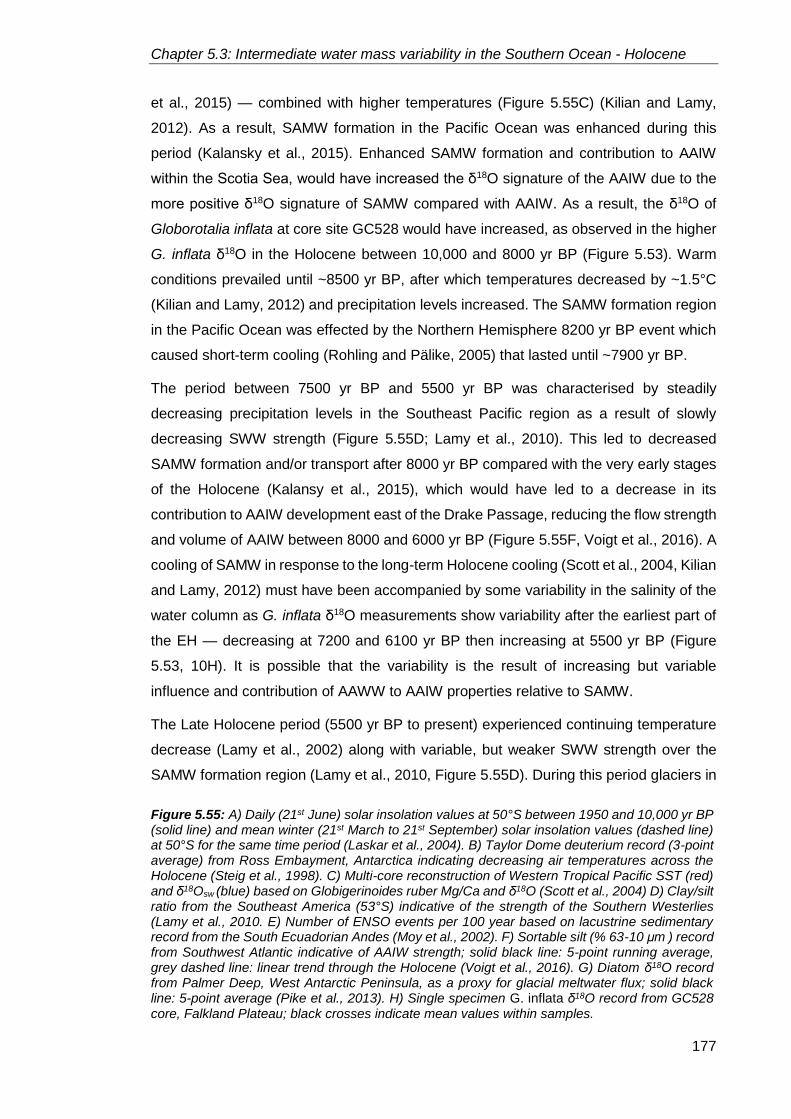
Chapter 5.3: Intermediate water mass variability in the Southern Ocean - Holocene
177
et al., 2015) — combined with higher temperatures (Figure 5.55C) (Kilian and Lamy,
2012). As a result, SAMW formation in the Pacific Ocean was enhanced during this
period (Kalansky et al., 2015). Enhanced SAMW formation and contribution to AAIW
within the Scotia Sea, would have increased the δ18O signature of the AAIW due to the
more positive δ18O signature of SAMW compared with AAIW. As a result, the δ18O of
Globorotalia inflata at core site GC528 would have increased, as observed in the higher
G. inflata δ18O in the Holocene between 10,000 and 8000 yr BP (Figure 5.53). Warm
conditions prevailed until ~8500 yr BP, after which temperatures decreased by ~1.5°C
(Kilian and Lamy, 2012) and precipitation levels increased. The SAMW formation region
in the Pacific Ocean was effected by the Northern Hemisphere 8200 yr BP event which
caused short-term cooling (Rohling and Pälike, 2005) that lasted until ~7900 yr BP.
The period between 7500 yr BP and 5500 yr BP was characterised by steadily
decreasing precipitation levels in the Southeast Pacific region as a result of slowly
decreasing SWW strength (Figure 5.55D; Lamy et al., 2010). This led to decreased
SAMW formation and/or transport after 8000 yr BP compared with the very early stages
of the Holocene (Kalansy et al., 2015), which would have led to a decrease in its
contribution to AAIW development east of the Drake Passage, reducing the flow strength
and volume of AAIW between 8000 and 6000 yr BP (Figure 5.55F, Voigt et al., 2016). A
cooling of SAMW in response to the long-term Holocene cooling (Scott et al., 2004, Kilian
and Lamy, 2012) must have been accompanied by some variability in the salinity of the
water column as G. inflata δ18O measurements show variability after the earliest part of
the EH — decreasing at 7200 and 6100 yr BP then increasing at 5500 yr BP (Figure
5.53, 10H). It is possible that the variability is the result of increasing but variable
influence and contribution of AAWW to AAIW properties relative to SAMW.
The Late Holocene period (5500 yr BP to present) experienced continuing temperature
decrease (Lamy et al., 2002) along with variable, but weaker SWW strength over the
SAMW formation region (Lamy et al., 2010, Figure 5.55D). During this period glaciers in
Figure 5.55: A) Daily (21st June) solar insolation values at 50°S between 1950 and 10,000 yr BP (solid line) and mean winter (21st March to 21st September) solar insolation values (dashed line) at 50°S for the same time period (Laskar et al., 2004). B) Taylor Dome deuterium record (3-point average) from Ross Embayment, Antarctica indicating decreasing air temperatures across the Holocene (Steig et al., 1998). C) Multi-core reconstruction of Western Tropical Pacific SST (red) and δ18Osw (blue) based on Globigerinoides ruber Mg/Ca and δ18O (Scott et al., 2004) D) Clay/silt ratio from the Southeast America (53°S) indicative of the strength of the Southern Westerlies (Lamy et al., 2010. E) Number of ENSO events per 100 year based on lacustrine sedimentary record from the South Ecuadorian Andes (Moy et al., 2002). F) Sortable silt (% 63-10 μm ) record from Southwest Atlantic indicative of AAIW strength; solid black line: 5-point running average, grey dashed line: linear trend through the Holocene (Voigt et al., 2016). G) Diatom δ18O record from Palmer Deep, West Antarctic Peninsula, as a proxy for glacial meltwater flux; solid black line: 5-point average (Pike et al., 2013). H) Single specimen G. inflata δ18O record from GC528 core, Falkland Plateau; black crosses indicate mean values within samples.
Figure 10: A) Daily (21st June) solar insolation values at 50°S between 1950 and 10,000 yr BP (solid line) and mean winter (21st March to 21st September) solar insolation values (dashed line) at 50°S for the same time period (Laskar et al., 2004). B) Taylor Dome deuterium record (3-point average) from Ross Embayment, Antarctica indicating decreasing air temperatures across the

Chapter 5.3: Intermediate water mass variability in the Southern Ocean - Holocene
178
the Southern Andes underwent periodic re-advances (Glasser et al., 2004; Wenzens,
2005) indicating highly variable, but consistently colder climate conditions compared to
the EH. The highly variable climate was most likely due to the increasing frequency and
intensity of ENSO events after ~4000 yr BP (Figure 5.55E; Moy et al., 2002). The climatic
cooling trend was also reflected in intermediate water temperatures (Rosenthal et al.,
2013) which decreased by ~1.5°C after 6000 yr BP. SAMW formation and/or transport
in the Southeast Pacific remained steady during the LH at earlier levels (Kalansky et al.,
2015) even in the face of these variable environmental conditions. This suggests, that
the observed increase in AAIW flow speed and volume (Figure 5.55F, Voigt et al., 2016)
and the decrease in Globorotalia inflata δ18O values after 5500 yr BP (Figure 5.53) is
related to the increased influence/input of AAWW to AAIW properties.
5.3.8.2 AAWW variability and its impact on AAIW properties and Globorotalia
inflata δ18O due to Holocene climate variability at the Antarctic Peninsula
and South Atlantic
The Antarctic Peninsula (AP) and South Atlantic section of the Southern Ocean were
impacted differently to the Southeast Pacific during the Early Holocene. The Early
Holocene Climate Optimum was present at high latitudes, as evidenced by ice-core-
derived temperature records (e.g. Masson et al., 2000; Figure 5.55B), however, it was
shorter lived (~11,000-9500 yr BP) than in lower latitudes. The period between 9500 yr
BP and 5500 yr BP was characterised by continuing deglaciation across the AP (Bentley
et al., 2006), however, the rate of glacial discharge along the West Antarctic Peninsula
(WAP) experienced a slowdown (Pike et al., 2013, Figure 5.55G) compared to the early
deglaciation. Large regional differences (during the time period 9500-5500 yr BP) also
existed between the apparently colder South Atlantic-Southern Ocean (Bianchi and
Gersonde, 2004) and the warmer AP (Domack, 2002) where sea ice cover also
decreased (Leventer et al., 2002; Barbara et al., 2016). The consistent, though slower
glacial discharge after 9500 yr BP would have promoted AAWW formation along the AP
contributing to AAIW generation further north in the Scotia Sea. Prior to 8000 yr BP,
SAMW, with its increased formation rate (see 1.2.5.1) would have had a greater influence
on AAIW properties especially as glacial discharge slowed down around 9000 yr BP
(Pike et al., 2013), leading to the high Globorotalia inflata δ18O (Figure 5.53). As SAMW
transport decreased towards the end of the EH, the constant advection of AAWW
towards AAIW formation regions would have caused AAIW δ18O to decrease thereby
causing G. inflata δ18O to decrease (Figure 5.53), however, the small variability observed
in the G. inflata record indicates that the relative contribution of AAWW and SAMW to
AAIW was variable. Altogether, the overall high (average 2.97‰) G. inflata δ18O during
Chapter 5.3: Intermediate water mass variability in the Southern Ocean - Holocene
179
the EH suggest that although AAWW (low δ18O) influenced AAIW properties at that time,
SAMW (high δ18O) exerted a greater impact.
Following the transitional period after the Early Holocene Climate Optimum, the period
between 4500 to 2800 yr BP experienced warmer temperatures at the WAP (Hodgson
et al., 2004). This warming was accompanied by increased primary productivity (Schmidt
et al., 1990), decreased sea ice cover (Shevenell et al., 1996; Domack et al., 2003) and
increased, but variable glacial meltwater discharge (Figure 5.55G; Pike et al., 2013;
Swann et al., 2017) as a result of increased concentration and intensity of ENSO events
(Figure 5.55E) related to the southward movement of the intertropical convergence zone
(Moy et al., 2002). The latest Holocene period since 2800 yr BP experienced even higher
levels of glacial meltwater discharge (Figure 5.55G; Pike et al., 2013) and seasonally
highly variable sea ice cover (Domack et al., 2002) due to atmospheric warming relating
to peak ENSO event frequency during the latest Holocene (Figure 5.55E). As a result of
the increased glacial discharge after 5000 yr BP (Pike et al., 2013), AAWW formation
would have been invigorated, increasing its relative proportion in AAIW formation in the
Scotia Sea thereby decreasing AAIW and thus Globorotalia inflata δ18O (Figure 5.55H).
This is supported by increasing AAIW flow speeds after the EH; indicated by sortable silt
records in the South Atlantic (Figure 5.55F, Voigt et al., 2016) as well as by the increasing
volume of AAIW after the mid-Holocene (Voigt et al., 2016) when SAWM formation was
steady (Kalansky et al., 2015).
Assessment of Holocene climate variability and its impact on SAMW and AAWW
formation during the Holocene shows that there is a clear link between Globorotalia
inflata δ18O at core site GC528 on the Falkland Plateau and climatic conditions further
afield. The observed 0.37‰ offset in G. inflata single specimen sample δ18O between
the EH and the LH (Figure 5.53) can therefore be explained by the variable relative
proportion and influence of SAMW and AAWW to AAIW at the core site. On average,
SAMW had a greater relative contribution to AAIW during the EH, leading to high G.
inflata δ18O (Figure 5.53A). In contrast, AAWW made up a greater proportion of AAIW in
the LH, decreasing average G. inflata δ18O.
5.3.9 Summary and Conclusion
Here the aim was to investigate variability in the seasonality of oceanographic conditions
during the Holocene period through the use of single specimen Globorotalia inflata stable
isotope analysis. Statistical analysis reveals significant difference in within-sample δ18O
variance (which are outside the analytical error) and significantly different environmental
conditions between the Early Holocene and Late Holocene period which is also reflected

Chapter 5.3: Intermediate water mass variability in the Southern Ocean - Holocene
180
by the ~0.2‰ difference in average δ18O between the Early and Late Holocene period.
G. inflata calcifies within Antarctic Intermediate Waters (AAIW) on the Falklands Plateau
below 150 m water depth. AAIW shows no significant seasonal variability which together
with the one peak flux of G. inflata per year (austral spring) means that the stable isotope
record is not a reflection of intra-annual variability, nor does it reflect local oceanographic
conditions. Instead it is proposed that the G. inflata at the core location records changes
in AAIW properties in response to source water variability. Due to the temperature- and
size-dependence of G. inflata the ~0.48‰ average within-sample δ18O variability
identified from the single specimen δ18O measurements is most likely the result of
different calcification patterns between individual specimens related to vital effects.
The Holocene AAIW source water variability is investigated by comparing the impact of
changing Subantarctic Mode Water (SAMW) and Antarctic Winter Water (AAIW) – the
source waters of AAIW – on Globorotalia inflata δ18O which is then assessed in terms of
Holocene Southern Ocean climate variability. SAMW, which derives from the South
Pacific, contributes relatively warm (~4.5 °C) waters to AAIW with a δ18O signature
(−0.15‰) that is relatively higher than the core AAIW δ18O (−0.21‰). In contrast, AAWW,
which derives from the Antarctic Peninsula, contributes cold (<1.5°C) and fresh (<34
PSU) waters to AAIW with a δ18O signature (−0.27‰) that is lower than the core AAIW
δ18O. The assessment of Holocene climate variability and its impact on SAMW and
AAWW formation revealed that during the Early Holocene SAMW provided a greater
contribution to AAIW than AAWW, increasing AAIW δ18O, which resulted in the high
(average of around +2.79‰) G. inflata δ18O between 9600 and 5500 yr BP. The relative
contribution of fresher and isotopically lower AAWW increased after 4700 yr BP as a
result of the increased glacial meltwater discharge along the Antarctic Peninsula and
decreased SAMW formation (compared to the Early Holocene). This increased AAWW
formations decreased AAIW δ18O in the Scotia Sea, resulting in the lower (average of
around +2.6‰) G. inflata δ18O between 4700 and 1700 yr BP. This assessment shows
the clear link between G. inflata δ18O at the Falkland Plateau and oceanographic
changes along the Antarctic Peninsula during the Holocene. Additionally, this study
highlights the applicability of G. inflata δ18O as a proxy for intermediate water variability
across the Southern Ocean.

181
6 Conclusions and Recommendations
This thesis provides insights into the use of single specimen foraminiferal stable isotope
analysis to study changes in seasonality in high latitude regions. In this final chapter, the
aims and objectives set out in Chapter 1 will be assessed against the findings of the
studies contained in Chapter 5.1, 5.2, and 5.3. Additionally, recommendations will be
made on the single specimen foraminiferal stable isotope method when applied in the
high latitudes, as well as on the analysis of morphological variability and foraminiferal
abundance.
6.1 Neogloboquadrina pachyderma abundance, vital effects,
and calcification depth variability in the Scotia Sea: results
from vertical plankton hauls
Single specimen stable isotope analysis was carried out on modern Neogloboquadrina
pachyderma (Np) specimens that were collected by vertical plankton hauls in the Scotia
Sea. The aim of this chapter was to assess the variability in the stable isotope record
across the mid to high latitudes of the Scotia Sea in order to provide a region-specific
record of vital effects. Additionally, variability in the abundance and morphotypes of Np
was also assessed.
Neogloboquadrina pachyderma abundance varies by up to two orders of magnitude
between the most southerly station south of the Southern Boundary of the Antarctic
Circumpolar Currents and one of the most northerly station located on the southern edge
of the Polar Front. Alongside the equatorward increase in Np numbers, the depth of peak
Np abundance at each stations increased from south to north across the study area. The
pattern of Np flux and depth of peak Np numbers at the stations is consistent with
previous plankton tow studies conducted in the Atlantic sector of the Southern Ocean
(Mortyn and Charles, 2003) and confirms the role of temperature and chlorophyll α
concentration on Np flux.
Previous studies of Southern Ocean Neogloboquadrina pachyderma highlighted the
existence of a number of different morphotypes and genotypes within the species which
were linked to different environmental conditions (Kennett, 1968; Darling et al., 2004)
and parts of the foraminiferal life cycle (Vautravers et al., 2013). To avoid the possibility
of morphology-related isotope variability prior to the single specimen isotope analysis,
the Neogloboquadrina pachyderma specimens were inspected under light microscope

Chapter 6: Conclusions
182
and separated into morphotypes. Three morphotypes were identified (Np-A, Np-B, and
Np-C), with the first two representing adult forms (with a secondary crust) whose
distribution is separated by the Southern Antarctic Circumpolar Current. In contrast, the
third morphotype represents juvenile, pre-gametogenic specimens that dominated the
assemblage at one station west of South Georgia.
Similarly to Np abundance, a latitudinal gradient is present in δ18Onp as a result of the
south to north temperature increase across the study area. δ18Onp differences across the
Scotia Sea are also linked to differences in shell size/weight and morphotypes, as
heavier specimens have higher δ18Onp, and the juvenile, Np-C specimens show the
lowest δ18Onp. The relationship between size and δ18Onp is similar to that observed in Np
by previous studies (e.g. Bausch et al., 1997; Hillaire-Marcel et al., 2004).
The Scotia Sea displays a wide range of oceanographic variability (see Chapter 5.1.3
and 5.1.4), the result of which is variability in the depth of the mixed layer and the
pycnocline across the study area and the depth of peak Np abundance. Foraminiferal
calcite equilibrium δ18O is closely linked to temperature, and as a result, it varies spatially
and with depth. Both calcification depths and vital effects - the deviation from equilibrium
calcification due to biological and or kinetic processes (Ravelo and Hillaire-Marcel, 2007)
- show variability across the Scotia Sea in relation to morphotypes and local
hydrography. The juvenile morphotype (Np-C), which calcifies within the mixed layer
shows a negative offset of ~0.6‰ from mixed layer δ18Oeq. In contrast, Np-A
morphotypes show variable calcification depths and vital offsets. Calcification in
equilibrium below the mixed layer by Np-A was observed at three stations, two of which
were open ocean settings, and one an enclosed bay. This equilibrium calcification below
the mixed layer agrees well with another Np study in the northern Pacific (Asahi et al.,
2015), while other plankton tow studies observed negative fractionations of up to 1‰
(e.g. Bausch, et al., 1997; Volkmann and Mensch, 2001; Mortyn and Charles, 2003).
Some Np-A specimens also show calcification in equilibrium within the mixed layer at all
the stations where they were present, as well as out of equilibrium (−0.46‰ vital offset)
within the mixed layer at one station. This variable offset from δ18Oeq is most likely the
result of calcification, and secretion of the secondary crust within the mixed layer
supporting previous suggestions that it is not temperature-driven, but instead controlled
by biological processes (Jonkers et al., 2016; Fenhrenbacher et al., 2017).

Chapter 6: Conclusions
183
6.2 Seasonal variability of Neogloboquadrina pachyderma
abundance, morphology, and stable isotope composition at
the West Antarctic Peninsula
A complete assessment of Neogloboquadrina pachyderma abundance, morphology, and
single specimen isotope variability over a period of six year (2006-2013) at the
continental shelf off Palmer Deep, West Antarctic Peninsula was presented in this
chapter. The aim of this chapter was to create a modern record of seasonal and
interannual variability of Np properties in relation to environmental changes in the high
latitude regions.
Neogloboquadrina pachyderma flux displays both intra- and inter-annual variability in the
sediment trap record. Flux varies from near zero to over 300 tests/m2/day between the
winter and summer months, with two distinct pulses occurring, one in austral late spring
and one in late summer. The first peak Np flux takes place soon after the winter sea ice
dissipates and coincides with the early chlorophyll bloom. The peak Np flux occurs during
the second chlorophyll bloom when surface water temperatures are the highest and the
water column is stratified. Although Np flux decreases in-between the two blooms it
remains above values observed during the winter months. The bimodal pattern of Np flux
and the pattern of environmental properties during the year suggest that the development
of optimum growing conditions created by a combination of environmental variables
determine the Np shell flux. These include food availability, maximum SST, and timing
of sea ice retreat that determine the strength of the biological productivity. The bimodal
Np flux pattern has previously been observed in the North Atlantic (Rolund and Bé, 1971;
Jonkers et al., 2010), while in the Arctic (Kohfeld et al., 1996; Simstich et al., 2003) and
in the northern Weddell Sea (Donner and Wefer, 1994) a single peak flux was recorded
highlighting the importance of the optimum growing conditions for Np abundance.
The study site is located within the outer marginal ice zone, an area of high biological
productivity (Smith et al., 2008). The availability of nutrients and the physical properties
of the water column vary both temporally and spatially in this region (Smith et al., 1995).
In particular, the extent of the sea ice off the shore of the WAP shows high inter-annual
variability (Stammerjohn et al., 2008a). As a result, the timing and amplitude of the Np
flux varies year-on-year. The timing of the first peak flux moves from November to
October in 2011-12 compared to the other years, the second peak flux moves from late
January to late February in 2010-11, while the amplitude varies by three orders of
magnitude between 2007-08 and 2010-11 as a direct result of changes in the timing of
sea ice melt and development of the chlorophyll bloom.

Chapter 6: Conclusions
184
Two distinct morphotypes of Neogloboquadrina pachyderma were identified in the
sediment trap samples, an adult morphotype, Np-A, and a juvenile morphotype, Np-C
(following from Chapter 5.1). Along with flux, Np morphology also displays both intra-and
inter-annual variability. Largest Np specimens are found in the spring-summer months,
and show differences in size between the years, with the highest Np peak flux specimens
of Nov-Jan 2010-11obtaining the largest shell sizes. Similarly to size, the translucency
of the specimens also shows intra-annual variability showing greater calcification of
summer specimens compared to winter ones. Detailed statistical analysis revealed that
the morphological variability in the sediment trap record is driven by sea ice and
chlorophyll concentration, similarly to Np flux. Increased sea ice concentration/longer
sea ice season together with lower chlorophyll concentration creates unfavourable
conditions for Np to complete their life cycle. Only if Np specimens are already mature,
more robust can they survive these conditions to reproduce once sea ice melts and
nutrients concentrations are higher, although their overall flux will be reduced.
Neogloboquadrina pachyderma calcification depth varies between 45 and 100 m during
the summer months, assuming no vital offset, which falls within existing studies of Np
calcification depths in the Southern Ocean (Mortyn and Charles, 2003) and in the
Antarctic Peninsula (Hendry et al., 2009). Np δ18O values show inter-and inter-annual
variability, similarly to flux and morphology; displaying a maximum of 0.5‰ difference
between winter values of 2008 and 2012, and a more than 3‰ difference between May
and December 2012 Np δ18O values. The relationship between Np δ18O and δ18Oeq also
shows variability, as Np δ18O follows δ18Oeq between October and May but diverges
during the winter season. The inter-annual variability is most likely the result of a number
of reasons, including the mortality of post-gametogenic specimens that became dormant
during the winter season leading to higher δ18Onp values between March and September
and years with low intra-annual variability, and negative offset from δ18Oeq. Another
possibility is the presence of small, juvenile, Np-C morphotypes that have not secreted
their calcite crust leading to the low δ18Onp (relating to the ontogenic calcite), such as
those during the winter season of 2012. The single specimen Np δ18O record shows a
clear link between morphology, environmental conditions, and δ18O. Heaviest δ18Onp
values coincide with the largest test sizes, and the greatest number of specimens that
obtained their secondary crust at the end of their life cycle, during times of optimum
growing conditions. The annual record of δ18Onp and size show a clear seasonal trend,
with increasing size, encrustation, and δ18Onp from spring to summer followed by
decreasing size, encrustation, and δ18Onp from the autumn as growing conditions
deteriorate (SST and chlorophyll concentration decrease and sea ice concentration

Chapter 6: Conclusions
185
increases). An overall synthesis of seasonal variability in flux, morphology, and δ18O can
be found in Chapter 5.2.9 (Figure 5.45).
The sediment trap record highlighted the impact of atmospheric teleconnections between
El Niño-Southern Oscillation/Southern Annular Mode (ENSO/SAM) and high latitude
atmospheric settings. A positive SAM coinciding with a strong La Niña in 2010 led to
anomalously low sea level pressure over the Bellingshausen Sea crating strong north-
northwesterly winds between September 2010 and February 2011 that resulted in an
early sea ice retreat and late sea ice advance (Meredith et al., 2017). Simultaneously,
the upwelling of nutrient-rich, warm Upper Circumpolar Current (UCDW) waters over the
continental shelf increased in recent times due to ENSO/SAM (Martinshon and McKee,
2012) creating more favourable conditions for phytoplankton growth (Prézelin et al.,
2004). The result of these atmospheric and oceanographic conditions was the
proliferation of larger, rounder, and more encrusted Neogloboquadrina pachyderma with
high δ18Onp in the spring of 2010, leading to a flux of over 1000 specimen/m2/day, an
anomalous number in the six-year long record. These 2010 samples emphasised the
impact of ENSO/SAM on the marine ecosystem around the Antarctic Peninsula.
Additionally, it also showed how sediment samples can be overwhelmed by anomalous
years with very high number of Np potentially skewing paleoceanographic
reconstructions.
6.3 Investigating intermediate water mass variability in the
Southern Ocean during the Holocene
Single specimen isotope analysis was carried out on Globorotalia inflata specimens
collected from a sediment core recovered from the Falkland Plateau in the Scotia Sea.
The aim of this chapter is to use the foraminiferal isotope record to investigate
intermediate water variability relating to environmental and climatic changes in the
southern high latitudes during the Holocene period.
The single specimen Globorotalia inflata record displays a statistically significant
variability in within-sample δ18O range during the Holocene, as well as significantly
different environmental conditions between the Early and Late Holocene period. The
single specimen δ18O record shows an average of ~0.48‰ within-sample range across
the Holocene which is linked to different calcification patterns between individual
specimens, particularly, as G. inflata specimens have a large variability in vital offsets
(±0.4‰) related to physiological and ecological effects (Niebler et al., 1999). Significant
within-sample variability in Early Holocene samples were outside the ±0.4‰ range and
thus could be a sign of greater decadal variability at those times. However, the resolution

Chapter 6: Conclusions
186
of the sediment core and the within-sample specimen numbers prevents more detailed
interpretation of these higher within-sample variability.
Globorotalia inflata was identified as an intermediate water species, supporting previous
assessments in the southern mid latitudes (Wilke et al., 2006; Groeneveld and Chiessi,
2011). At the Falkland Plateau G. inflata was shown to calcify within Antarctic
Intermediate Water (AAIW) below 150 m water depth making it a useful species to study
changes in this water mass over longer periods. A modern assessment of oceanographic
conditions around the Falkland Plateau (Sirota and Sundakov, 2014) revealed that AAIW
does not show significant seasonal variability at this location. As such, the average 0.2‰
G. inflata δ18O variability between the Early and Late Holocene can be considered as the
result of changes in AAIW properties in response to source water variability.
Antarctic Intermediate Water is primarily made up of Subantarctic Mode Water (SAMW)
and Antarctic Winter Water (AAWW) (Garabato et al., 2009), and thus, its δ18O signature
is determined by the balance between these two water masses with widely different
temperatures, salinities, and thus δ18O values (Meredith et al., 1999). The portion of
SAMW that enters the Drake Passage is warmer (~4.5°C) and isotopically heavier
(−0.15‰) than the core AAIW (−0.21‰). In contrast, AAWW is colder, fresher, and
isotopically lighter (<1.5°C, <34 PSU, less than −0.27‰) than the core AAIW. Hence,
variability between the contributions of the two source waters have a clear impact on
AAIW δ18O, and as a consequence, G. inflata δ18O.
A detailed assessment of Holocene climate variability revealed that during the Early
Holocene SAMW provided a greater contribution to AAIW formation than AAWW
resulting in the higher average G. inflata δ18O values (+2.8‰) recorded between 9600
and 5500 yr BP. After this period, increased glacial meltwater discharge along the
Antarctic Peninsula increased the contribution of AAWW to AAIW at the same time as
SAMW formation decreased relative to the Early Holocene. As a result, AAIW δ18O
decreased, as seen in the lower average G. inflata δ18O values (+2.6‰) between 4700
and 1700 yr BP. The G. inflata δ18O record shows a strong link between high latitude
oceanographic processes and mid latitude water mass variability and highlights the
possibility of using this proxy to study long term intermediate water variability in the
Southern Ocean.
6.4 Recommendations to improve methods
In this thesis I utilised single specimen foraminiferal δ18O to attempt to investigate
changes in seasonality in the high latitudes. Single specimen foraminiferal δ18O has been
used successively in tropical regions, where species are larger in size, and intra- and

Chapter 6: Conclusions
187
inter-annual variability is large thanks to monsoon and ENSO activities (Koutavas et al.,
2006; Khider et al., 2011; Scroxton et al., 2011; Ford et al., 2015). In this section I aim to
summarise my findings relating to the single specimen method as well as to the
morphological and abundance studies.
Recommendations for single specimen foraminiferal isotope analysis:
Analysis of a minimum of 30, preferably 50, specimens in each sample to ensure
statistically significant results in statistical analysis.
Each Foraminifera specimen, especially when small polar species like
Neogloboquadrina pachyderma is used, should be weighed to ensure carbonate
mass is enough for isotope analysis. Although it is a time-consuming exercise,
by doing this, it is possible to limit the number of unreliable isotope results.
Separate Neogloboquadrina pachyderma specimens into morphotypes to limit
the possibility of morphotype-related isotope variability. In particular, remove
juvenile specimens from samples prior to analysis as the δ18O of ontogenic calcite
is significantly lower than the secondary crust due to biological processes
(changes relating to physical processes will be masked).
If Neogloboquadrina pachyderma is used to reconstruct long term seasonality, it
is important to constrain genotypic variability, which is linked to frontal
boundaries.
Use of Quantile-Quantile plots (if possible) would aid the assessment of
difference is distribution between two time periods (see Ford et al., 2015).
Recommendations for morphometric analysis:
Weigh every shell analysed for morphometrics to be able to determine changes
in density.
If possible, use a combination of individually mounted specimens and automated
microscope setup, where a camera moves on a platform and takes photos of
individual specimens. This would reduce errors relating to different orientations
of the specimens.
Use automated image analysis techniques to speed up image processing.
Explore the use of Fourier shape analysis (Healy-Williams, 1992; Eynaud et al.,
2009) to identify morphotypes.
Recommendations for plankton tow studies:
Use of MOCNESS nets (Multiple Opening and Closing Net, with and
Environmental Sensing System) similarly to Kohfeld et al. (1996), and Mortyn and

Chapter 6: Conclusions
188
Charles (2003). A MOCNESS net can be equipped with sensors that measure in
situ water temperature, salinity, fluorescence, and water flow through the nets,
providing truly concomitant foraminiferal abundance numbers and water property
data. It also rescinds the need for a separate CTD to measure these properties,
although water samples for δ18Osw would need to be collected by a CTD. The net
captures samples at distinct, separate depth intervals giving a picture of
foraminifera species and abundance variability across a range of depths.
Use of a flow meter in order to calculate true foraminiferal abundance (in #/m3 of
seawater).
189
7. References
Allen, C. S. et al. 2010. A record of Holocene glacial and oceanographic variability in Neny Fjord, Antarctic Peninsula. Holocene 20(4), pg. 551-564. Allen, C. S. et al. 2011. Last glacial–interglacial sea-ice cover in the SW Atlantic and its potential role in global deglaciation. Quaternary Science Reviews 30(19–20), pg. 2446-2458. Arkhipkin, A. I. et al. 2004. The influence of seasonal environmental changes on ontogenetic migrations of the squid Loligo gahi on the Falkland shelf. Fisheries Oceanography 13(1), pg. 1-9. Asahi, H. et al. 2015. Seasonal variability of δ18O and δ13C of planktic foraminifera in the Bering Sea and central subarctic Pacific during 1990-2000. Paleoceanography 30(10), pg. 1328-1346. B. Brown, M. and Forsythe, A. 1974. Robust Tests for Equality of Variances. Journal of the American Statistical Association 69, pg. 364-367. Barbara, L. et al. 2016. Environmental responses of the Northeast Antarctic Peninsula to the Holocene climate variability. Paleoceanography 31(1), pg. 131-147. Barker, P. F. and Camerlenghi, A. 2002. Glacial History of the Antarctic Peninsula from Pacific Margin Sediments. In: Barker, P.F., Camerlenghi, A., Acton, G.D., and Ramsay, A.T.S. (Eds.), Proceedings of the Ocean Drilling Program, Scientific Results, 178. [Online]. <http:// www-odp.tamu.edu/publications/178_SR/VOLUME/SYNTH/SYNTH.PDF. Available on: [Accessed: 14/09/2017]. Bauch, D. et al. 1997. Oxygen isotope composition of living Neogloboquadrina pachyderma (sin) in the Arctic Ocean. Earth and Planetary Science Letters 146(1-2), pg. 47-58. Bauch, D. et al. 2000. The imprint of anthropogenic CO2 in the Arctic Ocean: evidence from planktic δ13C data from watercolumn and sediment surfaces. Deep Sea Research Part II: Topical Studies in Oceanography 47(9), pg. 1791-1808. Bauch, D. et al. 2002. Carbon isotopes and habitat of polar planktic foraminifera in the Okhotsk Sea: the ‘carbonate ion effect’ under natural conditions. Marine Micropaleontology 45(2), pg. 83-99. Be, A. W. H. 1980. GAMETOGENIC CALCIFICATION IN A SPINOSE PLANKTONIC FORAMINIFER, GLOBIGERINOIDES-SACCULIFER (BRADY). Marine Micropaleontology 5(3), pg. 283-310. Bemis, B. E. et al. 1998. Reevaluation of the oxygen isotopic composition of planktonic foraminifera: Experimental results and revised paleotemperature equations. Paleoceanography 13(2), pg. 150-160. Bentley, M. J. et al. 2006. Geomorphological evidence and cosmogenic 10Be/26Al exposure ages for the Last Glacial Maximum and deglaciation of the Antarctic Peninsula Ice Sheet. Geological Society of America bulletin. 118(9), pg. 1149-1159. Bentley, M. J. et al. 2009. Mechanisms of Holocene palaeoenvironmental change in the Antarctic Peninsula region. Holocene 19(1), pg. 51-69. Berben, S. M. P. et al. 2017. A late-Holocene multi-proxy record from the northern Norwegian margin: Temperature and salinity variability. Holocene 27(6), pg. 822-834.
190
Berger, W. H. et al. 1978. Stable isotopes in deep-sea carbonates: Box core ERDC-92, West Equatorial Pacific. Oceanologica Acta 1(2), pg. 203-216. Bianchi, C. and Gersonde, R. 2004. Climate evolution at the last deglaciation: the role of the Southern Ocean. Earth and Planetary Science Letters 228(3-4), pg. 407-424. Boltovskoy, E. 1971. Ecology of the planktonic Foraminifera living in the surface layer of Drake Passage. Micropaleontology 17(1), pg. 53-68. Boltovskoy, E. et al. 1996. Planktic foraminifera from the southwestern Atlantic (30 degrees-60 degrees S): Species-specific patterns in the upper 50 m. Marine Micropaleontology 28(1), pg. 53-72. Bouvier-Soumagnac, Y. and Duplessy, J.-C. 1985. Carbon and oxygen isotopic composition of planktonic foraminifera from laboratory culture, plankton tows and recent sediment; implications for the reconstruction of paleoclimatic conditions and of the global carbon cycle. The Journal of Foraminiferal Research 15(4), p. 302. Broecker, W. S. and Peng, T. 1982. Tracers in the sea. Lamont-Doherty Geological Observatory, Columbia University. 690 pages. Broecker, W. S. and Peng, T. H. 1974. Gas exchange rates between air and sea. Tellus 26(1-2), pg. 21-35. Bromwich, D. H. et al. 2013. Central West Antarctica among the most rapidly warming regions on Earth. Nature Geoscience 6(2), pg. 139-145. Bé, A. W. H. 1969. Planktonic Foraminifera. In Folio 11: Distribution of Selected Groups of Marine Invertebrates in Waters South of 35 ° S Latitude. New York, pg. 9-12. Caromel, A. G. M. et al. 2015. Morphological Change During The Ontogeny Of The Planktic Foraminifera. Journal of Micropalaeontology. pg. 2-19. Carstens, J. et al. 1997. Distribution of planktic foraminifera at the ice margin in the Arctic (Fram Strait). Marine Micropaleontology 29(3), pg. 257-269. Charles, C. D. and Fairbanks, R. G. 1990. Glacial to interglacial changes in the isotopic gradients of Southern Ocean surface water. In: Bleil, U. and Thiede, J. eds. Geological History of the Polar Oceans: Arctic Versus Antarctic. Norwell, Massachusetts: Kluwer Academic Publishers, pg. 519-538. Chiessi, C. M. et al. 2007. Signature of the Brazil-Malvinas Confluence (Argentine Basin) in the isotopic composition of planktonic foraminifera from surface sediments. Marine Micropaleontology 64(1-2), pg. 52-66. Clarke, A. et al. 2007. Introduction. Antarctic ecology from genes to ecosystems: the impact of climate change and the importance of scale. Philosophical Transactions of the Royal Society B-Biological Sciences 362(1477), pg. 5-9. Clem, K. R. and Fogt, R. L. 2013. Varying roles of ENSO and SAM on the Antarctic Peninsula climate in austral spring. Journal of Geophysical Research-Atmospheres 118(20). pg. 11,481-11,492. Cleroux, C. et al. 2007. Deep-dwelling foraminifera as thermocline temperature recorders. Geochemistry Geophysics Geosystems 8, pg 1-19.

191
Cleroux, C. et al. 2013. Reconstructing the upper water column thermal structure in the Atlantic Ocean. Paleoceanography 28(3), pg. 503-516. Cook, A. J. et al. 2005. Retreating glacier fronts on the Antarctic Peninsula over the past half-century. Science 308(5721), pg. 541-544. Cook, A. J. et al. 2016. Ocean forcing of glacier retreat in the western Antarctic Peninsula. Science 353(6296), pg. 283-286. Dalziel, I. W. D. et al. 2013. The Scotia Arc: Genesis, Evolution, Global Significance. Annual Review of Earth and Planetary Sciences, Vol 41 41, pg. 767-793. Darling, K. F. et al. 2006. A resolution for the coiling direction paradox in Neogloboquadrina pachyderma. Paleoceanography 21(2). PA2011. Darling, K. F. et al. 2004. Molecular evidence links cryptic diversification in polar planktonic protists to quaternary climate dynamics. Proceedings of the National Academy of Sciences of the United States of America 101(20), pg. 7657-7662. Deacon, G. E. R. 1937. The Hydrology of the Southern Ocean. Cambridge, U.K.: Cambridge University Press, pg. 124. Dingle, R. V. and Lavelle, M. 1998. Antarctic Peninsula cryosphere: Early Oligocene (c. 30 Ma) initiation and a revised glacial chronology. Journal of the Geological Society 155, pg. 433-437. Domack, E. W. 2002. A synthesis for site 1098: Palmer Deep. In: Barker, P.F. et al. eds. Proceedings of the ocean drilling program, scientific results. Texas A&M University: Ocean Drilling Program. Domack, E. W. et al. 2003. Environmental setting of the Antarctic Peninsula. Antarctic Peninsula Climate Variability: Historical and Paleoenvironmental Perspectives 79, pg. 1-13. Donner, B. and Wefer, G. 1994. Flux and stable isotope composition of Neogloboquadrina pachyderma and other planktonic foraminifers in the Southern Ocean (Atlantic sector). pg. Deep-Sea Research 1 41(11/12), pg. 1733-1743. Ducklow, H. et al. 2012. The Marine System of the Western Antarctic Peninsula. Antarctic Ecosystems. John Wiley & Sons, Ltd, pg. 121-159. Ducklow, H. W. 2008. Long-term studies of the marine ecosystem along the west Antarctic Peninsula Preface. Deep-Sea Research Part Ii-Topical Studies in Oceanography 55(18-19), pg. 1945-1948. Ducklow, H. W. et al. 2007. Marine pelagic ecosystems: The West Antarctic Peninsula. Philosophical Transactions of the Royal Society B-Biological Sciences 362(1477), pg. 67-94. Eagles, G. 2010. The age and origin of the central Scotia Sea. Geophysical Journal International 183(2), pg. 587-600. Elderfield, H. and Ganssen, G. 2000. Past temperature and delta O-18 of surface ocean waters inferred from foraminiferal Mg/Ca ratios. Nature 405(6785), pg. 442-445. Elderfield, H. et al. 2002. The relationship between shell size and Mg/Ca, Sr/Ca, δ18O, and δ13C of species of planktonic foraminifera. Geochemistry, Geophysics, Geosystems 3(8), pg. 1-13.
192
Emery, W. J. 1977. Antarctic Polar Frontal Zone from Australia to the Drake Passage. Journal of Physical Oceanography 7, pg. 811-822. Emiliani, C. 1955. Pleistocene Temperatures. The Journal of Geology 63(6), pg. 538-578. Epstein, S. et al. 1953. REVISED CARBONATE-WATER ISOTOPIC TEMPERATURE SCALE. Geological Society of America Bulletin 64(11), pg. 1315-1325. Epstein, S. and Mayeda, T. 1953a. Variation of O-18 content of waters from natural sources. Geochimica et Cosmochimica Acta 4(5), pg. 213-224. Epstein, S. et al. 1977. Oxygen and Hydrogen Isotopic Ratios in Plant Cellulose. Science 198(4323), pg. 1209-1215. Erez, J. 1978. The influence of differential production and dissolution of the stable isotope composition of planktonic foraminifera. Ph.D Thesis. Woods Hole-MIT Joint Program. Erez, J. a Luz, B. 1983. Experimental paleotemperature equation for planktonic foraminifera. Geochimica et Cosmochimica Acta 47(6), pg. 1025-1031. Evans, D. G. et al. 2014. The imprint of Southern Ocean overturning on seasonal water mass variability in Drake Passage. Journal of Geophysical Research: Oceans 119(11), pg. 7987-8010. Eynaud, F. 2011. Planktonic foraminifera in the Arctic: Potentials and issues regarding modern and quaternary populations. IOP Conference Series: Earth and Environmental Science 14(1). 012005. Eynaud, F. et al. 2009. Morphological variability of the planktonic foraminifer Neogloboquadrina pachyderma from ACEX cores: Implications for Late Pleistocene circulation in the Arctic Ocean. Micropaleontology 55(2-3), pg. 101-116. Fairbanks, R. G. 1989. A 17,000-year glacio-eustatic sea level record: influence of glacial melting rates on the Younger Dryas event and deep-ocean circulation. Nature 342(6250), pg. 637-642. Fairbanks, R. G. et al. 1980. VERTICAL-DISTRIBUTION AND ISOTOPIC COMPOSITION OF LIVING PLANKTONIC-FORAMINIFERA IN THE WESTERN NORTH-ATLANTIC. Science 207(4426), pg. 61-63. Fairbanks, R. G. et al. 1982. VERTICAL-DISTRIBUTION AND ISOTOPIC FRACTIONATION OF LIVING PLANKTONIC-FORAMINIFERA FROM THE PANAMA BASIN. Nature 298(5877), pg. 841-844. Faure, G. 1986. Principles of Isotope Geology. New York, NY: John Wiley and Sons Inc., pg. 335. Fehrenbacher, J. S. et al. 2017. Link between light-triggered Mg-banding and chamber formation in the planktic foraminifera Neogloboquadrina dutertrei. Nature Communications 8, 15441. Feldmeijer, W. et al. 2013. The effect of chemical pretreatment of sediment upon foraminiferal-based proxies. Geochemistry Geophysics Geosystems 14(10), pg. 3996-4014. Fogt, R. L. a Bromwich, D. H. 2006. Decadal variability of the ENSO teleconnection to the high-latitude South Pacific governed by coupling with the southern annular mode. Journal of Climate 19(6), pg. 979-997. Fogt, R. et al. 2011. Understanding the SAM influence on the South Pacific ENSO teleconnection. Climate Dynamics 36(7-8), pg. 1555-1576.
193
Ford, H. L. et al. 2015. Reduced El Nino-Southern Oscillation during the Last Glacial Maximum. Science 347(6219), pg. 255-258. Frew, R. D. et al. 1995. Oxygen isotope study of water masses in the Princess Elizabeth Trough, Antarctica. Marine Chemistry 49(2), pg. 141-153. Ganssen, G. M. and Kroon, D. 2000. The isotopic signature of planktonic foraminifera from NE Atlantic surface sediments: implications for the reconstruction of past oceanic conditions. Journal of the Geological Society, London 157(3), pg. 693-699. Ganssen, G. M. et al. 2011. Quantifying sea surface temperature ranges of the Arabian Sea for the past 20 000 years. Climate of the Past 7(4), pg. 1337-1349. Garabato, A. C. N. et al. 2002. Modification and pathways of Southern Ocean Deep Waters in the Scotia Sea. Deep-Sea Research Part I-Oceanographic Research Papers 49(4), pg. 681-705. Garabato, A. C. N. et al. 2003. Water mass conversion, fluxes, and mixing in the Scotia Sea diagnosed by an inverse model. Journal of Physical Oceanography 33(12), pg. 2565-2587. Garabato, A. C. N. et al. 2009. Variability of Subantarctic Mode Water and Antarctic Intermediate Water in the Drake Passage during the Late-Twentieth and Early-Twenty-First Centuries. Journal of Climate 22(13), pg. 3661-3688. Glasser, N. F. et al. 2004. Late Pleistocene and Holocene palaeoclimate and glacier fluctuations in Patagonia. Global and Planetary Change 43(1), pg. 79-101. Gleiber, M. R. et al. 2012. Time series of vertical flux of zooplankton fecal pellets on the continental shelf of the western Antarctic Peninsula. Marine Ecology Progress Series 471, pg. 23-36. Gonfiantini, R. 1986. Chapter 3 - ENVIRONMENTAL ISOTOPES IN LAKE STUDIES A2 - FRITZ, P. In: Fontes, J.C. ed. The Terrestrial Environment, B. Amsterdam: Elsevier, pg. 113-168. Gordon, A. L. and Huber, B. A. 1984. Thermohaline stratification below the Southern Ocean sea ice. Journal of Geophysical Research: Oceans 89(C1), pg. 641-648. Goudeau, M. L. S. et al. 2015. Seasonality variations in the Central Mediterranean during climate change events in the Late Holocene. Palaeogeography Palaeoclimatology Palaeoecology 418, pg. 304-318. Groeneveld, J. and Chiessi, C. M. 2011. Mg/Ca of Globorotalia inflata as a recorder of permanent thermocline temperatures in the South Atlantic. Paleoceanography 26, PA2203. Houghton J. T. et al. 2001. Climate change 2001: The scientific basis. Contribution of Working Group I to the Third Assessment Report of the Intergovernmental Panel on Climate Change. Cambridge University Press, Cambridge. pg. 881. Hammer, Ø. and Harper, D. A. T. 2006. Paleontological Data Analysis. Blackwell Publishing, pg. 351. Hammer, Ø. et al. 2001. PAST: Paleontological statistics software package for education and data analysis. Palaeontologia Electronica 4(1), pg. 9. Hanawa, K. and D.Talley, L. 2001. Chapter 5.4 Mode waters. In: Siedler, G. et al. eds. International Geophysics. Vol. 77. Academic Press, pg. 373-386. Hanslik, D. et al. 2010. Quaternary Arctic Ocean sea ice variations and radiocarbon reservoir age

194
corrections. Quaternary Science Reviews 29(25-26), pg. 3430-3441. Harangozo, S. A. 2000. A search for ENSO teleconnections in the west Antarctic Peninsula climate in Austral winter. International Journal of Climatology 20(6), pg. 663-679. Hartley, H. O. 1950. THE USE OF RANGE IN ANALYSIS OF VARIANCE. Biometrika 37(3-4), pg. 271-280. Healy-Williams, N. and Williams, D. F. 1981. FOURIER-ANALYSIS OF TEST SHAPE OF PLANKTONIC-FORAMINIFERA. Nature 289(5797), pg. 485-487. Healy-Williams, N. 1992. Stable isotope differences among morphotypes of Neogloboquadrina pachyderma (Ehrenberg): implications for high-latitude palaeoceanographic studies. Terra Nova 4(6), pg. 693-700. Hemleben, C. and Spindler, M. 1983. Recent advances in research on living planktonic foraminifera Utrech Micropaleontological bulletins 30, pg. 141-170. Hemleben, C. et al. 1989. Modern Planktonic Foraminifera. New York: Springer-Verlag, pg. 376. Hendry, K. R. and Rickaby, R. E. M. 2008. Opal (Zn/Si) ratios as a nearshore geochemical proxy in coastal Antarctica. Paleoceanography 23(2). PA2218. Hendry, K. R. et al. 2009. Controls on stable isotope and trace metal uptake in Neogloboquadrina pachyderma (sinistral) from an Antarctic sea-ice environment. Earth and Planetary Science Letters 278(1-2), pg. 67-77. Hibbert, F. D. et al. 2010. British Ice Sheet dynamics inferred from North Atlantic ice-rafted debris records spanning the last 175 000 years. Journal of Quaternary Science 25(4), pg. 461-482. Hilbrecht, H. 1996. Extant Planktic Foraminifera and the Physical Environment in the Atlantic and Indian Oceans: An Atlas based on CLIMAP and Levitus (1982) Data. Zurich: Mitteilungen aus dem Geologischen Institut der Eidgen. Technischen Hochschule und der Universität Zürich, Neue Folge, pg. 93 Hillaire-Marcel, C. et al. 2004. Size-dependent isotopic composition of planktic foraminifers from Chukchi Sea vs. NW Atlantic sediments—implications for the Holocene paleoceanography of the western Arctic. Quaternary Science Reviews 23(3), pg. 245-260. Hodgson, D. A. et al. 2004. Paleolimnological studies from the Antarctic and sub-Antarctic islands In: Pienitz, R. et al. eds. Developments in paleoenvironmental research volume 8. Long-term environmental change in Arctic and Antarctic Lakes Springer, pg. 419-474. Hoefs, J. 1997. Stable Isotope Geochemistry. Berlin: Springer-Verlag. pg. 286. Hoffmann, G. and Heimann, M. 1997. Water isotope modeling in the Asian monsoon region. Quaternary International 37(Supplement C), pg. 115-128. Holmgren, S. U. et al. 2013. Holocene environmental changes on Nightingale Island, South Atlantic, based on diatom floristic changes in an infilled pond. Palaeogeography Palaeoclimatology Palaeoecology 378, pg. 45-51. Horel, J. D. and Wallace, J. M. 1982. PLANETARY-SCALE ATMOSPHERIC PHENOMENA ASSOCIATED WITH THE SOUTHERN OSCILLATION - REPLY. Monthly Weather Review 110(10), pg. 1497-1497.

195
Hoskins, B. J. and Karoly, D. J. 1981. THE STEADY LINEAR RESPONSE OF A SPHERICAL ATMOSPHERE TO THERMAL AND OROGRAPHIC FORCING. Journal of the Atmospheric Sciences 38(6), pg. 1179-1196. Huber, R. et al. 2000. Shell size variation of the planktonic foraminifer Neogloboquadrina pachyderma sin. in the Norwegian–Greenland Sea during the last 1.3 Myrs: implications for paleoceanographic reconstructions. Palaeogeography, Palaeoclimatology, Palaeoecology 160(3–4), pg. 193-212. Jacobs, S. S. and Comiso, J. C. 1997. Climate variability in the Amundsen and Bellingshausen Seas. Journal of Climate 10(4), pg. 697-709. Jennings, A. E. et al. 2017. Ocean forcing of Ice Sheet retreat in central west Greenland from LGM to the early Holocene. Earth and Planetary Science Letters 472, pg. 1-13. Johnson, S. 2006. Stephen Johnson on Digital Photography. O'Reilly Media, Incorporated. pg. 320. Jolliffe, I. T. 2002. Principal Component Analysis. New York Springer-Verlag. pg. 488. Jongman, R. H. G. et al. 1995. Data analysis in community and landscape ecology. 2nd Edition. Cambridge, University of Cambridge. pg. 299. Jonkers, L. et al. 2010. Seasonal stratification, shell flux, and oxygen isotope dynamics of left-coiling N. pachyderma and T. quinqueloba in the western subpolar North Atlantic. Paleoceanography 25, pg. 13. Jonkers, L. et al. 2013. Seasonal patterns of shell flux, δ18O and δ13C of small and large N. pachyderma (s) and G. bulloides in the subpolar North Atlantic. Paleoceanography 28(1). pg. 164-174. Jonkers, L. et al. 2015. Lunar periodicity in the shell flux of planktonic foraminifera in the Gulf of Mexico. Biogeosciences 12(10), pg. 3061-3070. Jonkers, L. et al. 2016. Chamber formation leads to Mg/Ca banding in the planktonic foraminifer Neogloboquadrina pachyderma. Earth and Planetary Science Letters 451. pg. 177-184. Kalansky, J. et al. 2015. Southern Ocean contributions to the Eastern Equatorial Pacific heat content during the Holocene. Earth and Planetary Science Letters 424, pg. 158-167. Kennett, J. P. 1968. Latitudinal Variation in Globigerina pachyderma (Ehrenberg) in Surface Sediments of the Southwest Pacific Ocean. Micropaleontology 14(3), pg. 305-318. Khider, D. et al. 2011. Assessing El Nino Southern Oscillation variability during the past millennium. Paleoceanography 26, pg. 20. PA3222 Kilian, R. and Lamy, F. 2012. A review of Glacial and Holocene paleoclimate records from southernmost Patagonia (49-55 degrees S). Quaternary Science Reviews 53, pg. 1-23. Kim, S.-T. and O'Neil, J. R. 1997. Equilibrium and nonequilibrium oxygen isotope effects in synthetic carbonates. Geochimica et Cosmochimica Acta 61(16), pg. 3461-3475. King, J. C. 1994. RECENT CLIMATE VARIABILITY IN THE VICINITY OF THE ANTARCTIC PENINSULA. International Journal of Climatology 14(4), pg. 357-369. King, J. C. and Turner, J. 1997. Antarctic Meteorology and Climatology. Cambridge: Cambridge University Press. pg. 409

196
King, J. C. et al. 2003. Antarctic peninsula climate variability and its causes as revealed by analysis of instrumental records. Antarctic Peninsula Climate Variability: Historical and Paleoenvironmental Perspectives 79, pg. 17-30. King, J. C. et al. 2013. Antarctic Peninsula Climate Variability and Its Causes as Revealed by Analysis of Instrumental Records.Antarctic Peninsula Climate Variability: Historical and Paleoenvironmental Perspectives. American Geophysical Union, pg. 17-30. Kipp, N. G. 1976. New Transfer Function for Estimating Past Sea-Surface Conditions from Sea-Bed Distribution of Planktonic Foraminiferal Assemblages in the North Atlantic. In: Cune, R.M. and Hays, J.D. eds. Investigation of Late Quaternary Paleoceanography and Paleoclimatology. Geological Society of America. Vol. 145. Kohfeld, K. E. et al. 1996. Neogloboquadrina pachyderma (sinistral coiling) as paleoceanographic tracers in polar oceans: Evidence from northeast water Polynya plankton tows, sediment traps, and surface sediments. Paleoceanography 11(6), pg. 679-699. Koutavas, A. et al. 2006. Mid-Holocene El Nino-Southern Oscillation (ENSO) attenuation revealed by individual foraminifera in eastern tropical Pacific sediments. Geology 34(12), pg. 993-996. Koutavas, A. and Joanides, S. 2012. El Nino-Southern Oscillation extrema in the Holocene and Last Glacial Maximum. Paleoceanography 27. PA4208. Kozdon, R. et al. 2009. Intratest oxygen isotope variability in the planktonic foraminifer N. pachyderma: Real vs. apparent vital effects by ion microprobe. Chemical Geology 258(3-4), pg. 327-337. Kroopnick, P. et al. 1972. Total CO2, 13C, and dissolved δ18O at Geosecs II in the North Atlantic. Earth and Planetary Science Letters 16(1), pg. 103-110. Kroopnick, P. M. 1985. The distribution of 13C of ΣCO2 in the world oceans. Deep Sea Research Part A. Oceanographic Research Papers 32(1), pg. 57-84. Kucera, M. and Kennett, J. P. 2002. Causes and consequences of a middle Pleistocene origin of the modern planktonic foraminifer Neogloboquadrina pachyderma sinistral. Geology 30(6), pg. 539-542. Kucera, M. 2007. Chapter Six Planktonic Foraminifera as Tracers of Past Oceanic Environments. Developments in Marine 1, pg. 213-262. Kuroyanagi, A. et al. 2011. Seasonal variation in the oxygen isotopic composition of different-sized planktonic foraminifer Neogloboquadrina pachyderma (sinistral) in the northwestern North Pacific and implications for reconstruction of the paleoenvironment. Paleoceanography 26. PA4215. Kwok, R. and Comiso, J. C. 2002. Southern Ocean climate and sea ice anomalies associated with the Southern Oscillation. Journal of Climate 15(5), pg. 487-501. Lamy, F. et al. 2001. Holocene rainfall variability in southern Chile: a marine record of latitudinal shifts of the Southern Westerlies. Earth and Planetary Science Letters 185(3-4), pg. 369-382. Lamy, F. et al. 2010. Holocene changes in the position and intensity of the southern westerly wind belt. Nature Geoscience 3(10), pg. 695-699. Lamy, F. et al. 2002. High- and low-latitude climate control on the position of the southern Peru-Chile Current during the Holocene. Paleoceanography 17(2). pg. 16-1 – 16-10. PA1028.

197
Larter, R. D. et al. 2011. RRS James Clark Ross, Cruise JR244: Marine Geoscience and Physical Oceanography, Southern Weddell Sea and South Orkney Continental Shelf, January to March 2011. British Antarctic Survey, Cambridge. Leduc, G. et al. 2009. Modes of eastern equatorial Pacific thermocline variability: Implications for ENSO dynamics over the last glacial period. Paleoceanography 24, PA3202. Lefebvre, W. and Goosse, H. 2005. Influence of the Southern Annular Mode on the sea ice-ocean system: the role of the thermal and mechanical forcing. Ocean Science 1(3), pg. 145-157. Lefebvre, W. et al. 2004. Influence of the Southern Annular Mode on the sea ice-ocean system. Journal of Geophysical Research-Oceans 109(C9), C09005. Lehman, S. J. and Keigwin, L. D. 1992. SUDDEN CHANGES IN NORTH-ATLANTIC CIRCULATION DURING THE LAST DEGLACIATION. Nature 356(6372), pg. 757-762. Lehmann , E. L. and Romano , J. P. 2005. Testing Statistical Hypotheses. New York, USA: Springer-Verlag pg. 786. Levene, H. 1960. Robust tests for equality of variances. In: Olkin, I. and Hotelling, H. eds. Contributions to Probability and Statistics: Essays in Honor of Harold Hotelling. Stanford University Press, pg. 278–292. Leventer, A. et al. 2002. Laminations from the Palmer Deep: A diatom-based interpretation. Paleoceanography 17(3), pg. PAL 3-1-PAL 3-15. Li, Z. X. 2000. Influence of Tropical Pacific El Nino on the SST of the Southern Ocean through atmospheric bridge. Geophysical Research Letters 27(21), pg. 3505-3508. Little, M. G. et al. 1997. Rapid palaeoceanographic changes in the Benguela Upwelling System for the last 160,000 years as indicated by abundances of planktonic foraminifera. Palaeogeography Palaeoclimatology Palaeoecology 130(1-4), pg. 135-161. Livermore, R. et al. 2005. Paleogene opening of Drake Passage. Earth and Planetary Science Letters 236(1-2), pg. 459-470. Locarnini, R. A. et al. 2013. World Ocean Atlas 2013, Volume 1: Temperature. Silver Spring, MD: NOAA, pg. 40. Lohmann, G. P. 1995. A MODEL FOR VARIATION IN THE CHEMISTRY OF PLANKTONIC-FORAMINIFERA DUE TO SECONDARY CALCIFICATION AND SELECTIVE DISSOLUTION. Paleoceanography 10(3), pg. 445-457. Loncaric, N. et al. 2006. Oxygen isotope ecology of recent planktic foraminifera at the central Walvis Ridge (SE Atlantic). Paleoceanography 21(3), PA3009. Malmgren, B. et al. 1972. Biometric Analysis of Phenotypic Variation: Globigerina pachyderma (Ehrenberg) in the South Pacific Ocean. Micropaleontology 18(2), pg. 241-248. Malmgren, B. A. 1983. RANKING OF DISSOLUTION SUSCEPTIBILITY OF PLANKTONIC-FORAMINIFERA AT HIGH-LATITUDES OF THE SOUTH-ATLANTIC OCEAN. Marine Micropaleontology 8(3), pg. 183-191. Marshall, G. 2016. The Climate Data Guide: Marshall Southern Annular Mode (SAM) Index (Station-based). [Online]. Available on: https://climatedataguide.ucar.edu/climate-data/marshall-

198
southern-annular-mode-sam-index-station-based [Accessed]: 5/05/2016. Marshall, G. J. 2003a. Trends in the southern annular mode from observations and reanalyses. Journal of Climate 16(24), pg. 4134-4143. Marshall, G. J. 2003b. Trends in the Southern Annular Mode from Observations and Reanalyses. Journal of Climate 16(24), pg. 4134-4143. Marshall, G. J. and Bracegirdle, T. J. 2015. An examination of the relationship between the Southern Annular Mode and Antarctic surface air temperatures in the CMIP5 historical runs. Climate Dynamics 45(5-6), pg. 1513-1535. Marshall, G. J. et al. 2006. The impact of a changing Southern Hemisphere Annular Mode on Antarctic Peninsula summer temperatures. Journal of Climate 19(20), pg. 5388-5404. Martinson, D. G. and McKee, D. C. 2012. Transport of warm Upper Circumpolar Deep Water onto the western Antarctic Peninsula continental shelf. Ocean Science 8(4), pg. 433-442. Martinson, D. G. et al. 2008. Western Antarctic Peninsula physical oceanography and spatio-temporal variability. Deep-Sea Research Part Ii-Topical Studies in Oceanography 55(18-19), pg. 1964-1987. Massom, R. A. et al. 2006. Extreme anomalous atmospheric circulation in the West Antarctic Peninsula region in Austral Spring and Summer 2001/02, and its profound impact on sea ice and biota. Journal of Climate 19(15), pg. 3544-3571. Masson, V. et al. 2000. Holocene climate variability in Antarctica based on 11 ice-core isotopic records. Quaternary Research 54(3), pg. 348-358. Matthews, A. J. and Meredith, M. P. 2004. Variability of Antarctic circumpolar transport and the Southern Annular Mode associated with the Madden-Julian Oscillation. Geophysical Research Letters 31(24), L24312. McCartney, M. S. 1977. Subantarctic Mode Water. In: Angel, M.V. ed. A Voyage of Discovery: George Deacon 70th Anniversary Volume. Oxford: Pergamon Press, pg. 103-119. McConnaughey, T. 1989. 13C and 18O isotopic disequilibrium in biological carbonates: II. In vitro simulation of kinetic isotope effects. Geochimica et Cosmochimica Acta 53(1), pg. 163-171. Meredith, M. P. et al. 1999. Distribution of oxygen isotopes in the water masses of Drake Passage and the South Atlantic. Journal of Geophysical Research-Oceans 104(C9), pg. 20949-20962. Meredith, M. P. et al. 2004a. Impact of the 1997/98 ENSO on upper ocean characteristics in Marguerite Bay, western Antarctic Peninsula. Journal of Geophysical Research-Oceans 109(C9). C09013 Meredith, M. P. et al. 2004b. Changes in the ocean transport through Drake Passage during the 1980s and 1990s, forced by changes in the Southern Annular Mode. Geophysical Research Letters 31(21), L21305. Meredith, M. P. and King, J. C. 2005. Rapid climate change in the ocean west of the Antarctic Peninsula during the second half of the 20th century. Geophysical Research Letters 32(19). L19604. Meredith, M. P. et al. 2008a. Variability in the freshwater balance of northern Marguerite Bay, Antarctic Peninsula: Results from delta O-18. Deep-Sea Research Part Ii-Topical Studies in

199
Oceanography 55(3-4), pg. 309-322. Meredith, M. P. et al. 2008b. On the interannual variability of ocean temperatures around South Georgia, Southern Ocean: Forcing by El Nino/Southern Oscillation and the Southern Annular Mode. Deep-Sea Research Part Ii-Topical Studies in Oceanography 55(18-19), pg. 2007-2022. Meredith, M. P. et al. 2010. Changes in the freshwater composition of the upper ocean west of the Antarctic Peninsula during the first decade of the 21st century. Progress in Oceanography 87(1-4), pg. 127-143. Meredith, M. P. et al. 2011. SUSTAINED MONITORING OF THE SOUTHERN OCEAN AT DRAKE PASSAGE: PAST ACHIEVEMENTS AND FUTURE PRIORITIES. Reviews of Geophysics 49, RG4005. Meredith, M. P. et al. 2013. The Freshwater System West of the Antarctic Peninsula: Spatial and Temporal Changes. Journal of Climate 26(5), pg. 1669-1684. Meredith, M. P. et al. 2017. Changing distributions of sea ice melt and meteoric water west of the Antarctic Peninsula. Deep-Sea Research Part Ii-Topical Studies in Oceanography 139, pg. 40-57. Metcalfe, B. et al. 2015. Late Pleistocene glacial-interglacial shell-size-isotope variability in planktonic foraminifera as a function of local hydrography. Biogeosciences 12(15), pg. 4781-4807. Moller, T. et al. 2013. The effect of sea surface properties on shell morphology and size of the planktonic foraminifer Neogloboquadrina pachyderma in the North Atlantic. Palaeogeography Palaeoclimatology Palaeoecology 391, pg. 34-48. Montes-Hugo, M. et al. 2009. Recent Changes in Phytoplankton Communities Associated with Rapid Regional Climate Change Along the Western Antarctic Peninsula. Science 323(5920), pg. 1470-1473. Morard, R. et al. 2011. Worldwide Genotyping in the Planktonic Foraminifer Globoconella inflata: Implications for Life History and Paleoceanography. Plos One 6(10). e26665. Morard, R. et al. 2016. Tracing shifts of oceanic fronts using the cryptic diversity of the planktonic foraminifera Globorotalia inflata. Paleoceanography 31(9), pg. 1193-1205. Mortyn, P. G. and Charles, C. D. 2003. Planktonic foraminiferal depth habitat and delta O-18 calibrations: Plankton tow results from the Atlantic sector of the Southern Ocean. Paleoceanography 18(2). 1037. Mosby, H. 1934. The waters of the Atlantic Antarctic Ocean. Scientific Results of the Norwegian Antarctic Expedition 11. Pg.1-131. Moy, C. M. et al. 2002. Variability of El Nino/Southern Oscillation activity at millennial timescales during the Holocene epoch. Nature 420(6912), pg. 162-165. Mulitza, S. et al. 1997. Planktonic Foraminifera as recorders of past surface-water stratification. Geology 25(4) pg. 335-338. Niebler, H. S. and Gersonde, R. 1998. A planktic foraminiferal transfer function for the southern South Atlantic Ocean. Marine Micropaleontology 34(3-4), pg. 213-234. Niebler, H.-S. et al. 1999. Oxygen Isotope Values of Planktic Foraminifera: A Tool for the Reconstruction of Surface Water Stratification. pg. 165-189.

200
Ninnemann, U. S. a Charles, C. D. 1997. Regional differences in Quaternary Subantarctic nutrient cycling: Link to intermediate and deep water ventilation. Paleoceanography 12(4), pg. 560-567. Orsi, A. H. and Whitworth III, T. 2005. Hydrographic Atlas of the World Ocean Circulation Experiment (WOCE). Volume 1: Southern Ocean. Southampton, U.K.: International WOCE Project Office. Orsi, A. H. et al. 1995. ON THE MERIDIONAL EXTENT AND FRONTS OF THE ANTARCTIC CIRCUMPOLAR CURRENT. Deep-Sea Research Part I-Oceanographic Research Papers 42(5), pg. 641-673. Ortiz, J. D. et al. 1996. Deep-dwelling planktonic foraminifera of the northeastern Pacific Ocean reveal environmental control of oxygen and carbon isotopic disequilibria. Geochimica et Cosmochimica Acta 60(22), pg. 4509-4523. Peck, V. L. et al. 2015. Oceanographic variability on the West Antarctic Peninsula during the Holocene and the influence of upper circumpolar deep water. Quaternary Science Reviews 119, pg. 54-65. Peeters, F. J. C. et al. 2002. The effect of upwelling on the distribution and stable isotope composition of Globigerina bulloides and Globigerinoides ruber (planktic foraminifera) in modern surface waters of the NW Arabian Sea. Global and Planetary Change 34(3), pg. 269-291. Peterson, R. G. and Whitworth, T. 1989. THE SUB-ANTARCTIC AND POLAR FRONTS IN RELATION TO DEEP-WATER MASSES THROUGH THE SOUTHWESTERN ATLANTIC. Journal of Geophysical Research-Oceans 94(C8), pg. 10817-10838. Pflaumann, U. et al. 1996. SIMMAX: A modern analog technique to deduce Atlantic sea surface temperatures from planktonic foraminifera in deep-sea sediments. Paleoceanography 11(1), pg. 15-35. Philander, S. G. H. 1983. EL-NINO SOUTHERN OSCILLATION PHENOMENA. Nature 302(5906), pg. 295-301. Pike, J. et al. 2013. Glacial discharge along the west Antarctic Peninsula during the Holocene. Nature Geoscience 6(3), pg. 199-202. Poppe, L. J. et al. 2000. Grain-size analysis of marine sediments: Methodology and data processing. In: Poppe, L.J. ed. USGS East-Coast sediment analysis: Procedures, database, and georeferenced displays USGS, Coastal and Marine Geology, Woods Hole Field Center. Portilho-Ramos, R. D. et al. 2014. PLANKTONIC FORAMINIFERAL VARIATIONS IN THE SOUTHWESTERN ATLANTIC SINCE THE LAST GLACIAL-INTERGLACIAL CYCLE. Palaios 29(1-2), pg. 38-44. Prezelin, B. B. et al. 2000. The linkage between Upper Circumpolar Deep Water (UCDW) and phytoplankton assemblages on the west Antarctic Peninsula continental shelf. Journal of Marine Research 58(2), pg. 165-202. Prezelin, B. B. et al. 2004. Physical forcing of phytoplankton community structure and primary production in continental shelf waters of the Western Antarctic Peninsula. Journal of Marine Research 62(3), pg. 419-460. Pritchard, H. D. et al. 2012. Antarctic ice-sheet loss driven by basal melting of ice shelves. Nature 484(7395), pg. 502-505.
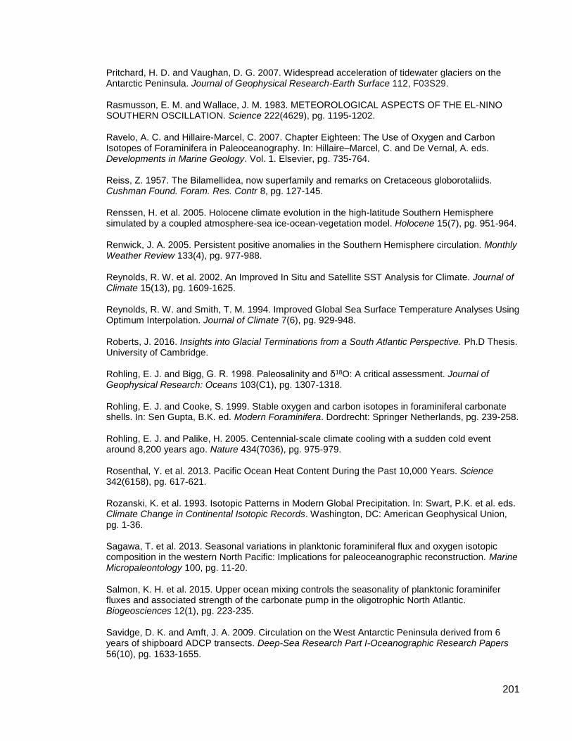
201
Pritchard, H. D. and Vaughan, D. G. 2007. Widespread acceleration of tidewater glaciers on the Antarctic Peninsula. Journal of Geophysical Research-Earth Surface 112, F03S29. Rasmusson, E. M. and Wallace, J. M. 1983. METEOROLOGICAL ASPECTS OF THE EL-NINO SOUTHERN OSCILLATION. Science 222(4629), pg. 1195-1202. Ravelo, A. C. and Hillaire-Marcel, C. 2007. Chapter Eighteen: The Use of Oxygen and Carbon Isotopes of Foraminifera in Paleoceanography. In: Hillaire–Marcel, C. and De Vernal, A. eds. Developments in Marine Geology. Vol. 1. Elsevier, pg. 735-764. Reiss, Z. 1957. The Bilamellidea, now superfamily and remarks on Cretaceous globorotaliids. Cushman Found. Foram. Res. Contr 8, pg. 127-145. Renssen, H. et al. 2005. Holocene climate evolution in the high-latitude Southern Hemisphere simulated by a coupled atmosphere-sea ice-ocean-vegetation model. Holocene 15(7), pg. 951-964. Renwick, J. A. 2005. Persistent positive anomalies in the Southern Hemisphere circulation. Monthly Weather Review 133(4), pg. 977-988. Reynolds, R. W. et al. 2002. An Improved In Situ and Satellite SST Analysis for Climate. Journal of Climate 15(13), pg. 1609-1625. Reynolds, R. W. and Smith, T. M. 1994. Improved Global Sea Surface Temperature Analyses Using Optimum Interpolation. Journal of Climate 7(6), pg. 929-948. Roberts, J. 2016. Insights into Glacial Terminations from a South Atlantic Perspective. Ph.D Thesis. University of Cambridge. Rohling, E. J. and Bigg, G. R. 1998. Paleosalinity and δ18O: A critical assessment. Journal of Geophysical Research: Oceans 103(C1), pg. 1307-1318. Rohling, E. J. and Cooke, S. 1999. Stable oxygen and carbon isotopes in foraminiferal carbonate shells. In: Sen Gupta, B.K. ed. Modern Foraminifera. Dordrecht: Springer Netherlands, pg. 239-258. Rohling, E. J. and Palike, H. 2005. Centennial-scale climate cooling with a sudden cold event around 8,200 years ago. Nature 434(7036), pg. 975-979. Rosenthal, Y. et al. 2013. Pacific Ocean Heat Content During the Past 10,000 Years. Science 342(6158), pg. 617-621. Rozanski, K. et al. 1993. Isotopic Patterns in Modern Global Precipitation. In: Swart, P.K. et al. eds. Climate Change in Continental Isotopic Records. Washington, DC: American Geophysical Union, pg. 1-36. Sagawa, T. et al. 2013. Seasonal variations in planktonic foraminiferal flux and oxygen isotopic composition in the western North Pacific: Implications for paleoceanographic reconstruction. Marine Micropaleontology 100, pg. 11-20. Salmon, K. H. et al. 2015. Upper ocean mixing controls the seasonality of planktonic foraminifer fluxes and associated strength of the carbonate pump in the oligotrophic North Atlantic. Biogeosciences 12(1), pg. 223-235. Savidge, D. K. and Amft, J. A. 2009. Circulation on the West Antarctic Peninsula derived from 6 years of shipboard ADCP transects. Deep-Sea Research Part I-Oceanographic Research Papers 56(10), pg. 1633-1655.

202
Schiebel, R. and Hemleben, C. 2005. Modern Planktic Foraminifera. Paläontologische Zeitschrift 79(1), pg. 135-148. Schmidt, G. A. et al. 1999. Global Seawater Oxygen-18 Database - v1.22 [Online]. https://data.giss.nasa.gov/o18data/ Available on: [Accessed: 07/2016]. Schmidt, D. N. et al. 2004a. Size distribution of Holocene planktic foraminifer assemblages: biogeography, ecology and adaptation. Marine Micropaleontology 50(3-4), pg. 319-338. Schmidt, D. N. et al. 2004b. The evolutionary history of size variation of planktic foraminiferal assemblages in the Cenozoic. Palaeogeography Palaeoclimatology Palaeoecology 212(1-2), pg. 159-180. Schmidt, R. et al. 1990. Holocene diatom flora and stratigraphy from sediment cores of two Antarctic lakes (King George Island). Journal of Paleolimnology 3(1), pg. 55-74. Scroxton, N. et al. 2011. Persistent El Nino-Southern Oscillation variation during the Pliocene Epoch. Paleoceanography 26. Shackleton, N. J. and Opdyke, N. D. 1973. Oxygen isotope and palaeomagnetic stratigraphy of Equatorial Pacific core V28-238: Oxygen isotope temperatures and ice volumes on a 105 year and 106 year scale. Quaternary Research 3(1), pg. 39-55. Shevenell, A. et al. 1996. Record of Holocene palaeoclimate change along the Antarctic Peninsula: evidence from glacial marine sediments, Lallemand Fjord. Papers and Proceedings of the Royal Society of Tasmania, 130 (2). pg. 55-64. Simstich, J. et al. 2003. Paired δ18O signals of Neogloboquadrina pachyderma (s) and Turborotalita quinqueloba show thermal stratification structure in Nordic Seas. Marine Micropaleontology 48(1–2), pg. 107-125. Sirota, A. and Sundakov, A. 2014. Seasonal variation in oceanographic conditions on the eastern and southern parts of the shelf and continental slope of the Falklands Islands in 1999-2014. Marine Satellite Technologies. pg.26. Skvarca, P. and De Angelis, H. 2013. Impact Assessment of Regional Climatic Warming on Glaciers and Ice Shelves of the Northeastern Antarctic Peninsula.Antarctic Peninsula Climate Variability: Historical and Paleoenvironmental Perspectives. American Geophysical Union, pg. 69-78. Sloyan, B. M. and Rintoul, S. R. 2001. Circulation, renewal, and modification of Antarctic mode and intermediate water. Journal of Physical Oceanography 31(4), pg. 1005-1030. Smith, D. A. and Klinck, J. M. 2002. Water properties on the west Antarctic Peninsula continental shelf: a model study of effects of surface fluxes and sea ice. Deep-Sea Research Part Ii-Topical Studies in Oceanography 49(21), pg. 4863-4886. Smith, J. A. et al. 2010. The presence of polynyas in the Weddell Sea during the Last Glacial Period with implications for the reconstruction of sea-ice limits and ice sheet history. Earth and Planetary Science Letters 296(3-4), pg. 287-298. Smith, R. C. et al. 1995. The Palmer LTER: A long-term ecological research program at Palmer Station, Antarctic. Oceanography 8(3), pg. 77-86. Smith, R. C. et al. 2008. Bellingshausen and western Antarctic Peninsula region: Pigment biomass and sea-ice spatial/temporal distributions and interannual variabilty. Deep Sea Research Part II:

203
Topical Studies in Oceanography 55(18), pg. 1949-1963. Smith, W. O. and Nelson, D. M. 1985. Phytoplankton Bloom Produced by a Receding Ice Edge in the Ross Sea: Spatial Coherence with the Density Field. Science 227(4683), pg. 163-166. Spero, H. J. and Parker, S. L. 1985. Photosynthesis in the symbiotic planktonic foraminifer Orbulina universa, and its potential contribution to oceanic primary productivity. The Journal of Foraminiferal Research 15(4), pg. 273-281. Spero, H. J. and Williams, D. F. 1990. EVIDENCE FOR SEASONAL LOW-SALINITY SURFACE WATERS IN THE GULF OF MEXICO OVER THE LAST 16,000 YEARS. Paleoceanography 5(6), pg. 963-975. Spero, H. J. 1992. Do planktic foraminifera accurately record shifts in the carbon isotopic composition of seawater ΣCO2? Marine Micropaleontology 19(4), pg. 275-285. Spero, H. J. and Lea, D. W. 1993. Intraspecific stable isotope variability in the planktic foraminiferaGlobigerinoides sacculifer: Results from laboratory experiments. Marine Micropaleontology 22(3), pg. 221-234. Spero, H. J. and Lea, D. W. 1996. Experimental determination of stable isotope variability in Globigerina bulloides: implications for paleoceanographic reconstructions. Marine Micropaleontology 28(3), pg. 231-246. Spero, H. et al. 1997. Effect of seawater carbonate concentration on foraminiferal carbon and oxygen isotopes. Nature 390, pg. 497-500. Spindler, M. 1990. A COMPARISON OF ARCTIC AND ANTARCTIC SEA ICE AND THE EFFECTS OF DIFFERENT PROPERTIES ON SEA ICE BIOTA. Geological History of the Polar Oceans: Arctic Versus Antarctic 308, pg. 173-186. Spindler, M. 1996. On the salinity tolerance of the planktonic foraminifera Neogloboquadrina pachyderma from Antarctic sea ice. Proceedings of the NIPR Symposium on Polar Biology 9, pg. 85-91. Spindler, M. et al. 1978. LIGHT AND ELECTRON-MICROSCOPIC OBSERVATIONS OF GAMETOGENESIS IN HASTIGERINA-PELAGICA (FORAMINIFERA). Journal of Protozoology 25(4), pg. 427-433. Spindler, M. et al. 1979. LUNAR PERIODICITY OF REPRODUCTION IN THE PLANKTONIC FORAMINIFER HASTIGERINA-PELAGICA. Marine Ecology Progress Series 1(1), pg. 61-64. Stammerjohn, S. E. et al. 2003. Ice-atmosphere interactions during sea-ice advance and retreat in the western Antarctic Peninsula region. Journal of Geophysical Research-Oceans 108(C10). 3329. Stammerjohn, S. E. et al. 2008a. Sea ice in the western Antarctic Peninsula region: Spatio-temporal variability from ecological and climate change perspectives. Deep-Sea Research Part Ii-Topical Studies in Oceanography 55(18-19), pg. 2041-2058. Stammerjohn, S. E. et al. 2008b. Trends in Antarctic annual sea ice retreat and advance and their relation to El Nino-Southern Oscillation and Southern Annular Mode variability. Journal of Geophysical Research-Oceans 113(C3). C03S90. Stangeew, E. 2001. Distribution and isotopic composition of living planktonic foraminifera N. pachyderma (sinistral) and T. quinqueloba in the high latitude North Atlantic. Ph.D. Thesis. Universität zu Kiel, Germany.
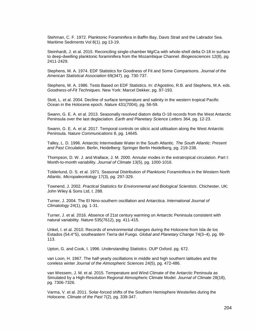
204
Stehman, C. F. 1972. Planktonic Foraminifera in Baffin Bay, Davis Strait and the Labrador Sea. Maritime Sediments Vol 8(1). pg 13-19. Steinhardt, J. et al. 2015. Reconciling single-chamber Mg/Ca with whole-shell delta O-18 in surface to deep-dwelling planktonic foraminifera from the Mozambique Channel. Biogeosciences 12(8), pg. 2411-2429. Stephens, M. A. 1974. EDF Statistics for Goodness of Fit and Some Comparisons. Journal of the American Statistical Association 69(347). pg. 730-737. Stephens, M. A. 1986. Tests Based on EDF Statistics. In: d'Agostino, R.B. and Stephens, M.A. eds. Goodness-of-Fit Techniques. New York: Marcel Dekker, pg. 97-193. Stott, L. et al. 2004. Decline of surface temperature and salinity in the western tropical Pacific Ocean in the Holocene epoch. Nature 431(7004), pg. 56-59. Swann, G. E. A. et al. 2013. Seasonally resolved diatom delta O-18 records from the West Antarctic Peninsula over the last deglaciation. Earth and Planetary Science Letters 364, pg. 12-23. Swann, G. E. A. et al. 2017. Temporal controls on silicic acid utilisation along the West Antarctic Peninsula. Nature Communications 8, pg. 14645. Talley, L. D. 1996. Antarctic Intermediate Water in the South Atlantic. The South Atlantic: Present and Past Circulation. Berlin, Heidelberg: Springer Berlin Heidelberg, pg. 219-238. Thompson, D. W. J. and Wallace, J. M. 2000. Annular modes in the extratropical circulation. Part I: Month-to-month variability. Journal of Climate 13(5), pg. 1000-1016. Tolderlund, D. S. et al. 1971. Seasonal Distribution of Planktonic Foraminifera in the Western North Atlantic. Micropaleontology 17(3), pg. 297-329. Townend, J. 2002. Practical Statistics for Environmental and Biological Scientists. Chichester, UK: John Wiley & Sons Ltd, t. 288. Turner, J. 2004. The El Nino-southern oscillation and Antarctica. International Journal of Climatology 24(1), pg. 1-31. Turner, J. et al. 2016. Absence of 21st century warming on Antarctic Peninsula consistent with natural variability. Nature 535(7612), pg. 411-415. Unkel, I. et al. 2010. Records of environmental changes during the Holocene from Isla de los Estados (54.4°S), southeastern Tierra del Fuego. Global and Planetary Change 74(3–4), pg. 99-113. Upton, G. and Cook, I. 1996. Understanding Statistics. OUP Oxford. pg. 672. van Loon, H. 1967. The half-yearly oscillations in middle and high southern latitudes and the coreless winter Journal of the Atmospheric Sciences 24(5), pg. 472-486. van Wessem, J. M. et al. 2015. Temperature and Wind Climate of the Antarctic Peninsula as Simulated by a High-Resolution Regional Atmospheric Climate Model. Journal of Climate 28(18), pg. 7306-7326. Varma, V. et al. 2011. Solar-forced shifts of the Southern Hemisphere Westerlies during the Holocene. Climate of the Past 7(2), pg. 339-347.

205
Vaughan, D. G. et al. 2003. Recent rapid regional climate warming on the Antarctic Peninsula. Climatic Change 60(3), pg. 243-274. Vautravers, M. J. et al. 2013. Palaeoenvironmental records from the West Antarctic Peninsula drift sediments over the last 75 ka. In: Hambrey, M.J., Barker, P. F., Barrett, P. J., Bowman, V., Davies, B., Smellie, J. L. & Tranter, M. eds. Antarctic Palaeoenvironments and Earth-Surface Processes. London: Geological Society, London, Special Publications, pg. 263-276. Venables, H. et al. 2012. Fronts and habitat zones in the Scotia Sea. Deep Sea Research II, 59-60. pg. 14-24. Vincent, E. and Berger, W. H. 1981. Planktonic foraminifera and their use in Paleoceanography. In: Emiliani, C. ed. The oceanic lithosphere. The sea. Vol. 7. Hoboken, N. J.: Wiley-Interscience, pg. 1025-1119. Voigt, I. et al. 2016. Holocene changes in Antarctic Intermediate Water flow strength in the Southwest Atlantic. Palaeogeography Palaeoclimatology Palaeoecology 463, pg. 60-67. Volkmann, R. a Mensch, M. 2001. Stable isotope composition (δ18O, δ13C) of living planktic foraminifers in the outer Laptev Sea and the Fram Strait. Marine Micropaleontology 42(3-4), pg. 163-188. von Gyldenfeldt, A. B. et al. 2000. Estimation of the catchment area of a sediment trap by means of current meters and foraminiferal tests. Deep-Sea Research Part Ii-Topical Studies in Oceanography 47(9-11), pg. 1701-1717. Watkins, A. B. and Simmonds, I. 1999. A late spring surge in the open water of the Antarctic sea ice pack. Geophysical Research Letters 26(10), pg. 1481-1484. Watkins, J. 2016. JR304: Ecosystems, Western Core Box & Moorings Incorporating CGS projects 95, 99 and 101. Cambridge, UK: British Antarctic Survey. Wefer, G. and Berger, W. H. 1991. Isotope paleontology: growth and composition of extant calcareous species. Marine Geology 100(1), pg. 207-248. Weiss, R. F. et al. 1979. Geochemical studies of the Weddell Sea. Deep Sea Research Part A. Oceanographic Research Papers 26(10), pg. 1093-1120. Wenzens, G. 2005. Glacier advances east of the Southern Andes between the Last Glacial Maximum and 5,000 BP compared with lake terraces of the endorrheic Lago Cardiel (49°S, Patagonia, Argentina). Zeitschrift für Geomorphologie, NF 49(4) pg. 433-454. White, W. B. and Peterson, R. G. 1996. An Antarctic circumpolar wave in surface pressure, wind, temperature and sea-ice extent. Nature 380(6576), pg. 699-702. Whitworth, T. 1980. ZONATION AND GEOSTROPHIC FLOW OF THE ANTARCTIC CIRCUMPOLAR CURRENT AT DRAKE PASSAGE. Deep-Sea Research Part a-Oceanographic Research Papers 27(7), pg. 497-507.
Wilke, I. et al. 2006. The influence of seawater carbonate ion concentration 𝐶𝑂32−on the stable
carbon isotope composition of the planktic foraminifera species Globorotalia inflata. Marine Micropaleontology 58(4), pg. 243-258. Williams, D. F. et al. 1988. Shape and isotopic differences between conspecific foraminiferal morphotypes and resolution of paleoceanographic events. Palaeogeography, Palaeoclimatology,

206
Palaeoecology 64(3), pg. 153-162. Wit, J. C. et al. 2010. Approaches to unravel seasonality in sea surface temperatures using paired single-specimen foraminiferal δ18O and Mg/Ca analyses. Paleoceanography 25, PA4220. Wolter, K. 2016. Multivariate ENSO index [Online]. Earth System Research Laboratory, NOAA: Available on: https://www.esrl.noaa.gov/psd/enso/mei/ [Accessed: 15/05/2016]. Wolter, K. and Timlin, M. S. 1998. Measuring the strength of ENSO events: How does 1997/98 rank? Weather 53(9), pg. 315-324. Yuan, X. J. 2004. ENSO-related impacts on Antarctic sea ice: a synthesis of phenomenon and mechanisms. Antarctic Science 16(4), pg. 415-425. Zweng, M. M. et al. 2013. World Ocean Atlas 2013, Volume 2: Salinity. Silver Spring, MD: NOAA, pg. 39.
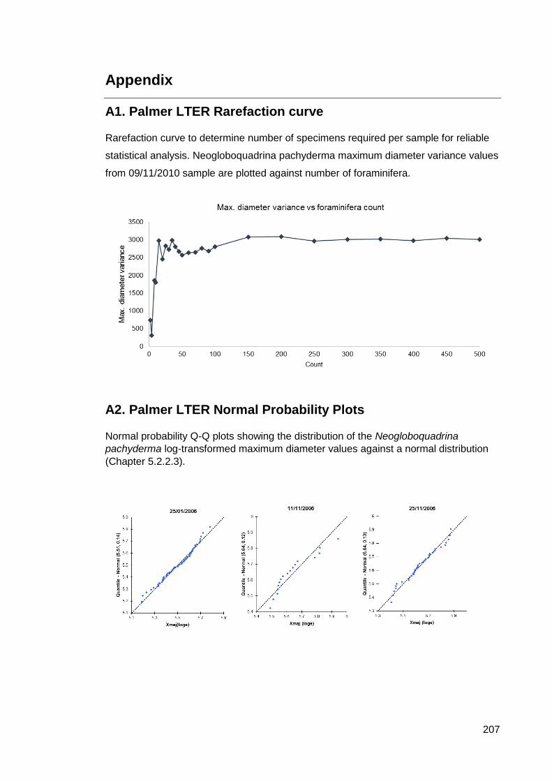
207
Appendix
A1. Palmer LTER Rarefaction curve
Rarefaction curve to determine number of specimens required per sample for reliable
statistical analysis. Neogloboquadrina pachyderma maximum diameter variance values
from 09/11/2010 sample are plotted against number of foraminifera.
A2. Palmer LTER Normal Probability Plots
Normal probability Q-Q plots showing the distribution of the Neogloboquadrina
pachyderma log-transformed maximum diameter values against a normal distribution
(Chapter 5.2.2.3).

208

209

210

211
A3. Palmer LTER correlations between Xmaj and PCA F1 score
Correlations between log-transformed maximum diameter values of Neogloboquadrina
pachyderma and the first principal component score of the PCA analysed on the four
size-invariant morphological parameters (circularity ratio, box ratio, elongation ratio and
compactness coefficient, Table 5.9

212

213
Copyright © 2022 FDOKUMEN