University of Pennsylvania University of Pennsylvania

ScholarlyCommons ScholarlyCommons

Departmental Papers (EES) Department of Earth and Environmental Science

January 2005

The Development Of A Modern Foraminiferal Data Set For Sea-The Development Of A Modern Foraminiferal Data Set For Sea-

Level Reconstructions, Wakatobi Marine National Park, Southeast Level Reconstructions, Wakatobi Marine National Park, Southeast

Sulawesi, Indonesia Sulawesi, Indonesia

Benjamin P. Horton University of Pennsylvania, bphorton@sas.upenn.edu

John E. Whittaker Natural History Museum

Katie H. Thomson University of Durham

Michael I. J. Hardbattle University of Durham

Andrew Kemp University of Durham

See next page for additional authors

Follow this and additional works at: https://repository.upenn.edu/ees_papers

Recommended Citation Recommended Citation Horton, B. P., Whittaker, J. E., Thomson, K. H., Hardbattle, M. I., Kemp, A., Woodroffe, S. A., & Wright, M. R. (2005). The Development Of A Modern Foraminiferal Data Set For Sea-Level Reconstructions, Wakatobi Marine National Park, Southeast Sulawesi, Indonesia. Retrieved from https://repository.upenn.edu/ees_papers/49

Postprint version. Published in Journal of Foraminiferal Research, Volume 35, Number 1, January 2005, pages 1–14.

This paper is posted at ScholarlyCommons. https://repository.upenn.edu/ees_papers/49 For more information, please contact repository@pobox.upenn.edu.

The Development Of A Modern Foraminiferal Data Set For Sea-Level The Development Of A Modern Foraminiferal Data Set For Sea-Level Reconstructions, Wakatobi Marine National Park, Southeast Sulawesi, Indonesia Reconstructions, Wakatobi Marine National Park, Southeast Sulawesi, Indonesia

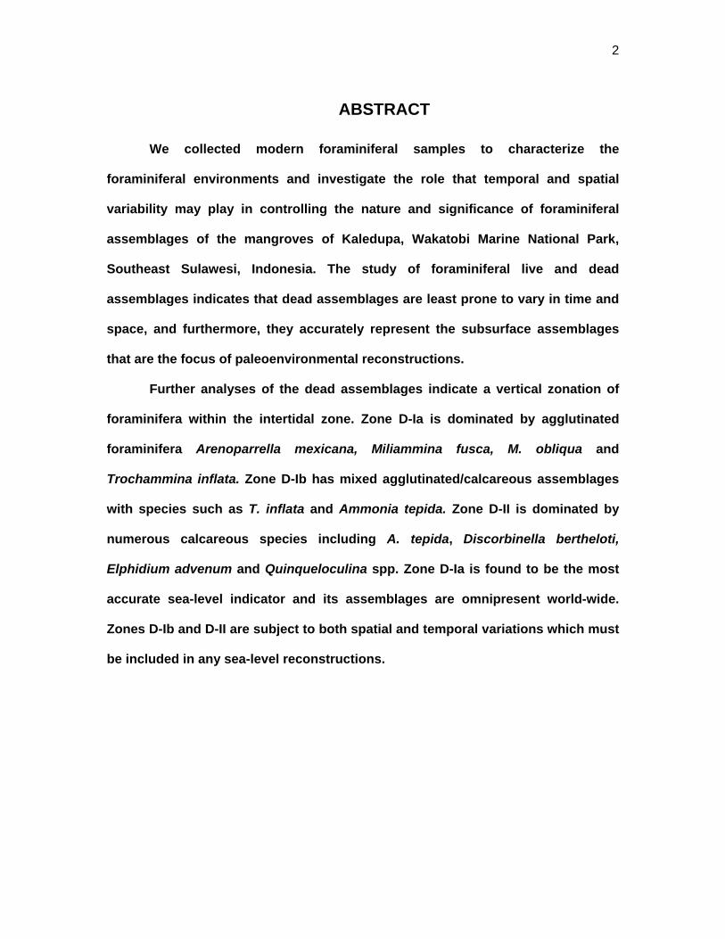
Abstract Abstract We collected modern foraminiferal samples to characterize the foraminiferal environments and investigate the role that temporal and spatial variability may play in controlling the nature and significance of foraminiferal assemblages of the mangroves of Kaledupa, Wakatobi Marine National Park, Southeast Sulawesi, Indonesia. The study of foraminiferal live and dead assemblages indicates that dead assemblages are least prone to vary in time and space, and furthermore, they accurately represent the subsurface assemblages that are the focus of paleoenvironmental reconstructions.

Further analyses of the dead assemblages indicate a vertical zonation of foraminifera within the intertidal zone. Zone D-Ia is dominated by agglutinated foraminifera Arenoparrella mexicana, Miliammina fusca, M. obliqua and Trochammina inflata. Zone D-Ib has mixed agglutinated/calcareous assemblages with species such as T. inflata and Ammonia tepida. Zone D-II is dominated by numerous calcareous species including A. tepida, Discorbinella bertheloti, Elphidium advenum and Quinqueloculina spp. Zone D-Ia is found to be the most accurate sea-level indicator and its assemblages are omnipresent world-wide. Zones D-Ib and D-II are subject to both spatial and temporal variations which must be included in any sea-level reconstructions.

Comments Comments Postprint version. Published in Journal of Foraminiferal Research, Volume 35, Number 1, January 2005, pages 1–14.

Author(s) Author(s) Benjamin P. Horton, John E. Whittaker, Katie H. Thomson, Michael I. J. Hardbattle, Andrew Kemp, Sarah A. Woodroffe, and Matthew R. Wright

This journal article is available at ScholarlyCommons: https://repository.upenn.edu/ees_papers/49

1

The development of a modern foraminiferal data set

for sea-level reconstructions, Wakatobi Marine National

Park, Southeast Sulawesi, Indonesia

BENJAMIN. P. HORTON1*, JOHN E. WHITTAKER2, KATIE. H. THOMSON3,

MICHAEL I. J. HARDBATTLE3, ANDREW KEMP3, SARAH. A. WOODROFFE3 AND

MATTHEW R. WRIGHT3

RRH: FORAMINIFERA OF INDONESIA

LRH: BP HORTON AND OTHERS

1 Department of Earth and Environmental Science, University of Pennsylvania,

Philadelphia, PA 19104-6316, USA. 2 Micropaleontology Research, Department of Palaeontology, The Natural History

Museum, London, SW7 5BD, UK.

3 Department of Geography, University of Durham, South Road, Durham, DH1

3LE, UK.

* Corresponding author: Tel: 215 898 5725; Fax: 215 898 0964; E-mail:

XXXX@sas.upenn.edu.

2

ABSTRACT

We collected modern foraminiferal samples to characterize the

foraminiferal environments and investigate the role that temporal and spatial

variability may play in controlling the nature and significance of foraminiferal

assemblages of the mangroves of Kaledupa, Wakatobi Marine National Park,

Southeast Sulawesi, Indonesia. The study of foraminiferal live and dead

assemblages indicates that dead assemblages are least prone to vary in time and

space, and furthermore, they accurately represent the subsurface assemblages

that are the focus of paleoenvironmental reconstructions.

Further analyses of the dead assemblages indicate a vertical zonation of

foraminifera within the intertidal zone. Zone D-Ia is dominated by agglutinated

foraminifera Arenoparrella mexicana, Miliammina fusca, M. obliqua and

Trochammina inflata. Zone D-Ib has mixed agglutinated/calcareous assemblages

with species such as T. inflata and Ammonia tepida. Zone D-II is dominated by

numerous calcareous species including A. tepida, Discorbinella bertheloti,

Elphidium advenum and Quinqueloculina spp. Zone D-Ia is found to be the most

accurate sea-level indicator and its assemblages are omnipresent world-wide.

Zones D-Ib and D-II are subject to both spatial and temporal variations which must

be included in any sea-level reconstructions.

3

INTRODUCTION

The recent transition of the earth climate system from a glacial to interglacial

state produced a dramatic global sea-level response. Regions distant from the major

glaciation centers, known as far-field sites, are typically characterized by relative sea-

level (RSL) rise of ~120 m since the last glacial maximum (LGM) due, largely, to the

influx of glacial meltwater to the oceans. In contrast, RSL dropped by many hundreds of

meters in regions once covered by the major ice sheets (near- and intermediate-field

sites) as a consequence of the isostatic ‘rebound' of the solid Earth (Lambeck and

others, 2002; Peltier and others, 2002; Shennan and others, 2002). Field observations of

RSLs from far field locations provide essential constraints to geophysical models

because model predictions depend upon three mechanisms: ocean siphoning caused

mainly by gravitational effects due to the collapse of peripheral forebulges (Mitrovica and

Peltier 1991); continental levering associated with local ocean loading; and global ice

melt since the LGM (magnitude and source).

Although much contemporary research to test such theoretically derived models

has focused on data sets from near- and intermediate-field sites (e.g., Shennan and

others, 2000; Shennan and Horton, 2002), it is widely recognized that far-field sites

provide the best possible estimate of the ‘eustatic function’ (Clark and others, 1978;

Fleming and others, 1998; Yokoyama and others, 2001; Peltier, 2002). Consequently,

model-derived reconstructions are increasingly recognizing the importance of these

areas to constrain and test their geophysical earth models. With notable exceptions

(Fairbanks, 1989, 1990; Bard and others, 1996; Chappell and others, 1998; Nunn and

Peltier, 2001; Yokoyama and others, 2001), few studies have examined the sea-level

histories from tectonically stable far-field areas. Furthermore, much of the data is derived

from cored corals, which ‘are not the clear indicators of past sea-levels that they are

4

sometimes suggested to be’ (Hopley, 1986). Problems encountered focus on the large

elevational range exhibited by some coral species and the delayed response of a reef

system to the sea-level change. Consequently, this study of Wakatobi Marine National

Park, Southeast Sulawesi, Indonesia, which is a tectonically stable far-field site, begins

to address the need to acquire accurate sea-level indicators (e.g., foraminifera) in

locations away from major plate boundaries.

Many researchers have used foraminiferal distributions across the intertidal zone

of temperate saltmarshes as sea-level indicators (e.g., Scott and Medioli, 1978, 1980a;

Patterson, 1990; Gehrels, 1994; de Rijk, 1995; Horton, 1999; Horton and others, 1999a

b; Gehrels and others, 2001). The intertidal distributions can be divided into two parts:

an agglutinated assemblage that is restricted to the vegetated marsh; and a calcareous

assemblage that dominates the mudflats and sandflats of the intertidal zone. The

agglutinated assemblage is commonly employed as a sea-level indicator in the

reconstruction of former sea levels. Saltmarsh foraminiferal zonation is a significantly

more accurate indicator of sea level than undifferentiated marsh deposits since well-

defined zones subdividing the marsh increase the vertical resolution of the deposits

(Scott and Medioli, 1978). Furthermore, Scott and others (2001) state that vertical

zonations are observed in marshes throughout the world, and suggest that marsh

foraminifera are ubiquitous worldwide. However, studies of microfossils and their

relationship to RSL in coastal and estuarine environments from tropical or subtropical

environments to support this conclusion are sparse, indeed, non-existent for Indonesia.

Thus, this paper seeks to document, for the first time, some characteristics of modern

foraminiferal environments in the central Wakatobi Marine National Park province for use

in paleoenvironmental interpretations made from Quaternary sediments of Indonesia.

This paper also discusses which assemblage constituents (live, dead and/or

total) are best applied for foraminiferal-based sea-level reconstructions studies in tropical

5

locations and investigates the role that temporal and spatial variability may play in

controlling the nature and significance of foraminiferal assemblages. Many researchers

state that total assemblages most accurately represent general environmental conditions

because they integrate seasonal and temporal fluctuations (e.g., Scott and others,

2001). However, Murray (1991, 2000) suggests that the use of total assemblages

disregards changes that will affect live assemblages after their death. Furthermore,

depositional changes are sample dependent because the greater the vertical depth of a

sample, the more important the dead contribution. Horton (1999) indicates that the dead

assemblages from temperate marshes are the most appropriate for paleoenvironmental

studies because these assemblages are less susceptible to seasonal variations and

closely resemble subsurface assemblages. Horton (1999) and Horton and Edwards

(2003) concluded that if the live assemblages are variable and not transferred into

subsurface environments, their combination with the dead assemblage to produce a total

assemblage simply degrades the utility of the latter. Thus, in this paper we have only

investigated the live and dead assemblages.

STUDY AREA

Extending over 13,900 km2, the Wakatobi Marine National Park includes all coral

reefs, islands, and communities within its boundaries and is centered around the main

islands in the Wakatobi archipelago (Fig. 1). The area is considered ‘a geological and

biological anomaly’ (Daws and Fujita, 1999) and is located at a zone of transition

between the two distinct faunas associated with the Asian and Australian continents.

Wallace (1869) postulated that the islands of Sulawesi had been isolated far longer than

the surrounding islands, giving evolution a much greater opportunity to shape a unique

fauna.

6

The field site is located on a tidal mangrove creek system on the northern coast

of the island of Kaledupa (Fig. 1B). At the mouth of the creek, and along much of the

coast of Kaledupa, is a 150 m-wide fringing mangrove swamp, with vegetation up to 7 m

in height. The mangroves of Kaledupa exhibit a pronounced zonation of species similar

to many other mangrove swamps (e.g., Chapman, 1944, Macnae, 1968; Snedaker,

1982) with a fringing Rhizophora zone, transgressing into a mixed

Rhizophora/Sonneratia zone and then an Avicennia mangrove zone (Barnes, written

communication, 2002). The landward edge of the mangrove environment terminates on

an exposed coral terrace. Tides in the area are semi-diurnal and microtidal, with mean

spring tidal ranges of 1.6 m. On the flood tide, water enters the mangroves and saltflats

via a network of small channels.

METHODOLOGY

Samples of surface sediment were collected from 20 stations along two 160 m

transects (A and B). Both transects cross the intertidal zone from an exposed former

coral terrace through a mangrove swamp and onto an unvegetated intertidal mudflat. All

stations were leveled to sea level using a level and staff at regular spatial and temporal

intervals throughout the study, and the tidal curve from Boeton Island was used to

calculate elevations with respect to Indonesian Height Datum (IHD). At each station, one

sample of approximately 10 cm3 volume (10 cm2 surface sample by 1 cm thick) was

taken for foraminiferal analysis.

To investigate the role that temporal and spatial variability may play in controlling

the nature and significance of foraminiferal assemblages, samples were taken twice

during a two-month period (Transects A1 and A2) and once from an additional adjacent

transect (Transect B). Foraminiferal sample preparation followed Scott and others

(2001). The species were identified with reference to a number of publications, namely

7

Collins (1958), Albani (1968), Albani and Yassini (1993), Brönnimann and Whittaker

(1993), Yassini and Jones (1995), Hayward and others (1999a) and Revets (2000), and

by study of reference collections in the Natural History Museum, London (Plate 1).

Samples were stored in buffered ethanol with protein stain Rose Bengal to identify

organisms living at the time of collection, and thus allow the analyses of live and dead

assemblages (Walton, 1952; Scott and Medioli, 1980b; Murray, 1991; Murray and

Bowser, 2000).

We used two multivariate methods to detect, describe and classify patterns within

the live and dead foraminiferal data set: unconstrained cluster analysis and detrended

correspondence analysis (DCA). Unconstrained cluster analysis based on the

unweighted Euclidean distance, using no transformation or standardization of the

percentage data, was used to classify modern samples into more-or-less homogeneous

faunal zones (clusters). Detrended correspondence analysis, an ordination technique,

was used to represent samples as points in a multidimensional space. Similar samples

are located together and dissimilar samples apart. Thus, cluster analysis is effective in

classifying the samples according to their foraminiferal assemblage but, DCA gives

further information about the pattern of variation within and between groups. This is

important, as the precise boundaries between clusters can be arbitrary. Thus, we

selected reliable faunal zones when the samples within each cluster were mutually

exclusive in ordination space. The elevation of each station within the reliable clusters

determined the vertical zonation of each intertidal environment.

We employed Student's T-Test to determine whether two samples from A1 and

A2, and A1 and B are likely to have come from the same two underlying populations. We

use a two-tailed distribution.

8

RESULTS

Forty species of foraminifera were identified from the study of surface samples

from the mangroves of Kaledupa. The maximum number of species per 10 cm3 sample

was 23, with maximum and minimum foraminiferal total (live plus dead) abundance of

632 and 134 individuals per sample, respectively. The live and dead assemblages are

dominated by three agglutinated species, Arenoparrella mexicana, Miliammina fusca,

and Trochammina inflata, and four calcareous species, Ammonia tepida, Discorbinella

bertheloti, Elphidium advenum and Quinqueloculina spp.

LIVE ASSEMBLAGES

The live assemblage of Transect A1 is dominated by calcareous species, which

represent over 75% of the total count. Calcareous taxa such as A. tepida, E. advenum,

D. bertheloti, and Q. spp. dominate the unvegetated mudflat and fringing Rhizophora

mangrove section of the transect (0 - 60 m along the transect). Maximum percentages of

E. advenum (15%), A. tepida (30%) and D. bertheloti (13%) occur 0 m, 18 m and 40 m

along the transect, respectively (Fig. 2). In addition, the Rhizophora floral zone has a

relatively high foraminiferal abundance, with an average count of 253 live specimens per

10 cm3. The Rhizophora/Sonneratia floral zone (60 - 90 m along the transect) is also

dominated by calcareous species with the maximum percentage of Haynesina

depressula occurring within this zone (12%). However, there is an increasing agglutinate

presence, in particular T. inflata, which reaches 22% 90 m along the transect. The

majority of calcareous species are replaced by agglutinated species within the Avicennia

mangrove zone (90 - 160 m along the transect). However, maximum percentages of Q.

spp. (71%) occur 120 m along the transect. The maximum percentage of the dominant

9

agglutinated taxa T.inflata, M. fusca, and A. mexicana occur within this Avicennia zone

(24%, 41% and 16%, respectively).

The total number of live foraminifera from the twenty stations of the Transect A1

is 3648 compared to 4102 specimens for the temporal Transect A2 (taken 2 months

later). There are also differences in the dominant live foraminiferal species (Fig. 3). The

relative contribution of Q. spp. between 5 and 32m along the transect is greater than

30% at each sampling station of Transect A1 compared to less than 19% for Transect

A2. Furthermore, 90 m along the transect the relative contributions of Q. spp. are 44%

on A1 to 15% on A2, whereas 105 m along the transect A1 is 8% and A2 is 30%.

Indeed, T-tests suggest that the relative abundances of Q. spp. between transects A1

and A2 are statistically significantly different and did not come from the same underlying

population (Table 1). Other notable differences include lower percentages of T. inflata

between 128 m and 150 m along the transect for A1 (<16%) compared to Transect A2

(>26%), and appreciably lower percentages of A. mexicana at the landward edge of the

transect (5% on A1 to 56% on A2).

The total number of live foraminifera also increases from the original transect

(A1) to spatial Transect B (4057 specimens) taken adjacent to A1. The difference in

contribution of Q. spp. between transects is amplified 90 m along the transect (44% on

A1 to 6% on B), whereas 105 m along the transect A1 is 8% and B is 44% (Fig. 4). Other

notable dissimilarities include the increase in relative abundance of M. fusca 150 m

along the transect (13% on A1 to 44% on B) and a corresponding decrease in A.

mexicana (41% on A1 to 19% on B). Statistical analyses (T-tests) support the inference

that these three species show significantly different assemblages between transects A1

and B (Table 1).

10

DEAD ASSEMBLAGES

There is an increase in the relative abundance of agglutinated foraminifera in the

dead assemblage, with agglutinated species contributing over 35% to the total dead

assemblage of Transect A1. However, the unvegetated mudflat and fringing mangrove

floral zones are dominated by calcareous foraminifera such as A. tepida, E. advenum, D.

bertheloti, H. depressula and Q. spp., with the two most dominant species reaching their

maximum abundance within this zone (A. tepida - 30% and Q. spp. 37%). The

unvegetated mudflat and fringing mangrove have the highest foraminiferal counts within

the intertidal zone with an average count of 216 dead species per 10 cm3 (Fig. 5).

The Rhizophora/Sonneratia mangrove zone shows an increasing contribution of

agglutinated species, most notably T. inflata. However, A. tepida contributes at least

16% at each station and the zone still possesses the maximum abundances of

numerous calcareous species, including A. takanabensis and H. depressula (28% and

14%, respectively). Nevertheless, the tendency of the increasing contribution of

agglutinated species continues within the Avicennia mangrove zone, which is dominated

by agglutinated species such as T.inflata, M. fusca, M. obliqua and A. mexicana;

agglutinated species make up at least 65% of the assemblage landwards of 105 m.

The foraminiferal dead assemblage count is relatively stable among the original

(A1), temporal (A2) (Fig. 6) and spatial (B) (Fig. 7) transects. The total number of dead

foraminifera is also relatively constant; 3712 on A1, 3708 on A2 and 3955 specimens on

B. Statistical analyses do not show any significant differences although there are

noteworthy differences at individual stations (Table 1). For example, the relative

contribution of A. mexicana fluctuates from 12% on A1 to 32% on A2, and 48% on A1 to

12% on A2 at 120 m and 150 m along the transect, respectively.

11

DISCUSSION

There is much debate about which foraminiferal assemblage constituents (live,

dead and/or total) to use for sea-level reconstructions (Buzas, 1968; Scott and Medioli,

1980b; Scott and Leckie, 1990; de Rijk, 1995; Murray, 2000; Scott and others, 2001).

These studies have, however, concentrated on foraminiferal species from temperate

intertidal areas. This new study assesses the applicability of live and dead assemblages

from tropical environments. Analyses of the spatial and temporal variations of the

dominant species show that the dead assemblages are less susceptible to temporal and

spatial variations compared to live counterparts. We investigated this further by

examining the differences in the vertical zonation of the live and dead assemblage.

Figures 8 and 9 both show the combined foraminiferal data (original A1, temporal A2

and spatial B transects) of the live and dead assemblages separated into three reliable

zones by cluster analysis and DCA. The live assemblages do not show any vertical

zonations due to the heterogeneity of living assemblages in space and time, in particular

Zone L-Ib, which covers the full elevational range of the transects. Similar spatial and

temporal variations have been documented by many studies (Buzas, 1968; Schafer,

1968; Jones and Ross, 1979; Schafer and Mudie, 1980; Alve and Murray, 1999, 2001;

Murray and Alve, 2000; Swallow, 2000; Buzas and others, 2002; Hippensteel and

others, 2002; Horton and Edwards, 2003). Schafer and Mudie (1980) discovered an

order of magnitude difference in average foraminiferal number between pairs of sites.

Alve and Murray (2001) demonstrated significant temporal variability over a 27-month

period with the number of species found at any single sampling event varying between 5

and 22. Such temporal and spatial patterns of live assemblages reflect the impact of

factors such as seasonality, predation, reproduction, mode, sources and distribution

12

pattern of food particles and species interactions (Buzas, 1968; Schafer, 1968; Scott and

others, 2001).

In contrast to the live assemblages, the dead assemblages present a more

homogeneous spatial and temporal distribution as a probable consequence of post-

mortem lateral and vertical mixing of empty tests by biological and physical agents (Scott

and others, 2001). The dead assemblages assimilate all temporal variation and spatial

patchiness into an ‘average signal’ that tends to reduce the inter-sample variance. For

example, the combined dead assemblages are classified into three reliable zones that

show a strong vertical zonation (Fig. 9), which indicates that the distribution of dead

foraminifera are a direct function of elevation, with the duration and frequency of

intertidal exposure as the most important environmental factors.

Agglutinated species A. mexicana, M. fusca, M. obliqua and T. inflata dominate

Zone D-Ia, which is found at the landward edge of the mangrove study site with an

elevational range of 2.02 - 1.02 m IHD (range 0.20 m). Similar faunal assemblages have

been observed at the landward margins of both tropical mangroves and temperate

saltmarshes. Brönnimann and others (1992) and Brönnimann and Whittaker (1993)

found assemblages of A. mexicana in mangrove sediments of the Fiji and Malay

archipelagos, respectively. Assemblages dominated by T. inflata have been identified by

Haslett (2001) and Horton and others (2003) at the landward limit of mangrove

distributory channels from the Great Barrier Reef coastline, Australia. Many studies have

identified high abundances of M. fusca in the mangroves of Fiji, southwest Australia,

Brazil, New Zealand, northern Australia and the Great Barrier Reef coastline

(Brönnimann, and others, 1992; Bronnimann and Whittaker, 1993; Yassini and Jones,

1995; Debenay and others, 1998, 2000; Hayward and others, 1999a, b; Wang and

Chappell, 2001; Horton and others, 2003). Studies of temperate saltmarshes have

commonly identified a high marsh zone dominated by T. inflata and a low marsh zone

13

dominated by M. fusca (Scott and Medioli, 1978, 1980a; Gehrels, 1994; Horton, 1999;

Horton and others, 1999a; Spencer, 2000; Hippensteel and others, 2000; Horton and

Edwards, 2003, 2004 in press).

Faunal Zone D-Ib has a mixed agglutinated/calcareous assemblage composed of

Ammonia species, with lower frequencies of T. inflata and M. obliqua. The zone ranges

from 1.90 - 1.60 m IHD (range 0.30 m). Other tropical and temperate studies have

observed mixed agglutinated/calcareous assemblage zones but with an increase in the

relative abundance of the former (Scott and Medioli, 1978, 1980a; Gehrels, 1994;

Yassini and Jones, 1995; Debenay and others, 1998, 2000; Hayward and others,

1999a,b ; Wang and Chappell, 2001; Horton and Edwards, 2003; Horton and others,

2003).

Zone D-II is found at the seaward edge of the transects and is dominated by

numerous calcareous species such as A. tepida, D. bertheloti, E. advenum and Q. spp.,

with a relatively large elevation range of 1.71 - 0.47 m IHD (range 1.24 m). Other

calcareous faunal zones with relatively high abundances of A. tepida are common in

many tropical or subtropical locations (Hayward and others, 1996; Debenay and others,

2000; Wang and Chappell 2001; Horton and others, 2003), although there are many

species that are site specific. For example, studies of tidal flat environments of the Great

Barrier Reef coastline by McIntyre (1997) and Horton and others (2003) have identified a

foraminiferal faunal zone dominated by cosmopolitan Ammonia species, in addition to

Miliolinella spp., the endemic E. discoidale multiloculum and extinct Pararotalia venusta.

The presence of P. venusta indicates some reworking of material within the intertidal

zone of this study site. Analyses of temperate saltmarshes show differences from the

Kaledupan transect. Studies of British saltmarshes display tidal flat assemblages

dominated by Haynesina germanica and other Elphidium species (Horton, 1999;

14

Edwards and Horton, 2000; Murray and Alve, 2000; Gehrels and others, 2001; Horton

and Edwards, 2003, 2004 in press).

IMPLICATIONS FOR SEA-LEVEL STUDIES

The understanding of former sea levels based on the identification and

interpretation of foraminiferal assemblages requires that their indicative meaning is

known, i.e., the vertical relationship of the local environment in which the assemblage

accumulated to a reference tide level (van de Plassche, 1986; Shennan, 1986; Horton

and others, 1999b; 2000). The indicative meaning is commonly expressed in terms of an

indicative range and a reference tidal level, the former being a vertical range within

which the assemblage can occur, and the latter a tidal level to which the assemblage is

assigned, e.g., mean high high water (MHHW) (Fig. 10).

Estimates of the indicative meaning of faunal zones from the mangroves of

Kaledupa (Table 2) are developed from the premise that zones found vertically adjacent,

without a hiatus, must have formed in environments that existed side by side in space

(Walthers Law). Therefore, the transition from faunal Zone D-Ib to Zone D-II has an

indicative range equal to the range of the transition from one zone to the other, not that

of the individual zone. For example, the indicative range of Zone D-II is ± 0.62 m,

whereas the range of Zone D-Ib directly above Zone D-II is only ± 0.06 m. The ranges

cover the elevational limits of the boundary when observed during the 2 sampling

months.

Despite the conclusion that dead assemblages are less variant than live

assemblages in most spatial and temporal fluctuations, it is important to identify any

variations in the vertical zonation that must be included in any sea-level reconstruction to

avoid errors in accuracy and precision (Horton and Edwards, 2003). Multivariate

15

analyses of each individual transect (A1, A2 and B) show that the elevational range of

the Zone D-Ia remains virtually constant; however, spatial and temporal variations in the

dead assemblages are observed for faunal zones D-Ib and D-II (Fig. 11). The elevation

of the boundary between zones D-Ib and D-II fluctuates from 1.86 m IHD at A1 to 1.42 m

IHD at B, suggesting that some of the variability in the live assemblages is being

transmitted to the dead assemblages.

In addition to spatial and temporal variations, it is also important for sea-level

reconstructions to assess the influence of post-depositional processes on the

assemblage constituents. Thus, subsurface dead assemblages, the focus of

paleoenvironmental reconstructions, were collected from the mudflat, fringing

Rhizophora, mixed Rhizophora/Sonneratia and Avicennia environments to determine

which modern assemblage constituents are most appropriate for paleoenvironmental

reconstruction. Subsurface samples were collected at a depth of 12 cm; 97% of live

specimens occurred above this depth. Scatter plots (Fig. 12) show a clear positive linear

correlation between the subsurface and surface dead assemblages (r2 = 0.90) from

Transect A1. The dead assemblages fluctuate little between the subsurface and surface

because calcareous species such as Q. spp. are relatively minor contributors to surface

dead assemblages in mangrove environments. In contrast, the live assemblages (r2 =

0.29) show little relationship to subsurface dead assemblages. The live assemblages of

the surface samples incorporate live calcareous species, which can represent over 85%

of the assemblage from mangrove floral zones. However, post-depositional changes

result in calcareous species being removed and the subsurface assemblages become

more dominated by agglutinated species. Calcareous tests can be rapidly destroyed

after death through dissolution in acidic pore waters (Green and others, 1993).

16

CONCLUSIONS

The study of foraminiferal dead assemblages of the mangroves of Kaledupa

indicates that the assemblage accurately represents the subsurface assemblages which

are the focus of paleoenvironmental reconstructions, and furthermore that they do not

show spatial and temporal fluctuations as much as the live assemblages. Statistical

analyses of the dead assemblages support numerous studies from temperate or tropical

regions that indicate a vertical zonation of foraminifera within the intertidal zone:

Agglutinated foraminifera such as A. mexicana, T. inflata, and M. fusca dominate Zone

D-Ia; Zone D-Ib contains a mixed agglutinated/calcareous assemblages with species

such as T. inflata and A. tepida; and Zone D-II is dominated by numerous calcareous

species. Zone D-Ia is found to be the most accurate sea-level indicator and its

assemblages are omnipresent world-wide. Zone D-Ib and D-II are subject to both spatial

and temporal variations, which must be incorporated into any sea-level reconstructions.

A data repository of all foraminiferal (percentage and raw counts) and

environmental data can be found on the following website:

http://www.geography.dur.ac.uk/information/official_sites/bph.html

ACKNOWLEDGMENTS

The authors thank all staff of Operation Wallacea Ltd., in particular, Richard

Barnes, Tim Coles, Dave Smith, Steve Mcmellor, Steve Oliver and Magnus Johnson.

We acknowledge and greatly appreciate the funding by Operation Wallacea Ltd and the

University of Durham’s Council Fund for Students Traveling Abroad. The authors also

17

thank Andy Kemp, John Metcalfe, Andy Fenton, James Kahane, Dave Taylor and Katie

White for their skills in the field, and David Blackman, Proudman Oceanographic

Laboratory, for tidal predictions for Indonesian Ports. The authors also wish to express

their gratitude for the help and support given by the Department of Geography,

University of Durham and the Natural History Museum, London. In particular the authors

would like to thank the two reviewers, Robin Edwards and Bruce Hayward and the

editor, Laurel Collins, for their help and advice.

REFERENCES

ALBANI, A.D., 1968, Recent foraminifera from Port Hacking, New South Wales:

Contributions from the Cushman Foundation for Foraminiferal Research, v. 19, p.

85-119.

_________, and YASSINI, I., 1993, Taxonomy and distribution of the family Elphididdae

(Foraminiferida) from shallow Australian waters: University of New South Wales

Centre for Marine Science, Technical Contribution Number 5. p51.

ALVE, E., and MURRAY, J.W., 1999, Marginal marine environments of the Skagerrak and

Kattegat: a baseline study of living (stained) benthic foraminiferal ecology:

Palaeogeography, Palaeoclimatology, Palaeoecology, v. 146, p. 171-193.

_________, and _________, 2001, Temporal variability in vertical distributions of live (stained)

intertidal foraminifera, southern England: Journal of Foraminiferal Research, v.

31, p 2-11.

BARD, E., HAMELIN, B., ARNOLD, M., MONTAGGIONI, L., CABIOCH, G., FAURE, G., and

ROUGERIE, F., 1996, Deglacial sea-level record from Tahiti corals and the timing

of global meltwater discharge: Nature, v. 382, p. 241-244.

18

BRÖNNIMANN, P., WHITTAKER, J.E., and ZANINETTI, L., 1992, Brackish water foraminifera

from mangrove sediments of southwestern Viti Levu, Fiji Islands, Southwest

Pacific: Revue de Paléobiologie, v. 11, p. 13-65.

_________, and _________, 1993, Taxonomic revision of some recent agglutinated foraminifera

from the Malay Archipelago in the Millett Collection: Bulletin of the Natural History

Museum, London (Zoology), v. 59, p.107-124.

BUZAS, M.A., 1968, On spatial distribution of foraminifera: Contributions from the

Cushman Foundation Foraminiferal Research, v. 19, p. 1-11.

_________, HAYAK, L.-A.C., REED, S.A., and JETT, J.A., 2002, Foraminiferal densities over

five years in the Indian River Lagoon, Florida: A model of pulsating patches:

Journal of Foraminiferal Research, v 32, p 68-92.

CHAPMAN, V.J., 1944, The Cambridge University expedition to Jamaica. Part 1. A study

of the botanical processes concerned in the development of the Jamaican shore

line: Botanical Journal of the Linnean Society, v. 52, p. 407-447.

CHAPPELL, J., OTA, Y., and CAMPBELL, C., 1998. Decoupling post-glacial tectonism and

eustasy at Huon Peninsula, Papua New Guinea: Geological Society Special

Publication, v. 146, p. 31-40.

CLARK, J. A., FARRELL, W.E., and PELTIER, W.R., 1978, Global changes in post glacial

sea level: a numerical calculation: Quaternary Research, v. 9, p. 265-287.

COLLINS, A.C., 1958. Foraminifera: Scientific Reports of the Great Barrier Reef

Expedition 1928-29, v. 6, p. 335-437.

DAWS, G., and FUJITA, M., 1999, Archipelago: the Islands of Indonesia: from the

Nineteenth Century Discoveries of Alfred Russell Wallace to the Fate of Forests

and Reefs in the Twenty-first Century: University of California Press, Berkeley,

254 pp.

19

DEBENAY, J–P., EICHLER, B., BECK, DULEBA, W., BONETTI, C., and EICHLER-COELHO, C.,

1998. Stratification in coastal lagoons: Its influence on foraminiferal assemblages

in two Brazilian lagoons: Marine Micropaleontology, v. 35, p. 65-89.

_________, GUILLOU, J.–J., REDOIS, F., and GESLIN, E., 2000, Distribution trends of

foraminiferal assemblages in paralic environments. In: Martin, R.E (Ed.)

Environmental Micropaleontology, Volume 15 of Topics in Geobiology: Kluwer

Publishers, New York, p. 39-67.

EDWARDS, R.J., and HORTON, B.P., 2000, High Resolution Records of Relative Sea-

Level Change from U.K. Salt-marsh Foraminifera: Marine Geology, v. 169, p. 41-

56.

FAIRBANKS, R.G., 1989, A 17,000-year glacio-eustatic sea level record: influence of

glacial melting rates on the Younger Dryas event and deep-ocean circulation:

Nature, v. 342, p. 637-642.

_________, 1990, The age and origin of the ‘Younger Dryas climate event’ in Greenland ice

cores: Paleoceanography, v. 5, p. 937-948.

FLEMING, K., JOHNSTON, P., ZWARTZ, D., YOKOYAMA, Y., LAMBECK, K., and CHAPPELL, J.,

1998, Defining the eustatic sea-level curve since the last glacial maximum using

far and intermediate-field sites: Earth and Planetary Science Letters, v. 163, p.

327-342.

GEHRELS, W.R., 1994, Determining relative sea-level change from saltmarsh

foraminifera and plant zones on the coast of Maine, USA: Journal of Coastal

Research, v. 10, p. 990-1009.

_________, ROE, H.M., and CHARMAN, D.J., 2001, Foraminifera, testate amoebae and

diatoms as sea-level indicators in UK saltmarshes: a quantitative multiproxy

approach: Journal of Quaternary Science, v. 16, p. 201-220.

20

GREEN, M. A., ALLER, R. C. and ALLER, J. Y., 1993, Carbonate dissolution and temporal

abundances of foraminifera in Long Island Sound sediments: Limnology and

Oceanography, 38, p. 331-345.

HASLETT, S.K., 2001, The Palaeoenvironmental implications of the distribution of

intertidal foraminifera in a tropical Australian estuary: a reconnaissance study:

Australian Geographical Studies, v. 39 (1), p. 67-74.

HAYWARD, B.W., GRENFELL, H., CAIRNS, G., and SMITH, A., 1996, Environmental controls

on benthic foraminifera and thecamoebian associations in a New Zealand tidal

inlet: Journal of Foraminiferal Research, v. 38, p. 249-259.

_________, _________, REID, C.M., and HAYWARD, K.A., 1999a, Recent New Zealand shallow

water benthic foraminifera: taxonomy, ecological distribution, biogeography, and

use in palaeoenvironmental assessment: Institute of Geological and Nuclear

Science Ltd, Lower Hutt, New Zealand.

_________, _________, and SCOTT, D.B., 1999b, Tidal range of marsh foraminifera for

determining former sea-level heights in New Zealand: New Zealand Journal of

Geology and Geophysics, v. 42, 395-413.

HIPPENSTEEL, S.P., MARTIN, R.E., NIKITINA, D., and PIZZUTO, J. , 2000, The formation of

Holocene marsh foraminiferal assemblages, middle Atlantic Coast, U.S.A.:

implications for Holocene sea-level change: Journal of Foraminiferal Research, v.

30, p. 272-293.

_________, _________, and _________, 2002, Interannual variation of marsh foraminiferal

assemblages (Bombay Hook National Wildlife Refuge Smyrna, DE): Do

foraminiferal assemblages have a memory?: Journal of Foraminiferal Research,

v. 32, p. 97-109.

HOPLEY, D., 1986, Corals and reefs as indicators of palaeo-sea levels, with special

reference to the Great Barrier Reef. In: van de Plassche, O. (Ed.), Sea-level

21

Research: A Manual for the Collection and Evaluation of Data, Geo Books,

Norwich, p. 195-228.

HORTON, B.P., 1999, The contemporary distribution of intertidal foraminifera of Cowpen

Marsh, Tees Estuary, UK: implications for studies of Holocene sea-level

changes: Palaeogeography, Palaeoclimatology, Palaeoecology Special Issue, v.

149, p. 127-149.

_________, and EDWARDS, R.J., 2003, Seasonal distributions of foraminifera and their

implications for sea-level studies. SEPM (Society for Sedimentary Geology)

Special Publication No. 75, 21-30.

_________, and _________, 2004, The application of local and regional transfer functions to

reconstruct former sea levels, North Norfolk, England. The Holocene in press.

_________, _________, and LLOYD, J.M., 1999a, UK intertidal foraminiferal distributions:

implications for sea-level studies: Marine Micropaleontology, v. 36, p. 205-223.

_________, _________, and _________, 1999b, Reconstruction of former sea levels using a

foraminiferal-based transfer function. Journal of Foraminiferal Research, v. 29,

117-129.

_________, _________, and _________, 2000, Implications of a microfossil transfer function in

Holocene sea-level studies. In: Shennan, I. and Andrews, J.E. (Eds.) Holocene

land-ocean interaction and environmental change around the western North Sea,

Geological Society Special Publication, 166, p. 41-54.

_________, LARCOMBE, P., WOODROFFE, S. A., WHITTAKER, J.E., WRIGHT, M.W. and WYNN,

C., 2003, Contemporary foraminiferal distributions of the Great Barrier Reef

coastline, Australia: implications for sea-level reconstructions: Marine Geology.

V. 3320, p. 1-19.

JONES, J. R., and ROSS, C. A., 1979, Seasonal distribution of foraminifera in Samish Bay,

Washington: Journal of Paleontology, 53, 245-257.

22

LAMBECK, K., ESAT, T.M., and POTTER, E-K., 2002, Links between climate and sea levels

for the past three million years: Nature, v. 419, p. 199-206.

MACNAE, W., 1968, A general account of the fauna and flora of mangrove swamps and

forests in the Indo-West-Pacific region: Advances in Marine Biology, v. 6, p. 73-

270.

MCINTYRE, C., 1997, The Holocene sedimentology and stratigraphy of the inner shelf of

the Great Barrier Reef; deposits of buried shorelines: MSc thesis, Department of

Earth Sciences, James Cook University of North Queensland, 201 pp.

MITROVICA, J.X., and PELTIER, W.R., 1991, On postglacial geoid subsidence over the

equatorial oceans: Journal of Geophysical Research, v. 96, p. 20053-20071.

MURRAY, J. W., 1991, Ecology and palaeoecology of benthic foraminifera: Longman

Scientific and Technical, Harlow, England, 397 pp.

_________, 2000, JFR Comment: The enigma of the continued use of total assemblages in

ecological studies of benthic foraminifera: Journal of Foraminiferal Research, v.

30, p. 244-245.

_________, and ALVE, E., 1999, Natural dissolution of modern shallow water benthic

foraminifera: taphonomic effects on the palaeoecological record:

Palaeoclimatology, Palaeoecology Special Issue, v. 146, p. 195-209.

_________, and _________, 2000, Major aspects of foraminifera variability (standing crop and

biomass) on a monthly scale in an intertidal zone: Journal of Foraminiferal

Research, v. 30, p. 177-191.

_________, and BOWSER, S.S. 2000, Mortality, protoplasm decay rate, and reliability of

staining techniques to recognize ‘living’ Foraminifera: a review: Journal of

Foraminiferal Research, v. 30 p. 66-70.

NUNN, P. D., and PELTIER, W.R. 2001, Far-field test of the ICE-4G model of Global

isostatic response to deglaciation using empirical and theoretical Holocene sea-

23

level reconstructions for the Fiji Islands, Southwestern Pacific: Quaternary

Research, v. 55, p. 203-214.

PATTERSON, R. T., 1990, Intertidal benthic foraminifera biofacies on the Fraser River

Delta, British Columbia: Micropaleontology, v. 36, p. 229-244.

PELTIER, W.R., 2002, On eustatic sea level history: Last Glacial Maximum to Holocene:

Quaternary Science Reviews, v. 21, p. 377-396.

_________, SHENNAN, I., DRUMMOND, R., and HORTON, B.P., 2002, On the post-glacial

isostatic adjustment of the British Isles and the shallow visco-elastic structure of

the Earth: Geophysical Journal International, v. 148, p. 443-475.

PLASSCHE, O. VAN DE, 1986, Sea-level Research: A Manual for the Collection and

Evaluation of Data, Geo Books, Norwich, 617 pp.

REVETS, S. A., 2000, Foraminifera of Leschenault Inlet: Journal of the Royal Society of

Western Australia, v. 83, p. 365-375.

RIJK, S. DE, 1995, Salinity control on the distribution of salt marsh Foraminifera (Great

Marshes, Massachusetts): Journal of Foraminiferal Research, v. 25, p. 156-166.

SCHAFER, C.T., 1968, Lateral and temporal variation of foraminiferal populations living in

nearshore water areas: Atlantic Oceanographic Laboratory Report, no. 68-4, 27

pp.

_________, and MUDIE, P.J., 1980, Spatial variability of foraminifera and pollen in nearshore

sediments, St Georges Bay, Nova Scotia: Canadian Journal of Earth Science, v.

17, p. 313-324.

SCOTT, D.K., and LECKIE, R.M., 1990, Foraminiferal zonation of Great Sippwissett Salt

Marsh (Falmouth, Massachusetts): Journal of Foraminiferal Research, v. 20, p.

248-266.

SCOTT, D.B., and MEDIOLI, F.S., 1978, Vertical zonation of marsh foraminifera as

accurate indicators of former sea levels: Nature, v. 272, p. 528-531.

24

_________, and _________, 1980a, Quantitative studies of marsh foraminifera distribution in

Nova Scotia: implications for sea-level studies: Journal of Foraminiferal

Research, Special Publication, v. 17, 1-58.

_________, and _________, 1980b, Living vs. total foraminifera populations: their relative

usefulness in palaeoecology: Journal of Paleontology, v. 54, p. 814-831.

_________, _________, and SCHAFER, C.T., 2001, Monitoring in coastal environments using

foraminifera and thecamoebian indicators: Cambridge University Press,

Cambridge, 177pp.

SHENNAN, I., 1986. Flandrian sea-level changes in the Fenland, II: Tendencies of sea-

level movement, altitudinal changes and local and regional factors. Journal of

Quaternary Science, v. 1, 155-179.

_________, and HORTON, B.P., 2002, Relative sea-level changes and crustal movements of

the UK, Journal of Quaternary Science, v. 16, p. 511-526.

_________, _________, INNES, J. B., LLOYD, J. L., MCARTHUR, J. J., and RUTHERFORD, M. M.,

2000, Holocene crustal movements and relative sea-level changes on the east

coast of England, in Shennan, I. and Andrews, J. E., eds., Holocene land-ocean

interaction and environmental change around the western North Sea: Geological

Society Special Publication, v. 166, p. 275-299.

_________, PELTIER, W.R., DRUMMOND, R., and HORTON, B.P., 2002, Global to local scale

parameters determining relative sea-level changes and the post-glacial isostatic

adjustment of Great Britain: Quaternary Science Reviews, v. 21, p. 397-408.

SNEDAKER, S.C., 1982, Mangrove species zonation: why? In: Sen, D.N. and Rajpurohit,

K.S. (Eds.) Contributions to the Ecology of Halophytes: The Hague, The

Netherlands, p. 111-125.

SPENCER, R.S., 2000, Foraminiferal assemblages from a Virginia saltmarsh, Phillips

Creek, Virginia: Journal of Foraminiferal Research, v. 30, 143-155.

25

SWALLOW, J.E., 2000, Intra-annual variability and patchiness in living assemblages of

salt-marsh foraminifera from Mill Rythe Creek, Chichester Harbour, England:

Journal of Micropalaeontology, v. 19, p. 9-22.

WALLACE, A.R., [1869] 1962. The Malay Archipelago: The Land of the Orang-utan and

the Bird of Paradise. A Narrative of Travel with Studies of Man and Nature:

Macmillan, London. Reprint: Dover Publications, New York.638pp.

WALTON, W. R., 1952, Techniques for recognition of living foraminifera: Contributions

from Cushman Foundation for Foraminiferal Research, v. 3, p. 56-60.

WANG, P., and CHAPPELL, J., 2001, Foraminifera as Holocene environmental indicators in

the South Alligator River, Northern Australia: Quaternary International. v. 83-85.

YASSINI, I., and JONES, B. G., 1995, Foraminiferida and ostracoda from estuarine and

shelf environments on the southeastern coast of Australia: University of

Wollongong Press, Wollongong, 484 pp.

YOKOYAMA, Y., PURCELL, A. LAMBECK, K., and JOHNSTON, P., 2001, Shore-line

reconstruction around Australia during the Last Glacial Maximum and Late

Glacial Stage: Quaternary International, v. 83-85, p. 9-18.

26

TABLES

Table 1. T-Test to determine whether two samples (from A1 and A2, A1 and B)

are likely to have come from the same two underlying populations and thus assess

temporal and spatial influences. Values in bold exceed the p < 0.05 significance value

(2.09) and indicate rejection of the null hypothesis that the A1 and A2, and A1 and B are

equal.

Table 2. Indicative range and reference tide level for faunal zones of the

mangroves of Kaledupa.

27

Table 1

Temporal (A1 and A2) Spatial (A1 and B)

Species Live Dead Live Dead

Quinqueloculina spp. 2.94 1.82 5.51 0.54

Ammonia tepida 0.92 0.20 1.66 2.00

Elphidium advenum 3.10 0.09 2.08 0.54

Discorbinella bertheloti 0.84 1.15 1.19 0.79

Trochammina inflata 0.82 0.64 0.39 0.62

Miliammina fusca 1.02 0.28 2.38 0.55

Arenoparrella mexicana 1.97 0.22 2.20 0.93

28

Table 2.

Indicative

Range

Reference Water Level Reference Water Level

(m IHD)

Zone D-Ia ± 10 cm MHHW 1.92 m

Zone D-I directly

above Zone D-Ib

± 4 cm MHHW – 6 cm 1.86 m

Zone D-Ib ± 15 cm [MHHW +MLHW]/2 - 3 cm 1.75 cm

Zone D-Ib directly

above Zone D-II

± 6 cm MLHW – 6 cm 1.66 cm

Zone D-II ± 62 cm MHLW+ 15 cm 1.09 cm

29

FIGURES

Figure 1 Location map of study area. (A) Kaledupa, Wakatobi Marine National Park, (B)

Transects A and B on a tidal mangrove creek and (C) Sulawesi, Indonesia.

30

Figure 2 Live foraminiferal abundance (%) of seven foraminiferal species and foraminiferal

populations of the mangroves of Kaledupa Transect A1. The elevation, tidal levels

(mean high high water (MHHW), mean low high water (MLHW) and mean high

low water (MHLW) and mean low low water (MLLW) and floral zonation are

indicated.

31

Figure 3 Live foraminiferal abundance (%) of seven foraminiferal species and foraminiferal

populations of the mangroves of Kaledupa Transect A2. The elevation, tidal levels (mean

high high water (MHHW), mean low high water (MLHW) and mean high low water (MHLW)

and mean low low water (MLLW) and floral zonation are indicated.

32

Figure 4 Live foraminiferal abundance (%) of seven foraminiferal species and foraminiferal

populations of the mangroves of Kaledupa Transect B. The elevation, tidal levels

(mean high high water (MHHW), mean low high water (MLHW) and mean high

low water (MHLW) and mean low low water (MLLW) and floral zonation are

indicated.

33

Figure 5 Dead foraminiferal abundance (%) of seven foraminiferal species and

foraminiferal populations of the mangroves of Kaledupa Transect A1. The

elevation, tidal levels (mean high high water (MHHW), mean low high water

(MLHW) and mean high low water (MHLW) and mean low low water (MLLW) and

floral zonation are indicated.

34

Figure 6 Dead foraminiferal abundance (%) of seven foraminiferal species and

foraminiferal populations of the mangroves of Kaledupa Transect A2. The

elevation, tidal levels (mean high high water (MHHW), mean low high water

(MLHW) and mean high low water (MHLW) and mean low low water (MLLW) and

floral zonation are indicated.

35

Figure 7 Dead foraminiferal abundance (%) of seven foraminiferal species and

foraminiferal populations of the mangroves of Kaledupa Transect B. The

elevation, tidal levels (mean high high water (MHHW), mean low high water

(MLHW) and mean high low water (MHLW) and mean low low water (MLLW) and

floral zonation are indicated.

36

Figure 8 (a) Unconstrained cluster analysis based on unweighted Euclidean distances

showing the live foraminiferal assemblages versus order of samples on

dendrogram, (b) detrended correspondence analysis and (c) vertical zonation of

the mangroves of Kaledupa transects A1, A2 and B. Only samples with counts

greater than 40 individuals and species which reach 2% of the total sum are

included.

37

Figure 9 (a) Unconstrained cluster analysis based on unweighted Euclidean distances

showing the dead foraminiferal assemblages versus order of samples on

dendrogram, (b) detrended correspondence analysis and (c) vertical zonation of

the mangroves of Kaledupa transects A1, A2 and B. Only samples with counts

greater than 40 individuals and species which reach 2% of the total sum are

included.

38

Figure 10 The indicative meaning of the mangroves of Kaledupa illustrating the indicative

range (IR) and reference water level (RWL) for Zone D-II. Mean high high water

(MHHW), mean low high water (MLHW) and mean high low water (MHLW) are

shown.

Figure 11 Vertical zonations of the Transects A1, A2 and B of the mangroves of Kaledupa

determined by unconstrained cluster analysis based on unweighted Euclidean

distance and detrended correspondence analysis of relative abundances of dead

individuals. Only samples with counts greater than 40 individuals and species

which reach 2% of the total sum are included.

39

Figure 12 Scatter plots and r2 showing the relationship between (a) live and (b) dead surface

and subsurface foraminiferal assemblages (%) from the mangroves of Kaledupa.

PLATE 1

1. Miliammina fusca (Brady). a. side view, X136. b. oblique apertural view, X176.

c. side view, X176. 2. Miliammina oblique (Heron-Allen and Earland). a. side view, X200.

b. apertural view, X200. 3. Arenoparrella mexicana (Anderson). a. side view, X200. b.

oblique apertural view, X200. 4. Trochammina inflata (Montagu). a. side view, X176. b.

40

side view, X176. c. edge view, X176. d. oblique apertural view, X176. 5. Discorbinella

bertheloti (d’Orbigny). a. spiral view, X200. b. apertural view, X200. 6. Haynesina

depressula (Walker and Jacob). a. side view, X200. b. edge view, X200. 7. Elphidium

advenum (Cushman). a. side view, X200. b. edge view, X200. 8. Ammonia tepida

(Cushman). a. spiral view, X200. b. apertural view, X200. 9. Ammonia takanabensis

(Ishizaki). a. spiral view, X200. b. apertural view, X200.

41