Please turn over...

Second–Year Electromagnetism Summer 2018

Caroline Terquem

Vacation work: Problem set 0

Revisions

At the start of the second year, you will receive the second part of the Electromagnetism

course. This vacation work contains a set of problems that will enable you to revise the

material covered in the first year Electromagnetism course.

Some of the problems below are taken from:

Introduction to Electrodynamics, David J. Griffiths, 4th Edition

Electricity and Magnetism, Edward M. Purcell and David J. Morin, 3rd Edition.

Electrostatics

Problem 1: Field and potential from charged ring

A thin ring of radius a carries a charge q uniformly distributed. Consider the ring to lie

in the x–y plane with its centre at the origin.

a) Find the electric field E at a point P on the z–axis.

b) Find the electric potential V at P .

c) A charge −q with mass m is released from rest far away along the axis. Calculate

its speed when it passes through the centre of the ring. (Assume that the ring is

fixed in place).

Problem 2: Field from charged disc

The ring in the previous problem is replaced by a thin disc of radius a carrying a charge

q uniformly distributed. Consider the disc to lie in the x–y plane with its centre at the

origin.

a) Find the electric field E at a point P on the z–axis.

b) Check that the values of E at z = 0 and in the limit z a are consistent with

expectations.

1

Problem 3: Hydrogen atom

According to quantum mechanics, the hydrogen atom in its ground state can be described

by a point charge +q (charge of the proton) surrounded by an electron cloud with a charge

density ρ(r) = −Ce−2r/a0 . Here a0 is the Bohr radius, 0.53×10−10 m, and C is a constant.

a) Given that the total charge of the atom is zero, calculate C.

b) Calculate the electric field at a distance r from the nucleus.

c) Calculate the electric potential, V (r), at a distance r from the nucleus. We give:∫ (1

αr′+ 1

)e−αr

′

r′dr′ = −e−αr

αr.

Problem 4: Energy of a charged sphere

We consider a solid sphere of radius a and charge Q uniformly distributed.

a) Calculate the electric field E(r) and the electric potential V (r) at a distance r from

the centre of the sphere.

Find the energy U stored in the sphere three different ways:

b) Use the potential energy of the charge distribution due to the potential V (r):

U =1

2

∫VρV dτ,

where ρ is the charge density and the integral is over the volume V of the sphere.

c) Use the energy stored in the field produced by the charge distribution:

U =

∫space

ε0E2

2dτ,

where the integral is over all space.

d) Calculate the work necessary to assemble the sphere by bringing successively thin

charged layers at the surface.

Problem 5: Conductors

A metal sphere of radius R1, carrying charge q, is surrounded by a thick concentric metal

shell of inner and outer radii R2 and R3. The shell carries no net charge.

a) Find the surface charge densities at R1, R2 and R3.

b) Find the potential at the centre, choosing V = 0 at infinity.

c) Now the outer surface is grounded. Explain how that modifies the charge distribu-

tion. How do the answers to questions (a) and (b) change?

2

Please turn over...

Magnetostatics

Problem 6: Force on a loop

A long thin wire carries a current I1 in

the positive z–direction along the axis

of a cylindrical co-ordinate system. A

thin, rectangular loop of wire lies in

a plane containing the axis, as repre-

sented on the figure. The loop carries

a current I2.

a) Find the magnetic field due to

the long thin wire as a function

of distance r from the axis.

b) Find the vector force on each

side of the loop which results

from this magnetic field.

c) Find the resultant force on the

loop.

Problem 7: Magnetic field in off–centre hole

A cylindrical rod carries a uniform current density

J . A cylindrical cavity with an arbitrary radius is

hollowed out from the rod at an arbitrary location.

The axes of the rod and cavity are parallel. A

cross section is shown on the figure. The points

O and O′ are on the axes of the rod and cavity,

respectively, and we note a = OO′.

a) Show that the field inside a solid cylinder can be written as B = (µ0J/2)z×r,

where z is the unit vector along the axis and r is the position vector measured

perpendicularly to the axis.

b) Show that the magnetic field inside the cylindrical cavity is uniform (in both mag-

nitude and direction).

3

Problem 8: Magnetic field at the centre of a sphere

A spherical shell with radius a and uniform surface charge density σ spins with angular

frequency ω around a diameter. Find the magnetic field at the centre.

Problem 9: Motion of a charged particle in a magnetic field

A long thin wire carries a current I in the positive z–direction along the axis of a cylindrical

co-ordinate system. A particle of charge q and mass m moves in the magnetic field

produced by this wire. We will neglect the gravitational force acting on the particle as it

is very small compared to the magnetic force.

a) Is the kinetic energy of the particle a constant of motion?

b) Find the force F on the particle, in cylindrical coordinates.

c) Obtain the equation of motion, F = mdv/dt, in cylindrical coordinates for the

particle.

d) Suppose the velocity in the z–direction is constant. Describe the motion.

Electromagnetic induction

Problem 10: Growing current in a solenoid

An infinite solenoid has radius a and n turns per

unit length. The current grows linearly with time,

according to I(t) = kt, k > 0. The solenoid is looped

by a circular wire of radius r, coaxial with it. We

recall that the magnetic field due to the current in

the solenoid is B = µ0nI inside the solenoid and zero

outside.

a) Without doing any calculation, explain which

way the current induced in the loop flows.

b) Use the integral form of Faraday’s law, which

is∮

E ·dl = −dΦ/dt, to find the electric field in

the loop for both r < a and r > a. Check that

the orientation of E agrees with the answer to

question (a).

c) Verify that your result satisfies the local form

of the law, ∇×E = −∂B/∂t.

4

Maxwell’s equations

Problem 11: Energy flow into a capacitor

A capacitor has circular plates with radius

a and is being charged by a constant current

I. The separation of the plates is w a.

Assume that the current flows out over the

plates through thin wires that connect to

the centre of the plates, and in such a way

that the surface charge density σ is uniform,

at any given time, and is zero at t = 0.

a) Find the electric field between the plates as a function of t.

b) Consider the circle of radius r < a shown on the figure (and centered on the axis of

the capacitor). Using the integral form of Maxwell’s equation ∇×B = ε0µ0∂E/∂t

over the surface delimited by the circle, find the magnetic field at a distance r from

the axis of the capacitor.

c) Find the energy density u and the Poynting vector S in the gap. Check that the

relation:∂u

∂t= −∇ · S,

is satisfied.

d) Consider a cylinder of radius b < a and length w inside the gap. Determine the

total energy in the cylinder, as a function of time. Calculate the total power flowing

into the cylinder, by integrating the Poynting vector S over the appropriate surface.

Check that the power input is equal to the rate of increase of energy in the cylinder.

e) When b = a, and assuming that we can still neglect edge effects in that case, check

that the total power flowing into the capacitor is:

d

dt

(1

2QV

),

where V is the voltage across the capacitor (since QV/2 is the energy stored in the

electric field in the capacitor).

5

Please turn over...

Second–Year Electromagnetism Michaelmas Term 2018

Caroline Terquem

Problem set 1

Potentials

Problem 1: Magnetic vector potential

We consider a finite segment of straight wire of length 2L carrying a steady current I.

a) Calculate the magnetic vector potential A at a point P a distance r from the wire

along the perpendicular bisector. We give:

ˆdz√z2 + a2

= ln(z +

√z2 + a2

).

b) Using B = ∇×A and assuming L r, calculate the magnetic field at P . Check

that your answer is consistent with what is expected from Ampere’s law.

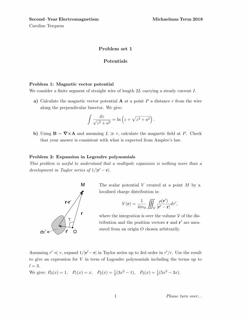
Problem 2: Expansion in Legendre polynomials

This problem is useful to understand that a multipole expansion is nothing more than a

development in Taylor series of 1/|r′ − r|.

The scalar potential V created at a point M by a

localised charge distribution is:

V (r) =1

4πε0

˚V

ρ(r′)

|r′ − r|dτ ′,

where the integration is over the volume V of the dis-

tribution and the position vectors r and r′ are mea-

sured from an origin O chosen arbitrarily.

Assuming r′ r, expand 1/|r′− r| in Taylor series up to 3rd order in r′/r. Use the result

to give an expression for V in term of Legendre polynomials including the terms up to

l = 3.

We give: P0(x) = 1, P1(x) = x, P2(x) = 12(3x2 − 1), P3(x) = 1

2(5x3 − 3x).

1

Problem 3: Dipole

a) Show that the energy of a physical dipole p in an electric field E (not necessarily

uniform) is given by U = −p ·E.

b) We consider two dipoles p1 and p2 and note r the position vector of p2 measured

from p1. Show that the interaction energy of the two dipoles is:

Uint =1

4πε0r3[p1 · p2 − 3 (p1 · r) (p2 · r)] ,

where r = r/r.

c) Draw graphs showing how Uint depends upon the relative orientation of the dipoles

in the following cases: (i) p1 is parallel to r, (ii) p1 is perpendicular to r.

Problem 4: Quadrupole

A system of three charges, aligned along the z–axis,

consists of a charge −2q at the origin O and two +q

charges at z = −a and z = a. We note (r, θ, ϕ) the

spherical coordinates.

a) Find the potential at r a using the multipole expansion with origin at O. Justify

why this system of charges is called a quadrupole.

We give: P0(x) = 1, P1(x) = x, P2(x) = 12(3x2 − 1).

b) Show that there is not translational force or couple on the quadrupole in a uniform

electric field.

c) We consider a point charge Q placed at a point P a distance r a away from the

quadrupole. Show that the torque about P on the quadrupole due to the charge is

Γ = 3Qqa2 sin 2θ/(4πε0r3) and find its direction.

d) Find the energy of the quadrupole in the potential of the chargeQ. In which direction

does the quadrupole rotate under the effect of the torque?

2

Please turn over...

Problem 5: Electric field due to a sphere with surface charge density ∝ cos θ

We consider a sphere of radius R and a spherical coordinate system (r, θ, ϕ) with origin

at the centre of the sphere. The surface of the sphere carries a charge density σ = k cos θ.

a) Calculate the potential V using the fact that it satisfies Laplace’s equation both

inside and outside the sphere. Hint: write the solution of the equation in term of

Legendre polynomials and choose V = 0 at infinity.

b) Find the electric field E produced by the sphere.

c) Calculate the electric dipole moment p of the charge distribution. Check that the

electric field outside the sphere calculated in the previous question is that due to the

dipole moment p. What can you conclude about the higher multipoles? Express the

field inside the sphere as a function of the polarization of the sphere, which is the

dipole moment per unit volume.

d) A surface charge density ∝ cos θ can be obtained by superimposing two solid spheres

with same radius R, opposite charges Q and −Q uniformly distributed over their

volume, and centres slightly apart (separation d R), as shown on the figure. From

a point outside the spheres, the situation is the same as if the charges were at the

centre of the spheres.

Find the relation between Q, d and p for the electric field

outside the spheres to be the same as in the previous ques-

tion. Using Gauss’s theorem to obtain the contribution

from each sphere, calculate the field in the region where the

spheres overlap and show that it is the same as in the previ-

ous question.

Problem 6: Metal sphere in a uniform electric field (Pb 5 needs to be done first)

A metal sphere of radius R with no net charge is placed in a uniform electric field E = E0z,

where z is a unit vector.

a) Explain qualitatively how the field modifies the charge distribution in the sphere

and how this, in turn, affects the electric field.

b) Calculate the electric potential V outside the sphere using the fact that it satisfies

Laplace’s equation. Hint: write the solution of the equation in term of Legendre

polynomials and choose V = 0 at the surface of the sphere.

c) Using the boundary condition on the electric field, calculate the charge density σ at

the surface of the sphere.

d) Using the results from Problem 5, question b, give an expression for the electric field

produced by σ. Find the total field inside the sphere. Comment.

3

Problem 7: Magnetic field due to a spinning sphere

We consider a sphere of radius R which carries a uniform surface charge density σ and

spins with angular velocity ω around a diameter. We use spherical coordinates (r, θ, ϕ)

with origin at the centre of the sphere and the z–axis along the rotation axis.

a) Find the surface current density K(r) as a function of θ. Hint: Consider a ring with

a small thickness at the surface of the sphere and perpendicular to the rotation axis.

b) Justify that the magnetic field produced by the surface current can be written under

the form B = ∇Ψ, where Ψ is a scalar function. Show that Ψ satisfies Laplace’s

equation inside and outside the sphere. Write the boundary conditions on Ψ. Cau-

tion: Ψ is not continuous at r = R (explain why).

c) Write Ψ in term of Legendre polynomials. Show that the l = 1 term in the expan-

sion, with appropriate coefficients, satisfies Laplace’s equation inside and outside the

sphere with the boundary conditions given above. Justify that this is the solution.

d) Find the magnetic field B produced by the sphere.

e) Consider a ring with a small thickness at the surface of the sphere and perpendicular

to the rotation axis. Write the magnetic dipole moment of this ring. Find the total

magnetic dipole moment m of the sphere.

f) Check that the magnetic field outside the sphere calculated in question d is that

due to the dipole moment m. What can you conclude about the higher multipoles?

Express the field inside the sphere as a function of the magnetization of the sphere,

which is the dipole moment per unit volume.

Problem 8: Separation of variables in cylindrical coordinates

a) Solve Laplace’s equation by separation of variables in cylindrical coordinates, as-

suming there is no dependence on z.

b) Consider an infinitely long straight wire along the z–axis which carries a uniform

line charge λ. Calculate the electric field using Gauss’s theorem. Find the potential

and check that it is a solution of Laplace’s equation found in question a.

c) Consider an infinitely long metal pipe of radius R placed at right angle to a uniform

electric field E0. Using the result from question a and appropriate boundary condi-

tions, find the potential outside the pipe. Calculate the charge density induced on

the pipe.

4

Please turn over...

Second–Year Electromagnetism Michaelmas Term 2018

Caroline Terquem

Problem set 2

Electric and magnetic fields in matter

Some of the problems below are taken from:

Introduction to Electrodynamics, David J. Griffiths, 4th Edition

Electric fields in matter

Problem 1: Capacitance and dielectrics

We consider a parallel plate capacitor consisting of two metal surfaces of area A separated

by a distance d. We assume d A1/2, so that edge effects can be neglected and the

electric field can be considered to be uniform between the plates.

a) The capacitor is connected to a battery so that a charge +Q0 is brought from one

plate to the other. Using Gauss’s law, calculate the electric field E0 between the

plates. Find the potential difference ∆V0 between the plates and the capacitance

C0. Calculate the potential energy U0 stored in the capacitor.

b) We now insert a linear dielectric material between the plates while the capacitor

remains connected to the battery, which supplies the potential difference ∆V0. Ex-

perimentally, it is found that the charge Q on the plates is increased. Explain why.

By representing the system as the superposition of a vacuum capacitor and a polar-

ized dielectric slab, calculate the total electric field E in the capacitor in terms of Q

and the polarization P . By substituting P = ε0χeE, find the relation between the

displacement vector D and Q. Calculate Q in terms of Q0 and the capacitance C in

terms of C0. Calculate the change in the stored potential energy of the capacitor in

terms of U0.

c) We now come back to question (a) and disconnect the battery before inserting a

dielectric material between the capacitor plates. Experimentally, it is found that the

potential difference ∆V between the plates decreases. Explain why. Calculate the

capacitance C in terms of C0 and the change in the stored potential energy of the

capacitor in terms of U0.

1

Problem 2: Capacitor half–filled with a dielectric

We insert a slab of linear dielectric material of dielectric

constant εr and thickness d next to the positive plate in a

parallel plate capacitor. The distance between the plates

is 2d, their area is A and they carry a (free) charge density

±σ .

a) Find the electric displacement vector D, the electric field E and the polarization P

in each region.

b) Find the potential difference between the plates and the capacitance C. Show that

the system can be regarded as two capacitors connected in series.

c) Find the location and amount of all bound charge. Using the distribution of free

and bound charges, recalculate the electric field E in each region.

Problem 3: Force on a dielectric

We insert a portion of a slab of linear dielectric material of dielectric constant εr and

thickness d on the left hand side of a parallel plate capacitor consisting of two conducting

plates of length L, width w and thickness d.

a) We connect the capacitor to a battery to charge the plates, and then disconnect

the battery. The total charge on each plate then remains constant equal to ±Q,

corresponding to surface charge densities ±σ′ and ±σ′′ on the left and right hand

sides, respectively. Using Gauss’s law, write the electric fields E′ and E′′ on the left

and right hand sides in terms of σ′ and σ′′. Find the relation between σ′ and σ′′.

Using the fact that Q is constant, write σ′′ in terms of x and the different constants.

Find the potential difference between the plates, and then the stored potential energy

U of the system, in terms of x. Write the relation between the change in energy,

dU , when the dielectric is pulled out a distance dx, and the electric force F exerted

by the plates on the dielectric. Calculate F in terms of x. Does this force pull the

dielectric into the capacitor or push it out?

2

Please turn over...

b) We now repeat the experiment but leave the capacitor connected to the battery,

which supplies the potential difference ∆V . Calculate U in terms of x and the

different constants. Write the relation between dU and F when the dielectric is

pulled out a distance dx. Make sure to include all contributions to the work done in

the system. Calculate F in terms of x and show that it is the same as in question

(a).

c) The result obtained above can be verified experimentally. However, we have assumed

in our calculation that the electric field was uniform between the plates and zero

outside. If that were the case in reality, would there be a force on the dielectric?

Where does this force come from, and how is it possible that we obtain the right

answer given the simplified model we have used?

Problem 4: Sphere with a frozen–in polarization

A sphere of radius R made of a dielectric material carries a frozen–in polarization P(r) =

kr, where k is a constant and r is the position vector measured from the centre of the

sphere. There are no free charges anywhere.

a) Calculate the bound charges.

b) Using Gauss’s law, find the electric field E inside and outside the sphere.

c) Using the expression of E and P, find the electric displacement vector D inside and

outside the sphere. Check that it satisfies Gauss’s law. Is the dielectric linear?

Problem 5: Electric field within a cavity inside a dielectric

The electric field inside a large piece of dielectric is E0 and the polarization is P, so that

the displacement vector is D = ε0E0 + P. A cavity is hollowed out of the material. It is

small enough that the field and the polarization can be taken as uniform within it. We

also assume that the polarization in the dielectric is frozen–in, so that it does not change

when the cavity is hollowed out. Calculate, in the cavity, the field in terms of E0 and P

and the displacement in terms of D0 and P in the following cases:

a) The cavity is a small sphere [Hint: Use the superposition principle and, to calculate

the electric field inside a uniformly polarized sphere, use the results of Problem 5 in

Problem set 1],

b) The cavity is shaped like a long thin needle parallel to P,

c) The cavity is a thin, circular wafer perpendicular to the polarization.

3

Magnetic fields in matter

Problem 6: Cylinder with a frozen–in magnetization

An infinitely long cylinder of radius R made of a magnetic material carries a frozen–in

magnetization M = krz, where r is the distance from the axis of the cylinder, z is the

unit vector along the axis and k is a constant. There is no free current anywhere. Find

the magnetic field B inside and outside the cylinder by two different methods:

a) Locate all the bound currents and calculate the field they produce,

b) Use Ampere’s law for H and the relationship between B, H and M to derive B.

Problem 7: Magnetic field in a coaxial cable

A long coaxial cable of inner radius a and outer radius b is

filled with an insulating material of magnetic susceptibility

χm. A current I flows down the inner conductor and returns

along the outer one, uniformly distributed over the surfaces.

Find the magnetic field B in the magnetic material between

the conductors. As a check, calculate the magnetization M

and the bound currents, and confirm that, together with the

free currents, they generate the correct field.

Problem 8: Air gap in an inductor

We consider a toroidal core made of an iron alloy

with cross sectional area A and radius R A1/2.

We make an inductor from the core by wrapping

around it N turns of a wire carrying a current I,

to use it as an energy storage device.

We increase the current from 0 until the material saturates, which happens when the

magnetic field B inside it reaches the value Bsat. Before saturation is reached, the material

can be regarded as being linear with relative permeability µr.

a) Calculate the magnetic field B in the core and the inductance L. Find the maximum

current I1 that the inductor can carry before the core saturates. Calculate the

magnetic energy W1 that is stored in the inductor when the current reaches the

value I1. If I is increased beyond I1, how does the inductance vary?

4

b) To increase the energy that can be stored in

the inductor, we have to find a way of increas-

ing the saturation current while keeping L con-

stant. This can be done by introducing an air

gap of width w into the core. We take w R,

so that we can neglect magnetic fringing, that

is to say the bulging out of the magnetic field

lines as they enter air from the magnetic ma-

terial.

Calculate the magnetic field B in the core and the number of turns of wire we now

have to wrap around the core to keep L constant. Find the maximum current I2 this

second inductor can carry before the core saturates and compare it with I1. Calculate

the energy W2 stored in the magnetic field at the point of saturation and compare

it with W1. Compare the energy stored in the magnetic material with that stored

in the air gap. For numerical applications, use R = 10 cm, w = 3 mm and µr = 1500.

c) Some of the energy stored in the

inductor can be recovered by

decreasing the current back to

0. The figure shows the B −H

curves (hysteresis loops) mea-

sured on a toroidal core without

and with gap (the straight lines

inside the loops are the magne-

tization curves).

Show on these curves how much energy is released per unit volume by the magnetic

material in the core after the current is returned to 0. Comment.

d) Explain what would be the advantages of using iron, and especially soft iron, to

make magnetic cores. Iron, however, has a major disadvantage when the inductor is

used with alternating currents. Can you think of what it is?

5

Please turn over...

Second–Year Electromagnetism Michaelmas Term 2018

Caroline Terquem

Problem set 3

Electromagnetic waves

Problem 1: Poynting vector and resistance heating

This problem is not about waves but is useful to understand how energy is transferred in

a circuit.

A cylindrical resistor with radius a, length L and resistance R is connected to a battery

which supplies a potential difference V . The resulting steady current I which flows along

the resistor is uniform through its cross-section.

a) Find the electric field E and magnetic field B on the surface of the resistor.

b) Calculate the Poynting vector S on the surface of the resistor. Find the power flowing

through the surface of the resistor. Compare with the rate at which work is done on

the charges in the resistor by the electromagnetic field.

c) We have found above that there is a flow of energy going into the resistor. This energy

has to come from outside the resistor, and therefore there has to be an electric field

outside giving an inward radial Poynting vector. Justify that this is the case.

d) The energy entering the resistor comes from the battery: energy flows along the wires

connecting the battery to the resistor. This requires a component of the electric

field perpendicular to the wires. Such a field is produced by charges that have to be

present on the surface of the wires for a steady current to flow. Assuming the charge

distribution sketched on the figure, draw the Poynting vector in the different parts

of the circuit to show how energy flows from the battery to the resistor. Comment

on where the energy flows. Is there any energy returning to the battery?

(adapted from Galili & Goihbarg, 2005, Energy transfer in electrical circuits: a

qualitative account, American Journal of Physics, 73, 141)

1

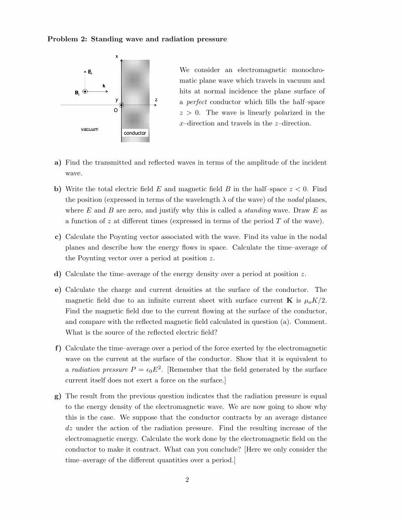
Problem 2: Standing wave and radiation pressure

We consider an electromagnetic monochro-

matic plane wave which travels in vacuum and

hits at normal incidence the plane surface of

a perfect conductor which fills the half–space

z > 0. The wave is linearly polarized in the

x–direction and travels in the z–direction.

a) Find the transmitted and reflected waves in terms of the amplitude of the incident

wave.

b) Write the total electric field E and magnetic field B in the half–space z < 0. Find

the position (expressed in terms of the wavelength λ of the wave) of the nodal planes,

where E and B are zero, and justify why this is called a standing wave. Draw E as

a function of z at different times (expressed in terms of the period T of the wave).

c) Calculate the Poynting vector associated with the wave. Find its value in the nodal

planes and describe how the energy flows in space. Calculate the time–average of

the Poynting vector over a period at position z.

d) Calculate the time–average of the energy density over a period at position z.

e) Calculate the charge and current densities at the surface of the conductor. The

magnetic field due to an infinite current sheet with surface current K is µoK/2.

Find the magnetic field due to the current flowing at the surface of the conductor,

and compare with the reflected magnetic field calculated in question (a). Comment.

What is the source of the reflected electric field?

f) Calculate the time–average over a period of the force exerted by the electromagnetic

wave on the current at the surface of the conductor. Show that it is equivalent to

a radiation pressure P = ε0E2. [Remember that the field generated by the surface

current itself does not exert a force on the surface.]

g) The result from the previous question indicates that the radiation pressure is equal

to the energy density of the electromagnetic wave. We are now going to show why

this is the case. We suppose that the conductor contracts by an average distance

dz under the action of the radiation pressure. Find the resulting increase of the

electromagnetic energy. Calculate the work done by the electromagnetic field on the

conductor to make it contract. What can you conclude? [Here we only consider the

time–average of the different quantities over a period.]

2

Please turn over...

Problem 3: Fresnel’s formulas

A monochromatic plane wave:

Ei = E0i ei(ki·r−ωt), Bi =1

cki×Ei,

is incident on the flat surface of a linear medium with

dielectric constant εr (and µ = µ0) at an angle θi to

the normal.

Here ki is the unit vector in the direction of propagation, and the tilde denotes complex

quantities. We choose the origin of time so that the amplitude of the wave, E0i, is real.

This gives rise to reflected and transmitted waves:

Er = E0r ei(kr·r−ωt), Br =1

ckr×Er, and Et = E0t ei(kt·r−ωt), Bt =

1

vkt×Et,

where v is the velocity of the wave in the dielectric.

a) Use the dispersion relation ω(k) and the boundary conditions at the interface to find

the angle of reflection θr (between kr and the z–axis) and the angle of transmission

(or refraction) θt (between kt and the z–axis) in terms of the angle of incidence θi

(Snell’s law). If the index of refraction n < 1, show that there is a critical angle θic

above which there is no transmitted wave (this is called total internal reflection).

b) We assume that the incident wave is linearly polarized with polarization normal to

the plane of incidence. We assume that the reflected and transmitted waves have

the same polarization (this can be shown by assuming a more general polarization

and using the boundary conditions). Use the boundary conditions to find E0r and

E0t as a function of E0i and θi (Fresnel’s formulas). Plot schematically the reflection

coefficient R =∣∣∣E0r/E0i

∣∣∣2 as a function of θi for the cases n > 1 and n < 1.

c) Suppose now that the incident wave is linearly polarized with polarization parallel

to the plane of incidence. Again we assume that the reflected and transmitted waves

also have a linear polarization parallel to the plane of incidence. Use the boundary

conditions to find E0r and E0t as a function of E0i and θi (Fresnel’s formulas). Show

that there is no reflection at a certain value of θi, called Brewster’s angle. Plot

schematically R as a function of θi for the cases n > 1 and n < 1. What happens to

an unpolarized beam incident at Brewster’s angle?

d) At Brewster’s angle, show that θr + θt = 90. The incident wave induces oscillations

of the bound electrons at the surface of the dielectric. These electrons then act

as oscillating dipoles which are the source of the reflected and transmitted waves.

Given that dipoles do not radiate energy in the direction of their dipole moment,

can you explain why there is no reflection at Brewster’s angle?

3

Problem 4: Waves in the ionosphere

The ionosphere is a region of the upper atmosphere which is ionized by solar (UV) ra-

diation. It may be simply described as a dilute gas of charged particles, composed of

electrons and ionized air (N2 and O2) molecules. The number density ne of free electrons

is maximum at about 200 to 400 km above the surface of the Earth. At higher altitudes, ne

decreases because the density of air molecules to be ionized decreases. At lower altitudes,

ne decreases because UV radiation from the sun has been absorbed in layers above.

a) We assume that the ionosphere can be modelled as a collisionless plasma. Write the

equation of motion for an electron assuming an external electric field and neglecting

the local field. Show that the dielectric constant is given by εr = 1 − ω2p/ω

2, with

ω2p = nee

2/(ε0m), where −e and m are the electron’s charge and mass, respectively.

Write the dispersion relation ω(k). Show that for ω < ωp, waves cannot propagate

in the plasma.

b) Suppose that waves are emitted at the surface of the Earth toward the ionosphere.

For waves with polarization both perpendicular and parallel to the plane of incidence,

show that for ω > ωp there is a range of angles of incidence for which reflection is

not total, but for larger angles there is a total reflection back toward the Earth. [Use

the results of Problem 3].

c) A radio amateur emits a wave with a wavelength of 21 m (corresponding to high

frequency or shortwave broadcast) in the early evening. This wave is received by

another radio amateur located 1000 km away, but not by other amateurs located

closer. Assuming that the wave is being reflected by the so–called F layer of the

ionosphere at a height of 300 km (the altitude at which reflection occurs can be

determined from the travel time of the signal), calculate the electron density ne.

Compare with the known maximum and minimum F layer densities of 2× 106 cm−3

in the daytime and (2–4)× 105 cm−3 at night.

d) The cutoff frequency ωp corresponding to ne ∼ 105–106 cm−3 is of a few 107 rad s−1.

FM radio and television signals have frequencies much larger than this value. What

happens to these signals when they hit the ionosphere? Why are AM signals, with

frequencies between 3 and 30 MHz, used for long distance (including intercontinental)

communication?

e) From the BBC website: AM reception can vary a great deal from day to night because

of differences in the atmosphere. You may get good, clear reception during the day,

but after sunset the signal may fade or become distorted. Signals travel further at

night, so you may get interference from other transmitters, and you may even hear

stations from outside the UK. Why do radio signals travel farther at night than in

the day?

4

Please turn over...

Problem 5: Waves in a good conductor

We consider an ohmic conductor with conductivity σ, permittivity ε0 and permeability

µ0. We assume that the conductor is excellent, that is to say σ ωε0.

a) Show that the conductor can be described as a dielectric with complex dielectric

constant εr = 1 + iσ/(ωε0). An electromagnetic monochromatic plane wave propa-

gates through the conductor. Write the dispersion relation and find the wavenum-

ber in terms of the penetration depth δ =√

2/(ωµ0σ). Compare the group and

phase velocities. Is dispersion normal or anomalous? Show that the impedance is

Z = (1− i)/(δσ).

b) Calculate the time–average over a period of the Poynting vector, 〈S〉, at a location

z along the direction of propagation of the wave. Calculate the time–average over

a period of the rate at which work is done on the charges contained in the volume

delimited by the surfaces at z = z1 and z = z2. Verify that it is equal to the

time–average over a period of the flux of the Poynting vector into the volume.

c) Calculate the time–average over a period of the energy density, 〈u〉. Is the energy

carried mainly by the electric field or by the magnetic field? Calculate the velocity

at which energy is transported (it is given by |〈S〉| /〈u〉). Compare with the group

velocity. Comment.

5

Problem 6: Dielectric losses

In general, the response of dielectric materials to a varying electric field is described by

a complex dielectric constant, which is associated with energy losses. In this problem, we

are going to derive an energy equation for the wave and quantify the losses.

a) Write Maxwell’s equations for a dielectric with µ = µ0, a complex dielectric constant

and no conduction current nor free charges. First write the equations using com-

plex notations, and then separate all the quantities into real and imaginary parts.

Remember that the physical fields are the real part of the complex quantities. By

taking the dot product of E with the equation giving ∇×B, derive an energy equa-

tion for the wave (follow the same procedure as in sections 4.3.1 and 4.3.2 of the

Lecture Notes). Give the expression for the rate at which energy is dissipated per

unit volume in the dielectric.

b) The time–average over a period of the Poynting vector in a dielectric with complex

dielectric constant is:

〈S〉 =

⟨E×Bµ0

⟩= zcn′

ε0E20

2e−2k

′′z,

where z is the direction of propagation, E0e−k′′z is the amplitude of the electric field,

n′ is the real part of the complex index of refraction and k′′ is the imaginary part of

the complex wavenumber (see section 5.6.3 of the Lecture Notes). Verify that the

flux of 〈S〉 into a volume delimited by the surfaces at z = z1 and z = z2 is equal

to the time–average over a period of the rate at which energy is dissipated in the

volume.

c) In Maxwell’s equations (in complex notations), we now add a conduction current

that obeys Ohm’s law. Show that the imaginary part of the dielectric constant can

be incorporated into an effective conductivity and recover the rate of energy loss in

the dielectric by drawing an analogy with ohmic dissipation.

6

Please turn over...

Second–Year Electromagnetism Michaelmas Term 2018

Caroline Terquem

Problem set 4

Special relativity, Transmission lines and Resonant cavities

Electromagnetism and special relativity

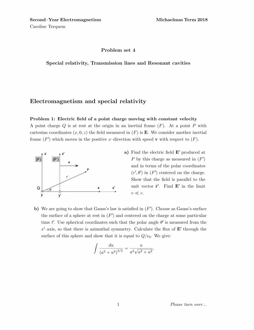
Problem 1: Electric field of a point charge moving with constant velocity

A point charge Q is at rest at the origin in an inertial frame (F ). At a point P with

cartesian coordinates (x, 0, z) the field measured in (F ) is E. We consider another inertial

frame (F ′) which moves in the positive x–direction with speed v with respect to (F ).

a) Find the electric field E′ produced at

P by this charge as measured in (F ′)

and in terms of the polar coordinates

(r′, θ′) in (F ′) centered on the charge.

Show that the field is parallel to the

unit vector r′. Find E′ in the limit

v c.

b) We are going to show that Gauss’s law is satisfied in (F ′). Choose as Gauss’s surface

the surface of a sphere at rest in (F ′) and centered on the charge at some particular

time t′. Use spherical coordinates such that the polar angle θ′ is measured from the

x′–axis, so that there is azimuthal symmetry. Calculate the flux of E′ through the

surface of this sphere and show that it is equal to Q/ε0. We give:

ˆdu

(a2 + u2)3/2=

u

a2√a2 + u2

.

1

c) The figure (from E. Purcell & D. Morin,

Electricity and Magnetism) shows a repre-

sentation of the electric field in (F ′) (the

dot in the centre represents the charge, and

the density of field lines indicates the in-

tensity of the field). Justify that the circu-

lation of the electric field along the closed

path ABCDA is non zero. Comment.

d) Calculate the magnetic field B′ of the charge Q as measured in (F ′). [Hint: Use the

fact that the magnetic field is zero in (F ).] Find B′ in the limit v c. What is the

magnetic field of a charge moving at constant velocity v?

Problem 2: Interaction between a moving charge and other moving charges

In an inertial frame (F ), we consider a line of positive charges all moving to the right with

constant speed v. There is also a line of negative charges all moving to the left with the

same speed v. The total charges of the positive and negative lines are equal and opposite.

We view the lines as continuous distributions with linear charge densities +λ and −λ,

as measured in (F ). This is an ideal representation of a wire containing both ions and

electrons. At a distance d from the axis of the wire, there is a charge q which moves to

the right with speed u < v.

a) Calculate the net charge and the net current in the wire. Find the electric field E

and magnetic field B at the position of the charge, and the force f = q(E + u×B)

on q, as measured in (F ).

b) We now consider the inertial frame (F ′) which moves to the right at speed u. The

charge q is at rest in (F ′). Find the velocities v′+ and v′− of the positive and negative

lines in (F ′) and show that γ± ≡ 1/√

1− v′2±/c2 = γ(1∓ uv/c2

)/√

1− u2/c2, where

γ ≡ 1/√

1− v2/c2. Calculate the charge densities λ′± of the lines as measured in

(F ′) and the net charge λ′ = λ′+ + λ′− in terms of λ, u, v and c. Find the electric

field E′ at the position of the charge, and the force f ′ = qE′ on q, as measured in

(F ′). Compare f and f ′.

2

Please turn over...

Transmission lines

Problem 3: Practical types of transmission lines

Calculate the capacitance per unit length, the inductance per unit length and the speed at

which signals propagate for the following transmission lines. In each case, the conductors

are separated by a material of electric permittivity ε and magnetic permeability µ. The

figures show a cross section of the lines, which extend in the direction perpendicular to

the figure.

a) Coaxial cable: b) Strip line:

Problem 4: Short and open circuited transmission lines

Calculate the input impedance Z1 of a length l of a loss-free transmission line of charac-

teristic impedance Z0 terminated by an open circuit. Calculate the input impedance Z2

of the same transmission line terminated by a short circuit. Show that the lines can be

used to create an equivalent inductor or capacitor. Show that Z1Z2 = Z20 . Discuss the

applications of such transmission lines (also called stubs).

Problem 5: Power transmitted into a load

A wave travels along a loss–free transmission line of characteristic impedance Z1 which

is terminated by a load of impedance Z2. Show that the fraction of the incident power

time–averaged over a wave period transmitted into the load is t = 4Z1 Re(Z2)/ |Z1 + Z2|2.

Problem 6: Transmission lines in parallel

A transmission line with a characteristic impedance Z0 = 200 Ω is terminated by a resistor

R = 600 Ω. Calculate the input admittance Y (inverse of the impedance) of the line at

one–sixth of a wavelength from the end.

A short–circuited stub of line (with the same

characteristic impedance) is added in parallel

at this point. What should be its length in

order to cancel the reflected signal travelling

back towards the source? [Hint: Match the

admittances.]

3

Resonant cavities

Problem 7: Earth and ionosphere as a resonant cavity: Schumann resonances

This problem is taken from section 8.9 of Jackson, Classical Electrodynamics

On a global scale, the Earth and the

lower ionosphere can be idealized as two

perfectly conducting, concentric spheres

with radii a and b. Therefore, they form

a resonant electromagnetic cavity which

can support resonant standing waves, as

sketched on the figure. The resonant

frequencies are called Schumann reso-

nances, as they were first predicted by

the physicist Winfried Otto Schumann in

1952 (although Tesla may have observed

them before 1900).

The characteristic wavelength of the lowest frequency mode is on the order of the largest

dimension of the cavity, that is to say on the order of magnitude of the Earth’s circumfe-

rence. The modes therefore have extremely low frequencies. Such modes can be excited

by lightning and they are detected at various research stations around the world. The aim

of this problem is to calculate the resonant frequencies of the Earth–ionosphere cavity. We

will focus on TM modes, as they have the lowest frequencies (in spherical coordinates, TM

and TE modes have no radial component of the magnetic and electric field, respectively).

We note (r, θ, ϕ) the spherical coordinates and assume that the problem has azimuthal

symmetry (no ϕ–dependence).

a) Using∇ ·B = 0 and Faraday’s law∇×E = −∂B/∂t, show that Bθ = 0 and Eϕ = 0.

Write the boundary conditions at r = a and r = b.

b) Assuming a time–dependence of e−iωt, show that B satisfies the following equation:

ω2

c2B−∇× (∇×B) = 0,

and that the ϕ–component of this equation can be written under the form:

ω2

c2(rBϕ) +

∂2

∂r2(rBϕ) +

1

r2

[1

sin θ

∂

∂θ

(sin θ

∂ (rBϕ)

∂θ

)− rBϕ

sin2 θ

]= 0.

c) We look for solutions to this equation under the form:

Bϕ =F (r)

rG(θ).

4

Show that G(θ) is the associated Legendre polynomial Pml (θ) with m = ±1. Since

the two solutions P−1l and P 1l only differ by a constant of proportionality, we fix

m = 1. Write the components of the fields in terms of F (r), P 1l (cos θ) and Pl(cos θ),

and the boundary conditions satisfied by F at r = a and r = b. We give:

d

dθ

[sin θP 1

l (cos θ)]

= −l(l + 1) sin θPl(cos θ),

where Pl(cos θ) is a Legendre polynomial.

d) Show that the differential equation satisfied by F (r) is:

d2F

dr2+

[ω2

c2− l(l + 1)

r2

]F = 0.

We assume that the height of the ionosphere is small compared to the radius of the

Earth (h = b − a a) so that 1/r2 can be approximated by 1/a2 in the above

equation. Calculate the solution of the above equation that satisfies the boundary

conditions at r = a and r = b. Show that the (Schumann) resonant frequencies are:

ωln =c

a

√l(l + 1) + n2π2

a2

h2,

where n is a positive integer.

e) The Earth–ionosphere cavity is excited by lightning bolts which generate radial elec-

tric fields and contain a large spectrum of frequencies. The components with a fre-

quency close to a Schumann frequency have the largest amplitude as they correspond

to normal modes of the cavity.

This spectrum shows the first seven reso-

nance modes (corresponding to n = 0).

The resonant frequencies are 7.5, 14.5,

20.0, 27.5, 31.5, 37.5 and 43.7 Hz. The

measurements shown on this figure were

carried out at Lavangsdalen, in Norway

(geographic latitude 70N) in March 1966

(from T. R. Larsen & A. Egeland, Fine

Structure of the Earth–Ionosphere Cavity

Resonances, 1968, Journal of Geophysical

Research, 73, 15).

Compare the measured frequencies with

those calculated above. Comment.

5