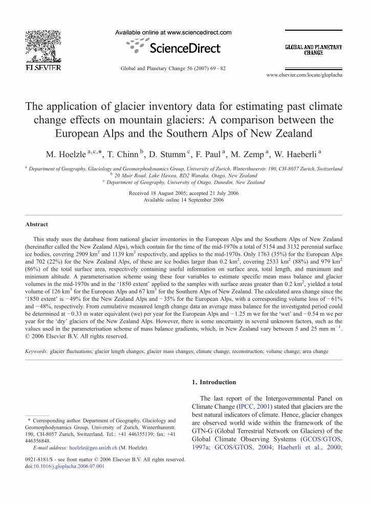
ge 56 (2007) 69–82www.elsevier.com/locate/gloplacha

Global and Planetary Chan

The application of glacier inventory data for estimating past climatechange effects on mountain glaciers: A comparison between the

European Alps and the Southern Alps of New Zealand

M. Hoelzle a,c,⁎, T. Chinn b, D. Stumm c, F. Paul a, M. Zemp a, W. Haeberli a

a Department of Geography, Glaciology and Geomorphodynamics Group, University of Zurich, Winterthurerstr. 190, CH-8057 Zurich, Switzerlandb 20 Muir Road, Lake Hawea, RD2 Wanaka, Otago, New Zealand

c Department of Geography, University of Otago, Dunedin, New Zealand

Received 18 August 2005; accepted 21 July 2006Available online 14 September 2006

Abstract

This study uses the database from national glacier inventories in the European Alps and the Southern Alps of New Zealand(hereinafter called the New Zealand Alps), which contain for the time of the mid-1970s a total of 5154 and 3132 perennial surfaceice bodies, covering 2909 km2 and 1139 km2 respectively, and applies to the mid-1970s. Only 1763 (35%) for the European Alpsand 702 (22%) for the New Zealand Alps, of these are ice bodies larger than 0.2 km2, covering 2533 km2 (88%) and 979 km2

(86%) of the total surface area, respectively containing useful information on surface area, total length, and maximum andminimum altitude. A parameterisation scheme using these four variables to estimate specific mean mass balance and glaciervolumes in the mid-1970s and in the ‘1850 extent’ applied to the samples with surface areas greater than 0.2 km2, yielded a totalvolume of 126 km3 for the European Alps and 67 km3 for the Southern Alps of New Zealand. The calculated area change since the‘1850 extent’ is −49% for the New Zealand Alps and −35% for the European Alps, with a corresponding volume loss of −61%and −48%, respectively. From cumulative measured length change data an average mass balance for the investigated period couldbe determined at −0.33 m water equivalent (we) per year for the European Alps and −1.25 m we for the ‘wet’ and −0.54 m we peryear for the ‘dry’ glaciers of the New Zealand Alps. However, there is some uncertainty in several unknown factors, such as thevalues used in the parameterisation scheme of mass balance gradients, which, in New Zealand vary between 5 and 25 mm m−1.© 2006 Elsevier B.V. All rights reserved.

Keywords: glacier fluctuations; glacier length changes; glacier mass changes; climate change; reconstruction; volume change; area change

⁎ Corresponding author. Department of Geography, Glaciology andGeomorphodynamics Group, University of Zurich, Winterthurerstr.190, CH-8057 Zurich, Switzerland. Tel.: +41 446355139; fax: +41446356848.

E-mail address: hoelzle@geo.unizh.ch (M. Hoelzle).

0921-8181/$ - see front matter © 2006 Elsevier B.V. All rights reserved.doi:10.1016/j.gloplacha.2006.07.001

1. Introduction

The last report of the Intergovernmental Panel onClimate Change (IPCC, 2001) stated that glaciers are thebest natural indicators of climate. Hence, glacier changesare observed world wide within the framework of theGTN-G (Global Terrestrial Network on Glaciers) of theGlobal Climate Observing Systems (GCOS/GTOS,1997a; GCOS/GTOS, 2004; Haeberli et al., 2000;

70 M. Hoelzle et al. / Global and Planetary Change 56 (2007) 69–82

Haeberli and Dedieu, 2004; Haeberli et al., 2002;WMO, 1997). The GTN-G is led by the World GlacierMonitoring Service (WGMS, http://www.wgms.ch), thesuccessor to the 1894 founded international glaciercommission (Forel, 1895). WGMS collects data basedon the Global Hierarchical Observing Strategy (GHOST),which consists of five tiers (GCOS/GTOS, 1997b; IUGG(CCS)/UNEP/UNESCO, 2005). An extensive amount ofdata on topographic glacier parameters, based on tier 5 ofthe GHOST, has been built up in past regional glacierinventories (IAHS(ICSI)/UNEP/UNESCO, 1989), whichare currently updated by modern remote sensing methodswithin the Global Land Ice Measurements from Space(GLIMS, http://www.glims.org) project (Bishop et al.,

Fig. 1. A)Distribution of inventory glaciers (WGI=World Glacier Inventory) aGlaciers) in the European Alps. B)Distribution of inventory glaciers (WGI) anOnly glaciers on the Southern Island of New Zealand were used in the analysglaciers in the Southern Alps of New Zealand (a)=North_dry, (b) Fiord (‘wet’model used to draw the elevations is based on http://edc.usgs.gov/products/e

2004; Kieffer et al., 2000). Repetition of the glacierinventories should be undertaken at periods compatiblewith the characteristic dynamic response times ofmountain glaciers (a few decades). However, currentglacier down-wasting as observed in several mountainareas will probably require more updates of inventories inshorter time intervals (Paul et al., 2007-a).

The glacier inventories helpwith assessing the problemof representivity of continuous measurements withindifferent mountain areas, which can only be carried outon a few selected glaciers. A climate signal extracted fromone single glacier is often not very representative fora whole mountain range. The understanding of globaleffects of climate change can only be achieved by

nd of glaciers with length change measurements (FoG=Fluctuations ofd of glaciers with length change measurements (FoG) in New Zealand.is. The letters a) to g) are used to differentiate between ‘wet’ and ‘dry’), (c) West (‘wet’), (d) East_wet and (e) East_dry). The digital elevationlevation/gtopo30/hydro/index.html.

Table 1Parameterised values used in the calculations

Parameters EU Alps NZ Alps ‘wet’ NZ Alps ‘dry’

τ [Pa] 1.3·105 1.8·105 1.2·105

δb /δh [mm m−1] 7.5 15 5ρ [kg m−3] 900 900 900g [m s−2] 9.81 9.81 9.81A [a−1 Pa−8] 0.16 0.16 0.16n 3 3 3

Fig. 1 (continued ).

71M. Hoelzle et al. / Global and Planetary Change 56 (2007) 69–82

comparing the long-term behaviour of glaciers withindifferent mountain ranges. The European Alps wereanalysed in detail by Haeberli and Hoelzle (1995) and areanalysis was recently done by Zemp et al. (in press-b).This data is now ready to compare with other mountainranges. The Southern Alps of New Zealand (hereinaftercalled the New Zealand Alps) are particularly interestingfor such a comparison, because they are situated at asimilar latitude in the Southern Hemisphere as theEuropean Alps in the Northern Hemisphere. However,both mountain ranges have quite different climaticconditions. The method used to assess climate changeeffects on glacier change in both regions are based onsimple dynamic considerations and steady state condi-tions, which could be approximated for 1850 and the mid1970s. Both inventories showa very high accuracy and are

perfectly suited to apply the method described in detail byHaeberli andHoelzle (1995). Based on this application theNew Zealand inventory (Chinn, 1991; 2001) is comparedwith the European Alps in this study (Fig. 1). Bothinventories are included in the WGMS database stored at

72 M. Hoelzle et al. / Global and Planetary Change 56 (2007) 69–82

WGMS in Zurich, Switzerland and at the National Snowand Ice Data Center (NSIDC, http://nsidc.org) in Boulder,Colorado, USA (Hoelzle and Trindler, 1998).

In this paper we show: a) an application of an existingglacier parameterisation scheme to two glacier inventoriesin two differentmountain ranges to compare characteristicvariables like balance at the tongue, ice thickness, etc., b)a method of mean specific mass balance and volumereconstruction based on observed equilibrium line altitude

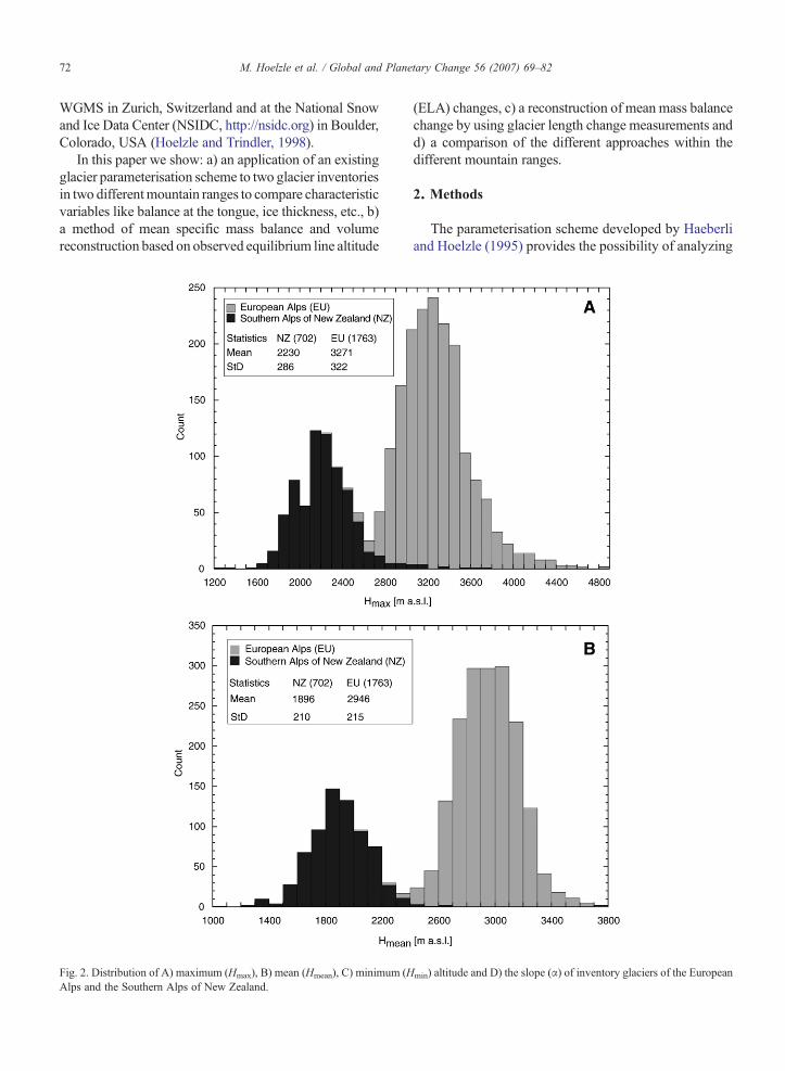
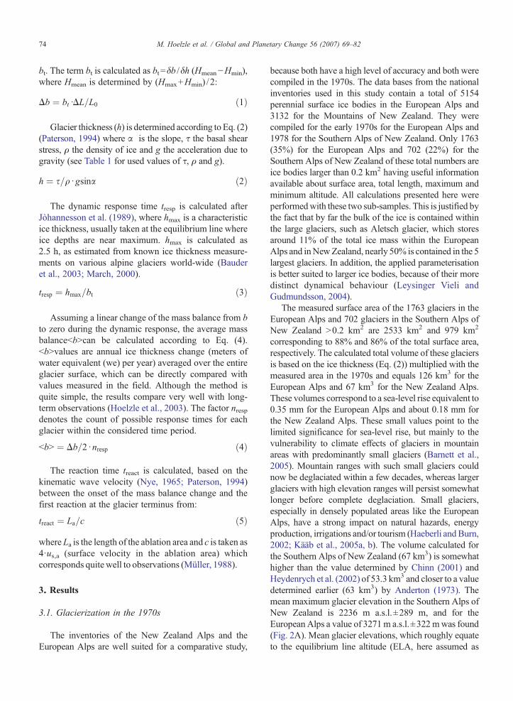
Fig. 2. Distribution of A) maximum (Hmax), B) mean (Hmean), C) minimum (HAlps and the Southern Alps of New Zealand.

(ELA) changes, c) a reconstruction of mean mass balancechange by using glacier length change measurements andd) a comparison of the different approaches within thedifferent mountain ranges.

2. Methods

The parameterisation scheme developed by Haeberliand Hoelzle (1995) provides the possibility of analyzing

min) altitude and D) the slope (α) of inventory glaciers of the European

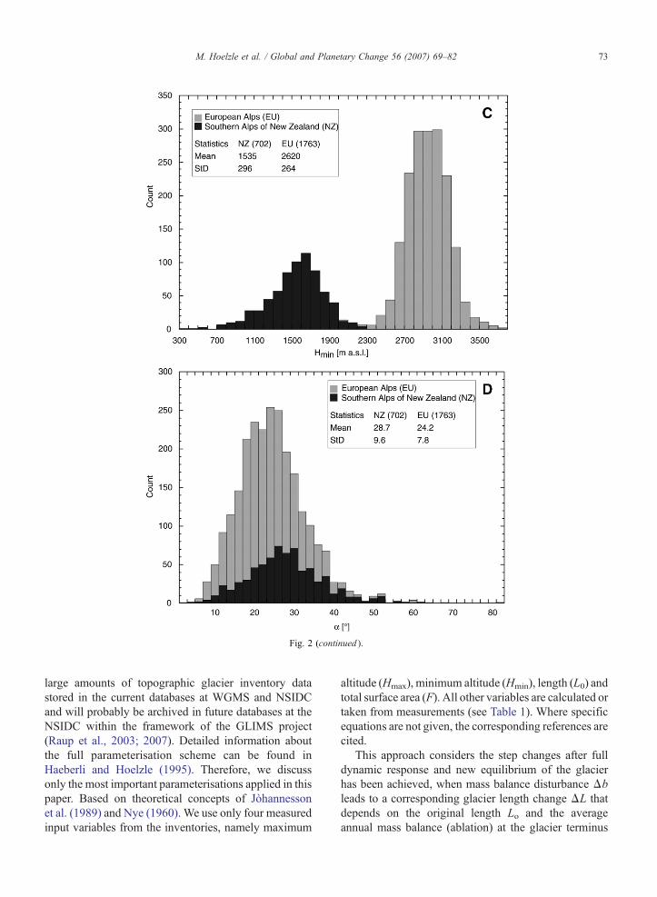
Fig. 2 (continued ).

73M. Hoelzle et al. / Global and Planetary Change 56 (2007) 69–82

large amounts of topographic glacier inventory datastored in the current databases at WGMS and NSIDCand will probably be archived in future databases at theNSIDC within the framework of the GLIMS project(Raup et al., 2003; 2007). Detailed information aboutthe full parameterisation scheme can be found inHaeberli and Hoelzle (1995). Therefore, we discussonly the most important parameterisations applied in thispaper. Based on theoretical concepts of Jòhannessonet al. (1989) and Nye (1960). We use only four measuredinput variables from the inventories, namely maximum

altitude (Hmax), minimum altitude (Hmin), length (L0) andtotal surface area (F). All other variables are calculated ortaken from measurements (see Table 1). Where specificequations are not given, the corresponding references arecited.

This approach considers the step changes after fulldynamic response and new equilibrium of the glacierhas been achieved, when mass balance disturbance Δbleads to a corresponding glacier length change ΔL thatdepends on the original length Lo and the averageannual mass balance (ablation) at the glacier terminus

74 M. Hoelzle et al. / Global and Planetary Change 56 (2007) 69–82

bt. The term bt is calculated as bt =δb /δh (Hmean−Hmin),where Hmean is determined by (Hmax+Hmin) / 2:

Db ¼ btdDL=L0 ð1Þ

Glacier thickness (h) is determined according to Eq. (2)(Paterson, 1994) where α is the slope, τ the basal shearstress, ρ the density of ice and g the acceleration due togravity (see Table 1 for used values of τ, ρ and g).

h ¼ s=qd gsina ð2Þ

The dynamic response time tresp is calculated afterJòhannesson et al. (1989), where hmax is a characteristicice thickness, usually taken at the equilibrium line whereice depths are near maximum. hmax is calculated as2.5 h, as estimated from known ice thickness measure-ments on various alpine glaciers world-wide (Bauderet al., 2003; March, 2000).

tresp ¼ hmax=bt ð3Þ

Assuming a linear change of the mass balance from bto zero during the dynamic response, the average massbalancebbNcan be calculated according to Eq. (4).bbNvalues are annual ice thickness change (meters ofwater equivalent (we) per year) averaged over the entireglacier surface, which can be directly compared withvalues measured in the field. Although the method isquite simple, the results compare very well with long-term observations (Hoelzle et al., 2003). The factor nrespdenotes the count of possible response times for eachglacier within the considered time period.

bbN ¼ Db=2d nresp ð4Þ

The reaction time treact is calculated, based on thekinematic wave velocity (Nye, 1965; Paterson, 1994)between the onset of the mass balance change and thefirst reaction at the glacier terminus from:

treact ¼ La=c ð5Þ

where La is the length of the ablation area and c is taken as4·us,a (surface velocity in the ablation area) whichcorresponds quite well to observations (Müller, 1988).

3. Results

3.1. Glacierization in the 1970s

The inventories of the New Zealand Alps and theEuropean Alps are well suited for a comparative study,

because both have a high level of accuracy and both werecompiled in the 1970s. The data bases from the nationalinventories used in this study contain a total of 5154perennial surface ice bodies in the European Alps and3132 for the Mountains of New Zealand. They werecompiled for the early 1970s for the European Alps and1978 for the Southern Alps of New Zealand. Only 1763(35%) for the European Alps and 702 (22%) for theSouthern Alps of New Zealand of these total numbers areice bodies larger than 0.2 km2 having useful informationavailable about surface area, total length, maximum andminimum altitude. All calculations presented here wereperformedwith these two sub-samples. This is justified bythe fact that by far the bulk of the ice is contained withinthe large glaciers, such as Aletsch glacier, which storesaround 11% of the total ice mass within the EuropeanAlps and inNewZealand, nearly 50% is contained in the 5largest glaciers. In addition, the applied parameterisationis better suited to larger ice bodies, because of their moredistinct dynamical behaviour (Leysinger Vieli andGudmundsson, 2004).

The measured surface area of the 1763 glaciers in theEuropean Alps and 702 glaciers in the Southern Alps ofNew Zealand N0.2 km2 are 2533 km2 and 979 km2

corresponding to 88% and 86% of the total surface area,respectively. The calculated total volume of these glaciersis based on the ice thickness (Eq. (2)) multiplied with themeasured area in the 1970s and equals 126 km3 for theEuropean Alps and 67 km3 for the New Zealand Alps.These volumes correspond to a sea-level rise equivalent to0.35 mm for the European Alps and about 0.18 mm forthe New Zealand Alps. These small values point to thelimited significance for sea-level rise, but mainly to thevulnerability to climate effects of glaciers in mountainareas with predominantly small glaciers (Barnett et al.,2005). Mountain ranges with such small glaciers couldnow be deglaciated within a few decades, whereas largerglaciers with high elevation ranges will persist somewhatlonger before complete deglaciation. Small glaciers,especially in densely populated areas like the EuropeanAlps, have a strong impact on natural hazards, energyproduction, irrigations and/or tourism (Haeberli and Burn,2002; Kääb et al., 2005a, b). The volume calculated forthe Southern Alps of New Zealand (67 km3) is somewhathigher than the value determined by Chinn (2001) andHeydenrych et al. (2002) of 53.3 km3 and closer to a valuedetermined earlier (63 km3) by Anderton (1973). Themean maximum glacier elevation in the Southern Alps ofNew Zealand is 2236 m a.s.l.±289 m, and for theEuropeanAlps a value of 3271m a.s.l.±322mwas found(Fig. 2A). Mean glacier elevations, which roughly equateto the equilibrium line altitude (ELA, here assumed as

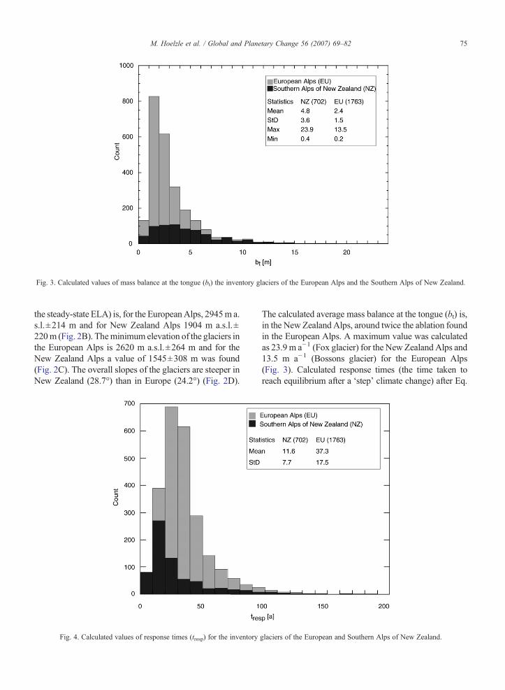
Fig. 3. Calculated values of mass balance at the tongue (bt) the inventory glaciers of the European Alps and the Southern Alps of New Zealand.

75M. Hoelzle et al. / Global and Planetary Change 56 (2007) 69–82

the steady-state ELA) is, for the EuropeanAlps, 2945m a.s.l.±214 m and for New Zealand Alps 1904 m a.s.l.±220m (Fig. 2B). Theminimum elevation of the glaciers inthe European Alps is 2620 m a.s.l.±264 m and for theNew Zealand Alps a value of 1545±308 m was found(Fig. 2C). The overall slopes of the glaciers are steeper inNew Zealand (28.7°) than in Europe (24.2°) (Fig. 2D).

Fig. 4. Calculated values of response times (tresp) for the inventory

The calculated average mass balance at the tongue (bt) is,in the New Zealand Alps, around twice the ablation foundin the European Alps. A maximum value was calculatedas 23.9 m a−1 (Fox glacier) for the New Zealand Alps and13.5 m a−1 (Bossons glacier) for the European Alps(Fig. 3). Calculated response times (the time taken toreach equilibrium after a ‘step’ climate change) after Eq.

glaciers of the European and Southern Alps of New Zealand.

76 M. Hoelzle et al. / Global and Planetary Change 56 (2007) 69–82

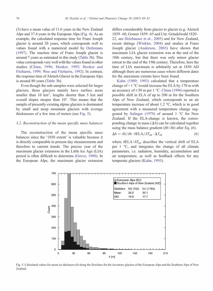
(3) have a mean value of 11.6 years in the New ZealandAlps and 37.4 years in the European Alps (Fig. 4). As anexample, the calculated response time for Franz Josephglacier is around 20 years, which corresponds well tovalues found with a numerical model by Oerlemans(1997). The reaction time of Franz Joseph glacier isaround 7 years as estimated in this study (Table 3b). Thisvalue corresponds verywell with the values found in otherstudies (Chinn, 1996; Hooker, 1995; Hooker andFitzharris, 1999; Woo and Fitzharris, 1992). In contrast,the response time of Aletsch Glacier in the European Alpsis around 80 years (Table 3b).

Even though the sub-samples were selected for largerglaciers, these glaciers mainly have surface areassmaller than 10 km2, lengths shorter than 5 km andoverall slopes steeper than 10°. This means that thesample of presently existing alpine glaciers is dominatedby small and steep mountain glaciers with averagethicknesses of a few tens of meters (see Fig. 5).

3.2. Reconstruction of the mean specific mass balances

The reconstruction of the mean specific massbalances since the ‘1850 extent’ is valuable because itis directly comparable to present day measurements andtherefore to current trends. The precise year of themaximum glacier extension in the Little Ice Age (LIA)period is often difficult to determine (Grove, 1988). Inthe European Alps, the maximum glacier extension

Fig. 5. Calculated values for mean ice thickness (h) along the flowlines for theZealand.

differs considerably from glacier to glacier (e.g. Aletsch1859–60, Gorner 1859–65 and Unt. Grindelwald 1820–22, see Holzhauser et al., 2005) and for New Zealand,recent datings (Winkler, 2004) and studies at FranzJoseph glacier (Anderson, 2003) have shown thatmaximum LIA glacier extension was at the end of the18th century, but that there was only minor glacierretreat to the end of the 19th century. Therefore, here thetime of LIA maximum is arbitrarily set at 1850 ADalthough there are numerous cases where different datesfor the maximum extents have been found.

Kuhn (1989; 1993) calculated that a temperaturechange of +1 °C would increase the ELA by 170 m withan accuracy of ±50 m per 1 °C. Chinn (1996) reported apossible shift in ELA of up to 200 m for the SouthernAlps of New Zealand, which corresponds to an airtemperature increase of about 1.2 °C, which is in goodagreement with a measured temperature change sug-gested by Salinger (1979) of around 1 °C for NewZealand. If the ELA-change is known, the corres-ponding change in mass (Δb) can be calculated togetherusing the mass balance gradient (δb /δh) after Eq. (6).

Db ¼ db=dhd dELA=dTaird DTair ð6Þwhere δELA/δTair describes the vertical shift of ELAper 1 °C, and integrates the change of all climateparameters, i.e. radiation, humidity, accumulation andair temperature, as well as feedback effects for anytemperate glaciers (Kuhn, 1993).

inventory glaciers of the European Alps and the Southern Alps of New

77M. Hoelzle et al. / Global and Planetary Change 56 (2007) 69–82

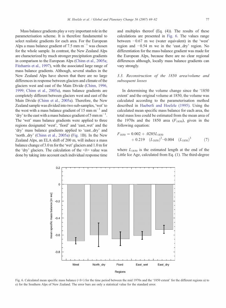
Mass balance gradients play a very important role in theparameterisation scheme. It is therefore fundamental toselect realistic gradients for each area. For the EuropeanAlps a mass balance gradient of 7.5 mm m−1 was chosenfor the whole sample. In contrast, the New Zealand Alpsare characterized by much stronger precipitation gradientsin comparison to the European Alps (Chinn et al., 2005a;Fitzharris et al., 1997), with the associated large range ofmass balance gradients. Although, several studies in theNew Zealand Alps have shown that there are no largedifferences in response between glaciers and climate of theglaciers west and east of the Main Divide (Chinn, 1996,1999; Chinn et al., 2005a), mass balance gradients arecompletely different between glaciers west and east of theMain Divide (Chinn et al., 2005a). Therefore, the NewZealand samplewas divided into two sub-samples, ‘wet’ tothe west with a mass balance gradient of 15 mm m−1 and‘dry’ to the eastwith amass balance gradient of 5mmm−1.The ‘wet’ mass balance gradients were applied to threeregions designated ‘west’, ‘fiord’ and ‘east_wet’ and the‘dry’ mass balance gradients applied to ‘east_dry’ and‘north_dry’ (Chinn et al., 2005a) (Fig. 1B). In the NewZealand Alps, an ELA shift of 200 m, will induce a massbalance change of 3.0m for the ‘wet’ glaciers and 1.0m forthe ‘dry’ glaciers. The calculation of the bbN value wasdone by taking into account each individual response time

Fig. 6. Calculated mean specific mass balance (bbN) for the time period betwe) for the Southern Alps of New Zealand. The error bars are only a statistica

and multiples thereof (Eq. (4)). The results of thesecalculations are presented in Fig. 6. The values rangebetween −0.67 m we (water equivalent) in the ‘west’region and −0.54 m we in the ‘east_dry’ region. Nodifferentiation for the mass balance gradient was made forthe European Alps, because there are no clear regionaldifferences although, locally mass balance gradients canvary strongly.

3.3. Reconstruction of the 1850 area/volume andsubsequent losses

In determining the volume change since the ‘1850extent’ and the original volume at 1850, the volume wascalculated according to the parameterisation methoddescribed in Haeberli and Hoelzle (1995). Using thecalculated mean specific mass balance for each area, thetotal mass loss could be estimated from the mean area ofthe 1970s and the 1850 area (F1850), given in thefollowing equation:

F1850 ¼ 0:002þ :0285L1850þ 0:219 ðL1850Þ2−0:004 ðL1850Þ3 ð7Þ

where L1850 is the estimated length at the end of theLittle Ice Age, calculated from Eq. (1). The third-degree

een the mid 1970s and the ‘1850 extent’ for the different regions a) tol value for the standard error.

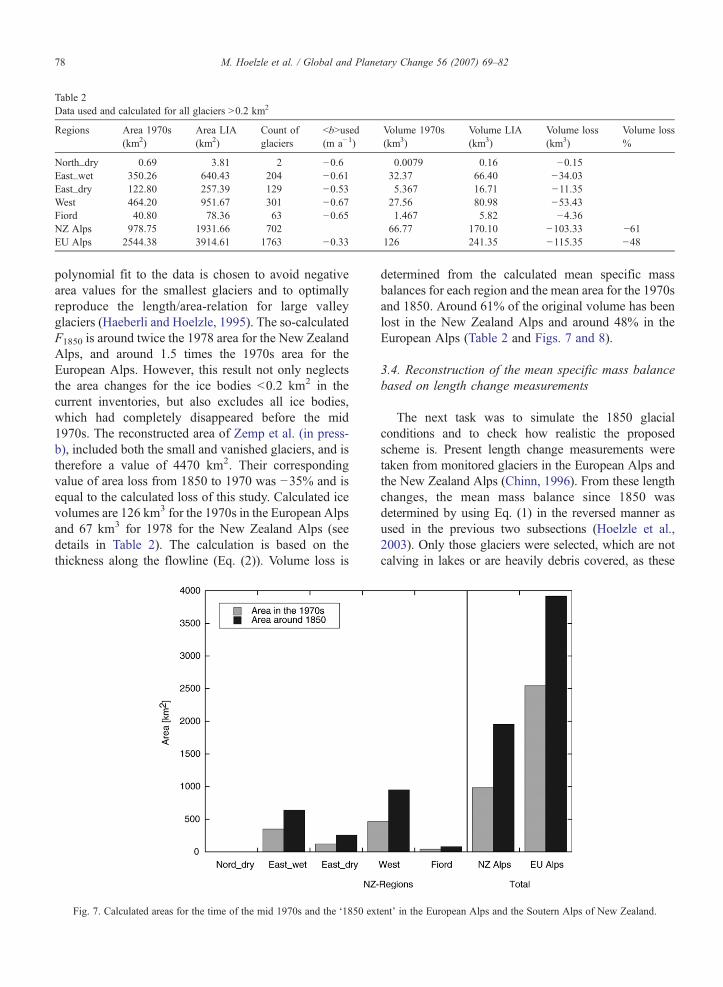
Table 2Data used and calculated for all glaciers N0.2 km2

Regions Area 1970s(km2)

Area LIA(km2)

Count ofglaciers

bbNused(m a−1)

Volume 1970s(km3)

Volume LIA(km3)

Volume loss(km3)

Volume loss%

North_dry 0.69 3.81 2 −0.6 0.0079 0.16 −0.15East_wet 350.26 640.43 204 −0.61 32.37 66.40 −34.03East_dry 122.80 257.39 129 −0.53 5.367 16.71 −11.35West 464.20 951.67 301 −0.67 27.56 80.98 −53.43Fiord 40.80 78.36 63 −0.65 1.467 5.82 −4.36NZ Alps 978.75 1931.66 702 66.77 170.10 −103.33 −61EU Alps 2544.38 3914.61 1763 −0.33 126 241.35 −115.35 −48

78 M. Hoelzle et al. / Global and Planetary Change 56 (2007) 69–82

polynomial fit to the data is chosen to avoid negativearea values for the smallest glaciers and to optimallyreproduce the length/area-relation for large valleyglaciers (Haeberli and Hoelzle, 1995). The so-calculatedF1850 is around twice the 1978 area for the New ZealandAlps, and around 1.5 times the 1970s area for theEuropean Alps. However, this result not only neglectsthe area changes for the ice bodies b0.2 km2 in thecurrent inventories, but also excludes all ice bodies,which had completely disappeared before the mid1970s. The reconstructed area of Zemp et al. (in press-b), included both the small and vanished glaciers, and istherefore a value of 4470 km2. Their correspondingvalue of area loss from 1850 to 1970 was −35% and isequal to the calculated loss of this study. Calculated icevolumes are 126 km3 for the 1970s in the European Alpsand 67 km3 for 1978 for the New Zealand Alps (seedetails in Table 2). The calculation is based on thethickness along the flowline (Eq. (2)). Volume loss is

Fig. 7. Calculated areas for the time of the mid 1970s and the ‘1850 ex

determined from the calculated mean specific massbalances for each region and the mean area for the 1970sand 1850. Around 61% of the original volume has beenlost in the New Zealand Alps and around 48% in theEuropean Alps (Table 2 and Figs. 7 and 8).

3.4. Reconstruction of the mean specific mass balancebased on length change measurements

The next task was to simulate the 1850 glacialconditions and to check how realistic the proposedscheme is. Present length change measurements weretaken from monitored glaciers in the European Alps andthe New Zealand Alps (Chinn, 1996). From these lengthchanges, the mean mass balance since 1850 wasdetermined by using Eq. (1) in the reversed manner asused in the previous two subsections (Hoelzle et al.,2003). Only those glaciers were selected, which are notcalving in lakes or are heavily debris covered, as these

tent’ in the European Alps and the Soutern Alps of New Zealand.

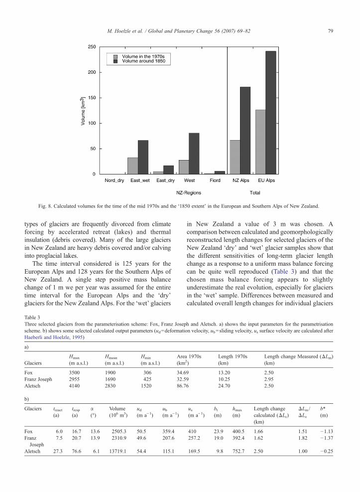
Fig. 8. Calculated volumes for the time of the mid 1970s and the ‘1850 extent’ in the European and Southern Alps of New Zealand.

79M. Hoelzle et al. / Global and Planetary Change 56 (2007) 69–82

types of glaciers are frequently divorced from climateforcing by accelerated retreat (lakes) and thermalinsulation (debris covered). Many of the large glaciersin New Zealand are heavy debris covered and/or calvinginto proglacial lakes.

The time interval considered is 125 years for theEuropean Alps and 128 years for the Southern Alps ofNew Zealand. A single step positive mass balancechange of 1 m we per year was assumed for the entiretime interval for the European Alps and the ‘dry’glaciers for the New Zealand Alps. For the ‘wet’ glaciers

Table 3Three selected glaciers from the parameterisation scheme: Fox, Franz Josepscheme. b) shows some selected calculated output parameters (ud=deformatiHaeberli and Hoelzle, 1995)

a)

GlaciersHmax

(m a.s.l.)Hmean

(m a.s.l.)Hmin

(m a.s.l.)Area(km

Fox 3500 1900 306 34.6Franz Joseph 2955 1690 425 32.5Aletsch 4140 2830 1520 86.7

b)

Glaciers treact(a)

tresp(a)

α(°)

Volume(106 m3)

ud(m a−1)

ub(m a−1)

Fox 6.0 16.7 13.6 2505.3 50.5 359.4Franz

Joseph7.5 20.7 13.9 2310.9 49.6 207.6

Aletsch 27.3 76.6 6.1 13719.1 54.4 115.1

in New Zealand a value of 3 m was chosen. Acomparison between calculated and geomorphologicallyreconstructed length changes for selected glaciers of theNew Zealand ‘dry’ and ‘wet’ glacier samples show thatthe different sensitivities of long-term glacier lengthchange as a response to a uniform mass balance forcingcan be quite well reproduced (Table 3) and that thechosen mass balance forcing appears to slightlyunderestimate the real evolution, especially for glaciersin the ‘wet’ sample. Differences between measured andcalculated overall length changes for individual glaciers

h and Aletsch. a) shows the input parameters for the parametrisationon velocity, ub=sliding velocity, us surface velocity are calculated after

1970s2)

Length 1970s(km)

Length change Measured (ΔLm)(km)

9 13.20 2.509 10.25 2.956 24.70 2.50

us(m a−1)

bt(m)

hmax

(m)Length changecalculated (ΔLc)(km)

ΔLm/ΔLc

b*(m)

410 23.9 400.5 1.66 1.51 −1.13257.2 19.0 392.4 1.62 1.82 −1.37

169.5 9.8 752.7 2.50 1.00 −0.25

80 M. Hoelzle et al. / Global and Planetary Change 56 (2007) 69–82

can be considerable and are explained by the uncertain-ties in the parameterisation scheme applied, and byvariable climate/mass balance conditions at each glacier.The mass balance forcing for each glacier can becorrected according to Eq. (8) to fit the measured lengthchanges.

b* ¼ DLm=DLcd bbNi=1 ð8Þ

where b* is the corrected average mass balance, ΔLm isthe measured length change,ΔLc is the calculated lengthchange andbbNi is the mean mass balance for theindividual regions. These corrections from Eq. (8) to themass balance forcing for each glacier to fit the measuredlength change gives an average annual mass balance(b*) of −0.33±0.09 m we per year for glaciers in theEuropean Alps. In New Zealand, the average annualmass balance for the ‘wet’ glaciers is −1.25±0.9 m weper year and for the ‘dry’ glaciers −0.54±0.5 m we peryear. The calculated mass balance change Δb for the‘wet’ glaciers in the New Zealand Alps is around 5 mand for the ‘dry’ glaciers around 1 m. The latter valuecorresponds quite well with the value used in theparameterisation scheme, whereas the value for the‘wet’ glaciers is, much higher than the value of 3 m usedin the parameterisation. This suggests that the glaciershave reacted even more sensitively than assumed in ourparameterisation and that it is possible that ourcalculated mass loss is at the lower boundary of theuncertainty range.

4. Discussion and conclusions

The calculations and estimations presented in thisstudy are built on four very simple geometric parameterscontained in detailed glacier inventories. This justifies thesimplicity of the applied algorithms but also means thatthe uncertainties involved with the proposed procedureare considerable. Indeed, the large scatter in derivedparameters such as mass balance at the tongue, responsetimes etc. points to the fact that the applied parameterisa-tion scheme is more useful for relatively large glaciersthan for small ice bodies. The large glaciers dominate theoverall mass changes and hence, make the estimates ofcorresponding changes probably quite realistic. This isclearly indicated by the parameterisation results of thelarge glaciers such as Aletsch or Franz Joseph, whichshow quite realistic computation results (Table 3b) incomparison to detailed numerical studies (Oerlemans,1997). Themodel is not tuned in any kind to the EuropeanAlps, where the model has been applied for the first time.The only factor changed in the model is the mass balance

gradient and the basal shear stress (see Table 1). Thevalues used for these parameters in the study are all basedon measurements. In any case, the striking sensitivity ofglacierization in mountain areas to atmospheric warmingtrends clearly appears in both mountain regions, althoughsome marked differences do exist. The calculations of themean specific mass balance change for the investigatedperiod show no large differences between maritime andthe ‘dry’ glaciers within New Zealand (Fig. 6). However,the mean specific mass balances calculated for NewZealand are close to twice than the values determined forthe European Alps and indeed for other mountain areas(Hoelzle et al., 2003). In addition, the calculations showthat the relative mass loss seems to be considerably largerin the New Zealand Alps than in the European Alps andthe comparison of the measured length changes suggestsan even more pronounced difference. Therefore, thecalculated mass loss given here for the Southern Alps ofNew Zealand is probably at the lower limit of theuncertainty range.

The ongoing glacier behaviour after the mid-1970swas sometimes quite different between the EuropeanAlpsand the New Zealand Alps. After a period of glacieradvance in the 1970s and early 1980s in the EuropeanAlps, the glaciers experienced a strong retreat during thefollowing 20 years with an even more pronounced massloss at the beginning of the 21st century (Paul et al., 2004).Today the glacier surface area in the European Alps isaround 2270 km2 (Zemp et al., in press-b). In contrast, allglaciers in New Zealand have overall experienced apositive mass balance and some have advanced stronglyduring the 1990s. This is especially true for the ‘wet’glaciers in New Zealand; the sample is clearly dominatedby maritime, highly sensitive glaciers with correspondinghigh precipitation and therefore strong mass turn over.This period of advances was coming to an end at thebeginning of the new century (Chinn et al., 2005b). Theglaciers in theNewZealandAlpswill probably react moresensitively to a future temperature increase than those inthe European Alps. Not only because of their greatersensitivity, as expressed by the mass balance gradient, butalso because of the generally low altitude of the ELA inthe New Zealand Alps promoting a higher percentage ofrain rather than snowfall in the future.

Due to increasing uncertainties and pronounced non-linearities such as changing response times with changingglacier size etc., calculations for scenarios with a trend tocontinuously accelerate climate and mass balance forcingbeyond the early decades in the 21st century can be order-of-magnitude-estimates only. Annual mass losses of 2 to3 m per year such as observed in the year 2003 in theEuropean Alps (Frauenfelder et al., 2005; IUGG(CCS)/

81M. Hoelzle et al. / Global and Planetary Change 56 (2007) 69–82

UNEP/UNESCO/WMO, 2005; Zemp et al., 2005) andwhich must be expected to continue into the future, IPCCscenarios of temperature increase will certainly reduce thesurface area and volume of alpine glaciers to a few percentof the values estimated for the ‘1850 extent’ within the21st century. With such a trend, only the largest andhighest-reaching alpine glaciers could persist into the22nd century. These glaciers will be affected by drasticchanges in geometry as well and down-wasting ratherthan active retreat will be the dominant process of glacierreaction (Paul et al., 2004, 2007-a). This implies thatparameterisation schemes like the one presented herewould no longer be applicable. Therefore, moderntechnologies like remote sensing have to be used tomeasure the accelerating glacier change and alpine widemass balance (Machguth et al., in press; Paul et al., inpress-b) and ELAmodels (Zemp et al., 2007-a) need to beapplied for the extrapolation of glacier down-wasting intothe future.

This comparison between two different Alpineregions demonstrates the potential and limitations ofthe parameterisations of existing inventories. Their uselies especially in quantitatively inferring past averagedecadal to secular mean specific mass balances forunmeasured glaciers by analyzing cumulative lengthchange from moraine mapping, satellite imagery, aerialphotography and long-term observations (Haeberli andHolzhauser, 2003).

Acknowledgments

Wewould like to thank IvanWoodhatch for his help inimproving the English in the first version of this paper.The present study was carried out within the data analysiswork for the World Glacier Monitoring Service withspecial grants from UNEP, a personal research grant fromthe Swiss National Science Foundation (PIOI2-111008/1)and as part of the EU Research Programme ALP-IMP(EU: EVK2-CT-2002-00148, BBW: 01.0498-2). Theauthors are very grateful to the constructive commentsof Stephan Winkler, Per Holmlund and ChristophSchneider, which helped to improve the paper.

References

Anderson, B., 2003. The Response of Franz Joseph Glacier to ClimateChange. University of Canterbury, Christchurch, 129 pp.

Anderton, P.W., 1973. The significance of perennial snow and icecover to the water resources of the South Island. New ZealandJournal of Hydrology (NZ) 12 (1), 6–18.

Barnett, T.P., Adam, J.C., Lettenmaier, D.P., 2005. Potential impacts ofa warming climate on water availability in snow-dominatedregions. Nature 438, 303–309.

Bauder, A., Funk, M., Gudmundsson, G.H., 2003. The ice-thicknessdistribution of Unteraargletscher, Switzerland. Annals of Glaciology37, 331–336.

Bishop, M.P., et al., 2004. Global Land Ice Measurements from Space(GLIMS): remote sensing and GIS investigations of the Earth'scryosphere. Geocarto International 19 (2), 57–85.

Chinn, T.J., 1991. Glacier inventory of New Zealand. Institute ofGeological and Nuclear Sciences.

Chinn, T.J., 1996. New Zealand glacier responses to climate change ofthe past century. New Zealand Journal of Geology and Geophysics39 (3), 415–428.

Chinn, T.J., 1999. NewZealand glacier response to climate change of thepast 2 decades. Global and Planetary Change 22 (1–4), 155–168.

Chinn, T.J., 2001. Distribution of the glacial water resources of NewZealand. Journal of Hydrology New Zealand 40 (2), 139–187.

Chinn, T.J., Heydenrych, C., Salinger, M.J., 2005a. Use of the ELA as apractical method of monitoring glacier response to climate in NewZealand's Southern Alps. Journal of Glaciology 51 (172), 85–95.

Chinn, T.J., Winkler, S., Salinger, M.J., Haakensen, N., 2005b. Recentglacier advances in Norway and New Zealand; a comparison oftheir glaciological and meteorological causes. Geografiska Annaler87A (1), 141–157.

Fitzharris, B.B., Chinn, T.J., Lamont, G.N., 1997. Glacier massbalance fluctuations and atmospheric circulation patterns over theSouthern Alps, New Zealand. International Journal of Climatology17 (7), 745–763.

Forel, F.A., 1895. Les variations périodiques des glaciers. Discourspréliminaire. Extrait des Archives des Sciences physiques etnaturelles, vol. XXXIV, pp. 209–229.

Frauenfelder, R., Zemp, M., Haeberli, W., Hoelzle, M., 2005.Worldwide glacier mass balance measurements. Trends and firstresults of an extraordinary year in Central Europe, Ice and ClimateNews, pp. 9–10.

GCOS/GTOS, 1997a. GCOS/GTOS Plan for terrestrial climate relatedobservations. WMO, vol. 796. World Meteorological Organiza-tion, Geneva.

GCOS/GTOS, 1997b. GHOST Global Hierarchical ObservingStrategy. WMO, vol. 862. World Meteorological Organization,Geneva.

GCOS/GTOS, 2004. Implementation plan for the Global ObservingSystem for Climate in support of the UNFCCC. WMO, vol. 1219.World Meteorological Organization, Geneva.

Grove, J.M., 1988. The Little Ice Age. Methuen, London, 498 pp.Haeberli, W., Burn, C.R., 2002. Natural hazards in forests: glacier and

permafrost effects as related to climate change. In: Sidle, R.C.(Ed.), Environmental Change and Geomorphic Hazards in Forests.IUFRO Research Series. CABI Publishing, Wallingford/NewYork, pp. 167–202.

Haeberli, W., Hoelzle, M., 1995. Application of inventory data forestimating characteristics of and regional climate-change effects onmountain glaciers: a pilot study with the European Alps. Annals ofGlaciology 21, 206–212.

Haeberli, W., Dedieu, J.-P., 2004. Cryosphere monitoring in mountainbiosphere reserves: challenges for integrated research on snow andice. In: Lee, C., Schaaf, T. (Eds.), Global change in mountainregions (GLOCHAMORE). Global environmental and socialmonitoring. UNESCO, Vienna, pp. 29–33.

Haeberli, W., Holzhauser, H., 2003. Alpine glacier mass changesduring the past two millenia. PAGES News 11 (1), 13–15.

Haeberli, W., Cihlar, J., Barry, R., 2000. Glacier Monitoring within theGlobal Climate Observing System— a contribution to the FritzMüller Memorial. Annals of Glaciology 31, 241–246.

82 M. Hoelzle et al. / Global and Planetary Change 56 (2007) 69–82

Haeberli, W., Maisch, M., Paul, F., 2002. Mountain glaciers in globalclimate-related observation networks. World MeteorologicalOrganization Bulletin 51 (1), 1–8.

Heydenrych, C., Salinger, M.J., Fitzharris, B.B., Chinn, T.J., 2002.Annual glacier volumes in New Zealand 1993–2001. NationalInstitute of Water and Atmospheric Research Limited, Auckland.

Hoelzle, M., Trindler, M., 1998. Data management and application. In:Haeberli, W., Hoelzle, M., Suter, S. (Eds.), Into the SecondCentury of World Glacier Monitoring: Prospects and Strategies.Studies and Reports in Hydrology. UNESCO, Paris, pp. 53–72.

Hoelzle, M., Haeberli, W., Dischl, M., Peschke, W., 2003. Secularglacier mass balances derived from cumulative glacier lengthchanges. Global and Planetary Change 36 (4), 295–306.

Holzhauser, H., Magny, M., Zumbühl, H.J., 2005. Glacier and lake-level variations in west-central Europe over the last 3500 years.Holocene 15 (6), 789–801.

Hooker, B.L., 1995. Advance and Retreat of the Franz Josef Glacier inrelation to climate. Dissertation in Dip Sci Thesis, University ofOtago, Dunedin.

Hooker, B.L., Fitzharris, B.B., 1999. The correlation between climaticparameters and the retreat and advance of Franz Josef Glacier, NewZealand. Global and Planetary Change 22, 39–48.

IAHS(ICSI)/UNEP/UNESCO (Ed.), 1989. World Glacier Inventory.Status 1988, Paris.

IPCC, 2001. Third assessment report, Working Group 1. CambridgeUniversity Press, Cambridge.

IUGG(CCS)/UNEP/UNESCO, 2005. Fluctuations of Glaciers 1995–2000, Vol. VIII. In: Haeberli, W., Zemp, M., Frauenfelder, R.,Hoelzle, M., Kääb, A. (Eds.), World Glacier Monitoring Service,Zürich, vol. 8. 288 pp.

IUGG(CCS)/UNEP/UNESCO/WMO, 2005. Glacier Mass BalanceBulletin no. 8. In: Haeberli, W., Noetzli, J., Zemp, M., Baumann,S., Frauenfelder, R., Hoelzle, M. (Eds.), World Glacier MonitoringService, Zürich, vol. 8. 100 pp.

Jòhannesson, T., Raymond, C., Waddington, E., 1989. Time-scale foradjustment of glaciers to changes in mass balance. Journal ofGlaciology 35 (121), 355–369.

Kieffer, H.H. et al., 2000. New eyes in the sky measure glaciers and icesheets. EOS, Transactions American Geophysical Union, 81(24):265, 270–271.

Kuhn, M., 1989. The response of the equilibrium line altitude toclimatic fluctuations: theory and observations. In: Oerlemans, J.(Ed.), Glacier fluctuations and climatic change. Kluwer, Dodrecht,pp. 407–417.

Kuhn, M., 1993. Possible future contributions to sea level change fromsmall glaciers. In: Warrick, R.A., Barrow, E.M., Wigley, T.M.L.(Eds.), Climate and sea level change observations, projections andimplications. Cambridge University Press, Cambridge, pp. 134–143.

Kääb, A., et al., 2005a. Remote sensing of glacier-and permafrost-related hazards in high mountains: an overview. Natural Hazardsand Earth System Sciences 5, 527–554.

Kääb, A., Reynolds, J.M., Haeberli, W., 2005b. Glacier and permafrosthazards in high mountains. In: Huber, M., Bugmann, H.K.M.,Reasoner, M.A. (Eds.), Global Change and Mountain Regions (Astate of Knowledge Overview). Advances in Global ChangeResearch. Springer, Dordrecht, pp. 225–234.

Leysinger Vieli, G.J.-M.C., Gudmundsson, G.H., 2004. On estimatinglength fluctuations of glaciers caused by changes in climaticforcing. Journal of Geophysical Research 109, F01007.

Machguth, H., Paul, F., Hoelzle, M., Haeberli, W., in press. Distributedglaciermass balancemodelling as an important component ofmodernmulti-level glacier monitoring. Annals of Glaciology, 43.

March, R.S., 2000. Mass balance, meteorological, ice motion, surfacealtitude, runoff, and ice thickness data at Gulkana Glacier, Alaska,1995 balance year. 00-4074. U.S. Geological Survey WaterResources Investigations.

Müller, P., 1988. Parametrisierung der Gletscher-Klima-Beziehung fürdie Praxis: Grundlagen und Beispiele. 95, Versuchsanstalt fürWasserbau, Hydrologie und Glaziologie, ETH Zürich.

Nye, J.F., 1960. The response of glaciers and ice-sheets to seasonal andclimatic changes. Proceedings of the Royal Society of London.Series A 256, 559–584.

Nye, J.F., 1965. The flow of a glacier in a channel of rectangular, ellipticor parabolic cross-section. Journal of Glaciology 5, 661–690.

Oerlemans, J., 1997. Climate sensitivity of Franz Josef Glacier, NewZealand, as revealed by numerical modelling. Arctic and AlpineResearch 29, 233–239.

Paterson, W.S.B., 1994. The Physics of Glaciers, 3rd ed. PergamonPress Ltd. 380 pp.

Paul, F., Kääb, A., Maisch, M., Kellenberger, T., Haeberli, W., 2004.Rapid disintegration of Alpine glaciers observed with satellite data.Geophysical Research Letters 31 (21), L21402.

Paul, F., Kääb, A., Haeberli, W., 2007a. Recent glacier changes in theAlps observed from satellite: Consequences for future monitoringstrategies. Global and Planetary Change 56, 111–122.doi:10.1016/j.gloplacha.2006.07.007.

Paul, F., Machguth, H., Hoelzle, M., Salzmann, N., Haeberli, W., inpress-b. Alpine-wide distributed glacier mass balance modelling: atool for assessing future glacier change? In: Orlove, B., Wiegandt,E., Luckman, B.H. (Editors), The darkening peaks: Glacial retreatin scientific and social context. University of California Press.

Raup, B., et al., 2003. Global Land Ice Measurements from Space(GLIMS) Database at NSIDC. Eos Transactions. Supplement 84.

Raup, B., et al., 2007. The GLIMS geospatial glacier database: a newtool for studying glacier change. Global and Planetary Change 56,101–110. doi:10.1016/j.gloplacha.2006.07.018.

Salinger, M.J., 1979. New Zealand climate: the temperature record,historical data and some agricultural implications. Climate Change2, 109–126.

Winkler, S., 2004. Lichenometric dating of the ‘Little Ice Age’maximum in Mt. Cook National Park, Southern Alps, NewZealand. Holocene 14 (6), 911–920.

WMO, 1997. GCOS/GTOS plan for terrestrial climate-relatedobservation. Version 2.0, World Meteorological Organization.

Woo, M., Fitzharris, B.B., 1992. Reconstruction of mass balancevariations for Franz Joseph glacier, New Zealand, 1913 to 1989.Arctic and Alpine Research 24 (4), 281–290.

Zemp, M., Frauenfelder, R., Haeberli, W., Hoelzle, M., 2005.Worldwide glacier mass balance measurements: general trendsand first results of the extraordinary year 2003 in CentralEurope, XIII Glaciological Symposium, Shrinkage of theGlaciosphere: Facts and Analysis. Data of Glaciological Studies[Materialy glyatsiologicheskikh issledovaniy]. Moscow, Russia,vol. 99, pp. 3–12.

Zemp, M., Hoelzle, M., Haeberli, W., 2007a. Distributed modelling ofthe regional climatic equilibrium line altitude of glaciers in theEuropean Alps. Global and Planetary Change 56, 83–100.doi:10.1016/j.gloplacha.2006.07.002.

Zemp, M., Paul, F., Hoelzle, M., Haeberli, W., in press-b. Glacierfluctuations in the European Alps 1850–2000: an overview andspatio-temporal analysis of available data. In: Orlove, B.,Wiegandt, E., Luckman, B.H. (Editors), The darkening peaks:Glacial retreat in scientific and social context. University ofCalifornia Press.