E L S E V I E R Fuzzy Sets and Systems 95 (1998) 273-293

FU|ZY sets and systems

The application of fuzzy logic in automatic modelling of electromechanical systems

P.J. Costa Branco*, J.A. Dente CA UTL-Laborat6rio de Mecatr6niea, Instituto Superior T~cnico, Av. Rovisco Pais, 1096, Lisbon Codex, Portugal

Received April 1996; revised August 1996

Abstract

Electromechanical systems are usually modelled using energy conversion theory. However, this representation is not accurate enough. The reasons are the presence of non-linear relations between the variables, changes in system parameters, and the difficulty encountered sometimes in taking into account, in a simple and precise way, physical phenomena like, friction, viscosity, and saturation. So, it is useful to automatically extract the relations that represent the system behaviour.

We investigate in this paper three fuzzy learning algorithms which represent the development of our study and are used for automatic modelling of electromechanical systems. We begin with a very simple algorithm. Some problems are pointed as containing the requisites to be a good model; next, two methods which are composed of a fuzzy-cluster-based algorithm and a fuzzy-supervised-learning algorithm are employed. We explore their learning capabilities in situations like modelling in a direct and inverse way, the amount of information necessary to build a good model, and the problem of selecting the information relevant to the learning process. The algorithms are analysed in an experimental system in our laboratory. We close with a simple control application for the relationship between fuzzy modelling and electro- mechanical systems designing a feedforward learning controller for the experimental system. © 1998 Elsevier Science B.V. All rights reserved.

Keywords: Linguistic modelling; Approximate reasoning; Pattern recognition; Machine learning

1. Introduction

The conventional approaches for modelling electromechanical systems use differential or difference equations, partial differential equations, and so on. These model formalisms can present some drawbacks: (a) the mathematical models are not a complete system representation since there are simplifications even for the simpler models, (b) they do not allow the inclusion of heuristic information permitting to expand the systems operating range, and (c) the internal structure of electromechanical systems usually contain non- linear relations difficult to model or, when the model available is accurate enough, the system parameter values are difficult to obtain, In high-performance applications and for control purposes, there is a need for

* Corresponding author.

0165-0114/98/$19.00 © 1998 Elsevier Science B.V. All rights reserved Pl l S01 65-01 14(96)00265-5

274 P.J. Costa Branco, J.A. Dente / Fuzzy Sets and Systems 95 (1998) 273-293

extracting automatically the model characterising the relations between system variables. If we have a better representation for the dynamics of the electromechanical system, a better system control will be possible.

This paper investigates the use of fuzzy logic for automatic modelling electromechanical systems. This association will permit to incorporate learning capabilities that are useful for control purposes, as, for example, in compensate non-linear terms that affect system dynamics.

The paper is organised as follows. Section 2 gives a brief overview of fuzzy linguistic modelling to characterise the logical operations used by the learning algorithms. Section 3 describes the experimental system employed in our study. In Section 4, we present the three fuzzy algorithms that use different learning approaches to model the system. The algorithms are compared and studied for different cases like their different learning capabilities, the modelisation of the electromechanical system in a direct and inverse way, and the quantity of examples needed to build a reasonable model. Section 5 presents a simple real-time control application that exemplifies the potentialities of using fuzzy models of electromechanical systems in tracking controllers design.

2. Fuzzy linguistic modelling

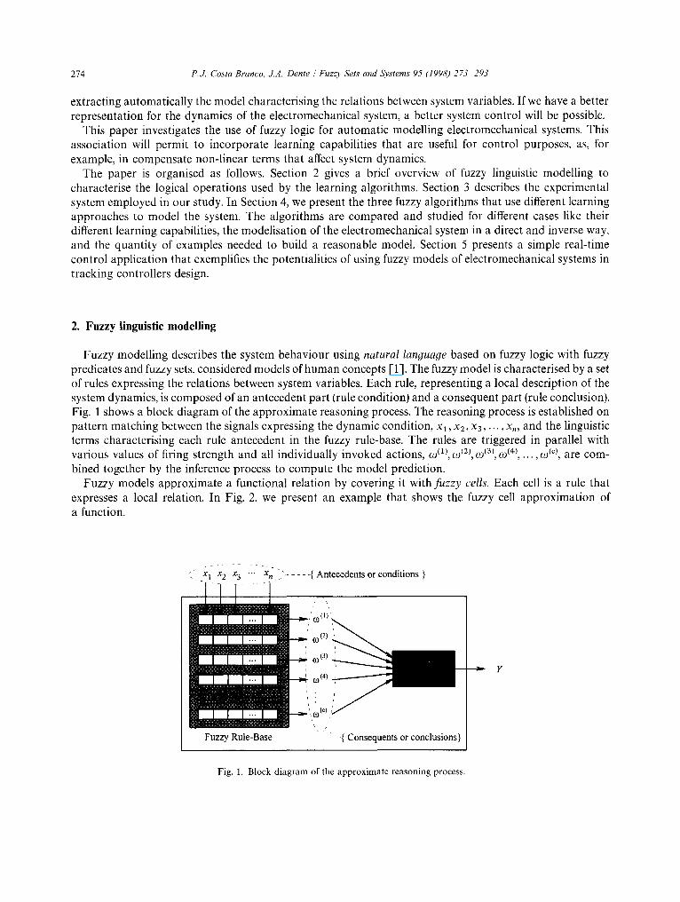
Fuzzy modelling describes the system behaviour using natural language based on fuzzy logic with fuzzy predicates and fuzzy sets, considered models of human concepts [ 1]. The fuzzy model is characterised by a set of rules expressing the relations between system variables. Each rule, representing a local description of the system dynamics, is composed of an antecedent part (rule condition) and a consequent part (rule conclusion). Fig. 1 shows a block diagram of the approximate reasoning process. The reasoning process is established on pattern matching between the signals expressing the dynamic condition, Xl, x2, x3 . . . . . x,, and the linguistic terms characterising each rule antecedent in the fuzzy rule-base. The rules are triggered in parallel with various values of firing strength and all individually invoked actions, (D (1), (2) (2), (D (3), 09 (4) . . . . , co to), are com- bined together by the inference process to compute the model prediction.

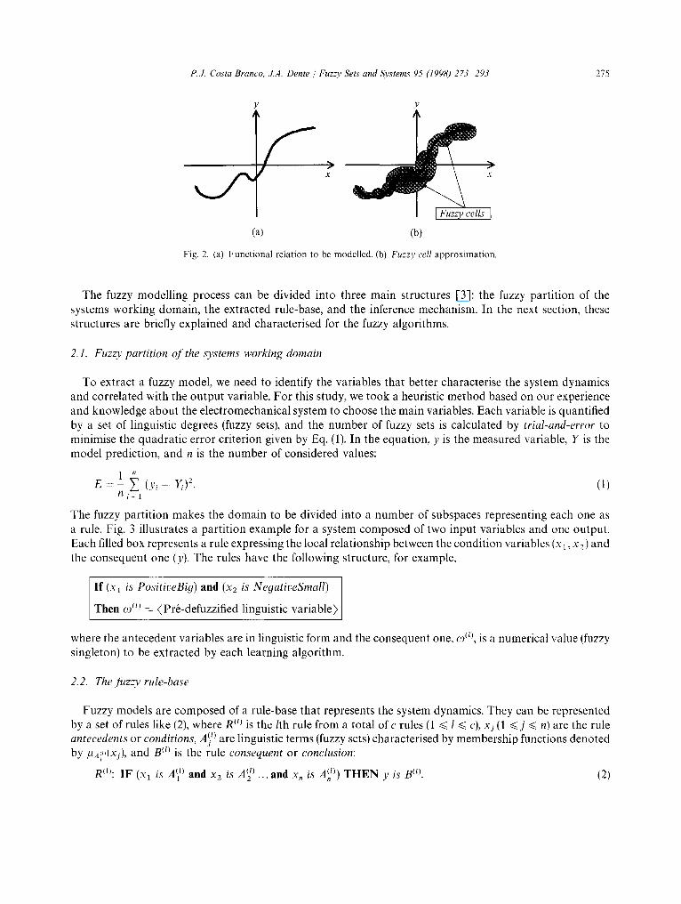
Fuzzy models approximate a functional relation by covering it with fuzzy cells. Each cell is a rule that expresses a local relation. In Fig. 2, we present an example that shows the fuzzy cell approximation of a function.

~ . - x I x 2 x 3 "'" Xn - ;- { Antecedents or conditions }

2onsequents or conclusions}

Fig. 1. Block diagram of the approximate reasoning process.

P.J. Costa Branco, J.A. Dente / Fuzzy Sets and Systems 95 (1998) 273 293

Y Y

cells

(a) (b)

Fig. 2. (a) Functional relation to be modelled. (b) Fuzzy cell approximation.

275

The fuzzy modelling process can be divided into three main structures [3]: the fuzzy partition of the systems working domain, the extracted rule-base, and the inference mechanism. In the next section, these structures are briefly explained and characterised for the fuzzy algorithms.

2.1. Fuzzy partition q[ the systems working domain

To extract a fuzzy model, we need to identify the variables that better characterise the system dynamics and correlated with the output variable. For this study, we took a heuristic method based on our experience and knowledge about the electromechanical system to choose the main variables. Each variable is quantified by a set of linguistic degrees (fuzzy sets), and the number of fuzzy sets is calculated by trial-and-error to minimise the quadratic error criterion given by Eq. (1). In the equation, y is the measured variable, Y is the model prediction, and n is the number of considered values:

1 E ~ - - Z ( Y i - y/)2. (1)

Y/i=l

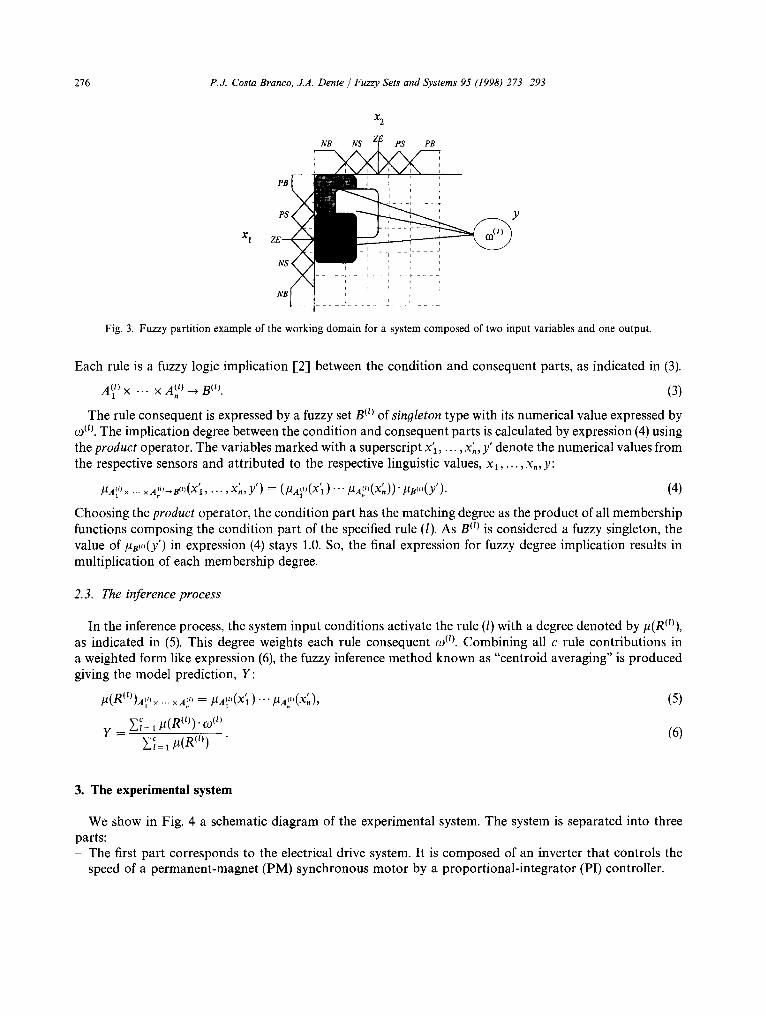
The fuzzy partition makes the domain to be divided into a number of subspaces representing each one as a rule. Fig. 3 illustrates a partition example for a system composed of two input variables and one output. Each filled box represents a rule expressing the local relationship between the condition variables (x l, x2) and the consequent one (y). The rules have the following structure, for example,

If (Xl is PositiveBig) and (x2 is NegativeSmall)

Then ~o °) = (Pr6-defuzzified linguistic variable)

where the antecedent variables are in linguistic form and the consequent one, (o I~), is a numerical value (fuzzy singleton) to be extracted by each learning algorithm.

2.2. The fuzzy rule-base

Fuzzy models are composed of a rule-base that represents the system dynamics. They can be represented by a set of rules like (2), where R m is the lth rule from a total ofc rules (1 ~< 1 ~< c), xj (1 ~ j ~< n) are the rule antecedents or conditions, A} ~) are linguistic terms (fuzzy sets) characterised by membership functions denoted by I~A~,,(Xj), and B m is the rule consequent or conclusion:

Rill: I F ( x 1 is A~ t) and x2 is A~ ) . . . and x . is ~l) B m A. ) T H E N y is . (2)

276 P.J. Costa Branco, J.A. Dente / Fuzzy Sets and Systems 95 (1998) 273-293

X2

X 1

Fig. 3. Fuzzy partition example of the working domain for a system composed of two input variables and one output.

Each rule is a fuzzy logic implication [2] between the condition and consequent parts, as indicated in (3).

A~ t) X ... X Atn z) ~ B (t). (3)

The rule consequent is expressed by a fuzzy set B (~) of sinoleton type with its numerical value expressed by ~o (t). The implication degree between the condition and consequent parts is calculated by expression (4) using the produc t operator. The variables marked with a superscript x'~, ..., x',, y' denote the numerical values from the respective sensors and attributed to the respective linguistic values, Xl . . . . . x,, y:

]AA~') . . . . . A~t)--B(')(Xtl . . . . . X'n, y ' ) ~- (~lA~')(Xtl ) "" ~lA{ " (Xn) ) " ~lB(t,(y' ). (4)

Choosing the produc t operator, the condition part has the matching degree as the product of all membership functions composing the condition part of the specified rule (l). As B al is considered a fuzzy singleton, the value of PB,)(Y') in expression (4) stays 1.0. So, the final expression for fuzzy degree implication results in multiplication of each membership degree.

2.3. The inference proces s

In the inference process, the system input conditions activate the rule (l) with a degree denoted by #(R")), as indicated in (5). This degree weights each rule consequent co "). Combining all c rule contributions in a weighted form like expression (6), the fuzzy inference method known as "centroid averaging" is produced giving the model prediction, Y:

#(R(Z))A~') . . . . . a~.,, = IAA,I',(X' 1) ' ' ' ,uA~,,(X'n) , (5)

y ~.= Z~= 1 ~(R(/))" (-0(1)

Z~= 1 P(R(~) (6)

3. The experimental system

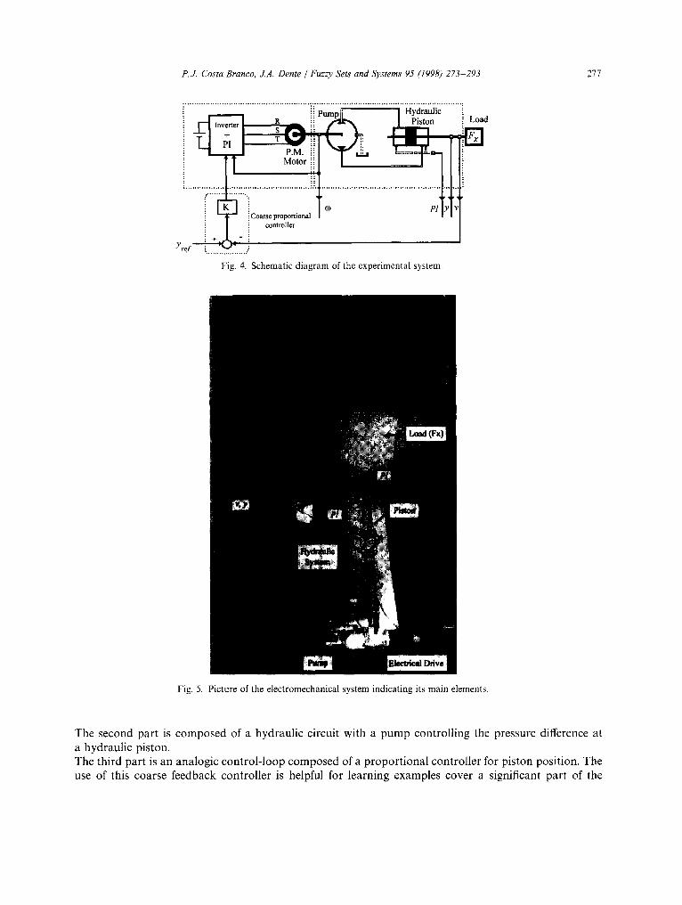
We show in Fig. 4 a schematic diagram of the experimental system. The system is separated into three parts: - The first part corresponds to the electrical drive system. It is composed of an inverter that controls the

speed of a permanent-magnet (PM) synchronous motor by a proportional-integrator (PI) controller.

P.J. Costa Branco, J.A. Dente / Fuzzy Sets and Systems 95 (1998) 273-293 277

r - " - " - - I i i Pump ~ ~ Hydraulic , R _ ;-. Piston . . ~ l n v ~ r t e r [ S ~ . ~ Load

l ' I r _ ~: ~! m l LLM

' T Motor)i I ml " I I I

Fi-ll - - i Coarse proportional / I I

i controller

Yref +m'l )q " ! . . . . . . . . . . . . . . . . . . f

Fig. 4. Schematic diagram of the experimental system.

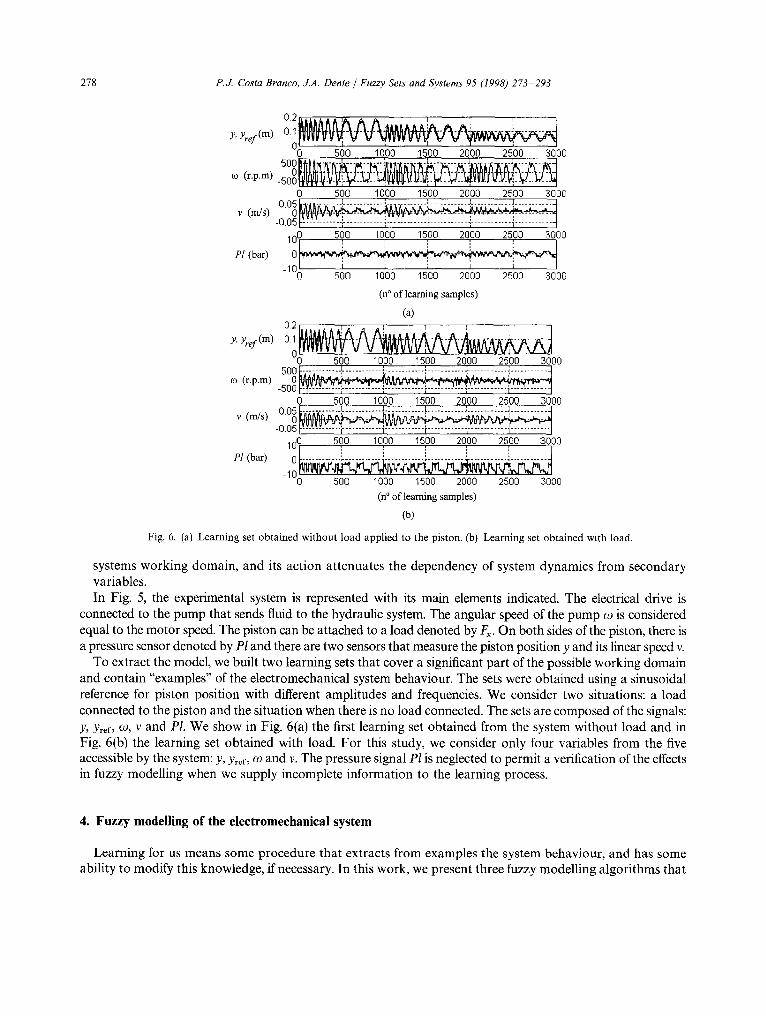
Fig. 5. Picture of the electromechanical system indicating its main elements.

The second part is composed of a hydraulic circuit with a pump controlling the pressure difference at a hydraulic piston. The third part is an analogic control-loop composed of a proport ional controller for piston position. The use of this coarse feedback controller is helpful for learning examples cover a significant part of the

278 P.J. Costa Branco, ~A. Dente / Fuzzy Sets and Systems 95 (1998) 273 293

0 2 i i 1 ~ i 0 1 [ ~ J ~ A ~ J ~ ~ " A - - , ~ - A ! - - - . . - . - - - - - ] - - - - - - - - J - - i ' - - - ~ . . . . . " . . . . . . Y'Yref(m) [¥VyVVV~ V V ~ V V V V V V ~ V t g ~ / g W ~ N t ~

00 500 1000 1500 2000 2500 3000

co ( r . p . m ) . 5 0 0 ~ V t ~ q ~ ~ l L ~ _ ~ _ y i . . ~ . . ~ . . . u t

0 500 1000 1500 2000 2500 3000

v (m/s) 0,0~ . . . . ~ : : - : : : - : : : : -o.o5 I::-' ......... ~ ...... 1 ... . . . . . . . . -I

,-,0 500 10,00 15,00 2000 25,00 3000 , ' , , ',

; ' i . . . . 101 i ~ ~ ~ ~ I " 0 500 1000 1500 2000 2500 3000

(n ° o f l e aming samples)

(a) 0.2 I : : : i

Y, Yref (m) 0 1 0 ~

-0 500 1000 1500 2000 2500 3000 500 ............ ~ ..... !---: . . . . . . .

co (r .p.m) -500 F ~ ~ . . . . . . l ' ' ' ' [ . . . . . . .

0 500 1000 1500 2000 2500 3000 o

4.05 F ~ ~ ...... i . . . . . . . . . . . -I 100 500 1000 1500 2000 2500 3000

PI (bar) 0 . . . . . . . . . . . . i . . . . . . . . . . . . : . . . . . . . . . . . . ~ . . . . . . . . . . . : . . . . . . . . . . . ~ . . . . . . . . . . .

_10 ~ 0 500 1000 1500 2000 2500 3000

(n ° o f learn ing samples)

(b)

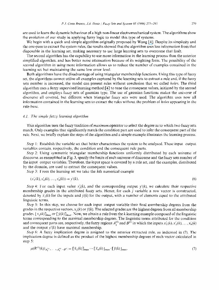
Fig . 6, (a) L e a r n i n g set o b t a i n e d w i t h o u t l o a d a p p l i e d t o t he p i s t on . (b) L e a r n i n g set o b t a i n e d w i t h load .

systems working domain, and its action attenuates the dependency of system dynamics from secondary variables. In Fig. 5, the experimental system is represented with its main elements indicated. The electrical drive is

connected to the pump that sends fluid to the hydraulic system. The angular speed of the pump co is considered equal to the motor speed. The piston can be attached to a load denoted by F~. On both sides of the piston, there is a pressure sensor denoted by Pl and there are two sensors that measure the piston position y and its linear speed v.

To extract the model, we built two learning sets that cover a significant part of the possible working domain and contain "examples" of the electromechanical system behaviour. The sets were obtained using a sinusoidal reference for piston position with different amplitudes and frequencies. We consider two situations: a load connected to the piston and the situation when there is no load connected. The sets are composed of the signals: Y, Yref, co, v and Pl. We show in Fig. 6(a) the first learning set obtained from the system without load and in Fig. 6(b) the learning set obtained with load. For this study, we consider only four variables from the five accessible by the system: y, &of, co and v. The pressure signal Pl is neglected to permit a verification of the effects in fuzzy modelling when we supply incomplete information to the learning process.

4. Fuzzy modelling of the electromechanical system

Learning for us means some procedure that extracts from examples the system behaviour, and has some ability to modify this knowledge, if necessary. In this work, we present three fuzzy modelling algorithms that

P.£ Costa Branco, .LA. Dente / Fuzzy Sets and Systems 95 (1998) 273-293 279

are used to learn the dynamic behaviour of a high non-linear electromechanical system. The algorithms show the evolution of our study in applying fuzzy logic to model this type of systems.

We begin with a quick and simple algorithm originally proposed by Wang [4]. Despite its simplicity and the one-pass to extract the system rules, the results showed that the algorithm uses less information from that disposable in the learning set, making necessary to use large learning sets to overcome that fault.

The second algorithm has the capability to use more information in the learning process than the anterior simplified algorithm, and has better noise attenuation because of its weighting form. The possibility of the second algorithm in using more information allows us to reduce the number of examples contained in the learning set but maintaining the same low error level.

Both algorithms have the disadvantage of using triangular membership functions. Using this type of fuzzy set, the algorithms cannot utilise all examples captured by the learning sets to extract a rule and, if the fuzzy sets number is increased, the model can present rules without conclusion that we called holes. The third algorithm uses a fuzzy supervised learning method [4] to tune the consequent values, initiated by the second algorithm, and employs fuzzy sets of gaussian type. The use of gaussian functions makes the universe of discourse all covered, but different when triangular fuzzy sets were used. The algorithm uses now all information contained in the learning sets to extract the rules without the problem of holes appearing in the rule-base.

4.1. The simple fuzzy learning algorithm

This algorithm uses the fuzzy tradition of maximum operator to select the degree as to which two fuzzy sets match. Only examples that significantly match the condition part are used to infer the consequent part of the rule. Next, we briefly explain the steps of the algorithm and a simple example illustrates the learning process.

Step 1: Establish the variable set that better characterises the system to be analysed. These input output variables contain, respectively, the condition and the consequent rule parts.

Step 2: Using symmetric triangular membership functions uniformly distributed by each universe of discourse, as exemplified in Fig. 3, specify the limits of each universe of discourse and the fuzzy sets number of the input-output variables. Therefore, the input space is covered by a rule set, and the examples, distributed by the domain, are used to extract the consequent values.

Step 3: From the learning set we take the kth numerical example

(x'l (k), x'2 (k),..., x',(k)) - , y'(k). (6)

Step 4: For each input value x'j(k), and the corresponding output y'(k), we calculate their respective membership grades in the attributed fuzzy sets. Hence, for each j variable a row vector is constructed, denoted by Y i(k) for the inputs and )7(k) for the output, with a number of elements equal to the attributed linguistic terms.

Step 5: In this step, we choose for each input output variable their final membership degrees from the grades in the respective vectors, Yj(k) or y(k). The selected grades are the highest degrees from all membership grades , [xj(k)]ma x or [y(k)]ma x. NOW, we obtain a rule from the k learning example composed of the linguistic terms corresponding to the maximal membership degrees. The linguistic terms attributed for the condition and consequent parts are, respectively, the fuzzy regions AS~) and B {t) in which the inputs x'~ (k), x'2(k) . . . . . x',(k) and the output y'(k) have maximal membership.

Step 6: A fuzzy implication degree is assigned to the anterior extracted rule, as indicated in (7). The implication degree is defined as the product of the highest membership degrees of each vector calculated in step 5:

R,) /.t( (k))a,',x ... x A"'~B"},, = E:~l (k)]max "'" [Y,(k)]max " [)7(k)]max. (7)

280 P.J. Costa Branco, J.A. Dente / Fuzzy Sets and Systems 95 (1998) 273 293

Step 7: As there are usually many learning examples spanned by the working domain, there will be different values for the consequent part in the same rule region. For each example in the rule region (l), we compare its implication degree #(R")(k)) with the anterior one p(R")(k - 1)) to chose the final consequent value ~o(l)(k) as

#(R(l)(k))a(1 I) . . . . . All)~B (l) > #(R(l)(k - 1))A(lZ) . . . . . A( ')-~a", then c0(~)(k) = y'(k),

#(R(t)(k))Ai',× ×AII)--.B ,l) ~ #(R(t)(k 1))Ai', × ×A(,,-~B,) then o~")(k) = ~o(t)(k - 1). (8)

Step 8: When two rules have the same linguistic terms in IF part but a different linguistic term in THEN part, the rules are said to be in conflict. To resolve this problem in the conflict group, only the rule with highest implication degree is accepted. This indicates the rule with the highest connection degree between the condition and the consequent part. At last, if it is not the end of the learning set, the algorithm goes again to step 3 to pick up the next example.

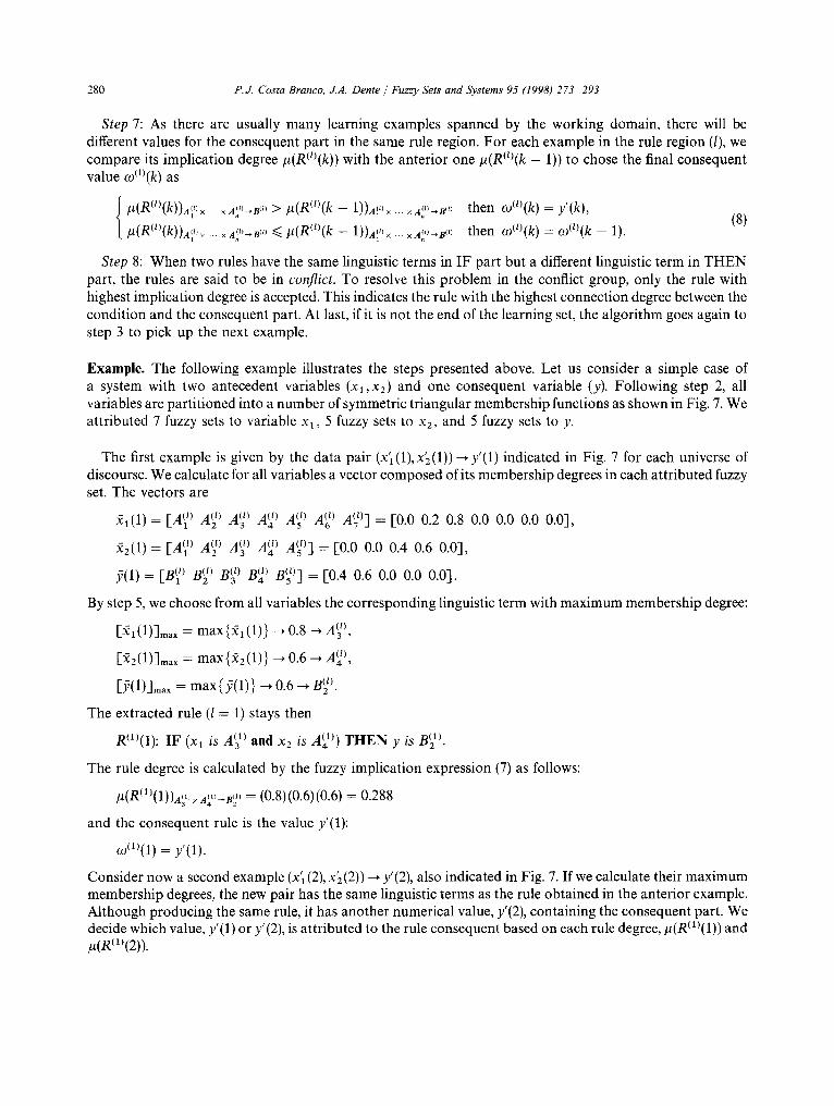
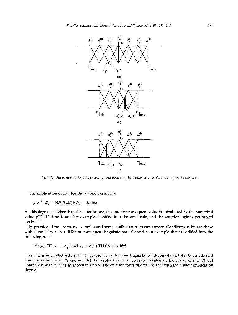
Example. The following example illustrates the steps presented above. Let us consider a simple case of a system with two antecedent variables (Xl,X2) and one consequent variable (y). Following step 2, all variables are partitioned into a number of symmetric triangular membership functions as shown in Fig. 7. We attributed 7 fuzzy sets to variable xx, 5 fuzzy sets to x2, and 5 fuzzy sets to y.

The first example is given by the data pair (x'1(1), x~(1))~ y'(1) indicated in Fig. 7 for each universe of discourse. We calculate for all variables a vector composed of its membership degrees in each attributed fuzzy set. The vectors are

Xl(1) = [A (l) A(2 l) --3A(t) A4-(t) A(l) A~) A?)] = [0.0 0.2 0.8 0.0 0.0 0.0 0.0],

ff2(1) = [,A(t ~) a(~ ) A(3 t) A(~ ) A(5 ~)] = [-0.0 0.0 0.4 0.6 0.0],

~9(1) = [B(1 ') o2n(') B(3') B~) B(s')] = [-0.4 0.6 0.0 0.0 0.0].

By step 5, we choose from all variables the corresponding linguistic term with maximum membership degree:

['Xl(1)]max max{Y1(1)} -~0.8 ~A(t) AI 3

[ ' ) ' C 2 ( 1 ) ] m a x = max{f2(1)} --* 0.6 --* A,(t),

[ y ( l ) J m a x = max{y(1)} --, 0.6 ~/~2-(1).

The extracted rule (l = 1) stays then

R(1)(1): IF (xl is A(31) and x2 is A(41)) THEN y is B(21).

The rule degree is calculated by the fuzzy implication expression (7) as follows:

(1) ,1) = ( 0 . 8 ) (0.6) (0.6) = 0.288 ~(R(1)(I))A~'× A, ~ B 2

and the consequent rule is the value y'(1):

~o(~)(1) = y ' (1 ) .

Consider now a second example (X'l (2), x~(2)) ~ y'(2), also indicated in Fig. 7. If we calculate their maximum membership degrees, the new pair has the same linguistic terms as the rule obtained in the anterior example. Although producing the same rule, it has another numerical value, y'(2), containing the consequent part. We decide which value, y'(1) or y'(2), is attributed to the rule consequent based on each rule degree,/1(R(1)(1)) and #(R(1)(2)).

P.J. Costa Branco, J.A. Dente / Fuzzy Sets and Systems 95 (1998) 273-293 281

m m X,l(l) xi(2 ) . . . .

(a)

l A 0) A (1) A ( ) 3 A (I) A~I)

x.fl . Z ~ x ,~ / + ~'lln x '2(2) x'2(l) ~Mlax

(b)

B (I) ~(1) u(l) 3 R(I) B~I)

Y~min ~ ' Y[max y'(1) y'(2)

(e)

Fig. 7. (a) Par t i t ion of x l by 7 fuzzy sets. (b) Par t i t ion of x2 by 5 fuzzy sets. (c) Par t i t ion of y by 5 fuzzy sets.

The implication degree for the second example is

p(Rm(2)) = (0.9) (0.55)(0.7) = 0.3465.

As this degree is higher than the anterior one, the anterior consequent value is substituted by the numerical value y'(2). If there is another example classified into the same rule, and the anterior logic is performed again.

In practice, there are many examples and some conflicting rules can appear. Conflicting rules are those with same IF part but different consequent linguistic part. Consider an example that is codified into the following rule:

R(3)(k): IF (xl is At3 3) and x2 is A~4 3)) THEN y is B] 3).

This rule is in conflict with rule (1) because it has the same linguistic condition (A3 and A4) but a different consequent linguistic (B1 and not B2). TO resolve this, it is necessary to calculate the degree of rule (3) and compare it with rule (1), as shown in step 8. The only accepted rule will be that with the highest implication degree.

282 P.~ Costa Branco, J.A. Dente / Fuzzy Sets and Systems 95 (1998) 273 293

4.2. Fuzzy modellin9 the electromechanical system usiny the simplified algorithm

In this section, we apply the fuzzy simplified algorithm to extract the electromechanical system model. Two test sets with examples not "seen" during the learning process are employed to verify the generalisation capability of the extracted model. The test sets were obtained by making the piston move back and forward, in a random way, into its operating region of 0.2 m. The sets are different in the sense that one was obtained with a load applied to the piston and the other obtained without a load in the piston. All results are plotted with the values in percentage of the nominal values.

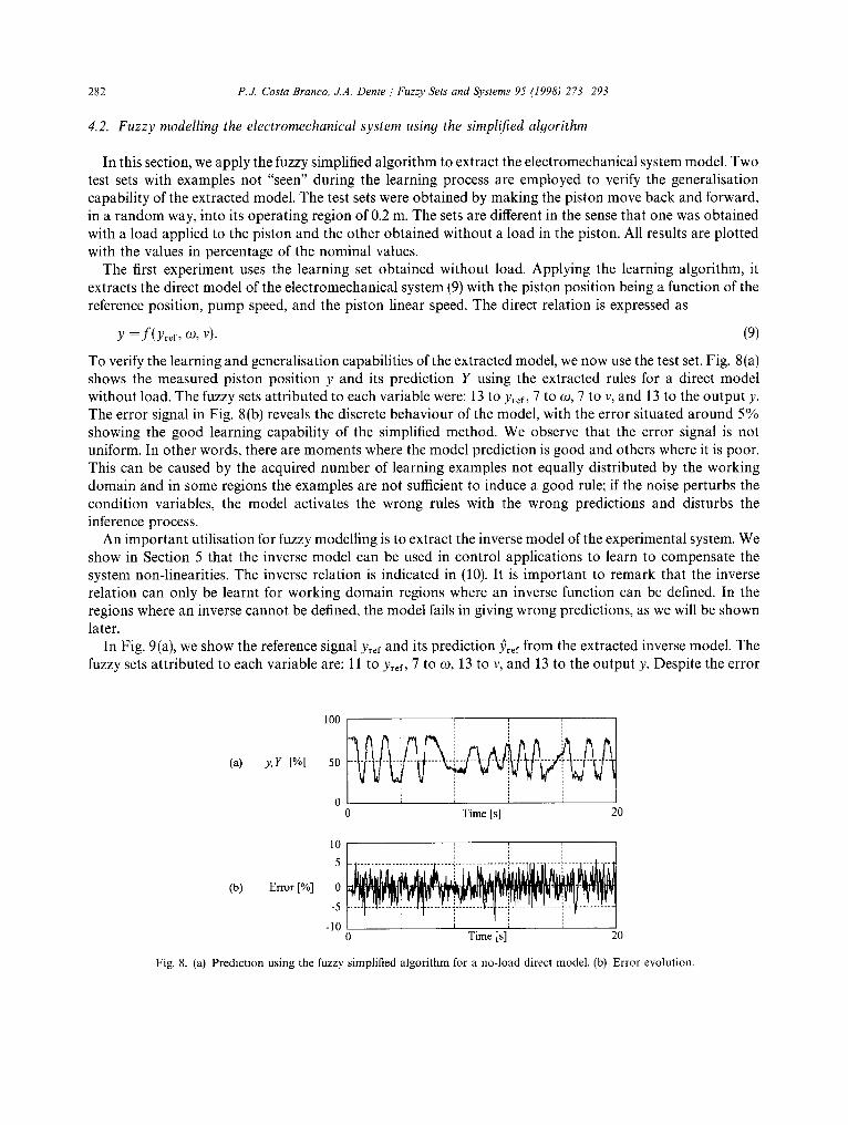
The first experiment uses the learning set obtained without load. Applying the learning algorithm, it extracts the direct model of the electromechanical system (9) with the piston position being a function of the reference position, pump speed, and the piston linear speed. The direct relation is expressed as

Y =f(Yref, (~O, V). (9)

To verify the learning and generalisation capabilities of the extracted model, we now use the test set. Fig. 8(a) shows the measured piston position y and its prediction Y using the extracted rules for a direct model without load. The fuzzy sets attributed to each variable were: 13 to Yref, 7 to O9, 7 to V, and 1 3 to the output y. The error signal in Fig. 8(b) reveals the discrete behaviour of the model, with the error situated around 5% showing the good learning capability of the simplified method. We observe that the error signal is not uniform. In other words, there are moments where the model prediction is good and others where it is poor. This can be caused by the acquired number of learning examples not equally distributed by the working domain and in some regions the examples are not sufficient to induce a good rule; if the noise perturbs the condition variables, the model activates the wrong rules with the wrong predictions and disturbs the inference process.

An important utilisation for fuzzy modelling is to extract the inverse model of the experimental system. We show in Section 5 that the inverse model can be used in control applications to learn to compensate the system non-linearities. The inverse relation is indicated in (10). It is important to remark that the inverse relation can only be learnt for working domain regions where an inverse function can be defined. In the regions where an inverse cannot be defined, the model fails in giving wrong predictions, as we will be shown later.

In Fig. 9(a), we show the reference signal Yref and its prediction 33ref from the extracted inverse model. The fuzzy sets attributed to each variable are: 11 to Yrer, 7 to co, 13 to v, and 13 to the output y. Despite the error

100

(a) y, Y [%] 50

0 Time [s] 20

(b) Error [%]

10 5

0

-5

-10

i l

I i i I 0 Time is] 20

Fig. 8. (a) Prediction using the fuzzy simplified algorithm for a no-load direct model. (b) Error evolution.

P.J. Costa Branco, J.A. Dente / Fuzzy Sets' and Systems 95 (1998) 273 293 283

(a) Yref, Yref I%1 50 . . . . . . .

0 0 Time [s] 20

(b) Error [%]

10

5

0

-5

-10

I

0 Time [s] 20

Fig. 9. (a) Inverse modelling using the fuzzy simplified algorithm for a no-load model. (b) Error evolution.

signal in Fig. 9(b) situated around 5%, it generally increases when the piston changes its direction. In this situation, the pump reverts its rotation and works, for some seconds, in a dead zone for which there is no defined inverse. The pump rotates in the dead zone, but there is no fluid debited to the hydraulic circuit. No matter what speed (co) the pump has, the hydraulic circuit is disconnected from the electrical system.

Yref = f l(y, co, V) (10)

The learning algorithm itself causes some errors, but they can originate from incomplete information supplied during the learning process. The next experiment underlines this aspect. In the following case, we employ the learning set obtained by applying load to the piston. The presence of the load makes it necessary to provide the learning process with the pressure signal information to obtain a more complete model, although, we did not take into account the pressure signal in our results. With this assumption, we will put in evidence the low performance obtained by the extracted load model if there is information fault during the learning phase.

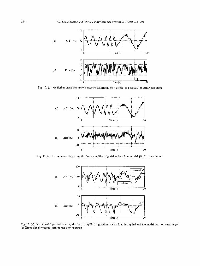
Fig. 10 shows the prediction results when using the fuzzy simplified algorithm for a direct load model. The fuzzy sets attributed to each variable were: 11 to Yref, 7 to co, 11 to V, and 13 to the output y. The oscillatory behaviour in error signal (Fig. 10(b)) indicates that the learning process needs more information. In this case, the pressure signal Pl contained the information.

In the results of Fig. 11, we combine the two anterior situations: the inverse problem and the presence of load. When modelling the load system, the learning process needs the pressure signal, and to extract the inverse model we have the problem of the pump dead zone. The fuzzy sets attributed to each variable are: 13 to Yref, 13 to co, 11 to V, and 13 to the output y. Fig. 11 shows that the model error increased considerably, although it still shows a good modelling performance indicating the effectiveness of the algorithm.

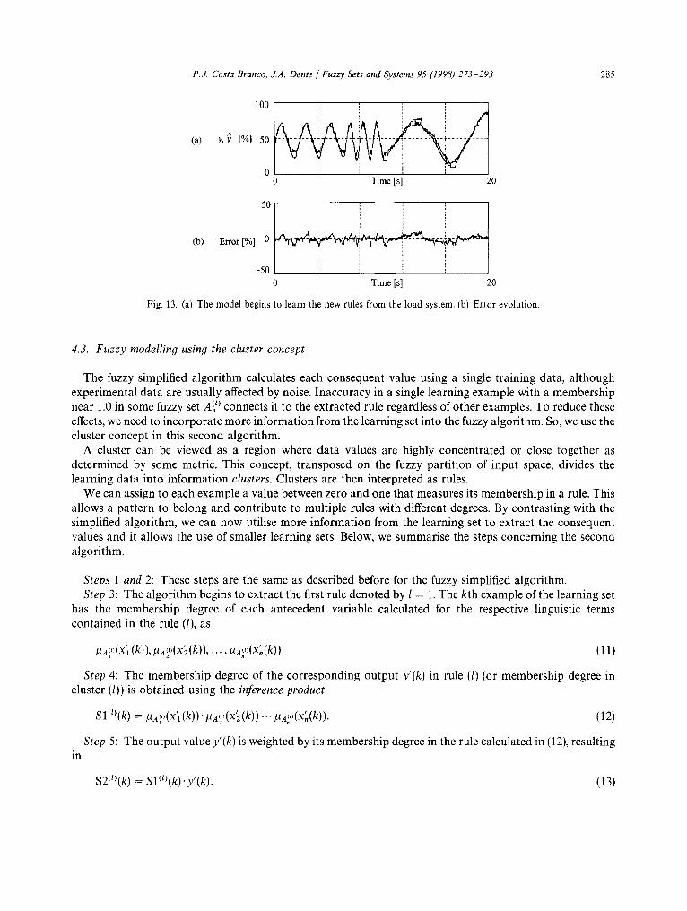
It follows that the model extracted from the no-load learning set is used to predict the piston behaviour when there is a load connected. The fuzzy sets attributed to each variable are: 7 to Yref, 7 to CO, 7 to V, and 13 to the output y. The model response, as seen in Fig. 12, presents large errors. If some examples of the load system behaviour are presented to the fuzzy learning algorithm, this begins to change the old relations to express the new behaviour. Fig. 13 presents the results of the learning process after the model begins to learn the new system dynamics, with the error signal decreasing significantly (Fig. 13(b)).

284 P.J. Costa Branco, J.A. Dente / Fuzzy Sets and Systems 95 (1998) 273-293

100

(a) y, Y [%] 50

i

Time [s] 20

(b) Error [%]

10

5

0

-5

-10 0 Time [s] 20

Fig. 10. (a) Prediction using the fuzzy simplified algorithm for a direct load model. (b) Error evolution.

100

(a) Y,Y [%] 50

0 Time [s] 20

(b) Error [%] 0

-10 ............... ~ .............. i ............... ," .............. ~ . . . . . . . . . . . . . .

Time [s] 20

Fig. 11. (a) Inverse modelling using the fuzzy simplified algorithm for a load model. (b) Error evolution.

100

(a) Y,Y [%] 50

Time [s] 20

50

(b) Error [%] 0

-50 0 Time [s] 20

Fig. 12. (a) Direct model prediction using the fuzzy simplified algorithm when a load is applied and the model has not learnt it yet. (b) Error signal without learning the new relations.

P.J. Costa Branco, J.A. Dente / Fuzzy Sets and Systems 95 (1998) 273-293 285

100

(a) Y, ~ [%1 50

Time Is] 20

(b) Error [%] 0

-50 0 Time [s] 20

Fig. 13. (a) The model begins to learn the new rules from the load system. (b) Error evolution.

4.3. Fuzzy modelling using the cluster concept

The fuzzy simplified algorithm calculates each consequent value using a single training data, although experimental data are usually affected by noise. Inaccuracy in a single learning example with a membership near 1.0 in some fuzzy set At, ~) connects it to the extracted rule regardless of other examples. To reduce these effects, we need to incorporate more information from the learning set into the fuzzy algorithm. So, we use the cluster concept in this second algorithm.

A cluster can be viewed as a region where data values are highly concentrated or close together as determined by some metric. This concept, transposed on the fuzzy partition of input space, divides the learning data into information clusters. Clusters are then interpreted as rules.

We can assign to each example a value between zero and one that measures its membership in a rule. This allows a pattern to belong and contribute to multiple rules with different degrees. By contrasting with the simplified algorithm, we can now utilise more information from the learning set to extract the consequent values and it allows the use of smaller learning sets. Below, we summarise the steps concerning the second algorithm.

Steps 1 and 2: These steps are the same as described before for the fuzzy simplified algorithm. Step 3: The algorithm begins to extract the first rule denoted by I = 1. The kth example of the learning set

has the membership degree of each antecedent variable calculated for the respective linguistic terms contained in the rule (l), as

~A?(xi (k)), . A i , , ( x ' ~ ( k ) ) . . . . . ~A:.(x;(k)). (11)

Step 4: The membership degree of the corresponding output y'(k) in rule (1) (or membership degree in cluster (I)) is obtained using the inference product

Sl")(k) = ~A,,,(x'~ (k))" pA?(x'2(k)) ... pA~,(x',(k)). (12)

Step 5: The output value y'(k) is weighted by its membership degree in the rule calculated in (12), resulting in

S 2 l / ) ( k ) = Sl(l)(k) • y'(k). (13)

286 P.J. Costa Branco, J.A. Dente / Fuzzy Sets and Systems 95 (1998) 273-293

Step 6: If it is not the end of the learning set, the algorithm adds recursively the weighted output S2~)(k) and the rule membership degree Sl(~)(k) as shown in (14). The variable denoted by Numerator adds all weighted example contributions contained in the specified rule (l) and the variable Denominator sums all the respective membership degrees to normalise the example contributions:

Numerator --+ Numerator + (S2")(k)), (14)

Denominator --+ Denominator + (Sl~l)(k)).

Next, the next learning example is picked

k -+ k + 1 (15)

and the algorithm returns to step 3. Step 7: If the learning set has finished, the consequent value co ~t) for rule (l) is calculated by the expression

Numerator co ~1) = . (16)

Denominator

Step 8: The algorithm follows now to the next rule,

1-+l+ 1 (17 )

starts again with the first learning example,

k --+ 0 (18)

and returns to step 3.

Example. We continue with the example described for the first algorithm to illustrate the anterior steps. Suppose that we want to extract the consequent value for the following rule with l = 1:

R(1)(k): I F (X 1 is A~ 1) a n d x 2 is A] 1)) T H E N co (1) = ?.

Let (X'l (1), x~ ( 1 ), y'( 1 )) and (x', (2), x~ (2), y' (2)) be the learning pairs, as in the first example, with the respective membership values in fuzzy sets A~ 1) and ,.~a(1) of rule R(1)(k). Using the anterior learning algorithm, the consequent value is calculated as

¢o(1) = [#A~'(X'I(1))'I~A~"(X'2(1))]Y'(1) + [#a~l'(X'l(Z))'#a~'(X'z(2))]y'(2)

[#ay(X'x(1))' #A~I'(X~(1))] + [I~A~'(X'I(2))" #A~,(X~(2))]

Let us consider another rule. If we use the fuzzy simplified algorithm, the rule

R(Z)(k): I F (xl is A(2 2) a n d x2 is A 3(2)) T H E N co(2) = 9,.

would never be extracted from the two anterior learning pairs, and an empty rule appears. Although applying the present algorithm, more information can be used than that local one. So, the rule consequent part is computed by

(/)(2) __ E]'~A~ 2 , (x t l (1))'/2A~'(X~(1))] y'(1) + [#A~,(X'~ (2))'#A~'(X'2(2))]y'(2)

[t~a~=,(X'l(1))" #A~='(X'2 (1))] + [#A~2,(X'1(2))" /~A~,(X~(2))]

P.J. Costa Branco, J.A. Dente / Fuzzy Sets and Systems 95 (1998) 273 293 287

4.4. Modelling the electromechanical system usin 9 the fuzzy-cluster-based algorithm

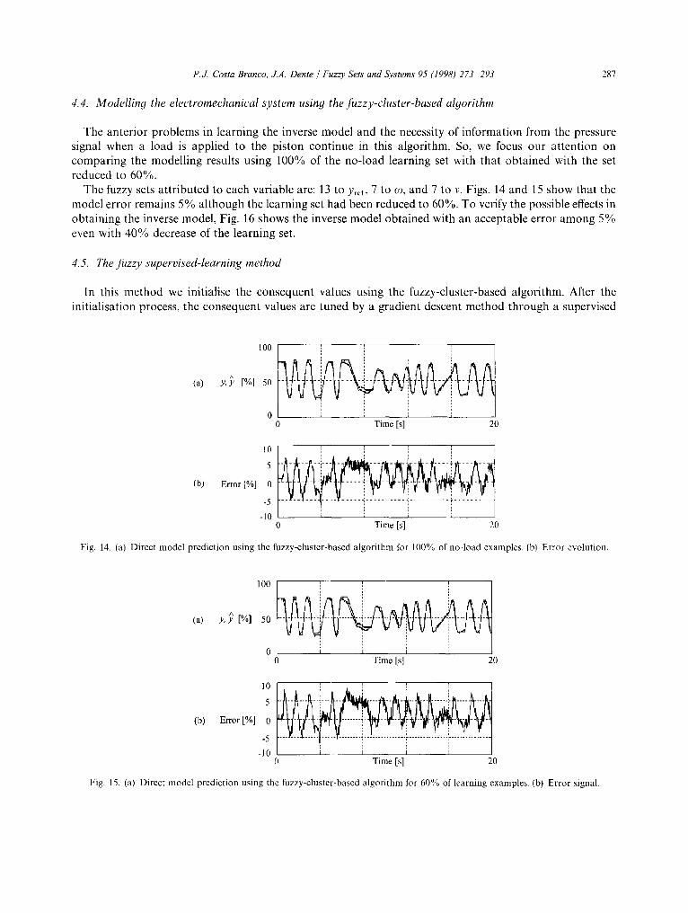
The anterior problems in learning the inverse model and the necessity of information from the pressure signal when a load is applied to the piston continue in this algorithm. So, we focus our attention on comparing the modelling results using 100% of the no-load learning set with that obtained with the set reduced to 60%.

The fuzzy sets attributed to each variable are: 13 to Yref, 7 to Oa, and 7 to v. Figs. 14 and 15 show that the model error remains 5% although the learning set had been reduced to 60%. To verify the possible effects in obtaining the inverse model, Fig. 16 shows the inverse model obtained with an acceptable error among 5% even with 40% decrease of the learning set.

4.5. The Juzzy supervised-learning method

In this method we initialise the consequent values using the fuzzy-cluster-based algorithm. After the initialisation process, the consequent values are tuned by a gradient descent method through a supervised

(a)

100

y, ~ [%] 50

0 0 Time [s] 20

(b) Error [%]

10

5

0

-5

-10 i i ;

0 Time [s] 20

Fig. 14. (a) Direct model prediction using the fuzzy-cluster-based algorithm for 100% of no-load examples. (b) Error evolution.

100

(a) y,.~ [%1 50

0 Time [s] 20

(b)

10

5

E~or[%] 0

-5

-10

l

0 Time [s] 20

Fig. 15. (a) Direct model prediction using the fuzzy-cluster-based algorithm for 60% of learning examples. (b) Error signal.

288 P.,L Costa Branco, J.A. Dente / Fuzzy Sets and Systems 95 (1998) 273-293

A

(a) Y~ef ' Yrq [%1

100 50

0 Time [s] 20

(b) Error [%1

10

5

0

-5

-10 0 Time [s] 20

Fig. 16. (a) Inverse model prediction using the fuzzy-cluster-based algorithm for 60% of no-load examples. (b) Error evolution.

learning [4]. The gradient technique changes the consequent values to minimise the error between the fuzzy model output and the measured one.

In the anterior algorithms, the consequent values are contained in the limits of the output variable. Now, each rule output is interpreted as a function of its conditions, and the rules can acquire values out of its universe of discourse limits permitting to reduce the number of necessary model rules. The membership functions in this method are gaussian type. This makes the universe of discourse to be all differently covered, when triangular fuzzy sets are used. The algorithm passes now to utilise all information contained in the learning set to extract the consequent values, and the problem of appearing rules without consequent value disappears.

The membership functions denoted by ~A~J'(Xti) a r e defined by the expression

• V 1 ['X: - - b j \ 2 - ] #A?(Xi) = a[ exp -- ~ (19)

where 1 ~< i ~< n refers to an antecedent variable (i) from the n considered antecedent variables; 1 ~<j ~< nl considers the j membership function in all ni membership functions attributed to variable (i); a~ define the maximum of the gaussian function being a,J. " = 1; b~ is the centre of gaussian function; and c{ defines its shape. Now, we describe the algorithm by its steps.

Step 1: Establish the set of system variables that contains the condition and the rule consequence parts.

Step 2: Specify the limits of the universe of discourse and the fuzzy sets number for each variable. Set the gaussian fuzzy sets, dividing in equal parts the universe of discourse, using the parameters b~ and c~.

Step 3: Use the fuzzy-cluster-based algorithm to initialise the rule consequent values co u). Step 4: After the initialisation process, the values are tuned by the gradient descent method. There are two

parameters necessary to be fixed: the learning parameter c~ and the number of iterations K. Step 5: Get the kth example from the learning set

(xl (k), x l (k), . . . , x',(k)) --, y'(k). (20)

P.~L Costa Branco, J.A. Dente / Fuzzy Sets and Systems 95 (1998) 273-293 289

Step 6: For the anterior condition set, x'(k) = x'~ (k), x'e(k) . . . . , x'.(k), compute the response of the initialised model composed of a total of c rules using

Y(x ' (k)) = Z~=I (l~'= 1 I~a~,,(x)(k)))" o (t) (21)

Step 7: Tune the rule consequent values using the gradient descent method. It changes the consequent values to minimise an objective function E usually expressed by the squared inference error

E = ½(Y(x'(k)) - y'(k)) 2. (22)

Compute the error between the measured output y' (k) for the k th input data x' (k) = (x'l (k), x~ (k) . . . . . x', (k)), and the fuzzy reasoning output for same input, expressed in Eq. (21) by Y(x'(k)).

Step 8: Using the gradient method, the learning rule is expressed as

0E co"l(k + 1) = corn(k) - ~ &o(t ) . (23)

Using the chain rule to calculate the derivative term OE/&o ~), the adaptation law is expressed by

co(Z)(k + 1) = co(l)(k) -- e (Y(x ' (k) ) - y(k))r]~.= 1 #AJ"(x)(k)) (24)

X;=, (1-I7= 1 ~A~"(xj(k))) Step 9: If the k iteration number is enough to obtain a small quadratic error E, stop tuning. If not, the

algorithm returns to step 5.

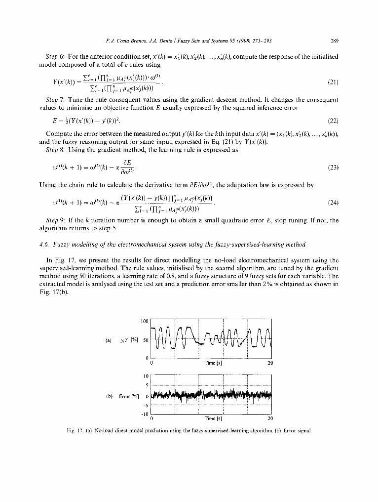
4.6. Fuzzy modelling o f the electromechanical system usin 9 the fuzzy-supervised-learning method

In Fig. 17, we present the results for direct modelling the no-load electromechanical system using the supervised-learning method. The rule values, initialised by the second algorithm, are tuned by the gradient method using 50 iterations, a learning rate of 0.8, and a fuzzy structure of 9 fuzzy sets for each variable. The extracted model is analysed using the test set and a prediction error smaller than 2% is obtained as shown in Fig. 17(b).

100

(a) y,Y l%] 50

0 Time [s] 20

(b) Error [%]

5 ....................................... ÷ ....................................... " ...................

-10 i l 0 Time [s] 20

Fig. 17. (a) No-load direct model prediction using the fuzzy-supervised-learning algorithm. (b) Error signal.

290 P.J. Costa Branco, ~LA. Dente / Fuz~ Sets and Systems 95 (1998) 273-293

100

(a) y,Y [%] 50

Time Is] 20

5

(b) Error [%] 0

-5

-10 0 Time Is] 20

Fig. 18. (a) Direct load model prediction using the fuzzy-supervised-learning algorithm. (b) Error signal.

100

(a) y,Y [%] 50

(b) Error [%]

Load system [ " \

0 Time [S] ] No-load system J 20

l0 i , i i

5 . . . . . i . . . . . . . . ' . . . . . . . . . . . . . . . . . . . . .

0 ! " -

?o 0 Time [s] 20

Fig. 19. (a) Prediction for a direct load system without learning the new dynamics, yet. (b) Error evolution.

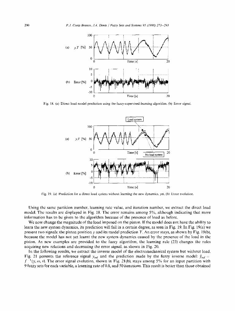
Using the same partition number, learning rate value, and iteration number, we extract the direct load model. The results are displayed in Fig. 18. The error remains among 5%, although indicating that more information has to be given to the algorithm because of the presence of load as before.

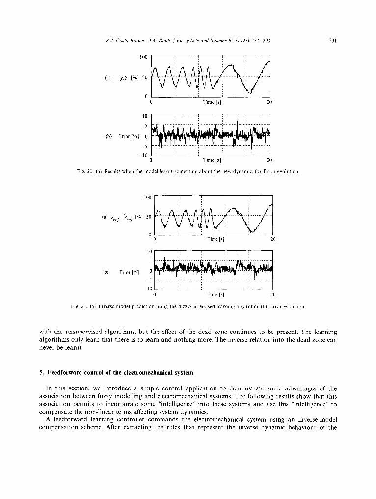
We now change the magnitude of the load imposed on the piston. If the model does not have the ability to learn the new system dynamics, its prediction will fail in a certain degree, as seen in Fig. 19. In Fig. 19(a) we present two signals: the piston position y and its model prediction Y. An error stays, as shown by Fig. 19(b), because the model has not yet learnt the new system dynamics caused by the presence of the load in the piston. As new examples are provided to the fuzzy algorithm, the learning rule (23) changes the rules acquiring new relations and decreasing the error signal, as shown in Fig. 20.

In the following results, we extract the inverse model of the electromechanical system but without load. Fig. 21 presents the reference signal Yref and the prediction made by the fuzzy inverse model: )~ref = f - l ( y , ~0, V). The error signal evolution, shown in Fig. 21(b), stays among 5% for an input partition with 9 fuzzy sets for each variable, a learning rate of 0.8, and 50 iterations. This result is better than those obtained

P.J. Costa Branco, J.A. Dente / Fuzzy Sets and Systems 95 (1998) 273 293 291

100

(a) y,Y [%] 50

0 Time [s] 20

(b) Error [%]

10

5

0

-5

-10 0 Time [s] 20

Fig. 20. (a) Results when the model learnt something about the new dynamic. (b) Error evolution.

100

/x

(a) Yref' Yref [%1 50

0 Time [s] 20

(b) Error [%]

10

5

0

-5

-10 0 Time [s] 20

Fig. 2l. (a) Inverse model prediction using the fuzzy-supervised-learning algorithm. (b) Error evolution.

with the unsupervised algorithms, but the effect of the dead zone continues to be present. The learning algorithms only learn that there is to learn and nothing more. The inverse relation into the dead zone can never be learnt.

5. Feedforward control of the electromechanical system

In this section, we introduce a simple control application to demonstrate some advantages of the association between fuzzy modelling and electromechanical systems. The following results show that this association permits to incorporate some "intelligence" into these systems and use this "intelligence" to compensate the non-linear terms affecting system dynamics.

A feedforward learning controller commands the electromechanical system using an inverse-model compensation scheme. After extracting the rules that represent the inverse dynamic behaviour of the

292 P.Ji Costa Branco, J.A. Dente / Fuzzy Sets and Systems 95 (1998) 273 293

J Inverse Fuzzy

Yref Model v

I v I °

Electro-mechanical System Y

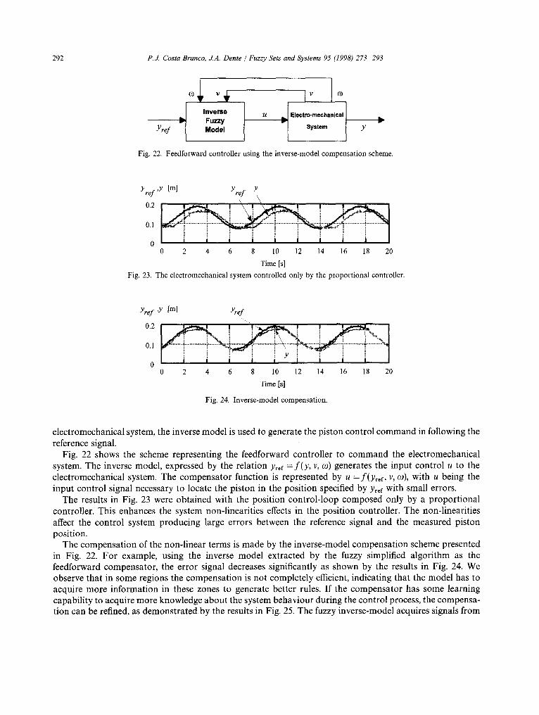
Fig. 22. Feedforward controller using the inverse-model compensation scheme.

Yref 'y [m] Yref Y

0.2 ~ \ : : : : :

0.1

0 ! ! 0 2 4 6 8 10 12 14 16 18 20

Time [s]

Fig. 23. The electromechanical system controlled only by the proportional controller.

Yref "y [m]

0.2

0.1

~ d

I I i I I 0 2 4 6 8 10 12 14 16 18 20

Time [sl

Fig. 24. Inverse-model compensation.

electromechanical system, the inverse model is used to generate the piston control command in following the reference signal.

Fig. 22 shows the scheme representing the feedforward controller to command the electromechanical system. The inverse model, expressed by the relation Yr~f = f (Y , v, co) generates the input control u to the electromechanical system. The compensator function is represented by u =f(Yr~f, v, (n), with u being the input control signal necessary to locate the piston in the position specified by Yr~f with small errors.

The results in Fig. 23 were obtained with the position control-loop composed only by a proportional controller. This enhances the system non-linearities effects in the position controller. The non-linearities affect the control system producing large errors between the reference signal and the measured piston position.

The compensation of the non-linear terms is made by the inverse-model compensation scheme presented in Fig. 22. For example, using the inverse model extracted by the fuzzy simplified algorithm as the feedforward compensator, the error signal decreases significantly as shown by the results in Fig. 24. We observe that in some regions the compensation is not completely efficient, indicating that the model has to acquire more information in these zones to generate better rules. If the compensator has some learning capability to acquire more knowledge about the system behaviour during the control process, the compensa- tion can be refined, as demonstrated by the results in Fig. 25. The fuzzy inverse-model acquires signals from

P.J. Costa Branco, J.A. Dente / Fuzzy Sets and Systems 95 (1998) 273-293 293

Yref 'y [m]

0.2 I ! . . . k ~ ! ! ! ~ . ~ , I ! ! ~ e ~ , ~

t i .......... ~ ~ i ~ ..!..:~ i ......... i . . . . . . . . . . . . L Y i o / i i i i i i

0 2 4 6 8 10 12 14 16 18 20

Time Is l

Fig. 25. Inverse-model compensation with real-time learning and control.

the electromechanical system, changes the rules to incorporate the new knowledge, and increases its control performance.

6. Conclusion

We studied in this paper the use of fuzzy-logic for automatic modelling of electromechanical systems. Three fuzzy modelling approaches were investigated each one being characterised by its learning and generalisation properties. It was shown that learning performance, no matter which algorithm is used, depends on information quantity present in the training set, the variables chosen to characterise the system dynamics, and that the algorithms learn only that there is to learn (we show that the learning algorithms only extract an inverse model if we define the existence of the inverse function). A simple control application was presented to put in evidence some potentialities of the association between fuzzy models and electromechani- cal systems to generate self-learnin9 control systems. A feedforward learning controller using an inverse- model compensation scheme was used to command the electromechanical system. The experimental results demonstrated that the incorporation of learning capabilities into the control system permit increase its performance and produce more autonomous electromechanical drive systems.

References

[1] J.C. Bezdek and S.K. Pal, Fuzzy Models for Pattern Recognition (IEEE Press, New York, 1992). [2] D. Dubois and H. Prade, Fuzzy Sets and Systems - Theory and Applications (Academic Press, New York, 1980). [3] M. Sugeno and T. Yasukawa, A fuzzy-logic-based approach to qualitative modelling, 1EEE Trans. Fuzzy Systems 1 (1993) 7 31. [4] L.X. Wang, Adaptive Fuzzy Systems and Control (Prentice-Hall, Englewood Cliffs, NJ, 1995).