Theory and Methodology

The ability to compensate for suboptimal capacity decisions byoptimal pricing decisions

Bernd Skiera *, Martin Spann

Department of Electronic Commerce, Goethe-University, Mertonstr. 17, 60054 Frankfurtam Main, Germany

Received 1 August 1997; accepted 1 September 1998

Abstract

Certain companies have high capacity cost and rather moderate production cost. These companies usually assume

that deciding about their capacity is quite critical. Frequently, however, they are able to adjust the demand for their

products to the available capacity by setting appropriate prices, that is higher (lower) than current prices in the presence

of under-capacity (over-capacity). We argue that appropriate prices can reduce the adverse e�ects of non-optimal

capacities. We analyze the sensitivity of pro®t in such a situation for a company in a monopolistic market, selling a non-

storable product and facing ¯uctuating but interdependent demand across two time periods which allows to pro®tably

di�erentiate prices. Therefore, we state optimality conditions for prices in situations of variable and given capacities and

describe a procedure to determine them. The main suggestion of this analysis is that, within the bounds of the normative

models and speci®c parameters examined, optimal prices can substantially reduce the adverse e�ects of capacity de-

viating from its optimum. In this way, pro®t is rather insensitive to deviations of capacity from its optimum. The

implications of this ®nding are discussed for a number of situations. Ó 1999 Elsevier Science B.V. All rights reserved.

Keywords: Marketing; Pricing; Capacity; Peak-load pricing; Flat maximum principle

1. Introduction

Companies which are, for example, organizingconcerts, managing recreation centers or runninghotels face the following problem. They have alimited capacity such as seats for a concert, tennisor squash courts for a recreation center and roomsin a hotel and want to sell the usage of that ca-

pacity in a way maximizing pro®t. Their situationis regularly characterized by at least some mo-nopolistic power, a cost structure in which capac-ity cost ± and hence ®xed cost ± are oftenpredominant, and ¯uctuating but interdependentdemand across time periods. Usually, such com-panies assume that choosing the optimal capacityis a rather critical decision (e.g. Greenley, 1989;Klinge, 1997). Frequently, however, they are ableto adjust the demand for their products in eachtime period to the available capacity by increasing(decreasing) prices in the case that demand exceeds

European Journal of Operational Research 118 (1999) 450±463www.elsevier.com/locate/orms

* Corresponding author. Tel.: 49 69 798 22377; fax: 49 69 798

28973; e-mail: skiera@wiwi.uni-frankfurt.de

0377-2217/99/$ ± see front matter Ó 1999 Elsevier Science B.V. All rights reserved.

PII: S 0 3 7 7 - 2 2 1 7 ( 9 8 ) 0 0 3 4 6 - 4

(falls below) capacity. Hence, it seems possible tocompensate for incurred losses in sales and pro®tby scarce capacities at least to some extent byhigher prices, and to compensate for the additionalcost for over-capacity by higher sales from lowerprices.

Surprisingly, the ability to compensate forsuboptimal capacity decisions by optimal pricingdecisions has not been systematically analyzed inthe literature. The primary focus of most papersdealing with the well-known peak-load pricingproblem is on simultaneously optimizing the pricesfor the di�erent time periods and the required ca-pacity (for an overview see Crew et al. (1995)). Themajor part of these papers considers the case ofwelfare maximization in a situation of independentdemand across time periods. Only few of themaddress pro®t maximization (Bailey and White,1974; Burness and Patrick, 1991; Crew andKleindorfer, 1986; Crew et al., 1995) and interde-pendent demand across time periods (Pressman,1970; Burness and Patrick, 1991; Berg andTschirhart, 1988; Crew and Kleindorfer, 1986).Yet, these pro®t maximization approaches regardthe simultaneous optimization of prices and ca-pacity only. The e�ect of a given (and not neces-sarily optimal) capacity on pro®t is onlyconsidered in welfare maximization approaches(Pressman, 1970; Berg and Tschirhart, 1988).However, apart from the statement of Berg andTschirhart (1988) that welfare decreases if capacitydeviates from the optimum, these approaches havenot focused on determining the sensitivity of wel-fare to deviations of capacity from its optimum.The only ones who analyzed the e�ects of devia-tions of capacity from its optimum on welfare areKoschat et al. (1995). Their implication is thatwelfare is very sensitive to a varying capacity.Unfortunately, they only considered welfare (andnot pro®t) and additionally held prices for di�er-ent capacities constant, thus preventing pricesfrom compensating for the adverse e�ects of asuboptimal capacity.

The aim of this paper is to analyze the ability tocompensate for suboptimal capacity decisions byoptimal pricing decision which could also be con-sidered as the sensitivity of pro®t to varying sizesof capacity. We analyze this e�ect analytically and,

where unavoidable, numerically in a static envi-ronment for a monopolistic ®rm which faces ¯uc-tuating but interdependent demand across twotime periods. Therefore, we state optimality con-ditions for prices in situations of variable andgiven capacities and describe a procedure to de-termine them. The e�ects of di�erent shapes ofdemand functions, varying relations betweenmarginal production and capacity costs and dif-ferent price as well as cross price elasticities for thedi�erent time periods on the sensitivity of pro®tare analyzed. The implications of our ®ndings arediscussed for a number of situations.

Our analysis contributes to the knowledge thathas been derived by examining the validity of the``¯at maximum principle'' (Chintagunta, 1993;Silver and Tull, 1986; Tull et al., 1986). The studieswithin that area analyze the important question ofwhether it is really necessary to strive for optimalsolutions or whether it su�ces to aim for solutionswhich are within a fairly broad range (e.g. �25%)around the optimum. Tull et al. (1986) and Chin-tagunta (1993) analyzed the sensitivity of pro®tsfor varying advertising budgets. Their result is thatpro®t is rather insensitive as long as advertisingelasticities are positive but smaller than approxi-mately 0.5. This is the range usually found inempirical studies (see Assmus et al., 1984; Hans-sens et al., 1990; Lodish et al., 1995). AlthoughTull et al. (1986) and Chintagunta (1993) focusedonly on the marketing instrument advertising, it islikely that the validity of the ¯at maximum prin-ciple for advertising budgets holds for other mar-keting budget instruments (e.g. sales forceexpenditures) as well. Silver and Tull (1986) ana-lyzed the validity of the ¯at maximum principle forprice as a marketing instrument. Their conclusionis that pro®t is insensitive as long as ®xed cost israther small. Thus, their analysis suggests thatcompanies with high ®xed cost (e.g. capacity cost)should carefully choose their prices.

In contrast to these studies, we analyze the sen-sitivity of pro®t to deviations of capacity from itsoptimum under the condition that optimal pricingdecisions are used to compensate for the losses in-curred by suboptimal capacity decisions. Hence, weare the ®rst to analyze the validity of the ¯at max-imum principle for decisions which are not typically

B. Skiera, M. Spann / European Journal of Operational Research 118 (1999) 450±463 451

within the responsibility of marketing managers,but whose suboptimality might be compensatedfor by marketing managers' good decisions. Thus,we analyze how strong the performances of mar-keting managers are a�ected by the capacity de-cisions usually made by others. Stated di�erently,we focus whether marketing managers in a situa-tion of a suboptimal capacity are still able to actnearly as pro®table as if they could decide aboutthe available capacity. Consequently, we analyzewhether complaints from marketing managersabout substantial losses in pro®t due to subopti-mal capacities are justi®ed or not.

The remainder of this paper is organized asfollows. In Section 2, we analyze the ability tocompensate for suboptimal capacity decisions byoptimal pricing decisions in the case where acompany does not face a ¯uctuating demandacross time periods, and hence, price di�erentia-tion across periods is not pro®table. Section 3 ex-tends this analysis to the case of varying andinterdependent demand across two time periodsthat allows the company to pro®tably di�erentiateprices across periods (e.g. peak and o�-peak pric-es). In each of these sections, we, ®rst, outline theoptimality conditions for prices in situations ofvariable and given capacities, second, describe aprocedure to determine optimal prices and capac-ity, and, third, analyze the sensitivity of pro®t todeviations of capacity from its optimum eitheranalytically or numerically. Implications and pos-sible directions for future research in Section 4conclude this contribution.

2. Analysis for uniform demand across time periods

In this section, we analyze the ability to com-pensate for suboptimal capacity decisions by op-timal pricing decisions in case of an uniformdemand across time periods for a pro®t maximiz-ing company in a monopolistic market selling anon-storable product (such as the use of squashcourts in a recreation center or rooms in a hotel).The cost structure is such that most of the costs arecapacity cost and hence, marginal production costis relatively low. We proceed as follows. First, weoutline the optimality conditions for prices in sit-

uations of variable and given capacities and thendescribe a procedure to determine them. Next, wedetermine analytically the sensitivity of pro®t todeviations of capacity from its optimum. A closed-form solution of this deviation cannot be providedfor general shapes of demand functions. There-fore, we choose the two most prominent demandfunctions (linear and multiplicative) and provideclosed-form solutions as well as numerical exam-ples for the sensitivity of pro®t for both of them.For the sake of simplicity, we assume constantmarginal production and capacity cost throughoutour analysis.

2.1. Optimal prices

We assume that a company's pro®t functioncan be stated in the following general form, wheretotal costs consist of production and capacity costswhich increase with the produced quantity and thecapacity size, respectively. The demand and costfunction are deterministic and continuously dif-ferentiable.

p � p � x p� � ÿ C x p� �;Q� �; �1�where p is the pro®t, p > 0 the price, x p� � the priceresponse function with ox=op < 0, C x;Q� � the costfunction, x > 0 the total quantity produced andsold (non-storable good), Q > 0 the capacity,oC=ox > 0 the marginal production cost, oC=oQ >0 the marginal capacity cost.

2.1.1. Variable capacityIf a company can adjust its production output

as well as its capacity, then the solution of thefollowing optimization problem maximizes thepro®t incurred:

maxP ;Q

p � p x�p� ÿ C�x�p�;Q�subject to x6Q: �2�Solving the corresponding Lagrange functionleads to the following optimal price and capacity(see Simon, 1989; Varian, 1992):

p� � oC=ox� oC=oQ1� 1=e

with e � oxop

px< ÿ1; �3�

452 B. Skiera, M. Spann / European Journal of Operational Research 118 (1999) 450±463

Q� � x p�� �; �4�where p� is the optimal price, e < ÿ1 the elasticityof demand with respect to price, Q� the optimalcapacity.

Eq. (3) is the well-known Amoroso±Robinsonrelation which states that the optimal price isachieved if marginal revenue equals marginal cost.The marginal cost term consists of marginal pro-duction cost plus marginal capacity cost. As wehave assumed that marginal capacity cost exceedsmarginal production cost, the optimal price ismostly in¯uenced by the former. In addition, theoptimal capacity equals the demand at the optimalprice (Eq. (4)).

2.1.2. Given capacityIn many cases, however, companies cannot

adjust their current (suboptimal) capacity on ashort-run basis, thus capacity cost is ®xed. In sucha situation, the pro®t function (1) yields the La-grange function (5):

L�p; k� � p x�p� ÿ C�x�p�;Q� � k �Qÿ x�p��: �5�The optimization of that Lagrange function

leads to the following ®rst order conditions: 1

p� � oC=ox� k1� 1=e

; �6�

Qÿ x P 0; k�Qÿ x� � 0; kP 0; �7�

and the Lagrange multiplier:

k � p� 1� 1=e� � ÿ oC=@x; �8�

where Q is the given capacity, p� the optimal pricefor the given capacity, k the Lagrange multiplier.

The Lagrange multiplier k in Eq. (6) replacesthe marginal capacity cost in Eq. (3). The value ofthat Lagrange multiplier k re¯ects the deviation ofthe capacity from its optimum. If the capacity istoo small (large), the Lagrange multiplier k will behigher (lower) than the marginal capacity cost,thus yielding higher (lower) prices. If the given

capacity turns out to be optimal, k equals themarginal capacity cost and p� equals p�.

According to the Kuhn±Tucker conditions inEq. (7) (see Pressman, 1970; Takayama, 1994),two di�erent situations are possible for the optimalsolution:

(i) The quantity sold equals the given capacity(x � Q). Hence, the value of the Lagrange mul-tiplier is either positive or equal to zero (k P 0).(ii) The quantity sold is smaller than the givencapacity (x < Q). Hence, the value of the La-grange multiplier must be equal to zero(k � 0) for the Kuhn±Tucker conditions tohold.Thus, the value of the Lagrange multiplier k in

Eq. (8) can be used in order to determine whichsituation is the optimal one. Therefore, the fol-lowing sequential procedure checks in a ®rst stepwhether the optimum is described by a situation inwhich the quantity sold equals the given capacity,thus

Q � x�p0�; �9�where p0 is the price in the presence of a givencapacity that achieves a demand equal to capacity,such that the price p0 is determined by the inverseprice response function:

p0 � xÿ1�Q� � xÿ1�sQ�� � xÿ1�s x�p���; �10�where p � xÿ1�x� is the inverse price responsefunction, s � Q=Q� the relative deviation of thegiven capacity compared to the optimal capacity.

Eq. (10) yields the optimal price, if the Kuhn±Tucker conditions hold, i.e., if the Lagrange mul-tiplier k in Eq. (8) for the price p0 is non-negative.Otherwise the second situation with the quantitysold below the given capacity is the optimal one. Inthis case, the Lagrange multiplier k is equal to zeroand the optimal price can be determined byEq. (6).

2.2. Sensitivity analysis

In this section we derive analytically the sensi-tivity of pro®t to deviations of capacity from itsoptimum, and thus, the ability to compensate for

1 Details of these and all other necessary calculations are

available from the authors.

B. Skiera, M. Spann / European Journal of Operational Research 118 (1999) 450±463 453

suboptimal capacity decisions by optimal pricingdecisions. Therefore, we compare the pro®t of acompany which is able to optimize its price andcapacity (Eqs. (3) and (4)) with the pro®t of acompany which has a given capacity (which mightbe suboptimal and, thus, deviate from the opti-mum) and, hence, can only optimize its price. Toderive at closed-form solutions, we derive all re-sults for the case that a company always sets theprice in such a way that the quantity sold equalsthe given capacity. That way we only heuristicallydetermine the price p0 for the case of a given ca-pacity. This price p0 equals the optimal price p� ifthe Lagrange multiplier k (Eq. (8)) is non-negative.Otherwise, pro®t could be increased by increasingthe price to p�, thus leaving part of the givencapacity unused. Hence, the pro®t deviation d0

derived by comparing the results from simulta-neously optimizing price and capacity by Eqs. (3)and (4) with the price p0 set heuristically byEq. (10) represents an upper bound for the sensi-tivity of pro®t to deviations of capacity from itsoptimum.

d0 � p0 ÿ p�

p�; �11�

where p� is the pro®t for simultaneously optimiz-ing price and capacity, p0 the pro®t for a givencapacity ( Q � sQ�) and setting the price such thatdemand equals capacity.

In order to determine this pro®t deviation d0, weuse Eqs. (3) and (4) to calculate p� and Q�, andthus p�, and Eq. (10) to calculate p0 and the in-formation about the given capacity Q � sQ� todetermine p0. Inserting both pro®ts p� and p0 inEq. (11) and simplifying yields the following pro®tdeviation:

d0 � s�p0 ÿ p��p� ÿ oC=oxÿ oC=oQ

� �sÿ 1�

� s�xÿ1�sx�p��� ÿ p��p� ÿ oC=oxÿ oC=oQ

� �sÿ 1�: �12�

Further simpli®cation of Eq. (12) is only pos-sible for speci®c price response functions. Themeta-analyses from Tellis (1988) and Mauerer(1995) show that the linear and the multiplicativeprice response functions are the ones most often

used. Therefore, we present the sensitivity of pro®tin a greater detail for these two response func-tions.

2.2.1. Multiplicative price response functionThe main feature of a multiplicative price re-

sponse function is a constant price elasticity ofdemand

x�p� � a pe; �13�where a > 0 is the scaling parameter.

Due to its iso-elasticity, this function implies aformulation of p� which is identical to Eq. (3) forthe case of optimizing price and capacity. For thecase of a given capacity, we insert the inversemultiplicative price response function in Eq. (10),yielding

p0 � s1=e � p� � s1=e � oC=ox� oC=oQ1� 1=e

� �: �14�

Eq. (14) states that the price p0 increases in caseof a shortage of capacity (s < 1) (and vice versa)and that the relation of the two prices p� and p0 isonly in¯uenced by the deviation of capacity fromits optimum and the price elasticity. For the pro®tdeviation we yield

d0 � esÿ es1=e�1 � sÿ 1: �15�

Eq. (15) states that the pro®t deviation dependsonly on the deviation of capacity from its optimumand the price elasticity of demand. This pro®t de-viation increases with higher absolute values forboth of them.

In order to provide some numerical examples,we vary the price elasticity around the averagevalues of ÿ1.76 and ÿ1.88 of the meta-analyses ofTellis (1988) and Mauerer (1995) in an interval of[ÿ1.1; ÿ4]. This range of values also correspondsapproximately to the results of various empiricalstudies summarized in Hanssens et al. (1990). Thecapacity deviations are varied by up to �50%around the optimum. For these variations, theprice p0 (Eq. (10)) is always optimal as long asmarginal capacity costs are not smaller thanmarginal production costs.

454 B. Skiera, M. Spann / European Journal of Operational Research 118 (1999) 450±463

Table 1 summarizes the pro®t deviations forthese variations. The pro®t deviation increaseswith higher deviations of capacity from its opti-mum and higher absolute values of the elasticities.Yet, these results indicate that pro®t is rather in-sensitive to deviations of capacity from its opti-mum. A price elasticity of ÿ2 and a given capacityof 25% below (above) the optimal capacity, forexample, reduces pro®t only by 1.8% (1.4%). It isworth noting that the pro®t is less sensitive to anover-sized capacity than to an under-sized one.This is due to the non-linear e�ect of a multipli-cative price response function that the absolutesales e�ect of a price change increases with lowerprices (see Simon, 1989).

2.2.2. Linear price response functionThe second function which we analyze in more

detail is the linear price response function

x�p� � aÿ mp with e � ÿmpaÿ mp

< 0

for p < a=m; �16�where a > 0 is the maximum of sales, m > 0 theabsolute change in sales resulting from a change inprice by one unit, a=m the maximum price (seeSimon, 1989).

In this function, the value of the price elasticityof demand changes with price. Eqs. (17) and (4)determine the optimal price and capacity.

p� � �oC=ox� oC=oQ�m� a2m

: �17�The heuristic that the demand equals the given

capacity yields in Eq. (18) p0.

p0 � 2a� s��oC=ox� oC=oQ�mÿ a�2m

: �18�Numerical analyses showed that this price p0

(Eq. (18)) leads more often to non-optimal pricesthan the corresponding price for the multiplicativeprice response function in Eq. (14) and, thus,leaves, most probably, more room for improve-ment.

The substitution of Eqs. (17) and (18) inEq. (12) results in the following ± surprisinglysimple ± formula for the pro®t deviation:

d0 � ÿ�sÿ 1�2: �19�That formula (19) states that the pro®t devia-

tion depends only on the deviation of capacityfrom its optimum. Numerical examples for variousdeviations of capacity from its optimum are shownin Table 2. These results indicate that the pro®tdeviation is higher for a linear than for a multi-plicative price response function. However, for agiven capacity in a range of �25% around theoptimal capacity, pro®t decreases only by 6.3%.Tull et al. (1986) still consider this sensitivity ofpro®t as ``¯at''. The sensitivity is symmetricaround the optimum (see Fig. 1) because of the

Table 1

Pro®t deviation for varying price elasticities and capacities in the case of a multiplicative price response function.

d0 [%] s

e 0.5 0.75 0.9 Q* 1.1 1.25 1.5

ÿ1.10 ÿ1.7 ÿ0.3 0.0 0.0 0.0 ÿ0.2 ÿ0.9

ÿ1.25 ÿ3.7 ÿ0.7 ÿ0.1 0.0 ÿ0.1 ÿ0.5 ÿ1.9

ÿ1.50 ÿ5.9 ÿ1.2 ÿ0.2 0.0 ÿ0.2 ÿ0.9 ÿ3.3

ÿ1.75 ÿ7.5 ÿ1.5 ÿ0.2 0.0 ÿ0.2 ÿ1.2 ÿ4.3

ÿ2.00 ÿ8.6 ÿ1.8 ÿ0.3 0.0 ÿ0.2 ÿ1.4 ÿ5.1

ÿ2.25 ÿ9.4 ÿ2.0 ÿ0.3 0.0 ÿ0.3 ÿ1.6 ÿ5.7

ÿ2.50 ÿ10.1 ÿ2.1 ÿ0.3 0.0 ÿ0.3 ÿ1.7 ÿ6.1

ÿ2.75 ÿ10.6 ÿ2.3 ÿ0.3 0.0 ÿ0.3 ÿ1.8 ÿ6.5

ÿ3.00 ÿ11.0 ÿ2.4 ÿ0.3 0.0 ÿ0.3 ÿ1.9 ÿ6.9

ÿ3.25 ÿ11.4 ÿ2.4 ÿ0.4 0.0 ÿ0.3 ÿ2.0 ÿ7.2

ÿ3.50 ÿ11.7 ÿ2.5 ÿ0.4 0.0 ÿ0.3 ÿ2.0 ÿ7.4

ÿ3.75 ÿ11.9 ÿ2.6 ÿ0.4 0.0 ÿ0.4 ÿ2.1 ÿ7.6

ÿ4.00 ÿ12.2 ÿ2.6 ÿ0.4 0.0 ÿ0.4 ÿ2.1 ÿ7.8

B. Skiera, M. Spann / European Journal of Operational Research 118 (1999) 450±463 455

linear price e�ect that a linear price responsefunction has on the demand.

Fig. 1 compares the plots of the pro®t deviationfor the two analyzed price response functions. This®gure exhibits an extremely ¯at maximum formultiplicative price response functions, even forprice elasticities as high as ÿ3.5. The pro®t devi-ation for linear response functions is substantiallyhigher. Yet, the e�ects of deviations of capacity ofup to �25% from its optimum are not higher thanÿ6.3%. Therefore, the sensitivity of pro®t is loweven in the case of a linear price response function.In cases where the price p0 is not optimal, thesensitivity of pro®t might be decreased by usingthe optimal price p� instead of the price p0 whichhas been derived heuristically. Due to these results,we conclude that the ability to compensate forsuboptimal capacity decisions by optimal pricingdecisions is high in case of an uniform demandacross time periods.

3. Analysis for varying and interdependent demand

across time periods

In this section, we extend our analysis to thecase of varying and interdependent demand

across two equal-length time periods where it ispro®table for companies to di�erentiate pricesacross time periods (e.g. peak and o�-peak pric-es). We proceed with our analysis in a similarway to the proceeding section. First, we outlinethe optimality conditions for prices in situationsof variable and given capacities and describe aprocedure to determine them. Then, we analyzenumerically and partly analytically the sensitivityof pro®t to deviations of capacity from its opti-mum. Again, as we cannot determine the sensi-tivity of pro®t for general shapes of demandfunctions, we use multiplicative and linear priceresponse functions to provide a more detailedanalysis.

3.1. Optimal prices

For the case of varying and interdependentdemand across time periods, we expand the pro®tfunction in (1) to (20) and assume, as frequentlyhas been done in the literature (e.g. Crew et al.,1995), that the demand of the peak period lieseverywhere above the demand of the o�-peak pe-riod for similar prices and that the two periods areof equal length:

Table 2

Pro®t deviations for varying capacities in case of a linear price response function

s 0.5 0.75 0.9 Q* 1.1 1.25 1.5

d0 (%) ÿ25.0 ÿ6.3 ÿ1.0 0.0 ÿ1.0 ÿ6.3 ÿ25.0

Fig. 1. Sensitivity of pro®t for di�erent shapes of demand functions (multiplicative functions are labeled with the value of their

elasticity, e.g. ÿ2.5).

456 B. Skiera, M. Spann / European Journal of Operational Research 118 (1999) 450±463

pT � p1x1�p1; p2� � p2x2�p1; p2�ÿ C�x1�p1; p2�; x2�p1; p2�;Q�; �20�

where subscript 1 denotes the peak period, sub-script 2 denotes the o�-peak period, subscript Tdenotes the case of ¯uctuating demand across timeperiods, pT is the pro®t of both periods, p1�2� > 0the price in the peak (o�-peak) period, x1�2��p1; p2�the price response function of the peak (o�-peak)period, C�x1; x2;Q� the cost function, x1�2� > 0 thetotal quantity produced and sold (non-storablegood) in the peak (o�-peak) period, oC=ox1�2� > 0the marginal production cost in the peak (o�-peak)period.

3.1.1. Variable capacityIf a company is able to optimize prices in

each of the two periods as well as capacity, thefollowing maximization problem needs to besolved:

maxp1;p2;Q

pT � p1x1�p1; p2� � p2x2�p1; p2�ÿ C�x1�p1; p2�; x2�p1; p2�;Q�

s:t: x16Q; x26Q: �21�The corresponding Lagrange function yields

the following solution:

p�1 � e1e2 ÿ c1c2 � e2 ÿ x1

x2c1

� �� p�2 � e1e2 ÿ c1c2 � e1 ÿ x2

x1c2

� ��e1e2 ÿ c1c2�

� oCox1

� oCox2

� oCoQ

; �22�

with

jeij > jcjj; e1�2� < ÿ1;

and

e1e2 ÿ c1c2 > max ei ÿ �xj=xi�cj

�� ��for i; j � 1; 2 and i 6� j;

Q� ÿ x1 P 0; k1�Q� ÿ x1� � 0; k1 P 0; �23�

Q� ÿ x2 P 0; k2�Q� ÿ x2� � 0; k2 P 0; �24�where

e1�2� � p1�2�=x1�2�ÿ �

ox1�2�=oP1�2�ÿ �

is the elasticity ofthe demand of the peak (o�-eak) period with re-spect to the price of the peak (o�-peak) period (i.e.the direct price elasticity),c2�1� � p2�1�=x1�2�

ÿ �ox1�2�=oP2�1�ÿ �

is the elasticity ofthe demand of the peak (o�-peak) period withrespect to the price of the o�-peak (peak) period(i.e. the cross-price elasticity),p�1�2� is the optimal price of the peak (o�-peak)period.

Eq. (22) represents a speci®cation of the well-known ``marginal revenue equals marginal cost''-condition for monopolistic pro®t maximization(e.g. Simon, 1989; Varian, 1992). Therefore, thepro®t maximizing price structure is characterizedby the equality of joint marginal revenues (left sideof Eq. (22)) and joint marginal costs (right side ofEq. (22)) in both periods. At least the peak de-mand is always equal to capacity because capacitycost strictly increases with capacity and the as-sumption that the peak demand is always in excessof the o�-peak demand for similar prices in thetwo periods. Therefore, the procedure to calculatethe optimal solution has to consider the two pos-sible situations that:

(i) either the demand in both periods equals theoptimal capacity, or(ii) the peak demand equals the optimal capac-ity and the o�-peak demand is smaller thanthe optimal capacity.Since peak demand is always equal to optimal

capacity, the corresponding Kuhn±Tucker condi-tions (Eq. (23)) hold. Therefore, optimal pricesand capacity are again determined by a sequentialprocedure which is build upon the Kuhn±Tuckerconditions for the o�-peak period (Eq. (24)).

In a ®rst step, the solution for the optimalprices and the optimal capacity is derived for thesituation that both demands are equal to the ca-pacity

Q� � x1 p�1; p�2

ÿ � � x2 p�1; p�2

ÿ �: �25�

Eqs. (22) and (25) are used to determine the opti-mal prices p�1; p

�2 and the optimal capacity Q�.

According to Eq. (24), this result is an optimum ifthe Lagrange multiplier of the o�-peak period k2

(Eq. (26)) is non-negative.

B. Skiera, M. Spann / European Journal of Operational Research 118 (1999) 450±463 457

k2 � p�2 �p�2e1 ÿ p�1�x1=x2�c1

e1e2 ÿ c1c2

ÿ oCox2

: �26�

Otherwise the optimal solution is characterizedby an o�-peak demand below optimal capacitysuch that k2 equals zero

Q� � x1 p�1; p�2

ÿ �> x2 p�1; p

�2

ÿ �: �27�

Thus, the maximization problem in Eq. (21)has to be solved under the condition that only thepeak demand equals the capacity which leads tothe following solution:

p�1 �e1

1� e1

oCox1

� oCoQ

� �ÿ

x2

x1c2 p�2 ÿ oC=ox2

ÿ �1� e1

;

�28�

p�2 �e2

1� e2

oCox2

ÿ x1=x2 c1 p�1 ÿ oC=ox1 � oC=oQ� �� �1� e2

: �29�

The optimal prices and the optimal capacity arecalculated by Eqs. (27)±(29). Now, only the peakdemand completely uses and accordingly deter-mines the capacity (Eq. (27)). Therefore, the peakprice has to bear the whole marginal capacity cost(Eqs. (28) and (29)). Thus, in contrast to the for-mer decision rule in (22), marginal capacity cost isno longer split between the prices of the two pe-riods.

3.1.2. Given capacityIn this case, the pro®t function (20) has to be

modi®ed to incorporate the capacity constraintsfor the peak and o�-peak demand (x16Q andx26Q). That modi®ed pro®t function yields thefollowing Lagrange function:

L�p1; p2; k1; k2� � p1x1�p1; p2� � p2x2�p1; p2�ÿ C�x1�p1; p2�; x2�p1; p2�;Q� � k1�Qÿ x1�p1; p2�� � k2�Qÿ x2�p1; p2��:

�30�The optimization of the Lagrange function (30)

leads to the following ®rst order conditions:

p1�2� � e1�2�1� e1�2�

oCox1�2�

� k1�2�

� �ÿ p2�1� ÿ oC

ox2�1�� k2�1�

� �� � �x2�1�=x1�2��c2�1��1� e1�2�� ;

�31�

Qÿ x1�2�P 0; k1�2��Qÿ x1�2�� � 0; k1�2�P 0;

�32�and the Lagrange multipliers

k1�2� � p1�2�

� p1�2�e1�2� ÿ p2�1��x2�1�=x1�2��c2�1�e1e2 ÿ c1c2

ÿ oCox1�2�

;

�33�where p�1�2� is the optimal price in the peak (o�-peak) period for a given capacity, k1�2� the La-grange multiplier of the peak (o�-peak) period.

Comparable to the case of a uniform demand,the marginal capacity costs in Eq. (22) are substi-tuted by the Lagrange multipliers of both periods(Eq. (31)). According to Eq. (33), the Lagrangemultipliers represent marginal revenues less mar-ginal production cost, i.e. the marginal pro®t atthe capacity limit.

Now, the capacity cost represents ®x cost suchthat three di�erent situations are possible for theoptimal solution (see also the Kuhn±Tucker con-ditions in Eq. (32)):

(i) The demand in both periods equals the givencapacity (Q � x1 � x2). Accordingly, the valuesof the Lagrange multipliers of both periodsare either positive or equal to zero (k1 P 0;k2 P 0).(ii) The peak demand equals the given capacityand the o�-peak demand is smaller than the giv-en capacity (Q � x1 > x2). Hence, the Lagrangemultiplier of the peak period is either positive orequal to zero and the Lagrange multiplier of theo�-peak period must be equal to zero (k1 P 0;k2 � 0).(iii) Peak and o�-peak demand are smaller thanthe given capacity. As a result of Eq. (32), theLagrange multipliers of both periods must beequal to zero (k1 � 0; k2 � 0).

458 B. Skiera, M. Spann / European Journal of Operational Research 118 (1999) 450±463

Again, the optimal solution is derived through asequential three-step procedure which examines®rst the situation in which the demands of bothperiods equal the given capacity:

Q � x1�p�1 ; p�2 �; �34�

Q � x2�p�1 ; p�2 �: �35�The solution for the ®rst situation (i.e. the

variables p�1 ; p�2 ; k1 and k2) is determined by the

two Eq. (31) for the prices p�1 ; p�2 ; and Eqs. (34)

and (35). Accordingly to the Kuhn±Tucker con-ditions in Eq. (32), this solution is the optimum ifthe Lagrange multipliers of the peak- and the o�-peak period (Eq. (33)) are non-negative.

Otherwise, the second situation is examined inwhich peak demand is equal and o�-peak demandis smaller than the given capacity. Hence, the La-grange multiplier of the o�-peak period must beequal to zero for the Kuhn±Tucker conditions ofthe o�-peak period to hold. The solution of thesecond situation (i.e. the variables p�1 ; p

�2 ; and k1) is

determined by the two equations (31) for the pricesp�1 ; p

�2 ; and Eq. (34). This solution is optimal if the

Lagrange multiplier of the peak period is non-negative.

Otherwise, the third situation with both de-mands smaller than the given capacity is the op-timal solution. In this case, the Lagrangemultipliers must be equal to zero and the optimalsolution is determined (i.e. the variables p�1 ; p

�2 ;) by

the two equations (31) for the prices p�1 ; p�2 :

3.2. Sensitivity analysis

In this section we analyze numerically andpartly analytically the sensitivity of pro®t to de-viations of capacity from its optimum, and thus,the ability to compensate for suboptimal capacitydecisions by optimal pricing decisions, in situa-tions of varying and interdependent demandacross two time periods of equal-length. Again, wecompare the pro®t for the optimization of pricesand capacity with the pro®t in the situation whereonly prices are optimized for a given capacity.Thus, the pro®t deviation is stated in the followingform:

d�T �p�T ÿ p�T

p�T�36�

where d�T is the pro®t deviation applying optimalprices (p�1; p

�2; p

�1 and p�2 ;), p�T the pro®t for simul-

taneously optimizing prices and capacity, p�T thepro®t for a given capacity and setting the optimalprices p�1 ; p

�2 .

Again, simpli®cation is only possible if priceresponse functions are stated in a speci®c form.Thus, we continue to present a more detailedanalysis for multiplicative and linear price re-sponse functions in both periods.

3.2.1. Multiplicative price response functionAll price elasticities of multiplicative price re-

sponse functions are constant. Since we havesubstitution e�ects between both periods, thefunctions possess negative direct and positive crossprice elasticities:

x1�p1; p2� � a1pe1

1 pc1

2 ; �37�

x2�p1; p2� � a2pe2

2 pc2

1 ; �38�with jeij > jcjj for i 6� j; e1�2� < ÿ1 and c1�2� > 0,where a1�2� > 0 is the scaling parameter of the peak(o�-peak) period.

The numerical analysis in the case where onlythe peak demand is equal to the optimal capacityalways yields an optimal o�-peak price convergingto in®nity and an optimal peak price converging tothe value of the Amoroso±Robinson relation for auniform demand (Eq. (3)). Hence, if the o�-peakdemand is relatively small compared to that of thepeak period and if the substitution e�ect of the o�-peak price on the peak demand is rather strong, itis optimal to refrain from o�-peak sales in favor ofpeak sales. This result occurs because the elastici-ties and hence the price-e�ects of multiplicativefunctions are constant, even if prices converge onin®nity. Our result of an o�-peak price convergingto in®nity implies an o�ering in the o�-peak periodto be unfavorable and thus leads to a problem ofuniform demand that has been analyzed in Sec-tion 2.2.1.

For our numerical examples, we choose valuesfor the rather price-insensitive peak (ÿ1.2; ÿ1.8),the more price-sensitive o�-peak period (ÿ2; ÿ4)

B. Skiera, M. Spann / European Journal of Operational Research 118 (1999) 450±463 459

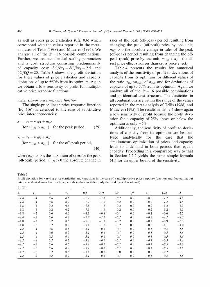
as well as cross price elasticities (0.2; 0.6) whichcorrespond with the values reported in the meta-analyses of Tellis (1988) and Mauerer (1995). Weanalyze all of the 24� 16 possible combinations.Further, we assume identical scaling parametersand a cost structure consisting predominantlyof capacity cost: oC=ox1 � oC=ox2 � 2:5 andoC=oQ � 20. Table 3 shows the pro®t deviationfor these values of price elasticities and capacitydeviations of up to �50% from its optimum. Againwe obtain a low sensitivity of pro®t for multipli-cative price response functions.

3.2.2. Linear price response functionThe single-price linear price response function

(Eq. (16)) is extended to the case of substitutiveprice interdependencies:

x1 � a1 ÿ m1p1 � n1p2

�for m1�2� > n2�1�� for the peak period; �39�

x2 � a2 ÿ m2p2 � n2p1

�for m1�2� > n2�1�� for the off-peak period;

�40�where a1�2� > 0 is the maximum of sales for the peak(o�-peak) period, m1�2� > 0 the absolute change in

sales of the peak (o�-peak) period resulting fromchanging the peak (o�-peak) price by one unit,n1�2� > 0 the absolute change in sales of the peak(o�-peak) period resulting from changing the o�-peak (peak) price by one unit, m1�2� > n2�1� the di-rect price e�ect stronger than cross price e�ect.

Table 4 presents the results for numericalanalysis of the sensitivity of pro®t to deviations ofcapacity from its optimum for di�erent values ofthe ratio a1�2�=m1�2�, of n1�2� and for deviations ofcapacity of up to 50% from its optimum. Again weanalyze all of the 24� 16 possible combinationsand an identical cost structure. The elasticities inall combinations are within the range of the valuesreported in the meta-analysis of Tellis (1988) andMauerer (1995). The results in Table 4 show againa low sensitivity of pro®t because the pro®t devi-ation for a capacity of 25% above or below theoptimum is only ÿ6.3.

Additionally, the sensitivity of pro®t to devia-tions of capacity from its optimum can be ana-lyzed analytically for the case that thesimultaneous optimization of prices and capacityleads to a demand in both periods that equalscapacity. Proceeding in a comparable way to thatin Section 2.2.2 yields the same simple formula(41) for an upper bound of the sensitivity.

Table 3

Pro®t deviation for varying price elasticities and capacities in the case of a multiplicative price response function and ¯uctuating but

interdependent demand across time periods (values in italics only the peak period is o�ered)

d�T (%) s

e1 e2 c1 c2 0.5 0.75 0.9 Q* 1.1 1.25 1.5

ÿ1.8 ÿ4 0.6 0.6 ÿ7.7 ÿ1.6 ÿ0.2 0.0 ÿ0.2 ÿ1.2 ÿ4.5

ÿ1.8 ÿ4 0.6 0.2 ÿ7.7 ÿ1.6 ÿ0.2 0.0 ÿ0.2 ÿ1.2 ÿ4.5

ÿ1.8 ÿ4 0.2 0.6 ÿ7.5 ÿ1.6 ÿ0.2 0.0 ÿ0.2 ÿ1.2 ÿ4.3

ÿ1.8 ÿ4 0.2 0.2 ÿ7.5 ÿ1.6 ÿ0.2 0.0 ÿ0.2 ÿ1.2 ÿ4.3

ÿ1.8 ÿ2 0.6 0.6 ÿ4.1 ÿ0.8 ÿ0.1 0.0 ÿ0.1 ÿ0.6 ÿ2.2

ÿ1.8 ÿ2 0.6 0.2 ÿ7.7 ÿ1.6 ÿ0.2 0.0 ÿ0.2 ÿ1.2 ÿ4.5

ÿ1.8 ÿ2 0.2 0.6 ÿ5.9 ÿ1.2 ÿ0.2 0.0 ÿ0.2 ÿ0.9 ÿ3.3

ÿ1.8 ÿ2 0.2 0.2 ÿ7.1 ÿ1.5 ÿ0.2 0.0 ÿ0.2 ÿ1.1 ÿ4.0

ÿ1.2 ÿ4 0.6 0.6 ÿ3.1 ÿ0.6 ÿ0.1 0.0 ÿ0.1 ÿ0.5 ÿ1.6

ÿ1.2 ÿ4 0.6 0.2 ÿ3.1 ÿ0.6 ÿ0.1 0.0 ÿ0.1 ÿ0.5 ÿ1.6

ÿ1.2 ÿ4 0.2 0.6 ÿ3.1 ÿ0.6 ÿ0.1 0.0 ÿ0.1 ÿ0.5 ÿ1.6

ÿ1.2 ÿ4 0.2 0.2 ÿ3.1 ÿ0.6 ÿ0.1 0.0 ÿ0.1 ÿ0.5 ÿ1.6

ÿ1.2 ÿ2 0.6 0.6 ÿ3.1 ÿ0.6 ÿ0.1 0.0 ÿ0.1 ÿ0.5 ÿ1.6

ÿ1.2 ÿ2 0.6 0.2 ÿ3.1 ÿ0.6 ÿ0.1 0.0 ÿ0.1 ÿ0.5 ÿ1.6

ÿ1.2 ÿ2 0.2 0.6 ÿ1.4 ÿ0.3 0.0 0.0 0.0 ÿ0.2 ÿ0.7

ÿ1.2 ÿ2 0.2 0.2 ÿ3.1 ÿ0.6 ÿ0.1 0.0 ÿ0.1 ÿ0.5 ÿ1.6

460 B. Skiera, M. Spann / European Journal of Operational Research 118 (1999) 450±463

d0T � ÿ�sÿ 1�2: �41�Again, the sensitivity of pro®t to deviations of

capacity from its optimum is rather low.

4. Conclusions

Our analysis shows that the ability to com-pensate for suboptimal capacity decisions by op-timal pricing decisions is fairly high so that pro®tis rather insensitive to a varying capacity. Thereason for this insensitivity is that adjustments inprices can be used to compensate for the adversee�ects of capacity deviations from the optimum.Hence, the main conclusion of this paper is thatsuboptimal capacities have only a minor in¯uenceon pro®ts as long as prices are set optimally. This,in turn, infers two major implications. First, itsuggests that complaints of marketing managersabout substantial losses in pro®t being incurred bysuboptimal capacity sizes are, at least for thenormative models and parameters examined here,not justi®ed. Rather, these managers might actu-ally fail to set prices appropriately. Second, it in-dicates that managers who report aboutsubstantial increases in pro®t by augmenting their

capacity have not, at least under the circumstancesanalyzed here, set prices in an optimal way beforetheir adjustment of capacity. Hence, capacityproblems are in fact pricing problems. Conse-quently, managers facing a demand higher (lower)than the available capacity should consider in-creasing (decreasing) the corresponding prices as aviable way out.

This insensitivity of pro®t accords companies ahigh ¯exibility in establishing their capacities.Thus, rules of thumb might be su�cient to decideabout the capacity to be build up. However, pric-ing decision have to be made very carefully. Thatalso indicates that managers should make sure thatsu�cient resources are available to support goodpricing decisions. Decisions on capacity levelsmight also be guided by strategic considerations.When employing market penetration strategies,companies will not have to fear signi®cant losses inpro®t from building up large capacities. On theother hand, companies being reluctant to build uplarge capacities, e.g. due to a high risk or a small®nancial budget, might opt for lower capacitieswithout having to su�er substantial losses in pro®t.

Researchers who attempt to relate capacity sizeto pro®t in empirical studies should make sure thatthey really cover a broad range of capacity sizes

Table 4

Pro®t deviation for varying parameter values and capacities in the case of a linear price response function and ¯uctuating but in-

terdependent demand across time periods (values in italics only the peak demand equals the optimal capacity; elasticities calculated at

the optimal capacity level)

d�T (%) s

a1/m1 a2/m2 n1 n2 0.5 0.75 0.9 Q* 1.1 1.25 1.5 e1 e2 c1 c2

125 15 10 10 ÿ24.3 ÿ5.7 ÿ0.8 0.0 ÿ0.8 ÿ4.5 ÿ11.9 ÿ1.5 ÿ2.0 0.1 0.8

125 15 10 5 ÿ23.2 ÿ5.3 ÿ0.8 0.0 ÿ0.8 ÿ5.0 ÿ13.0 ÿ1.5 ÿ2.2 0.1 0.5

125 15 5 10 ÿ25.0 ÿ6.2 ÿ1.0 0.0 ÿ0.9 ÿ5.0 ÿ12.6 ÿ1.5 ÿ1.7 0.1 0.8

125 15 5 5 ÿ24.1 ÿ5.7 ÿ0.8 0.0 ÿ0.8 ÿ5.0 ÿ13.2 ÿ1.5 ÿ1.7 0.1 0.4

125 25 10 10 ÿ24.7 ÿ6.0 ÿ0.9 0.0 ÿ0.6 ÿ3.7 ÿ9.8 ÿ1.6 ÿ1.8 0.2 0.8

125 25 10 5 ÿ22.6 ÿ4.9 ÿ0.8 0.0 ÿ0.8 ÿ4.4 ÿ11.4 ÿ1.5 ÿ2.0 0.2 0.5

125 25 5 10 ÿ25.0 ÿ6.2 ÿ1.0 0.0 ÿ1.0 ÿ4.7 ÿ11.3 ÿ1.6 ÿ1.7 0.1 0.8

125 25 5 5 ÿ24.2 ÿ5.7 ÿ0.8 0.0 ÿ0.7 ÿ4.4 ÿ11.6 ÿ1.5 ÿ1.5 0.1 0.4

30 15 10 10 ÿ25.0 ÿ6.3 ÿ1.0 0.0 ÿ1.0 ÿ6.3 ÿ25.0 ÿ3.5 ÿ2.9 0.2 0.4

30 15 10 5 ÿ25.0 ÿ6.3 ÿ1.0 0.0 ÿ1.0 ÿ6.3 ÿ25.0 ÿ3.7 ÿ2.8 0.2 0.2

30 15 5 10 ÿ25.0 ÿ6.3 ÿ1.0 0.0 ÿ1.0 ÿ6.3 ÿ25.0 ÿ3.7 ÿ3.1 0.1 0.4

30 15 5 5 ÿ25.0 ÿ6.3 ÿ1.0 0.0 ÿ1.0 ÿ6.2 ÿ25.0 ÿ4.0 ÿ3.1 0.1 0.2

30 25 10 10 ÿ25.0 ÿ6.3 ÿ1.0 0.0 ÿ1.0 ÿ6.2 ÿ24.3 ÿ3.0 ÿ2.3 0.3 0.4

30 25 10 5 ÿ25.0 ÿ6.2 ÿ1.0 0.0 ÿ1.0 ÿ6.2 ÿ24.0 ÿ3.1 ÿ2.2 0.3 0.2

30 25 5 10 ÿ25.0 ÿ6.2 ÿ1.0 0.0 ÿ1.0 ÿ6.2 ÿ24.9 ÿ2.9 ÿ2.4 0.1 0.4

30 25 5 5 ÿ25.0 ÿ6.3 ÿ1.0 0.0 ÿ1.0 ÿ6.3 ÿ24.7 ÿ3.2 ÿ2.5 0.2 0.2

B. Skiera, M. Spann / European Journal of Operational Research 118 (1999) 450±463 461

and thus, most probably, large deviations of thecapacities from their respective optimums. Other-wise, the demonstrated insensitivity would make itrather di�cult to establish a signi®cant relation-ship between these two variables. Researchers at-tempting to ®nd a relationship between prices andpro®t might encounter similar di�culties if thevarying prices arise from varying capacities.

A relaxation of the assumption of equal-lengthtime periods usually displays the o�-peak periodto be relatively longer than the peak period. Theportion of the o�-peak period on total revenuesusually increases with its relative duration. Sincethe peak demand lies everywhere above the o�-peak demand, the e�ect of a suboptimal capacityon pro®t is dominated by the e�ect on the peakperiod. Hence, an increasing portion of the o�-peak period on total revenues relatively dimin-ishes the pro®t losses due to a suboptimal ca-pacity during the peak period. If the pro®t-losses(due to a suboptimal capacity) are comparablysmaller during the o�-peak period, a shorter peakperiod will lead to an even lower sensitivity ofpro®t than the assumption of equal-length timeperiods.

Future research might want to verify our resultsin empirical projects and investigate whethermanagers might have reasons not considered hereto refrain from setting prices in the optimal way toadjust demand to their available capacity. Fur-thermore, it would be interesting to know whetherour results hold for other situations than thoseconsidered here, too. Such situations might con-sider more than two time periods or other func-tional forms for the response functions.

Future research might also use our results andanalyze their e�ects upon the regulation of mo-nopolies. Lower prices increase consumer surplusand, as long as producer surplus is reduced by alower amount, welfare. Therefore, we would sug-gest to require a regulated company to build uprather high capacities because high capacitiesconcede lower prices. The impact of this high ca-pacity on losses in pro®t of the regulated companyshould be fairly low whereas the lower pricesshould substantially increase consumer surplus.Hence, the result would be a gain in welfare thatmight be ``almost Pareto-optimal''.

Acknowledgements

We appreciated many helpful comments fromS�onke Albers, Horst Herberg, Joachim Schleichand the three anonymous referees. Any remainingerrors are the responsibility of the authors. Fi-nancial support provided by the SchmalenbachGesellschaft is gratefully acknowledged.

References

Assmus, G., Farley, J.U., Lehmann, D.R., 1984. How adver-

tising a�ects sales: Meta-analysis of econometric results.

Journal of Marketing Research 21, 65±74.

Bailey, E.E., White, L.J., 1974. Reversals in peak and o�-peak

prices. Bell Journal of Economics and Management Science

5, 75±92.

Berg, S.V., Tschirhart, J., 1988. Natural Monopoly Regulation,

Cambridge University Press, Cambridge.

Burness, H.S., Patrick, R.H., 1991. Peak-load pricing with

continuous and interdependent demand. Journal of Regu-

latory Economics 3, 69±88.

Chintagunta, P.K., 1993. Investigating the sensitivity of equi-

librium pro®t to advertising dynamics and competitive

e�ects. Management Science 39, 1146±1162.

Crew, M.A., Kleindorfer, P.R., 1986. The Economics of Public

Utility Regulation, Macmillan, London.

Crew, M.A., Fernando, C.S., Kleindorfer, P.R., 1995. The

theory of peak-load pricing: A survey. Journal of Regula-

tory Economics 8, 215±248.

Greenley, G.E., 1989. Strategic Management, Prentice Hall

International, Hempstead.

Hanssens, D.M., Parsons, L.J., Schultz, R.L., 1990. Market

Response Models: Econometric and Time Series Analysis,

Kluwer Academic Publishers, Dordrecht.

Klinge, R.C., 1997. Kapazit�atsplanung in Dienstleistung-

sunternehmen: Planungs- und Gestaltungsprobleme, Gabler

Verlag, Wiesbaden.

Koschat, M.A., Srinagesh, P., Uhler, L.J., 1995. E�cient price

and capacity choices under uncertain demand: An empirical

analysis. Journal of Regulatory Economics 7, 5±26.

Lodish, L.M., Abraham, M., Kalmenson, S., Livelsberger, J.,

Lubetkin, B., Richardson, B., Stevens, M.E., 1995. How TV

advertising works: A meta-analysis of 389 real world split

cable TV advertising experiments. Journal of Marketing

Research 32, 125±139.

Mauerer, N., 1995. Die Wirkung absatzpolitischer Instrumente.

Metaanalyse empirischer Forschungsarbeiten, Gabler Ver-

lag, Wiesbaden.

Pressman, I., 1970. A mathematical formulation of the peak-

load pricing problem. Bell Journal of Economics and

Management Science 1, 304±326.

Silver, M., Tull, D.S., 1986. Pricing and the ¯at-maximum

principle. Managerial and Decision Economics 7, 203±206.

462 B. Skiera, M. Spann / European Journal of Operational Research 118 (1999) 450±463

Simon, H., 1989. Price Management, Elsevier, Amsterdam.

Takayama, A., 1994. Analytical Methods in Economics,

Harvester Wheatsheaf, New York.

Tellis, G.J., 1988. The price elasticity of selective demand: A

meta-analysis of econometric models of sales. Journal of

Marketing Research 25, 331±341.

Tull, D.S., Wood, V.R., Duhan, D., Gillpatrick, T., Robertson,

K.R., Helgeson, J.G., 1986. Leveraged decision making in

advertising: The ¯at maximum principle and its implica-

tions. Journal of Marketing Research 23, 25±32.

Varian, H.R., 1992. Microeconomic Analysis, Norton, New

York.

B. Skiera, M. Spann / European Journal of Operational Research 118 (1999) 450±463 463