TEXTUAL ENTAILMENT FOR MODERN STANDARD ARABIC
282
TEXTUAL ENTAILMENT FOR MODERN STANDARD ARABIC A THESIS SUBMITTED TO THE UNIVERSITY OF MANCHESTER FOR THE DEGREE OF DOCTOR OF P HILOSOPHY IN THE FACULTY OF ENGINEERING AND P HYSICAL S CIENCES 2013 By Maytham Abualhail Shahed Alabbas School of Computer Science
-
Upload
khangminh22 -
Category
Documents
-
view
2 -
download
0
Transcript of TEXTUAL ENTAILMENT FOR MODERN STANDARD ARABIC

TEXTUAL ENTAILMENT FORMODERN STANDARD ARABIC
A THESIS SUBMITTED TO THE UNIVERSITY OF MANCHESTER
FOR THE DEGREE OF DOCTOR OF PHILOSOPHY
IN THE FACULTY OF ENGINEERING AND PHYSICAL SCIENCES
2013
ByMaytham Abualhail Shahed Alabbas
School of Computer Science

Contents
Abstract 12
Declaration 13
Copyright 14
Dedication 15
Acknowledgements 16
Publications based on the thesis 17
Arabic transliterations 19
List of abbreviations and acronyms 20
1 Introduction 231.1 Overview . . . . . . . . . . . . . . . . . . . . . . . . . . . . . . . . 231.2 Overview of the challenges of Arabic processing . . . . . . . . . . . 241.3 A general framework of RTE . . . . . . . . . . . . . . . . . . . . . . 261.4 Research goals . . . . . . . . . . . . . . . . . . . . . . . . . . . . . 271.5 ArbTE system architecture . . . . . . . . . . . . . . . . . . . . . . . 281.6 Contributions . . . . . . . . . . . . . . . . . . . . . . . . . . . . . . 301.7 Thesis outline . . . . . . . . . . . . . . . . . . . . . . . . . . . . . . 31
2 Background: textual entailment 342.1 Entailment in linguistics . . . . . . . . . . . . . . . . . . . . . . . . 342.2 Entailment in logic . . . . . . . . . . . . . . . . . . . . . . . . . . . 382.3 What is TE? . . . . . . . . . . . . . . . . . . . . . . . . . . . . . . . 42
2.3.1 Entailment rules . . . . . . . . . . . . . . . . . . . . . . . . 43
2

2.3.2 Characteristics of TE . . . . . . . . . . . . . . . . . . . . . . 452.3.3 Previous approaches to RTE . . . . . . . . . . . . . . . . . . 48
2.3.3.1 Surface string similarity approaches . . . . . . . . 492.3.3.2 Syntactic similarity approaches . . . . . . . . . . . 512.3.3.3 Entailment rules-based approaches . . . . . . . . . 532.3.3.4 Deep analysis and semantic inference approaches . 552.3.3.5 Classification-based approaches . . . . . . . . . . . 58
2.3.4 Applications of TE solutions . . . . . . . . . . . . . . . . . . 60
3 Background: structural analysis 623.1 Introduction . . . . . . . . . . . . . . . . . . . . . . . . . . . . . . . 623.2 Ambiguity in natural languages . . . . . . . . . . . . . . . . . . . . . 62
3.2.1 Lexical ambiguity . . . . . . . . . . . . . . . . . . . . . . . 623.2.2 Structural ambiguity . . . . . . . . . . . . . . . . . . . . . . 643.2.3 Scope ambiguity . . . . . . . . . . . . . . . . . . . . . . . . 67
3.3 Sources of ambiguities in Arabic . . . . . . . . . . . . . . . . . . . . 683.3.1 Writing system and structure of words . . . . . . . . . . . . . 68
3.3.1.1 Lack of diacritical marks . . . . . . . . . . . . . . 683.3.1.2 Cliticisation . . . . . . . . . . . . . . . . . . . . . 71
3.3.2 Syntactic freedom and zero items . . . . . . . . . . . . . . . 713.3.2.1 Word order variation . . . . . . . . . . . . . . . . . 713.3.2.2 Pro-dropping . . . . . . . . . . . . . . . . . . . . . 723.3.2.3 Zero copula . . . . . . . . . . . . . . . . . . . . . 733.3.2.4 Construct phrases . . . . . . . . . . . . . . . . . . 743.3.2.5 Coordination . . . . . . . . . . . . . . . . . . . . . 763.3.2.6 Referential ambiguity . . . . . . . . . . . . . . . . 77
3.4 Arabic processing tools . . . . . . . . . . . . . . . . . . . . . . . . . 783.4.1 POS tagging . . . . . . . . . . . . . . . . . . . . . . . . . . 78
3.4.1.1 POS tagsets . . . . . . . . . . . . . . . . . . . . . 803.4.1.2 POS taggers . . . . . . . . . . . . . . . . . . . . . 81
3.4.2 Syntactic parsing . . . . . . . . . . . . . . . . . . . . . . . . 893.4.2.1 Phrase structure parsing . . . . . . . . . . . . . . . 893.4.2.2 Dependency parsing . . . . . . . . . . . . . . . . . 90
4 Arabic linguistic analysis 954.1 Introduction . . . . . . . . . . . . . . . . . . . . . . . . . . . . . . . 95
3

4.2 POS tagging . . . . . . . . . . . . . . . . . . . . . . . . . . . . . . . 974.2.1 The taggers . . . . . . . . . . . . . . . . . . . . . . . . . . . 984.2.2 Improving POS tagging . . . . . . . . . . . . . . . . . . . . 102
4.2.2.1 Backoff strategies . . . . . . . . . . . . . . . . . . 1044.3 Dependency parsing . . . . . . . . . . . . . . . . . . . . . . . . . . . 109
4.3.1 Arabic treebanks . . . . . . . . . . . . . . . . . . . . . . . . 1094.3.1.1 From PATB to dependency trees . . . . . . . . . . 111
4.3.2 Individual parsers . . . . . . . . . . . . . . . . . . . . . . . . 1224.3.2.1 Improve parsing . . . . . . . . . . . . . . . . . . . 126
4.4 Combine taggers and parsers . . . . . . . . . . . . . . . . . . . . . . 1324.4.1 Experiments . . . . . . . . . . . . . . . . . . . . . . . . . . 132
4.4.1.1 Individual combinations of parsers and taggers . . . 1324.4.2 Merging combinations . . . . . . . . . . . . . . . . . . . . . 134
4.5 Summary . . . . . . . . . . . . . . . . . . . . . . . . . . . . . . . . 138
5 Tree matching 1395.1 Overview . . . . . . . . . . . . . . . . . . . . . . . . . . . . . . . . 1395.2 Zhang-Shasha’s TED algorithm . . . . . . . . . . . . . . . . . . . . 1435.3 Extended TED with subtrees . . . . . . . . . . . . . . . . . . . . . . 147
5.3.1 Find a sequence of edit operations . . . . . . . . . . . . . . . 1475.3.1.1 Complete example . . . . . . . . . . . . . . . . . . 151
5.3.2 Find a sequence of subtree edit operations . . . . . . . . . . . 1625.4 Optimisation algorithms . . . . . . . . . . . . . . . . . . . . . . . . 167
5.4.1 Genetic algorithms . . . . . . . . . . . . . . . . . . . . . . . 1675.4.2 Artificial bee colony algorithm . . . . . . . . . . . . . . . . . 170
5.5 Arabic lexical resources . . . . . . . . . . . . . . . . . . . . . . . . . 1735.5.1 Lexical relations . . . . . . . . . . . . . . . . . . . . . . . . 173
5.5.1.1 Synonyms . . . . . . . . . . . . . . . . . . . . . . 1735.5.1.2 Antonyms . . . . . . . . . . . . . . . . . . . . . . 1755.5.1.3 Hypernyms and hyponyms . . . . . . . . . . . . . 175
5.5.2 Lexical resources . . . . . . . . . . . . . . . . . . . . . . . . 1785.5.2.1 Acronyms . . . . . . . . . . . . . . . . . . . . . . 1785.5.2.2 Arabic WordNet . . . . . . . . . . . . . . . . . . . 1785.5.2.3 Openoffice Arabic thesaurus . . . . . . . . . . . . 1805.5.2.4 Arabic dictionary for synonyms and antonyms . . . 1805.5.2.5 Arabic stopwords . . . . . . . . . . . . . . . . . . 180
4

6 Arabic textual entailment dataset preparation 1856.1 Overview . . . . . . . . . . . . . . . . . . . . . . . . . . . . . . . . 1856.2 RTE dataset creation . . . . . . . . . . . . . . . . . . . . . . . . . . 1856.3 Dataset creation . . . . . . . . . . . . . . . . . . . . . . . . . . . . . 187
6.3.1 Collecting T-H pairs . . . . . . . . . . . . . . . . . . . . . . 1886.3.2 Annotating T-H pairs . . . . . . . . . . . . . . . . . . . . . . 191
6.4 Arabic TE dataset . . . . . . . . . . . . . . . . . . . . . . . . . . . . 1936.4.1 Testing dataset . . . . . . . . . . . . . . . . . . . . . . . . . 198
6.5 Spammer detector . . . . . . . . . . . . . . . . . . . . . . . . . . . . 1996.6 Summary . . . . . . . . . . . . . . . . . . . . . . . . . . . . . . . . 203
7 Systems and evaluation 2057.1 Introduction . . . . . . . . . . . . . . . . . . . . . . . . . . . . . . . 205
7.1.1 The current systems . . . . . . . . . . . . . . . . . . . . . . 2057.1.1.1 Surface string similarity systems . . . . . . . . . . 2067.1.1.2 Syntactic similarity systems . . . . . . . . . . . . . 207
7.1.2 Results . . . . . . . . . . . . . . . . . . . . . . . . . . . . . 2127.1.2.1 Binary decision results . . . . . . . . . . . . . . . 2137.1.2.2 Three-way decision results . . . . . . . . . . . . . 2167.1.2.3 Linguistically motivated refinements . . . . . . . . 2187.1.2.4 Optimisation algorithms performance . . . . . . . . 222
8 Conclusion and future work 2278.1 Main thesis results . . . . . . . . . . . . . . . . . . . . . . . . . . . 2278.2 Main contributions . . . . . . . . . . . . . . . . . . . . . . . . . . . 2348.3 Future directions . . . . . . . . . . . . . . . . . . . . . . . . . . . . 234
A Logical form for long sentence 268
B Possible interpretations for short sentence 270
C CoNLL-X data file format 275
D Analysis of the precision and recall 277
E RTE2 results and systems 281
Word count: 69,425
5

List of tables
2.1 Logic types for NLP. . . . . . . . . . . . . . . . . . . . . . . . . . . 382.2 Some informal definitions for TE. . . . . . . . . . . . . . . . . . . . 432.3 Some output conditions of TE engines, according to approach of par-
ticipants in the RTE challenge. . . . . . . . . . . . . . . . . . . . . . 43
3.1 The active inflection forms for the regular sound verb �I.
��J�» kataba “he
wrote” (form I:�
É�ª
�¯ f aςala -
�É
�ª
�®
�K ya f .ςulu). . . . . . . . . . . . . 79
3.2 The derivative words for word I.�J» ktb “to write”. . . . . . . . . . . . 80
4.1 Coarse-grained and fine-grained tag numbers, gold-standard and singletagger. . . . . . . . . . . . . . . . . . . . . . . . . . . . . . . . . . . 103
4.2 Tagger accuracies in isolation, with and without TBR. . . . . . . . . . 1034.3 Precision (P) and recall (R) and F-score for combinations of pairs of
taggers, with and without TBR. . . . . . . . . . . . . . . . . . . . . 1044.4 Precision (P) and recall (R) and F-score for combinations of three tag-
gers, with and without TBR. . . . . . . . . . . . . . . . . . . . . . . 1044.5 Backoff to AMIRA or MADA or MXL when there is no majority
agreement. . . . . . . . . . . . . . . . . . . . . . . . . . . . . . . . . 1054.6 Confidence levels for individual tags. . . . . . . . . . . . . . . . . . . 1064.7 Backoff to most confident tagger. . . . . . . . . . . . . . . . . . . . . 1064.8 LA and UA accuracies for parsing, different head percolation table
entry orders and treatments of coordination. . . . . . . . . . . . . . . 1194.9 The average length of sentence and the maximum length of sentence
for each training and testing dataset. . . . . . . . . . . . . . . . . . . 1234.10 Accuracy results for a total of CPOSTAGs. . . . . . . . . . . . . . . 1254.11 Five worst behaving words. . . . . . . . . . . . . . . . . . . . . . . . 1264.12 Highest LA for MSTParser, MALTParser1 and MALTParser2, gold-
standard and PATBMC corpora. . . . . . . . . . . . . . . . . . . . . . 127
6

4.13 Precision (P), recall (R) and F-score for combinations of pairs of parsers,PATBMC corpus. . . . . . . . . . . . . . . . . . . . . . . . . . . . . . 127
4.14 Precision (P), recall (R) and F-score for combinations of three parsers,PATBMC corpus. . . . . . . . . . . . . . . . . . . . . . . . . . . . . . 128
4.15 LA of backoff to two parsers (MSTParser, MALTParser1 and MALTParser2)using the first and the second proposals, PATBMC corpus. . . . . . . 129
4.16 LA of backoff to other parser (MSTParser, MALTParser1 and MALTParser2)where there is no agreement between two parsers, PATBMC corpus. . . 129
4.17 LA of backoff to two parsers (MALTParser1, MALTParser2 and MALTParser3)where there is no agreement between at least two parsers, PATBMC cor-pus. . . . . . . . . . . . . . . . . . . . . . . . . . . . . . . . . . . . 130
4.18 LA of backoff to other parser (MALTParser1, MALTParser2 and MALTParser3)where there is no agreement between two parsers, PATBMC corpus. . . 130
4.19 Highest LA for MSTParser, MALTParser1 and MALTParser2 for PATBMC
corpus, fourfold cross-validation with 4000 training sentences and 1000testing sentences. . . . . . . . . . . . . . . . . . . . . . . . . . . . . 130
4.20 Some POS tags with trusted parsers(s) for head and DEPREL, PATBMC
corpus. . . . . . . . . . . . . . . . . . . . . . . . . . . . . . . . . . . 1314.21 LA for backoff to the most confident parser, PATBMC corpus, fourfold
cross-validation with 4000 training sentences and 1000 testing sentences.1314.22 MSTParser and MALTParser1 accuracies, multiple taggers compared
with gold-standard tagging. . . . . . . . . . . . . . . . . . . . . . . . 1334.23 Precision (P), recall (R) and F-score for different tagger1: parser1+
tagger2: parser2 combinations. . . . . . . . . . . . . . . . . . . . . . 136
6.1 High-level characteristics of the RTE Challenges problem sets. . . . . 1866.2 ArbTEDS annotation rates, 600 pairs. . . . . . . . . . . . . . . . . . 1946.3 ArbTEDS text’s range annotation rates, three annotators agree, 600 pairs.1956.4 ArbTEDS_test dataset text’s range annotation, 600 binary decision pairs.1996.5 Reliability measure of our annotators, strategy A. . . . . . . . . . . . 2006.6 Reliability measure of our annotators, strategy B. . . . . . . . . . . . 202
7.1 Performance of ETED compared with the simple bag-of-words, Lev-enshtein distance and ZS-TED, binary decision Arabic dataset. . . . . 214
7.2 Performance of ETED compared with the simple bag-of-words andZS-TED, binary decision RTE2 dataset. . . . . . . . . . . . . . . . . 214
7

7.3 Comparison between ETED, simple bag-of-words, Levenshtein dis-tance and ZS-TED, three-way decision Arabic dataset. . . . . . . . . 217
7.4 Performance of ETED compared with the simple bag-of-word and ZS-TED, three-way decision RTE2 dataset. . . . . . . . . . . . . . . . . 217
7.5 Comparison between several versions of ETED+ABC with various lin-guistically motivated costs, binary decision. . . . . . . . . . . . . . . 221
7.6 Comparison between GA and ABC algorithm for five runs, optimise F-score where fitness parameters are a=1 and b=0 (i.e. fitness= F-score). 223
7.7 Comparison between GA and ABC algorithm for five runs, optimiseaccuracy (Acc.) where fitness parameters are a=0 and b=1 (i.e. fitness=accuracy). . . . . . . . . . . . . . . . . . . . . . . . . . . . . . . . . 223
7.8 Comparison between GA and ABC algorithm for five runs, optimiseboth F-score and accuracy with a slight priority to F-score, wherefitness parameters are a=0.6 and b=0.4 (i.e. fitness= F-score×0.6 +Acc.×0.4). . . . . . . . . . . . . . . . . . . . . . . . . . . . . . . . 223
C.1 CoNLL-X data file format. . . . . . . . . . . . . . . . . . . . . . . . 276
8

List of figures
1.1 General RTE architecture (Burchardt, 2008). . . . . . . . . . . . . . . 271.2 General diagram of ArbTE system. . . . . . . . . . . . . . . . . . . . 29
2.1 Logical approach structure to check natural language entailment. . . 39
3.1 Possible syntactic trees for sentence in (3.9). . . . . . . . . . . . . . . 663.2 Ambiguity caused by the lack of diacritics. . . . . . . . . . . . . . . . 703.3 AMIRA output for the Arabic sentence in (3.30). . . . . . . . . . . . 833.4 MADA output for the sentence in (3.30). For each word, the predi-
cations of the SVM classifiers are indicated by ‘;;MADA’ line. Eachanalysis is preceded by its score, while the selected analysis is markedwith ‘*’. For each word in the sentence, only the two top scoring anal-yses are shown because of the space limitation. . . . . . . . . . . . . 85
3.5 MXL output for the Arabic sentence in (3.30). . . . . . . . . . . . . . 863.6 Three taggers output for the Arabic sentence in (3.30). . . . . . . . . 863.7 Phrase structure tree for (3.31a) (Nivre, 2010). . . . . . . . . . . . . . 903.8 Projective dependency tree for (3.31a) (Nivre, 2010). . . . . . . . . . 913.9 Non-projective dependency tree for (3.31b) (Nivre, 2010). . . . . . . 91
4.1 Two combined taggers and parsers strategies. . . . . . . . . . . . . . 964.2 Our coarse-grained tagset. . . . . . . . . . . . . . . . . . . . . . . . 994.3 Coarse-grained and fine-grained tag examples. . . . . . . . . . . . . . 1004.4 Comparing basic taggers and combination strategies for Arabic sen-
tence in (4.1). . . . . . . . . . . . . . . . . . . . . . . . . . . . . . . 1084.5 From phrase structure trees to dependency trees. . . . . . . . . . . . . 1124.6 Phrase structure tree with trace. . . . . . . . . . . . . . . . . . . . . . 1144.7 Comparing PATB phrase structure and dependency format (without
POS tags and labels) in PADT, CATiB and our preferred conversionfor the sentence in (4.2). . . . . . . . . . . . . . . . . . . . . . . . . 117
9
4.8 Reconstruct coordinated structures. . . . . . . . . . . . . . . . . . . . 1174.9 Complex coordinated structures. . . . . . . . . . . . . . . . . . . . . 1184.10 Head percolation table version (7). . . . . . . . . . . . . . . . . . . . 1214.11 MSTParser’s UA and LA by POS tag. . . . . . . . . . . . . . . . . . 1234.12 MSTParser, LA and UA for testing 1000 sentences for different train-
ing dataset sizes, gold-standard tagging. . . . . . . . . . . . . . . . . 1244.13 MALTParser1, LA and UA for testing 1000 sentences for different
training dataset sizes, gold-standard tagging. . . . . . . . . . . . . . . 124
5.1 Constructing Euler string for a tree. . . . . . . . . . . . . . . . . . . 1425.2 Klein’s tree edit distance algorithm (Klein, 1998). . . . . . . . . . . . 1425.3 Two trees, Tx and Ty. . . . . . . . . . . . . . . . . . . . . . . . . . . 1435.4 Tree edit operations. . . . . . . . . . . . . . . . . . . . . . . . . . . 1445.5 Two trees T1 and T2 with their left-to-right postorder traversal (the sub-
scripts) and keyroots (bold items). . . . . . . . . . . . . . . . . . . . 1455.6 The edit operation direction used in our algorithm. Each arc that im-
plies an edit operation is labeled: “i” for an insertion, “d” for deletion,“x” for exchanging and “m” for no operation (matching). . . . . . . . 149
5.7 Computing the optimal path for the two trees in Figure 5.5. . . . . . . 1515.8 Selected forest for loop 0. . . . . . . . . . . . . . . . . . . . . . . . . 1525.9 Selected forest for loop 1. . . . . . . . . . . . . . . . . . . . . . . . . 1545.10 Selected forest for loop 2. . . . . . . . . . . . . . . . . . . . . . . . . 1555.11 Selected forest for loop 3. . . . . . . . . . . . . . . . . . . . . . . . . 1575.12 Selected forest for loop 4. . . . . . . . . . . . . . . . . . . . . . . . . 1585.13 Selected forest for loop 5. . . . . . . . . . . . . . . . . . . . . . . . . 1605.14 T1 and T2 mapping, single edit operations. . . . . . . . . . . . . . . . 1625.15 Two trees, T3 and T4, with their postorder traversal. . . . . . . . . . . 1655.16 Mapping between T3 and T4 using ZS-TED and ETED. . . . . . . . . 1665.17 The relations between hypernym and hyponym. . . . . . . . . . . . . 1765.18 Arabic acronyms examples. . . . . . . . . . . . . . . . . . . . . . . . 1795.19 Paired synsets for AWN and PWN. . . . . . . . . . . . . . . . . . . . 1795.20 Arabic synonym examples, Openoffice Arabic thesaurus. . . . . . . . 1805.21 Arabic dictionary for synonym and antonym examples. . . . . . . . . 1805.22 Arabic neologism examples. . . . . . . . . . . . . . . . . . . . . . . 181
6.1 Some examples from the RTE1 development set as XML format. . . . 187
10

6.2 Some English T-H pairs collected by headline-lead paragraph technique.1906.3 Annotate new pair’s interface. . . . . . . . . . . . . . . . . . . . . . 1936.4 Organise our data for strategy B. . . . . . . . . . . . . . . . . . . . . 201
7.1 Chromosome structure for binary decision output, Cbinary-decision, forZS-TED. . . . . . . . . . . . . . . . . . . . . . . . . . . . . . . . . . 209
7.2 Chromosome structure for three-way decisions output, Cthree-decision,for ZS-TED. . . . . . . . . . . . . . . . . . . . . . . . . . . . . . . . 210
7.3 Food source structure for binary decision output, FSeted-binary-decision,for ETED. . . . . . . . . . . . . . . . . . . . . . . . . . . . . . . . . 212
7.4 Food source structure for three-ways decision output, FSeted-three-decision,for ETED. . . . . . . . . . . . . . . . . . . . . . . . . . . . . . . . . 212
7.5 The performance of GA. . . . . . . . . . . . . . . . . . . . . . . . . 2247.6 The performance of ABC. . . . . . . . . . . . . . . . . . . . . . . . 225
8.1 General diagram of extended ArbTE system. . . . . . . . . . . . . . . 235
C.1 Dependency tree for the sentence ‘John eats happily.’ . . . . . . . . . 276C.2 CoNLL format for the sentence ‘John eats happily.’ . . . . . . . . . . 276
D.1 Precision, recall and F-score for low coverage classifier (P=20). . . . . 278D.2 Precision, recall and F-score for high coverage classifier (P=40). . . . 278D.3 Precision, recall and F-score for modest coverage classifier (P=16). . . 279D.4 Effectiveness of the threshold on the performance of a classifier. . . . 280
11

AbstractTEXTUAL ENTAILMENT FOR MODERN STANDARD ARABIC
Maytham Abualhail Shahed AlabbasA thesis submitted to the University of Manchester
for the degree of Doctor of Philosophy, 2013
This thesis explores a range of approaches to the task of recognising textual entailment
(RTE), i.e. determining whether one text snippet entails another, for Arabic, where we are
faced with an exceptional level of lexical and structural ambiguity. To the best of our knowl-
edge, this is the first attempt to carry out this task for Arabic. Tree edit distance (TED) has
been widely used as a component of natural language processing (NLP) systems that attempt
to achieve the goal above, with the distance between pairs of dependency trees being taken as a
measure of the likelihood that one entails the other. Such a technique relies on having accurate
linguistic analyses. Obtaining such analyses for Arabic is notoriously difficult. To overcome
these problems we have investigated strategies for improving tagging and parsing depending
on system combination techniques. These strategies lead to substantially better performance
than any of the contributing tools. We describe also a semi-automatic technique for creating
a first dataset for RTE for Arabic using an extension of the ‘headline-lead paragraph’ tech-
nique because there are, again to the best of our knowledge, no such datasets available. We
sketch the difficulties inherent in volunteer annotators-based judgment, and describe a regime
to ameliorate some of these. The major contribution of this thesis is the introduction of two
ways of improving the standard TED: (i) we present a novel approach, extended TED (ETED),
for extending the standard TED algorithm for calculating the distance between two trees by
allowing operations to apply to subtrees, rather than just to single nodes. This leads to useful
improvements over the performance of the standard TED for determining entailment. The key
here is that subtrees tend to correspond to single information units. By treating operations on
subtrees as less costly than the corresponding set of individual node operations, ETED con-
centrates on entire information units, which are a more appropriate granularity than individual
words for considering entailment relations; and (ii) we use the artificial bee colony (ABC) al-
gorithm to automatically estimate the cost of edit operations for single nodes and subtrees and
to determine thresholds, since assigning an appropriate cost to each edit operation manually
can become a tricky task.
The current findings are encouraging. These extensions can substantially affect the F-
score and accuracy and achieve a better RTE model when compared with a number of string-
based algorithms and the standard TED approaches. The relative performance of the standard
techniques on our Arabic test set replicates the results reported for these techniques for English
test sets. We have also applied ETED with ABC to the English RTE2 test set, where it again
outperforms the standard TED.
12

Declaration
No portion of the work referred to in this thesis has beensubmitted in support of an application for another degree orqualification of this or any other university or other instituteof learning.
13

Copyright
i. The author of this thesis (including any appendices and/or schedules to this the-sis) owns certain copyright or related rights in it (the “Copyright”) and s/he hasgiven The University of Manchester certain rights to use such Copyright, includ-ing for administrative purposes.
ii. Copies of this thesis, either in full or in extracts and whether in hard or electroniccopy, may be made only in accordance with the Copyright, Designs and PatentsAct 1988 (as amended) and regulations issued under it or, where appropriate,in accordance with licensing agreements which the University has from time totime. This page must form part of any such copies made.
iii. The ownership of certain Copyright, patents, designs, trade marks and other in-tellectual property (the “Intellectual Property”) and any reproductions of copy-right works in the thesis, for example graphs and tables (“Reproductions”), whichmay be described in this thesis, may not be owned by the author and may beowned by third parties. Such Intellectual Property and Reproductions cannotand must not be made available for use without the prior written permission ofthe owner(s) of the relevant Intellectual Property and/or Reproductions.
iv. Further information on the conditions under which disclosure, publication andcommercialisation of this thesis, the Copyright and any Intellectual Propertyand/or Reproductions described in it may take place is available in the Univer-sity IP Policy (see http://documents.manchester.ac.uk/DocuInfo.aspx?DocID=487), in any relevant Thesis restriction declarations deposited in the Uni-versity Library, The University Library’s regulations (see http://www.manchester.ac.uk/library/aboutus/regulations) and in The University’s policyon presentation of Theses.
14

Dedication
This thesis is dedicated to the memory of my father (Allah give him his mercy),
who cannot witness the completion of my PhD thesis, but I know that he would have
been very proud of me.
To my mother, who is like a candle–it consumes itself to light the way for others.
To my family: with love and appreciation.
15

Acknowledgements
To complete a PhD in a reputed university is a mighty undertaking, and I could nothave reached the finish line without the financial aid, advice, influence and support ofinstitutions and people.
My thanks are due first to my sponsor, the ministry of higher education and scien-tific research of the Republic of Iraq, for the financial aid to study in the UK. I hope tobe able to transfer the knowledge I acquired here to Iraqi institutions as a repaymentof part of my debt to Iraqi people.
I owe an enormous debt of gratitude to my supervisor, Professor Allan Ramsay, forbeing such a wonderful supervisor and for being unfailingly generous with his timeand his support throughout my graduate career. His valuable insights and ideas helpedme get over various hurdles during my study and put me back on the right track, whenI was about to go off the rails or lose confidence. He has prepared me for academic lifeand it has been a great experience and opportunity to work with him.
I am truly indebted and thankful to Carmel Roche, director of English languageprogrammes in the university language centre of Manchester, for her recommendationand support. Without her assistance I could not have started my study on time.
I would like to express my deepest appreciation to all staff of Iraqi Cultural Attachéin London for their ingenuity to manage the affairs of Iraqi students and overcome thedifficulties that face us during our stay in the UK.
My special thanks and appreciations go to our volunteer annotators who were in-volved in annotating our dataset: Mohammad Merdan, Saher Al-Hejjaj, Fatimah Fu-raiji, Siham Al-Rikabi, Khansaa Al-Mayah, Iman Alsharhan, Wathiq Al-Mudhafer andMajda Al-Liabi. I am indebted also to all the researchers whose non-commercial soft-ware I used during this study.
I would extended my thanks to all colleagues and friends (too many to list), inparticular Yasser Sabtan for countless productive discussions. Assistance provided byChristopher Connolly, Nizar Al-Liabi, Khamis Al-Qubaeissy, Sareh Malekpour andSardar Jaf was greatly appreciated.
Last but not least, there are no words that can express my thanks to my familyenough for their sacrifice and love throughout my life. I would thank them for every-thing.
Finally, I offer my deepest thank to everybody, who has always stood by me, en-couraged me along the way even by a word and believed that I could do it.
16

Publications based on the thesis
The substantial ideas of this thesis have been peer-reviewed and published in the fol-lowing publications in chronological order.1
Peer-reviewed journals
j1 Alabbas, M. and Ramsay, A. (2013). Natural language inference for Arabic us-ing extended tree edit distance with subtrees. Journal of Artificial Intelligence
Research. Forthcoming in Volume 47.
Peer-reviewed conferences and workshops
c1 Alabbas, M. (2011). ArbTE: Arabic textual entailment. In Proceedings of the
2nd Student Research Workshop associated with the International Conference
Recent Advances in Natural Language Processing (RANLP 2011), pp. 48–53,Hissar, Bulgaria. RANLP 2011 Organising Committee.
c2 Alabbas, M. and Ramsay, A. (2011a). Evaluation of combining data-driven de-pendency parsers for Arabic. In Proceedings of the 5th Language & Technology
Conference: Human Language Technologies (LTC 2011), pp. 546–550, Poznan,Poland.2
c3 Alabbas, M. and Ramsay, A. (2011b). Evaluation of dependency parsers for longArabic sentences. In Proceedings of the 2011 International Conference on Se-
mantic Technology and Information Retrieval (STAIR’11), pp. 243–248, Putra-jaya, Malaysia. IEEE, doi:10.1109/STAIR.2011.5995796.
c4 Alabbas, M. and Ramsay, A. (2012a). Arabic treebank: from phrase-structure treesto dependency trees. In Proceedings of the META-RESEARCH Workshop on Ad-
vanced Treebanking at the 8th International Conference on Language Resources
and Evaluation (LREC 2012), pp. 61–68, Istanbul, Turkey.
1The papers c1-c7 are cited in the text and therefore also appear in the full bibliography, while thepapers j1 and c8-c9 are not, since they are in press.
2This paper is selected as one of the best papers presented at the LTC 2011, and an extended andupdated version of it will appear in the Springer Verlag, LNAI Series before the end of 2013.
17

18
c5 Alabbas, M. and Ramsay, A. (2012b). Combining black-box taggers and parsersfor modern standard Arabic. In Proceedings of the Federated Conference on
Computer Science and Information Systems (FedCSIS-2012), pp. 19 –26, Wrocław,Poland. IEEE.
c6 Alabbas, M. and Ramsay, A. (2012c). Dependency tree matching with extendedtree edit distance with subtrees for textual entailment. In Proceedings of the
Federated Conference on Computer Science and Information Systems (FedCSIS-
2012), pp. 11–18, Wrocław, Poland. IEEE.
c7 Alabbas, M. and Ramsay, A. (2012d). Improved POS-tagging for Arabic by com-bining diverse taggers. In Iliadis, L., Maglogiannis, I., and Papadopoulos, H.(Eds.), Artificial Intelligence Applications and Innovations (AIAI), volume 381of IFIP Advances in Information and Communication Technology, pp. 107–116.Springer Berlin-Heidelberg, Halkidiki, Thessaloniki, Greece, doi:10.1007/978-3-642-33409-2_12.
c8 Alabbas, M. and Ramsay, A. (2013). Optimising tree edit distance with subtreesfor textual entailment. Forthcoming in: Proceedings of the International Con-
ference on Recent Advances in Natural Language Processing (RANLP 2013),Hissar, Bulgaria.
c9 Alabbas, M. (2013). A dataset for Arabic textual entailment. Forthcoming in:Proceedings of the 3rd Student Research Workshop associated with the Interna-
tional Conference Recent Advances in Natural Language Processing (RANLP
2013), Hissar, Bulgaria.

Arabic transliterations3
Letter HSB BW Unicode name Letter HSB BW Unicode nameZ' ’ ’ Hamza
D Z Za’�@ A | Alif-Madda above ¨ ς E Ayn @ Â >/O Alif-Hamza above
¨ γ g Ghayn
Zð w &/W Waw-Hamza above - _ _ Tatweel
@
A </I Alif-Hamza below
¬ f f Fa’
Zø y } Ya’-Hamza above �� q q Qaf
@ A A Alif ¼ k k Kaf
H. b b Ba’ È l l Lam�è h p Ta’-Marbuta Ð m m Meem�
H t t Ta’ à n n Nun
�H θ v Tha’ è h h Ha’
h. j j Jeem ð w w Waw
h H H Ha’ ø ý Y Alif-Maqsura
p x x Kha’ ø
y y Ya’
X d d Dal Arabic diacriticsX ð * Dhal �� a a Fatha, i.e. /a/
P r r Ra’ �� u u Damma, i.e. /u/P z z Zay �� i i Kasra, i.e. /i/
� s s Sen �� ã F Fathatan, i.e. /an/�
� š $ Shen �� u N Dammatan, i.e. /un/
� S S Sad ��
i K Kasratan, i.e. /in/
� D D Dhad �P ~ ~ Shadda
T T Ta’ �Q� . o Sukun (zero
vowel)
3Our system, dataset and Penn Arabic treebank (PATB) (Maamouri and Bies, 2004) internally usethe Buckwalter (BW) Arabic transliteration scheme (Buckwalter, 2004). However, the transcription ofArabic examples in this thesis follows Habash-Soudi-Buckwalter (HSB) transliteration scheme (Habashet al., 2007) for transcribing Arabic symbols. This scheme extends Buckwalter’s scheme to increase itsreadability while maintaining the one-to-one correspondence with Arabic orthography as representedin standard encodings of Arabic, such as Unicode. System internal examples will be presented in theBuckwalter scheme.
19

List of abbreviations and acronyms
The following table describes the significance of various abbreviations and acronymsused throughout the thesis.
Abbr. Full form1st first person2nd second person3rd third personABC artificial bee colonyADJP adjective phraseADVP adverb phraseAPI application programming interfaceArbTE Arabic textual entailmentAWN Arabic WordNetBAMA Buckwalter Arabic morphological analyzerBEP precision-recall breakeven pointBIUTEE Bar Ilan university textual entailment engineBLEU bilingual evaluation understudyBoW bag-of-wordsBPC base phrase chunkerCATiB Columbia Arabic treebankCoNLL conference on natural language learningCP complement phraseCPOSTAG coarse-grained part-of-speech tagDE differential evolutionDEPREL dependency relationDIRT discovery of inference rules from textdu. dualEA evolutionary algorithmERTS extended reduced tagsetETED extended tree edit distanceEWN Euro WordNetfem. feminineGA genetic algorithmGPSG generalised phrase structure grammar
Continued on next page
20

21
H hypothesisHPSG head-driven phrase structure grammarIE information extractionIR information retrievalLA labelled attachment scoreLD Levenshtein distanceLDC linguistic data consortiumLHS left-hand sideMADA morphological analysis and disambiguation for ArabicMALTParser models and algorithms for language technology parsermasc. masculineMC most confident (tagger)MLN Markov logic networkMSA modern standard ArabicMSTParser minimum spanning tree parserMT machine translationMXL maximum likelihoodNE named-entityNIST national institute of standards and technologyNLI natural language inferenceNLP natural language processingNP noun phraseNPI negative polarity itemO objectOVS object-verb-subjectP precisionPADT Prague Arabic dependency treebankPARASITE pragmatics = reasoning about the speaker’s intentionsPASCAL pattern analysis, statistical modelling and computational learningPATB Penn Arabic treebankPc probability of crossoverpl. pluralPm probability of mutationPOS part-of-speechPP propositional phrasepro-drop pronoun-droppingPSO particle swarm optimizationPWN Princeton WordNetQA question answering
Continued on next page

22
R recallRC relative clauseRHS right-hand sideRTE recognising textual entailmentRTED robust tree edit distanceRTS reduced tagsetS subjectSAMA standard Arabic morphological analyzersg. singularssGA steady state genetic algorithmSVM support vector machineSVO subject-verb-objectT textTBL transformation-based learningTBR transformation-based retaggingTE textual entailmentTEASE textual entailment anchor set extractionTED tree edit distanceUA unlabelled attachment scoreUX uniform crossoverV verbVOS verb-object-subjectVP verb phraseVSM vector space modelVSO verb-subject-objectXDG extended dependency graphZS-TED Zhang-Shasha’s tree edit distance

Chapter 1
Introduction
1.1 Overview
One key task for natural language systems is to determine whether one text fragmententails another. Entailment can be defined as a relationship between two sentenceswhere the truth of one sentence, the entailing expression, forces the truth of anothersentence, what is entailed. For instance, (1.1a) entails (1.1b) whereas (1.2a) does notentail (1.2b).
(1.1) Entailment
a. The couple are divorced.
b. The couple were married.
(1.2) Non-entailment
a. John wrote a story.
b. John wrote a funny story.
For logicians and semanticists, the most obvious technique for doing this is via alogical-based approach. This involves translating both text fragments into a formalmeaning representation (e.g. first-order logic) and then applying automated reasoningtools to determine their relationship. This approach has the power and precision weneed to handle quantifiers, negation, conditionals and so on. It can succeed in restricteddomains, but it fails on open-domain natural language inference (NLI) evaluations.The difficulty is plain, since natural language is complex and obtaining full and ac-curate formal representations of meaning from natural language expressions presents
23

CHAPTER 1. INTRODUCTION 24
countless thorny problems, such as anaphora, ambiguity, extragrammatically and oth-ers.
The challenges of NLI are quite different from those encountered in formal de-duction: the emphasis is on informal reasoning, lexical semantic knowledge, and vari-ability of linguistic expression, rather than on long chains of formal reasoning (Mac-Cartney, 2009). A more recent, and better-known, formulation of the NLI task is therecognising textual entailment (RTE) task, which contrasts with the standard defini-tion of entailment above, described by Dagan et al. (2006) as a task of determining, fortwo text fragments text T and hypothesis H, whether “. . . typically, a human reading T
would infer that H is most likely true.” According to these authors, entailment holdsif the truth of H, as interpreted by a typical language user, can be inferred from themeaning of T. The RTE task is in some ways easier than the classical entailment task,and has led to a number of approaches that diverge from the tradition logical-based one(Blackburn et al., 2001).
The system described in this thesis, Arabic textual entailment (ArbTE) system,embodies an investigation into the effectiveness of existing textual entailment (TE)approaches when they are applied to modern standard Arabic (MSA, or Arabic),1 andincludes extensions which deal with the specific problems posed by the language. RTEapproaches have been developed very recently and have largely been applied to Englishtexts. There is very little work on applying TE techniques to Arabic (we have, infact, so far found no such work), and little evidence that the existing approaches willwork for it. The key problem for Arabic is that it is more ambiguous than English,for reasons described below, which makes it particularly challenging to determine therelations between text snippets, so that many of the existing approaches to TE are likelyto be inapplicable.
1.2 Overview of the challenges of Arabic processing
The Arabic language raises many challenges for natural language processing (NLP).Firstly, Arabic contains an exceptionally high level of lexical ambiguity. This arisesfrom two sources: (i) Arabic is written with the short vowels, and a number of otherphonetically distinctive items, omitted; and (ii) at the same time, it has very produc-tive derivational morphology, which means that for any root there will be a number
1MSA is the Arabic language version which we are concerned with in the current work. When werefer to Arabic throughout this thesis, we mean MSA.

CHAPTER 1. INTRODUCTION 25
of derived forms which differ only in their short vowels; and it has complex non-concatenative inflectional morphology, which means that there are forms of the samelexeme2 which differ in a variety of ways. The second point here means that the omis-sion of short vowels is much more problematic than is the case in, for instance, English,where text-messages also omit short vowels. The English sentence ‘she snt me a txt
msg’ is easy to interpret, despite the lack of vowels in the open-class words, becausethere are very few, if any, other words in English that would produce the same forms.The situation in Arabic is very different, with a single written form corresponding to10 or more different lexemes.
It should be noted that it is the combination of lack of diacritics and productivederivational and inflectional morphology that leads to the problem. The lack of diacrit-ics is not, by itself, an insurmountable problem.
In addition, Arabic is highly syntactically flexible (Daimi, 2001). It has a compara-tively free word order, where sentence components can be reordered without affectingthe core meaning (non-canonical word orders are usually employed to change the fo-cus of a sentence without changing its propositional content). In this case, a lot ofambiguity occurs at the syntactic level, and needs a more complex analysis. This aswell results in structural ambiguity, with each morphological analysis having morethan a single meaning. So, besides the regular sentence of verb-subject-object (VSO),Arabic allows other potential surface forms such as SVO and VOS constructions. Thepotential of allowing such non-canonical orders leads to a large amount of ambiguity(Alabbas and Ramsay, 2011a).
Arabic also contains numerous clitic items (prepositions, pronouns and conjunc-tions), so that it is often difficult to determine just what items are present in the firstplace.
Furthermore, Arabic is a pro-drop language (Attia, 2012). It is similar to someother languages, such as Spanish, Italian and Japanese, where subject pronouns canbe omitted. Again, the potential absence of a subject is not unique to Arabic, but itis worse here than in a number of other languages because Arabic verbs can typicallyoccur either intransitively or transitively (and to complicate matters even further theactive and passive forms of a verb are often indistinguishable in the written form). Insuch cases, it is hard to tell whether a sequence consisting of a verb and a followingnoun phrase (NP) is actually an intransitive use of the verb, with the NP as subject, or
2A lemma (or lexeme) is referred to as “the more abstract units which occur in different inflec-tional ‘forms’ according to the syntactic rules involved in the generation of the sentences”(Jurafsky andMartin, 2009).

CHAPTER 1. INTRODUCTION 26
a transitive use with a zero subject, or indeed a passive use.Finally, Arabic makes use of ‘equational sentences’, consisting of an NP and a
predication (e.g. another NP or a prepositional phrase (PP)). Given that Arabic nounstypically do not carry overt case markers, it is very hard to tell whether two adjacentnouns form a complex NP, with one of the nouns serving as an adjective; or a ‘constructNP’, where one of them is serving as a possessive determiner; or a verbless sentence.Thus, there is considerable scope for ambiguity in the analysis of Arabic sentences.They also tend to be rather long. The typical sentence length is 20 to 30 words, andsentences whose length exceeds 100 words are not uncommon, and this also poses aproblem for traditional parsing algorithms.
1.3 A general framework of RTE
RTE has been recently introduced as a generic task by Dagan et al. (2006). The maingoal of RTE is constructing systems able to capture the semantic variability of languageexpressions and performing NLIs. These systems can be incorporated in NLP appli-cations. The RTE task takes a pair of text fragments (T and H) and checks whetheran entailment relationship holds between them or not. The task covers all languagevariability phenomena, such as lexical, semantic and syntactic variations.
A standard RTE system pipeline consists of the following main stages:
Linguistic analysis. This system begins by applying different off-the-shelf linguisticanalysis tools on both T and H, in order to generate linguistic annotations which willbe useful later in processing. The respective levels of analysis range from tokenisationthrough syntactic parsing to logical analysis.
T and H comparison. Different techniques are used to make comparison between T
and H, such as lexical alignment (Hickl et al., 2006) and transformations on syntactictrees (Kouylekov and Magnini, 2005a). In addition, some techniques use n-grams orunigrams to measure lexical overlap, or use WordNet as lexical substitution and logicalinference (Bos and Markert, 2006b). A feature vector, which supports a similaritymeasure of T and H, is considered the typical result for this stage.

CHAPTER 1. INTRODUCTION 27
Entailment decision. This stage generally uses machine learning, trained on thetraining datasets of the RTE, to make the final entailment decision.
The architecture in Figure 1.1, for instance, instantiates this general notion wherelinguistic analysis is represented by preprocessing; T and H comparison is representedby comparative analysis; and the entailment decision is made by a classifier that makesuse of a feature vector.
PreprocessingComparative
analysisClassifier
T
H
yes
no
Feature vector
Figure 1.1: General RTE architecture (Burchardt, 2008).
1.4 Research goals
RTE is considered a complex task that requires deep language understanding. Thetechniques used for it have been developed considerably in the last few years, espe-cially for English texts. ArbTE system is a step forward in this regard. It will inves-tigate the effectiveness of existing TE techniques to Arabic where we are confrontedwith levels of ambiguity higher than other languages, such as English. There is verylittle work on applying TE techniques to Arabic, and little evidence that the existingapproaches will work for it.
The ArbTE system aims to achieve the following goals:
g1: Design TE algorithms for Arabic. The specific problems we will investigate inthis field are the following:
p1: Part of the problem here is that the standard algorithms rely on having accu-rate syntactic analyses of the relevant texts, and there are no wide-coveragehigh-precision parsers for Arabic. The lack of such parsers is not simply amatter of lack of investment and effort: Arabic, particularly written modern

CHAPTER 1. INTRODUCTION 28
Arabic, poses a number of problems for parsing algorithms which are notpresent for most other languages. In order to overcome this problem in thecurrent project, we had to make a choice between two options: (i) adaptingthe TE algorithms so that they can be applied to partial or highly ambiguoussyntactic analyses; or (ii) improving the accuracy of parsing itself by usingvarious strategies such as system combination techniques.
We have decided to work with the second option, which is the easy one be-cause we did not want to complicate the TE algorithms without a necessity.
p2: Collect Arabic RTE datasets (i.e. development set and test set). Currentlythere is no suitable dataset for Arabic.
p3: Develop extensions to existing TE algorithms to make them more robust andmore effective.
g2: Use the Arabic testing set to compare the effectiveness of different combinationsof sub-components and select the most accurate combination.
The reasons for realising TE computationally fall into two main categories:
• Internal goals: defining the entailment will provide the computer with the abilityto carry out inferences in order to achieve a better understanding of natural languageand will also make it possible to explore other linguistic tasks, such as paraphrase,contradiction, presupposition and others.
• External goals: tackling this task will open the door to applications of these ideasin many areas of NLP, such as question answering (QA), semantic search, informa-tion extraction (IE), and multi-document summarisation.
1.5 ArbTE system architecture
The ArbTE system uses a fairly orthodox TE architecture that consists of three mainstages as shown in Figure 1.2 (Alabbas, 2011). At each stage we attempt to exploitvariations on the standard machinery to help us overcome the extra problems raised bywritten Arabic as explained below.

CHAPTER 1. INTRODUCTION 29
Does not entail
Arabic Text Arabic Hypothesis
Arabic linguistics
analysis
Arabic linguistics
analysis
Structural rules
Tree edit distance algorithm
Entailment decision
T H
T’ H’
Score
Unknown
Entails
Arabic
lexical
resources
Figure 1.2: General diagram of ArbTE system.
Arabic linguistic analysis. This part of the system represents the preprocessingstage that is responsible for converting both input T and H from natural form to depen-dency trees. To achieve this goal, we first fix acronyms by using a manually-collectedArabic resource and then two state-of-the-art dependency parsers, i.e. MSTParser (Mc-Donald and Pereira, 2006) and MALTParser (Nivre et al., 2007), are used.
Both parsers are trainable. They can be used to induce a parsing model from tree-bank data and parse new tagged data using an induced model. To provide tagged data tothese parsers, three state-of-the-art part-of-speech (POS) taggers, i.e. AMIRA (Diab,2009), MADA (Habash et al., 2009b) and a home-grown MXL tagger (Ramsay andSabtan, 2009), are used.
Tree matching. This part will use a tree edit distance (TED) algorithm, as devel-oped by Zhang and Shasha (1989), with our extended version with subtree operations,extended TED (ETED), to make matching between both T and H dependency trees.Using edit distance between two dependency trees will provide us with different ad-vantages, as follows:
• The complexity is lower than for full-scale theorem proving.
• It is robust. One can do it even when one has partial syntactic analyses or is forsome other reason unable to build logical forms.

CHAPTER 1. INTRODUCTION 30
• Different knowledge sources can be expressed by edit operations for resolving theproblems of language variability. This is because the lexical and syntactic entail-ment rules will be used to model the variability phenomena of lexical, syntactic andsemantic.
In this part of the system, we also exploit synonyms, antonyms, hypernyms andhyponyms relations encoded by using some Arabic lexical resources (such as ArabicWordNet (AWN) (Black et al., 2006), Openoffice Arabic thesaurus and others) whenexchanging items in a tree.
Entailment decision. This part of the system is responsible for making the final en-tailment decision. The score resulting from the second stage is checked here to decidea particular judgement using either one threshold (binary-decision) or two thresholds(three-way decision). Such thresholds are estimated either empirically on the trainingdata (e.g. Kouylekov, 2006) or automatically by using optimisation algorithms such asgenetic algorithm (GA) or artificial bee colony (ABC), as in our project.
1.6 Contributions
The main contributions of this work are:
1. ArbTE system is the first work in TE for Arabic (we have so far found no suchwork).3 The task of RTE for Arabic is interesting. We think that the RTE commu-nity will benefit a lot from work about TE in languages other than English and inparticular about Arabic, which has a lot of characteristics described in Section 1.2that make it challenging for NLP in general.
2. Applying our technique relies on having accurate linguistic analyses, which is adifficult task, particularly for Arabic since the problem of ambiguity is worse inArabic than in English. To overcome these problems we have carried out a numberof experiments with our taggers and parsers in order to improve their performance(i.e. deal with problem p1). These experiments show in particular the followingmain results:
• Our conversion from phrase structure to dependency trees allows parsers toperform accurately even for long sentences exceeding 100 words (Alabbasand Ramsay, 2012a).
3Confirmed by the reviewers of our paper in (Alabbas, 2011).

CHAPTER 1. INTRODUCTION 31
• Combining the output of three different taggers can produce more accurateresults than each tagger produces by itself (Alabbas and Ramsay, 2012d).
• Combining the output of multiple data-driven dependency parsers can pro-duce more accurate results, even for imperfectly tagged text, than each parserproduces by itself for texts with the gold-standard tags (Alabbas and Ramsay,2011a).
• Combining different tagger:parser pairs where each parser uses a differenttagger gives better precision than recall, as expected, which may be useful forsome tasks (Alabbas and Ramsay, 2012b).
3. We have built, using a novel semi-automatic method, a new Arabic RTE dataset. Anew dataset is required, since there are no available RTE datasets for Arabic (i.e.solve problem p2).
4. Our work implements two novel improvements to Zhang-Shasha’s TED algorithm(i.e. solve problem p3), as follows:
(i) Extending the set of edit operations to cover the subtrees transformation op-erations as well as the standard single nodes edit operations, ETED (Alabbasand Ramsay, 2012c).
(ii) Using the ABC algorithm (Karaboga et al., 2012) to estimate, automatically,relevant costs of edit operations (for single node and subtree) and of thresh-old(s) for the user defined application and testing data for different domainsinstead of expertise-based scheme.
1.7 Thesis outline
In this chapter, Introduction, we have presented the research problem and what varietyof Arabic is the target of analysis and processing. Then, the general framework of RTEis explained with our research goals and contributions. The remainder of the thesis isorganised as follows.
Chapter 2, Background: textual entailment, introduces the problem of entailment asoutlined under the perspectives of both linguistics and logic, and then the RTE task ispresented in some detail. Next, related work in the areas of RTE is reviewed. At the

CHAPTER 1. INTRODUCTION 32
end of the chapter, the main applications of RTE are explained.
Chapter 3, Background: structural analysis, describes briefly the sources of ambiguityin natural language, and the challenges of Arabic NLP are discussed in some detail.The chapter ends with description of three state-of-the-art POS taggers (i.e. MADA,AMIRA and MXL) and two state-of-the-art dependency parsers (i.e. MSTparser andMALTParser).
Chapter 4, Arabic structural analysis, presents the experimental results of improvingour preprocessing stage. The chapter starts with improving the POS taggers subtaskby using the three taggers described in Chapter 3. Next, two techniques to improvethe parsing subtask, which depends on the two parsers described in Chapter 3 and theresults of improving POS taggers, are discussed. The material in this chapter is derivedin large part from our papers c2-c5 and c7.
Chapter 5, Trees matching, describes a number of popular distance-based approachesto tree matching. Then, Zhang-Shasha’s TED algorithm is discussed with our exten-sion to this algorithm to take into consideration subtree edit operations as well as editoperations on single nodes (i.e. delete, insert and exchange). After that, two opti-misation algorithms, i.e. GA and ABC, that will be used to estimate the cost of editoperations and to determine thresholds for TED are outlined. The chapter ends with abrief description of the Arabic lexical resources that are used in our work (e.g. AWNand Openoffice Arabic thesaurus) to support us with some relations between words(e.g. synonyms, antonyms and hypernyms). The material in this chapter is derived inlarge part from our papers j1 and c6.
Chapter 6, Arabic textual entailment dataset preparation, starts with presenting our ef-forts for constructing a training set and testing set for Arabic TE systems, since there isno suitable dataset available for Arabic. Next, two diverse techniques are discussed tocheck the reliability of a number of volunteer annotators. The material in this chapteris derived in large part from our paper c9.
Chapter 7, Systems and evaluation, describes the design and implementation of RTEsystems to Arabic based on different approaches, such as bag-of-words (BoW) and

CHAPTER 1. INTRODUCTION 33
distance-based algorithms, such as Levenshtein distance (LD) and TED. Then, differ-ent ways for calculating cost functions for the different edit operations using GA andABC algorithm, are discussed. The material in this chapter is derived in large part fromour papers c1 and c8.
Chapter 8, Conclusion, concludes the final remarks of the thesis. The chapter endswith suggesting directions for future improvements and research.

Chapter 2
Background: textual entailment
In this chapter the various notions of consequence in linguistics will be reviewed (Sec-tion 2.1). In Section 2.2, the standard notion of entailment in logic will be brieflyintroduced and its problems as a model for NLI will also be discussed. In Section 2.3,the notion of textual entailment (TE) with its characteristics will be presented, a briefsummary of TE techniques will be presented and main applications of RTE will beoutlined.
2.1 Entailment in linguistics
The term entailment can be defined as a relationship between two sentences where thetruth of one sentence S1, the entailing expression, forces the truth of another sentenceS2, what is entailed (though the opposite may not be true). Notice that, if S1 is true,then S2 must also be true; also if S2 is false, then S1 must be false (Bloomer et al.,2005). By contrast, nothing is said about the truth value of S2, when S1 is false. Hence,S1 is more informative than S2 when S1 entails S2, because the information that S2 car-ries is included in the information that S1 carries. For instance, let consider (2.1) and(2.2).
(2.1) Entailment
a. The president was assassinated.
b. The president is dead.
34

CHAPTER 2. BACKGROUND: TEXTUAL ENTAILMENT 35
(2.2) Non-entailment
a. No student came to class early.
b. No student came to class.
In (2.1), if the president was assassinated, then s/he is clearly dead, i.e. (2.1a)entails (2.1b), but the reverse does not hold. The reason is that if the president was‘assassinated’ is true, then there is no way to avoid the conclusion that the presidentis ‘dead’, primarily because the meaning of ‘assassinated’, which means “murder (animportant person) in a surprise attack for political (or religious) reasons”, in (2.1a).Notice that entailment arises from our background knowledge of language. It thereforerelies on the relevant sentence constituents rather than context. By contrast, (2.2a) doesnot entail (2.2b), but the reverse does. The reason is that if it is true that ‘No student
came to class early’, then it is not necessary for ‘No student came to class’ to be true.This is because there may be some student who came to class late.
Entailment also plays an essential role in defining and testing many other funda-mental relations. For instance, when S1 entails S2 and vice versa, in this case S1 and S2
are equivalent, or are paraphrases of each other or synonymous, which means they aretrue in exactly the same situations, or mutually entailing as in (2.3).
(2.3) Equivalent
a. The terrorist is dead.
b. The terrorist is not alive.
Furthermore, S1 and S2 are contradictories if S1 entails not-S2 and S2 entails not-S1 (i.e. each sentence entails the negation of the another) so that when one sentenceis true the other must be false (Riemer, 2010), as shown in (2.4). Consequently, acontradiction occurs when a sentence contains contradictory entailment (i.e. when asentence is followed by the negation of an entailed sentence), as in (2.5). Cruse (2011)defines contrariety in terms of entailment as follows: “S1 and S2 are contraries if and
only if S1 entails not-S2, but not-S2 does not entail S1 (and vice versa).” This meansthat the two sentences are considered to be contraries if and only if each of them entailsthe negation of the other, while the latest one does not entail the first one, as in (2.6).

CHAPTER 2. BACKGROUND: TEXTUAL ENTAILMENT 36
(2.4) Contradictory
a. No student likes exams.
b. At least one student likes exams.
(2.5) Contradiction (cannot be true in any situation)
John came to university and had a good time and John did not come to university.
Here, ‘John came to university and had a good time’ entails ‘John came to university’,hence (2.5) is a contradiction because (2.5) contains contradictory entailment.
(2.6) Contrariety
a. These cars are red.
b. These cars are blue.
Entailment also could be used to test a presupposition, which is something assumedto be true in a sentence which asserts other information (Hudson, 2000), for two propo-sitions P and Q as follows: P presupposes Q if both P and not-P entail Q (Bublitz andNorrick, 2011), as in (2.7).
(2.7) Presupposition
a. John’s car is red.
b. John has a car.
Here, ‘John’s car is red’ and ‘John’s car is not red’ both entail ‘John has a car’, hence(2.7a) presupposes (2.7b).
The entailment concept above can be generalised for a set of sentences S1, ...,Sn
and another sentence S. For simplicity, a set of entailing sentences are equated witha single one by joining the sentences using ‘and’ as shown in (2.8). In this case, theconjunction is true just when each individual sentence in the set is true. Also, it depictsexactly those situations that can be described by each one of the individual sentences.
(2.8) Entailment between a set of sentences and one sentence
a. All mammals are animals and all cows are mammals.
b. All cows are animals.

CHAPTER 2. BACKGROUND: TEXTUAL ENTAILMENT 37
Two systematic patterns of entailment can be extracted from the above examplesbetween sets and subsets. Upward entailment is concerned with entailment from asubset to a set (i.e. from more specific to less specific); but not vice versa. In otherwords, it means that if a proposition P is true of a set F, it is true of supersets ofF. By contrast, downward entailment, which is the opposite of upward entailment,is concerned with entailment from a set to a subset (i.e. from less specific to morespecific); but not vice versa (Chierchia and McConnell-Ginet, 2000). In other words,it means that if a proposition P is true of a set F, it is true of subsets of F. Upward anddownward entailment are illustrated in (2.9) and (2.10) respectively.
(2.9) Upward entailment
a. Some horses are black.
b. Some animals are black.
(2.10) Downward entailment
a. No animals are green.
b. No horses are green.
In both (2.9) and (2.10), the sentence (a) entails the sentence (b), but not vice versa.Accordingly, the quantifier ‘some’ triggers an upward entailment in (2.9), whereas thequantifier ‘no’ involves a downward entailment in (2.10). In general, a downward en-tailment environment is created by negation so that according to Fauconnier-Ladusawhypothesis (Zwarts, 1998): negative polarity items (NPIs) can be licensed1 in the scopeof the downward entailment environment (see Saeed, 2009), as in (2.11).
(2.11) NPIs
a. ?Every student is ever writing report.
b. No student is ever writing report.
Entailment has a number of properties, here are the main two:
• Non-cancellability: entailment cannot be cancelled by adding some explicit mate-rial. Let us consider, for instance, the pair of sentences in (2.1): if (2.1b) is not true(i.e. the president is not dead), then (2.1a) could not be true as well, because what-ever it is that happened to ‘the president’ would not be considered as absolutely1Licensed is a linguistics technical term, which means approximately ‘permitted by the grammar’.

CHAPTER 2. BACKGROUND: TEXTUAL ENTAILMENT 38
an assassination. In fact, there is no qualification that one could insert in to (2.1a)while preserving its meaning to make it stop entailing (2.1b).
• Non-detachability: the entailment will not change when some identical semanticcontent words (or phrases) are replaced by others. This is because the entailmentrelies solely upon the sentence’s truth conditional content.
2.2 Entailment in logic
Logic has been widely used as a framework to model semantics of natural language.NLP researchers use different types of logic in their approaches, these logic types arelisted in Table 2.1, where we note that as the expressive power of a language increasesso does the complexity of reasoning with it. This has important consequences for theuse of formal languages as a means of capturing natural language semantics. If the cho-sen language is not expressive enough, distinctions between different natural languagesentences will be lost; but if we choose to use highly expressive formal languages, wehave to accept that inference will become very difficult.
Logic ComplexityAttribute: value pairs LinearPropositional logic
NP-completeDescription logicFirst order logic Semi-decidableModal logic (temporal logic) (recursively enumerable)Default logic UndecidableIntensional logic
Incomplete(typed λ -calculus, set theory and property theory)
Table 2.1: Logic types for NLP.
As explained earlier, entailment can be defined as a relationship between two sen-tences where the truth of one sentence forces the truth of another sentence. This lin-guistic concept of entailment can be formalised logically as a relation between sets oflogical formulae (which are the basic building blocks of any logic, also called propo-
sitions). Thus, if P = {P1, . . . ,Pn} is a set of formulae and Q is a formula, P logicallyentails Q if and only if every model of P is also a model of Q (Jago, 2007), i.e. thefollowing is true:
(P1∧P2∧ . . .∧Pn) |= Q. (2.1)

CHAPTER 2. BACKGROUND: TEXTUAL ENTAILMENT 39
So, logical entailment depends on the concept of truth and truth conditions. Graph-ically, entailment between two formulae is denoted as: P |= Q, which stands for “P
entails Q”, whereas P 2 Q stands for “P does not entail Q”.
The general structure to checking entailment between natural language sentencesby using a logical approach is shown in Figure 2.1.
Natural language
entails
Natural language sentence 1
Natural language sentence 2
Theore
m p
rover
YES
NO
Logic
Logical representation 1
Logical representation 2
Figure 2.1: Logical approach structure to check natural language entailment.
In short, the sentences are translated from natural language into some logical form.Then, a theorem prover is used to check whether logical entailment holds between thetwo logical forms or not. An important point for this technique is that it succeededin representing the meaning of natural language mathematically. For example, (2.12)uses this technique to test the entailment for the sentences (2.12a) and (2.12b).
(2.12) Logical entailment for natural language (simple example)
a. All fruit are nourishing and all apples are fruit.
∀x f ruit(x)→ nourishing(x) ∧ ∀x apple(x)→ f ruit(x)
b. All apples are nourishing.
∀x apple(x)→ nourishing(x)
A more complex example will be explained in (2.13), which needs additionalknowledge to prove the logical entailment between two sentences. The logical formsfor these sentences given below were obtained by the PARASITE2 system (Ramsay,1999; Seville and Ramsay, 2001).
2This acronym comes from “PrAgmatics = ReAsoning about the Speaker’s InTEnsions”.

CHAPTER 2. BACKGROUND: TEXTUAL ENTAILMENT 40
(2.13) Logical entailment (complex example that needs additional knowledge)
a. John and Mary got divorced.
exists(_A,
(event(_A, divorce)
& (theta(_A,
object,
(ref(lambda(_B, named(_B, ’Mary’)))
& ref(lambda(_C, named(_C, ’John’))))
& aspect(ref(lambda(_D, past(now, _D))), simplePast,_A)))))
b. They had been married.
exists(_A :: {past(ref(lambda(_B, past(now, _B))), _A)},
exists(_C,
(event(_C, marry)
&(theta(_C,
object,
ref(lambda(_D, centred(_D, lambda(_E, thing(_E))))))
&aspect(_A, simplePast, _C)))))
c. They are not still married.
not(exists(_A,
(event(_A, marry)
&(theta(_A,
object,
ref(lambda(_B, centred(_B, lambda(_C, thing(_C))))))
&(unfinished(_A) & aspect(now, simplePast, _A))))))
d. John and Mary will get divorced.
exists(_A :: {future(now, _A)},
exists(_B,
(event(_B, divorce)
&(theta(_B,
object,
(ref(lambda(_C, named(_C, ’Mary’)))!2
& ref(lambda(_D, named(_D, ’John’)))!0))
& aspect(_A, simplePast, _B)))))

CHAPTER 2. BACKGROUND: TEXTUAL ENTAILMENT 41
The sentences in (2.13) are fairly simple, but the reasoning required to judge that(2.13a) should entail each of (2.13b) and (2.13c) requires considerable backgroundknowledge and inferential power. It is easy make logical forms for these sentences, asshown in (2.13), but the reasoning involved in getting them right involves as follows:
i. Understanding that ‘divorce’ is a process that terminates a marriage.
ii. Doing the temporal reasoning that if something is terminated then it must haveexisted before the termination took place, and that it no longer exists after thetermination.
The sentence (2.13d), on the other hand, does not entail sentence (2.13b) (actually(2.13b) does not even make any sense as a follow-up to (2.13d), because the referentialnature of ‘had been’ requires the context to contain some past instant). Strictly speak-ing it does not even entail ‘They are married’, though one probably would want a TEsystem to say that it does; and it certainly does not entail (2.13c).
So getting these right, using any approach to entailment, requires considerableamounts of background knowledge about temporal relations, as well as the link be-tween divorce and marriage.
Blackburn et al. (2001) argue that it is extremely difficult to construct logical formsfor complex sentences. There is no obvious reason why one should not be able toproduce a logical form for any sentence that one can parse (though there are, clearly,problems with ambiguous sentences: if there are many structural analyses one willget many logical forms, and s/he has to have some way of choosing between them).However, if the sentence is very long as in (2.14), its logical form will be very complex,as given in Appendix A.
(2.14) Sentence with long logical form
I know she thinks that the man who you were talking to wants to marry her.
In fact, the problem here is not the size of the logical form, but it is the depth ofnesting. Theorem provers can cope with knowledge bases consisting of millions offacts, but they cannot cope with the kind of nested propositions in this logical form.According to the theoretical and practical argument of Blackburn et al. (2001), it isimpossible to establish a logic-based approach to the semantics of natural languagebecause it does not easily scale, as following:

CHAPTER 2. BACKGROUND: TEXTUAL ENTAILMENT 42
1. It is very difficult, and may even be impossible, to use Montague-like compositionalrules to obtain logical forms for natural language texts. The key problems here areambiguity (there are as yet no reliable algorithms for making the right choice whenconfronted with multiple interpretations) and extragrammatically (compositionalsemantics is generally carried out by annotating the rules of the grammar beingused for analysing the input text. These annotations are usually added to hand-crafted grammar rules. Freely occurring texts often break, or at least bend, therules of a typical hand-crafted grammar: it is very hard to see how to construct alogical form in this way if the text under consideration is not described by the rulesof the grammar, because it is unclear where the construction rules will come from).
2. A huge amount of knowledge is required (e.g. about word meaning), and the task offormalising such knowledge has proved intractable (the CYC3 project (Lenat andGuha, 1990), for instance, has failed to provide a suitable knowledge base despitevery large amounts of effort).
The situation is, in fact, made worse by the fact that many phenomena in natu-ral language appear to be higher-order (Ramsay and Field, 2008), which makes theprospect of efficient reasoning over logical forms even more remote, as shown in Table2.1. This technique gives very high precision, but very low recall with most exist-ing theorem provers and knowledge bases. Attention has therefore recently shifted tocarrying out shallow inference on freely occurring texts. This task, known as textual
entailment (TE), involves developing inference techniques that can be applied directlyto natural language text, with the aim of extracting information that is implicit in suchtext without needing to use the logical-based approach.
2.3 What is TE?
There is no formal definition of TE. Therefore, new challenges are posed for both the-oretical studies of the semantics of natural language and actual systems design. Daganand Glickman (2004) described TE, which is a pre-theoretical notion, as a directionaland probabilistic relationship between an entailing natural language text T and an en-tailed natural language hypothesis H. These authors state that entailment (T entails H
or H is a consequent of T) holds if the meaning (or truth) of H, as interpreted by atypical language user, can be inferred from the meaning of T. Table 2.2 summarises
3This acronym comes from “encyclopedia”.

CHAPTER 2. BACKGROUND: TEXTUAL ENTAILMENT 43
different informal definitions for TE, while Table 2.3 explains some output conditionsof TE engines.
Authors According to Definition of TEDagan et al. (2006) “We say that T entails H if the meaning of
H can be inferred from the meaning of T, aswould typically be interpreted by people.”
Chierchia andMcConnell-Ginet(2000)
formal semantics “A text T entails another text H if H is true inevery circumstance (possible world) in whichT is true.”
Guidelines of RTE-4 challenge
approach of partic-ipants in the RTEchallenge
“T entails H if the truth of H can be inferredfrom T within the context induced by T.”
Table 2.2: Some informal definitions for TE.
Authors Output conditions of TE enginesKouylekovand Magnini(2005b)
“T entails H if we have a sequence of transformations applied to T suchthat we can obtain H with an overall cost below a certain thresholdempirically estimated on the training data.”
Pérez and Al-fonseca (2005)
“If the BLEU’s4 output is higher than a threshold value the entailmentis marked as TRUE, otherwise as FALSE.”
Pazienza et al.(2005b)
“T entails H if we succeed to extract a maximal subgraph of XDGT5
that is in a subgraph isomorphism relation with XDGH , through thedefinition of two functions fC and fD”, where C is the constituents, D isthe dependencies, fC : CT →CH and fD : DT → DH .
Table 2.3: Some output conditions of TE engines, according to approach of participantsin the RTE challenge.
2.3.1 Entailment rules
Many researchers use rules to deal with TE. Entailment (or rewriting) rules, in thiscontext, have been introduced to provide pieces of broad-scale knowledge bases forsemantic variability patterns that may support entailment judgements (Dagan et al.,2009) with some degree of confidence. An entailment rule is a rule in which the left-hand side (LHS) entails its right-hand side (RHS), denoted by ‘LHS→RHS’, in certaincontexts under the same variable instantiations. More specifically, a rule is defined
4This acronym comes from “Bilingual Evaluation Understudy”.5This acronym (i.e. XDG) comes from “Extended Dependency Graph”.

CHAPTER 2. BACKGROUND: TEXTUAL ENTAILMENT 44
as a directional relation between LHS and RHS, corresponding to text fragments (heretermed templates), either text patterns (or parse subtrees) with variables or lexical termsas in (2.15). Typically, such rules should be applied solely in specific contexts, definedas relevant contexts by Szpektor et al. (2007). For instance, the rule (2.15a) can beused in the context of ‘buying’ events, so we should not apply it for ‘Students acquired
a new language’.
(2.15) Entailment rules
a. X acquire Y→ X buy Y (Templates with variables)
b. X was found in Y→ Y contains X (Templates with variables)
c. laptop→ computer (Lexical terms)
d. letter→ message (Lexical terms)
Recently, a lot of methods have been suggested for automatic acquisition of suchrules, ranging from distributional similarity to finding shared contexts (e.g. Lin andPantel, 2001; Ravichandran and Hovy, 2002; Shinyama et al., 2002; Barzilay and Lee,2003; Szpektor et al., 2004; Sekine, 2005; Callison-Burch, 2008; Szpektor and Dagan,2008; Zhao et al., 2009; Aharon et al., 2010; Cabrio et al., 2012). We focus here ontwo representative and widely-used unsupervised acquisition methods.
• DIRT6 was proposed by Lin and Pantel (2001) as a method based on an extendedversion of Harris’s distributional hypothesis, i.e. words that occur in the same con-texts tend to have similar meanings, but it operates at the syntactic level. In thismethod, if two dependency paths (i.e. binary relationships between two nounsonly), which are extracted from dependency trees of parsed corpora, tend to occurin similar contexts, the meanings of these paths tend to be similar. Then, both firstand last words (i.e. nouns) of the extracted paths are replaced by slot fillers, whichcorresponds to variables in entailment rules.
• TEASE7 is a bootstrapping-based method proposed by Szpektor et al. (2004). Un-like the DIRT method, TEASE uses the web to collect its rules rather than parsedcorpora. It starts with a lexical-syntactic template or a parse subtree with linkeditems called anchors as given input (the available knowledge collection consists of136 different templates that were given as input). These anchors are lexical items6This acronym comes from “Discovery of Inference Rules from Text”.7This acronym comes from “Textual Entailment Anchor Set Extraction”.
CHAPTER 2. BACKGROUND: TEXTUAL ENTAILMENT 45
describing the context of the template in a sentence. Then, it extracts verb-basedexpressions for the other candidate templates for entailment relations with the inputtemplate.
Both DIRT and TEASE avoid the problem of determining the direction of the en-tailment relation, so the resulting relation can be ‘LHS entails RHS’, ‘RHS entailsLHS’ or each entails the other (paraphrases) under the same variable instantiations.
2.3.2 Characteristics of TE
The RTE task is defined implicitly by the guidelines given to the annotators, sincethese determine which T-H pairs a system should accept. These guidelines, which aregiven below, contain some ambiguities and even potential inconsistencies which ratherundermine the clarity of the task.
1. Entailment is a directional relationship (i.e. H must be entailed from the given T,while the opposite is not necessary) as shown in (2.16), in which (2.16a) entails(2.16b), whereas the reverse does not.
(2.16) Entailment is a directional relationship
a. I saw a black cat.
b. I saw a cat.
2. T must explain H. Dagan et al. (2006) state that “In principle, the hypothesis must
be fully entailed by the text. Judgment should be false if the hypothesis includes
parts that cannot be inferred from the text.” The above quotation appears to sug-gest that additional knowledge may not be used to demonstrate entailment. In thefollowing examples, we will show that entailment almost always requires the useof different types of background knowledge.
(2.17) No background knowledge at all
a. I saw a cat.
b. I saw a cat.
(2.18) Basic logic
a. I saw a cat and it was black.
b. I saw a cat.

CHAPTER 2. BACKGROUND: TEXTUAL ENTAILMENT 46
(2.19) Basic logic and semantic structure of natural language
a. I saw a black cat.∃x black(x)∧ cat(x)
b. I saw a cat.∃x cat(x)
(2.20) Lexical relations
a. I saw a cat.
b. I saw an animal.
c. I saw an Albigensian.
d. I saw a heretic.
But, the question here is how many lexical relations are needed. In (2.20), forinstance, anyone will judge that (2.20a) entails (2.20b) because ‘cat’ is a hyponymof ‘animal’, whereas even a great number of native English speakers do not knowthat (2.20c) entails (2.20d).
(2.21) Encyclopedic knowledge
a. John and Mary got divorced.
b. John and Mary had been married.
c. John and Mary are (still) married.
d. John is allergic to eggs.
e. John should not eat pancakes.
In (2.21), there is a relationship between the definition of ‘divorced’ in the T andthe definition of ‘marriage’ in the H (i.e. the divorce means the end of marriage).So, (2.21a) entails (2.21b) because ‘John and Mary got divorced’ means that Johnand Mary married before that. On the other hand, (2.21a) does not entail (2.21c)because ‘John and Mary got divorced’ means that the marriage bond between themis dissolved, which leads to that ‘John and Mary are not (still) married’.
In contrast, in spite of the fact that there is no word in H that has a relation withthe definition of ‘allergic’ in the T, which means having an allergy, (2.21d) entails(2.21e). This example involves a chain of reasoning–that because John is sensitiveto eggs and pancakes contain eggs, so John will be sensitive to pancakes as well.

CHAPTER 2. BACKGROUND: TEXTUAL ENTAILMENT 47
These examples show that entailment cannot be done without background knowl-edge, but the question here is how much, and what sort, of background knowledgeis allowed, in apparent contradiction to guideline 2.
3. Entailment is a probabilistic relationship (i.e. the relation is not deterministic).The annotation guidelines for the annotators of the RTE datasets by Dagan et al.(2006) state that “[...] cases in which inference is very probable (but not completely
certain) are still judged at true”, as shown in (2.22), which represents a pair #586from the PASCAL8 RTE Challenge dataset. In this example, it is annotated aspositive because the context looks to indicate that the person actually died in 1993.
(2.22) Entailment is probabilistic (pair #586 in RTE1 dataset)
a. The two suspects belong to the 30th Street gang, which became embroiled
in one of the most notorious recent crimes in Mexico: a shootout at the
Guadalajara airport in May, 1993, that killed Cardinal Juan Jesus Posadas
Ocampo and six others.
b. Cardinal Juan Jesus Posadas Ocampo died in 1993.
Actually, one of the challenging problems for modeling TE is inclusion of ‘very
probable’. An example can be useful, consider the example in (2.23).
(2.23) Inclusion of very probable
a. X% of the swans in the world are white.
b. John’s swan is white.
c. John’s swan is probably white.
The question here is what are the least values of X that make entailment between(2.23a) and (2.23b) and between (2.23a) and (2.23c) respectively. We have made anannotation test by asking 20 people to solve this question. The answers are differentvalues for X for both entailments. Then, we asked the same people with X=90 andthe answers are 60% with (2.23a) entails (2.23b), 20% that (2.23a) does not entail(2.23b) and 20% said they do not know, whereas all of them answered that (2.23a)entails (2.23c) because of the presence of ‘probably’.
8This acronym comes from “Pattern Analysis, Statistical Modelling and Computational Learning”.
CHAPTER 2. BACKGROUND: TEXTUAL ENTAILMENT 48
4. Background knowledge should be admissible. Dagan et al. (2006) state that “Anno-
tators were allowed to assume common background knowledge of the news domain
such as that a company has a CEO [. . . ]. However, it was considered unacceptable
to presume knowledge such as that Yahoo bought Overture for 1.63 billion dollars.”
In this quotation, the part of sentence “a company has a CEO”, which the authorssay is allowable, is not going to be common knowledge for most native Englishspeakers.
Furthermore, in (2.24), which represents pair #1586 from the RTE1 dataset, theseauthors argue that the rules defining what represents acceptable background knowl-edge may be hypothesis dependent. So, the annotators consider that Arabic is theYemen national language as background knowledge. Also, the authors explain thatdeciding the entailment between ‘Grew up in Yemen’ and ‘speaks Arabic’ may beassumed as background knowledge.
(2.24) Background knowledge (pair #1586, RTE1, QA, entailment=TRUE)
a. The Republic of Yemen is an Arab, Islamic and independent sovereign state
whose integrity is inviolable, and no part of which may be ceded.
b. The national language of Yemen is Arabic.
In fact, it is not clear what “assume common background knowledge” means. Inaddition, there is no formal definition yet of TE that makes it possible in some wayto determine what knowledge is required for a given inference.
To sum up, the annotation guidelines for the annotators of the RTE corpora in Daganet al. (2006) seem vague in interpreting the background knowledge and some contra-diction is also found between the points 2 and 4.
2.3.3 Previous approaches to RTE
Various approaches for modeling TE have been suggested in the literature. These ap-proaches range from shallow approaches based on measuring lexical similarity to deepapproaches based on full semantic interpretation. Many of these approaches are robust-but-shallow approaches based on lexical matching. Some of these approaches apply thematching algorithm directly to the surface string (Section 2.3.3.1), while others con-vert T-H pairs to syntactic trees before carrying out matching (Section 2.3.3.2). Thesematching algorithms may make use of lexical resources such as WordNet. Lately, there

CHAPTER 2. BACKGROUND: TEXTUAL ENTAILMENT 49
has been an activity with respect to more structured meaning representations, abstract-ing away from the semantically irrelevant surface (Section 2.3.3.3). Other systemsapply deep-but-brittle approaches based on full semantic interpretation, such as logicalinference (Section 2.3.3.4).
2.3.3.1 Surface string similarity approaches
Many RTE recognition approaches operate directly on simple surface representationswithout computing more elaborate syntactic or deeper analyses, though possibly afterapplying some preprocessing natural language actions, such as part-of-speech (POS)tagging or named-entities (NEs) recognition. These approaches depend only on somemeasures of lexical similarity between individual words. Some of these approaches,for instance, apply a bag-of-words (BoW) model to each T-H pair (e.g. Glickman et al.,2005; Jijkoun and de Rijke, 2005; Adams, 2006). Primarily, for every word in H, themost similar word in T is calculated according to a lexical scoring function, whichmaps ordered pairs of words to real values in the interval [0,1] (i.e. close or equal to1 for a pair of similar words and close or equal to 0 for a pair of dissimilar words),and compare the similarity score against a threshold. This threshold is usually learnedautomatically from a development set of T-H pairs. Different lexical scoring functionsare used as measures of lexical similarity (or perhaps the somewhat weaker notionof lexical relatedness), including number of common words, distributional similaritymeasures (Lin, 1998b), taxonomy-based scoring functions (e.g. the WordNet-basedsemantic distance measure (Jiang and Conrath, 1997)) or combinations of several com-ponent scoring functions (Malakasiotis and Androutsopoulos, 2007), including mea-sures originating from machine translation (MT) evaluation (Finch et al., 2005; Pérezand Alfonseca, 2005; Zhang and Patrick, 2005; Wan et al., 2006). The latter have beendeveloped to automatically compare machine-translations against human-authored ref-erence translations. A well-known measure in this regard is the BLEU method pro-posed by Papineni et al. (2002), which roughly speaking is a method for automaticevaluation of MT systems. It examines the percentage of word n-gram (sequences ofconsecutive words) coincidences between an output text of a MT system and a set ofhuman-generated translations, and takes the geometric average of the percentages ob-tained for different values of n. BLEU’s output is always a real number in the interval[0,1] indicating how similar the candidate output and the reference are. On the strengthof the BLEU output, the entailment is judged as positive or negative between T-H pairs(Pérez and Alfonseca, 2005). In fact, using n-gram word similarity is very popular

CHAPTER 2. BACKGROUND: TEXTUAL ENTAILMENT 50
among the systems for RTE (Ferrández et al., 2007; Pakray et al., 2011a; Buscaldiet al., 2012; Neogi et al., 2012). Iftene (2009), for instance, states that there were 6n-gram based systems in 2006, 11 systems in 2007 and over 14 systems in 2008.
Alternatively, a string edit distance such as Levenshtein distance (LD) (Leven-shtein, 1966), which finds the minimum number of edit distance operations (i.e. aninsertion, deletion or exchanging of a single item) needed to transform one string toanother, or any other string distance method is computed for the T-H pairs.
More sophisticated word-based approaches use vector space models (VSMs), alsoknown as term vector models, of semantics. VSMs start by representing input languageexpressions as vectors of identifiers, like terms or tokens. Of course the term, whichis the measure for the similarity comparison, depends on what is being compared butterms are normally single words, keywords, phrases or sentences. Such vectors showhow strongly a term co-occurs with other terms in strings or corpora (Lin, 1998b). Inthis regard, syntactic information can possibly be taken into consideration (Padó andLapata, 2007), e.g. the co-occurring words participate in particular syntactic depen-dencies. Then, the vectors of a single term are combined by using a compositionalvector-based meaning representation theory. Eventually, each one of the two input ex-pressions is mapped to a single vector that attempts to capture its meaning, e.g. eachexpression vector could be the sum or product of the vectors of its words, but moreelaborate techniques have also been suggested (e.g. Mitchell and Lapata, 2008; Erkand Padó, 2009).
These models could be used in TE recognition by checking if H’s vector is par-ticularly close to that of a part (e.g. phrase or sentence) of T. Intuitively, this wouldcheck if what H says is implicit in what T says (Androutsopoulos and Malakasiotis,2010), though we must be careful with some expressions such as negations that do notpreserve truth values (Zaenen et al., 2005; MacCartney and Manning, 2009).
A number of VSMs strategies have been suggested in the literature, such as la-tent semantic analysis (Landauer and Dumais, 1997), Cosine similarity, Manhattandistance, Euclidean distance, Jaccard similarity coefficient, Dice similarity coefficientand others.
The main limitations of surface string similarity based approaches come from thefact that these approaches do not take into account any syntactical or semantic infor-mation. For example, BoW models ignore altogether the word order and the syntaxof the input T-H pairs, and make no attempt at semantic interpretation. So, such anapproach gives positive answers for T-H pairs with highly common words, even when

CHAPTER 2. BACKGROUND: TEXTUAL ENTAILMENT 51
the meaning is different. BoW, for instance, cannot distinguish between ‘John loves
Mary’ and ‘Mary loves John’ since it ignores predicate-argument structure.
2.3.3.2 Syntactic similarity approaches
Another common approach is to work at the syntactic level. The idea here is to convertboth T and H from natural language expressions into syntactic trees using syntacticparsing. Then, one of a range of transformation-based models is applied to explicitlytransform T’s parse tree into H’s parse tree, using a sequence of transformations (e.g.Kouylekov and Magnini, 2005a; Kouylekov, 2006; Bar-Haim et al., 2007; Harmeling,2009; Mehdad, 2009; Mehdad and Magnini, 2009; Wang and Manning, 2010; Heilmanand Smith, 2010). The best transformation sequence (i.e. the one of lowest cost or ofhighest probability) indicates whether T entails H. Such a sequence may be referredto as a ‘proof’, in the sense that it is used to ‘prove’ H from T (Stern et al., 2012).Dependency parsers (Kübler et al., 2009) are popular in this regard, as in other NLPareas in recent years. Instead of showing hierarchically the syntactic constituents (e.g.noun phrases (NPs) and verb phrases (VPs)) of a sentence, the output of a dependencyparser is a graph (usually a tree) where words are vertices and syntactic relations aredependency relations. Each vertex therefore has a single parent, except the root of thetree. A dependency relation holds between dependent (a syntactically subordinate ver-tex) and head (another vertex on which it is dependent). So, the dependency structurerepresents head-dependent relations between vertices that are classified by dependencytypes such as SBJ ‘subject’, OBJ ‘object’, ATT ‘attribute’, etc. It allows us to be sen-sitive to the fact that the links in a dependency tree carry linguistic information aboutrelations between complex units, and hence to ensure that when we compare two treeswe are paying attention to these relations.
Different transformation-based models, using various types of transformations inorder to derive H from T, are suggested. Herrera et al. (2005), for instance, used thenotion of tree inclusion (Kilpeläinen, 1992), which obtains one tree from another bydeleting nodes. Other systems (e.g. Herrera et al., 2006; Marsi et al., 2006) used a treealignment algorithm (Meyers et al., 1996), which produces a multiple sequence align-ment on a set of sequences over a fixed tree. Tree edit distance (TED) (Selkow, 1977;Tai, 1979; Zhang and Shasha, 1989; Klein et al., 2000; Pawlik and Augsten, 2011) isanother example of a transformation-based model in that it computes the sequence ofpredefined transformations (e.g. insertion, deletion and exchanging of nodes) with theminimum cost that turns one tree into the other. To obtain more accurate predictions,

CHAPTER 2. BACKGROUND: TEXTUAL ENTAILMENT 52
it is important to define an appropriate inventory of transformations and assign appro-priate costs (or probability estimations) to the transformations during a training stage(Kouylekov and Magnini, 2005a; Mehdad, 2009; Mehdad and Magnini, 2009; Harmel-ing, 2009). For instance, exchanging a noun with its synonyms should be less costlythan exchanging it with an unrelated one. Heilman and Smith (2010) extended theabove mentioned operations by defining nine additional edit operations (e.g. ‘move-sibling’, ‘relabel-edge’, ‘move-subtree’ and others), since the available transforma-tions are limited in capturing certain interesting and prevalent semantic phenomena.This extended set of edit operations allows certain combinations of the basic opera-tions to be treated as single steps, and hence provides shorter (and therefore cheaper)derivations. The fine-grained distinctions between, for instance, different kinds of in-sertions also make it possible to assign different weights to different variations on thesame operation. Nonetheless, these operations continue to operate on individual nodesrather than on subtrees (despite its name, even ‘move-subtree’ appears to be definedas an operation on nodes rather than on subtrees). Comparably, a heuristic set of 28transformations, which include numbers of node-substitutions and restructuring of theentire parse tree, is suggested by Harmeling (2009).
The semantic validity of transformation-based inference is usually modeled bydefining a cost for each edit operation. Selecting relevant costs for these edit opera-tions depends on different parameters such as the nature of nodes and applications. Forinstance, TED has been used for matching RNA structures. In this area, the costs thatwould be appropriate when using TED for matching parse trees might be completelyinappropriate. One solution to overcome this challenge could consist of assigning costsbased on an expert valuation (e.g. Kouylekov and Magnini, 2005a), but they are usu-ally learned automatically (e.g. Harmeling, 2009; Mehdad, 2009; Wang and Manning,2010; Heilman and Smith, 2010; Stern and Dagan, 2011), e.g. particle swarm opti-mization (PSO), which is a stochastic technique that mimics the social behaviour ofbird flocking and fish schooling (Parasuraman, 2012), is used for estimating and opti-mising the cost of each edit operation for TED (Mehdad, 2009; Mehdad and Magnini,2009). Typically, the sum of the costs of the individual transformation is a global costfor a complete sequence of transformations.
As we have seen, the above systems limited to the standard tree edit operations(i.e. insertion, deletion and exchanging of nodes) can use an exact algorithm that findsthe optimal solution. Nevertheless, for the extended set of tree edit operations it isunlikely that efficient exact algorithms for finding lowest cost sequences are available

CHAPTER 2. BACKGROUND: TEXTUAL ENTAILMENT 53
(Heilman and Smith, 2010), since all these transformations work on single nodes. Anappropriate solution for this harder case is using transformations on subtrees as well ason single nodes, which is one of our focuses in the current thesis (see Chapter 4).
Iftene and Balahur-Dobrescu (2007) and Zanzotto et al. (2009), on the other hand,compare the parse tree of H against subtrees of T’s parse tree. It may be possible tomatch the parse tree of H against a single subtree of T, in effect a single syntacticwindow on T.
Computing similarities at the syntactic level can often be more accurate than sur-face string approaches. Consider the pair of sentences in (2.25).
(2.25) H is substring from T (pair #2081, RTE1, QA, entailment=FALSE)
a. The main race track in Qatar is located in Shahaniya, on the Dukhan Road.
b. Qatar is located in Shahaniya.
In this example, working at the surface string level suggests, wrongly, that T en-tails H since T includes verbatim H. In contrast, at the syntax level T does not entailH because in the syntactic representations of the two sentences: ‘Qatar’ is the sub-ject of ‘located in Shahaniya’ in H, but in T it is not. This example shows a typicalexample of situations where operating at a higher level than surface strings leads tomore reliable detection of similarities. However, the approaches that operate at thesyntactic-semantic level do not necessarily outperform in practice approaches that op-erate on surface level (Wan et al., 2006; Burchardt et al., 2007, 2009) due to the factthat parsers make mistakes. Hence, the syntactic-semantic representations of the inputexpressions cannot always be computed accurately, which may introduce problems tothe next step of processing.
2.3.3.3 Entailment rules-based approaches
One way to deal with TE is through entailment rule representation, which specifies thegeneration of entailed sentences from a source sentence. For instance, an entailmentrule ‘LHS→RHS’ can be applied to a given text, if LHS can be inferred from this textwith appropriate variable instantiations. Then, the application deduces that RHS canalso be inferred from the text under the same variables. Given the rule (2.26a), a TErecogniser could figure out that (2.27b) can be inferred from (2.27a) by transforming‘Barcelona lost to Real Madrid’ into ‘Real Madrid thump Barcelona.’

CHAPTER 2. BACKGROUND: TEXTUAL ENTAILMENT 54
(2.26) Entailment rules
a. X lost to Y→ Y thump X
b. X acquire Y→ X learn Y
c. X won Y→ X played Y
(2.27) Entailment pair for the rule (2.26a)
a. Barcelona lost to Real Madrid in the Copa del Rey semi-final second leg.
b. Real Madrid thump Barcelona.
(2.28) Sentence samples for the rule (2.26b)
a. Students acquired a new language.
b. Students learn a new language.
c. Students learn a new shirt.
The idea of this type of recognition approach is to search for a sequence of inference-preserving transformations, such as lexical substitutions (e.g. synonyms or hypernyms-hyponyms) and predicate-template substitutions, that turns one expression (or its syn-tactic or semantic representation) to the other (e.g. de Salvo Braz et al., 2005; Bar-Haimet al., 2007; Dinu and Wang, 2009). So, T entails H if such a sequence is found. Someapproaches associate with each rule a probability (possibly extracted from a trainingset), which reflects the degree of reliability of this rule to produce an entailed expres-sion. In this case, we may search for the sequence of transformations with the lowestcost less than a threshold, much as in edit distance-based approaches that computethe minimum (string or tree) edit distance between T and H (see Section 2.3.3.2), orof high probability that exceeds a confidence threshold (Harmeling, 2009). Also, onewould take into account the contexts where rules are applied, because a rule may notbe valid in all contexts (i.e. relevant contexts), e.g. the different possible senses ofthe words it involves. The rule (2.26b), for instance, should be applied solely when Y
corresponds to some sort of knowledge, e.g. using this rule for the sentence (2.28a)we can correctly infer the sentence (2.28b). However, given the sentence (2.28a), theplausible entailment rule (2.26b) would incorrectly infer the sentence (2.28c). Onepossible solution that has been suggested to make such resources more precise is at-taching selectional preferences to entailment rules (e.g. Basili et al., 2007; Pantel et al.,2007; Szpektor et al., 2008). These are semantic classes which correspond to the an-chor values of an entailment rule and have the role of making precise the context in

CHAPTER 2. BACKGROUND: TEXTUAL ENTAILMENT 55
which the rule can be applied (e.g. in the rule (2.26c), LHS entails RHS solely when Y
refers to some sort of competition, but LHS does not entail RHS if Y refers to a musicalinstrument). Then, one can use a rule solely in the contexts similar to those in which itwas acquired.
However, transforming T into H is impossible in many cases when only knowledge-based transformations are allowed (Stern et al., 2012). This limitation is dealt with byStern and Dagan (2011)’s open-source integrated framework, BIUTEE,9 which incor-porates knowledge-based transformations with a set of predefined tree edit transforma-tions.
Furthermore, when operating at the semantic representations level, the sequencesought is actually a proof that T entails H, and it may be obtained by exploiting theo-rem provers. Bos and Markert (2006a), for instance, used hand-crafted rules but theirnumber did not get close to the level of coverage needed. Other researchers discusshow to search for an optimal sequence of transformations over parse trees (e.g. Sternand Dagan, 2011; Stern et al., 2012). As we mentioned in Section 2.3.3.2, such asequence can be seen as proofs at the syntactic level, when both T and H and theirreformulations are represented by dependency trees. Moreover, some researchers em-ploy sequences of transformations to bring T closer to H. Then, the support vectormachine (SVM) recogniser is used to judge if the transformed T and H constitute apositive TE pair or not.
2.3.3.4 Deep analysis and semantic inference approaches
Different approaches can be considered part of this group. For logicians and semanti-cists, the most obvious approach to address TE between T and H relies on full seman-tic interpretation (i.e. logical inferences, see Figure 2.1): translate both T and H intoformal meaning representations φT and φH respectively (e.g. Kamp and Reyle, 1993;Moldovan and Rus, 2001), and then apply automated reasoning tools to determineinferential validity (e.g. Bos and Markert, 2006a,b; Tatu and Moldovan, 2005, 2007;Wotzlaw and Coote, 2010). To check which logical relation type for the input prob-lem holds, two kinds of automated reasoning tools are used: finite model builders (e.g.
9This acronym comes from “Bar Ilan University Textual Entailment Engine”. Available at: http://u.cs.biu.ac.il/~nlp/downloads/biutee/protected-biutee.html

CHAPTER 2. BACKGROUND: TEXTUAL ENTAILMENT 56
Mace410 and Paradox11) and first-order provers (e.g. Vampire,12 Bliksem,13 Otter14
and Prover915). Logical inference involves generating pairs of formulae 〈φT ,φH〉 forany possible readings of T-H pairs, and then checking if (φT ∧BK) |= φH , where BK
is background knowledge, which contains common sense knowledge that is assumedto be known by an ordinary person and meaning postulates (Carnap, 1952). In fact,formulating a reasonably complete BK may be, in practice, a very difficult task. Onecandidate solution to solve this problem, partially, is to obtain common sense knowl-edge from some available lexical resources, such as WordNet or extended WordNet,16
which provides also logical meaning representations extracted from WordNet’s glosses(e.g. Moldovan and Rus, 2001; Tatu et al., 2006). For instance, an axiom like the fol-lowing can be added to BK, since ‘assassinate’ is a hyponym of ‘kill’ in WordNet (e.g.Moldovan and Rus, 2001; Bos and Markert, 2006b; Tatu and Moldovan, 2007).
∀x∀y assassinate(x,y)⇒ kill(x,y) (2.2)
Also, frame-based resources such as FrameNet,17 or other similar resources, wereinvestigated in some systems (e.g. Tatu and Moldovan, 2005; Burchardt and Frank,2006; Delmonte et al., 2007) to acquire additional semantic axioms. A number of sys-tems for RTE use other verb-oriented resources, such as VerbNet 18 or VerbOcean,19
which is a broad-coverage semantic network of verbs. These resources provide seman-tic and syntactic frames for a wide range of English verbs as well as other information(e.g. Balahur et al., 2008; Wang et al., 2009). Other systems used the web as a re-source for extracting their rules, NEs and BK (e.g. Bar-Haim et al., 2008; Mehdadet al., 2009). Iftene and Balahur-Dobrescu (2007), for instance, used a semi-automatictechnique to build BK depending on the NEs for extracting particular types of infor-mation (e.g. is-a relationships ‘Netherlands [is] Holland’) from online encyclopedias(e.g. Wikipedia). Other systems also used additional resources, such as YAGO,20 as a
10http://www.cs.unm.edu/~mccune/mace4/11http://vlsicad.eecs.umich.edu/BK/Slots/cache/www.cs.chalmers.se/~koen/paradox/12http://www.vprover.org/13http://www.ii.uni.wroc.pl/~nivelle/software/bliksem/14http://www.cs.unm.edu/~mccune/otter/15http://www.cs.unm.edu/~mccune/prover9/16http://xwn.hlt.utdallas.edu/17https://framenet.icsi.berkeley.edu/fndrupal/18http://verbs.colorado.edu/~mpalmer/projects/verbnet.html19http://demo.patrickpantel.com/demos/verbocean/20http://www.mpi-inf.mpg.de/yago-naga/yago/

CHAPTER 2. BACKGROUND: TEXTUAL ENTAILMENT 57
source of ontological knowledge.A further approach is to use no particular BK, and measure the difference of the
minimum model size that satisfies both φT and φH , compared to the minimum modelsize that satisfies φT on its own (Bos and Markert, 2006b). The greater differencemeans the more BK is required for (φT ∧BK) |= φH to hold, which makes it moredifficult for speakers to accept that T entails H.
In fact, this kind of approach has high precision to handle negation, conditionals,quantifiers, and so on. It can succeed in restricted domains, but it fails on open-domainNLI evaluations, such as RTE. The difficulty comes from the fact that natural languageis massively complex, and the full and accurate translation of natural language expres-sions into formal meaning representations presents countless thorny problems, sincenatural language expressions are often ambiguous, especially out of context.
In this regard, some researchers (e.g. Garrette et al., 2011; Qiu et al., 2012) useMarkov logic networks (MLNs), which are a powerful framework combining first-order logic and probabilistic reasoning, so a BK here is a set of first-order logic withweights (Richardson and Domingos, 2006), for representing natural language seman-tics. Then, a MLN inference engine (e.g. Alchemy21 or Tuffy22) is used to deriveanswers from BK.
The second interesting recent development has been the application of natural log-
ics (Lakoff, 1970), which provide a conceptual and formal framework for analysingnatural inferential systems in human reasoning, without full semantic interpretation.Natural logics use meaning representations that are essentially phrase-structured nat-ural language sentences, and compute entailments as sequences of substitutions forconstituents (words or phrases) (e.g. Van Benthem, 1988; Sánchez, 1991; Van Ben-them, 1995; Van Eijck, 2007; Nairn et al., 2006; Chambers et al., 2007; MacCartneyand Manning, 2008, 2009; MacCartney, 2009; Cabrio and Magnini, 2011).
The third possibility is exploiting ontology-based reasoning. Siblini and Kosseim(2008) presented a system that automatically acquires formal semantic representations(i.e. a description logic based ontology) from T and H, and then aligns the createdontologies. By learning from the available RTE datasets, their system can then discoverwhether T entails H or not using the information collected from its ontology alignmentphase.
21http://alchemy.cs.washington.edu/22http://hazy.cs.wisc.edu/hazy/tuffy/
CHAPTER 2. BACKGROUND: TEXTUAL ENTAILMENT 58
In general, translation to logic form abstracts away from irrelevant surface differ-ences. For instance, both the active and passive forms of a sentence may be mapped tothe same representations at semantic level (i.e. logical formula). This makes checkingtheir similarity clearer than simply working at the surface or syntax level.
2.3.3.5 Classification-based approaches
At a certain level, the entailment problem can be simply considered as a classifica-tion problem. Machine learning-based TE recognition approaches underpin combin-ing the similarity measures at different levels (lexical, syntactic or semantic) and pos-sibly other features by using machine learning (Mitchell, 1997; Alpaydin, 2010; Flach,2012; Wu, 2013). These approaches take advantage of the availability of trainingdatasets (through a training stage), and formulate TE algorithms as classifiers (througha classification stage). Such approaches follow two stages. During the training stage,each T-H pair is represented by a feature space (or vector) ( f1,.., fn) as input to a learn-ing algorithm (typically SVMs) to induce a trained classifier. Once trained, this classi-fier, during the classification stage, is used to check the entailment between T-H testingpairs after converting them to feature vectors.
Most approaches employ a supervised machine learning algorithm (e.g. SVMs,Naïve Bayes, decision trees, AdaBoost and others) (e.g. Bos and Markert, 2006a; Bur-chardt et al., 2007; Hickl, 2008; Nielsen et al., 2009; Zanzotto et al., 2009; Gaonacet al., 2010; Pham et al., 2011) to train on feature spaces of an annotated dataset inorder to classify an unseen dataset. They train a classifier on vectors correspondingto training T-H pairs, which are manually classified as entailed or not entailed pairs.Then, the classifier examines the features of unseen pairs in order to classify them asentailed or not entailed pairs.
Converting each T-H pair from natural language into a feature space may needsome preprocessing actions (Zhang and Patrick, 2005) such as POS tagger, parser,stemmer, NEs, dates/times converter to a consistent format (Hobbs, 1978; Lappin andLeass, 1994; Mitkov, 2002; Mollá et al., 2003; Delmonte et al., 2007; Yang et al.,2008; Pakray et al., 2010, 2011b), normalising of morphosyntactic variations (e.g. mayconvert passive sentences to active ones) and other actions.
The major issue in using machine learning-based approaches is the type of featurevector which allows for an effective learning of the entailment recognition rules. Themain concern therefore is finding a suitable feature space. There are various possible

CHAPTER 2. BACKGROUND: TEXTUAL ENTAILMENT 59
feature spaces: similarity feature space, entailment triggers and content feature (Zan-zotto et al., 2009). In similarity feature space, the feature space contains the scoresof a variety of features, including features about lexical, syntactic, semantic and pos-sibly other features. Most approaches use a feature space at lexical level such as thepercentage of common (or semantically related) words between T and H (e.g. Corleyand Mihalcea, 2005), Levenshtein distance (LD) (e.g. Neogi et al., 2012), the length ofthe longest common subsequence between T and H (e.g. Newman et al., 2006; Hicklet al., 2006) or other text distance measures. Another feature could model the polari-ty/modality differences across T and H (e.g. Iftene and Balahur-Dobrescu, 2007; Tatuand Moldovan, 2007). At the syntactic level, a feature could represent the percentageof common dependencies between T and H (e.g. Haghighi et al., 2005; Pazienza et al.,2005a) or the longest common syntactic subtree between T and H (e.g. Katrenko andAdriaans, 2006). At the semantic level, the percentage of shared semantic relations ofT and H could be a suitable feature (Zanzotto et al., 2009). In (2.29), for instance, pos-sible (feature,value) pair could be (WordsInCommon,11) or (LongestSubsequence,8).
(2.29) TE example (Zanzotto et al., 2009)
a. At the end of the year, all solid companies pay dividends.
b. At the end of the year, all solid insurance companies pay dividends.
Entailment triggers, on the other hand, are another possible feature space whichmodel complex relations between T and H. These features include (de Marneffe et al.,2006; Inkpen et al., 2006; MacCartney et al., 2006): polarity features (presence/ab-sence of negative polarity) as in (2.30), antonym features (presence/absence of antony-mous words in T and H) as in (2.31), adjunct features (dropping/adding of syntacticadjunct when moving from T to H) as in (2.32) and passive features (presence/absenceof a transformation from active to passive when moving from T to H or vice versa).
(2.30) Polarity features example
a. TE is very difficult.
b. TE is not hard.
(2.31) Antonym features example (Zanzotto et al., 2009)
a. Oil price is surging.
b. Oil prices are falling down.

CHAPTER 2. BACKGROUND: TEXTUAL ENTAILMENT 60
(2.32) Adjunct features example
a. John goes fishing.
b. John goes fishing every day.
Another possible feature space is that of content features, which model the contentof T and H rather than modeling the distance between them. Zanzotto et al. (2009)use feature spaces that encode directly parts of T and H, or parts of their syntactic-semantic representations (roughly speaking, the feature space contains all the parsetree fragments of T and H) instead of vectors that contain mostly scores measuring thesimilarity between T and H.
2.3.4 Applications of TE solutions
Many NLP problems can be formulated in terms of RTE even though full RTE systemsremain a distant goal. An effective facility for RTE could enable a wide range ofimmediate applications. Here, we outline the main such applications.
Question answering. In open-domain question answering (QA), current systems re-turn one or more ranked candidate answers from a large collection of documents toa question posed in natural language. In many cases the correct answer may not bethe top one but it is nonetheless one of the returned candidates. Many approachestherefore employ an RTE solution to re-rank these candidate answers in order to se-lect a good one. The underlying idea is simple: evaluate whether the target questioncan be inferred from candidate answers from the source document and ignore non-entailing ones (e.g. Punyakanok et al., 2004; Harabagiu and Hickl, 2006; Schlaefer,2007; Sacaleanu et al., 2008; Wang and Neumann, 2008; Celikyilmaz et al., 2009;Negri and Kouylekov, 2009; Heilman and Smith, 2010; Ou and Zhu, 2011).
Automatic summarisation. A key challenge in multi-document summarisation,which aims to construct summaries from multiple source documents describing thesame events, is the elimination of redundancy. An RTE system can be used to ensurethat the summary does not contain any sentences that entail each other (i.e. para-phrases). Such systems can be also useful in ensuring correctness, i.e. the summarymust accurately reflect the content of the source document(s), by checking that thesummary is implied by the source document(s) (e.g. Lacatusu et al., 2006; Lloret et al.,2008).

CHAPTER 2. BACKGROUND: TEXTUAL ENTAILMENT 61
Semantic search. Semantic search aims to improve the ability to retrieve documentsfrom a huge source collection, whether on the web or within some searchable datas-pace, based on the semantic content of the query and the documents rather than simplykeyword-based search. Here, the ability of an effective RTE system to identify docu-ments in which the given search queries can be inferred from their context would makeit possible to offer a form of semantic retrieval not available in existing keyword-basedsearches. The application of RTE systems to retrieve such documents has been ex-plored by Clinchant et al. (2006) and Kotb (2006).
Evaluation of MT systems. MT evaluation uses statistical measures to evaluate thecandidate translation of MT systems and human-generated reference translations. Thedominant metric, in this regard, is n-gram (e.g. it is used by BLEU), but this measureoperates over surface forms only without taking into account syntactic and semanticreformulations (Callison-Burch et al., 2006). This limitation can be mitigated by aneffective RTE system. Such a system can assess approximate semantic equivalencebetween a candidate translation of MT system and a reference translation: if the candi-date and the reference entail each other, then it is probably a good translation, even ifthe surface forms of the two translations are quite different (e.g. Padó et al., 2009a,b).

Chapter 3
Background: structural analysis
3.1 Introduction
As pointed out in the introductory chapter, we will investigate various techniques forthe task of RTE for Arabic, which raises many challenges for NLP, where we are facedwith an exceptional level of lexical and structural ambiguity. In this chapter, it is expe-dient to start by shedding light on the ambiguities that occur in natural languages, withparticular emphasis on those related to our current study (Section 3.2). Then, we willexplain, in some detail, the sources of these ambiguities in Arabic (Section 3.3). At theend of the chapter, we will discuss different NLP tools that deal with our preprocessingstage, i.e. POS taggers and syntactic parsers (Section 3.4).
3.2 Ambiguity in natural languages
Processing natural language is a difficult task. The difficulty comes from varioussources. One of these sources is ambiguity. Words, phrases or sentences that havedouble or multiple meanings are said to be ambiguous. The ambiguity in a natural lan-guage arises in different ways, which are in general subdivided into three main kinds:lexical, structural and scope ambiguities. All these kinds will be discussed in furtherdetail below.
3.2.1 Lexical ambiguity
Lexical (or word-level) ambiguity is extremely common in natural language. A stringof words (an utterance) may lead to double or multiple interpretations simply because
62

CHAPTER 3. BACKGROUND: STRUCTURAL ANALYSIS 63
a single word has two or more meanings. Some types of lexical ambiguities are dis-cussed below.
• Homonyms vs. Polysemes: homonyms are words which have the same written orspoken forms but which differ in meaning and origin, whereas words with the samewritten or spoken forms and several but related meanings are called polysemes. Forinstance, homonymy can be illustrated through the word ‘left’. It has two unrelatedmeanings, i.e. “opposite of right” and “past tense of leave” as shown in (3.1). Onthe other hand, polysemy can be illustrated through the word ‘lamb’. It has tworelated meanings, i.e. “the young sheep (animal)” and “the meat of domestic sheep(that animal)” as shown in (3.2).
(3.1) Homonyms
a. My left hand.
b. He left the class early.
(3.2) Polysemes
a. He ate roast lamb yesterday.
b. He bred two lambs on his farm.
• Homographs vs. Homophones: homographs are words that are spelled the samebut differ in meaning and possibly POS class. On the other hand, homophones arewords which have the same spoken form but which differ in meaning and writtenform. For instance, the word ‘close’ is a homograph, since the same written formrepresents two words with different pronunciations and meanings, i.e. as a verb itmeans “move so that an opening or passage is obstructed; make shut”, whereas asan adverb it means “near in time, place or relationship” as shown in (3.3). On theother hand, the words ‘steel’ (i.e. noun, “an alloy of iron with small amounts ofcarbon”) and ‘steal’ (i.e. verb, “to take (the property of another) without right orpermission”) are homophones, since they have the same spoken form /sti:l/ butdiffer in written form and meaning, as shown in (3.4).
(3.3) Homographs (but not homophones)
a. Please, close the door.
b. Do not get too close to the fire.
CHAPTER 3. BACKGROUND: STRUCTURAL ANALYSIS 64
(3.4) Homophones (but not homographs)
a. It is made of steel.
b. I did not steal it.
Many words are both homographs and homonyms, e.g. ‘left’ and ‘lamb’ from (3.1)and (3.2). Other words display combinations of homography and homophony, forinstance, the word ‘row’ has one written form, two spoken forms and three differentmeanings, as in (3.5).
(3.5) Lexical ambiguity
a. Row a boat.
b. A row of houses.
c. We rowed about money last night.
d. The cats were making a row this morning.
The word ‘row’ in (3.5a) (verb, “propel with oars”) and (3.5b) (noun, “an arrange-ment of persons or things in a line”) are homonyms, homographs and homophones,whereas in (3.5c) (verb, “dispute; quarrel”) and (3.5d) (noun, “commotion; a noisydisturbance”) are polysemes, homographs and homophones; but (3.5a) and (3.5c) arenot homophones, and likewise (3.5b) and (3.5d).
3.2.2 Structural ambiguity
This kind of ambiguity results from various aspects of the grammar of language. Theseaspects often come from the classification of words or from the arrangement of wordsand structures. Typically, in this kind of ambiguity two or more syntactic analyseslead to several possible interpretations. In this regard, we will focus on four types ofstructural ambiguity, as described below.
• Attachment ambiguity: this occurs when a particular constituent of a sentence,such as a prepositional phrase (PP) or a relative clause (RC), could be attached tomore than one part of a sentence. For instance, a common pattern of attachmentambiguity is a PP that may modify either the preceding NP or the preceding VP asin (3.6).

CHAPTER 3. BACKGROUND: STRUCTURAL ANALYSIS 65
(3.6) PP-attachment
I saw the man in the park with a telescope.
The sentence (3.6) has five different interpretations based on the way the PPs ‘in
the park’ and ‘with the telescope’ are attached: I saw [the man [in the park [with a
telescope]]] “I saw the man. The man was in the park. The park had a telescope.”or I saw [the man [in the park][with a telescope]] “I saw the man. The man wasin the park. The man had a telescope.” or I saw [the man [in the park]] [with a
telescope] “I saw the man. The man was in the park. I used a telescope to see him.”or I saw [the man][in the park [with a telescope]] “I saw the man. I was in the park.The park had a telescope.” or I saw [the man] [in the park] [with a telescope] “Isaw the man. I was in the park. I used a telescope to see him.”
• Word order problems arise when the regular structure of a sentence (e.g. verb-subject-object (VSO) in Arabic and SVO in English) can be rewritten in differentways without affecting the core meaning, such as OVS and other acceptable struc-tures of the sentence. This can happen in English as in (3.7) but tends not to lead toambiguity, whereas in Arabic it is both common and problematic as in (3.8).
(3.7) English word order variation
a. An old man was sitting at the front of the bus. (S+V+PP)
b. At the front of the bus was sitting an old man. (PP+V+S)
(3.8) Arabic word order variation
a. ÕΪÖÏ @YJÒÊ
�JË @ ÐQ�
�g@ (VSO/VOS)
AHtrm Al+tlmyð Al+mς lm
respected the+pupil the+teacher
b. �ÕΪÖÏ @
�YJÒÊ
�JË @ ÐQ�
�g@ (VSO)
AHtrm Al+tlmyðu Al+mς lma
respected the+pupil (nom.) the+teacher (acc.)“The pupil respected the teacher”
c. �ÕΪÖÏ @
�YJÒÊ
�JË @ ÐQ�
�g@ (VOS)
AHtrm Al+tlmyða Al+mς lmu
respected the+pupil (acc.) the+teacher (nom.)“The teacher respected the pupil”
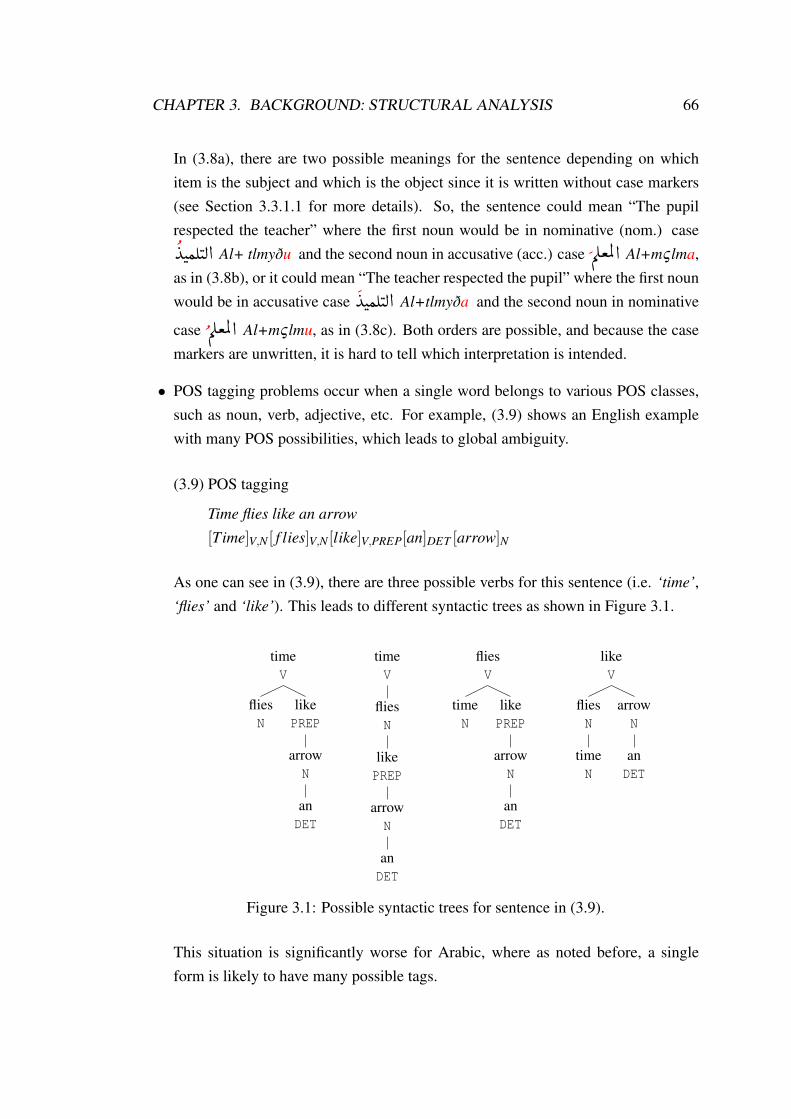
CHAPTER 3. BACKGROUND: STRUCTURAL ANALYSIS 66
In (3.8a), there are two possible meanings for the sentence depending on whichitem is the subject and which is the object since it is written without case markers(see Section 3.3.1.1 for more details). So, the sentence could mean “The pupilrespected the teacher” where the first noun would be in nominative (nom.) case�YJÒÊ
�JË @ Al+ tlmyðu and the second noun in accusative (acc.) case �ÕΪÖÏ @ Al+mς lma,
as in (3.8b), or it could mean “The teacher respected the pupil” where the first nounwould be in accusative case
�YJÒÊ
�JË @ Al+tlmyða and the second noun in nominative
case �ÕΪÖÏ @ Al+mς lmu, as in (3.8c). Both orders are possible, and because the casemarkers are unwritten, it is hard to tell which interpretation is intended.
• POS tagging problems occur when a single word belongs to various POS classes,such as noun, verb, adjective, etc. For example, (3.9) shows an English examplewith many POS possibilities, which leads to global ambiguity.
(3.9) POS tagging
Time flies like an arrow
[Time]V,N [ f lies]V,N [like]V,PREP[an]DET [arrow]N
As one can see in (3.9), there are three possible verbs for this sentence (i.e. ‘time’,‘flies’ and ‘like’). This leads to different syntactic trees as shown in Figure 3.1.
timeV
fliesN
likePREP
arrowN
anDET
timeV
fliesN
likePREP
arrowN
anDET
fliesV
timeN
likePREP
arrowN
anDET
likeV
fliesN
timeN
arrowN
anDET
Figure 3.1: Possible syntactic trees for sentence in (3.9).
This situation is significantly worse for Arabic, where as noted before, a singleform is likely to have many possible tags.

CHAPTER 3. BACKGROUND: STRUCTURAL ANALYSIS 67
• Pronoun-dropping (pro-drop or zero pronouns) problems mean that pronouns canbe deleted when considered redundant or unnecessary in a sentence. Arabic, likeother languages (e.g. Japanese, Spanish and Italian), is considered a pro-drop lan-guage, whereas English is usually not. However, in fact, the English language doesallow both subject and object pronouns to be dropped as shown in (3.10).
(3.10) English pro-drop
φ 1 Keep φ out of the reach of children.
“(You) keep (it) out of the reach of children.”
However, the relatively fixed order of English and the lack of variation in subcate-gorisation frames again mean that it does not tend to lead to ambiguity. In (3.11),however, pro-drop gives rise to two distinct structural analyses.
(3.11) Arabic pro-drop
B@
ñ� I. ËA¢Ë@ φ È A�
sÂl Al+TAlb swAlA
asked the+student question“(He) asked the student a question” or “The student asked a question”
In (3.11), there are two different meanings for the Arabic sentence: “(He) askedthe student a question” (which has a possibility for a pro-drop subject following theverb) or “The student asked a question” (where the verb can be both transitive orditransitive). The difference between Arabic and English is that pro-drop in Arabiccan lead to structural ambiguity because the reader must decide whether there is apro-drop or not, whereas in English it mainly leads to referential ambiguity.
3.2.3 Scope ambiguity
One common type of ambiguity is scoping ambiguity that arises at a logico-semanticlevel. This ambiguity concerns quantifier scope ambiguity, and it can arise when sen-tences include more than one noun phrase that has a quantifier expression such as‘some’, ‘every’, ‘a few’ or others in specific positions. For instance, the sentences in(3.12) and (3.13) are semantically ambiguous (i.e. each sentence has two differentmeanings), but syntactically unambiguous.
1The symbol φ will always show the position of the deleted pronoun.

CHAPTER 3. BACKGROUND: STRUCTURAL ANALYSIS 68
(3.12) English quantifier scope ambiguity
Three students met with every professor.“Three particular students each met all of the professors” or “Each profes-sor was visited by three students, but possibly different students meeting witheach”
(3.13) Arabic quantifier scope ambiguity�ék. Ag. X ÈAg. QË @ É¿ É¿
@
Âkl kl Al+rjAl djAjh
ate all the+men a-chicken“All the men ate the same chicken” or “Each man from those men ate a chicken,but possibly not the same chicken”
3.3 Sources of ambiguities in Arabic
As we have just seen, languages display the same kinds of ambiguity. There are, how-ever, various properties of Arabic, and particularly of written Arabic, which mean thatArabic contains many more instances of ambiguity. These properties will be discussedin some detail below.
3.3.1 Writing system and structure of words
3.3.1.1 Lack of diacritical marks
Arabic is written with optional diacritics2 (short vowels and a range of other phonolog-ical effects), which are usually absent, often leading to multiple ambiguities (Nelkenand Shieber, 2005). This is particularly problematic because the diacritics are oftenthe only difference between different words (especially derived forms) and between
2Diacritisation in Arabic is done by adding special symbols called �HA¿Qk HrkAt “diacritical
marks” to help in spoken language. Some of these special symbols are put above normal Arabic char-acters, such as the short vowels known as Damma ( �
éÖÞ�, �� ,u, /u/), Fatha ( �
éj�J¯, �� ,a, /a/) and a zero
vowel known as Sukun ( àñº�, �P ,.), while others are put under them, such as the short vowel known as
Kasra ( �èQå�», �� ,i, /i/). In addition, nunation diacritics, i.e. Dammatan (Õæ
� áKñ
J�K, �� ,u, /un/), Fathatan
(i�J¯ áKñ
J�K, �� ,ã, /an/) and Kasratan (Qå�» áKñ
J�K, �
�,i, /in/), represent an indefinite morpheme consist-
ing of a short vowel followed by the phoneme /n/. Finally, the lengthening diacritic Shadda ( �èY
��, �P,~)
represents gemination of the previous consonant (Alabbas et al., 2012).

CHAPTER 3. BACKGROUND: STRUCTURAL ANALYSIS 69
inflected forms of the same word. This, consequently, makes morphological analysisof the language very challenging. This is because a certain lemma (or lexeme) in Ara-bic can be interpreted in various ways. Hence, a single word can have various senses,where determining the sense is based on the context in which the word is used. Further-more, a noun in Arabic can be diacritised in three different ways for the nominative,accusative and genitive cases, which can be even more ambiguous at the structural orgrammatical level. The following examples explain the effect of diacritisation on themeaning of the word.
(3.14) Different pronunciations distinguish between a noun and verb
I.�J» ktb
verb: �I.
��J�» kataba “wrote”
noun: I.
��J�» kutub “books”
(3.15) Different pronunciations distinguish between active and passive
i�J¯ ftH
Active: �i
��J�¯ fataHa “opened”
Passive: �i
�J�
�¯ futiHa “was opened”
(3.16) Different pronunciations distinguish between imperative and declarative
©Ò�J�@ Astmς
Imperative: ©Ò�
��J�@ Astamiς “listen!”
Declarative: �©
�Ò
��J�@ Astamaςa “listened”
(3.17) Different pronunciations distinguish between a variety of gender and persondifferences
�IÖÞ�P rsmt��
I�ÖÞ
�� �P rasam.tu Drew (1st.sg.) “I drew”
��I
�ÖÞ
�� �P rasam.ta Drew (2nd.masc.sg.) “You drew”
�I�
�ÖÞ
�� �P rasam.ti Drew (2nd.fem.sg.) “You drew”
��I
�ÖÞ
�� �P rasamat. Drew (3rd.fem.sg.) “She drew”

CHAPTER 3. BACKGROUND: STRUCTURAL ANALYSIS 70
(3.18) Duplication of the middle letter in some verbs to make the verb transitive (causative)(Attia, 2012)
É�ð wSl�
�
��ð waSala “arrived”
�É
���
�ð waS~ala “connect”
Figure 3.2 shows an example for an Arabic word without diacritics ÕΫ ς lm, whichgives seven different readings after adding the diacritic marks.
Arabic diacritics word POS Gloss�ÕΫ
� ς ilmu noun knowledge�Õ�Î
�« ςalamu noun flag
�ÕÎ�
�« ςalima verb (intransitive, active) knew
�ÕÎ�
�« ςulima verb (intransitive, passive) is known
�Õ
��Î
�« ςal~ama verb (transitive, active, indicative) taught
Õ
��Î
�« ςal~im verb (transitive, active, imperative) teach!
�Õ
��Î
�« ςul~ima verb (transitive, passive) is taught
Figure 3.2: Ambiguity caused by the lack of diacritics.
In (3.19), for instance, the sentence (3.19a), �éªÒm.
Ì'@ ÐñK ZAg. jA’ ywm Al+jmς h, hastwo different meanings: “(He) came on Friday” if the word ÐñK ywm is in accusativecase ( �
ÐñK ywma) as in (3.19b), whereas it means “Friday came” if the word ÐñK ywm
is in nominative case ( �ÐñK ywmu) as in (3.19c).
(3.19) Lack of diacritical marks
a. �éªÒm.
Ì'@ ÐñK ZAg.
jA’ ywm Al+jmς h
b. �éªÒm.
Ì'@�ÐñK ZAg. ( �
ÐñK ywma in accusative case)
jA’ ywma Al+jmς h
came Friday“(He) came on Friday”

CHAPTER 3. BACKGROUND: STRUCTURAL ANALYSIS 71
c. �éªÒm.
Ì'@�ÐñK ZAg. ( �
ÐñK ywmu in nominative case)
jA’ ywmu Al+jmς h
came Friday“Friday came”
3.3.1.2 Cliticisation
Arabic is a clitic language. Clitics are morphemes that have the syntactic characteris-tics of a word but are bound to other words (Attia, 2012). Arabic contains numerousclitic items (prepositions, pronouns and conjunctions), so that it is often difficult todetermine just what items are present in the first place. For example, the word úÍ@ð
wAly in (3.20) can be analysed into five different ways (Habash, 2010). Each of thesecases has a different diacritisation. So, a combination of three Arabic words can show200+ alternatives of distinct meaning.
(3.20) Numerous clitic items
úÍ@ð wAly
úÍ@ð wAly “ruler”
ø
+úÍ@+ð w+Aly+y “and to me”
úÍ @+ð w+Aly “and I follow”
ø
+È�@+ð w+Al+y “and my clan”
úÍ�@+ð w+Aly “and automatic”
3.3.2 Syntactic freedom and zero items
3.3.2.1 Word order variation
Arabic is highly syntactically flexible (Daimi, 2001). It has a comparatively free wordorder, where sentence components can be exchanged without affecting the core mean-ing. This results in structural ambiguity, with each morphological analysis having morethan a single meaning. So, besides the regular sentence of VSO, Arabic allows otherpotential surface forms such as VOS, SVO and OVS constructions. The potential ofallowing variations on the canonical order leads to a large amount of ambiguity. AnArabic word order example is shown in (3.21).

CHAPTER 3. BACKGROUND: STRUCTURAL ANALYSIS 72
(3.21) Word order (distinguish between subject and object)
a. �Ê�Ë@ É�J�¯ ù
£Qå
��Ë @ (SVO/OVS)
Al+šrTy qtl Al+lS
the+policeman killed the+thief
b. ��Ê�Ë @ É
�J�¯ �ù
£Qå
��Ë @ (SVO)
Al+šrTyu qtl Al+lSa
the+policeman (nom.) killed the+thief (acc.)“The policeman killed the thief”
c. ��Ê�Ë @ É
�J�¯ �ù
£Qå
��Ë @ (OVS)
Al+šrTya qtl Al+lSu
the+policeman (acc.) killed the+thief (nom.)“The thief killed the policeman”
In (3.21a), there are two possible meanings for the sentence depending on the distinc-tion between nominative subject and accusative object, since the diacritics are missing.So, the sentence means “The policeman killed the thief” where the first noun ù
£Qå
��Ë @
Al+šrTy “the policeman” is in the nominative case �ù£Qå
��Ë @ Al+šrTyu and the second
noun �Ê�Ë@ Al+lS “the thief” is in the accusative case ��Ê�Ë @ Al+lSa, as in (3.21b).
While it means “The thief killed the policeman” where the first noun ù£Qå
��Ë @ Al+šrTy
“the policeman” is in the accusative case �ù£Qå
��Ë @ Al+šrTya and the second noun �Ê�Ë@
Al+lS “the thief” is in the nominative case ��Ê�Ë @ Al+lSu, as in (3.21c).
3.3.2.2 Pro-dropping
Arabic is a pro-drop language (Ryding, 2005). According to the pro-drop theory, “a
null class (pro) is permitted in a finite clause subject place if the agreement features on
the verb are rich enough to enable its content to be recovered” (Baptista, 1995). Thepro-drop, which is referred to as Q�
��J�ÖÏ @ Q�Ò
�Ë@ Al+Dmyr Al+msttr “tacit pronoun”,
can lead to structural ambiguity by leaving any syntactic parser with the challenge todetermine if there is a dropped pronoun or not in the subject position, which is madeworse by the fact that a large number of Arabic verbs can have both transitive andintransitive forms, or ditransitive and transitive forms, or indeed all three. To makematters even worse, it is generally impossible to tell the difference between active andpassive forms by inspecting the surface form. In case that just one NP follows one of

CHAPTER 3. BACKGROUND: STRUCTURAL ANALYSIS 73
these verbs, the ambiguity appears. This contrasts with English, where the canonicalorder is SVO, so that losing the subject does not cause confusion about the object. Forexample, the Arabic sentence in (3.22) has two different interpretations.
(3.22) Arabic pro-drop (Attia, 2012)�ék. A
�g. YË@
�I
�Ê�¿
� @
Âakalat Al+djAjh
ate(fem.) the+chicken“The chicken ate” or “(She) ate the chicken”
The ambiguity in (3.22) arises from two facts: (i) the verb�
É�¿
� @ Âakala “to
eat” can be both transitive or intransitive (in this case the meaning is �ék. A
�g. YË@
�I
�Ê�¿
� @
Âakalat Al+djAjh “The chicken ate”); and (ii) there is a potential pro-drop subjectùë hy “she”, which is understood from the feminine mark on the verb (in this case
the meaning is �ék. Ag. YË@ (ù
ë)
�IÊ¿
@ Âakalat (hy) Al+djAjh “(She) ate the chicken”).
3.3.2.3 Zero copula
A copula is a verb that links a sentence predicate with the subject. According to Arabgrammarians, there are two types of Arabic sentence: a nominal sentence that startswith a noun and a verbal sentence that starts with a verb. There is a special type of anominal sentence called an equational sentence, where the sentence does not containa verb. Basically, the equational sentence consists of two main parts:
@Y
�JJ. ÖÏ @ Al+mbtdÂ
“the subject”, which is NP, and Q�.mÌ'@ Al+xbr “the predicate”, which can be an NP, an
adjective phrase (ADJP), a complement phrase (CP), an adverb phrase (ADVP) or aPP. The equational sentence usually starts with a definite noun (the subject) followedby the predicate. Some Arabic equational sentences are shown in (3.23).
(3.23) Arabic equational sentences
a. I. �J.£ Ég. QË@ (NP predicate)
Al+rjl Tbyb
the+man a-doctor“The man is a doctor”

CHAPTER 3. BACKGROUND: STRUCTURAL ANALYSIS 74
b. I. J£ ÕΪÖÏ @ (ADJ predicate)
Al+mς lm Tyb
the+teacher nice“The teacher is nice”
c. �Ë@ ú
¯ I. ËA¢Ë@ (PP predicate)
Al+TAlb fy Al+Sf
the+student in the+class“The student is in the class”
The standard subject-predicate order for equational sentences is reversed undercertain constraints, for instance if the subject is indefinite, as in (3.24).
(3.24) Indefinite subject follows a predicate phrase
I. ËA£
�Ë@ ú
¯
fy Al+Sf TAlb
in the+class a-student“In the class there is a student”
These appear to be examples where the copula is omitted. This only happens inpresent tense affirmative sentences–if a sentence is in the past, future or present tensenegative the verbs
àA¿ kAn “to be” and ��Ë lys “be not” are used, where they makethe first noun (the subject) in the nominative case and the second noun (the predicate)in the accusative case.
3.3.2.4 Construct phrases
Nouns can be used as adjectives, or as possessive determiners (in so-called ‘constructphrases’ or ‘genitive construct’ or ‘annexation structure’), with typically little inflec-tional morphology to mark such uses (Alabbas and Ramsay, 2011b). According toRyding (2005), “in Arabic, two nouns may be linked together in a relationship where
the second noun determines the first by identifying, limiting, or defining it, and thus
the two nouns function as one phrase or syntactic unit.” Moreover, Arabic nouns canbe linked together without any overt marker, whereas two English nouns are joinedtogether by different markers, such as the suffix “-’s” on possessing noun or a posses-sive phrase “of”. Note that this is largely a problem of written Arabic, since in thespoken language the case markers are generally pronounced, thus making the role ofeach noun clear. Arab grammarians refer to the construct phrase as Idafa, �
é¯A
�@
ADAfh

CHAPTER 3. BACKGROUND: STRUCTURAL ANALYSIS 75
“annexation”. In the construct phrase, the first noun, i.e.
¬A
�Ó mDAf “the added” (inso-called ‘construct state’),3 must be indefinite (which can be in any case: nominative,genitive or accusative) and it does not take the nunation (Schulz et al., 2000). It isfurther worth noting that the initial noun in such phrases will carry the definite form ofthe case marker even though it does not have a definite article. The second noun, i.e.éJË @
¬A
�Ó mDAf Alyh “annexing noun or amplifying noun”, may be either definite
or indefinite (which is always in genitive case). Some construct phrases are shown in(3.25), whereas (3.26) shows an example of a noun as an adjective.
(3.25) Construct phrases (Idafa)
a. È�YªË@ �QK
Pð
wzyru Al+ςdli
minister the+justice“The minister of justice”
b. h
�
C¯ ñK.
@
Âbw flAHi
father Falah“Falah’s father”
c. �� � KQË @
�Èñ�ð
wSwlu Al+ryysi
arrival the+president“The arrival of the president”
(3.26) Noun as adjective
Y�K
��éJ. J
�®k
Hqybhu ydi
a-bag hand“A handbag”
Also, an NP can be the second part of a different construct phrase. This can beextended recursively creating an Idafa chain, where all the words except for the first
3In fact, there are three grammatical states of nouns in Arabic, the indefinite state (e.g. “a queen”),the definite state (e.g. “the queen”) and construct state, which indicates that the noun is the head of aconstruct phrase, (e.g. “the queen of ...”).

CHAPTER 3. BACKGROUND: STRUCTURAL ANALYSIS 76
word must be genitive and all the words except for the last word must be in constructstate. An example of an Idafa chain is illustrated in (3.27).
(3.27) Idafa chain
a. �é�»Qå
��Ë @
�è�P@X@
�� Êm.
× �� � KP P
�Ag.
��ѫ
�áK. @ (Habash, 2010)
Abnu ςm~i jAri ryysi mjlsi AdArhi Al+šrkhi
son uncle neighbour chief committee management the+company“the cousin of the CEO’s neighbour”
b. Y� ÊJ. Ë @�é�Óñºk
��AJ�
��ém�� (Schulz et al., 2000)
SHhu syAshi Hkwmthi Al+bldi
appropriateness policy government the+country“The appropriateness of the policy of the government of the country”
3.3.2.5 Coordination
Coordination in Arabic is either syndetic (i.e. where terms are linked by an explicitconjunction) or asyndetic (i.e. where terms are linked without an explicit conjunc-tion). In case of syndetic conjunction, which is preferred and very common, somelinguistic units are omitted when one or more of the conjunctive particles namely, +ð
w+ “and”, +
¬ f+ “and” and Õç�' θuma “then”, are used to connect words, phrases,
clauses and simple sentences to produce compound or complex sentences. Arabic syn-detic coordination example is illustrated in (3.28).
(3.28) Syndetic coordination
+ ð w+ “and”
�Ó @ Õç'QÓð YK
P h. ð Q�K
tzwj zyd w+mrym Âms
married Zaid and+Maryam yesterday“Zaid and Maryam married yesterday”Who got married yesterday?“Zaid got married to Maryam” or “Zaid got married and so did Maryam”
The second meaning, i.e. “Zaid got married and so did Maryam”, for sentence in (3.28)exemplifies the verbal ellipsis, which refers to syntactically null realisation of a verbof the subsequent clause, of a structurally parallel construction whose meaning can berecovered from the previous clause.

CHAPTER 3. BACKGROUND: STRUCTURAL ANALYSIS 77
3.3.2.6 Referential ambiguity
As mentioned before, a pro-drop in English mainly causes referential ambiguity. Incontrast, in Arabic this type of ambiguity arises when some of the linguistic units areomitted, and replaced by a referring expression to denote these units. Some Arabicreferential ambiguity examples are shown in (3.29).
(3.29) Referential ambiguity
a. Description�é
j�
��Ó Aî
EB
ú
�GPAJ� úΫ ½
�J�. J
�®k ©
�
�� B
lA tDς Hqybtk ς lý syArty lAnhA mtsxh
do-not put your-bag on my-car because-it dirty“Do not put your bag on my car because it is dirty”What is dirty?“Your bag is dirty” or “My car is dirty”
b. The annexationéK. A
�J» AJÊ« YÒm× ù¢«
@
ÂςTý mHmd ς lyA ktAbh
gave Muhammad Ali his-book“Muhammad gave Ali his book”Whose is the book?“Muhammad” or “Ali”
c. Relative clauseYÒm×
�HQîE.
@ ú
�æË @
�éÊJÒm.
Ì'@�èPAJ�Ë@
�H@
X
�ékñÊË@ è
Yë
hðh Al+lwHh ðAt Al+syArh Al+jmylh Alty Âbhrt mHmdthis the+painting of the+car the+beautiful which dazzled Muhammad
“This is the painting of the beautiful car, which dazzled Muhammad”What dazzled Muhammad?“The painting” or “The beautiful car”
In Section 3.3, we have seen several sources of ambiguity in Arabic. Each ofthese in isolation is problematic, but when they are multiplied together their effect be-comes significantly worse. Appendix B shows how even a very short Arabic sentence

CHAPTER 3. BACKGROUND: STRUCTURAL ANALYSIS 78
such as I.�J» �P@YË@ I.
�J» ktb Al+dArs ktb can produce a large number of interpreta-
tions (i.e. 20 interpretations according to the PARASITE system (Ramsay and Man-sour, 2004), such as
�A�J.
��J�»
��P
�@�YË@
�I.
��J�» kataba Al+dArsu kutubAa “The student wrote
books”,�A�J.
��J�»
��P
�@�YË@ I.�
��J�» kutub Al+dAirsu kutubAa “The books of the student (are)
books”, etc.). The situation is much worse as we come to look at longer examples. Inregular usage, the average sentence length of Arabic is 20 to 30 words and sentenceswith 100+ words are not uncommon, since written Arabic rarely contains punctuationmarks even though the Arabic language has them. This makes Arabic NLP challengingin general and specifically the task of determining the relationship between two sen-tences, which is the aim of the current work, significantly more difficult than it alreadyis for English.
3.4 Arabic processing tools
As mentioned before, the Arabic language is more ambiguous than most other lan-guages (e.g. English), which makes Arabic NLP a challenge. Therefore, many toolsare produced in the literature for processing different subtasks of Arabic languageautomatically (e.g. tokenisation, stemming, morphological analysing, POS tagging,parsing, etc.) in order to use them in solving larger tasks, such as machine translation(MT), question answering (QA) and others. In the current work, we will focus only ontwo subtasks: POS tagging, which sometimes internally uses other subtasks, such astokenisation and morphological analysis, and parsing. These two subtasks are consid-ered as preprocessing stages in our main system for Arabic textual entailment (ArbTE)system.
3.4.1 POS tagging
POS tagging is the process of assigning a correct POS tag (e.g. noun, verb or adverb)to each word of a sentence. This is a non-trivial task. It is not just having a set of wordswith their POS tags (e.g. some words are ambiguous, having more than one POS tag atthe same time). Arabic is known for its morphological richness and syntactic complex-ity (Attia, 2012). It is an extremely inflectional language, where inflection is a processthat adds affixes to a word to produce several forms of the same word. For instance,the active inflection of the regular sound verb4 verb �
I.
��J�» kataba “he wrote” (form I:
4Sound verbs do not have a ð w and ø
y as one of the three root letters.

CHAPTER 3. BACKGROUND: STRUCTURAL ANALYSIS 79
�É
�ª
�¯ f aςala -
�É
�ª
�®
�K ya f .ςulu) has 34 forms, which are summarised in Table 3.1, and
another 28 forms for passive. It is also a derivational language, where derivation is aprocess of forming new words from the current words by changing the pattern and themeaning of derivative words as shown in Table 3.2.
Past Present Imperative
3rd
masc.
sg.�
I.
��J�» kataba �
I.
��J�º
�K yak.tubu —
“he wrote” “he writes”
du. AJ.
��J�» katabA
à�
AJ.
��J�º
�K yak.tubAni —
“they wrote” “they write”
pl. @ñ�J.
��J�» katabuwA
�àñJ.
��J�º
�K yak.tubwna —
“they wrote” “they write”
fem.
sg.��
I��.
��J�» katabat. �
I.
��J�º
��K tak.tubu —
“she wrote” “she writes”
du. A�J��.
��J�» katabatA
à�
AJ.
��J�º
��K tak.tubAni —
“they wrote” “they write”
pl.��.
��J�» katab.na
��.
��J�º
�K yak.tub.na —
“they wrote” “they write”
2nd
masc.
sg.��
I��.
��J�» katab.ta �
I.
��J�º
��K tak.tubu �
I.
��J�»
�@ Auk.tub.
“you wrote” “you write” “write!”
du. A��J��.
��J�» katab.tumA
à�
AJ.
��J�º
��K tak.tubAni AJ.
��J�»
�@ Auk.tubA
“you wrote” “you write” “write!”
pl.�Õ
��æ
�J.
��J�» katab.tum.
�àñ
�J.
��J�º
��K tak.tubuwna @ñ
�J.
��J�»
�@ Auk.tubuwA
“you wrote” “you write” “write!”
fem.
sg.�
I�
��.
��J�» katab.ti
�á�J.�
��J�º
��K tak.tubiyna ú
æ.�
��J�»
�@ Auk.tubiy
“you wrote” “you write” “write!”
du. A��J��.
��J�» katab.tumA
à�
A�J.
��J�º
��K tak.tubaAni A
�J.
��J�»
�@ Auk.tubaA
“you wrote” “you write” “write!”
pl.
�����J.
��J�» katab.tun~a
��.
��J�º
��K tak.tub.na
��.
��J�»
�@ Auk.tub.na
“you wrote” “you write” “write!”
1st
masc. sg.��
I��.
��J�» katab.tu �
I.
��J�»
� @ Aak.tubu —
& “I wrote” “I write”fem. du.& A
�J��.
��J�» katab.naA �
I.
��J�º
�K nak.tubu —
pl. “we wrote” “we write”
Table 3.1: The active inflection forms for the regular sound verb �I.
��J�» kataba “he
wrote” (form I:�
É�ª
�¯ f aςala -
�É
�ª
�®
�K ya f .ςulu).

CHAPTER 3. BACKGROUND: STRUCTURAL ANALYSIS 80
Word Morphological pattern Derivative word
I.�J» ktb “to write” Èñª
®Ó mfςwl H. ñ
�JºÓ mktwb “written”
É«A¯ fAς l I.
�KA¿ kAtb “writer”
Table 3.2: The derivative words for word I.�J» ktb “to write”.
3.4.1.1 POS tagsets
The tags should be chosen, in principle, from a well-defined and comprehensive tagset(or list of POS). Traditionally, Arab grammarians classify the words into three cate-gories: Õæ�
@ Asm “noun”, ɪ
¯ fς l “verb” and
¬Qk Hrf “particle”. This classifica-
tion is very coarse and it is not often used computationally, because it does not provideenough information to support further analysis. Arabic POS tagsets can be very big. Ahuge number of (partially orthogonal) features (such as POS, gender, number, clitics,voice, etc.) are determined in order to carry out morphological analysis of a specificword in a specific context. In Arabic, for instance, this can produce around 333,000theoretically potential combinations of morphemes. In contrast, English tagsets havearound 50 tags that cover all morphological variations (Habash, 2010). In fact, thereis no optimal POS tagset, because each application needs a different tagset (Habash,2010). We present here, briefly, three Arabic tagsets that we deal with in the currentwork.
3.4.1.1.1 Buckwalter tagsetThe Buckwalter tagset is an Arabic tagset developed by Tim Buckwalter. It is
a very rich tagset that can be used for tokenised and untokenised text. The to-kenised tags are used in the Penn Arabic treebank (PATB) (Maamouri and Bies, 2004),whereas untokenised tags are what is produced by the Buckwalter Arabic morpho-logical analyser (BAMA) (Buckwalter, 2004). The tokenised variants are derivedfrom untokenised tags. This tagset uses approximately 70 basic subtag symbols(e.g. NOUN ‘noun’, NSUFF ‘nominal suffix’, IND ‘indefinite’ and NOM ‘nominative’)(Habash, 2010). These subtags are combined to form over 170 morpheme tags, suchas NSUFF_FEM_SG ‘feminine singular nominal suffix’ and CASE_IND_NOM ‘nominativeindefinite’. For instance, the Buckwalter tag for the Arabic word �
éÊJ�k HSylh “out-come” is NOUN+NSUFF_FEM_SG+CASE_IND_NOM. A full description of this tagset is pre-sented by Buckwalter (2004).

CHAPTER 3. BACKGROUND: STRUCTURAL ANALYSIS 81
3.4.1.1.2 Reduced tagsetReduced tagset (RTS), also known as the ‘Bies’ tagset, was developed by Ann
Bies and Dan Bikel. It includes 24 tags derived from the POS tagset of thePenn English treebank. It is a coarse tagset since it ignores a lot of distinc-tions in Arabic. For instance, it uses JJ tag for all adjectives regardless oftheir inflections (e.g. the following tags ADJ, DET+ADJ, ADJ+CASE_INDEF_GEN andDET+ADJ+NSUFF_FEM_SG+CASE_DEF_GEN are grouped into JJ). The Arabic word�éÊJ�k HSylh “outcome” is tagged using this tagset as NN ‘noun’. A full descrip-tion of this tagset is presented by Habash (2010, p. 82).
3.4.1.1.3 Extended reduced tagsetThe extended reduced tagset (ERTS) is a superset of RTS tagset. ERTS adds addi-
tional morphological features to those contained in RTS, such as gender, number anddefiniteness. For example, it uses M for ‘masculine’, F for ‘feminine’, Du for ‘dual’and S for ‘plural’, while the absence of any number markers is used for ‘singular’.The Arabic word �
éÊJ�k HSylh “outcome” is tagged using this tagset as NNF. A fulldescription of this tagset is presented by Diab (2007).
3.4.1.2 POS taggers
In this section, we will discuss in some detail two well-known Arabic toolkits, AMIRA(Diab, 2009) and MADA (Habash et al., 2009b), which achieve state-of-the-art accu-racies in Arabic tagging, and a home-grown Arabic MXL tagger (Ramsay and Sabtan,2009), which obtains results that are comparable with these two. In addition, we willdiscuss transformation-based learning (TBL) tagger, or Brill’s tagger (Brill, 1995), forretagging the results of each previous tagger to patch the mistakes. We will use theArabic sentence in (3.30) to show the actual results of each tagger.
(3.30) Arabic sentence
. QÖ�ß
ñÖÏ @ ú
¯
�JkAK.
�é�Ô
g ¼PA
��
šArk xmsh bAHθyn fy Al+mwtmr .
participated five researchers in the+conference .“Five researchers participated in the conference.”

CHAPTER 3. BACKGROUND: STRUCTURAL ANALYSIS 82
3.4.1.2.1 AMIRAThe AMIRA toolkit is a set of tools built as a successor to the ASVMTools (Diab
et al., 2004). It includes three main modules that are briefly reviewed below (Diab,2009).
• AMIRA-TOKThe first module is a clitic tokeniser (AMIRA-TOK). Throughout its processes,AMIRA does not trust in morphological analysis or generation tools. AMIRA-TOKtherefore directly learns the generalisations of clitic tokenisation from the PATB’sclitic segmentation without relying on rules explicitly. AMIRA-TOK segmentsoff the following set of clitics: separating conjunctions, affixival prepositions andpronouns, future mark, proclitic and definite article. AMIRA-TOK has a high F-score of 0.992.
• AMIRA-POS
AMIIRA-POS tagging module produces the following tagsets: RTS, ERTS orERTS_PER (i.e. ERTS with person information) POS tags. POS tagging hereis done using the SVM-based classification approach applying character n-gram asfeatures in the sequence models. AMIRA-POS tagger is reported to achieve over96% accuracy, for ERTS it is 96.13% and RTS 96.15%.
• AMIRA-BPCThis module of AMIRA is a base phrase chunker (BPC), which is the first steptowards shallow syntactic parsing. In this module, a sequence of adjacent words aregrouped together to form a syntactic phrase, such as NPs and VPs. For instance, anEnglish example of BPC would be [I]NP [would eat]V P [red luscious apples]NP [on
Sundays]PP. The longest possible base phrases are produced by the BPC with notmuch internal recursion, which is done as a deterministic post process. The BPCinternally uses ERTS POS tagset even if a user requested the RTS as POS tagset byusing an internal mapping process from RTS to ERTS POS tagset.
AMIRA v2.1 provides three options for running the system. These options are:5
tok-only (run the AMIRA-TOK only), tok+pos (run the AMIRA-TOK and then theAMIRA-POS tagger) and all (run all modules in the following sequence: the AMIRA-TOK, the AMIRA-POS and then the AMIRA-BPC). Figure 3.3 shows the output ofAMIRA for the Arabic sentence in (3.30) using ERTS_PER tagset.
5See AMIRA configuration file in AMIRA-2.1/configs/default.amiraconfig.

CHAPTER 3. BACKGROUND: STRUCTURAL ANALYSIS 83
Input sentence: $Ark xmsp bAHvyn fy Alm&tmr.AMIRA-TOK $Ark xmsp bAHvyn fy Alm&tmr .AMIRA-POS $Ark@@@VBD_MS3 xmsp@@@NNCD_FS bAHvyn@@@NNS_MP fy@@@IN
Alm&tmr@@@DET_NN .@@@PUNCAMIRA-BPC [VP $Ark/VBD_MS3] [NP xmsp/NNCD_FS] [NP bAHvyn/NNS_MP]
[PP fy/IN Alm&tmr/DET_NN] ./PUNC
Figure 3.3: AMIRA output for the Arabic sentence in (3.30).
3.4.1.2.2 MADAMADA6 toolkit is a utility that accepts raw text as input and outputs, in one op-
eration, POS tags, lexemes, diacritisations and full morphological analyses. MADAdistinguishes between morphological analysis problems (handled by morphologicalanalyser) and morphological disambiguation. This toolkit consists of two main partsexplained below (Habash et al., 2009b).
• MADAMADA operates in stages. First, it uses a list of potential analyses for each wordencountered in the text (word context is not considered at this point) provided byBAMA or the standard Arabic morphological analyser (SAMA) (Maamouri et al.,2010). Then, it makes use of up to 19 orthogonal features to rank this list of analysesin order to select a proper analysis for each word in the list. Fourteen morphologicalfeatures out of 19 features that MADA predicts use 14 SVMs that are trained on thePATB. The remaining 5 features capture spelling variations and n-gram statistics.MADA’s analysis consists of the word’s diacritised form, its lexeme, its morpho-logical features and an English glossary entry.
MADA ranks the possible analyses by appending a numerical score to each analysisand sorting these analyses in descending order and the highest score is flagged with‘*’ as correct analysis for that word in the context. Because MADA picks out a fullanalysis from BAMA/SAMA, all decisions concerning morphological ambiguity,lexical ambiguity, tokenisation, diacritisation and POS tagging in any possible POStagset are made in a single step.
MADA internally depends on three resources, which must be installed separately.These resources are: BAMA/SAMA, SRILM7 toolkit (specifically the disambig
utility to construct lexeme n-gram) (Stolcke, 2002) and SVMTools package to op-erate its SVMs (Giménez and Màrquez, 2004).
6This acronym comes from “Morphological Analysis and Disambiguation for Arabic”.7This acronym comes from “Stanford Research Institute Language Modeling”.

CHAPTER 3. BACKGROUND: STRUCTURAL ANALYSIS 84
• TOKENTOKEN is regarded as a general tokeniser for Arabic. It provides an easy-to-useresource for tokenising an Arabic text of MADA-disambiguated items into a wideset of possible tokenisation schemes. In fact, MADA takes the decision on whetheran Arabic word has a conjunction or preposition clitic, whereas if and how such cli-tics are separated is determined by TOKEN (accounting for different morphotacticsand normalisation) before using them in an application.
TOKEN accepts a MADA-disambiguated file as input and a description of a tokeni-sation scheme, which specifies how the tokenisation is done.
TOKEN uses morphological generation (through BAMA/SAMA), internally, torecreate the word once different clitics are separated. This guarantees that the formof the generated word is normalised and consistent with other occurrences of thatword.
MADA tagger is reported to achieve around 97.6% accuracy. Figure 3.4 shows theoutput of MADA for the Arabic sentence in (3.30). In this example the tokenisationwas very straightforward, and the main content relates to the tagger.
3.4.1.2.3 Maximum-likelihood taggerRamsay and Sabtan (2009) produced a maximum-likelihood (MXL) tagger, trained
on Quran, which makes use of very simple clues based on the characters at the be-ginning and end of a word along with transition probabilities between tags, and thenpatches the errors in this initial assignment. We have updated MXL to work with MSAby retraining it on the PATB. This tagger accepts as input a raw or tokenised text andoutputs the text with its POS tag only. We will simply outline the basic principles thatit is based on and note its accuracy here.
MXL operates in two stages, as follows:
• In the first stage we use two simple kinds of statistic:
(i) the conditional likelihood that a word which starts with the same two or threeletters or ends with the same two or three letters as the one we are trying totag has a given tag;
(ii) the transition probabilities between tags. We use a weighted combination ofthese to produce a maximum-likelihood guess at the current tag. This processproduced about 95.2% accuracy when we tested it on PATB.

CHAPTER 3. BACKGROUND: STRUCTURAL ANALYSIS 85
;;; SENTENCE $Ark xmsp bAHvyn fy Alm&tmr .;;WORD $Ark;;MADA: $Ark asp:p cas:na enc0:0 gen:m mod:i num:s per:3 pos:verb prc0:0 prc1:0 prc2:0 prc3:0
stt:na vox:a*1.005981 diac:$Araka lex:$Arak_1 bw:+$Arak/PV+a/PVSUFF_SUBJ:3MS gloss:participate_with;share_with
pos:verb prc3:0 prc2:0 prc1:0 prc0:0 per:3 asp:p vox:a mod:i gen:m num:s stt:na cas:naenc0:0 rat:na source:lex stem:$Arak stemcat:PV
_0.943160 diac:$Ariko lex:$Arak_1 bw:+$Arik/CV+o/CVSUFF_SUBJ:2MS gloss:participate_with;share_withpos:verb prc3:0 prc2:0 prc1:0 prc0:0 per:2 asp:c vox:a mod:i gen:m num:s stt:na cas:naenc0:0 rat:na source:lex stem:$Arik stemcat:CV
;;WORD xmsp;;MADA: xmsp asp:na cas:n enc0:0 gen:f mod:na num:s per:na pos:noun_num prc0:0 prc1:0 prc2:0
prc3:0 stt:c vox:na*0.979649 diac:xamosapu lex:xamos_1 bw:+xamos/NOUN_NUM+ap/NSUFF_FEM_SG+u/CASE_DEF_NOM gloss:five
pos:noun_num prc3:0 prc2:0 prc1:0 prc0:0 per:na asp:na vox:na mod:na gen:f num:s stt:ccas:n enc0:0 rat:y source:lex stem:xamos stemcat:Nap
_0.963989 diac:xamosapi lex:xamos_1 bw:+xamos/NOUN_NUM+ap/NSUFF_FEM_SG+i/CASE_DEF_GEN gloss:fivepos:noun_num prc3:0 prc2:0 prc1:0 prc0:0 per:na asp:na vox:na mod:na gen:f num:s stt:ccas:g enc0:0 rat:y source:lex stem:xamos stemcat:Nap
... 12 additional options omitted ...;;WORD bAHvyn;;MADA: bAHvyn asp:na cas:g enc0:0 gen:m mod:na num:p per:na pos:noun prc0:0 prc1:0 prc2:0 prc3:0
stt:i vox:na*1.000161 diac:bAHiviyna lex:bAHiv_1 bw:+bAHiv/NOUN+iyna/NSUFF_MASC_PL_GEN gloss:scholar;researcher
pos:noun prc3:0 prc2:0 prc1:0 prc0:0 per:na asp:na vox:na mod:na gen:m num:p stt:i cas:genc0:0 rat:y source:lex stem:bAHiv stemcat:Nall
_0.966692 diac:bAHiviyna lex:bAHiv_1 bw:+bAHiv/ADJ+iyna/NSUFF_MASC_PL_GEN gloss:searching pos:adjprc3:0 prc2:0 prc1:0 prc0:0 per:na asp:na vox:na mod:na gen:m num:p stt:i cas:g enc0:0rat:y source:lex stem:bAHiv stemcat:Nall
... 6 additional options omitted ...;;WORD fy;;MADA: fy asp:na cas:na enc0:0 gen:na mod:na num:na per:na pos:prep prc0:na prc1:0 prc2:0 prc3:0
stt:na vox:na*1.033497 diac:fiy lex:fiy_1 bw:+fiy/PREP+ gloss:in pos:prep prc3:0 prc2:0 prc1:0 prc0:na per:na
asp:na vox:na mod:na gen:na num:na stt:na cas:na enc0:0 rat:na source:lex stem:fiystemcat:FW-Wa
_0.914319 diac:fiy~a lex:fiy_1 bw:+fiy/PREP+ya/PRON_1S gloss:in pos:prep prc3:0 prc2:0 prc1:0prc0:na per:na asp:na vox:na mod:na gen:na num:na stt:na cas:na enc0:1s_pron rat:nasource:lex stem:fiy stemcat:FW-Wa-y
... 5 additional options omitted ...;;WORD Alm&tmr;;MADA: Alm&tmr asp:na cas:g enc0:0 gen:m mod:na num:s per:na pos:noun prc0:Al_det prc1:0 prc2:0
prc3:0 stt:d vox:na*1.019825 diac:Almu&otamari lex:mu&otamar_1 bw:Al/DET+mu&otamar/NOUN+i/CASE_DEF_GEN
gloss:conference;convention pos:noun prc3:0 prc2:0 prc1:0 prc0:Al_det per:na asp:na vox:namod:na gen:m num:s stt:d cas:g enc0:0 rat:y source:lex stem:mu&otamar stemcat:NduAt
_0.948217 diac:Almu&otamara lex:mu&otamar_1 bw:Al/DET+mu&otamar/NOUN+a/CASE_DEF_ACCgloss:conference;convention pos:noun prc3:0 prc2:0 prc1:0 prc0:Al_det per:na asp:na vox:namod:na gen:m num:s stt:d cas:a enc0:0 rat:y source:lex stem:mu&otamar stemcat:NduAt
... 2 additional options omitted ...;;WORD .;;MADA: . asp:na cas:na enc0:na gen:na mod:na num:na per:na pos:punc prc0:na prc1:na prc2:na
prc3:na stt:na vox:na*1.045299 diac:. lex:._0 bw:./PUNC gloss:. pos:punc prc3:na prc2:na prc1:na prc0:na per:na asp:na
vox:na mod:na gen:na num:na stt:na cas:na enc0:na rat:na source:puncSENTENCE BREAK
Figure 3.4: MADA output for the sentence in (3.30). For each word, the predicationsof the SVM classifiers are indicated by ‘;;MADA’ line. Each analysis is preceded by itsscore, while the selected analysis is marked with ‘*’. For each word in the sentence,only the two top scoring analyses are shown because of the space limitation.
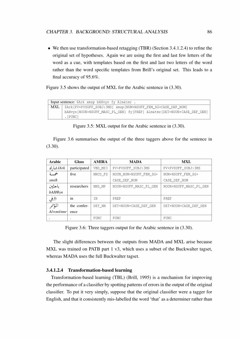
CHAPTER 3. BACKGROUND: STRUCTURAL ANALYSIS 86
• We then use transformation-based retagging (TBR) (Section 3.4.1.2.4) to refine theoriginal set of hypotheses. Again we are using the first and last few letters of theword as a cue, with templates based on the first and last two letters of the wordrather than the word specific templates from Brill’s original set. This leads to afinal accuracy of 95.6%.
Figure 3.5 shows the output of MXL for the Arabic sentence in (3.30).
Input sentence: $Ark xmsp bAHvyn fy Alm&tmr .MXL $Ark[PV+PVSUFF_SUBJ:3MS] xmsp[NUM+NSUFF_FEM_SG+CASE_DEF_NOM]
bAHvyn[NOUN+NSUFF_MASC_PL_GEN] fy[PREP] Alm&tmr[DET+NOUN+CASE_DEF_GEN].[PUNC]
Figure 3.5: MXL output for the Arabic sentence in (3.30).
Figure 3.6 summarises the output of the three taggers above for the sentence in(3.30).
Arabic Gloss AMIRA MADA MXL¼PA
�� šArk participated VBD_MS3 PV+PVSUFF_SUBJ:3MS PV+PVSUFF_SUBJ:3MS
�é�Ô
g
xmshfive NNCD_FS NOUN_NUM+NSUFF_FEM_SG+
CASE_DEF_NOM
NUM+NSUFF_FEM_SG+
CASE_DEF_NOMá�
�JkAK.
bAHθynresearchers NNS_MP NOUN+NSUFF_MASC_PL_GEN NOUN+NSUFF_MASC_PL_GEN
ú
¯ fy in IN PREP PREP
QÖ�ß
ñÖÏ @
Al+mwtmrthe confer-ence
DET_NN DET+NOUN+CASE_DEF_GEN DET+NOUN+CASE_DEF_GEN
. . PUNC PUNC PUNC
Figure 3.6: Three taggers output for the Arabic sentence in (3.30).
The slight differences between the outputs from MADA and MXL arise becauseMXL was trained on PATB part 1 v3, which uses a subset of the Buckwalter tagset,whereas MADA uses the full Buckwalter tagset.
3.4.1.2.4 Transformation-based learningTransformation-based learning (TBL) (Brill, 1995) is a mechanism for improving
the performance of a classifier by spotting patterns of errors in the output of the originalclassifier. To put it very simply, suppose that the original classifier were a tagger forEnglish, and that it consistently mis-labelled the word ‘that’ as a determiner rather than

CHAPTER 3. BACKGROUND: STRUCTURAL ANALYSIS 87
a complementiser in situations where the preceding word was a verb and the followingword was a pronoun (e.g. in examples like “I know that she loves me”). Then a typicalimplementation of TBL would introduce a rule that said “if ‘that’ has been labelled as
DT and the preceding word is a verb and the following word is a pronoun then relabel
it as COMP.”
The key to the success of this notion is the presence of a suitable set of rule tem-plates. Brill’s original templates are represented by Lager (1999) as Prolog rules ofthe kind shown below:
t1(A,B,C)
# tag:A>B
<- tag:C@[-1].
...
t5(A,B,C)
# tag:A>B
<- tag:C@[-1,-2].
...
t9(A,B,C,D)
# tag:A>B
<- tag:C@[-1] & tag:D@[1].
...
The first of these says that you can have rules that will retag an item whose tag is Aas B if the tag of the preceding word is C. Thus this template might be instantiated to
t1(det,comp,verb)
# tag:det>comp
<- tag:verb@[-1].
in order to retag an item from DET to COMP if the preceding word was a VERB (i.e. this isa rather extreme case of a rule for patching cases like the one involving ‘that’ above).
The standard algorithm explores all instantiations of every template to find theone that produces the greatest net improvement in the tagset (a rule that changes 100incorrect tags to correct ones and 30 correct ones to incorrect ones produces a net gainof 70, and hence is better than one that changes 65 incorrect tags to correct ones andintroduces no new errors (net gain 65) or one that makes 110 improvements and 50new errors (net gain 60)). This rule is then applied to the entire training set, and the
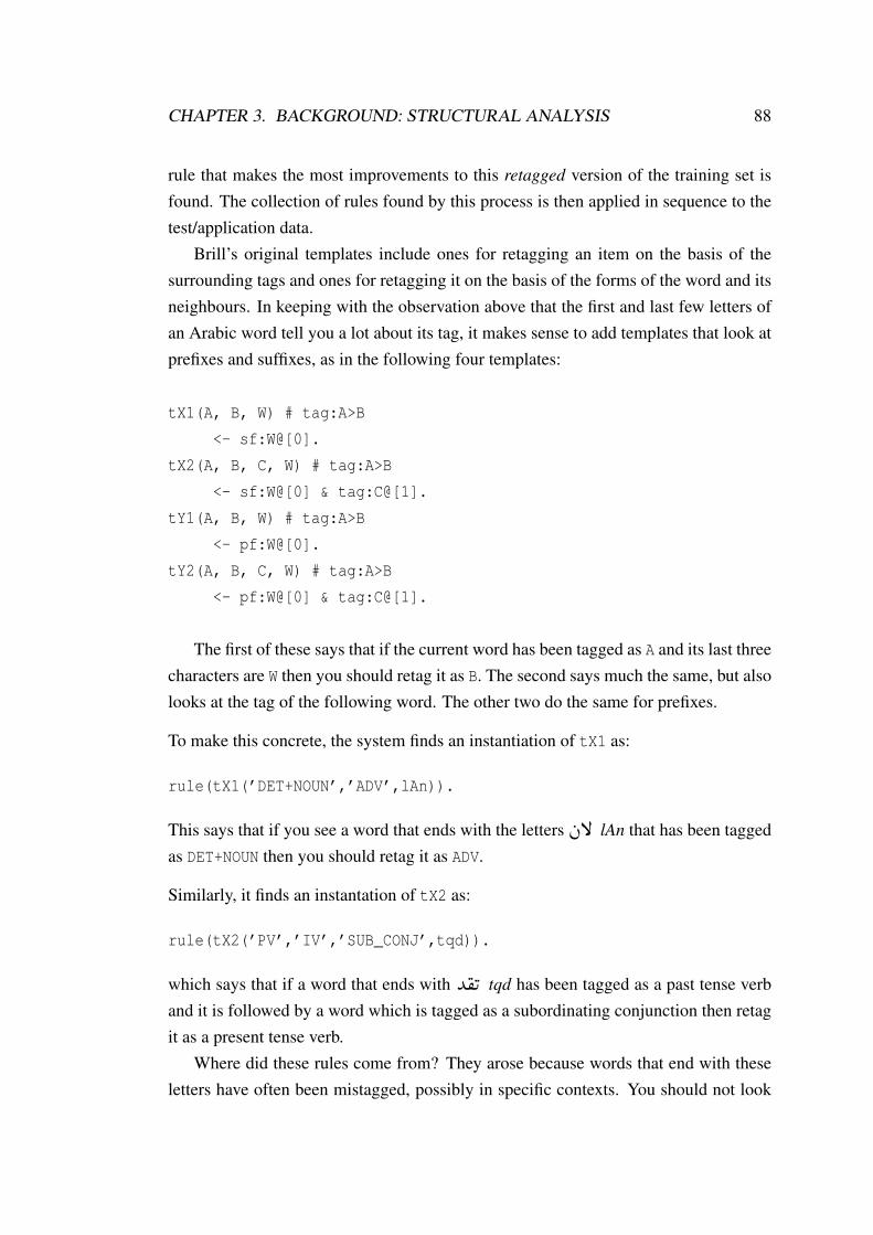
CHAPTER 3. BACKGROUND: STRUCTURAL ANALYSIS 88
rule that makes the most improvements to this retagged version of the training set isfound. The collection of rules found by this process is then applied in sequence to thetest/application data.
Brill’s original templates include ones for retagging an item on the basis of thesurrounding tags and ones for retagging it on the basis of the forms of the word and itsneighbours. In keeping with the observation above that the first and last few letters ofan Arabic word tell you a lot about its tag, it makes sense to add templates that look atprefixes and suffixes, as in the following four templates:
tX1(A, B, W) # tag:A>B
<- sf:W@[0].
tX2(A, B, C, W) # tag:A>B
<- sf:W@[0] & tag:C@[1].
tY1(A, B, W) # tag:A>B
<- pf:W@[0].
tY2(A, B, C, W) # tag:A>B
<- pf:W@[0] & tag:C@[1].
The first of these says that if the current word has been tagged as A and its last threecharacters are W then you should retag it as B. The second says much the same, but alsolooks at the tag of the following word. The other two do the same for prefixes.
To make this concrete, the system finds an instantiation of tX1 as:
rule(tX1(’DET+NOUN’,’ADV’,lAn)).
This says that if you see a word that ends with the letters àB lAn that has been tagged
as DET+NOUN then you should retag it as ADV.
Similarly, it finds an instantation of tX2 as:
rule(tX2(’PV’,’IV’,’SUB_CONJ’,tqd)).
which says that if a word that ends with Y�®�K tqd has been tagged as a past tense verb
and it is followed by a word which is tagged as a subordinating conjunction then retagit as a present tense verb.
Where did these rules come from? They arose because words that end with theseletters have often been mistagged, possibly in specific contexts. You should not look
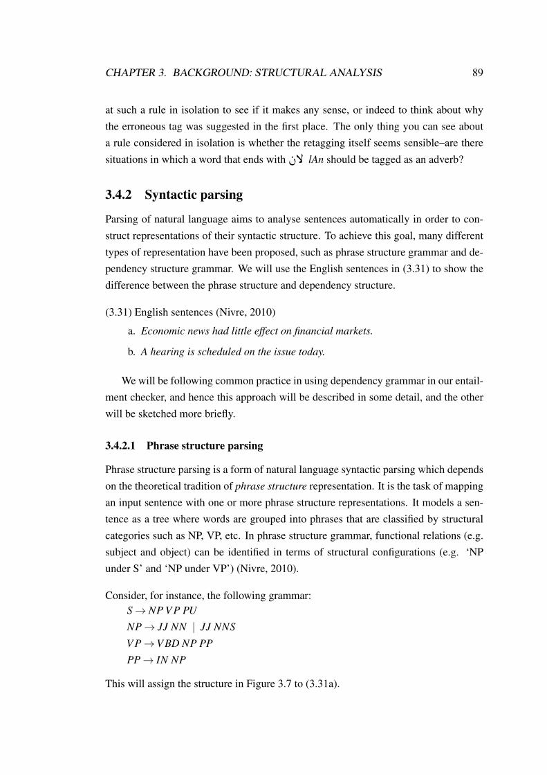
CHAPTER 3. BACKGROUND: STRUCTURAL ANALYSIS 89
at such a rule in isolation to see if it makes any sense, or indeed to think about whythe erroneous tag was suggested in the first place. The only thing you can see abouta rule considered in isolation is whether the retagging itself seems sensible–are theresituations in which a word that ends with
àB lAn should be tagged as an adverb?
3.4.2 Syntactic parsing
Parsing of natural language aims to analyse sentences automatically in order to con-struct representations of their syntactic structure. To achieve this goal, many differenttypes of representation have been proposed, such as phrase structure grammar and de-pendency structure grammar. We will use the English sentences in (3.31) to show thedifference between the phrase structure and dependency structure.
(3.31) English sentences (Nivre, 2010)
a. Economic news had little effect on financial markets.
b. A hearing is scheduled on the issue today.
We will be following common practice in using dependency grammar in our entail-ment checker, and hence this approach will be described in some detail, and the otherwill be sketched more briefly.
3.4.2.1 Phrase structure parsing
Phrase structure parsing is a form of natural language syntactic parsing which dependson the theoretical tradition of phrase structure representation. It is the task of mappingan input sentence with one or more phrase structure representations. It models a sen-tence as a tree where words are grouped into phrases that are classified by structuralcategories such as NP, VP, etc. In phrase structure grammar, functional relations (e.g.subject and object) can be identified in terms of structural configurations (e.g. ‘NPunder S’ and ‘NP under VP’) (Nivre, 2010).
Consider, for instance, the following grammar:S→ NP V P PU
NP→ JJ NN | JJ NNS
V P→V BD NP PP
PP→ IN NP
This will assign the structure in Figure 3.7 to (3.31a).

CHAPTER 3. BACKGROUND: STRUCTURAL ANALYSIS 90
SS
VPVP
NPNP
PPPP
NPNP
JJJJ
NNSNNS
PUPU
ININ
NNNN
JJJJ
NPNP
JJJJ
NNNN
VBDVBD
financialfinancial
marketsmarkets
..
onon
effecteffect
littlelittle
EconomicEconomic
newsnews
hadhad
Figure 3.7: Phrase structure tree for (3.31a) (Nivre, 2010).
3.4.2.2 Dependency parsing
Dependency parsing is a syntactic parsing form that depends on the theoretical traditionof dependency grammar. It is the task of mapping an input sentence to a dependencytree. It models a sentence as a graph (often, but not always a tree) where words arevertices and grammatical functions (or syntactic relations) are directed edges (or de-pendency relations). Each vertex therefore has a single parent, except the root of thetree. A dependency relation holds between dependent, i.e. a syntactically subordinatevertex, and head, i.e. another vertex on which it is dependent. So, the dependencystructure represents head-dependent relations between vertices that are classified bydependency types such as SBJ ‘subject’, OBJ ‘object’, ATT ‘attribute’, etc. Depen-dency parsing is thus viewed computationally as a structured prediction problem withtrees as structured variables. Each sentence, in principle, has exponentially many can-didate dependency trees. Figure 3.8 shows the dependency tree for (3.31a), where thearrows between pairs of vertices represent the dependency relations pointing from thehead to dependent, while the labels on arrows indicate the dependency types.
Formally speaking, for an input sentence with n words S = w1, . . . ,wn, a legal de-pendency tree is T = (V,A), consisting of a set V of vertex V ⊆ {ROOT0,w1, . . . ,wn}and a set A of dependency relations A ⊆ V ×R×V , R is a set of dependency typesR ⊆ {r1, . . . ,rn−1}, if (wi,r,w j) ∈ A then (wi,r′,w j) 6∈ A for all r 6= r′. The depen-dency tree has n+1 vertices, each vertex corresponds to a word in the sentence plus theartificial root vertex (ROOT0), i.e. for any i≤ n (i,r,0) 6∈ A. Since the structure of a de-pendency tree is acyclic, which means it does not contain cycles, i.e. for all wi,w j ∈ A,

CHAPTER 3. BACKGROUND: STRUCTURAL ANALYSIS 91
Figure 3.8: Projective dependency tree for (3.31a) (Nivre, 2010).
if wi → w j, then it is not the case that w j →∗ wi (Kübler et al., 2009). For example,we can define the sets of vertices and dependency relations from the dependency treeshown in Figure 3.8 as follows:
V= {ROOT, Economic, news, had, little, effect, on, financial, markets, .}A= {(ROOT, PRED, had), (news, ATT, Economic), (had, SBJ, news),
(effect, ATT, little), (had, OBJ, effect), (effect, ATT, on),(markets, ATT, financial), (on, PC, markets), (had, PU, .)}
Here, the verb ‘had’ is the head of the noun ‘news’ with the dependency type SBJ.The same verb ‘had’ also heads another noun ‘effect’ with another dependency typeOBJ.
A dependency tree is either projective, if dependency arcs do not cross when de-picted on one side of the sentence (i.e. every vertex has a continuous projection) asshown in Figure 3.8, or non-projective, if the previous constraint is not satisfied, asshown in Figure 3.9. More formally, a tree is considered projective, if and only if forevery dependency arc (i,r, j) ∈ A and node x ∈V, i < x < j or j < x < i then there is asubset of dependency arcs {(i,r, i1),(i1,r1, i2), . . . ,(ix−1,rx−1, ix)} ∈ A such that ix = x.
Figure 3.9: Non-projective dependency tree for (3.31b) (Nivre, 2010).

CHAPTER 3. BACKGROUND: STRUCTURAL ANALYSIS 92
In recent years, there has been a considerable interest in dependency parsing. Thereare a number of reasons for this. First, dependency-based syntactic representationsseem to be effective in many areas of NLP, such as machine translation (MT), informa-tion extraction (IE) and textual entailment (TE), thanks to their transparent encodingof predicate-argument structure (Alabbas and Ramsay, 2011b). Second, it is generallyperceived that dependency grammar is better suited than phrase structure grammar forflexible or free word order languages, such as Arabic, Czech, and so on (Alabbas andRamsay, 2011a). Third, and most importantly, the dependency-based approach hasled to the development of fast, robust and reasonably accurate syntactic parsers for anumber of languages.
Broadly speaking, dependency parsing may be either data-driven or grammar-based. In the current work, we focus on supervised data-driven dependency parsers,which presuppose that input sentences to machine learning have been annotated withtheir correct dependency structures. There are two different problems in superviseddependency parsers that need to be solved computationally: learning problem andparsing problem (or inference problem) (Kübler et al., 2009). These problems are rep-resented as follows:
• Learning: given a training set of sentences D that are annotated with their depen-dency structure, induce a parsing model M that can be used to parse new sentencesSi=1..n.
• Parsing: given a parsing model M and sentences Si=1..n, derive the optimal depen-dency graph Gi for each sentence Si according to M.
We will focus here on two state-of-the-art language independent data-driven parsers,as described below.
3.4.2.2.1 MALTParserMALTParser8 is a language independent system for data-driven dependency pars-
ing that can be used to induce a parsing model from a dependency treebank for anylanguage. Then, it uses this induced parsing model to parse new data for that lan-guage (Nivre et al., 2007). It is categorised, according to the categorisation of parsersby Kübler et al. (2009), as a transition-based parsing system based on the theoretical
8This acronym comes from “Models and Algorithms for Language Technology Parser”. Freelyavailable at: http://www.maltparser.org/.

CHAPTER 3. BACKGROUND: STRUCTURAL ANALYSIS 93
framework of inductive dependency parsing (which depends on an algorithm of de-terministic parsing in combination with inductive machine learning to predict the nextaction of the parser) presented by Nivre (2006). Transition-based parsers model thesequence of decisions of a shift-reduce parser to predict the next state of the system,given the current state and features over parsing decisions’ history as well as the inputsentence. The parser, at inference time, starts with an initial state and based on thepredictions of the model, the parser greedily moves to subsequent states until reachinga termination state. The parsing methodology depends on three main components:9
• Deterministic parsing algorithms, which are defined in terms of a transition system,in order to construct labeled dependency graphs (Yamada and Matsumoto, 2003;Nivre, 2003). The transition system consists of a set of configurations and a set oftransitions between configurations. Deterministic parsing is implemented duringthe transition system as greedy best-first search.
• History-based models for predicting the next parser action at nondeterministic choicepoints (Ratnaparkhi, 1997; Collins, 2003). The transition history is represented bya feature vector, which can be used as input to a classifier for predicting the nexttransition in order to guide the deterministic parser (Hall, 2008).
• Discriminative learning to map histories to parser actions (Yamada and Matsumoto,2003; Hall et al., 2006). Discriminative machine learning can be used to train a clas-sifier when it is given a set of transition sequences derived from a treebank. Duringparsing, the classifier is used to distinguish between different possible transitionsgiven a feature vector representation of the current configuration.
MALTParser supports both projective and non-projective parsing. It implementsnine deterministic parsing algorithms. These algorithms are: Nivre arc-eager, Nivrearc-standard, Covington non-projective, Covington projective, Stack projective, Stackswap-eager, Stack swap-lazy, Planar and 2-Planar. It also supports two machine learn-ing algorithms: LIBSVM10 (Chang and Lin, 2011) and LIBLINEAR11 (Fan et al.,2008).
According to the observation of McDonald and Nivre (2007), MALTParser per-forms better on dependencies that are further from the root of a tree (e.g. pronouns,nouns dependencies) and those with shorter dependencies.
9The following characterisation is taken from the MALTParser documentation.10This acronym comes from “Library for Support Vector Machines”.11This acronym comes from “Library for Large Linear Classification”.

CHAPTER 3. BACKGROUND: STRUCTURAL ANALYSIS 94
Users can also turn MALTParser into a phrase structure parser, which parses con-tinuous and discontinuous phrases with both phrase labels and grammatical functions(Bhatt and Xia, 2012; Hall and Nivre, 2008a,b).
3.4.2.2.2 MSTParserMaximum-spanning tree parser (MSTParser)12 is a language independent system
for data-driven dependency parsing, which can be used to induce a parsing model fromtreebank data and to parse new data using an induced model (McDonald and Pereira,2006). It is categorised, according to the categorisation of parsers in (Kübler et al.,2009), as a graph-based parsing system. It is also a parser generator for dependencyparsing, which can be used to create a parser for any language by giving it a depen-dency treebank of this language. A graph-based parser defines a candidate dependencygraph space for a sentence. In the learning stage, the parser assigns, for each sentence,scores to the candidate dependency graphs in order to induce a parsing model M. In theparsing stage, the parser finds, for each input sentence, the highest scoring dependencygraph, given the parsing model M. This method is commonly called maximum span-ning tree parsing because the problem of finding the highest scoring dependency graphand the problem of finding a maximum spanning tree in a dense graph are equivalent,under certain assumptions. This allows the parser to find solutions for both projectiveand non-projective trees.
Typically, MSTParser depends on global training and inference algorithms. Theaim here is to learn models in which correct trees have higher weights than the weightsof incorrect trees. A global search is run in order to find the highest weighted depen-dency tree. This operation typically is NP-hard (McDonald and Satta, 2007). Thisoften requires the scope of MSTParser features to be limited to a tiny number (usuallytwo) and/or resort to approximate inference (McDonald and Pereira, 2006).
According to the observation of McDonald and Nivre (2007), MSTParser performsbetter on dependencies that are closer to the root of a tree (e.g. verbs, conjunctions andprepositions dependencies) and those with longer dependencies.
In Section 3.4, we have described three Arabic taggers and two machine learningparsers, which have achieved state-of-the-art results for a number of languages such asEnglish and Arabic (Kübler et al., 2009). We will use them in our preprocessing stage(Chapter 4) to convert T-H pairs from natural expressions into dependency trees.
12Freely available at: http://www.seas.upenn.edu/~strctlrn/MSTParser/MSTParser.html.

Chapter 4
Arabic linguistic analysis
4.1 Introduction
In this chapter we present a preprocessing stage for our Arabic textual entailment(ArbTE) system. This stage is responsible for converting both elements of an Ara-bic T-H pair from raw texts into dependency trees. It consists of two main subtasks:POS tagging, which internally uses other subtasks, such as tokenisation and morpho-logical analysis, and parsing. In order to achieve this goal, three state-of-the-art Arabictaggers (see Section 3.4.1.2) and two state-of-the-art language-independent data-drivendependency parsers (see Section 3.4.2.2) are used. The PATB is used as training andtesting data for experiments as explained below.
We have a task, structural analysis, which involves two linked subtasks, taggingand parsing, and we have several tools that can carry out each of the subtasks. Howthese tools work is not our concern here. For us they are simply black-boxes whichrequire an input in order to give us an output. What does matter here is how to improvethe performance of the overall task. We are therefore going to try to improve theperformance of the standard components by varying parameters and combining theminstead of improving each component itself.
In order to improve the performance of the overall task, we will investigate twostrategies: (i) combined strategy I: in this strategy, there is one pipeline of processesthat consists of two consecutive subtasks, i.e. combined taggers and combined parsers.In this strategy, we will receive a raw text as input to the pipeline and tag this text bycombined taggers (Section 4.2) to produce tagged text, which is the input to the nextsubtask, combined parsers (Section 4.3), to produce the final parsed tree as shown inFigure 4.1a; and (ii) combined strategy II: in this strategy, there are two pipelines of
95

CHAPTER 4. ARABIC LINGUISTIC ANALYSIS 96
processes, where each pipeline consists of two consecutive subtasks, individual tag-ger and individual parser. In this strategy, we will receive a raw text as input for bothpipelines and tag this text using the tagger of each pipeline. Then, each parser willreceive its own tagged text to produce its own parsed tree. The final parsed tree willrepresent the combined parsed trees for both pipelines (Section 4.4) as shown in Fig-ure 4.1b.
In Section 4.2 and Section 4.3 we will discuss the results of combined strategy I,and in Section 4.4 we will discuss the results of combined strategy II.
Raw text
Combined taggers
Tagged text
Combined parsers
Parsed tree
Raw text
Tagger1
Tagged text1
Parser1
Parsed tree
Tagger2
Tagged text2
Parser2
Recombination
Parsed tree1 Parsed tree2
(a) Combined strategy I (b) Combined strategy II
Figure 4.1: Two combined taggers and parsers strategies.
In order to check the effectiveness of the POS taggers, the parsers and our tech-niques, we use four common evaluation measures:
• Precision (P)A measure of the ability of a system to present only correctly labelled items, as inEquation 4.1.
P =number o f correctly labelled items retrieved
total number o f items retrieved. (4.1)

CHAPTER 4. ARABIC LINGUISTIC ANALYSIS 97
• Recall (R)A measure of the ability of a system to present all correctly labelled items, as inEquation 4.2.
R =number o f correctly labelled items retrieved
number o f items in collection. (4.2)
• F-scoreF-score is a measure of a test’s accuracy. The general formula for positive real β isexplained in Equation 4.3.
Fβ = (1+β2)× P×R
(β 2×P)+R. (4.3)
The traditional measure is the F-score (or F1), which is the harmonic mean of pre-cision and recall as in Equation 4.4.
F-score = 2× P×RP+R
. (4.4)
The F1-score can be interpreted as a weighted average of the precision and recall,where an F1-score reaches its best value at 1 and worst value at 0.
• AccuracyIf every item is assigned a label, then precision and recall are the same. Under thoseconditions, it is common practice to refer to this single value as accuracy.
4.2 POS tagging
The process of assigning a correct POS tag (i.e. noun, verb, adverb or others) to eachword of a sentence is called POS tagging. This process is considered an essentialstep for most natural language applications. In general, however, POS taggers makemistakes, and since tagging is the first step in most NLP systems these mistakes willlead to problems in all subsequent stages of analysis. It is thus important to obtain thehighest possible accuracy at this initial stage of processing.

CHAPTER 4. ARABIC LINGUISTIC ANALYSIS 98
4.2.1 The taggers
We are interested here in improving POS tagging accuracy. We have carried out anumber of experiments with state-of-the-art taggers (AMIRA 2.0 (Section 3.4.1.2.1),MADA 3.1 (Section 3.4.1.2.2) and a home-grown tagger, MXL, with comparable ac-curacy (Section 3.4.1.2.3)), using the PATB (Maamouri and Bies, 2004) as a gold-
standard corpus.
Gold-standard tags
We used PATB (Part 1 v3 using ‘without-vowel’ set of trees)1 as a resource for ourexperiments. The words in the PATB are already tagged. This provides us with abenchmark to evaluate the consequences of using taggers that do not provide 100%accuracy: we are unlikely to achieve higher accuracy when we tag the test sets usingone of the taggers below than we obtain when we use the original tags of the PATB.In subsequent discussion we refer to the tags we obtain this way as gold-standard tags.Even these tags are not guaranteed to be 100% accurate–they have been obtained bysome mixture of automatic and manual tagging, and both of these are liable to error.However, this is the most accurate available set of tags, and furthermore any systematicerrors will also appear in the training set, and hence may be compensated for when theparsers are trained. We use this set for reference–if for some experiment we obtainN accuracy with the gold tags and N′ using one of the taggers then we know that thetagger has introduced an error of N−N′.
The PATB uses a very fine-grained set of tags, which carry a great deal of syntac-tically relevant information (particularly case-marking). In particular, case-marking,and to a lesser extent number and gender marking, in Arabic is carried by diacriticswhich are unwritten in normal text. Thus the only way to extract this information isby making guesses based on the syntactic context. Given that the task of the parser isto determine the syntactic context, it is hard to see how reliable guesses about it canbe made prior to parsing. Marton et al. (2010, 2013), for instance, note that addingthe case-marking tags supplied by MADA actually decreases the accuracy of parsing,because the parser gives considerable weight to them, but the tagger only manages toassign them correctly in 86% of cases. A feature which is both significant and hard todetermine is not a reliable cue.
1Catalog number LDC2005T02 from the Linguistic Data Consortium (LDC). Available at: http://www.ldc.upenn.edu/Catalog/catalogEntry.jsp?catalogId=LDC2005T02

CHAPTER 4. ARABIC LINGUISTIC ANALYSIS 99
We therefore collapsed this very fine-grained set of 305 tags, which appear in theversion of the PATB used here, to a more coarse-grained set with 39 distinct tags, asshown in Figure 4.2. Reducing the granularity of the PATB tagset is fairly commonpractice, since some of the most fine-grained tags are very hard indeed to distinguishsimply on the basis of local clues, which are what most taggers depend on. Unfor-tunately there is no universally accepted coarse-grained version, so we simply madewhat seemed like a reasonable compromise. We will return to this in Section 4.4. Thedifferences between these two tagsets are illustrated in Figure 4.3, where the coarseset has one entry for imperfective verbs and the fine one has 44, of which a few 1stperson cases are included in Figure 4.3, and the coarse set has one entry for nouns andthe fine one has 47, differing mainly in case and gender markers. It is worth notingthat many of the distinctions made in the fine-grained tagset are invisible in the writtenform–feminine nouns, for instance, do not carry distinctive case markers. Tagging withthe fine-grained tagset is therefore likely to be extremely difficult. The final version ofour tagger ‘MC’ achieves around 99.5% accuracy on the coarse-grained tagset (see Ta-ble 4.7), which is significantly better than the performance of other taggers (Al Shamsiand Guessoum, 2006; AlGahtani et al., 2009; El Hadj et al., 2009; Diab et al., 2004)on this kind of tagset, whereas we achieve 96% with the full 305 tags (MADA, for in-stance, obtains 96.6% on the coarse-grained tagset but only 93.6% on the fine-grained(351-element) one).
ABBREVADJADVCONJ/ICONJCVCVSUFF_DODEM_PRONDETDET+ADJDET+NOUN
DET+NOUN_PROPDET+NUMEMPH_PARTEXCEPT_PARTFOCUS_PARTFUT+IVINTERJINTERROG_PARTIVIVSUFF_DO
LATINNEG_PARTNOUNNOUN_PROPNO_FUNCNUMPARTPOSS_PRONPREPPRON
PUNCPVPVSUFF_DORC_PARTREL_ADVREL_PRONSUBSUB_CONJVERB_PART
Figure 4.2: Our coarse-grained tagset.
AMIRA
The first tagger we use is AMIRA. This tagger is reported to achieve around 97%accuracy on its target tagset.
Using AMIRA, however, highlights one of the problems that arise when we tryto compare its retagged corpus with other corpora. The PATB is tagged, but with
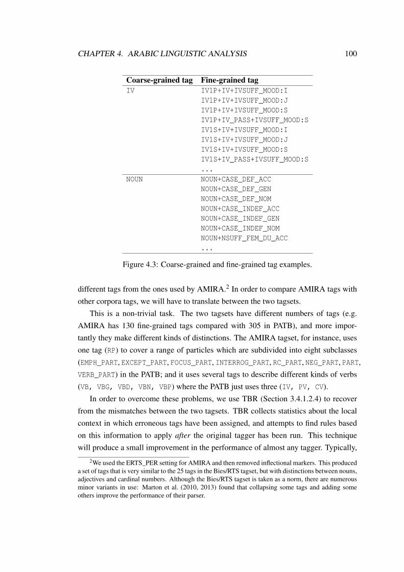
CHAPTER 4. ARABIC LINGUISTIC ANALYSIS 100
Coarse-grained tag Fine-grained tagIV IV1P+IV+IVSUFF_MOOD:I
IV1P+IV+IVSUFF_MOOD:JIV1P+IV+IVSUFF_MOOD:SIV1P+IV_PASS+IVSUFF_MOOD:SIV1S+IV+IVSUFF_MOOD:IIV1S+IV+IVSUFF_MOOD:JIV1S+IV+IVSUFF_MOOD:SIV1S+IV_PASS+IVSUFF_MOOD:S...
NOUN NOUN+CASE_DEF_ACCNOUN+CASE_DEF_GENNOUN+CASE_DEF_NOMNOUN+CASE_INDEF_ACCNOUN+CASE_INDEF_GENNOUN+CASE_INDEF_NOMNOUN+NSUFF_FEM_DU_ACC...
Figure 4.3: Coarse-grained and fine-grained tag examples.
different tags from the ones used by AMIRA.2 In order to compare AMIRA tags withother corpora tags, we will have to translate between the two tagsets.
This is a non-trivial task. The two tagsets have different numbers of tags (e.g.AMIRA has 130 fine-grained tags compared with 305 in PATB), and more impor-tantly they make different kinds of distinctions. The AMIRA tagset, for instance, usesone tag (RP) to cover a range of particles which are subdivided into eight subclasses(EMPH_PART, EXCEPT_PART, FOCUS_PART, INTERROG_PART, RC_PART, NEG_PART, PART,VERB_PART) in the PATB; and it uses several tags to describe different kinds of verbs(VB, VBG, VBD, VBN, VBP) where the PATB just uses three (IV, PV, CV).
In order to overcome these problems, we use TBR (Section 3.4.1.2.4) to recoverfrom the mismatches between the two tagsets. TBR collects statistics about the localcontext in which erroneous tags have been assigned, and attempts to find rules basedon this information to apply after the original tagger has been run. This techniquewill produce a small improvement in the performance of almost any tagger. Typically,
2We used the ERTS_PER setting for AMIRA and then removed inflectional markers. This produceda set of tags that is very similar to the 25 tags in the Bies/RTS tagset, but with distinctions between nouns,adjectives and cardinal numbers. Although the Bies/RTS tagset is taken as a norm, there are numerousminor variants in use: Marton et al. (2010, 2013) found that collapsing some tags and adding someothers improve the performance of their parser.

CHAPTER 4. ARABIC LINGUISTIC ANALYSIS 101
taggers that achieve scores in the mid 90s are boosted by 2-3%–the lower the originalaccuracy, the greater the typical improvement. When we used it for comparing theoriginal tags produced by AMIRA and the gold-standard tags the score improved fromaround 90% to just over 95% for the coarse-grained tagset. Some of this improvementarises simply from rules that spot that the two tagsets use different names for the samethings (e.g. that things that are called JJ are called ADJ in the PATB) but some of itcomes from learning how to split coarse-grained AMIRA tags into fine-grained PATBones.
There is a further problem with using AMIRA. The fact that Arabic allows a rangeof items to be cliticised (conjunctions, prepositions and pronouns) makes it difficulteven to tokenise text reliably. This means that not only does AMIRA sometimes assigndifferent tags from the PATB, it sometimes even splits the text into different numbersof tokens (AMIRA’s tokenisation of the PATB text differs from that in the PATB itself,with around 98% agreement between the two).
In order to solve this problem, we constructed a version of the corpus which hasthe same size (i.e. number of tokens) as the gold-standard one. We replaced PATB tagsby a coarse copy of the AMIRA tags, using hand-coded substitution rules, and thenreplaced these by fine-grained AMIRA tags where the substituted tags were compatiblewith tags actually assigned by AMIRA. Thus if the PATB assigned a word the tag ADJ
we replaced it by the AMIRA tag JJ. We then inspected the tags assigned by AMIRAitself: if the tag assigned to this word was one of AMIRA’s fine-grained adjective tags,e.g. JJR, then we used this instead. If, on the other hand, the hand-coded replacementfor the PATB tag was incompatible with the one assigned by AMIRA then we retainedthe hand-coded one. This gave us a version of the treebank that had the same numberof tokens as the original PATB, with as many items as possible given the tags assignedby AMIRA and the others given hand-coded AMIRA equivalents of the original PATBtags.
MADA
MADA uses the Buckwalter tagset (Section 3.4.1.1.1), which is a slightly extendedversion of the tagset used in PATB Part 1 v3 with some extra classification of nouns(e.g. NOUN_QUANT ‘quantifier noun’ and ADJ_COMP ‘comparative adjective’). The fine-grained MADA retagged version contains 351 tags compared to 305 tags in the PATBcorpus. Fortunately the MADA tags are a strict superset of the standard PATB set, andhence can be reduced to either the standard fine-grained version or our coarse version

CHAPTER 4. ARABIC LINGUISTIC ANALYSIS 102
by omitting the extra classification of nouns, so we do not have the same problemsusing MADA with the PATB as we have with AMIRA.
We also applied TBR to the output of MADA, because although we were not facedwith mapping incompatible tagsets in the same way as with AMIRA, using TBR nearlyalways provides a small improvement, amounting in this case to an increase from94.1% to 96.7%. We applied the same technique that we used in AMIRA to get aMADA version of the corpus that has the same size as the gold-standard one becauseMADA’s tokeniser also has small variance from the gold-standard (around 1%).
MXL
We also use Ramsay and Sabtan (2009)’s maximum-likelihood tagger, MXL. The ad-vantage of this tagger is that because we retrained it on the PATB, the tags it uses areexactly the PATB tags and the tokenisation is exactly the PATB tokenisation. We there-fore do not need to overcome problems associated with mismatches between tag sets.As with AMIRA and MADA, we obtained a final small improvement by using TBR.
4.2.2 Improving POS tagging
One popular technique for improving tagging accuracy is tagger combination. Thisapproach involves combining different taggers to exploit the unique properties of eachtagger and reduce some of the random errors. This technique has been applied todifferent languages such as English (Brill and Wu, 1998), Swedish (Sjöbergh, 2003),Telugu (Rama Sree and Kusuma Kumari, 2007), Italian (Søgaard, 2009) and Polish(Sniatowski and Piasecki, 2012) and the results were encouraging, but has not to ourknowledge been applied to Arabic. We evaluate different techniques for combiningPOS taggers for Arabic for both coarse-grained and fine-grained tagsets.
For all experiments in the current thesis, we used AMIRA v2.0 with Yamcha toolkitv0.33,3 and we used MADA 3.1 with SVMTools v1.3.14 and SRLIM v1.5.125 andSAMA v3.1 (catalog number LDC2010L01) from the LDC.6
Table 4.1 summarises the coarse-grained and fine-grained tags for the gold-standardcorpus and the three retagged corpora by the taggers: AMIRA, MADA and MXL. Ta-ble 4.2 summarises the accuracy of the three taggers on our gold-standard set using
3http://chasen.org/~taku/software/yamcha/.4http://www.lsi.upc.edu/~nlp/SVMTool/5http://www.speech.sri.com/projects/srilm/download.html6http://www.ldc.upenn.edu/Catalog/catalogEntry.jsp?catalogId=LDC2010L01

CHAPTER 4. ARABIC LINGUISTIC ANALYSIS 103
the built-in tagsets and coarse versions of each, and shows the improvements that areobtained in each case by applying TBR. This provides a reference point: the best ofthe three taggers is MADA, which achieves 96.7% on the coarse-grained version of itsbuilt-in tagset if we also apply TBR and 93.6% on the fine-grained version, again afterapplying TBR. The goal here is to see whether we can improve on this by utilising theother taggers, despite the fact that their individual performance is worse.
Tagset Gold-standard AMIRA MADA MXLCoarse-grained 39 29 56 39Fine-grained 305 130 351 305
Table 4.1: Coarse-grained and fine-grained tag numbers, gold-standard and single tag-ger.
Tagset TBR AMIRA MADA MXL
Coarse-grained× 89.6% 94.1% 95.2%√
95.3% 96.7% 95.6%
Fine-grained× 84.3% 91.7% 89.7%√
88.8% 93.6% 91.2%
Table 4.2: Tagger accuracies in isolation, with and without TBR.
The first observation is that when the taggers agree on how to tag a given item theyare more likely to be right than when they disagree. This is fairly obvious–if you havea set of taggers which assign different tags to an item then at least one of them mustbe wrong. Table 4.3 substantiates this observation–each column shows the precision(Equation 4.1), recall (Equation 4.2) and F-score (Equation 4.4) for a particular pair oftaggers simply taking cases where they agree and leaving words on which they disagreeuntagged. Thus the combination of MADA and MXL achieves a precision of 99.5%on the coarse-grained tagset and 99% on the fine-grained one. Table 4.4 shows whathappens when we combine all three taggers, either taking the majority view when atleast two of them agree or demanding that all three agree. In the latter case we obtaina precision of 99.9% for the coarse-grained tagset and 99.2% for the fine-grained one.

CHAPTER 4. ARABIC LINGUISTIC ANALYSIS 104
Metrics Tagset TBR AMIRA-MADA AMIRA-MXL MADA-MXL
PCoarse-grained
× 96.3% 97.7% 99.3%√99.5% 98.8% 99.5%
Fine-grained× 94.7% 92.9% 98.9%√
95.8% 94.3% 99%
RCoarse-grained
× 86.1% 84.3% 90.1%√91.9% 94.1% 94.6%
Fine-grained× 84.9% 79.8% 83.3%√
85.6% 81.6% 86.4%
F-scoreCoarse-grained
× 0.909 0.905 0.945√0.955 0.964 0.97
Fine-grained× 0.895 0.858 0.904√
0.904 0.875 0.923
Table 4.3: Precision (P) and recall (R) and F-score for combinations of pairs of taggers,with and without TBR.
Condition Tagset TBR P R F-score
At least two taggers agreeCoarse-grained
× 95.1% 93.5% 0.943√98.4% 97.8% 0.981
Fine-grained× 90.7% 87.8% 0.892√
92.8% 90.5% 0.916
All three taggers agreeCoarse-grained
× 99.5% 83% 0.905√99.9% 90.9% 0.952
Fine-grained× 99.1% 77.8% 0.871√
99.2% 79.8% 0.885
Table 4.4: Precision (P) and recall (R) and F-score for combinations of three taggers,with and without TBR.
The cost, of course, is that the recall goes down, because there are places wherethey disagree, and in these cases no tag is assigned. What should we do in such cases?
4.2.2.1 Backoff strategies
Our first proposal was to take the majority view when at least two of the taggersagreed, and to backoff to one or other when there was no common view (Zeman andŽabokrtsky, 2005). The results of this are shown in Table 4.5 where column ‘AMIRA’shows the result of backing off to AMIRA when there is no majority view, column‘MADA’ shows the result of backing off to MADA and column ‘MXL’ shows the re-sult of backing off to MXL. The results for the coarse-grained tagset are markedlybetter than for any of the taggers individually, though there is only a very slight im-provement over the original MADA scores for the fine-grained set. Interestingly, the

CHAPTER 4. ARABIC LINGUISTIC ANALYSIS 105
best results are obtained by backing off to MXL rather than to AMIRA or MADA(98.2% vs. 97.5% or 97.9%, despite the fact that MADA’s individual performance isbetter than MXL’s (96.7% vs. 95.6%) (the results in this table and in Table 4.7 arefor accuracy rather than precision or recall because under this approach every itemreceives a tag).
Tagset TBR Majority voting, backoff toAMIRA MADA MXL
Coarse-grained× 92.3% 93.8% 94.9%√
97.5% 97.9% 98.2%
Fine-grained× 87.5% 88.8% 89.6%√
90.6% 91.5% 91.8%
Table 4.5: Backoff to AMIRA or MADA or MXL when there is no majority agreement.
The fact that backing off to any of AMIRA or MADA or MXL improved the per-formance suggested that it was worth investigating other backoff strategies. If majorityvote + backoff to an arbitrary tagger is better than any single tagger in isolation, thenperhaps there is something we can backoff to which will do even better.
We return to the observation that in cases where all three taggers disagree, at mostone of them can be right. Given that they each employ different information about thematerial being tagged, it is likely that they are systematically prone to different kindsof errors.
We therefore collected statistics about the kinds of things they each get right. Howlikely, for instance, is AMIRA to be right when it assigns the tag DET+NNP? Table 4.6shows an excerpt of this data, showing the likelihood that each tagger is right for agiven assigned tag, e.g. for the given instance of the word �
éJÊJ«AÖÞ�B@ AlAsmAςylyh
“Ismailia” the correct tag was DET+NOUN_PROP (as in gold-standard): AMIRA sug-gested DET+NNP, MADA suggested DET+ADJ and MXL suggested DET+NOUN. BecauseAMIRA is right 100% of the time when it suggests DET+NNP, whereas MADA is right97.5% of the time when it suggests DET+ADJ and MXL is right only 92.1% of the timewhen it suggests DET+NOUN, DET+NNP was chosen. For B@
AlA “except”, MADA’s
suggestion of EXCEPT_PART was accepted because MADA is right 100% of the timewhen it suggests EXCEPT_PART, which is better than the reliability of either of the othersuggestions. For Q�
« γyr “other than”, MXL’s suggestion of NEG_PART was accepted
because MXL is right 98.2% of the time when it suggests NEG_PART, which is betterthan the reliability of either of the other suggestions.
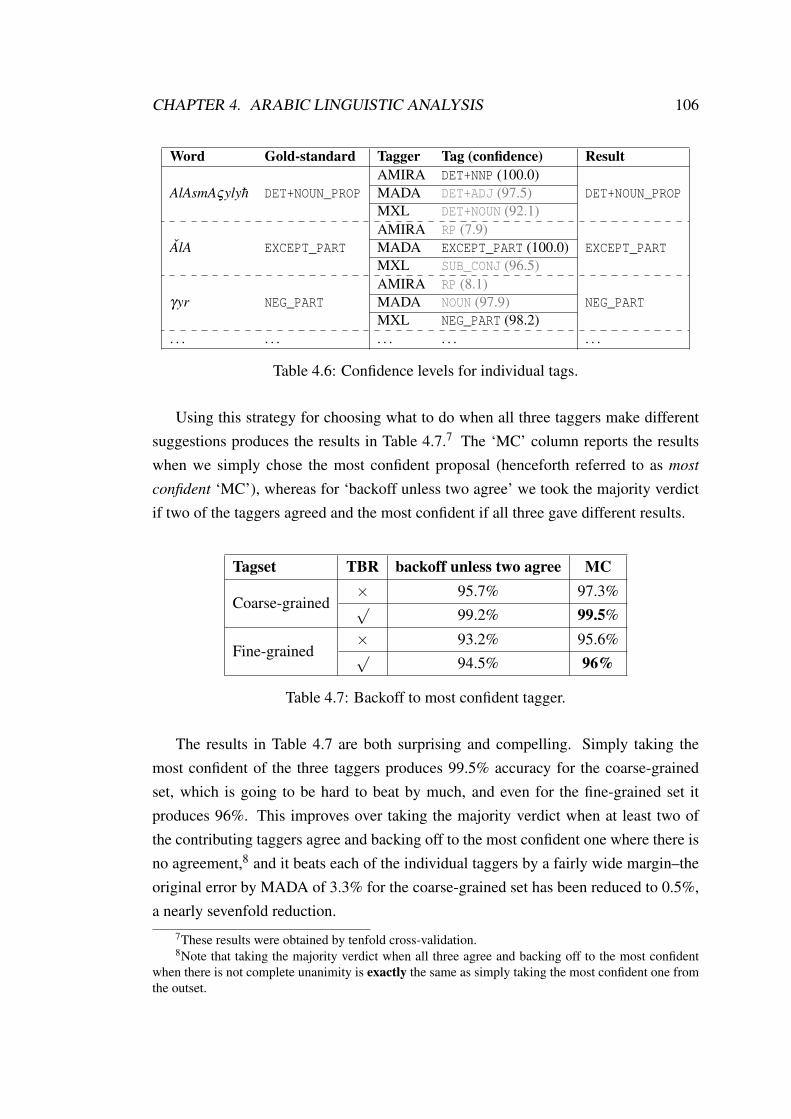
CHAPTER 4. ARABIC LINGUISTIC ANALYSIS 106
Word Gold-standard Tagger Tag (confidence) Result
AlAsmAςylyh DET+NOUN_PROPAMIRA DET+NNP (100.0)
DET+NOUN_PROPMADA DET+ADJ (97.5)MXL DET+NOUN (92.1)
AlA EXCEPT_PARTAMIRA RP (7.9)
EXCEPT_PARTMADA EXCEPT_PART (100.0)MXL SUB_CONJ (96.5)
γyr NEG_PARTAMIRA RP (8.1)
NEG_PARTMADA NOUN (97.9)MXL NEG_PART (98.2)
. . . . . . . . . . . . . . .
Table 4.6: Confidence levels for individual tags.
Using this strategy for choosing what to do when all three taggers make differentsuggestions produces the results in Table 4.7.7 The ‘MC’ column reports the resultswhen we simply chose the most confident proposal (henceforth referred to as most
confident ‘MC’), whereas for ‘backoff unless two agree’ we took the majority verdictif two of the taggers agreed and the most confident if all three gave different results.
Tagset TBR backoff unless two agree MC
Coarse-grained× 95.7% 97.3%√
99.2% 99.5%
Fine-grained× 93.2% 95.6%√
94.5% 96%
Table 4.7: Backoff to most confident tagger.
The results in Table 4.7 are both surprising and compelling. Simply taking themost confident of the three taggers produces 99.5% accuracy for the coarse-grainedset, which is going to be hard to beat by much, and even for the fine-grained set itproduces 96%. This improves over taking the majority verdict when at least two ofthe contributing taggers agree and backing off to the most confident one where there isno agreement,8 and it beats each of the individual taggers by a fairly wide margin–theoriginal error by MADA of 3.3% for the coarse-grained set has been reduced to 0.5%,a nearly sevenfold reduction.
7These results were obtained by tenfold cross-validation.8Note that taking the majority verdict when all three agree and backing off to the most confident
when there is not complete unanimity is exactly the same as simply taking the most confident one fromthe outset.

CHAPTER 4. ARABIC LINGUISTIC ANALYSIS 107
In order to make the previous results clearer, let us consider the Arabic sentence in(4.1), which is taken from the gold-standard corpus.
(4.1) Arabic sentence example from gold-standard corpusYªK. ÉJ
K @Qå� @ úÍ@ @ðQ
¯ @ñ
KA¿ ÈA
®£
@ð ZA�
� Ñî
DJK. AJj��Ó AJ
K A
JJ. Ë
àðQå
��« ©Òm.
��' Y
�¯ð
. áKYÊJ. Ë @á�K. XðYmÌ'@ úΫ
�èC�ÊË ÐñJË @ ú
ÎJ
K @Qå�B@ H. Aj�
�B@
wqd tjmς ςšrwn lbnAnyA msyHyA bynhm nsA’ wÂTfAl kAnwA frwA Alý
AsrAyyl bςd AlAnsHAb AlAsrAyyly Alywm llSlAh ς lý AlHdwd byn Albldyn.
“Twenty Lebanese Christians already gathered, including women and children,
who fled to Israel after the Israeli withdrawal today to pray on the border be-
tween the two countries.”
Figure 4.4 summarises the results obtained by each tagger individually comparedwith the two techniques that are shown in Table 4.7 (i.e. ‘backoff unless two agree’and ‘MC’) for the sentence (4.1). For this sentence, MXL gives better accuracy thanboth AMIRA and MADA (88.5% vs. 84.6% for other two taggers). Interestingly, theMC technique gives full accuracy 100%. This result is better than each tagger in iso-lation and the ‘backoff unless two agree’ technique, which gives the same accuracyas the best tagger (i.e. MXL, 88.5%). As can be seen in Figure 4.4, for instance, thecorrect tag for the tokens á�K. byn “between” and YªK. bςd “after” is PREP (as in gold-standard corpus). The ‘backoff unless two agree’ technique gives an incorrect result(i.e. NOUN) because both AMIRA and MADA identify this token as noun, whereas theMC technique gives the correct result (i.e. PREP) because MXL identifies it as a prepo-sition and it has a more confident score than AMIRA and MADA (98.7 vs. 72.6 and86.2 respectively). According to our observation, we found out that most confidenttagger gives better results than the agreement in most cases when two taggers agreeand backoff to which ever tagger is more confident (which may be one of these or maybe the other one).
In Section 4.2, we have shown a rather simple mechanism for combining taggerswhich can provide considerable improvements in accuracy. If you measure the likeli-hood that a tagger is right when it suggests a particular tag, and then take the suggestionwith highest score in each case then you can decrease the error rate substantially. Thekey is that the different taggers tend to make different systematic mistakes. The ac-curacy statistics capture these systematic mistakes, so a low score is likely to reflecta case where the tagger is making one of its characteristic errors, and in such caseswe take the output of one of the others. This simple approach outperforms strategies
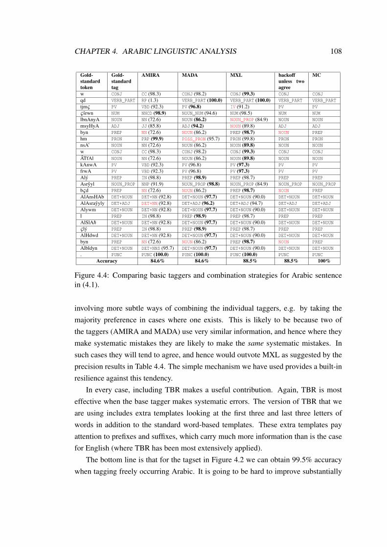
CHAPTER 4. ARABIC LINGUISTIC ANALYSIS 108
Gold-standardtoken
Gold-standardtag
AMIRA MADA MXL backoffunless twoagree
MC
w CONJ CC (98.3) CONJ (98.2) CONJ (99.3) CONJ CONJqd VERB_PART RP (1.3) VERB_PART (100.0) VERB_PART (100.0) VERB_PART VERB_PARTtjmς PV VBD (92.3) PV (96.8) IV (91.2) PV PVςšrwn NUM NNCD (98.9) NOUN_NUM (94.6) NUM (98.5) NUM NUMlbnAnyA NOUN NN (72.6) NOUN (86.2) NOUN_PROP (84.9) NOUN NOUNmsyHyA ADJ JJ (85.8) ADJ (94.2) NOUN (89.8) ADJ ADJbyn PREP NN (72.6) NOUN (86.2) PREP (98.7) NOUN PREPhm PRON PRP (99.9) POSS_PRON (95.7) PRON (99.8) PRON PRONnsA’ NOUN NN (72.6) NOUN (86.2) NOUN (89.8) NOUN NOUNw CONJ CC (98.3) CONJ (98.2) CONJ (99.3) CONJ CONJÂTfAl NOUN NN (72.6) NOUN (86.2) NOUN (89.8) NOUN NOUNkAnwA PV VBD (92.3) PV (96.8) PV (97.3) PV PVfrwA PV VBD (92.3) PV (96.8) PV (97.3) PV PVAlý PREP IN (98.8) PREP (98.9) PREP (98.7) PREP PREPAsryyl NOUN_PROP NNP (91.9) NOUN_PROP (98.8) NOUN_PROP (84.9) NOUN_PROP NOUN_PROPbςd PREP NN (72.6) NOUN (86.2) PREP (98.7) NOUN PREPAlAnsHAb DET+NOUN DET+NN (92.8) DET+NOUN (97.7) DET+NOUN (90.0) DET+NOUN DET+NOUNAlAsrayyly DET+ADJ DET+NN (92.8) DET+ADJ (96.2) DET+ADJ (94.7) DET+ADJ DET+ADJAlywm DET+NOUN DET+NN (92.8) DET+NOUN (97.7) DET+NOUN (90.0) DET+NOUN DET+NOUNl PREP IN (98.8) PREP (98.9) PREP (98.7) PREP PREPAlSlAh DET+NOUN DET+NN (92.8) DET+NOUN (97.7) DET+NOUN (90.0) DET+NOUN DET+NOUNς lý PREP IN (98.8) PREP (98.9) PREP (98.7) PREP PREPAlHdwd DET+NOUN DET+NN (92.8) DET+NOUN (97.7) DET+NOUN (90.0) DET+NOUN DET+NOUNbyn PREP NN (72.6) NOUN (86.2) PREP (98.7) NOUN PREPAlbldyn DET+NOUN DET+NNS (95.7) DET+NOUN (97.7) DET+NOUN (90.0) DET+NOUN DET+NOUN. PUNC PUNC (100.0) PUNC (100.0) PUNC (100.0) PUNC PUNC
Accuracy 84.6% 84.6% 88.5% 88.5% 100%
Figure 4.4: Comparing basic taggers and combination strategies for Arabic sentencein (4.1).
involving more subtle ways of combining the individual taggers, e.g. by taking themajority preference in cases where one exists. This is likely to be because two ofthe taggers (AMIRA and MADA) use very similar information, and hence where theymake systematic mistakes they are likely to make the same systematic mistakes. Insuch cases they will tend to agree, and hence would outvote MXL as suggested by theprecision results in Table 4.4. The simple mechanism we have used provides a built-inresilience against this tendency.
In every case, including TBR makes a useful contribution. Again, TBR is mosteffective when the base tagger makes systematic errors. The version of TBR that weare using includes extra templates looking at the first three and last three letters ofwords in addition to the standard word-based templates. These extra templates payattention to prefixes and suffixes, which carry much more information than is the casefor English (where TBR has been most extensively applied).
The bottom line is that for the tagset in Figure 4.2 we can obtain 99.5% accuracywhen tagging freely occurring Arabic. It is going to be hard to improve substantially

CHAPTER 4. ARABIC LINGUISTIC ANALYSIS 109
on this score. Given that Marton et al. (2010, 2013) have argued that coarse-grainedtagsets are actually more useful than fine-grained ones for parsing, which is the usualnext step in the chain, we are fairly satisfied with this result.
4.3 Dependency parsing
In recent years, dependency parsing has become widely used in machine translation(MT), question answering (QA), relation extraction and many other NLP applications(Kübler et al., 2009) for a number of reasons:
• It provides uniform treatments for a wide range of typologically different lan-guages, since it hides differences that arise from different surface word orders andemphasises the functional relations between words, which tend to be similar acrosslanguages.
• It can be useful for semantics. It supports compositional semantics, since it can beeasier to attach compositional rules directly to lexical items than to assign them tolarge numbers of phrase structure rules; and it supports less formal approaches tosemantics, e.g. via TE, since it is easier to generalise dependency trees as the basisof approximate inference rules than to use phrase structure rules for this purpose.
• It is possible to induce robust and fairly accurate dependency parsers, e.g. MST-Parser and MALTParser (see Section 3.4.2.2), from treebanks of suitably annotateddependency trees.
Recall that our ultimate goal is to develop a TE system for Arabic (Alabbas, 2011).An efficient technique to check entailment between two sentences is using TED match-ing between dependency trees for the two sentences. We therefore need to be able toobtain dependency trees by parsing input Arabic texts, and hence we need dependencytreebanks for training our dependency parsers (i.e. MSTParser and MALTParser withvarious parsing algorithms). We used here MSTParser 0.2 (i.e. uses second-order edgefeatures) and MALTParser 1.7.1.
4.3.1 Arabic treebanks
The focus of the current section is on the nature of the training data. Dependencygrammar is a general framework, with a myriad major and minor variations. The

CHAPTER 4. ARABIC LINGUISTIC ANALYSIS 110
distinctions between different versions of dependency grammar are usually debatedin terms of their linguistic adequacy, but it is likely that different sets of dependencyrelations will produce different levels of accuracy when used for inducing parsers. Inparticular, we want to investigate the effects of different ways of turning the phrasestructure trees in the PATB, which is the largest easily available set of training data forArabic, into dependency trees.
The four best-known Arabic treebanking efforts are the PATB (Maamouri andBies, 2004), the Prague Arabic dependency treebank (PADT) (Smrž et al., 2008),Columbia Arabic treebank (CATiB) (Habash and Roth, 2009) and Quranic Arabic tree-bank (Dukes et al., 2013). PATB is a phrase structure treebank, whereas the others aredependency treebanks. PATB and PADT are annotated with rich morphological infor-mation, very fine-grained POS tags, semantic roles, diacritisation and lemmas. Thisallows these treebanks to be used for training different NLP applications (e.g. tokeni-sation, POS tagging, diacritisation, morphological disambiguation and others) as wellas parsing (Habash and Roth, 2009). In contrast, much of the detailed morphologicaland POS information is not provided in CATiB. The use of any of these treebanks astraining data raises problems:
• The trees in PATB are phrase structure trees, and hence are not directly useable fortraining dependency parsers.
• PADT uses very fine-grained POS tags, and there is no readily available tagger forassigning PADT labels.9
• CATiB uses a very coarse-grained set of just six POS tags (i.e. NOM ‘non-propernominals including nouns, pronouns, adjectives and adverbs’, PROP ‘proper nouns’,VRB ‘active-voice verbs’, VRB-PASS ‘passive-voice verbs’, PRT ‘particles such asprepositions or conjunctions’ and PNX ‘punctuation’) (Habash and Roth, 2009). Inparticular, all verbs are grouped under a single heading (i.e. VRB), with no dis-tinction between present and past; and all nominals are also grouped together (i.e.NOM), with no distinction between nouns or numbers, or even between definite andindefinite forms. Other researchers have noted that dependency parsers can copewith very coarse-grained POS tags, but the loss of this information makes the treesin CATiB unsuitable for our underlying goal of inferring TE rules from trees.
9Personal correspondence with Dr. Otakar Smrž, who is one of the PADT designers.

CHAPTER 4. ARABIC LINGUISTIC ANALYSIS 111
• Quranic Arabic treebank provides three levels of analysis: morphological annota-tion, a syntactic treebank and a semantic ontology. This treebank contains classicalArabic, which is the only language of the Quran and Sunna (prophetic traditions).It is the direct ancestor language of MSA, which is the language that is used in mostcurrent government communications, media, news, publications, books, etc. Thistreebank is unsuitable for our purposes because the vocabulary, and to a lesser ex-tent the grammatical structure, does not correspond to the news articles from whichwe have obtained our T-H pairs.
Of the four, PATB seemed most suitable for our purposes, since we have taggersthat can assign the tags used in PATB and the information it contains is what we needfor inferring TE rules. We therefore need to convert PATB trees to dependency trees,which we do by using the standard phrase structure to dependency transformation al-gorithm (given in Figure 4.5), using a percolation table to choose the head daughter inthe phrase structure tree.
This raises an interesting question: since PATB does not explicitly embody a notionof the ‘head’ of a tree, we have some freedom about how to construct the percolationtable. Should the head of an NP be the main noun or the determiner? Should the headof a verbless sentence be the subject or the predicate? Should the head of a conjoinedphrase be the conjunction itself or the head of the first conjunct?
There are theoretical grounds for choosing one way of answering these questionsrather than another, but they also have empirical consequences. It seems likely thatone set of choices will provide the parsers with a more easily recognisable set of de-pendency relations than another. It may turn out that the parsers perform best with aset of trees that were obtained using a theoretically unappealing percolation table (e.g.we will see in Section 4.3.1.1.1 that choosing the first conjunct of a conjoined pair pro-duces better results than choosing the conjunction itself, but it is much easier to obtaina formal interpretation from trees where the conjunction is the head (Gazdar, 1980)).It is, however, a straightforward matter to transform trees that are based on one notionof conjunction to ones based on another, so from a practical point of view we want tofind the percolation table that allows the parsers to produce the most accurate results.
4.3.1.1 From PATB to dependency trees
We used PATB Part 1 v3.0 as a resource that provides us with annotations of Ara-bic at different levels of structure (at the word, the phrase and the sentence levels).

CHAPTER 4. ARABIC LINGUISTIC ANALYSIS 112
PATB is annotated for POS tag, morphological disambiguation and for syntactic struc-ture. It also provides diacritisations, empty categories, some semantic tags and lemmachoice. Because PATB is already tagged, the effects of lexical ambiguity are substan-tially reduced–we know which items are nouns and which are verbs, and we knowabout the clitics that have been attached to them. We still have no information abouttransitivity, which is itself a problem for parsing, but the gross lexical ambiguity thatis brought about by the lack of diacritics in modern standard Arabic (MSA) has beeneliminated. The PATB includes 734 stories representing 145,386 words (166,068 to-kens after clitic segmentation; the number of Arabic tokens is 123,796). The sentencesin PATB, which contains just over 5000 phrase structure trees, are fairly long–the av-erage sentence length is around 28 words per tree, with some trees containing 100+words.
Converting phrase structure trees to dependency trees is a straightforward task, solong as (i) you can identify the item in each subtree which contains the head; and (ii)there are no constructions with zero-heads. Assuming that these two conditions hold,the algorithm in Figure 4.5 will convert a phrase structure tree to a dependency tree.
1. If you are looking at a leaf node, turn it into a tree with nodaughters.
2. a). Otherwise, choose the subtree which contains the head: turnit into a dependency tree: call this D.
b). Turn all the other subtrees into dependency trees, and addthem as daughters of D.
Figure 4.5: From phrase structure trees to dependency trees.
The only difficult part of this algorithm, which has been discussed by Xia andPalmer (2001), is the selection of the subtree which contains the head. The approachwe have taken to this task is to look for all the trees headed by a given label, and find allthe labels for their subtrees. This gives us a list of labels for potential head daughtersfor each non-terminal label (a ‘head percolation table’ (Collins, 1997)). We then orderthese in terms of candidacy for being the head daughter, in terms of what we believe tobe the correct dependency structure, and we use this preference order for ‘choose the
subtree which contains the head: turn it into a dependency tree’ in the above algorithm.For instance, in the head percolation table the entry (S left VP) means that the headchild of an S is the first child of the S from the left with the label VP.
Here, the head percolation table is semi-automatically generated from PATB by

CHAPTER 4. ARABIC LINGUISTIC ANALYSIS 113
grouping the related tags in one tag and then finding the possible heads for each one.After that, for each table’s entry we order the possible heads manually according to itspriority.10 Then, the above algorithm is used to generate the dependency tree recur-sively. We used six dependency relations as an initial step to construct our treebank.These relations are: SBJ ‘subject’, OBJ ‘object’, ROOT ‘root’, COORD ‘coordi-nate’, PX ‘punctuation’ and DEP ‘dependent’.
There are, however, a number of problems that arise when applying this algorithmto PATB:
• Very large numbers of Arabic sentences begin with the conjunction +ð w+ “and”.The most plausible reading is that this item implicitly conjoins the first clause inthe current sentence to the previous sentence, and hence should be taken as itshead. This clashes with the treatment in the PATB, where the conjunction is takento be the head of the whole sentence. This makes a difference in cases wherethe sentence has the general form CONJ S1 CONJ S2 CONJ ... CONJ Sn, wherewe bracket it as CONJ (S1 CONJ S2 CONJ ... CONJ Sn) and the PATB bracketsit as (CONJ S1) CONJ S2 CONJ ... CONJ Sn. There are a surprising number ofsuch cases, and the rebracketing makes a noticeable difference to parsing accuracy.We therefore have to restructure these trees, and we also mark sentence-initial +ð
w+ “and” with a special tag (i.e. ICONJ) to prevent the parsers confusing it withmore normal conjunctive uses of this item. By doing this, the parser’s accuracy isimproved by around 0.4% as shown in Section 4.3.1.1.1.
• The PATB deals with free word-order by using traces, where the function of an ex-traposed item is co-indexed with an item whose label indicates whether it is a sub-ject or object, as shown in Figure 4.6, where the relative pronoun
à@YÊË @ All*An
“who (3rd.masc.du)” is co-indexed with a trace which is itself taken to be the sub-ject of
àAÒëA�� y+sAhm+An “contribute to (3rd.masc.du)”.
This does not really make sense within a dependency-based framework. The useof traces is antithetical to the basic idea of dependency grammar, namely that syn-tactic structure is determined by relations between words: a trace is not a word,and as such has no place in dependency grammar, at least as strictly conceived (e.g.Hudson, 1984). We therefore systematically transform the PATB so that traces areeliminated, with the topicalised NP treated as a proper constituent of the sentence,
10The consequences of using different versions of the percolation table are discussed in Section4.3.1.1.1

CHAPTER 4. ARABIC LINGUISTIC ANALYSIS 114
[S [S [CONJ w-][VP [VERB -gyr]
[NP-SBJ [NP [DET+NOUN Al+mSrf+An]][PUNC ,][SBAR [WHNP-1 [REL_PRON All*An]]
[S [VP [VERB y+sAhm+An][NP-SBJ-1 [-NONE- *T*]]...]]]]]]]
Figure 4.6: Phrase structure tree with trace.
e.g. in Figure 4.6 the relative pronoun à@
YÊË @ All*An “who” is taken to be a depen-
dent (as subject) of àAÒëA�� y+sAhm+An “contribute to” despite appearing higher
in the original phrase structure tree.
• Arabic allows ‘verbless’ or ‘equational’ sentences, consisting of an NP and somekind of predication (another NP, a PP, an adjective) (Alabbas, 2011; Attia, 2012). Itis tempting to think of these constructions as containing a zero-copula (the fact thattheir negated and past forms do include an explicit copula supports this analysis).As noted above, we prefer to eliminate empty items, especially heads.
The standard treatment of such sentences assumes that the predication is the head,largely on semantic grounds. This is almost certainly the right thing to do, butgiven that the parsers we are using exploit clues extracted from the local contextto guide their decisions, it seemed worth investigating the effects of choosing ei-ther the subject or the predication as the head–if it turns out the parsers can morereliably assign labels when the subject is the head, we can easily transform the re-sulting dependency tree to the more normal form once it has been constructed. Overa number of experiments, it turns out that there is around a 2% overall increase inaccuracy if the subject is taken to be the head (Alabbas and Ramsay, 2012a). Wetherefore make this unintuitive switch–if we can identify the constituents of a verb-less sentence more easily by taking the subject as the head, then the extra cost ofinverting this move later seems well worth paying.
• The PATB uses a very fine-grained set of tags (305 tags), which carry a great dealof syntactically relevant information (particularly case-marking). Because of thedifficulty of accurately assigning tags from this fine-grained tagset, we collapsedthis set to a coarse-grained set with 39 distinct tags as we explained before in Sec-tion 4.2.1 (gold-standard tags), as suggested by Marton et al. (2010, 2013).

CHAPTER 4. ARABIC LINGUISTIC ANALYSIS 115
The dependency trees to be used by the parsers also have to be labelled with func-tional relations. Since dependency grammar is entirely concerned with relations be-tween words, any information beyond simple constituency has to be encoded in thelabels on the relations. Such relations tend not be explicitly marked in phrase structuretrees, since they are often implied by the label of the local tree (to put it simply, it is notnecessary to mark the NP daughter of a sentence as its subject, because this is implicitin the rule that says that a sentence may be made out of an NP and a VP). We there-fore have to impose a set of functional relations. We cannot use a very fine-grainedset of labels here, because the information in PATB simply does not provide enoughinformation. The only labels we can assign with any degree of confidence relate toconjunctions, and to the subject and object of the verb.
There is no consensus about the set of relations to be used in dependency grammar.Some authors, for instance, take it that the auxiliary dominates the verb it is associatedwith, while others take the opposite view. Similarly, coordinating conjunctions aresometimes treated as heads and sometimes as modifiers. We investigated three issues:
• Is the determiner or the noun the head of an NP? Where an NP contains adeterminer, some theories (e.g. categorial grammar) treat the determiner as the headand others (e.g. generalised phrase structure grammar (GPSG) (Gazdar, 1985),head-driven phrase structure grammar (HPSG) (Pollard and Sag, 1994)) treat it as adependent of the noun. Other frameworks take it be something more like a modifier.Arabic makes less use of determiners than some other languages, since there is noindefinite article and the definite article is treated as a part of the noun to which itis attached, but it does have numbers and demonstrative determiners, and choosingwhether these are heads or dependents may make a difference.
• Is the subject or the predication the head of verbless sentences? Arabic verblesssentences are widely regarded as containing an invisible ‘zero’ copula. If the copulawas present, it would be the head, but since it is missing then either the subject orthe predication will have to be chosen. Which of these makes the parser performbetter?
• What is the head of a conjoined phrase? The choice of how to deal with con-junctions in dependency grammar is widely disputed, with reasonable argumentsbeing put forward on both sides. Some authors, for instance, take it that the coor-dinating conjunctions are treated as heads, whereas others treat them as modifiers.

CHAPTER 4. ARABIC LINGUISTIC ANALYSIS 116
These differences show up in PADT and CATiB. PADT considers the coordinat-ing conjunction as the head of the conjunction and others depend on it, whereasCATiB considers the head of the first conjunct of a conjunction as the head of thecoordinating conjunction, which in turn heads the second conjunct.
We will use the sentence in (4.2), from (Habash et al., 2009a), to highlight thedifferences between our conversion and the other Arabic dependency treebanks.
(4.2) Arabic sentence (Habash et al., 2009a)
úæ
�AÖÏ @ ÈñÊK @ ú
¯ AKPñ�ð
àA
JJ. Ë @ðP@ P l�
'A�
Ë@
àñ�Ô
g
xmswn Alf sA’H zArwA lbnAn w+swryA fy Aylwl AlmaDy
“Fifty thousand tourists visited Lebanon and Syria last September”
As can be seen in Figure 4.7,11 our dependency tree is different from the othersin the sentential part l�
'A�
Ë@
àñ�Ô
g xmswn Alf sA’H “Fifty thousand tourists”, be-
cause we considered the NOUN as the head not NOUN_NUM and the others are dependent,whereas both PADT and CATiB considered the first NOUN_NUM as the head. Further-more, we follow the CATiB treatment of the conjoined NP AKPñ�ð
àA
JJ. Ë lbnAn w+swryA
“Lebanon and Syria”, where the head is the first noun, with the conjunction as its soledaughter and the second noun as a daughter of the conjunction.
It should be noted that this treatment of conjunction cannot be obtained from theoriginal PATB tree by the algorithm in Figure 4.5. The conjoined phrase AKPñ�ð
àA
JJ. Ë
lbnAn w swryA “Lebanon and Syria” has three constituents–the conjunction and twoNPs. Specifying that the conjunction has priority over any other constituent in thepercolation table would produce the subtree given for this phrase in PADT. Specifyingthat the conjunction has lower priority than one of the NPs would produce a subtreewith either
àAJJ. Ë lbnAn “Lebanon” (or possibly AKPñ� swryA “Syria”) as its head and the
conjunction and the other noun as daughters. There is no way to get the conjunctionas a daughter of
àAJJ. Ë lbnAn “Lebanon” and then AKPñ� swryA “Syria” as a daughter of
the conjunction by using the algorithm in Figure 4.5. In order to obtain trees of thiskind, we transform the original phrase structure tree so that structures of the form T1
become T2 in Figure 4.8. If we then assign DUMMY the lowest possible priority in thepercolation table and CONJ the highest possible priority for the entry of DUMMY in thetable we obtain CATiB-style trees for coordinated structures.
11We deleted the POS tags and dependency relations from dependency trees to compare the treestructures only.

CHAPTER 4. ARABIC LINGUISTIC ANALYSIS 117
!"#$%&'
(")$*"+
("
(,-()(-../01"2(34
56789:40;<=>?>@AB
C"
CDE%"CF."
GHI8HJ#K;#=L?0?@MNB
(")'%O+
(,(D
!"!
("),%O
(,-()"E,"PM>#11
QRST9UV</#<=WMV/<3<B
*,(O
8X;X=/<NB
(,-()"E,"PM>#11
78IYT0;KA#='AK?/B
"")$."
(""ED"
Z[>A=?<B
(,-()"E,"\M<
]Y^8_`AU;U
=';a@M4VMKB
(,-()"E,"\M<
HQ6Tb[#U4#PA=U/0@B
("
(,-()(-.PM>#11
HQc#U>
=@d3e0/<NB
("
(,-(2<NM>\M<
7Tfg0#Bh=@3eK?0@B
56789:40;<=>?>@AB
GHI8HJ#K;#=L?0?@MNB
HQc#U>
=@d3e0/<NB
7Tfg0#Bh=@3eK?0@B
8X;X=/<NB
QRST9UV</#<=WMV/<3<B
78IYT0;KA#='AK?/B
Z[>A=?<B
]Y^8_`AU;U
='Ma@M4VMKB
HQ6Tb[#U4#PA=U/0@B
56789:40;<=>?>@AB
GHI8HJ#K;#=L?0?@MNB
HQc#U>
=@d3e0/<NB
7Tfg0#Bh=@3eK?0@B
8X;X=/<NB
QRST9UV</#<=WMV/<3<B
78IYT0;KA#='AK?/B
Z[>A=?<B
]Y^8_`AU;U
='Ma@M4VMKB
HQ6Tb[#U4#PA=U/0@B
56789:40;<=>?>@AB
GHI8HJ#K;#=L?0?@MNB
HQc#U>
=@d3e0/<NB
7Tfg0#Bh=@3eK?0@B
8X;X=/<NB
QRST9UV</#<=WMV/<3<B
78IYT0;KA#='AK?/B
Z[>A=?<B
]Y^8_`AU;U
='Ma@M4VMKB
HQ6Tb[#U4#PA=U/0@B
!"#P$& !*#$?%& !,-EiP$&
Figure 4.7: Comparing PATB phrase structure and dependency format (without POStags and labels) in PADT, CATiB and our preferred conversion for the sentence in (4.2).
S
A CONJ B
S
A DUMMY
CONJ B
T1 T2
Figure 4.8: Reconstruct coordinated structures.
We extend this treatment to cover cases where we have a complex coordinatedexpression where several of the conjuncts are linked by commas in addition to explicitconjunctions, converting phrase structure trees like the initial tree T1 in Figure 4.9 tothe tree D1 in this figure instead of D2. This is the treatment used in experiment (7)below.
4.3.1.1.1 Conversion resultsTo check the effectiveness of our conversion version of PATB to dependency tree
format, we used it to train MSTParser and MALTParser with the default parsing algo-rithm (i.e. Nivre arc-eager), which we will refer to as MALTParser1. The aim here wasto see how changes in the structure of the trees affect the performance of the parser:
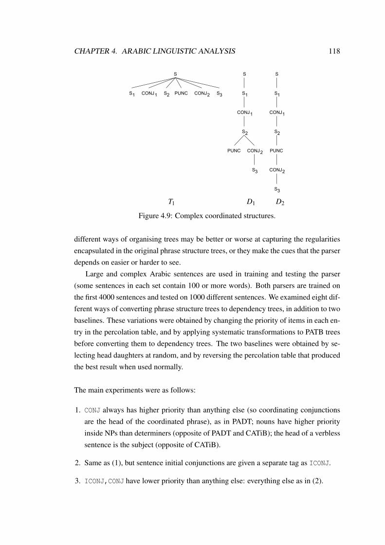
CHAPTER 4. ARABIC LINGUISTIC ANALYSIS 118
S3
S3
CONJ2
PUNC CONJ2
PUNC
S2
S2
CONJ1
CONJ1
S1
CONJ1
S2
PUNC CONJ2
S3
S1
S1
S S S
T1 D1 D2
Figure 4.9: Complex coordinated structures.
different ways of organising trees may be better or worse at capturing the regularitiesencapsulated in the original phrase structure trees, or they make the cues that the parserdepends on easier or harder to see.
Large and complex Arabic sentences are used in training and testing the parser(some sentences in each set contain 100 or more words). Both parsers are trained onthe first 4000 sentences and tested on 1000 different sentences. We examined eight dif-ferent ways of converting phrase structure trees to dependency trees, in addition to twobaselines. These variations were obtained by changing the priority of items in each en-try in the percolation table, and by applying systematic transformations to PATB treesbefore converting them to dependency trees. The two baselines were obtained by se-lecting head daughters at random, and by reversing the percolation table that producedthe best result when used normally.
The main experiments were as follows:
1. CONJ always has higher priority than anything else (so coordinating conjunctionsare the head of the coordinated phrase), as in PADT; nouns have higher priorityinside NPs than determiners (opposite of PADT and CATiB); the head of a verblesssentence is the subject (opposite of CATiB).
2. Same as (1), but sentence initial conjunctions are given a separate tag as ICONJ.
3. ICONJ,CONJ have lower priority than anything else: everything else as in (2).

CHAPTER 4. ARABIC LINGUISTIC ANALYSIS 119
4. Same as (2) but determiners have higher priority than nouns in NPs.
5. CATiB-style treatment of conjunctions (as discussed above). Everything else as in(2).
6. Same as (5) but determiners have higher priority than nouns in NPs.
7. Same as (5), but commas in coordinated expressions are not treated as though theywere conjunctions (i.e. tree D1 in Figure 4.9, not tree D2).
8. Same as (7), but the head of a verbless sentence is assumed to be its predicationrather than its subject.
The labelled attachment score (LA), i.e. the percentage of tokens with correcthead and dependency relation (DEPREL),12 and unlabelled attachment score (UA),i.e. the percentage of tokens with correct head (regardless of the DEPREL label), forthe various transformations of PATB to dependency tree format are shown in Table 6.2.
# Items order for each entry in the head percolation MSTParser MALTParser1table LA UA LA UARandom head (baseline 1) 20.2% 20.6% 19.3% 19.7%Inverse of best table, i.e. table (7) (baseline 2) 73.5% 74.3% 71.7% 72.7%
1 CONJ has higher priority than other items 80.1% 81.5% 79.1% 80.4%2 Split CONJ into CONJ and ICONJ 80.5% 81.9% 79.4% 80.7%3 ICONJ,CONJ have lowest possible priority 80.8% 82.2% 79.7% 80.9%4 Same as (3) but determiners above nouns in NPs 80.3% 81.7% 79.3% 80.2%5 Same as (2) but CATiB-style conjunctions 82.5% 83.9% 81.3% 82.2%6 Same as (5) but determiners above nouns in NPs 82.3% 83.7% 81.1% 81.9%7 Same as (5) but commas in conjunctions not treated
as conjunctions (i.e. tree D1 in Figure 4.9, not tree D2)82.8% 84.2% 81.5% 82.6%
8 Same as (7) but head of verbless sentence is predication 82.3% 83.8% 81.2% 81.0%
Table 4.8: LA and UA accuracies for parsing, different head percolation table entryorders and treatments of coordination.
Varying the treatments of conjunction, NPs and verbless sentences can affectthe performance of MSTParser by around 2.7% compared with around 2.4% forMALTParser1. The individual changes are not dramatic, but then each such changeonly affects one set of relations: there are, for instance, only around 800 determinersin the test set, out of a total of just over 25000 words. So if every instance of a de-terminer was labelled correctly in (3) and incorrectly in (4) there would only be a 3%
12See Conference on Natural Language Learning (CoNLL)-X format in Appendix C.

CHAPTER 4. ARABIC LINGUISTIC ANALYSIS 120
difference in the total score, so the actual swing of about 0.5% between these two casesfor both parsers is quite significant.
The results of the experiments in Section 4.3.1.1.1 show that changing the rulesfor converting phrase structure trees to dependency trees can affect a parser’s accuracyeven with the same parser and the same training and testing data. For MSTParser, weobtained LA of 82.8% and UA of 84.2% for the head percolation table version (7)with CATiB-style treatment of conjunction, compared with LA ranging from 80.1%to 82.5% and UA from 81.5% to 83.9% for other percolation tables and treatments ofconjunction. For MALTParser1, we obtained LA of 81.5% and UA of 82.6% for thesame head percolation table, compared with LA ranging from 79.1% to 81.5% and UAfrom 80.2% to 82.2% for other percolation tables and treatments of conjunction. Asnoted in Table 6.2, both parsers give better results for the head percolation table version(7), which is explained in Figure 4.10, with preference to MSTParser for all eightversions. It may be that one form of tree captures the underlying regularities betterthan another, or it may be that one form makes the contextual clues more visible tothe parser than another. Consider, for instance, the coordinated expression in (4.2): theassociation between the verb @ðP@ P zArwA “visit” and the name
àAJJ. Ë lbnAn “Lebanon” is
likely to be stronger than that between the verb and ð w “and”, so the link between theverb and the name is more likely to be learnt and retrieved when the dependency treesare structured as in CATiB than the link between the verb and the conjunction wouldbe if the trees followed the PADT approach to conjunction.
Where two dependency formats are intertranslatable (e.g. taking either the subjector the predicate to be the head of an equational sentence), then it makes sense to usethe version which produces the optimal parser output, since under these circumstancesit can be translated to the alternative if that seems preferable for some task. In particu-lar, transforming coordinated expressions so that the first conjunct becomes the head isreversible, even in cases like ‘young men and women’ which have multiple interpreta-tions “(young men) and women” or “young (men and women)”. Converting the first ofthese so that ‘men’ becomes the head leaves ‘young’ and ‘and’ as daughters, whereasthe second will have ‘and’ as the sole daughter of ‘man’, and ‘young’ and ‘women’ asdaughters of ‘and’. If the new tree is appropriately labelled then there is no problemwith re-transforming it back to the original.

CHAPTER 4. ARABIC LINGUISTIC ANALYSIS 121
Tag Possible head(s)S PV, IV, IV_PASS, VP, S-NOM-SBJ, PART, SQ, SBAR, S, NP, PP, ICONJ,
CONJNP NP, NOUN, DET+NOUN, NOUN_PROP, NUM, PRON, REL_PRON, ABBREV,
DEM_PRON, ADJ, DET+ADJ, PART, SBAR, ICONJ, CONJVP IV, FUT+IV, PV, VP, S-NOM-OBJ, IV_PASS, PV_PASS, CV, PART, NOUN,
DET+NOUN, NP, NO_FUNC, ADJ, DET+ADJ, ICONJ, CONJPP PREP, PART, NOUN, DET+NOUN, NP, PP, ICONJ, CONJSBAR PV, SUB, S, SBAR, S-CLF, ICONJ, CONJQP NOUN, DET+NOUN, NUM, ABBREV, PART, ICONJ, CONJPRN S, PRN, NP, ADJ, DET+ADJ, SBAR, ADJP, ICONJ, CONJPRT PART, PRT, ICONJ, CONJUCP UCP, S, ICONJ, CONJNAC S, NP, SBAR, PP, ICONJ, CONJS-NOM VP, ICONJ, CONJS-TMP VPS-NOM-OBJ VP, NPWHPP ADV, ICONJ, CONJSQ VPS-CLF VP, NP, ADJ, DET+ADJ, SBAR, NAC, PP, ICONJ, CONJINTJ INTERJNX NOUN, DET+NOUN, NOUN_PROPS-NOM-SBJ VPS-SBJ-SBJ VP, ICONJ, CONJQP-OBJ NOUN, DET+NOUNSBARQ SQSBARQ-PRD SFRAG NP, ICONJ, CONJX PV, IV, PREP, ICONJ, CONJADJP PP, NOUN, DET+NOUN, ADJ, DET+ADJ, PREP, ICONJ, CONJADVP NUM, ADJ, DET+ADJ, PREP, ICONJ, CONJWHNP NOUN, DET+NOUN, SUB_CONJCONJP NOUN, DET+NOUN, PREP, ICONJ, CONJWHADVP PREP, ICONJ, CONJS-ADV VP, PP, NP, ICONJ, CONJS-PRD VP, PP, ADV, NPDUMMY first tag from the left
Figure 4.10: Head percolation table version (7).
Figure 4.11, for instance, shows the final MSTParser’s accuracy results (when thehead percolation table (7) is used) for the coarse-grained POS tags (CPOSTAGs)13
that were obtained by CoNLL-X evaluation script,14 which evaluates a parser outputwith respect to a gold-standard. This figure shows UA and LA for each class of word,where column 3 (‘right head’: UA) shows how many times words of that class havebeen assigned as daughters in links with the right head, column 5 (‘right DEPREL’)
13See CoNLL-X format in Appendix C.14Available at: http://ilk.uvt.nl/conll/software.html#eval.

CHAPTER 4. ARABIC LINGUISTIC ANALYSIS 122
shows how many times words of the class have been assigned as daughters in linkswith the right label, and column 7 (‘both right’: LA) shows how many times theyhave been assigned the right head and the right label.15 The most striking thing aboutthis table is the score for prepositions: these are common (12% of the total numberof words) and the parser does very poorly at finding their heads (73% UA). This isunsurprising, since getting the right head for a preposition is equivalent to solving thePP-attachment problem, which is notoriously difficult. In general, we need very largeamounts of training data before straightforward statistical techniques can detect thelexical patterns that underly successful strategies for PP-attachment.
4.3.2 Individual parsers
Once we had converted the PATB to dependency tree format, we used it to carry outa range of experiments with MSTParser and MALTParser1. In the following experi-ments, we will use the head percolation table version (7) to convert the PATB to de-pendency trees.
Default features are used for both parsers except adding feature model -F ‘ara.par’for training MALTParser1, which gives us a slight improvement on the parsing accu-racy. First, we were particularly interested in how the accuracy of the parsers variedwith the size of the training set. Our dataset is reasonably large (5000 sentences), butthere is always a concern that using an even larger training set will lead to improvedperformance. We therefore trained the parsers on a series of training sets of increasingsize, in order to see how the size of the training set affected the parsers’ performance,and to estimate the asymptotic accuracy. Both parsers were trained on 16 datasets,starting with 250 sentences and incrementing by 250 sentences up to a maximum of4000 sentences. These training sentences represent the first 4000 sentences in ourdataset. During the training step, both parsers took (for some training datasets) a fewhours, but on average MSTParser is faster than MALTParser1. In the testing step, thesame 1000 sentences, which represent the last 1000 sentences in our dataset, are usedto test both parsers after each training step on one of the training datasets. Both parserstook a few minutes for the testing step, with MSTParser running noticeably faster thanMALTParser1. Table 4.9 explains the average length of sentence and the maximumlength of sentence, in terms of words, for each training and testing dataset.
15This table contains just 34 entries–some of the full set of 39 tags do not appear as heads in the testset, either because they never appear as heads at all or because they are rare and hence happen not tooccur in the test set (e.g. PUNC and LATIN).

CHAPTER 4. ARABIC LINGUISTIC ANALYSIS 123
Accuracy words right head(UA)
% rightDEPREL
% both right(LA)
%
total 25643 21590 84% 24013 94% 21231 83%NOUN 4459 3719 83% 3898 87% 3591 81%PREP 4075 2981 73% 4005 98% 2979 73%DET+NOUN 3567 3210 90% 3209 90% 3080 86%NOUN_PROP 2462 2142 87% 2282 93% 2107 86%DET+ADJ 2023 1819 90% 1929 95% 1818 90%PV 1447 1302 90% 1424 98% 1302 90%CONJ 967 704 73% 966 100% 704 73%ADJ 927 757 82% 846 91% 753 81%NUM 786 653 83% 755 96% 649 83%ICONJ 750 721 96% 745 99% 721 96%IV 746 596 80% 712 95% 583 78%SUB_CONJ 700 617 88% 698 100% 617 88%DET+NOUN_PROP 514 444 86% 457 89% 434 84%POSS_PRON 495 446 90% 457 92% 436 88%PRON 373 328 88% 340 91% 319 86%REL_PRON 318 307 97% 315 99% 307 97%DEM_PRON 194 183 94% 187 96% 181 93%NEG_PART 175 138 79% 160 91% 138 79%ADV 128 90 70% 122 95% 89 70%NO_FUNC 109 66 61% 99 91% 64 59%FUT+IV 78 63 81% 74 95% 63 81%PVSUFF_DO 76 76 100% 72 95% 72 95%VERB_PART 71 70 99% 71 100% 70 99%ABBREV 56 41 73% 56 100% 41 73%IVSUFF_DO 46 45 98% 41 89% 41 89%REL_ADV 27 23 85% 26 96% 23 85%PART 25 17 68% 23 92% 17 68%DET 14 11 79% 14 100% 11 79%EXCEPT_PART 16 10 63% 13 81% 10 63%FOCUS_PART 10 5 50% 9 90% 5 50%INTERJ 5 3 60% 4 80% 3 60%INTERROG_PART 2 1 50% 2 100% 1 50%CV 1 1 100% 1 100% 1 100%SUB 1 1 100% 1 100% 1 100%
Figure 4.11: MSTParser’s UA and LA by POS tag.
Dataset(s) Average sentence length Maximum sentence length250 33 109500 33 107
750-1000 33 1211250-4000 28 127
Test dataset (1000) 34 134
Table 4.9: The average length of sentence and the maximum length of sentence foreach training and testing dataset.

CHAPTER 4. ARABIC LINGUISTIC ANALYSIS 124
Figures 4.13 and 4.12 illustrate LA and UA excluding punctuation for training setof increasing size (i.e. all 16 datasets) and for MSTParser and MALTParser1 respec-tively.
250 500 750 1000 1250 1500 1750 2000 2250 2500 2750 3000 3250 3500 3750 400072
74
76
78
80
82
84
86
Training dataset size (sentences)
Accu
racy (
%)
MSTParser (gold−standard tagging)
LA
UA
Figure 4.12: MSTParser, LA and UA for testing 1000 sentences for different trainingdataset sizes, gold-standard tagging.
250 500 750 1000 1250 1500 1750 2000 2250 2500 2750 3000 3250 3500 3750 400068
70
72
74
76
78
80
82
Training dataset size (sentences)
Accu
racy (
%)
MALTParser1 (gold−standard tagging)
LA
UA
Figure 4.13: MALTParser1, LA and UA for testing 1000 sentences for different train-ing dataset sizes, gold-standard tagging.
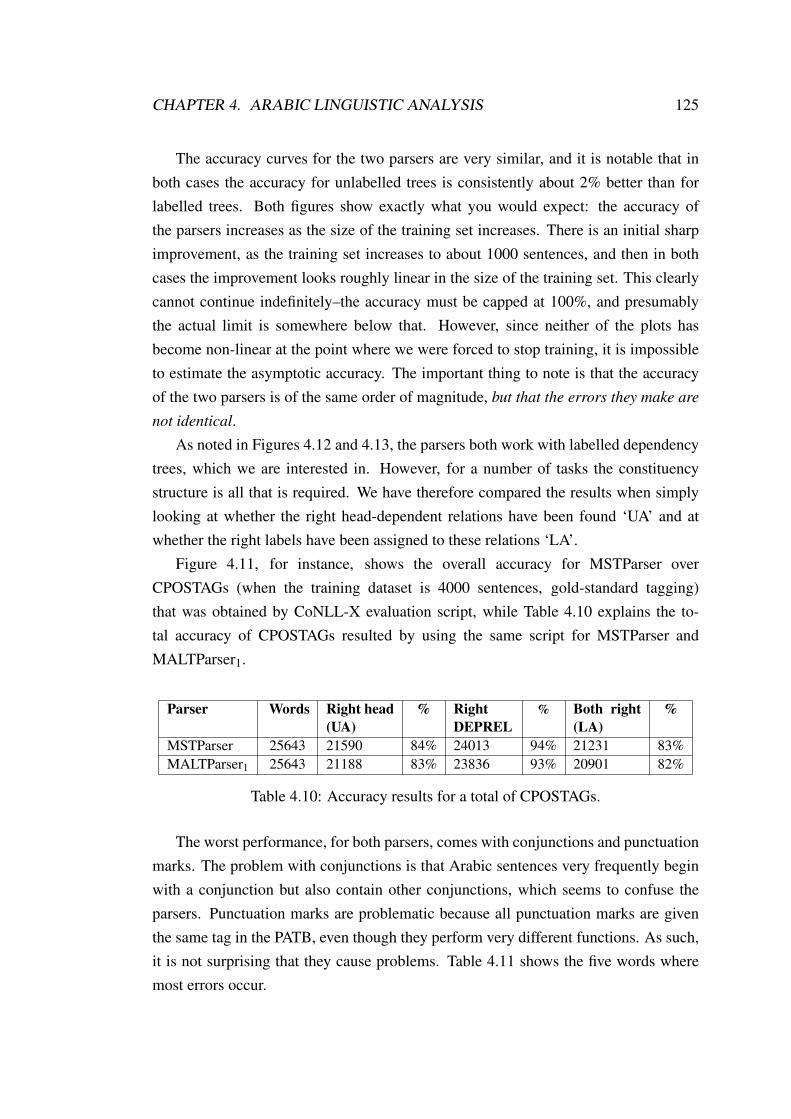
CHAPTER 4. ARABIC LINGUISTIC ANALYSIS 125
The accuracy curves for the two parsers are very similar, and it is notable that inboth cases the accuracy for unlabelled trees is consistently about 2% better than forlabelled trees. Both figures show exactly what you would expect: the accuracy ofthe parsers increases as the size of the training set increases. There is an initial sharpimprovement, as the training set increases to about 1000 sentences, and then in bothcases the improvement looks roughly linear in the size of the training set. This clearlycannot continue indefinitely–the accuracy must be capped at 100%, and presumablythe actual limit is somewhere below that. However, since neither of the plots hasbecome non-linear at the point where we were forced to stop training, it is impossibleto estimate the asymptotic accuracy. The important thing to note is that the accuracyof the two parsers is of the same order of magnitude, but that the errors they make are
not identical.As noted in Figures 4.12 and 4.13, the parsers both work with labelled dependency
trees, which we are interested in. However, for a number of tasks the constituencystructure is all that is required. We have therefore compared the results when simplylooking at whether the right head-dependent relations have been found ‘UA’ and atwhether the right labels have been assigned to these relations ‘LA’.
Figure 4.11, for instance, shows the overall accuracy for MSTParser overCPOSTAGs (when the training dataset is 4000 sentences, gold-standard tagging)that was obtained by CoNLL-X evaluation script, while Table 4.10 explains the to-tal accuracy of CPOSTAGs resulted by using the same script for MSTParser andMALTParser1.
Parser Words Right head(UA)
% RightDEPREL
% Both right(LA)
%
MSTParser 25643 21590 84% 24013 94% 21231 83%MALTParser1 25643 21188 83% 23836 93% 20901 82%
Table 4.10: Accuracy results for a total of CPOSTAGs.
The worst performance, for both parsers, comes with conjunctions and punctuationmarks. The problem with conjunctions is that Arabic sentences very frequently beginwith a conjunction but also contain other conjunctions, which seems to confuse theparsers. Punctuation marks are problematic because all punctuation marks are giventhe same tag in the PATB, even though they perform very different functions. As such,it is not surprising that they cause problems. Table 4.11 shows the five words wheremost errors occur.

CHAPTER 4. ARABIC LINGUISTIC ANALYSIS 126
Conjunctions MSTParser MALTParser1Any Head DEPREL Both Any Head DEPREL Both
ú
¯ fy “in”/PREP 315 315 22 22 328 328 26 26
+ ð w+ “and”/CONJ 249 249 0 0 232 232 1 1+ È l+ “for”/PREP 171 170 10 9 158 157 9 8áÓ mn “of/from”/PREP 157 156 6 5 149 148 8 7
+ H. b+ “in”/PREP 137 137 9 9 140 140 9 9
Table 4.11: Five worst behaving words.
As noted, conjunctions are difficult to handle. The other items are all prepositionsfor which the head has been misidentified. This just shows that data-driven dependencyparsing is not a solution to the perennial problem of PP-attachment.
4.3.2.1 Improve parsing
The results for individual parsers in isolation in Section 4.3.2 are still lower than whatwe aspire to. We therefore aim in the current section to investigate the evaluation ofdifferent strategies to improve parsing for Arabic by combining parsers, just as weimproved tagging by combining taggers. To make our experiments more realistic, thePATB is retagged by using our MC tagger which achieved 99.5% accuracy comparedwith a gold-standard one with 39 coarse-grained tags. This gives us a version of thecorpus, we called it PATBMC corpus, which is almost perfectly tagged (i.e. we usedhere combined strategy I, which is explained in Figure 4.1a).
In the current experiments we will use MSTParser and three parsing algorithms forMALTParser: MALTParser1, MALTParser2 using Stack swap-eager, which producesnon-projective graphs, and MALTParser3 using Planar. As with the gold-standardcorpus (see Figure 4.13 and Figure 4.12) the accuracy of the parsers increases as thesize of training set increases by using the same 16 sizes of training sets that were usedfor gold-standard before. Also, MSTParser still works better than the others on thesedatasets. Therefore, in the remaining experiments in this section, we will concentrateon the LA of the parsers when the training set is 4000 sentences, which provides thehighest accuracy for each parser. The highest accuracy for each parser is explained inTable 4.12 for PATBMC corpus with equivalent accuracy for the gold-standard corpus.

CHAPTER 4. ARABIC LINGUISTIC ANALYSIS 127
Parser LAGold-standard PATBMC
MSTParser 82.8% 82.7%MALTParser1, Nivre arc-eager 81.5% 81.4%MALTParser2, Stack swap-eager 81.2% 81.1%MALTParser3, Planar 81.1% 81%
Table 4.12: Highest LA for MSTParser, MALTParser1 and MALTParser2, gold-standard and PATBMC corpora.
Because of the ambiguity in Arabic, parsing is difficult and the accuracy is lowerthan for dependency parsing of many languages. It is thus even more important to findways of making the best possible use of the available resources. As we have shownbefore, combining Arabic POS taggers gives better accuracy than each one in isolation.We therefore try here to see how best to combine the parsers. To achieve this goal, weused two approaches as explained below.
We will start our experiment with the three parsers: MSTParser, MALTParser1 andMALTParser2. The first observation is that when the parsers agree on how to connect(i.e. head) and label (i.e. DEPREL) a given item they are more likely to be right thanwhen they disagree. This is fairly obvious–as before, if you have a set of parsers whichassign different head and DEPREL to an item then at least one of them must be wrong.Table 4.13 substantiates this observation–each row shows the precision, recall and F-score for a particular pair of parsers simply taking cases where they agree and leavingwords on which they disagree without head or DEPREL. Thus the combination ofMSTParser and MALTParser1 achieves a precision of 89.4% and recall 72.1%. Table4.14 shows what happens when we combine all three parsers, either taking the majorityview when at least two of them agree or demanding that all three agree (i.e. MSTParser,MALTParser1 and MALTParser2). In the latter case we obtain a precision of 92.3%and recall 67.2%.
Pair of parsers P R F-scoreMSTParser+MALTParser1 89.4% 72.1% 0.799MSTParser+MALTParser2 89.8% 73.2% 0.807MALTParser1+MALTParser2 88.7% 71.8% 0.794
Table 4.13: Precision (P), recall (R) and F-score for combinations of pairs of parsers,PATBMC corpus.

CHAPTER 4. ARABIC LINGUISTIC ANALYSIS 128
Parser P R F-scoreAt least two parsers agree 84.8% 80.3% 0.825Three parsers agree 92.3% 67.2% 0.778
Table 4.14: Precision (P), recall (R) and F-score for combinations of three parsers,PATBMC corpus.
It is notable that the precision on the cases where they agree is considerably higherthan the accuracy of any parser in isolation. Furthermore, when we combine only twoparsers, we find that the combination of MSTParser with other parsers gives better pre-cision than the accuracy of either parser in isolation, while combining MALTParser1
and MALTParser2 give lower precision, recall and F-score than other combinations oftwo parsers.
On the other hand, combining three parsers where they agree gives better precisionthan where at least two parsers agree and also for any combination of two parsers, butwith low recall and F-score.
4.3.2.1.1 Backoff strategiesIn order to improve the accuracy (not the precision only) of parsing, we applied
three different combinations of experiments depending on voting. Our first proposalwas to take the majority view when at least two of the parsers agreed, and to backoffto two different parsers (i.e. by taking the head from one parser and the DEPREL fromthe other one) when there was no common view (Zeman and Žabokrtsky, 2005). Thesecond proposal is the same as the first one, except that we back off unless they allagree, rather than doing so if they all disagree. We back off to two different parsers bytaking the head from one parser and the DEPREL from other one. The results of thesetwo proposals are shown in Table 4.15.
The results of these experiments show that the first proposal gives better LA re-sults than the second one and than the highest LA for all parsers in isolation for bothPATBMC and gold-standard corpora. The second proposal, on the other hand, failed toachieve the highest LA for all in isolation parsers.
The third proposal was to take the majority view when two of the parsers agreed,and to backoff to the other parser (i.e. by taking both the head and the DEPREL froma different parser) when there was no common view. The results of this proposal areshown in Table 4.16.

CHAPTER 4. ARABIC LINGUISTIC ANALYSIS 129
Backoff to LAHead DEPREL At least two agree All agreeMSTParser MALTParser1 84.2% 79.6%MSTParser MALTParser2 84.1% 79.8%MALTParser1 MSTParser 83.8% 78.7%MALTParser1 MALTParser2 83.6% 78.4%MALTParser2 MSTParser 83.8% 79.3%MALTParser2 MALTParser1 83.7% 78.5%
Table 4.15: LA of backoff to two parsers (MSTParser, MALTParser1 andMALTParser2) using the first and the second proposals, PATBMC corpus.
Agree Backoff to LAMSTParser+MALTParser1 MALTParser2 83.8%MSTParser+MALTParser2 MALTParser1 83.7%MALTParser1+MALTParser2 MSTParser 84.8%
Table 4.16: LA of backoff to other parser (MSTParser, MALTParser1 andMALTParser2) where there is no agreement between two parsers, PATBMC corpus.
The results of this experiment show that the third proposal gives better results thanthe highest accuracy for all parsers in isolation for both PATBMC and gold-standardcorpora (see Table 4.12). Also, the best result is generally obtained by combiningMALTParser1 and MALTParser2 parsers where they agree, backoff to MSTParser.This technique achieved 84.8%, which is the highest LA for all experimental results inthe current thesis.
In the next experiments, we re-apply the previous three proposals for the threeMALTParsers only (i.e. MALTParser1, MALTParser2 and MALTParser2) to check ifthese proposals still give positive results. The results of these experiments are shownin Tables 4.17 and 4.18 respectively.
Again the results of first and third proposals give better results than the highestaccuracy for all MALTParsers in isolation for both PATBMC and gold-standard corpora(see Table 4.12). Also, applying the first and third proposals for combining MSTParserwith MALTParsers gives better improvement in results than applying the same twoproposals for combining MALTParsers only.
In the next experiment, we used a new proposal that depends on majority vote+ backoff to the most confident parser as well as only most confident parser insteadof majority vote + backoff to an arbitrary parser, just as we did with the taggers.

CHAPTER 4. ARABIC LINGUISTIC ANALYSIS 130
Backoff to LAHead DEPREL At least two agree All agreeMALTParser1 MALTParser2 82% 78.1%MALTParser1 MALTParser3 81.9% 77.8%MALTParser2 MALTParser1 82.8% 78.3%MALTParser2 MALTParser3 82.8% 78.1%MALTParser3 MALTParser1 81.8% 77.6%MALTParser3 MALTParser2 81.6% 77.2%
Table 4.17: LA of backoff to two parsers (MALTParser1, MALTParser2 andMALTParser3) where there is no agreement between at least two parsers, PATBMCcorpus.
Agree Backoff to LAMALTParser1+MALTParser2 MALTParser3 81.6%MALTParser1+MALTParser3 MALTParser2 82.3%MALTParser2+MALTParser3 MALTParser1 82.1%
Table 4.18: LA of backoff to other parser (MALTParser1, MALTParser2 andMALTParser3) where there is no agreement between two parsers, PATBMC corpus.
Therefore, for MSTParser, MALTParser1 and MALTParser2 we computed the statis-tics about the correct head and the correct DEPREL of each POS tag in the ‘MC’coarse-grained tagset (39 tags) where each parser agrees with the gold-standard. Ac-cording to these confidence scores, we can decide how much each parser should betrusted for each POS tag. We trained the parsers on 3000 sentences from the first4000 sentences in the corpus and used the other 1000 sentences to compute confidencescores using fourfold cross-validation. The highest LA for MSTParser, MALTParser1
and MALTParser2 is given in Table 4.19.
Parser LAMSTParser 81.6%MALTParser1 79.7%MALTParser2 79.6%
Table 4.19: Highest LA for MSTParser, MALTParser1 and MALTParser2 for PATBMCcorpus, fourfold cross-validation with 4000 training sentences and 1000 testing sen-tences.
Some POS tags with their trusted parser(s) for both head and DEPREL are givenin Table 4.20.

CHAPTER 4. ARABIC LINGUISTIC ANALYSIS 131
POS tag Trusted parser(s) for head Trusted parser(s) for DEPRELADJ, NEG_PART MALTParser1 MALTParser1
CONJ, NOUN_PROP MSTParser MALTParser2
PV MALTParser2 MSTParserDET+NOUN_PROP MALTParser2 MALTParser1
NOUN, IV MSTParser MSTParserPRON MALTParser2 MALTParser2
PSEUDO_VERB MALTParser1 MSTParser, MALTParser2
Table 4.20: Some POS tags with trusted parsers(s) for head and DEPREL, PATBMCcorpus.
As shown in Table 4.20, we find that, for instance, MALTParser1 should be trustedwhen the POS tag is ADJ or NEG_PART for both the head and the DEPREL, whereasMALTParser2 should be trusted when the POS tag is PRON. On the other hand, in thecase where the POS tag is CONJ or NOUN_PROP MSTParser should be trusted for thehead only, whereas MALTParser2 should be trusted for the DEPREL. Also, in the caseof PSEUDO_VERB POS tag, MALTParser1 should be trusted for the head, whereas MST-Parser or MALTParser2 for the DEPREL. The results of this experiment are shown inTable 4.21.
Parser LAMSTParser+MALTParser1, backoff to the most confident parser 80.1%MSTParser+MALTParser2, backoff to the most confident parser 79.9%MALTParser1+MALTParser2, backoff to the most confident parser 81.4%At least two parsers agree, backoff to the most confident parser 81.9%Three parsers agree, backoff to the most confident parser 79.7%Most confident parser only 78.9%
Table 4.21: LA for backoff to the most confident parser, PATBMC corpus, fourfoldcross-validation with 4000 training sentences and 1000 testing sentences.
The above results show that combining parsers depending on the most confidentparser for each POS tag can produce accuracy better than each parser produces byitself, but this is not the best of our combinations. The proposal when we took themajority verdict if at least two parsers agreed and the most confident if all three parsersgave different results gives a better result than others and than each parser in isolation.Also, the proposal when we simply chose the most confident fails to give good re-sults compared with the same proposal for combining POS taggers, which gives betterresults for tagging.

CHAPTER 4. ARABIC LINGUISTIC ANALYSIS 132
In Section 4.3.2.1, we have presented a parsing combining system, which usesthe output of different dependency parsers to combine their individual advantages andcompute a joint parse, which produces results for imperfectly tagged text with accu-racy higher than the best individual parser’s accuracy for perfectly tagged text. Wehave shown empirically that combining different parsers by voting techniques for im-perfectly tagged text may produce considerable quality improvements over using indi-vidual parsers in isolation. The confidence based combining technique that we used fortagging, on the other hand, can produce better accuracy than each component producesby itself, but does not beat the voting one.
From all the experiments described above, the best strategy was to use two versionsof MALTParser, and to backoff to MSTParser if they disagreed. This strategy achieved84.8% accuracy, compared to the 82.7% achieved by MSTParser by itself (i.e. the bestparser in isolation). The strategy of relying on the most confident of the contributingtools, which was extremely effective for tagging, did not work so well for parsing.
4.4 Combine taggers and parsers
Sections 4.2 and 4.3 describe combined strategy I (Figure 4.1a). Following this strat-egy, we achieve 84.8% accuracy for dependency trees. We now turn to combinedstrategy II (Figure 4.1b) to see whether this can improve on combined strategy I.
4.4.1 Experiments
The key question here is: if a tagger assigns tags with accuracy AT and a parser assignsroles to words with accuracy AP, will the combination of the tagger and parser achieveAT ×AP or more or less?
4.4.1.1 Individual combinations of parsers and taggers
In the current experiments we will concentrate on scores for labelled trees. In everycase the scores for unlabelled ones are about 2% higher, for all tagger:parser combina-tions and training sets.
Table 4.22 shows the effects of combining the taggers and parsers. In both caseswe have included the results for the gold-standard tags as a benchmark.

CHAPTER 4. ARABIC LINGUISTIC ANALYSIS 133
Parser Accuracy Gold-standard AMIRA MADA MXL MC
MSTParserLA 82.8% 80.4% 81.3% 81.7% 82.7%UA 84.2% 82.1% 83.3% 83.3% 84.1%
MALTParser1LA 81.5% 78.1% 79.8% 79.3% 81.4%UA 82.6% 79.5% 81.4% 80.4% 82.4%
Table 4.22: MSTParser and MALTParser1 accuracies, multiple taggers compared withgold-standard tagging.
Both MSTParser and MALTParser1 do better when trained and tested with thecorpus tagged by our MC tagger than other taggers. Parsing with MC tagger givesaccuracies approximately similar to these with gold-standard for both parsers. This isbecause MC tagger gives high tagging accuracy 99.5% compared with gold-standardone. Also, these parsers do better on the corpus tagged by MADA or MXL than whenwe used AMIRA, despite the fact that the three taggers achieve very similar scoreswhen viewed simply as taggers (AMIRA 95.3%, MADA 96.7% and MXL 95.6%).
We considered two possible causes for this difference: that it arises because of thedifference between the tagsets used by the taggers, or that it arises from the differencesin tokenisation.
Different tagsets: although the sizes of the two tagsets are similar, the nature of thetags themselves is different. The MXL tags, which are a coarse-grained variant ofthe tags used in the PATB itself, seem to provide more information about syntacticrelations than the AMIRA set. In particular, the fine-grained distinctions between sin-gular and plural nouns, and between various verb forms, that AMIRA provides are notactually very useful when trying to see whether two items are related.
It may be that the information about particles that MXL is sensitive to but AMIRAis not is likely to be useful for parsing: knowing, for instance, that some particle ex-pects the next item to be a verb-initial sentence, whereas another expects a subject-initial sentence, may well be useful.
In order to see whether this was the cause of the difference, we used the version ofthe AMIRA corpus that was constructed before in Section 4.2.1 (see page 101), whichhas the same size as the gold-standard one, where all the tags were compatible withthe tags in the PATB, but where some were AMIRA refinements of the originals.
Using the gold-standard tags obtained directly from the PATB scores 82.8%, usingthe AMIRA tagset scores 80.4%. The only differences are that where the PATB tag

CHAPTER 4. ARABIC LINGUISTIC ANALYSIS 134
translates to an AMIRA tag, and the tag assigned by AMIRA is compatible with thetranslation but is finer-grained, we have used the one assigned by AMIRA; and thatwhere several PATB tags translate to the same AMIRA tag (e.g. particles) we havesimply used the commonest translation. These results strongly suggest that the choiceof tags is significant, since in this experiment the two sets are compatible at everypoint, but the AMIRA tags include fine-grained distinctions that are made by AMIRAbut not ones that are made in the PATB. Thus the decrease in accuracy of the parsermust be due solely to the loss of information that arises when we merge PATB tags.
Tokenisation: the other potential problem is that AMIRA’s tokeniser segments thetext differently from the way that it is segmented in the PATB. In the PATB, for in-stance, the string ½Ë
YË lðlk “therefore” is treated as a single subordinating conjunc-
tion, whereas AMIRA breaks it into a preposition È l “for” and a determiner ½ËX
ðlk “that”. Similarly, in the PATB the string úÍ ly “mine” is split into two tokens
(a preposition È l “for”, and a pronoun ø
y “me”), whereas AMIRA treats it as asingle proper noun. This caused us problems when trying to use AMIRA to tag thetreebank, since the leaves in the trees did not always correspond to tokens in the outputof AMIRA. The difference in tokenisation affected around 2% of tokens, so since theparser performed around 2% worse with AMIRA than with the other taggers it seemedplausible that this was the source of the discrepancy.
In order to investigate the effect of this problem, we produced a version of thecorpus where we replaced sequences where the PATB had a single token and AMIRAhad several by the hand-coded AMIRA equivalent of the PATB tag, and likewise wherethe PATB had several tokens and AMIRA had one by the sequence of hand-codedAMIRA equivalents of the PATB tags.
This gave us a version of the treebank that had the same number of tokens as theoriginal PATB, with as many items as possible given the tags assigned by AMIRAand the others given hand-coded AMIRA equivalents of the original PATB tags. Theresults suggest that this is not the source of the problem, since AMIRA produces almostidentical results (no difference to three significant figures) no matter whether its owntokeniser or the tokenisation used in the PATB is used.
4.4.2 Merging combinations
A given tagger:parser combination will make errors. If two such combinations producedifferent parents for some word, then at least one of them must be wrong. So if we

CHAPTER 4. ARABIC LINGUISTIC ANALYSIS 135
take the output of two combinations and reject all instances of words where the twosuggest different parents for a word, we must improve the precision, because we willbe throwing away items where we know that one of the combinations has made amistake. The other one may, of course, have got the parent for this word right, butsince we cannot tell which has got it wrong and which has got it right, we have todistrust the output of each. We will also decrease the recall, because there will nowbe items for which we have discarded the parents suggested by the parsers, and hencewe will end up with no parent assigned to them. The question is: does the increase inprecision compensate for the decrease in recall?
If the sets of mistakes that were made by the two combinations were comple-mentary, then the precision of the merged output would be 1 and the recall wouldbe 1− (w1 +w2), where wi is the error rate of combination i. The F-score for themerge if the combinations have complementary distributions would thus be (1−(w1+
w2))/(1− (w1 +w2)/2). If, on the other hand, the two combinations made exactly thesame mistakes then the F-score for the merge would be (1−w1). In other words, forcombinations with similar accuracy, the highest precision will come if the errors theymake are complementary, and the highest F-score will come if they make identicalerrors.
Table 4.23 shows the precision, recall and F-score for all possible pairs of combi-nations of tagger:parser, e.g. that if you use MSTParser having tagged using AMIRAand MALTParser1 having tagged using MADA then the precision is 89.3%, the recallis 66.3% and the F-score is 0.761. This table includes cases where one or both theparsers were combined with the gold-standard tags. These cases are greyed out, be-cause in any real situation the gold-standard tags would not be available.
Table 4.23 roughly bears out the observations above. The best precision is gener-ally obtained by using different taggers for each part of the combination (so the bestprecision for AMIRA:MSTParser comes from merging it with MADA:MALTParser1,the best for MXL:MSTParser comes from merging it with MADA:MALTParser1, andthe best for MADA:MSTParser from merging it with MXL:MALTParser1); and thebest F-score is generally obtained by using the same tagger with the two parsers.
The impetus for Section 4.4 arose from a simple query: what happens if you com-bine a tagger whose accuracy is AT with a parser whose accuracy is AP? It turns outthat the answer is often better than AT ×AP. When, for instance, we combine MST-Parser, for which we get an accuracy of 82.8% when using the gold-standard tags, andMXL, whose accuracy is 95.6%, we get 81.7%, which is noticeably greater than the

CHAPTER 4. ARABIC LINGUISTIC ANALYSIS 136
MSTParser withtagger
MALTParser1with tagger
P R F-score
gold-standard
gold-standard 89.3% 72.3% 0.799AMIRA 87.5% 61.4% 0.722MADA 90.5% 57.8% 0.705MXL 89.8% 60.1% 0.720MC 89.1% 72.1% 0.797
AMIRA
gold-standard 89% 58.5% 0.706AMIRA 87.9% 69.1% 0.774MADA 89.3% 66.3% 0.761MXL 89% 68.4% 0.774MC 89% 60.3% 0.719
MADA
gold-standard 89.4% 57.8% 0.702AMIRA 85.3% 70.8% 0.774MADA 88.6% 69.7% 0.780MXL 88.9% 68.1% 0.771MC 89.4% 57.8% 0.719
MXL
gold-standard 89.1% 59.9% 0.716AMIRA 84.7% 73.2% 0.785MADA 89.3% 67.7% 0.770MXL 88.1% 57.6% 0.697MC 89.1% 62.1% 0.732
MC
gold-standard 89.2% 72.1% 0.797AMIRA 87.7% 61.9% 0.726MADA 90.2% 58.2% 0.707MXL 89.5% 60.7% 0.723MC 89.4% 72.1% 0.798
Table 4.23: Precision (P), recall (R) and F-score for different tagger1: parser1+ tagger2:parser2 combinations.
79.2% that you would expect if the errors simply compounded one another. It seemsas though the fact that the training set contains the same pattern of errors as the test setautomatically provides a degree of compensation.
Closer inspection shows that the nature of the tagsets has a substantial effect. Be-cause MXL uses the PATB tagset, which was presumably chosen because it carriedthe kind of information that is required for parsing, it interacted better with both theparsers than AMIRA, which uses a general purpose tagset which is not tuned to thistask. The mismatch between AMIRA’s built-in tokeniser and the tokenisation in thetreebank caused us some technical problems, but does not seem to be a critical factorin the accuracy of the combination of AMIRA with the two parsers.

CHAPTER 4. ARABIC LINGUISTIC ANALYSIS 137
We have also investigated the effects of merging the outputs of pairs of tagger:parsercombinations. The results here are broadly as expected–the precision of the combina-tion is always better than the accuracy of either of the contributing pairs (which isinevitable), and using a different tagger with each parser in the combination producesthe greatest improvement in precision (which is what we expected, but it needed con-firmation).
The results above arise from investigating combinations of specific tools–four tag-gers × two parsers. Are these results compromised by the fact that we chose thesespecific tools, or are there general lessons to be learnt? The taggers all use differentmechanisms and different information, and the parsers also use substantially differentapproaches. The fact that nonetheless we get fairly consistent results in Section 4.4.2suggests that there may be some robustness about the conclusions. It seems that nomatter which tagger and which parser we use we get results that are better than youwould expect just by looking at the individual performance of the components. Themain result of the second set of experiments–that taking the combined output of twodifferent tagger:parser combinations improves the precision–is almost inevitable, butthere is a tendency for combinations that involve different taggers to achieve greaterprecision than ones where the two parsers are combined with a single tagger.
It seems likely that this pattern would be repeated if other parsers or taggers wereused: mistakes made by a combination of a tagger Tr and a parser Pr could be causedeither by Tr or by Pr. If Tr is combined with some other parser Pr′, then the mistakescaused by Tr will almost certainly arise again, and will not be spotted when the output
of the two combinations is merged, whereas a combination of another tagger Tr′ withPr′ will not repeat the mistakes introduced by Tr. Thus although our experimentswere limited to a specific set of tools and a specific language (as any experimentsmust be) we believe that the results are likely to be applicable if other tools are used.The critical issue is that the tools should be distinct, either using different principles ordifferent underlying data (training sets, rule sets), so that they do indeed make mistakesin different places. This observation is likely to transfer to other languages, not justother tools for handling Arabic. If you have multiple taggers and parsers which makedistinct mistakes (which is likely to happen if they are based on different principles oruse different features) then combining them will inevitably improve the precision andis likely to also improve the F-score.

CHAPTER 4. ARABIC LINGUISTIC ANALYSIS 138
4.5 Summary
In this chapter, we have described the performance of our preprocessing stage. We havecarried out a number of experiments with state-of-the-art taggers (AMIRA, MADA,a home-grown tagger, MXL and our combined tagger, MC, which depends on themost confident score with comparable accuracy) and parsers (notably MSTParser andMALTParser with various parsing algorithms), using the PATB as training data. Theseexperiments show in particular the following main results:
• Our conversion from phrase structure to dependency trees allows parsers to performaccurately even for long sentences exceeding 100 words (Alabbas and Ramsay,2012a).
• Combining three different taggers using voting or a very simple approach, whichdepends on the most confident score, can lead to significant improvements over thebest individual tagger (Alabbas and Ramsay, 2012d).
• Combining the output of multiple data-driven dependency parsers can producemore accurate results, even for imperfectly tagged text, than each parser producesby itself for texts with the gold-standard tags (Alabbas and Ramsay, 2011a).
• If you train and test with a flawed tagger and flawed parser, the parser may learn tocompensate for the errors made by the tagger (Alabbas and Ramsay, 2012b).
• Combining different tagger:parser pairs where each parser uses a different taggerincreases precision, as expected, but at the cost of decreasing recall (Alabbas andRamsay, 2012b).
In short, we have shown in this chapter that the combined strategy I (Sections 4.2and 4.3) to combine taggers and parsers gives better accuracy compared to the com-bined strategy II (Section 4.4) that gives better precision, which may be useful for sometasks.

Chapter 5
Tree matching
5.1 Overview
Recently, comparison of tree-structured data is a growing interest in various diverseareas such as image analysis, XML databases, automatic theorem proving, computa-tional biology and NLP (Mehdad and Magnini, 2009). Tree edit distance (TED) isconsidered to be one of the most effective techniques in this field. However, one of themain drawbacks of TED is that transformation operations are applied solely on singlenodes. This problem is solved in the current work by updating TED to allow subtreetransformation operations as well. This makes the extended TED more effective andflexible than the standard one, especially for applications that pay attention to relationsamong nodes (e.g. deleting a modifier subtree, in linguistic trees, should be cheaperthan the sum of deleting its components individually).
As we have already mentioned, the TED algorithm developed by Zhang and Shasha(1989), which forms the basis of our work, will be used in the current work to find thematching between two dependency trees for Arabic text snippets (T and H). In thissection, different approaches for TED algorithms will be presented and the reason forusing Zhang-Shasha’s algorithm will be explained.
The tree edit distance metric is a common similarity measure for rooted orderedtrees. It is a generalisation of the well-known string edit distance problem, whichis to determine the distance between two strings by measuring the minimum cost ofedit operations needed to transform one string into the other. The edit operations aredeletion, insertion or exchanging of a single character. Generally, the edit distancebetween two strings refers to the Levenshtein distance or linear distance introduced byLevenshtein (1966). The pseudo-code of the Levenshtein distance algorithm is given
139

CHAPTER 5. TREE MATCHING 140
in Algorithm 5.1.
Algorithm 5.1 Pseudo-code of Levenshtein distance algorithmstr1,str2 the first and second string respectively.m and n the length of str1 and str2 respectively.D table with m+1 rows and n+1 columns.γ(str1[i]→∧) cost of deleting the ith character from str1
γ(∧→ str2[ j]) cost of inserting the jth character of str2 into str1
γ(str1[i]→ str2[ j]) cost of exchanging the ith character of str1 with the jth character of str2
1: D[0,0]← 02: for i← 0 to m do3: D[i,0]← i4: end for5: for j← 0 to n do6: D[0, j]← j7: end for8: for i← 1 to m do9: for j← 1 to n do
10: D[i, j]]← min(D[i−1, j]]+ γ(str1[i]→∧), // deletion11: D[i, j−1]]+ γ(∧→ str2[ j]), // insertion12: D[i−1, j−1]+ γ(str1[i]→ str2[ j])) // changing13: end for14: end for15: return D[m,n]
The Levenshtein distance solves the string edit distance problem by using dynamicprogramming (Dasgupta et al., 2006; Cormen et al., 2009). It takes the main problemand splits it into sub-problems, solving each sub-problem only once and rememberingthe results in the matrix D for later. Then, it computes its solution bottom-up by syn-thesising it from smaller sub-solutions and by trying several possibilities and choicesbefore it arrives at the optimal set of choices for the whole problem. The idea here is touse the cheapest edit operations possible to transform one string to another. Typically,each edit operation costs 1 except that exchanging similar items costs 0. So, the Lev-enshtein distance does not calculate the similarity between two strings but the distancein cost measures.
Tree edit operations such as delete, insert and exchange were proposed by Selkow(1977) as an extension to the string edit operations used in the Levenshtein distance.

CHAPTER 5. TREE MATCHING 141
Selkow implements a recursive algorithm for computing the minimum sequence of op-erations that transforms one tree to another. In Selkow’s algorithm, delete and insertoperations are specific operations that are enabled solely on tree leaves, whereas ex-change can be applied at every node. There is a nonnegative real cost associated witheach edit operations.
In contrast, Tai (1979) proposed an unrestricted edit model. This author uses adynamic programming algorithm to solve the tree-to-tree correction problem betweentwo trees. Tai’s algorithm runs in O(m3n3) time and space for trees T1 and T2 withm and n nodes respectively. All trees are considered to be rooted, ordered and la-beled. The root is the first node that is visited and the subtrees are then traversed inpreorder. This algorithm is an extension of a string-to-string correction algorithm thatwas proposed by Wagner and Fischer (1974). Tai’s algorithm uses the following basicoperations: (i) exchanging a node’s label; (ii) deleting a node other than the root, i.e.all the children of a deleted node become the children of the parent of that node; and(iii) inserting a node, i.e. an inserted node becomes a parent to some or all the sequencein the left to right order of its parent.
Subsequently, Zhang and Shasha (1989) improved Tai’s algorithm and obtainedO(m2n2) time and O(mn) space. These authors presented an efficient technique thatis based on dynamic programming to calculate the approximate tree matching for tworooted postordered trees. Approximate tree matching allows users to match a tree withsolely some parts of another tree not a whole. In this algorithm, for all the offspringof each node, the lowest cost mapping has to be calculated before the node is met.Hence, the least cost mapping can be chosen right away. For this purpose, the algorithmpursues the keyroots of the tree, which are a set that includes all nodes having a leftsibling as well as the root of the tree. Accordingly, the number of keyroots must beidentical to the sum of leaves in the tree.
Klein (1998) improves Zhang-Shasha’s algorithm using heavy paths (Sleator andTarjan, 1983) to decompose the larger tree and obtains O(n2m log m) time and space,which means his algorithm requires less time but more space than Zhang-Shasha’salgorithm. A heavy path of a tree is a path that starts at the root and goes from eachvertex v to the child of v whose subtree contains the largest number of vertices. Hisalgorithm uses Euler strings to encode the trees. The Euler string of an ordered androoted tree T is a string generated as follows: replace each edge {x,y} of T by darts,which are two oppositely directed arcs (x,y) and (y,x) (e.g. for a dart a in Figure 5.1,the oppositely directed arc corresponding to this dart will be a′). Then, an Euler tour

CHAPTER 5. TREE MATCHING 142
of the darts of T is defined by the depth-first search traversal of T (visiting each node’schildren according to their order).
a
b
c
d
a
a’
b
c
b’
c’aa’cbb’c’
Figure 5.1: Constructing Euler string for a tree.
This algorithm depends on dynamic programming to calculate the edit distance be-tween two trees T1 and T2 as shown in Figure 5.2, where dist(s, t) is the edit distancebetween two substrings s and t, E(T ) is the Euler string of T , and E∗(T ) is the Eulerstring of T , interpreted as a cyclic string. Note that the string edit distance here is notan ordinary problem because the Euler string has a pair of darts (e.g. a and a′) whichaffects the edit distance calculation.
• If T2 is an unrooted tree, root it arbitrarily.
• Find a heavy-path decomposition of T2, and then identify the relevantsubstrings of each special subtree of T2.
• By dynamic programming, calculate dist(s, t) for every substring s of thecyclic string E∗(T1) and every relevant substring t of T2.
• For the rooted distance, output dist(s′, t ′), where s′ = E(T1) and t ′ = E(T2).
• For the unrooted distance, output mins∈R(T1)dist(s, t ′), where t ′ = E(T2) (notethat the min is over all Euler strings of rooted versions of T1).
Figure 5.2: Klein’s tree edit distance algorithm (Klein, 1998).
The difference between Klein’s algorithm and Zhang-Shasha’s algorithm lies inthe set of subforests that are involved in the decomposition (Dulucq and Touzet, 2005).This leads to different time complexities in worst case (i.e. O(n3 log n) in Klein’s algo-rithm compared with O(n4) in Zhang-Shasha’s algorithm). Nevertheless, this does notnecessarily mean that Klein’s method is better than Zhang-Shasha’s method, becauseeach algorithm’s performance depends on the shape of the two trees to be compared.

CHAPTER 5. TREE MATCHING 143
In Figure 5.3, to transform the tree Tx into Ty, for instance, Klein’s solution requires 84different recursive calls, whereas the Zhang-Shasha’s solution requires just 72 (Dulucqand Touzet, 2005).
Tx Ty
Figure 5.3: Two trees, Tx and Ty.
Demaine et al. (2009) develop the first worst-case optimal algorithm for computingthe tree edit distance between two rooted ordered trees. These authors also use heavypaths, but differ from Klein’s method by switching the trees such that the larger subtreeis decomposed in each recursive step. Their algorithm runs in O(n2m(1+logm
n )) timeand O(mn) space. These authors show a solution for binary trees and explain how toextend their solution to general trees.
Recently, Pawlik and Augsten (2011) show that the efficiency of the previous al-gorithms for computing the tree edit distance heavily depends on the tree shape andruns into their worst cases for some data instances. These authors generalise the pre-vious methods and develop a new algorithm called robust tree edit distance (RTED)with O(n3) time (with n > m) and O(mn) space. Their algorithm is efficient for all treeshapes. Also, it never runs in the worst case if a best solution exists.
We have chosen to work with Zhang-Shasha’s algorithm because the intermediatestructures produced by this algorithm allow us to detect and respond to operations onsubtrees.
5.2 Zhang-Shasha’s TED algorithm
Zhang-Shasha’s TED algorithm (we will refer, henceforth, to this algorithm as ZS-TED) is considered an efficient technique based on dynamic programming to calculatethe approximate tree matching for two rooted ordered trees. Ordered trees are trees in

CHAPTER 5. TREE MATCHING 144
which the left-to-right order among siblings is significant. Approximate tree matchingallows us to match a tree with just some parts of another tree. There are three oper-ations, namely deleting, inserting and exchanging a node, which can transform oneordered tree to another. Deleting a node x means attaching its children to the parent ofx. Insertion is the inverse of deletion. This means an inserted node becomes a parentof a consecutive subsequence in the left to right order of its parent. Exchanging a nodealters its label. Each operation is associated with a nonnegative real cost. These costsare exchanged to match the requirements of specific applications. All these editingoperations are illustrated in Figure 5.4 (Bille, 2005).
l1 l2
(a) An exchanging of the node label (l1→ l2).
l1 l1
l2
(b) Deleting the node labeled (l2→∧).
l1 l1
l2
(c) Inserting a node labeled l2 as the child of thenode labeled l1 (∧→ l2).
Figure 5.4: Tree edit operations.
In ZS-TED, tree nodes are compared using a left-to-right postorder traversal, whichvisits the nodes of a tree starting with the leftmost leaf descendant of the root andproceeding to the leftmost descendant of the right sibling of that leaf, the right siblings,and then the parent of the leaf and so on up the tree to the root. The last node visitedwill always be the root. An example of the postorder traversal and the leftmost leaf

CHAPTER 5. TREE MATCHING 145
descendant of a tree is shown in Figure 5.5. In this figure, there are two trees, T1 withm=6 nodes and T2 with n=6 nodes. The subscript for each node is considered theorder of this node in the postorder of the tree. So, the postorder of T1 is a,b,c,e,d,f andthe postorder for T2 is b,c,a,e,d,f. The leftmost leaf descendant of the subtrees of T1
headed by the nodes a,b,c,e,d,f are 1,2,1,4,1,1 respectively, and similarly the leftmostleaf descendant of b,c,a,e,d,f in T2 are 1,1,3,3,1,1.
f6
d5
c3
a1 b2
e4
f6
d5
c2
b1
e4
a3
T1 T2
Figure 5.5: Two trees T1 and T2 with their left-to-right postorder traversal (the sub-scripts) and keyroots (bold items).
For all the descendants of each node, the least cost mapping has to be calculatedbefore the node is encountered, in order that the least cost mapping can be selectedright away. To achieve this, the algorithm pursues the keyroots of the tree, which aredefined as a set that contains the root of the tree plus all nodes having a left sibling.Concentrating on the keyroots is critical to the dynamic nature of the algorithm, sinceit is the subtrees rooted at keyroots that allow the problem to be split into independentsubproblems of the same general kind. The keyroots of a tree are decided in advance,permitting the algorithm to distinguish between tree distance (the distance betweentwo nodes when considered in the context of their left siblings in the trees T1 andT2) and forest distance (the distance between two nodes considered separately fromtheir siblings and ancestors but not from their descendants) (Kouylekov, 2006). Forillustration, the keyroots in each tree in Figure 5.5 are marked in bold.
For each node, the computation to find the least cost mapping (the tree distance)between a node in the first tree and one in the second depends solely on mapping thenodes and their children. To find the least cost mapping of a node, then, one needsto recognise the least cost mapping from all the keyroots among its children, plus thecost of its leftmost child. Because the nodes are numbered according to the postorder

CHAPTER 5. TREE MATCHING 146
traversal, the algorithm proceeds in the following steps (Kouylekov, 2006): (i) themappings from all leaf keyroots are determined; (ii) the mappings for all keyroots atthe next higher level are decided recursively; and (iii) the root mapping is found. Al-gorithm 5.2 shows the pseudo-code of ZS-TED (Zhang and Shasha, 1989).
Algorithm 5.2 Pseudo-code of ZS-TED.T[i] the ith node of T, labeled in postorderl(i) the leftmost leaf descendant of the subtree rooted at iK(T) the keyroots of tree T, K(T) = {k ∈T|¬∃ k1 >k with l(k1) = l(k)}/0 a null treeFD[T1[i, i1],T2[ j, j1]] the forest distance from nodes i to i1 in T1 to nodes j to j1 in T2, if i< i1
then T1[i, i1] = /0.γ(T1[i]→∧) cost of deleting the ith node from T1γ(∧→ T2[ j]) cost of inserting the jth node of T2 into T1γ(T1[i]→ T2[ j]) cost of exchanging the ith node of T1 with the jth node of T2m and n the number of nodes in T1 and T2 respectively|X | the length of X (i.e. the number of nodes in X, e.g. |T1|= m)min function return minimum item among three items.
1: compute l1(m), l2(n),K1(T1),K2(T2)2: for x← 1 to |K1(T1)| do3: for y← 1 to |K2(T2)| do4: FD[ /0, /0]← 05: for i← l1(x) to x do6: FD[T1[l1(x), i], /0]← FD[T1[l1(x), i−1], /0]+ γ(T1[i]→∧)7: end for8: for j← l2(y) to y do9: FD[ /0,T2[l2(y), j]]← FD[ /0,T2[l2(y),y−1]]+ γ(∧→ T2[ j])
10: end for11: for i← l1(x) to x do12: for j← l2(y) to y do13: if (l1(i) == l1(x)and l2( j) == l2(y)) then14: FD[T1[l1(x), i],T2[l1(y), j]]← min(15: FD[T1[l1(x), i−1],T2[l2(y), j]]+ γ(T1[i]→∧),16: FD[T1[l1(x), i],T2[l2(y), j−1]]+ γ(∧→ T2[ j]),17: FD[T1[l1(x), i−1],T2[l2(y), j−1]]+ γ(T1[i]→ T2[ j]))18: D[i, j]← FD[T1[l1(x), i],T2[l2(y), j]]19: else20: FD[T1[l1(x), i],T2[l1(y), j]]← min(21: FD[T1[l1(x), i−1],T2[l2(y), j]]+ γ(T1[i]→∧),22: FD[T1[l1(x), i],T2[l2(y), j−1]]+ γ(∧→ T2[ j]),23: FD[T1[l1(x), i−1],T2[l2(y), j−1]]+D[i, j])24: end if25: end for26: end for27: end for28: end for29: return D[m,n]

CHAPTER 5. TREE MATCHING 147
5.3 Extended TED with subtrees
The main weakness of ZS-TED is that it is not able to do transformations on subtrees(i.e. delete subtree, insert subtree and exchange subtree). The output of ZS-TED isthe lowest cost sequence of operations on single nodes. We extend this to find thelowest cost sequence of operations on nodes and subtrees. This algorithm, which wecall extended TED (ETED), is defined as follows:
1. Run ZS-TED and compute the standard alignment from the results, according toAlgorithm 5.3 (Section 5.3.1).
2. Go over the alignment and group subtree operations. Where a sequence of identicaloperations applies to a set of nodes comprising a subtree, they are replaced by asingle operation, whose cost is determined by some appropriate function of thecosts of the individual nodes, according to Algorithm 5.4 (Section 5.3.2). A varietyof functions could be applied here, depending on the application.
It should be noted here that while we apply this technique to modify ZS-TEDO(n4), it could also be applied to any other algorithm for finding tree edit distance, e.g.Klein’s O(n3logn) algorithm (Klein, 1998), Demaine et al. O(n3) algorithm (Demaineet al., 2009) or RTED O(n3) algorithm (Pawlik and Augsten, 2011), since the extensionoperates on the output of the original algorithm. The additional time cost of O(n2) isnegligible since it is less than the time cost for any available TED algorithm.
5.3.1 Find a sequence of edit operations
In order to find the sequence of edit operations that transforms one tree into another, thecomputation proceeds as follows: ZS-TED contains two matrices D and FD. Thesematrices D and FD are used for recording the results of individual subproblems: D
is used to store the tree distance between trees rooted at pairs of nodes in the twotrees, and FD is used to store the ‘forest distance’ between sequences of nodes. FD
is used as a temporary store while the tree edit distance between pairs of keyroots isbeing calculated. We have extended the standard algorithm, which computes the cost
of the cheapest edit sequence, so that it also records the edit operations themselves(Algorithm 5.3). This involves adding two new matrices, DPATH and FDPATH, tohold the appropriate sequences of edit operations–DPATH to hold the edit sequencesfor trees rooted at pairs of nodes and FDPATH to hold the edit sequences for forests. D

CHAPTER 5. TREE MATCHING 148
and DPATH are permanent arrays, whereas FD and FDPATH are reinitialised for eachpair of keyroots.
Algorithm 5.3 Pseudo-code of ZS-TED with edit sequencesT [i, j] ith to jth nodes in the postorder enumeration of tree T (T [i, i] is written T [i])l(i) the leftmost leaf descendant of the subtree rooted at iK(T ) the keyroots of tree T,K(T ) = {k ∈ T : ¬∃k1 > k with l(k1) = l(k)}D[i, j] the tree distance between two nodes T1[i] and T2[ j]FD[T1[i, i1],T2[ j, j1]] the forest distance from nodes i to i1 in T1 to nodes j to j1 in T2DPAT H[i, j] edit sequence for trees rooted at two nodes T1[i] and T2[ j]FDAT H[T1[i, i1],T2[ j, j1]] edit sequence for forests covered by nodes i to i1 in T1 to nodes j to j1 in T2γ(T1[i]→∧) cost of deleting the ith node from T1γ(∧→ T2[ j]) cost of inserting the jth node of T2 into T1γ(T1[i]→ T2[ j]) cost of exchanging the ith node of T1 with the jth node of T2m,n the number of nodes in T1 and T2 respectivelybest choose the best cost and path from a set of options
1: for x← 1 to |K1(T1)| do2: for y← 1 to |K2(T2)| do3: FD[ /0, /0]← 04: FDPAT H[ /0, /0]← “ ”5: for i← l1(x) to x do6: FD[T1[l1(x), i], /0]← FD[T1[l1(x), i-1], /0]+ γ(T1[i]→∧)7: FDPAT H[T1[l1(x), i], /0]← FDPAT H[T1[l1(x), i-1], /0]+ “d”8: end for9: for j← l2(y) to y do10: FD[ /0,T2[l2(y), j]]← FD[ /0,T2[l2(y),y-1]]+ γ(∧→ T2[ j])11: FDPAT H[ /0,T2[l2(y), j]]← FDPAT H[ /0,T2[l2(y),y-1]]+ “i”12: end for13: for i← l1(x) to x do14: for j← l2(y) to y do15: if (l1(i) == l1(x)and l2( j) == l2(y)) then16: cost, path← best({FD[T1[l1(x), i-1],T2[l2(y), j]]+ γ(T1[i]→∧),17: FDPAT H[T1[l1(x), i-1],T2[l2(y), j]]+ “d”},18: {FD[T1[l1(x), i],T2[l2(y), j-1]]+ γ(∧→ T2[ j]),19: FDPAT H[T1[l1(x), i],T2[l2(y), j-1]]+ “i”},20: {FD[T1[l1(x), i-1],T2[l2(y), j-1]]+ γ(T1[i]→ T2[ j])),21: FDPAT H[T1[l1(x), i-1],T2[l2(y), j-1]]+ “m”/“x”})22: FD[T1[l1(x), i],T2[l2(y), j]]← cost23: D[i, j]← cost24: FDPAT H[T1[l1(x), i],T2[l2(y), j]]← path25: DPAT H[i, j]← path26: else27: cost, path← best({FD[T1[l1(x), i-1],T2[l2(y), j]]+ γ(T1[i]→∧),28: FDPAT H[T1[l1(x), i-1],T2[l2(y), j]]+ “d”},29: {FD[T1[l1(x), i],T2[l2(y), j-1]]+ γ(∧→ T2[ j]),30: FDPAT H[T1[l1(x), i],T2[l2(y), j-1]]+ “i”},31: {FD[T1[l1(x), i-1],T2[l2(y), j-1]]+D[i, j]),32: FDPAT H[T1[l1(x), i-1],T2[l2(y), j-1]]+DPAT H[i][ j]})33: FD[T1[l1(x), i],T2[l1(y), j]]← cost34: FDPAT H[T1[l1(x), i],T2[l1(y), j]]← path35: end if36: end for37: end for38: end for39: end for40: return D[n,m],DPAT H[n,m]
The algorithm iterates over keyroots, and is split into two main stages for each pairof keyroots: the initialisation phase (lines 3–12) deals with the first row and column,where we assume that every cell in the first row is reached by appending the insert

CHAPTER 5. TREE MATCHING 149
operation “i” to the cell to its left and every cell in the first column is reached byappending the delete operation “d” to the cell above it, with appropriate costs. Thisis exactly parallel to the initialisation of the standard dynamic time warping algorithmfor calculating string edit distance, as though we were treating the task of matching thesubsets of the subtrees rooted at T1[x] and T2[y] as a string matching problem betweenthe nodes in these two trees as sequences enumerated in postorder.
The second stage (lines 13–37) traces the cost and edit sequence for transformingeach sub-sequence of the sequence of nodes dominated T1[x] to each sub-sequence ofthe sequence of nodes dominated T2[x], by considering whether the nodes in these werereached from the cell to the left by an insert, or from the cell above by a delete, or bythe cell diagonally above and left by either a match “m” or an exchange “x”. There aretwo cases to be considered here:
(i) If the two sequences under consideration are both trees (tested at line 15), thenwe know that we have considered every possible way of exchanging one into theother, and hence we can record the cost in both FD and D, and the edit sequencein both FDPATH and DPATH. In this case, we calculate the cost of moving alongthe diagonal by inspection of the two nodes. See Figure 5.6 for an illustration ofthis notion.
(ii) If one or both of the sequences is a forest we retrieve the cost of moving alongthe diagonal from DPATH, and we just store the costs in FD and FDPATH.
i-1,j-1
i,j-1 i,j
i-1,j
i
dx/m
Figure 5.6: The edit operation direction used in our algorithm. Each arc that impliesan edit operation is labeled: “i” for an insertion, “d” for deletion, “x” for exchangingand “m” for no operation (matching).
In both cases, we gather the set of {cost,path} pairs that result from consideringinsert/delete/exchange operations on the preceding sub-sequences, and choose the bestsuch pair to store in the various arrays. This is again very similar to the corresponding

CHAPTER 5. TREE MATCHING 150
element of the string edit algorithm, with the added complication that calculating thetree edit costs and sequences for a pair of keyroots involves calculating the costs andedit sequences for all pairs of sub-sequences of the nodes below those roots. The resultsfor pairs of keyroots are stored permanently, and are utilised during the calculations forsub-sequences at the next stage.
Figure 5.7 illustrates the intuition of how to compute this optimal path for T1 andT2 trees in Figure 5.5. In this figure, the cells representing concordance of the optimalsequence of edit operations that transform T1 into T2 are highlighted in red (the boldcharacter in the cells of FDPATH array (Figure 5.7b) represents the current edit oper-ation), whereas the final optimal path is the last cell (at final row and column).
T2 b c a e d f
T1 0 ↑ 1 ↑ 2 ↑ 3 ↑ 4 ↑ 5 ↑ 6
a d...
......
......
...
1... 1
... 2... 2
... 3... 4
... 5
b → m...
......
......
2 1... 2
... 3... 4
... 5... 6
c · · · · · · 99K m...
......
...
3 2 1 i 2... 3
... 4... 5
e · · · · · · · · · · · · · · · · · · · · · 99K m...
...
4 3 2 2 2... 3
... 4
d · · · · · · · · · · · · · · · · · · · · · · · · · · · · · · 99K m...
5 4 3 3 3 2 3f · · · · · · · · · · · · · · · · · · · · · · · · · · · · · · · · · · · · 99K m
6 5 4 4 4 3 2
(a). Temporary array FD

CHAPTER 5. TREE MATCHING 151
T2 b c a e d f
T1 - i ii iii iiii iiiii iiiiiia d x xi iim iimi iimii iimiiib dd dm dmi dmii dmiii dmiiii dmiiiiic ddd dmd dmm dmmi dmmii dmmiii dmmiiiie dddd dmdd dmmd dmmx dmmim dmmimi dmmimiid ddddd dmddd dmmdd dmmxd dmmimd dmmimm dmmimmif dddddd dmdddd dmmddd dmmxdd dmmimdd dmmimmd dmmimmm
(b). FDPATH array
Figure 5.7: Computing the optimal path for the two trees in Figure 5.5.
The mapping between two trees can be found from the final sequence of edit oper-ations by mapping the nodes corresponding to match operation ‘m’ only.
In order to find the complexity for ZS-TED with the sequence of edit operations, letus consider the space complexity first. ZS-TED (Algorithm 5.2) uses a permanent arrayfor D and a temporary array for FD. Each of these two arrays requires space O(mn).So, the space complexity for ZS-TED is O(mn). In ETED, we use two permanentarrays for D and DPATH and two temporary arrays for FD and FDPATH. Each ofthese four arrays requires space O(mn). So, the space complexity for ZS-TED withour updating is still O(mn).
Consider the time complexity for ZS-TED with our updating. ZS-TED has timecomplexity equal to O(m2n2). Algorithm 5.3 shows our added rules to ZS-TED. Ateach point, a constant time operation in the original has been changed to a new constanttime operation. There is thus no change in the time complexity. This means timecomplexity is still O(m2n2).
In short, the space and time complexities of ZS-TED with our updating to find thesequence of edit operations are still the same as the space and time complexities of thestandard one.
5.3.1.1 Complete example
As an example to apply ZS-TED that is shown in Algorithm 5.2, consider the two treesin Figure 5.5. For simplicity, we assume that the cost of each single operation will be1 except matching will cost 0, as in Zhang and Shasha (1989). The results of applying

CHAPTER 5. TREE MATCHING 152
this algorithm step-by-step are shown below, where ‘d’, ‘i’, ‘m’ and ‘x’ correspond todeleting a node, inserting a node, matching a node and exchanging a node respectively.
Loop 0:
1 2 3 4 5 6 1 2 3 4 5 6l1= 1 2 1 4 1 1 l2= 1 1 3 3 1 1
1 2 3 1 2K1= 2 4 6 K2= 4 6
↑ ↑x y
x = 1→ i = K1[x] = 2→ l1[i] = 2y = 1→ j = K2[y] = 4→ l2[ j] = 3
Therefore, in this loop ZS-TED computes the distance between the following forests(T1[2−2] = b) and (T2[3−4] = a,e) which are shown in Figure 5.8.
•
•
•
• b2
•
•
•
•
•
e4
a3
T1 T2
Figure 5.8: Selected forest for loop 0.

CHAPTER 5. TREE MATCHING 153
j= 3 4 1 2 3 4 5 6i= 0 1 2 12 1 1 2 2 1 2
3456
temporary array FD permanent array D
where items in red mean l1(i) = l1(x) and l2( j) = l2(y).
T2 a e
T1 - i iib d x xi
FDPATH array
Loop 1:
1 2 3 4 5 6 1 2 3 4 5 6l1= 1 2 1 4 1 1 l2= 1 1 3 3 1 1
1 2 3 1 2K1= 2 4 6 K2= 4 6
↑ ↑x y
x = 1→ i = K1[x] = 2→ l1[i] = 2y = 2→ j = K2[y] = 6→ l2[ j] = 1
Therefore, in this loop ZS-TED computes the distance between the following forests(T1[2−2] = b) and (T2[1−6] = b,c,a,e,d, f ) which are shown in Figure 5.9.

CHAPTER 5. TREE MATCHING 154
•
•
•
• b2
•
f6
d5
c2
b1
e4
a3
T1 T2
Figure 5.9: Selected forest for loop 1.
j= 1 2 3 4 5 6 1 2 3 4 5 6i= 0 1 2 3 4 5 6 12 1 0 1 2 3 4 5 2 0 1 1 2 4 5
3456
temporary array FD permanent array D
where items in red mean l1(i) = l1(x) and l2( j) = l2(y).
T2 b c a e d fT1 - i ii iii iiii iiiii iiiiiib d m mi mii miii miiii miiiii
FDPATH array
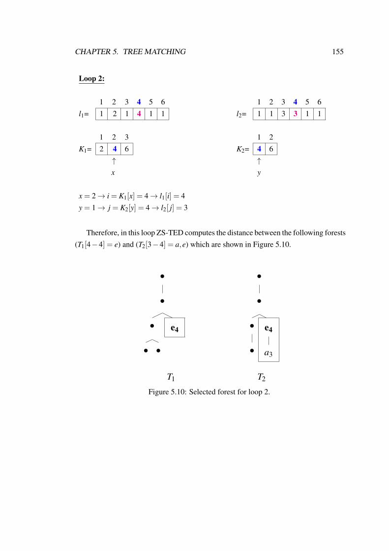
CHAPTER 5. TREE MATCHING 155
Loop 2:
1 2 3 4 5 6 1 2 3 4 5 6l1= 1 2 1 4 1 1 l2= 1 1 3 3 1 1
1 2 3 1 2K1= 2 4 6 K2= 4 6
↑ ↑x y
x = 2→ i = K1[x] = 4→ l1[i] = 4y = 1→ j = K2[y] = 4→ l2[ j] = 3
Therefore, in this loop ZS-TED computes the distance between the following forests(T1[4−4] = e) and (T2[3−4] = a,e) which are shown in Figure 5.10.
•
•
•
• •
e4
•
•
•
•
e4
a3
T1 T2
Figure 5.10: Selected forest for loop 2.

CHAPTER 5. TREE MATCHING 156
j= 3 4 1 2 3 4 5 6i= 0 1 2 14 1 1 1 2 0 1 1 2 4 5
34 1 156
temporary array FD permanent array D
where items in red mean l1(i) = l1(x) and l2( j) = l2(y).
T2 a e
T1 - i iie d x im
FDPATH array
Loop 3:
1 2 3 4 5 6 1 2 3 4 5 6l1= 1 2 1 4 1 1 l2= 1 1 3 3 1 1
1 2 3 1 2K1= 2 4 6 K2= 4 6
↑ ↑x y
x = 2→ i = K1[x] = 4→ l1[i] = 4y = 2→ j = K2[y] = 6→ l2[ j] = 1
Therefore, in this loop ZS-TED computes the distance between the following forests(T1[4−4] = e) and (T2[1−6] = b,c,a,e,d, f ) which are shown in Figure 5.11.

CHAPTER 5. TREE MATCHING 157
•
•
•
• •
e4
f6
d5
c2
b1
e4
a3
T1 T2
Figure 5.11: Selected forest for loop 3.
j= 1 2 3 4 5 6 1 2 3 4 5 6i= 0 1 2 3 4 5 6 14 1 1 2 3 3 4 5 2 0 1 1 2 4 5
34 1 2 1 1 4 556
temporary array FD permanent array D
where items in red mean l1(i) = l1(x) and l2( j) = l2(y).
T2 b c a e d f
T1 - i ii iii iiii iiiii iiiiiie d x xi xii iiim iiimi iiimii
FDPATH array

CHAPTER 5. TREE MATCHING 158
Loop 4:
1 2 3 4 5 6 1 2 3 4 5 6l1= 1 2 1 4 1 1 l2= 1 1 3 3 1 1
1 2 3 1 2K1= 2 4 6 K2= 4 6
↑ ↑x y
x = 3→ i = K1[x] = 6→ l1[i] = 1y = 1→ j = K2[y] = 4→ l2[ j] = 3
Therefore, in this loop ZS-TED computes the distance between the following forests(T1[1−6] = a,b,c,e,d, f ) and (T2[3−4] = a,e) which are shown in Figure 5.12.
f6
d5
c3
a1 b2
e4
•
•
•
•
e4
a3
T1 T2
Figure 5.12: Selected forest for loop 4.
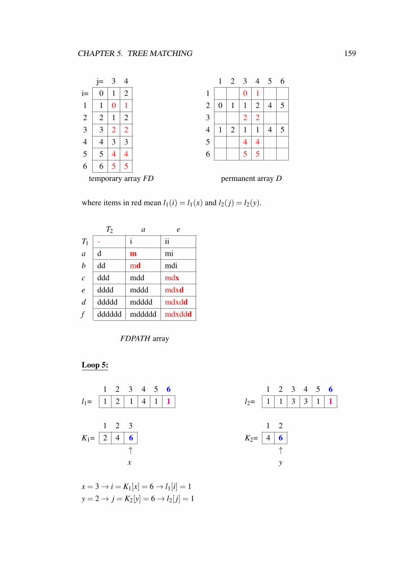
CHAPTER 5. TREE MATCHING 159
j= 3 4 1 2 3 4 5 6i= 0 1 2 1 0 11 1 0 1 2 0 1 1 2 4 52 2 1 2 3 2 23 3 2 2 4 1 2 1 1 4 54 4 3 3 5 4 45 5 4 4 6 5 56 6 5 5
temporary array FD permanent array D
where items in red mean l1(i) = l1(x) and l2( j) = l2(y).
T2 a e
T1 - i iia d m mib dd md mdic ddd mdd mdxe dddd mddd mdxdd ddddd mdddd mdxddf dddddd mddddd mdxddd
FDPATH array
Loop 5:
1 2 3 4 5 6 1 2 3 4 5 6l1= 1 2 1 4 1 1 l2= 1 1 3 3 1 1
1 2 3 1 2K1= 2 4 6 K2= 4 6
↑ ↑x y
x = 3→ i = K1[x] = 6→ l1[i] = 1y = 2→ j = K2[y] = 6→ l2[ j] = 1

CHAPTER 5. TREE MATCHING 160
Therefore, in this loop ZS-TED computes the distance between the following forests(T1[1− 6] = a,b,c,e,d, f ) and (T2[1− 6] = b,c,a,e,d, f ) which are shown in Figure5.13.
f6
d5
c3
a1 b2
e4
f6
d5
c2
b1
e4
a3
T1 T2
Figure 5.13: Selected forest for loop 5.
j= 1 2 3 4 5 6 1 2 3 4 5 6i= 0 1 2 3 4 5 6 1 1 2 0 1 4 51 1 1 2 2 3 4 5 2 0 1 1 2 4 52 2 1 2 3 4 5 6 3 2 1 2 2 4 53 3 2 1 2 3 4 5 4 1 2 1 1 4 54 4 3 2 2 2 3 4 5 4 3 4 4 2 35 5 4 3 3 3 2 3 6 5 4 5 5 3 26 6 5 4 4 4 3 2
temporary array FD permanent array D
where items in red mean l1(i) = l1(x) and l2( j) = l2(y).

CHAPTER 5. TREE MATCHING 161
T2 b c a e d f
T1 - i ii iii iiii iiiii iiiiiia d x xi iim iimi iimii iimiiib dd dm dmi dmii dmiii dmiiii dmiiiiic ddd dmd dmm dmmi dmmii dmmiii dmmiiiie dddd dmdd dmmd dmmx dmmim dmmimi dmmimiid ddddd dmddd dmmdd dmmxd dmmimd dmmimm dmmimmif dddddd dmdddd dmmddd dmmxdd dmmimdd dmmimmd dmmimmm
FDPATH array
So, the final distance is 2 which represents the final values (at final row and column)in the D array. The last value in the DPATH array represents the final sequence of editoperations, which is: dmmimmm. According to this path, we can define an alignment
between two postorder trees. The alignment between two trees T1 and T2 is obtainedby inserting a gap symbol (‘_’) into either T1 or T2, according to the type of edit op-eration, so that the resulting strings S1 and S2 are the same length as the sequence ofedit operations. The gap symbol is inserted into S2 when the edit operation is delete(‘d’), whereas it is inserted in S1 when the edit operation is insert (‘i’). Otherwise, thenodes of T1 and T2 are inserted into S1 and S2 respectively. The following is an optimalalignment between T1 (a,b,c,e,d,f ) and T2 (b,c,a,e,d,f ):
S1: a b c _ e d f
d m m i m m mS2: _ b c a e d f
This means:
d: Delete (a) from T1
m: Leave (b) without changem: Leave (c) without change
i: Insert (a) into T1
m: Leave (e) without changem: Leave (d) without changem: Leave (f ) without change

CHAPTER 5. TREE MATCHING 162
The final mapping between T1 and T2 is shown in Figure 5.14. For each mappingfigure the insertion, deletion, matching and exchanging operations are shown with sin-gle, double, single dashed and double dashed outline respectively. The matching nodes(or subtrees) are linked with dashed arrows.
f6 f6
d5
c3 e4
b2a1
f6
d5
e4c2
b1 a3
Figure 5.14: T1 and T2 mapping, single edit operations.
5.3.2 Find a sequence of subtree edit operations
Extending ZS-TED to cover subtree operations will give us more flexibility when com-paring trees (especially linguistic trees). The key to this algorithm is that we have tofind maximal sequences of identical edit operations which correspond to subtrees. Asequence of nodes (in our case, more than one) in postorder corresponds to a subtreeif the following conditions are satisfied: (i) the first node is a leaf; and (ii) the left-most sibling of the last node in the sequence (i.e. the root of a subtree) is the sameas the first node in the sequence. These two conditions can be checked in constanttime, since the leftmost sibling of a node can be determined for each node in advance.We can hence find maximal sequences corresponding to subtrees by scanning forwardsthrough the sequence of node operations to find sequences of identical operations, andthen scanning backwards through such a sequence until we find the point at whichit covers a subtree. This involves potentially O(n2) steps–n forward steps to find se-quences of identical operations, and then possibly n-1 backward steps each time to findsub-sequences corresponding to subtrees. As an example, the sequence of nodes a,b,c
in tree T1 in Figure 5.5 is a subtree because a is a leaf and the leftmost of the last node

CHAPTER 5. TREE MATCHING 163
c is 1, which represents the first node a. On the other hand, the sequence of nodesa,b,c,e in the same tree is not a subtree because a is a leaf, but the leftmost of the lastnode e is 4, which represents itself, not the first node a.
Algorithm 5.4 contains the pseudo-code to find the optimal sequence of singleand subtree edit operations for transforming T1 into T2. Ep=1..L ∈ {“d”, “i”, “x”, “m”}in this algorithm is an optimal sequence of node edits for transforming T1 into T2,obtained by applying the technique in Section 5.3.1, and S1 and S2 are the alignmentsfor T1 and T2 obtained after applying this sequence of node edits.
As shown in Algorithm 5.4, to find the optimal single and subtree edit operationssequence that transforms T1 into T2, each maximal sequence of identical operationsis checked to see whether it contains subtree(s) or not. Checking whether such a se-quence corresponds to a subtree depends on the type of edit operation, according tothe following rules: (i) if the operation is “d”, the sequence is checked on the firsttree; (ii) if the operation is “i”, the sequence is checked on the second tree; and (iii)otherwise, the sequence is checked on both trees. After that, if the sequence of oper-ations corresponds to a subtree, then all the symbols of the sequence are replaced by“+” except the last one (which represents the root of the subtree). Otherwise, check-ing starts from a sub-sequence of the original, as explained below. For instance, letus consider Eh, ...,Et , where 1 ≤ h < L, 1 < t ≤ L, h < t, is a sequence of the same
edit operation, i.e. Ek=h..t ∈ {“d”, “i”, “x”, “m”}. Let us consider h0 = h. We firstlycheck nodes S1
h, ...,S1t and S2
h, ...,S2t to see whether or not they are the heads of sub-
trees. If Ek is “d”, the nodes S1h, ...,S
1t are checked, if it is “i” the nodes S2
h, ...,S2t are
checked, and otherwise, the nodes S1h, ...,S
1t and S2
h, ...,S2t are checked. All edit oper-
ations Eh, ...,Et−1 are replaced by “+” when this sequence corresponds to a subtree.Then, we start checking from the beginning of another sequence from the left of thesubtree Eh, ...,Et , i.e. t = h−1. Otherwise, the checking is applied with the sequencestarting from the next position, i.e. h = h+ 1. The checking is continued until h = t.After that, when the (t−h) sequences that start with different positions and end with t
position do not contain a subtree, the checking starts from the beginning with the newsequence, i.e. h = h0 and t = t−1. The process is repeated until h = t.
In order to find the complexity for Algorithm 5.4, let us consider the space com-plexity first. Algorithm 5.4 uses three permanent arrays for E, S1 and S2. Each ofthese three arrays requires space O(L). So, the space complexity for Algorithm 5.4 isO(m+n), when L≤ m+n.
Consider the time complexity for Algorithm 5.4. The preprocessing to find each

CHAPTER 5. TREE MATCHING 164
Algorithm 5.4 Pseudo-code to find subtree edit operationsE the sequence of edit operations that transform tree T1 into tree T2, Ep=1..L ∈{“d”,“i”,“x”,“m”}L the length of the sequence of edit operations ES1,S2 the optimal alignment for T1 and T2 respectively, when the length of S1 = S2 = L
1: repeat2: ERoot← EL3: F ← L4: repeat5: while (F ≥ 2 and EF−1 == ERoot) do6: F ← F−17: end while8: if (F == L) then9: L← L−1
10: ERoot← EL11: F ← L12: end if13: until (F < L and F ≥ 2 and EF−1 6= ERoot)or (L = 0)14: F0← F15: while (F < L) do16: while (F < L) do17: IsSubtree← true18: while (F < L and IsSubtree) do19: if (ERoot =“d” and S1
F ..S1L is subtree)or
20: (ERoot =“i” and S2F ..S
2L is subtree)or
21: ((ERoot in {“x”,“m”})and (S1F ..S
1L and S2
F ..S2L are subtrees)) then
22: Replace EF ..EL−1 with “+”23: L← F−124: F ← F025: else26: IsSubtree← f alse27: end if28: end while29: F ← F +130: end while31: L← L−132: F ← F033: end while34: L← F0−135: until (L≤ 0)36: return E
largest sequence of the same edit operations takes linear time less than m+ n. ETEDdoes not change the main loops but inserts only new two arrays (i.e. DPATH andFDPATH). So, the time is 2×O(m2n2), which means that time complexity is stillO(m2n2).
In brief, the space and time complexities of ETED are still the same of the spaceand time complexities of the standard one.

CHAPTER 5. TREE MATCHING 165
The costs of subtrees are changed to match the requirements of specific applica-tions, but for illustration in the current chapter we will simply take the cost of a subtreeoperation to be half the sum of the costs of the individual operations that make it up.
To explain how the subtree operations are applied, let us consider the followingtwo trees T3 and T4 in Figure 5.15.
a7
b3
e1 f2
c5
g4
d6
a7
c2
g1
d6
x5
y3 z4
T3 T4
Figure 5.15: Two trees, T3 and T4, with their postorder traversal.
According to ZS-TED, the distance is 6 and final sequence of single node edit op-eration is: dddmmiiimm. This means:
d: Delete (e) from T3
d: Delete (f ) from T3
d: Delete (b) from T3
m: Leave (g) without changem: Leave (c) without change
i: Insert (y) into T3
i: Insert (z) into T3
i: Insert (x) into T3
m: Leave (d) without changem: Leave (a) without change
According to ETED, the cost is 3 and the sequence of operations as follows: thereis a sequence of ‘d’, ‘m’ and ‘i’ in the result. These sequences consist of three subtrees(i.e. the three deleted nodes, the first two matched nodes and the three inserted nodes):ddd mm iii mm. So, the final result is: ++d +m ++i mm.

CHAPTER 5. TREE MATCHING 166
This means:
++d: Delete subtree (e,f,b) from T3
+m: Leave subtree (g,c) without change++i: Insert subtree (y,z,x) into T3
m: Leave (d) without changem: Leave (a) without change
The final mapping between T3 and T4 is shown in Figure 5.16 according to ZS-TEDand ETED.
a7
c5
e1
a7
d6c2
g1 x5f2
b3
g4
d6
y3 z4
T3 T4
(a) ZS-TED
a7
c5
e1
a7
d6c2
g1 x5f2
b3
g4
d6
y3 z4
T3 T4
(b) ETED
Figure 5.16: Mapping between T3 and T4 using ZS-TED and ETED.

CHAPTER 5. TREE MATCHING 167
Using TED poses a challenge of selecting relevant costs for edit operations sincealterations in these costs or choosing a different combination of them can lead to drasticchanges in TED performance (Mehdad and Magnini, 2009). One solution to overcomethis challenge could consist of assigning costs based on an expert valuation, but theyare usually learned automatically. The following section describes in some detail twoalgorithms that we will use for this task. A number of experiments that use thesealgorithms is discussed in Chapter 7.
5.4 Optimisation algorithms
In this section, we describe two well-known optimisation algorithms, namely geneticalgorithms (GAs) and artificial bee colony (ABC) algorithm, which we will use toestimate the cost of each edit operation (i.e. for single nodes and for subtrees) andthreshold(s) of TED based on application and type of system output.
5.4.1 Genetic algorithms
Genetic algorithms (GAs) were first extensively described by Holland (1975). Theywere later developed by several researchers such as Goldberg (1989) and have beenwidely investigated for a variety of application areas. GAs are general tools for searchand optimisation based on the mechanics of natural selection. GAs are a sub-class ofevolutionary algorithms (EAs), which generate solutions to optimisation problems us-ing techniques inspired by natural evolution, such as selection, mutation and crossover(Sivanandam and Deepa, 2008).
A GA starts with an initial population of solutions (chromosomes or genotype). Ineach generation, solutions from the current population are taken and used to form anew population by modifying the selected solutions’ genome (recombined and possi-bly randomly mutated). This is motivated by a hope that the new population will bebetter than the old one. Solutions which are selected to form new solutions (offspring)are selected according to their fitness–the more suitable they are the more chancesthey have to reproduce. The algorithm terminates when either a maximum number ofgenerations has been produced, or a satisfactory fitness level has been reached for thepopulation. The general algorithmic structure of GA is given in Algorithm 5.5.

CHAPTER 5. TREE MATCHING 168
Algorithm 5.5 The basic algorithm for GA1: Initialise population;2: repeat3: Evaluation;4: Reproduction;5: Crossover;6: Mutation;7: until (termination conditions are met);
The main steps of GA are summarised below.
1. Initialisation: initialisation of a candidate solution population is usually uniformlyrandomly generated, although it may be more effective to incorporate problemknowledge (if such knowledge exists about the problem solution) or any other kindof information in this step;
2. Evaluation: once the population is initialised or when a new solution offspring iscreated, it is necessary to calculate the fitness value of the candidate solutions byusing the user-defined fitness function that measures how good a solution is. Thefitness function depends on the application and selecting a suitable one is crucial tothe success of the approach;
3. Selection: through this step, a number of individuals is selected as parents forthe next generation according to their fitness values, with the fittest ones beingfavoured, so a mechanism which encourages the best individuals’ survival is im-posed. The main idea here lies in ensuring that high performance individuals tendto contribute more of their features to successive generations. The most commonselection schemes are: (i) roulette-wheel selection: the better the individuals are,the more chances to be selected they have; and (ii) tournament selection: a numberof individuals is randomly chosen from the population and the best one from themis selected as a parent, with this process repeated as often as individuals must bechosen;
4. Crossover: the crossover operator combines two or more parts from selected par-ents for creating new offspring, which are possibly better. The offspring solutionis ideally different from any of its parents, but contains combined building blocksfrom them. This operator applies with a rate called probability of crossover (Pc).The most popular crossover operators are: (i) one-point crossover: randomly select

CHAPTER 5. TREE MATCHING 169
a crossover point within two parents and interchange the two parent genes at thispoint to produce two new offsprings; (ii) two-point crossover: randomly select twocrossover points within two parents and interchange the two parent genes betweenthese two points to produce two new offsprings; and (iii) uniform crossover: evalu-ate each corresponding gene in the parents for exchanging with a fixed probability,typically 0.5;
5. Mutation: the mutation operator randomly modifies a single solution. There aremany mutation operators, which usually affect one or more loci (genes or com-ponents) of the solution. This operator applies with a rate called probability of
mutation (Pm), which is generally much smaller than Pc. Mutation provides a mech-anism for restoring lost and unexplored genetic material into the population and forsearching regions of the allele space not generated by other operators. It can beused to prevent the premature convergence of GA to sub-optimal solutions. Themost popular mutation operators are: (i) flip bit operator: take the randomly cho-sen genome and invert its value to any value between upper and lower bounds forthat gene except the current value; (ii) uniform operator: replace the value of therandomly chosen gene with a selected uniform random value from the user-definedallowable range for that gene; and (iii) Gaussian operator: add a unit Gaussiandistributed random value to the chosen gene. The new gene value is clipped, if itfalls outside of the user-defined allowable range for that gene;
6. Replacement: the new offspring created through steps 3-5 replaces the individualpopulation according to a given criterion. There are many strategies for the re-placement of the offspring population by the individual population such as simplyreplace the entire parent population with the offspring, replace parents only if theoffsprings are fit or elitist replacement which preserves the best individual alongthe evolution is a popular criterion;
7. Termination conditions: the steps 2-6 complete one cycle of GA, which is com-monly called a generation. This cycle is repeated until a termination condition hasbeen reached. The most common terminating conditions are: (i) a fixed number ofgenerations is reached; (ii) a solution that satisfies minimum criteria is found; (iii)all individuals in the population are identical (converge); and (iv) combinations ofthe above.
After evolution stops the best solution in the current population is returned as thecandidate solution to the problem.

CHAPTER 5. TREE MATCHING 170
The most well-known GA is steady state GA (ssGA), for which the pseudo-code isgiven in Algorithm 5.6 (Alba and Dorronsoro, 2008). In each generation of ssGA (line4-8), two parents are selected from the whole population with a given selection crite-rion (line 4). These two parents are recombined (line 5) and then one of the obtainedoffsprings is mutated (line 6). The mutated offspring is evaluated (line 7) and then itis inserted back into the population (line 8), typically replacing the population’s worstindividual (if the offspring is fitter). This generation is repeated until the terminationcondition is met (line 9).
Algorithm 5.6 The basic algorithm for ssGApopsize size of population.population population.pc, pm probability of crossover and mutation, respectively.
1: Initialisation(population,popsize);2: Evaluation(population);3: repeat4: parents← Selection(population,popsize);5: offspring← Crossover(pc,parents);6: offspring←Mutation(pm,offspring);7: Evaluation(offspring);8: Replacement(population,popsize,offspring);9: until (termination conditions are met);
10: return the best individual in the population.
5.4.2 Artificial bee colony algorithm
The artificial bee colony algorithm (ABC) was proposed recently by Karaboga (2005)as an optimisation algorithm depending on the intelligent foraging behaviour of ahoney bee swarm. In this optimisation algorithm, the colony of artificial bees consistsof three groups. First, employed bees going to the food source (a possible solutionto the problem to be optimised) that they have visited previously. Second, onlookerswaiting to choose a food source. Third, scouts carrying out random search. The firsthalf of the colony consists of the employed artificial bees and the second half includesthe onlookers and scouts. The number of employed bees is equal to the number of foodsources. The employed bee of an abandoned food source becomes a scout. The gen-eral algorithmic structure of the ABC optimisation approach is shown in Algorithm 5.7

CHAPTER 5. TREE MATCHING 171
(Karaboga and Akay, 2009; Akay and Karaboga, 2012; Karaboga et al., 2012).
Algorithm 5.7 The basic algorithm for ABC1: Initialisation phase;2: repeat3: Employed bees phase;4: Onlooker bees phase;5: Scout bees phase;6: Memorise the best solution achieved so far;7: until (termination conditions are met);
As can be seen in Algorithm 5.7, this algorithm carries out three main phases dur-ing each cycle: employed bees phase, onlooker bees phase and scout bees phase, inaddition to the initialisation phase which is applied once at the beginning of the algo-rithm. These phases are described briefly in the following steps.
1. Initialisation phase: in this phase, the population of food sources (solutions) isinitialised by randomly distributed scout bees and control parameters are set suchas the number of food sources (SN), the number of optimisation parameters (D)and the maximum cycle number (MCN). The following definitions might be usedin this phase (Equations 5.1 and 5.2).
xi j = l j + rand(0,1)× (u j− l j), i = 1, . . . ,SN, j = 1, . . . ,D, (5.1)
where l j and u j are the lower and upper bounds of the parameter xi j, respectively.
f it(xi),xi ∈ RD, i = 1, . . . ,SN, (5.2)
where xi is a position of food source (solution) as a D-dimensional vector andf it(xi) is the nectar (objective function) that determines how good a solution is.
After the initialisation phase, the population of food source positions is subjectedto repeated cycles (cycle= 1, ..., MCN) of three major processes: updating feasiblesolutions (step 2), selecting feasible solutions (step 3) and avoiding sub-optimalsolutions (step 4).
2. Employed bees phase: in order to update feasible solutions, artificial employedbees explore new candidate food source positions having more nectar within the

CHAPTER 5. TREE MATCHING 172
neighbourhood of the previously selected food source in their memory. They find aneighbour food source (vi j) using the formula given by Equation 5.3:
vi j = xi j +φi j(xi j− xk j), (5.3)
where xk j is a randomly selected food source, k ∈ {1,2, ...,SN} (i.e. should bedifferent from i) and j in the range [1,D] are randomly chosen indexes, and φi j
is a uniformly distributed random number in the range [-1,1], which is used toadjust the old solution to become a new one in the next generation. The xi j− xk j
is a difference of position in a particular dimension. In each cycle, the algorithmchanges each position in solely one dimension in order to increase the diversity ofsolution in the search space.
After that, the fitness of each produced food source is calculated and a greedy se-lection is applied between it and its parent. In other words, the produced solutioncompetes with its parent and the better one wins the competition for the next gen-eration. Then, employed bees will return to their hive and share their food sourceinformation with onlooker bees waiting over there.
3. Onlooker bees phase: in this phase, each artificial onlooker bee probabilisticallyselects one of the proposed food sources depending on the fitness value obtained bythe employed bees. To achieve this goal, the roulette-wheel selection scheme canbe used. The probability value (pi) that a food source (xi) will be selected by anonlooker bee can be calculated by Equation 5.4:
pi =f it(xi)
∑SNi=1 f it(xi)
. (5.4)
After a food source is probabilistically selected, a neighbourhood source vi j is de-termined using Equation 5.3, and its fitness value is computed using Equation 5.2.As in the previous phase, a greedy selection is applied between two sources.
4. Scout bees phase: in this phase, employed bees whose food source positions havenot been improved through a number of trials (called ‘limit’) become scouts andtheir solutions are abandoned and replaced by new positions that are randomly de-termined by the scouts using Equation 5.5. This helps avoid sub-optimal solutions.
xi j = xminj + rand[0,1](xmax
j − xminj ), (5.5)

CHAPTER 5. TREE MATCHING 173
where xminj and xmax
j are the lower and upper bounds of the food source position indimension j, respectively.
The steps 2-4 are repeated until a termination criterion is satisfied such as a maxi-mum cycle number is reached or meeting an error tolerance.
The ABC algorithm has been widely used in many optimisation applications, sinceit is easy to implement and has few control parameters. The detailed pseudo-code ofthe ABC algorithm is given in Algorithm 5.8 (Akay and Karaboga, 2012).
To ensure that we get the best possible performance when comparing two tokens(i.e. on surface string level) or nodes (i.e. on syntactic level), we supplement eachsystem used in the current thesis with a range of Arabic lexical resources to provideit with some lexical relations such as synonyms. These resources are discussed in thenext section.
5.5 Arabic lexical resources
We derived our lexical rules from a range of Arabic lexical resources (Section 5.5.2)in order to provide us with different lexical relations (Section 5.5.1).
5.5.1 Lexical relations
In our work, we take into account the following lexical relations when we comparetwo tokens or nodes.
5.5.1.1 Synonyms
Synonyms are different words that signify similar, or sometimes identical, meanings.Synonymous words can be used in different contexts with extremely similar mean-ing. Synonyms can be any part-of-speech (POS) (e.g. verbs, nouns, adjectives, etc.).Examples of Arabic synonyms are shown in (5.1).
(5.1) Synonyms
a. Verbsù¢«
@ ÂςTý “to give” ≡ i
JÓ mnH ≡ �
�®
K @ Ânfq ≡ I. ëð whb

CHAPTER 5. TREE MATCHING 174
Algorithm 5.8 Detailed pseudo-code of the ABC algorithmSN number of food sources (i.e. half of colony size).D number of optimisation parameters.xi j solution i,j, i = 1 ...SN, j = 1 ...D.triali the non-improvement number of the solution xi, used for abandonment.MCN maximum cycle number.limit number of trials, e.g. limit = SN×D.
1: Initialise the population of solutions xi, j, i = 1...SN, j = 1...D, triali = 0;2: Evaluate the population;3: cycle = 1;4: repeat
{- - - Produce a new food source population for Employed bee - - -}5: for i = 1 to SN do6: Produce a new food source vi for the employed bee of the food source xi by using
(5.3) and evaluate its quality;7: Apply a greedy selection process between vi and xi and select the better one;8: If solution xi does not improve triali = triali + 1, otherwise triali = 0;9: end for
10: Calculate the probability values pi by (5.4) for the solutions using fitness values;{- - - Produce a new food source population for onlookers - - -}
11: t= 0, i= 112: repeat13: if random < pi then14: Produce a new vi j food source by (5.3) for the onlooker bee;15: Apply a greedy selection process between vi and xi and select the better one;16: If solution xi does not improve triali = triali + 1, otherwise triali= 0;17: t = t + 1;18: end if19: i = i + 1;20: if i=SN then21: i=0;22: end if23: until (t=SN)
{- - - Determine Scout - - -}24: if max(triali)> limit then25: Replace xi with a new randomly produced solution by (5.1);26: end if27: Memorise the best solution achieved so far;28: cycle = cycle+1;29: until (cycle = MCN)

CHAPTER 5. TREE MATCHING 175
b. Nouns�èX@P@
ArAdh “determination” ≡ Õæ
Ò�
�� tSmym ≡ �
éÖß Q« ςzymh
c. AdjectivesYê¢
�Ó mDThd “oppressed” ≡ ÐñÊ
¢Ó mDlwm
So, when two words W1 and W2 are synonyms this leads to the conclusion that W1
entails W2 as well as W2 entails W1.
5.5.1.2 Antonyms
Antonyms are gradable adjectives (note that, in the narrow sense, the term is frequentlyused as a synonym for opposite). The comparative forms of antonyms vary accordingto whether they presuppose the positive forms or not (Aronoff and Rees-Miller, 2003).For example, something that is ‘longer’ than something else does not need to be ‘long’.Compared with something that is ‘hotter’ than something else, it has to be ‘hot’. There-fore, ‘longer’ is impartial, whereas ‘hotter’ is committed. According to Cruse (2011)and Aronoff and Rees-Miller (2003), three relatively well-defined groups of antonymscan be distinguished as shown in (5.2).
(5.2) Antonym groups
a. Polar antonyms (i.e. both members of a pair are impartial in the comparative)Q��
�¯ qSyr “short” : ÉKñ£ Twyl “long”
b. Overlapping antonyms (i.e. one member of a pair is committed in the compar-ative, the other is impartial)
YJk. jyd “good” : Zø
XP rdy “bad”
c. Equipollent antonyms (i.e. both members are committed in the comparative)
PAg HAr “hot” : XPAK. bArd “cold”
In contrast with synonyms, a word W1 entails not W2 if they are antonyms.
5.5.1.3 Hypernyms and hyponyms
Hypernyms refer to a general category (i.e. a word whose semantic meaning is moregeneric than another word), whereas hyponyms refer to a subset of that category (i.e.

CHAPTER 5. TREE MATCHING 176
a word whose semantic meaning is more specific than another word). Figure 5.17 il-lustrates examples for hypernym and hyponym words.
ناويح
HywAn“Animal”
دسأ
Âsd“Lion”
Is a hypernym of
Is a hyponym of
نولlwn
“Colour”
رضخأÂxDr
“Green”
Is a hypernym of
Is a hyponym of
ةهكاف
fAkhħ
“Fruit”
ةزوم
mwzħ
“Banana”
Is a hypernym of
Is a hyponym of
Figure 5.17: The relations between hypernym and hyponym.
Similar to synonym, a word W1 entails a word W2 if W1 is a hyponym of W2, whereasW1 does not entail W2 if W1 is a hypernym of W2.
We intend here to exploit the synonym, antonym, subset and superset sense rela-tions when exchanging items in a tree. Roughly speaking, if comparing one tree toanother requires the exchange of two lexical items, the comparison will be more plau-sible if the item in the source tree is a synonym or hyponym of the one in the targettree.
In order to make use of these relations, we need to deal with lexical ambiguity. Wedo this by following a similar approach to Hobbs disambiguation via ‘abduction’ (seeHobbs, 2005)). In our TE system, we consider that T entails H if there is any readingof H which can be inferred from any reading of T. Doing this will allow our system todelay making decisions about potentially ambiguous lexical items as described below.
• It is reasonably safe to assume that if W1 has a sense which is a synonym or hy-ponym of some sense of W2 then a sentence involving W1 will entail a similar sen-tence involving W2 as shown in (5.3) and (5.4) respectively.
• It is reasonably safe to assume that if W1 has a sense which is a hypernym of some

CHAPTER 5. TREE MATCHING 177
sense of W2 then a sentence involving W1 will not entail a similar sentence involvingW2 as shown in (5.4).
• It is reasonably safe to assume that if W1 is an antonym of W2 then a sentenceinvolving W1 will contradict a similar sentence involving W2 as shown in (5.5).During the tree matching, we intend to exchange two antonyms word with costhigher than exchanging other words, since the presence of antonyms is an indicationthat the two sentences are in direct conflict.
This will definitely be quicker, and may be more reliable, than trying to disam-biguate the two from first principles and then looking for entailment relationships.
(5.3) Synonym example
a. �Ó @ A
�JJË
�IK
@P
rÂyt lyθA Âms
I-saw Laith/lion yesterday“I saw Laith yesterday” or “I saw lion yesterday”
b. �Ó @ @Y�
@
�IK
@P
rÂyt ÂsdA frHA
I-saw lion yesterday“I saw lion yesterday”
Since one of �IJË lyθ “Laith/lion” meanings (i.e. “lion”) is a synonym of Y�
@ Âsd
“lion”, (5.3a) entails (5.3b) and vice versa.
(5.4) Hyponym/Hypernym example
a. �Ó @ AÓA�k
�IK
@P
rÂyt HsAmA Âms
I-saw Hussam/sword yesterday“I saw Hussam yesterday” or “I saw sword yesterday”
b. �Ó @ AgC�
�IK
@P
rÂyt slAHA frHA
I-saw weapon yesterday“I saw weapon yesterday”
Since one of ÐA�k HsAm “Hussm/sword” meanings (i.e. “sword”) is a hyponymof hC� slAHA “weapon”, (5.4a) entails (5.4b) but the reverse does not hold. Disam-biguation algorithms typically make use of information about the context. When doing

CHAPTER 5. TREE MATCHING 178
TE, the text is the context–it would be very strange to ask whether ‘I bought an apple
yesterday’ entailed ‘I bought a computer yesterday’ in a context where ‘apple’ was akind of fruit.
(5.5) Antonyms example
a. �HAKYj
�JË @ áÓ Q�
�JºË@ð �Q
®Ë@ áÓ Q�
�JºË@ A
JÓAÓ
@
rÂmAmnA Alkθyr mn Al+frS w+Alkθyr mn Al+thdyAt
Before-us many of opportunities and+many of challenges“Before us are many opportunities and many challenges”
b. �HAKYj
�JË @ áÓ Q�
�JºË@ð �Q
®Ë@ áÓ ÉJÊ
�®Ë @ A
JÓAÓ
@
rÂmAmnA Alqlyl mn Al+frS w+Alkθyr mn Al+thdyAt
Before-us few of opportunities and+many of challenges“Before us are few opportunities and many challenges”
Since Q��JºË@ Alkθyr “many” is an antonym of ÉJÊ
�®Ë @ Alqlyl “few”, (5.5a) does not
entail (5.5b).
5.5.2 Lexical resources
We use the following lexical resources in order to provide us with the lexical relationsthat are explained in Section 5.5.1. The first resource (i.e. acronyms) is used duringthe preprocessing stage, i.e. before POS tagging, while the others are used during thematching stage.
5.5.2.1 Acronyms
We manually collected a set of acronyms from different Arabic websites. An acronymis a word formed from the initial letters of a name or by combining initial letters orparts of a series of words. Figure 5.18 illustrates some examples of these acronyms.
5.5.2.2 Arabic WordNet
A WordNet is a machine-readable large lexical database. Words (such as nouns, verbs,adjectives and adverbs) are grouped into clusters of synonyms, called ‘synsets’, thateach express a unique word sense (concept/meaning). Typically, it provides examplesand definitions for the synsets that are interlinked through conceptual-semantic andlexical relations. The main WordNet relation among words is synonymy, while the

CHAPTER 5. TREE MATCHING 179
Acronyms Meaningúæ� ú
G.
úG.
�éJ
K A¢�
Q�. Ë @�é«@
XB
@
�é JJë
by by sy hy’h Al+AðAς h Al+bryTAnyhBBC British Broadcasting Corporation
ñ�KA
K ú
æ�Ê£
B@ ÈAÖÞ
��
Êg
nAtw Hlf smAl Al+ÂTlsyNATO North Atlantic Treaty Organization
Figure 5.18: Arabic acronyms examples.
most frequent relations among synsets are hyperonymy and hyponymy. These tworelations allow the WordNet to be interpreted hierarchically as a lexical ontology.
WordNet is freely and publicly available for different languages, such as English(also called Princeton WordNet (PWN)), Spanish, German, Italian, Polish, Euro Word-Net (EWN) and Arabic. The Arabic WordNet (AWN) (Black et al., 2006) follows thedesign and contents of PWN and EWN. Arabic synsets are paired with synsets in PWNand are mappable to synsets in EWN. In AWN, Arabic words are represented by theirlemmas (abstracting away from morphological inflections). The PWN is significantlybigger than AWN. Figure 5.19 illustrates the various synsets involving the verb P@ P zAr
in Arabic and its translation in English “visit”. In this figure, every row represents twosynsets that have been paired up, Arabic and English (Habash, 2010).
Arabic WordNet Synset English WordNet Synset
¬A£ TAf,P@X dAr,H. Ag. jAb,ÈAg. jAl,Èñm.��' tjwl,P@ P zAr tour
YëA�
� šAhd,ø @P rÂý,P@ P zAr visit, see
úÍ@
Q¯A� sAfr Alý, P@ P zAr visit, travel to
P@ P zAr visit, call in, call
H. A� @ ÂSAb, È Q
K @ Ânzl, i. « P
@ Âzς j,úÎ
�JK. @ Abtlý, visit, inflict, bring down,
I. � Sb, �Q
¯ frD, ék. ð wjh impose
��XPX drdš, �
HXAm��' tHAdθ , QÓA�
�� tsAmr visit, chew the fat, shoot the
breeze, chat, confabulate
Figure 5.19: Paired synsets for AWN and PWN.
The information in AWN, while very useful, is sparse in comparison to the PWN.We therefore used various other Arabic lexical resources, described below, to provideus with more information about relation between words.
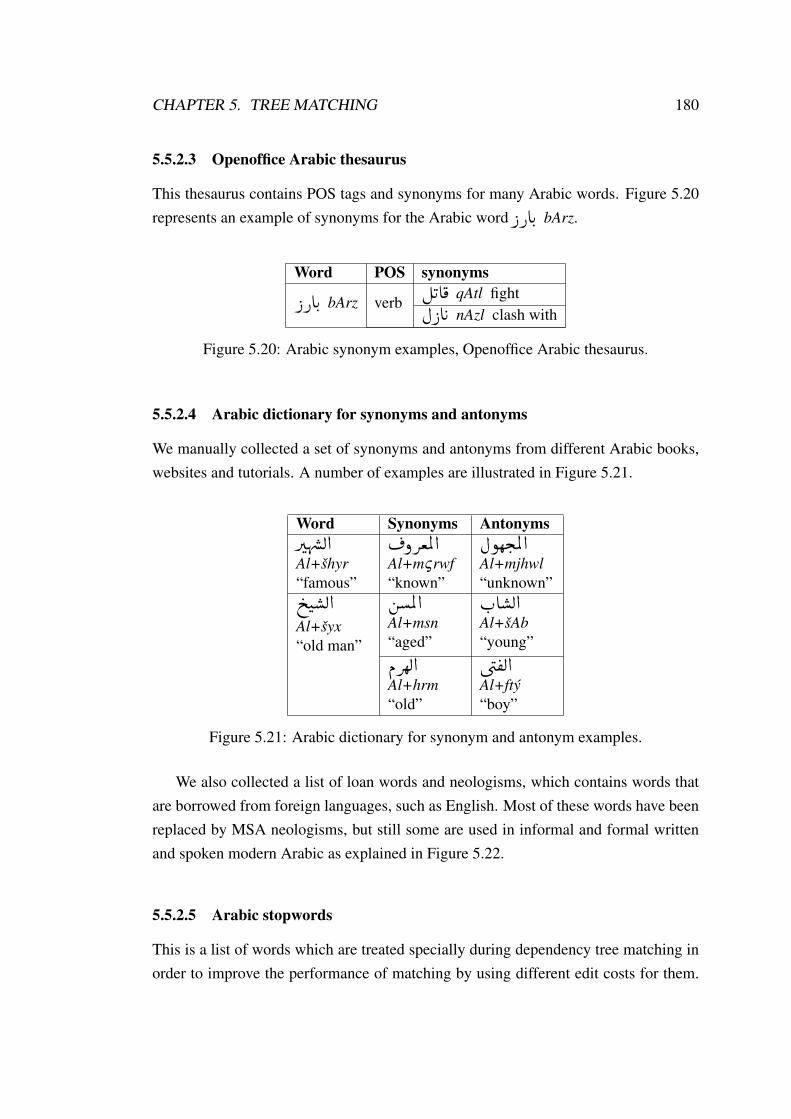
CHAPTER 5. TREE MATCHING 180
5.5.2.3 Openoffice Arabic thesaurus
This thesaurus contains POS tags and synonyms for many Arabic words. Figure 5.20represents an example of synonyms for the Arabic word PPAK. bArz.
Word POS synonymsPPAK. bArz verb
�KA
�¯ qAtl fight
È PAK nAzl clash with
Figure 5.20: Arabic synonym examples, Openoffice Arabic thesaurus.
5.5.2.4 Arabic dictionary for synonyms and antonyms
We manually collected a set of synonyms and antonyms from different Arabic books,websites and tutorials. A number of examples are illustrated in Figure 5.21.
Word Synonyms AntonymsQ�îD
��Ë @
Al+šhyr“famous”
¬ðQªÖÏ @
Al+mςrwf“known”
Èñêj. ÖÏ @
Al+mjhwl“unknown”
qJ�
�Ë@
Al+šyx“old man”
á�ÖÏ @
Al+msn“aged”
H. A�
�Ë@
Al+šAb“young”
ÐQêË @
Al+hrm“old”
ú�æ
®Ë @
Al+ftý“boy”
Figure 5.21: Arabic dictionary for synonym and antonym examples.
We also collected a list of loan words and neologisms, which contains words thatare borrowed from foreign languages, such as English. Most of these words have beenreplaced by MSA neologisms, but still some are used in informal and formal writtenand spoken modern Arabic as explained in Figure 5.22.
5.5.2.5 Arabic stopwords
This is a list of words which are treated specially during dependency tree matching inorder to improve the performance of matching by using different edit costs for them.

CHAPTER 5. TREE MATCHING 181
Loan word Neologism�AK. bAS bus �
éʯAg HAflh bus
Pñ�¯ðQK. brwfswr professor
XA�J�
@ ÂstAð professor
ñKX@P rAdyw radio ¨AKYÓ mðyAς radio
Figure 5.22: Arabic neologism examples.
There is not a common list of stop words for all applications, since each applicationhas its specific list of stop words. In our work, the following examples are taken intoconsideration.
• The verb ÐA�¯ qAm “to do” with all its conjugations. An example is explained in
(5.6).
(5.6) The verb ÐA�¯ qAm “to do”
a. H. A�JºË@ PA
�kAK.
�IÔ
�¯
qmt bAHDAr Al+ktAb
I-did bring the+book“I did bringing the book”
b. H. A�JºË@
�HQå
�k@
AHDrt Al+ktAb
I-bring the+book“I bring the book”
• The particles Y�¯ qd or Y
�®Ë lqd, when followed by a past tense verb, denote either
complete action or emphasis. It may be translated as “indeed”, “already” or “really”but sometimes it is not translatable. Ryding (2005) states that “The use of ‘qd’ with
past tense serves to confirm the meaning of the past tense by emphasising that the
action did indeed happen.” An example is explained in (5.7).
(5.7) The particle Y�¯ qd “already”
a. é�J�K. úÍ@ Ég. QË@ I. ë
X Y
�¯
qd ðhb Al+rjl AlY byth
already went the+man to his-house“The man already went to his house”

CHAPTER 5. TREE MATCHING 182
b. é�J�K. úÍ@ Ég. QË@ I. ë
X
ðhb Al+rjl AlY byth
went the+man to his-house“The man went to his house”
• Cognate accusative ( ��Ê¢Ó Èñª
®Ó mfςwl mTlq), which is used to add emphasis by
using a verbal noun (PY�Ó mSdr) derived from the main verb or predicate that itdepends on. An example is given in (5.8).
(5.8) Cognate accusative
a. @YKY�
� Ag. Aj.�Jk@
àñj.
�Jm�'
yHtjwn AHtjAjA šdydA
protesting protest a strong“? Protesting a strong protest”
b. @YKY�
�àñj.
�Jm�'
yHtjwn šdydA
protesting a strong“They are protesting strongly”
• Explicit pronouns, e.g. ñë hw “he/it” or ùë hy “she/it”, are used in a number of
different ways and sometimes as a nonessential part of a clause. One of their func-tions is to emphasise the omitted subject of a verb. The pronoun is not necessary tomark the subject of a verb since verbs incorporate the subject into their inflections.The pronoun, however, may be used along with the verb in order to emphasise orfortify the subject. In (5.11a), the pronoun could be omitted as in (5.11b), whichwould still be grammatically correct; however, the emphasis on the subject wouldbe reduced.
(5.9) Pronouns to emphasise the subject of a verb
a. ø
Qj�Ë@ hA�J®ÖÏ @ ñë
àñºJ�
sykwn hw Al+mftAH Al+sHry
will-be it the+key magic“It will be the magic key”

CHAPTER 5. TREE MATCHING 183
b. ø
Qj�Ë@ hA�J®ÖÏ @
àñºJ�
sykwn Al+mftAH Al+sHry
will-be the+key magic“(It) will be the magic key”
Such pronouns may also be used presumptively to emphasise a subject which hasbeen realised as a full NP. An example is illustrated in (5.10).
(5.10) Separate personal pronouns
a. YJkñË@ YËñË@ ñë YÒm×
mHmd hw Al+wld Al+wHyd
Muhammad he the+child only“Muhammad (he) is the only child”
b. YJkñË@ YËñË@ YÒm×
mHmd Al+wld Al+wHyd
Muhammad the+child only“Muhammad is the only child”
• The particles à@
An “verily, indeed, truly” and
à @ Ân “that”, which emphasise the
sentence after them. An example is explained in (5.11).
(5.11) The particles à@
An “indeed”
a. �éª
���.
�éÖßQk. è
Yë
à@
An hðh jrymh bšς h
indeed this a-repugnant crime“Indeed, this is a repugnant crime”
b. �éª
���.
�éÖßQk. è
Yë
hðh jrymh bšς h
this a-repugnant crime“This is a repugnant crime”
• The forms of implicit emphasis (ø
ñJªÖÏ @ YJ»ñ
�JË @ Al+twkyd Al+mςnwy), such as
�®
K nfs “same, himself/herself/itself”, á�« ςyn “selfsame, identical”, and others
with specific conditions (Badawi et al., 2004). An example is illustrated in (5.12).

CHAPTER 5. TREE MATCHING 184
(5.12) Implicit emphasis
a. H. A�JºË@ �
®
K
�IK
Q��
��@
Aštryt nfs Al+ktAb
I-bought same the+book“I bought the same book”
b. H. A�JºË@
�IK
Q��
��@
Aštryt Al+ktAb
I-bought the+book“I bought the book”
Chapter 6
Arabic textual entailment datasetpreparation
6.1 Overview
There are fewer resources for TE for Arabic than for other languages, and the man-power for constructing such a resource is hard to come by. In this chapter, we describeour efforts for creating a first dataset for training and testing a TE system for Arabic.We describe in Section 6.2 a general description of the English RTE datasets. Next,we start in Section 6.3 with our technique for collecting potential T-H pairs for a de-velopment set and testing set for TE systems, using an extension of the headline-lead
paragraph technique and then we describe our online system to annotate the collecteddata. The Arabic dataset for TE systems and a regime to ameliorate some of the dif-ficulties that arise from using the above technique are discussed in Section 6.4. InSection 6.5, we sketch how we can detect spammer annotator(s) from a number ofvolunteer annotators, since it is difficult to know in advance how dependable thoseannotators are.
6.2 RTE dataset creation
The RTE dataset contains two parts: development set (for training) and test set (fortesting). Each dataset consists of T-H pairs with their gold-standard annotation. Thetexts in these datasets were collected from the web from a variety of sources, such asnewswire text. In some cases, they were collected from available datasets or systems.They contain one or two sentences (a trend to increase over time) and tend to be fairly
185

CHAPTER 6. ARABIC TEXTUAL ENTAILMENT DATASET PREPARATION186
long compared with hypotheses (e.g. the average in RTE1 is 25 words, 28 words inRTE2, 30 words in RTE3 and 39 words in RTE4). In contrast, the hypotheses arequite short single sentences (e.g. averaging 11 words in RTE1, 8 words in RTE2 and 7words in RTE3 and RTE4), which were manually constructed for each correspondingtext. The organisers of the RTE Challenges have released a large test set, which con-tains several hundred problems of natural language inference (NLI) as summarised inTable 6.1. Some examples of RTE1 development set are shown in Figure 6.1.
Name Year Sponsor Development set (#problems) Test set (#problems)RTE1 2005 PASCAL 576 800RTE2 2006 PASCAL 800 800RTE3 2007 PASCAL 800 800RTE4 2008 NIST1 – 1000RTE5 2009 NIST 600 (main task) 600 (main task)
Table 6.1: High-level characteristics of the RTE Challenges problem sets.
The first three RTE Challenges were presented as a binary classification task ‘YES’or ‘NO’ with fairly even numbers of ‘YES’ and ‘NO’ problems. Beginning with RTE4,there were three-way classifications (‘YES’, ‘NO’ or ‘CONTRADICT’, to distinguishcases in which H contradicts T from those in which H is compatible with, but notentailed by, T).
A lot of RTE problem characteristics should be emphasised. Examples in the RTEare collected from a wide variety of sources, such as the web, focusing on the gen-eral news domain; therefore systems must be domain-independent. From a humanviewpoint, the inferences required are to some extent superficial and do not involvelong chains of reasoning. There are also some questions that are expressly designedto frustrate simplistic techniques (see pair 2081 in Figure 6.1). As explained beforein Section 2.3, there is no formal definition for TE and the current characterisationis informal and approximate: whether a competent speaker with basic knowledge ofthe world would typically infer H from T. Entailment will certainly depend on bothlinguistic and world knowledge, while the required world knowledge scope is left un-specified (see Section 2.3.2).
In spite of the informality of the entailment definition, human judges exhibit agree-ment rate 91–96% on the RTE task (Dagan et al., 2006). Then, in principle, the ma-chine performance upper bound should be high, while practically, results show that the
1This acronym comes from “National Institute of Standards and Technology”.

CHAPTER 6. ARABIC TEXTUAL ENTAILMENT DATASET PREPARATION187
<pair id="13" value="TRUE" task="IR"><t>iTunes software has seen strong sales in Europe.</t><h>Strong sales for iTunes in Europe.</h>
</pair><pair id="110" value="TRUE" task="IR">
<t>Wal-Mart faces huge sex discrimination suit</t><h>Wal-Mart faces a sex-discrimination suit</h>
</pair><pair id="826" value="TRUE" task="CD">
<t>A car bomb exploded outside a U.S. military base near Baji.</t><h>A car bomb exploded outside a U.S. military base near Beiji.</h>
</pair><pair id="2081" value="FALSE" task="QA">
<t>The main race track in Qatar is located in Shahaniya, on theDukhan Road.</t>
<h>Qatar is located in Shahaniya.</h></pair><pair id="147" value="TRUE" task="RC">
<t>The Philippine Stock Exchange Composite Index rose 0.1 percent to1573.65.</t>
<h>The Philippine Stock Exchange Composite Index rose.</h></pair><pair id="148" value="FALSE" task="RC">
<t>The Philippine Stock Exchange Composite Index rose 0.1 percent to1573.65.</t>
<h>The Philippine Stock Exchange Composite Index dropped.</h></pair>
Figure 6.1: Some examples from the RTE1 development set as XML format.
RTE task is extremely difficult for machines. For instance, in the first PASCAL RTEcompetition, lower accuracies were achieved, i.e. 50–59% (Dagan et al., 2006). In latercompetitions, participants reported higher accuracies, but this is partially attributableto the test sets of RTE having become substantially easier (MacCartney, 2009).
6.3 Dataset creation
In order to train and test a TE system for Arabic, we need an appropriate dataset. Tothe best of our knowledge, no such datasets are available for Arabic, so we have hadto develop one. We did not want to produce a set of T-H pairs by hand–partly because
CHAPTER 6. ARABIC TEXTUAL ENTAILMENT DATASET PREPARATION188
doing so is a lengthy and tedious process, but more importantly because hand-codeddatasets are liable to embody biases introduced by the developer. If the dataset is usedfor training the system, then the rules that are extracted will be little more than anunfolding of information explicitly supplied by the developers. If it is used for testingthen it will only test the examples that the developers have chosen, which are likely tobe biased, albeit unwittingly, towards the way they think about the problem.
We also need to cope with the fact that we do not have access to a large teamof willing (or paid!) annotators. Whilst it is possible to collect potential T-H pairsautomatically, or semi-automatically, these pairs then have to be annotated. If TE isabout trying to develop systems that will make the same decisions about whether T
entails H as a person, then we need, at least for testing, to know what a person wouldsay. Given that we are intending to follow standard practice and use machine learningalgorithms to extract at least some of the inference rules our system will be using,we also need annotated data from which to extract them. We therefore need to getas much data as possible from a rather unreliable set of annotators. In particular, ourannotators are under no obligation to do anything, and we are relying entirely on theirgoodwill. This means that we do not know how many examples a given annotator willdo, nor when they will do them. Furthermore, a number of them are based in otherinstitutions, or even other countries, and we have no way of verifying in advance thatthey will make sensible judgements. TE is about whether a typical adult language userwould say that T entailed H, rather than about whether it really does entail it. Thusin one sense the judgements that our annotators make cannot fail to be correct–theyare typical adult Arabic speakers, so their judgements are what we want to reproduce.Nonetheless, there will be cases where an annotator has misunderstood the task thatwe have set them, and we need to be able to spot, and recover from, such cases.
We investigate here a semi-automatic technique for creating a dataset for a TEsystem for Arabic. Our current technique consists of two tools. The first tool is re-sponsible for automatically collecting T-H pairs from news websites (Section 6.3.1),while the second tool is an online annotation system that allows annotators to annotateour collected pairs manually (Section 6.3.2).
6.3.1 Collecting T-H pairs
We start by extracting candidate T-H pairs automatically. A number of TE datasetshave been produced for different languages, such as English,2 Greek (Marzelou et al.,
2Available at: http://www.nist.gov/tac/2011/RTE/index.html

CHAPTER 6. ARABIC TEXTUAL ENTAILMENT DATASET PREPARATION189
2008), Italian (Bos et al., 2009), German and Hindi (Faruqui and Padó, 2011). Someof these datasets were collected by the so-called headline-lead paragraph technique(Bayer et al., 2005; Burger and Ferro, 2005) from newspaper corpora, pairing the firstparagraph of an article, as T, with its headline, as H. This is based on the observationthat a news article’s headline is very often a partial paraphrase of the first paragraph ofthis article, conveying thus a comparable meaning. The current work is a step forwardin this respect. We use the general idea of headline-lead paragraph strategy with ourextension to improve the quality of the T-H pairs.
The most promising idea here is by posing queries to a search engine and filteringthe responses for sentences that do (and do not) entail the query. We are currentlybuilding a corpus of T-H pairs by using headlines that have been automatically ac-quired from Arabic newspapers’ and TV channels’ websites (in our case, we used AlJazeera http://www.aljazeera.net/, Al Arabiya http://www.alarabiya.net/
and BBC Arabic http://www.bbc.co.uk/arabic/ websites as resources for ourheadlines) as queries to be input to Google via the standard Google-API, and thenselecting the first paragraph, which usually represents the most related sentence(s) inthe article with the headline (Bayer et al., 2005; Burger and Ferro, 2005), of each ofthe first 10 returned pages. This technique produces a large number of potential pairswithout any bias in either the texts or the hypotheses. To improve the quality of thesentence pairs that resulted from the query, we use two conditions to filter the results:(i) the length of a headline must be at least more than five words to avoid very smallheadlines; and (ii) the number of common words (either in surface forms or lemmaforms)3 between both sentences must be less than 80% of the headline length to avoidhaving excessively similar sentences. The problem is illustrated by (6.1).
(6.1) Positive entailment pair with highly similar common words
a. About 1500 lung cancer patients die unnecessarily each year.
b. 1500 lung cancer deaths unnecessary.
The problem here is that (6.1a) and (6.1b) are so similar that there would be verylittle to learn from them if they were used in the training phase of a TE system; andthey would be almost worthless as a test pair–virtually any TE system will get thispair right, so they will not serve as a discriminatory test pair. In the current work, weapply both conditions above to 85% of the T-H pairs from both training and testing
3When we mention common words throughout this chapter, we mean either in surface forms orlemma forms.

CHAPTER 6. ARABIC TEXTUAL ENTAILMENT DATASET PREPARATION190
sets. We then apply the first condition only on the remaining 15% of T-H pairs in orderto leave some similar pairs, especially non-entailments, to foil simplistic approaches(e.g. bag-of-words).
In order to find pairs that were not unduly similar, we matched headlines from onesource with stories from another. Major stories are typically covered by a range of out-lets, usually with variations in emphasis or wording. Stories from different sources canbe linked by looking for common words in the headlines–it is unlikely that there willbe two stories about, for instance, neanderthals in the news at the same time, so verystraightforward matching based on low frequency words and proper names is likely tofind articles about the same topic. The terminology and structure of the first sentencesof these articles, however, are likely to be quite different. Thus using a headline fromone source and the first sentence from an article about the same story but from anothersource is likely to produce T-H pairs which are not excessively similar. Figure 6.2shows, for instance, the results of headlines with their lead-paragraphs from varioussites (CNN, BBC and Reuters) that mention Berlusconi on a given day’s headline.
Source Headline (Hypothesis) Lead paragraph (Text) ResultCNN Berlusconi says he will not
seek another term.Italian Prime Minister Silvio Berlusconi said Fri-day he will not run again when his term expires in2013.
YES
BBC Silvio Berlusconi vows notto run for new term in 2013.
Italian Prime Minister Silvio Berlusconi has con-firmed that he will not run for office again whenhis current term expires in 2013.
YES
Reuters Berlusconi says he will notseek new term.
Italian Prime Minister Silvio Berlusconi declaredon Friday he would not run again when his termexpires in 2013.
YES
Figure 6.2: Some English T-H pairs collected by headline-lead paragraph technique.
We can therefore match a headline of one newspaper with related sentences fromanother one. We have tested this technique on different languages, such as English,Spanish, German, Turkish, Bulgarian, Persian and French. We carried out a seriesof informal experiment with native speakers to see whether the resulting T-H pairscontain a mixture of cases where T does or does not entail H (the latter are needed atleast for testing: a test set with no negative examples will not penalise systems thatsimply assume that every pair is a positive example). The results were encouraging, tothe point where we took this as the basic method for suggesting T-H pairs.

CHAPTER 6. ARABIC TEXTUAL ENTAILMENT DATASET PREPARATION191
Most of the Arabic articles that are returned by this process typically contain verylong sentences (upwards of 100 words), where only a small part has a direct relation-ship to the query. With very long sentences of this kind, it commonly happens that onlythe first part of T is relevant to H. This is typical of Arabic text, which is often writtenwith very little punctuation, with elements of the text linked by conjunctions ratherthan being broken into implicit segments by punctuation marks such as full stops andquestion marks. Thus what we really want as the text is actually the first conjunct ofthe first sentence, rather than the whole of the first sentence.
In order to find the first conjunct, we use MSTParser to get a picture of the structureof the sentence. As we have seen before in Chapter 4, parsing Arabic is very difficult,and most attempts to use MSTParser as a parser for Arabic score around 83%. Formany purposes this is a rather disappointing level of accuracy, though it seems to be thecurrent state of the art for parsing Arabic (other well-known dependency parsers, e.g.MALTParser, are generally reported as being slightly less accurate (around 81%), andgrammar-driven parsers usually just fail when confronted with the very long sentencesthat are found in Arabic newspapers and websites). For our current purposes, however,we simply need to find the first conjunction that links two sentences, rather than linkingtwo substructures (e.g. two noun phrases (NPs)). MSTParser does this quite reliably,so that parsing and looking for the first conjunct is a more reliable way of segmentinglong Arabic sentences than simply segmenting the text at the first conjunction. Forinstance, selecting the second conjunction in segment (6.2) will give us the completesentence ‘John and Mary go to school in the morning’, since it links two sentences. Incontrast, selecting the first conjunction in segment (6.2) will give us solely the propernoun ‘John’, since it links two NPs (i.e. ‘John’ and ‘Mary’).
(6.2) Segmenting sentence
John and Mary go to school in the morning and their mother prepares the lunch.
6.3.2 Annotating T-H pairs
The pairs that are collected in the first stage still have to be marked-up by humanannotators, but at least the process of collecting them is as nearly bias-free as possible.The annotation is performed by volunteers, and we have to rely on their goodwill bothin terms of how many examples they are prepared to annotate and how carefully theydo the job. We therefore have to make the task as easy possible, to encourage them

CHAPTER 6. ARABIC TEXTUAL ENTAILMENT DATASET PREPARATION192
to do large numbers of cases, and we have to manage the problems that arise fromhaving a mixture of people, with different backgrounds, as annotators. In one wayhaving non-experts is very positive: as noted before, TE is about the judgements thata typical speaker would make. Not the judgements that a logician would make, or thejudgements that a carefully briefed annotator would make, but the judgements that atypical speaker would make. From this point of view, having a mixture of volunteerscarrying out the task is a good thing: their judgements will indeed be those of a typicalspeaker.
At the same time, there are problems associated with this strategy. Our volunteersmay just have misunderstood what we want them to do, or they may know what wewant but be careless about how they carry it out. We therefore have to be able to detectannotators who, for whatever reason, have not done the job properly. The systemtherefore has to be able to measure the reliability of each annotator to avoid unreliableones. We have investigated the use of different strategies to achieve this goal (seeSection 6.5). According to the results of these strategies, the system will decide toblock the annotator’s annotation account and then remove the annotations of unreliableannotator(s) from the system database.
Because our annotators are geographically distributed, we have developed an on-line annotation system. The system presents the annotator with sentences that theyhave not yet seen and that are not fully annotated (here, annotated by three annota-tors) and asks them to mark this pair as positive ‘YES’, negative ‘NO’ or unknown‘UN’. The system also provides other options, such as revisiting a pair that they havepreviously annotated, reporting sentences that have such gross misspellings or syntac-tic anomalies that it is impossible to classify them, skipping the current pair when auser chooses not to annotate this pair, and general comments (to send any suggestionabout improving the system). The final annotation of each pair is computed when itis fully annotated by three annotators–when an annotator clicks ‘Next’, they are giventhe next sentence that has not yet been fully annotated. This has the side-effect ofmixing up annotators: since annotators do their work incrementally, it is very unlikelythat three people will all click ‘Next’ in lock-step, so there will be inevitable shufflingof annotators, with each person having a range of different co-annotators. The currentannotation tool interface is shown in Figure 6.3. All information about articles, an-notators, annotations and other information such as comments is stored in a MySQLdatabase.

CHAPTER 6. ARABIC TEXTUAL ENTAILMENT DATASET PREPARATION193
Figure 6.3: Annotate new pair’s interface.
6.4 Arabic TE dataset
The current dataset, namely Arabic TE dataset (ArbTEDS), consists of 618 T-H pairs.These pairs are randomly chosen from thousands of pairs collected by using the toolexplained in Section 6.3.1. These pairs cover a number of subjects such as politics,business, sport and general news. We used eight expert and non-expert volunteer an-notators4 to identify the different pairs as ‘YES’, ‘NO’ or ‘UN’ pairs in the ArbTEDS.Those annotators follow nearly the same annotation guidelines as those for building theRTE task dataset (Dagan et al., 2006) (see Section 2.3.2). They used the online systemexplained in Section 6.3.2 to annotate our collected headline-lead paragraph pairs. Us-ing a web-based annotation tool provides us with different advantages, especially thatit is available for many annotators in a lot of places.
Table 6.2 summarises these individual results: the rates on the cases where an an-notator agrees with at least one co-annotator (average around 91%) are considerablyhigher than those in the case where the annotator agrees with both the others (averagearound 78%). This suggests that the annotators found this a difficult task. Table 6.2
4All our annotators are Arabic native speaker PhD students, who are the author’s colleagues. Someof them are linguistics students, whereas the others are working in fields related to NLP.

CHAPTER 6. ARABIC TEXTUAL ENTAILMENT DATASET PREPARATION194
shows that comparatively few of the disagreements involve one or more of the anno-tators saying ‘UN’–for 600 of the 618 pairs at least two annotators both chose ‘YES’or both chose ‘NO’ (the missing 18 pairs arise entirely from cases where two or threeannotators chose ‘UN’ or where one said ‘YES’, one said ‘NO’ and one said ‘UN’.These 18 pairs are annotated as ‘UN’ and they are eliminated from our dataset, leaving600 binary annotated pairs).
Agreement YES NO≥ 2 agree 478 (80%) 122 (20%)
3 agree 409 (68%) 69 (12%)
Table 6.2: ArbTEDS annotation rates, 600 pairs.
We were expecting annotators to make frequent use of the ‘Unknown’ option. Thefact that they did not means that it is inevitable that the top row in Table 6.2 will covervirtually the entire set. Does that mean that we should trust the majority decision inevery case?
This is appealing, since it maximises the size of the dataset. The fact that the rateof agreement drops so dramatically when we insist on unanimity suggests that it is nota good idea. We have average agreement between three annotators in 78% of cases,compared to 91% of average agreement between at least two. The frequency of caseswhere there is not total agreement indicates that, for the text types we are working with(the headline from a story and the first one or two clause(s) of the first sentence of alinked story) people find it very difficult to carry out this task. It seems likely, then, thata computer will also find it very difficult to carry it out. If we use cases where thereis majority agreement as our training set, we are likely to learn rules from exampleswhich do not in fact exemplify sound (or even plausible/probabilistic) inferences. Ifwe use them as the test set, we will be asking the system questions to which even oursubjects have not given consistent answers. We therefore plan to use only exampleswhere there is a unanimous verdict for both training and testing.
Is it possible to predict which cases will lead to disagreements? One obvious candi-date is sentence length. It seems plausible that people will find long sentences harder tounderstand than short ones, and that there will be more disagreement about sentencesthat are hard to understand than about easy ones. Further statistical analysis results forthe version of the dataset when there is unanimity between annotators is summarisedin Table 6.3. We analyse the rates of this strategy that are shown in Table 6.2 accordingto the text’s length, when the H average length is around 10 words and the average of
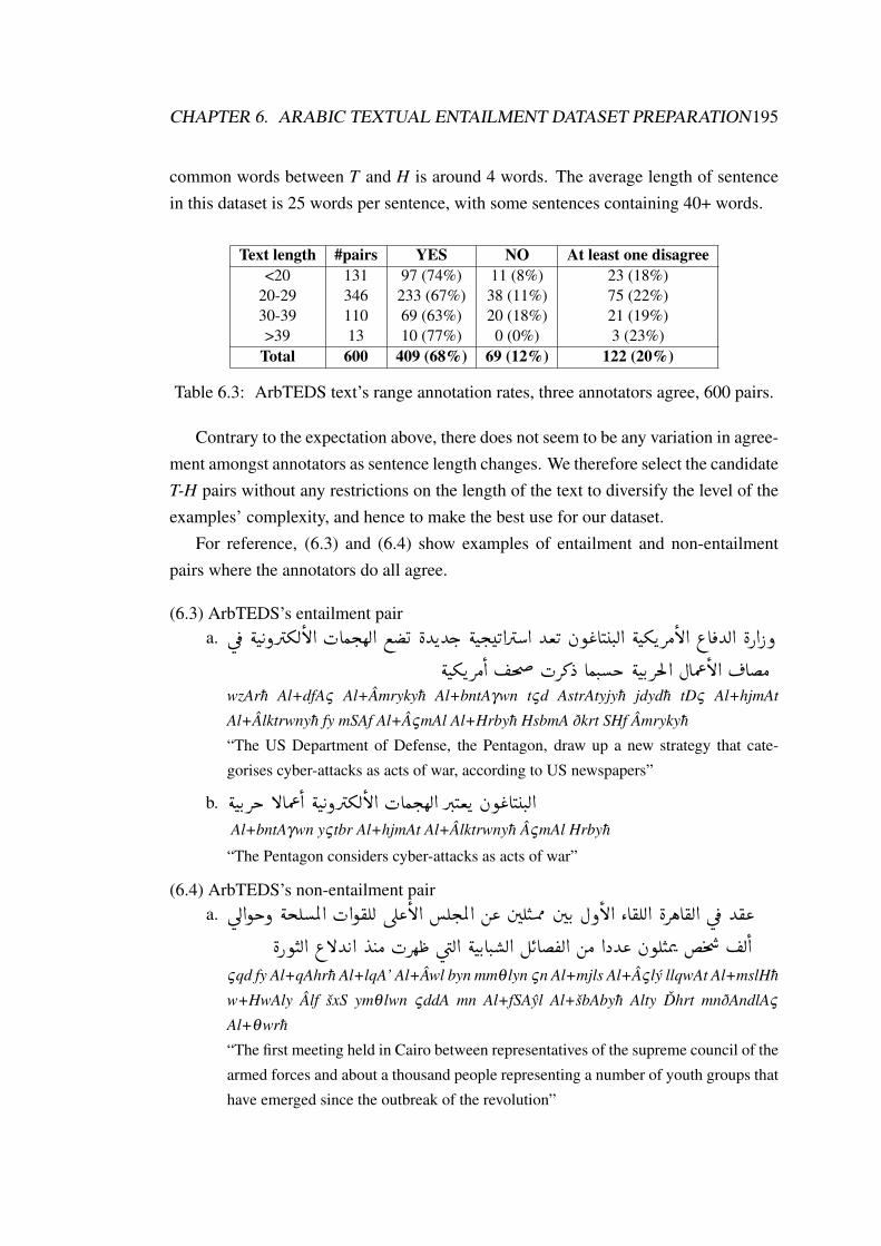
CHAPTER 6. ARABIC TEXTUAL ENTAILMENT DATASET PREPARATION195
common words between T and H is around 4 words. The average length of sentencein this dataset is 25 words per sentence, with some sentences containing 40+ words.
Text length #pairs YES NO At least one disagree<20 131 97 (74%) 11 (8%) 23 (18%)
20-29 346 233 (67%) 38 (11%) 75 (22%)30-39 110 69 (63%) 20 (18%) 21 (19%)>39 13 10 (77%) 0 (0%) 3 (23%)
Total 600 409 (68%) 69 (12%) 122 (20%)
Table 6.3: ArbTEDS text’s range annotation rates, three annotators agree, 600 pairs.
Contrary to the expectation above, there does not seem to be any variation in agree-ment amongst annotators as sentence length changes. We therefore select the candidateT-H pairs without any restrictions on the length of the text to diversify the level of theexamples’ complexity, and hence to make the best use for our dataset.
For reference, (6.3) and (6.4) show examples of entailment and non-entailmentpairs where the annotators do all agree.
(6.3) ArbTEDS’s entailment paira. ú
¯
�éJ
KðQ�
�ºË B@
�HAÒj. êË @ ©
�
��
�èYKYg.
�éJj. �
�K @Q
���@ Yª
�K
àñ
«A
�J�J. Ë @
�éJºKQÓ
B@ ¨A
¯YË@
�èP@ Pð
�éJºKQÓ
@
m�� �
HQ»X AÒJ.�k
�éJK. QmÌ'@ ÈAÔ«
B@
¬A�Ó
wzArh Al+dfAς Al+Âmrykyh Al+bntAγwn tςd AstrAtyjyh jdydh tDς Al+hjmAt
Al+Âlktrwnyh fy mSAf Al+ÂςmAl Al+Hrbyh HsbmA ðkrt SHf Âmrykyh
“The US Department of Defense, the Pentagon, draw up a new strategy that cate-
gorises cyber-attacks as acts of war, according to US newspapers”
b. �éJK. Qk BAÔ«
@
�éJ
KðQ�
�ºË B@
�HAÒj. êË @ Q�.
�JªK
àñ
«A
�J�J. Ë @
Al+bntAγwn yς tbr Al+hjmAt Al+Âlktrwnyh ÂςmAl Hrbyh
“The Pentagon considers cyber-attacks as acts of war”
(6.4) ArbTEDS’s non-entailment paira. ú
Í@ñkð
�éjÊ�ÖÏ @
�H@ñ
�®ÊË úΫ
B@ �Êj. ÖÏ @ á«
á�Ê�JÜØ
á�K. Èð B@ ZA
�®ÊË @
�èQëA
�®Ë @ ú
¯ Y
�®«
�èPñ
�JË @ ¨BY
K @
Y
JÓ
�HQê
£ ú
�æË @
�éJK. AJ.
��Ë@ É
KA�
®Ë @ áÓ @XY«
àñÊ
�JÖß �
m�
��
Ë @
ςqd fy Al+qAhrh Al+lqA’ Al+Âwl byn mmθ lyn ςn Al+mjls Al+Âς lý llqwAt Al+mslHh
w+HwAly Âlf šxS ymθ lwn ςddA mn Al+fSAyl Al+šbAbyh Alty Dhrt mnðAndlAς
Al+θwrh
“The first meeting held in Cairo between representatives of the supreme council of the
armed forces and about a thousand people representing a number of youth groups that
have emerged since the outbreak of the revolution”

CHAPTER 6. ARABIC TEXTUAL ENTAILMENT DATASET PREPARATION196
b. Qå�Ó ú
¯ Õ» AmÌ'@ ø
Qº�ªË@ �Êj. ÖÏ @ð
�èPñ
�JË @ H. AJ.
��
á�K. Z A�®Ë Èð
@ Y
�®«
ςqd Âwl lqA’ byn šbAb Al+θwrh w+Al+mjls Al+ςskry Al+HAkm fy mSr
“A first meeting held between the youth of the revolution and Egypt’s ruling military
council”
In (6.3), the three annotators are agreed that (6.3a) entails (6.3b) because all theinformation of the hypothesis is embedded in the text. In (6.4), on the other hand,they all agree that (6.4a) does not entail (6.4b) because there is no evidence in the textabout ø
Qº�ªË@ �Êj. ÖÏ @ Al+mjls Al+ςskry “the military council” is Qå�Ó ú
¯ Õ» AmÌ'@
Al+HAkm fy mSr “Egypt’s ruling”, which appears in the hypothesis.Given the lack of agreement amongst annotators, it seemed worth investigating
whether it would be possible to pre-filter the test cases. It is extremely easy to collectmore potential T-H pairs, so if we could find pairs where our annotators were morelikely to agree then we would get a larger dataset for the same amount of annotatoreffort.
Inspection of individual cases where one annotator disagreed with the others indi-cated that structural ambiguity is a major source of disagreement between annotators.Typically, in this kind of ambiguity two or more syntactic analyses lead to severalpossible interpretations. For instance, (6.5) shows a T-H pair when text has structuralambiguity.
(6.5) Pair with text has structural ambiguity
a. I saw the man with the telescope.
b. The man has a telescope.
In the above example, there is a prepositional phrase (PP)-attachment structuralambiguity in the text. So, the PP ‘with the telescope’ can be attached to either ‘saw’
or ‘the man’, i.e. something X with the telescope, and it is either the man or the seeingevent. Therefore, there are two meanings for the text, “The man has a telescope” or “Iused the telescope to see the man” (the seeing was done with a telescope). In this case,there are three possibilities for annotators’ judgement, as follows:
• Consider that the first meaning is satisfied. They will tag the pair as positive entail-ment ‘YES’.
• Consider that the second meaning is satisfied. They will tag the pair as negativeentailment ‘NO’.

CHAPTER 6. ARABIC TEXTUAL ENTAILMENT DATASET PREPARATION197
• Consider that both meanings are satisfied. They will tag the pair as ‘UN’.
Hence, the three annotators, for instance, disagree when they annotated the pairgiven in (6.6) because the phrase �
HA�¯CªË@ QK
Qª�JË ltςzyz Al+ς lAqAt “for fence-mending”
in the text is ambiguous. They do not know if it is attached with “Poland” or with “theleaders of central and Eastern Europe are members of the European Union”.
(6.6) ArbTEDS’s ambiguous pair
a. ù
�®�JÊKð
�éJK. Pð
B@ é
�JËñk.
áÓ�èQ�
g
B@
�éÊgQÖÏ @ ú
¯ @Y
JËñK. Pð QK AÓAK. ð
@ ¼@PAK. ú
¾KQÓ
B@ ��
KQË @
�HA
�¯CªË@ QK
Qª�JË ú
G.Pð
B@ XAm�
�'B@ ú
¯ ZA
�«
B@ AK. Pð
@ ú
�¯Qå
��ð ¡�ð ZAÔ« QK. AîD
¯
Al+ryys Al+Âmryky barAk ÂwbAmA yzwr bwlndA fy Al+mrhlh Al+Âxyrh mn jwlth
Al+Âwrbyh w+yltqy fyhA bzςmA’ wsd w+šrqy ÂwrbA Al+ÂςDA’ fy Al+atHAd
Al+Âwrby ltςzyz Al+ς lAqAt
“US President Barack Obama visits Poland in the last phase of his European trip and
he will join leaders of central and eastern Europe nations that are members of the
European Union for fence-mending”
b. �HA
�¯CªË@ QK
Qª�JË @Y
JËñK. Pð QK AÓAK. ð
@ ��
KQË @
Al+ryys ÂwbAmA yzwr bwlndA ltςzyz Al+ς lAqAt
“President Obama visits Poland for fence-mending”
The problem seems to be that some people are cautious about interpreting sen-tences involving attachment ambiguities, on the grounds that if a sentence has multipleinterpretations then you cannot be sure which one was intended, and hence you cannotbe sure about what it entails, and some are less wary or are plain unaware that the textwas ambiguous in the first place. It is hard to detect where there is an attachment ambi-guity automatically–using MSTParser to parse the text will tell us where there is a PPthat has been attached to some preceding noun or verb, but it will not straightforwardlytell us whether there was an alternative attachment site. In any case, TE is about whata typical speaker will conclude about a T-H pair, and if there is no uniformity amongour annotators about what to do in the face of ambiguity then we cannot say what atypical speaker would do: all our annotators are native speakers, so they should all be‘typical’. If their interpretation of the relationship between an ambiguous T and thecorresponding H is systematically varied, the idea of a typical speaker is somewhereundermined. This further strengthens the view that we should only use T-H pairs whereall the annotators agree.

CHAPTER 6. ARABIC TEXTUAL ENTAILMENT DATASET PREPARATION198
6.4.1 Testing dataset
It is worth noting in Table 6.2 that a substantial majority of pairs are marked positively–that T does indeed entail H. This is problematic, at least when we come to use thedataset for testing. For testing we need a balanced set: if we use a test set where 80%of cases are positive then a system which simply marks every pair positively will score80%. It is hard, however, to get pairs where T and H are related but T does not entailH automatically. To solve this problem, three strategies are possible, as follows:
Strategy I: it would be easy to get cases where T does not entail H, simply by takingthe first sentence from an unrelated article, but this also will not pose a problem for aTE system.
Strategy II: we could ask the reliable annotators, whom we find according to thestrategies explained in Section 6.5, to make minor changes to T or H to get non-entailing T-H pairs, but this is liable to embody biases introduced by the annotator(i.e. experimenter’s bias).
Strategy III: select the paragraph (except the lead paragraph) in the article thatshares the highest number of common words with the headline for the first 10 returnedpages. We called this technique headline keywords-rest paragraph. It produces a largenumber of potential texts, which are related to the main keywords of the headlines,without any bias.
In the current work, we need a testing set with balanced ‘YES’ and ‘NO’ pairs (i.e.300 pairs for each group). In order to construct a testing set from the dataset describedin Table 6.3, we follow three steps: (i) we first selected randomly 300 entailed pairsfrom the 409 entailed pairs (‘YES’ column in Table 6.3); (ii) we have already 69 notentailed unanimously marked by annotators (‘NO’ column in Table 6.3), so we stillneed to construct 231 not entailed pairs. We therefore collect 231 headlines from therest of the 109 entailed pairs in step (i) and from 122 pairs which are not annotatedas ‘YES’ or ‘NO’ because at least one annotator disagrees with others (‘at least onedisagree’ column in Table 6.3); and (iii) apply the strategy III on these 231 headlinesand ask the reliable annotators, whom we determine according to the strategies ex-plained in Section 6.5, to select a potential text for each headline that it does not entail.

CHAPTER 6. ARABIC TEXTUAL ENTAILMENT DATASET PREPARATION199
The distribution of our testing set (a 50%-50% split of ‘YES’ and ‘NO’ pairs), namelyArbTEDS_test, is summarised in Table 6.4.
Text’s length #pairs YES NO<20 131 74 (56%) 57 (44%)
20-29 346 165 (48%) 181 (52%)30-39 110 53 (48%) 57 (52%)>39 13 8 (62%) 5 (38%)
Total 600 300 300
Table 6.4: ArbTEDS_test dataset text’s range annotation, 600 binary decision pairs.
For example, if you apply the strategy III on the entailed pair in (6.3) to constructa not entailed pair, you could get a pair as illustrated in (6.7).
(6.7) Non-entailment pair for entailment pair in (6.3)
a. �HAKBñË@ éË
�Qª
�J�K ú
GðQ�
�ºË@ Ðñj. ë ø
@ úΫ XQË@ :
à
AK.
àñ
«A
�J�J. Ë @ Õæ�AK.
�HYj
�JÖÏ @ hQå�
XQÊË�éËðA¢Ë@ úΫ
�ékðQ¢Ó
�H@PAJ
mÌ'@ É¿ áºËð É
�JÖÏ AK.
àñºK
à
@ AKPðQå
� ��Ë
�èYj
�JÖÏ @
Ðñj. êË @ @Yë úΫ
SrH Al+mtHdθ bAsm Al+bntAγwn bÂn: Al+rd ς lý Ây hjwm Alktrwny ttςrD lh
Al+wlAyAt Al+mtHdh lys DrwryA Ân ykwn bAlmθ l wlkn kl Al+xyarAt mTrwHh llrd
ς lý hðA Al+hjwm
“The Pentagon spokesman declared that: a response to any cyber-attack on the US
would not necessarily be a cyber-response and all options would be on the table to
respond to this attack”
b. �éJK. Qk BAÔ«
@
�éJ
KðQ�
�ºË B@
�HAÒj. êË @ Q�.
�JªK
àñ
«A
�J�J. Ë @
Al+bntAγwn yς tbr Al+hjmAt Al+Âlktrwnyh ÂςmAl Hrbyh
“The Pentagon considers cyber-attacks as acts of war”
As can be seen in (6.7), there are around 3 words from 6 common words betweenT and H, but it is marked as not entailed.
6.5 Spammer detector
In the current work, we need to cope with the challenges that arise from relying on vol-unteer annotators. The main challenge here is that it is hard to know in advance howreliable those annotators are. We therefore describe in the current section a regime that

CHAPTER 6. ARABIC TEXTUAL ENTAILMENT DATASET PREPARATION200
helps us to compensate for this challenge. There are several operational definitions of‘annotator reliability’ in use by many researchers, reflecting different viewpoints aboutwhat is reliable agreement between annotators. We apply two different strategies todetect annotators who, for whatever reasons, have not done the job properly and markthem as ‘spammer’. The system will then decide to block the account of these spam-mer annotators and then remove their annotations from the system database. Thesestrategies are explained below.
Strategy A: this strategy uses joint-probability of agreement, which is the most sim-ple (and weakest) measure of reliability. This method finds the number of times theannotators agree divided by the total number of annotations. We find here the joint-probability of agreement of selecting ‘Unknown’ option for each annotators, if thisrate exceeds 20%, the annotator will be marked as spammer. The results obtained forapplying this strategy are presented in Table 6.5.
Annotator IDANT1 ANT2 ANT3 ANT4 ANT5 ANT6 ANT7 ANT8
#pairs 336 212 468 100 317 226 95 100rate of ‘Un-known’ option
0% 1.4% 1.5% 0% 1.2% 1.3% 2% 0%
Table 6.5: Reliability measure of our annotators, strategy A.
As can be see from the table above, all rates are very small (less than or equal 2%).These findings indicate that there is no spammer in our annotators.
Strategy B: we used here a statistical measure for assessing the reliability of agree-ment among our annotators when assigning categorical ratings to a number of anno-tating T-H pair of sentences. This measure is called kappa, which takes chance agree-ment into consideration (i.e. in contrast with strategy A). We use Fleiss’s kappa (Fleiss,1971), which is a generalisation of Cohen’s kappa (Cohen, 1960) statistic to provide ameasurement of agreement among a constant number of raters n, where each of the k
subjects are rated by n > 2 raters. Let ki j be the number of raters who assign the ith
subject to the jth category (i = 1, . . . ,k and j = 1, . . . ,c). The kappa can be defined as(Gwet, 2012):
kappa =p0− pe
1− pe, (6.1)

CHAPTER 6. ARABIC TEXTUAL ENTAILMENT DATASET PREPARATION201
where
p0 =
k
∑i=1
c
∑j=1
k2i j−nk
kn(n−1)(6.2)
and
pe =c
∑j=1
p2j , (6.3)
where
p j =1nk
k
∑i=1
ki j. (6.4)
The numerator of Equation 6.1 (p0− pe) gives the degree of agreement actuallyachieved above chance, whereas the denominator (1− pe) gives the degree of agree-ment that is attainable above chance. Kappa is scored as a number between 0 and 1,while the higher kappa is the higher agreement (i.e. kappa=1 is complete agreement).
In our case, we need a global measure of agreement, which corresponds to theannotator reliability. We carry out the following steps:5
1. The current annotator is ANTi, i=1.
2. Create table for the ANTi. This table includes all sentences annotated by ANTi, andincludes also as columns the other annotators who annotated the same sentencesas ANTi. Because each annotator has a range of different co-annotators, a moreeffective way to organise our data is similar to the table shown in Figure 6.4. If anannotator does not annotate a sentence, then the corresponding cell should be leftblank.
Sen_ID ANT1 ANT2 ANT3 ANT4 ANT5 ANT6 ANT7 ANT81 YES YES NO2 YES NO NO3 NO NO UN4 YES YES YES... ... ... ... ... ... ... ... ...
600 YES NO YES
Figure 6.4: Organise our data for strategy B.
5These steps are proposed by specialist in inter-rater reliability, Dr. Kilem L. Gwet, StatisticalConsultant, Advanced Analytics, LLC. http://www.agreestat.com/.

CHAPTER 6. ARABIC TEXTUAL ENTAILMENT DATASET PREPARATION202
3. Compute the multiple-annotator version of kappa, as in Equation 6.1, for all anno-tators in that table.
4. Compute another kappa for all annotators except ANTi in that table.
5. If the kappa calculated in the step 4 exceeds that of step 3 significantly, then ANTi
is possibly a spammer.
6. i=i+1.
7. If i exceeds 8 (i.e. number of our annotators), then stop.
8. Repeat this process from step 2 for the ANTi.
To identify a ‘spammer’, you need to compare each annotator to something else (orsome other group of annotators). If you take one annotator at a time, you will not beable to compute kappa, which takes chance agreement into consideration. You needtwo annotators or more to compute kappa.
We find out the kappa for each annotator with his/her co-annotators and anotherkappa for his/her co-annotators only for our eight annotators using the above steps, asshown in Table 6.6.
Kappa Annotator ID Meanfor ANT1 ANT2 ANT3 ANT4 ANT5 ANT6 ANT7 ANT8
ANTi 0.62 0.47 0.60 0.49 0.58 0.59 0.65 0.58 0.57ANTi’s co-annotators
0.55 0.50 0.53 0.52 0.61 0.61 0.68 0.57 0.57
Table 6.6: Reliability measure of our annotators, strategy B.
The first thing to note about the results in Table 6.6 is that all kappa values between0.4-0.79 represent a moderate to substantial level of agreement beyond chance aloneaccording to the kappa interpretation given by Landis and Koch (1977) and Altman(1991). Also, the variation between the kappa including an annotator and the kappaof his/her co-annotators only is comparatively slight for all annotators. The averageof both kappas for all annotators is equal (i.e. 0.57), which suggests that the strengthof agreement among our annotators is moderate (i.e. 0.4 ≤ kappa ≤ 0.59). We havesolely three annotators (ANT1, ANT3 and ANT8) where the kappas including them arehigher than kappas for their co-annotators. The other annotators have kappas less thanthe kappas of their co-annotators but these differences are very slight.
CHAPTER 6. ARABIC TEXTUAL ENTAILMENT DATASET PREPARATION203
We have applied different strategies for detecting weakest annotators. The findingsof these strategies suggest that all our annotators are reliable and we can use theirannotated dataset in our work.
6.6 Summary
We have outlined an approach to the task of creating a dataset for a TE task for workingwith a language where we have to rely on volunteer annotators. To achieve this goal,we tested two main tools. The first tool, which depends on the Google-API, is respon-sible for acquisition of T-H pairs based on the headline-lead paragraph technique ofnews articles. We have updated this idea in two ways: (i) for the training dataset, weuse a headline from one source and the lead paragraph from an article with a closelylinked headline, but from a different source. This notion is applicable to the collectionof such a dataset for any language. It has two benefits. Firstly, it makes it less likelythat the headline will be extracted directly from the sentence that is being linked to,since different sources will report the same event slightly differently. Secondly, it willbe more likely than the original technique to produce T-H pairs where T entails H withfew common words between T and H; and (ii) for the testing dataset, we use the sametechnique for training to collect the entailed pairs, while we use a different techniquewhich selects the paragraph, other than the lead one, from the article that gives thehighest number of common words between both headline and paragraph to collect thenon-entailed pairs. This is particularly important for testing, since for testing you wanta collection which is balanced between pairs where T does entail H and ones whereit does not. This technique will be more likely than the original technique and theupdated technique for training to produce T-H pairs with a large number of commonwords between T and H where T does not entail H, which will pose a problem for a TEsystem. Getting T-H pairs where T is reasonably closely linked to H but does not entailit automatically is quite tricky. If the two are clearly distinct, then they will not pose avery difficult test. As shown in Table 6.2, by using the updated headline-lead paragraphtechnique, we have a preponderance of positive examples, but there is a non-trivial setof negative ones, so it is at least possible to extract a balanced test set. We thereforeapply the headline keywords-rest paragraph technique to construct a balanced test setfrom our annotated dataset as shown in Table 6.4.
As can be seen in Table 6.2, if we take the majority verdict of the annotators we findthat 80% of the dataset are marked as entailed pairs, 20% as not entailed pairs. When

CHAPTER 6. ARABIC TEXTUAL ENTAILMENT DATASET PREPARATION204
we require unanimity between annotators, this becomes 68% entailed and 12% notentailed pairs. This drop in coverage, together with the fact that the ratio of entailed:notentailed moves from 100:25 to 100:17, suggests that relying on the majority verdict isunreliable, and we therefore intend to use only cases where all three annotators agreefor both training and testing.
In order to make sure that our data is reliable, two different strategies are appliedto check unreliable annotator(s). The strategy A is the simple one that depends onthe rate of selecting ‘unknown’ option. The strategy B depends on kappa coefficient,which takes chance into consideration. Both strategies suggest that all our annotatorsare reliable.

Chapter 7
Systems and evaluation
7.1 Introduction
In Chapter 5, we described the ETED algorithm which we propose to use for in-ferring semantic entailment between two text snippets, and we discussed the use ofoptimisation algorithms for calculating the necessary edit operation costs and thresh-olds. In this chapter, we will present the results of a series of experiments involvingthese algorithms. These experiments cover two types of decisions: binary decision(Section 7.1.2.1) and three-way decision (Section 7.1.2.2); and they make use of twodatasets–the Arabic TE test set (ArbTEDS_test, see Section 6.4.1) and the EnglishRTE2 test set.
7.1.1 The current systems
We explore here a range of systems for the Arabic TE task, beginning with systemswhich are simple and robust but approximate, and proceeding to progressively moresophisticated systems. These systems can be divided into two main groups: surfacestring similarity systems (systems 1-3, Section 7.1.1.1) and syntactic similarity sys-tems (systems 4-20, Sections 7.1.1.2 and 7.1.2.3). Systems 1-6 described below arereimplementations of standard approaches that have been done for other languages,such as English. We include these to provide baselines and to confirm that when ap-plied to Arabic they produce results which are similar to those obtained for English.Our contributions are covered by systems 7-20, which represent different versions ofour ArbTE system.
205

CHAPTER 7. SYSTEMS AND EVALUATION 206
7.1.1.1 Surface string similarity systems
We have investigated here different lexical-based systems as follow.
System 1: BoW. The recent surge in interest in the problem of TE was initiated by in-formation retrieval (IR) community researchers, who have exploited simple represen-tations (e.g. bag-of-words (BoW) representation) with great success. If we approachthe TE task from this direction, then a reasonable starting point is simply to represent T
and H by vectors encoding the counts of the words they contain. Then, some measuresof vector similarity are used to predict inferential validity (i.e. matching each wordin H to the word in T which best supports it). Despite the fact that the BoW repre-sentation might seem highly impoverished, BoW models have been shown to be aneffective method in addressing a wide range of NLP tasks, such as text categorisation,word sense disambiguation and others.
System 1 is a simple BoW which measures the similarity between T and H as thenumber of common words between them (either in surface forms or lemma forms),divided by the length of H, when the highest similarity is better.
The main drawback of BoW models is that they measure approximate lexical sim-ilarity, without regard to syntactic–and even the word order–or semantic structure ofthe input sentences. This makes them very imprecise, and they can then therefore beeasily led astray especially when every word in H also appears in T as in ‘John kissed
Mary’ and ‘Mary kissed John’ (i.e. it ignores predicate-argument structure).
System 2: LD1. This system uses the Levenshtein distance (LD) algorithm (Algo-rithm 5.1) to measure the difference between T and H as the number of mismatchedwords between them (either in surface forms or lemma forms), when the lowest dif-ference is better. The word operation costs (deletion γ(W1→∧), insertion γ(∧→W2)
and exchange γ(W1 →W2)) are set as below, where W1 and W2 are two words, ‘⊆’means ‘is subsumed by’ and POSW is the POS tag of W.
γ(W1→∧) = 0.5, (7.1)
γ(∧→W2) = 1, (7.2)

CHAPTER 7. SYSTEMS AND EVALUATION 207
γ(W1→W2) =
0 W1 ⊆W2&POSW1 = POSW2,
γ(W1→∧)+ γ(∧→W2) otherwise.(7.3)
System 3: LD2. The same as for LD1 except that the cost of exchanging non-identicalwords is the Levenshtein distance between the two words (LDword(W1,W2)), with lowercosts for vowels, as in Equation 7.4 divided by the length of the longer of the two words(derived and inflected forms of Arabic words tend to share the same consonants, at leastin the root, so this provides a very approximate solution to the task of determiningwhether two forms correspond to the same lexical item).
γ(W1→W2) =
0 W1 ⊆W2&POSW1 = POSW2,
LDword(W1,W2) otherwise,(7.4)
where the costs of deleting a character γ(C1 → ∧), inserting a character γ(∧ → C2)
and exchanging a character γ(C1→C2) are 0.5, 1 and 1.5 respectively for consonants,while the costs for vowels are half the costs for consonants.
7.1.1.2 Syntactic similarity systems
The systems in this group work at the syntactic level. These systems follow three steps:
(i) Each sentence is preprocessed by a tagger and a parser in order to convert themto dependency trees. We use the strategy II (Section 4.4) that merging the threetaggers on the basis of their confidence levels (which gives us 99.5% accuracy onthe tagset illustrated in Figure 4.2) and then using three parsers (MSTParser plustwo parsing algorithms from the MALTParser collection) gives around 85% forlabelled accuracy (see Table 4.16), which is the best result we have seen for thePATB. We use these combinations in a series of experiments which involve thenext two steps.
(ii) Pairs of dependency trees are matched using either ZS-TED or ETED to obtain ascore for each pair.
(iii) Either one threshold (for simple entails/fails-to-entail tests) or two (for entails/unknown/fails-to-entail tests) are used to determine whether this score shouldlead to a particular judgement.

CHAPTER 7. SYSTEMS AND EVALUATION 208
We tested the following systems, where system 7 and upward represent our ArbTEsystem with different settings.
System 4: ZS-TED1. This system uses ZS-TED with a manually-determined set offixed costs. The costs of deleting a node γ(N1→∧), inserting a node γ(∧→ N2) andexchanging a node γ(N1→ N2) are explained below, where N1 and N2 are two nodes.
γ(N1→∧) = 0, (7.5)
γ(∧→ N2) = 10, (7.6)
γ(N1→ N2) =
0 N1 ⊆ N2&POSN1 = POSN2,
γ(N1→∧)+ γ(∧→ N2) otherwise.(7.7)
System 5: ZS-TED2. Using TED poses a challenge of selecting a combination of costsfor its three standard edit operations with threshold(s), which is hard when dealing withcomplex problems. This is because alterations in these costs can lead to drastic changesin TED performance (Mehdad and Magnini, 2009). Selecting relevant costs for thesebasic operations depends mainly on the nature of nodes and applications. For instance,inserting a noun node into a syntactic tree is different from inserting a node into anXML data tree. One strategy could be by estimating these costs based on an expertvaluation. Such a strategy may not be effectively done in domains where the level ofexpertise is very limited.
System 5 uses expert knowledge to assign costs and threshold(s) for ZS-TED.These costs depend on a set of stopwords and on sets of synonyms and hypernyms,obtained from our lexical resources (Section 5.5). These costs are an updated versionof the costs used by Punyakanok et al. (2004). They are calculated using the followingequations.
γ(N1→∧) =
5 N1 is a stopword,
7 otherwise,(7.8)

CHAPTER 7. SYSTEMS AND EVALUATION 209
γ(∧→ N2) =
5 N2 is a stopword,
100 otherwise,(7.9)
γ(N1→ N2) =
0 N1 ⊆ N2,
5 N1 is a stopword,
100 N2 ⊆ (or is an antonym) o f a node N1,
50 otherwise.
(7.10)
System 6: ZS-TED+GA. An alternative strategy for the challenge explained in theprevious system (see ZS-TED2) would be to estimate the cost of each edit operationautomatically. Bernard et al. (2008) tried to learn a generative or discriminative proba-bilistic edit distance model from the training data. Other approaches used optimisationalgorithms such as genetic algorithm (GA) (Habrard et al., 2008) and particle swarmoptimisation (PSO) (Mehdad, 2009).
System 6 uses a GA to estimate the costs of edit operations and threshold(s) forZS-TED. The chromosome (Cbinary-decision) for binary decision output is shown in Fig-ure 7.1, where θ is the threshold, and the fitness ( fbinary-decision) for binary decisionoutput is explained in Equation 7.11.
γ(N1→∧) γ(∧→ N2) γ(N1→ N2) θ
Figure 7.1: Chromosome structure for binary decision output, Cbinary-decision, for ZS-TED.
fbinary-decision(Cbinary-decision) = a×F-score+b×accuracy, (7.11)
where a and b are real numbers in the interval [0,1]. Providing different values for a
and b makes it possible to optimise the system for different applications–in the currentexperiments, a is 0.6 and b is 0.4, which effectively puts more emphasis on precisionthan on recall, but for other tasks different values could be used.
For three-way decisions, the chromosome (Cthree-decision) is the same as for binarydecisions except that we use two thresholds as illustrated in Figure 7.2, where θl and

CHAPTER 7. SYSTEMS AND EVALUATION 210
θu are the lower and upper thresholds respectively, and the fitness ( fthree-decision) forthree-way decision is explained in Equation 7.12.
γ(N1→∧) γ(∧→ N2) γ(N1→ N2) θl θu
Figure 7.2: Chromosome structure for three-way decisions output, Cthree-decision, forZS-TED.
fthree-decision(Cthree-decision) = F-score. (7.12)
We used the steady state GA (ssGA) (Algorithm 5.6) as a version of the GA with thefollowing settings:
• population size is 40 chromosomes;
• the selection scheme is the tournament selection, which selects, as a parent, thefittest individual from a subset of individuals randomly chosen from the originalpopulation, with this process repeated as often as individuals must be chosen.
The main advantage of this operator is speed of execution, since it does not needfirstly to sort population during its work and it also works on parallel architecture,since all selections could take place simultaneously, which is what happens in na-ture;
• the crossover operator is uniform crossover (UX), which evaluates each correspond-ing gene in the parents for exchanging with a fixed probability, here set to 0.5. Thisoperator is applied with probability Pc equal to 0.9;
• the mutation operator is Gaussian mutation, which adds a unit Gaussian distributedrandom value to the randomly chosen gene. The new value of this gene is clipped ifit falls outside the user-defined lower and upper bounds for that gene. This operatoris applied with probability Pm equal to 0.1;
• the replacement operator is tournament replacement which replaces the worst indi-vidual from a subset of individuals randomly chosen from the original population ifit is fitter than an offspring, with this process repeated as often as individuals mustbe replaced.
• the generation is repeated for 100 generations.

CHAPTER 7. SYSTEMS AND EVALUATION 211
To prevent premature convergence (i.e. a population converging too early), we cal-culate the difference between the mean of population fitness of the current generationwith the mean of the previous one. If the difference between them is less than 0.01 for15 consecutive generations, we generate a new population by keeping the best individ-ual from the last population and randomly generating the others (we will refer to thisprocess as repopulation).
System 7: ZS-TED+ABC. The same as ZS-TED+GA system except using ABC algo-rithm (Algorithm 5.8) instead of GA as the optimisation algorithm. The food sources(i.e. the food source is equivalent to the chromosome in GA) are the same as thechromosomes of system 6 and the nectars are also the same as the fitness functions ofsystem 6. We used the ABC algorithm with the following settings:
• the colony size equals the population size of GA, i.e. 40 solutions;
• the percentages of onlooker bees and employed bees were 50% of the colony;
• the number of scout bees was selected as one;
• the maximum number of cycles for foraging equals the maximum number of gen-eration for GA, i.e. 100 cycles.
System 8: ETED1. This system uses ETED with manually assigned costs. The costsfor single nodes are the same for the ZS-TED1 experiment and the costs for subtreesare half the sum of the costs of their parts.
System 9: ETED2. This system uses ETED with the same costs for single nodes thatare applied to ZS-TED2 (see Equations 7.8, 7.9 and 7.10) and the following costs forsubtrees, where S1 and S2 are two subtrees.
γ(S1→∧) = 0, (7.13)
γ(∧→ S2) = double the sum o f costs o f its parts, (7.14)
γ(S1→ S2) =
0 S1 is identical to S2,
hal f the sum o f costs o f its parts otherwise.(7.15)

CHAPTER 7. SYSTEMS AND EVALUATION 212
System 10: ETED+ABC. This system uses the ABC algorithm to estimate the costs ofedit single and subtree operations and threshold(s) for ETED. For binary decision out-put, the food source (FSeted-binary-decision) is the extended version of the chromosomeof GA for binary decision (Cbinary-decision, Figure 7.1) which contains three additionalparameters α , β and η for subtree operations, where α is the multiplier for the sumof the costs of the individual deletions in a deleted subtree, β is the multiplier for thesum of the costs of the individual insertions in an inserted subtree, and η is the mul-tiplier for the sum of the costs of the individual exchanges in an exchanged subtree,as explained in Figure 7.3. The fitness is the same as fbinary-decision (Equation 7.11).For three-way decisions, the food source (FSeted-three-decision) is the extended versionof the chromosome of GA for the three-way decision (Cthree-decision, Figure 7.2) whichcontains the above three additional parameters α , β and η for subtree operations, asillustrated in Figure 7.4. The fitness for three-way decision is the same as fthree-decision
(Equation 7.12). We do not include GA results for ETED, as extensive comparison ofthe standard GA and the ABC algorithm on the ZS-TED experiments shows that theABC algorithm consistently produces better results for the same number of iterations.
γ(N1→∧) γ(∧→ N2) γ(N1→ N2) θ α β η
Figure 7.3: Food source structure for binary decision output, FSeted-binary-decision, forETED.
γ(N1→∧) γ(∧→ N2) γ(N1→ N2) θl θu α β η
Figure 7.4: Food source structure for three-ways decision output, FSeted-three-decision,for ETED.
7.1.2 Results
We carried out experiments using the systems in Section 7.1.1 with two types of de-cisions, either simple binary choice between ‘YES’ and ‘NO’ (Section 7.1.2.1) or athree-way choice between ‘YES’, ‘UN’ and ‘NO’ (not ‘contradicts’) (Section 7.1.2.2).These results include, for the Arabic test set, four groups of systems: (i) the bag-ofwords (BoW) system (system 1); (ii) Levenshtein distance systems (systems 2-3); (iii)ZS-TED-based systems (systems 4-7); and (iv) ETED-based systems (systems 8-10).

CHAPTER 7. SYSTEMS AND EVALUATION 213
Moreover, although we are primarily interested in Arabic, we have also carried outparallel sets of experiments on the English RTE2 test set, using the Princeton EnglishWordNet (PWN) as a resource for deciding whether a word in T may be exchanged forone in H, in order to demonstrate that the general approach is robust across languages.
Because the TED algorithms work with dependency tree analyses of the input texts,we have used a copy of the RTE2 dataset that has been analysed using MINIPAR(Lin, 1998a).1 The RTE2 test set contains around 800 T-H pairs, but a number of theMINIPAR analyses have multiple heads and hence do not correspond to well-formedtrees, and there are also a number of cases where the segmentation algorithm that wasused produces multi-word expressions. After eliminating problematic pairs of this kindwe are left with 730 pairs, split evenly between positive and negative examples.
Since we are mainly concerned here with the difference between ZS-TED andETED, we have omitted the Levenshtein distance systems (second group) from ourexperimented systems for the RTE2 test set and have simply kept the basic bag-of-words system as a baseline. Previous authors (e.g. Kouylekov, 2006; Mehdad andMagnini, 2009) have shown that ZS-TED consistently outperforms string-based sys-tems on this dataset, and there is no need to replicate that result here. So, the resultsfor RTE2 include three groups of systems: (i) the bag-of words (BoW) system (system1); (iii) ZS-TED with manually specified weights (systems 5); and (iv) ETED-basedsystems (systems 9-10).
7.1.2.1 Binary decision results
In this type of decision, text T entails hypothesis H when the cost of matching is less(more in case of bag-of-words) than a threshold. The results of these experiments,in terms of precision (P), recall (R) and F-score (F) (see Equations 4.1, 4.2 and 4.4respectively) for ‘YES’ class and accuracy (Acc.), are shown in Table 7.1 for Arabictest set and in Table 7.2 for RTE2 test set.
Most experiments on TE tasks only report F-score or accuracy: in certain situationsit may be more important to have decisions that are trustworthy (high precision, as instring-based systems) or to be sure that you have captured as many positive examplesas possible (high recall,2 as in syntactic-based systems), or to have a good balance
1The RTE2 preprocessed datasets available at: http://u.cs.biu.ac.il/~nlp/RTE2/Datasets/RTE-2\%20Preprocessed\%20Datasets.html
2This might be useful, for instance, with ETED being used as a low cost filter in a question answer-ing (QA) system, where the results of a query to a search engine might be filtered by ETED before beingpassed to a system employing full semantic analysis and deep reasoning, which are high precision but

CHAPTER 7. SYSTEMS AND EVALUATION 214
between these (high F-score). It is easy to change the balance between precision andrecall, simply by changing the threshold that is used for determining whether it is safeto say that T entails H–we could have chosen thresholds for syntactic-based systemsthat increased the precision and decreased the recall, so that the results more closelymatched string-based systems. We used in the current study F1-score (or balanced F-score, see Equation 4.4), which is the harmonic mean of precision and recall comparedwith the other commonly F-scores that are the F0.5-score, which puts more emphasison precision than recall, and the F2-score, which weights recall higher than precision.So, in F1-score, both precision and recall have the same effect on the final result of themeasure, when any increment in precision or recall or both will lead to an incrementin the F-score (for more details, see Appendix D). We used in the current experimentsa mixture between F-score and accuracy by specifying the fitness parameters that ef-fectively put slightly more emphasis on F-score than on accuracy (i.e. F-score×a +accuracy×b, where a=0.6 and b=0.4).
Group System Pyes Ryes Fyes Acc. Fyes× 0.6+Acc.× 0.4(i) (1) BoW 63.6% 43.7% 0.518 59.3% 0.548
(ii)(2) LD1 64.7% 44% 0.524 60% 0.554(3) LD2 65% 47.7% 0.550 61% 0.574
(iii)
(4) ZS-TED1 57.7% 64.7% 0.61 58.7% 0.601(5) ZS-TED2 61.6% 73.7% 0.671 63.8% 0.658(6) ZS-TED+GA 59.2% 92% 0.721 64.3% 0.690(7) ZS-TED+ABC 60.1% 91% 0.724 65.3% 0.696
(iv)(8) ETED1 59% 65.7% 0.621 60% 0.613(9) ETED2 63.2% 75% 0.686 65.7% 0.674(10) ETED+ABC 61.5% 92.7% 0.739 67.3% 0.713
Table 7.1: Performance of ETED compared with the simple bag-of-words, Levenshteindistance and ZS-TED, binary decision Arabic dataset.
Group System Pyes Ryes Fyes Acc. Fyes× 0.6+Acc.× 0.4(i) (1) BoW 53.1% 49.9% 0.514 52.9% 0.520(ii) Levenshtein distance systems are omitted from this test(iii) (5) ZS-TED2 52.9% 62.5% 0.573 53.5% 0.558
(iv)(9) ETED2 54.2% 66.6% 0.598 55.2% 0.580(10) ETED+ABC 55.4% 70.1% 0.619 56.8% 0.599
Table 7.2: Performance of ETED compared with the simple bag-of-words and ZS-TED, binary decision RTE2 dataset.
are also time-consuming.

CHAPTER 7. SYSTEMS AND EVALUATION 215
First of all, we want to point out that in our test set since the output split evenlyas ‘YES’ and ‘NO’, always guessing ‘YES’ every time (most-common-class classi-fier) would get precision, recall, F-score and accuracy equal to 50, 100, 0.67 and 50,respectively. This classifier would achieve perfect recall, but mediocre precision andaccuracy, since these are equal to the proportion of ‘YES’ answer in our test set. Mostresearchers therefore look at accuracy, though a few try to optimise F-score. In our ex-periments, we choose to optimise a mixture of accuracy and F-score, since optimisingany one of them depends on the nature of the problem and application.
The first two groups in Table 7.1 show the performance of the string-based systems:the simple bag-of-words (BoW) (system 1) and two versions of the Levenshtein dis-tance, LD1 (system 2) and LD2 (system 3). ZS-TED-based systems (third group) givebetter results than the string-based systems (first and second groups). As we expected,ZS-TED with optimisation algorithm systems (systems 6-7), which automatically es-timated edit costs and threshold, produce better performance than using ZS-TED withintuition-based edit costs and threshold (system 5), which in turn produces better per-formance than ZS-TED with a simple set of fixed edit costs (system 4). Noting that,using the ABC algorithm (system 7) produces better results for the same amount ofeffort than a traditional GA (system 6) with the advantage of employing fewer controlparameters.
The key observation about the results in Table 7.1, however, is that the extendedversion of TED with subtree operations, ETED (fourth group), improves the perfor-mance of our systems (systems 8-10) for Arabic by roughly 2% in both F-score andaccuracy compared with ZS-TED (third group) and roughly 19% in F-score and 6% inaccuracy compared with string-based systems (first and second groups). This findingsupports the main hypothesis of this thesis that extended TED with subtree operations,ETED, is more effective and flexible than the standard one, ZS-TED, especially forapplications that pay attention to relations among nodes (e.g. linguistic trees). Thisallows the algorithm to treat semantically coherent parts of the tree as single items,thus allowing for instance entire modifiers (such as prepositional phrases (PPs)) to beinserted or deleted as single units.
The pattern in Table 7.2 is similar to that in Table 7.1. ZS-TED (system 5) is betterthan BoW (system 1), and ETED (systems 9-10) is a further improvement over ZS-TED (system 5). While it is not competitive with the best RTE2 systems, it achievedan accuracy (56.8%) which is higher than that of more than a third of the RTE2 par-ticipants (average accuracy of 41 systems (23 teams) is 58.5% and median accuracy

CHAPTER 7. SYSTEMS AND EVALUATION 216
of those systems is 58.3%, see Appendix E), in spite of the fact that the preprocessedRTE2 test set that we used is not accurately parsed. Many of those teams had accessto preprocessing systems and resources for English which were not available for oursystem, since English is not the focus of our attention in the present study.
The key point here is that in both sets of experiments, the F-scores improve as wemove from string-based measures to ZS-TED and then again when we use ETED; andthat they are remarkably similar for the two datasets, despite the fact that they werecollected by different means, are in different languages, and are parsed using differentparsers.
Given that the value of the measure that we are optimising in these experiments isa mixture of accuracy and F-score, which is itself a mixture of precision and recall,it is hard to predict how the individual components will behave. In other experimentslater in the present chapter we optimise for accuracy by itself (Table 7.7) and for F-score by itself (Table 7.6), and in both cases the same systems produce the best results.It is, however, interesting to note that in Tables 7.1 and 7.2 the settings that achievethe highest score for our mixture of accuracy and F-score for the string-based systemslead to higher precision than recall, whereas for the syntactic-based systems (where thescore for the mixture is higher) the optimal systems have higher recall than precision.Appendix D contains an explanation of why this happens.
7.1.2.2 Three-way decision results
In this type of decision, we use two thresholds, one to trigger a positive answer if thecost of matching is lower than the lower threshold (exceeds the upper one for the bag-of-words algorithm) and the other to trigger a negative answer if the cost of matchingexceeds the upper one (mutatis mutandis for bag-of-words). Otherwise, the result willbe ‘UN’. The reason for making a three-way decision is to drive systems to make moreprecise distinctions. Note that we are not distinguishing here between {T entails H,T and H are compatible, T contradicts H}, but between {T entails H, I do not knowwhether T entails H, T does not entail H}. This is a more subtle distinction, reflectingthe system’s confidence in its judgement, but it can be extremely useful when decidinghow to act on its decision.
The results of this experiment, in terms of precision (P), recall (R) and F-score (F),are shown in Tables 7.3 and 7.4 for Arabic and RTE2 test sets, respectively.
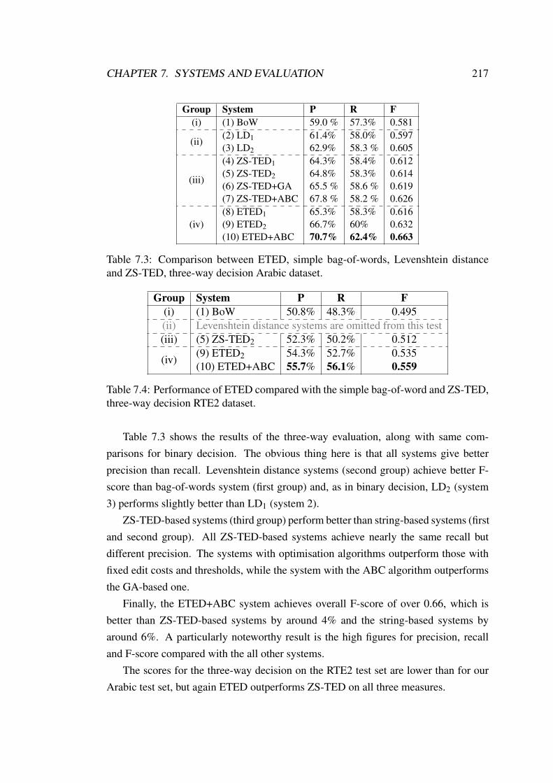
CHAPTER 7. SYSTEMS AND EVALUATION 217
Group System P R F(i) (1) BoW 59.0 % 57.3% 0.581
(ii)(2) LD1 61.4% 58.0% 0.597(3) LD2 62.9% 58.3 % 0.605
(iii)
(4) ZS-TED1 64.3% 58.4% 0.612(5) ZS-TED2 64.8% 58.3% 0.614(6) ZS-TED+GA 65.5 % 58.6 % 0.619(7) ZS-TED+ABC 67.8 % 58.2 % 0.626
(iv)(8) ETED1 65.3% 58.3% 0.616(9) ETED2 66.7% 60% 0.632(10) ETED+ABC 70.7% 62.4% 0.663
Table 7.3: Comparison between ETED, simple bag-of-words, Levenshtein distanceand ZS-TED, three-way decision Arabic dataset.
Group System P R F(i) (1) BoW 50.8% 48.3% 0.495(ii) Levenshtein distance systems are omitted from this test(iii) (5) ZS-TED2 52.3% 50.2% 0.512
(iv)(9) ETED2 54.3% 52.7% 0.535(10) ETED+ABC 55.7% 56.1% 0.559
Table 7.4: Performance of ETED compared with the simple bag-of-word and ZS-TED,three-way decision RTE2 dataset.
Table 7.3 shows the results of the three-way evaluation, along with same com-parisons for binary decision. The obvious thing here is that all systems give betterprecision than recall. Levenshtein distance systems (second group) achieve better F-score than bag-of-words system (first group) and, as in binary decision, LD2 (system3) performs slightly better than LD1 (system 2).
ZS-TED-based systems (third group) perform better than string-based systems (firstand second group). All ZS-TED-based systems achieve nearly the same recall butdifferent precision. The systems with optimisation algorithms outperform those withfixed edit costs and thresholds, while the system with the ABC algorithm outperformsthe GA-based one.
Finally, the ETED+ABC system achieves overall F-score of over 0.66, which isbetter than ZS-TED-based systems by around 4% and the string-based systems byaround 6%. A particularly noteworthy result is the high figures for precision, recalland F-score compared with the all other systems.
The scores for the three-way decision on the RTE2 test set are lower than for ourArabic test set, but again ETED outperforms ZS-TED on all three measures.
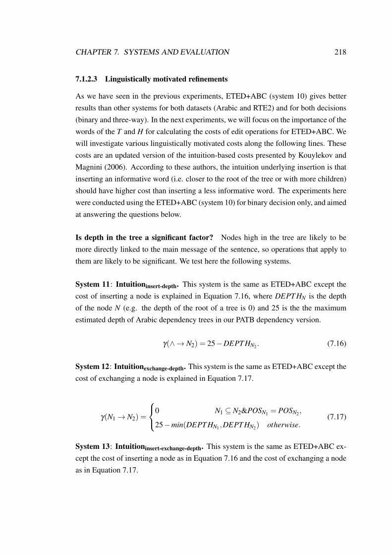
CHAPTER 7. SYSTEMS AND EVALUATION 218
7.1.2.3 Linguistically motivated refinements
As we have seen in the previous experiments, ETED+ABC (system 10) gives betterresults than other systems for both datasets (Arabic and RTE2) and for both decisions(binary and three-way). In the next experiments, we will focus on the importance of thewords of the T and H for calculating the costs of edit operations for ETED+ABC. Wewill investigate various linguistically motivated costs along the following lines. Thesecosts are an updated version of the intuition-based costs presented by Kouylekov andMagnini (2006). According to these authors, the intuition underlying insertion is thatinserting an informative word (i.e. closer to the root of the tree or with more children)should have higher cost than inserting a less informative word. The experiments herewere conducted using the ETED+ABC (system 10) for binary decision only, and aimedat answering the questions below.
Is depth in the tree a significant factor? Nodes high in the tree are likely to bemore directly linked to the main message of the sentence, so operations that apply tothem are likely to be significant. We test here the following systems.
System 11: Intuitioninsert-depth. This system is the same as ETED+ABC except thecost of inserting a node is explained in Equation 7.16, where DEPT HN is the depthof the node N (e.g. the depth of the root of a tree is 0) and 25 is the the maximumestimated depth of Arabic dependency trees in our PATB dependency version.
γ(∧→ N2) = 25−DEPT HN2. (7.16)
System 12: Intuitionexchange-depth. This system is the same as ETED+ABC except thecost of exchanging a node is explained in Equation 7.17.
γ(N1→ N2) =
0 N1 ⊆ N2&POSN1 = POSN2 ,
25−min(DEPT HN1,DEPT HN2) otherwise.(7.17)
System 13: Intuitioninsert-exchange-depth. This system is the same as ETED+ABC ex-cept the cost of inserting a node as in Equation 7.16 and the cost of exchanging a nodeas in Equation 7.17.

CHAPTER 7. SYSTEMS AND EVALUATION 219
System 14: Intuitionall-depth. This system is the same as ETED+ABC except multi-plying each cost of a node with (25- the depth of this node in the tree). The costs forthis system are explained in the following equations.
γ(N1→∧) = γ(N1→∧)× (25−DEPT HN1), (7.18)
γ(∧→ N2) = γ(∧→ N2)× (25−DEPT HN2), (7.19)
γ(N1→N2) =
0 N1 ⊆ N2&POSN1 = POSN2,
γ(N1→ N2)× (25−min(DEPT HN1,DEPT HN2)) otherwise.(7.20)
Is number of daughters for a node a significant factor? Nodes with large numbersof daughters are likely to carry a large amount of information, so operations involvingthese are likely to be significant. We test here the following systems.
System 15: Intuitioninsert-daughters. This system is the same as ETED+ABC exceptthe cost of inserting a node is explained in Equation 7.21, where DT RSN is the numberof daughters of the node N.
γ(∧→ N2) = DT RSN2. (7.21)
System 16: Intuitionexchange-daughters. This system is the same as ETED+ABC exceptthe cost of exchanging a node is explained in Equation 7.22.
γ(N1→ N2) =
0 N1 ⊆ N2&POSN1 = POSN2,
max(DT RSN1,DT RSN2) otherwise.(7.22)
System 17: Intuitioninsert-exchange-daughters. This system is the same as ETED+ABCexcept the cost of inserting a node as in Equation 7.21 and the cost of exchanging anode as in Equation 7.22.

CHAPTER 7. SYSTEMS AND EVALUATION 220
Is number of descendants for a node a significant factor? Although nodes withlarge numbers of daughters are likely to carry a large amount of information, there isno guarantee that ones with few daughters do not, since the daughters themselves mayhave large numbers of daughters. Hence, we looked at number of descendants as analternative measure of information content. We test here the following systems.
System 18: Intuitioninsert-descendants. This system is the same as ETED+ABC exceptthe cost of inserting a node is explained in Equation 7.23, where DCT SN is the numberof descendants of the node N.
γ(∧→ N2) = DCT SN2. (7.23)
System 19: Intuitionexchange-descendants. This system is the same as ETED+ABC ex-cept the cost of exchanging a node is explained in Equation 7.24.
γ(N1→ N2) =
0 N1 ⊆ N2&POSN1 = POSN2,
max(DCT SN1 ,DCT SN2) otherwise.(7.24)
System 20: Intuitioninsert-exchange-descendants. This system is the same as ETED+ABCexcept the cost of inserting a node as in Equation 7.23 and the cost of exchanging anode as in Equation 7.24.
The results of the above intuition-based experiments are summarised in the Ta-ble 7.5 for both Arabic and RTE2 datasets.
As can be seen from Table 7.5, the performance of some versions of ETED+ABCwith various linguistically motivated costs (systems 11, 12, 16 and 19) is better thanthe performance of ETED+ABC (system 10, here as a baseline), which is the bestsystem in the previous experiments. The systems in Table 7.5 can be divided into twomain groups: systems which focus on the importance of the words in the trees (systems11-14) and systems which focus on the information content (systems 15-20). The keyobservation in this table is that the best result arises from looking at whether insertedinformation is high in the tree, i.e. is closely related to the main topic. Therefore, bytaking into account the depth of an inserted node as edit cost for this node, we obtaineda promising approach (system 11), which outperforms all the other 19 systems in this

CHAPTER 7. SYSTEMS AND EVALUATION 221
Dataset System Pyes Ryes Fyes Acc. Fyes× 0.6+
Acc.× 0.4
ArbTEDS
(10) ETED+ABC (baseline) 61.5% 92.7% 0.739 67.3% 0.713(11) Intuitioninsert-depth 63.9% 90.3% 0.749 69.7% 0.728(12) Intuitionexchange-depth 64.9% 86.3% 0.741 69.8% 0.724(13) Intuitioninsert-exchange-depth 60.1% 91.3% 0.725 65.3% 0.696(14) Intuitionall-depth 59% 88.3% 0.708 63.5% 0.679(15) Intuitioninsert-daughters 60.6% 82.7% 0.70 64.5% 0.678(16) Intuitionexchange-daughters 66.3% 83.3% 0.739 70.5% 0.725(17) Intuitioninsert-exchange-daughters 62.6% 88% 0.731 67.7% 0.709(18) Intuitioninsert-descendants 62.8% 81.7% 0.710 66.7% 0.693(19) Intuitionexchange-descendants 64% 88.3% 0.742 69.3% 0.722(20) Intuitioninsert-exchange-descendants 61.2% 93% 0.738 67% 0.711
RTE2(10) ETED+ABC (baseline) 55.4% 70.1% 0.619 56.8% 0.599(11) Intuitioninsert-depth 56.1% 71.8% 0.63 57.8% 0.609
Table 7.5: Comparison between several versions of ETED+ABC with various linguis-tically motivated costs, binary decision.
thesis (systems 1-10 and 12-20). This system produces better F-score by around 1%and accuracy by around 2.5% than the baseline (system 10).
Another observation is that the systems 12, 16 and 19, which are about saying thesame thing in different words between T and H, outperform the other systems (exceptsystem 11, which is about adding information in high position in the tree). This is notunexpected–trees with large numbers of daughters or descendants (systems 16 and 19)are likely to carry a large amount of information, so replacing these is likely to makea significant change to the meaning. It is unclear whether system 12 performs wellbecause it is looking at nodes high in the tree, which are important (as with system11); or because nodes high in the tree are likely to have large numbers of descendants(as with systems 16 and 19).
By applying the best system (system 11) which we obtained for Arabic in theseexperiments to the RTE2 test set, we again got the same conclusion that this systemoutperforms the baseline (system 10), which is the best system in the previous exper-iments for RTE2 test set (see Table 7.2). This system attained F-score and accuracygain of 2% and 1% respectively over the baseline. It achieved an accuracy (57.8%)higher than that of nearly half of the RTE2 participants (see Appendix E). Since mostexperiments on RTE2 task only report accuracy, we re-implemented system 11 to opti-mise accuracy only (i.e. the objective function (fitness) = accuracy). The result of thissystem achieved an accuracy (58.5%) which is higher than half of the RTE2 partici-pants and higher than the median accuracy of the whole set of RTE2 systems. We can

CHAPTER 7. SYSTEMS AND EVALUATION 222
thus claim that our system would have put us in the top half of the RTE2 competition,despite the fact that we were using a parser which achieves only 80% accuracy and thatthe only resource we have used is WordNet.
Overall, the present findings of these experiments are encouraging and seem to beconsistent with those of other studies (e.g. Kouylekov and Magnini, 2006) and suggestthat further work in this regard would be very worthwhile.
7.1.2.4 Optimisation algorithms performance
In this section, we will answer the question as to which algorithm (GA or ABC al-gorithm) works best for our task? To answer this question, we need to answer threemain subsidiary questions: (i) how good a value does it produce? (ii) how quicklydoes it produce this value? and (iii) is there any evidence that it is not stuck at a localmaximum?
In general, to answer the above questions, we have to experiment to find out, sincethey are applications-independent. All experiments here use ZS-TED+GA where theGA replaces all but the current leading candidate once the average fitness has (nearly)converged to the fitness of the leader (system 6), and ZS-TED+ABC (system 7). Gen-erally, the most serious challenge in the use of optimisation algorithms is concernedwith the quality of the results, in particular whether or not an optimal solution is beingreached. One way of providing some degree of insurance is to compare results ob-tained for n times under different seeds of initial population. We therefore performedboth algorithms five times with different random seeds for each run and the same ini-tial seed for both algorithms. For each set of five runs, we used different values offitness parameters a and b, depending on what should be optimised (F-score, accuracyor both). To assess the reliability of GA and ABC algorithm, we calculate the averageperformance of GA and ABC algorithm for the whole set of runs. A more reliablealgorithm should produce (in our case) a higher value for mean, preferably near to theglobal maximum one.
The performance of GA and ABC algorithm for each run under the same conditionsas well as the average performance for the five runs is given in Tables 7.6, 7.7 and 7.8.Each table represents a different fitness function.

CHAPTER 7. SYSTEMS AND EVALUATION 223
Run#Optimisation algorithmGA ABC algorithm
F-score Acc. F-score Acc.1 0.723 64.2% 0.726 65%2 0.721 63.7% 0.725 65.2%3 0.723 64% 0.726 65.2%4 0.718 63.8% 0.722 65%5 0.722 63.8% 0.726 65.3%
Mean 0.721 63.9% 0.725 65.1%
Table 7.6: Comparison between GA and ABC algorithm for five runs, optimise F-scorewhere fitness parameters are a=1 and b=0 (i.e. fitness= F-score).
Run#Optimisation algorithmGA ABC algorithm
F-score Acc. F-score Acc.1 0.719 64.5% 0.715 66%2 0.720 64.7% 0.714 65.8%3 0.719 64.5% 0.712 65.5%4 0.718 64.7% 0.715 66%5 0.720 64.8% 0.717 66.2%
Mean 0.719 64.6% 0.715 65.9%
Table 7.7: Comparison between GA and ABC algorithm for five runs, optimise accu-racy (Acc.) where fitness parameters are a=0 and b=1 (i.e. fitness= accuracy).
Run#Optimisation algorithm
GA ABC algorithmF-score Acc. F-score×0.6+Acc.×0.4 F-score Acc. F-score×0.6+Acc.×0.4
1 0.713 65% 0.688 0.720 65.3% 0.6932 0.721 64.3% 0.690 0.724 65.3% 0.6963 0.715 65% 0.689 0.725 65.2% 0.6964 0.721 64% 0.689 0.723 65.2% 0.6955 0.711 64.7% 0.685 0.723 65.3% 0.695
Mean 0.716 64.6% 0.688 0.723 65.3% 0.695
Table 7.8: Comparison between GA and ABC algorithm for five runs, optimise bothF-score and accuracy with a slight priority to F-score, where fitness parameters area=0.6 and b=0.4 (i.e. fitness= F-score×0.6 + Acc.×0.4).
As can be seen from the results presented in Tables 7.6–7.8, ABC algorithm out-performs GA in all runs and for different types of fitness in terms of the quality of theresults (average of best fitness 0.725 (F-score), 65.9% (accuracy) and 0.695 (mixture

CHAPTER 7. SYSTEMS AND EVALUATION 224
of F-score and accuracy) compared to 0.721 (F-score), 64.6% (accuracy) and 0.688(mixture of F-score and accuracy) for GA) (answer for the first question).
It is hard to answer the third question, but the results in Tables 7.6–7.8 provide uswith some evidence that both algorithms work effectively to avoid getting stuck at alocal maximum. In spite of the fact that both algorithms started from different points(random seeds) for each run, they achieved nearly similar results in each run, withABC algorithm slightly superior to GA.
In order to compare the behaviour of the ABC algorithm more clearly with thebehaviour of GA, we used ‘performance graphs’ (Negnevitsky, 2011). Such a graphis a curve showing the performance of the best individual in the population as wellas a curve showing the average performance of the entire population over the chosennumber of generations (cycles).
Figures 7.5 and 7.6 demonstrate plots of the best and average values of the fitnessacross 500 generations (cycles) for GA and ABC algorithm respectively, where bothalgorithms have been run with the same initial population and the same population size(colony size) equal to 100. The other settings for GA are the same for ZS-TED+GA(see system 6). In these graphs, the x-axis indicates how many generations (cycles)have been created and evaluated at the particular point in the run, and the y-axis repre-sents the fitness value at that point.
0 50 100 150 200 250 300 350 400 450 5000.1
0.2
0.3
0.4
0.5
0.6
0.7
Generation
Fitne
ss
The performance of GA
Best fitness
Mean fitness
Figure 7.5: The performance of GA.
The first thing to note in Figure 7.5 is that the best fitness is more than doubledover the 500 generations. The best fitness curve rises fairly steeply at the beginningof the experiment (until generation number 46), but stays nearly flat for a long time atthe end, with very small increments at generations 65, 96 and 430 respectively, while

CHAPTER 7. SYSTEMS AND EVALUATION 225
0 50 100 150 200 250 300 350 400 450 5000.1
0.2
0.3
0.4
0.5
0.6
0.7
Cycle
Fitness (
necta
r)
The performance of ABC algorithm
Best fitness
Mean fitness
Figure 7.6: The performance of ABC.
the average fitness curve shows more than a triple improvement over the same period.This curve rises rapidly at the beginning of the experiment, but then as the populationconverges nearly on the best solution, it rises more slowly, and finally flattens at theend. At this point we replace all but the best chromosome with a new random popu-lation, in order to try to avoid premature convergence at a local maximum. The shapeof the curve following this repopulation step is almost identical to the shape followingthe initial random population, and the pattern seems to repeat following the secondrepopulation step. This suggests that the system has explored the space of possibilitiesexhaustively, since it seems to follow the same pattern each time it starts with a freshrandomly chosen population.
On the other hand, the best fitness curve obtained by the ABC algorithm in Fig-ure 7.6 again more than doubled over the 500 cycles but to a higher value than that forGA (0.696 compared with 0.689 for GA). It shows an even steeper improvement at thebeginning of the experiment (until cycle 5), which converges very quickly to the bestsolution (answer for the second question), but stays nearly flat for a long time at theend (again apart from very minor increments at cycles 19 and 22 respectively). The av-erage fitness curve shows more than a triple improvement over the same period but lessthan that for GA. This curve starts with gradual improvement at the beginning of theexperiment (until cycle 26), and then it shows erratic behaviour between 0.5 and 0.6.This is because in ABC algorithm, while a stochastic selection scheme (i.e. similar to‘roulette wheel selection’ in GA) based on the nectar (fitness) values is carried out byonlooker bees, a greedy selection scheme as in differential evolution (DE) is used byonlookers and employed bees to make a selection between the position of a food source

CHAPTER 7. SYSTEMS AND EVALUATION 226
(a possible solution) in their memory and the new food source position. Furthermore, arandom selection process is achieved by using scouts. Also, the production mechanismof the neighbour food source used in ABC is similar to the mutation process, whichis self-adapting, of DE. From this perspective, in ABC algorithm, the solutions in thecolony (population) directly affect the mutation operation since the operation is basedon the difference of two members of the colony. In this way, the information of a goodmember of the colony is distributed among the other members due to the greedy se-lection mechanism employed and the mutation operation to generate a new member ofthe colony. Unlike GA, ABC algorithm does not have explicit crossover. However, inABC the transfer of good information between the members is achieved by the muta-tion process, whereas in GA it is managed by the mutation and the crossover operatorstogether. Therefore, although the local converging speed of a standard GA is quitegood, GA might encounter the premature convergence in optimising some problems ifthe initial population does not have a sufficient diversity. On the other hand, while theintensification process is controlled by the stochastic and the greedy selection schemesin the ABC, the diversification is controlled by the random selection. It seems thatthe problem of getting stuck in local maxima has been avoided (answer for the thirdquestion).
We also find that any increment after a sufficient value for colony size does notimprove the performance of the ABC algorithm significantly (0.696 for 40 colony sizeand 100 cycles compared to 0.698 for 100 colony size and 500 cycles). For this reason,we carried out this work with colony size of 40, which can provide an acceptableconvergence speed for search.
To conclude, simulation results show that the performance of ABC algorithm, interms of the quality of results, convergence speed and avoidance of local maxima, isbetter than GA under the same conditions although ABC algorithm used fewer param-eters than GA. Its performance is very good in terms of the local and the global opti-misation due to the selection schemes employed and the neighbour production mecha-nism used. Consequently, it can be concluded that ABC algorithm based approach cansuccessfully be used in the optimisation of transformation-based TE systems.

Chapter 8
Conclusion and future work
During this thesis, we have explored a number of systems for the task of RTE for Ara-bic (Chapter 7), ranging from the robust, but imprecise, bag-of-words model based onapproximate measures of semantic similarity to more deep systems based on pattern-matching such as transformation-based approaches. We have also examined the im-provements of tagging and parsing for Arabic (Chapter 4), which play a role in most ofour approaches as a preprocessing step. We have also created a first dataset for ArabicRTE task (Chapter 6).
In this final chapter, we seek to address two main questions: what have we learnedabout the task of RTE for Arabic, and what are the most promising directions for futureresearch in this area?
8.1 Main thesis results
This thesis has examined the task of RTE for Arabic from different angles, and wehope to have made important contributions in various areas.
In Chapter 4, we experimented with a number of strategies to improve our prepro-cessing stage to convert our input from raw texts into dependency trees. The two mainfindings for these experiments are summarised below.
The first major finding was that we presented a very simple strategy for combin-ing POS taggers which leads to substantial improvements in accuracy. In experimentswith combining three Arabic taggers (AMIRA, MADA and an in-house maximum-likelihood (MXL)), the current strategy significantly outperformed voting-based strate-gies for both a coarse-grained set of tags (39 tags, see Table 4.2) and the original finer-grained of the PATB with 305 tags. The accuracy of a tagger clearly depends on the
227

CHAPTER 8. CONCLUSION AND FUTURE WORK 228
granularity of the tagset: the contributing taggers produced accuracies from 95.5% to96.7% on the coarse-grained tagset, and from 88.8% to 93.6% on the fine-grained one(see Table 4.2).
The key to the proposed combining strategy is that each of the contributing taggersis likely to make systematic mistakes; and that if they are based on different principlesthey are likely to make different systematic mistakes. If we classify the mistakes thata tagger makes, we should be able to avoid believing it in cases where it is likely tobe wrong. So long as the taggers are based on sufficiently different principles, theyshould be wrong in different places.
We therefore collected confusion matrices for each of the individual taggers show-ing how likely they were to be right for each category of item–how likely, for instance,was MADA to be right when it proposed to tag some item as a noun (very likely–accuracy of MADA when it proposes NN is around 98%), how likely was AMIRA tobe right when it proposed the particle tag RP (very unlikely–accuracy of 8% in thiscase)? Given these tables, we simply took the tagger whose prediction was most likelyto be right.
We compared the results of this simple strategy with a strategy proposed by Zemanand Žabokrtsky (2005), in which you accept the majority view if at least two of thetaggers agree, and you backoff to one of them if they all disagree, and with a varia-tion on that where you accept the majority view if two agree and backoff to the mostconfident if they all disagree (see Tables 4.5 and 4.7).
All four strategies produce an improvement over the individual taggers. The factthat majority voting works better when backing off to MXL than to MADA, despite thefact that MADA works better in isolation, is thought-provoking. It seems likely to bethat this arises from the fact that MADA and AMIRA are based on similar principles,and hence are likely to agree even when they are wrong. This hypothesis suggestedthat looking at the likely accuracy of each tagger on each case might be a good backoffstrategy. It turns out that it is not just a good backoff strategy, as shown in the column1 (‘backoff unless two agree’) of Table 4.7: it is even better when used as the mainstrategy (column 2: ‘MC’). The differences between columns 1 and 2 are not huge,1
but that should not be too surprising, since these two strategies will agree in every casewhere all three of the contributing taggers agree, so the only place where these two willdisagree is when one of the taggers disagrees with the others and the isolated tagger is
1In terms of error rate the difference looks more substantial, since the error rate, 0.005, for column2 for the fine-grained set is 60% of that for column 1, 0.007; and for the coarse-grained set the error ratefor column 2, 0.04, is 73% of that for column 1, 0.055.

CHAPTER 8. CONCLUSION AND FUTURE WORK 229
more confident than either of the others.The idea reported here is very simple, but it is also very effective. We have reduced
the error in tagging with fairly coarse-grained tags to 0.005, and we have also produceda substantial improvement for the fine-grained tags, from 93.6% for the best of theindividual taggers to 96% for the combination.
The second major hypothesis was that given the success of the approach outlinedabove for tagging, it might be worth applying the same idea to parsing. We there-fore tried using it with a combination of dependency parsers, for which we usedMSTParser and two variants from the MALTParser family, namely Nivre arc-eager
(MALTParser1) and Stack swap-eager (MALTParser2). We tested a number of strate-gies including: (i) the three parsers in isolation; (ii) a strategy in which we select a pairand trust their proposals wherever they agree, and backoff to the other one when theydo not; (iii) a strategy in which we select a pair and trust them whenever they agree,and backoff to whichever parser is most confident (which may be one of these or maybe the other one) when they do not; and (iv) strategies where we either just use themost confident one, or where we take either a unanimous vote or a majority vote, andbackoff to the most confident one if this is inconclusive.
The results of these strategies (see Tables 4.15–4.18 and 4.21) indicate that forparsing, simply relying on the parser which is most likely to be right when choosing thehead for a specific dependent in isolation does not produce the best overall result, andindeed does not even surpass the individual parsers in isolation. For these experiments,the best results were obtained by asking a predefined pair of parsers whether theyagree on the head for a given item, and backing off to the other one when they do not.This fits with Henderson and Brill (1999)’s observations about a similar strategy fordependency parsing for English. It seems likely that the problem with relying on themost confident parser for each individual daughter-head relation is that this will tendto ignore the big picture, so that a collection of relations that are individually plausible,but which do not add up to a coherent overall analysis, will be picked.
Thus, it seems that the success of the proposed method for taggers depends cru-cially on having taggers that exploit different principles, since under those circum-stances the systematic errors that the different taggers make will be different; and onthe fact that POS tags can be assigned largely independently (though of course eachof the individual taggers makes use of information about the local context, and inparticular about the tags that have been assigned to neighbouring items). The reasonwhy simply taking the most likely proposals in isolation is ineffective when parsing

CHAPTER 8. CONCLUSION AND FUTURE WORK 230
may be that global constraints such as Henderson and Brill’s ‘no crossing brackets’requirement are likely to be violated. Interestingly, the most effective of our strate-gies for combining parsers takes two parsers that use the same learning algorithm andsame feature sets but different parsing strategies (MALTParser1 and MALTParser2),and relies on them when they agree; and backs off to MSTParser, which exploits fun-damentally different machinery, when these two disagree. In other words, it makesuse of two parsers that depend on very similar underlying principles, and hence arelikely to make the same systematic errors, and backs off to one that exploits differentprinciples when they disagree.
We then investigated two techniques to combine taggers and parsers for improvingour preprocessing stage. The first technique, which is combine taggers and combineparsers, suggests that a flawed parser may learn to compensate for the errors madeby a flawed tagger. By applying combining parsers (second finding) on text taggedby combining taggers (first finding), we got accuracy (around 85% for labelled accu-racy, which is the best result we have seen for the PATB) higher than applying eachparser in isolation on gold-standard tagged text (around 82%-83%). The second tech-nique (combining different tagger:parser pairs where each parser uses a different tag-ger) shows that applying such a technique will increase precision, but decrease recall,which may be useful for some tasks.
We have not carried out a parallel set of experiments on taggers or parsers forlanguages other than Arabic because we are interested here in Arabic. In situationswhere three (or more) distinct approaches to a problem of this kind are available, itseems at least worthwhile investigating whether the proposed methods of combinationwill work.
In Chapter 5, we extended ZS-TED, which computes the minimal cost to transformone tree into another. The extended version, ETED, fixes the main weakness of ZS-TED, which is that it is not able to do transformations on subtrees (i.e. delete subtree,insert subtree and exchange subtree). To achieve this goal, we firstly run ZS-TED(which uses only single node edit operations) and compute the standard alignmentfrom the results, as in Section 5.3.1; and then we go over the alignment and groupsubtrees operations, i.e. for every consecutive k deletions that correspond to an entiresubtree reduce the edit distance score by α×k+β for any desired α and β , which arein the interval [0,1], as in Section 5.3.2.
It is important to note that although we apply this technique on modifying ZS-TED,it can also work on modifying any other TED algorithms such as Klein’s algorithm or

CHAPTER 8. CONCLUSION AND FUTURE WORK 231
Demaine et al.’s algorithm or Pawlik-Augsten’s algorithm.2 Furthermore, the addi-tional time cost is O(n2), which is negligible since it is less than the time cost for anyavailable TED algorithms.
In fact, ETED is more effective and flexible than ZS-TED, especially for applica-tions that pay attention to relations among nodes (e.g. in linguistic trees, deleting amodifier subtree should be cheaper than the sum of deleting its components individu-ally).
In Chapter 6, we undertook the first attempt at creating a dataset for training andtesting Arabic TE systems. We examined two main tools for creating our dataset:
(i) Collecting the dataset: we apply two techniques here: (a) for the training dataset,we use a headline (as H) from one source and the lead-paragraph (as T) from anews article about the same story but from another source for 10 returned pages.This technique enables us to collect a huge amount of T-H pairs without any biasin a short time, but with a preponderance of positive examples (see Table 6.2)with minimum common words between each T-H pair; and (b) for the testingdataset, we update the previous technique, since we need here a balance betweenpositive and negative pairs. We use the same technique that we used for trainingto collect entailment pairs, since such technique is promising in this regard (seeTable 6.2), while we use a paragraph from a news article which gives a high num-ber of common words with a closely linked headline. This technique enables usto collect a huge amount of non-entailment pairs with a large number of commonwords between each pair without any bias.
(ii) Annotating our dataset: we develop here an online system that allows each an-notator to annotate any number of pairs, revisit previous annotated pairs, sendcomments to the administrator and other options. This system has a number ofadvantages such as allowing people to annotate our dataset from different placesor countries and allows saving different information about each pair such as orig-inal articles, number of words in each sentence, number of common words andothers.
Each pair was annotated by three annotators. The annotator agreement (whereall annotators agree) is around 78% compared with 91% where each annotatoragrees with at least one co-annotator. This suggests that the annotators found thisa difficult task.
2For more detailed description about these algorithms see (Bille, 2005).

CHAPTER 8. CONCLUSION AND FUTURE WORK 232
We also tested the reliability of our annotators by using two different techniques:(a) the rate of selecting ‘unknown’ option for each annotator; and (b) calculated kappacoefficient for each annotator, which takes chance into account. These techniquesenable us to detect unreliable annotator(s). The results of these analyses suggest thatthere are no unreliable annotators among our annotators.
Finally, in Chapter 7, we explored a range of approaches to natural language infer-ence (NLI), particularly the RTE task of determining whether one text snippet entailsanother, beginning with robust but approximate methods, and proceeding to progres-sively more precise approaches such as transformation-based approaches. These ap-proaches include: (i) bag-of-words (system 1); (ii) the Levenshtein distance with twodifferent settings (systems 2-3); (iii) ZS-TED with different settings (system 4-7); and(iv) ETED with different settings (system 8-10). We applied these systems to our Ara-bic test set and some of them to the RTE2 test set for two types of decisions: binarydecision (‘yes’/‘no’) and three-way decision (‘yes’/‘unknown’/‘no’) (see Tables 7.1–7.4).
The results of these experiments show that, as expected, TED-based systems out-perform the string-based systems, and ETED-based systems outperform ZS-TED-basedsystems. The key point with ETED is that subtrees tend to correspond to single infor-mation units. By treating operations on subtrees as less costly than the correspond-ing set of individual node operations, ETED concentrates on entire information units,which are a more appropriate granularity than individual words for considering entail-ment relations.
Selecting a combination of thresholds and costs for the TED’s primitive edit op-erations is a challenge, and becomes very hard when dealing with complex problems.Choosing suitable edit costs depends on different parameters such as the nature ofnodes and applications (e.g. deleting a verb node from a syntactic tree is differentfrom deleting a symbol in RNA structure). One possible solution to overcoming thischallenge could consist of assigning costs based on an expert valuation, but it may notbe efficiently done in domains where the expertise is very limited. Furthermore, evenif the level of expertise is good, assigning an appropriate cost to each edit operationcan become a tricky task. An alternative solution is to estimate each edit cost automat-ically. We therefore investigated the use of different optimisation algorithms, and haveshown that using these algorithms produces better performance than setting the costsof edit operations by hand, and that using the ABC algorithm produces better resultsfor the same amount of effort as traditional GA.

CHAPTER 8. CONCLUSION AND FUTURE WORK 233
Next, we investigated an improvement to the ETED+ABC (system 10), the bestsystem among the systems 1-10, by testing various linguistically motivated costs suchas the depth of a node, number of daughters, number of descendants and combinationsbetween them (systems 11-20). The results of these experiments (see Table 7.5) showthat the performances of some of ETED+ABC with linguistically motivated costs (sys-tems 11, 12, 16 and 19) are better than the performance of ETED+ABC with constantedit costs (system 10). By taking into account the depth of an inserted node as editcost for this node (the word’s importance), we obtained a promising approach (system11) which outperforms all the other 19 systems in this thesis (systems 1-10 and 12-20). This system produces better F-score by around 1% and accuracy by around 2.5%than the baseline (system 10). This is due to the specific nature of the dependencytree where the higher position nodes in it are more relevant to the meaning expressedby a certain phrase (i.e. the main relation between the nodes is at the top of the tree).Similarly, taking into account the amount of information in a subtree (as with systems12, 16 and 19) can help the system decide how important this subtree is. This helps itmake judgements about the significance of applying an operator to the subtree.
The findings are encouraging on the Arabic test set, particularly the improvementin F-score and accuracy. The fact that some of these results were replicated for theEnglish RTE2 test set, where we had no control over the parser that was used to producedependency trees from the T-H pairs, provides some evidence for the robustness of ourapproach. We anticipate that in both cases having a more accurate parser (our parserfor Arabic attains around 85% accuracy on the PATB, MINIPAR is reported to attainabout 80% on the Suzanne corpus) would improve the performance of both ZS-TEDand ETED.
In short, we have carried out a number of experiments on our dataset using a vari-ety of standard TE algorithms (bag-of-words, Levenshtein distance, tree edit distance).The results of these experiments were comparable with the results of using these algo-rithms with the standard RTE2 dataset. This suggests that the data we have collectedis comparable with the RTE2 set in terms of the difficulty of the TE task–not full oftrivial entailments that can be captured simply by counting words, but not full of T-H
pairs where the connection requires so much background knowledge that the standardtechniques are unusable. As such, we believe that this dataset is likely to be a use-ful resource for researchers wishing to investigate the cross-linguistic effectiveness ofvarious TE algorithms.

CHAPTER 8. CONCLUSION AND FUTURE WORK 234
8.2 Main contributions
In the summary of the discussion above of the main thesis results, the current projecthas made the following main contributions:
1. We have converted the PATB from phrase structure form into a dependency tree-bank.
2. We have updated the MXL Arabic tagger to work with MSA rather than the classi-cal Arabic used in the Holy Quran.
3. We have improved the performance of tagging by combining taggers based on con-fidence which produces substantially better performance than any of the contribut-ing taggers.
4. We have improved the performance of parsing by combining parsers based on ma-jority voting which produces substantially better performance than any of the con-tributing parsers.
5. We have created semi-automatically the first dataset for Arabic RTE task.
6. We have updated the standard TED algorithm to deal with both single and subtreeoperations, i.e. ETED, rather than single operations only.
7. We have improved the performance of TED algorithms by estimating automaticallythe relevant edit costs of operations and thresholds by using ABC algorithm.
8. We have developed the first system for Arabic RTE task.
We have shown that ETED is effective for the English RTE2 dataset. A number ofthe other algorithms have potential for application to languages other than Arabic, butthis remains to be investigated.
8.3 Future directions
What does the future hold for the current research on TE for Arabic? There are variousavenues for further work related to the research presented in this thesis, both within theapproaches and systems discussed, and more generally for the application areas of TE.
The following suggestions are provided for the future work to improve the currentsystem:
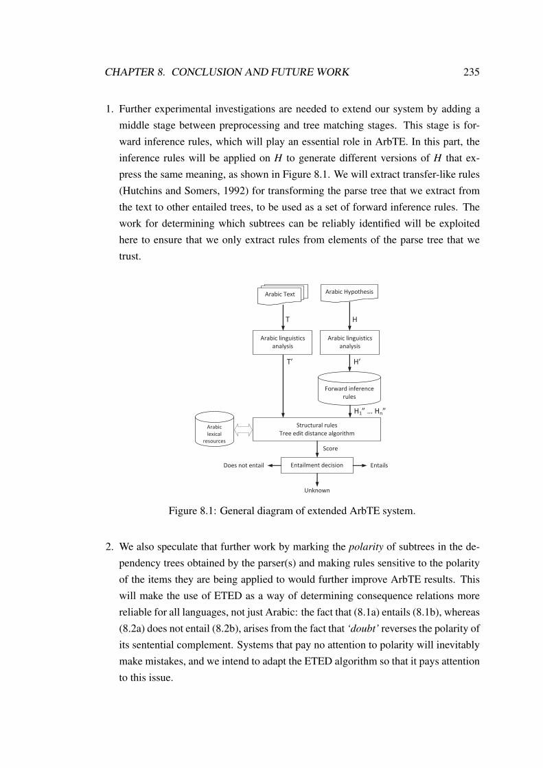
CHAPTER 8. CONCLUSION AND FUTURE WORK 235
1. Further experimental investigations are needed to extend our system by adding amiddle stage between preprocessing and tree matching stages. This stage is for-ward inference rules, which will play an essential role in ArbTE. In this part, theinference rules will be applied on H to generate different versions of H that ex-press the same meaning, as shown in Figure 8.1. We will extract transfer-like rules(Hutchins and Somers, 1992) for transforming the parse tree that we extract fromthe text to other entailed trees, to be used as a set of forward inference rules. Thework for determining which subtrees can be reliably identified will be exploitedhere to ensure that we only extract rules from elements of the parse tree that wetrust.
H1” … Hn”
Does not entail
Arabic Text Arabic Hypothesis
Arabic linguistics
analysis
Arabic linguistics
analysis
Forward inference
rules
Structural rules
Tree edit distance algorithm
Entailment decision
T H
T’ H’
Score
Unknown
Entails
Arabic
lexical
resources
Figure 8.1: General diagram of extended ArbTE system.
2. We also speculate that further work by marking the polarity of subtrees in the de-pendency trees obtained by the parser(s) and making rules sensitive to the polarityof the items they are being applied to would further improve ArbTE results. Thiswill make the use of ETED as a way of determining consequence relations morereliable for all languages, not just Arabic: the fact that (8.1a) entails (8.1b), whereas(8.2a) does not entail (8.2b), arises from the fact that ‘doubt’ reverses the polarity ofits sentential complement. Systems that pay no attention to polarity will inevitablymake mistakes, and we intend to adapt the ETED algorithm so that it pays attentionto this issue.

CHAPTER 8. CONCLUSION AND FUTURE WORK 236
(8.1) Polarity (Entailment)
a. I believe that a woman did it.
b. I believe that a human being did it.
(8.2) Polarity (Non-entailment)
a. I doubt that a woman being did it.
b. I doubt that a human did it.
3. Further investigation and experimentation into ETED is strongly recommended.As we have seen in Section 7.1.2.4, applying ETED with linguistically motivatedcosts gives better results than other systems in this thesis. More broadly, research isneeded to apply ETED more deeply by associating a vector space model with eachnode in a tree. Such a vector, for instance, might contain more details about thenode such as POS tag, word frequency, lemma, taxonomy-based score, the depthof node, its number of daughters and others. Then, when we compare between twonodes we should pay attention to these features.
4. As we have seen in Chapter 4, combining systems gives better results than eachsystem in isolation for different aspects of NLP such as POS tagging and parsing.A further study could assess this technique for the TE task itself. So, going for-ward, we will need to look at ways to combine different systems–including notonly lexical overlap or syntactic based systems–in order to take advantage of them.
5. Further work needs to be done to complete establishing our dataset. The ArabicTE dataset presented in this thesis can be utilised for reference; however this is aninitial dataset. It is expected that the initial dataset will be expanded with additionalpairs and decisions (three-ways).
6. We intend to use our system to improve the quality of the candidate input for QAor IE systems, since such techniques have not been investigated so far for Arabic.
7. Another interesting task for future exploration is applying our technique on the Qur-Sim corpus (Sharaf and Atwell, 2012) which contains pairs of semantically similaror related Quranic verses. TED can be seen as providing a family of measures ofsemantic relatedness, with the weights chosen in Chapter 7 providing an asymmet-ric measure corresponding roughly to entailment. It would be interesting to try to

CHAPTER 8. CONCLUSION AND FUTURE WORK 237
find weights which correspond to other forms of relatedness such as that embodiedin the QurSim.
8. We intend to make our Arabic RTE task dataset and the stand-off annotations of thedependency version of the PATB (because of the licence) available to the scientificcommunity thus allowing other researchers to duplicate our experiments to comparethe effectiveness of our algorithms with alternative approaches.
In the end we would like to conclude that the work in this area (i.e. determiningwhether one text snippet can be inferred from another) is very challenging, in partic-ular for Arabic where we are faced with an exceptional level of lexical and structuralambiguity. We think that any attempt in this regard for languages other than Englishwill bring benefits for the whole RTE community.
In addition to the specific contributions outlined before, we hope to have achievedan aim through this project greater than the announced ones, which is to catalyse otherresearchers to investigate NLI for Arabic more seriously, far from being merely a for-mal topic of linguists and semanticists. Achieving this goal will open the door toinvestigate the applications of this task to solve various real-world challenges such asQA, IE and others. Consequently, it constitutes a topic ripe for the attention of NLPresearchers in order to remedy the gap between the available techniques for Arabic andthose that have been done for other languages such as English.

Bibliography
Adams, R. (2006). Textual entailment through extended lexical overlap. In Proceed-
ings of the 2nd PASCAL Challenges Workshop on Recognising Textual Entailment,pp. 128–133, Venice, Italy.
Aharon, R., Szpektor, I., and Dagan, I. (2010). Generating entailment rules fromFrameNet. In Proceedings of the 48th Annual Meeting of the Association for Com-
putational Linguistics (ACL 2010)–Short Papers, pp. 241–246, Uppsala, Sweden.Association for Computational Linguistics.
Akay, B. and Karaboga, D. (2012). A modified artificial bee colony algo-rithm for real-parameter optimization. Information Sciences, 192:120 – 142,doi:10.1016/j.ins.2010.07.015.
Al Shamsi, F. and Guessoum, A. (2006). A hidden Markov model-based POS tag-ger for Arabic. In 8es Journées internationales d’Analyse statistique des Données
Textuelles (JADT-2006), pp. 31–42, Besançon, France.
Alabbas, M. (2011). ArbTE: Arabic textual entailment. In Proceedings of the 2nd
Student Research Workshop associated with the International Conference Recent
Advances in Natural Language Processing (RANLP 2011), pp. 48–53, Hissar, Bul-garia. RANLP 2011 Organising Committee.
Alabbas, M., Khalaf, Z., and Khashan, K. (2012). BASRAH: an automatic systemto identify the meter of Arabic poetry. Natural Language Engineering, 1(1):1–19,doi:10.1017/S1351324912000204.
Alabbas, M. and Ramsay, A. (2011a). Evaluation of combining data-driven depen-dency parsers for Arabic. In Proceedings of the 5th Language & Technology Con-
ference: Human Language Technologies (LTC 2011), pp. 546–550, Poznan, Poland.
238

BIBLIOGRAPHY 239
Alabbas, M. and Ramsay, A. (2011b). Evaluation of dependency parsers for long Ara-bic sentences. In Proceedings of 2011 International Conference on Semantic Tech-
nology and Information Retrieval (STAIR’11), pp. 243–248, Putrajaya, Malaysia.IEEE, doi:10.1109/STAIR.2011.5995796.
Alabbas, M. and Ramsay, A. (2012a). Arabic treebank: from phrase-structure treesto dependency trees. In Proceedings of the META-RESEARCH Workshop on Ad-
vanced Treebanking at the 8th International Conference on Language Resources
and Evaluation (LREC 2012), pp. 61–68, Istanbul, Turkey.
Alabbas, M. and Ramsay, A. (2012b). Combining black-box taggers and parsers formodern standard Arabic. In Proceedings of Federated Conference on Computer
Science and Information Systems (FedCSIS-2012), pp. 19 –26, Wrocław, Poland.IEEE.
Alabbas, M. and Ramsay, A. (2012c). Dependency tree matching with extended treeedit distance with subtrees for textual entailment. In Proceedings of Federated Con-
ference on Computer Science and Information Systems (FedCSIS-2012), pp. 11–18,Wrocław, Poland. IEEE.
Alabbas, M. and Ramsay, A. (2012d). Improved POS-tagging for Arabic by combin-ing diverse taggers. In Iliadis, L., Maglogiannis, I., and Papadopoulos, H. (Eds.),Artificial Intelligence Applications and Innovations (AIAI), volume 381 of IFIP
Advances in Information and Communication Technology, pp. 107–116. SpringerBerlin-Heidelberg, Halkidiki, Thessaloniki, Greece, doi:10.1007/978-3-642-33409-2_12.
Alba, E. and Dorronsoro, B. (2008). Cellular Genetic Algorithms. OperationsResearch/Computer Science Interfaces Series. New York, USA: Springer Sci-ence+Business Media, LLC.
AlGahtani, S., Black, W., and McNaught, J. (2009). Arabic part-of-speech taggingusing transformation-based learning. In Proceedings of the 2nd International Con-
ference on Arabic Language Resources and Tools, pp. 66–70, Cairo, Egypt. TheMEDAR Consortium.
Alpaydin, E. (2010). Introduction to Machine Learning. Cambridge, Massachusetts,USA: MIT Press.

BIBLIOGRAPHY 240
Altman, D. (1991). Practical Statistics for Medical Research. London, UK: Chapmanand Hall.
Androutsopoulos, I. and Malakasiotis, P. (2010). A survey of paraphrasing and textualentailment methods. Journal of Artificial Intelligence Research, 38(1):135–187.
Aronoff, M. and Rees-Miller, J. (2003). The Handbook of Linguistics. Oxford, UK:Blackwell.
Attia, M. (2012). Ambiguity in Arabic Computational Morphology and Syntax: A
Study within the Lexical Functional Grammar Framework. Saarbrücken, Germany:LAP Lambert Academic Publishing.
Badawi, E., Carter, M., and Gully, A. (2004). Modern Written Arabic: A Comprehen-
sive Grammar. London, UK: Routledge.
Balahur, A., Lloret, E., Ferrández, O., Montoyo, A., Palomar, M., and Muñoz, R.(2008). The DLSIUAES team’s participation in the TAC 2008 tracks. In Proceed-
ings of the 1st Text Analysis Conference (TAC 2008), Gaithersburg, Maryland, USA.National Institute of Standards and Technology.
Baptista, M. (1995). On the nature of pro-drop in capeverdean creole. Technical report,Harvard Working Papers in Linguistics, 5: 3-17.
Bar-Haim, R., Berant, J., Dagan, I., Greental, I., Mirkin, S., Shnarch, E., and Szpek-tor, I. (2008). Efficient semantic deduction and approximate matching over com-pact parse forests. In Proceedings of the 1st Text Analysis Conference (TAC 2008),Gaithersburg, Maryland, USA. National Institute of Standards and Technology.
Bar-Haim, R., Dagan, I., Greental, I., and Shnarch, E. (2007). Semantic inference atthe lexical-syntactic level. In Proceedings of the 22nd AAAI Conference on Artificial
Intelligence (AAAI-07), pp. 871–876, Vancouver, British Columbia, Canada. AAAIPress.
Barzilay, R. and Lee, L. (2003). Learning to paraphrase: an unsupervised approachusing multiple-sequence alignment. In Proceedings of the Human Language Tech-
nology: Conference of the North American Chapter of the Association for Computa-
tional Linguistics (HLT-NAACL 2003), pp. 16–23, Edmonton, Canada. Associationfor Computational Linguistics, doi:10.3115/1073445.1073448.

BIBLIOGRAPHY 241
Basili, R., De Cao, D., Marocco, P., and Pennacchiotti, M. (2007). Learning selectionalpreferences for entailment or paraphrasing rules. In Proceedings of the International
Conference on Recent Advances in Natural Language Processing (RANLP 2007),pp. 1–6, Borovets, Bulgaria. RANLP 2007 Organising Committee.
Bayer, S., Burger, J., Ferro, L., Henderson, J., and Yeh, A. (2005). MITRE’s sub-missions to the EU PASCAL RTE Challenge. In Proceedings of the1st PASCAL
Recognising Textual Entailment Challenge, pp. 41–44, Southampton, UK.
Bernard, M., Boyer, L., Habrard, A., and Sebban, M. (2008). Learning prob-abilistic models of tree edit distance. Pattern Recognition, 41(8):2611–2629,doi:10.1016/j.patcog.2008.01.011.
Bhatt, R. and Xia, F. (2012). Challenges in converting between treebanks: a case studyfrom the HUTB. In Proceedings of the META-RESEARCH Workshop on Advanced
Treebanking at the 8th International Conference on Language Resources and Eval-
uation (LREC 2012), pp. 53–60, Istanbul, Turkey.
Bille, P. (2005). A survey on tree edit distance and related problems. Theoretical
Computer Science, 337(1-3):217–239, doi:10.1016/j.tcs.2004.12.030.
Black, W., Elkateb, S., Rodriguez, H., Alkhalifa, M., Vossen, P., Pease, A., and Fell-baum, C. (2006). Introducing the Arabic WordNet project. In Proceedings of the
3rd International WordNet Conference (GWC-06), pp. 295–299, Jeju Island, Korea.
Blackburn, P., Bos, J., Kohlhase, M., and de Nivelle, H. (2001). Inference and compu-tational semantics. In Bunt, H. and Muskens, R.and Thijsse, E. (Eds.), Computing
Meaning, volume 77 of Studies in Linguistics and Philosophy, pp. 11–28. SpringerNetherlands, doi:10.1007/978-94-010-0572-2_2.
Bloomer, A., Griffiths, P., and Merrison, A. (2005). Introducing Language in Use: A
Coursebook. New York, USA: Routledge.
Bos, J. and Markert, K. (2006a). Recognising textual entailment with robust log-ical inference. In Quiñonero Candela, J., Dagan, I., Magnini, B., and d’AlchéBuc, F. (Eds.), Machine Learning Challenges. Evaluating Predictive Uncertainty,
Visual Object Classification, and Recognising Tectual Entailment, volume 3944of Lecture Notes in Computer Science, pp. 404–426. Springer Berlin-Heidelberg,doi:10.1007/11736790_23.

BIBLIOGRAPHY 242
Bos, J. and Markert, K. (2006b). When logical inference helps determining textualentailment (and when it doesn’t). In Proceedings of the 2nd PASCAL Challenges
Workshop on Recognising Textual Entailment, pp. 98–103, Venice, Italy.
Bos, J., Zanzotto, F., and Pennacchiotti, M. (2009). Textual entailment at EVALITA2009. In Proceedings of the 11th Conference of the Italian Association for Artificial
Intelligence, pp. 1–7, Reggio Emilia, Italy.
Brill, E. (1995). Transformation-based error-driven learning and natural languageprocessing: a case study in part-of-speech tagging. Computational Linguistics,21(4):543–565.
Brill, E. and Wu, J. (1998). Classifier combination for improved lexical disambigua-tion. In Proceedings of the Conference of the 36th Annual Meeting of the Association
for Computational Linguistics and 17th International Conference on Computational
Linguistics (COLING-ACL ’98), pp. 191–195, Montréal, Quebec, Canada. Associa-tion for Computational Linguistics.
Bublitz, W. and Norrick, N. (2011). Foundations of Pragmatics. Berlin, Germany:Walter de Gruyter.
Buckwalter, T. (2004). Buckwalter Arabic morphological analyzer version 2.0. Lin-guistic Data Consortium, LDC Catalog No.: LDC2004L02.
Burchardt, A. (2008). Modeling Textual Entailment with Role-Semantic Information.PhD thesis, Department of Computational Linguistics, Saarland University, Saar-brücken, Germany.
Burchardt, A. and Frank, A. (2006). Approaching textual entailment with LFG andFrameNet frames. In Proceedings of the 2nd PASCAL Challenges Workshop on
Recognising Textual Entailment, pp. 92–97, Venice, Italy.
Burchardt, A., Pennacchiotti, M., Thater, S., and Pinkal, M. (2009). Assessing theimpact of frame semantics on textual entailment. Natural Language Engineering,15(4):527–550, doi:10.1017/S1351324909990131.
Burchardt, A., Reiter, N., Thater, S., and Frank, A. (2007). A semantic approach totextual entailment: system evaluation and task analysis. In Proceedings of the ACL-
PASCAL Workshop on Textual Entailment and Paraphrasing, pp. 10–15, Prague,Czech Republic. Association for Computational Linguistics.

BIBLIOGRAPHY 243
Burger, J. and Ferro, L. (2005). Generating an entailment corpus from news head-lines. In Proceedings of the ACL Workshop on Empirical Modeling of Semantic
Equivalence and Entailment, pp. 49–54, Ann Arbor, Michigan, USA. Associationfor Computational Linguistics.
Buscaldi, D., Tournier, R., Aussenac-Gilles, N., and Mothe, J. (2012). IRIT: textualsimilarity combining conceptual similarity with an n-gram comparison method. InProceedings of the 1st Joint Conference on Lexical and Computational Semantics
(*SEM 2012), pp. 552–556, Montréal, Canada. Association for Computational Lin-guistics.
Cabrio, E. and Magnini, B. (2011). Defining specialized entailment engines using nat-ural logic relations. In Vetulani, Z. (Ed.), Human Language Technology. Challenges
for Computer Science and Linguistics, volume 6562 of Lecture Notes in Computer
Science, pp. 268–279. Springer Berlin-Heidelberg, doi:10.1007/978-3-642-20095-3_25.
Cabrio, E., Magnini, B., and Ivanova, A. (2012). Extracting context-rich entailmentrules from Wikipedia revision history. In Proceedings of the 3rd Workshop on the
People’s Web Meets NLP, Association for Computational Linguistics (ACL 2012),pp. 34–43, Jeju, Republic of Korea. Association for Computational Linguistics.
Callison-Burch, C. (2008). Syntactic constraints on paraphrases extracted from parallelcorpora. In Proceedings of the 2008 Conference on Empirical Methods in Natural
Language Processing (EMNLP 2008), pp. 196–205, Honolulu, Hawaii. Associationfor Computational Linguistics.
Callison-Burch, C., Osborne, M., and Koehn, P. (2006). Re-evaluating the role ofBLEU in machine translation research. In Proceedings of 11th Conference of the
European Chapter of the Association for Computational Linguistics (EACL 2006),pp. 249–256, Trento, Italy. Association for Computational Linguistics.
Carnap, R. (1952). Meaning postulates. Philosophical Studies: An International Jour-
nal for Philosophy in the Analytic Tradition, 3(5):65–73.
Celikyilmaz, A., Thint, M., and Huang, Z. (2009). A graph-based semi-supervisedlearning for question-answering. In Proceedings of the Joint Conference of the 47th
Annual Meeting of the Association for Computational Linguistics and 4th Interna-
tional Joint Conference on Natural Language Processing of the Asian Federation of
BIBLIOGRAPHY 244
Natural Language Processing (ACL-IJCNLP 2009), volume 1, pp. 719–727, Sun-tec, Singapore. Association for Computational Linguistics and Asian Federation ofNatural Language Processing.
Chambers, N., Cer, D., Grenager, T., Hall, D., Kiddon, C., MacCartney, B., de Marn-effe, M., Ramage, D., Yeh, E., and Manning, C. (2007). Learning alignments andleveraging natural logic. In Proceedings of the ACL-PASCAL Workshop on Textual
Entailment and Paraphrasing, pp. 165–170, Prague, Czech Republic. Associationfor Computational Linguistics.
Chang, C. and Lin, C. (2011). LIBSVM: a library for support vector ma-chines. ACM Transactions on Intelligent Systems and Technology (TIST), 2(3):27,doi:10.1145/1961189.1961199.
Chierchia, G. and McConnell-Ginet, S. (2000). Meaning and Grammar: An Introduc-
tion to Semantics. Cambridge, Massachusetts, USA: MIT Press.
Clinchant, S., Goutte, C., and Gaussier, E. (2006). Lexical entailment for informa-tion retrieval. In Lalmas, M., MacFarlane, A., Rüger, S., Tombros, A., Tsikrika,T., and Yavlinsky, A. (Eds.), Advances in Information Retrieval, volume 3936of Lecture Notes in Computer Science, pp. 217–228. Springer Berlin-Heidelberg,doi:10.1007/11735106_20.
Cohen, J. (1960). A coefficient of agreement for nominal scales. Educational and
Psychological Measurement, 20(1):37–46.
Collins, M. (1997). Three generative, lexicalised models for statistical parsing. InProceedings of the 35th Annual Meeting of the Association for Computational Lin-
guistics and 8th Conference of the European Chapter of the Association for Compu-
tational Linguistics (ACL’97), pp. 16–23, Madrid, Spain. Association for Computa-tional Linguistics.
Collins, M. (2003). Head-driven statistical models for natural language parsing. Com-
putational Linguistics, 29(4):589–637, doi:10.1162/089120103322753356.
Corley, C. and Mihalcea, R. (2005). Measuring the semantic similarity of texts. In Pro-
ceedings of the ACL Workshop on Empirical Modeling of Semantic Equivalence and
Entailment, pp. 13–18, Ann Arbor, Michigan, USA. Association for ComputationalLinguistics.

BIBLIOGRAPHY 245
Cormen, T., Leiserson, C., Rivest, R., and Stein, C. (2009). Introduction to Algorithms.Cambridge, Massachusetts, USA: MIT Press.
Cruse, A. (2011). Meaning in Language: An Introduction to Semantics and Pragmat-
ics. Oxford, UK: Oxford University Press.
Dagan, I., Dolan, B., Magnini, B., and Roth, D. (2009). Recognizing textual en-tailment: rational, evaluation and approaches. Natural Language Engineering,15(04):i–xvii, doi:10.1017/S1351324909990209.
Dagan, I. and Glickman, O. (2004). Probabilistic textual entailment: generic ap-plied modeling of language variability. In Proceedings of the PASCAL Workshop
on Learning Methods for Text Understanding and Mining, pp. 26–29, Grenoble,France.
Dagan, I., Glickman, O., and Magnini, B. (2006). The PASCAL recognising textual en-tailment challenge. In Quiñonero-Candela, J., Dagan, I., Magnini, B., and d’AlchéBuc, F. (Eds.), Machine Learning Challenges. Evaluating Predictive Uncertainty,
Visual Object Classification, and Recognising Tectual Entailment, volume 3944of Lecture Notes in Computer Science, pp. 177–190. Springer Berlin-Heidelberg,doi:10.1007/11736790_9.
Daimi, K. (2001). Identifying syntactic ambiguities in single-parse Arabic sentence.Computers and the Humanities, 35(3):333–349, doi:10.1023/A:1017941320947.
Dasgupta, S., Papadimitriou, C., and Vazirani, U. (2006). Algorithms. New York,USA: McGraw-Hill.
de Marneffe, M., MacCartney, B., Grenager, T., Cer, D., Rafferty, A., and Manning,C. (2006). Learning to distinguish valid textual entailments. In Proceedings of the
2nd PASCAL Challenges Workshop on Recognising Textual Entailment, pp. 74–79,Venice, Italy.
de Salvo Braz, R., Girju, R., Punyakanok, V., Roth, D., and Sammons, M. (2005).An inference model for semantic entailment in natural language. In Proceedings of
20th National Conference on Artificial Intelligence and the 17th Innovative Applica-
tions of Artificial Intelligence Conference, pp. 1043–1049, Pittsburgh, Pennsylvania,USA. AAAI Press/MIT Press.
BIBLIOGRAPHY 246
Delmonte, R., Bristot, A., Boniforti, M., and Tonelli, S. (2007). Entailment andanaphora resolution in RTE-3. In Proceedings of the ACL-PASCAL Workshop on
Textual Entailment and Paraphrasing, pp. 48–53, Prague, Czech Republic. Associ-ation for Computational Linguistics.
Demaine, E., Mozes, S., Rossman, B., and Weimann, O. (2009). An optimal decom-position algorithm for tree edit distance. ACM Transactions on Algorithms (TALG),6(1):2:1–2:19, doi:10.1145/1644015.1644017.
Diab, M. (2007). Improved Arabic base phrase chunking with a new enriched POS tagset. In Proceedings of the 2007 Workshop on Computational Approaches to Semitic
Languages: Common Issues and Resources, pp. 89–96, Prague, Czech Republic.Association for Computational Linguistics.
Diab, M. (2009). Second generation tools (AMIRA 2.0): fast and robust tokenization,POS tagging, and base phrase chunking. In Proceedings of the 2nd International
Conference on Arabic Language Resources and Tools, pp. 285–288, Cairo, Eygpt.The MEDAR Consortium.
Diab, M., Hacioglu, K., and Jurafsky, D. (2004). Automatic tagging of Arabic text:from raw text to base phrase chunks. In Proceedings of Human Language Technolo-
gies: Conference of the North American Chapter of the Association of Computa-
tional Linguistics (HLT-NAACL 2004), pp. 149–152, Boston, Massachusetts, USA.Association for Computational Linguistics.
Dinu, G. and Wang, R. (2009). Inference rules and their application to recognizing tex-tual entailment. In Proceedings of the 12th Conference of the European Chapter of
the Association for Computational Linguistics (EACL 2009), pp. 211–219, Athens,Greece. Association for Computational Linguistics.
Dukes, K., Atwell, E., and Habash, N. (2013). Supervised collaboration for syntacticannotation of quranic Arabic. Language Resources and Evaluation, 47(1):33–62,doi:10.1007/s10579-011-9167-7.
Dulucq, S. and Touzet, H. (2005). Decomposition algorithms for the treeedit distance problem. Journal of Discrete Algorithms, 3(2-4):448–471,doi:10.1016/j.jda.2004.08.018.

BIBLIOGRAPHY 247
El Hadj, Y., Al-Sughayeir, I., and Al-Ansari, A. (2009). Arabic part-of-speech taggingusing the sentence structure. In Proceedings of the 2nd International Conference
on Arabic Language Resources and Tools, pp. 241–245, Cairo, Egypt. The MEDARConsortium.
Erk, K. and Padó, S. (2009). Paraphrase assessment in structured vector space: ex-ploring parameters and datasets. In Proceedings of the Workshop on Geometrical
Models of Natural Language Semantics (GEMS’09), pp. 57–65, Athens, Greece.Association for Computational Linguistics.
Fan, R., Chang, K., Hsieh, C., Wang, X., and Lin, C. (2008). LIBLINEAR: a libraryfor large linear classification. The Journal of Machine Learning Research, 9:1871–1874.
Faruqui, M. and Padó, S. (2011). Acquiring entailment pairs across languages and do-mains: a data analysis. In Proceedings of the 9th International Conference on Com-
putational Semantics (IWCS’11), pp. 95–104, Oxford, UK. Association for Compu-tational Linguistics.
Ferrández, O., Micol, D., Muéoz, R., and Palomar, M. (2007). DLSITE-1: lexicalanalysis for solving textual entailment recognition. In Kedad, Z., Lammari, N.,Métais, E., Meziane, F., and Rezgui, Y. (Eds.), Natural Language Processing and
Information Systems, volume 4592 of Lecture Notes in Computer Science, pp. 284–294. Springer Berlin-Heidelberg, doi:10.1007/978-3-540-73351-5_25.
Finch, A., Hwang, Y., and Sumita, E. (2005). Using machine translation evaluationtechniques to determine sentence-level semantic equivalence. In Proceedings of the
3rd International Workshop on Paraphrasing (IWP 2005), pp. 17–24, Jeju Island,Korea. Asian Federation of Natural Language Processing.
Flach, P. (2012). Machine Learning: The Art and Science of Algorithms that Make
Sense of Data. Cambridge, UK: Cambridge University Press.
Fleiss, J. (1971). Measuring nominal scale agreement among many raters. Psycholog-
ical Bulletin, 76(5):378–382.
Gaonac, M., Gelbukh, A., and Bandyopadhyay, S. (2010). Recognizing textual entail-ment using a machine learning approach. In Sidorov, G., Aguirré, A., and García,C. (Eds.), Advances in Soft Computing, volume 6438 of Lecture Notes in Computer

BIBLIOGRAPHY 248
Science, pp. 177–185. Springer Berlin-Heidelberg, doi:10.1007/978-3-642-16773-7_15.
Garrette, D., Erk, K., and Mooney, R. (2011). Integrating logical representations withprobabilistic information using Markov logic. In Proceedings of the 9th Interna-
tional Conference on Computational Semantics (IWCS’11), pp. 105–114, Oxford,UK. Association for Computational Linguistics.
Gazdar, G. (1980). A cross-categorial semantics for coordination. Linguistics & Phi-
losophy, 3:407–409.
Gazdar, G. (1985). Generalized Phrase Structure Grammar. Cambridge, Mas-sachusetts, USA: Harvard University Press.
Giménez, J. and Màrquez, L. (2004). SVMTool: a general POS tagger generator basedon support vector machines. In Proceedings of the 4th International Conference on
Language Resources and Evaluation (LREC 2004), pp. 43–46, Lisbon, Portugal.
Glickman, O., Dagan, I., and Koppel, M. (2005). Web based probabilistic textual en-tailment. In Proceedings of the 1st PASCAL Recognising Textual Entailment Chal-
lenge, pp. 33–36, Southampton, UK.
Goldberg, D. (1989). Genetic Algorithms in Search, Optimization, and Machine Learn-
ing. Reading, Massachusetts, USA: Addison-Wesley.
Gwet, K. (2012). Handbook of Inter-Rater Reliability: The Definitive Guide to Mea-
suring the Extent of Agreement Among Multiple Raters. Gaithersburg, USA: Ad-vanced Analytics Press, LLC.
Habash, N. (2010). Introduction to Arabic Natural Language Processing. SynthesisLectures on Human Language Technologies. USA: Morgan & Claypool Publishers.
Habash, N., Faraj, R., and Roth, R. (2009a). Syntactic annotation in the ColumbiaArabic treebank. In Proceedings of the 2nd International Conference on Arabic
Language Resources and Tools, pp. 125–132, Cairo, Egypt. The MEDAR Consor-tium.
Habash, N., Rambow, O., and Roth, R. (2009b). MADA+TOKAN: a toolkit for Arabictokenization, diacritization, morphological disambiguation, POS tagging, stemmingand lemmatization. In Proceedings of the 2nd International Conference on Arabic

BIBLIOGRAPHY 249
Language Resources and Tools, pp. 102–109, Cairo, Eygpt. The MEDAR Consor-tium.
Habash, N. and Roth, R. (2009). CATiB: the Columbia Arabic treebank. In Pro-
ceedings of the Joint Conference of the 47th Annual Meeting of the Association
for Computational Linguistics and the 4th International Joint Conference on Natu-
ral Language Processing of the Asian Federation of Natural Language Processing
(ACL-IJCNLP 2009)–Short Papers, pp. 221–224, Suntec, Singapore. Associationfor Computational Linguistics and Asian Federation of Natural Language Process-ing.
Habash, N., Soudi, A., and Buckwalter, T. (2007). On Arabic transliteration. Arabic
Computational Morphology, pp. 15–22.
Habrard, A., Iñesta, J., Rizo, D., and Sebban, M. (2008). Melody recognition withlearned edit distances. In Vitoria Lobo, N., Kasparis, T., Roli, F., Kwok, J., Geor-giopoulos, M., Anagnostopoulos, G., and Loog, M. (Eds.), Structural, Syntactic,
and Statistical Pattern Recognition, volume 5342 of Lecture Notes in Computer Sci-
ence, pp. 86–96. Springer Berlin-Heidelberg, doi:10.1007/978-3-540-89689-0_13.
Haghighi, A., Ng, A., and Manning, C. (2005). Robust textual inference via graphmatching. In Proceedings of the Conference on Human Language Technology
and Empirical Methods in Natural Language Processing (HLT-EMNLP 2005),pp. 387–394, Vancouver, BC, Canada. Association for Computational Linguistics,doi:10.3115/1220575.1220624.
Hall, J. (2008). Transition-Based Natural Language Parsing with Dependency and
Constituency Representations. PhD thesis, Acta Wexionensia, Computer Science,Växjö University, Sweden.
Hall, J. and Nivre, J. (2008a). A dependency-driven parser for German dependency andconstituency representations. In Proceedings of the ACL Workshop on Parsing Ger-
man (PaGe08), pp. 47–54, Columbus, Ohio, USA. Association for ComputationalLinguistics.
Hall, J. and Nivre, J. (2008b). Parsing discontinuous phrase structure with grammat-ical functions. In Nordström, B. and Ranta, A. (Eds.), Advances in Natural Lan-
guage Processing, volume 5221 of Lecture Notes in Computer Science, pp. 169–180. Springer Berlin-Heidelberg, doi:10.1007/978-3-540-85287-2_17.

BIBLIOGRAPHY 250
Hall, J., Nivre, J., and Nilsson, J. (2006). Discriminative classifiers for determinis-tic dependency parsing. In Proceedings of the 21st International Conference on
Computational Linguistics and 44th Annual Meeting of the Association for Com-
putational Linguistics (COLING-ACL 2006)–Main Conference Poster Sessions, pp.316–323, Sydney, Australia. Association for Computational Linguistics.
Harabagiu, S. and Hickl, A. (2006). Methods for using textual entailment in open-domain question answering. In Proceedings of the 21st International Conference
on Computational Linguistics and the 44th annual meeting of the Association for
Computational Linguistics (COLING-ACL 2006), pp. 905–912, Sydney, Australia.Association for Computational Linguistics, doi:10.3115/1220175.1220289.
Harmeling, S. (2009). Inferring textual entailment with a probabilisti-cally sound calculus. Natural Language Engineering, 15(4):459–477,doi:10.1017/S1351324909990118.
Heilman, M. and Smith, N. (2010). Tree edit models for recognizing textual entail-ments, paraphrases, and answers to questions. In Proceedings of the Human Lan-
guage Technologies: Conference of the North American Chapter of the Association
of Computational Linguistics (HLT-NAACL 2010), pp. 1011–1019, Los Angeles,California, USA. Association for Computational Linguistics.
Henderson, J. and Brill, E. (1999). Exploiting diversity in natural language process-ing: combining parsers. In Proceedings of the 1999 Joint SIGDAT Conference
on Empirical Methods in Natural Language Processing and Very Large Corpora
(EMNLP/VLC-99), pp. 187–194, Maryland, USA. Association for ComputationalLinguistics.
Herrera, J., Peñas, A., Rodrigo, A., and Verdejo, F. (2006). UNED at PASCAL RTE-2challenge. In Proceedings of the 2nd PASCAL Challenges Workshop on Recognising
Textual Entailment, pp. 38–43, Venice, Italy.
Herrera, J., Peñas, A., and Verdejo, F. (2005). Textual entailment recognition based ondependency analysis and WordNet. In Proceedings of the 1st PASCAL Recognising
Textual Entailment Challenge, pp. 21–24, Southampton, UK.
Hickl, A. (2008). Using discourse commitments to recognize textual entailment. InProceedings of the 22nd International Conference on Computational Linguistics
(COLING 2008), pp. 337–344, Manchester, UK.

BIBLIOGRAPHY 251
Hickl, A., Williams, J., Bensley, J., Roberts, K., Rink, B., and Shi, Y. (2006). Recog-nizing textual entailment with LCC’s GROUNDHOG system. In Proceedings of the
2nd PASCAL Challenges Workshop on Recognising Textual Entailment, pp. 80–85,Venice, Italy.
Hobbs, J. (1978). Resolving pronoun references. Lingua, 44(4):311 – 338,doi:10.1016/0024-3841(78)90006-2.
Hobbs, J. (2005). Abduction in natural language understading. In Horn, L. and Ward,G. (Eds.), The Handbook of Pragmatics, Blackwell Handbooks in Linguistics, pp.724–740. USA: Blackwell Publishing.
Holland, J. (1975). Adaptation in Natural and Artificial Systems. Cambridge, Mas-sachusetts, USA: The University of Michigan Press.
Hudson, G. (2000). Essential Introductory Linguistics. Oxford, UK: Blackwell Pub-lishers Ltd.
Hudson, R. (1984). Word Grammar. Oxford, UK: Basil Blackwell.
Hutchins, W. and Somers, H. (1992). An Introduction to Machine Translation. London,UK: Academic Press.
Iftene, A. (2009). Textual Entailment. PhD thesis, Faculty of Computer Science,Alexandru Ioan Cuza University of Iasi, Romania.
Iftene, A. and Balahur-Dobrescu, A. (2007). Hypothesis transformation and semanticvariability rules used in recognizing textual entailment. In Proceedings of the ACL-
PASCAL Workshop on Textual Entailment and Paraphrasing, pp. 125–130, Prague,Czech Republic. Association for Computational Linguistics.
Inkpen, D., Kipp, D., and Nastase, V. (2006). Machine learning experiments for textualentailment. In Proceedings of the 2nd PASCAL Challenges Workshop on Recognis-
ing Textual Entailment, pp. 10–15, Venice, Italy.
Jago, M. (2007). Formal Logic. Philosophy Insights. Tirril, UK: Humanities-Ebooks.
Jiang, J. and Conrath, D. (1997). Semantic similarity based on corpus statistics andlexical taxonomy. In Proceedings of the 10th International Conference on Research
in Computational Linguistics (ROCLING X), pp. 8–22, Taiwan, China.
BIBLIOGRAPHY 252
Jijkoun, V. and de Rijke, M. (2005). Recognizing textual entailment using lexical simi-larity. In Proceedings of the 1st PASCAL Recognising Textual Entailment Challenge,pp. 73–76, Southampton, UK.
Jurafsky, D. and Martin, J. (2009). Speech and Language Processing : An Introduction
to Natural Language Processing, Computational Linguistics, and Speech Recogni-
tion. New Jersey, USA: Prentice Hall.
Kamp, H. and Reyle, U. (1993). From Discourse to Logic: Introduction to Modelthe-
oretic Semantics of Natural Language, Formal Logic and Discourse Representation
Theory. Dordrecht, The Netherlands: Kluwer Academic Publishers.
Karaboga, D. (2005). An idea based on honey bee swarm for numerical optimization.Technical report, Department of Computer Engineering, Faculty of Engineering,Erciyes University, Turkey.
Karaboga, D. and Akay, B. (2009). A comparative study of artificial beecolony algorithm. Applied Mathematics and Computation, 214(1):108–132,doi:10.1016/j.amc.2009.03.090.
Karaboga, D., Gorkemli, B., Ozturk, C., and Karaboga, N. (2012). A comprehensivesurvey: artificial bee colony (ABC) algorithm and applications. Artificial Intelli-
gence Review, pp. 1–37, doi:10.1007/s10462-012-9328-0.
Katrenko, S. and Adriaans, P. (2006). Using maximal embedded syntactic subtreesfor textual entailment recognition. In Proceedings of the 2nd PASCAL Challenges
Workshop on Recognising Textual Entailment, pp. 33–37, Venice, Italy.
Kilpeläinen, P. (1992). Tree matching problems with applications to structured textdatabases. Technical Report A-1992-6, Department of Computer Science, Univer-sity of Helsinki, Helsinki, Finland.
Klein, P. (1998). Computing the edit-distance between unrooted ordered trees. InProceedings of the 6th Annual European Symposium on Algorithms (ESA ’98), pp.91–102, Venice, Italy. Springer-Verlag.
Klein, P., Tirthapura, S., Sharvit, D., and Kimia, B. (2000). A tree-edit-distance al-gorithm for comparing simple, closed shapes. In Proceedings of the 17th annual
ACM-SIAM Symposium on Discrete Algorithms (SODA 2000), pp. 696–704, SanFrancisco, California, USA. Society for Industrial and Applied Mathematics.

BIBLIOGRAPHY 253
Kotb, Y. (2006). Toward efficient peer-to-peer information retrieval based on textualentailment. In Proceedings of the 2006 IEEE/WIC/ACM International Conference
on Web Intelligence and Intelligent Agent Technology (WI-IATW ’06), pp. 455–458,Hong Kong, China. IEEE Computer Society, doi:10.1109/WI-IATW.2006.132.
Kouylekov, M. (2006). Recognizing Textual Entailment with Tree Edit Distance: Ap-
plication to Question Answering and Information Extraction. PhD thesis, DIT, Uni-versity of Trento, Italy.
Kouylekov, M. and Magnini, B. (2005a). Recognizing textual entailment with treeedit distance algorithms. In Proceedings of the 1st PASCAL Recognising Textual
Entailment Challenge, pp. 17–20, Southampton, UK.
Kouylekov, M. and Magnini, B. (2005b). Tree edit distance for textual entailment. InNicolov, N., Bontcheva, K., Angelova, G., and Mitkov, R. (Eds.), Recent Advances
in Natural Language Processing IV: Selected Papers from RANLP 2005, volume 292of Current Issues in Linguistic Theory, pp. 168–176. John Benjamins PublishingCompany, Amsterdam/Philadelphia.
Kouylekov, M. and Magnini, B. (2006). Tree edit distance for recognizing textualentailment: estimating the cost of insertion. In Proceedings of the 2nd PASCAL
Challenges Workshop on Recognising Textual Entailment, pp. 68–73, Venice, Italy.
Kübler, S., McDonald, R., and Nivre, J. (2009). Dependency Parsing. SynthesisLectures on Human Language Technologies. USA: Morgan & Claypool Publishers.
Lacatusu, F., Hickl, A., Roberts, K., Shi, Y., Bensley, J., Rink, B., Wang, P., and Taylor,L. (2006). LCC’s GISTexter at DUC 2006: multi-strategy multi-document summa-rization. In Proceedings of Document Understanding Conference (DUC 2006) at
HLT-NAACL 2006, Brooklyn, New York, USA. National Institute of Standards andTechnology.
Lager, T. (1999). µ-TBL lite: a small, extendible transformation-based learner. InProceedings of the 9th European Conference on Computational Linguistics (EACL-
99), pp. 279–280, Bergen, Norway. Association for Computational Linguistics.
Lakoff, G. (1970). Linguistics and natural logic. Synthese, 22(1):151–271.

BIBLIOGRAPHY 254
Landauer, T. and Dumais, S. (1997). A solution to Plato’s problem: the latent se-mantic analysis theory of acquisition, induction, and representation of knowledge.Psychological Review, 104(2):211–240.
Landis, J. and Koch, G. (1977). The measurement of observer agreement for categori-cal data. Biometrics, 33:159–174.
Lappin, S. and Leass, H. (1994). An algorithm for pronominal anaphora resolution.Computational Linguistics, 20(4):535–561.
Lenat, D. and Guha, R. (1990). Building Large Scale Knowledge Based Systems.Reading, Massachusetts, USA: Addison Wesley.
Levenshtein, V. (1966). Binary codes capable of correcting deletions, insertions andreversals. Soviet Physics-Doklady, 10(8):707–710.
Lin, D. (1998a). Dependency-based evaluation of MINIPAR. In Proceedings of the
Workshop on the Evaluation of Parsing Systems at the 1st International Conference
on Language Resources and Evaluation (LREC ’98), pp. 317–330, Granada, Spain.
Lin, D. (1998b). An information-theoretic definition of similarity. In Proceedings of
the 15th International Conference on Machine Learning (ICML ’98), pp. 296–304.Madison, Wisconsin, USA.
Lin, D. and Pantel, P. (2001). DIRT-discovery of inference rules from text. In Pro-
ceedings of the 7th ACM SIGKDD Conference on Knowledge Discovery and Data
Mining, pp. 323–328, San Francisco, California, USA. doi:10.1145/502512.502559.
Lloret, E., Ferrández, O., Muñoz, R., and Palomar, M. (2008). A text summarizationapproach under the influence of textual entailment. In Proceedings of the 5th Inter-
national Workshop on Natural Language Processing and Cognitive Science (NLPCS
2008), pp. 22–31, Barcelona, Spain. INSTICC Press.
Maamouri, M. and Bies, A. (2004). Developing an Arabic treebank: methods, guide-lines, procedures, and tools. In Proceedings of the Workshop on Computational Ap-
proaches to Arabic Script-based Languages (Semitic ’04), pp. 2–9, Geneva, Switzer-land. Association for Computational Linguistics.
Maamouri, M., Graff, D., Bouziri, B., Krouna, S., Bies, A., and Kulick, S. (2010).LDC standard Arabic morphological analyzer (SAMA) version 3.1. Linguistic DataConsortium, LDC Catalog No.: LDC2010L01.

BIBLIOGRAPHY 255
MacCartney, B. (2009). Natural Language Inference. PhD thesis, Department ofComputer Science, Stanford University, USA.
MacCartney, B., Grenager, T., de Marneffe, M., Cer, D., and Manning, C. (2006).Learning to recognize features of valid textual entailments. In Proceedings of the
Human Language Technology Conference of the North American Chapter of the As-
sociation of Computational Linguistics (HLT-NAACL 2006), pp. 41–48, New York,USA. Association for Computational Linguistics, doi:10.3115/1220835.1220841.
MacCartney, B. and Manning, C. (2008). Modeling semantic containment and exclu-sion in natural language inference. In Proceedings of the 22nd International Con-
ference on Computational Linguistics (COLING 2008), pp. 521–528, Manchster,UK.
MacCartney, B. and Manning, C. (2009). An extended model of natural logic. In Pro-
ceedings of the 8th International Conference on Computational Semantics (IWCS-
8), pp. 140–156, Tilburg, The Netherlands. Association for Computational Linguis-tics.
Malakasiotis, P. and Androutsopoulos, I. (2007). Learning textual entailment usingSVMs and string similarity measures. In Proceedings of the ACL-PASCAL Work-
shop on Textual Entailment and Paraphrasing, pp. 42–47, Prague, Czech Republic.Association for Computational Linguistics.
Marsi, E., Krahmer, E., Bosma, W., and Theune, M. (2006). Normalized alignment ofdependency trees for detecting textual entailment. In Proceedings of the 2nd PAS-
CAL Challenges Workshop on Recognising Textual Entailment, pp. 56–61, Venice,Italy.
Marton, Y., Habash, N., and Rambow, O. (2010). Improving Arabic dependency pars-ing with lexical and inflectional morphological features. In Proceedings of the
NAACL HLT 2010 1st Workshop on Statistical Parsing of Morphologically-Rich
Languages, pp. 13–21, Los Angeles, California, USA. Association for Computa-tional Linguistics.
Marton, Y., Habash, N., and Rambow, O. (2013). Dependency parsing of modernstandard Arabic with lexical and inflectional features. Computational Linguistics,39(1):161–194.

BIBLIOGRAPHY 256
Marzelou, E., Zourari, M., Giouli, V., and Piperidis, S. (2008). Building a Greekcorpus for textual entailment. In Proceedings of the 6th International Conference
on Language Resources and Evaluation (LREC 2008), pp. 1680–1686, Marrakech,Morocco. European Language Resources Association.
McDonald, R. and Nivre, J. (2007). Characterizing the errors of data-driven depen-dency parsing models. In Proceedings of the 2007 Joint Conference on Empirical
Methods in Natural Language Processing and Computational Natural Language
Learning (EMNLP-CoNLL 2007), pp. 122–131, Prague, Czech Republic. Associa-tion for Computational Linguistics.
McDonald, R. and Pereira, F. (2006). Online learning of approximate dependencyparsing algorithms. In Proceedings of the 11th Conference of the European Chapter
of the Association for Computational Linguistics (EACL 2006), pp. 81–88, Trento,Italy. Association for Computational Linguistics.
McDonald, R. and Satta, G. (2007). On the complexity of non-projective data-drivendependency parsing. In Proceedings of the 10th International Conference on Pars-
ing Technologies (IWPT 2007), pp. 121–132, Prague, Czech Republic. Associationfor Computational Linguistics.
Mehdad, Y. (2009). Automatic cost estimation for tree edit distance using particleswarm optimization. In Proceedings of the 47th Annual Meeting of the Associ-
ation for Computational Linguistics and the 4th International Joint Conference on
Natural Language Processing of the the Asian Federation of Natural Language Pro-
cessing (ACL-IJCNLP 2009)–Short Papers, pp. 289–292, Suntec, Singapore. Asso-ciation for Computational Linguistics.
Mehdad, Y. and Magnini, B. (2009). Optimizing textual entailment recognition us-ing particle swarm optimization. In Proceedings of the 2009 Workshop on Applied
Textual Inference (TextInfer 2009), pp. 36–43, Suntec, Singapore. Association forComputational Linguistics.
Mehdad, Y., Negri, M., Cabrio, E., Kouylekov, M., and Magnini, B. (2009). Using lex-ical resources in a distance-based approach to RTE. In Proceedings of the 2nd Text
Analysis Conference (TAC 2009), Gaithersburg, Maryland, USA. National Instituteof Standards and Technology.
BIBLIOGRAPHY 257
Meyers, A., Yangarber, R., and Grishman, R. (1996). Alignment of shared forests forbilingual corpora. In Proceedings of the 16th International Conference on Computa-
tional Linguistics (COLING 1996), volume 1, pp. 460–465, Copenhagen, Denmark.doi:10.3115/992628.992708.
Mitchell, J. and Lapata, M. (2008). Vector-based models of semantic composition.In Proceedings of the Conference of 46th Annual Meeting of the Association for
Computational Linguistics: Human Language Technology (ACL-08: HLT), pp. 236–244, Columbus, Ohio, USA. Association for Computational Linguistics.
Mitchell, T. (1997). Machine Learning. New York, USA: McGraw-Hill.
Mitkov, R. (2002). Anaphora Resolution. Studies in Language and Linguistics. Lon-don, UK: Longman.
Moldovan, D. and Rus, V. (2001). Logic form transformation of WordNet and itsapplicability to question answering. In Proceedings of the 39th Annual Meeting
on Association for Computational Linguistics (ACL 2001), pp. 402–409, Toulouse,France. Association for Computational Linguistics, doi:10.3115/1073012.1073064.
Mollá, D., Schwitter, R., Rinaldi, F., Dowdall, J., and Hess, M. (2003). Anaphoraresolution in ExtrAns. In Proceedings of the 2003 International Symposium on Ref-
erence Resolution and Its Applications to Question Answering and Summarization,pp. 23–25, Venice, Italy.
Nairn, R., Condoravdi, C., and Karttunen, L. (2006). Computing relative polarity fortextual inference. In Proceedings of Inference in Computational Semantics Work-
shop (ICoS-5), pp. 67–76, Buxton, England.
Negnevitsky, M. (2011). Artificial Intelligence: A Guide to Intelligent Systems. Har-low, England: Pearson Education-Addison Wesley.
Negri, M. and Kouylekov, M. (2009). Question answering over structured data: anentailment-based approach to question analysis. In Proceedings of the International
Conference of Recent Advances in Natural Language Processing (RANLP 2009),pp. 305–311, Borovets, Bulgaria. Association for Computational Linguistics.
Nelken, R. and Shieber, S. (2005). Arabic diacritization using weighted finite-statetransducers. In Proceedings of the ACL Workshop on Computational Approaches to

BIBLIOGRAPHY 258
Semitic Languages, pp. 79–86, Ann Arbor, Michigan, USA. Association for Com-putational Linguistics, doi:10.3115/1621787.1621802.
Neogi, S., Pakray, P., Bandyopadhyay, S., and Gelbukh, A. (2012). JU_CSE_NLP:language independent cross-lingual textual entailment system. In Proceedings of
the 1st Joint Conference on Lexical and Computational Semantics (*SEM 2012),pp. 689–695, Montréal, Canada. Association for Computational Linguistics.
Newman, E., Stokes, N., Dunnion, J., and Carthy, J. (2006). Textual entailment recog-nition using a linguistically–motivated decision tree classifier. In Quiñonero Can-dela, J., Dagan, I., Magnini, B., and d’Alché Buc, F. (Eds.), Machine Learning
Challenges. Evaluating Predictive Uncertainty, Visual Object Classification, and
Recognising Tectual Entailment, volume 3944 of Lecture Notes in Computer Sci-
ence, pp. 372–384. Springer Berlin-Heidelberg, doi:10.1007/11736790_21.
Nielsen, R., Ward, W., and Martin, J. (2009). Recognizing entailment in in-telligent tutoring systems. Natural Language Engineering, 15(4):479–501,doi:10.1017/S135132490999012X.
Nivre, J. (2003). An efficient algorithm for projective dependency parsing. In Pro-
ceedings of the 8th International Workshop on Parsing Technologies (IWPT 2003),pp. 149–160, Nancy, France. Association for Computational Linguistics.
Nivre, J. (2006). Inductive Dependency Parsing, volume 34 of Text, Speech and Lan-
guage Technology. Springer.
Nivre, J. (2010). Dependency parsing. Language and Linguistics Compass, 4(3):138–152, doi:10.1111/j.1749-818X.2010.00187.x.
Nivre, J., Hall, J., Nilsson, J., Chanev, A., Eryigit, G., Kübler, S., Marinov, S.,and Marsi, E. (2007). MaltParser: a language-independent system for data-driven dependency parsing. Natural Language Engineering, 13(02):95–135,doi:10.1017/S1351324906004505.
Ou, S. and Zhu, Z. (2011). An entailment-based question answering system oversemantic web data. In Xing, C., Crestani, F., and Rauber, A. (Eds.), Digital Li-
braries: For Cultural Heritage, Knowledge Dissemination, and Future Creation,volume 7008 of Lecture Notes in Computer Science, pp. 311–320. Springer Berlin-Heidelberg, doi:10.1007/978-3-642-24826-9_39.

BIBLIOGRAPHY 259
Padó, S., Galley, M., Jurafsky, D., and Manning, C. (2009a). Machine translationevaluation with textual entailment features. In Proceedings of the 4th Workshop on
Statistical Machine Translation, pp. 37–41, Athens, Greece. Association for Com-putational Linguistics.
Padó, S., Galley, M., Jurafsky, D., and Manning, C. (2009b). Robust machine transla-tion evaluation with entailment features. In Proceedings of the Joint conference of
the 47th Annual Meeting of the Association for Computational Linguistics and the
4th International Joint Conference on Natural Language Processing of the Asian
Federation of Natural Language Processing (ACL-IJCNLP 2009), pp. 297–305,Suntec, Singapore. Association for Computational Linguistics.
Padó, S. and Lapata, M. (2007). Dependency-based construction ofsemantic space models. Computational Linguistics, 33(2):161–199,doi:10.1162/coli.2007.33.2.161.
Pakray, P., Bandyopadhyay, S., and Gelbukh, A. (2010). Textual entailment andanaphora resolution. In Proceedings of the 3rd International Conference on Ad-
vanced Computer Theory and Engineering (ICACTE 2010), volume 6, pp. V6–334–V6–336, Chengdu, China. IEEE, doi:10.1109/ICACTE.2010.5579163.
Pakray, P., Neogi, S., Bandyopadhyay, S., and Gelbukh, A. (2011a). A textual en-tailment system using web based machine translation system. In Proceedings of
the 9th NTCIR Workshop Meeting on Evaluation of Information Access Technolo-
gies: Information Retrieval, Question Answering and Cross-Lingual (NTCIR-9), pp.365–372, Tokyo, Japan. National Institute of Informatics.
Pakray, P., Neogi, S., Bhaskar, P., Poria, S., Bandyopadhyay, S., and Gelbukh, A.(2011b). A textual entailment system using anaphora resolution. In Proceedings
of the 4th Text Analysis Conference (TAC 2011), Gaithersburg, Maryland, USA.National Institute of Standards and Technology.
Pantel, P., Bhagat, R., Coppola, B., Chklovski, T., and Hovy, E. (2007). ISP: learninginferential selectional preferences. In Proceedings of the Human Language Tech-
nology: Conference of the North American Chapter of the Association of Compu-
tational Linguistics (HLT-NAACL 2007), pp. 564–571, Rochester, New York, USA.Association for Computational Linguistics.

BIBLIOGRAPHY 260
Papineni, K., Roukos, S., Ward, T., and Zhu, W. (2002). BLEU: a method forautomatic evaluation of machine translation. In Proceedings of the 40th An-
nual Meeting on Association for Computational Linguistics (ACL 2002), pp. 311–318, Philadelphia, Pennsylvania, USA. Association for Computational Linguistics,doi:10.3115/1073083.1073135.
Parasuraman, D. (2012). Handbook of Particle Swarm Optimization: Concepts, Prin-
ciples & Applications. Nottingham, UK: Auris Reference Limited.
Pawlik, M. and Augsten, N. (2011). RTED: a robust algorithm for the tree edit distance.Proceedings of the VLDB Endowment, 5(4):334–345.
Pazienza, M., Pennacchiotti, M., and Zanzotto, F. (2005a). A linguistic inspection oftextual entailment. In Bandini, S. and Manzoni, S. (Eds.), AI*IA 2005: Advances
in Artificial Intelligence, volume 3673 of Lecture Notes in Computer Science, pp.315–326. Springer Berlin-Heidelberg, doi:10.1007/11558590_32.
Pazienza, M., Pennacchiotti, M., and Zanzotto, F. (2005b). Textual entailment as syn-tactic graph distance: a rule based and a SVM based approach. In Proceedings of the
1st PASCAL Recognising Textual Entailment Challenge, pp. 11–13, Southampton,UK.
Pérez, D. and Alfonseca, E. (2005). Application of the BLEU algorithm for recog-nising textual entailments. In Proceedings of the 1st PASCAL Recognising Textual
Entailment Challenge, pp. 9–12, Southampton, UK.
Pham, Q., Nguyen, L., and Shimazu, A. (2011). A machine learning based textualentailment recognition system of JAIST team for NTCIR9 RITE. In Proceedings of
the 9th NTCIR Workshop Meeting on Evaluation of Information Access Technolo-
gies: Information Retrieval, Question Answering and Cross-Lingual (NTCIR-9), pp.302–309, Tokyo, Japan. National Institute of Informatics.
Pollard, C. and Sag, I. (1994). Head-Driven Phrase Structure Grammar. Chicago,USA: Chicago University Press.
Punyakanok, V., Roth, D., and Yih, W. (2004). Natural language inference via depen-dency tree mapping: an application to question answering. Computational Linguis-
tics, 6:1–10.

BIBLIOGRAPHY 261
Qiu, X., Cao, L., Liu, Z., and Huang, X. (2012). Recognizing inference in texts withMarkov logic networks. 11(4):15:1–15:23, doi:10.1145/2382593.2382597.
Rama Sree, R. and Kusuma Kumari, P. (2007). Combining POS taggers for improvedaccuracy to create Telugu annotated texts for information retrieval. In Proceedings of
the 3rd International Conferences on the Universal Digital Library (ICUDL 2007),Pittsburgh, PA, USA.
Ramsay, A. (1999). Parsing with discontinuous phrases. Natural Language Engineer-
ing, 5(3):271–300, doi:10.1017/S1351324900002242.
Ramsay, A. and Field, D. (2008). Everyday language is highly intensional. In Pro-
ceedings of the 2008 Conference on Semantics in Text Processing (STEP ’08), pp.193–206, Venice, Italy. Association for Computational Linguistics.
Ramsay, A. and Mansour, H. (2004). The parser from an Arabic text-to-speech sys-tem. In Traitement automatique du language naturel (TALN ’04), pp. 315–324, Fès,Morroco.
Ramsay, A. and Sabtan, Y. (2009). Bootstrapping a lexicon-free tagger for Arabic. InProceedings of the 9th Conference on Language Engineering (ESOLEC 2009), pp.202–215, Cairo, Egypt.
Ratnaparkhi, A. (1997). A linear observed time statistical parser based on maximumentropy models. In Proceedings of the 2nd Conference on Empirical Methods in
Natural Language Processing (EMNLP ’97), pp. 1–10, Providence, Rhode Island,USA. Association for Computational Linguistics.
Ravichandran, D. and Hovy, E. (2002). Learning surface text patterns for a ques-tion answering system. In Proceedings of the 40th Annual Meeting on Association
for Computational Linguistics (ACL 2002), pp. 41–47, Philadelphia, Pennsylvania,USA. Association for Computational Linguistics, doi:10.3115/1073083.1073092.
Richardson, M. and Domingos, P. (2006). Markov logic networks. Machine Learning,62:107–136, doi:10.1007/s10994-006-5833-1.
Riemer, N. (2010). Introducing Semantics. Cambridge, UK: Cambridge UniversityPress.

BIBLIOGRAPHY 262
Ryding, K. (2005). A Reference Grammar of Modern Standard Arabic. Cambridge,UK: Cambridge University Press.
Sacaleanu, B., Orasan, C., Spurk, C., Ou, S., Ferrandez, O., Kouylekov, M., and Negri,M. (2008). Entailment-based question answering for structured data. In Demon-
stration Papers of the 22nd International Conference on Computational Linguistics
(COLING 2008), pp. 173–176, Manchester, UK.
Saeed, J. (2009). Semantics. Oxford, UK: Blackwell.
Sánchez, V. (1991). Studies on Natural Logic and Categorial Grammar. PhD thesis,University of Amsterdam, The Netherlands.
Schlaefer, N. (2007). A Semantic Approach to Question Answering. Saarbrücken,Germany: VDM Verlag Dr. Mueller e.K.
Schulz, E., Krahl, G., and Reuschel, W. (2000). Standard Arabic: An Elementary-
Intermediate Course. Cambridge, UK: Cambridge University Press.
Sekine, S. (2005). Automatic paraphrase discovery based on context and keywords be-tween NE pairs. In Proceedings of the 3rd International Workshop on Paraphrasing
(IWP 2005), pp. 80–87, Jeju Island, Korea. Asian Federation of Natural LanguageProcessing.
Selkow, S. (1977). The tree-to-tree editing problem. Information Processing Letters,6(6):184–186, doi:10.1016/0020-0190(77)90064-3.
Seville, H. and Ramsay, A. (2001). Capturing sense in intensional contexts. In Pro-
ceedings of the 4th International Workshop on Computational Semantics, pp. 319–334, Tilburg, The Netherlands.
Sharaf, A. and Atwell, E. (2012). QurSim: a corpus for evaluation of relatednessin short texts. In Proceedings of the 8th International Conference on Language
Resources and Evaluation (LREC 2012), pp. 2295–2302, Istanbul, Turkey. EuropeanLanguage Resources Association.
Shinyama, Y., Sekine, S., and Sudo, K. (2002). Automatic paraphrase acquisitionfrom news articles. In Proceedings of the 2nd International Conference on Human
Language Technology Research (HLT ’02), pp. 313–318, San Diego, California,USA. Morgan Kaufmann Publishers Inc.

BIBLIOGRAPHY 263
Siblini, R. and Kosseim, L. (2008). Using ontology alignment for the TAC RTE chal-lenge. In Proceedings of the 1st Text Analysis Conference (TAC 2008), Gaithersburg,Maryland, USA. National Institute of Standards and Technology.
Sivanandam, S. and Deepa, S. (2008). Introduction to Genetic Algorithms. Berlin,Germany: Springer Verlag Berlin-Heidelberg.
Sjöbergh, J. (2003). Combining POS-taggers for improved accuracy on Swedishtext. In Proceedings of the 14th Nordic Conference of Computational Linguistics
(NODALIDA 2003), Reykjavik, Iceland.
Sleator, D. and Tarjan, R. (1983). A data structure for dynamic trees. Journal of
Computer and System Sciences, 26(3):362–391, doi:10.1016/0022-0000(83)90006-5.
Smrž, O., Bielicky, V., Kourilová, I., Krácmar, J., Hajic, J., and Zemánek, P. (2008).Prague Arabic dependency treebank: a word on the million words. In Proceedings of
the Workshop on Arabic and Local Languages (LREC 2008), pp. 16–23, Marrakech,Morocco. European Language Resources Association.
Sniatowski, T. and Piasecki, M. (2012). Combining Polish morphosyntactic taggers.In Bouvry, P., Kłopotek, M., Leprévost, F., Marciniak, M., Mykowiecka, A., andRybinski, H. (Eds.), Security and Intelligent Information Systems, volume 7053of Lecture Notes in Computer Science, pp. 359–369. Springer Berlin-Heidelberg,doi:10.1007/978-3-642-25261-7_28.
Søgaard, A. (2009). Ensemble-based POS tagging of Italian. In IAAI-EVALITA, Reg-gio Emilia, Italy.
Stern, A. and Dagan, I. (2011). A confidence model for syntactically-motivated en-tailment proofs. In Proceedings of the International Conference Recent Advances
in Natural Language Processing (RANLP 2011), pp. 455–462, Hissar, Bulgaria.RANLP 2011 Organising Committee.
Stern, A., Stern, R., Dagan, I., and Felner, A. (2012). Efficient search fortransformation-based inference. In Proceedings of the 50th Annual Meeting of the
Association for Computational Linguistics (ACL 2012)–Long Papers, volume 1, pp.283–291, Jeju Island, Korea. Association for Computer Linguistics.

BIBLIOGRAPHY 264
Stolcke, A. (2002). SRILM-an extensible language modeling toolkit. In Proceed-
ings of 7th International Conference on Spoken Language Processing (ICSLP 2002-
INTERSPEECH 2002), pp. 901–904, Denver, Colorado, USA. International SpeechCommunication Association.
Szpektor, I. and Dagan, I. (2008). Learning entailment rules for unary templates. InProceedings of the 22nd International Conference on Computational Linguistics
(COLING 2008), pp. 849–856, Manchester, UK.
Szpektor, I., Dagan, I., Bar-Haim, R., and Goldberger, J. (2008). Contextual pref-erences. In Proceedings of the Conference 46th Annual Meeting of the Association
for Computational Linguistics: Human Language Technologies (ACL-08: HLT), pp.683–691, Columbus, Ohio, USA. Association for Computational Linguistics.
Szpektor, I., Shnarch, E., and Dagan, I. (2007). Instance-based evaluation of entailmentrule acquisition. In Proceedings of the 45th Annual Meeting of the Association
of Computational Linguistics (ACL 2007), pp. 456–463, Prague, Czech Republic.Association for Computational Linguistics.
Szpektor, I., Tanev, H., Dagan, I., and Coppola, B. (2004). Scaling web-based acqui-sition of entailment relations. In Proceedings of the 2004 Conference on Empirical
Methods in Natural Language Processing (EMNLP 2004), pp. 41–48, Barcelona,Spain. Association for Computational Linguistics.
Tai, K. (1979). The tree-to-tree correction problem. Journal of the ACM, 26(3):422–433, doi:10.1145/322139.322143.
Tatu, M., Iles, B., Slavick, J., Novischi, A., and Moldovan, D. (2006). COGEX atthe second recognizing textual entailment challenge. In Proceedings of the 2nd
PASCAL Challenges Workshop on Recognising Textual Entailment, pp. 104–109,Venice, Italy.
Tatu, M. and Moldovan, D. (2005). A semantic approach to recognizing tex-tual entailment. In Proceedings of the Conference on Human Language Tech-
nology and Empirical Methods in Natural Language Processing (HLT/EMNLP
2005), pp. 371–378, Vancouver, Canada. Association for Computational Linguis-tics, doi:10.3115/1220575.1220622.

BIBLIOGRAPHY 265
Tatu, M. and Moldovan, D. (2007). COGEX at RTE3. In Proceedings of the ACL-
PASCAL Workshop on Textual Entailment and Paraphrasing, pp. 22–27, Prague,Czech Republic. Association for Computational Linguistics.
Van Benthem, J. (1988). The semantics of variety in categorial grammar. Categorial
Grammar, 25:37–55.
Van Benthem, J. (1995). Language in Action: Categories, Lambdas, and Dynamic
Logic. Cambridge, Massachusetts, USA: MIT Press.
Van Eijck, J. (2007). Natural logic for natural language. In Cate, B. and Zeevat,H. (Eds.), Logic, Language, and Computation, volume 4363 of Lecture Notes in
Computer Science, pp. 216–230. Springer Berlin-Heidelberg, doi:10.1007/978-3-540-75144-1_16.
Wagner, R. and Fischer, M. (1974). The string-to-string correction problem. Journal
of the ACM, 21(1):168–173, doi:10.1145/321796.321811.
Wan, S., Dras, M., Dale, R., and Paris, C. (2006). Using dependency-based featuresto take the “para-farce” out of paraphrase. In Proceedings of the Australasian Lan-
guage Technology Workshop (ALTW 2006), pp. 131–138, Sydney, Australia.
Wang, M. and Manning, C. (2010). Probabilistic tree-edit models with structured latentvariables for textual entailment and question answering. In Proceedings of the 23rd
International Conference on Computational Linguistics (COLING 2010), volume 2,pp. 1164–1172, Beijing, China. Coling 2010 Organizing Committee.
Wang, R. and Neumann, G. (2008). Using recognizing textual entailment as a coreengine for answer validation. In Peters, C., Jijkoun, V., Mandl, T., Müller, H.,Oard, D., Peñas, A., Petras, V., and Santos, D. (Eds.), Advances in Multilingual
and Multimodal Information Retrieval, volume 5152 of Lecture Notes in Computer
Science, pp. 387–390. Springer Berlin-Heidelberg, doi:10.1007/978-3-540-85760-0_50.
Wang, R., Zhang, Y., and Neumann, G. (2009). A joint syntactic-semantic represen-tation for recognizing textual relatedness. In Proceedings of the 2nd Text Analysis
Conference (TAC 2009), pp. 1–7, Gaithersburg, Maryland, USA. National Instituteof Standards and Technology.

BIBLIOGRAPHY 266
Wotzlaw, A. and Coote, R. (2010). Recognizing textual entailment with deep-shallowsemantic analysis and logical inference. In Proceedings of the 4th International
Conference on Advances in Semantic Processing (SEMAPRO 2010), pp. 118–125,Florence, Italy. International Academy, Research, and Industry Association.
Wu, Y. (2013). Integrating statistical and lexical information for recog-nizing textual entailments in text. Knowledge-Based Systems, 40:27–35,doi:10.1016/j.knosys.2012.11.009.
Xia, F. and Palmer, M. (2001). Converting dependency structures to phrase structures.In Proceedings of the 1st International Conference on Human Language Technology
Research (HLT 2001), pp. 1–5, San Diego, USA. Association for ComputationalLinguistics, doi:10.3115/1072133.1072147.
Yamada, H. and Matsumoto, Y. (2003). Statistical dependency analysis with supportvector machines. In Proceedings of the 8th International Workshop on Parsing Tech-
nologies (IWPT 2003), pp. 195–206, Nancy, France.
Yang, X., Su, J., and Tan, C. (2008). A twin-candidate model forlearning-based anaphora resolution. Computational Linguistics, 34(3):327–356,doi:10.1162/coli.2008.07-004-R2-06-57.
Zaenen, A., Karttunen, L., and Crouch, R. (2005). Local textual inference: can itbe defined or circumscribed? In Proceedings of the ACL Workshop on Empirical
Modeling of Semantic Equivalence and Entailment (EMSEE 2005), pp. 31–36, AnnArbor, Michigan, USA. Association for Computational Linguistics.
Zanzotto, F., Pennacchiotti, M., and Moschitti, A. (2009). A machine learn-ing approach to textual entailment recognition. Natural Language Engineering,15(04):551–582, doi:10.1017/S1351324909990143.
Zeman, D. and Žabokrtsky, Z. (2005). Improving parsing accuracy by combiningdiverse dependency parsers. In Proceedings of the 9th International Workshop
on Parsing Technology (IWPT 2005), pp. 171–178, Vancouver, British Columbia,Canada. Association for Computational Linguistics.
Zhang, K. and Shasha, D. (1989). Simple fast algorithms for the editing distancebetween trees and related problems. SIAM Journal of Computing, 18(6):1245–1262,doi:10.1137/0218082.

BIBLIOGRAPHY 267
Zhang, Y. and Patrick, J. (2005). Paraphrase identification by text canonicalization.In Proceedings of the Australasian Language Technology Workshop (ALTW 2005),volume 3, pp. 160–166, Sydney, Australia.
Zhao, S., Wang, H., Liu, T., and Li, S. (2009). Extracting paraphrase pat-terns from bilingual parallel corpora. Natural Language Engineering, 15(4):503,doi:10.1017/S1351324909990155.
Zwarts, F. (1998). Three types of polarity. Studies in Linguistics and Philosophy,69:177–238.
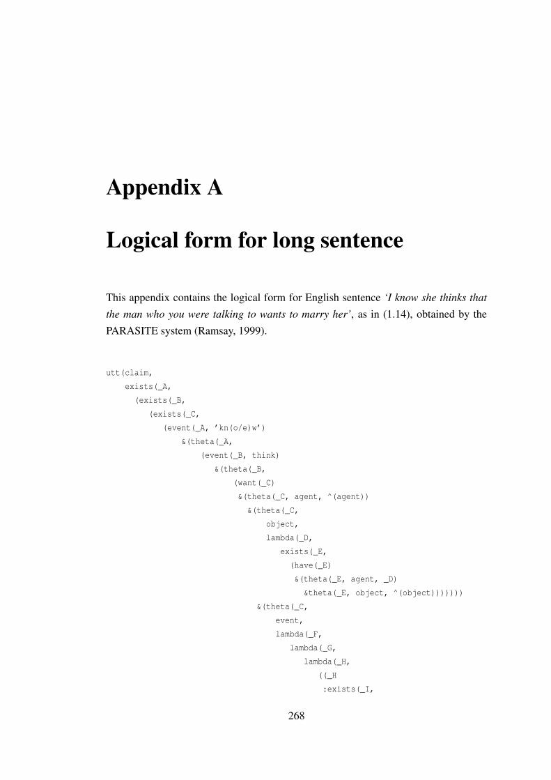
Appendix A
Logical form for long sentence
This appendix contains the logical form for English sentence ‘I know she thinks that
the man who you were talking to wants to marry her’, as in (1.14), obtained by thePARASITE system (Ramsay, 1999).
utt(claim,
exists(_A,
(exists(_B,
(exists(_C,
(event(_A, ’kn(o/e)w’)
&(theta(_A,
(event(_B, think)
&(theta(_B,
(want(_C)
&(theta(_C, agent, ^(agent))
&(theta(_C,
object,
lambda(_D,
exists(_E,
(have(_E)
&(theta(_E, agent, _D)
&theta(_E, object, ^(object)))))))
&(theta(_C,
event,
lambda(_F,
lambda(_G,
lambda(_H,
((_H
:exists(_I,
268

APPENDIX A. LOGICAL FORM FOR LONG SENTENCE 269
(event(_I,
marry)
&(theta(_I,
object,
(ref(lambda(_J,
centred(_J,
lambda(_K,
f(_K)))))
! 15))
&theta(_I,
agent,
_L)))))
: _F)))))
&theta(_C,
agent,
(ref(lambda(_M,
(sort(’m(a/e)n’, _M, _N, _O)
& exists(_P,
(event(_P, talk)
& (theta(_P,
agent,
(ref(lambda(_Q,
hearer(_Q)))
! 8))
& (to(_P, _M)
& aspect(ref(lambda(_R,
past(now,
_R))),
prog,
_P))))))))
! 5)))))))
& theta(_B,
agent,
(ref(lambda(_S, centred(_S,lambda(_T,f(_T)))))
! 2)))))
& (theta(_A, agent, ref(lambda(_U, speaker(_U)))!0)
& aspect(now, simple, _C)))))
& aspect(now, simple, _B)))
& aspect(now, simple, _A))))

Appendix B
Possible interpretations for shortsentence
This appendix contains an Arabic sentence with its dependency trees as parsed byPARASITE system.
20 interpretations of ’the student wrote a book’, arising from:
-- ktb could be kataba or kattaba
-- kataba could be intransitive or transitive
-- kattaba could be transitive or ditransitive
-- either of them could be active or passive
-- in every case, the subject could be 0, or AldArs, or ktb
-- ’AlDars ktb’ could be "the student’s book"
+ there’s one that means "the student’s book is a book", which comes from having
a zero copula.
The corresponding English sentence is unambiguous, whereas from a simple Arabic
sentence containing a verb and two nouns in canonical order we get 20 analyses.
| ?- in arabic. ktb AldArs ktb. ^
/**** DEPENDENCY TREE (1) ***************
.
--------------------------------------
kattaba (make write)
-----------------------------------
kutubN (book) AldArisoa (student)
****/
270
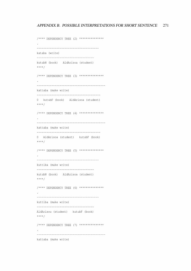
APPENDIX B. POSSIBLE INTERPRETATIONS FOR SHORT SENTENCE 271
/**** DEPENDENCY TREE (2) ***************
.
--------------------------------------
kataba (write)
-----------------------------------
kutubN (book) AldArisoa (student)
****/
/**** DEPENDENCY TREE (3) ***************
.
------------------------------------------
kattaba (make write)
---------------------------------------
0 kutubF (book) AldArisoa (student)
****/
/**** DEPENDENCY TREE (4) ***************
.
------------------------------------------
kattaba (make write)
---------------------------------------
0 AldArisoa (student) kutubF (book)
****/
/**** DEPENDENCY TREE (5) ***************
.
--------------------------------------
kuttiba (make write)
-----------------------------------
kutubN (book) AldArisoa (student)
****/
/**** DEPENDENCY TREE (6) ***************
.
--------------------------------------
kuttiba (make write)
-----------------------------------
AldArisou (student) kutubF (book)
****/
/**** DEPENDENCY TREE (7) ***************
.
------------------------------------------
kattaba (make write)

APPENDIX B. POSSIBLE INTERPRETATIONS FOR SHORT SENTENCE 272
---------------------------------------
0 kutubF (book) AldArisoa (student)
****/
/**** DEPENDENCY TREE (8) ***************
.
------------------------------------------
kattaba (make write)
---------------------------------------
0 AldArisoa (student) kutubF (book)
****/
/**** DEPENDENCY TREE (9) ***************
.
-----------------------------
kattaba (make write)
--------------------------
0 kutuba
-------------------
AldArisoi (student)
****/
/**** DEPENDENCY TREE (10) ***************
.
-----------------------------
kataba (write)
--------------------------
0 kutuba
-------------------
AldArisoi (student)
****/
/**** DEPENDENCY TREE (11) ***************
.
--------------------------------------
kattaba (make write)
-----------------------------------
AldArisou (student) kutubF (book)
****/
/**** DEPENDENCY TREE (12) ***************
.
--------------------------------------
kataba (write)

APPENDIX B. POSSIBLE INTERPRETATIONS FOR SHORT SENTENCE 273
-----------------------------------
AldArisou (student) kutubF (book)
****/
/**** DEPENDENCY TREE (13) ***************
.
-------------------------
kataba (write)
----------------------
kutubu
-------------------
AldArisoi (student)
****/
/**** DEPENDENCY TREE (14) ***************
.
-------------------------
kuttiba (make write)
----------------------
kutubu
-------------------
AldArisoi (student)
****/
/**** DEPENDENCY TREE (15) ***************
.
-------------------------
kutiba (write)
----------------------
kutubu
-------------------
AldArisoi (student)
****/
/**** DEPENDENCY TREE (16) ***************
.
-----------------------------
kuttiba (make write)
--------------------------
0 kutuba
-------------------
AldArisoi (student)
****/

APPENDIX B. POSSIBLE INTERPRETATIONS FOR SHORT SENTENCE 274
/**** DEPENDENCY TREE (17) ***************
.
-----------------------------------------
nomsent
--------------------------------------
kutubu kutubN (book)
-------------------
AldArisoi (student)
****/
/**** DEPENDENCY TREE (18) ***************
.
--------------------------------------
kattaba (make write)
-----------------------------------
AldArisou (student) kutubF (book)
****/
/**** DEPENDENCY TREE (19) ***************
.
--------------------------------------
kataba (write)
-----------------------------------
AldArisou (student) kutubF (book)
****/
/**** DEPENDENCY TREE (20) ***************
.
--------------------------------------
kuttiba (make write)
-----------------------------------
AldArisou (student) kutubF (book)
****/

Appendix C
CoNLL-X data file format
Data in the CoNLL file follows the following rules:
• Each sentence is separated by a blank line.
• A sentence consists of tokens, each token starting on a new line.
• A token is described by ten fields (see Table C.1).1 Fields are separated by a singletab character. Space/blank characters are not allowed within fields.
• The ID, FORM, CPOSTAG, POSTAG, HEAD and DEPREL fields are guaranteedto contain non-dummy (i.e. non-underscore) values for all languages.
• Sentences are UTF-8 encoded (Unicode).
For instance, Figure C.1 shows the dependency tree (according to Stanford parser)for the sentence ‘John eats happily.’ while its corresponding CoNLL format is shownin Figure C.2 .
1See http://ilk.uvt.nl/conll/#dataformat
275

APPENDIX C. CONLL-X DATA FILE FORMAT 276
# Field name Description1 ID Token counter, starting at 1 for each new sentence.2 FORM Word form or punctuation symbol.3 LEMMA Lemma or stem (depending on particular data set) of word form, or an under-
score if not available.4 CPOSTAG Coarse-grained POS tag, where tagset depends on the language.5 POSTAG Fine-grained POS tag, where the tagset depends on the language, or identical
to the coarse-grained part-of-speech tag if not available.6 FEATS Unordered set of syntactic and/or morphological features (depending on the
particular language), separated by a vertical bar (|), or an underscore if notavailable.
7 HEAD Head of the current token, which is either a value of ID or zero (‘0’). Note thatdepending on the original treebank annotation, there may be multiple tokenswith an ID of zero.
8 DEPREL Dependency relation to the HEAD. The set of dependency relations dependson the particular language. Note that depending on the original treebank anno-tation, the dependency relation may be meaningful or simply ‘ROOT’.
9 PHEAD Projective head of current token, which is either a value of ID or zero (‘0’), oran underscore if not available. Note that depending on the original treebankannotation, there may be multiple tokens an with ID of zero. The dependencystructure resulting from the PHEAD column is guaranteed to be projective (butis not available for all languages), whereas the structures resulting from theHEAD column will be non-projective for some sentences of some languages(but is always available).
10 PDEPREL Dependency relation to the PHEAD, or an underscore if not available. Theset of dependency relations depends on the particular language. Note that de-pending on the original treebank annotation, the dependency relation may bemeaningful or simply ‘ROOT’.
Table C.1: CoNLL-X data file format.
ROOT
eats(VBZ)
NSUBJ
John(NNP)
ADVMOD
happily(RB)
PX
.(PUNC)
Figure C.1: Dependency tree for the sentence ‘John eats happily.’
1 John _ NNP NNP _ 2 NSUBJ _ _2 eats _ VBZ VBZ _ 0 ROOT _ _3 happily _ RB RB _ 2 ADVMOD _ _4 . _ PUNC PUNC _ 2 PX _ _
Figure C.2: CoNLL format for the sentence ‘John eats happily.’

Appendix D
Analysis of the precision and recall
In this appendix, we will try to answer the following question: why do we get highprecision for string-based classifiers and high recall for syntactic-based ones?
In order to answer this question, suppose we have a population made up of Ysand Ns, where there are two sorts of Y: Ps, which can be identified on the basis ofsome feature P (P might, for instance, be ‘number of words in common’), and Qs,which cannot; and we have a classifier CP which can recognise Ps but cannot tell thedifference between Qs and Ns.
Now imagine that we have a population made up of p Ps and q Qs, and r Ns,and assume that p+ q and r are both 50. We can apply our classifier using a strategywhich says ‘Trust the classifier when it says yes, and for some proportion n of theremainder just make a 50:50 guess’. Varying values of n roughly correspond to varyingthresholds–if n is 0 then we are applying a very strict threshold, because we are saying‘Only say yes if you are absolutely sure’, whereas if n is 1 then we are saying ‘Say yes
if you think that there is any possibility that the thing you are looking at is a Y’.Under these conditions, CP (which can recognise Ps but nothing else) will say yes
p+n×0.5× (q+ r) times, and it will be right p+n×0.5×q times, out of a total ofp+q possible times; and it will say no (q+ r)(1−n×0.5) times, and it will be rightr×n×0.5 times. So its precision will be (p+n×0.5×q)/(p+n×0.5× (q+ r)), itsrecall will be (p+ n× 0.5× q)/(p+ q), and its accuracy will be (p+ n× 0.5× (q−r))/(p+q+ r).
How do precision, recall and accuracy behave as n varies? If p < 25, then themaximum value of F-score occurs when n is 1. If p > 25 then the maximum value ofF-score occurs when n is 0.
How does this apply to the data in Tables 7.1 and 7.2? Suppose that there is a set of
277

APPENDIX D. ANALYSIS OF THE PRECISION AND RECALL 278
T-H pairs which one of the string-based algorithms, e.g. bag-of-words, can accuratelymark as yes, but that this algorithm is completely unreliable outside this set. Then Pwould be the sentences that this algorithm could accurately mark as yes, Q would bethe other sentences that were in fact yes but that it could not identify, and N are all theno pairs. If P is quite small, i.e. less than half the total number of yes examples, thenthe value of n that gives the highest F-score overall is 1, as in Figure D.1.
0 0.1 0.2 0.3 0.4 0.5 0.6 0.7 0.8 0.9 10
0.1
0.2
0.3
0.4
0.5
0.6
0.7
0.8
0.9
1
How often do I just guess if the classifier says ‘no’
Valu
e
P
R
F1
A
0.6×F1+0.4×A
Figure D.1: Precision, recall and F-score for low coverage classifier (P=20).
Suppose, instead, that we were using a classifier which covered quite a large part ofthe yes set accurately. In that case the value of n that gives the highest F-score overallis 0, as in Figure D.2.
0 0.1 0.2 0.3 0.4 0.5 0.6 0.7 0.8 0.9 10.2
0.3
0.4
0.5
0.6
0.7
0.8
0.9
1
How often do I just guess if the classifier says ‘no’
Valu
e
P R F1 A 0.6×F
1+0.4×A
Figure D.2: Precision, recall and F-score for high coverage classifier (P=40).
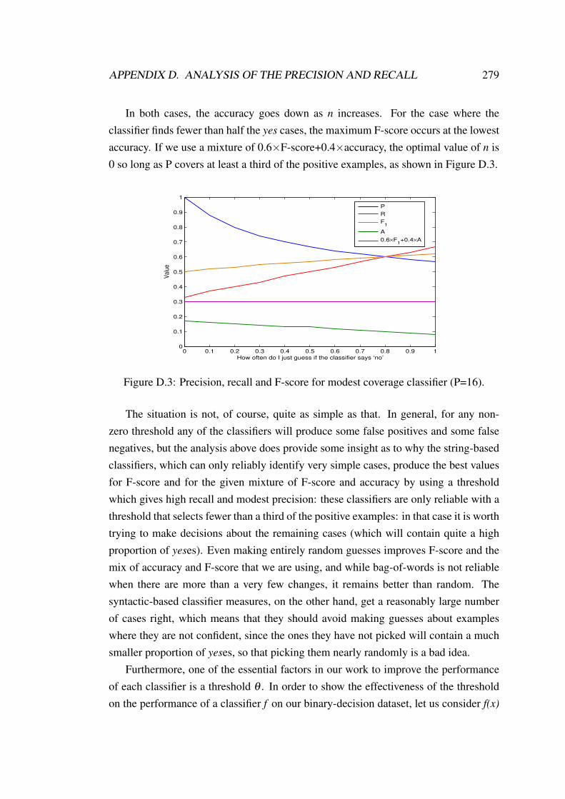
APPENDIX D. ANALYSIS OF THE PRECISION AND RECALL 279
In both cases, the accuracy goes down as n increases. For the case where theclassifier finds fewer than half the yes cases, the maximum F-score occurs at the lowestaccuracy. If we use a mixture of 0.6×F-score+0.4×accuracy, the optimal value of n is0 so long as P covers at least a third of the positive examples, as shown in Figure D.3.
0 0.1 0.2 0.3 0.4 0.5 0.6 0.7 0.8 0.9 10
0.1
0.2
0.3
0.4
0.5
0.6
0.7
0.8
0.9
1
How often do I just guess if the classifier says ‘no’
Val
ue
P
R
F1
A
0.6×F1+0.4×A
Figure D.3: Precision, recall and F-score for modest coverage classifier (P=16).
The situation is not, of course, quite as simple as that. In general, for any non-zero threshold any of the classifiers will produce some false positives and some falsenegatives, but the analysis above does provide some insight as to why the string-basedclassifiers, which can only reliably identify very simple cases, produce the best valuesfor F-score and for the given mixture of F-score and accuracy by using a thresholdwhich gives high recall and modest precision: these classifiers are only reliable with athreshold that selects fewer than a third of the positive examples: in that case it is worthtrying to make decisions about the remaining cases (which will contain quite a highproportion of yeses). Even making entirely random guesses improves F-score and themix of accuracy and F-score that we are using, and while bag-of-words is not reliablewhen there are more than a very few changes, it remains better than random. Thesyntactic-based classifier measures, on the other hand, get a reasonably large numberof cases right, which means that they should avoid making guesses about exampleswhere they are not confident, since the ones they have not picked will contain a muchsmaller proportion of yeses, so that picking them nearly randomly is a bad idea.
Furthermore, one of the essential factors in our work to improve the performanceof each classifier is a threshold θ . In order to show the effectiveness of the thresholdon the performance of a classifier f on our binary-decision dataset, let us consider f(x)

APPENDIX D. ANALYSIS OF THE PRECISION AND RECALL 280
is the output of f for an input x. According to the characteristics of our problem, x
will be a positive example if f (x)< θ for transformation-based classifiers (for bag-of-words, it should be f (x) > θ ) and a negative example otherwise. Thus, the scores ofprecision and recall of the classifiers depend on the choice of θ . Figure D.4 illustratesthe precision, recall and F-score for ZS-TED-based classifier for 43 different thresholds(from 44 to 128 incremented by 2), while the edit costs for ZS-TED are 2, 20 and 4 fordelete a node, insert a node and exchange a node, respectively.
44 48 52 56 60 64 68 72 76 80 84 88 92 96 100 104 108112 116 120 124 1280.1
0.2
0.3
0.4
0.5
0.6
0.7
0.8
0.9
1
Threshold
Valu
e
P
R
F1
Figure D.4: Effectiveness of the threshold on the performance of a classifier.
As you can see in Figure D.4, a lower threshold means higher precision, but usuallya lower recall, while better F-score is achieved when we have higher recall. Also, avery high threshold means a classifier saying the same thing every time (i.e. equal toour most common class baseline). At some point, the values of precision and recallare equal (when threshold equal to 70 in Figure D.4). This means that the number ofpairs classified to be positive is the same as the actual number of positive pairs in ourdataset. This value is known as precision-recall breakeven point (BEP).
Selecting a suitable measure of the quality of such a classifier is a tricky task, whichdepends on different factors such as the nature of the problem and the application. So,in our problem, the user of the classifier should choose a suitable threshold by takinginto account what sort of tradeoffs are available or preferable. For instance, if we desirea precision above the BEP, we must accept that our recall will be below the BEP, andvice versa, since we used the balanced F-score.

Appendix E
RTE2 results and systems
The following table illustrates the submission results and system description for RTE2.Systems for which no component is indicated used lexical overlap.
System Description
First Author (Group) Acc
urac
y
Aver
age
Prec
isio
n
Lex
ical
Rel
atio
nD
B
n-gr
am/S
ubse
quen
ceov
erla
p
Synt
actic
Mat
chin
g/A
lignm
ent
Sem
antic
Rol
eL
abel
ling/
Fram
Net
/Pro
pban
k
Log
ical
Infe
renc
e
Cor
pus/
Web
-Bas
edSt
atis
tics
ML
Cla
ssifi
catio
n
Para
phra
seTe
mpl
ates
/Bac
kgro
und
Kno
wle
dge
Acq
uisi
tion
ofE
ntai
lmen
tCor
pora
Adams (Dallas) 0.6262 0.6282 X X X
Bos (Rome & Leeds)0.6162 0.6689 X X X0.6062 0.6042 X X X X X
Burchart (Saarland)0.5900 X X0.5775 X X X X
Clarke (Sussex)0.5275 0.5254 X X0.5475 0.5260 X
de Marneffe (Stanford)0.5763 0.6131 X X X X X0.6050 0.5800 X X X X X
Delmonte (Venice) 0.5475 0.5495 X X X X
Ferrández (Alicante)0.5563 0.6089 X X X0.5475 0.5743 X X
281
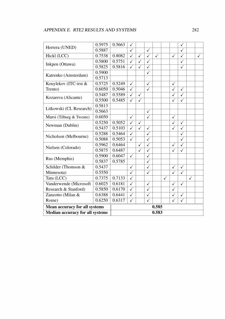
APPENDIX E. RTE2 RESULTS AND SYSTEMS 282
Herrera (UNED)0.5975 0.5663 X X0.5887 X X X
Hickl (LCC) 0.7538 0.8082 X X X X X X X
Inkpen (Ottawa)0.5800 0.5751 X X X X0.5825 0.5816 X X X X
Katrenko (Amsterdam)0.5900 X0.5713
Kouylekov (ITC-irst & 0.5725 0.5249 X X XTrento) 0.6050 0.5046 X X X X
Kozareva (Alicante)0.5487 0.5589 X X X X0.5500 0.5485 X X X X
Litkowski (CL Research)0.58130.5663 X
Marsi (Tilburg & Twente) 0.6050 X X X
Newman (Dublin)0.5250 0.5052 X X X X0.5437 0.5103 X X X X X
Nicholson (Melbourne)0.5288 0.5464 X X X0.5088 0.5053 X X X
Nielsen (Colorado)0.5962 0.6464 X X X X0.5875 0.6487 X X X X
Rus (Memphis)0.5900 0.6047 X X0.5837 0.5785 X
Schilder (Thomson & 0.5437 X X X XMinnesota) 0.5550 X X X XTatu (LCC) 0.7375 0.7133 X X XVanderwende (Microsoft 0.6025 0.6181 X X X XResearch & Stanford) 0.5850 0.6170 X X XZanzotto (Milan & 0.6388 0.6441 X X X XRome) 0.6250 0.6317 X X X X
Mean accuracy for all systems 0.585Median accuracy for all systems 0.583