Text Formatting with L A T E X Table of Contents Creating A L A T E X Document 7 2.1 Document...

Text Formatting with LATEX

A Tutorial

Academic and Research Computing, April 2007

Table of Contents

1. LATEX Basics 11.1 What is TEX? . . . . . . . . . . . . . . . . . . . . . . . . . . . . . . . . . 11.2 What is LATEX? . . . . . . . . . . . . . . . . . . . . . . . . . . . . . . . . 11.3 How LATEX Works . . . . . . . . . . . . . . . . . . . . . . . . . . . . . . . 21.4 The LATEX Input File . . . . . . . . . . . . . . . . . . . . . . . . . . . . . 2

1.4.1 Entering LATEX Commands . . . . . . . . . . . . . . . . . . . . . . 21.4.2 Entering Text . . . . . . . . . . . . . . . . . . . . . . . . . . . . . 31.4.3 Special Characters . . . . . . . . . . . . . . . . . . . . . . . . . . 41.4.4 Structure of the Input File . . . . . . . . . . . . . . . . . . . . . . 4

1.5 Some LATEX Vocabulary . . . . . . . . . . . . . . . . . . . . . . . . . . . 5

2. Creating A LATEX Document 72.1 Document Classes . . . . . . . . . . . . . . . . . . . . . . . . . . . . . . . 72.2 Class Options . . . . . . . . . . . . . . . . . . . . . . . . . . . . . . . . . 72.3 Packages . . . . . . . . . . . . . . . . . . . . . . . . . . . . . . . . . . . . 82.4 Making a Title Page . . . . . . . . . . . . . . . . . . . . . . . . . . . . . 92.5 Making a Table of Contents . . . . . . . . . . . . . . . . . . . . . . . . . 92.6 Behind the Scenes . . . . . . . . . . . . . . . . . . . . . . . . . . . . . . . 10

2.6.1 Auxiliary Files . . . . . . . . . . . . . . . . . . . . . . . . . . . . 102.6.2 How a Page is Built . . . . . . . . . . . . . . . . . . . . . . . . . . 10

2.7 Example: Report Class . . . . . . . . . . . . . . . . . . . . . . . . . . . . 112.8 Example: Letter Class . . . . . . . . . . . . . . . . . . . . . . . . . . . . 12

3. Document Layout 133.1 Line Spacing . . . . . . . . . . . . . . . . . . . . . . . . . . . . . . . . . . 133.2 Paragraphs . . . . . . . . . . . . . . . . . . . . . . . . . . . . . . . . . . 133.3 Text Justification . . . . . . . . . . . . . . . . . . . . . . . . . . . . . . . 143.4 Margins . . . . . . . . . . . . . . . . . . . . . . . . . . . . . . . . . . . . 143.5 Headers, Footers, and Page Numbering . . . . . . . . . . . . . . . . . . . 15

ii ♦ Contents

4. Within the Text 164.1 Section Headings . . . . . . . . . . . . . . . . . . . . . . . . . . . . . . . 164.2 Changing Type Style and Size . . . . . . . . . . . . . . . . . . . . . . . . 174.3 Starting New Lines and New Pages . . . . . . . . . . . . . . . . . . . . . 184.4 Leaving Horizontal and Vertical Space . . . . . . . . . . . . . . . . . . . 184.5 Drawing Rules . . . . . . . . . . . . . . . . . . . . . . . . . . . . . . . . . 184.6 Footnotes . . . . . . . . . . . . . . . . . . . . . . . . . . . . . . . . . . . 194.7 Centering . . . . . . . . . . . . . . . . . . . . . . . . . . . . . . . . . . . 194.8 Quotations . . . . . . . . . . . . . . . . . . . . . . . . . . . . . . . . . . . 194.9 Reproducing Text As-Is . . . . . . . . . . . . . . . . . . . . . . . . . . . 204.10 Lists . . . . . . . . . . . . . . . . . . . . . . . . . . . . . . . . . . . . . . 214.11 Cross References . . . . . . . . . . . . . . . . . . . . . . . . . . . . . . . 22

5. Tabular Material 235.1 Tabbing . . . . . . . . . . . . . . . . . . . . . . . . . . . . . . . . . . . . 235.2 Tabular . . . . . . . . . . . . . . . . . . . . . . . . . . . . . . . . . . . . 24

5.2.1 A Simple Ruled Table . . . . . . . . . . . . . . . . . . . . . . . . 255.2.2 Using Paragraph Columns, Spanning Columns . . . . . . . . . . . 265.2.3 Aligning on the Decimal Point . . . . . . . . . . . . . . . . . . . . 275.2.4 Suppressing Leading or Trailing Space . . . . . . . . . . . . . . . 27

6. Mathematics 286.1 In-line Math . . . . . . . . . . . . . . . . . . . . . . . . . . . . . . . . . . 286.2 Display Math (for unnumbered equations) . . . . . . . . . . . . . . . . . 296.3 Equation Environment (for numbered equations) . . . . . . . . . . . . . . 296.4 Eqnarray Environment (for multiline equations) . . . . . . . . . . . . . . 306.5 Array Environment (for matrices, etc.) . . . . . . . . . . . . . . . . . . . 316.6 Building Mathematical Expressions . . . . . . . . . . . . . . . . . . . . . 32

6.6.1 Superscripts and Subscripts . . . . . . . . . . . . . . . . . . . . . 326.6.2 Spaces in Math Mode . . . . . . . . . . . . . . . . . . . . . . . . . 326.6.3 Dots, Braces, and Bars . . . . . . . . . . . . . . . . . . . . . . . . 326.6.4 Fractions . . . . . . . . . . . . . . . . . . . . . . . . . . . . . . . . 336.6.5 Radicals, Integrals, and Summations . . . . . . . . . . . . . . . . 336.6.6 Large Delimiters . . . . . . . . . . . . . . . . . . . . . . . . . . . 34

7. Including Graphics 357.1 Creating the Graphics File . . . . . . . . . . . . . . . . . . . . . . . . . . 357.2 Importing the Graphic into your LATEX Document . . . . . . . . . . . . . 357.3 Viewing the Output . . . . . . . . . . . . . . . . . . . . . . . . . . . . . . 36

8. Placing Figures & Tables (Floats) 378.1 Making a Caption . . . . . . . . . . . . . . . . . . . . . . . . . . . . . . . 378.2 Examples . . . . . . . . . . . . . . . . . . . . . . . . . . . . . . . . . . . 388.3 Overcoming Problems with Float Placement . . . . . . . . . . . . . . . . 408.4 Landscape Figures and Tables . . . . . . . . . . . . . . . . . . . . . . . . 40

April 2007

Contents ♦ iii

9. Preparing a Bibliography 419.1 Using LATEX’s built-in Method . . . . . . . . . . . . . . . . . . . . . . . . 419.2 Using BibTEX . . . . . . . . . . . . . . . . . . . . . . . . . . . . . . . . . 42

9.2.1 Overview . . . . . . . . . . . . . . . . . . . . . . . . . . . . . . . 429.2.2 Creating the .bib File . . . . . . . . . . . . . . . . . . . . . . . . 439.2.3 Running BibTEX . . . . . . . . . . . . . . . . . . . . . . . . . . . 439.2.4 Bibliography Styles . . . . . . . . . . . . . . . . . . . . . . . . . . 449.2.5 For More Information . . . . . . . . . . . . . . . . . . . . . . . . . 45

10.Special Topics 4610.1 Managing a Large Document . . . . . . . . . . . . . . . . . . . . . . . . . 4610.2 Generating an Index . . . . . . . . . . . . . . . . . . . . . . . . . . . . . 4610.3 Including hyperlinks . . . . . . . . . . . . . . . . . . . . . . . . . . . . . 4710.4 Accents and Special Characters . . . . . . . . . . . . . . . . . . . . . . . 49

Appendix A: Mathematical Symbols 50

Appendix B: Error Messages 53

Resources 55General Information on LATEX . . . . . . . . . . . . . . . . . . . . . . . . . . . 55LATEX packages . . . . . . . . . . . . . . . . . . . . . . . . . . . . . . . . . . . 55LATEX Thesis . . . . . . . . . . . . . . . . . . . . . . . . . . . . . . . . . . . . 55Mathematical Expressions . . . . . . . . . . . . . . . . . . . . . . . . . . . . . 56Symbols . . . . . . . . . . . . . . . . . . . . . . . . . . . . . . . . . . . . . . . 56Graphics . . . . . . . . . . . . . . . . . . . . . . . . . . . . . . . . . . . . . . . 56BibTEX . . . . . . . . . . . . . . . . . . . . . . . . . . . . . . . . . . . . . . . 57Installing LATEX . . . . . . . . . . . . . . . . . . . . . . . . . . . . . . . . . . . 57

Academic and Research Computing, RPI

Text Formatting with LATEX

This document describes the LATEX language. For specifics of how to runit on various platforms (e.g., Windows or unix), see the LATEX Informationpage (http://www.rpi.edu/dept/arc/training/latex/), and follow thelinks for the on-line tutorials. The above web page also contains informationon preparing a thesis or a resume, as well as many examples and links toother helpful information.

Chapter 1. LATEX Basics

1.1 What is TEX?

• TEX is the typesetting language upon which LATEX is built. It was designed andwritten by Donald Knuth especially for math and science. TEX is pronounced“Tech,” similar to “Bach.”

• TEX is portable. It is available for most computers and is used all over the world.TEX documents can be moved easily from one system to another, as long as therequired fonts are on both systems.

• TEX comes with its own set of fonts, called “Computer Modern,” used by default.These fonts exist in a variety of styles, including serif, sans serif, typewriter (fixedpitch), and an extensive set of mathematical symbols. It’s also possible to useother font families, such as Times, Palatino, etc.

• TEX is also a programming language, making it possible to create commands thatsimplify its use.

1.2 What is LATEX?

• LATEX is a TEX macro package, originally written by Leslie Lamport, that simplifiesthe use of TEX. All the above features of TEX, including portability, also apply toLATEX. LATEX is pronounced either “Lay-tech” or “Lah-tech.”

• Most LATEX commands are “high-level” (such as chapter and section) and specifythe logical structure of a document. The author rarely needs to be concerned withthe details of document layout, concentrating instead on the content. Most plainTEX commands also work with LATEX.

• The document class determines how the document will be formatted. LATEX pro-vides several standard document classes from which to choose.

• LATEX is flexible, gives you complete control, handles big, complex documents withease, and never crashes or corrupts your files.

1

http://www.rpi.edu/dept/arc/training/latex/

2 ♦ Chapter 1. LATEX Basics

1.3 How LATEX Works

To use LATEX, you first create a plain ASCII text file with any text editor. In this fileyou type both the text of your document and the LATEX commands to format it. Youthen typeset your document, usually by clicking a button on a toolbar or selecting amenu item. Nowadays there are two routes for processing a LATEX document:

• The traditional way is to run the latex program, which creates a DVI (DeviceIndependent) file. This file is in binary format and not viewed directly. Youthen run a previewing program for viewing on screen and/or the dvips programto create a PostScript file for viewing or for printing via the ghostview/GSViewprogram. GSView can also convert the document to PDF format.

• Alternatively you can run the relatively recent pdflatex program to create a PDFfile for viewing or printing, usually with Adobe’s Acrobat Reader.

The second method is more direct for PDF output, but the first is quicker and moreconvenient for previewing.

1.4 The LATEX Input File

LATEX input files have names that end with the extension .tex: for example, an accept-able file name might be myfile.tex. (Never use spaces in file names.) The input filecontains both the text of your document and the LATEX commands needed to format it.The first command in the file, \documentclass, defines the style of the document.

1.4.1 Entering LATEX Commands

To distinguish them from text, all LATEX commands (also called control sequences) startwith a backslash “\”. A command name consists of letters only and is ended by a spaceor a non letter (such as a comma, period, brace, etc). If it ends with a space, the spaceis “consumed” by LATEX and does not appear in the output. An example is \today,which prints the current date. To avoid having the space after the command disappear,do the following:\today\ is a good day. produces: April 16, 2007 is a good day.

There are also commands that consist of the backslash followed by exactly one non-letter. They are most often used to put a special symbol in the text. For example \$

prints a $ (which cannot be entered directly because LATEX uses it to begin math mode).Spaces after these control symbols are not consumed.

LATEX commands are case-sensitive. Most are all lowercase. A few commands use thefirst letter in uppercase such as \Delta → ∆. Fewer still use all uppercase.

April 2007

1.4 The LATEX Input File ♦ 3

Some commands take an “argument,” placed within curly braces after the commandname. For example, \textbfthis text is bold prints the text inside the braces inboldface type: this text is bold

LATEX uses grouping to limit the effect of certain commands. Braces ... are used tobegin and end groups. (An environment is also a group; see page 5.) For example, the\large command is usually used inside a group:\large this is bigger than normal produces: this is bigger than normalA command such as \large is called a “declaration” because, unless it is given withina group, its effect will continue until another declaration (in this case \normalsize)counteracts it. Note the difference between a declaration used inside a group and acommand like \textbf..., which will not work unless an argument is provided insidea pair of braces following the command name.

The symbol % can be used to put a comment in your input file. When LATEX sees a %, itignores the rest of the line.

When you use commands that specify a length, such as a command to set the size of amargin or a command to leave a certain amount of space, you will need to specify theunits of measurement. LATEX recognizes the following units:

cm centimeter pt printer’s point, ≈ 72 per inchmm millimeter em font-dependent width of “m”in inch ex font-dependent height of “x”

1.4.2 Entering Text

In the input file, words are separated by leaving one or more blank spaces. Paragraphsare separated by leaving one or more blank lines. (You can also use the command \par

to indicate a new paragraph.) LATEX ignores multiple blank spaces and multiple blanklines in input files.

Type single quotation marks by using the left (‘) and right (’) single quote marks onyour keyboard. Type left double quotation marks by using using two single left quotes(‘‘), and type right double quotation marks by using either two single right quotes (’’)or the double quote key (").

There are three kinds of dashes in typeset documents: the hyphen (for compound words),the endash (for such things as page number ranges), and the emdash (used as a punc-tuation mark in English prose). Since there is only one dash on the keyboard, type -,--, and --- to get -, –, and — .

To prevent two words from being split at a line break, tie them together with the tildecharacter: for example Mr.~Smith will never appear with “Mr.” at the end of one lineand “Smith” at the start of the next.

Note that some characters have special meaning to LATEX and must be entered in aspecial way, as described in the next section.



1.4.3 Special Characters

Certain characters have special meaning to LATEX. An example is the % sign, whichindicates that the remainder of the line is a comment and should not be processed.Below is the complete list of special characters. To have these characters print in youroutput, you must type them in your input file as shown below.

Character Type in file Special LATEX meaning# \# Parameter in a macro; also used in tables$ \$ Used to begin and end math mode% \% Used for comments in the source file& \& Tab mark, used in alignments

\ Used in math mode for subscriptsˆ \ˆ Used in math mode for superscripts˜ \˜ Tie character, used to produce a “hard” space \ Used to begin a group or an argument \ Used to end a group or an argument\ $\backslash$ Used to begin a control sequence< $<$ (or \textless) Otherwise, produces ¡> $>$ (or \textgreater) Otherwise, produces ¿

1.4.4 Structure of the Input File

LATEX input files must conform to a certain structure. They begin with the command\documentclass, and all the text of the document must be contained between thecommands \begindocument and \enddocument.

\documentclass[options]class

Preamble

\begindocument

Document text

\enddocument

In the first command above, class specifies the type of document you intend to create.You can choose from one of the LATEX classes described in the next chapter. If you wish,you can also include one or more options to modify the behavior of the document class.

The preamble is the section of the file between the \documentclass... command andthe \begindocument command. This is the place to put commands that will influencethe style of your entire document and macro definitions that you will use later. You mayalso load packages that add new features to LATEX. Text is not allowed in the preamble.

April 2007

1.5 Some LATEX Vocabulary ♦ 5

The \begindocument command indicates the end of the preamble and the beginningof your text. A corresponding \enddocument command always ends your files. Areally short LATEX input file might look like:

\documentclassarticle

\begindocument

This LaTeX file is short and sweet. It uses the article class,

a good all-purpose layout. There is nothing in the preamble, which

is perfectly acceptable.

This is a new paragraph. \textitHere’s some italic text

and \textbfsome bold text.

\small The text inside these braces is smaller than normal.

Now the text size is back to normal.

\enddocument

this produces:

This LaTeX file is short and sweet. It uses the article class, a good all-purpose layout.There is nothing in the preamble, which is perfectly acceptable.

This is a new paragraph. Here’s some italic text and some bold text. The text insidethese braces is smaller than normal. Now the text size is back to normal.

Longer examples, one using report class and one using letter class are included at theend of the next chapter.

1.5 Some LATEX Vocabulary

Commands produce text or space. For example, \hspace2in and \vspace2in arecommands that create 2 inches of horizontal and vertical space, respectively, and\textitsome italic words puts the contents of its argument in italic type.Many commands take arguments, either mandatory or optional; some commands,like \today don’t.

Mandatory arguments supply information required for a command to execute. Forexample, \hspace2in needs the information provided by the argument to gen-erate the horizontal space. Mandatory arguments are enclosed in braces: .

Optional arguments are allowed on some commands and are enclosed in square brack-ets: [ ]. For example, the size of type to be used for your main text is an optionalargument in the \documentclass command. To use the article class in 11-pointtype, you would type \documentclass[11pt]article. Without this optionalargument, you would get the default 10-point type.



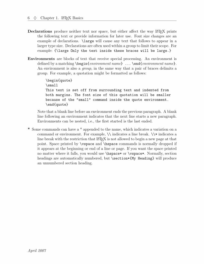
Declarations produce neither text nor space, but either affect the way LATEX printsthe following text or provide information for later use. Font size changes are anexample of declarations. \large will cause any text that follows to appear in alarger type size. Declarations are often used within a group to limit their scope. Forexample: \large Only the text inside these braces will be large.

Environments are blocks of text that receive special processing. An environment isdefined by a matching \beginenvironment name ... \endenvironment name.An environment is also a group, in the same way that a pair of braces delimits agroup. For example, a quotation might be formatted as follows:

\beginquote

\small

This text is set off from surrounding text and indented from

both margins. The font size of this quotation will be smaller

because of the "small" command inside the quote environment.

\endquote

Note that a blank line before an environment ends the previous paragraph. A blankline following an environment indicates that the next line starts a new paragraph.Environments can be nested, i.e., the first started is the last ended.

* Some commands can have a * appended to the name, which indicates a variation on acommand or environment. For example, \\ indicates a line break. \\* indicates aline break with the restriction that LATEX is not allowed to begin a new page at thatpoint. Space printed by \vspace and \hspace commands is normally dropped ifit appears at the beginning or end of a line or page. If you want the space printedno matter where it falls, you would use \hspace* or \vspace*. Normally, sectionheadings are automatically numbered, but \section*My Heading will producean unnumbered section heading.

April 2007

Chapter 2. Creating A LATEX Document

2.1 Document Classes

The document class determines the overall layout of the document. There are fivestandard classes distributed with LATEX:

article for simple or short documents, including journal articles, and short reports. Agood all-purpose class.

report for small books and longer reports containing chapters.

book for books.

letter for letters, either business or personal.

slides for making transparencies for projection on a screen.

These classes provide preset formats with default margins, paragraph formatting, andspecial commands suitable for producing specific sections. For example, the article,report, and book classes include a variety of commands to format section headings(\part, \chapter, \section, \subsection, \subsubsection, etc.), as well as com-mands to produce a title page and a table of contents. There are minor differencesbetween these three classes. The book class, for example, uses a smaller printed pagesize—about 5×7.5 inches—and is formatted for two-sided printing by default. Thearticle class is intended for shorter works and does not have chapters (so articles canbe easily included in reports or books). The letter class provides special commands toproduce the salutation, address, and closing.

These four classes are single-spaced by default, and have 10, 11, and 12-point type sizesavailable as options. 10 points is the default size.

The slides class uses sans-serif type fonts much larger than the usual ones and expectsthe document to be divided up into 1-page sections.

At Rensselaer, there is an additional class called thesis, which may be used to produceeither a master’s or a doctoral thesis with a format that meets the requirements of theOffice of Graduate Education. It was written by Academic and Research Computing(ARC) using the report class as a base. The file thesis.cls is available for downloadfrom the thesis web page, http://helpdesk.rpi.edu/update.do?artcenterkey=325.To use the thesis class, begin your document with the line:

\documentclassthesisInstructions are in ARC document, Preparing A Thesis with LATEX, available from thethesis web page.

2.2 Class Options

A document class may be modified by options, which are placed in square brackets afterthe \documentclass command. Multiple options are separated by commas:

\documentclass[option,option,option ]class

7

http://helpdesk.rpi.edu/update.do?artcenterkey=325

8 ♦ Chapter 2. Creating A LATEX Document

The standard class options include:

10pt, 11pt, 12pt Selects the point size of main font for the document. If no option isspecified, 10pt is assumed. This document uses 12-point type.

twocolumn Produces two-column pages.

titlepage Causes the \maketitle command to generate the title page on a separatepage for the article class. This option is not necessary for the book and report

classes, as they print separate title pages by default.

leqno Puts equation numbers on left side. (They are on the right by default.)

fleqn Left-aligns equations. (They are centered by default.)

twoside Formats for printing on both sides of paper. (Whether the document is actuallyprinted two-sided depends on the printer.) Twoside is the default for the book class,but not for any of the other classes.

openright If the twoside option is in effect, chapters will begin on right hand pages.This is the default for the book class. It does not apply to the article class,which does not contain chapters. (The opposite of openright is openany.)

2.3 Packages

There are a large number of LATEX packages available that provide a variety of additionalfeatures. Many packages are considered part of LATEX; others are provided by expertusers worldwide. If you sometimes find that the features of standard LATEX do notprovide the special formatting you want, chances are good that you can find a packageto meet your needs. A package generally consists of one or more files that contain extradefinitions and macros. Some packages are simple; others are complex and can containoptions. The file names usually have the extension .sty.

You load a package with the \usepackage command, which should come immediatelyafter the \documentclass command in your input file. The command has the form:

\usepackage[options ]package Each package may be included with its own \usepackage command, or you may useone command to load several packages by separating their names with commas. Forexample, if you are inserting graphics in your document (see chapter 7.), the packagegraphicx provides the commands to do this. The beginning of your input file mightlook like:

\documentclass[11pt]article

\usepackagegraphicx

The \usepackage command above instructs LATEX to read the file graphicx.sty.

April 2007

2.4 Making a Title Page ♦ 9

In addition to graphicx there are many other packages available, including packages torotate text, use PostScript fonts (e.g., Times, Palatino, etc), and customize such thingsas headers and footers, citations and captions. Packages come with their own documen-tation. Many packages are routinely distributed with LATEX and will already be on yoursystem. You’ll find documentation for these packages in the doc subdirectory of yourinstallation. For example, if you are using the TeXLive 2005 distribution for Windows,package documentation is in folders under C:\TeXLive2005\texmf-dist\doc\latex\.

To see a current list of all available packages with brief descriptions, look at the Com-prehensive TeX Archive Network (CTAN) catalog,http://texcatalogue.sarovar.org/brief.html.

2.4 Making a Title Page

If you are using the article, report, or book class, you may want a title page for yourdocument. To do this, you need to supply text for the title, author, and date, and thentell LATEX to generate the title page with the command \maketitle. In your LATEXinput file, type commands such as the ones below. The \maketitle command, whichactually prints the title page, must follow the \begindocument command; the othercommands, which just provide the information, can be placed in the preamble if youprefer.

\titleThis is the Title % provide title info

\authorMy Name % provide author info

\datethe date % provide date

\maketitle % format and print title page

This is illustrated in the example of using the report class later in this chapter. If thereare several authors, you can separate their names with \and, or you can separate themwith \\ if you would like each name centered on a separate line. If you omit the \date

command, LATEX will use the current date. If you want no date at all, use \date.

In the report and book classes, the title information appears on its own page. In thearticle class, it appears at the top of the first page of text. You can instruct thearticle class to make a separate page by using the documentclass option titlepage.

2.5 Making a Table of Contents

The command \tableofcontents, usually placed in the input file right after the\maketitle command, creates a table of contents using the information in the sec-tion headings (part, chapter, section, etc.). Since this information is taken from theprevious run, you will need to run LATEX twice on a new document for the entries in thetable of contents to show up.


http://texcatalogue.sarovar.org/brief.html


2.6 Behind the Scenes

2.6.1 Auxiliary Files

Part of the convenience of LATEX is its ability to do cross references (see section 4.11)and to create a table of contents, a list of tables, and a list of figures.

Forward reference numbers, as well as page numbers for sections, figures and tables, areunknown when LATEX is first processing the input file. LATEX stores this informationin auxiliary files as it processes the job. A second run allows LATEX to extract theinformation from its auxiliary files and complete the table of contents, etc. Therefore allinformation used by LATEX for tables of contents, etc. is from the previous run. The onlyway to be sure that all this material is correct is to format the file twice after makingany changes. Usually for drafts, the difference between runs is not enough to matter,but for final versions you should remember to run LATEX twice before printing.

The auxiliary files have the same “root” name as the LATEX input file, but differentextensions. For example, all documents need an AUX file. If the input file is namedmyfile.tex, the AUX file will be named myfile.aux. Other auxiliary files (see the listbelow) are needed only if you are producing a table of contents, etc. Auxiliary files arecreated automatically as they are needed.

filename.aux always neededfilename.toc for table of contentsfilename.lot for list of tablesfilename.lof for list of figures

2.6.2 How a Page is Built

When TEX or LATEX builds a page, it considers all the parts (words, lines, paragraphs,etc.) to be different sized boxes. It starts with a simple box, an individual letter, andthen builds words, which are considered to be hboxes (horizontal boxes). The wordsare then put together with glue to form a line, which is a larger hbox. A group ofhboxes stacked together vertically (with glue between them) form a vbox (vertical box).A page is a large vbox made up of several smaller ones. You do not normally need to beconcerned with this, but sometimes (such as when an error message refers to an “overfullhbox,” meaning a line is too long and sticks out into the margin) it is helpful to knowhow TEX works.

April 2007

2.7 Example: Report Class ♦ 11

2.7 Example: Report Class

\documentclass[11pt]report % Report class in 11 points

\raggedright % Do not right-justify

\parindent0pt \parskip8pt % make block paragraphs

\begindocument % End of preamble, start of

% document text.

\title\bf An Example of Report Class % Supply information

\authorYours Truly % for the title page.

\date\today % Use current date.

\maketitle % Print title page.

\pagenumberingroman % Roman page number for toc

\setcounterpage2 % Make it start with "ii"

\tableofcontents % Print table of contents

\chapterA Main Heading % Make a "chapter" heading

\pagenumberingarabic % Start text with arabic 1

Most of this example applies to the article and book classes

as well as to the report class. In article class, however,

the default position for the title information is at the top

of the first text page rather than on a separate page. Also, article

class does not have a ‘‘chapter" command.

A blank line starts a new paragraph. \textitNote this: it will be

printed in italic type.

\sectionA Subheading % Make a "section" heading

The following sectioning commands are available:

\beginquote % Start "set off", indented text

part \\ % "\\" forces a new line

chapter \\ % not available in article class

section \\

subsection \\

subsubsection \\

paragraph \\

subparagraph

\endquote % End of indented text

The *-form (e.g., ‘‘section*") suppresses the section number and

does not make a TOC entry.

\enddocument % The required last line



2.8 Example: Letter Class

\documentclass[12pt]letter % letter class, 12 points

\address555 Main St.\\Sometown, NY 12345 % Return address

\signatureMy Name\\My Title % Name for signature

\begindocument % End of preamble

\beginletterMr.~Smith\\ President, % Begin letter by giving

Big Name Co.\\Bigburg, MI 45678 % recipient’s address

\openingDear Mr.~Smith: % Name for salutation

This is the letter class. It provides a format for standard parts

of a business letter. As you can see, it uses many commands that

do not exist in the article, report, and book classes.

This is a new paragraph.

\closingSincerely, % Format for the closing.

% The name is taken from

% \signature command above.

\ccMy Boss % Name(s) of those

% receiving copies

\endletter % End of letter

\enddocument % The required last line

April 2007

Chapter 3. Document Layout

Defaults for all aspects of the document layout are set by the document classes. However,if you want to change the defaults, there are commands that enable you to do so.Commands controlling features that apply to the whole document should be placed inthe preamble1.

3.1 Line Spacing

The default is single spacing. If you want larger interline spacing for your document, youcan use the \linespread command in the preamble. The following command producesa document with double spacing:

\linespread1.6

For “line and a half” spacing, use the value 1.3. The default spread is 1.

An alternative and more flexible way to control the linespacing is to use the packagesetspace. With this package, footnotes, figures, and tables remain single-spaced. Thepackage also defines a new environment called singlespace, which you can use to includesingle-spaced sections within your document. To use the setspace package to producea double-spaced document, include after the \documentclass command:

\usepackagesetspace

and, in addition, put the command

\doublespacing

somewhere in the preamble.

You could use \onehalfspacing instead of \doublespacing, or you could use the com-mand \setstretchn (specifying your own value for n—usually between 1 and 2) toset the spacing to whatever you want.

3.2 Paragraphs

To start a new paragraph, either leave a blank line or use the control sequence \par.By default, paragraphs are indented by 1.5em, which means 1.5 times the point sizeof the current font. (1 em is about the width of an “M”.) No extra blank spaceis inserted between paragraphs. The commands \parindent and \parskip controlparagraph indentation and paragraph separation. To get block paragraphs, for example,include in the preamble the commands:

\parindent=0in

\parskip=8pt % this is variable, choose the number you want

1the section between the \documentclass command and the \begindocument command

13

14 ♦ Chapter 3. Document Layout

3.3 Text Justification

By default, LATEX justifies your text horizontally so that both left and right margins aresmooth. If you prefer “ragged right” text, you can use the declaration:

\raggedright

Note that this has the side-effect of wiping out the paragraph indentation. (It assumesyou want everything flush left.) If you want indented paragraphs, you must specificallyrequest it (i.e., \parindent=1.5em) after the \raggedright declaration.

Vertical justification is controlled by using either \flushbottom or \raggedbottom.\flushbottom makes all text pages the same height, adding extra vertical space if nec-essary. \raggedbottom allows the height to vary a bit from page to page. \flushbottomis the default for the book class and for the twoside option in the article and reportclasses; otherwise \raggedbottom is the default.

3.4 Margins

Changing default margins, which depend on the class and the font size, is not as easyas you might think. The best way to control margins is to use the geometry package.This package has many options and extensive documentation in manual.pdf found inyour directory ...\doc\latex\geometry\. The following examples should be obvious:

\usepackage[margin=1in]geometry % 1 inch margins all around

\usepackage[left=1.2in,right=1in,top=1in,bottom=.8in]geometry

If you really want to do it manually, you need to know that internally top and left marginsare set in reference to a value of one inch (which means that setting these margins equalto 0 produces one-inch margins). Therefore, setting topmargin to -.5in produces a topmargin of .5 inches. The opposite margins (bottom and right) are determined indirectlyby setting the height (textheight) and width (textwidth) of the text area.

to set margin change the commandtop margin \topmargin

bottom margin \textheight

left margin (for odd pages or single sided) \oddsidemargin

left margin (for even pages, if using twoside) \evensidemargin

right margin \textwidth

LATEX also leaves .5 inch at the top of the page for a header and about .6 inch at thebottom of the page for a footer. You must take this into account when choosing valuesfor topmargin and textheight. The values below leave one inch between the paperedge and the text on all four sides.

\setlength\topmargin-.5in % top margin is .5 in

\setlength\oddsidemargin0in % left margin is 1 in on right pages

\setlength\evensidemargin0in % same for left pages, 2-sided document

\setlength\textwidth6.5in % leaves 1 in for right margin

\setlength\textheight9in % 9 inches reserved for the text

April 2007

3.5 Headers, Footers, and Page Numbering ♦ 15

3.5 Headers, Footers, and Page Numbering

The output page consists of the head, the body and the foot. Header and footer material,such as page numbers and/or section titles, appear in the head or the foot. All theclasses (except letter) print at least the page number by default.

If you don’t like the default action of the document class, you can determine what goesinto the head and foot by using the pagestyle command. This command is often placedjust after a \chapter or a similar command. There are four standard page styles:

\pagestyleplain: The page number is in the foot and the head is empty. This isthe default page style for the article and report document classes.

\pagestyleempty: The head and foot are both empty.

\pagestyleheadings: The page number and current section heading (the level ofthe heading is determined by the document class) is put in the head; the foot isempty. This is the default for the book class.

\pagestylemyheadings: Similar to the headings page style, except you specify theinformation (other than the page number) that goes in the head by using themarkboth and markright commands. markboth is used for two-sided docu-

ments, and markright is used for one-sided:

\markbothleftheaderrightheader\markrightrightheader

\thispagestylestyle: Changes the page style for the current page only. For example,to have nothing in the head and foot for the current page without affecting thestyle for the rest of the pages, use \thispagestyleempty.

You can also specify arabic (the default) or roman page numbering either in the preambleor in the text. It is common to put \pagenumberingroman before the text begins and\pagenumberingarabic after the first \chapter command. These commands alsoset the page number to 1. You can change the page number counter yourself with acommand such as \setcounterpage2.

If the above pagestyle commands don’t do what you want, there is a package calledfancyhdr that allows you to customize your headers and footers in an easy way. Withthis package you can define three-part headers and footers (left, right, and center), multi-line headers and footers, separate headers and footers for even and odd pages, and more.To use it, include the following commands in the preamble:

\usepackagefancyhdr

\pagestylefancy

For simple use, you need only to include the following 6 commands in your preamble, sup-plying your text inside the in each case: \lhead, \chead, \rhead, \lfoot,cfoot, \rfoot. To suppress the horizontal line drawn by default under the header,use \renewcommand\headrulewidth0pt. For more information, see fancyhdr.pdf

in your directory ...\doc\latex\fancyhdr\.


Chapter 4. Within the Text

Within the text, there will always be certain sections that require special treatment—such as a different size of type, indentation, or special placement on the page. Somespecialized areas of text (particularly those that require indentation) are formatted withthe help of LATEX environments.

4.1 Section Headings

Since documents of any length are usually divided into sections, the classes article,report, and book have a set of commands which take the name of the section as anargument. The author uses these commands in the proper order, providing the sectionname, and LATEX takes care of formatting the headings (boldface, larger typesize, etc.)and numbering them appropriately. The sectioning commands are:

\part \section \paragraph

\chapter \subsection \subparagraph

\subsubsection

Note that the \chapter command is not available in article class. The \part headingis rarely used. It divides a very large document into parts, and does not affect thenumbering used for the other headings. In most document classes, headings made withthe lowest level headings, \paragraph and \subparagraph, are not numbered by default.

If you include the command \tableofcontents at the beginning of your document,LATEX takes the section headings and page numbers from the previous run of the docu-ment and inserts a table of contents at the place the command was issued. (Note thatyou need to process the document through LATEX twice to ensure an up-to-date table ofcontents.)

Normally section headings appear in the table of contents exactly as they do in the text.However, if a heading is too long to fit nicely into the table of contents, you can providea shorter version as an optional argument:

\section[A short heading for the TOC]This is a much longer

heading that will appear in the text of the document

You can make less formal headings by using the sectioning commands with a star (*)appended to the command names listed above. In this case, the section headings willnot show up in the table of contents and will not be numbered. For example, to make asection heading called “Introduction” that is not numbered and does not appear in thetable of contents, use the command:

\section*Introduction

16

4.2 Changing Type Style and Size ♦ 17

4.2 Changing Type Style and Size

Sometimes you may want to change the style or size of text that is not a section heading.The following LATEX commands change the style of the text you supply as an argument:

\textit... italic Italic shape, used mostly for emphasis\textsl... slanted Slanted shape, a bit different from italic\textsc... Small Caps Small caps shape, use sparingly\textup... upright Upright shape, usually the default

\textbf... boldface Boldface series, often used for headings\textmd... medium Medium series, usually the default

\textrm... roman Roman family, usually the default\textsf... sans serif Sans Serif family, used for posters, etc.\texttt... typewriter Typewriter family, fixed-pitch characters

\emph... emphasized Use for emphasis, usually changes to italic

These commands can be combined, provided the font thus requested actually exists. Forexample, the command \textbf\textitThis is bold italic produces: This isbold italic.

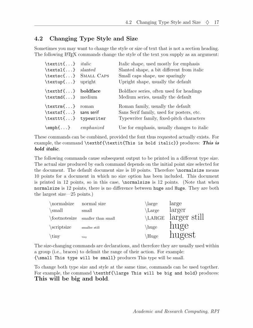
The following commands cause subsequent output to be printed in a different type size.The actual size produced by each command depends on the initial point size selected forthe document. The default document size is 10 points. Therefore \normalsize means10 points for a document in which no size option has been included. This documentis printed in 12 points, so in this case, \normalsize is 12 points. (Note that whennormalsize is 12 points, there is no difference between huge and Huge. They are boththe largest size—25 points.)

\normalsize normal size \large large\small small \Large larger\footnotesize smaller than small \LARGE larger still\scriptsize smaller still \huge huge\tiny tiny \Huge hugest

The size-changing commands are declarations, and therefore they are usually used withina group (i.e., braces) to delimit the range of their action. For example:\small This type will be small produces This type will be small.

To change both type size and style at the same time, commands can be used together.For example, the command \textbf\large This will be big and bold produces:This will be big and bold.


18 ♦ Chapter 4. Within the Text

4.3 Starting New Lines and New Pages

Normally LATEX decides where to start a new line and a new page, always trying to pickthe most aesthetically pleasing break points. But sometimes you want to force the startof a new line or page. The command \\ will force a new line. For example,

This will be on one line\\ this will be on the next line

If you want extra space between two lines, do not use two \\ commands in a row.Instead use an optional parameter (given inside square brackets) to specify the amountof blank space. For example, the following command will leave an extra space of 10points between the lines:

This will be on one line\\[10pt] this will be on the next line

To force a new page, the simplest command is \newpage, which starts a new pageimmediately. There is also the command \clearpage, which acts like \newpage exceptthat it also forces any leftover figures or tables to print before starting the new page.With the twoside documentclass option, the command \cleardoublepage produces ablank page, if necessary, to ensure that the new page starts on a new sheet of paper.

4.4 Leaving Horizontal and Vertical Space

The commands \hspace and \vspace leave horizontal and vertical space in your text.Both commands take a mandatory parameter—the amount of blank space you want toleave. For example, \vspace3in will leave 3 inches of blank space in your text. Ifvertical space is requested in the middle of a paragraph, the space will appear after thecurrent line has ended.

Space requested by the \hspace and \vspace commands disappears if it falls at thebeginning or end of a line or page. To create space that remains no matter where itfalls, use the variations \hspace* and \vspace*. For example, the following lines:

This text starts at the left margin\\

\hspace*1inThis text starts a new line after a one-inch space

produces:

This text starts at the left marginThis text starts a new line after a one-inch space

4.5 Drawing Rules

To draw a line (horizontal or vertical) on the page, use the \rule command:

\rule[lift]widthheight

width is the horizontal dimension, height is the vertical dimension, and the optionalparameter lift is the amount raised above the baseline. For example, the line below wasdrawn with the command \rule\textwidth1pt.

April 2007

4.6 Footnotes ♦ 19

4.6 Footnotes

Footnotes are numbered automatically by LATEX. The command \footnotefootnotetext should be placed exactly where you want the footnote number to appear, with noextra space between the \footnote command and the text before it. For example:

This is text with a note.\footnoteThis is the note text.

Here it is at the bottom of the page.

produces:

This is text with a note.2

4.7 Centering

If you have only one line to center, it’s easiest to use the plain TEX command\centerline; for example,

\centerlineThis line will be centered.

If you have several lines to be centered horizontally, the center environment is conve-nient. The example below produces three lines, each horizontally centered.

\begincenter

This is line one. \\

This is line two. \\

This is line three.

\endcenter

There is also the declaration \centering, which is always used within a group—either apair of braces or an environment. This is useful when you don’t want the extra verticalspace surrounding the center environment.

4.8 Quotations

The quote environment begins a new line and indents text from both sides. Itis delimited with \beginquote and \endquote. Any special effects (suchas changes to the type size or style) started within the quote environmentare terminated by \endquote.

New paragraphs are block style: that is, no indent and a blank line as sepa-ration. This section is inside a quote environment.

There is also a very similar environment called quotation. The only difference is thatparagraphs in the quotation environment are indented with no blank line between.

2This is the note text. Here it is at the bottom of the page.



4.9 Reproducing Text As-Is

To reproduce new lines and spaces exactly as they are in your input file, you have achoice of several methods.

The verbatim environment prints its text in typewriter-style type and sets it off fromthe rest of the document with blank lines before and after. (It does not indent.) To useit, surround the text with the commands \beginverbatim and \endverbatim. Theonly LATEX command obeyed inside this environment is \endverbatim. For example,the following input

\beginverbatim

All spacing is displayed in verbatim as entered.

So are special characters ! @ # & * ( ) _ ] \ | > <

verbatim is used to display LaTeX commands in this document.

\endverbatim

produces:

All spacing is displayed in verbatim as entered.

So are special characters ! @ # & * ( ) _ ] \ | > <

verbatim is used to display LaTeX commands in this document.

A variation on the verbatim environment, called the alltt environment, is providedby a package. It is used in the same way as the verbatim environment and worksthe same, in that spaces and lines are retained from the input file. The difference isthat LATEX commands are recognized inside this environment. It cannot be used toreproduce LATEX commands, but it is very useful if you want to print in roman or italictype instead of typewriter. Before you can use this environment, you must include thecommand \usepackagealltt following the \documentclass command.

If the text is short enough to be contained on one input line and should not be set off,you can use the \verb command. For example,

\verb+This is inside the \verb command+

produces:

This is inside the \verb command

Note that the “+” is used here to delimit the verbatim text. Any character except the“*” can be used as the delimiter.

April 2007

4.10 Lists ♦ 21

4.10 Lists

The three LATEX list environments all use the \item command to start new items in thelist. The enumerate environment numbers items sequentially, the itemize environmentputs a bullet in front of each item, and the description environment puts a boldfaceword or phrase in front of each item.

The following examples show both the output and the input used to create them.

Example of Enumerate\beginenumerate

\item Sugar

\item Cream

\item Chocolate

\endenumerate

1. Sugar

2. Cream

3. Chocolate

Example of Itemize\beginitemize

\item Mix all ingredients together.

\item Boil until the thermometer

reaches 112 $^\circ$C.

\item Stir and cool.

\enditemize

• Mix all ingredients together.

• Boil until the thermometerreaches 112 C.

• Stir and cool.

Example of Description

\begindescription

\item[dog] A loving animal that

likes to sleep on the furniture.

\item[cat] Aloof creature that can

warm your feet on a winter’s night

\item[horse] Large animal, gives

great rides. Eats a lot, luckily

doesn’t sleep on the furniture.

\enddescription

dog A loving animal that likes tosleep on the furniture.

cat Aloof creature that can warmyour feet on a winter’s night

horse Large animal, gives great rides.Eats a lot, luckily doesn’t sleepon the furniture.

Below is an example of nesting list environments:

Here are some useful environments:

\beginitemize

\item center environment

\item quote environment

\item the three list environments:

\beginenumerate

\item enumerate (uses numbers)

\item itemize (uses bullets)

\item description (uses words)

\endenumerate

\enditemize

Here are some useful environments:

• center environment

• quote environment

• the three list environments:

1. enumerate (uses numbers)

2. itemize (uses bullets)

3. description (uses words)



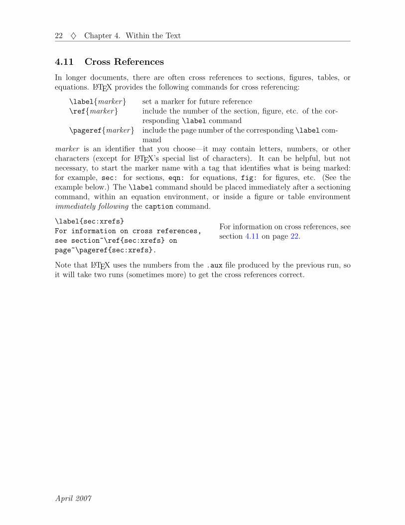
4.11 Cross References

In longer documents, there are often cross references to sections, figures, tables, orequations. LATEX provides the following commands for cross referencing:

\labelmarker set a marker for future reference\refmarker include the number of the section, figure, etc. of the cor-

responding \label command\pagerefmarker include the page number of the corresponding \label com-

mandmarker is an identifier that you choose—it may contain letters, numbers, or othercharacters (except for LATEX’s special list of characters). It can be helpful, but notnecessary, to start the marker name with a tag that identifies what is being marked:for example, sec: for sections, eqn: for equations, fig: for figures, etc. (See theexample below.) The \label command should be placed immediately after a sectioningcommand, within an equation environment, or inside a figure or table environmentimmediately following the caption command.

\labelsec:xrefs

For information on cross references,

see section~\refsec:xrefs on

page~\pagerefsec:xrefs.

For information on cross references, seesection 4.11 on page 22.

Note that LATEX uses the numbers from the .aux file produced by the previous run, soit will take two runs (sometimes more) to get the cross references correct.

April 2007

Chapter 5. Tabular Material

There are two environments in LATEX for formatting tabular material: the tabbing

environment, which uses \begintabbing. . . \endtabbing, and the tabular envi-ronment, which uses \begintabular. . . \endtabular.

The tabbing environment works in a manner similar to a typewriter—you set the tabsand then move from one to another. Tab stops may be reset on any line. Page breakswithin the tabbed material are allowed since each line is processed individually.

The tabular environment allows you to construct a much fancier looking table: forexample, you can specify the alignment of each column and use horizontal and verticallines. However, these tables cannot be broken across pages because LATEX reads in theentire table at once to establish correct column widths. Often material inside a tabular

environment is placed inside the table environment, which ensures that if it can’t fit atthe current location it will be “floated” to an appropriate location. For information onusing the table environment, see Chapter 8..

5.1 Tabbing

Tabbing uses the following commands:

\= Set a tab stop

\> Move right to the next tab stop

\\ Terminate a line

Tabs are usually set in the first line but may also be added in later lines. A special lineending with the command \kill may be used to set tabs but not print the line. Beloware two examples of tabbing. Note that the last entry does not require a \\ to end theline.

Example 1: A Very Simple Case

\begintabbing

Column 1 \= Column 2 \= Column 3 \= Column4 \\

Col 1 \> Col 2 \> Col 3 \> Col 4 \\

one \> two \> three \> four

\endtabbing

Produces:

Column 1 Column 2 Column 3 Column 4Col 1 Col 2 Col 3 Col 4one two three four

23

24 ♦ Chapter 5. Tabular Material

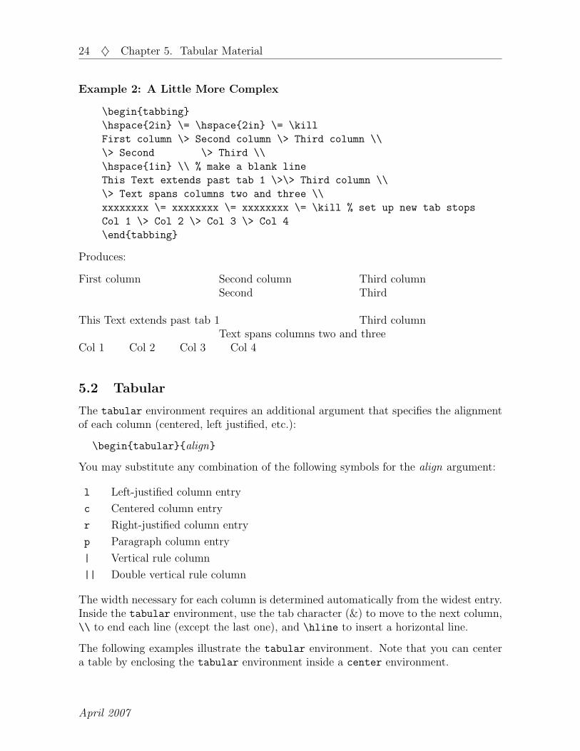
Example 2: A Little More Complex

\begintabbing

\hspace2in \= \hspace2in \= \kill

First column \> Second column \> Third column \\

\> Second \> Third \\

\hspace1in \\ % make a blank line

This Text extends past tab 1 \>\> Third column \\

\> Text spans columns two and three \\

xxxxxxxx \= xxxxxxxx \= xxxxxxxx \= \kill % set up new tab stops

Col 1 \> Col 2 \> Col 3 \> Col 4

\endtabbing

Produces:

First column Second column Third columnSecond Third

This Text extends past tab 1 Third columnText spans columns two and three

Col 1 Col 2 Col 3 Col 4

5.2 Tabular

The tabular environment requires an additional argument that specifies the alignmentof each column (centered, left justified, etc.):

\begintabularalign

You may substitute any combination of the following symbols for the align argument:

l Left-justified column entry

c Centered column entry

r Right-justified column entry

p Paragraph column entry

| Vertical rule column

|| Double vertical rule column

The width necessary for each column is determined automatically from the widest entry.Inside the tabular environment, use the tab character (&) to move to the next column,\\ to end each line (except the last one), and \hline to insert a horizontal line.

The following examples illustrate the tabular environment. Note that you can centera table by enclosing the tabular environment inside a center environment.

April 2007

5.2 Tabular ♦ 25

5.2.1 A Simple Ruled Table

\begincenter

\begintabular|l|c|r| % 3 cols (left, ctr, right); vert. lines

\hline % draw horizontal line

Name & Oblateness & Diameter \\

\hline

Mercury & 0 & 3,100 \\

Venus & 0 & 7,700 \\

Earth & 1/297 & 7,927 \\

Mars & 1/192 & 4,200 \\

Jupiter & 1/15 & 88,700 \\

Saturn & 1/9.5 & 75,100 \\

Uranus & 1/14 & 32,100 \\

Neptune & 1/40 & 27,700 \\

Pluto & ? & 3,600\\

\hline

\endtabular

\endcenter

Produces:

Name Oblateness DiameterMercury 0 3,100Venus 0 7,700Earth 1/297 7,927Mars 1/192 4,200Jupiter 1/15 88,700Saturn 1/9.5 75,100Uranus 1/14 32,100Neptune 1/40 27,700Pluto ? 3,600


26 ♦ Chapter 5. Tabular Material

5.2.2 Using Paragraph Columns, Spanning Columns

The following example illustrates making paragraphs within a table and placing textacross multiple columns using the \multicolumn command. This command has theform:

\multicolumnnpositem

where n is the number of columns to be spanned, pos specifies the alignment of the item,and item is the text.

This example is inside the table environment, which ensures that the table will be“floated” rather than broken across a page (see chapter 8. on page 37) and also providesthe opportunity to supply a caption. In this example, the optional parameter [hb]

specifies that the table should appear “here” or at the bottom of the page.

To center tabular material inside the table environment, you can use the declaration\centering, which has the same effect as the center environment. (The centeringaction will be confined to inside the table environment.)

\begintable[hb] % place table ‘‘here’’ or at bottom of page

\centering

\captionMore Things You can Do With Tabular

\bigskip

\begintabular|l|l|p2.5in|

\hline

\multicolumn2|c|Text in columns 1 and 2

& A paragraph 2.5 inches wide \\

\hline

Column 1 & Column 2 & This text is a paragraph. It will wrap

around to the next line if necessary. \\

Column 1 & Column 2 & The paragraph column \\

\hline

\endtabular

\endtable

Table 1: More Things You can Do With Tabular

Text in columns 1 and 2 A paragraph 2.5 inches wideColumn 1 Column 2 This text is a paragraph. It will

wrap around to the next line if nec-essary.

Column 1 Column 2 The paragraph column

April 2007

5.2 Tabular ♦ 27

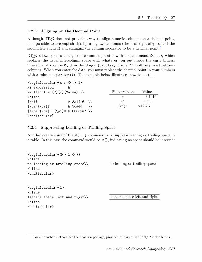
5.2.3 Aligning on the Decimal Point

Although LATEX does not provide a way to align numeric columns on a decimal point,it is possible to accomplish this by using two columns (the first right-aligned and thesecond left-aligned) and changing the column separator to be a decimal point.3

LATEX allows you to change the column separator with the command @..., whichreplaces the usual intercolumn space with whatever you put inside the curly braces.Therefore, if you use @. in the \begintabular line, a “.” will be placed betweencolumns. When you enter the data, you must replace the decimal point in your numberswith a column separator (&). The example below illustrates how to do this.

\begintabularc r @. l

Pi expression &

\multicolumn2cValue \\

\hline

$\pi$ & 3&1416 \\

$\pi^\pi$ & 36&46 \\

$(\pi^\pi)^\pi$ & 80662&7 \\

\endtabular

Pi expression Valueπ 3.1416ππ 36.46

(ππ)π 80662.7

5.2.4 Suppressing Leading or Trailing Space

Another creative use of the @... command is to suppress leading or trailing space ina table. In this case the command would be @, indicating no space should be inserted:

\begintabular@ l @

\hline

no leading or trailing space\\

\hline

\endtabular

no leading or trailing space

\begintabularl

\hline

leading space left and right\\

\hline

\endtabular

leading space left and right

3For an another method, see the dcolumn package, provided as part of the LATEX “tools” bundle.


Chapter 6. Mathematics

One of the greatest strengths of LATEX is its ability to typeset formulas and equations. Tomake it easier to enter mathematical text, LATEX has defined several hundred Greek sym-bols, mathematical symbols, delimiters, and operators. These are listed in Appendix Aof this memo.

LATEX has several modes for setting math text, which are described below. When inmath mode, LATEX sets type differently than when in text mode. For example, all lettersare set in the math italic typeface, and spaces in the input are ignored because LATEXuses its own “mathematically correct” spacing. Therefore, if you want to use normaltext or retain spaces while in math mode, you must enclose this text with an “mbox”:\mboxthis is normal text. Also, new paragraphs are not allowed within mathmode, so be sure not to leave any blank lines.

If your mathematical expressions are particularly complex or sophisticated, you maywant to look at AMS-LATEX, a collection of packages that provides extensions toLATEX’s mathematical capabilities. The amssymb package provides additional math-ematical symbols; the amsmath package provides additional environments for build-ing mathematical expressions. For help with using AMSLATEX, see The Short MathGuide for LATEX, at: ftp://ftp.ams.org/pub/tex/doc/amsmath/short-math-guide.pdf.The official documentation is amsldoc.pdf, which you can find on your system in...\doc\latex\amslatex\.

6.1 In-line Math

LATEX’s in-line math environment allows you to place mathematical formulas in the midstof ordinary text. Typically such mathematical formulas are roughly the same size as thetext they’re embedded in. This environment can be invoked in one of three ways:

$ . . . $ (Used in plain TEX)$ . . . $

\beginmath . . . \endmath

The following paragraph is typical of the use of in-line math:

The quadratic equation $ax^2+bx+c = 0$ has two roots whose nature

depends on the sign of the discriminant $d = \sqrtb^2 - 4ac$.

If $d>0$, then there are two distinct real roots; if $d=0$,

then there are two real and equal roots; and if $d<0$,

then the two roots are conjugate complex numbers.

produces:

The quadratic equation ax2 + bx + c = 0 has two roots whose nature depends on thesign of the discriminant d =

√b2 − 4ac. If d > 0, then there are two distinct real roots;

if d = 0, then there are two real and equal roots; and if d < 0, then the two roots areconjugate complex numbers.

28

ftp://ftp.ams.org/pub/tex/doc/amsmath/short-math-guide.pdf

6.2 Display Math (for unnumbered equations) ♦ 29

6.2 Display Math (for unnumbered equations)

The displaymath environment puts space before and after equations and centersthem by default. For left-justified equations, include fleqn as an option in thedocumentclass command: for example, \documentclass[fleqn]article. Like in-line math, displaymath can be invoked in one of three ways:

$$ . . . $$ (Used in plain TEX)\[ . . . \]

\begindisplaymath . . . \enddisplaymath

The next paragraph illustrates the solution to the quadratic equation:

The quadratic equation $ax^2 + bx + c = 0$ has two roots

\[ x = \frac-b \pm \sqrtb^2 - 4ac2a \]

where the nature of the roots is determined by the sign

of the discriminent $b^2 - 4ac$.

produces:

The quadratic equation ax2 + bx+ c = 0 has two roots

x =−b±

√b2 − 4ac

2a

where the nature of the roots is determined by the sign of the discriminent b2 − 4ac.

6.3 Equation Environment (for numbered equations)

The equation environment is exactly like the displaymath environment except that anequation number in parentheses is placed to the right of the displayed formula. (Forleft-side numbering, include leqno as an option to the \documentclass command.)The environment is invoked with \beginequation. . . \endequation as illustratedbelow:

The derivative of the function $f(x)$ at the point $x_0$ is

\beginequation

f’(x_0) =

\lim_x \rightarrow x_0

\fracf(x) - f(x_0)x - x_0

\endequation

produces:

The derivative of the function f(x) at the point x0 is

f ′(x0) = limx→x0

f(x)− f(x0)

x− x0

(1)


30 ♦ Chapter 6. Mathematics

6.4 Eqnarray Environment (for multiline equations)

The eqnarray environment builds a three-column array of numbered equations, withthe first column right-justified, the second centered, and the third left-justified. It isused mainly for displaying multi-line formulas. It numbers each line by default, but youcan include the command \nonumber on any line to suppress the equation number. (Oryou can use the alternative environment eqnarray*, which does not number any lines.)The following example illustrates this environment. Note that you can use the \label

and \ref commands to refer to equation numbers in the text.

These three products can be expanded and simplified to

produce these equations:

\begineqnarray

(a + b)(a + b) & = & a^2 + ab + ba + b^2 \nonumber \\

& = & a^2 + 2ab + b^2 \labeleq:simp1 \\

(a + b)(a - b) & = & a^2 - ab + ba - b^2 \nonumber \\

& = & a^2 - b^2 \labeleq:simp2 \\

(a + b)^3 & = & a^3 + 3a^2b + 3ab^2 + b^3 \labeleq:simp3

\endeqnarray

The results after simplification are shown in equations

\refeq:simp1, \refeq:simp2, and \refeq:simp3.

produces:

These three products can be expanded and simplified to produce these equations:

(a+ b)(a+ b) = a2 + ab+ ba+ b2

= a2 + 2ab+ b2 (1)

(a+ b)(a− b) = a2 − ab+ ba− b2

= a2 − b2 (2)

(a+ b)3 = a3 + 3a2b+ 3ab2 + b3 (3)

The results after simplification are shown in equations 1, 2, and 3.

The amsmath package provides additional environments for formatting multiline equa-tions (e.g., split, align, gather, etc) and is highly recommended.

April 2007

6.5 Array Environment (for matrices, etc.) ♦ 31

6.5 Array Environment (for matrices, etc.)

The array environment is not itself a math environment; it must be enclosed within amath environment of your choosing. It is used for building rectangular arrays of numbers,matrices, etc. array is the math equivalent of tabular and uses the same syntax.

Here is an example of the array environment used to build a 5× 5 magic square:

\[

\beginarrayccccc

17& 24& 1& 8& 15\\

23& 5& 7& 14& 16\\

4& 6& 13& 20& 22\\

10& 12& 19& 21& 3\\

11& 18& 25& 2& 9

\endarray

\]

produces:

17 24 1 8 1523 5 7 14 164 6 13 20 2210 12 19 21 311 18 25 2 9

Here is an example for a general matrix:

\beginequation

A = \left(

\beginarraycccc

a_1,1 & a_1,2 & \ldots & a_1,n \\

a_2,1 & a_2,2 & \ldots & a_2,n \\

\vdots & \vdots & \ddots & \vdots \\

a_m,1 & a_m,2 & \ldots & a_m,n

\endarray

\right)

\endequation

produces:

A =

a1,1 a1,2 . . . a1,n

a2,1 a2,2 . . . a2,n...

.... . .

...am,1 am,2 . . . am,n

(4)

Section 6.6.6 (Large Delimiters) on page 34 has more examples of arrays.



6.6 Building Mathematical Expressions

6.6.1 Superscripts and Subscripts

In math mode, the symbols ‘ˆ’ and ‘ ’ are used to make superscripts and subscripts. Ifmore than one character is to be used as a superscript or subscript, enclose the charactersin braces. For example:

\[ 2^2^2 = 2^4 = 4^2 \]

\[ a^2_i_1 = b^2_i,j \]

\[ _2F^1_3 \]

\[ _2^1P^3_4 \]

produces:222

= 24 = 42

a2i1

= b2i,j

2F13

12P

34

6.6.2 Spaces in Math Mode

In math mode, LATEX ignores blanks typed in the input. However, the following symbolsallow you to add (or subtract) small amounts of space in your equations:

\; thick space \: medium space \, thin space \! negative space

In addition, you can make a larger space (about the width of an “M”) with the command\quad. The command \qquad provides twice as much space.

6.6.3 Dots, Braces, and Bars

The commands \ldots, \cdots, \vdots, and \ddots are used to produce a stringof three dots on the base line, on the math centerline, vertically, or on the diagonal,respectively. The commands \overline, \underline, \overbrace, and \underbrace

are used to build horizontal groups. For example:

\begineqnarray*

2^n & = &\overbrace2\times2\times\cdots\times 2^\mboxn terms\\

k\cdot x & = &\underbracex + x + \cdots + x_\mboxk terms

\endeqnarray*

produces:

2n =

n terms︷︸︸︷2× 2× · · · × 2

k · x = x+ x+ · · ·+ x︸︷︷︸k terms

April 2007

6.6 Building Mathematical Expressions ♦ 33

6.6.4 FractionsThe ‘/’ can be used to make simple fractions, but the \frac commmand is used for mostfractions; its two arguments are the numerator and denominator. Two variations of afraction are provided by the plain TEX commands \atop and \choose.

$$ \fracab \qquad \fraca/bc/d

\qquad a\atop b \qquad a\choose b $$

$$ 1 + 2 + 3 + \cdots + n = \fracn(n+1)2 $$

$$ \lim_n\rightarrow\infty\frac1n=0

\qquad y’’=\fracd^2ydx^2 $$

produces:a

b

a/b

c/d

a

b

(a

b

)

1 + 2 + 3 + · · ·+ n =n(n+ 1)

2

limn→∞

1

n= 0 y′′ =

d2y

dx2

6.6.5 Radicals, Integrals, and SummationsThe \sqrt command creates a square root sign for its mandatory argument. An optionalargument for the radicand allows you to construct cube roots, nth roots, etc. The signautomatically grows to fit the argument, as these examples show:

$$ \sqrt2=1.4142 \qquad c=\sqrta^2+b^2

\qquad \sqrt[3]8=2 \qquad \sqrt\fracn(n+1)2 $$

produces: √2 = 1.4142 c =

√a2 + b2

3√

8 = 2

√n(n+ 1)

2

Integral signs are produced with the \int command, and summation signs are producedwith the \sum command. These symbols are often used with superscripts and subscripts:

$$\sum^\infty_n=1 \qquad \int^b_a e^x^2\,dx $$

$$\sqrt\sum_i=1^ni \qquad \sum_\stackreli=1j=2^\infty$$

$$\sum \Delta V=\int\!\!\!\int\!\!\!\int_V dv $$

produces:∞∑

n=1

∫ b

aex2

dx

√√√√ n∑i=1

i∞∑i=1j=2∑

∆V =∫∫∫

Vdv



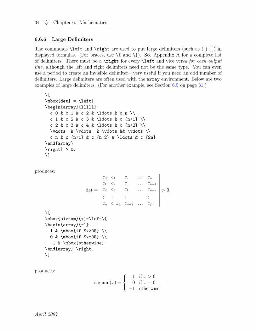
6.6.6 Large Delimiters

The commands \left and \right are used to put large delimiters (such as ( ) [ ]) indisplayed formulas. (For braces, use \ and \). See Appendix A for a complete listof delimiters. There must be a \right for every \left and vice versa for each outputline, although the left and right delimiters need not be the same type. You can evenuse a period to create an invisible delimiter—very useful if you need an odd number ofdelimiters. Large delimiters are often used with the array environment. Below are twoexamples of large delimiters. (For another example, see Section 6.5 on page 31.)

\[

\mboxdet = \left|

\beginarraylllll

c_0 & c_1 & c_2 & \ldots & c_n \\

c_1 & c_2 & c_3 & \ldots & c_n+1 \\

c_2 & c_3 & c_4 & \ldots & c_n+2 \\

\vdots & \vdots & \vdots && \vdots \\

c_n & c_n+1 & c_n+2 & \ldots & c_2n

\endarray

\right| > 0.

\]

produces:

det =

∣∣∣∣∣∣∣∣∣∣∣∣∣

c0 c1 c2 . . . cnc1 c2 c3 . . . cn+1

c2 c3 c4 . . . cn+2...

......

...cn cn+1 cn+2 . . . c2n

∣∣∣∣∣∣∣∣∣∣∣∣∣> 0.

\[

\mboxsignum(x)=\left\

\beginarrayrl

1 & \mboxif $x>0$ \\

0 & \mboxif $x=0$ \\

-1 & \mboxotherwise

\endarray \right.

\]

produces:

signum(x) =

1 if x > 00 if x = 0−1 otherwise

April 2007

Chapter 7. Including Graphics

7.1 Creating the Graphics File

The easiest way to put graphics into your LATEX document is to first create the graphicusing a software package, such as Maple, Matlab, CorelDRAW, Xfig, Gnuplot, etc. Youcan also use a Windows application such as Word or Excel to create an eps (EncapsulatedPostScript) file by printing to a file following certain steps, described inhttp://www.rpi.edu/dept/arc/training/latex/Examples/graphics.pdf .

If you are using LATEX plus dvips to produce your final output, you should save thegraphic as encapsulated PostScript (eps), the only acceptable format. If you are usingpdfLATEX (which produces a pdf file directly), acceptable formats are pdf, jpeg, or png,but not eps. A general rule of thumb for graphics formats is to use pdf or eps for vectorgraphics (line art, graphs, etc), jpeg for photographs, and png for screen shots.

If you are using pdfLATEX and your graphics files are in eps format, you can convertthem to pdf using the epstopdf utility, which is most likely on your system. Run thisprogram from the command line (in Windows, open a command window and cd to theappropriate folder):

epstopdf myfigure.eps generates myfigure.pdf

After doing this, you will have two files for your graphic, one eps and one pdf.

If you are using LATEX plus dvips, the jpeg2ps utility is handy. It converts JPEG imagesto eps files without uncompressing the images. The JPEG data is simply “wrapped”with PostScript, yielding considerably smaller PostScript files. Use it from the commandline:

jpeg2ps -h image.jpg > image.eps

You may already have jpeg2ps on your system; if not, you can download it from:http://www.ctan.org/tex-archive/support/jpeg2ps/.

7.2 Importing the Graphic into your LATEX Document

LaTeX’s standard graphics bundle includes two packages for importing graphics:graphics and graphicx. The extended package, graphicx, provides a more conve-nient method of supplying parameters and is recommended. Therefore first step is toput in your preamble the command:

\usepackagegraphicx

This package defines a new command called \includegraphics, which allows you tospecify the name of the graphic file as well as supply optional arguments for scaling or ro-tating. So, at the spot you want to insert the graphic (named for example, myfigure.epsor myfigure.pdf) use the \includegraphics command, for example:

35

http://www.rpi.edu/dept/arc/training/latex/Examples/graphics.pdf

http://www.ctan.org/tex-archive/support/jpeg2ps/

36 ♦ Chapter 7. Including Graphics

\includegraphics[width=4in]myfigure note filename extension is omitted

If you want to be able to process your file using either latex or pdflatex, you’ll needto have your graphics files in both eps format and one of the others, such as pdf. Thenomit the filename extension on the \includegraphics command: latex will look foran eps file, and pdflatex will look for a pdf, jpg, or png file.

The \includegraphics command also provides optional arguments for scaling or ro-tating the figure. Inside the [...], you can specify a number of optional arguments,separated by commas. In the example above, width=4in will scale the width of graphicto four inches. Since no height is specified, the height will be scaled so that the figureremains in proportion. The most commonly used arguments are:

width scale graphic to the specified width (aspect ratio preserved)height scale graphic to the specified height (aspect ratio preserved)scale scale graphic by scale factor. (scale=2 makes the graphic twice as large

as its natural size; scale=.5 makes it half as large.)angle rotate graphic by specified number of degrees. A positive number in-

dicates the counter-clockwise direction. (angle=90 rotates 90 degreescounter-clockwise.)

Note that in the following example, the graphic is first rotated counter-clockwise by 90degrees and then scaled to a width that will just fit within the margins:

\includegraphics[angle=90,width=\textwidth]myfigure

Usually the includegraphics command is put inside the figure environment, whichallows the image to move or “float” to another location so that it is never split betweenpages. The figure environment is described in chapter 8..

7.3 Viewing the Output

If your graphics files are in pdf, jpeg or png formats, you can run pdfLATEX and viewthe result with Acrobat or GSView. If your files are eps, it is important to note thatafter running LATEX, the resulting .dvi file does not actually contain the eps graphics;it only contains commands that the printer driver, dvips, subsequently uses to includethe graphics when making the PostScript file. Most dvi previewers try to display epsfiles (ususually by calling on ghostscript), but rotated material may not display properlyin the dvi preview. To see a correct display, run dvips to make a PostScript file andthen use GSView/ghostview to view it.

Complete documentation for the graphics bundle is in the file grfguide.pdf; look for iton your system. Information on the graphicx package is in section 4.4. For an extensivetreatment of including graphics, see Using Imported Graphics in LATEX and pdfLATEX byKeith Reckdahl of Stanford University. It includes all you would ever want to know withmany examples: http://www.ctan.org/tex-archive/info/epslatex.pdf.

April 2007

http://www.ctan.org/tex-archive/info/epslatex.pdf

Chapter 8. Placing Figures & Tables (Floats)

If you have figures or tables in your document, you’ll want to make sure that they arenot broken across pages. To accomplish this, LATEX provides two environments, figureand table, which move or “float” the material inside the environment to a locationwhere it all fits. Meanwhile, LATEX fills the current page with text to avoid half emptypages. The commands to use these two environments look like:

\beginfigure \begintable

... figure material ... ... tabular material ...

\endfigure \endtable

There are also “starred” versions of these environments (table* and figure*), which,in 2-column text, place floats across both columns.

Note that these environments have nothing to do with actually preparing your figuresor tabular material (discussed in chapters 5. and 7.); they only ensure that whatevermaterial is inside the environment gets “floated” and is not broken between pages.

To place the floated material, LATEX first tries to put the figure or table at the top ofthe current page. If it doesn’t fit there, it next tries the bottom of the current page,then the top of the next page. Failing that, it will try to place the figure or table ona page containing only floated material (no text). Usually, the default behavior placesthe floats satisfactorily. However, if you wish, you can supply an optional parameter tospecify a list of preferred locations; for example, if you begin a table:

\begintable[htp]

LATEX will first try to place the table “here”—that is, at the spot you gave the\begintable command, then the top of the next page, and finally on a page con-taining only floats (which often means on a page by itself). The possible positioningparameters are:

h here: at the place in the text where the environment occurs.t top: at the top of a text page.b bottom: at the bottom of a text page.p page: on a special page containing only floats.

8.1 Making a Caption

The floated material usually includes a numbered caption. Within the figure or tableenvironment, you can supply a caption with the command \captioncaption text.Usually the caption for a table is typed above the table and the caption for a figurebelow the figure. The table environment prefixes the caption text with “Table n:”(where n is the number of the table supplied by LATEX); the figure environment prefixesthe text with “Figure n:”. In fact, the caption prefix is the only difference between thefigure and table environments. The \caption command also supplies information fora List of Figures and/or a List of Tables. To print out such a list at the beginning of

37

38 ♦ Chapter 8. Placing Figures & Tables (Floats)

your document, simply place the command \listoftables or \listoffigures afterthe \tableofcontents command.

If your caption is very long and you do not want the whole thing repeated in the listof figures or tables, you can use an optional parameter (specified in square brackets) tosupply a shorter version for the List. For example, a table caption might look like:

\caption[A short caption for the list of tables]This is a very

long caption for this table, requiring lots of explanation.

It could go on for several lines.

You can also use the \label command (see section 4.11 on cross referencing) so thatyou can refer to your figure or table elsewhere in the document. Note that the \label

command must immediately follow the caption command. If it precedes the caption,the number used in the reference will be incorrect.

8.2 Examples

Note that you can put anything inside the figure environment: it can be text, a diagram,an image (see chapter 7.) or any other kind of illustration. Likewise, a table environmentcan contain any LATEX commands or text, but usually contains tabular material insidethe tabular environment (see section 5.2).

The example below encloses tabular material in the table environment, which allows itto to float to an appropriate spot in the text. This table is floated to the top of the nextpage because there is not enough room for it to be placed “here”. Note the placementof the \caption and \label commands in this example and the example figure on thenext page.

\begintable[htp]

\captionContract Expenses to Date

\labeltab:exp

\begincenter

\begintabularlr

Item & Amount\\

\hline

Salaries (research assistants, secretary) & \$24,000 \\

Travel expenses & \$8,000 \\

Software & \$2,000 \\

\cline2-2 \\[-8pt]

Total & \$34,000

\endtabular

\endcenter

\endtable

April 2007

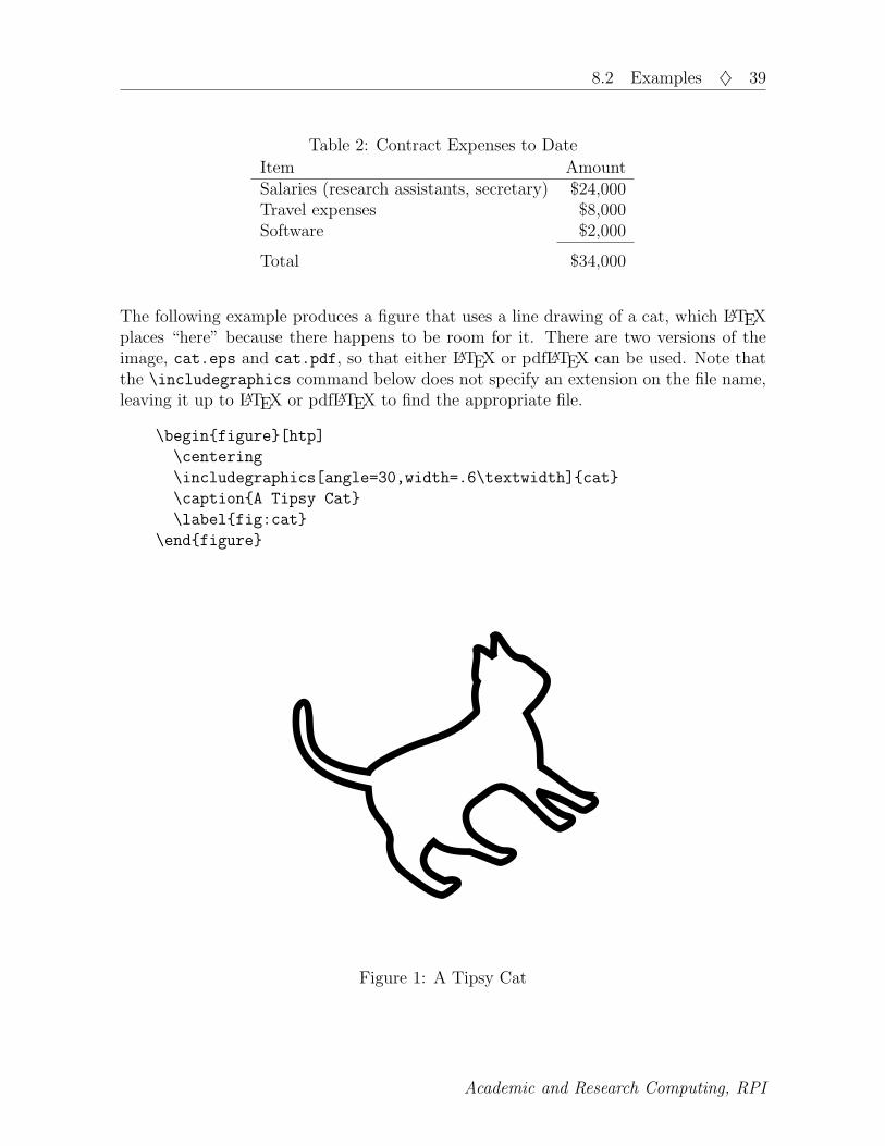
8.2 Examples ♦ 39

Table 2: Contract Expenses to Date

Item AmountSalaries (research assistants, secretary) $24,000Travel expenses $8,000Software $2,000

Total $34,000

The following example produces a figure that uses a line drawing of a cat, which LATEXplaces “here” because there happens to be room for it. There are two versions of theimage, cat.eps and cat.pdf, so that either LATEX or pdfLATEX can be used. Note thatthe \includegraphics command below does not specify an extension on the file name,leaving it up to LATEX or pdfLATEX to find the appropriate file.

\beginfigure[htp]

\centering

\includegraphics[angle=30,width=.6\textwidth]cat

\captionA Tipsy Cat

\labelfig:cat

\endfigure

Figure 1: A Tipsy Cat


40 ♦ Chapter 8. Placing Figures & Tables (Floats)

8.3 Overcoming Problems with Float Placement

When placing floated material, LATEX follows certain rules, explained in detail in Lam-port’s LATEX User’s Guide and Reference Manual, section C.9. If you find that yourtable or figure is not appearing where you think it should, it could be that LATEX’s con-straints on how much of a text page can be taken up by floats are getting in the way.You can override these constraints by including a ! in the optional argument containingthe positioning parameters. For example, if you use \begintable[!htp], LATEX willtry extra hard to place the float where you want it.

Do NOT give only one possible placement parameter (e.g., h), because if the float cannotbe placed where you specified, it could be pushed to the end of the section or documentwith all subsequent figures or tables behind it.

LATEX has room in its memory to hold only a certain number of floats. If you wantto include many figures or tables together, without intervening text, you can avoidproblems by including the command \clearpage after every approximately 10 floats.This command prints all queued floats and starts a new page.

8.4 Landscape Figures and Tables

To print an entire figure or table, including the caption, in landscape orientation, usethe rotating package (in addition to graphicx for images). Load it in the preamble asusual with the \usepackage command:

\usepackagerotating

This package defines two new environments, sidewaysfigure and sidewaystable,which you then use in place of the standard LATEX environments figure and table.The sideways environments always put the landscape table or figure on a page by itself.For example, to make a landscape page containing a rotated graphic and caption, usecommands such as:

\beginsidewaysfigure

\includegraphicsmyfigure

\captionTurn the page sideways to look at this figure.

\endsidewaysfigure

The file http://www.rpi.edu/dept/arc/training/latex/Examples/exrotating.texcontains examples of using both the graphicx and the rotating packages to includelandscape figures and tables. To see the results after running pdflatex, view the outputin the filehttp://www.rpi.edu/dept/arc/training/latex/Examples/exrotating.pdf.

Full documentation for the rotating package is in the book, The LATEX Companion byMittlebach and Goossens.

April 2007

http://www.rpi.edu/dept/arc/training/latex/Examples/exrotating.tex

http://www.rpi.edu/dept/arc/training/latex/Examples/exrotating.pdf

Chapter 9. Preparing a Bibliography

LATEX provides built-in support for citing references, which is straightforward and rel-atively easy to use. However, it’s not very flexible. If your bibliography is large or ifyou use the same references in several documents, you may prefer to use BibTEX, acompanion program to LATEX that allows you to store all your references in an externaldatabase file. You can then refer to this database in your LATEX document, and cite anyreference within it. Both methods are described below.

9.1 Using LATEX’s built-in Method

To prepare a bibliography the “standard” way, the first step is to cite various workswithin your text using the \citekey command. key is a reference keyword of yourchoosing that identifies the work. For example your document might include, at theappropriate places, the commands: \citelamport \citekopka \citegoossens.These commands place numbers (enclosed in square brackets) in the text that match thenumbers automatically generated in the bibliography. (Remember to run LATEX twiceto get correct numbers in the text!)

To include an item in the bibliography without citing it in the text, use the \nocite

command; for example: \nocitesmith,jones.

Then, at the end of the document, you format the bibliography, sorting the entries asyou wish them to appear, using the a special environment called thebibliography.

Below is an example of a thebibliography environment, followed by the output itproduces. On the \beginthebibliography line, the width of the item in the secondpair of braces determines the indent of the entries. This item is usually a dummy numberwith as many digits as the highest-numbered entry. In this case, the “9” indicates thereare fewer than 10 entries. If there are 10 or more but less than 100, use the number 99.

Within this environment, each entry starts with the \bibitem command. The argumentfor this command is the same keyword used in the corresponding \cite command inthe text. The \bibitem commands automatically generate a number in square bracketsbefore each entry. The first entry in the list will be numbered 1.

Note that in the book and report classes, Bibliography is used as the chapter title;in the article class, References is used as the section heading.

\beginthebibliography9\bibitemlamport Leslie Lamport. \textit\LaTeX\ -- A Document

Preparation System. Addison-Wesley, second edition, Reading, MA, 1994.\bibitemkopka Helmut Kopka and Patrick W.~Daly. \textitA Guide

to \LaTeX. Addison-Wesley, fourth edition, Boston, MA, 2004.\bibitemgoossens Michel Goossens, Frank Mittelbach, et al. \textitThe

\LaTeX\ Companion. Addison-Wesley, second edition, Boston, MA, 2004.\endthebibliography

41

42 ♦ Chapter 9. Preparing a Bibliography

References[1] Leslie Lamport. LATEX – A Document Preparation System. Addison-Wesley,

Reading, MA, second edition, 1994.

[2] Helmut Kopka and Patrick W. Daly. A Guide to LATEX. Addison-Wesley, fourthedition, Boston, MA, 2004.

[3] Michel Goossens, Frank Mittelbach et al. The LATEX Companion. Addison-Wesley, second edition, Boston, MA, 2004.

If you want to change the heading for the reference listing, just change the value of\refname (for article class) or \bibname (book or report class) by adding a line like thisin your preamble: \renewcommand\bibnameLiterature Cited.

If you like, you can choose a label to identify the work in both the text and in thebibliography, instead of the number assigned by LATEX. You do this by including anoptional label on the \bibitem command. (The \cite command doesn’t change.) Forexample, to refer to the third book as “companion,” its entry in the thebibliography

environment would be:

\bibitem[companion]goossens Michel Goossens, Frank Mittelbach, et al.

\textitThe \LaTeX\ Companion. Addison-Wesley, second edition,

Boston, MA, 2004.

9.2 Using BibTEX

9.2.1 Overview

BibTEX automatically generates a list of references from information contained in abibliographic database—a file you create whose name ends with the extension .bib.The entries in your .bib file are called in your LATEX file with various \cite commands,just as in the built-in method described above. In your LATEX file, you provide just twomore pieces of information: A bibliographystyle command to specify the formattingstyle of the citations and the bibliography (this can appear anywhere in your LATEXfile), and at the point you want the bibliography printed, a bibliography command toprovide the name of the .bib file.

After processing your document through LATEX (or pdfLATEX) you run BibTEX, whichwill format the citations according to the style you’ve specified. You then need to runLATEX (or pdfLATEX) again to process the output created by BibTEX, and finally oncemore to resolve the references. Your resulting output will then contain your citationsand formatted bibliography.

April 2007

9.2 Using BibTEX ♦ 43

9.2.2 Creating the .bib File

The .bib file is a plain text file that you create and edit with any text editor. Thefollowing example of a Bibtex entry illustrates the structure. Each entry begins withthe document type preceded by the “@” sign. This is followed by a unique label thatyou make up and that you will use to cite the entry in your text. Then each field (inany order) uses the format keyword = data. Note that the data can be enclosed ineither quotation marks or braces, and each line except the last must end with a comma.

@articleHefferon04,

author = "Jim Hefferon",

title = "CTAN for Starters",

year = "2004",

journal = "TUGBoat",

volume = "25",

number = "2",

pages = "126--127"

The above example refers to an article within a journal. There are many differentdocument types: book, article (in a journal), article (in a collection), chapter (in abook), thesis, report, paper (in a Proceedings), etc. There is a prescribed set of fieldsfor each type of document. A book entry might look like:

@bookKopka04,

author = Helmut Kopka and Patrick W.~Daly,

title = Guide to \LaTeX,

edition = fourth,

publisher = Addison-Wesley,

address = Boston, MA,

year = 2004

If a work has more than one author, separate them with the keyword “and” so BibTEXcan distinguish the different names. If the BibTEX style does not preserve all yourcapitalization (for example within titles), you can tell BibTEX to keep them by usingbraces around the letters in question.

9.2.3 Running BibTEX

After processing your file with LATEX (or pdfLATEX), you run the BibTEX program byclicking on the BibTEX toolbar icon (if your editor has one), or by typing the com-mand bibtex followed by the name of your document without the .tex extension. Theinformation for every document you have cited will be extracted from your database,formatted according to the style you specify, and stored in a bibliographic (.bbl) fileready for LATEX to use. When you run LATEX again it will build the bibliography fromthe .bbl file and generate warnings about unresolved references. Subsequent runs willresolve the references, and the warnings will disappear.


44 ♦ Chapter 9. Preparing a Bibliography

Suppose you have a file called myrefs.bib that contains the two bibliographics entriesabove, and the file testbib.tex contains the following:


\begindocument

We are testing the use of Bib\TeX\ using two entries.

One is a book \citekopka04, and the other is an

article in a journal. \citehefferon04

\bibliographystyleplain % use style plain.bst

\bibliographymyrefs % find references in myrefs.bib

\enddocument

The result of running LATEX, then BibTEX then LATEX twice more would be:

We are testing the use of BibTEX using two entries. One is a book [2],and the other is an article in a journal. [1]

References[1] Jim Hefferon. CTAN for Starters. TUGBoat, 25(2):126–127, 2004.

[2] Helmut Kopka and Patrick W. Daly. Guide to LATEX. Addison-Wesley,Boston, MA, fourth edition, 2004.

9.2.4 Bibliography Styles

Bibliography styles are files (with the extension .bst), that tell BibTEX how to formatthe information in the .bib file. The standard styles are:

plain entries are sorted alphabetically and are labelled with numbers.unsrt the same as plain except entries appear in the order in which they were cited.abbrv the same as plain except names, month names, journal names are abbreviated.alpha entries are sorted alphabetically, and the labels are made from the author’s or

authors’ (or editor’s) name and the year of publication.

The .../bst subdirectory of your TEX installation contains the styles (.bst files) in-stalled by default, and the The LATEX Companion, chapter 12, describes others.

There are also various LATEX packages that provide other styles, such as author-datecitations instead of numbers. To use one of these packages, you need to include its namewith the normal \usepackage command in your preamble. One highly recommended andflexible package is Natbib. In addition to loading the Natbib package in the preamble,you need to use a bibliography style that supports the author-date style. (Some possiblechoices are “plainnat”, “unsrtnat”, “abbrvnat” and “apalike”.) Also, Natbib uses slightvariations of the \cite command: you just append a “t” (for textual) or “p” (forparenthetical), to the basic \cite command, for example:

April 2007

9.2 Using BibTEX ♦ 45

Citation command Natbib output\citethefferon04 Hefferon (2004)\citephefferon04 (Hefferon, 2004)\citet[chapter 4]kopka04 Kopka and Daly (2004, chapter 4)\citep[see][chap.~4]kopka04 (see Kopka and Daly, 2004, chap. 4)

Using the same myrefs.bib file as in the previous example, and changing thetestbib.tex file to read:


\usepackagenatbib

\begindocument

We are testing the use of Bib\TeX\ using two entries.

One is a book by \citetkopka04, and the second is an

article in a journal \citephefferon04.

\bibliographystyleapalike % use style apalike.bst

\bibliographymyrefs % find references in myrefs.bib

\enddocument

produces, after running LATEX, then BibTEX, then LATEX twice more:

We are testing the use of BibTEX using two entries. One is a book by Kopkaand Daly (2004); the second is an article in a journal (Hefferon, 2004).

ReferencesHefferon, J. (2004). CTAN for Starters. TUGBoat, 25(2):126–127.

Kopka, H. and Daly, P. W. (2004). Guide to LATEX. Addison-Wesley, Boston,MA, fourth edition.

9.2.5 For More Information

For more information on LATEX’s built-in method and on using BibTEX, see any of thethree books in section 9.1.

For on-line information on BibTEX, there is an excellent tutorial by Andrew Roberts:http://www.andy-roberts.net/misc/latex/latextutorial3.html

A longer, more complete document covering both LaTeX’s basic bibliography methodand BibTEX is Tame the BeaST by Nicolas Markey:http://tug.ctan.org/tex-archive/info/bibtex/tamethebeast/ttb_en.pdf

An excellent, concise overview of the Natbib package is the file natnotes.pdf, and theNatbib manual is in natbib.pdf. You can find both these files at:http://www.ctan.org/tex-archive/macros/latex/contrib/natbib/


http://www.andy-roberts.net/misc/latex/latextutorial3.html

http://tug.ctan.org/tex-archive/info/bibtex/tamethebeast/ttb_en.pdf

http://www.ctan.org/tex-archive/macros/latex/contrib/natbib/

Chapter 10. Special Topics

10.1 Managing a Large Document

If you are preparing a book, thesis, or any document with multiple parts, it’s convenientto work on the different chapters or sections separately. To do this, create a separate .texfile for each section, and create a “root” .tex file that contains the \documentclass

command, the preamble material, the \begindocument and \enddocument com-mands, and multiple \include commands. The \include commands tell LATEX to readthe separate .tex files that contain the text of the document. Each \include commandstarts a new page in your output. Note that the individual section files do not include\begindocument and \enddocument commands.

The command, \includeonly, which must go in the preamble, can be used to selectfrom the \include list only certain file(s) to be processed.

As an example, the root file for a book with 6 chapters might be called mybook.tex,and the files for the chapters might be named chap1.tex, chap2.tex, etc. The root filemybook.tex, which is the file on which you run LATEX, would look something like:

\documentclassbook

\includeonlychap1,chap2 % only these files will be processed

\begindocument

\includechap1

\includechap2

\includechap3

\includechap4

\includechap5

\includechap6

\enddocument

10.2 Generating an Index

It is relatively easy to generate an index by using LATEX commands combined with thesupport program MakeIndex. This memo covers just the basics of MakeIndex; detailsare in the documentation accompanying the program, makeindex.dvi, which should bealready on your system under the doc folder. For example, if you are using TeXLive2005 on Windows, you’ll find the documentation in:C:\TeXLive2005\texmf-dist\doc\makeindex\base\makeindex.dvi.

Suppose your LATEX input file is called myfile.tex. To make an index, you need to dothe following things in that file:

1. Load the package makeidx with the command: \usepackagemakeidx

2. In the preamble, place the command: \makeindex

46

10.3 Including hyperlinks ♦ 47

3. At the place you want the index to appear (usually the end of the document), putthe command: \printindex

4. Put index entries throughout the text (as close as possible to the actual word orphrase being indexed) using the command \indexentry, where entry is the indexentry. Examples of various index entries are shown in the table at the bottom ofthe page.

Now, generate the index by running LATEX, then running makeindex, and finally runningLATEX once more. If you don’t have a “makeindex” button on the toolbar of youreditor/shell, you can run it from the command line or use the editor’s Help feature toadd it to the toolbar. Below is an example of doing the 3-step process from the commandline. Note that you should not include the filename extensions on your commands; theprograms will then do the right thing.

latex (or pdflatex) myfile In addition to producing the .dvi or pdf file, this generatesthe file myfile.idx, which contains all the index entriesand page numbers.

makeindex myfile MakeIndex processes myfile.idx and produces the filemyfile.ind, which contains the LATEX commands to for-mat the index.

latex (or pdflatex) myfile When LATEX or pdfLATEX finds the \printindex com-mand, it reads in the file myfile.ind. The resulting out-put includes the formatted index.

If you change your document after producing the .ind file, be sure to run MakeIndexagain to create an up-to-date .ind file before running LATEX for the final time.

The package showidx, which comes with LATEX, prints all index entries in the margin ofthe text. This is a useful tool for checking the index in draft copies.

Examples of Index Entries

LATEX Input Index Entry Comments

\indexcolors colors, 14 Main entry\indexcolors!blue blue, 14 Subentry under “colors”\indexcolors!blue!navy navy, 15 Subsubentry\indexgnu@\textslgnu gnu, 22 Formatted text\indexgnat|\textbf gnat, 25 Formatted page number

10.3 Including hyperlinks

Both LATEX and pdfLATEX can use the hyperref package to place live links in the PDFfile. By including \usepackagehyperref as the last package in your preamble, youwill automatically get bookmarks corresponding to your sections, and hyperlinks fromyour tables of contents and \cite and \ref references. The package has a number ofoptions; some of the most useful are:


48 ♦ Chapter 10. Special Topics

colorlinks makes the text of the link colored instead of framed with a box. It’s also pos-sible to choose the color of the links with the linkcolor, urlcolor, and citecolor

options.

plainpages=false distinguishes between frontmatter and mainmatter page numbers.With this option, hyperref writes different anchors for pages “ii’ and “2”.

pdfpagelabels sets PDF page labels so that Acrobat Reader displays the page numberas (say) “iv (4 of 40)” rather than simply “4 of 40”. plainpages=false andpdfpagelabels are usually used together.

breaklinks allows a line break in a long link (such as a TOC entry). Works withpdfLATEX only.

linktocpage makes the page number, not the text, the link in TOC, LOF, and LOT.It’s especially useful if you use LATEX and dvips to get your PDF file, as this methodcannot use breaklinks. If you also have long URLs in the body of the thesis, thebreakurl package can help. For documentation, look on your system for the filebreakurl.pdf.

The hyperref package also provides the command \urlURL to link to a URL from thetext, for example: \urlhttp://www.ctan.org/ or \urlmailto:[email protected] command \hrefURLtext provides a more sophisticated method, where“URL” is the address and “text” is the text displayed in the document. Forexample, to avoid having the text “mailto:” appear in the document, use\hrefmailto:[email protected]@rpi.edu.

Be sure to run LATEX or pdfLATEX twice to ensure correct hyperlinks.

Abbreviated example file:

\documentclassreport

\usepackageifpdf % to use same .tex file for both latex & pdflatex

% the following specifies different options to hyperref depending on

% whether latex or pdflatex is being run.

\ifpdf

\usepackage[colorlinks,linkcolor=blue,urlcolor=blue,citecolor=blue,

plainpages=false,pdfpagelabels,breaklinks]hyperref

\else

\usepackage[colorlinks,linkcolor=blue,urlcolor=blue,citecolor=blue,

plainpages=false,pdfpagelabels,linktocpage]hyperref

\fi

\begindocument

... body of your document goes here ...

\enddocument

The official documentation for hyperref is manual.pdf. Look for it on your system in.../doc/latex/hyperref/.

April 2007

10.4 Accents and Special Characters ♦ 49

10.4 Accents and Special Characters

LATEX provides commands that allow you to print accents required by many Europeanlanguages. The table below shows how to apply a variety of accents to the letter o. Ofcourse, any other letter can be used in place of o.

If you want to place an accent on top of an i or a j, however, you need to print themwithout their dots. You can print a dotless i or j by typing \i and \j. For example, ı isformed by typing \u\i.

o \‘o o \’o o \ô o \~oo \=o o \.o o \"o o \roo \uo o \vo o \Ho o \coo. \do o

¯\bo oo \too

Note that the accent commands that are control symbols (i.e., they consist of just onenon-letter) can also be used without braces. For example \ô and \ô both produceo.

The special letters that are part of European languages can be generated with thefollowing commands:

œ \oe Œ \OE æ \ae Æ \AEa \aa A \AA ø \o Ø \Oß \ss SS \SS l \l L \L¡ !‘ ¿ ?‘

For example:

na\"\ive, r\’esum\’e, \AAngstr\om, se\~norita, stra\sse

produces:

naıve, resume, Angstrøm, senorita, straße


Appendix A

Mathematical SymbolsAll the following symbols (except the “non-mathematical symbols” listed on the nextpage) must be used in math mode. To use one of the symbols in ordinary text, put itin math mode by surrounding it with dollar signs: $\alpha$ → α.

The AMSLATEX package, amssymb, provides additional math symbols. For a list, seehttp://www.rpi.edu/dept/arc/training/latex/amssymblist.pdf.

Greek Alphabetα \alpha ι \iota % \varrhoβ \beta κ \kappa σ \sigmaγ \gamma λ \lambda ς \varsigmaδ \delta µ \mu τ \tauε \epsilon ν \nu υ \upsilonε \varepsilon ξ \xi φ \phiζ \zeta o o1 ϕ \varphiη \eta π \pi χ \chiθ \theta $ \varpi ψ \psiϑ \vartheta ρ \rho ω \omega

Γ \Gamma Ξ \Xi Φ \Phi∆ \Delta Π \Pi Ψ \PsiΘ \Theta Σ \Sigma Ω \OmegaΛ \Lambda Υ \Upsilon

Capitals not shown are produced with English capital letters.

1An ordinary “o” looks Greek when used in a math environment: $o$ → o.

Miscellaneous Symbolsℵ \aleph ′ \prime ∀ \forallh \hbar ∅ \emptyset ∃ \existsı \imath ∇ \nabla ¬ \neg \jmath

√\surd [ \flat

` \ell > \top \ \natural℘ \wp ⊥ \bot ] \sharp< \Re ‖ \Vert or \| ♣ \clubsuit= \Im 6 \angle ♦ \diamondsuit∂ \partial 4 \triangle ♥ \heartsuit∞ \infty 3 \Diamond ♠ \spadesuit

0 \mho 2 \Box \ \backslash∑ \sum∏ \prod

∐ \coprod∫\int

∮\oint 1 \Join

The symbols whose names are underlined require latexsym, a standard LATEX package.Load it with the command: \usepackagelatexsym.

50

http://www.rpi.edu/dept/arc/training/latex/amssymblist.pdf

♦ 51

Non-Mathematical Symbols

These symbols can be used in either text mode or math mode:

† \dag ‡ \ddag § \S ¶ \P c© \copyright £ \pounds

Function Names

When using function names in a math environment, you can prefix them with a \ sothat they will print as normal text rather than in italics:

\arccos \arcsin \arctan \arg \cos \cosh\cot \coth \csc \deg \det \dim\exp \gcd \hom \inf \ker \lg\lim \liminf \limsup \ln \log \max\min \Pr \sec \sin \sinh \sup\tan \tanh

Delimiters

The following symbols can expand in size to “fit around” the expressions they delimit. Tomake a delimiter the right size, use it with the \left ... \right commands describedin section 6.6.6.

( ( ) ) b \lfloor c \rfloor

[ [ ] ] d \lceil e \rceil

\ \ 〈 \langle 〉 \rangle

| | ‖ \| ↑ \uparrow ⇑ \Uparrow

/ / \ \backslash ↓ \downarrow ⇓ \Downarrow

l \updownarrow m \Updownarrow

Relational Operators

≤ \le or \leq ≥ \geq ≡ \equiv≺ \prec \succ ∼ \sim \preceq \succeq ' \simeq \ll \gg \asymp⊂ \subset ⊃ \supset ≈ \approx⊆ \subseteq ⊇ \supseteq ∼= \cong< \sqsubset = \sqsupset ⊥ \perp

v \sqsubseteq w \sqsupseteq ./ \bowtie∈ \in 3 \ni ∝ \propto` \vdash a \dashv |= \models^ \smile | \mid

.= \doteq

_ \frown ‖ \parallel6< \not< 6> \not> 6= \not=

Note that \not before a relation will negate it.The symbols whose names are underlined require the latexsym package.


52 ♦ Appendix A: Mathematical Symbols

Binary Operators

± \pm ∩ \cap ∨ \vee∓ \mp ∪ \cup ∧ \wedge\ \setminus ] \uplus ⊕ \oplus· \cdot u \sqcap \ominus× \times t \sqcup ⊗ \otimes∗ \ast / \triangleleft \oslash? \star . \triangleright \odot \diamond o \wr † \dagger \circ © \bigcirc ‡ \ddagger• \bullet 4 \bigtriangleup q \amalg÷ \div 5 \bigtriangledown \lhd \unlhd \unrhd \rhd

The symbols whose names are underlined require the latexsym package.

Math Accents

a \hata a \checka a \breveaa \acutea a \gravea a \tildeaa \bara ~a \veca a \dotaa \ddota x− y \widehatx-y xyz \widetildexyz

Arrows

← \leftarrow ←− \longleftarrow ↑ \uparrow⇐ \Leftarrow ⇐= \Longleftarrow ⇑ \Uparrow→ \rightarrow −→ \longrightarrow ↓ \downarrow⇒ \Rightarrow =⇒ \Longrightarrow ⇓ \Downarrow↔ \leftrightarrow ←→\longleftrightarrow l \updownarrow⇔ \Leftrightarrow ⇐⇒\Longleftrightarrow m \Updownarrow7→ \mapsto 7−→ \longmapsto \nearrow← \hookleftarrow → \hookrightarrow \searrow \leftharpoonup \rightharpoonup \swarrow \leftharpoondown \rightharpoondown \nwarrow \rightleftharpoons ; \leadsto

The symbols whose names are underlined require the latexsym package.

April 2007

Appendix B

Error MessagesMost files need some debugging before they print properly. This section describes somecommon errors and shows how to correct them.

Responding to Errors

When LATEX finds an error, it generates a message such as:

! Undefined control sequence.l.9 \secton

Introduction?

This means the \section command was misspelled, and the error occurred on line 9 ofthe input file.

You can respond with:

h for help

x for exit

press the Return key to ignore it and hope for the best. LATEX will try to recoverfrom the error and continue processing. Sometimes you can tell from viewing theoutput what went wrong.

If it stops with a * prompt, it often means you have forgotten \enddocument. Enterit at the prompt (and fix the file later).

If you mistyped the file name or for some other reason LATEX cannot find a file, it willask for another filename. If you don’t want to enter a new filename, quit the programby typing Ctrl-d or Ctrl-c. Another handy “Emergency stop sequence” is Ctrl-z.

Windows users: Do not simply close the Command window without responding!The window may disappear but LATEX is still running, which will cause confusion whenyou run it again.

Some Common Errors

• A command was misspelled and LATEX doesn’t recognize it.

• You have a special character (e.g., &, $, #, %) in the text. Enter these as \&, \$,\# or \%.

• Whatever you \begin..., you must \end.... This includes braces: ... .• You inserted too many tabs on the line before the \\.

• A command wasn’t given all its arguments and is trying to use the rest of the filefor an argument.

53

54 ♦ Appendix B: Error Messages

Errors About Boxes

Another common error (actually just a warning) refers to an underfull hbox (or vbox).These errors are harmless and may be safely ignored. They mean there is more blankspace on a line (or page) than LATEX thinks is aesthetically pleasing. (LATEX is veryfussy.)

Sometimes underfull hbox messages are the result of using the linebreak command (\\)inappropriately. LATEX will generate this warning if you use \\ just before or after a newparagraph or before starting an environment that begins on a new line anyway.

Errors that refer to “overfull hboxes” mean that a line is too long. For example, youmight get a message such as this one:

Overfull \textbfhbox (19.45158pt too wide) in paragraph at

lines 1206--1215

LATEX is warning you that a line sticks out into the margin. It was forced to do thisbecause otherwise the line would contain unacceptably wide white spaces. Dependingon how the output actually looks, you may or may not want to correct the problem.To correct it, you could reword the sentence so that it breaks better, or instruct LATEXhow to hyphenate a certain word. Suppose LATEX doesn’t know how to hyphenate theword “environment” that occurs in the line. You can make LATEX put the hyphens in“environment” temporarily or permanently. To do it permanently, put the followingcommand in the preamble (note: more than one word can be added in the command ifwords are separated by spaces):

\hyphenationen-vi-ron-ment

For a temporary fix, put discretionary hyphens \- in the offending word where it appearsin the text. This is a one-time fix, and unused discretionary hyphens do not show up inthe text:

en\-vi\-ron\-ment

Errors Relating to Memory

Sometimes LATEX complains that it’s out of memory, but it usually isn’t. The symptomslisted below can be fixed as described:

It won’t do all your tables or figures Put \clearpage between them.It won’t do a three-page table That’s right, it must be broken up.You just want one big paragraph Sorry, LATEX needs breaks.You are using tabular Did you leave out a \\

or have too many tabs on a line?It won’t take the caption Use \caption[short list entry ]Very long caption

to trim size for listoftables/figures entryYou have nested environments Are they in First-In, Last-Out order?

April 2007

Resources

General Information on LATEX

Books

LATEX – A Document Preparation System by Leslie Lamport. Addison-Wesley, secondedition, Reading, MA, 1994.

A Guide to LATEX by Helmut Kopka and Patrick W. Daly. Addison-Wesley, fourthedition, Boston, MA, 2004.

The LATEX Companion by Michel Goossens, Frank Mittelbach, et al. Addison-Wesley,second edition, Boston, MA, 2004.

On line

For on-line tutorials, example files, and links to other information, see the RensselaerLATEX Information page: http://www.rpi.edu/dept/arc/training/latex/

A longer, more complete Introduction than this document is The Not So ShortIntroduction to LATEX2ε by Tobias Oetiker (150 pages):http://www.ctan.org/tex-archive/info/lshort/english/lshort.pdf

A useful on-line command reference is:http://computing.ee.ethz.ch/.soft/latex/green/ltx-2.html

The official LATEX searchable FAQ is at: http://www.tex.ac.uk/faq

A good resource for all kinds of information is the TEX Users Group (TUG) athttp://tug.org.

You can also earch the Comprehensive TeX Archive Network (CTAN):http://tug.ctan.org/search.html

LATEX packages

For a list of available packages with brief descriptions, see the CTAN catalog:http://texcatalogue.sarovar.org/brief.html.

When you find a package you think may help you, before downloading it from CTAN,check first to see if you already have it installed. If not, you will need to download itand then install it. The following, from the FAQ, describes how to install a newpackage: http://www.tex.ac.uk/cgi-bin/texfaq2html?label=instpackages

LATEX Thesis

The Rensselaer thesis web page,http://helpdesk.rpi.edu/update.do?artcenterkey=325, has links to downloadRensselaer’s thesis class and to several documents that will help you prepare yourthesis and create the PDF files necessary for electronic submission.

55

http://www.rpi.edu/dept/arc/training/latex/

http://www.ctan.org/tex-archive/info/lshort/english/lshort.pdf

http://computing.ee.ethz.ch/.soft/latex/green/ltx-2.html

http://www.tex.ac.uk/faq

http://tug.org

http://tug.ctan.org/search.html

http://texcatalogue.sarovar.org/brief.html

http://www.tex.ac.uk/cgi-bin/texfaq2html?label=instpackages

http://helpdesk.rpi.edu/update.do?artcenterkey=325

56 ♦ Resources

Mathematical Expressions

For information on using AMSLaTeX, see The Short Math Guide for LATEX, at:ftp://ftp.ams.org/pub/tex/doc/amsmath/short-math-guide.pdf

A detailed treatment of math, including both standard LaTeX and AMSLaTeX isMath Mode by Herbert Voss (150 pages):http://www.tex.ac.uk/tex-archive/info/math/voss/mathmode/Mathmode.pdf

Symbols

A list of AMS Font symbols is at:http://www.rpi.edu/dept/arc/training/latex/amssymblist.pdf

A manageable list of many useful symbols is “The Great, Big List of LATEX Symbols”compiled by David Carlisle, Scott Pakin, and Alexander Holt,http://www.rpi.edu/dept/arc/training/latex/LaTeX_symbols.pdf

The Comprehensive LATEX Symbols List (Pakin) shows all the possible symbols andthe packages required to access them (>100 pages):http://tug.ctan.org/tex-archive/info/symbols/comprehensive/symbols-letter.pdf

Graphics

Rensselaer example files, input and output

Files that illustrate how to import graphics and also how to create eps files fromWindows applications:http://www.rpi.edu/dept/arc/training/latex/Examples/graphics.tex (input)http://www.rpi.edu/dept/arc/training/latex/Examples/graphics.pdf (output)

Examples of using both the graphicx and the rotating packages to include landscapefigures and tables:http://www.rpi.edu/dept/arc/training/latex/Examples/exrotating.tex (input)http://www.rpi.edu/dept/arc/training/latex/Examples/exrotating.pdf (output)

General graphics information

Complete documentation for the graphics bundle is in the file grfguide.pdf; look forit on your system. Information on the graphicx package is in section 4.4.

A helpful discussion of graphics formats, inporting graphics, and tools for conversion isStrategies for including graphics in LATEX documents by Klaus Hoppner athttp://www.tug.org/pracjourn/2005-3/hoeppner/hoeppner.pdf

For an extensive treatment of including graphics, see Using Imported Graphics inLATEX and pdfLATEX by Keith Reckdahl (∼120 pages):http://www.ctan.org/tex-archive/info/epslatex.pdf

April 2007

ftp://ftp.ams.org/pub/tex/doc/amsmath/short-math-guide.pdf

http://www.tex.ac.uk/tex-archive/info/math/voss/mathmode/Mathmode.pdf

http://www.rpi.edu/dept/arc/training/latex/amssymblist.pdf

http://www.rpi.edu/dept/arc/training/latex/LaTeX_symbols.pdf

http://tug.ctan.org/tex-archive/info/symbols/comprehensive/symbols-letter.pdf

http://www.rpi.edu/dept/arc/training/latex/Examples/graphics.tex

http://www.rpi.edu/dept/arc/training/latex/Examples/graphics.pdf

http://www.rpi.edu/dept/arc/training/latex/Examples/exrotating.tex

http://www.rpi.edu/dept/arc/training/latex/Examples/exrotating.pdf

http://www.tug.org/pracjourn/2005-3/hoeppner/hoeppner.pdf

http://www.ctan.org/tex-archive/info/epslatex.pdf

♦ 57

Conversion utilities (see also page 35)

The epstopdf utility converts eps files to pdf files. It is very likely part of yourTeX/LaTeX distribution.

The jpeg2ps utility converts JPEG images to eps files without uncompressing theimages. If you don’t already have jpeg2ps on your system, you can get it from:http://www.ctan.org/tex-archive/support/jpeg2ps/

BibTEX

There is extensive material on BibTEX in the three books mentioned in the first section.

For on-line information on BibTEX, there is a helpful tutorial by Andrew Roberts:http://www.andy-roberts.net/misc/latex/latextutorial3.html

A longer, more complete document covering both LATEX’s basic bibliography methodand BibTEX is Tame the BeaST by Nicolas Markey:http://tug.ctan.org/tex-archive/info/bibtex/tamethebeast/ttb_en.pdf

An excellent, concise overview of the Natbib package is the file natnotes.pdf, and theNatbib manual is in natbib.pdf. You can find both these files at:http://www.ctan.org/tex-archive/macros/latex/contrib/natbib/

Installing LATEX

The TeXLive distribution is a comprehensive TeX system with binaries for Windowsand most flavors of Unix, including GNU/Linux. It also provides the popular MacTeXdistribution and ProTeXt (see below). TeXLive is distributed each year on DVD andCD by the TeX Users Group to its members. For more information on TeXLive, seehttp://tug.org/texlive/. Downloading is free, but the download is huge.Therefore, with the exception of TeXLive for Windows (see below), the best way to getthe distribution may be to join TUG (http://tug.org/join.html).

Windows

• TeXLive: Rensselaer has made TeXLive for Windows available on RCS space.For general information see the Readme file,http://www.rpi.edu/dept/arc/software/latex-doc/Readme-RPI.html.To install the software, follow the detailed installation instructions athttp://www.rpi.edu/dept/arc/software/latex-doc/install-windows.pdf.You should print these instruction for easier use when installing.

• MikTeX: This popular distribution can be downloaded free fromhttp://miktex.org/. It’s not quite as inclusive as TeXLive, but has a nice“package manager” that makes it easy to install new packages. It uses its ownpreviewer, called Yap. An easy way to install MikTeX is to use ProTeXt(http://tug.org/protext/), which guides the installation via an explanatory


http://www.ctan.org/tex-archive/support/jpeg2ps/

http://www.andy-roberts.net/misc/latex/latextutorial3.html

http://tug.ctan.org/tex-archive/info/bibtex/tamethebeast/ttb_en.pdf

http://www.ctan.org/tex-archive/macros/latex/contrib/natbib/

http://tug.org/texlive/

http://tug.org/join.html

http://www.rpi.edu/dept/arc/software/latex-doc/Readme-RPI.html

http://www.rpi.edu/dept/arc/software/latex-doc/install-windows.pdf

http://miktex.org/

http://tug.org/protext/

58 ♦ Resources

pdf file with clickable links. ProTeXt is also included with recent TeXLivedistributions.

You will need an editor/shell to work with LATEX on Windows. WinShell(http://winshell.org) and WinEdt (http://winedt.com) are both highlyrecommended.

UNIX systems

Linux and other UNIX-like systems usually have TeX/LaTeX as an installation option,so you may already have it installed. To check if it’s on your system, just type latex

at a command prompt. If it’s not there, you may be able to install it easily using yoursystem administration package management tool. Another excellent option is TeXLive,which is likely to be more up-to-date than the version that came with your system.

Macintosh

The highly recommended MacTeX distribution is a complete, easy-to-install TeXdistribution for Mac OS X users that requires Mac OS 10.3 or higher. Information andinstallation instructions are at http://tug.org/mactex/. It is also included withrecent TeXLive distributions.

April 2007

http://winshell.org

http://winedt.com

http://tug.org/mactex/

Text Formatting with L A T E X Table of Contents Creating A L A T E X Document 7 2.1 Document...

Documents

Transcript of Text Formatting with L A T E X Table of Contents Creating A L A T E X Document 7 2.1 Document...