1

TESTING THE TWIN DEFICIT HYPOTHESIS:

THE CASE OF CENTRAL AND EASTREN EUROPEAN COUNTRIES

GANCHEV G., TSENKOV V., STAVROVA E,

South-West University, Blagoevgrad

gtganch@yahoo.com

JEL: F32

Abstract

Recent developments in the economies of the CEE countries bring into question the validity of the twin deficit hypothesis since we observed combination of high current account deficits and prevailingly stable fiscal positions before the crisis and just the opposite combination after it. This paper analyses the theoretical foundations of the twin deficit hypothesis and the alternative explanations. Different econometric techniques are applied to test the validity of the different approaches on the basis of a panel data for CEE countries. OLS panel regression shows relatively modest positive connection between current account and fiscal deficits what confirms the twin deficit paradigm. On the other hand, the twin deficit hypothesis can be rejected in the case of Bulgaria and Estonia. The vector autoregressive analysis is also not compatible with the twin deficit hypothesis. Further research is necessary to overcome these contradictory results.

Keywords: current account targeting, twin deficit hypothesis, panel regression, vector autoregressive analysis

1. Introduction

The twin deficit hypothesis, i.e. the belief that fiscal deficits are closely associated with current

account deficits, has been the cornerstone of fiscal policy in many CEE countries especially in countries like

Estonia and Bulgaria where currency board monetary regimes were introduced. This is so, because the

currency board establishes an automatic link between the balance of payments and domestic money supply,

so if the twin deficit hypothesis is true, policymakers can control both the balance of payments and money

supply via the fiscal position. Consequently, balanced or surplus budgets would guarantee external and

internal equilibrium. Yet in spite of significant fiscal surpluses generated in recent years, the current account

deficit in Bulgaria and Estonia expanded continuously, exceeding in some periods 20% of GDP. Only under

the impact of the global financial crisis in 2009 did the current account deficits narrow in parallel with the

decline of fiscal surpluses. Developments in the other CEE countries were similar. These patterns contradict

the conventional twin deficit hypothesis and require an in-depth analysis of the interplay between the fiscal

and external sectors.

2

The principal goal of this paper is to test the twin deficit hypothesis on a panel data sample for CEE

countries members of EU (Bulgaria, Check Republic, Estonia, Hungary, Latvia, Lithuania, Poland,

Romania, Slovakia and Slovenia) for the period 1998-2009. The paper first discusses the theoretical

foundations of the twin deficit hypothesis and the main competing theories. It then applies different

econometric techniques to test the validity of these theories. This study is relevant because the twin deficit

hypothesis has not been recently in the focus of the research in the context of CEE economies, and because

the existing empirical papers often yield contradictory results.

The paper is organised as follows. Section 2 discusses the origin and the main assumptions of the

twin deficit hypothesis. Section 3 presents the main alternative explanations: the Ricardian equivalence and

the structural gap hypotheses. Section 4 presents the results of econometric tests of different hypotheses

using panel regression, vector autoregression and vector and other techniques. Section 5 summarizes the

main findings.

2. The origin of the twin deficit concept

The idea that the current account deficit may be connected in some way to the fiscal situation and

that having internal and external deficits at the same time may be risky for the economy is usually associated

with the IMF and the name of Jacques J. Polak (2001), one of the founders the monetary approach to the

balance of payments.1 According to Polak, the increase in domestic credit could have a lasting negative

impact on the current account, while increases in exports and output have transitory positive effects (Polak,

1997). Consequently, control over domestic credit is of crucial importance for guaranteeing external balance.

Since domestic credit consists of credit to the government and credit to the private sector, and since

economic policy should try to avoid crowding-out of the private sector, it is essential to avoid fiscal deficits

in order to achieve external stability and economic growth.

Another strand of the twin deficit hypothesis comes from neo-Keynesian attempts at constructing an

economic policy model allowing for simultaneous external and internal equilibrium. The traditional neo-

Keynesian thesis assumes that the exchange rate should be used to attain external equilibrium while fiscal

policy should be used to attain internal equilibrium.

This conventional neo-Keynesian target-instrument assignment is challenged by the so-called New

Cambridge School, which argues that in many cases it would be more appropriate to use fiscal policy to

sustain the external equilibrium, and exchange rate policy to manage the internal balance. While Polak’s

analysis focused on domestic credit, the New Cambridge School emphasized the role of the private sector’s

1 Polak distinguishes between two monetary approaches to the balance of payments: the short-term Keynesian and a long-term

approach developed by Harry Johnson.

3

marginal propensity to spend.2 In particular, the New Cambridge School builds its conclusions on a specific

variant of the main macroeconomic identity:

)()()( TGYAXM dp

(1)

where M stands for imports, X for exports, pA is absorption (i.e., investment and consumption of

the private sector), dY is disposable income of the private sector, G stands for government expenses, and T

are taxes.

The New Cambridge School assumes that the private sector maintains a constant proportion of its net

financial assets in relation to disposable income:

dp YV

(2)

where pV stands for net financial assets of the private sector and is a coefficient. By definition,

net financial assets vary proportionately to the difference between income and expenses of the private sector,

pdp AYV . If, in addition, we assume that dp YV , dd gYY , where g is the growth rate of the

disposable income, we obtain:

dp gYV

(3)

After some transformations we can represent private sector expenditure as a function of private sector

disposable income:

dp YgA )1(

(4)

One special feature of equation (4) is that the relationship between expenditure and income in the

private sector is derived from a ratio between the stock (net financial assets) and flow (disposable income).

This is not typical of the Keynesian school and is closer to monetarism and the monetary approach to the

balance of payments.3

2 This presentation of the New Cambridge School approach is based on Gandolfo (1987). 3 A modern variant of the New Cambridge School is not limited to the twin deficit hypothesis and is based on a more general

concept of so-called stock-flow consistent models (Dos Santos and Silva, 2009).

4

The New Cambridge School further assumes that the expression )1( g represents the marginal

propensity to spend. If the coefficient from equation (3) is small – i.e., if the financial surplus of the

private sector is small and constant – then the coefficient )1( g will be close to unity so long as g is also a

small number. If this is the case, the marginal propensity to spend equals unity, i.e. disposable income is

equal to expenditure:

TGXM (5)

In other words, the (internal) fiscal deficit equals the (external) current account deficit. We must

emphasize, however, that equation (5), unlike equation (1), is not an identity – it is an equation that is valid

under certain assumptions. We must also add that all variants of the neo-Keynesian theory assume, perhaps

not in such extreme form, a close relationship between the fiscal and current account deficits (Abell, 1980).

3. Alternative interpretations of the twin deficit hypothesis

The New Cambridge School is not the only theoretical interpretation of the interaction between the

fiscal and current account deficits. The main competing theories include the monetary approach to the

balance of payments, the so called Ricardian equivalence and the structural gap approach.

The conclusions of the Monetary Approach to the Balance of Payments (Johnson, 1977) are similar

to neo-Keynesian theory, but they are based on the idea that fiscal deficits may increase the money supply.

When money holdings exceed the economic agents’ desired long-term real monetary balances, spending and

acquisition of foreign assets expand, which leads to the worsening of the current account (Harberger, 2008).

The other critiques of the New Cambridge School and theories with similar conclusions follow two

main lines of argument. First, equation (5) can hold only if the private sector does not react to fiscal policy

measures. If, for example, the government intends to generate fiscal surpluses in order to narrow the current

account deficit, the private sector may react by cutting savings in such a way that the effect of fiscal

tightening will be offset. This is the critique from the point of view of the theory of rational expectations and

the so-called Ricardian equivalence. In an influential paper, Barro (1989) argued that economic agents

rationally expect that a higher fiscal deficit will result in higher taxes in the future, and therefore react by

increasing their current savings. This leaves the interest rate, investment and the current account balance

unchanged. Accordingly, there should be no connection between the fiscal and current account deficits.

The second critique of the New Cambridge School focuses on foreign investors’ behaviour. Equation

(5) assumes not only that the internal propensity to save is low and constant, but also that the external sector

has a low and constant propensity to invest in the respective country. The latter assumption is rejected by the

5

so-called structural gap hypothesis, which argues that, by filling the gap between the investment and saving

of the domestic private sector, foreign saving can be an active factor in the financing of the current account

deficit. The main insight of the structural gap hypothesis is that the world financial system is closed.4 This

means that the increase in saving above investment in one country, e.g., in China, leads to an increase in

investment and current account deficit in another country or countries (Feyrer and Scambaugh, 2009). The

size of external imbalances is determined by the relative competitiveness of individual economies.

It must be emphasized that, from a statistical point of view, a causal relationship between the fiscal

and current account deficits may be just the opposite of the assignment of instruments to targets normally

assumed in economic policy. For example, if the government considers that running a fiscal surplus is a way

to reduce the current account deficit (the so-called current account targeting)5, then a statistical test may

establish a causal relationship from the current account to the fiscal surplus and not vice versa (Summers,

1988). This follows from the fact that at, least in the short run, changes in the current account precede the

reactions of fiscal policy, so that the current account deficit may be related to the fiscal surplus by Granger-

type causality.

In general, when the government reacts to the current account deficit at time t (or t-1, t-2, etc.) by

increasing the fiscal surplus at time t (or t+1, t+2, etc.), the causality from the current account deficit to the

fiscal surplus is likely to strengthen as the time lag increases. If , however, the government anticipates a

worsening of the current account at time t+1 and starts running fiscal surpluses at time t, a causal

relationship could be established from the fiscal surplus to the current account deficit.

We can summarize this discussion in the following way. Neo-Keynesian theory and the New

Cambridge School in particular (but also monetarist theory) postulate the existence of a causal relationship

between fiscal and current account deficits. The neoclassical or the rational expectations approach postulates

the existence of an opposite relationship: as the government increases its budget deficit, the private sector

saves more, which leads to a reduction in the current account deficit. Finally, the structural gap approach

argues that in small open economies the current account deficit must lead in the long run to fiscal surpluses.

These considerations imply that the relationship between the fiscal and current account deficits

needs to be determined empirically because established theories do not provide a clear guidance. In

analytical terms, this relationship should be considered from both long-run equilibrium and short-run

adjustment perspectives. In the long term, the relationship between the fiscal and current account deficits in

an open economy can be expected to be positive, because foreign capital inflows facilitate the financing of

4 The fact that the world financial system is closed has another interesting consequence: if the twin deficit hypothesis is true in

its strong form, then the sum of current account deficits of all countries in the world should equal the sum of all fiscal deficits, and the sum of current account surpluses should equal the sum of fiscal surpluses. Put differently, the twin deficit hypothesis means that all countries cannot have simultaneously fiscal deficits.

5 If the government is targeting the current account, it should generate fiscal surpluses in case domestic investment exceeds domestic saving, and deficits in the opposite case. Current account targeting also implies a negative correlation of the private and public saving/investment gaps (Kohler, 2005).

6

fiscal deficits, while the outflows of capital make the financing of fiscal deficits more difficult and force

governments to cut spending or raise taxes. In the short-term however, the widening of the current account

deficit can be correlated with a reduction of the fiscal deficit, given that capital inflows typically boost

economic growth and fiscal revenue while capital outflow is correlated with economic decline and

worsening of the fiscal position.

4. Econometric tests of the twin deficit hypothesis

The existing econometric tests of the twin deficit hypothesis provide mixed results. The main

conclusion is that the nature of this relationship varies across countries and periods. This is true in the case

of the Middle East and North African countries (Hashemzadeh and Wilson, 2006), as well as in the case of

the USA (Grier and Haichun, 2009). Different studies come to different conclusions depending on data sets

and methodologies applied (Barbosa-Filho et. al., 2006).

There are relatively few studies on the twin deficit hypothesis in Central and Eastern Europe. Most

studies confirm the twin deficit hypothesis, especially those using panel data sets, but at the same time find

that the relationship between the current account and fiscal deficits varies among countries. Fidrmuc (2002)

even discovered a negative correlation between the fiscal and current account deficits in Bulgaria and

Estonia. The research of Aristovnik and Zajc (2001) is also inconclusive. By contrast, a strong confirmation

of the twin deficit hypothesis was found in the case of Ukraine (Vyshnyak, 2000). Herrmann and Jochem

(2005) also found evidence in support of the twin deficit hypothesis in Central and Eastern Europe. One

explanation for these divergent results could be the different degrees of integration of Central and Eastern

European countries with the global financial markets (see Kohler, 2005). Countries with a higher degree of

integration with the global financial markets may enjoy greater confidence in domestic financial system and

hence a higher level of domestic saving. This makes Ricardian equivalence and structural gap theories more

probable explanations of the current account-fiscal deficit interdependencies. If this is the case, a country-

specific analysis may be required in addition to the panel data analysis. See for example Ganchev (2010).

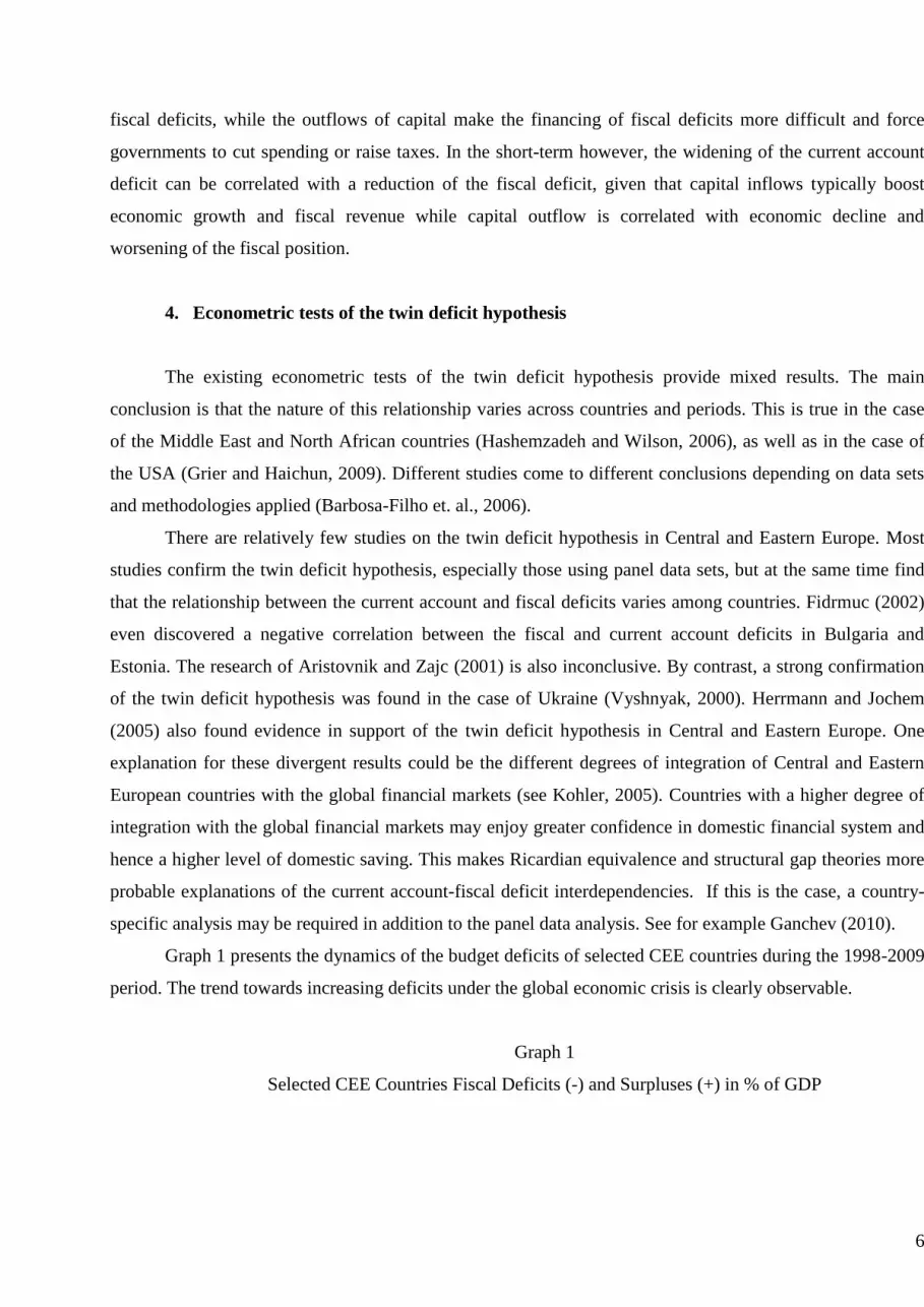
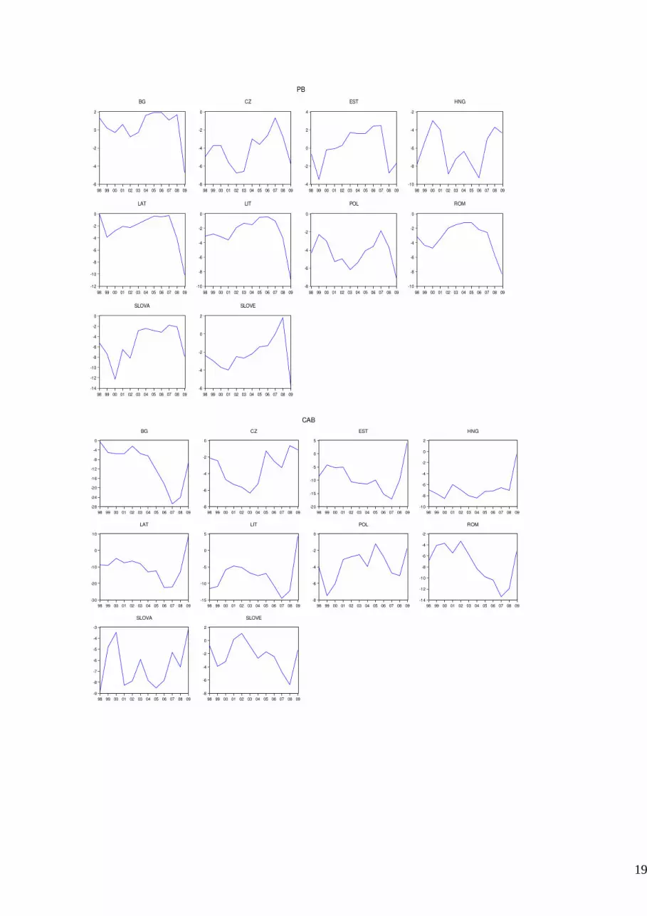
Graph 1 presents the dynamics of the budget deficits of selected CEE countries during the 1998-2009

period. The trend towards increasing deficits under the global economic crisis is clearly observable.

Graph 1

Selected CEE Countries Fiscal Deficits (-) and Surpluses (+) in % of GDP

7

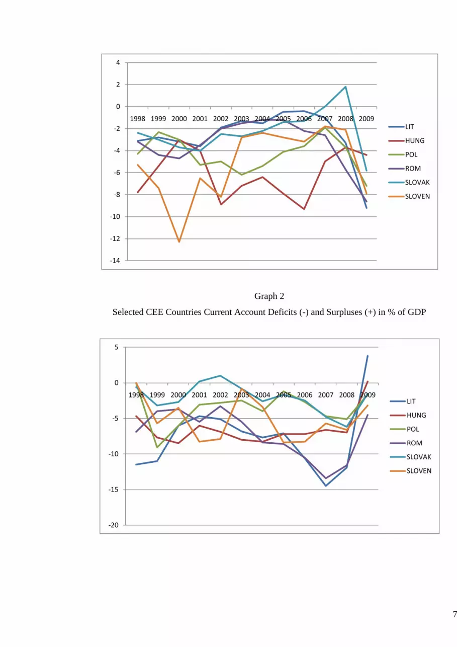
Graph 2

Selected CEE Countries Current Account Deficits (-) and Surpluses (+) in % of GDP

-14

-12

-10

-8

-6

-4

-2

0

2

4

1998 1999 2000 2001 2002 2003 2004 2005 2006 2007 2008 2009

LIT

HUNG

POL

ROM

SLOVAK

SLOVEN

-20

-15

-10

-5

0

5

1998 1999 2000 2001 2002 2003 2004 2005 2006 2007 2008 2009

LIT

HUNG

POL

ROM

SLOVAK

SLOVEN

8

In its turn the Graph 2 depicts selected CEE countries current accounts developments. Here also a

trend is observable but in terms of improving rather than worsening of deficits.

The econometric analysis of the relationship between the fiscal and current deficits usually involves

the application of Granger causality techniques (Chang and Hsu, 2009) and vector autoregression models

(Hashemzadeh and Wilson, 2006). In addition to the evaluation of the relationship between the two deficits

and their lagged values, the VAR models allow for the calculation of the so-called impulse responses and

variance decompositions. The impulse response analysis informs us about the dynamic impact of certain

variables, including their lagged values, on a given variable. The variance decomposition provides

information about the percentage of variation of a given variable that can be explained by its own lagged

values or other variables.

First we performed a standard panel regression of current account (dependent variable CAB) against

the budget deficit (independent variable PB). The regression equation is of the following type:

it it ity x u (6)

Were ity is the dependent variable, the current account balance of the i-th country in the period t and

itx is the independent variable, the budget balance of the i-th country in the period t.

An important precondition for good results under OLS is to avoid the omission of explanatory

variables. So we add a auxiliary dummy variable iz . Finally we obtain an extended equation:

it i it ity x u where i iz (7)

As a first step we perform and OLS regression without a dummy variable assuming that the current

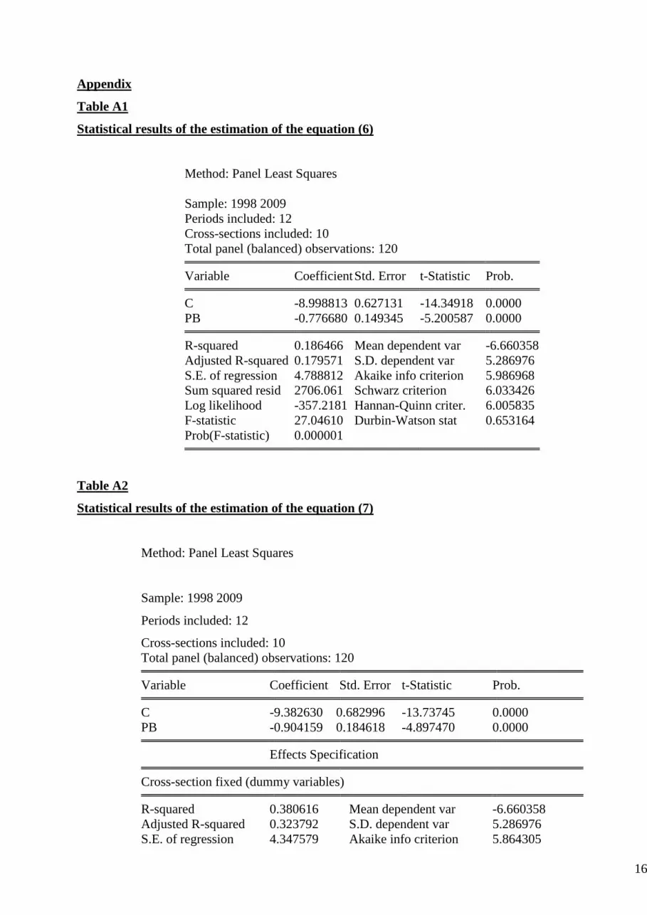
account balance (CAB) dynamics can be explained by fiscal balance variations (PB). The results are given in

the Table A1 in the Appendix.

Data does not support the existence of strong dependence between current account and fiscal sector

position- the value 2R is relatively small. The values of the standard error of the regression and the standard

deviation of the dependent variable also confirm that this type of regression equation does not give us a good

explanation of the dynamics of the dependent variable.

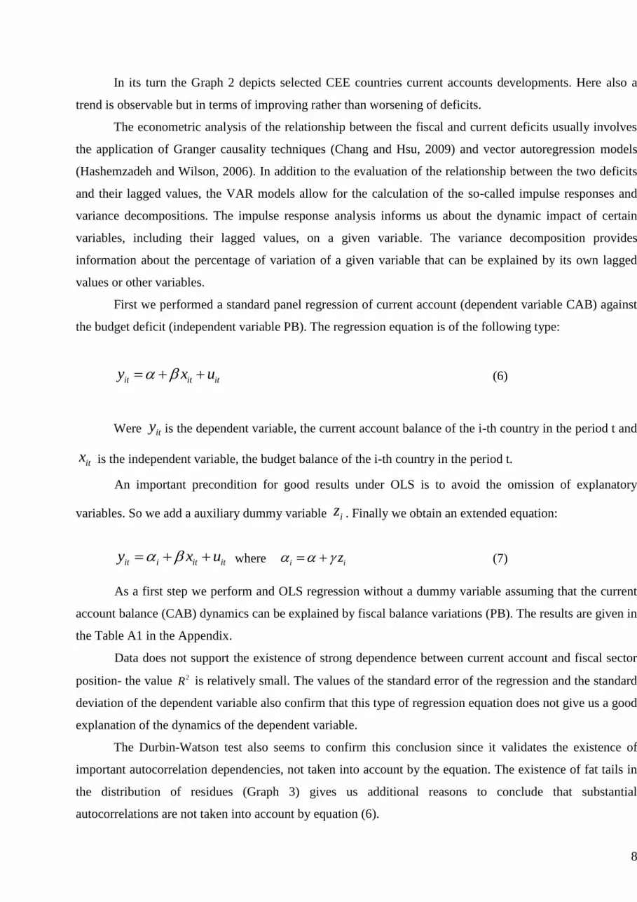
The Durbin-Watson test also seems to confirm this conclusion since it validates the existence of

important autocorrelation dependencies, not taken into account by the equation. The existence of fat tails in

the distribution of residues (Graph 3) gives us additional reasons to conclude that substantial

autocorrelations are not taken into account by equation (6).

9

Graph 3

Distribution of the residues itu

The results of the estimation of the equation (7) are given in the Table A2 in the Appendix. The

comparison of the estimations of (6) and (7) shows that the results of the latter have significantly better

statistical properties. The Akaike information criterion and Schwartz criterion as well as 2R return much

better values. We observe also slight decline of the standard deviation of the residues itu .

This leads us to the conclusion that we cannot explain the dynamics of CAB only by the variable PB.

This is substantiated by the values of the regression coefficients i = -9.382630 and = -0.904159 from

the Table A2 which corresponds to the и iz from (7). We can also rise the hypothesis that the current

account is influenced not by some additional variable, but mainly by its own lagged values. In the same time

we must admit, that the coefficients of the regression estimates of the equations (6) and (7) are significantly

different from zero, so the relationship between the current account and the fiscal deficit wile relatively

modest in terms of explanation of CAB dynamics, are nevertheless statistically meaningful.

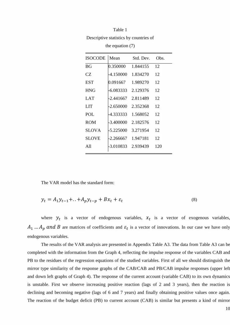
Table 1 presents the statistical results of the regression coefficient before the variable PB by

countries. The coefficients are negative for all countries with the exception of Bulgaria and Estonia. It means

that the twin deficits hypothesis is confirmed for all countries (the rise of fiscal deficit generates decline of

current account deficit and vice versa). Only in the case of Bulgaria and Estonia we observe an opposite

relationship- fiscal deficits are correlated with improvement of current accounts and surpluses coincide with

high current accounts deficits. The latter result coincides with the findings of Fidrmuc (2002) and Ganchev

(2010). Since the two countries apply a currency board regimes and rigorous fiscal policy characterized by

high fiscal surpluses in periods of intensive economic growth and minimal deficits under economic decline,

we must conclude, that this type of policy mix is not consistent with the twin deficit paradigm.

0

2

4

6

8

10

12

14

16

-15 -10 -5 0 5 10

Series: Standardized ResidualsSample 1998 2009Observations 120

Mean -6.59e-16Median 0.611942Maximum 12.20746Minimum -17.02684Std. Dev. 4.768649Skewness -0.708995Kurtosis 4.531571

Jarque-Bera 21.78201Probability 0.000019

10

Table 1

Descriptive statistics by countries of

the equation (7)

ISOCODE Mean Std. Dev. Obs.

BG 0.350000 1.844155 12

CZ -4.150000 1.834270 12

EST 0.091667 1.989270 12

HNG -6.083333 2.129376 12

LAT -2.441667 2.811489 12

LIT -2.650000 2.352368 12

POL -4.333333 1.568052 12

ROM -3.400000 2.182576 12

SLOVA -5.225000 3.271954 12

SLOVE -2.266667 1.947181 12

All -3.010833 2.939439 120

The VAR model has the standard form:

(8)

where is a vector of endogenous variables, is a vector of exogenous variables, are matrices of coefficients and is a vector of innovations. In our case we have only

endogenous variables.

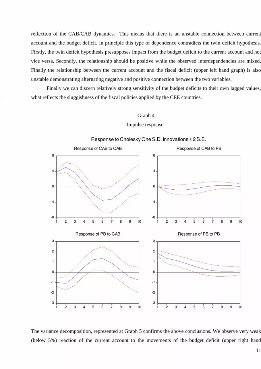
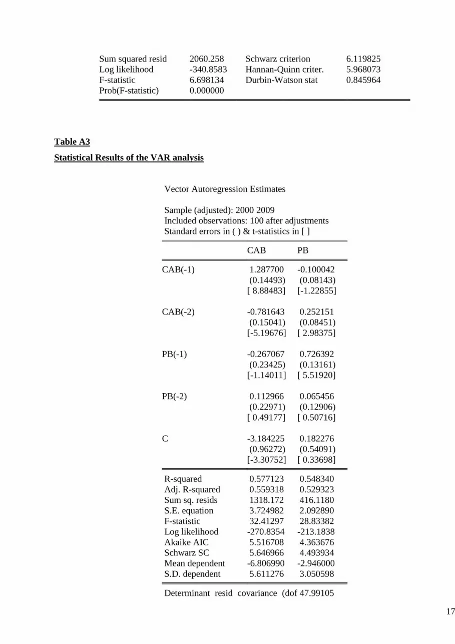
The results of the VAR analysis are presented in Appendix Table A3. The data from Table A3 can be

completed with the information from the Graph 4, reflecting the impulse response of the variables CAB and

PB to the residues of the regression equations of the studied variables. First of all we should distinguish the

mirror type similarity of the response graphs of the CAB/CAB and PB/CAB impulse responses (upper left

and down left graphs of Graph 4). The response of the current account (variable CAB) to its own dynamics

is unstable. First we observe increasing positive reaction (lags of 2 and 3 years), then the reaction is

declining and becoming negative (lags of 6 and 7 years) and finally obtaining positive values once again.

The reaction of the budget deficit (PB) to current account (CAB) is similar but presents a kind of mirror

11

reflection of the CAB/CAB dynamics. This means that there is an unstable connection between current

account and the budget deficit. In principle this type of dependence contradicts the twin deficit hypothesis.

Firstly, the twin deficit hypothesis presupposes impact from the budget deficit to the current account and not

vice versa. Secondly, the relationship should be positive while the observed interdependencies are mixed.

Finally the relationship between the current account and the fiscal deficit (upper left hand graph) is also

unstable demonstrating alternating negative and positive connection between the two variables.

Finally we can discern relatively strong sensitivity of the budget deficits to their own lagged values,

what reflects the sluggishness of the fiscal policies applied by the CEE countries.

Graph 4

Impulse response

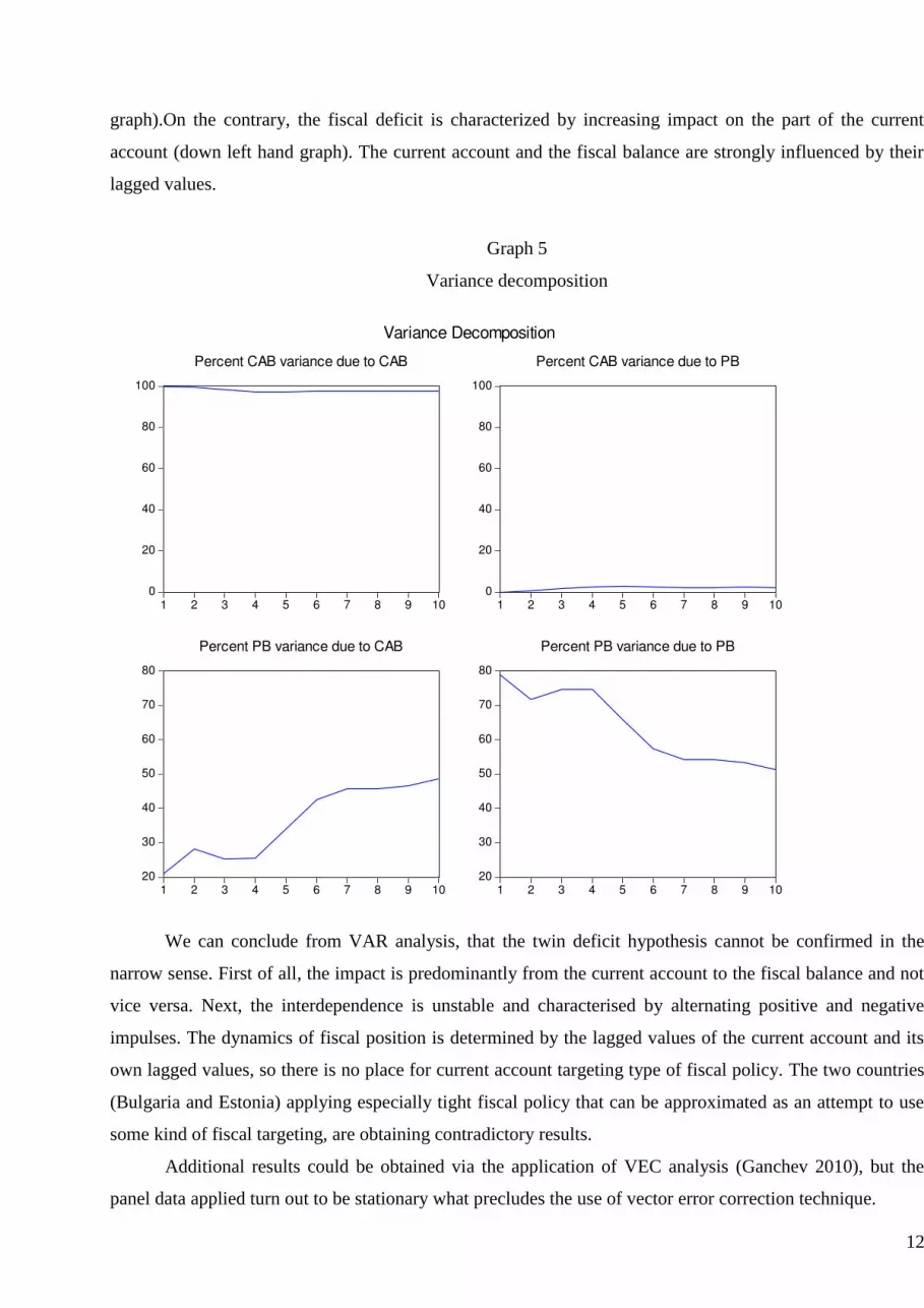
The variance decomposition, represented at Graph 5 confirms the above conclusions. We observe very weak

(below 5%) reaction of the current account to the movements of the budget deficit (upper right hand

-8

-4

0

4

8

1 2 3 4 5 6 7 8 9 10

Response of CAB to CAB

-8

-4

0

4

8

1 2 3 4 5 6 7 8 9 10

Response of CAB to PB

-3

-2

-1

0

1

2

3

1 2 3 4 5 6 7 8 9 10

Response of PB to CAB

-3

-2

-1

0

1

2

3

1 2 3 4 5 6 7 8 9 10

Response of PB to PB

Response to Cholesky One S.D. Innovations ± 2 S.E.

12

graph).On the contrary, the fiscal deficit is characterized by increasing impact on the part of the current

account (down left hand graph). The current account and the fiscal balance are strongly influenced by their

lagged values.

Graph 5

Variance decomposition

We can conclude from VAR analysis, that the twin deficit hypothesis cannot be confirmed in the

narrow sense. First of all, the impact is predominantly from the current account to the fiscal balance and not

vice versa. Next, the interdependence is unstable and characterised by alternating positive and negative

impulses. The dynamics of fiscal position is determined by the lagged values of the current account and its

own lagged values, so there is no place for current account targeting type of fiscal policy. The two countries

(Bulgaria and Estonia) applying especially tight fiscal policy that can be approximated as an attempt to use

some kind of fiscal targeting, are obtaining contradictory results.

Additional results could be obtained via the application of VEC analysis (Ganchev 2010), but the

panel data applied turn out to be stationary what precludes the use of vector error correction technique.

0

20

40

60

80

100

1 2 3 4 5 6 7 8 9 10

Percent CAB variance due to CAB

0

20

40

60

80

100

1 2 3 4 5 6 7 8 9 10

Percent CAB variance due to PB

20

30

40

50

60

70

80

1 2 3 4 5 6 7 8 9 10

Percent PB variance due to CAB

20

30

40

50

60

70

80

1 2 3 4 5 6 7 8 9 10

Percent PB variance due to PB

Variance Decomposition

13

5. Conclusions

This paper studied the theoretical underpinnings of the twin deficit hypothesis and tested various

interpretations of this hypothesis on a sample of CEE countries panel data. The main findings can be

summarised as follows.

The panel type regression confirms the existence of positive connection between the current account

and fiscal balance. The connection however is not very significant and the application of control dummy

variable reveals that factors other the fiscal deficit should affect the dependent variable. There are also two

exceptions to the rule- Bulgaria and Estonia, were we can observe negative relationship between the current

account and fiscal balance. The letter results coincide with the earlier findings of Fidrmuc (2002) and

Ganchev (2010).

The VAR analysis gives additional interesting results. It does not confirm the existence of robust

positive relationship between the current account and the fiscal balance but rather the opposite. In the same

time it yields strong impact from the current account to the fiscal balance what contradicts in principle the

twin deficit hypothesis. The fiscal position is determined by the current account dynamics and the lagged

values of the fiscal deficit. Under these conditions we can assume some kind of current account targeting if

and only if we accept the hypothesis, that the impact of the current account is disguising a deliberate policy

of the fiscal authorities to use the fiscal instrument against the negative current account trends with lag

between 4 and 8 years. Additional research is needed to confirm or reject this hypothesis.

At this stage the rational expectations and structural gap theories seem to be a better explanation of

the existing data than the twin deficit hypothesis.

The results for Bulgaria and Estonia require further explanation. In these two cases we can reject the

twin deficits hypothesis because of the positive relationship between the current account and the fiscal

balance on the basis of regression analysis. This rejection is especially intriguing given the fact that both

countries are pursuing stringent fiscal policies with special emphasize on the current account targeting.

Additional research is necessary to clarify the connection between the currency board regimes imposed in

these countries and the twin deficit concept based fiscal policies.

14

Literature

Abell, J. (1980).Twin Deficits during the 1980s: An Empirical Investigation. Journal of

Macroeconomics, 1990, 12, рр. 81-96.

Aristovnik, A. , Zajc, K. (2001). Current Account performance and Fiscal Policy: Evidence on the

Twin Deficits in Central and Eastern Europe. INFER, Annual Conference- Economics of Transition: Theory,

Experience and EU Enlargement.

Barbosa-Filho N., Rada C., Taylor L., Zamparelly L. (2006). Fiscal, Foreign and Private Net

Borrowing: Widely Accepted Theories Don’t Closely Fit the Facts. Federal University of Rio de Janeiro,

Department of Economic and Social Affairs (DESA), United Nations, and Schwartz Center for Economic

Policy Analysis, New School

Barro, R. J. (1989). The Ricardian Approach to Budget Deficits. Journal of Economic Perspectives,

3:2, рр 37-54.

Chang, J-C, Hsu Z. (2009). Causality Relationships between the Twin Deficits in the Regional

Economy. Department of Economics, National Chi Nan University.

Dos Santos C.H., Silva A.C.M. (2009). Revisiting “New Cambridge”: the Three Financial Balances

in a General Stock-Flow Consistent Applied Modeling Strategy, Texto para Discussão. IE/UNICAMP,

Campinas, n. 169, out. 2009.

Feyrer J., Scambaugh J.C. (2009). Global Saving and Global Investment: The Transmission of

Identified Fiscal Shocks. NBER, Working Paper Series, June 2009.

Fidrmuc J. (2002). Twin Deficits: Implications of Current Account and Fiscal Imbalances for the

Accession Countries. Focus on Transition, 2/2002, pp. 72-83

Ganchev G. (2010), The Twin Deficit Hypothesis: The Case of Bulgaria. Financial theory and

Practice 34 (4) pp. 357-377

Gandolfo G. (1987). International Monetary Theory and Open Economy Macroeconomics.

International Еconomics II, Springer-Verlag, pp. 280-285

Granger C. (1981). Some properties of time series data and their use in econometric model

specification. Journal of Econometrics, 1981/16, pp. 121-130

Grier K. and Haichun Y. (2009). Twin Sons of Different Mothers: The Long and the Short of the

Twin Deficit Debate. Economic Inquiry, vol. 47, No 4, October 2009, pp. 625-638

Harberger A. (2008). Lessons from Monetary and Real Exchange Rate Economics. Cato Journal,

Vol. 28, No. 2 (Spring/Summer 2008), pp. 225-235

15

Hashemzadeh N., Wilson L. (2006). The Dynamics of Current Account and Budget Deficits in

Selected Countries in the Middle East and North Africa. International Research Journal of Finance and

Economics, Issue 5, 2006, pp. 111-129

Herrmann S., Jochen A. (2005). Determinants of Current Account Developments in the Central and

East European EU Member States –Consequences for the Enlargement of the Euro Area. Bundesbank,

Discussion Papers, Series 1: Economic Studies No 32/2005

Johnson H. (1977). The Monetary Approach to the Balance of Payments: A Nontechnical Guide.

Journal of International Economics, vol. 7, pp. 251-68

Kohler M. (2005). International Capital Mobility and Current Account Targeting in Central and

Eastern European Countries. Centre for European Economic Research (ZEW), Discussion Paper No. 05-51

Polak J. J. (1997). The IMF Monetary Model at Forty, International Monetary Fund, WP/97/49

Polak J. J. (2001). The Two Monetary Approaches to the Balance of Payments: Keynesian and

Johnsonian. International Monetary Fund, WP/01/100

Summers L. H. (1988). Tax Policy and International Competitiveness, in J. Frenkel (eds)

International Aspects of Fiscal Policies, Chicago UP, pp. 349-375

Vyashnyak O. (2000). Twin Deficit Hypothesis: The Case of Ukraine. National University “Kyiv-

Mohyla Academy”

16

Appendix

Table A1

Statistical results of the estimation of the equation (6)

Method: Panel Least Squares Sample: 1998 2009 Periods included: 12 Cross-sections included: 10 Total panel (balanced) observations: 120 Variable Coefficient Std. Error t-Statistic Prob. C -8.998813 0.627131 -14.34918 0.0000 PB -0.776680 0.149345 -5.200587 0.0000 R-squared 0.186466 Mean dependent var -6.660358 Adjusted R-squared 0.179571 S.D. dependent var 5.286976 S.E. of regression 4.788812 Akaike info criterion 5.986968 Sum squared resid 2706.061 Schwarz criterion 6.033426 Log likelihood -357.2181 Hannan-Quinn criter. 6.005835 F-statistic 27.04610 Durbin-Watson stat 0.653164 Prob(F-statistic) 0.000001

Table A2

Statistical results of the estimation of the equation (7)

Method: Panel Least Squares

Sample: 1998 2009

Periods included: 12

Cross-sections included: 10 Total panel (balanced) observations: 120 Variable Coefficient Std. Error t-Statistic Prob. C -9.382630 0.682996 -13.73745 0.0000 PB -0.904159 0.184618 -4.897470 0.0000 Effects Specification Cross-section fixed (dummy variables) R-squared 0.380616 Mean dependent var -6.660358 Adjusted R-squared 0.323792 S.D. dependent var 5.286976 S.E. of regression 4.347579 Akaike info criterion 5.864305

17

Sum squared resid 2060.258 Schwarz criterion 6.119825 Log likelihood -340.8583 Hannan-Quinn criter. 5.968073 F-statistic 6.698134 Durbin-Watson stat 0.845964 Prob(F-statistic) 0.000000

Table A3

Statistical Results of the VAR analysis

Vector Autoregression Estimates Sample (adjusted): 2000 2009 Included observations: 100 after adjustments Standard errors in ( ) & t-statistics in [ ] CAB PB CAB(-1) 1.287700 -0.100042 (0.14493) (0.08143) [ 8.88483] [-1.22855] CAB(-2) -0.781643 0.252151 (0.15041) (0.08451) [-5.19676] [ 2.98375] PB(-1) -0.267067 0.726392 (0.23425) (0.13161) [-1.14011] [ 5.51920] PB(-2) 0.112966 0.065456 (0.22971) (0.12906) [ 0.49177] [ 0.50716] C -3.184225 0.182276 (0.96272) (0.54091) [-3.30752] [ 0.33698] R-squared 0.577123 0.548340 Adj. R-squared 0.559318 0.529323 Sum sq. resids 1318.172 416.1180 S.E. equation 3.724982 2.092890 F-statistic 32.41297 28.83382 Log likelihood -270.8354 -213.1838 Akaike AIC 5.516708 4.363676 Schwarz SC 5.646966 4.493934 Mean dependent -6.806990 -2.946000 S.D. dependent 5.611276 3.050598 Determinant resid covariance (dof 47.99105

18

adj.) Determinant resid covariance 43.31192 Log likelihood -472.2091 Akaike information criterion 9.644182 Schwarz criterion 9.904699

Graph A1

Public Deficits (PB) and current account (CAB) graphs of the CEE countries

19

-6

-4

-2

0

2

98 99 00 01 02 03 04 05 06 07 08 09

BG

-8

-6

-4

-2

0

98 99 00 01 02 03 04 05 06 07 08 09

CZ

-4

-2

0

2

4

98 99 00 01 02 03 04 05 06 07 08 09

EST

-10

-8

-6

-4

-2

98 99 00 01 02 03 04 05 06 07 08 09

HNG

-12

-10

-8

-6

-4

-2

0

98 99 00 01 02 03 04 05 06 07 08 09

LAT

-10

-8

-6

-4

-2

0

98 99 00 01 02 03 04 05 06 07 08 09

LIT

-8

-6

-4

-2

0

98 99 00 01 02 03 04 05 06 07 08 09

POL

-10

-8

-6

-4

-2

0

98 99 00 01 02 03 04 05 06 07 08 09

ROM

-14

-12

-10

-8

-6

-4

-2

0

98 99 00 01 02 03 04 05 06 07 08 09

SLOVA

-6

-4

-2

0

2

98 99 00 01 02 03 04 05 06 07 08 09

SLOVE

PB

-28

-24

-20

-16

-12

-8

-4

0

98 99 00 01 02 03 04 05 06 07 08 09

BG

-8

-6

-4

-2

0

98 99 00 01 02 03 04 05 06 07 08 09

CZ

-20

-15

-10

-5

0

5

98 99 00 01 02 03 04 05 06 07 08 09

EST

-10

-8

-6

-4

-2

0

2

98 99 00 01 02 03 04 05 06 07 08 09

HNG

-30

-20

-10

0

10

98 99 00 01 02 03 04 05 06 07 08 09

LAT

-15

-10

-5

0

5

98 99 00 01 02 03 04 05 06 07 08 09

LIT

-8

-6

-4

-2

0

98 99 00 01 02 03 04 05 06 07 08 09

POL

-14

-12

-10

-8

-6

-4

-2

98 99 00 01 02 03 04 05 06 07 08 09

ROM

-9

-8

-7

-6

-5

-4

-3

98 99 00 01 02 03 04 05 06 07 08 09

SLOVA

-8

-6

-4

-2

0

2

98 99 00 01 02 03 04 05 06 07 08 09

SLOVE

CAB