Testing the expected utility maximization hypothesis

with limited experimental data

James B. Coopera, Thomas Russellb,*, Paul A. Samuelsonc

aMathematics Department, Johannes Kepler University, Linz, USAbDepartment of Economics, Santa Clara University,

300 Kenna Hall, Santa Clara, CA 95063, USAcDepartment of Economics, Massachusetts Institute

of Technology, Cambridge, MA, USA

Received 4 April 2003; received in revised form 1 December 2003; accepted 8 December 2003

Abstract

In this article we use some old ideas of Franklin to derive the partial differential equation (St Robert

Equation) characterizing the level curves of expected utility maximizing preferences over simple

gambles. We also provide conditions under which an incomplete family of level curves permits an

investigator to determine whether or not the subject maximizes expected utility and if so under what

conditions preferences can be recovered uniquely.

# 2004 Elsevier B.V. All rights reserved.

Keywords: Expected utility; Limited experimental data; Recovering preferences

1. Introduction

Despite the appeal of its axiomatic foundations, the expected utility maximization

hypothesis is only one among many theories of how individuals take decisions under

uncertainty. To an empiricist, any claim of this hypothesis to preeminence must be based on

its superior predictive performance.

One way to compare such performance is to present an individual with a parameterized

family of probability density functions and ask him/her to indicate those parameter

combinations over which they are indifferent. The resulting family of level curves in

parameter space would presumably have one shape if the individual maximized expected

utility and a different shape if behavior followed some other rule. To exploit such data, of

Japan and the World Economy

16 (2004) 391–407

* Corresponding author. Tel.: þ1-408-554-6953; fax: þ1-408-554-2331.

E-mail address: trussell@scu.edu (T. Russell).

0922-1425/$ – see front matter # 2004 Elsevier B.V. All rights reserved.

doi:10.1016/j.japwor.2003.12.005

course, it is necessary to know the mathematical form of the shape of the level curves in the

case in which the subject is an expected utility maximizer (EUM).1

In this paper, we examine a general approach to this question using a neglected technique

due to Franklin (1927). As a by-product of this technique, we examine in detail the

experiment in which the individual reports the certainty equivalence of the gamble in which

they are given equal chances to gain $x and lose $y. We show how to recover the utility

function (up to linear transforms) when expected utility is being maximized in this case.

Finally we address the question of what can be learned when experimental data is limited.

We will show that in this experimental setting, knowing even an infinite number of level

curves is not enough to verify expected utility maximization, though knowledge of three

level curves may be sufficient to rule it out. Moreover, even if we make the strong

assumption that the individual is an EUM, and even if we know an infinite number of level

curves, we cannot determine preferences uniquely, because in this case there can still be an

infinite number of different expected utility maximizing preferences consistent with the

data. We investigate the case of two given level curves in depth and characterize all

possible utility functions consistent with the given curves in this case. The whole paper

may be read as an extension of the recent paper by Samuelson (in press).

2. Franklin’s method

The method developed by Franklin was motivated by a problem in classical physics, but

its relationship to economics is easily seen. Franklin assumed that a family of level curves

in the plane had been obtained experimentally, and asked how we would know if they could

have been generated as the ‘‘indifference curves’’ of a harmonic function H (i.e. a function

of two variables for which Hxx þ Hyy ¼ 0).

To see the relevance of this for the testing of economic behavior, consider the experiment

recently discussed by Samuelson (op.cit.) He examines indifference curves in the para-

meter space x, y, where the set of probability density functions to be evaluated are delta

functions which offer a gain of $x with probability 1/2 and loss of $y with probability 1/2.

Assume initially that these are the level curves z ¼ c of the function

z ¼ f ðx; yÞwhere z gives the dollar equivalent of the gamble. By the nature of the experiment, f is a

symmetric function. An individual will be an EUM if the function f can be recalibrated to

have the form2

12

UðxÞ þ 12

UðyÞ (1)

1 In the case of the ‘‘Matschak/Machina triangle,’’ it is well known that the level curves of an EUM are

parallel straight lines Matschak (1950), Machina (1982) and deviations from this shape can be used to

characterize various non expected utility maximizing models, see Camerer (1995). More generally Schneeweiss

(1966) and Chipman (1973) have discussed the shape of EUM level curves on the parameters of a number of

standard probability density functions including the Gaussian and the LEvy-stable class.2 Technically this requires the existence of a diffeomorphism F with the property that F(f) has this form for a

suitable function U of one variable.

392 J.B. Cooper et al. / Japan and the World Economy 16 (2004) 391–407

Bearing in mind that a function f of two variables splits as the sum of two separate

functions of the variables (i.e. f (x, y) has the form gðxÞ þ hðyÞ) if and only if (under suitable

smoothness assumptions and for appropriate domains of definition) its mixed partial

derivative @2f=@x@y vanishes, we see that the mathematical question becomes ‘‘When does

a function f of two variables have a reparameterization gðx; yÞ ¼ Fðf ðx; yÞÞ which satisfies

the partial differential equation gxy ¼ 0’’? Fortunately Franklin’s method can be extended

to deal with the general second- order linear partial differential operator as in the following

result.

Theorem 1. We consider the general second-order linear partial differential operator

Lðf Þ ¼P2

i;j¼1aijfij þP2

l¼1bifl where the aij and the bl are smooth functions applied to a

smooth function f (all functions of two variables). We use the subscript notation to denote

partial derivatives (e.g. f11 and f12 denote @2f=@x2 and @2f=@x@y, respectively). Then there

is a recalibration u ¼ F � f of f which satisfies the partial differential equation if and only if

LðuÞ ¼ 0 and only if the expression

Fðf Þ ¼P2

ij¼1aijfij þP2

l¼1blflP2i;j¼1aijfifj

(2)

is constant on the level curves of f.

Proof. Substitute the above operator for the Laplace operator in Franklin’s proof and

follow the steps given there. &

In order to obtain a representation as a partial differential equation we simply take the

directional derivatives of the F(f) along the level curves of f, i.e. in the direction

perpendicular to the gradient of f and set them equal to zero. This leads to the (third-

order) equation:

�f2@

@xþ f1

@

@y

� �Fðf Þ ¼ 0 (3)

It is a routine, if rather tedious, exercise to compute the explicit form of this equation. It can

be done by hand or by using a symbolic differentiation program such as Mathematica. For

our purposes it will suffice to consider some explicit cases where the computations are

quite tractable.

Example 1 (The Samuelson Case). For the experiment presenting the subject with a pair

of equal probability delta functions, we obtain the equation Fðf Þ ¼ fxy=fxfy and so we

obtain the equation:

�fy

@

@x

fxy

fxfy

� �þ fx

@

@y

fxy

fxfy

� �¼ 0 (4)

J.B. Cooper et al. / Japan and the World Economy 16 (2004) 391–407 393

(In such concrete situations it is more convenient to denote the partials by letter subscripts

than by numerical subscripts). This leads to the equation:3

�f 2y ðfxfxxy � fxyfxxÞ þ f 2

x ðfyfxyy � fxyfyyÞ ¼ 0 (5)

which was obtained by Samuelson.

This equation is one of a number of characterizations of a hexagonal 3-web in the plane.

Here, the 3-web consists of the level curves, the verticals, and the horizontals.4 This

geometrical approach to EUM drawing on the work of Thomsen, Blaschke, and Bol is the

basis of Debreu (1960) implicit characterization of EUM behavior. We return to this point

later.

Example 2 (The Gaussian Case). In this paper, we concentrate on the simple delta

function experiment. To show the power of the Franklin approach, however, we briefly

demonstrate its applicability to experimental curves obtained as the level curves defined on

the parameter space m, s of a family of Gaussians. This case is discussed by Chipman

(op.cit.) and Schneeweiss (op.cit.). The key observation from the Franklin viewpoint is that

the Gaussian family

Nðm; sÞ ¼ s�1ð2pÞ�1=2exp �ðx � mÞ2

2s2

!

satisfies the second-order differential parameter restriction:

s�1 @N

@s¼ @2N

@m2

in the parameters m and s.

Since expected utility is a linear operator on density functions, this restriction will be

inherited by the level curves of an EUM drawn on the family of Gaussians parameterized

by mean and standard deviation.

In our terms, we have

Lðf Þ ¼ @2

@x2� y�1 @

@y

so that the condition is that

fy

ðy � fxxÞf 2x

be constant along level curves. The differential equation is thus

�fy@

@x

fy

ðy � fxxÞf 2x

� �þ fx

@

@y

fy

ðy � fxxÞf 2x

� �¼ 0 (6)

3 Professor Goldberg has pointed out that in web geometry this equation is known as the St. Robert equation,

see Akivis and Shelekhov (1992, p. 43).4 A very fruitful alternative characterization notes that the Blaschke/Chern curvature 2-form of this 3-web

must be zero, see Russell (2003).

394 J.B. Cooper et al. / Japan and the World Economy 16 (2004) 391–407

which leads to the equation

fxfy

fxy

y � fxxx

� �� f 2

x

yfyy � fy

y2 � fyxx

� �þ 2

fy

y � fxx

� �ðfxfxx � fyfxxÞ ¼ 0 (7)

cf. Chipman (op.cit.) Eq. (2.33). This equation is necessary but not sufficient. Sufficient

conditions are given by Chipman (op.cit.).

Clearly we may apply this approach to any family of density functions so long as there

is some parameterization which satisfies a second-order partial differential restriction.

Of course, this approach can also be applied to suitable systems of equations and to

equations in higher dimensions (this was one of the reasons for the use of the summation

notation in the formulation of Theorem 1). Thus, the authors have computed ‘‘uncali-

brated’’ versions of the Cauchy–Riemann equations (i.e. equations which determine

when the level curves of two given functions u and v are in fact the level curves of the

real and imaginary parts of an analytic function) and the Laplacian operator in higher

dimensions. Interestingly, in the latter case the uncalibrated version of the Laplace

equation is a system of third-order equations. (Details are available from the authors on

request.)

We now return to the Samuelson delta function experiment, however, to show how the

Franklin approach allows us to recover the utility function from the experimental level

curves.

3. Recovering the utility function 1: full information

When we are given a family of level curves which satisfy the Samuelson PDE (5), we can

be certain that some expected utility function is being maximized. We cannot hope to

recover the underlying utility function U uniquely, since any linear transformation aU þ b;

a; b > 0 will describe the underlying preferences just as well. We therefore now show how

to use the experimental level curves to recover U00/U0, the Arrow/Pratt risk aversion

coefficient, from which all members of the class of utility functions representing the same

preferences can be obtained by integration.

We have

Result 1. When a family of level curves satisfies the Samuelson PDE, the Arrow/Pratt risk

aversion coefficient U00/U0 is given by U00=U0 ¼ d log S=dx where S is the slope function

S ¼ fx=fy

Proof. By a simple calculation from Eq. (1) we have F0fx ¼ ð1=2ÞU0 and F00f 2x þ F0fxx ¼

ð1=2ÞU00. Since F00/F0 satisfies the Samuelson PDE, we have F00=F0 ¼ �fxy=fxfy. The

formula then follows by re-arrangement. &

Result 1 sheds light on a number of special cases.

Case 1 (Homotheticity). Suppose that in addition to satisfying the Samuelson PDE, the

family of level curves is homothetic. Then Burk (1936, p. 42) showed that the resulting

J.B. Cooper et al. / Japan and the World Economy 16 (2004) 391–407 395

utility function was of the class now called in financial economics CRRA, i.e. Constant

Relative Risk Averse.5 This class satisfies �U00=U0 ¼ 1=kx for some constant k. By Result

1, the level curves must therefore satisfy d log S=d log x ¼ r (some constant), i.e. the

elasticity of substitution must be a constant.

Case 2 (HARA). As a generalization of the homothetic level curves, we have the curves

which are homothetic to a point possibly not the origin. Such systems are sometimes

called quasihomothetic. In this case, the utility function belongs to the class of functions

which satisfy the differential equation U00=U0 ¼ 1=gðx � x0Þ By setting x0 ¼ 0 we

recover the CRRA class, and by setting x0 ¼ 1 we have the case of constant absolute

risk aversion CARA.6 Obviously, an EUM will have HARA preferences if and only

if the slope of the experimental level curves satisfies the equation d log S=dx ¼ð1=gðx � x0ÞÞ.

4. Recovering the utility function 2: limited information

When we are given the complete family of level curves of a function which satisfies the

Samuelson PDE (5), we can recover preferences by solving a differential equation. It

remains to discuss what happens if we are given less than complete information. In the

present section, we explore what can be said if we are given a finite number of curves. Two

issues arise.

(1) How much information do we need in order to determine whether or not the

individual is an EUM? This can be regarded as an existence problem—given a finite

family of curves, can they be embedded into a complete family which satisfies

Samuelson’s condition?

(2) If we take it as given that an individual maximizes expected utility, how much

information do we need to determine which utility function describes the preferences?

This can be regarded as a uniqueness problem—we assume a priori that a family of

curves can be embedded into a complete family satisfying Samuelson’s condition and

ask whether the latter family is then unique. (This can be thought of as a type of

boundary problem.)7

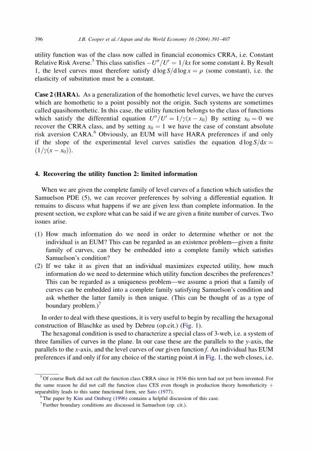
In order to deal with these questions, it is very useful to begin by recalling the hexagonal

construction of Blaschke as used by Debreu (op.cit.) (Fig. 1).

The hexagonal condition is used to characterize a special class of 3-web, i.e. a system of

three families of curves in the plane. In our case these are the parallels to the y-axis, the

parallels to the x-axis, and the level curves of our given function f. An individual has EUM

preferences if and only if for any choice of the starting point A in Fig. 1, the web closes, i.e.

5 Of course Burk did not call the function class CRRA since in 1936 this term had not yet been invented. For

the same reason he did not call the function class CES even though in production theory homotheticity þseparability leads to this same functional form, see Sato (1977).

6 The paper by Kim and Omberg (1996) contains a helpful discussion of this case.7 Further boundary conditions are discussed in Samuelson (op. cit.).

396 J.B. Cooper et al. / Japan and the World Economy 16 (2004) 391–407

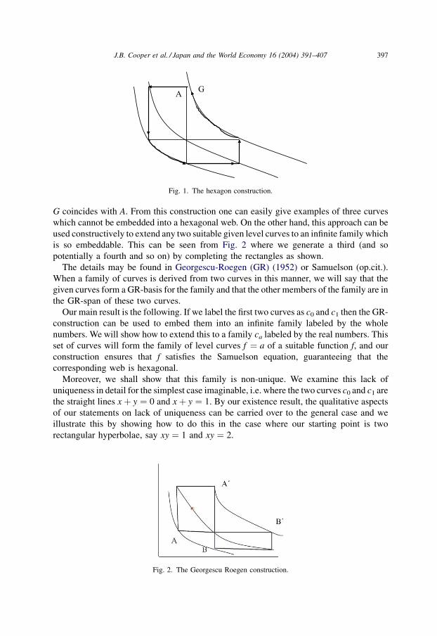
G coincides with A. From this construction one can easily give examples of three curves

which cannot be embedded into a hexagonal web. On the other hand, this approach can be

used constructively to extend any two suitable given level curves to an infinite family which

is so embeddable. This can be seen from Fig. 2 where we generate a third (and so

potentially a fourth and so on) by completing the rectangles as shown.

The details may be found in Georgescu-Roegen (GR) (1952) or Samuelson (op.cit.).

When a family of curves is derived from two curves in this manner, we will say that the

given curves form a GR-basis for the family and that the other members of the family are in

the GR-span of these two curves.

Our main result is the following. If we label the first two curves as c0 and c1 then the GR-

construction can be used to embed them into an infinite family labeled by the whole

numbers. We will show how to extend this to a family ca labeled by the real numbers. This

set of curves will form the family of level curves f ¼ a of a suitable function f, and our

construction ensures that f satisfies the Samuelson equation, guaranteeing that the

corresponding web is hexagonal.

Moreover, we shall show that this family is non-unique. We examine this lack of

uniqueness in detail for the simplest case imaginable, i.e. where the two curves c0 and c1 are

the straight lines x þ y ¼ 0 and x þ y ¼ 1. By our existence result, the qualitative aspects

of our statements on lack of uniqueness can be carried over to the general case and we

illustrate this by showing how to do this in the case where our starting point is two

rectangular hyperbolae, say xy ¼ 1 and xy ¼ 2.

A G

Fig. 1. The hexagon construction.

Fig. 2. The Georgescu Roegen construction.

J.B. Cooper et al. / Japan and the World Economy 16 (2004) 391–407 397

The consequences of this result for the problems we mentioned above can be stated

informally as follows:

Case 1 (The EUM hypothesis when one level curve is known). It is clear from the above

discussion that knowing one level curve of a postulated utility function provides no

information on the EUM hypothesis whatsoever.

In particular, we cannot tell whether the EUM hypothesis is satisfied and even if we

assume a priori that it is, we cannot deduce information about further level curves since we

can choose a second curve at random (within the parameters of our results) and embed it as

below into a full family of curves which satisfy the Samuelson condition.

Case 2 (The EUM hypothesis when two curves are known). Again the knowledge of

two curves alone can provide no information on whether the EUM hypothesis is satisfied or

not and the questions we examine are the following: Given two curves, are we always

permitted to assume that there is some set of EU maximizing preferences whose level

curves include the two given curves, and if so are these EU preferences unique? Stated

more mathematically, this asks: Given two curves, can we embed them into a hexagonal

web and if so, in many ways? The following theorems deal with these questions. The first

covers existence:

Theorem 2. Suppose that we have two diagonally symmetric curves in suitable position

(this will be made precise below). Then there exists a symmetric function z ¼ f ðx; yÞ whose

level curves contain the two given curves and which satisfies the Samuelson equation (so

that its level curves, together with the parallels to the axes as above, form a hexagonal web).

We will sketch a proof of this result in the appendix.8

It follows from this result that there exists a function U which is unique up to a linear

change of variable which is such that the family of curves is the level curves of the function

U(z) where UðzÞ ¼ ð1=2ÞðUðxÞþUðyÞÞ.We now turn to the question of uniqueness. We remark that the web condition that we are

considering is clearly unchanged under the coordinate transformation:

Z ¼ UðzÞ; X ¼ UðxÞ; Y ¼ UðyÞsince this leaves the parallels to the axes unchanged.

This transforms our two initial curves into two of the parallel lines from the family

1=2ðx þ yÞ ¼ c, which we assume for simplicity to be the curves with c ¼ 0 and c ¼ 1.

This can be used to translate the qualitative aspects of the following result on uniqueness

over to the general case:

Theorem 3. Denote the two curves x þ y ¼ 0 and x þ y ¼ 1 by c0 and c1. Then for any

‘‘small perturbation’’ g which satisfies the condition that g is an odd periodic function, i.e.

satisfies the conditions gð�xÞ ¼ �gðxÞ and gðxÞ ¼ gð1 þ xÞ, we have:

8 A more rigorous and complete treatment of the mathematical aspects of this paper is in preparation.

398 J.B. Cooper et al. / Japan and the World Economy 16 (2004) 391–407

The family of level curves of the function f ðx;yÞ ¼ ð1=2ÞðgðxÞþgðyÞÞ contains c0 and c1

and satisfies Samuelson’s condition. Furthermore, any such family is of this form.

We remark here that the smallness of the perturbation mentioned in the formulation is

such as to ensure that the perturbed identity functionfðxÞ ¼ x þ gðxÞ be a diffeomorphism.

It is, for example, well known that this is the case if the Lipschitz-constant of g is smaller

than one.

Remark. The linear web wðx; yÞ ¼ z associated with any such function V is of the form

f 12ðUðxÞ þ gðUðxÞ

� �þ UðyÞ þ gðUðyÞÞÞÞ ¼ z (8)

where f is the inverse of U þ gðUÞ, this to ensure that on the diagonal of the web

wðx; xÞ ¼ fðx; xÞ ¼ x, a condition required by the nature of the experiment generating the

data.

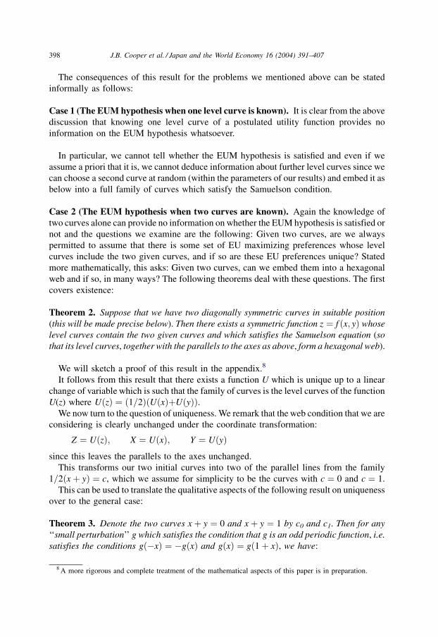
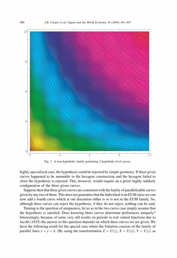
Example. We illustrate the non-uniqueness result with an example. Suppose that the two

given curves are rectangular hyperbolae. Then of course, there is a simple and natural way

to embed them into a hexagonal web. We simply use the family xy ¼ c since the function

f ðx; yÞ ¼ xy clearly satisfies the Samuelson equation. However, there are many other ways

and Fig. 3 shows a non-hyperbolic family which satisfies this condition and which is

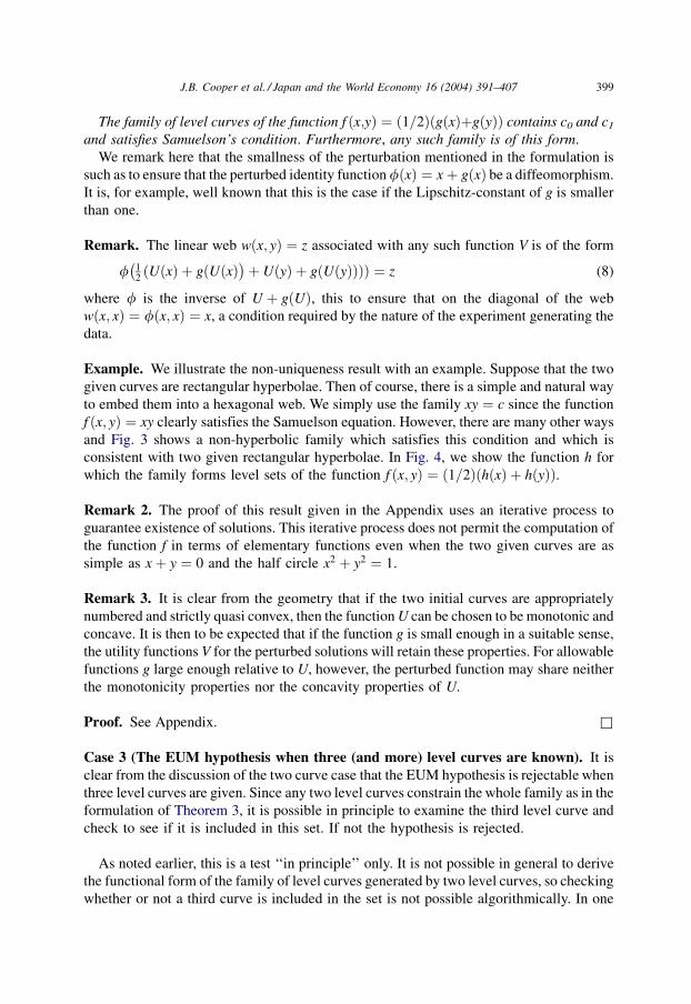
consistent with two given rectangular hyperbolae. In Fig. 4, we show the function h for

which the family forms level sets of the function f ðx; yÞ ¼ ð1=2ÞðhðxÞ þ hðyÞÞ.

Remark 2. The proof of this result given in the Appendix uses an iterative process to

guarantee existence of solutions. This iterative process does not permit the computation of

the function f in terms of elementary functions even when the two given curves are as

simple as x þ y ¼ 0 and the half circle x2 þ y2 ¼ 1.

Remark 3. It is clear from the geometry that if the two initial curves are appropriately

numbered and strictly quasi convex, then the function U can be chosen to be monotonic and

concave. It is then to be expected that if the function g is small enough in a suitable sense,

the utility functions V for the perturbed solutions will retain these properties. For allowable

functions g large enough relative to U, however, the perturbed function may share neither

the monotonicity properties nor the concavity properties of U.

Proof. See Appendix. &

Case 3 (The EUM hypothesis when three (and more) level curves are known). It is

clear from the discussion of the two curve case that the EUM hypothesis is rejectable when

three level curves are given. Since any two level curves constrain the whole family as in the

formulation of Theorem 3, it is possible in principle to examine the third level curve and

check to see if it is included in this set. If not the hypothesis is rejected.

As noted earlier, this is a test ‘‘in principle’’ only. It is not possible in general to derive

the functional form of the family of level curves generated by two level curves, so checking

whether or not a third curve is included in the set is not possible algorithmically. In one

J.B. Cooper et al. / Japan and the World Economy 16 (2004) 391–407 399

highly specialized case, the hypothesis could be rejected by simple geometry. If three given

curves happened to be amenable to the hexagon construction and the hexagon failed to

close the hypothesis is rejected. This, however, would require an a priori highly unlikely

configuration of the three given curves.

Suppose then that three given curves are consistent with the family of parallelizable curves

given by any two of them. This does not guarantee that the individual is an EUM since we can

now add a fourth curve which at our discretion either is or is not in the EUM family. So,

although three curves can reject the hypothesis, if they do not reject, nothing can be said.

Turning to the question of uniqueness, let us as in the two curve case simply assume that

the hypothesis is satisfied. Does knowing three curves determine preferences uniquely?

Interestingly, because of some very old results on periods in real valued functions due to

Jacobi (1835) the answer to this question depends on which three curves we are given. We

have the following result for the special case where the foliation consists of the family of

parallel lines x þ y ¼ k. (By using the transformation Z ¼ UðzÞ, X ¼ UðxÞ, Y ¼ UðyÞ as

Fig. 3. A non-hyperbolic family generating 2 hyperbolic level curves.

400 J.B. Cooper et al. / Japan and the World Economy 16 (2004) 391–407

above the general case can be reduced to this one and so the qualitative aspects of the result

can be carried over.)

Theorem 4. Suppose we are given three level curves of an individual who satisfies the

EUM hypothesis. By appropriate choice of coordinates let these curves be given by

x þ y ¼ 0, x þ y ¼ 1, and x þ y ¼ k.

Then

(a) If the third curve is given by x þ y ¼ k, k irrational, preferences are determined

uniquely.

(b) If the third curve is given by x þ y ¼ k, k rational but not an integer, there is more

than one preference system consistent with the three given curves, but a smaller

number of preference systems than were consistent with any two of the curves.

(c) If the third curve is given by x þ y ¼ k, k an integer, no additional information

regarding preferences is added by the third curve.

Proof. Let U(z) be one utility function consistent with the three given curves. Let

VðzÞ ¼ UðzÞ þ gðUðzÞÞ be a potential second utility function. By Theorem 3, since

x þ y ¼ 0 and x þ y ¼ 1, g(�) must have period 1. &

(a) If k is irrational, g(�) must also have period k, where k is irrational. But it is a well

known result that a smooth, non-constant, real valued function cannot have two

distinct periods unless the ratio of the periods is rational. Hence, g(�) is a constant and

preferences are determined uniquely.

2 4 6

-1

1

2

U(W)

Fig. 4. The utility function generating Fig. 3.

J.B. Cooper et al. / Japan and the World Economy 16 (2004) 391–407 401

(b) In general, if a function has two periods, say l and m, it has period mlþ nm for

integers m and n. It thus has the smallest positive number which has such a

representation as a period. Thus, if k is rational, say of the form p/q, g will have a

period of size 1/q. Clearly, the addition of the third curve reduces the periodicity in

the preference functions consistent with two initially given curves. Indeed for q large,

g will be almost constant and in this case, given that practical measuring devices are

finitely calibrated, we will have uniqueness for all practical purposes.

(c) If k is an integer any third curve is already in the GR span of the other two and so no

new information is added.

This result implies that generically three level curves will determine preferences.

Case 4 (Four and more curves). The analysis of the three curve case is easily expanded to

the case of four or more curves. Depending on the nature of the curve added, it may

determine preferences fully, reduce the degree of indeterminacy in preferences, or, if

unlucky, add no new information.

5. Conclusion

The PDE derived by Samuelson (op. cit.) provides a test of the EUM hypothesis in a

simple experimental setting. In this paper, we have extended this test in two directions.

In the first place, we have shown (using Franklin’s method) that when the Samuelson

PDE is satisfied, it is straightforward to derive the form of the latent utility function. Since

in many applied areas the shape of the utility function is of some importance (for example,

in financial economics dynamic hedging strategies are highly dependent on which class of

utility function applies),9 it is valuable to know how to use this simple experiment to

determine the function class.

In the second place, we have shown that we could be given a great deal of data

(an infinite number of level curves) and still not be able to determine whether or not the

individual maximizes expected utility. Moreover, even if we are told that the individual

does maximize expected utility we may still not be able to determine the underlying

preferences. Since the paper provides the precise bounds on preferences, however, we

could in principle calculate the range of behavior consistent with the maximizing of

expected utility even when we cannot pin down the exact preferences As Samuelson

(op.cit.) notes, there is reason to believe that this range may be quite small.

Acknowledgements

Russell acknowledges the support of a Leavey Grant from Santa Clara University in the

writing of this paper. The authors also wish to thank professor V. Goldberg for comments

on an earlier version.

9 We owe this point to Ed Omberg.

402 J.B. Cooper et al. / Japan and the World Economy 16 (2004) 391–407

Appendix A.

Proof of Theorem 2. Let A be a suitable subset of R2. A is foliated by the verticals and the

horizontals and we suppose we are given two further curves in suitable position. We will

demonstrate a construction which embeds these two curves into a third foliation which

forms a parallelizable (hexagonal) web with the first two. This third foliation is not unique,

the method of construction yielding all possible foliations.

The central fact that we use is the result that a family uðx; yÞ ¼ c of curves forms a

parallelizable web with the parallels to the coordinate axes if and only if u can be

recalibrated to the form f ðxÞ þ gðyÞ for functions f and g of one variable (Blaschke). When

the foliation is symmetric then uðx; yÞ ¼ uðy; xÞ so that f and g coincide.

There are two steps in the construction. First we show that a given curve together with a

‘‘distance’’ function on this curve can be used to generate a parallelizable web which

includes the given curve. Next we show that two given curves can be used to define a

canonical unit distance. The function which gives distances less than unity can then be

imposed arbitrarily. This fact guarantees existence but not uniqueness, the arbitrariness in

the choice of distance function being equivalent to the ambiguity in preferences

Suppose then that we have a single curve of the form y ¼ f ðxÞ where, for convenience,

we assume that f is defined on the real line. We suppose that we have a strictly increasing,

smooth function r(x) of one variable and regard this as inducing a ‘‘ distance’’ along the

curve by declaring the length of the segment from

ðx; f ðxÞÞ to ð�x; f ð�xÞÞ to be rð�xÞ � rðxÞ for x < �x

We consider the locus of all points P for which the distance QR (in this sense) is constant a(see Fig. 5).

This means that if Q has the coordinates (x, f (x)), then R has the coordinates

ðr�1ðaþ rðxÞÞÞ; f ðr�1ðaþ rðxÞÞÞ

y y=f(x)

Locus of points at a horizontal distance = α from the line

y=f(x) Q P

R

x

ρ

= αρ

Fig. 5. The constant distance foliation

J.B. Cooper et al. / Japan and the World Economy 16 (2004) 391–407 403

Hence, P is the point (X, Y) where

X ¼ r�1ðaþ rðxÞÞ; Y ¼ f ðxÞThus

x ¼ f�1ðYÞand

x ¼ r�1ðrðXÞ � aÞHence, we have

f�1ðYÞ ¼ r�1ðrðXÞ � aÞor

rf�1ðYÞ � rðXÞ ¼ a

This shows that the foliation generated by all curves which are a constant distance along

the x-axis from a given curve together with the verticals and the horizontals forms a

parallelizable web.

Now suppose that we have two curves in suitable position. We need some restrictions on

the curves to make the construction below work. A sufficient set of restrictions is that the

two curves are defined on the same interval, are monotonic, and have the same limits on the

interval. These restrictions would typically be met in this economic experiment. As we now

show, there is a natural assignment of the distance r ¼ 1 along the curves corresponding

precisely to the GR/S construction. To each possible assignment of a distance function

which gives the distance r ¼ 1 as above, there corresponds a particular parallizable

(hexagon) web, and therefore a particular expected utility preference system. We start with

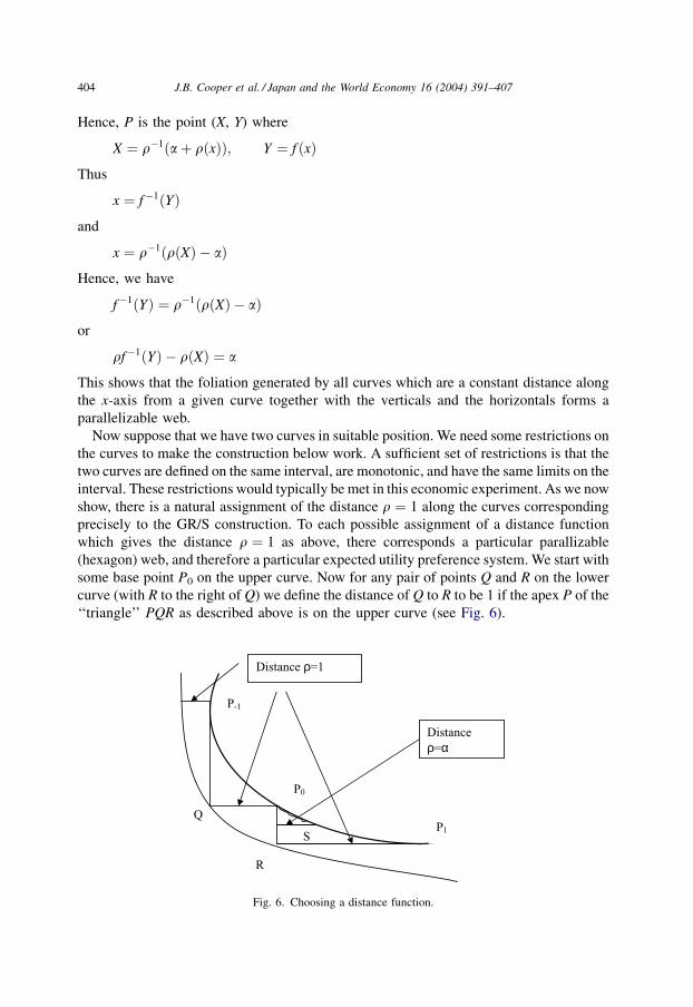
some base point P0 on the upper curve. Now for any pair of points Q and R on the lower

curve (with R to the right of Q) we define the distance of Q to R to be 1 if the apex P of the

‘‘triangle’’ PQR as described above is on the upper curve (see Fig. 6).

P-1

Distance ρ=1

P1 S

Distance ρ=α

P0

R

Q

Fig. 6. Choosing a distance function.

404 J.B. Cooper et al. / Japan and the World Economy 16 (2004) 391–407

Since we know what it means to have a distance one along the curve, we can start at P0

and obtain a sequence P1, P2, and so on (by iteration) so that the distance from Pn to

P(nþ1) is always 1. Going to the left we define Pð�1Þ;Pð�2Þ; . . . analogously. We now

know how to define r at these points (namely n at Pn—more precisely at the x-coordinate

of Pn).

We are now free to choose r between P0 and P1 (of course, continuous, strictly

increasing and with value 0 at P0 and 1 at P1).

This then determines r everywhere by the natural extension process.

Thus if S is a point between P0 and P1 where r has the value a, then r has the value 1 þ wa at that point between P1 and P2 whose distance from is 1. Once we have r, the above

construction gives us the required flat web.

If the given curve is symmetric about the diagonal y ¼ x and we choose r to have the

corresponding symmetry properties, then the curves constructed in this manner are also

symmetric. (In this case, we choose P0 to be the intersection of the curve with the diagonal

y ¼ x.)

We now consider uniqueness. Here, we will only consider the symmetric case.

We begin with the case of extrapolating between the two curves x þ y ¼ 0 and

x þ y ¼ 1. All cases can be reduced to this one. Suppose that we have a function f of

one variable so that the level curve

f ðxÞ þ f ðyÞ ¼ 0

corresponds to y ¼ �x and

f ðxÞ þ f ðyÞ ¼ 1

to y ¼ 1 � x.

Then f ð�xÞ þ f ðxÞ ¼ 0, i.e. f ð�xÞ ¼ �f ðxÞ and f ðyÞ ¼ 1 � f ðxÞ ¼ f ð1 � xÞ.Hence, f satisfies the two conditions:

f ð�xÞ þ f ðxÞ ¼ 0 and f ð1 � xÞ þ f ðxÞ ¼ 1

If we write f(x) in the form x þ gðxÞ (i.e. as a perturbation of the identity function), then

these translate into the conditions:

gð�xÞ ¼ �gðxÞ and gð1 � xÞ ¼ �gðxÞfrom which follow that gð1 þ xÞ ¼ gðxÞ, i.e. g is 1 periodic.

Hence, the general solution has the form

f ðxÞ þ f ðyÞ ¼ c

where f ðxÞ ¼ x þ gðxÞ and g is an odd 1 periodic function (so that gð0Þ ¼ 0 ¼ gð1Þ).Periodicity and oddness of g will make it useful to employ the fact that g has a Fourier

sine representation so that f has the form

x þX1n¼1

an sin 2pnx

This representation has been used to illustrate the construction in Mathematica. Details are

available from the authors.

J.B. Cooper et al. / Japan and the World Economy 16 (2004) 391–407 405

For the following, it will be useful to incorporate more general constants (in place of 0

and 1 above). Thus, if f ðxÞ þ f ðyÞ ¼ c corresponds to y þ x ¼ c and f ðxÞ þ f ðyÞ ¼ d

corresponds to y þ x ¼ d then we have, with

x ¼ ðd � cÞX þ c

2

y ¼ ðd � cÞY þ c

2

(so that X ¼ ð1=ðd � cÞÞðx � ðc=2Þ)

X þ Y ¼ c , 1

d � cðx þ yÞ þ c ¼ c , x þ y ¼ 0

X þ Y ¼ d , 1

d � cðx þ yÞ þ c ¼ d , x þ y ¼ 1

and so the general solution

f ðxÞ ¼ x þX1n¼1

an sin 2pnx

translates into

�f ðxÞ ¼ 1

d � cX � c

2

h iþX1n¼1

an sin 2pn1

d � cX � c

2

h i� �

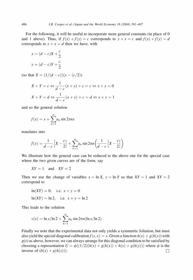
We illustrate how the general case can be reduced to the above one for the special case

where the two given curves are of the form, say

XY ¼ 1 and XY ¼ 2

Then we use the change of variables x ¼ ln X, y ¼ ln Y so that XY ¼ 1 and XY ¼ 2

correspond to

lnðXYÞ ¼ 0; i:e: x þ y ¼ 0

lnðXYÞ ¼ ln 2; i:e: x þ y ¼ ln 2

This leads to the solution

vðxÞ ¼ ln x=ln 2 þX1n¼1

an sin 2pnðln x=ln 2Þ

Finally we note that the experimental data not only yields a symmetric foliation, but must

also yield the special diagonal calibration f ðx; xÞ ¼ x. Given a function hðxÞ þ gðhðxÞ) with

g(x) as above, however, we can always arrange for this diagonal condition to be satisfied by

choosing a representation U ¼ fðð1=2ÞðhðxÞ þ gðhðxÞÞ þ hðyÞ þ gðhðyÞÞÞ where f is the

inverse of (hðxÞ þ gðhðxÞÞÞ. &

406 J.B. Cooper et al. / Japan and the World Economy 16 (2004) 391–407

References

Akivis, M.A., Shelekhov, A.M., 1992. Geometry and Algebra of Multidimensional Three-Webs (Transl. from

Russian by V.V. Goldberg). Kluwer Academic Publishers, Dordrecht.

Burk, A., 1936. Real income, expenditure proportionality, and Frisch’s ‘‘New Methods of Measuring Marginal

Utility’’. Review of Economic Studies 4 (1), 33–52.

Camerer, C., 1995. ‘‘Individual Decision Making.’’ The Handbook of Experimental Economics. In: John, H.

Kagel, Alvin, E. Roth (Eds.), Princeton University Press, Princeton, Chapter 8, pp. 587–703.

Chipman, J.S., 1973. The ordering of portfolios in terms of mean and variance. Review of Economic Studies 40

(2), 167–190.

Debreu, G., 1960. Topological Methods in Cardinal Utility Theory. In: Arrow, K.J., Karlin, S., Suppes, P. (Eds.),

Mathematical Methods in the Social Sciences, pp. 16–26.

Franklin, P., 1927. A geometric characterization of equipotential and stream lines. Journal of Mathematics and

Physics 6 (4), 191–200.

Georgescu-Roegen, N., 1952. A diagramatic analysis of complementarity. Southern Journal of Economics 19,

1–20.

Kim, T.S., Omberg, E., 1996. Dynamic non myopic portfolio behavior. Review of Financial Studies 9, 141–161.

Machina, M.J., 1982. ‘Expected Utility’ Analysis without the Independence Axiom. Econometrica 50, 277–323.

Matschak, J., 1950. Rational Behavior, Uncertain Prospects, and Measurable Utility. Econometrica 18, 111–141.

Russell, T., 2003. How quasi rational are you II? Chern curvature measures local failure of the expected utility

maximization axioms. Economic Letters 81 (3), 379–382.

Samuelson, P.A., in press ‘‘A Basic Partial Differential Equation to Test Non-Introspectively the Expected

{Utility} Hypothesis.’’

Sato, R., 1977. Homothetic and non-homothetic CES production functions. American Economic Review 67 (4),

559–569.

Schneeweiss, H., 1966. Entscheidungs kriterien bei Risko. Springer–Verlag, Berlin.

J.B. Cooper et al. / Japan and the World Economy 16 (2004) 391–407 407