Atmospheric Research 181 (2016) 312–321

Contents lists available at ScienceDirect

Atmospheric Research

j ourna l homepage: www.e lsev ie r .com/ locate /atmosres

Temporal variability of atmospheric turbidity and DNI attenuation in thesugarcane region, Botucatu/São Paulo/Brazil

Cícero Manoel dos Santos, João Francisco Escobedo ⁎Rural Engineering Department, FCA/UNESP, Botucatu, São Paulo, Brazil

⁎ Corresponding author at: Faculdade de CiênciasLaboratorio de Radiometria Solar, Departmento de EngeRua José Barbosa de Barros, n° 1780, Botucatu/SP 18.610-

E-mail address: escobedo@fca.unesp.br (J.F. Escobedo)

http://dx.doi.org/10.1016/j.atmosres.2016.07.0120169-8095/© 2016 Elsevier B.V. All rights reserved.

a b s t r a c t

a r t i c l e i n f o

Article history:Received 9 February 2016Received in revised form 2 July 2016Accepted 8 July 2016Available online 10 July 2016

In this study, attenuation of direct normal solar irradiance (DNI) in Botucatu / São Paulo, an area under theinfluence of local and adjacent agricultural burning, is expressed using the Linke's turbidity factor (TL) in theperiod from 1996 to 2008. Two methodologies represented as TLDj and TLLi were used. Temporal variability(hourly average for the season and monthly average) is presented. Turbidity was correlated with wind speedand air temperature. Frequency distribution and cumulative frequency are analyzed to determine turbiditypredominance levels in the local atmosphere. Optical depth information of aerosols at 550 nm (AOD550nm) andwater vaporwere obtained by the Terra satellite using theMODIS sensor. The highest degree of DNI transmissionis observed in themorning. Close to solar noon, transmission is smaller (greatest TL value). Diurnal TL variabilityis more evident in the hot period than in the cold period. May and June were the months of lowest DNI attenu-ation (highest atmospheric transparency). The highest DNI attenuation occurs in spring (TLDj = 4.22± 0.05 andTLLi = 4.65 ± 0.06) and summer (TLDj = 4.27 ± 0.14 and TLLi = 4.69 ± 0.15). Wind speed and air temperaturewere positively correlatedwith TL. In N28% of hours of clear sky, turbidity exceeded the value of 4.0. The region ofBotucatu seems to be influenced by water vapor and aerosols from different origins. This study concludes thatthese factors significantly reduce DNI incidence on the surface, with higher atmospheric transparency in thecold period and lower atmospheric transparency in the warm period.

© 2016 Elsevier B.V. All rights reserved.

Keywords:Atmospheric transparencyAerosolsWater vaporPollutionDirect Normal Irradiance

1. Introduction

Direct normal solar irradiance (DNI) has essential applicationsin solar concentration technology, such as climate forcing and controllerof terrestrial biodiversity (Batlles et al., 2000).When crossing a cloudlessatmosphere, DNI is attenuated by two main processes: scattering byaerosols and absorption bywater vapor, especially at visible and infraredwavelengths. Aerosols are tiny solid or liquid particles suspended in theair that follow themovement of airmasses and can have terrestrial origin(agricultural burning, industrial smoke, dust storms, volcanic eruptions)and marine origin such as sea spray (López and Batlles, 2004). Inclear sky conditions, the concentration of aerosols and water vaporcontent in the atmosphere affects the magnitude and variability of DNI(Gueymard, 2012). Aerosols and water vapor affect the level of atmo-spheric transparency, and attenuation caused in DNI is called turbidity.

Determining atmospheric turbidity requires detailed DNI measures,both of broadband and spectral bands (Salazar, 2011; Ellouz et al.,2013). Acquisition and maintenance of these sensors are almost

Agronômicas (FCA/UNESP),nharia Rural, Fazenda Lageado,307, Brazil..

unfeasible due to the high cost of importing and maintenance (DosSantos et al., 2014; Souza et al., 2016). Therefore, atmospheric turbidityis usually estimated by parametric models.

Typically, atmospheric turbidity in clear sky conditions is represent-ed by the Linke's turbidity factor (TL) or Ångström turbidity coefficient(β). TL referes to the total spectrum and describes optical tickness in theatmosphere as a result of two distinct combinations, absorption bywater vapor and scattering by particulate matter in a dry and clearatmosphere (Kasten, 1996; El-Metwally, 2013). Based on this fact,TL is adequate to characterize total attenuation by the atmosphere(Kasten, 1980). Because the turbidity coefficient (β) refers to thenumber of aerosols in the atmosphere, it is accepted as a representativeindex of turbidity caused by aerosols and corresponds to the aerosoloptical depth in 1 μm (Masmoudi et al., 2002). For convenience of useand ability to represent optical thickness of a dry and clean atmosphere,TL is often used as the first option (Ellouz et al., 2013). Calculatingturbidity is important in themodeling of local climate in climate studies,air pollution studies, indirect measure of DNI, indirect measure of theconcentration of particulates suspended in the air, and water vaporthat absorbs, reflects, or scatters solar radiation (López and Batlles,2004; Trabelsi and Masmoudi, 2011).

TL has been reported for numerous places (Hussain et al., 2000;Formenti et al., 2002; Diabaté et al., 2003; Polo et al., 2009a; Eltbaakh

313C.M. Santos, J.F. Escobedo / Atmospheric Research 181 (2016) 312–321

et al., 2012; Bertin and Frangi, 2013; Inman et al., 2015; Khalil andShaffie, 2016). Using hourly data from nine Spanish regions, Polo et al.(2009b) proposed and evaluated a methodology to estimate dailyLinke's turbidity in clear sky conditions based on measures of globalhorizontal irradiance at noon. The authors reported relative root meansquare deviation (rRMSE) from 12.0% to 30.9%. In Greece, Rapti (2000)used data of global and diffuse solar radiation to analyze diurnaland seasonal variations of atmospheric turbidity using TL. Diurnal andseasonal fluctuations of atmospheric transparency hadminimumvaluesin summer afternoons, and maximum values in winter mornings. InThailand, Chaiwiwatworakul and Chirarattananon (2004) determinedand analyzed atmospheric turbidity based on TL and β indices usingtwo-and-a-half-year-long measures. Atmospheric turbidity was lowand stable during the dry season and high in the rainy season (Marchto August). Turbidity increases in the morning at noon and decreasesduring the afternoon. Annual mean values for TL and β were 3.306and 0.098, respectively. However, studies on the temporal variabilityof TL and atmospheric transparency in Brazil are few, particularly forthe state of São Paulo. In studies on the atmosphere of Rio de Janeiro,Brazil, Flores et al. (2015) calculated the atmospheric turbidity basedon the Ångström turbidity coefficient (β) and showed a decreasein summer months. The authors highlighted the wide availability ofwater vapor resulting from maritime influences and the great plantarea.

Responsible for emitting large amounts of aerosols and gases intothe atmosphere, burning of native forests for agricultural productionand use of agricultural practices are still common activities in Brazil(Oliveira et al., 2011). This paper aims at determining TL under clearsky conditions in the agro-industrial region of Botucatu, state ofSão Paulo, where the economy is based on industry, agricultural activi-ties (production of sugar and alcohol) and trade. Two Linke's turbiditymethodologies (TLDj and TLLi) are used and compared in order toanalyze their effect and influence on the turbidity level. Correlationbetween turbidity and wind speed and air temperature was shown.Analyses of turbidity, frequency of occurrence, and cumulative fre-quency seem to characterize the turbidity index with atmosphericconditions. This work evaluates the rising pollution levels in theatmosphere of Botucatu, highlighting the period of lower atmo-spheric transparency (higher turbidity), likely factors responsiblefor the DNI attenuation and likely places of origin. This study alsoshows the trend of turbidity variability.

Fig. 1.Map showing the main sugarcane producing areas in Brazil and municipalities in Sãimages.

2. Materials and methods

2.1. Description of location and climate

Data used in this study were obtained from the solar RadiometryStation at the College of Agricultural Sciences from Botucatu, FCA/UNESP (22°53′09″S, 48°26′42″W and average altitude of 786 m).Botucatu is a municipality located in the Midwestern region of SãoPaulo state (Fig. 1), with a total area of 1482.642 km2 and estimatedpopulation in 2015 of approximately 139,483 inhabitants (IBGE,2015). The city has high altitude gradient between 400 and 500 min the lowest region (peripheral depression) and between 700 and900 in the mountain region (Western Highlands). This differencecauses changes in air temperature and winds. Distant 221 km fromthe Atlantic Ocean and 235 km from the capital São Paulo, withSavanna and Atlantic forest biome, Botucatu features warm temper-ate climate (mesothermal), hot and humid summer with high pre-cipitation, and dry winter (Escobedo et al., 2011). According to theKöppen's climatic classification, based on monthly pluviometricand thermometric data, the climate of the Botucatu region is Cwa,characterized by the tropical climate of altitude, with rain in thesummer and drought in the winter and mean temperature of thehottest month higher than 22 °C (CPA, 2016). With the Cwa climatepredominantly in all central region, São Paulo state has seven dis-tinct climatic types, mostly humid climate.

From October to March, rainfall is of microclimatic nature, fromthe free convection process and macroclimatic events as a resultof the convergence of humid air masses coming from the Amazonregion and southern Atlantic Ocean, which leads to the formationof the South Atlantic Convergence Zone (SACZ) and FrontalSystems (Jones et al., 2004; Reboita et al., 2010; Teramoto andEscobedo, 2012). From June to September, the central region ofBrazil is dominated by an area of high pressure, low rainfall, andlight winds in the lower troposphere, with convection in the Ama-zon moved to the northwestern part of South America (Freitaset al., 2005; Satyamurty et al., 1998). In the months of dry season,especially in August and September, the burning practice of sugar-cane in cities nearby Botucatu is observed, which is held to harveststalks (Codato et al., 2008). Because of burning, there is a signifi-cant increase in particulate concentrations in the local atmosphere(Allen et al., 2004). There is an additional load of aerosols from

o Paulo. Adapted from UNICA http://www.unica.com.br/production-map/ and Google

314 C.M. Santos, J.F. Escobedo / Atmospheric Research 181 (2016) 312–321

burning brought from the Amazon region of Bolivia, Paraguay, andArgentina to southern Brazil through atmospheric circulation(Videla et al., 2013; Portillo-Quintero et al., 2013). Almost all firesare caused by humans, whether on purpose or accidentally. Thus,the effect of aerosols can extrapolate from local scale and be deci-sive in the pattern of planetary redistribution of energy from thetropics to mid and high latitudes through convective transportprocesses (Freitas et al., 2005), resulting in changes in the hydro-logical cycle, due to changes in atmospheric temperature and cloudstructure.

The presence of two hydroelectric dams, Jurumirim (23.15°S;48.04°W) and Barra Bonita (22.37°S; 48.19°W) next to Botucatu, isworth mentioning. Jurumirim dam is 70 km away from Botucatu andhas a reservoir of approximately 449 km2. The Barra Bonita dam,30 km away from Botucatu, is 308 km2. Their structures representchanges in land cover and local microclimate. Changes of this magni-tude cause significant interference in the turbulence of the atmospherein micro- and mesoscale, modifying the radiation balance and micro-physics of clouds (Rosenfeld, 1999).

2.2. Database and model

2.2.1. Description of measuresIn the TL calculation, DNI measures were obtained from Febru-

ary 1996 to December 2008, through an Eppley NIP pyrheliometercoupled to an Eppley solar tracker ST3. Global solar irradiance (RG)was monitored by an Eppley pyranometer PSP and diffuse solarirradiance (RD) by an Eppley pyranometer PSP with a 40 cm radiusand a 10 cm width ring (Dal Pai et al., 2014). All sensors were con-nected to a Campbell Datalogger CR1000 programmed to storeaverages every 5 min. The sensors were annually calibrated bythe comparative method (WMO, 2008). Hourly clear sky valueswere used for DNI. As atmospheric turbidity is an index for clearsky conditions, the criteria used in the selection of data to beapplied in the models were based on Karayel et al. (1984). Thecriteria adopted for clear sky are as follows: DNI that exceeds200 Wm−2 and a ratio of diffuse irradiance to global irradianceof b1/3. It was considered that the atmospheric transmissivity RG

(kt) could not be b0.675.Optical depth values of aerosol at 550 nm (AOD550nm) and

water vapor were used in this study. AOD550 values were obtainedby the Terra satellite using the MODIS sensor (Moderate ResolutionImaging Spectroradiometer), which makes measurements in theBotucatu region between 10:00 UTC and 11:00 UTC, and areregarded as daily values. The error expected for AOD550 providedby MODIS is: Δ(AOD550) = 0.05 ± 0.15(AOD550) (Remer et al.,2008). Water vapor data were obtained from the MODIS sensoraboard the Terra satellite. Water vapor value by MODIS has anerror from 5% to 10% (Gao and Kaufman, 2003). MODIS sensordata were downloaded from atmospheric products GIOVANNI(http://disc.sci.gsfc.nasa.gov/giovRNAi/overview/index.html) to anarea of 0.2° latitude × 0.2° longitude around the measurementlocation. AOD550 and water vapor data were separated for clearsky conditions.

2.2.2. Linke's turbidity (TL)Linke's turbidity (TL) (Linke, 1922) expresses the number of

atmospheres (clean and dry) that produce, at the direct irradianceon top of the atmosphere, attenuation similar to an actual atmo-sphere (Pedrós et al., 1999; Hussain et al., 2000). Modificationsand improvements have been suggested for TL (Kasten, 1996;Zakey et al., 2004; Mavromatakis and Franghiadakis, 2007). Inthis work, TL was calculated using methodologies (Djafer andIrbah, 2013) and (Li and Lam, 2002), represented as TLDj and TLLi,respectively.

2.2.3. Methodology (TLDj)Linke's turbidity (Djafer and Irbah, 2013) (TLDj) is determined by the

equation

TLDj ¼ T lk �1

δRa mað Þ1

δRk mað Þð1Þ

where Tlk is a TL correction factor (Eq. (2)) and it is related to the directsolar irradiance (Trabelsi and Masmoudi, 2011; Kasten, 1980), δRk(ma)and δRa(ma) are both Rayleigh integral optical thickness. δRk(ma)is the Rayleigh integral optical thickness (dimensionless) (Eq. (3))given by Kasten (1980), and δRa(ma) is the integral optical thickness(dimensionless) (Eq. (4)) given by Louche et al. (1986) and adjustedby Kasten (1996). The subscript k represents the “Kasten” author,and the subscript a represents the word “adjusted.” The new adjust-ment was necessary because Kasten (1980), initially, had taken intocosideration only the molecular dispersion and ozone absorption.Absorption by the permanent atmospheric gases was not includedinto the calculations leading to smaller values of the integral opticalthickness (Mavromatakis and Franghiadakis, 2007).

T lk ¼ 0:90þ 9:40� sin hð Þ½ �x 2� ln I0 hð Þ � R0

R

� �� �� �‐ ln DNI hð Þ½ �

� �ð2Þ

where h is the solar elevation angle (degrees), I0(h) is the solarconstant (1367 Wm−2), DNI (h) is the direct solar irradiance in themeasured incidence (Wm−2), and R0 and R are the instant distanceand the average distance between earth and sun, respectively. TheR0/R ratio is called the eccentricity correction factor of the Earth'sorbit (E0) (Iqbal, 1983).

1δRa mað Þ ¼ 6:6296þ 1:7513�ma−0:1202�m2

a þ 0:0065

�m3a−0:00013�m4

a ð3Þ

1δRk mað Þ ¼ 9:40þ 0:90�ma ð4Þ

ma is the optical mass of the actual pressure given equation:

ma ¼ mr � pp0

� �ð5Þ

mr is the relative optical mass defined as a function of the solarelevation angle (h) in degrees (Cañada et al., 1993):

mr ¼ sin hð Þ þ 0:15� 3:885þ hð Þ−1:253h i−1

ð6Þ

The p/p0 ratio is the relationship between local pressure and stan-dard pressure (at sea level) and was calculated as a function of thelocal altitude (H) in meters (Iqbal, 1983) by the expression

pp0

¼ exp −0:0001184� Hð Þ ð7Þ

2.2.4. Methodology (TLLi)The TL calculation using (Li and Lam, 2002) (TLLi) arises from the

definition that DNI for the entire solar spectrum and under clear skycondition can be calculated:

DNI hð Þ ¼ I0 hð Þ exp −TLLiδRk mað Þð Þ ð8Þ

Reorganized Eq. (8) to TLLi:

TLLi ¼ln

I0 hð ÞDNI hð Þ

� �

δRk mað Þ½ � ð9Þ

Table 1Types of atmosphere for different levels of atmospheric turbidity.

Types of atmosphere TL Visibility (km)

Rayleigh and pure atmosphere 1 340Clear, warm air 2 28Turbid, moist, warm air 3 11Polluted atmosphere 4–8 b5

315C.M. Santos, J.F. Escobedo / Atmospheric Research 181 (2016) 312–321

Parameters δRk(ma), I0(h), andDNI(h) have been previously defined.TLLi was used to calculate the optical mass and actual pressure (ma)(Eq. (5)), and mris a function of the zenith angle (Z) in degrees(Eq. (10)):

mr ¼ cos Z þ 0:15� 93:885−Zð Þ−1:253h i−1

ð10Þ

Considering the TL equations above, TLDj and TLLi values can be easilyobtained directly from DNI measurements performed with the pyrheli-ometer installed in Botucatu.

Typical TL values usually range from1 to 10; higher valuesmean thatDNI is more attenuated and the atmosphere has high concentration ofaerosol and high water vapor content (less transparent atmosphere).This study will consider the characterization of atmosphere types asso-ciated with the TL levels (Table 1) (Leckner, 1978).

3. Results and discussion

3.1. Diurnal and seasonal variation of the Linke's turbidity

Based on Eqs. (1)–(10), Linke's turbidity values were calculatedfor hours of clear sky. The average hourly turbidity values withmethod-ologies (TLDj and TLLi) are shown in Fig. 2a. Thehourly variation of TLDj is

Fig. 2. (a) Average hourly Linke's turbidity variation a

Fig. 3. Seasonal variability of the Linke's turbidity in Botucatu from

similar to that of TLLi; however, TLLi has values on average 10.3% greaterthan TLDj. The mean deviation of 10.3% in values of TL is a result of dif-ferences between methods and to the integral optical thickness factorand eccentricity correction factor of the Earth's orbit. Variations of TLhave also been reported in studies (Li and Lam, 2002; Wen and Yeh,2009) for Hong Kong and Taichung Harbor, respectively, in the analysesof fourmodels. Turbidity has variability throughout the day, increases inthemorning anddecreases in the afternoon,withmaximumvalues nearsolar noon. The maximum values coincide with the period of greatestsolar incidence in the day. Therefore, in this analysis, the variability isexplained based on the elevation of the radiant flux intensity through-out the day for each hour. Other factors may influence hourly turbidityfluctuation: meteorological conditions, local pollution, water vapor,aerosols that originated from seasonal forest fires, and local industrialactivities (Bilbao et al., 2014).

Relative deviation (DTL, %)was calculated byDTL (%)= [(TLh – TLm) /TLh] × 100, where TLm and TLh are the values of the total averageTL curves and average hourly values, respectively (Fig. 2b). PositiveDTL values are indicative that the average value is lower than hourlyvalues. DTL values for TLDj and TLLi varied, respectively, between−29.82% and −26.58% and between 14.09% and 17.35%. Consideringthe time interval from 7:00 a.m. to 4:00 p.m., DTL has lower amplitudeand shows average value of DTLDj = 5.02 ± 8.69% and DTLLi =7.89% ± 8.20%. Trabelsi and Masmoudi (2011) pointed out that watervapor in the atmosphere, aerosols, and the variability of the variousmeteorological variables that influence the atmosphere are crucial inthe amplitude of DTL.

DNI attenuation during the day in the seasons was presented asaverage values for morning (until 09:30 a.m.), close to solar noon(between 10:30 a.m. and 1:30 p.m.) and afternoon (after 1:30 p.m.)(Fig. 3a, b). For this analysis, all hours of clear sky in the study periodwere used. The highest degree of DNI transmission is observed in themorning for spring and summer. Close to solar noon, transmission is

nd (b) deviation for Botucatu from 1996 to 2008.

1996 to 2008. (a) Methodology TLDj and (b) methodology TLLi.

Table 2Seasonal variability of the Linke's turbidity in Botucatu from 1996 to 2008.

Season Morning Close to solar noon Afternoon

TLDj Spring 3.38 ± 0.49 4.43 ± 0.17 3.65 ± 0.64Summer 3.33 ± 0.43 4.53 ± 0.35 3.62 ± 0.64Autumn 2.97 ± 0.19 3.34 ± 0.09 2.83 ± 0.36Winter 3.04 ± 0.41 3.52 ± 0.06 3.03 ± 0.34Average 3.18 ± 0.37 3.95 ± 0.16 3.30 ± 0.47

TLLi Spring 3.72 ± 0.30 4.47 ± 0.52 4.14 ± 0.66Summer 4.41 ± 0.26 5.53 ± 0.46 4.35 ± 0.60Autumn 3.54 ± 0.31 4.02 ± 0.22 3.70 ± 0.45Winter 3.61 ± 0.11 3.89 ± 0.10 3.63 ± 0.26Average 3.26 ± 0.66 4.35 ± 0.20 3.66 ± 0.49

316 C.M. Santos, J.F. Escobedo / Atmospheric Research 181 (2016) 312–321

lower, and consequently, the greater the atmospheric turbidity value.This is related to the optical state of the atmosphere in the seasons.Atmospheric turbidity has different variation in the hot/wet season(spring and summer) and cold/dry (fall and winter), but variation ofTLDj (Fig. 3a) is similar to that of TLLi (Fig. 3b). Diurnal variability ofatmospheric turbidity is evident during the heating phase, while inthe cold period, turbidity varied slightly (Uscka-Kowalkowsk, 2013).

Among seasons, atmospheric turbidity has average variabilityof≈17%. In diurnal evolution, the maximum average value is observedin the summer (TLDj= 3.83± 0.62) and theminimum average value inthe autumn (TLDj= 3.05± 0.26). The lowest atmospheric transparency(higher turbidity) occurs in the spring and summer. The TLDj value forspring near solar noon is (4.43 ± 0.17), and for summer, values are3.33 ± 0.43 and 3.62± 0.64 in themorning and afternoon, respectively(Table 2). In the diurnal evolution, highest transparency (low turbidity)occurs in the autumn and winter. TLLi value for fall in the morningand afternoon is lower than 4. When compared to values in themorning and afternoon, larger TL values are observed around thesolar culmination.

Fig. 4. Variation of the Linke's turbidity in Botucatu from 1996 to 2008. (a

Fig. 5. Average monthly values from 2000 to 2008, consideri

3.2. Analysis of monthly average Linke's turbidity

Average monthly turbidity values were obtained from the hourlyturbidity values for each month. Average monthly annual evolution ofthe Linke's turbidity and average values according to the season forTLDj and TLLi are shown in Fig. 4(a, b). Atmospheric turbidity valuesreveal thatMay and Julywere themonths of the lowest DNI attenuation(high atmospheric transparency), while January was the least transpar-ent month (higher DNI attenuation) (Fig. 4a). Increased atmosphericturbidity is also visible in the months of summer and spring. BetweenApril and August, the atmosphere is less turbid (TLDj smaller than 3.46and TLLI smaller than 3.93). Elevation in radiant flux intensity through-out the day has great influence on changes of atmospheric turbidityat different scales, but water vapor and aerosols are the most decisiveparameters on seasonal variability.

The period of highest and lowest atmospheric transparency is evi-dent when considering the seasons (Fig. 4b). Most DNI attenuationoccurs in spring (TLDj = 4.22 ± 0.05 and TLLi = 4.65 ± 0.06) and sum-mer (TLDj = 4.27 ± 0.14 and TLLi = 4.69 ± 0.15), months in which themovement of particulatematerials that advance to the state of São Paulowith the South Atlantic Frontal Systems (during the spring, especially)and with the South Atlantic Convergence Zone (SACZ) (during thesummer) are the highest in the year (Allen et al., 2004). In springand summer, water vapor content in the atmosphere and the increasein aerosols (Fig. 5a, b) that originated from the burning of biomass(sugarcane, pastures, forests and native forests) for agricultural produc-tion and farming in regions near the state of São Paulo and the Amazonregion (Holben et al., 2001; França et al., 2014) are the main factorsresponsible for the increase in atmospheric turbidity and DNI attenua-tion in Botucatu.

In the summer, increased turbidity is caused mainly by increasedwater vapor concentration in the atmosphere. Increased turbiditydue to atmospheric water vapor and aerosols is also connected to air

) Average annual variation. (b) Average annual variation per season.

ng only days of clear sky. (a) Water vapor and (b) AOD.

Table 3Average monthly atmospheric Linke's turbidity with TLDj and TLLi for Botucatu from 1996 to 2008.

Linke's turbidity (TLDj)

1996 1997 1998 1999 2000 2001 2002 2003 2004 2005 2006 2007 2008

J – 3.90 ± 0.72 4.46 ± 0.67 4.78 ± 0.90 4.43 ± 0.85 4.30 ± 0.89 4.14 ± 0.90 4.25 ± 1.06 4.55 ± 1.52 4.43 ± 1.20 4.10 ± 1.33 4.99 ± 1.45 4.47 ± 1.91F 4.50 ± 0.77 3.94 ± 0.63 4.42 ± 0.87 4.14 ± 0.93 4.19 ± 0.91 4.82 ± 1.43 4.02 ± 1.36 3.95 ± 0.78 4.26 ± 1.07 4.05 ± 0.86 4.23 ± 0.99 3.92 ± 0.81 5.71 ± 2.07M 4.48 ± 1.10 3.90 ± 0.68 4.22 ± 0.85 3.82 ± 0.93 4.36 ± 0.98 4.04 ± 0.69 3.67 ± 0.59 4.55 ± 1.59 3.94 ± 0.70 3.94 ± 0.76 4.15 ± 0.85 4.37 ± 1.74 4.35 ± 1.27A 3.64 ± 0.61 3.45 ± 0.73 3.41 ± 0.86 3.44 ± 0.62 3.21 ± 0.51 3.50 ± 0.84 3.44 ± 0.51 4.16 ± 2.18 3.92 ± 1.20 4.05 ± 0.76 3.06 ± 0.49 3.80 ± 0.75 3.57 ± 0.98M 3.33 ± 0.53 3.17 ± 0.61 2.98 ± 0.56 3.14 ± 0.79 3.31 ± 0.77 3.32 ± 1.16 3.23 ± 1.11 2.99 ± 0.63 3.16 ± 0.59 3.56 ± 1.04 2.98 ± 0.50 3.57 ± 1.11 3.19 ± 0.61J 3.56 ± 1.49 3.03 ± 0.76 3.28 ± 0.80 2.97 ± 0.51 3.60 ± 0.81 3.78 ± 1.23 3.10 ± 0.51 3.38 ± 1.07 3.51 ± 1.13 3.33 ± 0.84 3.04 ± 0.60 3.09 ± 0.71 3.21 ± 0.66J 3.21 ± 0.63 3.41 ± 0.73 3.58 ± 0.73 3.36 ± 0.82 3.09 ± 0.75 3.34 ± 0.91 2.96 ± 0.77 3.18 ± 0.52 3.32 ± 0.78 3.06 ± 0.69 3.26 ± 0.70 3.01 ± 0.64 3.03 ± 0.76A 3.50 ± 0.99 2.84 ± 0.51 4.57 ± 0.72 3.60 ± 0.83 3.44 ± 0.72 3.55 ± 0.83 3.73 ± 0.89 3.27 ± 0.86 3.18 ± 0.98 3.64 ± 1.04 3.53 ± 0.78 3.11 ± 0.64 3.31 ± 0.64S 4.03 ± 1.00 4.20 ± 0.85 4.59 ± 1.16 4.30 ± 0.88 3.98 ± 0.42 4.20 ± 1.33 4.48 ± 1.03 3.64 ± 0.85 4.47 ± 0.92 4.28 ± 1.39 3.64 ± 0.69 3.88 ± 0.81 3.84 ± 1.01O 4.09 ± 0.67 3.04 ± 0.00 4.12 ± 0.83 4.24 ± 0.96 4.52 ± 0.97 4.54 ± 1.86 4.74 ± 0.59 3.77 ± 0.99 3.69 ± 0.86 4.53 ± 0.74 4.20 ± 0.93 4.36 ± 0.70 4.40 ± 0.69N 3.56 ± 0.66 – 3.90 ± 0.57 4.00 ± 0.81 4.34 ± 1.12 5.70 ± 1.18 4.17 ± 0.96 4.18 ± 1.10 4.01 ± 0.84 3.90 ± 0.75 4.12 ± 0.96 3.89 ± 0.99 4.10 ± 0.65D 4.56 ± 0.82 – 4.31 ± 0.69 4.45 ± 0.99 4.51 ± 0.90 3.88 ± 1.35 3.79 ± 0.71 4.39 ± 0.77 4.43 ± 0.90 4.20 ± 0.92 4.13 ± 0.68 4.22 ± 1.37 3.87 ± 0.85Average 3.86 ± 0.84 3.49 ± 0.62 3.99 ± 0.78 3.85 ± 0.83 3.91 ± 0.81 4.08 ± 1.14 3.79 ± 0.83 3.81 ± 1.03 3.87 ± 0.96 3.92 ± 0.92 3.70 ± 0.79 3.85 ± 0.98 3.92 ± 1.01

Linke's turbidity (TLLi)

1996 1997 1998 1999 2000 2001 2002 2003 2004 2005 2006 2007 2008

J – 4.32 ± 0.79 4.94 ± 0.74 5.29 ± 0.99 4.90 ± 0.94 4.76 ± 0.98 4.58 ± 0.99 4.70 ± 1.17 4.99 ± 1.59 4.72 ± 1.50 4.54 ± 1.48 5.51 ± 1.60 4.69 ± 2.07F 4.84 ± 0.83 4.36 ± 0.70 4.88 ± 0.96 4.58 ± 1.02 4.64 ± 1.01 5.24 ± 1.39 4.46 ± 1.50 4.37 ± 0.86 4.71 ± 1.18 4.48 ± 0.95 4.68 ± 1.09 4.34 ± 0.89 5.86 ± 1.81M 4.90 ± 1.20 4.31 ± 0.74 4.67 ± 0.94 4.23 ± 1.03 4.83 ± 1.08 4.47 ± 0.76 4.06 ± 0.65 5.02 ± 1.76 4.36 ± 0.77 4.36 ± 0.83 4.47 ± 0.69 4.83 ± 1.91 4.55 ± 1.04A 4.08 ± 0.66 3.79 ± 0.71 3.77 ± 0.97 3.81 ± 0.69 3.55 ± 0.57 3.88 ± 0.93 3.81 ± 0.57 4.50 ± 2.30 4.34 ± 1.33 4.49 ± 0.85 3.39 ± 0.54 4.20 ± 0.83 3.95 ± 1.09M 3.83 ± 0.59 3.52 ± 0.67 3.30 ± 0.62 3.47 ± 0.89 3.63 ± 0.89 3.67 ± 1.30 3.57 ± 1.24 3.25 ± 0.74 3.49 ± 0.65 3.95 ± 1.15 3.30 ± 0.56 3.96 ± 1.23 3.49 ± 0.69J 4.10 ± 1.58 3.34 ± 0.84 3.64 ± 0.88 3.29 ± 0.56 3.97 ± 0.93 4.17 ± 1.37 3.44 ± 0.57 3.75 ± 1.19 3.84 ± 1.30 3.69 ± 0.93 3.35 ± 0.69 3.37 ± 0.82 3.55 ± 0.75J 3.73 ± 0.71 3.78 ± 0.81 3.95 ± 0.83 3.72 ± 0.91 3.30 ± 0.83 3.62 ± 0.83 3.26 ± 0.86 3.52 ± 0.57 3.68 ± 0.86 3.40 ± 0.76 3.61 ± 0.77 3.34 ± 0.71 3.35 ± 0.84A 4.00 ± 1.11 3.15 ± 0.57 5.06 ± 0.79 3.99 ± 0.92 3.81 ± 0.80 3.93 ± 0.91 4.14 ± 0.98 3.59 ± 0.99 3.52 ± 1.09 4.03 ± 1.16 3.88 ± 0.88 3.44 ± 0.71 3.58 ± 0.62S 4.50 ± 1.09 4.65 ± 0.94 5.08 ± 1.28 4.76 ± 0.97 4.36 ± 0.50 4.65 ± 1.48 4.87 ± 1.09 4.02 ± 0.95 4.83 ± 0.84 4.72 ± 1.55 4.03 ± 0.77 4.29 ± 0.89 4.25 ± 1.11O 4.46 ± 0.74 3.36 ± 0.00 4.56 ± 0.92 4.69 ± 1.06 4.89 ± 0.96 5.01 ± 2.06 5.24 ± 0.65 4.17 ± 1.09 4.09 ± 0.96 5.02 ± 0.81 4.61 ± 0.98 4.82 ± 0.77 4.87 ± 0.76N 3.77 ± 0.72 – 4.31 ± 0.63 4.43 ± 0.89 4.80 ± 1.23 6.30 ± 1.31 4.61 ± 1.06 4.62 ± 1.21 4.44 ± 0.92 4.26 ± 0.90 4.55 ± 1.05 4.30 ± 1.09 4.54 ± 0.72D 4.83 ± 0.89 – 4.77 ± 0.77 4.92 ± 1.09 4.99 ± 0.99 4.30 ± 1.49 4.20 ± 0.78 4.86 ± 0.85 4.88 ± 1.01 4.65 ± 1.01 4.57 ± 0.75 4.67 ± 1.51 4.28 ± 0.94Average 4.28 ± 0.92 3.86 ± 0.68 4.41 ± 0.86 4.26 ± 0.92 4.31 ± 0.89 4.50 ± 1.23 4.19 ± 0.91 4.20 ± 1.14 4.27 ± 1.04 4.31 ± 1.03 4.08 ± 0.85 4.26 ± 1.08 4.25 ± 1.04

317C.M

.Santos,J.F.Escobedo/A

tmospheric

Research181

(2016)312–321

318 C.M. Santos, J.F. Escobedo / Atmospheric Research 181 (2016) 312–321

circulation, which is important for transporting air masses and the tem-poral variation of turbidity (Elminir et al., 2006, de Freitas et al., 2005).In the cold season (autumn and winter), days with low rainfall, theatmosphere is frequently lighter with lower concentrations of watervapor and aerosols in the local atmosphere. The seasonal variability ofatmospheric turbidity described in the literature (Grenier et al., 1995;Power and Goyal, 2003; Uscka-Kowalkowsk, 2013), as observed inBotucatu/SP, shows maximum values in spring and summer and mini-mum values in autumn and winter.

Average monthly annual turbidity values show low variation amongthe 13 studied years (Table 3), with maximum TLDj values (5.70 ±1.18) in October 2001 and minimum value of (2.84 ± 0.51) in August1997. Minimum TLLi value (3.15 ± 0.57) was recorded in August 1997and maximum (6.30 ± 1.31) in October 2001. TLLI values were 9.31%higher than TLDj values, and this difference may be related to the equa-tions used. Turbidity indicated growing trend, and this effect may bedue to increased burning (illegal deforestation in the Amazon rainforestand fires), increased urbanization and local, and regional industrial ex-pansion. Depending on the location, urbanization is the main factor re-sponsible for increased pollution and atmospheric turbidity in majorregions (Rahoma and Hassan, 2012). Turbidity indexes obtained forBotucatu are similar to those found for 3 regions of Bangladesh, TL be-tween 3.46 and 4.83 (Hussain et al., 2000) and in places in Africa(TL = 3.50) (Diabaté et al., 2003). Atmospheric turbidity with TLDj andTLLi are lower than those obtained in Hong Kong, TL between 3.70 and5.26 (Li and Lam, 2002). Despite these results, each site has differentcharacteristics and weather conditions; consequently, different turbiditylevels are found.

3.3. Comparisons of TL calculated in Botucatu with those available on theSoDA Website

Inserting latitude, longitude, and altitude of the place of interest,it is possible to obtain the monthly Linke's turbidity using globalmaps for any place in the world via SoDA website (www.soda-is.com).Linke's turbidity (TLSoDA) is based on a series of global data fromsatellites, water vapor, aerosols, and from information on turbidityon the surface (Hove and Manyumbu, 2013). Monthly TL values(Table 4) available on SoDA are higher in spring/summer and lowerin autumn/winter; this seasonality resembles those obtained inthis workwith TLDj and TLLi, corroborating higher atmospheric trans-parency in autumn/winter and lower in spring/summer. The atmo-spheric turbidity calculated by TLDj and TLLI is, respectively, 15.80%and 23.52% greater than that TLSoDA. The variation coefficient (vc)expressed as percentage is indicative of data dispersion and wasused in this study. TLDj has vc = 12.04%, TLLi has vc = 11.76%, andTLSoDA has variation coefficient equal to 9.66%. Estimates with satel-lites are subject to larger errors, and then the results obtained in thisstudy are more representative because they have been determinedwith surface measures. However, the estimates provided by SoDAcannot be disregarded.

Monthly changes can be observed considering the modulation ofthe observed profile. The amplitude of the turbidity variation is cal-culated by: [TL(max) -TL(min)] / [TL(max) + TL(min)]. Based onlocal data, modulation with TLDj and TLLi was 15.41 and 15.14%, re-spectively. Using the TLSoDA results, modulation is 13.84%. On CreteIsland, modulation was ~18% (Mavromatakis and Franghiadakis,2007).

Table 4Linke's turbidity available on SoDA (www.soda-is.com).

Month Jan Feb Mar Apr May Jun Jul Aug Sep Oct Nov Dec

TLSoDA 3.40 3.70 3.70 3.60 3.30 3.10 2.80 2.80 3.40 3.00 3.20 3.10

3.4. Polynomial correlations for the Linke's turbidity

Fig. 4 shows that fourth-degree polynomial models have beenadjusted for the temporal variation of TLDj and TLLI, respectively(Eqs. (11) and (12)), and shows how the variability occurs for everymonth throughout the year. This polynomial degree was chosen forpresenting high correlation coefficient and lower error. The coefficientsdepend on the month of the year as input. The main application ofthis polynomial regression is in filling some gaps in the number oflocal data or regions with similar climatic conditions.

TLDj ¼ 4:03þ 0:71� T−0:38� T2 þ 0:05� T3−0:002� T4 ð11Þ

TLLi ¼ 4:47þ 0:72� T−0:39� T2 þ 0:06� T3−0:002� T4 ð12Þ

Determination coefficients were high and equal (R2 = 0.88). Thisresult shows that there is good relationship between monthly turbidityvariation andmonths of the year in Botucatu. The polynomial equationsenable determination of monthly TL values (in the hourly partition ofDNI) with high correlation coefficient (0.94); therefore, the averagemonthly atmospheric turbidity can be obtained. In 28 locations inItaly, a study by Cucumo et al. (2000) generated eighth-grade polyno-mial equations with error of ±5%. The present results are according tothose found for the Ghardaia region, province of Algeria, in whichsixth-grade polynomial equations as a function of the yearswere adjust-ed (Djafer and Irbah, 2013).

3.5. Relationship between Linke's turbidity and meteorological parameters

Atmospheric turbidity depends on the short-term variation of localweather conditions (air temperature, wind speed, and direction) andlong-term climate variability (Chaâbane et al., 2004). Wind (speedand direction), for example, can carry enough moisture and suspendedparticulate material in the air (aerosols) from distant sources and playan important role in spatial and temporal variation of the atmosphericturbidity (Masmoudi et al., 2003). Therefore, the influence of the aver-age wind speed on the Linke's turbidity in Botucatu was analyzed.

The atmospheric turbidity in Botucatu increases with increasingwind speed (Fig. 6a). Intervals of 0.40 m/s were separated for thewind speed in order to better analyze the temporal variability. In thisstudy, wind speed ranged from 3.40 to 7.40m/s, with maximum valuesprevailing in the spring. For wind speed values lower than 5.0 m/s, theaverage turbidity is TLDj = 3.92 ± 0.54 and TLLi = 4.32 ± 0.58. Whenthe wind speed reaches average value of 7.40m/s, TL can reach averagevalues equal to TLDj = 4.51± 0.58 and TLLi= 4.97± 0.27. These resultsare characteristic of local effects, both climatic conditions and humaninfluence.

The influence of wind speed was analyzed as a function of the tur-bidity variation interval. With wind speed ≥5.0 m/s, it was found8.59% of turbidity with TLDj values ≥4.50. When TLLi b 5.0, 73.54%of the observations are for wind speed between 3.0 and 5.0 m/s. In theresults of this study, wind speed was positively correlated with atmo-spheric turbidity with r = 0.355 for TLDj and r = 0.353 for TLLi. Atmo-spheric turbidity can correlate positively or negatively with wind. InCairo, Egypt, for example, atmospheric turbidity decreaseswith increas-ing wind speed, Elminir et al. (2006), which can be explained by the airflux caused by buildings.

Fig. 6b shows the variation of the Linke's turbidity TLDj and TLLiaccording to air temperature. Similarly to wind speed, air temperatureis of utmost importance in climate studies, as it varies in space, time,and altitude. Thus, it is possible to analyze turbidity variability with airtemperatures in the range [15.50–24.50 °C] at 0.50 °C interval. TLincreases linearly with the air temperature. The minimum turbidityvalue (TLDj = 2.81 ± 0 and TLLi = 3.10 ± 0) occurs when the averageair temperature is 15.50 °C and maximum (TLDj = 4.14 ± 0.29 andTLLi = 4.57 ± 0.32) when the air temperature is 24.5 °C. The lowest

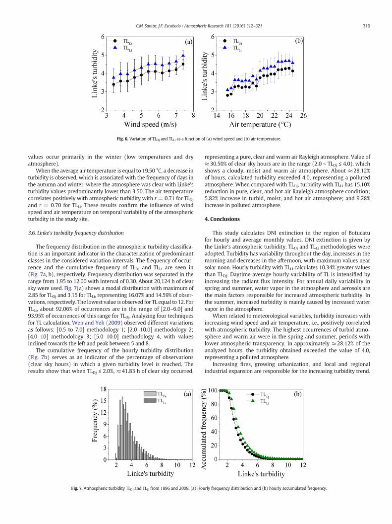
Fig. 6. Variation of TLDj and TLLi as a function of (a) wind speed and (b) air temperature.

319C.M. Santos, J.F. Escobedo / Atmospheric Research 181 (2016) 312–321

values occur primarily in the winter (low temperatures and dryatmosphere).

When the average air temperature is equal to 19.50 °C, a decrease inturbidity is observed, which is associated with the frequency of days inthe autumn and winter, where the atmosphere was clear with Linke'sturbidity values predominantly lower than 3.50. The air temperaturecorrelates positively with atmospheric turbidity with r = 0.71 for TLDjand r = 0.70 for TLLi. These results confirm the influence of windspeed and air temperature on temporal variability of the atmosphericturbidity in the study site.

3.6. Linke's turbidity frequency distribution

The frequency distribution in the atmospheric turbidity classifica-tion is an important indicator in the characterization of predominantclasses in the considered variation intervals. The frequency of occur-rence and the cumulative frequency of TLDj and TLLi are seen in(Fig. 7a, b), respectively. Frequency distribution was separated in therange from 1.95 to 12.00 with interval of 0.30. About 20,124 h of clearsky were used. Fig. 7(a) shows a modal distribution with maximum of2.85 for TLDj and 3.15 for TLLi, representing 16.07% and 14.59% of obser-vations, respectively. The lowest value is observed for TL equal to 12. ForTLLi, about 92.06% of occurrences are in the range of [2.0–6.0] and93.95% of occurrences of this range for TLDj. Analyzing four techniquesfor TL calculation, Wen and Yeh (2009) observed different variationsas follows: [0.5 to 7.0] methodology 1; [2.0–10.0] methodology 2;[4.0–10] methodology 3; [5.0–10.0] methodology 4, with valuesinclined towards the left and peak between 5 and 8.

The cumulative frequency of the hourly turbidity distribution(Fig. 7b) serves as an indicator of the percentage of observations(clear sky hours) in which a given turbidity level is reached. Theresults show that when TLDj ≤ 2.0%, ≈41.83 h of clear sky occurred,

Fig. 7. Atmospheric turbidity TLDj and TLLi from 1996 and 2008. (a) Hou

representing a pure, clear and warm air Rayleigh atmosphere. Value of≈30.50% of clear sky hours are in the range (2.0 b TLDj ≤ 4.0), whichshows a cloudy, moist and warm air atmosphere. About ≈28.12%of hours, calculated turbidity exceeded 4.0, representing a pollutedatmosphere. When compared with TLDj, turbidity with TLLi has 15.10%reduction in pure, clear, and hot air Rayleigh atmosphere condition;5.82% increase in turbid, moist, and hot air atmosphere; and 9.28%increase in polluted atmosphere.

4. Conclusions

This study calculates DNI extinction in the region of Botucatufor hourly and average monthly values. DNI extinction is given bythe Linke's atmospheric turbidity. TLDj and TLLi methodologies wereadopted. Turbidity has variability throughout the day, increases in themorning and decreases in the afternoon, with maximum values nearsolar noon. Hourly turbidity with TLLI calculates 10.34% greater valuesthan TLDj. Daytime average hourly variability of TL is intensified byincreasing the radiant flux intensity. For annual daily variability inspring and summer, water vapor in the atmosphere and aerosols arethe main factors responsible for increased atmospheric turbidity. Inthe summer, increased turbidity is mainly caused by increased watervapor in the atmosphere.

When related to meteorological variables, turbidity increases withincreasing wind speed and air temperature, i.e., positively correlatedwith atmospheric turbidity. The highest occurrences of turbid atmo-sphere and warm air were in the spring and summer, periods withlower atmospheric transparency. In approximately ≈28.12% of theanalyzed hours, the turbidity obtained exceeded the value of 4.0,representing a polluted atmosphere.

Increasing fires, growing urbanization, and local and regionalindustrial expansion are responsible for the increasing turbidity trend.

rly frequency distribution and (b) hourly accumulated frequency.

320 C.M. Santos, J.F. Escobedo / Atmospheric Research 181 (2016) 312–321

In Brazil, burning of native forests for agricultural production and cattleranching in the Amazon rainforest region, as well as agricultural burn-ing and sugarcane burning in regions near Botucatu, are great villainsin increasing particulate matter in the atmosphere. In the southeasternregion of Brazil, due to atmospheric circulation, these events alter theatmosphere pattern. In the summer, air circulation is also responsiblefor carrying enough moisture from the Amazon region to southeasternBrazil. Therefore, the atmosphere of Botucatu seems to be influencedby aerosols and water vapor from different origins. These two parame-ters alter the DNI distribution in the atmosphere and are critical in theradiant flux density on the surface.

There is a state law in São Paulo establishing a reduction in thepractice of sugarcane burning; however, the solid residue from crushedsugarcane (bagasse) is used as renewable industrial fuel, so the biomasscombustion emissions probably have not reduced (Scaramboni et al.,2015). This paper shows that the effect on the studyperiod is significant,and environmental public policies should be considered.

Therefore, with deforestation of native forests and increasingurbanization, further studies should be carried out in order to analyzenew standards in the atmosphere and in DNI distribution. Furtherstudies have become indispensable because recent studies have shownthat accidental and intentional fires have increased. These fires occurmainly in the states of the Amazon rainforest region and cause air pollu-tion with damages to health of millions of people and to aviation.

Acknowledgments

This work was supported by CAPES, CNPq and FAPESP. We alsoacknowledge associated NASA personnel for the production of dataused in this research and SoDA website.

References

Allen, A.G., Cardoso, A.A., Da Rocha, G.O., 2004. Influence of sugar cane burning on aerosolsoluble íon composition in Southeastern Brazil. Atmos. Environ. 38, 5025–5038.

Batlles, F.J., Rubio, M.A., Tovar, J., et al., 2000. Empirical modeling of hourly direct irradi-ance by means of hourly global irradiance. Energy 25, 675–688.

Bertin, A., Frangi, J.P., 2013. Contribution to the study of the wind and solar radiation overGuadeloupe. Energy Convers. Manag. 75, 593–602.

Bilbao, J., Román, R., Miguel, A., 2014. Turbidity coefficients from normal direct solar irra-diance in central Spain. Atmos. Res. 143, 73–84 (2014).

Cañada, J., Pinazo, J.M., Boscá, J.V., 1993. Determination of Ångström's turbidity coefficientat Valencia. Renew. Energy 3, 621–626.

Chaâbane, M., Masmoudi, M., Medhioub, K., 2004. Determination of Linke turbidityfactor from solar radiation measurement in northern Tunisia. Renew. Energy 29,2065–2076.

Chaiwiwatworakul, P., Chirarattananon, S., 2004. An investigation of atmospheric turbid-ity of Thai sky. Energy Build. 36, 650–659.

Codato, G., Oliveira, A.P., Soares, J., et al., 2008. Global and diffuse solar irradiances inurban and rural areas in southeast Brazil. Theor. Appl. Climatol. 93, 57–73.

CPA, 2016. Clima dos Municípios Paulistas. Disponivel em http://www.cpa.unicamp.br/outras-informacoes/clima_muni_086.html (Acesso em b17/06/2016N. [In portuguese]).

Cucumo, M., Kaliakatsos, D., Marinelli, V., 2000. A calculation method for the estimation ofthe Linke turbidity factor. Renew. Energy 19, 249–258.

Dal Pai, A., Escobedo, J.F., Dal Pai, E., et al., 2014. Estimation of hourly, daily and monthlymean diffuse radiation based on MEO shadowring correction. Energy Procedia 57,1150–1159.

Diabaté, L., Remund, J., Wald, L., 2003. Linke turbidity factors for several sites in Africa. Sol.Energy 75, 111–119.

Djafer, D., Irbah, A., 2013. Estimation of atmospheric turbidity over Ghardaïa city. Atmos.Res. 128, 76–84.

Dos Santos, C.M., Souza, J.L., Ferreira Junior, R.A., et al., 2014. On modeling global solarirradiation using air temperature for Alagoas State, Northeastern Brazil. Energy 71,388–398.

Ellouz, F., Masmoudi, M., Medhioub, K., 2013. Study of the atmospheric turbidity overNorthern Tunisia. Renew. Energy 51, 513–517.

El-Metwally, M., 2013. Indirect determination of broadband turbidity coefficients overEgypt. Meteorog. Atmos. Phys. 119, 71–90.

Elminir, K.H., Hamid, R.H., El-Hussainy, F., et al., 2006. The relative influence of the anthro-pogenic air pollutants on the atmospheric turbidity factors measured at an urbanmonitoring station. Sci. Total Environ. 368, 732–743.

Eltbaakh, Y.A., Ruslan, M.H., Alghoul, M.A., et al., 2012. Issues concerning atmosphericturbidity indices. Renew. Sust. Energ. Rev. 16, 285–6294.

Escobedo, J.F., Gomes, E.N., Oliveira, A.P., et al., 2011. Ratios of UV, PAR and NIR compo-nents to global solar radiation measured at Botucatu site in Brazil. Renew. Energy36, 169–178.

Flores, J.L., Karam, H.A., Filho, E.P.M., et al., 2015. Estimation of atmospheric turbidityand surface radiative parameters using broadband clear sky solar irradiance models

in Rio de Janeiro-Brasil. Theor. Appl. Climatol. http://dx.doi.org/10.1007/s00704-014-1369-7.

Formenti, P., Winkler, H., Fourie, P., et al., 2002. Aerosol optical depth over a remote semi-arid region of South Africa from spectral measurements of the daytime solar extinc-tion and the nighttime stellar extinction. Atmos. Res. 62, 11–32.

França, D., Longo, K., Rudorff, B., et al., 2014. Pre-harvest sugarne burning emission inven-tories based on remote sensing data in the state of state of São Paulo, Brazil. Atmos.Environ. 99, 446–456.

Freitas, S.R., Longo, K.M., Dias, M.A.F.S., et al., 2005. Monitoring the transport of biomassburning emissions in South America. Environ. Fluid Mech. 5, 135–167.

Gao, B.C., Kaufman, Y.J., 2003.Water vapour retrievals using moderate resolution imagingspectroradiometer (MODIS) near-infrared channels. J. Geophys. Res. 108 (D13), 4389.http://dx.doi.org/10.1029/2002JD003023.

Grenier, J.C., de La Casinière, A., Cabot, T., 1995. Atmospheric turbidity analyzed by meansof standardized Linke's turbidity factor. J. Appl. Meteorol. 34, 1449–1458.

Gueymard, C.A., 2012. Temporal variability in direct and global irradiance at various timescales as affected by aerosols. Sol. Energy 86, 3544–3553.

Holben, B.N., et al., 2001. An emerging ground-based aerosol climatology: aerosol opticaldepth from AERONET. J. Geophys. Res. 106 (11), 12.067–12.097.

Hove, T., Manyumbu, E., 2013. Estimates of the Linke turbidity factor over Zimbabweusing ground-measured clear-sky global solar radiation and sunshine records basedon a modified ESRA clear-sky model approach. Renew. Energy 52, 190–196.

Hussain, M., Khatun, S., Rasul, M.G., 2000. Determination of atmospheric turbidity inBangladesh. Renew. Energy 20, 325–332.

IBGE, 2015. Diretoria de Pesquisas—DPE—Coordenação de População e IndicadoresSociais—COPIS. 2014. Acesso em: b10/12/2015N. Disponível em http://cod.ibge.gov.br/2378L.

Inman, R.H., Edson, J.G., Coimbra, C.F.M., 2015. Impact of local broadband turbidity esti-mation on forecasting of clear sky direct normal irradiance. Sol. Energy 117, 125–138.

Iqbal, M., 1983. An Introduction to Solar Radiation. Academic Press, New York, p. 390.Jones, C., Carvalho, L.M.V., Higgins, R.W., et al., 2004. Climatology of tropical intraseasonal

convective anomalies: 1979–2002. J. Clim. 17, 523–539.Karayel, M., Navvab, M., Ne'eman, E., et al., 1984. Zenith luminance and sky luminance

distributions for daylighting calculations. Energy Build. 6 (3), 283–291.Kasten, F., 1980. A simple parameterization of the pyrheliometer formula of the Linke

turbidity factor. Meteorol. Rundsch. 33, 124–127.Kasten, F., 1996. The Linke turbidity factor based on improved values of the integral

Rayleigh optical thickness. Sol. Energy 56 (3), 239–244.Khalil, S.A., Shaffie, A.M., 2016. Attenuation of the solar energy by aerosol particles: a

review and case study. Renew. Sust. Energ. Rev. 54, 363–375.Leckner, B., 1978. The spectral distribution of solar radiation at the earth's surface—

elements of a model. Sol. Energy 20, 143–150.Li, D.H.W., Lam, J.C., 2002. A study of atmospheric turbidity for Hong Kong. Renew. Energy

25, 1–13.Linke, E., 1922. Transmission-koeffizient und Trübungsfaktor. Beitr. Phys. der freien

Atmos. 10, 91–103.López, G., Batlles, F.J., 2004. Estimate of the atmospheric turbidity from three broad-band

solar radiation algorithms: a comparative study. Ann. Geophys. 22, 2657–2668.Louche, A., Peri, G., Iqbal, M., 1986. An analysis of Linke turbidity factor. Sol. Energy 37 (6),

393–396.Masmoudi, M., Belghith, I., Chaabane, M., 2002. Elemental particle size distributions:

measured and estimated dry deposition in Sfax region (Tunisian). Atmos. Res. 63,209–219.

Masmoudi, M., Chaâbane, M., Medhioub, K., et al., 2003. Variability of aerosol opticalthickness and atmospheric turbidity in Tunisia. Atmos. Res. 66, 175–188.

Mavromatakis, F., Franghiadakis, Y., 2007. Direct and indirect determination of the Linketurbidity coefficient. Sol. Energy 81, 896–903.

Oliveira, B.F.A., Ignotti, E., Hacon, S.S., 2011. A systematic review of the physical andchemical characteristics of pollutants from biomass burning and combustion offossil fuels and health effects in Brazil. Cad. Saúde Pública, Rio de Janeiro 27,1678–1698.

Pedrós, R., Utrillas, M.P., Martínez-Lozano, J.A., et al., 1999. Values of broad-band turbiditycoefficients in a Mediterranean coastal site. Sol. Energy 66 (1), 11–20.

Polo, J., Zarzalejo, L.F., Salvador, P., et al., 2009a. Angstrom turbidity and ozone columnestimations from spectral solar irradiance in a semi-desertic environment in Spain.Sol. Energy 83, 257–263.

Polo, J., Zarzalejo, L.F., Martın, L., et al., 2009b. Estimation of daily Linke turbidity factor byusing global irradiance measurements at solar noon. Sol. Energy 83, 1177–1185.

Portillo-Quintero, C., Sanchez-Azofeifa, A., Espirito-Santo,M.M., 2013.Monitoring defores-tation with MODIS Active Fires in Neotropical dry forest: Na analysis of local-scaleassessments in Mexico, Brazil and Bolivia. J. Arid Environ. 97, 150–159.

Power, H.C., Goyal, A., 2003. Comparison of aerosol and climate variability over Germanyand South Africa. Int. J. Climatol. 23, 921–941.

Rahoma, U.A.L.I., Hassan, A.H., 2012. Determination of atmospheric turbidity and itscorrelation with climatologically parameters. Am. J. Environ. Sci. 8, 597–604.

Rapti, A.S., 2000. Atmospheric transparency, atmospheric turbidity and climatic parame-ters. Sol. Energy 69, 99–111.

Reboita, M.S., Gan, M.A., Rocha, R.P., et al., 2010. Regimes de precipitação na América doSul: Uma revisão bibliográfica. Rev. Bras. Meteorol. 25, 185–204 (in portuguese).

Remer, L.A., et al., 2008. Global aerosol climatology from the MODIS satellite sensors.J. Geophys. 113, 1–18.

Rosenfeld, D., 1999. TRMM observed first direct evidence of smoke from forest firesinhibiting rainfall. Geophys. Res. Lett. 26 (20), 3105–3108.

Salazar, G.A., 2011. Estimation of monthly values of atmospheric turbidity using mea-sured values of global irradiation and estimated values from CSR and Yang Hybridmodels. Study case: Argentina. Atmos. Environ. 45, 2465–2472.

Satyamurty, P., Nobre, C., Silva Dias, P., 1998. South America. In: Karoly, D., Vincent, D.(Eds.), Meteorology of the Southern HemisphereMeteorological Monographs 27(49). American Meteorological Society, Boston, pp. 119–139.

Scaramboni, C., Urban, R.C., Lima-Souza, M., et al., 2015. Total sugars in atmosphericaerosols: an alternative tracer for biomass burning. Atmos. Environ. 100, 185–192.

321C.M. Santos, J.F. Escobedo / Atmospheric Research 181 (2016) 312–321

Souza, J.L., Lyra, B.G., Santos, C.M., et al., 2016. Empirical models of daily and monthlyglobal solar irradiation using sunshine duration for Alagoas State, NortheasternBrazil. Sustain. Energy Technol. Assess. 14, 35–45.

Teramoto, E.T., Escobedo, J.F., 2012. Análise da frequência anual das condições de céuem Botucatu, São Paulo. Rev. Bras. Engenharia Agrícola Ambient. 16 (9), 985–992(in portuguese).

Trabelsi, A., Masmoudi, M., 2011. An investigation of atmospheric turbidity overKerkennah Island in Tunisia. Atmos. Res. 101, 22–30.

Uscka-Kowalkowsk, J., 2013. An analysis of the extinction of direct solar radiation onMt. Kasprowy Wierch, Poland. Atmos. Res. 134, 175–185.

Videla, F.C., Barnaba, F., Angelini, F., et al., 2013. The relative role of Amazonian and non-Amazonian fires in building up the aerosol optical depth in South America: a five yearstudy (2005–2009). Atmos. Res. 122, 298–309.

Wen, C.-C., Yeh, H.-H., 2009. Analysis of atmospheric turbidity levels at Taichung Harbornear the Taiwan Strait. Atmos. Res. 94, 168–177.

WMO – World Meteorological Organization, 2008. Guide to meteorological Instrumentsand Methods of Observation. WMO-n°8, Seventh Edition, 157–197, Geneva,Switzerland.

Zakey, A.S., Abdelwahab, M.M., Makar, P.A., 2004. Atmospheric turbidity over Egypt.Atmos. Environ. 38, 1579–1591.