Michalak1.pdf - Berkeley Atmospheric Sciences Center

Geostatistics:

Principles of spatial analysis

Anna M. Michalak

Department of Civil and Environmental Engineering

Department of Atmospheric, Oceanic and Space Sciences

The University of Michigan

A.M. Michalak ([email protected])

Key Points

! If the parameter(s) that you are modeling exhibits spatial

(and/or temporal) autocorrelation, this feature must be taken

into account to avoid biased solutions

! Spatial (and/or temporal) autocorrelation can be used as a

source of information in helping to constrain parameter

distributions

! The field of geostatistics provides a framework for addressing

the above two issues


Outline

! Motivation for geostatistical tools

! What is geostatistics?

! Traditional applications

! Application to OCO sampling design

! Introduction to inverse modeling

! Application to groundwater contamination

! Application to CO2 flux estimation


What is Geostatistics?

! A short answer:

" An interpolation and extrapolation toolkit

! A more sophisticated answer:

" All of the above for modeling spatial relationship of available data

and building from such a model (e.g. kriging, stochastic

simulation, …)

! Formal definition

" Analysis and prediction of spatial or temporal phenomena (e.g.

pollutant concentrations, soil porosities, elevations, etc.)


Spatial Correlation

! Measurements in close proximity to each other generally exhibit

less variability than measurements taken farther apart.

! Assuming independence, spatially-correlated data may lead to:

1. Biased estimates of model parameters

2. Biased statistical testing of model parameters

! Spatial correlation can be accounted for by using geostatistical

techniques


0 200 400 600 800 10000

100

200

300

400

500

600

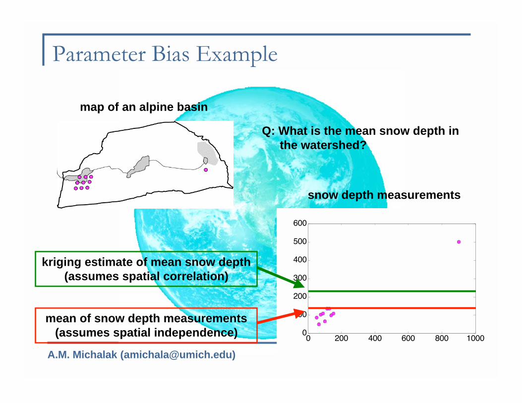
Parameter Bias Example

map of an alpine basin

snow depth measurements

0 200 400 600 800 10000

100

200

300

400

500

600

mean of snow depth measurements

(assumes spatial independence)

kriging estimate of mean snow depth

(assumes spatial correlation)

0 200 400 600 800 10000

100

200

300

400

500

600

Q: What is the mean snow depth in

the watershed?


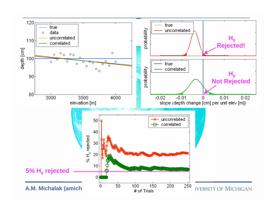
Example cont�

H0 is TRUE

5% H0 rejected

5% H0

Rejected

5% H0

Rejected

H0

Rejected!

H0

Not Rejected


Variogram Model

! Used to describe spatial correlation

4

3

2

1

z(x) = m(x) + !(x)


Geostatistics in Practice

! Main uses:

" Data integration

" Numerical models for prediction

" Numerical assessment (model) of uncertainty

2 4 61

2

3

4

5

6

2 4 61

2

3

4

5

6


Caveats

Save time & effort

Provide causal / physical

relationshipsIntegrate data

Create dataExpand from data

Replace good or additional

dataHonor data

Fully automate estimation

process

Provide practical solution to

real problems

DOESN’TDOES

Geostatistics is a set of decision-making tools


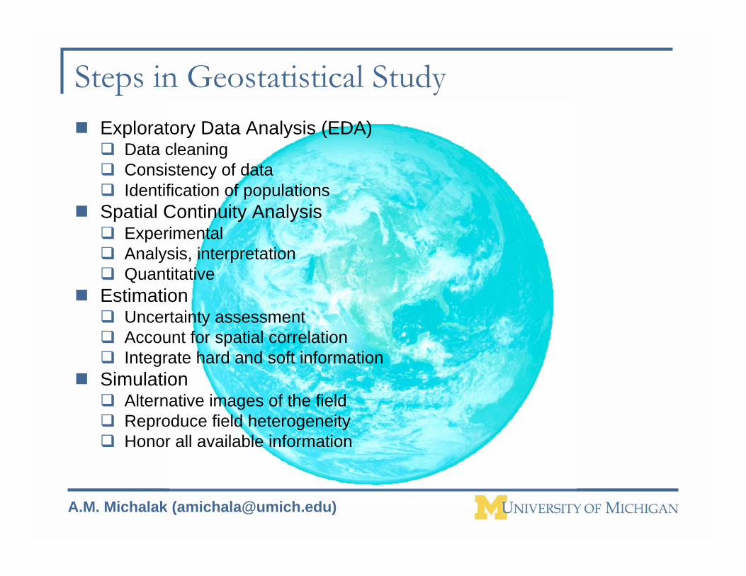
Steps in Geostatistical Study

! Exploratory Data Analysis (EDA)" Data cleaning

" Consistency of data

" Identification of populations

! Spatial Continuity Analysis" Experimental

" Analysis, interpretation

" Quantitative

! Estimation" Uncertainty assessment

" Account for spatial correlation

" Integrate hard and soft information

! Simulation" Alternative images of the field

" Reproduce field heterogeneity

" Honor all available information


Go to Matlab�


OCO Satellite

! Planned launch in September

2008

! Will provide global column-

integrated CO2 measurements

! 1ppm measurement accuracy at

a 1000km scale.


OCO Measurements

! 1ppm measurement accuracy at

a 1000km scale.

! Processing all spectral

radiances to XCO2 is

computationally prohibitive.

! Limit Sampling to optimal

locations


OCO Subsampling Strategy

! Objective:

" Determine optimal sampling locations as a function of time and

space that allow for the interpolation of XCO2 at unsampled

locations with estimation error within a set threshold

! Recent work:

" Define modeled XCO2 spatial variability using CASA-MATCH data

(Olsen and Randerson 2004) subsampled at 1pm local time

" Preliminary approach for identifying optimal sampling locations


Sample Modeled XCO2 Data

April July

August October


Optimal Sampling Locations

! Optimal sampling locations = potential sampling locations

that will achieve a set estimation error threshold at

unsampled locations

! Estimation error = estimation standard deviation at

unsampled locations

! Geostatistical interpolation tools:

" Use spatial correlation as a basis of estimation

" Provide best linear unbiased estimates

" Quantify associated estimation error


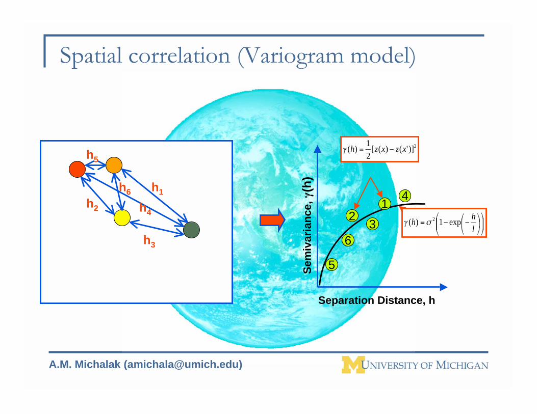
Spatial correlation (Variogram model)

!!"

#$$%

&!"

#$%

&''=

l

hh exp1)( 2()

h1

h4

h3

h2

h6

h5

4

23

6

5

Separation Distance, hS

em

ivari

an

ce, !(h

)

2)]'()([2

1)( xzxzh !="

1


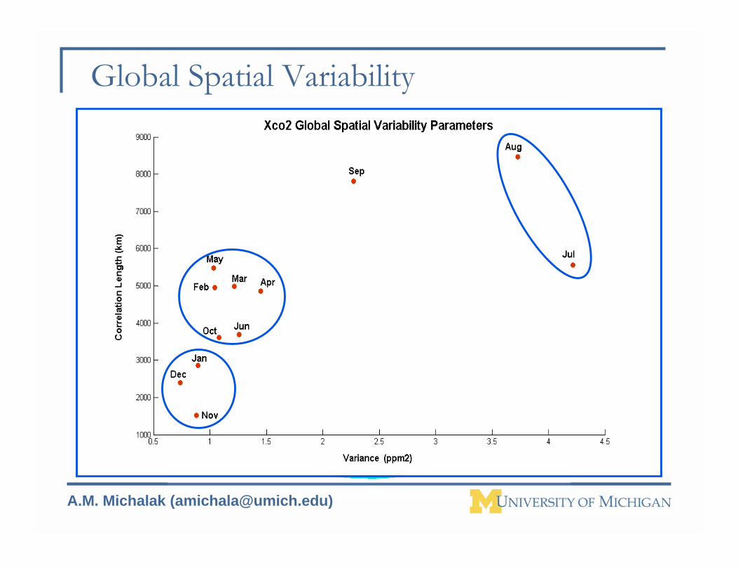
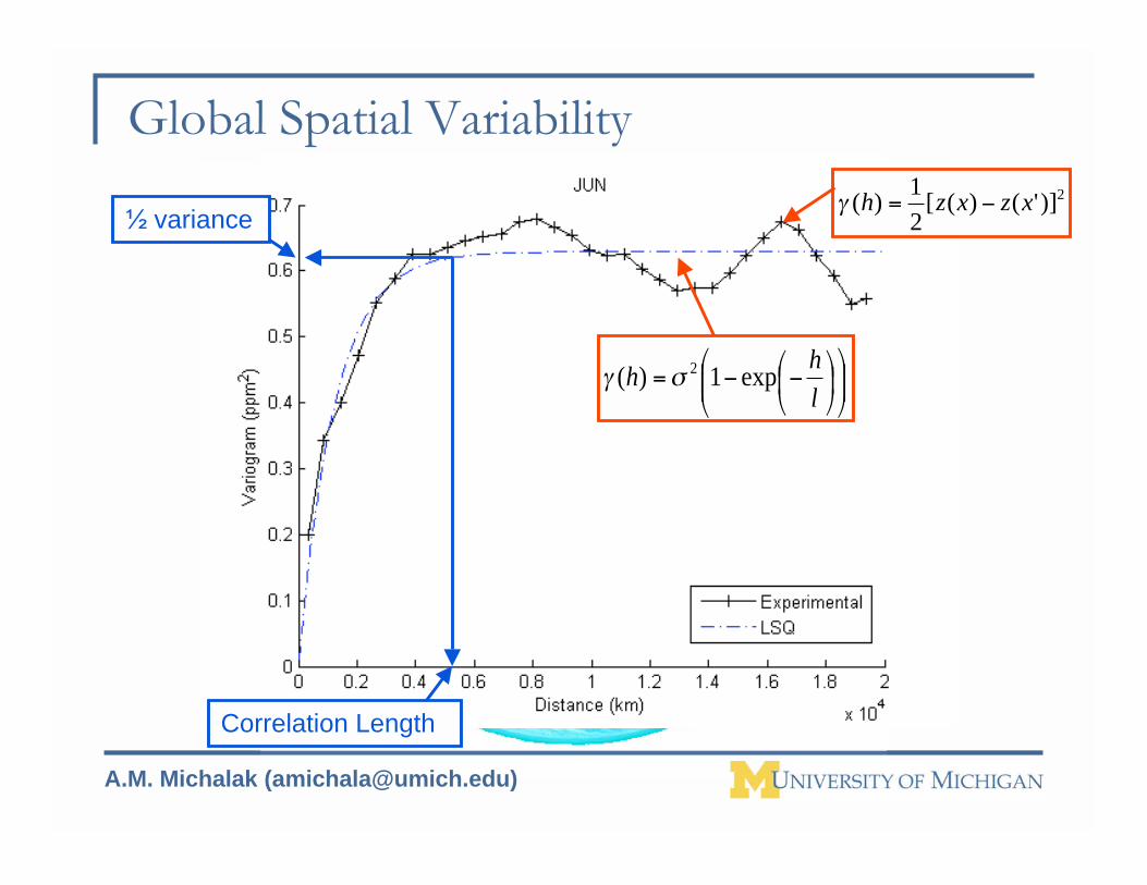
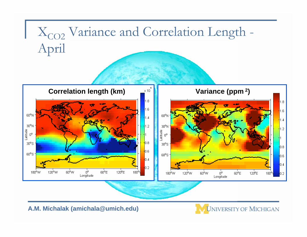
Global Spatial Variability

2)]'()([2

1)( xzxzh !="

! variance

Correlation Length

!!"

#$$%

&!"

#$%

&''=

l

hh exp1)( 2()


Global Spatial Variability


Local Variability (2000 km radius)

2000 km

5.5

degrees


XCO2 Variance and Correlation Length -

April

Correlation length (km) Variance (ppm 2)


Distance to Achieve 1ppm Uncertainty (h0)

! h0 = max distance from the

interpolation point to sample for

1ppm error

! h0 depends on spatial variability

near interpolation point

! Interpolation at each grid point

on a 5.5o by 5.5o global grid

!"

#$%

&''=

2

max

0

21ln

(

Vlh

h0 =?

Vmax=1ppm


Maximum Sampling Interval h0 - April

Maximum sampling interval (km)


Regular Grid Sampling Uncertainty

AprilJuly


Optimal Sampling Locations and

Associated Uncertainties

AprilJuly


Sampling Constraints

! Aerosols

! Clouds

! Satellite track

! Maximum (sub)sampling rate

! Albedo

! Measurement error

! Temporal aggregation

! Others?


Conclusions from OCO Study

! XCO2 exhibits strong spatial correlation

! XCO2 covariance structure is variable in space and time

! Uniform sampling will not achieve uniform/acceptable

interpolation uncertainty

! Geostatistical tools can be used to incorporate the variability in

the XCO2 covariance structure into a subsampling protocol


Inverse Modeling


Inverse models

! Geostatistical inverse modeling objective function:

H = transport information

s = unknown fluxes

y = CO2 measurements

R = model-data mismatch covariance

Q = spatial/temporal covariance of flux deviations from trendX and ! = model of the trend

)()()()( 11 !! XsQXsHsyRHsy ""+""="" TT

sL

Deterministic

component

Stochastic

component

!" Ts QHX +=ˆ


Bayesian Inference Applied to Inverse Modeling for

Inferring Historical Forcing

Posterior probability

of historical forcingPrior information

about forcing

p(y) probability of

measurements

Likelihood of forcing given

available measurements

y : available observations (n!1)

s : discretized historical forcing (m!1)


Dover Air Force Base Case Study

! Dover Air Force Base located in Delaware, U.S.A.

! Unconfined aquifer underlain by two-layer aquitard

! Aquitard cores used to infer PCE

and TCE contamination history

in aquifer

! Solute transport controlled by

diffusive process:

Lxx

cD

t

cR

aqaq

<<!

!=

!

!0

2

1

2

1

1

1

+!<<"

"=

"

"xL

x

cD

t

cR

aqaq

2

2

2

2

2

2


TCE at Location PPC11

Time variation of

boundary condition

Measured TCE concentration

as a function of depth


TCE at Location PPC13

Time variation of

boundary condition

Measured TCE concentration

as a function of depth


Sources of Atmospheric CO2 Information

North American Carbon Program


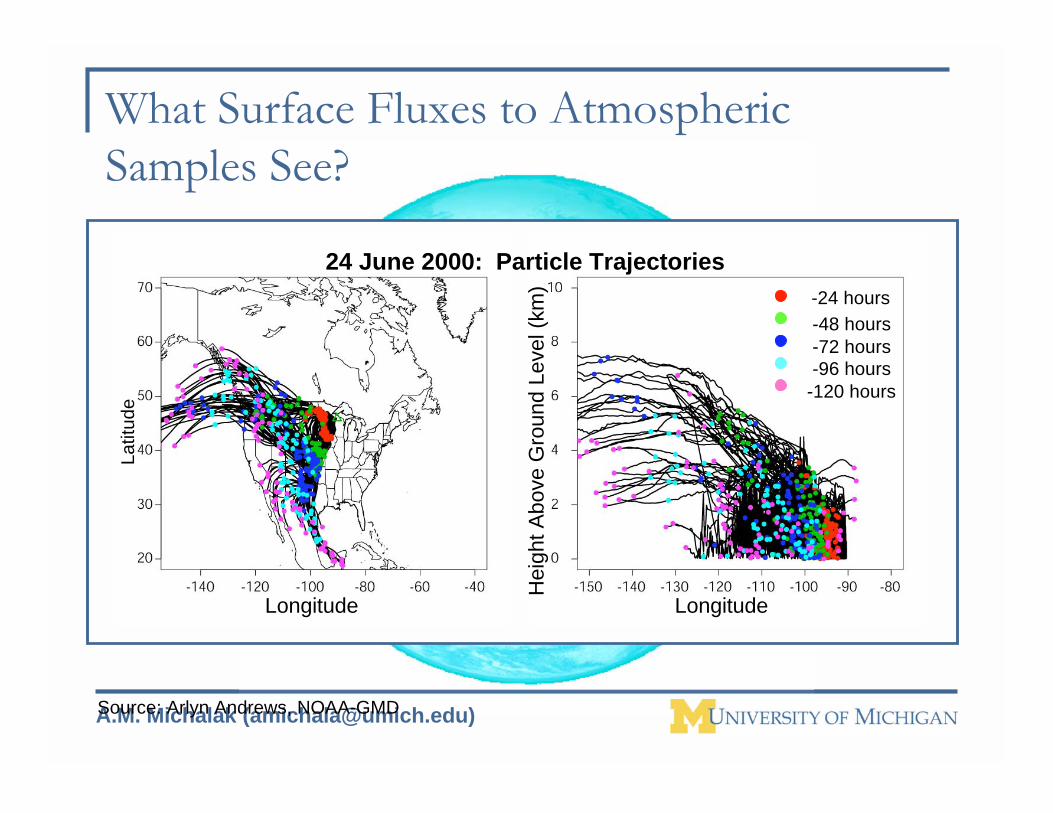
Longitude Longitude

La

titu

de

Heig

ht A

bove G

round L

evel (k

m)

24 June 2000: Particle Trajectories

-24 hours

-48 hours

-72 hours

-96 hours

-120 hours

What Surface Fluxes to Atmospheric

Samples See?

Source: Arlyn Andrews, NOAA-GMD


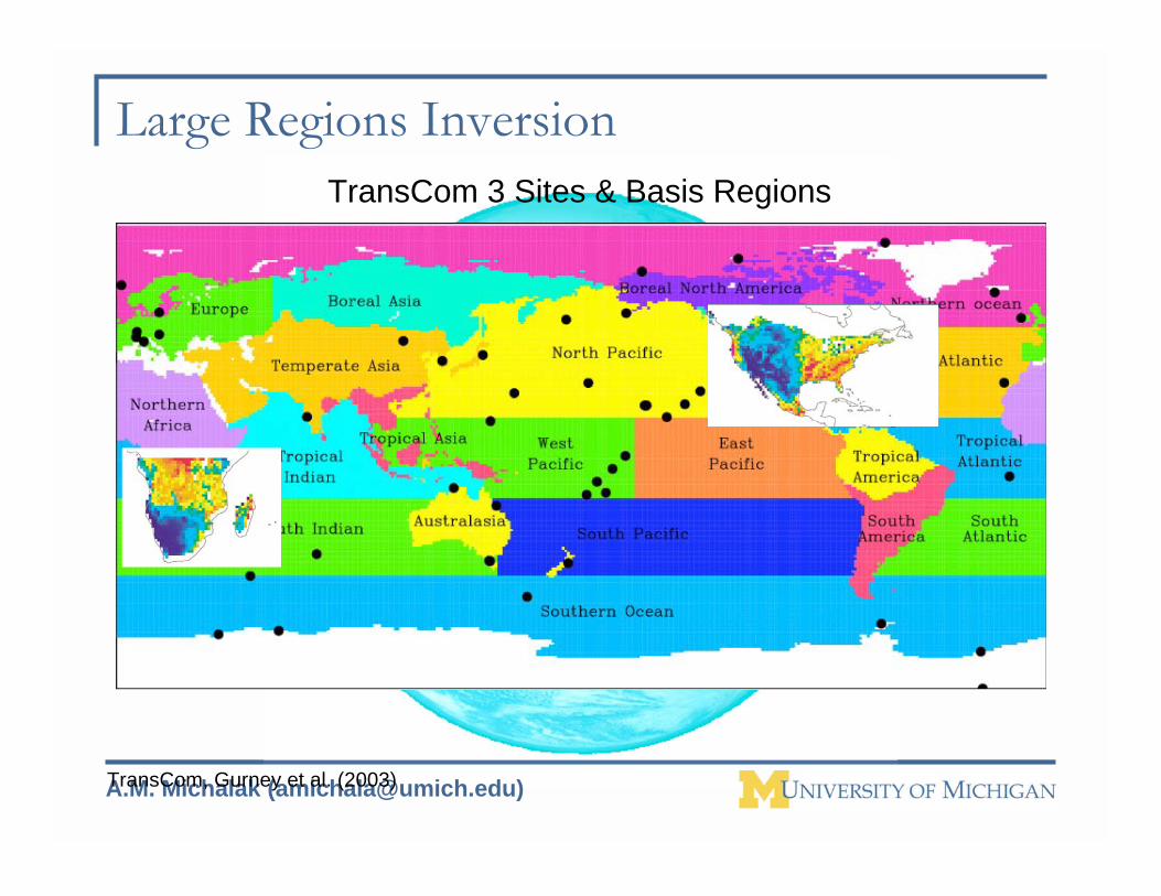
Large Regions Inversion

TransCom, Gurney et al. (2003)

TransCom 3 Sites & Basis Regions


Study Goals

!"Estimate carbon fluxes at fine spatial resolution (3.75o x 5.0o)

#"Avoid use of prior flux estimates

$"Incorporate and quantify effect of available auxiliary data

Questions:

% What will be the effect on estimated fluxes and their

uncertainties?

% Is there sufficient information in the atmospheric

measurements to “see” the relationship between auxiliary

data and fluxes?


Auxiliary Data and Carbon Flux Processes:

Image Source: NCAR

Terrestrial Flux:

Photosynthesis(FPAR, LAI, NDVI)

Respiration

(temperature)

Oceanic Flux:

Gas transfer

(sea surface

temperature, air

temperature)

Anthropogenic

Flux:

Fossil fuel

combustion

(GDP density,population)

Other:

Spatial trends

(sine latitude,

absolute value

latitude)

Environmental

parameters:

(precipitation,

%land use, Palmer

drought index)


Sample Auxiliary Data


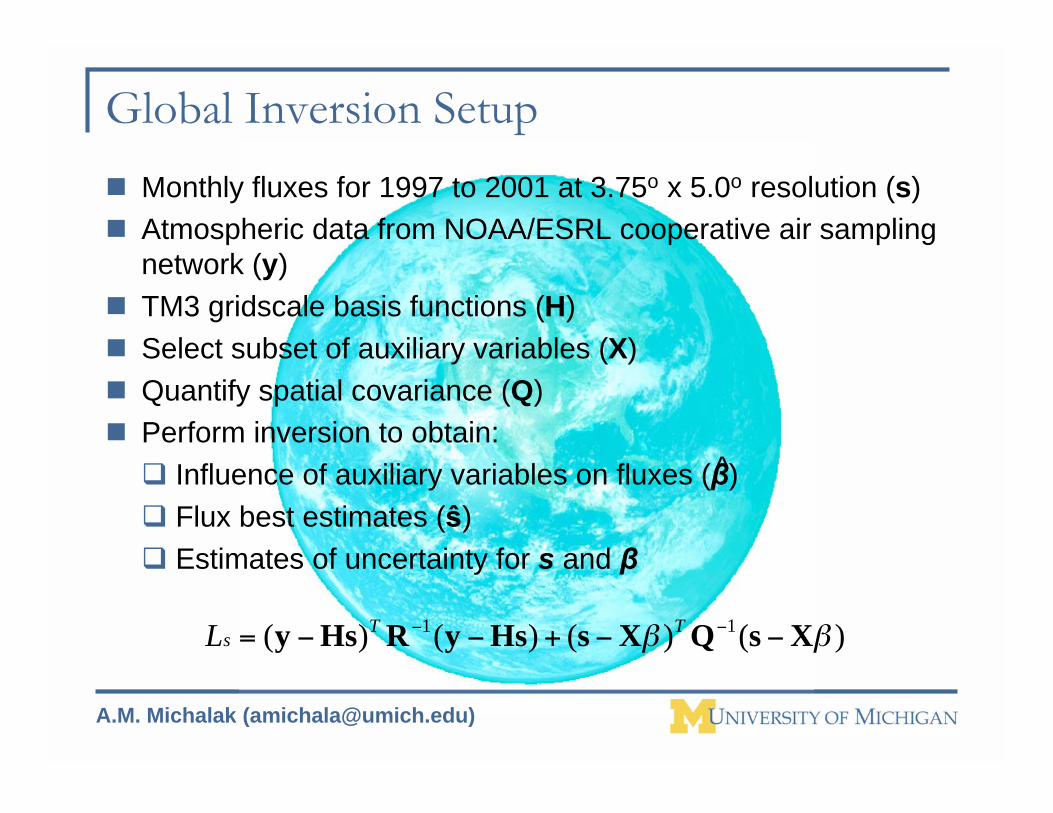
Global Inversion Setup

! Monthly fluxes for 1997 to 2001 at 3.75o x 5.0o resolution (s)

! Atmospheric data from NOAA/ESRL cooperative air sampling

network (y)

! TM3 gridscale basis functions (H)

! Select subset of auxiliary variables (X)

! Quantify spatial covariance (Q)

! Perform inversion to obtain:

" Influence of auxiliary variables on fluxes (!)

" Flux best estimates (!)

" Estimates of uncertainty for s and !

^

)()()()( 11 !! XsQXsHsyRHsy ""+""="" TT

sL


Final Set of Auxiliary VariablesCombined physical understanding with results of VRT to choose final set

of auxiliary variables:

• GDP Density

• Leaf Area Index (LAI)

• Fraction of photosynthetically active radiation (FPAR)

• Percent forest / shrub

• Precipitation

3.02.89.110.84.9|!/"|

-0.21.05.7-4.41.5! - 2"

-1.00.23.7-6.40.6! + 2"

-0.60.64.7-5.41.1!

F/SPrecip.FPARLAIGDPVariable


Building up the Best Estimate


Location of 22 Transcom Regions

Southern Ocean

Boreal Asia

South Pacific South Indian

Europe

North Pacific

North Atlantic

Temperate Asia

South Atlantic

Tropical Indian

Tropical East Pacific

Northern Africa

Tropical Atlantic

Tropical West

Pacific

Australia

Boreal

North America

South

America

Southern

Africa

Temperate

North America

Tropical

America

Tropical Asia

Northern Ocean

(SoOc)

(SoIn)

(BoAs)

(SoPa)

(NoPa)

(TrIn)

(TeAs)

(NoAt)

(SoAt)

(TEPa)

(Euro)

(TrAt)

(BNAm)

(NoAf)

(TWPa)

(SoAf)

(TrAm)

(TNAm)

(Aust)

(SoAm)

(TrAs)

(NoOc)


Conclusions - Methodology

! Geostatistical inverse modeling avoids the use of prior fluxestimates

! Covariance structure of flux residuals and model-datamismatch can be quantified using atmospheric data

! Benefit of auxiliary data can be quantified

! Fluxes and the influence of auxiliary data are estimatedconcurrently (w/ uncertainties)

! Approaches maximizes the use of information whileminimizing assumptions

! Geostatistical inverse modeling not constrained by priorestimates

" Provides independent validation of bottom-up estimates in well-constrained regions

" Approach well suited to show inter-annual variability

" Provides accurate measure of uncertainty


Key Points

! If the parameter(s) that you are modeling exhibits spatial

(and/or temporal) autocorrelation, this feature must be taken

into account to avoid biased solutions

! Spatial (and/or temporal) autocorrelation can be used as a

source of information in helping to constrain parameter

distributions

! The field of geostatistics provides a framework for addressing

the above two issues


Acknowledgments

! Collaborators:

" Pieter Tans, Adam Hirsch, Lori Bruhwiler, Kevin Schaefer, Wouter Peters, Andy JacobsonNOAA/CMDL

" Alanood Alkhaled, Sharon Gourdji, Charles Humphriss, Meng Ying Li, Miranda Malkin, KimMueller, and Shahar Shlomi, UM

" Bhaswar Sen and Charles Miller, JPL

" Kevin Gurney, Purdue U.

" Peter Kitanidis, Stanford U.

! Funding sources:

" Elizabeth C. Crosby Research Award

" University Corporation for Atmospheric Research (UCAR)

" National Oceanic and Atmospheric Administration (NOAA)

" National Aeronautic and Space Administration (NASA) and Jet Propulsions Laboratory (JPL)

" National Science Foundation (NSF)

" Michigan Space Grant Consortium (MSGC)

! Data providers:

" NOAA / CMDL cooperative air sampling network

" Seth Olsen (LANL) and Jim Randerson (UCI)

" Christian Rödenbeck, MPIB

" Kevin Schaefer, NOAA / ESRL

" NOAA CDC NASA, EROS USGS, CEISIN, Global Precipitation Climatology Centre, UCAR


QUESTIONS?

[email protected]

http://www-personal.engin.umich.edu/~amichala/

Michalak1.pdf - Berkeley Atmospheric Sciences Center

Documents

Transcript of Michalak1.pdf - Berkeley Atmospheric Sciences Center