Temporal Network Optimization Subject to

Connectivity Constraints⋆

George Mertzios1, Othon Michail2,Ioannis Chatzigiannakis2, and Paul G. Spirakis2,3

1 School of Engineering and Computing Sciences, Durham University, UK2 Computer Technology Institute & Press “Diophantus” (CTI), Patras, Greece

3 Department of Computer Science, University of Liverpool, UKEmail: george.mertzios@durham.ac.uk, michailo, ichatz, spirakis@cti.gr

Abstract. In this work we consider temporal networks, i.e. networksdefined by a labeling λ assigning to each edge of an underlying graph G

a set of discrete time-labels. The labels of an edge, which are naturalnumbers, indicate the discrete time moments at which the edge is avail-able. We focus on path problems of temporal networks. In particular, weconsider time-respecting paths, i.e. paths whose edges are assigned by λ

a strictly increasing sequence of labels. We begin by giving two efficientalgorithms for computing shortest time-respecting paths on a temporalnetwork. We then prove that there is a natural analogue of Menger’s the-orem holding for arbitrary temporal networks. Finally, we propose twocost minimization parameters for temporal network design. One is thetemporality of G, in which the goal is to minimize the maximum numberof labels of an edge, and the other is the temporal cost of G, in whichthe goal is to minimize the total number of labels used. Optimization ofthese parameters is performed subject to some connectivity constraint.We prove several lower and upper bounds for the temporality and thetemporal cost of some very basic graph families such as rings, directedacyclic graphs, and trees.

1 Introduction

A temporal (or dynamic) network is, loosely speaking, a network that changeswith time. This notion encloses a great variety of both modern and traditionalnetworks such as information and communication networks, social networks,transportation networks, and several physical systems.

In this work, embarking from the foundational work of Kempe et al. [KKK00],we consider discrete time, that is, we consider networks in which changes occurat discrete moments in time, e.g. days. This choice is not only a very natural

⋆ Supported in part by (i) the project FOCUS implemented under the “ARISTEIA”Action of the OP “Education and Lifelong Learning” and co-funded by the EU(ESF) and Greek National Resources, (ii) the FET EU IP project MULTIPLEX

under contract no 317532, and (iii) the EPSRC Grant EP/G043434/1. Full version:http://ru1.cti.gr/aigaion/?page=publication&kind=single&ID=977

abstraction of many real systems but also gives to the resulting models a purelycombinatorial flavor. In particular, we consider those networks that can be de-scribed via an underlying graph G and a labeling λ assigning to each edge ofG a (possibly empty) set of discrete labels. Note that this is a generalization ofthe single-label-per-edge model used in [KKK00], as we allow many time-labelsto appear on an edge. These labels are drawn from the natural numbers andindicate the discrete moments in time at which the corresponding connection isavailable. For example, in the case of a communication network, availability ofa communication link at some time t may mean that a communication protocolis allowed to transmit a data packet over that link at time t.

In this work, we initiate the study of the following fundamental network de-sign problem: “Given an underlying (di)graph G, assign labels to the edges ofG so that the resulting temporal graph λ(G) minimizes some parameter whilesatisfying some connectivity property”. In particular, we consider two cost opti-mization parameters for a given graph G. The first one, called temporality of G,measures the maximum number of labels that an edge of G has been assigned.The second one, called temporal cost of G, measures the total number of labelsthat have been assigned to all edges of G (i.e. if |λ(e)| denotes the number oflabels assigned to edge e, we are interested in

∑

e∈E |λ(e)|). Each of these twocost measures can be minimized subject to some particular connectivity prop-erty P that the temporal graph λ(G) has to satisfy. In this work, we considertwo very basic connectivity properties. The first one, that we call the all pathsproperty, requires the temporal graph to preserve every simple path of its under-lying graph, where by “preserve a path of G” we mean that the labeling shouldprovide at least one strictly increasing sequence of labels on the edges of thatpath (we also call such a path time-respecting).

For an illustration, consider a directed ring u1, u2, . . . , un. We want to deter-mine the temporality of the ring subject to the all paths property, that is, wewant to find a labeling λ that preserves every simple path of the ring and at thesame time minimizes the maximum number of labels of an edge. Consider thepaths P1 = (u1, . . . , un) and P2 = (un−1, un, u1, u2). It is immediate to observethat an increasing sequence of labels on the edges of path P1 implies a decreasingpair of labels on edges (un−1, un) and (u1, u2). On the other hand, path P2 usesfirst (un−1, un) and then (u1, u2) thus it requires an increasing pair of labelson these edges. It follows that in order to preserve both P1 and P2 we have touse a second label on at least one of these two edges, thus the temporality is atleast 2. Next, consider the labeling that assigns to each edge (ui, ui+1) the labelsi, n+ i, where 1 ≤ i ≤ n and un+1 = u1. It is not hard to see that this labelingpreserves all simple paths of the ring. Since the maximum number of labels thatit assigns to an edge is 2, we conclude that the temporality is also at most 2. Insummary, the temporality of preserving all simple paths of a directed ring is 2.

The other connectivity property that we define, called the reach property,requires the temporal graph to preserve a path from node u to node v wheneverv is reachable from u in the underlying graph. Furthermore, the minimizationof each of our two cost measures can be affected by some problem-specific con-

2

straints on the labels that we are allowed to use. We consider here one of themost natural constraints, namely an upper bound of the age of the constructedlabeling λ, where the age of a labeling λ is defined to be equal to the maximumlabel of λ minus its minimum label plus 1. Now the goal is to minimize the costparameter, e.g. the temporality, satisfy the connectivity property, e.g. all paths,and additionally guarantee that the age does not exceed some given natural k.Returning to the ring example, it is not hard to see, that if we additionally re-strict the age to be at most n− 1 then we can no longer preserve all paths of aring using at most 2 labels per edge. In fact, we must now necessarily use theworst possible number of labels, i.e. n− 1 on every edge.

Minimizing such parameters may be crucial as, in most real networks, mak-ing a connection available and maintaining its availability does not come forfree. At the same time, such a study is important from a purely graph-theoreticperspective as it gives some first insight into the structure of specific familiesof temporal graphs (e.g. no temporal ring exists with fewer than n + 1 labels).Finally, we believe that our results are a first step towards answering the follow-ing fundamental question: “To what extent can algorithmic and structural resultsof graph theory be carried over to temporal graphs?”. For example, is there ananalogue of Menger’s theorem for temporal graphs? One of the results of thepresent work is an affirmative answer to the latter question.

1.1 Related Work

Single-label Temporal Graphs and Menger’s Theorem. The model oftemporal graphs that we consider in this work is a direct extension of the single-label model studied in [Ber96] and [KKK00] to allow for many labels per edge.In [KKK00], Kempe et al., among other things, proved that there is no analogueof Menger’s theorem, at least in its original formulation, for arbitrary single-label temporal networks. In this work, we go a step ahead showing that if onereformulates Menger’s theorem in a way that takes time into acount then a verynatural temporal analogue of Menger’s theorem is obtained. Furthermore, in thepresent work, we consider a path as time-respecting if its edges have strictlyincreasing labels and not non-decreasing as in the above papers.

Continuous Availabilities (Intervals). Some authors have naturally assumedthat an edge may be available for continuous time-intervals. The techniques usedthere are quite different than those needed in the discrete case [XFJ03, FT98].

Distributed Computing on Dynamic Networks. A notable set of recentworks has studied (distributed) computation in worst-case dynamic networks inwhich the topology may change arbitrarily from round to round (see e.g. [KLO10,MCS12]). Population protocols [AAD+06] and variants [MCS11a] are collectionsof passively mobile finite-state agents that compute something useful in thelimit. Another interesting direction assumes random network dynamicity and theinterest is on determining “good” properties of the dynamic network that holdwith high probability and on designing protocols for distributed tasks [CMM+08,AKL08]. For introductory texts cf. [CFQS12, MCS11b, Sch02].

3

Distance Labeling. A distance labeling of a graph G is an assignment of uniquelabels to the vertices of G so that the distance between any two vertices can beinferred from their labels alone [GPPR01, KKKP04]. There, the labeling param-eter to be minimized is the binary length of an appropriate distance encoding,which is different from our cost parameters.

1.2 Contribution

In Section 2, we formally define the model of temporal graphs under consid-eration and provide all further necessary definitions. In Section 3, we give twoefficient algorithms for computing shortest time-respecting paths. Then in Sec-tion 4 we present an analogue of Menger’s theorem which we prove valid forarbitrary temporal graphs. In the full paper, we also apply our Menger’s ana-logue to substantially simplify the proof of a recent result on distributed tokengathering. In Section 5, we formally define the temporality and temporal costoptimization metrics for temporal graphs. In Section 5.1, we provide several up-per and lower bounds for the temporality of some fundamental graph familiessuch as rings, directed acyclic graphs (DAGs), and trees, as well as an inter-esting trade-off between the temporality and the age of rings. Furthermore, weprovide in Section 5.2 a generic method for computing a lower bound of thetemporality of an arbitrary graph w.r.t. the all paths property, and we illustrateits usefulness in cliques and planar graphs. Finally, we consider in Section 5.3the temporal cost of a digraph G w.r.t. the reach property, when additionallythe age of the resulting labeling λ(G) is restricted to be the smallest possible.We prove that this problem is APX-hard. To prove our claim, we first prove(which may be of interest in its own right) that the Max-XOR(3) problem isAPX-hard via a PTAS reduction from Max-XOR. In Max-XOR(3) problem, weare given a 2-CNF formula φ, every literal of which appears in at most 3 clauses,and we want to compute the greatest number of clauses of φ that can be simul-taneously XOR-satisfied. Then we provide a PTAS reduction from Max-XOR(3)to our temporal cost minimization problem. On the positive side, we providean (r(G)/n)-factor approximation algorithm for the latter problem, where r(G)denotes the total number of reachabilities in G.

2 Preliminaries

Given a (di)graph G = (V,E), a labeling of G is a mapping λ : E → 2IN, that is,a labeling assigns to each edge of G a (possibly empty) set of natural numbers,called labels.

Definition 1. Let G be a (di)graph and λ be a labeling of G. Then λ(G) is thetemporal graph (or dynamic graph) of G with respect to λ. Furthermore, G isthe underlying graph of λ(G).

We denote by λ(E) the multiset of all labels assigned to the underlying graphby the labeling λ and by |λ| = |λ(E)| their cardinality (i.e. |λ| =

∑

e∈E |λ(e)|).

4

We also denote by λmin = minl ∈ λ(E) the minimum label and by λmax =maxl ∈ λ(E) the maximum label assigned by λ. We define the age of a tempo-ral graph λ(G) as α(λ) = λmax−λmin+1. Note that in case λmin = 1 then we haveα(λ) = λmax. For every graph G we denote by LG the set of all possible labelingsλ of G. Furthermore, for every k ∈ N, we define LG,k = λ ∈ LG : α(λ) ≤ k.

For every time r ∈ IN, we define the rth instance of a temporal graph λ(G)as the static graph λ(G, r) = (V,E(r)), where E(r) = e ∈ E : r ∈ λ(e) is the(possibly empty) set of all edges of the underlying graphG that are assigned labelr by labeling λ. A temporal graph λ(G) may be also viewed as a sequence of staticgraphs (G1, G2, . . . , Gα(λ)), where Gi = λ(G, λmin + i − 1) for all 1 ≤ i ≤ α(λ).Another, often convenient, representation of a temporal graph is the following.

Definition 2. The static expansion of a temporal graph λ(G) is a DAG H =(S,A) defined as follows. If V = u1, u2, . . . , un then S = uij : λmin − 1 ≤ i ≤λmax, 1 ≤ j ≤ n and A = (u(i−1)j , uij′) : if j = j′ or (uj , u

′j) ∈ E(i) for some

λmin ≤ i ≤ λmax.

A journey (or time-respecting path) J of a temporal graph λ(G) is a path(e1, e2, . . . , ek) of the underlying graph G = (V,E), where ei ∈ E, together withlabels l1 < l2 < . . . < lk such that li ∈ λ(ei) for all 1 ≤ i ≤ k. In words, ajourney is a path that uses strictly increasing edge-labels. If labeling λ definesa journey on some path P of G then we also say that λ preserves P . A naturalnotation for a journey is (e1, l1), (e2, l2), . . . , (ek, lk) where each (ei, li) is called atime-edge. A (u, v)-journey J is called foremost from time t ∈ IN if l1 ≥ t and lkis minimized. We say that a journey J leaves from node u (arrives at, resp.) attime t if (u, v, t) ((v, u, t), resp.) is a time-edge of J . Two journeys are called out-disjoint (in-disjoint, respectively) if they never leave from (arrive at, resp.) thesame node at the same time. If, in addition to the labeling λ, a positive weightw(e) > 0 is assigned to every edge e ∈ E, then we get a weighted temporalgraph. If this is the case, then a journey J is called shortest if it minimizes thesum of the weights of its edges.

Throughout the text, unless otherwise stated, we denote by n the numberof nodes of (di)graphs and by d(G) the diameter of a (di)graph G, that is thelength of the longest shortest path between any two nodes of G. Finally, by δuwe denote the degree of a node u ∈ V (G) (in case of an undirected graph G).

3 Journey Problems

Theorem 1. Let λ(G) be a temporal graph, s ∈ V be a source node, and tstarta time s.t. λmin ≤ tstart ≤ λmax. There is an algorithm that correctly computesfor all w ∈ V \s a foremost (s, w)-journey from time tstart. The running timeof the algorithm is O(nα3(λ) + |λ|).

Theorem 2. Let λ(G) be a weighted temporal graph and let s, t ∈ V . Assumealso that |λ(e)| = 1 for all e ∈ E. Then, we can compute a shortest journey Jbetween s and t in λ(G) (or report that no such journey exists) in O(m logm+∑

v∈V δ2v) = O(n3) time, where m = |E|.

5

4 A Menger’s Analogue for Temporal Graphs

In this section, we prove that, in contrast to an important negative result from[KKK00], there is a natural analogue of Menger’s theorem that is valid for alltemporal networks. In the full paper, we also apply our theorem to substantiallysimplify the proof of a recent token gathering result.

When we say that we remove node departure time (u, t) we mean that weremove all edges leaving u at time t, i.e. we remove the set (u, v) ∈ E : t ∈λ(u, v). So, when we ask how many node departure times are needed to separatetwo nodes s and v we mean how many node departure times must be selected sothat after the removal of all the corresponding time-edges the resulting temporalgraph has no (s, v)-journey.

Theorem 3 (Menger’s Temporal Analogue). Take any temporal graphλ(G), where G = (V,E), with two distinguished nodes s and v. The maximumnumber of out-disjoint journeys from s to v is equal to the minimum number ofnode departure times needed to separate s from v.

Proof. Assume, in order to simplify notation, that λmin = 1. Take thestatic expansion H = (S,A) of λ(G). Let ui1 and uin represent s andv over time, respectively (first and last colums, respectively), where 0 ≤i ≤ λmax. We extend H as follows. For each uij , 0 ≤ i ≤ λmax − 1,with at least 2 outgoing edges to nodes different than u(i+1)j , e.g. to nodesu(i+1)j1 , u(i+1)j2 , . . . , u(i+1)jk , we add a new node wij and the edges (uij , wij)and (wij , u(i+1)j1), (wij , u(i+1)j2), . . . , (wij , u(i+1)jk). We also define an edge ca-pacity function c : A → 1, λmax as follows. All edges of the form (uij , u(i+1)j)take capacity λmax and all other edges take capacity 1. We are interested in themaximum flow from u01 to uλmaxn. As this is simply a usual static flow network,the max-flow min-cut theorem applies stating that the maximum flow from u01

to uλmaxn is equal to the minimum of the capacity of a cut separating u01 fromuλmaxn. Finally, observe that (i) the maximum number of out-disjoint journeysfrom s to v is equal to the maximum flow from u01 to uλmaxn and (ii) the min-imum number of node departure times needed to separate s from v is equal tothe minimum of the capacity of a cut separating u01 from uλmaxn. ⊓⊔

5 Minimum Cost Temporal Connectivity

In this section, we introduce (in Definition 3) the temporality and temporal costmeasures. These measures can be minimized subject to some particular connec-tivity property P that the labeled graph λ(G) has to satisfy. For simplicity ofnotation, we consider the connectivity property P as a subset of the set LG of allpossible labelings λ on the (di)graph G. Furthermore, the minimization of eachof these two cost measures can be affected by some problem-specific constraintson the labels that we are allowed to use. We consider one of the most naturalconstraints, namely an upper bound on the age of the constructed labeling.

6

Definition 3. Let G = (V,E) be a (di)graph, αmax ∈ N, and P be a connectivityproperty. Then the temporality of (G,P, αmax) is

τ(G,P, αmax) = minλ∈P∩LG,αmax

maxe∈E

|λ(e)|

and the temporal cost of (G,P, αmax) is

κ(G,P, αmax) = minλ∈P∩LG,αmax

∑

e∈E

|λ(e)|

Furthermore τ(G,P) = τ(G,P,∞) and κ(G,P) = κ(G,P,∞).

Note that Definition 3 can be stated for an arbitrary property P of the labeledgraph λ(G) (e.g. some proper coloring-preserving property). Nevertheless, weonly consider here P to be a connectivity property of λ(G). In particular, weinvestigate the following two connectivity properties P:

– all-paths(G) = λ ∈ LG : for all simple paths P of G, λ preserves P,– reach(G) = λ ∈ LG : for all u, v ∈ V where v is reachable from v in G, λ

preserves at least one simple path from u to v.

5.1 Basic Properties of Temporality Parameters

5.1.1 Preserving All Paths. We begin with some simple observations onτ(G, all paths). Recall that given a (di)graph G our goal is to label G so that allsimple paths of G are preserved by using as few labels per edge as possible. Firstnote that if p(G) is the length of the longest path in G then τ(G, all paths) ≤p(G) for all graphs G: just give to every edge the labels 1, 2, . . . , p(G).

A topological sort of a digraph G is a linear ordering of its nodes such thatif G contains an edge (u, v) then u appears before v in the ordering. It is wellknown that a digraph G can be topologically sorted iff is a DAG.

Proposition 1. If G is a DAG then τ(G, all paths) = 1.

Proof. Take a topological sort u1, u2, . . . , un of G. Give to every edge (ui, uj),where i < j, label i. ⊓⊔

5.1.2 Preserving All Reachabilities. Now, instead of preserving all paths,we impose the apparently simpler requirement of preserving just a single pathbetween every reachability pair u, v ∈ V . We claim that it is sufficient to un-derstand how τ(G, reach), behaves on strongly connected digraphs. Let C(G)be the set of all strongly connected components of a digraph G. The followinglemma proves that, w.r.t. the reach property, the temporality of any digraph Gis upper bounded by the maximum temporality of its components.

Lemma 1. τ(G, reach) ≤ maxC∈C(G) τ(C, reach) for every digraph G.

7

Lemma 1 implies that any upper bound on the temporality of preserving thereachabilities of strongly connected digraphs can be used as an upper boundon the temporality of preserving the reachabilities of general digraphs. An in-teresting question is whether there is some bound on τ(G, reach) either for alldigraphs or for specific families of digraphs. By using Lemma 1, it can be provedthat indeed there is a very satisfactory generic upper bound.

Theorem 4. τ(G, reach) ≤ 2 for all digraphs G.

5.1.3 Restricting the Age. Now notice that for all G we haveτ(G, reach, d(G)) ≤ d(G); recall that d(G) denotes the diameter of (di)graphG. Indeed it suffices to label each edge by 1, 2, . . . , d(G). Thus, a clique Ghas trivially τ(G, reach, d(G)) = 1 as d(G) = 1 and we can only have largeτ(G, reach, d(G)) in graphs with large diameter. For example, a directed ring Gof size n has τ(G, reach, d(G)) = n− 1. Indeed, assume that from some edge e,label 1 ≤ i ≤ n− 1 is missing. It is easy to see that there is some shortest pathbetween two nodes of the ring that in order to arrive by time n−1 must use edgee at time i. As this label is missing, it uses label i + 1, thus it arrives by timen which is greater than the diameter. On a ring we can preserve the diameteronly if all edges have the labels 1, 2, . . . , n− 1.

On the other hand, there are graphs with large diameter in whichτ(G, reach, d(G)) is small. This may also be the case even if G is strongly con-nected. For example, consider the graph with nodes u1, u2, . . . , un and edges(ui, ui+1) and (ui+1, ui) for all 1 ≤ i ≤ n− 1. In words, we have a directed linefrom u1 to un and an inverse one from un to u1. The diameter here is n−1 (e.g.the shortest path from u1 to un) but τ(G, reach, d(G)) = 1: simply label onepath 1, 2, ..., n− 1 and label the inverse one 1, 2, ..., n− 1 again, i.e. give to edges(ui, ui+1) and (un−i+1, un−i+2) label i. Now consider an undirected tree T .

Theorem 5. If T is an undirected tree then τ(T, all paths, d(T )) ≤ 2.

We next present an interesting trade-off between the temporality and the ageof a directed ring.

Theorem 6. If G is a directed ring and α = (n−1)+k, where 1 ≤ k ≤ n−1, thenτ(G, all paths, α) = Θ(n/k) and in particular ⌊n−1

k+1 ⌋ + 1 ≤ τ(G, all paths, α) ≤⌈ nk+1⌉+ 1. Moreover, τ(G, all paths, n− 1) = n− 1 (i.e. when k = 0).

5.2 A Generic Method for Lower Bounding Temporality

We show here that there are graphs G for which τ(G, all paths) = Ω(p(G))(recall that p(G) denotes the length of the longest path in G), that is graphsin which the optimum labeling, w.r.t. temporality, is very close to the triviallabeling λ(e) = 1, 2, . . . , p(G), for all e ∈ E.

Definition 4. Call a set K = e1, e2, . . . , ek ⊆ E(G) of edges of a digraph Gan edge-kernel if for every permutation π = (ei1 , ei2 , . . . , eik) of K there is asimple path of G that visits all edges of K in the ordering defined by π.

8

The following theorem states that an edge-kernel of size k needs at least klabels on some edge(s).

Theorem 7 (Edge-kernel Lower Bound). If a digraph G contains an edge-kernel of size k then τ(G, all paths) ≥ k.

The usefulness of Theorem 7 is that it allows us to establish a lower bound kon the temporality of a graph G by only proving the existence of an edge-kernelof size k in G. We now apply this to complete digraphs and planar graphs.

Lemma 2. If G is a complete digraph of order n then it has an edge-kernel ofsize ⌊n/2⌋.

Now Theorem 7 implies that if G is a complete digraph then ⌊n/2⌋ ≤τ(G, all paths) ≤ n− 1.

Lemma 3. There exist planar graphs having edge-kernels of size Ω(n1

3 ).

5.3 Computing the Cost

5.3.1 Hardness of Approximation. Consider a boolean formula φ in con-junctive normal form with two literals in every clause (2-CNF). Let τ be a truthassignment of the variables of φ and α = (ℓ1 ∨ ℓ2) be a clause of φ. Then α isXOR-satisfied in τ , if one of the literals ℓ1, ℓ2 of the clause α is true in τ andthe other one is false in τ . The number of clauses of φ that are XOR-satisfiedin τ is denoted by |t(φ)|. The formula φ is XOR-satisfiable if there exists atruth assignment τ of φ such that every clause of φ is XOR-satisfied in τ . TheMax-XOR problem is the following maximization problem: given a 2-CNF for-mula φ, compute the greatest number of clauses of φ that can be simultaneouslyXOR-satisfied in a truth assignment τ , i.e. compute the greatest value for |t(φ)|.The Max-XOR( k) problem is the special case of the the Max-XOR problem,where every literal of the input formula φ appears in at most k clauses of φ.Max-XOR is known to be APX-hard, i.e. it does not admit a PTAS unlessP = NP [KMSV99, CKS01]. In the next lemma we prove that Max-XOR(3)remains APX-hard by providing a PTAS reduction from Max-XOR.

Lemma 4. The Max-XOR(3) problem is APX-hard.

Now we provide a reduction from the Max-XOR(3) problem to the problemof computing κ(G, reach, d(G)). Let φ be an instance formula of Max-XOR(3)with n variables x1, x2, . . . , xn and m clauses. Since every variable xi appears inφ (either as xi or as xi) in at most 3 clauses, it follows that m ≤ 3

2n. We willconstruct from φ a graph Gφ having length of a directed cycle at most 2. Then,as we prove in Theorem 8, κ(Gφ, reach, d(Gφ)) ≤ 39n − 4m − 2k if and only ifthere exists a truth assignment τ of φ with |t(φ)| ≥ k, i.e. τ XOR-satisfies atleast k clauses of φ. Since φ is an instance of Max-XOR(3), we can replace everyclause (xi ∨ xj) by the clause (xi ∨ xj) in φ, since (xi ∨ xj) = (xi ∨ xj) in XOR.Furthermore, whenever (xi ∨ xj) is a clause of φ, where i < j, we can replace

9

this clause by (xi∨xj), since (xi∨xj) = (xi∨xj) in XOR. Thus, we can assumew.l.o.g. that every clause of φ is either of the form (xi ∨ xj) or (xi ∨ xj), i < j.

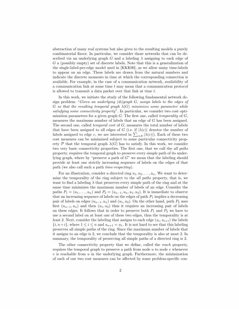
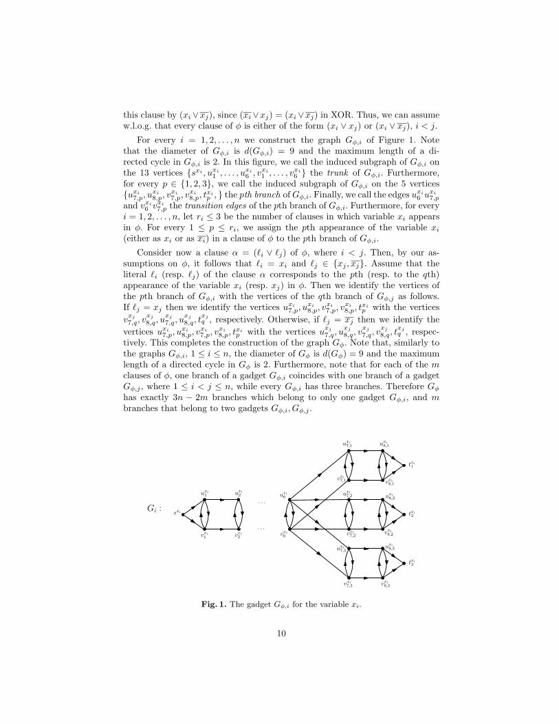
For every i = 1, 2, . . . , n we construct the graph Gφ,i of Figure 1. Notethat the diameter of Gφ,i is d(Gφ,i) = 9 and the maximum length of a di-rected cycle in Gφ,i is 2. In this figure, we call the induced subgraph of Gφ,i onthe 13 vertices sxi , uxi

1 , . . . , uxi

6 , vxi

1 , . . . , vxi

6 the trunk of Gφ,i. Furthermore,for every p ∈ 1, 2, 3, we call the induced subgraph of Gφ,i on the 5 verticesuxi

7,p, uxi

8,p, vxi

7,p, vxi

8,p, txip , the pth branch ofGφ,i. Finally, we call the edges u

xi

6 uxi

7,p

and vxi

6 vxi

7,p the transition edges of the pth branch of Gφ,i. Furthermore, for everyi = 1, 2, . . . , n, let ri ≤ 3 be the number of clauses in which variable xi appearsin φ. For every 1 ≤ p ≤ ri, we assign the pth appearance of the variable xi

(either as xi or as xi) in a clause of φ to the pth branch of Gφ,i.

Consider now a clause α = (ℓi ∨ ℓj) of φ, where i < j. Then, by our as-sumptions on φ, it follows that ℓi = xi and ℓj ∈ xj , xj. Assume that theliteral ℓi (resp. ℓj) of the clause α corresponds to the pth (resp. to the qth)appearance of the variable xi (resp. xj) in φ. Then we identify the vertices ofthe pth branch of Gφ,i with the vertices of the qth branch of Gφ,j as follows.If ℓj = xj then we identify the vertices uxi

7,p, uxi

8,p, vxi

7,p, vxi

8,p, txip with the vertices

vxj

7,q, vxj

8,q, uxj

7,q, uxj

8,q, txjq , respectively. Otherwise, if ℓj = xj then we identify the

vertices uxi

7,p, uxi

8,p, vxi

7,p, vxi

8,p, txip with the vertices u

xj

7,q, uxj

8,q, vxj

7,q, vxj

8,q, txjq , respec-

tively. This completes the construction of the graph Gφ. Note that, similarly tothe graphs Gφ,i, 1 ≤ i ≤ n, the diameter of Gφ is d(Gφ) = 9 and the maximumlength of a directed cycle in Gφ is 2. Furthermore, note that for each of the mclauses of φ, one branch of a gadget Gφ,i coincides with one branch of a gadgetGφ,j , where 1 ≤ i < j ≤ n, while every Gφ,i has three branches. Therefore Gφ

has exactly 3n − 2m branches which belong to only one gadget Gφ,i, and mbranches that belong to two gadgets Gφ,i, Gφ,j .

. . .

. . .

uxi

1

vxi

1vxi

2

uxi

2

Gi : sxi

uxi

6

vxi

6

uxi

7,1 uxi

8,1

vxi

7,3 vxi

8,3

vxi

7,1 vxi

8,1

vxi

7,2vxi

8,2

uxi

7,2 uxi

8,2

uxi

7,3uxi

8,3

txi

1

txi

2

txi

3

Fig. 1. The gadget Gφ,i for the variable xi.

10

Theorem 8. There exists a truth assignment τ of φ with |t(φ)| ≥ k if and onlyif κ(Gφ, reach, d(Gφ)) ≤ 39n− 4m− 2k.

Using Theorem 8, we are now ready to prove the main theorem of this section.

Theorem 9 (Hardness of Approximating the Temporal Cost). Theproblem of computing κ(G, reach, d(G)) is APX-hard, even when the maximumlength of a directed cycle in G is 2.

Proof. Denote now by OPTMax-XOR(3)(φ) the greatest number of clauses thatcan be simultaneously XOR-satisfied by a truth assignment of φ. Then Theo-rem 8 implies that

κ(Gφ, reach, d(Gφ)) ≤ 39n− 4m− 2 ·OPTMax-XOR(3)(φ)

Note that a random assignment XOR-satisfies each clause of φ with probability12 , and thus we can easily compute (even deterministically) an assignment τ thatXOR-satisfies m

2 clauses of φ. Therefore OPTMax-XOR(3)(φ) ≥m2 , and thus, since

every variable xi appears in at least one clause of φ, it follows that n ≤ m ≤2 ·OPTMax-XOR(3)(φ1).

Assume that there is a PTAS for computing κ(G, reach, d(G)). Then, forevery ε > 0 we can compute in polynomial time a labeling λ for the graph Gφ,such that |λ| ≤ (1 + ε) · κ(Gφ, reach, d(Gφ)).

Given such a labeling λ we can compute by the sufficiency part (⇐) of theproof of Theorem 8 a truth assignment τ of φ such that 39n−4m−2|t(φ)| ≤ |λ|,i.e. 2|t(φ)| ≥ 39n− 4m− |λ|.

Therefore it follows by all the above that 2|t(φ)| ≥ 39n − 4m − (1 + ε) ·κ(Gφ, reach, d(Gφ)) ≥ 39n−4m−(1+ε)·

(

39n− 4m− 2 ·OPTMax-XOR(3)(φ))

=ε (4m− 39n)+2(1+ε)·OPTMax-XOR(3)(φ)≥ −35εm+(2+2ε)·OPTMax-XOR(3)(φ)≥ −35ε · 2OPTMax-XOR(3)(φ) + (2 + 2ε) · OPTMax-XOR(3)(φ) = (2 − 68ε) ·OPTMax-XOR(3)(φ) and thus

|t(φ)| ≥ (1− 34ε) ·OPTMax-XOR(3)(φ).

That is, assuming a PTAS for computing κ(G, reach, d(G)), we obtain a PTASfor the Max-XOR(3) problem, which is a contradiction by Lemma 4. Thereforecomputing κ(G, reach, d(G)) is APX-hard. Finally, notice that the constructedgraph Gφ has maximum length of a directed cycle at most 2. ⊓⊔

5.3.2 Approximating the Cost. In this section, we provide an approxima-tion algorithm for computing κ(G, reach, d(G)), which complements the hard-ness result of Theorem 9. Given a digraph G define, for every u ∈ V , u’s reach-ability number r(u) = |v ∈ V : v is reachable from u| and r(G) =

∑

u∈V r(u),that is r(G) is the total number of reachabilities in G.

Theorem 10. There is an r(G)n−1 -factor approximation algorithm for computing

κ(G, reach, d(G)) on any weakly connected digraph G.

11

References

[AAD+06] D. Angluin, J. Aspnes, Z. Diamadi, M. J. Fischer, and R. Peralta. Com-putation in networks of passively mobile finite-state sensors. DistributedComputing, pages 235–253, March 2006.

[AKL08] C. Avin, M. Koucky, and Z. Lotker. How to explore a fast-changing world(cover time of a simple random walk on evolving graphs). In Proceedingsof the 35th international colloquium on Automata, Languages and Pro-gramming (ICALP), Part I, pages 121–132. Springer-Verlag, 2008.

[Ber96] K. A. Berman. Vulnerability of scheduled networks and a generalizationof Menger’s theorem. Networks, 28[3]:125–134, 1996.

[CFQS12] A. Casteigts, P. Flocchini, W. Quattrociocchi, and N. Santoro. Time-varying graphs and dynamic networks. IJPEDS, 27[5]:387–408, 2012.

[CKS01] N. Creignou, S. Khanna, and M. Sudan. Complexity classifications ofboolean constraint satisfaction problems. SIAM Monographs on DiscreteMathematics and Applications, 2001.

[CMM+08] A. E. Clementi, C. Macci, A. Monti, F. Pasquale, and R. Silvestri. Flood-ing time in edge-markovian dynamic graphs. In Proc. of the 27th ACMSymp. on Principles of distributed computing (PODC), pages 213–222,2008.

[FT98] L. Fleischer and E. Tardos. Efficient continuous-time dynamic networkflow algorithms. Operations Research Letters, 23[3]:71–80, 1998.

[GPPR01] C. Gavoille, D. Peleg, S. Perennes, and R. Raz. Distance labeling ingraphs. In Proc. of the 12th annual ACM-SIAM symposium on Discretealgorithms (SODA), pages 210–219, Philadelphia, PA, USA, 2001.

[KKK00] D. Kempe, J. Kleinberg, and A. Kumar. Connectivity and inference prob-lems for temporal networks. In Proceedings of the 32nd annual ACMsymposium on Theory of computing (STOC), pages 504–513, 2000.

[KKKP04] M. Katz, N. A. Katz, A. Korman, and D. Peleg. Labeling schemes forflow and connectivity. SIAM Journal on Computing, 34[1]:23–40, 2004.

[KLO10] F. Kuhn, N. Lynch, and R. Oshman. Distributed computation in dy-namic networks. In Proceedings of the 42nd ACM symposium on Theoryof computing (STOC), pages 513–522, New York, NY, USA, 2010. ACM.

[KMSV99] S. Khanna, R. Motwani, M. Sudan, and U. Vazirani. On syntactic versuscomputational views of approximability. SIAM Journal on Computing,28[1]:164–191, 1999.

[MCS11a] O. Michail, I. Chatzigiannakis, and P. G. Spirakis. Mediated populationprotocols. Theoretical Computer Science, 412[22]:2434–2450, May 2011.

[MCS11b] O. Michail, I. Chatzigiannakis, and P. G. Spirakis. New Models for Pop-ulation Protocols. N. A. Lynch (Ed), Synthesis Lectures on DistributedComputing Theory. Morgan & Claypool, 2011.

[MCS12] O. Michail, I. Chatzigiannakis, and P. G. Spirakis. Causality, influence,and computation in possibly disconnected synchronous dynamic networks.In 16th International Conference on Principles of Distributed Systems(OPODIS), pages 269–283, 2012.

[Sch02] C. Scheideler. Models and techniques for communication in dynamic net-works. In Proceedings of the 19th Annual Symposium on Theoretical As-pects of Computer Science (STACS), pages 27–49, 2002.

[XFJ03] B. Xuan, A. Ferreira, and A. Jarry. Computing shortest, fastest, and fore-most journeys in dynamic networks. International Journal of Foundationsof Computer Science, 14[02]:267–285, 2003.

12