2018 Final Report (City of Brainerd SAUD 2018 [12/31/2018 ...
Upload
khangminh22Category
view
1download
0
TECHNICAL UNIVERSITY – SOFIAPLOVDIV BRANCH
SEVENTH INTERNATIONAL SCIENTIFIC CONFERENCE“ENGINEERING, TECHNOLOGIES AND SYSTEMS”
TECHSYS 201817-19 May, Plovdiv
PROCEEDINGS СБОРНИК ДОКЛАДИ
ТЕХНИЧЕСКИ УНИВЕРСИТЕТ – СОФИЯФИЛИАЛ ПЛОВДИВ
СЕДМА МЕЖДУНАРОДНА НАУЧНА КОНФЕРЕНЦИЯ“ТЕХНИКА, ТЕХНОЛОГИИ И СИСТЕМИ”
ТЕХСИС 201817-19 май, Пловдив
ISSN Online: 2535-0048

The conference will be held within the framework of the Science Days of Technical University of Sofia under the patronage of Prof DSc Georgi Mihov - Rector of the Technical University of Sofia.
Конференцията ще се проведe в рамките на Дни на науката на Технически университет - София под патронажа на проф. дтн. Георги Михов - Ректор на Технически Университет - София.
TECHNICAL UNIVERSITY – SOFIA, PLOVDIV BRANCH
SEVENTH INTERNATIONAL SCIENTIFIC CONFERENCE“ENGINEERING, TECHNOLOGIES AND SYSTEMS”
TECHSYS 201817-19 May, Plovdiv
ТЕХСИС 201817-19 май, Пловдив
ТЕХНИЧЕСКИ УНИВЕРСИТЕТ – СОФИЯ, ФИЛИАЛ ПЛОВДИВ
СЕДМА МЕЖДУНАРОДНА НАУЧНА КОНФЕРЕНЦИЯ“ТЕХНИКА, ТЕХНОЛОГИИ И СИСТЕМИ”
3
TECHNICAL UNIVERSITY - SOFIA, PLOVDIV BRANCH
Organizing Committee:
Honorary Chairman: Prof. DSc Georgi MihovChairman: Prof. Dr. Valyo NikolovVice Chairman: Assoc. Prof. Dr. Nikola Shakev
Members:Prof. Dr. Grisha Spasov Assoc. Prof. Dr. Pepo Yordanov,Assoc. Prof. Dr. Krum Kutryansky Assoc. Prof. Dr. Hristian Panajotov, Assoc. Prof. Dr. Valentin Vladimirov Assoc. Prof. Dr. Angel LengerovAssoc. Prof. Dr. Nikola Georgiev Assoc. Prof. Dr. Toni Mihova,Assoc. Prof. Dr. Nikolay Kakanakov Assoc. Prof. Dr. Dimitar Petrov Assoc. Prof. Dr. Ivan Kostov Assoc. Prof. Dr. Valentina Proycheva Assoc. Prof. Dr. Anton Lechkov Assoc. Prof. Dr. Dechko RuschevAssoc. Prof. Dr. Borislav Penev Prof. Dr. Dobrin Seizinski
International Programme Committee:
Chairmаn: Prof. Dr. Michail Petrov, TU-Sofia, Branch Plovdiv
Members:Prof. DSc Andre Barraco, FranceProf. Dr. Ernst Wintner, AustriaProf. DSc. Venelin Jivkov, BulgariaProf. DSc. Vesko Panov, BulgariaProf. DSc Marin Nenchev, BulgariaProf. DSc Emil Nikolov, BulgariaProf. DSc Radi Romanski, BulgariaProf. DSc. Stanimir Karapetkov, BulgariaProf. DSc Todor Stoilov, BulgariaProf. DSc Edmunds Teirumnieks, LatviaProf. DSc Mark Himbert, FranceProf. DSc Ivan Jachev, BulgariaProf. Dr., Dr.h.c. Nikolay Ganev, Czech Republic Prof. Dr. Ivaylo Banov, BulgariaProf. Dr. Veselka Boeva, BulgariaProf. Dr. Mladen Velev, BulgariaProf. Dr. Daniela Goceva, BulgariaProf. Dr. Petar Gecov, Bulgaria
Prof. Dr. Lubomir Dimitrov, Bulgaria Prof. Dr. Frantisek Zezulka, Czech Republic Prof. Dr. Angel Zumbilev, BulgariaProf. Dr. Ilia Iliev, BulgariaProf. DSc Okyay Kaynak, TurkeyProf. Dr. Nikola Kasabov, New ZealandProf. Dr. Ivan Kralov, BulgariaProf. Dr. Petr Louda, Czech Republic Prof. Dr. Valeri Mladenov, BulgariaProf. Dr. Ognyan Nakov, BulgariaProf. Dr. Galidia Petrova, BulgariaProf. Dr. Marsel Popa, RomaniaProf. Dr. Vladimir Pulkov, BulgaraiaProf. Dr. Georgi Todorov, BulgariaProf. DSc. Chavdar Damianov, BulgariaProf. Dr. Andon Topalov, BulgariaProf. Dr. Sedat Sunter, TurkeyProf. Dr. Ahmed Hafaifa, AlgeriaAssoc. Prof. Dr. Abdellah Kouzou, Algeria
Scientific Secretary: Dr. Sevil AhmedTechnical Secretary: Eng. Tsvetan Petrov, Eng. Christo Christev, Eng. Lalka Boteva
ISSN Online: 2535-0048

4
ТЕХНИЧЕСКИ УНИВЕРСИТЕТ – СОФИЯ, ФИЛИАЛ ПЛОВДИВ
Организационен комитет:Почетен председател: проф. дтн. Георги МиховПредседател: проф. д-р Въльо НиколовЗам.-председател: доц. д-р Никола Шакев
Членове:проф. д-р Гриша Спасов доц. д-р Пепо Йордановдоц. д-р Крум Кутрянски доц. д-р Христиан Панайотов,доц. д-р Валентин Владимиров доц. д-р Ангел Ленгеровдоц. д-р Никола Георгиев доц. д-р Тони Миховадоц. д-р Николай Каканаков доц. д-р Димитър Петровдоц. д-р Иван Костов доц. д-р Валентина Пройчевадоц. д-р Антон Лечков доц. д-р Дечко Русчевдоц. д-р Борислав Пенев проф. д-р Добрин Сейзински
Програмен комитет:Председател: проф. д-р Михаил Петров, ТУ–София, филиал Пловдив
Членове:проф. дтн. Андре Барако, Францияпроф. дтн. Ернст Винтнер, Австрияпроф. дтн. Венелин Живков, ТУ – София, Българияпроф. дтн. Веско Панов, ТУ – София, Българияпроф. дтн. Марин Ненчев, ТУ – София, ф-л Пловдив, Българияпроф. дтн. Емил Николов, ТУ – София, Българияпроф. дтн. Ради Романски, ТУ – София, Българияпроф. дтн. Станимир Карапетков, ТУ – София, Българияпроф. дтн. Тодор Стоилов, БАН, Българияпроф. дтн. Едмундс Теирумниекс, Латвияпроф. дтн. Марк Химберт, Францияпроф. дтн. Иван Ячев, ФНТС, ТУ – София, Българияпроф. д-р, д-р х.к. Николай Ганев, Чехияпроф. д-р Ивайло Банов, ТУ – София, Българияпроф. д-р Веселка Боева, ТУ – София, ф-л Пловдив, Българияпроф. д-р Младен Велев, ТУ – София, Българияпроф. д-р Даниела Гоцева, ТУ – София, Българияпроф. д-р Петър Гецов, ИКИ, БАН, Българияпроф. д-р Любомир Димитров, ТУ – София, България
проф. д-р Франтишек Зезулка, Чехияпроф. д-р Ангел Зюмбилев, ТУ – София, ф-л Пловдив, Българияпроф. д-р Илия Илиев, ТУ – София, Българияпроф. д-р Окияй Кайнак, Турцияпроф. д-р Никола Касабов, Нова Зеландияпроф. д-р Иван Кралов, ТУ – София, Българияпроф. д-р Петр Лауда, Чехияпроф. д-р Валери Младенов, ТУ – София, Българияпроф. д-р Огнян Наков, ТУ – София , Българияпроф. д-р Галидия Петрова, ТУ – София, ф-л Пловдив, Българияпроф. д-р Марсел Попа, Румънияпроф. д-р Владимир Пулков, ТУ – София, Българияпроф. д-р Георги Тодоров, ТУ – София, Българияпроф. дтн Чавдар Дамянов, Българияпроф. д-р Андон Топалов, ТУ – София, ф-л Пловдив, Българияпроф. д-р Седат Сюнтер, Турцияпроф. д-р Ахмед Хафайфа, Алжирдоц. д-р Абделлах Кузу , Алжир
Научен секретар: д-р инж. Севил АхмедТехнически секретариат: инж. Цветан Петров, инж. Христо Христев, инж. Лалка Ботева

CONTENTSPLENARY PAPERS • ПЛЕНАРНИ ДОКЛАДИ1. BaSiCS Of iNduSTry 4.0 ...................................................................................................... i-11
Prof. Eng. Frantisek Zezulka, PhD
Faculty of Electrical Engineering and Communication, Department of Control and Instrumentation, Brno University of Technology, Brno, Czech Republic
2. MaTriX CONVErTEr TECHNOLOGy aNd iTS aPPLiCaTiONS ..........................................................i-12
Prof. Eng. Sedat Sünter, PhD
The University of Firat, Turkey
SECTION 1 • СЕКЦИЯ 1 AUTOMATION AND CONTROL SYSTEMS Автоматика и системи за управление
1. PETR MARCON, FRANTISEK ZEZULKA, ZDENEK BRADAC ....................................................... II-2TERMINOLOGY OF INDUSTRY 4.0
2. ZDENEK BRADAC, FRANTISEK ZEZULKA, PETR MARCON ........................................................ II-8TECHNICAL AND THEORETICAL BASIS OF INDUSTRY 4.0 IMPLEMENTATION
3. KRASIMIRA STOILOVA, TODOR STOILOV, MIROSLAV VLADIMIROV ..................................... II-13RESOURCE ALLOCATION BY PORTFOLIO OPTIMIZATION
4. RADOSLAV HRISCHEV ................................................................................................................ II-19PLANNING AND IMPLEMENTATION OF THE ERP SYSTEM IN PACKAGING PRODUCTION. PRACTICAL ASPECTS
5. BORISLAV RUSENOV, ALBENA TANEVA, IVAN GANCHEV, MICHAIL PETROV ....................... II-23SYSTEM DEVELOPMENT FOR MACHINE VISION INTELLIGENT QUALITY CONTROL OF LOW VOLTAGE MINIATURE CIRCUIT BREAKERS
6. STOITCHO PENKOV, ALBENA TANEVA, MICHAIL PETROV, KIRIL HRISTOZOV, ROBERT KAZALA ....................................................................................... II-30
CONTROL SYSTEM APPLICATION USING LORAWAN7. ALEXANDRA GRANCHAROVA, ALBENA GEORGIEVA, IVANA VALKOVA ............................... II-36
DESIGN OF EXPLICIT MODEL PREDICTIVE CONTROLLER FOR A QUADRUPLE-TANK SYSTEM
8. SHERIF SHERIF, JORDAN KRALEV, VESELIN KUNCHEV ........................................................... II-42MODELING OF BIPED ROBOT WITH SIMMECHANICSTM TOOLBOX IN MATLAB©
I-5
4
ТЕХНИЧЕСКИ УНИВЕРСИТЕТ – СОФИЯ, ФИЛИАЛ ПЛОВДИВ
Организационен комитет:Почетен председател: проф. дтн. Георги МиховПредседател: проф. д-р Въльо НиколовЗам.-председател: доц. д-р Никола Шакев
Членове:проф. д-р Гриша Спасов доц. д-р Пепо Йордановдоц. д-р Крум Кутрянски доц. д-р Христиан Панайотов,доц. д-р Валентин Владимиров доц. д-р Ангел Ленгеровдоц. д-р Никола Георгиев доц. д-р Тони Миховадоц. д-р Николай Каканаков доц. д-р Димитър Петровдоц. д-р Иван Костов доц. д-р Валентина Пройчевадоц. д-р Антон Лечков доц. д-р Дечко Русчевдоц. д-р Борислав Пенев проф. д-р Добрин Сейзински
Програмен комитет:Председател: проф. д-р Михаил Петров, ТУ–София, филиал Пловдив
Членове:проф. дтн. Андре Барако, Францияпроф. дтн. Ернст Винтнер, Австрияпроф. дтн. Венелин Живков, ТУ – София, Българияпроф. дтн. Веско Панов, ТУ – София, Българияпроф. дтн. Марин Ненчев, ТУ – София, ф-л Пловдив, Българияпроф. дтн. Емил Николов, ТУ – София, Българияпроф. дтн. Ради Романски, ТУ – София, Българияпроф. дтн. Станимир Карапетков, ТУ – София, Българияпроф. дтн. Тодор Стоилов, БАН, Българияпроф. дтн. Едмундс Теирумниекс, Латвияпроф. дтн. Марк Химберт, Францияпроф. дтн. Иван Ячев, ФНТС, ТУ – София, Българияпроф. д-р, д-р х.к. Николай Ганев, Чехияпроф. д-р Ивайло Банов, ТУ – София, Българияпроф. д-р Веселка Боева, ТУ – София, ф-л Пловдив, Българияпроф. д-р Младен Велев, ТУ – София, Българияпроф. д-р Даниела Гоцева, ТУ – София, Българияпроф. д-р Петър Гецов, ИКИ, БАН, Българияпроф. д-р Любомир Димитров, ТУ – София, България
проф. д-р Франтишек Зезулка, Чехияпроф. д-р Ангел Зюмбилев, ТУ – София, ф-л Пловдив, Българияпроф. д-р Илия Илиев, ТУ – София, Българияпроф. д-р Окияй Кайнак, Турцияпроф. д-р Никола Касабов, Нова Зеландияпроф. д-р Иван Кралов, ТУ – София, Българияпроф. д-р Петр Лауда, Чехияпроф. д-р Валери Младенов, ТУ – София, Българияпроф. д-р Огнян Наков, ТУ – София , Българияпроф. д-р Галидия Петрова, ТУ – София, ф-л Пловдив, Българияпроф. д-р Марсел Попа, Румънияпроф. д-р Владимир Пулков, ТУ – София, Българияпроф. д-р Георги Тодоров, ТУ – София, Българияпроф. дтн Чавдар Дамянов, Българияпроф. д-р Андон Топалов, ТУ – София, ф-л Пловдив, Българияпроф. д-р Седат Сюнтер, Турцияпроф. д-р Ахмед Хафайфа, Алжирдоц. д-р Абделлах Кузу , Алжир
Научен секретар: д-р инж. Севил АхмедТехнически секретариат: инж. Цветан Петров, инж. Христо Христев, инж. Лалка Ботева

SECTION 2 • СЕКЦИЯ 2 ELECTRICAL ENgINEERINg AND ELECTRONICS Електротехника и електроника
1. AHMET SENPINAR ...................................................................................................................... II-49THE IMPORTANCE OF SOLAR ANGLES IN MPPT SYSTEMS
2. MARGARITA DENEVA, PEPA UZUNOVA, VALKO KAZAKOV, VANIA PLACHKOVA, KAMEN IVANOV, MARIN NENCHEV AND ELENA STOYKOVA ............................................................ II-54
USE OF INTERFERENCE WEDGED STRUCTURE AS AN ATTRACTIVE, SIMPLEST, LIGHT POWER DIVIDING ELEMENT
3. DINYO KOSTOV ............................................................................................................................ II-60COMPARATIVE ANALYSIS OF FAULT CURRENT LIMITERS
4. ONUR KAYA , CETIN AKINCI, EMEL ONAL ................................................................................. II-64CALCULATION OF DIELECTRIC DISSIPATION FACTOR AT VARIABLE FREQUENCIES OF MODEL TRANSFORMER
5. SARANG PATIL ............................................................................................................................. II-69TWO NEW TYPES OF COMPACT ULTRA-WIDE BANDWIDTH ANTENNAS FOR 3-AXIS RF FIELD STRENGTH MEASUREMENT.
6. SVETLIN STOYANOV.................................................................................................................... II-75AN EXPERIMENTAL SETUP FOR DETERMINATION OF THE RESONANT FREQUENCIES OF A MECHANICAL FRAME STRUCTURE
7. NIKOLA GEORGIEV ..................................................................................................................... II-79STUDYING AN AXIAL GENERATOR WITH ROTATING MAGNETS IN ITS STATOR WINDINGS
8. VASIL SPASOV, IVAN KOSTOV, IVAN HADZHIEV ...................................................................... II-83IMPLEMENTATION OF A NOVEL FORCE COMPUTATION METHOD IN THE FEMM SOFTWARE
9. IVAN HADZHIEV, DIAN MALAMOV, VASIL SPASOV, DIMITAR NEDYALKOV ......................... II-89STUDYING THE ELECTRICAL AND THERMAL FIELDS, PRODUCED BY THE CURRENT IN THE INSULATION OF A MIDDLE VOLTAGE CABLE
10. SVETOSLAV IVANOV, YANKA IVANOVA ................................................................................... II-95RESEARCH OF OPTICAL RECEIVER FOR PLASTIC OPTICAL FIBERS
11. YANKA IVANOVA, SVETOSLAV IVANOV ................................................................................... II-99RESEARCH OF TRANSMITTER FOR PLASTIC OPTICAL FIBER
12. ILIYA PETROV .............................................................................................................................II-103ERROR IN SIMULATION OF ANALOG CIRCUIT IN PROTEUS
I-6

SECTION 3 • СЕКЦИЯ 3 INFORMATICS AND COMPUTER SYSTEMS AND TECHNOLOgIES Информатика и компютърни системи и технологии
1. ERDİNÇ UZUN, TARIK YERLİKAYA, OĞUZ KIRAT ...................................................................II-108COMPARISON OF PYTHON LIBRARIES USED FOR WEB DATA EXTRACTION
2. ERDİNÇ UZUN, TARIK YERLİKAYA, OĞUZ KIRAT ....................................................................II-114OBJECT-BASED ENTITY RELATIONSHIP DIAGRAM DRAWING LIBRARY: ENTREL.JS
3. GÜNGÖR YILDIRIM, YETKIN TATAR ..........................................................................................II-120AN ALTERNATIVE EXECUTION MODEL FOR OPTIMUM BIG DATA HANDLING IN IoT-WSN CLOUD SYSTEMS
4. SENOL SEN, TARIK YERLIKAYA .................................................................................................II-125MAN IN THE MIDDLE ATTACK WITH ARP SPOOFING
5. TiHOMir TENEV, diMiTar BirOV ........................................................................................ ii-130SECURITY PATTERNS FOR MICROSERVICES LOCATED ON DIFFERENT VENDORS
6. TariK yErLİKaya, CaNaN aSLaNyÜrEK ........................................................................... ii-134RSA ENCRYPTION ALGORITHM AND CRYPTANALYSIS OF RSA
7. MEHMET VuraL, MuHarrEM TuNCay GENÇOĞLu ............................................................ ii-137EMBEDDED AUDIO CODING USING LAPLACE TRANSFORM FOR TURKISH LETTERS
8. VENETa aLEKSiEVa, SVETOSLaV SLaVOV ........................................................................... ii-145MANAGED ACTIVE DIRECTORY IN DIRECTORY-AS-A-SERVICE
9. TONy KaraVaSiLEV, ELENa SOMOVa ................................................................................. ii-151OVERCOMING THE SECURITY ISSUES OF NOSQL DATABASES
10. daNiEL TrifONOV, HriSTO VaLCHaNOV ............................................................................ ii-157VIRTUALIZATION AND CONTAINERIZATION SYSTEMS FOR BIG DATA
11. diMiTar GarNEVSKi, PETya PaVLOVa .............................................................................. ii-161PERFORMANCE ESTIMATION OF PARALLEL APPLICATION FOR SOLAR IMAGES PROCESSING
12. VLadiMir diMiTrOV, dENiTSa TSONiNa ........................................................................... ii-165PROGRAMMING TOOLS FOR RELIABLE USER AUTHENTICATION ACROSS MULTIPLE SERVERS
13. aTaNaS KOSTadiNOV ......................................................................................................... ii-171TESTING AND DIAGNOSTICS OF COMPUTER SYSTEMS
14. Maria POPOVa, K. MariNCHESHKi, Maria MariNOVa .................................................... ii-175SIMULATING HYPERCUBE ARCHITECTURE IN PARALLEL COMPUTING
15. TEOdOra HriSTEVa, Maria MariNOVa ............................................................................ ii-178USING GRAPHIC PROCESSING UNITS FOR IMPROVING PERFORMANCE OF DEEP LEARNING PROCESSES
16. GEOrGi iLiEV ....................................................................................................................... ii-182MOBILE CROWDSOURCING FOR VIDEO STREAMING
I-7

17. diMiTrE KrOMiCHEV ......................................................................................................... ii-188FAST GAUSSIAN FILTERING FOR SPEED FOCUSED FPGA BASED CANNY EDGE DETECTION COMPUTATIONS
18. diMiTrE KrOMiCHEV ......................................................................................................... ii-194EFFICIENT COMPUTATION OF ORTHOGONAL GRADIENTS TO BE USED IN SPEED FOCUSED FPGA BASED CANNY EDGE DETECTION
19. PETya PaVLOVa ................................................................................................................... ii-198STATISTICAL ANALYSIS OF DEVIATIONS OF HUMAN MEMORY FOR COLORS
20. GEOrGi PaZHEV .................................................................................................................. ii-204SURVEY OF METHODS AND TECHNOLOGIES FOR BUILDING OF SMART HOMES
SECTION 4 • СЕКЦИЯ 4 MECHANICAL, TRANSPORT AND AVIATION ENGINEERINGМашиностроене, транспорт и авиация
1. HaTiCE POLaT, KuBra CELiK, HaLuK ErEN ....................................................................... ii-212NATURAL BARRIER WALL DESIGN FOR RADIATION AND NOISE PROBLEM ON THE ECOLOGICAL AIRPORTS
2. ZHiVKO iLiEV, GEOrGi diNEV ............................................................................................. ii-217POSSIBILITIES FOR A COMPARATIVE STUDY OF THE VIBRATIONS IN A COMPLEX PENDULUM JAW CRUSHER
3. EMiL VELEV ......................................................................................................................... ii-223STUDIES THE INFLUENCE OF THE GATE DIAMETER USING HOT RUNNER SYSTEM
4. HriSTO METEV, KaLiN KruMOV, aNGEL LENGErOV .......................................................... ii-227DETERMINATION OF INACCURACIES IN THE REPORTING BY TURNING THE PHENOMENON OF HEREDITY TECHNOLOGY
5. MirOSLaV aLEKSiEV, STaNiSLaV aLEKSiEV ....................................................................... ii-233ONE-WAY BEARINGS - TYPES OF STRUCTURES
6. MirOSLaV aLEKSiEV, STaNiSLaV aLEKSiEV ...................................................................... ii-237THEORETICAL DETERMINATION OF THE GRAVITY CLASS FOR MILLING WITH A HIGHLY PRODUCING SURFACE
7. NiKOLay GuEOrGuiEV, aLEKSaNdar KOLarOV, VENCiSLaV PEHiVaNSKi, OGNiaN TOdOrOV .............................................................................................................. ii-241
METHODOLOGY FOR EVALUATION OF RADIO ELECTRONIC COUNTERMEASURE OF UNMANNED AERIAL VEHICLES
8. GEOrGi GEOrGiEV, PETar GETSOV, NiKOLay TuLESHKOV, diMO ZafirOV ...................... ii-247URBAN AIR MOBILITY
9. iLKO TarPOV, SiLViya SaLaPaTEVa ................................................................................... ii-251ANALYSIS OF THE ORGANIZATIONAL ACTIVITIES FOR THE REPLACEMENT OF WAGONS WITH MOTORCYCLES FOR TRAINS IN RAILWAY STATION PLOVDIV
I-8

10. GEOrGi VaLKOV, VaLyO NiKOLOV ...................................................................................... ii-255CLASSIFICATION OF TERRAIN FORKLIFTS
11. SiLViNa iLiEVa .................................................................................................................... ii-261CORRECTION OPTIONS ON THE EXPOSURE OF A DIGITAL PHOTOGRAPH IN RAW AND JPEG FORMATS IN ADOBE PHOTOSHOP
12. VLadiMir aNGELOV ............................................................................................................ ii-267QUALITY RESEARCH OF HSWO PRINTING IN SHORT AND MEDIUM PRINT RUNS
SECTION 5 • СЕКЦИЯ 5 INDUSTRIAL MANAgEMENT and NATURAL SCIENCES Индустриален мениджмънт и природни науки
1. TONi MiHOVa,VaLENTiNa NiKOLOVa-aLEXiEVa, MiNa aNGELOVa ................................. ii-274CONCEPTUAL IMPACT MODEL OF PROCESS MANAGEMENT ON THE MEAT INDUSTRY ENTERPRISES IN BULGARIA
2. TOdOr TOdOrOV, GEOrGi TSaNEV ................................................................................... ii-280ANALYSIS OF THE MEAN FIELD APPROXIMATION FOR TRAINING THE DEEP BOLTZMANN MACHINE
3. TaNya GiGOVa .................................................................................................................... ii-286CLASSIFICATION OF BUSINESS PROCESSES
4. aNTONia LaZarOVa ........................................................................................................... ii-292DATA VALIDATION FOR STUDIES RELATED TO THE SOCIAL ROLE OF SEX
5. aNGELiNa POPOVa ............................................................................................................ ii-297CORROSION PROTECTION WITH INHIBITORS QUATERNARY AMMONIUM BROMIDES
6. KaLiNa KaMarSKa ............................................................................................................ ii-301INVESTIGATION OF THE CORROSION BEHAVIOR OF ALUMINIUM ALLOYS EN AW-2011 and EN AW-2024
7. ZLaTKO ZLaTaNOV, rayCHO rayCHEV, CHaVdar PaSHiNSKi .......................................... ii-305MATRIX EXAMINATION OF STATIC UNDEFINED PLANAR FRAME UNDER STATIC LOAD
8. ZLaTKO ZLaTaNOV .............................................................................................................. ii-309MATRIX EXAMINATION OF CONTINUOUS BEAM
9. HriSTiNa SPiridONOVa, GaLiNa CHErNEVa .................................................................... ii-313APPLICATIONS OF THEORY OF INVARIANTS IN SENSITIVITY SURVEY OF FREQUENT SELECTIVE CIRCUITS
10. GEOrGi PaSKaLEV .............................................................................................................. ii-317VARIATIONAL PRINCIPLE FOR A CLASS OF NONLOCAL BOUNDARY VALUE PROBLEMS
I-9

PLENARY PAPERS • ПЛЕНАРНИ ДОКЛАДИ
I-10
© international Scientific Conference on Engineering, Technologies and Systems TECHSyS 2018, Technical university – Sofia, Plovdiv branch 17– 19 May 2018, Plovdiv, Bulgaria

Basics of Industry 4.0
Prof. Eng. Frantisek Zezulka, PhD Faculty of Electrical Engineering and Communication, Department of Control and Instrumentation, Brno University of Technology, Brno, Czech Republic
The lecture deals with fundamental ideas, goals, requirements, and corresponding principles and technologies to enable solving the goals of the 4th industrial revolution. The presentation discusses the keywords strongly connected with the fundaments of Industry 4.0, including the following items: digitalization, virtualization, Cyber physical systems (CPS), factory of the Future, standardization, open communication, Internet of Things (IoT) and Industrial Internet of Things (IIoT), cooperation, functional safety, cyber security, cloud and edge computing, modelling of the all production supply chain, top and shop floors.
These keywords will be associated to theoretical basis of Industry 4.0 and information and communication technology, which are to fulfil design and implementation of new production principles and their physical realization in factories of the future. The theoretical implementation basis goes out from: Reference Architecture Model of the Industry 4.0 (RAMI 4.0), new business models, models developed from the RAMI 4.0 (first one is the Industry 4.0 Component Model), Unified Modelling Language (UML), Open Platform Communication – Unified Architecture (OPC UA), Time Sensitive Networks (TSN), big data and big data processing, Asset Administration Shell (AAS), Digital Twins.
Author’s aim is to enable interested colleagues from industrial as well as academic community to find the proper way how to be in the main development and implementation stream of technologies and knowledges for design, realization, commissioning, maintenance and supervision of factories of the future.
At last but not least, the contribution will refer of outputs from ad hoc audits in industrial factories in the South Moravia region with a goal of evaluation of their ability to implement the Industry 4.0 principles, procedures and technologies.
In the end of the contribution listeners will be acquainted with goals and technologies of one cooperation international project among German and Czech SMEs and University Research Centers. The project calls Digital representation of Assets as a configurable AAS for OT and IT production systems (RACAS) and deals with development and implementation of a framework for an according customer dependent configurable implementation of AASs. Main challenge is that the AAS interact conform and interoperable in the Industry 4.0 systems and can be widely adopted to the different needs of the asset types. Configuration of the I4.0 components is one of the big challenges which are to be done to succeed in any Industry 4.0 implementation and will be solved in this project.
I-11
© international Scientific Conference on Engineering, Technologies and Systems TECHSyS 2018, Technical university – Sofia, Plovdiv branch 17– 19 May 2018, Plovdiv, Bulgaria

MATRIX CONVERTER TECHNOLOGY AND ITS APPLICATIONS
Professor Sedat Sünter studied at The University of Firat, Turkey.
He received a B.Sc. (First Class) in Electrical Engineering in 1986 and subsequently MSc in 1989. From 1988 to 1991 he worked as a Research Assistant at The University of Firat involved in teaching and research in power electronic systems. He received a scholarship from Turkish Government for PhD study abroad in 1991. Consequently, He was accepted by The University of Nottingham, UK and received his PhD in Electrical and Electronic Engineering in the area of power electronic
systems in 1995. Since 1995 he has been a Lecturer in Power Electronics at the University of Firat, Turkey. He has been promoted to Associate Professor in 2000 and received full Professor of Power Electronics at Firat University in July 2006. He has been in UK as visiting professor for three months in 2013. In literature, an algorithm on Matrix Converters has been referred to his name as “Sunter-Clare Algorithm”. He was vice Dean of the Faculty of Engineering in Firat University between 2004 and 2007. Since 2014, Professor Sünter is Head of The International Office in Firat University. He is also Institutional Coordinator of Erasmus+ Program. His research interests are: Power electronic converters and modulation strategies, matrix converters, resonant converters, variable speed drive systems, renewable and energy. Professor Sünter has a number of papers published in various journals and conference proceedings.
Matrix converter can achieve the ac-ac conversion without needing a dc link since it performs the conversion directly from ac to ac. In addition, multiphase matrix converters have a sinusoidal input current and output voltage waveforms with adjustable amplitude and frequency. The converter structure has bi-directional power switches which provide regenerative operation of the motor. These converters have drawn the interest of the researchers due to several desirable characteristics, including fast dynamic, high power/volume ratio, inherent capability of four-quadrant operation and low harmonic contents. General types of matrix converters and their modulation and control algorithms will be presented with input and output waveforms.
The main application of the matrix converter is variable speed induction motor drive systems. However, the converter can be used in variable speed wind turbine generation systems as well by replacing the conventional back-to-back converters. In this case, the power flow can be provided in single stage without requiring any dc link by placing the matrix converter between the rotor windings of DFIG and the utility power lines. Moreover, both synchronous and subsynchronous operations are allowed. Some simulation and experimental results for both applications will also be presented.
I-12
© international Scientific Conference on Engineering, Technologies and Systems TECHSyS 2018, Technical university – Sofia, Plovdiv branch 17– 19 May 2018, Plovdiv, Bulgaria

MATRIX CONVERTER TECHNOLOGY AND ITS APPLICATIONS
Professor Sedat Sünter studied at The University of Firat, Turkey.
He received a B.Sc. (First Class) in Electrical Engineering in 1986 and subsequently MSc in 1989. From 1988 to 1991 he worked as a Research Assistant at The University of Firat involved in teaching and research in power electronic systems. He received a scholarship from Turkish Government for PhD study abroad in 1991. Consequently, He was accepted by The University of Nottingham, UK and received his PhD in Electrical and Electronic Engineering in the area of power electronic
systems in 1995. Since 1995 he has been a Lecturer in Power Electronics at the University of Firat, Turkey. He has been promoted to Associate Professor in 2000 and received full Professor of Power Electronics at Firat University in July 2006. He has been in UK as visiting professor for three months in 2013. In literature, an algorithm on Matrix Converters has been referred to his name as “Sunter-Clare Algorithm”. He was vice Dean of the Faculty of Engineering in Firat University between 2004 and 2007. Since 2014, Professor Sünter is Head of The International Office in Firat University. He is also Institutional Coordinator of Erasmus+ Program. His research interests are: Power electronic converters and modulation strategies, matrix converters, resonant converters, variable speed drive systems, renewable and energy. Professor Sünter has a number of papers published in various journals and conference proceedings.
Matrix converter can achieve the ac-ac conversion without needing a dc link since it performs the conversion directly from ac to ac. In addition, multiphase matrix converters have a sinusoidal input current and output voltage waveforms with adjustable amplitude and frequency. The converter structure has bi-directional power switches which provide regenerative operation of the motor. These converters have drawn the interest of the researchers due to several desirable characteristics, including fast dynamic, high power/volume ratio, inherent capability of four-quadrant operation and low harmonic contents. General types of matrix converters and their modulation and control algorithms will be presented with input and output waveforms.
The main application of the matrix converter is variable speed induction motor drive systems. However, the converter can be used in variable speed wind turbine generation systems as well by replacing the conventional back-to-back converters. In this case, the power flow can be provided in single stage without requiring any dc link by placing the matrix converter between the rotor windings of DFIG and the utility power lines. Moreover, both synchronous and subsynchronous operations are allowed. Some simulation and experimental results for both applications will also be presented.
SECTION 1 • СЕКЦИЯ 1
AUTOMATION AND CONTROL SYSTEMS
АвтоМАтИкА И сИстЕМИ зА упрАвлЕнИЕ
© International Scientific Conference on Engineering, Technologies and Systems TECHSYS 2018, Technical University – Sofia, Plovdiv branch 17– 19 May 2018, Plovdiv, Bulgaria
II-1

Copyright © 2018 by Technical University of Sofia, Plovdiv branch, Bulgaria ISSN Online: 2535-0048
Copyright by Technical University - Sofia, Plovdiv branch, Bulgaria
TERMINOLOGY OF INDUSTRY 4.0
PETR MARCON, FRANTISEK ZEZULKA, ZDENEK BRADAC
Abstract: Industry 4.0 is sat to be a fourth industrial and scientific – technologic revolution. However, due to the recent development, it will be more very sophistic and very rapid evolution of scientific – technological background of existing and recent state of the art of existing industrial production, organization of work, new business models and business praxis in high-developed countries all over the world. The benefit of the Industry 4.0 to the existing technological development is not only in new IT technologies, but also in the organization of work in a massive implementation of new materials, life cycle management, and quality of work, safety and security features of industrial, technological and other production. Paper deals with terminology, which is necessary for understanding of goals, procedures, aspects and implementation of Industry 4.0 principle. Paper introduces in technologies, aspects, habits, sources, standards and theories and their application in a systematics and standardized way.
Key words: cyber physical system, digitalization, Industry 4.0, RAMI model
1. Introduction When the Industry 4.0 (I4.0) system of
production are to be successfully implemented and are to bring expected and asked support in concurrency with economies without I4.0 features, it is necessary to understand, enhance, implement and integrate into modern enterprises of the future following technologies, aspects, habits, sources, standards and theories, their application and some others in a systematics and standardized way. Let us introduce you in the background terminology of the I4.0, hence in such terms and their content as Digitization, OPC UA, UML, RFID, Cloud and edge computing and control, Cyber - physical systems, Vertical and horizontal integration of control, IEC 62443, IEC 62264/IEC 61512, IEC 62890, and Standards for I4.0 in preparation.
Authors are persuade that the first step in I4.0 future is a good understanding of the I4.0 process, state of the art of initial I4.0 ideas and following the step by step development works in correction of initial ideas and in standardization activities of the most appropriate procedures of the I4.0 systems implementation. Let us know to begin with short specification of above mentioned areas, their contents and description.
2. Industry 4.0 terminology The following subchapters describes the
basic terminology of I4.0.
2.1. Industry 4.0 Industry 4.0 are all activities related to new
style of industrial production in smart future factories. It is said to be the 4th technical revolution. However, in the reality, the I4.0 is a very rapid evolution in many aspects of human style of living, particularly in activities connected with industrial production.
In the Europe, the Internet of Things (IoT) is sorted into the CIoT (Commercial Internet of Things) and the IIoT (Industrial Internet of Things). The CIoT abbreviation is not frequently used and the IoT is used for Internet of whichever things. But in the United States of America technical terminology, the IoT represents the all issue which are in the Europe covered by the I4.0 activities [1], [2].
2.2. Digitalization Digitalization is the process of converting
information into a digital (i.e. computer-readable) format, in which the information is organized into bits. The result is the representation of an object, image, sound, document or signal (usually an analog signal) by generating a series of numbers that describe a discrete set of its points or samples. The result is called digital representation or, more specifically, a digital image, for the object, and digital form, for the signal. In modern practice, the digitized data is in the form of binary numbers, which facilitate computer processing and other operations, but, strictly speaking, digitizing simply
© International Scientific Conference on Engineering, Technologies and Systems TECHSYS 2018, Technical University – Sofia, Plovdiv branch 17 – 19 May 2018, Plovdiv, Bulgaria

means the conversion of analog source material into a numerical format; the decimal or any other number system that can be used instead [3,4].
From the I4.0 point of view, digitalization is the crucial topic. Digitalization of process variables, market and economy of industrial production has been started evolutionary thanks to digital control systems (PLC, DCS, embedded control systems, information and IT technologies, economy of production – MES and ERP system). In the new generation of industrial production, digitalization of information appears in the whole human activities. Therefore, it is also very important for new production and market models and production.
The I4.0 initial principle and idea goes out from very comprehensive digitalization of data from the whole production chain. It is non – systematically provided already in the existing production. The digitalization for the future fabric needs to be not only comprehensive more than the existing one, but it has to be provided in the systematic way to be used in the most appropriate way when it is needed, in the real time and without failure, non- correct interpretation and should be obtained (measured) only one time for more applications and use. A good example how to realize such a goal is in implementation existing and future generation of MESs (Manufacturing Execution System) and ERP systems.
2.3. OPC Unified Architecture (OPC UA) The OPC UA is a machine-to-machine
communication protocol for industrial automation developed by the OPC Foundation. Shortly OPC UA is an open standardized SW interface on highest communication levels in production control systems.
The Foundation's goal for OPC-UA was to provide a path forward from the original OPC communications model (namely the Microsoft Windows-only process exchange COM/DCOM) that would better meet the emerging needs of industrial automation. The original OPC is named OLE for Process Control, whereas OLE is Object Linking and Embedding. The original OPC is applied in different technologies such as in building automation, discrete manufacturing, process control and many others and is no more intended for the Microsoft Windows OS only, but it enables to include other data transportation technologies including Microsoft's .NET Framework, XML, and even the OPC Foundation's binary-encoded TCP format [5].
On the other hand the OPC UA differs significantly from its predecessor, Open Platform Communications (OPC). OPC UA better meets the emerging needs of industrial automation [1].
OPC UA shows distinguishing characteristics are:
• Focus on communicating with industrial equipment and systems for data collection and control.
• Open - freely available and implementable without restrictions or fees.
• Cross-platform - not tied to one operating system or programming language.
• Service-oriented architecture (SOA).
• Robust security.
• Integral information model, which is the foundation of the infrastructure necessary for information integration where vendors and organizations can model their complex data into an OPC UA namespace take advantage of the rich service-oriented architecture of OPC UA. There are over 35 collaborations with the OPC Foundation currently. Key industries include pharmaceutical, oil and gas, building automation, industrial robotics, security, manufacturing and process control [5].
Even for above mentioned features, OPC UA is very convenient for the Industry 4.0 information and communication infrastructure. It enables free, open, rapid, safety and security and at least soft real – time communication.
The first version of the Unified Architecture was released in 2006. The current version of the specification is on 1.03 (10 Oct 2015). The new version of OPC UA now has added publish/subscribe in addition to the client/server communications infrastructure [5].
2.4. UML The Unified Modeling Language (UML) is
a general-purpose, developmental, modeling language in the field of software engineering, that is intended to provide a standard way to visualize the design of a system. In 1997 UML was adopted as a standard by the Object Management Group (OMG), and has been managed by this organization ever since. In 2005 UML was also published by the International Organization for Standardization (ISO) as an approved ISO standard [6]. Since then the standard has been periodically revised to cover the latest revision of UML [3]. It is originally based on the notations of the Booch method, the object-
Copyright by Technical University - Sofia, Plovdiv branch, Bulgaria
TERMINOLOGY OF INDUSTRY 4.0
PETR MARCON, FRANTISEK ZEZULKA, ZDENEK BRADAC
Abstract: Industry 4.0 is sat to be a fourth industrial and scientific – technologic revolution. However, due to the recent development, it will be more very sophistic and very rapid evolution of scientific – technological background of existing and recent state of the art of existing industrial production, organization of work, new business models and business praxis in high-developed countries all over the world. The benefit of the Industry 4.0 to the existing technological development is not only in new IT technologies, but also in the organization of work in a massive implementation of new materials, life cycle management, and quality of work, safety and security features of industrial, technological and other production. Paper deals with terminology, which is necessary for understanding of goals, procedures, aspects and implementation of Industry 4.0 principle. Paper introduces in technologies, aspects, habits, sources, standards and theories and their application in a systematics and standardized way.
Key words: cyber physical system, digitalization, Industry 4.0, RAMI model
1. Introduction When the Industry 4.0 (I4.0) system of
production are to be successfully implemented and are to bring expected and asked support in concurrency with economies without I4.0 features, it is necessary to understand, enhance, implement and integrate into modern enterprises of the future following technologies, aspects, habits, sources, standards and theories, their application and some others in a systematics and standardized way. Let us introduce you in the background terminology of the I4.0, hence in such terms and their content as Digitization, OPC UA, UML, RFID, Cloud and edge computing and control, Cyber - physical systems, Vertical and horizontal integration of control, IEC 62443, IEC 62264/IEC 61512, IEC 62890, and Standards for I4.0 in preparation.
Authors are persuade that the first step in I4.0 future is a good understanding of the I4.0 process, state of the art of initial I4.0 ideas and following the step by step development works in correction of initial ideas and in standardization activities of the most appropriate procedures of the I4.0 systems implementation. Let us know to begin with short specification of above mentioned areas, their contents and description.
2. Industry 4.0 terminology The following subchapters describes the
basic terminology of I4.0.
2.1. Industry 4.0 Industry 4.0 are all activities related to new
style of industrial production in smart future factories. It is said to be the 4th technical revolution. However, in the reality, the I4.0 is a very rapid evolution in many aspects of human style of living, particularly in activities connected with industrial production.
In the Europe, the Internet of Things (IoT) is sorted into the CIoT (Commercial Internet of Things) and the IIoT (Industrial Internet of Things). The CIoT abbreviation is not frequently used and the IoT is used for Internet of whichever things. But in the United States of America technical terminology, the IoT represents the all issue which are in the Europe covered by the I4.0 activities [1], [2].
2.2. Digitalization Digitalization is the process of converting
information into a digital (i.e. computer-readable) format, in which the information is organized into bits. The result is the representation of an object, image, sound, document or signal (usually an analog signal) by generating a series of numbers that describe a discrete set of its points or samples. The result is called digital representation or, more specifically, a digital image, for the object, and digital form, for the signal. In modern practice, the digitized data is in the form of binary numbers, which facilitate computer processing and other operations, but, strictly speaking, digitizing simply
II-3

Copyright by Technical University - Sofia, Plovdiv branch, Bulgaria
modeling technique (OMT) and object-oriented software engineering (OOSE), which it has integrated into a single language [4], [7], [8].
UML is not a development method by itself; however, it was designed to be compatible with the leading object-oriented software development methods of its time, for example OMT, Booch method, Objectory and especially RUP that it was originally intended to be used with when work began at Rational Software [7].
It is important to distinguish between the UML model and the set of diagrams of a system. A diagram is a partial graphic representation of a system's model. The set of diagrams need not completely cover the model and deleting a diagram does not change the model. The model may also contain documentation that drives the model elements and diagrams (such as written use cases) [8].
There are many type of diagrams sorted in:
Structural UML diagrams: Class diagram, Component diagram, Composite structure diagram, Deployment diagram, Object diagram, Package diagram, Profile diagram.
Behavioural UML diagrams: Activity diagram, Communication diagram, Interaction overview diagram, Sequence diagram, State diagram, Timing diagram, Use case diagram.
In UML, one of the key tools for behaviour modelling is the use-case model, caused by OOSE. Use cases are a way of specifying required usages of a system. Typically, they are used to capture the requirements of a system, that is, what a system is supposed to do. Simply, the Use case diagram – shows possible kinds of the use, it serves to the specification of users requirements in the analytical period of a system design [7], [8].
2.5. RFID [6] Radio-frequency identification (RFID) uses
electromagnetic fields to automatically identify and track tags attached to objects. The tags contain electronically stored information. Passive tags collect energy from a nearby RFID reader's interrogating radio waves. Active tags have a local power source (such as a battery) and may operate hundreds of meters from the RFID reader. Unlike a barcode, the tag need not be within the line of sight of the reader, so it may be embedded in the tracked object. RFID is one method for Automatic Identification and Data Capture (AIDC) [1].
RFID tags are used in many industries, for example, an RFID tag attached to an automobile during production can be used to track its progress through the assembly line; RFID-tagged pharmaceuticals can be tracked through warehouses; and implanting RFID microchips in livestock and pets allows for positive identification of animals.
Since RFID tags can be attached to cash, clothing, and possessions, or implanted in animals and people, the possibility of reading personally-linked information without consent has raised serious privacy concerns [6]. These concerns resulted in standard specifications development addressing privacy and security issues. ISO/IEC 18000 and ISO/IEC 29167 use on-chip cryptography methods for untraceability, tag and reader authentication, and over-the-air privacy. ISO/IEC 20248 specifies a digital signature data structure for RFID and barcodes providing data, source and read method authenticity. This work is done within ISO/IEC JTC 1/SC 31 Automatic identification and data capture techniques. Tags can also be used in shops to expedite checkout, and to prevent theft by customers and employees.
In 2014, the world RFID market was worth US$8.89 billion, up from US$7.77 billion in 2013 and US$6.96 billion in 2012. This figure includes tags, readers, and software/services for RFID cards, labels, fobs, and all other form factors. The market value is expected to rise to US$18.68 billion by 2026, [6].
In the Industry 4.0 environment the RFID chips will create very important information storages and very decentralized control elements. The Asset Administration Shell (AAS), the crucial element of the future industrial production, will be in many applications placed in a RFID chip. The RFID chip enables not only to carry initial information about what should be done with the production component, but it can carry the all information of the component during the whole production time.
2.6. Cloud and edge computing and control Cloud computing is an information
technology (IT) paradigm that enables ubiquitous access to shared pools of configurable system resources and higher-level services that can be rapidly provisioned with minimal management effort, often over the Internet. Cloud computing relies on sharing of resources to achieve coherence and economies of scale, similar to a public utility [6].
II-4

Third-party clouds enable organizations to focus on their core businesses instead of expending resources on computer infrastructure and maintenance [1]. Advocates note that cloud computing allows companies to avoid or minimize up-front IT infrastructure costs. Proponents also claim that cloud computing allows enterprises to get their applications up and running faster, with improved manageability and less maintenance, and that it enables IT teams to more rapidly adjust resources to meet fluctuating and unpredictable demand [1-3]. Cloud providers typically use a "pay-as-you-go" model, which can lead to unexpected operating expenses if administrators are not familiarized with cloud-pricing models [4].
Since the launch of Amazon EC2 in 2006, the availability of high-capacity networks, low-cost computers and storage devices as well as the widespread adoption of hardware virtualization, service-oriented architecture, and autonomic and utility computing has led to growth in cloud computing.
Edge computing is a way how to remove delay and overload of communication infrastructure in Industry 4.0 factories of future. It is clear, after 2 – 3 years history of first I 4.0 case studies, that Industry 4.0 components will not be mostly equipped by very powerful distributed computer systems (situated in AASs), as it was expected by the initial ideas of the Industry 4.0 infrastructure. It seems to be more efficient to provide computing for production purposes on the edge among physical and virtual domains (in a fog). The edge computing will be provided on the level of servers (private or public) and only one part of computing will be done in clouds.
2.7. Cyber - physical systems A cyber-physical (also styled cyber
physical) system (CPS) is a mechanism that is controlled or monitored by computer-based algorithms, tightly integrated with the Internet and its users. In cyber-physical systems, physical and software components are deeply intertwined, each operating on different spatial and temporal scales, exhibiting multiple and distinct behavioural modalities, and interacting with each other in a myriad of ways that change with context [1]. Examples of CPS include smart grid, autonomous automobile systems, medical monitoring, process control systems, robotics systems, and automatic pilot avionics [6], [10].
CPS involves transdisciplinary approaches, merging theory of cybernetics, mechatronics, design and process science [3],[11] The process control is
often referred to as embedded systems. In embedded systems, the emphasis tends to be more on the computational elements, and less on an intense link between the computational and physical elements. CPS is also similar to the Internet of Things (IoT), sharing the same basic architecture; nevertheless, CPS presents a higher combination and coordination between physical and computational elements [6].
Precursors of cyber-physical systems can be found in areas as diverse as aerospace, automotive, chemical processes, civil infrastructure, energy, healthcare, manufacturing, transportation, entertainment, and consumer appliances [6].
Unlike more traditional embedded systems, a full-fledged CPS is typically designed as a network of interacting elements with physical input and output instead of as standalone devices [7]. The notion is closely tied to concepts of robotics and sensor networks with intelligence mechanisms proper of computational intelligence leading the pathway. Ongoing advances in science and engineering will improve the link between computational and physical elements by means of intelligent mechanisms, dramatically increasing the adaptability, autonomy, efficiency, functionality, reliability, safety, and usability of cyber-physical systems.[8] This will broaden the potential of cyber-physical systems in several dimensions, including: intervention (e.g., collision avoidance); precision (e.g., robotic surgery and nano-level manufacturing); operation in dangerous or inaccessible environments (e.g., search and rescue, firefighting, and deep-sea exploration; coordination (e.g., air traffic control, war fighting); efficiency (e.g., zero-net energy buildings); and augmentation of human capabilities (e.g., healthcare monitoring and delivery) [5].
2.8. Vertical and horizontal integration of control
2.8.1. Vertical integration (VI) In microeconomics and management,
vertical integration is an arrangement in which the supply chain of a company is owned by that company [12]. Usually each member of the supply chain produces a different product or (market-specific) service, and the products combine to satisfy a common need. It is contrasted with horizontal integration, wherein a company produces several items which are related to one another. Vertical integration has also described management styles that bring large portions of the supply chain not only under a common ownership, but also into one corporation (as in the 1920s when the Ford
Copyright by Technical University - Sofia, Plovdiv branch, Bulgaria
modeling technique (OMT) and object-oriented software engineering (OOSE), which it has integrated into a single language [4], [7], [8].
UML is not a development method by itself; however, it was designed to be compatible with the leading object-oriented software development methods of its time, for example OMT, Booch method, Objectory and especially RUP that it was originally intended to be used with when work began at Rational Software [7].
It is important to distinguish between the UML model and the set of diagrams of a system. A diagram is a partial graphic representation of a system's model. The set of diagrams need not completely cover the model and deleting a diagram does not change the model. The model may also contain documentation that drives the model elements and diagrams (such as written use cases) [8].
There are many type of diagrams sorted in:
Structural UML diagrams: Class diagram, Component diagram, Composite structure diagram, Deployment diagram, Object diagram, Package diagram, Profile diagram.
Behavioural UML diagrams: Activity diagram, Communication diagram, Interaction overview diagram, Sequence diagram, State diagram, Timing diagram, Use case diagram.
In UML, one of the key tools for behaviour modelling is the use-case model, caused by OOSE. Use cases are a way of specifying required usages of a system. Typically, they are used to capture the requirements of a system, that is, what a system is supposed to do. Simply, the Use case diagram – shows possible kinds of the use, it serves to the specification of users requirements in the analytical period of a system design [7], [8].
2.5. RFID [6] Radio-frequency identification (RFID) uses
electromagnetic fields to automatically identify and track tags attached to objects. The tags contain electronically stored information. Passive tags collect energy from a nearby RFID reader's interrogating radio waves. Active tags have a local power source (such as a battery) and may operate hundreds of meters from the RFID reader. Unlike a barcode, the tag need not be within the line of sight of the reader, so it may be embedded in the tracked object. RFID is one method for Automatic Identification and Data Capture (AIDC) [1].
RFID tags are used in many industries, for example, an RFID tag attached to an automobile during production can be used to track its progress through the assembly line; RFID-tagged pharmaceuticals can be tracked through warehouses; and implanting RFID microchips in livestock and pets allows for positive identification of animals.
Since RFID tags can be attached to cash, clothing, and possessions, or implanted in animals and people, the possibility of reading personally-linked information without consent has raised serious privacy concerns [6]. These concerns resulted in standard specifications development addressing privacy and security issues. ISO/IEC 18000 and ISO/IEC 29167 use on-chip cryptography methods for untraceability, tag and reader authentication, and over-the-air privacy. ISO/IEC 20248 specifies a digital signature data structure for RFID and barcodes providing data, source and read method authenticity. This work is done within ISO/IEC JTC 1/SC 31 Automatic identification and data capture techniques. Tags can also be used in shops to expedite checkout, and to prevent theft by customers and employees.
In 2014, the world RFID market was worth US$8.89 billion, up from US$7.77 billion in 2013 and US$6.96 billion in 2012. This figure includes tags, readers, and software/services for RFID cards, labels, fobs, and all other form factors. The market value is expected to rise to US$18.68 billion by 2026, [6].
In the Industry 4.0 environment the RFID chips will create very important information storages and very decentralized control elements. The Asset Administration Shell (AAS), the crucial element of the future industrial production, will be in many applications placed in a RFID chip. The RFID chip enables not only to carry initial information about what should be done with the production component, but it can carry the all information of the component during the whole production time.
2.6. Cloud and edge computing and control Cloud computing is an information
technology (IT) paradigm that enables ubiquitous access to shared pools of configurable system resources and higher-level services that can be rapidly provisioned with minimal management effort, often over the Internet. Cloud computing relies on sharing of resources to achieve coherence and economies of scale, similar to a public utility [6].
II-5

Copyright by Technical University - Sofia, Plovdiv branch, Bulgaria
River Rouge Complex began making much of its own steel rather than buying it from suppliers) [12].
Vertical integration and expansion is desired because it secures the supplies needed by the firm to produce its product and the market needed to sell the product. Vertical integration and expansion can become undesirable when its actions become anti-competitive and impede free competition in an open marketplace. Vertical integration is one method of avoiding the hold-up problem. A monopoly produced through vertical integration is called a "vertical monopoly".
2.8.2. Horizontal Integration (HI) HI is the process of a company increasing
production of goods or services at the same part of the supply chain. A company may do this via internal expansion, acquisition or merger [1], [3], [6].
The process can lead to monopoly if a company captures the vast majority of the market for that product or service [3].
Horizontal integration contrasts with vertical integration, where companies integrate multiple stages of production of a small number of production units.
Benefits of horizontal integration to both the firm and society may include economies of scale and economies of scope. For the firm, horizontal integration may provide a strengthened presence in the reference market. It may also allow the horizontally integrated firm to engage in monopoly pricing, which is disadvantageous to society as a whole and which may cause regulators to ban or constrain horizontal integration [13].
2.9. Standards for I4.0 IEC 62264 is an international standard for
enterprise-control system integration. This standard is based upon ANSI/ISA-95.
ANSI/ISA-95, or ISA-95 as it is more commonly referred, is an international standard from the International Society of Automation for developing an automated interface between enterprise and control systems. This standard has been developed for global manufacturers. It was developed to be applied in all industries, and in all sorts of processes, like batch processes, continuous and repetitive processes.
The objectives of ISA-95 are to provide consistent terminology that is a foundation for supplier and manufacturer communications provide consistent information models, and to provide
consistent operations models which is a foundation for clarifying application functionality and how information is to be used [1], [6], [14],
ANSI/ISA-95.00.01-2000, Enterprise-Control System Integration Part 1: Models and Terminology consists of standard terminology and object models, which can be used to decide which information, should be exchanged.
3. Conclusion Paper brings a short comprehensive
overview of terminology and specification of basic items concerned and available links among them to enable specialists from industry to understand what is for implementation of I 4.0 principles necessary. Author are persuade that the first step in Industry 4.0 implementation should be done in a very good understanding of I 4.0 terminology That’s why the paper utilizes many information sources including internet accessible papers and vocabularies and use them as modules in the engineering construction of the paper. Authors believe, that such a papers are in time of starting phases of Industry 4.0 principles, technologies, procedures implementation the most useful for the consequent development and implementation I4.0 principles into industrial praxis.
ACKNOWLEDGEMENT
The research was carried out under support of Technology Agency of the Czech Republic (TF04000074). The authors also gratefully acknowledge financial support from the Ministry of Education, Youth and Sports under projects No. CZ.02.2.69/0.0/0.0/16_027/0008371 and LO1210 - “Energy for Sustainable Development (EN-PUR)” solved in the Centre for Research and Utilization of Renewable Energy).
REFERENCES
1. Manzei, Ch., Schleupner, L., Heinze R. (2016). Industrie 4.0 im internationalen Kontext. VDE Verl. GmbH, Beuth Verlag, Berlin.
2. Zezulka, F., Marcon, P., Vesely, I., Sajdl, O. (2016). Industry 4.0 – An Introduction in the phenomenon. IFAC-PapersOnLine, 49(25), pp. 8-12.
3. Internet of Things. In: Wikipedia: the free encyclopedia [online]. San Francisco (CA): Wikimedia Foundation, 2001[cit. 2018-02-22]. http://en.wikipedia.org/wiki/Internet_of_things
4. Digitalization. In: Wikipedia: the free encyclopedia [online]. San Francisco (CA): Wikimedia Foundation, 2001[cit. 2018-02-22]. http://en.wikipedia.org/wiki/Digitization
II-6

5. OPC Unified Architecture. In: Wikipedia: the free encyclopedia [online]. San Francisco (CA): Wikimedia Foundation, 2001[cit. 2018-02 22]. https://en.wikipedia.org/wiki/OPC_Unified_Architecture
6. Time-Sensitive Networking. In: Wikipedia: the free encyclopedia [online]. San Francisco (CA): Wikimedia Foundation, 2001[cit. 2018-02 22]. https://en.wikipedia.org/wiki/Time-Sensitive_Networking
7. Unified Modeling Language. In: Wikipedia: the free encyclopedia [online]. San Francisco (CA): Wikimedia Foundation, 2001[cit. 2018-02 22]. https://en.wikipedia.org/wiki/Unified_Modeling_Language
8. Cernohorsky J. (2013), Řídicí systémy s počítači. Učební text a návody do cvičení. Skriptum, VSB – TU Ostrava, pp. 77 – 107.
9. Cloud computing. In: Wikipedia: the free encyclopedia [online]. San Francisco (CA): Wikimedia Foundation, 2001[cit. 2018-02 22]. https://cs.wikipedia.org/wiki/Cloud_computing
10. Cyber-physical system. In: Wikipedia: the free encyclopedia [online]. San Francisco (CA): Wikimedia Foundation, 2001[cit. 2018-02 22]. https://en.wikipedia.org/wiki/Cyber-physical_system
11. Industrie 4.0 (2016). Open Automation, Special Issue to the Hannover Industriemesse 2016, VDE Verlag, pp. 2 – 4
12. Vertical integration. In: Wikipedia: the free encyclopedia [online]. San Francisco (CA): Wikimedia Foundation, 2001[cit. 2018-02 22]. https://en.wikipedia.org/wiki/Vertical_integration
13. Horizontal integration. In: Wikipedia: the free encyclopedia [online]. San Francisco (CA): Wikimedia Foundation, 2001[cit. 2018-02 22]. https://en.wikipedia.org/wiki/Horizontal_integration
14. Industrie 4.0 – Technical Assets (Basic terminology concepts, life cycles and administration models, Status Report, ZVEI, VDE/VDI, 2016
Contacts: Department of Control and Instrumentation Faculty o Electrical Engineering and Communication Brno University of Technology Technicka 12 61600 Brno Czech Republic E-mail: [email protected] E-mail:[email protected] E-mail:[email protected]
Copyright by Technical University - Sofia, Plovdiv branch, Bulgaria
River Rouge Complex began making much of its own steel rather than buying it from suppliers) [12].
Vertical integration and expansion is desired because it secures the supplies needed by the firm to produce its product and the market needed to sell the product. Vertical integration and expansion can become undesirable when its actions become anti-competitive and impede free competition in an open marketplace. Vertical integration is one method of avoiding the hold-up problem. A monopoly produced through vertical integration is called a "vertical monopoly".
2.8.2. Horizontal Integration (HI) HI is the process of a company increasing
production of goods or services at the same part of the supply chain. A company may do this via internal expansion, acquisition or merger [1], [3], [6].
The process can lead to monopoly if a company captures the vast majority of the market for that product or service [3].
Horizontal integration contrasts with vertical integration, where companies integrate multiple stages of production of a small number of production units.
Benefits of horizontal integration to both the firm and society may include economies of scale and economies of scope. For the firm, horizontal integration may provide a strengthened presence in the reference market. It may also allow the horizontally integrated firm to engage in monopoly pricing, which is disadvantageous to society as a whole and which may cause regulators to ban or constrain horizontal integration [13].
2.9. Standards for I4.0 IEC 62264 is an international standard for
enterprise-control system integration. This standard is based upon ANSI/ISA-95.
ANSI/ISA-95, or ISA-95 as it is more commonly referred, is an international standard from the International Society of Automation for developing an automated interface between enterprise and control systems. This standard has been developed for global manufacturers. It was developed to be applied in all industries, and in all sorts of processes, like batch processes, continuous and repetitive processes.
The objectives of ISA-95 are to provide consistent terminology that is a foundation for supplier and manufacturer communications provide consistent information models, and to provide
consistent operations models which is a foundation for clarifying application functionality and how information is to be used [1], [6], [14],
ANSI/ISA-95.00.01-2000, Enterprise-Control System Integration Part 1: Models and Terminology consists of standard terminology and object models, which can be used to decide which information, should be exchanged.
3. Conclusion Paper brings a short comprehensive
overview of terminology and specification of basic items concerned and available links among them to enable specialists from industry to understand what is for implementation of I 4.0 principles necessary. Author are persuade that the first step in Industry 4.0 implementation should be done in a very good understanding of I 4.0 terminology That’s why the paper utilizes many information sources including internet accessible papers and vocabularies and use them as modules in the engineering construction of the paper. Authors believe, that such a papers are in time of starting phases of Industry 4.0 principles, technologies, procedures implementation the most useful for the consequent development and implementation I4.0 principles into industrial praxis.
ACKNOWLEDGEMENT
The research was carried out under support of Technology Agency of the Czech Republic (TF04000074). The authors also gratefully acknowledge financial support from the Ministry of Education, Youth and Sports under projects No. CZ.02.2.69/0.0/0.0/16_027/0008371 and LO1210 - “Energy for Sustainable Development (EN-PUR)” solved in the Centre for Research and Utilization of Renewable Energy).
REFERENCES
1. Manzei, Ch., Schleupner, L., Heinze R. (2016). Industrie 4.0 im internationalen Kontext. VDE Verl. GmbH, Beuth Verlag, Berlin.
2. Zezulka, F., Marcon, P., Vesely, I., Sajdl, O. (2016). Industry 4.0 – An Introduction in the phenomenon. IFAC-PapersOnLine, 49(25), pp. 8-12.
3. Internet of Things. In: Wikipedia: the free encyclopedia [online]. San Francisco (CA): Wikimedia Foundation, 2001[cit. 2018-02-22]. http://en.wikipedia.org/wiki/Internet_of_things
4. Digitalization. In: Wikipedia: the free encyclopedia [online]. San Francisco (CA): Wikimedia Foundation, 2001[cit. 2018-02-22]. http://en.wikipedia.org/wiki/Digitization
II-7

Copyright © 2018 by Technical University of Sofia, Plovdiv branch, Bulgaria ISSN Online: 2535-0048
These devices collect useful data with the help of various existing technologies and then autonomously flow the data between other devices.
It is useful to separate IoT into two systems. The CIoT (Commercial IoT) and the IIoT (Industrial IoT). The two systems differ in performance and in applications. While the CIoTs give less stress to the hard – real time communication, the IIoT enables communication in near real time parameters. Next the CIoT is performed to be a standard commercial homogenous Ethernet based networks, the IIoT is based on heterogeneous industrial networks based on industrial Ethernet standards. Therefore, in the IIoT networks has to be solved gateways among different communication protocols. It deals with strongly oriented issues – application of internet technologies and networks in industry and for purposes of information exchange among components of industrial production.
The commercial CIoT are intended for more commercial issues and activities such as Smart Building, Smart home, Infotainment Systems, Connected Cars, Smart TV and utilize for connection purposes cloud and big data as well as homogenous TCP/IP networks. The IIoT on the other hand are used for communication in Smart Grids, Smart Cities, Smart Factories, in the all activities of the I4.0 and uses heterogeneous Industrial Ethernet as well as the industrial Fieldbuses and lower industrial networks and protocols.
2.2. Time-Sensitive Networking The Time-Sensitive Networking (TSN) is a
set of standards under development by the Time-Sensitive Networking task group of the IEEE 802.1 working group [1]. The TSN task group was formed at November 2012 by renaming the existing Audio / Video Bridging Task Group (see [11]) and continuing its work. The name changed because of extension of the working area of the standardization group. The standards define mechanisms for the time-sensitive transmission of data over Ethernet networks.
The majority of projects define extensions to the IEEE 802.1Q – Virtual LANs [3]. These extensions in particular address the transmission of very low transmission latency and high availability. Possible applications include converged networks with real time Audio/Video Streaming and real-time control streams, which are used in automotive or industrial control facilities.
Work is also currently being carried out in AVnu Alliance's specially created Industrial group to define Compliance & Interoperability requirements for TSN networked elements [11].
Time sensitive networks are to be general communication tools for communication in the I4.0 environment. They have to fulfill real time requirements on the larger process area then do that industrial Ethernet standards (IE) such as Profinet, PowerLink, Ethernet/IP, EtherCAT and other IEC 61588 standards for real time communication among control systems, operator level, sensors and actuators in the industrial automation systems. The TSN are under development, but the success of the I4.0 implementation is dependent on their standardization. A close cooperation of IEC 61588 standards and development of the standardization process of TSNs is expected. The reason of the TSN topic stems from importance of real – time topic in the Industry 4.0 production, which differs from the existing industrial communication networks in the huge amount of links, entities, data, conditions, distances, heterogeneity of components and business models in smart factories of the future.
3. Models of Industry 4.0 principles, procedures, technologies
The following subchapters describe two I4.0 models, namely RAMI 4.0 and I4.0 component model.
3.1. Industry 4.0: RAMI 4.0 The Authors of the RAMI 4.0 (Reference
Architecture Model Industry 4.0) model are BITCOM, VDMA and ZVEI. They decided to develop a 3D model because the model should represent all different manually interconnected features of the technical – economical properties. The model SGAM, which was developed for purposes of communication in networks of renewable energy sources, seemed to be as an appropriate model for the Industry 4.0 applications as well. The RAMI 4.0 is a small modification of the SGAM (Smart Grid Architecture Model).
Fig. 1. RAMI 4.0 model
Because into the SGAM as well as into the RAMI 4.0 enter approximately 15 industrial
Hi e
r ar c
hy L
ev
el s
I EC
62
26
4/ / I E
C 6
15
12
Value S treamIE C62890LayersBusiness
Functional
Information
Communication
Integration
Asset
Connected WorldEnterpriseWork UnitStationControl DeviceField DeviceProductDevolopment Maintenance/usageType Production Maintenance/usageInstance
Copyright by Technical University - Sofia, Plovdiv branch, Bulgaria
TECHNICAL AND THEORETICAL BASIS OF INDUSTRY 4.0 IMPLEMENTATION
ZDENEK BRADAC, FRANTISEK ZEZULKA, PETR MARCON
Abstract: This paper uses specified terminology to explain theoretical bases of the Industry 4.0 (I4.0). Consequently, paper deals with both the RAMI and the I4.0 component models, which create a theoretical basis of I4.0 principles and their implementation in case studies and next in their implementation into the industrial praxis. Paper uses the German way to develop and implement I4.0 principles into different case studies. Paper’s topics give stress on communication systems of the I4.0 and specifies IoT for I4.0 purposes. It deals also with the most recent communication system for purposes of all control levels and makes attention to Time Sensitive Networks. The last part of the paper is an introduction of the creation of the “electronic rucksack”, hence the Asset Administration Shell (AAS). Authors introduces readers in this crucial non – simple topic which enables virtualization and modeling of the all production chain.
Keywords: Asset Administration Shell, IIoT, Industry 4.0, RAMI, TSN
1. Introduction The Industry 4.0 (I4.0) begins and ends
with very huge communication activity among components of the production. It is enabled with already existing communication and digitization of information. However, the I4.0 will need still greater information flow then it needs existing state of the art of the industrial production. Next, digitalization and communication have to be more systemic, more rapid, more ordered, more cooperative, more economic. The technical background for it is in recent development of already existing digitalization of information from controlled process, cyber physical-systems and information from the all-technical – economical – marketing chain. Have a look in up to date systems, which will enable this development, hence the TSN, IIoT, RAMI model, I4.0 component model and particularly into the crucial I4.0 item, the Asset Administration Shell (AAS).
2. Communication systems for purposes of Industry 4.0 This chapter deals with the Industrial
Internet of Things and Time Sensitive Networking.
2.1. The Industrial Internet of Things (IIoT) The Internet of things (IoT) is the network
of physical devices, vehicles, home appliances and other items embedded with electronics, software, sensors, actuators, and connectivity, which enables these objects to connect and exchange data. Each
thing is uniquely identifiable through its embedded computing system but is able to inter-operate within the existing Internet infrastructure. [1-4].
Experts estimate that the IoT will consist of about 30 billion objects by 2020 [5]. It is also estimated that the global market value of IoT will reach $7.1 trillion by 2020 [6].
The IoT allows objects to be sensed or controlled remotely across existing network infrastructure, creating opportunities for more direct integration of the physical world into computer-based systems, and resulting in improved efficiency, accuracy and economic benefit in addition to reduced human intervention.
When IoT is augmented with sensors and actuators, the technology becomes an instance of the more general class of cyber-physical systems, which also encompasses technologies such as smart grids, virtual power plants, smart homes, intelligent transportation and smart cities.
"Things," in the IoT sense, can refer to a wide variety of devices such as heart monitoring implants, biochip transponders on farm animals, cameras streaming live feeds of wild animals in coastal waters, automobiles with built-in sensors, DNA analysis devices for environmental, food, pathogen monitoring or field operation devices that assist firefighters in search and rescue operations [7-9]. Legal scholars suggest regarding "things" as an "inextricable mixture of hardware, software, data and service" [10].
© International Scientific Conference on Engineering, Technologies and Systems TECHSYS 2018, Technical University – Sofia, Plovdiv branch 17 – 19 May 2018, Plovdiv, Bulgaria

These devices collect useful data with the help of various existing technologies and then autonomously flow the data between other devices.
It is useful to separate IoT into two systems. The CIoT (Commercial IoT) and the IIoT (Industrial IoT). The two systems differ in performance and in applications. While the CIoTs give less stress to the hard – real time communication, the IIoT enables communication in near real time parameters. Next the CIoT is performed to be a standard commercial homogenous Ethernet based networks, the IIoT is based on heterogeneous industrial networks based on industrial Ethernet standards. Therefore, in the IIoT networks has to be solved gateways among different communication protocols. It deals with strongly oriented issues – application of internet technologies and networks in industry and for purposes of information exchange among components of industrial production.
The commercial CIoT are intended for more commercial issues and activities such as Smart Building, Smart home, Infotainment Systems, Connected Cars, Smart TV and utilize for connection purposes cloud and big data as well as homogenous TCP/IP networks. The IIoT on the other hand are used for communication in Smart Grids, Smart Cities, Smart Factories, in the all activities of the I4.0 and uses heterogeneous Industrial Ethernet as well as the industrial Fieldbuses and lower industrial networks and protocols.
2.2. Time-Sensitive Networking The Time-Sensitive Networking (TSN) is a
set of standards under development by the Time-Sensitive Networking task group of the IEEE 802.1 working group [1]. The TSN task group was formed at November 2012 by renaming the existing Audio / Video Bridging Task Group (see [11]) and continuing its work. The name changed because of extension of the working area of the standardization group. The standards define mechanisms for the time-sensitive transmission of data over Ethernet networks.
The majority of projects define extensions to the IEEE 802.1Q – Virtual LANs [3]. These extensions in particular address the transmission of very low transmission latency and high availability. Possible applications include converged networks with real time Audio/Video Streaming and real-time control streams, which are used in automotive or industrial control facilities.
Work is also currently being carried out in AVnu Alliance's specially created Industrial group to define Compliance & Interoperability requirements for TSN networked elements [11].
Time sensitive networks are to be general communication tools for communication in the I4.0 environment. They have to fulfill real time requirements on the larger process area then do that industrial Ethernet standards (IE) such as Profinet, PowerLink, Ethernet/IP, EtherCAT and other IEC 61588 standards for real time communication among control systems, operator level, sensors and actuators in the industrial automation systems. The TSN are under development, but the success of the I4.0 implementation is dependent on their standardization. A close cooperation of IEC 61588 standards and development of the standardization process of TSNs is expected. The reason of the TSN topic stems from importance of real – time topic in the Industry 4.0 production, which differs from the existing industrial communication networks in the huge amount of links, entities, data, conditions, distances, heterogeneity of components and business models in smart factories of the future.
3. Models of Industry 4.0 principles, procedures, technologies
The following subchapters describe two I4.0 models, namely RAMI 4.0 and I4.0 component model.
3.1. Industry 4.0: RAMI 4.0 The Authors of the RAMI 4.0 (Reference
Architecture Model Industry 4.0) model are BITCOM, VDMA and ZVEI. They decided to develop a 3D model because the model should represent all different manually interconnected features of the technical – economical properties. The model SGAM, which was developed for purposes of communication in networks of renewable energy sources, seemed to be as an appropriate model for the Industry 4.0 applications as well. The RAMI 4.0 is a small modification of the SGAM (Smart Grid Architecture Model).
Fig. 1. RAMI 4.0 model
Because into the SGAM as well as into the RAMI 4.0 enter approximately 15 industrial
Hi e
r ar c
hy L
ev
el s
I EC
62
26
4/ / I E
C 6
15
12
Value S treamIE C62890LayersBusiness
Functional
Information
Communication
Integration
Asset
Connected WorldEnterpriseWork UnitStationControl DeviceField DeviceProductDevolopment Maintenance/usageType Production Maintenance/usageInstance
Copyright by Technical University - Sofia, Plovdiv branch, Bulgaria
TECHNICAL AND THEORETICAL BASIS OF INDUSTRY 4.0 IMPLEMENTATION
ZDENEK BRADAC, FRANTISEK ZEZULKA, PETR MARCON
Abstract: This paper uses specified terminology to explain theoretical bases of the Industry 4.0 (I4.0). Consequently, paper deals with both the RAMI and the I4.0 component models, which create a theoretical basis of I4.0 principles and their implementation in case studies and next in their implementation into the industrial praxis. Paper uses the German way to develop and implement I4.0 principles into different case studies. Paper’s topics give stress on communication systems of the I4.0 and specifies IoT for I4.0 purposes. It deals also with the most recent communication system for purposes of all control levels and makes attention to Time Sensitive Networks. The last part of the paper is an introduction of the creation of the “electronic rucksack”, hence the Asset Administration Shell (AAS). Authors introduces readers in this crucial non – simple topic which enables virtualization and modeling of the all production chain.
Keywords: Asset Administration Shell, IIoT, Industry 4.0, RAMI, TSN
1. Introduction The Industry 4.0 (I4.0) begins and ends
with very huge communication activity among components of the production. It is enabled with already existing communication and digitization of information. However, the I4.0 will need still greater information flow then it needs existing state of the art of the industrial production. Next, digitalization and communication have to be more systemic, more rapid, more ordered, more cooperative, more economic. The technical background for it is in recent development of already existing digitalization of information from controlled process, cyber physical-systems and information from the all-technical – economical – marketing chain. Have a look in up to date systems, which will enable this development, hence the TSN, IIoT, RAMI model, I4.0 component model and particularly into the crucial I4.0 item, the Asset Administration Shell (AAS).
2. Communication systems for purposes of Industry 4.0 This chapter deals with the Industrial
Internet of Things and Time Sensitive Networking.
2.1. The Industrial Internet of Things (IIoT) The Internet of things (IoT) is the network
of physical devices, vehicles, home appliances and other items embedded with electronics, software, sensors, actuators, and connectivity, which enables these objects to connect and exchange data. Each
thing is uniquely identifiable through its embedded computing system but is able to inter-operate within the existing Internet infrastructure. [1-4].
Experts estimate that the IoT will consist of about 30 billion objects by 2020 [5]. It is also estimated that the global market value of IoT will reach $7.1 trillion by 2020 [6].
The IoT allows objects to be sensed or controlled remotely across existing network infrastructure, creating opportunities for more direct integration of the physical world into computer-based systems, and resulting in improved efficiency, accuracy and economic benefit in addition to reduced human intervention.
When IoT is augmented with sensors and actuators, the technology becomes an instance of the more general class of cyber-physical systems, which also encompasses technologies such as smart grids, virtual power plants, smart homes, intelligent transportation and smart cities.
"Things," in the IoT sense, can refer to a wide variety of devices such as heart monitoring implants, biochip transponders on farm animals, cameras streaming live feeds of wild animals in coastal waters, automobiles with built-in sensors, DNA analysis devices for environmental, food, pathogen monitoring or field operation devices that assist firefighters in search and rescue operations [7-9]. Legal scholars suggest regarding "things" as an "inextricable mixture of hardware, software, data and service" [10].
II-9

Copyright by Technical University - Sofia, Plovdiv branch, Bulgaria
branches, the RAMI 4.0 model enables looks from different aspects. That’s why layers in the vertical axis represent the look from different aspects (a look from the market aspect, a look from a perspective of functions, information, communication, a look from an integration ability of the components) [1], [12].
Very important criterion in the modern engineering is the product life cycle with the value stream, which it contains. The left – hand horizontal axis displays this feature. There are expressed e.g. constant data acquisition throughout the life cycle. Even the totally digitization of the whole development – market chain offers great potential for improvement of products, machines, and other layers of the I4.0 architecture throw-out the all life cycle. This look corresponds well with the IEC 62890 draft standard.
The next model axis (right in the horizontal level) describes function position of the components in the I4.0. In this axis, there is specified the functionality of the components, no any specification for implementation but the function assignment only. The axis respects both IEC 6224 and the 61512 standards. However, the IEC 6224 and the 61512 standards are intended for specification of components in a position in one enterprise or works unit only. Therefore, the highest level in the axis horizontal right is the connected world.
3.2. Industry 4.0: Component Model The second very important model for
purposes of the I4.0 that has been developed by BITCOM, VDMA and ZVEI during the last year is the I4.0 components model (see Fig. 2). It is intended to help producers and system integrators to create HW and SW components for the I4.0. It is the first and the only (in July 2016) specific model which goes out from the RAMI 4.0 model.
It enables better description of cyber – physical features and enables description of communication among virtual and cyber – physical objects and processes. The HW and SW components of future production will be able to fulfil requested tasks by means of implemented features specified in the I4.0 components model.
The most important feature is the communication ability among the virtual objects and processes with real object and processes of production while this model specifies the conform communication. Physical realization of it is that any component of the I4.0 system takes an electronic container (shell) of secured data during the all life cycle. The data are available to all entities of the technical – production chain.
Fig. 2. Industry 4.0 components model [14]
Therefore this model goes out from a standardized, secure and safety real time communication of all components of production. The electronic container (shell) of data and the all Industry 4.0 component model is specified in the Fig. 3 [14]. The main important part of I4.0 components is the AAS, see the Fig. 3.
4. Asset Administration Shell The most important development has been
done in specification of the Asset Administration Shell (AAS). The AAS is the crucial item in the all Industry 4.0 idea. It creates an interface between the physical and virtual production steps. AAS is a virtual digital and active representation of an I4.0 component in the I4.0 system [15,16].
Fig. 3. Asset Administration Shell [6]
Any component of production in the I4.0 environment has to have an administrative shell. The structure of the AAS has to fulfill requirements of different aspects of production and has to enable functionality of I4.0 components from all basic perspective: market, construction, power, function,
II-10

positioning, security, communication ability, understandability.
The AAS is composed from a body and a header. The header contains identifying details regarding the asset administration shell and the represented asset. The body contains a certain number of submodels for an asset-specific characterization of the asset administration shell [6].
As it can be seen in the Fig. 3, the AAS is made of a series of submodels. These represent different aspects of the asset concerned. For example, they may contain a description relating to safety or security, but could also outline various process capabilities such as drilling or installation. Possible submodels of an AAS are pictured in the Fig. 4.
Administration Shell IEC TR 62794 & IEC 62832 Digital factory
Submodels Standards
Identification ISO 29005 or URI unique ID
Communication IEC 61784 Fieldbus profiles
Engineering
IEC 61360/ISO13584 Standard data elem. IEC 61987 Data sturctures and elements Ecl@ss Database with product classes
Configuration IEC 61804 EDDL IEC 62453 FDT
Safety (SIL)
EN ISO 13849 EN/IEC 61508 Functional safety discrete EN/IEC 61511 Functional safety process EN/IEC 62061 Safety of machinery
Security IEC 62443 Network and system security
Lifecycle status IEC 62890 Lifecycle Energy Efficiency ISO/IEC 20140-5
Condition monitoring VDMA 24582 Condition monitoring
Examples of AAS using
Drilling, Milling, Deep drawing, Clamping, Welding, Painting, Mounting, Inspecting, Validating …
Fig. 4. Possible submodels of an asset administration shell [16]
The aim is that to standardize only one submodel for each aspect. Thus it will be possible to search for e.g. a welding machine with searching for an AAS containing “welding” with appropriate properties. Second submodel in the example e.g. “energy efficiency” could ensure that the welding
stand can be able to save electricity when it is not in operation mode.
Each submodel contains a structured quantity of properties that can refer to data snd functions. A standardized format based on IEC 61360 is required for the properties. Data and functions may be available in various, complementary formats.
The properties of all the submodels therefore result in a constantly readable directory of the key information or, as it were, the Manifest of the asset administration shell and thus of the I4.0 components. To enable binding semantics, asset administration shells, assets, submodels and properties must be clearly identified. Permited global identifiers are ISO 29002 – 5 (e.g. eCl@ss and IEC Common Data Directionaries) and URIs (Unique Resource Identifiers, e.g. for ontologies).
Next Fig. 5 [16] shows how an interaction pattern is directed towards the domain specific submodels in the asset administration shell. It is shown on a possible example from a discrete manufacturing process.
Fig. 5. Interaction pattern directed towards the domain – specific submodels in the AAS [16]
According the language for Industry 4.0 the Fig. 6 shows an approach to this idem from the sub-working standardization group [16]:
Fig. 6. An approach to the topic “ languages of I4.0”
II-11

Copyright by Technical University - Sofia, Plovdiv branch, Bulgaria
For such purposes is by any component of I 4.0 one interaction mamager, which is responsible of processing of interaction patterns in the network. A domain – independent basic ontology safeguards the connection with the domain – specific submodels in the AAS.
5. Conclusion Paper goes out from the contribution
Marcon P., Zezulka F., Bradac Z.: Terminology of Industry 4.0, Proc. of TechSys 2018, Plovdiv 2018 [17] and uses specified terminology to explain theoretical bases of the I4.0.
Paper’s topics give stress on communication systems of the I4.0 and specifies IoT for I 4.0 purposes. It deals also with the most up to date communication system for purposes of all control levels and make attention to Time Sensitive Networks.
Consequently, paper deals with both the RAMI and the I4.0 component models, which create a theoretical basis of I4.0 principles and their implementation in case studies and next in their implementation into the industrial praxis. Paper uses the German way to develop and implement I4.0 principles into different case studies.
ACKNOWLEDGEMENT
The authors gratefully acknowledge financial support from the Ministry of Education, Youth and Sports under projects No. LO1210 - “Energy for Sustainable Development (EN-PUR)” solved in the Centre for Research and Utilization of Renewable Energy).The research was carried out under support of Technology Agency of the Czech Republic (TF04000074).
REFERENCES 1. Manzei, Ch., Schleupner, L., Heinze R. (2016).
Industrie 4.0 im internationalen Kontext. VDE Verl. GmbH, Beuth Verlag, Berlin.
2. Zezulka, F., Marcon, P., Vesely, I., Sajdl, O. (2016). Industry 4.0 – An Introduction in the phenomenon. IFAC-PapersOnLine, 49(25), pp. 8-12.
3. Marcon, P. et al. (2017), Communication technology for industry 4.0. Progress In Electromagnetics Research Symposium - Spring (PIERS), St. Petersburg, pp. 1694-1697, doi: 10.1109/PIERS.2017.8262021
4. Internet of Things. In: Wikipedia: the free encyclopedia [online]. San Francisco (CA): Wikimedia Foundation, 2001[cit. 2018-02-22]. http://en.wikipedia.org/wiki/Internet_of_things
5. Digitalization. In: Wikipedia: the free encyclopedia [online]. San Francisco (CA):
Wikimedia Foundation, 2001[cit. 2018-02-22]. http://en.wikipedia.org/wiki/Digitization
6. Special Issue to the Hannover Industriemesse 2016, VDE Verlag, pp. 2 – 4.
7. Cloud computing. In: Wikipedia: the free encyclopedia [online]. San Francisco (CA): Wikimedia Foundation, 2001[cit. 2018-02 22]. https://cs.wikipedia.org/wiki/Cloud_computing
8. Computer and Automation. Fachmedium der Automatisierungstechnik, 9-2017
9. Cyber-physical system. In: Wikipedia: the free encyclopedia [online]. San Francisco (CA): Wikimedia Foundation, 2001[cit. 2018-02 22]. https://en.wikipedia.org/wiki/Cyber-physical_system
10. Vertical integration. In: Wikipedia: the free encyclopedia [online]. San Francisco (CA): Wikimedia Foundation, 2001[cit. 2018-02 22]. https://en.wikipedia.org/wiki/Vertical_integration
11. Time-Sensitive Networking. In: Wikipedia: the free encyclopedia [online]. San Francisco (CA): Wikimedia Foundation, 2001[cit. 2018-02 22]. https://en.wikipedia.org/wiki/Time-Sensitive_Networking
12. Industrie 4.0 (2016). Open Automation, Special Issue to the Hannover Industriemesse 2016, VDE Verlag, pp. 2 – 4.
13. VDI/VDE. (March 2016). Gesellschaft Mess- und Automatisierungstechnik. Status report Industrie 4.0 – Technical Assets. Basic terminology concepts.
14. VDI/VDE. (2015). Gesellschaft Mess- und Automatisierungstechnik. Status report. Reference Architecture Model Industrie 4.0 (RAMI 4.0).
15. ZVEI, VDI/VDE. (March 2016). Industrie 4.0. Technical Assets, Status Report.
16. ZVEI (April 2017). Examples of Assets Administration Shell for Industrie 4.0 Components- Basic Part.
17. Walter K.D. (2016). Die „Thinks“ im Nebel, Computer and Automation, vol. 8, pp. 12-14.
18. Marcon, P., Zezulka, F. and Bradac Z. (2018), Terminology of Industry 4.0. In Proc. Of TechSys 2018, Plovdiv.
Contacts: Department of Control and Instrumentation Faculty of Electrical Engineering and Comunication, Brno University of Technolgy Technicka 12, 61600 Brno, Czech Republic E-mail:[email protected] E-mail: [email protected] E-mail:[email protected]
II-12

Copyright © 2018 by Technical University of Sofia, Plovdiv branch, Bulgaria ISSN Online: 2535-0048Copyright by Technical University - Sofia, Plovdiv branch, Bulgaria
RESOURCE ALLOCATION BY PORTFOLIO OPTIMIZATION
KRASIMIRA STOILOVA, TODOR STOILOV, MIROSLAV VLADIMIROV
Abstract: An optimal allocation of financial resources based on the Portfolio theory is worked out. Standard portfolio optimization problem is defined and solved on the base of statistical data of four financial indices, available at the Bulgarian stock exchange. The optimization problem of linear-quadratic programming is solved for different values of the coefficient, formalizing the investor’s preferences for having risk during the investment process. Assessments and comparisons of the investment solutions are presented. Graphical illustrations of the problems’ solutions are given.
Key words: Portfolio theory, investments, optimization
1. Introduction The allocation of investments for a set of financial assets (securities, bounds), bought or sold from the stock exchange is a practical task, which is a current activity for many investors. The investor’ goal is to invest today capital in financial assets in order to obtain later return by selling their assets. Each asset for the investor has a potential for future income. The set of securities is called “portfolio”. The investor wants to know which is the best combination of the securities in the portfolio in order to receive better return. It means that there are different opportunities to allocate the investments for a set of financial assets, bought from the stock exchange. Which asset to be chosen and what amount of them to be bought concerns the decision making of the investor. A formal model for supporting such decision making is the portfolio theory [1]. The formalization of the portfolio theory results in definition and solution of a portfolio optimization problem. It gives as solution the optimal allocation of financial resources for trading financial assets. For the investment process the target is to maximize the return while the investment risk has to be minimal [2,3,4,5]. The problem of portfolio optimization targets the optimal resource allocation in investment process [5,7,8].
2. Portfolio Optimization Problem The analytical relations between the portfolio risk Vp, portfolio return Ep and the
values of the investment per type of assets xi according to the portfolio theory are [5]
xExEE T
i
n
iip
1 (1)
xxjixxV T
j
n
j
n
iip cov(.)),cov(
1
(2)
where Ei - the average value of the return of asset i ;
Tn
T EEE ),...,( 1 - a vector with dimension 1 x n; cov(i, j) –the covariation coefficient between the
assets i and j . The covariation is calculated from available historical statistical data for the returns of assets i and j. The matrix cov(.) by definition is a symmetric one, or cov(i, j)=cov(j, i).
Relation (1) is the quantitative evaluation of the portfolio return. Relation (2) formalizes the quantitative assessment of the portfolio risk. The portfolio problem solutions xi , i=1,n determine the relative amounts of the investment per security i . The covariation is determined from previously available statistical data of the returns of assets i and j and it represents a symmetrical matrix:
nxnnnnn
nn
),cov()2,cov()1,cov(
),2cov()2,2cov()1,2cov(),1cov()2,1cov()1,1cov(
cov(.)
© International Scientific Conference on Engineering, Technologies and Systems TECHSYS 2018, Technical University – Sofia, Plovdiv branch 17 – 19 May 2018, Plovdiv, Bulgaria

Copyright by Technical University - Sofia, Plovdiv branch, Bulgaria
1. An initial value of for the investor’s preferences is chosen, for instance =0 . This corresponds to investor who is far from risky decisions.
2. The portfolio problem is solved with the stated
]cov(.)
21[min xExx TT
x
xT×1 = 1 and the optimal solution x() is found. 3. Evaluation of the portfolio risk and portfolio
return according to (1) – (2):
)(cov(.))( TTp xxV , )(xEE T
p . These values give one point of the relation
)( ppp EVV , which belongs to the efficiency frontier. 4. New value new=old+ is chosen, where is
determined by considerations for completeness by considering the set of = [0,+]. Then, go to point 2.
For each solution of the portfolio optimization problem one point of the space
)( ppp EVV , belonging to the curve of the efficiency frontier is found, Fig.1.
Fig.1. Efficiency frontier of the portfolio optimization
For practical cases of individual investor, problem (1) is solved with a set of values ofaccording to the expert’s experience [9]. Having a set of solutions x( ) the final value of * for that investor is empirically estimated, which gives also the final optimal portfolio solution x( *) as well.
3. Assesment of Bulgarian financial indices according to the Portfolio theory
This research illustrate the application of the portfolio theory for the Bulgarian stock exchange. Currently, this market is assessed by evaluation of four indices: SOFIX, BGBX40, BGTR30 and BGREIT. This research assumes that each index represents a particular security. Applying the portfolio theory by definition and solution of a portfolio optimization problem with these securities will give information about which part of the stock exchange is preferable for investment. For the definition of the portfolio problem it is necessary to evaluate the correlations, respectively the covariation matrix for these four indices. For the evaluations of the covariation matrix it has been used public data of the Bulgarian stock exchange, available from [6]. Each of these four indices, SOFIX, BGBX40, BGTR30 and BGREIT, evaluated for the Bulgarian stock exchange is calculated according to predefined rules of usage of characteristics of established set of securities. This research analyzes the behavior of these indices and as a result it recommends to the investors which part of the stock exchange, assessed by the corresponding index is preferable for investment receiving better return. The statistical data about the behavior of the four indices for a period of one year are given in Table 1 [6]
Table 1 Statistical data of 4 Bulgarian indices SOFIX BGBX40 BGTR30 BGREIT
30.1.2018 712,73 138,23 571,59 115,41
29.12.2017 677,45 132 555,98 116,1
30.11.2017 665,03 130,49 547,89 113,99
31.10.2017 671,41 131,19 547,08 115,88
29.9.2017 688,11 134,34 559,26 114,88
31.8.2017 705,44 134,85 553,9 115,33
31.7.2017 715,21 135,52 548,7 115,01
30.6.2017 703,46 134,22 535,47 113,78
31.5.2017 661,23 130,61 516,72 111,12
28.4.2017 657,29 130,25 519,92 108,39
30.3.2017 633,04 124,9 502,24 108,78
28.2.2017 611,12 120,56 486,06 107,83
28.1.2017 610,1 117,72 471,76 107,61 The covariant matrix according to the financial data is in the form
Vp
Ep
The components cov(i,j) are evaluated from the profits of assets i and j )(2)1( ,,, N
iii RRR and )(2)1( ,,, N
jjj RRR for discrete time moments (1), (2),…, (N). The covariation’s component between assets i and j is calculated as
))((
))(())((1),cov()()(
)2()2()1()1(
jN
jiN
i
jjiijjii
ERER
ERERERER
Nji
where
)()2()1(1 Niiii RRR
NE
,
)()2()1(1 Njjjj RRR
NE
are the average profits of the assets i and j for the period ],....,2,1[ NT . Particularly, the value
2),cov( iii gives the variation of the return of asset i. The portfolio theory defines the so called standard optimization problem as [2]
]cov(.)
21[min xExx TT
x
(3) xT.1 = 1 ,
where cov(.) – is a symmetrical positively defined square matrix n x n , E - is a (n x 1) vector of the average profits of the assets for the period of time ],....,2,1[ NT ; - is a parameter of the investor’s preferences to undertake risk in the investment process.
1
11 , is a unity vector, n × 1;
The constraint of the optimization problem presents the equation 121 nxxx , which is a formalization of the assumption that the full amount of the resources are devoted for the investments. If the right side of the constraint is less than 1, this means that all amount of the investments are not effectively used. The investment per different assets has to be performed for the total amount of the available investment resources, numerically presented as relative value of 1. The solutions xi , i=1,n give the relative values of the investment, which are allocated for the assets i, i=1,n.
The component of the goal function xxV T
p cov(.) is the quantitative assessment of the portfolio risk. The component xEE T
p is the quantitative value of the portfolio return. The goal function of problem (3) targets the minimization of the portfolio risk Vp as well as the maximization of its return Ep. The parameter formalizes the investor’s ability to undertake risk and it has numerical value in the range [0, + ]. When =0 the investor is very cautious (even coward) and his main goal is to decrease the risk of the investment,
]cov(.)[min xxT
x. For the case =+ the investor
has forgotten the existence of risk in the investments. His target is to obtain a maximal return from the investment. For that case the relative weight of the return in the goal function is most weighted, and then the optimization problem has an analytical form: ][max][min xExЕ T
x
T
x .
Thus, in the portfolio problem it is introduced a new unknown parameter , which assesses the investor’s preferences for undertaking risk in decision making. This parameter influences the portfolio problem, making it a parametric one. Respectively, for a new value of , the portfolio problem (3) has to be solved again. The trivial case when is not properly estimated the optimization problem has to be solved for a set of . For practical reasons, the portfolio problem has to be multiple solved with a set of values for the coefficient of the investor’s preferences to undertake risk. The numerical assessment of parameter is a subjective task of the financial analyzer. This coefficient strongly influences the definition and respectively the solutions of the portfolio problem. Respectively, changes also the final investment decision. The portfolio theory uses the relation risk-return Vp=Vp(Ep) for the assessment of the portfolio characteristics, which result from the combinations of the assets, used in the portfolio. The investors have to choose optimal portfolios from this relation Vp=Vp(Ep), which is titled “efficiency frontier”. This “efficiency frontier” is not evidently found. Points from this curve can be found by solving the portfolio optimization problem with different values of the parameter . The “efficiency frontier” is evaluated point after point according to the iterative numerical procedure:
II-14

Copyright by Technical University - Sofia, Plovdiv branch, Bulgaria
1. An initial value of for the investor’s preferences is chosen, for instance =0 . This corresponds to investor who is far from risky decisions.
2. The portfolio problem is solved with the stated
]cov(.)
21[min xExx TT
x
xT×1 = 1 and the optimal solution x() is found. 3. Evaluation of the portfolio risk and portfolio
return according to (1) – (2):
)(cov(.))( TTp xxV , )(xEE T
p . These values give one point of the relation
)( ppp EVV , which belongs to the efficiency frontier. 4. New value new=old+ is chosen, where is
determined by considerations for completeness by considering the set of = [0,+]. Then, go to point 2.
For each solution of the portfolio optimization problem one point of the space
)( ppp EVV , belonging to the curve of the efficiency frontier is found, Fig.1.
Fig.1. Efficiency frontier of the portfolio optimization
For practical cases of individual investor, problem (1) is solved with a set of values ofaccording to the expert’s experience [9]. Having a set of solutions x( ) the final value of * for that investor is empirically estimated, which gives also the final optimal portfolio solution x( *) as well.
3. Assesment of Bulgarian financial indices according to the Portfolio theory
This research illustrate the application of the portfolio theory for the Bulgarian stock exchange. Currently, this market is assessed by evaluation of four indices: SOFIX, BGBX40, BGTR30 and BGREIT. This research assumes that each index represents a particular security. Applying the portfolio theory by definition and solution of a portfolio optimization problem with these securities will give information about which part of the stock exchange is preferable for investment. For the definition of the portfolio problem it is necessary to evaluate the correlations, respectively the covariation matrix for these four indices. For the evaluations of the covariation matrix it has been used public data of the Bulgarian stock exchange, available from [6]. Each of these four indices, SOFIX, BGBX40, BGTR30 and BGREIT, evaluated for the Bulgarian stock exchange is calculated according to predefined rules of usage of characteristics of established set of securities. This research analyzes the behavior of these indices and as a result it recommends to the investors which part of the stock exchange, assessed by the corresponding index is preferable for investment receiving better return. The statistical data about the behavior of the four indices for a period of one year are given in Table 1 [6]
Table 1 Statistical data of 4 Bulgarian indices SOFIX BGBX40 BGTR30 BGREIT
30.1.2018 712,73 138,23 571,59 115,41
29.12.2017 677,45 132 555,98 116,1
30.11.2017 665,03 130,49 547,89 113,99
31.10.2017 671,41 131,19 547,08 115,88
29.9.2017 688,11 134,34 559,26 114,88
31.8.2017 705,44 134,85 553,9 115,33
31.7.2017 715,21 135,52 548,7 115,01
30.6.2017 703,46 134,22 535,47 113,78
31.5.2017 661,23 130,61 516,72 111,12
28.4.2017 657,29 130,25 519,92 108,39
30.3.2017 633,04 124,9 502,24 108,78
28.2.2017 611,12 120,56 486,06 107,83
28.1.2017 610,1 117,72 471,76 107,61 The covariant matrix according to the financial data is in the form
Vp
Ep
II-15

SOFIX BGBX40 BGTR30 BGREIT SOFIX cov(1,1) cov(1,2) cov(1,3) cov(1,4) BGBX40 cov(2,1) cov(2,2) cov(2,3) cov(2,4) BGTR30 cov(3,1) cov(3,2) cov(3,3) cov(3,4) BGREIT cov(4,1) cov(4,2) cov(4,3) cov(4,4)
All the components of the covariant matrix using the data of the Bulgarian indices consisting the portfolio are calculated. The covariant matrix according to Table 1 is Cov() =
SOFIX BGBX40 BGTR30 BGREIT SOFIX 1178,053 190,601 896,482 93,672 BGBX40 190,601 32,965 157,193 15,373 BGTR30 896,482 157,193 856,949 87,683 BGREIT 93,672 15,373 87,683 10,372
Using the data from Table 1, the average returns of the four indices are: ET=[670,12 130,38 532,04 112,62].
Having the parameters for Cov() and E[.], the optimization problem (3) is defined up to the value of the coefficient σ. The optimization problem (3) is solved several times by using different values of the coefficient of the investor’s preferences to undertake risk σ. The steps of the above sequence of calculations gives as solutions the allocation of the investment per securities x( *). Additionally, using relations (1) and (2) the Return( *) and Risk ( *) are evaluated for different values of σ. It means that for each σ the portfolio optimization problem (3) has been solved. The calculation environment for the problem’s solution is the popular software application of Excel –Solver. For the different values of σ the portfolio optimization problem gives solutions x1, x2, x3, x4 , given in Table 2. The values of Risk and Return for each σ are given in the right two columns of Table 2. The results of the optimization solutions show that for small values of σ (0; 0,1) the investments should be done to BGREIT. When σ varies between 0,2 and 0,8 the investments to BGREIT should decrease and the investments to SOFIX should increase. For 1< σ< 2 the investments to SOFIX and BGTR30 increase and the investment to BGREIT decrease. For σ>2 the optimization results recommend the investments to be done only to SOFIX.
Table 2 Portfolio optimization problem’s solutions
σ SOFIX
BG BX 40
BG TR 30
BG REIT Risk Return
x1 x2 x3 x4
0 0 0 0 1 10,37 112,62 0,1 0 0 0 1 10,37 112,62 0,2 0,0282 0 0 0,9718 15,86 128,33
0,25 0,0560 0 0 0,9439 22,84 143,85 0,3 0,0839 0 0 0,9161 31,38 159,38
0,35 0,1117 0 0 0,8883 41,47 174,90 0,4 0,1396 0 0 0,8604 53,12 190,42
0,45 0,1952 0 0 0,8047 81,06 221,47 0,5 0,1952 0 0 0,8047 81,06 221,47 0,6 0,2509 0 0 0,7490 115,21 252,52 0,8 0,3623 0 0 0,6376 202,14 314,61
1 0,4737 0 0 0,5263 313,91 376,71 1,5 0,7253 0 0,037 0,2377 703,48 532,51
2 0,9776 0 0,022 0 1165,59 667,04 2,5 1 0 0 0 1178,05 670,12
3 1 0 0 0 1178,05 670,12 3,5 1 0 0 0 1178,05 670,12
The variations of the Risk and Return according to σ are presented in Figures 2 and 3. The variation of Risk to Return is presented in Fig.4. This curve represents the efficiency frontier. The investor chooses a point of this curve to allocate the investment resources in optimal manner. For example, the investor can choose Risk 100 and the corresponding value of Return is about 240. It means that the investments should be allocated to two financial funds: 75% to BGREIT and about 25% to SOFIX, Fig.5. If the investor prefers better Return , grater than 670, it means that the resources must be allocated only to one fund - SOFIX.
Fig.2. The portfolio Risk according to σ
II-16

Copyright by Technical University - Sofia, Plovdiv branch, Bulgaria
Fig.3. The portfolio Return according to σ
Fig.4 The Efficiency frontier (Return/Risk)
Fig.5 Optimal solutions changes/sigma
The variation of each of the fourth indices are presented in Fig.6 – Fig.9.
Fig.6 Optimal solutions changesSOFIX /sigma
Fig.7 Optimal solutions changesBGBX40 /sigma
Fig.8 Optimal solutions changesBGTR30 /sigma
Fig.9 Optimal solutions changes BGREIT /sigma
-0,20
0,20,40,60,81
1,2
0 1 2 3 4
Fina
ncia
l Ind
ices
sigma
Optimal solutions/sigma
SOFIX BGBX40 BGTR30 BGREIT
-0,5
0
0,5
1
1,5
0 1 2 3 4
SOFI
X
sigma
SOFIX/sigma
0
0,5
1
0 1 2 3 4
BGBX
40
sigma
BGBX40
-0,02
0
0,02
0,04
0 1 2 3 4
BGTR
30
sigma
BGTR30
-2
0
2
0 1 2 3 4BGRE
IT
sigma
BGREIT
II-17

4. Conclusions The Portfolio theory is a strong theoretical
support for financial resource allocation. The mathematical formalization of the financial process is on the base of solving linear-quadratic optimization problem so called standard portfolio optimization problem. The peculiarity is that this problem depends on a coefficient σ which represents the investor’s relation to take a risk. That is why the portfolio optimization problem and its corresponding solutions depend on the value of σ. The standard portfolio optimization problem for different values of σ is solved. The most popular Bulgarian financial available indices are used for the assessment of the financial investments. The main characteristics of the portfolio optimization problem – Return and Risk, which determine the main portfolio characteristic - efficiency frontier are obtained in results of problem’s solutions. Analysis of solutions variations and assessment of their behavior is proposed. This research provides an actual analysis for the recent behavior of the Bulgarian stock exchange. The results obtained provide advices to the investors which part of the Bulgarian stock exchange to be used for investment. The added value of this research concerns the definition and solution of a portfolio problem, which addresses the dynamical behavior of the Bulgarian stock exchange. As a result this research provides a comparative analysis for real assets which are under trade on the Bulgarian stock exchange.
REFERENCES 1. Bodie, Z., Kane, A., Marcus, A. (2000).
Investments. Naturela, Sofia, 906 p. 2. Campbell J., Chacko G., Rodriguez, J., Viceira,
L. (2002) Strategic asset allocation in a continuous-time VAR model, Harvard Institute of Economic Research, Harvard University Cambridge, Massachusetts, 1-21.
3. Kohlmann, M., Tang, S. (2003) Minimization of risk and linear quadratic optimal control
theory. SIAM J. Control optim, Vol. 42, No. 3, 1118–1142
4. Magiera P., Karbowski, A. (2001) Dynamic portfolio optimization with expected value-variance criteria. Preprints of the 9th IFAC Symposium on LSS’01, Bucharest, Romania, 308-313.
5. Sharpe W. (2000). Portfolio theory & Capital markets, Mc Grow Hill, No4.
6. http://infostock.bg 7. Sharpe, W. Adaptive asset allocation policies.-
J. Financial Analysts. Vol. 66 issue 5, 2010, pp.45-49.
8. Schulmerich, M., Leporcher, Y.M., EU C.H. Applied asset and risk management. A guide to Modern Portfolio Management and behavior-driven markets. 2015, XVII, 476 p, ISBN 978-3-642-55443-8.
9. Vatchova B. "Logical method for knowledge discovery based on real data sets" Proceedings of the IADIS European Conference Data Mining 2011, Rome, Italy, ISBN: 978-972-8939-53-3 © 2011 IADIS, pp.203-207. Acknowledgement
This work has been partly supported by project H12/8, 14.07.2017 of the Bulgarian National Science fund: Integrated bi-level optimization in information service for portfolio optimization, contract ДH12/10, 20.12.2017
Contacts Krasimira Stoilova Todor Stoilov Institute of Information and Communication Technologies – Bulgarian Academy of Sciences Acad. G.Bonchev str., bl.2, Sofia 1113 Tel. +359 2 979 27 74 E-mail: [email protected] [email protected] Miroslav Vladimirov University of Economics - Varna 77, Boris I bul., Varna 9002 E-mail: [email protected]
II-18

Copyright © 2018 by Technical University of Sofia, Plovdiv branch, Bulgaria ISSN Online: 2535-0048Copyright by Technical University - Sofia, Plovdiv branch, Bulgaria
PLANNING AND IMPLEMENTATION OF THE ERP SYSTEM IN PACKAGING PRODUCTION. PRACTICAL ASPECTS
RADOSLAV HRISCHEV
Abstract: The article presents practical aspects - necessary conditions, model of planning and implementation of a specialized ERP system for packaging production at a plant, part of multinational company. Are explored main problems in implementing of such systems.
Key words: ERP, packaging production, Kiwiplan
1. Introduction Evolutionary automation of production in
industrial plants goes through the building of a sustainable IT infrastructure, the development and implementation of simples specialized IT systems / financial, human resources management, warehouse, manufacturing, etc./ to come to the need of ERP /Enterprise Resource Planning/ systems.
ERP systems cover all /or almost/ all information flows and provide the needed information to employees and managers to quickly make efficient decisions, make business processes more effective and help to reduce costs and increase revenue in organization. In a complex ERP system, software solutions are becoming more flexible and user-friendly. However, ERP systems are expensive and time-consuming investment that requires serious and professional planning.
In the specialized literature [2], the implementation of the ERP systems is defined as a key element of FoF - Factory of Future building, together with the renovation of the production facilities - technologies, machines and equipment.
2. Implementation of ERP system in a packing plant In this article is explored an example of
implementation of specialized ERP system for the managing of plant for packaging production – boxes from corrugated board, part of a large multinational company.
The basic requirements for implementing of ERP system:
• Comply with group policies - it should be compatible with the existing systems in the main company, preferably to be part of corporate ERP system. This leads to a significant reduction of deployment costs,
based on shared experience and the cost of the needed IT infrastructure - equipment, licenses, administration and maintenance.
• To be integrated with existing corporate systems - financial, BI, CRM and others. As a rule, multinational companies are using unified financial systems - mainly SAP.
Be flexible and scalable; to consist of separate standalone integrated modules. This allows only those modules that are in line with business processes to be deployed. On the other way, with the expansion of the business can be easily added new modules if it’s necessary.
• To have an upgrade and maintenance policy and rules. One of the most popular packaging plant
management ERP systems for cardboard and corrugated packaging production is Kiwiplan - http://www.kiwiplan.com [1]. The system is widely distributed around the world and has more than 600 corporate customers with more than 680 covered plants.
Fig. 1. Kiwiplan in the word
© International Scientific Conference on Engineering, Technologies and Systems TECHSYS 2018, Technical University – Sofia, Plovdiv branch 17 – 19 May 2018, Plovdiv, Bulgaria

Copyright by Technical University - Sofia, Plovdiv branch, Bulgaria
Presentation of current plant status - Local Management
Analyze standard process flow Detailed analysis / process area Presentation of analyzed plant status -
Process Management Discussion of results Managers Board
approval meeting
• Readiness Phase Kick off meeting Basic training Detailed HW requirement Detailed Interface requirement Install & configure System Review costing
• Implementation Phase Populate Master data Setup costing/pricing Setup users & printers
Enter customers & Project designs Train local users Check and implement market and legal
requirements Adopt SAP interface Make plant HW infrastructure ready Setup reporting
• Go-Live Phase RSS GoLive first Enter all FGS & WIP orders Relabel all stock with new labels Enter all open orders into the system Adopt planning schedule Test corrugator interface
• Go Live Post Go-Live Phase Support the plant in the processes Adopt reporting Troubleshooting Update the system
All steps have their meaning. Analysis Phase - this stage is a time of a
complete detailed review of the production processes, of the existing information systems, outlines the possible gaps and advantages of the new ERP system. This is the time to make decisions – about time of implementation, budget, responsibility.
Readiness Phase - preparatory phase. Proper planning and building of infrastructure /hardware, communications systems, licenses, interfaces/ is the result of the preliminary investigation and determine the scope of the system. Key users of the system training also predetermines the implementation of the system as deadlines.
Implementation Phase - Implementation of the system. At this stage, the infrastructure is "aliving", the system is adapted according to the legal requirements according to the location of the plant. Specific reports are also being developed, for example required by the public authorities. In this phase starts the training of users in a test ERP environment.
Go-Live Phase - start of the project. Enter all data from the old system to the new ERP, re-label the available product in stock finished product. This stage is a critical. Incorrect input of previously prepared information may result in huge losses from misplaced queries, erroneous pricing and availability. Interfaces to the existing external systems are tested and real work is start.
Post Go-Live – This step is predicted to find the possible problems and mistakes and gives the opportunity to make some fine settings on the system.
3.3. Distribution of responsibilities The main factor for success of the project is
the correct distribution of responsibilities [3]. On the following table can be seen an example of possible distribution.
Table 1. Distribution of responsivities
The success of the implementation depends on the tempo of the weakest chain in the future system. According to statistics, only 30% to 60% of the implemented ERP systems are successful. In big and complicated structures, it can be stopped or blocked on a lot of levels for a variety of reasons. For a successful implementation, the following key steps are necessary:
Fixing the budget; Creating a working team of specialists at all
levels; Choosing the right team leader. He must
have organizational experience and full authority;
The system is built on a modular principle
and is extensively flexible. All modules are presented on the diagram /Fig. 2/ and are connected with embedded interfaces.
Fig. 2. Structure scheme of Kiwiplan
Main modules of Kiwiplan: Enterprise Sales Processing /ESP/ -
managing of the sales Roll Stock System /RSS/ - roll paper
warehouse system Corrugator Scheduling /CSC/ - planning of
corrugated and boxes production Production Control System /PCS/ -
managing of the production Data Warehouse – finish good store
management Truck Scheduling System /TSS/ -
expedition and loading The system is bidirectional linked to the
control systems of the corrugated aggregates and converting /for the boxes/ production machines. This means that in real-time production systems are exchanging information with the ERP system. Operators of the machines on a special terminals production machines monitored the required order parameters and outputs.
3. Example of implementation of ERP system Kiwiplan in a packaging plant The specificities of this implementation are
existing already implemented modules SAP R3 - FI /Finance/, CO /Controlling/ MM /Material Management/. Additionally, in the plant was in use own process management IS, developed by the local IT specialists of the plant by request of users, accurately reflecting the workflows of the units of the plant. This has resulted in resistance of implementation at various levels, from machine operators up to management. On the other hand, the availability of information in a structured electronic Data Bases facilitated the migration of data at the ERP implementation stage.
3.1. Customization of the system for current
structure of the plant The structure of the implemented system
shown on the Figure 3.
Fig. 3. Structure scheme of concrete implementation of Kiwiplan
In this implementation process, not all the system modules have been used. As an example, the quality control is done through another system because of special characteristics of the process and client needs. This has reduced the expenses/costs of the system implementation. On the figure /Fig.3/ shows also interfaces to existing SAP modules. In fact, this is done by BCS /Business Connect Servers/.
3.2. Logical model of implementation For the project realization, a model of
implementation - ERP Kiwiplan has been created.
Fig. 4. Model of implementation
It includes the whole process in fiver basic steps:
• Analysis Phase
II-20

Copyright by Technical University - Sofia, Plovdiv branch, Bulgaria
Presentation of current plant status - Local Management
Analyze standard process flow Detailed analysis / process area Presentation of analyzed plant status -
Process Management Discussion of results Managers Board
approval meeting
• Readiness Phase Kick off meeting Basic training Detailed HW requirement Detailed Interface requirement Install & configure System Review costing
• Implementation Phase Populate Master data Setup costing/pricing Setup users & printers
Enter customers & Project designs Train local users Check and implement market and legal
requirements Adopt SAP interface Make plant HW infrastructure ready Setup reporting
• Go-Live Phase RSS GoLive first Enter all FGS & WIP orders Relabel all stock with new labels Enter all open orders into the system Adopt planning schedule Test corrugator interface
• Go Live Post Go-Live Phase Support the plant in the processes Adopt reporting Troubleshooting Update the system
All steps have their meaning. Analysis Phase - this stage is a time of a
complete detailed review of the production processes, of the existing information systems, outlines the possible gaps and advantages of the new ERP system. This is the time to make decisions – about time of implementation, budget, responsibility.
Readiness Phase - preparatory phase. Proper planning and building of infrastructure /hardware, communications systems, licenses, interfaces/ is the result of the preliminary investigation and determine the scope of the system. Key users of the system training also predetermines the implementation of the system as deadlines.
Implementation Phase - Implementation of the system. At this stage, the infrastructure is "aliving", the system is adapted according to the legal requirements according to the location of the plant. Specific reports are also being developed, for example required by the public authorities. In this phase starts the training of users in a test ERP environment.
Go-Live Phase - start of the project. Enter all data from the old system to the new ERP, re-label the available product in stock finished product. This stage is a critical. Incorrect input of previously prepared information may result in huge losses from misplaced queries, erroneous pricing and availability. Interfaces to the existing external systems are tested and real work is start.
Post Go-Live – This step is predicted to find the possible problems and mistakes and gives the opportunity to make some fine settings on the system.
3.3. Distribution of responsibilities The main factor for success of the project is
the correct distribution of responsibilities [3]. On the following table can be seen an example of possible distribution.
Table 1. Distribution of responsivities
The success of the implementation depends on the tempo of the weakest chain in the future system. According to statistics, only 30% to 60% of the implemented ERP systems are successful. In big and complicated structures, it can be stopped or blocked on a lot of levels for a variety of reasons. For a successful implementation, the following key steps are necessary:
Fixing the budget; Creating a working team of specialists at all
levels; Choosing the right team leader. He must
have organizational experience and full authority;
II-21

Permanent control over the steps and the preparation of the system implementation according to the projects phases.
The main factor is planning and building a
stable IT structure, according to the specific requirements of the system – Wi-Fi covering of the stores and production areas, installation of specialized equipment – MDC /machine data connectors/, forklift terminals, scanners, etc.
4. Results of the implementation The result of the implementation is difficult
to be defined uniquely because it’s a complex amount from the work of all units, but can be depicted as a sum of the cost savings on the one hand and the realized benefits on the other /Fig. 5/.
Fig. 5. Bidirectional benefit generation
Implementing of ERP system doesn’t mean automatically generating benefits. According to recent research, a significant amount of implementations not only doesn’t bring revenues, but can also generate losses.
The reasons can be externally, for example, market situation, but also an internal one, due to improper planning of implementation, too short deadlines, inability of staff to work with the system, system or IT infrastructure instability. For example, in wrong built communication connectivity, downtimes and customer problems are possible.
Of course, with a careful analysis of business processes, detailed planning, the creation of an efficient team with sufficient budget and implementation time, the ERP system provides huge competitive advantages for the business.
In this example, the implementation of the Kiwiplan ERP system led to a steady growth of volumes and profits of 3-12% on an annual basis.
Time deployment of Kiwiplan in a plant produced more than 100000 m2 of packaging per year was 14 months with a budget of 800,000 €.
For more than five-year exploitation downtime of factory due to ERP system and IT infrastructure problems on an annual basis does not exceed 20 minutes.
5. Conclusion To conclude, ERP-system implementation
does not have an alternative on the industry, because it allows flexible and effective management of the processes. Especially for the medium and large companies.
The availability of information system covering all information processes enables tracking and managing key business activities, processing much more information, and providing access to quality analytics and queries. This allow managers different levels and business executives make the right decisions within the required timeframe. It is a system which unites all the processes in a big industrial factory, gives an opportunity to control all the key activities in the company, and makes access to analyses and references easier.
The presented case in the article is a general example and can be used as a model for implementing different ERP systems in another branches of the industry.
REFERENCES
1. Kiwiplan – official site of the company www.kiwiplan.com
2. Moutaz Haddaraab, Ahmed Elragala (2015). The Readiness of ERP Systems for the Factory of the Future Publisher, Conference on Enterprise Information Systems, HCist 2015 October 7-9, 2015
3. Heechun Yang (2016). Project team right-sizing for the successful ERP implementation, Information Technology and Quantitative Management (ITQM 2016)
Authors’ contacts PhD, Eng. Radoslav Hrischev Technical University–Sofia, Branch Plovdiv 25 Tsanko Dystabanov St. 4000 Plovdiv, Bulgaria E-mail: [email protected]
II-22

Copyright © 2018 by Technical University of Sofia, Plovdiv branch, Bulgaria ISSN Online: 2535-0048Copyright by Technical University - Sofia, Plovdiv branch, Bulgaria
SYSTEM DEVELOPMENT FOR MACHINE VISION INTELLIGENT QUALITY CONTROL OF LOW VOLTAGE
MINIATURE CIRCUIT BREAKERS BORISLAV RUSENOV, ALBENA TANEVA, IVAN GANCHEV, MICHAIL PETROV
Abstract: An intelligent system for automated quality control of manufacturing process applications, based on machine vision is presented in this paper. The quality of many produced parts in manufacturing processes depend on dimensions and surface features. The presented automated machine vision system analyzes those geometric and surface features and decides about the quality by utilizing statistical analysis. Refined methods for geometric and surface features extraction are presented also. The efficiency of processing algorithms and the usage of an advanced analysis as a substitution of human visual quality control are investigated and confirmed.
Key words: quality control, machine vision, intelligent systems
1. Introduction Many industrial processes use or require
visual inspection in quality control as an integrated part of their production stages. Such processes are based on visual perception principles to successfully determine levels of product quality by quantifying its visual appearance in general and some specific visual features, respectively [1]. A visual inspection system is based on machine vision principles by using acquisition cameras and also, one or more industrial computers. The main motivation for machine vision implementation is economic factors, which constantly require less production costs.
One of processes that use machine vision for product quality control is the production in mechanical manufacturing processes [2]. The production phases are more or less automated. The exception is quality control stage with mostly human vision inspection. Some production lines still use human vision in quality control. The main reason lies in complexity of this task. Human resources are used because the visual quality control process is very complex and highly demanding and often should be on-line adaptive on changeable quality requests in classification stage of production. Because of human features limitations as controlling element in production line, man becomes one of the weakest and unreliable links. By replacing the human with machine, the whole process should have better production yield and could be more efficient [3].
Industrial control system (ICS) is a general term that encompasses several types of control systems used in industrial production, including
supervisory control and data acquisition (SCADA) systems, distributed control systems (DCS), and other smaller control system configurations such as programmable logic controllers (PLC) often found in the industrial sectors and critical infrastructures. Industrial automation is a discipline that includes knowledge and expertise from various branches of engineering including electrical, electronics, chemical, mechanical, communications and more recently computer and software engineering.
In order to stay on top of a competitive market, companies have to keep their production costs as low as possible. One element of their strategy is to collect production and control data, analyze it to find improvements, and incorporate those improvements in each new plant.
The role of including quality control in other control systems may lie in control and information flow of plants, in integrating processing machines, in the Manufacturing Execution Systems (MES) [7] that monitor the processes, and in the data-based Enterprise Resource Planning (ERP) [8] system that provides decision support.
Process quality control system is a novel computer-aided process quality control system, which integrates hardware and software. The system could realize quality data collection, transmission, storage, quality monitoring and quality statistical analysis for spare parts production process. It could accomplish the collection and monitoring of quality data automatically in field. Once the production process has problems, it can give an alarm and begin to analyze, providing a basis for process quality control. Furthermore, it can also carry out offline quality statistical analysis of
Permanent control over the steps and the preparation of the system implementation according to the projects phases.
The main factor is planning and building a
stable IT structure, according to the specific requirements of the system – Wi-Fi covering of the stores and production areas, installation of specialized equipment – MDC /machine data connectors/, forklift terminals, scanners, etc.
4. Results of the implementation The result of the implementation is difficult
to be defined uniquely because it’s a complex amount from the work of all units, but can be depicted as a sum of the cost savings on the one hand and the realized benefits on the other /Fig. 5/.
Fig. 5. Bidirectional benefit generation
Implementing of ERP system doesn’t mean automatically generating benefits. According to recent research, a significant amount of implementations not only doesn’t bring revenues, but can also generate losses.
The reasons can be externally, for example, market situation, but also an internal one, due to improper planning of implementation, too short deadlines, inability of staff to work with the system, system or IT infrastructure instability. For example, in wrong built communication connectivity, downtimes and customer problems are possible.
Of course, with a careful analysis of business processes, detailed planning, the creation of an efficient team with sufficient budget and implementation time, the ERP system provides huge competitive advantages for the business.
In this example, the implementation of the Kiwiplan ERP system led to a steady growth of volumes and profits of 3-12% on an annual basis.
Time deployment of Kiwiplan in a plant produced more than 100000 m2 of packaging per year was 14 months with a budget of 800,000 €.
For more than five-year exploitation downtime of factory due to ERP system and IT infrastructure problems on an annual basis does not exceed 20 minutes.
5. Conclusion To conclude, ERP-system implementation
does not have an alternative on the industry, because it allows flexible and effective management of the processes. Especially for the medium and large companies.
The availability of information system covering all information processes enables tracking and managing key business activities, processing much more information, and providing access to quality analytics and queries. This allow managers different levels and business executives make the right decisions within the required timeframe. It is a system which unites all the processes in a big industrial factory, gives an opportunity to control all the key activities in the company, and makes access to analyses and references easier.
The presented case in the article is a general example and can be used as a model for implementing different ERP systems in another branches of the industry.
REFERENCES
1. Kiwiplan – official site of the company www.kiwiplan.com
2. Moutaz Haddaraab, Ahmed Elragala (2015). The Readiness of ERP Systems for the Factory of the Future Publisher, Conference on Enterprise Information Systems, HCist 2015 October 7-9, 2015
3. Heechun Yang (2016). Project team right-sizing for the successful ERP implementation, Information Technology and Quantitative Management (ITQM 2016)
Authors’ contacts PhD, Eng. Radoslav Hrischev Technical University–Sofia, Branch Plovdiv 25 Tsanko Dystabanov St. 4000 Plovdiv, Bulgaria E-mail: [email protected]
© International Scientific Conference on Engineering, Technologies and Systems TECHSYS 2018, Technical University – Sofia, Plovdiv branch 17 – 19 May 2018, Plovdiv, Bulgaria

Copyright by Technical University - Sofia, Plovdiv branch, Bulgaria
the quality data derived from the machining field, guaranteeing after-process control of processing quality.
2. Quality Control System The complete system block diagram in
Figure 1 presents the role of the SCADA system; the quality measurement data is collected from the final product and stored in special registers inside the controller/ Remote Terminal Unit (RTU) which in this case is a programmable logic controller (PLC). This data is transferred to the SCADA node using industrial network which could be a local or remote network, this data is analyzed and a control decision to tune the controller if necessary to ensure that the product is within the bounds of required quality.
Fig. 1. Quality control system block diagram
Process quality data acquisition and controlling contents include the monitoring of parameters process product quality testing. Process parameters monitoring is realized by measuring the relevant parameters on product quality characteristics. Process product quality testing is achieved by testing products’ quality feature in the machining processes or machining process interval. Common processing measurement parameters for example could include cutting force, temperature, spindle motor current changes, vibration and noise signals. Process quality control should establish the correlation between process parameters and the final product quality characteristics, and ensure the quality of the final product by the adjustment to parameters.
Role of SCADA in Quality Management A production process includes the quality
assurance testing of samples from each product lot. The test data is used to produce a certificate of conformance report for such a lot. The data is collected from test equipment, then sometimes manually entered into a customized database form, and then formatted to produce the certificate of conformance. Manual data entry is time-consuming, error-prone, and repetitive. Here is the challenge to introduce a supervisory control system to automate that process and integrate data collection with its
other manufacturing systems. With the automation of the quality assurance process by electronically collecting data from the measurement tools, the operator does not need to write test measurements into a form and then into a computerized spreadsheet. Dozens of samples with up to hundreds of measurements are displayed; with manual work, the system can only handle a limited number of measurements. In being automated, it can be upgraded to manage much more. After data collection, a system can retrieve the expected measurement values from database for the samples of that lot.
A summary screen might he immediately displayed to the operator indicating, for each sample, whether all measurements were within control limits, within specification limits, or outside specification limits. The operator can also view details about each sample and adjust the data manually. Any data modifications are stored in an audit trail, and the initial raw data is kept for historical records. When the operator is satisfied that the data is correct, the system sends this validated data to its database, and it is possible to produce the certificate of conformance. Time saving for these procedures is significant: it could easily take an operator longer to record the measurement data than it takes the tool to create it. A supervisory control system brings the time for the whole process, from measurement to a report, down to a matter of seconds.
3. Description of an application system. A typical machine vision and quality
control system has the structure shown on fig.2.
Fig. 2. Structure of a typical machine vison system
The system includes: camera, light sources, a transport system for moving the inspected products, control modules and actuators. Typically, the transport system is a part of the production process. The cameras are positioned so that the inspected parts or finished article falls into the camera's work area. In general, the control module serves to process the camera signal and to communicate with the executive actuator. If it is
II-24

Copyright by Technical University - Sofia, Plovdiv branch, Bulgaria
provided, it serves with the quality measurement system and the SCADA system of the factory as well, where the inspected product is manufactured. The light source allows accurately determine the right amount of light flux to properly capture the scene.
3.1. Machine vision system of low voltage miniature circuit breakers. In the manufacture of miniature circuit breakers, a number of parameters are considered for their reliable operation. One of these is the distance between the bimetal plate and a specific design hole. For each type of automatic circuit breaker this parameter must be within specified limits. The subject of this article is the development of a system for qualifying this parameter. Figure 3 shows the required Quality Score.
Fig. 3. Parameter for inspection
The task of identifying and separating the inappropriate incoming product from the incoming good one is accomplished by the laboratory machine vision system for testing purposes shown in Fig. 4.
Fig. 4. Laboratory machine vision system
The system of machine vision and quality control of low voltage miniature circuit breakers is constructed schematically according to Fig. 5.
Fig. 5. Structure of machine vision and quality control system
Few words about the part. The size of the inspected part is about 30X30mm. The inspected parameter (distance) is from 2.0 to 6.0 mm. To choose the right resolution is important to know the size of the smallest feature to detect. To have a stable detection is necessary to have at least 3 pixels covering that area. It is not always possible to detect a feature by interpreting a single pixel. Several pixels across the feature can ensure it is not an aberration. In our task the smallest part is a hole with diameter of 0.8 mm. We measure a distance between center of this hole and the bimetal. That means our smallest part is 0.4 mm. If for stable detection we must have at least 3 pixels for this part, then the size of the pixel would be at least 0,13mm.
The smart camera model FQ2 [4] of the manufacturer for industrial automation company Omron was used. The equipment includes a visual inspection camera with embedded setup controller with predefined different quality parameters and embedded light source with controller. This camera already has had an EtherNet/IPTM interface for digital output control. The available inspection camera for this task is model FQ2-S45100N. The field of view is shown on fig.6.
Fig. 6. Field of view of the inspection camera FQ2
II-25

Copyright by Technical University - Sofia, Plovdiv branch, Bulgaria
The resolution of described camera is 350,000 pixels (752X480). The size of the image element is ½ inch color CMOS sensor (6.4mm X 4.8mm). That means the size of the pixel is 8µm. This is enough for stable detection of the smallest part of the low voltage miniature circuit breakers.
The controller of the visual inspection camera allows operation in industry most frequently recognition modes. Камерата предлага 3 режима за окачествяване на геометрични размери: „Edge pitch”, „Edge position” and „Еdge width”.
Fig. 7. Edge measurements of the inspection camera FQ2
In this work, the "Edge width" criterion is used. The smart sensor has created group settings files for each particular miniature circuit breaker type. Each group setting includes a shutter speed, white balance, a set of filters, and a function for offsetting the motion position of the scanned object. With these tools, it is possible to highlight the desired characteristic feature in order to work the Edge width criterion. In our case this is the distance between the bimetal plate and the technological opening shown in Fig.3 For the purposes of the manufacturing process, the camera controller also sets a tolerance for the qualified parameter. A tolerance is defined within which the parameter defines the product as fit or the exit beyond these limits defines it as unfit. This is achieved with the Expression function, shown on fig.8.
Fig. 8. Function “Expession” of the inspection
camera FQ2
The embedded digital outputs of the intelligent camera are used to send signal to the programmable logic controller PLC of the low voltage miniature circuit breakers manufacturing machine. When an unsecured low voltage miniature circuit breaker is detected, the cycle stops and the actuator removes the product. After that well trained worker adjusts the desired distance between the bimetal and the described in fig.3 hole. When the adjustment procedure is done, the worker returns the circuit breaker for new inspection.
In order to be able to derive full information about the quantity of inferior production which is evident and what is deviation in relation to the set parameters, it is necessary to use more digital outputs. Intelligent camera FQ2 has a datalog function. This feature allows keeping a file with a table of values for each criterion measurement. For a modern production system, this data exchange is not fast and effective enough. It requires human intervention to be processed, which means it can not be included in the enterprise's SCADA system.
When using such a camera included in a SCADA system it is no longer a problem. The high-speed EtherNet/IPTM interface allows to be achieved the necessary data exchange.
Fig. 9. EtherNet/IPTM data exchange between the inspection camera FQ2 and machine controller.
Significant improvements are also in recognition algorithms. This generation of intelligent cameras have the high-tech Shape Search III algorithm [3], [6]. It allows work with complex objects in light interference conditions and poor background. Several objects entering the camera's work area can be inspected simultaneously, even if objects are poorly or partially illuminated or rotated and overlapped. It is possible to measure distances between the outline of an object, detection of defects such as cracks, for example. There is compensation for displacement and rotation of the object. The ability to recognize text, different types of bar code and 2D code is built in. All of these features make it possible to expand the range of possible smart camera application areas. In addition to the enhanced recognition algorithms, a significant difference is also noted in the camera
II-26

Copyright by Technical University - Sofia, Plovdiv branch, Bulgaria
setup. The setting of inspection areas is dramatically simplified compared to the previous FQ equipment.
4. Experimental results and quality analysis The results of the quality control of the described
of low voltage miniature circuit breaker are systematized for further processing. They are arranged in a table describing in detail: the type of defect that has occurred and number of defects of the type, change in which the defect occurred, date of occurrence, batch, operator, etc. To analyze the defects of production, first a Pareto diagram is built. The Pareto diagram for low voltage miniature circuit breakers is shown in Fig.10.
Fig. 10. Pareto chart of inspection of low voltage miniature circuit breaker
Three or five most pronounced defects/ problems are inspected. Each of them is subjected to thorough investigation using the Root cause analysis (RCA) method. RCA is a technique used to identify the conditions that initiate the occurrence of an undesired activity or state. The process of problem solving used to identify the underlying or initiating source of a nonconformance. In order to reach the cause of the defects, the so-called "Fishbone” diagram is built and shown in Fig. 11.
In the major bones or contributing to the occurrence of defects are: Man Power (Personnel) Machines (Equipment) Materials (Reagents and Supplies) Methods
Fig. 11. Fishbone diagram
Besides the described techniques for analysis of defects and measures for their removal, a quick analysis of the condition of a defect also gives Time series plots. Time series plot can be used to visualise things that vary over time to also present in which order they occurred. A time series plot diagram can be constructed without advanced statistical software. Another advantage is that it is easy to interpret without deeper statistic knowledge and gives the possibility to see trends and process variation.
A graph of the development over time of several types of low voltage miniature circuit breakers the most pronounced defect of a Pareto diagram of Fig. 7 is shown below. Every used inspection instrument in constructed scene has it own data wich can be outputted trough serial channel or can be saved in *.csv file format in so called datalog function. For the purpose of getting test results for this paper a datalog function of the vision sensor is used.
Type 1:
Fig. 12. Low voltage miniature circuit breaker
The part of the whole datalog file is shown on fig.13
Time series plot of detected width in Type 1 low voltage miniature circuit breaker is shown on fig14.
The desired distance between bimetal and technological hole for this type low voltage miniature circuit breaker is 6.0mm +/- 0.5mm.
The part of the whole datalog file is shown on fig.14
Time series plot of detected width in Type 1 low voltage miniature circuit breaker is shown on fig16. The desired distance between bimetal and technological hole for this type low voltage miniature circuit breaker is 5.2mm +/- 0.6mm.
II-27

Copyright by Technical University - Sofia, Plovdiv branch, Bulgaria
Fig. 13. Datalog file of low voltage miniature
circuit breaker Type 1
Fig. 14. Time series plot of low voltage miniature circuit breaker Type 1
Type 2:
Fig. 15. Low voltage miniature circuit breaker
Fig. 16. Datalog file of low voltage miniature circuit breaker Type 2
Fig. 17. Time series plot of low voltage miniature circuit breaker Type 2
Thus, the accumulated and evaluated data from the quality control of the low voltage miniature circuit breaker can be used not only to enhance and permanently stabilize the quality. They are also to take preventative measures in servicing the machinery and equipment, involved in the production of the materials and elements involved n the final product.
02468
10
1 4 7 10 13 16 19 22 25 28 31 34 37 40
Detected width / Judge
0
5
10
15
1 4 7 10 13 16 19 22 25 28 31 34 37 40 43
Detected width / Judge
II-28

Copyright by Technical University - Sofia, Plovdiv branch, Bulgaria
5. Conclusion An intelligent system for automated quality
control of manufacturing process applications based on machine vision is presented in this paper. The quality of many produced parts in manufacturing processes depends on dimensions and surface features. The presented automated machine vision system analyzes those geometric and surface features and decides about tile quality by utilizing statistical analysis. Refined methods for geometric and surface features extraction are presented also. The efficiency of processing algorithms and the usage of an advanced analysis as a substitution of human visual quality control are investigated and confirmed.
The presented machine vision system has purpose to replace a human vision quality controller in the manufacture of low voltage miniature circuit breaker. The presented system consists of at least two cameras for image registration and one computer. After the image acquisition and trimming basic optic parameters, the geometric and surface analysis is performed. Geometric analysis relies on contour tracing method where several geometric inspection methods are united into one. Using this method, the complete time for analysis is reduced to acceptable limits suited for real time operations.
REFERENCES
[1] Batchelor B.G., Whealan P.F. (2002). Intelligent vision systems for industry.
[2] Forsyth D.A., Ponce J. (2003)., Computer vision. A modern approach. Whiliams publishing house.
[3] Gonzalez R., Woods R. (2002)., Digital image processing. Whiliams publishing house
[4]http://www.omron.com/technology/core/thinkAndSee/
[5] Said Ibrahim Abu Al-Roos SCADA Online Product Quality Control.(2013)
[6] OMRON Corporation, Technology overview Pattern Matching Algorithm Shape search Ⅲ
[7] Jürgen Kletti (Ed.) Manufacturing Execution Systems – MES. Springer-Verlag Berlin Heidelberg 2007. p.271
[8] Monk, Ellen; Wagner, Bret (2006). Concepts in Enterprise Resource Planning (Second ed.). Boston: Thomson Course Technology.
Authors’ contacts
Organization: Technical University Sofia, Plovdiv branch
Address: 25, Tsanko Dyustabanov Str., 4000 Plovdiv, Bulgaria
E-mail: [email protected] E-mail: [email protected] E-mail: [email protected] E-mail: [email protected]
Copyright by Technical University - Sofia, Plovdiv branch, Bulgaria
Fig. 13. Datalog file of low voltage miniature
circuit breaker Type 1
Fig. 14. Time series plot of low voltage miniature circuit breaker Type 1
Type 2:
Fig. 15. Low voltage miniature circuit breaker
Fig. 16. Datalog file of low voltage miniature circuit breaker Type 2
Fig. 17. Time series plot of low voltage miniature circuit breaker Type 2
Thus, the accumulated and evaluated data from the quality control of the low voltage miniature circuit breaker can be used not only to enhance and permanently stabilize the quality. They are also to take preventative measures in servicing the machinery and equipment, involved in the production of the materials and elements involved n the final product.
02468
10
1 4 7 10 13 16 19 22 25 28 31 34 37 40
Detected width / Judge
0
5
10
15
1 4 7 10 13 16 19 22 25 28 31 34 37 40 43
Detected width / Judge
II-29

Copyright © 2018 by Technical University of Sofia, Plovdiv branch, Bulgaria ISSN Online: 2535-0048
Copyright by Technical University - Sofia, Plovdiv branch, Bulgaria
CONTROL SYSTEM APPLICATION USING LORAWAN
STOITCHO PENKOV, ALBENA TANEVA, MICHAIL PETROV, KIRIL HRISTOZOV, ROBERT KAZALA
Abstract: The goal of this work is to apply LoRaWAN to the system control development. A designed network with low cost equipment is used for industrial application. The solution is related to WSN using network protocols and standards summarized in this article. The main goal is focused on WSN to collect data and net operation by combining low energy protocol and transmission method. In the developed network project for industrial data exchange MQTT protocol and LoRaWAN are used. An application for control system purpose is presented. For the system implementation a LoRa gateway is used, combining iC880A LoRaWAN® Concentrator board and Rpi 3 as a host controller. The control algorithm, for a loop system operating, is developed. It is implemented in open source programming environment. Some advantages of the developed network with MQTT and LoRa are given. The preliminary investigations for verification are conducted. The real test with sending and receiving data between the connected nodes are made. The recent work can be viewed as an example related to the so called low cost automation.
Key words: Industrial Network, LoRaWAN, WSN, Low Cost Automation (LCA), IoT
1. Introduction In recent years, many different network
specifications are applied to the industrial systems [1]. The communications respectively industrial networks are the key technologies of the present and the near future. Using network in industrial applications is usual, complex, responsible, and sometimes dangerous tasks. More complex problem is when there is no power supply or electricity. There are many different ways to solve, depending of cases. It is case of highly dynamic phenomena a solution of such problem is to use low cost nodes equipped with relevant networked sensors for data collection. Several nodes can be organized and formed a grid which will bring more complexity, and we will gather all needed information. The paper presents wireless networked sensors (WSN) for data collection in control system application. Each node has to be equipped with sensor and communication hardware. If the goal is to measure air pollution environment, or to gather info under the sky, it could be use nodes with GPS to get exact location, but considering power plan that is not energy efficient. Where is needed can be used mobiles and flying robots for deploying these nodes, and at moment when nodes are deployed, it can be marked GPS position. Thus are covered large areas and different surfaces. One of the main factors for
such system development is the implementation cost. In order to achieve it is appropriate to use low-power nodes, which are in the frame of LoRaWAN.
This paper is focused on configuration and development of the LoRa network gate and nodes with temperature and light monitoring system. This work summarizes solutions related to the network protocols and standards for predefined application. Proposition of node based sensor network with specified low energy protocols are presented. The control system application with feedback is planned to be further development.
2. Layer protocols Regarding to the OSI model is important to
discuss the way of data transmission through layers. In this point of view, the transmission method will be summarized.
2.1 LoRa™ is a proprietary spread spectrum modulation scheme that is derivative of Chirp Spread Spectrum modulation (CSS). It trades data rate for sensitivity within a fixed channel bandwidth. It implements a variable data rate utilizing orthogonal spreading factors, which allows the system designer to trade data rate for range or power. Furthermore, the network performance is optimized in a constant bandwidth. LoRa™ is a PHY layer implementation and is agnostic with to higher-layer implementations. This allows LoRa™
© International Scientific Conference on Engineering, Technologies and Systems TECHSYS 2018, Technical University – Sofia, Plovdiv branch 17 – 19 May 2018, Plovdiv, Bulgaria

to coexist and interoperate with existing network architectures. This application note explains some of the basic concepts of LoRa™. Modulation and the advantages of the scheme can provide when deploying both fixed and mobile low-power real-world communications networks [6].
2.2 LoRaWAN™ /layer2/ is a Low Power Wide Area Network (LPWAN) specification intended for wireless battery operated Things in a regional, national or global network LoRaWAN would correspond to the Media Access Control (MAC) layer. LoRaWAN targets key requirements of Internet of Things (IoT) such as secure bi-directional communication, mobility and localization services. It specification provides seamless interoperability among smart Things without the need of complex local installations and gives back the freedom to the user, developer, businesses enabling the roll out of IoT. The choice of transport protocol, when internet connectivity is need basically, is reduced to two options TCP and UDP. The Protocols allow multiple devices to communicate effectively using the Internet. However, the determination way for different data types, how are divided and stored in frames, are required. In case of a system design for collecting data in order to reduce the workload, related to the data exchange organization, it is possible to use application-layer protocols. There is variety of options. One is to use industrial automation protocols. In problem definition arises high cost of implementation. By analyzing network protocols, extra attention should be pay to the model they use for data exchange. Many of the technologies used in modern computer systems use a data exchange model referred to as Request-Response. However, when you try to use such a model for data exchange in the sensor network you can encounter some difficulties.
Fig. 1. Physical layer parameters of some network
technology
A possible solution is using the Publish-Subscribe method. In this method, the data publishing modules send it to a server called the broker, which then sends the data to clients subscribed to certain information. Using these methods of data exchange allows the clients to receive not all the information sent by the node, but only the data that interest. There is also no need to constantly calling the modules that generate information about the data. On the fig.1 is presented physical layer parameters of different Low Energy protocols, applicable to the IoT. A better option for recent purpose is LoRaWAN. Some features show that it has advantages: low power and complexity, high battery life, low cost implementation, easy maintenance, use free bandwidth regarding to the listed licensed network types.
2.3 MQTT protocol Among different options described one of
the most appropriate is MQTT protocol (Message Queue Telemetry Transport), details in [5]. It was designed in 1999 for transferring data from telemetry devices. The main goal of the designers was to create an efficient protocol to transfer data from devices with limited hardware resources, which is equipped with a low-performance microprocessors and a small amount of memory. Also expected to work in networks with severely limited bandwidth for data transmission. The protocol uses a publish-subscribe method and transmits the data over TCP/IP or UDP. In its implementation requires a special computer called a messages broker. The task of the broker is to collect messages and sending them to devices interested in specific information. Fig. 2 shows the organization diagram for data exchanging between Publishers and Subscribers by MQTT Broker.
Fig. 2. Organization of data exchange in MQTT.
MQTT protocol messages are assigned to names that are topics. In context of the client and the broker, there is no need to configure the topic. The client sends a message to a specific topic. If there is a particular topic the broker will update its data, in the absence a new topic will be created automatically, to which will be assigned the information transmitted in the message. Topics may be organized in a hierarchical manner using the
Publisher 1MQTT Broker
Subscriber 2Topic 1
Topic 2Publisher 2
Subscriber 1
Subscriber 3
II-31

Copyright by Technical University - Sofia, Plovdiv branch, Bulgaria
separator in the form of a forward slash (/). This allows us to organize data in a broker in a manner similar to the file system. Example topic for networked grid nodes may have the following form:
LoRaNet1/NODE1/sensor3/DATA
An important feature of the MQTT protocol
is the ability to manage the quality of service by implementing QoS (Quality of Service). It allows you to manage the way to deliver a message and confirmation of its receipt. LoRaWAN has several different classes of end-point devices to address the different needs reflected in the wide range of applications.
3. System design and configuration The developed solution for industrial
system combines LoRa and MQTT and follows from Infrastructure Overview [2], fig.3. Therefore could be achieved LPWAN based LoRaWAN, including Gates (G), Nodes (N), connected to each G, in the frame of the things network (TTN), presented on fig.4. It is evident there is variety of tasks: many sensor types, devices through Gateway to the many user defined applications.
Fig. 3. Overview of the LoRa network
Fig. 4. Overview of the developed network
The network can consist of thousands nodes. In case of new LoRaWAN project is need a Gateway in case with no LoRa coverage. The proposed solution includes a Gateway. This can be viewed as an advantage of the application, fig.4. LoRaWAN uses licence-free spectrum, usually ISM (Industrial, Scientific, Medical) bands to communicate over the air. In Europe, ETSI regulates the ISM band access on the 868MHz and 433MHz bands. The usage of these bands is submitted to limitations: The output power (EIRP) of the transmitter shall not exceed 14dBm or 25mW, and the duty cycle imposed in Europe by ETSI is limited to 1% (for devices) or 10% (for gateways) depending on the used sub-band.
Fig. 5. Designed LPWAN and Assembled Gateway
On the next fig.5 is shown the used and connected LoRa node. In this way is developed and obtained network based on LoRAWAN. The node is equipped with thermometer and light sensor, hence could be used as feedback in industrial control system application with low cost, as well as in standalone security and/or fire alarm system, battery operated in places with no electricity, as well as part of home automation system, etc..
Fig. 6. A single node in the developed network.
LoRa gateway packet forwarder is built by combining iC880A LoRaWAN® Concentrator board at 868 MHz and a Rpi 3 for a host controller, interconnected via SPI bus. Gateway forwards received from Air packets to a public LoRa server, in our case TheThingsNetwork using Semtech packet-forwarding protocol. Then MQTT protocol is used to traverse collected packets to our user
II-32

Copyright by Technical University - Sofia, Plovdiv branch, Bulgaria
separator in the form of a forward slash (/). This allows us to organize data in a broker in a manner similar to the file system. Example topic for networked grid nodes may have the following form:
LoRaNet1/NODE1/sensor3/DATA
An important feature of the MQTT protocol
is the ability to manage the quality of service by implementing QoS (Quality of Service). It allows you to manage the way to deliver a message and confirmation of its receipt. LoRaWAN has several different classes of end-point devices to address the different needs reflected in the wide range of applications.
3. System design and configuration The developed solution for industrial
system combines LoRa and MQTT and follows from Infrastructure Overview [2], fig.3. Therefore could be achieved LPWAN based LoRaWAN, including Gates (G), Nodes (N), connected to each G, in the frame of the things network (TTN), presented on fig.4. It is evident there is variety of tasks: many sensor types, devices through Gateway to the many user defined applications.
Fig. 3. Overview of the LoRa network
Fig. 4. Overview of the developed network
The network can consist of thousands nodes. In case of new LoRaWAN project is need a Gateway in case with no LoRa coverage. The proposed solution includes a Gateway. This can be viewed as an advantage of the application, fig.4. LoRaWAN uses licence-free spectrum, usually ISM (Industrial, Scientific, Medical) bands to communicate over the air. In Europe, ETSI regulates the ISM band access on the 868MHz and 433MHz bands. The usage of these bands is submitted to limitations: The output power (EIRP) of the transmitter shall not exceed 14dBm or 25mW, and the duty cycle imposed in Europe by ETSI is limited to 1% (for devices) or 10% (for gateways) depending on the used sub-band.
Fig. 5. Designed LPWAN and Assembled Gateway
On the next fig.5 is shown the used and connected LoRa node. In this way is developed and obtained network based on LoRAWAN. The node is equipped with thermometer and light sensor, hence could be used as feedback in industrial control system application with low cost, as well as in standalone security and/or fire alarm system, battery operated in places with no electricity, as well as part of home automation system, etc..
Fig. 6. A single node in the developed network.
LoRa gateway packet forwarder is built by combining iC880A LoRaWAN® Concentrator board at 868 MHz and a Rpi 3 for a host controller, interconnected via SPI bus. Gateway forwards received from Air packets to a public LoRa server, in our case TheThingsNetwork using Semtech packet-forwarding protocol. Then MQTT protocol is used to traverse collected packets to our user
application server. It can has multiple gateways to cover wider areas. The Nodes are built by using Murata LoRa SOC type ABZ, which contains SX1278 for radio front-end and STM32L0 as MCU. It is ported an open source LoRa stack implementation by IBM, called LIMC to this particular platform. The nodes are powered from a long live lithium battery CR123A type. It can be combined with different type of sensors connected to analog or digital GPIO’s, or using the built-in I2C and SPI buses. For temperature and humidity DHT22 is the cheapest and reliable option, but also have BMP180, HYT261, CCS821. Furthermore each node has 1-Wire iButton compatible bus, a digital thermometer DS18B20 and token ID reader socket for DS1990, which can be used for security authentication. There are multicolor LEDs and a buzzer on node’s board for human interaction, buttons and spare GPIOs to wire it in custom user applications. Simple example of and a user application can be environmental real-time monitor and logger. The attached sensors generate feedback data, updating to the network on predefined intervals, or immediately in case of over passing the threshold values. For example temperature, humidity, air pressure, pollution and light sensing are normally changing slowly and will be updated on schedule. If some of the readings change a lot, an immediate update event would be processed. Any external trigger from GPIO (for e.g. PIR sensor or MC) will be transmitted immediately or delayed, depending of the current operational mode – armed, monitoring, status report.
Fig. 7. Components overall view of the developed Network
Each transmission has sequential ID number, and various payload, but always will carry status report for battery level and important circuits (e.g. Temperature loop). The sent information will reach TTN via route from LoRa packet, through the
gateway concentrator, VPN and Internet. Then our application server registered to corresponding MQTT channel and topics will receive the message to process and forward to the user application and front-end which are logged with necessary credentials to have monitoring and/or control authority. All components of the developed Network /Gateway with installed packet forwarder and nodes On the fig.7 the G (iC880A LoRaWAN® Concentrator board), an integrated light and temperature sensors in each N (NODE - Raspberry pi 3) are presented. Hence a MSN with LoRa for control system application is achieved.
4. The developed algorithm For the WSN operation a simple algorithm
is developed, shown below:
The main steps are devoted on checking for
state, range of collecting data and delta. A part of program loaded on Raspberry pi 3 as GATE, regarding to the algorithm is:
"gateway_conf": "gateway_ID": "B827EBFFFE79235B", "servers": [ "server_address": "router.eu.thethings.network", "serv_port_up": 1700, "serv_port_down": 1700, "serv_enabled": true ], "ref_latitude": 42.1517592, "ref_longitude": 24.7381178, "ref_altitude": 17, "contact_email": "[email protected]", "description": "TTN TU-Plovdiv Gate 001"
II-33

Copyright by Technical University - Sofia, Plovdiv branch, Bulgaria
Setting the network key and app key to the NODE using terminal is given on fig.8. An assigned Gateway ID, to the “router of the things network”, using port 1700, giving the position of our gate to predefined coordinates, is established.
Fig. 8. Programing of the Node
5. Experiments and results The real test and verification in the
presented WSN with sending and receiving data between the connected node (N), (G) and TTN are made. The followed figures show the results of information exchanging (packets and payload) in the frame of the developed network, denoted with TU-Plovdiv Gate 001. Due to the successful registration at TTN the configured and programmed gate starts operate. The Network Session Key, AppSession Key and Device Address are set to the nodes, using ABP activation, can be seen on fig. 9, 10. The messages are forwarded between the nodes. It is established real communication between recent nodes in the frame of TTN.
Fig. 9. Registering to TTN
The device parameters are shown on next fig.10. Real received messages are count (average 5382) and can be seen in menu gateway overview,
Hence it can be seen the chosen activation method ABP, device address, NSK and AppSK.
Fig. 10. Setting an activation method
Fig. 11. Overall view of the GATE
Fig. 12. Data of the GATE operating
II-34

Copyright by Technical University - Sofia, Plovdiv branch, Bulgaria
Setting the network key and app key to the NODE using terminal is given on fig.8. An assigned Gateway ID, to the “router of the things network”, using port 1700, giving the position of our gate to predefined coordinates, is established.
Fig. 8. Programing of the Node
5. Experiments and results The real test and verification in the
presented WSN with sending and receiving data between the connected node (N), (G) and TTN are made. The followed figures show the results of information exchanging (packets and payload) in the frame of the developed network, denoted with TU-Plovdiv Gate 001. Due to the successful registration at TTN the configured and programmed gate starts operate. The Network Session Key, AppSession Key and Device Address are set to the nodes, using ABP activation, can be seen on fig. 9, 10. The messages are forwarded between the nodes. It is established real communication between recent nodes in the frame of TTN.
Fig. 9. Registering to TTN
The device parameters are shown on next fig.10. Real received messages are count (average 5382) and can be seen in menu gateway overview,
Hence it can be seen the chosen activation method ABP, device address, NSK and AppSK.
Fig. 10. Setting an activation method
Fig. 11. Overall view of the GATE
Fig. 12. Data of the GATE operating
Single packet data can be seen on fig.13. Payload size, used frequency, etc. can be seen on fig.12. These data could be appropriately representing the temperature and light monitoring readings. The next step of program development is to ensure the proper, useful and readable interface to the users.
Fig. 13. Confirmation of the application data transmission
6. Conclusion The work is devoted on developing,
configuration and commissioning of the LoRaWAN for system control purpose in the case of missing 220V supply. A solution is found out by combination between the LoRaWAN network and MQTT protocol.
Some advantages of the system are: easy maintenance; low cost; low energy consumption; reliability and control system applicability; easy connection to the Internet, long lifecycle. The number of system nodes can be enlarged with up to more than 1000 nodes connected with one gate (G). In the particular test application for the industrial network development it is obtained promising results. To industrial environment for monitoring process values like temperature, air conditioning systems and etc. Each “node” could present sensor one or many, or robot sensors, connected the main node through the Gateway with LoRa. The paper shows an example of the use of open network protocols in networked mobile robot sensor system. MQTT protocol allowed for the use of standardized methods for data exchange in the sensor network. Also greatly simplified the integration of new nodes, the use of nodes information from other systems and integrating with the Internet. The use of open protocols simplifies software development work, especially when it consists of a large number of independent nodes. Also simplifies the maintenance process, since it is possible to read information about the industrial values and the status of individual sensors without having to use special tools.
The project is made to the stage designed, configured, program developed in the frame of the network and readiness for low cost control system application. The achieved results (fig.9-13) show the promising future work. Next improvement could be devoted on program development to ensure the proper, user interface, regarding to the process control tasks. The future work will be focused on many other applications designing, depicted by separate NODES on fig. 4.
REFERENCES
1. M. Rizzi, P. Ferrari, A.Flammini, E.Sisinni, Evaluation of the IoT LoRAWAN solution for distributed measurement applications, IEEE Transactions on Instrumentation and Measurement September 2017, DOI: 10.1109/TIM.2017.2746378
2. IBM Research - Zurich: Industry & Cloud Solutions, Industry Solutions, Cross-Industry: LRSC, LoRaWAN, www.research.ibm.com - February 7, 2015
3. https://www.thethingsnetwork.org/ 4. IMST GmbH, iC880A Quick Start Guide –
Quick Start Guide Document ID:4100/40140/0078
5. https://market.thingpark.com/solutions/tracking/ic880a-lorawan-concentrator-868mhz-404802
6. Comparison of 6LoWPAN and LPWAN for the Internet of Things – Article in Australian Journal of Electrical and Electronics Engineering, December 2017 DOI 10.1080/1448837X.2017.1409920
Department of Control Systems Technical University–Sofia, Branch Plovdiv 25 Tsanko Diustabanov St. 4000 Plovdiv
Phone : +359 032 659 585 E-mail: [email protected] E-mail: [email protected] E-mail: [email protected] E-mail: [email protected] E-mail: [email protected]
II-35

Copyright © 2018 by Technical University of Sofia, Plovdiv branch, Bulgaria ISSN Online: 2535-0048Copyright © by Technical University - Sofia, Plovdiv branch, Bulgaria
СИНТЕЗ НА ЯВЕН МОДЕЛНО ПРЕДСКАЗВАЩ РЕГУЛАТОР ЗА СИСТЕМА ОТ ЧЕТИРИ
РЕЗЕРВОАРА
АЛЕКСАНДРА ГРЪНЧАРОВА, АЛБЕНА ГЕОРГИЕВА, ИВАНА ВЪЛКОВА
Резюме: Синтезиран е явен моделно предсказващ регулатор за управление на система от четири резервоара. При явните методи всички изчисления, свързани със синтеза на оптималното управление, се извършват предварително и по този начин се избягва необходимостта от оптимизация в реално време. Явният предсказващ регулатор е непрекъсната, по части линейна функция на състоянието, дефинирана върху полихедрално разделяне на четиримерното пространство на състоянието на системата от резервоари.
Ключови думи: моделно предсказвашо управление, многопараметрично квадратично програмиране, система от четири резервоара
DESIGN OF EXPLICIT MODEL PREDICTIVE CONTROLLER FOR A QUADRUPLE-TANK
SYSTEM ALEXANDRA GRANCHAROVA, ALBENA GEORGIEVA, IVANA VALKOVA
Abstract: In this paper, an explicit model predictive controller for a quadruple-tank system is designed. The explicit methods have the advantage to avoid the real-time optimization, since all computations related to the solution of the model predictive control problem are performed off-line for all initial states of interest. The explicit predictive controller for the quadruple-tank system is a continuous, piecewise affine function of the system state, defined on a polyhedral partition of the four dimensional state space.
Key words: model predictive control, multi-parametric quadratic programming
1. Увод Моделното предсказващо управление
(МПУ) използва явен модел на динамиката на обекта за управление при предсказване и оптимизиране на неговото бъдещо поведение. Схемата на система за автоматично управление, основана на МПУ, е дадена на Фиг. 1.
Оптимизация (МПУ)
Обект
r(t)
u(t) y(t)
измервания
задание
вход изход
Фиг. 1. Схема на САУ, основана на МПУ.
Основните причини за успешното приложение на моделното предсказващо управление са следните [1]: • МПУ е лесноприложим за управлението на
многомерни обекти, за разлика от конвенционалните методи за управление (например ПИД), при които законът за управление се синтезира за едномерен обект. По такъв начин отпада необходимостта от декуплиране на динамичните канали в обекта.
• МПУ дава възможност да се използват сложни аналитични модели на динамиката на обекта, които в повечето случаи са нелинейни. Аналитичните модели произтичат от законите на физичните и
© International Scientific Conference on Engineering, Technologies and Systems TECHSYS 2018, Technical University – Sofia, Plovdiv branch 17 – 19 May 2018, Plovdiv, Bulgaria

химичните трансформации, които настъпват в обекта, и чрез тях може много по-точно да се предскаже и оптимизира неговото бъдещо действие в сравнение с линейните входно-изходни модели от вида „черна кутия”, получени на базата на експериментални данни.
• МПУ е метод за управление, който позволява стриктно отчитане на ограниченията, наложени на управляващите въздействия, на променливите на състоянието и на изходните променливи на обекта. Обикновено ограниченията, наложени на изходните променливи на даден обект, са свързани с изискванията за качеството на крайния продукт. Най-често ограниченията на управляващите въздействия произтичат от характеристиките на насищане на изпълнителните механизми. Много често на управляващите въздействия са наложени също и ограничения на скоростта на промяна на техните стойности, например вентилите имат ограничени скорости на отваряне и затваряне.
• МПУ е метод за оптимално управление и позволява на обекта да работи близо до активиране на наложените ограничения. По такъв начин той позволява по-ефективната работа на обекта в сравнение с конвенционалните методи за управление.
В последните две десетилетия усилията на много изследователи са насочени към разработването на явни методи за МПУ [2] - [10]. При тези методи всички изчисления, свързани със синтеза на оптималното управление, се извършват предварително и по този начин се избягва необходимостта от оптимизация в реално време. Това прави възможно приложението на МПУ при сложни процеси с малък интервал на дискретизация, а простата софтуерна и хардуерна реализация на явния предсказващ регулатор гарантират надеждността на системата за управление. В [2] е доказано, че оптималното решение на задачата за МПУ на линейни дискретни системи с ограничения е непрекъсната, по части линейна функция на състоянието, дефинирана върху полихедрално разделяне на пространството на състоянието. Разработен е и подход за синтез на точно явно МПУ чрез решаване на еквивалентната задача на многопараметричното квадратично програмиране. Тук, този подход е приложен за синтез на явен моделно предсказващ регулатор за система от четири резервоара.
2. Метод за точно явно МПУ на линейни дискретни системи с ограничения Тук накратко е разгледан подходът [2] за
синтез на явни моделно предсказващи регулатори за линейни системи с ограничения.
2.1. Формулиране на задачата за МПУ на линейни системи с ограничения Разглежда се задачата за регулиране към
началото на линейната дискретна система:
( 1) ( ) ( )x k Ax k Bu k+ = + (1) ( ) ( )y k Cx k= (2)
при удовлетворяване на следните ограничения:
min max min max( ) , ( )y y k y u u k u≤ ≤ ≤ ≤ (3)
във всички дискретни моменти 0k ≥ . В (1)-(2), ( ) nx k ∈ , ( ) mu k ∈ и ( ) py k ∈ са векторите
съответно на състоянието, управлението и изхода, miny , maxy и minu , maxu са p - и m -мерни вектори и двойката ( , )A B е стабилизируема.
Моделното предсказващо управление (МПУ) решава задачата за регулиране при наличието на ограничения по следния начин [2]. Нека в текущия момент k да е известна измерената стойност на вектора на състоянието x . Тогава оптимизационната задача:
* ( ) min ( , )U
V x J U x= (4)
при дадено |k kx x= и спазване на ограниченията:
min | max , 1, ... ,k i ky y y i N+≤ ≤ = (5) min max , 0,1, ... , 1k iu u u i N+≤ ≤ = − (6) |k N kx + ∈Ω (7) 1| | , 0,1, ... , 1k i k k i k k ix Ax Bu i N+ + + += + = − (8) | | , 1, ... ,k i k k i ky Cx i N+ += = (9)
се решава във всеки момент k , където N е хоризонтът на предсказване, T T T
1[ , ... , ]k k NU u u + −≡ съдържа променливите за оптимизация, |k i kx + е предсказаният вектор на състоянието в момента k i+ , получен чрез прилагане на последователността от управляващи въздействия 1, ... ,k k iu u + − към модела (1)-(2), започвайки от състоянието x , а Ω е полихедрална терминална област. В (4) критерият за оптималност се определя с израза:
1T T
| |0
T| |
( , )N
k i k k i k k i k ik
k N k k N k
J U x x Qx u Ru
x Px
−
+ + + +=
+ +
⎡ ⎤= +⎣ ⎦
+
∑ (10)
II-37

Copyright © by Technical University - Sofia, Plovdiv branch, Bulgaria
Тук 0TQ Q= , 0TR R= и 0P са тегловни
матрици. Предполага се, че двойката 12( , )Q A е
наблюдаема (например TQ C C= при положение, че двойката ( , )C A е наблюдаема).
Mоделното предсказващо управление се основава на идеята за преместващия се хоризонт. Това означава, че в текущия момент k се изчислява решението на оптимизационната задача (4)-(10) (оптималната траектория на управлението):
* * *1( ) [ , ... , ]k k NU k u u + −= (11)
но на обекта се прилага само първата стойност:
*( ) ku k u= (12)
Останалите оптимални стойности се пренебрегват и задачата за оптимално управление се решава наново в следващия момент 1k + , като се използва новата измерена стойност x на състоянието на обекта. Устойчивостта на системата за управление се постига чрез включване на терминалното областно ограничение (7) във формулировката на задачата за МПУ и използване на терминална целева функция | |
Tk N k k N kx Px+ + в критерия (10).
Ограничението (7) „принуждава” състоянието на системата в края на хоризонта на предсказване да влезе в предварително определена инварианта област Ω , която съдържа началото, т.е. 0∈Ω .
2.2. Метод за точно явно МПУ В [2] е разработен подход за точно явно
моделно предсказващо управление на линейни дискретни системи с ограничения чрез многопараметрично квадратично програмиране. Известно е, че предсказаният вектор на състоянието в момента k i+ може да се изрази по следния начин:
1
| 10
ii j
k i k k i jj
x A x A Bu−
+ + − −=
= +∑ (13)
Когато в оптимизационната задача (4)-(10) |k i kx + се замести с (13), тя добива вида:
* T T1 1( ) min2 2
T
UV x x Yx U HU x FU⎧ ⎫= + +⎨ ⎬
⎩ ⎭(14)
при спазване на ограниченията:
GU W Ex≤ + (15)
Тук матриците 0TH H= и , , , , F Y G W E могат лесно да се получат от (4)-(10) и (13) при
известни матрици A , B и C на линейната система и известни тегловни матрици Q , R и P в критерия за оптималност.
Оптимизационната задача (14)-(15) е задача на квадратичното програмиране (Quadratic Program - QP). Тъй като тази задача зависи от текущото състояние x на системата, реализацията на МПУ налага решаването в реално време на задача на квадратичното програмиране във всеки дискретен момент от време. Въпреки че съществуват ефективни методи и софтуерни средства за квадратично програмиране, изчисляването на оптималното управление е свързано със значителни изчислителни усилия. Поради това доскоро МПУ се прилагаше предимно за “бавни” и/или “малки” обекти.
Формулираната по-горе задача за МПУ дава зависимостта на управляващото въздействие ( )u k от състоянието ( )x k x= по неявен начин – чрез (14)-(15). Чрез разглеждането на x като вектор от параметри целта на подхода в [2] е задачата на квадратичното програмиране (14)-(15) да се реши в off-line режим по отношение на всички стойности x , които представляват интерес, и зависимостта на u от x да се изрази по явен начин.
Като се имат предвид понятията, използвани при изследване на операциите, задачите на математическото програмиране, които зависят само от един скаларен параметър, се наричат задачи на параметричното програмиране, докато задачите, които зависят от вектор от параметри, са известни като задачи на многопараметричното програмиране. Съгласно тази терминология оптимизационната задача (14)-(15) е задача на многопараметричното квадратично програмиране (multi-parametric Quadratic Program - mp-QP).
В [2] е разработен алгоритъм за изразяване на решението * ( )U x и на минималната стойност * *( ) ( ( ), )V x J U x x= на критерия за оптималност като явни функции на параметрите x и са охарактеризирани аналитичните свойства на тези функции. Нека
nX ⊆ е полихедрална област от пространството на състоянието, в която се търси явната зависимост * ( )U x , а fX X⊆ е осъществимата област, т.е. областта от параметри x X∈ , за които mp-QP задачата (14)-(15) има решение. В [2] е доказано, че осъществимата област fX е изпъкнала,
оптималното решение * ( ) : mNfU x X е
II-38

непрекъсната, по части линейна функция, а оптималната стойност на целевата функция
* ( ) : fV x X е непрекъсната, изпъкнала и по части квадратична функция. На базата на тези резултати в [2] е разработен алгоритъм за решаване в off-line режим на mp-QP задачи. В резултат на изпълнението на този алгоритъм се получава точното явно решение * ( )u f x= на задачата за моделно предсказващо управление (4)-(10) във вида на следната по части линейна функция:
*1 2 MPCако , 1, ... ,i i i iu K x k H x h i N= + ≤ = (16)
Тук полихедралните области i iH x h≤ ,
MPC1, ... ,i N= представляват разделяне (структуриране) на разглежданата област X от пространството на състоянието.
За изчисляване на управляващото въздействие в реално време се прилага следният алгоритъм [2]:
Алгоритъм 1: 1. В текущия момент k се получава
измерената стойност x на вектора на състоянието.
2. Определя се полихедралната област i iH x h≤ , в която се намира x .
3. Стойността на управляващото въздействие, която се прилага на обекта, е
1 2( ) i iu k K x k= + . В [5] е разработен софтуерен пакет
(Multi-Parametric Toolbox - MPT) в средата на Matlab за синтез на явно МПУ за линейни и хибридни (по части линейни) системи с ограничения. С този тулбокс могат да се решават разнообразни задачи – както по отношение на вида на критерия за оптималност (линеен, квадратичен или минимално време), така и по отношение на математическото описание на линейната система (системи с постоянни адитивни смущения, системи с политопни неопределености, хибридни системи).
3. Синтез на явен предсказващ регулатор за система от четири резервоара Подходът [2] е приложен за синтез на
явен моделно предсказващ регулатор за лабораторна система от четири резервоара.
3.1. Нелинеен аналитичен модел на динамиката на системата Системата от четири резервоара е
представена схематично на Фиг. 2 [11]. Целта е да се регулира нивото на долните два резервоара
чрез използването на две помпи. Управляващи въздействия са 1v и 2v (електрическите напрежения, подадени към помпите), а регулируеми променливи са 1y и 2y (нивата в резервоарите 1 и 2). Четирите резервоара на лабораторната система са направени от плексигласови тръби. Всеки резервоар е с височина 20 [cm] и диаметър 6 [cm]. Двете помпи имат капацитет 2.5 [l/min]. За измерване на нивата се използват капацитивни електроди.
резервоар 2
резервоар3
резервоар 4
помпа 1 помпа 2
v1 v2 y1 y2
резервоар 1
Фиг. 2. Система от четири резервоара [11].
Аналитичният модел, описващ динамиката на системата е [11]:
31 1 11 1 3 1
1 1 1
2 2aa kh gh gh vA A A
γ= − + + (17)
2 4 2 22 2 4 2
2 2 2
2 2a a kh gh gh vA A A
γ= − + + (18)
3 2 23 3 2
3 3
(1 )2a kh gh vA A
γ−= − + (19)
4 1 14 4 1
4 4
(1 )2a kh gh vA A
γ−= − + (20)
Тук, iA е площта на напречното сечение на i -тия резервоар, ia
е площта на напречното
сечение на отвора на изхода от i -тия резервоар, ih е нивото на водата в i -тия резервоар.
Електрическото напрежение, приложено към i -тата помпа е iv като съответстващият му разход на водата е i ik v . Стойностите на параметрите
1 2, (0, 1)γ γ ∈ се определят от положенията на двата вентила. Разходът на входящия поток за
II-39

Copyright © by Technical University - Sofia, Plovdiv branch, Bulgaria
резервоар 1 е 1 1 1k vγ , а за резервоар 4 е
1 1 1(1 )k vγ− . Разходите на входящите потоци за резервоари 2 и 3 са 2 2 2k vγ и 2 2 2(1 )k vγ− , съответно. Земното ускорение е означено с g . Измерените стойности на двете нива (в резервоари 1 и 2) са 1 1cy k h= и 2 2cy k h= , където
ck е константа. Стойностите на параметрите на системата от 4 резервоара са дадени в Табл. 1.
Таблица 1. Стойности на параметрите [11].
Параметър Стойност
1 3,A A 28 [cm2]
2 4,A A 32 [cm2]
1 3,a a 0.071 [cm2]
2 4,a a 0.057 [cm2]
ck 0.50 [V/ cm]
1 2[ , ]k k [3.33, 3.35] [cm3/Vs]
1 2[ , ]γ γ [0.7, 0.6]
g 981 [cm/s2]
3.2. Линеаризиран модел на динамиката на системата Целта на управлението е нивата 1h и 2h
да се поддържат на следните зададени стойности:
* *1 212.4 [cm] , 12.7 [cm]h h= = (21)
Съответните стойности на 3 4 1 2, , ,h h v v в установен режим са:
* *3 4
* *1 2
1.6 [cm] , 1.45 [cm]
3.04 [V] , 2.97 [V]
h h
v v
= =
= = (22)
Чрез въвеждане на променливите * , 1,2,3,4i i ix h h i= − = и * , 1,2i i iu v v i= − = , и
линеаризиране на нелинейните зависимости в модела (17)-(20), се получава следният линеаризиран модел [11]:
( ) ( ) ( )( ) ( )
x t Ax t Bu ty t Cx t
= +=
(23)
3 1 1
11 1 3
2 24
22 2 4
2 2
33
1 1
4 4
1 00 0
1 00 0, (1 )1 00 0 0
(1 )10 0 0 0
0 0 00 0 0c
c
A kAT AT
kAAT A TA B kAT
kT A
kC k
γ
γ
γ
γ
⎡ ⎤ ⎡ ⎤−⎢ ⎥ ⎢ ⎥⎢ ⎥ ⎢ ⎥⎢ ⎥ ⎢ ⎥−⎢ ⎥ ⎢ ⎥
= =⎢ ⎥ ⎢ ⎥−−⎢ ⎥ ⎢ ⎥
⎢ ⎥ ⎢ ⎥−⎢ ⎥ ⎢ ⎥−⎢ ⎥ ⎢ ⎥
⎣ ⎦ ⎣ ⎦⎡ ⎤= ⎢ ⎥⎣ ⎦
(24) В (24), , 1,2,3,4iT i = са времеконстантите на системата, които се определят с:
*2 , 1,2,3,4i i
ii
A hT ia g
= = (25)
3.3. Синтез на явен моделно предсказващ регулатор Нека в текущия дискретен момент k
измереният вектор на състоянието на системата от четири резервоара да е T
1 2 3 4[ , , , ]x x x x x= . Задачата за оптимално регулиране на нивата в резервоари 1 и 2 се състои в решаването в момента k на следната задача за моделно предсказващо управление:
* ( ) min ( , )U
V x J U x= (26)
при дадено |k kx x= и спазване на ограниченията: 1,3.04 [ ] 2.96 [V], 0,1, ... , 1k i uV u i N+− ≤ ≤ = − (27) 2,2.97 [ ] 3.03 [V], 0,1, ... , 1k i uV u i N+− ≤ ≤ = − (28)
1| | , 0,1, ... , 1k i k k i k k ix Ax Bu i N+ + + += + = − (29)
В (29), A и B са матриците в дискретизирания линеен модел на системата от четири резервоара (интервал на дискретизация 2 [ ]sT s= ). Kритерият ( , )J U x се определя с:
1
T T, | , | , ,
1 0( , )
uNN
i k i k i k i k i k i i k ii i
J U x x Qx u Ru−
+ + + += =
= +∑ ∑ (30)
където N е хоризонтът на предсказване, uN е хоризонтът на управление, T T T
1[ , ... , ]uk k NU u u + −≡ е
траекторията на управляващото въздействие в рамките на хоризонта на управление, а Q и R са положително определени тегловни матрици.
Изборът на хоризонтите N , uN и тегловните матрици Q и R в критерия (30) е от съществено значение за качеството на МПУ. За да има задачата за МПУ осъществимо решение е необходимо хоризонтите да са достатъчно големи. От друга страна, прекалено големият
II-40

хоризонт би довел до значителни изчислителни усилия при синтеза на явния предсказващ регулатор. В общия случай правилата за настройване на тегловните матрици Q и R при синтеза на линейно-квадратичен регулатор в отсъствие на ограничения са подходящи и при избора на начални приближения за матриците Q и R при синтеза на МПУ.
За синтеза на явния моделно предсказващ регулатор за управление на системата от четири резервоара е използван софтуерният пакет MPT [5]. Хоризонтите на предсказване и управление са 5N = , 2uN = , a тегловните матрици в критерия (30) са
diag(10,10,1,1)Q = , diag(1,1)R = . На Фиг. 3 са дадени траекториите на променливите на състоянието и управляващите въздействия, получени с явния моделно предсказващ регулатор. Броят на полихедралните области в структурата на 4-мерното пространство на състоянието на регулатора е 4127.
Фиг. 3. Оптимални траектории на състоянието и управлението.
От Фиг. 3 се вижда, че в началото на преходния процес двете управляващи въздействия са приели максимално възможните стойности, а оптималните траектории на двете регулируеми променливи 1 1y x= и 2 2y x= затихват бързо, без пререгулиране.
ЛИТЕРАТУРА 1. Maciejowski, J. M. (2002). Predictive Control
with Constraints, Pearson Education Limited. 2. Bemporad, А., Morari, M., Dua, V.,
Pistikopoulos, E. N. (2002). The explicit linear quadratic regulator for constrained systems. Automatica, vol.38, pp.3-20.
3. Johansen T.A., Grancharova, A. (2003). Approximate explicit constrained linear model predictive control via orthogonal search tree. IEEE Transactions on Automatic Control, vol.48, No.5, pp.810-815.
4. Johansen, T.A., Petersen, I., Slupphaug, O. (2002). Explicit suboptimal linear quadratic regulation with input and state constraints. Automatica, vol.38, pp.1099-1111.
5. Kvasnica, M., Grieder, P., Baotić, M., Morari, M. (2004). Multi-parametric toolbox (MPT). Hybrid Systems: Computation and Control, pp.121-124.
6. Tøndel, P., Johansen, T.A., Bemporad, A. (2003). An algorithm for multi-parametric quadratic programming and explicit MPC solutions. Automatica, vol.39, pp.489-497.
7. Alessio, A., Bemporad, A. (2009). A survey on explicit model predictive control. In: L. Magni, D. M. Raimondo, F. Allgöwer (Eds.), Nonlinear Model Predictive Control: Towards New Challenging Applications, LNCIS, vol. 384, Springer-Verlag, Germany, pp.345-370.
8. Domínguez, L.F., Narciso, D.A., Pistikopoulos, E.N. (2010). Recent advances in multiparametric nonlinear programming. Computers and Chemical Engineering, vol.34, pp.707-716.
9. Grancharova, A., Johansen, T.A. (2012). Explicit Nonlinear Model Predictive Control: Theory and Applications. LNCIS, vol.429, Springer-Verlag, Heidelberg, Germany.
10. Oberdieck, R., Diangelakis, N.A., Nascu, I., Papathanasiou, M.M., Sun, M., Avraamidou, S., Pistikopoulos, E.N. (2016). On multi-parametric programming and its applications in process systems engineering. Chemical Engineering Research and Design.
11. Johansson, K.H. (2000). The quadruple-tank process: A multivariable laboratory process with an adjustable zero, IEEE Transactions on Control Systems Technology, pp.456-465.
Контакти: Александра Грънчарова Катедра „Автоматизация на производството”, ХТМУ-София E-mail: [email protected]
II-41

Copyright © 2018 by Technical University of Sofia, Plovdiv branch, Bulgaria ISSN Online: 2535-0048Copyright by Technical University - Sofia, Plovdiv branch, Bulgaria
МОДЕЛИРАНЕ НА КРАЧЕЩ РОБОТ ЧРЕЗ БИБЛИОТЕКА SIMMECHANICSTM В MATLAB©
ШЕРИФ ШЕРИФ, ЙОРДАН КРАЛЕВ, ВЕСЕЛИН КЪНЧЕВ
Резюме: Целта на статията е да се изгради симулационен модел на лабораторен прототип на крачещ робот разработен от авторите. Представеният модел е механична система от 17 твърди тела и има 17 ротационни степени на свобода. SimMechanics осигурява среда за симулиране на множество модели за 3D механични системи, като например роботи. SimMechanics формулира и решава уравненията за движение на цялата механична система. Могат да се вградят напълно сглобени елементи от CAD с включени всички маси, инерции, степени на свобода, ограничения и 3D геометричен модел. Има опция за автоматично генериране на 3D анимация, която позволява да се визуализира динамиката на системата.
Ключови думи: моделиране, крачещ робот, SimMechanics, хуманоид, мобилен робот
MODELING OF BIPED ROBOT WITH SIMMECHANICSTM TOOLBOX IN MATLAB©
SHERIF SHERIF, JORDAN KRALEV, VESELIN KUNCHEV
Abstract: The purpose of the paper is to build a simulation model of a laboratory prototype of a biped model developed by the authors. The presented model is a mechanical system of 17 rigid bodies and has 17 rotational degrees of freedom. SimMechanics provides a simulation environment of various models of 3D mechanical systems such as robots. SimMechanics derives and solves motion equations of the whole mechanical system. There is an option to model fully assembled systems from CAD with included inertial parameters, degrees of freedom and constraints defined in the 3D geometrical model. There is also an option for automatic production of a 3D animation video for correspondent visualization of system dynamics.
Key words: modeling, biped robot, SimMechanicsTM, humanoid, mobile robot
1. Въведение От 1970 г. до момента са проведени
много проучвания за двукрак ходещ робот. По време на този период, двукракият ходещ робот е придобил наименованието си на хуманоиден робот с развитието на технологията. Много изследователи очакват, че индустрията на хуманоидните роботи ще бъде лидерът на технологиите на XXI век и човечеството накрая ще влезе в ера, в която има поне по един робот във всеки дом. В момента, хуманоидни робот са разработили доста изследователски групи чрез платформен робот. Добре познати хуманоидни роботи са Asimo на Honda и Atlas на Boston Dynamics.
Обектът, който се моделира представлява лабораторен макет на крачещ робот. Роботът се състои от седемнадесет степени на свобода (17 DoF), които се
осигуряват с помощта на сервомотори разположени по цялата конструкция и са разпределени по следният начин: общо десет сервомотора за конструкцията на краката – по пет за всеки крак, шест серводвигателя за конструкцията на ръцете – по три за всяка ръка и един сервомотор за главата. Връзката между сервомоторите се осъществява с помощта на алуминиевата конструкция на робота и чрез свързващи елементи.
На фиг. 1 е показана конструкцията на сглобения лабораторен макет на крачещ робот. Конструкцията е изградена от 1 мм алуминиева сплав, която е лека и с висока якост.
2. Моделиране При моделирането на крачещия робот е
създаден нелинеен модел чрез използване на библиотеката SimMechanicsTM в Simulink.
© International Scientific Conference on Engineering, Technologies and Systems TECHSYS 2018, Technical University – Sofia, Plovdiv branch 17 – 19 May 2018, Plovdiv, Bulgaria

Фиг. 1. Лабораторен макет на крачещ робот
На фиг. 2 е даден механичният модел,
изграден чрез библиотека SimMechanicsTM в Simulink на разработения лабораторен макет на хуманоиден робот.
2.1. Блок за работна област на машината На фиг. 3 е даден блокът за работната
област на машината, който определя работната област на механичната симулация за машината, към която е свързан. Този блок има настройки за линеаризация и визуализация.
Фиг. 3. Блок за работна област на машината
2.2. Блок за опорна точка
На фиг. 4 е показан блокът за опорна точка, който се използва в механичния модел.
Фиг. 2. Механичен модел на крачещ робот
Този блок се използва, като опорна точка
за цялата система, когато е в покой и също така като неподвижна основа за прикрепване на машини елементи, например основата, под която е разположен робота. Блокът за опорна точка се свързва към блока за става за да се определи местоположението в абсолютната координатна система.
Фиг. 4. Блок за опорна точка
2.3. Блок за ставна връзка с шест степени
на свобода На фиг. 5 е даден блокът за ставна връзка
с шест степени на свобода. В този блок има три транслационни и три ротационни степени на свобода. Блокът представлява най-общо движение на символичното свободно тяло (F) по отношение на символичното опорно тяло (B).
II-43

Copyright by Technical University - Sofia, Plovdiv branch, Bulgaria
Фиг. 5. Блок за ставна връзка с шест степени на
свобода 2.4. Блок за твърдо тяло
Даден е на фиг. 6. Чрез този блок се моделират твърдите връзки, конструкцията на стъпалата и крайните елементи в структурата на ръцете на крачещият робот. Блокът за твърдо тяло е един от основните елементи във всички механични модели на механизмите.
Фиг. 6. Блок за твърдо тяло
Блокът за твърдо тяло позволява да се
уточняват следните параметри : Масови свойства – те включват масата
на тялото и си взаимодействат с транслационните сили и инерционните моменти определящи въртящия момент.
Координатните системи на тялото –първоначално блока за твърдо тяло определя три локални координатни системи, една свързана с центъра на тежестта на тялото (CG) и две други (CS1 и CS2 ), съответно свързани с две други точки на тялото, които се определят от проектанта.
За изчисляване на инерционният момент на сервомотора, той ще се разгледа като еквивалент на паралелепипед, даден на фиг. 7.
Фиг. 7. Еквивалент на сервомотор
В Таблица 1 са дадени формулите за инерционните моменти на правоъгълен паралелепипед по трите оси, спрямо масата и страните му.
Таблица 1. Формули за инерционните моменти
Jx Jy Jz
След като се изчислят инерционните моменти по трите оси, те се въвеждат в една матрица на инерционните моменти J, която има следният вид:
[
] (1)
По главният диагонал, както се забелязва от формулата са въведени инерционните моменти по осите, а извън диагоналните елементи са нули, понеже инерционият момент е изчислен спрямо центъра на тежестта, тоест осите на координатната система съвпадат с точката на центъра на тежестта. Матрицата на инерционните моменти се въвежда в диалоговия прозорец включващ всички настройки на блока за твърдо тяло.
2.5. Блок за земна реакция На фиг. 8 е дадена подсистемата на
вътрешната структура на блока.
Фиг. 8. Вътрешна структура на блока за земна
реакция Блокът за сензор (Body Sensor) измерва движението по координатната система на блока за твърдо тяло, към който е свързан блока за земна реакция, също така има опция да измерва всички комбинации от транслационни и ротационни движения. Блокът за движение (Body Actuator) въвежда в движение блока за твърдо тяло с обобщен сигнал за сила, представляващ сила/въртящ момент приложен върху тялото.
II-44

Блокът Mux служи за получаване на компонентите на вектора, като броят на изходите показва, колко стълба ще има във вектора. Най-важна е информация по y оста, понеже тя представлява височината между земята и конструкцията на стъпалото, а информация за преместване по осите x и z не е необходима, понеже движенията ще се извършват по идеално гладка повърхност и силата на земната реакция е насочена нагоре, само по y оста. Блокът Demux получава информация само за компонента от y оста, и е вектор с един стълб. Блокът за сравнение (Compare To Constant) сравнява числото, което идва на входа му с зададеното в блока за разрешение (Enable Subsystem).
2.5.1. Блок за разрешение На фиг. 9 е показана вътрешната
структура на блока.
Фиг. 9. Вътрешна структура на блока за
разрешение Блокът Enable, разрешава изпълнението
на подсистемата на блока за земна реакция. Тази подсистема се изпълнява само при условие, че има единица в блока Enable, тоест когато има контакт със земята, понеже ако няма контакт със земята ще се получи нула в Enable блока и подсистемата няма да се изпълнява.
От вътрешната структура на блока, се забелязва, че той се състои от един П-регулатор, който е с отрицателен знак, понеже е отрицателна обратна връзка.
На фиг. 10 е дадена графиката за вертикалното положение на конструкцията на крака от механическия модел на крачещия робот (фиг. 2).
Фиг. 10. Изходен сигнал на блока за сензор
На фиг. 11 е дадена графиката за силата на реакция на опората.
Фиг. 11. Входен сигнал на блока за движение
От фиг. 10 и фиг. 11 може да се
констатира, че има процес на взаимодействие със земната повърхност. Земната повърхност е моделирана като система от пружина и логически елемент, поради което има флуктуации в характеристиките. Когато конструкцията на кракът има контакт с земната повърхност, характеристиката на графиките започва да нараства и логическият елемент е единица, а когато няма контакт с земната повърхност нарастването в характеристиките спират и започва да намалява и съответно логическият елемент е нула.
2.6. Блок за ротационна става Блокът за ротационна става е показан на
фиг. 12. Дефиницията движение в библиотека SimMechanics представлява степен на свобода (DoF), която едно тяло (свободно тяло) има по отношение на друго тяло (опорно тяло). Опорното тяло може да бъде подвижно твърдо тяло или земя. За разлика от физическото движение, в SimMechanicsTM движението няма маса, въпреки че някои движения имат пространствено разширение.
Фиг. 12. Блок за ротационна става
Блоковете за стави в SimMechanicsTM
придават само една степен на свобода на системата, понеже блоковете за твърдо тяло не носят никаква информация за степените на свобода. За разлика от физическите стави, които добавят нови направления на движение от една
II-45

Copyright by Technical University - Sofia, Plovdiv branch, Bulgaria
страна, а от друга страна намаляват възможността за движение в друга посока.
Библиотеката SimMechanicsTM има богат набор от блокове за моделиране на различни видове стави.
2.7. Блок за сервомотор На фиг. 13 е дадена вътрешната
структура на блока за сервомотор.
Фиг. 13. Модел на сервомотора Моделът, както и реалния обект има два
контура, един по скорост и един по положение. Съответно контурът по скорост е вътрешен контур, а контура по положение - външен контур.
Синтезирани са два П-регулатора, като единия е регулатор по скорост (P speed regulator), а другия по позиция (P position regulator).
Степен на свобода на задвижването на ставата (Joint Actuator) е с обобщена сила/въртящ момент или линейна/ъглова позиция, скорост и сигнал за ускорение. Блока за става се свързва с блока за твърдо тяло за да се покаже списъкът на степените на свобода на ставата.
Сензорът за става (Joint Sensor) измерва линейна/ъглова позиция, скорост, ускорение, изчислява сила/въртящ момент и/или реакция на силата/въртящия момент на степента на свобода на ставата. Може да се използват кватерниони, а не Ойлерови ъгли.
Блока за непрекъснатост на ъгъла (Continuous Angle) конвертира непрекъснати, неограничени ъгли на изхода, подавайки му на входа прекъснати, ограничени ъгли и скорост. Има настройка за избор на мерна единица на ъгъла и ъгловата скорост.
На фиг. 14 е показана преходната характеристика на обекта и модела. Може да се направи извод, че преходните характеристики на модела и обекта са сравнително еднакви, на моменти има разминавания, които не са толкова голямо значение.
Фиг. 14. Изходен сигнал на модела и обекта
Данните за реалната преходна
характеристика на сервомотора са свалени чрез жироскоп и след това вмъкнати в работното пространство на Matlab за да се начертае графиката.
3. Симулационни изследвания На фиг. 15 е показан геометричният
модел на крачещия робот, който се визуализира от механичния му модел (фиг. 2), а чрез блока за работна област на машината се задават параметрите на визуализацията.
Фиг. 15. Геометричен модел на крачещия робот
Има съответствие между лабораторния
макет на крачещия робот и геометричния му модел по отношение на геометричните параметри, които са размерите по трите оси и физическия параметър – център на тежестта.
II-46

На фиг. 16, фиг. 17 и фиг.18 е дадена част от геометричния модел на хуманоида, както може да се види изследването се отнася за конструкцията на стъпалото.
Фиг. 16. Начално
състояние
Фиг. 17. Етап на достигане на крайното състояние
Фиг. 18. Крайно
състояние
На тези три фигури е показана,
конструкцията на стъпалото в различен етап на достигане на заданието.
На фиг. 19 е дадена точната част от механичния модел (фиг.2), чрез която се задвижва частта от геометричния модел дадена на трите фигури по-горе.
Фиг. 19. Модел на ставата
На фиг. 20 е дадена преходната
характеристика на сервомотора по позиция.
Фиг. 20. Изходен сигнал на модела на ставата
Както се вижда, от блока за константата
в частта на механичния модел, който се задвижва, заданието на сервомотора е 45о. От изходния сигнал, който се взема от модел на става може да се направи заключение, че той
достига заданието от 45о с голямо бъзродействие и без никакво пререгулиране.
4. Заключение В настоящият доклад е разгледан
проблемът за моделиране на крачещ робот. Изграден е лабораторен макет на хуманоиден робот състоящ се от седемнадесет степени на свобода (17 DoF).
Създаден е модел на сервомоторът, който се използва. За снемане на експерименталните данни е разработена система за събиране на входно-изходни данни и са реализирани два П-регулатора.
Нелинейният модел на робота е създаден чрез използване на някои основни блокове намиращи се в библиотека SimMechanicsTM, както и създадените допълнителни блокове. Основните блокове са два, блока за твърдо тяло , чрез който се моделират твърдите връзки и блока за ротационна става за моделиране на степените на свобода.
Направени са симулационни изследвания върху модела, за да се демонстрира функционалността му.
ЛИТЕРАТУРА
1. Jung-Yup Kim, Ill-Woo Park and Jun-Ho Oh. Walking Control Algorithm of Biped Humanoid Robot on Uneven and Inclined Floor. HUBO Laboratory, Humanoid Robot Research Center, Department of Mechanical Engineering, Korea Advanced Institute of Science and Technology.
2. MathWorks. SimMechanicsTM User’s Guide. R2011b.
Контакти: Шериф Юсуф Шериф ТУ - София Адрес: бул. „Климент Охридски “ 8 Телефон: 089 348 1730 E-mail: [email protected] Йордан Константинов Кралев ТУ - София Адрес: бул. „Климент Охридски“ 8 Телефон: 088 209 3195 E-mail: [email protected] Веселин Валентинов Кънчев ТУ - София Адрес: бул. „Климент Охридски“ 8 Телефон: 087 870 8878 E-mail: [email protected]
II-47

SECTION 2 • СЕКЦИЯ 2
ELECTRICAL ENgINEERINg AND ELECTRONICS
ЕлЕктротЕхнИкА И ЕлЕктронИкА
THE IMPORTANCE OF SOLAR ANGLES IN MPPT SYSTEMS
AHMET SENPINAR
Abstract: The movement of the world around the solar system and its axis results in the change in the position of the sun according to the world. This causes the different seasons and day lengths in year. One way of the utilizing solar energy is using solar array systems which generates electricity energy as expose to the solar radiation on it. At these systems, to obtain high efficiency from the solar radiation, the fixed and tracking solar array systems are used. Fixed systems are located at certain slope with horizontal. This slope changes with seasons and position of the region. Calculating optimum slope angle depend on the seasons in year at the region, the amount of energy which was obtained the solar radiation is provided increasing. Keywords: Solar Angles, Fixed Array, Slope Angle.
1. Introduction Some kind of energy like the sun, wind,
geothermal, biomass and wave energy produce a part of alternative/renewable energy sources. Solar energy has significant importance on human health and environment because of its abundance, renewability and pollution free.
Energy obtained from the sun on earth per unit time is known as the solar constant and is represented by GSC. The value of the solar constant as accepted by the World Radiation Center is 1367 W/m2 (1.96 cal/cm2 min) [1]. The sun is a gaseous body, with a mass of approximately 2* 1030 kg and a diameter of 1.39*109 m. The distance from the sun to earth is approximately 1.49*1011 m.
There are different using areas of pv systems and these increase day by day on the World. Some of these areas are as follow: house with pv energy, street illumination, cooling, pumping water, traffic signalling, pv plants, hybrid (sun+wind) systems, space systems, and telecommunication systems etc. [2-4].
In some PV systems, motion of the sun is wanted to be tracked in a day. The purpose of these systems is to increase the system’s efficiency. Therefore, two different systems which were the fixed and the tracking system were established for applications of the stand-alone PV system [5, 6].
Different sun-tracking systems have been developed to track the sun’s movement across the sky [7–19].
The value of the solar angles coming to the surface of the array in any fixed or tracking array varies with the geographical location of the settlement in which the array is located, the date of
that day and the time of day. Fixed systems are systems in which the array of solar cells is placed with a specific fixed slope. The slope angle changes according to the season and region. Tracking arrays follow the sun to maximize the incident beam radiation on their surfaces. Tracking control is based on angles of incidence and surface azimuth angles. Solar tracking systems are more expensive and complex than fixed systems.
PV arrays can be mounted to track the sun, but fixed systems must be maintained at a certain angle to the horizontal to fully exploit available sunlight at the location. If this slope angle is determined well, the amount of insolation and the generated energy increase. To maximize energy, solar panels, such as photovoltaic modules, are usually oriented toward the equator with an optimal slope angle from the horizon, which depends on climatic conditions and site latitude [20-23]. Some solar angles as follows;
1.1. Latitude angle The angle Ø on the earth’s surface measured North or South of the equator to a point is its latitude. Latitude values increases toward the poles, with the North pole being 90°, and the South pole -90°.
1.2.Declination angle (δ) The declination angle is the angular position of the sun at solar noon with respect to the plane of the equator, north positive,-23,45º≤δ≤23,45º. The declination δ can be found from the equation of Cooper:
© International Scientific Conference on Engineering, Technologies and Systems TECHSYS 2018, Technical University – Sofia, Plovdiv branch 17– 19 May 2018, Plovdiv, Bulgaria
II-48
Copyright © 2018 by Technical University of Sofia, Plovdiv branch, Bulgaria ISSN Online: 2535-0048
THE IMPORTANCE OF SOLAR ANGLES IN MPPT SYSTEMS
AHMET SENPINAR
Abstract: The movement of the world around the solar system and its axis results in the change in the position of the sun according to the world. This causes the different seasons and day lengths in year. One way of the utilizing solar energy is using solar array systems which generates electricity energy as expose to the solar radiation on it. At these systems, to obtain high efficiency from the solar radiation, the fixed and tracking solar array systems are used. Fixed systems are located at certain slope with horizontal. This slope changes with seasons and position of the region. Calculating optimum slope angle depend on the seasons in year at the region, the amount of energy which was obtained the solar radiation is provided increasing. Keywords: Solar Angles, Fixed Array, Slope Angle.
1. Introduction Some kind of energy like the sun, wind,
geothermal, biomass and wave energy produce a part of alternative/renewable energy sources. Solar energy has significant importance on human health and environment because of its abundance, renewability and pollution free.
Energy obtained from the sun on earth per unit time is known as the solar constant and is represented by GSC. The value of the solar constant as accepted by the World Radiation Center is 1367 W/m2 (1.96 cal/cm2 min) [1]. The sun is a gaseous body, with a mass of approximately 2* 1030 kg and a diameter of 1.39*109 m. The distance from the sun to earth is approximately 1.49*1011 m.
There are different using areas of pv systems and these increase day by day on the World. Some of these areas are as follow: house with pv energy, street illumination, cooling, pumping water, traffic signalling, pv plants, hybrid (sun+wind) systems, space systems, and telecommunication systems etc. [2-4].
In some PV systems, motion of the sun is wanted to be tracked in a day. The purpose of these systems is to increase the system’s efficiency. Therefore, two different systems which were the fixed and the tracking system were established for applications of the stand-alone PV system [5, 6].
Different sun-tracking systems have been developed to track the sun’s movement across the sky [7–19].
The value of the solar angles coming to the surface of the array in any fixed or tracking array varies with the geographical location of the settlement in which the array is located, the date of
that day and the time of day. Fixed systems are systems in which the array of solar cells is placed with a specific fixed slope. The slope angle changes according to the season and region. Tracking arrays follow the sun to maximize the incident beam radiation on their surfaces. Tracking control is based on angles of incidence and surface azimuth angles. Solar tracking systems are more expensive and complex than fixed systems.
PV arrays can be mounted to track the sun, but fixed systems must be maintained at a certain angle to the horizontal to fully exploit available sunlight at the location. If this slope angle is determined well, the amount of insolation and the generated energy increase. To maximize energy, solar panels, such as photovoltaic modules, are usually oriented toward the equator with an optimal slope angle from the horizon, which depends on climatic conditions and site latitude [20-23]. Some solar angles as follows;
1.1. Latitude angle The angle Ø on the earth’s surface measured North or South of the equator to a point is its latitude. Latitude values increases toward the poles, with the North pole being 90°, and the South pole -90°.
1.2.Declination angle (δ) The declination angle is the angular position of the sun at solar noon with respect to the plane of the equator, north positive,-23,45º≤δ≤23,45º. The declination δ can be found from the equation of Cooper:
© International Scientific Conference on Engineering, Technologies and Systems TECHSYS 2018, Technical University – Sofia, Plovdiv branch 17 – 19 May 2018, Plovdiv, Bulgaria

δ= 23,45.sin(365
))284.(360( n )(º) (1)
where n represents the day of the year (n=1, for 1 January) [1].
Fig.1. Change of declination angle
1.3. Zenith angle (θz)
The zenith angle (qz) is the angle between the vertical and the line to the sun and is calculated as follows [1]: cosθz = cosδ.cosØ.cosw + sinδ.sinØ (2)
1.4. Solar altitude angle (αs)
It is the amount of angle that the horizontal direction with the direction of the sun. Since the zenit angle has been completed at 90º, here is the altitude of the sun; αs + θz= 90° , αs = 90°- θz (3)
1.5. Solar incidence angle (θ) It is the amount of angle between the light coming directly to a surface and the normal of that surface. This angle represents the angle of incidence of sun. This angle is calculated as follows: cosθ = cosθz .cosβ + sinθz.sinβ.cos(γs-γ) (4) where γ, is the surface azimuth angle.
1.6. Slope angle(β) This angle is the angle between the plane of the surface in question and the horizontal, The slope angle varies between 0º≤ β≤180º.
tanβ = tanθz |cosγs | (5)
2. The tilt angle of the fixed or tracking array
The fixed systems, on the other hand, are installed at a certain tilt angle which varies depending on the geographical location and time of day. The tracking systems are classified into two groups: a single axis and two axes. The rotation motion in practice is usually horizontal east-west, horizontal north-south, vertical, or parallel to the earth’s axis. For a plane rotated about a horizontal east-west axis with a single daily adjustment so that beam radiation is normal to the surface at noon each day [1], cos θ = sin2δ + cos2δ.cosω (6) and the slope angle of this array β = | Ø- δ | (7) where, θ represents angle of incidence, which is the angle between the beam radiation on a surface and the normal to that surface, ω represents hour angle which is the angular displacement of the sun east or west of the local meridian due to rotation of the earth on its axis at 15º per hour.
Tracking PV systems are classified by their motions. Rotation can be about a single axis (horizontal eastewest, horizontal northesouth, or parallel to the Earth’s axis), or it can be about two axes. For a plane rotated about a horizontal east-west axis with continuous adjustment to minimize the angle of incidence [1], cos θ = (1- cos2δ. sin2ω)1/2 (8) the slope angle of this array tanβ = tanθz |cosγs | (9)
The amount of insolation received at different locations across Turkey varies
II-50

according to geographical position and local climatic conditions. Thus, the researcher calculated an optimal slope angle for 9 cities across Turkey using data on insolation levels and meteorological records from 2014.
The meteorological data for the 9 cities are shown in Tables 3 and 4 along with the
average monthly and seasonal optimal slope angles. First, monthly average values for each city were calculated. The annual average slope angle value (0,9*Ø) degrees was then calculated using the monthly average values [1].
Table 1. Monthly Average Values of Optimum Slope Angles for 9 Different Cities in Turkey
City January February March April May June July. August September October November December
Ankara 60,40 52,88 41,94 30,06 20,75 16,48 18,45 26,26 37,56 49,40 58,61 62,65
Mugla 57.96 50.44 39.50 27.62 18.31 14.04 16.01 23.82 35.12 46.96 56.17 60.21
Elazig 59,52 52,00 41,06 29,18 19,87 15,60 17,57 25,38 36,68 48,52 57,73 61,77
Samsun 62.01 54.49 43.55 31.67 22.36 18.09 20.06 27.87 39.17 51.01 60.22 64.26
Istanbul 61,85 54,33 43,39 31,51 22,20 17,93 19,90 27,71 39,01 50,85 60,06 64,10
Malatya 59.05 51.53 40,59 28,71 19,40 15,13 17,10 24,91 36,21 48,05 57,26 61,30
Mersin 57,32 49,80 38,86 26,98 17,67 13,40 15,37 23,18 34,48 46,32 55,53 59,57
Sinop 62,85 55,33 44,39 32,51 23,20 18,93 20,90 28,71 40,01 51,85 61,06 65,10
Canakkale 60.93 53.41 42.47 30.59 21.28 17.01 18.98 26.79 38.09 49.93 59.14 63.18
Table 2. Seasonal and Annual Average Values of Optimum Slope Angles for 9 Different Cities in Turkey
Latitude-Longitude and Seasonal values as degree
City Latitude Longitude Spring Summer Autumn Winter Annual values
Ankara 39,56 32,52 30,92 20,40 48,52 58,64 35,60
Mugla 37.12 38.22 28.48 17.96 46.08 56.20 33.40
Elazig 38,68 39,14 30,04 19,52 47,64 57,76 34,82
Samsun 41.17 36.20 32.53 22.01 50.13 60.25 37.05
Istanbul 41,01 28,58 32,37 21,85 49,97 60,09 36,91
Malatya 38.21 38.19 29.57 19.05 47.17 57.29 34.38
Mersin 36,48 34,38 27,84 17,32 45,44 55,56 32,83
Sinop 42,01 35,09 33,37 22,85 50,97 61,09 37,81
Canakkale 40.09 26.24 31.45 20.93 49.05 59.17 36.08
II-51

3. Conclusion The continuity of the sun has advantages because it does not require maintenance costs, it has no adverse effect on the environment, it is established in a short time, and the storage of the energy obtained. In addition, obtaining energy from these sources allows us to use our existing resources for a longer period of time. With the help of the solar array, the fixed arrays are placed in such a way as to have the slope angles varying in MPPT systems according to the geographical position of the region used, in order to utilize the sunlight at high speed while obtaining the electric energy. Monthly, seasonal and annual optimum values of different cities were calculated for optimum slope angle. When these values are examined, it is advantageous to use optimum values which vary according to the seasons instead of annual average values, since there is a big difference between winter and summer. At the end of each season, these slopes are manually adjusted to provide efficient operation of the solar array system.
REFERENCES
1. BeckmanWA, Duffie JA. Solar engineering of thermal processes. 2nd ed. Canada: JohnWiley and Sons Inc.; 1991.
2. Chambouleyron, I. (1996). Photovoltaics in the developing World. Elsevir.Energy, Vol.21,
No.5, p385-394. 3. Green, J.M., Wilson, M., Cawood, W. (2001).
Maphephethe rural electrification (photovoltaic) programme: the constraints on the adoption of solar home systems. Development Southern Africa, Vol:18, No.1, p19-30.
4. Kuwano Yukinori (1998). Progress of photovoltaic system for houses and buildings in Japan. Elsevie., Renewable Energy, Vol:15, p535-540.
5. Helwa, N.H., Bahgat, A.B.G., El Shafee, A.M.R. and El Shenawy, E.T. (2000), Maximum Collactable Solar Energy by Different Solar Tracking Systems, Taylor and Francis, Energy Sources, vol.22, pp. 23-34.
6. Şenpınar, Ahmet (2005), The Control of The Stand-Alone Photovoltaic Cell Systems By Computer, PhD Thesis, Firat University
Graduate School of Natural and Applied Sciences, Elazig, Turkey.
7. Al-Soud MS, Abdallah E, Akayleh A, Abdallah S, Hrayshat ES. A parabolic solar cooker with automatic two axes sun tracking system. Appl Energy 2010;87:463–70.
8. Kuo YC, Liang TJ, Chen JF. Novel maximum-power-point-tracking controller for photovoltaic energy conversion system. IEEE Trans Ind Electron 2001;48:3.
9. Yi Ma, Guihua Li, Runsheng Tang. Optical performance of vertical axis three azimuth angles tracked solar panels. Appl Energy 2011;88(5):1784–91.
10. Tian Pau Chang. The gain of single-axis tracked panel according to extraterrestrial radiation. Appl Energy 2009;86(7–8):1074–9.
11. Hadi H, Tokuda S, Rahardjo S. Evaluation of performance photovoltaic system with maximum power point (MPP). Sol Energy Mater Sol Cells 2002;2670:1–6.
12. Tian Pau Chang. Output energy of a photovoltaic module mounted on a single axis tracking system. Appl Energy 2009;86(10):2071–8.
13. Koutroulis E, Kalaitzakis K, Voulgaris NC. Development of a microcontrollerbased, photovoltaic maximum power point tracking control system. IEEE Trans Power Electron 2001;16(1):46–54.
14. Prapas DE, Norton B, Probert SD. Sensor system for aligning a single-axis tracker with direct solar insolation. Appl Energy 1986;25(1):1–8.
15. Karimova KhS, Saqib MA, Akhter P, Ahmed MM, Chattha JA, Yousafzai SA. A simple photo-voltaic tracking system. Sol Energy Mater Sol Cells 2005;87:49–59.
16. Roth P, Georgiev A, Boudinov H. Design and construction of a system for suntracking.
Renew Energy 2004;29:393–402. 17. Illanes R, De Francisco A, Torres JL, De Blas
M, Appelbaum J. Comparative study by simulation of photovoltaic pumping systems with stationary and polar tracking arrays. Prog Photovolt: Res Appl 2003;11:453–65.
18. Tomson T. Discrete two-positional tracking of solar collectors. Renew Energy 2008;33(March):400–5.
19. Mohamad AA. Efficiency improvements of photo-voltaic panels using a Suntracking system. Appl Energy 2004;79:345–54.
20. Gunerhan H, Hepbasli A. Determination of the optimum tilt angle of solar collectors for building applications. Building and Environment 2007;42(2):779e83.
21. Gopinathan KK, Maliehe NB, Mpholo MI. A study on the intercepted insolation as a function of slope and azimuth of the surface. Energy 2007;32(3):213e20.
22. Tang R, Wu T. Optimal tilt-angles for solar collectors used in China. Applied Energy 2004;79(3):239e48.
23. Benghanem M. Optimization of tilt angle for solar panel: case study for Madinah, Saudi Arabia. Applied Energy 2011;88(4):1427e33.
Author: Ahmet SENPINAR Firat University, College of Technical Science,Elazig/Turkey [email protected]
II-52

20. Gunerhan H, Hepbasli A. Determination of the optimum tilt angle of solar collectors for building applications. Building and Environment 2007;42(2):779e83.
21. Gopinathan KK, Maliehe NB, Mpholo MI. A study on the intercepted insolation as a function of slope and azimuth of the surface. Energy 2007;32(3):213e20.
22. Tang R, Wu T. Optimal tilt-angles for solar collectors used in China. Applied Energy 2004;79(3):239e48.
23. Benghanem M. Optimization of tilt angle for solar panel: case study for Madinah, Saudi Arabia. Applied Energy 2011;88(4):1427e33.
Author: Ahmet SENPINAR Firat University, College of Technical Science,Elazig/Turkey [email protected]
II-53

Copyright © 2018 by Technical University of Sofia, Plovdiv branch, Bulgaria ISSN Online: 2535-0048Copyright by Technical University - Sofia, Plovdiv branch, Bulgaria
USE OF INTERFERENCE WEDGED STRUCTURE AS AN ATTRACTIVE, SIMPLEST, LIGHT POWER DIVIDING
ELEMENT
MARGARITA DENEVA1, PEPA UZUNOVA2, VALKO KAZAKOV1,VANIA PLACHKOVA1, KAMEN IVANOV1, MARIN NENCHEV1 AND ELENA STOYKOVA3
Abstract: Based on our previous experience in the field of the interference wedged structure (IWS) [2-5], we have considered and developed new competitive applications of such structures. We demonstrate that IWS can be used as an attractive, simplest, light power dividing element for fixed wavelength spatially and spectrally narrow light (laser) beam. This assures: 1) precisely and variably controlled ratio of the reflected and transmitted power by simple translation of the list-like wedged structure (having wedge angle of ~10-5 rad) in its plane; 2) the separation is practically without energy losses; 3) in the optical scheme with complex geometry of the beam propagation, the power ratio control do not provide beam propagation change. In the work we also show that, as an additional advantage, the power ratio control in some specific cases can be combined with spectral control with noted advantages. We show that the application of the composed tunable interference wedged structures [6] can assure an additional advantage such as guarantied operation for a single line for complex wavelength combined beams.
Key words: wedge interference structure, light power dividing element
1. Introduction The well established interferential devices, based on the Mickelson, Fabry-Perot, Mach-Zender type interferometers and Bragg’s gratings, have essential practical applications [1]. The applications, presented in the literature, include precise measurements of widths and components of spectral lines, spectral analyzers and filters, fiber optics, use in measurement systems, quality assessment of optical elements, metrology, interferential microscopy and spectral control in laser devices. Here, we consider specific type of interferometer devices, which are not so popular, however present essential potential – Interference Wedged Structures (IWS) [1-6]. Actually, the main and known type of wedged structure is the Fizeau-Interferometer (FI) and its solid version – Interference Wedge (IW). There are many similarities between the FI and the type of Fabry-Perot Interferometer. Fabry-Perot interferometer is a structure built by two transmissive strongly parallel reflectors whereas Fizeau Interferometer consists of two partially transmissive reflectors inclined at a small angle in the order of 10-5 rad with respect to each other. This difference leads to essential difference in the properties [1-3]. The
discussed devices present potential for both instrumentation base for scientific research and instrumentation for measurement in modern industrial and contol activities (micrometer displacements, spectral analysis for detection of material composition, healthcare and ecology).
In the previous our work we have developed more detailed theory and cycles of experimental investigation and spectral application of interference wedged structures, especially for attractive laser spectral control [2-5]. We have found a new property of IW – the non-Snellius spectral selective reflection and have introduced new spectral selective element – Reflecting Interference Wedge (RIW), the last being with an essential potential in laser technology [3-5]. In the last our works we have also introduced new elements - Tunable Composed Wedged Interference Structures (CWIS) [6] that present list-like elements with selection of a single, narrow resonance, tunable at the entire length of the structure by simple translation in its plane. These structures represent combinations of layer-mirrors, separated by transparent wedged multi-layers with convenient parameters. The pioneering analysis
© International Scientific Conference on Engineering, Technologies and Systems TECHSYS 2018, Technical University – Sofia, Plovdiv branch 17 – 19 May 2018, Plovdiv, Bulgaria

and experimental investigations show essential potential of such structures. Nevertheless and actually the CWIS have promising applications, some of which are considered in the work. The noted potentials make necessary ongoing scientific research activity to develop knowledge of interference phenomena in such wedged structures and elements and to propose and develop new ideas concerning the use of its potential.
Actually, the main applications of the IWS relate with use of its spectral properties - spectral selectors and spectral control elements [1,7]. The main aim of the work is, as development of previous our ideas [8], to present and demonstrate one new and competitive application of the interference wedged structures, concerning its potential in solutions of energetic problems, where the laser beam is attractive, simplest, light power dividing element, assuring: precisely and variably controlled ratio, work practically without energy losses and without beam propagation direction change.
2. Basic principle of the use of wedged structures as laser beam splitting loss-less elements with precise division control and without beam propagation disturbance
The IWS’s, which we have investigated, constitute each by single or multi separating transparence layers with reflecting layers – mirrors in the separating and the end surfaces of the wedged layers. Due to the compactness and simplicity of employment, such hard structures are preferred for practical use and this is the reason that we have investigated mainly such type of IWS. Also, here, as in pioneering work, concerning presentation of the noted in the Introduction new technique, we will direct our attention to the applications of simplest single wedged layer structure (single angle structure). Such structure represents so-called Interference Wedge (IW), noted above [1-3]. The application of the other, more complex–composite tunable wedged interference structure, which application is more convenient for certain case (high spectral resolution and sensibility with power variation by translation) will be object of other publications.
The typical schematic, with noted in the picture composed elements and the real view of the IW is shown in Fig.1a and 1b. The construction parameters of the IW’s, used in the work, are – length of the wedge arms of (2-5) cm, the thickness of the separating wedge layer e ~ (2-10) µm (at the half length of the wedge arms; must be also quartz
plate ~ 100-800 m) and refractive index of n1=1.5; apex angle α = (2-5)x10-5 rad; reflectivity of consisted multi-dielectric mirrors Ri of (70-90)%. This composition with full thickness of ~ (7-15) m and for the noted apex angle difference between the thickness of the starting of the structure and its end is (1-2) m. Thus for the wedge arms’ length of 4 cm the structure is practically completely parallel plate (Fig.2). The structure was layered on the ~ 1 mm thickness well parallel glass or quartz plate. Thus all the composition - the wedged structure at the support, was practically completely flat-parallel list-like element.
(a)
(b)
Fig.1. (a) Schematic of the one angle IWS structure with sown two transmission resonances at the same wavelength λ1; (b) photograph of two working structures (left, composition of wedged separating layer with e ~ 5 µm with despite two layer-mirrors and at 1 mm glass supports; right – the IW in metallic holder, two mirrors with quartz glass separating wedge).
The property of IW to be spectral filter [1-3], tunable by simple translation of its plane, is illustrated by the schematic in Fig.2(a). The
II-55

Copyright by Technical University - Sofia, Plovdiv branch, Bulgaria
incident beam is composed by superimposed beams with a series of wavelengths λ1, λ2, λ3 ….. , and at a given line, parallel of the wedge angle apex line, the IW transmits only one beam at line resonant λ2; with translation of IW in its plane along the wedge arm, the selection – linear with translation, is at other resonant and respectively IW transmits for the beam with other wavelength - e.g λ5, etc.
The real photograph, showing the different line of the transmission for two-wavelength illumination, is shown in Fig.2(b) (the illuminating beam contains the wavelengths 0.6328 m and 0.5951 m – red and yellow He-Ne lasers). With sliding the IW, the wavelength transmission resonance is changed. For obtained such wavelength separation the beam must be with small diameter, compared with the distance of the line of equal thickness of the wedge. The typical distance for the given above wedges is 10-15 mm and thus, the beam diameter must be of order of 1-3 mm to coincide well with linewidth of the wedge resonant line.
(a)
(b)
Fig.2. The properties of IW to be spectral filter, tunable by simple translation of its plane. (a) Schematic illustration and (b) Real photographs that show the transmission in two different wavelengths at two places of the interference wedged structure (in the case IW). The change of the place is by translation of the structure in its plane (left for 0.6328 µm and right for 0.5941 µm).
For all experimental investigations, concerning the study of the interference wedged structure (reported here and in series of other) we have composed complex laboratory installation. The installation permits to superimpose in one beam many laser beams (red - 0.6328 µm and yellow - 0.594 µm from He-Ne lasers, green – 0.53 µm from Nd-YAG second harmonic, narrow spectrum and large spectrum semiconductor red ~ 0.63-0.65 µm lasers and variety of semiconductor diodes – red, yellow, green, blue). The illumination is with large parallel beam of 6 cm diameter and with acceptable uniformity of the typically illuminated area of 4 cm or with a small diameter of 1-3 mm. The light powers (of order of milli- watts) were measured via high quality professional “Power meter Thorlabs” (measurement from nW to tens of mW with possibility of registered wavelength adjustment). The graphs of relative intensity distribution of incident and the passed beam profiles were obtained using professional beam scope or by computer treatment of the photographs of the spots using appropriate programming and control for absence of saturation.
Let’s we illuminate the IWS (in particular IW) with a narrow spectral line beam (~ 0.05-1) nm and let’s this beam has diameter of order of 1-3 mm. Outside the resonance line the beam will be completely reflected by the structure. When the beam approaches to the resonance line, the IWS starts to be particularly transparent for the beam and with approaching to the exact place (line) of the resonance the transmissivity will increase. The beam will be separated at two parts – transmitted and reflected. The ratio of the two parts will depends on the distance of the beam from the line of exact resonance (maximum transmission). The approaching of the beam to the resonance line can be obtained either by translation of the IWS in its plane or by beam translation. In practice, the interesting case is by translation of the IWS in its plane. Below, are shown the results of our calculations, prepared following the approach in [2]. The calculation gives the wedge transmission as a function of distance from the exact resonance. In the example of calculation we consider IW as one-angle structure (IWS, Fig.1a) with optical thickness of 20 m, wedge apex angle of 1.2x10⁻⁵ rad, equal reflectivity of the mirrors R=0.9, length of the side planes of the wedge l = 4 cm. Here, for correct comparison theory-experiment, we will study Gaussian beam with 1 mm Gaussian radius (e.g. Ar-ion laser, He-Ne laser and other). The wavelength is 0.6328 µm (He-Ne laser beam).
The approach for theoretical analysis with result for computer simulation is related to the
1 2 3 4 5…
2
1 2 3 4 5…
controlled I
5
IW position AIW position B
tuning
analytical treatment of the path of the beam rays in the structure (Fig.3) taking into account the complexity of the optical paths and correspondingly summing [2,3]. It is based on the decomposition of the complex amplitude of the incident light beam on the plane waves in its plane z, which in paraxial approximation is described by the expression:
𝑔𝑔(𝑥𝑥, 𝑧𝑧) = exp[𝑖𝑖𝑖𝑖(𝑧𝑧 − 𝑧𝑧0)] ∫ 𝐺𝐺0(𝑎𝑎) ×∞
−∞
× exp(𝑖𝑖2𝜋𝜋𝜋𝜋𝑥𝑥) 𝑑𝑑𝑎𝑎. (1)
where is a unit-amplitude plane wave propagating in direction given by the directional
cosines and , is the Fourier transform of and
represents the angular spectrum of the field at the plane . The propagation axis of the incident beam, which is also its axis of symmetry, coincides also with the propagation direction of the plane wave with a directional cosine . The wedge response at an arbitrary point P(x,z) to single component from the beam angular spectrum that falls on the wedge surface at angle 0
arcsin is
𝜏𝜏(𝑥𝑥, 𝑧𝑧, 𝜂𝜂) = 𝑇𝑇 ∑ 𝑅𝑅𝑝𝑝−1𝛺𝛺𝑝𝑝 𝑐𝑐𝑐𝑐𝑐𝑐∞
𝑝𝑝=1 𝜀𝜀𝑝𝑝
× exp[𝑖𝑖2(𝑝𝑝 − 1)𝜋𝜋] exp [𝑖𝑖𝜑𝜑𝑝𝑝(𝑥𝑥, 𝑧𝑧, 𝜂𝜂)] (2) where R=rr' with r(t) and r'(t') being the reflection coefficients of the front and rear wedge surfaces. Using this approach, it can be obtained [2] the transmitted intensity IT (x,z,) distribution for a Gaussian from:
𝐼𝐼𝑇𝑇(𝑥𝑥, 𝑧𝑧, 𝜆𝜆) = 𝑎𝑎2𝑇𝑇2(𝑆𝑆12 + 𝑆𝑆2
2)… , (3)
where
𝑆𝑆1 = ∑ 𝑅𝑅𝑝𝑝−1𝛺𝛺𝑝𝑝 𝑐𝑐𝑐𝑐𝑐𝑐∞𝑝𝑝=1 𝜀𝜀𝑝𝑝; (4)
𝑆𝑆2 = ∑ 𝑅𝑅𝑝𝑝−1𝛺𝛺𝑝𝑝 𝑐𝑐𝑖𝑖𝑠𝑠∞𝑝𝑝=1 𝜀𝜀𝑝𝑝 (5)
with p and p , which are functions of x, z, x0, z0, wavelength, incident angle and the apex angle [3].
Obtained by the calculation graphs of the transmission (noted in the graphs as “Trans.”) and reflection (“Refl.”) at the resonance as function of the wedge thickness e are presented in Fig.3(a) for spatial finite beam (we accept for limitation 2-times the Gaussian radius - the last of 1 mm). In Fig.3(b)
are plotted the expanded part of Fig.3(a) around the exact resonant position. In this figure is also shown schematically the incident laser beams BP1 and BP2 in two positions of incidence points P1 and P2.
(a)
(b)
Fig.3. (a) Computer simulation of the transmitted (Trans.) and Reflected (Refl.) relative intensities for the function of the wedged thickness around the exact resonance maximum of the transmission at wavelength 632 nm; (b) – the expanded part of Fig.3(a) around the exact maximum of transmission. The transmissed and reflected relative intensities are given as function of thickness e – top scale and X – bottom scale, where X corresponds to the e - length along the wedge arm. In the graph in Fig.3(b) are shown schematically the incident beams BP1 and BP2 for two position of incidence.
3. Experiment Now, as example, for the ~ 1 mm Gaussian
diameter He-Ne laser beam (λ = 0.6328 µm, real diameter of the diaphragm of 1.7 mm, and passed power of ~ 160 µW, incident 200 µW), we show the obtained experimental graphs of transmission power in arbitrary units as function of the distance X from the position of the center of the resonance.
The IW structure used is with e = 8 µm thickness, mirror reflectivity R = 0.85 and index of the refraction n = 1.5. The experimentally measured transmitted power (consideration for λ= 0.6328 µm) as a function of distance X is given in Fig.4. As it is
g x
exp 2i
2 21 1 / 2 0G g x
,g x z
0z z
0
II-56

analytical treatment of the path of the beam rays in the structure (Fig.3) taking into account the complexity of the optical paths and correspondingly summing [2,3]. It is based on the decomposition of the complex amplitude of the incident light beam on the plane waves in its plane z, which in paraxial approximation is described by the expression:
𝑔𝑔(𝑥𝑥, 𝑧𝑧) = exp[𝑖𝑖𝑖𝑖(𝑧𝑧 − 𝑧𝑧0)] ∫ 𝐺𝐺0(𝑎𝑎) ×∞
−∞
× exp(𝑖𝑖2𝜋𝜋𝜋𝜋𝑥𝑥) 𝑑𝑑𝑎𝑎. (1)
where is a unit-amplitude plane wave propagating in direction given by the directional
cosines and , is the Fourier transform of and
represents the angular spectrum of the field at the plane . The propagation axis of the incident beam, which is also its axis of symmetry, coincides also with the propagation direction of the plane wave with a directional cosine . The wedge response at an arbitrary point P(x,z) to single component from the beam angular spectrum that falls on the wedge surface at angle 0
arcsin is
𝜏𝜏(𝑥𝑥, 𝑧𝑧, 𝜂𝜂) = 𝑇𝑇 ∑ 𝑅𝑅𝑝𝑝−1𝛺𝛺𝑝𝑝 𝑐𝑐𝑐𝑐𝑐𝑐∞
𝑝𝑝=1 𝜀𝜀𝑝𝑝
× exp[𝑖𝑖2(𝑝𝑝 − 1)𝜋𝜋] exp [𝑖𝑖𝜑𝜑𝑝𝑝(𝑥𝑥, 𝑧𝑧, 𝜂𝜂)] (2) where R=rr' with r(t) and r'(t') being the reflection coefficients of the front and rear wedge surfaces. Using this approach, it can be obtained [2] the transmitted intensity IT (x,z,) distribution for a Gaussian from:
𝐼𝐼𝑇𝑇(𝑥𝑥, 𝑧𝑧, 𝜆𝜆) = 𝑎𝑎2𝑇𝑇2(𝑆𝑆12 + 𝑆𝑆2
2)… , (3)
where
𝑆𝑆1 = ∑ 𝑅𝑅𝑝𝑝−1𝛺𝛺𝑝𝑝 𝑐𝑐𝑐𝑐𝑐𝑐∞𝑝𝑝=1 𝜀𝜀𝑝𝑝; (4)
𝑆𝑆2 = ∑ 𝑅𝑅𝑝𝑝−1𝛺𝛺𝑝𝑝 𝑐𝑐𝑖𝑖𝑠𝑠∞𝑝𝑝=1 𝜀𝜀𝑝𝑝 (5)
with p and p , which are functions of x, z, x0, z0, wavelength, incident angle and the apex angle [3].
Obtained by the calculation graphs of the transmission (noted in the graphs as “Trans.”) and reflection (“Refl.”) at the resonance as function of the wedge thickness e are presented in Fig.3(a) for spatial finite beam (we accept for limitation 2-times the Gaussian radius - the last of 1 mm). In Fig.3(b)
are plotted the expanded part of Fig.3(a) around the exact resonant position. In this figure is also shown schematically the incident laser beams BP1 and BP2 in two positions of incidence points P1 and P2.
(a)
(b)
Fig.3. (a) Computer simulation of the transmitted (Trans.) and Reflected (Refl.) relative intensities for the function of the wedged thickness around the exact resonance maximum of the transmission at wavelength 632 nm; (b) – the expanded part of Fig.3(a) around the exact maximum of transmission. The transmissed and reflected relative intensities are given as function of thickness e – top scale and X – bottom scale, where X corresponds to the e - length along the wedge arm. In the graph in Fig.3(b) are shown schematically the incident beams BP1 and BP2 for two position of incidence.
3. Experiment Now, as example, for the ~ 1 mm Gaussian
diameter He-Ne laser beam (λ = 0.6328 µm, real diameter of the diaphragm of 1.7 mm, and passed power of ~ 160 µW, incident 200 µW), we show the obtained experimental graphs of transmission power in arbitrary units as function of the distance X from the position of the center of the resonance.
The IW structure used is with e = 8 µm thickness, mirror reflectivity R = 0.85 and index of the refraction n = 1.5. The experimentally measured transmitted power (consideration for λ= 0.6328 µm) as a function of distance X is given in Fig.4. As it is
g x
exp 2i
2 21 1 / 2 0G g x
,g x z
0z z
0
II-57

Copyright by Technical University - Sofia, Plovdiv branch, Bulgaria
expected, the continuous decreasing of the transmitted power moving away from the center is registered.
Fig.4. Experimentally measured transmission through the wedged interference structure (arbitrary units) as function of the distance X of the beam from the exact position of the resonance (for details - see the text).
It is of interest the intensity distribution in the transmitted spot. The typical experimentally observed distribution for the considered above case is shown in Fig.5 - with the solid line; the dropped line is the Gaussian distribution function. The investigation shows that in the case of the IWS, discussed above, the distribution in the intensity in transmitted beam repeats well the incident beam.
Fig.5. Intensity distribution in the transmitted (solid line) and in the incident beam (dropped line).
In general, for incident angles to 10-30 angular degrees (depending on the IW thickness), the distribution is with acceptable conservation. As example, the distortion is essential for the high wedge thickness of order of 200 µm and incidence angle higher than 15 angular degrees (the case for glass or quartz wedge separator), the change of the distribution is not acceptable for many applications. In this case the Interference Wedged Structure can be also applied as simplest controlled transmission filter.
4. Conclusion In the work we have developed, as a
pioneering study, new possibility for employment
of Interference Wedged Structure (IWS) as competitive for many cases beam splitting and power separation element. The essential moment is the simplicity of the control. Also, if the structure is prepared by materials with high illuminating power density resistance, the application is possible for beams with very high powers (~ MW/cm2 and GW/cm2). The given theoretical estimations compared with the experimental study confirm the expected advantages - precisely and variably controlled ratio of the reflected and transmitted power, obtained by simple translation of the list-like wedged structure in its plan; separation is practically without energy losses; there are not changes of the geometry of the beam propagation –in transmission and in reflection during the ratio variation. The last is essential difference in comparison with application of other techniques - based on FP interferometer, due to the variation of the transmitted and reflected beams during the control by variation of the incident angle.
The presented in the work development and results concern the one angle IWS with thickness of order of 2 - 20 µm and incident angles for the illuminating beam less than 40 angular degrees. As limitation, can be noted that in general, good reproducibility of the shape of incident beam can be guaranteed for the illuminating beam incident angles to the 10-40 angular degrees (depending on the IW thickness). The distortion is essential for the high wedge thickness of order of 200 µm and incident angle higher than 15 angular degrees (the case for glass or quartz wedge separator), the change of the distribution is not acceptable for many applications. Also in these cases, for separation of needed power part of the incident beam, the Interference Wedged Structure can be applied as simplest controlled transmission filter by its sliding in its plane along the length of the angle arms.
ACKNOWLEDGEMENTS
The work is supported by National Scientific Found – Bulgaria, contr. DN 17/7 (2017).
REFERENCES
1. Born M. and E. Wolf (1999). Principles of Optics. Cambridge University Press.
2. Stoykova E. and Nenchev M. (2010). Gaussian Beam Interaction with Air-gap Fizeau Wedge. J. Opt. Soc. of America, 27, 58-68.
II-58

3. Nenchev M. and Stoykova E. (2001). Fizeau wedge with unequal mirrors for spectral control and coupling in a linear laser oscillator-amplifier system. Appl. Optics, 40 (27), 5402-5411 and the literature therein
4. Nenchev M., Meyer Y.H. (1981). Two-wavelength dye-laser operation using a reflecting Fizeau interferometer. Applied Physics, 24, 7-9.
5. Deneva M., Uzunova P., Nenchev M. (2007). Tunable subnanosecond laser pulse generationusing an active mirror concept. Optical and Quantum Electronics 39, 193-212.
6. Nenchev M., Deneva M., Stoykova E. (2017). Development of composite wavelength tunable interference wedged structures for laser technology, spectroscopy and optical communications. Photonica-2017, Intern. Confer. Book, p.141, Belgrade, Bulg.Patent , BG Patent reg. No 110967/ed.2017/, Wavelength division /multiplexing devices
7. Kajava, T. Lauranto T., and Salomaa, R. (1993). Fizeau interferometer in spectral measurements. J. Opt. Soc. of America, 27, 58-68.
8. Nenchev M., Deneva M, Stoykova E., Project DN 17/7, NSF – Bulgaria (2017) ; Patent BG, Reg. No 110967 / ed.2017/, Wavelength division /multiplexing devices
CONTACTS Margarita Deneva, Valko Kazakov, Vania Plachkova, Kamen Ivanov, Marin Nenchev
Technical University of Sofia, R&D Department, “Quantum and Optoelectronics” Scientific Laboratory (QOEL) and Plovdiv Branch, Department of Optoelectronics and Laser Engineering, FEA Plovdiv 4000 , 25 “Tsanko Diustabanov” Str. Bulgaria
Pepa Uzunova
Medical University of Sofia, Sofia 1431, 15 “Acad. Ivan Geshov” Blvd. Bulgaria
Elena Stoykova
Institute of Optical Materials and Technologies, Bulgarian Academy of Sciences, Sofia 1113, 109, “Acad. G. Bontchev” Str. Bulgaria
For communications:
Marin Nenchev E-mail: [email protected]
Margarita Deneva E-mail: [email protected]
II-59

Copyright © 2018 by Technical University of Sofia, Plovdiv branch, Bulgaria ISSN Online: 2535-0048Copyright by Technical University - Sofia, Plovdiv branch, Bulgaria
СРАВНИТЕЛЕН АНАЛИЗ НАОГРАНИЧИТЕЛИ НА ТОК НА КЪСО
СЪЕДИНЕНИЕ
ДИНЬО КОСТОВ
Резюме: Този доклад е насочен към анализирането на известни конструкции наограничители на ток на късо съединение (ОТКС). За целта е предложен един подходза сравнение на известните за тях параметри. Получените резултати сапредставени в графичен вид и е направен анализ.
Ключови думи: ограничители на ток на късо съединение
COMPARATIVE ANALYSIS OF FAULT CURRENT LIMITERS
DINYO KOSTOV
Abstract: This report is aimed at analyzing known fault current limiter constructions (FCL). For this purpose, one approach is proposed to compare the parameters known to them. The results obtained are presented graphically and analyzed.
Key words: fault current limiters
1. ВъведениеСтойността на тока на късо съединение (к.с.)
е важен параметър, определящ цената, габаритите и ефективността на електрическитемашини и апарати[1,2,3]. Ограничаването натоковете на к.с. в съществуващата електро-апаратура /трансформатори, двигатели, кабелнилинии, шинопроводи, защитна и комутационнаапаратура/ е съпроводено с подобряване наустойчивостта на електроенергийната система[4] и на някои от показателите за качество наелектроенергията [5,6].
Към момента съществуват няколкоизвестни способи за редуциране на токовете нак.с., които са се наложии в практиката: използуване на предпазители със стопяемавложка [7], на прекъсвачи [3], на въздушниреактори или трансформатори с повишеноразсейване [8] или чрез промяна вконфигурацията на мрежата [9].
През последните години се полагатусилия в разработването на нови алтернативниустройства за редуциране на токовете на к.с.[4]. Една група от тези устройства са т.нар.
ограничители на ток на късо съединение. Ограничителят на ток на к.с. (ОТКС) еустройство предназначено да ограничи ударния итрайния ток на к.с. до стойности, които непредизвикват значително термично и електро-динамично натоварване на електросъоръже-нията. При такива условия защитната апаратурасравнително лесно ще изключи наличното всистемата к.с. Водещo място в провежданитеизследвания и съответно - във финансирането напилотни проекти, разработването, реализиране-то и изпитването при реални условия на ОТКС, заемат държави като САЩ, Германия, Япония, Китай, Италия и др [10].
Поради разнородните конструкции ипринципи на действие е трудно да се направисравнение на различни видове ОТКС.
В доклада е предложен един подход засравняване на известни конструкции на ОТКС. Зацелта техните параметри се привеждат къмпараметрите на т.нар."еталонна" конструкция наОТКС. Представени са и са анализираниполучените резултати.
© International Scientific Conference on Engineering, Technologies and Systems TECHSYS 2018, Technical University – Sofia, Plovdiv branch 17 – 19 May 2018, Plovdiv, Bulgaria

2. Принцип на действие на ОТКСНезависимо от голямото разнообразие от
типове ОТКС и принципи на действие, ОТКСнай-общо могат да се представят катосъоръжения, включени последователно наизточникаи на товара, а тяхното преназначение еда се намали тока на к.с. в разпределителните. Врежим на готовност (наричан още режим наизчакване) те имат малък импеданс. Привъзникване на късо съединение те увеличаватсвоя импеданс и така – се ограничава протичащия ток на к.с., предотвратява севъзникването на големи електродинамични силии силно загряване на електрическитесъоръжения.
ОТКС условно се състои от два блока - блок А и блок Б (фиг.1.).
Фиг. 1. Принципна схема за включване наОТКС в електрическата мрежа
Блокът А е свързан последователно къмтовара. Блокът Б следи необходимите параметрина мрежата (напрежение, ток, мощност). Привъзникване на к.с. във веригата, съпроводено с протичане на свръхток, блокът Б подава сигналкъм блока А и променя неговото състояние - отниско импедансно то преминава към високоимпедансно състояние. В резултат от работата надвата блока - А и Б, се реализира намаляване натока к.с. (фиг.2). В някои случаи, двата блока - управляващия (Б) и управлявания (А) сеобединяват в един общ блок.
2.1. Изисквания към ОТКСОсновни изисквания към ОТКС са [11],
[12], [13], [14], [10],[15], [16], [17]: а/да могат да издържат напреженията и
токовете в мястото на монтаж; б/ да имат нисък импеданс, малък пад на
напрежение и ниски загуби на мощност в режимна готовност;
в/да имат висок импеданс в момента навъзникване на късо съединение;
г/времето за готовност да бъдесправнително малко за да могат да ограничатпротичащия свръхток преди края на първияполупериод;
д/да имат малко време за възстановяванеслед задействане; е/ да имат висока електродинамичнаустойчивост;
ж/ да имат висока термична устойчивост; да имат с висока надеждност и с дълъг срок наексплоатация;
Фиг. 2. Влияние на ОТКС кърху тока на к.с.
з/да имат лесна поддръжка ипрофилактика;
е/да бъдат с ниска цена и с малкиразмери.
Към ОТКС се предявяват разнородни ипонякога взаимноизключващи се изисквания– напр. да се ограничава ударния ток, носъщевременно да се изчака подаването на сигналза задействане на релейните защити [17] и др.
Съществуват многобройни класифика-ции на ОТКС [18], [19], [20], [21], [22]. Една оттях е от CIGRE[23], [24]:
а/ пасивни ОТКС – имат сравнителноголям импеданс в режим на готовност и в режимна токоограничаване. В тази група се включваттокоограничаващите реактори за средно и високонапрежение [25], [26], [28] или ограничители наток с постоянни магнити [28].
б/ активни ОТКС – имат малък импедансв режим на готовност и голям импеданс привъзникване на късо съединение.
II-61

Copyright by Technical University - Sofia, Plovdiv branch, Bulgaria
0,8
1
1,2
1,4
1,6
1,8
2
0,4 0,6 0,8 1 1,2 1,4 1,6 1,8 2
OTKC 1OTKC 2OTKC 4OTKC 5
K$
Ki
Фиг. 8. Линейни зависимоси засебестойността на ОТКС
3. Анализ на получените резултатиНа фиг.4 до фиг.8, с удебелени линии са
изобразени ОТКС, в които са използванисуперпроводящи материали и криогеннисистеми, с тънка линия са изобразени ОТКС, изработени от конвенционални материали. Заразгледаните ОТКС са образувани линейнизависимости спрямо мощността на мрежата. Тези зависимости са показани на фиг.4. Отразгледаните конструкции само конструкция 5 и 7 работят в мрежа с по – голяма мощност, тотази на еталонния ОТКС.
Линейните зависимости на трайниятток на к.с. са изобразени на фиг.5. Отполучените зависимости може да се направизаключение, че само ограничители 4,5 и 7 са страен ток на к.с., по–нисък от този наеталонната конструкция.
Поради липсата на информация заостаналите ограничители, на фиг.6 саизобразени линейните зависимости наограничители 1 и 4. Относно коефициента сина ограничаване ОТКС 4 има по – голямоограничаване от ОТКС 1 и от еталонниятОТКС.
На фиг.7 са изобразени линейнитехарактеристики на габаритните показатели. Изобразени са такива характеристики за ОТКС2,4,5,6 и 7. Ограничители 4,5 и 7 са с по–малкигабарити, в сравнение с еталонния ОТКС.
На фиг.8 са изобразени линейнитезависимости за себестойността на проектите итехната реализация за ОТКС 1, 2, 4, 5. Всекиедин от разгледаните ОТКС коства повечефинансов ресурс от разглежданата еталоннаконструкция.
От сравнението на различнитеконструкции се вижда, че използването на
свръхпроводящи материали значителноподобрява характеристиките на ОТкс. Приразглежданите конструкции на ОТкс, изпълнени с конвенционални материали, сенаблюдава по – влошени характеристикиотносно трайният ток на к.с., коефициента наограничаване, габаритните размери, въпрекипо – ниско мощната мрежа, в което работят.
В сравнение с еталонната конструкциявсички ОТкс са значително по – скъпи.
От иобразените линейнихарактеристики можем да се направизаключение, че ОТкс 4,5 и 7 са най – ефективни, спямо разглежданите параметри. Себестойността на конструкциите на ОТкс 4,5 и 7 е ниска, сравнено с останалите разгледаниконструкции.
Поради липсата на част от критериитене е възможно да бъде направено пълносравнение на всички основни параметри наОТкс, разгледани в материала. Предстой дабъдат направени пълни сравнителни анализипри наличие на информация отностноразглежданите конструкци.
4. ИзводиВ доклада е предложен един подход за
сравняване на ОТКС с различни конструкции иразлични параметри. Привеждайки известнитепараметри на ОТКС към параметрите нат.нар."еталонна конструкция" на ОТКС стававъзможно да се сравняват различнитеконструкции.
От получените резултати и построенитепо тях линейни характеристики могат да бъдатнаправени следните изводи:
• Демонстрираният в материала подход засравнителен анализ показва високи резултати.
• Получените по този метод резултати сеобработват и визуализират лесно.
• По този начин се дава възможност за лесносравнение на ОТКС от различен вид, различентип и различни работни напрежения.
ЛИТЕРАТУРА1. N.Watson, Power System Electromagnetic
Transient Simulation, IET Power and Energy series 39, 2007
2. J.Schlabbach, Short –circuit currents, IET Power and Energy series 51, 2008
3. К.М. Малчев, Токове на късо съединение велектрическите системи, София
4. Fr.Moriconi, A.Nelson, L.Masur, Development and deployment of saturated-core FCL, IEEE Trans.on Apllied Superconductivity, 2010
II-62

5. D.Ioka, H.Shimizu, Y.Yokomizu, M.Goto, T.Matsumura, Effect of fault current limiter, IEEE2003, Power Tech Conference, Bologna, Italy
6. J.S.Kim, S.H.Kim, J.C.Kim, Analysis on fault current limiting and bus-voltage sag suppressing operations of SFCLs using magnetic coupling of two coils, Physica C - Superconducting and application, 02 nov.2010.
7. К.Александров Специален курс поелектрически апарати
8. Fault current limiters – application, principles and experience, CIGRE WG A3.16, Tokyo, 2005.
9. M.Tarafdar Hagn, New series resonance type fault current limiter, International Conf. on Power Systems Transients (IPST2011), june, Delft, Netherlands, 2011.
10. Fault current limiters in electrical medium and high voltage systems, CIGRE WG A3.10, august, 2003
11. E.C.W.de Jong, J.Bozelie. Performance evaluation of equipment under sever grid conditions, 21-st Int.Conf.on Electricity Distribution, Frankfurt, june, 2011.
12. T.Hoshino, I.Muta, H.Tsukiji, Recovery time of superconducting non-inductive reactor type fault current limiter, IEEE Trans. on Magnetics, vol.32.no.4, july, 1996, pp.2403-2406.
13. X.Wu, J.Mutale, N.Jemkins, G.Strbac. An investigation of network splittimg for fault level reduction, MCEE, UK, sept., 2003.
14. M.Farsadi, T.S.Dizaji,B.Kakesoury. Modified Parallel resonance Type Fault Current Limiter
15. N.D.Tleis. Power system modeling and fault analysis, Theory and Practice, 2008,ISBN:978-0-7506-8074-5
16. J.Kozak, T.Janowski. Application of HTS fault current limiters in power network
17. Y.Zhang,. Determining critical activation time of inductive fault current limiters in electric power systems, IEEE, 2011.
18. M.Steurer, Current limiters – state of the art, 4th Workshop&Conference on EHV Technology, July 1998.
19. K.Smedley, Development of fault current controller technology, University of California, PIER, June, 2011
20. Fault current limiters – application, principles and experience, CIGRE WG A3.16, Tokyo, 2005.
21. А.Wolsky, Fault current limiters: Some recent developments, Santa Fe, NM, USA, May, 2011
22. N.Hayakawa, H.Okubo. Progress in development of superconducting fault current limiting transformer (SCFCLT), august, 2010
23. Fault current limiters, Report on the CIGRE WG A3.10, by CIGRE WG 13.10
24. Heino Schmitt. Fault Current Limiters Report on the Activities of CIGRE WG A3.16, CIGRE Working Group A3.16
25. Стефанов И., Стоянов С. Справочник наенергетика, т.1, Техника, София, 1981г
26. O.Mendrock. Short-circuit current limitation by series reactors, Energize, Austria, oct.2009, pp.45-49
27. Poornima G P, Role of Fault Current Limiter in Power System Network, International Journal Of Engineering And Computer Science ISSN:2319-7242 Vol.3 Issue 6, June, 2014, pp.6453-6457.
28. Peter Wilson. Modeling the Non Linear Behavior of a Magnetic Fault Current Limiter, ADVANCED ELECTROMAGNETICS, Vol. 1, No. 1, May 2012
29. Janos Kosaa, Novel 3-phase inductive fault current limiter, Physics Procedia 36 ( 2012 ) pp.1258 – 1263Janos Kosaa, Novel 3-phase inductive fault current limiter, Physics Procedia 36 ( 2012 ) pp.1258 – 1263
30. Jeff Moscrop Design and development of a 3-phase saturated core high temperature superconducting fault current limiter.
31. Janos Kosaa. Novel 3-phase inductive fault current limiter.
32. Jin-Seok Kim, Sung-Hun Lim, Jae-Chul Kim. Comparative Analysis on Current Limiting Characteristics of Hybrid Superconducting FCL, Journal of Electrical Engineering & Technology Vol.7, No.5, pp. 659-663, 2012
33. E.S.Ibrahim. Electromagnetic fault current limiter, Electric Power System Research, 42, 1997, pp.189-194.
34. T.Hoshino, K.Ohkubo, M.Etoh. Recovery time of superconducting non-inductive reactor type fault current limiter, IEEE Trans. on Magnetics, vol.32.no.4, july, 1996, pp.2403-2406.
Контакти: Име на автора: Диньо Иванов КостовОрганизация: Технически Университет - София, Електротехнически Факултет, кат.Електрически апаратиАдрес:гр.Раднево, ул. Яне Сандаснки 8 Телефон:0884833356 E-mail: [email protected]
II-63

Copyright © 2018 by Technical University of Sofia, Plovdiv branch, Bulgaria ISSN Online: 2535-0048
CALCULATION OF DIELECTRIC DISSIPATION FACTOR AT VARIABLE
FREQUENCIES OF MODEL TRANSFORMER
ONUR KAYA, T. CETIN AKINCI, EMEL ONAL
Abstract: The condition of the insulation is essential for secure and reliable operation of transformer. Measuring capacitance and dissipation/power factor helps us to determine insulation condition in bushings or between windings. Changes in capacitance can indicate mechanical displacements of windings or partial breakdown in bushings. Aging and degradation of the insulation, coupled with the ingress of water, increase the amount of energy that is converted to heat in the insulation. The rate of these losses is measured as dissipation factor. With testing systems, you can even determine the capacitance and dissipation/power factor at variable frequency. Therefore, aging phenomena can be detected earlier, and corresponding action such as repair, oil treatment or drying can be initiated. At this study, the dissipation factors of the model transformer is analyzed at variable different frequency range. Especially the analyses at low frequencies range of transformers are very important nowadays in terms of energy saving.
1. Introduction The power transformer is one of the most important parts of any electrical transmission and distribution service. Although the transformer is a stationary device and its design is quite simple, the maintenance of the power transformer is rather troublesome [1]. Despite major advances in power equipment design in recent years, the weak link in the chain is still an insulation system. A greasy paper insulation system in a power transformer can deteriorate under electrical, thermal and environmental stress even under normal operating conditions [2]. Unexpected failures result in major degradations in operating systems, resulting in unplanned outages and power distribution problems [3]. Many power transformers are old nowadays. It is a very expensive solution to replace transformers with new ones just because they are old. Because most of these transformers can work for many years. Since the life of a transformer is directly related to the insulation quality, monitoring of the insulation condition of the transformers is an important issue [4]. Accurately assessing and monitoring the condition of the oil-paper insulation system is necessary to understand how long the life of the transformer remains and not only increases the reliability of the power source, but also reduces maintenance costs [5]. At this study, the model transformer is analyzed at different frequencies range.
2. Measurement and Analysis Principles Several recent techniques have been developed for monitoring transformers in recent years [6]. Some of these techniques are Recovery Voltage Measurement (RVM) or Polarization Depolarization Current Measure (PDC). Dielectric analysis can also be done in the frequency domain as in our work, as in Frequency Domain Spectroscopy (FDS) technique [7]. Frequency Domain Spectroscopy (FDS) diagnostic techniques have recently become more popular than other techniques. One of the reasons is that the measurement of the loss factor (tan δ) is independent of the transformer geometry (shape). Another advantage of FDS is that it is less noisy than other insulation measurement methods (PDC, RVM) [8]. Numerous studies on the application of FDS measurements have shown that measurements between high and low voltage are least influenced by the shape, weather, and external factors [6]. Frequency Domain Spectroscopy (FDS) can measure loss factors and capacity at low voltages and at all frequencies [9]. That is, it shows the general aging condition and moisture content of oil-paper insulation of the FDS transformer [10]. It is necessary to know the equivalent circuit of the capacitance to understand these analyzes well. Because an insulator can be represented a capacitance as mathematical model. Figure 1 shows a capacitance with parallel resistance as an equivalent circuit of insulator.
Copyright by Technical University - Sofia, Plovdiv branch, Bulgaria
Fig. 1. . Equivalent capacitance circuit and vector diagram
As seen in Figure 1, the total current IT, flows from the insulator. This current has two components, IR (ohmic) and IC (capacitive). The angle between the capacitive current IC and the total IT current is δ and the angle between the ohmic current IR and the total IT current is θ. These angle values give the information about the level of insulation. Here the loss factor is tan δ = IR / IC. The power factor is cos θ = IR / IT [11]. Insulation of the transformer cannot be detected when measured with a constant frequency. A complete diagnosis can be made thanks to the measured loss factor (FDS) [11]. Since the aging of the transformer insulation is a slow-moving process, the analysis of the transformer can be applied using the loss factor (tan δ). The dielectric loss factor tan δ is one of the key parameters for evaluating the high-voltage insulation condition. Because this method can remove the effects caused by random errors. However, the dielectric loss factor can be affected by various factors such as strong electromagnetic disturbance due to normal operation of devices and environmental temperature and humidity [12].
In this study, the insulation condition is observed by using (Insulation Diagnostics Systems) IDA 200 as shown in figure 2. IDA 200 is designed for diagnostic measurements of electrical insulation.
Fig. 2. Insulation diagnosis system equipment
By using IDA 200 it is possible to identify insulation materials in most high voltage installations (e.g power transformers, measuring transformers, bushings, paper- insulated cables).The diagnostic measurement is made by applying a relatively low voltage up to 140 V. The IDA 200 measures capacitance and dielectric
losses at different frequencies both above and below the frequency. By using filtering does not allow harmonics. Electrical insulation occurs in all three forms: solid (such as cellulosic paper and porcelain), liquid (such as mineral oil), and gas. Insulation systems with solid and liquid insulation are suitable for IDA 200 measurements. However, IDA 200 is not suitable for pure gas insulated systems. Most power transformer's insulation system consists of oil and cellulose. Both materials change their dielectric properties throughout the lifetime of the transformer. When only a constant frequency is measured, the property changes in different materials are indistinguishable. Analysis of the measured dissipation factor frequency characteristic allows the inspected insulation to be diagnosed more accurately. The system measures the impedance of a sample with variable voltage and frequency. A Digital Signal Processing (DSP) unit produces a test signal of a desired frequency. This signal is amplified by an internal amplifier and then applied to the sample. The voltage and current are measured using a voltage divider and an electrometer. For measurement input, the IDA 200 uses the DSP unit which multiplies the input (measurement) signals by the reference sine voltages and then combines the results on a series of loops. By using this method, noise are almost completely filtered. Thus, the IDA 200 operates at low voltage levels with high efficiency [13]. At this study, the model transformer is analysed by using IDA 200. The model transformer is called “Pancake Model Transformer”. The model consists of eight shaped coils with ducts between them. The ratio of barriers and spacers to oil ranged from 15 to 100 % as described in the following table 1. This simulates the main insulation of different transformers.
Table 1.The ratio of oil and spacers of pancake transformer
Connection Oil / Barriers Oil / Spacers CH-B 83 / 17 85 / 15 DG-CH 72 / 28 72 / 28 E-DG 50 / 50 45 / 55 F-E 0 / 100 0 / 100
3. The Results of Measurements When measuring the dielectric loss factor tan δ, the transformer tank and its windings are treated as a natural capacity. In our two-winding transformer, as in our example, there are three capacitors, between the windings and the tank and also between the windings [14]. The two windings transformer with 25 MVA three phase and 110/20 kV used in this study is shown at figure 3.
© International Scientific Conference on Engineering, Technologies and Systems TECHSYS 2018, Technical University – Sofia, Plovdiv branch 17 – 19 May 2018, Plovdiv, Bulgaria

Copyright by Technical University - Sofia, Plovdiv branch, Bulgaria
Fig. 1. . Equivalent capacitance circuit and vector diagram
As seen in Figure 1, the total current IT, flows from the insulator. This current has two components, IR (ohmic) and IC (capacitive). The angle between the capacitive current IC and the total IT current is δ and the angle between the ohmic current IR and the total IT current is θ. These angle values give the information about the level of insulation. Here the loss factor is tan δ = IR / IC. The power factor is cos θ = IR / IT [11]. Insulation of the transformer cannot be detected when measured with a constant frequency. A complete diagnosis can be made thanks to the measured loss factor (FDS) [11]. Since the aging of the transformer insulation is a slow-moving process, the analysis of the transformer can be applied using the loss factor (tan δ). The dielectric loss factor tan δ is one of the key parameters for evaluating the high-voltage insulation condition. Because this method can remove the effects caused by random errors. However, the dielectric loss factor can be affected by various factors such as strong electromagnetic disturbance due to normal operation of devices and environmental temperature and humidity [12].
In this study, the insulation condition is observed by using (Insulation Diagnostics Systems) IDA 200 as shown in figure 2. IDA 200 is designed for diagnostic measurements of electrical insulation.
Fig. 2. Insulation diagnosis system equipment
By using IDA 200 it is possible to identify insulation materials in most high voltage installations (e.g power transformers, measuring transformers, bushings, paper- insulated cables).The diagnostic measurement is made by applying a relatively low voltage up to 140 V. The IDA 200 measures capacitance and dielectric
losses at different frequencies both above and below the frequency. By using filtering does not allow harmonics. Electrical insulation occurs in all three forms: solid (such as cellulosic paper and porcelain), liquid (such as mineral oil), and gas. Insulation systems with solid and liquid insulation are suitable for IDA 200 measurements. However, IDA 200 is not suitable for pure gas insulated systems. Most power transformer's insulation system consists of oil and cellulose. Both materials change their dielectric properties throughout the lifetime of the transformer. When only a constant frequency is measured, the property changes in different materials are indistinguishable. Analysis of the measured dissipation factor frequency characteristic allows the inspected insulation to be diagnosed more accurately. The system measures the impedance of a sample with variable voltage and frequency. A Digital Signal Processing (DSP) unit produces a test signal of a desired frequency. This signal is amplified by an internal amplifier and then applied to the sample. The voltage and current are measured using a voltage divider and an electrometer. For measurement input, the IDA 200 uses the DSP unit which multiplies the input (measurement) signals by the reference sine voltages and then combines the results on a series of loops. By using this method, noise are almost completely filtered. Thus, the IDA 200 operates at low voltage levels with high efficiency [13]. At this study, the model transformer is analysed by using IDA 200. The model transformer is called “Pancake Model Transformer”. The model consists of eight shaped coils with ducts between them. The ratio of barriers and spacers to oil ranged from 15 to 100 % as described in the following table 1. This simulates the main insulation of different transformers.
Table 1.The ratio of oil and spacers of pancake transformer
Connection Oil / Barriers Oil / Spacers CH-B 83 / 17 85 / 15 DG-CH 72 / 28 72 / 28 E-DG 50 / 50 45 / 55 F-E 0 / 100 0 / 100
3. The Results of Measurements When measuring the dielectric loss factor tan δ, the transformer tank and its windings are treated as a natural capacity. In our two-winding transformer, as in our example, there are three capacitors, between the windings and the tank and also between the windings [14]. The two windings transformer with 25 MVA three phase and 110/20 kV used in this study is shown at figure 3.
II-65

Copyright by Technical University - Sofia, Plovdiv branch, Bulgaria
Fig. 3. Simple display of capacitances of two-winding
transformers
Capacitance values are the values between the low voltage windings and the transformer tank and the high voltage windings and the transformer tank. Here;
CL: Capacity value between low voltage windings and transformer tank
CH: Capacity value between high voltage windings and transformer tank
CHL: Capacity value between transformer high and low voltage windings
In the following graphs, the power factor, loss factor tan δ and capacity curves of some of the CH-B connections of the pancake transformer for CHL, CH and CL are shown in figure 4, 5, 6 respectively.
Fig. 4. CHL change for CH-B connection (140 V)
Fig. 5. CH change for CH-B connection (140 V)
Fig. 6. CL change for CH-B connection (140 V)
The high voltage bushings are critical components of the power transformer and particularly, capacitive high voltage bushings need care and regular tests to avoid sudden failures. These bushings have a measurement tap-point at their base and both the capacitance between this tap and the inner conductor (normally called C1) and the capacitance between the tap and ground (normally called C2) are measured. An increase of C1 indicates partial breakdowns of the internal layers. To determine bushing losses, dissipation factor tests are performed. H1, H2 and H3 are default labels for bushings of different phases. H1C1: measurement of bushing H1 main insulation, C1, H2C1: measurement of bushing H2 main insulation, C1, H3C1: measurement of bushing H3 main insulation, C1, H1C2: measurement of bushing H1 insulation between test tap and ground sleeve, C2, H2C2: measurement of bushing H2 insulation between test tap and ground sleeve, C2, H3C2: measurement of bushing H3 insulation between test tap and ground sleeve, C2. According to measurement results, dissipation factor, and power factor and capacitance C1 variation are obtained for CH-B connection of pancake transformer can be shown in figure 7. C1 capacitance value is evaluated as the main insulation of transformer. As seen from figures of 4, 5 and 6, dissipation factor and power factor values are high at low frequencies. As the frequency values increase, dissipation factor, and power factor also decrease. In figure 5 and 6, the capacitance values are not changed, but in figure 4, it is slightly higher than the values at low frequencies. The dissipation factor and capacitance of CH, CL, CHL, C1 and C2 are shown for the frequency of 60 Hz in table 2. The dissipation factor and power factor of CHL are higher than that of CL and CH for the frequencies of low range.
II-66

Copyright by Technical University - Sofia, Plovdiv branch, Bulgaria
Fig. 7. C1H1 change for CH-B connection (140 V)
Table 2. Tan 𝛿𝛿 and capacitance values of CH-B
connections of model transformer for the frequency of 60 Hz
The pancake transformers have different oil spacers ratio as shown in table 1. CH-B connections has the largest oil ratio while F-E connections has 0 amount of oil. The additional analysis for F-E connections with the aim of comparison is seen in figure 8.
Fig. 8. CHL change for F-E connection (75 V)
The variations of the dissipation factor and power factor of F-E connections are smaller than that of CH-B connections. This case can be explained by the fact that there are fewer losses due to lack of oil.
4. Conclusion In this study, the dissipation, loss factor and capacitance values of CHL, CH and CL, C1H1 are given for CH-B type connection of the pancake model transformer. In the loss factor and power factor curves of CH, CL and C1H1 are found to be very close to each other at the high frequency range. However, these values at low frequencies are very different each other. So the dissipation factor, power factor and capacitance values are more determinative for us. The dissipation factor of CHL for a frequency of 0.1 Hz in CH-B mode is approximately 2.5 times greater than that of CH and approximately 7 times greater than that of CL. On the frequency of 60 Hz, the dissipation factor of CHL is approximately 1.5 times higher than that of CH and approximately 2 times higher than that of CL. At the frequency of 1000 Hz, the rates are quite variable. At the low frequencies, the dissipation factor value is the highest for CHL, while at the lower frequency, the dissipation factor is the lowest. While the dissipation factor of CL and CH are close to each other, the dissipation factor of CHL are about 1.5 times smaller than that of CL and CH. Today, transmission and production at low frequencies is preferred due to the fact that losses are low. In particular, since diagnostic tests are performed at low frequencies such as 0.1 Hz, a more detailed analysis of low frequency experiments is required. The capacity and dissipation factor changes give us information about the type of error. For example, short circuit turns and changing of magnetizing are seen at the low frequency response while the medium frequency response is sensitive to hoop buckling and axial movement faults in the transformers. The high frequency response is sensitive to the part of the properties of windings and grounding problems. For this reason, the capacitance and dissipation analysis according to frequency are very important for detecting faults in transformers.
REFERENCES
1. [1] Y. Hadjadj, I. Fofana, F. Meghnefi, H. Ezzaidi, “Assessing Oil Paper Insulation Conditions by Poles computed from Frequency Domain Spectroscopy” IEEE International Conference on Dielectric Liquids (ICDL), 2011 Norway.
2. [2] Tang, M.; Lei, M.; Xu, H.; Lu, Y.; Wei, X.; Wu, P.; Zhang, G. Frequency domain characteristics and insulation condition evaluation of power transformer oil-paper insulation. In Proceedings of the 2012 International Conference on High Voltage Engineering and Application (ICHVE), Shanghai, China, 17–20 September 2012; pp. 443–446.
3. [3] Betie, A.; Meghnefi, F.; Fofana, I.; Yéo, Z. On the Impacts of Ageing and Moisture
II-67

Copyright by Technical University - Sofia, Plovdiv branch, Bulgaria
on Dielectric Response of Oil Impregnated Paper Insulation Systems. In Proceedings of the IEEE Annual Conference on Electrical Insulation and Dielectric Phenomena (CEIDP), Montreal, Canada, 14–17 October 2012; pp. 219–222.
4. [4] I. Fofana, H. Hemmatjou, F. Meghnefi, M. Farzaneh, A. Setayeshmehr, H. Borsi and E. Gockenbach] “Low Temperature and Moisture Effects on Oil-Paper Insulation Dielectric Response in Frequency Domain” IEEE Electrical Insulation Conference EIC, 2009. 2009.
5. [5] De Nigris, M.; Passaglia, R.; Berti, R.; Bergonzi, L.; Maggi, R. Application of Modern Techniques for the Condition Assessment of Power Transformers; International Council on Large Electric Systems: Paris, France, 2004.
6. [6] C. Ekanayake ; T. K. Saha ; H. Ma ; D. Allan “Application of Polarization Based Measurement Techniques for Diagnosis of Field Transformers” IEEE Power and Energy Society General Meeting, 2010 USA.
7. [7] [Impact of Temperature on the Frequency Domain Dielectric Spectroscopy for the Diagnosis of Power Transformer Insulation J H Yew, Member, T K Saha, Senior Member, A J Thomas, Student Member IEEE]
8. [8] [Determination of Water Content in Transformer Solid Insulation by Frequency Domain Spectroscopy BELÉN GARCÍA, BAUDILIO VALECILLOS, JUAN CARLOS BURGOS Electrical Engineering Department University Carlos III, Madrid C/ Butarque 15, Leganés Madrid SPAIN]
9. [9][Application of Low Frequency Dielectric Spectroscopy to Estimate
Condition of Mineral Oil-A.A. Shayegani, H. Borsi, E. Gockenbach and H. Mohseni]
10. [10] [On the Frequency Domain Dielectric Response of Oil-paper Insulation at Low Temperatures -I. Fofana, H. Hemmatjou, F. Meghnefi, M. Farzaneh, A. Setayeshmehr, H. Borsi and E. Gockenbach]
11. [11] Insulation Diagnostics Spectrometer IDA 200: User’s Manual; Programma Electric AB: Täby, Sweden, 2000.
12. [12] [Analytical Processing of On-line Monitored Dissipation Factor Based on Morphological Filter-N. Wang, F. C. Lu and H. M. Li]
13. [13] [Güç Trafolarında Arıza Tespitine Yönelik Gelişmiş Tanı Testleri- Nihat PAMUK- TEİAŞ 5. İletim Tesis ve İşletme Grup Müdürlüğü Test Grup Başmühendisliği, 54100, Sakarya]
14. [14][Güç Transformatörlerinde Güç Faktörü Testleri Ve Enerji Kalitesine Etkileri-Hakan Çuhadaroğlu, Yılmaz Uyaroğlu, Gökşin Sönmez, Haluk Yılmaz]
15. [15][A Comparative Test and Consequent Improvements on Dielectric Response Methods M. Koch1*, S. Tenbohlen, M. Kruger, A. Kraetge University of Stuttgart, IEH, Pfaffenwaldring 47, 70569 Stuttgart, Germany 2 Omicron electronics GmbH, Oberes Ried 1, 6833 Klaus, Austria]
Authors’ contacts Istanbul Technical University Cognitive Systems Lab. Istanbul Turkey [email protected] [email protected] [email protected]
II-68

Copyright © 2018 by Technical University of Sofia, Plovdiv branch, Bulgaria ISSN Online: 2535-0048
Copyright by Technical University - Sofia, Plovdiv branch, Bulgaria
on Dielectric Response of Oil Impregnated Paper Insulation Systems. In Proceedings of the IEEE Annual Conference on Electrical Insulation and Dielectric Phenomena (CEIDP), Montreal, Canada, 14–17 October 2012; pp. 219–222.
4. [4] I. Fofana, H. Hemmatjou, F. Meghnefi, M. Farzaneh, A. Setayeshmehr, H. Borsi and E. Gockenbach] “Low Temperature and Moisture Effects on Oil-Paper Insulation Dielectric Response in Frequency Domain” IEEE Electrical Insulation Conference EIC, 2009. 2009.
5. [5] De Nigris, M.; Passaglia, R.; Berti, R.; Bergonzi, L.; Maggi, R. Application of Modern Techniques for the Condition Assessment of Power Transformers; International Council on Large Electric Systems: Paris, France, 2004.
6. [6] C. Ekanayake ; T. K. Saha ; H. Ma ; D. Allan “Application of Polarization Based Measurement Techniques for Diagnosis of Field Transformers” IEEE Power and Energy Society General Meeting, 2010 USA.
7. [7] [Impact of Temperature on the Frequency Domain Dielectric Spectroscopy for the Diagnosis of Power Transformer Insulation J H Yew, Member, T K Saha, Senior Member, A J Thomas, Student Member IEEE]
8. [8] [Determination of Water Content in Transformer Solid Insulation by Frequency Domain Spectroscopy BELÉN GARCÍA, BAUDILIO VALECILLOS, JUAN CARLOS BURGOS Electrical Engineering Department University Carlos III, Madrid C/ Butarque 15, Leganés Madrid SPAIN]
9. [9][Application of Low Frequency Dielectric Spectroscopy to Estimate
Condition of Mineral Oil-A.A. Shayegani, H. Borsi, E. Gockenbach and H. Mohseni]
10. [10] [On the Frequency Domain Dielectric Response of Oil-paper Insulation at Low Temperatures -I. Fofana, H. Hemmatjou, F. Meghnefi, M. Farzaneh, A. Setayeshmehr, H. Borsi and E. Gockenbach]
11. [11] Insulation Diagnostics Spectrometer IDA 200: User’s Manual; Programma Electric AB: Täby, Sweden, 2000.
12. [12] [Analytical Processing of On-line Monitored Dissipation Factor Based on Morphological Filter-N. Wang, F. C. Lu and H. M. Li]
13. [13] [Güç Trafolarında Arıza Tespitine Yönelik Gelişmiş Tanı Testleri- Nihat PAMUK- TEİAŞ 5. İletim Tesis ve İşletme Grup Müdürlüğü Test Grup Başmühendisliği, 54100, Sakarya]
14. [14][Güç Transformatörlerinde Güç Faktörü Testleri Ve Enerji Kalitesine Etkileri-Hakan Çuhadaroğlu, Yılmaz Uyaroğlu, Gökşin Sönmez, Haluk Yılmaz]
15. [15][A Comparative Test and Consequent Improvements on Dielectric Response Methods M. Koch1*, S. Tenbohlen, M. Kruger, A. Kraetge University of Stuttgart, IEH, Pfaffenwaldring 47, 70569 Stuttgart, Germany 2 Omicron electronics GmbH, Oberes Ried 1, 6833 Klaus, Austria]
Authors’ contacts Istanbul Technical University Cognitive Systems Lab. Istanbul Turkey [email protected] [email protected] [email protected]
Copyright by Technical University - Sofia, Plovdiv branch, Bulgaria
TWO NEW TYPES OF COMPACT ULTRA-WIDE BANDWIDTH ANTENNAS FOR 3-AXIAL RF
FIELD STRENGTH MEASUREMENT.
SARANG M PATIL
Abstract: In later years, embedded systems and smart sensors have been of increasing interest for a machine to machine (M2M) communication and automation of services. Embedded systems also improve the standard of living by offering a higher level of functionality to the home, workplace and to the environment we live in. To manage the situation with an increasing density of mobile electronic devices where many are equipped with wireless communication technology, EMC issues must be considered at the planning stage. The EMC regulations are an essential step since they are helping people to realize that it is necessary to address electromagnetic compatibility problems. The problems have to be solved before products involving electronic circuits can be put on the market. Using electromagnetic compatibility test probe to identify situations where EMC problems may occur, the EMI threats can be reduced by EMC barriers in the design of electronic devices. Conventional field strength sensors use different detection Methods, each having advantages and disadvantages. Electromagnetic fields are conventionally measured using diode detectors or thermocouple detectors. The diode is limited in dynamic range. We present two new types of ultra-wideband antennas for EMC measurements: the calculable Rod-dipole antennas and the Hexagonal shape fractal dipole antenna. Three orthogonal dipole antennas connected with the hybrid coupler; result in a fast, broadband, and high dynamic range field strength probe. Both antennas have a compact size and Broad bandwidth for flexibility in EMC measurement tests. The antennas have a low manufacture cost and lightweight, easy for installation, the concept described, and simulation results are shown.
Keywords: Ansys HFSS, Broad Bandwidth Antenna, Electromagnetic Compatibility, Fractal Antenna, pre-compliance test, 3-axis field probe.
1. Introduction The necessity of electromagnetic
compatibility (EMC) is not that obvious for people with no experience from electronic design. It is, however, necessary for modern electronic devices to be designed with electromagnetic compatibility issues in mind to fulfill all safety and protection requirements and offer the functionality and quality expected from the device. An apparatus both emits and receives electromagnetic energy conducted on attached cables or radiated from enclosures and cables. That is just a side effect when an electronic device is offering some functionality and cannot be avoided entirely.
Because of this undesired side effect there are legislated demands on the device regarding its electromagnetic properties. Which means that a manufacturer of an apparatus covered by the directive must design the equipment and specify how it should be used so that it does not cause
electromagnetic disturbance harming other devices that do comply with the directive? Also, the apparatus must be designed to be immune to an average level of electromagnetic energy in the environment it is intended to be used. Most electronic design engineers well understand that it is essential to meet requirements on EMC. However, the lack of easy to use design tools to address EMC problems often makes EMC fixing necessary at a late stage in the design process. Better knowledge of EMC barriers as components and design blocks can simplify EMC considerations at an early design stage.
Many EMC antennas are available in the market, such as ETS-Lindgren EMC antennas [1], active LogPer directional antennas [2], etc.
Electric field strength is conventionally measured using thermocouple elements or diode detectors [3], [4]. The thermocouple is used for determining the real root mean square (RMS) of a signal, but it is too slow to measure the envelope
© International Scientific Conference on Engineering, Technologies and Systems TECHSYS 2018, Technical University – Sofia, Plovdiv branch 17 – 19 May 2018, Plovdiv, Bulgaria

and peak of fast-changing fields, such as the ones described earlier. The diode is limited in dynamic range because the diode-based detection is square-law with a small signal but becomes linear with a significant signal until it is overloaded and damaged. To measure all three components of electric field vector, a tailor-made antenna type called "Tripole" is most beneficial over conventional antenna; different EM wave field is measuring antenna with the comparison is discussed in previous work [5]. In this paper, we present two ultra-wideband antennas as alternatives to EMC antennas in the market. Both antennas have a compact size, excellent reflection coefficient, stable gain therefore linearly increased antenna factor with frequencies. Besides, these two antennas can have different port setups, offering flexibility to varying tests in EMC measurements. The manufacturing cost of the antennas is also low.
2. Three-Axial Rod Dipole Structure Three-axis antenna consists of three
orthogonal dipole antenna oriented as shown in figure1.The response of each dipole is more strongly to linear polarized signal that matches the antenna elements. Each element output of this array is proportional to the vector field components Ex, Ey, and Ez.
Fig. 1. Simulated Return loss for a dipole antenna.
The antenna consists of an array of three orthogonally arranged dipole elements, each with its Feed line along with hybrid balun. Wide-band, calculable dipole antenna along with balun design and dimensions, has explained in previous work [6], the single dipole antenna is designed for reference frequency 1.3GHz to cover the range of frequencies from 900MHz to 3.2GHz. Unique antenna geometry along with coaxial cable with specified length placed orthogonally to each other, like one dipole on X-axis, second on y-Axis and third on Z-axis
respectively. The result of this geometry explained in the following section.
2.1 Return Loss S11 of Single dipole For the wide-band coverage from 700MHz to
3GHz, the reference frequency is set to 1.3GHz and accordingly a dipole dimension is calculated using a standard formula of the dipole. So dipole total length L is 10.3cm including the gap between two is GL =7mm. For this sizes, the antenna is simulated using hfss v18.0.
Fig.2. Simulated Return loss for a dipole antenna.
See Figure 2 is returned loss of calculable reference antenna with the balun, As per above graph, marker one start from 900MHz and end at a 3.2GHz frequency and for this 0.9-3.2GHz frequency range return loss S11 value less than -10dB. Maximum peak is detected at frequency 1.3GHz, and its value is -39.96dB.
2.2 Return Loss S11 of three orthogonal dipole
In electric field strength measuring case, for high accuracy, three crosses orthogonal dipole are arranged. Return loss s11 of XY plane is shown in figure 3; it shows that return loss is below -10dB for the range of frequency approximately from 900MHz to 3GHz, similarly return loss S11 of xz and yz plane are shown in figure 4 and 5 respectively.
Fig.3. Simulated Return loss S11 in XY
Plane
II-70

and peak of fast-changing fields, such as the ones described earlier. The diode is limited in dynamic range because the diode-based detection is square-law with a small signal but becomes linear with a significant signal until it is overloaded and damaged. To measure all three components of electric field vector, a tailor-made antenna type called "Tripole" is most beneficial over conventional antenna; different EM wave field is measuring antenna with the comparison is discussed in previous work [5]. In this paper, we present two ultra-wideband antennas as alternatives to EMC antennas in the market. Both antennas have a compact size, excellent reflection coefficient, stable gain therefore linearly increased antenna factor with frequencies. Besides, these two antennas can have different port setups, offering flexibility to varying tests in EMC measurements. The manufacturing cost of the antennas is also low.
2. Three-Axial Rod Dipole Structure Three-axis antenna consists of three
orthogonal dipole antenna oriented as shown in figure1.The response of each dipole is more strongly to linear polarized signal that matches the antenna elements. Each element output of this array is proportional to the vector field components Ex, Ey, and Ez.
Fig. 1. Simulated Return loss for a dipole antenna.
The antenna consists of an array of three orthogonally arranged dipole elements, each with its Feed line along with hybrid balun. Wide-band, calculable dipole antenna along with balun design and dimensions, has explained in previous work [6], the single dipole antenna is designed for reference frequency 1.3GHz to cover the range of frequencies from 900MHz to 3.2GHz. Unique antenna geometry along with coaxial cable with specified length placed orthogonally to each other, like one dipole on X-axis, second on y-Axis and third on Z-axis
respectively. The result of this geometry explained in the following section.
2.1 Return Loss S11 of Single dipole For the wide-band coverage from 700MHz to
3GHz, the reference frequency is set to 1.3GHz and accordingly a dipole dimension is calculated using a standard formula of the dipole. So dipole total length L is 10.3cm including the gap between two is GL =7mm. For this sizes, the antenna is simulated using hfss v18.0.
Fig.2. Simulated Return loss for a dipole antenna.
See Figure 2 is returned loss of calculable reference antenna with the balun, As per above graph, marker one start from 900MHz and end at a 3.2GHz frequency and for this 0.9-3.2GHz frequency range return loss S11 value less than -10dB. Maximum peak is detected at frequency 1.3GHz, and its value is -39.96dB.
2.2 Return Loss S11 of three orthogonal dipole
In electric field strength measuring case, for high accuracy, three crosses orthogonal dipole are arranged. Return loss s11 of XY plane is shown in figure 3; it shows that return loss is below -10dB for the range of frequency approximately from 900MHz to 3GHz, similarly return loss S11 of xz and yz plane are shown in figure 4 and 5 respectively.
Fig.3. Simulated Return loss S11 in XY
Plane
Fig.4. Simulated Return loss S11 in XZ
plane
Fig.5. Simulated Return loss S11 in YZ
plane
2.3 Polar radiation pattern
Polar radiation pattern at frequency 2GHz shown in figure 6; antenna provides a perfect pattern with maximum gain is 2.3 dB,
Fig.6. Polar radiation pattern of antenna at 2GHz.
2.4 3D Radiation and Directivity Seen in figure 7, the Smith chart of the
antenna, characteristics impedance is most crucial aspect in antenna designing, theoretically power and cable impedance was considered as 50Ω, a per the simulation results with Smith chart characteristics impedance is calculate, impedance value is approximately equal to theoretical consideration, as per the result characteristics impedance is 73.53 at 1.35 GHz frequency.
Fig.7. Smith chart of dipole antenna
2.5 3D Radiation and Directivity 3D radiation pattern and 3D directivity is
shown in figure 8 and 9 respectively
Fig.8. 3D Radiation pattern of an antenna.
Fig.9. 3D Directivity plot.
3. Three-Axis Fractal Dipole Structure Three-axis antenna consists of three
orthogonal cross-coupled dipole-arms placed in X, Y and Z axis. The antenna orientation as shown in figure 10.
The antenna array consists of the three orthogonally placed dipole elements, each with its Feed line. Design of hexagonal fractal dipole antenna along with feeding techniques has explained in [7] previous work. A single dipoleantenna is designed for reference frequency
II-71

3GHz to cover the range of frequencies from 2 GHz to 12GHz. Unique antenna geometry along with coaxial connector with above-specified length placed orthogonally to each other, like one dipole on X-axis, second on a y-axis and third on Z-axis respectively. The result of this geometry explained in the following section.
Fig. 10. Proposed HFSS module of 3-Axis Orthogonal fractal dipole.
3.1 Return Loss S11 of Single dipole
For the Ultra-wideband coverage from 2GHz
to 12GHz, the reference frequency is set to 3GHz, and accordingly, dipole dimensions are designed using a hexagonal shaped fractal dipole. So dipole whole substrate dimension is 44mm*33mm including a gap between two arms.
Fig.11. Simulated Return loss for dipole antenna
Figure 11 shows the return loss (S11) of the
hexagonal fractal dipole antenna, As per above fig. 11, marker m1 start from 2.8GHz and end at the 12GHz frequency and for this frequency range return loss S11 value is less than -10dB. Maximum peak is detected at frequency 8.2 GHz, and its value is -22.dB.This design provides excellent agreement between mathematical model and simulator design.
3.2 Return Loss S11 of three orthogonal Dipole.
In electric field strength measuring case, for high accuracy measurement of field strength, three crosses orthogonal dipole are arranged. Return loss S11 shown in figure 12; it shows that return loss is below -10dB for the range of frequency approximately from 0.5 GHz to 12GHz with minimum value is -29.19. The graph of S21 and S22 is shown in figure 13 and 14
Fig.12.Simulated Return loss S11.
Fig.13. Simulated Return loss S21.
Fig.14. Simulated Return loss S22.
3.3 .VSWR plot
VSWR plot shown in figure 15; it shows that
antenna is a good radiator for the range of frequency approximately from 2.8 GHz to 8.83GHz with minimum value is 1 and second band is observed from 9.5-11.17GHz with a minimum amount less than 1.
II-72

Fig.15. Simulated VSWR plot.
3.4 .Polar radiation pattern of antenna at
3GHz. Polar radiation pattern at frequency 3GHz
shown in figure 16; the antenna provides the perfect design with maximum gain is 19.0 dB,
Fig. 16 The polar radiation pattern of an antenna at 3GHz.
3.5 . 3D Radiation pattern and Directivity 3D radiation pattern and 3D directivity are
shown in figure 17 and 18 respectively.
Fig.17. 3D Radiation Pattern of an
Antenna.
Fig.18. 3D Directivity Plot.
4. Conclusion We present two new ultra-wideband antennas
as alternatives to EMC antennas in the market. Both antennas have some characteristics, such as stable antenna gain and fixed phase center location, full bandwidth which may be interpreting for some EMC measurements.
Acknowledgment
The author would like to thank Prof Peter Petkov for helpful guidance to design the antenna module and important discussion, comments during experimentation, author also like to acknowledge the financial support given by Technical University of Sofia, Bulgaria. "This material is based upon work supported by the Bulgarian Science Fund under Grant No DN07/19/15.12.2016”
REFERENCES
1. ETS-Lindgren antennas: available at http://www.ets-lindgren.com /emc antennas.
2. LogPer antennas: available at http://www.aaronia.com/products/antennas/.
3. H. I. Bassen and G. S. Smith, “Electric field probes—A review,” IEEE Trans. Antennas Propag., vol. AP-31, no. 5, pp. 710–718, Sep. 1983.
4. M. Kanda, “Standard probes for electromagnetic field measurements,”IEEE Trans. Antennas Propag., vol. AP-41, no. 10, pp. 1349–1364, Oct.1993.
5. Mr.sarang M. Patil, Prof.Peter Z Petkov, and Prof.boncho G Bonev, "A review on recent antenna designing techniques For electromagnetic compatibility(EMC) test, "International Scientific Conference on Engineering, Technologies and Systems TECHSYS 2017, Technical University – Sofia, Plovdiv branch, May 2017, ISSN Online: 2535-0048
6. Mr.Sarang M. Patil, Prof.Peter Z. Petkov, Prof.Boncho G. Bonev and Hitesh Singh,” The Design and Modeling of Wideband Calculable Standard Rod-Dipole reference antenna for Broad Bandwidth Applications ,”IEEE International Conference on Infocom Technologies and Unmanned Systems (ICTUS'2017)”,Amity Directorate of Engineering & Technology (ADET),Dubai during 18th-20th December 2017.(Accepted and Presented for Publication)
7. Mr.Sarang M. Patil, Prof.Peter Z. Petkov, Prof.Boncho G. Bonev and Hitesh Singh, “A Novel Design of Enhanced Ultra-wide
II-73

Bandwidth Fractal Dipole Antenna for Wireless Applications”,IEEE 5th International Conference on "Computing for Sustainable Global Development," Bharati Vidyapeeth's
Institute of Computer Applications and Management (BVICAM), New Delhi (INDIA) 14th - 16th March 2018(Accepted)
Authors’ contacts Organization: Research Fellow, Department of RCVT, Faculty of Telecommunication. Technical University of Sofia Sofia, Bulgaria [email protected]
II-74

Copyright © 2018 by Technical University of Sofia, Plovdiv branch, Bulgaria ISSN Online: 2535-0048
Bandwidth Fractal Dipole Antenna for Wireless Applications”,IEEE 5th International Conference on "Computing for Sustainable Global Development," Bharati Vidyapeeth's
Institute of Computer Applications and Management (BVICAM), New Delhi (INDIA) 14th - 16th March 2018(Accepted)
Authors’ contacts Organization: Research Fellow, Department of RCVT, Faculty of Telecommunication. Technical University of Sofia Sofia, Bulgaria [email protected]
Copyright by Technical University - Sofia, Plovdiv branch, Bulgaria
AN EXPERIMENTAL SETUP FOR DETERMINATION OF THE RESONANT
FREQUENCIES OF A MECHANICAL FRAME STRUCTURE
SVETLIN STOYANOV
Abstract: An experimental setup is developed to measure, process, and analyze the free vibrations of a plane frame structure. The vibration signal processing is realized in the software systems LabView and Matlab. The vibration spectrograms are obtained. The resonance frequencies are determined and compared with theoretical results from the corresponding eigenvalue problem solution.
Key words: experimental setup, resonant frequencies, natural frequencies, eigenvalue problem, the Fourier transform, frame structure, finite elements method, Abaqus, LabView, Matlab
1. Introduction The resonant frequencies and the
corresponding natural mode shapes of a mechanical structure can be obtained by modal or by operational analysis. In the case of modal analysis, the excitation applied to the mechanical structure investigated is fully known. Usually, one uses an impulse hammer to realize excitation force with a known value. However, when the vibration analysis is realized in working conditions, the input excitations are unknown or partially known. This analysis is named operational analysis.
In [4] is presented an investigation of the natural and resonant frequencies of a cantilever beam. The frame structures are, however, more commonly used in the areas of mechanical and civil engineering [2]. The determination of the frequency response function of a mechanical structure requires the value of the excitation force to be known [3]. However, the resonant frequencies can be obtained without knowing of the excitation force value, based only to the structure response [4]. Taking into account that the resonant frequencies are the most important information to generate or to avoid resonance, the aim of this work is to develop an experimental setup for determination of the resonant frequencies of a frame structure.
2. Theoretical background By applying of Newton’s second law of
motion, one obtains the government equation of the mechanical structure free vibration:
[𝑀𝑀]𝑋 + [𝐶𝐶]𝑋 + [𝐾𝐾]𝑋𝑋 = 0, (1)
where [M], [C], and [K] are the mass, damping, and stiffness matrix of the mechanical structure investigated; 𝑋𝑋, 𝑋, and 𝑋 are the vectors, which contains the displacement, velocity, and acceleration of each structure degree of freedom. The displacement 𝑋𝑋 can be described as a harmonic function of a vibration amplitude 𝜙𝜙 and a circular frequency 𝜔𝜔 as follows:
𝑋𝑋 = 𝜙𝜙 𝑠𝑠𝑠𝑠𝑠𝑠(𝜔𝜔𝜔𝜔). (2)
Substituting (2) in (1), and neglecting of the damping leads to the eigenvalue problem [1]:
(−𝜔𝜔2[𝑀𝑀] + [𝐾𝐾])𝜙𝜙 = 0 (3)
with the characteristic equation
|[𝐾𝐾] −𝜔𝜔2[𝑀𝑀]| = 0. (4)
The frequency 𝜔𝜔 represents the natural circular frequency, its square represents the eigenvalue with the corresponding eigenvector 𝜙𝜙, which describes the mode shape of the system.
When the mass matrix is positive definite, all eigenvalues are positive. Rigid body modes and instabilities cause the mass matrix to be indefinite. Rigid body modes produce zero eigenvalues and instabilities produce negative eigenvalues [1].
© International Scientific Conference on Engineering, Technologies and Systems TECHSYS 2018, Technical University – Sofia, Plovdiv branch 17 – 19 May 2018, Plovdiv, Bulgaria

3. The experimental setup description The experimental setup created includes a
plane steel frame structure, a piezoelectric accelerometer, a signal conditioner, a data acquisition device, and a computer system. For the measured signal processing, a LabView virtual instrument is developed. A photo of the setup is
shown on Fig. 1. A drawing of the plane frame used in the setup is shown on Fig. 2. The accelerometer is attached at point A. The type of the piezoelectric accelerometer used is KD 35. This accelerometer has voltage sensitivity of 5.01 mV/ms-2 and resonance frequency above 10 kHz.
Fig. 1. A photo of the setup created
Fig. 2. A drawing of the frame used it the experimental setup
The voltage generated from the accelerometer is amplified by a signal conditioner SCM5B-40. This signal conditioner provides a channel of analog input, which is amplified, isolated, and converted to a high-level analog voltage output. The amplified analog voltage is converted then to a digital voltage through a data acquisition device NI USB-6009. After that, the vibration signal is processed by LabView virtual instrument developed. The virtual instrument is able to realize the Fourier transform and obtain the vibration spectrograms. Also, the virtual instrument developed finds the peak points on the spectrograms
and determine some of the resonant frequencies of the frame structure investigated.
4. Theoretical results A CAD model of the frame structure is
created in the integrated working environment of the software system Abaqus. The corresponding eigenproblem is solved according to (3) and the natural frequencies and mode shapes are determined. The first thirteen of the natural frequencies are shown in Table 1, and the first six natural mode shapes are presented on Fig. 3. Some of the nodes and antinodes are also shown.
Table 1. Theoretically obtained values for the natural frequencies
N Natural frequency, Hz
N Natural frequency, Hz
1 254 8 1112 2 315 9 1236 3 414 10 1540 4 706 11 1795 5 839 12 2111 6 901 13 2410 7 1039
II-76

3. The experimental setup description The experimental setup created includes a
plane steel frame structure, a piezoelectric accelerometer, a signal conditioner, a data acquisition device, and a computer system. For the measured signal processing, a LabView virtual instrument is developed. A photo of the setup is
shown on Fig. 1. A drawing of the plane frame used in the setup is shown on Fig. 2. The accelerometer is attached at point A. The type of the piezoelectric accelerometer used is KD 35. This accelerometer has voltage sensitivity of 5.01 mV/ms-2 and resonance frequency above 10 kHz.
Fig. 1. A photo of the setup created
Fig. 2. A drawing of the frame used it the experimental setup
The voltage generated from the accelerometer is amplified by a signal conditioner SCM5B-40. This signal conditioner provides a channel of analog input, which is amplified, isolated, and converted to a high-level analog voltage output. The amplified analog voltage is converted then to a digital voltage through a data acquisition device NI USB-6009. After that, the vibration signal is processed by LabView virtual instrument developed. The virtual instrument is able to realize the Fourier transform and obtain the vibration spectrograms. Also, the virtual instrument developed finds the peak points on the spectrograms
and determine some of the resonant frequencies of the frame structure investigated.
4. Theoretical results A CAD model of the frame structure is
created in the integrated working environment of the software system Abaqus. The corresponding eigenproblem is solved according to (3) and the natural frequencies and mode shapes are determined. The first thirteen of the natural frequencies are shown in Table 1, and the first six natural mode shapes are presented on Fig. 3. Some of the nodes and antinodes are also shown.
Table 1. Theoretically obtained values for the natural frequencies
N Natural frequency, Hz
N Natural frequency, Hz
1 254 8 1112 2 315 9 1236 3 414 10 1540 4 706 11 1795 5 839 12 2111 6 901 13 2410 7 1039
Copyright by Technical University - Sofia, Plovdiv branch, Bulgaria
Fig. 3. Theoretically obtained natural mode shapes
5. Experimental results and comparison The experimental setup created is used to
determine some of the resonant frequencies of the frame structure used. For this purpose, an impulse initial excitation is applied at point A of the frame. This cause the frame to start running free damped vibrations. The vibration acceleration time-diagram is shown on Fig. 4. The vibration time-domain signal of a point of the system is polyharmonic, i.e.
it is a sum of harmonics each with its own amplitude and frequency. The frequencies of these harmonics are free damped vibration frequencies, i.e. they are some of the resonant frequencies of the structure investigated. Therefore, these resonant frequencies can be determined by decomposing the polyharmonic signal through the Fourier transform. The acceleration spectrograms obtained and the resonant peaks are shown on Fig. 5.
Fig. 4. A time-diagram of the measured vibration acceleration
II-77

Fig. 5. A spectrogram of the measured vibration acceleration
From (3), one can see that the natural frequencies are derived neglecting the system damping. Therefore, they are higher than the corresponding resonance frequencies. The difference, however, can be usually neglected [4]. Thus, this comparative study is done by comparison the experimentally obtained resonance frequencies
to the theoretically obtained natural frequencies. The results are shown in Table 2. For the 3rd and 8th natural mode shape, the top frame member has no deformations (Fig. 3) and the corresponding resonant frequencies cannot be determined with an accelerometer mouthed at point A (Fig. 2).
Table 2. The results comparison
Mode N
Theoretically obtained natural frequency, Hz
Experimentally obtained natural frequency, Hz
Absolute difference, Hz
Relative difference, %
1 254 244 10 4 2 315 332 15 5 3 414 - - - 4 706 718 10 1 5 839 830 10 1 6 901 918 15 2 7 1039 996 44 4 8 1112 - - - 9 1236 1182 54 4
6. Conclusion An experimental setup for determination of
the resonant frequencies of a plane frame is created. The results obtained with the setup are compared to theoretical results and the difference is under 6%.
REFERENCES
1. Dessault Systemes Simulia Corp. (2011). Abaqus 6.14 Theory Manual. Providence, RI, USA
2. Madhu, Ps. and Venugopal T. (2014). Static Analysis, Design Modification and Modal Analysis of Structural Chassis Frame. International Journal of Engineering Research and Applications (IJERA), volume 4.
3. Peng, Y., Li, B., and Mao, X. (2018). A method to obtain the in-process FRF of a
machine tool based on operational modal analysis and experiment modal analysis. The International Journal of Advanced Manufacturing Technology, volume 95.
4. Stoyanov, S. (2017). Sensors mass influence on the natural frequency of a cantilever beam. Journal of the Technical University - Sofia Plovdiv branch, Bulgaria “Fundamental Sciences and Applications”, volume 23.
Authors’ contacts Organization: "Angel Kanchev" University of Ruse Address: 36 Zahari Stoianov str., POB 7005, Ruse, Bulgaria E-mail: [email protected]
II-78

Copyright © 2018 by Technical University of Sofia, Plovdiv branch, Bulgaria ISSN Online: 2535-0048Copyright by Technical University - Sofia, Plovdiv branch, Bulgaria
STUDYING AN AXIAL GENERATOR WITH ROTATING
MAGNETS IN ITS STATOR WINDINGS
NIKOLA GEORGIEV
Abstract: An axial generator with modified construction has been considered here, with rotating magnets in its stator windings. Simulation by the finite elements method Femm 4.2 has been carried out and both the distribution of the magnetic induction and the induced e.m.f. in one stator winding have been obtained. A model in OrCAD has been created, by means of which the phase voltage on an active load has been simulated and then compared to the experimentally measured phase voltage. A scheme of a voltage doubler has also been simulated in OrCAD and the obtained phase voltage has been compared to the measured rectified voltage. The obtained models simulate with good precision the operation of the studied generator.
Key words: axial, generator, rotating, magnets, permanent
1. Introduction
Low power axial generators with permanent magnets in their rotors find application in practice most frequently as wind or hydro-generators due to their simple, reliable and easy to produce construction. There are no excitation windings or current in these generators, which leads to high efficiency in operation [1], while the considerable air gap reduces the magnetic attraction between the rotor and the stator, as well as the resistive moment [2].
Single-phase axial generators are easier to produce than the three-phase ones and the voltage in them is higher. Papers [3] and [4] consider similar single-phase generators with two rotors and a stator, for which the flux linkage has been calculated by the finite elements method, from where the r.m.s. value of the phase e.m.f. has been calculated.
The present paper presents a model of the magnetic field in one stator winding in a low power axial two-rotor generator with rare-earth magnets and one stator with rotating permanent magnets in it, developed by the finite elements method Femm 4.2.
2. Exposition
The axial generator, considered here, consists of two steel rotors with dimensions D200хH4 mm with sixteen rare-earth magnets each, measuring 20х20х10 mm. The stator, made of turbonit, measures 240х 240х4 mm and has eight windings
with 600 turns of a conductor with cross-sectional area S=0,385 mm2 in each. The air gap (the distance between two opposite magnets in the rotors) is lg=40 mm.
The two-dimensional method of finite elements Femm 4.2 [5] is used in the process of modeling, since this is the way of defining the magnetic induction along the vertical for a stator winding of the generator. After that the magnetic flux is defined and the induced e.m.f. in one of the stator windings of the generator with rotating magnets is calculated at active load of 10 .
Fig. 1 shows the constructive scheme of the studied two-rotor generator with rotating magnets in its stator windings and the notations in the figure are as it follows: 1 – the turbonit stator; 2 – the stator windings; 3 – the steel rotors and 4 – the rotor magnets; by 5 the rotating rare-earth magnets in the stator windings are denoted.
Fig.1. Generator with rotating magnets in its stator windings
4 3 2 1 5
© International Scientific Conference on Engineering, Technologies and Systems TECHSYS 2018, Technical University – Sofia, Plovdiv branch 17 – 19 May 2018, Plovdiv, Bulgaria

Copyright by Technical University - Sofia, Plovdiv branch, Bulgaria
By means of the method of finite elements Femm 4.2 the distribution of the magnetic field in the two-rotor single phase generator is obtained at
different angles of rotation of the permanent magnets in the stator windings – Fig. 2.
Fig.2. Distribution of the magnetic field in the generator with rotating magnets in its stator windings
Fig. 3 shows the integral magnetic induction for 1 m3 along the vertical Bcy, as well as the volume of the stator winding Vc.
Fig.3. With their help the magnetic induction for the
volume of the stator winding B′c is calculated and it is equal to
,cy
cc
BB T
V
. (1)
By means of the defined magnetic induction it is possible to calculate the induced e.m.f. at different angles of rotation of the permanent magnet in one stator winding [6]
cosce t N AB , (2)
where: N is the number of turns in the winding; - the circular frequency; A - the cross-sectional area of the winding;
- the angle measured in degrees.
The circular frequency can be expressed by the
number of revolutions per minute n and the number of pole pairs of the generator р
2. .60
p n . (3)
From expressions (2) and (3) for the induced
e.m.f. in one stator winding it is obtained
. cos
30 cpe t N n AB
. (4)
With the help of the expression (1) and Fig. 3
the change of the integral magnetic induction for the volume of the stator winding is found – Fig. 4, while the induced e.m.f. at different angles of rotation of the permanent magnet in one stator winding at active load is obtained from expression (4) and Fig. 4 – Fig. 5.
II-80

Copyright by Technical University - Sofia, Plovdiv branch, Bulgaria
By means of the method of finite elements Femm 4.2 the distribution of the magnetic field in the two-rotor single phase generator is obtained at
different angles of rotation of the permanent magnets in the stator windings – Fig. 2.
Fig.2. Distribution of the magnetic field in the generator with rotating magnets in its stator windings
Fig. 3 shows the integral magnetic induction for 1 m3 along the vertical Bcy, as well as the volume of the stator winding Vc.
Fig.3. With their help the magnetic induction for the
volume of the stator winding B′c is calculated and it is equal to
,cy
cc
BB T
V
. (1)
By means of the defined magnetic induction it is possible to calculate the induced e.m.f. at different angles of rotation of the permanent magnet in one stator winding [6]
cosce t N AB , (2)
where: N is the number of turns in the winding; - the circular frequency; A - the cross-sectional area of the winding;
- the angle measured in degrees.
The circular frequency can be expressed by the
number of revolutions per minute n and the number of pole pairs of the generator р
2. .60
p n . (3)
From expressions (2) and (3) for the induced
e.m.f. in one stator winding it is obtained
. cos
30 cpe t N n AB
. (4)
With the help of the expression (1) and Fig. 3
the change of the integral magnetic induction for the volume of the stator winding is found – Fig. 4, while the induced e.m.f. at different angles of rotation of the permanent magnet in one stator winding at active load is obtained from expression (4) and Fig. 4 – Fig. 5.
Copyright by Technical University - Sofia, Plovdiv branch, Bulgaria
Fig.4.
Fig.5.
By means of OrCAD – Fig. 6. – the instant form of the e.m.f. for one stator winding of the generator with rotating magnets in its stator windings is modeled. By V1, V2 and V3 here the electromotive voltages in instant form are denoted for the first, second and third harmonics respectively, while the active resistance and the inductivity of the stator winding are denoted by R1 and L1 correspondingly. R2 denotes the active load, connected to the winding.
Fig.6.
The total e.m.f. in instant form for one stator winding is the sum of the electromotive voltages of the first, second and third harmonics
1 2 3e t e t e t e t . (5)
Fig. 7 presents the simulated change of the total
phase voltage on the active load.
Fig.7.
Fig. 8 shows the voltage on the load in in-stant form for a stator winding with a rotating mag-net, measured by an oscilloscope.
Fig.8.
When comparing the figures 7 and 8 it can be seen that the instant form of the phase voltage for one winding of the generator with rotating magnets in its stator windings in OrCAD well simulates the real phase voltage. In order to test the simulations of the generator with rotating magnets in the stator windings, their phase voltage is rectified by means of the voltage doubler as in Fig. 9. The rectified phase voltage from the model in OrCAD is Umod=4,8 V at n=500 min-1, Fig.10.
II-81

Copyright by Technical University - Sofia, Plovdiv branch, Bulgaria
Fig.9.
Fig.10.
Table 1 presents the phase voltages, both measured and calculated by the model, at n=100, 300 and 500 revolutions per minute for one stator winding, as well as the relative error of the model in OrCAD.
Table 1. n, min-1 100 300 500 Umod , V 0,96 2,88 4,8 Umeas , V 0,91 2,74 4,62 δ, % 5,49 5,11 3,89
3.Conclusion
An axial generator with modified construction with rotating magnets in the stator windings has been considered. From a simulation by the method of finite elements Femm 4.2, the distribution of the magnetic induction at different angles of rotation of the permanent magnet in one stator winding has been obtained.
A model in OrCAD has been obtained, by means of which the phase voltage on an active load has been simulated and compared to the experimentally measured phase voltage. A scheme of the stator winding, as well as of a voltage doubler, have also been simulated in OrCAD and the obtained voltage has been compared to the measured rectified phase voltage.
The maximum relative error is comparatively low δ=5,49 %, which confirms that the models, obtained by means of Femm 4.2 and OrCAD, simulate with good precision the operation of the studied generator.
References:
[1] Gieras, J and Wang, R. (2004). Axial flux per-manent magnet brushless machines”, Dordrecht Netherlands: Kluwer Academic Publishers. [2] Mohammad, M. and Widyan, S. (2006). Optimization, Construction and Test of Rare-Earth Permanent-Magnet Electrical Machines with New Topology for Wind Energy Applications, Fakultät IV–Elektrotechnik und Informatik der Technischen Universität, Berlin, pp. 17-22. [3] Wang, R. and Kamper, M. (2005). Optimal Design of a Coreless Stator Axial Flux Permanent-Magnet Generator, IEEE Transactions on magnetics, vol. 41. [4] Wannakarn, P. and Kinnares, V. (2011). Microcontroller based Grid Connected Inverter for Axial Flux Permanent Magnet Generator, IEEE PEDS 2011, Singapore. [5] Meeker, D. (2006). Finite Element Method Magnetics – Version 4.0, User’s Manual. [6] Gupta, B. R. and Singhal, V. (2007) Energy conversion, Paperback, ISBN 978-81-224-2061-6, pp.6-7.
Department of Electrical Engineering Technical University–Sofia, Branch Plovdiv 25 Tsanko Dystabanov St. 4000 Plovdiv BULGARIA E-mail: nikola.georgiev @tu-plovdiv.bg
IMPLEMENTATION OF A NOVEL FORCE COMPUTATION METHOD IN THE FEMM
SOFTWARE
VASIL SPASOV, IVAN KOSTOV, IVAN HADZHIEV
Abstract: A novel force computation method is implemented in the Finite Element Method Magnetics software - the nodal force method. For this purpose supplementary code is developed in C++ and added to the FEMM source code. In addition to force computation, the extended version of FEMM enables also force visualization that was not possible until now. To demonstrate the capabilities of the extended version of FEMM, the forces of threemodels are computed and visualized – two current-carrying copper busbars, an AlNiCo permanent magnet with steel core and a benchmark non-linear dc electromagnet. A comparison is made between the newly implemented nodal force method and the available Maxwell’s stress tensor method from the viewpoint of accuracy and visualizationcapabilities.
Key words: Finite element method, electromagnetic force, nodal force method, FEMM
1. IntroductionFinite Element Method Magnetics
(FEMM) is a finite element software for solving 2D problems in low frequency magnetics and electrostatics [1]. The program addresses linear and nonlinear magnetostatic problems, time harmonic magnetic problems and others. FEMM has been extensively used in science, engineering, industryand for teaching electromagnetics in higher education [2]. It is a free, open source, accurate and low computational cost product. There is no limit on the problem size – the maximum number of finite elements and nodes is limited only by the amount of available memory. This enables to solve problems resulting in more than a million elements on a personal computer.
The aim of this paper is to extend the capabilities of the FEMM software when computing and visualizing electromagnetic forces of electrical devices. For that purpose the mathematical model of a novel electromagnetic force computation method -the nodal force method, is developed [3, 4]. This mathematical model is implemented in the FEMM postprocessor by developing a C++ code.
To verify the extended version of FEMM, the forces of three models are computed and visualized. The models are two current-carrying copper buses, an AlNiCo permanent magnet with steel core and a benchmark non-linear dc electromagnet.
The present paper is organized as follows. The derivation and analysis of the nodal force method are presented in Section 2. The implementation of the nodal force method and the force visualization enhancements to FEMM are discussed in Section 3. The accuracy of the extended version of FEMM is validated numerically in Section 4. Finally, conclusions are drawn in Section 5.
2. Derivation of the nodal force methodThe nodal force method (NFM) is derived
for the two-dimensional case using first-order nodal triangular finite elements. In NFM the work Wδperformed by electromagnetic force for displacement uδ is [5]:
)y,xk,i(;dk
)u(W iik =Ω
∂δ∂
τ−=δ ∫∫ . (1)
Here ikτ are the Maxwell stress tensor components and Ω is the analyzed region.
The Maxwell stress tensor components are defined as:
[ ]
ττ
ττ=
−
−
µ=
yyyx
xyxx
22yxy
yx22
x
0 B5.0BBB
BBB5.0B1T , (2)
where 0µ is the permeability of air, B is the magnetic flux density magnitude and jB )y,xj( =is the magnetic flux density component along the two axes.
Copyright by Technical University - Sofia, Plovdiv branch, Bulgaria
II-82

Copyright © 2018 by Technical University of Sofia, Plovdiv branch, Bulgaria ISSN Online: 2535-0048Copyright by Technical University - Sofia, Plovdiv branch, Bulgaria
Fig.9.
Fig.10.
Table 1 presents the phase voltages, both measured and calculated by the model, at n=100, 300 and 500 revolutions per minute for one stator winding, as well as the relative error of the model in OrCAD.
Table 1. n, min-1 100 300 500 Umod , V 0,96 2,88 4,8 Umeas , V 0,91 2,74 4,62 δ, % 5,49 5,11 3,89
3.Conclusion
An axial generator with modified construction with rotating magnets in the stator windings has been considered. From a simulation by the method of finite elements Femm 4.2, the distribution of the magnetic induction at different angles of rotation of the permanent magnet in one stator winding has been obtained.
A model in OrCAD has been obtained, by means of which the phase voltage on an active load has been simulated and compared to the experimentally measured phase voltage. A scheme of the stator winding, as well as of a voltage doubler, have also been simulated in OrCAD and the obtained voltage has been compared to the measured rectified phase voltage.
The maximum relative error is comparatively low δ=5,49 %, which confirms that the models, obtained by means of Femm 4.2 and OrCAD, simulate with good precision the operation of the studied generator.
References:
[1] Gieras, J and Wang, R. (2004). Axial flux per-manent magnet brushless machines”, Dordrecht Netherlands: Kluwer Academic Publishers. [2] Mohammad, M. and Widyan, S. (2006). Optimization, Construction and Test of Rare-Earth Permanent-Magnet Electrical Machines with New Topology for Wind Energy Applications, Fakultät IV–Elektrotechnik und Informatik der Technischen Universität, Berlin, pp. 17-22. [3] Wang, R. and Kamper, M. (2005). Optimal Design of a Coreless Stator Axial Flux Permanent-Magnet Generator, IEEE Transactions on magnetics, vol. 41. [4] Wannakarn, P. and Kinnares, V. (2011). Microcontroller based Grid Connected Inverter for Axial Flux Permanent Magnet Generator, IEEE PEDS 2011, Singapore. [5] Meeker, D. (2006). Finite Element Method Magnetics – Version 4.0, User’s Manual. [6] Gupta, B. R. and Singhal, V. (2007) Energy conversion, Paperback, ISBN 978-81-224-2061-6, pp.6-7.
Department of Electrical Engineering Technical University–Sofia, Branch Plovdiv 25 Tsanko Dystabanov St. 4000 Plovdiv BULGARIA E-mail: nikola.georgiev @tu-plovdiv.bg
IMPLEMENTATION OF A NOVEL FORCE COMPUTATION METHOD IN THE FEMM
SOFTWARE
VASIL SPASOV, IVAN KOSTOV, IVAN HADZHIEV
Abstract: A novel force computation method is implemented in the Finite Element Method Magnetics software - the nodal force method. For this purpose supplementary code is developed in C++ and added to the FEMM source code. In addition to force computation, the extended version of FEMM enables also force visualization that was not possible until now. To demonstrate the capabilities of the extended version of FEMM, the forces of threemodels are computed and visualized – two current-carrying copper busbars, an AlNiCo permanent magnet with steel core and a benchmark non-linear dc electromagnet. A comparison is made between the newly implemented nodal force method and the available Maxwell’s stress tensor method from the viewpoint of accuracy and visualizationcapabilities.
Key words: Finite element method, electromagnetic force, nodal force method, FEMM
1. IntroductionFinite Element Method Magnetics
(FEMM) is a finite element software for solving 2D problems in low frequency magnetics and electrostatics [1]. The program addresses linear and nonlinear magnetostatic problems, time harmonic magnetic problems and others. FEMM has been extensively used in science, engineering, industryand for teaching electromagnetics in higher education [2]. It is a free, open source, accurate and low computational cost product. There is no limit on the problem size – the maximum number of finite elements and nodes is limited only by the amount of available memory. This enables to solve problems resulting in more than a million elements on a personal computer.
The aim of this paper is to extend the capabilities of the FEMM software when computing and visualizing electromagnetic forces of electrical devices. For that purpose the mathematical model of a novel electromagnetic force computation method -the nodal force method, is developed [3, 4]. This mathematical model is implemented in the FEMM postprocessor by developing a C++ code.
To verify the extended version of FEMM, the forces of three models are computed and visualized. The models are two current-carrying copper buses, an AlNiCo permanent magnet with steel core and a benchmark non-linear dc electromagnet.
The present paper is organized as follows. The derivation and analysis of the nodal force method are presented in Section 2. The implementation of the nodal force method and the force visualization enhancements to FEMM are discussed in Section 3. The accuracy of the extended version of FEMM is validated numerically in Section 4. Finally, conclusions are drawn in Section 5.
2. Derivation of the nodal force methodThe nodal force method (NFM) is derived
for the two-dimensional case using first-order nodal triangular finite elements. In NFM the work Wδperformed by electromagnetic force for displacement uδ is [5]:
)y,xk,i(;dk
)u(W iik =Ω
∂δ∂
τ−=δ ∫∫ . (1)
Here ikτ are the Maxwell stress tensor components and Ω is the analyzed region.
The Maxwell stress tensor components are defined as:
[ ]
ττ
ττ=
−
−
µ=
yyyx
xyxx
22yxy
yx22
x
0 B5.0BBB
BBB5.0B1T , (2)
where 0µ is the permeability of air, B is the magnetic flux density magnitude and jB )y,xj( =is the magnetic flux density component along the two axes.
Copyright by Technical University - Sofia, Plovdiv branch, Bulgaria
© International Scientific Conference on Engineering, Technologies and Systems TECHSYS 2018, Technical University – Sofia, Plovdiv branch 17 – 19 May 2018, Plovdiv, Bulgaria

The displacement is interpolated by the well-known continuous and piecewise-differentiable shape functions iN of nodal triangular elements [6]:
nin
ii uNu δ=δ ∑ , (3)
where n is the number of element nodes and i is the shape function number.
Replacing (3) in (1) yields:
nin
iik ud
kNW δ
Ω
∂∂
τ−=δ ∑ ∫∫ ; )y,xk,i( = . (4)
On the other hand, the completed work is equal to:
nin
ni ufW δ=δ ∑ , (5)
where nif is the thi component )y,xi( = of the nodal force acting on node n .
After equating (4) to (5) it is obtained for the nodal force:
∫∫ Ω∂∂
τ−= dk
Nf iikni
. (6)
Based on (6), the x component of the force of node n of one triangular finite element can be computed by the 2D finite element method as follows:
( ) ekxykxxnx Scbf ⋅τ+τ−= . (7)Here kb and kc are the shape functions
coefficients of the nodal first-order triangle and eSis its area.
The integration in (6) for a node is performed for all elements to which the node belongs. The total force acting on a part is obtained by summing up the nodal forces of all nodes included in the part.
Next the computer implementation of NFM will be analyzed. Formula (7) shows that the nodal force method uses only quantities that have already been computed during the finite element analysis. In other words, due to the absence of additional arithmetic operations, the NFM needs less CPU time as compared to the Maxwell’s stress tensor method (MSTM).
To perform (7), no integration contour should be defined, as required by the MSTM in FEMM. Thus two more advantages are to be expected: the NFM can be implemented fully automatically in models of arbitrary shape and its accuracy is not affected by the choice of the integration contour needed by the MSTM [1].
Another important advantage of the NFM is that it directly computes the local electromagnetic force, i.e. the force acting on every finite element node. Therefore, to create vector plots of force, no additional post-processing is needed. In contrast, the Maxwell’s stress tensor method calculates only
global force. Local force is often needed for the analysis and design of electrical devices and for post-processing purposes, as shown below in Section 4.
The above-mentioned advantages make the NFM very attractive to use. Due to these advantages, the NFM has been the method of choice to extend the capabilities of the FEMM software.
3. Implementation of the nodal force method in the FEMM softwareThe nodal force method is implemented in
the Finite Element Method Magnetics softwareusing object-oriented programming in C++ [7]. To visualize the computed force, supplementary code is developed and added to the FEMM source code.
First a base ForceAlgorithm class is createdwhich defines the common attributes and member functions of all descendent algorithms [7]. The NodalForce class inherits the ForceAlgorithm characteristics and specifies additional methods related to the implementation of the nodal force algorithm. This enables to easily add other classes such as the VirtualWorkForce in the future.
The ForceAlgorithm class defines a virtual function solve(). This means that all derived algorithm classes from this class must provide their own implementation of the function, thus defining a common pattern of usage. As a child of ForceAlgorithm, the NodalForce class contains the code needed to actually perform the calculation in solve(). The implementation details of the above algorithm are hidden by abstraction in the ForceAlgorithm class.
The class ForceAlgorithm stands at the base of the class hierarchy. It contains methods and attributes which are common to the different algorithms. They include parameters of one finite element such as the magnetic flux density components and magnetic permeabilities along the two axes. A MeshNode array is created containing the element node coordinates. Memory is allocated dynamically in the constructor of ForceAlgorithm for the result returned from solve(). The destructor of ForceAlgorithm cares for memory deallocation.
The NodalForce class is a subclass of ForceAlgorithm and inherits all attributes from the parent class. The forces acting on the three nodes of one finite element are calculated in solve(). For this purpose the Maxwell stress tensor components in (2), the shape function coefficients and the force components in (7) are computed and assigned to variables. Then the method solve() returns the force vectors in the three nodes of the finite element being analyzed.
The invocation of the nodal force algorithm is done in the Block Integrals section of the code.
II-84

The Block Integral is applied over the selected integration areas from the model. After the integration areas are selected, invocation of the nodal force algorithm can be done.
The method add_vector_result performs the integration in (6). This integration is carried out by summing up the force components along the two axes on the nodes of the selected finite elements. The reference passing avoids duplication of objects in memory while calculating the nodal force.
Due to the extension of FEMM by the nodal force method, the original Block Integrals dialog for invoking the Nodal Force algorithm is modified by adding one more entry (Nodal Force) to the drop-down list. The modified dialog of the extended version of FEMM is shown in Fig. 1.
Fig. 1. Modified dialog for theNodal Force algorithm
As shown in Section 2, an important advantage of the nodal force method is that it computes local force. To utilize this advantage, the visualization capabilities of FEMM are enhanced by developing supplementary code in C++ and adding it to the source code. The original View context menu is modified by adding one more entry (Force vectors) to the drop-down list in Fig. 2.
Fig. 3 shows the entirely new dialog designed for the purposes of force visualization.
The local forces acting on the finite elements nodes are displayed as vectors whose direction coincides with the direction of force. The length of these vectors is obtained by scaling the magnitude of forces using the Choose scale slider at the top of the dialog in Fig. 3. The value in the Maximum length edit box shows the longest vector length when the slider is set to the rightmost position.
The vectors of computed forces are drawn as arrows. As seen in Fig. 3, several options for the head angle, length and colour of arrows are
provided. Applications of the developed visualization enhancements are given in the next section.
Fig. 2. Modified context menu for the Nodal Force visualization
Fig. 3. New dialog for the Nodal Force visualization
The above described extensions to the Finite Element Method Magnetics source code are made according to the Document/View Architecture (MFC) [8].
Copyright by Technical University - Sofia, Plovdiv branch, Bulgaria
II-85

4. Accuracy validation and visualization bythe extended version of FEMM In this section the accuracy of the extended
version of FEMM is validated by comparing the implemented nodal force method with the Maxwell’s stress tensor method, available in the conventional FEMM. For that purpose three modelsare analyzed and their electromagnetic forces are visualized by the new FEMM capabilities.
The first model consists of two copper busbars carrying currents of 100 kA in the same direction [9]. The geometry is shown in Fig. 4. The dimensions are in centimeters. The finite element mesh has 25427 nodes and 50295 triangles.
Fig. 4. Geometry of the copper busbars
Table 1 shows the total x-axis electromagnetic forces between the busbars when the currents flow in the same direction. The forcesare computed analytically, by the Maxwell stress tensor method and by the nodal force method.
Table 1. Forces between the busbarsAnalytical [N] MSTM [N] NFM [N]
6333 6328 6336
The vector plot of the local forces acting on the finite element nodes is shown in Fig. 5. The plot is generated using the visualization enhancements to FEMM described in the previous section.
The plot in Fig. 5 confirms the theory that conductors carrying currents of the same directions attract each other. As expected, the nodal forces act only in the current-carrying regions. Due to the nature of the nodal force method, the local force vectors originate from the finite elements nodes.
Fig. 5. Vector plot of the forces on the busbars
The second model is a non-linear AlNiCo permanent magnet with steel core [9]. The dimensions in centimeters are shown in Fig. 6. The finite element mesh has 71394 nodes and 141915 triangles.
Fig. 6. Geometry of the AlNiComagnet with steel core
Table 2 shows the total y-axis force acting on the steel armature, computed by the MSTM and NFM. The computed forces by the two methods are very close which confirms the accuracy of the built-in nodal force method.
Table 2. Forces on the steel armatureMSTM [N] NFM [N]
1290 1293 N
The vector plot of the forces acting on the steel and on the permanent magnet is shown in Fig. 7. The plot is generated using the new visualization capabilities of FEMM.
Fig. 7. Vector plot of the forces on the magnet
II-86

The third model is a non-linear dc electromagnet. This is a benchmark model used for evaluating the accuracy of the methods for force computation as well as for validation of computer programs [10].
The electromagnet has complex geometry, very small air gaps and uneven magnetic flux distribution. To saturate the steel, the excitation current is varied within a wide range.
The geometry of the model is shown in Fig. 8. The electromagnet is comprised of a steel yoke 1, coil 2 and a central pole 3. The yoke and the central pole are made of steel. The coil has 381 turns and is fed by dc current. The reluctivity curve of steel is given in [10]. To analyze the steel saturation effect, the total current in the coil has values 1000, 2000, 3000, 4000 and 5000 ampereturns. The finite element mesh has 81225 nodes and 162145 first order triangles.
Fig. 8. Geometry of the benchmark electromagnet
Table 3 shows the y-axis forces acting on the central pole. They are computed by the newly implemented NFM and the standard MSTM in FEMM. The relative error in force by the NFM and the MSTM is determined by the formula:
MSTMMSTMNFMr F/)FF( −=ε , (8)where NFMF and MSTMF are the forces by the NFM and MSTM, respectively.
The force by the MSTM is used as reference in (8) instead of the measured values in[10], since the benchmark model analyzed in this paper is two-dimensional.
The absolute values of the relative errors in force are given in Table. 3. They show that the NFM, implemented in FEMM, has excellent accuracy, the maximum relative error in force beingless than 1%.
Table 3. Y-axis forces acting on the central pole and relative error
current [A] NFM [N] MSTM [N] rε [%]1000 324.5 326.9 0.732000 1363.6 1369.5 0.433000 3170.4 3186.3 0.504000 5727.8 5741.5 0.245000 8693.8 8721.7 0.32
The vector plot of the nodal forces on the pole and yoke at current 1000 A is shown in Fig. 9.The plot is generated using the visualization enhancements to FEMM.
Fig. 9. Forces on the pole and yoke
A zoomed-in view of the force distribution in the upper left corner of the pole is given in Fig. 10.
Fig. 10. Forces on the upper left corner of pole
Fig. 11 shows the forces on the lower left half of the pole and yoke.
Copyright by Technical University - Sofia, Plovdiv branch, Bulgaria
II-87

Fig. 11. Forces on the lower left halfof the pole and yoke
The results from Figures 9, 10 and 11 show that the force has complex distribution and attracts the pole to the yoke. As expected, in the upper part of the pole the force is directed both along the x and y axes, while in the lower part it is mostly along the y axis. Due to the different mesh sizes in the yoke and central pole, the magnitudes of the force vectors on both sides of the air gap in Fig. 11 are different.
The results from Tables 1, 2 and 3 confirm the accuracy of the extended version of the Finite Element Method Magnetics software. There is a very good agreement between the forces computed by the NFM and the MSTM.
5. ConclusionThe capabilities of the FEMM software are
enhanced by adding a novel method for force computation and visualization - the nodal force method. The NFM is implemented using object-oriented programming in C++.
The extended version of FEMM is validated by comparing the added-on nodal force method with the Maxwell’s stress tensor method. The forces of three models are computed and visualized. The results show that the NFM has excellent accuracy.
The visualization capabilities of FEMM are also enhanced by developing supplementary code in C++ and adding it to the source code. Vector plots of the electromagnetic forces of the three modelsare created. The plots yield reasonable results.
Based on these plots it can be concluded, that nodal forces are localized only on the surface nodes of the steel and on all nodes of the current-carrying coil. This coincides well with the real physical situation where force acts only on the surface of magnetic materials, while the force in electric conductors manifests itself as a volumetric force (Lorentz force).
The extended version of the Finite Element Method Magnetics software can be used for research and design purposes, as well as for teaching numerical methods in electromagnetismand CAD systems at higher schools.
REFERENCES
1. Meeker, D. (2006). FEMM 4.2 Magnetostatictutorial.
2. Baltzis, K. (2008). The FEMM package: a simple, fast and accurate open source electromagnetic tool in science and engineering. Journal of Engineering Science and Technology Review, Vol. 1, pp. 83-89.
3. Spasov, V., Noguchi, S., and Yamashita, H. (2001). Comparison of the methods for electromagnetic force computation by edge elements. Proceedings of the Third Asian Symposium on Applied Electromagnetics,Hangzhou, China, May 28-30, pp. 111-114.
4. Spasov, V., Noguchi, S., and Yamashita, H.(2001). Comparative analysis of the force computation methods in the 3D FEM with edge and nodal elements. Electrical Engineering Research Conference, Kita Kyushu, Japan, SA-01-22, RM-01-90,pp. 9-13.
5. Spasov, V. (2005). Computation of electromagnetic force by the nodal force method. XIV-th International Symposium onElectrical Apparatus and Technologies SIELA 2005, Plovdiv, Vol. II, pp. 139-144.
6. Salon, S. (1995). Finite element analysis of electrical machines, 247 p. Kluwer.
7. Preiss, B. (1998). Data structures and algorithms with object-oriented design patterns in C++, 688 p. Wiley.
8. Prosise, J. (2003). Programming Windows with MFC, 1376 p. Microsoft Press.
9. Brandisky, K., and Yatcheva, I. (2002). CAD systems in electromagnetism, CIELA, 244 p.Sofia.
10. Takahashi, N., Nakata, T., et al. (1994). Investigation of a model to verify software for 3-D static force calculation. IEEE Transactions on Magnetics, Vol. 30, No. 5, pp. 3483-3487.
Assoc. Prof. Vasil Spasov, Ph.D.Department of Electrical EngineeringE-mail: [email protected]
Assoc. Prof. Ivan Kostov, Ph.D.Control Systems DepartmentE-mail: [email protected]
Assistant Prof. Ivan Hadzhiev, Ph.D.Department of Electrical EngineeringE-mail: [email protected]
Technical University - Sofia Branch Plovdiv 25 Tsanko Dyustabanov Str.
STUDYINGTHEELECTRICALANDTHERMALFIELDS,PRODUCEDBYTHECURRENTINTHEINSULATIONOFAMIDDLEVOLTAGECABLE
IVANHADZHIEV,DIANMALAMOV,VASILSPASOV,DIMITARNEDYALKOV
Abstract:
Keywords:
1.IntroductionPower supply cables are widely used in
electricitydistributionnetworks.Undergroundcablelines are frequently used with middle voltageelectricity grids. Most part of these cables areexploited for many years. During the exploitationtheir electrical insulation is ageing.Theprocessofinsulation ageing is speeded up by thermaloverloads [1], [2], [3].Oneof themain factors forfailures in thepower supplycables is thedamagedelectricalinsulation,whichisduetopartialinternaldischargesinsideitsinterior.
This paper describes experimental andnumerical studies of the current, flowing throughthe insulationofapowersupplycableAOSB type(aluminum conductor, individual coating of thestrands,powercable,leadclad)formiddlevoltage.The experimental tests have been conducted atdirect testing voltage. The numerical studies havebeen carried out by means of a synthesizedcomputer model of the cable in the programmingpackage Comsol. Based on of the developedcomputer model, the distribution of both theelectrical and the magnetic field of the cable havebeen obtained. Finally, a comparison between theobtained numerical and experimental results hasbeendrawn.
2.FailuresinthemiddlevoltageelectricalcablesStatistical analysis of the failures in the
middle voltage electrical cables has been carriedout.TheresultsareshowninFig.1÷Fig.4.
II-88

Copyright © 2018 by Technical University of Sofia, Plovdiv branch, Bulgaria ISSN Online: 2535-0048
STUDYINGTHEELECTRICALANDTHERMALFIELDS,PRODUCEDBYTHECURRENTINTHEINSULATIONOFAMIDDLEVOLTAGECABLE
IVANHADZHIEV,DIANMALAMOV,VASILSPASOV,DIMITARNEDYALKOV
Abstract:
Keywords:
1.IntroductionPower supply cables are widely used in
electricitydistributionnetworks.Undergroundcablelines are frequently used with middle voltageelectricity grids. Most part of these cables areexploited for many years. During the exploitationtheir electrical insulation is ageing.Theprocessofinsulation ageing is speeded up by thermaloverloads [1], [2], [3].Oneof themain factors forfailures in thepower supplycables is thedamagedelectricalinsulation,whichisduetopartialinternaldischargesinsideitsinterior.
This paper describes experimental andnumerical studies of the current, flowing throughthe insulationofapowersupplycableAOSB type(aluminum conductor, individual coating of thestrands,powercable,leadclad)formiddlevoltage.The experimental tests have been conducted atdirect testing voltage. The numerical studies havebeen carried out by means of a synthesizedcomputer model of the cable in the programmingpackage Comsol. Based on of the developedcomputer model, the distribution of both theelectrical and the magnetic field of the cable havebeen obtained. Finally, a comparison between theobtained numerical and experimental results hasbeendrawn.
2.FailuresinthemiddlevoltageelectricalcablesStatistical analysis of the failures in the
middle voltage electrical cables has been carriedout.TheresultsareshowninFig.1÷Fig.4.
© International Scientific Conference on Engineering, Technologies and Systems TECHSYS 2018, Technical University – Sofia, Plovdiv branch 17 – 19 May 2018, Plovdiv, Bulgaria

3.Experimentalstudyofamiddlevoltagecable
3.1.ConstructionofthestudiedcableObject of study is a middle voltage cable
AOSB type (aluminum conductor, individualcoating of the strands, power cable, leadclad),whoseconstructionisshowninFig.5.Thedataofthe cable is as follows: diameter of the aluminumcore7,7mm;thicknessofthesemiconductorshield 0,3mm; thickness of the paperoil insulation 5,5mm; thickness of the lead mantle (coating) –1,5mm;cablelength–0,8m.
3.2.ExperimentalresultsExperimentaltestswereconductedwiththe
described cable at direct testing voltage inaccordancewith[4].Thetestswerecarriedoutbyatesting system BPS 5000d, produced by thecompany SebaKMT. The values of the current,flowingthroughtheinsulation,aregiveninTable1.
Directvoltage
[kV]Currentthroughtheinsulation
[mA]1 5 0
2 10 0,0007
3 15 0,002
4 20 0,0045
5 25 0,007
6 30 0,01
7 35 0,013
8 40 0,017
9 45 0,022
10 50 0,027
Fig.6 shows the obtained graphical
dependence of the current, flowing through theinsulation,onthetestingvoltage.
II-90

4.Numericalstudyofamiddlevoltagecable4.1.Mathematicalmodel
The mathematical model consists of twocomponents (electricaland thermal), relatedby theelectrical conductance, which depends on thetemperature. The electric field is described by thefollowingsetofequations[5]:
. 0 ;∇ =J (1)
. ;ρ∇ =D (2)
( ). ; σ ω= eJ E D J (3)
,= −∇E (4)
where: J is the current density vector; eJ is thecurrent density of the external sources; D is theelectricfluxdensity; ρ isthevolumedensityoftheelectric charges; E is the electric field intensity;
( )σ is the electrical conductivity taking intoaccountitsdependenceonthetemperature; istheelectricscalarpotential.
The electrical problem is solved with thefollowingboundaryconditions:
electrical potential, corresponding to thetestingvoltageofthecable,ispredeterminedalongthesurfaceofthecurrentcarryingcore;
electrical potential, equal to 0, ispredeterminedalong thesurfaceoftheleadmantle(coating).
The mathematical model for defining thedistributionofthethermalfieldisdescribedbythethermalconductivityequation:
.( ) , λ−∇ ∇ = (5)
where: λ isthecoefficientofthermalconductivity; are heat sources in the power cable; is thetemperature.
The thermal problem is solved with thefollowingboundarycondition:
ambient temperature of 20[оС] ispredetermined for the surface of the lead mantle(coating).
4.2.ComputermodelBasedonthecableconstructionandonthe
mathematical model, described above, an axialsymmetricalcomputermodelwassynthesizedinthesoftware program Comsol [6]. The finite elementmethodisusedfortheanalysisofthemodelanditsmesh is shown in Fig.7. The electricalcharacteristics of the insulation (dielectricpermeability,specificconductivityandtgδ),andthethermal physical characteristics of the insulation
(the coefficient of thermal conductivity, specificheatcapacityandvolumedensity)areinaccordancewiththetechnicaldataofanewcable.Thecoupledelectricalthermal problem is solved both at directandatalternatingelectricfield.
4.3.NumericalresultsatdirectelectricfieldThestudieswereconductedwithoutcurrent
in the currentcarrying core at direct voltage of25kV. Figs.8,9 and10 show the obtained resultsforthedistributionofthescalarelectricalpotential,the intensity of the electric field and the specificlosses,correspondingly, inaradialcrosssectionofthe cable. Fig.11 shows the vector distribution ofthecurrentdensityintheinsulationofthecable.
II-91

Figs.12and13 illustrate thechangeof thethermalfieldinthecable.
4.4.NumericalresultsatalternatingelectricfieldThestudieswereconductedwithoutcurrent
flow in the currentcarrying core at alternatingvoltagewithr.m.s.valueof25kVandfrequency50Hz.Fig.14and15showtheobtainedresultsofthedistribution of the scalar electric potential and theintensityoftheelectricfieldinaradialcrosssectionofthecable,correspondingly.
Fig.16and17showthespecificlossesandthethermalfieldinthecable,respectively.
II-92

4.4.NumericalresultsatalternatingelectricfieldThestudieswereconductedwithoutcurrent
flow in the currentcarrying core at alternatingvoltagewithr.m.s.valueof25kVandfrequency50Hz.Fig.14and15showtheobtainedresultsofthedistribution of the scalar electric potential and theintensityoftheelectricfieldinaradialcrosssectionofthecable,correspondingly.
Fig.16and17showthespecificlossesandthethermalfieldinthecable,respectively.
II-93

5.ComparisonbetweentheobtainednumericalandexperimentalresultsFig.18showsthegraphicaldependenciesof
the current, flowing through the insulation, on thetestingvoltage,obtainedbothfromtheexperiments(curve1)andfromthenumericalstudies(curve2).
Fig.19showsthegraphicaldependenciesofthecurrent,flowingthroughtheinsulation,atdirectvoltage (curve2) andalternatingvoltage (curve1)with frequency 50Hz, obtained from the computermodel.
6.ConclusionBased on the obtained experimental data,
thefollowingconclusionscanbedrawn:the highest incident record of failures in
the insulation formiddlevoltage cablesbelongs tothefollowingtypesofcables:AOSB,SAHEkTandSAPEkT;
the main reason for failures in middlevoltagecablesistheirinsulation;
the nonlinear relationship between thecurrent through the insulation and the appliedvoltageiscausedbytheageingoftheinsulationanddeteriorationofitsparameters.
Thecurrent, flowing through the insulationatalternatingvoltagewithfrequency50Hz,ismuchhigher than the current at direct voltage. Thisrequires theuseofapowerful sourcewhen testingtheinsulationbymeansofalternatingvoltage.
ЛИТЕРАТУРА
1. PopaI.,DolanA.(2016).Numericalmodeling
of power cables, ,pp.262265.
2. Li Y., Yongchun Y., Li Y., Yuan P., Li J.(2009). Coupled electromagneticthermalmodelingthetemperaturedistributionofXLPEcable, ,APPEEC,AsiaPacific,pp.14.
3. Garrido C., Otero F., Cidras J. (2003).Theoreticalmodeltocalculatesteadystateandtransient ampacity and temperature in buriedcables,vol.18,pp.667677.
4. BDS 3156:1977 – (inBulgarian).
5. Yatchev I., Marinova, I. (2011). ,,Sofia.(inBulgarian).
6. .(2011).
AssistantProf.IvanHadzhiev,Ph.D.DepartmentofElectricalEngineeringEmail:[email protected],Ph.D.DepartmentofElectricalEngineeringEmail:[email protected],Ph.D.DepartmentofElectricalEngineeringEmail:[email protected],BranchPlovdiv25TsankoDyustabanovStr.4000Plovdiv,BulgariaTelephonenumber:+35932659686Eng.DimitarNedyalkov,M.Sc.ElektrorazpredelenieYugEAD(EPYug)37HristoG.DanovStr.4000Plovdiv,BulgariaEmail:[email protected]
II-94

Copyright © 2018 by Technical University of Sofia, Plovdiv branch, Bulgaria ISSN Online: 2535-0048Copyright by Technical University - Sofia, Plovdiv branch, Bulgaria
RESEARCH OF OPTICAL RECEIVER FOR PLASTIC OPTICAL FIBERS
SVETOSLAV IVANOV, YANKA IVANOVA
Abstract: In the proposed article was conducted a research of designed optical receiver for plastic optical fiber with the possibility to receive digital information from the output of sensor devices and for control of actuators. The results of the measurements are presented in tabular and graphical form. From the experimental results obtained, the basic static and dynamic parameters of the optical receiver were calculated. The proposed schematics of the suitable transmitter and the designed receiver were studied for plastic optical fiber, with length 10m.
Key words: digital interface, optical network, optical receiver, plastic optical fiber.
1. Introduction The use of optical fibers for transmission
has been investigated intensely. An optically powered device combined with optical data transfer offers several advantages compared to systems using electrical connections. Optical transmission systems consist of a light source, a transmission medium and a light receiver. The overall system performance depends on the efficiency of opto-electronic converter devices, temperature and illumination dependent losses, attenuation of the transmission medium and coupling between transmitter and fiber [1,2]. The purpose of the preamplifier is to provide a low-noise interface in order to receive the small detector photocurrent. Ideally, the preamplifier is a high-quality current-in/voltage out amplifier with high bandwidth to pass the desired bit rate. Unfortunately, most solid state FET amplifiers are of the voltage-in/voltage-out or voltage-in/current-out variety. There are several methods of overcoming this problem. In the simplest case, the photocurrent is converted into a voltage and then amplified by a voltage amplifier. An alternative to the high-impedance design is the transimpedance design, shown in figure 1. In this topology, a voltage-in/voltage-out amplifier is converted to current-in/voltage-out by using a resistor RF in feedback. The amplifier input is assumed to be biased at ground in order to bias the photodetector.
When designing fiber-optic systems suitable for local area networks (LANs), two conditions must be accomplished, low cost and high performance. Obviously this is not an easy task as such conditions are strongly dependent on
technology well as on the design of the whole optical network.
Fig.1. Optical preamplifier with noiseless feedback This optical receiver can find application in a special open Sensor/Actuator Bus, it is finding a road acceptance in the factory automation industry[4,5].
It is also a standard digital interface for communication in industrial CNC applications. The standard defines two data rates: 2 MBd and 4 MBd and was formed to allow data transfer between numerical controls and drives via fiber-optic rings, with voltage isolation and noise immunity.
The most commonly used photodetectors are the PIN. The material composition of the device determines the wavelength sensitivity. In general, silicon devices are used for detection in the visible portion of the spectrum, for example germanium PIN is used between 800 nm and 1500 nm.
The power arriving at the detector must be sufficient to allow clean detection with few errors. Clearly, the signal at the receiver must be larger than the noise. The power at the detector, Pr, must
© International Scientific Conference on Engineering, Technologies and Systems TECHSYS 2018, Technical University – Sofia, Plovdiv branch 17 – 19 May 2018, Plovdiv, Bulgaria

be above the threshold level or receiver sensitivity Ps.
The purpose of the designed and tested device is to create a fiber optical receiver with a stepped profile fiber, capable of reliably accepting digital signals in industrial control systems.
2. Optical receiver circuit Figure 2 shows the principle circuit of the
designed optical receiver. As a converter of optical energy in electrical, a PIN photodiode is used VD1 (SFH250). The first step realized with the operational amplifier U1 (LF157), is a current-to-voltage converter. With the Uref source a single reference voltage level is set on the non-inverting input of the operational amplifier. This determines the output potential of the operational amplifier, which in turn sets the operating point of transistor Q1. Frequently dependent feedback of U1 improves the performance of the converter. With the transistors Q1 and Q2, an amplifying and phasoinvert step is realized. The transistor Q1 performs a DC amplifier function with frequency dependent voltage feedback. The capacitor C3
provides higher gain for high frequencies (fig.2). When a light pulse is received, the output signal of U1 becomes more negative, resulting in a clogging of transistor Q1. In this way the potential of its drain is growing. With the Q2 transistor, an RC amplifier circuit with a strong negative voltage feedback is implemented. When a light pulse enters at the receiver input, the drain voltage of transistor Q2 increases in absolute value. In both cases the transistors are connected according to a common source scheme. Differences in the way signals are transferred and in the value of negative feedbacks allow for a certain effect. It consists in that the two output signals from the two steps are equal in absolute value, but with opposing signs at any moment of time. These two signals go to the right and to the inverse input of the video amplifier U2(LM733). The right and the inverse output of the video amplifier U2 are respectively connected to the non-inverting and inverting input of the comparator U3(LM710).
Fig. 2. Optical receiver circuit
The comparator U3 has a TTL compatible
output that allows direct matching of the optical receiver with the following decoder circuits.
Transducer from current to voltage converts the photocurrent, generated by the photo receiver in a voltage with the following dependence:
03. 4. 2
3 4ref FR RU U I R
R R
, (1)
where: Uref is the voltage applied to the non-inverting input of U1; IF is the current generated by the photodiode VD1.
PN-transistors with their own N channel work on a common source scheme. The input impedance of these circuits is capacitive [3]:
1in
inZ
C , (2)
where Cin is the input capacity of the studied scheme. When running the JFET transistors in saturated mode, the output impedance of the amplifier Rout is equal to the load resistance RL:
out LR R (3)
II-96

Copyright by Technical University - Sofia, Plovdiv branch, Bulgaria
In the case where the RL is significantly less than the internal resistance of the transistor and the input impedance of the next stage, the voltage gain coefficient KU is determined by the formula:
.U LK S R (4)
The frequency at which KU decreases to UK / 2 , FH is determined by the formula:
12. . .H
in gF
C R (5)
where Rg is the internal resistance of the signal generator. There is no external correction of the gain when connecting the U2 differential video
amplifier. In this way a gain of 10 is selected. The frequency band of the amplifier is 120MHz and the input impedance is 250kΩ.
3. Results and discussion A study of amplitude values of amplified
pulses from U1 was performed in frequency function. The results obtained are shown in table 1, such as:
- Umax represents the amplitude value of the output signal at input of a light pulse at the input of the receiver;
- Umin represents the amplitude of the output signal in the absence of a light pulse, i. during a pause.
The graph of the measurements made is shown in figure 3.
Table 1 F,MHz 0,15 0,3 0,45 0,6 0,75 0,9 1,05 1,2 1,35 1,5 1,8 2,1 2,4 2,7 3
Umax, mV
-50 -50 -60 -70 -80 -90 -100 -110 -120 -120 -140 -140 -141 -143 -143
Umin, mV
-250 -250 -240 -230 -220 -210 -200 -190 -185 -180 -160 -150 -148 -147 -146
ΔU, mV
200 200 180 160 140 120 100 80 65 60 20 10 7 4 3
Fig.3. Gain – frequency characteristic of the receiver
It is seen that the gain coefficient starts to decrease rapidly at frequency from 200kHz to 2MHz. The reason for that is the capacitance of the LED in the visible area of the transmitter and the frequency properties of the amplifier U1.
The advantage of the U1 converter from current to voltage is the absence of the need for corrections. The noise of this amplifier can be much smaller than in the regular amplifier without corrections.
It is known to provide an error rate of less than10-9, it is necessary to provide a signal-to-noise ratio >12. When constructing the circuit, a signal supply is required to compensate for some deviations from the theoretical calculations, such as pulse width and reserve to ensure reliability. For these reasons, it is selected signal/noise ratio K:
050
100150200250
0,15 0,3 0,45 0,6 0,75 0,9 1,05 1,2 1,35 1,5 1,8 2,1 2,4 2,7 3ΔU [m
V]
F [MHz]
II-97

20noise
UKU
(6)
The required minimum photodiode current to achieve the set signal / noise ratio K = 20 has a value Imin>686nA. The required light flux detected by the optical receiver to generate this current has a value
Rmin :
7
Rmin6,86.10 2,28
0,3I WR
(7)
In the last formula: R – represents the sensitivity of PIN photodiode of the wavelength λ=660nm, measured in A/W. The main technical parameters of the optical receiver are:
1) Equivalent noise power: -123,28.10 W/ Hz ; 2) Rise time of the output voltage: t=40ns; 3) Sensitivity threshold of receiver for BER
1.10-9, equal to 28,6dBm, when Imin(K=12)=4,1.10-7A and Φmin(K=12)=1,37.10-6W;
4) Dynamic power range D when Pmin=1,37μW and Pmax=140μW
max
min10.lg 20PD dB
P ; (8)
5) Width of the received bandwidth: 3MHz.
4.Conclusion Designed and studied optical receiver is
intended to receive digital signals at maximum frequency 3MHz, transmitted through plastic optical fiber. Experimental studies were conducted using an optical fiber transducer and a 10 m long plastic optical fiber. The theoretical analyzes and the results of the measurements made prove the efficiency of the digital signal receiver and the
possibility of application in different areas of the technique.
Areas of application of the designed optical receiver are: Industrial Control Data Links; Factory Automation Data Links; Voltage Isolation Applications; PLCs; Motor Drives; Automotive engineering; Sensor, Meter and Actuator Interfaces.
REFERENCES
1. Dumke M., Heiserich G. (2010). Power Transmission by Optical Fibers for Component Inherent Communication, Systemics, cybernetics and informatics, Volume 8, ISSN: 1690-4524.
2. Massa N. (2000) Springfield Technical Community College Springfield, Massachusetts, Fiber Optic Telecommunication, University of Connecticut.
3. Stevens A. (1995) An integrate-and-dump receiver for fiber optic networks, Columbia University.
4. Verhoeven C., van Staveren A. (2003) Structured electronic design—Negative feedback amplifiers. Dordrecht: Kluwer Academic Publishers.
5. Nosal Z. (2004). Integrated circuits for high speed optoelectronics. International Conference on Microwaves, Radar and Wireless Communications, 2, 445–455.
Contacts : Svetoslav Ivanov Yanka Ivanova Department of Electrical Engineering Technical University–Sofia, Branch Plovdiv 25 Tsanko Dystabanov St. 4000 Plovdiv BULGARIA E-mail: [email protected] E-mail: [email protected]
Copyright by Technical University - Sofia, Plovdiv branch, Bulgaria
RESEARCH OF TRANSMITTER FOR PLASTIC OPTICAL FIBER
YANKA IVANOVA, SVETOSLAV IVANOV
Abstract: Plastic optical fibers with the use of LED transmitters and receivers, emitting light in the visible area, are used in building automation and in industry. In this article is explored the projected optical transmitter with a LED that emits light in the visible area. An analysis of the transient processes and the frequency properties of the transmitter is made.
Key words: digital systems, LED, plastic optical fiber, transmitter, Visible Light Communication VLC.
1. Introduction Fiber optics communication system
includes an optical transmitter, fibers (they act as channels) and optical receiver at the other side. So it is very important to start from the beginning of fiber optics. Huge reductions in material attenuation have been obtained. Optical fibers offer greater information capacity arising than any other system. Message signals (in form of electrical signal) are converted to optical signals and then transmitted over the optic cable either with the help of laser or light emitting diodes (LED’s) via optical transmitter[1].
Benefits of fiber optics are: As compared to the metallic based system,
this system allows much longer intervals of signal transmission due to low attenuation;
Various high-tech application requires an ever increasing amount of bandwidth so it provides large bandwidth and are lighter in weight;
As optical fibers are dielectric in nature it can be installed in areas where electromagnetic interference is present, including radio frequency interference;
It is very tough to remotely detect the signal being transmitted within the cable until and unless the optical fiber is accessed.
The most important parameters of communication for normal user are high data rate and mobility. Radio wireless networks could realize these two parameters, therefore they became so successful. However, user demands on data rate continuously increase; therefore it is necessary to find other solutions and improvements. In this field optical links begin gradually more and more establish, because they are able to provide high data rate and mobility is also possible increasing to several times of the output generated power. The word "digital" in fiber optics means much the same
as it does in electronics. Digital gates, circuits or systems are those in which there are two defined states — a "high" or digital 1, and "low", a digital 0. An illustration is shown in figure1. In all digital systems a "low" or digital 0 does not necessarily mean zero voltage or zero optical signal. A digital 0 means a lower state than the digital 1 state. In the electronics industry, the definitions of a digital 1 and 0 are defined within a logic family. For example, the established limits for the electronic TTL logic family are that Vhigh must be between 2.0 and 5.0 volts and Vlow between 0 and 0.8 volts.
Fig. 1. The two states of digital and
fiber optic systems
A very simple electronic circuit that can be connected to the output of any TTL or CMOS logic gate for driving a LED is shown in figure 2. It drives an LED with up to 50 mA of current, and a frequency of several megahertz.
Fig. 2. Single NPN transistor
switching circuit for driving a fiber optic LED
II-98

Copyright © 2018 by Technical University of Sofia, Plovdiv branch, Bulgaria ISSN Online: 2535-0048Copyright by Technical University - Sofia, Plovdiv branch, Bulgaria
RESEARCH OF TRANSMITTER FOR PLASTIC OPTICAL FIBER
YANKA IVANOVA, SVETOSLAV IVANOV
Abstract: Plastic optical fibers with the use of LED transmitters and receivers, emitting light in the visible area, are used in building automation and in industry. In this article is explored the projected optical transmitter with a LED that emits light in the visible area. An analysis of the transient processes and the frequency properties of the transmitter is made.
Key words: digital systems, LED, plastic optical fiber, transmitter, Visible Light Communication VLC.
1. Introduction Fiber optics communication system
includes an optical transmitter, fibers (they act as channels) and optical receiver at the other side. So it is very important to start from the beginning of fiber optics. Huge reductions in material attenuation have been obtained. Optical fibers offer greater information capacity arising than any other system. Message signals (in form of electrical signal) are converted to optical signals and then transmitted over the optic cable either with the help of laser or light emitting diodes (LED’s) via optical transmitter[1].
Benefits of fiber optics are: As compared to the metallic based system,
this system allows much longer intervals of signal transmission due to low attenuation;
Various high-tech application requires an ever increasing amount of bandwidth so it provides large bandwidth and are lighter in weight;
As optical fibers are dielectric in nature it can be installed in areas where electromagnetic interference is present, including radio frequency interference;
It is very tough to remotely detect the signal being transmitted within the cable until and unless the optical fiber is accessed.
The most important parameters of communication for normal user are high data rate and mobility. Radio wireless networks could realize these two parameters, therefore they became so successful. However, user demands on data rate continuously increase; therefore it is necessary to find other solutions and improvements. In this field optical links begin gradually more and more establish, because they are able to provide high data rate and mobility is also possible increasing to several times of the output generated power. The word "digital" in fiber optics means much the same
as it does in electronics. Digital gates, circuits or systems are those in which there are two defined states — a "high" or digital 1, and "low", a digital 0. An illustration is shown in figure1. In all digital systems a "low" or digital 0 does not necessarily mean zero voltage or zero optical signal. A digital 0 means a lower state than the digital 1 state. In the electronics industry, the definitions of a digital 1 and 0 are defined within a logic family. For example, the established limits for the electronic TTL logic family are that Vhigh must be between 2.0 and 5.0 volts and Vlow between 0 and 0.8 volts.
Fig. 1. The two states of digital and
fiber optic systems
A very simple electronic circuit that can be connected to the output of any TTL or CMOS logic gate for driving a LED is shown in figure 2. It drives an LED with up to 50 mA of current, and a frequency of several megahertz.
Fig. 2. Single NPN transistor
switching circuit for driving a fiber optic LED
© International Scientific Conference on Engineering, Technologies and Systems TECHSYS 2018, Technical University – Sofia, Plovdiv branch 17 – 19 May 2018, Plovdiv, Bulgaria

The purpose of the constructed and investigated device in this article is to create a high efficiency LED transmitter with a wide bandwidth of the transmitted signal and circuit with a small number of elements.
2. Investigation of a LED transmitter for plastic fiber
The structured LED transmitter is shown in figure 3. It contains the LED1 connected to the PN transistor source with N-channel (N-channel JFET)-Q1. The drain of the transistor is connected to the power source plus, and the gate with the potentiometer slider R1. The potentiometer is connected to the output of the U2B inverter, the input of the last inverter is connected to the output of the U1A inverter. The input of the last inverter is a data input.
Fig. 3. Scheme of a LED transmitter for plastic
fiber
The current through the LED has one minimum value. When the inverter output log1 level appears, on the Q1 gate-source the voltage is equal to the difference between the input voltage and the voltage drop on LED1 and R2. In this way, the current through the LED is increased to a value that can be adjusted with the potentiometer R1.
2.1. Transmitter transient characteristics h(t)
The frequency of the input pulses is 1MHz, and their period is 1000ns. Their amplitude value at the input of the optical transmitter is 5V. The pulses are generated by the MFG-8216A pulse generator. From the oscillogram shown in figure 4, it can be seen that the tdelay(off) delay is equal to 16ns. When turning on the delay tdelay(on) is 10ns. The pulse is TTL-level.
Output pulses represent a voltage drop across the resistor R2, connected in series to the LED. Proportional to this current is the intensity of the light emitting of the LED. From the pulse parameters shown in figure 5, the frequency characteristics of the transmitter can be determined.
Fig. 4. Oscillogram for determining the time parameters of the transmitter current pulse
(CH1- input pulse for the transmitter, CH2- shape of the current through the LED)
The oscillogram shows that the rise time of
the pulse is tr=29,5ns. The maximum pulse value is 3,17V. The time of the pulse fall tf е 19,5ns. The average value of the voltage on R2 is 2,63V.
Fig. 5. Oscillogram to determine the frequency characteristics of the transmitter
It is known that the frequency, phase and
transient characteristics are interconnected. By knowing the rise time tr, determined by the transient characteristic, the upper limit frequency can be determined fb [2].
9
0,35 0,35 11,86429,5.10b
r
f MHzt (1)
R195%
Q1
LED1
R2
Uin
Ucc
U1A U2B
II-100

Copyright by Technical University - Sofia, Plovdiv branch, Bulgaria
2.2. Estimation of linearity of transmission characteristics of the optical transmitter
The table of current values flowing through the LED, IF, depending on the values of the input control voltage Uc for the transmitter, are shown in table 1.
Table 1 Uc, V 0,1 0,9 1,7 2,3 2,9 3,54
IF,mA 8,38 22,1 37,9 49,6 60,8 70,4
The proportionality coefficient K is determined by the formula:
max min
max min
62,02 18,03 /3,44
I IK mA VU U
(2)
The beginning of the transmission
characteristic starts at a current value through the LED IF=8,38mA at a voltage value Uc=0,1V. The difference between the measured value and the calculated maximum current value is:
meas. calc. 72,2 70,4 1,8I I I mA (3) It is determined the ratio
.
1,8 0,02570,4meas
II
(4)
Consequently, the transmitter non-linearity coefficient reaches a maximum value of 2.5%, at the maximum value of the input control signal.
2.3. Signal/noise ratio of the optical transmitter
Fluctuation voltage depends on thermodynamic temperature T and active resistance R. It is a periodic function of time and its constituent occupies even spectrum equal to Δf and has the following value [3,4]:
2
, 4. . . 1.noise RE K T R f , (5)
where R1 is the resistance of the control signal source for transmitter.
In the PN transistor with N-channel (N-channel JFET), as an amplifier, the main source of noise is the channel resistance. This determines the value of Unoise represented by the formula:
0,7.4. .
noiseТ
К ТUS
, (6)
where Sт is the slope of the input characteristic of the transistor. A widespread measure for estimate of the impact of fluctuation losses is the coefficient of noise Fnoise. The coefficient of noise for the circuit of the optical transmitter Fnoise is calculated with the expression [5]:
21
24. . . . .S
noisegen е
UFK T f R К
, (7)
where: US1 is the measured effective voltage value
with an electronic voltmeter at zero input signal; K=1,38.10-23J/K°- Boltzmann's constant; Δf is equivalent frequency transmission
band; Rgen- value of the active resistance of the
source; T – temperature in degrees Kelvin [K°]. The coefficient Ке is measured at a supply
voltage Ugen at the input of the transmitter (exceeding, for example, with one order the noise voltage at the input of the transistor). The value of the output voltage in this case is US2. The gain Ke is determined by the formula:
2Se
gen
UKU
(8)
For the circuit of the optical transmitter after substitution with the measured values it is obtained
2
23 6 2
0,005 276 7044.1,38.10 .298.13.10 .1000.0,65noiseF (9)
Normally the coefficient of noise Nnoise is
expressed in decibels by the formula:
10.lg 10.lg276 704 54noise noiseN F dB (10) Another indicator expressing the effect of noise is the ratio of the nominal voltage of the signal U2 to the noise voltage at the output 2noiseU :
2
2noise
UKU
(11)
This ratio has highest value with a minimum coefficient of noise. For the optical transmitter circuit the signal/noise ratio is equal to
21 4 2000,005
K (12)
II-101

This ratio, expressed in log units, is equal to
[ ] 20.lg 52dBK K dB (13)
Amplifier input noise voltage 1noiseU can be determined by the dependence [5]: 1 . 1 .4. . . 1. /noise e noiseU K F K T R f K (14)
About the scheme:
1 0,008noiseU V (15)
3. Conclusion The created and investigated LED
transmitter has a high efficiency. It allows wide frequency band of the transmitted signal using a plastic optical fiber and it is a circuit with a small number of elements. From the calculations made and the measurements of the signals the following conclusions can be drawn:
The high signal/noise ratio of the optical transmitter, K[dB] =52 dB, makes it also applicable in analogue data transmission systems;
The effective value of the noise voltage at the output of the transmitter is lower than the noise voltage at its input. The reason for that is the N-channel JFET transistor connection scheme- circuit common drain and low noise level in this kind of transistors.
LITERATURE:
1. Vitasek J., Siska P., Kepak S. (2014). “ VLC transmitter with plastic optical fibers for indoor free space optic networks”, Optics and optoelectronics, pages 617-621, Volume 12, number 6, special issue. 2. Войшвило Г., Усилительные устройства. Радио и связь, Москва, 1983. 3. Soumya, Shivangi singh (2014). “Fiber optics communication in computer networking and security” International Journal of Electrical, Electronics and Data Communication, ISSN: 2320-2084, Volume-2, Issue-3, March-2014. 4. Dimitrov D., Peev M. (2010) ”Анализ на функциите и някои характеристики на светодиодни драйвери” XIV НК с международно участие BulLight, 10-12 юни, 2010 г.. Варна, България, ISSN 1314-0787 Pages: III.22 – III.27. 5. Кръстев П., Измервания в радиоелектрониката. Техника, София, 1977.
Contacts : Yanka Ivanova Svetoslav Ivanov Department of Electrical Engineering Technical University–Sofia, Branch Plovdiv 25 Tsanko Dystabanov St. 4000 Plovdiv BULGARIA E-mail: [email protected] E-mail: [email protected]
II-102

Copyright © 2018 by Technical University of Sofia, Plovdiv branch, Bulgaria ISSN Online: 2535-0048
Copyright by Technical University - Sofia, Plovdiv branch, Bulgaria
ERROR IN SIMULATION OF ANALOG CIRCUIT IN PROTEUS
ILIYA PETROV
Abstract: In the paper is presented a problem in simulation of particular analog circuit for measuring of resistance in program simulator ISIS Professional from the Proteus package. The manual analysis and the simulation in other program simulator of electronic and electric circuits OrCAD PSpice shows error that is less than 1%, while in ISIS Professional the error is more than 40%. The correcting scheme is proposed for implementation of the whole simulation of the temperature measuring system with Pt100 that includes microprocessor part too. Successful simulation in attractive animation and interactive mode in ISIS Professional shows that the efforts to correct the wrong results in simulation of the analog circuit are worth.
Key words: simulation of analog circuit, error, ISIS Professional
1. Introduction In the field of CAD systems in electronics
the package OrCAD PSpice [1] have become a standard. The great companies in electronic industry propose along with their physical components and its PSpice models. OrCAD PSpice gives the results of the simulations directly on the schematic, or if one main and additional analysis is enabled – as graphs. The results are emerged after the calculations and they are static, unchangeable until next simulation run.
The simulator ISIS Professional [2] has two main advantages in comparison with OrCAD PSpice. First, the simulation could be started in animation mode that gives more realistic view of research and design process. The other advantage is simulation of microprocessor circuits with their Assembler code also in animation mode. These properties of ISIS Professional make it preferable for education purposes in electronics [3].
The discussed problem in the paper emerged when attempting to simulate scheme for measuring temperature with Pt100 (Platinum 100 Ohm) transducer. The availability of schematic model of Pt100 encourages the modeling of the measuring system. But after the choice of the concrete analog circuit with Op Amp for measuring resistance, drawing the schematic in graphic editor in ISIS Professional, and starting the simulation in animated mode, the results have been disappointing – the error was more that 40%.
Manual analysis of the circuit and post simulation in OrCAD PSpice was made, and they
confirmed that the expected error should not be more than 1% in the worst case. The origin of the error is not identified so far, and to make the successful simulation, the correcting circuit was designed. One of the hypotheses of the error in simulation of this type of circuits in ISIS Professional is that in the scheme there is positive and negative feedback.
Further in the paper will be regarded only analog circuit in which the problem with simulation is occurred.
2. Design and simulation Pt100 is resistive transducer that changes
the resistance according to the temperature [4]. It has 100 Ohm resistance by 0°C, and between 18,52 Ohm to 390,48 Ohm in temperature interval from –200°C to 850°C. So measuring the temperature is reduced to measuring comparatively low resistances. The circuit for measuring resistances is given in [5]. It is multi range measuring circuit that could be used only in the highest range from 100 Ohm to 1kOhm for concrete measuring circumstances.
2.1. Manual analysis of the circuit In the cited bibliography the error of the
circuit for measuring resistance is not given, so in this part of the paper the manual analysis of the circuit is accomplished. The precision could be increased if the resistor of negative feedback is changed to 990 kOhm rather than 1MOhm. The analyzed circuit is given on Fig.1.
© International Scientific Conference on Engineering, Technologies and Systems TECHSYS 2018, Technical University – Sofia, Plovdiv branch 17 – 19 May 2018, Plovdiv, Bulgaria

Fig. 1. Circuit for measuring resistance
Using First Kirchhoff’s Law and Ohm’s Law for the current I1, I2, and I3 we obtain:
x
xxoutxref
RU
RUU
RUE
4
.
3
. (1)
Assuming R3=100kOhm and R4=10MOhm, the voltage Ux is expressing by the following equation:
x
outxrefxx RM
URERU
101100100 ..
(2)
In denominator in expression (2) the part 101Rx for Rx<400Ohm could be neglected and the error will be below 0.5%. Using this simplification and the gain of non-inverting amplifier with Op Amp we reach expression (3) for output voltage:
x
refxx Rk
ERU
100100 . (3)
Neglecting Rx in comparison with 100kOhm, the error will be below 0.4%. So with total error below 1% the output voltage can be written as:
xxrefx
x Rk
RkER
U 012,01
12.100
100 . (4)
In the last expression (4) is assumed reference voltage 12V, from power voltages of Op Amp and the linear function is seen between measured resistance and output voltage.
2.2. Simulation in OrCAD PSpice The above analyzed circuit is drawn in
OrCAD PSpice by Schematic editor (Fig.2). The value chosen for the resistor, shown on the figure is
100Ohm that corresponds to measuring 0°C. There is not enabled any particular main or parametric analysis, the results are shown directly on the drawn circuit.
Fig. 2. Simulation of the circuit in OrCAD PSpice
The expected value of the output voltage is 1,2V, and the calculated in the simulation is 1,198V, that is only 2mV absolute error. The relative error is 0,17%. It must be taken account that the Op Amp used in the simulation is general purpose but not precise and despite this fact the results in OrCAD PSpice show expected error.
2.3. Simulation in ISIS Professional The whole system for measuring
temperature in ISIS Professional from Proteus package is shown on Fig.3.
Fig. 3. Whole drawn and simulated circuit of measuring temperature in ISIS Professional
In the figure is seen the transducer Pt100, analog part of the circuit, microcontroller MC68HC11 and its microprocessor system part, and alpha numeric display with its controller. All these parts have simulation models in ISIS Professional, and the simulation could be run in animated mode where the measurements could be
Copyright by Technical University - Sofia, Plovdiv branch, Bulgaria
accomplished interactively. For example, with buttons of Pt100 the resistance is changed while the simulation is running. The source code on Assembler language for MC68HC11 is also written for simulation to be possible.
Let’s return to the emphasis of the paper – the error in analog part in ISIS Professional. If the limitation from –50°C to 500°C is introduced for measuring interval, for the lowest temperature the output of analog circuit in ISIS Proteus gives the result of the simulation 1,10572V. By the same conditions OrCAD PSpice gives 961,79mV. The ideal value is 0,012.80,31=963,72mV. So the relative error for ISIS Professional is about 14%, and for OrCAD PSpice – 0,2%.
The calculated voltages for maximal value of temperature, where the resistance of Pt100 is 280,98Ohm are: ISIS Professional – 2,00444, ideal value 0,012.280,98 = 3,37176V, OrCAD PSpice gives difference 2,76mV. Here the relative error in ISIS Professional is more than 40%.
It is obvious, that in the analog circuit the correcting scheme is needed. The whole analog part is shown on Fig.4.
Fig. 4. Analog part of the circuit in ISIS Professional
Correcting circuit consists of scheme of inverting amplifier with Op Amp U10:B and resistors R10 and R9. Other part of correcting scheme is circuit for inverting magnification and offset. It has two inputs, one for input signal, and other, for reference voltage that may generate the offset voltage. The components for this part are Op Amp U11:A and resistors R11, R12 and R13.
The gain of the inverting amplifier must be:
6794,210572,100444,296372,037176,3
MK (5)
This is the ratio between R10 and R9. In the last part of correcting circuit magnified and inverted input is connected to one of the edges of R11. The other edge is connected to the inverting input of Op Amp and from the property of Op Amp with negative feedback, this node has 0V (virtual ground). The current through R11 could be found from Ohm’s Law.
By the same way, could be found the current through R13. The difference here is that the voltage drop is a constant (12V). The output of the corrected analog circuit will be voltage drop across the resistor of the feedback R12 with inverted sign. The voltage drop is obtaining from the sum of the currents through R11 and R13. The expression of the output voltage is as following:
)02(,212.1312
1112
uRRu
RRuout (6)
The values of resistors R12 and R11 are equal, 10kOhm. R13 is calculated to 59,4kOhms. The last value in (6) is the offset voltage that is needed to put the output in the desired range. After the running of the simulation the value of resistor R9 is tuned to 26,852kOhm.
3. Results of the simulations of the whole circuit in ISIS Professional The results of the simulation are
summarized in Table 1. The first column presents the central measuring temperature with corresponding resistance of transducer Pt100. The second column is the concrete set value of Pt100 in the simulation and the next is corresponding temperature according to the datasheet of Pt100. The next column is input of the A/D Converter that is the output of corrected analog scheme. The 5-th column is the indicated temperature on LCD alpha numerical display, and the last is absolute error in degree Celsius.
Table 1. Simulation results by some temperatures
T, ºС
RPt
100,
Ω
Cor
resp
ondi
ng T
, ºС
Inpu
t of
AD
C, V
Indi
cate
d T,
ºС
Abs
olut
e er
ror,
ºС
-50 ºС (80,31 Ω)
81,11 -48 0,96632 -47,7 0,3 81,10 -48 0,966196 -49,8 1,8 80,29 -50 0,956152 -49,8 0,2 80,28 -50 0,956027 -52,0 2
II-104

Copyright by Technical University - Sofia, Plovdiv branch, Bulgaria
accomplished interactively. For example, with buttons of Pt100 the resistance is changed while the simulation is running. The source code on Assembler language for MC68HC11 is also written for simulation to be possible.
Let’s return to the emphasis of the paper – the error in analog part in ISIS Professional. If the limitation from –50°C to 500°C is introduced for measuring interval, for the lowest temperature the output of analog circuit in ISIS Proteus gives the result of the simulation 1,10572V. By the same conditions OrCAD PSpice gives 961,79mV. The ideal value is 0,012.80,31=963,72mV. So the relative error for ISIS Professional is about 14%, and for OrCAD PSpice – 0,2%.
The calculated voltages for maximal value of temperature, where the resistance of Pt100 is 280,98Ohm are: ISIS Professional – 2,00444, ideal value 0,012.280,98 = 3,37176V, OrCAD PSpice gives difference 2,76mV. Here the relative error in ISIS Professional is more than 40%.
It is obvious, that in the analog circuit the correcting scheme is needed. The whole analog part is shown on Fig.4.
Fig. 4. Analog part of the circuit in ISIS Professional
Correcting circuit consists of scheme of inverting amplifier with Op Amp U10:B and resistors R10 and R9. Other part of correcting scheme is circuit for inverting magnification and offset. It has two inputs, one for input signal, and other, for reference voltage that may generate the offset voltage. The components for this part are Op Amp U11:A and resistors R11, R12 and R13.
The gain of the inverting amplifier must be:
6794,210572,100444,296372,037176,3
MK (5)
This is the ratio between R10 and R9. In the last part of correcting circuit magnified and inverted input is connected to one of the edges of R11. The other edge is connected to the inverting input of Op Amp and from the property of Op Amp with negative feedback, this node has 0V (virtual ground). The current through R11 could be found from Ohm’s Law.
By the same way, could be found the current through R13. The difference here is that the voltage drop is a constant (12V). The output of the corrected analog circuit will be voltage drop across the resistor of the feedback R12 with inverted sign. The voltage drop is obtaining from the sum of the currents through R11 and R13. The expression of the output voltage is as following:
)02(,212.1312
1112
uRRu
RRuout (6)
The values of resistors R12 and R11 are equal, 10kOhm. R13 is calculated to 59,4kOhms. The last value in (6) is the offset voltage that is needed to put the output in the desired range. After the running of the simulation the value of resistor R9 is tuned to 26,852kOhm.
3. Results of the simulations of the whole circuit in ISIS Professional The results of the simulation are
summarized in Table 1. The first column presents the central measuring temperature with corresponding resistance of transducer Pt100. The second column is the concrete set value of Pt100 in the simulation and the next is corresponding temperature according to the datasheet of Pt100. The next column is input of the A/D Converter that is the output of corrected analog scheme. The 5-th column is the indicated temperature on LCD alpha numerical display, and the last is absolute error in degree Celsius.
Table 1. Simulation results by some temperatures
T, ºС
RPt
100,
Ω
Cor
resp
ondi
ng T
, ºС
Inpu
t of
AD
C, V
Indi
cate
d T,
ºС
Abs
olut
e er
ror,
ºС
-50 ºС (80,31 Ω)
81,11 -48 0,96632 -47,7 0,3 81,10 -48 0,966196 -49,8 1,8 80,29 -50 0,956152 -49,8 0,2 80,28 -50 0,956027 -52,0 2
II-105

-25 ºС (90,19 Ω)
90,99 -23 1,08864 -21,7 1,3 90,98 -23 1,08852 -23,9 0,9 90,17 -25 1,0785 -23,9 1,1 90,16 -25 1,0785 -26,0 1,0
0 ºС (100 Ω)
100,08 0 1,20086 02,0 2 100,07 0 1,20073 00,0 0 99,25 -3 1,19062 00,0 3 99,24 -3 1,1905 -02,2 0,8
25 ºС (109,73
Ω)
110,02 25,8 1,32321 28,0 2,2 110,01 25,8 1,32309 25,9 0,1 109,19 24,6 1,31301 25,9 1,3 109,18 24,6 1,31301 23,7 0,9
50 ºС (119,40
Ω)
119,16 49,4 1,43539 52,0 2,6 119,15 49,4 1,43539 49,7 0,3 118,33 47,2 1,42522 49,7 2,5 118,32 47,2 1,42509 47,5 0,2
100 ºС (138,51
Ω)
138,35 99,6 1,6699 103,3 3,7 138,34 99,6 1,66977 101,1 1,5 137,51 97,3 1,65966 101,1 3,8 137,50 97,3 1,65966 98,9 1,6
200 ºС (175,86
Ω)
175,38 198,8 2,1185 205,5 6,7 175,37 198,8 2,11838 203,1 5,3 174,53 196,4 2,10827 203,1 6,7 174,52 196,4 2,10815 200,7 4,3
500 ºС (280,98
Ω)
281,24 500,8 3,37258 500,2 0,6 281,23 500,8 3,37246 497,8 3 280,37 498,2 3,36245 497,8 0,4 280,36 498,2 3,36233 495,4 2,8
From Table 1 is seen that the absolute error
is maximal 6,7°C at 200°C. That corresponds to relative error 3,35%. The results show that the simulation of the whole circuit is successful, and with the proposed correction is presented real world measuring experiments.
4. Conclusion From the variety of programs for simulation
electronic and electric circuits ISIS Professional
from Proteus package stands out as most user-friendly and interactive. The animating mode, the availability of microprocessor models, models of various displays, including graph LCD, different interfaces, transducers, actuators and other executive mechanisms make simulations in ISIS maximal approaching to real world experimental work. The found significant error presented in this paper shows that there are unsolved problems with simulations, especially, by analog circuits. That could be in favor of further research work for scientist that use ISIS Professional and for programmers that develop this software.
After the applying the correcting scheme the simulation in ISIS Professional is made possible.
It must be taken into account that the error is remarked in animation mode. Analyses in graph mode are not made.
REFERENCES
1. http://www.orcad.com/ 2. https://www.labcenter.com/ 3. Cika, D. and Grundler, D. (2010). Proteus
Virtual System Modelling Used for Microcontroller Education. Proceedings of the 33rd International Convention MIPRO, vol. 2, pp. 1034–1038.
4. www.micropic.com/PDF/pt100.pdf. 5. Clayton, G. and Newby, B. (1997).
Operational Amplifiers, pp.341. Tehnika, Sofia.
Iliya Petrov Department of Electronics, Technical University-Sofia, branch Plovdiv E-mail: [email protected]
II-106

SECTION 3 • СЕКЦИЯ 3
INFORMATICS AND COMPUTER SYSTEMS AND TECHNOLOgIES
ИнфорМАтИкА И коМпютърнИ сИстЕМИ И тЕхнологИИ
© International Scientific Conference on Engineering, Technologies and Systems TECHSYS 2018, Technical University – Sofia, Plovdiv branch 17– 19 May 2018, Plovdiv, Bulgaria
II-107

Copyright © 2018 by Technical University of Sofia, Plovdiv branch, Bulgaria ISSN Online: 2535-0048
Copyright by Technical University - Sofia, Plovdiv branch, Bulgaria
COMPARISON OF PYTHON LIBRARIES USED FOR WEB DATA EXTRACTION
ERDİNÇ UZUN, TARIK YERLİKAYA, OĞUZ KIRAT
Abstract: There are several libraries for extracting useful data from web pages in Python. In this study, we compare three different well-known extraction libraries including BeautifulSoup, lxml and regex. The experimental results indicate that regex achieves the best results with an average of 0.071 ms. However, it is difficult to generate correct extraction rules for regex when the number of inner elements is not known. In experiments, only %43.5 of the extraction rules are suitable for this task. In this case, BeautifulSoup and lxml, which are the DOM-based libraries, are used for extraction process. In experiments, lxml library yields the best results with an average of 9.074 ms.
Key words: HTML, DOM, Web Data Extraction, Python
1. Introduction Over the years, due to increased content on
the Internet, it has become harder and harder to differentiate between meaningful and unnecessary contents on the web pages. Web data extraction [1] (also known as web content extraction, web scraping, web harvesting, etc.) is the process of extracting user required information from web pages. A large amount of data is continuously created and shared online. Web data extraction systems allow to easily collect these data with limited expert user effort [2]. In this study, we will explain how to access this data from web pages. Moreover, time results of libraries in Python that can be used extraction process are compared.
Web data extraction methods can be classified into three different categories: Wrapper based methods [3], DOM (Document Object Model) based methods [4] and machine learning based methods [5]. Wrapper in this task is a program that extracts data of a particular information from web pages. DOM-based methods utilize structure, tags and attributes of HTML. Machine learning-based methods are on state-of-the-art machine learning algorithm and these methods require labeled data obtained from the DOM. This paper focuses on libraries that can be used for this task. Overall performance in terms of accuracy, time efficiency, memory and processor efficiency varies dramatically depending on the library and algorithms used, even while using libraries classified in the same category.
In this paper, we will discuss time efficiencies of web extraction methods including
regular expressions and two different data extraction libraries in Python programming language called BeautifulSoup [6] and lxml [7], both can be categorized as a DOM based library.
2. Extraction from a Web Page DOM [8] is an interface that categorizes
each element in an HTML or any other XML-based document into nodes of a tree structure. Each node represents a part of the document and can contain other nodes. DOM standard is handled by World Wide Web Consortium, like HTML. The contents of DOM Tree can be changed by programming languages such as JavaScript, C#, Java, Python and etc.
A web page is downloaded after being requested by a web user via a browser. After downloading, the downloaded document is processed and the DOM elements are produced. Each DOM element is interpreted by the web browser to construct the DOM tree while displaying a web page. DOM elements can also be accessed and modified during the display in a web browser of a web page using client-side JavaScript.
There is a relationship between the DOM and the web page as shown in Fig. 1. This web is from www.collinsdictionary.com that presents dictionaries for English or bilingual word reference and plus thesauruses for expanding your word power. In this web domain, <h2> is an HTML element that defines the most important heading. Moreover, this element have an attribute (class) and value of attribute (h2_entry) that provide additional information for the element.
© International Scientific Conference on Engineering, Technologies and Systems TECHSYS 2018, Technical University – Sofia, Plovdiv branch 17 – 19 May 2018, Plovdiv, Bulgaria

Fig. 1. Relationship between the DOM and the web page
There are a lot of HTML elements such as <span>, <div>, <a>, and etc. in a web page. Fig. 1 shows only a crucial part of a web page that can be used in extraction process. Additionally, these elements have attributes such as id, class, title, href, data-scr-mp3 and etc. id and class are widely used attributes useful for applying styles and manipulating an element with DOM and JavaScript. These information can be used for extraction process. For example, the following rules can be used in this task.
<h2 class="h2_entry"> : Title of a web
page <div class="content definitions cobuild br">
: All definitions <span class="form inflected_forms type-infl">
: Word forms <div class="hom"> : sub definitions
Web pages in a web domain have similar elements. When the appropriate element is selected from a web page, it can be used to extract other web pages of web domain. For example, these rules can be utilized in the other web pages of this domain. In experiments, we have downloaded 30 different web pages for 10 different web domain. Moreover, we have prepared 1-4 rules for every web domain.
3. Regular Expressions and Data Extraction Libraries for Python Using regular expressions is the well-
known technique that can be used in the extraction process. However, it can cause problems when the number of inner tags is ambiguous. In this situation, the DOM-based libraries can be utilized as a solution for these problems.
3.1. Regular Expressions Regular expressions (sometimes called as
regex or regexp) is a sequence of characters to define a search pattern. Regular expressions can be handled using the “re” module in Python. For this module, we firstly prepared extraction pattern shown in Code 1. For example, this code returns the pattern <h2. class..h2_entry.>(.*?)</h1> for an extraction rule of <h2 class="h2_entry">.
Code 1. Preparing a pattern for a given rule def prepare_regex(pattern):
return pattern.replace(" ", ".").replace("\"", ".").replace("'", ".").replace("=", ".") + "(.*?)" + "</" + parse_TagName(pattern) + ">"
def parse_TagName(element): return element[(element.find('<') + 1):(element.find(' '))]
For an extraction rule, there are two
different extraction techniques: the whole document can be searched or the extraction process can be finalized by finding the first record. For some extraction rules, terminating the extraction process after the first extraction can improve the extraction processing time. “re” module supports two different extraction techniques. Code 2 finalizes the extraction process after finding the relevant content.
re.seach method scans through string looking for the first location and return a corresponding match object. If no position in the string matches the pattern, Code 2 returns empty string. However, if more than one record exists, the entire document should be looked at. Code 3 extracts all content from a web page. Code 2. Extracting the first record with re import re
II-109
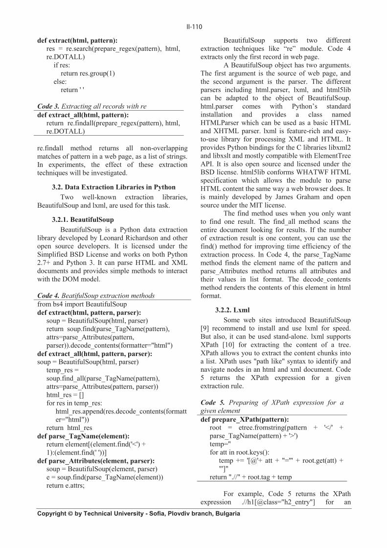
Copyright by Technical University - Sofia, Plovdiv branch, Bulgaria
def extract(html, pattern): res = re.search(prepare_regex(pattern), html, re.DOTALL) if res: return res.group(1) else: return ' '
Code 3. Extracting all records with re def extract_all(html, pattern):
return re.findall(prepare_regex(pattern), html, re.DOTALL)
re.findall method returns all non-overlapping matches of pattern in a web page, as a list of strings. In experiments, the effect of these extraction techniques will be investigated.
3.2. Data Extraction Libraries in Python Two well-known extraction libraries,
BeautifulSoup and lxml, are used for this task.
3.2.1. BeautifulSoup BeautifulSoup is a Python data extraction
library developed by Leonard Richardson and other open source developers. It is licensed under the Simplified BSD License and works on both Python 2.7+ and Python 3. It can parse HTML and XML documents and provides simple methods to interact with the DOM model. Code 4. BeatifulSoup extraction methods from bs4 import BeautifulSoup def extract(html, pattern, parser):
soup = BeautifulSoup(html, parser) return soup.find(parse_TagName(pattern), attrs=parse_Attributes(pattern, parser)).decode_contents(formatter="html")
def extract_all(html, pattern, parser): soup = BeautifulSoup(html, parser)
temp_res = soup.find_all(parse_TagName(pattern), attrs=parse_Attributes(pattern, parser)) html_res = [] for res in temp_res:
html_res.append(res.decode_contents(formatter="html"))
return html_res def parse_TagName(element):
return element[(element.find('<') + 1):(element.find(' '))]
def parse_Attributes(element, parser): soup = BeautifulSoup(element, parser) e = soup.find(parse_TagName(element)) return e.attrs;
BeautifulSoup supports two different extraction techniques like “re” module. Code 4 extracts only the first record in web page.
A BeautifulSoup object has two arguments. The first argument is the source of web page, and the second argument is the parser. The different parsers including html.parser, lxml, and html5lib can be adapted to the object of BeautifulSoup. html.parser comes with Python’s standard installation and provides a class named HTMLParser which can be used as a basic HTML and XHTML parser. lxml is feature-rich and easy-to-use library for processing XML and HTML. It provides Python bindings for the C libraries libxml2 and libxslt and mostly compatible with ElementTree API. It is also open source and licensed under the BSD license. html5lib conforms WHATWF HTML specification which allows the module to parse HTML content the same way a web browser does. It is mainly developed by James Graham and open source under the MIT license.
The find method uses when you only want to find one result. The find_all method scans the entire document looking for results. If the number of extraction result is one content, you can use the find() method for improving time efficiency of the extraction process. In Code 4, the parse_TagName method finds the element name of the pattern and parse_Attributes method returns all attributes and their values in list format. The decode_contents method renders the contents of this element in html format.
3.2.2. Lxml Some web sites introduced BeautifulSoup
[9] recommend to install and use lxml for speed. But also, it can be used stand-alone. lxml supports XPath [10] for extracting the content of a tree. XPath allows you to extract the content chunks into a list. XPath uses "path like" syntax to identify and navigate nodes in an html and xml document. Code 5 returns the XPath expression for a given extraction rule.
Code 5. Preparing of XPath expression for a given element def prepare_XPath(pattern):
root = etree.fromstring(pattern + '</' + parse_TagName(pattern) + '>') temp='' for att in root.keys():
temp += '[@'+ att + "='" + root.get(att) + "']"
return ".//" + root.tag + temp
For example, Code 5 returns the XPath expression .//h1[@class="h2_entry"] for an
extraction rule of <h2 class="h2_entry">. Code 6 has two function for extracting all results and the first result. Code 6. Extraction with lxml from lxml import etree from io import StringIO def extract_all(html, pattern):
parser = etree.HTMLParser() tree = etree.parse(StringIO(html), parser) result = etree.tostring(tree.getroot()) root = tree.getroot() my_list = [] yol = prepare_XPath(pattern) for elem in root.findall(yol):
my_list.append(etree.tostring(elem, encoding='unicode'))
return my_list def extract(html, pattern):
parser = etree.HTMLParser() tree = etree.parse(StringIO(html), parser) result = etree.tostring(tree.getroot()) root = tree.getroot() elem = root.find(prepare_XPath(pattern)) return etree.tostring(elem, encoding='unicode')
In Code 6, find method efficiently returns only the first match. findall method returns a list of matching Elements.
Table 1. Information about dataset
Domain Category Avg. (KB) Aliexpress Shopping 93.66 Bild Newspaper 67.49 Booking Trip 689.11 Collinsdictionary Dictionary 38.93 Ebay Shopping 297.35 Imkb Movie 214.23 Sciencedirect Articles 48.65 Tchibo Shopping 27.61 Tutorialspoint Articles 28.56 W3schools Articles 58.01 153.36
4. Experiments We prepare a dataset which contains web
pages on many different content types, including scientific articles, dictionary, movies, newspaper articles, shopping, and trip/hotel information. For constructing this dataset, we have designed a simple crawler to download web pages. Then, this crawler downloads 30 web pages for every domain. Table 1 gives the average file size of web domains for this
dataset. Moreover, we prepare extraction rules (like in Section 2) for every domain. All experiments are carried out on a computer using Intel Core i5-3.2Ghz processor and 8 GB RAM running Windows 10 operating system.
For measuring extraction time of these methods, we use time.clock method. This method returns wall-clock seconds elapsed, as a floating point number. This method is based on the Win32 function QueryPerformanceCounter.
4.1. Time results of Regex There are two techniques in regular
expressions. Table 2 indicates the extraction time results and whether the result of the extraction is correct or not.
Table 2. Time results and accuracy of regex
Method Avg. (ms) extract 0.071 extract_all 0.307 0.189 Accuracy: 390 / 600 = %43.5
As expected, focusing only on one result rather than looking at the entire document has yielded better results. Extract method is 4.324 times faster than Extract_All method. However, 43.5% of the extraction rules give the correct result. In this case, DOM-based methods can be considered as a solution.
4.2. Time results of BeautifulSoup BeautifulSoup supports two different
extraction techniques and three different parsers for this task. Table 3 indicates the extraction time results.
Table 3. Time results of BeautifulSoup
Method Parser Avg. (ms) extract html.parser 820.075 extract_all html.parser 1192.317 extract lxml 591.583 extract_all lxml 1025.892 extract html5lib 2191.472 extract_all html5lib 2626.747
1408.014
II-110

Copyright by Technical University - Sofia, Plovdiv branch, Bulgaria
def extract(html, pattern): res = re.search(prepare_regex(pattern), html, re.DOTALL) if res: return res.group(1) else: return ' '
Code 3. Extracting all records with re def extract_all(html, pattern):
return re.findall(prepare_regex(pattern), html, re.DOTALL)
re.findall method returns all non-overlapping matches of pattern in a web page, as a list of strings. In experiments, the effect of these extraction techniques will be investigated.
3.2. Data Extraction Libraries in Python Two well-known extraction libraries,
BeautifulSoup and lxml, are used for this task.
3.2.1. BeautifulSoup BeautifulSoup is a Python data extraction
library developed by Leonard Richardson and other open source developers. It is licensed under the Simplified BSD License and works on both Python 2.7+ and Python 3. It can parse HTML and XML documents and provides simple methods to interact with the DOM model. Code 4. BeatifulSoup extraction methods from bs4 import BeautifulSoup def extract(html, pattern, parser):
soup = BeautifulSoup(html, parser) return soup.find(parse_TagName(pattern), attrs=parse_Attributes(pattern, parser)).decode_contents(formatter="html")
def extract_all(html, pattern, parser): soup = BeautifulSoup(html, parser)
temp_res = soup.find_all(parse_TagName(pattern), attrs=parse_Attributes(pattern, parser)) html_res = [] for res in temp_res:
html_res.append(res.decode_contents(formatter="html"))
return html_res def parse_TagName(element):
return element[(element.find('<') + 1):(element.find(' '))]
def parse_Attributes(element, parser): soup = BeautifulSoup(element, parser) e = soup.find(parse_TagName(element)) return e.attrs;
BeautifulSoup supports two different extraction techniques like “re” module. Code 4 extracts only the first record in web page.
A BeautifulSoup object has two arguments. The first argument is the source of web page, and the second argument is the parser. The different parsers including html.parser, lxml, and html5lib can be adapted to the object of BeautifulSoup. html.parser comes with Python’s standard installation and provides a class named HTMLParser which can be used as a basic HTML and XHTML parser. lxml is feature-rich and easy-to-use library for processing XML and HTML. It provides Python bindings for the C libraries libxml2 and libxslt and mostly compatible with ElementTree API. It is also open source and licensed under the BSD license. html5lib conforms WHATWF HTML specification which allows the module to parse HTML content the same way a web browser does. It is mainly developed by James Graham and open source under the MIT license.
The find method uses when you only want to find one result. The find_all method scans the entire document looking for results. If the number of extraction result is one content, you can use the find() method for improving time efficiency of the extraction process. In Code 4, the parse_TagName method finds the element name of the pattern and parse_Attributes method returns all attributes and their values in list format. The decode_contents method renders the contents of this element in html format.
3.2.2. Lxml Some web sites introduced BeautifulSoup
[9] recommend to install and use lxml for speed. But also, it can be used stand-alone. lxml supports XPath [10] for extracting the content of a tree. XPath allows you to extract the content chunks into a list. XPath uses "path like" syntax to identify and navigate nodes in an html and xml document. Code 5 returns the XPath expression for a given extraction rule.
Code 5. Preparing of XPath expression for a given element def prepare_XPath(pattern):
root = etree.fromstring(pattern + '</' + parse_TagName(pattern) + '>') temp='' for att in root.keys():
temp += '[@'+ att + "='" + root.get(att) + "']"
return ".//" + root.tag + temp
For example, Code 5 returns the XPath expression .//h1[@class="h2_entry"] for an
extraction rule of <h2 class="h2_entry">. Code 6 has two function for extracting all results and the first result. Code 6. Extraction with lxml from lxml import etree from io import StringIO def extract_all(html, pattern):
parser = etree.HTMLParser() tree = etree.parse(StringIO(html), parser) result = etree.tostring(tree.getroot()) root = tree.getroot() my_list = [] yol = prepare_XPath(pattern) for elem in root.findall(yol):
my_list.append(etree.tostring(elem, encoding='unicode'))
return my_list def extract(html, pattern):
parser = etree.HTMLParser() tree = etree.parse(StringIO(html), parser) result = etree.tostring(tree.getroot()) root = tree.getroot() elem = root.find(prepare_XPath(pattern)) return etree.tostring(elem, encoding='unicode')
In Code 6, find method efficiently returns only the first match. findall method returns a list of matching Elements.
Table 1. Information about dataset
Domain Category Avg. (KB) Aliexpress Shopping 93.66 Bild Newspaper 67.49 Booking Trip 689.11 Collinsdictionary Dictionary 38.93 Ebay Shopping 297.35 Imkb Movie 214.23 Sciencedirect Articles 48.65 Tchibo Shopping 27.61 Tutorialspoint Articles 28.56 W3schools Articles 58.01 153.36
4. Experiments We prepare a dataset which contains web
pages on many different content types, including scientific articles, dictionary, movies, newspaper articles, shopping, and trip/hotel information. For constructing this dataset, we have designed a simple crawler to download web pages. Then, this crawler downloads 30 web pages for every domain. Table 1 gives the average file size of web domains for this
dataset. Moreover, we prepare extraction rules (like in Section 2) for every domain. All experiments are carried out on a computer using Intel Core i5-3.2Ghz processor and 8 GB RAM running Windows 10 operating system.
For measuring extraction time of these methods, we use time.clock method. This method returns wall-clock seconds elapsed, as a floating point number. This method is based on the Win32 function QueryPerformanceCounter.
4.1. Time results of Regex There are two techniques in regular
expressions. Table 2 indicates the extraction time results and whether the result of the extraction is correct or not.
Table 2. Time results and accuracy of regex
Method Avg. (ms) extract 0.071 extract_all 0.307 0.189 Accuracy: 390 / 600 = %43.5
As expected, focusing only on one result rather than looking at the entire document has yielded better results. Extract method is 4.324 times faster than Extract_All method. However, 43.5% of the extraction rules give the correct result. In this case, DOM-based methods can be considered as a solution.
4.2. Time results of BeautifulSoup BeautifulSoup supports two different
extraction techniques and three different parsers for this task. Table 3 indicates the extraction time results.
Table 3. Time results of BeautifulSoup
Method Parser Avg. (ms) extract html.parser 820.075 extract_all html.parser 1192.317 extract lxml 591.583 extract_all lxml 1025.892 extract html5lib 2191.472 extract_all html5lib 2626.747
1408.014
II-111

Copyright by Technical University - Sofia, Plovdiv branch, Bulgaria
lxml parser for BeautifulSoup is the best
parser for this task. html5lib and html.parser are just not very good results. As expected, the time results of extract methods are better than the time results of extract_all methods in all parsers. Finally, we examine lxml parser with its methods.
4.3. Time results of lxml The lxml library is a binding for the C
libraries libxml2 and libxslt. It is unique in that it combines the speed and XML feature completeness of these libraries with the simplicity of a native Python API. It can be used with BeautifulSoup, but it can be also utilized stand-alone. In this section, we examine this library stand-alone.
Table 4. Time results of lxml
Method Avg. (ms) extract 9.047 extract_all 9.480 9.277
Time results of lxml is better than time results of BeautifulSoup. lxml parser in BeautifulSoup makes the results better, but the use of lxml stand-
alone provides a much better improvement. (See Fig. 2 and 3 for comparing all libraries)
5. Conclusion In this study, libraries of Python for
extracting data from web pages are compared in order to understand their time durations. As expected, the experimental results show that regex gives better time duration with 0.071 ms. However, 43.5% of the extraction rules give the correct result. In this case, DOM-based libraries including BeautifulSoup and lxml can be considered as a solution. Lxml (stand-alone) provides better time results in DOM-based libraries. BeautifulSoup gave worse results because of extra processes for creating DOM even when using lxml parser.
In future work, we will need to develop more effective and effective methods for this task. Moreover, time results of other languages [11] on this task are compared.
Additional Information
All codes are open-source. Source codes and dataset are as follows.
https://github.com/erdincuzun/WebDataExtractionInPython
A: All extraction results, 1: only first result
Fig. 2. Average time duration results of Regex and lxml
II-112

Copyright by Technical University - Sofia, Plovdiv branch, Bulgaria
lxml parser for BeautifulSoup is the best
parser for this task. html5lib and html.parser are just not very good results. As expected, the time results of extract methods are better than the time results of extract_all methods in all parsers. Finally, we examine lxml parser with its methods.
4.3. Time results of lxml The lxml library is a binding for the C
libraries libxml2 and libxslt. It is unique in that it combines the speed and XML feature completeness of these libraries with the simplicity of a native Python API. It can be used with BeautifulSoup, but it can be also utilized stand-alone. In this section, we examine this library stand-alone.
Table 4. Time results of lxml
Method Avg. (ms) extract 9.047 extract_all 9.480 9.277
Time results of lxml is better than time results of BeautifulSoup. lxml parser in BeautifulSoup makes the results better, but the use of lxml stand-
alone provides a much better improvement. (See Fig. 2 and 3 for comparing all libraries)
5. Conclusion In this study, libraries of Python for
extracting data from web pages are compared in order to understand their time durations. As expected, the experimental results show that regex gives better time duration with 0.071 ms. However, 43.5% of the extraction rules give the correct result. In this case, DOM-based libraries including BeautifulSoup and lxml can be considered as a solution. Lxml (stand-alone) provides better time results in DOM-based libraries. BeautifulSoup gave worse results because of extra processes for creating DOM even when using lxml parser.
In future work, we will need to develop more effective and effective methods for this task. Moreover, time results of other languages [11] on this task are compared.
Additional Information
All codes are open-source. Source codes and dataset are as follows.
https://github.com/erdincuzun/WebDataExtractionInPython
A: All extraction results, 1: only first result
Fig. 2. Average time duration results of Regex and lxml
A: All extraction results, 1: only first result, BS: BeautifulSoup, P1: html.parser, P2: lxml, P3: html5lib Fig. 3. Average time duration results BeautifulSoup Parsers
REFERENCES
1. Rahman, A.F.R., Alam, H. and Hartono, R. (2001). Content extraction from HTML documents, International workshop on Web document Analysis, pp. 7-10, 2001.
2. Ferrara, E., De Meo, P., Fiumara, G., Baumgartner, R. (2014). Web data extraction, applications and techniques: A survey, Knowledge-Based Systems, Volume 70, 2014, pp. 301-323.
3. Flesca, S., Manco, G., Masciari, E., Rende, E., Tagarelli, A. (2004). Web wrapper induction: a brief survey”, In: AI Communications, vol. 17, pp. 57–61. IOS Press, Amsterdam.
4. Álvarez-Sabucedo, L. M., Anido-Rifón, L. E. and Santos-Gago, J. M. (2009). Reusing web contents: a DOM approach, Softw: Pract. Exper., 39: 299–314. doi:10.1002/spe.901.
5. Fu, L., Meng, Y., Xia Y. and Yu, H. (2010). Web Content Extraction based on Webpage Layout Analysis”, Second International Conference on Information Technology and Computer Science, Kiev, 2010, pp. 40-43.
6. BeatifulSoup,https://www.crummy.com/software/BeautifulSoup/, (12.04.2018)
7. lxml, http://lxml.de/, (12.04.2018) 8. DOM, https://developer.mozilla.org/en-
US/docs/Web/API/Document_Object_Model/Introduction, (12.04.2018)
9. Crummy,https://www.crummy.com/software/BeautifulSoup/bs4/doc/, (12.04.2018)
10. XPath, https://www.w3.org/TR/xpath/, (12.04.2018)
11. Uzun, E., Buluş, H. N., Doruk, A., Özhan, E. (2017). Evaluation of Hap, AngleSharp and HtmlDocument in web content extraction. International Scientific Conference’2017 (UNITECH’17), Gabrovo, Bulgaria, November 17-18, Vol. II – pp. 275-278.
Authors’ contacts Erdinç Uzun, Organization: Namık Kemal University,
Çorlu Faculty of Engineering, Computer Engineering Department
Address: NKÜ Çorlu Mühendislik Fakültesi Dekanlığı, Silahtarağa Mahallesi Üniversite 1.Sokak, No:13, 59860 Çorlu / Tekirdağ / TURKEY
Phone (optional): +90 (282) 250 2325 E-mail: [email protected] Tarık Yerlikaya (Corresponding author) Oğuz Kırat Organization: Trakya University, Faculty of
Engineering, Computer Engineering Department
Address: Trakya Üniversitesi Ahmet Karadeniz Yerleşkesi Mühendislik Fakültesi 22020 Merkez / Edirne /TURKEY
Phone (optional): +90 (284) 226 1217 / 2215
E-mail: [email protected], [email protected]
II-113

Copyright © 2018 by Technical University of Sofia, Plovdiv branch, Bulgaria ISSN Online: 2535-0048
Copyright by Technical University - Sofia, Plovdiv branch, Bulgaria
OBJECT-BASED ENTITY RELATIONSHIP DIAGRAM DRAWING LIBRARY: ENTREL.JS
ERDİNÇ UZUN, TARIK YERLİKAYA, OĞUZ KIRAT
Abstract: An entity relationship diagram (ERD) is a visual helper for database design. ERD gives information about the relations of entity sets and the logical structure of databases. In this paper, we introduce an open source JavaScript Library named EntRel.JS in order to design sophisticated ERDs by writing simple codes. This library, which we have developed to facilitate this task, is based on our obfc.js library. It generates a SVG output on the client side for modern browsers. The SVG output provides storage efficiency when compared to existing ERD drawings created with existing drawing applications. Moreover, we present our animation library to gain action for elements in your web page.
Key words: Entity relationship diagrams, SVG, JavaScript
1. Introduction The internet has been evolving for over 25
years with some standards including HTML (HyperText Markup Language), CSS (Cascading Style Sheets), JavaScript, XML (eXtensible Markup Language) and so on. These standards are shared by the W3C throughout the world, and browser developers release updates to support these standards. The W3C [1] continues to set standards on a number of different issues. In this study, one of these standards is SVG (Scalable Vector Graphics) [2] that is used for drawing entity relationship diagrams (ERDs) and JavaScript language is used for creating these ERDs with simple codes.
ER modeling was developed for increasing the clarity of database design by Peter Chen[3]. This model is the result for systematic data analysis of system. It is usually drawn in a graphical form named ER diagrams including entities, their attributes and relationships between entities. This model is typically implemented as a database. Software developers and database designers can easily discuss the design of database and software over the ER diagram. Therefore, this subject is the basis of the database courses. ER design can be created very quickly with our library introduced in this study.
The ERD drawing process can be done on the server or client side by using the drawing applications including Microsoft Visio, OpenOffice / LibreOffice Draw, Dia, Diagramly and so on. The drawing file stored on the server side is displayed in the browser in the <img> element. On the other hand, it can still be prepared on the server side and
displayed in the CANVAS [4] or SVG elements used for drawing graphics in HTML 5. In this study, the SVG is suitable for our study instead of CANVAS. CANVAS is typically used in web-based games, while it allows the drawing process with JavaScript codes. Because SVG is a vector-based system, the browser is not affected by the magnification. It was chosen for this reason. It can also be drawn on the client side by using JavaScript’s advantage and holding fewer code on the server side. This makes the server load lighter and the drawing works are made on the client side. However, with the JavaScript file loaded once, it is only necessary for utilizing the AJAX (asynchronous JavaScript and XML) [5] in order to upload the required code. AJAX improves the bandwidth performance of web-based applications. In this study, the object creation codes are stored in the server, and drawing with the EntRel.JS library is performed on the client side.
The EntRel.JS library (Entity Relationship) is based on the obfc.JS library (Object-Based Flow Charts) [6] that we develop is an object-based library for drawing SVG flow charts across modern web browsers. It makes easily to construct objects, links and connections. Moreover, it dispatches a click event when an object or a line is clicked and descriptions can be added for all clicks. The EntRel.JS allows you to design complex ERDs by writing short codes. SVG output is parsed from these texts and the SVG output is produced on the client side.
Technologies such as SVG, JavaScript and AJAX are used in many different subjects such as numerical graphics, networking, geography,
medicine and electricity. For example, Saito and Ouyang [7] indicate how to draw data on the client side with ChartML. They use SVG and JavaScript in the client side and they produce graphs. Some studies [8-11] focus on how network topologies can be displayed on the browser by using SVG, JavaScript and AJAX. Yin and Zang [12] describe SVG and AJAX technologies in the Web geographic Information system. Fang and et al. [13] explain the use of these technologies in local thermal power plant management. Birr and et al. [14] introduces how three-dimensional medical data can be demonstrated in the Web environment. Alhirabi and Butler [15] perform the gene notation using SVG.
This study presents a JavaScript Library to create ERDs with objects. Moreover, you can also easily link objects to each other. Draw function of these objects produces a SVG output in browsers. Moreover, we introduce an animation library (animation.JS) that we developed.
2. obfc.JS library Before explaining the EntRel.JS library, we
give information about obfc.JS library that we developed earlier. obfc.JS has 24 different SVG shapes for drawing flow charts. In this section, we will describe the most basic features of this library.
2.1. Creating an object Before creating an object, you add obfc.js
file and SVG element to body of a web page. Then, you connect library to the id of the SVG element. Code 1 indicates these lines. Code 1. Preparing library and creating an object <script src="obfc.min.js"></script> <svg id="demo" width="600" height="700"> </svg> <script> prepare_SVG("demo"); var object2 = add_theObject(new Process(300, 150, 1, ["Line 1", "Line 2"], 10)); </script>
To draw an object, add_theObject function can be used for the given SVG element. add_theObject is a function that adds the object into a given SVG element and returns this object. This returned object is used for drawing lines between two objects. There are 24 different SVG objects in obfc.JS. “Process” is the one of objects from 24 different objects. There are 9 parameters for creating an object. First two parameters are required, others are optimal.
Object_Name(_middle_x, _middle_y, _size, _text, _text_size, _description, _fill_color, _stroke_color, _text_color);
_middle_x and middle_y: centre of the object. (Required)
_size: For example, default size of a process object width is 125 and height is 50. _size value is multiplied by these values.
_text and _text_size: Text is written in the center of an object. This parameter can be defined string value or array[“”, “”…]. If your text is too long, you can use array for creating lines.
_description: These value can be coded in HTML format. These value is displayed in a HTML element that contains “desc” id after clicking an object or a line.
_fill_color: Default value is white. But, the object color can be determined with this parameter.
_stroke_color: Default value is black. _text_color: Default value is black.
2.1. Creating lines between objects After creating all objects, objects can be
linked by using draw_theLine function. Code 2. Creating lines between two objects <script> …. var o_line1 = draw_theLine(new Line(object1, object2)); </script>
Fig. 1. Output of Code 2
Line is a function that determines the path for given two objects and their positions. This function has 9 parameters. First two parameter is required and others are optimal.
Line(object1, object2, position1, position2, _text, _text_size, _description, _stroke_color, _text_color);
object1 ve object2: are variables that is defined in the previous section.
© International Scientific Conference on Engineering, Technologies and Systems TECHSYS 2018, Technical University – Sofia, Plovdiv branch 17 – 19 May 2018, Plovdiv, Bulgaria

Copyright by Technical University - Sofia, Plovdiv branch, Bulgaria
OBJECT-BASED ENTITY RELATIONSHIP DIAGRAM DRAWING LIBRARY: ENTREL.JS
ERDİNÇ UZUN, TARIK YERLİKAYA, OĞUZ KIRAT
Abstract: An entity relationship diagram (ERD) is a visual helper for database design. ERD gives information about the relations of entity sets and the logical structure of databases. In this paper, we introduce an open source JavaScript Library named EntRel.JS in order to design sophisticated ERDs by writing simple codes. This library, which we have developed to facilitate this task, is based on our obfc.js library. It generates a SVG output on the client side for modern browsers. The SVG output provides storage efficiency when compared to existing ERD drawings created with existing drawing applications. Moreover, we present our animation library to gain action for elements in your web page.
Key words: Entity relationship diagrams, SVG, JavaScript
1. Introduction The internet has been evolving for over 25
years with some standards including HTML (HyperText Markup Language), CSS (Cascading Style Sheets), JavaScript, XML (eXtensible Markup Language) and so on. These standards are shared by the W3C throughout the world, and browser developers release updates to support these standards. The W3C [1] continues to set standards on a number of different issues. In this study, one of these standards is SVG (Scalable Vector Graphics) [2] that is used for drawing entity relationship diagrams (ERDs) and JavaScript language is used for creating these ERDs with simple codes.
ER modeling was developed for increasing the clarity of database design by Peter Chen[3]. This model is the result for systematic data analysis of system. It is usually drawn in a graphical form named ER diagrams including entities, their attributes and relationships between entities. This model is typically implemented as a database. Software developers and database designers can easily discuss the design of database and software over the ER diagram. Therefore, this subject is the basis of the database courses. ER design can be created very quickly with our library introduced in this study.
The ERD drawing process can be done on the server or client side by using the drawing applications including Microsoft Visio, OpenOffice / LibreOffice Draw, Dia, Diagramly and so on. The drawing file stored on the server side is displayed in the browser in the <img> element. On the other hand, it can still be prepared on the server side and
displayed in the CANVAS [4] or SVG elements used for drawing graphics in HTML 5. In this study, the SVG is suitable for our study instead of CANVAS. CANVAS is typically used in web-based games, while it allows the drawing process with JavaScript codes. Because SVG is a vector-based system, the browser is not affected by the magnification. It was chosen for this reason. It can also be drawn on the client side by using JavaScript’s advantage and holding fewer code on the server side. This makes the server load lighter and the drawing works are made on the client side. However, with the JavaScript file loaded once, it is only necessary for utilizing the AJAX (asynchronous JavaScript and XML) [5] in order to upload the required code. AJAX improves the bandwidth performance of web-based applications. In this study, the object creation codes are stored in the server, and drawing with the EntRel.JS library is performed on the client side.
The EntRel.JS library (Entity Relationship) is based on the obfc.JS library (Object-Based Flow Charts) [6] that we develop is an object-based library for drawing SVG flow charts across modern web browsers. It makes easily to construct objects, links and connections. Moreover, it dispatches a click event when an object or a line is clicked and descriptions can be added for all clicks. The EntRel.JS allows you to design complex ERDs by writing short codes. SVG output is parsed from these texts and the SVG output is produced on the client side.
Technologies such as SVG, JavaScript and AJAX are used in many different subjects such as numerical graphics, networking, geography,
medicine and electricity. For example, Saito and Ouyang [7] indicate how to draw data on the client side with ChartML. They use SVG and JavaScript in the client side and they produce graphs. Some studies [8-11] focus on how network topologies can be displayed on the browser by using SVG, JavaScript and AJAX. Yin and Zang [12] describe SVG and AJAX technologies in the Web geographic Information system. Fang and et al. [13] explain the use of these technologies in local thermal power plant management. Birr and et al. [14] introduces how three-dimensional medical data can be demonstrated in the Web environment. Alhirabi and Butler [15] perform the gene notation using SVG.
This study presents a JavaScript Library to create ERDs with objects. Moreover, you can also easily link objects to each other. Draw function of these objects produces a SVG output in browsers. Moreover, we introduce an animation library (animation.JS) that we developed.
2. obfc.JS library Before explaining the EntRel.JS library, we
give information about obfc.JS library that we developed earlier. obfc.JS has 24 different SVG shapes for drawing flow charts. In this section, we will describe the most basic features of this library.
2.1. Creating an object Before creating an object, you add obfc.js
file and SVG element to body of a web page. Then, you connect library to the id of the SVG element. Code 1 indicates these lines. Code 1. Preparing library and creating an object <script src="obfc.min.js"></script> <svg id="demo" width="600" height="700"> </svg> <script> prepare_SVG("demo"); var object2 = add_theObject(new Process(300, 150, 1, ["Line 1", "Line 2"], 10)); </script>
To draw an object, add_theObject function can be used for the given SVG element. add_theObject is a function that adds the object into a given SVG element and returns this object. This returned object is used for drawing lines between two objects. There are 24 different SVG objects in obfc.JS. “Process” is the one of objects from 24 different objects. There are 9 parameters for creating an object. First two parameters are required, others are optimal.
Object_Name(_middle_x, _middle_y, _size, _text, _text_size, _description, _fill_color, _stroke_color, _text_color);
_middle_x and middle_y: centre of the object. (Required)
_size: For example, default size of a process object width is 125 and height is 50. _size value is multiplied by these values.
_text and _text_size: Text is written in the center of an object. This parameter can be defined string value or array[“”, “”…]. If your text is too long, you can use array for creating lines.
_description: These value can be coded in HTML format. These value is displayed in a HTML element that contains “desc” id after clicking an object or a line.
_fill_color: Default value is white. But, the object color can be determined with this parameter.
_stroke_color: Default value is black. _text_color: Default value is black.
2.1. Creating lines between objects After creating all objects, objects can be
linked by using draw_theLine function. Code 2. Creating lines between two objects <script> …. var o_line1 = draw_theLine(new Line(object1, object2)); </script>
Fig. 1. Output of Code 2
Line is a function that determines the path for given two objects and their positions. This function has 9 parameters. First two parameter is required and others are optimal.
Line(object1, object2, position1, position2, _text, _text_size, _description, _stroke_color, _text_color);
object1 ve object2: are variables that is defined in the previous section.
II-115

Copyright by Technical University - Sofia, Plovdiv branch, Bulgaria
position1 and position2: are position information of objects. There are four positions for all shapes. Top=0, Bottom=1, Left=2 and Right=3. But, when these values are not entered or entered “-1”, this function automatically determines these position by calculating differences between all unused positions. (Unused position means that this position is used for creating lines)
_text and _text_size: text in line. This function selects the longest sub-line for writing text.
description, _stroke_color, _text_color: (same with previous section)
Moreover, you can determine connection points manually as shown in Code 3. Code 3. <script> var object1 = add_theObject(new Process(100, 75, 1, "Hello 1", 12)); var object2 = add_theObject(new Process(300, 150, 1, "Hello 2", 12)); var o_line1 = draw_theLine(new Line(object1, object2, 0, 1)); var o_line2 = draw_theLine(new Line(object1, object2, 2, 2)); var o_line3 = draw_theLine(new Line(object1, object2, 1, 3)); </script>
Fig. 2. Output of Code 3
In this example, position informations are added to link two objects. For example, 0 means top of object1 and 1 means bottom of object2. There are three lines in this example. Moreover, obfc.js has
jumping mechanism in collision of lines. For more information, you can visit the following web page:
https://www.e-adys.com/obfc-js/object-based-flow-charts-obfc-js/
3. EntRel.JS EntRel.JS is JavaScript Library for creating
ERDs with simple JavaScript methods. Figure 3 gives information about the location of the libraries in the Web. Libraries of obfc.JS, EntRel.JS and Animation.JS takes the drawing code from a server and parse these codes for drawing into an SVG element. The file sizes of bfc.JS, EntRel.JS and Animation.JS are 78 KB, 3.85 KB and 3.62 KB. The first installation of these libraries is loaded into the browser cache, and these libraries are not updated on other requests.
There are two main classes for creating diagrams as FlatLine and Entity. Entity class derived from Process class of obfc.js. For better understanding this object, you can examine Section 2.1.
Entity(_middle_x, _middle_y, _size, _text, _attributes, _text_size, _weak, _description, _fill_color, _stroke_color, _text_color)
The fifth parameter contain extra information about attributes of an entity. You can define 8 attribute in array format for an entity. For example:
[null, “AuthorID(PK)”, “AuthorName”, “AuthorSurName”]
The first attribute contain a null value so that it can be drawn. The first four attributes are in top and others are in bottom. Weak parameter is used for a weak entity that cannot be uniquely identified by its attributes alone.
FlatLine connects the objects. FlatLine class derived from Line class of obfc.js. FlatLine don’t contain an arrow in drawing. Code 4 is an example for Entity and FlatLine. Moreover, Fig 4 is output of Code 4.
obfc.js entrel.js animation.js …Script Codes…
Server Side Client Side
Web Browsers Mozilla Chrome IE Safari (A browser with SVG support)
obfc.js entrel.js animation.js
ERDs Script Codes
SVG Output HTTP Request
XMLHTTP Request
AJAX
II-116

Copyright by Technical University - Sofia, Plovdiv branch, Bulgaria
position1 and position2: are position information of objects. There are four positions for all shapes. Top=0, Bottom=1, Left=2 and Right=3. But, when these values are not entered or entered “-1”, this function automatically determines these position by calculating differences between all unused positions. (Unused position means that this position is used for creating lines)
_text and _text_size: text in line. This function selects the longest sub-line for writing text.
description, _stroke_color, _text_color: (same with previous section)
Moreover, you can determine connection points manually as shown in Code 3. Code 3. <script> var object1 = add_theObject(new Process(100, 75, 1, "Hello 1", 12)); var object2 = add_theObject(new Process(300, 150, 1, "Hello 2", 12)); var o_line1 = draw_theLine(new Line(object1, object2, 0, 1)); var o_line2 = draw_theLine(new Line(object1, object2, 2, 2)); var o_line3 = draw_theLine(new Line(object1, object2, 1, 3)); </script>
Fig. 2. Output of Code 3
In this example, position informations are added to link two objects. For example, 0 means top of object1 and 1 means bottom of object2. There are three lines in this example. Moreover, obfc.js has
jumping mechanism in collision of lines. For more information, you can visit the following web page:
https://www.e-adys.com/obfc-js/object-based-flow-charts-obfc-js/
3. EntRel.JS EntRel.JS is JavaScript Library for creating
ERDs with simple JavaScript methods. Figure 3 gives information about the location of the libraries in the Web. Libraries of obfc.JS, EntRel.JS and Animation.JS takes the drawing code from a server and parse these codes for drawing into an SVG element. The file sizes of bfc.JS, EntRel.JS and Animation.JS are 78 KB, 3.85 KB and 3.62 KB. The first installation of these libraries is loaded into the browser cache, and these libraries are not updated on other requests.
There are two main classes for creating diagrams as FlatLine and Entity. Entity class derived from Process class of obfc.js. For better understanding this object, you can examine Section 2.1.
Entity(_middle_x, _middle_y, _size, _text, _attributes, _text_size, _weak, _description, _fill_color, _stroke_color, _text_color)
The fifth parameter contain extra information about attributes of an entity. You can define 8 attribute in array format for an entity. For example:
[null, “AuthorID(PK)”, “AuthorName”, “AuthorSurName”]
The first attribute contain a null value so that it can be drawn. The first four attributes are in top and others are in bottom. Weak parameter is used for a weak entity that cannot be uniquely identified by its attributes alone.
FlatLine connects the objects. FlatLine class derived from Line class of obfc.js. FlatLine don’t contain an arrow in drawing. Code 4 is an example for Entity and FlatLine. Moreover, Fig 4 is output of Code 4.
obfc.js entrel.js animation.js …Script Codes…
Server Side Client Side
Web Browsers Mozilla Chrome IE Safari (A browser with SVG support)
obfc.js entrel.js animation.js
ERDs Script Codes
SVG Output HTTP Request
XMLHTTP Request
AJAX
Fig. 3. Location of the EntRel.JS and Animation.JS in the Web
Code 4. An example ERD <script> prepare_SVG("demo"); var object1 = add_theObject(new Entity(300, 350, 0.75, "Books", [null, null, null, null, null, "BookID(PK)", "Title"], 16)); var object2 = add_theObject(new Entity(65, 150, 0.75, "Authors", [null, "AID(PK)", "AName", "ASurname"], 16)); var object3 = add_theObject(new Entity(300, 150, 0.75, "Types", [null, "TID(PK)", "TName"], 16)); var object4 = add_theObject(new Entity(500, 150, 0.75, "Publishers", [null, "PID(PK)", "PName", "Location"], 16)); var object5 = add_theObject(new Decision(65, 250, 0.75, ["R1"], 12)); var object6 = add_theObject(new Decision(300, 250, 0.75, ["R2"], 12)); var object7 = add_theObject(new Decision(500, 250, 0.75, ["R3"], 12));
var o_line1 = draw_theLine(new FlatLine(object2, object5, null, null, "N")); var o_line2 = draw_theLine(new FlatLine(object5, object1, 1, 2, "N")); var o_line3 = draw_theLine(new
FlatLine(object3, object6, null, null, "N")); var o_line4 = draw_theLine(new FlatLine(object6, object1, null, null, "N")); var o_line5 = draw_theLine(new FlatLine(object4, object7, null, null, "N")); var o_line6 = draw_theLine(new FlatLine(object7, object1, 1, 3, "1")); </script>
Fig. 4. Output of Code 3
In Code 4, (PK) keyword defines a primary key of an entity. Moreover, (DE) keyword defines
derived attributes and (MV) keyword is for multivalued attributes. There are four entity objects
II-117

Copyright by Technical University - Sofia, Plovdiv branch, Bulgaria
and three Decision objects created from obfc.JS library. And these objects link with six FlatLine. Now let's add animation to this drawing.
4. animation.JS With animation.js, you can easily animate
your a desired element of child elements in your web page. Navigation bar of this animation contains links: Previous, Next, Show All, Hide All, Start Animation, and Stop Animation. Code 5 is a simple animation code. Code 5. Creating an animation a web page <script src="animation.min.js"></script> <script> initializeAnimation(null, ".animation", "div,p", "#masthead,#secondary"); </script> Add animation.min.js your web page, then call
initializeAnimation method for configuration of the animation.
The first parameter of this method is the number of elements. But this parameter is used by other libraries: obfc.js and entrel.js.
The second parameter is the base element of animation. You can use a selector for setting this parameter.
Third parameter is inner elements in the base element. You can use more than one selector for selecting the desired elements.
Fourth parameters is used to set opacity of the selected elements.
Moreover, you can set time interval for animation and opacity for elements. For example: (Append the following code to Code 5)
opacity = 0.1; //opacity of elements timeInterval = 3000; //3 seconds
For creating links for navigating animation in a web page, you can append Code 6 for your web page.
Code 6. Navigation bar <div id="anavbar" class="anavbar" style="display:none"> <ul class="horizontal"> <li><a id="pre">Previous</a></li> <li><a id="next">Next</a> </li> <li><a id="show">Show All</a> </li> <li><a id="hide">Hide All</a> </li> <li><a id="start">Start Animation</a> </li> <li><a id="stop">Stop Animation</a> </li> </ul> </div>
5. The use of obfc.JS and EntReel.JS with amination.JS For creating animations, you can group the
objects created by obfc.JS and EntReel.JS using an array. If two objects are together, these objects can be grouped together. (For example ([object5, object2])). You can append the following codes to Code 4 for creating animation in Fig 4.
var groups = [object1, [object5, object2], [o_line1, o_line2], [object6, object3], [o_line3, o_line4], [object7, object4], [o_line5, o_line6]]; prepareClassforAnimation(groups); initializeAnimation(groups.length - 1);
prepareClassforAnimation method prepares objects for animation. initializeAnimation method starts animation. For testing animation, you can visit the following web page:
https://www.e-adys.com/web_tasarimi_programlama/entrel-js-creating-entity-relationship-diagrams-with-javascript-and-svg/
6. Conclusion In this study, the open source EntRel.JS and
animation.JS Libraries that we developed and the functions of these libraries to draw ERDs in the Web environment are introduced. Thanks to this library, drawings are made quickly with very little code. Unlike other drawing applications, the links between shapes are automatically feasible. SVG output occupies very little space according to the other image formats.
In future studies, we plan to develop a design library that enables drawing and drag-and-drop functionality through the Web page without writing codes. We are also aiming to group some designs and share them in a web environment. Finally, we intend to develop new libraries for different subjects including logic circuits, data structures, database management systems, software engineering and system analysis in order to draw different shapes.
Additional Information
All codes are open-source. Web addresses and help documents are as follows.
https://github.com/erdincuzun/obfc.js https://github.com/erdincuzun/entrel.js https://github.com/erdincuzun/Animation.js https://www.e-adys.com/
II-118

Copyright by Technical University - Sofia, Plovdiv branch, Bulgaria
and three Decision objects created from obfc.JS library. And these objects link with six FlatLine. Now let's add animation to this drawing.
4. animation.JS With animation.js, you can easily animate
your a desired element of child elements in your web page. Navigation bar of this animation contains links: Previous, Next, Show All, Hide All, Start Animation, and Stop Animation. Code 5 is a simple animation code. Code 5. Creating an animation a web page <script src="animation.min.js"></script> <script> initializeAnimation(null, ".animation", "div,p", "#masthead,#secondary"); </script> Add animation.min.js your web page, then call
initializeAnimation method for configuration of the animation.
The first parameter of this method is the number of elements. But this parameter is used by other libraries: obfc.js and entrel.js.
The second parameter is the base element of animation. You can use a selector for setting this parameter.
Third parameter is inner elements in the base element. You can use more than one selector for selecting the desired elements.
Fourth parameters is used to set opacity of the selected elements.
Moreover, you can set time interval for animation and opacity for elements. For example: (Append the following code to Code 5)
opacity = 0.1; //opacity of elements timeInterval = 3000; //3 seconds
For creating links for navigating animation in a web page, you can append Code 6 for your web page.
Code 6. Navigation bar <div id="anavbar" class="anavbar" style="display:none"> <ul class="horizontal"> <li><a id="pre">Previous</a></li> <li><a id="next">Next</a> </li> <li><a id="show">Show All</a> </li> <li><a id="hide">Hide All</a> </li> <li><a id="start">Start Animation</a> </li> <li><a id="stop">Stop Animation</a> </li> </ul> </div>
5. The use of obfc.JS and EntReel.JS with amination.JS For creating animations, you can group the
objects created by obfc.JS and EntReel.JS using an array. If two objects are together, these objects can be grouped together. (For example ([object5, object2])). You can append the following codes to Code 4 for creating animation in Fig 4.
var groups = [object1, [object5, object2], [o_line1, o_line2], [object6, object3], [o_line3, o_line4], [object7, object4], [o_line5, o_line6]]; prepareClassforAnimation(groups); initializeAnimation(groups.length - 1);
prepareClassforAnimation method prepares objects for animation. initializeAnimation method starts animation. For testing animation, you can visit the following web page:
https://www.e-adys.com/web_tasarimi_programlama/entrel-js-creating-entity-relationship-diagrams-with-javascript-and-svg/
6. Conclusion In this study, the open source EntRel.JS and
animation.JS Libraries that we developed and the functions of these libraries to draw ERDs in the Web environment are introduced. Thanks to this library, drawings are made quickly with very little code. Unlike other drawing applications, the links between shapes are automatically feasible. SVG output occupies very little space according to the other image formats.
In future studies, we plan to develop a design library that enables drawing and drag-and-drop functionality through the Web page without writing codes. We are also aiming to group some designs and share them in a web environment. Finally, we intend to develop new libraries for different subjects including logic circuits, data structures, database management systems, software engineering and system analysis in order to draw different shapes.
Additional Information
All codes are open-source. Web addresses and help documents are as follows.
https://github.com/erdincuzun/obfc.js https://github.com/erdincuzun/entrel.js https://github.com/erdincuzun/Animation.js https://www.e-adys.com/
REFERENCES
1. World Wide Web Consortium, https://www.w3.org/, (14.06.2018)
2. Scalable Vector Graphics, https://www.w3.org/Graphics/SVG/, (14.06.2018)
3. Chen, P. (1976). The Entity-Relationship Model - Toward a Unified View of Data. ACM Transactions on Database Systems. 1 (1): 9–36.
4. HTML 5 Canvas, https://www.w3.org/TR/2dcontext/, (14.06.2018)
5. AJAX, https://developer.mozilla.org/en-US/docs/Web/Guide/AJAX, (14.06.2018)
6. Uzun, E., Buluş, H. N. (2017). Object-based flowchart drawing library. International Conference on Computer Science and Engineering (UBMK 2017), Antalya, Turkey, 5-8 Oct. 2017, pp. 110-115.
7. Saito, T. and Ouyang, J. "Client-side data visualization," 2009 IEEE International Conference on Information Reuse & Integration, Las Vegas, NV, 2009, pp. 194-199. doi: 10.1109/IRI.2009.5211550.
8. Valle, R. D. T., Passos, D., Albuquerque, C. and Muchaluat Saade, D. C. (2008). Mesh Topology Viewer (MTV): an SVG-based interactive mesh network topology visualization tool. 2008 IEEE Symposium on Computers and Communications, Marrakech, pp. 292-297.
9. Lin, T., Zou, F., Kienle, H. M. and Muller, H. A. (2008). A domain-customizable SVG-based graph editor for software visualizations. 2008 IEEE International Conference on Software Maintenance, Beijing, 2008, pp. 466-467.
10. Fan, C., Wu, Y. and Wang, F. (2009). SVG based on Ajax and its application in graphical network topology management. 2009 IEEE International Conference on Communications Technology and Applications, Beijing.
11. Kehe, W., Tingting, W., Yanwen, A. and Wenjing, Z. (2015). Study on the Drawing Method of Project Network Diagram. 2015 7th International Conference on Intelligent Human-Machine Systems and Cybernetics, Hangzhou, 2015, pp. 95-98.
12. Yin, F. and Zhang, L. (2010). Research of WebGIS based on SVG and Ajax technology.
2nd IEEE International Conference on Information and Financial Engineering, Chongqing, pp. 629-632.
13. Fang, W., Zhang, J., Hu, B., Zhang, Q. and Ha, X. (2011). Graphics and data web publishing for local thermal power plant management information system. 2011 International Conference on Multimedia Technology, Hangzhou, 2011, pp. 337-340.
14. Birr, S., Mönch, J., Sommerfeld, D., Preim, U. and Preim, B. (2013). The LiverAnatomyExplorer: A WebGL-Based Surgical Teaching Tool. in IEEE Computer Graphics and Applications, vol. 33, no. 5, pp. 48-58.
15. Alhirabi, N. and Butler, G. (2015). A visual spreadsheet using HTML5 for whole genome display. 2015 IEEE Conference on Computational Intelligence in Bioinformatics and Computational Biology (CIBCB), Niagara Falls, ON, 2015, pp. 1-7.
Authors’ contacts Erdinç Uzun, Organization: Namık Kemal University,
Çorlu Faculty of Engineering, Computer Engineering Department
Address: NKÜ Çorlu Mühendislik Fakültesi Dekanlığı, Silahtarağa Mahallesi Üniversite 1.Sokak, No:13, 59860 Çorlu / Tekirdağ / TURKEY
Phone (optional): +90 (282) 250 2325 E-mail: [email protected] Tarık Yerlikaya (Corresponding author) Oğuz Kırat Organization: Trakya University, Faculty of
Engineering, Computer Engineering Department
Address: Trakya Üniversitesi Ahmet Karadeniz Yerleşkesi Mühendislik Fakültesi 22020 Merkez / Edirne /TURKEY
Phone (optional): +90 (284) 226 1217 / 2215
E-mail: [email protected], [email protected]
II-119

Copyright © 2018 by Technical University of Sofia, Plovdiv branch, Bulgaria ISSN Online: 2535-0048
Copyright by Technical University - Sofia, Plovdiv branch, Bulgaria
AN ALTERNATIVE EXECUTION MODEL FOR OPTIMUM BIG DATA HANDLING IN IOT-WSN
CLOUD SYSTEMS
GÜNGÖR YILDIRIM, YETKIN TATAR
Abstract: Wireless sensor networks (WSNs) are one of the fundamental IoT subsystems, which can produce big data. In line with this, the quality of data collected by sub-WSN systems is an important parameter. Eliminating redundant information and making the collected data understandable/interpretable will increase the efficiency and enable an easy integration with other IoT systems. In the paper, for the cloud system involving sub-WSN systems, an intermediate execution model which improves the quality of the collected data is proposed. The model includes semantic and data fusion/aggregation components in order to make the data more understandable and optimal. The model also proposes an approach that enables an interactive data analysis to be done between the data clients and the provider system. With this interactive model, it is aimed that the clients can execute their own data fusion and aggregation algorithms on the understandable big data set.
Key words: WSN, IoT, Sensor Cloud, Big Data
1. Introduction Nowadays, many different technologies
may come together under IoT systems and play role in the solution of more complicated problems. IoT systems, which inherently have a heterogeneous structure, usually obtain the measurement data needed from sensor networks. Therefore, WSNs are one the fundamental subsystems of IoT projects. Traditional WSNs are generally closed systems designed for goal-oriented applications. The general processes such as data collection, storage and analysis are performed within the same system. In traditional WSNs, the data gathered are stored in three different ways. These are “internal storage”, “Centralized storage” and “hybrid storage” [1]. In the internal storage, the data gathered are stored in the resources of the system in a distributed fashion. This type of storage is often preferred in the WSN systems with a large number of nodes. The centralized storage is a method usually used in small scale WSNs. In the centralized storage, the data is collected and handled in a central unit which is often external. The hybrid method is the combination of the other methods. It is not efficient to use the three methods in big scale IoT WSN systems due to some factors, such as the limited resources of WSNs and the possibility that the data gathered may reach big data sizes. IoT systems often deploy WSNs as subsystems. The WSN systems that integrate with IoT systems may have a
traditional structure or advanced features which use the IoT technologies such as 6LowPAN, RPL. Furthermore, these different WSNs may exist under the roof of a single IoT system (e.g., sensor cloud systems). One of the basic problems that arise in IoT systems which involve many different WSNs or a big scale WSN is the big and heterogeneous data management. The storage and handling of big data in IoT systems are usually carried out by a separated subunit involving big data management technologies [12, 13]. On the other hand, although today’s big data technologies have advanced features and enough flexibility, the quality of the gathered data may need to be improved. When considered the adverse situations such as redundancy and repeating, which decrease the quality of both data and communication, the importance of the quality of the big data can be better understood in terms of the performance of an IoT system. For this purpose, data aggregation and data fusion operations are used in traditional WSNs [2]. However, these are not sufficient. Data aggregation operations are performed generally on the WSN nodes and usually goal-orientation. On the other hand, it is too difficult to execute the same data aggregation operations in an IoT system involving many heterogeneous WSNs. In addition, the content of the data which are demanded by the clients of an IoT system is also an important issue. The fact that the clients can access the interpreted
© International Scientific Conference on Engineering, Technologies and Systems TECHSYS 2018, Technical University – Sofia, Plovdiv branch 17 – 19 May 2018, Plovdiv, Bulgaria

meaningful data instead of raw sensor data increases the service quality and enables an efficient big data management.
This paper proposes an effective intermediate execution model which can increase the quality and usability of the big data for IoT WSN systems like sensor clouds. The model focuses mostly on creating client-defined meaningful data, and efficient big data collection. In addition to these, an analytic approach which expresses the relation between WSNs and big data creation and shows its effect on the energy consumption in a WSN system, is also presented in the paper.
2. Related Works In 2020 if we consider that the measured
data from climate is going to reach 100 PB and 150 million sensors will be used in the experiment LHC in Europe, hence, it can be better understood the importance of the relation between WSN and big data [3] The literature studies about the relation of WSNs and big data are mostly related to the optimization processes taking place before the big data is stored. In a study [4], an algorithm that creates small data sets reflecting the character of the real big data is introduced. In the study, it is stated that the small data sets provide a successful big data management. The work in [5] focuses on the creation of big data in cluster based WSN systems which have a large number of sensor nodes. For these types of WSNs, algorithms towards the selection of optimum cluster head and the obtainment of optimum big data by mobile nodes are proposed. In the study, MULE and SENMA models are introduced for the mobile data collection. The study states that the design of big scale WSN systems can be quickly accomplished and the optimum big data quality can be achieved. In the other study [6] adaptive data collection algorithms towards the optimum big data management for periodical WSN systems are proposed. In the system operations, the algorithms take into account the association between node sampling rate and the current state of the physical phenomena. The study expresses that the big data collection can be achieved more efficiently by the algorithms proposed. Different approaches towards the integration of WSN and big data technologies can be also found in the literature [7-11].
3. Theoretical Relation Between WSNs and Big Data The theoretical expression of WSN-big data
relation could be useful in terms of showing the process of creation and communication of big data and the effect on the energy consumption in the
nodes. Accordingly, assume that there are “n” sensor nodes in a WSN running on a periodical operating mode.
𝑊𝑊 = 𝑑𝑑1, 𝑑𝑑2, . . 𝑑𝑑𝑛𝑛, 1 ≤ 𝑖𝑖 ≤ 𝑛𝑛, (1)
𝑇𝑇 = 𝑡𝑡1, 𝑡𝑡2, 𝑡𝑡3. . 𝑡𝑡𝑗𝑗, 𝑗𝑗 ≥ 1, (2)
There are “j” resources types in the WSN and they are the member of the set “T”. For instance, “t1”, “t2”, “t3” denote analog LM35 temperature sensor, digital DS18B20 temperature sensor and ADXL345 3-axis accelerometer sensor, respectively. “Ё” is the resource entity matrix with “j x n” dimension, showing which node has what resources. A sensor node may theoretically have “j” resources. In this case, “Ё” can be expressed as;
Ё =
[ 𝑘𝑘1
𝑑𝑑1 𝑘𝑘2𝑑𝑑1 . . 𝑘𝑘𝑗𝑗
𝑑𝑑1
𝑘𝑘1𝑑𝑑2 𝑘𝑘2
𝑑𝑑2 . . 𝑘𝑘𝑗𝑗𝑑𝑑2
. . . . . . . .𝑘𝑘1
𝑑𝑑𝑛𝑛 𝑘𝑘2𝑑𝑑2 . . 𝑘𝑘𝑗𝑗
𝑑𝑑𝑛𝑛] (3)
The entity value of each member of the
matrix can be defined as a Boolean type.
𝑘𝑘𝑗𝑗𝑑𝑑𝑖𝑖 = 1 , 𝑖𝑖𝑖𝑖 𝑡𝑡𝑗𝑗 ∈ 𝑑𝑑𝑖𝑖
0 , 𝑜𝑜𝑡𝑡ℎ𝑒𝑒𝑒𝑒𝑒𝑒𝑖𝑖𝑒𝑒𝑒𝑒 (4)
On the other hand, the pre-defined matrix
“B” denotes the data size produced by each resource in the system. The matrix is given as;
𝐵𝐵 = [𝑏𝑏1 𝑏𝑏2 . . 𝑏𝑏𝑗𝑗] (5)
Besides, the node state matrix given in Eq.6
shows whether the nodes in the WSN are in active state or not;
𝑁𝑁𝑠𝑠 = [𝑒𝑒1 𝑒𝑒2 . . 𝑒𝑒𝑛𝑛] , 𝑒𝑒𝑖𝑖 = 0 , 𝑑𝑑𝑖𝑖 𝑒𝑒𝑠𝑠𝑒𝑒𝑒𝑒𝑠𝑠/𝑜𝑜𝑖𝑖𝑖𝑖 𝑒𝑒𝑖𝑖 = 1 𝑑𝑑𝑖𝑖 𝑎𝑎𝑎𝑎𝑡𝑡𝑖𝑖𝑎𝑎𝑒𝑒 (6)
If it is assumed that all the nodes in the
system run with a frequency, “f” in a duration of “P”, and their clocks are synchronous, the data size “D (byte)” gathered in the WSN will be;
𝐷𝐷 = 𝑖𝑖𝑓𝑓 [𝑁𝑁𝑠𝑠 𝑓𝑓 [Ё 𝑓𝑓 𝐵𝐵𝑇𝑇]] (7)
II-121

Copyright by Technical University - Sofia, Plovdiv branch, Bulgaria
Fig.I. The Proposed Pre-Execution Model for Big Data Management in IoT-WSN Systems
The radio operations of a node are the phase in
which energy consumption is the highest. According to the energy consumption model given in [14,15], the power consumptions in transmitting (ETx) and receiving modes (ERx) of a node in the WSN;
𝐸𝐸𝑇𝑇𝑇𝑇 = 𝑏𝑏𝑖𝑖 𝑥𝑥 (Ɲ + Ɛ 𝑥𝑥 𝑑𝑑2) (8)
𝐸𝐸𝑅𝑅𝑇𝑇 = 𝑏𝑏𝑖𝑖 𝑥𝑥 Ɲ (9)
where; Ɲ and Ɛ are the radio unit and amplifier constants; “𝑏𝑏𝑖𝑖” denotes the data size to be send/received and “d” is the transmission distance
As can be seen, in the case where n, j and f are too big, the data size and energy consumption will be too big. If the limited resources of a WSN are taken under consideration, the storage techniques used in traditional WSN systems will not be suitable for big scale IoT WSN systems.
4. Basic System Model The type and data operations in IoT-WSN
can be more different than those of traditional WSNs. For example, in the traditional WSNs, while the “data aggregation” is used in order to eliminate the redundancy and repeating situations, data fusion is used for inference and correlation operations. However, these methods alone are not sufficient for an IoT system since it can have different types of clients and resources. For this reason, the handling of the data to be collected or stored according to a specific working model is essential for efficient big
data operations. Besides, the type of the service in which the data gathered will be used is quite important. Namely, the clients getting services from IoT-WSN systems usually take raw or filtered data. In addition to this, some clients may demand the system to store the data sent from their own systems. On the other hand, clients are more interested on meaningful data rather than the raw data. The fact that the interpretation/semantic operations carried out in the provider side will bring a significant service quality and variation. Furthermore, these meaningful data can be either shared with other clients or can be used in other data mining solutions. What is important here is that a software infrastructure between the clients and the IoT-WSN system is deployed.
In Fig. I, an intermediate system infrastructure, which can perform efficient big data operations in an IoT-WSN system, is presented [15]. The proposed system focuses on three important operations. The first one is the regulatory operations which eliminate redundancy/repeating situations. The regulatory operations consist of two sub-processes. The data aggregation process is a central operation and usually performed in WSNs. This process is optional because of the fact that all WSNs cannot offer it. However, the similarity detection process is applied to all data from sub-WSNs. The similarity detection process is necessary to obtain the optimum data. In the process, the similarity ratio on different data sets is found and then the found ratio is compared with a threshold
II-122

Copyright by Technical University - Sofia, Plovdiv branch, Bulgaria
Fig.I. The Proposed Pre-Execution Model for Big Data Management in IoT-WSN Systems
The radio operations of a node are the phase in
which energy consumption is the highest. According to the energy consumption model given in [14,15], the power consumptions in transmitting (ETx) and receiving modes (ERx) of a node in the WSN;
𝐸𝐸𝑇𝑇𝑇𝑇 = 𝑏𝑏𝑖𝑖 𝑥𝑥 (Ɲ + Ɛ 𝑥𝑥 𝑑𝑑2) (8)
𝐸𝐸𝑅𝑅𝑇𝑇 = 𝑏𝑏𝑖𝑖 𝑥𝑥 Ɲ (9)
where; Ɲ and Ɛ are the radio unit and amplifier constants; “𝑏𝑏𝑖𝑖” denotes the data size to be send/received and “d” is the transmission distance
As can be seen, in the case where n, j and f are too big, the data size and energy consumption will be too big. If the limited resources of a WSN are taken under consideration, the storage techniques used in traditional WSN systems will not be suitable for big scale IoT WSN systems.
4. Basic System Model The type and data operations in IoT-WSN
can be more different than those of traditional WSNs. For example, in the traditional WSNs, while the “data aggregation” is used in order to eliminate the redundancy and repeating situations, data fusion is used for inference and correlation operations. However, these methods alone are not sufficient for an IoT system since it can have different types of clients and resources. For this reason, the handling of the data to be collected or stored according to a specific working model is essential for efficient big
data operations. Besides, the type of the service in which the data gathered will be used is quite important. Namely, the clients getting services from IoT-WSN systems usually take raw or filtered data. In addition to this, some clients may demand the system to store the data sent from their own systems. On the other hand, clients are more interested on meaningful data rather than the raw data. The fact that the interpretation/semantic operations carried out in the provider side will bring a significant service quality and variation. Furthermore, these meaningful data can be either shared with other clients or can be used in other data mining solutions. What is important here is that a software infrastructure between the clients and the IoT-WSN system is deployed.
In Fig. I, an intermediate system infrastructure, which can perform efficient big data operations in an IoT-WSN system, is presented [15]. The proposed system focuses on three important operations. The first one is the regulatory operations which eliminate redundancy/repeating situations. The regulatory operations consist of two sub-processes. The data aggregation process is a central operation and usually performed in WSNs. This process is optional because of the fact that all WSNs cannot offer it. However, the similarity detection process is applied to all data from sub-WSNs. The similarity detection process is necessary to obtain the optimum data. In the process, the similarity ratio on different data sets is found and then the found ratio is compared with a threshold
value. Cosine and Dice are some of the similarity functions preferred for this purpose in literature [6]. After these processes, the obtained data can be shared with the clients or stored in the system. The intermediate execution system proposes a working model that the clients can interpret and customize the data at which they demand on the provider side. This consists of two sub-processes. The first is the client interpretation process in which the clients perform their own data fusion operations. The second is the fact that output of the data fusion is sent to the semantic function unit. The data obtained at the end of these processes can be shared with other clients demanding it, or can be stored on the big data file system. The most important advantage of the system is that it enables the clients to quickly interpret the data from different resources existing in different WSNs. The client-defined meaningful data can help other clients to select the analysis data for data mining operations. The model is based on a software framework which can be used on both the client side and provider side. With the help of the framework, all operations prepared by clients on the client side can be easily executed on the provider side. The created meaningful data will also increase the quality and usability of the big data on the system.
5. Conclusion In this work, it has been discussed how
WSN systems can be big data sources, and most efficiently how the created big data can be managed. In the study, it is also shown that the data storage techniques, used in traditional WSNs, are not suitable for IoT-WSN systems like sensor clouds. Nowadays, the big data management in IoT-WSN systems is among the active study areas. Especially, improvements in the quality of big data are an important subtitle in this area. Direct storage of raw sensor data in IoT-WSN systems leads to reducing the quality of big data. In addition, some adverse factors such as redundancy and repeating make the analysis of the stored big data harder. As a solution, an intermediate execution working model, which both eliminates the redundancy in the data coming and enables the data to be interpreted and shared, has been proposed. The originality of the proposed model is that the system allows the clients to carry out their data fusion operations on the provider side. This can be provided with a software framework infrastructure. This type of framework, which could be developed by today’s object oriented languages, can provide quite flexibility for the big data management of IoT-WSN systems. The model used in both simulation and practical environment is open to development.
Acknowledgment This study has been supported by the
project of dept. of FUBAP of F.U, “Mo-bile Communication Technologies and Wireless Sensor Networks Laboratory”, project no: MF1420..
REFERENCES
1. Hung C.C., Hsieh C.-C.,(2017), Big Data Management On Wireless Sensor Networks, Big Data Analytics for Sensor-Network Collected Intelligence, doi: http://dx.doi.org/10.1016/B978-0-12-809393-1.00005
2. Chhabra S., Singh D., (2015), Data Fusion and Data Aggregation/Summarization Techniques in WSNs: A Review, International Journal of Computer Applications, Vol. 121 – No.19.
3. Overpeck J. T. Meehl, G. A. Bony, S., and Easterling D. R., (2011), Climate data challenges in the 21st century, Science(Washington), , vol. 331, no. 6018, pp. 700–702.
4. Brumfiel G.,(2011), Down the petabyte highway. Nature ,vol. 469, no. 20, pp. 282–283
5. Cheng S., Cai Z., Li J., Fang X., (2015), Drawing Dominant Dataset From Big Sensory Data in Wireless Sensor Networks, IEEE Conference on Computer Communications INFOCOM,, doi: 10.1109/INFOCOM.2015.7218420
6. Medlej M., (2014), Big data management for periodic wireless sensor Networks. Doctoral Thesis, The University of Franche Comté
7. Rios L.G., Diguez J.A.I., (2014) Big Data Infrastructure for analyzing data generated by Wireless Sensor Networks, IEEE International Congress on Big Data proc, doi:10.1109/BigData.Congress.2014.142
8. Ang K.L.M., Seng J.K. P., Zungeru A. M.,(2017), Optimizing Energy Consumption for Big Data Collection in Large-Scale Wireless Sensor Networks With Mobile Collectors, IEEE Systems Journal, doi: 10.1109/JSYST.2016.2630691
9. Zeng J., Wang T., Lai Y., (2017), Data Delivery from WSNs to Cloud based on a Fog Struc-ture, International Conference on Advanced Cloud and Big Data proc., pp:104-109
10. Christos A., Anadiotis G., Morabito G.o, Palazzo S. (2016),An SDN-Assisted Framework for Optimal Deployment of MapReduce Functions in WSNs, IEEE
II-123

Copyright by Technical University - Sofia, Plovdiv branch, Bulgaria
Transactions on Mobile Computing, Vol. 15, No. 9
11. Chung W. Y., Yu P.S, Huang C.J, (2013) Cloud Computing System Based on Wireless Sen-sor Network, Proceedings of the 2013 Federated Conference on Computer Science and Information Systems, pp. 877–880
12. Yildirim G., Hallac I.R., Aydin G., Tatar Y, (2015), Running genetic algorithms on Hadoop for solving high dimensional optimization problems, Application of Information and Communication Technologies (AICT), 9th International Conference on, 2015, doi: 10.1109/ICAICT.2015.7338506
13. Yildirim G., Aydin G., Alli H., Tatar Y., (2014), An Analysis of Chaos-Based the FCW Op-timization Algorithm by Hadoop. Eleco 2014 Elektrik – Elektronik – Bilgisayar ve Biyomedikal Mühendisligi Sempozyumu
14. Heinzelman W., Chandrakasan A., and Balakrishnan H.,(2000), Energy-Efficient Commu-nication Protocol for Wireless Microsensor Networks. In Proceedings of the Hawaii Conference on System Sciences
15. Yildirim G., (2018), Design Of A Distributed-Parallel Cyber Physical System Based On Virtual Wireless Network, Doctoral Thesis, Firat University Institute of Science and Technology, Turkey
Gungor YILDIRIM Firat Univ. Computer Engineering Elazig/Turkey [email protected] Yetkin TATAR Firat Univ. Computer Engineering Elazig/Turkey [email protected]
Copyright by Technical University - Sofia, Plovdiv branch, Bulgaria
MAN IN THE MIDDLE ATTACK WITH ARP SPOOFING
SENOL SEN, TARIK YERLIKAYA
Abstract: Computers within a network need to have two addresses information to communicate with other computers. The first address information is the Physical MAC Address, and the second address information is the IP Address. ARP Poisoning can be defined as the intervening between network devices and computers by intercepting IP and MAC Addresses mapping tables within the network by attackers. Man In The Middle Attack is an attack type defined as listening and changing the traffic passing between the target and network elements (server, switch, router or modem) within a network. If the attacker can poison the ARP tables of the target and network device within the network, that is, he enters his MAC Address as "MAC Address of the Network Device" in the table of the target computer and "MAC Address of the Destination Computer" in the ARP table of the network device, that means he is in. In this case, the traffic between the target computer and the network device crosses over the attacker. Attacker can listen and change this traffic. Man In The Middle (MITM) Attacks are realized in Layer 2 (Data Link) in the OSI Model, so the attacker can command all the traffic after he succeeded. Although this type of attack is a well known type of attack on network security, it isn't prioritized for taking protection precaution. In this article, Man In The Middle Attack has been made via arp spoofing on our network with Ettercap software which is installed on Kali Linux and as a result ftp, pop3 usernames and passwords of unencrypted applications are captured. Again, our article describes the main precautions to take for this attack.
Key words: ARP Spoofing, Man in the Middle Attack
1. Introduction Man in the Middle Attack is an attack type
defined as listening and changing the traffic passing between the target and network elements (server, switch, router or modem) within a network. If the attacker can poison the ARP tables of the target and network device within the network, that is, he enters his MAC Address as "MAC Address of the Network Device" in the table of the target computer and "MAC Address of the Destination Computer" in the ARP table of the network device, that means he is in. In this case, the traffic between the target computer and the network device crosses over the attacker. Attacker can listen and change this traffic. Man In The Middle (MITM) Attacks are realized in Layer 2 (Data Link) in the OSI Model, so the attacker command all the traffic after he succeeded. Although this type of attack is a well known type of attack on network security, it isn't prioritized for taking protection precaution.
2. What is the ARP (Address Resolution Protocol)?
IP addresses, MAC addresses, and Default gateway addresses are required for computers to communicate properly in a network. The IP address is used to identify the network where the packet will go. When the corresponding packet arrives at the target network, the transmission within the LAN (Local Area Network) is performed through the physical layer. In this transmission, the destination is now determined according to the MAC address and the packet is directed in this direction. Communication of devices within a LAN is done according to MAC addresses through ARP protocol. Arp protocol is used to resolve network layer addresses to link layer addresses and to store these matches in the table. ARP allows the matching of IP addresses to the physical machine address (MAC address), and all MAC addresses and IP addresses which match that address are stored in the table named ARP Cache. Each device has its own ARP Cache table and keeps the changes within the network by updating the table. For example, when a new device is connected to the network, other devices add the MAC-IP information of the newly arrived device to the ARP table [1].
II-124

Copyright © 2018 by Technical University of Sofia, Plovdiv branch, Bulgaria ISSN Online: 2535-0048
Copyright by Technical University - Sofia, Plovdiv branch, Bulgaria
Transactions on Mobile Computing, Vol. 15, No. 9
11. Chung W. Y., Yu P.S, Huang C.J, (2013) Cloud Computing System Based on Wireless Sen-sor Network, Proceedings of the 2013 Federated Conference on Computer Science and Information Systems, pp. 877–880
12. Yildirim G., Hallac I.R., Aydin G., Tatar Y, (2015), Running genetic algorithms on Hadoop for solving high dimensional optimization problems, Application of Information and Communication Technologies (AICT), 9th International Conference on, 2015, doi: 10.1109/ICAICT.2015.7338506
13. Yildirim G., Aydin G., Alli H., Tatar Y., (2014), An Analysis of Chaos-Based the FCW Op-timization Algorithm by Hadoop. Eleco 2014 Elektrik – Elektronik – Bilgisayar ve Biyomedikal Mühendisligi Sempozyumu
14. Heinzelman W., Chandrakasan A., and Balakrishnan H.,(2000), Energy-Efficient Commu-nication Protocol for Wireless Microsensor Networks. In Proceedings of the Hawaii Conference on System Sciences
15. Yildirim G., (2018), Design Of A Distributed-Parallel Cyber Physical System Based On Virtual Wireless Network, Doctoral Thesis, Firat University Institute of Science and Technology, Turkey
Gungor YILDIRIM Firat Univ. Computer Engineering Elazig/Turkey [email protected] Yetkin TATAR Firat Univ. Computer Engineering Elazig/Turkey [email protected]
Copyright by Technical University - Sofia, Plovdiv branch, Bulgaria
MAN IN THE MIDDLE ATTACK WITH ARP SPOOFING
SENOL SEN, TARIK YERLIKAYA
Abstract: Computers within a network need to have two addresses information to communicate with other computers. The first address information is the Physical MAC Address, and the second address information is the IP Address. ARP Poisoning can be defined as the intervening between network devices and computers by intercepting IP and MAC Addresses mapping tables within the network by attackers. Man In The Middle Attack is an attack type defined as listening and changing the traffic passing between the target and network elements (server, switch, router or modem) within a network. If the attacker can poison the ARP tables of the target and network device within the network, that is, he enters his MAC Address as "MAC Address of the Network Device" in the table of the target computer and "MAC Address of the Destination Computer" in the ARP table of the network device, that means he is in. In this case, the traffic between the target computer and the network device crosses over the attacker. Attacker can listen and change this traffic. Man In The Middle (MITM) Attacks are realized in Layer 2 (Data Link) in the OSI Model, so the attacker can command all the traffic after he succeeded. Although this type of attack is a well known type of attack on network security, it isn't prioritized for taking protection precaution. In this article, Man In The Middle Attack has been made via arp spoofing on our network with Ettercap software which is installed on Kali Linux and as a result ftp, pop3 usernames and passwords of unencrypted applications are captured. Again, our article describes the main precautions to take for this attack.
Key words: ARP Spoofing, Man in the Middle Attack
1. Introduction Man in the Middle Attack is an attack type
defined as listening and changing the traffic passing between the target and network elements (server, switch, router or modem) within a network. If the attacker can poison the ARP tables of the target and network device within the network, that is, he enters his MAC Address as "MAC Address of the Network Device" in the table of the target computer and "MAC Address of the Destination Computer" in the ARP table of the network device, that means he is in. In this case, the traffic between the target computer and the network device crosses over the attacker. Attacker can listen and change this traffic. Man In The Middle (MITM) Attacks are realized in Layer 2 (Data Link) in the OSI Model, so the attacker command all the traffic after he succeeded. Although this type of attack is a well known type of attack on network security, it isn't prioritized for taking protection precaution.
2. What is the ARP (Address Resolution Protocol)?
IP addresses, MAC addresses, and Default gateway addresses are required for computers to communicate properly in a network. The IP address is used to identify the network where the packet will go. When the corresponding packet arrives at the target network, the transmission within the LAN (Local Area Network) is performed through the physical layer. In this transmission, the destination is now determined according to the MAC address and the packet is directed in this direction. Communication of devices within a LAN is done according to MAC addresses through ARP protocol. Arp protocol is used to resolve network layer addresses to link layer addresses and to store these matches in the table. ARP allows the matching of IP addresses to the physical machine address (MAC address), and all MAC addresses and IP addresses which match that address are stored in the table named ARP Cache. Each device has its own ARP Cache table and keeps the changes within the network by updating the table. For example, when a new device is connected to the network, other devices add the MAC-IP information of the newly arrived device to the ARP table [1].
© International Scientific Conference on Engineering, Technologies and Systems TECHSYS 2018, Technical University – Sofia, Plovdiv branch 17 – 19 May 2018, Plovdiv, Bulgaria

3. How does ARP work? When a packet arrives to be forwarded to a
router or switch, it is first checked whether there is a record in the MAC address table for the destination IP address. If the destination MAC address can be found in the table, the packet is sent to the interface side where the MAC address is located. If the Mac address is not in the table, an ARP Broadcast packet is sent to each computer (ARP Request) with the question "Who does this IP address belong to and what is the Mac address?". In response to this, the owner of the corresponding IP address gives the Mac address, but this time it broadcasts only unicast to the sender of the ARP Request (ARP Replay). Now that the target Mac address is known, the packet is redirected and the table is updated by entering this newly learned IP-Mac information into the Mac Cache table. ARP table information can be seen with arp -a command. Arp messages only wander around internal network boundaries. They can not be sent from a network to a network located in another space. When going to a different network, it writes the Mac address of the router at the Destination Mac address, it changes that title in the router and places the next address to arrive (Next hop). For this reason, we do not have a chance to learn the MAC address of any other device in another network [1].
4. ARP Spoofing ARP Spoofing, also known as ARP
Poisoning. It can be defined as the intervening between network devices and computers by intercepting IP and MAC Addresses mapping tables within the network by attackers. All devices in the Local Area Network need a default gateway address to communicate with external networks. With ARP poisoning, ARP cache modified / poisoned systems become ready for Man in the Middle attacks. The source system checks the ARP tables when it wants to communicate with the target system. If the ARP cache is poisoned via ARP spoofing attack, the mechanism begins to operate differently. When the source system controls the ARP tables before communicating, it is connected to the attacker computer instead of the target computer because ARP cache is changed [2].
In the Figure 1, the network has an IP block of 10.40.48.0/22. The gateway which is the portal has received the 10.40.48.1 IP address, and for example if the users want to connect to www.trakya.edu.tr web site, a request should be sent to the website's IP address 193.255.140.50. Since this IP is not in the internal network (10.40.48.0/22), the packets are sent to the default gateway and the route of the packet is now
determined by the gateway or router. Mac address - IP address match is kept in the Mac cache table.
Fig. 1. Network used for testing
The Mac cache table is updated with ARP Announcements. If an attacker connected to the network makes an ARP announcement that includes the gateway's IP address and its own MAC address, the other devices update the MAC address table and now see the attacker's IP address as the device to go to when trying to reach the default gateway. The attacker can listen and read all the unencrypted packets coming to him to access the internet. The packets are directed to the real default gateway address and the response from the internet page is sent back to the attacker by the router. Because the device that sent these request packets to the router was the attacker's device. The attacker also reviews these response packets and directs them to the real owner. During this process all the traveling packets are passed on their own, so if no encryption is used, the contents of all packets can be accessed. The user wanted to open an internet page, and as a result, the page was opened, there is no doubt because there is no disconnection, but the packets are actually coming from the attacker.
Example Attack: In this example, the
victims' POP3 and FTP passwords has been captured by changing the default gateway’s MAC address with the Ettercap [3] software running on Kali Linux(10.40.50.59). Our 2 victims both have windows 7 (10.40.50.56) and windows 8.1 (10.40.48.33) operating system. The steps and the results of the attack are given below. 1. Display of ARP records on victims’s computers (Fig. 2. and Fig. 3.)
2. Display ARP table on the attacker (10.40.50.59) computer (Fig. 4.). 3. Start EtterCap application on the attacker device and select Sniff -> Unified Sniffing option from the
II-126

3. How does ARP work? When a packet arrives to be forwarded to a
router or switch, it is first checked whether there is a record in the MAC address table for the destination IP address. If the destination MAC address can be found in the table, the packet is sent to the interface side where the MAC address is located. If the Mac address is not in the table, an ARP Broadcast packet is sent to each computer (ARP Request) with the question "Who does this IP address belong to and what is the Mac address?". In response to this, the owner of the corresponding IP address gives the Mac address, but this time it broadcasts only unicast to the sender of the ARP Request (ARP Replay). Now that the target Mac address is known, the packet is redirected and the table is updated by entering this newly learned IP-Mac information into the Mac Cache table. ARP table information can be seen with arp -a command. Arp messages only wander around internal network boundaries. They can not be sent from a network to a network located in another space. When going to a different network, it writes the Mac address of the router at the Destination Mac address, it changes that title in the router and places the next address to arrive (Next hop). For this reason, we do not have a chance to learn the MAC address of any other device in another network [1].
4. ARP Spoofing ARP Spoofing, also known as ARP
Poisoning. It can be defined as the intervening between network devices and computers by intercepting IP and MAC Addresses mapping tables within the network by attackers. All devices in the Local Area Network need a default gateway address to communicate with external networks. With ARP poisoning, ARP cache modified / poisoned systems become ready for Man in the Middle attacks. The source system checks the ARP tables when it wants to communicate with the target system. If the ARP cache is poisoned via ARP spoofing attack, the mechanism begins to operate differently. When the source system controls the ARP tables before communicating, it is connected to the attacker computer instead of the target computer because ARP cache is changed [2].
In the Figure 1, the network has an IP block of 10.40.48.0/22. The gateway which is the portal has received the 10.40.48.1 IP address, and for example if the users want to connect to www.trakya.edu.tr web site, a request should be sent to the website's IP address 193.255.140.50. Since this IP is not in the internal network (10.40.48.0/22), the packets are sent to the default gateway and the route of the packet is now
determined by the gateway or router. Mac address - IP address match is kept in the Mac cache table.
Fig. 1. Network used for testing
The Mac cache table is updated with ARP Announcements. If an attacker connected to the network makes an ARP announcement that includes the gateway's IP address and its own MAC address, the other devices update the MAC address table and now see the attacker's IP address as the device to go to when trying to reach the default gateway. The attacker can listen and read all the unencrypted packets coming to him to access the internet. The packets are directed to the real default gateway address and the response from the internet page is sent back to the attacker by the router. Because the device that sent these request packets to the router was the attacker's device. The attacker also reviews these response packets and directs them to the real owner. During this process all the traveling packets are passed on their own, so if no encryption is used, the contents of all packets can be accessed. The user wanted to open an internet page, and as a result, the page was opened, there is no doubt because there is no disconnection, but the packets are actually coming from the attacker.
Example Attack: In this example, the
victims' POP3 and FTP passwords has been captured by changing the default gateway’s MAC address with the Ettercap [3] software running on Kali Linux(10.40.50.59). Our 2 victims both have windows 7 (10.40.50.56) and windows 8.1 (10.40.48.33) operating system. The steps and the results of the attack are given below. 1. Display of ARP records on victims’s computers (Fig. 2. and Fig. 3.)
2. Display ARP table on the attacker (10.40.50.59) computer (Fig. 4.). 3. Start EtterCap application on the attacker device and select Sniff -> Unified Sniffing option from the
Copyright by Technical University - Sofia, Plovdiv branch, Bulgaria
menu on the application and mark the corresponding interface (eth0).
Fig. 2. The victim's IP number is 10.40.48.33 before the attack ARP output
Fig. 3. The victim's IP number is 10.40.50.56 before the attack ARP output
Fig. 4. Attacker (10.40.50.59) display ARP table on the computer
Fig. 5. Ettercap host list
4. On the Ettercap menu, select the Hosts -> Scan for hosts option to browse the computers connected to the network and display the computers via Hosts -> Host Lists option (Fig. 5.). 5. Computers with IP addresses 10.40.48.33 and 10.40.50.56 that will be poisoned are added to the first destination by clicking Add to Target 1 option. Since the ftp and e-mail addresses that the victims want to reach are not in the local network, the default gateway is added as the 2nd destination. 6. Start sniffing from the menu with Start -> Start Sniffing option.
Fig. 6. Ettercap interface
Fig. 7. Ettercap interface
7. With the option Mitm -> Arp poisoning from the menu, Arp poisoning is selected as the attack type. The Sniff remote connections option should be selected on the query screen. 8. Plugins are used via Plugins -> Manage plugins option on the Ettercap menu. For example, the chk_poison plugin is used to test whether the Arp poisoning attack was successful. The other plugins
II-127

we use in this attack are the repoison_arp and remote_browser plugins. Repoison_arp continues to poison at regular intervals so that the entry on the Mac address table will fill up the table when the time elapses and the entry is deleted. Remote_browser also allows to see the links directly on the ettercap screen that the victim computers try to reach via the web browser.
Fig. 8. Ettercap plugins
9. When the arp tables on the victim computers are reviewed again, it is seen that the attack is correctly done and the MAC address of the attacker (00: 0e: 29: 7e: 0d: 88) is written instead of MAC address of the default gateway. (The actual Gateway MAC address is 00: 0e: b1: d9: 91: fd)
Fig. 9. Default gateway(10.40.48.1) mac spoofing
10. All the traffic of the victim computers is now passing through the attacking computer. As a result, the FTP user name and password of victim computer with 10.40.48.33 IP; the mail account user name and password used in Microsoft Outlook of victim computer with 10.40.50.56 IP have been captured.
Fig. 10. FTP user name and password of victim computer with IP number 10.40.48.33
Fig. 11. Mail account user name and password of victim computer with IP number 10.40.50.56
Copyright by Technical University - Sofia, Plovdiv branch, Bulgaria
5. Conclusion Man In The Middle (MITM) Attacks done
with ARP spoofing are realized in Layer 2 (Data Link) in the OSI Model, so the attacker command all the traffic after he succeeded.
Although this type of attack is a well known type of attack on network security, it isn't prioritized for taking protection precaution. In this article, Man In The Middle Attack has been done via arp spoofing on our network with Ettercap software which is installed on Kali Linux and as a result ftp, pop3 usernames and passwords of unencrypted applications are captured. The precautions that can be taken against this attack are as follows [4]: • Physical Security: Since attacks such as sniffing and spoofing are directed to systems in the same network, security must be provided physically first. Access and intervene to the network by unauthorized persons will override the security from the beginning.
• Subnetting: Splitting the network into small VLANs and abstracting the authorized users from the external environment will reduce the attack space of the arp poisoning attack.
• TTL (Time To Live) values of packets: By comparing the TTL values of the incoming packets with the values of the old packets, you can see whether the packets are coming from the real source or from a spoofed source.
• Encryption: If the traffic flowing on the network is encrypted, it will not work because the packets can not be read even if they are captured.
• Static ARP Inputs: This attack is prevented because filling the ARP table statically will put the need away for ARP announcements, but the applicability is low for large networks. • Observe the system using softwares such as ARP Wathcher, ARP Guard in the internal network. For example, using open source tools such as ArpON and Arpalert, the ARP protocol can be reliably operated.
REFERENCES
1. Türkoğlu, C., What is ARP Poisoning, How is it Constrained, How is it Prevented?, http://blog.btrisk.com
2. BGA, Man in the Middle attack and ARP Spoofing, https://www.bgasecurity.com.
3. Ettercap Project, http://www.ettercap-project.org/.
4. Albahadır, H. (2016). Hacking Interface, 214-224, Kodlab, İstanbul (2016).
Organization: Trakya University Address: Information Technologies Department Balkan Campus Edirne/TURKEY Phone: +905367409955 E-mail: [email protected] E-mail: [email protected]
II-128

we use in this attack are the repoison_arp and remote_browser plugins. Repoison_arp continues to poison at regular intervals so that the entry on the Mac address table will fill up the table when the time elapses and the entry is deleted. Remote_browser also allows to see the links directly on the ettercap screen that the victim computers try to reach via the web browser.
Fig. 8. Ettercap plugins
9. When the arp tables on the victim computers are reviewed again, it is seen that the attack is correctly done and the MAC address of the attacker (00: 0e: 29: 7e: 0d: 88) is written instead of MAC address of the default gateway. (The actual Gateway MAC address is 00: 0e: b1: d9: 91: fd)
Fig. 9. Default gateway(10.40.48.1) mac spoofing
10. All the traffic of the victim computers is now passing through the attacking computer. As a result, the FTP user name and password of victim computer with 10.40.48.33 IP; the mail account user name and password used in Microsoft Outlook of victim computer with 10.40.50.56 IP have been captured.
Fig. 10. FTP user name and password of victim computer with IP number 10.40.48.33
Fig. 11. Mail account user name and password of victim computer with IP number 10.40.50.56
Copyright by Technical University - Sofia, Plovdiv branch, Bulgaria
5. Conclusion Man In The Middle (MITM) Attacks done
with ARP spoofing are realized in Layer 2 (Data Link) in the OSI Model, so the attacker command all the traffic after he succeeded.
Although this type of attack is a well known type of attack on network security, it isn't prioritized for taking protection precaution. In this article, Man In The Middle Attack has been done via arp spoofing on our network with Ettercap software which is installed on Kali Linux and as a result ftp, pop3 usernames and passwords of unencrypted applications are captured. The precautions that can be taken against this attack are as follows [4]: • Physical Security: Since attacks such as sniffing and spoofing are directed to systems in the same network, security must be provided physically first. Access and intervene to the network by unauthorized persons will override the security from the beginning.
• Subnetting: Splitting the network into small VLANs and abstracting the authorized users from the external environment will reduce the attack space of the arp poisoning attack.
• TTL (Time To Live) values of packets: By comparing the TTL values of the incoming packets with the values of the old packets, you can see whether the packets are coming from the real source or from a spoofed source.
• Encryption: If the traffic flowing on the network is encrypted, it will not work because the packets can not be read even if they are captured.
• Static ARP Inputs: This attack is prevented because filling the ARP table statically will put the need away for ARP announcements, but the applicability is low for large networks. • Observe the system using softwares such as ARP Wathcher, ARP Guard in the internal network. For example, using open source tools such as ArpON and Arpalert, the ARP protocol can be reliably operated.
REFERENCES
1. Türkoğlu, C., What is ARP Poisoning, How is it Constrained, How is it Prevented?, http://blog.btrisk.com
2. BGA, Man in the Middle attack and ARP Spoofing, https://www.bgasecurity.com.
3. Ettercap Project, http://www.ettercap-project.org/.
4. Albahadır, H. (2016). Hacking Interface, 214-224, Kodlab, İstanbul (2016).
Organization: Trakya University Address: Information Technologies Department Balkan Campus Edirne/TURKEY Phone: +905367409955 E-mail: [email protected] E-mail: [email protected]
II-129

Copyright © 2018 by Technical University of Sofia, Plovdiv branch, Bulgaria ISSN Online: 2535-0048Copyright by Technical University - Sofia, Plovdiv branch, Bulgaria
SECURITY PATTERNS FOR MICROSERVICES LOCATED ON DIFFERENT VENDORS
TIHOMIR TENEV, DIMITAR BIROV
Abstract: The security holds a significant part of designing a cloud application, since it operates, in many cases, with sensitive information. There is an agile architecture style, which is mainly used in constructing a distributed application with advantage of independent partition scalability - Microservice architecture style. For mitigating security threats as disclosing or tampering of sensitive information, and not only, we suggest using Security patterns. In that paper, we estimate the issues that stands while designing a secure application, where the microservices are located in different Platform as a Service vendors. The first contribution is in making a vulnerable analysis and discovering the threats in this regard by using STRIDE. The second contribution is in providing recommendations of the proposed security patterns. That approach facilitates developers in better finding of the appropriate security pattern depend on their scenario.
Key words: Software architecture, Microservices, Security Patterns, Vulnerable analysis
1. Introduction The security is one of the main concern in
designing distributed application, since it operates, in many cases, with sensitive information. Working toward mitigating of the security gaps, at earlier phase of application constructing, prevents sequential problems. There is an agile architecture style [1], which can be used for building a cloud application with advantage of independent partition scalability - Microservice architecture style [2].
Cloud system is functional part of distributed system [3] and has ability to grow with contemporary activities, which rapidly increases its complexity. The National Institute of Standards and Technology (NIST) [4] categorizes cloud context in meaning of three service models: Software as a Service (SaaS), Platform as a Service (PaaS) and Infrastructure as a Service (IaaS). The significant model, that we consider here, is Platform as a Service. It provides platform for deploying customer application, and exclude supporting of any hardware assets. In our case example, a Microservice based application is split and located on two PaaS vendors (Fig. 1).
Microservice architecture style is a new trend for an agile and decoupled partitioning of business logic [5], where each part is adapted to a bounded context. Those constraints lead to splitting an application into small services (microservices) accessible with lightweight mechanism. One approach for enhancing the security with microservices is by using Security patterns [6].
The roots of Security patterns are Design patterns [7]. Both types describe a solution for а problem, which occurs frequently in a certain case. Furthermore, each pattern should consider certain software constraints to implement the resolution accordingly. Taking into account the advantages of using Design patterns, we trust Security pattern approach for giving a resolution for a specific domain, as is security for microservices.
Fig. 1. Cloud ecosystem with two PaaS vendors
The problem that we consider here is how to enhance the security within a microservice based cloud application, if the same is split and spread on two PaaS vendors. One of the advantages of using cloud based application is the possibility of splitting the application and distributing on different PaaS vendors as Amazon AWS [8], Microsoft Azure [9], Google App Engine [10] etc. In such a case, the lightweight communication among the parties
© International Scientific Conference on Engineering, Technologies and Systems TECHSYS 2018, Technical University – Sofia, Plovdiv branch 17 – 19 May 2018, Plovdiv, Bulgaria

Copyright by Technical University - Sofia, Plovdiv branch, Bulgaria
SECURITY PATTERNS FOR MICROSERVICES LOCATED ON DIFFERENT VENDORS
TIHOMIR TENEV, DIMITAR BIROV
Abstract: The security holds a significant part of designing a cloud application, since it operates, in many cases, with sensitive information. There is an agile architecture style, which is mainly used in constructing a distributed application with advantage of independent partition scalability - Microservice architecture style. For mitigating security threats as disclosing or tampering of sensitive information, and not only, we suggest using Security patterns. In that paper, we estimate the issues that stands while designing a secure application, where the microservices are located in different Platform as a Service vendors. The first contribution is in making a vulnerable analysis and discovering the threats in this regard by using STRIDE. The second contribution is in providing recommendations of the proposed security patterns. That approach facilitates developers in better finding of the appropriate security pattern depend on their scenario.
Key words: Software architecture, Microservices, Security Patterns, Vulnerable analysis
1. Introduction The security is one of the main concern in
designing distributed application, since it operates, in many cases, with sensitive information. Working toward mitigating of the security gaps, at earlier phase of application constructing, prevents sequential problems. There is an agile architecture style [1], which can be used for building a cloud application with advantage of independent partition scalability - Microservice architecture style [2].
Cloud system is functional part of distributed system [3] and has ability to grow with contemporary activities, which rapidly increases its complexity. The National Institute of Standards and Technology (NIST) [4] categorizes cloud context in meaning of three service models: Software as a Service (SaaS), Platform as a Service (PaaS) and Infrastructure as a Service (IaaS). The significant model, that we consider here, is Platform as a Service. It provides platform for deploying customer application, and exclude supporting of any hardware assets. In our case example, a Microservice based application is split and located on two PaaS vendors (Fig. 1).
Microservice architecture style is a new trend for an agile and decoupled partitioning of business logic [5], where each part is adapted to a bounded context. Those constraints lead to splitting an application into small services (microservices) accessible with lightweight mechanism. One approach for enhancing the security with microservices is by using Security patterns [6].
The roots of Security patterns are Design patterns [7]. Both types describe a solution for а problem, which occurs frequently in a certain case. Furthermore, each pattern should consider certain software constraints to implement the resolution accordingly. Taking into account the advantages of using Design patterns, we trust Security pattern approach for giving a resolution for a specific domain, as is security for microservices.
Fig. 1. Cloud ecosystem with two PaaS vendors
The problem that we consider here is how to enhance the security within a microservice based cloud application, if the same is split and spread on two PaaS vendors. One of the advantages of using cloud based application is the possibility of splitting the application and distributing on different PaaS vendors as Amazon AWS [8], Microsoft Azure [9], Google App Engine [10] etc. In such a case, the lightweight communication among the parties
Patterns Spoofing Tampering Repudiation Information Disclosure
Denial of Service
Elevation of Privilege
3rd Party Communication x xAGENCY GUARD x xAGENT AUTHENTICATOR xApplication Firewall x xCloud Access Security Broker x xIntegration Reverse Proxy xKnown Partners x x x
happens either directly with REST [11] or by using API Gateway [12] as mediator.
In that paper, we contribute with vulnerable analysis and recommendation of using security patterns. We make the vulnerable analysis by using threat modelling approach named STRIDE [13]. Here STRIDE stands for Spoofing, Tampering, Repudiation, Information Disclosure, Denial of Service and Elevation of Privilege. Considering this, we were able to connect each of the security patterns to at least one STRIDE category and then to shape the recommendations. That methodology increases the comprehensibility and make our recommendations about the area of using security patterns more trustworthy.
The paper is structured as follows: Section 2 explains what each of the STRIDE categories means and provide vulnerable analysis in regard to distributing microservices on different PaaS vendors. Section 4 shows а set of security patterns and gives recommendation for each of them. Section 5 shows other papers in that matter. Section 6 derives conclusion and place the next steps for future work.
2. Vulnerable Analysis The possibility of spreading microservices
on different PaaS vendors makes microservice architecture style one of the most preferable approaches in nowadays. However, this benefit raises a concern in design perspective – how to enhance the security. In our paper we made a vulnerable analysis to shatter the distributing concept into subdivisions. Such an approach gives more clarity about the points that a certain security pattern protects.
For making the vulnerable analysis we decided to use threat model approach entitled STRIDE [13]. Here STRIDE stands for Spoofing, Tampering, Repudiation, Information Disclosure, Denial of Service and Elevation of Privilege. Each of those categories is explained toward distributing microservices on different PaaS vendors for identifying the types of attacks that a microservice may encounter:
Spoofing is a type of fraud where a violator tries to gain access to a microservice system or information by pretending to be the user. For
example, when a certain user waits for a microservice to trigger some event, and the event is triggered by an unauthorized user, usually this leads to irrelevant proceeding.
Tampering means making illegal changes of a data flow when a user should not. In many cases, tampering leads to adjusting the content of a file, memory unit or data, transferred over network. In some cases, the microservice data perhaps is persisted in a filesystem and keeping the integrity is a must.
Repudiation is in meaning of rejecting to accept something. An example is when a user did something, but claims he didn`t touch it. This in many cases lead to less responsibilities. Such threat can be caught with logging of each activity per-formed by a user and/or a microservice.
Information Disclosure is in situation when an unauthorized user/microservice can operate with an information, which is forbidden for disclosing. The data source perhaps come from a running process, filesystem or data flow. The best way to mitigate that risk is to enhance the confidentiality.
Denial of Service mostly stands for exhausting of a hardware asset - memory, CPU, data store etc. Example is filling up the network bandwidth, which inflict high degree of response time among microservices. That category requires improving the microservice availability.
Elevation of Privilege observes cases, where a user has the possibility to do something without required access rights. For example, only administrators should operate with major services within an Operating System. Looking for authorization methods will mitigate those threats.
3. Security Recommendations Standing by the principles of those three
things – distributing microservices to different PaaS vendors, the needs of security enhancement and making a vulnerable analysis; we prepared a list of security patterns (Table 1) along with recommendations that can assist developers in building a secure application based on microservice architecture style.
Table 1. Security Patterns for microservices deployed on different vendors
II-131

Copyright by Technical University - Sofia, Plovdiv branch, Bulgaria
Each security pattern has its own structure.
In many cases, it consists of several sections - Intent, Context, Problem, Solution, Structure, Implementation, Consequences and Known uses. However, we decided to emphasize on two of them – Context and Solution. They helped us to shape the recommendations. The Context describes the nature of a situation, which includes domain assumption and expectation of a system environment. The Solution guide us how to solve a problem by providing a decision.
In next several paragraphs we provide recommendations for each pattern from Table 1:
3rd Party Communication [14] gives several requirements in the process of negotiation of a business relationship between PaaS vendors. It has as a main intention to restrict all the information they persist and convey. Following all the requirements will prevent further data Tampering and/or Information Disclosure.
AGENCY GUARD [15] gives more clarity about implementing a guard mediator for accessing microservices. Direct access to a microservice is forbidden due to the risk of misuse. Therefore, redirecting all the traffic to pass through the API Gateway prevents Tampering and Information Disclosure.
AGENT AUTHENTICATOR [15] provides solution on how to secure the calls between two vendors by using authenticator for access granting and session keeping. The pattern can be enforced in API Gateway to prevent Spoofing.
Application Firewall [16] [17] encourage developers to use application firewall, based on specific policies, for filtering incoming requests. There is a case where a malicious user tries to gain access from Vendor 1 to Vendor 2. Applied in API Gateway it works against Spoofing and Denial of Service.
Cloud Access Security Broker [18] provides complete solution and can be used as third-party application for conveying authenticated users among microservices deployed on different places. It works towards Spoofing and Elevation of Privilege.
Integration Reverse Proxy [6] advises developers to store and frequently update all the metadata about each distributed software component in one data source. In that context, a microservice metadata, as addresses, access method etc., should be persist in one place, because sometimes a vendor may adjust its network configuration and this perhaps lead to microservice unavailability. The patter works against Daniel of Service.
Known Partners [6] advises developers to seek for vendors, which are in sufficient relationship. At least they are negotiated already and authenticate themselves in a secure manner. This pattern helps in preventing Spoofing, Information Disclosure and Elevation of Privilege.
4. Related Works In [19], Roman Malisetti reviews a secure
method, which relies on REST communication. The patterns he enforces are: Transport level security (TLS/SSL), which provides secure peer-to-peer authentication; OAuth, which enables consumers to access services through UI API, without using service credentials; Token-based authentication, which can be applied with OAuth together and can be used for exposing services over REST or SOAP. Here we enrich our list with more security patterns for different aspects.
Similar as [19], Anivella Sudhakar [20] represents techniques for REST securing. He describes differences between securing of REST and HTTP. Such mechanisms are: HTTP Authentication Schemes, which consist of Basic Authentication Scheme and Digest Authentication Scheme; Token-Based Authentication, which supports in authenticating of REST services; Transport Layer Security (TLS) and Secure Socket Layer (SSL); OAuth and OpenID.
Hafiz et al [21] show similar method, however, their categorization present an approach, which follows “one pattern per one STRIDE point”. Here is not the same, because a pattern may participate in more than one STRIDE point.
The focus at [14] is mainly against securing of web applications. They distinguish security patterns in two directions: procedural and structural. Structural patterns can be applied in already completed product, while procedures are aimed in phase of planning and writing software. Many of listed patterns don`t match our paper. However, “Application Firewall” is borrowed to enrich our classification.
Fern et al [22] consider only three security patterns: Authorization, Role-Based Access Control, and Multilevel Security. They argue that these are the only three basic patterns that can be applied at each level of entire system. However, there are many scenarios, which require specific patterns. For instance, Known Partners [6] advises developers to seek for vendors, which are in sufficient relationship.
5. Conclusion Our paper aims to show how security
patterns can assist in designing a secure cloud application based on Microservice architecture
style. In particular we consider the possibility of spreading microservices on different PaaS vendors. In that context, we did а vulnerable analysis for estimating the threaten points, which need taking into account. The approach that we followed is based on the STRIDE. It guides us to shatter the subject into six categories - Spoofing, Tampering, Repudiation, Information Disclosure, Denial of Service and Elevation of Privilege. After we complete with the estimation, we start looking for the most applicable security patterns. Initially, the patterns provide rather common solutions and hence we prepared recommendations for each of them. The benefit here is that the reader can recognize and use them toward designing a secure application.
Further work is considered in researching of other security patterns, which match the rest aspects of an application align with Microservice architecture style – the data that a microservice persist, the accounts and identity etc. After covering the aspects, the follow step is to adopt a running case example to illustrate and discuss the patterns in more detail.
REFERENCES
1. Newman, S. (2015). Building Microservices, O’Reilly Media Inc.
2. Fowler, M. and Lewis, J. (2014). Microservices a definition of this new architectural term. from: http://martinfowler.com/articles/microservices.html.
3. Richard, M. (2015), Software Architecture Patterns, Page 27 – 35, O’Reilly Media Inc.
4. Mell, P. and Grance, T. (2009). The NIST Definition of Cloud Computing, Pages 800-145
5. Oberhauser, R. and Stigler, S. (2017). Microflows: Enabling Agile Business Process Modeling to Orchestrate Semantically-Annotated Microservices, Proceeding of the Seventh International Symposium on Business Modeling and Software Design (BMSD 2017), pp 19-28.
6. Schumacher, M., Fernandez-Buglioni, E., Hybertson, D., Bushmann, F. and Sommerlad, P. (2006). Security Patterns Integrating Security and Systems Engineering
7. Gamma, E., Helm, R., Johnson, R. and Vlissides, J. (1995). Design Patterns – Elements of Reusable Object-Oriented Software, Addison-Wesley Professional.
8. Amazon Web Services Home Page, https://aws.amazon.com/
9. Microsoft Azure Home Page, https://azure.microsoft.com/en-us
10. Google App Engine Home Page, https://cloud.google.com/appengine/
11. Fielding, R. (2000). Representational State Transfer (REST), Chapter 5.
12. Richardson, C. and Smith, F. (2016). MICROSERVICES From Design to Deployment, pp 15-20, NGiNX Inc 2016.
13. Shostack, A. (2014). THREAT MODELING: Designing for Security 1st Edition, WILEY.
14. Romanosky, S. (2001). Security design patterns part 1.
15. Mouratidis, H., Giorgini, P., and Schumacher, M. (2003). Security patterns for agent systems, in Proceedings of the European Conference on Pattern Languages of Programs. UVK -Universitaetsverlag Konstanz, pp. 399–416.
16. Nelly Delessy-Gassant, S. R., Fernandez E. B. and Larrondo-Petrie, M. M. (2004). Patterns for application firewalls, in Proceedings of the Conference on Pattern Languages of Programs, pp. 1–19.
17. Fernandez, E. B., Larrondo-petrie, M. M., Seliya, N., Delessy, N., and Herzberg, A. (2003). A pattern language for firewalls, in Proceedings of the Conference on Pattern Languages of Programs, pp. 1–13.
18. Fernandez, E. B., Yoshioka, N. and Washizaki, H. (2015). Patterns for Security and Privacy in Cloud Ecosystems, Evolving Security and Privacy Requirements Engineering (ESPRE), 2015 IEEE 2nd Workshop.
19. Malisetti, R. (2011). Securing RESTful Services with Token-Based Authentication, CA Technology Exchange, vol.1, 2011, Page 43-48.
20. Sudhakar, A. (2011), Techniques for Securing REST, CA Technology Exchange, vol.1, 2011, Page 32-40.
21. Hafiz, M., Adamczyk, P. and Johnson, R. (2012). Growing a pattern language (for security), Onward!, Pages 139-158.
22. Fern, E. and Pan, R. (2001). A pattern language for security models, PLoP 2001 Conference.
Authors Contact: Name: Tihomir Tenev Organization: Faculty of Mathematics and Informatics, Sofia University “St. Kliment Ohridski” Address: 5 James Bourchier blvd., Sofia, Bulgaria Email: [email protected] Name: Dimitar Birov Organization: Faculty of Mathematics and Informatics, Sofia University “St. Kliment Ohridski” Address: 5 James Bourchier blvd., Sofia, Bulgaria Email: [email protected]
II-132

Copyright by Technical University - Sofia, Plovdiv branch, Bulgaria
Each security pattern has its own structure.
In many cases, it consists of several sections - Intent, Context, Problem, Solution, Structure, Implementation, Consequences and Known uses. However, we decided to emphasize on two of them – Context and Solution. They helped us to shape the recommendations. The Context describes the nature of a situation, which includes domain assumption and expectation of a system environment. The Solution guide us how to solve a problem by providing a decision.
In next several paragraphs we provide recommendations for each pattern from Table 1:
3rd Party Communication [14] gives several requirements in the process of negotiation of a business relationship between PaaS vendors. It has as a main intention to restrict all the information they persist and convey. Following all the requirements will prevent further data Tampering and/or Information Disclosure.
AGENCY GUARD [15] gives more clarity about implementing a guard mediator for accessing microservices. Direct access to a microservice is forbidden due to the risk of misuse. Therefore, redirecting all the traffic to pass through the API Gateway prevents Tampering and Information Disclosure.
AGENT AUTHENTICATOR [15] provides solution on how to secure the calls between two vendors by using authenticator for access granting and session keeping. The pattern can be enforced in API Gateway to prevent Spoofing.
Application Firewall [16] [17] encourage developers to use application firewall, based on specific policies, for filtering incoming requests. There is a case where a malicious user tries to gain access from Vendor 1 to Vendor 2. Applied in API Gateway it works against Spoofing and Denial of Service.
Cloud Access Security Broker [18] provides complete solution and can be used as third-party application for conveying authenticated users among microservices deployed on different places. It works towards Spoofing and Elevation of Privilege.
Integration Reverse Proxy [6] advises developers to store and frequently update all the metadata about each distributed software component in one data source. In that context, a microservice metadata, as addresses, access method etc., should be persist in one place, because sometimes a vendor may adjust its network configuration and this perhaps lead to microservice unavailability. The patter works against Daniel of Service.
Known Partners [6] advises developers to seek for vendors, which are in sufficient relationship. At least they are negotiated already and authenticate themselves in a secure manner. This pattern helps in preventing Spoofing, Information Disclosure and Elevation of Privilege.
4. Related Works In [19], Roman Malisetti reviews a secure
method, which relies on REST communication. The patterns he enforces are: Transport level security (TLS/SSL), which provides secure peer-to-peer authentication; OAuth, which enables consumers to access services through UI API, without using service credentials; Token-based authentication, which can be applied with OAuth together and can be used for exposing services over REST or SOAP. Here we enrich our list with more security patterns for different aspects.
Similar as [19], Anivella Sudhakar [20] represents techniques for REST securing. He describes differences between securing of REST and HTTP. Such mechanisms are: HTTP Authentication Schemes, which consist of Basic Authentication Scheme and Digest Authentication Scheme; Token-Based Authentication, which supports in authenticating of REST services; Transport Layer Security (TLS) and Secure Socket Layer (SSL); OAuth and OpenID.
Hafiz et al [21] show similar method, however, their categorization present an approach, which follows “one pattern per one STRIDE point”. Here is not the same, because a pattern may participate in more than one STRIDE point.
The focus at [14] is mainly against securing of web applications. They distinguish security patterns in two directions: procedural and structural. Structural patterns can be applied in already completed product, while procedures are aimed in phase of planning and writing software. Many of listed patterns don`t match our paper. However, “Application Firewall” is borrowed to enrich our classification.
Fern et al [22] consider only three security patterns: Authorization, Role-Based Access Control, and Multilevel Security. They argue that these are the only three basic patterns that can be applied at each level of entire system. However, there are many scenarios, which require specific patterns. For instance, Known Partners [6] advises developers to seek for vendors, which are in sufficient relationship.
5. Conclusion Our paper aims to show how security
patterns can assist in designing a secure cloud application based on Microservice architecture
style. In particular we consider the possibility of spreading microservices on different PaaS vendors. In that context, we did а vulnerable analysis for estimating the threaten points, which need taking into account. The approach that we followed is based on the STRIDE. It guides us to shatter the subject into six categories - Spoofing, Tampering, Repudiation, Information Disclosure, Denial of Service and Elevation of Privilege. After we complete with the estimation, we start looking for the most applicable security patterns. Initially, the patterns provide rather common solutions and hence we prepared recommendations for each of them. The benefit here is that the reader can recognize and use them toward designing a secure application.
Further work is considered in researching of other security patterns, which match the rest aspects of an application align with Microservice architecture style – the data that a microservice persist, the accounts and identity etc. After covering the aspects, the follow step is to adopt a running case example to illustrate and discuss the patterns in more detail.
REFERENCES
1. Newman, S. (2015). Building Microservices, O’Reilly Media Inc.
2. Fowler, M. and Lewis, J. (2014). Microservices a definition of this new architectural term. from: http://martinfowler.com/articles/microservices.html.
3. Richard, M. (2015), Software Architecture Patterns, Page 27 – 35, O’Reilly Media Inc.
4. Mell, P. and Grance, T. (2009). The NIST Definition of Cloud Computing, Pages 800-145
5. Oberhauser, R. and Stigler, S. (2017). Microflows: Enabling Agile Business Process Modeling to Orchestrate Semantically-Annotated Microservices, Proceeding of the Seventh International Symposium on Business Modeling and Software Design (BMSD 2017), pp 19-28.
6. Schumacher, M., Fernandez-Buglioni, E., Hybertson, D., Bushmann, F. and Sommerlad, P. (2006). Security Patterns Integrating Security and Systems Engineering
7. Gamma, E., Helm, R., Johnson, R. and Vlissides, J. (1995). Design Patterns – Elements of Reusable Object-Oriented Software, Addison-Wesley Professional.
8. Amazon Web Services Home Page, https://aws.amazon.com/
9. Microsoft Azure Home Page, https://azure.microsoft.com/en-us
10. Google App Engine Home Page, https://cloud.google.com/appengine/
11. Fielding, R. (2000). Representational State Transfer (REST), Chapter 5.
12. Richardson, C. and Smith, F. (2016). MICROSERVICES From Design to Deployment, pp 15-20, NGiNX Inc 2016.
13. Shostack, A. (2014). THREAT MODELING: Designing for Security 1st Edition, WILEY.
14. Romanosky, S. (2001). Security design patterns part 1.
15. Mouratidis, H., Giorgini, P., and Schumacher, M. (2003). Security patterns for agent systems, in Proceedings of the European Conference on Pattern Languages of Programs. UVK -Universitaetsverlag Konstanz, pp. 399–416.
16. Nelly Delessy-Gassant, S. R., Fernandez E. B. and Larrondo-Petrie, M. M. (2004). Patterns for application firewalls, in Proceedings of the Conference on Pattern Languages of Programs, pp. 1–19.
17. Fernandez, E. B., Larrondo-petrie, M. M., Seliya, N., Delessy, N., and Herzberg, A. (2003). A pattern language for firewalls, in Proceedings of the Conference on Pattern Languages of Programs, pp. 1–13.
18. Fernandez, E. B., Yoshioka, N. and Washizaki, H. (2015). Patterns for Security and Privacy in Cloud Ecosystems, Evolving Security and Privacy Requirements Engineering (ESPRE), 2015 IEEE 2nd Workshop.
19. Malisetti, R. (2011). Securing RESTful Services with Token-Based Authentication, CA Technology Exchange, vol.1, 2011, Page 43-48.
20. Sudhakar, A. (2011), Techniques for Securing REST, CA Technology Exchange, vol.1, 2011, Page 32-40.
21. Hafiz, M., Adamczyk, P. and Johnson, R. (2012). Growing a pattern language (for security), Onward!, Pages 139-158.
22. Fern, E. and Pan, R. (2001). A pattern language for security models, PLoP 2001 Conference.
Authors Contact: Name: Tihomir Tenev Organization: Faculty of Mathematics and Informatics, Sofia University “St. Kliment Ohridski” Address: 5 James Bourchier blvd., Sofia, Bulgaria Email: [email protected] Name: Dimitar Birov Organization: Faculty of Mathematics and Informatics, Sofia University “St. Kliment Ohridski” Address: 5 James Bourchier blvd., Sofia, Bulgaria Email: [email protected]
II-133

Copyright © 2018 by Technical University of Sofia, Plovdiv branch, Bulgaria ISSN Online: 2535-0048 Copyright by Technical University - Sofia, Plovdiv branch, Bulgaria
RSA ENCRYPTION ALGORITHMAND CRYPTANALYSIS OF RSA
TARIK YERLİKAYA, CANAN ASLANYÜREK
Abstract: With the development of technology the amount of information roaming through network is increasing in a daily basis, and this brings about the issues of information security. In this study, encryption algorithms that are used for the transmission of secure data were classified and RSA cryptosystem that one of the public key cryptography algorithms used of information security and digital signature was investigated. First, it announced the features of asymmetric and symmetric encryption algorithms. The structure and features of RSA cryptosystem algorithm was announced. Focused on cryptanalysis and performance of RSA cryptosystem.
Key words: RSA, Encryption Algorithms, Cryptanalysis
1. Introduction
The privacy of information of great importance has been known since ancient times. For this reason, there are many methods developed for the confidentiality of information. For this reason, there are many methods developed for the confidentiality of information. Previously these methods the displacement of the characters of the text, and of the deterioration of the shape of the text was performed. By the developing technology, with computers has evolved into methods.
Cryptology, cryptography (encryption) and
cryptanalysis (decoding) is divided into two. Cryptography, works to protect the security of communication [1]. Cryptanalysis is a set of methods involving analysis of cryptosystems.
Cryptography, symmetric and asymmetric
cryptography are divided into two groups. 20. Century, widely used in symmetric cryptography is used a single key called a secret key for encryption and decryption operations [2]. Those who use this method should make a secure channel to share the key.
Public-key cryptosystem, asymmetric
cryptography, called public and private key,
two different keys is used. While in the encryption process public key and the private key is used in the decryption process. The person who learns the public key cannot open the encrypted text. Because it is difficult to obtain the private key from the public key. The RSA algorithm was publicly described in 1977 by Ron Rivest, Adi Shamir and Leonard Adleman at MIT. In cryptography, RSA is an algorithm for public key cryptography [1,2,4,10].
This study will examine encryption
algorithms. It will focus on the widely used RSA encryption algorithm. Performance and cryptanalysis of RSA cryptosystem will be examined
2. Encryption Algorithms Encryption techniques are generally
classified in two groups [4,5]: Symmetric Encryption Algorithms Asymmetric Encryption Algorithms Symmetric encryption algorithms are
algorithms for cryptography that use the same secret key for both encryptions of plaintext and decryption of cipher text. This key is known by the sender and receiver. Symmetric
© International Scientific Conference on Engineering, Technologies and Systems TECHSYS 2018, Technical University – Sofia, Plovdiv branch 17 – 19 May 2018, Plovdiv, Bulgaria

Copyright by Technical University - Sofia, Plovdiv branch, Bulgaria
RSA ENCRYPTION ALGORITHMAND CRYPTANALYSIS OF RSA
TARIK YERLİKAYA, CANAN ASLANYÜREK
Abstract: With the development of technology the amount of information roaming through network is increasing in a daily basis, and this brings about the issues of information security. In this study, encryption algorithms that are used for the transmission of secure data were classified and RSA cryptosystem that one of the public key cryptography algorithms used of information security and digital signature was investigated. First, it announced the features of asymmetric and symmetric encryption algorithms. The structure and features of RSA cryptosystem algorithm was announced. Focused on cryptanalysis and performance of RSA cryptosystem.
Key words: RSA, Encryption Algorithms, Cryptanalysis
1. Introduction
The privacy of information of great importance has been known since ancient times. For this reason, there are many methods developed for the confidentiality of information. For this reason, there are many methods developed for the confidentiality of information. Previously these methods the displacement of the characters of the text, and of the deterioration of the shape of the text was performed. By the developing technology, with computers has evolved into methods.
Cryptology, cryptography (encryption) and
cryptanalysis (decoding) is divided into two. Cryptography, works to protect the security of communication [1]. Cryptanalysis is a set of methods involving analysis of cryptosystems.
Cryptography, symmetric and asymmetric
cryptography are divided into two groups. 20. Century, widely used in symmetric cryptography is used a single key called a secret key for encryption and decryption operations [2]. Those who use this method should make a secure channel to share the key.
Public-key cryptosystem, asymmetric
cryptography, called public and private key,
two different keys is used. While in the encryption process public key and the private key is used in the decryption process. The person who learns the public key cannot open the encrypted text. Because it is difficult to obtain the private key from the public key. The RSA algorithm was publicly described in 1977 by Ron Rivest, Adi Shamir and Leonard Adleman at MIT. In cryptography, RSA is an algorithm for public key cryptography [1,2,4,10].
This study will examine encryption
algorithms. It will focus on the widely used RSA encryption algorithm. Performance and cryptanalysis of RSA cryptosystem will be examined
2. Encryption Algorithms Encryption techniques are generally
classified in two groups [4,5]: Symmetric Encryption Algorithms Asymmetric Encryption Algorithms Symmetric encryption algorithms are
algorithms for cryptography that use the same secret key for both encryptions of plaintext and decryption of cipher text. This key is known by the sender and receiver. Symmetric
Copyright by Technical University - Sofia, Plovdiv branch, Bulgaria
encryption algorithm runs faster than asymmetric encryption algorithms. However, symmetric encryption algorithms are powerless against attacks than asymmetric encryption algorithms. The sender encrypts plaintext and sends it to the recipient. The receiver converts the text that is encrypted with a secret key to plaintext. For this reason, key is shared between the sender and receiver. This is one disadvantage of symmetrical encryption algorithms. Because, if the encryption key is known the obtaining of information is very simple. Examples of common symmetric algorithms include AES, DES, 3DES, Blowfish, IDEA and RC4[4,6]. There is no problem of secret key asymmetric encryption algorithms. Asymmetric encryption systems are used different keys for encryption and decryption operations. These keys are called a public key and private key. These keys are generated together. The person with any of these keys cannot produce the other key this is impossible. Therefore, asymmetric encryption is more secure than symmetric encryption. Performance of asymmetric algorithms is significantly lower than symmetric algorithms. In asymmetric algorithms both sender and recipient has pair of keys. The private key of person belongs to him. The private key mustn't be known by anyone else. The public key of person is used by anyone who wants to send a message to this person. The sender encrypts the message with the public key of the recipient. The recipient opens the message with private key of own.
3. RSA Encryption RSA encryption system is best known
of asymmetric encryption algorithms [7]. RSA is made of the initial letters of the surnames of Ron Rivest, Adi Shamir, and Leonard Adleman, who first publicly described the algorithm in 1977[3,8]. This encryption has been developed on the basis of a simple mathematical account. Then it is developed compatible with asymmetric encryption algorithms. Both message encryption and digital signature process is used safely [9,11]. RSA encryption algorithm used public and private keys are generated by the receiver. The public key is open to everyone. The sender encrypts the message with this public key and
sends it. The receiver opens the message with the secret key and obtains the original message. The RSA algorithm involves four steps: key generation, key distribution, encryption and decryption. The following key generation, encryption and decryption processes are given.
4. Key generation algorithm 1. Generate a pair of large, random primes p and q. 2. Compute the modulus N as N = p.q and
(N) = (p-1).(q-1) 3. Choose an integer e, 1 < e < (N), such that gcd(e, (N)) = 1. 4. Compute the secret exponent d, 1 < d < (N), such that ed ≡ 1 (mod (N)) 5. Output (N, e) as the public key and (N, d) as the private key. N is known as the modulus e is known as the public exponent d is known as the secret exponent
5. Encryption 1. The sender generates the public key of recipient. (N,e) 2. Represents the plaintext message as a positive integer m, 1 < M < N 3. Computes the cipher text C mod N 4. Sends the cipher text c to recipient.
6. Decryption Recipient does the following:
1 mod N
e. d 1 mod
e. d k. + 1
k . M
M mod N
Cryptanalysis of RSA Encryption Algorithm cryptanalysis is related to the breaking of the password. Cryptanalysis is a process of finding weaknesses in
II-135

Copyright by Technical University - Sofia, Plovdiv branch, Bulgaria
cryptographic algorithms and using these weaknesses to decipher the cipher text without knowing the secret key. Cryptanalysis is an important tool in assessing the reliability of encryption algorithms. The RSA algorithm encryption method widely used because it is attacked a lot. Cryptanalytic attacks on RSA algorithm either aim at exploiting the mathematical vulnerabilities of RSA. RSA encryption algorithm uses a very large prime numbers. So it is difficult to solve. These are Factorization Attack, Timing & Brute-Force Attacks, Implementation Attacks, Mathematical Brute-Force Attack. This algorithm breaks can be explained in several different ways. But the most damaging attack is a cryptanalyst find the secret key from the public key. The one who carried out these attacks, all encrypted messages can be read. There is an easy way to do it in the RSA encryption algorithm. This way, the primes factorization of N separation or calculating p and q. D can be calculated using p,q and e. This decryption process is in the most difficult thing in the primes factorization of N separation. To make more secure of the RSA algorithm is used a very large number N.
7. Conclusion With the development of technology
the amount of information roaming through network is increasing in a daily basis, and this brings about the issues of information security. The transmission of information to the desired address must be performed safely. Encryption / decryption (encryption-decryption) is used to ensure the security of data in computer networks. In information security, digital signature widely is used RSA one of the public key encryption. RSA crypto system used in large numbers to provide the security. If the number N is large, the factorization process takes longer. This also reduces the operating speed of the algorithm.
In this study, RSA encryption algorithm is one of the most important asymmetric encryption algorithms was announced. The cryptanalysis of RSA
algorithm are examined. Consequently, there is one important RSA encryption algorithms used today. Importance is increasing day by day. Large prime numbers are used to make this algorithm more secure. Reduces the efficiency of this algorithm. In order to increase the efficiency of this algorithm, scientists continue to work.
REFERENCES [1] Yıldırım H. M ., 2014. Bilgi Güvenliği ve Kriptoloji. Uluslararası Adli Bilişim Sempozyum, http://hmurat.bilkent.edu.tr/kripto-01062014.pdf. [2] Okumuş, İ., 2012. RSA Kritosisteminin Hızını Etkileyen Faktörler, Doktora Tezi, Atatürk Üniversitesi. [3] Schneider B. ”Applied Cryptography Second Edition”, John Wiley & Sons, Inc., New York, 1996. [4] Stallings W., “Cryptography and Network Security: Principles and Practice”, ISBN 0-13-869017-0, Prentice Hall, 1998. [5] Schneier, B., “Applied Cryptology, Second Edition: Protocols, Algorithms, and Source Code in C”, Wiley Publishing, (1996) [6] Salomaa, A., “Public-Key Cryptography”, Springer Verlag, New York, (1990). [7] Bellare, M., and Rogaway, P ., “Optimal Asymmetric Encryption-How to encrypt with RSA”. Advances in Cryptology-CRYPTO’94. [8] Yıldırım, K. , 2006. Veri Şifrelenmesinde Simetrik Ve Asimetrik Anahtarlama Algoritmalarının Uygulanması. Y. Lisans Tezi, Kocaeli Üniversitesi. [9] Koltuksuz A., “Elektronik Ticarette Güvenlik, Özgürlük Denetimi, Doğruluk- Bütünlük ve Sayısal İmza“, 4.Türkiye İnternet Konferansı, 1998, İstanbul, Türkiye. [10] Yerlikaya, T. , 2006. Yeni Şifreleme Algoritmalarının Analizi, Doktora Tezi, Trakya Üniversitesi. [11] Yerlikaya, T., Buluş, E., Ve Buluş, H. N. 2007. RSA Şifreleme Algoritmasının Pollard Rho Yöntemi İle Kriptanalizi.
Organization: Tarık YERLİKAYA Trakya University Canan ASLANYÜREK Kırklareli University
EMBEDDED AUDIO CODING USING LAPLACE TRANSFORM FOR TURKISH LETTERS
MEHMET VURAL,1 MUHARREM TUNCAY GENÇOĞLU 2*
Abstract: In this paper a different cryptographic method is introduced by using Power series transform. A new algorithm for cryptography is produced. The extended Laplace transform of the exponential function is used to encode an explicit text. The key is generated by applying the modular arithmetic rules to the coefficients obtained in the transformation. Here, ASCII codes used to hide the mathematically generated keys strengthen the encryption. Text steganography is used to make it difficult to break the password. The made encryption is reinforced by audio steganography. To hide the presence of the cipher text, it is embedded in another open text with a stenographic method. Later, this text is buried in an audio file. For decryption it is seen that the inverse of the Power series transform can be used for decryption easily. Experimental results are obtained by making a simulation of the proposed method. As a result, embedded text is increased security by hiding inside an audio file. Keywords: Cryptography, Power Series Transform, Data Encryption, Embedded Image 2000 AMS Classification: 94A60, 11T71, 14G50, 68P25
1. Introduction The confidential communication, with the technological progress ıt has varied in terms of form and methods have maintained continuous its importance. To be very important of privacy in applications; protected information before hand of third parties were aimed to sending related destination and studies in this direction were made [2,3,5,6]. Network security problem has become very important in recent years. E-banking, e-commerce, e-government, e-mail, SMS services, security of ATMs, and the existence of financial information has become indispensable in our lives. Protecting the information that is processed and transferred in these environments or to ensure safety is of great importance. There are many threats such as unauthorized access, damage, etc. while data communication is being performed in the digital environment. In order to eliminate these threats many encryption techniques are developed [5-7, 9]. Cryptography is the all of mathematical technical studies related to information security. Cryptology is a cipher science and ensures security of information. The main goal of cryptography is to allow communication of two people through non-secure channels. Encryption is the process of blocking information to make it unreadable without special knowledge. These operations are expressed using an algorithm. In general this is called the symmetric algorithms. For encryption and decryption must be
used the same secret key in the symmetric algorithms [2]. The converse is also true. The security of these algorithms is related with the secret key [5]. The original information is known as plain text and cryptic text is encrypted format of this text. Encrypted text message contains all of the information in plain text message but it is not a readable format by a human or a computer without a suitable mechanism to decryption. The cipher is often expressed with parameters called key which is as part of the external information. Decryption is almost impossible without an appropriate key. Advanced Encryption Standard (AES) method is the most used. Encryption converts data into an incomprehensible format and makes difficult to access the actual data, however, cannot ensure the confidentiality of communications. Steganography as word meaning means hidden text or covered text. The objective of the Steganography is hide the presence of a message and is create a channel to the implicit [8]. It is art of storing information which cannot be detected the presence [9]. The aim of this study; the steganography and cryptography are used together to increase the security for confidential data. Power series are used for cryptography. Later this process is supported by an 8-bit ASCII code and is held in high security applications for confidential data combined with steganography. In the second section of the study; definitions and some standard results are given for the proposed
II-136

Copyright © 2018 by Technical University of Sofia, Plovdiv branch, Bulgaria ISSN Online: 2535-0048 Copyright by Technical University - Sofia, Plovdiv branch, Bulgaria
cryptographic algorithms and using these weaknesses to decipher the cipher text without knowing the secret key. Cryptanalysis is an important tool in assessing the reliability of encryption algorithms. The RSA algorithm encryption method widely used because it is attacked a lot. Cryptanalytic attacks on RSA algorithm either aim at exploiting the mathematical vulnerabilities of RSA. RSA encryption algorithm uses a very large prime numbers. So it is difficult to solve. These are Factorization Attack, Timing & Brute-Force Attacks, Implementation Attacks, Mathematical Brute-Force Attack. This algorithm breaks can be explained in several different ways. But the most damaging attack is a cryptanalyst find the secret key from the public key. The one who carried out these attacks, all encrypted messages can be read. There is an easy way to do it in the RSA encryption algorithm. This way, the primes factorization of N separation or calculating p and q. D can be calculated using p,q and e. This decryption process is in the most difficult thing in the primes factorization of N separation. To make more secure of the RSA algorithm is used a very large number N.
7. Conclusion With the development of technology
the amount of information roaming through network is increasing in a daily basis, and this brings about the issues of information security. The transmission of information to the desired address must be performed safely. Encryption / decryption (encryption-decryption) is used to ensure the security of data in computer networks. In information security, digital signature widely is used RSA one of the public key encryption. RSA crypto system used in large numbers to provide the security. If the number N is large, the factorization process takes longer. This also reduces the operating speed of the algorithm.
In this study, RSA encryption algorithm is one of the most important asymmetric encryption algorithms was announced. The cryptanalysis of RSA
algorithm are examined. Consequently, there is one important RSA encryption algorithms used today. Importance is increasing day by day. Large prime numbers are used to make this algorithm more secure. Reduces the efficiency of this algorithm. In order to increase the efficiency of this algorithm, scientists continue to work.
REFERENCES [1] Yıldırım H. M ., 2014. Bilgi Güvenliği ve Kriptoloji. Uluslararası Adli Bilişim Sempozyum, http://hmurat.bilkent.edu.tr/kripto-01062014.pdf. [2] Okumuş, İ., 2012. RSA Kritosisteminin Hızını Etkileyen Faktörler, Doktora Tezi, Atatürk Üniversitesi. [3] Schneider B. ”Applied Cryptography Second Edition”, John Wiley & Sons, Inc., New York, 1996. [4] Stallings W., “Cryptography and Network Security: Principles and Practice”, ISBN 0-13-869017-0, Prentice Hall, 1998. [5] Schneier, B., “Applied Cryptology, Second Edition: Protocols, Algorithms, and Source Code in C”, Wiley Publishing, (1996) [6] Salomaa, A., “Public-Key Cryptography”, Springer Verlag, New York, (1990). [7] Bellare, M., and Rogaway, P ., “Optimal Asymmetric Encryption-How to encrypt with RSA”. Advances in Cryptology-CRYPTO’94. [8] Yıldırım, K. , 2006. Veri Şifrelenmesinde Simetrik Ve Asimetrik Anahtarlama Algoritmalarının Uygulanması. Y. Lisans Tezi, Kocaeli Üniversitesi. [9] Koltuksuz A., “Elektronik Ticarette Güvenlik, Özgürlük Denetimi, Doğruluk- Bütünlük ve Sayısal İmza“, 4.Türkiye İnternet Konferansı, 1998, İstanbul, Türkiye. [10] Yerlikaya, T. , 2006. Yeni Şifreleme Algoritmalarının Analizi, Doktora Tezi, Trakya Üniversitesi. [11] Yerlikaya, T., Buluş, E., Ve Buluş, H. N. 2007. RSA Şifreleme Algoritmasının Pollard Rho Yöntemi İle Kriptanalizi.
Organization: Tarık YERLİKAYA Trakya University Canan ASLANYÜREK Kırklareli University
EMBEDDED AUDIO CODING USING LAPLACE TRANSFORM FOR TURKISH LETTERS
MEHMET VURAL,1 MUHARREM TUNCAY GENÇOĞLU 2*
Abstract: In this paper a different cryptographic method is introduced by using Power series transform. A new algorithm for cryptography is produced. The extended Laplace transform of the exponential function is used to encode an explicit text. The key is generated by applying the modular arithmetic rules to the coefficients obtained in the transformation. Here, ASCII codes used to hide the mathematically generated keys strengthen the encryption. Text steganography is used to make it difficult to break the password. The made encryption is reinforced by audio steganography. To hide the presence of the cipher text, it is embedded in another open text with a stenographic method. Later, this text is buried in an audio file. For decryption it is seen that the inverse of the Power series transform can be used for decryption easily. Experimental results are obtained by making a simulation of the proposed method. As a result, embedded text is increased security by hiding inside an audio file. Keywords: Cryptography, Power Series Transform, Data Encryption, Embedded Image 2000 AMS Classification: 94A60, 11T71, 14G50, 68P25
1. Introduction The confidential communication, with the technological progress ıt has varied in terms of form and methods have maintained continuous its importance. To be very important of privacy in applications; protected information before hand of third parties were aimed to sending related destination and studies in this direction were made [2,3,5,6]. Network security problem has become very important in recent years. E-banking, e-commerce, e-government, e-mail, SMS services, security of ATMs, and the existence of financial information has become indispensable in our lives. Protecting the information that is processed and transferred in these environments or to ensure safety is of great importance. There are many threats such as unauthorized access, damage, etc. while data communication is being performed in the digital environment. In order to eliminate these threats many encryption techniques are developed [5-7, 9]. Cryptography is the all of mathematical technical studies related to information security. Cryptology is a cipher science and ensures security of information. The main goal of cryptography is to allow communication of two people through non-secure channels. Encryption is the process of blocking information to make it unreadable without special knowledge. These operations are expressed using an algorithm. In general this is called the symmetric algorithms. For encryption and decryption must be
used the same secret key in the symmetric algorithms [2]. The converse is also true. The security of these algorithms is related with the secret key [5]. The original information is known as plain text and cryptic text is encrypted format of this text. Encrypted text message contains all of the information in plain text message but it is not a readable format by a human or a computer without a suitable mechanism to decryption. The cipher is often expressed with parameters called key which is as part of the external information. Decryption is almost impossible without an appropriate key. Advanced Encryption Standard (AES) method is the most used. Encryption converts data into an incomprehensible format and makes difficult to access the actual data, however, cannot ensure the confidentiality of communications. Steganography as word meaning means hidden text or covered text. The objective of the Steganography is hide the presence of a message and is create a channel to the implicit [8]. It is art of storing information which cannot be detected the presence [9]. The aim of this study; the steganography and cryptography are used together to increase the security for confidential data. Power series are used for cryptography. Later this process is supported by an 8-bit ASCII code and is held in high security applications for confidential data combined with steganography. In the second section of the study; definitions and some standard results are given for the proposed
© International Scientific Conference on Engineering, Technologies and Systems TECHSYS 2018, Technical University – Sofia, Plovdiv branch 17 – 19 May 2018, Plovdiv, Bulgaria

method respectively. In the third section, flow diagrams are given together with recommended method and practice. In the fourth section, the evaluations of the results from the study are situated. 1.1. Our Contribution We wrote a Power series transformation algorithm which can be used in the encryption methods existed in the literature. Next, we buried a hidden text into any audio by cryptology and steganography. We suggested a hybrid method for crypto machines. In this article, a new information security model based on the Taylor series for steganography is proposed. The proposed model is used for both cryptography and steganography. The
characterization of the proposed model is given as follows.
A new method, in which steganography and cryptography are used together, is proposed.
The proposed steganography method is a media independent steganography method. This method is used for both in audio steganography and text steganography.
A Taylor series based coding method is defined mathematically and practically.
The method is simulated and the simulation results are shown in the experimental results clearly.
2. Preliminaries Definition 2.1. Let f (t) be defined for t>0. We say f is of exponential order if there exist numbers α, M>0 so that |𝑓𝑓(𝑡𝑡)| ≤ 𝑀𝑀𝑒𝑒∝𝑡𝑡 (2.1) If f (t) is exponential function, then we have f (t) =∞ for t→∞ [1]. Definition 2.2. Let f (t) be given for t≥0 and assume the function satisfy the property of α exponential order and t, s ∈R. The Laplace transform of f (t) is defined by [1] 𝐹𝐹(𝑠𝑠) = ∫ 𝑒𝑒−𝑠𝑠𝑡𝑡∞
0 𝑓𝑓(𝑡𝑡)𝑑𝑑𝑡𝑡 . (2.2) Let’s define a new transformation function by expanding the Laplace transformation using Definitions 1 and 2. Definition 2.3. Transformation of f (t) for every t≥0 is defined as: 𝐹𝐹(ℎ) = 𝑇𝑇[𝑓𝑓(𝑡𝑡)] = ∫ 1
ℎ 𝑒𝑒−𝑡𝑡ℎ
∞0 𝑓𝑓(𝑡𝑡)𝑑𝑑𝑡𝑡. (2.3)
(Extended Power Series Transformation) We present f (t) =T⁻¹ [F (h)] to define the inverse transformation of f (t). Obtained extended power series transformation has the following standard results [3] 1.𝑇𝑇𝑡𝑡𝑛𝑛 = 𝑛𝑛!
𝑠𝑠𝑛𝑛+1 ⇒ 𝑇𝑇−1 1𝑠𝑠𝑛𝑛+1 = 𝑡𝑡𝑛𝑛
𝑛𝑛!
2.𝑇𝑇𝑡𝑡𝑛𝑛𝑒𝑒𝑠𝑠𝑡𝑡 = 𝑛𝑛!.ℎ𝑛𝑛
(1−𝑠𝑠ℎ)𝑛𝑛+1 ⇒ 𝑇𝑇−1 ℎ𝑛𝑛
(1−𝑠𝑠ℎ)𝑛𝑛+1 =𝑡𝑡𝑛𝑛.𝑒𝑒𝑠𝑠𝑡𝑡
𝑛𝑛! (t≥0) (2.4) Definition 2.4. In order to keep the text information in the computer memory computer system assigns a numerical value to each letter or symbol. This process depends on the encoding system. By setting the numerical value of symbols, in order to represent non-numeric or alphabetic type of information on the computer the most commonly used as the coding system is used in ASCII coding system. Definition 2.5. The process of fitting a data or message into another object is called steganography. The goal is to conceal the existence of the message [6]. 3. The Proposed Method Combining cryptography and steganography methods, the application stages that increase the data security and privacy of this proposed hybrid model are as follows. 3.1. Encryption In this method, a new encryption method based on the Taylor series is proposed. The steps of the proposed method are as follows. Step 1: The Taylor series is expanded with 𝑒𝑒𝑡𝑡. Then this value is multiplied by 𝑡𝑡3 to generalize the mathematical relation to be used in the encryption algorithm. Step 2: The number values corresponding to the letters in the alphabet are applied to the text to be encrypted.
II-138

method respectively. In the third section, flow diagrams are given together with recommended method and practice. In the fourth section, the evaluations of the results from the study are situated. 1.1. Our Contribution We wrote a Power series transformation algorithm which can be used in the encryption methods existed in the literature. Next, we buried a hidden text into any audio by cryptology and steganography. We suggested a hybrid method for crypto machines. In this article, a new information security model based on the Taylor series for steganography is proposed. The proposed model is used for both cryptography and steganography. The
characterization of the proposed model is given as follows.
A new method, in which steganography and cryptography are used together, is proposed.
The proposed steganography method is a media independent steganography method. This method is used for both in audio steganography and text steganography.
A Taylor series based coding method is defined mathematically and practically.
The method is simulated and the simulation results are shown in the experimental results clearly.
2. Preliminaries Definition 2.1. Let f (t) be defined for t>0. We say f is of exponential order if there exist numbers α, M>0 so that |𝑓𝑓(𝑡𝑡)| ≤ 𝑀𝑀𝑒𝑒∝𝑡𝑡 (2.1) If f (t) is exponential function, then we have f (t) =∞ for t→∞ [1]. Definition 2.2. Let f (t) be given for t≥0 and assume the function satisfy the property of α exponential order and t, s ∈R. The Laplace transform of f (t) is defined by [1] 𝐹𝐹(𝑠𝑠) = ∫ 𝑒𝑒−𝑠𝑠𝑡𝑡∞
0 𝑓𝑓(𝑡𝑡)𝑑𝑑𝑡𝑡 . (2.2) Let’s define a new transformation function by expanding the Laplace transformation using Definitions 1 and 2. Definition 2.3. Transformation of f (t) for every t≥0 is defined as: 𝐹𝐹(ℎ) = 𝑇𝑇[𝑓𝑓(𝑡𝑡)] = ∫ 1
ℎ 𝑒𝑒−𝑡𝑡ℎ
∞0 𝑓𝑓(𝑡𝑡)𝑑𝑑𝑡𝑡. (2.3)
(Extended Power Series Transformation) We present f (t) =T⁻¹ [F (h)] to define the inverse transformation of f (t). Obtained extended power series transformation has the following standard results [3] 1.𝑇𝑇𝑡𝑡𝑛𝑛 = 𝑛𝑛!
𝑠𝑠𝑛𝑛+1 ⇒ 𝑇𝑇−1 1𝑠𝑠𝑛𝑛+1 = 𝑡𝑡𝑛𝑛
𝑛𝑛!
2.𝑇𝑇𝑡𝑡𝑛𝑛𝑒𝑒𝑠𝑠𝑡𝑡 = 𝑛𝑛!.ℎ𝑛𝑛
(1−𝑠𝑠ℎ)𝑛𝑛+1 ⇒ 𝑇𝑇−1 ℎ𝑛𝑛
(1−𝑠𝑠ℎ)𝑛𝑛+1 =𝑡𝑡𝑛𝑛.𝑒𝑒𝑠𝑠𝑡𝑡
𝑛𝑛! (t≥0) (2.4) Definition 2.4. In order to keep the text information in the computer memory computer system assigns a numerical value to each letter or symbol. This process depends on the encoding system. By setting the numerical value of symbols, in order to represent non-numeric or alphabetic type of information on the computer the most commonly used as the coding system is used in ASCII coding system. Definition 2.5. The process of fitting a data or message into another object is called steganography. The goal is to conceal the existence of the message [6]. 3. The Proposed Method Combining cryptography and steganography methods, the application stages that increase the data security and privacy of this proposed hybrid model are as follows. 3.1. Encryption In this method, a new encryption method based on the Taylor series is proposed. The steps of the proposed method are as follows. Step 1: The Taylor series is expanded with 𝑒𝑒𝑡𝑡. Then this value is multiplied by 𝑡𝑡3 to generalize the mathematical relation to be used in the encryption algorithm. Step 2: The number values corresponding to the letters in the alphabet are applied to the text to be encrypted.
Step 3: The numbers found are replaced in the generalized encryption algorithm. Step 4: The Power series transform is applied to the function obtained from here. Step 5: The obtained coefficients are found mod 28 values. Step 6: Instead of these numbers, the encryption keys are found by taking the quotients in the mode operation. Step 7: The text is encrypted by writing the letters corresponding to these keys. Step 8: Encrypted text is converted to ASCII code and the corresponding numbers are found. Then these numbers are converted into a binary system. Step 9: These numbers are hidden into any text by a method that the user will specify. Step 10: Create Stego Object and sender sends this embedded audio file. Example Assume that we want to send the message “FIRAT”. Firstly we consider extended Taylor series with 𝑒𝑒𝑡𝑡: 𝑓𝑓(𝑥𝑥) = 𝑓𝑓(𝑎𝑎) + 𝑓𝑓′(𝑎𝑎)
1! (𝑥𝑥 − 𝑎𝑎) + 𝑓𝑓′′(𝑎𝑎)2! (𝑥𝑥 − 𝑎𝑎)2 +
⋯ + 𝑓𝑓𝑛𝑛(𝑎𝑎)𝑛𝑛! (𝑥𝑥 − 𝑎𝑎)ⁿ + ⋯
= ∑ 𝑓𝑓𝑛𝑛(𝑎𝑎)𝑛𝑛! (𝑥𝑥 − 𝑎𝑎)ⁿ∞
𝑛𝑛=0 . (3.1) Then, if we expand: 𝑒𝑒𝑡𝑡 = 1 + 𝑡𝑡
1! + 𝑡𝑡2
2! + 𝑡𝑡3
3! + ⋯ = ∑ 𝑡𝑡𝑛𝑛
𝑛𝑛!∞𝑛𝑛=0
(3.2) With t³, then we get: 𝑡𝑡³𝑒𝑒𝑡𝑡 = 𝑡𝑡³ + 𝑡𝑡4
1! + 𝑡𝑡5
2! + 𝑡𝑡6
3! + ⋯ = ∑ 𝑡𝑡𝑛𝑛+3
𝑛𝑛!∞𝑛𝑛=0 (3.3)
Therefore, we obtain:
𝑓𝑓(𝑡𝑡) = ∑ 𝐾𝐾𝑛𝑛𝑡𝑡𝑛𝑛+3
𝑛𝑛!∞𝑛𝑛=0 .
(3.4) If we enumerate letters of the alphabet from scratch "FIRAT” plain text is equal 6,9,19,0,22. If we write K₀=6, K₁=9, K₂=19, K₃=0, K₄=22 in to (3.4), we get
𝑓𝑓(𝑡𝑡) = ∑ 𝐾𝐾𝑛𝑛𝑡𝑡𝑛𝑛+3
𝑛𝑛!
∞
𝑛𝑛=0
= 𝐾𝐾0 𝑡𝑡³0! + 𝐾𝐾1
𝑡𝑡4
1! + 𝐾𝐾2𝑡𝑡5
2! + 𝐾𝐾3𝑡𝑡6
3! + 𝐾𝐾4𝑡𝑡7
4! (3.5) If we apply extended power series transformation to both sides of (3.5), we get
𝑇𝑇[𝑓𝑓(𝑡𝑡)](ℎ) = 𝑇𝑇[∑ 𝐾𝐾𝑛𝑛𝑡𝑡𝑛𝑛+3
𝑛𝑛!
∞
𝑛𝑛=0](ℎ)
= 𝑇𝑇[𝐾𝐾0
𝑡𝑡³0! + 𝐾𝐾1
𝑡𝑡4
1! + 𝐾𝐾2𝑡𝑡5
2! + 𝐾𝐾3𝑡𝑡6
3! + 𝐾𝐾4𝑡𝑡7
4!](ℎ)
= 6.3! ℎ³ + 9.4! ℎ⁴ + 19.5! ℎ5
2! + 0.6! ℎ6
3!+ 22.7! ℎ7
4!∑ 𝐾𝐾𝑛𝑛(𝑛𝑛 + 3)! ℎ𝑛𝑛+3
𝑛𝑛!∞𝑛𝑛=0 = 36ℎ³ + 216ℎ4 +
1140 ℎ5
2! + 0 ℎ6
3! + 4620 ℎ7
4! . (3.6) The provisions of 36,216,1140,0,4620 in the modes (28) are (𝐾𝐾𝑛𝑛) 8,20,20,0,0. If we write quotient in mode operation instead of these numbers, we obtain the key (𝐾𝐾𝑛𝑛
′ ) 1, 7,40,0,165. "FIRAT” plain text converts "HSSAA” by (3.3). If we convert “HSSAA” encrypted text to 8-bit characters in the ASCII code we obtain 72, 83,83,65,65. If these codes are written in binary system we get the keys(1001000)2,(1010001)2 , (1010001)2, (1000001)2, (1000001)2. ASCII 8 bit keys are in the text as follows: A provision giving the binary number system in the space between each word of the text namely if the number between two words 1 then we get (1)2 and we define 2 with (0)2.
Table 1. Embedded Text
Günümüzde gelişen teknoloji ile birlikte gizli tutulması gereken verilerin dışarıdan ulaşılması ve bazı sistemler yardımıyla, bilginin kaynağından başka bir yere aktarılması veya bilginin değiştirilmesi bilginin sahipleri için çok ciddi sorunlar oluşturmaktadır. Bilginin gizli kalmaması bireyleri, toplumları ve devletleri çok kötü şekillerde etkileyeceği için bu konu önemli ve tehlikeli bir tehdit oluşturmaktadır
Today, with the development of technology, accessing the data that need to be kept secret from outside and transferring the information from other sources through the help of some systems or changing the information constitute very serious problems for the owners of the information. This is an important and dangerous threat because the inability of information to be kept secret will affect individuals, societies and states in very bad ways.
II-139

Sender also send this text clearly with (1, 7, 40, 0,165) secret key. Hence theorem can be following Theorem 3.1. The given plain text in terms of (𝐾𝐾𝑛𝑛) , under Laplace transform of 𝐾𝐾𝑛𝑛
𝑡𝑡𝑛𝑛+3
𝑛𝑛! (ℎ), can be converted to cipher text, (𝐾𝐾𝑛𝑛
′ ) = (𝐾𝐾𝑛𝑛) − 28𝑞𝑞𝑛𝑛 (n=0, 1, 2…) (3.7) Where a key 𝑞𝑞𝑛𝑛 = 𝐾𝐾𝑛𝑛−𝐾𝐾𝑛𝑛′
28 (n=0, 1, 2…) (3.8) 3.2. Decryption Steps of the proposed decryption method are given below. Step 1: The receiver opens embedded audio file and writes hidden ASCII codes into the text. Step 2: He finds the letters corresponding to these codes.
Step 3: He obtains the numbers corresponding to the letters. Step 4: These numbers and the secret key are written in place of the inverse power series. Step 5: The letters corresponding to the coefficients obtained here are written. Step 6: The first clear text is obtained. Example The recipient receives a text message and by reading the spaces between words with software that will get the data buried create the necessary numerical equivalents. If these numbers are divided into 8-bits groups then ASCII provision of the data buried has been obtained. We can see the hidden data buried “HSSAA” in the Table 2.
Table 2. Embedded text and solution
Günümüzde gelişen teknoloji ile birlikte gizli tutulması gereken verilerin dışarıdan ulaşılması ve bazı sistemler yardımıyla, bilginin kaynağından başka bir yere aktarılması veya bilginin değiştirilmesi bilginin sahipleri için çok ciddi sorunlar oluşturmaktadır. Bilginin gizli kalmaması bireyleri, toplumları ve devletleri çok kötü şekillerde etkileyeceği için bu konu önemli ve tehlikeli bir tehdit oluşturmaktadır Text Bits 100
1000 101
0001 101
0001 100
0001 100
0001 Secret Data 72 83 83 65 65
Şifreli Message H S S A A If we write H,S,S,A,A→8,20,20,0,0 and secret key values (1,7,40,0,165) into 𝐴𝐴𝑛𝑛 = 𝐾𝐾𝑛𝑛−𝐾𝐾𝑛𝑛′
28 𝟑𝟑𝟑𝟑 = 28𝑥𝑥1 + 8 𝟐𝟐𝟐𝟐𝟑𝟑 = 28𝑥𝑥7 + 20 𝟐𝟐𝟐𝟐𝟏𝟏𝟏𝟏 = 28𝑥𝑥40 + 20 𝟏𝟏 = 28𝑥𝑥0 + 0 𝟏𝟏𝟑𝟑𝟐𝟐𝟏𝟏 = 28𝑥𝑥165 + 0 are obtained. If we apply these values 36,216,1140,0,4620 to the
∑ 𝐾𝐾𝑛𝑛(𝑛𝑛 + 3)! ℎ𝑛𝑛+3
𝑛𝑛!
∞
𝑛𝑛=0
then, we get ∑ 𝐾𝐾𝑛𝑛(𝑛𝑛 + 3)! ℎ𝑛𝑛+3
𝑛𝑛!∞𝑛𝑛=0 = 36ℎ³ + 216ℎ⁴ +
1140 ℎ5
2! + 0 ℎ6
3! + 4620 ℎ7
4!
= 6.3! ℎ³ + 9.4! ℎ⁴ + 19.5! ℎ5
2! + 0.6! ℎ6
3! + 22.7! ℎ7
4! . (3.7) If we apply inverse Extended Power Series Transformation to both sides of the (3.7), then we get
𝑇𝑇−1 [∑ 𝐾𝐾𝑛𝑛(𝑛𝑛 + 3)! ℎ𝑛𝑛+3
𝑛𝑛!∞𝑛𝑛=0 ] =
𝑇𝑇⁻¹[6.3! ℎ³ + 9.4! ℎ⁴ + 19.5! ℎ5
2! + 0.6! ℎ6
3! +22.7! ℎ7
4! ]
∑ 𝐾𝐾𝑛𝑛𝑡𝑡𝑛𝑛+3
𝑛𝑛!∞𝑛𝑛=0 = 6. 𝑡𝑡³ + 9. 𝑡𝑡⁴ + 19. 𝑡𝑡5
2! + 0. 𝑡𝑡6
3! +22. 𝑡𝑡7
4! . If we convert the 𝐾𝐾𝑛𝑛coefficients we will get the first plain text 6,9,19,0,22→F,I,R,A,T. Hence theorem can be following Theorem 3.2. The given cipher text in terms of (𝐾𝐾𝑛𝑛
′ ), with a given key 𝑞𝑞𝑛𝑛, can be converted top lain text (𝐾𝐾𝑛𝑛) under the inverse Laplace transform of 𝑇𝑇−1 [∑ 𝐾𝐾𝑛𝑛(𝑛𝑛 + 3)! ℎ𝑛𝑛+3
𝑛𝑛!∞𝑛𝑛=0 ]=∑ 𝐾𝐾𝑛𝑛
𝑡𝑡𝑛𝑛+3
𝑛𝑛!∞𝑛𝑛=0 ,
Where 𝐾𝐾𝑛𝑛 = 28𝑞𝑞𝑛𝑛 + 𝐾𝐾𝑛𝑛
′ (n=0, 1, 2…). Operations performed in this section are shown in Figure 1 and Figure 2.
II-140

Sender also send this text clearly with (1, 7, 40, 0,165) secret key. Hence theorem can be following Theorem 3.1. The given plain text in terms of (𝐾𝐾𝑛𝑛) , under Laplace transform of 𝐾𝐾𝑛𝑛
𝑡𝑡𝑛𝑛+3
𝑛𝑛! (ℎ), can be converted to cipher text, (𝐾𝐾𝑛𝑛
′ ) = (𝐾𝐾𝑛𝑛) − 28𝑞𝑞𝑛𝑛 (n=0, 1, 2…) (3.7) Where a key 𝑞𝑞𝑛𝑛 = 𝐾𝐾𝑛𝑛−𝐾𝐾𝑛𝑛′
28 (n=0, 1, 2…) (3.8) 3.2. Decryption Steps of the proposed decryption method are given below. Step 1: The receiver opens embedded audio file and writes hidden ASCII codes into the text. Step 2: He finds the letters corresponding to these codes.
Step 3: He obtains the numbers corresponding to the letters. Step 4: These numbers and the secret key are written in place of the inverse power series. Step 5: The letters corresponding to the coefficients obtained here are written. Step 6: The first clear text is obtained. Example The recipient receives a text message and by reading the spaces between words with software that will get the data buried create the necessary numerical equivalents. If these numbers are divided into 8-bits groups then ASCII provision of the data buried has been obtained. We can see the hidden data buried “HSSAA” in the Table 2.
Table 2. Embedded text and solution
Günümüzde gelişen teknoloji ile birlikte gizli tutulması gereken verilerin dışarıdan ulaşılması ve bazı sistemler yardımıyla, bilginin kaynağından başka bir yere aktarılması veya bilginin değiştirilmesi bilginin sahipleri için çok ciddi sorunlar oluşturmaktadır. Bilginin gizli kalmaması bireyleri, toplumları ve devletleri çok kötü şekillerde etkileyeceği için bu konu önemli ve tehlikeli bir tehdit oluşturmaktadır Text Bits 100
1000 101
0001 101
0001 100
0001 100
0001 Secret Data 72 83 83 65 65
Şifreli Message H S S A A If we write H,S,S,A,A→8,20,20,0,0 and secret key values (1,7,40,0,165) into 𝐴𝐴𝑛𝑛 = 𝐾𝐾𝑛𝑛−𝐾𝐾𝑛𝑛′
28 𝟑𝟑𝟑𝟑 = 28𝑥𝑥1 + 8 𝟐𝟐𝟐𝟐𝟑𝟑 = 28𝑥𝑥7 + 20 𝟐𝟐𝟐𝟐𝟏𝟏𝟏𝟏 = 28𝑥𝑥40 + 20 𝟏𝟏 = 28𝑥𝑥0 + 0 𝟏𝟏𝟑𝟑𝟐𝟐𝟏𝟏 = 28𝑥𝑥165 + 0 are obtained. If we apply these values 36,216,1140,0,4620 to the
∑ 𝐾𝐾𝑛𝑛(𝑛𝑛 + 3)! ℎ𝑛𝑛+3
𝑛𝑛!
∞
𝑛𝑛=0
then, we get ∑ 𝐾𝐾𝑛𝑛(𝑛𝑛 + 3)! ℎ𝑛𝑛+3
𝑛𝑛!∞𝑛𝑛=0 = 36ℎ³ + 216ℎ⁴ +
1140 ℎ5
2! + 0 ℎ6
3! + 4620 ℎ7
4!
= 6.3! ℎ³ + 9.4! ℎ⁴ + 19.5! ℎ5
2! + 0.6! ℎ6
3! + 22.7! ℎ7
4! . (3.7) If we apply inverse Extended Power Series Transformation to both sides of the (3.7), then we get
𝑇𝑇−1 [∑ 𝐾𝐾𝑛𝑛(𝑛𝑛 + 3)! ℎ𝑛𝑛+3
𝑛𝑛!∞𝑛𝑛=0 ] =
𝑇𝑇⁻¹[6.3! ℎ³ + 9.4! ℎ⁴ + 19.5! ℎ5
2! + 0.6! ℎ6
3! +22.7! ℎ7
4! ]
∑ 𝐾𝐾𝑛𝑛𝑡𝑡𝑛𝑛+3
𝑛𝑛!∞𝑛𝑛=0 = 6. 𝑡𝑡³ + 9. 𝑡𝑡⁴ + 19. 𝑡𝑡5
2! + 0. 𝑡𝑡6
3! +22. 𝑡𝑡7
4! . If we convert the 𝐾𝐾𝑛𝑛coefficients we will get the first plain text 6,9,19,0,22→F,I,R,A,T. Hence theorem can be following Theorem 3.2. The given cipher text in terms of (𝐾𝐾𝑛𝑛
′ ), with a given key 𝑞𝑞𝑛𝑛, can be converted top lain text (𝐾𝐾𝑛𝑛) under the inverse Laplace transform of 𝑇𝑇−1 [∑ 𝐾𝐾𝑛𝑛(𝑛𝑛 + 3)! ℎ𝑛𝑛+3
𝑛𝑛!∞𝑛𝑛=0 ]=∑ 𝐾𝐾𝑛𝑛
𝑡𝑡𝑛𝑛+3
𝑛𝑛!∞𝑛𝑛=0 ,
Where 𝐾𝐾𝑛𝑛 = 28𝑞𝑞𝑛𝑛 + 𝐾𝐾𝑛𝑛
′ (n=0, 1, 2…). Operations performed in this section are shown in Figure 1 and Figure 2.
Fig. 1. Flow Diagram of Encryption System
Fig. 2. Flow Diagram of Decryption System
4. Experimental Results In this article, recommended the method for both text and image media is applied. A simulation program is carried out to obtain experimental results. Text steganography and image steganography results are obtained in the performed
simulation. Simulation of text steganography windows Fig. 3 and 4 are shown. Fig. 3 shows encryption method and data embedding window and Fig.4 shows the data extraction and decryption window, respectively.
II-141

Fig. 3. Encryption window of the simulation
Fig. 4. Decryption window of the simulation
In this part of the simulation, audios are used as data hiding media. Original audio window is shown in Fig. 5.
Fig. 5. Original window for audio.
Data encryption and embedding window is shown in Fig. 6
Fig. 6. Data encryption and embedding window for audio.
Matlab window for audio is shown in Fig. 7.
II-142

Fig. 3. Encryption window of the simulation
Fig. 4. Decryption window of the simulation
In this part of the simulation, audios are used as data hiding media. Original audio window is shown in Fig. 5.
Fig. 5. Original window for audio.
Data encryption and embedding window is shown in Fig. 6
Fig. 6. Data encryption and embedding window for audio.
Matlab window for audio is shown in Fig. 7.
II-143

Fig. 7. Matlab window for audio.
5. Conclusion and Recommendations The proposed algorithm is created by using the power series transformation. Keys generated using this algorithm is applied to the method known as substitution method in the literature. In our practice, the keys obtained by the proposed method that emerged as an end result of digitization are used. A hybrid model is developed by using steganography to provide high security and explained in detail. The user can hide this massage which is obtained by taking the coefficient 𝑞𝑞𝑛𝑛 instead of the coefficient (𝐾𝐾𝑛𝑛′) and also presence of this message is hidden with ASCII code. Then, using another password, an encrypted text can be hidden into a text by the proposed method. Then the encrypted text is embedded in an audio file. In this way the security level of the data can be increased. As a result, Embedded text is increased security by hiding inside an audio file.
References
[1] Aydın, M., Gökmen , G., Kuryel, B., Gündüz, G. Diferansiyel Denklemler ve Uygulamaları, Barış Yayınları. SS 332-349, 1990. [2] Delfs, H. and Knebl, H. Introduction to Cryptography Principles and Applications, Springer 2007. [3] Gençoğlu, M.T. Use of Integral Transform in Cryptology. Science and Eng. J of Fırat Univ.,28 (2), 217-220, 2016. [4] Johnson, N.F. and Jajodia, S. Exploring steganography: Seeing the unseen, Computer, 31 (2), 26-34, 1998.
[5] Koç, Ç.K. Cryptographic Engineering, Springer. PP 125-128, 2009. [6] Martin, K.M. Everyday Cryptography Fundamental Principles and Applications, Oxford University Press 2012. [7] Paar, C. and Pelzl, J. Understanding Cryptography, Springer 2010. [8] Usha, S., Sathish Kumal G. A, Boopathybagan., K. A. Secure Triple Level Encryption Method Using Cryptography and Steganography, International Conference on Computer Science and Network Technology, IEEE 2011. [9] Yalman, Y. and Ertürk, İ. Kişisel Bilgi Güvenliğinin Sağlanmasında Steganografi Bilminin Kullanımı.ÜNAK 2009 Bilgi Çağında Varoluş ”Fırsatlar Ve Tehditler” Sempozyumu 2009.
Authors’ contacts 2 Fırat University, Vocational School of Technical Sciences, 23119 Elazig, Turkey, 1 Fırat University, graduate Student, Faculty of Thecnology, 23119 Elazig, Turkey, *Correspondence: [email protected]
Copyright by Technical University - Sofia, Plovdiv branch, Bulgaria
MANAGED ACTIVE DIRECTORY IN DIRECTORY-AS-A-SERVICE
VENETA ALEKSIEVA, SVETOSLAV SLAVOV
Abstract: Active Directory (AD) is the one of the last categories to make the transition to the cloud. AD as SaaS will give solution to the IT administrators can take advantage of the synchronized directories between on-premises to the cloud, and by doing that the same identity will be used on both environments. In this paper is proposed an web-based management system for AD, which provided a seamless and simple experience to the IT administrators and synchronize directories between on-premises to the cloud, and by doing that the same identity is used on both environments.
Key words: Active Directory, Directory as a Service, SaaS
1. Introduction Nowadays with the advent of SaaS and
managed services, a number of IT management tool categories are making the leap to be delivered as outsourced services. Active Directory (AD), which is a Windows OS directory service since 1999, is the fundament on which network security is built. However, not only have IT resources dramatically changed in the last two decades since the beginning of AD, but IT administrators don’t want to have to deal with the costs and time it takes to manage Active Directory hardware. With all of the benefits of moving to the cloud, including lower upfront costs and maintenance, AD is the one of the last categories to make the transition to the cloud. The Directory-as-a-Service allows IT administrators to create a secure and centralized environment that offers users access to all of their IT resources [1,2].
In the cloud era, any organization can have zillions of applications available to end users, so having usernames and passwords for every single application like we used to have in the past is just not practical anymore. AD as SaaS will give solution to the IT administrators with one set of credentials to authenticate to systems (Mac, Linux and Windows), legacy and web-based applications, on-prem and virtual files, and wired and wireless networks. Furthermore, IT administrators don’t have to worry about upkeep, maintenance, or the complex management that often comes with an on-prem identity management solution. Moreover, an organization can take advantage of the synchronized directories between on-premises to the cloud, and by doing that the same identity will be used on both
environments, providing a seamless and simple experience to the end users.
A comprehensive web based directory service platform is highly sought after in modern IT organizations. This approach present only web-based system for management of ADs.
2. AD and Directory-as-a-Service
Active Directory worked as an organization would have AD located on-prem, and an internal IT team was responsible for managing the identity provider. AD worked on a direct connect model, so any IT resources needed to be close to the AD server. If hosting AD at a third party location will require the VPNs and will increase networking and security work.
Fig. 1. Directory-as-a-Service
Directory-as-a-Service (fig.1) simplifies task execution on devices including globally updating policy settings, modifying registry settings, applying patches, and changing system configurations. It ensures consistency across company environment, by allowing IT administrators to group like objects and apply the same policies and configurations across them. Requests to authenticate users are sent to the Cloud via LDAP protocol. The Cloud agent can also be deployed on the Windows, Mac, and Linux devices
II-144

Copyright © 2018 by Technical University of Sofia, Plovdiv branch, Bulgaria ISSN Online: 2535-0048
Fig. 7. Matlab window for audio.
5. Conclusion and Recommendations The proposed algorithm is created by using the power series transformation. Keys generated using this algorithm is applied to the method known as substitution method in the literature. In our practice, the keys obtained by the proposed method that emerged as an end result of digitization are used. A hybrid model is developed by using steganography to provide high security and explained in detail. The user can hide this massage which is obtained by taking the coefficient 𝑞𝑞𝑛𝑛 instead of the coefficient (𝐾𝐾𝑛𝑛′) and also presence of this message is hidden with ASCII code. Then, using another password, an encrypted text can be hidden into a text by the proposed method. Then the encrypted text is embedded in an audio file. In this way the security level of the data can be increased. As a result, Embedded text is increased security by hiding inside an audio file.
References
[1] Aydın, M., Gökmen , G., Kuryel, B., Gündüz, G. Diferansiyel Denklemler ve Uygulamaları, Barış Yayınları. SS 332-349, 1990. [2] Delfs, H. and Knebl, H. Introduction to Cryptography Principles and Applications, Springer 2007. [3] Gençoğlu, M.T. Use of Integral Transform in Cryptology. Science and Eng. J of Fırat Univ.,28 (2), 217-220, 2016. [4] Johnson, N.F. and Jajodia, S. Exploring steganography: Seeing the unseen, Computer, 31 (2), 26-34, 1998.
[5] Koç, Ç.K. Cryptographic Engineering, Springer. PP 125-128, 2009. [6] Martin, K.M. Everyday Cryptography Fundamental Principles and Applications, Oxford University Press 2012. [7] Paar, C. and Pelzl, J. Understanding Cryptography, Springer 2010. [8] Usha, S., Sathish Kumal G. A, Boopathybagan., K. A. Secure Triple Level Encryption Method Using Cryptography and Steganography, International Conference on Computer Science and Network Technology, IEEE 2011. [9] Yalman, Y. and Ertürk, İ. Kişisel Bilgi Güvenliğinin Sağlanmasında Steganografi Bilminin Kullanımı.ÜNAK 2009 Bilgi Çağında Varoluş ”Fırsatlar Ve Tehditler” Sempozyumu 2009.
Authors’ contacts 2 Fırat University, Vocational School of Technical Sciences, 23119 Elazig, Turkey, 1 Fırat University, graduate Student, Faculty of Thecnology, 23119 Elazig, Turkey, *Correspondence: [email protected]
Copyright by Technical University - Sofia, Plovdiv branch, Bulgaria
MANAGED ACTIVE DIRECTORY IN DIRECTORY-AS-A-SERVICE
VENETA ALEKSIEVA, SVETOSLAV SLAVOV
Abstract: Active Directory (AD) is the one of the last categories to make the transition to the cloud. AD as SaaS will give solution to the IT administrators can take advantage of the synchronized directories between on-premises to the cloud, and by doing that the same identity will be used on both environments. In this paper is proposed an web-based management system for AD, which provided a seamless and simple experience to the IT administrators and synchronize directories between on-premises to the cloud, and by doing that the same identity is used on both environments.
Key words: Active Directory, Directory as a Service, SaaS
1. Introduction Nowadays with the advent of SaaS and
managed services, a number of IT management tool categories are making the leap to be delivered as outsourced services. Active Directory (AD), which is a Windows OS directory service since 1999, is the fundament on which network security is built. However, not only have IT resources dramatically changed in the last two decades since the beginning of AD, but IT administrators don’t want to have to deal with the costs and time it takes to manage Active Directory hardware. With all of the benefits of moving to the cloud, including lower upfront costs and maintenance, AD is the one of the last categories to make the transition to the cloud. The Directory-as-a-Service allows IT administrators to create a secure and centralized environment that offers users access to all of their IT resources [1,2].
In the cloud era, any organization can have zillions of applications available to end users, so having usernames and passwords for every single application like we used to have in the past is just not practical anymore. AD as SaaS will give solution to the IT administrators with one set of credentials to authenticate to systems (Mac, Linux and Windows), legacy and web-based applications, on-prem and virtual files, and wired and wireless networks. Furthermore, IT administrators don’t have to worry about upkeep, maintenance, or the complex management that often comes with an on-prem identity management solution. Moreover, an organization can take advantage of the synchronized directories between on-premises to the cloud, and by doing that the same identity will be used on both
environments, providing a seamless and simple experience to the end users.
A comprehensive web based directory service platform is highly sought after in modern IT organizations. This approach present only web-based system for management of ADs.
2. AD and Directory-as-a-Service
Active Directory worked as an organization would have AD located on-prem, and an internal IT team was responsible for managing the identity provider. AD worked on a direct connect model, so any IT resources needed to be close to the AD server. If hosting AD at a third party location will require the VPNs and will increase networking and security work.
Fig. 1. Directory-as-a-Service
Directory-as-a-Service (fig.1) simplifies task execution on devices including globally updating policy settings, modifying registry settings, applying patches, and changing system configurations. It ensures consistency across company environment, by allowing IT administrators to group like objects and apply the same policies and configurations across them. Requests to authenticate users are sent to the Cloud via LDAP protocol. The Cloud agent can also be deployed on the Windows, Mac, and Linux devices
© International Scientific Conference on Engineering, Technologies and Systems TECHSYS 2018, Technical University – Sofia, Plovdiv branch 17 – 19 May 2018, Plovdiv, Bulgaria

for task and policy management, survivability, and security auditing.
Transition of AD to Directory-as-a-Service need the services to be treated as abstract objects, decomposed set of more basic components or service objects. The creation of new services and new service instances is simplified, and will allow the IT administrator to validate and analyze the performance of these higher-level services in a fashion that parallels the construction of those services and service instances.
Together, these basic AD services and support functions can be orchestrated to produce more sophisticated service constructs that can be easily replicated and customized, reserved, activated, and then operationally monitored and verified throughout the lifecycle of the entire AD service.
3. Related works Since twenty years the EU project
GÉANT[3] operates the pan-European GÉANT network (more than 73 national networks-NRENs), delivering advanced multi-domain services and facilitates joint-research activity that drives innovation and providing the best possible infrastructure to ensure that Europe remains in the forefront of research. Software Defined Networking (SDN) and technologies such as Network Function Virtualization (NFV) and Network as a Service (NaaS) offer national research and education networking (NREN) organizations the ability to overcome the limitations imposed by more traditional service provider technologies. But its version of AD isn't a cloud version of the on-prem Active Directory solution.
Some cloud organizations such as Amazon Web Services (AWS) have introduced a managed Active Directory solution for their own IaaS platform [4]. AWS exposes a series of domain join settings during the virtual machine instance creation process in the Virtual Private Cloud (VPC). AWS gives two options to base your Active Directory environment - on the Standard or Enterprise edition of Windows Server. [5]
Azure has its version of AD, called Azure Active Directory. But it isn’t a cloud version of the on-prem Active Directory solution. Azure AD can be integrated with an existing Windows Server Active Directory, giving organizations the ability to leverage their existing on-premises identity investments to manage access to cloud based SaaS applications. [6] Active Directory Domain Services is hierarchical Database with forest and domains. Whereas Azure AD is flat system without any forest, domains and trusts.
In the case of both AWS and Azure, the end result is that their managed Active Directory approach is really for use within their cloud infrastructure.
In [7] is presented the advantages of JumpCloud Directory-as-a-Service® against the traditional services as Microsoft® Active Directory® (AD) and OpenLDAP™. While both of these solutions are great for homogenous, on-prem IT networks, the issue with AD and OpenLDAP is that modern IT organizations seek to eliminate the majority of their on-prem infrastructure in favor of cloud solutions.
Up to this moment Active Directory as a Service solution which is a replacement to the on-prem Active Directory doesn’t really exist.
4. Web-based system for management of ADs, named MATEX The developed Web-based system
(MATEX) manages ADs. The server side is based on PowerShell skripts and cmdlets. The system has developed with Visual Studio 2010, ASP.NET, C#, and Windows Powershell. The architecture of the MATEX is presented on the Figure 2.
Fig. 2. The Architecture of the MATEX
The MATEX has worked on three virtual machines (VM) - two servers (BGVARNADC01, JPTOKYODC01) and one client USTESTPC01. On the first server BGVARNADC01 (Windows Server 2012R2 Std) / VM have started AD Primary Domain Controller (PDC) and all FSMO roles holder, DHCP Primary server, ISS Web server, File server, SMTP server, Backup server. On the second server JPTOKYODC01 (Windows Server 2012R2 Std)/ VM have started AD Domain Controller server, DHCP backup server, WSUS server, File Server, Backup Server. The third VM USTESTPC01 (Windows 7 Pro)/VM has role of client workstation and there have configured Dynamic DNS record to joined into the domain and IP settings from DHCP server.
The Matex.com domain is made up of two domain controllers (DCs) - BGVARNADC01 and JPTOKYODC01, which a bidirectionally replicate all AD containers and DNS containers. Thus, a change or action done on one DC is replicated and
II-146

for task and policy management, survivability, and security auditing.
Transition of AD to Directory-as-a-Service need the services to be treated as abstract objects, decomposed set of more basic components or service objects. The creation of new services and new service instances is simplified, and will allow the IT administrator to validate and analyze the performance of these higher-level services in a fashion that parallels the construction of those services and service instances.
Together, these basic AD services and support functions can be orchestrated to produce more sophisticated service constructs that can be easily replicated and customized, reserved, activated, and then operationally monitored and verified throughout the lifecycle of the entire AD service.
3. Related works Since twenty years the EU project
GÉANT[3] operates the pan-European GÉANT network (more than 73 national networks-NRENs), delivering advanced multi-domain services and facilitates joint-research activity that drives innovation and providing the best possible infrastructure to ensure that Europe remains in the forefront of research. Software Defined Networking (SDN) and technologies such as Network Function Virtualization (NFV) and Network as a Service (NaaS) offer national research and education networking (NREN) organizations the ability to overcome the limitations imposed by more traditional service provider technologies. But its version of AD isn't a cloud version of the on-prem Active Directory solution.
Some cloud organizations such as Amazon Web Services (AWS) have introduced a managed Active Directory solution for their own IaaS platform [4]. AWS exposes a series of domain join settings during the virtual machine instance creation process in the Virtual Private Cloud (VPC). AWS gives two options to base your Active Directory environment - on the Standard or Enterprise edition of Windows Server. [5]
Azure has its version of AD, called Azure Active Directory. But it isn’t a cloud version of the on-prem Active Directory solution. Azure AD can be integrated with an existing Windows Server Active Directory, giving organizations the ability to leverage their existing on-premises identity investments to manage access to cloud based SaaS applications. [6] Active Directory Domain Services is hierarchical Database with forest and domains. Whereas Azure AD is flat system without any forest, domains and trusts.
In the case of both AWS and Azure, the end result is that their managed Active Directory approach is really for use within their cloud infrastructure.
In [7] is presented the advantages of JumpCloud Directory-as-a-Service® against the traditional services as Microsoft® Active Directory® (AD) and OpenLDAP™. While both of these solutions are great for homogenous, on-prem IT networks, the issue with AD and OpenLDAP is that modern IT organizations seek to eliminate the majority of their on-prem infrastructure in favor of cloud solutions.
Up to this moment Active Directory as a Service solution which is a replacement to the on-prem Active Directory doesn’t really exist.
4. Web-based system for management of ADs, named MATEX The developed Web-based system
(MATEX) manages ADs. The server side is based on PowerShell skripts and cmdlets. The system has developed with Visual Studio 2010, ASP.NET, C#, and Windows Powershell. The architecture of the MATEX is presented on the Figure 2.
Fig. 2. The Architecture of the MATEX
The MATEX has worked on three virtual machines (VM) - two servers (BGVARNADC01, JPTOKYODC01) and one client USTESTPC01. On the first server BGVARNADC01 (Windows Server 2012R2 Std) / VM have started AD Primary Domain Controller (PDC) and all FSMO roles holder, DHCP Primary server, ISS Web server, File server, SMTP server, Backup server. On the second server JPTOKYODC01 (Windows Server 2012R2 Std)/ VM have started AD Domain Controller server, DHCP backup server, WSUS server, File Server, Backup Server. The third VM USTESTPC01 (Windows 7 Pro)/VM has role of client workstation and there have configured Dynamic DNS record to joined into the domain and IP settings from DHCP server.
The Matex.com domain is made up of two domain controllers (DCs) - BGVARNADC01 and JPTOKYODC01, which a bidirectionally replicate all AD containers and DNS containers. Thus, a change or action done on one DC is replicated and
Copyright by Technical University - Sofia, Plovdiv branch, Bulgaria
is visible to the other. The default replication time is one hour.
The Organization Unit (OU) structure is divided into 3 levels for easier management and classification of users and resources (Region Level - Africa, Asia, Europe ...; Country Level - China, India, Japan ...;Site Level - Fuji, Kobe, Tokyo ....). It is presented on Figure 3.
Fig. 3. The OU structure
The DNS functionality in MATEX is integrated into the Active Directory as dynamic sign-up allowed only for domain customers. This fact does not allow personal computers from outside the domain to be registered. Aging / Scavenging functionality is set, and both options are 7 days. This means, that dynamic DNS record will be automatically deleted after 14 days if the client machine is inactive during this time. (See fig.4)
Fig. 4. The Zone Aging / Scavenging properties
Dynamic zone matex.com allows the IT administrators to automatically register and create a record of all Windows machines in the domain. The DNS structure has the additional functionality to create static entries in the local DNS zones. (See fig.5)
BGVARNADC01 has installed a DHCP feature and a DHCP scope is set to deliver IP addresses and network settings to customers in the MATEX network. The first 20 addresses are not distributed, but they are reserved for devices that
require a static IP address. The rest of the IP addresses (from 192.168.159.20 to 192.168.159.254) can be taken by customers.(See fig.6)
Fig. 5. The DNS Manager
Fig. 6. The DHCP service
Since the server operating system is W2012R2, a DHCP failover is set up between them. This means that if the leading DHCP server (in case on fig.7 BGVARNADC01) is inaccessible for 5 minutes, JPTOKYODC01 will activate MATEX scope on himself and will start distributing addresses. The idea is not to disrupt the user's ability to work. When BGVARNADC01 becomes available, roles on both servers will be re-exchanged.
Fig. 7. The DHCP failover
Both servers are also used as file servers where a group folder structure has been created for each department. (fig.8)
II-147

Fig. 8. The File Server Resource Manager
The feature File Server Resource Manager is installed to manage directory contents and data size. Quotas are set for each folder. Hard quotas do not allow the limit to be exceeded, and soft quotas allow only by informing them that the limit is exceeded. Each quota is set to send a notification by mail if the folder size exceeds 90%. (fig.9).
Fig. 9. The Exceeded Quotas in the File Server Resource Manager
File screening is also set up, which prohibits the uploading of audio and video files to any of the servers. If a user attempts to write such a file, the system will not allow and will send an email to the server administrator.
The group directories on both servers are backup by the built-in Windows Server Backup feature. It is set every Friday to make a backup of the group structure to the destination - backup folder on the server. After the completion of each backup, an email is sent with the result - successful or not.
Fig. 10. The Windows Server Backup
To install all the updates from Microsoft to the operating systems in the domain, Windows Server Update Services (WSUS) feature of JPTOKYODC01 is install. (Fig.11) Approved for installation and download are all
patches for the Windows 10 client operating system and for Windows Server 2012 R2 servers.
Fig. 11. The Windows Server Update Services
The MATEX features offers: Manage (create / delete) user accounts in the
domain. When creating, fill in the full name, the user name account, password, OU where is account, e-mail, and phone number are created. When deleting, only the username is filled in.(fig.12-left) AD user information, which includes when the last password was changed and the account was locked. It can help administrators in troubleshooting of an user account issue. This information can be send to e-mail to the administrator.(fig.12-right)
Fig. 12. Manage of users
Manage (add / remove) rights to manage the various objects in OUs. There is a possibility to grant user rights to manage only computer objects, only groups, only users in the corresponding OU or manage all objects in the OU (OU Management).(fig.13-left)
The MATEX has the functionality to create County (2nd) level OUs and Site (3rd) level OUs, while creating and empowering the four delegation groups - OU Management, Computer Account Management, User Account Management and Group Account Management. (fig.13-right)
II-148

Fig. 8. The File Server Resource Manager
The feature File Server Resource Manager is installed to manage directory contents and data size. Quotas are set for each folder. Hard quotas do not allow the limit to be exceeded, and soft quotas allow only by informing them that the limit is exceeded. Each quota is set to send a notification by mail if the folder size exceeds 90%. (fig.9).
Fig. 9. The Exceeded Quotas in the File Server Resource Manager
File screening is also set up, which prohibits the uploading of audio and video files to any of the servers. If a user attempts to write such a file, the system will not allow and will send an email to the server administrator.
The group directories on both servers are backup by the built-in Windows Server Backup feature. It is set every Friday to make a backup of the group structure to the destination - backup folder on the server. After the completion of each backup, an email is sent with the result - successful or not.
Fig. 10. The Windows Server Backup
To install all the updates from Microsoft to the operating systems in the domain, Windows Server Update Services (WSUS) feature of JPTOKYODC01 is install. (Fig.11) Approved for installation and download are all
patches for the Windows 10 client operating system and for Windows Server 2012 R2 servers.
Fig. 11. The Windows Server Update Services
The MATEX features offers: Manage (create / delete) user accounts in the
domain. When creating, fill in the full name, the user name account, password, OU where is account, e-mail, and phone number are created. When deleting, only the username is filled in.(fig.12-left) AD user information, which includes when the last password was changed and the account was locked. It can help administrators in troubleshooting of an user account issue. This information can be send to e-mail to the administrator.(fig.12-right)
Fig. 12. Manage of users
Manage (add / remove) rights to manage the various objects in OUs. There is a possibility to grant user rights to manage only computer objects, only groups, only users in the corresponding OU or manage all objects in the OU (OU Management).(fig.13-left)
The MATEX has the functionality to create County (2nd) level OUs and Site (3rd) level OUs, while creating and empowering the four delegation groups - OU Management, Computer Account Management, User Account Management and Group Account Management. (fig.13-right)
Copyright by Technical University - Sofia, Plovdiv branch, Bulgaria
Fig. 13. AD Permissions Management
Manage access to the group directories on file servers and generate all group folders on a particular file server, select the required folder(s), select the account(s),which should be given / removed rights and the type of rights (FULL or READ).
5. Experimental Results To determine the performance of the
MATEX are applied various tests, by simulating employability for a certain number of users, who use the site at the same time. The numbers of requests per second are presented on figures 14,15,16,17.
Fig. 14. Time: 60 seconds / Users: 5
Fig. 15. Time: 60 seconds / Users: 10
Fig. 16. Time: 60 seconds / Users: 15
Fig. 17. Time: 60 seconds / Users: 20
The MATEX manages simultaneous queries of 5, 10 and 15 users simultaneously at the same time. In case of 20 simultaneously active users, there are already observed moments where productivity falls significantly at certain times.
All web pages and scripts from the MATEX load for approximately the same amount of time for multiple user queries. The time taken per requests are presented on figures 18,19,20,21.
Fig. 18. Time taken per request for http://matexad/CreateUser.aspx
Fig. 19. Time taken per request 1for http://matexad/UserInfo.aspx
Fig. 20. Time taken per request for http://matexad/ADPermissionManagement.aspx
II-149

Fig. 21. Time taken per request for http://matexad/OUManagement.aspx
The average time of multiple "clicks" was measured for a different number of users (5,10,15) made at the same time. The results are presented in the Table 1. For the number of users 5 (fig.22), 10 (fig.23), and 15(fig.24) the average measured time of multiple "clicks" is very small.
Fig. 22. The average time of multiple "clicks" for 5 users
Fig. 23. The average time of multiple "clicks" for 10 users
Fig. 24. The average time of multiple "clicks" for 15 users
Fig. 25. The average time of multiple "clicks" for 20 users
For 20 users (fig.25), the average time doubled. The conclusion is that 20 is the limit of both active users who use the MATEX, because over this number the productivity and performance slow down.
6. Conclusion In this paper is proposed an web-based
management system for AD, which provided a seamless and simple experience to the IT administrators. To determine the performance of the MATEX are applied various tests, by simulating employability for a certain number of users, who use the web-based system in the same time. It works well with up to 20 active users simultaneously.
REFERENCES
1. Bhargava R., What is DaaS – A Directory-as-a-Service®?, https://jumpcloud.com/blog/ what-is-daas-directory-as-a-service/, September 2014.
2. Bluhm N., Managed Active Directory®(AD), https://securityboulevard.com/2018/01/managed-active-directory-ad/, January 2018.
3. GEANT, https://www.geant.org 4. Start Building on AWS Today,
https://aws.amazon.com/, [last visited on March 2018]
5. Posey B., How To Create an AWS-Based Active Directory Forest, https://virtualizationreview.com/articles/2018/01/08/create-an-aws-based-ad-forest.aspx, January 2018.
6. Gilbert J., M. Tillman, What is Azure Active Directory?, https://docs.microsoft.com/en-us/azure/active-directory/active-directory-whatis, July 2017.
7. Lujan V., Web Based Directory Service Platform, https://jumpcloud.com/blog/web-based-directory-service-platform/, January 2018.
Veneta Aleksieva, Svetoslav Slavov Organization: Technical University of Varna Address:Str. Studentska 1, Varna , 9010 Phone (optional): +35953383439 E-mail: [email protected], [email protected]
II-150

Copyright © 2018 by Technical University of Sofia, Plovdiv branch, Bulgaria ISSN Online: 2535-0048Copyright by Technical University - Sofia, Plovdiv branch, Bulgaria
OVERCOMING THE SECURITY ISSUES OF NOSQL DATABASES
TONY KARAVASILEV, ELENA SOMOVA
Abstract: With the current escalating popularity and use of NoSQL databases, the amount of sensitive data stored in these types of systems is increasing significantly, which exposes a lot of security vulnerabilities, threats and risks. This paper presents effective ways to mitigate or even completely overcome them. The purpose of the developed practical tests using MongoDB is to evaluate how applying those security measures can affect the overall system performance. The results of this experimental research are presented in this article.
Key words: security, encryption, databases, NoSQL, MongoDB, RESTful API, firewall
1. Introduction Due to the spreading use of modern cloud
computing solutions and the increasingly larger data volumes for storage, the adoption of a new class of non-relational databases has arisen, also known as NoSQL or “Not Only SQL”. Such kind of databases have existed even before relational and object-oriented database management systems but was resurrected and developed in the recent years by information technology companies for providing private problem solutions for their growing distributed web applications with millions of users. The main advantage of these databases is that they cope up with processing and storing unstructured data way better than standard relational SQL solutions. [1]
The simplicity of their design, schema-less models and primitive query languages allows them to perform, scale and distribute much better in certain situations. These databases provide an alternative for storing some types of data more efficiently than other ones and support advanced clustering solutions, including load balancing and transparent backup features.
Using a NoSQL database depends entirely on the problem it must solve and the data type it is going to store. Depending on the type of unstructured data, there are four main subclasses of non-relation databases to choose from:
Document-oriented – document string formats; Column-oriented – column or tabular nesting; Graph-based – graph structures with nodes; Key-value store – unique associative arrays.
Some solution can also provide more than one model available and are called multi-model
systems, this may or may not include relational functionalities. Other traditional SQL solutions have merged a lot of the NoSQL capabilities (clustering, sharding, XML/JSON document objects and linear structures like the array type) and are forming a new database class called NewSQL, unfortunately inheriting a lot of the non-relational security and data integrity problems. Clearly, there are no set standards and these databases allow a bit more flexibility. This the main reasons why they are typically used for caching purposes, search engine implementations, file storage and activity logging.
Unlike relational database management systems, these types of software products do not have complex mechanisms to guarantee data consistency and have almost no support for security features at the database level. Having that said, this makes them vulnerable to both security threats and irreversible data loss, which is a serious problem building up over the years. [2]
The main purpose of this article is pointing out the security risks introduced by the use of modern non-relational databases and effective ways to mitigate or completely overcome them. There are multiple issues pointed out and a detailed explanation of how they can be eliminated with the use of end-to-end encryption and a security-oriented configuration of all services. This paper includes a practical implementation of how to integrate the explained security precautions and extended tests showing how this affects the overall system performance and the data storage volume size.
This research is also a part of ongoing work in developing an advanced PHP object-oriented software framework for cryptographic services.
© International Scientific Conference on Engineering, Technologies and Systems TECHSYS 2018, Technical University – Sofia, Plovdiv branch 17 – 19 May 2018, Plovdiv, Bulgaria

2. NoSQL security issues and their remedies When using NoSQL as a solution for
dealing with sensitive and top secret data in the real world a few problems may occur. Even when using paid non-relational database systems, paid vendor support and hiring well-paid professional database administrators, you can introduce big security holes in your system and compromise the overall data privacy, putting your company at imminent risk.
The next sections show the most frequent issues that come with these type of systems and effective ways of overcoming them completely.
2.1. Lack of authorization features In general, most professional NoSQL
solutions have either only basic access control mechanism or do not support any at all. This proposes a huge problem in the overall application security and leaves out an open possibility of hostile access without any credentials or restrictions set. [1]
A common mistake that big data fans do is to use the default product installation credentials and configuration. It is a must to enable and use strong authentication credential. In the case where there is a huge lack of authorization functionalities, access control restrictions, user role capabilities and auditing features in the chosen NoSQL system, the only thing we can do to mitigate the problem is to build a RESTful API (Application Programming Interface) around our database solution. A lot of in-memory key-value solutions and search engines suffer from this problem by design. Building our own application layer of access restriction on top of an unprotected system is a common professional security approach. Also, implementing access tokens as credentials for the Web API clients is a great way of boosting security.
Overcoming this security issue is obligatory and must not be underestimated. It is important to note that message queue broker systems also suffer from the same authentication security problems, although they are not technically database solutions.
2.2. Transport encryption and client drivers Sadly, a lot of modern NoSQL products do
not provide network transport layer encryption over TLS/SSL. The lack of this security trait is both on server and client side. The support of different programming language consumption drivers is not good enough and may introduce the risk of data corruption, theft or even loss. Faulty drivers may injure the system stability and performance a lot. [2]
If your desired solution supports transport encryption, always use TLS/SSL for client-server communications and try to avoid the use of self-signed generated certificates. When your NoSQL has no such capabilities implemented, your best
option is to restrict non-encrypted connections via the use of firewalls and develop a RESTful API on top of your database which accepts only communications via HTTPS (HTTP over TLS/SSL) encrypted traffic, using the most supported client programming language and up to date drivers.
Mitigating this security threat actually upgrades the proposed solution in the last authorization section by forcing the use of encrypted communication protocols and highly supported client library connection drivers.
2.3. Missing database encryption features Most of the relational database systems
have built-in encryption storage engines, encryption aggregate functions and data integrity features. In the other corner, modern NoSQL solutions lack such at-rest encryption functionalities and store data as plain text which imposes too many security risks.
There are only a few paid cloud or enterprise NoSQL products that support native storage encryption engines and embedded recovery functionalities. Mitigating this problem can be done by developing a transparent encryption application layer. This kind of software layer encrypts data before sending it to the database and decrypts it before returning it to your software. The transparent middleware can either be implemented directly in your application’s client connection internal library or on another server, acting as a communication proxy between the database and the application. The only limitation created by using this approach is that you cannot search directly inside the encrypted fields via the database query language. [3]
A good approach is to include this feature when building a RESTful API. It is also encouraging to combine it with native storage encryption functions when there are such available.
2.4. NoSQL Injections and CSRF attacks With the emergence of new query formats
and languages, most of the old SQL injection techniques are pointless but this does not make NoSQL immune to query injections. Every non-relation product can be attacked or exploited, depending on the type of your database language query, used message formats and its available native application programming interfaces. [4]
The main cause for the rise of these NoSQL injection attacks is because a lot of non-relational database systems provide either an embedded RESTful API or load one via third-party extensions, that use JSON or XML formats. This can enable an attacker to execute valid malicious code, such as native JavaScript code, via the request’s payload data. As spoken before, building your own custom RESTful API on top of the database is a common
II-152

2. NoSQL security issues and their remedies When using NoSQL as a solution for
dealing with sensitive and top secret data in the real world a few problems may occur. Even when using paid non-relational database systems, paid vendor support and hiring well-paid professional database administrators, you can introduce big security holes in your system and compromise the overall data privacy, putting your company at imminent risk.
The next sections show the most frequent issues that come with these type of systems and effective ways of overcoming them completely.
2.1. Lack of authorization features In general, most professional NoSQL
solutions have either only basic access control mechanism or do not support any at all. This proposes a huge problem in the overall application security and leaves out an open possibility of hostile access without any credentials or restrictions set. [1]
A common mistake that big data fans do is to use the default product installation credentials and configuration. It is a must to enable and use strong authentication credential. In the case where there is a huge lack of authorization functionalities, access control restrictions, user role capabilities and auditing features in the chosen NoSQL system, the only thing we can do to mitigate the problem is to build a RESTful API (Application Programming Interface) around our database solution. A lot of in-memory key-value solutions and search engines suffer from this problem by design. Building our own application layer of access restriction on top of an unprotected system is a common professional security approach. Also, implementing access tokens as credentials for the Web API clients is a great way of boosting security.
Overcoming this security issue is obligatory and must not be underestimated. It is important to note that message queue broker systems also suffer from the same authentication security problems, although they are not technically database solutions.
2.2. Transport encryption and client drivers Sadly, a lot of modern NoSQL products do
not provide network transport layer encryption over TLS/SSL. The lack of this security trait is both on server and client side. The support of different programming language consumption drivers is not good enough and may introduce the risk of data corruption, theft or even loss. Faulty drivers may injure the system stability and performance a lot. [2]
If your desired solution supports transport encryption, always use TLS/SSL for client-server communications and try to avoid the use of self-signed generated certificates. When your NoSQL has no such capabilities implemented, your best
option is to restrict non-encrypted connections via the use of firewalls and develop a RESTful API on top of your database which accepts only communications via HTTPS (HTTP over TLS/SSL) encrypted traffic, using the most supported client programming language and up to date drivers.
Mitigating this security threat actually upgrades the proposed solution in the last authorization section by forcing the use of encrypted communication protocols and highly supported client library connection drivers.
2.3. Missing database encryption features Most of the relational database systems
have built-in encryption storage engines, encryption aggregate functions and data integrity features. In the other corner, modern NoSQL solutions lack such at-rest encryption functionalities and store data as plain text which imposes too many security risks.
There are only a few paid cloud or enterprise NoSQL products that support native storage encryption engines and embedded recovery functionalities. Mitigating this problem can be done by developing a transparent encryption application layer. This kind of software layer encrypts data before sending it to the database and decrypts it before returning it to your software. The transparent middleware can either be implemented directly in your application’s client connection internal library or on another server, acting as a communication proxy between the database and the application. The only limitation created by using this approach is that you cannot search directly inside the encrypted fields via the database query language. [3]
A good approach is to include this feature when building a RESTful API. It is also encouraging to combine it with native storage encryption functions when there are such available.
2.4. NoSQL Injections and CSRF attacks With the emergence of new query formats
and languages, most of the old SQL injection techniques are pointless but this does not make NoSQL immune to query injections. Every non-relation product can be attacked or exploited, depending on the type of your database language query, used message formats and its available native application programming interfaces. [4]
The main cause for the rise of these NoSQL injection attacks is because a lot of non-relational database systems provide either an embedded RESTful API or load one via third-party extensions, that use JSON or XML formats. This can enable an attacker to execute valid malicious code, such as native JavaScript code, via the request’s payload data. As spoken before, building your own custom RESTful API on top of the database is a common
Copyright by Technical University - Sofia, Plovdiv branch, Bulgaria
trait but if done incorrectly may easily be exploited via NoSQL injections. Also, it is possible to accomplish some cross-site request forgery attacks (CSRF) and user session hijacking.
The best way of avoiding this kind of attacks is via input sanitization, especially when creating your own RESTful API. The cleansing of the received data includes validations, filtering, whitelisting, blacklisting, regular expressions and escaping of special characters. Another good practice is adding a per client pseudo-randomly generated token with time-to-live (TTL) expiration or regeneration period for avoiding forged user requests. Every request must contain a valid token or the request will not be handled and the user may become suspended after a given number of retries. The disabling or firewall blocking of unused native APIs and extensions is always recommended.
Mitigating this security risk upgrades the previously proposed solution by adding extra input validations and further request integrity verification enchantments.
2.5. Cluster desynchronization issues Most NoSQL products advertise their
decentralization features like sharding and clustering as a data-friendly way to scale out, containing no single point of failure. It is important to note that almost all SQL solutions support these features but have more reliable and time-tested realizations than non-relation systems. [2]
When using sharding, each data partition or shard is held on a separate database server instance and distributing the data on more than one machine. Some features can include storing duplicates of the shards on other servers for backup reasons. The main problem is that even if one server crashes you may end up with losing a certain amount of shards without any real backup and compromise the overall stored information. Knowing this, a malicious attacker may exploit a misconfigured cluster or penetrate known vendor vulnerabilities to destroy, hold for ransom or modify your data.
As previously noted, another traditional solution for scaling out, load balancing or creating active backups is called clustering. Supported types may include master-slave replication, master-master replication, shared-nothing clustering, auto-sharding, hybrid storage and other high availability distributed approaches. Most of those clustering techniques provide a certain amount of guarantee for data integrity, backup and availability on hardware or software failures. There are a lot of hidden problems like cluster desynchronization and some failover dead-locking situations where your information gets corrupted or even irreversible lost. This may lead to security leaks where sensitive data
is being returned to users or gets permanently defective without any real backup.
As with any other product, there is a huge gap between what is being advertised or sold and what you get in reality. A large portion of the NoSQL community follows certain solutions for philosophical reasons rather than practically proven production use cases. In theory, both SQL and NoSQL clustering solutions can fully eliminate all failure cases but in reality, when misused, misconfigured or not implemented correctly they can create even bigger security and integrity issues.
The contra measures you can take involve hourly backups to at least two separate physical devices and creating simulations of all know crisis situations before using the clustering configuration in a production environment. Also, keep your database solution up to date, always encrypt your backups and never store them on the same production machine. Only then you can fully harvest their true performance and backup gains.
2.6. Virtualization leaks and disk theft risks Even when you have encrypted your
database and have taken security measures you are still not immune to physical disk theft or virtualization snapshot leaks. [5]
The security threats of stealing the physical disk or the virtual machine backup clone files involve gaining database credentials or sensitive data via log files analysis, raw cache files, unencrypted database diagnostic tables or persistent in-memory data structures. Other risks include gaining access to guest virtual machine clones or virtualization snapshots which contain memory dumps of a passed machine state and are full of unencrypted database structures, active in-memory key-value collections or even loaded application credentials.
To mitigate these security issues you must apply transparent disk encryption on all physical disks, virtualization host environments and virtual machine guests with a strong encryption key. This operating system feature can be used without causing any decrease in the overall system performance. Note that if you lose or forget your secret password, you will not be able to start up your operating system or restore any usable data from your drive.
3. Analyzing and improving the MongoDB database security With the increasing use of MongoDB in
both startups and enterprise solutions worldwide and also being one of the most feature-rich NoSQL databases the need of implementing security protection has become huge. The next sections
II-153

provide a detailed practical analysis of security hotspots and how to tighten up the overall database protection using previously discussed approaches.
3.1. Overview of MongoDB features MongoDB is the most popular document-
oriented store that uses JSON (JavaScript Object Notation) format documents providing flexible and easily changeable schemas. It also provides server-side scripting with JavaScript and binary-encoded serialization of JSON-like documents. This open-source NoSQL software is provided for free and also has an enterprise paid version with extended features and live support. [6]
MongoDB provides a huge variety of high availability clustering features like load balancing, replication and sharding. It some cases it also can be used efficiently as a file storage server or powerful caching system. The query language supports aggregation, range queries, regular expressions and different field indexing types.
The main problem is that the default security configuration of MongoDB has been exploited many times in production setups during the years and even held for ransom. The next sections will discuss how to avoid a security breach by taking certain precautions.
3.2. Enforcing authorization, auditing and input data sanitization After the product installation, the database
access is publicly exposed without any credentials or verification configured, making it easy for anyone to connect and take full control of the database. A lot of system architects neglect MongoDB’s initial configuration and are commonly hacked for it.
To avoid this, you must enable all native authentication features. First of all, you have to add a user administrator for the MongoDB instance and define different limited access roles for every other client account that can connect to the database. Next, you must enable the native system auditing facility for keeping track of all configuration changes and log access history. For even further hardening, you can set running of the database processes with a dedicated operating system user account that has limited permissions. In some cases, disabling server-side scripting on database level can remove the possibility of some types of NoSQL. Also, if you use a cluster setup then never forget to define proper authentication between cluster members and always use long complex credentials.
Finally, to reduce the access, even more, it is a great idea to develop an internal RESTful API that connects to the database by using only a limited user account. Also, when developing such adapter
software, you can completely sanitize your data input, use advanced session forgery protection techniques and create complicated authentication features. Remember to allow only direct connections from the internal API and block all native MongoDB client communications via network or system firewall.
This way you ensure that malicious code execution or unauthorized access to the database is not possible and will not disable the use of native MongoDB high availability cluster configurations. Also, you can reliably scale out and increase performance by deploying multiple instances of your API and using a network traffic load balancer for distributing the incoming request between them.
It is important to note that unlike MongoDB a huge amount of the NoSQL solutions do not provide even basic authentication features. Either way, you would have no real choice but to develop your own internal database adapter software.
3.3. Using encrypted communications and limiting network exposure When installing the product, a lot of people
leave out the default access port and connection protocol publicly exposed. You must always change the default port and switch to encrypted TLS/SSL communications for both all your cluster servers and client machines. This way your data is protected in-transfer and cannot be altered by man-in-the-middle attacks (MITM).
You must never leave a MongoDB server instance visible over the Internet or accessible in non-management computer networks. You can even disable the MongoDB networking service and switch to using UNIX sockets instead, especially if you are going to use only one server instance and hide it behind an isolated RESTful API.
However, enabling the network is a must when using clustering configurations and the most professional way of protecting any type of server instances is to combine the use of network firewalls with Virtual Local Area Networks (VLAN). This way you can partition and isolate different networks with limited access to other devices or computers.
Always limit the network exposure on every service you use and switch to the use of encrypted protocol connections only. Remember, a service that is not visible or accessible cannot be easily exploited, flooded or hacked.
3.4. Applying data storage encryption The data protection at-rest is truly important
but most databases do not provide native encryption functions or secure storage engines. For example, MongoDB provides native encryption only for its enterprise paid version since a few years back. It is
II-154

Copyright by Technical University - Sofia, Plovdiv branch, Bulgaria
recommended to use it when available and also develop a transparent encryption middleware. [6]
When creating such encryption application layer, you must always encrypt sensitive fields before inserting into the database and decrypt after fetching them back. This can be included in your RESTful API logic. The main limitation of using such middleware is that searching inside encrypted document values is not possible without having to first decrypt them all.
Another good habit is to always enable the operating system transparent disk encryption to ensure data and system logs safety even if a physical disk theft occurs. The use of this feature will not harm performance and significantly increase the overall server security. You can also encrypt service log files over time, implement encrypted application file logging adapter classes and minimize the amount of service related details.
4. Testing environment specification For the results to be adequate we have
chosen to run the tests in a virtual machine environment created with Oracle VM VirtualBox version 5.2.8 hypervisor. The setup consists of two virtual machines. The first one is running Apache 2.4.18 with PHP 7.2.3-FPM (FastCGI Process Manager implementation) for connecting to the database and executing the experiments. The second one has a single MongoDB 3.6.3 server instance for the data storage purposes.
The specification of the allocated resources for each of the machines is shown in Table 1.
Table 1. Virtual machine specification
Detail CPU Intel i7-6700HQ, 2 cores, 2.59GHz, 6 MB L3 RAM DDR4, SODIMM, 4096 MB, 2.40 MHz GPU Intel HD Graphics 530, 16 MB, 2.40 MHz HDD 42GB, 7200 RPM, 32 MB cache, 2GB swap LAN VirtualBox Intel PRO/1000 MT 82540EM OS Ubuntu Server 16.04.3 LTS x64, Kernel 4.4.0
The virtual machines have been installed
with all available updates, kernel drivers and virtualization-specific packages. The connection between them will be over the host-only networking mode embedded in VirtualBox to avoid any network slowness and ensure the executed tests accuracy. On the first virtual machine, all settings are set by default, with the exception of boosting the values for maximum random-access memory (RAM) usage for PHP. The second machine will be configured twice for every experiment. All tests will first be executed with the default insecure configuration. Next, the tests will be repeated with MongoDB authorization enabled, using a self-
signed TSL/SSL certificate for communication and applying an encryption middleware via PHP.
The created encryption middleware uses the AES-256 CTR algorithm via the OpenSSL PHP [7] native extension functions and the Base64 encoding core functions for converting to a storage-friendly format. The main purpose of this setup is to simulate both plain and encrypted pseudo-API to MongoDB communications and to compare results.
5. Costs of implementing security measures Although applying end-to-end encryption is
a must, are there any consequences of using it in your production environment? To answer this question, we have created several practical experiments using MongoDB to evaluate the performance and storage costs. The next sections describe the executed tests and show their results.
5.1. Experiments suite overview The experiments include the insertion of
10000000 (ten million) records containing pseudo-random cryptographically generated strings with a fixed length of 1000 printable ASCII characters and the fetching of 20 records from the middle of the collection via an extra inserted 10-digit integer field. The integer field will act as a unique creation identifier for easier lookup and will be created with an ascending index. Since we will be retrieving records from the middle of the collection, it would not matter if we use an ascending or descending index lookup. We will also leave the default MongoDB “_id” field creation but use projection when querying the database to not get it with other results. Also, all encrypted data will be converted to Base64 strings for storage in MongoDB documents.
The time spent executing a test shown is just for the section of the program that does iteration, encryption, decryption, data insertion, collection lookup and records retrieval. The time needed for generating cryptographically the pseudo-random strings is explicitly excluded. Every single experiment is executed 10 times and the average result of those runs is taken as final. Execution time results will be shown in seconds with 6-digit precision after the decimal point and storage size results will be displayed in bytes.
5.2. Record insertion results This experiment will test the situations
when you need to store big string data and compare the average insertion time from PHP and the record storage size on disk. The results for both plain record creation and using the transparent encryption middleware are shown in Table 2.
II-155

Table 2. Ten million records insertion
Plain With Encryption Total Time 1493.585353 1620.437595 Average Time 0.000149 0.000162 Average Object 1052 1388 Index Storage 212541440 212492588 Collection Size 10629316608 14346072064 Database Size 11156746240 14977986560
As we can see from the results, when
applying encryption, the overall database storage size has significantly increased by 34.25%. Also, the total record creation time has become with 8.49% slower but is still rapid.
Having in mind that we would probably encrypt only sensitive data fields like passwords and credit card numbers, the cost of applying encryption is relatively tolerable.
5.3. Record retrieval results The second test will apply to the scenarios
where we need to execute a complex query lookup in huge data collections like the created ones in the previous experiment. To simulate this, we will query the database to fetch the first twenty records after the fifth million record, using our creation identifier. After that, drop the created extra index for our identifier and run the query again to see a more precise contrast between plain and application decryption fetching. The results for record retrieval experiments are shown in Table 3.
Table 3. Twenty records retrieval
Plain With Decrypting With index 0.000644 0.000855 Without index 11.763420 16.326245
The time increase caused by the use of application decryption with index fetching is 32.76% and with non-index retrieval is 38.79%. It is important to note that the experiment also showed the huge performance boost of using field indexing.
The results show that the application decryption will not slow us down significantly when the correct schema approach is being applied.
6. Conclusion This paper has created a practical analysis
of NoSQL database solutions and evaluated the
performance and storage costs of applying end-to-end encryption. It summarizes the best approaches to overcoming common NoSQL security problems.
The most interesting results from the experiments are:
Building an API around the NoSQL solution in a security-driven matter and setting up an isolated network is the best safeguard approach;
Using a transparent encryption middleware can increase the disk storage size significantly but does not hurt the overall system performance;
Searching directly inside encrypted fields via the database query language is only available when using native database encryption engines;
Querying the database by index scan is more than 18000 times faster than using full scan.
REFERENCES
1. J. Sadalage, P., and Fowler, M. (2012). NoSQL Distilled: A Brief Guide to the Emerging World of Polyglot Persistence. ISBN-13: 978-0321826626.
2. Okman, L., Gal-Oz, N., Gonen, Y., Gudes, Eh., and Abramov, J. (2011). Security Issues in NoSQL Databases. DOI: 10.1109/TrustCom.2011.70.
3. Tian, X., Huang, B., and Wu, M. (2014). A transparent middleware for encrypting data in MongoDB. DOI: 10.1109/IWECA.2014.6845768.
4. Ron, Av., Shulman-Peleg, Al., and Bronshtein, Em. (2015). No SQL, No Injection? Examining NoSQL Security. arXiv:1506.04082 [cs.CR].
5. Grubbs, P., Ristenpart, Th., and Shmatikov, V. (2017). Why Your Encrypted Database Is Not Secure. DOI: 10.1145/3102980.3103007.
6. https://docs.mongodb.com/manual/index.html 7. http://php.net/manual/en/ref.openssl.php
Contacts: UNIVERSITY OF PLOVDIV PAISII HILENDARSKI 24 TZAR ASEN PLOVDIV E-mail: [email protected] E-mail: [email protected]
II-156

Copyright © 2018 by Technical University of Sofia, Plovdiv branch, Bulgaria ISSN Online: 2535-0048
Table 2. Ten million records insertion
Plain With Encryption Total Time 1493.585353 1620.437595 Average Time 0.000149 0.000162 Average Object 1052 1388 Index Storage 212541440 212492588 Collection Size 10629316608 14346072064 Database Size 11156746240 14977986560
As we can see from the results, when
applying encryption, the overall database storage size has significantly increased by 34.25%. Also, the total record creation time has become with 8.49% slower but is still rapid.
Having in mind that we would probably encrypt only sensitive data fields like passwords and credit card numbers, the cost of applying encryption is relatively tolerable.
5.3. Record retrieval results The second test will apply to the scenarios
where we need to execute a complex query lookup in huge data collections like the created ones in the previous experiment. To simulate this, we will query the database to fetch the first twenty records after the fifth million record, using our creation identifier. After that, drop the created extra index for our identifier and run the query again to see a more precise contrast between plain and application decryption fetching. The results for record retrieval experiments are shown in Table 3.
Table 3. Twenty records retrieval
Plain With Decrypting With index 0.000644 0.000855 Without index 11.763420 16.326245
The time increase caused by the use of application decryption with index fetching is 32.76% and with non-index retrieval is 38.79%. It is important to note that the experiment also showed the huge performance boost of using field indexing.
The results show that the application decryption will not slow us down significantly when the correct schema approach is being applied.
6. Conclusion This paper has created a practical analysis
of NoSQL database solutions and evaluated the
performance and storage costs of applying end-to-end encryption. It summarizes the best approaches to overcoming common NoSQL security problems.
The most interesting results from the experiments are:
Building an API around the NoSQL solution in a security-driven matter and setting up an isolated network is the best safeguard approach;
Using a transparent encryption middleware can increase the disk storage size significantly but does not hurt the overall system performance;
Searching directly inside encrypted fields via the database query language is only available when using native database encryption engines;
Querying the database by index scan is more than 18000 times faster than using full scan.
REFERENCES
1. J. Sadalage, P., and Fowler, M. (2012). NoSQL Distilled: A Brief Guide to the Emerging World of Polyglot Persistence. ISBN-13: 978-0321826626.
2. Okman, L., Gal-Oz, N., Gonen, Y., Gudes, Eh., and Abramov, J. (2011). Security Issues in NoSQL Databases. DOI: 10.1109/TrustCom.2011.70.
3. Tian, X., Huang, B., and Wu, M. (2014). A transparent middleware for encrypting data in MongoDB. DOI: 10.1109/IWECA.2014.6845768.
4. Ron, Av., Shulman-Peleg, Al., and Bronshtein, Em. (2015). No SQL, No Injection? Examining NoSQL Security. arXiv:1506.04082 [cs.CR].
5. Grubbs, P., Ristenpart, Th., and Shmatikov, V. (2017). Why Your Encrypted Database Is Not Secure. DOI: 10.1145/3102980.3103007.
6. https://docs.mongodb.com/manual/index.html 7. http://php.net/manual/en/ref.openssl.php
Contacts: UNIVERSITY OF PLOVDIV PAISII HILENDARSKI 24 TZAR ASEN PLOVDIV E-mail: [email protected] E-mail: [email protected]
Copyright by Technical University - Sofia, Plovdiv branch, Bulgaria
VIRTUAIZATION AND CONTAINERIZATION SYSTEMS FOR BIG DATA
DANIEL TFRIFONOV, HRISTO VALCHANOV
Abstract: In the case of processing unstructured, semi-structured and structured data as well as research data of historical and statistical nature, the traditional relational database management systems are not a rational choice and have been replaced by other solutions such as large data storage systems - Big data. Distributed data processing systems such as Apache Hadoop are better solution. Building such a system requires the availability of multiple machines, which is a serious investment even for the large companies. The use of virtualization platforms can solve a number of existing problems. Increasingly, however, an attractive technology emerges as an alternative to virtualization - the containerization technology. Containers solve some of the problems typical of hypervisors and virtual machines. The performance comparison of large data processing system implemented on virtual machines and containers is presented in this paper.
Key words: Big data, Apache Hadoop, Virtualization, Containerization
1. Introduction The amount of generated data daily grows
faster. All this amount of information is required not only to be stored but also processed. Data becomes more and more diverse in nature and less structured. In the case of processing unstructured, semi-structured and structured data as well as research data of historical and statistical nature, the traditional relational database management systems are not a rational choice and have been replaced by other solutions such as large data storage systems - Big data. Big data is used not only by all software giants like Google, Microsoft, AWS, Facebook, Ebay, Booking, New York Stock Exchange, but also by many smaller companies and research centers [1].
The desktop analytics tools and relational databases often have problems dealing with large amounts of heterogeneous data, so distributed data processing systems such as Apache Hadoop [2] are better solution. Hadoop is a cluster system of a small number of controlling nodes and a large number of computing and data storage nodes. This robust distribution allows calculations on huge volumes of data to be done for a very short time, with each node processing only its local data.
Developing of such a system is a serious investment even for large companies, because dozen machines are needed for achieving benefit from the distributed processing. The use of virtualization platforms (VPs) can solve a number of existing problems. This can be done in several
directions. These platforms provide economical calculations, reducing the need for investment in new equipment. At the same time, VPs reduce the cost of support, including reinstalling operating systems and software. Increasingly, however, an attractive technology emerges as an alternative to VP - Container Technology. Containers solve some of the problems typical for hypervisors and virtual machines. Because of their simple architecture they provide better performance than virtual machines. At the same time, they allow fastest and more flexible providing of resources and availability of new applications.
This paper presents a study of the performance of large volume data processing systems based on virtual machines and containers.
2. Virtualization Virtualization is defined as "an abstract
presentation of the computer's physical resources on a virtual computer using specialized software" [3]. The virtualization platform virtualizes the hardware resources of the computers. It creates a fully functional virtual machine on which a standalone operating system and applications can run, just like on a real computer.
Virtualization is implemented with dedicated hypervisor software that distributes the computer hardware resources dynamically and transparently between virtual machines. Several operating systems can work simultaneously on a physical computer and share hardware resources
© International Scientific Conference on Engineering, Technologies and Systems TECHSYS 2018, Technical University – Sofia, Plovdiv branch 17 – 19 May 2018, Plovdiv, Bulgaria

with each other. By encapsulating the entire machine, including a processor, memory, operating system and network devices, the virtual machine is fully compatible with all standard x86 operating systems, applications and drivers.
There are two main types of virtualization environments: hosted and bare-metal (Fig. 1).
Fig. 1. Hypervisor types
In hosted environments (type 2) hypervisors are software applications running under the operating system. The hypervisor controls the lower-level resources that are assigned by the operating system. This type of hypervisors is mainly used in systems where different I/O devices are needed and they can be supported by the host operating system. Another usage is in low performance client systems. Examples of such type of hypervisors are: Microsoft Virtual Server [4], VMware Server, and VMware Workstation [5].
In bare-metal environments (type 1) the hypervisors are software systems that work directly on host hardware. This results in higher performance and performance. This type of hypervisors is a preferred virtualization approach. Examples of such hypervisors are: Citrix XenServer [6], VMware ESXi [7], Microsoft Hyper-V [8].
3. Containerization The difference between virtualization and
containerization is mainly at the place of the virtualization layer and the way the system resources are used. Containerization, also called “container-based virtualization”, “para-virtualization” or “application virtualization”, is a virtualization method for deploying and running of distributed applications at the operating system level without the need to run an entire virtual machine for each application. Instead, multiple isolated systems, called containers, are run on a single host and have access to the kernel of the operating system (Fig. 2).
The container is a lightweight, stand-alone, executable software package that includes everything it needed to do: code, libraries, system applications and settings. The software inside the container is executed in the same way, no matter the
environment. Containers isolate the software from the environment, for example between the development environment and the work environment. They help to reduce conflicts between teams that use different software on the same infrastructure.
Fig. 2. System with virtual machines and with containers
Because the containers share the same operating system kernel with the host machine, they can be more effective than virtual machines, which require separate operating systems. The host operating system restricts the access of the container to the physical resources such as processor and memory, so a container cannot consume all system resources. The containers start faster and use less computing time and memory than virtual machines. Containers share common files that reduce disk space usage. There are a number of container-based solutions such as Linux-VServer [9], OpenVZ [10], Docker [11].
4. Big data processing One of the widely used systems for
processing large volumes of data is Hadoop. Hadoop is an open-source software developed in Java. Hadoop has a number of code execution tools and scripts in different programming languages. It consists of two main parts - a storage part and a data processing part. The storage component is the distributed file system - Hadoop Distributed File System (HDFS). It has a block organization, each block having a size of 256MB. The blocks that make up a file are distributed across all nodes of the distributed system. In order to achieve a redundancy, Hadoop maintains block replications. The data store is Hive. Hive offers easy data aggregation, temporary queries and other large data analyzes. Queries use a language similar to SQL, known as HiveQL.
The data processing part is MapReduce. This is a programming model for parallel processing of multiple tasks. One of the main aspects of MapReduce programming is that MapReduce splits the tasks in such a way that they allow their parallel execution on a distributed system of computing nodes. Contrary to traditional
Host hardware
Hypervisor Hypervisor
Guest OS
Libs
Appl A
Guest OS
Libs
Appl A’
Guest OS
Libs
Appl B
VM
Host hardware
Hypervisor Host OS
Libs
Appl A
Appl A’
Libs
Appl B
Con
tain
er
Host hardware
Host Operating System
Hypervisor
Virtual Machine
Virtual Machine
Host hardware
Hypervisor
Virtual Machine
Virtual Machine
type 2 type 1
II-158

with each other. By encapsulating the entire machine, including a processor, memory, operating system and network devices, the virtual machine is fully compatible with all standard x86 operating systems, applications and drivers.
There are two main types of virtualization environments: hosted and bare-metal (Fig. 1).
Fig. 1. Hypervisor types
In hosted environments (type 2) hypervisors are software applications running under the operating system. The hypervisor controls the lower-level resources that are assigned by the operating system. This type of hypervisors is mainly used in systems where different I/O devices are needed and they can be supported by the host operating system. Another usage is in low performance client systems. Examples of such type of hypervisors are: Microsoft Virtual Server [4], VMware Server, and VMware Workstation [5].
In bare-metal environments (type 1) the hypervisors are software systems that work directly on host hardware. This results in higher performance and performance. This type of hypervisors is a preferred virtualization approach. Examples of such hypervisors are: Citrix XenServer [6], VMware ESXi [7], Microsoft Hyper-V [8].
3. Containerization The difference between virtualization and
containerization is mainly at the place of the virtualization layer and the way the system resources are used. Containerization, also called “container-based virtualization”, “para-virtualization” or “application virtualization”, is a virtualization method for deploying and running of distributed applications at the operating system level without the need to run an entire virtual machine for each application. Instead, multiple isolated systems, called containers, are run on a single host and have access to the kernel of the operating system (Fig. 2).
The container is a lightweight, stand-alone, executable software package that includes everything it needed to do: code, libraries, system applications and settings. The software inside the container is executed in the same way, no matter the
environment. Containers isolate the software from the environment, for example between the development environment and the work environment. They help to reduce conflicts between teams that use different software on the same infrastructure.
Fig. 2. System with virtual machines and with containers
Because the containers share the same operating system kernel with the host machine, they can be more effective than virtual machines, which require separate operating systems. The host operating system restricts the access of the container to the physical resources such as processor and memory, so a container cannot consume all system resources. The containers start faster and use less computing time and memory than virtual machines. Containers share common files that reduce disk space usage. There are a number of container-based solutions such as Linux-VServer [9], OpenVZ [10], Docker [11].
4. Big data processing One of the widely used systems for
processing large volumes of data is Hadoop. Hadoop is an open-source software developed in Java. Hadoop has a number of code execution tools and scripts in different programming languages. It consists of two main parts - a storage part and a data processing part. The storage component is the distributed file system - Hadoop Distributed File System (HDFS). It has a block organization, each block having a size of 256MB. The blocks that make up a file are distributed across all nodes of the distributed system. In order to achieve a redundancy, Hadoop maintains block replications. The data store is Hive. Hive offers easy data aggregation, temporary queries and other large data analyzes. Queries use a language similar to SQL, known as HiveQL.
The data processing part is MapReduce. This is a programming model for parallel processing of multiple tasks. One of the main aspects of MapReduce programming is that MapReduce splits the tasks in such a way that they allow their parallel execution on a distributed system of computing nodes. Contrary to traditional
Host hardware
Hypervisor Hypervisor
Guest OS
Libs
Appl A
Guest OS
Libs
Appl A’
Guest OS
Libs
Appl B
VM
Host hardware
Hypervisor Host OS
Libs
Appl A
Appl A’
Libs
Appl B
Con
tain
er
Host hardware
Host Operating System
Hypervisor
Virtual Machine
Virtual Machine
Host hardware
Hypervisor
Virtual Machine
Virtual Machine
type 2 type 1
Copyright by Technical University - Sofia, Plovdiv branch, Bulgaria
relational database management systems that cannot grow to handle large amounts of data, the programming in the Hadoop MapReduce environment allows users to run applications on a huge number of machines, which also includes the processing of thousands of terabytes data.
5. Experimental study and results The VMware ESXi 6.5 hypervisor is chosen
as a platform for virtualization, and the Docker as a container. The choice of these two platforms is dictated by their wide use, high productivity and capabilities.
The test environment is built on the DELL CS24-TY server system, which has the following hardware:
2 CPU 4 cores Xeon L5520 with Hyper Threading technology;
72Gb RAM; 1,8 TB storage. On the machine, the two platforms are
installed sequentially and the corresponding performance tests on the Big Data system are performed on them. There are 5 separate Ubuntu 16.4 LTS (64-bit) virtual machines installed on VMware. In virtual machines, a Hadoop system is installed, which is divided into 3 computational nodes (data nodes), 1 master (name node) and 1 secondary (secondary name node). The Docker is installed on the Ubuntu 16.4 LTS (64-bit) operating system, and 5 separate containers are created. The same Hadoop system is placed in the containers.
The tests are selected to meet the requirements of different hardware devices: processor, memory, and storage devices.
The first test tests the performance of the system when processing data in semi-structured form. Such processing is consistently imposed on Big Data systems, as input data quite often come from heterogeneous sources and are in different formats. The test is a Java application (WordCount) executed directly by Hadoop and calls MapReduce. MapReduce crawls the file and divides the text into separate words by removing the punctuation – the “Map” phase of the task. The next phase is “Reduce”. It reduces the result to a file containing name-value pairs, indicating for each encountered word how many times they are detected. The processing data are one of the latest Wikipedia (EN) archives with only English content used. It is provided as a bz2 archive in which there is xml file of approximately 62GB. Figure 3 shows the results of the test.
The results show an advantage of ~ 4.5% for containerization and Docker. This is expected, given that the maximum amount of memory is used during the test, and each virtual machine uses
approximately 1.3GB of memory that is otherwise used by Hadoop. The access to the disk storage for virtualization is potentially slightly slower, which also slightly increases the lead of the Docker. Another important point is the long time to complete the test. This is due to the low performance of the system drives, and it is possible for higher speed devices to differ from the results obtained in this test setup.
Fig. 3. WordCount test results
The second test is complex in terms of processor work and I/O operations - Hive dataset import. This test uses MapReduce again. It reads the contents of the text file enwiki-20170701-pages-articles-multistream.xml and imports it into a non-relation table MongoDB. The number of columns of the table is 2, the first is the title of the article, and the second is the entire text. The text processing requires processor time and memory, while reading from the file and writing to the database loads up the discs. The writing requires 3 times more I/O operations due to the replication factor. The results are shown in Fig.4.
Fig. 4. Hive dataset test results
It should be noted that this test does not give a clear result for the advantage of virtualization or containerization. It runs faster than the first test because the text is stored in a different format in the database, and data processing is limited to retrieving from the text and writing to the database. The difference in WordCount and Hive database import execution time is not great again due to the specificity of disk storage. This test should end much faster if there is a separate hard drive or even SSD for each data node. In such a study of test systems with real and virtual machines where two virtual machines are running on a real one, the
II-159

virtual ones perform better because they utilize the processor's use. In contrast, the real ones are not fully loaded at any point during the test time. In this study, no such behavior is observed since the hardware used is a single computer system and the load in both cases is fully.
The third test evaluates the storage system. It runs in two parts: TestDFSIO-write records 100GB of data in the Hadoop-HDFS file system, and TestDFSIO-read reads them back. Because of the replication factor, the write test triggers 3 times more I/O operations than the reading test and generates significant network traffic. The results are presented in Fig.5.
Fig. 5. DFSIO test results
In this test the results are much more interesting. It is clear that the tests with writing are about 3 times slower than those with reading. This is normal and it is precisely because of the replication factor and the specificity of the test cluster. The replication factor is 3, and the same number are the data nodes, i.e. each computing machine takes up the entire volume of data on its disk, while reading is performed simultaneously from the all three machines. If the replication factor remains 3 and the computational nodes are more, then the difference in read and write times will be proportionally smaller. In large systems with hundreds of computing nodes, there is virtually no difference between read and write speeds, although the replication factor there may even reach 5. A slight advantage is again for containerization due to the fact that the disk access through the virtual disk controller is bit more slowly than through the interface provided by containerization.
6. Conclusions On the basis of the tests carried out, it was
found that containerization produced somewhat better results in most cases. If there already have an installed server with a hypervisor, it does not need to be reinstalled with a single operating system and containers because the productivity gap is not that
big. Additionally, other virtual machines can be used in the hypervisor while the cluster is not in use. It should be noted that tests generally go much slower than expected. The reason is in shared two discs for all 5 virtual machines in one case, and containers in the other. As a recommendation for implementation of a system of this type, it is better to use at least one disk and more precisely a SSD drive for each virtual machine or container. Then the performance of the Hadoop system would be more real. The main difference in performance comes from having a larger amount of memory used in the container system because otherwise it is occupied by the operating systems of virtual machines (5 x 1.3GB) and the hypervisor (2.26GB).
As recommendation when building new systems for big data processing, it is profitable to implement them with containers because the performance of hardware is slightly better, and it also makes it easier to administer the system - just one operating system for maintenance.
REFERENCES
1. Want To Use Big Data?
https://www.forbes.com/sites/bernardmarr/2017/08/14/want-to-use-big-data-why-not-start-via-google-facebook-amazon-etc/#5dd460173d5d.
2. T. White. Hadoop: The Definitive Guide. O’Reilly, 2015.
3. J. Drews. Going Virtual, Network Computing, Vol. 17, No. 9, p. ES 5, 2006.
4. Microsoft Virtual Server. https://www.microsoft.com/windowsserversystem/virtualserver/.
5. VMware. https://www.vmware.com. 6. Xen Server. https://xenserver.org/ 7. ESXi. https://www.vmware.com/products/esxi-
and-esx.html. 8. Server Virtualization. http://www.microsoft.com. 9. Linux-VServer. http://linux-vserver.org/. 10. OpenVZ Linux Containers Wiki.
http://openvz.org/. 11. Docker – Build, Ship, and Run Any App,
Anywhere. http://www.docker.com/.
Contacts Hristo Valchanov, Daniel Trifonov Technical University of Varna 9010, Varna, 1 Studentska Str. phone: +359 52 383 278 E-mail: [email protected]
II-160

Copyright © 2018 by Technical University of Sofia, Plovdiv branch, Bulgaria ISSN Online: 2535-0048
Copyright by Technical University - Sofia, Plovdiv branch, Bulgaria
PERFORMANCE ESTIMATION OF PARALLEL APPLICATION FOR SOLAR IMAGES
PROCESSING
DIMITAR GARNEVSKI, PETYA PAVLOVA
Abstract: Many of the implemented parallel versions of applications are based on sequential ones. In the process of creating the parallel version or improving it, it is necessary to estimate the performance of the application using different metrics. The problem gains more weight in cases where different techniques are used to create parallelism in the studied application. In the current work will be examined a performance estimation of a created parallel version of an application for processing a series of images of the solar corona.
Key words: parallel computing, performance, image processing, algorithms, OpenCL, OpenMP, MPI
1. Introduction The choice to a parallel processing
environment is based on the capability to achieve maximum performance on given devices, as well as the applicability of a paradigm for parallel programming to the problem solved. Regardless of whether a sequential or parallel algorithm is estimated, the primary parameter used for measurement is time, as well as parameters that are associated with it. By calculating the time required to execute an algorithm or its individual parts, the appropriate conclusions about the performance of an algorithm can be made. During estimation of software and measuring their parameters, the following parameters can be calculated and evaluated:
Speedup - the times of successive and parallel execution, where the time of consecutive execution is the sum of the total calculation time required for each task, and the time in the parallel execution is a planned time frame for a limited number of processors.
( ) Pn
i iP TTS ∑ ==
1 (1)
Efficiency - parallel program performance is a measure of CPU usage where Sp = Speedup, Np = Number of processors
PP NSEFF /=
(2) Overheads - measured the extra time
required by the parallel program to perform the calculations
)/( PsPH NTTO −= (3)
where OH = Overheads, TP = Parallel time, TS = Serial time, Np = Number of processors
In terms of distributed computing can be defined also: • Fork time - time needed to distribute data
between a number of processors • Join Time - the time needed to collect the
results of a number of processors
2. Parallel application for solar images processing The method for motion tracking and
mapping, based on solar corona images [1] proposes an ability for modeling the dynamical changes in solar prominences during its evolution. Parallel implementation of it was presented in [2].
The process of image processing is divided into the following basic steps: • Loading images into the application • Pre-processing of input images with filtering,
which includes conversion to the internal format, clearing noise, adding artificial sunshine [6][7]
• Implemented algorithm creates a motion map by correlating two frames and generates visualization of the motion
• Write output motion map to the disk Sample input image and generated output
from the application are shown on Fig.1 and Fig.2
© International Scientific Conference on Engineering, Technologies and Systems TECHSYS 2018, Technical University – Sofia, Plovdiv branch 17 – 19 May 2018, Plovdiv, Bulgaria

Fig. 1. Input sample image. Wavelength 304Å, captured with SDO/AIA on 22.06.2014
Fig. 2. Motion map generated from two input gray-scale images of the solar corona with wavelength
304Å.
Estimated parallel software uses following paradigms for parallel programming: • Massively parallel processing with OpenCL
[3]. Used as the primary platform for the implementation of image processing filters
• Shared memory parallel processing with OpenMP [5]. Used as an ancillary tool for partitioning code that perform the conversion and processing operations involving different data structures, as well as parts of filters that perform operations such as reduction and can therefore be relatively efficiently implemented using OpenMP and to run on a CPU.
• Distributed computing with MPI [4]. Library aims to provide communication when performing parallel processing applications on distributed systems. In current work, MPI is used in a console version of the application that can be run on a cluster. Using MPI, tasks are distributed across application instances, as well as data processing during the processing process.
2.1. Single process application Estimated parallel software can be divided
into number of common blocks shown on Fig.3. Single process parallel application uses OpenCL and OpenMP ad pre-processing stage. Pre-processing stage includes sequential execution of three filter: noise normalization, Mexican hat filter and median filter. Processing stage which involves motion map generation and it conversion to result image (via HSV color space) uses OpenCL kernel.
Fig. 3. Parallel computing on single node
2.2. Distributed processing In the implemented application, MPI is used
to synchronize the execution over multiple nodes and to perform data exchange between nodes. Lack of dependencies on the image pre-processing stage, each image being processed using OpenCL filters within a single node, the filters being executed on a GPGPU or CPU computing device. At the pre-processing stage, MPI's primary task is to allocate the number of tasks (inputs) for each of the nodes involved in the processing.
Fig. 4. Distributed computing in the estimated application
II-162

Fig. 1. Input sample image. Wavelength 304Å, captured with SDO/AIA on 22.06.2014
Fig. 2. Motion map generated from two input gray-scale images of the solar corona with wavelength
304Å.
Estimated parallel software uses following paradigms for parallel programming: • Massively parallel processing with OpenCL
[3]. Used as the primary platform for the implementation of image processing filters
• Shared memory parallel processing with OpenMP [5]. Used as an ancillary tool for partitioning code that perform the conversion and processing operations involving different data structures, as well as parts of filters that perform operations such as reduction and can therefore be relatively efficiently implemented using OpenMP and to run on a CPU.
• Distributed computing with MPI [4]. Library aims to provide communication when performing parallel processing applications on distributed systems. In current work, MPI is used in a console version of the application that can be run on a cluster. Using MPI, tasks are distributed across application instances, as well as data processing during the processing process.
2.1. Single process application Estimated parallel software can be divided
into number of common blocks shown on Fig.3. Single process parallel application uses OpenCL and OpenMP ad pre-processing stage. Pre-processing stage includes sequential execution of three filter: noise normalization, Mexican hat filter and median filter. Processing stage which involves motion map generation and it conversion to result image (via HSV color space) uses OpenCL kernel.
Fig. 3. Parallel computing on single node
2.2. Distributed processing In the implemented application, MPI is used
to synchronize the execution over multiple nodes and to perform data exchange between nodes. Lack of dependencies on the image pre-processing stage, each image being processed using OpenCL filters within a single node, the filters being executed on a GPGPU or CPU computing device. At the pre-processing stage, MPI's primary task is to allocate the number of tasks (inputs) for each of the nodes involved in the processing.
Fig. 4. Distributed computing in the estimated application
Copyright by Technical University - Sofia, Plovdiv branch, Bulgaria
3. Test data The application presented in the second part
uses a series of input images. As input data are used images of solar disk captured using the SDO (Solar Dynamics Observatory) space probe, the AIA (Atmospheric Imaging Assembly) tool. Images where captured on 22.06.2014 with wavelength 304Å. Sample input image (top 50% part) is shown on Fig.1. Original images from SDO/AIA are with size 4096 x 4096 pixels and file format JPEG 2000. Due some limitations of serial version of the algorithm we use scaled down to 1024 x 1024 pixels images in JPEG file format. Available count of input images is 100.
4. Performance estimation Before performance estimation we must
specify our test environment in which we perform software execution and time measurements. All measurements were performed on machine with Intel Core i5 2520M CPU (with support of SSE4.2, EM64T, AVX), 8 GB of RAM, hard drive is a SSD and Linux OS. OpenCL platform is version OpenCL 1.2 with AMD provided driver (due lack of Intel drivers for older CPUs). In case of distributed computing with MPI we use local area network and second machine with identical parameters.
4.1. Single process application Based on Fig.4 which represents
processing on a multi node we can define time measuring points for the application. As the serial and parallel versions of the application uses same input and output of the framework for i/o operations (OpenCV) we skip time measuring in stages "load images" and "write results" and concentrate over pre-processing and processing stages.
Fig. 5. Time measurement moments
Pre-processing stage on Fig.5 was divided into convert (prepares image structure) and filtering (three filters mentioned in 2.1) operations. Summarized results (10 series of input 10 images) of sequential and parallel execution times of this operations is shown in Table 1, Fig. 6 and Fig. 7.
Table 1. Execution times (seconds) of preprocessing (for single image)
Serial Parallel
Series Convert Filtering Convert Filtering
1 0.235 0.560 0.008 0.049 2 0.220 0.548 0.006 0.046 3 0.220 0.548 0.008 0.047 4 0.220 0.548 0.007 0.045 5 0.220 0.559 0.006 0.045 6 0.220 0.546 0.007 0.046 7 0.219 0.546 0.007 0.045 8 0.222 0.551 0.007 0.046 9 0.228 0.554 0.007 0.046 10 0.224 0.549 0.006 0.045
AVG 0.223 0.551 0.010 0.046
Fig. 6. Comparison of convert operation
Fig. 7. Comparison of pre-processing stage
Execution times of common processing algorithm of motion map construction by correlation of two images is shown in Table 2 and Fig. 8.
II-163

Table 2. Execution times (seconds) of correlation algorithm (per iteration)
Series Serial Parallel SP
1 1.239 0.085 15 2 1.225 0.093 13 3 1.225 0.083 15 4 1.225 0.082 15 5 1.233 0.083 15 6 1.224 0.083 15 7 1.231 0.088 14 8 1.283 0.087 15 9 1.233 0.083 15
10 1.234 0.083 15 AVG 1.235 0.085 15
Fig. 8. Comparison of execution times of correlation algorithm
In terms of OpenCL environment we also can specify overhead, generated from initialization of OpenCL context, queues and compilation of kernels source code. Average time need for this initialization after 10 starts of the application is around 0.859 s.
4.2. Distributed processing Version of the parallel application with MPI
distribute calculations between multiple nodes in defined network. Application splits available work between nodes in sequential batches with size M or M+1 images (count of input images / Np). Exchange of the data is minimized, so each node will send/receive maximum two images after the end of pre-process stage. First node only sends 1 image, and the last one receive one image. Average time need for image exchange in local area network after 10 starts of the application is around 0.02 s for each exchange and performed synchronization. Total execution time of each node include overhead from MPI initialization and communication (images exchange) and overhead from OpenCL initialization.
5. Conclusions At the end we can make some conclusions
about performance of the estimated applications. Individual stages of the parallel version on single node achieved about 15 times speedup compared to the serial version. Overhead from OpenCL initialization (~0.859 s) can be earned back after processing of single pair of images. Distributed version of the application preserves gained speedup due significantly small footprint of exchange operations that involves MPI. For two identical nodes in MPI network final speedup of the parallel version is 7. Depending of number of nodes and number of input pictures performance of the distributed version may vary, so the basic objective in this case is balance between size of batch on each node and number of data exchange operation between nodes.
REFERENCES
1. Petya Pavlova, Dimitar Garnevski, Kostadinka Koleva (2016). Optimization of a motion tracking and mapping method based on images of the solar corona. Bulgarian Astronomical Journal, Volume 24
2. Dimitar Garnevski. Implementation of software architecture for complex analysis of solar corona images, TECHSYS 2017, “Fundamental Sciences and Applications” vol.23, ISSN 1310-8271
3. Benedict Gaster, Lee Howes. Heterogeneous Computing with OpenCL
4. Marc Snir, Jack Dongarra, Janusz S. Kowalik, Steven Huss-Lederman, Steve W. Otto, David W. Walker.MPI: The Complete Reference
5. Barbara Chapman, Gabriele Jost, Ruud van der Pas.Using OpenMP. Portable Shared Memory Parallel Programming
6. Al Bovik. (2004). Handbook of image and video processing, Academic Press. Canada.
7. Rafael C. Gonzalez Richard E. Woods (2002) Digital Image Processing, 2nd Edition, Prentice Hall
Dimitar Garnevski Department of Electrical Engineering Technical University–Sofia, Branch Plovdiv 25 Tsanko Diustabanov St. 4000 Plovdiv E-mail: [email protected]
II-164

Copyright © 2018 by Technical University of Sofia, Plovdiv branch, Bulgaria ISSN Online: 2535-0048
Table 2. Execution times (seconds) of correlation algorithm (per iteration)
Series Serial Parallel SP
1 1.239 0.085 15 2 1.225 0.093 13 3 1.225 0.083 15 4 1.225 0.082 15 5 1.233 0.083 15 6 1.224 0.083 15 7 1.231 0.088 14 8 1.283 0.087 15 9 1.233 0.083 15
10 1.234 0.083 15 AVG 1.235 0.085 15
Fig. 8. Comparison of execution times of correlation algorithm
In terms of OpenCL environment we also can specify overhead, generated from initialization of OpenCL context, queues and compilation of kernels source code. Average time need for this initialization after 10 starts of the application is around 0.859 s.
4.2. Distributed processing Version of the parallel application with MPI
distribute calculations between multiple nodes in defined network. Application splits available work between nodes in sequential batches with size M or M+1 images (count of input images / Np). Exchange of the data is minimized, so each node will send/receive maximum two images after the end of pre-process stage. First node only sends 1 image, and the last one receive one image. Average time need for image exchange in local area network after 10 starts of the application is around 0.02 s for each exchange and performed synchronization. Total execution time of each node include overhead from MPI initialization and communication (images exchange) and overhead from OpenCL initialization.
5. Conclusions At the end we can make some conclusions
about performance of the estimated applications. Individual stages of the parallel version on single node achieved about 15 times speedup compared to the serial version. Overhead from OpenCL initialization (~0.859 s) can be earned back after processing of single pair of images. Distributed version of the application preserves gained speedup due significantly small footprint of exchange operations that involves MPI. For two identical nodes in MPI network final speedup of the parallel version is 7. Depending of number of nodes and number of input pictures performance of the distributed version may vary, so the basic objective in this case is balance between size of batch on each node and number of data exchange operation between nodes.
REFERENCES
1. Petya Pavlova, Dimitar Garnevski, Kostadinka Koleva (2016). Optimization of a motion tracking and mapping method based on images of the solar corona. Bulgarian Astronomical Journal, Volume 24
2. Dimitar Garnevski. Implementation of software architecture for complex analysis of solar corona images, TECHSYS 2017, “Fundamental Sciences and Applications” vol.23, ISSN 1310-8271
3. Benedict Gaster, Lee Howes. Heterogeneous Computing with OpenCL
4. Marc Snir, Jack Dongarra, Janusz S. Kowalik, Steven Huss-Lederman, Steve W. Otto, David W. Walker.MPI: The Complete Reference
5. Barbara Chapman, Gabriele Jost, Ruud van der Pas.Using OpenMP. Portable Shared Memory Parallel Programming
6. Al Bovik. (2004). Handbook of image and video processing, Academic Press. Canada.
7. Rafael C. Gonzalez Richard E. Woods (2002) Digital Image Processing, 2nd Edition, Prentice Hall
Dimitar Garnevski Department of Electrical Engineering Technical University–Sofia, Branch Plovdiv 25 Tsanko Diustabanov St. 4000 Plovdiv E-mail: [email protected]
Copyright by Technical University - Sofia, Plovdiv branch, Bulgaria
ПРОГРАМНИ СРЕДСТВА ЗА ОСИГУРЯВАНЕ НА НАДЕЖДНА АВТЕНТИКАЦИЯ НА
ПОТРЕБИТЕЛ ПРЕД МНОЖЕСТВО СЪРВЪРИ
ВЛАДИМИР ДИМИТРОВ, ДЕНИЦА ЦОНИНА
Резюме: В статията се разглежда проектирането и реализирането на програмно решение, което да позволява на потребител да се впише еднократно в мултисървърно приложение и по този начин да получи достъп до всичките му отдалечени ресурси, които се отнасят за него, независимо от местоположението им. Реализацията на сървъра за автентикация е сравнително опростена, което предполага много възможности за разширяване на функционалностите му и осигуряване на допълнителна надеждност.
Ключови думи: сървър за автентикация, OAuth, OAuth2.0, токен, REST архитектура
PROGRAMMING TOOLS FOR RELIABLE USER AUTHENTICATION ACROSS MULTIPLE
SERVERS
VLADIMIR DIMITROV, DENITSA TSONINA
Abstract: This article discusses the design and the implementation of a software product that allows a user to make a single sign-on instance into a multi-server application and thus to gain access of its all remote resources that are referenced to him regardless of their location. The implementation of the authentication server is relatively simple, which implies many possibilities for future expanding of its functionality and providing additional reliability.
Key words: server for authentication, OAuth, OAuth2.0, token, REST architecture
1. Въведение Всички големи софтуерни компании
поддържат свой сървър за автентикация. Това се налага от фактът, че почти всеки софтуер предполага съхранение на голямо количество данни. Често по една или друга причина тези данни се съхраняват на множество от сървъри. По този начин се постига сигурност, по-добра възможност за възстановяване на системата при внезапен проблем и модулярност. Потребителят обаче не разбира, че информацията, която използва, се намира на различни локации, тъй като достъпът му до данните, където и да се намират те, се осъществява мигновено, без преход от една система в друга. От друга страна, използването на отделен сървър за автентикация в модулярните системи спомага за минимизиране
на кибератаките, тъй като въпросният сървър е максимално защитен и не е нужно същите средства за защита да се прилагат и на останалите сървъри, защото информацията на тях не може да бъде отъждествена с определен потребител. Сървърите за автентикация намират приложение и когато става въпрос за функционалност от типа SSO (Single Sign-On). В този случай вписването с име и парола в една система позволява автоматичното вписване на определен потребител в множество предварително дефинирани други системи [1]. Подобна функционалност е изключително популярна в социалните мрежи и всички add-on приложения и игри, които ги разширяват, както и в повечето големи имейл сървъри. Възможността за използване на една и съща регистрация в
© International Scientific Conference on Engineering, Technologies and Systems TECHSYS 2018, Technical University – Sofia, Plovdiv branch 17 – 19 May 2018, Plovdiv, Bulgaria

множество различни системи спестява не само постоянното въвеждане на име и парола, но и необходимостта от създаване на нова регистрация в дадено приложение.
Целта на сървъра за автентикация като част от мултифункционална система е да систематизира на една единствена локация всички потребителски данни и да ги отдели от останалите данни в системата, като същевременно осигури сигурността им. Въпреки това, потребителите на системата продължават да имат достъп до всички данни, които се отнасят до тях и които се счита, че трябва да могат да достъпват. Предполага се обаче, че на сървърите, съдържащи тяхната информация, има и информация, към която те нямат достъп – например – когато клиент в банка достъпва акаунта си с цел интернет банкиране, той има достъп само до собствените си сметки, не и до тези на останалите клиенти на банката. Същевременно потребителите въвеждат името и паролата си само веднъж. Това поставя въпросът как да разберем кой клиент коя информация може да достъпва, без да знаем името и паролата му, след като част от тази информация се намира на друг сървър. Следователно се налага изобретяването на начин, по който потребителите да могат да се автентикират пред останалите сървъри от приложението, без да въвеждат паролите си отново, с цел осигуряване на по- голяма безопасност на данните им.
Решението, което e предложено е базирано на Spring oAuth2 автентикация и се състои от три основни части:
1. Сървър за автентикация. 2. Сървър, в който се съхраняват данни -
1. 3. Сървър, в който се съхраняват данни -
2. Потребителят комуникира с трите
сървъра чрез REST заявки. Сървърът за автентикация и сървърите с ресурси не комуникират пряко помежду си.
На фигура 1 е показан начинът на работа на сървър за автентикация. Най-общо казано, сървърът за автентикация функционира по следния начин: Потребителят желае да достъпи информация, която се намира в основното приложение. За да се случи това обаче той трябва да удостовери самоличността си. Тъй като потребителят вече е въвел паролата и името си при вписването си в приложението, те се пазят в сървърът за автентикация. За да не ги въвежда повторно при достъп до останалите сървъри в системата, сървърът за автентикация му поверява така нареченият токен. В същото време, сървърът
на който се намира информацията, която потребителят се опитва да достъпи, е настроен така, че да поддържа и изисква токен автентикация. Получавайки токен от потребителя, той проверява валидността му и дали е издаден от неговия сървър за автентикация. Това се случва чрез парола, която се пази на двата сървъра и с която е подписан токенът. Ако тази парола не съвпада, на потребителя се отказва достъп до информацията, която се опитва да достъпи. Ако паролата съвпада и токенът е валиден, потребителят получава достъп до информацията. Всеки токен има предварително дефиниран срок на валидност. След изтичането му, той не може да бъде използван повече [2].
Фиг. 1. Функция на сървър за автентикация
II-166

Copyright by Technical University - Sofia, Plovdiv branch, Bulgaria
На фигура 2 е показан структурата на приложение, което използва сървър за автентикация.
Фиг. 2. Структура на приложение, използващо сървър за автентикация
При проектирането и реализацията на приложението е обърнато внимание на няколко програмни решения [3] [4] [5], предоставящи изключително надеждна автентикация пред множество от сървъри. Предоставените решения са съпътствани от множество допълнителни функционалности, пряко и непряко свързани с автентикацията на потребителите. Важно е да се отбележи, че цената на тези решения не е за пренебрегване и често компаниите предпочитат
да имплементират свой сървър за автентикация, който макар и ограничен, се оказва доста по- евтин.
2. Архитектура на приложението Приложението се състои от 3 части –
сървър за автентикация и два сървъра, на които се пази информация за потребителите. С цел по-добро структурно представяне на информацията, приложението имитира система за данъчно деклариране на собственост. Единият сървър с информация предоставя достъп до недвижимите имоти на потребителя, а другият – до движимото имущество.
.
Фиг. 3. Архитектура на приложението
Целта на сървърът за автентикация е да
осигури единен достъп до трите сървъра, без да предоставя паролата на потребителя на останалите два. По този начин потребителските данни, които могат да се окажат обект на хакерски атаки, се пазят на едно единствено място, което може да бъде допълнително подсигурено и обезопасено. За сметка на това, информацията на останалите два сървъра не може да бъде отъждествена с даден клиент, тъй като единствената клиентска информация, която се пази, освен данните за движимото или недвижимото му имущество, е случайно генериран идентификационен номер.
Достъпът на сървърът за автентикация се осъществява посредством име и парола, а на сървърите с информация – посредством токен- криптирана поредица от символи, подписана с парола, която уверява, че потребителят наистина е този, за когото се представя.
2.1. Use-case UML диаграма
II-167

Фиг. 4. Use-case диаграма
2.2. Deployment диаграма
Фиг. 5. Deployment диаграма
II-168

Фиг. 4. Use-case диаграма
2.2. Deployment диаграма
Фиг. 5. Deployment диаграма
Copyright by Technical University - Sofia, Plovdiv branch, Bulgaria
2.3. Interaction диаграма
Фиг. 6. Interaction диаграма
3. Реализация на сървъра за автентикация Сървърът за автентикация е базиран на
Spring oAuth2 рамката и следва REST архитектурата. След стартирането си, сървърът остава включен и очаква REST заявки, които да изпълни.
За създаване на нов потребител в базата е необходимо да са попълнени задължителните полета „име“, „фамилия“ и „електронна поща“. Идентичността на регистрираните потребители се осигурява от колоната email, т.е. не могат да съществуват два или повече записа с един и същи адрес на електронната поща. За всеки потребител се генерира и автоматично UUID (Universally Unique Identifier – идентификационен код), който също е уникален и спомага за осигуряването на връзката между сървъра за автентикация и сървърите за информация. Паролата се пази криптирана чрез хеш функцията SHA-256. Паролата е известна само на потребителя, който я е задал и не е видима от базата или от друга част на приложението. За допълнителна сигурност, преди криптирането на паролата към нея се конкатенира произволно генерирана поредица от символи, наречена „salt“. За всяка парола се генерира произволно нов salt. Хеширането позволява по-късното удостоверяване, без да се пази паролата като некриптиран текст. Тъй като salt стринговете не трябва да се помнят от хората, те не натоварват потребителите и същевременно предоставят допълнителна защита на личните им данни. Понеже salt стринговете са различни, те защитават най-вече често използваните пароли или потребителите, които използват една и съща парола в няколко системи. Въпреки идентичността на паролите, хешът им изглежда
по коренно различен начин благодарение на различния salt.
След регистрация, потребителят получава имейл на посочения от него адрес с код за активация. В случай, че той е активирал акаунта си с този код, записът в базата за този потребител се маркира като „активен“ или „1“. В противен случай потребителят е неактивен и записът остава „0“. Неактивните потребители не могат да влязат в системата, тъй като се счита, че имейлът, който са предоставили е грешен или чужд.
Заявката изпраща като товар (payload) паролата и потвърдената парола, след като провери, че стойностите им съвпадат напълно. Кодът за активация, предварително получен по имейл, се праща като част от Request URL в основната част на заявката. При несъвпадение на паролите, заявка до сървъра изобщо не се праща, тъй като валидацията на страницата се грижи за консистентността на данните. Изпратеният код за активация в заявката се сравнява с тези в базата данни и при липса на неактивен потребител с такъв код, сървърът връща грешка.
Кодът, който се изпраща по имейл се пази в колоната “invitation token”. Той представлява стандартен произволно генериран стринг и не е подсигурен допълнително чрез алгоритми за криптиране, тъй като не носи никаква важна информация. Колоната “invitation token expiry date” маркира точната дата и час в който валидността на кода изтича. По подразбиране, валидността е два календарни дни от датата на генериране на кода като тя може да бъде променена. След активирането на даден
II-169

потребител, полето в базата, пазещо кода за активацията му автоматично става null.
Осъществена е интеграция с Gmail акаунт, който се явява и подател на имейлите от името на приложението
След активирането на потребителя, той вече може да достъпи трите сървъра. Влизайки в сървърът за автентикация, той автоматично получава достъп и до другите два достъпа посредством жетон – токен, който още се нарича JWT (джот). Жетонът представлява дълга поредица от символи, които на пръв поглед изглеждат случайно генерирани. Жетоните са подписани от ключа на сървъра, така че сървърът да е в състояние да удостовери, че подписът е законен. Жетоните са проектирани да бъдат компактни, URL-безопасни и използваеми най-вече в уеб браузър единично влизане (SSO) контекст. Жетоните могат да бъдат потвърдени и криптирани. Те обикновено имат три части: заглавие, полезен товар и подпис.
Константата oAuth.SECRET_KEY е свързващото звено между сървъра за автентикация и сървърите с информация. Ако жетонът е подписан с код, различен от този в сървъра с информация, достъпът на потребителя ще бъде отказан. Същото би се случило и ако валидността на жетона е изтекла. Самоличността на потребителя се удостоверява от неговия персонален идентификационен номер (UUID). По този начин се гарантира, че всеки потребител има достъп само до собствената си информация, но не и до тази на останалите потребители.
Двата сървъра, на които се пази информацията са сравнително прости по устройство. Тяхната единствена цел е съхранение и предоставяне на информация след подходяща автентикация. Те не пазят пароли в базата си, единствения идентификатор, който се пази е UUID идентификационен номер на всеки потребител, който се използва, за осъществяване на връзката между потребителя и информацията, с която може да разполага от сървъра.
Тестова постановка при регистрация на нов потребител в системата е достъпна на адрес: https://my.pcloud.com/publink/show?code=XZMQAm7ZWJey85DuM7J4J7k9ADEsI8UBowak
4. Заключение Резултатът от тази разработка е решение
на един разпространен проблем. Разделянето на потребителските данни от ресурсите, които потребителите достъпват, е от изключително значение за опазването на пароли и други видове чувствителна информация [6]. Далеч по-удобно за потребителя е да въведе паролата и името си само веднъж, вместо няколко пъти, за система,
която ползва няколко отдалечени сървъра за съхранение на информация. Разбира се, сървърът може да се използва и за преход между две или повече системи и функционалност от типа SSO. Същевременно отделният сървър за автентикация значително подобрява структурата на кода, тъй като функционалността, свързана с потребителската информация се пази на един единствен сървър и не се имплементира на всеки от ресурсните сървъри.
Реализацията на сървъра за автентикация е сравнително опростена, което предполага много възможности за разширяване на функционалностите му и осигуряване на допълнителна надеждност и удобство. Опростената реализация не води до загуба на ефективност, тъй като ключовите алгоритми за подписване и удостоверяване на произхода на информацията са имплементирани.
Програмната имплементация на сървъра за автентикация дава възможности за бъдещо развитие на идеята. Възможно е използването на по-надежден алгоритъм за подписване на жетоните, както и криптиране на целия жетон преди изпращането му и декриптиране след получаването му. Допълнителна сигурност от този тип обаче би увеличила времето за издаване на жетон, което налага допълнителна работа с цел оптимизация на процеса в условията на бавни ключове и още една стъпка с криптиране и декриптиране.
ЛИТЕРАТУРА
1. Wang, G., Yu, J. and Xie, Q. (2013). Security Analysis of a Single Sign-On Mechanism for Distributed Computer Networks. IEEE Transactions on Industrial Informatics, Volume 9, Issue 1, 294-302.
2. https://www.rfc-editor.org/pdfrfc/rfc7523.txt.pdf
3. https://www.vasco.com/products/management-platforms/identikey-authentication-server.html
4. https://www.rcdevs.com/products/openotp/ 5. https://www.hidglobal.com/products/software/
activid/activid-authentication-server 6. Beltran, V. (2016). Characterization of web
single sign-in protocols. IEEE Communications Magazine, Volume 54, Issue 7, 24-30.
Department of Computer Systems Technical University of Sofia 8 Kliment Ohridski Blvd. 1000 Sofia BULGARIA E-mail: [email protected] E-mail: [email protected]
II-170

Copyright © 2018 by Technical University of Sofia, Plovdiv branch, Bulgaria ISSN Online: 2535-0048
Copyright by Technical University - Sofia, Plovdiv branch, Bulgaria
TESTING AND DIAGNOSTICS OF COMPUTER SYSTEMS
ATANAS KOSTADINOV
Abstract: This paper presents some important aspects of the educational process in testing and diagnostics of computer systems subject in Technical University – Sofia, Plovdiv branch. Many years we teach to the students how to deal with computer systems problems and especially with personal computers ones. We hope that received, refreshed and obtained knowledge in above-mentioned subject could help the computer specialists to diagnose and eventually to solve some simple problems which could be appeared in the computer systems.
Key words: testing, diagnostics, computer systems, personal computers, syllabus, software and hardware tools
1. Introduction Testing and diagnostics of computer
systems (TDCS) is a compulsory elective subject in Technical University – Sofia, Plovdiv branch. Similar courses could be found in different universities, as well as professional education institutions in abroad [1, 2, 3, 4, 5, 6, 7, 8, 9]. This specific knowledge could be used in order to be performed diagnostics and eventually to be solved some simple problems which appeared during computer systems work [10, 11]. Small number of students can continue increasing your knowledge and experience in case of working as personal computer (PC) support engineers.
Some years ago, a laboratory manual was published [12]. Because the content of this publication is a quite large, it could be used in lectures, too. Our experience shows that this subject is interesting for the students. Most of them pass the written exam in the form of test from the first time. Small group of students must appear for the second and third time in order to pass the exam.
2. Diagnostics of computer systems In this section of the paper а short
information about the lectures and laboratory exercises topics of TDCS will be given. In the lectures as well in the laboratory exercises the testing and diagnostics of computer systems main components are presented. In every computer system they are the processor (Central Processing Unit – CPU), the memories, the video subsystem, etc. In the next lines will be given information about these components, their diagnostics and used test
programs. All main PC components are tested during the POST (Power-on self-test). Unfortunately, this initial test does not guarantee that if the component passes the test everything is OK. There are additional comprehensive tests which could find more problems than the above-mentioned one.
2.1. Processor diagnostics and test programs As processor tests are used different tasks
and corresponding programs. They could be as example calculating complex matrix, calculating Pi, fast Fourier transformation, different sorting algorithms, etc [13]. In order to be performed above-mentioned tests, we should have at least a partially working PC.
There are additional CPU tests as burn-in and stability ones. They very heavily load the processor and due to that the more power and heat are generated. During work of these test programs, it should be observed the temperature of the CPU. The results of testing the microprocessor are presented in Fig. 1 [13].
Fig. 1. CPU testing
© International Scientific Conference on Engineering, Technologies and Systems TECHSYS 2018, Technical University – Sofia, Plovdiv branch 17 – 19 May 2018, Plovdiv, Bulgaria

2.2. RAM (Random Access Memory) diagnostics and test programs RAM is another very important PC
component. RAM test includes write, read and compare operations [12, 14] realized with help of previously checked CPU. In every of the memory cell is written a digital value called sample. Then is performed memory read operation. These two numbers (written and read ones) are compared each other. If there is no difference between them, we could expect that the checked memory cell is working properly otherwise it will be a problem with this cell.
In this way, it have to be checked every of the RAM cell. It is possible after finishing the test to be started new one again (next pass) or the tests to be started one by one for a given period of time. A special case is using the DOS (Disk Operation System). This operating system is smaller than others used in the PCs today. The test program can check a part of RAM, and then DOS could be loaded in the verified cells. Using this approach, it is able to be tested all available memory cells.
A part of RAM testing using Windows operating system is shown in Fig. 2 [14].
Fig. 2. RAM testing
2.3. HDD (Hard Disk Drive) diagnostics and test programs Hard disk drive is another type of
nonvolatile memory. The very large capacity of contemporary HDDs has able to store an extremely big amount of digital information (terabytes). Hard disk drive contains the operating system as
well different types of software as example software drivers, application programs, files with the results of application programs, Internet files, etc.
There are two major producers of HDDs – the American firms Seagate and Western Digital. Based on this, the different test programs are able to be used in PCs. In Fig. 3, the results from Western Digital Data LifeGuard Diagnostic [15] test program for Windows operating system are presented.
Fig. 3. HDD testing
2.4. Video subsystem diagnostics and test programs Main components of the PC video
subsystem are the video card and the monitor. The video processor located on the video card could be tested using different programs. Video RAM memory which is another major component of the video card is able to be tested as it was explained in previous paragraph especially using write, read and compare operations. This type of testing is presented in Fig. 4 [16].
Fig. 4. Video RAM testing
II-172

2.2. RAM (Random Access Memory) diagnostics and test programs RAM is another very important PC
component. RAM test includes write, read and compare operations [12, 14] realized with help of previously checked CPU. In every of the memory cell is written a digital value called sample. Then is performed memory read operation. These two numbers (written and read ones) are compared each other. If there is no difference between them, we could expect that the checked memory cell is working properly otherwise it will be a problem with this cell.
In this way, it have to be checked every of the RAM cell. It is possible after finishing the test to be started new one again (next pass) or the tests to be started one by one for a given period of time. A special case is using the DOS (Disk Operation System). This operating system is smaller than others used in the PCs today. The test program can check a part of RAM, and then DOS could be loaded in the verified cells. Using this approach, it is able to be tested all available memory cells.
A part of RAM testing using Windows operating system is shown in Fig. 2 [14].
Fig. 2. RAM testing
2.3. HDD (Hard Disk Drive) diagnostics and test programs Hard disk drive is another type of
nonvolatile memory. The very large capacity of contemporary HDDs has able to store an extremely big amount of digital information (terabytes). Hard disk drive contains the operating system as
well different types of software as example software drivers, application programs, files with the results of application programs, Internet files, etc.
There are two major producers of HDDs – the American firms Seagate and Western Digital. Based on this, the different test programs are able to be used in PCs. In Fig. 3, the results from Western Digital Data LifeGuard Diagnostic [15] test program for Windows operating system are presented.
Fig. 3. HDD testing
2.4. Video subsystem diagnostics and test programs Main components of the PC video
subsystem are the video card and the monitor. The video processor located on the video card could be tested using different programs. Video RAM memory which is another major component of the video card is able to be tested as it was explained in previous paragraph especially using write, read and compare operations. This type of testing is presented in Fig. 4 [16].
Fig. 4. Video RAM testing
Copyright by Technical University - Sofia, Plovdiv branch, Bulgaria
The PC’s video monitor can be tested using specialized and vendor-specific software. These utilities are able to check the colors, geometry of the screen, convergence of the pixels, color gradients, color spectrum, etc. In Fig. 5 [17] are shown the test results of the concrete video monitor.
Fig. 5. PC’s video monitor test results
3. Benchmarking computer systems The benchmark tests are very often used in
order to be measured the performance of the whole computer system or the performance of the PC building components [18]. The benchmarking tools are consisted usually of one program or a set of programs used in the process of performance evaluation of computer systems [19]. The different metrics could be used [20] as final results. They are able to be MIPS (Million instructions per second), FLOPS (Floating-point operations per second), MB/s and so on. The results of the benchmarking can be used in comparison between different computer systems and also between different PC components. In order this evaluation to be correct should be applied the same test programs and the same version of the benchmarking software.
In Fig. 6, 7, 8 and 9 are presented the test results received from benchmark tool [21] which evaluate the performance of the whole computer system, disk and video subsystems.
Fig. 6. Whole computer system benchmark results
Fig. 7. Disk subsystem benchmark results
Fig. 8. 2D Video subsystem benchmark results
II-173

Fig. 9. 3D Video subsystem benchmark results
4. Conclusions In this paper, some important aspects of the
educational process in testing and diagnostics subject are presented.
This bachelor’s compulsory elective course is very suitable for our students, because they have to learn or have to refresh their knowledge in above-mentioned topic.
The computer systems are very complex structure consisting of many different hardware and software components.
The obtained and refreshed skills will help the students to diagnose and eventually to solve some problems which could appear during computer systems work.
5. Acknowledgments I would like to thanks to my colleague
Assistant Professor PhD Mollov for his cooperation during presenting this subject to the bachelor’s students and for his help in publishing a manual of the laboratory exercises.
REFERENCES
1. http://www.thestug.org/tutorials/Basic%20PC%20Maintenance%20and%20Backup.pdf
2. http://www.navttc.org/downloads/curricula/ VOC/Computer_Hardware_Technician.pdf
3. http://www.lssc.edu/faculty/betti_mcturk/.../ Syllabus/HARDWARE%20SYLLABUS.pdf
4. https://www.lewisu.edu/academics/comsci/pdf/Lewis-AAS-CIT.pdf
5. http://math.mercyhurst.edu/~platte/syllabi/comp_oper_term2_11-12.php
6. https://www.scitraining.ca/pc-repair
7. http://mrkalifm.weebly.com/computer-diagnostic--repair.html
8. https://www.waynesville.k12.mo.us/Page/4144 9. http://dec.nure.ua/en/en-info-discipline-ceme/ 10. Schneider, W. (1981). Basic computer
troubleshooting and preventive computer maintenance operation. Behavior research methods & Instrumentation, volume (13), pp. 153-162.
11. Lemeš, S. (2014). Odrzavanje racunarskih sistema (Maintenance of computer systems). Brdarević, S. and Jašarević S. (ed.), Proceedings of the 3rd conference Odrzavanje (Maintenance) 2014, pp. 53-60. University of Zenica, Zenica, Bosnia and Herzegovina.
12. Mollov, V. and Kostadinov, A. (2014). Testing and diagnostics of computer systems (in Bulgarian). Technical University - Sofia, Sofia, Bulgaria.
13. http://www.7byte.com/index.php?page=hotcpu 14. http://cpu.rightmark.org/ 15. https://support.wdc.com/downloads.aspx?p=3 16. https://mikelab.kiev.ua/index_en.php?page=
PROGRAMS/vmt_en 17. https://www.passmark.com/products
/monitortest.htm 18. Menascé, D., and Almeida, V. (2001),
Capacity planning for Web services: metrics, models, and methods, Prentice Hall, Upper Saddle River, USA.
19. Bouckaert, S., Gerwen, J., Moerman, I., Phillips, S. and Wilander, J. (2010), Benchmarking computers and computer networks, EU FIRE, White Paper.
20. Eeckhout, L. (2010), Computer Architecture Performance Evaluation Methods, Morgan & Claypool Publishers, San Rafael, USA.
21. https://www.passmark.com/products/pt.htm
Authors’ contacts Organization: Technical University – Sofia, Plovdiv branch Address: 25 Tsanko Diustabanov Str. Phone (optional): +359 32 659 726 E-mail: [email protected]
II-174

Copyright © 2018 by Technical University of Sofia, Plovdiv branch, Bulgaria ISSN Online: 2535-0048
Copyright by Technical University - Sofia, Plovdiv branch, Bulgaria
СИМУЛИРАНЕ НА АРХИТЕКУРА ХИПЕРКУБ В ПАРАЛЕЛНОТО ПРОГРАМИРАНЕ
М. ПОПОВА, K.МАРИНЧЕШКИ, M. МАРИНОВА
Резюме: Паралелна система с много процесори може да бъде издградена на базата на архитектурата хиперкуб, която е една от най-ефективните в областта. Всеки процесор в мрежата кореспондира с останалите чрез съобщения и така се определят и изпълняват задачите. Врзъките в системата са изградени на принципна на куб с n-измерения, като на всеки връх има процесор. Концепцията на хиперкуба и алгоритмите, свързани с него, са разгърнати в този документ. Симулирането и изследването на хиперкуб система с 64 възела е извършено със софтуера OmNet++.
Ключови думи: паралелна система, хиперкуб, връзки, процесор, възел, OmNet++
SIMULATING HYPERCUBE ARCHITECTURE IN PARALLEL COMPUTING
M. POPOVA, K. MARINCHESHKI, M. MARINOVA
Abstract: A parallel computer system which includes many processors can be based on the hypercube architecture. In this network each processor has only local memory and sends messages to the others for coordinating the tasks. Connections are built on the concept of an n-dimensional cube with a processor at each vertex. In this paper you can get familiar with the concept of the hypercube architectures and its algorithms. A simulation of a 64-node hypercube was done with the program OmNet++.
Keywords: parallel computer system, hypercube, connections, OmNet++
1. Увод Хиперкуб системата свързва много
процесори, които имат модули памет и разпределят правилно данните по тресето. Двоичните дървета имат логаритмичен диаметър, но малко разполовяване, а хиперкубът има много по-голямо разполовяване. Хиперкуба е решетка с максимален брой измерения равен на: q = log2 p. С увеличаване на измеренията става по-трудно да се визуализира и създаде алгоритъма за решетката, но като се използва логаритъма на хиперкуба нещата се опростяват. Всеки хиперкуб може да съдържа 3-4 или дори повече измерения, които съответстват на степените на двойката в следната формула: p = 2q. В нашия случай ще разгледаме куб, който се състои от 6 на брой измерения, съответно 64
звена. Ако използваме двоична бройна система за номериране на възлите, то тогава, чрез gray code номерираме съседите на всеки един възел.
000
001
010
011
100
101
110
111
Фиг. 1. Номериране на възлите в хиперкуба
© International Scientific Conference on Engineering, Technologies and Systems TECHSYS 2018, Technical University – Sofia, Plovdiv branch 17 – 19 May 2018, Plovdiv, Bulgaria

Фиг. 2. Хиперкуб 6-D с 64 възела
2. Различни начини за сортиране и обхождане Има няколко вида сортировки, като
всеки от тях си има своите особености.Това са например Bitonic sorting, randomized. Те са развивани през ралични периоди от време и имат различно време за реализация. Има 3 категории на практично сортиране:
1. Deterministic 1-1, O(log2p)-time 2. Deterministic k-k, optimal for n >> p –
(ползва се при високи стойности на к) 3. Probabilistic (1-1 or k-k) Обхождането може да се осъществи по
няколко начина off-line – когато пътищата са зададени в таблици предварително и on-line – когато се изчисляват по време на реализацията. Oblivious – Пътя зависи само от началната и крайната точка (може да се увеличи времето за изпълнения и не се препоръчва), adaptive – влияе се от връзките между звената. Тъй като при хиперкуба има много връзки, това позволява много начини за изчисляване на пътищата, което осигурява включване на повече процесори в работата, а не едни да са по-натоварени от останалите.
Фиг. 3. Пример за добро разпарареляване на задачите, използвайки butterfly network в
разгърнат вид на куба(улеснява визуализацията на пътя)
Съответния хиперкуб е с 2q редове и q+1 колони, като q в случая е 3. При кубове с по-голяма размерност расте q и съответно редовете и колоните.
Фиг. 4. Неудачен пример за избиране на пътища
Фиг. 5. Тук се забелязва как изглежда в кубичен вид избирането на път в хиперкуба при
адаптивно обхождане.
3. Реализация чрез Omnet++ Number Omnet++ IDE е базирано на
Eclipse и работи както под Linux ОС, така и под Windows. Той има библиотеки, които са компонентно базирани на C++ и се използва главно за мрежови симулации. Най често използвания framework на Omnet е именно INET, който предлага разновидни мрежови протоколи като MANET или IPv6. Използват се също така специфични NED файлове, в които се дефинират компонентите на мрежата. Всеки такъв файл има 2 вида изгледи:
II-176

Фиг. 2. Хиперкуб 6-D с 64 възела
2. Различни начини за сортиране и обхождане Има няколко вида сортировки, като
всеки от тях си има своите особености.Това са например Bitonic sorting, randomized. Те са развивани през ралични периоди от време и имат различно време за реализация. Има 3 категории на практично сортиране:
1. Deterministic 1-1, O(log2p)-time 2. Deterministic k-k, optimal for n >> p –
(ползва се при високи стойности на к) 3. Probabilistic (1-1 or k-k) Обхождането може да се осъществи по
няколко начина off-line – когато пътищата са зададени в таблици предварително и on-line – когато се изчисляват по време на реализацията. Oblivious – Пътя зависи само от началната и крайната точка (може да се увеличи времето за изпълнения и не се препоръчва), adaptive – влияе се от връзките между звената. Тъй като при хиперкуба има много връзки, това позволява много начини за изчисляване на пътищата, което осигурява включване на повече процесори в работата, а не едни да са по-натоварени от останалите.
Фиг. 3. Пример за добро разпарареляване на задачите, използвайки butterfly network в
разгърнат вид на куба(улеснява визуализацията на пътя)
Съответния хиперкуб е с 2q редове и q+1 колони, като q в случая е 3. При кубове с по-голяма размерност расте q и съответно редовете и колоните.
Фиг. 4. Неудачен пример за избиране на пътища
Фиг. 5. Тук се забелязва как изглежда в кубичен вид избирането на път в хиперкуба при
адаптивно обхождане.
3. Реализация чрез Omnet++ Number Omnet++ IDE е базирано на
Eclipse и работи както под Linux ОС, така и под Windows. Той има библиотеки, които са компонентно базирани на C++ и се използва главно за мрежови симулации. Най често използвания framework на Omnet е именно INET, който предлага разновидни мрежови протоколи като MANET или IPv6. Използват се също така специфични NED файлове, в които се дефинират компонентите на мрежата. Всеки такъв файл има 2 вида изгледи:
Copyright by Technical University - Sofia, Plovdiv branch, Bulgaria
Фиг. 6. Sоurce view и Design view. В Design view могат да се нареждат компонентите, които
да съответстват на определената логика и да генерират код в source view
Фиг. 7. Фрагмент от кода, касаещ главния модул на програмата
Фиг. 8. В нашата симулация възпроизвеждаме куб с 6 измерения и 64 възела.
Фиг. 9. При нея се наблюдава обхождането на всеки един възел. В лога се показва всяко едно
настъпващо събитие(event) и времето, което е отнело за неговото изпълнение.
4. Заключение Програмата, която разглеждаме
разполага с много възможности и е подходяща за симулиране на паралелни системи. Програмата се използва предимно за образователни цели и дава възможност за възпроизвежне на разнообразни топологии в real time, при което може да се направи обективна преценка за бързодействието и ефективността на системата.
5. Източници 1. https://www.omnetpp.org/doc/omnetpp/tictoc-tutorial/part1.html 2. https://en.wikipedia.org/wiki/OMNeT%2B%2B 3. https://www.ece.ucsb.edu/~parhami/pres_folder/f32-book-parallel-pres-pt2.pdf
II-177

Copyright © 2018 by Technical University of Sofia, Plovdiv branch, Bulgaria ISSN Online: 2535-0048
USING GRAPHIC PROCESSING UNITS FOR IMPROVING PERFORMANCE OF DEEP LEARNING PROCESSES
TEODORA HRISTEVA, SPAS TOMOV, MARIA MARINOVA
Abstract: GPUs have proven to be significantly important for deep learning because they can process lots of little bits of data in parallel and deep learning networks are designed to analyze massive amounts of data at speed. GPU-accelerated computing has now grown into a mainstream movement supported by the latest operating systems. We made an experiment running a neural network on CPU and GPU alternatively to prove the performance advantages of using GPUs for deep learning tasks.
Key words: deep learning, CUDA, GPU, TensorFlow
1.INTRODUCTION
The GPU’s advanced capabilities were originally used primarily for 3D game rendering. But now those capabilities are being harnessed more broadly to accelerate computational workloads in areas such as deep learning, financial modeling, cutting-edge scientific research and much more. GPUs are optimized for taking huge batches of data and performing the same operation over and over very quickly, unlike PC microprocessors, which tend to skip all over the place. Architecturally, the CPU is composed of just few cores with lots of cache memory that can handle a few software threads at a time. In contrast, a GPU is composed of hundreds of cores that can handle thousands of threads simultaneously. The ability of a GPU with 100+ cores to process thousands of threads can accelerate some software by 100x over a CPU alone. What is more, the GPU achieves this acceleration while being more power- and cost-efficient than a CPU. In the PC of today the GPU can now take on many multimedia tasks, such as accelerating Adobe Flash video, transcoding (translating) video between different formats, image recognition, virus pattern matching and others.
\
Fig. 1. GPU computations
2.PROCESS DESCRIPTION 2.1 CUDA architecture
CUDA is a parallel computing platform and application programming interface (API) model created by Nvidia. It allows software developers and software engineers to use a CUDA-enabled graphics processing unit (GPU) for general purpose. The CUDA platform is a software layer that gives direct access to the GPU's virtual instruction set and parallel computational elements, for the execution of compute kernels. The CUDA platform is designed to work with programming languages such as C, C++, and Fortran. This accessibility makes it easier for specialists in
© International Scientific Conference on Engineering, Technologies and Systems TECHSYS 2018, Technical University – Sofia, Plovdiv branch 17 – 19 May 2018, Plovdiv, Bulgaria

USING GRAPHIC PROCESSING UNITS FOR IMPROVING PERFORMANCE OF DEEP LEARNING PROCESSES
TEODORA HRISTEVA, SPAS TOMOV, MARIA MARINOVA
Abstract: GPUs have proven to be significantly important for deep learning because they can process lots of little bits of data in parallel and deep learning networks are designed to analyze massive amounts of data at speed. GPU-accelerated computing has now grown into a mainstream movement supported by the latest operating systems. We made an experiment running a neural network on CPU and GPU alternatively to prove the performance advantages of using GPUs for deep learning tasks.
Key words: deep learning, CUDA, GPU, TensorFlow
1.INTRODUCTION
The GPU’s advanced capabilities were originally used primarily for 3D game rendering. But now those capabilities are being harnessed more broadly to accelerate computational workloads in areas such as deep learning, financial modeling, cutting-edge scientific research and much more. GPUs are optimized for taking huge batches of data and performing the same operation over and over very quickly, unlike PC microprocessors, which tend to skip all over the place. Architecturally, the CPU is composed of just few cores with lots of cache memory that can handle a few software threads at a time. In contrast, a GPU is composed of hundreds of cores that can handle thousands of threads simultaneously. The ability of a GPU with 100+ cores to process thousands of threads can accelerate some software by 100x over a CPU alone. What is more, the GPU achieves this acceleration while being more power- and cost-efficient than a CPU. In the PC of today the GPU can now take on many multimedia tasks, such as accelerating Adobe Flash video, transcoding (translating) video between different formats, image recognition, virus pattern matching and others.
\
Fig. 1. GPU computations
2.PROCESS DESCRIPTION 2.1 CUDA architecture
CUDA is a parallel computing platform and application programming interface (API) model created by Nvidia. It allows software developers and software engineers to use a CUDA-enabled graphics processing unit (GPU) for general purpose. The CUDA platform is a software layer that gives direct access to the GPU's virtual instruction set and parallel computational elements, for the execution of compute kernels. The CUDA platform is designed to work with programming languages such as C, C++, and Fortran. This accessibility makes it easier for specialists in
parallel programming to use GPU resources, in contrast to prior APIs like Direct3D and OpenGL, which required advanced skills in graphics programming. The graphics processing unit (GPU), as a specialized computer processor, addresses the demands of real-time high-resolution 3D graphics compute-intensive tasks. Recently GPUs had evolved into highly parallel multi-core systems allowing very efficient manipulation of large blocks of data. This design is more effective than general-purpose central processing unit (CPUs) for algorithms in situations where processing large blocks of data is done in parallel. Here is an example of CUDA processing flow:
- Copy data from main memory to GPU memory
- CPU initiates the GPU compute kernel - GPU's CUDA cores execute the kernel in
parallel - Copy the resulting data from GPU memory to
main memory The CUDA platform is accessible to software developers through CUDA-accelerated libraries, compiler directives such as OpenACC, and extensions to industry-standard programming languages including C, C++ and Fortran. In addition to libraries, compiler directives, CUDA C/C++ and CUDA Fortran, the CUDA platform supports other computational interfaces, including the Khronos Group's OpenCL, Microsoft's DirectCompute, OpenGL Compute Shaders and C++ AMP.Third party wrappers are also available for Python, Perl, Fortran, Java, Ruby, Lua, Common Lisp, Haskell, R, MATLAB, IDL, and native support in Mathematica. In the computer game industry, GPUs are used for graphics rendering, and for game physics calculations (physical effects such as debris, smoke, fire, fluids). CUDA has also been used to accelerate non-graphical applications in computational biology, cryptography, machine learning and other fields. CUDA provides both a low level API and a higher level API. The initial CUDA SDK was made public for Microsoft Windows and Linux. Mac OS X support was later added in version 2.0.[13] CUDA works with all Nvidia GPUs from the G8x series onwards, including GeForce, Quadro and the Tesla line. CUDA is compatible with most standard
operating systems. Nvidia states that programs developed for the G8x series will also work without modification on all future Nvidia video cards, due to binary compatibility.
Fig. 2. Processing flow on CUDA
2.2 Pascal architecture Pascal is the codename for a GPU
microarchitecture developed by Nvidia, as the successor to the Maxwell architecture.
Architectural improvements of the GP100 architecture include the following:
- In Pascal, an SM (streaming
multiprocessor) consists of 64 CUDA cores. Maxwell packed 128, Kepler 192, Fermi 32 and Tesla only 8 CUDA cores into an SM; the GP100 SM is partitioned into two processing blocks, each having 32 single-precision CUDA Cores, an instruction buffer, a warp scheduler, 2 texture mapping units and 2 dispatch units.
- CUDA Compute Capability 6.0. - High Bandwidth Memory 2 — some
cards feature 16 GiB HBM2 in four stacks with a total of 4096-bit bus with a memory bandwidth of 720 GB/s.
- Unified memory — a memory architecture, where the CPU and GPU can access both main system memory and memory on the graphics card with the help of a technology called "Page Migration Engine".
- NVLink — a high-bandwidth bus between the CPU and GPU, and between multiple
II-179

GPUs. Allows much higher transfer speeds than those achievable by using PCI Express; estimated to provide between 80 and 200 GB/s.
- 16-bit (FP16) floating-point operations (colloquially "half precision") can be executed at twice the rate of 32-bit floating-point operations ("single precision") and 64-bit floating-point operations (colloquially "double precision") executed at half the rate of 32-bit floating point operations.
- More registers — twice the amount of registers per CUDA core compared to Maxwell.
- More shared memory. - Dynamic load balancing scheduling
system. This allows the scheduler to dynamically adjust the amount of the GPU assigned to multiple tasks, ensuring that the GPU remains saturated with work except when there is no more work that can safely be distributed to distribute. Nvidia therefore has safely enabled asynchronous compute in Pascal's driver.
- Instruction-level and thread-level preemption..
2.3 TensorFlow TensorFlow is an open-source software
library for dataflow programming across a range of tasks. It is a symbolic math library, and is also used for machine learning applications such as neural networks.
TensorFlow was developed by the Google Brain team for internal Google use. It was released under the Apache 2.0 open source license on November 9, 2015.
TensorFlow is Google Brain's second generation system. While the reference implementation runs on single devices, TensorFlow can run on multiple CPUs and GPUs (with optional CUDA and SYCL extensions for general-purpose computing on graphics processing units). TensorFlow is available on 64-bit Linux, macOS, Windows, and mobile computing platforms including Android and iOS.
TensorFlow computations are expressed as stateful dataflow graphs. The name TensorFlow derives from the operations that such neural networks perform on multidimensional data arrays. These arrays are referred to as "tensors".
EXPERIMENTAL TEST For our experiment we used: - 64-bit desktop - Windows 7 - GPU with Pascal architecture - CUDA® Toolkit 9.0. - Python 3 - TensorFlow - Iris flower data set – a popular data set, introduced by Ronald Fisher We created a program that makes the following steps: - Import and parse the data sets. - Create feature columns to describe the data. - Select the type of model - Train the model. - Evaluate the model's effectiveness. - Let the trained model make predictions.
We executed the program using the computer’s CPU and then run it again, this time using the GPU and measured the time of execution in both cases.
RESULTS
The result are as follows:
Fig. 3. Results from the experiment
We received 18 minutes when running on CPU and only 2 minutes on GPU.
II-180

GPUs. Allows much higher transfer speeds than those achievable by using PCI Express; estimated to provide between 80 and 200 GB/s.
- 16-bit (FP16) floating-point operations (colloquially "half precision") can be executed at twice the rate of 32-bit floating-point operations ("single precision") and 64-bit floating-point operations (colloquially "double precision") executed at half the rate of 32-bit floating point operations.
- More registers — twice the amount of registers per CUDA core compared to Maxwell.
- More shared memory. - Dynamic load balancing scheduling
system. This allows the scheduler to dynamically adjust the amount of the GPU assigned to multiple tasks, ensuring that the GPU remains saturated with work except when there is no more work that can safely be distributed to distribute. Nvidia therefore has safely enabled asynchronous compute in Pascal's driver.
- Instruction-level and thread-level preemption..
2.3 TensorFlow TensorFlow is an open-source software
library for dataflow programming across a range of tasks. It is a symbolic math library, and is also used for machine learning applications such as neural networks.
TensorFlow was developed by the Google Brain team for internal Google use. It was released under the Apache 2.0 open source license on November 9, 2015.
TensorFlow is Google Brain's second generation system. While the reference implementation runs on single devices, TensorFlow can run on multiple CPUs and GPUs (with optional CUDA and SYCL extensions for general-purpose computing on graphics processing units). TensorFlow is available on 64-bit Linux, macOS, Windows, and mobile computing platforms including Android and iOS.
TensorFlow computations are expressed as stateful dataflow graphs. The name TensorFlow derives from the operations that such neural networks perform on multidimensional data arrays. These arrays are referred to as "tensors".
EXPERIMENTAL TEST For our experiment we used: - 64-bit desktop - Windows 7 - GPU with Pascal architecture - CUDA® Toolkit 9.0. - Python 3 - TensorFlow - Iris flower data set – a popular data set, introduced by Ronald Fisher We created a program that makes the following steps: - Import and parse the data sets. - Create feature columns to describe the data. - Select the type of model - Train the model. - Evaluate the model's effectiveness. - Let the trained model make predictions.
We executed the program using the computer’s CPU and then run it again, this time using the GPU and measured the time of execution in both cases.
RESULTS
The result are as follows:
Fig. 3. Results from the experiment
We received 18 minutes when running on CPU and only 2 minutes on GPU.
3. CONCLUSION Using GPUs is for deep learning
computational task is a good way to gain speed and greater performance. GPUs have proven to be significantly important for deep learning because they can process a lot of data in parallel and neural networks are designed to analyze massive amounts of data at speed. GPU-accelerated computing has now grown into a mainstream movement supported by the latest operating systems. The reason for the wide and mainstream acceptance is that the GPU is a computational powerhouse, and its capabilities are growing faster than those of the x86 CPU. Our experiment shows that GPUs can be significantly helpful in the complex computations in the neural networks.
BIBLIOGRAPHY
1. https://developer.nvidia.com 2. https://www.notebookcheck.net/Nvidia-
Pascal-Architecture-Overview 3. Nick MCClure, "TensorFlow Machine
Learning Cookbook", Packt Publishing, 2017
4. A. Géron, Hands-On Machine Learning with Scikit-Learn and TensorFlow, O’Reilly,
5. Ian Goodfellow, Yoshua Bengio, Aaron Courville-Deep Learning,MIT Press
6. Li Deng,Dong Yu Deep Learning: Methods and Applications,Now, 2014.
7. Dean, Jeff; Monga, Rajat; et al., "TensorFlow: Large-scale machine learning on heterogeneous systems" Google Research, November 10, 2015 Teodora Hristeva Technical University - Sofia, Branch Plovdiv Telephone: +359 899 862 656 Email: [email protected]
II-181

Copyright © 2018 by Technical University of Sofia, Plovdiv branch, Bulgaria ISSN Online: 2535-0048Copyright by Technical University - Sofia, Plovdiv branch, Bulgaria
MOBILE CROWDSOURCING FOR VIDEO STREAMING
GEORGI ILIEV
Abstract: This paper focuses on the concept of collective internet activities, known as the crowdsourcing paradigm. A general architecture of a mobile crowdsourcing system for video data streaming is proposed. The implementation of the idea in Footlikers platform is presented with extended capabilities for real-time broadcasting and receiving amateur football match video. A key software part of the system is a mobile application with iOS and Android support, which permits the users of the Footlikers platform to live stream picture and sound from football games to other users using the application. The proposed crowdsourcing architecture is realized using main client-server (Footlikers.com) and WOWZA video streaming engine, deployed on Amazon EC2 machine. Results of the program realization of the developed system prototype are presented, intended for amateur football competitions based and organized in France, Belgium and Luxembourg.
Key Words: mobile application, crowdsourcing architecture, Amazon Compute Cloud (EC2), Representational State Transfer (REST)
1. Introduction Modern ICT and software applications
provide great opportunities for communication and information sharing. When such activities are performed by organized groups of users to achieve a common goal (with or without payment), they refer to the crowdsourcing category. Crowdsourcing finds application in a variety of areas of practice, from the use of collective work of the crowd through social network platforms such as Wikipedia (from 2001), Freelancer (from 2004), Facebook and Twitter to areas like urban surveillance [1], environmental sensing [2], disaster management [3], crowd intelligence [4], and more. The crowdsourcing paradigm finds growing interest and development in the scientific literature. New concepts, principles and classifications are being developed to build and operate crowdsourcing platforms, systems, tools and services [5, 6].
In the field of mobile services and crowdsourcing systems there is a huge amount of publications (see [7, 8, 6] and the literature cited there). Specifically, they concern the development of standards, concepts and tools for creating and sharing movies and videos in the context of mobile crowdsourcing and the Big Data paradigm, in which this type of information is included. Overviews of the current state of development and future challenges associated with the processes of video streaming, main architectures and services adopted over the
years for streaming live and pre-recorded videos, including the internet of things paradigm are presented in [8]. More aspects, including necessary RESTful web-services and cloud computing could be found in [10, 11].
The aim of this study is to propose a concept and architecture for the creation of a mobile crowdsourcing system which provides the extended features for live broadcasting and receiving amateur video from the football matches. An implementation is developed as a mobile crowdsourcing application in the frame of the social network platform footlikers.com [12]. An application in the same field but without crowdsourcing is described in [13].
2. General architecture for mobile video crowdsourcing Designing a crowdsourcing system for video
streaming from mobile devices to other mobile devices involves the development of a specific architecture and a mobile application for quality transmission of information. To achieve greater flexibility and parallel asynchronous video processing, the system is expected to work in cloud environments.
We propose the concept of general crowdsourcing architecture in the case of mobile video streaming, which is presented schematically in Fig. 1. In a simplified case this comprises three main components: active crowd of broadcasters, i.e., users
© International Scientific Conference on Engineering, Technologies and Systems TECHSYS 2018, Technical University – Sofia, Plovdiv branch 17 – 19 May 2018, Plovdiv, Bulgaria

Fig. 1. General mobile crowdsourcing architecture for video streaming.
who generate and upload the video films from the football games using their mobile phones or tablets, platform for processing the video data and a passive crowd of viewers (i.e., users who watch). For the users, a specialized mobile application for video streaming is needed.
The crowdsourcing platform is assuming to have at least two subsystems or components – a main server and a streaming engine. The last one is expected to provide cloud services for multi scalable video streaming with adjustable video quality depending on the internet connection speed and type of the current mobile device. The described simpler approach to create video streaming from a mobile device, as shown in Fig. 1, is the more standard and thus typical for any live stream application.
3. The Footlikers crowdsourcing application We further describe the author’s system
Footlikers for live video streaming among registered users of the system. We will note that user participation is voluntary and the user can choose their own type of crowdsourcing activity. For the broadcaster this also depends on the permission of the football club authorities.
3.1. System functionalities For the creation of the system the following
functional requirements were specified:
To ensure secure access control the existing users of the platform Footlikers must be able to login in the mobile application by using their current account registration in Footlikers. New
user account registrations can only be handled in the website of Footlikers.
The application must support only two types of user sessions: Broadcaster – can stream picture and sound
from camera and microphone of his mobile device by using the mobile application
Viewer – can watch the live video feed on his mobile device inside the application.
The viewer must be able to see and consult the week match schedule of his favorite football teams. When a specific match is being broadcasted, there is a green icon indicator which informs the Viewer that he can tap on the selected line and initiate the reception of the live feed from the Broadcaster.
There is no limit regarding the number of viewers that want to access and use the application to view matches. Every user of the mobile application has access to every football match which is being broadcasted, not only his own favorite teams. There is a built-in search engine which helps the viewer to do that. No payment is required for the broadcasting and viewing of live video feed at this moment.
The Broadcaster must be able to choose a desired football match from the match schedule, for which he has permissions to broadcast. These permissions are set via the administrative club panel from the website by the club owners or official club administrators. When he is ready with the selection, the live stream is launched. The Broadcaster must also receive picture and sound from his own broadcast on his mobile device. The Broadcaster must be able to fully
Streaming engine
Crowdsourcing system
Broadcasters (active crowd)
Mobile APP
Video data
Viewers (passive crowd)
Mobile APP
Video data
Main Server
Video streaming
Storage
Scalable Cloud Streaming Services
II-183

Copyright by Technical University - Sofia, Plovdiv branch, Bulgaria
control the live feed, by start, stop or pause functionalities.
Every type of user of the mobile application has the possibility to use the search engine to find a specific football match from the week’s match schedule. The search engine is working with the name of the desired team in a football match. The personal team favorites and preferences are by default proposed to the users on top of the match schedule for the day.
The match schedule is created in the website Footlikers [12]. The changes of the match program are on a weekly basis.
The live broadcast is only available to users that are using the mobile application of Footlikers.com
3.2. Football match scenarios
A football match has a multitude of different statuses and scenarios, which could be taken into account:
1. Match start 2. End of first-half 3. Start of second-half 4. Match end These are normally the standard four stages
of any football match. After which, depending on the match result and the type of the competition it can continue with additional stages:
5. Start of first additional time 6. End of first additional time 7. Start of second additional time 8. End of second additional time If the winner is still not decided then a last
set of stages is available:
9. Penalty session start 10. Penalty session end 11. Match end For processing the video transmissions,
these basic time stages require additional processing of user requests to the server.
3.3. Architecture The Footlikers system architecture to deliver
the above-mentioned functionalities is shown in Fig. 2. It follows the general approach from Fig. 1. The first of the main components is the Footlikers mobile application, designed for the users. The mobile application was always sending requests to the main server footlikers.com [12]. This is realized via the RESTFUL API (Representational State Transfer), an application program interface (API) that uses different HTTP requests. This is followed by the initialization and usage of the WOWZA streaming server engine [14], operating within AMAZON EC2 Machine, to deliver the video stream to all Viewer mobile devices. So, in fact, any kind of info throughout the football game was being handled by RESTFUL API. The communication between the users and the WOWZA engine is processed with the Real-Time Messaging Protocol (RTMP) [15].
4. Software implementation The main software development of the
mobile application is based on the utilization of ADOBE AIR platform for developing hybrid mobile applications [16]. The programming language which is used to code the business logic is ActionScript. It is then pre-compiled and re-compiled to build two versions: one for iOS and one for Android.
Fig. 2. Footlikers mobile crowdsourcing architecture for video streaming.
HTTP
FOOTLIKERS REST API (PHP)
AMAZON EC2
WOWZA (Java)
HTTP HTTP Broad caster
Viewer
II-184

Copyright by Technical University - Sofia, Plovdiv branch, Bulgaria
control the live feed, by start, stop or pause functionalities.
Every type of user of the mobile application has the possibility to use the search engine to find a specific football match from the week’s match schedule. The search engine is working with the name of the desired team in a football match. The personal team favorites and preferences are by default proposed to the users on top of the match schedule for the day.
The match schedule is created in the website Footlikers [12]. The changes of the match program are on a weekly basis.
The live broadcast is only available to users that are using the mobile application of Footlikers.com
3.2. Football match scenarios
A football match has a multitude of different statuses and scenarios, which could be taken into account:
1. Match start 2. End of first-half 3. Start of second-half 4. Match end These are normally the standard four stages
of any football match. After which, depending on the match result and the type of the competition it can continue with additional stages:
5. Start of first additional time 6. End of first additional time 7. Start of second additional time 8. End of second additional time If the winner is still not decided then a last
set of stages is available:
9. Penalty session start 10. Penalty session end 11. Match end For processing the video transmissions,
these basic time stages require additional processing of user requests to the server.
3.3. Architecture The Footlikers system architecture to deliver
the above-mentioned functionalities is shown in Fig. 2. It follows the general approach from Fig. 1. The first of the main components is the Footlikers mobile application, designed for the users. The mobile application was always sending requests to the main server footlikers.com [12]. This is realized via the RESTFUL API (Representational State Transfer), an application program interface (API) that uses different HTTP requests. This is followed by the initialization and usage of the WOWZA streaming server engine [14], operating within AMAZON EC2 Machine, to deliver the video stream to all Viewer mobile devices. So, in fact, any kind of info throughout the football game was being handled by RESTFUL API. The communication between the users and the WOWZA engine is processed with the Real-Time Messaging Protocol (RTMP) [15].
4. Software implementation The main software development of the
mobile application is based on the utilization of ADOBE AIR platform for developing hybrid mobile applications [16]. The programming language which is used to code the business logic is ActionScript. It is then pre-compiled and re-compiled to build two versions: one for iOS and one for Android.
Fig. 2. Footlikers mobile crowdsourcing architecture for video streaming.
HTTP
FOOTLIKERS REST API (PHP)
AMAZON EC2
WOWZA (Java)
HTTP HTTP Broad caster
Viewer
When we arrive at the final screen of the application, depending on our session (Broadcaster/Viewer), the mobile application uses NetConnection, which is a native class from the ADOBE AIR Framework, which initiates an open connection to the WOWZA server. This is followed by NetStream via RTMP. In general we use the standard build-in framework classes of ADOBE AIR like: APIManager, VideoStream Manager and others.
The user interface of the mobile application is in French. The welcome screen with login fields is shown in Fig. 3.
Fig. 3. Footlikers Login screen.
The login requests towards the RESTFUL API are being handled via a specific URL depending on the type of event and access token which has to pass to guarantee credentials to the API. After a successful login, we have the choice between the two modes of the application: Broadcaster or Viewer as shown in Fig. 4.
Fig. 4. Mode selection screen.
Depending on the choice, the UI adapts accordingly and shows the next screens, which are of course different for Broadcaster and Viewer. The following screen (Fig. 5) is with the match schedule for Broadcaster, and analogous is for the Viewer (Fig. 6). It is the event which happens after you tap on the football match which differs.
Fig. 5. Broadcaster match schedule screen.
Fig. 6. Viewer match schedule screen.
After selecting а possible football match, NetConnection starts and the application will demand for microphone and camera permission from the device, depending on iOS/Android settings of the user. From this point on we trigger the video stream protocol RTMP and receive/send video and audio data with our mobile device.
Fig. 7 shows an example of Broadcaster screen and Fig. 8 shows the Viewer screen.
II-185

Copyright by Technical University - Sofia, Plovdiv branch, Bulgaria
Fig. 7. Broadcaster filming screen.
Fig. 8. Viewer watch screen.
As for the built-in search engine of the application it is working as it follows: we search for “Paris Saint Germain”, the engine reacts on each keystroke of the touch screen keyboard and triggers an event which makes a query that locally searches in the application. To make the search engine much more economic in terms of requests, it does not send or receive any data. The whole match schedule of the week is downloaded as a JSON object when the user authenticates on screen. So the search is actually a basic search on a prefetched dataset. To access the search screen, there is a blue button “Other” (“Autres”) at the bottom as shown on Fig. 5 and Fig. 6.
5. Conclusion The proposed general architecture and the
developed crowdsourcing system for video streaming is exclusively designed for a specific social group – football fans, coaches, staff, journalists and other people interested in football competitions of amateur leagues in France, Belgium and Luxembourg.
In general, for this kind of sport events, there always has been a lack of multimedia tools so that football fans watch their favorite local teams without having to go to the stadium. But the users that are registered in Footlikers will have this ability to do so and to be always with their team when they can’t attend the match.
In terms of software implementation, the developed crowdsourcing application Footlikers
delivers a vast range of services which are strictly planned and organized.
The proposed architecture can be easily scaled and altered to include many other features like posting comments, sharing moments from the match, transmitting pictures etc.
Another feature which is being planned is the possibility to stream not only to mobile devices, but also to users logged in the Footlikers website, that will benefit from larger and more convenient screen.
ACKNOWLEDGEMENT
This research was partially supported by the Scientific and Research Department of University of Plovdiv Paisii Hilendarski, grant MU17-FMI-003.
REFERENCES
1. Monahan, T. and Mokos, J.T. (2013). Crowdsourcing urban surveillance: The development of homeland security markets for environmental sensor networks. Geoforum, volume 49, pp. 279-288.
2. Ganti, R.K., Ye, F., and Lei, H. (2011). Mobile crowdsensing: current state and future challenges, IEEE Communications Magazine, volume 49, 11, pp. 32-39.
3. Poblet, M., García-Cuesta, E., and Casanovas, P. (2014). Crowdsourcing tools for disaster management: A review of platforms and methods. In Casanovas, P. et al. (eds.) AI Approaches to the Complexity of Legal Systems, pp. 261-274. LNCS 8929. Springer, Berlin.
4. Peng, X., Gu, J., Tan, T.H., Sun, J., Yu, Y., Nuseibeh, B., and Zhau, W. (2018). CrowdService: Optimizing Mobile Crowdsourcing and Service Composition. ACM Transactions on Internet Technology (TOIT), volume 18, Issue 2, Issue-in-Progress, Article No. 19, ACM New York, NY, USA.
5. Brabham, D.C. (2013). Crowdsourcing. The MIT Press, Cambridge, Massachusetts.
6. Prpić, J., and Kietzmann, J. (2018). Crowd Science 2018: The Promise of IT-Mediated Crowds. In Proceedings of the 51st Hawaii International Conference on System Sciences, (HICSS), pp. 4085-4093. http://scholarspace.manoa.hawaii.edu/bitstream/10125/50402/1/paper0515.pdf
7. Hetmank, L. (2013). Components and functions of crowdsourcing systems – a systematic literature review. Wirtschaftsinformatik Proceedings 2013, volume 4, pp. 55-69.
8. Fuchs-Kittowski, F. and Faust, D. (2014). Architecture of mobile crowdsourcing systems. In: Baloian, N., Burstein, F., Ogata, H., Santoro, F., and Zurita, G. (eds.) Collaboration and Technology. CRIWG, 2014. Lecture Notes in
II-186

Copyright by Technical University - Sofia, Plovdiv branch, Bulgaria
Fig. 7. Broadcaster filming screen.
Fig. 8. Viewer watch screen.
As for the built-in search engine of the application it is working as it follows: we search for “Paris Saint Germain”, the engine reacts on each keystroke of the touch screen keyboard and triggers an event which makes a query that locally searches in the application. To make the search engine much more economic in terms of requests, it does not send or receive any data. The whole match schedule of the week is downloaded as a JSON object when the user authenticates on screen. So the search is actually a basic search on a prefetched dataset. To access the search screen, there is a blue button “Other” (“Autres”) at the bottom as shown on Fig. 5 and Fig. 6.
5. Conclusion The proposed general architecture and the
developed crowdsourcing system for video streaming is exclusively designed for a specific social group – football fans, coaches, staff, journalists and other people interested in football competitions of amateur leagues in France, Belgium and Luxembourg.
In general, for this kind of sport events, there always has been a lack of multimedia tools so that football fans watch their favorite local teams without having to go to the stadium. But the users that are registered in Footlikers will have this ability to do so and to be always with their team when they can’t attend the match.
In terms of software implementation, the developed crowdsourcing application Footlikers
delivers a vast range of services which are strictly planned and organized.
The proposed architecture can be easily scaled and altered to include many other features like posting comments, sharing moments from the match, transmitting pictures etc.
Another feature which is being planned is the possibility to stream not only to mobile devices, but also to users logged in the Footlikers website, that will benefit from larger and more convenient screen.
ACKNOWLEDGEMENT
This research was partially supported by the Scientific and Research Department of University of Plovdiv Paisii Hilendarski, grant MU17-FMI-003.
REFERENCES
1. Monahan, T. and Mokos, J.T. (2013). Crowdsourcing urban surveillance: The development of homeland security markets for environmental sensor networks. Geoforum, volume 49, pp. 279-288.
2. Ganti, R.K., Ye, F., and Lei, H. (2011). Mobile crowdsensing: current state and future challenges, IEEE Communications Magazine, volume 49, 11, pp. 32-39.
3. Poblet, M., García-Cuesta, E., and Casanovas, P. (2014). Crowdsourcing tools for disaster management: A review of platforms and methods. In Casanovas, P. et al. (eds.) AI Approaches to the Complexity of Legal Systems, pp. 261-274. LNCS 8929. Springer, Berlin.
4. Peng, X., Gu, J., Tan, T.H., Sun, J., Yu, Y., Nuseibeh, B., and Zhau, W. (2018). CrowdService: Optimizing Mobile Crowdsourcing and Service Composition. ACM Transactions on Internet Technology (TOIT), volume 18, Issue 2, Issue-in-Progress, Article No. 19, ACM New York, NY, USA.
5. Brabham, D.C. (2013). Crowdsourcing. The MIT Press, Cambridge, Massachusetts.
6. Prpić, J., and Kietzmann, J. (2018). Crowd Science 2018: The Promise of IT-Mediated Crowds. In Proceedings of the 51st Hawaii International Conference on System Sciences, (HICSS), pp. 4085-4093. http://scholarspace.manoa.hawaii.edu/bitstream/10125/50402/1/paper0515.pdf
7. Hetmank, L. (2013). Components and functions of crowdsourcing systems – a systematic literature review. Wirtschaftsinformatik Proceedings 2013, volume 4, pp. 55-69.
8. Fuchs-Kittowski, F. and Faust, D. (2014). Architecture of mobile crowdsourcing systems. In: Baloian, N., Burstein, F., Ogata, H., Santoro, F., and Zurita, G. (eds.) Collaboration and Technology. CRIWG, 2014. Lecture Notes in
Computer Science, volume 8658, pp. 121-136. Springer, Cham.
9. Pereira, R. and Pereira, E.G. (2016). Video streaming: Overview and challenges in the internet of things. In Dobre, C. and Xhafa, F. (eds.), Pervasive Computing, Next Generation Platforms for Intelligent Data Collection, pp. 417-444.
10. Richardson, L., Ruby, S., and Hansson, D.H. (2007). RESTful Web Services. O’Reilly Media, Sebastopol.
11. Christensen, J.H. (2009). Using RESTful web-services and cloud computing to create next generation mobile applications. In Proceedings of OOPSLA '09, 24th ACM SIGPLAN conference companion on Object oriented programming systems languages and applications, ACM, pp. 627-634, Orlando, Florida, USA.
12. Footlikers. www.footlikers.com 13. Mickulicz, N.D. Narasimhan, P. and Gandhi, R.
(2013). YinzCam: Experiences with in-venue
mobile video and replays. In Proceedings of LISA ’13: 27th Large Installation System Administration Conference, November 3–8, 2013, Washington, D.C., pp. 133-143.
14. WOWZA Streaming Engine. https://www.wowza.com/products/streaming-engine
15. Parmar, H. and Thornburgh M. (eds.) (2012). Adobe’s Real Time Messaging Protocol. Adobe. http://www.images.adobe.com/content/dam/Adobe/en/devnet/rtmp/pdf/rtmp_specification_1.0.pdf
16. Adobe AIR technology. http://www.adobe.com/products/air.html
Contacts: Georgi Iliev University of Plovdiv Paisii Hilendarski E-mail: [email protected]
II-187

Copyright © 2018 by Technical University of Sofia, Plovdiv branch, Bulgaria ISSN Online: 2535-0048
Copyright by Technical University - Sofia, Plovdiv branch, Bulgaria
FAST GAUSSIAN FILTERING FOR SPEED FOCUSED FPGA BASED CANNY EDGE
DETECTION COMPUTATIONS
DIMITRE KROMICHEV
Abstract: The paper is focused on a novel computational approach guaranteeing fastest execution of Gaussian smoothing to be implemented in a speed orientated FPGA based Canny. Analyzed are the two capital dimensions of FPGA speed accomplishment - maximum clock frequency and minimum clock cycles required for obtaining a correct result, in view of integer arithmetic capabilities and advanced organization of computations within the weighted average filter. Presented is a new integer division replacing algorithm ensuring optimal calculation options in terms of speed. Exact speed gain is set forth in comparison to the available Gaussian smoothing realizations
Key words: FPGA, Canny, Gaussian filtering, speed, organization of computations, integer arithmetic, clock frequency, clock cycle, speed gain
1. Introduction For speed orientated FPGA based Canny
Gaussian smoothing represents a focal point due to the following specific aspects: 1) It commences the Canny computations, and thus generally determines the efficiency of pipelining in terms of speed; 2) The weighted average filter's size can vary vastly, the sole restriction being for the side to be an odd number; 3) The weighted average filter's coefficients' magnitudes can vary widely, and can be on the order of several thousands; 4) Marthematically, the function calculating the weighted average pixel value includes integer arithmetic operations that are indispensable for all of the Canny algorithm; 5) Actually, it is one of these operations that defines the highest clock frequency which is to be employed as a timing analysis constraint for testing the whole bulk of Canny computations's being tangible/intangible with respect to accomplishing the optimal speed goal; 6) Being a square neighbourhood operation, it encompasses all the capital parameters impacting Canny computations in terms of speed; 7) It brings to the fore the demand for a reliable mechanism which guarantees the invulnerability of Canny's organization of computations to the variability of input image and filter's matrix in terms of size.
All these facts having been taken into account, the objective of this paper is to propose an advanced technology of Gaussian filtering focused entirely on speed. The task is to define the optimal clock frequency ad most advantageous number of
clock cycles for the smoothing function to execute accurately and reliably, and on that basis, a novel organization of computations will be set forth. Comparison with the avalable realizations of Gaussian smoothing will be drawn to exhibit the achieved speed gain. Relevant to the conducted experiments and conclusions arrived at are only gray-scale images. The targeted hardware is Intel (formerly Altera) FPGAs (hereafter referred to only as Altera FPGAs). Quartus II TimeQuest Analizer is used for setting timing analysis constraints and testing the feasibility of the proposed computational approach.
2. Literature survey All the implementations of Gaussian
smoothing for FPGA based Canny described in the literature boil down to several computational approaches: 1) Sequential. It generally features traversing successively all of the square neigbourhood pixel by pixel to convolve with the required coefficients in the filter matrix with each multiplication result being added to the previous one stored in a register. Then comes the division by the normalization factor [8]. Main flaw in view of speed: privation of pipelining and parallel calcuilations; total dependence upon filter's size; repetitive use of pixels for filtering a single image row/column 2) Separability orientated. Gaussian filter being separable, for a coefficient matrix of size ZxZ two consecutive sets of multiplications are applied: 1xZ followed by Zx1. The results of
© International Scientific Conference on Engineering, Technologies and Systems TECHSYS 2018, Technical University – Sofia, Plovdiv branch 17 – 19 May 2018, Plovdiv, Bulgaria

multiplication having been summed up, division by the normalization factor is executed. This approach is implemented in two variants: with [5] or without distributivity [7].Capital flaws in terms of speed: extensive use of sequential logic for intermediate storage and successive multiplications including the same square neighbourhood pixels; repetitive use of pixels for filtering a single image row/column; 3) Symmetry orientated. The total number of different coefficient magnitudes in a Gaussian filter is
N = [(Z+1)*(Z+3)]/8 (1)
where N is the number of different coefficient magnitudes; Z is an odd number; it is the side of a Gaussian filter of particular size. Following this, all image pixels positioned under filter matrix coefficients of identical magnitude are summed up, and then the multiplications by the targeted coefficients are realized. Then all the multiplication results are summed up. Finally, division by the normalization factor is performed Here, there are several variants: all pixels pertaining to a coefficient magnitude are summed up, and then all multiplications are realized simultaneously [6]; different coefficient magnitudes being distributed unevenly accross the filter matrix, and the image pixels being set at the Gaussian filter's input in sequential order, when all the pixels pertaining to a certain coefficient's magnitude are summed up the multiplication by the targeted coefficient is realized immediately [4]; column/row-wise multiplications and additions with intermediate storage.[6]. With speed being in focus, the flaws of this approach are: layers of addition with their number being directly proportional to the size of filter matrix; repetitive use of pixels for filtering a single image row/column.
1. The proposed technology of Gaussian smoothing targeting optimal speed 3.1. Integer arithmetic performance Speed performance of Canny on FPGA has
two standard peremptory dimensions - maximum clock rate and minimum clock cycles to calculate a plausible result. The former being a priority, the optimal operating frequency of the Gaussian smoothing indispensable integer arithmetic should be tackled in the first place. The filtering function's mathematics demands multiplication, addition and division, the latter being totally incompatible with accomplishing the speed goal in terms of its conventional execution on Altera FPGAs [1][2]. Compared to addition, it is way too slow under the same test conditions. Therefore, we have
implemented an integer division replacing algorithm which guarantees less than half the clock cycle at the highest clock frequencies the Altera FPGA families can sustain. It is based on bit slicing and weighted average filter coeficients' modification by employing a filter specific constant calculated in advance. This algorithm has no division procedure and the only mathematics it includes is a single addition of the rounding bit to the integer number represented by the sliced set of consecutive bits. Therefore, the utilized integer division replacing algorithm is not impacted by the magnitude of the dividend, and can be entirelly relied upon in terms of being the fastest among all of the Gaussian smoothing arithmetic operations, whatever the size of the filtering matrix and the coefficients' values. Total mathematical accuracy of results is ensured.
The optimal clock rate contest between the remaining two integer arithmetic operations - multiplication and addition, is in favour of the latter. On Altera FPGAs the ''+'' operator and the LPM function are realized by default as ripple carry adders, which, the dedicated carry chains being taken into account [1][2], provide the fastest results for the purposes of Canny implementation. Thus, of all the integer arithmetic Gaussian smoothing is based upon, it is the multiplication executed employing the embedded hard multipliers that proves to be the slowest, and consequently serves as a reference point for determining the highest clock frequency to be used as constraint in the timing analysis.
To recapitulate, there are two practical limits for the highest clock frequency Altera FPGA based Canny, and Gaussian smoothing as its module, can achieve - the performance of on-chip memory and the performance of hard multipliers. A prerequisite to weighted average filtering's being definitive for the entire Canny algorithm is reducing all successive computational modules' integer arithmetic operations to a very limited set comprising only the fastest available, which are rated in descending order as follows: division (using the integer division replacing algorithm), addition, subtraction (it is as fast as addition), and hard multiplication. With respect to the fact that a hard multiplier performance never exceeds that of the on-chip memory [1][2], there is only one conclusion to be drawn: the optimal clock rate of entire Canny algorithm is solely determined by the maximum clock frequency of the embedded multipliers for the highest speed grade on a particular Altera FPGA family.
Scrutinizing the entire range of Atera's FPGAs, considerable differences in performance are to be encountered with most of the families when it
II-189

Copyright by Technical University - Sofia, Plovdiv branch, Bulgaria
comes to the different operational modes of hard multipliers. The latter depend on input data width. The fastest - that of 9x9 configuration, is not applicable taking into account the possible Gaussian filters' coefficients' magnitudes. Thus, although there are options for larger input data widths available for hard multipliers in the upperr class Altera FPGAs, it is actually the 18x18 hard multiplier operational mode in its highest speed grade that sets the standard for optimal clock frequency for Gaussian smoothing, and consequently, for all of the Altera FPGA oprientated Canny.
Dealing with the other optimal speed requrement formulated as the minimum amount of clock cycles taken to achieve accurate result at the highest clock frequency, Gaussian filtering integer arithmetic presents the following picture. Targeting a single clock cycle execution, it is of crucial importance not to use input and output registers for the appropriate multiplication LPM_MULT function [3]. Otherwise, whatever the clock frequen cy, this integer arithmetic operation will require two additional clock cycles.
The hard multiplier's maximum frequency is the actual measure for the minimum clock period as a reciprocal to this frequency. It has to be long enough to satisfy the generalized indispensable timing analysis inequality:
Tclk ≥ Dclk-to-Q(1) + Dlogic + Tset-up(2) +/- Tskew (2)
where Tclk is the clock period Tclk-to-Q(1) is the clock-to-output
propagation delay of the prepositioned register; Tlogic is the propagation delay of the combinational logic (the hard multiplier); Tset-up(2) is the set up time of the postpositioned register. Tskew is the delay of the signal between the clock inputs of the two registers. In view of the fact that in Gaussian filtering
it is only Tlogic that is practically manageable in terms of selecting the appropriate hard multiplier input widths, two main consequences are to follow: 1) the total propagation delay of any combinational logic in the Gaussian module as well as the entire Canny cannot exceed the propagation delay of the employed hard multiplier; 2) the targerted shortest clock cycle can only asccomodate a single multiplication, i.e. accumulating the numerator of the Gaussian filtering fraction requires more than one clock cycle to add up two consecutive
convolution results. The exact number of these additional clock cycles depends upon the ripple carry adder's propagation delay, which is directly proportional to the input data width. Therefore, a very serious situation needs to be tackled here.
For equal input data widths the adder has a smaller propagation delay than the multiplier. The diffuculty is that both the size and coefficient magnitudes of Gaussian filter can vary enormously. Thus, aiming at proposing an advanced Gaussian smoothing organization of computations, a comfortable positive slack should be guaranteed for arbitrary filter matrix sizes and coefficient values. Therefore, it is quite computationally unreliable to calculate the numerator of the averiging fraction by sequentially adding up all the multiplication results for the input image pixels pertaining to a square neighbourhood directly, as they are set at the multiplier's output - this can lead to values at the adder inputs which will violate the constraints following from (2), and force the system into metastability and failure. In order to ensure that adding a convolution result to the sum of previous convolutions results will be executed within a single clock cycle under all conditions, a substantially different approach is needed. Its feasibility is due to the fact that the delay of the proposed integer division replacing algorithm is much smaller than the hard multiplier's delay. And this is to be presented in the paragraphs to follow.
3. 2. Organization of computations 3.2.1. Basic assumptions The optimal speed focused Gaussian
smoothing computations require the following basic assumptions: 1) Image pixels are set at the Gaussian filter's input in sequential order at the rate of a pixel per clock cycle; 2) The clock frequency of setting the image pixels at the input is equal to the clock rate Gaussian filter operates at; 3) The image is processed in a row-wise fashion; 4) All image pixels needed for the filtering operation are accessible in a specifically predefined mode.
3.2.2. Integer arithmetic operations’ execution order For an input image pixel to be filtered all
the pixel values belonging to the square neighbourhood defined by the Gaussian smoothing matrix is multiplied by the appropriate coefficients. The convolutions are executed sequentially, the way the image pixels are set at the filter's input - one per clock cycle. No distributivity is employed.
Tageting the optimal clock frequency and obeying the restrictions imposed by (2), within a clock period a single multiplication of an image
II-190

Copyright by Technical University - Sofia, Plovdiv branch, Bulgaria
comes to the different operational modes of hard multipliers. The latter depend on input data width. The fastest - that of 9x9 configuration, is not applicable taking into account the possible Gaussian filters' coefficients' magnitudes. Thus, although there are options for larger input data widths available for hard multipliers in the upperr class Altera FPGAs, it is actually the 18x18 hard multiplier operational mode in its highest speed grade that sets the standard for optimal clock frequency for Gaussian smoothing, and consequently, for all of the Altera FPGA oprientated Canny.
Dealing with the other optimal speed requrement formulated as the minimum amount of clock cycles taken to achieve accurate result at the highest clock frequency, Gaussian filtering integer arithmetic presents the following picture. Targeting a single clock cycle execution, it is of crucial importance not to use input and output registers for the appropriate multiplication LPM_MULT function [3]. Otherwise, whatever the clock frequen cy, this integer arithmetic operation will require two additional clock cycles.
The hard multiplier's maximum frequency is the actual measure for the minimum clock period as a reciprocal to this frequency. It has to be long enough to satisfy the generalized indispensable timing analysis inequality:
Tclk ≥ Dclk-to-Q(1) + Dlogic + Tset-up(2) +/- Tskew (2)
where Tclk is the clock period Tclk-to-Q(1) is the clock-to-output
propagation delay of the prepositioned register; Tlogic is the propagation delay of the combinational logic (the hard multiplier); Tset-up(2) is the set up time of the postpositioned register. Tskew is the delay of the signal between the clock inputs of the two registers. In view of the fact that in Gaussian filtering
it is only Tlogic that is practically manageable in terms of selecting the appropriate hard multiplier input widths, two main consequences are to follow: 1) the total propagation delay of any combinational logic in the Gaussian module as well as the entire Canny cannot exceed the propagation delay of the employed hard multiplier; 2) the targerted shortest clock cycle can only asccomodate a single multiplication, i.e. accumulating the numerator of the Gaussian filtering fraction requires more than one clock cycle to add up two consecutive
convolution results. The exact number of these additional clock cycles depends upon the ripple carry adder's propagation delay, which is directly proportional to the input data width. Therefore, a very serious situation needs to be tackled here.
For equal input data widths the adder has a smaller propagation delay than the multiplier. The diffuculty is that both the size and coefficient magnitudes of Gaussian filter can vary enormously. Thus, aiming at proposing an advanced Gaussian smoothing organization of computations, a comfortable positive slack should be guaranteed for arbitrary filter matrix sizes and coefficient values. Therefore, it is quite computationally unreliable to calculate the numerator of the averiging fraction by sequentially adding up all the multiplication results for the input image pixels pertaining to a square neighbourhood directly, as they are set at the multiplier's output - this can lead to values at the adder inputs which will violate the constraints following from (2), and force the system into metastability and failure. In order to ensure that adding a convolution result to the sum of previous convolutions results will be executed within a single clock cycle under all conditions, a substantially different approach is needed. Its feasibility is due to the fact that the delay of the proposed integer division replacing algorithm is much smaller than the hard multiplier's delay. And this is to be presented in the paragraphs to follow.
3. 2. Organization of computations 3.2.1. Basic assumptions The optimal speed focused Gaussian
smoothing computations require the following basic assumptions: 1) Image pixels are set at the Gaussian filter's input in sequential order at the rate of a pixel per clock cycle; 2) The clock frequency of setting the image pixels at the input is equal to the clock rate Gaussian filter operates at; 3) The image is processed in a row-wise fashion; 4) All image pixels needed for the filtering operation are accessible in a specifically predefined mode.
3.2.2. Integer arithmetic operations’ execution order For an input image pixel to be filtered all
the pixel values belonging to the square neighbourhood defined by the Gaussian smoothing matrix is multiplied by the appropriate coefficients. The convolutions are executed sequentially, the way the image pixels are set at the filter's input - one per clock cycle. No distributivity is employed.
Tageting the optimal clock frequency and obeying the restrictions imposed by (2), within a clock period a single multiplication of an image
pixel by a coefficient is executed. The resulting value is stored into a register. The next clock cycle accomodates two consecutive integer arithmetic operations: the convolution value stored in the register is divided by the Gaussian filter’s normalization factor, and then the divisiom result is added to the previous division results, the achieved value being stored into another register functioning as accumulaor. All the image pixels belonging to the square neighbourhood defined by the Gaussian smoothing matrix of size ZxZ having been traversed by means of applying the proposed integer arithmetic opetations’ execution oeder, the value stored into the accumulator register after the (Z*Z)th integer division is the final value representing the required Gaussian smoothed image pixel. The flow of compuations being entirely pipelned, starting from clock cycle # 2 each clock cycle a multiplication, a division, and an addition are realized. In terms of speed, there are two facts of crucial importance. Whatever the size of Gaussian filter and its coefficients' magnitudes, the combined propagation delays of integer division and addition is always smaller than the propagation delay of the hard multiplier. This is due to the following: 1) The employed integer division replacing algorithm based on bit slicing requires the adding of a single bit to a set of consecutive bits whose count is always significantly smaller than the multiplier’s inputs. With the fast dedicated carry chains on Altera FPGAs, as well as the sircumstance that addiion is faster than multiplication under the same test conditions, taken into account, it is a very small poretion of the hard multiplier’s delay that the division replacing algorithm’s delay is equal to. 2) The maximum value resulting from the integer division can be 255. Thus, in the whole computational pricess of accumulating the division results for the purpose of calculating the final smoothed pixel value, in terms of propagation delay, the worst possible case scenario is an 8-bit operand at the adder’s input. Actually, the larger the filter matrix, the smaller the values to be accumulated through addition. Therefore, the difference between multiplier’s delay and integer division replacing algorirhm’s delay is always large enough to accommodate the combined transport delay and adder’s delay. Consequently, the proposed execution order of arithmetic operations guarantees that rhe optimal clock frequency defined by the hard multipliet’s topmost performance cannot be impacted by the size of the Gaussian filter and the magnitude of its coefficients. So, this technoligy ensures that the optimal clock rate of the entire FPGA orientated Canny is independent from the
smoothing matrix numeriical characteristics. For any number of input image pixels pertaining to a square neighbourhood which are set consecutively at the Gaussian module’s input the required count of clock cycles to be processed at the highest clock frequency is expresssed as Ccycle = Npixel + 1 (3)
where Ccycle is the total of clock cycles taken for a set of consecuve image pixels from a square neighbourhood to be processed;
Npixel is the number of image pixels from square neighbourhood which are set consecutively at the filter’s input.
3.2.3. Parallel filtering of consecutive input image pixels
The smoothing of pixel # 1 pertaining to an input image row using a Gaussian filter of size ZxZ is realized in the following fashion : 1) in clock cycle # 1, pixel # 1 from column # Z - (Z-1) of the square neighbourhood is multiplied by the appropriate coefficient from column # Z - (Z-1) of the filter matrix; 2) in clock cycle # 2, the convolution # 1 result is divided by the normalization factor, and the resulting value is stored in the accumulator register; simultaneoisly,, pixel # 2 from column # Z - (Z-1) is multiplyed by the appropriate coefficient from column # Z - (Z-1); 3) in clock cycle # 3, pixel # 3 from column # Z - (Z-1) is multiplied by the appropriate coefficient from column # Z - (Z-1); simultaneoisly, the convolutio# 2 result is divided by the normalization factor, the resulting value is added to the previous division result, and the value is stored in the accumulator register. The pipelined calcilations are repeated until the entire column is traversed. Then the process continues with the pixels and coefficients from column # Z - (Z-2). And here is the point where the parallel smoothing of consecutve input image pixels starts. This is based on the fact that the pixels from column # Z - (Z-2) are at the same time the pixels pertaining to column # Z - (Z-1) in the square neighbourhood of the second imput image pixel to be filtered. Thus, in terms of speed, the essential efficiency of the proposed organization of computations is focused on the parallel multiplication of one and the same image pixels by the appropriate coefficients pertaining to different columns of the Gaussian filter. For a filter matrix of size ZxZ, the count of consecutive input image pixels that are simultaneously being subjected to smoothing is
II-191

Copyright by Technical University - Sofia, Plovdiv branch, Bulgaria
equal to Z. The latter being an odd number, Gaussian filter features a central column with relation to which the right hand columns represent an outward bound projection of the left hand columns in terms of coefficients’ magnitudes. Therefore, for each clocl cycle an image pixel will be multiplied by Z number of coefficients of which (Z-1)/2 number of coefficients have ane and the same magnitude. Thus, for each clock cycle actually (Z-1)/2 number of multiplications prove to be definitely redundand. As an immediate consequence, the total count of hard multipliers employed in the parallel smoothing is considerbly reduced to (Z+1)/2. The value resulting from a single multiplication is directly used in the filtering computations involving all the input image pixels for which, in a particular clock cycle, the smooting matrix coefficients coincide in terms of magnitude. In accomplishing the goal of Gaussian filtering optimal speed, the decisive advantage of the proposed organization of computations is defined by the fact that an input image pixel value is used only once during the entire bulk of calculations demanded for the smoothing of a whole input image row. In this way, applying this computational approach, smooting an image pixel by utilizing a Gaussian matrix of size ZxZ requires exactlty Z+1 (4) clock cycles at the maximum clock frequency that is tangibly guaranteed by the hard multiplier performance for a particular FPGA family.
4. Evaluating the proposed approach to Gaussian smoothing in terms of speed 4.1. Research methodology
The feasibility of the presented advaced technology of Gaussian filtering should most plausibly be proved and reliably assessed on the platform of its being compared with other methods that have been used and described in the literature so far. Tbe Gaussian matrix utilized to conduct the analyses and arrive at the conclusions has the following parameters: size - 5x5, ơ - 1.4, normalization factor - 159. Altera’s Quartus Version 12.0 and TimeQuest Analyzer are employed in scritinizing the proposed technology’s computational accuracy and setting the constraints required to reveal the veracity of its optimal speed capabilities. The targeted Altera FPGAs this research deals with are the 130 nm, 90 nm, 65 nm, 40 nm, and 28 nm Cyclone and Stratix families.
The experimentally secured results focus exhaustively on the basic optimal speed indicators – maximum clock frequency of executon and minimum clock cycles demanded for the Gaussian
smoothing of a single input image pixel. The reference value for maximum clock rate is determined on the basis of the 18x18 hard multiplier performance in its highest speed grade for a particular FPGA family. Taking into account this numerical limitation, the comparative evaluation benefits from studying and analyzing the impact of several major integer division techniques on the two basic speed parameters.
4.2. Results and analyses The achieved results for the highest clock
frequencies of Gaussian filtering computations for the targeted Altera FPGA families are shown in Table 1.
Table 1. Maximum clock frequencies of Gaussian smoothing
Gaussian smoothing Fmax for various integr division techniques (MHz)
FPGA family
18x18 hard multiplier Fmax (MHz)
Altera LPM_DIVIDE (Divider) IP Core
Multiplication by the reciprocal of the divisor
Our algorithm
Cyclone I
187 28 88 187
Cyclone II
246 32 121 246
Cyclone III
279 39 136 279
Cyclone IV
282 41 139 282
Cyclone V
286 44 277 286
Stratix I
217 34 107 217
Stratix II
367 57 181 367
Stratix III
458 70 442 458
Stratix IV
534 81 521 534
Stratix V
595 97 588 595
. The total amount of clock cycles required for filering a single image pixel with Gaussian matrix of size 5x5 through employing various computational approaches are shown in Table 2. Table 2. Number of clock cycles required for smoothing a single image pixel with 5x5 Gaussian filter
II-192

Copyright by Technical University - Sofia, Plovdiv branch, Bulgaria
equal to Z. The latter being an odd number, Gaussian filter features a central column with relation to which the right hand columns represent an outward bound projection of the left hand columns in terms of coefficients’ magnitudes. Therefore, for each clocl cycle an image pixel will be multiplied by Z number of coefficients of which (Z-1)/2 number of coefficients have ane and the same magnitude. Thus, for each clock cycle actually (Z-1)/2 number of multiplications prove to be definitely redundand. As an immediate consequence, the total count of hard multipliers employed in the parallel smoothing is considerbly reduced to (Z+1)/2. The value resulting from a single multiplication is directly used in the filtering computations involving all the input image pixels for which, in a particular clock cycle, the smooting matrix coefficients coincide in terms of magnitude. In accomplishing the goal of Gaussian filtering optimal speed, the decisive advantage of the proposed organization of computations is defined by the fact that an input image pixel value is used only once during the entire bulk of calculations demanded for the smoothing of a whole input image row. In this way, applying this computational approach, smooting an image pixel by utilizing a Gaussian matrix of size ZxZ requires exactlty Z+1 (4) clock cycles at the maximum clock frequency that is tangibly guaranteed by the hard multiplier performance for a particular FPGA family.
4. Evaluating the proposed approach to Gaussian smoothing in terms of speed 4.1. Research methodology
The feasibility of the presented advaced technology of Gaussian filtering should most plausibly be proved and reliably assessed on the platform of its being compared with other methods that have been used and described in the literature so far. Tbe Gaussian matrix utilized to conduct the analyses and arrive at the conclusions has the following parameters: size - 5x5, ơ - 1.4, normalization factor - 159. Altera’s Quartus Version 12.0 and TimeQuest Analyzer are employed in scritinizing the proposed technology’s computational accuracy and setting the constraints required to reveal the veracity of its optimal speed capabilities. The targeted Altera FPGAs this research deals with are the 130 nm, 90 nm, 65 nm, 40 nm, and 28 nm Cyclone and Stratix families.
The experimentally secured results focus exhaustively on the basic optimal speed indicators – maximum clock frequency of executon and minimum clock cycles demanded for the Gaussian
smoothing of a single input image pixel. The reference value for maximum clock rate is determined on the basis of the 18x18 hard multiplier performance in its highest speed grade for a particular FPGA family. Taking into account this numerical limitation, the comparative evaluation benefits from studying and analyzing the impact of several major integer division techniques on the two basic speed parameters.
4.2. Results and analyses The achieved results for the highest clock
frequencies of Gaussian filtering computations for the targeted Altera FPGA families are shown in Table 1.
Table 1. Maximum clock frequencies of Gaussian smoothing
Gaussian smoothing Fmax for various integr division techniques (MHz)
FPGA family
18x18 hard multiplier Fmax (MHz)
Altera LPM_DIVIDE (Divider) IP Core
Multiplication by the reciprocal of the divisor
Our algorithm
Cyclone I
187 28 88 187
Cyclone II
246 32 121 246
Cyclone III
279 39 136 279
Cyclone IV
282 41 139 282
Cyclone V
286 44 277 286
Stratix I
217 34 107 217
Stratix II
367 57 181 367
Stratix III
458 70 442 458
Stratix IV
534 81 521 534
Stratix V
595 97 588 595
. The total amount of clock cycles required for filering a single image pixel with Gaussian matrix of size 5x5 through employing various computational approaches are shown in Table 2. Table 2. Number of clock cycles required for smoothing a single image pixel with 5x5 Gaussian filter
Total number of clock cycles employimg various integr division techniques
Approach Hard multiplier Fmax applicablle or not applicablle
Altera Divider IP Core
Multiplication by the reciprocal of the divisor
Our algorithm
Sequential No 32 28 26
Separanility without distributivity
No 34 30 28
Separanility with distributivity
No 30 28 26
Symmetry with simultaneous multiplication
No 32 28 26
Symmetry with sequential multiplication
No 34 39 28
Symmetry with intermediate storage
No 22 18 16
Our organization of computations
Yes - - 6
These results demonstrate that the
priposed advanced organization of computations has no match on a comparative basis in terms of both maximum clock frequency as defined by the hard multiplier performance and minimum amount of clock cycles demanded for smoothing an image pixel. Taking into account the combined impact of the two basic speed paraneters on the overall speed enhacement, the comparative evaluation shows that the presented technology of Gaussian smoothing secures a speed increase on the order of 6.1 - 12.7 times across the entire bulk of targeted Altera FPGA families. That fact renders the proposed computational approach optimal as well as most reliable for the purposes of a speed focused FPGA based implementation of Canny.
5. Conclusion Presented in this paper is an advanced
technology of Gaussian filtering computatuins aimed at securing optimal speed. Integer arithmetic performance is scrutinized and the upper speed limit of Gaussian calculations, and therefore the entire FPGA based Canny, is defined. Employed is a new purposely designed integer division replacing algorithm based on bit slicing which allows for an appropriate ordering of arithmetic operations so that the maximum click frequecy is always guaranteed.
A new organization of computations is set forth. It is capable of ensuring the parallel filtering of consecutive image pixels whose number is equal to the side of the smoothing matrix. The proposed technology is evaluated on a comparatve and experimental basis to prove its being reliable as well as tangible for the purposes of securing optimal computational results in terms of the two capital speed parameters – maximum clock rate and minimum clock cycles required for a single image pixel to be filtered.
REFERENCES
1. Altera Corporation. Cyclone I - V Device Handbook. 2014, Volume 1 2. Altera Corporation. Stratix I – V Device Handbook. 2014, Volume 1 3. Altera Corporation. Integer Arithmetic IP Cores User Guide, 2014 4. Chandrashekar N.S., K. R. Nataraj. Design and Implementation of a Modified Canny Edge Detector based on FPGA, International Journal of Advanced Electrical and Electronics Engineering, (IJAEEE). 2013, Vol.2, (1), pp. 17-21 5. Chandrashekar N.S., K. R. Nataraj. NMS and Thresholding Architecture used for FPGA based Canny Edge Detector for Area Optimization, Proceeding of International Conference on Control, Communication and Power Engineering. 2013, pp. 80-84 6. Divya. D., P. S.. Sushma. FPGA Implementation of a Distributed Canny Edge Detector, International Journal of Advanced Computational Engineering and Networking. 2013, Vol. 1, (5), pp. 46-51 7. Shamlee V., Jeyamani.. A Split Canny Edge Detection: Algorithm and its FPGA Implementation. International Journal of Science and Research (IJSR). 2014, Vol. 3, pp. 1198 -1205 8. Veeranagoudapatil, Chitra Prabhu (2015). Distributed Canny Edge Detector: Algorithm & FPGA Implementation, International Journal for Research in Applied Science & Engineering Technology (IJRASET), Vol. 3 (5), pp. 586-588
Plovdiv University Paisii Hilendarski Plovdiv 4000 24 Tzar Asen Street e-mail: [email protected]
II-193

Copyright © 2018 by Technical University of Sofia, Plovdiv branch, Bulgaria ISSN Online: 2535-0048
Copyright by Technical University - Sofia, Plovdiv branch, Bulgaria
EFFICIENT COMPUTATION OF ORTHOGONAL GRADIENTS TO BE USED IN
SPEED FOCUSED FPGA BASED CANNY EDGE DETECTION
DIMITRE KROMICHEV
Abstract: In a speed focused FPGA orientated Canny implementation, the orthogonal gradients module ought to secure both reliable results for the next stage to work with and efficient organization of computations capable of guaranteeing the execution of integer arithmetic for minimum amount of clock cycles at the highest clock rate. The goal is to boost pipelining efficieny of the entire Canny algorthm in terms of ensuring that the square neighbourhood based Sobel filtering calculations are up to the task of materializing a non-intermittent mathematically accurate flow of computations once the processing has started.
Key words: orthogonal gradients, FPGA, Canny, algorithm, pipelining, clock frequency, clock cycle
1. Introduction
Canny is a gradient based contour detector. The two most important requirements for its FPGA based hardware implementation are accuracy and speed, the former being a function of the mathematical exactness of computational mechanisms within each of the modules and framed by the utmost utilization of FPGA capabilities. Speed depends upon several factors, among them of tremendous significance being the organization of computation. Sobel filtering is Canny’s second stage and a square neighbourhood operation, and as such definitely accounts for both the performance of its own calculations and the speed capabilities of the entire contour deceting algorithm in terms of boosting pipelining efficiency. FPGA functionalities and characteristics should be taken into account by the computational approaches in terms of utilizing those favourable to fast executions whereas avoiding operations and methods serving as bottlenecks. Thus, in FPGA-based Canny every single algorithm requires a multifaceted approach targeting the results’ being reliable as well as feasible. Speed is worthy of being set as an accomplishable goal only on the peremptory platform of total mathematical accuracy of calculations thus ensuring the detected contours’ veracity. The objective of this paper is to present an efficient organization of computations for Canny’s
orthogonal gradients module aimed at speeding up the FPGA-based image processing calculations.
The task is to describe in detail the sequence of steps, to thoroughly analyze the computational reliabilty, to expose the characteristics, and to point out the applicability of the proposed computational approach in view of the FPGA functionalities. The targeted hardware is Intel (formerly Altera) FPGAs (hereafter referred to only as Altera FPGAs). Quartus II TimeQuest Analizer is used for setting timing analysis constraints and testing the feasibility of the proposed computational approach. Relevant to the analyses and conclusions arrived at in this paper are only gray-scale images.
2. Literature survey Described in the literature are two main
approaches addressing Sobel filtering on FPGA. Most commonly, the proposed computational techniques rely only on sequentially adding up the results of multiplying the positive and negative coefficients in the Sobel masks with the Gaussian filtered pixels in the appropriate positions in the square neighbourhood to calculate the x- and y- gradients[1][4][5][8][10][11][12][13][14][15]. This approach is aimed at speeding up execution at the expense of economizing on calculations. The flaws here are: lack of precision; difficulties with tackling the negative values and additional steps to be taken in the next Canny module for the purpose of
© International Scientific Conference on Engineering, Technologies and Systems TECHSYS 2018, Technical University – Sofia, Plovdiv branch 17 – 19 May 2018, Plovdiv, Bulgaria

avoiding division by zero; taking into account that the computed results can exceed the maximum value of a gray-scale image pixel, an appropriate scaling is demanded. The other approach is applied comparatively more rarely [2][3][6][7][9][16]. Here there is some averaging employed following the multiplication and addition steps - in these cases the divisor is 2. Flaws: redundand operations to work with the negative values and avoid division by zero; need for scaling.
3. Orthogonal gradients’ mathematics Gaussian filtering having been applied, the total number of pixels in the input image is reduced, and the total number of filtered image pixels is : M*N – [M – (Z-1)] * (Z-1) + N * (Z-1) (1) where MxN is the input image size
ZxZ is the filter matrix size.
The exact number of available Gaussian smoothed pixels required for this module to commence the parallel computations of the vertical and horizontal gradients applying the two Sobel filters should be:
2*(N-(Z-1)) + 4 . (2)
The filtered fixels are stored in revolving Dual-port RAMs for the purposes of guaranteeing the access to all the pixels under the Sobel masks within a single clock cycle, thus emplpoying pipelining of computations, and saving memory. As gradient filters, the two Sobel matrices have positive and negative coefficients. If in a 3x3 neighborhood C(x,y) is the central pixel, and the numbers of neighboring pixels are as shown (Fig. 1) ,
x y Fig. 1. 3x3 neighborhood pixels
the equations used to calculate the x gradient and the y gradient for C(x,y) are of two types: 1) Exact mathematics - used to accurately calculate the gradients:
(3)
, (4) where N1..N8 are the neighboring pixels
in the 3x3 neighborhood as defined by the two Sobel filters (Fig. 2.)
Gх Gу Fig. 2. Sobel masks for x and y The values calculated here are within the intetval [-255,255].There are two important facts here: 1) Division by the sum of positive coefficients in the Sobel masks avoids the need for scaling; 2) The difference in signs of the values calculated for both gradients is applied in the speed optimization of gradient direction computations. The multipliers and the divisors being a power of 2, integer arithmetic guarantees a maximum speed of computations in this module. 2) Approximation. Gх = [(N3 + 2N4 + N5) – (N1 + 2N8 + N7)] (5) Gу = [(N7 + 2N6 + N5) – (N1+ 2N2 + N3)] , (6)
where N1..N8 are the neighboring pixels
in the 3x3 neighborhood. With division by the power of 2 being dropped out, the values calculated here are within the intetval [-1020,1020]. Consequently, proper scaling is required for all the results to fit within the maximum gray scale image pixel range, and that can possibly introduce disproportionalities impacting the qualities of the detected contours.
4. Efficient computation of orthogonal gradients
Being a square neighbourhood operation, Sobel filtering can start executing as soon as the condition determined by (2) has been satisfied. From that clock cycle on the organization of computations
N1
N2
N3
N8
С (х.y)
N4
N7
N6
N5
-1 -2 -1
0 0 0
1 2 1
-1 0 1
-2 0 2
-1 0 1
II-195

Copyright by Technical University - Sofia, Plovdiv branch, Bulgaria
should guarantee the non-intermittent securing of x- and y-gradient values at the input of the next Canny module for the pipelining in all of the contour detector to be able to function with optimal efficiency. Therefore, the smallest Gaussian filter’s size, which is 3x3, defines the plausible upper speed limit measured in clock cycles for the Sobel filtering to successfully accomplish the goal of ensuring a continuous data flow beneficial to boosting pipelining. Taking into account that the feasible maximum speed of Gaussian smoothing with a coefficient matrix of size ZxZ is Z+1 (7) clock cycles at the highest clock frequency determined by the optimal hard multiplier’s speed in a particular Altera FPGA family, Sobel filtering has the task of securing mathematically accurate x- and y-gradient values at the inputs of the next Canny’s stage every (Z+2)th (8) clock cycle. Thus, (8) represents the upper speed limit of pipelining speed for in orthogonal gradients calculation. Mathematical exactness of results requirng the use of (3) and (4), the proposed efficient organization of computations encompasses the following sequence of steps. 1) Being stored in Dual-port RAMs, all the pixels from the square neighbourhoods defined by the two Sobel filter matrices (Fig. 2.) are accessible within a single clock cycle. This allows for parallel execution of addition and multiplication by 2, the latter being achieved through emulating shift left operation. 2) In the next clock cycle, addition and multiplication results from the previous cycle are added. 3) As a result of the calculations in the previous clock cycle there are four values in stock. Two of them can be only positive or zero, and the other two can only be negative or zero. These values’ being positive or negatve is determined exclusively on the basis of their being calculated through utilizing coefficients pertaining to particular positions in the Sobel filters – the columns of negative coefficients as opposed to the columns of positive coefficients. Therefore, with their signs being positionally bound, these four values can be processed just as positive integers. The essence of this approach is to calculate which value is larger, and depending on its position information on the signs of the x- and y-gradients is sent directly to the next Canny’s module. This is accomplished by means of
executing twelve parallel subtractions and checking with relation to zero. 4) The two resulting positve values computed in the previous cycle are divided parallelly by 4 in terms of emulating right shift operation. This secures the exact values of both gradients. Thus, with this organization of computations, the accurate calculation of orthogonal gradients is completed in 4 clock cycles. Therefore, the condition defined by (8) is satisfied.
5. Conclusion In this paper, presented and analyzed is an
efficient technology for computing the orthogonal gradients to be implemented in speed focused FPGA based Canny. A thorough description of the approach’s peculiarities is set forth. The algorithm is scrutinized in terms of its applicability, computational reliability and speed characteristics. The technological capabilities of efficiently avoiding speed eroding computational approaches and satisfying the peremptory demand for mathematical accuracy and plausibility of results pinpoints the feasibility of the proposed technology as a tangible tool for enhancing Canny’s performance on FPGA.
REFERENCES
1. Anupsingh Ramprakashsingh Rajput and Samina Jafar (2013). Improved Distributed Canny Edge Detector in VHDL, International Journal of Electrical, Electronics & Communication Engineering, Vol. 3 (6), pp. 291-295 2. Aravindh G. and Manikandababu C. S. (2015), Algprithm and Implementation of Distributed Canny Edge Detector on FPGA, ARPN Journal of Engineering and Applied Sciences, Vol. 10 (7), pp. 3208-3216 3. Chaithra N. M. and Ramana Reddy K. V. (2013). Implementation of Canny Edge Detection Algorithm on FPGA and displaying Image through VGA Interface, International Journal of Engineering and Advanced Technology (IJEAT,, Volume 2 (6), pp. 243-247 4. Chandrashekar N.S. and Nataraj K.R. (2013). Design and Implementation of a Modified Canny Edge Detector Based on FPGA, International Journal of Advanced Electrical and Electronics Engineering, (IJAEEE), Vol. 2 (1), pp. 16-21 5. Parminder Kaur and Ravi Kant (2014), A Review on: Comparision and Analysis of Edge Detection Techniques, International Journal of Engineering Research and General Science, Volume 2 (3) pp. 102-109
II-196

6 . Ping Zhou, Wenjun Ye, Yaojie Xia and Qi Wang (2011), An Improved Canny Algorithm for Edge Detection, Journal of Computational Information Systems, Vol. 7 (5), pp. 1516-1523 7. Pooja Ameta and Mahesh Kumar Porwal (2015). A Review on Edge Detection Technique, International Journal of Advanced Engineering Research and Science (IJAERS), Vol 2 (4), pp. 48-53 8. Poonam Dhankhar and Neha Sahu (2013). A Review and Research of Edge Detection Techniques for Image Segmentation, International Journal of Computer Science and Mobile Computing, IJCSMC, Vol. 2 (7), pp.86 – 92 9. Qian Xu, Chakrabarti C., Karam L. J. (2011), A distributed Canny edge detector and its implementation on FPGA, Digital Signal Processing Workshop and IEEE Signal Processing Education Workshop (DSP/SPE), pp. 500 – 505 10. Rajwinder Kaur, Monika Verma, Kalpna and Harish Kundra (2014), Classification of Various Edge Detectors, International Journal of Computer Science and Information Technology (IJCSIT) Vol. 2 (5), pp.16-23 11. Raman Maini, Himanshu Aggarwal (2009). Study and Comparison of Various Image Edge Detection Techniques, International Journal of Image Processing (IJIP), Vol. 3 (1), pp.
1-12 12. Ramgundewar, Pallavi, Hingway, S .P. and Mankar, K. (2015). Design of modified Canny Edge Detector based on FPGA for Portable Device, Journal of The International Association of Advanced Technology and Science, Volume 16 (2), pp. 210-214 13. Rashmi, Mukesh Kumar and Rohini Saxena (2013). Algorithm and Technique on Various Edge Detection: A Survey, Signal & Image Processing : An International Journal (SIPIJ) Vol.4 (3), pp. 65-75 14. William McIlhagga (2011). The Canny Edge Detector Revisited, International Journal of Computer Vision, Vol. 91 (3), pp. 251-261 15. Worthington, P.L (2002). Enhanced Canny edge detection using curvature consistency, Proceedings. 16th International Conference on Pattern Recognition, vol.1, pp. 596–599 16. Veeranagoudapatil, Chitra Prabhu (2015). Distributed Canny Edge Detector: Algorithm & FPGA Implementation, International Journal for Research in Applied Science & Engineering Technology (IJRASET), Vol. 3 (5), pp. 586-588
Plovdiv University Paisii Hilendarski Plovdiv 4000 24 Tzar Asen Street e-mail: [email protected]
II-197

Copyright © 2018 by Technical University of Sofia, Plovdiv branch, Bulgaria ISSN Online: 2535-0048Copyright by Technical University - Sofia, Plovdiv branch, Bulgaria
СТАТИСТИЧЕСКИ АНАЛИЗ НА ОТКЛОНЕНИЯ В ЗРИТЕЛНА ПАМЕТ ЗА ЦВЯТ
ПЕТЯ ПАВЛОВА
Резюме: В настоящата работа е разработена методика за оценяване на отклоненията в зрителното възприятие за цвят. Направен е анализ на натрупани данни от проведени тестове на зрителна памет с използване на цветните полета от GretagMacbeth color checker. Получените статистически резултати са сравнени с установените особености за възприятие и спектралните зони на действие на сензорите в човешкото око..
Ключови думи: памет за цвят, визуално възприятие, субективни измервания
STATISTICAL ANALYSIS OF DEVIATIONS OF HUMAN MEMORY FOR COLORS
PETYA PAVLOVA
Abstract: The material presents a technique for estimation the deviation of human color perception. The analysis uses collection of data from tests for memory of colors on the base of colored regions from GretagMacbeth color checker. Obtained statistical results are compared with the established peculiarities of perception for colors and spectral areas of color matching functions of human eye..
Key words: memory for colors, visual perception, subjective measurements
1. Въведение Възприятието на цвят е особеност на
човешкото зрение, което носи информация за много неща от заобикалящия ни свят. Времето за възникване на усещане е от порядъка на 0,1-0,25 s, а паметта – от 0,05 до 0,2 s. Индивидуалните способности за различаване на цветове са от значение за специфични професионални области като текстилната и печатна индустрия – възпроизвеждане на точен цвят; дискретната електроника – избор на елементи с цветен код. Възприятието е използвано и за диагностика в психиатрията – за състояние на психиката и в офталмологията за състоянието на ретината на окото.
Цветът е трикомпонентна величина съставена от ахроматичен параметър за яркост и двойка параметри за цветност: цветови тон и наситеност. Измерването, оценката и генерирането на цветове е стандартизирано в базова колориметрична система CIEXYZ [1]. Яркостта се оценява чрез относителни единици прямо физическата яркост на осветяващия източник. Наситеността е степен на освободеност от бяло, а цветовият тон се задава чрез ъглово отстояние от посоката на червеното.
Физически съществуващите цветове се свързват с монохромни потоци светлина с дължина на вълната във видимия оптичен диапазон. Освен тях, за зрението ни е присъща видимост на пурпурни цветове, които нямат физически аналог, а са смес от преобладаващо червено и синьо. На фигура 1 (приложение 2) е показана диаграмата на цветност в базовата XYZ система. В средата на диаграмата е зоната на ахроматичните цветове. Последните се задават с цветова температура на топлинен източник, възпроизвеждащ лъчение, чиито координати на цветност са в тази зона. Терминът, който се използва е точка на бялото. Цветовете са допълнителни по насрещни радиални направления отчетени спрямо точката на бялото. Смесени в равни количества те възпроизвеждат ахроматичен цвят. Всички видими цветове, разположени по образувателната на фигурата имат спектрално лъчение със съответната дължина на вълната . Цветовете от пурпурната зона се представят чрез дължината на допълващия ги цвят, взета със знак минус.
Запаметяването и изборът на точен цвят се влияят от адаптацията към цветовете, която ни е присъща. Адаптирането винаги е насочено към увеличаване на контраста, който се
© International Scientific Conference on Engineering, Technologies and Systems TECHSYS 2018, Technical University – Sofia, Plovdiv branch 17 – 19 May 2018, Plovdiv, Bulgaria

възприема. Особеностите на цветовата адаптация на зрението включват [2,3]
Едновременен контраст: Два предмета с различна яркост, отместват усещането към увеличаване на контраста. Два цвята, поставени един до друг увеличават цветовия контраст чрез отместване към допълнителния цвят на фона. Всеки цвят на фона на своя допълнителен се усеща като по-наситен. Поставени един до друг предмети с еднакъв цветови тон, но с различна наситеност, по-слабо наситеният се отмества към допълнителния, увеличавайки контраста.
Адаптация към яркост на цветовете При голяма яркост на зададен цвят в наблюдаваното поле чувствителността към него намалява, за сметка на увеличаване на чувствителността към по-слабото възбуждане в посока увеличаване на контраста
Константност на цветовете Цветът се запазва независимо от изменението на осветеността в определени граници. При слаба осветеност са видими само червени, зелени и виолетови предмети, оранжеви, небесно-сини и жълти стават червени, зелени и сини (ефект на Бецолд-Брюке). Те са резултат от яркостна адаптация на сензорите в окото към светло – намаляване на възприятието при увеличаване на яркостта; и към тъмно – увеличаване на възприятието при намаляване на яркостта.
Целта на настоящия статистически анализ е определяне на приоритетните отклонения при избор на цвят, съответстващ на запаметено цветно поле с голяма площ.
2. Метод на изследване
2.1 Описание на експеримента
Предложеният тест се провежда при наблюдение на мониторен екранна 18-те оцветени полета на тестера на GretagMacbeth –фигура 2 (приложение 2). Те са синтезирани в два варианта: равномерно оцветено поле без рамка от сиво (Ng) и с рамка от сив фон (Gr). Полетата са синтезирани с два размера: максимален размер на екрана– Фиг.3а и 3б, и 9 на брой малки полета за избор, като комбинация от поле без отклонение и полета с отклонения в цветност и цветност и яркост при намалена площ –Фиг. 3в (приложение 2).
Данни за тестовите полета Подбраните стойности са дефинирани в
Lab система (конкретните данни за полетата са дадени в [4]) при точка на бялото за източник D50. Рамкиращият сив фон на вариант 3б е оразмерен на 2% от общата площ на екрана със стойности на цвето-образуващите за средно сиво (R=G=B=127) .Избраните отклонения в малките полета са по отношение на Lab системата, както следва: -5 и +5 по ос a, -5 и +5 по ос b; и в комбинация с отклонение в яркостта и два от базовите цвята в цветността: -3 по a, -3 по b и -2 по L; -3 по a, -3 по b и +2 по L, +3 по a,+3 по b и -2 по L; +3 по a, +3 по b и +2 по L. Общата разлика ΔE [], която се формира като отклонение за всяко поле е приблизително 5. Отклонение на +a или +b означава донасищане на цвета. Отклонение на –a и –b дава обезцветяване. Добавяне на +L или –L променя размера на равнината на цветност в зависимост от разликата от базовата стойност за яркостта: колкото по-близо до ниво 50 е резултата, толкова размера е по-голям. Наредбата на деветте полета за всеки цвят е различна.
Процедура по начална калибровка Тестът се провежда при средно осветление,
(осветеност 121-135 (мах= 255)) и фиксирана цветна температура на осветлението-7500 К.Използвани са 17“ монитори, с начална калибровка към 9000 К, гама корекция 2,2. В таблица 1 (приложение 2) са дадени ъгловите размери на наблюдаваните полета от разстояние 40 см. Цветовете на монитора се настройват до съвпадение на цвета на визуализираните полета на тестера с измерените с колориметър.
Тестова процедура Тестовата процедура включва:
-наблюдение на полето с голяма площ за 4-6 с.; -смяна на изображението с полетата с малки площи; - избор на поле, което според тествания има същия цвят като предходното с голяма площ; -преминаване към следващ цвят.
Приложените резултати са от тестване на 43 индивида на възраст между 20 и 32 г.
2.2 Обработка на данните За осъществяване на анализа получените
данни са третирани по следната методика: Всяко поле е приведено към дължина на вълната на съответстващ спектрален цвят. За целта са използвани стандартни трансформации по пресмятане [5]. Пурпурната зона е представена чрез допълнителен цвят (с
II-199

Copyright by Technical University - Sofia, Plovdiv branch, Bulgaria
отрицателната дължина на вълната на насрещния спектрален цвят). Статистическите данни от тестването са приведени в проценти Данните са прегрупирани и подредени по нарастваща дължина на вълната. Пурпурната зона е свалена преди видимия диапазон чрез добавка на 800 към дължината на вълната. Направена е съпоставка на хистограмите за процентно натрупване с кривите на възприятие на средно-статистически наблюдател, за всяко начално дефинирано отклонение.
Тестът се провежда при средно осветление, (осветеност 121-135 (мах= 255)) и фиксирана цветна температура на осветлението-7500К. Използвани са 17“ монитори, с начална калибровка към 9000 К, гама корекция 2,2. В таблица 1 са дадени ъгловите размери на наблюдаваните полета от разстояние 40 см.
3. Резултати
В таблица 2 (приложение 1) са подредени дължините на вълната за всяко използвано цветно поле. Процентното разпределение от направените избори по време на тестването е показано в таблица 3 (приложение 1). На графиките на фигура 4 (приложение 1) са показани последователно разпределенията на процентните попадения според дължината на вълната за всички малки цветни полета. Всяко поле е отбелязано с отместването си. В синьо са полетата без наличен кант, а в розово – с наличен такъв.
Получените сумарни данни в таблица 3 ясно показват приоритетен избор на поле, отместено към увеличаване на наситеността и увеличаване на яркостта. Според разпределението по дължини на вълната – най-често правилен избор се прави, когато оцветяването е в интервала 588.1-590.4 nm. Тенденция за отместванията към донасищане на червено (+5а) се наблюдава за цветовете в пурпурната гама. Избор с отместване към насищане на синьо – (+5b) е наличен в интервала 451.9 – 485.5 nm. Избор с донасищане с увеличаване на яркостта - (+3a+3b+3L) се получава при наблюдение на светло-виолетово (пурпурна зона) -569 nm и интервала 559.8 – 582.2 nm. За останалите варианти, изборът е относително равномерно разпределен. Трябва да се отбележи и липсата на избор на донасищане към 593.7 nm червено (+5а) при липсващ и наличен сив кант за 589.4 (Light skin).
На фигура 5 (приложение 1) е показано отражението на максималните попадения в кривите на чувствителност на зрителните сензори. Както може да се види от съответствието на зоните, най-често правилен избор се прави при комбинация на действащи сензори за зелено и червено с приоритет на червеното (оранжевата зона). Избор с донасищане се прави в зоните на преход на приоритета на сензорите. 4. Заключение
От получените данни и направения анализ могат да се направят две хипотези:
1. Паметта за цветове следва особеностите на възприятие за донасищане на цвета при наличие на фон със сходно оцветяване;
2. Погрешен избор се прави основно при цветовете, въздействащи в зоната на преход в приоритета на чувствителността на сензорите. Като възможности направеното изследване може да послужи в направления: -при разработване на тестове за професионална пригодност и - при кодиране в изображения на скрити водни знаци или друга информация.
ЛИТЕРАТУРА
1. International commission on illumination, Colorimetry. Third Edition. Publication CIE N15.3:2004 http://cie.mogi.bme.hu/cie_arch/kee/div1/tc148.pdf 2. Stiles W S, J.M. Burch. Foveal Threshold Sensitivity on Fields of Different Colors The π Mechanisms of Stiles: An Historical Review.N.P.L. Colour-matching Investigation: Final Report (1958) http://cvrl.ioo.ucl.ac.uk/cmfs.htm 3. The nature of cognition / edited by Robert J. Sternberg, A BRADFORD BOOK THE MIT PRESS CAMBRIDGE, MASSACHUSETTS, London, England, 1999, ISBN 0-262-69212-0 4. Павлова П., Св. Камишев. Компютърно базирано тестване на зрителна памет за цвят, списание на ТУ-София, филиал Пловдив „Фундаментални науки и приложения“ т.21, бр.1, 2015 стр.207-210, ISSN 1310-8271(материали от конференция Техсис 2015 в ТУ София, филиал Пловдив)
5. www.brucelindbloom.com
Контакти: доц. д-р Петя Павлова ТУ София, филиал Пловдив E-mail: [email protected]
II-200

Copyright by Technical University - Sofia, Plovdiv branch, Bulgaria
отрицателната дължина на вълната на насрещния спектрален цвят). Статистическите данни от тестването са приведени в проценти Данните са прегрупирани и подредени по нарастваща дължина на вълната. Пурпурната зона е свалена преди видимия диапазон чрез добавка на 800 към дължината на вълната. Направена е съпоставка на хистограмите за процентно натрупване с кривите на възприятие на средно-статистически наблюдател, за всяко начално дефинирано отклонение.
Тестът се провежда при средно осветление, (осветеност 121-135 (мах= 255)) и фиксирана цветна температура на осветлението-7500К. Използвани са 17“ монитори, с начална калибровка към 9000 К, гама корекция 2,2. В таблица 1 са дадени ъгловите размери на наблюдаваните полета от разстояние 40 см.
3. Резултати
В таблица 2 (приложение 1) са подредени дължините на вълната за всяко използвано цветно поле. Процентното разпределение от направените избори по време на тестването е показано в таблица 3 (приложение 1). На графиките на фигура 4 (приложение 1) са показани последователно разпределенията на процентните попадения според дължината на вълната за всички малки цветни полета. Всяко поле е отбелязано с отместването си. В синьо са полетата без наличен кант, а в розово – с наличен такъв.
Получените сумарни данни в таблица 3 ясно показват приоритетен избор на поле, отместено към увеличаване на наситеността и увеличаване на яркостта. Според разпределението по дължини на вълната – най-често правилен избор се прави, когато оцветяването е в интервала 588.1-590.4 nm. Тенденция за отместванията към донасищане на червено (+5а) се наблюдава за цветовете в пурпурната гама. Избор с отместване към насищане на синьо – (+5b) е наличен в интервала 451.9 – 485.5 nm. Избор с донасищане с увеличаване на яркостта - (+3a+3b+3L) се получава при наблюдение на светло-виолетово (пурпурна зона) -569 nm и интервала 559.8 – 582.2 nm. За останалите варианти, изборът е относително равномерно разпределен. Трябва да се отбележи и липсата на избор на донасищане към 593.7 nm червено (+5а) при липсващ и наличен сив кант за 589.4 (Light skin).
На фигура 5 (приложение 1) е показано отражението на максималните попадения в кривите на чувствителност на зрителните сензори. Както може да се види от съответствието на зоните, най-често правилен избор се прави при комбинация на действащи сензори за зелено и червено с приоритет на червеното (оранжевата зона). Избор с донасищане се прави в зоните на преход на приоритета на сензорите. 4. Заключение
От получените данни и направения анализ могат да се направят две хипотези:
1. Паметта за цветове следва особеностите на възприятие за донасищане на цвета при наличие на фон със сходно оцветяване;
2. Погрешен избор се прави основно при цветовете, въздействащи в зоната на преход в приоритета на чувствителността на сензорите. Като възможности направеното изследване може да послужи в направления: -при разработване на тестове за професионална пригодност и - при кодиране в изображения на скрити водни знаци или друга информация.
ЛИТЕРАТУРА
1. International commission on illumination, Colorimetry. Third Edition. Publication CIE N15.3:2004 http://cie.mogi.bme.hu/cie_arch/kee/div1/tc148.pdf 2. Stiles W S, J.M. Burch. Foveal Threshold Sensitivity on Fields of Different Colors The π Mechanisms of Stiles: An Historical Review.N.P.L. Colour-matching Investigation: Final Report (1958) http://cvrl.ioo.ucl.ac.uk/cmfs.htm 3. The nature of cognition / edited by Robert J. Sternberg, A BRADFORD BOOK THE MIT PRESS CAMBRIDGE, MASSACHUSETTS, London, England, 1999, ISBN 0-262-69212-0 4. Павлова П., Св. Камишев. Компютърно базирано тестване на зрителна памет за цвят, списание на ТУ-София, филиал Пловдив „Фундаментални науки и приложения“ т.21, бр.1, 2015 стр.207-210, ISSN 1310-8271(материали от конференция Техсис 2015 в ТУ София, филиал Пловдив)
5. www.brucelindbloom.com
Контакти: доц. д-р Петя Павлова ТУ София, филиал Пловдив E-mail: [email protected]
Приложение 1 Таблица 2 Дължини на вълната за различните случаи
Таблица 3 Статистическо разпределение на попаденията в % Ng – без сив кант, Gr – със сив кант
0 +5a -5a +5b -5b +3a+3b -2L +3a+3b +2L -3a-3b -2L -3a-3b +2L
Dark skin Ng 31 14 2 0 10 2 18 4 18 Gr 37 9 2 9 2 7 12 5 16
Light skin Ng 24 0 4 4 14 8 18 8 18 Gr 23 0 0 5 7 9 14 28 14
Blue sky Ng 8 8 8 18 4 2 22 6 22 Gr 2 2 21 26 0 5 12 0 28
Olive green Ng 8 6 4 12 12 6 41 4 6 Gr 12 12 9 16 21 7 19 2 5
Light violet Ng 22 0 4 4 6 12 33 8 10 Gr 9 5 12 26 2 9 12 9 16
Light blue-green
Ng 6 8 10 6 22 10 10 2 24 Gr 9 14 5 2 26 5 21 0 16
Orange Ng 27 4 6 16 8 8 10 4 16 Gr 26 9 5 23 5 5 21 5 2
Violet Ng 20 12 6 16 10 8 6 2 18 Gr 12 9 7 19 7 21 7 2 16
Red Ng 2 22 12 6 20 12 8 2 14 Gr 14 33 2 7 9 12 9 5 9
Purple Ng 4 31 4 2 16 6 29 0 8 Gr 9 37 2 9 14 5 14 5 7
Yellow-green Ng 10 6 0 14 4 10 39 6 8 Gr 21 7 7 9 7 5 30 9 5
Orange- yellow
Ng 10 8 8 20 10 8 27 4 4 Gr 16 12 9 9 5 2 44 0 2
Blue Ng 12 12 18 18 16 0 6 6 10 Gr 14 14 12 23 12 5 2 7 12
Green Ng 8 20 14 10 8 18 8 6 6 Gr 5 21 19 5 5 14 19 14 0
Dark red Ng 12 10 2 2 20 20 16 8 8 Gr 5 14 2 7 21 28 5 7 12
Yellow Ng 4 16 14 8 6 8 29 10 4 Gr 7 16 14 14 5 9 23 9 2
Magenta Ng 4 20 4 6 14 14 29 4 4 Gr 0 19 5 5 19 23 12 14 5
Cyan Ng 8 18 4 22 2 16 18 4 6 Gr 12 12 2 35 5 9 19 5 2
Σ Ng 12 12 7 10 11 10 20 5 12 Gr 13 14 8 14 9 10 16 7 9
0 +5a
-5a
+5b
-5b
+3a+
3b -
2L
+3a+
3b
+2L
-3a-
3b -
2L
-3a-
3b
+2L
Dark skin 590,4 596 584,9 587,7 596,3 591,6 591,3 589,4 589,3 Light skin 589,4 593,7 585,1 587,1 593,6 590,2 590,1 588,6 588,6 Blue sky 477,1 469,8 481,1 477,1 477,1 474,1 474 480,2 480,3
Olive green 560,7 554,9 566,1 563,6 555,4 559,6 559,8 561,8 562 Light violet 366 -566,4 464,1 451,9 -567,3 -569 -569 443,3 442,4
Light blue-green 502,2 501,9 502,6 509 497,8 505,3 505,3 499,3 499,3 Orange 588,1 590 586 587,5 588,6 589,1 588,8 587,3 587 Violet 461,8 446 469,2 465,9 454,3 459,4 458,4 465,2 464,7 Red 627,7 642,1 618 613,3 -496,3 622,6 621,3 640,6 638,7
Purple -559,4 -554,3 -563,8 -563,7 -551,5 -559,9 -559,8 -558,8 -558,7 Yellow-green 565,5 563,8 567,6 566,1 564,8 564,5 564,8 566,3 566,5
Orange- yellow 581,4 583,1 579,6 581,2 581,6 582,4 582,2 580,4 580,3 Blue 456 437,5 464,8 462 443,8 455,1 452,9 458,9 457,4
Green 548,7 544,6 552,7 552,2 543,5 548,5 548,9 548,4 548,7 Dark red 616,4 623,2 610,9 610,9 627,3 616,9 615 618,3 616,7 Yellow 575,5 573,9 577 575,5 575,4 574,5 574,6 576,4 576,4
Magenta -513,3 -511,1 -516,4 -524,3 -507 -516,7 -516,8 -510,1 -510,1 Cyan 486,6 487,7 485,3 485,5 488,1 486,5 486,6 486,6 486,7
II-201

Copyright by Technical University - Sofia, Plovdiv branch, Bulgaria
0
+5a
-5a
+5b
-5b
+3a+3b-2L
+3a+3b+2L
-3a-3b-2L
-3a-3b+2L
Фиг. 4. Разпределения на процентните попадения според дължината на вълната за
всички малки цветни полета
01020304050
01020304050
01020304050
01020304050
01020304050
01020304050
01020304050
01020304050
-10
10
30
50
II-202

Copyright by Technical University - Sofia, Plovdiv branch, Bulgaria
0
+5a
-5a
+5b
-5b
+3a+3b-2L
+3a+3b+2L
-3a-3b-2L
-3a-3b+2L
Фиг. 4. Разпределения на процентните попадения според дължината на вълната за
всички малки цветни полета
01020304050
01020304050
01020304050
01020304050
01020304050
01020304050
01020304050
01020304050
-10
10
30
50
Фиг. 5 Криви на спектрална чувствителност и зони на приоритетен избор
Приложение 2
Фиг.1 Диаграма на цветност и
допълнителни цветове а) б) в)
Фиг.3 Тестови изображения на полета с големи площи и изображение на комбинираните
полета за избор
Фиг.2 Цветен тестер на GretagMacbeth
Таблица 1. Ъглови размери на използваните полета
-0,5
0
0,5
1
1,5
2
2,5
3
3,5
350 400 450 500 550 600 650 700
направление област X Y
Голяма площ 48o 37o Голяма площ на сив фон 46o 35o Малка площ 5,6o 4,3o
-510 nm
II-203

Copyright © 2018 by Technical University of Sofia, Plovdiv branch, Bulgaria ISSN Online: 2535-0048Copyright by Technical University - Sofia, Plovdiv branch, Bulgaria
A SURVEY OF METHODS AND TECHNOLOGIES FOR BUILDING OF SMART HOMES
GEORGI PAZHEV
Abstract: This paper explores the main concepts for development of smart home and presents basic architectures employed. From the wide variety of developments in the recent years, a survey of some of the most significant ones has been made. They use technologies such as cloud computing, IoT (Internet of Things), and interfaces such as ZigBee, Bluetooth, Ethernet, WiFi.
Key words: smart home, Internet of Things (IoT), Advanced Metering Infrastructure (AMI), Cloud Computing
1. Introduction Smart home has been subject of research
over the past fifty years, and the interest continues to present days. There are several projects which are created about this topic – from smart grid infrastructure to development of smart home projects based on industrial automation built by commercial products and open source hardware. There are three main categories of smart home (SH) technologies [1]: in-home; home–to-grid; home/grid-to-enterprise.
In-home technologies include local monitoring and control capabilities. They address the intelligent management of devices available in the SH, extracting and utilizing both internal and external information. If present, they provide the optimum usage of the locally produced energy, supplying local loads and injecting the surplus on the grid. Alternatively, as a result of a demand-side management strategy, it reduces local consumption for satisfying external power peak demand, thus improving customers’ profits, due to favorable tariffs.
Home-to-grid technologies include measurement capabilities, remote control and monitoring. These are mostly used to interconnect houses and to connect them with grid operators and utilities, thus enabling reciprocal real-time information exchanges.
Home/grid-to-enterprise technologies are mainly used to link the information generated within the smart home with enterprise services. They support the management of the infrastructure
via decision-support functionality that can be used to apply control strategies.
The basic node of the energy management system, which could be a whole or a part of the smart home is the metering unit. The metering unit represents the interface between the grid and the end user – it is main element of full integration of smart home with the smart grid (Fig. 1) [1]. In the 1990s the utilities began introducing of automated meter reading (smart meter) with the ability of unidirectional communications of the energy consumption to a central unit by means of power-lines or wireless communications, thus yielding significant reductions in billing costs and inaccuracy. A smart meter is a digital, advanced device with high accuracy, control, and configuration functionality with better theft-detection ability. Meter communications can be from the meter to the devices in the buildings and from the meter to the energy utility.
Fig.1. Smart Home with smart metering
© International Scientific Conference on Engineering, Technologies and Systems TECHSYS 2018, Technical University – Sofia, Plovdiv branch 17 – 19 May 2018, Plovdiv, Bulgaria

AMI (Advanced Metering Infrastructure) represents a full exploitation of meters’ capabilities, allowing full automation of the billing process and adding flexibility to time-of-use billing. AMI meters maintain continuous bidirectional communications with the utility and automatically read either on schedule or on demand by the enterprise billing system. This mechanism provides an opportunity for the utility to perform real-time system analysis and gather feedback on power utilization as well as to upload information on the smart meter, allowing local policy aiming for energy management and consumption reduction.
2. Conceptual basics for building of smart homes Smart homes nowadays are equipped with
many devices such as smart meter, in-home displays, renewable energy sources and storage, and smart appliances such as washing machine, refrigerators, TV, oven, thermostat, HVAC, lights, and plugs for electrical cars [2]. A home area network is considered the backbone communication network that connects these devices. It is a two-way communication that is utilized in the demand response, advance metering infrastructure, distributed energy generations and storage. The U.S Department of Energy presents two types of home area network architectures namely: utility managed and utility and consumer managed.
Fig. 2. Utility Managed architecture
2.1. Utility managed architecture In this architecture, the utility monitors
controls and manages smart home appliances via its private network. This architecture is shown in Fig. 2 [2]. The smart appliances are connected to the utility control server via utility gateway and network. The smart appliances send information to a smart meter, which collects and stores information data and then send it to utility control server through utility gateway. The utility is capable of monitoring the power consumption for billing purposes and it can control the appliances. The user
is connected to the utility via internet. He has only access to information that is provided by the utility– he has no control and can only monitor the performance of appliances.
2.2 Utility and consumer managed architecture
This architecture is shown in Fig. 3 [2]. The internet gateway and the utility gateway are connected in home with intermediate hub. The users and the appliances can exchange data and control commands through this common gateway/hub. Home owners can access their home appliances’ control system directly through Internet gateway as well as through the utility server. Furthermore, any relevant information about the appliances can also be delegated to a third part through the Internet.
Fig. 3. Utility and Consumer Managed architecture
3. Related work The smart home is created because of the
following main purposes – comfortability, entertainment, health care, energy management and surveillance and security. Chandra Sukanya Nandyala and Haeng-Kon Kim proposed healthcare system architecture, which is based on both Cloud and Fog computing as shown in Fig. 4 [3].
Fig. 4. Fog and IoT-based real-time u-healthcare monitoring
II-205

Copyright by Technical University - Sofia, Plovdiv branch, Bulgaria
This architecture is based on four tiers: Health Sensor tier, Fog tier, Core tier and Cloud tier. The Health Sensor tier is designed for M2M (Machine to Machine) interactions and collects, process the data, and issues control commands to the actuators. It also filters the data to be consumed locally, and sends the rest to the higher tiers. The Fog (Edge) tier works like sensing, control and correlation. It supports wired and wireless connectivity. This tier must support many different protocols, such as Zigbee, IEEE 802.11, 3G and 4G to accommodate a variety of endpoints. Additionally, this tier must be modular to scale to meet the growth requirements. The components and services offered within one module should be similar so that additional modules can be added in a short span of time. The health sensors from health sensor tier collect data and forward that information to the controllers. The controller can forward any information gathered from the sensors to other devices in the Fog. The health controller is able to process this data locally, analyze and determine optimal health patterns to take action on it. Using this information the controller will send signals to actuators in the system to transmit data or notifies to medical staff and family members via mobile devices.
The Core tier tasks are to provide paths to carry as well as transfer data and network information between numerous sub-networks. The traffic profile is the critical variation between IoT and traditional core network layers.
The Cloud tier tasks are to host applications and to manage the IoT architecture. This tier contains data centers for network management and applications.
For reducing the energy consumption several decisions for building of home energy management system are proposed. Ihsan Ullah suggests an architecture of home energy management system, which is based on load priority for high power appliances like air cooling system, water heating, electric vehicle charger and air conditioning and execution of demand response (DR) events [4]. A DR event is defined as an action taken to alter the electricity demand in response to the changes in the electricity prices over time. A customer that takes part in the DR program can be informed of a DR event by an external signal from the retailer through his smart meter. During a DR event the home energy management algorithm allows the residents to run their appliances as long as the total household consumption remains below the specified demand limit. At the same time home energy management algorithm takes into account
the load priority and customer comfort preferences. Jongbae Kim et al. suggest an IoT (Internet of Things) home energy management system for dynamic home area networks (Fig. 5) [5]. They propose an energy management system based on user-centric service domains where the user-centric services are provided autonomously, based on the contextual information related to users and environments. The user uses a nomadic agent (smart phone or tablet) to enter the service domain. The networked devices (e.g. networked appliances, networked lighting systems, smart meters, and networked PV systems) in home area networks exchange data via the nomadic agent, by constructing peer-to-peer (P2P) connections.
Fig. 5. Home energy management system for dynamic home area networks
The implementation of smart homes is based on creation of heterogeneous sensor networks. There are variety of network interfaces and protocols for building automation. The sensor network is using gateways to provide transparent work of the applications. The sensors and actuators provide variety wired and wireless interfaces like I2C, 1-wire, Bluetooth, ZigBee, WiFi and so on. The sensors measure the parameters of environment and send data to a control gateway. This gateway collects data, stores and analyze them and could forward them to cloud network for the further analysis. Variety of proposals exist for building home automation. Zubir Nabi at al. suggest a cloud based smart home environment named Clome. The Clome architecture is shown in Fig. 6 [6]. All entities inside the house are connected to the outside world through a programmable network switch. All applications and smart appliances have a CPU-heavy end staged in the cloud represented by S and a thin-client end represented by C. Applications in the cloud can make use of both simple storage and a transactional database. Users interact with and control the system and all applications through a
II-206

Copyright by Technical University - Sofia, Plovdiv branch, Bulgaria
This architecture is based on four tiers: Health Sensor tier, Fog tier, Core tier and Cloud tier. The Health Sensor tier is designed for M2M (Machine to Machine) interactions and collects, process the data, and issues control commands to the actuators. It also filters the data to be consumed locally, and sends the rest to the higher tiers. The Fog (Edge) tier works like sensing, control and correlation. It supports wired and wireless connectivity. This tier must support many different protocols, such as Zigbee, IEEE 802.11, 3G and 4G to accommodate a variety of endpoints. Additionally, this tier must be modular to scale to meet the growth requirements. The components and services offered within one module should be similar so that additional modules can be added in a short span of time. The health sensors from health sensor tier collect data and forward that information to the controllers. The controller can forward any information gathered from the sensors to other devices in the Fog. The health controller is able to process this data locally, analyze and determine optimal health patterns to take action on it. Using this information the controller will send signals to actuators in the system to transmit data or notifies to medical staff and family members via mobile devices.
The Core tier tasks are to provide paths to carry as well as transfer data and network information between numerous sub-networks. The traffic profile is the critical variation between IoT and traditional core network layers.
The Cloud tier tasks are to host applications and to manage the IoT architecture. This tier contains data centers for network management and applications.
For reducing the energy consumption several decisions for building of home energy management system are proposed. Ihsan Ullah suggests an architecture of home energy management system, which is based on load priority for high power appliances like air cooling system, water heating, electric vehicle charger and air conditioning and execution of demand response (DR) events [4]. A DR event is defined as an action taken to alter the electricity demand in response to the changes in the electricity prices over time. A customer that takes part in the DR program can be informed of a DR event by an external signal from the retailer through his smart meter. During a DR event the home energy management algorithm allows the residents to run their appliances as long as the total household consumption remains below the specified demand limit. At the same time home energy management algorithm takes into account
the load priority and customer comfort preferences. Jongbae Kim et al. suggest an IoT (Internet of Things) home energy management system for dynamic home area networks (Fig. 5) [5]. They propose an energy management system based on user-centric service domains where the user-centric services are provided autonomously, based on the contextual information related to users and environments. The user uses a nomadic agent (smart phone or tablet) to enter the service domain. The networked devices (e.g. networked appliances, networked lighting systems, smart meters, and networked PV systems) in home area networks exchange data via the nomadic agent, by constructing peer-to-peer (P2P) connections.
Fig. 5. Home energy management system for dynamic home area networks
The implementation of smart homes is based on creation of heterogeneous sensor networks. There are variety of network interfaces and protocols for building automation. The sensor network is using gateways to provide transparent work of the applications. The sensors and actuators provide variety wired and wireless interfaces like I2C, 1-wire, Bluetooth, ZigBee, WiFi and so on. The sensors measure the parameters of environment and send data to a control gateway. This gateway collects data, stores and analyze them and could forward them to cloud network for the further analysis. Variety of proposals exist for building home automation. Zubir Nabi at al. suggest a cloud based smart home environment named Clome. The Clome architecture is shown in Fig. 6 [6]. All entities inside the house are connected to the outside world through a programmable network switch. All applications and smart appliances have a CPU-heavy end staged in the cloud represented by S and a thin-client end represented by C. Applications in the cloud can make use of both simple storage and a transactional database. Users interact with and control the system and all applications through a
natural user interface. Traditional devices such as PCs, smart phones, and tablets are also connected to the same network and can also be used to access applications staged on the cloud. The implementation of this architecture is based on high speed OpenFlow gateway switch which connects the home appliance to the cloud. For implementation of natural user interface is used a Microsoft Xbox Kinect device, which contains built in RGB camera, depth sensor and microphone for detection of user gestures and voice commands.
Fig. 6.Clome Architecture
Anindya Maiti suggests another cloud based home automation model called Home Automation as a Service (HAaaS) [7]. This cloud service architecture is based on PaaS, where computer hardware, operating system, data storage and network bandwidth are outsourced, while application and data are managed by the HAaaS (Fig. 7) [7].
Fig. 7. Home Automation as a Service Architecture
For realizing of amalgamation of cloud and home automation the bridge link is the internet and there are considered two approaches to realize them
– using an internet gateway or using Internet of Things (IoT).
Chih-Yung Chang et al. suggest a smart home architecture based on created IoT Access Point [8]. Fig. 8 [8] depicts the application scenario of the IoT AP for smart life where three network types are considered. The first one is Ethernet, which allows an Access Point connecting to Internet; the second one is Wi-Fi, which provides Internet connection for handheld devices via an Access Point; the third one is ZigBee, which is characterized by low-power and commonly embedded in sensors for environmental monitoring or event detection.
Fig. 8. Smart Home Architecture based on IoT Access Point
Moataz Soliman et al. suggest a smart home architecture, which integrates Internet of Things with Web services and Cloud Computing as shown in Fig. 9 [9].
Fig. 9. Smart home architecture, based on integration of IoT with Web services
This architecture contains the following major components – microcontroller-enabled sensors; microcontroller-enabled actuators; database/data store; Server API layer and web application. The microcontroller-enabled sensors
II-207

Copyright by Technical University - Sofia, Plovdiv branch, Bulgaria
measure the home conditions. The microcontroller-enabled actuators receive commands transferred by the microcontroller for performing certain actions. The commands are issued based on the interaction between the microcontroller and Cloud services. The database/data store component stores data from microcontroller-enabled sensors and Cloud services for data analysis and visualization, and serves as command queue being sent to actuators as well. The Server API layer, which is between front-end and back-end, facilitates processing the data received from the sensors and storing the data in database. It also receives commands from the web application client to control the actuators and stores the commands in database. The actuators make requests to consume the commands in the database through the server. The Web application, which is serving as Cloud services, enables to measure and visualize sensor data, and control devices using a mobile device.
Another smart home automation work is the voice assistant Amazon Echo (Amazon Alexa). This assistant is made by Amazon and suggested in vary variants – echo dot, echo, echo plus, echo spot and echo show. Echo device is a smart speaker, which can play music and execute voice commands given by the user. This smart speaker provides features like hands free calling and messaging, voice recognition and control of appliances. The implementation of the features is based on skills, which Echo looks for them at the Amazon Alexa Service Platform as shown in Fig. 10.
Fig. 10. Amazon Echo skill architecture
As shown in Fig. 10 [10] the user speaks to Echo, using trigger words so that Echo knows that it is being addressed, and identifies the skill that the user wishes to interact with. The Echo device sends a request to the Alexa Service Platform, which handles speech recognition, turning the user’s speech into tokens identifying the “intent” and any associated contextual parameters. The intent and parameters for the user’s request are then sent as a JSON encoded text document to the server side skill implementation for processing. The server side skill
receives the JSON via a HTTP request. The skill code parses the JSON, reading the intent and context, and then performs suitable processing to retrieve data appropriate to those. A response JSON document is then sent back to the Alexa Service Platform containing both the text that Alexa should speak to the user and markup containing text and an optional image URL for a “card” that appears in the Alexa companion smartphone app. The Alexa Service Platform receives the response, and uses text to speech to speak the response to the user whilst also pushing a card to the Alexa companion app.
4. The ideal smart home Which are the requirements for the ideal smart
home? That is the basic question, which needs to be answered. The smart home has to respond and satisfy the needs of very different groups of domestics. For this it is necessary to know the requirements and needs of the household, interested in having a Smart Home.
A survey conducted in 2012 in Poland explored the behavior of households to predict the usage of the most frequently used home appliencies. Krzysztof Gajowniczek and Tomasz Zabkowski explored the usage of electricity by using smart meters in households [11]. The households are situated in a flat of about 140 m2 floor area and were equipped with various home appliances including a washing machine, refrigerator, dishwasher, iron, electric oven, two TV sets, audio set, coffee maker, desk lamps, computer, and a couple of light bulbs. The data were gathered during 60 days, starting from 29 August until 27 October 2012. For the analysis they extracted 44 days for which they gathered a set of user behavioral information such as devices’ operational characteristics at the household. With their analysis they are found the probabilities for activation of each home appliance at the whole day and they are grouping activation of each appliance at the whole day and whole week. Such surveys give basic information for further developments so they could be based on the consumer requirements.
The smart home proposals, which are mentioned in section 3 could be compared by following parameters – latency, scalability, hardware requirements, complexity, bandwidth size-requirements and their dependencies. This comparison is represented in table 1.
II-208

Copyright by Technical University - Sofia, Plovdiv branch, Bulgaria
measure the home conditions. The microcontroller-enabled actuators receive commands transferred by the microcontroller for performing certain actions. The commands are issued based on the interaction between the microcontroller and Cloud services. The database/data store component stores data from microcontroller-enabled sensors and Cloud services for data analysis and visualization, and serves as command queue being sent to actuators as well. The Server API layer, which is between front-end and back-end, facilitates processing the data received from the sensors and storing the data in database. It also receives commands from the web application client to control the actuators and stores the commands in database. The actuators make requests to consume the commands in the database through the server. The Web application, which is serving as Cloud services, enables to measure and visualize sensor data, and control devices using a mobile device.
Another smart home automation work is the voice assistant Amazon Echo (Amazon Alexa). This assistant is made by Amazon and suggested in vary variants – echo dot, echo, echo plus, echo spot and echo show. Echo device is a smart speaker, which can play music and execute voice commands given by the user. This smart speaker provides features like hands free calling and messaging, voice recognition and control of appliances. The implementation of the features is based on skills, which Echo looks for them at the Amazon Alexa Service Platform as shown in Fig. 10.
Fig. 10. Amazon Echo skill architecture
As shown in Fig. 10 [10] the user speaks to Echo, using trigger words so that Echo knows that it is being addressed, and identifies the skill that the user wishes to interact with. The Echo device sends a request to the Alexa Service Platform, which handles speech recognition, turning the user’s speech into tokens identifying the “intent” and any associated contextual parameters. The intent and parameters for the user’s request are then sent as a JSON encoded text document to the server side skill implementation for processing. The server side skill
receives the JSON via a HTTP request. The skill code parses the JSON, reading the intent and context, and then performs suitable processing to retrieve data appropriate to those. A response JSON document is then sent back to the Alexa Service Platform containing both the text that Alexa should speak to the user and markup containing text and an optional image URL for a “card” that appears in the Alexa companion smartphone app. The Alexa Service Platform receives the response, and uses text to speech to speak the response to the user whilst also pushing a card to the Alexa companion app.
4. The ideal smart home Which are the requirements for the ideal smart
home? That is the basic question, which needs to be answered. The smart home has to respond and satisfy the needs of very different groups of domestics. For this it is necessary to know the requirements and needs of the household, interested in having a Smart Home.
A survey conducted in 2012 in Poland explored the behavior of households to predict the usage of the most frequently used home appliencies. Krzysztof Gajowniczek and Tomasz Zabkowski explored the usage of electricity by using smart meters in households [11]. The households are situated in a flat of about 140 m2 floor area and were equipped with various home appliances including a washing machine, refrigerator, dishwasher, iron, electric oven, two TV sets, audio set, coffee maker, desk lamps, computer, and a couple of light bulbs. The data were gathered during 60 days, starting from 29 August until 27 October 2012. For the analysis they extracted 44 days for which they gathered a set of user behavioral information such as devices’ operational characteristics at the household. With their analysis they are found the probabilities for activation of each home appliance at the whole day and they are grouping activation of each appliance at the whole day and whole week. Such surveys give basic information for further developments so they could be based on the consumer requirements.
The smart home proposals, which are mentioned in section 3 could be compared by following parameters – latency, scalability, hardware requirements, complexity, bandwidth size-requirements and their dependencies. This comparison is represented in table 1.
Table 1. Comparison of smart home proposals
As represented in table 1 the proposals are evaluated in scale of following grades: low, middle and high. In the first proposal, which is based on Fog computing, the hardware requirements are set to high because of the requirements of computer hardware to store local information need for the instantly decisions and multiple gateways about creation of the Fog network (Fog tier). The complexity of the structure of this proposal is high because it uses three paradigms simultaneously – Cloud, Fog and IoT. These paradigms require provision of variety of networks, network protocols and gateways for their integration. In this proposal the usage of these paradigms makes the latency to the low grade, which is a very good advantage. Decisions that need to be made immediately are made by the Fog, but the decisions that take a long time to do so are made by the Cloud tier.
The second proposal “Clome” is evaluated to high bandwidth requirements, high hardware requirements, low scalability, high complexity and high latency. The complexity is high because the usage of different hardware platforms for each appliance and for the need of high bandwidth OpenFlow gateway switch, which connects the home automation to the Cloud. The scalability is low because of the dependency by the application suite provided by the Cloud. From one side there are variety of home appliances, which does not provide Cloud integration and from other side is the requirement of each appliance to be compatible with the Cloud. The hardware requirements are high because the usage of Microsoft XBox Kinect and OpenFlow switch. The latency is high because the system must reference to the Cloud platform for each decision.
The IoT Access point is evaluated to low complexity because it uses only three types of networks – ZigBee, WiFi and Ethernet. The scalability is set to high because both interfaces ZigBee and WiFi are highly scalable and most of the appliances provide WiFi and ZigBee. In this proposal there is an achievement of low latency with low hardware and low bandwidth requirements.
The IoT Energy Management system for dynamic home network with the nomadic agent is characterized with low latency, low complexity, high scalability and low bandwidth and hardware requirements. In this proposal there are the same achievement as in IoT Access Point – low latency based on low complexity with low hardware and bandwidth requirements. The only disadvantage is the dependency of the location with the nomadic agent. This is a disadvantage because the following reason - only the nomadic agent could have connection with the central server. The consequence of this generates the dependency of location of the nomadic agent. When the nomadic agent is out of the room or house the user cannot control the appliances remotely.
In both proposals HAaaS and Amazon Alexa all parameters are evaluated to high grade. They are open platforms, which are based on IoT and Cloud computing paradigms. Their latency is high because both systems are controlled by the Cloud. Especially Amazon Alexa sends the audio data obtained by the user speech to the Cloud. Then Cloud process tokenized JSON requests to find the skill, after that executes the skill with parameters given by the user’s speech and responses with the result to the Amazon Echo sound device. All transactions to the Cloud machine for each command by home appliance or by user speech leads the latency to high grade. Therefore it requires not only high bandwidth requirements but also high hardware requirements need for the processing of the data.
The last proposal is characterized with low complexity – it uses ZigBee network for connection with all home appliances and uses Ethernet for interaction with remote server, which is used to collect sensor data and controlling of the appliances. This network is highly scalable – it provides variety of connected devices at the same time. The latency is set to middle grade because there are needed requests to the server’s database for loading the commands, which must be executed by the sensor or actuator. If the control commands, which must be executed by each actuator or sensor, are loaded by them only one time (during initial configuration of the home automation) by usage of local permanent memory with multiple cycles (flash ROM or EEPROM), then the latency will get low. The bandwidth and hardware requirements are also evaluated to low grade, because the parts of this home automation proposal does not send big data, which could load the communication environment and hardware platforms.
II-209

Copyright by Technical University - Sofia, Plovdiv branch, Bulgaria
5. Conclusion In the modern world of rapid technological
progress, modern technologies have entered not only in industry and industrial production, but also in the everyday life of all households. This striving to facilitate and improve everyday life and lifestyle predetermine the growing interest and research into smart homes. The variety of networks and technologies available so far are a good prerequisite for building a smart home - from M2M and IoT to Cloud and Fog Computing.
REFERENCES
1. Gungor V., Sahin D. et al., (2012). Smard Grid and smart homes-key players and pilot projects, IEEE Industrial Electronics Magazine, December, p.18-34
2. Hafeez A., Kandil N., et al., (2014). Smart Home Area Networks Protocols within Smart Grid Context. Engineering and Technology Publishing, Vol. 9, 9, p.665-671
3. Nandyala, C., Kim, H. (2016). From Cloud to Fog and IoT-Based Real-Time U-Healthcare Monitoring for Smart Homes and Hospitals, International Journal of Smart Home, Vol. 10, No. 2, pp. 187-196
4. Ullah Ihsan (2015). A survey of home energy management system for residential customers. IEEE 29th International Conference on Advanced Information Networking and Applications.
5. Kim J., Byun J., Jeong D. et al. (2015). An IoT – Based Home Energy Management System over Dynamic Home Area Networks, International Journal of Distributed Sensor
Networks, Hindawi Publishing Corporation, Volume 2015, 15 pages
6. Nabi Z., Alvi A., (2014). Clome: The practical implications of Cloud-based smart home, Cornell University, arXiv:1405.0047 [cs.CY]
7. Maiti, A. (2012). Home Automation as a Service, International Journal of Computer Networks and Wireless Communications, Volume 2, 3, p. 421-427
8. Chang C., Kuo C., Chen J et al. (2015). Design and Implementation of an IoT Access Point for Smart Home, Applied Sciences, 5, p. 1882-1903
9. Soliman, M. et al. (2013). Smart Home: Integrating Internet of Things with Web Services and Cloud Computing. IEEE International Conference on Cloud Computing Technology and Science. pp. 317-320
10. Modus. (2016). Build an Alexa Skill with Python and AWS Lambda, https://moduscreate.com/blog/build-an-alexa-skill-with-python-and-aws-lambda/
11. Gajowniczek K., Zabkowski T. (2015). Data Mining Techniques for Detecting Household Characteristics Based on Smart Meter Data, Energies, Volume 8, pp. 7407-7427
Contacts: Georgi Pazhev Technical University of Sofia – Branch Plovdiv Plovdiv, bul Sankt Peterburg 63 Phone: +359897454436 E-mail: [email protected]
II-210

Copyright by Technical University - Sofia, Plovdiv branch, Bulgaria
5. Conclusion In the modern world of rapid technological
progress, modern technologies have entered not only in industry and industrial production, but also in the everyday life of all households. This striving to facilitate and improve everyday life and lifestyle predetermine the growing interest and research into smart homes. The variety of networks and technologies available so far are a good prerequisite for building a smart home - from M2M and IoT to Cloud and Fog Computing.
REFERENCES
1. Gungor V., Sahin D. et al., (2012). Smard Grid and smart homes-key players and pilot projects, IEEE Industrial Electronics Magazine, December, p.18-34
2. Hafeez A., Kandil N., et al., (2014). Smart Home Area Networks Protocols within Smart Grid Context. Engineering and Technology Publishing, Vol. 9, 9, p.665-671
3. Nandyala, C., Kim, H. (2016). From Cloud to Fog and IoT-Based Real-Time U-Healthcare Monitoring for Smart Homes and Hospitals, International Journal of Smart Home, Vol. 10, No. 2, pp. 187-196
4. Ullah Ihsan (2015). A survey of home energy management system for residential customers. IEEE 29th International Conference on Advanced Information Networking and Applications.
5. Kim J., Byun J., Jeong D. et al. (2015). An IoT – Based Home Energy Management System over Dynamic Home Area Networks, International Journal of Distributed Sensor
Networks, Hindawi Publishing Corporation, Volume 2015, 15 pages
6. Nabi Z., Alvi A., (2014). Clome: The practical implications of Cloud-based smart home, Cornell University, arXiv:1405.0047 [cs.CY]
7. Maiti, A. (2012). Home Automation as a Service, International Journal of Computer Networks and Wireless Communications, Volume 2, 3, p. 421-427
8. Chang C., Kuo C., Chen J et al. (2015). Design and Implementation of an IoT Access Point for Smart Home, Applied Sciences, 5, p. 1882-1903
9. Soliman, M. et al. (2013). Smart Home: Integrating Internet of Things with Web Services and Cloud Computing. IEEE International Conference on Cloud Computing Technology and Science. pp. 317-320
10. Modus. (2016). Build an Alexa Skill with Python and AWS Lambda, https://moduscreate.com/blog/build-an-alexa-skill-with-python-and-aws-lambda/
11. Gajowniczek K., Zabkowski T. (2015). Data Mining Techniques for Detecting Household Characteristics Based on Smart Meter Data, Energies, Volume 8, pp. 7407-7427
Contacts: Georgi Pazhev Technical University of Sofia – Branch Plovdiv Plovdiv, bul Sankt Peterburg 63 Phone: +359897454436 E-mail: [email protected]
SECTION 4 • СЕКЦИЯ 4
MECHANICAL, TRANSPORT AND AvIATION ENgINEERINg
МАшИностроЕнЕ, трАнспорт И АвИАцИя
© International Scientific Conference on Engineering, Technologies and Systems TECHSYS 2018, Technical University – Sofia, Plovdiv branch 17– 19 May 2018, Plovdiv, Bulgaria
II-211

Copyright © 2018 by Technical University of Sofia, Plovdiv branch, Bulgaria ISSN Online: 2535-0048
Copyright by Technical University - Sofia, Plovdiv branch, Bulgaria
NATURAL BARRIER WALL DESIGN FOR RADIATION AND NOISE PROBLEM ON THE ECOLOGICAL AIRPORTS
HATICE POLAT1, KUBRA CELIK2, HALUK EREN3*
Abstract: The airports located nearby to cities are affecting human life negatively due to emitted radiation and noise. Ecological airports are aiming to increase the life quality. The ecological barriers built around the airport could decrease the emitted radiation and noise. With this study, the airports will be designed more environmentally friendly places for humans. This study will investigate the ecological airports' factors in terms of plant cover, the geometric shape of the plants and density of the cover that can be placed around the airports. Thus, the installation cost will be calculated with an optimization function with different parameters. With this function, a proposal has been developed to ensure that such an ecological discipline is compatible with time, labor, monetary cost, and climate or terrestrial conditions. The structure of airports also affects climatic events. This will also include factors such as greenhouse effect reduction, fresh air supply, and oxygen production.
Key words: ecological airports, airport design, natural acoustic barriers
1. Introduction The airports emits radiation [1][2] and noise
to [3] nearby urban areas. Airplanes create noise, especially on departure and landings [4]. Emitted radiation created from both airport station and devices. These two factors are quite harmful for human health and ecological balance. Noise affects people's hearing health and perception in the negative direction, disrupting the physiological and psychological balance [5][6]. Radiation, on the other hand, affects the human body and cell genetics [7].
90% of aviation activities are done in ground place, and the remaining 10% are done in the air. The people living in the near-urban sides are being influenced from airports. Accordingly, social and environmental responsibility is important for airports. Many airports have begun to develop a sustainable environmental design for future [8].
Sustainability policies for airports affect the quality of life of future generations. Airports should also be a model and leader for the environmental transformation of the zone in which they are involved. The environmental impacts resulting from the construction and operation of airports can be solved by the planned international "biopolitics" to be developed in the context of "environmental bioethics" [9].
Urban settlements should not be allowed by governments, especially near airports [10]. The structure of settlements that will evolve over time should be considered. Noise barrier zone areas could be established according to the intensity of the noise in the residential areas near the airport [11] [12] [13].
When sound barrier walls are provided by artificial materials [14], the cost of these materials is high. In addition, because of their psychological and aesthetic effects, plant materials are preferred on noise barriers [15][16]. The General Directorate of Forestry of Turkey uses plants to prevent the noise and exhaust gases on highways. Trees are selected according to their height. For example, the bush type plants are grown in the first line and then long trees are planted for noise barrier walls [17].
The noise barrier should be planted from the noise side, beginning with the bush type trees and short trees, and at the inside with the trees with thick leaves and conifer trees. The dense plant cover is very important in reducing noise [18]. Planted areas and walls reduce also radiation, balance heat and cold and reduce the noise level [19][20]. For airport design; the barrier walls should be considered.
1.1. Problem Statements Factors affecting the life quality of people
living in the surrounding urban areas of airports need to be reduced. These negative factors are electromagnetic radiation emission and noise problem.
1.2. Proposed Approaches In this study, it is aimed to produce a solution
that will prevent the noise problem and radiation around the airports and protect the urban areas from harmful effects. In this work, an optimization study of barrier zone consist of plants is done between urban area and airports.
© International Scientific Conference on Engineering, Technologies and Systems TECHSYS 2018, Technical University – Sofia, Plovdiv branch 17 – 19 May 2018, Plovdiv, Bulgaria

1.3. Contributions The airports have become indispensable
parts of our lives. For this reason, airports might be designed more environmentally. As an answer to this question; the airports should be located far away from the urban areas. And a forestry area should be planted between airport zone and urban areas. In Fig. 1 sketched forestry area nearby the airport is given. Forestry area is designed as acoustic and radiation barriers for urban areas.
Fig. 1: Forestry area between airport zone and
urban areas The area between the airport and the urban
area should not be empty, a forestry area could be grown between them. Green plants could be grown in the airport. The livestock should not be done near airports. The farm animals could be affected by harmful emissions from airports like radiation and noise. Trees absorb the negative factors that affect the living organisms. Thus, biodiversity is ensured. There may be greenery park zones for people in this kind of barrier areas near airports. People can be encouraged to voluntarily take care of the forest area. Thus, peoples could spend time in nature. Lastly, an estimate of cost must be made.
For instance, Fig. 2 shows a similar example of Frankfurt Airport. There is a green area between Frankfurt Airport and the nearest urban area.
Fig. 2: Satellite image of Frankfurt Airport
1.4. Outline (Layout) In the second session, the system theory of
barrier zone design is given for selected airport. In this part, the selected barrier plant cover properties are discussed and sketched. In the subsections, the installation and operation costs are estimated with the developed equation.
2. System Theory (Preliminaries) The ecological airport design needs system
diagram. In Fig 3. the generated system diagram in this study is given.
Fig. 3: System diagram
The barrier plant cover could be located
between airport and urban area zone. When determining the plant variety, the following must be considered in Table 1. After planting the proper barrier plant cover, the different type trees could be grown on the urban side of the forestry area.
Table 1: Selected barrier plant cover properties
Selected plants should be large and hard-leafed Trees with a common leaf texture should be preferred Trees that do not fall in the winter should be selected The leaf texture should have lied to the ground The trees should be arrayed densely
Bushes should be grown on the airport side
of the barrier plant cover. Trees such as cypress, hornbeam, oak, beech, spruce, juniper can be planted behind the bush line. On the system diagram of the barrier plant cover, the trees could be shown as symbols. In this study, the triangle symbol indicates trees such as cypress, pine, poplar, beech, spruce. The round symbol symbolizes trees such as hornbeam, oak, plane, ash. Trees that are not planted for barrier walls can be expressed as rectangles. Fig. 4 shows the plants that are schematized in this study.
In the design of the plant density, 10 plant species were examined. The distance between the plants must be minimum for the barrier wall. The trees should be positioned closest to each other considering the root structure of the trees. The spacing between the leaves of both trees may be 60 cm. Thus, precautions against a possible forest fire have been taken. The plants must be as deep and at least 5 m high as possible in order to be effective in noise suppression [13].
II-213

Copyright by Technical University - Sofia, Plovdiv branch, Bulgaria
cypress
pine
poplar
spruce
hornbeam
oak
plane
Other plants
Fig. 4: The plants schematized in this study
Fig. 5 shows the schematic of the designed
barrier plant cover in this study for radiation and acoustic barriers
Fig. 5: Schematic of the designed barrier
plant cover According to the recent studies, the barrier
wall must be at least 16-20 m. The altitude should be at least 14 m. The direction, place and severity of the voice that the airport has emitted around should be
measured. Thus, it is determined in which area the acoustic waves are concentrated. The barrier wall should be designed thicker in these intense areas.
2.1. Installation and operation cost The cost of installation of the designed forest
area can be calculated. The cost formula (X) can be calculated as follows;
𝑋𝑋 = 𝑛𝑛𝑛𝑛𝑛𝑛 +𝑚𝑚𝑚𝑚𝑛𝑛 +𝑀𝑀𝑛𝑛 (1)
where LC indicates labor cost, n shows the number of workman, PC defines plant cost, m shows the tree number, MC remarks material cost.
3. Discussions The calculated results about ecological
airport installation costs are given in Table 2.
Table 2: Total installation cost X 46.000 Euro, Total Installation cost n 100 workman LC 400 euro m 500 tree PC 10 euro for each tree MC 1000 euro total
The total installation cost X is calculated as; X=40.000+5.000+1.000=46.000 Euro
The operation cost of designed forest area
per month can be calculated. For daily operations 10 workmen are needed. And artesian wells can be installed for irrigation. In Table 3 total operation cost is given.
Table 3:Total operation cost Y 4500 Euro, Total operation cost per month n 10 workman LC 400 euro per month MC for irrigation 500 euro
The total operation cost per month Y could be calculated as; Y:10x400+500=4500 Euro
3.1. Change of barrier plant cover over time After planting the barrier cover, the trees will
be change during time. The height and density will be the key parameters in this variation period. In Fig. 6 the estimated plant cover change is given for each century.
The trees in the forest can die after a certain time and thus the density of plant cover can be reduced. However, if the forest continues to be maintained, new trees will be planted instead of dead trees. Thus, continuity of plant cover is ensured.
II-214

Fig. 6: Barrier plant cover changing depending on
time
4. Conclusions In this study, noise and radiation problems
which may occur in residential areas around the airport were sought. Between the urban area and the airport, a barrier zone consisting of a forested area is designed. In the study the trees that can be used in the barrier zone are modeled. Installation and operation costs are calculated in the forest area. The plant cover changing during time is examined. This study could help the governments and airport designers for architecting greener ecological transportation places. In the future works, the planted barrier wall theory could be developed with the estimations of radiation or light effects and new generation material solutions.
REFERENCES
[1] Bergot T., Escobar J., and Masson V. (2015). Effect of small-scale surface heterogeneities and buildings on radiation fog: Large-eddy simulation study at Paris-Charles de Gaulle airport. Q. J. R. Meteorol. Soc., vol. 141, no. 686, pp. 285–298.
[2] Stolaki S., Pytharoulis I., and Karacostas T. (2012). A Study of Fog Characteristics Using a Coupled WRF–COBEL Model Over Thessaloniki Airport, Greece. Pure Appl. Geophys., vol. 169, no. 5–6, pp. 961–981.
[3] Brueckner J. (2008). Airport noise regulation, airline service quality, and social welfare. Transportation Research Part B: Methodological, Volume 42, Issue 1, Pages 19-37.
[4] Lu, C., & Morrell, P. (2006). Determination and applications of environmental costs at different sized airports–aircraft noise and engine emissions. Transportation, 33(1), 45-61.
[5] Stansfeld S. and Matheson M. (2003). Noise pollution: non-auditory effects on health. Br. Med. Bull., vol. 68, no. 1, pp. 243–257.
[6] Goines, L., & Hagler, L. (2007). Noise pollution: a modern plague. Southern Medical Journal-Birmingham Alabama-, 100(3), 287.
[7] Zamanian, A., & Hardiman, C. (2005). Electromagnetic radiation and human health: A review of sources and effects. High Frequency Electronics, 4(3), 16-26.
[8] Ruble, V. M. (2011). Status Report on Sustainable Airports in the United States: Case Study of Chicago O'Hare International Airport. Illinois: Department of Political Science in the Graduate School Southern
Illinois University Carbondale. [9] Oto N., (2010). Havaalanlarının Çevresel
Etkileri, Çevre Dostu Havaalanı Planlama, Uygulama ve İşletme Esasları; Esenboğa Havalimanı Örneği. Doctorate Dissertation
,
Ankara University, Social Science Institute.
[10] Carley M. and Christie I. (2017). Managing Sustainable Development. Routledge,75-78.
[11] Kang, J. (2006). Urban sound environment. CRC Press.
[12] Zhang, J., Wu, X., Zheng, L., & He, L. (2017). On the specification of general sound environmental zones and planning. In Inter-Noise and Noise-Con Congress and Conference Proceedings (Vol. 255, No. 4, pp. 3423-3434). Institute of Noise Control Engineering.
[13] Zaporozhets, O., Tokarev, V., & Attenborough, K. (2011). Aircraft Noise: Assessment, prediction and control. CRC Press.
[14] Kotzen, B., & English, C. (2014). Environmental noise barriers: a guide to their acoustic and visual design.
II-215

Copyright by Technical University - Sofia, Plovdiv branch, Bulgaria
Organization : Fırat University Department :School of Aviation, Dept.
of Air Traffic Management,
Address : Sivil Havacılık Yüksekokulu Yazıkonak Beldesi Konak Mahallesi Ali Şengez Bulvarı 23180 Elazığ – TURKEY
Phone : +90 424 237 00 00 E-mail : [email protected]
CRC Press. [15] Kotzen, B. (2002). Plants and environmental
noise barriers. In International Conference on Urban Horticulture 643(pp. 265-275).
[16] Peleszezak, P. (2007). U.S. Patent Application No. 11/630,210.
[17] “ogm.” [Online]. Available: https://www.ogm.gov.tr/ekutuphane/Sayfalar/Projeler.aspx. [Accessed: 04-Apr-2018].
[18] Givoni B. (1991). Impact of planted areas on urban environmental quality: A review. Atmos. Environ. Part B. Urban Atmos., vol. 25, no. 3, pp. 289–299.
[19] Ottelé M., Perini K., Fraaij A., Haas E., and Raiteri R. (2011). Comparative life cycle analysis for green façades and living wall systems. Energy Build., vol. 43, no. 12, pp. 3419–3429.
[20] Saadatian O. et al. (2013). A review of energy aspects of green roofs. Renew. Sustain. Energy Rev., vol. 23, pp. 155–168.
Contacts:
Copyright by Technical University - Sofia, Plovdiv branch, Bulgaria
POSSIBILITIES FOR A COMPARATIVE STUDY OF THE VIBRATIONS IN A COMPLEX
PENDULUM JAW CRUSHER
ZHIVKO ILIEV, GEORGI DINEV
Abstract: An algorithm is developed for the functional analysis of the movement of complex pendulum jaw crushers. This makes it possible to gather comprehensive information about the occurrence of defects in the course of the exploitation. The efficiency of applying the FEMA method in improving the quality of constituent details with pronounced defects is given solid grounds through this analysis. A particular case is discussed: analysis of the state through monitoring and diagnostics of antifriction bearings.
Key words: complex pendulum jaw crusher, vibrations, bearings
1. Major considerations To guarantee the quality of the products, the
Failure Mode and Effects Analysis (FEMA) method is increasingly being applied as a means of reducing errors during systems analysis that is aimed at detecting the causes of these errors. The risk for defects in the mechanisms to occur is assessed through FEMA. The assessment is based on a previously performed Pareto-analysis for establishing the factors that dominate the efficiency of the constituent details [1, 4, 10].
2. Functional analysis of the mechanism
In order to carry out a functional analysis, a structural classification is offered of the separate details of a complex pendulum jaw crusher (see Table 1). The object of this study is a crusher operating within the “Balsha” Mining Plant. It is given in figures 1, 2, and 3 [2].
2.1. Analysis of the defects with the bearings
through the FEMA method
The FEMA method can be employed in the analysis of possible errors that may arise during the production and exploitation of heavily loaded details of the crusher head. For this purpose, the state of the mechanism needs to be known through the Pareto method with the dominating factors that best reflect the occasional failures in the course of
its exploitation [9, 11, 12]. Also, to diagnose bearing units and other elements in terms of vibrations, a software package can be used for the processing of experimental data related to their normal state of efficiency. These methods can be employed in decision making when it comes to replacing machine elements. The conclusions are drawn by experts. The applicability of this approach is illustrated by the following example of the replacement of an antifriction bearing.
Fig.1 Complex pendulum jaw crusher
II-216

Copyright © 2018 by Technical University of Sofia, Plovdiv branch, Bulgaria ISSN Online: 2535-0048Copyright by Technical University - Sofia, Plovdiv branch, Bulgaria
POSSIBILITIES FOR A COMPARATIVE STUDY OF THE VIBRATIONS IN A COMPLEX
PENDULUM JAW CRUSHER
ZHIVKO ILIEV, GEORGI DINEV
Abstract: An algorithm is developed for the functional analysis of the movement of complex pendulum jaw crushers. This makes it possible to gather comprehensive information about the occurrence of defects in the course of the exploitation. The efficiency of applying the FEMA method in improving the quality of constituent details with pronounced defects is given solid grounds through this analysis. A particular case is discussed: analysis of the state through monitoring and diagnostics of antifriction bearings.
Key words: complex pendulum jaw crusher, vibrations, bearings
1. Major considerations To guarantee the quality of the products, the
Failure Mode and Effects Analysis (FEMA) method is increasingly being applied as a means of reducing errors during systems analysis that is aimed at detecting the causes of these errors. The risk for defects in the mechanisms to occur is assessed through FEMA. The assessment is based on a previously performed Pareto-analysis for establishing the factors that dominate the efficiency of the constituent details [1, 4, 10].
2. Functional analysis of the mechanism
In order to carry out a functional analysis, a structural classification is offered of the separate details of a complex pendulum jaw crusher (see Table 1). The object of this study is a crusher operating within the “Balsha” Mining Plant. It is given in figures 1, 2, and 3 [2].
2.1. Analysis of the defects with the bearings
through the FEMA method
The FEMA method can be employed in the analysis of possible errors that may arise during the production and exploitation of heavily loaded details of the crusher head. For this purpose, the state of the mechanism needs to be known through the Pareto method with the dominating factors that best reflect the occasional failures in the course of
its exploitation [9, 11, 12]. Also, to diagnose bearing units and other elements in terms of vibrations, a software package can be used for the processing of experimental data related to their normal state of efficiency. These methods can be employed in decision making when it comes to replacing machine elements. The conclusions are drawn by experts. The applicability of this approach is illustrated by the following example of the replacement of an antifriction bearing.
Fig.1 Complex pendulum jaw crusher
© International Scientific Conference on Engineering, Technologies and Systems TECHSYS 2018, Technical University – Sofia, Plovdiv branch 17 – 19 May 2018, Plovdiv, Bulgaria

Fig.2 Cross section of a complex pendulum
jaw crusher
Table 1. Structural classification of the
details
Details Major functions 1 Eccentric shaft 1.1. Transmission of
motion to the jaw 1.2. Transmission of axial and radial forces to the bearings
2
Pendulum jaw eccentric shaft
2. Transmission of radial and axial forces to the jaw
3
Pendulum jaw
3. Regulation of the fraction size
4
Hull
4.1. Supporting the pendulum jaw shaft 4.2. Shaft bearing in the body
5
Bearing joints
5.1. Shaft bearing with the jaw 5.2. Transmission of forces to the body
6
Bearing caps
6.1. Maintaining the bearing in an axial direction 6.2. Protection against dirt
7
Cap bolts
7.1 Transmission of axial forces to the body
8
Crusher case
8.1. Holds the constituent details of the crusher. 8.2. Takes the load from the shaft and the pendulum jaw. 8.3. Protects against external influences in the course of the operation of the crusher.
2.2. Means of measurement. The hardware part comprises the Arduino
Меga development part and ММА7361sensors for the measurement of acceleration along three directions. The parameters of the development system that are relevant to the device developed are: - an АТmega 2560 microcontroller with a clock frequency of 16 МHz;
- a 10-bit analog-to-digital converter; - 16 analog inputs and 54 input/output
digital pins; - the maximum data exchange rate is
115200 bps; - SRAM - 8kB. The MMA7361sensor for measuring
acceleration offers the following opportunities: - Selectable range (+/- 1.5 or 6g); - Maximum sensitivity 800mV/g; - Analog output signal; Power supply for Arduino Меga is provided
via the USB port of the portable computer and the voltage to the MMA7361 sensors is provided by the development system itself.
II-218

Copyright by Technical University - Sofia, Plovdiv branch, Bulgaria
Fig. 3 General view of the crusher
Fig. 4 Diagram of the sensor location on
the crusher
The software allows unlimited recording of each of the 12 directions. The minimum sampling interval is 4.1615 milliseconds, the limiting condition being the number of measuring directions and the interface abilities to connect to the portable computer (HP 6730 s). The interval can be programmed to extend or be shortened by reducing the measuring directions. Numeric integration of the records has been made to obtain the dominant spectral density frequencies.
Fig. 5 Diagram of the measuring hardware
Figure 4 shows a diagram of the location of
the measuring sensors, in positions 1 and 2 respectively. The microprocessor system (MPS) connects to a portable computer (PC) via a USB cable. Each sensor has its own measurement coordinate system. Thus, sensor 1 has the frame of axes X1, Y1, and Z1. Respectively, sensor 2 has the frame of axes X2, Y2, and Z2. The principle of the electrical circuit for the measuring hardware is given in figure 5.
3. Result analysis The dominant frequencies obtained are part
of the function of the spectral density of the vibrations during the operation of the crusher [12].
Fig. 6 Dominant frequencies for sensor 1
and axis X1
II-219

Fig. 7 Dominant frequencies for sensor 1
and axis Y1
Fig. 8 Dominant frequencies for sensor 1
and axis Z1
Fig. 9 Dominant frequencies for sensor 2
and axis X2
Fig. 10 Dominant frequencies for sensor 2
and axis Y2
Fig. 11 Dominant frequencies for sensor 2
and axis Z2
If a particular element, like a bearing, a shaft, or an axle, is damaged, shock loads occur in the course of their operation. These loads depend on the state of the elements, as well as on the way they are transmitted through the other parts of the crusher. For this reason, the frequency characteristics are examined [6]. The frequencies generated by various defects are clearly distinguished and provide information during machine vibro-diagnostics.
Figure 6 gives the dominant frequencies for sensor 1 and axis X1. Peaks can be seen at three characteristic points on the graph, namely 0.15m/s2
at point 1; 0.1 m/s2 at point 2; and 0.07 m/s2 at point 3.
The dominant frequencies for sensor 2 and axis X2 аre given in figure 9. Particular points are marked that correspond to the frequency peaks. They are point 1 and point 2 with the respective
II-220

Copyright by Technical University - Sofia, Plovdiv branch, Bulgaria
values of 0.4 m/s2 and 0.25 m/s2. With the two sensors and the respective axes of X1 and X2, the maximum values are within the frequency range of up to 20Hz, whereby their common origin is indicated. As for the second sensor, the peak of 0.4 m/s2 is registered around 80Hz but is missing with the first sensor and obviously differs in nature.
Figure 7 shows the dominant frequencies for sensor 1 and axis Y1. Three peaks are clearly seen and are marked with three points: 0.24 m/s2 at point 1; 0.17 m/s2 at point 2; and 0.1 m/s2 at point 3.
For axis Y2 and sensor 2, the peaks are also within the frequency range of up to 20Hz. As can be seen from the graph in figure 10, the values for the three specific points are: 0.2 m/s2 at point 3; 0.3 m/s2 at point 2; and 0.35 m/s2at point 1. The oscillographs for axes Z1 and Z2 from sensors 1 and 2 are given in figures 8 and 11 respectively. Two peaks are found in the first graph (fig. 8): 0.05 m/s2 at point 1 and slightly over 0.045 m/s2 at point 2. Figure 11, too, shows peaks at two characteristic points: 0.078 m/s2 at point 1 and 0.068 m/s2 at point 2. Point 2 is within the range of up to 20Hz which coincides with the peaks in figures 5, 6, and 9. Point 1, however, coincides with the peak at point 1 in figure 8. These values are indicative of the common origin of the former (those of up to 20Hz) but also indicate as to another cause of the origin of the peaks at frequencies around 80Hz.
3.1. Study of the frequencies due to bearing defects [2, 5].
Input parameters: n = 250 min-1 - revolutions per minute of the
eccentric shaft; d – diameter of the rolling balls, mm For bearing SKF 23 244 (ø 220 x ø 400 x
144) as shown in fig.1 at position 26: D external=400 mm; D internal=220 mm For bearing 23 152 (ø 260 x ø 440 x 144) as
shown in fig.1 at position 25; contact angle (SKF 23 244, SKF
23 152); Е= 2.1011, N/m2 - module of elasticity of
steel (SKF 23 244, SKF 23 152); - specific weight of the
rolling balls; D external=440 mm; D internal=260 mm Dinternal=260 mm
(1) (2)
Rotational frequency of the eccentric shaft [5]:
(3)
Rotational frequency of the separator [5]: (4)
Rotational frequency of the rolling balls:
(5)
Vibration due to a defect in the form of the rolling balls:
(6) Vibration due to a defect in the form of the
inside track: (7)
Z - number of rolling balls in a row (8)
Vibration due to a defect in the form of the
outside track: (9)
Resonance frequency of the rolling balls: (10)
Vibration due to a separator clearance: (11)
Optimum pendulum frequency of the jaw - angle of seizure of the material;
К = 0.8 – factor taking into account the friction force during unloading of the material
S=26, mm - Jaw run Jaw vibration:
(12)
4. Conclusion The results obtained from the analytical
study of the frequencies resulting from bearing defects are given in Table 2. The peaks of the dominant frequencies that appear around 80Hz (figures 8 and 11) may be attributed to defects in the outside form of the bearings. The frequencies for these defects have been analytically obtained and are within the range of 85.8-98.8 Hz.
In terms of frequency, the first harmonics that have their peaks around and up to 20 Hz (figures 6, 7, 8, and 10) coincide or are very close to those resulting from the separator rotation: 17.88–18.21 Hz (Таблица 2). Therefore, coincidences due to defects in the bearing bodies are out of the question.
The remaining frequencies in the analytical study are much greater than those measured in the study which is indicative to the lack of damaged parts and elements.
II-221

Table 2. Results of frequencies due to defects
SKF 23 244 SKF 23 152
D,mm 310 350
d,mm 45 45
f shaft 41.6 Hz 41.6 Hz
f separ. 17.88Hz 18.21 Hz
f rolling 138Hz 157Hz
f1 387Hz 495Hz
f2 115Hz 128Hz
z 7 7
f3 85.8Hz 98.8Hz
freson. 258MHz 258MHz
f 1.78Hz 1.8Hz
z 4.17Hz 4.17Hz
4.1. Conclusions.
An algorithm is developed for the functional analysis of the movement of complex pendulum jaw crushers. This makes it possible to gather comprehensive information about the occurrence of defects in the course of the exploitation. The efficiency of applying the FEMA method in improving the quality of constituent details with pronounced defects is given solid grounds through this analysis. In the case of machine element replacement, methods are offered for decision taking and for drawing conclusions based on frequency amplitudes [5, 7, 8, 12].
REFERENCES
1. Брагин В., Ф. Чобан (1997), “Оценка риска и последствий отказов комплексной системы”, конструкций процессов, Рынок и качество, Ярославль, кн.1. 2. Iliev Zh., Bogdanov I., Ivanov N., (2015) “Analysis of the vibration state of the eccentric shaft with the bearings of a complex pendulum jaw crusher”- XVI Balkan mineral processing congress, Belgrad, Serbia. 3. Бараков А., Н. Бараков, А. Азовцев,(2000) Мониторинг и диагностика. Санкт-Петербург. 4. Динев Г. (2004) “Методи за подобряване и възстановяване на зъбни колела от колоосни редуктори”, СОФТТРЕЙД,
5. Пожидаева В.,(2013),“Вибродиагностика на машини и съоръжения в добивната и преработващата промишленост” ISBN 978-954-353-221-6,София. 6. Mitrev R., Janosevic D., Marinkovic D., (2017), “Dynamical modelling of hydraulic excavator considered as a multibody system” Tehnicki vjisnik 24(supplement 2).doi: 10.17559/TV-20151215150306. 7. Хаджийски В., С. Стефанов(2007.), Компютърен инженерен анализ на машинни елементи, COSMOSWORKS, Издателство на ХТ, 8. Генадиев Г. ,(2001), „Изразходване на ресурса на машините и качество на системата за техническо обслужване и ремонт“, Издателство виртуален център за музика, култура и научни изследвания, София. 9. Корийков Ц. (1998).“Управление на качеството“, Печатна база на Русенски университет, Русе. 10. Динев Г. (2009), Основи на конструкторското документиране на зъбни предавки, СОФТТРЕЙД, 11. Marin D., N Predancea, Dan-Michail Marin(2010) „Impact test in working space of milling centers“, Proceeding of the Fifth International Conference Optimization on of the Robots and Manipulators, OPTIROB, Published by Research Publishing Services, pp.114-118. 12. Панов В. (2009), „Анализ на вибрационното състояние на топкова мелница“, XVIII ННТК с международно участие АДП, София.
Faculty of Mining Electromechanics University of Mining and Geology”St.Ivan Rilski”, Sofia Prof. Boyan Kamenov Str. 1700 Sofia BULGARIA E-mail: [email protected] Faculty of Mechanical Engineering Technical University of Sofia 8, Kliment Ochridski Blvd. 1000 Sofia BULGARIA E-mail: [email protected]
II-222

Copyright © 2018 by Technical University of Sofia, Plovdiv branch, Bulgaria ISSN Online: 2535-0048Copyright by Technical University - Sofia, Plovdiv branch, Bulgaria
ИЗСЛЕДВАНЕ РАЗМЕРА НА ДИАМЕТЪРА НА ВТОКА ПРИ ШПРИЦВАНЕ НА ЧРЕЗ
ИЗПОЛЗВАНЕ НА ТОПЛА ДЮЗА
ЕМИЛ ВЕЛЕВ
Резюме: При проектирането на инструментална екипировка използваща метода на леене с топла дюза е важно да се изследва диаметъра на втока през който ще преминава материала. Това е възможно чрез използване на съвремени софтуерни решения, които намаляват времето за проектиране и изработка на инструменталната екипировка.
Ключови думи: леене с топла дюза, симулация, диаметър на втока
STUDIES THE SIZE OF THE GATE DIAMETER USING HOT RUNNER MOLDING SYSTEM
EMIL VELEV
Abstract: In designing tooling using the hot runner molding method, it is important to investigate the diameter of the gate through which the material will pass. This is possible through the use of modern software solutions, which reduce the designing and manufacturing time of molding equipment.
Key words: molding with hot nozzle, simulation, gate diameter
1. Въведение Изработването на пластмасови детайли,
с различна големина, форма и цвят с използването на шприцавтомати и шприцмашини са технологии навлезни широко в полимерната индустрия. При шприцването на пластмаси се получава минимално количество отпадъчен продукт, който може да бъде събран и рециклиран в технологичния процес.
В последните години широко навлизат шприцформите използващи топли дюзи. Това се дължи на предимствата, които притежават:
- намаляване времето за производство на детайла;
- възможността да се дозира материала много точно;
- липсата на леякова система, което намалява производствените разходи;
- подобряване качеството на изделието.
Фиг. 1 Едноканална дюза
Топлите дюзи биват едноканални или многоканални. Едноканалните, показана на фиг.1, се използват както за шприцване на един детайл, така и за шприцване на много детайли, когато са с малък обем.
На фиг.2 е показана многоканална топла дюза. Те се използват за шприцване на много детайли или за един когато е необходимо да се захрани от много места. Това се налага да се
© International Scientific Conference on Engineering, Technologies and Systems TECHSYS 2018, Technical University – Sofia, Plovdiv branch 17 – 19 May 2018, Plovdiv, Bulgaria

направи когато детайла е един, но с много голям обем и подаването на материала само от едно място е недостатъчно за пълното запълване на детайла, защото той ще изтине преди да е запълнил целия обем.
Фиг. 2 Многоканална дюза
Избора на топлата дюза се извършва на базата на следните параметри:
- тегло на детайла; - скорост на шприцване; - вискозитет на материала. Значителни подобрения на технологията
могат да бъдат постигнати посредством използване на CAD/CAM системи за проектиране и производство на шприцформите, както и виртуални инструменти за компютърно симулиране на леенето под налягане чрез сложни алгоритми, за да се елиминират потенциалните грешки, загуби на материал при реалната операция и да се оптимизира дизайна на шприцформите.
Всички тези технологични подобрения на процеса на шприцване позволяват оптимален контрол на качеството, който е основен приоритет при изработката на изделия за бита, промишлеността, медицинско оборудване или електроника например, намаляване на разходите и времето за производство на пластмасови изделия и значително повишаване на екологичните им характеристики поради намалената консумация на енергия.
2. Разработване на компютърен модел За да може да се извърши компютърно
симулиране на процесите на леене е необходимо да се изработи първо точен 3D модел на детайла, а след това и инструменталната екипировка.
На фиг. 3 е показана принципната схема на един такъв инструмент.
Фиг. 3 Принципна схена на шприцформа
Всички детайли, освен формообразуващите плочи, изхвъргачите, колонките и втулките се изработват от конструкционна стомана за намаляване себестойността на инструмента. Формооразуващите плочи се изработват от висококачествена стоманта, която се подлага на термична обработка за да се повиши износоустойчивостта им. Тази обработва може да бъде закаляване във вакуумни пещи за да се предотврати окисляване на работните повърхностти пещи или карбонитриране.
На фиг. 4 е показан детайла, за който е необходимо да се изработи инструмент за неговото производство като се извърши предварителна компютърна симилация за определяне на диаметъра на отвора през който ще преминава материала.
Фиг. 4 Детайл
Характерното за разглеждания детайл е,
че е изработен от полипропилен (PP) с размери 0.4 mm дебелина на стената, височина 58.15 mm и максимален диаметър 105 mm. Грамажа на детайла е 8.5 гр.
Именно тънката стена, голямата производствена програма и сремежа да се намалят производствените разходи наложи използване на топла дюза.
II-224

Copyright by Technical University - Sofia, Plovdiv branch, Bulgaria
Фиг. 5 Диаграма даваща зависимоста между диаметъра, грамажа и видама на
материала
На фиг. 5 е показана графичната зависимост, предоставена от производителя на топлата дюза, Heatlock, която е една от водещите фирми за оборудване на инструменталното производство с елементи и възли за леене с изпозване на топли дюзи, между диаметъра на отвора през който мина материала, вида на материала и грамажа, който може да бъде шприцван на един удар от машината.
Както може да се види материала полипропилен се характеризира с ниска плътност (на графиката е показан със син цвят).
Фиг. 6 Диаметър на изследвания отвор За грамажа на детайла от
графиката може да се предполага, че диаметъра на отвора през който ще преминава материала, ще бъде около 1mm (означен с ØD на фиг. 6).
Фиг.7 Симулация при диаметър на отвора Ø0.7 mm
На фиг. 7 е показана
компютърната симилация на заливане с използване на програмата SolidWorks Plastics, която е модул от програмата SolidWorks. Избрана е тази програма защото позволява да бъде изработен 3D модел на детайла, пълна техническа документация инструмента за неговата изработка.
Симулацията е направена при диаметър на отвора Ø0.7 mm. От фигурата се вижда, че материала застива преди да изпълни напълно формата. Необходимо е да бъде увеличен диаметъра на отвора през който преминава матариала.
Фиг.8 Симулация при диаметър на отвора Ø0.8 mm
На фиг. 8 е показана компютърната симилация на заливане с при диаметър на отвора Ø0.8 mm. Видно е ,че материала все още не запълва напълно формата.
II-225

Фиг.9 Симулация при диаметър на отвора Ø0.9 mm
Фиг.10 Симулация при диаметър на
отвора Ø0.95 mm На фиг. 9, 10 са показани симулациите
съответно при диаметър на отвора Ø0.9 mm и Ø0.95 mm. Както може да се види и при двата случая материала напълно е запълнил детайла. Във втория случай имаме по равномерно температурно разпределение в обема на детайла
На фиг. 11 показан разрез на инструмента за производството на детайла. Оптимизация на процеса леене на пластмаси под налягане може да бъде постигната посредством интегриране в производството на високотехнологични леякови системи в
инструменталната екипировка, позволяващи значително разширяване на обхвата на възможностите на технологията.
3. Заключение Използвайки съвременни софтуерни
решения е възможно да се изследва влиянието на диаметъра на втока през, който ще преминава шприцвания материал като по този начин се намалява времето за проектиране и подобрява качеството на полуаваното изделие.
Acknowledgement
The author would like to acknowledge the support of the "Research & Development" division of
UNIVERSITY OF PLOVDIV PAISII HILENDARSKI in the project: ФП17-ТК-006/ 25.04.2017.
ЛИТЕРАТУРА
1. SolidWorks. 2. Heatlock, Hot-runner solution catalogues. 3. Инженеринг ревю, бр. 3 2015.
Контакти: Емил Велев Пловдивски университет „Паисий Хилендарски“ ул. Цар Асен 24, 4000 Център, Пловдив 0878/805438 E-mail: [email protected]
Фиг. 11 Разрез на действителния
инструмент
II-226

Copyright © 2018 by Technical University of Sofia, Plovdiv branch, Bulgaria ISSN Online: 2535-0048Copyright by Technical University - Sofia, Plovdiv branch, Bulgaria
OПРЕДЕЛЯНЕ НА ТОЧНОСТТА ПРИ СТРУГОВАНЕ С ОТЧИТАНЕ НА ЯВЛЕНИЕТО
ТЕХНОЛОГИЧНА НАСЛЕДСТВЕНОСТ
ХРИСТО МЕТЕВ1, КАЛИН КРУМОВ1, АНГЕЛ ЛЕНГЕРОВ2
Резюме: За определяне на сумарната неточност при струговане по аналитико-изчислителния метод с отчитане на явлението технологична наследственост се получава зависимост за фиксираните (детерминиращи) съставни и съставните, отчитащи взаимното влияние на различните неточности в зависимост от технологическите условия. Получените зависимости дават възможност за повишаване ефективността на аналитико-изчислителния метод за определяне на сумарната неточност при струговане. Направен е сравнителен анализ на точността с и без отчитане на явлението технологична наследственост.
Ключови думи: технологична наследственост, струговане, геометрия, точност, елементарни неточности.
DETERMINATION OF INACCURACIES IN THE REPORTING BY TURNING THE PHENOMENON OF
HEREDITY TECHNOLOGY
HRISTO METEV1, KALIN KRUMOV1, ANGEL LENGEROV2
Abstract: For the determination of the total inaccuracy in machining in analytical and calculation method taking into account the phenomenon of technological heredity in development are obtained for fixed (deterministic) component and composite, taking into account the mutual influence of various inaccuracies depending on technological conditions for machining. It was created based on the level dependencies, allowing increased efficiency of the method for determining the total inaccuracy in processing lathes. A comparative analysis of the accuracy with and without taking into account the phenomenon of technological heredity.
Key words: technological heredity, turning, geometry, accuracy, elemental inaccuracies
1. Въведение Основна задача на машиностроителното
производство е повишаване качеството, надеждността и дълготрайността на произвежданата продукция, т.е. нейните потребителски свойства. Решаването на тази задача се извършва чрез рационален избор на подходяща последователност от технологически операции за изработване на детайлите (изделията), като особено внимание трябва да се отделя на осигуряването на геометричната точност и физико-механичните свойства на повърхностния слой на детайлите.
За установяване на обективни закономерности е необходимо всестранно изучаване на получаваната точност, при отчитане на явлението "технологична наследственост", както в рамките на конкретните технологически операции, така и за целия технологически процес.
За определяне на очакваната неточност при струговане с отчитане на явлението технологична наследственост на ниво преход е предложен метод с прилагане на матричния подход, даващ възможност за най-пълно описание на механизма на формиране на съставните неточности и взаимното им влияние
© International Scientific Conference on Engineering, Technologies and Systems TECHSYS 2018, Technical University – Sofia, Plovdiv branch 17 – 19 May 2018, Plovdiv, Bulgaria

1,2, разработена е методика за определяне на коефициентите на трансформация при обстъргване 3, позволяваща определяне на очакваната точност при отчитане взаимното влияние на съставните неточности.
При определяне на сумарната неточност са необходими, както фиксираните (детерминирани) съставни, така и съставните, отчитащи взаимното влияние на различните неточности в операцията 1,2. Това налага необходимостта от получаването на зависимости за определяне на коефициентите на трансформация и съставните неточности от технологическите условия, което е цел на настоящата работа.
2. Изложение Недостатък на зависимостите за
определяне на сумарната неточност по аналитико-изчислителният метод е, че повечето елементарни неточности се определят таблично или чрез статистическо обработване на данни. За отстраняване на този недостатък съществува математически апарат, позволяващ определяне на елементарните неточности с използването на теорията на подобие, отчитайки физико-механичните характеристики на обработвания и инструменталния материал, вида на металорежещите машини, параметрите на режещия инструмент, стабилността на детайла и др. В този случай, общата неточност, получена в процеса на механичното обработване чрез рязане се определя от израза (1) [1,2], като се отчитат само неточностите, свързани с процеса рязане:
риди итдтдj , (1)
където j е неточност от недостатъчна стабилност на технологичната система МПИД,
итд - неточност от температурни деформации на режещия инструмент;
дтд - неточност от температурни деформации на обработвания детайл;
рии - неточност от износването на режещия инструмент.
Използвайки подхода за определяне на сумарната неточност при обработване, за елементарните неточности в (1) са получени зависимостите [1,2]
j = ( j )D – jитд ,a (
итд )D –
–jдтд ,a (
дтд )D + jрии ,a (
рии )D ,
итд = – итдj ,a ( j )D + (
итд )D +
+итд
дтдa (
дтд )D – итдрии ,a (
рии )D ,
дтд = – дтдj ,a ( j )D +
дтдитд ,a (итд )D +
+(дтд )D –
дтдрии ,a (рии )D ,
рии = рииj ,a ( j )D –
рииитд ,a (итд )D –
–риидтд ,a (
дтд )D + (рии )D , (2)
където jитд ,a - коефициент на трансформация
на прехода (прохода) на неточността от температурни деформации на режещия инструмент
итд в съставящата неточност от недостатъчна стабилност на технологичната система МПИД j на сумарната неточност;
jдтд ,a - коефициент на трансформация на прехода (прохода) на неточността от температурни деформации на детайла
дтд в съставящата неточност j на сумарната
неточност; jрии ,a - коефициент на трансфор-
мация на прехода (прохода) на неточността свързана с износването на режещия инструмент
рии в съставящата неточност j на сумарната
неточност; итдj ,a - коефициент на трансфор-
мация на прехода (прохода) на неточността j в съставящата неточност
итд на сумарната
неточност; итддтд ,a - коефициент на трансфор-
мация на прехода (прохода) на неточността дтд
в съставящата неточност итд на сумарната
неточност; итдрии ,a - коефициент на трансфор-
мация на прехода (прохода) на неточността рии
в съставящата неточност итд на сумарната
неточност; дтдj ,a - коефициент на трансфор-
мация на прехода (прохода) на неточността j в съставящата неточност
дтд на сумарната
неточност; дтдитд ,a - коефициент на трансфор-
мация на прехода (прохода) на неточността итд
в съставящата неточност дтд на сумарната
неточност; дтдрии ,a - коефициент на трансфор-
мация на прехода (прохода) на неточността рии
в съставящата неточност дтд на сумарната
неточност; рииj ,a - коефициент на трансфор-
II-228

Copyright by Technical University - Sofia, Plovdiv branch, Bulgaria
мация на прехода (прохода) на неточността j в съставящата неточност
рии на сумарната
неточност; рииитд ,a - коефициент на трансфор-
мация на прехода (прохода) на неточността итд
в съставящата неточност рии на сумарната
неточност; риидтд ,a - коефициент на трансфор-
мация на прехода (прохода) на неточността дтд
в съставящата неточност рии на сумарната
неточност. Стойностите на фиксираните (детер-
минирани) неточности ( j )D, (итд )D, (
дтд )D, (
рии )D са тъждествени със стойностите на величините на съответните неточности, получени при използване на класическият аналитико-изчислителен метод за тяхното определяне.
Зависимости за определяне на коефициентите на трансформация
С помощта на разработена методика 3 е създадена база от данни за коефициентите на трансформация на съставните на сумарната неточност при обстъргване на заготовки от стомана ХН77ТЮР, построени са графични зависимости на същите от скоростта на рязане vc, главния установъчен ъгъл r , спомагателния установъчен ъгъл '
r , радиуса при върха на инструмента r 4 и са получени апроксимиращи зависимости от вида
11'1111,
fer
dr
bc
ayx rvfCa , (3)
където ax,y е коефициент на трансформация на неточността y в неточност x; C1, a1, b1, e1, f1 – коефициент и степенни показатели, получени при обработване на резултатите от изчисления 4 (табл.1)
Таблица 1. Коефициенти и степенни показатели в зависимостите за коефициентите на трансформация от технологическите условия на обработване при струговане на заготовки от
материал ХН77ТЮР и материал на режещата част на инструмента К20
Елемен-тарни неточ-
ности x
11'1111,
fer
dr
bc
ayx rvfCa
Елементарни неточности y j тд,д тд,и ри,и
C1 a1 b1 C1 a1 b1 C1 a1 b1 C1 a1 b1
j - - - 9,60.10-11 0,6729 -4,4209 2,76.10-5 2,1620 -1,2756 4,29.10-5 1,9675 -6,7447 тд,д 2,78.106 0,1990 4,1482 - - - 1,41.107 -0,4587 0,0365 3,33.10-5 1,7293 -0,4673 тд,и 2,19.102 0,4856 3,1232 1,01.10-4 2,2206 -1,9138 - - - 3,94.105 1,8479 1,6962 ри,и 0,020 0,5175 -4,0112 4,34 1,8848 -0,0792 0,301 2,9977 0,4953 - - -
d1 e1 f1 d1 e1 f1 d1 e1 f1 d1 e1 f1
j - - - 4,0424 1,6920 -0,0569 2,3320 0,3282 -0,4025 1,0057 1,6468 -0,7093 тд,д -3,3139 -0,7990 0,3696 - - - -4,8950 -0,9221 0,4265 -4,7813 -0,887 0,5779 тд,и -2,8105 1,2991 -3,9964 -3,5271 2,0646 -2,0663 - - - -3,8541 1,2810 -3,6234 ри,и 0,6100 -0,8339 -0,8481 1,6289 -2,0701 -0,6646 1,4698 -1,5775 -0,5520 - - -
Създадената база от степенни
зависимости за определяне на коефициентите на трансформация позволява да се повиши ефективността на аналитико-изчислителния метод за определяне на сумарната неточност при струговите обработки.
Зависимости за определяне на елементарните неточности при струговане с отчитане на явлението технологична наследственост
С помощта на разработената методика, използвана при получаване на зависимостите за коефициентите на трансформация 2,3, са получени зависимости за елементарните
неточности от технологическите условия на обработване
fedbc
ay rvCf)x( , (4)
където коефициентът C и степенните показатели a, b, d, e и f, получени при струговане на заготовки от материал ХН77ТЮР и материал на режещата част К30 са дадени в табл.2.
С помощта на (4) са определени детерминираните и стойностите, отчитащи взаимното влияние на елементарните неточ-ности при обстъргване на външна цилиндрична повърхнина на детайл от материал стомана ХН77TЮР при следните изходни данни:
II-229

Таблица 2. Коефициенти и степенни показатели в зависимостите за съставните неточности от технологическите условия на обработване при струговане на заготовки от материал ХН77ТЮР и
материал на режещата част на инструмента К30
Елементарни
неточности
(x) y
fedbc
ay rvCf)x(
Елементарни неточности x
j дтд
итд
рии
C а b C а b C а b C а b
(x) D 28,82 0,6497 0,0241 70,28 0,178 0,3066 67,44 0,7232 0,4716 50,52 0,6027 2,6286
(x) j - - - 14,66 0,0949 0,0816 632,80 0,5451 0,7682 16,56 0,5242 1,4892
(x) тд,д 16,18 0,6874 0,499 - - - 138,38 0,1666 0,6977 3,71 0,1933 0,6878
(x) тд,и 2,51 -0,0557 0,2969 17,42 0,1699 0,2778 - - - 1,41 -0,0087 0,0325
(x) и,ри 11,36 0,4658 0,4976 37,98 0,4355 0,3522 123,83 0,002 0,8029 - - -
d e f d e f d e f d e f
(x) D 0,4203 0,0394 0,089 -0,081 -0,1376 0,0033 0,2408 0,2062 -0,0071 0,2433 0,227 -0,1481
(x) j - - - 0,0928 0,0255 -0,0735 -0,1147 -0,2212 -0,2406 0,4255 0,1172 -0,2438
(x) тд,д 0,6009 0,1016 0,0816 - - - 0,0121 -0,2299 -0,2383 0,5139 0,1156 -0,2196
(x) тд,и 0,6075 0,0785 0,0487 0,1154 0,0261 -0,595 - - - 0,5372 0,1209 -0,2018
(x) и,ри 0,5427 0,114 0,0831 0,1006 0,0258 -0,0669 -0,0197 -0,24 -0,2527 - - -
материал на режещата част на
инструмента – К30; геометрия на режещата част –
,mm5,0r,15,45,5,12 ' m50 ; геометрия на обработвания детайл:
обработван диаметър d = 80mm, дължина на обработваната повърхнина l = 200mm;
диапазон на вариране на техно-логическите условия на обработването: f = 0,06…0,30 mm/tr; v = 0,4…0,8 m/s; r = 45…90; r
= 15...60; r = 0,5…1,0 mm. Извършени са изчисления и са построени
графични зависимости 5, анализът на които позволява да се направят изводите:
1. Получените зависимости за детерминираните стойности на елементарните съставни на сумарната неточност при струговане и стойностите на неточностите с отчитане на взаимното им влияние от технологическите условия на обработване (3) са с висока степен на достоверност, като средната неточност при изчисляване с тях е от порядъка на 12.
2. Зависимости (4), позволяват опреде-ляне на елементарните неточности с отчитане на взаимното им влияние, без да е необходимо използването на трудоемките зависимости (2). 3.С увеличаване на подаването f :
- детерминираните стойности на елементарните неточности нарастват, в резултат от нарастване на силовите и топлинните деформации;
- неточностите (j)тд,и и (и,ри)тд,и нама-ляват, а останалите неточности нарастват, което се обяснява с по-интензивното нарастване на топлинните спрямо силовите деформации, в резултат на което топлинното удължаване на ножа, водещо до намаляване на диаметъра на обработваната повърхнина (при обстъргване) в известна степен компенсира неточностите j и и, ри. 4.С увеличаване на скоростта на рязане vc, елементарните неточности нарастват, като резултат от нарастване на топлинните деформации.
5.С увеличаване на главния r и спомагателния r установъчни ъгли неточностите в резултат от топлинни деформации намаляват, поради намаляване на преминаващото в детайла количество топлина в резултат по-малката контактна дължината на режещия ръб на инструмента. 6.С увеличаване на радиуса при върха на инструмента r, неточността j нараства, в резултат нарастване на деформацията на срязвания слой метал, водеща до нарастване на радиалната съставна на силата на рязане Fp, определяща j.
II-230

Copyright by Technical University - Sofia, Plovdiv branch, Bulgaria
Сравнения на неточности при струговане с и без отчитане на явлението технологична наследственост
При същите изходни данни е направен сравнителен анализ на точността с и без отчитане на явлението технологична наследственост, като за целта са проведени изчисления и експериментални изследвания в последователността:
1. С помощта на зависимости (3), за избрания диапазон на изменение на технологичните условия са изчислени коефициентите на трансформация на елементарните неточности Δx,Δya .
2. С помощта на зависимости (4), за избрания диапазон на изменение на технологичните условия са изчислени детерминираните стойности на елементарните неточности ( j )D, (
дтд )D, (итд )D и (
рии )D. 3. С определените детерминирани
стойности на елементарните неточности е определена сумарната неточност без отчитане на взаимното влияние на елементарните неточности 1
= ( j )D – (итд )D –(
дтд )D + (рии )D. (5)
4. С използване на детерминираните стойности на елементарните неточности и ( j )D, (
итд )D, (дтд )D, (
рии )D и коефициентите на
трансформация Δx,Δya , получени с помощта на изведените зависимости (3) и (4) са определени стойностите на сумарната неточност при стругово обработване с отчитане на взаимното влияние на елементарните неточности, използвайки зависимости (2) 5.
5. Съпоставени са сумарните неточности с и без отчитане на взаимното влияние на елементарните неточности с резултатите от проведените експерименти.
а
б
в
г
д
Фиг. 1. Графични зависимости на сумарната неточност при стругово обработване от подаването f (a), скоростта на рязане vс (б),
главния установъчен ъгъл r (в), спомагателния установъчен ъгъл r
(г) и радиуса при върха на инструмента r (д) при обработване на
заготовки от материал ХН77ТЮР и материал на режещата част К30
С получените резултати са построени графични зависимости за сумарната неточност, без отчитане на влиянието на елементарните неточности (1), с отчитане на влиянието на елементарните неточности (2) и със значения на
II-231

сумарната неточност, получени от експерименталните данни (3) (фиг.1).
Анализът на получените резултати позволява да се направят изводите:
1. В по-голяма част от случаите абсолют-ните стойности на сумарната неточност при стругово обработване, определени с отчитане на взаимното влияние на елементарните неточности, са по-големи от абсолютните стойности на сумарната неточност, определени без отчитане на взаимното влияние на елементарните неточности. Това потвърждава необходимостта от отчитане на влиянието на технологичната наследственост при определяне на сумарната неточност при стругово обработване.
От графичните зависимости се вижда, че стойностите на сумарната неточност, получени от експерименталните данни, са по-големи от стойностите, изчислени без отчитане на влиянието на технологичната наследственост, и са близки до стойностите изчислени с отчитане на влиянието ѝ.
3. Заключение 1. Определянето на сумарната неточност
при струговане по аналитико-изчислителния метод с отчитане на явлението технологическа наследственост е възможно с помощта на получените зависимости за фиксираните (детерминирани) съставни и съставните, отчитащи взаимното влияние на различните неточности в зависимост от технологическите условия при които протича процеса.
2. Получените зависимости дават възможност за повишаване ефективността на аналитико-изчислителния метод за определяне на сумарната неточност при стругово обработване.
3. От проведеният сравнителен анализ се вижда, че това е особено важно при обработване на прецизни детайли, точността на размерите на които е от порядъка на 8 12 m, тъй като с такива величини абсолютните стойности на сумарната неточност с отчитане на явлението технологична наследственост на ниво проход превишават абсолютните стойности на
тези неточности без отчитане влиянието на технологичната наследственост.
ЛИТЕРАТУРА
1. Метев Х., Кузманов Т., Станев С., Крумов К. (2015) Анализ и оценка на сумарната неточност и взаимното влияние на нейните съставящи с отчитане на явлението технологическа наследственост. сп. „Машиностроене и машинознание“, бр.23, с. 3-7, Варна, ISSN 1312-8612.
2. Метев Х., Кузманов Т., Крумов К. (2015) Определяне на точността с отчитане на явлението технологическа наследственост. сп. „Известия на ТУ – Габрово“, т.49, с. 21-28, ISSN 1310-6686.
3. Метев Х., Кузманов Т., Крумов К., Станев С. (2015) Методика за определяне на коефициентите на трансформация при обстъргване с отчитане на явлението технологическа наследственост. сп. „Машиностроене и машинознание“, бр.23, с. 8-11 Варна, ISSN 1312-8612.
4. Метев Х., Кузманов Т., Крумов К., Ковачев Т. (2016) Определяне на коефициентите на трансформация при струговане с отчитане на явлението технологическа наследстве-ност. Младежки форум „Наука, технологии, иновации, бизнес - 2016“, сб. докл., с. 62-66, ISSN 2367-8569, Пловдив.
5. Метев Х., Кузманов Т., Крумов К. (2016) Определяне на елементарните неточности при струговане с отчитане на явлението технологическа наследственост. Национал-на научно-техническа конференция с международно участие „Екология и здраве“, сб. докл. с. 459-465, Пловдив, ISSN 2367 – 9530.
Контакти Христо Метев, Калин Крумов Технически университет - Габрово Адрес: гр. Габрово Телефон: 066 827 257, 066 827 268 E-mail: [email protected]
II-232

Copyright © 2018 by Technical University of Sofia, Plovdiv branch, Bulgaria ISSN Online: 2535-0048Copyright by Technical University - Sofia, Plovdiv branch, Bulgaria
ЕДНОПОСОЧНИ ЛАГЕРНИ ОПОРИ- ВИДОВЕ КОНСТРУКЦИИ
МИРОСЛАВ АЛЕКСИЕВ, СТАНИСЛАВ АЛЕКСИЕВ
Резюме: Много от механизмите в машиностроенето трябва да се движат само еднопосочно това предотвратява аварии и злополуки. В статията са посочени конструкции позволяващи еднопосочно дижение на различни машинни механизми.
Ключови думи: Еднопосочни , лагери, опори за движение по различни повърхнини.
ONE-WAY BEARINGS - TYPES OF STRUCTURES
MIROSLAV ALEKSIEV, STANISLAV ALEKSIEV
Abstract: Many mechanisms in machine building have to move only one way, preventing accidents and accidents. The article mentions constructions allowing unidirectional diversion of different machine mechanisms.
Key words: One-way bearings, bearings for movement on different surfaces.
1. Въведение Еднопосочните механизми в
машиностроенето намират широко приложение. Всички двигатели с вътрешно горене се въртят само в едно посока. Много от механизмите в машиностроенето трябва да се движат само еднопосочно това предотвратява аварии и злополуки. Предаването на двежение в обратна посока е недопустимо. Всичко това определя актуалността на темата.
Основна цел на настоящата статията е да се посочат конструкции позволяващи еднопосочно дижение на различни машинни механизми, както по равнина така и по дъга от окръжност.
2. Конструкция на заклинващ еднопосочен модул
На фиг.1 е посочена конструкцията на заклинващ еднопосочен модул. Модула се състои от 4 ролки. Двете големи ролки осигуряват предвижване на горния обект спрямо долния, чрез триене по търкаляне т.е. намалено. Двете малки ролки са заклинващи една спрямо друга и едновременно с това по горния и долния
обект. Това е възможно само, ако ъгъл W е по-малък от ъгъла на триене между контактуващите елементи. Контакта е както между двете ролки, така и между ролката и плоскоста на горния и долния елемент. Двете странични големи ролки поддържат малките в готовност да заклинят, т.е. винаги в контакт. Всяка от ролките на фиг.1. винаги е в контакт в 3 линии, което я ориентира в пространството еднозначно (ако механизма е без хлабини и деформации).
Фиг. 1. Конструкция на заклинващ еднопосочен
модул
© International Scientific Conference on Engineering, Technologies and Systems TECHSYS 2018, Technical University – Sofia, Plovdiv branch 17 – 19 May 2018, Plovdiv, Bulgaria

3. Видове конструкции на еднопосочни лагерни опори използващи заклинващия еднопосочен модул На фиг. 2 е посочена конструкцията на
еднопосочна лагерна опора за предвижване в една посока на равнинни обекти. Посоката на движение е показана на фигурата, когато долната опора е неподвижна, а се движи горната само на дясно. Еднопосочната лагерна опора за движение на равнинни повърхнини, много наподобява веригата на танк и е получила названието си „танкетка“. От моментното разпределение на скоростите се вижда, че танкетката се движи с два пъти по-малка скорост от горния обект. Ако обекта е доста голям, може да се добавят танкетки в дясната част и да се вземат такива от лявата, които вече не са в контакт, т.е. да се преместват тежки обекти в една посока, без да им се позволава да се връщат обратно.
Фиг. 2. Еднопосочната лагерна опора за движение на равнинни повърхнини-
„еднопосочна танкетка“
Ако на фиг.2 се премахнат ролките, които се движат по равнинния участък, се получава частен случай. На фиг. 3 е посочена конструкцията на еднопосочна лагерна опора за валове, или кратко еднопосочен лагер. Ако вала в остта е неподвижен то външната гривна може да се върти около него така, както е показано. Този случай е разработен от доц. Алексиев и гл.ас Стоев [2,3].
Фиг. 3. Еднопосочен лагер
На фиг. 4 е посочена конструкцията на еднопосочна лагерна опора за предвижване в една посока на обекти по дъга от окръжност. Закръгленията в двата края на лагерните опори на фиг. 2 и фиг. 4 служат за осигуряване на постоянен (непрекаснат) поток от заклинващи модули. Ако, ги нямаше тези участъци, механизма ще е отворен и ролките ще се разпилеят.
Фиг. 4. Еднопосочна лагерна опора за предвижване в една посока на обекти по дъга
от окръжност.
Ако обектите са огромни по размер, тогава кострукцията на фиг. 3 е нетехнологична, понеже се налага да се ползват големи ролки. Тогва може да се ползва еднопосочна лагерна опора за предвижване в една посока на обекти по окръжност, изобразена на фиг. 5.
II-234

Copyright by Technical University - Sofia, Plovdiv branch, Bulgaria
Фиг. 5. Еднопосочна лагерна опора за предвижване в една посока на обекти по
окръжност
Ако заклинващите елементи осигуряват необходимия спирачен момент, то те могат да са по-малко на брой. На фиг. 6 е посочена примерна конструкция с два заклинващи елемента изградена от някалко заклинващи модула.
Фиг. 6. Конструкция с два заклинващи елемента
Използвайки заклинващия модул могат да се създават различни конструкции на еднопосочни механизми. Важно условие за да работи заклинващия модул във всички положения в които се намира и то с всички заклинващи ролки е необходимо да е спазено условието ъгъл W е по-малък от ъгъла на триене между контактуващите елементи. В случая изобразен на фиг.7 и двата ъгъла W1 и W2 трябва да са по-малки от ъгъла на триене.
Фиг. 7. Проверка на двата ъгъла W1 и W2 отговарят ли на условието да са по-малки от
ъгъла на триене
4. Заключение
4.1 Изпълнена е целта на настоящата статията, като в нея са посочени конструкции позволяващи еднопосочно дижение на различни машинни механизми, както по равнина така и по дъга от окръжност. 4.2 Посочено е и условието на което да отговаря заклинващия модул за осъществяване на работоспособноста на механизма.
II-235

ЛИТЕРАТУРА
1. Mastercam mill9. 2. Ст. Алексиев, Ст Стоев „ Експлоатациооно
изпитване на ролкова еднопосочна радиална лагерна опора“ Списание на ТУ София филиал Пловдив“ Том 21, книга 2, 2015г ISSN 1310-8271 стр 71-74
3. Ст Стоев, Ст. Алексиев „Проектиране и изработване на стенд за изпитване на еднопосочни съединители“ Списание на ТУ София филиал Пловдив“ Том 21, книга 2, 2015г ISSN 1310-8271 стр 75-78
Контакти: Маг. инж. Мирослав Станиславов Алексиев Катедра „Машиностроителна техника и технологии“, ТУ – София, Филиал Пловдив Тел.:0878229739 E-mail: [email protected] Доц. д-р Станислав Любенов Алексиев Катедра „Машиностроителна техника и технологии“, ТУ – София, Филиал Пловдив Тел.:0888494149 E-mail: [email protected]
II-236

Copyright © 2018 by Technical University of Sofia, Plovdiv branch, Bulgaria ISSN Online: 2535-0048Copyright by Technical University - Sofia, Plovdiv branch, Bulgaria
ТЕОРЕТИЧНО ОПРЕДЕЛЯНЕ НА КЛАСА НА ГРАПАВОСТ ПРИ ФРЕЗОВАНЕ С
ВИСОКОПРОИЗВОДИТЕЛНА ФРЕЗА
МИРОСЛАВ АЛЕКСИЕВ, СТАНИСЛАВ АЛЕКСИЕВ
Резюме: Теоретичното определяне на класа на грапавост е от ключово значение за постигане на максимална производителност с нужното качество на обработваната повърхнина. Това спомага за създаването на ефективни технологии от технолога и настройчика на машините с ЦПУ
Ключови думи: клас на грапавост, фрезоване, високопроизводителна фреза, машини с ЦПУ
THEORETICAL DETERMINATION OF THE GRAVITY CLASS FOR MILLING WITH A
HIGHLY PRODUCING SURFACE
MIROSLAV ALEKSIEV, STANISLAV ALEKSIEV
Abstract: The theoretical determination of the roughness class is key to achieving maximum productivity with the required surface quality. This helps to create efficient technologies by the technologist and tuner of CNC machines.
Key words: roughness class, milling, high-performance mill, CNC machines
1. Въведение С увеличане на призводителността се
увеличава и класа на грапавост, понеже операцията се извършва със завишени режими на рязане. Максималната скорост на рязане се определя от двойката обработван и обработващ матириал и нейното определяне става от каталога на фирмата производител на инстумента. Максималната дълбочина на рязяне, зависи от вида на инструмента и неговата режеща част. Подаването първоначално може да се вземе от каталог, но то се ограничава от класа на грапавост. Теоретичното му определяне дава възможност на технолога и програмиста за постигане на максимално подаване, а от там и най-голяма производителност. Всичко това определя актуалността на темата.
Основна цел на настоящата разработка е да се определят теоретично височините на грапавините при зададен режим на рязане, а от там и класа на грапавост.
2. Теоретично определяне на класа на грапавост при фрезоване с високопроизводителна фреза Класа на грапавост се определя със
стандартизирани параметри. Rа - се определя само на действитено
обработена реална повърхнина, чрез грапавомер.
Rz – по определение представлява височина на грапавините на профила по десет точки – средната от абсолютните стойности на петте най-високи издатини и петте най-ниски падини на профила в границите на базовата дължина Ln. Графичния смисъл на Rz е показан на фиг.1.
© International Scientific Conference on Engineering, Technologies and Systems TECHSYS 2018, Technical University – Sofia, Plovdiv branch 17 – 19 May 2018, Plovdiv, Bulgaria

Фиг. 1. Rz височина на грапавините на профила по десет точки - средната от абсолютните стойности на петте най-високи издатини и
петте най-ниски падини на профила в границите на базовата дължина Ln.
Най-високите издатини и най-ниските падини на профила на обработваната повърхнина магат да бъдат определени теоретично или графично, след като се знае каква следа по обработваната повърхнина оставя режещия ръб от всяка пластинка на иструмента. За целта е необходимо да се подбере режещ инструмент. На фиг.2. е показан вида на високопроизводителна фреза по цилиндричната повърхнина от каталога на фима ISCAR. Фрезата е с три канала с по три завъртяни пластинки на всеки канал по цилиндричната повърхнина. Всяка от пластинките е оцветена с различен цвят. Инструмента е завъртян три пъти за да се виждат всичките девет режещи пластини.
Фиг. 2. Изглед на високопроизводителна фреза по цилиндричната повърхнина
Фиг. 3. Изглед на високопроизводителна фреза по челната повърхнина
На фиг.4 е показана следата от режещия ръб, която жълтата пластинка ще оставя обработвайки равнинната повърхнина за два оборота на фрезата с определено подаване. Повърхнината на фиг.4. се построява с уравнение 1.
(1)
Където: dи – диаметър на инструмента lpч – дължина на режещия ръб раположен по челната повърхнина на инструмента ϕ1 – ъгъл на завъртане на инструмента около оста му. ϕ1 се изменя от 0⁰ ÷ 360⁰ за един оборот на инструмента. f – подаването за един оборот [mm/tr] ξ – централния ъгъл на който се намира всеки отделен режещ зъб.
Фиг. 4. Следа от жълтата пластинка обработваща равнинна повърхнина на
разположена централен ъгъл ξ=0º
На фиг. 5 е показана следата от режещия ръб, която светло синята пластинка ще оставя обработвайки равнинната повърхнина за два оборота на фрезата с определено подаване.
Фиг. 5. Следа от светло синята пластинка обработваща равнинна повърхнина на разположена централен ъгъл ξ=120º
На фиг. 6 е показана следата от режещия ръб, която червената пластинка ще оставя обработвайки равнинната повърхнина за два оборота на фрезата с определено подаване.
Фиг. 6. Следа от червената пластинка обработваща равнинна повърхнина
разположена на централен ъгъл ξ=240º
II-238

Copyright by Technical University - Sofia, Plovdiv branch, Bulgaria
На фиг.7 са показани следите от всичките три режещи ръбове от челото на фрезата, когато тя обработва равнинна повърхнина.
Фиг. 7. Следите от всичките три режещи ръбове
От фиг.7 се вижда че подаването f за един оборот на инструмента е максимално защото в противен случай по повърхнината ще останат не обработени участъци.
На фиг.8 е показана следата от режещия ръб, която жълтата пластинка ще оставя обработвайки страничната повърхнина. Повърхнината на фиг.8 се построява с уравнение 2.
Където:
lpц – дължина на режещия ръб раположен по цилиндричната повърхнина на инструмента
Фиг. 8. Следа от жълтата пластинка обработваща странична повърхнина разположена на централен ъгъл ξ=0º.
На фиг.9 са показани следите от всичките девет режещи ръбове от
цилиндричната част на фрезата, когато тя обработва страничната повърхнина.
Фиг. 9. Следите от всичките девет режещи ръбове
На фиг.10 е показано 3D повърхнини получени от всичките девет режещи ръба от цилиндричната част на фрезата, увеличени за да може да се онагледи получените презастъпвания от тях.
Фиг. 10. Увеличено от фиг.9
На практика подаването е много по-малко от колкото е използвано за получаването на фиг.10, но ако се използва реалното подаване трудно ще се изобразят всичките следи. От 3D моделът могат да се вземат петте най-високите издатини и петте най-ниските падини на профила и да се получи числена стойност за Rz. Освен това се получава визуална представа за реалната повърхнина. Променяйки стойностtа на подаването f в уравнение 1 и 2 се получават различни стоиности за Rz . Тези стоиности се сравняват с посочените в техническата документация за обработваната повърхнина. Целта е да се използва максималното подаване за да се получи максималната производителност отговаряща на посочената грапавост.
II-239

3. Заключение 3.1. Определени са теоретично
височините на грапавините при зададен режим на рязане, а от там и класа на грапавост.
3.2. Посочен е пътят за постигане на максимална производителност на технологичната операция при зададена грапавост.
ЛИТЕРАТУРА
1. https://www.iscar.com/eCatalog/Index.aspx 2. SolidWorks 2014x64 Edition. 3. Mastercam mill9.
Контакти: Маг. инж. Мирослав Станиславов Алексиев Катедра „Машиностроителна техника и технологии“, ТУ – София, Филиал Пловдив Тел.:0878229739 E-mail: [email protected] Доц. д-р Станислав Любенов Алексиев Катедра „Машиностроителна техника и технологии“, ТУ – София, Филиал Пловдив Тел.:0888494149 E-mail: [email protected]
II-240

Copyright © 2018 by Technical University of Sofia, Plovdiv branch, Bulgaria ISSN Online: 2535-0048 Copyright 2018 by Technical University - Sofia, Plovdiv branch, Bulgaria
International Conference on Engineering, Technologies and Systems TECHSYS 2018, Technical University – Sofia, Plovdiv branch 17 – 19 May 2018, Plovdiv, Bulgaria
МЕТОДИКА ЗА ОЦЕНКА НА ВЪЗМОЖНОСТИТЕ ЗА РАДИОЕЛЕКТРОННО
ПРОТИВОДЕЙСТВИЕ НА БЕЗПИЛОТНИ ЛЕТАТЕЛНИ АПАРАТИ
НИКОЛАЙ ГЕОРГИЕВ, АЛЕКСАНДЪР КОЛАРОВ, ВЕНЦИСЛАВ ПЕХЛИВАНСКИ, ОГНЯН ТОДОРОВ
Резюме: В настоящия материал е представена методика за оценка на възможностите за РЕП на РЕА на БЛА и по-специално на нейната система за спътникова навигация.
Ключови думи: БЛА, радиоелектронни устройства, радиоелектронно противодействие.
METHODOLOGY FOR EVALUATION OF RADIO ELECTRONIC COUNTERMEASURE OF
UNMANNED AERIAL VEHICLES
NIKOLAY GUEORGUIEV, ALEKSANDAR KOLAROV, VENCISLAV PEHIVANSKI, OGNIAN TODOROV
Abstract: This paper presents a methodology for assessing the countermeasure capabilities against radio-electronic devices of UAV and in particular of its satellite navigation system.
Key words: UAV, radio-electronic devices, radio-electronic countermeasure
1. Въведениe Съвременните безпилотни летателни
апарати (БЛА) са оборудвани със сложна радиоелектронни средства (РЕС) позволяваща им да изпълняват с висока ефективност широк кръг задачи – от наблюдение и разузнаване на земната повърхност до целеуказване и нанасяне на огневи удари. Те са важен компонент на все по-нарастващите рискове от нерегламентирани и злонамерени действия по различни обекти, включително и от критичната инфрасруктура, което налага преоценка на мерките и способите за тяхната защита[1,2,3].
Наличието на тези РЕС обуславя уязвимостта на БЛА от въздействието на преднамерени радиоелектронни смущения, които могат да нарушат ефективността практически на всяко едно устройство или система влизаща в състава на БЛА. Това се потвърждава от факта, че основен компонент в
почти всички системи за борба с БЛА са средства за редиоелектронно противодействие (РЕП). Въпреки важността на проблема за РЕП на РЕС на БЛА в съществуващата литература не е описана конкретрна методика за нейната оценка. В настоящия материал е представена методика за оценка на възможностите за РЕП на РЕА на БЛА и по-специално на нейната система за спътникова навигация.
2. Изложение Независимо от типа на БЛА и
предназначението му, в неговия състав влизат редица радиоелектронни средства, най-често срещаните от които са[4,5]:
- приемник на сигналите на спътниковите навигационни системи (GPS/ГЛОНАСС/GALILEO/BEJGOU);
© International Scientific Conference on Engineering, Technologies and Systems TECHSYS 2018, Technical University – Sofia, Plovdiv branch 17 – 19 May 2018, Plovdiv, Bulgaria

Copyright 2018 by Technical University - Sofia, Plovdiv branch, Bulgaria
- командно и навигационни радиолинии;
- радиолинии за предаване на видео, телеметрична и друга информация;
- устройства за видео, инфрачервено, лазерно и радиолокационно разузнаване
- бордова цифрова изчислителна машина или автопилот;
- устройство за архивиране на видеоинформация и др.
Организираните радиоелектронни въздействия върху дадено РЕС от състава на БЛА могат да доведат до един или няколко от следните резултати:
- да бъде изведено от строя чрез изгаряне на входни радиоелектронни елементи (при свъръх мощен радисигнал, на този етап само теоритична възможност);
- да бъде включено в система за подаване на лъжливи данни (фиктивно небе, фиктивно управление), свързано с насочване на полета на БЛА в избрана от създаващия смущенията посока:
- да получава хаотични и периодични лъжливи данни (имитиращи спътниковите или командно-навигационните), в резултат на което да се наруши изпълнението на полетния си график и да се влоши точността на разузнавателната информация;
- да се влоши качеството или да се преустанови възможността за получаване и/или предаване на разузнавателни данни;
- да преустанови получаването на данни от спътниковите навигационни системи (т.е. да бъде подавена), в резултат на което БЛА да преустанови изпълнението на задачати и най-често да се приземи, с което рискува да бъде заловен;
- да се нарушат възможностите за работа на бордовата апаратура за управление на полета и на устройствата за архивиране на информацията и пр.
Едни от основните РЕС от състава на БЛА са тези за спътникова навигация, за командните радиолинии и за предаване на видео, телеметрична и друга информация.
Системите за спътникова навигация са предназначени за определяне на собствените
координати на БЛА в процеса на полета им, което е необходимо както при полета по зададения маршрут, така и за точното определяне на координатите на различните обекти и като следствие - за ефективно целеуказване и/или получаване на точна разузнавателна информация. Спътниковите навигационни системи имат три основни компонента[4,5]:
- космически - приемо-предаватели разположени на сателити;
- контролен - приемо-предаватели в станции, разположени на земната повърхност и управлявани от съответния ръководител на навигационната система;
- потребителски - приемници, разположен в съответния потребител, в случая - в БЛА.
Мощностите на спътниковите излъчвания са от порядъка на 25-30W, а усилването на антенните им системи е между 13 и 15dB. В повечето случаи това създава ниво на сигнала на земнта повърхност от порядъка на -160dB, което при собствен шум на потребителските приемници от под -180dB осигурява отношение сигнал/шум от над 20dB[4,5].
Системите за командните радиолинии и за предаване на видео, телеметрична и друга информация от състава на БЛА са с твърде разнообразни характеристики. Един от основните параметри имащи отношение към радиоелектронното им противодействие - работните им честоти са в диапазони от няколко стотин мегахерца (напр. за БЛА от типа 3DR Ardu Copter Quad-C е около 433 Mhz) до няколко гигахерца (например за квадрокоптер тип PHANTOM 3 STANDART 2.4 GHz) [4].
В Таблица 1 са дадени основните работни честоти на системите за управление и за предаване на данни на най-често използваните БЛА с малък радиус на действие.
Таблица1. Основни работни честоти на системите за управление и предаване на данни
по ред
Условен тип на диапазона
Основна работна честота
1. Нискочестотен 432-434 MHz 2. Средночестотен 902-928MHz 3. Високочестотен 2400-2485 MHz 4. Свръх високочестотен 5725-5875MHz
По аналогия със системите за сателитна
навигация и при системите за управление и за
II-242

Copyright 2018 by Technical University - Sofia, Plovdiv branch, Bulgaria
предаване на данни стремежът е да се осигури отношение между мощнстта на полезния сигнал и на собствените шумове на приемника от състава на БЛА от порядъка на 15-20dB.
Средствата за разузнаване от състава на БЛА работят в различни честотни диапазони – от целия видим спектър (за «дневните» видеокамери), през инфрачервения спектър (главно в диапазона 8-12 µm – за инфрачервените и лазерни средства за разузнаване и целеуказване) до радиодиапазона (обикновенно около 9-24 GHz, с тенденция до над 40 GHz) [4].
Бордовите изчислителна машини, управлението на автопилота, устройствата за архивиране на данни и пр. РЕС от състава на БЛА са чувствителни към високоенергийни електромагнитни въздействия с различни честоти, зависещи до голама степен от конструктивното им изпълнение – тип на материала, геометрични размери и пр.
От изложеното може да се направи извода, че оценката на възможностите за радиоелектронно противодействие на БЛА е сложна задача, както поради разнообразието на бордовите РЕС и на честотите които те използват, така и поради сложността за теоритично прогнозиране на резултатите от прилагането на едни или други радиосмущения. В общия случай може да се предположи, че:
- радиосмущението трябва да е в диапазона на работа на съответното РЕС на БЛА, т.е. средството за радиелектронно противодействие (СРП) трябва да многоканално (с отделен канал за всеки тип РЕС на БЛА, на които се цели да се противодейства), като отделните канали да са или с под-канали, или широкодиапазонни по спектър или да са с пренастройващи се работни честоти;
- отчитайки високите стойности на работните честоти на РЕС на БЛА може да се предположи, че френеловата зона няма да влияе съществено и може да се пренебрегнe дори и ако в реални условия месността е силно пресечена. От това следва, че радиелектронното противодействие е в състояние да се осъществи само в зоната на пряката видимост мевду БЛА и СРП.
В съответствие с тези изводи единственият достоверен метод за оценката на възможностите за радиоелектронно
противодействие на БЛА е чрез натурни изпитвания.
Методиката за провеждане на натурни изпитвания за оценката на възможностите за радиоелектронно противодействие на БЛА предполага наличието на конкретна действаща СРП и включва:
1. Осигуряване на обект на радиоелектронно противодействие. В най-добрия случай това е реален БЛА за който желаем да оценим ефекта от въздействие на дадената СРП. При липса на възможност за осигуряване на реалeн тип БЛА е възможно той да се замени с модел, състоящ се от произволен БЛА оборудван с радиоелекторнни средства използвани от реалния или със близки до тези РЕС характеристики. В този случай е необходимо моделът да се оборудва само с тези РЕС по които СРП е предвидено да въздейства.
2. В зависимост от целите на организирането на радиоелектронното противодействие, се определят степените който представляват интерес за оценяване. В общия случай те могат да са три – ефективно противодействие (напр. пълно отсъствие на комуникация или навигационена информация), частично противодействие (напр. отсъствие на комуникация или навигационна информация в над 60% от времето) и слабо противодействие (напр. отсъствие на комуникация или навигационна информация в над 30% от времето).
3. Определя се потенциалната зона за въздействие на СРП върху БЛА, която съответства на разстоянието за пряка видимост на СРП, като с отчитене на рефракцията се използва формулата:
+ ) (1)
където: - зона на пряка видимост между СРП
и БЛА в километри; - височина на антенната система
на СРП в метри; - височина на полет на БЛА в
метри. 4. Определят се опитно
максималните зони за типовите противодействия. За целта:
4.1. СРП се разполага на равна позизция, или на позиция с равен участък в даден сектор осигуряващ нулеви ъгли на закритие (за изключване на влияние на местни предмети е препоръчително този участък да е поне 60%).
II-243

Copyright 2018 by Technical University - Sofia, Plovdiv branch, Bulgaria
4.2. БЛА осъществява полети в центъра на равния участък на различни височини и разстояния от СРП. Необходимо е височините и разстоянията до СРП да са такива, че БЛА да е в зоната на пряка видимост на СРП.
4.3. Препоръчва се първоначалната височина на полет да е 150-200 метра. За тази височина се извършва оценка на въздействието на СРП по приетите в т.3 степени за различни разстояния, като се препоръчва измението на разстоянията да започне от максималното (т.е. зоната за пряка видимост за съответната височина на полет) и да е със стъпка равна на 0.1 от него.
4.4. Ако степента на радиоелектронно противодействие е „ефективно“ още на разстоянието за пряка видимост за първоначалната височина на полета, то експериментите за тази височина се преустановяват и се преминава към експеримент за следващи височини. Препоръчва се следващите височини на полет да нарастват два пъти спрямо предишната.
4.5. Ако степента на радиоелектронно противодействие е „частично“, още на разстоянието за пряка видимост за съответната височина на полет, то експериментите за тази височина продължава чрез намаляване, а след това чрез увеличаване на разстоянието между БЛА и СРП със стъпки равни на 0.1 от първоначалното разстояние до достигане съответно на „ефективно противодействие“ или „слабо противодействие“.
4.6. Ако тези ефекти не се постигнат в зоната за пряка видимост за тази висичина се преминава към полет на следваща височина. Препоръчва се тя да е два пъти от предишната. В рамките на този полет се извършват операциите описани в т. 4.3, 4.4 и 4.5.
4.7. Процедурата продължава до достигане на максимални височини на полета ба БЛА или ако резултатите се приемат от потребителя за достатъчни (напр. ако на даден етап релната зона за максимално ефективно противодействие е достъчна и не е необходимо да се оценява с колко тя би могла да превиши желаната от потребителя зона за ефективно противодействие).
4.8. При необходимост, за повишаване на точността на оценката на зона за максимално ефективно противодействие по разстояние и/или височина е възможно в граничните зони на преход от една към друга степен на въздействие експериментите да се
провеждат с намаляващи стъпки, до определяне на границите за преход с желаната точност.
5. Определяне на реалните зони за противодействие в реални условия. Очевидно за всяка височина на полета тези зони са равни или по-малки от максималните. Намаляването се дължи на реалните обекти намиращи се между позицията на СРП и БЛА, които създават определени ъгли на закритие. Оценката на ефекта от редиоелектронното противодействиш в реални условия се облекчава значително при използването на електронна карта на местността. В този случай процедурата е като следва:
5.1. Определят се релните зоните за пряка видимост в различни азимунтални направления за различни височини на полет на БЛА. Препоръчва се стъпката за определяне на направленията по азимут да е от 10 градуса, като включва задължително направленията на всички местни предмети превишаващи 50 метра и намиращи се на разстояния над 1 км. от позицията на СРП, или превишаващи антената на СРП и намиращи се на разстояние под 1 км. от него.
5.2. Сравняват се релните зони за пряка видимост в съответните направления и височини с максималните зони за типовите противодействия получени по процедурата описана в т.4.
5.3. По-малката от двете зони по т.5.2. определя реалната зона за дадения тип противодействие в дадено направление за дадена височина.
На Фиг.1 е показана опитната постановка за оценка на възможностите на СРП разработено от ИМСТЦХА-БАН за радиоелектронно противодействие на БЛА от тип „квадрокоптер“.
Оценяваното СРП е предназначено за нарушаване на GPS приемника на БЛА. За това, в съответствие с т. 2 от предложената методика се прие, че интерес представлява оценката на зоната за ефективно противодействие.
II-244

Copyright 2018 by Technical University - Sofia, Plovdiv branch, Bulgaria
Фиг.1. Позиция за разполагане на смутител на сателитна комуникация
Прие се също така, че зона на ефективно противодействие от един километър удоволетворява потребителя и при нейното достигане не е необходимо продължаване на експериметите за определяне на действителните и размери.
В съответствие с т. 3 и т. 4 от предложената методика беше избрана позиция в района на кв. Горубляне. Резултатите от действието на смутителя се рeгистрират визуално и на пулта за управление на БЛА. Визуално, при подавяне на сателитния приемник на БЛА, се наблюдаваше неустойчив полет с промяна на височината и посоката на полета. На пулта за управление се наблюдаваше промяна на статуса (броят) на спътниците, от които се получава сигнал. В момента когато се фиксираше подавяне на сателитния приемник местоположението на БЛА се определяше по реалните данните за полета (височина, направление, разстояние и др.), изобразяващи се на пулта за дистанционно управление. Така снетите данни се регистрираха в табличен вид и в последствие бяха анализирани от експертния екип на ИМСТЦХА.
Визуално, при подавяне на сателитния приемник на БЛА, се наблюдаваше неустойчив полет с промяна на височината и посоката на полета. На пулта за управление се наблюдаваше промяна на статуса (броят) на спътниците, от които се получава сигнал.
В момента когато се фиксираше подавяне на сателитния приемник местоположението на БЛА се определяше по реалните данните за полета (височина, направление, разстояние и др.), изобразяващи се на пулта за дистанционно управление. Така снетите данни се регистрираха в табличен вид.
В резултат от екесперимента беше констатирано, че при височини на полет над 20 метра GPS системата на БЛА губи връзка със спътнковите компоненти и летателния апарат преминава към неуправляем снижаващ се полет с последващо приземяване.
При височини на полет до 20 м. зоната за подавяне на GPS системата на БЛА се изменяше почти линейно, като скоростта на нейното нарастване беше около 300 метра по разстояние за 5 метра височина. Под 5-7 метра височина на полет на дрона не се наблюдава подавяне на спътниковата му система за навигация.
Реалните зони за ефективно противодействие бяха оценени при хипотеза за разполагане на СРП отново в района на кв.Горубляне, но в район с наличие на възвишения от местни предмети. Прилагайки методиката описана в т. 5. При позициониране на СРП в района на кв. Горубляне се получиха резултатите показани на Фиг.2 и Фиг.3.
Фиг.2. Зони за подавяне при височина на полета на БЛА 20 м и 50 м
Фиг.3. Зони за подавяне при височина на полета на БЛА 100 м, 200 м и 500 м
3. Заключение В материала е предложена методика за
провеждане на натурни изпитвания с цел оценка на възможностите за радиоелектронно противодействие на БЛА. Методиката не включва изчисляване на енергетичните съотношения „смущение/полезен сигнал” като база за предварителна оценка на потенциалната зона за подавяне на бордовите приемници на GPS от РЕС. Причината е в различната степен на защита на различните типове бордови приемници, някои от които са в състояние да функционират в условията на „подшумов” режим. Въпреки това, по принцип може да се приеме, че при отношение „шум/полезен сигнал” над 30dB и попадане в честотния канал на бордовия РЕС, въздействието е ефективно (РЕС е напълно подавен).
II-245

Copyright 2018 by Technical University - Sofia, Plovdiv branch, Bulgaria
ЛИТЕРАТУРА
1. Stoichev K., Bratanov D., Bourdzhiev S. Model of Decision Making System in multivariate disasters “BULECHO”. Втора част, 2013, ISBN:978-954-92552-7-0.
2. Кирил Стойчев. Разработване на необходими инструменти за координиране на вътрешно-секторните дейности за защита на критична инфраструктура в ситуация на много-странна/многовариантна терористична заплаха. Повишаване способността за защита на ключови обекти от критичната инфраструктура в България - BULCIP. Сборник материали с резултатите от изпълнението на задачите по проект НОМЕ/2010/ CIPS/AG/019, Втора част, ИМСТЦХ-БАН; ГД "Пожарна безопасност и защита на населението"-МВР; Академия на МВР; ВА "Г. С. Раковски"; РУ "А. Кънчев", 2013, ISBN:978-954-92552-7-0, 1-176
3. Stoichev К., D. Bratanov, S. Burdzhiev, D. Dimitrov, V. Panevski, G. Georgiev, G. Damjanov. Improvement of the urban security and defence through the implementation of advanced detection sensor system. Сб. докл. Четвърта национална конференция с международно участие „Металознание, хидро- и аеродинамика, национална сигурност ’2014, 2015, ISSN:1313-8303, 355.
4. Концепция за въздушно наблюдение и разузнаване с БЛА, МО, юли 2012г, www.mod.bg/bg/doc/drugi/20120607_Koncepcia_vazdushno_nabljudenie.pdf.
5. Satellite navigation, https://en.wikipedia. org/wiki/satellite_navigation#cite_note-18
Контакти:
1. Николай Георгиев Адрес: София 1574, ул. "Шипченски проход" 67. Институт по металознание, съоръжения и технологии „Акад. Ангел Балевски“ с Център по хидро- и аеродинамика – БАН (ИМСТЦХ–БАН), тел: (+359 2) 46-26-250 факс: (+359 2) 46-26-202 E-mail: [email protected] 2. Александър Коларов Адрес: София 1574, ул. "Шипченски проход" 67. ИМСТЦХ–БАН. тел.: + 359 52 370 512 факс: + 359 52 370 514 E-mail: [email protected] 3. Венцислав Пехливански Адрес: София 1574, ул. "Шипченски проход" 67. ИМСТЦХ–БАН, тел: (+359 2) 46-26-250 факс: (+359 2) 46-26-202 E-mail: [email protected] 4. Огнян Тодоров Адрес: София 1574, ул. "Шипченски проход" 67. ИМСТЦХ–БАН, тел: (+359 2) 46-26-250 факс: (+359 2) 46-26-202 E-mail: [email protected]
II-246

Copyright © 2018 by Technical University of Sofia, Plovdiv branch, Bulgaria ISSN Online: 2535-0048Copyright by Technical University - Sofia, Plovdiv branch, Bulgaria
ГРАДСКА АВИАЦИОННА МОБИЛНОСТ
ГЕОРГИ ГЕОРГИЕВ, ПЕТЪР ГЕЦОВ, НИКОЛАЙ ТУЛЕШКОВ, ДИМО ЗАФИРОВ
Резюме: Съществуващите в момента Планове за Устойчива Градска Мобилност не предвиждат мерки за стимулиране на по-бързото въвеждане на електромобили, на автономни автомобили и персонални авиационни превозни средства. Разглежда се развитието на пътническия и товарен транспорт в градските и крайградските зони. Резултатите от изследването ще се използват за планиране на устойчива градска мобилност; осигуряване на пътна и трафик информация; нискоемисионна логистика; бъдещи инфраструктурни мрежи, включително и планове за подобряване на екологичната обстановка.
Ключови думи: градска авиационна мобилност, персонални безпилотни летателни апарати, урбанизация, персонални авиационни превозни средства
URBAN AIR MOBILITY
GEORGI GEORGIEV, PETAR GETSOV, NIKOLAY TULESHKOV, DIMO ZAFIROV
Abstract: The current sustainable urban mobility plans do not provide for measures to stimulate more rapid introduction of electric cars, the autonomous cars and personal aviation vehicles. The development of passenger and freight transport in urban and peri-urban areas is object of the research. The results of the survey will be used for the planning of sustainable urban mobility; providing road and traffic information; ecological logistics; future infrastructure networks, including plans to improve ecological environment.
Key words: urban air mobility, personal drones, urbanization, personal aviation vehicles
1. Въведение
Само в ЕС транспортните задръствания понастоящем струват почти 100 милиарда евро годишно [1]. Това е само материалното изражение на несъвършенствата в съществуващите транспортни системи. От инциденти с автомобили в света загиват над 125 000 човека годишно. Дори и при неголеми разстояния се губят часове за придвижване до работното място и до дома. Всичко това силно влошава качеството на живот, поради което се търсят алтернативни транспортни решения, при които да се използват организационни и технологични иновации.
Населението на света се концентрира в градовете. Очаква се 80 % от живеещите по света девет милиарда души през 2050 г. да обитават градските зони. Много от
градовете трудно се справят със социални и екологични проблеми, които са в резултат на пренаселване, бедност, замърсяване и трафик. Затова осигуряването на ефективна мобилност в градските райони е ключово предизвикателство за бъдещото им развитие.
2. Състояние на градската мобилност
Проучване на „Евробарометър“ сочи, че 9 от 10 жители на ЕС смятат, че положението с трафика в тяхната зона на обитаване трябва да бъде оптимизирано. Концепцията за устойчива мобилност отива по-далеч от справянето с проблемите с трафика и възможностите за транспортиране. Тя има и по-широко значение, което включва свързаността между регионите и достъпността и връзката
© International Scientific Conference on Engineering, Technologies and Systems TECHSYS 2018, Technical University – Sofia, Plovdiv branch 17 – 19 May 2018, Plovdiv, Bulgaria

на населените места с градските центрове, градското планиране и инфраструктура, темпа на икономическа активност и на живот на гражданите. Градските зони са жизненоважни за конкурентността и устойчивостта на европейската транспортна система,
В момента по изискване на ЕС за всяко по-голямо населено място се разработват Планове за Устойчива Градска Мобилност (ПУГМ), като политиките и мерките в тях трябва да включват следното:
• Всички видове и форми на транспорт
• Цялата градска агломерация • Обществен и частен • Пътнически и товарен • Моторизиран и немоторизиран • Преместване и паркиране • Мобилност врата до врата
Основен недостатък на ПУГМ е, че са краткосрочни и в тях липсва дългосрочна визия за развитие на градската мобилност с използване на възникващите технологии. Градоустройствените планове оказват влияние на развитието на населените места десетилетия след приемането и изпълнението им, но в момента (с редки изключения) в тях не се предвижда, че в най-скоро време ще започне масово използване на електрически и автономни автомобили, както и на безпилотни въздушни транспортни средства. Това ще доведе до трудности при реализирането на екологична и икономична устойчива градска мобилност.
3. Идеализиран модел на бъдеща интелигентна градска мобилност
Поради бързото развитие на технологиите е трудно е да се предвиди какви ще бъдат всички нужди на жителите на градовете след 10 – 15 години, но е необходимо да изградим начален идеализиран модел на устойчиво развитие на градската мобилност, който да определи изискванията към градоустройството, бъдещите транспортни средства и управлението на движението. За изграждането му освен чрез традиционните методи на прогнозиране, като анализи на историческото развитие и на анкетирането,
трябва да се използват и най-новите методи, например проектиране на бъдещето (форсайт анализ) [2, 3, 4]. Освен това интелигентните системи за градска мобилност трябва да се разглеждат като ключови подсистеми на интелигентните градове [5], които ще осигуряват високо качество на живот на жителите си.
Начален идеализиран модел на устойчиво развитие на градската мобилност трябва да е динамичен и да се обновява през кратки периоди, за да е адекватен на бързото технологичното развитие и нуждите на ползвателите. В момента концепции за въздушна градска мобилност с безпилотни летателни апарати (БЛА) разработват Airbus, NASA, Boeing, Uber и други водещи компании, като през 2017 г. започнаха и тестове в градски условия.
Като радикално решение за бъдещата градска мобилност може да се разгледа възможността за използването на 3D пространството, вместо реално използваното в момента 1D, тоест да се използват превозни средства предвижващи се във въздуха.
Да разгледаме идеализиран модел на градска пътническа мобилност, базирана на използването на персонални безпилотни летателни апарати (ПБЛА).
Като основни начални изисквания в модела могат да се заложат:
За постигане на ниски разходи превозните средства да са собственост на компании за услуги, които да осигуряват необходимите ПБЛА точно навреме по заявка на клиента, през всяко време на денонощието и при всякакви метеорологични условия (с изключение на бури). Превозите да се извършват от врата до врата, като времето за пътуване да е до един час при условия на комфорт и свързаност, близки до тези у дома или в офиса. Безопасността на полетите да е близка до нивата на безопасност на пилотираните авиационни превози, или да ги надвишава. Цените за превозите да са по-ниски, отколкото при използване на лични автомобили.
Към градоустройството изискванията ще бъдат: жилищата и жилищните райони да позволяват безпрепятственото излитане и
II-248

Copyright by Technical University - Sofia, Plovdiv branch, Bulgaria
кацане на ПБЛА, както и да има летищни площадки за тяхната експлоатация. Очакваното намаляване на площите за улици и пътища при масово използване на ПБЛА да се използва за зони за отдих и спорт.
ПБЛА трябва да е вертикално излитащ и кацащ, за избягване на необходимостта от писти за излитане и кацане. Да е достатъчно безшумен, за да може да излита и каца в жилищни райони по всяко време на денонощието. Да може да извършва полет с продължителност минимум 2 часа без зареждане, на дистанции до 100 км, при крейсерска скорост над 200 км/ч. Да има нула вредни емисии.
Управлението на въздушното движение трябва да позволява безопасни полети на голям брой ПБЛА по оптимални (по време или икономичност) маршрути. То може да се базира на разработвания в момента модел за движение по 4D траектории за пилотираните летателни апарати.
На базата на тези изисквания може да се направи форсайт анализ за необходимото развитие на отделните подсистеми на градския въздушен транспорт, на базата на който да се създаде и пътна карта за етапите на реализирането му.
4. Пример за използване на ПБЛА
Разглеждаме като пример за използване на ПБЛА агломерационния ареал на град Пловдив. Според Националната концепция за пространствено развитие за периода 2013 – 2025 г. развитието трябва да се извършва по модела „умерен полицентризъм“ – фиг. 1
Фиг. 1 Модел на развитие „умерен
полицентризъм“
На фиг. 2 е дадена карта на транспортната достъпност – тоест зоната от която може да се използва квалифицирана работна ръка в зависимост от времето и разходите за пътуване. Времето за пътуване в тези зони е отчетено без наличието на задръствания.
Фиг.2 Транспортна достъпност На фиг. 3 е даден ареала на града с
радиус 100 км за използване на квалифициран персонал, при времетраене на пътуването в една посока до половин час.
Фиг. 3. Ареал на град Пловдив при
използване на ПБЛА Използването на ПБЛА освен, че ще
осигури наличието до много по-голям брой специалисти, ще намали и задръстванията, причинени от използването на голям брой автомобили.
5. Заключение
В заключение може да се обобщи, че осигуряването на градска мобилност, основана на използването на ПБЛА ще е
II-249

реализуемо още в следващото десетилетие и е необходимо да се отчита тази възможност при реализирането на планове за интелигентни градове и за устойчива градска мобилност.
ЛИТЕРАТУРА
1. https://www.eea.europa.eu/bg/articles/ot-gradski-prostranstva-do-gradski-ekosistemi
2. http://www.foresight-platform.eu/community/forlearn/what-is-foresight/
3. http://www.foresight-platform.eu/community/forlearn/why-do-foresight/
4. https://www.visionforesightstrategy.com/futurescribe
5. https://eu-smartcities.eu
Автори: Георги Петев Георгиев Fraunhofer Institute for Building Physics IBP, Holzkirchen Branch Fraunhoferstr. 10 | 83626 Valley | Germany +49 8024 643-612 [email protected] Петър Стефанов Гецов Институт за космически изследвания и технологии – БАН София 1113 ул. акад. Г. Бончев 1, блок 1 (+359) 02 988 35 03 [email protected] Николай Любомиров Тулешков ВСУ „Любен Каравелов” 1373 София ул. Суходолска 175 +359 887 247 717 [email protected] Димо Иванов Зафиров Институт за космически изследвания и технологии – БАН София 1113 ул. акад. Г. Бончев 1, блок 1 +359 887 204 662 [email protected]
II-250

Copyright © 2018 by Technical University of Sofia, Plovdiv branch, Bulgaria ISSN Online: 2535-0048Copyright by Technical University - Sofia, Plovdiv branch, Bulgaria
АНАЛИЗ НА ОРГАНИЗАЦИОННИТЕ ДЕЙНОСТИТЕ ПРИ ЗАМЯНА НА ВАГОНИТЕ С МОТРИСИ ЗА ВЛАКОВЕТЕ В ГАРА ПЛОВДИВ
ИЛКО ТЪРПОВ, СИЛВИЯ САЛАПАТЕВА
Резюме: В доклада ще бъде направен анализ на моментното състояние на организационните дейности по обработката на пътническите влакове от и за гара Пловдив и извършването на ежедневните дейности по почистване, екипиране и техническо обслужване на подвижния състав. Ще бъдат посочени и новите предизвикателства при заменянето на вагоните с мотрисни влакове.
Ключови думи: организация, обработка, вагони, мотриси, влакове, анализ
ANALYSIS OF THE ORGANIZATIONAL ACTIVITIES FOR THE REPLACEMENT OF
WAGONS WITH MOTORCYCLES FOR TRAINS IN RAILWAY STATION PLOVDIV
ILKO TARPOV, SILVIYA SALAPATEVA
Abstract: The report will analyze the current status of the organizational activities on the processing of passenger trains from and to Plovdiv station and the daily activities related to the cleaning, equipment and maintenance of the rolling stock. The new challenges of replacing wagons with modular trains will also be mentioned.
Key words: organization, processing, wagons, railcars, trains, analysis
1. Въведение Развитието на железопътния транспорт в
България налага, съвместно с реконструкцията и модернизацията на железния път, да се извърши и цялостна подмяна на тяговия подвижен състав. Това изискване се определя от наличието на физически и морално остарели локомотиви и вагони, от повишените изисквания на пасажерите, от подобряване на енергийната ефективност и не на последно място от екологичният аспект на железопътните превози.
Съгласно виждането на нарочна работна група към Министерството на транспорта информационните технологии и съобщенията и излезлите научни публикации по този въпрос [1], обновяването на подвижния парк ще се осъществи на два етапа, като през първия етап
ще се доставят 41 влака до края на 2023 г., а през втория етап - 45 до края на 2028 г.
Тази амбициозна програма на правителството налага да се обърне внимание и върху организацията на работа в централна гара Пловдив и свързаните с екипиране, преглед и ремонт обособени депа и постове. Новият подвижен състав ще изисква наред с обучение и преквалификация на кадрите да се промени и подобри както организацията на работа, така и прилежащата инфраструктура.
2. Анализ на влаковата работа и дейностите по обработка на пътническите състави в гара Пловдив С цел извършване на коректен анализ на
влаковата работа ще бъде използван актуалния
© International Scientific Conference on Engineering, Technologies and Systems TECHSYS 2018, Technical University – Sofia, Plovdiv branch 17 – 19 May 2018, Plovdiv, Bulgaria

график за движение на влаковете в сила от 17.12.2017 г. до 16.12.2018 г.
2.1. Анализ на влаковата работа в гара Пловдив От гара Пловдив по настоящия график
заминават 74 влака. От тях 17 бързи и 2 международни влака. От всички 19 бързи влака само за 4 гара Пловдив е отправна, а за останалите 15 Пловдив се явява посредна гара. От останалите 55 пътнически влака само 1 пристига от Свиленград и продължава движението си до гара Септември, а за останалите Пловдив е отправна гара.
Пристигащите влакове в гара Пловдив са 76 бр., от които 18 бързи и 58 пътнически. За 4 бързи влака Пловдив е крайна гара, а за 2 пътнически посредна.
В рамките на едно денонощие в техническа гара Пловдив се обслужват по план-график 8 състава с вагони и 5 мотрисни влака.
Нощният влак за Варна 8631/8636 и вл. 492/493/494 по релацията София – Истамбул - София, возят в състава си спален вагон, поради което тези влакове трябва да продължат да се обслужват с локомотив и вагони.
2.2. Дейностите по обработка на пътническите състави Под обработка на пътническите състави
в техническите гари се разбира извършването на всички операции за техническа, санитарно-хигиенна и екипировъчна подготовка на състава от изтеглянето му от приемния коловоз в техническа гара до подаването му на отправен коловоз за заминаване. Много от тези дейностите по обработка на пристигащите влакове в крайна гара отпадат при обслужване на същите с мотрисни състави.
Такива дейности са: - откачане на локомотив; - предварителен технически преглед; - разтоварване на колетни пратки; - прикачване на маневрен локомотив и
д.р. В техническите гари на пътническите
състави се извършват следните дейности: - външно и вътрешно почистване; - санитарен преглед и обработка; - технически преглед и ремонт; - снабдяване със санитарни материали; - за състави с вакуумни тоалетни се
извършва изпомпване на отходните води;
- екипиране с прясна вода за умивалници и wc;
- приемане на състава след контролна проверка;
- предаване на състава и подаването му в пътнически район.
Продължителността на описаните операции е от 50 до 70 минути и зависи от вида на вътрешното почистване – частично или основно. Общото време на престой на съставите в техническа гара зависи преди всичко от обвръзката със следващия заминаващ влак и това налага въвеждането на надеждна организация на труд в тези райони.
Важна особеност при обслужването на влаковите състави с мотрисни влакове е, че техническите прегледи по настояще се извършват в локомотивно депо. Това се дължи на наличието на обучен персонал, подходяща инфраструктура за преглед на ходовата част и покривно оборудване и на необходимостта от екипиране с пясък. В депото е изградена система за контрол на експлоатационните прегледи и отстраняване на малки случайни ремонти.
Посочените особености налагат мотрисните състави да преминават, както през техническият район, така и през локомотивно депо. Това удвоено служебно пътуване изисква времето от влак за влак, при необходимост за екипиране да се предвижда по-голямо, при „осъществяване на равномерност и ритмичност в работата на всички железопътни поделения и депа.”[2]
Времепътуването от Централна гара до техническа и обратно е 8 минути, а приемането в депо отнема до 20 минути.
3. Прогнози за брой и тип на новия тягов състав за нуждите на жп възел Пловдив От така направеният анализ за нуждите
на жп възел Пловдив ще бъдат необходими 1 брой шест-вагонен състав и 7 броя четири-вагонни мотрисни влака и един резервен. Тези състави ще обслужват направленията Пловдив-Варна, Пловдив-София, Пловдив-Стара Загора, Пловдив-Септември и Пловдив-Карлово. Това налага състава предвиден за бързи влакове да бъде с повишен комфорт и наличие на обособен сектор за бюфет.
Посочените прогнозни бройки ще могат да заменят старите вагони и да покрият нуждите на сега действащото разписание с нов модерен състав.
4. Техническо описание и характеристика на електрически мотрисни влакове Дезиро
Copyright by Technical University - Sofia, Plovdiv branch, Bulgaria
От 2007 г. в България се доставя модерен подвижен състав, който се различава съществено от стария парк и изисква нова организация на труда при обслужване на съставите в техническите гари. От наложилите се тенденции в производството на железопътен подвижен състав и вижданията на специалистите в тази област се предполага, че подмяната на старите вагони ще се осъществи с подобни мотриси на експлоатираните в момента. Поради тази причина на някои от важните характеристики свързани с обслужването на съставите ще бъде обърнато специално внимание.
Някои от по-важните технически характеристики на ЕМВ са представени в Таблица 1.[4]
Таблица 1. Технически данни на ЕМВ DESIRO
Тип и серия на ЕМВ серия 30 серия 31 Брой на вагоните в един
влак 3 4
Брой на тяговите вагони 2 2 Брой тоалетни в един влак 2 2
Максимално ускорение 0,88 m/s² 0,70 m/s² Максимална скорост 140 km/h 140 km/h
Обща дължина между автосцепките
57 660 mm
73 500 mm
Брой места за сядане в един влак 190 254
- Седалки, ІІ класа 180 244 - Сгъваеми седалки 10 10
4.1. Санитарна система Санитарната система включва
инсталация за прясна вода, умивалник, тоалетна система и инсталация за отходни води. Модулът на санитарния възел е съоръжен с интегрирани в стената мивка, огледало, съд за течен сапун, кошче за отпадъци и контейнер за хартиени кърпи. Модулът включва компактен WC c тоалетна чиния с капак, вентилен блок и т.н. За тоалетната хартия е предвидена стойка, а до нея може да се постави резервна ролка. Водата за промиване на тоалетната чиния и миенето на ръце се пуска с магнитни вентили, които се задействат чрез бутони с малък ход.
4.2. Инсталация за прясна вода Инсталацията за прясна вода захранва
мивката и тоалетната система. Резервоарът за прясна вода има обем от 120 литра и е монтиран в модул зад стенната облицовка. Той се пълни с вода чрез стандартни щуцери, които са
разположени от двете страни на вагона. Нивото на водата може да се контролира отвън чрез индикаторно устройство. Пълното изпразване на резервоара за прясна вода може да се осъществи посредством електро-пневматичен клапан, както и ръчно. Резервоарът за прясна вода е изработен от полиетилен, а резервоарът за отпадни води от неръждаема стомана.
4.3. Инсталация за отходни води Резервоарът за отходни води има обем
около 350 литра. Разположен е прав в модула за резервоара. Необходимостта от изпразване на резервоара се установява посредством датчик за ниво при напълване 100%. Следва съобщение на дисплея на пулта за управление на машиниста. Отходните води могат да бъдат изтеглени с помощта на помпа за отвеждане на отпадни води.
5. Тенденции при обработката на пътническите влакове обслужвани с мотриси Гаражните коловози в техническа гара са
с дължина от 335 метра. Това позволява предвиждането на съставите да се извършва заедно до три мотриси по система много единици и да бъде ангажиран само един машинист.
Изцяло ще отпадне необходимостта от предварително отопление на влака поради наличието на климатични системи в мотрисите и бързото темпериране на въздуха в тях. Съгласно направени изследвания по този въпрос [3] са необходими 20 минути предварително включване на климатичните системи, което може да се съчетае с маневрирането на състава от депо за гаров коловоз.
Наличието на една помпа за източване на отходните води на санитарните възли ще забави техническото обслужване на мотрисите и ще създаде предпоставки за закъснение на влаковете. Това налага закупуването на още една изпомпваща инсталация.
Капацитета на коловозното развитие в депо Пловдив и техническа гара е изпълнен със стар и бракуван подвижен състав, което от своя страна ще затрудни намирането на място за домуващите състави след извършване на необходимите прегледи.
От наличните два маневрени локомотива за обслужване на маневрената дейност ще трябва да се редуцират на един поради рязкото намаляване на обема работа от самостоятелното придвижване на мотрисите. Този факт ще
II-252

Copyright by Technical University - Sofia, Plovdiv branch, Bulgaria
От 2007 г. в България се доставя модерен подвижен състав, който се различава съществено от стария парк и изисква нова организация на труда при обслужване на съставите в техническите гари. От наложилите се тенденции в производството на железопътен подвижен състав и вижданията на специалистите в тази област се предполага, че подмяната на старите вагони ще се осъществи с подобни мотриси на експлоатираните в момента. Поради тази причина на някои от важните характеристики свързани с обслужването на съставите ще бъде обърнато специално внимание.
Някои от по-важните технически характеристики на ЕМВ са представени в Таблица 1.[4]
Таблица 1. Технически данни на ЕМВ DESIRO
Тип и серия на ЕМВ серия 30 серия 31 Брой на вагоните в един
влак 3 4
Брой на тяговите вагони 2 2 Брой тоалетни в един влак 2 2
Максимално ускорение 0,88 m/s² 0,70 m/s² Максимална скорост 140 km/h 140 km/h
Обща дължина между автосцепките
57 660 mm
73 500 mm
Брой места за сядане в един влак 190 254
- Седалки, ІІ класа 180 244 - Сгъваеми седалки 10 10
4.1. Санитарна система Санитарната система включва
инсталация за прясна вода, умивалник, тоалетна система и инсталация за отходни води. Модулът на санитарния възел е съоръжен с интегрирани в стената мивка, огледало, съд за течен сапун, кошче за отпадъци и контейнер за хартиени кърпи. Модулът включва компактен WC c тоалетна чиния с капак, вентилен блок и т.н. За тоалетната хартия е предвидена стойка, а до нея може да се постави резервна ролка. Водата за промиване на тоалетната чиния и миенето на ръце се пуска с магнитни вентили, които се задействат чрез бутони с малък ход.
4.2. Инсталация за прясна вода Инсталацията за прясна вода захранва
мивката и тоалетната система. Резервоарът за прясна вода има обем от 120 литра и е монтиран в модул зад стенната облицовка. Той се пълни с вода чрез стандартни щуцери, които са
разположени от двете страни на вагона. Нивото на водата може да се контролира отвън чрез индикаторно устройство. Пълното изпразване на резервоара за прясна вода може да се осъществи посредством електро-пневматичен клапан, както и ръчно. Резервоарът за прясна вода е изработен от полиетилен, а резервоарът за отпадни води от неръждаема стомана.
4.3. Инсталация за отходни води Резервоарът за отходни води има обем
около 350 литра. Разположен е прав в модула за резервоара. Необходимостта от изпразване на резервоара се установява посредством датчик за ниво при напълване 100%. Следва съобщение на дисплея на пулта за управление на машиниста. Отходните води могат да бъдат изтеглени с помощта на помпа за отвеждане на отпадни води.
5. Тенденции при обработката на пътническите влакове обслужвани с мотриси Гаражните коловози в техническа гара са
с дължина от 335 метра. Това позволява предвиждането на съставите да се извършва заедно до три мотриси по система много единици и да бъде ангажиран само един машинист.
Изцяло ще отпадне необходимостта от предварително отопление на влака поради наличието на климатични системи в мотрисите и бързото темпериране на въздуха в тях. Съгласно направени изследвания по този въпрос [3] са необходими 20 минути предварително включване на климатичните системи, което може да се съчетае с маневрирането на състава от депо за гаров коловоз.
Наличието на една помпа за източване на отходните води на санитарните възли ще забави техническото обслужване на мотрисите и ще създаде предпоставки за закъснение на влаковете. Това налага закупуването на още една изпомпваща инсталация.
Капацитета на коловозното развитие в депо Пловдив и техническа гара е изпълнен със стар и бракуван подвижен състав, което от своя страна ще затрудни намирането на място за домуващите състави след извършване на необходимите прегледи.
От наличните два маневрени локомотива за обслужване на маневрената дейност ще трябва да се редуцират на един поради рязкото намаляване на обема работа от самостоятелното придвижване на мотрисите. Този факт ще
II-253

наложи локомотивните машинисти да се явяват и освобождават в техническа гара.
6. Заключение От така направеният анализ на влаковата
работа и дейностите по обработка на пътническите състави в гара Пловдив, както и от представените тенденции при обработката на пътническите влакове обслужвани с мотриси, могат да се направят следните изводи:
- необходимо е отделянето на мотрисното движение от локомотивното, чрез обособяване на мотрисно депо в района на техническа гара;
- премахване на бракуваният подвижен състав с цел подобряване на маневрената способност и капацитета на обслужващите пунктове;
- удължаване на изтеглителния коловоз в района на Пост 3 с цел създаване на допълнително място за престой на обслужен състав;
- закупуване на инсталация за източване на отходните води на санитарните възли;
- монтиране на инсталации за прясна вода с цел едновременно зареждане на всички резервоари;
- удвоеното движение на състави от техническа гара за депо и обратно ще затрудни експлоатационната обстановка в Централна гара Пловдив.
ЛИТЕРАТУРА
1. Кръстев О., К. Велков , Стоилов В., Славчев
С. и Иван Петров (2017), Определяне броя и типа на новите влакове, необходими на „БДЖ-Пътнически превози“,Бул-Транс-2017.
2. Райков Р. и колектив (2002). Техническа експлоатация и безопасност на транспорта, София.
3. Търпов И., Р. Васева. (2011), Някои предложения за подобряване на енергийната ефективност при експлоатация на ЕМВ „Дезиро”. Международна научна конференция Techsys-2011 г., ТУ – София, филиал Пловдив.
4. Техническо описание “Електрически мотрисен влак Siemens Desiro СЕРИЯ 30/31 на БДЖ ЕАД”.
Контакти: гл. ас. д-р инж. Илко Търпов Технически университет – София, филиал Пловдив Адрес: Цанко Дюстабанов 25 Телефон: 0889 075605 E-mail: [email protected] доц. д-р инж. Силвия Салапатева Технически университет – София, филиал Пловдив Адрес: Цанко Дюстабанов 25 Телефон: 0893 691913 E-mail: [email protected]
II-254

Copyright © 2018 by Technical University of Sofia, Plovdiv branch, Bulgaria ISSN Online: 2535-0048Copyright by Technical University - Sofia, Plovdiv branch, Bulgaria
КЛАСИФИКАЦИЯ НА ТЕРЕННИ МОТОКАРИ
ГЕОРГИ ВЪЛКОВ, ВЪЛЬО НИКОЛОВ
Резюме: В настоящата публикация е предложена класификация на теренни мотокари, изградена на базата на техните конструктивни, функционални и експлоатационни особености като: начин на работа, предназначение, типови редове на товароподемност и височина на повдигане, конструкция на шасито, тип на трансмисията, източник на енергия, ходов движител, колесна формула и вид на работния орган.
Ключови думи: теренен мотокар, класификация.
CLASSIFICATION OF TERRAIN FORKLIFTS
GEORGI VALKOV, VALYO NIKOLOV
Abstract: This publication proposes a classification of field forklifts built on the basis of their constructional, functional and operational features such as: mode of operation, purpose, load capacity and lifting height, chassis design, transmission type, power source, wheel drive, wheel formula and type of working body.
Key words: classification, terrain forklifts
1. Конструктивни и експлоатационни особености на теренните мотокари Теренните мотокари, наричани още
високоповдигачи висока проходимост, се отнасят към подразделението на мотокарите универсални високоповдигачи, но се отличават със следните конструктивни и експлоатационни особености: 1) експлоатация при естествени терени характеризиращи се със значителни неравности и различни физико-технични свойства на почвата/структура,влажност и плътност/, водни препятствия и участъци със снежна покривка; 2) колесен движител с по-голям диаметър и специфичен грайфер на протектора, осигуряващи много добро сцепление и възможност за поставяне на вериги; 3) усилени двигателни и управляеми мостове портален тип за повишаване на пътния просвет; 4) увеличени показатели на профилната проходимост – преден и заден ъгли на проходимост,радиусите на напречна и надлъжна проходимост,както и вертикалният ход на управляемото колело спрямо шасито; 5) задвижване на четирите колела - колесна формула 4х4;
6) възможност за блокиране на междуколесните диференциали на предния и задния мост; 7) управление чрез завъртане на колелата на двата моста или чрез шарнирна рама; 8) Оптимално разпределение на теглото на мотокара и товара,върху мостовете, което от своя страна води до подобряване на устойчивостта на машината, по-добро сцепление и по-добри тягови качества на двигателните колела; 9) специфични работни органи и съоръжения.
Изхождайки от тяхната специфика, този тип мотокари намират основно приложение в следните отрасли: 1)хранителна промишленост и селско стопанство. 2) промишлено и гражданско строителство. 3) горска и дървообработваща промишленост. 4) пристанищни докове; 5) военно дело – армия и въоръжени сили. 6) редица други частни приложения, където се изисква механизиране на товаро-разтоварните дейности в места, където няма терени с твърдо и гладко покритие, като например площадки за преработка на скрап и рециклиране на отпадъци.
© International Scientific Conference on Engineering, Technologies and Systems TECHSYS 2018, Technical University – Sofia, Plovdiv branch 17 – 19 May 2018, Plovdiv, Bulgaria

2. Класификация теренните мотокари по начин на работа В техническата литература към
настоящия момент не е представена пълна и подробна класификация на теренните мотокари, поради което темата на настоящата публикация е актуална и би представлявала интерес за конструктори, научни ръководители, студенти и други заинтересовани лица, занимаващи се с проектирането, производството, маркетинга, продажбите и приложението на тези средства.
Основният стандарт, определящ класификацията на индустриалните мотокари е БДС EN ISO 5053 - 2007 - „Индустриални кари. Терминология“[1]. Този международен стандарт установява класификацията и определенията за различни типове самозадвижвани индустриални кари (самоходни кари), към които се отнасят и теренните мотокари. Той дава също термините и определенията за основните съставни елементи и принадлежности на карите, техните характеристики, специфични операции и елементи на безопасност.
Позовавайки се на [1] точка 3.1. “Класификация по начин на работа (действие) - теренните мотокари са посочени в т. 3.1.3.1.8. Кар повдигач за всички терени (неравни терени) - (EN - rough terrain forklift, FR - Chariot tous terrains): „Кар повдигач с противотежест, конструиран специално, за да работи върху естествени терени без подобрения, също така върху не нивелирани терени, такива като строителни площадки.“ (фиг. 1).
Фиг. 1.
По пълна класификация по този признак е дадена от Американската Правителствена Агенция OSHA (Occupational Safety & Health Administration). [2]. Съгласно нея, теренните мотокари са представени в клас 7: Class VII –
(Rough Terrain Forklift Trucks). Class VII - Rough Terrain Forklift is a generic term used to describe forklifts typically intended for us on unimproved natural terrain and disturbed terrain construction sites. However the term “rough terrain” does not imply that the forklift can be safely operated on every conceivable type of terrain, където са разделени в следните три основни групи: 1. Теренен мотокар с вертикална, класическа повдигателна уредба, тип симплекс, дуплекс или триплекс. Показаният на фиг. 2 пример е за мотокар, предназначен за работа при всякакви външни условия.
Фиг. 2.
3. Теренен мотокар с телескопична стрела или лостово-шарнирно повдигателно устройство, показан на фиг. 3.
Фиг. 3.
Показаният пример е за мотокар екипиран с телескопична стрела, чрез която операторът е способен да поеме от товарната площадка товари намиращи се на различно разстояние и височина спрямо предната част машината. Тази способност да достигне целта отпред на мотокара осигурява необходимата гъвкавост на водача при манипулации с товарите.
3. Теренен мотокар, монтиран на камион
или ремарке показан на Фиг 4.
II-256

Copyright by Technical University - Sofia, Plovdiv branch, Bulgaria
Показаната машина е малогабаритен триопорен кар с класическа повдигателна уредба на височина до 3 метра, предназначен да обслужва камиони и ремарката в места, където няма товаро-разтоварно оборудване. На практика те се явяват подемно-транспортни машини, прикачени към камиона.
Фиг. 4.
Трябва да се отбележи, че не всички машини от този тип се отнасят към теренните мотокари.
4. Класификация на теренните мотокари по типови редове на товароподемност и височина на повдигане Представените данни са извлечени от
направено проучване на проспектни материали на водещи производители и вносители като “Manitou”, ”AUSA”, ”MAST”, “CASE”, ”Agrimac”, ”Maximal” и др. Подбрани са най-важните параметри от типовия лист по VDI 2198 (издаден от съюза на германските инженери) – а именно товароподемност и височина на повдигане.
Теренните мотокари с вертикална мачта и класическа повдигателна уредба, могат да бъдат класифицирани по:
- товароподемност в следния типов ред: 1,5; 2; 2,5; 3; 4; 5; 6; 8 и 10 t;
- височина на повдигане в следния типов ред: 2,8; 3,3; 4; 4,5; 4,8; 5,2; 5,6; 6,4 и 7m. За теренните мотокари с телескопична
стрела съществуват други типови редове: - височина на повдигане: 6,9; 7,52 ;9,61;
11,64; 13,1; 15,8 и 17,7 m. - максимално предно изнасяне на товара:
4,16; 4,52; 7,06; 8,46; 9,34; 12,33 и 15,2 m Трябва да се отбележи, че тези два
параметъра не са задължителни. Съществуват и
други техни стойности, предлагани от производителите на теренни мотокари.
5. Класификация на теренните мотокари
по източника на енергия Най-пълната класификация по този
признак е дадена в БДС EN ISO 5053 - 2007 - „Индустриални кари. Терминология.“[1] Позовавайки са него, теренните мотокари могат да бъдат разпределени в следните групи: 1. Теренен мотокар с термичен бензинов двигател. 2. Теренен мотокар с термичен с втечнен нефтен газ (LPG) двигател. 3. Теренен мотокар с термичен със сгъстен природен газ (CNG) двигател. 4. Теренен мотокар с термичен бензинов + втечнен нефтен газ (LPG) двигател. 5. Теренен мотокар с термичен бензинов + сгъстен природен газ (CNG) двигател. 6. Теренен мотокар с термичен дизелов двигател. 7. Теренен мотокар електрически с акумулаторна батерия. 8. Теренен мотокар с термично електрическо задвижване (хибрид).
Мотокарите, разпределени в групите 7 и 8, все още са на етап опитни образци и не са влезли в редовно производство, предвид на специфичните условия на експлоатация на тези машини.
6. Класификация на теренните мотокари
по конструкцията на шасито По този показател теренните мотокари се
делят на два основни типа: 1. Мотокар с моноблоково шаси
Шасито представлява цялостна заварена моноблокова конструкция, към която се асемблират всички основни агрегати и компоненти - двигател, трансмисиия, мостове, кабина, повдигателна уредба и др.
На фиг. 5 е показан мотокар с моноблок шаси, произведство на фирма „CLAAS“ [5].
Фиг. 5.
II-257

2. Мотокар със съчленено шаси При него шасито се състои от две части,
предна и задна, шарнирно свързани помежду си. Към предната част се присъединяват повдигателната уредба и кабината, а към задната двигателят, трансмисията и останалите възли.
На фиг. 6 е показан мотокар със съчленено шаси, произведство на фирма „CLAAS“ [5].
Фиг. 6.
7. Класификация на теренните мотокари по типа на трансмисията Мотокарите висока проходимост по
отношение на трансмисията се делят на три основни групи:
1. Теренни мотокари с механична трансмисия – произвеждат се ограничено.
2. Теренни мотокари с хидромеханична трансмисия (с хидродинамичен предавател).
3. Теренни мотокари с хидростатична (хидрообемна) трансмисия.
8. Класификация на теренните мотокари
според типа на ходовия движител Според този показател има две основни
групи мотокари [3]: 1. Теренни мотокари с колесен движител
– обхващат около 98% от производството на тези кари.
2. Теренни мотокари с верижен движител – намират ограничено приложение и не са така популярни.
9. Класификация на теренните мотокари
според колесната формула По отношение на колесната формула има
две основни групи: 1. Теренен мотокар с колесна формула
4х2 /Машината има общо 4 ходови колела, 2 от които са двигателни./.
2. Теренен мотокар с колесна формула 4х4 /Машината има 4 ходови двигателни колела/.
При мотокарите с тази колесна формула имаме две основни подгрупи:
1.1 Машини с един управляем мост, и един двигателен;
1.2 Машини с два управляеми моста - и двата двигателни.
10. Класификация на теренните
мотокари според вида на работния орган Основният работен орган за всички
мотокари е виличният рог. С цел създаване на многофункционалност на машината, често виличните рогове се заменят със сменяеми съоръжения. Те представляват специализирани работни органи за обработване на специфични, често пъти непалетизирани товари, при нестандартни условия на експлоатация.
Понякога се смята, че сменяемите
съоръжения се поставят на мястото на виличните рогове, но това не винаги е така - съществуват сменяеми съоръжения, които са допълнения към вилицата на мотокара. Самото название, заимствано от европейските стандарти, създава илюзия за нещо, което се сменя /подменя/, но в действителност тези работни съоръжения често пъти са монтирани постоянно към карите. Следователно най-точното название би било „товарозахващащи устройства“.
В действителност видовете сменяеми
съоръжения могат да бъдат толкова, колкото видове товари и манипулации с тях е възможно да си представим. Броят на комбинациите кари – сменяеми съоръжения е трудно да се обхване.
Сменяемите съоръжения за теренните
мотокари могат да бъдат прости по конструкция и по-сложни. Съществуват обаче специфични характерни само за тях съоръжения /според обработвания товар-пръст пясък, бетон, селскостопанска или горска продукция/ с много сложна конструкция изискващи специална допълнителна хидравлична уредба наричана в литературата присъединителна уредба. Трябва да се знае основното - винаги товарподемността на комплекса кар – сменно съоръжение, вследствие теглото на съоръжението и изнесения масов център на товара, се намалява в сравнение със същия по товароподемност мотокар, снабден с виличен рог. [4]
В таблица 1 е дадена примерна
класификация на теренните мотокари, базирана на най-често срещаните работни съоръжения. позовавайки се на [5].
Copyright by Technical University - Sofia, Plovdiv branch, Bulgaria
Таблица 1
Теренен мотокар с основен работен орган рог виличен
Теренен мотокар с виличен
изравнител
Теренен мотокар с
позиционер Теренен мотокар с
виличен изравнител и позиционер
Теренен мотокар
с ротатор на 180° или 360°
Теренен мотокар с кламер за палети
за тухли
Теренен мотокар с обръщач на кош за
бетон
Теренен мотокар с работна платформа
за хора
Теренен мотокар с изсипваща количка под наклон 30° - 45°
Теренен мотокар със захват
за бали и сено
Теренен мотокар с
дорн
Теренен мотокар със
снегорин
Теренен мотокар
със захват за трупи
Теренен мотокар с кламер за варели и
рулони
Теренен мотокар
с кранова стрела
Теренен мотокар с кош за насипни
товари
Теренен мотокар
с обратна земекопна лопата. Мотокарът е снабден с багерно
устройство,поставено обратно на посоката на движение над капака на двигателя в задната
част на машината с отделно обособено работно място на оператора.
Допълнително в конструкцията са предвидени странични стабилизатори и допълнителна хидравлична уредба за осъществяване на
различните работни операции.
II-258

Copyright by Technical University - Sofia, Plovdiv branch, Bulgaria
Таблица 1
Теренен мотокар с основен работен орган рог виличен
Теренен мотокар с виличен
изравнител
Теренен мотокар с
позиционер Теренен мотокар с
виличен изравнител и позиционер
Теренен мотокар
с ротатор на 180° или 360°
Теренен мотокар с кламер за палети
за тухли
Теренен мотокар с обръщач на кош за
бетон
Теренен мотокар с работна платформа
за хора
Теренен мотокар с изсипваща количка под наклон 30° - 45°
Теренен мотокар със захват
за бали и сено
Теренен мотокар с
дорн
Теренен мотокар със
снегорин
Теренен мотокар
със захват за трупи
Теренен мотокар с кламер за варели и
рулони
Теренен мотокар
с кранова стрела
Теренен мотокар с кош за насипни
товари
Теренен мотокар
с обратна земекопна лопата. Мотокарът е снабден с багерно
устройство,поставено обратно на посоката на движение над капака на двигателя в задната
част на машината с отделно обособено работно място на оператора.
Допълнително в конструкцията са предвидени странични стабилизатори и допълнителна хидравлична уредба за осъществяване на
различните работни операции.
II-259

ЛИТЕРАТУРА
1. БДС ISO 5053-2007. Индустриални кари.
Терминология. 2007.
2. U.S. Department of Labor, 200 Constitition , Ave., NW, Washington, DC20210. OSHA “Occupational Safety & Health Administration“, Forklift Classifications,2015
3. Евтимов И. Електрокари и мотокари. Издателски комплекс при Русенски университет "Ангел Кънчев", Русе, 2014.
4. Стоилов Г., Карадимитров П. Сменяеми
съоръжения за кари високоповдигачи. Издателство “Техника“, София, 1989.
5. Technischer Prospekt von CLAAS, Unitrac der Geländestapler, Raussendorf Gmbh, Marienstrabe 14 - 4830 Gütersloh, 1989.
АВТОРИ инж. Георги Вълков Балканкар Рекорд АД гр.Пловдив 4004 ул.“Кукленско Шосе“17 Телефон:032/69-50-50 E-mail: [email protected]
проф. д-р. инж.Въльо Николов Технически Университет -София гр.Пловдив 4004 , ул.“Цанко Дюстабанов“ 25 Телефон:032/65-95-55 E-mail: [email protected]
II-260

Copyright © 2018 by Technical University of Sofia, Plovdiv branch, Bulgaria ISSN Online: 2535-0048Copyright by Technical University - Sofia, Plovdiv branch, Bulgaria
ВЪЗМОЖНОСТИ ЗА КОРЕКЦИЯ НА ЕКСПОНАЦИЯТА В ЦИФРОВО
ФОТОГРАФСКО ИЗОБРАЖЕНИЕ ЗАСНЕТО ВЪВ ФОРМАТИТЕ RAW И JPEG В СРЕДАТА
НА ADOBE PHOTOSHOP
СИЛВИНА Д. ИЛИЕВА
Резюме: Целта на експеримента е да изследва възможността за корекция на експонацията на цифрово фотографско изображение заснето в форматите RAW и JPEG в средата на Adobe Photoshop. За целта са заснети три снимки. Първото и вярно изображение е с правилна експонация, второто е с прекомерна експонация и третото е с недостатъчна експонация. Трите изображения са заснети и в двата формата. Второто и третото изображение се обработват с помоща на Adobe Photoshop като се експериментира само променяйки експонацията в RAW и JPEG формат на преекспонираните и неекспонираните изображения. Съответно за преекспонираното・2 бленди, а за неекспонираното +2 бленди. Методът, по който се прави изследването, е измерване на част от полетата на поставения в натюрморта ColorChecker Passport. Доклада представя визуално и експериментално кои от изображенията в двата формата дават по-голяма възможност за корекция и се доближават най-много до вярното изображение.
Ключови думи: цифрово фотографско изображение, корекция на експонацията, RAW, JPEG, Adobe Photoshop
CORRECTION OPTIONS ON THE EXPOSURE OF A DIGITAL PHOTOGRAPH IN RAW AND
JPEG FORMATS IN ADOBE PHOTOSHOP
SILVINA ILIEVA
Abstract: The target of the experiment is to research the options of correcting the exposure of a digital photograph taken in RAW and JPEG formats in Adobe Photoshop. For this goal were taken three pictures. The first image has the correct exposure, the second one is with overexposure and the third one has underexposure. The three images are shot in both formats. The second and third images are processed with Adobe Photoshop by experimenting only by changing the exposure in RAW and JPEG format of the overexposed and underexposed images. The edit is -2 blends and +2 blends for the overexposed and underexposed accordingly. The method used for this research is to measure part of the fields of the ColorChecker Passport in the image. The report presents visually and experimentally which of the images in both formats provide better correction options and are the closest to the original image.
Key words: digital photograph, exposure correction, RAW, JPEG, Adobe Photoshop
1. Основни положения.Фотографията се използва широко в
печатната, реклама и бизнес комуникацията
заради реализма и правдоподобността си. Факт, е че сме предразположени към визуалното и фотографията носи тежестта и силата на
© International Scientific Conference on Engineering, Technologies and Systems TECHSYS 2018, Technical University – Sofia, Plovdiv branch 17 – 19 May 2018, Plovdiv, Bulgaria

повечето печатни медии. Една от основните цели на полиграфията е отпечатването на продукт с най-високо качество. Затова неразделна част от полиграфията е и цифровото фотографско изображение. Качеството му след печат зависи от куп технически съображения – професионално ли е заснето, правилно ли е обработено и добре ли е отпечатано?
Цифровата фотография (дигитална фотография) се осъществява с цифрови фотоапарати. За разлика от класическата фотография, основана на фотохимични реакции, ползва електронни сензори за записване на изображения, използвайки разбираем от машините двоичен код. Цифровият фотоапарат е вид фотоапарат, в който изображението не се регистрира от фотографски филм, а от електронен сензор – CCD или CMOS матрица. Матрицата се състои от милиони независими един от друг светлочувствителни елементи - пиксели. Всеки пиксел преобразува попадналата върху него светлина в електричен заряд. Генерираните от матрицата електрични заряди се насочват към процесора. Процесорът на фотоапарата генерира от множеството електрични заряди едно цифрово изображение, което се съхранява в електронната памет на фотоапарата. Различните фотоапарати създават и съхраняват изображенията вразличен електронен формат.
Цифровото изображение се представя като набор от точки – пиксели подредени във вид на матрица. Пикселът (pixel, от английски picture element) се явява като основен елемент на цифровото изображение и се характеризира със следните особености:
Местоположението на пиксела се дефинира с неговия номер;
Пикселът няма размер; Разстоянието между пикселите се
определя с показателя Разделителната способност на
растерното изображението – ppi (pixel per inch – пиксел на инч) един инч е 2.54 см.
Пикселовото цифрово изображение е прието да се нарича растерно изображение.
Основните формати за цифровите фотографски изображения са:
2. JPEG форматСтандартът JPEG (ISO / IEC 10918) е
създаден през 1994 г. JPEG стандартът носи името на групата, която го е създала – Joint Photographic Experts Group. JPEG форматът извършва компресия с минимална загуба на
качество, като изследва пикселите в блокове 8x8 – т.е. 64 пиксела наведнъж. Приложенията на файловият формат JPEG са много и разнообразни. Той се използва в много интернет приложения, но е намерил мястото си както във всекидневието, така и в професионалния предпечат. JPEG файлът се кодира с помощта на регулируем алгоритъм със загуба на качество. Това означава, че за да се постигне по-малък размер на файла, част от информацията се изхвърля от него. В малки дози JPEG компресията може да бъда изключително ефективна. Използвана правилно, тя намалява размера на файла и улеснява работата с него без забележимо да влошава качеството на образа. Въпреки това, при използване на по-високо ниво на компресия, полученият файл може да съдържа шум и нежелани артефакти. Като се прилага по-висока степен на JPEG компресия, се намалява размера на файла, но влошава качеството на изображението. При добър баланс той позволява да се постигне високо качество на изображенията при много нисък обем. Никой друг формат не позволява компресия 20:1 при достатъчно качество. JPEG е отличен избор в много случаи, особено когато става дума за сложни изображения с много детайли и много цветове - фотографии и др.
3. RAW форматЗа разлика от JPEG, RAW не е
стандартизиран формат. Името му буквално означава „суров”. Всеки производител използва различни спецификации на данните и имена за RAW форматът. Например името, което Nikon използва да обозначи своите RAW файлове е NEF ( Nikon Electronic Format), докато тези на Canon се наричат CRW или CR2 в зависимост от модела на фотоаппарата. При Olimpus името е ORF, Pentax e PEF, Sony e ARW и така нататък. RAW е суровата информация, която идва директно от матрицата без никаква предварителна обработка. Обикновено тази информация е 8, 10 или 12 бита на пиксел. Предимствата на този формата са големи, тъй като изображението не е обработено. Данните от матрицата се свиват с архиватор, към тях се прикрепва заглавие с параметри на снимката, модел на апарата, дата на снимката, експонация, диафрагма и т.н., и всичко това се записва в файл който се нарича RAW. Всяка следваща обработка на данните се върши от програма конвертор.
В RAW файла се съдържа доста повече информация отколкото в едно готово изображение. JPEG и даже TIFF файловете от апарат имат дълбочина на цвета 8 бита на канал.
Copyright by Technical University - Sofia, Plovdiv branch, Bulgaria
Тоест всеки канал съдържа максимум 256 градации на яркостта. В RAW е записана информацията, която обичайно има 10 или дори 12 бита на точка, което дава 1024-4096 градации на яркостта. Това дава голям запас за всевъзможни изменения .
4. Видове конверториДа се напише универсален конвертор не е
толкова просто. Основния проблем е, че няма единен стандарт на RAW данните, и всеки производител ги записва както счете за нужно. Универсалният конвертор е длъжен да може да разчита всички различни формати и да знае особеностите на матрицата – цветови характеристики на филтрите, разположение на клетките в матрицата. Програмата трябва да умее да ултраполира данните, по възможност без загуба на рязкост и цвят и да ги записва в различни формати. Не е чудно, че такива 20 конвертори има и обикновено се създават от големи компании, професионално занимаващи се с цифрова обработка на изображения. Някои от най-известните конвертори на RAW са: плъгина на Photoshop - Camera Raw, Adobe Lightroom, Phase One, Capture One Pro, Bibble Labs Pro и пр
5. Цел на експеримента: Да се оцени експериментално и визуално
кои от изображенията, заснети в двата формата – RAW и JPEG дават по-голяма възможност за корекция на експонацията, като се доближават най-много до вярно заснетото изображение.
Фиг. 1. Опитната постановка с включен ColorChecker Passport
Опитната постановката (фиг.1) се извършва в студийни условия. Осветление то се състои от две осветителни тела със софт бокс. Цифровият апарат, с който е заснет натюрморта е марка Canon EOS 5D MARK II. Този модел има функция паралелен запис на RAW+JPEG
файлове, които са обект на изследването. Заснети са три изображения в двата формата – първото с вярна експонация, преекспонирано и недоекспонирано. В изображенията е включен Color Checker Passport.
X-Rite ColorChecker Passport представлява джобен еталон за цветна калибрация на цифрова камера. Той има три работни повърхности с общо 50 различни цветни елемента. Техните функции са:
Основната цветна таблица съдържа 24 специално подбрани цветни карета, представляващи основните цветове (синьо, червено и зелено), техните допълнителни (циан, магента и жълто), както и набор често срещани в природата съставни цветове плюс плавна градация от черно до бяло.
Допълнителната цветна таблица съдържа 26 цветни карета, които позволяват по-прецизна проверка на репродукционните способности на използваната камера.
Третата работна повърхност на прибора има 18% неутрално сиво покритие за ръчен баланс на бялото и прецизно определяне на експозицията.
Използваните багрила са спектрално неутрални и позволяват калибриране на цветовете на камерата при разнообразни светлинни условия.
Правилно експонираното изображение на фиг. 2 е заснето при следните условия - светлочувствителност ISO 100, бленда f 11 и скорост на затвора 1/125 сек.
Фиг. 2. Правилно експонирано изображение
Преекспонираното изображение (фиг. 3) е заснето при следните условия – ISO 100, бленда f 5,6 и скорост на затвора 1/125 от сек.
II-262

Copyright by Technical University - Sofia, Plovdiv branch, Bulgaria
Тоест всеки канал съдържа максимум 256 градации на яркостта. В RAW е записана информацията, която обичайно има 10 или дори 12 бита на точка, което дава 1024-4096 градации на яркостта. Това дава голям запас за всевъзможни изменения .
4. Видове конверториДа се напише универсален конвертор не е
толкова просто. Основния проблем е, че няма единен стандарт на RAW данните, и всеки производител ги записва както счете за нужно. Универсалният конвертор е длъжен да може да разчита всички различни формати и да знае особеностите на матрицата – цветови характеристики на филтрите, разположение на клетките в матрицата. Програмата трябва да умее да ултраполира данните, по възможност без загуба на рязкост и цвят и да ги записва в различни формати. Не е чудно, че такива 20 конвертори има и обикновено се създават от големи компании, професионално занимаващи се с цифрова обработка на изображения. Някои от най-известните конвертори на RAW са: плъгина на Photoshop - Camera Raw, Adobe Lightroom, Phase One, Capture One Pro, Bibble Labs Pro и пр
5. Цел на експеримента: Да се оцени експериментално и визуално
кои от изображенията, заснети в двата формата – RAW и JPEG дават по-голяма възможност за корекция на експонацията, като се доближават най-много до вярно заснетото изображение.
Фиг. 1. Опитната постановка с включен ColorChecker Passport
Опитната постановката (фиг.1) се извършва в студийни условия. Осветление то се състои от две осветителни тела със софт бокс. Цифровият апарат, с който е заснет натюрморта е марка Canon EOS 5D MARK II. Този модел има функция паралелен запис на RAW+JPEG
файлове, които са обект на изследването. Заснети са три изображения в двата формата – първото с вярна експонация, преекспонирано и недоекспонирано. В изображенията е включен Color Checker Passport.
X-Rite ColorChecker Passport представлява джобен еталон за цветна калибрация на цифрова камера. Той има три работни повърхности с общо 50 различни цветни елемента. Техните функции са:
Основната цветна таблица съдържа 24 специално подбрани цветни карета, представляващи основните цветове (синьо, червено и зелено), техните допълнителни (циан, магента и жълто), както и набор често срещани в природата съставни цветове плюс плавна градация от черно до бяло.
Допълнителната цветна таблица съдържа 26 цветни карета, които позволяват по-прецизна проверка на репродукционните способности на използваната камера.
Третата работна повърхност на прибора има 18% неутрално сиво покритие за ръчен баланс на бялото и прецизно определяне на експозицията.
Използваните багрила са спектрално неутрални и позволяват калибриране на цветовете на камерата при разнообразни светлинни условия.
Правилно експонираното изображение на фиг. 2 е заснето при следните условия - светлочувствителност ISO 100, бленда f 11 и скорост на затвора 1/125 сек.
Фиг. 2. Правилно експонирано изображение
Преекспонираното изображение (фиг. 3) е заснето при следните условия – ISO 100, бленда f 5,6 и скорост на затвора 1/125 от сек.
II-263

Фиг. 3. Прекспонирано изображение -2
бленди
Недоекспонираното изображение (фиг. 4) е заснето при следните условия - ISO 100, бленда f 22 и скорост на затвора 1/125 от сек.
Фиг. 4. Недоекспонирано изображение +2бленди
6. Метод на изследванеИзмерване на полета от Color Checker
Passport (фиг. 5) , който е включен в опитната постановка с инструмента пипета във Adobe Photoshop:
Фиг. 5. Фиг. 5 Color Checker Passport
1. 0%(К) бяло поле 2. 22% (К) черно поле 3. 37% (К) черно поле 4. 52%(К) черно поле 5. 67% (К) черно поле 6. 100% (К) черно поле 7. Blue (синьо) 8. Green (зелено) 9. Red (червено) 10. Yellow (жълто) 11. Magenta (пурпурно) 12. Cyan (синьо). Записване на измерените данни и
съставяне на таблици (табл. 1).
Таблица 1. Стойности наполетата в еталонната цветна скал, измерени във верния кадър
0
% 22%
37%
52%
67%
100%
R G B C M Y
R 255
199
161
122
84
0 255
0 0 0 236
255
G 255
199
161
122
84
0 0 255
0 174
0 242
B 255
199
161
122
84
0 0 0 255
239
140
0
Построяване на диаграми на база
цифровите стойности (фиг. 6).
Фиг. 6. Примерна диаграма
На фигурите по-долу последователно са представени резултатите от изследването със снимки. До всяка една от тях е поставена, построената диаграма на база измерените цифрови стойности, записани в таблиците.
II-264

Copyright by Technical University - Sofia, Plovdiv branch, Bulgaria
7. RAW експеримент
Фиг. 7. RAW експеримент без корекции
RAW с корекция на експонацията с -2, +2
Фиг. 8. RAW експеримент – оригинал и с корекции -2, +2бленди на експонацията
8. JPEG експеримент
Фиг. 9. JPEG експеримент без корекции
JPEG с корекция на експонацията с -2, +2
Фиг. 10. JPEG експеримент - оригинал и с корекции -2, +2 бленди на експонацията
9. ЗаключениеОт резултатите получени при съпоставка на
цифровите стойности и построените диаграми, както и от визуалната оценка на изображението се вижда, че оригинала в RAW формата има по-динамично цветопредаване и контраст от оригинала в JPEG формата.
Резултатите от експеримента показват, че RAW формата дава възможност за по-голяма корекция на експонацията почти без загуба на динамиката на цветопредаване и контраст.
JPEG формата търпи много по-малка корекция на експонацията и има голяма загуба на динамиката на цветопредаване и контраст поради компресията на този вид формат още при записа.
II-265

RAW формат дава отлични резултати и в двете посоки, докато при JPEG формат корекцията на недоекспонирания и особено на преекспонирания кадър дава крайно незадоволителни резултати.
Съхранението на изображения в RAW формат и използването на все по-нови конвертори за в бъдеще ще доведе до много по-добро качество на цифровото фотографско изображение.
ЛИТЕРАТУРА
Райън, У., Т. Коновър. Графичната Комуникация Днес, част първа, четвърто издание, София.: Дуо Дизайн, 2008.
Келби, С. Тайните на цифровата фотография, I част; София.: Алекссофт, 2014.
Преводач: Сирманов. В. Adobe Photoshop CS5, София.: Софпрес ООД, 2011.
http://macropic.net/RAW.html – посетен на 09.12.2014
http://foto-man.com/foto-softuer/130-raw-format-softuer.html – посетен на 09.12.2014
http://www.jpeg.org/ - посетен на 14.12.2014
http://photo-forum.net/ebook/page6-2.htm – посетен на19.12.2014
http://www.ipetar.com/digitalna-fotografiya/analogovivremena.html – посетен на 11.12.2014
Контакти – доц. д-р Силвина Илиева ТУ София, филиал Пловдив Адрес: Пловдив, ул Цанко Дюстабанов 25 Телефон: 0887551014 E-mail: [email protected]
II-266

Copyright © 2018 by Technical University of Sofia, Plovdiv branch, Bulgaria ISSN Online: 2535-0048
ИЗСЛЕДВАНЕ НА КАЧЕСТВОТО ПРИ РОЛНИЯ ИЛЮСТРАЦИОНЕН ОФСЕТОВ ПЕЧАТ В УСЛОВИЯТА
НА КЪСИ И СРЕДНИ ТИРАЖИ
ВЛАДИМИР АНГЕЛОВ
Резюме: Технологичните възможности на ролния, илюстрационен офсетов печат го нареждат днес като най-високопроизводителна печатна технология, обособена в самостоятелен индустриален пазарен сегмент на графичната индустрия. Известен като heat set web offset (HSWO), интегриращ в технологичните си характеристики газова сушилна инсталация при конфигуриране на печатната машина, този печатен способ се прилага за печат на широка гама от продукти – високотиражни луксозни списания, вложки за вестници, каталози, рекламни материали, фирмени брошури и т.н. Тази печатна технология успешно навлиза и в производството на етикети и опаковки в съответни тиражни интервали, с което значително разширява своята приложимост. С оглед основните тенденции в печата, а именно перманентно редуциране на тиражите, високи изисквания за качество на печата, както и възходящото развитие на дигиталните технологии за печат, HSWO печатът е поставен в доста уязвима ситуация, отразяваща се негативно на неговото приложение и развитие. Независимо, че е най-производителната технология от всички конвенционални офсетови технологични варианти, се появява необходимост от оптимизиране на разходите и приложението й при средни и дори ниски тиражи. Алтернативата към настоящата ситуация в графичната индустрия налага безкомпромисно контролиране и поддържане на високо качество. Ключови думи: илюстрационен ролен офсет, HSWO, овлажняващ разтвор, макулатури
QUALITY RESEARCH OF HSWO PRINTING IN SHORT AND MEDIUM PRINT RUNS
VLADIMIR ANGELOV
Abstract: Commercial web offset printing technology known as heat set web offset (HSWO) is proactive to improve continuously printing quality using high quality papers, specific inks and printing machines equipped with gas dryer system and thus achieving a high position in the graphic art industry. Developments in commercial web offset printing in recent years have to be made in a difficult situation, having in mind permanent short runs. Through ongoing product evolution resulting in a higher productivity of this printing method, it is necessary to adapt it in a real situation according to new market trends and quality research. This means more different printing job in middle and even short runs with the same printing quality keeping higher effectiveness.
Key words: HSWO, commercial web offset, quality research, paper wastage
1. Въведение HSWO-технологията е изключително
важна част от графичната индустрия, заемайки съществен пазарен дял с разнообразна гама от
продукти. Не напразно тази технология се описва много точно с израза „повече идеи за работа“. С разширяването на продуктовия си диапазон ролният илюстрационен офсет излиза
© International Scientific Conference on Engineering, Technologies and Systems TECHSYS 2018, Technical University – Sofia, Plovdiv branch 17 – 19 May 2018, Plovdiv, Bulgaria

от рамките на издателския печат и успешно се интегрира в печата на етикети и опаковки.
Техническата и стопанска ефективност при въвеждането в експлоатация на ролната оф-сетова технология (HSWO) зависи от решаването на комплекс от въпроси. Тук от решаващо значение е успоредно с избора на печатната машина да се решат въпросите, свързани с получаването на печатните форми, типа на хартията, мастилата, довършителната обработка на печатната продукция. Изборът, инсталирането и пускането в експлоатация на ролната офсетова машина, комплектована с газова сушилна инсталация, е един от най-съществените моменти. Сега съществуват редица машини с твърде различни конфигурации и за правилния избор при всеки конкретен случай е необходимо познание и анализ на тези характеристики с цел коректното управление. Необходимо е и изследване на пазарните и икономически фактори за развитието на heatset печата.
Като цяло проблемите, с които трябва да се справя графичната промишленост, са още по-сериозни за сектора на офсетовия ролен печат, върху който огромно влияние са оказали структурни и циклични предизвикателства като глобалното развитие на медийния сектор с разрастването на интернет. Това свива пазара на печатни продукти в областта на информацията, рекламата, издаелския бранш и др. Обемът на продукцията изглежда ще продължи да бележи спад през следващите години, заради развитието на онлайн публикациите, на рекламата по Интернет и промяната, която това развитие предизвиква в поведението на читателите.
През последните пет години се наблюдава тенденция към намаляване на производството на годишници и каталози. Това производство обаче е изключително важно за сектора на ролния илюстрационен офсетов печат. Ако тази тенденция продължи, ще има ново преструктуриране, нови сливания и затваряния на производства, придружени от допълнително съкращаване на работни места.
Ето как икономически, социални, пазарни, маркетингови и други фактори предначертават едно не толкова светло бъдеще за ролния офсетов печат. Всички тези темпове на развитие са предпоставка за насочване на усилията към мерки за адаптация.
1.1. Състояние на българския пазар В настоящата статия се разглеждат
възможностите (обзорно) за развитие и адаптация на HSWO печата, което е наложено от редица фактори в тенденции в графичната индустрия. Превантивния контрол на качеството е първи и основен метод за повишаване на ефективността на процеса в условията на късите тиражи.
Тенденциите предначертани още през
2012 г. остават валидни и днес през 2018 г. Сегментът на ролния офсетов илюстрационен печат (издателски) печат е пред сериозната задача на промени в маркетинговата и търговската си политика, оптимизация на разходи и капитали, завоюване на нови пазари и не на последно място технологична модификация с цел по-висока рентабилност и конкурентна способност. Водещи фирми на българския пазар, реализирали производство чрез ролния heatset печат споделят притеснение по отношение на тенденциите пред тази технология. В последните години се наблюдава изключителен спад в относителния дял, който HSWO печата заема като част от графичната индустрия (9-10%). Някои от собствениците на предприятия, в които технологията е част от производствения капацитет са пред дилема да го затворят. Други, за които той е движеща сила, са изправени пред безпощадната конкуренция на алтернативните технологии и дъмпинговите цени в пазара и нелоялна конкуренция. В борбата с всички тези неблагоприятни фактори, фирмите започват да търсят варианти за намаляване на разходите с цел икономическа рентабилност. Редица от тези мерки са доста кардинални като съкращаване на персонал, компромиси по отношение на материали, цени под себестойност и др. За да избегнат нежеланите промени, в някои производства са принудени да пренебрегнат границата на тиражите, разграничаващи листов от ролен печат, съответно да залагат в производствените си планове ниски тиражи, които са неефктивни в условията на ролен офсетов печат.
Според проучване направено в една от водещите фирми в страната, в която част от произвдоствения капацитет е именно HSWO, за последното тримесечие са отчетени следните резултати. (Табл. 1)
Както става ясно от Табл.1 данните са доста тревожни.
II-268

Таблица 1. Седмични тиражи при различни продукти за периода
01-03.2018
Продукт Макс. тираж (екз.)
Мин. тираж (екз.)
Среден тираж (екз.)
Списания 42000 19000 30500 Рекламни материали
10000 3000 6500
Вложки 70000 25000 47500 Фирмени каталози
20000 7500 13750
Промоционални листовки
60000 40000 50000
Други 6000 3000 45000
В графата други в таблицата са всички продукти, които не се класифицират в гореспоменатите, но все по-осезаемо стават част от продуктовата листа на ролния офсетов илюстрационен офсет. В редки сличаи фирмата споделя, че получава поръчки с тираж от и над половин милион екземпляра. Следва да се отбележи наличието на свръхкапацитет в тази технология, който не може да бъде използван. Вижда се, че средният тираж не надминава 150 000 екз., което рефлектира приблизително около 500 000 екз. за максималните нива. При максимално натоварване на производствента линия (скорост 50 000 об/час), този тираж може да бъде отпечатан за 10-12 часа. В таблицата не са отчетени отделни видове на така класифицираните групи продукти, но въпреки тяхното разнообразие се наблюдава затруднение в обезпечаването на производствения капацитет. Всичко това насочва погледа на технолози и мениджъри в посока оптимизация с основна цел намаляване на разходите при запазване на достигнатото високо качество на печата.
2. Технологично-конструктивна същност на HSWO В технологичен аспект HSWO
технологията покрива общовалидните специфики на традиционния офсетов печат. Това са: плоската печатна форма, индиректният трансфер на мастилото чрез междинно звено (гумено офсетово платно) и наличието на овлажняващ разтвор. Ролният офсет тук следва да се подразбира, че всички подсистеми са дублирани в печатната секция в т. нар. конфигурация гума срещу гума. Това значително увеличава производителността като едновремено се печатат лице и гръб на хартиената лента, но от друга страна усложнява процеса и контрола при поддържане на постояно
качество, опън на хартията и осигуряване на стабилен печатен процес.
Ето и някои технологични особености на традиционния HSWO печат:
- универсални heatset печатарски мастила с оптимална реология, лепливост 10-12 (инкометър); висока интензивност, с добри съхнещи свойства;
- алкохолен овлажняващ разтвор с pH- 5 – 5,5, с разход на IPA-8-9% и добавка към него 2-3,5 %;
- електропроводимост на овлажняващия разтвор 1200 – 1500 µS/cm; обща твърдост на използваната вода: 5-150D; хидрокарбонатно съдържание на водата: в интервала 50 до 250 mg/l;
- температурен интервал на сушилната пещ: вход-изход 180 – 1150С;
- охлаждаща система от валци; - силиконова система; - възможност за залепване и шиене с
тел на готовите сгънати коли. Главните съставни части на една ролна
офсетова печатна машина, конфигурирана по схемата гума/гума, са следните:............................................ 1.Ролодържател и хартиено-проводяща система;.и хартиено-проводяща с.......... 2.Печатни секции с мастилени и овлажняващи апарати 3.Сушилна пещ и охлаждащи валяци 4.Фалц-апарат, навиване на рола и листово из-веждане 5.Задвижване 6.Контролни устройства.......................................... Ролните апарати се конструират за автоматична смяна на ролите при работна скорост на машината. При употреба на рола с диаметър около 1200-1400 mm от една рола могат да се отпечатат средно около 30 000 екз., което количество е достатъчно, за да бъде спряна машината за миене на гумените платна. При работа с хартии, с намалена способност към прашене, или при наличие на предклиматизиране, машината може да се комплектова с двойна или тройна ролна звезда с автоматично залепване (auto-paster). Тя позволява смяната на ролите да става автоматично без намаляване работната скорост на машината. Предклиматизирането е процес, целящ възможно най-висока степен на обезпрашаване на хартията. Колкото по-малко прах има върху хартията, толкова по-рядко ще се налага да се спира за миене на гумените платна. С помощта на валове от проводящата система, субстратът се подава в печатната
II-269

секция. За да се гарантира стабилно преминаване на хартията от секция в секция и за да се избягнат междинните направляващи валяци, което е крайно нежелателно при печат върху пигментно покрити хартии, двата офсетови цилиндъра в някои случаи не са точно един върху друг, а са изместени по вертикалата на около 10°.
Формените цилиндри се конструират за 0,30 ÷ 0,35 mm дебелина на печатната форма с канална зона за закрепване 12 ÷ 15 mm, а офсетовите — за 1,90 ÷ 2,50 mm дебелина на гуменото платно. Към машините се доставят съоръжения за предварителна обработка на печатните форми и гумени платна (огъване, перфориране, закрепване към щангите и др.), което от своя страна позволява съществено намаляване на необходимото за подготовка време. За по-бързо постигане на желания пасер, положението на формените цилиндри може да се изменя и по време на движение: обиколният регистър на 360°, страничният регистър на ±5 mm, косо изместване (cocing devic) ±0,125mm.
Повечето машини имат много добре развити мастилени апарати с 10 до 18 валяка, с минимум 2, а обикновено З наносни вала с различен диаметър. Предаването на мастилото става или многостепенно, или с използването на набраздени преносни валяци, имащи самостоятелно плавно изменяемо задвижване. Разтривните валяци на много машини са предвидени за водно охлаждане, което предотвратява евентуалното изменение на реологията на печатните мастила при използването на високи работни скорости. Овлажняващите апарати са конструирани обикновено с 2 наносни валяка при различни дукторни системи, осигуряващи прецизното овлажняване на печатната форма. Към всяка печатна секция има отделна водна помпа с филтри.
При печат на многоцветна продукция върху хартии с ниска всмукваща способност е задължително комплектоването със сушилна инсталация и охлаждащи валяци. В сушилнята хартията се прекарва през зона с открит газов пламък, след което се обдухва с нагорещен въздух. В резултат на топлинното въздействие мастилото изсъхва до степен, позволяваща сгъването на продукцията във фалц-апарата без нарушаване целостта на мастиления филм и копиране. За да се придаде на хартията, след излизането ù от пещта, първоначалната еластичност и здравина, е необходимо тя да се охлади до нормална температура. Това става при преминаването ù през система от специални
охлаждащи водни валове с голям диаметър — 300 ÷ 400 mm Ø, които се охлаждат с водопроводна вода. Освен охлаждането валяците служат и за стабилизиране на хартията преди подаването ù във фалц-апарата. Производствените възможности на една ролна офсетова машина в голяма степен зависят от типа и конструкцията на фалц-апарата. В повечето случаи машините осигуряват сгъване на фуния, клапанно, ножово и двойно паралелно.
Енергетичното въздействие, на което се подлага хартията в сушилнята, не трябва да бъде повече от 1 - 1,2 s, което се определя от скоростта на движение (8-9m/s). Високата температура (180-2200С) и дългият престой в пещта могат да бъдат пагубни за продукта, като е възможна деформация. Силиконовата система, която работи с разредена до определена степен силиконова емулсия, служи за окончателно фиксиране и запечатване на мастиленото изображение и в известна степен изиграва буферна роля за предотвратяване на статичното електричество.
Към обезпечаването на тази технология се включват широка гама от субстрати на база различни видове високодобивни влакнести материали - термомеханична и химикотермомеханична маса в комбинация с рециклирани влакна и др.). Това са основно т. нар. LWC– хартии с ниска маса на пигментното покритие и суперкаландрираните SC хартии без пигментно покритие. Приложението на тези видове хартии за висококачествен ролен печат на луксозни списания, каталози и други рекламни материали се наложи и измести традиционните пигментно-покрити хромови хартии на целулозна основа.
Така обобщените технологични специфики са теоретично предпостановени, но те не са константни. Важно е да се отбележи, че при приложението на технологията, те се обособяват по различен начин, което в някои случаи може да натовари себестойността на продукта.
3. Качество на отпечатъка в услоявията на HSWO печата Качеството на готовия продукт е от
първостепенна важност, както е обикновено в печатната технология. В този смисъл важно е да отбележим ролята на субстрата, който освен, че съставлява около 70% от ценообразуването на крайния продукт, е основна характеристика за постигане на висококачествени параметри. Основните типове хартии за печат, които са характерни в тази технология, както стана ясно,
II-270

са SC и LWC хартиите, но това съвсем не изчерпва широката гама от субстрати. В тази група се включват и хартии като MFS, MFC, NP като в това число и подобрени вестникарски хартии. За да се анализира качеството на отпечатъка се използват резултати от две изследвания направени върху различни типове хартия. В Табл. 2 са дадени характеристики на отделните хартии използвани при качествения контрол.
Таблица 2. Характеристики на типовете хартия използвани при
контрола на качество
Свойства/ Хартии
Повърх- ност
Маса [g/m2]
Белота ISO [%]
Не- прозр. [%]
NP супер каландр.
45 60 91
SC гланц/мат 50 70 93 LWC гланц/мат 70 80 95 MWC гланц/мат 80 85 97 MFC сатинир.а 60 75 94
Контролът на качеството е направен на база редица измервания, съответно на SID (оптическа плътност на плътни полета), цветови коордонати за изграждане на цветови обхват, DG-нарастване на растеровия елемент и K-относителен контраст.
Фиг.1 показва стойностите на оптическите плътности, съответно за cyan, magenta, yellow и black, при различни типове хартия. От графиката се вижда, че хартиите с по-добри повърхностни характеристики, маса на кв. метър и различна степен на облагородяване, репродуцират по-високи стойности на оптическа плътност.
Фиг. 1. Оптическа плътност при различни
хартии отпечатана с HSWO
NP (подобрена вестникарска) и SC хартиите са нискограмажни без пигментно покритие, което
ги характеризира с по-ниска степен на белота и като цяло по-ниско качество на отпечатъка в сравниение с LWC и MWC. Те от своя страна също са нискограмажни, но с пигментно покритие с различна маса (ниска-LWC, средна-MWC). Това е основният фактор даващ превес на тази група хартии и в частност на LWC при по-висококачествените продукти отпечатвани чрез ролния офсетов илюстрационен печат. На база контролните скали върху отпечатаните продукти са измерени цветни координати на плътните полета за всеки отделен цвят. След измерените L*a*b* стойности е изчислена и цветовата разлика ∆E.
Фиг. 2. Цветови обхват на различни типове
хартия в heatset печата
На база резултатите посочени от измерването са построени и цветовите обхвати на трите типа хартия (MFC, LWC, MWC), показани на Фиг.2. Тези цветови обхвати дефинират възможностите на отделните субстрати за по-широк диапазон на цветовата репродукция. Достигнатите максимални стойности, които се отчитат по координатите на графиката, показват високото качество, постигнато при heatset печата и успоредно с това дават възможност за анализ при избора на хартия според изискванията за съответен продукт.
За по-пълен анализ на качеството, след измерване на контролните скали са отчетени оптическите плътности (SID) на плътни и полутонови полета. Тези стойности дават възможност за изчисляване на локален контраст като отношение на коефициентите на две съседни полета. Относителният контраст се определя по формулата:
0
0,5
1
1,5
2
Cyan Magenta Yellow Black
NP
SC
LWC
MWC
Density
-b
SC LWC MWC
+a
-a
+b 100 -80 -60 -40 -20 - 100
- 80 - 60 - 40 - 20 - 1
00
- -80
- -
60
- -40
- -
20
-20 – - 40 – - 60 – - 80 – -100-
II-271

K [%] = Dv−DrDv . 100 (1)
Където: Dv- оптическа плътност на 100% поле
Dr- оптическа плътност на полутоново поле, за предпочитане ¾ растерова плътност (70 % поле)
Таблица 3. Стойности на SID и K при различна растерова плътност
SID – 100% поле SID – 70% поле
SC LWC MWC SC LWC MWC
Cyan 1,2 1,4 1,6 0,9 1 1,2
Magenta 1 1,2 1,4 0,7 0,9 1
Yellow 0,8 1,2 1,3 0,6 0,9 0,9
Black 1,5 1,7 1,8 1,1 1,3 1,4
К [%] – относителен контраст
SC LWC MWC
Cyan 36 28
25
Magenta 30 25 28
Yellow 25 25 25
Black 26 23 22
От таблица 3 ясно се виждат стойностите за относителния контраст създаден при цветовата репродукция върху съответните субстрати. Получените резултати показват оптималност в контраста, който допринася за цялостното качество и по-добро възприятие на тоналност, градация и детайлност на отпечатания продукт.
В първите три точки на настоящия доклад се дефинират конструктивната и технологична същност на илюстрационния ролен офсет, както и неуспоримото му качество на печата. Всичко това може да бъде разгледано и по-глобално от гледна точка приложението на технологията в печатната индустрия. Това от своя страна нарежда HSWO печата сред технологиите подходящи за печат на средните и най-вече високи тиражи. Изключително високата му производителност го прави целесъобразен именно в този сектор.
Заключение Концепция за адаптация на HSWO
технологията към цикличните браншови
промени е разширяване диапазона за приложение и бъдещо развитие на технологията. Обзорът показва, че е наложащо да се търсят варианти за технологична оптимизация с две основни цели, снижаване на разходите, респективно по-ниска себестойност на продукта и поддържане на високо качество, като основен конкурентен фактор в условията на редуцирани тиражни стойности. Предимствата биха се реализирали в следните аспекти: разширяване на тиражните интервали към областта на късите серии; повишаване на качеството; намаляване на процента на макулатурите; намаляване на общите разходи за печата, в т. ч. намаляване на технологичното времето за подготовка на печатния процес.
Изводът е, че илюстрационният ролен офсетов печат има своето бъдеще като технология с голям капацитет и най-вече с огромното си поле за технологични нововъведения. Това е доказателство, че бъдещето на тази технология, позната като HSWO, безспорно е поставено на пътя на промените за оптимизация с основен мотив запазване или повишаване на качеството на цветова репродукция.
ЛИТЕРАТУРА 1. Kipphan, Helmut, (2001)Handbook of Print
Media, 1 - st ed., 1168, Springer 2. Сарджева Р., (2009) Технологии за печат,
Сиела софт анд паблишинг АД, ISBN 978-954-28-0606- 424, София.
3. Сарджева Р., (2012) „Изследване върху качеството на печата в ролния илюстрационен офсет“ списание на Технически университет – София, филиал Пловдив „Фундаментални науки и приложения“ Том18, ISSN 1310-8271
4. Ангелов Вл. (2014) „Изследване качеството на печата в условията на дигиталния сух офсетов печат (DI)“ Дипломна работа ОКС-магистър
5. ISO 12647-2:2004, Graphic Technology – Process control for the production of half-tone color separation, proof and production prints – Part 2: Offset lithographic processes
6. www.heidelberg.com 7. www.kba.com/en/
Контакти – Владимир Ангелов, Технически университет София, филиал - Пловдив гр. Пловдив, ул. „Цанко Дюстабанов“ 25 Телефон: +359896/ 151-226
E-mail: [email protected]
II-272

SECTION 5 • СЕКЦИЯ 5
INDUSTRIAL MANAgEMENT AND NATURAL SCIENCES
ИндустрИАлЕн МЕнИджМънт И прИроднИ нАукИ
© International Scientific Conference on Engineering, Technologies and Systems TECHSYS 2018, Technical University – Sofia, Plovdiv branch 17– 19 May 2018, Plovdiv, Bulgaria
II-273

Copyright © 2018 by Technical University of Sofia, Plovdiv branch, Bulgaria ISSN Online: 2535-0048Copyright by Technical University - Sofia, Plovdiv branch, Bulgaria
CONCEPTUAL IMPACT MODEL OF PROCESS MANAGEMENT ON THE MEAT INDUSTRY ENTERPRISES IN BULGARIA
TONI MIHOVA, VALENTINA NIKOLOVA-ALEXIEVA, MINA ANGELOVA
Abstract: The survey puts lots of emphasis on an approbation of a conceptual model for evaluation of influencing factors on the BPM activity of Bulgarian meat-processing enterprises, which allows to determine the direction and magnitude of the impact of BPM on their innovation, efficiency and competitiveness.
Key words: Conceptual Model, Business Process Management-BPM, meat-processing enterprises, reengineering, Six Sigma Lean
1. Introduction The main problem facing meat processing
plants is related to the effective management of their processes. Another problem is their insufficient competitiveness [1], [2], [3] due to the fact that most of them are forced to solve their current problems, especially in the years of severe financial crisis and afterwards, rather than concentrating its efforts for its strategic development [2], [8], [9]. This problem is also based on the inadequate ability to document and manage the main and auxiliary processes in the meat industry [2], [3], [9], [11].
The study supports the thesis that using the concept of business process management - BPM in the meat industry enterprises is a process approach that makes businesses more mature in their processes. The approach implements the best management Systems, principles, tools and techniques for documenting and managing processes, building a process architecture of the enterprise, and implementing it is a key success factor.
The purpose of the study is to reveal the dependencies and relationships between various factors of the management of business processes in enterprises of meat industry and their impact on the innovation activity, efficiency and competitiveness.
In order to achieve this goal, a survey was carried out in 156 different sized, state-owned and owned enterprises in the meat industry on the territory of Bulgaria in the period between February 2017 and October 2017. 138 of them completed the survey cards in full and provided an adequate response to the BPM tools they used, the innovations that implemented and evaluated the factors. Moreover, there is sufficient information about their financial position in the Commercial Register for the period 2009-2016.
The classification of enterprises by various signs shows their diversity and wide coverage. The following materials and methods were used in this study:
Target population - small, medium and large enterprises in the meat processing industry.
Method for collecting empirical data and tools - a personal interview with a paper-based questionnaire developed according to a specialized methodology [3],[7],[8],[11], incorporating the latest concepts in BPM, [1], [6], [7] Reengineering [4], [8], Six Sigma Lean, Redesign, TPM, Kaizen, "20 keys", "5S" and Outsourcing of Business Processes.
Sample type - zoning (stratified) sample. Sample volume - 156 meat industries
responding positively to the invitation to participate in the interview. Data from AMB, BSAF and BIA [5] were used as baseline data for the general population.
Scope of respondents - executive directors, financial managers, project managers, IT managers, external and internal consultants, experts.
Method for empirical data processing and tooling - SPSS 14.0.
2. Methodical conditions A description of a methodological approach
aimed at defining the main steps and interrelationship of the results from an empirical survey of business subjects from the Meat processing sector in Bulgaria is proposed.
The main objective of the approach is to present a system for assessing the impact of an identified complex of factors influencing the efficiency, innovation and competitiveness of meat processing enterprises at sectoral and regional level.
The following stages are included: Stage 1: Investigation of localization factors.
The purpose of this phase of the study is to investigate the views of economic operators, the
© International Scientific Conference on Engineering, Technologies and Systems TECHSYS 2018, Technical University – Sofia, Plovdiv branch 17 – 19 May 2018, Plovdiv, Bulgaria

status of localization factors in the region, and how many of these factors influence the impact of process management.
The main outcome of the Stage 1 analysis is the formulation of a Primary profile of enterprises applying process management as a basis for the type of applied management approaches (functional, resource, process) and business strategies (to produce a new product, to expand production capacity, improving quality, increasing market share, etc.), as it illustrates, albeit indirectly, the direction of the enterprise's innovation activity.
Stage 2: An exploration of maturity in terms of its processes. This stage complements the analysis and the results of the previous stage in the following aspects: while preserving the objective, the tasks and the general set of the survey introduce additional criteria to the subjects surveyed; modifying the consultation tool to fine-tune the thematic focus. On the basis of the findings from Stage 2, the main result is achieved: formulation of the intermediate profile of the enterprises with introduced process management. The account includes information about process management tools, innovation activity, financial performance, and competitors' business process advantages, and gives feedback on which processes are more mature, what advanced process management approaches they use, what management software they use , what is their innovative potential, what innovation strategies they use, what are the factors influencing efficient process management, which leads to increased innovation activity and increased competitiveness and which of these factors influence the localization and strategic direction of these enterprises.
Stage 3: Survey of Influential Factors on Business Process Management. At this stage of the methodological approach the analysis deepened on defining the extent and strength of the impact of influential factors. The outcome of the Stage 3 analysis is the definition of the Integrated Enterprise Profile, which shows the factors with their impact on the various meat processing companies, according to their process maturity, innovative activity and degree of competitiveness.
The main result of the overall application of the described methodological approach is the possibility to derive a conceptual model describing the impact of the factors influencing the efficiency of the process management in the surveyed enterprises. The conceptual model presents the logical framework of the steps for the proposed solution, namely:
Step 1: The starting point for research and evaluation is the definition of Business Process Management (BPM) as a dependent variable.
Step 2: Exploratory hypotheses are formulated.
Step 3: A correlation analysis follows, which determines the strength and direction of impact of the influencing factors.
Step 4: Using a regression analysis to measure the level (power) depending on the selected (dependent) variable by changes in the independent variables i.e. demonstrated in the presence of dependency.
Step 5: Check the significance of the hypothesis describing dependence and draw conclusions.
Approbation of the model in its part concerning the definition of dependent variables and compiling research hypotheses within this survey is the following:
Dependent variable - BPM is determined by the level of process maturity of enterprises; from the applied process management toolkit; of the innovative solutions used so far and the frequency of future application of the different types of innovation; by the type of technology being used; the development of the market environment and access to skilled human resources.
Independent variables - Possible factors influencing the thematic blocks of the questionnaire.
Formulation of hypotheses - Based on the preliminary statistical analysis, the following research hypotheses are to be examined:
Н1: Business Process Management (BPM) is directly related to the business start-up period, its capital structure and process maturity level; the reasons for starting the enterprise and the availability and implementation of strategic planning documents in the enterprise; the adequacy of process management tools used; from the introduction of teamwork; from the qualification of managers;
Н2: BPM is proportional, depending on: the expansion of business entities; positive attitudes towards the development of business units and the region in which they operate; innovation activity; experience in previous innovation projects; interaction between different types of innovative solutions; the possibility of joint projects with a business entity from another industry or competitor; inadequate provision of production and technical staff; of new technological solutions; from creating a competitive advantage;
Н3: BPM is heavily influenced by access to qualified human resources; appropriate placement locations; developed transport; support programs; the development of the market environment and the growth of business users; the productivity and efficiency of the business entity; of organizational
II-275

Copyright by Technical University - Sofia, Plovdiv branch, Bulgaria
culture; the introduction of environmental standards; from sustainable development initiatives;
Н4: BPM is less influenced by the state of production, transport and social infrastructure; the assessment of local government activities.
3. Basic results of the empiric survey Taking into account the peculiarities of the
market and the characteristics of the production process of the enterprises, the survey and analysis were carried out separately for each subsector of the meat processing industry - 'poultry', 'slaughter-houses', 'meat processing' and 'minced meat and meat preparations'.
It is assumed that the sub-sectoral affiliation of enterprises is determined by the predominantly produced output (more than 60%). Through this analysis a complete picture of the status and development of BPM in the meat processing enterprises is being developed. As a result of the analysis of the state of the meat processing industry and the number of respondents who responded adequately and completely to all questions, the authors conclude that, from the point of view of BPM, it is more appropriate to group companies by market segments i.e. the study should continue to regroup the participating enterprises in the market survey. After sifting the enterprises that do not apply the BPM tools and do not complete the questionnaire, the number of enterprises is reduced to 72 and the classification of the enterprises in the sample is as follows (see Figure 1):
The main object of the three-step empirical study is to bring out summary analytical characteristics of the studied meat processing plants, with the focus of the analysis being to define their level of maturity in terms of processes and the influential factors that affect an effective BPM. In order to achieve this goal, it is proposed to produce a corresponding profile (primary, intermediate, and integrated) after each study step of the surveyed enterprises to present specific elements of their activity.
The primary profile of the enterprises differentiates them according to the degree of process maturity in the meat processing subsectors, according to their business profile, legal-economic form, their localization in the territory of Bulgaria and their innovation activity in five groups: "2nd level of maturity"; "2-3 level of maturity"; "3rd level of maturity", "3-4 level of maturity" and "4th level of maturity".
Fig. 1. Signs of classification of surveyed
enterprises The definition of the level of maturity in
terms of business processes of the enterprises from the surveyed population is done by means of the answers received to questions 8 and 9 of the questionnaire (from the first stage of the survey), respectively on the knowledge and documentation of their processes, as well and the way the processes are organized. On this basis, the following types of enterprises are defined:
2 level of maturity, according to the CMM scale - 3%: which means that they start to differentiate their main processes and are oriented towards applying some instruments of the process coordination but are still subject to the chaotic survival decisions and encounter huge difficulties to remain competitive on the market.
2-3 level of maturity, according to the CMM scale - 12%: they have organized and documented processes and seek to understand how management and support processes have to be matched to support the main processes.
3 maturity level, according to the CMM scale - 25%: they have organized and documented processes, monitoring both their basic and auxiliary processes.
3-4 level of maturity, according to CMM scale - 43%: the processes are documented, for
•waterfowl -10 pсs; processed meat - 17 • chicken -10 pcs; beef and veal - 10 •red meat - 25 pcs
By markets
• Sofia District - 16 pcs; Plovdiv region -8; Haskovo -4; V.Tarnovo -4;
• Pazardzhik -3; Razgrad -2; Dobrich 2; Pernik-2; St.Zagora -2; Targovishte - 2
•Blagoevgrad -1; Bourgas -1; Varna-1; Pleven-1; Rousse-1, Yambol-1, Lovech-1
By territory
•up to 10 employees -0; up to 50 employees -14 pcs;
•up to 150 employees -48 pcs; over 150 employees -10 pcs
By size
•Sole Proprietorship-3 pcs; Sole Ltd -19; Ltd - 3 0pcs
•Joint-stock company -9; Single-Stock сompany -1pcs
Organizational-legal form
•1 level -0 pcs; 2 level -2 pcs; 2-3 level - 9 pcs. •3 level -18 pcs. 3-4 level -31 pcs; •4 level -12 pcs; 4-5 level -0 pcs; 5 level - 0 pcs
By process maturity level
II-276

engineering and for management. It is standardized and integrated into a methodology.
4 level of maturity, according to the CMM scale - 17%: enterprises that understand how their processes work and adapt their strategy and that they have high innovation activity to remain flexible and competitive on the market but have not yet introduced building process architecture.
The definition of the type of innovation activity of the enterprises from the surveyed group is made with the help of the answers given to question 12 concerning the prepared and implemented company strategies. On this basis, the following types of enterprises were identified:
Process innovators: implement a strategy for creating new processes and expanding production capacity (answer „a“). Their share is 42%.
Product Innovators: Applied a strategy for producing a new product (answer "b"). Their share is 31%.
Organizational innovators: implemented a strategy for radically changing the organization of work and creating new relationships with other enterprises (answer "c"), their share being 2%.
Marketing innovators: Subgroup A - applied a strategy for expanding the market share (12%) and subgroup B - applied strategies for entering new markets (11%).
Eco-innovators: they have put in place procedures to reduce the harmful impact on the environment. Their share is 2%.
It can be concluded that the majority of the meat processing enterprises surveyed strive to monitor and document their processes. Regarding the degree of process maturity, the main conclusion that can be made is that there are no meat industry enterprises that have achieved a fifth degree of maturity, on the scale of СMM, namely those who continuously monitor their processes, build a process architecture, appoint teams for each process and continuously innovate to remain adequate to market requirements. Another important conclusion is that there are no enterprises that are at the first level of maturity on the scale of СMM, ie those who do not know and do not follow their processes at all, act operatically and their survival is due to chaos, rather than adequate strategic management, they do not use Business Process Management (BPM) tools to remain competitive on the market.
Another conclusion is that the surveyed business structures exhibit their innovation activity most often through process innovations to expand production capacity; followed by marketing innovations; followed by product innovations such as the introduction of new products for the organization and, last but not least, through
organizational innovation, in the form of introducing new management systems and new relationships with other companies.
Regarding the relationship between BPM tools used, demonstrated innovation strategies and subsector profile, the following conclusions are drawn:
"2nd level of maturity" are rather product innovators that are relatively more influenced by the choice of legal form, year of establishment of the company, choice of settlement and choice in the formation and implementation of new product strategies, number of partners.
„2-3 level of maturity” are both product innovators and marketing innovators of the first type, ie they apply strategies to expand the market share that are affected in relative terms by the settlement in which they operate, the location and the legal form.
„3rd level of maturity” are both product innovators and process innovators that are influenced by the year of creation, the legal form and the number of partners.
„3-4 level of maturity” are process and organizational innovators as well as marketing innovators of the second type, ie they enter new markets, which are partly influenced by the number of partners, the staff size and the choice of settlement.
“4th level of maturity” eco-innovation, with process, organizational and marketing innovations tailored to environmental standards, food safety and sustainable development. They are influenced more strongly by the choice of the settlement, the year of creation and the legal form.
On the basis of the analyzed results for the different categories of enterprises, the following summaries can be drawn, regarding the main features of the Intermediate profile and its categories:
All five enterprise groups declare that they have experience in implementing BPM projects so far, with positive responses being predominantly high (over 70%). The highest value for this indicator is the "4 level of maturity" (84.6%), followed by "3-4 level of maturity" (81.3%), followed by "3 level of maturity" (75%) and "2-3 level of maturity" (74.2%), with the “2 level of maturity” (65%).
All five enterprise groups declare that they have used the various BAT tools, such as the 4th maturity level - mainly using Process Reengineering, Balanced Cards - BSc; process frames - (SCOR, ITIL), Six SIGMA for defect reduction and quality improvement, LEAN technology, SIX SIGMA LEAN, quality assurance standards HACCP, ISO 22000, ISO 9001, OHSAS
II-277

Copyright by Technical University - Sofia, Plovdiv branch, Bulgaria
18001; "20 keys" and KAIZEN have introduced process management systems - BPMS, ERP systems, BI, CRM, workflow; from 3-4 maturiry level - mainly based on process reengineering, redesign of poorly functioning processes, standardization and implementation of quality systems - HACCP, ISO 22000, ISO 9001; Just in time, LEAN technology, 20 keys, ERP systems; CRM, workflow; from 3rd maturity level - BMP tools used are process reengineering, work organization change systems, SIX SIGMA, 5 "S", continuous improvement, CRM, workflow; from 2-3 maturity level process documentation, quality standards - HACCP, ISO 9001, improvement of marriage and defects, through SIX SIGMA, improvement of working environment through 5 "S", process automation - workflow; from 2nd maturiry level - process documentation, process monitoring, 5 "S", implementation of quality standards and process automation.
All five groups of companies declare that they have experience in implementing innovative projects so far, with positive responses being predominantly high (73%). With the greatest value of this indicator are eco-innovators (89%), followed by product innovation (80%), followed by process innovators (79%), followed by the organizational innovators (75%), marketing innovators type 2 - pass in new markets (73%) followed by marketing innovators type 1 - expanding market share (72%).
The most preferred for future deployment are the following BPM tools: using process frameworks (SCOR, ITIL) and building process architectures are most preferred for 4 maturity levels (78%), process reengineering is most preferred for 3-4 maturity level (82%); SIX SIGMA and LEAN technology are the most preferred for 3 maturity level; 2-3 level of maturity prefer Balanced score cards - BSc and 20 "keys"; 2 maturity level prefer the implementation of quality standards; "Just-in-time" and 5 "S".
The most preferred information systems for future BPM-related projects are: 2 maturity level - workflow and CRM (72%); for 2-3 level of maturity - workflow, CRM, ERP (87%); for 3 maturity level - BP Modeling, CRM, ERP and BI (82%); for 3-4 maturity level - BP Modeling and BI (79%); for 4 level - BP Architecture; BI and BPMS (88%).
Most preferred for future innovate are eco-related products which have the highest index in the product innovators (81%), followed by marketing innovators type 2 - (73%). After them are preferably eco-related technologies, which have the highest index in the product innovators (68%). Next, process innovations are equally approved for product and organizational innovators (48%).
Services are relatively more preferable only to marketing innovators type 2 - entering new markets (56%).
A supplier, international company or consultant are the most preferred partners for joint BPM projects. A consultant is primarily for the 2 nd maturity level (56%) and 2-3 maturity level (67%). International company is a very important partner for the 3 rd maturity level and 3-4 maturity level, respectively (73% and 68%). Supplier is the most important partner for enterprises in the 4 maturity level (78%).
Supplier, client, international company and consultant are the most preferred partners for joint innovation. Type 1 product and marketing innovators would first choose a supplier or an international company (46%) and then contact a customer (42-48%) or a consultant (33-42%). In organizational innovators and marketing innovators type 2, the consultant is ranked first in favor (36-47%) and supplier (36.5-32%). The least favored by all partner groups is local authorities, competitors and funding institutions.
Consumer preferences are the most significant factor for the five types of enterprises by maturity, with the highest value for the 4 maturity level (92%). Human resources in the region are further influenced, with the highest value being for enterprises with a 3 maturity level (62%). For enterprises with 3-4 level of maturity and 2-3 level of maturity, intellectual property protection (43%) and the legal base (38%) rank third. In contrast, 2 levels of maturity rank third among the factors of availability of innovation partner (37%) and access to support programs (36-42,9%). The least significant for all categories of enterprises is the development of the local education system, the existence of clusters and the cooperation of branch organizations.
4. Conclusion The proposed conceptual model of BPM's
impacting factors can help businesses in the meat industry in Bulgaria to orientate where they are today and to serve as a navigator on their way to maturity in managing their business processes. Leading European and global companies focus their efforts on moving from the 4th to the 5th level of process maturity. They already have a process architecture that builds on their management system.
In the contemporary business environment, in order to become competitive and manage their processes efficiently, Bulgarian enterprises in the meat industry have to undertake a more synthetic and modern approach to process change that combines the best of process management, redesign, refinement and process automation.
REFERENCES
1. Алексиева В. (2013) „Управление на бизнес процесите в българските предприятия” ISBN-978-954-24-0189-6, Изд. „Интелексперт-96“
2. Mihova T., Nikolova-Alexieva V., (2016) ”Systematic comparison of existing and new approaches for monitoring compliance rules over business processes”, International virtual journal for science, techniques and innovations for the industry- MTM’15/2016, ISSN-1313-0226
3. Nikolova-Alexieva V., (2017) “Business Process Initiatives Applied to Bulgarian Meat Industry Enterprises“, Economics World Journal, ISSN: 2328-7144, ELSEVER
4. Nikolova- Alexieva V., (2012)”BPM model at the enterprise level”, World Conference of Business, Economics and Management-WBEM, Antalya, Turkey,
5. Data of AMB, BSAW, Agrostatistics at the Ministry of Agriculture and Food, data from FoodDrinkEurope, www.estat.com, www.nsi.bg
6. Angelova, M., Nikolova – Alexieva, V. (2017) “Opportunities for raising the entrepreneurial culture – a factor for competitiveness of the Bulgarian economy”; International scientific conference „Applied Modeling in Economics, Finance and Social Sciences“, Hisar, Bulgaria http://dataconferences.org/page/publications
7. Аngelova, М., Pastarmadjieva, D. (2017) “Challenges and opportunities for flexible crediting of small and medium-sized enterprises in Bulgaria”, International Conference on Engineering, Technologies and Systems
TECHSYS 2017, Technical University – Sofia, Plovdiv branch, Plovdiv, Bulgaria
8. Nikolova-Alexieva V., (2013) “Process maturity analysis of the Bulgarian enterprises” LUMEN, Iasi, Romania
9. Angelova M., (2017) Enterpreneurship in Bulgaria – possible or not for young people, Internаtional scientific journal "Мachines. Technologies. Materials” (Print ISSN 1313-0226, Web ISSN 1314-507X), 217, pp.44
10. Nikolova – Alexieva V., Mihova T., Gigova T, (2014), How Bulgarian busines uses process modelling tools, ІІ Міжнародної науково-практичної конференції „Особливості формування ефективної інновативно-інвестиційної моделі розвитку підприємства в сучасних умовах господарювання“, м. Житомир, 20–21 Листопада 2014 року, ISBN 978-966-683-426-6 © ЖДТУ
11. Mihova T.; Alexieva – Nikolova V., (2016), “Principles and instruments of lean methodology” International Conference on Engineering, Technologies and Systems TECHSYS 2016, Technical University – Sofia, Plovdiv branch 26 – 28 May
Toni Mihova, Tehcnical University Sofia, branch Plovdiv, 00359893690655, [email protected] Valentina Nikolova-Alexieva, University of food technologies, 4000 Plovdiv, 0035988569669 [email protected] Mina Angelova, University of Plovdiv Paisii Hilendarski, 24 Tzar Asen, 4000, Plovdiv, 00359887461272, [email protected]
II-278

REFERENCES
1. Алексиева В. (2013) „Управление на бизнес процесите в българските предприятия” ISBN-978-954-24-0189-6, Изд. „Интелексперт-96“
2. Mihova T., Nikolova-Alexieva V., (2016) ”Systematic comparison of existing and new approaches for monitoring compliance rules over business processes”, International virtual journal for science, techniques and innovations for the industry- MTM’15/2016, ISSN-1313-0226
3. Nikolova-Alexieva V., (2017) “Business Process Initiatives Applied to Bulgarian Meat Industry Enterprises“, Economics World Journal, ISSN: 2328-7144, ELSEVER
4. Nikolova- Alexieva V., (2012)”BPM model at the enterprise level”, World Conference of Business, Economics and Management-WBEM, Antalya, Turkey,
5. Data of AMB, BSAW, Agrostatistics at the Ministry of Agriculture and Food, data from FoodDrinkEurope, www.estat.com, www.nsi.bg
6. Angelova, M., Nikolova – Alexieva, V. (2017) “Opportunities for raising the entrepreneurial culture – a factor for competitiveness of the Bulgarian economy”; International scientific conference „Applied Modeling in Economics, Finance and Social Sciences“, Hisar, Bulgaria http://dataconferences.org/page/publications
7. Аngelova, М., Pastarmadjieva, D. (2017) “Challenges and opportunities for flexible crediting of small and medium-sized enterprises in Bulgaria”, International Conference on Engineering, Technologies and Systems
TECHSYS 2017, Technical University – Sofia, Plovdiv branch, Plovdiv, Bulgaria
8. Nikolova-Alexieva V., (2013) “Process maturity analysis of the Bulgarian enterprises” LUMEN, Iasi, Romania
9. Angelova M., (2017) Enterpreneurship in Bulgaria – possible or not for young people, Internаtional scientific journal "Мachines. Technologies. Materials” (Print ISSN 1313-0226, Web ISSN 1314-507X), 217, pp.44
10. Nikolova – Alexieva V., Mihova T., Gigova T, (2014), How Bulgarian busines uses process modelling tools, ІІ Міжнародної науково-практичної конференції „Особливості формування ефективної інновативно-інвестиційної моделі розвитку підприємства в сучасних умовах господарювання“, м. Житомир, 20–21 Листопада 2014 року, ISBN 978-966-683-426-6 © ЖДТУ
11. Mihova T.; Alexieva – Nikolova V., (2016), “Principles and instruments of lean methodology” International Conference on Engineering, Technologies and Systems TECHSYS 2016, Technical University – Sofia, Plovdiv branch 26 – 28 May
Toni Mihova, Tehcnical University Sofia, branch Plovdiv, 00359893690655, [email protected] Valentina Nikolova-Alexieva, University of food technologies, 4000 Plovdiv, 0035988569669 [email protected] Mina Angelova, University of Plovdiv Paisii Hilendarski, 24 Tzar Asen, 4000, Plovdiv, 00359887461272, [email protected]
II-279

Copyright © 2018 by Technical University of Sofia, Plovdiv branch, Bulgaria ISSN Online: 2535-0048
Copyright by Technical University - Sofia, Plovdiv branch, Bulgaria
ANALYSIS OF THE MEAN FIELD APPROXIMATION FOR TRAINING THE DEEP
BOLTZMANN MACHINE
TODOR TODOROV, GEORGI TSANEV
Abstract: The developers of the deep machine learning are essentially inspired from the activities of the human brain. The main goal in this area is to get a finite software model of human recognition approach. The deep learning architecture is based on the mean field approximation. Many authors a priory assume that the mean field approximation problem has a solution for all random initial guesses. Some of them just make a few steps applied the fixed point iteration to establish whether neurons in hidden layers are active or not. The present paper describes the area of application of the mean field approximation for training multilayer Boltzmann machine. We have a strong proof on the fact that mean field approximations are not convergent for all random initial guesses. The convergence strongly depends on the norms of the weight matrices. The new results are supported by computer implemented examples.
Key words: Deep Boltzmann Machine, mean field approximation, gradient iterative methods.
1. Introduction The contemporary voice control of
machines is related to deep belief learning. The Deep Boltzmann Machine became practically usable after R. Salakhutdinov and G. E. Hinton [1] had developed the mean field approximation algorithm to establish the state of neurons in hidden layers to be active. The mean field approximation requires the visible neurons to be fixed to the training data when a fixed-point iteration is performed. R. Salakhutdinov and G. E. Hinton extend their variational approach in the following publications [2,3,4]. After the pioneering paper of R. Salakhutdinov and G. E. Hinton [1] a lot of researchers [5,6,7,8] etc. have applied the mean field approximation when investigating Deep Boltzmann Machines. Having in mind that such procedures are executed a lot of times while training a neural network, the real application of a Deep Boltzmann Machine strongly depends on the convergence rate of the fixed point iteration. Most of the authors (see for instance [3] and [6]) have used the fixed-point iteration in order to obtain the probability of the neurons in a hidden layer to be active. Unfortunately this method has too low rate of convergence and very bad behavior when the weight matrices are non-positive definite or ill-conditioned. The two-point step size gradient method was obtained by J. Barzilai and J. Borwein
[9] way back in 1988. The method became popular [10] very fast because of the advantages like: no line search procedures, easy implementation and only slight dependence of the initial guesses etc.
The contributions of the present paper are described as follows. The paper is devoted to a numerical algorithm for solving the mean field approximation problem. The weak formulation of the original problem is transformed to an unconstrained minimization problem. Sufficient conditions for existence and uniqueness are rigorously proved. A strict proof that the weak solution can be used in the process of deep learning is made. The minimization problem is solved by the two-point step size gradient method. We emphasize on the fact that the choice of a steplength for the Barzilai-Borwein method is a crucial point with respect to the rate of convergence. Some steplengths assure convergence but with very slow rate. Inappropriate choice of the steplength causes divergence of the sequence of approximate solutions. The successful steplength for the two-point step size gradient method depends on the objective functional. The initial version of the Barzilai-Borwein method [9] was developed for quadratics in the two-dimensional case. Further, similar results were obtained by M. Raydan [11] in the n -dimensional case. T. D. Todorov [12] found a new steplength for quartics, which gives much
© International Scientific Conference on Engineering, Technologies and Systems TECHSYS 2018, Technical University – Sofia, Plovdiv branch 17 – 19 May 2018, Plovdiv, Bulgaria

better results than the classical steplength proposed by J. Barzilai and J. Borwein [9]. The number of necessary iterations for satisfying the stop criterion strongly depends of the variable steplength. Two original steplengths for solving the mean field approximation problem are obtained in the present investigation. The new steplengths are compared with the classical one and the fixed-point iteration is compared with the Barzilai-Borwein method. The time for training Deep Boltzmann Machine strongly depends on the initial guesses of the weighted matrices. Lower norms of the weighted matrices assure higher rate of convergence solving the mean field approximation problem and hence decreasing of the necessary time for training.
The rest of the paper is organized as follows. The problem of interest is defined in Section 2. The weak formulation and the associate unconstrained minimization problem is considered in Section 3. Sufficient conditions for existence and uniqueness of the weak solution are found in the same section. An iterative method for solving the associate unconstrained minimization problem is investigated in Section 4. Here a detail proof for convergence of the Barzilai-Borwein method is presented.
2. Setting the problem We begin with some basic definitions and
denotations. The vector space n with the standard basis 1 2, ,..., ne e e is provided with the Euclidean norm || || and the corresponding scalar product. The vectors , 1,2,...,ie i n are the columns of the
corresponding identity matrix and 1
ˆn
ii
e e
. The
norm in , kC k is denoted by ,||| |||k
and the norm in kL by ,|| ||k . Let F be a
k -differentiable map from n to n . Then the
norm of the k -th Fréchet derivative kD F x is given by
1 21
1
, ,..., .supi
k kn
i k
D F x D F x
A deep Boltzmann machine with p hidden layers and no more than s hidden units in each layer is an object of interest in the present paper. We assume that all hidden layers are connected excluding horizontal connections within a fixed layer. In the first stage of our investigation we suppose that all hidden units in all layers have the same length m , Figure 1. The latter means that all matrices ijW are square. Usually the weight matrices are rectangular, Figure 2. This case is considered further. We compile the following mean field approximation problem
1 1 12 1 1
2 2 21 2 2
1 2
...
...Sigm
... ... ... ... ... ... ......
r
r
r r r r r
v a O W W vv a W O W v
v a W W O v
, (1)
where r is the number of all hidden units in the neural network and Sigm ( )v is the multivariate sigmoid. Some blocks ijW are zero matrices since there are not connections within layers and usually the number of hidden units is not the same in the different layers. Concatenating the vectors
, 1,2,...,iv i r we obtain an n-dimensional vector
1 2, ,..., nv v v v . Then the problem (1) takes the following compact form
Find such that
Sigm , .
u
u a Wu a
(2)
Here W is n n block matrix and
| 0 1, 1,2,..., .niv v i n
Fig. 1. Neural network where all the hidden units in all layers
have the same length.
Fig. 2. Neural network with various lengths of the hidden units.
II-281

Copyright by Technical University - Sofia, Plovdiv branch, Bulgaria
3. The weak formulation and the associate unconstrained minimization problem
Let h be a uniform triangulation of the interval [0,1] with n linear finite elements. The associate finite element space h is spanned by nodal basis functions , 1,2,...,i i n . The space h is provided with the inner scalar product
,u v uvdx
.
A linear operator : hT defined by
1 2. , , , ,..., nTv v v
generates a subset ˆ |h v Tv v of h . The weak problem is compiled as follows
ˆFind such that
ˆ, ( ( ), ) 0, ,
h
h
u
u v s u v v
(3)
where ( ) Sigms v T a Wv and 1 .v T v The weak formulation is a very important part of our investigation. We look for a finite dimensional Hilbert space of continuous functions and a bijection between and . Note that the Gramian matrix of the basis functions is positive definite. As a particular example in our consideration we chose the finite element space ˆ
h . In this case the Gramian matrix is actually the mass matrix. The interval [0,1] is not essential for the proof of the main result. Any other finite closed interval can be successfully applied but we use the canonical one-dimensional simplex for the sake of simplicity. The choice of the piecewise linear trial functions is made for the same reasons. The operator T is the wanted bijection. Lemma 1 All solutions of the weak problem are also solutions of the equation (2). Proof. The zero vector does not belong to the set and the mass matrix M is symmetric and positive definite. Therefore the assertion of the Lemma results from the following equivalences:
, ( ( ), ) 0u v s u v Sigm( ) 0uMv a Wu Mv
Sigm( ) 0.u a Wu Mv Definition 1 The square matrix W is said to be -positive definite if 0, Tv Wv v . The main goal of the present investigation is to present problem (2) as a minimization problem. Therefore we define an objective functional
0
1( ) ( , ) ( ) ,12
vJ v v v s t dt
to associate weak form (3) with the following minimization problem
ˆ
arg min .hv
J v
(4)
Theorem 1 establishes existence and uniqueness of the solution of minimization problem (4). To prove this theorem we need the following denotations: sigm( )x is the well-known logistic function; diag( , 1,2,..., )i i n is n n a diagonal matrix with i in the main diagonal; I is the identity n n matrix; ˆdiag Sigm( )diag( -Sigm( )) .v a Wv e a Wu
Theorem 1 If the weight matrix W is V positive definite with spectral norm 4W then the problem (4) has a unique solution. Proof. The functional ( )J v is continuous, i.e. we have to prove that ( )J v is bounded below, coercive and convex. We estimate the second term in the objective functional using Hölder inequality
12
1, 2,0, 0,0
( ) ,1 | |v
s t dt s v s v
and the functional
22, 2,0,
12
J v v s v
2, 2,0,1 ˆ2 , .2 hv s v v
The latter inequality shows us that ( )J v is bounded below and coercive. It remains to prove that ( )J v is convex. For this purpose we calculate Fréchet derivatives of ( )J v :
( ) , ( ), ,DJ u v u v s u v
2 ( )( , ) , ( ( ). , )D J u v v v v DsD a Wu v
( , ) ( ( ) . , ) ( ) TTv v u Wv v v Mv u Wv Mv
.T TT Tv u Wv Mv v I u W Mv
Since 14
u and 4W the second
derivative 2 , 0D J u v v and the objective functional is strongly convex. Corollary 1 If the conditions of Theorem 1 hold then the problem (3) has a unique solution.
Proof. The problem (3) is equivalent to 0DJ u v , which means that the solution u of
(3) is the unique stationary point of the functional J v .
4. An iterative method for solving the unconstrained minimization problem
The object of investigation in this section is a two-point gradient method provided with various steplengths. We define the Barzilai-Borwein method
11, , , 1k k k
k
u v u v DJ u v k (5)
with a step k for the unconstrained minimization problem (4). The choice of the steplength is very important with respect to the rate of convergence and the overall necessary computational work. In the present investigation we propose the following original steplengths:
2 212, 2,
2 212, 2,
k kk
k k
u u
s u s u
12
1 2,
,ki i ii k
kk
ii k
I Ds u DJ u DJ u
DJ u
Additionally, we define the classical steplength
22,
k kk
k
DJ u u
u
, where 1,k k ku u u
1 .k k kDJ u DJ u DJ u The identity matrix and the identity operator are denoted by the same letter I. The steplength k is a preconditioned version of the step length
21
21 2,
,ˆ .
ki i ii k
kk
ii k
D J u DJ u DJ u
DJ u
The steplength ˆk gives better results than k but ˆk essentially increase computational complexity
of the problem. That is why further we analyze the method with the steplength k . Similar approach can be applied when k or ˆk are used.
Theorem 2 assures the convergence of the Barzilai-Borwein method independently of the initial guesses.
Theorem 2 The main result. Let the weight matrix W is V -positive definite and
4oW (6)
Then the sequence ku generated by the two-point
step size gradient method (5) with the steplength k converges Q-linearly to the weak solution .u Proof. The theorem is proved under random initial guesses. We just suppose that 0 1
ˆ, .hu u The
equality 11, , , 1k k k
k
u v u v DJ u v k
is transformed into the equality 1, , ( )k k k k ke v e v DJ u v DJ u v
having in mind that u is the solution of (3) and
k ke u u is the error in the approximate solution
ku . Applying the mean value theorem and replacing
1kv e we obtain
21 1 1 1
1, , , ,k k k k k k kk
e e e e D J u e e (7)
where k k k ku u e for some 0,1 .k Since
10 , ,4
v v
the steplength ˆk is estimated by 3 44 3k
The inequality 2014 kD J u
follows from
(6). We continue estimating the left hand side of (7)
21 1 12, 2,
1,k k k k kk
e e I D J u e e
12, 2, .k k ke e The contraction factor
k is bounded above by 01 3 1.4 16k
Finally
1 1 2,2, 2, , kk k ke e e k .
Further we suppose that all hidden units in the i-th layer have the same length im and
1,2,...,max .i
i pm m
Let ijh be the j-th hidden unit in the i-th hidden
layer and ,ij lkW h h be the weight matrix
generated by the connection between the neurons ijh and lkh , i k . We only consider the particular
case 0 i km m m . In this case the weight
matrix ,ij lk i i i k iW h h A m m B m m m is a block rectangular matrix. Similar approach can be used in the other cases. To obtain a problem
II-282

Proof. The problem (3) is equivalent to 0DJ u v , which means that the solution u of
(3) is the unique stationary point of the functional J v .
4. An iterative method for solving the unconstrained minimization problem
The object of investigation in this section is a two-point gradient method provided with various steplengths. We define the Barzilai-Borwein method
11, , , 1k k k
k
u v u v DJ u v k (5)
with a step k for the unconstrained minimization problem (4). The choice of the steplength is very important with respect to the rate of convergence and the overall necessary computational work. In the present investigation we propose the following original steplengths:
2 212, 2,
2 212, 2,
k kk
k k
u u
s u s u
12
1 2,
,ki i ii k
kk
ii k
I Ds u DJ u DJ u
DJ u
Additionally, we define the classical steplength
22,
k kk
k
DJ u u
u
, where 1,k k ku u u
1 .k k kDJ u DJ u DJ u The identity matrix and the identity operator are denoted by the same letter I. The steplength k is a preconditioned version of the step length
21
21 2,
,ˆ .
ki i ii k
kk
ii k
D J u DJ u DJ u
DJ u
The steplength ˆk gives better results than k but ˆk essentially increase computational complexity
of the problem. That is why further we analyze the method with the steplength k . Similar approach can be applied when k or ˆk are used.
Theorem 2 assures the convergence of the Barzilai-Borwein method independently of the initial guesses.
Theorem 2 The main result. Let the weight matrix W is V -positive definite and
4oW (6)
Then the sequence ku generated by the two-point
step size gradient method (5) with the steplength k converges Q-linearly to the weak solution .u Proof. The theorem is proved under random initial guesses. We just suppose that 0 1
ˆ, .hu u The
equality 11, , , 1k k k
k
u v u v DJ u v k
is transformed into the equality 1, , ( )k k k k ke v e v DJ u v DJ u v
having in mind that u is the solution of (3) and
k ke u u is the error in the approximate solution
ku . Applying the mean value theorem and replacing
1kv e we obtain
21 1 1 1
1, , , ,k k k k k k kk
e e e e D J u e e (7)
where k k k ku u e for some 0,1 .k Since
10 , ,4
v v
the steplength ˆk is estimated by 3 44 3k
The inequality 2014 kD J u
follows from
(6). We continue estimating the left hand side of (7)
21 1 12, 2,
1,k k k k kk
e e I D J u e e
12, 2, .k k ke e The contraction factor
k is bounded above by 01 3 1.4 16k
Finally
1 1 2,2, 2, , kk k ke e e k .
Further we suppose that all hidden units in the i-th layer have the same length im and
1,2,...,max .i
i pm m
Let ijh be the j-th hidden unit in the i-th hidden
layer and ,ij lkW h h be the weight matrix
generated by the connection between the neurons ijh and lkh , i k . We only consider the particular
case 0 i km m m . In this case the weight
matrix ,ij lk i i i k iW h h A m m B m m m is a block rectangular matrix. Similar approach can be used in the other cases. To obtain a problem
II-283

Copyright by Technical University - Sofia, Plovdiv branch, Bulgaria
corresponding to (2) we extend all weight matrices and hidden units as follows:
22
33
ˆ ˆ, , ,
,ˆ,
ij ij ij i kl kl kl k
ij klT T
h h h o h h h o
A B CW h h W O I D
C D I
where im mio and km m
ko are zero
vectors, k i iO m m m , i kC m m m and
k i kD m m m m are zero matrices, and
22 k i k iI m m m m and 33 k kI m m m m
are identical matrices. Then ˆ ˆ, mij klh h and W is
a m m matrix. Thus we reduce the rectangular version of the mean field approximation problem to a square one.
Table 1. The number of necessary iterations for satisfying the stop criterion when 1.W
\kv n 8 100 512 1024 2048 4096 6400
k 7 8 8 8 9 9 9
k 8 9 9 9 9 9 9
k 11 13 14 15 15 15 16
FPI 7 8 8 9 9 9 9
Table 2. The number , , 2k n obtained by
random initial guesses. \kv n 8 100 512 1024 2048 4096 6400
k 9 10 11 11 11 11 13
k 11 11 12 12 12 13 13
k 12 16 18 18 18 18 19
FPI 11 11 12 12 12 12 13
5. Experiments From the computational point of view
method (5) takes the following attractive form
11 Sigm 1 , 1k k k kk
u a Wu v u k
with the steplengths:
2. ,k k
kk
s u
u
Sigm ,k k ks u u
2 21
2 21
,Sigm Sigm
k kk
k k
u u
u u
12
1
.k
i i ii kk
kii k
s I u s
s
We consider different cases with respect to the features of the weight matrix. The stop criterion .kDJ u (8)
with 1310 is used throughout all our considerations. The number of necessary iterations , ,k n W for satisfying (8) is an object of
interest in this section. The fixed-point iteration is denoted by FPI in all tables.
Let's start with the case where W is V -positive definite and 4W , i.e. the weight matrix satisfies the requirements of Theorem 2. In this case we have very fast convergence for all steplengths. The same rate of convergence is also established for the fixed-point iteration. Table 1 and 2 indicate that the rate of convergence does not depend neither on the number of the hidden neurons nor the initial guesses. Further we analyze the case when 4W and the requirement for V -positivity is broken. We establish low rate of convergence in the cases when 4 20W . Some examples are presented in Table 3. In this case the traditional steplength proposed by J. Barzilai and J. Borwein [9] assures nonmonotone convergence of the error norm. The sequence ke converges monotonically to zero
when the method is applied with steplengths k and k . The best results for ill-conditioned matrix are obtained by the steplength k . The number
, , 4k n W grows nonlinearly when the
number of unknowns n tends to infinity. The convergence of the two point step size method is not influenced by whether the weight matrix is singular or not. The initial guesses does not affect on the rate of convergence as well. All computational tests with 20.5W and
4096n have failed since the Barzilai-Borwein method is divergent with all considered steplengths as well as the fixed-point iteration.
6. Conclusion The Barzilai-Borwein method for solving the
mean field approximation problem is studied in the present paper. Two original steplengths, which assure monotone decreasing of the norm of the error in approximate solutions are found. The mean filed approximation problem is reduced to a minimization one. The uniqueness and existence of
II-284

the weak solution are proved. A rigorous proof of the convergence theorem for the Barzilai-Borwein method with the steplength k is made. Table 3. The number of necessary iterations for satisfying the stop criterion when 4W .
kv 4096n ,20.1W
6400n ,17W
k divergence 930
k 1296 237
k 1037 204
FPI 1616 281
The same approach can be applied for the steplength k but it is totally inapplicable for the steplength k . The classical steplength k introduced by J. Barzilai and J. Borwein [9] for quadratics assures nonmonotone decreasing of the norm ke . A comparison between the two point step size gradient method and the fixed-point iteration method is made. The computational tests indicates that , , FPI, , , 4,k n W n W W
, , FPI, , , 4.k n W n W W
Moreover, the steplength k is superior in the case of ill-conditioned weight matrices. The features of the weight matrix affect the convergence of both considered methods. The mean field approximation problem has no solution in any case. The lack of solutions leads to improper working of the corresponding neural network. Any divergent mean field approximation procedure generates confusions in the process of deep machine learning. To avoid this difficulty, it is best to work with normalized weight matrices. Note that there is a higher rate of convergence with a smaller norm of the weight matrix. This is very important from the practical point of view.
Finally, a designing of artificial neural networks based on the mean field approximation without control on the features of the weight matrix can lead to confusions in the deep learning process.
REFERENCES
1. Salakhutdinov R. and Hinton G. E., Deep Boltzmann machines, In Proc. of the Int. Conf.
on Artificial Intelligence and Statistics (AISTATS 2009), pp. 448-455, 2009.
2. Salakhutdinov R., Learning Deep Boltzmann Machines using Adaptive MCMC, Appearing in Proceedings of 27 th International Conference on Machine Learning, Haifa, Israel, 2010.
3. Salakhutdinov R., Larochelle H., Efficient Learning of Deep Boltzmann Machines, Journal of Machine Learning Research, vol. 9, pp. 693-700, 2010.
4. Hinton G., Salakhutdinov R., An Efficient Learning Procedure for Deep Boltzmann Machines, Neural Computation, vol. 24, no. 8, pp. 1967-2006, 2012.
5. Cho K., Raiko T., Ilin A., Karhunen J., A Two-Stage Pretraining Algorithm for Deep Boltzmann Machines, Artificial Neural Networks and Machine Learning-ICANN 2013, Vol. 8131 of the series Lecture Notes in Computer Science, pp. 106-113.
6. Cho K., Raiko T., Ilin A., Gaussian-Bernoulli deep Boltzmann machine, IEEE International Joint Conference on Neural Networks, Dallas, Texas, USA, pp. 1-7, 2013.
7. Dremeau A., Boltzmann Machine and Mean-Field Approximation for Structured Sparse Decompositions, IEEE Transactions on Signal Processing, Vol. 60, Issue 7, 2012, pp. 3425-3438.
8. Srivastava N., Salakhutdinov R., Multimodal learning with Deep Boltzmann Machines, Journal of Machine Learning Research, vol. 15, pp. 2949-2980, 2014 .
9. Barzilai J., Borwein J. M., Two-point step size gradient methods, IMA Journal of Numerical Analysis, Vol. 8, Issue 1, 1988, pp. 141-148.
10. Birgin E. G., Martinez J. M., Raydan M., Spectral Projected Gradient methods: Review and Perspectives, Journal of Statistical Software, Vol. 60, Issue 3, 2014, pp. 1-21.
11. Raydan M., On the Barzilai and Borwein choice of steplength for the gradient method, IMA Journal of Numerical Analysis 13, 1993, 321-326.
12. Todorov T. D., Nonlocal problem for a general second-order elliptic operator, Computers & Mathematics with Applications, vol. 69, issue 5, 2015, pp. 411-422.
Authors’ contacts. Department of Mathematics and Informatics, Technical University of Gabrovo, 5300 Gabrovo, e-mail: [email protected]
Copyright by Technical University - Sofia, Plovdiv branch, Bulgaria
corresponding to (2) we extend all weight matrices and hidden units as follows:
22
33
ˆ ˆ, , ,
,ˆ,
ij ij ij i kl kl kl k
ij klT T
h h h o h h h o
A B CW h h W O I D
C D I
where im mio and km m
ko are zero
vectors, k i iO m m m , i kC m m m and
k i kD m m m m are zero matrices, and
22 k i k iI m m m m and 33 k kI m m m m
are identical matrices. Then ˆ ˆ, mij klh h and W is
a m m matrix. Thus we reduce the rectangular version of the mean field approximation problem to a square one.
Table 1. The number of necessary iterations for satisfying the stop criterion when 1.W
\kv n 8 100 512 1024 2048 4096 6400
k 7 8 8 8 9 9 9
k 8 9 9 9 9 9 9
k 11 13 14 15 15 15 16
FPI 7 8 8 9 9 9 9
Table 2. The number , , 2k n obtained by
random initial guesses. \kv n 8 100 512 1024 2048 4096 6400
k 9 10 11 11 11 11 13
k 11 11 12 12 12 13 13
k 12 16 18 18 18 18 19
FPI 11 11 12 12 12 12 13
5. Experiments From the computational point of view
method (5) takes the following attractive form
11 Sigm 1 , 1k k k kk
u a Wu v u k
with the steplengths:
2. ,k k
kk
s u
u
Sigm ,k k ks u u
2 21
2 21
,Sigm Sigm
k kk
k k
u u
u u
12
1
.k
i i ii kk
kii k
s I u s
s
We consider different cases with respect to the features of the weight matrix. The stop criterion .kDJ u (8)
with 1310 is used throughout all our considerations. The number of necessary iterations , ,k n W for satisfying (8) is an object of
interest in this section. The fixed-point iteration is denoted by FPI in all tables.
Let's start with the case where W is V -positive definite and 4W , i.e. the weight matrix satisfies the requirements of Theorem 2. In this case we have very fast convergence for all steplengths. The same rate of convergence is also established for the fixed-point iteration. Table 1 and 2 indicate that the rate of convergence does not depend neither on the number of the hidden neurons nor the initial guesses. Further we analyze the case when 4W and the requirement for V -positivity is broken. We establish low rate of convergence in the cases when 4 20W . Some examples are presented in Table 3. In this case the traditional steplength proposed by J. Barzilai and J. Borwein [9] assures nonmonotone convergence of the error norm. The sequence ke converges monotonically to zero
when the method is applied with steplengths k and k . The best results for ill-conditioned matrix are obtained by the steplength k . The number
, , 4k n W grows nonlinearly when the
number of unknowns n tends to infinity. The convergence of the two point step size method is not influenced by whether the weight matrix is singular or not. The initial guesses does not affect on the rate of convergence as well. All computational tests with 20.5W and
4096n have failed since the Barzilai-Borwein method is divergent with all considered steplengths as well as the fixed-point iteration.
6. Conclusion The Barzilai-Borwein method for solving the
mean field approximation problem is studied in the present paper. Two original steplengths, which assure monotone decreasing of the norm of the error in approximate solutions are found. The mean filed approximation problem is reduced to a minimization one. The uniqueness and existence of
II-285

Copyright © 2018 by Technical University of Sofia, Plovdiv branch, Bulgaria ISSN Online: 2535-0048Copyright by Technical University - Sofia, Plovdiv branch, Bulgaria
КЛАСИФИКАЦИЯ НА БИЗНЕС ПРОЦЕСИТЕ
ТАНЯ ГИГОВА
Резюме: В статията се идентифицират бизнес процесите според естеството на дейностите, равнището на управленските задачи, нивото в организационната структура, вида на организация на бизнес процеса, мащаба и степента на устойчивост. На тази база е разработена класификация на бизнес процесите.
Ключови думи: реинженеринг, бизнес процес, класификация на бизнес процесите
CLASSIFICATION OF BUSINESS PROCESSES
TANYA GIGOVA
Abstract: The article identifies business processes according to the nature of the activities, the level of management tasks, the level in the organizational structure, the type of organization of the business process, the scale and the degree of sustainability. On this basis has been developed a classification of business processes.
Key words: reengineering, business process, classification of business processes
1. Увод Разбирането на същността на
реинженеринга е невъзможно без осмислянето на същността на бизнес процесите в организацията. Отделянето в предприятието на бизнес процесите се явява важно условие за провеждане на рениженеринг. Ключова роля при това играе идентифицирането на бизнес процеса и неговото отнасяне към определена група бизнес процеси с подобна същност, цели и задачи, назначаване, място в йерархията и т.н.
2. Изложение Реинженерингът в [1] се дефинира като
фундаментално преосмисляне и радикален редизайн на бизнес процесите с цел постигнане на драстични подобрения в работата, цената, качеството, обслужването и бързината. Тази ―нова‖ концепция се свързва с определяне на радикалните подобрения в измеренията на организационната работоспособност, ефикасност и приспособимост [2].
Формулировката и класификацията на понятието „бизнес процес‖ използвани от различни изследователи е много разнообразна.
Във връзка с това възниква потребност от разработване на единна класификация на бизнес процесите.
Според [3] бизнес процесите могат да бъдат класифицирани в четири групи:
основни (централни) процеси; поддържащи (спомагателни) процеси; мениджмънт (ангажиран с
организиращите и контролиращи бизнес ресурси) процеси;
бизнес мрежови процеси (с обхват извън организационните граници). Според автора това схващане относно
класифицирането на бизнес процесите е прекалено общо, тъй като не е споменато по какъв признак са класифицирани тези процеси и необхващат в пълна степен всички бизнес процеси в различните предприятия.
Основните процеси в голяма част от източниците по реинженеринг [4, 5, 6, 7, 8, 9, 10, 11, 12, 13, 14, 15, 16, 17] се разглеждат като процеси които добавят стойност за заинтересованите страни (доставчици, клиенти, потребители, партньори). В [18, 19], тези процеси се разглеждат като съвкупност от дейности, започващи от входа на системата,
© International Scientific Conference on Engineering, Technologies and Systems TECHSYS 2018, Technical University – Sofia, Plovdiv branch 17 – 19 May 2018, Plovdiv, Bulgaria

които определят приоритетите на предприятието и реализацията на стратегическите му цели.
Някой автори [20, 21, 22, 23] смятат, че спомагателните процеси оказват положително въздействие при протичането на основните. Според други автори [24, 25] във всяко предприятие се разграничават еднотипни или разнообразни спомагателни процеси.
В трудовете на М. Портър и В. Милър [26, 27] се разглеждат бизнес процеси, които образуват верига от дейности в различните функционални единици на предприятието [28, 29] наречени междуфункционални процеси. При необходимост тези процеси могат да бъдат декомпозирани на по-малки елементи, наречени субпроцеси [5]. Според други автори [4, 30, 31, 32, 33], това се прави с цел да се диагностицира обхвата на стопанските процеси и да се приложи ефективен инструментариум за реинженеринг.
Някои автори [28, 12, 34], обособяват специфична група процеси, които „се осъществяват от отделните личности в предприятието‖, наречени индивидуални. Отъждествяват се с изпълнителите и техните индивидуални знания, умения и навици. При положение, че „работата свързана с приемането и се обслужва от едно лице, същата се дефинира като индивидуален процес‖ [28].
Томас Дейвънпорт класифицира процесите на вътрешни и външни [10, 35], което разграничение се забелязва и в изследванията на Оулд [36].
При прегледа на различните класификации на бизнес процесите, използвани от различни изследователи [4, 10, 11, 37, 38, 39, 40, 41, 42, 43, 44, 45, 46, 47, 48,49, 50, 51, 52, 53] и многообразието на дефиниции и становища по проблема автора сметна за необходимо да представи своето виждане по този въпрос под формата на обща класификация, представена в Таблица 1. При което някои класификации са обобщени, допълнени, преработени и трансформирани.
Поясненията на термините, не претендират за статут на определени понятия, но дават представа за характера и същността на различните видове бизнес процеси.
Текущи бизнес процеси са бизнес процеси обхващащи цялата търговска дейност на организацията, насочени към реализиране на печалба.
Бизнес процес развитие са процеси на усъвършенстване (подобряване) на произвежданите стоки или услуги, процеси на развитие на технологии, процеси на
модификация на оборудването и иновационни процеси.
Основни бизнес процеси са процеси, съсредоточени върху производството на стоки или предоставянето на услуги, явяващи се целеви обекти за създаването на предприятието и осигуряващи получаването на доходи.
Съпътстващи (свързани, сродни) бизнес процеси са процеси, фокусирани върху производството на стоки или предоставяне на услуги, явяващи се резултат от съпътстващите основното производство, производствената дейност на предприятието и също осигуряващи доход.
Спомагателни бизнес процеси са процеси, предназначени за поддържане на основните и съпътстващите процеси и насочени към поддържане на техните специфични черти.
Обезпечаващи (осигуряващи) бизнес процеси са процеси, предназначени за поддържане (жизненообезпечаване) на основните и съпътстващите процеси и ориентирани към поддържане на техните универсални черти.
Бизнес процес управление са процеси, обхващащи целия комплекс от функции на управлението на ниво на всеки бизнес процес и предприятието като цяло.
Външни бизнес процеси са процеси, чиято продукция е ориентирана към клиента на предприятието.
Вътрешни бизнес процеси са процеси, които произвеждат продукция, насочена към вътрешния клиент – друг процес.
Стратегически бизнес процеси са бизнес процеси на високо ниво в корпоративната йерархия, факторите на влияние, на които се явяват решенията на собственика (ръководството) и въздействието на околната среда, управляват се от входящата информация и са ориентирани за взимане на решения.
Тактически бизнес процеси са бизнес процеси на средно управленско ниво, управляват се от входяща и изходяща информация.
Оперативни бизнес процеси са бизнес процеси на ниско ниво, пряко въздействие на приетите решения, управляват се от изходна информация.
Бизнес процеси на предприятието, като цяло са бизнес процесите на върхово ниво, владелци (собственици) на които се явяват топ-мениджърите, заместниците на управителя (главния директор).
II-287

Copyright by Technical University - Sofia, Plovdiv branch, Bulgaria
Таблица 1. Класификация на бизнес процесите (авторско предложение)
Видове бизнес процеси Според естеството на дейностите
Текущи Основни Външни Съпътстващи Спомагателни Вътрешни Обезпечаващи Процес на управление
Развитие Според равнището на управленските задачи
Стратегически Тактически Оперативни
Според нивото в организационната структура
Ниво предприятие, като цяло Ниво управление Ниво отдел Ниво работно място Ниво описание на операциите
Според вида на организация на бизнес процеса
Балансирани „Примадона‖ „Самодоволни‖ Творчески Бюрократични Роботизирани Хаотични
Според мащаба Между фирмени Вътрешнофирмени (мрежови) Междуфункционални (хоризонтални) Вътрешнофункционални (подпроцеси)
Според степента на устойчивост (стабилност)
Непрекъснати Периодични Еднократни
Бизнес процес на ниво управление са
процесите от второ ниво, в които укрупнено са описани функциите на подразделенията на предприятията.
Бизнес процес на ниво отдел са третото ниво на подразделения и отдели.
Бизнес процес на работни места са четвърто ниво на детайлно описание на функции, изпълнявани на работното място.
Бизнес процес на описание на операции са пето, последно ниво на описание на операции, извършвани на работните места, под формата на длъжности и работни инструкции.
Балансирания (оптимален) бизнес процес се характеризира с високо ниво на определеност (сигурност) на задачи, организационна структура, ефективност на използване на ресурса, ориентация към клиента, квалификация на персонала, комуникация, обмен на информация, адаптираност към променящите се цели и потребности на компанията.
Бизнес процесите „примадона‖ имат високо ниво на определеност (сигурност) на
задачи, квалификация на персонала, обезпечаване със съвременни технологии, но нивото на организационната структура е ниско.
„Самодоволни‖ бизнес процеси – характеризират се с високо ниво на организационна структура, използване на ресурси, новости, сложност, но нивото на определяне на задачите е ниско, което изисква специализирани средства и оборудване, операторите на процеса не участват в други процеси и са заинтересовани в развитието на собствените си способности, а не в достигането на целите на предприятието.
Творческите бизнес процеси имат високо ниво на определеност на задачите и организационната структура, сътрудниците творчески подхождат към процеса, нивото на използване на ресурсите е ниско, процесът е ориентиран към сложен продукт и не е подходящ за масово производство.
Бюрократичните бизнес процеси имат високо ниво на сигурност (определеност) на задачите, голям обем информация, под формата
II-288

на правила и наредби, ниско ниво на използване на ресурсите и организационната структура, много бавни поради високата детайлизация.
Роботизираните бизнес процеси имат ниско ниво на определеност на задачите и организационната структура, но високо ниво на използване на ресурсите, значително внимание се обръща на автоматизация, на компютъризация.
Хаотичните бизнес процеси се характеризират с ниско ниво на определеност на задачите, на организационната структура, ефективността на използване на ресурсите, квалификацията на персонала, разпространени са във функционални организации и функционална фрагментация при ниско ниво на комуникация.
Между фирмени бизнес процеси са бизнес процеси, описващи комуникацията между предприятието и доставчиците, дъщерни дружества, дистрибутори.
Вътрешнофирмени бизнес процеси са мрежа на бизнес процесите обхващаща всички видове дейности на предприятието като цяло.
Между функционални (хоризонтални) бизнес процеси са бизнес процеси изцяло или частично включващи дейността на структурните звена на предприятието, имащи различна функционална и административна подчиненост.
Вътрешнофункционалните бизнес процеси (подпроцеси) са процесни (технологични) подразделения (единици), дейността на които е ограничена в рамките на едно функционално подразделение на организацията.
3. Заключение Реинженерингът е насочен към
повишаване ефективността на дейността на обекта, за създаване ценност (стойност) за клиента, което съответства на целите на бизнес процеса. Процес на реинженеринг са бизнес процесите, поради което ключова роля има отделянето, идентифицирането на бизнес процесите в предприятието. Реинженерингът на бизнес процесите е съвременен способ за управление, който допринася за постигане на висока конкурентоспособност на предприятията. Възприема се като един нов метод в управлението, с който да се преосмислят и препроектират бизнес процесите и дейностите на предприятията с цел постигане на по-високи резултати.
ЛИТЕРАТУРА
1. Hammer, M. and J. Champy, Reengineering the Corporation: A Manifesto for Business Revolution, Harper Business, New York, USA, 1993.
2. European Management Journal ,кн.4 стр.446, 1997.
3. Willcocks and Smith, IT-enabled Business Process Re-engineering: From Theory to Practice, Oxford University Working Papers OXIIM PAPER RDP 94/08, 1994.
4. Ангелов, К. Реинженеринг, МП Издателство на Технически университет-София, 2004.
5. Ангелов, К. Реинженеринг на стопанските процеси, МП Издателство на технически университет-София, 2008.
6. Ташев, А. Реинженерингът – път към положителна промяна, МП Издателство на технически университет – Пловдив, 2003.
7. Калигоров, Х., Каменов, К. Халачева, Т., Калигоров, М. Бизнес среда и малък бизнес, АИ „Д.А.Ценов‖-Свищов, 1982.
8. Нейкова, Р. Реинженрингът в управлението, Издателство „Експрес‖, Габрово, 2006.
9. Altinkemer, K., Chaturvedi, A., Kondareddy, S. ―Business process reengineering and organization performance: An Exploration of Issues‖. International Journal of Information Management, 1998, Vol.18, pp.381-392.
10. Davenport, T. Process Innovation: Reengineering Work trough Information technology, Harvard Business Scholl Press Publishing, 1993.
11. Davenport, T. ―Business Process Reengineering: Where it`s been, whereit`s going‖,pp.1-13. In: Grover, V., Kettinger, W (Eds), Business Process Change: Concepts, Methods and Technologies. Idea Group Publishing, 1995.
12. Ettlie, J. ―Product-process development integration in manufacturing‖. Management Science, 1995, Vol.41, pp.1224-1237.
13. Hammer, M. Beyond Reengineering: How the process-Centered Organization is Changing Our Work and Our Lives, Harper Collins Publishing, 1996.
14. Hammer, M. The Agenda: What Every Business Must do to Dominate the Decade, Random House Business Books Publishing, 2001.
15. Hammer, M., Stanton, S. (a) The Reengineering Revolution: A handbook. Harper Collins Publishing, 1995.
16. Hammer, M., Stanton, S. (b) ―How process enterprises really work‖. Harvard Business Review, 2001, Vol.77, pp.108-118.
II-289

Copyright by Technical University - Sofia, Plovdiv branch, Bulgaria
17. Handfield, R., Ragatz, G., Petersen, K., Monczka, R. ―Involving suppliers in new product development‖. California Management Review, 1999, vol.42, pp.59-82.
18. Cooper, R., Kleinshmidt, E. „An Investion into the new product process; Sateps, deficiencies and impact‖. Journal of Product Innovation Management, 1986, Vol.3, pp.71-85.
19. Paper, D., Dickinson, S. ―A comprehensive process improvement methodology: Experiences at caterpillar`s mossville engine center (MEC)‖, pp.94-106. In:Khosrowpour, M., Liebowitz, J. (Eds), Cases on Information Technology Management in Modern Organizations. Idea Group Publishing, 1997.
20. Даков, И. Производствен инженеринг, Издателство „Люрен‖, 2003.
21. Johanson, J., Vahlne, J-E. ―Co mmitment and opportunity development in the internationalization process: A note on the Uppsala internationalization process model‖.Management International Review, 2006, Vol.46, pp. 165-178.
22. Robson, M., Ulah, P. A Practical Guide to Business Process Re-engineering. Gower Publishing, 1996, pp.11-17, 19-40.
23. The Global Competitiveness Report 2009-2010. World Economic Forum publications, 08.09.2009.
24. Kinni, T. ―Reengineering: Righting wrong organizations‖. Industry Week, 1994, February 7, pp.14-16.
25. McDougall, P., Oviatt, B. ―International entrepreneurship: The intersection of two research paths‖. Academy of Management Journal, 2000, Vol.43, pp.902-908.
26. Porter, M., Millar, V. ―How information gives you competitive advantage‖. Harvard Business Review, 1985, Vol.85, pp.149-160.
27. Rajala, A. Marketing High-Technology: Organizing Marketing Activities in Process Automation Companies. Helsinki School of Economics Publishing, 1997, p.17.
28. Learner, F., Storper, M. ―The economic geography of the internet age‖. Journal of International Business Studies, 2001, Vol.32, pp.641-665.
29. Hitt, M., Harrison, J., Ireland, R. ―The market of corporate control and firm innovation‖. Academy of Management Journal, 1996, Vol.39, pp.1084-1119.
30. Ангелов, К. Ръководство за лабораторни упражнения по реинженеринг. МП Издателство на Технически университет - София, 2004.
31. Davenport, T., Beers, M. ―Managing information about processes‖. Journal of Management Information Systems, 1995, Vol.12, pp.57-80.
32. Hammer, M., Stanton, S. (a) The Reengineering Revolution: A handbook. Harper Collins Publishing, 1995.
33. Jones, M. ―The internationalization of small high-technology firms‖. Journal of international marketing, 1999, Vol.7, pp.15-41.
34. Kleinknecht, A., Poot, T. ―Do regions matter for research and development‖. Regional Studies, 1992, Vol.26, pp.221-232.
35. Davenport, T. ―Managing in the world of processes‖. Public Productivity and Management Review, 1994, Vol.18, pp.133-147.
36. Ould, M. Business Processes: Modeling and Analysis for Reengineering and Improvement. John Wiley and Sons Publishing, 1995, p1.
37. Буров Н.Н. Методические и организационные аспекты совершенствования бизнес-процессов промышленного предприятия: Дис. ... канд. экон. наук: 08.00.05 Рыбинск, 2006, 215 с.
38. Волков К.В., Попов Е.В. Современный реинжиниринг. Менеджмент в России и за рубежом. 2002, 4. С. 61 - 70.
39. Елиферов В.Г., Репин В.В. Бизнес-процессы: Регламентация и управление: Учебник. - М.: ИНФРА-М, 2006, 319 с.
40. Калянов Г.Н. Моделирование, анализ, реорганизация и автоматизация бизнес-процессов: Учеб. пособие. — М.: Финансы и статистика, 2006, 240 с.
41. Крючков В.Н. Реинжиниринг бизнес-процессов с точки зрения нейро-лингвического программирования. ЭКО. 2003, 11. С. 72 - 89.
42. БДС EG ISO 9000:2015 Системи за управление на качеството. Основни принципи и речник, Български институт за стандартизация, 2015-09-25, http://www.bds-bg.org/standard/?national_standard_id=79200
43. Рапопорт Б.М. Инжиниринг и моделирование бизнеса / Б.М. Рапопорт, А.И. Скубченко. - М.: ТАНДЕМ: ЭКСМОС, 2001, 239 с.
44. Рубцов СВ. Уточнение понятия «бизнес-процесс», Менеджмент в России и за рубежом. 2001. 6. С. 26-33.
45. Тельнов Ю.Ф. Реинжиниринг бизнес- процессов. Компонентная методология. - 2-е изд., перераб. и доп. — М.: Финансы и статистика, 2004, 320 с.
46. Черемных О.С., Черемных СВ.
Стратегический корпоративный реинжиниринг: процессно-стоимостной подход к управлению бизнесом: Учеб. пособие. - М.: Финансы и статистика, 2005, 736 с.
47. Шеер А.В. Бизнес-процессы. Основные понятия. Теория. Методы. — 2-е изд.: Пер. с англ.; Под ред. М.С. Каменовой. - М.: Весть-Метатехнология,1999, 152 с.
48. Ганчев П. Проектиране на системи за управление. Изателство „Софттрейт‖, 2008.
49. Каменов, К. Управление на промяната. Издателство „Абагар‖, Велико Търново, 1998.
50. Каменов, К. Основи на управлението. Издателство „Абагар‖, Велико Търново, 1998.
51. Димков, С. Информационни системи за мениджмънт. МП Издателство на
Технически университет – София, 2001. 52. Galbraith, J. Dasigning Organizations: An
Executive Guide to Strategy, Structure and Process. Jossey-Bass Publishing, 2002.
53. Доклад на Европейската комисия за ключовите показатели в областта на науката, технологиите и конкурентоспособността за 2008/2009г. Европейско информационно табло за 2008г. и ГД „Изследвания‖.
Контакти: Таня Бечева Гигова Технически университет София – филиал Пловдив Адрес: ул. „Цанко Дюстабанов‖ 25 E-mail: [email protected]
II-290

Стратегический корпоративный реинжиниринг: процессно-стоимостной подход к управлению бизнесом: Учеб. пособие. - М.: Финансы и статистика, 2005, 736 с.
47. Шеер А.В. Бизнес-процессы. Основные понятия. Теория. Методы. — 2-е изд.: Пер. с англ.; Под ред. М.С. Каменовой. - М.: Весть-Метатехнология,1999, 152 с.
48. Ганчев П. Проектиране на системи за управление. Изателство „Софттрейт‖, 2008.
49. Каменов, К. Управление на промяната. Издателство „Абагар‖, Велико Търново, 1998.
50. Каменов, К. Основи на управлението. Издателство „Абагар‖, Велико Търново, 1998.
51. Димков, С. Информационни системи за мениджмънт. МП Издателство на
Технически университет – София, 2001. 52. Galbraith, J. Dasigning Organizations: An
Executive Guide to Strategy, Structure and Process. Jossey-Bass Publishing, 2002.
53. Доклад на Европейската комисия за ключовите показатели в областта на науката, технологиите и конкурентоспособността за 2008/2009г. Европейско информационно табло за 2008г. и ГД „Изследвания‖.
Контакти: Таня Бечева Гигова Технически университет София – филиал Пловдив Адрес: ул. „Цанко Дюстабанов‖ 25 E-mail: [email protected]
II-291

Copyright © 2018 by Technical University of Sofia, Plovdiv branch, Bulgaria ISSN Online: 2535-0048Copyright by Technical University - Sofia, Plovdiv branch, Bulgaria
ВАЛИДАЦИЯ НА ДАННИ ПРИ ИЗСЛЕДВАНИЯ, СВЪРЗАНИ СЪС СОЦИАЛНАТА РОЛЯ НА ПОЛА
АНТОНИЯ ЛАЗАРОВА
Резюме: Основната цел на този научен доклад е на база на действаща нормативна уредба в Република България да представи способите за валидация на данни при изследвания, свързани със социалната роля на пола. При изграждане на този конструкт и постигането на основната цел следва да се дефинират две научни задачи:
1) Определяне на подходи, релевантни на действителността, чрез които могат да се валидират данни при изследвания, свързани със социалната роля на пола.
2) Изграждане на социални профили, при действителна валидация на данните от анкетни проучвания
Ключови думи: статистически данни, валидация на данни, социална роля на пола, социални профили
DATA VALIDATION FOR STUDIES RELATED TO THE SOCIAL ROLE OF SEX
ANTONIA LAZAROVA
Abstract: The main objective of this scientific report is based on a valid legal framework in the Republic of Bulgaria to present the means of validating data in studies related to the social role of sex. When constructing this construct and achieving the main goal, two scientific tasks should be defined:
1) Identify of reality relevant approaches from which data can be validated in studies related to the social role of sex.
2) 2) Building social profiles, in case of actual validation of surveys data
Key words: statistical data, data validation, social role of sex, social profiles
1. Нормативна уредба, свързана със социалната роля на пола Във фокуса на настоящият научен
доклад са представени два основни документа, в чийто обхват се разглежда социалната роля на пола в Република България – Закон за равнопоставеност на жените и мъжете [1] и Закон за защита от дискриминация [2]. И в двата нормативни документи обхвата на социалните роли на пола са посочени изключително точно в хипотезите на чл.1(1), (2) , чл. 2 до чл. 4(2)
включително от Закона за равнопоставеност на жените и мъжете, както е посочено в допълнителните разпоредби § 1. т.1. „Равнопоставеност на жените и мъжете“ е равни права и задължения, равни възможности за реализация и за преодоляване на пречки във всички области на обществения живот, като жените и мъжете са свободни да развиват своите лични способности и да правят избор без ограниченията на социалната роля на своя пол.“[1] На практика става ясно, че основният фокус и на двата документа е интегрирането на
© International Scientific Conference on Engineering, Technologies and Systems TECHSYS 2018, Technical University – Sofia, Plovdiv branch 17 – 19 May 2018, Plovdiv, Bulgaria

равнопоставеността на жените и мъжете, както и оценка на въздействието по признак пол, възприета като част „ от социалната оценка и включва оценката на въздействието на нормативните актове и стратегическите документи относно положението на жените и мъжете, така че, прилагайки тези предложения, да се осигури неутрализиране на дискриминационните ефекти и да се насърчи равнопоставеността на половете.[1]
При така дефинираният нормативен конструкт възниква обективната необходимост да се изследват добрите европейски практики при проучвания, свързани със социалната роля на пола, както и ясно да се очертаят ограниченията при работа с първични статистически данни, свързани с пола. Изхождайки от хипотезата на чл. 6 (1),(2) от Конституцията на Република България [3] и разпоредбите на Закона за статистиката[4], следва да се има предвид, че при валидацията на данни при изследвания, свързани със социалната роля на пола е необходимо да се следва алгоритъма:
Стабилност, яснота, обективност и пълнота на данните
Статистическа значимост на изчислените параметри, като се осигури безпристрастност при третирането на респондентите
Качество на приближението на база на алтернативен коефициент на корелация [5]
2. Подходи за валидация на данни при изследвания, свързани със социалната роля на пола Изследванията, свързани със социалната
роля на пола в България следва да се предхождат от разбирането, че това са теми, които в обществото имат стериотипизация, доста често стигаща до стигматизация и не на последно място пораждат множество предразсъдъци. В следствие на тази социална действителност възниква обективната необходимост едновременно да се използват два подхода, структурно различни в рамките на едно такова изследване.
Първият подход предполага валидирането на данните да се извършва на базата интегрирано използване на психологически скали и статистически подход. Безспорно този подход е удобен и доста често използван, защото се базира на количествени оценки, като едновременно с това те се валидират чрез скала на лъжата (ММРI тест).[6] С цел преодоляване на естествения стремеж на
лицата да се представят в благоприятна светлина и едновременно с това да се преодолеят предразсъдъците по въпросите за социалната роля на пола, статистическата практика създава възможности чрез кумулативни въпроси в рамките на изследването, това лесно да се случи.
Вторият подход предполага едновременно използване на социология и статистика, като следва да се има предвид, че реалното осъзнаване на социалната роля на пола при различните лица в социума е строго индивидуално като процес. Възприемането на поведенчески модели в обществото „отвън“, отпадането на стигматизацията върху възможностите на жените да извършват типично мъжки професии и реално да имат управленски функции в големи организации, да имат по – висока заплата от партньора си доведе и до ново разбиране в българското общество за социалната роля на пола. При валидация на данни при изследвания, свързани със социалната роля на пола през призмата на социологията и статистическата практика, следва да се използва фактологичното изучаване на определен проблем [7], характерно за социологичните анкети и многообразие от слаби статистически скали и прекъснати метрирани признаци.
Тези два подхода, само по себе си интердисциплинарно, могат успешно да се окрупнят в рамките на една анкетна карта. По този начин ефективно може чрез статистически заключения и надеждни корелационни коефициенти да се измери социалната роля на пола в България.
Чрез изграждането на такава анкетна карта могат да се изградят рамките и да се определят детерминантите, свързани със социалната роля на пола – ролите и структурата на семейството, доходите, разходите и семейната издръжка, професионалната реализация на мъжете и жените, сексуалната ориентация.
3. Изграждане на социални профили, при действителна валидация на данните от анкетни проучвания Проведено е пилотно изследване за
апробиране на анкетна карта, в която има интегрирани скали на лъжата, фактологични въпроси и кумулативни въпроси, извън стандартизираните статистически скали за измерване. Употребата на кумулативни въпроси способства за структуриране на анкетната карта по начин, който подпомага въвеждането на скали на лъжата и фактологичните въпроси, без това да създава негативни усещания от респондентите.
II-293

Copyright by Technical University - Sofia, Plovdiv branch, Bulgaria
В периода 20.12.2017 до 1.02.2018 година изследването е проведено на територията на три населени места, избрани на случаен принцип – София, Пловдив и Раковски. Ще се представят възможностите за изграждане на социални профили, при действителна валидация на данни от анкетни проучвания, касаещи социалната роля на пола в България. Общите данни за съвкупността отговарят на изискванията залегнали в преходните и заключителните разпоредби на Закона за статистиката и на добрите европейски статистически практики. Въпросникът, пилотен по своя характер, съдържа в себе си 1 дихотомен признак, 6 метрирани прекъснати признаци, които касаят възрастта на анкетираните лица, доходите им в рамките на домакинството и доходът на цялото домакинство, разходите на лицата по структури и стойността на ежемесечните им покупки, 11 категориийни признаци, 9 фактологични въпроса [7], 5 кумулативни въпроса и интегрирана скала на лъжата (L)[6].
Фиг. 1. Общи данни за съвкупността по пол от пилотно проучване в периода -
20.12.2017 до 1.02.2018 година
Фиг. 2. Общи данни за съвкупността според населеното място от пилотно
проучване в периода - 20.12.2017 до 1.02.2018 година
Таблица 1. Общи данни за съвкупността според сексуалната ориентация от пилотно
проучване в периода - 20.12.2017 до 1.02.2018 година
Общи данни за съвкупността според сексуалната ориентация от пилотно проучване в периода - 20.12.2017 до
1.02.2018 година Вашата сексуална
ориентация е: Мъже Жени
Хетеросексуална 31 38 Хомосексуална 9 10
Бисексуална 4 11 Асексуална 1 1
Грейсексуална 0 0 Пансексуална 0 1
Интерсексуалност 0 0 Друга…
*Моля, посочете 0 0
В представените данни в рамките на
съвкупността става ясно, че въпросите, формулирани за пол, сексуална ориентация и населеното място, не нарушават разбирането на потребителите за допустимост на запитванията. На практика са спазени разпоредбите на Закона за защита от дискриминация.
В таблица 2 броят лица е домакинството са детерминирани и на база на фактическото състояние на техните домакинства, което предполага освен реалния брой лица да се отчете и структурата на домакинството, детерминирана по пол. На база на същият логически конструкт детайлизирано е представена професията, която лицата упражняват, като този въпрос в рамките на анкетната карта е отворен и дава реална възможност за обективизиране на отговорите им и надлежно статистическо окрупняване по категориен признак.
Таблица 2. Общи данни за съвкупността според броя лица в домакинството от пилотно
проучване в периода - 20.12.2017 до 1.02.2018 година
Общи данни за съвкупността според броя лица в домакинството от пилотно проучване
в периода - 20.12.2017 до 1.02.2018 година Броя на лицата в
домакинството Ви е: Мъже Жени
Едно лице (живея сам/а)
27 29
Две лица (живея с
партньор/родител/самотен родител с дете)
11 18
II-294

Три лица (самотен родител с
две деца/семейство или фактическо съжителство
с едно дете)
5 7
Четири лица (в брак/фактическо
съжителство с едно дете)
1 5
Пет лица (в брак с три деца)
1 2
Таблица 3. Общи данни за съвкупността според професията от пилотно проучване в периода -
20.12.2017 до 1.02.2018 година (отворен въпрос)
Общи данни за съвкупността според професията от пилотно проучване в периода -
20.12.2017 до 1.02.2018 година Вашата
професия е: Мъже Жени
Лекар/ка 3 7 Адвокат/ка 5 9
Служител/ка в частна фирма
12 13
Служител/ка в държавна
администрация
1 3
Собственик / чка на малък бизнес
5 6
IT – специалист/ка 7 6 Охранител/ка 4 1 В майчинство 0 2 Безработен/а 1 10 Студент/ка 7 4
На графики 3, 4 и 5 са представени данните от пилотното проучване, като са измерени отклоненията при отговор на един и същ въпрос, но различно структуриран в рамките на анкетната карта. Правят впечатление изключително високите нива на скалата на лъжата при въпроси от икономическо естество, касаещи издръжката на семейството и вземането на решенията за покупки в рамките му. Изключително трудно е да се изградят профили, детерминиращи социалната роля на пола, заради дълбоко вкоренени вярвания и разбирания за стереотипните роли на пола в рамките на българските семейства (домакинства). Оказва се на практика, че жените са склонни да лъжат за обема на отговорностите, с които са се нагърбили в рамките на семейството си (домакинството си) и са склонни да проектират вярванията си и надеждите си, отколкото да отговорят честно за реалната ситуация, в която се намират. Това е особено видно в графика 5, на която е зададен въпроса, чия е отговорността за възпитанието на децата, като фокуса е насочен към жените, а
техните отговори подсказват желание и партньорите им да участват в този процес.
Фиг. 3. Издръжка на семейството с въведена скала на лъжата от пилотно проучване в периода - 20.12.2017 до 1.02.2018 година
Фиг. 4. Вземане на решения за покупки в домакинството – разпределяне на бюджет и отговорности с въведена скала на лъжата и
фактологични въпроси от пилотно проучване в периода - 20.12.2017 до 1.02.2018 година
II-295

Copyright by Technical University - Sofia, Plovdiv branch, Bulgaria
Фиг. 5. Отговорността за възпитанието на децата на база на фактологични въпроси и
въведена скала на лъжата от пилотно проучване в периода - 20.12.2017 до
1.02.2018 година
4. Изводи На база на представените общи данни за
съвкупността става ясно, че социалните роли на пола в българското общество са се променили. Все повече лица живеят сами или са самотни родители във възрастовата група от 30 до 35 години, като по-голямата част от анкетираните лица са висшисти или в момента учат висше образование и се стремят към добра професионална реализация. Ролята на жените в семейството, обаче е силно променена, като на практика те носят отговорност за професионалната си реализация, възпитанието и отглеждането на децата, носят доходи, почти, колкото партньорите си и вземат самостоятелни решения за покупки. Колкото и феминистично да звучат тези констатации от графиките е видно, че поради уважение, патриархални стигми, още битуващи в съзнанието на жените, те се опитват да „пазят“ статуквото и обществено приемливата роля на партньора си в очите на обществото.
5. Заключение Представените данни отговарят на
изискванията на Закона за статистиката на
Република България [4] и въпреки въведените скали за лъжа, те надеждно могат да изградят и валидират проучване, свързано със социалната роля на пола, която се изразява освен чрез принадлежност към определен физичен пол и чрез професията, сексуалната ориентация, структурата на семействата и домакинствата, доходите и отговорностите в рамките на едно съжителство, в брак или при самостоятелно живеене.
ЛИТЕРАТУРА
1. Закон за равнопоставеност на жените и
мъжете, Обн., ДВ., бр. 33 от 26.04.2016 г., Интернет адрес: https://www.lex.bg/bg/laws/ldoc/2136803101
2. Закон за защита от дискриминация, Обн. ДВ. бр. 86 от 30 Септември 2003г., В сила от 01.01.2004 г., изм. ДВ. бр.7 от 19 Януари 2018г., Интернет адрес: https://www.lex.bg/laws/ldoc/2135472223
3. Конституцията на Република България, Обн., ДВ, бр. 56 от 13.07.1991 г., в сила от 13.07.1991 г., доп. ДВ. бр.100 от 18 Декември 2015г., Интернет адрес: http://www.parliament.bg/bg/const
4. Закон за статистиката, Обн., ДВ, бр. 57 от 25.06.1999 г., изм., бр. 7 от 19.01.2018 г., Интернет адрес: http://www.nsi.bg/ bg/content/553/basic-page/закон-за-статистиката
5. http://web.uni-plovdiv.bg/nick/LNLM/LNLM_03_Validation.pdf
6. Собчик,Л. Стандартизированный многофакторный метод исследования личности (СМИЛ). Практическое руководство к традиционному и компьютерному вариантам теста, 2009, с. 5-6.
7. www.freewebs.com/salchev/Glava_10_Sociology_prez.ppt
Антония Лазарова Европейско висше училище по икономика и мениджмънт – Пловдив Адрес: гр. Пловдив, ул. „Задруга“ 18 Телефон: 0893336424 E-mail: [email protected]
II-296

Copyright © 2018 by Technical University of Sofia, Plovdiv branch, Bulgaria ISSN Online: 2535-0048Copyright by Technical University - Sofia, Plovdiv branch, Bulgaria
CORROSION PROTECTION WITH INHIBITORS QUATERNARY AMMONIUM BROMIDES
ANGELINA POPOVA
Abstract: Two quaternary ammonim bromides are used as inhibitors of mild steel corrosion in 1 M HCl. Their behavior is studied with the application of gravimetric and potentiodynamic voltammetry methods. Additional gravimetric experiments are carried in 1 M H2SO4 aiming a comparison of the protective properties observed. The information summarized leads to the conclusion that the inhibitive properties of the bromides investigated depend on their concentration and molecular structure.
Key words: mild steel, corrosion, inhibitors.
1. Introduction The enormous material losses in the field of
industry caused by corrosion make the latter a significant economic problem. That is why the elaboration of methods for corrosion protection is a research trend of great priority [1-3].
The use of corrosion inhibitors is an approach of great importance [4,5]. In an acid medium the inhibition is exercised by a layer of the inhibitor’s adsorbed molecules. The elucidation of a connection between the protective properties and the molecular structure of the organic substances used as inhibitors in aqueous acid solutions is of a profound interest.
It is found that compounds of the group of the quaternary ammonium salts provide very good protective properties. The molecular structure of the substances studied is chosen to outline the effect of the adsorbed species area through comparing the behavior of molecules of a different size (Table 1). The compounds used in this investigation are specifically synthesized and studied for the first time as inhibitors..
2. Experimental Two classical techniques were used to
determine the corrosion inhibitor characteristics of the quaternary ammonium bromides – gravimetry and potentiodynamic voltammetry.
The gravimetric measurements were carried out at definite time intervals of 24h at a room temperature (20±2oC) using an analytical balance. The specimens of an area of 11.3 cm2 were of a round shape to avoid edges effects attributed to high-speed corrosion proceeding. The preliminary treatment included pickling in a solution containing
concentrated HNO3 and H2SO4, washing with distilled water and an ethanol-ether mixture. Three specimens were immersed simultaneously in every beaker containing 250 mL of the test solution.
The potentiodynamic polarization experiments were carried out in a conventional three- compartment electrochemical cell. A mild steel cylinder pressed into a Teflon holder served as a working electrode (WE). Its working area of 0.5 cm2 remained precisely fixed. A saturated calomel electrode (SCE) connected through a salt bridge was used as a reference electr4ode, while platinum sheet acted as counter electrode. Prior to each experiment the WE was wet abraded with 600-grade emery paper, rinsed with distilled water and an ethanol-ether mixture. Then it was inserted immediately into the glass cell which contained 250 mL of the test solution.
EG&G Instruments PAR model 273 potentiostat monitored by an IBM personal computer via a GPIB-IIA interface and M342 software were used to run the tests as well as to collect and treat the experimental data.
The polarization curves were recorded from ca -250 mV to +130 mV vs. the measured corrosion potential corrE with a scan rate of 0.2 mV/s starting one minute after the immersion of the WE in the test solution. The anodic (ba) and cathodic (bc) Tafel constants, the corrosion potential (Ecorr) and the corrosion current density (jcorr) were determined using PARCalc342 data analysis technique.
All plots and calculated parameters were mean values of at least five independent experiments. Standard deviations were also reported.
© International Scientific Conference on Engineering, Technologies and Systems TECHSYS 2018, Technical University – Sofia, Plovdiv branch 17 – 19 May 2018, Plovdiv, Bulgaria

The inhibitor efficiency IE (%) was calculated from the gravimetric and potentiodynamic measurements using the relations:
0(%) x1000
w wiIEw
(1)
,,0(%) x100
,0
j jcorr icorrIEjcorr
(2)
where w0 and w1 in g/m2h are the average corrosion rates in absence and presence of an inhibitor, while jcorr,0 and jcorr,i are the corresponding corrosion current densities.
3. Results and Discussion 3.1. Inhibiting efficiency
Gravimetric tests. The quaternary ammonium salts are studied in1M HCl and 1M H2SO4 solutions of a wide concentration range. The highest possible concentration value is limited by the plateau reached in the corresponding concentration dependence of the inhibiting efficiency or the compound solubility (10-3 M for SS). The mean values of the corrosion rate, w (g/m2h), and that the corresponding inhibiting efficiency, IE (%), evaluated in accordance with Eq. (1), are determined for each concentration studied. Fig. 1 illustrates the results obtained in 1 M HCl medium, while Fig. 2 – those in 1 M H2SO4 solution. It is worth noting that the value of the surface coverage degree, θ, is plotted on the ordinate axis assuming that IE(%)=θx100. The same data is used in adsorption characteristics determination. The figures pointed above show that the efficiency of the compounds studied depends on their concentration. It is seen that the protective effect increases initially with the increase of the concentration, ci. It changes slightly upon reaching a definite concentration value accepted as an optimal one. The latter has a different characteristic value for each inhibitor. The difference in the
Таблица 1. Investigated quaternary ammonium salts as inhibitors
Compounds Structural formulae
3-Methylbenzo[d]thiazol- 3-ium bromide (МТВ)
N+
S
CH3
Br-
3,4-Dihydro-2H-benzo[4,5] thiazolo[2,3-b][1,3]thiazin- 5-ium bromide (SS)
Фиг. 1. Inhibition efficiency and adsorption isotherms of quaternary ammonium bromides in 1 M HCl - experimental
gravimetric data referring to SS () and MTB (◊).
Фиг. 2. Inhibition efficiency and adsorption isotherms of quaternary ammonium
bromides in 1 M H2SO4 - experimental gravimetric data referring to SS () and
MTB (◊).
inhibiting properties of the three compounds is obviously connected with the difference in their molecular structure. It is more vividly expressed at low and medium concentration values.
The comparison of the inhibitors in 1 M HCl in view of the maximal efficiency reached leads to the following line: SS (90.0%) > MTB (88.0%).
At a concentration of 1x10⁻⁴ M the line changes to: SS (86.5%) > MTB (26.0%).
The same line is obtained at lower inhibitor concentrations as well.
II-298

The inhibitor efficiency IE (%) was calculated from the gravimetric and potentiodynamic measurements using the relations:
0(%) x1000
w wiIEw
(1)
,,0(%) x100
,0
j jcorr icorrIEjcorr
(2)
where w0 and w1 in g/m2h are the average corrosion rates in absence and presence of an inhibitor, while jcorr,0 and jcorr,i are the corresponding corrosion current densities.
3. Results and Discussion 3.1. Inhibiting efficiency
Gravimetric tests. The quaternary ammonium salts are studied in1M HCl and 1M H2SO4 solutions of a wide concentration range. The highest possible concentration value is limited by the plateau reached in the corresponding concentration dependence of the inhibiting efficiency or the compound solubility (10-3 M for SS). The mean values of the corrosion rate, w (g/m2h), and that the corresponding inhibiting efficiency, IE (%), evaluated in accordance with Eq. (1), are determined for each concentration studied. Fig. 1 illustrates the results obtained in 1 M HCl medium, while Fig. 2 – those in 1 M H2SO4 solution. It is worth noting that the value of the surface coverage degree, θ, is plotted on the ordinate axis assuming that IE(%)=θx100. The same data is used in adsorption characteristics determination. The figures pointed above show that the efficiency of the compounds studied depends on their concentration. It is seen that the protective effect increases initially with the increase of the concentration, ci. It changes slightly upon reaching a definite concentration value accepted as an optimal one. The latter has a different characteristic value for each inhibitor. The difference in the
Таблица 1. Investigated quaternary ammonium salts as inhibitors
Compounds Structural formulae
3-Methylbenzo[d]thiazol- 3-ium bromide (МТВ)
N+
S
CH3
Br-
3,4-Dihydro-2H-benzo[4,5] thiazolo[2,3-b][1,3]thiazin- 5-ium bromide (SS)
Фиг. 1. Inhibition efficiency and adsorption isotherms of quaternary ammonium bromides in 1 M HCl - experimental
gravimetric data referring to SS () and MTB (◊).
Фиг. 2. Inhibition efficiency and adsorption isotherms of quaternary ammonium
bromides in 1 M H2SO4 - experimental gravimetric data referring to SS () and
MTB (◊).
inhibiting properties of the three compounds is obviously connected with the difference in their molecular structure. It is more vividly expressed at low and medium concentration values.
The comparison of the inhibitors in 1 M HCl in view of the maximal efficiency reached leads to the following line: SS (90.0%) > MTB (88.0%).
At a concentration of 1x10⁻⁴ M the line changes to: SS (86.5%) > MTB (26.0%).
The same line is obtained at lower inhibitor concentrations as well.
Copyright by Technical University - Sofia, Plovdiv branch, Bulgaria
The inhibitor’s sequence following their highest efficiency in 1 M H2SO4 is as follows: MTB (94.0%) ≈ SS (92.5%).
At a concentration of 1x10⁻⁴ M the line changes to: SS (91.0%) > MTB (60.0%)
The results of the gravimetric investigation show that all two compounds have inhibitive properties in 1 M HCl and 1 M H2SO4. The latter results are slightly better than those in HCl. The difference is better outlined in presence of MTB.
SS provides the best protective properties in 1 M HCl in the whole concentration range studied. It is also the best inhibitor among those investigated in 1 M H2SO4 at the concentration values used. In fact MTB is slightly better but at concentrations higher than SS maximal concentration studied. The latter is in fact insoluble at these MTB concentrations.
Potentiodynamic voltammetry tests. The potentiodynamic voltammetry investigations are carried out in 1 M HCl at various concentrations of the inhibitors. The polarization curves recorded provide the determination of the electrochemical parameters as the corrosion current density, jcorr, the corrosion potential, Ecorr, the cathodic and anodic Tafel slopes, bc and ba, correspondingly, the polarization resistance, Rp. The variation of the electrochemical parameters provides to follow the effect of the inhibitors on the kinetics of the corrosion process. The values obtained for SS are listed in Table 2.
Таблица 2. Electrochemical parameters
SS
ci M
Ecorr
mV -bc
mV/dec ba
mV/dec jcorr
μA/cm2 1x10⁻⁶ -520 2 136 3 70 4 458 47 1x10⁻⁵ -520 3 136 4 75 4 315 16
1x10⁻⁴ -530 2 140 4 89 2 195 12
5x10⁻⁴ -532 2 140 5 110 7 160 4
1x10⁻³ -540 2 143 4 145 11 146 6 With concentration increase Ecorr shifts in a
positive direction in presence of MTB, while the presence of SS brings about a shift in the opposite direction. The values of the Tafel slopes, bc and ba, increase with the increase of all compounds concentration. The results pointed above lead to the conclusion that all compounds are in fact general mixed type inhibitors. MTB shows slightly better expressed anodic behavior, while that of SS tends to the cathodic one.
The corrosion current density, which is a measure of the corrosion rate decreases with increase of the inhibitor’s concentration, ci. This is valid for all compounds studied. The inhibiting efficiency, IE (%) , is evaluated on the ground of the values of jcorr with the application of Eq. (2). The dependence of IE (%) on ci is presented in Fig. 4. It is evident that the inhibiting effect increases with the concentration increase in case of all compounds studied. This result is in correspondence with the gravimetric findings. It is worth noting that the values of IE (%) found potentiodynamically are generally lower than those obtained gravimetrically. This is most probably due to the different exposure time in the solution – it is 24 h in the course of the gravimetric tests, while the polarization curves are potentiodynamically recorded immediately after the electrode immersion. Irrespective of this difference the sequence of the inhibitors in respect to their efficiency stays unchanged.
Фиг. 3. Dependence of the inhibiting efficiency, IE (%), on the inhibitors
concentration, ci (M) obtained on the ground of the potentiodynamic
voltammetric data obtained: SS () and MTB (◊).
Thus the inhibitors line obtained on the ground of the highest effect recorded at the highest available concentration is as follows: SS (79.19) > MTB (69.1%).
At a concentration of 1x10⁻⁴ M the line becomes: SS (72.1%) > MTB (10.0%). It has to be underlined that the lines just presented coincide with those obtained gravimetrically in 1 M HCl.
The results obtained with potentiodynamic voltammetry application show that SS has the best protective properties in the whole concentration range studied. It can be concluded that the
II-299

molecular structure affects also the inhibitive properties displayed.
3.2. On the inhibiting activity and molecular structure relation
The different inhibiting properties shown by the two compounds obtained in the course of study with the application of different methods are due to the difference in their molecular structure.
The quaternary ammonium bromides dissociate in acidic solutions giving ammonium cations and a bromine anion, Br-. We assume that the cation structure determines the difference of the inhibitive properties. The effect of Br-presence in the solution cannot be excluded because of this anion disposition to specific adsorption on the metal surface [5, 6]. This can result to a change of the surface charge or a synergistic effect, i.e. Br- contribute to the inhibiting effect observed. On the other hand, Br- can favor the adsorption by decreasing the cations repulsion in the adsorption layer (the positive values of the interaction adsorption parameter indicate actual attraction in the adsorption layer).
We assume that the juxtaposition of MTB on one hand and SS on the other can outline the effect of the adsorbed species surface area (in fact of the cationic part in this case). The experimental results show that MTB is a weaker inhibitor when compared to SS at an identical concentration. This is most probably due to the smaller surface of its cationic part.
At this stage of our investigations we assume a probability of Br- specific adsorption on the metal surface in both acidic solutions. This brings about a negative charge to the surface and explains the relatively close inhibiting efficiency in both acids. This effect can also favor the physical adsorption of the molecules cationic part.
4. Conclusions The two compounds investigated show
protective properties in case of mild steel corrosion in 1 M HCl and 1 M H2SO4 . Their inhibiting effect increases with their concentration increase.
The results obtained show that the molecular structure affects essentially the inhibitive properties when compared at identical concentrations. We assume that physical adsorption of the molecules cationic parts takes place at the negatively charged metal surface.
REFERENCES
1. Shrier, L. L. (1981), Corrosion, Metallurgia,
Moscow. 2. Zhuk, N. P. (1976), Course of Corrosion and
Metal Protection, Metallurgia, Moscow. 3. Roberge, P. R. (2000), Handbook of Corrosion
Engineering, McCrow-Hill, New York. 4. Rozenfeld, I.L. (1977), Corrosion inhibitors,
Khimiya, Moscow. 5. Popova, A., Christov, M., Vasilev, A., and
Zwetanova, A. (2011), Mono- and dicationic benzothiazolic quaternary ammonium bromides as mild steel corrosion inhibitors. Part I: Gravimetric and voltammetric results, Corrosion Science, 53, 679-686.
Department of Physical Chemistry University of Chemical Technology and Metallurgy 8, Kl. Ohridski Bld. ,1756 Sofia, BULGARIA E-mail: [email protected]
II-300

Copyright © 2018 by Technical University of Sofia, Plovdiv branch, Bulgaria ISSN Online: 2535-0048
ИЗСЛЕДВАНЕ НА КОРОЗИОННОТО ПОВЕДЕНИЕ НА АЛУМИНИЕВИ СПЛАВИ EN AW-2011 и EN AW-2024
КАЛИНА КАМАРСКА
Резюме: Алуминиевите сплави са конструкционни материали използващи се широко в областта на автомобилостроенето, самолетостроенето и химическата промишленост. При тяхната експлоатация, в природни или технологични среди, те са в контакт с агресивни компоненти и взаимодействайки с тях постепенно се разрушават. Изследването на корозия на тези материали е от огромно технологично значение, дължащо се на нарастващото им индустриално приложение. В настоящата статия са представени резултатите от изследване на корозионното поведение на алуминиеви сплави EN AW-2011 и EN AW-2024 в разтвори на азотна киселина (HNO3) и в разтвори натриев хлорид (NaCl) с различни стойности на рH на средата. Корозионната устойчивост на образците от алуминиеви сплави е определена чрез гравиметричен метод. Получените резултати показват, че скоростта на корозия на изследваните алуминиеви сплави зависи от характера на средата и от концентрация на азотна киселина.
Ключови думи: алуминиеви сплави EN AW-2011 и ENAW-2024, корозионна устойчивост
INVESTIGATION OF THE CORROSION BEHAVIOR OF ALUMINIUM ALLOYS EN AW-2011 and EN AW-2024
KALINA KAMARSKA
Abstract :This article presents the results of study about corrosion behaviour of aluminium alloys EN AW-2011 and EN AW-2024 in solution of nitric acid (HNO3) and in solution of sodium chloride (NaCl) at different pH. The corrosion resistance of thus alloys defined by gravimetric method. The results showed that the pH and concentration of nitric acid can influence the corrosion rate of this alloys
Key words: aluminum alloys EN AW-2011 and EN AW-2024, corrosion resistance
1. Основни положения Алуминиевите сплави се прилагат в
промишлеността, благодарение на редица ценни свойства като ниско тегло, висока якост, твърдост и способност да образуват плътен защитен слой от Al2O3. Корозионото поведение на алуминия и сплавите му до голяма степен се определя от химичната устойчивост на този слой [1]. Всяко въздействие, което допринася за снемане на този слой или неговото разрохване усилва корозията на алуминия. От същствено значение за скоростта му на корозия са характера (pH), състава, концентрацията, температурата и други параметри на корозионната среда [2]. В неутрална среда алуминият е умерено устойчив, а в кисела и в алкална среда има висока стойност на скоростта на корозия [3]. Присъствието на агресивни
йони, като например хлоридни, активавират корозионния процес, нарушават стабилността и цялостта на пасивния слой [4]. Азотната киселина въздейства по различен начин на алуминия - разреданата азотна киселина (10÷60%) интензивно го разрушава, а концентрираната пасивира повърхността му и корозията намалява.
Корозионното поведение на алуминиевите сплави също зависи от характеристиките на основния метал, от химичния състав и броя на легиращите елементи [5]. За подобряване на механичните свойства на алуминия към него се прибавят определени елементи, но те пораждат електрохимична хетерогенност в микроструктурата и са сред основните причини за корозия на сплави му [6].
© International Scientific Conference on Engineering, Technologies and Systems TECHSYS 2018, Technical University – Sofia, Plovdiv branch 17 – 19 May 2018, Plovdiv, Bulgaria

Изследваните алуминиеви сплави EN AW-2011 и ENAW-2024 се отнасят към серията 2xxx сплави, при които основният легиращ елемент е медта (до 5%) и като добавки неголеми количества (общо 2-3%) магнезий, манган, желязо, силиций др.
Тези сплави са особено подходящи за части и конструкции изискващи висок коефициент на якост и често се използват при направата на детайли, за които е необходимо добра здравина при температури до 150° C. EN AW-2011 намира приложение при израборване на гайки, болтове, винтове, шпилки, части за автомобили и други. EN AW-2024 се употребява за изработване на високоякостни детайли, болтове, винтове както и за високоустойчеви конструкционни компоненти, колела за камиони, летателни апарати, автомобилни части и други. Спрямо останалите алуминиеви сплави, сплавите от тази серия са с по-ниско корозионна устойчивост [7]. Една от причините за това е много по-високото количество мед, която отслабва защитните свойства на оксидния слой [8].
Целта на настоящото изследване е да се установи корозионната устойчивост на алуминиеви сплави EN AW-2011 и EN AW-2024 в разтвори на азотна киселина и в разтвори на натриев хлорид с различни стойности на рH на средата и така да се сравни корозионото им поведение в тези среди.
2. Методика Изследвани са образци от алуминиеви
сплави с обща повърхнина 8,54 см2. 2.1. Изследване на скоростта на
корозия на алуминиеви сплави EN-AW 2011 и EN-AW 2024 в разтвори с различна концентрация на азотна киселина
Корозионното поведение алуминиевите образци е установено в 10%, 30%, 50% и 60% разтвори на азотната киселина при температура 50±5º С. Преди изпитването образците са поставени в етилов алкохол за 5 мин., промити са с дестилирана вода и са подсушени. След което са поставени в посочените разтвори на азотна киселина в продължение на 4 часа. Масата на образците е измерена преди (m1) и след (m2) изпитването с помощта на аналитична везна Acculab ATILON с точност до ± 0,0001g.
За оценка на корозионната устойчивост на изследваните сплави, при посочените условия, е използван гравиметричният метод като по промяната на теглото на изпитваните образци в корозионната среда е определена скоростта на корозия (Кm):
𝐾𝐾𝑚𝑚 𝑚𝑚 − 𝑚𝑚 𝑆𝑆 ∙ 𝑡𝑡 𝑔𝑔 𝑚𝑚 ∙ ℎ ,
където m1 – масата на изходния образец, g;
m2 – масата на образеца след корозионното изпитвание, g;
S – площта на образеца, m2; t – времето на изпитване, h. От стойността на Кm се правят изводи за
корозионното поведение на образците от алуминиеви сплави.
2.2. Изследване на скоростта на корозия на алуминиеви сплави EN-AW 2011 и EN-AW 2024 в разтвори с различно pH на средата
Корозионата устойчивост на алуминиевите образци е определена в два разтвора с различна концентрация на NaCl (1% и 3%) при стойности на pH от 1 до 13. За достигане на нужната стойност на pH на средата към разтворите са добавени солна киселина или натриева основа. pH на средата е измерено с лабораторен pH метър MS2006. Преди изпитването образците са поставени в етилов алкохол за 5 мин., промити са с дестилирана вода и са подсушени. След което са поставени в 1% разтвор NaCl и в 3% разтвори NaCl при pH на средата от 1 до 13 при стайна температура в продължение на 4 часа. Масата на образците е измерена преди (m1) и след (m2) изпитването с аналитична везна Acculab ATILON с точност до ± 0,0001g. Корозионната устойчивост на образците от алуминиеви сплави е определена чрез гравиметричен метод като за изчисление се използва формула (1).
3. Резултати и обсъждане 3.1. Резултати от изследване на
корозионното поведение на алуминиеви сплави EN AW-2011 и EN AW-2024 в разтвори с различна концентрация на азотна киселина
На фиг.1 е показана сравнителната графика изразяваща зависимостта на скоростта на корозия на алуминиеви сплави EN AW-2011 и EN AW-2024 от концентрация на азотна киселина при температура 50±5º С. Получените даните за скоростта им на корозия (табл. 1) са обработени чрез гравиметричния метод и служат за оценка на корозионната им устойчивост.
Резултатите показват, че скоростта на корозия на изследваните алуминиеви сплави зависи от концентрация на азотна киселина. В разредена азотна киселина алуминиевите сплави активно се разтварят [9, 10 , 11].
II-302

Изследваните алуминиеви сплави EN AW-2011 и ENAW-2024 се отнасят към серията 2xxx сплави, при които основният легиращ елемент е медта (до 5%) и като добавки неголеми количества (общо 2-3%) магнезий, манган, желязо, силиций др.
Тези сплави са особено подходящи за части и конструкции изискващи висок коефициент на якост и често се използват при направата на детайли, за които е необходимо добра здравина при температури до 150° C. EN AW-2011 намира приложение при израборване на гайки, болтове, винтове, шпилки, части за автомобили и други. EN AW-2024 се употребява за изработване на високоякостни детайли, болтове, винтове както и за високоустойчеви конструкционни компоненти, колела за камиони, летателни апарати, автомобилни части и други. Спрямо останалите алуминиеви сплави, сплавите от тази серия са с по-ниско корозионна устойчивост [7]. Една от причините за това е много по-високото количество мед, която отслабва защитните свойства на оксидния слой [8].
Целта на настоящото изследване е да се установи корозионната устойчивост на алуминиеви сплави EN AW-2011 и EN AW-2024 в разтвори на азотна киселина и в разтвори на натриев хлорид с различни стойности на рH на средата и така да се сравни корозионото им поведение в тези среди.
2. Методика Изследвани са образци от алуминиеви
сплави с обща повърхнина 8,54 см2. 2.1. Изследване на скоростта на
корозия на алуминиеви сплави EN-AW 2011 и EN-AW 2024 в разтвори с различна концентрация на азотна киселина
Корозионното поведение алуминиевите образци е установено в 10%, 30%, 50% и 60% разтвори на азотната киселина при температура 50±5º С. Преди изпитването образците са поставени в етилов алкохол за 5 мин., промити са с дестилирана вода и са подсушени. След което са поставени в посочените разтвори на азотна киселина в продължение на 4 часа. Масата на образците е измерена преди (m1) и след (m2) изпитването с помощта на аналитична везна Acculab ATILON с точност до ± 0,0001g.
За оценка на корозионната устойчивост на изследваните сплави, при посочените условия, е използван гравиметричният метод като по промяната на теглото на изпитваните образци в корозионната среда е определена скоростта на корозия (Кm):
𝐾𝐾𝑚𝑚 𝑚𝑚 − 𝑚𝑚 𝑆𝑆 ∙ 𝑡𝑡 𝑔𝑔 𝑚𝑚 ∙ ℎ ,
където m1 – масата на изходния образец, g;
m2 – масата на образеца след корозионното изпитвание, g;
S – площта на образеца, m2; t – времето на изпитване, h. От стойността на Кm се правят изводи за
корозионното поведение на образците от алуминиеви сплави.
2.2. Изследване на скоростта на корозия на алуминиеви сплави EN-AW 2011 и EN-AW 2024 в разтвори с различно pH на средата
Корозионата устойчивост на алуминиевите образци е определена в два разтвора с различна концентрация на NaCl (1% и 3%) при стойности на pH от 1 до 13. За достигане на нужната стойност на pH на средата към разтворите са добавени солна киселина или натриева основа. pH на средата е измерено с лабораторен pH метър MS2006. Преди изпитването образците са поставени в етилов алкохол за 5 мин., промити са с дестилирана вода и са подсушени. След което са поставени в 1% разтвор NaCl и в 3% разтвори NaCl при pH на средата от 1 до 13 при стайна температура в продължение на 4 часа. Масата на образците е измерена преди (m1) и след (m2) изпитването с аналитична везна Acculab ATILON с точност до ± 0,0001g. Корозионната устойчивост на образците от алуминиеви сплави е определена чрез гравиметричен метод като за изчисление се използва формула (1).
3. Резултати и обсъждане 3.1. Резултати от изследване на
корозионното поведение на алуминиеви сплави EN AW-2011 и EN AW-2024 в разтвори с различна концентрация на азотна киселина
На фиг.1 е показана сравнителната графика изразяваща зависимостта на скоростта на корозия на алуминиеви сплави EN AW-2011 и EN AW-2024 от концентрация на азотна киселина при температура 50±5º С. Получените даните за скоростта им на корозия (табл. 1) са обработени чрез гравиметричния метод и служат за оценка на корозионната им устойчивост.
Резултатите показват, че скоростта на корозия на изследваните алуминиеви сплави зависи от концентрация на азотна киселина. В разредена азотна киселина алуминиевите сплави активно се разтварят [9, 10 , 11].
Фиг. 1. Корозионно поведение на алуминиеви сплави EN AW-2011 и EN AW-2024 в разтвори на
азотна киселина при температура 50±5º С
С увеличаване на концентрация на азотна киселина между 10÷60% при температура 50±5ºС скоростта на корозия на посочените сплави нараства (фиг.1). Стойността на скоростта на корозия на EN AW-2011 е по-ниска и тя е по-подходяща за употреба в подобна среда.
Таблица 1. Скорост на корозия на образци от алуминиеви сплави EN AW-2011 и EN AW-2024 при конценртация на азотна киселина от 10% до 60 % при температура 50±5º С на опит
Концентрация на азотна киселина (CHNO3), %
Скорост на корозия на
EN AW-2011 (Km),
g/ м2. h)
Скорост на корозия на
EN AW-2024 (Km),
g/ m2. h) 1 10% HNO3 0,0275 0,0480 2 30% HNO3 0,0283 0,0532 3 50% HNO3 0,0292 0,0591 4 60% HNO3 0,0383 0,0635
3.2. Резултати от изследване на скоростта на корозия на алуминиеви сплави EN-AW 2011 и EN-AW 2024 в 1% и 3% разтвори на NaCl в различен pH интервал
Получените даните са обработени чрез гравиметричния метод и са представени таблично (табл. 2 и 3).
Изследваните алуминиеви сплави демонстрират различна поведение в 1% разтвор на NaCl в кисела среда (pH=1 и 2). При сплав EN AW-2011се наблюдава по-висока загуба на тегло и значително по-висока стойност на скоростта на корозия от тази на EN AW-2024. Сплав EN AW-2024 е с по-висока корозионна устойчива и е подходяща за употреба в подобна среда. В 1% разтвор на NaCl в алкална среда двете сплави
показват сходно поведение и са сравнително устойчеви.
С увеличаване на концентрацията на NaCl се забелязва, че се увеличава скоростта на корозия [12]. По-чувствително това се наблюдава в кисела (рН=1) и алкална среда (рН=13).
В 3% NaCl в силно кисела среда стойността на корозия на EN AW-2011 е по-висока от EN AW-2024. В 3% NaCl в силно алкална среда тези сплави също са неустойчиви. Това вероятно се дължи на наличието на агресивните хлоридни йони, които нарушат стабилността на защитния филм върху повърхността алуминиевите сплави и са причина за корозията им [4]. При проследяване на корозионното поведение на образеци EN AW-2011 и EN AW-2024 в силно алкална среда (pH=13) се забелязва, че в 3% разтвор на NaCl бурно се отделяне газ водород и има най-голяма загуба на тегло на алуминиевите образци. Това показва, че тези сплави проявяват неустойчивост в посочената среда, много бързо се разрушават и те не са подходящи за направата на детайли, работещи в подобни условия.
Таблица 2.
Скорост на корозия на образеци от алуминиеви сплави EN AW-2011и EN AW-2024 в 1% разтвор на NaCl в различен pH интервал
pH на разтвора
NaCl , %
Km EN AW-2011
Km EN AW-2024
1 1% 0,0371 0,0009 2 1% 0,0351 0,0006 7 1% 0,0017 0,0006 12 1% 0,0020 0,0020 13 1% 0,0026 0,0020
3 Таблица 3.
Скорост на корозия на образеци от алуминиеви сплави EN AW-2011 и EN AW-2024 в 3% разтвор на NaCl в различен pH интервал
pH NaCl , %
Km EN AW-2011
Km EN AW-2024
1 3% 0,0462 0,0030 2 3% 0,0371 0,0017 7 3% 0,0023 0,0014 12 3% 0,0043 0,0020 13 3% 0,1984 0,2263
4. Заключение 1. Получените резултати показват, че в
разредана азотна киселина (10÷60%) при температура 50±5ºС изследваните алуминиеви сплави интензивно се разрушават. С
EN AW-2011
EN AW-2024
00,010,020,030,040,050,060,07
10% HNO3
30% HNO3
50% HNO3
60% HNO3
Ско
рост
на
коро
зия
Km
EN AW-2011 и EN AW-2024 в HNO3
II-303

увеличаване на концентрация на HNO3 се наблюдава увеличаване на скоростта им на корозия. В изследваната корозионна среда EN AW-2011 е с по-висока корозионна устойчивост от EN AW-2024 и тя е по-подходяща за употреба в подобни условия.
2. В изследваните силно кисели среди, в разтвори на NaCl, ауминиева сплав EN AW-2024 е с по-висока корозионна устойчивост спрямо EN AW-2011 и е по-подходяща да се използване на детайли, работещи в среди с подобен състав.
3. В силно алкална среда (pH=13) с увеличаване на концентрацията на NaCl скоростта на корозия на изследваните сплави EN AW-2011 и EN AW-2024 се увеличава и те са корозионно неустойчиви.
ЛИТЕРАТУРА
1. Рачев, Р. (2000). Корозия и защита на
металите, Нови знания, София. 2. Велева, М., Копчев, П., Обрешков, К.
(1987). Химия, Наука и изкуство, София. 3. Велева, М., Стойчев, Д., Копчев, П.,
Обрешков, К. (1999). Химия на конструкционните и експлоатационните материали. Мултипринт, София.
4. Huang, I.-Wen. (2016). Uniform Corrosion and General Dissolution of Aluminum Alloys 2024-T3, 6061-T6, and 7075-T6. Dissertation for the Degree Doctor of Philosophy in the Graduate School. Columbus, Ohio. Volume (79-01), 197
5. Esquivel, J. and R. K. Gupta. (2017). Corrosion Behavior and Hardness of Al–M (M: Mo, Si, Ti, Cr) Alloys. Acta Metallurgica Sinica(English letters), 30, 333-341.
6. Sukiman, N.,Zhou,X., Birbilis,N., Hughes, A., Mol, J. Garcia, S., Thompson G. (2012). Durability and corrosion of aluminium and its alloys: overview, property space, techniques and developments. In Aluminium Alloys – New Trends in Fabrication and Applocations, 224 – 262Intech Publications, Rijeka.
7. Davis, J. R. (2001). Alloying: Understanding the Basics, ASM International, USA.
8. Vargel, C. (2004). Corrosion of Aluminium. Elsevier Ltd.,New York.
9. Schütze, M., Wieser,D., Bender, R. (2010). Corrosion Resistance of Aluminium andAluminium Alloys, 636. Wiley-VCH Verlag GmbH, Weinheim.
10. Ярославцева, О., Останина, Т. Н., Рудой, В. М., Мурашова, И. Б. (2015). Коррозия и защита металлов. Издательство Уральского университета, Екатеринбург.
11. Ghali, E. (2000). Aluminum and Aluminum Alloys. In Revie, R. W. (ed.), Uhlig's Corrosion Handbook, Second Edition, 677-715. Wiley, Hoboken.
12. Cicolin, D., Trueba, M., Trasattim S. (2013). Effect of chloride concentration, pH and dissolved oxygen, on therepassivation of 6082-T6 Al alloy. Electrochimica Acta, 124,27–35.
Department of Mathematics, Physics, Chemistry Technical University–Sofia, Branch Plovdiv 25 Tsanko Dystabanov St. 4000 Plovdiv BULGARIA E-mail:[email protected] E-mail:
II-304

Copyright © 2018 by Technical University of Sofia, Plovdiv branch, Bulgaria ISSN Online: 2535-0048
увеличаване на концентрация на HNO3 се наблюдава увеличаване на скоростта им на корозия. В изследваната корозионна среда EN AW-2011 е с по-висока корозионна устойчивост от EN AW-2024 и тя е по-подходяща за употреба в подобни условия.
2. В изследваните силно кисели среди, в разтвори на NaCl, ауминиева сплав EN AW-2024 е с по-висока корозионна устойчивост спрямо EN AW-2011 и е по-подходяща да се използване на детайли, работещи в среди с подобен състав.
3. В силно алкална среда (pH=13) с увеличаване на концентрацията на NaCl скоростта на корозия на изследваните сплави EN AW-2011 и EN AW-2024 се увеличава и те са корозионно неустойчиви.
ЛИТЕРАТУРА
1. Рачев, Р. (2000). Корозия и защита на
металите, Нови знания, София. 2. Велева, М., Копчев, П., Обрешков, К.
(1987). Химия, Наука и изкуство, София. 3. Велева, М., Стойчев, Д., Копчев, П.,
Обрешков, К. (1999). Химия на конструкционните и експлоатационните материали. Мултипринт, София.
4. Huang, I.-Wen. (2016). Uniform Corrosion and General Dissolution of Aluminum Alloys 2024-T3, 6061-T6, and 7075-T6. Dissertation for the Degree Doctor of Philosophy in the Graduate School. Columbus, Ohio. Volume (79-01), 197
5. Esquivel, J. and R. K. Gupta. (2017). Corrosion Behavior and Hardness of Al–M (M: Mo, Si, Ti, Cr) Alloys. Acta Metallurgica Sinica(English letters), 30, 333-341.
6. Sukiman, N.,Zhou,X., Birbilis,N., Hughes, A., Mol, J. Garcia, S., Thompson G. (2012). Durability and corrosion of aluminium and its alloys: overview, property space, techniques and developments. In Aluminium Alloys – New Trends in Fabrication and Applocations, 224 – 262Intech Publications, Rijeka.
7. Davis, J. R. (2001). Alloying: Understanding the Basics, ASM International, USA.
8. Vargel, C. (2004). Corrosion of Aluminium. Elsevier Ltd.,New York.
9. Schütze, M., Wieser,D., Bender, R. (2010). Corrosion Resistance of Aluminium andAluminium Alloys, 636. Wiley-VCH Verlag GmbH, Weinheim.
10. Ярославцева, О., Останина, Т. Н., Рудой, В. М., Мурашова, И. Б. (2015). Коррозия и защита металлов. Издательство Уральского университета, Екатеринбург.
11. Ghali, E. (2000). Aluminum and Aluminum Alloys. In Revie, R. W. (ed.), Uhlig's Corrosion Handbook, Second Edition, 677-715. Wiley, Hoboken.
12. Cicolin, D., Trueba, M., Trasattim S. (2013). Effect of chloride concentration, pH and dissolved oxygen, on therepassivation of 6082-T6 Al alloy. Electrochimica Acta, 124,27–35.
Department of Mathematics, Physics, Chemistry Technical University–Sofia, Branch Plovdiv 25 Tsanko Dystabanov St. 4000 Plovdiv BULGARIA E-mail:[email protected] E-mail:
Copyright by Technical University - Sofia, Plovdiv branch, Bulgaria
МАТРИЧНО ИЗСЛЕДВАНЕ НА СТАТИЧЕСКИ НЕОПРЕДЕЛИМА РАВНИННА РАМКА ПОД
ДЕЙСТВИЕ НА СТАТИЧЕН ТОВАР
ЗЛАТКО ЗЛАТАНОВ, РАЙЧО РАЙЧЕВ, ЧАВДАР ПАШИНСКИ
Резюме: В статията е разгледана статически неопределима равнинна рамка, натоварена на огъване. Използван е матричен запис на решението по силов метод. Представен е алгоритъм на решение.
Ключови думи: матрично уравнение; матрица на преместванията; матрица на податливостта; диаграми; вътрешни усилия.
MATRIX EXAMINATION OF STATIC UNDEFINED PLANAR FRAME UNDER STATIC
LOAD
ZLATKO ZLATANOV, RAYCHO RAYCHEV, CHAVDAR PASHINSKI
Abstract: A statically undefined planar frame loaded with bending is examined in the paper. A matrix type of a strong method is used. An algorithm of solution is presented.
Key words: matrix equation; matrix of displacements; matrix of susceptibility; diagrams; internal efforts.
1. Въведение С развитието на съвременните
технологии и приложението им в инженерната практика, матричния запис намира все по-широко приложение в литературата по механика. При него не става дума за икономия в изчислителните операции, а само за по-кратко записване на начина по който те трябва да бъдат извършени. Матричния запис е за предпочитане пред класическия. Всички операции в механиката се записват удобно в матрична форма.
2. Постановка на задачата и формиране на матричното уравнение. Да се построят диаграмите на
вътрешните усилия на статически неопределима равнинна рамка от даденото външно натоварване (Фиг. 1)
Фиг. 1.
Рамката е три пъти статически неопределима. Основната система е показана на Фиг. 2. Единичните диаграми са показани на Фиг. 3, Фиг. 4, Фиг. 5, и Фиг. 6.
© International Scientific Conference on Engineering, Technologies and Systems TECHSYS 2018, Technical University – Sofia, Plovdiv branch 17 – 19 May 2018, Plovdiv, Bulgaria

Фиг. 2.
Фиг. 3.
Фиг. 4.
Фиг. 5.
Фиг. 6.
Редуцирани дължини:
2
1 2 3
;13. 1,5; 4; 1,5;2
C
C
J JJ
l l l lJ
Каноничните уравнения при силовия метод в матрична форма имат вида:
0X p ; (1)
където:
11 12 1
21 22 2
1 2
......
......................
n
nik
n n nn
- матрица на
преместванията; 11
22 ;
p
p
n np
XX
X p
X
- матрици-
колонки. Коефициентите и свободните членове на
каноничните уравнения се определят от изразите:
11 12 111 21 1 1 1
21 22 2212 22 2 2
1 2
1 2 1 2
. .
0 0 00 0 0
. . ;0 0 00 0 0
Tik i K
T T T Tnr t
T T T Tnr t
r r r rnT T T T
tn n rn tn t t tn
M A M
M M MM M M M AM M MAM M M M
A M M MAM M M M M M M
където: n - брой на неизвестните 1 nX X ;
II-306

Copyright by Technical University - Sofia, Plovdiv branch, Bulgaria
t - брой на участъците, на които се разделя конструкцията при определянето на преместванията 1,2,ik r t .
Аналогично:
111 21 1 1
2 212 22 2
1 2
. .
0 00 0
. . ;
0 0
T oi p
T T Tpt
T T Tpt
T T Ttn n tn tp
p M A M
MM M M AA MM M M
AM M M M
където:
TiM - матрица-ред, елементите на която
представляват стойностите на моментите в участък i , получени от натоварване 1iX .
kM - матрица-колонка, елементите на която представляват стойността на коефициентите в даден участък, предизвикани от 1;kX
0pM - матрица-колонка, елементите на
която представляват моментите от външното натоварване в участъците;
А – матрица на податливостта, елементите на която зависят от вида на TM , pMи от инерционните моменти в даден участък.
11
2 1 31,53 01 2 06
2 1 040 31 2 362 1 31,53 0 21;1 2 06
12
2 1 040 31 2 162 1 11,53 0 6,25;1 2 16
13
2 1 11,53 01 2 162 1 140 3 0,25;1 2 06
22
2 1 040 11 2 16
2 1 11,51 1 2,833;1 2 16
23
2 1 140 1 0,667;1 2 06
33
2 1 11,51 11 2 16
2 1 141 0 2,833;1 2 06
1
2 1 901,53 01 2 06
1 0 0 02 .2 0 1,5 1,5 0 2 0 . 24 231;3
0 0 1 0
p
2
1 0 0 02 .2 0 1,5 1,5 0 2 0 . 24 32;3
0 0 1 0p
3
2 1 901,51 11 2 06
1 0 0 02 .2 0 1,5 1,5 0 2 0 . 24 35,5;3
0 0 1 0
p
След определянето на матриците и p , се решава (1) и се получават стойностите на
неизвестните iX . Окончателните усилия в статично неопределимата система от даденото външно натоварване се определят от израза:
111 21 1 1
2 212 22 2
1 2
X
. ;
op i p
T T Tpt
T T Tpt
T T Tnn n tn tp
M M M
MM M M XX MM M M
XM M M M
Заместваме в уравнение (1) и получаваме:
II-307

1
2
3
21 6,25 0,25 2316,25 2,833 0,667 32 00,25 0,667 2,833 35,5
XXX
; (2)
От решението на система (2) чрез MATLAB получаваме стойностите на неизвестните :iX
1 2 321,75; 36,21; 2,05;X X X
Окончателната моментова диаграма (Фиг. 7) получаваме от уравнението:
0
3 0 10 0 10 0 1 21,75
1,5 0,5 0,5 36,213 1 0 2,053 1 00 1 0
900024 ;000
p i pM M X M
Фиг. 7.
pN и pQ диаграмите се намират чрез разрези и редукция, като се използва отворена схема на конструкцията (Фиг. 8 и Фиг. 9).
Фиг. 8.
Фиг. 9.
3. Заключение Матричният запис на решението на
статически неопределимата рамка е по-кратък и по-компактен.
ЛИТЕРАТУРА
1. Ангелов, И. (2011). Матрична механика Статика.
2. Карамански, Т. (1976). Числени методи в строителната механика.
3. Карамански, Т. Рангелов, Р (1976). Методическо ръководство за решаване на задачи по строителна статика.
4. Квартирников, А. Строителна статика част II.
Контакти: Златко Златанов Организация: Технически университет – София, филиал Пловдив E-mail: [email protected] Райчо Райчев Организация: Технически университет – София, филиал Пловдив E-mail: [email protected] Чавдар Пашински Организация: Технически университет – София, филиал Пловдив E-mail: [email protected]
II-308

Copyright © 2018 by Technical University of Sofia, Plovdiv branch, Bulgaria ISSN Online: 2535-0048
1
2
3
21 6,25 0,25 2316,25 2,833 0,667 32 00,25 0,667 2,833 35,5
XXX
; (2)
От решението на система (2) чрез MATLAB получаваме стойностите на неизвестните :iX
1 2 321,75; 36,21; 2,05;X X X
Окончателната моментова диаграма (Фиг. 7) получаваме от уравнението:
0
3 0 10 0 10 0 1 21,75
1,5 0,5 0,5 36,213 1 0 2,053 1 00 1 0
900024 ;000
p i pM M X M
Фиг. 7.
pN и pQ диаграмите се намират чрез разрези и редукция, като се използва отворена схема на конструкцията (Фиг. 8 и Фиг. 9).
Фиг. 8.
Фиг. 9.
3. Заключение Матричният запис на решението на
статически неопределимата рамка е по-кратък и по-компактен.
ЛИТЕРАТУРА
1. Ангелов, И. (2011). Матрична механика Статика.
2. Карамански, Т. (1976). Числени методи в строителната механика.
3. Карамански, Т. Рангелов, Р (1976). Методическо ръководство за решаване на задачи по строителна статика.
4. Квартирников, А. Строителна статика част II.
Контакти: Златко Златанов Организация: Технически университет – София, филиал Пловдив E-mail: [email protected] Райчо Райчев Организация: Технически университет – София, филиал Пловдив E-mail: [email protected] Чавдар Пашински Организация: Технически университет – София, филиал Пловдив E-mail: [email protected]
Copyright by Technical University - Sofia, Plovdiv branch, Bulgaria
МАТРИЧНО ИЗСЛЕДВАНЕ НА НЕПРЕКЪСНАТА ГРЕДА
ЗЛАТКО ЗЛАТАНОВ
Резюме: В статията е разгледана непрекъсната греда, натоварена на огъване. Матричният запис, който се използва за решението по силов метод е за предпочитане при конструкции с по-голяма степен на статическа неопределимост. Непрекъснатата греда е четири пъти статически неопределима.
Ключови думи: непрекъсната греда; матрично уравнение; матрица на податливостта; матрица на преместванията.
MATRIX EXAMINATION OF CONTINUOUS BEAM ZLATKO ZLATANOV
Abstract: The paper examines a continuous beam loaded with bending. The matrix type used for the solution by force method is preferable for constructions with a greater degree of static uncertainty. The continuous beam is four times statically indeterminate.
Key words: continuous beam, matrix equation, matrix of displacements; matrix of susceptibility;
1. Основни положения Непрекъснатите греди представляват
непрекъснати от стави прави греди, подпрени върху повече от две подпори. Те намират широко приложение в машиностроенето и строителството поради икономическите им предимства, поради благоприятното разпределение на огъващите моменти..
За статически неопределими величини се приемат опорните моменти.
Съвременният софтуер за решаване на инженерни задачи съдържа в основата си математични методи. Матричният запис на решението намира все по-голямо приложение. Операциите се записват по-кратко в матрична форма.
2. Постановка на задачата и формиране на матричното уравнение. Да се построят диаграмите на
вътрешните усилия на непрекъсната греда (фиг.1) от даденото външно натоварване.
Непрекъснатата греда е четири пъти статически неопределима. Основната система е показана на фиг.2. Единичните диаграми са показани на фиг.3.
Фиг. 1.
Фиг. 2.
© International Scientific Conference on Engineering, Technologies and Systems TECHSYS 2018, Technical University – Sofia, Plovdiv branch 17 – 19 May 2018, Plovdiv, Bulgaria

Фиг. 3.
Каноничните уравнения при силов метод в матрична форма имат вида:
0X p ; (1)
където: ik - матрица на преместванията;
11 12 13 14
21 22 23 24
31 32 33 34
41 42 43 44
ik
; (2)
;X p - матрици-колонки;
11
22
3 3
4 4
;
p
p
p
p
XX
x pXX
; (3)
Коефициентите и свободните членове на каноничните уравнения се определят от изразите:
11 12 111 21 1 1 1
21 22 2212 22 2 2
1 2
1 2 1 2
. .
0 0 00 0 0
. . ;0 0 00 0 0
Tik i K
T T T Tnr t
T T T Tnr t
r r r rnT T T T
tn n rn tn t t tn
M A M
M M MM M M M AM M MAM M M M
A M M MAM M M M M M M
111 21 1 1
2 212 22 2
1 2
. .
0 00 0
. . ;
0 0
T oi p
T T Tpt
T T Tpt
T T Ttn n tn tp
p M A M
MM M M AA MM M M
AM M M M
(4)
където: TiM - матрица ред-моменти в участък i
от 1ix ;
kM - матрица колонка-моменти в
участък K от 1Kx ; opM - матрица колонка-моменти от
външно натоварване в участъците; A - матрица на податливостта.
0 0
0 2 0
0 0
C
Cr
C
JJ
JAJ
JJ
- матрица на податливостта в участък r, елементите на която зависят от вида на
TM , pM и от инерционните моменти в участъка
Ако диаграмите M и PM са праволинейни в участък r и инерционния момент в участъка е постоянен:
2 1;
1 26rr
mp r rrrC
dsa cfEJ
11
2 1 030 11 2 16
2 1 121 0 1,67;1 2 06
II-310

Фиг. 3.
Каноничните уравнения при силов метод в матрична форма имат вида:
0X p ; (1)
където: ik - матрица на преместванията;
11 12 13 14
21 22 23 24
31 32 33 34
41 42 43 44
ik
; (2)
;X p - матрици-колонки;
11
22
3 3
4 4
;
p
p
p
p
XX
x pXX
; (3)
Коефициентите и свободните членове на каноничните уравнения се определят от изразите:
11 12 111 21 1 1 1
21 22 2212 22 2 2
1 2
1 2 1 2
. .
0 0 00 0 0
. . ;0 0 00 0 0
Tik i K
T T T Tnr t
T T T Tnr t
r r r rnT T T T
tn n rn tn t t tn
M A M
M M MM M M M AM M MAM M M M
A M M MAM M M M M M M
111 21 1 1
2 212 22 2
1 2
. .
0 00 0
. . ;
0 0
T oi p
T T Tpt
T T Tpt
T T Ttn n tn tp
p M A M
MM M M AA MM M M
AM M M M
(4)
където: TiM - матрица ред-моменти в участък i
от 1ix ;
kM - матрица колонка-моменти в
участък K от 1Kx ; opM - матрица колонка-моменти от
външно натоварване в участъците; A - матрица на податливостта.
0 0
0 2 0
0 0
C
Cr
C
JJ
JAJ
JJ
- матрица на податливостта в участък r, елементите на която зависят от вида на
TM , pM и от инерционните моменти в участъка
Ако диаграмите M и PM са праволинейни в участък r и инерционния момент в участъка е постоянен:
2 1;
1 26rr
mp r rrrC
dsa cfEJ
11
2 1 030 11 2 16
2 1 121 0 1,67;1 2 06
Copyright by Technical University - Sofia, Plovdiv branch, Bulgaria
22
2 1 020 11 2 16
2 1 141 0 2,00;1 2 06
33
2 1 040 11 2 16
2 1 121 0 2,00;1 2 06
44
2 1 020 11 2 16
2 1 111 0 1,00;1 2 06
12
2 1 021 0 0,33;1 2 16
13 0;
14 0;
23
2 1 041 0 0,67;1 2 16
24 0;
34
2 1 021 0 0,33;1 2 16
1
1 0 0 02 .1,5 0 0,5 0,5 0 2 0 . 13,53
0 0 1 0
1 0 0 01 0,5 0,5 0 0 1 0 . 10 18,5;
0 0 1 0
p
2
1 0 0 01 0 0,5 0,5 0 1 0 . 10
0 0 1 0
1 0 0 0 00
0 1 0 0 012
1 0,5 0,75 0,5 0,25 0 0 0 1 0 0 . 25;16
0 0 0 1 00
0 0 0 0 1
p
3
1 0 0 0 00
0 1 0 0 012
1 0 0,25 0,5 0,75 0,5 0 0 1 0 0 .16
0 0 0 1 00
0 0 0 0 1
1 0 0 02 .1 0,5 0,5 0 0 2 0 . 2 21,333;3
0 0 1 0
p
4
1 0 0 02 .1 0 0,5 0,5 0 2 0 . 23
0 0 1 0
2 1 011 0 2,333;1 2 66
p
Получените стойности заместваме в уравнение (1) и получаваме:
1
2
3
4
1,67 0,33 0 00,33 2,00 0,67 0
.0 0,67 2,00 0,330 0 0,33 1,00
18,525
0;21,332,33
XXXX
(5)
От решението на система (5) чрез MATLAB получаваме стойностите на неизвестните iX :
1 2 3 49,43; 8,27; 7,94; 0,31;X X X X
3. Окончателни диаграми Стойностите в характерните точки
1 16 на окончателната моментова диаграма (фиг. 4), получаваме от уравнение (6).
II-311

Copyright by Technical University - Sofia, Plovdiv branch, Bulgaria
ПРИЛОЖЕНИЕ НА ТЕОРИЯ НА ИНВАРИАНТНОСТТА ПРИ ИЗСЛЕДВАНЕ НА ЧУВСТВИТЕЛНОСТ НА ЧЕСТОТНО
СЕЛЕКТИВНИ ВЕРИГИ
ХРИСТИНА СПИРИДОНОВА, ГАЛИНА ЧЕРНЕВА
Резюме: При проектиране на честотно–селективни вериги се поставят строги изисквания не само към техните честотни характеристики, но и към допустимите отклонения от номиналните им стойности, т.е. чувствителност на тези характеристики.
В настоящата работа се предлага един подход за приложение на теорията на инвариантността за анализ на характеристиките на честотно-селективни вериги в зависимост от относителните изменения на параметрите им. Ключови думи: честотно–селективни вериги, чувствителност, инвариантност
APPLICATIONS OF THEORY OF INVARIANTS IN SENSITIVITY SURVEY OF FREQUENT SELECTIVE CIRCUITS
HRISTINA SPIRIDONOVA, GALINA CHERNEVA
Abstract: With designing frequency selective circuits, it is necessary to meet severe requirements put not only to their frequency characteristics, but also to the admissible deviations from the nominal values, i.e. sensitivity of those characteristics.
The paper presents an approach to applications of theory of invariants to analysis of the characteristics of frequency selective circuits depending on the relative changes of their parameters. Key words: frequency selective circuits, sensitivity, invariants
1. Въведение Методите от теория на чувствителността
представляват универсален апарат за решаване на редица задачи, свързани с анализ и диагностика на електрически вериги. Те позволяват да се изследва влиянието на вариациите на параметрите на веригата върху нейната устойчивост и качествени показатели [1,2]. При еквивалентни преобразувания на веригите се установява, че някои суми на функциите на чувствителността представляват постоянни величини и не се променят, т.е. те са инвариантни към реализацията на електрическата верига. В предлаганата статия се определят инварианти на чувствителността на времевите и честотните характеристики, въз основа на които се формират критерии за устойчивост на електрическите вериги. Изведените зависимости са приложени към реактивна структура, за която е доказано, че
сумарните показатели на чувствителност са инвариантни към конкретната реализация на веригата и се определят от свойствата на схемната функция. 2. Инвариантност на функциите на чувствителност на характеристиките на електрическите вериги Аналитичният израз на много от характеристиките на електрическите вериги може да се представи във вида [4]: nyyxFyxF ,....,),( 1
, (1)
където х е независима променлива - честота, време, комплексната променлива р, nyyy ,....1
е вектор от параметрите на
елементите на веригата.
0 0 0 0 00,5 0 0 0 13,51,0 0 0 0 01,0 0 0 0 00,5 0,5 0 0 100 1,0 0 0 00 1,0 0 0 9,43 00 0,75 0,25 0 8,27
.0 0,5 0,5 0 7,940 0,25 0,75 0 0,310 0 1,0 00 0 1,0 00 0 0,5 0,50 0 0 1,00 0 0 1,00 0 0 0
08,78
9, 439, 43
1,158,278,27
12 3,81;
16 7,8912 3,970 7,940 7,942 1,810 0,310 0,316 6
(6)
M и Q -диаграмите са показани на фиг.4 .
Фиг. 4.
4. Заключение
Матричният запис на решението на
непрекъснатата греда доказва своята актуалност.
ЛИТЕРАТУРА 1. Ангелов, И. (2011). Матрична механика
Статика. 2. Карамански, Т. (1976). Числени методи в
строителната механика. 3. Карамански, Т. Рангелов, Р (1976).
Методическо ръководство за решаване на задачи по строителна статика.
4. Квартирников, А. Строителна статика част II.
5. Кисьов, И. (1978). Съпротивление на материалите.
Контакти: Златко Златанов Организация: Технически университет – София, филиал Пловдив E-mail: [email protected]
II-312

Copyright © 2018 by Technical University of Sofia, Plovdiv branch, Bulgaria ISSN Online: 2535-0048Copyright by Technical University - Sofia, Plovdiv branch, Bulgaria
ПРИЛОЖЕНИЕ НА ТЕОРИЯ НА ИНВАРИАНТНОСТТА ПРИ ИЗСЛЕДВАНЕ НА ЧУВСТВИТЕЛНОСТ НА ЧЕСТОТНО
СЕЛЕКТИВНИ ВЕРИГИ
ХРИСТИНА СПИРИДОНОВА, ГАЛИНА ЧЕРНЕВА
Резюме: При проектиране на честотно–селективни вериги се поставят строги изисквания не само към техните честотни характеристики, но и към допустимите отклонения от номиналните им стойности, т.е. чувствителност на тези характеристики.
В настоящата работа се предлага един подход за приложение на теорията на инвариантността за анализ на характеристиките на честотно-селективни вериги в зависимост от относителните изменения на параметрите им. Ключови думи: честотно–селективни вериги, чувствителност, инвариантност
APPLICATIONS OF THEORY OF INVARIANTS IN SENSITIVITY SURVEY OF FREQUENT SELECTIVE CIRCUITS
HRISTINA SPIRIDONOVA, GALINA CHERNEVA
Abstract: With designing frequency selective circuits, it is necessary to meet severe requirements put not only to their frequency characteristics, but also to the admissible deviations from the nominal values, i.e. sensitivity of those characteristics.
The paper presents an approach to applications of theory of invariants to analysis of the characteristics of frequency selective circuits depending on the relative changes of their parameters. Key words: frequency selective circuits, sensitivity, invariants
1. Въведение Методите от теория на чувствителността
представляват универсален апарат за решаване на редица задачи, свързани с анализ и диагностика на електрически вериги. Те позволяват да се изследва влиянието на вариациите на параметрите на веригата върху нейната устойчивост и качествени показатели [1,2]. При еквивалентни преобразувания на веригите се установява, че някои суми на функциите на чувствителността представляват постоянни величини и не се променят, т.е. те са инвариантни към реализацията на електрическата верига. В предлаганата статия се определят инварианти на чувствителността на времевите и честотните характеристики, въз основа на които се формират критерии за устойчивост на електрическите вериги. Изведените зависимости са приложени към реактивна структура, за която е доказано, че
сумарните показатели на чувствителност са инвариантни към конкретната реализация на веригата и се определят от свойствата на схемната функция. 2. Инвариантност на функциите на чувствителност на характеристиките на електрическите вериги Аналитичният израз на много от характеристиките на електрическите вериги може да се представи във вида [4]: nyyxFyxF ,....,),( 1
, (1)
където х е независима променлива - честота, време, комплексната променлива р, nyyy ,....1
е вектор от параметрите на
елементите на веригата.
© International Scientific Conference on Engineering, Technologies and Systems TECHSYS 2018, Technical University – Sofia, Plovdiv branch 17 – 19 May 2018, Plovdiv, Bulgaria

Ако функцията F(x, у ) е еднородна функция от -та степен относно аргументите у1,...уn, то за нея е изпълнено [5]:
nn1 yyFy y F ,....,,......., 1
(2) където е произволно число.
След диференциране на израз (2) спрямо се получава:
nn
n
2
2
1
1
y,......,yFy
y F
.......y
y Fy
y F
11
. (3)
Ако се разделят двете страни на равенство (3) на F(у1,...уn) и се положи =1, се получава, че
constFy
yF i
n
i i
1 (4)
От получената зависимост (4) следва, че
ако F(x, у ) е схемна функция на електрическата верига от вида (1), то сумата от функциите на чувствителност по всички параметри на веригата е постоянна величина, т.е. тя е инвариантна. В общия случай това е функционална (алгебрична) зависимост между функциите на чувствителност на веригата спрямо нейните параметри, не съдържаща променливи на състоянието.
Нека F(х, у ) е операторна схемна функция на електрическата верига от вида:
F(х, у )=F(р, CLR ,, ), (5) където CLR ,, са параметри на резисторите, индуктивностите и кондензаторите във веригата. Инвариантността на функциите на чувствителност на (5) се основава на свойствата на схемните функции, използвани при нормиране по амплитуда и по честота:
0000 ,),,,( ypFCLRpF , (6)
0000 ,),,,( yp FCLRpF , (7) където 0000 ,, CLRy е векторът на номиналните параметри на веригата ,
=1, -1, 0, в зависимост от това дали F(р) е съпротивление, проводимост или предавателна функция.
Ако означим вариациите на параметрите на елементите с у и в изрази (6) и (7) положим :
01
уу
(8)
след което от двете страни на всяко равенство извадим израза на номиналната функция F(р, у ), се получава, че изменението на схемната функция е:
ypFy
yypF ,1,0
(9)
ypFy
ypypFLC ,1,0
(10)
Зависимости (9) и (10) показват, че разглежданите вариации на F(р, у ) зависят само от свойствата на номиналната функция и са инвариантни към всички еквивалентни вериги, реализиращи дадената функция. Аналогични резултати могат да бъдат получени и за чисто реактивни структури на електрическите вериги. От получените зависимости за операторната схемна функция на веригата следват аналогични съотношения и свойства за честотните характеристики F(j) на електрическата верига.
Въз основа на инвариантността на функциите на чувствителност на F(р, CLR ,, ) може да се докаже и инвариантността на времевите функции на електрическата верига, които [4] се получават чрез обратното преобразуване на Лаплас L-1, (=0):
pFLtg 1 , (11)
ppFLth 1 . (12)
След преминаване от уравнения (6) и (7) към съответните операторни образи на времевите функции, се извършва обратното преобразуване на Лаплас. Полученият резултат може да се запише във вида:
0000 ,),,,( y tgCLRtg , (13)
0000 ,),,,( y thCLRth . (14)
Получените зависимости показват, че сумарните чувствителности на времевите функции на електрическите вериги в приетия
II-314

Copyright by Technical University - Sofia, Plovdiv branch, Bulgaria
елементен базис зависят само от свойствата на функцията и са инвариантни към еквивалентните преобразувания на веригата.
3. Изследване на параметричната чувствителност на пасивна честотно-селективна електрическа верига
Параметричната чувствителност на честотната характеристика на една честотно-селективна верига, по отношение на реактивния елемент k, може да се изрази като:
jF
k
kjFjSk
, (15)
Ако NL и NC са броят съответно на
индуктивните и капацитивни елементи във веригата, то параметричната чувствителност е сума от чувствителностите по отделните видове реактивни елементи [6]:
C
k
L
kk
N
kC
N
kL SSjS
11 . (16)
От друга страна комплексната
чувствителност може да се представи като:
kF
kk jQSkk
jjFk
kjF
jS
, (17)
където FkS е относителната чувствителност
на АЧХ на веригата, а kQ е относителната
чувствителност на ФЧХ. Въз основа на (16) и (17) за относителните чувствителности на веригата може да се запише:
F
FF
CCF
FL
LF
S kN
k k
kN
k k
Fk
CL
11, (18)
CL N
kCk
N
kLkk QQQ
11. (19)
От зависимости (18) и (19) следва, че
сумарните функции на параметрична чувствителност спрямо различните реактивни елементи при детерминирани отклонения на параметрите от един вид са инвариантни към реализацията на електрическата верига.
Сумарната относителната чувствителност на АЧХ може да се представи в ред на Тейлор [5], в който функциите на чувствителност от първи и втори ред са съответно:
FL
LF
S kN
k k
FL
L
11 ,
FC
CF
S kN
k k
FC
L
11 , (20)
2
12
LN
k
k
k
FL F
LLF
S , 2
12
LN
k
k
k
FC F
CCF
S .
(21) По зависимости (20) и (21) са изчислени максималните стойности (по модул) на относителните чувствителности от първи и втори ред за НЧФ на Чебишев от 7 ред [3], с неравномерност на затихване в лентата на пропускане а=0,28 dB и затихване а0=28 dB в лентата на задържане при честота Ω=1,3. Техните зависимости на изменение от нормираната честота Ω са построени на фиг.1.
20
1
5
10
15
0,20 0,4 0,6 0,8 1,2 1,4 1,6 1,8 2
CS1
LS1
CS1
LS1
а)
20
1
5
10
15
CS2
LS2
0 0,2 0,4 0,6 0,8 1,2 1,4 1,6 1,8 2
CS2
LS2
б) Фиг.1
От получените графични зависимости се вижда, че сумарните функции на параметрична чувствителност спрямо различните реактивни
Ако функцията F(x, у ) е еднородна функция от -та степен относно аргументите у1,...уn, то за нея е изпълнено [5]:
nn1 yyFy y F ,....,,......., 1
(2) където е произволно число.
След диференциране на израз (2) спрямо се получава:
nn
n
2
2
1
1
y,......,yFy
y F
.......y
y Fy
y F
11
. (3)
Ако се разделят двете страни на равенство (3) на F(у1,...уn) и се положи =1, се получава, че
constFy
yF i
n
i i
1 (4)
От получената зависимост (4) следва, че
ако F(x, у ) е схемна функция на електрическата верига от вида (1), то сумата от функциите на чувствителност по всички параметри на веригата е постоянна величина, т.е. тя е инвариантна. В общия случай това е функционална (алгебрична) зависимост между функциите на чувствителност на веригата спрямо нейните параметри, не съдържаща променливи на състоянието.
Нека F(х, у ) е операторна схемна функция на електрическата верига от вида:
F(х, у )=F(р, CLR ,, ), (5) където CLR ,, са параметри на резисторите, индуктивностите и кондензаторите във веригата. Инвариантността на функциите на чувствителност на (5) се основава на свойствата на схемните функции, използвани при нормиране по амплитуда и по честота:
0000 ,),,,( ypFCLRpF , (6)
0000 ,),,,( yp FCLRpF , (7) където 0000 ,, CLRy е векторът на номиналните параметри на веригата ,
=1, -1, 0, в зависимост от това дали F(р) е съпротивление, проводимост или предавателна функция.
Ако означим вариациите на параметрите на елементите с у и в изрази (6) и (7) положим :
01
уу
(8)
след което от двете страни на всяко равенство извадим израза на номиналната функция F(р, у ), се получава, че изменението на схемната функция е:
ypFy
yypF ,1,0
(9)
ypFy
ypypFLC ,1,0
(10)
Зависимости (9) и (10) показват, че разглежданите вариации на F(р, у ) зависят само от свойствата на номиналната функция и са инвариантни към всички еквивалентни вериги, реализиращи дадената функция. Аналогични резултати могат да бъдат получени и за чисто реактивни структури на електрическите вериги. От получените зависимости за операторната схемна функция на веригата следват аналогични съотношения и свойства за честотните характеристики F(j) на електрическата верига.
Въз основа на инвариантността на функциите на чувствителност на F(р, CLR ,, ) може да се докаже и инвариантността на времевите функции на електрическата верига, които [4] се получават чрез обратното преобразуване на Лаплас L-1, (=0):
pFLtg 1 , (11)
ppFLth 1 . (12)
След преминаване от уравнения (6) и (7) към съответните операторни образи на времевите функции, се извършва обратното преобразуване на Лаплас. Полученият резултат може да се запише във вида:
0000 ,),,,( y tgCLRtg , (13)
0000 ,),,,( y thCLRth . (14)
Получените зависимости показват, че сумарните чувствителности на времевите функции на електрическите вериги в приетия
II-315

елементи слабо се различават. Следователно при детерминирани отклонения на параметрите от един вид, те са инвариантни към реализацията на електрическата верига.
4. Изводи Получените инвариантни суми на
относителната чувствителност (20) и (21) могат да се използват като показатели за стабилност и чувствителност на честотно-селективните вериги. Те определят детерминираните (зависимост (20)) и случайните (21) съставящи на вариациите на съответната функция на веригата. Тъй като те са функция на честотата, то за всяка честота може да се определят граничните отклонения на характеристиките на веригата от техните номинални стойности.
Литература 1. Гехер К. Теория чувствительности и
допусков электронных цепей. М.: Сов. радио, 2003.
2. Prasad S.C., Singh R.P. Group delay sensitivity-its estimation and application. The Radio and Electronic Engineer, 2001
3. Чернева Г., А. Андонов. Оценка на параметричната чувствителност на честотно-
селективни електрически вериги чрез енергийните характеристики на елементите им, сп. ”Механика, транспорт, комуникации”, ISSN 1312-3823, 2/2008 , стр.7.1-7.5
4.Трифонов И.И. Расчет электронных цепей с заданными частотными характеристиками. - М.: Радио и связь, 2008.
5. Корн Г., Т.Корн. Справочник по математике, Москва, 1986
6. Cherneva G., Andonov A. Theoretical and probability Analysis of Frequency Selective Circuits, Journal Advances in Electrical and Electronic Engineering, Journal of the University of Zilina. ISSN 1336-1376, 3/2008 p.437-439
ХРИСТИНА СПИРИДОНОВА, ГАЛИНА ЧЕРНЕВА Висше транспортно училище „Тодор Каблешков” бул. Гео Милев 158, София БЪЛГАРИЯ 029709259, 023709265 E-mail: [email protected], [email protected]
II-316

Copyright © 2018 by Technical University of Sofia, Plovdiv branch, Bulgaria ISSN Online: 2535-0048
елементи слабо се различават. Следователно при детерминирани отклонения на параметрите от един вид, те са инвариантни към реализацията на електрическата верига.
4. Изводи Получените инвариантни суми на
относителната чувствителност (20) и (21) могат да се използват като показатели за стабилност и чувствителност на честотно-селективните вериги. Те определят детерминираните (зависимост (20)) и случайните (21) съставящи на вариациите на съответната функция на веригата. Тъй като те са функция на честотата, то за всяка честота може да се определят граничните отклонения на характеристиките на веригата от техните номинални стойности.
Литература 1. Гехер К. Теория чувствительности и
допусков электронных цепей. М.: Сов. радио, 2003.
2. Prasad S.C., Singh R.P. Group delay sensitivity-its estimation and application. The Radio and Electronic Engineer, 2001
3. Чернева Г., А. Андонов. Оценка на параметричната чувствителност на честотно-
селективни електрически вериги чрез енергийните характеристики на елементите им, сп. ”Механика, транспорт, комуникации”, ISSN 1312-3823, 2/2008 , стр.7.1-7.5
4.Трифонов И.И. Расчет электронных цепей с заданными частотными характеристиками. - М.: Радио и связь, 2008.
5. Корн Г., Т.Корн. Справочник по математике, Москва, 1986
6. Cherneva G., Andonov A. Theoretical and probability Analysis of Frequency Selective Circuits, Journal Advances in Electrical and Electronic Engineering, Journal of the University of Zilina. ISSN 1336-1376, 3/2008 p.437-439
ХРИСТИНА СПИРИДОНОВА, ГАЛИНА ЧЕРНЕВА Висше транспортно училище „Тодор Каблешков” бул. Гео Милев 158, София БЪЛГАРИЯ 029709259, 023709265 E-mail: [email protected], [email protected]
VARIATIONAL PRINCIPLE FOR A CLASS OF NONLOCAL BOUNDARY VALUE PROBLEMS
GEORGI P. PASKALEV
Abstract. For considered nonlocal boundary value problem for hyperbolic-parabolic type PDE an implicit symmetrizing operator [4] is build. Equivalence of the problem to the problem of minimization of quadratic functional is proved. Existence and uniqueness of the generalized solution are obtained.
Key words: hyperbolic-parabolic type equation, nonlocal problem, variational principle, negative norm of Lax.
1. Introduction
Let ),...,(,1 1 mxxxm and mRD
be a bounded domain with a boundary D and
).,0(),,0( TDTDG
1
)(][
uDDxauM xx is a strong elliptic
operator, where )()( DCxa
1:,)()( Gxxaxa .
Let we have
,),(0),( Gxtxtk
,0),0(),( DxxkxTk
,),0(),( DxxbxTb .0. constC
Consider the equation
),,(][ xtfuL (1)
where
.),(][),(][ 2 CuuDxtbuMuDxtkuL tt
We shall propose also that
.),(0),(),(2 GxtxtkDxtb t
The equation (1) is a of hyperbolic-parabolic
type in D and on the bottoms of the cylindrical
domain D it is of hyperbolic type.
Let 1,0 is a real number. Consider
the following boundary value problem. To find a
solution to the equation (1) in G, satisfying the
boundary conditions:
)2(.1,0),,0(),(,0 ixuDxTuDu i
tit
2.Function spaces and definition
Let )(~ GC be the space of infinitely smooth
in )(GC functions, satisfying the boundary
conditions (2) and )(~ GC is the corresponding
space of infinitely smooth in G functions,
satisfying the boundary conditions ad joint to (2):
)3(.1,0),,(),0(,0 ixTvDxvDv it
it
© International Scientific Conference on Engineering, Technologies and Systems TECHSYS 2018, Technical University – Sofia, Plovdiv branch 17 – 19 May 2018, Plovdiv, Bulgaria

Define )(1 GH as the closure of )(~ GC with respect to the norm
.)4(.)(
1
22
1
G q
xit dtdxuDDv
Let )(,*1 GH is the closure of the space
)(~ GC with respect to the norm (4). The scalar
product in )(2 GL we shall denote by 0(.,.) and
the corresponding norm - by ..0
Let the constant is defined by the
following equality:
.12
Te
For any element )(,*1 GHv and if is
the Laplace operator, denote by Kv the solution of
the following nonlocal problem (1) with boundary
conditions (3):
v],-v[(Kv)L * te
.1,0),,(),0(,0 ixTKvDxKvDKv it
it
From the a priori estimates, near to the obtained in
the paper [1]:
),(~),( 2
010 GCuuCuDeLu tt
),(~),( *2
020* GCvvCvDevL t
t
where 21 ,CC are positive constants, it follows that
if the constant C is sufficiently large, then the
solution Kv exists and is unique.
By integration by parts, now, for any functions
)(~, GCvu , it obtains that
)5(),(~,],[),( #10 GCvuvuKvLu
where
,])()[(1
2222#
1
G
xtt dtdxuDuDeu
is a norm, equivalent to (4) and such that
2. const .
Changing the places of u and ,v we have
(6) ).(~,],[),( #10 GCvuvuKuLv
From (5) and (6) follows that the operator L is
symmetricK [2].
Now for vu we have
),(~),(2#
10 GCuuKuLu
which means that L also is positiveK
operator [2].
Definition: The function )(~ 1 GHu is called a
generalized solution to the problem (1),(2) if
).(~],[),( 1#10 GHvvuKvf
3.Main results
Theorem 1: The function )(~ 1 GHu is a
generalized solution to the problem (1),(2) if and
only if u realizes the minimum of the quadratic
functional
)7(),(2][ 0
2#
1KufuuD
in the space )(~1 GH .
II-318

Define )(1 GH as the closure of )(~ GC with respect to the norm
.)4(.)(
1
22
1
G q
xit dtdxuDDv
Let )(,*1 GH is the closure of the space
)(~ GC with respect to the norm (4). The scalar
product in )(2 GL we shall denote by 0(.,.) and
the corresponding norm - by ..0
Let the constant is defined by the
following equality:
.12
Te
For any element )(,*1 GHv and if is
the Laplace operator, denote by Kv the solution of
the following nonlocal problem (1) with boundary
conditions (3):
v],-v[(Kv)L * te
.1,0),,(),0(,0 ixTKvDxKvDKv it
it
From the a priori estimates, near to the obtained in
the paper [1]:
),(~),( 2
010 GCuuCuDeLu tt
),(~),( *2
020* GCvvCvDevL t
t
where 21 ,CC are positive constants, it follows that
if the constant C is sufficiently large, then the
solution Kv exists and is unique.
By integration by parts, now, for any functions
)(~, GCvu , it obtains that
)5(),(~,],[),( #10 GCvuvuKvLu
where
,])()[(1
2222#
1
G
xtt dtdxuDuDeu
is a norm, equivalent to (4) and such that
2. const .
Changing the places of u and ,v we have
(6) ).(~,],[),( #10 GCvuvuKuLv
From (5) and (6) follows that the operator L is
symmetricK [2].
Now for vu we have
),(~),(2#
10 GCuuKuLu
which means that L also is positiveK
operator [2].
Definition: The function )(~ 1 GHu is called a
generalized solution to the problem (1),(2) if
).(~],[),( 1#10 GHvvuKvf
3.Main results
Theorem 1: The function )(~ 1 GHu is a
generalized solution to the problem (1),(2) if and
only if u realizes the minimum of the quadratic
functional
)7(),(2][ 0
2#
1KufuuD
in the space )(~1 GH .
Theorem 2: For each function )(GLf there
exists a unique solution to the variational problem
to minimize the quadratic functional (7) in the space
)(~1 GH . The problem (7) is correctly posed - to the
small variance of f in )(2 GL corresponds a
small variance of the solution in ).(~1 GH
4. Proofs
To prove the above theorems we need to obtain
the following estimate.
Lemma: There exists a positive constant 04 C , such that
).(~140
GCvvCKv
Proof.
Since )(~ 1 GHKv , using the a priori
estimate from [1] we have
131
*30
][)( vveCKvLCKv t
1
0413
),(sup
uuvv
CvvCu
,),(
sup14
1
14 vC
uuv
Cu
where 0.3 constC , 1
* ][
KvL is a negative
norm of Lax and *L is the corresponding formally
ad joint operator to .L
The proofs follow the standard scheme,
used in the papers [2-7].
As is well known, the presented approach is
classical for elliptic partial differential equations.
For some classes non elliptic partial differential
equations with constant coefficients the above
variational approach is presented in the papers [3-
7]. For such equations we can use the Fourier
transform to build the symmetrizing operator and
to obtain the corresponding estimate. From the other
hand for equations with variable coefficients it is
necessary to build a symmetrizing operator in
implicit form – for example as a solution to the ad
joined problem with a “special” right part.
REFERENCES
1. Karatoprakliev, G.D. (1987) Nonlocal boundary value problems for a class of mixed type equations, (Russ.), Diff. Uravnenia, Minsk, V.23, no.1, P.78-84.
2. Shalov, V.M. (1963) A solving of non self ad joint equations by the use the variational method. (Russ.), Dokl. A. N. SSSR, V.151, no.3, P.511-512.
3. Shalov, V.M. (1965) A principle of the minimum of quadratic functional. (Russ.), Diff. Uravnenia, Minsk, V.1,no.10,P.1338-1365.
4. Paskalev, G.P. (2017) Variational method for a class of higher order hyperbolic equations. Journal of the Technical University at Plovdiv, “Fundamental Sciences and Applications”, V.23, P.63-67.
5. Paskalev, G.P. (2013) Shalov’s variational method for the multidimensional wave equation. Journal of the Technical University at Plovdiv, “Fundamental Sciences and Applications”, V.19, P.141-145.
6. Paskalev, G.P. (1999) Variational method for the multidimensional heat equation. Journal of the Technical University at Plovdiv “Fundamental Sciences and Applications”, V.8, P.69-78.
7. Paskalev, G.P. (1992) On the investigation of boundary value problem for ultraparabolic equation with constant coeficients using variational method. (Russ.), Diff. Uravnenia, Minsk, V.28, no.9, P.1640-1641.
Department of Mathematics, Physics and Chemistry Technical University-Sofia, Plovdiv Branch 25 Tsanko Dyustabanov Str 4000 Plovdiv BULGARIA e-mail: [email protected]
II-319

PARTNERS AND SPONSORS
БЛАГОДАРНОСТИ ??????????
Copyright © 2022 FDOKUMEN