ZSOIL.PC 2018
557
ZSOIL.PC 2018 USER MANUAL Copyright 1985-2014 Zace Services Ltd, Software engineering P.O.Box 2, 1015 Lausanne, Switzerland Tel.+41 21 802 46 05, Fax 802 46 06 http://www.zsoil.com, Hotline [email protected] Soil, Rock and Structural Mechanics in dry or partially saturated media since 1985 GENEVA SWEDEN IRAN LOETSCHBERG since 1982 DATA PREPARATION
-
Upload
khangminh22 -
Category
Documents
-
view
1 -
download
0
Transcript of ZSOIL.PC 2018

ZSOIL.PC 2018 USER MANUAL
Copyright 1985-2014
Zace Services Ltd, Software engineering
P.O.Box 2, 1015 Lausanne, Switzerland
Tel.+41 21 802 46 05, Fax 802 46 06
http://www.zsoil.com, Hotline [email protected]
Soil, Rock and Structural Mechanics
in dry or partially saturated media
Time = 1060.00 s.
Properties
since 1985
GENEVA
SWEDEN
IRAN
LOETSCHBERG
since 1982
DATA PREPARATION
DATA PREPARATIONZSoilr.PC 2018manual
A. Truty Th. Zimmermann K. Podles R. Obrzudwith contribution by A. Urbanski and S. Commend
Zace Services Ltd, Software engineering
P.O.Box 224, CH-1028 Prverenges
Switzerland
(T) +41 21 802 46 05
(F) +41 21 802 46 06
http://www.zsoil.com,
hotline: [email protected]
since 1985

WARNING
Z Soil.PC is regularly updated for minor changes. We recommend that you send us your e-mail, as Z Soil owner, so that we can informyou of latest changes. Otherwise, consult our site regularly and download free upgrades to your version.
Latest updates to the manual are always included in the online help, so that slight differences with your printed manual will appear withtime; always refer to the online manual for latest version, in case of doubt.
Z Soil.PC 2018manual:1. Data preparation2. Tutorials and benchmarks3. Theory
ISBN 2-940009-08-2
Copyright c©1985–2018 by Zace Services Ltd, Software engineering. All rights reserved.
Published by Elmepress International, Lausanne, Switzerland

END-USER LICENSE AGREEMENT FOR ZACE’s Z SOIL.PC SOFTWARE
Read carefully this document, it is a legal agreement between you and Zace Services Ltd for the software product identified above. Byinstalling, copying, or otherwise using the software product identified above, you agree to be bound by the terms of this agreement. Ifyou do not agree to the terms of this agreement, promptly return the unused software product to the place from which you obtained itfor full refund (less shipping).
ZACE SERVICES LTD OFFERS A 60 DAYS MONEY–BACK GUARANTEE ON Z SOIL.PC
Z SOIL.PC (the Software) SOFTWARE PRODUCT LICENSE
The software Z Soil.PC is protected by copyright laws and international copyright treaties, as well as other intellectual property lawsand treaties. The Z Soil.PC software product is licensed, not sold.
1. GRANT OF LICENSE
A: Zace Services Ltd grants you, the customer, a non-exclusive license to use copies of Z Soil.PC. you may install copies of Z Soil.PCon an unlimited number of computers, provided that you use only one copy at the time.
B: You may make an unlimited number of copies of documents accompanying Z Soil.PC, provided that such copies shall be used onlyfor internal purposes and are not republished or distributed to any third party.
2. COPYRIGHT All title and copyrights in and to the Software product (including but not limited to images, photographs, text, applets,etc), the accompanying materials, and any copies of Z Soil.PC are owned by Zace Services Ltd. Z Soil.PC is protected by copyrightlaws and international treaties provisions. Therefore, you must treat Z Soil.PC like any other copyrighted material except that youmay make copies of the software for backup or archival purposes or install the software as stipulated under 1.
3. OTHER RIGHTS AND LIMITATIONS Limitations on Reverse Engineering, Decompilation, Disassembly. You may not reverse engineer,decompile, or disassemble the Software
A: No separation of components. Z Soil.PC is licensed as a single product and neither the Software’s components, nor any upgrademay be separated for use by more than one user at the time.
B: Rental. You may not rent or lease the software product.
C: Software transfer. You may permanently transfer all of your rights under this agreement, provided you do not retain any copies,and the recepient agrees to all the terms of this agreement.
D: Termination. Without prejudice to any other rights, Zace Services Ltd may terminate this agreement if you fail to comply with theconditions of this agreement. In such event, you must destroy all copies of the Software.
LIMITED WARRANTY
Zace Services Ltd. warrants that Z Soil.PC will a)perform substantially in accordance with the accompanying written material for aperiod of 90 days from the date of receipt, and b) any hardware accompanying the product will be free from defects in materials andworkmanship under normal use and service for a period of one year, from the date of receipt.
CUSTOMER REMEDIES
Zace Services Ltd entire liability and your exclusive remedy shall be at Zace’s option, either a)return of the price paid, or b) repair orreplacement of the software or hardware component which does not meet Zace’s limited warranty, and which is returned to Zace ServicesLtd, with a copy of proof of payment of Z Soil.PC. This limited warranty is void if failure of the Software or hardware component hasresulted from accident, abuse, or misapplication. Any replacement of software or hardware will be warranted for the remainder of theoriginal warranty period or 30 days, whichever is longer.
NO OTHER WARRANTIES
TO THE MAXIMUM EXTENT PERMITTED BY APPLICABLE LAW, ZACE SERVICES LTD DISCLAIMS ALL OTHER WAR-RANTIES, EITHER EXPRESS OR IMPLIED, INCLUDING, BUT NOT LIMITED TO, IMPLIED WARRANTIES OF MERCHANTABIL-ITY AND FITNESS FOR A PARTICULAR PURPOSE, WITH REGARD TO THE SOFTWARE PRODUCT, AND ANY ACCOMPA-NYING HARDWARE.
NO LIABILITY FOR CONSEQUENTIAL DAMAGES
TO THE MAXIMUM EXTENT PERMITTED BY LAW, IN NO EVENT SHALL ZACE SERVICES LTD BE LIABLE FOR ANY SPECIALINCIDENTAL, INDIRECT, OR CONSEQUENTIAL DAMAGES WHATSOEVER (INCLUDING, WITHOUT LIMITATION, DAMAGESFOR LOSS OF BUSINESS, PROFITS, BUSINESS INTERRUPTION, LOSS OF BUSINESS INFORMATION, OR ANY OTHER PECU-NIARY LOSS) ARISING OUT OF THE USE OF OR INABILITY TO USE THE SOFTWARE PRODUCT, EVEN IF ZACE SERVICESLTD HAS BEEN ADVISED OF THE POSSIBITY OF SUCH DAMAGES.
HOTLINE
During the first year following purchase, hotline assistance will be provided by Zace Services Ltd, by fax or e-mail exclusively. Thisservice excludes all forms of consulting on actual projects. This hotline assistance can be renewed, for following years, at a cost of 10%of current full package price.
THIS AGREEMENT IS GOVERNED BY THE LAWS OF SWITZERLAND
Lausanne, 01012018
Contents of Data Preparation
Acknowledgments iii
System requirements v
Getting started vii
PREFACE 1
1 INTRODUCTION 3
1.1 SIGN CONVENTION . . . . . . . . . . . . . . . . . . . . . . . . . . . . . 4
1.2 DEFINITIONS . . . . . . . . . . . . . . . . . . . . . . . . . . . . . . . . . 5
1.2.1 UNIT WEIGHTS . . . . . . . . . . . . . . . . . . . . . . . . . . . 6
1.2.2 ELASTICITY CONSTANTS . . . . . . . . . . . . . . . . . . . . . 7
1.3 UNITS TABLE . . . . . . . . . . . . . . . . . . . . . . . . . . . . . . . . 8
2 DATA PREPARATION AND POSTPROCESSING DESCRIPTION 9
2.1 FILES . . . . . . . . . . . . . . . . . . . . . . . . . . . . . . . . . . . . . 11
2.1.1 PARAMETRIC ANALYSIS . . . . . . . . . . . . . . . . . . . . . . 12
2.2 CONTROL . . . . . . . . . . . . . . . . . . . . . . . . . . . . . . . . . . 14
2.2.1 PROJECT PRESELECTION . . . . . . . . . . . . . . . . . . . . . 15
2.2.2 ANALYSIS & DRIVERS . . . . . . . . . . . . . . . . . . . . . . . 16
2.2.2.1 PROBLEM TYPE AND DRIVERS . . . . . . . . . . . . . 19
2.2.2.1.1 SINGLE PHASE (DEFORMATION) ANALYSIS . 21
2.2.2.1.1.1 INITIAL STATE . . . . . . . . . . . . . . 24
2.2.2.1.1.2 TIME DEPENDENT . . . . . . . . . . . 28
2.2.2.1.1.3 STABILITY . . . . . . . . . . . . . . . . 33
2.2.2.1.2 DEFORMATION COUPLED WITH FLOW . . . 37
2.2.2.1.2.1 INITIAL STATE . . . . . . . . . . . . . . 40
2.2.2.1.2.2 TIME DEPENDENT . . . . . . . . . . . 42
2.2.2.1.2.3 STABILITY . . . . . . . . . . . . . . . . 46
2.2.2.1.3 FLOW (STEADY STATE AND TRANSIENT) . . 50
September 21, 2018
ZSoilr-2D-2PHASE v.2018QuickHelp Theory Benchmarks Tutorials
DP–v

2.2.2.1.3.1 INITIAL STATE . . . . . . . . . . . . . . 53
2.2.2.1.3.2 TIME DEPENDENT . . . . . . . . . . . 54
2.2.2.1.4 HEAT TRANSFER . . . . . . . . . . . . . . . . 56
2.2.2.1.4.1 INITIAL STATE . . . . . . . . . . . . . . 58
2.2.2.1.4.2 TIME DEPENDENT . . . . . . . . . . . 59
2.2.2.1.5 HUMIDITY TRANSFER . . . . . . . . . . . . . 61
2.2.2.1.5.1 INITIAL STATE . . . . . . . . . . . . . . 63
2.2.2.1.5.2 TIME DEPENDENT . . . . . . . . . . . 64
2.2.2.1.6 TRANSIENT DYNAMICS . . . . . . . . . . . . 66
2.2.2.1.7 EIGENVALUES AND EIGENMODES . . . . . . 72
2.2.2.1.8 PUSHOVER . . . . . . . . . . . . . . . . . . . 75
2.2.2.2 ANALYSIS TYPES . . . . . . . . . . . . . . . . . . . . . 79
2.2.2.3 ASSOCIATED PREPROCESSED PROJECTS . . . . . . . 80
2.2.3 CONTROL . . . . . . . . . . . . . . . . . . . . . . . . . . . . . . 82
2.2.4 DYNAMICS . . . . . . . . . . . . . . . . . . . . . . . . . . . . . . 84
2.2.5 PUSHOVER . . . . . . . . . . . . . . . . . . . . . . . . . . . . . . 86
2.2.6 CONTACT ALGORITHM . . . . . . . . . . . . . . . . . . . . . . . 87
2.2.7 LINEAR EQUATION SOLVERS . . . . . . . . . . . . . . . . . . . 89
2.2.8 UNITS . . . . . . . . . . . . . . . . . . . . . . . . . . . . . . . . . 90
2.2.9 FINITE ELEMENTS . . . . . . . . . . . . . . . . . . . . . . . . . 94
2.2.10 RESULTS CONTENT . . . . . . . . . . . . . . . . . . . . . . . . 97
2.3 ASSEMBLY . . . . . . . . . . . . . . . . . . . . . . . . . . . . . . . . . . 100
2.3.1 PREPROCESSING . . . . . . . . . . . . . . . . . . . . . . . . . . 101
2.3.1.1 USER INTERFACE, MAIN MENU AND BASIC TOOLS . 102
2.3.1.1.1 Main preprocessor window . . . . . . . . . . . . 103
2.3.1.1.2 Popup/ribbon menu . . . . . . . . . . . . . . . 104
2.3.1.1.2.1 FILE . . . . . . . . . . . . . . . . . . . . 106
2.3.1.1.2.2 WINDOWS . . . . . . . . . . . . . . . . . 107
2.3.1.1.2.3 ASSEMBLY . . . . . . . . . . . . . . . . 110
2.3.1.1.2.4 UNDO . . . . . . . . . . . . . . . . . . . 111
2.3.1.1.2.5 VIEW . . . . . . . . . . . . . . . . . . . . 112
2.3.1.1.2.6 EDGES/FACES SELECTION . . . . . . . 113
2.3.1.1.2.7 GLOBAL SELECTION TOOLS . . . . . . 115
2.3.1.1.2.8 EDIT . . . . . . . . . . . . . . . . . . . . 119
September 21, 2018
ZSoilr-2D-2PHASE v.2018QuickHelp Theory Benchmarks Tutorials
DP–vi
2.3.1.1.2.9 PARAMETERS . . . . . . . . . . . . . . 123
2.3.1.1.2.10 DRAW . . . . . . . . . . . . . . . . . . . 124
2.3.1.1.2.11 MESH . . . . . . . . . . . . . . . . . . . 130
2.3.1.1.2.12 TOOLS . . . . . . . . . . . . . . . . . . . 132
2.3.1.1.2.13 OVERLAID MESHES . . . . . . . . . . . 133
2.3.1.1.2.14 FREQUENTLY USED TOOLS . . . . . . 135
2.3.1.1.2.15 SHOW CONSTRUCTION/EXCAVATION STEPS137
2.3.1.1.2.16 SETTINGS . . . . . . . . . . . . . . . . . 138
2.3.1.2 MACRO-MODEL . . . . . . . . . . . . . . . . . . . . . . 140
2.3.1.2.1 POINT . . . . . . . . . . . . . . . . . . . . . . 141
2.3.1.2.2 OBJECTS . . . . . . . . . . . . . . . . . . . . . 143
2.3.1.2.3 2D mesh mapping . . . . . . . . . . . . . . . . 152
2.3.1.2.4 Extrusion direction . . . . . . . . . . . . . . . . 155
2.3.1.2.5 Subdomain . . . . . . . . . . . . . . . . . . . . 156
2.3.1.2.6 SEEPAGE . . . . . . . . . . . . . . . . . . . . . 176
2.3.1.2.7 CONVECTION/RADIATION . . . . . . . . . . . 179
2.3.1.2.8 VISCOUS DAMPER . . . . . . . . . . . . . . . 182
2.3.1.2.9 INTERFACE . . . . . . . . . . . . . . . . . . . 185
2.3.1.2.10 PRESSURE BC . . . . . . . . . . . . . . . . . . 189
2.3.1.2.11 TEMPERATURE BC . . . . . . . . . . . . . . . 192
2.3.1.2.12 HUMIDITY BC . . . . . . . . . . . . . . . . . . 194
2.3.1.2.13 FLUID FLUX . . . . . . . . . . . . . . . . . . . 196
2.3.1.2.14 HEAT FLUX . . . . . . . . . . . . . . . . . . . 198
2.3.1.2.15 HUMIDITY FLUX . . . . . . . . . . . . . . . . 200
2.3.1.2.16 NAIL . . . . . . . . . . . . . . . . . . . . . . . . 202
2.3.1.2.17 SURFACE LOAD . . . . . . . . . . . . . . . . . 208
2.3.1.2.18 POINT LOAD . . . . . . . . . . . . . . . . . . . 215
2.3.1.3 FE MODEL . . . . . . . . . . . . . . . . . . . . . . . . . 218
2.3.1.3.1 COMMON METHODS FOR ALL FE MODEL COM-PONENTS . . . . . . . . . . . . . . . . . . . . . 219
2.3.1.3.2 NODE . . . . . . . . . . . . . . . . . . . . . . . 226
2.3.1.3.3 BEAM . . . . . . . . . . . . . . . . . . . . . . . 230
2.3.1.3.4 TRUSS/ANCHOR . . . . . . . . . . . . . . . . . 246
2.3.1.3.5 CONTINUUM 2D . . . . . . . . . . . . . . . . . 256
2.3.1.3.6 MEMBRANE . . . . . . . . . . . . . . . . . . . 262
September 21, 2018
ZSoilr-2D-2PHASE v.2018QuickHelp Theory Benchmarks Tutorials
DP–vii

2.3.1.3.7 INFINITE ELEMENT . . . . . . . . . . . . . . . 267
2.3.1.3.8 TENDON EMBEDDED IN CONTINUUM/SHELL 271
2.3.1.3.9 INTERFACE (SMALL DEFORMATION) . . . . . 274
2.3.1.3.10 INTERFACE (LARGE DEFORMATION) . . . . . 282
2.3.1.3.11 SEEPAGE . . . . . . . . . . . . . . . . . . . . . 286
2.3.1.3.12 CONVECTION/RADIATION . . . . . . . . . . . 290
2.3.1.3.13 VISCOUS DAMPER . . . . . . . . . . . . . . . . 294
2.3.1.3.14 SHELL HINGES . . . . . . . . . . . . . . . . . . 297
2.3.1.3.15 BOUNDARY CONDITIONS . . . . . . . . . . . . 300
2.3.1.3.15.1 SOLID BC . . . . . . . . . . . . . . . . . 301
2.3.1.3.15.2 TEMPERATURE BC . . . . . . . . . . . 307
2.3.1.3.15.3 HUMIDITY BC . . . . . . . . . . . . . . 310
2.3.1.3.15.4 PRESSURE BC . . . . . . . . . . . . . . 311
2.3.1.3.15.5 PERIODIC BC . . . . . . . . . . . . . . . 316
2.3.1.3.16 LOADS . . . . . . . . . . . . . . . . . . . . . . 320
2.3.1.3.16.1 BODY LOAD . . . . . . . . . . . . . . . 321
2.3.1.3.16.2 NODAL LOAD . . . . . . . . . . . . . . . 323
2.3.1.3.16.3 SURFACE LOAD . . . . . . . . . . . . . . 325
2.3.1.3.16.4 BEAM LOAD . . . . . . . . . . . . . . . 329
2.3.1.3.17 ADDED MASSES . . . . . . . . . . . . . . . . . 331
2.3.1.3.17.1 NODAL ADDED MASSES . . . . . . . . 332
2.3.1.3.17.2 DISTRIBUTED ADDED MASSES . . . . 334
2.3.1.3.17.3 FILTERING OF ADDED MASSES . . . . 336
2.3.1.3.18 DISTRIBUTED FLUX . . . . . . . . . . . . . . . 338
2.3.1.3.18.1 FLUID FLUX . . . . . . . . . . . . . . . . 339
2.3.1.3.18.2 HEAT FLUX . . . . . . . . . . . . . . . . 341
2.3.1.3.18.3 HUMIDITY FLUX . . . . . . . . . . . . . 342
2.3.1.3.19 INITIAL CONDITION . . . . . . . . . . . . . . . 343
2.3.1.3.19.1 INITIAL PRESSURE . . . . . . . . . . . . 344
2.3.1.3.19.2 INITIAL TEMPERATURE . . . . . . . . 347
2.3.1.3.19.3 INITIAL HUMIDITY . . . . . . . . . . . . 349
2.3.1.3.19.4 INITIAL STRESS . . . . . . . . . . . . . 352
2.3.1.3.19.5 INITIAL STRESS ON ELEMENT(S) . . . 355
2.3.1.3.19.6 INITIAL STRAIN . . . . . . . . . . . . . 359
September 21, 2018
ZSoilr-2D-2PHASE v.2018QuickHelp Theory Benchmarks Tutorials
DP–viii
2.3.1.3.19.7 INITIAL STRAIN ON ELEMENT(S) . . . 361
2.3.1.3.19.8 INITIAL DISPLACEMENT/VELOCITY . . 363
2.3.1.3.19.9 IMPOSED STRAINS ON BEAMS/SHELLS. . . . . . . . . . . . . . . . . . . . . . . 366
2.3.1.3.20 DRM DOMAINS (DOMAIN REDUCTION METHOD)368
2.3.1.3.21 KINEMATIC CONSTRAINTS . . . . . . . . . . . 371
2.3.1.3.22 NODAL LINK . . . . . . . . . . . . . . . . . . . 373
2.3.1.3.23 MESH TYING . . . . . . . . . . . . . . . . . . . 376
2.3.1.4 PUSHOVER CONTROL NODE . . . . . . . . . . . . . . 378
2.3.2 MESH INFO . . . . . . . . . . . . . . . . . . . . . . . . . . . . . 380
2.3.3 MATERIALS . . . . . . . . . . . . . . . . . . . . . . . . . . . . . 381
2.3.3.1 MATERIAL DATA BASE . . . . . . . . . . . . . . . . . . 383
2.3.3.2 CONTINUUM / STRUCTURE TYPE . . . . . . . . . . . 384
2.3.3.2.1 BEAMS AND AXISYMMETRIC SHELLS . . . . . 386
2.3.3.2.1.1 BEAM MODEL . . . . . . . . . . . . . . 387
2.3.3.2.1.2 AXISYMMETRIC SHELL MODEL . . . . 396
2.3.3.2.2 CONTACT . . . . . . . . . . . . . . . . . . . . 402
2.3.3.2.3 PILE INTERFACE . . . . . . . . . . . . . . . . . 407
2.3.3.2.4 PILE TIP INTERFACE . . . . . . . . . . . . . . 410
2.3.3.2.5 NAIL INTERFACE . . . . . . . . . . . . . . . . . 413
2.3.3.2.6 FIXED ANCHOR ZONE INTERFACE . . . . . . 416
2.3.3.2.7 CONTINUUM . . . . . . . . . . . . . . . . . . . 419
2.3.3.2.7.1 ELASTIC . . . . . . . . . . . . . . . . . 420
2.3.3.2.7.2 UNIT WEIGHT . . . . . . . . . . . . . . 421
2.3.3.2.7.3 FLOW . . . . . . . . . . . . . . . . . . . 423
2.3.3.2.7.4 CREEP . . . . . . . . . . . . . . . . . . 426
2.3.3.2.7.5 INITIAL K0 STATE . . . . . . . . . . . . 430
2.3.3.2.7.6 HEAT . . . . . . . . . . . . . . . . . . . 432
2.3.3.2.7.7 HUMIDITY . . . . . . . . . . . . . . . . 434
2.3.3.2.7.8 LOCAL STABILITY . . . . . . . . . . . . 435
2.3.3.2.7.9 DAMPING . . . . . . . . . . . . . . . . . 436
2.3.3.2.7.10 CONTINUUM: ELASTIC . . . . . . . . . 437
2.3.3.2.7.11 CONTINUUM: AGING CONCRETE . . . 438
2.3.3.2.7.12 CONTINUUM: CAP . . . . . . . . . . . 440
2.3.3.2.7.13 CONTINUUM: MODIFIED CAM-CLAY . 443
September 21, 2018
ZSoilr-2D-2PHASE v.2018QuickHelp Theory Benchmarks Tutorials
DP–ix
2.3.3.2.7.14 CONTINUUM: DRUCKER–PRAGER . . . 445
2.3.3.2.7.15 CONTINUUM: HOEK–BROWN (M-W) . 447
2.3.3.2.7.16 CONTINUUM: MOHR–COULOMB (M-W). . . . . . . . . . . . . . . . . . . . . . . 449
2.3.3.2.7.17 CONTINUUM: MULTILAMINATE . . . . 451
2.3.3.2.7.18 CONTINUUM: RANKINE (M-W) . . . . 453
2.3.3.2.7.19 CONTINUUM: MOHR-COULOMB . . . . 454
2.3.3.2.7.20 CONTINUUM: HS-small . . . . . . . . . 456
2.3.3.2.7.21 CONTINUUM: Densification model . . . . 459
2.3.3.2.7.22 CONTINUUM: HOEK–BROWN (true) . . 462
2.3.3.2.7.23 CONTINUUM: Plastic damage model forconcrete . . . . . . . . . . . . . . . . . . 466
2.3.3.2.8 CONTINUUM FOR STRUCTURES . . . . . . . . 469
2.3.3.2.9 HEAT CONVECTION . . . . . . . . . . . . . . 470
2.3.3.2.10 HEAT RADIATION . . . . . . . . . . . . . . . . 471
2.3.3.2.11 HUMIDITY CONVECTION . . . . . . . . . . . 472
2.3.3.2.12 INFINITE MEDIA . . . . . . . . . . . . . . . . . 473
2.3.3.2.13 MEMBRANES . . . . . . . . . . . . . . . . . . 474
2.3.3.2.13.1 FIBER MODEL . . . . . . . . . . . . . . 475
2.3.3.2.13.2 PLANE STRESS MODELS . . . . . . . . 477
2.3.3.2.13.3 MEMBRANE - FABRIC MODELS . . . . 479
2.3.3.2.14 SEEPAGE . . . . . . . . . . . . . . . . . . . . . 481
2.3.3.2.15 VISCOUS DAMPERS . . . . . . . . . . . . . . . 482
2.3.3.2.16 TRUSS (ANCHOR) MODEL . . . . . . . . . . . 483
2.3.3.2.17 BEAM NONLINEAR HINGES . . . . . . . . . . . 486
2.3.3.3 NON-STANDARD MATERIAL DATA . . . . . . . . . . . 489
2.3.3.4 MATERIAL DATA VALUES . . . . . . . . . . . . . . . . 492
2.3.4 EXISTENCE FUNCTION . . . . . . . . . . . . . . . . . . . . . . . 495
2.3.5 LOAD FUNCTION . . . . . . . . . . . . . . . . . . . . . . . . . . 497
2.3.6 EVOLUTION FUNCTION . . . . . . . . . . . . . . . . . . . . . . . 501
2.3.7 GRAVITY . . . . . . . . . . . . . . . . . . . . . . . . . . . . . . . 503
2.3.8 SEISMIC INPUT . . . . . . . . . . . . . . . . . . . . . . . . . . . . 505
2.3.9 TABLE OF REINFORCEMENT SETS FOR BEAMS . . . . . . . . . 507
2.4 ANALYSIS . . . . . . . . . . . . . . . . . . . . . . . . . . . . . . . . . . . 508
2.4.1 RESTART . . . . . . . . . . . . . . . . . . . . . . . . . . . . . . . 509
September 21, 2018
ZSoilr-2D-2PHASE v.2018QuickHelp Theory Benchmarks Tutorials
DP–x
2.4.2 BATCH PROCESSING . . . . . . . . . . . . . . . . . . . . . . . . 510
2.5 RESULTS . . . . . . . . . . . . . . . . . . . . . . . . . . . . . . . . . . . 511
2.5.1 POSTPROCESSING . . . . . . . . . . . . . . . . . . . . . . . . . . 512
2.5.1.1 HOW DO I...... . . . . . . . . . . . . . . . . . . . . . . . 513
2.5.1.2 HOW TO USE MACRO . . . . . . . . . . . . . . . . . . 515
2.5.1.3 HOW TO VISUALIZE STRESS RESULTANT ENVELOPESFOR STRUCTURAL ELEMENTS . . . . . . . . . . . . . 517
2.5.1.4 WORKING OUT RESULTS FROM PARAMETRIC ANALYSIS519
2.6 EXTRAS . . . . . . . . . . . . . . . . . . . . . . . . . . . . . . . . . . . . 524
2.7 SYSTEM CONFIGURATION . . . . . . . . . . . . . . . . . . . . . . . . . 525
2.8 HELP . . . . . . . . . . . . . . . . . . . . . . . . . . . . . . . . . . . . . 526
3 TROUBLESHOOTING 527
3.1 CALCULATION MODULE . . . . . . . . . . . . . . . . . . . . . . . . . . 528
3.1.1 ERRORS AND WARNINGS HANDLING . . . . . . . . . . . . . . . 529
September 21, 2018
ZSoilr-2D-2PHASE v.2018QuickHelp Theory Benchmarks Tutorials
DP–i

September 21, 2018
ZSoilr-2D-2PHASE v.2018QuickHelp Theory Benchmarks Tutorials
DP–ii
Acknowledgments
The sponsoring and/or technical contributions to ZSOIL V2018 or earlier versions of thefollowing companies and organizations are acknowledged:Geomod Ingnieurs Conseils SA, LausanneBG Ingnieurs Conseils SA, LausanneGEOS Ingnieurs Conseils SA, GeneveGVH Ingnieurs Conseils SA, TramelanSchneller, Ritz u.Partner AG, BrigStucky Ingnieurs Conseils SA, RenensEmch + Berger AG, BernBET Jean L. Sarf, LausanneLaboratory of Structural and Continuum Mechanics(LSC), EPFLLaboratory of Rock Mechanics(LMR), EPFLLaboratory of Soil Mechanics(LMS), EPFLThe Swiss Commission for the Encouragement of Scientific Research(CTI)
Lausanne, January 2018 Thomas Zimmermann
September 21, 2018
ZSoilr-2D-2PHASE v.2018QuickHelp Theory Benchmarks Tutorials
DP–iii

September 21, 2018
ZSoilr-2D-2PHASE v.2018QuickHelp Theory Benchmarks Tutorials
DP–iv

System requirements
ZSoilr 2018- Requirements:Processor : i5, i7 or Intel XEON; AMD not supportedSystem 64 bit: Windows: Windows 7 ,Windows 8 or 10RAM : 8-64 GB of RAM recommendedHard-disk space : 500 GBGraphical resolution : higher than 1280 x 1024 (1024 x 768 supported)Problem size limitations : hardware-dependentMax. test problem size : 1 200 000 dofs
average problem size in daily practice200 000 ÷ 500 000 dofs
September 21, 2018
ZSoilr-2D-2PHASE v.2018QuickHelp Theory Benchmarks Tutorials
DP–v

September 21, 2018
ZSoilr-2D-2PHASE v.2018QuickHelp Theory Benchmarks Tutorials
DP–vi
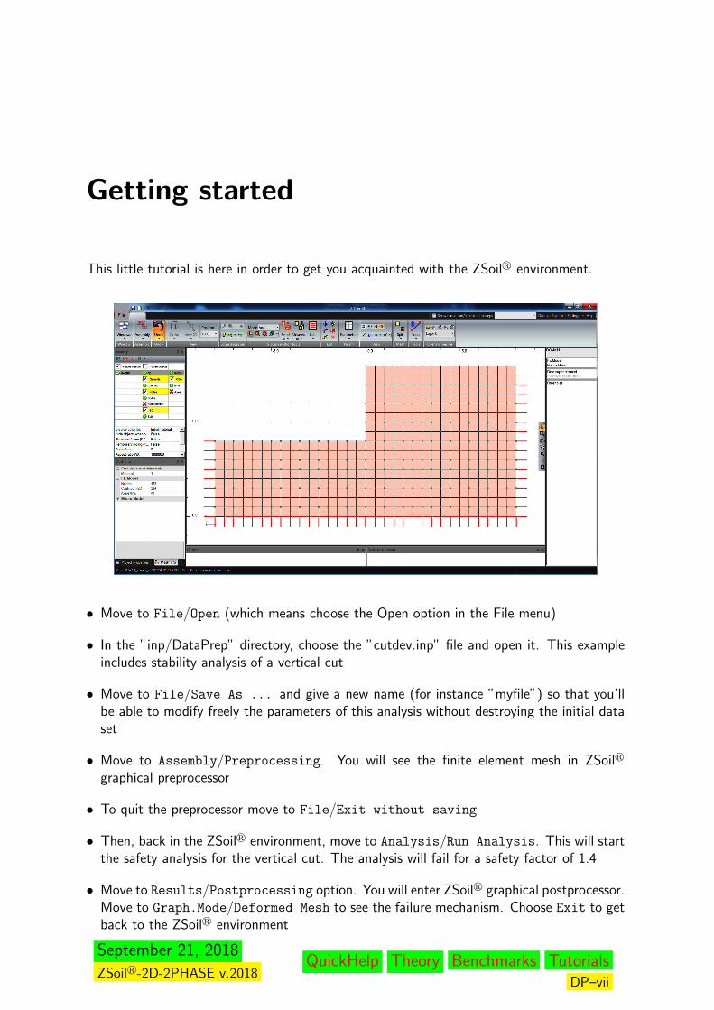
Getting started
This little tutorial is here in order to get you acquainted with the ZSoilr environment.
• Move to File/Open (which means choose the Open option in the File menu)
• In the ”inp/DataPrep” directory, choose the ”cutdev.inp” file and open it. This exampleincludes stability analysis of a vertical cut
• Move to File/Save As ... and give a new name (for instance ”myfile”) so that you’llbe able to modify freely the parameters of this analysis without destroying the initial dataset
• Move to Assembly/Preprocessing. You will see the finite element mesh in ZSoilr
graphical preprocessor
• To quit the preprocessor move to File/Exit without saving
• Then, back in the ZSoilr environment, move to Analysis/Run Analysis. This will startthe safety analysis for the vertical cut. The analysis will fail for a safety factor of 1.4
• Move to Results/Postprocessing option. You will enter ZSoilr graphical postprocessor.Move to Graph.Mode/Deformed Mesh to see the failure mechanism. Choose Exit to getback to the ZSoilr environment
September 21, 2018
ZSoilr-2D-2PHASE v.2018QuickHelp Theory Benchmarks Tutorials
DP–vii
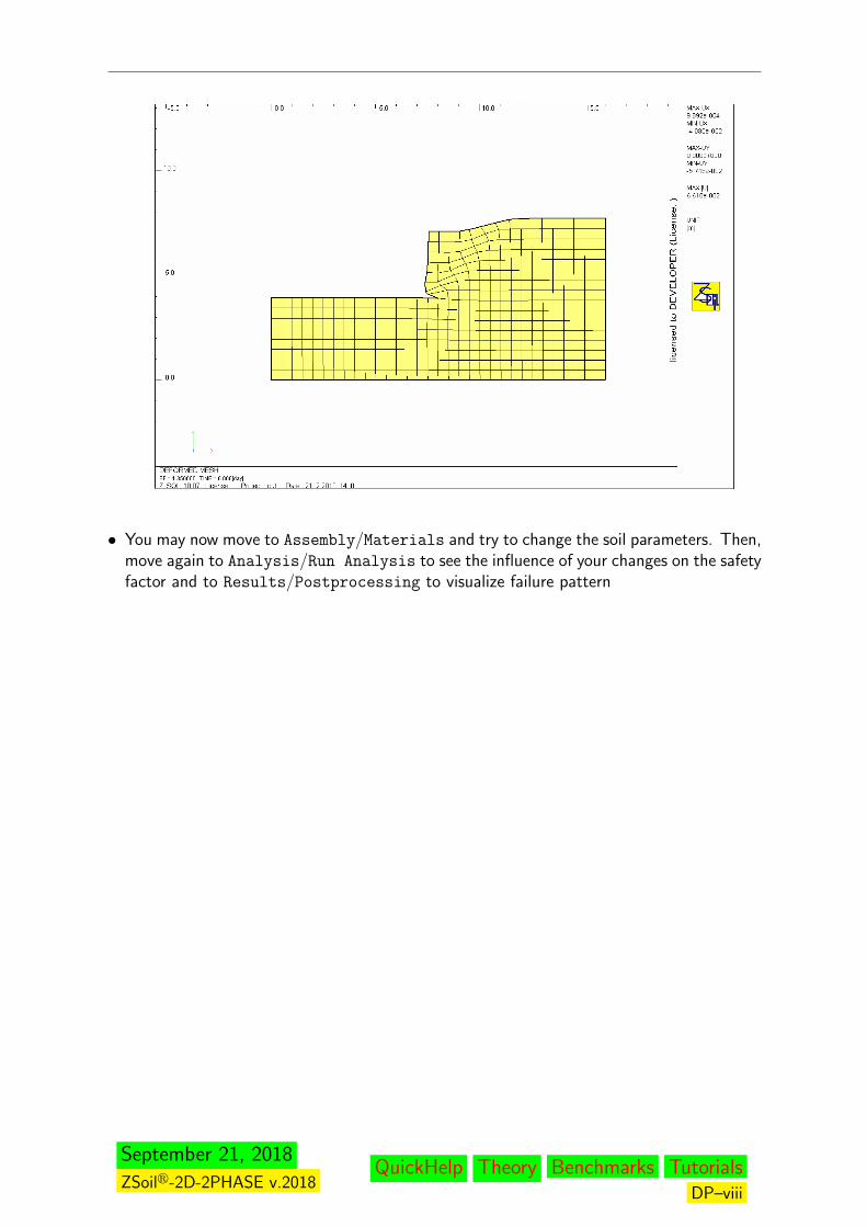
• You may now move to Assembly/Materials and try to change the soil parameters. Then,move again to Analysis/Run Analysis to see the influence of your changes on the safetyfactor and to Results/Postprocessing to visualize failure pattern
September 21, 2018
ZSoilr-2D-2PHASE v.2018QuickHelp Theory Benchmarks Tutorials
DP–viii
PREFACE
Document DATA PREPARATION MANUAL provides a help for the options offered in theprogram. In particular chapter:
INTRODUCTION gives preliminary information on sign convention, units and otherissues.
DATA PREPARATION DESCRIPTION gives definition and explanation of dataediting technique for all items present in the program. As often as possible, a simpleexample is used to illustrate the case.
TROUBLESHOOTING gives hints how to proceed in cases when error or warningmessages are issued.
More complicated examples of entering computational model data, related to practical prob-lems may be found in part: TUTORIALS .
The quickest approach to data preparation consists in loading an existing file, saving it undera different name (option SAVE AS in FILES) and then modifying it. Otherwise define a newmesh and load system with the graphical preprocessor (see e.g. Tutorial 1).
For the theoretical background see THEORETICAL MANUAL.
September 21, 2018
ZSoilr-2D-2PHASE v.2018QuickHelp Theory Benchmarks Tutorials
DP–1

September 21, 2018
ZSoilr-2D-2PHASE v.2018QuickHelp Theory Benchmarks Tutorials
DP–2

N Preface
Chapter 1
INTRODUCTION
Chapter INTRODUCTION gives preliminary information on:
Sign convention for stresses, strains, and fluid pressure
Definition e.g. cross–reference between elasticity constants, specific weight, etc.
Units table for data and result presentation
September 21, 2018
ZSoilr-2D-2PHASE v.2018QuickHelp Theory Benchmarks Tutorials
DP–3
N Preface N N Introduction
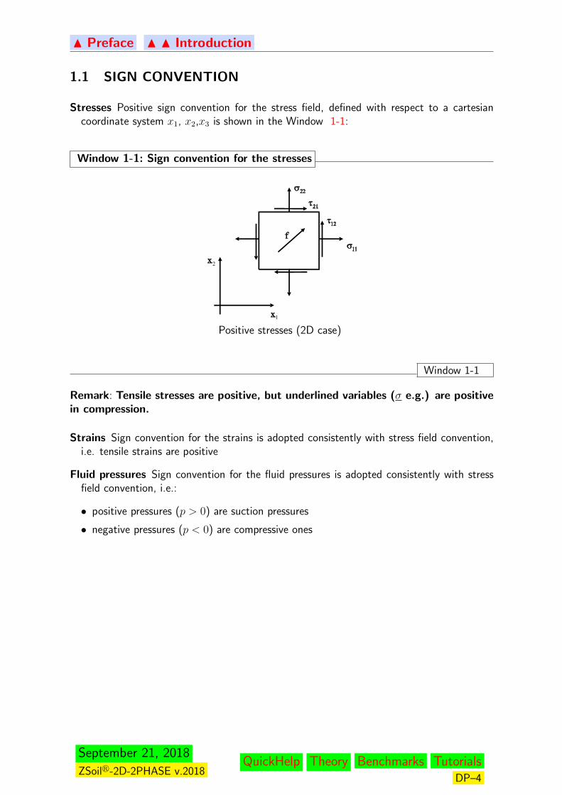
1.1 SIGN CONVENTION
Stresses Positive sign convention for the stress field, defined with respect to a cartesiancoordinate system x1, x2,x3 is shown in the Window 1-1:
Window 1-1: Sign convention for the stresses
Positive stresses (2D case)
Window 1-1
Remark: Tensile stresses are positive, but underlined variables (σ e.g.) are positivein compression.
Strains Sign convention for the strains is adopted consistently with stress field convention,i.e. tensile strains are positive
Fluid pressures Sign convention for the fluid pressures is adopted consistently with stressfield convention, i.e.:
• positive pressures (p > 0) are suction pressures
• negative pressures (p < 0) are compressive ones
September 21, 2018
ZSoilr-2D-2PHASE v.2018QuickHelp Theory Benchmarks Tutorials
DP–4

N Preface N N Introduction
1.2 DEFINITIONS
The following sections give information on:
Specific weight
Elasticity constants
September 21, 2018
ZSoilr-2D-2PHASE v.2018QuickHelp Theory Benchmarks Tutorials
DP–5

N Preface N N Introduction N N N Definitions
1.2.1 UNIT WEIGHTS
The items related to the definition of unit weight are summarized in the Window 1-2:
Window 1-2: Unit weight definition
• γ = γD + nSγF , unit weight for a two–phase, partially saturated media,
• γsat = γD + nγF = γB + γF , unit weight for a two phase, fully saturated media,
• γD = (1− n)γs, unit weight for a single phase, unsaturated i.e. dry, porous media,
• S =VFVp
– saturation ratio
• V = Vs + Vp, V – for volume,
• e =VpVs
, void ratio, e =n
1− nwhere:
• n =VpV
, porosity, n =e
1 + e,
with: (.)s – for solid skeleton, (.)p – for voids, (.)sat – for saturated soil, (.)D – for dry,(.)F – for pore fluid (water), (.)b – for buoyant soil
Window 1-2
September 21, 2018
ZSoilr-2D-2PHASE v.2018QuickHelp Theory Benchmarks Tutorials
DP–6
N Preface N N Introduction N N N Definitions
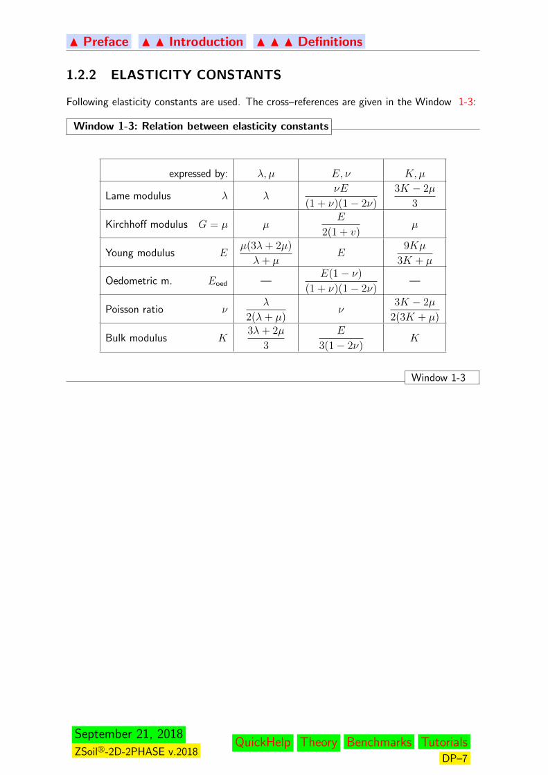
1.2.2 ELASTICITY CONSTANTS
Following elasticity constants are used. The cross–references are given in the Window 1-3:
Window 1-3: Relation between elasticity constants
expressed by: λ, µ E, ν K, µ
Lame modulus λ λνE
(1 + ν)(1− 2ν)
3K − 2µ
3
Kirchhoff modulus G = µ µE
2(1 + v)µ
Young modulus Eµ(3λ+ 2µ)
λ+ µE
9Kµ
3K + µ
Oedometric m. Eoed —E(1− ν)
(1 + ν)(1− 2ν)—
Poisson ratio νλ
2(λ+ µ)ν
3K − 2µ
2(3K + µ)
Bulk modulus K3λ+ 2µ
3
E
3(1− 2ν)K
Window 1-3
September 21, 2018
ZSoilr-2D-2PHASE v.2018QuickHelp Theory Benchmarks Tutorials
DP–7

N Preface N N Introduction
1.3 UNITS TABLE
Units listed in the table are default basic units
force length time temperature angle
kN m sec oC deg
Remarks:
1. Different sets of basic units can be used as well.
2. Moreover during data edition temporary units can be used.
For details of handling the units, see the subsection data preparation: UNITS
September 21, 2018
ZSoilr-2D-2PHASE v.2018QuickHelp Theory Benchmarks Tutorials
DP–8

N Preface
Chapter 2
DATA PREPARATION ANDPOSTPROCESSING DESCRIPTION
The structure of this chapter corresponds as strictly as possible to the structure of the userinterface as shown in the Window 2-1
Window 2-1: ZSoilrmenu: contents of popup menu
File Control Assembly Analysis Results Extras System Help
Window 2-1
September 21, 2018
ZSoilr-2D-2PHASE v.2018QuickHelp Theory Benchmarks Tutorials
DP–9
N Preface
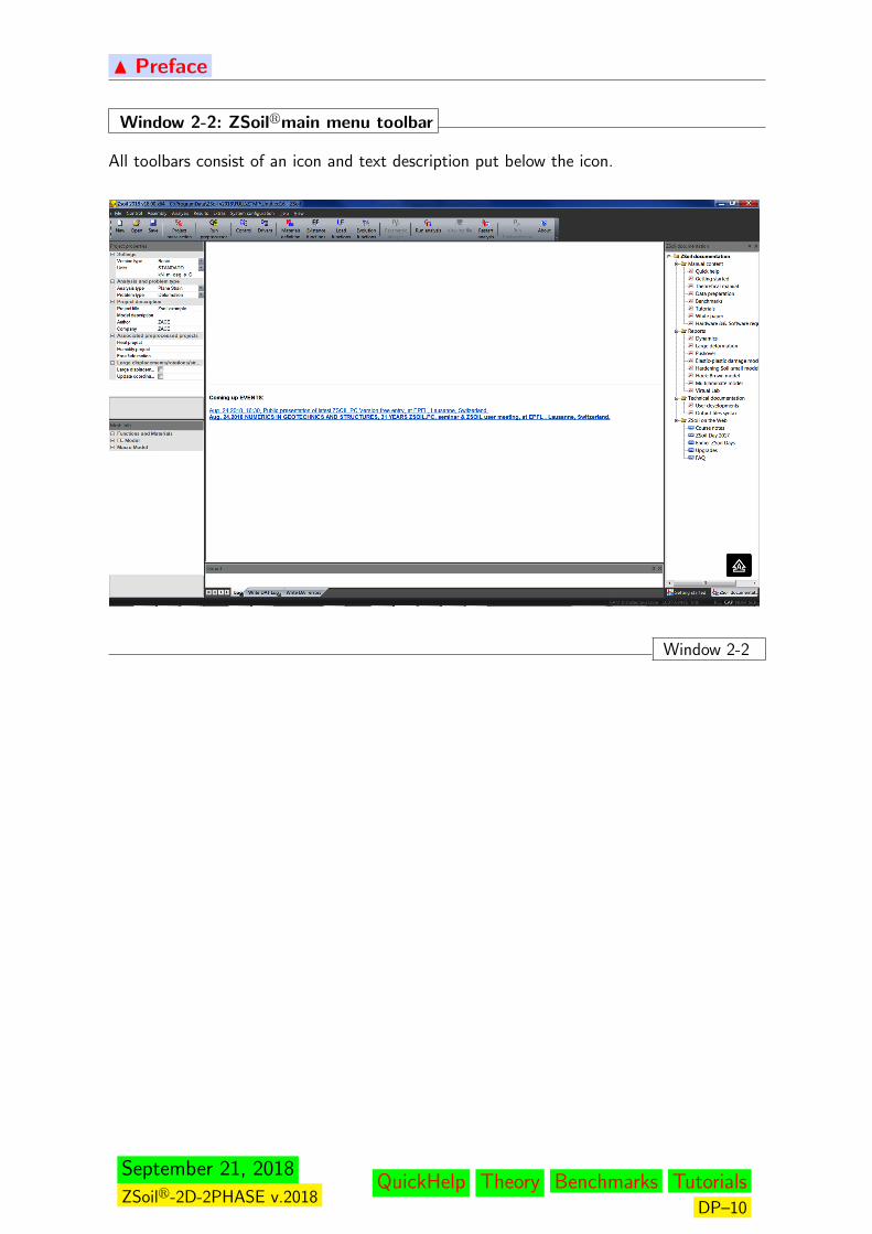
Window 2-2: ZSoilrmain menu toolbar
All toolbars consist of an icon and text description put below the icon.
Window 2-2
September 21, 2018
ZSoilr-2D-2PHASE v.2018QuickHelp Theory Benchmarks Tutorials
DP–10
N Preface N N Description
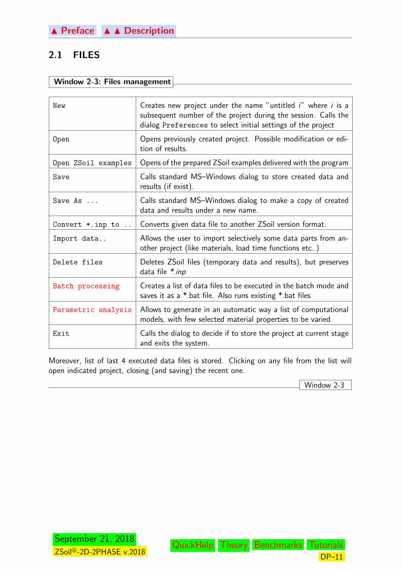
2.1 FILES
Window 2-3: Files management
New Creates new project under the name ”untitled i” where i is asubsequent number of the project during the session. Calls thedialog Preferences to select initial settings of the project
Open Opens previously created project. Possible modification or edi-tion of results.
Open ZSoil examples Opens of the prepared ZSoil examples delivered with the program
Save Calls standard MS–Windows dialog to store created data andresults (if exist).
Save As ... Calls standard MS–Windows dialog to make a copy of createddata and results under a new name.
Convert *.inp to .. Converts given data file to another ZSoil version format.
Import data.. Allows the user to import selectively some data parts from an-other project (like materials, load time functions etc..)
Delete files Deletes ZSoil files (temporary data and results), but preservesdata file *.inp
Batch processing Creates a list of data files to be executed in the batch mode andsaves it as a *.bat file. Also runs existing *.bat files
Parametric analysis Allows to generate in an automatic way a list of computationalmodels, with few selected material properties to be varied
Exit Calls the dialog to decide if to store the project at current stageand exits the system.
Moreover, list of last 4 executed data files is stored. Clicking on any file from the list willopen indicated project, closing (and saving) the recent one.
Window 2-3
September 21, 2018
ZSoilr-2D-2PHASE v.2018QuickHelp Theory Benchmarks Tutorials
DP–11

NPreface NNDescription NNNFile
2.1.1 PARAMETRIC ANALYSIS
Window 2-4: Parametric analysis
• To add a new property to be varied
1. Click by mouse on first free row under column Material and select one of the materialsalready defined in the data
2. Click by mouse next right column (under Group) in the same row and select subgroupof properties from which the property will be selected
3. Click by mouse next right column (under Parameter) in the same row and select oneof the properties to be varied
4. Click by mouse next right column (under Def.way) in the same row and select oneof the options Steps or Values; if you select Steps then the definition is completedby setting number of steps (in column No.of steps/values) and the two limitingvalues; if you select definition through Values then the definition is completed by settingnumber of values (in column No.of steps/values) and list of these values placed innext columns; in the example shown in the figure Young modulus will be equal toE = 30000, 40000, 50000, kPa while friction angle to φ = 22o, 25o, 30o respectively
• To delete property from the list put cursor in the first column (the whole row will behighlighted) and press button Delete
• To run all automatically generated data files press button Execute ;
Remark:
1. By pressing Execute program prepares all data files (*.inp files) that include all possiblecombinations of parameters to be varied and runs them immediately; each data file inheritsa name of the template data file and an automatic suffix is added to it; this suffix consists ofa chain of numbers (as many as number of properties to be varied) separated by underscorecharacter; if we take the data file foot for instance and will perform parametric analysis
September 21, 2018
ZSoilr-2D-2PHASE v.2018QuickHelp Theory Benchmarks Tutorials
DP–12

NPreface NNDescription NNNFile
of settlements assuming that Young modulus is parametrized by Steps (first row in thetable shown in the Figure) and friction angle is parametrized by Values (second row inthe table shown in the Figure) then the set of 9 data files will be created; the data filelabeled as foot 2 3 corresponds to the template data file foot second step of the firstparameter (E modulus) and third value of the second parameter (φ);
2. Plotting selected nodal (displacements / pressures) or element (stresses / forces) resultsvs one of the varied parameters can be made with aid of the graphical postprocessor (referto section 2.5.1.4)
Window 2-4
September 21, 2018
ZSoilr-2D-2PHASE v.2018QuickHelp Theory Benchmarks Tutorials
DP–13
N Preface N N Description
2.2 CONTROL
Following options allow to control the computation and content of the results
Window 2-5: Options in menu Control
Type of analysis (Plane strain, axisymmetry or 3D) and problem type (Deformation, Defor-mation+Flow, Seepage, Heat conduction, Humidity transfer) can be set in window Project
properties placed at left top corner of ZSoil main application.
Drivers Creates a list of drivers for selected analysis type.
Project preselection Selects main options like type of problem, units etc...
Control Sets convergence tolerances, type of nonlinear solver andfrequency of restart and results storage.
Dynamics Sets type and parameters for the time history analysisalgorithm and damping factors for dynamic drivers.
Pushover Sets parameters for Pushover driver
Contact Algorithm Sets up algorithm control data for treatment of contact.
Linear equations solvers Selects the linear equation solver
Units Handles units system
Results content Handles content of the resulting output files
Finite Elements Selects type of finite elements to be used
Window 2-5
September 21, 2018
ZSoilr-2D-2PHASE v.2018QuickHelp Theory Benchmarks Tutorials
DP–14

NPreface NNDescription NNNControl
2.2.1 PROJECT PRESELECTION
Window 2-6: Project preselection
Project preselection dialog box allows the user to edit major project properties (to be set alsounder Project properties in the main ZSoil application window but also at the graphicalpreprocessor level), to define extra information that will be present on all output screens andcustomize the preprocessor user interface.
Window 2-6
September 21, 2018
ZSoilr-2D-2PHASE v.2018QuickHelp Theory Benchmarks Tutorials
DP–15

NPreface NNDescription NNNControl
2.2.2 ANALYSIS & DRIVERS
Window 2-7: Analysis control
Key: Option: Comment: Remarks:A. Problem Deformation:
Deformation+Flow:Flow:Heat:Humidity:
2,3,4
B. Analysis 3D
Plane Strain
Axisymmetric
C. Driver The definition will dif-fer according to theactive Problem
1,7,8
D. Drivers list Displays the sequenceof drivers
5,6
E. Associated... Attach projects withcomputed nonstation-ary temperature, hu-midity and free fieldmotion fields, if rele-vant
3
F. Stage construction
algorithm
Each stage construc-tion step is treatedincrementally accord-ing to the internalsetup defined by press-ing button Settings
once � Activate op-tion is set ON
10
September 21, 2018
ZSoilr-2D-2PHASE v.2018QuickHelp Theory Benchmarks Tutorials
DP–16
NPreface NNDescription NNNControl
G. Large displacements
/ rotations
Activate geometricalnonlinearities by set-ting � Activate toON
9
Window 2-7
Remarks:
1. Some additional time steps will be automatically enforced by load and existence timefunctions, at each their characteristic time instances
2. The Problem Type must remain unchanged between restarts.
3. Humidity or Heat Transfer analysis should precede mechanical analysis if strains im-posed by nonstationary temperature and/or humidity fields are considered
4. A switch from Deformation + Flow or Deformation to Flow requires recalculation ofthe problem
5. Sequences of drivers can be prescribed which will engender automatic restarts. Otherwisehand restart is possible.
6. While performing Restart, changes introduced to driver control parameters may concernonly these drivers which are not completed yet. Those, which are completed must remainunchanged.
7. Note the difference in the meaning of the control parameter like Start, End, Increment,Multiplier (used to increase/decrease time increment) for different Drivers.
8. Although for most of the cases leaving Nonl. solver Settings as default is satisfac-tory, for some cases it may prove convenient to associate specific control setting with eachDriver in the sequel. If needed, use button Set under C1.5 to enter Control dialog boxand to set algorithm control data in a manner specific for given driver. Predefined controldata sets can be used as well by selection of its label from the listbox C1.5. See section2.2.3 CONTROL for details. In the current version of ZSoil an automatic switch of nonlin-ear solver is activated once the divergence of the iterative procedure occurs. However thisoption will slow down the computation speed. Optionally at the end of the driver one mayactivate automatic storage of the current stage of computation in a separate sub-directory(C1.7)
9. Switching from geometrically linear to geometrically nonlinear mode does not require anyextra action from the user; the only exception concerns standard contact elements whichcannot handle large deformations; in that case standard contact elements must be deletedand large deformation contact (node-segment) has to be added to the model; in additionuser must take the decision whether special fill algorithm designed for large deformationsis to be used (for detailed description refer to the dedicated report on handling largedeformations within Z Soil); in the current development displacements and rotations cenbe arbitrarily large while strains remain small
September 21, 2018
ZSoilr-2D-2PHASE v.2018QuickHelp Theory Benchmarks Tutorials
DP–17

NPreface NNDescription NNNControl
10. During stage construction analysis new layers of soil are usually added in a single incre-mental step; by activating this option each construction step can be subdivided into fewincremental steps, to avoid numerical problems (like lack of convergence or divergence of
iterative procedure), according to the setup to be defined by pressing button Settings ; in
addition each new layer of soil in the first time step will behave as incompressible (assumingν = 0.499999) and later on an original value of Poisson’s ratio is used
In the following sections see the details of setting:
PROBLEM TYPE AND DRIVERS
ANALYSIS TYPE
ASSOCIATED PREPROCESSED PROJECTS
September 21, 2018
ZSoilr-2D-2PHASE v.2018QuickHelp Theory Benchmarks Tutorials
DP–18

N Preface N N Descrip. N N N Control N N N N Analysis & ...
2.2.2.1 PROBLEM TYPE AND DRIVERS
Detailed explanation and examples of application of different drivers are given in next para-graphs for the following Problem types:
SINGLE PHASE (DEFORMATION) ANALYSIS
DEFORMATION COUPLED WITH FLOW
FLOW (STEADY STATE AND TRANSIENT)
HEAT TRANSFER (STEADY STATE AND TRANSIENT)
HUMIDITY TRANSFER (STEADY STATE AND TRANSIENT)
Related Topics
• Theory: ALGORITHMS
• LOCAL STABILITY CONTROLED AT THE MATERIAL LEVEL
September 21, 2018
ZSoilr-2D-2PHASE v.2018QuickHelp Theory Benchmarks Tutorials
DP–19
N Preface N N Descrip. N N N Control N N N N Analysis & ...
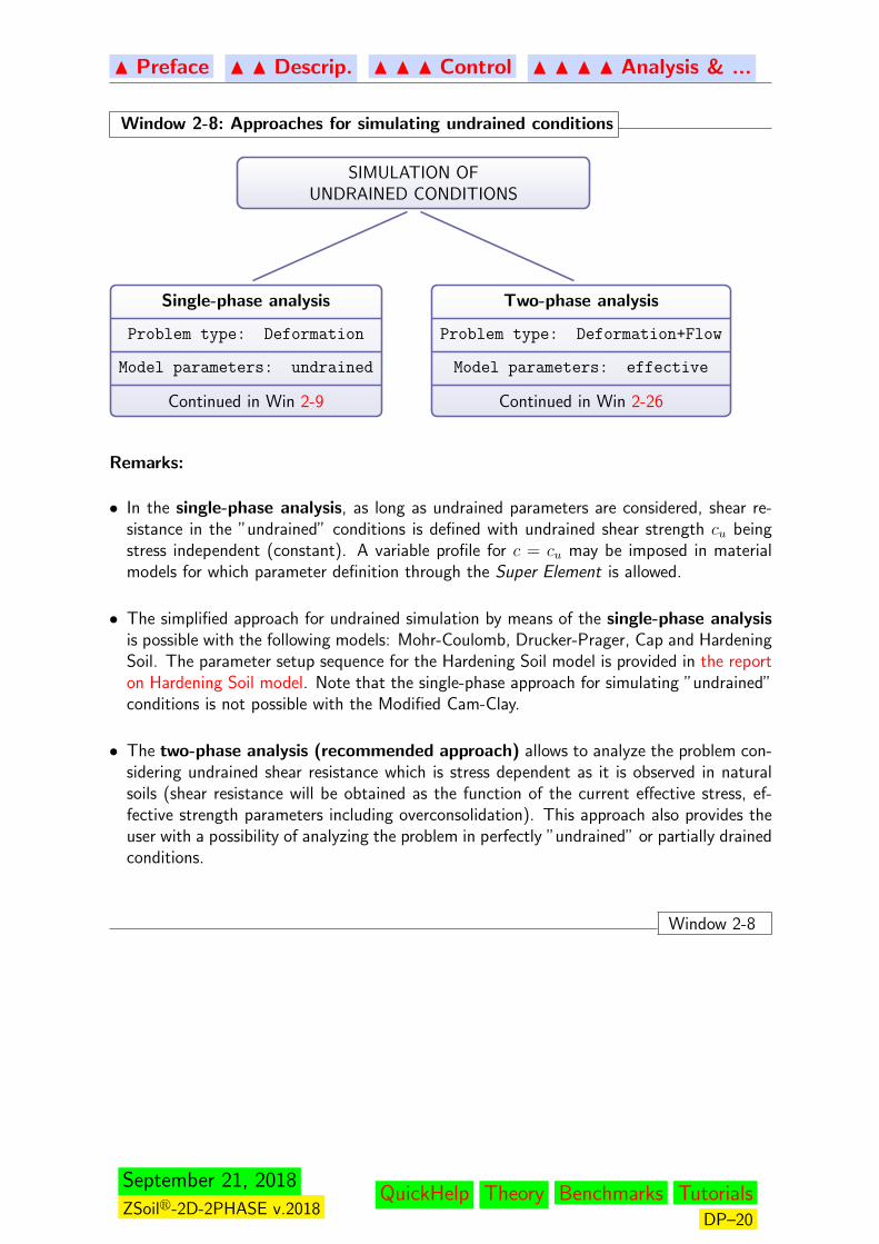
Window 2-8: Approaches for simulating undrained conditions
SIMULATION OFUNDRAINED CONDITIONS
Single-phase analysis
Problem type: Deformation
Model parameters: undrained
Continued in Win 2-9
Two-phase analysis
Problem type: Deformation+Flow
Model parameters: effective
Continued in Win 2-26
Remarks:
• In the single-phase analysis, as long as undrained parameters are considered, shear re-sistance in the ”undrained” conditions is defined with undrained shear strength cu beingstress independent (constant). A variable profile for c = cu may be imposed in materialmodels for which parameter definition through the Super Element is allowed.
• The simplified approach for undrained simulation by means of the single-phase analysisis possible with the following models: Mohr-Coulomb, Drucker-Prager, Cap and HardeningSoil. The parameter setup sequence for the Hardening Soil model is provided in the reporton Hardening Soil model. Note that the single-phase approach for simulating ”undrained”conditions is not possible with the Modified Cam-Clay.
• The two-phase analysis (recommended approach) allows to analyze the problem con-sidering undrained shear resistance which is stress dependent as it is observed in naturalsoils (shear resistance will be obtained as the function of the current effective stress, ef-fective strength parameters including overconsolidation). This approach also provides theuser with a possibility of analyzing the problem in perfectly ”undrained” or partially drainedconditions.
Window 2-8
September 21, 2018
ZSoilr-2D-2PHASE v.2018QuickHelp Theory Benchmarks Tutorials
DP–20
... N Control N N Analysis & ... N N N Problem types & ...
2.2.2.1.1 SINGLE PHASE (DEFORMATION) ANALYSIS
Unknowns: displacement field u(x)
For this Problem Type necessary data consist of:
• solid BC (fixities with possibly applied imposed displacements, rotations),
• solid loads (gravity, surface, nodal)
• mechanical and strength parameters, and unit weights set for each applied material model
Remarks:
1. Presence of the underground water, in cases when pressure field is known a priori, can betaken into account using two equivalent approaches: (here γD, γF means for dry soil andfluid unit weights and n for porosity)
• effective stresses (no pressure applied, buoyant weight γB = γD + (n− 1)γF used forsaturated media)
• total stress (initial pressure applied, saturated weight γSAT = γD + nγF used)
2. Strains induced by changes of temperature or humidity can be taken into account, seeAssociated projects
September 21, 2018
ZSoilr-2D-2PHASE v.2018QuickHelp Theory Benchmarks Tutorials
DP–21

... N Control N N Analysis & ... N N N Problem types & ...
Window 2-9: Single phase analysis for simulation of ”undrained” conditions
SINGLE PHASE ANALYSIS
Problem type: Deformation
Driver: Time dependent
Driver type: Driven Load
Total stress analysis
Unit weight:
γ (apparent) above water tableγSAT (saturated) below water tableExample: DataPrep/footwt.inp
Initial state:
Ko must be specifiedInitial pore pressure should beimposed (use Initial pressure)
Model parameters: undrained
φ = φu = 0o
ψ = 0o (to satisfy ψ ≤ φ)c = cuν = νu = 0.499
Effective stress analysis
Unit weight:
γD (dry) above water tableγB (buoyant) below water tableExample: DataPrep/footes.inp
Initial state:
Ko must be specified
Model parameters: undrained
φ = φu = 0o
ψ = 0o (to satisfy ψ ≤ φ)c = cuν = νu = 0.499
Remarks:
• These two methods are equivalent considering the presence of the ground water conditionsin a single-phase, deformation analysis.
• A variable profile for c = cu may be imposed in material models for which parameterdefinition through the Super Element is allowed.
• Ko has to be implicitly specified; otherwise Ko will be calculated as ν/(1− ν) taking thespecified νu = 0.499.
• In the case of total stress analysis and an existing ground water table, the initial porepressure should be imposed in order to obtain an effective stress field in the Initial State
analysis.
• Considering that the undrained conditions imply ε1 = ε3, undrained stiffness will be auto-matically computed accounting for the undrained Poisson’s coefficient νu = 0.499.
Window 2-9
Description of Drivers available for Problem type Deformation is given in sections:
INITIAL STATE
September 21, 2018
ZSoilr-2D-2PHASE v.2018QuickHelp Theory Benchmarks Tutorials
DP–22

... N Control N N Analysis & ... N N N Problem types & ...
TIME DEPENDENT
STABILITY
September 21, 2018
ZSoilr-2D-2PHASE v.2018QuickHelp Theory Benchmarks Tutorials
DP–23
... N Analysis & ... N N Drivers & ... N N N Single Phase
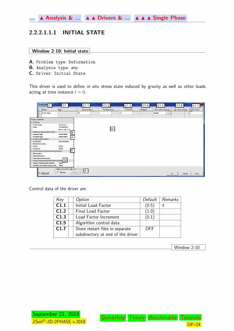
2.2.2.1.1.1 INITIAL STATE
Window 2-10: Initial state
A. Problem type: Deformation
B. Analysis type: anyC. Driver: Initial State
This driver is used to define in situ stress state induced by gravity as well as other loadsacting at time instance t = 0.
Control data of the driver are:
Key Option Default RemarksC1.1 Initial Load Factor (0.5) 4C1.2 Final Load Factor (1.0)C1.3 Load Factor Increment (0.1)C1.5 Algorithm control dataC1.7 Store restart files in separate OFF
subdirectory at end of the driver
Window 2-10
September 21, 2018
ZSoilr-2D-2PHASE v.2018QuickHelp Theory Benchmarks Tutorials
DP–24
... N Analysis & ... N N Drivers & ... N N N Single Phase
Remarks:
1. Driver Initial State: This driver controls the amplitude of loads which are non–zeroat time t = 0 (i.e. the corresponding load time function are non-zero at t = 0). Userprescribes: 0.5 for the Initial Load Factor; 0.1 for the Load Factor Increment and 1.0 forFinal value of the Load Factor; loads will be applied progressively as 0.5g, 0.6g..., 1.0g.
2. An initial state with zero deformation and non–zero stress-state will be generated.
3. Gravity is usually the main load to be considered for the initial state; set unit weights forall materials and gravity vector (in load menu) equal to (0,−1, < 0 >) for downwardsvertical gravity.
4. Load is usually gravity and/or other deadweight loads. Any Initial Load Factor valuegreater than 0.0 and less or equal to 1.0 is acceptable. The initial value equal to 0.5 isusually used.
5. During an Initial State analysis, time is fixed to t = 0. As the consequence:
• only these system components will be taken into account, which exist permanently orhave existence status set ON at t = 0,
• loads associated with the initial state must have a non-zero load function at t = 0; ifthe load function is equal to zero at t = 0, then the load is to be applied later.
• in case of time dependent material parameters, their values computed at t = 0 will betaken into account.
6. An Initial State driver can be run only once and must be the first in the list of drivers
7. Omitting Initial State and lack of the implicitly set initial effective stresses yields stressfree and zero deformation state as the initial condition.
8. Alternatively, if an initial stress field is known, it can be introduced using Initial Conditions
Initial Stress super elements in the Preprocessing session. Setting the initial guessfor initial effective stresses (using Initial conditions/Initial stresses option in the preproces-sor) is recommended for meshes in which size of elements varies significantly.
9. Each incremental step is computed in two runs due to algorithmic reasons.
10. After convergent run of an Initial State deformation is nullified. The only nonzerooutput concerns the stress state.
11. In case of the divergence deformation can be visualized in the Postprocessing. It helpsto identify source of the instability. This may happen due to surface instability caused byzero cohesion, improperly set boundary conditions or highly distorted (with high aspectratios) finite elements placed close to the free boundary
12. Some soil mechanics problems are characterized by a stress state which remains on theyield surface, i.e., on the limit of instability. It is therefore important to adopt appropriatematerial data to avoid triggering instability.
September 21, 2018
ZSoilr-2D-2PHASE v.2018QuickHelp Theory Benchmarks Tutorials
DP–25

... N Analysis & ... N N Drivers & ... N N N Single Phase
Window 2-11: Initial state example – dry medium
Data: TUTORIALS/ENV.INP
A. Problem type: Deformation
B. Analysis type: Plane strain
C. Driver: Initial State
Goals:
• To define an initial state with 2 existing buildings• To define a safety factor with respect to an increase in height of the right building (repre-
sented by an increasing load)
Remarks:
1. Driver Initial State: this driver controls the amplitude of loads which are non–zeroat time t = 0 (i.e. the corresponding load time function in non-zero at time zero); in thiscase gravity only will be activated since the load applied on the right building is multipliedby a load function which is zero at time t = 0. User prescribes: 0.5 the starting gravitymultiplier; gravity will be applied progressively as 0.5g, 0.6g..., 1.0g.
2. As underground water is not taken into account in this example, in material definitionγD1 = γD2 = 20kN/m3 is specified.
Window 2-11
September 21, 2018
ZSoilr-2D-2PHASE v.2018QuickHelp Theory Benchmarks Tutorials
DP–26
... N Analysis & ... N N Drivers & ... N N N Single Phase
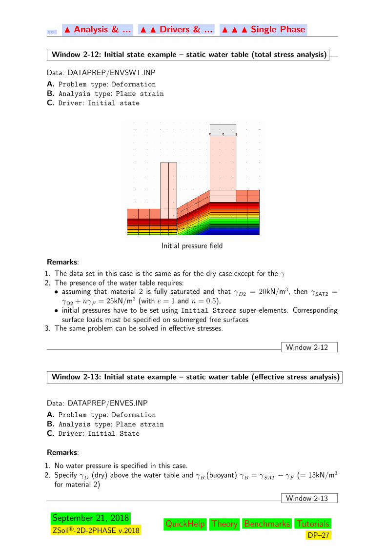
Window 2-12: Initial state example – static water table (total stress analysis)
Data: DATAPREP/ENVSWT.INP
A. Problem type: Deformation
B. Analysis type: Plane strain
C. Driver: Initial state
Initial pressure field
Remarks:
1. The data set in this case is the same as for the dry case,except for the γ2. The presence of the water table requires:• assuming that material 2 is fully saturated and that γD2 = 20kN/m3, then γSAT2 =γD2 + nγF = 25kN/m3 (with e = 1 and n = 0.5),• initial pressures have to be set using Initial Stress super-elements. Corresponding
surface loads must be specified on submerged free surfaces3. The same problem can be solved in effective stresses.
Window 2-12
Window 2-13: Initial state example – static water table (effective stress analysis)
Data: DATAPREP/ENVES.INP
A. Problem type: Deformation
B. Analysis type: Plane strain
C. Driver: Initial State
Remarks:
1. No water pressure is specified in this case.2. Specify γD (dry) above the water table and γB (buoyant) γB = γSAT − γF (= 15kN/m3
for material 2)
Window 2-13
September 21, 2018
ZSoilr-2D-2PHASE v.2018QuickHelp Theory Benchmarks Tutorials
DP–27
... N Analysis & ... N N Drivers & ... N N N Single Phase
2.2.2.1.1.2 TIME DEPENDENT
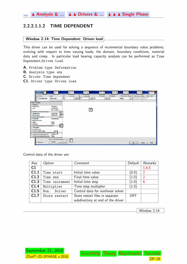
Window 2-14: Time Dependent: Driven load
This driver can be used for solving a sequence of incremental boundary value problems,evolving with respect to time varying loads, the domain, boundary conditions, materialdata and creep. In particular load bearing capacity analysis can be performed as Time
Dependent,Driven Load.
A. Problem type: Deformation
B. Analysis type: anyC. Driver: Time dependent
C1. Driver type: Driven load
Control data of the driver are:
Key Option Comment Default RemarksC1 1,4,5C1.1 Time start Initial time value (0.0) 2C1.2 Time end Final time value (1.0) 2C1.3 Time increment Initial time step (1.0) 6C1.4 Multiplier Time step multiplier (1.0)C1.5 Non. Solver Control data for nonlinear solverC1.7 Store restart Store restart files in separate OFF
subdirectory at end of the driver
Window 2-14
September 21, 2018
ZSoilr-2D-2PHASE v.2018QuickHelp Theory Benchmarks Tutorials
DP–28

... N Analysis & ... N N Drivers & ... N N N Single Phase
Remarks:
1. Driver type: Driven Load is the only available in this case.2. Time is treated as a physical parameter (consistently with material data) only if Creep
is activated (at the material level). In all other cases time may be treated as a fictitiousparameter, used mainly to manage loading process
3. Time parameter is used as a common argument of all existence and load functions.4. A sequence of Time Dependent Drivers can be defined, with different time step speci-
fication.5. Within a sequence of Time Dependent, Driven Load Drivers, an intermediate Stability
Driver can be added. It does not interfere the solution of Driven Load process comingnext, in any way.
6. Additional time steps will be automatically enforced by load and existence time functions,at all their characteristic points
7. Strains due to nonstationary temperature and/or humidity fields can be taken into account,see Associated Preprocessed Projects
September 21, 2018
ZSoilr-2D-2PHASE v.2018QuickHelp Theory Benchmarks Tutorials
DP–29

... N Analysis & ... N N Drivers & ... N N N Single Phase
Window 2-15: Driven load example – Surface footing (problem statement)
Data: BENCHMARKS/FOOT.INP
A. Problem type: Deformation
B. Analysis type: Plane Strain
C. Driver: Time Dependent
C1. Driver type: Driven Load
Goals:
• To estimate ultimate limit load applied downwards (in vertical direction) to the footing.The evolution of the loading process is controlled through load time function. Time in thiscase is a fictitious parameter.• To detect failure mechanism
Results:
Failure mechanism appears at time t = 3.8. The corresponding ultimate limit load is com-puted by multiplying the amplitude (equal to 1.0) of applied load by the value of the Load
Function at time 3.6 (last converged step) which yields:
qult = 1.0
[15 +
20− 15
8− 3(3.6− 3)
]= 15.6 kN/m2.
Remark:
A preliminary Initial State analysis is unnecessary as gravity is ignored in this problemand no other loads are present at time t = 0.
Window 2-15
September 21, 2018
ZSoilr-2D-2PHASE v.2018QuickHelp Theory Benchmarks Tutorials
DP–30

... N Analysis & ... N N Drivers & ... N N N Single Phase
Window 2-16: Driven load example – Surface footing with weighting soil
Data: DATAPREP/FOOTGR.INPA. Problem type: Deformation
B. Analysis type: Plane Strain
C. Driver: Time Dependent
C1. Driver type: Driven Load
Specify:• Unit Weight (Assembly→Materials) γD = 13,• Directional Gravity multiplier (Assembly→Gravity) = {0, -1};add an Initial State driver under Control→Analysis & Drivers with• Initial Load Factor = 0.5,• Final Load Factor = 1.0• Load Factor Increment = 0.1Results:
The distributed load with amplitude q = 5 kN/m2 is applied downwards. The ultimate limitload of value qult = 77 kN/m2, at the last converged step (t = 3.4), is detected.
Window 2-16
Window 2-17: Driven load example – Surface footing with a water table (total stress)
Data: DATAPREP/FOOTWT.INPA. Problem type: Deformation
B. Analysis type: Plane Strain
C. Driver: Time Dependent
C1. Driver type: Driven Load
Hydrostatic distribution of prescribed initial pressuresMaterial:• γD = 13kN/m3 (dry) above the water table,• γSAT = 18kN/m3 (saturated) below the water table.
Window 2-17
September 21, 2018
ZSoilr-2D-2PHASE v.2018QuickHelp Theory Benchmarks Tutorials
DP–31
... N Analysis & ... N N Drivers & ... N N N Single Phase
Window 2-18: Driven load example – Surface footing (effective stress solution)
Data: DATAPREP/FOOTES.INP
A. Problem type: Deformation
B. Analysis type: Plane Strain
C. Driver: Time Dependent
C1. Driver type: Driven Load
Specify:
• specification of γD = 13kN/m2 (dry) above the water table as before,• specification of γB = 8kN/m2 (buoyant) under the water table level.
Results:
The same ultimate load as in the previous case are obtained.
Remark:
Two methods of considering the presence of underground water in single phase, deformationanalysis are equivalent:
• effective stresses (no pressure applied, buoyant weight γB used for saturated media)• total stress (initial pressure applied, saturated weight γSAT used )
Window 2-18
Window 2-19: Driven load example – Axisymmetric footing (effective stress)
Data: DATAPREP/FOOTAES.INP
A. Problem type: Deformation
B. Analysis type: Axisymmetry
C. Driver: Time Dependent
C1. Driver type: Driven Load
Change the Analysis Type to Axisymmetry under (Control→Analysis & Drivers). Inmaterial model data (Drucker–Prager type), switch Size Adjustment to Intermediate
with ξ = 0.
Results:
The ultimate limit load qult = 95 kN/m2 is achieved.
Window 2-19
Remark:
The above examples can be run under displacement control instead of load control.
September 21, 2018
ZSoilr-2D-2PHASE v.2018QuickHelp Theory Benchmarks Tutorials
DP–32
... N Analysis & ... N N Drivers & ... N N N Single Phase
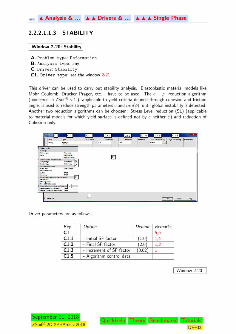
2.2.2.1.1.3 STABILITY
Window 2-20: Stability
A. Problem type: Deformation
B. Analysis type: anyC. Driver: Stability
C1. Driver type: see the window 2-21
This driver can be used to carry out stability analysis. Elastoplastic material models likeMohr–Coulomb, Drucker–Prager, etc... have to be used. The c − ϕ reduction algorithm(pioneered in ZSoilr v.1.), applicable to yield criteria defined through cohesion and frictionangle, is used to reduce strength parameters c and tan(φ), until global instability is detected.Another two reduction algorithms can be choosen: Stress Level reduction (SL) (applicableto material models for which yield surface is defined not by c neither φ) and reduction ofCohesion only.
Driver parameters are as follows:
Key Option Default RemarksC1 5,6C1.1 - Initial SF factor (1.0) 1,4C1.2 - Final SF factor (2.0) 1,2C1.3 - Increment of SF factor (0.02) 1C1.5 - Algorithm control data
Window 2-20
September 21, 2018
ZSoilr-2D-2PHASE v.2018QuickHelp Theory Benchmarks Tutorials
DP–33
... N Analysis & ... N N Drivers & ... N N N Single Phase
Remarks:
1. User prescribes Initial value of the safety factor (SF), its final value and increment. In theexample shown in Win.2-20 safety analysis will be carried out for SF = 1.0,1.1,1.2 up to3.0 or SF factor value at which an instability is detected
2. Restart from the last converged step is always possible. During restart user may adjust thefinal SF value and the increment to obtain solution with assumed accuracy
3. Stability driver can be used at any time, may be declared more than once (also in row) inthe list D of drivers; it does not affect results of next drivers
4. Stability driver can also be controlled at the material level to avoid early instabilities causedby flat and tiny sliding
5. Results (i.e. safety factor and failure pattern) are usually sensitive to the choice ofReduction method(C1) (see Window 2-21)
6. Deformation field visualized by the postprocessor at SF value corresponding to divergedsafety analysis step represents a failure pattern. If the failure pattern cannot be easilydetected it is recommended to visualize incremental deformation between last two safetyanalysis steps.
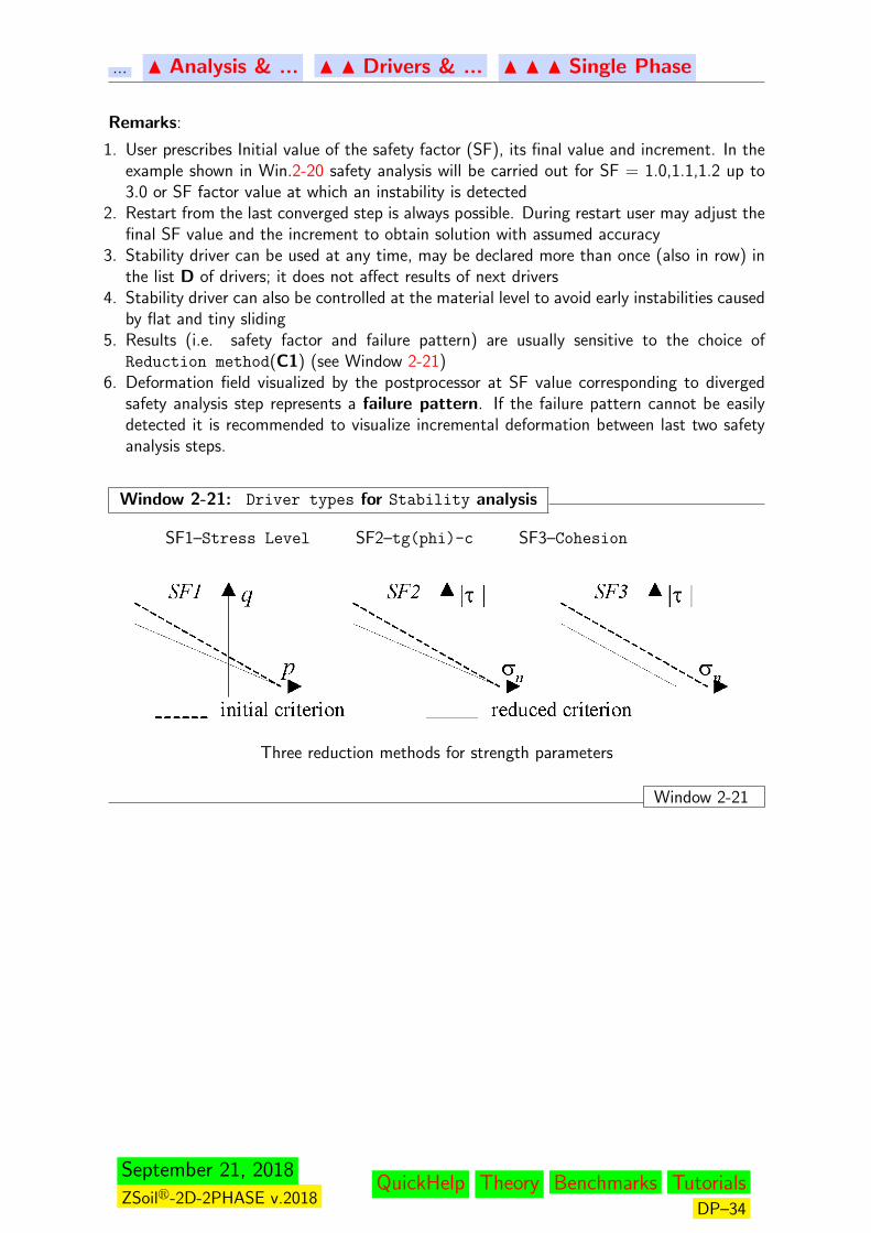
Window 2-21: Driver types for Stability analysis
SF1–Stress Level SF2–tg(phi)-c SF3–Cohesion
Three reduction methods for strength parameters
Window 2-21
September 21, 2018
ZSoilr-2D-2PHASE v.2018QuickHelp Theory Benchmarks Tutorials
DP–34
... N Analysis & ... N N Drivers & ... N N N Single Phase
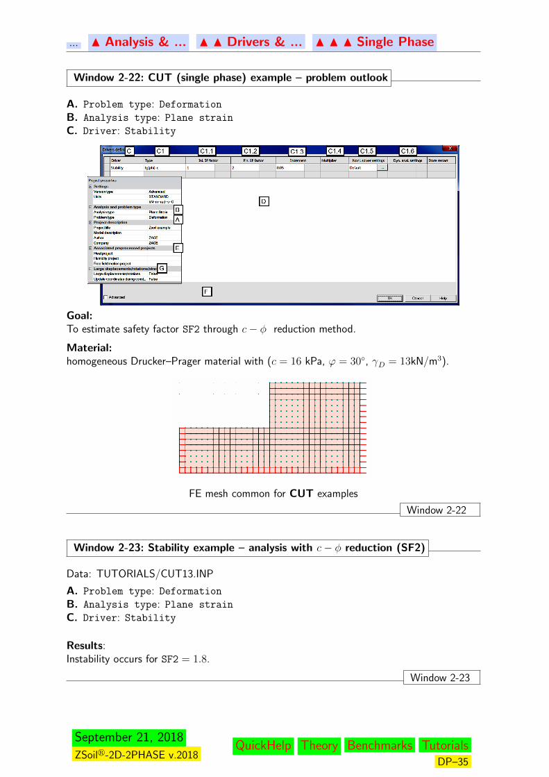
Window 2-22: CUT (single phase) example – problem outlook
A. Problem type: Deformation
B. Analysis type: Plane strain
C. Driver: Stability
Goal:To estimate safety factor SF2 through c− φ reduction method.
Material:homogeneous Drucker–Prager material with (c = 16 kPa, ϕ = 30◦, γD = 13kN/m3).
FE mesh common for CUT examples
Window 2-22
Window 2-23: Stability example – analysis with c− φ reduction (SF2)
Data: TUTORIALS/CUT13.INP
A. Problem type: Deformation
B. Analysis type: Plane strain
C. Driver: Stability
Results:Instability occurs for SF2 = 1.8.
Window 2-23
September 21, 2018
ZSoilr-2D-2PHASE v.2018QuickHelp Theory Benchmarks Tutorials
DP–35
... N Analysis & ... N N Drivers & ... N N N Single Phase
Window 2-24: Stability example – analysis with preliminary initial state
Data: DATAPREP/CUTIS.INPA. Problem type: Deformation
B. Analysis type: Plane strain
C. Driver: Stability
Specify a new driver (Initial State) with Initial Load Factor 0.5, Final Load Factor 1.0 andload increment 0.1.
Results:
Instability occurs for SF2 = 1.8.
Remark:
Notice that the preliminary initial state analysis influences the deformation state but has noinfluence on the safety factor (SF2 = 1.8).
Window 2-24
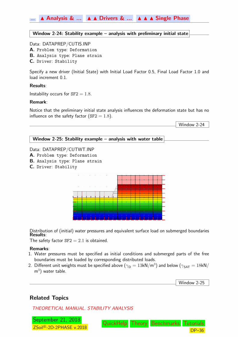
Window 2-25: Stability example – analysis with water table
Data: DATAPREP/CUTWT.INPA. Problem type: Deformation
B. Analysis type: Plane strain
C. Driver: Stability
Distribution of (initial) water pressures and equivalent surface load on submerged boundariesResults:The safety factor SF2 = 2.1 is obtained.
Remarks:1. Water pressures must be specified as initial conditions and submerged parts of the free
boundaries must be loaded by corresponding distributed loads.2. Different unit weights must be specified above (γD = 13kN/m3) and below (γSAT = 18kN/
m3) water table.
Window 2-25
Related Topics
THEORETICAL MANUAL. STABILITY ANALYSIS
September 21, 2018
ZSoilr-2D-2PHASE v.2018QuickHelp Theory Benchmarks Tutorials
DP–36
... N Control N N Analysis & ... N N N Drivers & ...
2.2.2.1.2 DEFORMATION COUPLED WITH FLOW
Unknowns:
displacement field u(x),
fluid pressure field p(x)
For this Problem Type necessary data consists of:
• solid BC (fixities with possibly applied imposed displacements, rotations),• fluid pressure BC (nodal fluid pressures, fluid heads, seepage surfaces),• solid loads (gravity, surface, nodal)• mechanical, seepage, strength parameters and unit weights, set for each applied material
model
Remarks:
1. Presence of underground water is taken into account in an automatic way (uncoupled orcoupled total stress analysis) corresponding to chosen Driver Type:• Driven Load+Steady state flow -each solution step consists of the two substeps;
steady state fluid flow problem is solved first for unknown p(x) and then resulting pressurefield is taken as an explicit input into the mechanical analysis substep (through extendedBishop’s effective stress principle).• Driven Load+Transient flow -each solution step consists of the two substeps; tran-
sient fluid flow problem is solved first for unknown p(x) and then resulting pressure fieldis taken as an explicit input into the mechanical analysis substep (through extendedBishop’s effective stress principle).• Driven Load (undrained) -a coupled system of equations including equilibrium and
fluid flow continuity (without divergence of Darcy velocity term) are solved for unknowns(u(x),∆pund(x)). Note that in that case pressure in the fluid is composed of two termsi.e. p (nodal pressures in the fluid coming from uncoupled/coupled deformation+flowanalysis) and undrained excess pore pressure ∆pund (at center of element). This drivercannot be followed by Driven Load+Steady state flow, Driven Load+Transient,Consolidation.• Consolidation -a coupled system of equations including equilibrium and fluid flow con-
tinuity are solved for unknowns (u(x), p(x)). In this case deformations may influencevariation of the pressure field and vice versa.
2. Unit weight of fully or partially saturated two-phase media is internally evaluated as afunction of the computed saturation ratio through γS = γD +nSγF , with γD, γF meaningfor dry soil and fluid unit weights, porosity n = e
1+eand saturation ratio S = S(Sr, α, γF ,
p)3. Strains induced by changes of temperature or humidity can be taken into account, see
Associated preprocessed projects
September 21, 2018
ZSoilr-2D-2PHASE v.2018QuickHelp Theory Benchmarks Tutorials
DP–37
... N Control N N Analysis & ... N N N Drivers & ...
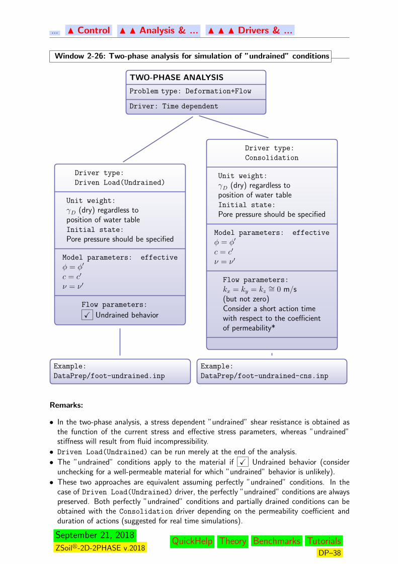
Window 2-26: Two-phase analysis for simulation of ”undrained” conditions
TWO-PHASE ANALYSIS
Problem type: Deformation+Flow
Driver: Time dependent
Driver type:
Driven Load(Undrained)
Unit weight:
γD (dry) regardless toposition of water tableInitial state:
Pore pressure should be specified
Model parameters: effective
φ = φ′
c = c′
ν = ν ′
Flow parameters:
X Undrained behavior
Example:
DataPrep/foot-undrained.inp
Driver type:
Consolidation
Unit weight:
γD (dry) regardless toposition of water tableInitial state:
Pore pressure should be specified
Model parameters: effective
φ = φ′
c = c′
ν = ν ′
Flow parameters:
kx = ky = kz ∼= 0 m/s(but not zero)Consider a short action timewith respect to the coefficientof permeability*
Example:
DataPrep/foot-undrained-cns.inp
Remarks:
• In the two-phase analysis, a stress dependent ”undrained” shear resistance is obtained asthe function of the current stress and effective stress parameters, whereas ”undrained”stiffness will result from fluid incompressibility.
• Driven Load(Undrained) can be run merely at the end of the analysis.
• The ”undrained” conditions apply to the material if X Undrained behavior (considerunchecking for a well-permeable material for which ”undrained” behavior is unlikely).
• These two approaches are equivalent assuming perfectly ”undrained” conditions. In thecase of Driven Load(Undrained) driver, the perfectly ”undrained” conditions are alwayspreserved. Both perfectly ”undrained” conditions and partially drained conditions can beobtained with the Consolidation driver depending on the permeability coefficient andduration of actions (suggested for real time simulations).
September 21, 2018
ZSoilr-2D-2PHASE v.2018QuickHelp Theory Benchmarks Tutorials
DP–38

... N Control N N Analysis & ... N N N Drivers & ...
• *The required minimal time step for the Consolidation analysis can be obtained for theassumed coefficient of permeability k from the equation for the critical time step ∆tcrit:
∆tmin ≥ ∆tcrit =γFh2
Eoedθk
(1
4+
1
6Eoedc
)(1)
where:c – compressibility of fluid = n/βF ; n-porosity, βF-fluid bulk modulusk – coefficient of permeabilityγF – fluid specific weightθ – integration coefficient (in ZSoil θ = 1)
Eoed =E(1− ν)
(1 + ν)(1− 2ν)oedometric stiffness modulus
h – element size
Window 2-26
Definition of the Driver(s)
INITIAL STATE
TIME DEPENDENT
STABILITY
for DEFORMATION COUPLED WITH FLOW are presented in following paragraphs.
September 21, 2018
ZSoilr-2D-2PHASE v.2018QuickHelp Theory Benchmarks Tutorials
DP–39
... N Analysis & ... N N Drivers & ... N N N Two Phase
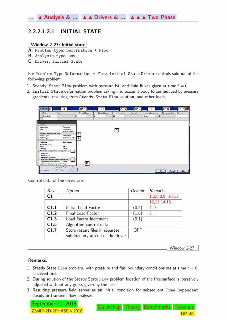
2.2.2.1.2.1 INITIAL STATE
Window 2-27: Initial stateA. Problem type: Deformation + Flow
B. Analysis type: anyC. Driver: Initial State
For Problem Type Deformation + Flow, Initial State Driver controls solution of thefollowing problem:
1. Steady State Flow problem with pressure BC and fluid fluxes given at time t = 02. Initial State deformation problem taking into account body forces induced by pressure
gradients, resulting from Steady State Flow solution, and other loads.
Control data of the driver are:
Key Option Default RemarksC1 1,2,6,8,9, 10,11,
12,13,14,15C1.1 Initial Load Factor (0.5) 4, 7C1.2 Final Load Factor (1.0) 5C1.3 Load Factor Increment (0.1)C1.5 Algorithm control dataC1.7 Store restart files in separate OFF
subdirectory at end of the driver
Window 2-27
Remarks:
1. Steady State Flow problem, with pressure and flux boundary conditions set at time t = 0,is solved first
2. During solution of the Steady State Flow problem location of the free surface is iterativelyadjusted without any guess given by the user
3. Resulting pressure field serves as an initial condition for subsequent Time Dependent
steady or transient flow analyses
September 21, 2018
ZSoilr-2D-2PHASE v.2018QuickHelp Theory Benchmarks Tutorials
DP–40

... N Analysis & ... N N Drivers & ... N N N Two Phase
4. This driver controls the amplitude of loads which are non–zero at time t = 0 (i.e. thecorresponding load time function are non-zero at t = 0). User prescribes: 0.5 for theInitial Load Factor; 0.1 for the Load Factor Increment and 1.0 for Final value of the LoadFactor; loads will be applied progressively as 0.5g, 0.6g..., 1.0g. In addition extra bodyloads resulting from water content and pressure gradients are automatically computed andconsistently (by means of incremental approach) treated during solution.
5. An initial state with zero deformation and non–zero stress-state will be generated.6. Gravity is usually the main load to be considered for the initial state; set unit weights for
all materials and gravity vector (in load menu) equal to (0,−1, < 0 >) for downwardsvertical gravity.
7. Any Initial Load Factor value greater than 0.0 and less or equal to 1.0 is acceptable.The initial value equal to 0.5 is usually used.
8. During an Initial State analysis, time is fixed to t = 0. As the consequence:• only these system components will be taken into account, which exist permanently or
have existence status set ON at t = 0,• loads associated with the initial state must have a non-zero load function at t = 0; if
the load function is equal to zero at t = 0, then the load is to be applied later.• in case of time dependent material parameters, their values computed at t = 0 will be
taken into account.9. An Initial State driver can be run only once and must be the first in the list of drivers
10. Omitting Initial State and lack of the implicitly set initial effective stresses yields stressfree and zero deformation state as the initial condition.
11. Alternatively, if an initial stresses field is known, it can be introduced using Initial
Conditions Initial Stress super elements in the Preprocessing session12. Each incremental step of mechanical analysis is computed in two runs due to algorithmic
reasons.13. After convergent run of an Initial State deformation is nullified. The only nonzero
output concerns the stress state and fluid pressure, and velocities14. In case of the divergence deformation can be visualized in the Postprocessing. It helps to
identify source of the instability. This may happen due to surface instability caused by zerocohesion, improperly set boundary conditions or highly distorted (with high aspect ratios)finite elements placed close to the free boundary; it may also happen if on submergedsurfaces equivalent load is not applied
15. Some soil mechanics problems are characterized by a stress state which remains on theyield surface, i.e., on the limit of instability. It is therefore important to adopt appropriatematerial data to avoid triggering instability.
Related Topics
• THEORETICAL MANUAL
F GEOTECHNICAL ASPECT: INITIAL STATE
F NUMERICAL IMPLEMENTATION: INITIAL STRESS
F NUMERICAL IMPLEMENTATION: INITIAL STATE
September 21, 2018
ZSoilr-2D-2PHASE v.2018QuickHelp Theory Benchmarks Tutorials
DP–41
... N Analysis & ... N N Drivers & ... N N N Two Phase
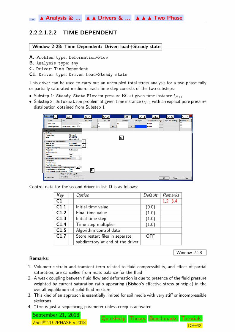
2.2.2.1.2.2 TIME DEPENDENT
Window 2-28: Time Dependent: Driven load+Steady state
A. Problem type: Deformation+Flow
B. Analysis type: anyC. Driver: Time Dependent
C1. Driver type: Driven Load+Steady state
This driver can be used to carry out an uncoupled total stress analysis for a two-phase fullyor partially saturated medium. Each time step consists of the two substeps:
• Substep 1: Steady State Flow for pressure BC at given time instance tN+1
• Substep 2: Deformation problem at given time instance tN+1 with an explicit pore pressuredistribution obtained from Substep 1
Control data for the second driver in list D is as follows:
Key Option Default RemarksC1 1,2, 3,4C1.1 Initial time value (0.0)C1.2 Final time value (1.0)C1.3 Initial time step (1.0)C1.4 Time step multiplier (1.0)C1.5 Algorithm control dataC1.7 Store restart files in separate OFF
subdirectory at end of the driver
Window 2-28Remarks:
1. Volumetric strain and transient term related to fluid compressibility, and effect of partialsaturation, are cancelled from mass balance for the fluid
2. A weak coupling between fluid flow and deformation is due to presence of the fluid pressureweighted by current saturation ratio appearing (Bishop’s effective stress principle) in theoverall equilibrium of solid-fluid mixture
3. This kind of an approach is essentially limited for soil media with very stiff or incompressibleskeletons
4. Time is just a sequencing parameter unless creep is activated
September 21, 2018
ZSoilr-2D-2PHASE v.2018QuickHelp Theory Benchmarks Tutorials
DP–42

... N Analysis & ... N N Drivers & ... N N N Two Phase
Window 2-29: Time Dependent: Driven load+Transient flow
A. Problem type: Deformation+Flow
B. Analysis type: anyC. Driver: Time Dependent
C1. Driver type: Driven Load+Transient flow
This driver can be used to carry out a weakly coupled total stress analysis for a two-phasefully or partially saturated medium. Each time step consists of the two substeps:
• Substep 1: Transient Flow for pressure BC at given time instance tN+1
• Substep 2: Deformation problem at given time instance tN+1 with an explicit pore pressuredistribution obtained from Substep 1
Control data for the second driver in list D is as follows:
Key Option Default RemarksC1 1,2, 3,4C1.1 Initial time value (0.0)C1.2 Final time value (10.0)C1.3 Initial time step (0.1)C1.4 Time step multiplier (1.0)C1.5 Algorithm control dataC1.7 Store restart files in separate OFF
subdirectory at end of the driver
Window 2-29Remarks:
1. Volumetric strain is canceled from mass balance for the fluid2. A weak coupling between fluid flow and deformation is due to presence of the fluid pressure
weighted by current saturation ratio appearing (Bishop’s effective stress principle) in theoverall equilibrium of solid-fluid mixture
3. This kind of an approach is essentially limited for soil media with very stiff or slightlycompressible skeletons
4. Time is a real time parameter, time stepping procedure is activated
September 21, 2018
ZSoilr-2D-2PHASE v.2018QuickHelp Theory Benchmarks Tutorials
DP–43
... N Analysis & ... N N Drivers & ... N N N Two Phase
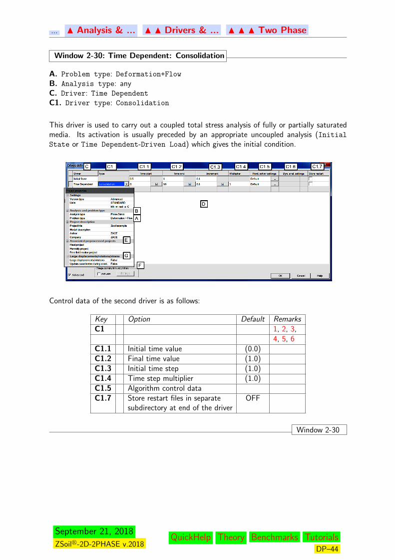
Window 2-30: Time Dependent: Consolidation
A. Problem type: Deformation+Flow
B. Analysis type: anyC. Driver: Time Dependent
C1. Driver type: Consolidation
This driver is used to carry out a coupled total stress analysis of fully or partially saturatedmedia. Its activation is usually preceded by an appropriate uncoupled analysis (InitialState or Time Dependent-Driven Load) which gives the initial condition.
Control data of the second driver is as follows:
Key Option Default RemarksC1 1, 2, 3,
4, 5, 6C1.1 Initial time value (0.0)C1.2 Final time value (1.0)C1.3 Initial time step (1.0)C1.4 Time step multiplier (1.0)C1.5 Algorithm control dataC1.7 Store restart files in separate OFF
subdirectory at end of the driver
Window 2-30
September 21, 2018
ZSoilr-2D-2PHASE v.2018QuickHelp Theory Benchmarks Tutorials
DP–44
... N Analysis & ... N N Drivers & ... N N N Two Phase
Remarks:
1. Time integration procedure of coupled system is performed2. All transient terms in the mass balance for the fluid are taken into account3. Unit weight of soil in partially saturated zone varies in time due to variation of current
saturation ratio; it is automatically computed4. Time is a real parameter5. Consolidation driver is more general than the uncoupled Driven Load+Transient;
however, applied time steps must be greater than the critical time step value to avoidnumerical oscillations in the pressure field1:
∆t ≥ 1
6
h2
θCv[s]
In Z SOIL, for the mixed displacement–pore pressure formulation the coefficient 1/6 givenby Vermeer is replaced by 1/4. With:
Cv =Eoedk
γF[m2/s]
Eoed =E(1− v)
(1 + v)(1− 2v)[N/m2]
where h is maximum element size, Cv is the coefficient of consolidation, k the Darcycoefficient [m/s], γF the fluid specific weight [N/m3], and θ is a numerical integrationparameter set to 1.0 by default.
6. As an alternative, a stabilized approach can be activated (under Control-Finite Elements)eliminating spurious pressure oscillations for any time step
Related Topics
• THEORETICAL MANUAL
F NUMERICAL IMPLEMENTATION – ULTIMATE LOAD ANALYSIS
F NUMERICAL IMPLEMENTATION – LOAD FUNCTIONS AND TIME STEPPING
1[Ver, 1981]
September 21, 2018
ZSoilr-2D-2PHASE v.2018QuickHelp Theory Benchmarks Tutorials
DP–45
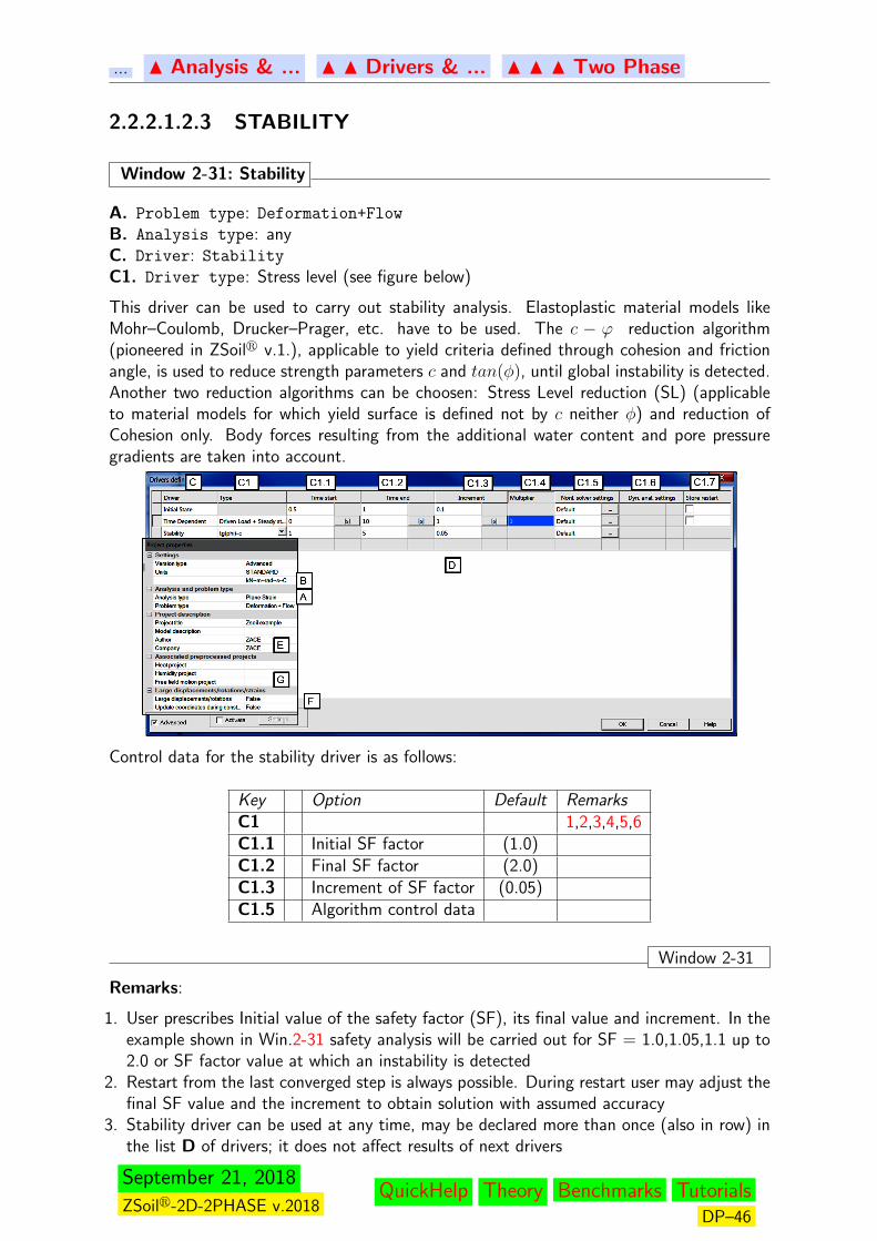
... N Analysis & ... N N Drivers & ... N N N Two Phase
2.2.2.1.2.3 STABILITY
Window 2-31: Stability
A. Problem type: Deformation+Flow
B. Analysis type: anyC. Driver: Stability
C1. Driver type: Stress level (see figure below)
This driver can be used to carry out stability analysis. Elastoplastic material models likeMohr–Coulomb, Drucker–Prager, etc. have to be used. The c − ϕ reduction algorithm(pioneered in ZSoilr v.1.), applicable to yield criteria defined through cohesion and frictionangle, is used to reduce strength parameters c and tan(φ), until global instability is detected.Another two reduction algorithms can be choosen: Stress Level reduction (SL) (applicableto material models for which yield surface is defined not by c neither φ) and reduction ofCohesion only. Body forces resulting from the additional water content and pore pressuregradients are taken into account.
Control data for the stability driver is as follows:
Key Option Default RemarksC1 1,2,3,4,5,6C1.1 Initial SF factor (1.0)C1.2 Final SF factor (2.0)C1.3 Increment of SF factor (0.05)C1.5 Algorithm control data
Window 2-31
Remarks:
1. User prescribes Initial value of the safety factor (SF), its final value and increment. In theexample shown in Win.2-31 safety analysis will be carried out for SF = 1.0,1.05,1.1 up to2.0 or SF factor value at which an instability is detected
2. Restart from the last converged step is always possible. During restart user may adjust thefinal SF value and the increment to obtain solution with assumed accuracy
3. Stability driver can be used at any time, may be declared more than once (also in row) inthe list D of drivers; it does not affect results of next drivers
September 21, 2018
ZSoilr-2D-2PHASE v.2018QuickHelp Theory Benchmarks Tutorials
DP–46
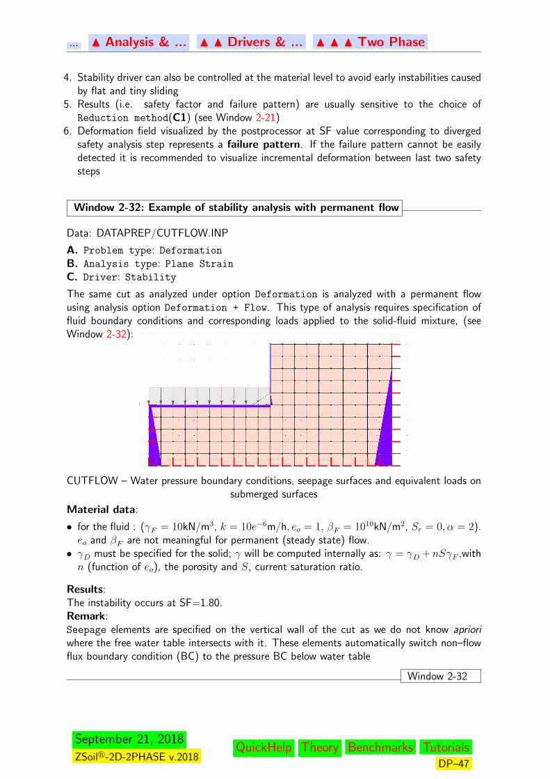
... N Analysis & ... N N Drivers & ... N N N Two Phase
4. Stability driver can also be controlled at the material level to avoid early instabilities causedby flat and tiny sliding
5. Results (i.e. safety factor and failure pattern) are usually sensitive to the choice ofReduction method(C1) (see Window 2-21)
6. Deformation field visualized by the postprocessor at SF value corresponding to divergedsafety analysis step represents a failure pattern. If the failure pattern cannot be easilydetected it is recommended to visualize incremental deformation between last two safetysteps
Window 2-32: Example of stability analysis with permanent flow
Data: DATAPREP/CUTFLOW.INP
A. Problem type: Deformation
B. Analysis type: Plane Strain
C. Driver: Stability
The same cut as analyzed under option Deformation is analyzed with a permanent flowusing analysis option Deformation + Flow. This type of analysis requires specification offluid boundary conditions and corresponding loads applied to the solid-fluid mixture, (seeWindow 2-32):
CUTFLOW – Water pressure boundary conditions, seepage surfaces and equivalent loads onsubmerged surfaces
Material data:
• for the fluid : (γF = 10kN/m3, k = 10e−6m/h, eo = 1, βF = 1010kN/m2, Sr = 0, α = 2).eo and βF are not meaningful for permanent (steady state) flow.• γD must be specified for the solid; γ will be computed internally as: γ = γD +nSγF ,withn (function of eo), the porosity and S, current saturation ratio.
Results:The instability occurs at SF=1.80.Remark:Seepage elements are specified on the vertical wall of the cut as we do not know aprioriwhere the free water table intersects with it. These elements automatically switch non–flowflux boundary condition (BC) to the pressure BC below water table
Window 2-32
September 21, 2018
ZSoilr-2D-2PHASE v.2018QuickHelp Theory Benchmarks Tutorials
DP–47
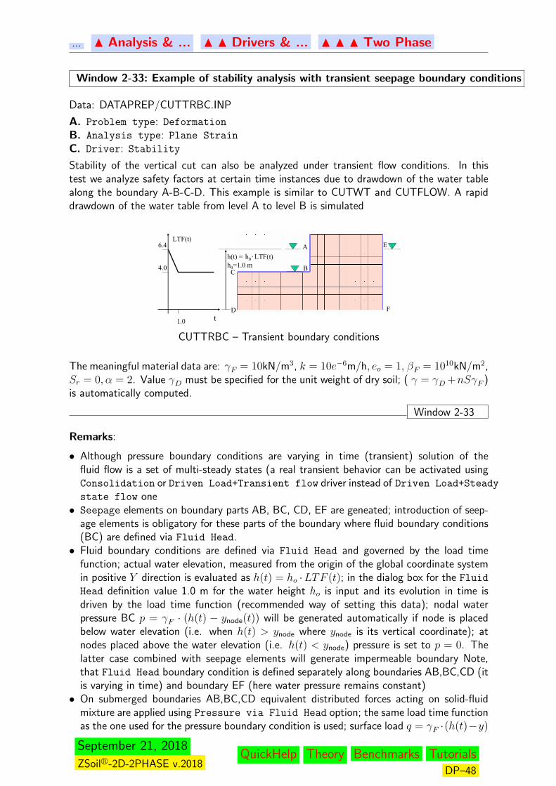
... N Analysis & ... N N Drivers & ... N N N Two Phase
Window 2-33: Example of stability analysis with transient seepage boundary conditions
Data: DATAPREP/CUTTRBC.INP
A. Problem type: Deformation
B. Analysis type: Plane Strain
C. Driver: Stability
Stability of the vertical cut can also be analyzed under transient flow conditions. In thistest we analyze safety factors at certain time instances due to drawdown of the water tablealong the boundary A-B-C-D. This example is similar to CUTWT and CUTFLOW. A rapiddrawdown of the water table from level A to level B is simulated
h(t) = h0⋅ LTF(t)h0=1.0 m
1.0 t
LTF(t)6.4
4.0
A
BC
D
E
F
CUTTRBC – Transient boundary conditions
The meaningful material data are: γF = 10kN/m3, k = 10e−6m/h, eo = 1, βF = 1010kN/m2,Sr = 0, α = 2. Value γD must be specified for the unit weight of dry soil; ( γ = γD +nSγF )is automatically computed.
Window 2-33
Remarks:
• Although pressure boundary conditions are varying in time (transient) solution of thefluid flow is a set of multi-steady states (a real transient behavior can be activated usingConsolidation or Driven Load+Transient flow driver instead of Driven Load+Steady
state flow one• Seepage elements on boundary parts AB, BC, CD, EF are geneated; introduction of seep-
age elements is obligatory for these parts of the boundary where fluid boundary conditions(BC) are defined via Fluid Head.• Fluid boundary conditions are defined via Fluid Head and governed by the load time
function; actual water elevation, measured from the origin of the global coordinate systemin positive Y direction is evaluated as h(t) = ho ·LTF (t); in the dialog box for the Fluid
Head definition value 1.0 m for the water height ho is input and its evolution in time isdriven by the load time function (recommended way of setting this data); nodal waterpressure BC p = γF · (h(t) − ynode(t)) will be generated automatically if node is placedbelow water elevation (i.e. when h(t) > ynode where ynode is its vertical coordinate); atnodes placed above the water elevation (i.e. h(t) < ynode) pressure is set to p = 0. Thelatter case combined with seepage elements will generate impermeable boundary Note,that Fluid Head boundary condition is defined separately along boundaries AB,BC,CD (itis varying in time) and boundary EF (here water pressure remains constant)• On submerged boundaries AB,BC,CD equivalent distributed forces acting on solid-fluid
mixture are applied using Pressure via Fluid Head option; the same load time functionas the one used for the pressure boundary condition is used; surface load q = γF ·(h(t)−y)
September 21, 2018
ZSoilr-2D-2PHASE v.2018QuickHelp Theory Benchmarks Tutorials
DP–48
... N Analysis & ... N N Drivers & ... N N N Two Phase
will be generated automatically at any time instance if the element boundary, to which thisload is applied, is submerged• Load time function for water elevation on AB,BC,CD parts is as follows:
t1 = 0 h1 = LTF(t1) = 6.4
t2 = 1 h2 = LTF(t2) = 4.0
On part EF constant LTF should be applied• Problem type Deformation+Flow is mandatory. Drivers Initial State, Driven Load+Steady
state flow, and Stability are activated successively with the following parameters:F Initial State(0.5,1;0.1;)F Stability(use SF2) (1.0; 3.0; 0.05; 1.0)F Driven Load+Steady state flow(0.0, 1.0, 1.0, 1.0)F Stability(use SF2) (1.0, 3.0, 0.05, 1.0)
Related Topics
• STABILITY ANALYSIS
• DEFORMATION COUPLED WITH FLOW
September 21, 2018
ZSoilr-2D-2PHASE v.2018QuickHelp Theory Benchmarks Tutorials
DP–49
... N Control N N Analysis & ... N N N Drivers & ...
2.2.2.1.3 FLOW (STEADY STATE AND TRANSIENT)
Unknown: fluid pressure field p(x)
For Flow problem type necessary data consists of:• fluid pressure BC (nodal fluid pressures, fluid heads, seepage surfaces),• fluid fluxes (distributed fluxes)• seepage parameters and unit weights
The two possible drivers for the fluid flow:
INITIAL STATETIME DEPENDENT
are described in next paragraphs.Remarks:
1. Tracking of the free surface is handled internally2. For Time Dependent driver the two options are available:• STEADY STATE
- for solving series of steady state problems (transient term concerning fluid compress-ibility and effect of partial saturation is canceled from fluid mass balance), evolutionarywith respect to time varying pressure boundary conditions, fluxes, domain geometry andmaterial data.• TRANSIENT FLOW
- for solving transient flow problem, evolutionary with respect to time varying pressureboundary conditions, fluxes, domain geometry and material data.
MATERIAL DATA
For both steady and transient flow material data should be specified for all materials models,except those marked as impermeable. Impermeable material zones are excluded from theflow analysis (finite elements in this zone do not have pressure degrees of freedom).
Continuum models (see Flow and Unit Weight data groups):
γF {[kNm−3]; [> 0]; [10]}fluid specific weight (Unit Weight)
k( ) {ms−1]; [> 0]; [1.0]}Darcy coefficients in principal directions of permeability (Flow)Remark:See Assembly→Materials→Data Group→Flow for detailed informationon how to set orientation of principal permeability directions
Sr {[−]; [0, 1]; [0]}residual saturation (Flow)
α {[m−1]; [> 0]; [2.0]}seepage parameter (Flow)
Transient Flow requires additional specification of:
eo {[−.]; [0, 10]; [0.0]}(initial) void ratio (Unit Weight)
βF {[kNm−2]; [> 0]; [10+38]]}fluid compressibility (Flow)
September 21, 2018
ZSoilr-2D-2PHASE v.2018QuickHelp Theory Benchmarks Tutorials
DP–50

... N Control N N Analysis & ... N N N Drivers & ...
NB. Since v.2012 one may cancel the gravity term in Darcy law.
FLUX AND PRESSURE TYPE BOUNDARY CONDITIONS
Fluid pressures [N/m2]
Flux [m/s]
selected part of the boundary
Drains or Seepage surface element
seepage surface
Flow boundary conditions
Remarks:
1. Pressure BC can be prescribed directly on nodes or element edges (faces in 3D) whileFlux are prescribed on element edges (faces in 3D)
2. Lack of pressure BC at certain part of the boundary means that this boundary is imper-meable
3. Seepage elements are directional and must be oriented with the arrow pointing outward,see the Window, otherwise the outflow sign will be changed. Constant or time–dependentpressure boundary conditions must be associated with the Seepage elements; by default,zero outsideexternal pressure is assumed. The element will switch automatically froma pressure boundary condition to no flux boundary condition when no flow through thesurface takes place.
4. The impermeable boundary Γ2, Γ3 could alternatively be modeled with Seepage elementsassociated with zero external pressure (default value). Γ1 could be modeled with Seepage
elements (directed outwards), while maintaining the applied pressure. On Γ4, q = 0, mustbe prescribed and on Γ5, Seepage elements must be present.
INITIAL CONDITIONS
The initial condition for flow problem corresponds to a prescribed pressure field at all nodalpoints.
Remarks:
1. The Steady State driver and the Initial State driver will both yield a solution ofSteady State Flow problem (initial pressure field).
2. For transient analysis, an Initial State driver should be run first or, alternatively, anInitial Pressure state has to be defined by the user(with aid of initial pressure super-elements)
September 21, 2018
ZSoilr-2D-2PHASE v.2018QuickHelp Theory Benchmarks Tutorials
DP–51

... N Control N N Analysis & ... N N N Drivers & ...
Related Topics• DRIVERS AND DRIVERS TYPES• SEEPAGE SURFACE MODEL
September 21, 2018
ZSoilr-2D-2PHASE v.2018QuickHelp Theory Benchmarks Tutorials
DP–52
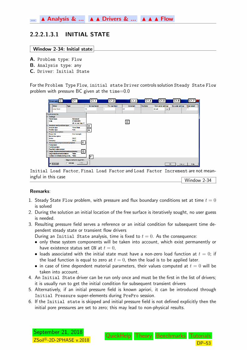
... N Analysis & ... N N Drivers & ... N N N Flow
2.2.2.1.3.1 INITIAL STATE
Window 2-34: Initial state
A. Problem type: Flow
B. Analysis type: anyC. Driver: Initial State
For the Problem Type Flow, initial state Driver controls solution Steady State Flow
problem with pressure BC given at the time=0.0
Initial Load Factor, Final Load Factor and Load Factor Increment are not mean-ingful in this case
Window 2-34
Remarks:
1. Steady State Flow problem, with pressure and flux boundary conditions set at time t = 0is solved
2. During the solution an initial location of the free surface is iteratively sought, no user guessis needed.
3. Resulting pressure field serves a reference or an initial condition for subsequent time de-pendent steady state or transient flow driversDuring an Initial State analysis, time is fixed to t = 0. As the consequence:• only these system components will be taken into account, which exist permanently or
have existence status set ON at t = 0,• loads associated with the initial state must have a non-zero load function at t = 0; if
the load function is equal to zero at t = 0, then the load is to be applied later.• in case of time dependent material parameters, their values computed at t = 0 will be
taken into account.4. An Initial State driver can be run only once and must be the first in the list of drivers;
it is usually run to get the initial condition for subsequent transient drivers5. Alternatively, if an initial pressure field is known apriori, it can be introduced through
Initial Pressure super-elements during PrePro session.6. If the Initial state is skipped and initial pressure field is not defined explicitly then the
initial pore pressures are set to zero; this may lead to non-physical results.
September 21, 2018
ZSoilr-2D-2PHASE v.2018QuickHelp Theory Benchmarks Tutorials
DP–53
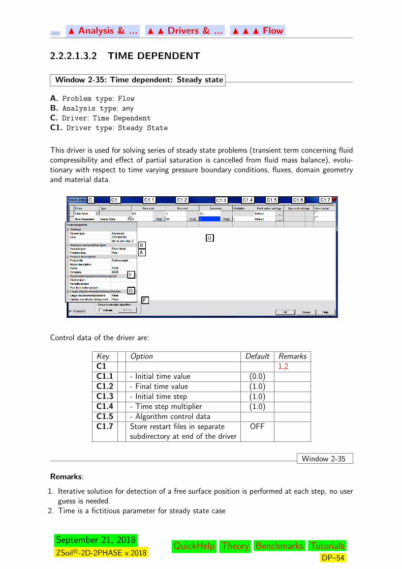
... N Analysis & ... N N Drivers & ... N N N Flow
2.2.2.1.3.2 TIME DEPENDENT
Window 2-35: Time dependent: Steady state
A. Problem type: Flow
B. Analysis type: anyC. Driver: Time Dependent
C1. Driver type: Steady State
This driver is used for solving series of steady state problems (transient term concerning fluidcompressibility and effect of partial saturation is cancelled from fluid mass balance), evolu-tionary with respect to time varying pressure boundary conditions, fluxes, domain geometryand material data.
Control data of the driver are:
Key Option Default RemarksC1 1,2C1.1 - Initial time value (0.0)C1.2 - Final time value (1.0)C1.3 - Initial time step (1.0)C1.4 - Time step multiplier (1.0)C1.5 - Algorithm control dataC1.7 Store restart files in separate OFF
subdirectory at end of the driver
Window 2-35
Remarks:
1. Iterative solution for detection of a free surface position is performed at each step, no userguess is needed.
2. Time is a fictitious parameter for steady state case
September 21, 2018
ZSoilr-2D-2PHASE v.2018QuickHelp Theory Benchmarks Tutorials
DP–54
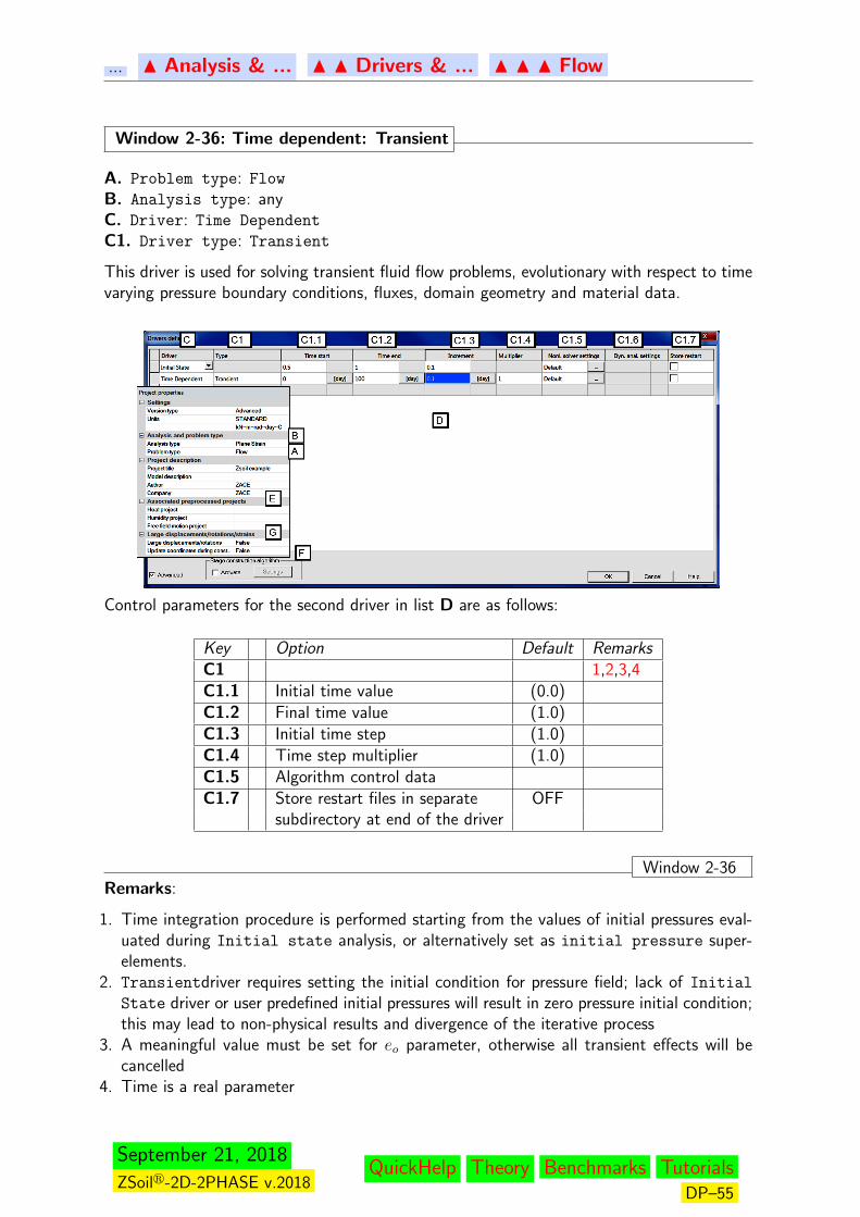
... N Analysis & ... N N Drivers & ... N N N Flow
Window 2-36: Time dependent: Transient
A. Problem type: Flow
B. Analysis type: anyC. Driver: Time Dependent
C1. Driver type: Transient
This driver is used for solving transient fluid flow problems, evolutionary with respect to timevarying pressure boundary conditions, fluxes, domain geometry and material data.
Control parameters for the second driver in list D are as follows:
Key Option Default RemarksC1 1,2,3,4C1.1 Initial time value (0.0)C1.2 Final time value (1.0)C1.3 Initial time step (1.0)C1.4 Time step multiplier (1.0)C1.5 Algorithm control dataC1.7 Store restart files in separate OFF
subdirectory at end of the driver
Window 2-36Remarks:
1. Time integration procedure is performed starting from the values of initial pressures eval-uated during Initial state analysis, or alternatively set as initial pressure super-elements.
2. Transientdriver requires setting the initial condition for pressure field; lack of Initial
State driver or user predefined initial pressures will result in zero pressure initial condition;this may lead to non-physical results and divergence of the iterative process
3. A meaningful value must be set for eo parameter, otherwise all transient effects will becancelled
4. Time is a real parameter
September 21, 2018
ZSoilr-2D-2PHASE v.2018QuickHelp Theory Benchmarks Tutorials
DP–55

... N Control N N Analysis & ... N N N Drivers & ...
2.2.2.1.4 HEAT TRANSFER
Unknown: temperature field T (x, t)
For Heat problem type necessary data consists of:
• temperature BC (nodal temperatures), convection BC• heat fluxes (distributed fluxes)• heat internal sources (due to hydration process in young concrete)• heat transfer parameters in material models
The two possible drivers:
INITIAL STATETIME DEPENDENT
are presented in next paragraphs.
Remarks:
1. Heat Transfer analysis can be carried out to solve:• Heat Transfer problem treated as standalone,• Heat Transfer problem to preprocess temperature field to be used later on for subse-
quent Deformation analysis. This temperature field yields imposed thermal strains inthe medium due to thermal dilatancy; Thermal dilatancy coefficient α has to be set atthe material level; Heat Transfer and Deformation (+Flow) analyses are definedand run as separate tasks. Then preprocessed temperature field has to be linked toDeformation or Deformation+Flow problem through→Associated preprocessed
projects in the Analysis & Drivers dialog box ( see Associated preprocessed
projects).2. For Time Dependent driver can be specialized to Steady State or Transient• STEADY STATE
- is used for solving series of steady state problems (transient term concerning heat ca-pacity and internal source term are cancelled), evolutionary with respect to time varyingtemperature boundary conditions, fluxes, domain geometry and material data.• TRANSIENT
- is used for solving transient heat problems, evolutionary with respect to time varyingtemperature, convection boundary conditions, fluxes, domain geometry and materialdata.
MATERIAL DATA
For continuum elements, any material model may be used and the only meaningful data areset under Heat group and contain:
heat conductivity λ {[kN/( · ◦K · day)], [> 0], [2.4]}(obligatory)
heat capacity c∗ {[kN/m2 · ◦K)], [> 0], [2000]}(obligatory for Transient analysis)
Additional data for heat source due to concrete hydration may be defined
September 21, 2018
ZSoilr-2D-2PHASE v.2018QuickHelp Theory Benchmarks Tutorials
DP–56

... N Control N N Analysis & ... N N N Drivers & ...
FLUX AND TEMPERATURE BOUNDARY CONDITIONS
• Temperature [oK], [oC] may be set on nodes.• Heat Flux [J/(m2day)] is defined on the boundary.• Heat Convection may be specified on selected part of the boundary by means of Heat
Convection elements with specialized material model. Heat Convection BC data are:F Ambient Temperature [oK], [oC] (may be time dependent and controlled by a Load
Time Function)F heat convention coefficient hT [kN/(m ·o K · day)]
Remarks:
1. If no Temperature, Heat Flux, nor Heat Convection is specified on the boundary it isequivalent to setting zero heat flux i.e. adiabatic conditions.
2. Setting Temperature at given part of the boundary excludes setting Heat Flux or HeatConvection and vice versa. Heat Flux and Heat Convection may coexist.
3. A Heat Source, can be optionally defined. In particular, a Heat Source due to concretehydration is available (within Heat data of material model)
INITIAL CONDITIONS
The initial conditions for Heat Transfer problem correspond to a prescribed temperaturefield at all nodal points.
Remarks:
1. The Initial State driver is equivalent to a Steady State problem at time t = 02. For transient analyses, an Initial State analysis should be performed first to serve for
the initial condition or, alternatively, initial temperatures can be set with aid of initialtemperature super-elements
Related Topics• Data Preparation:F DRIVERS AND DRIVERS TYPESF ASSOCIATED PREPROCESSED PROJECTSF CONVECTION SURFACE ELEMENTSF HEAT MATERIAL DATAF CONVECTION MODEL• Theory:F PROBLEM STATEMENTF HEAT TRANSFER
September 21, 2018
ZSoilr-2D-2PHASE v.2018QuickHelp Theory Benchmarks Tutorials
DP–57
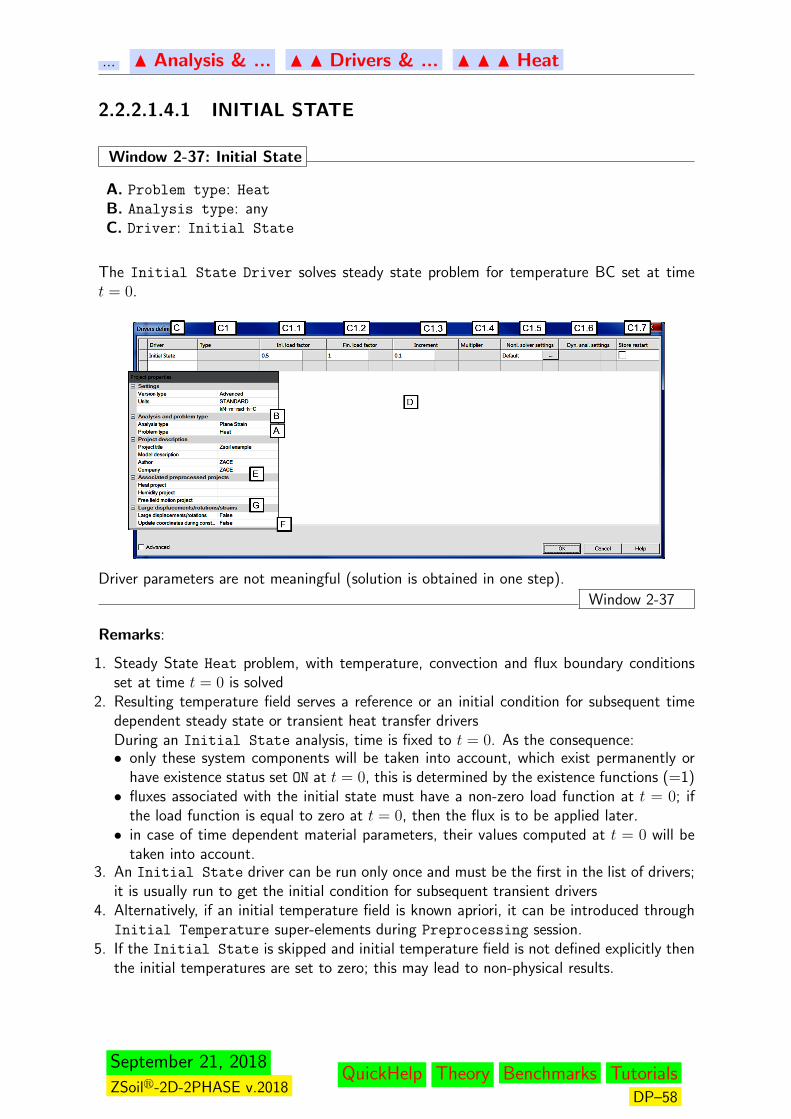
... N Analysis & ... N N Drivers & ... N N N Heat
2.2.2.1.4.1 INITIAL STATE
Window 2-37: Initial State
A. Problem type: Heat
B. Analysis type: anyC. Driver: Initial State
The Initial State Driver solves steady state problem for temperature BC set at timet = 0.
Driver parameters are not meaningful (solution is obtained in one step).
Window 2-37
Remarks:
1. Steady State Heat problem, with temperature, convection and flux boundary conditionsset at time t = 0 is solved
2. Resulting temperature field serves a reference or an initial condition for subsequent timedependent steady state or transient heat transfer driversDuring an Initial State analysis, time is fixed to t = 0. As the consequence:• only these system components will be taken into account, which exist permanently or
have existence status set ON at t = 0, this is determined by the existence functions (=1)• fluxes associated with the initial state must have a non-zero load function at t = 0; if
the load function is equal to zero at t = 0, then the flux is to be applied later.• in case of time dependent material parameters, their values computed at t = 0 will be
taken into account.3. An Initial State driver can be run only once and must be the first in the list of drivers;
it is usually run to get the initial condition for subsequent transient drivers4. Alternatively, if an initial temperature field is known apriori, it can be introduced through
Initial Temperature super-elements during Preprocessing session.5. If the Initial State is skipped and initial temperature field is not defined explicitly then
the initial temperatures are set to zero; this may lead to non-physical results.
September 21, 2018
ZSoilr-2D-2PHASE v.2018QuickHelp Theory Benchmarks Tutorials
DP–58
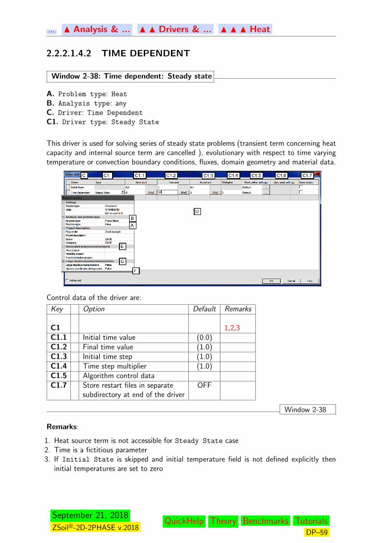
... N Analysis & ... N N Drivers & ... N N N Heat
2.2.2.1.4.2 TIME DEPENDENT
Window 2-38: Time dependent: Steady state
A. Problem type: Heat
B. Analysis type: anyC. Driver: Time Dependent
C1. Driver type: Steady State
This driver is used for solving series of steady state problems (transient term concerning heatcapacity and internal source term are cancelled ), evolutionary with respect to time varyingtemperature or convection boundary conditions, fluxes, domain geometry and material data.
Control data of the driver are:
Key Option Default Remarks
C1 1,2,3C1.1 Initial time value (0.0)C1.2 Final time value (1.0)C1.3 Initial time step (1.0)C1.4 Time step multiplier (1.0)C1.5 Algorithm control dataC1.7 Store restart files in separate OFF
subdirectory at end of the driver
Window 2-38
Remarks:
1. Heat source term is not accessible for Steady State case2. Time is a fictitious parameter3. If Initial State is skipped and initial temperature field is not defined explicitly then
initial temperatures are set to zero
September 21, 2018
ZSoilr-2D-2PHASE v.2018QuickHelp Theory Benchmarks Tutorials
DP–59

... N Analysis & ... N N Drivers & ... N N N Heat
Window 2-39: Time Dependent: Transient
A. Problem type: Heat
B. Analysis type: anyC. Driver: Time Dependent
C1. Driver type: Transient
This driver is used for solving transient thermal problems for varying in time, temperature,convection and heat flux boundary conditions, and internal heat sources.
Control parameters for the second driver are as follows:
Key Option Default Remarks
C1 1,2,3,4C1.1 Initial time value (0.0)C1.2 Final time value (1.0)C1.3 Initial time step (1.0)C1.4 Time step multiplier (1.0)C1.7 Store restart files in separate OFF
subdirectory at end of the driver
Window 2-39
Remarks:
1. Time integration procedure is performed starting from the values of initial temperaturesevaluated during Initial State analysis, or alternatively set as Initial Temperature
with aid of super-elements.2. Transient case must be selected to handle internal heat source term3. If Initial State is skipped and initial temperature field is not defined explicitly then
at the first time step zero temperatures will be taken as initial ones. This may lead tonon-physical results
4. Time is a real parameter
September 21, 2018
ZSoilr-2D-2PHASE v.2018QuickHelp Theory Benchmarks Tutorials
DP–60
... N Control N N Analysis & ... N N N Drivers & ...
2.2.2.1.5 HUMIDITY TRANSFER
Unknowns2: relative humidity field i.e. moisture potential, W (x, t), 0 < W < 1
For Humidity transfer problem type necessary data consists of:• humidity BC (nodal humidities), convection BC• humidity fluxes (distributed fluxes)• humidity transfer parameters in material models
The two possible drivers:INITIAL STATETIME DEPENDENTare presented in next paragraphs.
Remarks:1. Humidity Transfer analysis can be carried out to solve:• Humidity Transfer problem treated as standalone,• Humidity Transfer problem to preprocess humidity field to be used later on for sub-
sequent Deformation analysis. This humidity field yields imposed hygral strains in themedium due to hygral dilatancy; Hygral dilatancy coefficient β has to be set at thematerial level; Humidity Transfer and Deformation (+Flow) analyses are definedand run as separate tasks. Then preprocessed humidity field has to be linked toDeformation or Deformation+Flow problem through→Associated preprocessed
projects in the Analysis & Drivers dialog box ( see Associated preprocessed
projects).2. For Time Dependent driver can be specialized to Steady State or Transient• STEADY STATE
- is used for solving series of steady state problems , evolutionary with respect to timevarying humidity boundary conditions, fluxes, domain geometry and material data.• TRANSIENT
- is used for solving transient humidity transfer problems, evolutionary with respect totime varying humidity, convection boundary conditions, fluxes, domain geometry andmaterial data.
MATERIAL DATA
For continuum elements, any material model may be used and the only meaningful data areset under Humidity group and contain:
a {[−], [> 0], [0.05]}D1 {[m2/day], [> 0], [10−7]}W1 {[−], [0 < W1 < 1], [0.75]]}
Remark:
The data are used to relate diffusion conductivity D with respect to the moisture potentialW as a function:
D = D(W ) = D1
a+1− a
1 +
(1−W1−W1
)4
2concerns versions: ACADEMIC, PROFESSIONAL, EXPERT
September 21, 2018
ZSoilr-2D-2PHASE v.2018QuickHelp Theory Benchmarks Tutorials
DP–61

... N Control N N Analysis & ... N N N Drivers & ...
FLUX AND HUMIDITY BOUNDARY CONDITIONS
• Humidity (relative) [−] may be set on nodes.• Humidity Flux [1/(m2 · day)] through part of the boundary.• Humidity Convection may be specified on selected part of the boundary by means ofHumidity Convection elements with specialized material model. Humidity Convection
BC data are:F Ambient humidity [−] (may be time dependent, controlled by Load Time Function)F humidity convention coefficient hW [1/(m2 · day)]
Remarks:
1. As primary unknown i.e. relative humidity W is, by its nature, delimited by: 0 ≤ W ≤ 1thus the same limitations must be fulfilled by relative humidity values set through boundaryor initial conditions
2. If no Humidity, Humidity Flux, nor Humidity Convection is specified on the boundaryit is equivalent to setting zero humidity flux i.e. perfect isolation conditions.
3. Setting Humidity at given part of the boundary excludes setting Humidity Flux orHumidity Convection and vice versa. Humidity Flux and Humidity Convection maycoexist.
INITIAL CONDITIONS
The initial conditions for Humidity Transfer problem correspond to a prescribed humidityfield at all nodal points.
Remarks:
1. The Initial State driver is equivalent to a Steady State problem at time t = 02. For transient analyses, an Initial State analysis should be performed first to serve for
the initial condition or, alternatively, initial humidities can be set with aid of initial humiditysuper-elements
Related Topics• Data Preparation:F DRIVERS AND DRIVERS TYPESF ASSOCIATED PROJECTSF CONVECTION SURFACE ELEMENTSF HUMIDITY MATERIAL DATAF CONVECTION MODEL• Theory:F PROBLEM STATEMENTF HUMIDITY TRANSFER
September 21, 2018
ZSoilr-2D-2PHASE v.2018QuickHelp Theory Benchmarks Tutorials
DP–62
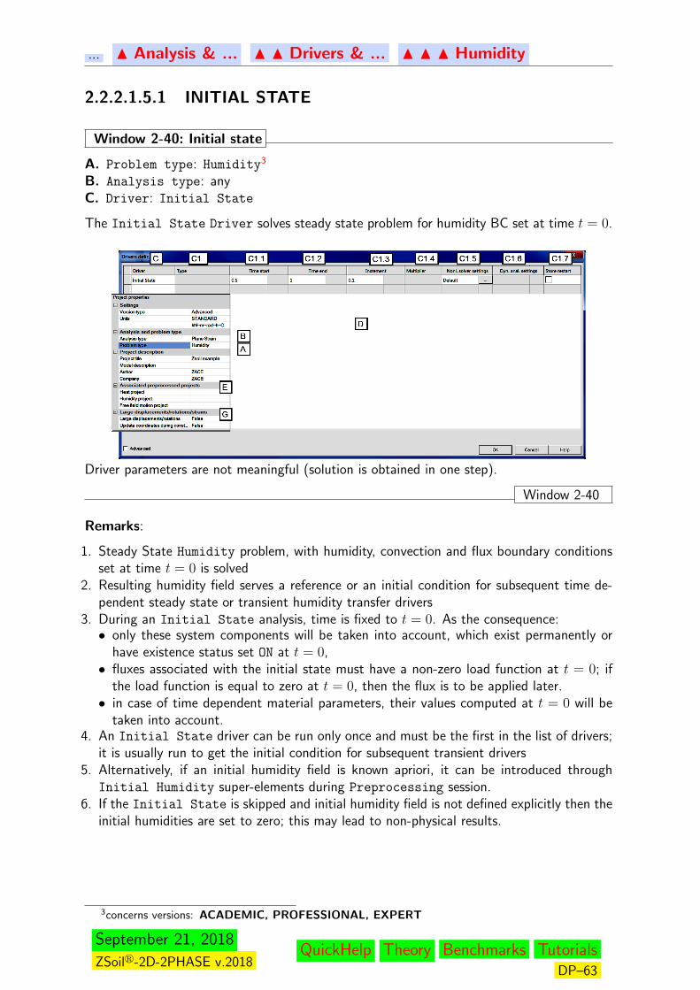
... N Analysis & ... N N Drivers & ... N N N Humidity
2.2.2.1.5.1 INITIAL STATE
Window 2-40: Initial state
A. Problem type: Humidity3
B. Analysis type: anyC. Driver: Initial State
The Initial State Driver solves steady state problem for humidity BC set at time t = 0.
Driver parameters are not meaningful (solution is obtained in one step).
Window 2-40
Remarks:
1. Steady State Humidity problem, with humidity, convection and flux boundary conditionsset at time t = 0 is solved
2. Resulting humidity field serves a reference or an initial condition for subsequent time de-pendent steady state or transient humidity transfer drivers
3. During an Initial State analysis, time is fixed to t = 0. As the consequence:• only these system components will be taken into account, which exist permanently or
have existence status set ON at t = 0,• fluxes associated with the initial state must have a non-zero load function at t = 0; if
the load function is equal to zero at t = 0, then the flux is to be applied later.• in case of time dependent material parameters, their values computed at t = 0 will be
taken into account.4. An Initial State driver can be run only once and must be the first in the list of drivers;
it is usually run to get the initial condition for subsequent transient drivers5. Alternatively, if an initial humidity field is known apriori, it can be introduced through
Initial Humidity super-elements during Preprocessing session.6. If the Initial State is skipped and initial humidity field is not defined explicitly then the
initial humidities are set to zero; this may lead to non-physical results.
3concerns versions: ACADEMIC, PROFESSIONAL, EXPERT
September 21, 2018
ZSoilr-2D-2PHASE v.2018QuickHelp Theory Benchmarks Tutorials
DP–63
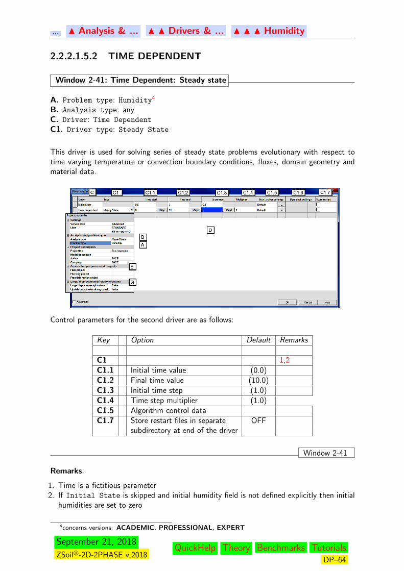
... N Analysis & ... N N Drivers & ... N N N Humidity
2.2.2.1.5.2 TIME DEPENDENT
Window 2-41: Time Dependent: Steady state
A. Problem type: Humidity4
B. Analysis type: anyC. Driver: Time Dependent
C1. Driver type: Steady State
This driver is used for solving series of steady state problems evolutionary with respect totime varying temperature or convection boundary conditions, fluxes, domain geometry andmaterial data.
Control parameters for the second driver are as follows:
Key Option Default Remarks
C1 1,2C1.1 Initial time value (0.0)C1.2 Final time value (10.0)C1.3 Initial time step (1.0)C1.4 Time step multiplier (1.0)C1.5 Algorithm control dataC1.7 Store restart files in separate OFF
subdirectory at end of the driver
Window 2-41
Remarks:
1. Time is a fictitious parameter2. If Initial State is skipped and initial humidity field is not defined explicitly then initial
humidities are set to zero
4concerns versions: ACADEMIC, PROFESSIONAL, EXPERT
September 21, 2018
ZSoilr-2D-2PHASE v.2018QuickHelp Theory Benchmarks Tutorials
DP–64
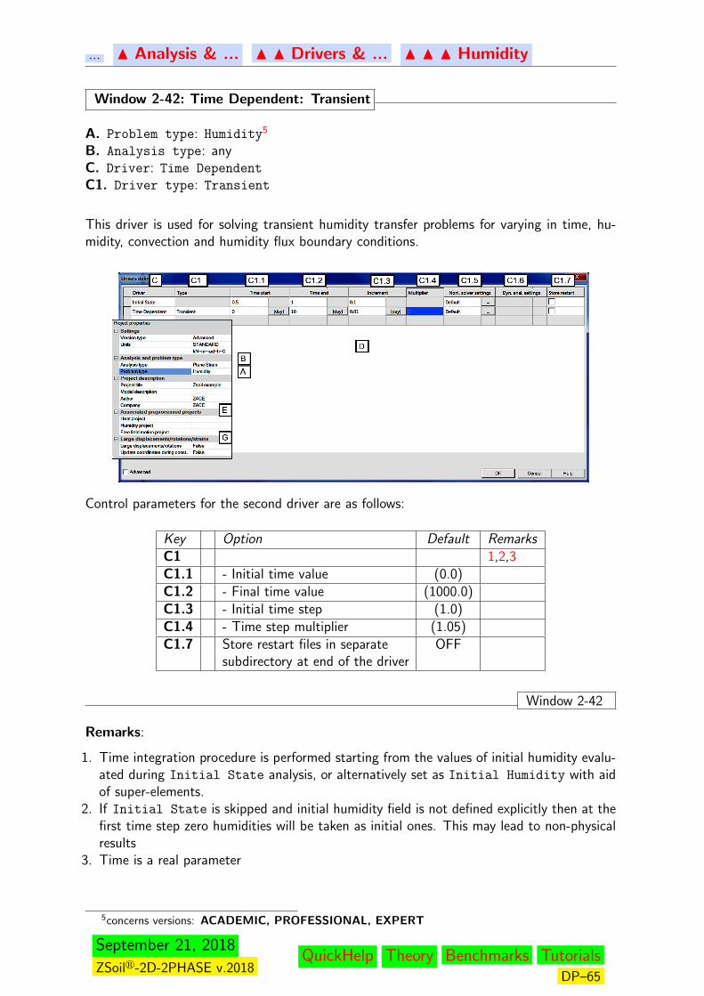
... N Analysis & ... N N Drivers & ... N N N Humidity
Window 2-42: Time Dependent: Transient
A. Problem type: Humidity5
B. Analysis type: anyC. Driver: Time Dependent
C1. Driver type: Transient
This driver is used for solving transient humidity transfer problems for varying in time, hu-midity, convection and humidity flux boundary conditions.
Control parameters for the second driver are as follows:
Key Option Default RemarksC1 1,2,3C1.1 - Initial time value (0.0)C1.2 - Final time value (1000.0)C1.3 - Initial time step (1.0)C1.4 - Time step multiplier (1.05)C1.7 Store restart files in separate OFF
subdirectory at end of the driver
Window 2-42
Remarks:
1. Time integration procedure is performed starting from the values of initial humidity evalu-ated during Initial State analysis, or alternatively set as Initial Humidity with aidof super-elements.
2. If Initial State is skipped and initial humidity field is not defined explicitly then at thefirst time step zero humidities will be taken as initial ones. This may lead to non-physicalresults
3. Time is a real parameter
5concerns versions: ACADEMIC, PROFESSIONAL, EXPERT
September 21, 2018
ZSoilr-2D-2PHASE v.2018QuickHelp Theory Benchmarks Tutorials
DP–65

... N Control N N Analysis & ... N N N Drivers & ...
2.2.2.1.6 TRANSIENT DYNAMICS
Window 2-43: Dynamics for single-phase soil-structure interaction problems
A. Problem type: Deformation
B. Analysis type: anyC. Driver: Dynamics
C1. Driver type: Driven load
This driver can be used for solving a transient dynamic soil-structure interaction problemsfor single-phase media. The domain reduction method (DRM) can be used to reduce size ofthe computational model by setting DRM boundary layer of elements in the preprocessor anddeclaring the free field motion project in the edit field under Associated preprocessed
projects
Control data of the driver are:
Key Option Comment Default RemarksC1 1,,3,5,6C1.1 Time start Initial time value (0.0) 2,3C1.2 Time end Final time value (10.0) 2,3C1.3 Time increment Initial time step (0.01) 3, 8C1.4 Multiplier Time step multiplier (1.0)C1.5 Nonl. Solver Control dataC1.6 Dyn. Solver Control dataC1.7 Store restart Store restart files in separate OFF
subdirectory at end of the driver
Window 2-43
September 21, 2018
ZSoilr-2D-2PHASE v.2018QuickHelp Theory Benchmarks Tutorials
DP–66
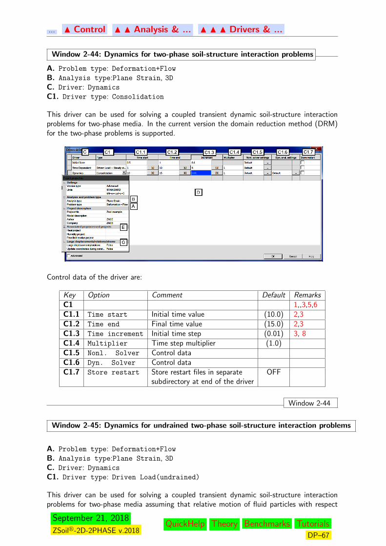
... N Control N N Analysis & ... N N N Drivers & ...
Window 2-44: Dynamics for two-phase soil-structure interaction problems
A. Problem type: Deformation+Flow
B. Analysis type:Plane Strain, 3DC. Driver: Dynamics
C1. Driver type: Consolidation
This driver can be used for solving a coupled transient dynamic soil-structure interactionproblems for two-phase media. In the current version the domain reduction method (DRM)for the two-phase problems is supported.
Control data of the driver are:
Key Option Comment Default RemarksC1 1,,3,5,6C1.1 Time start Initial time value (10.0) 2,3C1.2 Time end Final time value (15.0) 2,3C1.3 Time increment Initial time step (0.01) 3, 8C1.4 Multiplier Time step multiplier (1.0)C1.5 Nonl. Solver Control dataC1.6 Dyn. Solver Control dataC1.7 Store restart Store restart files in separate OFF
subdirectory at end of the driver
Window 2-44
Window 2-45: Dynamics for undrained two-phase soil-structure interaction problems
A. Problem type: Deformation+Flow
B. Analysis type:Plane Strain, 3DC. Driver: Dynamics
C1. Driver type: Driven Load(undrained)
This driver can be used for solving a coupled transient dynamic soil-structure interactionproblems for two-phase media assuming that relative motion of fluid particles with respect
September 21, 2018
ZSoilr-2D-2PHASE v.2018QuickHelp Theory Benchmarks Tutorials
DP–67

... N Control N N Analysis & ... N N N Drivers & ...
to the solid skeleton can be neglected. In the current version the domain reduction method(DRM) for this option is supported. Using this option the excess pore pressure is computedonly at the element center using penalty method. The penalty factor is set up assumingthe ratio between fluid bulk modulus (in undrained state) and elastic bulk modulus of the
skeletonKF
K= 106 (as default). In adition user may put a limit value for the total suction
pore pressure. The above data can be set in group Flow. It has to be emphasized that thetotal pore pressure can only be checked in the element as it consists of the pressure field (keptan nodes) resulting from the previous non-undrained drivers and undrained excess pressurethat is computed at the element center.
Control data of the driver are:
Key Option Comment Default RemarksC1 1,,3,5,6C1.1 Time start Initial time value (10.0) 2,3C1.2 Time end Final time value (15.0) 2,3C1.3 Time increment Initial time step (0.01) 3, 8C1.4 Multiplier Time step multiplier (1.0)C1.5 Nonl. Solver Control dataC1.6 Dyn. Solver Control dataC1.7 Store restart Store restart files in separate OFF
subdirectory at end of the driver
Window 2-45
Remarks:
1. Driver type: Driven Load is the only available driver for single-phase media, for two-phase both Consolidation and Driven Load(undrained) are available (the later onedoes not seem to be menaingful)
2. Time is treated as a physical parameter (consistently with material data)3. Time unit expressed in seconds ([s]) must be used4. Time parameter is used as a common argument of all existence and load time functions.5. A sequence of Dynamic Drivers can be defined, with different time step specification.6. Within a sequence of Dynamic, Driven Load Drivers, an intermediate Time Dependent
(i.e. concerning statics) or Stability Driver can be added.
September 21, 2018
ZSoilr-2D-2PHASE v.2018QuickHelp Theory Benchmarks Tutorials
DP–68
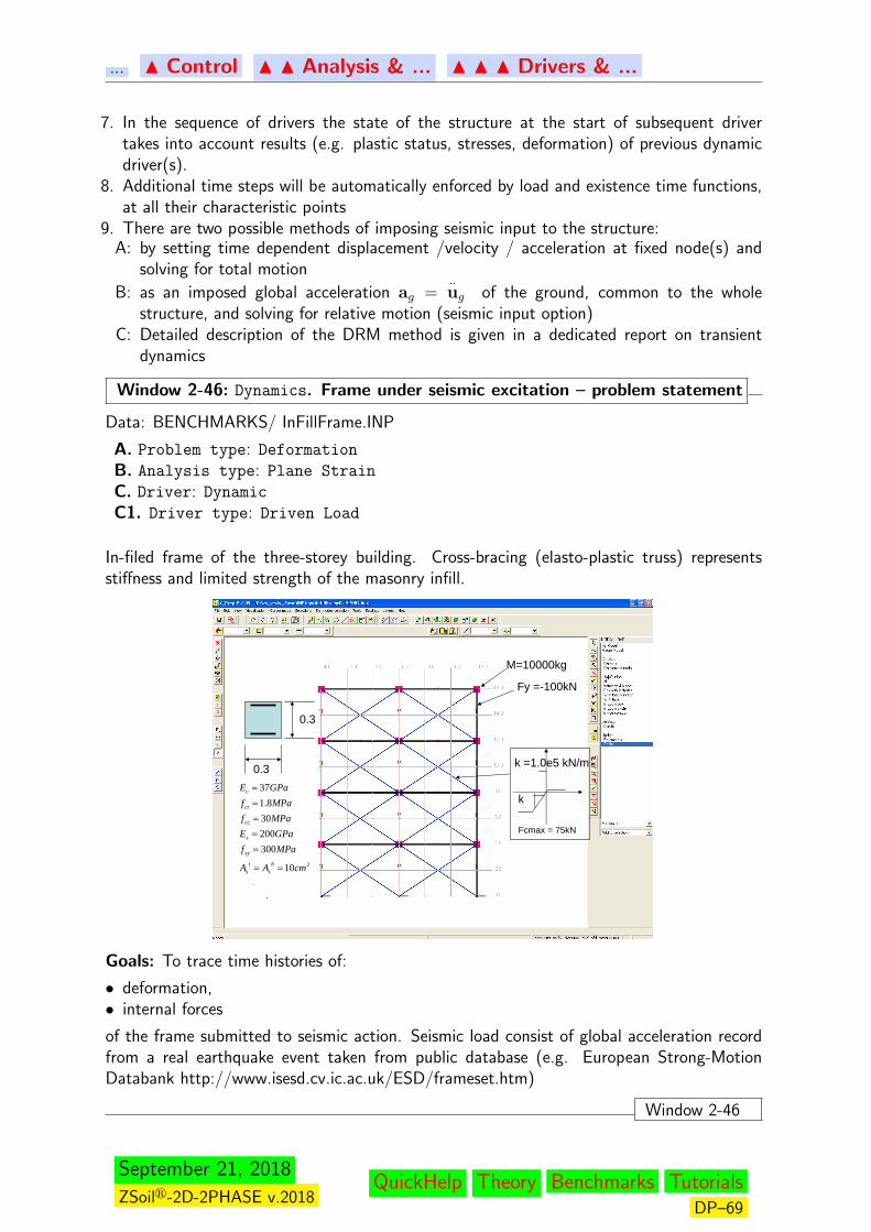
... N Control N N Analysis & ... N N N Drivers & ...
7. In the sequence of drivers the state of the structure at the start of subsequent drivertakes into account results (e.g. plastic status, stresses, deformation) of previous dynamicdriver(s).
8. Additional time steps will be automatically enforced by load and existence time functions,at all their characteristic points
9. There are two possible methods of imposing seismic input to the structure:A: by setting time dependent displacement /velocity / acceleration at fixed node(s) and
solving for total motion
B: as an imposed global acceleration ag =··ug of the ground, common to the whole
structure, and solving for relative motion (seismic input option)C: Detailed description of the DRM method is given in a dedicated report on transient
dynamics
Window 2-46: Dynamics. Frame under seismic excitation – problem statement
Data: BENCHMARKS/ InFillFrame.INP
A. Problem type: Deformation
B. Analysis type: Plane Strain
C. Driver: Dynamic
C1. Driver type: Driven Load
In-filed frame of the three-storey building. Cross-bracing (elasto-plastic truss) representsstiffness and limited strength of the masonry infill.
M=10000kg
Fy =-100kN
Fcmax = 75kN
k
k =1.0e5 kN/m
0.3
0.3
210
30020030
8.137
cmAA
MPafGPaE
MPafMPafGPaE
bs
ts
sy
s
cc
ct
c
==
=====
Goals: To trace time histories of:
• deformation,• internal forces
of the frame submitted to seismic action. Seismic load consist of global acceleration recordfrom a real earthquake event taken from public database (e.g. European Strong-MotionDatabank http://www.isesd.cv.ic.ac.uk/ESD/frameset.htm)
Window 2-46
September 21, 2018
ZSoilr-2D-2PHASE v.2018QuickHelp Theory Benchmarks Tutorials
DP–69
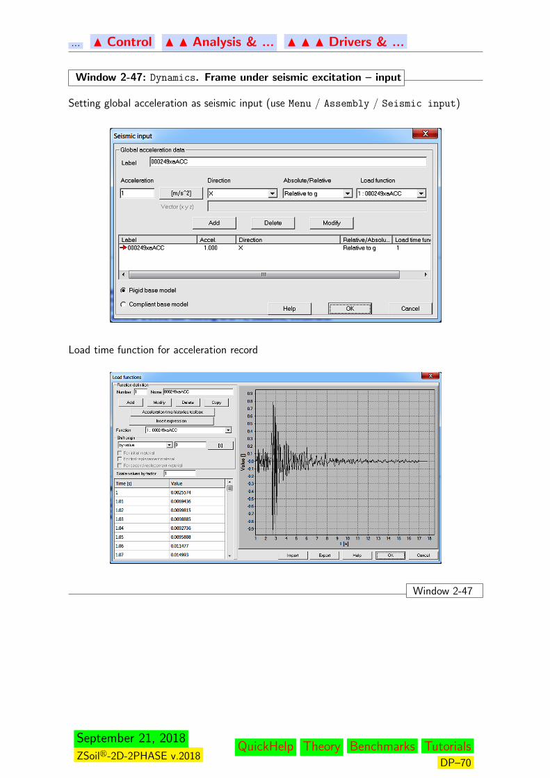
... N Control N N Analysis & ... N N N Drivers & ...
Window 2-47: Dynamics. Frame under seismic excitation – input
Setting global acceleration as seismic input (use Menu / Assembly / Seismic input)
Load time function for acceleration record
Window 2-47
September 21, 2018
ZSoilr-2D-2PHASE v.2018QuickHelp Theory Benchmarks Tutorials
DP–70
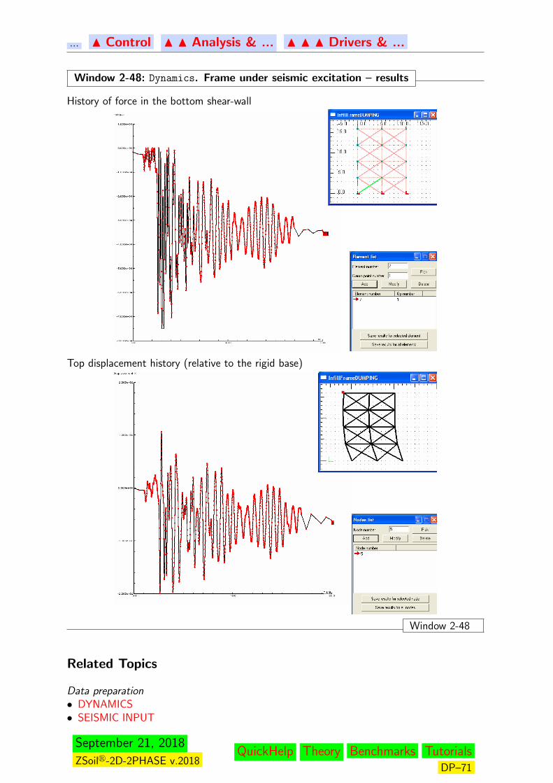
... N Control N N Analysis & ... N N N Drivers & ...
Window 2-48: Dynamics. Frame under seismic excitation – results
History of force in the bottom shear-wall
Top displacement history (relative to the rigid base)
Window 2-48
Related Topics
Data preparation• DYNAMICS• SEISMIC INPUT
September 21, 2018
ZSoilr-2D-2PHASE v.2018QuickHelp Theory Benchmarks Tutorials
DP–71

... N Control N N Analysis & ... N N N Drivers & ...
2.2.2.1.7 EIGENVALUES AND EIGENMODES
Window 2-49: Eigenvalues and eigenmodes
A. Problem type: Deformation
B. Analysis type: anyC. Driver: Eigenvalues
C1. Driver type:
In the Deformation mode this driver can be used for detection of declared number of eigen-values and corresponding eigenmodes for single-phase media including structural elements.
Control data of the driver are:
Key Option Comment Default Remarks
C1.1 No of modes 1, 2
C1.6 Dyn. Solver Control data
Remarks:
1. Number of detected eigenvalues is limited by total number of free degrees of freedom2. For each eigen-mode mass participation factors are computed for all directions
Window 2-49
September 21, 2018
ZSoilr-2D-2PHASE v.2018QuickHelp Theory Benchmarks Tutorials
DP–72
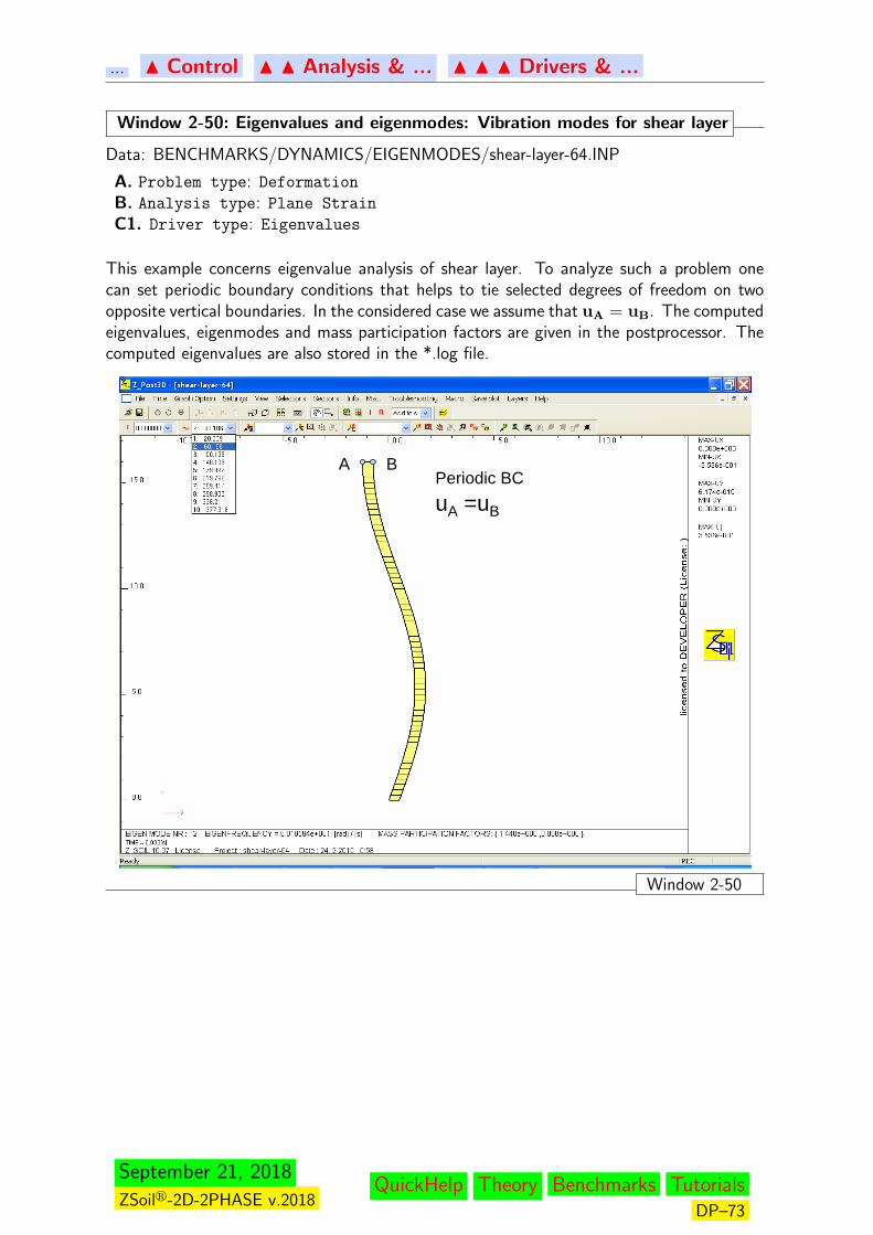
... N Control N N Analysis & ... N N N Drivers & ...
Window 2-50: Eigenvalues and eigenmodes: Vibration modes for shear layer
Data: BENCHMARKS/DYNAMICS/EIGENMODES/shear-layer-64.INP
A. Problem type: Deformation
B. Analysis type: Plane Strain
C1. Driver type: Eigenvalues
This example concerns eigenvalue analysis of shear layer. To analyze such a problem onecan set periodic boundary conditions that helps to tie selected degrees of freedom on twoopposite vertical boundaries. In the considered case we assume that uA = uB. The computedeigenvalues, eigenmodes and mass participation factors are given in the postprocessor. Thecomputed eigenvalues are also stored in the *.log file.
A B
uA =uB
Periodic BC
Window 2-50
September 21, 2018
ZSoilr-2D-2PHASE v.2018QuickHelp Theory Benchmarks Tutorials
DP–73

... N Control N N Analysis & ... N N N Drivers & ...
Window 2-51: Eigenvalues and eigenmodes
A. Problem type: Deformation+Flow
B. Analysis type: anyC. Driver: Eigenvalues
C1. Driver type:
In the Deformation+Flow mode this driver can be used for detection of declared number ofeigenvalues and corresponding eigenmodes for two-phase media including structural elements.Contrary to the Deformation mode the mass matrix of continuum elements includes watercontent corresponding to the current saturation ratio. Hence it is recommended to run theInitial state driver first and then continue with the Eigenvalue one.
Control data of the driver are:
Key Option Comment Default Remarks
C1.1 No of modes 1, 2
C1.6 Dyn. Solver Control data
Remarks:
1. Number of detected eigenvalues is limited by total number of free degrees of freedom2. For each eigen-mode mass particicpation factors are computed for all directions
Window 2-51
Related Topics
Data preparation
• DYNAMICS• SEISMIC INPUT
September 21, 2018
ZSoilr-2D-2PHASE v.2018QuickHelp Theory Benchmarks Tutorials
DP–74
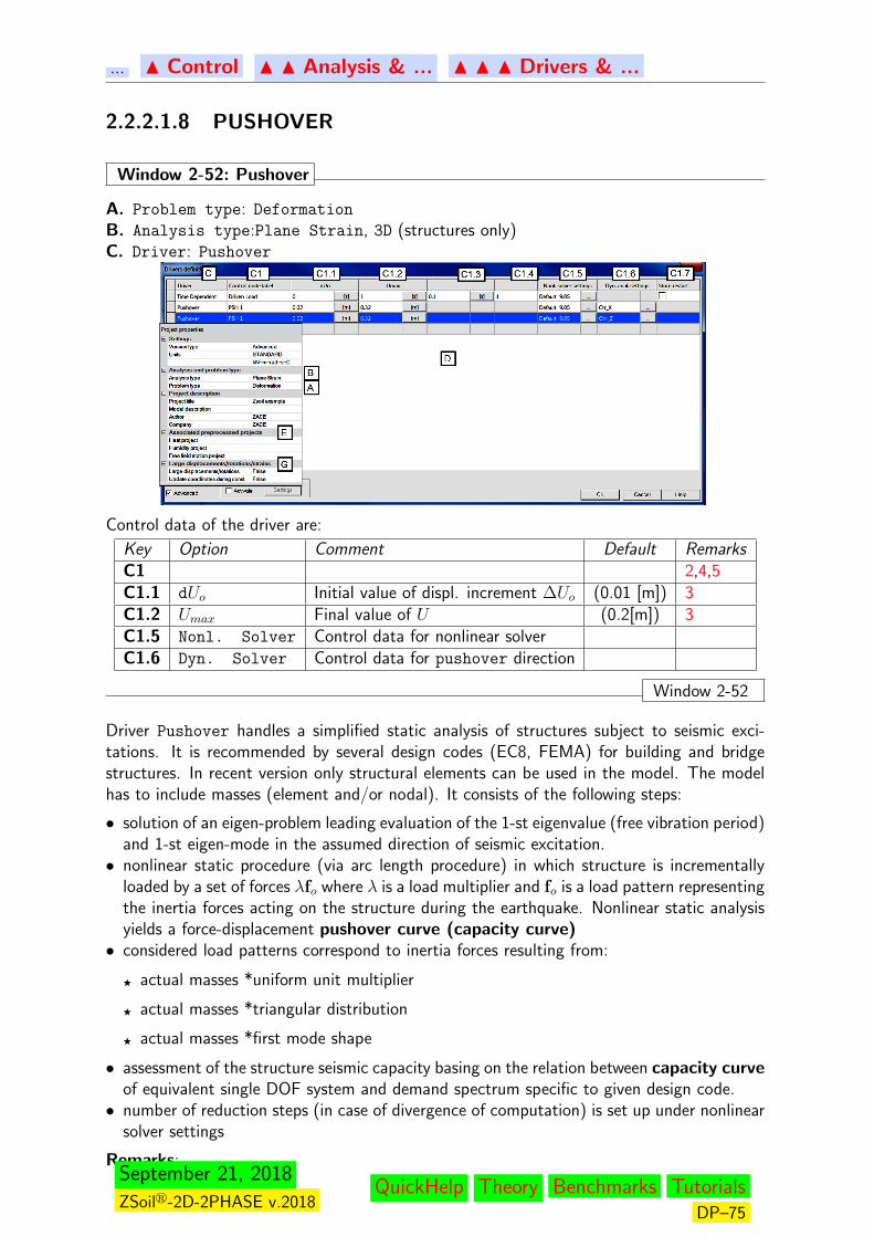
... N Control N N Analysis & ... N N N Drivers & ...
2.2.2.1.8 PUSHOVER
Window 2-52: Pushover
A. Problem type: Deformation
B. Analysis type:Plane Strain, 3D (structures only)C. Driver: Pushover
Control data of the driver are:
Key Option Comment Default RemarksC1 2,4,5C1.1 dUo Initial value of displ. increment ∆Uo (0.01 [m]) 3C1.2 Umax Final value of U (0.2[m]) 3C1.5 Nonl. Solver Control data for nonlinear solverC1.6 Dyn. Solver Control data for pushover direction
Window 2-52
Driver Pushover handles a simplified static analysis of structures subject to seismic exci-tations. It is recommended by several design codes (EC8, FEMA) for building and bridgestructures. In recent version only structural elements can be used in the model. The modelhas to include masses (element and/or nodal). It consists of the following steps:
• solution of an eigen-problem leading evaluation of the 1-st eigenvalue (free vibration period)and 1-st eigen-mode in the assumed direction of seismic excitation.• nonlinear static procedure (via arc length procedure) in which structure is incrementally
loaded by a set of forces λfo where λ is a load multiplier and fo is a load pattern representingthe inertia forces acting on the structure during the earthquake. Nonlinear static analysisyields a force-displacement pushover curve (capacity curve)• considered load patterns correspond to inertia forces resulting from:
F actual masses *uniform unit multiplier
F actual masses *triangular distribution
F actual masses *first mode shape
• assessment of the structure seismic capacity basing on the relation between capacity curveof equivalent single DOF system and demand spectrum specific to given design code.• number of reduction steps (in case of divergence of computation) is set up under nonlinear
solver settings
Remarks:September 21, 2018
ZSoilr-2D-2PHASE v.2018QuickHelp Theory Benchmarks Tutorials
DP–75
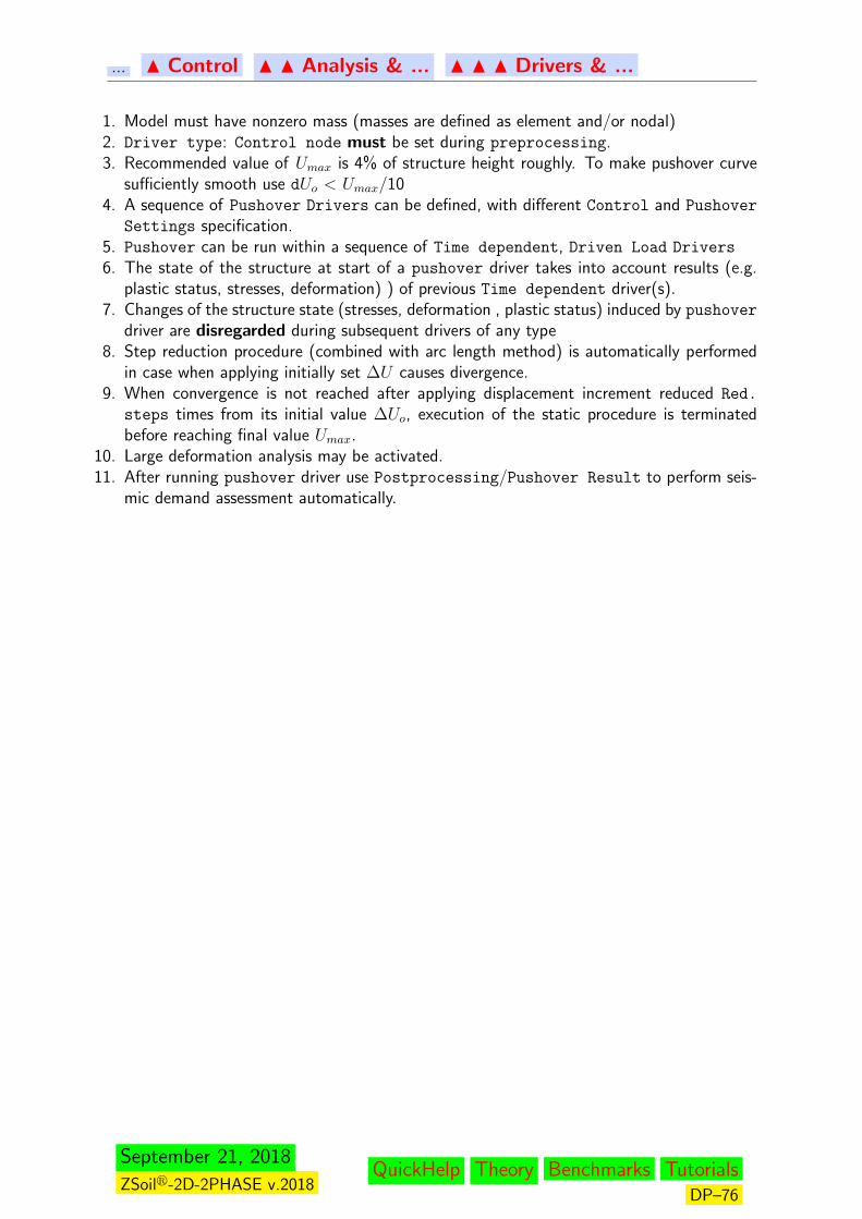
... N Control N N Analysis & ... N N N Drivers & ...
1. Model must have nonzero mass (masses are defined as element and/or nodal)2. Driver type: Control node must be set during preprocessing.3. Recommended value of Umax is 4% of structure height roughly. To make pushover curve
sufficiently smooth use dUo < Umax/104. A sequence of Pushover Drivers can be defined, with different Control and Pushover
Settings specification.5. Pushover can be run within a sequence of Time dependent, Driven Load Drivers
6. The state of the structure at start of a pushover driver takes into account results (e.g.plastic status, stresses, deformation) ) of previous Time dependent driver(s).
7. Changes of the structure state (stresses, deformation , plastic status) induced by pushover
driver are disregarded during subsequent drivers of any type8. Step reduction procedure (combined with arc length method) is automatically performed
in case when applying initially set ∆U causes divergence.9. When convergence is not reached after applying displacement increment reduced Red.
steps times from its initial value ∆Uo, execution of the static procedure is terminatedbefore reaching final value Umax.
10. Large deformation analysis may be activated.11. After running pushover driver use Postprocessing/Pushover Result to perform seis-
mic demand assessment automatically.
September 21, 2018
ZSoilr-2D-2PHASE v.2018QuickHelp Theory Benchmarks Tutorials
DP–76
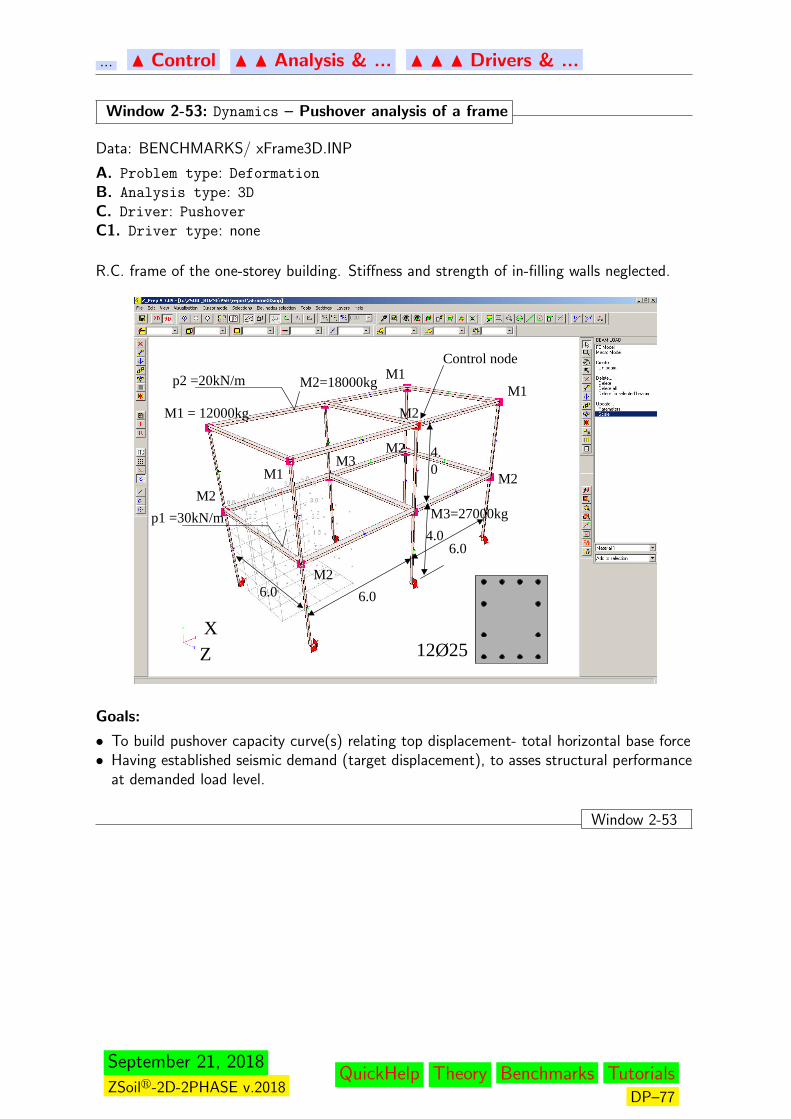
... N Control N N Analysis & ... N N N Drivers & ...
Window 2-53: Dynamics – Pushover analysis of a frame
Data: BENCHMARKS/ xFrame3D.INP
A. Problem type: Deformation
B. Analysis type: 3D
C. Driver: Pushover
C1. Driver type: none
R.C. frame of the one-storey building. Stiffness and strength of in-filling walls neglected.
6.0
6.0
6.0
4.0
4.0
p2 =20kN/m
p1 =30kN/m
Control node
M1 = 12000kg
M1
M1M1
M2=18000kg
M2
M2
M2
M2
M2M3
M3=27000kg
12Ø25XZ
Goals:
• To build pushover capacity curve(s) relating top displacement- total horizontal base force• Having established seismic demand (target displacement), to asses structural performance
at demanded load level.
Window 2-53
September 21, 2018
ZSoilr-2D-2PHASE v.2018QuickHelp Theory Benchmarks Tutorials
DP–77
... N Control N N Analysis & ... N N N Drivers & ...
Window 2-54: Pushover – Results
Original (multi-DOF) capacity curves for two pushover runsMulti DOF Capacity Curve
0
200
400
600
800
1000
1200
0 0.05 0.1 0.15 0.2 0.25 0.3 0.35
d [m]
V [k
N]
Vb (PSH 1/Ctr_X)Vb (PSH 1/Ctrl_Z)
Seismic demand assessment using EC8 design spectrum (under Menu / Results / Pushover
results)
displacement demand
Remarks:1. The demand of the building is given by the design spectrum provided by the design codes
transformed to ADRS format.2. In order to compare the capacity curve to the demand curve given by the design spectrum,
the nonlinear pushover curves of the multi-DOF system are first transformed to equivalentsingle-DOF SDOF, then are approximated by elastic-perfectly plastic (or bilinear) curves
3. After evaluation of target displacement during seismic demand assessment automatic pro-cedure, all static analysis results (including deformation, internal forces), giving hints onperformance of the structure under given seismic event, can be traced at the demandedlevel of control displacement
Window 2-54
Related Topics
Data Preparation:• DRIVERS AND DRIVERS TYPES• PUSHOVER
September 21, 2018
ZSoilr-2D-2PHASE v.2018QuickHelp Theory Benchmarks Tutorials
DP–78
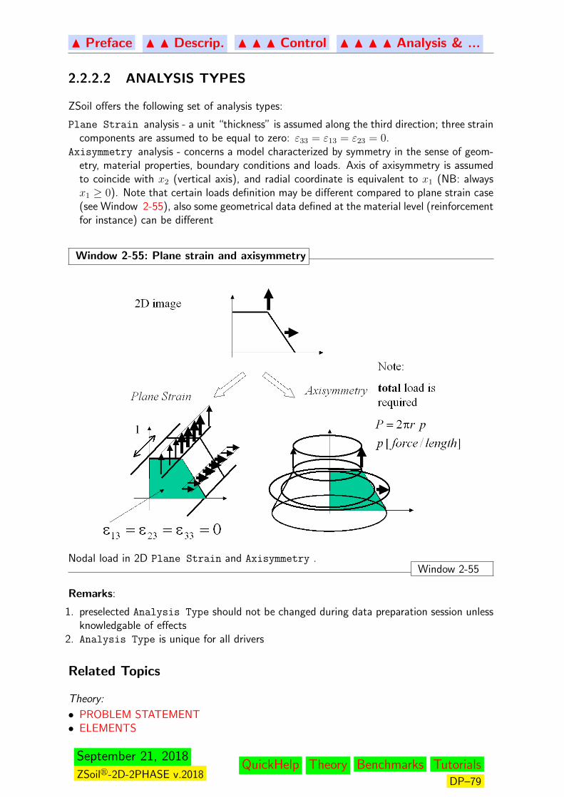
N Preface N N Descrip. N N N Control N N N N Analysis & ...
2.2.2.2 ANALYSIS TYPES
ZSoil offers the following set of analysis types:
Plane Strain analysis - a unit “thickness” is assumed along the third direction; three straincomponents are assumed to be equal to zero: ε33 = ε13 = ε23 = 0.
Axisymmetry analysis - concerns a model characterized by symmetry in the sense of geom-etry, material properties, boundary conditions and loads. Axis of axisymmetry is assumedto coincide with x2 (vertical axis), and radial coordinate is equivalent to x1 (NB: alwaysx1 ≥ 0). Note that certain loads definition may be different compared to plane strain case(see Window 2-55), also some geometrical data defined at the material level (reinforcementfor instance) can be different
Window 2-55: Plane strain and axisymmetry
Nodal load in 2D Plane Strain and Axisymmetry .Window 2-55
Remarks:
1. preselected Analysis Type should not be changed during data preparation session unlessknowledgable of effects
2. Analysis Type is unique for all drivers
Related Topics
Theory:
• PROBLEM STATEMENT• ELEMENTS
September 21, 2018
ZSoilr-2D-2PHASE v.2018QuickHelp Theory Benchmarks Tutorials
DP–79
N Preface fs N N Descrip. N N N Control N N N N Analysis & ...
2.2.2.3 ASSOCIATED PREPROCESSED PROJECTS
Decoupled thermo-mechanical or moisture-mechanical problems can be solved in two steps.The thermal/hygral problem is solved first. Results of Heat Transfer and Humidity
Transfer projects can then be reused as an input for subsequent Deformation analyzesrun to compute stresses caused by imposed thermal and/or hygral strains.
The dynamic time history analysis to be carried out with aid of the Domain Reduction Method(DRM) has to be run in two steps. In the first one the free field motion is found by runningtime history analysis of a simple model (shear layer for instance). Results of this simple model(displacements, velocities and accelerations) are then reused by the DRM method to find theresponse of the soil-structure interaction model that includes relatively low number of degreesof freedom.
• Heat Transfer project, if associated with Deformation (+Flow), includes time depen-dent temperature field used to compute thermal strains in computational domain. Thermaldilatancy coefficient is specified at the material level (group Heat) of deformation project• Humidity Transfer project, if associated with Deformation (+Flow), includes time
dependent humidity field used to compute hygral strains in computational domain. Hygraldilatancy coefficient is specified at the material level (group Humidity) of deformationproject• Free field motion project includes displacement, velocity and acceleration time histories
to be applied to the set of continuum elements selected as a DRM boundary layer.
Remarks:
• Computational models for Heat and Humidity analyses may include exclusively continuumand convection elements (in case of heat analysis convection/radiation elements can alsobe used) (truss, membrane, shell, beam elements may appear in the model but will beignored during computation)• Meshes used for Heat Humidity and later on for Deformation(+Flow) analyses can be
all different• Time scale for Heat Humidity and later on Deformation(+Flow) analyses must be
coherent• Increments of imposed strains are computed based on temperature and/or humidity incre-
ment computed for two time instances tN+1 and tN ; for that reason a single steady statethermal solution will yield zero thermal strains (as the reference temperature is equivalentto the current one, hence no temperature change is detected)• To take an effect of variation of thermal/or hygral strains in structural elements like
beams or shells a layered approach must be activated (for corresponding material modelsNon--Linear checkbox in the material dialog box must be activated); corresponding tem-peratures and/or humidities will be projected from Heat and/or Humidity mesh to anyintegration point in beam or shell cross section• First running of Deformation(+Flow) problem with preprocessed thermal and/or humidity
fields takes a considerable amount of time due to the fact that each integration point incontinuum, shell, beam, membrane or truss element must be projected onto Heat and/orHumidity mesh• To learn on how to build DRM models for dynamic soil-structure interaction problems,
please refer to the dedicated report
September 21, 2018
ZSoilr-2D-2PHASE v.2018QuickHelp Theory Benchmarks Tutorials
DP–80

N Preface fs N N Descrip. N N N Control N N N N Analysis & ...
Related Topics• Data Preparation:F HEAT TRANSFERF HUMIDITY TRANSFERF HEAT TRANSFER DATA GROUPF HUMIDITY TRANSFER DATA GROUP• Theory:F PROBLEM STATEMENTF HEAT TRANSFER
September 21, 2018
ZSoilr-2D-2PHASE v.2018QuickHelp Theory Benchmarks Tutorials
DP–81
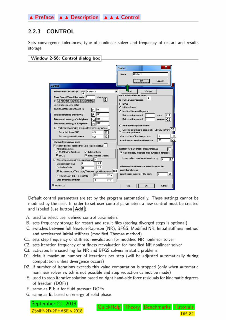
N Preface N N Description N N N Control
2.2.3 CONTROL
Sets convergence tolerances, type of nonlinear solver and frequency of restart and resultsstorage.
Window 2-56: Control dialog box
Default control parameters are set by the program automatically. These settings cannot bemodified by the user. In order to set user control parameters a new control must be createdand labeled (use button Add ).
A. used to select user defined control parametersB. sets frequency storage for restart and result files (storing diverged steps is optional)C. switches between full Newton-Raphson (NR), BFGS, Modified NR, Initial stiffness method
and accelerated initial stiffness (modified Thomas method)C1. sets step frequency of stiffness reevaluation for modified NR nonlinear solverC2. sets iteration frequency of stiffness reevaluation for modified NR nonlinear solverC3. activates line searching for NR and BFGS solvers in static problemsD1. default maximum number of iterations per step (will be adjusted automatically during
computation unless divergence occurs)D2. if number of iterations exceeds this value computation is stopped (only when automatic
nonlinear solver switch is not possible and step reduction cannot be made)E. used to stop iterative solution based on right hand-side force residuals for kinematic degrees
of freedom (DOFs)F. same as E but for fluid pressure DOFsG. same as E, based on energy of solid phase
September 21, 2018
ZSoilr-2D-2PHASE v.2018QuickHelp Theory Benchmarks Tutorials
DP–82

N Preface N N Description N N N Control
H. same as G, based on energy of fluid phaseI. contrary to the standard load control most cases kinematic loading programs require sharper
convergence tolerances; therefore tolerance for the RHS norm as well as the one for thesolid energy have to be decreased
I1. sets reduction factor for the RHS tolerance to be used in kinematic loading programs(standard tolerance defined in (E) will be multiplied by the factor given in (I1))
I2. sets reduction factor for the energy tolerance to be used in kinematic loading programs(standard tolerance defined in (G) will be multiplied by the factor given in (I2))
J. allows to try to use different nonlinear solvers once the assumed one fails to converge(certain drivers require specific nonlinear solvers; therefore user setting will be changed inthe calculation module automatically; for instance steady state seepage analysis requiresdamped NR method to be used); the general rule is such that for 3D models we do alwaystry to start from BFGS nonlinear solver while for 2D ones we do start from full NR bydefault; it is also possible to to setup active nonlinear solvers
K. flag that activates automatic step reduction in case of divergence of a given step; this optionis meaningful for Initial state, Stability, Time Dependent drivers and Transient
dynamics
K1. sets maximum number of step reduction trialsK2. value of the factor that reduces step size (∆t, SF or increment of gravity load for the
Initial state)K3. activates adaptive time step (for Time dependent or Transient dynamics drivers) am-
plification (if previously the step was reduced)K3a. time step size can be amplified when ratio of number of iterations needed to achieve the
convergence state to the declared max. number of iterations per step (D1) is less thangiven value
K3b. time step size, if possible, will be amplified by a given factor (larger than 1.0 but less than1.0 divided by the reduction factor K2)
L. flag that allows the calculation module to increase maximum number of iterations oncethe iterative scheme is converging slowly
L1. once the flag (L) is set on maximum number of iterations will be increased by a given valueM. once the absolute maximum number of iterations (D2) is exceeded the RHS tollerance is
amplified by a given factor
Remarks:1. No user input mandatory, the screen is initialized with default values2. In case of convergence problems, especially for softening materials, use Initial stiffness
stiffness method3. Activating line searches for NR and BFGS solvers may help to stabilize convergence4. During run one may trace the convergence status interactively through the calculation
module dialog box (one may modify convergence tolerances and enforce the calculationmodule to skip to the next step, or skip to the next nonlinear solver)
Window 2-56
Related Topics
Theory• ALGORITHMS
September 21, 2018
ZSoilr-2D-2PHASE v.2018QuickHelp Theory Benchmarks Tutorials
DP–83
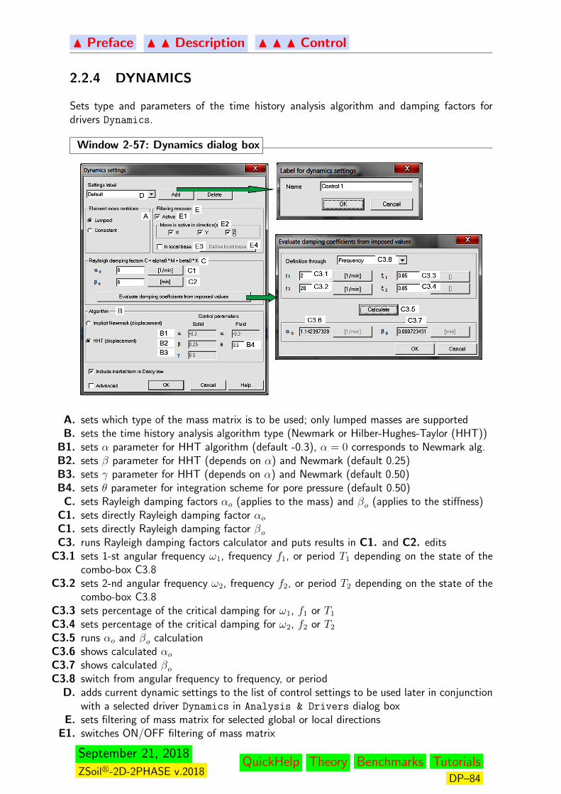
N Preface N N Description N N N Control
2.2.4 DYNAMICS
Sets type and parameters of the time history analysis algorithm and damping factors fordrivers Dynamics.
Window 2-57: Dynamics dialog box
A. sets which type of the mass matrix is to be used; only lumped masses are supportedB. sets the time history analysis algorithm type (Newmark or Hilber-Hughes-Taylor (HHT))
B1. sets α parameter for HHT algorithm (default -0.3), α = 0 corresponds to Newmark alg.B2. sets β parameter for HHT (depends on α) and Newmark (default 0.25)B3. sets γ parameter for HHT (depends on α) and Newmark (default 0.50)B4. sets θ parameter for integration scheme for pore pressure (default 0.50)
C. sets Rayleigh damping factors αo (applies to the mass) and βo (applies to the stiffness)C1. sets directly Rayleigh damping factor αoC1. sets directly Rayleigh damping factor βoC3. runs Rayleigh damping factors calculator and puts results in C1. and C2. edits
C3.1 sets 1-st angular frequency ω1, frequency f1, or period T1 depending on the state of thecombo-box C3.8
C3.2 sets 2-nd angular frequency ω2, frequency f2, or period T2 depending on the state of thecombo-box C3.8
C3.3 sets percentage of the critical damping for ω1, f1 or T1C3.4 sets percentage of the critical damping for ω2, f2 or T2C3.5 runs αo and βo calculationC3.6 shows calculated αoC3.7 shows calculated βoC3.8 switch from angular frequency to frequency, or period
D. adds current dynamic settings to the list of control settings to be used later in conjunctionwith a selected driver Dynamics in Analysis & Drivers dialog box
E. sets filtering of mass matrix for selected global or local directionsE1. switches ON/OFF filtering of mass matrix
September 21, 2018
ZSoilr-2D-2PHASE v.2018QuickHelp Theory Benchmarks Tutorials
DP–84

N Preface N N Description N N N Control
E2. selects active directions for mass matrixE3. selects local or global coordinate system to filter mass matrix along selected directionsE4. activates a dialog box to set up the local coordinate system for mass filtering (note that
for local systems defined through the vector in 3D only filtering in the local X direction(vector direction) is meaningful as the other two directions are not defined in a uniquemanner)
Remark:Assumed damping factors apply to all materials unless overwritten locally in Materials
Window 2-57
Related TopicsTheory
• ALGORITHMS
September 21, 2018
ZSoilr-2D-2PHASE v.2018QuickHelp Theory Benchmarks Tutorials
DP–85

N Preface N N Description N N N Pushover
2.2.5 PUSHOVER
Sets parameters for drivers: Pushover
Window 2-58: Pushover dialog box
A
B
D
B1B2B3
D1D2D3
D4D5D6
C
A. sets which type of the mass matrix (to extract the first mode) is to be used; only lumpedmasses are supported
B. activates mass matrix filtering according to the direction vector (masses on that directionwill only be active) (this can be necessary to isolate properly the first mode)
B1. sets x component of the direction vectorB1. as above but y directionB3. as above but z direction (meaningful for 3D problems)
C. adds current pushover settings to the list of control settings to be used later in conjunctionwith a selected driver Pushover in Analysis & Drivers dialog box
D. selects pushover force pattern (Modal/Uniform/Linear) (Modal is equivalent to the shapeof the first eigenmode)
D1. force gradient for the Linear pattern in X directionD2. as above but for Y directionD2. as above but for Z directionE1. X coordinate of the reference point (where F=0) for the Linear patternE2. as above but Y coordinateE2. as above but Z coordinate
Window 2-58
Related Topics
Theory:
• ALGORITHMS
September 21, 2018
ZSoilr-2D-2PHASE v.2018QuickHelp Theory Benchmarks Tutorials
DP–86
NPreface NNDescription NNNControl
2.2.6 CONTACT ALGORITHM
This option is meaningful exclusively for computational models including small or largedeformation contact elements6. It applies both to the contact interfaces working in thecontinuity mode and true frictional contact interfaces. A common problem of the standardpenalty approach used for problems of contacting elasto-plastic media is that the resultingover-penetration is too large and contact stresses may be underestimated. Using high valuesfor penalty stiffness we may observe loss of convergence and oscillatory contact stress distri-butions. In the case of soil-structure interaction the stress resultants in structural elements(beams, shells) may be underestimated as well. To handle this deficiency an AugmentedLagrangian Approach can be used. In the current contact formulation (segment to segmentapproach for small deformations and node-segment for large deformations) each time thestate of global static equilibrium is achieved, penalty stiffness is increased (by default byfactor of 2).
The following control parameters (group A) have to be set once the Augmented Lagrangianapproach is activated (see Window 2-59)
1. Maximum number of augmentations (do not exceed 5 as each augmentation increasescomputational cost)
2. Maximum acceptable value of over-penetration
3. Penalty stiffness multiplier (default is 2.0); at each augmentation step contact stiffness isamplified by this factor in order to speedup the convergence (if the initial contact stiffnessis relatively large this parameter must be kept equal to 1.0)
4. Maximum allowed value of the amplification factor for contact penalty stiffness (defaultis 100.0); if we would assume the stiffness multiplier equal to 10.0 then after the secondaugmentation the total amplification factor would be equal to 100.0; hence after secondaugmentation stiffness would not be amplified
Contact frictional interfaces may frequently cause lack of convergence or divergence of iter-ative schemes. This usually happens when oscillatory switches from stick/sliding to openingoccur. In order to damp this effect one may activate extra numerical damping (group C ofparameters in the dialog) in which current tangent stiffness is perturbed by the elastic oneusing the following scheme (value of α is usually problem dependent)
K = (1− f)Kep + fKe
f = exp(−α iter2)
For contact interfaces working in the continuity mode we use the same computational methodas for standard frictional ones but Coulomb’s friction law and tensile cut-off are neglected.In some situations we may observe that the displacement or pressure continuity conditionis not satisfied to an assumed level of accuracy. To correct this defficiency we may amplifyautomatically set (by the calculation module) penalty stiffness (for continuity mode interfacesdefault amplification factors are 102 times larger than for the frictional ones) by a given
6concerns versions: ACADEMIC, PROFESSIONAL, EXPERT only
September 21, 2018
ZSoilr-2D-2PHASE v.2018QuickHelp Theory Benchmarks Tutorials
DP–87

NPreface NNDescription NNNControl
coefficient. This can be made independently for the solid phase (continuity of displacements)and fluid one (continuity of pore water pressures) (group B of parameters in dialog box).
Window 2-59: Control parameters for handling true frictional contact/continuity interfaces
Control data for true frictional contact/continuity interfaces
Window 2-59
For the detailed explanation of the above settings see the theory under:
Related Topics
Theory:
• INTERFACES• CONTACT• AUGMENTED LAGRANGIAN APPROACH
September 21, 2018
ZSoilr-2D-2PHASE v.2018QuickHelp Theory Benchmarks Tutorials
DP–88

NPreface NNDescription NNNControl
2.2.7 LINEAR EQUATION SOLVERS
Window 2-60: Selection of linear equation solver
The two linear equations solvers can be used:
• Skyline - based on Cholesky’s decomposition; this solver is recommended for 2D prob-lems as it has very good diagnostics for detection of singularities• Sparse - based on Gauss elimination; this powerful solver is recommended for large 2D
and 3D computations; however it does not have extended diagnostic tools as skyline does;this solver may be run in core or out of core mode; the latter version is recommended whensolving large problems on machines with insufficient RAM size.
Remark:
This setting is saved with a given project but can also be used as a global setting for all newprojects (use Save settings in CFG button in the dialog box).
Window 2-60
September 21, 2018
ZSoilr-2D-2PHASE v.2018QuickHelp Theory Benchmarks Tutorials
DP–89
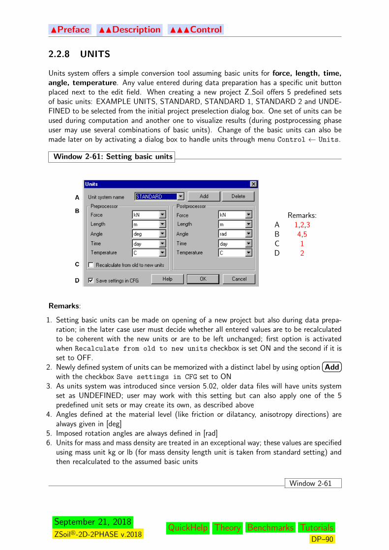
NPreface NNDescription NNNControl
2.2.8 UNITS
Units system offers a simple conversion tool assuming basic units for force, length, time,angle, temperature. Any value entered during data preparation has a specific unit buttonplaced next to the edit field. When creating a new project Z Soil offers 5 predefined setsof basic units: EXAMPLE UNITS, STANDARD, STANDARD 1, STANDARD 2 and UNDE-FINED to be selected from the initial project preselection dialog box. One set of units can beused during computation and another one to visualize results (during postprocessing phaseuser may use several combinations of basic units). Change of the basic units can also bemade later on by activating a dialog box to handle units through menu Control ← Units.
Window 2-61: Setting basic units
Remarks:A 1,2,3B 4,5C 1D 2
Remarks:
1. Setting basic units can be made on opening of a new project but also during data prepa-ration; in the later case user must decide whether all entered values are to be recalculatedto be coherent with the new units or are to be left unchanged; first option is activatedwhen Recalculate from old to new units checkbox is set ON and the second if it isset to OFF.
2. Newly defined system of units can be memorized with a distinct label by using option�� ��Add
with the checkbox Save settings in CFG set to ON3. As units system was introduced since version 5.02, older data files will have units system
set as UNDEFINED; user may work with this setting but can also apply one of the 5predefined unit sets or may create its own, as described above
4. Angles defined at the material level (like friction or dilatancy, anisotropy directions) arealways given in [deg]
5. Imposed rotation angles are always defined in [rad]6. Units for mass and mass density are treated in an exceptional way; these values are specified
using mass unit kg or lb (for mass density length unit is taken from standard setting) andthen recalculated to the assumed basic units
Window 2-61
September 21, 2018
ZSoilr-2D-2PHASE v.2018QuickHelp Theory Benchmarks Tutorials
DP–90

NPreface NNDescription NNNControl
Window 2-62: Example of units conversion
Let assume that basic units are: [kN],[m],[s],[deg],[C]. Suppose that value for Young modulusE is equal to 8000 [psi] (i.e. [lb/in2]) and we want to have it in kN/m2. To convert thevalue proceed as follows:
1. Open Materials→Elastic dialog. A default value of 100000 [kN/m2] appears in Young
modulus edit field.2. Click on the unit button next to the E edit field3. In the dialog box for units conversion set temporary units for force to [lbf] and for length
to [in]4. Enter value 8000.05. Close the dialog with button
�� ��OK6. Value of 55155.31 [kN/m2] will appear in Young modulus edit field
Window 2-62
September 21, 2018
ZSoilr-2D-2PHASE v.2018QuickHelp Theory Benchmarks Tutorials
DP–91
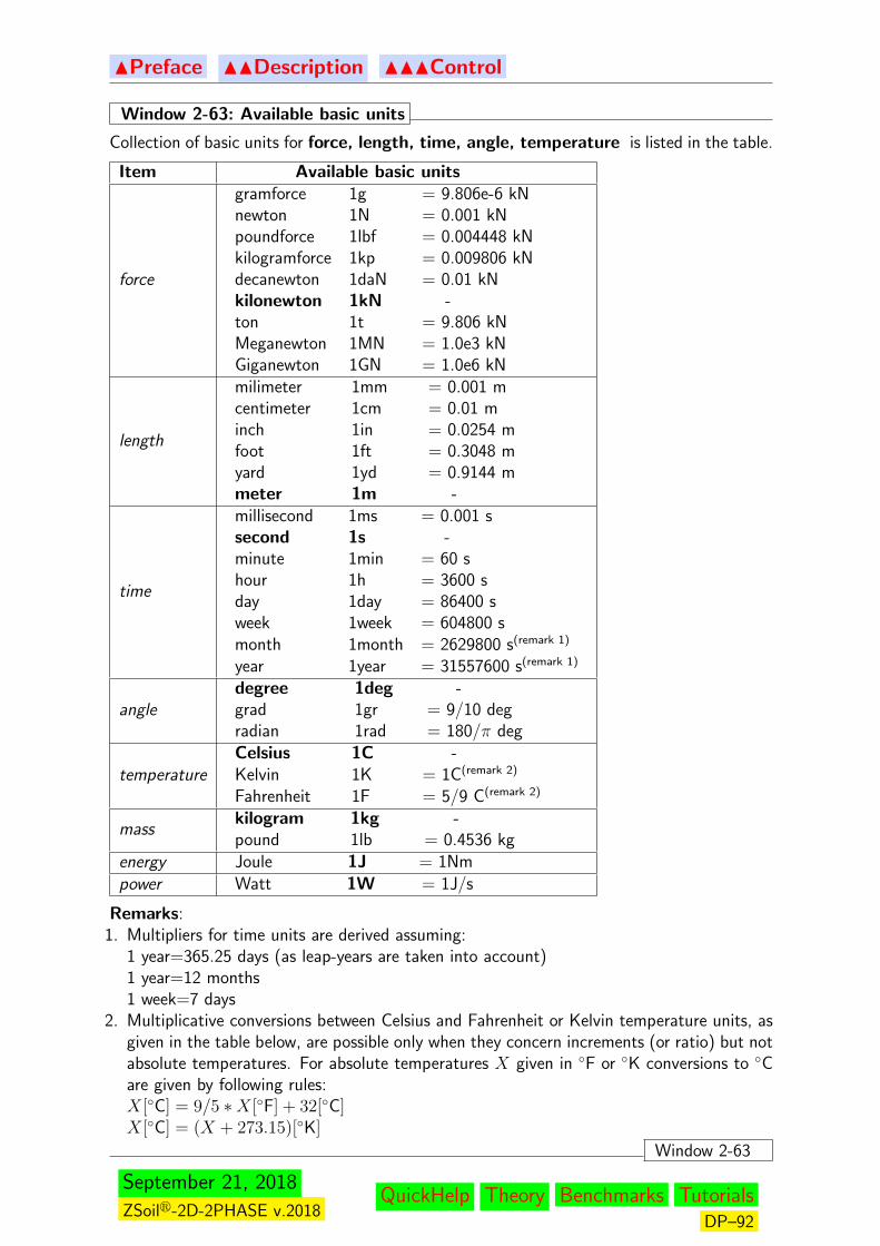
NPreface NNDescription NNNControl
Window 2-63: Available basic units
Collection of basic units for force, length, time, angle, temperature is listed in the table.
Item Available basic units
force
gramforce 1g = 9.806e-6 kNnewton 1N = 0.001 kNpoundforce 1lbf = 0.004448 kNkilogramforce 1kp = 0.009806 kNdecanewton 1daN = 0.01 kNkilonewton 1kN -ton 1t = 9.806 kNMeganewton 1MN = 1.0e3 kNGiganewton 1GN = 1.0e6 kN
length
milimeter 1mm = 0.001 mcentimeter 1cm = 0.01 minch 1in = 0.0254 mfoot 1ft = 0.3048 myard 1yd = 0.9144 mmeter 1m -
time
millisecond 1ms = 0.001 ssecond 1s -minute 1min = 60 shour 1h = 3600 sday 1day = 86400 sweek 1week = 604800 smonth 1month = 2629800 s(remark 1)
year 1year = 31557600 s(remark 1)
angledegree 1deg -grad 1gr = 9/10 degradian 1rad = 180/π deg
temperatureCelsius 1C -Kelvin 1K = 1C(remark 2)
Fahrenheit 1F = 5/9 C(remark 2)
masskilogram 1kg -pound 1lb = 0.4536 kg
energy Joule 1J = 1Nmpower Watt 1W = 1J/s
Remarks:1. Multipliers for time units are derived assuming:
1 year=365.25 days (as leap-years are taken into account)1 year=12 months1 week=7 days
2. Multiplicative conversions between Celsius and Fahrenheit or Kelvin temperature units, asgiven in the table below, are possible only when they concern increments (or ratio) but notabsolute temperatures. For absolute temperatures X given in ◦F or ◦K conversions to ◦Care given by following rules:X[◦C] = 9/5 ∗X[◦F] + 32[◦C]X[◦C] = (X + 273.15)[◦K]
Window 2-63
September 21, 2018
ZSoilr-2D-2PHASE v.2018QuickHelp Theory Benchmarks Tutorials
DP–92

NPreface NNDescription NNNControl
Window 2-64: Compound units
• Compound units consist of products or quotients of basic units. For instance, when forceunit is set to [N] and length unit is set to [mm] then the resulting unit for stresses will be[N/mm2].
• Commonly used stress compound units and their representation through basic units are asfollows:Pascal: 1 Pa=1 N/m2
kiloPascal: 1 kPa=1 kN/m2=103 N/m2
MegaPascal: 1 MPa=1 MN/m2=103 kN/m2=106N/m2
Pound force per square inch: 1 psi=6895 Pa=6.895 kPa
Window 2-64
September 21, 2018
ZSoilr-2D-2PHASE v.2018QuickHelp Theory Benchmarks Tutorials
DP–93
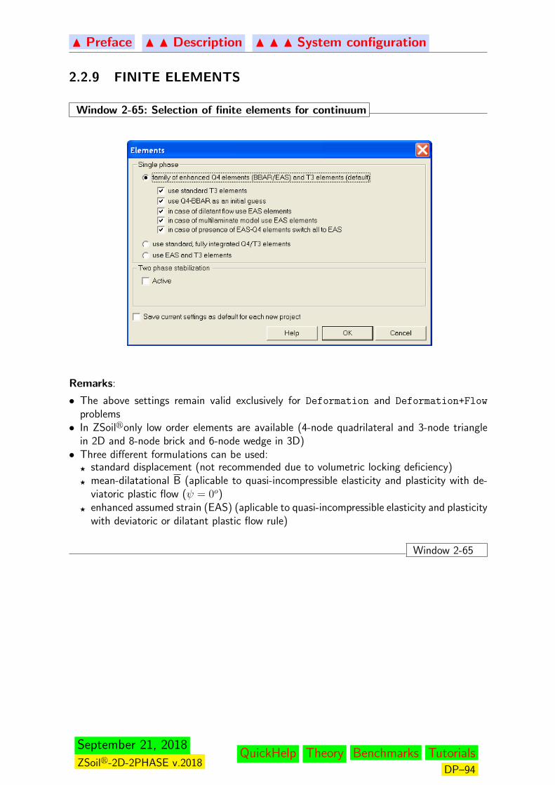
N Preface N N Description N N N System configuration
2.2.9 FINITE ELEMENTS
Window 2-65: Selection of finite elements for continuum
Remarks:
• The above settings remain valid exclusively for Deformation and Deformation+Flow
problems• In ZSoilronly low order elements are available (4-node quadrilateral and 3-node triangle
in 2D and 8-node brick and 6-node wedge in 3D)• Three different formulations can be used:F standard displacement (not recommended due to volumetric locking deficiency)F mean-dilatational B (aplicable to quasi-incompressible elasticity and plasticity with de-
viatoric plastic flow (ψ = 0o)F enhanced assumed strain (EAS) (aplicable to quasi-incompressible elasticity and plasticity
with deviatoric or dilatant plastic flow rule)
Window 2-65
September 21, 2018
ZSoilr-2D-2PHASE v.2018QuickHelp Theory Benchmarks Tutorials
DP–94
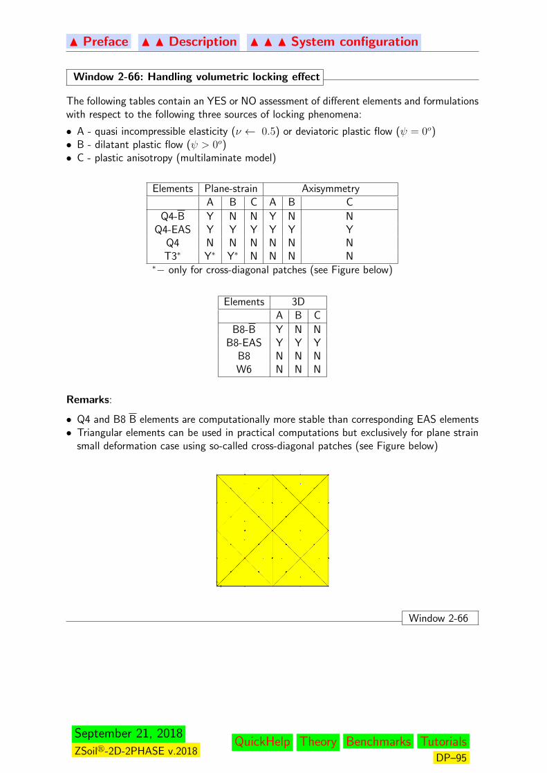
N Preface N N Description N N N System configuration
Window 2-66: Handling volumetric locking effect
The following tables contain an YES or NO assessment of different elements and formulationswith respect to the following three sources of locking phenomena:
• A - quasi incompressible elasticity (ν ← 0.5) or deviatoric plastic flow (ψ = 0o)• B - dilatant plastic flow (ψ > 0o)• C - plastic anisotropy (multilaminate model)
Elements Plane-strain AxisymmetryA B C A B C
Q4-B Y N N Y N NQ4-EAS Y Y Y Y Y Y
Q4 N N N N N NT3∗ Y∗ Y∗ N N N N
∗− only for cross-diagonal patches (see Figure below)
Elements 3DA B C
B8-B Y N NB8-EAS Y Y Y
B8 N N NW6 N N N
Remarks:
• Q4 and B8 B elements are computationally more stable than corresponding EAS elements• Triangular elements can be used in practical computations but exclusively for plane strain
small deformation case using so-called cross-diagonal patches (see Figure below)
Window 2-66
September 21, 2018
ZSoilr-2D-2PHASE v.2018QuickHelp Theory Benchmarks Tutorials
DP–95

N Preface N N Description N N N System configuration
Window 2-67: Default strategy for selection of continuum elements
The following default strategy is used for selection of optimal finite elements for continuum:
• First all Q4, B8 elements are set as B elements• If exists at least one material which exhibits dilatant plastic flow rule then all Q4, B8
elements related to that material are switched from B to EAS• If exists at least one material which corresponds to multilaminate model for rocks then all
Q4, B8 elements related to that material are switched from B to EAS• If at least one Q4 or B8 element was switched from B to EAS switch all elements to EAS
Remarks:
1. These settings can be used for current project (� Save current settings for.. is set to
OFF) but one can use them for all new projects if checkbox� Save current settings for..is set to ON
2. In order to avoid spurious pore pressure spatial oscillations for two-phase consolidationproblems (Deformation+Flow or Dynamics) and to avoid limitation put on the minimum
time step a stabilization procedure can be activated through � Two phase stabilizationcheckbox
Window 2-67
Related Topics
Theory:
• INCOMPRESSIBLE AND DILATANT MEDIA
September 21, 2018
ZSoilr-2D-2PHASE v.2018QuickHelp Theory Benchmarks Tutorials
DP–96
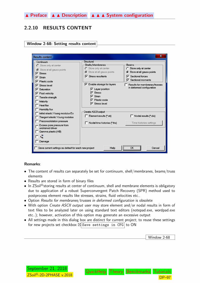
N Preface N N Description N N N System configuration
2.2.10 RESULTS CONTENT
Window 2-68: Setting results content
Remarks:
• The content of results can separately be set for continuum, shell/membranes, beams/trusselements• Results are stored in form of binary files• In ZSoilrstoring results at center of continuum, shell and membrane elements is obligatory
due to application of a robust Superconvergent Patch Recovery (SPR) method used topostprocess element results like stresses, strains, fluid velocities etc..• Option Results for membranes/trusses in deformed configuration is obsolete• With option Create ASCII output user may store element and/or nodal results in form of
text files to be analyzed later on using standard text editors (notepad.exe, wordpad.exeetc..); however, activation of this option may generate an excessive output• All settings made in this dialog box are distinct for current project; to reuse these settings
for new projects set checkbox � Save settings in CFG to ON
Window 2-68
September 21, 2018
ZSoilr-2D-2PHASE v.2018QuickHelp Theory Benchmarks Tutorials
DP–97
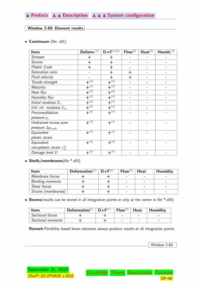
N Preface N N Description N N N System configuration
Window 2-69: Element results
• Continuum (file .s01)
Item Deform.(1) D+F(1)(2) Flow(2) Heat(3) Humid.(3)
Stresses + + - - -Strains + + - - -Plastic Code + + - - -Saturation ratio - + + - -Fluid velocity - + + - -Tensile strength +(4) +(4) - - -Maturity +(4) +(4) - - -Heat flux +(4) +(4) - - -Humidity flux +(4) +(4) - - -Initial modulus Eo +(4) +(4) - - -Unl.-rel. modulus Eur +(4) +(4) - - -Preconsolidation +(4) +(4) - - -pressure pcUndrained excess pore +(4) +(4) - - -pressure ∆pundrEquivalent +(4) +(4) - - -plastic strainEquivalent +(4) +(4) - - -viscoplastic strain εvpeqDamage level D +(4) +(4) - - -
• Shells/membranes(file *.s03)
Item Deformation(1) D+F(1) Flow(2) Heat HumidityMembrane forces + + - - -Bending moments + + - - -Shear forces + + - - -Strains (membranes) + + - - -
• Beams(results can be stored in all integration points or only at the center in file *.s04)
Item Deformation(1) D+F(1) Flow(2) Heat HumiditySectional forces + + - - -Sectional moments + + - - -
Remark:Flexibility based beam elements always produce results at all integration points
Window 2-69
September 21, 2018
ZSoilr-2D-2PHASE v.2018QuickHelp Theory Benchmarks Tutorials
DP–98
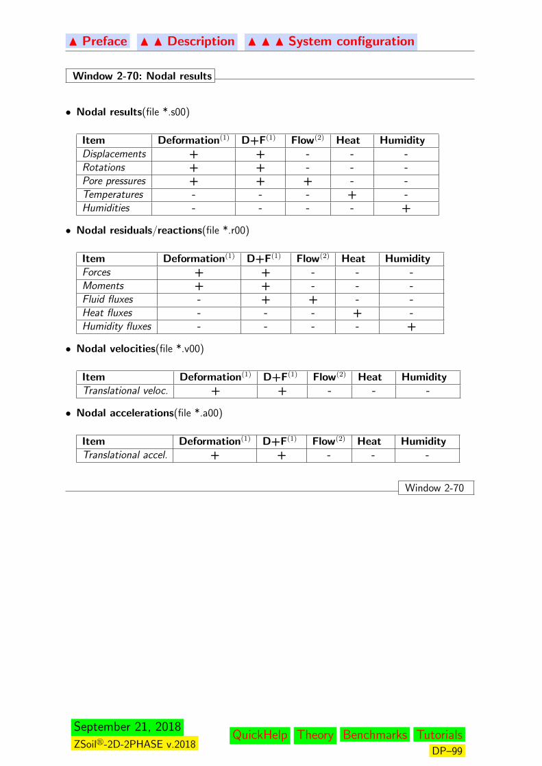
N Preface N N Description N N N System configuration
Window 2-70: Nodal results
• Nodal results(file *.s00)
Item Deformation(1) D+F(1) Flow(2) Heat HumidityDisplacements + + - - -Rotations + + - - -Pore pressures + + + - -Temperatures - - - + -Humidities - - - - +
• Nodal residuals/reactions(file *.r00)
Item Deformation(1) D+F(1) Flow(2) Heat HumidityForces + + - - -Moments + + - - -Fluid fluxes - + + - -Heat fluxes - - - + -Humidity fluxes - - - - +
• Nodal velocities(file *.v00)
Item Deformation(1) D+F(1) Flow(2) Heat HumidityTranslational veloc. + + - - -
• Nodal accelerations(file *.a00)
Item Deformation(1) D+F(1) Flow(2) Heat HumidityTranslational accel. + + - - -
Window 2-70
September 21, 2018
ZSoilr-2D-2PHASE v.2018QuickHelp Theory Benchmarks Tutorials
DP–99
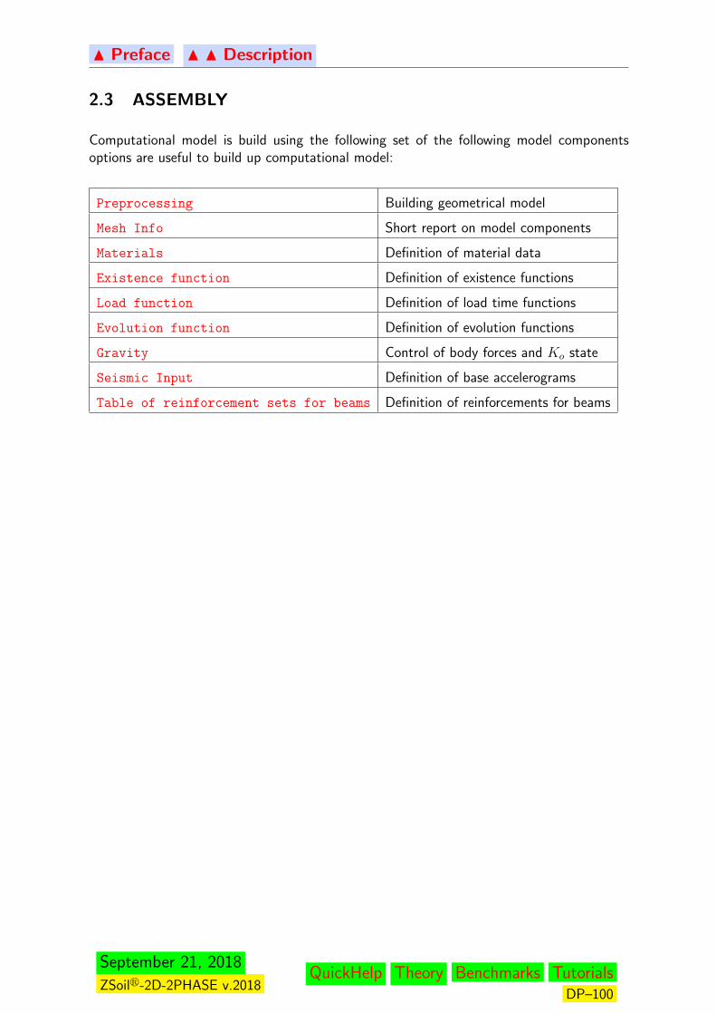
N Preface N N Description
2.3 ASSEMBLY
Computational model is build using the following set of the following model componentsoptions are useful to build up computational model:
Preprocessing Building geometrical model
Mesh Info Short report on model components
Materials Definition of material data
Existence function Definition of existence functions
Load function Definition of load time functions
Evolution function Definition of evolution functions
Gravity Control of body forces and Ko state
Seismic Input Definition of base accelerograms
Table of reinforcement sets for beams Definition of reinforcements for beams
September 21, 2018
ZSoilr-2D-2PHASE v.2018QuickHelp Theory Benchmarks Tutorials
DP–100
N Preface N N Description N N N Assembly
2.3.1 PREPROCESSING
The detailed description of all tools to be used during geometrical preprocessing are docu-mented in this section. Each tool is described first in the 2D and then in the 3D modelingcontext. Geometrical data preprocessing can be made on two basic levels:
• Macro-modeling level
• Finite Element model level
Macro-modeling is a set of CAD type tools which help the user to create geometrical modelusing basic objects like points, lines, polylines,arcs, circles, 2D/3D surfaces and 3D volumes.Using these objects as a skeleton user may then compose the geometrical model as a setof subdomains. Loads and boundary conditions can easily be applied to the macro-model.Meshing operation is treated here as a background action and it can be run several times fora given subdomain without loosing exact model geometry.
Computational model can also be built directly on the Finite Element level where elements,nodes and other model components are generated and/or updated one by one and control ofthe real model geometry is maintained by the resulting finite element mesh.
September 21, 2018
ZSoilr-2D-2PHASE v.2018QuickHelp Theory Benchmarks Tutorials
DP–101

NDescription N N Assembly N N N Preprocessing
2.3.1.1 USER INTERFACE, MAIN MENU AND BASIC TOOLS
User interface consists of the following items:
Main preprocessor window Preprocessor screen including ribbon type menus com-bined with toolbars, extra menus placed at top rightcorner and context menu placed in the right panel
September 21, 2018
ZSoilr-2D-2PHASE v.2018QuickHelp Theory Benchmarks Tutorials
DP–102
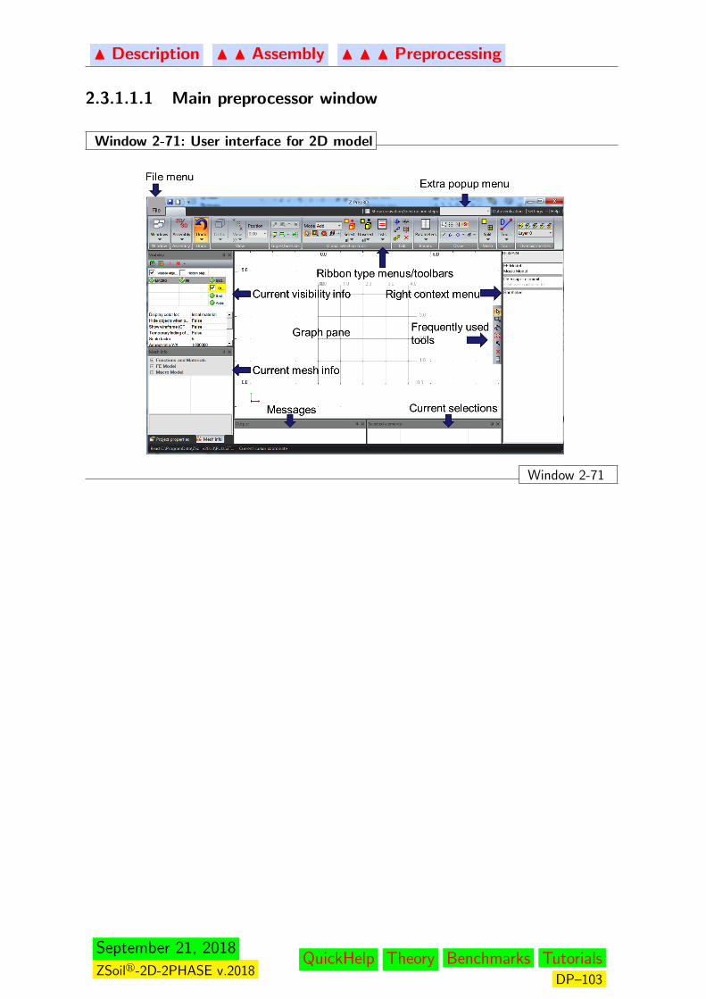
N Description N N Assembly N N N Preprocessing
2.3.1.1.1 Main preprocessor window
Window 2-71: User interface for 2D model
Window 2-71
September 21, 2018
ZSoilr-2D-2PHASE v.2018QuickHelp Theory Benchmarks Tutorials
DP–103
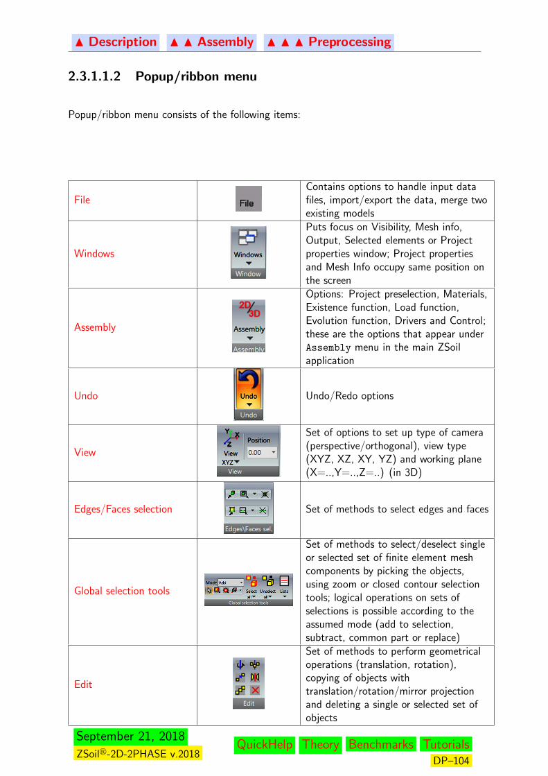
N Description N N Assembly N N N Preprocessing
2.3.1.1.2 Popup/ribbon menu
Popup/ribbon menu consists of the following items:
FileContains options to handle input datafiles, import/export the data, merge twoexisting models
Windows
Puts focus on Visibility, Mesh info,Output, Selected elements or Projectproperties window; Project propertiesand Mesh Info occupy same position onthe screen
Assembly
Options: Project preselection, Materials,Existence function, Load function,Evolution function, Drivers and Control;these are the options that appear underAssembly menu in the main ZSoilapplication
Undo Undo/Redo options
View
Set of options to set up type of camera(perspective/orthogonal), view type(XYZ, XZ, XY, YZ) and working plane(X=..,Y=..,Z=..) (in 3D)
Edges/Faces selection Set of methods to select edges and faces
Global selection tools
Set of methods to select/deselect singleor selected set of finite element meshcomponents by picking the objects,using zoom or closed contour selectiontools; logical operations on sets ofselections is possible according to theassumed mode (add to selection,subtract, common part or replace)
Edit
Set of methods to perform geometricaloperations (translation, rotation),copying of objects withtranslation/rotation/mirror projectionand deleting a single or selected set ofobjects
September 21, 2018
ZSoilr-2D-2PHASE v.2018QuickHelp Theory Benchmarks Tutorials
DP–104
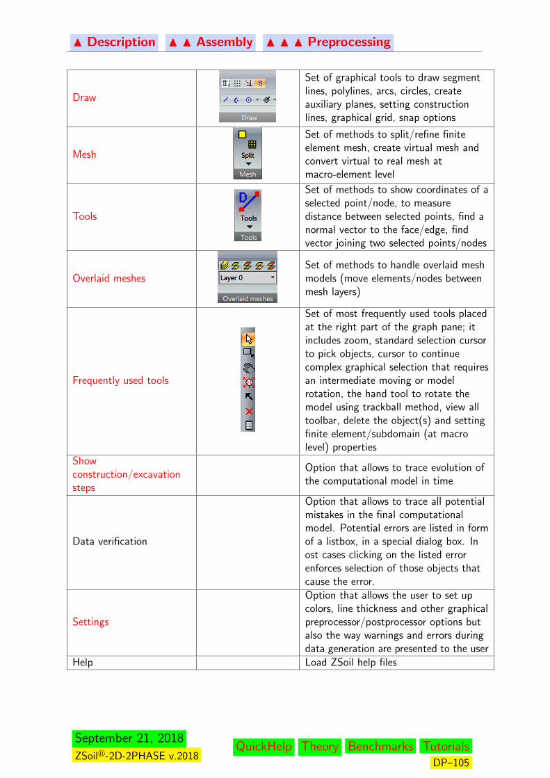
N Description N N Assembly N N N Preprocessing
Draw
Set of graphical tools to draw segmentlines, polylines, arcs, circles, createauxiliary planes, setting constructionlines, graphical grid, snap options
Mesh
Set of methods to split/refine finiteelement mesh, create virtual mesh andconvert virtual to real mesh atmacro-element level
Tools
Set of methods to show coordinates of aselected point/node, to measuredistance between selected points, find anormal vector to the face/edge, findvector joining two selected points/nodes
Overlaid meshesSet of methods to handle overlaid meshmodels (move elements/nodes betweenmesh layers)
Frequently used tools
Set of most frequently used tools placedat the right part of the graph pane; itincludes zoom, standard selection cursorto pick objects, cursor to continuecomplex graphical selection that requiresan intermediate moving or modelrotation, the hand tool to rotate themodel using trackball method, view alltoolbar, delete the object(s) and settingfinite element/subdomain (at macrolevel) properties
Showconstruction/excavationsteps
Option that allows to trace evolution ofthe computational model in time
Data verification
Option that allows to trace all potentialmistakes in the final computationalmodel. Potential errors are listed in formof a listbox, in a special dialog box. Inost cases clicking on the listed errorenforces selection of those objects thatcause the error.
Settings
Option that allows the user to set upcolors, line thickness and other graphicalpreprocessor/postprocessor options butalso the way warnings and errors duringdata generation are presented to the user
Help Load ZSoil help files
September 21, 2018
ZSoilr-2D-2PHASE v.2018QuickHelp Theory Benchmarks Tutorials
DP–105
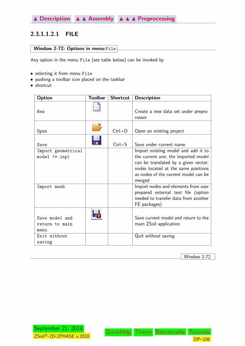
N Description N N Assembly N N N Preprocessing
2.3.1.1.2.1 FILE
Window 2-72: Options in menu:File
Any option in the menu File (see table below) can be invoked by
• selecting it from menu File
• pushing a toolbar icon placed on the taskbar• shortcut
Option Toolbar Shortcut Description
New Create a new data set under prepro-cessor
Open Ctrl+O Open an existing project
Save Ctrl+S Save under current nameImport geometrical
model (*.inp)
Import existing model and add it tothe current one; the imported modelcan be translated by a given vector;nodes located at the same positionsas nodes of the current model can bemerged
Import mesh Import nodes and elements from userprepared external text file (optionneeded to transfer data from anotherFE packages)
Save model and
return to main
menu
Save current model and return to themain ZSoil application
Exit without
saving
Quit without saving
Window 2-72
September 21, 2018
ZSoilr-2D-2PHASE v.2018QuickHelp Theory Benchmarks Tutorials
DP–106
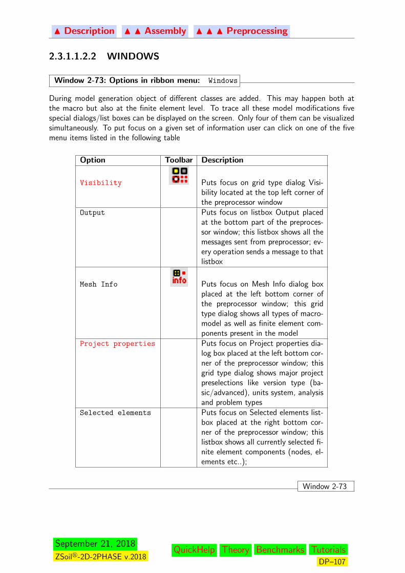
N Description N N Assembly N N N Preprocessing
2.3.1.1.2.2 WINDOWS
Window 2-73: Options in ribbon menu: Windows
During model generation object of different classes are added. This may happen both atthe macro but also at the finite element level. To trace all these model modifications fivespecial dialogs/list boxes can be displayed on the screen. Only four of them can be visualizedsimultaneously. To put focus on a given set of information user can click on one of the fivemenu items listed in the following table
Option Toolbar Description
Visibility Puts focus on grid type dialog Visi-bility located at the top left corner ofthe preprocessor window
Output Puts focus on listbox Output placedat the bottom part of the preproces-sor window; this listbox shows all themessages sent from preprocessor; ev-ery operation sends a message to thatlistbox
Mesh Info Puts focus on Mesh Info dialog boxplaced at the left bottom corner ofthe preprocessor window; this gridtype dialog shows all types of macro-model as well as finite element com-ponents present in the model
Project properties Puts focus on Project properties dia-log box placed at the left bottom cor-ner of the preprocessor window; thisgrid type dialog shows major projectpreselections like version type (ba-sic/advanced), units system, analysisand problem types
Selected elements Puts focus on Selected elements list-box placed at the right bottom cor-ner of the preprocessor window; thislistbox shows all currently selected fi-nite element components (nodes, el-ements etc..);
Window 2-73
September 21, 2018
ZSoilr-2D-2PHASE v.2018QuickHelp Theory Benchmarks Tutorials
DP–107
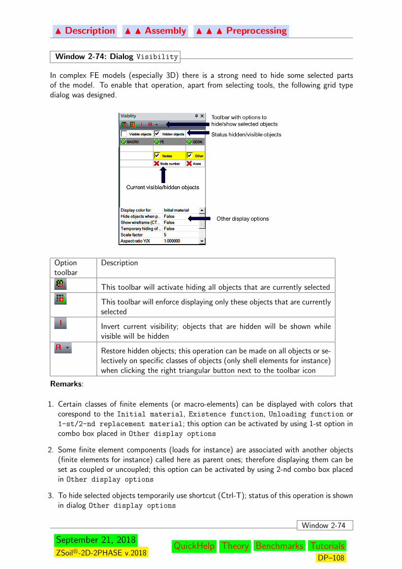
N Description N N Assembly N N N Preprocessing
Window 2-74: Dialog Visibility
In complex FE models (especially 3D) there is a strong need to hide some selected partsof the model. To enable that operation, apart from selecting tools, the following grid typedialog was designed.
Optiontoolbar
Description
This toolbar will activate hiding all objects that are currently selected
This toolbar will enforce displaying only these objects that are currentlyselected
Invert current visibility; objects that are hidden will be shown whilevisible will be hidden
Restore hidden objects; this operation can be made on all objects or se-lectively on specific classes of objects (only shell elements for instance)when clicking the right triangular button next to the toolbar icon
Remarks:
1. Certain classes of finite elements (or macro-elements) can be displayed with colors thatcorespond to the Initial material, Existence function, Unloading function or1-st/2-nd replacement material; this option can be activated by using 1-st option incombo box placed in Other display options
2. Some finite element components (loads for instance) are associated with another objects(finite elements for instance) called here as parent ones; therefore displaying them can beset as coupled or uncoupled; this option can be activated by using 2-nd combo box placedin Other display options
3. To hide selected objects temporarily use shortcut (Ctrl-T); status of this operation is shownin dialog Other display options
Window 2-74
September 21, 2018
ZSoilr-2D-2PHASE v.2018QuickHelp Theory Benchmarks Tutorials
DP–108
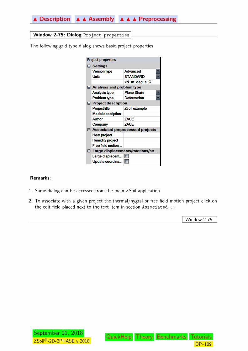
N Description N N Assembly N N N Preprocessing
Window 2-75: Dialog Project properties
The following grid type dialog shows basic project properties
Remarks:
1. Same dialog can be accessed from the main ZSoil application
2. To associate with a given project the thermal/hygral or free field motion project click onthe edit field placed next to the text item in section Associated...
Window 2-75
September 21, 2018
ZSoilr-2D-2PHASE v.2018QuickHelp Theory Benchmarks Tutorials
DP–109
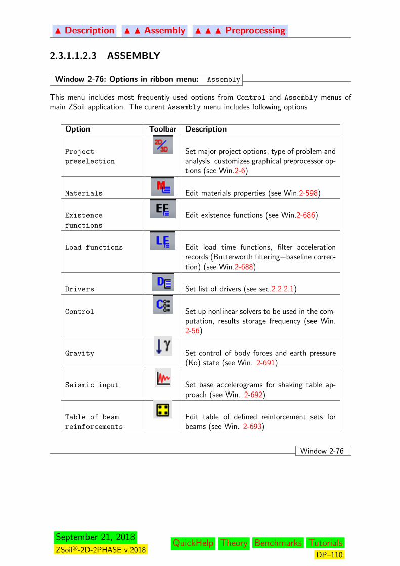
N Description N N Assembly N N N Preprocessing
2.3.1.1.2.3 ASSEMBLY
Window 2-76: Options in ribbon menu: Assembly
This menu includes most frequently used options from Control and Assembly menus ofmain ZSoil application. The curent Assembly menu includes following options
Option Toolbar Description
Project
preselection
Set major project options, type of problem andanalysis, customizes graphical preprocessor op-tions (see Win.2-6)
Materials Edit materials properties (see Win.2-598)
Existence
functions
Edit existence functions (see Win.2-686)
Load functions Edit load time functions, filter accelerationrecords (Butterworth filtering+baseline correc-tion) (see Win.2-688)
Drivers Set list of drivers (see sec.2.2.2.1)
Control Set up nonlinear solvers to be used in the com-putation, results storage frequency (see Win.2-56)
Gravity Set control of body forces and earth pressure(Ko) state (see Win. 2-691)
Seismic input Set base accelerograms for shaking table ap-proach (see Win. 2-692)
Table of beam
reinforcements
Edit table of defined reinforcement sets forbeams (see Win. 2-693)
Window 2-76
September 21, 2018
ZSoilr-2D-2PHASE v.2018QuickHelp Theory Benchmarks Tutorials
DP–110
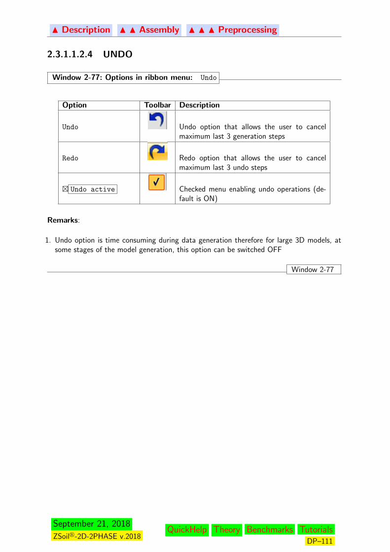
N Description N N Assembly N N N Preprocessing
2.3.1.1.2.4 UNDO
Window 2-77: Options in ribbon menu: Undo
Option Toolbar Description
Undo Undo option that allows the user to cancelmaximum last 3 generation steps
Redo Redo option that allows the user to cancelmaximum last 3 undo steps
� Undo active Checked menu enabling undo operations (de-fault is ON)
Remarks:
1. Undo option is time consuming during data generation therefore for large 3D models, atsome stages of the model generation, this option can be switched OFF
Window 2-77
September 21, 2018
ZSoilr-2D-2PHASE v.2018QuickHelp Theory Benchmarks Tutorials
DP–111

N Description N N Assembly N N N Preprocessing
2.3.1.1.2.5 VIEW
Window 2-78: Options in ribbon menu: View
Any option in menu View (see table below), which allows to control view and position of thecamera with respect to the model can be invoked by
• selecting it from menu View
• shortcut
Toolbar Shortcut Action
Ctrl+2 Set view in XY plane
Remarks:
1. To see whole model on the screen use shortcut Ctrl+F or use mouse scroll
2. To rotate camera along X axis use key X or Shift+X to rotate in the opposite direction
3. To rotate camera along Y axis use key Y or Shift+Y to rotate in the opposite direction
4. To rotate camera along Z axis use key Z or Shift+Z to rotate in the opposite direction
5. To rotate camera use right toolbar (hand); to translate camera use toolbar (hand) andpress Ctrl key (simultaneously)
Window 2-78
September 21, 2018
ZSoilr-2D-2PHASE v.2018QuickHelp Theory Benchmarks Tutorials
DP–112

N Description N N Assembly N N N Preprocessing
2.3.1.1.2.6 EDGES/FACES SELECTION
Window 2-79: Options in ribbon menu: Edges/Faces selection
Methods for edges and faces selection are organized in form of toolbars placed in two rows(see figure below). Only most frequently used options are visible. To activate more optionsa small button placed in 3-rd column has to be clicked.
Window 2-79
September 21, 2018
ZSoilr-2D-2PHASE v.2018QuickHelp Theory Benchmarks Tutorials
DP–113

N Description N N Assembly N N N Preprocessing
Window 2-80: Edges selection
Toolbar Description
Select/unselect one finite element edge
Select finite element edges which are fully covered by thezoom circle (infinite cylinder in 3D) once zoom is draggedfrom the left to the right side, or select all objects which areat least partially covered by the zoom circle once zoom isdragged from the right to the left side
Deselect all selected edges
Select finite element edges which are fully covered by thezoom circle (infinite cylinder in 3D) once zoom is draggedfrom the left to the right side, or select edges which areat least partially covered by the zoom circle once zoom isdragged from the right to the left side
Select finite element edges which are fully covered by theirregular contour
Select element edges along the line section defined by twopicked nodes
Select finite element edges which are fully covered by theirregular contour
Select finite element edges through Selection lists; han-dling this selection list is very similar to the one for selectionof elements (see Window 2-82) or nodes (see Window 2-83))
Remarks:
1. Selection by zoom box, zoom circle, irregular contour, inside box and between 2 nodesundergoes the rule set in the Selection mode
2. To select an edge inside of the computational domain (in a unique way) one of two elementsadjacent to the edge must be hidden
3. Selection of an edge inherits an information to which finite element this edge belongs;this information is of primary importance when generating seepage elements (2D) and/orapplying surface loads (2D)
Window 2-80
September 21, 2018
ZSoilr-2D-2PHASE v.2018QuickHelp Theory Benchmarks Tutorials
DP–114
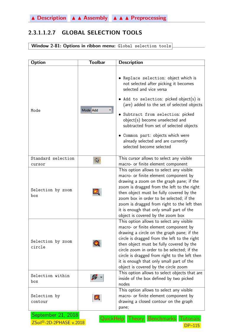
N Description N N Assembly N N N Preprocessing
2.3.1.1.2.7 GLOBAL SELECTION TOOLS
Window 2-81: Options in ribbon menu: Global selection tools
Option Toolbar Description
Mode
• Replace selection: object which isnot selected after picking it becomesselected and vice versa
• Add to selection: picked object(s) is(are) added to the set of selected objects
• Subtract from selection: pickedobject(s) become unselected andsubtracted from set of selected objects
• Common part: objects which werealready selected and are currentlyselected become selected
Standard selection
cursor
This cursor allows to select any visiblemacro- or finite element component
Selection by zoom
box
This option allows to select any visiblemacro- or finite element component bydrawing a zoom on the graph pane; if thezoom is dragged from the left to the rightthen object must be fully covered by thezoom box in order to be selected; if thezoom is dragged from right to the left thenit is enough that only small part of theobject is covered by the zoom box
Selection by zoom
circle
This option allows to select any visiblemacro- or finite element component bydrawing a circle on the graph pane; if thecircle is dragged from the left to the rightthen object must be fully covered by thecircle zoom in order to be selected; if thecircle is dragged from right to the left thenit is enough that only small part of theobject is covered by the circle zoom
Selection within
box
This option allows to select objects that areinside of the box defined by two pickednodes
Selection by
contour
This option allows to select any visiblemacro- or finite element component bydrawing a closed contour on the graphpane;
September 21, 2018
ZSoilr-2D-2PHASE v.2018QuickHelp Theory Benchmarks Tutorials
DP–115
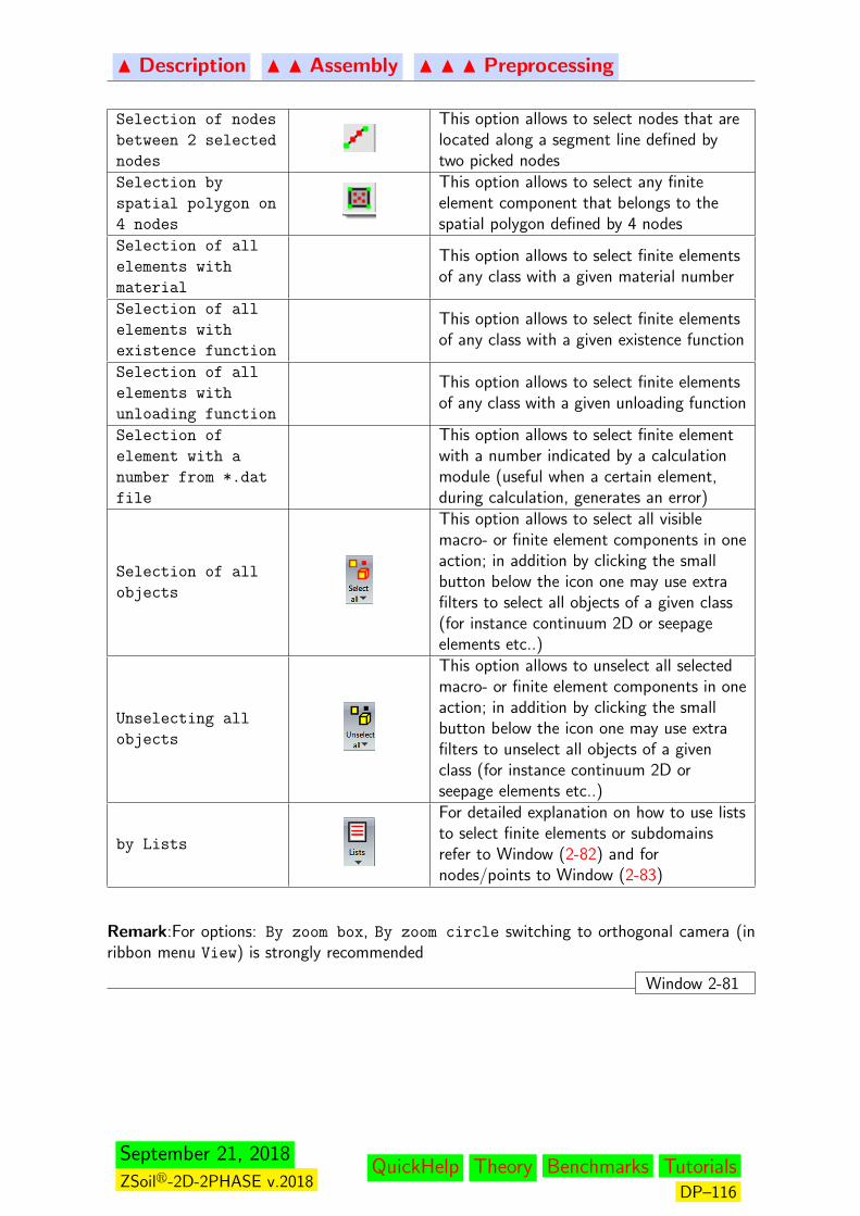
N Description N N Assembly N N N Preprocessing
Selection of nodes
between 2 selected
nodes
This option allows to select nodes that arelocated along a segment line defined bytwo picked nodes
Selection by
spatial polygon on
4 nodes
This option allows to select any finiteelement component that belongs to thespatial polygon defined by 4 nodes
Selection of all
elements with
material
This option allows to select finite elementsof any class with a given material number
Selection of all
elements with
existence function
This option allows to select finite elementsof any class with a given existence function
Selection of all
elements with
unloading function
This option allows to select finite elementsof any class with a given unloading function
Selection of
element with a
number from *.dat
file
This option allows to select finite elementwith a number indicated by a calculationmodule (useful when a certain element,during calculation, generates an error)
Selection of all
objects
This option allows to select all visiblemacro- or finite element components in oneaction; in addition by clicking the smallbutton below the icon one may use extrafilters to select all objects of a given class(for instance continuum 2D or seepageelements etc..)
Unselecting all
objects
This option allows to unselect all selectedmacro- or finite element components in oneaction; in addition by clicking the smallbutton below the icon one may use extrafilters to unselect all objects of a givenclass (for instance continuum 2D orseepage elements etc..)
by Lists
For detailed explanation on how to use liststo select finite elements or subdomainsrefer to Window (2-82) and fornodes/points to Window (2-83)
Remark:For options: By zoom box, By zoom circle switching to orthogonal camera (inribbon menu View) is strongly recommended
Window 2-81
September 21, 2018
ZSoilr-2D-2PHASE v.2018QuickHelp Theory Benchmarks Tutorials
DP–116
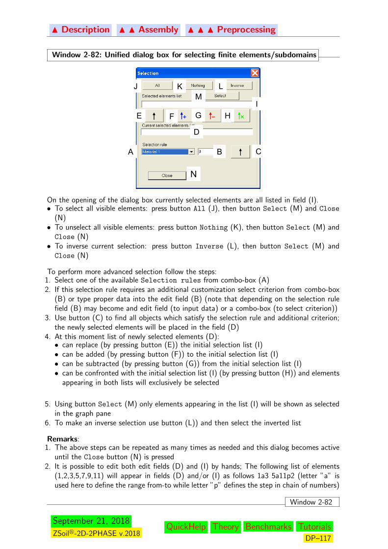
N Description N N Assembly N N N Preprocessing
Window 2-82: Unified dialog box for selecting finite elements/subdomains
A B C
D
E F G HI
J K LM
N
On the opening of the dialog box currently selected elements are all listed in field (I).• To select all visible elements: press button All (J), then button Select (M) and Close
(N)• To unselect all visible elements: press button Nothing (K), then button Select (M) andClose (N)• To inverse current selection: press button Inverse (L), then button Select (M) andClose (N)
To perform more advanced selection follow the steps:1. Select one of the available Selection rules from combo-box (A)2. If this selection rule requires an additional customization select criterion from combo-box
(B) or type proper data into the edit field (B) (note that depending on the selection rulefield (B) may become and edit field (to input data) or a combo-box (to select criterion))
3. Use button (C) to find all objects which satisfy the selection rule and additional criterion;the newly selected elements will be placed in the field (D)
4. At this moment list of newly selected elements (D):• can replace (by pressing button (E)) the initial selection list (I)• can be added (by pressing button (F)) to the initial selection list (I)• can be subtracted (by pressing button (G)) from the initial selection list (I)• can be confronted with the initial selection list (I) (by pressing button (H)) and elements
appearing in both lists will exclusively be selected
5. Using button Select (M) only elements appearing in the list (I) will be shown as selectedin the graph pane
6. To make an inverse selection use button (L)) and then select the inverted list
Remarks:1. The above steps can be repeated as many times as needed and this dialog becomes active
until the Close button (N) is pressed2. It is possible to edit both edit fields (D) and (I) by hands; The following list of elements
(1,2,3,5,7,9,11) will appear in fields (D) and/or (I) as follows 1a3 5a11p2 (letter ”a” isused here to define the range from-to while letter ”p” defines the step in chain of numbers)
Window 2-82
September 21, 2018
ZSoilr-2D-2PHASE v.2018QuickHelp Theory Benchmarks Tutorials
DP–117
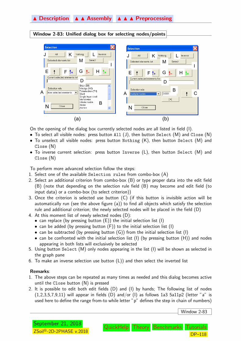
N Description N N Assembly N N N Preprocessing
Window 2-83: Unified dialog box for selecting nodes/points
A
D
E F G HI
J K LM
NB
A
D
E F G HI
J K LM
N
BC
(a) (b)
On the opening of the dialog box currently selected nodes are all listed in field (I).• To select all visible nodes: press button All (J), then button Select (M) and Close (N)• To unselect all visible nodes: press button Nothing (K), then button Select (M) andClose (N)• To inverse current selection: press button Inverse (L), then button Select (M) andClose (N)
To perform more advanced selection follow the steps:1. Select one of the available Selection rules from combo-box (A)2. Select an additional criterion from combo-box (B) or type proper data into the edit field
(B) (note that depending on the selection rule field (B) may become and edit field (toinput data) or a combo-box (to select criterion))
3. Once the criterion is selected use button (C) (if this button is invisible action will beautomatically run (see the above figure (a)) to find all objects which satisfy the selectionrule and additional criterion; the newly selected nodes will be placed in the field (D)
4. At this moment list of newly selected nodes (D):• can replace (by pressing button (E)) the initial selection list (I)• can be added (by pressing button (F)) to the initial selection list (I)• can be subtracted (by pressing button (G)) from the initial selection list (I)• can be confronted with the initial selection list (I) (by pressing button (H)) and nodes
appearing in both lists will exclusively be selected5. Using button Select (M) only nodes appearing in the list (I) will be shown as selected in
the graph pane6. To make an inverse selection use button (L)) and then select the inverted list
Remarks:1. The above steps can be repeated as many times as needed and this dialog becomes active
until the Close button (N) is pressed2. It is possible to edit both edit fields (D) and (I) by hands; The following list of nodes
(1,2,3,5,7,9,11) will appear in fields (D) and/or (I) as follows 1a3 5a11p2 (letter ”a” isused here to define the range from-to while letter ”p” defines the step in chain of numbers)
Window 2-83
September 21, 2018
ZSoilr-2D-2PHASE v.2018QuickHelp Theory Benchmarks Tutorials
DP–118

N Description N N Assembly N N N Preprocessing
2.3.1.1.2.8 EDIT
Window 2-84: Options in ribbon menu:Edit
Option Toolbar Description
Delete selected This option is used to delete a sin-gle picked object or group of selectedobjects (use shortcut Del)
Move selected This option is used to move a sin-gle picked object or group of selectedobjects by a given vector (see Win-dow (2-85))
Rotate selected This option is used to rotate a sin-gle picked object or group of selectedobjects by a given angle along givenaxis (see Window (2-86))
Copy by
translation
This option is used to copy a singlepicked object or group of selected ob-jects with a given vector ( see Win-dow (2-87))
Copy by rotation This option is used to copy a singlepicked object or group of selected ob-jects with a given vector ( see Win-dow (2-88))
Copy by symmetry This option is used to copy a singlepicked object or group of selected ob-jects by mirror projection ( see Win-dow (2-89))
Window 2-84
September 21, 2018
ZSoilr-2D-2PHASE v.2018QuickHelp Theory Benchmarks Tutorials
DP–119
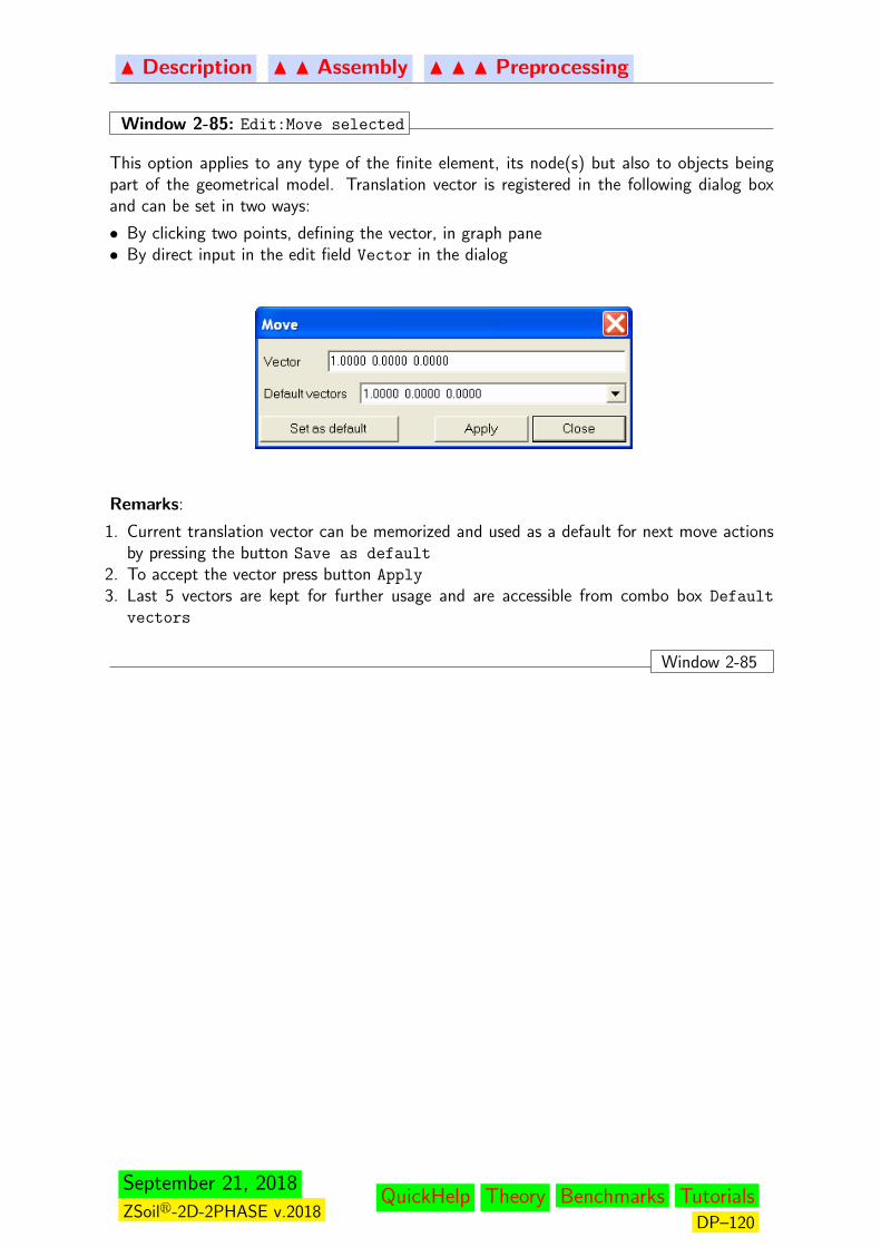
N Description N N Assembly N N N Preprocessing
Window 2-85: Edit:Move selected
This option applies to any type of the finite element, its node(s) but also to objects beingpart of the geometrical model. Translation vector is registered in the following dialog boxand can be set in two ways:
• By clicking two points, defining the vector, in graph pane• By direct input in the edit field Vector in the dialog
Remarks:
1. Current translation vector can be memorized and used as a default for next move actionsby pressing the button Save as default
2. To accept the vector press button Apply
3. Last 5 vectors are kept for further usage and are accessible from combo box Default
vectors
Window 2-85
September 21, 2018
ZSoilr-2D-2PHASE v.2018QuickHelp Theory Benchmarks Tutorials
DP–120
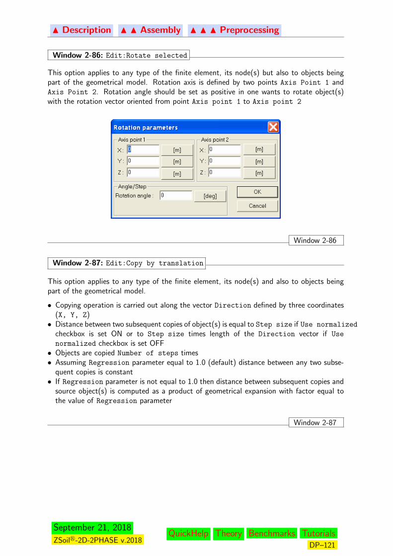
N Description N N Assembly N N N Preprocessing
Window 2-86: Edit:Rotate selected
This option applies to any type of the finite element, its node(s) but also to objects beingpart of the geometrical model. Rotation axis is defined by two points Axis Point 1 andAxis Point 2. Rotation angle should be set as positive in one wants to rotate object(s)with the rotation vector oriented from point Axis point 1 to Axis point 2
Window 2-86
Window 2-87: Edit:Copy by translation
This option applies to any type of the finite element, its node(s) and also to objects beingpart of the geometrical model.
• Copying operation is carried out along the vector Direction defined by three coordinates(X, Y, Z)• Distance between two subsequent copies of object(s) is equal to Step size if Use normalized
checkbox is set ON or to Step size times length of the Direction vector if Use
normalized checkbox is set OFF• Objects are copied Number of steps times• Assuming Regression parameter equal to 1.0 (default) distance between any two subse-
quent copies is constant• If Regression parameter is not equal to 1.0 then distance between subsequent copies and
source object(s) is computed as a product of geometrical expansion with factor equal tothe value of Regression parameter
Window 2-87
September 21, 2018
ZSoilr-2D-2PHASE v.2018QuickHelp Theory Benchmarks Tutorials
DP–121

N Description N N Assembly N N N Preprocessing
Window 2-88: Edit:Copy by rotation
This option applies to any type of the finite element, its node(s) and also to objects beingpart of the geometrical model.
• Copying operation is carried with rotation along the axis defined by two points Axis point
1, Axis point 2
• Angular distance between two subsequent copies of object(s) is equal to Rotation angle
• Objects are copied Number of steps times• Rotation angle should be set as positive in one wants to copy objects with the rotation
vector oriented from point Axis point 1 to Axis point 2
Window 2-88
Window 2-89: Edit:Copy by symmetry
This option applies to any type of the finite element, its node(s) and also to objects beingpart of the geometrical model.
• To run this option a fictitious plane must be created first• After this operation orientation (if applies) of copied objects is reversed• To initiate the action plane of symmetry must be pointed first
Window 2-89
September 21, 2018
ZSoilr-2D-2PHASE v.2018QuickHelp Theory Benchmarks Tutorials
DP–122
N Description N N Assembly N N N Preprocessing
2.3.1.1.2.9 PARAMETERS
Window 2-90: Options in ribbon menu:Parameters
Option Toolbar Description
Parameters This option is used to set Initial
material, 1-st replacement
material, 2-nd replacement
material, Existence function,Unloading function for a singlepicked element or group of selectedelements (if all are of the same class)
Window 2-90
September 21, 2018
ZSoilr-2D-2PHASE v.2018QuickHelp Theory Benchmarks Tutorials
DP–123
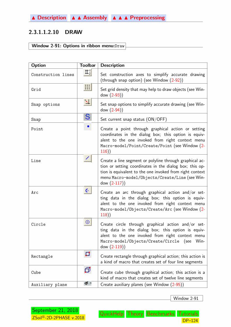
N Description N N Assembly N N N Preprocessing
2.3.1.1.2.10 DRAW
Window 2-91: Options in ribbon menu:Draw
Option Toolbar Description
Construction lines Set construction axes to simplify accurate drawing(through snap option) (see Window (2-92))
Grid Set grid density that may help to draw objects (see Win-dow (2-93))
Snap options Set snap options to simplify accurate drawing (see Win-dow (2-94))
Snap Set current snap status (ON/OFF)
Point Create a point through graphical action or settingcoordinates in the dialog box; this option is equiv-alent to the one invoked from right context menuMacro-model/Point/Create/Point (see Window (2-116))
Line Create a line segment or polyline through graphical ac-tion or setting coordinates in the dialog box; this op-tion is equivalent to the one invoked from right contextmenu Macro-model/Objects/Create/Line (see Win-dow (2-117))
Arc Create an arc through graphical action and/or set-ting data in the dialog box; this option is equiv-alent to the one invoked from right context menuMacro-model/Objects/Create/Arc (see Window (2-118))
Circle Create circle through graphical action and/or set-ting data in the dialog box; this option is equiv-alent to the one invoked from right context menuMacro-model/Objects/Create/Circle (see Win-dow (2-119))
Rectangle Create rectangle through graphical action; this action isa kind of macro that creates set of four line segments
Cube Create cube through graphical action; this action is akind of macro that creates set of twelve line segments
Auxiliary plane Create auxiliary planes (see Window (2-95))
Window 2-91
September 21, 2018
ZSoilr-2D-2PHASE v.2018QuickHelp Theory Benchmarks Tutorials
DP–124
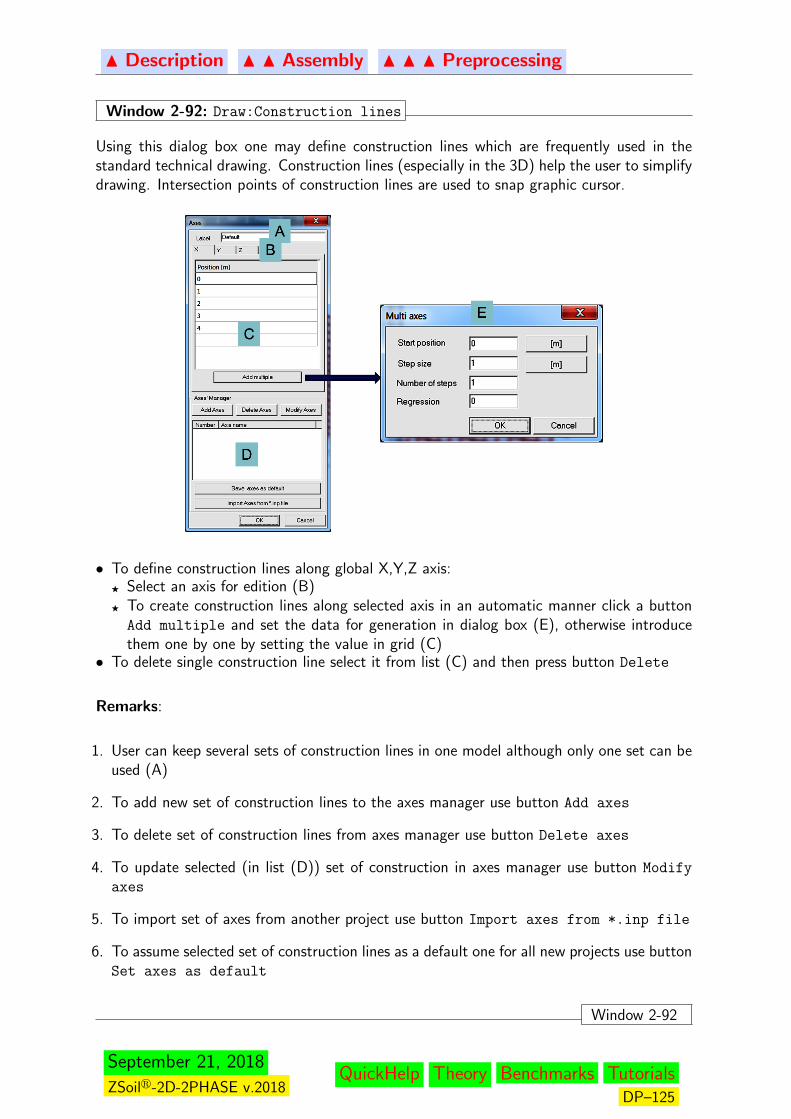
N Description N N Assembly N N N Preprocessing
Window 2-92: Draw:Construction lines
Using this dialog box one may define construction lines which are frequently used in thestandard technical drawing. Construction lines (especially in the 3D) help the user to simplifydrawing. Intersection points of construction lines are used to snap graphic cursor.
• To define construction lines along global X,Y,Z axis:F Select an axis for edition (B)F To create construction lines along selected axis in an automatic manner click a buttonAdd multiple and set the data for generation in dialog box (E), otherwise introducethem one by one by setting the value in grid (C)
• To delete single construction line select it from list (C) and then press button Delete
Remarks:
1. User can keep several sets of construction lines in one model although only one set can beused (A)
2. To add new set of construction lines to the axes manager use button Add axes
3. To delete set of construction lines from axes manager use button Delete axes
4. To update selected (in list (D)) set of construction in axes manager use button Modify
axes
5. To import set of axes from another project use button Import axes from *.inp file
6. To assume selected set of construction lines as a default one for all new projects use buttonSet axes as default
Window 2-92
September 21, 2018
ZSoilr-2D-2PHASE v.2018QuickHelp Theory Benchmarks Tutorials
DP–125
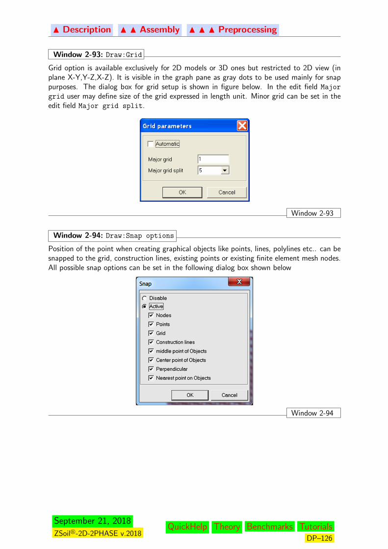
N Description N N Assembly N N N Preprocessing
Window 2-93: Draw:Grid
Grid option is available exclusively for 2D models or 3D ones but restricted to 2D view (inplane X-Y,Y-Z,X-Z). It is visible in the graph pane as gray dots to be used mainly for snappurposes. The dialog box for grid setup is shown in figure below. In the edit field Major
grid user may define size of the grid expressed in length unit. Minor grid can be set in theedit field Major grid split.
Window 2-93
Window 2-94: Draw:Snap options
Position of the point when creating graphical objects like points, lines, polylines etc.. can besnapped to the grid, construction lines, existing points or existing finite element mesh nodes.All possible snap options can be set in the following dialog box shown below
Window 2-94
September 21, 2018
ZSoilr-2D-2PHASE v.2018QuickHelp Theory Benchmarks Tutorials
DP–126

N Description N N Assembly N N N Preprocessing
Window 2-95: Draw: Auxiliary plane
Auxiliary planes are frequently used for projection purposes. Standard operations on planeslike moving, copying, rotating, deleting can be made by using toolbars from ribbon menuEdit.
Option Method Toolbar DescriptionCreate 2 nodes/points — Window 2-96
2 nodes — Window 2-97From dialog — Window 2-98
Window 2-95
September 21, 2018
ZSoilr-2D-2PHASE v.2018QuickHelp Theory Benchmarks Tutorials
DP–127

N Description N N Assembly N N N Preprocessing
Window 2-96: Auxiliary Planes:Create:2 nodes/points
Using this option one may create an auxiliary plane by picking two points or the two existingnodes. The two picked points will be first snapped to the existing nodes of the real meshprojected on the graph pane and then to the grid points, if snap options are set ON. Thisoption must be used with care because close to the picked point in the graph pane theremay appear several projected nodes/grid points and it may not be so easy to control theselection. So if one wants to create an auxiliary plane between the two existing nodes it isrecommended to use the option Create:2 nodes described in Window 2-97.
This option is valid only for 2D applications. The newly created plane is drawn as a linesegment with an orientation marker indicating the external normal to the plane.
External normal marker
Window 2-96
Window 2-97: Auxiliary Planes:Create:2 nodes
Using this option one may create an auxiliary plane by picking the two existing nodes. It isstrongly recommended to not to try to pick the node exactly (it is rather difficult action) butrather to select it by picking the existing element close to one of its vertices that coincideswith the node.
The newly created plane is drawn as a line segment with an orientation marker indicating theexternal normal to the plane (see Figure in Win.(2-97))
Window 2-97
September 21, 2018
ZSoilr-2D-2PHASE v.2018QuickHelp Theory Benchmarks Tutorials
DP–128
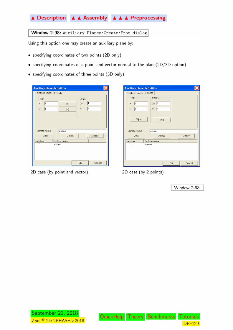
N Description N N Assembly N N N Preprocessing
Window 2-98: Auxiliary Planes:Create:From dialog
Using this option one may create an auxiliary plane by:
• specifying coordinates of two points (2D only)
• specifying coordinates of a point and vector normal to the plane(2D/3D option)
• specifying coordinates of three points (3D only)
2D case (by point and vector) 2D case (by 2 points)
Window 2-98
September 21, 2018
ZSoilr-2D-2PHASE v.2018QuickHelp Theory Benchmarks Tutorials
DP–129
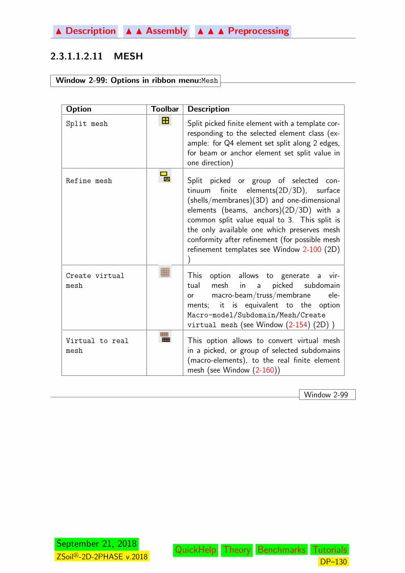
N Description N N Assembly N N N Preprocessing
2.3.1.1.2.11 MESH
Window 2-99: Options in ribbon menu:Mesh
Option Toolbar Description
Split mesh Split picked finite element with a template cor-responding to the selected element class (ex-ample: for Q4 element set split along 2 edges,for beam or anchor element set split value inone direction)
Refine mesh Split picked or group of selected con-tinuum finite elements(2D/3D), surface(shells/membranes)(3D) and one-dimensionalelements (beams, anchors)(2D/3D) with acommon split value equal to 3. This split isthe only available one which preserves meshconformity after refinement (for possible meshrefinement templates see Window 2-100 (2D))
Create virtual
mesh
This option allows to generate a vir-tual mesh in a picked subdomainor macro-beam/truss/membrane ele-ments; it is equivalent to the optionMacro-model/Subdomain/Mesh/Create
virtual mesh (see Window (2-154) (2D) )
Virtual to real
mesh
This option allows to convert virtual meshin a picked, or group of selected subdomains(macro-elements), to the real finite elementmesh (see Window (2-160))
Window 2-99
September 21, 2018
ZSoilr-2D-2PHASE v.2018QuickHelp Theory Benchmarks Tutorials
DP–130

N Description N N Assembly N N N Preprocessing
Window 2-100: Mesh refinement templates in 2D
The following 2D mesh refinement templates can be used for continuum quadrilateral ele-ments.
node edge, edge and nodes
selected edges element
selected elements
Remarks:
1. The above refinement applies exclusively to quadrilateral elements2. Adjacent beams, anchors or membrane elements will be automatically split to preserve
mesh conformity3. Mesh refinement can exclusively be run for real meshes4. The basic split value is equal to 3 and cannot be modified
Window 2-100
September 21, 2018
ZSoilr-2D-2PHASE v.2018QuickHelp Theory Benchmarks Tutorials
DP–131
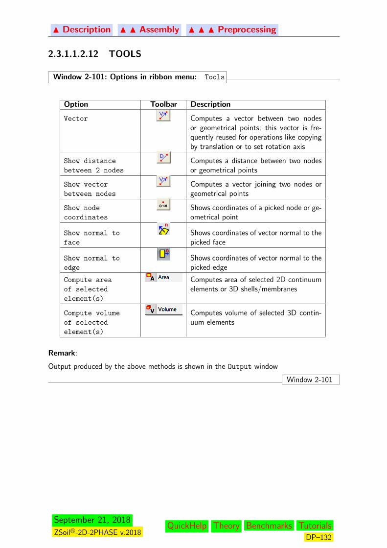
N Description N N Assembly N N N Preprocessing
2.3.1.1.2.12 TOOLS
Window 2-101: Options in ribbon menu: Tools
Option Toolbar Description
Vector Computes a vector between two nodesor geometrical points; this vector is fre-quently reused for operations like copyingby translation or to set rotation axis
Show distance
between 2 nodes
Computes a distance between two nodesor geometrical points
Show vector
between nodes
Computes a vector joining two nodes orgeometrical points
Show node
coordinates
Shows coordinates of a picked node or ge-ometrical point
Show normal to
face
Shows coordinates of vector normal to thepicked face
Show normal to
edge
Shows coordinates of vector normal to thepicked edge
Compute area
of selected
element(s)
Computes area of selected 2D continuumelements or 3D shells/membranes
Compute volume
of selected
element(s)
Computes volume of selected 3D contin-uum elements
Remark:
Output produced by the above methods is shown in the Output window
Window 2-101
September 21, 2018
ZSoilr-2D-2PHASE v.2018QuickHelp Theory Benchmarks Tutorials
DP–132
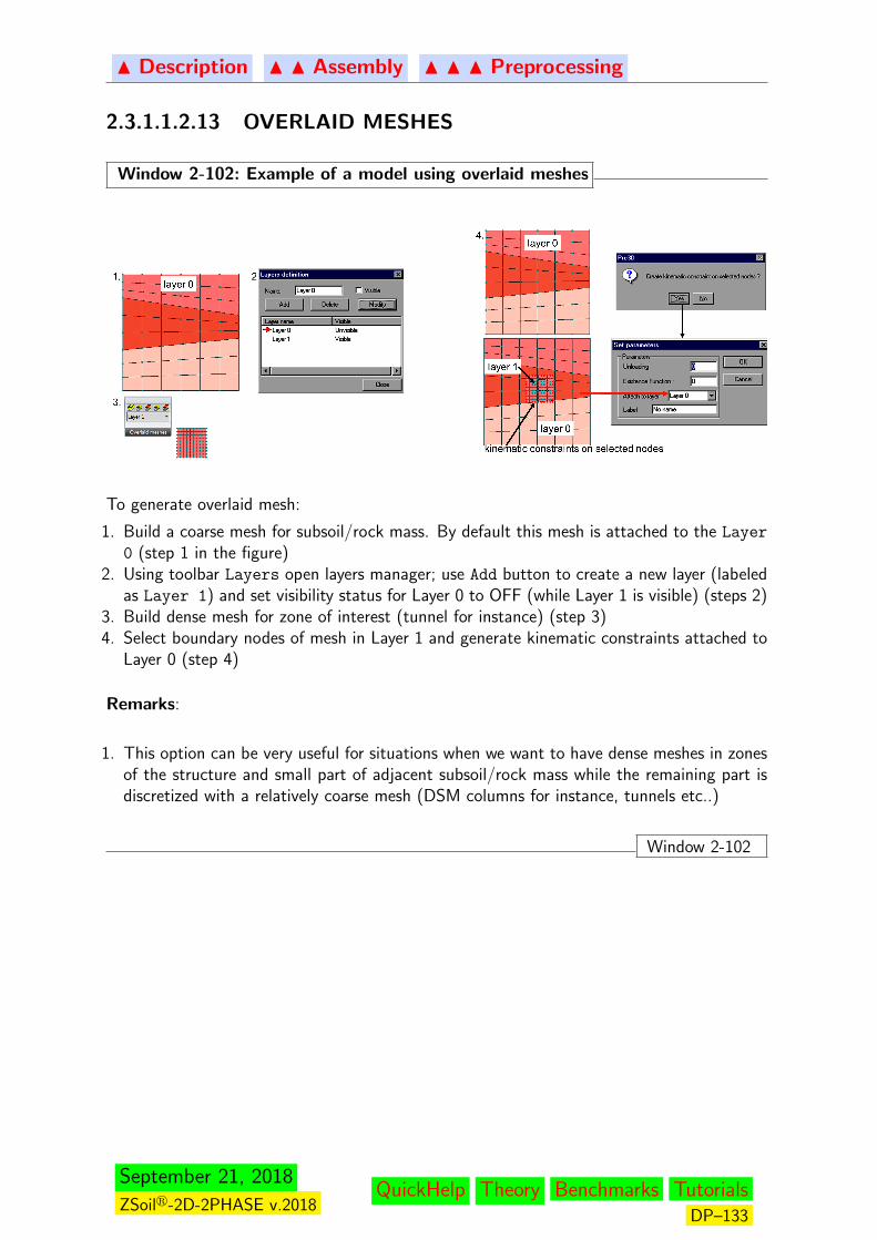
N Description N N Assembly N N N Preprocessing
2.3.1.1.2.13 OVERLAID MESHES
Window 2-102: Example of a model using overlaid meshes
To generate overlaid mesh:
1. Build a coarse mesh for subsoil/rock mass. By default this mesh is attached to the Layer
0 (step 1 in the figure)2. Using toolbar Layers open layers manager; use Add button to create a new layer (labeled
as Layer 1) and set visibility status for Layer 0 to OFF (while Layer 1 is visible) (steps 2)3. Build dense mesh for zone of interest (tunnel for instance) (step 3)4. Select boundary nodes of mesh in Layer 1 and generate kinematic constraints attached to
Layer 0 (step 4)
Remarks:
1. This option can be very useful for situations when we want to have dense meshes in zonesof the structure and small part of adjacent subsoil/rock mass while the remaining part isdiscretized with a relatively coarse mesh (DSM columns for instance, tunnels etc..)
Window 2-102
September 21, 2018
ZSoilr-2D-2PHASE v.2018QuickHelp Theory Benchmarks Tutorials
DP–133
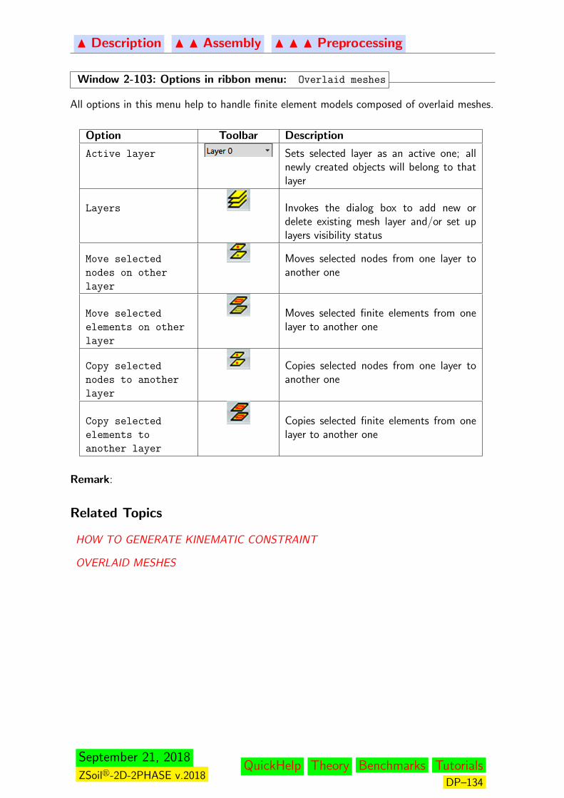
N Description N N Assembly N N N Preprocessing
Window 2-103: Options in ribbon menu: Overlaid meshes
All options in this menu help to handle finite element models composed of overlaid meshes.
Option Toolbar Description
Active layer Sets selected layer as an active one; allnewly created objects will belong to thatlayer
Layers Invokes the dialog box to add new ordelete existing mesh layer and/or set uplayers visibility status
Move selected
nodes on other
layer
Moves selected nodes from one layer toanother one
Move selected
elements on other
layer
Moves selected finite elements from onelayer to another one
Copy selected
nodes to another
layer
Copies selected nodes from one layer toanother one
Copy selected
elements to
another layer
Copies selected finite elements from onelayer to another one
Remark:
Related Topics
HOW TO GENERATE KINEMATIC CONSTRAINT
OVERLAID MESHES
September 21, 2018
ZSoilr-2D-2PHASE v.2018QuickHelp Theory Benchmarks Tutorials
DP–134
N Description N N Assembly N N N Preprocessing
2.3.1.1.2.14 FREQUENTLY USED TOOLS
Window 2-104: Options in ribbon menu:Frequently used tools
Option Toolbar Description
Standard selection
cursor
Activates standard selection cursor which al-lows to pick any geometrical object or finiteelement model component
Zoom This option allows to focus on a certain detailof the model; see for detailed information inWindow (2-105)
Camera manipulator Use like a track-ball to rotate or move camera; in the 2D mode only translation is possible;in the 3D to cancel rotation use this toolbarwith Ctrl key pressed down
View all This option is used to view whole model
Continue selection
for last action
Some generation methods (initial conditionson superelements for instance) require to pickseveral objects (points for instance) in order tofinish the action; at the same time these ob-jects may be hidden due to current projection;therefore we may need to rotate the camerafirst, just to see these objects, and then pickthem to finish the action; this cursor is de-signed for picking objects
Delete selected This option is used to delete a single pickedobject or group of selected objects (use short-cut Del) (NB. this toolbar appears also in Edit
ribbon menu)
Parameters This option is used to set Initial
material, 1-st replacement material,2-nd replacement material, Existence
function, Unloading function for a singlepicked element or group of selected elements(if all are of the same class); the same toolbaris available in ribbon menu Parameters
Window 2-104
September 21, 2018
ZSoilr-2D-2PHASE v.2018QuickHelp Theory Benchmarks Tutorials
DP–135

N Description N N Assembly N N N Preprocessing
Window 2-105: Toolbar: ZoomDuring definition of the zoom box the two rectangles are simultaneously drawn (see figurebelow), the blue (shown by dashed line) and black one (shown with solid line). The blue oneis the one defined by the user while the black one represents the zoom which will finally beaccepted to preserve the aspect ratio.
Zoom box drawnby user
Real zoom boxpreserving theaspect ratio
Window 2-105
September 21, 2018
ZSoilr-2D-2PHASE v.2018QuickHelp Theory Benchmarks Tutorials
DP–136
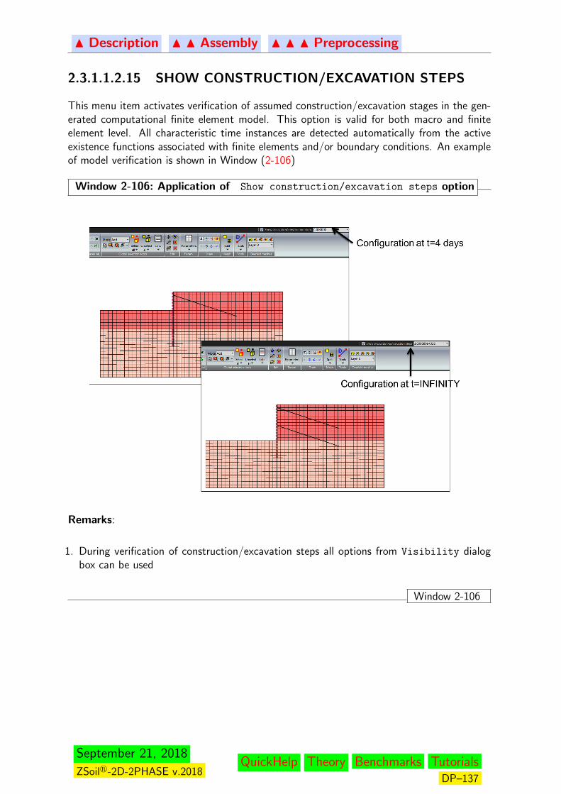
N Description N N Assembly N N N Preprocessing
2.3.1.1.2.15 SHOW CONSTRUCTION/EXCAVATION STEPS
This menu item activates verification of assumed construction/excavation stages in the gen-erated computational finite element model. This option is valid for both macro and finiteelement level. All characteristic time instances are detected automatically from the activeexistence functions associated with finite elements and/or boundary conditions. An exampleof model verification is shown in Window (2-106)
Window 2-106: Application of Show construction/excavation steps option
Remarks:
1. During verification of construction/excavation steps all options from Visibility dialogbox can be used
Window 2-106
September 21, 2018
ZSoilr-2D-2PHASE v.2018QuickHelp Theory Benchmarks Tutorials
DP–137
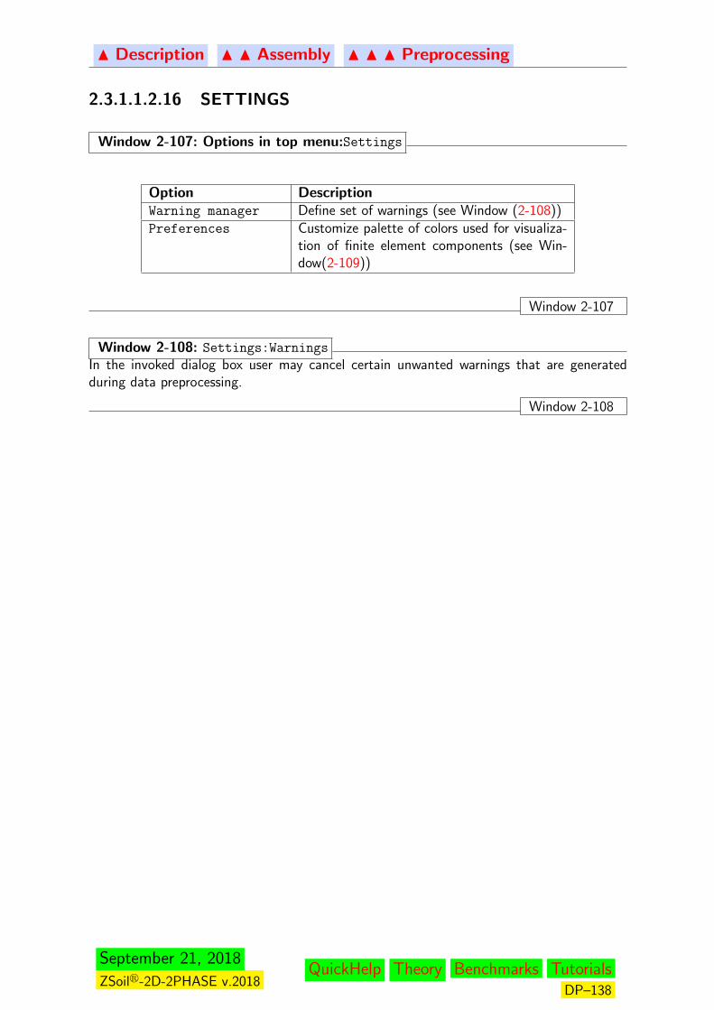
N Description N N Assembly N N N Preprocessing
2.3.1.1.2.16 SETTINGS
Window 2-107: Options in top menu:Settings
Option DescriptionWarning manager Define set of warnings (see Window (2-108))Preferences Customize palette of colors used for visualiza-
tion of finite element components (see Win-dow(2-109))
Window 2-107
Window 2-108: Settings:WarningsIn the invoked dialog box user may cancel certain unwanted warnings that are generatedduring data preprocessing.
Window 2-108
September 21, 2018
ZSoilr-2D-2PHASE v.2018QuickHelp Theory Benchmarks Tutorials
DP–138
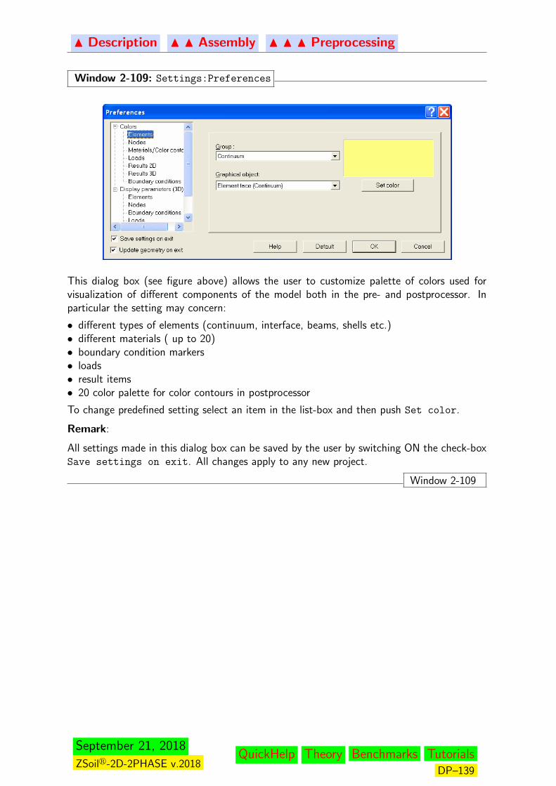
N Description N N Assembly N N N Preprocessing
Window 2-109: Settings:Preferences
This dialog box (see figure above) allows the user to customize palette of colors used forvisualization of different components of the model both in the pre- and postprocessor. Inparticular the setting may concern:
• different types of elements (continuum, interface, beams, shells etc.)• different materials ( up to 20)• boundary condition markers• loads• result items• 20 color palette for color contours in postprocessor
To change predefined setting select an item in the list-box and then push Set color.
Remark:
All settings made in this dialog box can be saved by the user by switching ON the check-boxSave settings on exit. All changes apply to any new project.
Window 2-109
September 21, 2018
ZSoilr-2D-2PHASE v.2018QuickHelp Theory Benchmarks Tutorials
DP–139
N Description N N Assembly N N N Preprocessing
2.3.1.2 MACRO-MODEL
The right context menu after clicking DOMAIN/Macro Model item gives an access to methodsthat can be used to create model components at the macro level. These components arelisted in table shown below
Point Contains all options to create, outline, update geometricalpoints
Objects Contains all options to create, outline, update geometricalobjects like lines, arcs, circles
2D meshing mapping Contains all options to mapp any 2D mesh on a new 2Ddomain
Extrusion direction Contains all options to select objects like lines, arcs to formso-called extrusion direction used later to extrude 3D sub-domains from 2D faces, and 3D surface subdomains (shells,membranes) from 3D edges
Subdomain Contains options to generate 2D/3D continuum subdomains,2D/3D membrane subdomains, 3D shell subdomains, macro-trusses and macro-beams and to create meshes
Pile Contains options to generate 3D piles (beam elements em-bedded in the continuum)
Nail Contains options to generate nails in 2D/3D (beam elementsembedded in the continuum)
Seepage Contains options to generate macro-seepage on 2D/3D con-tinuum subdomain boundaries
Convection Contains options to generate macro-convection on 2D/3Dcontinuum subdomain boundaries
Viscous damper Contains options to generate macro-viscous damper on2D/3D continuum subdomain boundaries
Interface Contains options to generate macro-contact interface on2D/3D continuum subdomain boundaries
Pressure BC Contains options to generate pressure BC on subdomainboundaries
Temperature BC Contains options to generate temperature BC on subdomainboundaries
Humidity BC Contains options to generate humidity BC on subdomainboundaries
Fluid flux Contains options to generate fluid fluxes on subdomainboundaries
Heat flux Contains options to generate heat fluxes on subdomainboundaries
Humidity flux Contains options to generate humidity fluxes on subdomainboundaries
Surface load Contains options to generate surface loads on subdomainboundaries
Point load Contains options to generate concentrated loads on geomet-rical points
September 21, 2018
ZSoilr-2D-2PHASE v.2018QuickHelp Theory Benchmarks Tutorials
DP–140
N Description N N Assembly N N N Preprocessing
2.3.1.2.1 POINT
Window 2-110: Options in menu: Point
Option Method Toolbar DescriptionCreate Point — Window 2-111Outline all options — Window 2-112Delete all options — Window 2-113Update all options — Window 2-114
Window 2-110
Window 2-111: Point:Create:Point
This option activates a graphic cursor with two(in 2D) or three (in 3D) orthogonal linesintersecting at current point position (see Window 2-94 for Snap to.. option).
Window 2-111
Window 2-112: Point:options in menu Outline
Method DescriptionSelect one object this option activates graphical cursor in the selection mode and
points are selected one by one by pointing them by mouseAll all points are selected; result of this action depends on the status
of Selection mode (see Window 2-81)In zoom box all points inside zoom rectangle are selectedIn zoom circle all points inside zoom circle are selectedInside contour all points inside irregular contour, drawn by mouse, are selectedDuplicated all points occupying the same geometrical position (with a de-
clared tolerance) are selectedSingle points all points not attached to any object (like line, circle, arc, polyline)
are selected
Window 2-112
Window 2-113: Point: options in menu Delete
Method DescriptionDelete if at least a single object is selected then Delete operation re-
moves selected points; otherwise points are removed one by oneby pointing them by mouse
Delete single
points
all points not attached to any object (line, arc, etc..) are removed
Remark:
After deleting points, objects adjacent to these points are removedWindow 2-113
September 21, 2018
ZSoilr-2D-2PHASE v.2018QuickHelp Theory Benchmarks Tutorials
DP–141
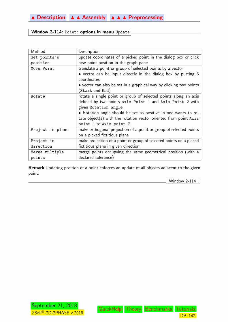
N Description N N Assembly N N N Preprocessing
Window 2-114: Point: options in menu Update
Method DescriptionSet points’s
position
update coordinates of a picked point in the dialog box or clicknew point position in the graph pane
Move Point translate a point or group of selected points by a vector• vector can be input directly in the dialog box by putting 3coordinates• vector can also be set in a graphical way by clicking two points(Start and End)
Rotate rotate a single point or group of selected points along an axisdefined by two points axis Point 1 and Axis Point 2 withgiven Rotation angle
• Rotation angle should be set as positive in one wants to ro-tate object(s) with the rotation vector oriented from point Axispoint 1 to Axis point 2
Project in plane make orthogonal projection of a point or group of selected pointson a picked fictitious plane
Project in
direction
make projection of a point or group of selected points on a pickedfictitious plane in given direction
Merge multiple
points
merge points occupying the same geometrical position (with adeclared tolerance)
Remark:Updating position of a point enforces an update of all objects adjacent to the givenpoint.
Window 2-114
September 21, 2018
ZSoilr-2D-2PHASE v.2018QuickHelp Theory Benchmarks Tutorials
DP–142

N Description N N Assembly N N N Preprocessing
2.3.1.2.2 OBJECTS
Window 2-115: Common methods for objects
Option Method Toolbar DescriptionCreate Point — Window 2-116
Line Window 2-117
Arc Window 2-118
Circle Window 2-119Line(s) on edge(s) — Window 2-120
Copy with translation Window 2-121
Copy with rotation Window 2-122
Copy by symmetry Window 2-123Copy by projection on plane Window 2-124Copy by projection on plane in
direction
Window 2-125
Split by plane Window 2-126Import DXF Window 2-127
Outline Options — Window 2-128Delete Options — Window 2-129Update Options — Window 2-130
Window 2-115
September 21, 2018
ZSoilr-2D-2PHASE v.2018QuickHelp Theory Benchmarks Tutorials
DP–143
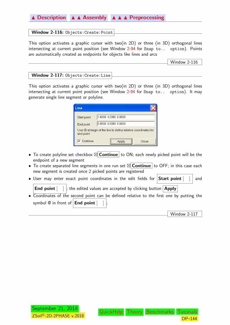
N Description N N Assembly N N N Preprocessing
Window 2-116: Objects:Create:Point
This option activates a graphic cursor with two(in 2D) or three (in 3D) orthogonal linesintersecting at current point position (see Window 2-94 for Snap to.. option). Pointsare automatically created as endpoints for objects like lines and arcs
Window 2-116
Window 2-117: Objects:Create:Line
This option activates a graphic cursor with two(in 2D) or three (in 3D) orthogonal linesintersecting at current point position (see Window 2-94 for Snap to.. option). It maygenerate single line segment or polyline.
• To create polyline set checkbox � Continue to ON; each newly picked point will be theendpoint of a new segment• To create separated line segments in one run set � Continue to OFF; in this case each
new segment is created once 2 picked points are registered
• User may enter exact point coordinates in the edit fields for Start point [ ] and
End point [ ] ; the edited values are accepted by clicking button Apply
• Coordinates of the second point can be defined relative to the first one by putting the
symbol @ in front of End point [ ] ;
Window 2-117
September 21, 2018
ZSoilr-2D-2PHASE v.2018QuickHelp Theory Benchmarks Tutorials
DP–144

N Description N N Assembly N N N Preprocessing
Window 2-118: Objects:Create:Arc
Arc can be defined using the two definitions:
• through center-start-end points (C-S-E), once } Center-Start-End radio-button is ON(characteritic points can be picked in the graph pane or defined by exact coordinates inthe dialog box)
• through start-end-radius (S-E-R) once } Start-End-Radius radio-button is ON (the twoendpoints can be picked in the graph pane or defined by exact coordinates, while radiusmust be explicitly entered in the dialog box)
These definitions are supplied with an additional information concerning arc orientation. Thisinformation consists of a definition of an auxiliary normal vector n∗ plus Clockwise orAnticlockwise orientation status. For the 2D case the two definitions are illustrated infigures below.
CS
E
clockwise
anticlockwise
C-S-E definition (2D) S-E-R definition (2D)
S
Eclockwise
anticlockwise
A singular case appears for C-S-E definition when C, S and E points are coaxial. In this case
an auxiliary normal vector n∗, set in the dialog box in the edit field Normal [ ] , helps to
select proper arc. This case in shown in the figure below (for both 2D and 3D case)
CS
E
xL
yLeyL=
n* x SE|| n* x SE ||
n*
clockwise
anticlockwise
C-S-E definition (2D/3D): C, S, E are coaxial
n
Window 2-118
September 21, 2018
ZSoilr-2D-2PHASE v.2018QuickHelp Theory Benchmarks Tutorials
DP–145
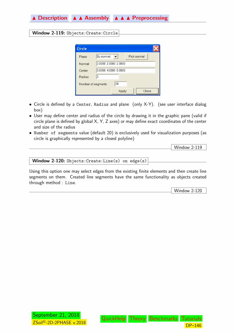
N Description N N Assembly N N N Preprocessing
Window 2-119: Objects:Create:Circle
• Circle is defined by a Center, Radius and plane (only X-Y). (see user interface dialogbox)• User may define center and radius of the circle by drawing it in the graphic pane (valid if
circle plane is defined by global X, Y, Z axes) or may define exact coordinates of the centerand size of the radius• Number of segments value (default 20) is exclusively used for visualization purposes (as
circle is graphically represented by a closed polyline)
Window 2-119
Window 2-120: Objects:Create:Line(s) on edge(s)
Using this option one may select edges from the existing finite elements and then create linesegments on them. Created line segments have the same functionality as objects createdthrough method : Line.
Window 2-120
September 21, 2018
ZSoilr-2D-2PHASE v.2018QuickHelp Theory Benchmarks Tutorials
DP–146
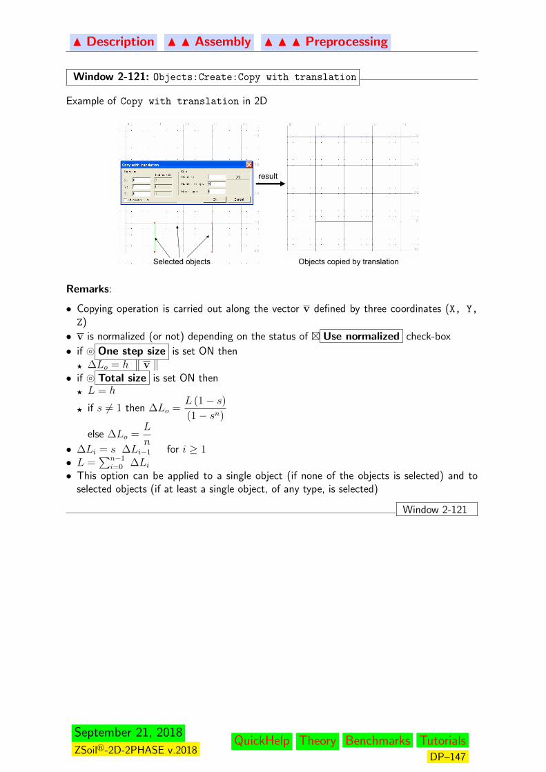
N Description N N Assembly N N N Preprocessing
Window 2-121: Objects:Create:Copy with translation
Example of Copy with translation in 2D
Selected objects Objects copied by translation
result
Remarks:
• Copying operation is carried out along the vector v defined by three coordinates (X, Y,
Z)
• v is normalized (or not) depending on the status of � Use normalized check-box
• if } One step size is set ON thenF ∆Lo = h ‖ v ‖• if } Total size is set ON thenF L = h
F if s 6= 1 then ∆Lo =L (1− s)(1− sn)
else ∆Lo =L
n• ∆Li = s ∆Li−1 for i ≥ 1• L =
∑n−1i=0 ∆Li
• This option can be applied to a single object (if none of the objects is selected) and toselected objects (if at least a single object, of any type, is selected)
Window 2-121
September 21, 2018
ZSoilr-2D-2PHASE v.2018QuickHelp Theory Benchmarks Tutorials
DP–147
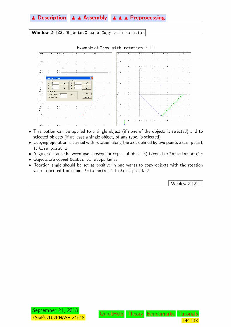
N Description N N Assembly N N N Preprocessing
Window 2-122: Objects:Create:Copy with rotation
Example of Copy with rotation in 2D
• This option can be applied to a single object (if none of the objects is selected) and toselected objects (if at least a single object, of any type, is selected)• Copying operation is carried with rotation along the axis defined by two points Axis point
1, Axis point 2
• Angular distance between two subsequent copies of object(s) is equal to Rotation angle
• Objects are copied Number of steps times• Rotation angle should be set as positive in one wants to copy objects with the rotation
vector oriented from point Axis point 1 to Axis point 2
Window 2-122
September 21, 2018
ZSoilr-2D-2PHASE v.2018QuickHelp Theory Benchmarks Tutorials
DP–148
N Description N N Assembly N N N Preprocessing
Window 2-123: Objects:Create:Copy by symmetry
This option can be used to make a copy of a single object (if none of the objects is selected)or group of selected objects by symmetrical projection with respect to the plane created underribbon menu Draw:Auxiliary Planes
• To run this option a fictitious plane must be created first• After this operation orientation of copied objects is reversed• To initiate the action plane of symmetry must be pointed first
Window 2-123
Window 2-124: Objects:Create:Copy by projection on plane
This option can be used to make a copy of a single object (if none of the objects is selected)or group of selected objects by projecting it (them) on the plane created under ribbon menuDraw:Auxiliary Planes
• To run this option a fictitious plane must be created first• To initiate the action the plane must be pointed first and the the object (if not selected)
Window 2-124
Window 2-125: Objects:Create:Copy by projection on plane in direction
This option can be used to make a copy of a single object (if none of the objects is selected)or group of selected objects by projecting it (them) on the plane in given direction• To run this option a fictitious plane must be created first• To initiate the action the plane must be pointed first and the the object (if not selected)
Window 2-125
Window 2-126: Objects:Create:Split by plane
Using this option user may split objects (lines, arcs, circles) into parts with aid of AuxiliaryPlanes.• To run this option an auxiliary plane must be created first• Action may be applied to a single object or set of selected objects• If set of selected objects is empty then auxiliary plane is pointed first and then each
object to be split one by one• If set of selected objects is not empty then after pointing auxiliary plane all selected
objects will be split• This option is very useful when generating Subdomains
Window 2-126
Window 2-127: Objects:Create:Import DXF
• Objects of type: lines, arcs, circles and splines (converted to polylines) are imported fromthe *.dxf file• dxf formats starting from AutoCAD 2000 are supported• Not meaningful and overlapped objects should be deleted from the *.dxf file to avoid
non-unique definitions in the preprocessor
Window 2-127
September 21, 2018
ZSoilr-2D-2PHASE v.2018QuickHelp Theory Benchmarks Tutorials
DP–149
N Description N N Assembly N N N Preprocessing
Window 2-128: Objects:options in menu Outline
Select one object this option activates graphical cursor in the selection modeand objects are selected one by one by pointing them bymouse
All all objects are selected; result of this action depends on thestatus of Selection mode (see Window 2-81)
In zoom box • if the zoom box is dragged from left to the right sidethen only fully covered, by the zoom rectangle, objects areselected;• if the zoom box is dragged from right to the left side theneven partially covered, by the zoom rectangle, objects areselected
In zoom circle • if the zoom circle is dragged from left to the right side thenonly fully covered, by the circle (cylinder in 3D), objects areselected• if the zoom circle is dragged from right to the left sidethen even partially covered, by the zoom circle (cylinder in3D), objects are selected
Select surrounding
contour
with this option user may select groups of objects (lines andarcs) which form a closed polygon; to enable this selectionuser must pick any point inside of the polygon; this optionis valid exclusively for the 2D case
Circles/arcs with
radius
using this option one may easily select all circles and/or arcswith a given radius
Window 2-128
Window 2-129: Objects: options in menu Delete
Delete if at least a single object is selected then Delete operationremoves selected elements; otherwise objects are removedone by one by pointing them by mouse
Remark:
After deleting lines and arcs their vertex points remain not removed; to delete them user canuse the option Delete Point from menu Point
Window 2-129
September 21, 2018
ZSoilr-2D-2PHASE v.2018QuickHelp Theory Benchmarks Tutorials
DP–150
N Description N N Assembly N N N Preprocessing
Window 2-130: Objects: options in menu Update
Parameters redefines parameters of picked object (does not work for se-lection)
Move translates an object or group of selected objects by a vector• vector can be input directly in the dialog box by putting3 coordinates and a factor (default=1.0) which scales thevector• vector can also be set in a graphical way by clicking twopoints (Start and End)
Rotate rotates a single pointed object or group of selected objectsalong an axis defined by two• points axis Point 1 and Axis Point 2 with givenRotation angle
• rotation angle should be set as positive in one wants torotate object(s) with the rotation vector oriented from pointAxis point 1 to Axis point 2
Split splits an object or group of selected objects on parts• number of subdivisions is defined in the edit field Split
• user may perform split operation with a regression param-eter (default=1.0, no regression) defined in the edit fieldRegression
• split with regression must be run carefully because depend-ing on the orientation of the object value of Regression
parameter can be smaller than 1.0 or larger than 1.0• special attention must be paid when making split withregression on group of selected objects as Regression pa-rameter applies to all objects
Project on plane projects the object on the plane• plane must be created using the Auxiliary planes op-tion
Project on plane in
direction
projects the object on the plane in given direction
• plane must be created using the Auxiliary planes op-tion
Intersection by
object(s)
Finds intersection points of two pointed objects or all inter-section points for group of selected objects• after finding intersection points objects are automaticallysplit into parts• this option is crucial for definition of Subdomains
Group lines to
polylines
groups all selected lines into one object treated as a polyline
Remark:
After deleting lines and arcs their endpoints remain undeleted; to remove them user can usethe option Delete Point
Window 2-130
September 21, 2018
ZSoilr-2D-2PHASE v.2018QuickHelp Theory Benchmarks Tutorials
DP–151
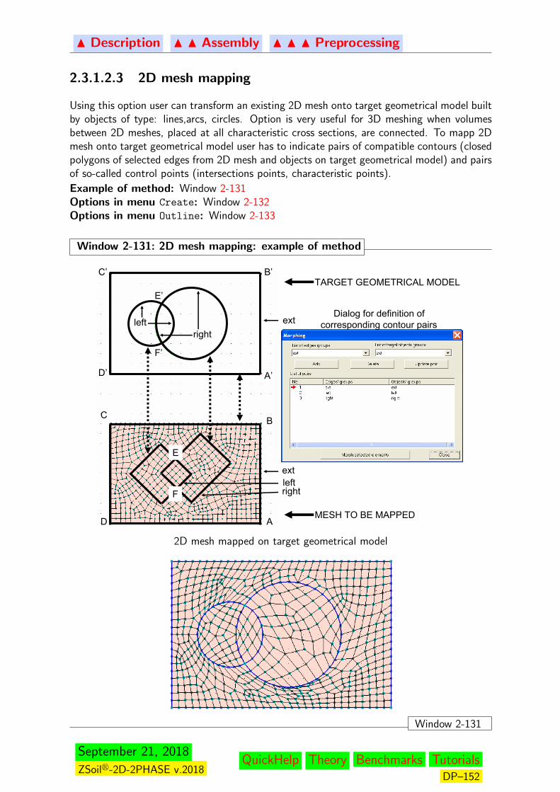
N Description N N Assembly N N N Preprocessing
2.3.1.2.3 2D mesh mapping
Using this option user can transform an existing 2D mesh onto target geometrical model builtby objects of type: lines,arcs, circles. Option is very useful for 3D meshing when volumesbetween 2D meshes, placed at all characteristic cross sections, are connected. To mapp 2Dmesh onto target geometrical model user has to indicate pairs of compatible contours (closedpolygons of selected edges from 2D mesh and objects on target geometrical model) and pairsof so-called control points (intersections points, characteristic points).
Example of method: Window 2-131Options in menu Create: Window 2-132Options in menu Outline: Window 2-133
Window 2-131: 2D mesh mapping: example of method
A
BC
D
A’
B’C’
D’
E’
F’
E
F
leftright
ext
ext
rightleft
TARGET GEOMETRICAL MODEL
MESH TO BE MAPPED
Dialog for definition ofcorresponding contour pairs
2D mesh mapped on target geometrical model
Window 2-131
September 21, 2018
ZSoilr-2D-2PHASE v.2018QuickHelp Theory Benchmarks Tutorials
DP–152
N Description N N Assembly N N N Preprocessing
Window 2-132: 2D mesh mapping: options in menu Create
Create edges
list
registers group of edges selected from 2D mesh
• Edges selected from 2D mesh must form closed polygon• Selected edges cannot be overlapped• In case when edges are placed in the 2D mesh interior it is recommendedthat elements on one side of the polygon formed by selected edges are hid-den first; this is important when using In zoom box, In zoom circle,In contour methods from toolbar for edges selection•When creating a list of selected edges user must label it for further usage
Create target
objects list
registers group of objects which form a target geometrical model
• Selected objects must form a closed polygon• Before registering a group of selected objects forming a polygon it isrecommended to carry out the intersection of all objects; in the exampleshown in 2-131 the two circles are intersected first and cross points E’ andF’ are created (each circle is split into two arcs)• Selected edges cannot be overlapped•When creating a list of selected objects forming closed polygon user mustlabel it for further usage
Create control
points
registers pairs of equivalent points in 2D mesh and target geometricalmodel• All intersections points must be registered (in the example shown inWindow 2-131 points E-E’ and F-F’ must be registered)• All characteristic points must be registered too (in the example shownin Window 2-131 these are the corner points: A-A’, B-B’, C-C’ and D-D’)
Run morphing performs mapping of the 2D mesh onto target geometrical model• Labeled groups of selected edges are kept under List of edges
groups combo-box• Labeled groups of selected target geometrical model objects are keptunder List of target objects groups combo-box•With button Add user may add a pair of compatible contours to the Listof pairs
• With button Delete user may remove a pair of compatible contoursfrom List of pairs
• With button Update user may modify a pair of compatible contours inList of pairs
• Morphing can be activated (with button Morph selected elements)once pairs of compatible contours in the 2D mesh and target geometricalmodel are defined, pairs of control points are defined and elements to bemapped from the 2D mesh are selected too(!)• Only selected elements from the 2D mesh will be mapped• After morphing the original mesh will fit boundaries of target geometricalmodel (see Window 2-131)
September 21, 2018
ZSoilr-2D-2PHASE v.2018QuickHelp Theory Benchmarks Tutorials
DP–153

N Description N N Assembly N N N Preprocessing
Window 2-132
Window 2-133: 2D mesh mapping: options in menu Outline
Edges with
label
selects all 2D mesh edges with a given label
Target objects
with label
selects all objects of target geometrical model with a given label
Control points
with label
selects pairs of control points (nodal point in the 2D mesh and geometricalpoint in the target geometrical model) with a given label
Remark:
All selection modes apply (see Window 2-81)Window 2-133
September 21, 2018
ZSoilr-2D-2PHASE v.2018QuickHelp Theory Benchmarks Tutorials
DP–154
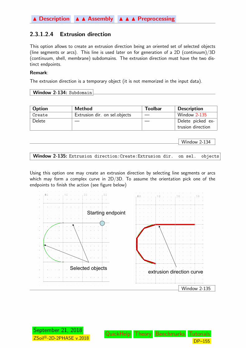
N Description N N Assembly N N N Preprocessing
2.3.1.2.4 Extrusion direction
This option allows to create an extrusion direction being an oriented set of selected objects(line segments or arcs). This line is used later on for generation of a 2D (continuum)/3D(continuum, shell, membrane) subdomains. The extrusion direction must have the two dis-tinct endpoints.
Remark:
The extrusion direction is a temporary object (it is not memorized in the input data).
Window 2-134: Subdomain
Option Method Toolbar DescriptionCreate Extrusion dir. on sel.objects — Window 2-135Delete — — Delete picked ex-
trusion direction
Window 2-134
Window 2-135: Extrusion direction:Create:Extrusion dir. on sel. objects
Using this option one may create an extrusion direction by selecting line segments or arcswhich may form a complex curve in 2D/3D. To assume the orientation pick one of theendpoints to finish the action (see figure below)
Starting endpoint
extrusion direction curveSelected objects
Window 2-135
September 21, 2018
ZSoilr-2D-2PHASE v.2018QuickHelp Theory Benchmarks Tutorials
DP–155

N Description N N Assembly N N N Preprocessing
2.3.1.2.5 Subdomain
All methods grouped in menu Subdomain are designed to create, outline and update sub-domains of type continuum 2D, continuum 3D, shells, membranes, beams, trusses. In thecontext of macro-modeling, subdomains are understood as large parts of the computationalmodel. User may define a subdomain, discretize it with a virtual mesh first and then with areal one, then may apply loads, fluxes and certain types of the boundary conditions to theboundary of the subdomain. Meshing procedure is treated here as a background operation,hence user may change the mesh and may update subdomain geometry while existing virtualor real mesh will be adapted to the new geometry.
Window 2-136: Subdomain
Option Method Toolbar DescriptionCreate 2D continuum inside contour — Window 2-137
2D continuum on contour — Window 2-138Beam on object(s) — Window 2-139Truss/Anchor on object(s) — Window 2-1402D Membrane on object(s) — Window 2-141Copy with rotation — Window 2-142Copy with translation — Window 2-143Copy by symmetry — Window 2-144
Outline all options — Window 2-145Delete all options — Window 2-146Parameters Standard setup — Window 2-147
Setup for beams — Window 2-148Define excavation front — Window 2-149Reverse direction — Window 2-152Reverse X-axis — Window 2-153
Mesh Create virtual mesh (2D) — Window 2-154
Window 2-136
September 21, 2018
ZSoilr-2D-2PHASE v.2018QuickHelp Theory Benchmarks Tutorials
DP–156
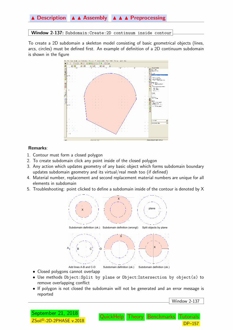
N Description N N Assembly N N N Preprocessing
Window 2-137: Subdomain:Create:2D continuum inside contour
To create a 2D subdomain a skeleton model consisting of basic geometrical objects (lines,arcs, circles) must be defined first. An example of definition of a 2D continuum subdomainis shown in the figure
Remarks:
1. Contour must form a closed polygon2. To create subdomain click any point inside of the closed polygon3. Any action which updates geometry of any basic object which forms subdomain boundary
updates subdomain geometry and its virtual/real mesh too (if defined)4. Material number, replacement and second replacement material numbers are unique for all
elements in subdomain5. Troubleshooting: point clicked to define a subdomain inside of the contour is denoted by X
planeX
X
X
X
Subdomain definition (ok.) Subdomain definition (wrong!) Split objects by plane
Add lines A-B and C-D
A B C D
Subdomain definition (ok.) Subdomain definition (ok.)
• Closed polygons cannot overlapp• Use methods Object:Split by plane or Object:Intersection by object(s) to
remove overlapping conflict• If polygon is not closed the subdomain will not be generated and an error message is
reported
Window 2-137
September 21, 2018
ZSoilr-2D-2PHASE v.2018QuickHelp Theory Benchmarks Tutorials
DP–157

N Description N N Assembly N N N Preprocessing
Window 2-138: Subdomain:Create:2D continuum on contour
This option allows to create a 2D subdomain bound by the set of selected objects which mustform a closed polygon. An example of this definition is shown in the figure
Selected contour Subdomain
Window 2-138
Window 2-139: Subdomain:Create:Beam on object(s)
Using this option one can create a beam subdomain on a single picked geometrical object orgroup of selected objects.
Remarks:1. Definition of the beam local coordinate system and offsets (of centroids with respect to
the master nodes) has to be made using option Update/Parameters ( see Win.(2-148)for details) for each
2. Definition of material, replacement and second replacement material numbers, existenceand unloading function numbers can be made using Update/Parameters option
Window 2-140: Subdomain:Create:Truss/Anchor on object
Using this option one can create a truss/anchor subdomain on a single picked geometricalobject or group of selected geometrical objects. A more enhanced option for creating anchorsincluding fixed anchor zones with interfaces is available at the FE level.
Remark:
Definition of material, replacement and second replacement material numbers, existence andunloading function numbers can be made using Update/Parameters option (see Win.(2-147))
Window 2-140
Window 2-141: Subdomain:Create:2D Membrane on object
Using this option one can create a 2D membrane subdomain on a single picked geometricalobject or group of selected geometrical objects.
Remark:
Definition of material, replacement and second replacement material numbers, existence andunloading function numbers can be made using Update/Parameters option (see Win.(2-147))
Window 2-141
September 21, 2018
ZSoilr-2D-2PHASE v.2018QuickHelp Theory Benchmarks Tutorials
DP–158

N Description N N Assembly N N N Preprocessing
Window 2-142: Subdomain:Create:Copy with rotation
This option allows to make copies of a selected subdomain(s) with simultaneous rotation. Itis fully coherent with the one designed for standard FE components (see.Win.(2-236))
Window 2-142
Window 2-143: Subdomain:Create:Copy with translation
This option allows to make copies of a selected subdomain(s) with simultaneous translation.It is fully coherent with the one designed for standard FE components (see.Win.(2-237))
Window 2-143
Window 2-144: Subdomain:Create:Copy by symmetry
This option allows to make a copy of a selected subdomain(s) by symmetrical projection withrespect to the picked plane (created under ribbon menu Draw:Auxiliary Planes). It isfully coherent with the one designed for standard FE components (see.Win.(2-238))
Window 2-144
Window 2-145: Subdomain:Options in menu Outline
Select one
subdomain
this option activates graphical cursor in the selection mode and sub-domains are selected one by one by pointing them by mouse
All all subdomains are selected; result of this action depends on the statusof Selection mode (see Window 2-81)
In zoom box if the zoom box is dragged from left to the right side then only fullycovered, by the zoom rectangle, subdomains are selectedif the zoom box is dragged from right to the left side then even partiallycovered, by the zoom rectangle, subdomains are selected
In zoom circle if the zoom circle is dragged from left to the right side then only fullycovered, by the circle (cylinder in 3D), subdomains are selectedif the zoom circle is dragged from right to the left side then evenpartially covered, by the zoom circle (cylinder in 3D), subdomains areselected
Window 2-145
September 21, 2018
ZSoilr-2D-2PHASE v.2018QuickHelp Theory Benchmarks Tutorials
DP–159
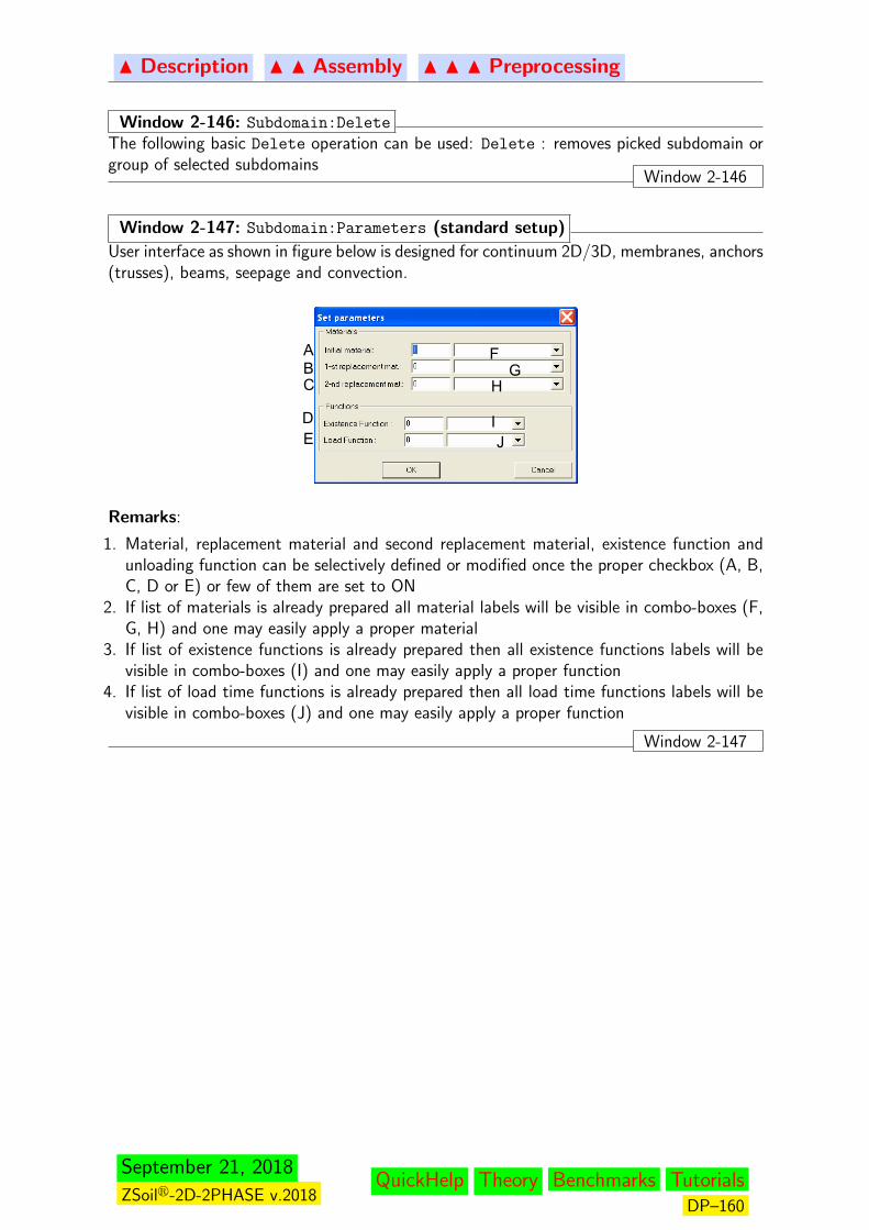
N Description N N Assembly N N N Preprocessing
Window 2-146: Subdomain:DeleteThe following basic Delete operation can be used: Delete : removes picked subdomain orgroup of selected subdomains
Window 2-146
Window 2-147: Subdomain:Parameters (standard setup)
User interface as shown in figure below is designed for continuum 2D/3D, membranes, anchors(trusses), beams, seepage and convection.
ABC
DE
FG
H
IJ
Remarks:
1. Material, replacement material and second replacement material, existence function andunloading function can be selectively defined or modified once the proper checkbox (A, B,C, D or E) or few of them are set to ON
2. If list of materials is already prepared all material labels will be visible in combo-boxes (F,G, H) and one may easily apply a proper material
3. If list of existence functions is already prepared then all existence functions labels will bevisible in combo-boxes (I) and one may easily apply a proper function
4. If list of load time functions is already prepared then all load time functions labels will bevisible in combo-boxes (J) and one may easily apply a proper function
Window 2-147
September 21, 2018
ZSoilr-2D-2PHASE v.2018QuickHelp Theory Benchmarks Tutorials
DP–160

N Description N N Assembly N N N Preprocessing
Window 2-148: Subdomain:Parameters (setup for beams)
User interface for 2D beams, definition of offset vectors and local beam coordinate systemare shown in the Figure below.
A
CD
EF
G
H
xL
Node:1
Node:2A1 A2
Default local axes xL, yL
xLyL
zL
Centroids
Offset definition by vectors: v A1, vA2
vA1
vA2
Node:1
Node:2
Master nodes
yL
3D option
Remarks:
1. By default the local xL axis of the beam is directed towards Node1-Node2 while local yLaxis is rotated by 90o with respect to the xL in anticlockwise direction
2. Position of the top fibers of the cross section is defined by the positive local yL axis3. Offsets of centroid nodes with respect to the master nodes can be given in global or local
beam coordinate system4. During computation real beam coordinates are shifted by given offset vectors5. Local xL and yL axes can be reversed
Window 2-148
September 21, 2018
ZSoilr-2D-2PHASE v.2018QuickHelp Theory Benchmarks Tutorials
DP–161
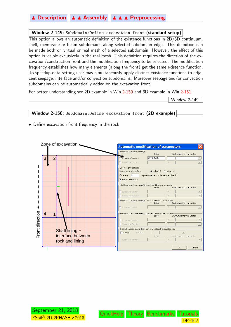
N Description N N Assembly N N N Preprocessing
Window 2-149: Subdomain:Define excavation front (standard setup)
This option allows an automatic definition of the existence functions in 2D/3D continuum,shell, membrane or beam subdomains along selected subdomain edge. This definition canbe made both on virtual or real mesh of a selected subdomain. However, the effect of thisoption is visible exclusively in the real mesh. This definition requires the direction of the ex-cavation/construction front and the modification frequency to be selected. The modificationfrequency establishes how many elements (along the front) get the same existence function.To speedup data setting user may simultaneously apply distinct existence functions to adja-cent seepage, interface and/or convection subdomains. Moreover seepage and/or convectionsubdomains can be automatically added on the excavation front.
For better understanding see 2D example in Win.2-150 and 3D example in Win.2-151.
Window 2-149
Window 2-150: Subdomain:Define excavation front (2D example)
• Define excavation front frequency in the rock
Zone of excavation
Shaft lining + interface betweenrock and lining
1
23
4
Fron
t dire
ctio
n
September 21, 2018
ZSoilr-2D-2PHASE v.2018QuickHelp Theory Benchmarks Tutorials
DP–162
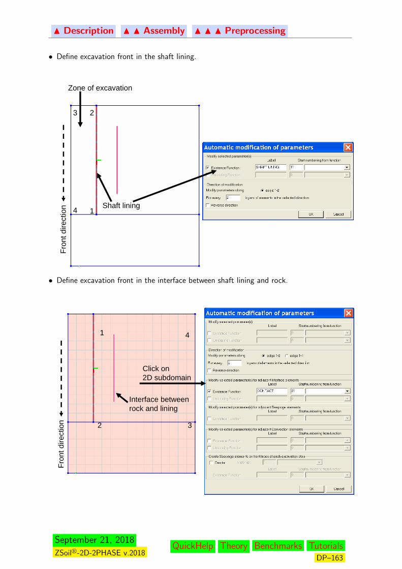
N Description N N Assembly N N N Preprocessing
• Define excavation front in the shaft lining.
Zone of excavation
Shaft lining1
23
4
Fron
t dire
ctio
n
• Define excavation front in the interface between shaft lining and rock.
Interface betweenrock and lining
1
2 3
4
Fron
t dire
ctio
n
Click on 2D subdomain
September 21, 2018
ZSoilr-2D-2PHASE v.2018QuickHelp Theory Benchmarks Tutorials
DP–163
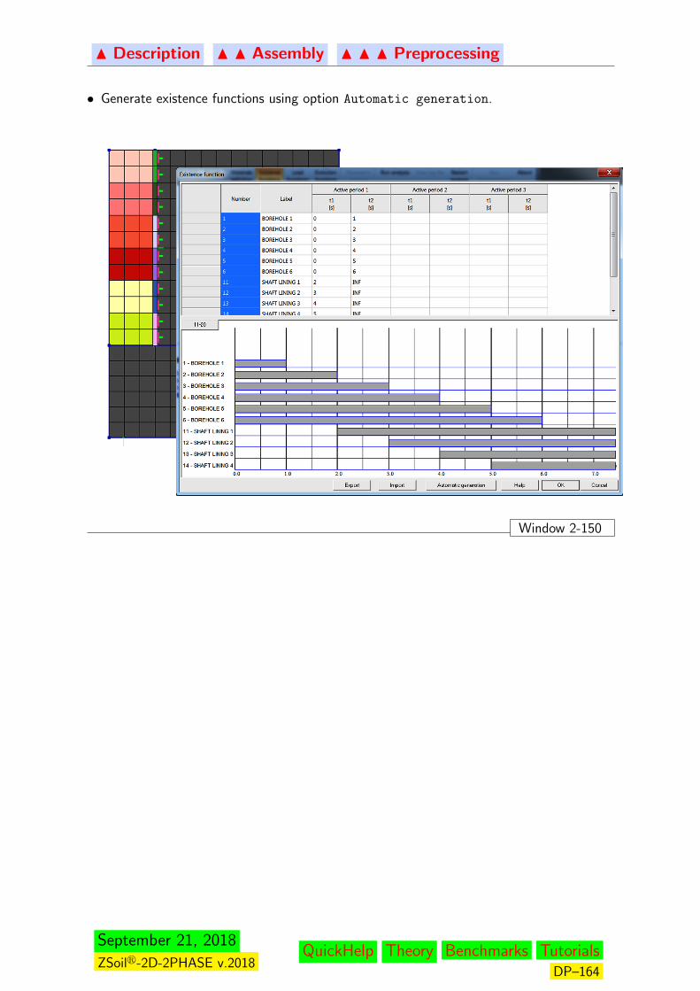
N Description N N Assembly N N N Preprocessing
• Generate existence functions using option Automatic generation.
Window 2-150
September 21, 2018
ZSoilr-2D-2PHASE v.2018QuickHelp Theory Benchmarks Tutorials
DP–164
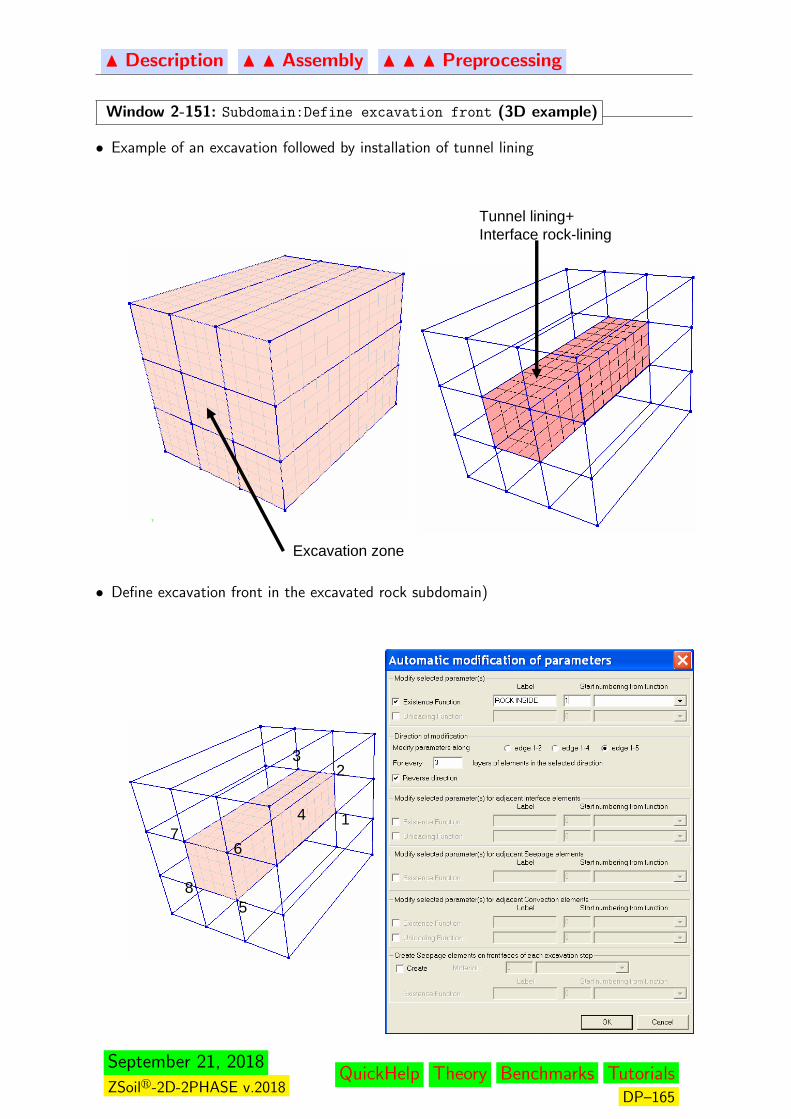
N Description N N Assembly N N N Preprocessing
Window 2-151: Subdomain:Define excavation front (3D example)
• Example of an excavation followed by installation of tunnel lining
Tunnel lining+Interface rock-lining
Excavation zone
• Define excavation front in the excavated rock subdomain)
1
23
4
5
67
8
September 21, 2018
ZSoilr-2D-2PHASE v.2018QuickHelp Theory Benchmarks Tutorials
DP–165
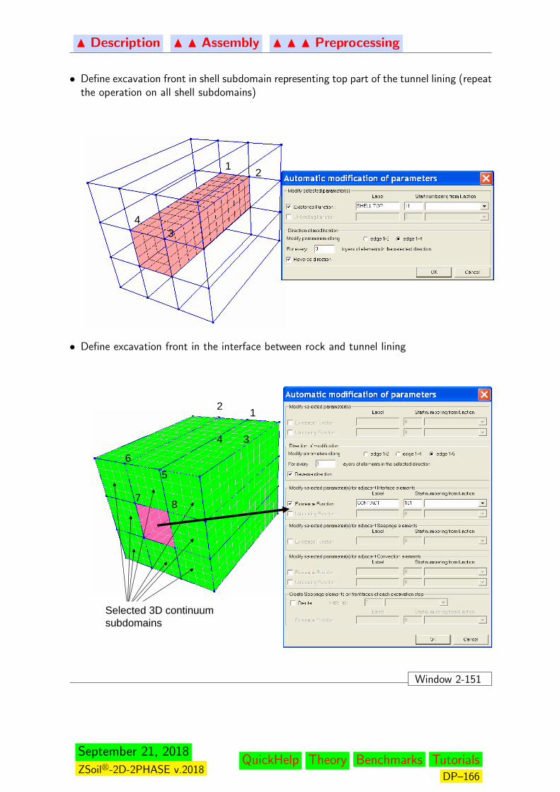
N Description N N Assembly N N N Preprocessing
• Define excavation front in shell subdomain representing top part of the tunnel lining (repeatthe operation on all shell subdomains)
1 2
34
• Define excavation front in the interface between rock and tunnel lining
12
34
56
7 8
Selected 3D continuum subdomains
Window 2-151
September 21, 2018
ZSoilr-2D-2PHASE v.2018QuickHelp Theory Benchmarks Tutorials
DP–166
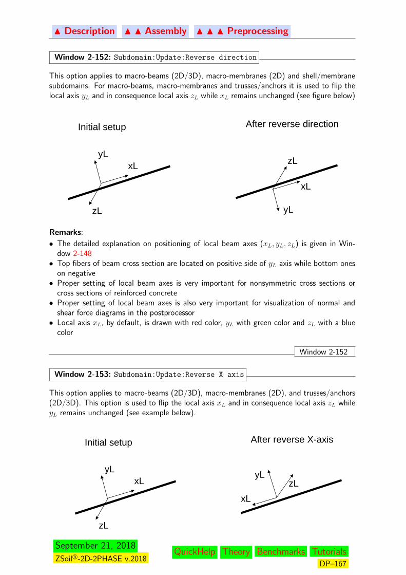
N Description N N Assembly N N N Preprocessing
Window 2-152: Subdomain:Update:Reverse direction
This option applies to macro-beams (2D/3D), macro-membranes (2D) and shell/membranesubdomains. For macro-beams, macro-membranes and trusses/anchors it is used to flip thelocal axis yL and in consequence local axis zL while xL remains unchanged (see figure below)
xLyL
zL
xL
yL
zL
Initial setup After reverse direction
zL
zL
Initial setup After reverse directionRemarks:
• The detailed explanation on positioning of local beam axes (xL, yL, zL) is given in Win-dow 2-148• Top fibers of beam cross section are located on positive side of yL axis while bottom ones
on negative• Proper setting of local beam axes is very important for nonsymmetric cross sections or
cross sections of reinforced concrete• Proper setting of local beam axes is also very important for visualization of normal and
shear force diagrams in the postprocessor• Local axis xL, by default, is drawn with red color, yL with green color and zL with a blue
color
Window 2-152
Window 2-153: Subdomain:Update:Reverse X axis
This option applies to macro-beams (2D/3D), macro-membranes (2D), and trusses/anchors(2D/3D). This option is used to flip the local axis xL and in consequence local axis zL whileyL remains unchanged (see example below).
xLyL
zL
xL
yLzL
Initial setup After reverse X-axis
September 21, 2018
ZSoilr-2D-2PHASE v.2018QuickHelp Theory Benchmarks Tutorials
DP–167

N Description N N Assembly N N N Preprocessing
Remarks:
• The detailed explanation on positioning of local beam axes (xL, yL, zL) is given in Win-dow 2-148• Top fibers of beam cross section are located on positive side of yL axis while bottom ones
on negative• Proper setting of local beam axes is very important for nonsymmetric cross sections or
cross sections of reinforced concrete• Proper setting of local axes is also very important for visualization of normal and shear
force diagrams in the postprocessor• Local axis xL, by default, is drawn with red color, yL with green color and zL with a blue
color
Window 2-153
September 21, 2018
ZSoilr-2D-2PHASE v.2018QuickHelp Theory Benchmarks Tutorials
DP–168

N Description N N Assembly N N N Preprocessing
Window 2-154: Subdomain:Mesh:Virtual mesh (2D continuum)
Any continuum 2D subdomain can be virtually discretized with 3 different grid types.
• (A) Structured:
F with quadrilateral (Q4) template (see Window 2-155)
F with triangular (T3) template (see Window 2-156)
• (B) Unstructured (automatic, quad only, meshing using Q-morph algorithm):
F with assumed element size (see Window 2-157)
F with assumed boundary split value (see Window 2-158)
• (C) Through morphing (using Q4 or T3 templates) (see Window 2-159)
A
B
C
D
Remarks:
1. Structural subdomains modeled with aid of continuum elements should be discretized usingStructured grids
2. Number of elements along common boundaries of adjacent subdomains can be controlledduring discretization once the Adjust split... checkbox (D) is set to ON
3. If Adjust split... is set to OFF then meshes in adjacent subdomains will not becompatible; special Mesh tying elements, available at the finite element level can remedythis problem
4. Virtual mesh is treated here as a guess for the real mesh but subdomain is not yet subdividedinto elements.
5. Button Apply allows to define control points of the subdomain (if structured mesh is to
be generated) without need for setting up the virtual mesh
Window 2-154
September 21, 2018
ZSoilr-2D-2PHASE v.2018QuickHelp Theory Benchmarks Tutorials
DP–169
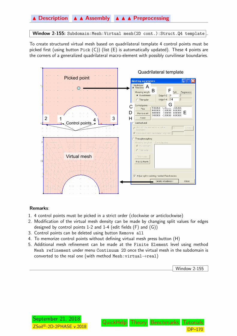
N Description N N Assembly N N N Preprocessing
Window 2-155: Subdomain:Mesh:Virtual mesh(2D cont.):Struct.Q4 template
To create structured virtual mesh based on quadrilateral template 4 control points must bepicked first (using button Pick (C)) (list (E) is automatically updated). These 4 points arethe corners of a generalized quadrilateral macro-element with possibly curvilinear boundaries.
12 34Control points
AB
CD E
Virtual mesh
Picked pointQuadrilateral template
F
G
H
Remarks:
1. 4 control points must be picked in a strict order (clockwise or anticlockwise)2. Modification of the virtual mesh density can be made by changing split values for edges
designed by control points 1-2 and 1-4 (edit fields (F) and (G))3. Control points can be deleted using button Remove all
4. To memorize control points without defining virtual mesh press button (H)5. Additional mesh refinement can be made at the Finite Element level using method
Mesh refinement under menu Continuum 2D once the virtual mesh in the subdomain isconverted to the real one (with method Mesh:virtual→real)
Window 2-155
September 21, 2018
ZSoilr-2D-2PHASE v.2018QuickHelp Theory Benchmarks Tutorials
DP–170
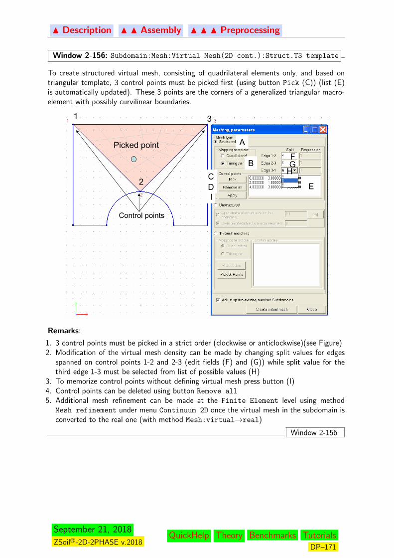
N Description N N Assembly N N N Preprocessing
Window 2-156: Subdomain:Mesh:Virtual Mesh(2D cont.):Struct.T3 template
To create structured virtual mesh, consisting of quadrilateral elements only, and based ontriangular template, 3 control points must be picked first (using button Pick (C)) (list (E)is automatically updated). These 3 points are the corners of a generalized triangular macro-element with possibly curvilinear boundaries.
1
2
3
A
BCD E
FGH
Picked point
Control points
I
Remarks:
1. 3 control points must be picked in a strict order (clockwise or anticlockwise)(see Figure)2. Modification of the virtual mesh density can be made by changing split values for edges
spanned on control points 1-2 and 2-3 (edit fields (F) and (G)) while split value for thethird edge 1-3 must be selected from list of possible values (H)
3. To memorize control points without defining virtual mesh press button (I)4. Control points can be deleted using button Remove all
5. Additional mesh refinement can be made at the Finite Element level using methodMesh refinement under menu Continuum 2D once the virtual mesh in the subdomain isconverted to the real one (with method Mesh:virtual→real)
Window 2-156
September 21, 2018
ZSoilr-2D-2PHASE v.2018QuickHelp Theory Benchmarks Tutorials
DP–171
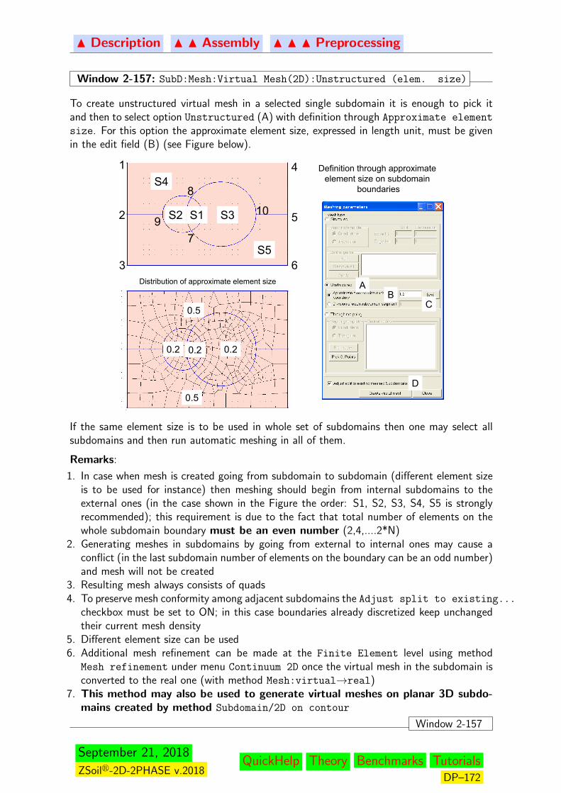
N Description N N Assembly N N N Preprocessing
Window 2-157: SubD:Mesh:Virtual Mesh(2D):Unstructured (elem. size)
To create unstructured virtual mesh in a selected single subdomain it is enough to pick itand then to select option Unstructured (A) with definition through Approximate element
size. For this option the approximate element size, expressed in length unit, must be givenin the edit field (B) (see Figure below).
S1S2 S3
S4
S5
1
2
3
4
5
6
7
8
910
BC
0.20.2 0.2
0.5
0.5
Distribution of approximate element size
Definition through approximateelement size on subdomain
boundaries
D
A
If the same element size is to be used in whole set of subdomains then one may select allsubdomains and then run automatic meshing in all of them.
Remarks:
1. In case when mesh is created going from subdomain to subdomain (different element sizeis to be used for instance) then meshing should begin from internal subdomains to theexternal ones (in the case shown in the Figure the order: S1, S2, S3, S4, S5 is stronglyrecommended); this requirement is due to the fact that total number of elements on thewhole subdomain boundary must be an even number (2,4,....2*N)
2. Generating meshes in subdomains by going from external to internal ones may cause aconflict (in the last subdomain number of elements on the boundary can be an odd number)and mesh will not be created
3. Resulting mesh always consists of quads4. To preserve mesh conformity among adjacent subdomains the Adjust split to existing...
checkbox must be set to ON; in this case boundaries already discretized keep unchangedtheir current mesh density
5. Different element size can be used6. Additional mesh refinement can be made at the Finite Element level using method
Mesh refinement under menu Continuum 2D once the virtual mesh in the subdomain isconverted to the real one (with method Mesh:virtual→real)
7. This method may also be used to generate virtual meshes on planar 3D subdo-mains created by method Subdomain/2D on contour
Window 2-157
September 21, 2018
ZSoilr-2D-2PHASE v.2018QuickHelp Theory Benchmarks Tutorials
DP–172
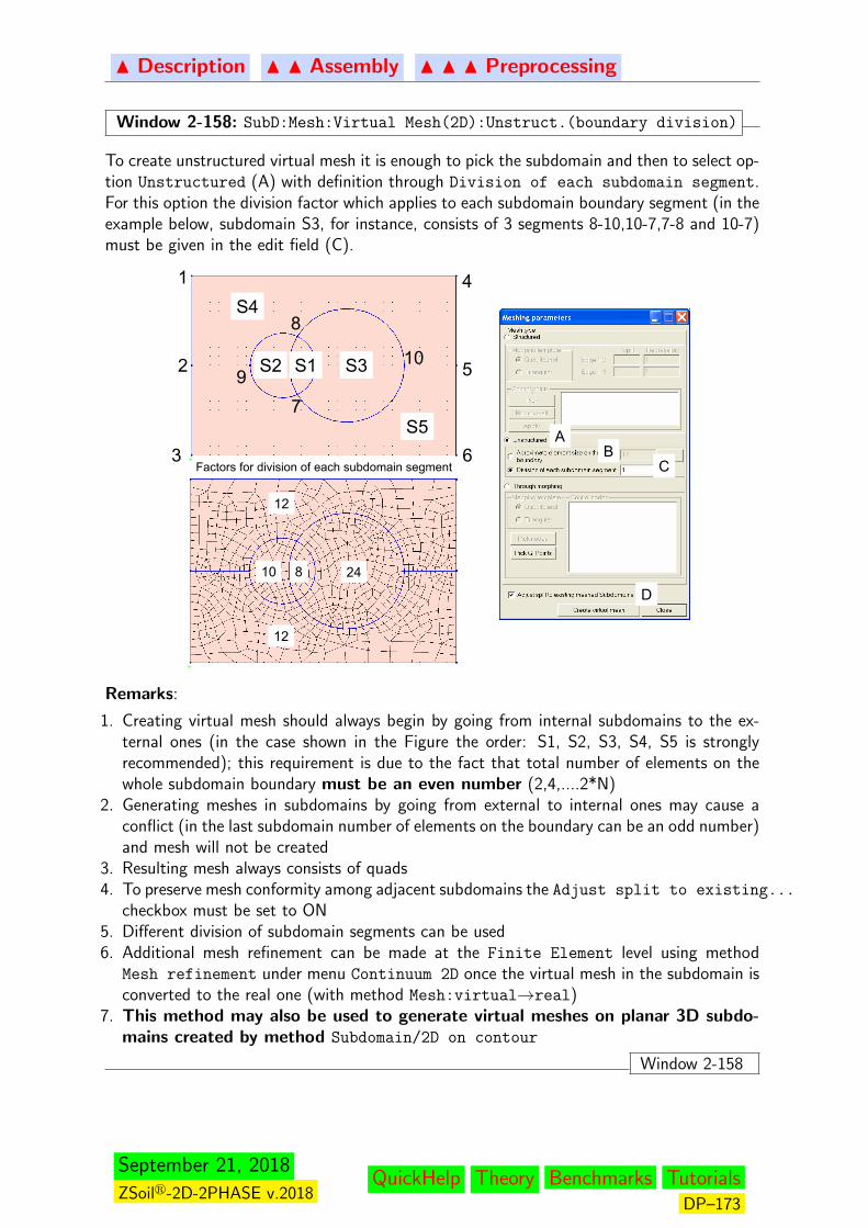
N Description N N Assembly N N N Preprocessing
Window 2-158: SubD:Mesh:Virtual Mesh(2D):Unstruct.(boundary division)
To create unstructured virtual mesh it is enough to pick the subdomain and then to select op-tion Unstructured (A) with definition through Division of each subdomain segment.For this option the division factor which applies to each subdomain boundary segment (in theexample below, subdomain S3, for instance, consists of 3 segments 8-10,10-7,7-8 and 10-7)must be given in the edit field (C).
3 6
S1S2 S3
S4
S5
1
2
4
5
7
8
910
Factors for division of each subdomain segment
810 24
12
12
BC
D
A
Remarks:
1. Creating virtual mesh should always begin by going from internal subdomains to the ex-ternal ones (in the case shown in the Figure the order: S1, S2, S3, S4, S5 is stronglyrecommended); this requirement is due to the fact that total number of elements on thewhole subdomain boundary must be an even number (2,4,....2*N)
2. Generating meshes in subdomains by going from external to internal ones may cause aconflict (in the last subdomain number of elements on the boundary can be an odd number)and mesh will not be created
3. Resulting mesh always consists of quads4. To preserve mesh conformity among adjacent subdomains the Adjust split to existing...
checkbox must be set to ON5. Different division of subdomain segments can be used6. Additional mesh refinement can be made at the Finite Element level using method
Mesh refinement under menu Continuum 2D once the virtual mesh in the subdomain isconverted to the real one (with method Mesh:virtual→real)
7. This method may also be used to generate virtual meshes on planar 3D subdo-mains created by method Subdomain/2D on contour
Window 2-158
September 21, 2018
ZSoilr-2D-2PHASE v.2018QuickHelp Theory Benchmarks Tutorials
DP–173
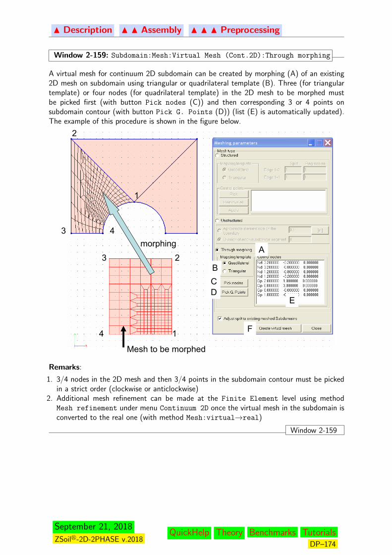
N Description N N Assembly N N N Preprocessing
Window 2-159: Subdomain:Mesh:Virtual Mesh (Cont.2D):Through morphing
A virtual mesh for continuum 2D subdomain can be created by morphing (A) of an existing2D mesh on subdomain using triangular or quadrilateral template (B). Three (for triangulartemplate) or four nodes (for quadrilateral template) in the 2D mesh to be morphed mustbe picked first (with button Pick nodes (C)) and then corresponding 3 or 4 points onsubdomain contour (with button Pick G. Points (D)) (list (E) is automatically updated).The example of this procedure is shown in the figure below.
1
23
4
1
2
3 4morphing
Mesh to be morphed
A
BCD
E
F
Remarks:
1. 3/4 nodes in the 2D mesh and then 3/4 points in the subdomain contour must be pickedin a strict order (clockwise or anticlockwise)
2. Additional mesh refinement can be made at the Finite Element level using methodMesh refinement under menu Continuum 2D once the virtual mesh in the subdomain isconverted to the real one (with method Mesh:virtual→real)
Window 2-159
September 21, 2018
ZSoilr-2D-2PHASE v.2018QuickHelp Theory Benchmarks Tutorials
DP–174

N Description N N Assembly N N N Preprocessing
Window 2-160: Subdomain:Mesh:Virtual→Real mesh
This method converts a temporary virtual mesh to the real one.
Remarks:
1. During mesh conversion (from virtual to real) real finite elements and nodal points arecreated
2. Additional mesh refinement can be made at the Finite Element level using method Mesh
refinement under menu corresponding to the specific class of elements (like continuum,shell etc..) or by activating the Mesh refinement toolbar
Window 2-160
Window 2-161: Subdomain:Mesh:Remove virtual mesh
This method removes a temporary virtual mesh in picked subdomain or group of selectedsubdomains.
Remarks:
1. Subdomain is not deleted2. Real mesh (if exists) remains undeleted
Window 2-161
Window 2-162: Subdomain:Mesh:Remove real mesh
This method removes a real mesh created in picked subdomain or group of selected subdo-mains
Remarks:
1. Subdomain is not deleted2. Virtual mesh (if exists) remains undeleted
Window 2-162
September 21, 2018
ZSoilr-2D-2PHASE v.2018QuickHelp Theory Benchmarks Tutorials
DP–175

N Description N N Assembly N N N Preprocessing
2.3.1.2.6 SEEPAGE
Window 2-163: Options in menu Seepage
Option Method Toolbar DescriptionCreate On Subdomain edge(s) — Window 2-164Outline All — Window 2-165
With material — Window 2-165With existence function — Window 2-165With label — Window 2-165
In zoom box Window 2-243
In zoom circle Window 2-244
Inside contour Window 2-245
Delete Delete Window 2-246Update Parameters — Window 2-166
Scale — Window 2-166Show — Window 2-166Hide — Window 2-166
Window 2-163
September 21, 2018
ZSoilr-2D-2PHASE v.2018QuickHelp Theory Benchmarks Tutorials
DP–176

N Description N N Assembly N N N Preprocessing
Window 2-164: Seepage:On Subdomain edges
New 2D seepage macro-element(s) is(are) created on selected subdomain edge(s).
Selected edge insubdomain 2D
Remarks:
1. This macro-element is meaningful for Flow and Deformation+Flow analyzes2. Seepage elements will be created on edges of the mesh of continuum elements once the
virtual and then the real mesh in the continuum subdomain is created3. Direction marker helps to identify on which continuum subdomain edge seepage macro-
element is created (if two subdomains share the same edge)4. More information on seepage elements (FE model level) is given in Win.(2-377)5. Any mesh refinement in the adjacent continuum automatically enforces mesh refinement
in the seepage macro-element
Window 2-164
September 21, 2018
ZSoilr-2D-2PHASE v.2018QuickHelp Theory Benchmarks Tutorials
DP–177
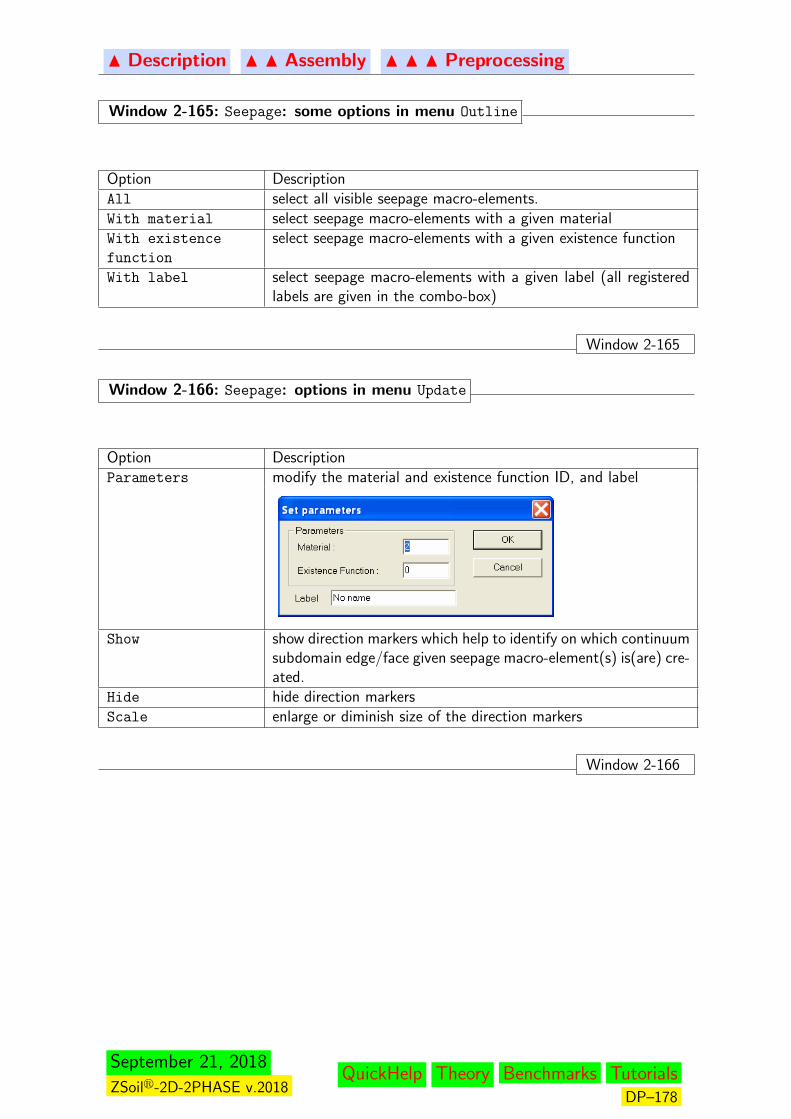
N Description N N Assembly N N N Preprocessing
Window 2-165: Seepage: some options in menu Outline
Option DescriptionAll select all visible seepage macro-elements.With material select seepage macro-elements with a given materialWith existence
function
select seepage macro-elements with a given existence function
With label select seepage macro-elements with a given label (all registeredlabels are given in the combo-box)
Window 2-165
Window 2-166: Seepage: options in menu Update
Option DescriptionParameters modify the material and existence function ID, and label
Show show direction markers which help to identify on which continuumsubdomain edge/face given seepage macro-element(s) is(are) cre-ated.
Hide hide direction markersScale enlarge or diminish size of the direction markers
Window 2-166
September 21, 2018
ZSoilr-2D-2PHASE v.2018QuickHelp Theory Benchmarks Tutorials
DP–178
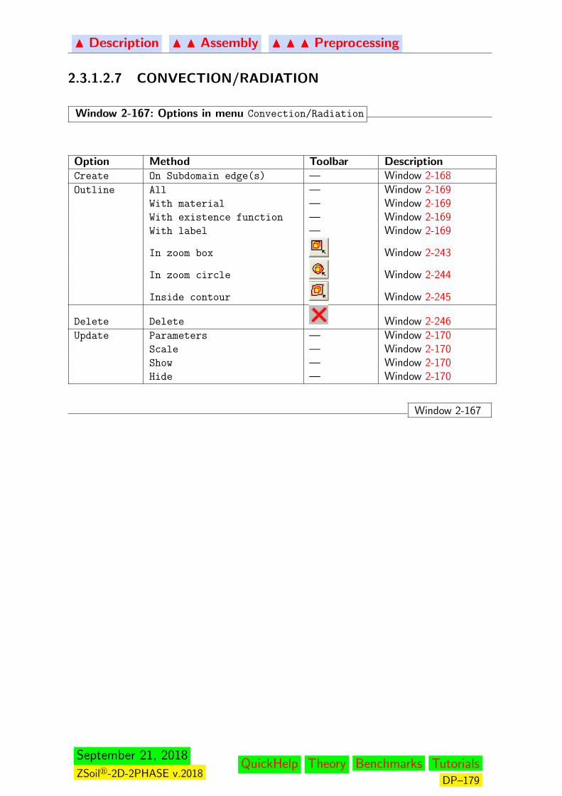
N Description N N Assembly N N N Preprocessing
2.3.1.2.7 CONVECTION/RADIATION
Window 2-167: Options in menu Convection/Radiation
Option Method Toolbar DescriptionCreate On Subdomain edge(s) — Window 2-168Outline All — Window 2-169
With material — Window 2-169With existence function — Window 2-169With label — Window 2-169
In zoom box Window 2-243
In zoom circle Window 2-244
Inside contour Window 2-245
Delete Delete Window 2-246Update Parameters — Window 2-170
Scale — Window 2-170Show — Window 2-170Hide — Window 2-170
Window 2-167
September 21, 2018
ZSoilr-2D-2PHASE v.2018QuickHelp Theory Benchmarks Tutorials
DP–179
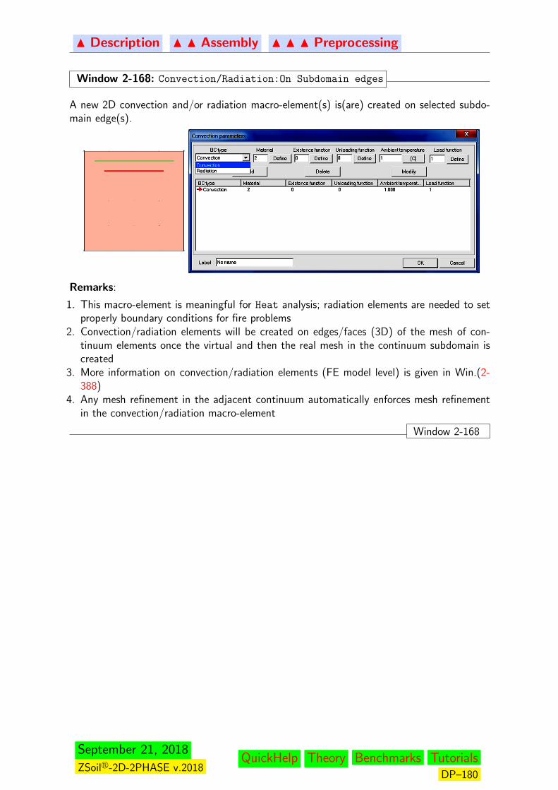
N Description N N Assembly N N N Preprocessing
Window 2-168: Convection/Radiation:On Subdomain edges
A new 2D convection and/or radiation macro-element(s) is(are) created on selected subdo-main edge(s).
Remarks:
1. This macro-element is meaningful for Heat analysis; radiation elements are needed to setproperly boundary conditions for fire problems
2. Convection/radiation elements will be created on edges/faces (3D) of the mesh of con-tinuum elements once the virtual and then the real mesh in the continuum subdomain iscreated
3. More information on convection/radiation elements (FE model level) is given in Win.(2-388)
4. Any mesh refinement in the adjacent continuum automatically enforces mesh refinementin the convection/radiation macro-element
Window 2-168
September 21, 2018
ZSoilr-2D-2PHASE v.2018QuickHelp Theory Benchmarks Tutorials
DP–180
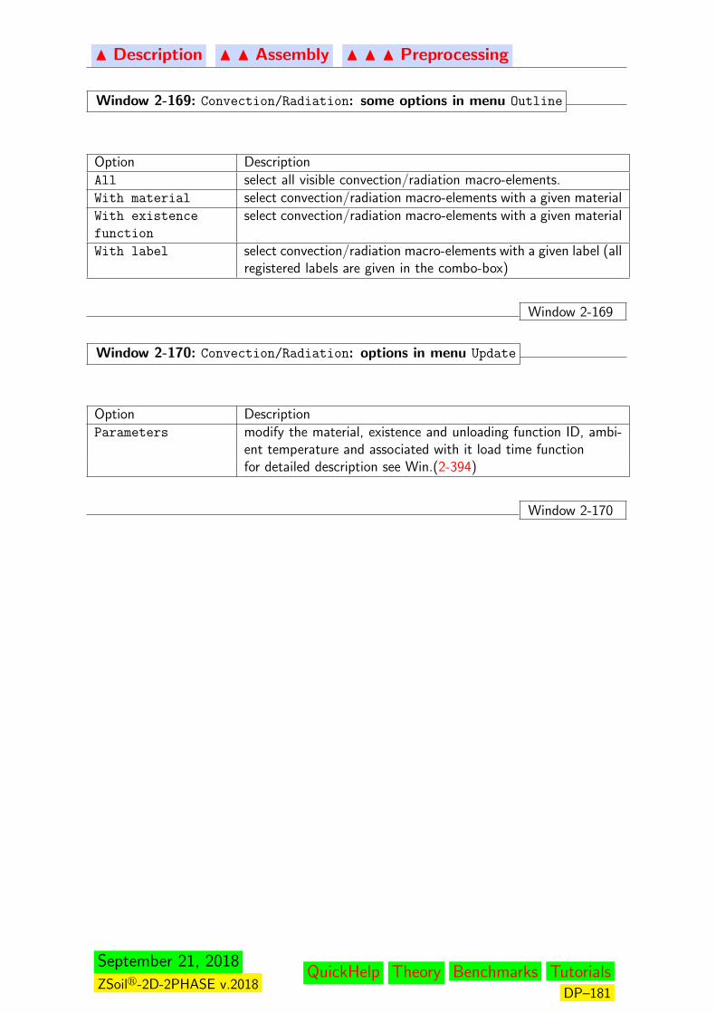
N Description N N Assembly N N N Preprocessing
Window 2-169: Convection/Radiation: some options in menu Outline
Option DescriptionAll select all visible convection/radiation macro-elements.With material select convection/radiation macro-elements with a given materialWith existence
function
select convection/radiation macro-elements with a given material
With label select convection/radiation macro-elements with a given label (allregistered labels are given in the combo-box)
Window 2-169
Window 2-170: Convection/Radiation: options in menu Update
Option DescriptionParameters modify the material, existence and unloading function ID, ambi-
ent temperature and associated with it load time functionfor detailed description see Win.(2-394)
Window 2-170
September 21, 2018
ZSoilr-2D-2PHASE v.2018QuickHelp Theory Benchmarks Tutorials
DP–181

N Description N N Assembly N N N Preprocessing
2.3.1.2.8 VISCOUS DAMPER
Window 2-171: Options in menu Viscous damper
Option Method Toolbar DescriptionCreate On Subdomain edge(s) — Window 2-172Outline All — Window 2-173
With material — Window 2-173With existence function — Window 2-173With label — Window 2-173
In zoom box Window 2-243
In zoom circle Window 2-244
Inside contour Window 2-245
Delete Delete Window 2-246Update Parameters — Window 2-174
Scale — Window 2-174Show — Window 2-174Hide — Window 2-174
Window 2-171
September 21, 2018
ZSoilr-2D-2PHASE v.2018QuickHelp Theory Benchmarks Tutorials
DP–182
N Description N N Assembly N N N Preprocessing
Window 2-172: Viscous damper:On Subdomain edges
A new 2D viscous damper macro-element(s) is(are) created on selected subdomain edge(s).
Remarks:
1. This macro-element is meaningful for Deformation or Deformation+Flow analyses whenrunning Transient dynamics driver
2. Viscous damper elements will be created on edges of the mesh of continuum elements oncethe virtual and then the real mesh in the continuum subdomain is created
3. More information on damper elements (FE model level) is given in Win.(2-396)4. Any mesh refinement in the adjacent continuum automatically enforces mesh refinement
in the damper macro-element
Window 2-172
Window 2-173: Viscous damper: some options in menu Outline
September 21, 2018
ZSoilr-2D-2PHASE v.2018QuickHelp Theory Benchmarks Tutorials
DP–183
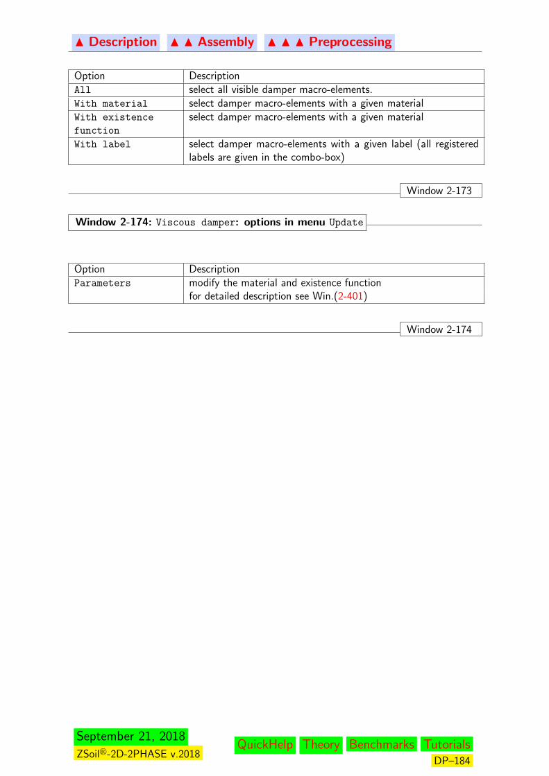
N Description N N Assembly N N N Preprocessing
Option DescriptionAll select all visible damper macro-elements.With material select damper macro-elements with a given materialWith existence
function
select damper macro-elements with a given material
With label select damper macro-elements with a given label (all registeredlabels are given in the combo-box)
Window 2-173
Window 2-174: Viscous damper: options in menu Update
Option DescriptionParameters modify the material and existence function
for detailed description see Win.(2-401)
Window 2-174
September 21, 2018
ZSoilr-2D-2PHASE v.2018QuickHelp Theory Benchmarks Tutorials
DP–184

N Description N N Assembly N N N Preprocessing
2.3.1.2.9 INTERFACE
Window 2-175: Options in menu Interface
Option Method Toolbar DescriptionzxCreate On Continuum subd.edge(s) — Window 2-176
On Structural
subdomain(s)
— Window 2-177
Outline All — Window 2-178With material — Window 2-178With existence function — Window 2-178With label — Window 2-178With attribute — Window 2-178
In zoom box Window 2-243
In zoom circle Window 2-244
Inside contour Window 2-245
Delete Delete Window 2-246Update Parameters — Window 2-179
Scale — Window 2-179Show direction — Window 2-179Hide direction — Window 2-179
Window 2-175
September 21, 2018
ZSoilr-2D-2PHASE v.2018QuickHelp Theory Benchmarks Tutorials
DP–185
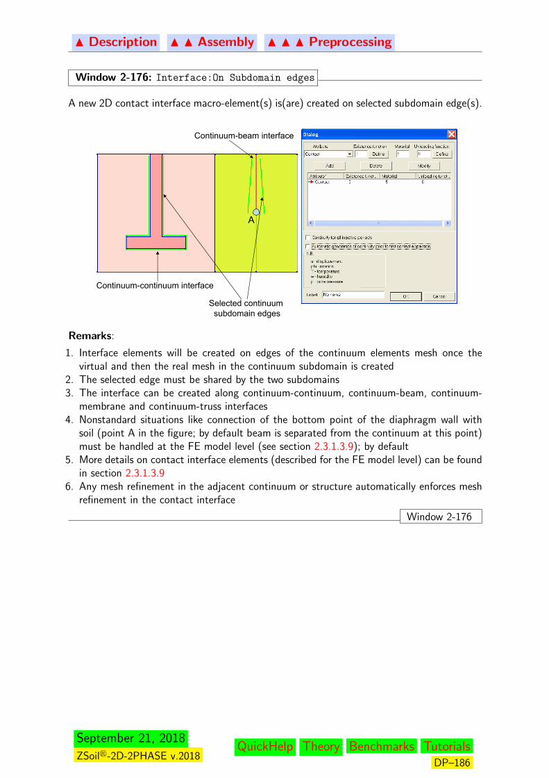
N Description N N Assembly N N N Preprocessing
Window 2-176: Interface:On Subdomain edges
A new 2D contact interface macro-element(s) is(are) created on selected subdomain edge(s).
Continuum-continuum interface
Continuum-beam interface
Selected continuum subdomain edges
A
Remarks:
1. Interface elements will be created on edges of the continuum elements mesh once thevirtual and then the real mesh in the continuum subdomain is created
2. The selected edge must be shared by the two subdomains3. The interface can be created along continuum-continuum, continuum-beam, continuum-
membrane and continuum-truss interfaces4. Nonstandard situations like connection of the bottom point of the diaphragm wall with
soil (point A in the figure; by default beam is separated from the continuum at this point)must be handled at the FE model level (see section 2.3.1.3.9); by default
5. More details on contact interface elements (described for the FE model level) can be foundin section 2.3.1.3.9
6. Any mesh refinement in the adjacent continuum or structure automatically enforces meshrefinement in the contact interface
Window 2-176
September 21, 2018
ZSoilr-2D-2PHASE v.2018QuickHelp Theory Benchmarks Tutorials
DP–186
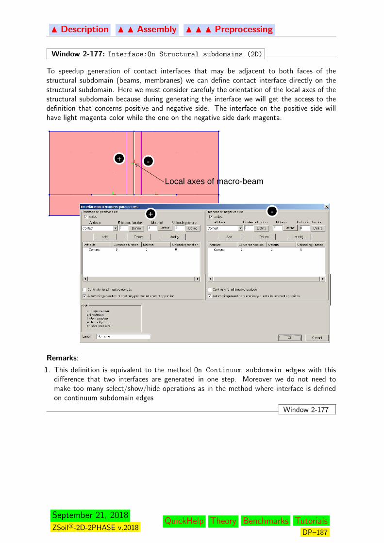
N Description N N Assembly N N N Preprocessing
Window 2-177: Interface:On Structural subdomains (2D)
To speedup generation of contact interfaces that may be adjacent to both faces of thestructural subdomain (beams, membranes) we can define contact interface directly on thestructural subdomain. Here we must consider carefuly the orientation of the local axes of thestructural subdomain because during generating the interface we will get the access to thedefinition that concerns positive and negative side. The interface on the positive side willhave light magenta color while the one on the negative side dark magenta.
-++
Local axes of macro beamLocal axes of macro-beam
++ -
Remarks:
1. This definition is equivalent to the method On Continuum subdomain edges with thisdifference that two interfaces are generated in one step. Moreover we do not need tomake too many select/show/hide operations as in the method where interface is definedon continuum subdomain edges
Window 2-177
September 21, 2018
ZSoilr-2D-2PHASE v.2018QuickHelp Theory Benchmarks Tutorials
DP–187
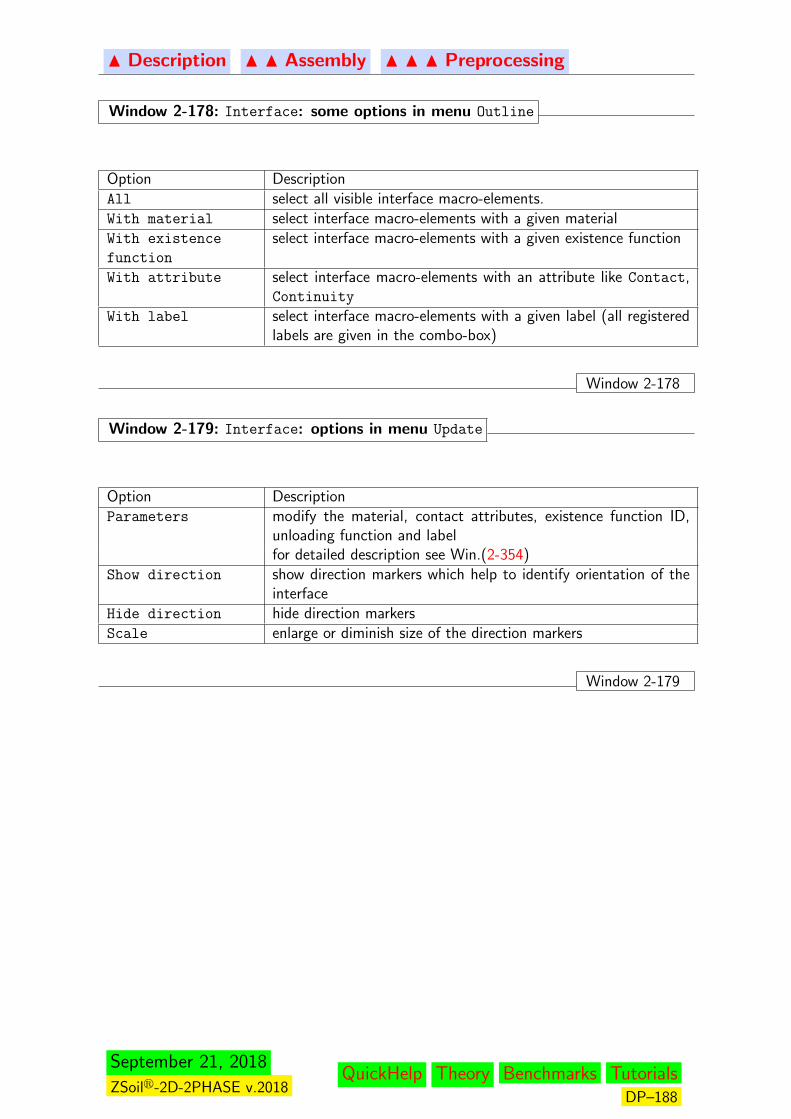
N Description N N Assembly N N N Preprocessing
Window 2-178: Interface: some options in menu Outline
Option DescriptionAll select all visible interface macro-elements.With material select interface macro-elements with a given materialWith existence
function
select interface macro-elements with a given existence function
With attribute select interface macro-elements with an attribute like Contact,Continuity
With label select interface macro-elements with a given label (all registeredlabels are given in the combo-box)
Window 2-178
Window 2-179: Interface: options in menu Update
Option DescriptionParameters modify the material, contact attributes, existence function ID,
unloading function and labelfor detailed description see Win.(2-354)
Show direction show direction markers which help to identify orientation of theinterface
Hide direction hide direction markersScale enlarge or diminish size of the direction markers
Window 2-179
September 21, 2018
ZSoilr-2D-2PHASE v.2018QuickHelp Theory Benchmarks Tutorials
DP–188
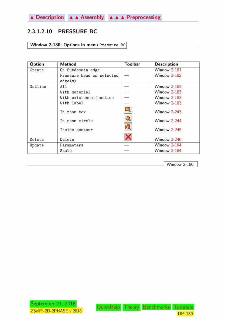
N Description N N Assembly N N N Preprocessing
2.3.1.2.10 PRESSURE BC
Window 2-180: Options in menu Pressure BC
Option Method Toolbar DescriptionCreate On Subdomain edge — Window 2-181
Pressure head on selected
edge(s)
— Window 2-182
Outline All — Window 2-183With material — Window 2-183With existence function — Window 2-183With label — Window 2-183
In zoom box Window 2-243
In zoom circle Window 2-244
Inside contour Window 2-245
Delete Delete Window 2-246Update Parameters — Window 2-184
Scale — Window 2-184
Window 2-180
September 21, 2018
ZSoilr-2D-2PHASE v.2018QuickHelp Theory Benchmarks Tutorials
DP–189
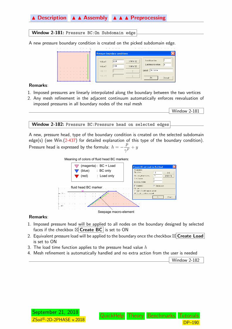
N Description N N Assembly N N N Preprocessing
Window 2-181: Pressure BC:On Subdomain edge
A new pressure boundary condition is created on the picked subdomain edge.
Remarks:
1. Imposed pressures are linearly interpolated along the boundary between the two vertices2. Any mesh refinement in the adjacent continuum automatically enforces reevaluation of
imposed pressures in all boundary nodes of the real mesh
Window 2-181
Window 2-182: Pressure BC:Pressure head on selected edges
A new, pressure head, type of the boundary condition is created on the selected subdomainedge(s) (see Win.(2-437) for detailed explanation of this type of the boundary condition).
Pressure head is expressed by the formula: h = − p
γF+ y
Meaning of colors of fluid head BC markers:
(magenta) : BC + Load(blue) : BC only(red) : Load only
fluid head BC marker
Seepage macro-elementRemarks:
1. Imposed pressure head will be applied to all nodes on the boundary designed by selectedfaces if the checkbox � Create BC is set to ON
2. Equivalent pressure load will be applied to the boundary once the checkbox� Create Loadis set to ON
3. The load time function applies to the pressure head value h4. Mesh refinement is automatically handled and no extra action from the user is needed
Window 2-182
September 21, 2018
ZSoilr-2D-2PHASE v.2018QuickHelp Theory Benchmarks Tutorials
DP–190

N Description N N Assembly N N N Preprocessing
Window 2-183: Pressure BC: some options in menu Outline
Option DescriptionAll select all visible Pressure BC macro-objects.With load time
function
select Pressure BC macro-objects with a given load time function
With existence
function
select Pressure BC macro-objects with a given existence function
With label select pressure BC macro-objects with a given label (all registeredlabels are given in the combo-box)
Window 2-183
Window 2-184: Pressure BC: options in menu Update
Option DescriptionParameters For pressure BC defined on edges/faces modify values at pressure
macro-object vertices, load time function, existence function IDand label
For pressure head BC pick the marker top modify pressure headvalue, load time and existence functions
h
Window 2-184
September 21, 2018
ZSoilr-2D-2PHASE v.2018QuickHelp Theory Benchmarks Tutorials
DP–191
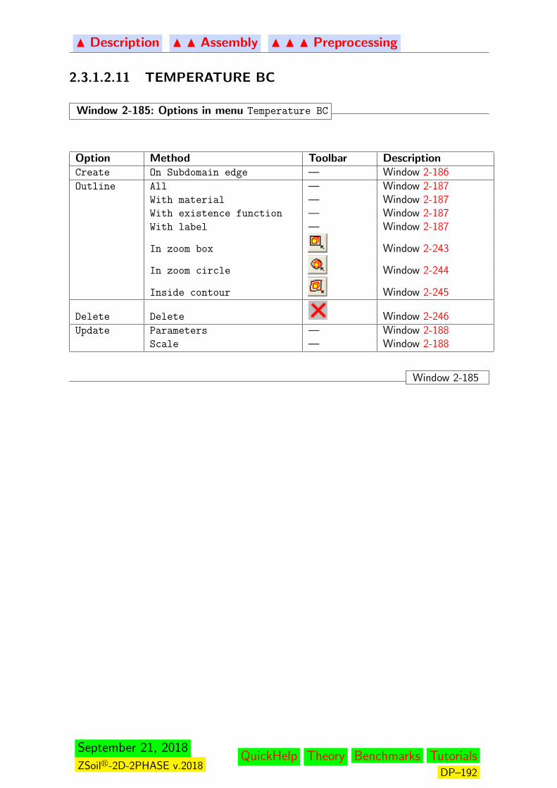
N Description N N Assembly N N N Preprocessing
2.3.1.2.11 TEMPERATURE BC
Window 2-185: Options in menu Temperature BC
Option Method Toolbar DescriptionCreate On Subdomain edge — Window 2-186Outline All — Window 2-187
With material — Window 2-187With existence function — Window 2-187With label — Window 2-187
In zoom box Window 2-243
In zoom circle Window 2-244
Inside contour Window 2-245
Delete Delete Window 2-246Update Parameters — Window 2-188
Scale — Window 2-188
Window 2-185
September 21, 2018
ZSoilr-2D-2PHASE v.2018QuickHelp Theory Benchmarks Tutorials
DP–192
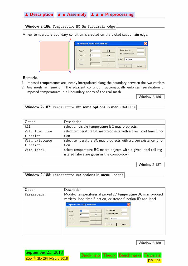
N Description N N Assembly N N N Preprocessing
Window 2-186: Temperature BC:On Subdomain edge
A new temperature boundary condition is created on the picked subdomain edge.
Remarks:
1. Imposed temperatures are linearly interpolated along the boundary between the two vertices2. Any mesh refinement in the adjacent continuum automatically enforces reevaluation of
imposed temperatures in all boundary nodes of the real mesh
Window 2-186
Window 2-187: Temperature BC: some options in menu Outline
Option DescriptionAll select all visible temperature BC macro-objects.With load time
function
select temperature BC macro-objects with a given load time func-tion
With existence
function
select temperature BC macro-objects with a given existence func-tion
With label select temperature BC macro-objects with a given label (all reg-istered labels are given in the combo-box)
Window 2-187
Window 2-188: Temperature BC: options in menu Update
Option DescriptionParameters Modify: temperatures at picked 2D temperature BC macro-object
vertices, load time function, existence function ID and label
Window 2-188
September 21, 2018
ZSoilr-2D-2PHASE v.2018QuickHelp Theory Benchmarks Tutorials
DP–193

N Description N N Assembly N N N Preprocessing
2.3.1.2.12 HUMIDITY BC
Window 2-189: Options in menu Humidity BC
Option Method Toolbar DescriptionCreate On Subdomain edge — Window 2-190Outline All — Window 2-191
With material — Window 2-191With existence function — Window 2-191With label — Window 2-191
In zoom box Window 2-243
In zoom circle Window 2-244
Inside contour Window 2-245
Delete Delete Window 2-246Update Parameters — Window 2-192
Scale — Window 2-192
Window 2-189
September 21, 2018
ZSoilr-2D-2PHASE v.2018QuickHelp Theory Benchmarks Tutorials
DP–194
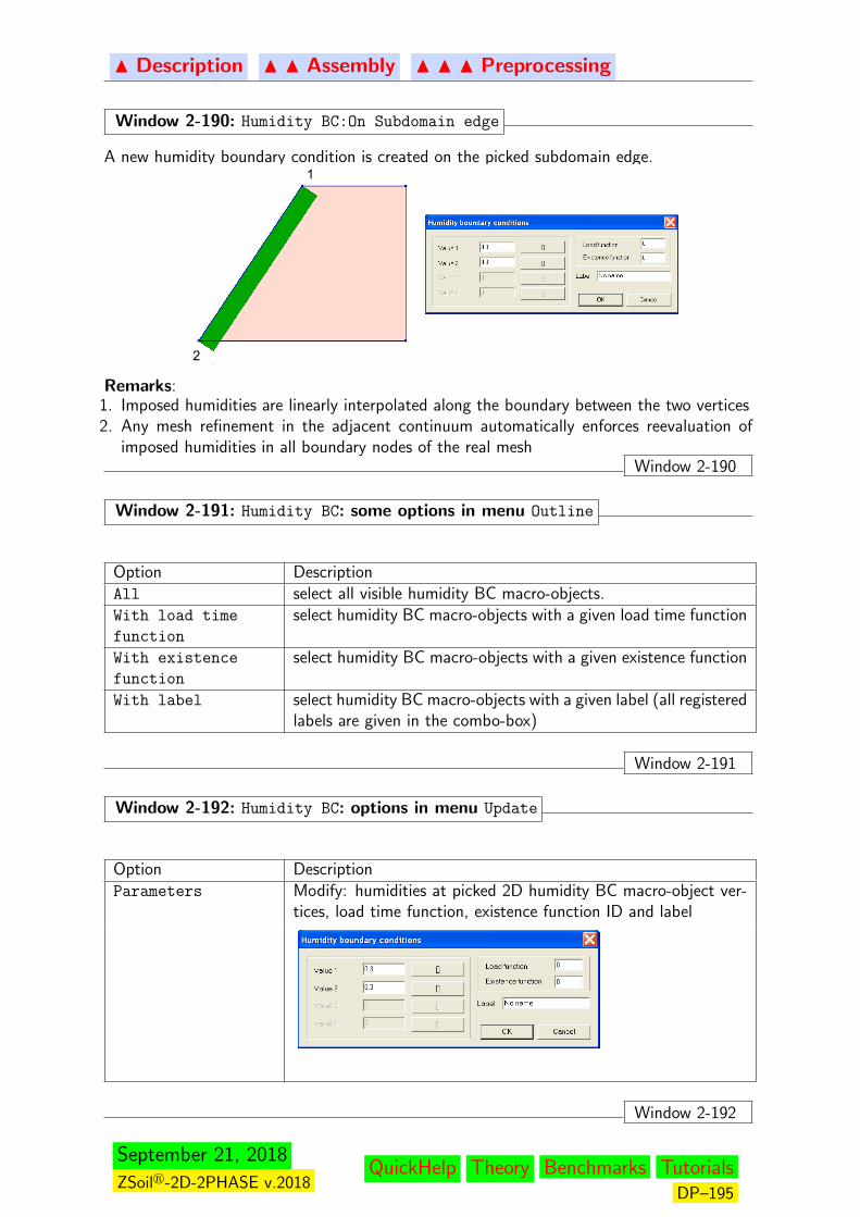
N Description N N Assembly N N N Preprocessing
Window 2-190: Humidity BC:On Subdomain edge
A new humidity boundary condition is created on the picked subdomain edge.1
2
Remarks:1. Imposed humidities are linearly interpolated along the boundary between the two vertices2. Any mesh refinement in the adjacent continuum automatically enforces reevaluation of
imposed humidities in all boundary nodes of the real meshWindow 2-190
Window 2-191: Humidity BC: some options in menu Outline
Option DescriptionAll select all visible humidity BC macro-objects.With load time
function
select humidity BC macro-objects with a given load time function
With existence
function
select humidity BC macro-objects with a given existence function
With label select humidity BC macro-objects with a given label (all registeredlabels are given in the combo-box)
Window 2-191
Window 2-192: Humidity BC: options in menu Update
Option DescriptionParameters Modify: humidities at picked 2D humidity BC macro-object ver-
tices, load time function, existence function ID and label
1
2Window 2-192
September 21, 2018
ZSoilr-2D-2PHASE v.2018QuickHelp Theory Benchmarks Tutorials
DP–195

N Description N N Assembly N N N Preprocessing
2.3.1.2.13 FLUID FLUX
Window 2-193: Options in menu Fluid flux
Option Method Toolbar DescriptionCreate On Subdomain edge — Window 2-194Outline All — Window 2-195
With material — Window 2-195With label — Window 2-195
In zoom box Window 2-243
In zoom circle Window 2-244
Inside contour Window 2-245
Delete Delete Window 2-246Update Parameters — Window 2-196
Scale — Window 2-196
Window 2-193
September 21, 2018
ZSoilr-2D-2PHASE v.2018QuickHelp Theory Benchmarks Tutorials
DP–196
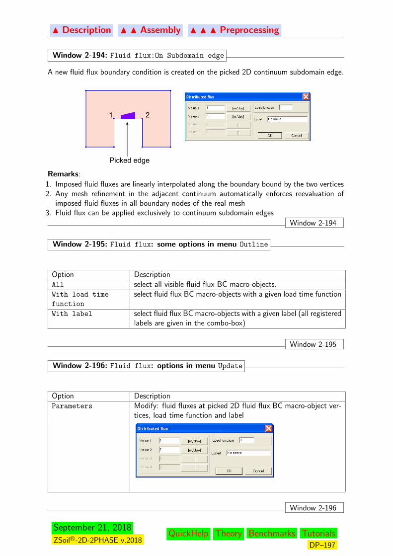
N Description N N Assembly N N N Preprocessing
Window 2-194: Fluid flux:On Subdomain edge
A new fluid flux boundary condition is created on the picked 2D continuum subdomain edge.
1 2
Picked edge
Remarks:
1. Imposed fluid fluxes are linearly interpolated along the boundary bound by the two vertices2. Any mesh refinement in the adjacent continuum automatically enforces reevaluation of
imposed fluid fluxes in all boundary nodes of the real mesh3. Fluid flux can be applied exclusively to continuum subdomain edges
Window 2-194
Window 2-195: Fluid flux: some options in menu Outline
Option DescriptionAll select all visible fluid flux BC macro-objects.With load time
function
select fluid flux BC macro-objects with a given load time function
With label select fluid flux BC macro-objects with a given label (all registeredlabels are given in the combo-box)
Window 2-195
Window 2-196: Fluid flux: options in menu Update
Option DescriptionParameters Modify: fluid fluxes at picked 2D fluid flux BC macro-object ver-
tices, load time function and label
1 2
Picked edgeWindow 2-196
September 21, 2018
ZSoilr-2D-2PHASE v.2018QuickHelp Theory Benchmarks Tutorials
DP–197

N Description N N Assembly N N N Preprocessing
2.3.1.2.14 HEAT FLUX
Window 2-197: Options in menu Heat flux
Option Method Toolbar DescriptionCreate On Subdomain edge — Window 2-198Outline All — Window 2-199
With material — Window 2-199With label — Window 2-199
In zoom box Window 2-243
In zoom circle Window 2-244
Inside contour Window 2-245
Delete Delete Window 2-246Update Parameters — Window 2-200
Scale — Window 2-200
Window 2-197
September 21, 2018
ZSoilr-2D-2PHASE v.2018QuickHelp Theory Benchmarks Tutorials
DP–198
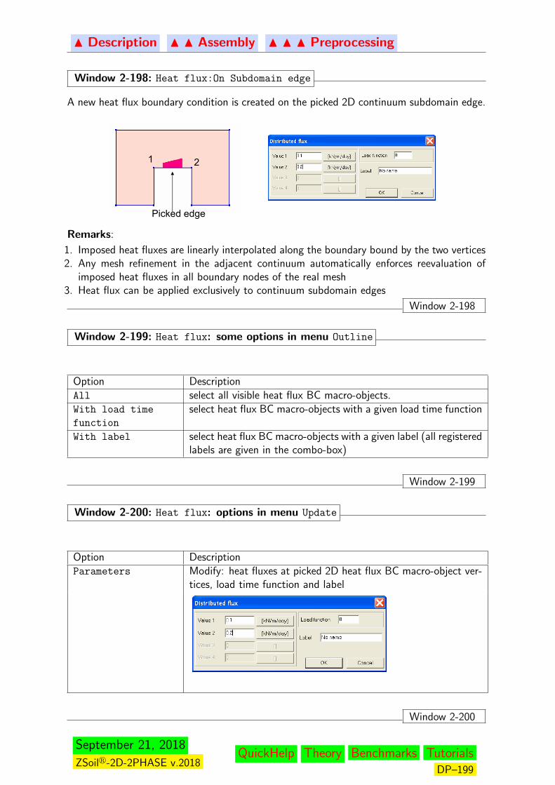
N Description N N Assembly N N N Preprocessing
Window 2-198: Heat flux:On Subdomain edge
A new heat flux boundary condition is created on the picked 2D continuum subdomain edge.
1 2
Picked edge
Remarks:
1. Imposed heat fluxes are linearly interpolated along the boundary bound by the two vertices2. Any mesh refinement in the adjacent continuum automatically enforces reevaluation of
imposed heat fluxes in all boundary nodes of the real mesh3. Heat flux can be applied exclusively to continuum subdomain edges
Window 2-198
Window 2-199: Heat flux: some options in menu Outline
Option DescriptionAll select all visible heat flux BC macro-objects.With load time
function
select heat flux BC macro-objects with a given load time function
With label select heat flux BC macro-objects with a given label (all registeredlabels are given in the combo-box)
Window 2-199
Window 2-200: Heat flux: options in menu Update
Option DescriptionParameters Modify: heat fluxes at picked 2D heat flux BC macro-object ver-
tices, load time function and label
1 2
Picked edge
Window 2-200
September 21, 2018
ZSoilr-2D-2PHASE v.2018QuickHelp Theory Benchmarks Tutorials
DP–199

N Description N N Assembly N N N Preprocessing
2.3.1.2.15 HUMIDITY FLUX
Window 2-201: Options in menu Humidity flux
Option Method Toolbar DescriptionCreate On Subdomain edge — Window 2-202Outline All — Window 2-203
With material — Window 2-203With label — Window 2-203
In zoom box Window 2-243
In zoom circle Window 2-244
Inside contour Window 2-245
Delete Delete Window 2-246Update Parameters — Window 2-204
Scale — Window 2-204
Window 2-201
September 21, 2018
ZSoilr-2D-2PHASE v.2018QuickHelp Theory Benchmarks Tutorials
DP–200

N Description N N Assembly N N N Preprocessing
Window 2-202: Humidity flux:On Subdomain edge
A new heat flux boundary condition is created on the picked 2D continuum subdomain edge.
1 2
Picked edge
Remarks:
1. Imposed humidity fluxes are linearly interpolated along the boundary bound by the twovertices
2. Any mesh refinement in the adjacent continuum automatically enforces reevaluation ofimposed humidity fluxes in all boundary nodes of the real mesh
3. Humidity flux can be applied exclusively to continuum subdomain edges
Window 2-202
Window 2-203: Humidity flux: some options in menu Outline
Option DescriptionAll select all visible humidity flux BC macro-objects.With load time
function
select humidity flux BC macro-objects with a given load timefunction
With label select humidity flux BC macro-objects with a given label (all reg-istered labels are given in the combo-box)
Window 2-203
Window 2-204: Humidity flux: options in menu Update
Option DescriptionParameters Modify: humidity fluxes at picked 2D humidity flux BC macro-
object vertices, load time function and label
1 2
Picked edgeWindow 2-204
September 21, 2018
ZSoilr-2D-2PHASE v.2018QuickHelp Theory Benchmarks Tutorials
DP–201
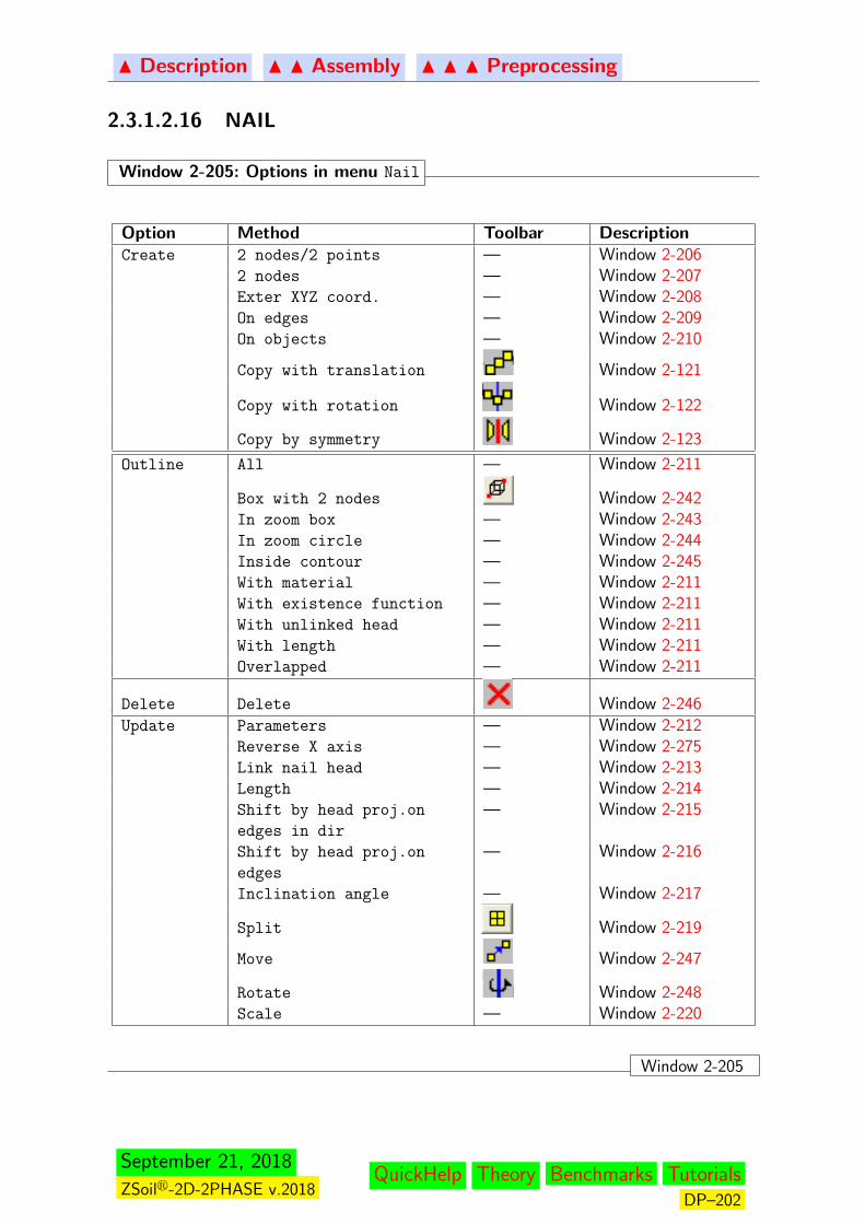
N Description N N Assembly N N N Preprocessing
2.3.1.2.16 NAIL
Window 2-205: Options in menu Nail
Option Method Toolbar DescriptionCreate 2 nodes/2 points — Window 2-206
2 nodes — Window 2-207Exter XYZ coord. — Window 2-208On edges — Window 2-209On objects — Window 2-210
Copy with translation Window 2-121
Copy with rotation Window 2-122
Copy by symmetry Window 2-123
Outline All — Window 2-211
Box with 2 nodes Window 2-242In zoom box — Window 2-243In zoom circle — Window 2-244Inside contour — Window 2-245With material — Window 2-211With existence function — Window 2-211With unlinked head — Window 2-211With length — Window 2-211Overlapped — Window 2-211
Delete Delete Window 2-246Update Parameters — Window 2-212
Reverse X axis — Window 2-275Link nail head — Window 2-213Length — Window 2-214Shift by head proj.on
edges in dir
— Window 2-215
Shift by head proj.on
edges
— Window 2-216
Inclination angle — Window 2-217
Split Window 2-219
Move Window 2-247
Rotate Window 2-248Scale — Window 2-220
Window 2-205
September 21, 2018
ZSoilr-2D-2PHASE v.2018QuickHelp Theory Benchmarks Tutorials
DP–202

N Description N N Assembly N N N Preprocessing
Window 2-206: Nail:Create:2 nodes/points
New nail macro-element (including interfaces) is created by picking the two points in thegraph pane. The two picked points will be first snapped to the existing nodes of the realmesh projected on the graph pane and then to the grid points according to the setup underSnap options. This option must be used with care because close to the picked point in thegraph pane there may appear several projected nodes/grid points and it may not be so easyto control the selection. So if one wants to create a nail between the two existing nodes it isrecommended to use the option Create:2 nodes described in Window 2-207. This optionis visible only at the macromodeling level.
Remarks:1. The default orientation of local yL and zL axes is set up automatically by the preprocessor
as the nail cross section is assumed to be circular; however, one may set it up in the editfields Beam director; setting local nail cross section coordinate system follows the sameprocedure as for beam elements ( see Window (2-148)
2. To flip orientation of exL base vector use option Update:Reverse X-axis
3. If � Create nail-soil interface is set ON then the frictional contact interface will beautomatically generated; this interface material will appear in the material menu as Nail
interface
4. If � Create nail-soil interface is set OFF then the full continuity of the displacementfield for both nail and continuum will be enforced
5. By default � Link nail head with is set ON; this way the top node (by default), will belinked with adjacent structural elements; note that linking of the nail head may be appliedonly to translational degrees of freedom;
September 21, 2018
ZSoilr-2D-2PHASE v.2018QuickHelp Theory Benchmarks Tutorials
DP–203
N Description N N Assembly N N N Preprocessing
6. Split parameter controls mesh density in nail macro-element; it is recommended to avoidtoo big differences in mesh densities between continuum and nails; such modeling maylead to axial force oscillations in the nail for high strength parameters of subsoil; usingautomatic split option usually helps to remedy the problem; two automatic split optionsare available ie. with the equal size or adaptive size (using exact intersection of the nailwith background mesh)
7. To avoid instabilities due to rigid rotation of the nail along its axis the rotation along localnail axis is fixed internally by the preprocessor
8. The shear ultimate stress in the nail is set up at the material level (nail interface) andexpressed in terms of the stresses rather then forces
9. To obtain meaningful results nails must be added to the computational model via existencefunctions; activating nails from the very beggining, without the initial state defined, usuallyresults in computation failure or wrong nail forces
10. Nails spacing in 2D is automaticaly inherited from the beam material used to model nailcore
11. The diameter of the injected nail zone is defined at the material level for the nail interface
Window 2-206
Window 2-207: Nail:Create:2 nodes
New nail macro-element is created by picking the two existing nodes in the graph pane. It isstrongly recommended to not to try to pick the node exactly (it is rather difficult action) butrather to select it by picking the existing element close to one of its vertices that coincideswith the node.
The selection rule is the only difference between this option and the one given in Window 2-206 so refer to that Window for remaining information.
Window 2-207
Window 2-208: Nail:Create:XYZ for 2 points
New nail macro-element element is created by entering X,Y,Z coordinates of its two endpointsin the dialog box. Setting of the nail endpoints is the only difference between this option andthe one given in Window 2-206 so refer to that Window for remaining information.
Window 2-208
Window 2-209: Nail:Create:On edge(s)
New nail macro-element(s) are generated on all selected edges (see figure below). Orientationof each nail macro-element element local x axis is coherent with orientation of the elementedge. The remaining nail setup is given in Window 2-206
Window 2-209
September 21, 2018
ZSoilr-2D-2PHASE v.2018QuickHelp Theory Benchmarks Tutorials
DP–204
N Description N N Assembly N N N Preprocessing
Window 2-210: Nail:Create:On object(s)
New nail macro-element(s) are generated on all selected geometrical objects (see figure be-low). Orientation of each nail macro-element local x axis is coherent with orientation of thegeometrical object. The remaining nail setup is given in Window 2-206
Window 2-210
Window 2-211: Nail: some options in menu Outline
Option DescriptionAll Select all visible nail macro-elementsWith existence
function
Select all visible nail macro-elements with a given existence func-tions
With nail material Select all visible nail macro-elements with a given nail materialWithout linked
head
Select all visible nail macro-elements without heads that are prop-erly linked (usually to the structural elements)
Window 2-211
Window 2-212: Nail:Update:Parameters
This option allows the user to modify setting for the selected nail or group of nails. In caseof group of nails this option is equivalent to the one designed for creating of nails describedin Win.( 2-206)
Window 2-212
Window 2-213: Nail:Update:Link nail head
This option allows the user to modify linking of the nail head with other elements of thecomputational model. The typical situation concerns connection of the nail head with thesheet-pile wall. Three options can be selected ie. linking to structural elements automaticaly,linking to continuum elements automaticaly or linking to selected elements of any class(structural or continuum). This definition will further be verified during data verificationstage when the full FE model is generated. Linking marker at the nail head gives only theinformation that linking decision was already taken. By default when the nail is created itshead will be linked to the adjacent structural element. Dialog boxes for this setting for asingle picked nail or group of selected nails are shown in the figure below. In case of multi-selection one may update linking of the nail head. Note that in the case of redefining linkingdefinition one additional option is present ie. Link to previously selected elements;this happens when the first definition was made with option to Selected elements. Formore information please refer to Win.(2-206)
September 21, 2018
ZSoilr-2D-2PHASE v.2018QuickHelp Theory Benchmarks Tutorials
DP–205
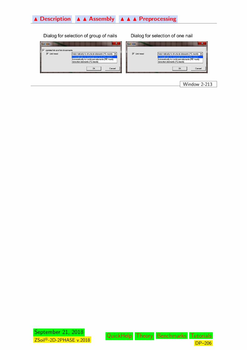
N Description N N Assembly N N N Preprocessing
Window 2-213
September 21, 2018
ZSoilr-2D-2PHASE v.2018QuickHelp Theory Benchmarks Tutorials
DP–206
N Description N N Assembly N N N Preprocessing
Window 2-214: Nail:Update:Length
This option allows the user to update length of selected nail(s).
Window 2-214
Window 2-215: Nail:Update:Shift by head proj.on edges in dir.
This option allows to shift nail head(s), by preserving nail(s) length and orientation, to theselected set of edges in a given direction.
Window 2-215
Window 2-216: Nail:Update:Shift by head proj.on edges
This option allows to shift nail head(s), by preserving nail(s) length and orientation, to theselected set of edges by means of a closest distance.
Window 2-216
Window 2-217: Nail:Update:Inclination angle
This option allows the user to modify inclination angle of nail(s) in the vertical plane. Duringthis operation nail head remains unmodified.
Window 2-217
Window 2-218: Nail:Update:Reverse X axis
This option helps to control orientation of the nail local X axis. This orientation must besuch that vector created between nail head and foot of the nail is the same as orientation ofthe X local axis. Using this option user may flip the orientation. This option is equivalent tothe one designed to control orientation of beam elements (see Win.(2-275))
Window 2-218
Window 2-219: Nail:Update:Split
This option allows the user to modify nail macro-element(s) mesh density. Some recommen-dations concerning split value are given in Win.(2-206).
Window 2-219
Window 2-220: Nail:Update:Scale
This option helps to scale size of the nail cross section in the graph pane. Note that thecross section is plot as quadrilateral (instead of cylindrical) to make rendering faster.
Window 2-220
September 21, 2018
ZSoilr-2D-2PHASE v.2018QuickHelp Theory Benchmarks Tutorials
DP–207
N Description N N Assembly N N N Preprocessing
2.3.1.2.17 SURFACE LOAD
Window 2-221: Options in menu Surface load
Option Method Toolbar DescriptionUNIFORM On Edge(s)(Uniform) — Window 2-222
VARIABLE On Edge (Variable) — Window 2-223PRESSURE On Edge (Pressure) — Window 2-224
On selected edges (HP) — Window 2-225PRESSURE
via Fluid
Head
On selected edges (SH) — Window 2-226
Outline All — Window 2-227In zoom box — Window 2-243In zoom circle — Window 2-244Inside contour — Window 2-245With load function — Window 2-227With label — Window 2-227
Delete Delete Window 2-246Update Parameters — Window 2-228
Scale — Window 2-228
Window 2-221
September 21, 2018
ZSoilr-2D-2PHASE v.2018QuickHelp Theory Benchmarks Tutorials
DP–208

N Description N N Assembly N N N Preprocessing
Window 2-222: Surface load:UNIFORM:On edge(s) (Uniform)
New uniform surface load is generated on a single picked subdomain edge or group of selectedsubdomain edges (if current selection list of edges is not empty) (see figure below). Thisoption is valid only in 2D.
Picked or selected edge
Remarks:
1. For fast selection purposes one may apply a distinct label to this definition2. This load is automatically split during mesh refinement3. The macromodel should not be deleted once the finite element model is generated (real
mesh already exists) otherwise the load will be deleted too
Window 2-222
September 21, 2018
ZSoilr-2D-2PHASE v.2018QuickHelp Theory Benchmarks Tutorials
DP–209
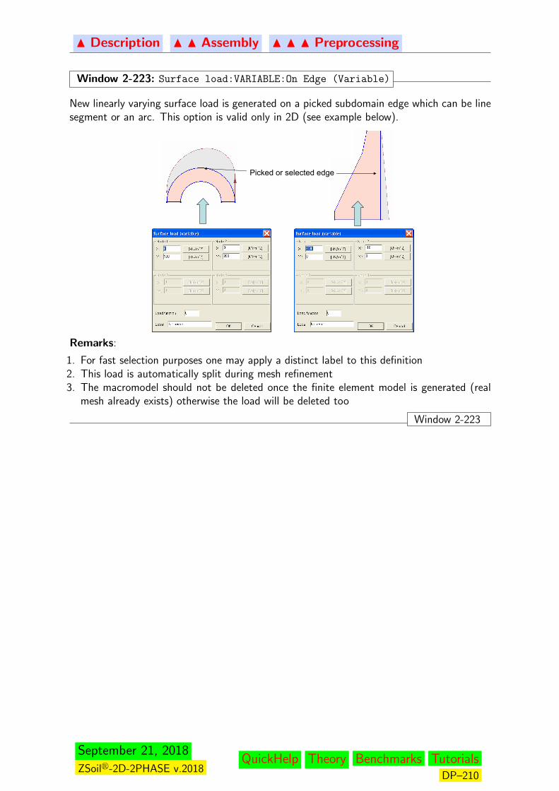
N Description N N Assembly N N N Preprocessing
Window 2-223: Surface load:VARIABLE:On Edge (Variable)
New linearly varying surface load is generated on a picked subdomain edge which can be linesegment or an arc. This option is valid only in 2D (see example below).
Picked or selected edge
Remarks:
1. For fast selection purposes one may apply a distinct label to this definition2. This load is automatically split during mesh refinement3. The macromodel should not be deleted once the finite element model is generated (real
mesh already exists) otherwise the load will be deleted too
Window 2-223
September 21, 2018
ZSoilr-2D-2PHASE v.2018QuickHelp Theory Benchmarks Tutorials
DP–210
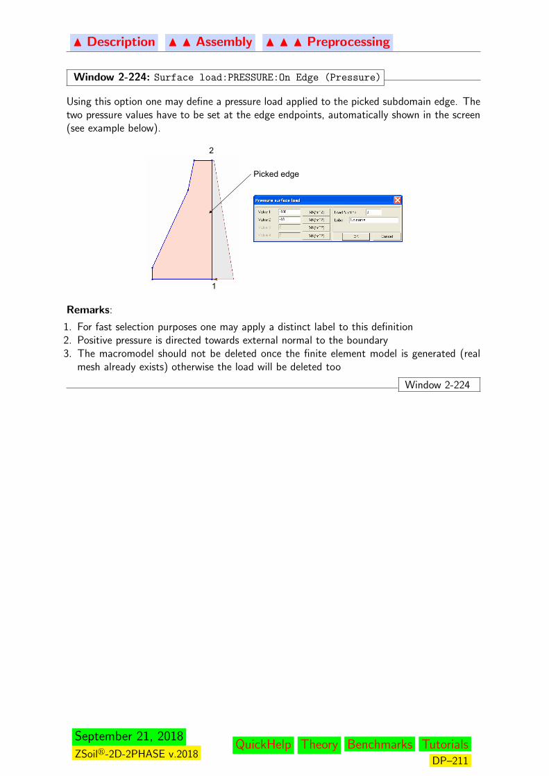
N Description N N Assembly N N N Preprocessing
Window 2-224: Surface load:PRESSURE:On Edge (Pressure)
Using this option one may define a pressure load applied to the picked subdomain edge. Thetwo pressure values have to be set at the edge endpoints, automatically shown in the screen(see example below).
1
2
Picked edge
Remarks:
1. For fast selection purposes one may apply a distinct label to this definition2. Positive pressure is directed towards external normal to the boundary3. The macromodel should not be deleted once the finite element model is generated (real
mesh already exists) otherwise the load will be deleted too
Window 2-224
September 21, 2018
ZSoilr-2D-2PHASE v.2018QuickHelp Theory Benchmarks Tutorials
DP–211
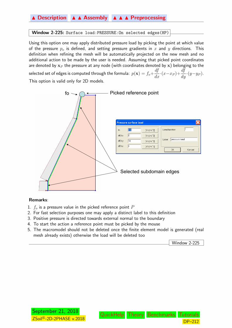
N Description N N Assembly N N N Preprocessing
Window 2-225: Surface load:PRESSURE:On selected edges(HP)
Using this option one may apply distributed pressure load by picking the point at which valueof the pressure po is defined, and setting pressure gradients in x and y directions. Thisdefinition when refining the mesh will be automatically projected on the new mesh and noadditional action to be made by the user is needed. Assuming that picked point coordinatesare denoted by xP the pressure at any node (with coordinates denoted by x) belonging to the
selected set of edges is computed through the formula: p(x) = fo+df
dx·(x−xP )+
df
dy·(y−yP ).
This option is valid only for 2D models.
fo
Selected subdomain edges
Picked reference point
Remarks:
1. fo is a pressure value in the picked reference point P2. For fast selection purposes one may apply a distinct label to this definition3. Positive pressure is directed towards external normal to the boundary4. To start the action a reference point must be picked by the mouse5. The macromodel should not be deleted once the finite element model is generated (real
mesh already exists) otherwise the load will be deleted too
Window 2-225
September 21, 2018
ZSoilr-2D-2PHASE v.2018QuickHelp Theory Benchmarks Tutorials
DP–212

N Description N N Assembly N N N Preprocessing
Window 2-226: SL: PRESSURE:On selected edges via Fluid head (SH)
Using this option one may apply pressure load to the selected edges using definition of the
fluid head (potential). Fluid head h, is defined as h = −pγ
+ y, where fluid specific weight is
denoted by γ and vertical coordinate by y. Distribution of the pressure applied to the edges(it is automatically computed inside of the calculation module), is derived from the aboveformula and filtered to cancel the pressure at any point located above elevation h. Thisdefinition when refining the mesh will automatically be projected on the new mesh and noadditional action to be made by the user is needed.
Selected subdomain edges
Pressure headmarker
Remarks:
1. For fast selection purposes one may apply a distinct label to this definition2. It is possible to apply the pressure towards or against the external normal3. Above the elevation h pressure is set to zero4. This load can automatically be generated when creating fluid pressure BC for Deformation+Flow
problems5. The macromodel should not be deleted once the finite element model is generated (real
mesh already exists) otherwise the load will be deleted too
Window 2-226
September 21, 2018
ZSoilr-2D-2PHASE v.2018QuickHelp Theory Benchmarks Tutorials
DP–213
N Description N N Assembly N N N Preprocessing
Window 2-227: Surface load: some options in menu Outline
Option DescriptionAll Select all visible surface loadsWith load time
function
Select all surface loads with a given load time function
With label Select all surface loads with a given label (all registered labels aregiven in the combo-box)
Window 2-227
Window 2-228: Surface load: some options in menu Update
Option DescriptionParameters This option activates a dialog box to update the applied surface
load description. The resulting dialog box, corresponds to theapplied load type (see creation methods in Win.(2-221))
Scale Using this option one may enlarge or diminish graphical size ofthe applied surface loads
Window 2-228
September 21, 2018
ZSoilr-2D-2PHASE v.2018QuickHelp Theory Benchmarks Tutorials
DP–214
N Description N N Assembly N N N Preprocessing
2.3.1.2.18 POINT LOAD
Window 2-229: Options in menu Point load
Option Method Toolbar DescriptionCreate On point/pile — Window 2-230Outline All — Window 2-231
between 4 nodes — Window 2-241Box with 2 nodes — Window 2-242In zoom box — Window 2-243In zoom circle — Window 2-244Inside contour — Window 2-245With load function — Window 2-232With label — Window 2-232
Delete Delete Window 2-246Update Parameters — Window 2-233
Scale — Window 2-234
Window 2-229
September 21, 2018
ZSoilr-2D-2PHASE v.2018QuickHelp Theory Benchmarks Tutorials
DP–215
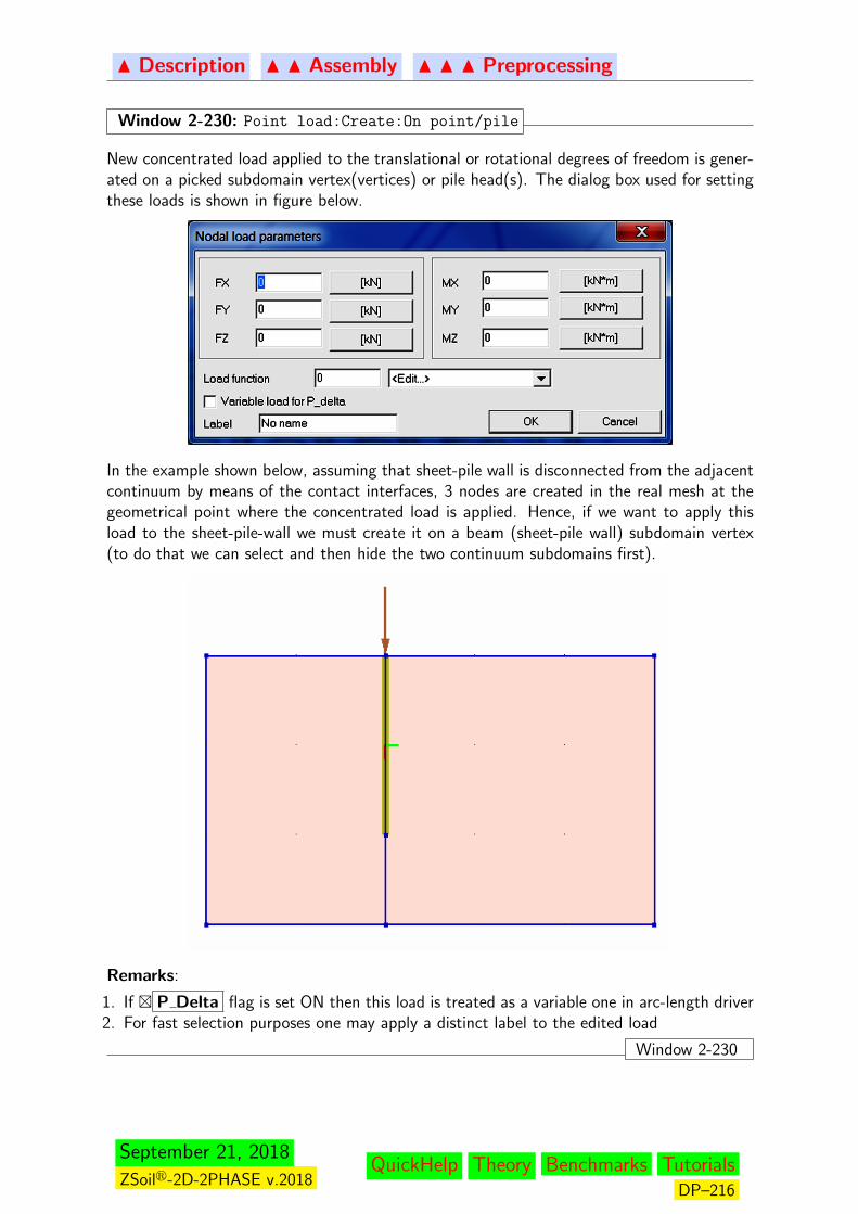
N Description N N Assembly N N N Preprocessing
Window 2-230: Point load:Create:On point/pile
New concentrated load applied to the translational or rotational degrees of freedom is gener-ated on a picked subdomain vertex(vertices) or pile head(s). The dialog box used for settingthese loads is shown in figure below.
In the example shown below, assuming that sheet-pile wall is disconnected from the adjacentcontinuum by means of the contact interfaces, 3 nodes are created in the real mesh at thegeometrical point where the concentrated load is applied. Hence, if we want to apply thisload to the sheet-pile-wall we must create it on a beam (sheet-pile wall) subdomain vertex(to do that we can select and then hide the two continuum subdomains first).
Remarks:
1. If � P Delta flag is set ON then this load is treated as a variable one in arc-length driver2. For fast selection purposes one may apply a distinct label to the edited load
Window 2-230
September 21, 2018
ZSoilr-2D-2PHASE v.2018QuickHelp Theory Benchmarks Tutorials
DP–216
N Description N N Assembly N N N Preprocessing
Window 2-231: Point load:Outline:All
This option selects all concentrated loads.
Window 2-231
Window 2-232: Point load:Outline:With load f., existence f., label
Using this option user may select concentrated force with a given load time function ID or agiven label. In case of a label one may select a single item from combo-box.
Window 2-232
Window 2-233: Point load:Update:Parameters
This option activates the dialog box to modify the applied concentrated force description, fora single picked point or group of selected points. The detailed description on how to set thedata is given in Window 2-230.
Remark:When running this option for group of selected points only default parameters willbe set in the dialog box.
Window 2-233
Window 2-234: Point load:Update:Scale
Using this option one may enlarge or diminish size of nodal vectors, representing concentratedforces, or arcs, representing concentrated moments. markers.
Window 2-234
September 21, 2018
ZSoilr-2D-2PHASE v.2018QuickHelp Theory Benchmarks Tutorials
DP–217
N Description N N Assembly N N N Preprocessing
2.3.1.3 FE MODEL
The list of all FE model components is listed in the following table.
Common methods Description of common methods to copy, outline, delete,update all FE model components (elements, nodes, BC etc..)
Node Methods to create, outline, update mesh nodesBeam Methods to create, outline, update beam elementsAnchor Methods to create, outline, update anchor (truss) elementsContinuum 2D Methods to create, outline, update continuum 2D elementsMembrane Methods to create, outline, update membrane elementsInfinite element Methods to create, outline, update infinite elementsTendons Contains options to generate prestressed tendons embedded
in continuum 2D/3D and shellsInterface Methods to create, outline, update contact interface ele-
mentsInterface (large deform.) Methods to create, outline, update large deformation contactSeepage Methods to create, outline, update seepage elementsConvection Methods to create, outline, update convection elementsViscous dampers Methods to create, outline, update viscous damper elementsShell hinge Methods to create, outline, update hinges in shell (with single
layer of nodes only) elementsBoundary conditions Methods to create, outline, update boundary conditionsLoads Methods to create, outline, update loadsAdded masses Methods to create, outline, update added masses needed for
dynamic or pushover driversDistributed flux Methods to create, outline, update distributed fluxes in Flow,
Heat and Humidity problemsInitial conditions Methods to create, outline, update initial conditionsNodal link Methods to create, outline, update kinematic constraints
(node to segment) to be satisfied in an exact way (withoutpenalty)
Kinematic constraints Methods to create, outline, update kinematic constraints(node to segment) to be satisfied using penalty method
Mesh tying Methods to create, outline, update mesh tying descriptionwhich allows to connect non-conforming meshes
September 21, 2018
ZSoilr-2D-2PHASE v.2018QuickHelp Theory Benchmarks Tutorials
DP–218
N Description N N Assembly N N N Preprocessing
2.3.1.3.1 COMMON METHODS FOR ALL FE MODEL COMPO-NENTS
Window 2-235: Common methods for FE model components
All options listed in table below are common for all FE model components like nodes, contin-uum, anchors, beams, membranes etc.. In dedicated menus for each specific FE componentuser will be referred to windows included in this section.
Option Method Toolbar Description
Create Copy with rotation Window 2-236
Copy with translation Window 2-237
Copy by symmetry Window 2-238
Outline UnSelect one..... Window 2-239
Between 2 nodes Window 2-240
Between 4 nodes Window 2-241
Box with 2 nodes Window 2-242
In zoom box Window 2-243
In zoom circle Window 2-244
Inside contour Window 2-245With label — Window 2-249
Delete Delete Window 2-246
Update Move Window 2-247
Rotate Window 2-248
Window 2-235
September 21, 2018
ZSoilr-2D-2PHASE v.2018QuickHelp Theory Benchmarks Tutorials
DP–219
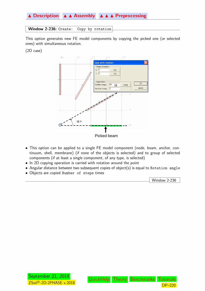
N Description N N Assembly N N N Preprocessing
Window 2-236: Create: Copy by rotation
This option generates new FE model components by copying the picked one (or selectedones) with simultaneous rotation.
(2D case)
Picked beam
α+
α
• This option can be applied to a single FE model component (node, beam, anchor, con-tinuum, shell, membrane) (if none of the objects is selected) and to group of selectedcomponents (if at least a single component, of any type, is selected)• In 2D copying operation is carried with rotation around the point• Angular distance between two subsequent copies of object(s) is equal to Rotation angle
• Objects are copied Number of steps times
Window 2-236
September 21, 2018
ZSoilr-2D-2PHASE v.2018QuickHelp Theory Benchmarks Tutorials
DP–220

N Description N N Assembly N N N Preprocessing
Window 2-237: Create: Copy by translation
Using this option new FE model components are generated by copying, with simultaneoustranslation, of a picked or selected components (see figure below)
LΔLo v v n
s
h
Remarks:
• Copying operation is carried out along the vector v defined by three coordinates (X, Y,
Z)• v is normalized (or not) depending on the status of Use normalized check-box• if One step size is set ON thenF ∆Lo = h ‖ v ‖• if Total size is set ON thenF L = h
F if s 6= 1 then ∆Lo =L (1− s)(1− sn)
else ∆Lo =L
n• ∆Li = s ∆Li−1 for i ≥ 1• L =
∑n−1i=0 ∆Li
Window 2-237
Window 2-238: Create: Copy by symmetry
This option can be used to make a copy of a single FE model component (if none of theobjects is selected) or group of selected components by symmetrical projection with respectto the plane created under ribbon menu Draw:Auxiliary Planes
• To run this option a fictitious plane must be created first• After this operation orientation of copied components (if applies) is reversed• To initiate the action plane of symmetry must be pointed first
Window 2-238
Window 2-239: Outline: [Un]Select one.....
By activating this option from menu dedicated for a certain finite element model (likeNode,Continuum 2D, etc..) user may select the component, by picking it in the graphicpane, in the Replace mode (selected object becomes unselected and vice versa).
Window 2-239
September 21, 2018
ZSoilr-2D-2PHASE v.2018QuickHelp Theory Benchmarks Tutorials
DP–221

N Description N N Assembly N N N Preprocessing
Window 2-240: Outline: Between 2 nodes
This option is used to select (according to the current Selection mode) group of FE modelcomponents, represented geometrically by points or line segments, belonging to the straightsegment defined by the 2 picked points.
Window 2-240
Window 2-241: Outline: Between 4 nodes
This option is used to select (according to the current Selection mode) FE componentswhich remain on the surface defined by 4 vertices constituting a macro-quadrilateral element(see figure). Surface is interpolated with aid of standard bilinear shape functions used for Q4element.
Selected nodes
Remarks:
1. any FE model component belongs to the surface if distance of its any vertex and its closestprojection on the surface remains very small compared to the characteristic size of themacro-quadrilateral
2. after activation of this method 4 nodes must be picked by the graphical cursor3. it is sufficient to pick a point close to the node but inside of the element4. this option is supported only for nodes
Window 2-241
Window 2-242: Outline: Box 2 nodes
This method is used to select FE model components in the fictitious box aligned with globalX,Y,Z directions and defined by the 2 picked points
Fictitious box
Window 2-242
September 21, 2018
ZSoilr-2D-2PHASE v.2018QuickHelp Theory Benchmarks Tutorials
DP–222

N Description N N Assembly N N N Preprocessing
Window 2-243: Outline: In zoom box
This option is used to select (according to the current Selection mode) all FE modelcomponents which are covered by the zoom box (infinite rectangular prism in 3D).
begin
begin
end
end
begin
begin
end
end
Draging box from left right Draging box from right left
Remarks:
1. if zoom is dragged from the left to the right side then objects which are fully covered bythe box will be selected
2. if zoom is dragged from the right to the left side then all objects which are fully or partiallycovered by the box will be selected
Window 2-243
Window 2-244: Outline: In zoom circle
This option is used to select (according to the current Selection mode) all FE modelcomponents which are covered by the zoom circle (infinite cylinder prism in 3D)
Remarks:
1. if zoom is dragged from the left to the right side then objects which are fully covered bythe box will be selected
2. if zoom is dragged from the right to the left side then all objects which are fully or partiallycovered by the box will be selected
Window 2-244
Window 2-245: Outline: Inside contour
This option is used to select (according to the current Selection mode) all FE modelcomponents which are covered by the irregular contour.Remarks:
1. contour must form a closed planar polygon
Window 2-245
September 21, 2018
ZSoilr-2D-2PHASE v.2018QuickHelp Theory Benchmarks Tutorials
DP–223

N Description N N Assembly N N N Preprocessing
Window 2-246: Delete: Delete
This option is used to:
1. delete single FE model component picked by the mouse if selection list of components ofa given class is empty
2. delete group of selected FE model components3. to pick the component use Standard selection cursor (see Window 2-81)
Remark:
Deletion of nodes will automatically cause deletion of adjacent elements
Window 2-246
Window 2-247: Update: Move
This option (see figure) is used to carry out translation of:
• single picked FE model component, or group of selected components, by using a toolbarMove.. (Window 2-84) in ribbon menu Edit, or menu Update/Move that is dedicated toeach FE model component (Node, Anchor etc....)
en
Move using vector [0,1,0] applied to: (a) element
(b) node
Remark:
Geometry of components adjacent to the translated one(s) will be automatically updated
Window 2-247
September 21, 2018
ZSoilr-2D-2PHASE v.2018QuickHelp Theory Benchmarks Tutorials
DP–224

N Description N N Assembly N N N Preprocessing
Window 2-248: Update: Rotate
This option (see figure) is used to carry out rotation of:
• single picked FE model component by using a toolbar (Window 2-84) in ribbon menu Edit,or menu Update/Rotate that is dedicated to each FE model component (Node, Anchoretc....)
e
Rotation around point P by α
A) nodes n1 n2
B) element e
(A) (B)
n1 n2
P P
α+ α+Remarks:
1. In the 2D rotation is carried out around a given point
2. Geometry of components adjacent to the rotated one(s) will be automatically updated
Window 2-248
Window 2-249: Outline: with label
Finite element components can be labeled through option Update/Label. Outline: with
label option is used to select a single finite element component or group of selected com-ponents with the same label (memorized in form of the list).
Window 2-249
September 21, 2018
ZSoilr-2D-2PHASE v.2018QuickHelp Theory Benchmarks Tutorials
DP–225
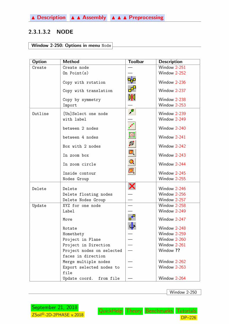
N Description N N Assembly N N N Preprocessing
2.3.1.3.2 NODE
Window 2-250: Options in menu Node
Option Method Toolbar DescriptionCreate Create node — Window 2-251
On Point(s) — Window 2-252
Copy with rotation Window 2-236
Copy with translation Window 2-237
Copy by symmetry Window 2-238Import — Window 2-253
Outline [Un]Select one node Window 2-239with label — Window 2-249
between 2 nodes Window 2-240
between 4 nodes Window 2-241
Box with 2 nodes Window 2-242
In zoom box Window 2-243
In zoom circle Window 2-244
Inside contour Window 2-245Nodes Group Window 2-255
Delete Delete Window 2-246Delete floating nodes — Window 2-256Delete Nodes Group — Window 2-257
Update XYZ for one node — Window 2-258Label — Window 2-249
Move Window 2-247
Rotate Window 2-248Homethety — Window 2-259Project in Plane — Window 2-260Project in Direction — Window 2-261Project nodes on selected
faces in direction
— Window ??
Merge multiple nodes — Window 2-262Export selected nodes to
file
— Window 2-263
Update coord. from file — Window 2-264
Window 2-250
September 21, 2018
ZSoilr-2D-2PHASE v.2018QuickHelp Theory Benchmarks Tutorials
DP–226
N Description N N Assembly N N N Preprocessing
Window 2-251: Node:Create:Create node
New node is generated at position picked in the graph pane (if Snap is active graphicalcursor will be snapped to some of the objects) or through through direct definition of X,Y,Zcoordinates in the appearing dialog box.
Window 2-251
Window 2-252: Node:Create:On Point(s)
New node(s) are generated at positions of selected geometrical points.
Window 2-252
Window 2-253: Node:Create:Import
This option allows to import nodes from the external text file in which nodes are stored usingthe following format (all values are separated by spaces):
node index-1 X Y Znode index-2 X Y Z........node index-N X Y Z
NB. node index is just an auxiliary counter
Window 2-253
Window 2-254: Node:Create:Nodes Group
This option allows to memorize selected nodes and label them. It is used mainly to enable alimited output of nodal displacements, velocities or accelerations at few nodal points duringdynamic transient analyses (when tuning damping in dynamic models for instance). Thisoption can be activated under Control/Results content menu.
Window 2-254
Window 2-255: Node:Outline:Nodes Group
This option allows to select all nodes memorized in Nodes Group under given label.
Window 2-255
Window 2-256: Node:Delete floating nodes
This function removes all nodes which are not attached to any existing finite element, inde-pendently on current elements visibility status.
Window 2-256
September 21, 2018
ZSoilr-2D-2PHASE v.2018QuickHelp Theory Benchmarks Tutorials
DP–227

N Description N N Assembly N N N Preprocessing
Window 2-257: Node:Delete Nodes Group
This option allows to delete selected group of nodes memorized under given label.
Window 2-257
Window 2-258: Node:Update/X Y Z for one node
This option allows to modify coordinates of a picked point. It can be done by picking thenode to be modified first and then, by picking new node position in the graph pane or bydirect definition of new node coordinates in the dialog box as shown below.
Window 2-258
Window 2-259: Node:Update/homothety
This option allows to perform homothetic transformation of node(s) coordinates with respectto the given axis. The idea of this transformation is shown in figure below.
P1
P2
A
O
A’
a
b
a+ba = Factor
new position
old position
Window 2-259
September 21, 2018
ZSoilr-2D-2PHASE v.2018QuickHelp Theory Benchmarks Tutorials
DP–228

N Description N N Assembly N N N Preprocessing
Window 2-260: Node:Update/Project on plane
This option is used for orthogonal projection of a node or group of selected nodes onto pickedauxiliary plane.
Remarks:
1. an auxiliary plane must be created first (ribbon menu Draw:Auxiliary Planes)2. to finalize the action projection plane must be picked with mouse
Window 2-260
Window 2-261: Node:Update/Project on plane in direction
This option is used for projection of node(s) in given direction indicated by vector v ontopicked auxiliary plane.
Window 2-261
Window 2-262: Node:Update/Merge multiple nodes
This option is used to detect nodes located approximately at the same position. Such situationmay happen due to errors made mainly during data generation of 3D models. By setting thetolerance for the distance user may unify all these nodes.
Window 2-262
Window 2-263: Node:Update/Export selected nodes to file
The main goal of this option is to export selected nodes coordinates to the external file andthen correct them via Excel (or another) application. Nodes are exported using the followingformat: Node index X Y ZIn this case Node index cannot be changed.
Window 2-263
Window 2-264: Node:Update/Update coord. from file
This option is coupled with option Node:Update/Export selected nodes to file. Itallows to update coordinates of exported nodes updated externally by Excel or other applica-tion. (see Window 2-263)
Window 2-264
September 21, 2018
ZSoilr-2D-2PHASE v.2018QuickHelp Theory Benchmarks Tutorials
DP–229

N Description N N Assembly N N N Preprocessing
2.3.1.3.3 BEAM
Window 2-265: Options in menu Beam
Option Method Toolbar DescriptionCreate 2 points/nodes — Window 2-266
2 nodes — Window 2-267Enter XYZ for 2 nodes — Window 2-268On edge(s) — Window 2-269On object(s) — Window 2-270
Copy with rotation Window 2-236
Copy with translation Window 2-237
Copy by symmetry Window 2-238On truss(es) — Window 2-271On truss(es) remove truss — Window 2-272
Outline Box with 2 nodes Window 2-242
In zoom box Window 2-243
In zoom circle Window 2-244
Inside contour Window 2-245
Delete Delete Window 2-246Update Parameters — Window 2-148
Direction — Window 2-273Reverse direction — Window 2-274Reverse X axis — Window 2-275Centroid — Window 2-276Hinge — Window 2-277Reinforcements set — Window 2-278Tendon — Window 2-285
Split Window 2-290
Move Window 2-247
Rotate Window 2-248Scale — Window 2-291
Window 2-265
September 21, 2018
ZSoilr-2D-2PHASE v.2018QuickHelp Theory Benchmarks Tutorials
DP–230
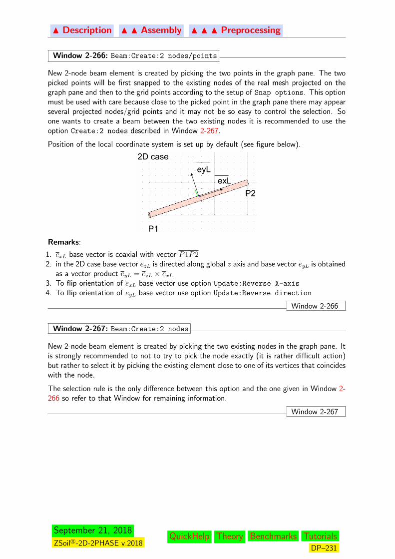
N Description N N Assembly N N N Preprocessing
Window 2-266: Beam:Create:2 nodes/points
New 2-node beam element is created by picking the two points in the graph pane. The twopicked points will be first snapped to the existing nodes of the real mesh projected on thegraph pane and then to the grid points according to the setup of Snap options. This optionmust be used with care because close to the picked point in the graph pane there may appearseveral projected nodes/grid points and it may not be so easy to control the selection. Soone wants to create a beam between the two existing nodes it is recommended to use theoption Create:2 nodes described in Window 2-267.
Position of the local coordinate system is set up by default (see figure below).
P1
P2exL
eyL2D case
P1 P2exL
eyL
ezL
3D case
Remarks:
1. exL base vector is coaxial with vector P1P22. in the 2D case base vector ezL is directed along global z axis and base vector eyL is obtained
as a vector product eyL = ezL × exL3. To flip orientation of exL base vector use option Update:Reverse X-axis
4. To flip orientation of eyL base vector use option Update:Reverse direction
Window 2-266
Window 2-267: Beam:Create:2 nodes
New 2-node beam element is created by picking the two existing nodes in the graph pane. Itis strongly recommended to not to try to pick the node exactly (it is rather difficult action)but rather to select it by picking the existing element close to one of its vertices that coincideswith the node.
The selection rule is the only difference between this option and the one given in Window 2-266 so refer to that Window for remaining information.
Window 2-267
September 21, 2018
ZSoilr-2D-2PHASE v.2018QuickHelp Theory Benchmarks Tutorials
DP–231

N Description N N Assembly N N N Preprocessing
Window 2-268: Beam:Create:XYZ for 2 points
New beam element is created by entering X,Y,Z coordinates of its two endpoints in thedialog box. Setting default local coordinate system of the beam follows the idea given inWindow 2-267
Window 2-268
Window 2-269: Beam:Create:On edge(s)
New beam element(s) are generated on all selected edges (see figure below). Orientation ofeach beam element local x axis is coherent with orientation of the element edge. Settingdefault local coordinate system of the beam follows the idea given in Window 2-267
selected edges
selected edges
Window 2-269
Window 2-270: Beam:Create:On object(s)
New beam element(s) are generated on all selected geometrical objects (see figure below).Orientation of each beam element local x axis is coherent with orientation of the geomet-rical object. Setting default local coordinate system of the beam follows the idea given inWindow 2-267
2D case
Remark:
Beams created on arcs are spanned on the arc endpoints hence it is recommended to splitthe arc first and then to create beams
Window 2-270
September 21, 2018
ZSoilr-2D-2PHASE v.2018QuickHelp Theory Benchmarks Tutorials
DP–232
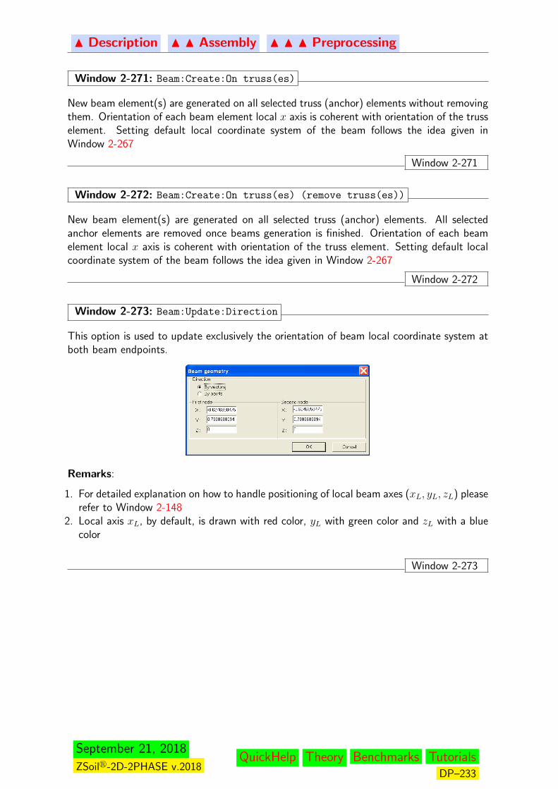
N Description N N Assembly N N N Preprocessing
Window 2-271: Beam:Create:On truss(es)
New beam element(s) are generated on all selected truss (anchor) elements without removingthem. Orientation of each beam element local x axis is coherent with orientation of the trusselement. Setting default local coordinate system of the beam follows the idea given inWindow 2-267
Window 2-271
Window 2-272: Beam:Create:On truss(es) (remove truss(es))
New beam element(s) are generated on all selected truss (anchor) elements. All selectedanchor elements are removed once beams generation is finished. Orientation of each beamelement local x axis is coherent with orientation of the truss element. Setting default localcoordinate system of the beam follows the idea given in Window 2-267
Window 2-272
Window 2-273: Beam:Update:Direction
This option is used to update exclusively the orientation of beam local coordinate system atboth beam endpoints.
Remarks:
1. For detailed explanation on how to handle positioning of local beam axes (xL, yL, zL) pleaserefer to Window 2-148
2. Local axis xL, by default, is drawn with red color, yL with green color and zL with a bluecolor
Window 2-273
September 21, 2018
ZSoilr-2D-2PHASE v.2018QuickHelp Theory Benchmarks Tutorials
DP–233
N Description N N Assembly N N N Preprocessing
Window 2-274: Beam:Update:Reverse direction
This option is used to flip the local axis yL and in consequence local axis zL while xL remainsunchanged.
Remarks:
• The detailed explanation on positioning of local beam axes (xL, yL, zL) is given in Win-dow 2-148• Top fibers of beam cross section are located on positive side of yL axis while bottom ones
on negative• Proper setting of local beam axes is very important for nonsymmetric cross sections or
cross sections of reinforced concrete• Proper setting of local beam axes is also very important for visualization of normal and
shear force diagrams in the postprocessor• Local axis xL, by default, is drawn with red color, yL with green color and zL with a blue
color
Window 2-274
Window 2-275: Beam:Update:Reverse X axis
This option is used to flip the local axis xL and in consequence local axis zL while yL remainsunchanged.
Remarks:
• The detailed explanation on positioning of local beam axes (xL, yL, zL) is given in Win-dow 2-148.• Top fibers of beam cross section are located on positive side of yL axis while bottom ones
on negative• Proper setting of local beam axes is very important for nonsymmetric cross sections or
cross sections of reinforced concrete• Proper setting of local beam axes is also very important for visualization of normal and
shear force diagrams in the postprocessor• In case when beams form a closed polygon their local xL axes should be oriented in one
direction• Local axis xL, by default, is drawn with red color, yL with green color and zL with a blue
color
Window 2-275
September 21, 2018
ZSoilr-2D-2PHASE v.2018QuickHelp Theory Benchmarks Tutorials
DP–234

N Description N N Assembly N N N Preprocessing
Window 2-276: Beam:Update:Centroid
This option is used to update exclusively position of centroids (positions of cross sectioncenters with respect to the master nodes) in the global or local (beam) coordinate system.
offset
Master nodescentroids
Remark:
Details on positioning local beam axes (xL, yL, zL) are given Window 2-148.
Window 2-276
Window 2-277: Beam:Update:Hinge
This option allows the user to define at left and/or right beam endpoint
1. an ideal hinge which relaxes some selected degree(s) of freedom
2. nonlinear uncoupled nonlinear spring with any type of the relation between the generalizedsectional force (moment) and relative displacement (rotation)
3. nonlinear coupled Janssen nonlinear spring that can be used to model segmental linings
These settings are made in the local basis defined by x− yL− zL axes. In addition user mayassociate an existence function(s) with the hinge/spring at any degree of freedom.
AA
A
Window 2-277
September 21, 2018
ZSoilr-2D-2PHASE v.2018QuickHelp Theory Benchmarks Tutorials
DP–235
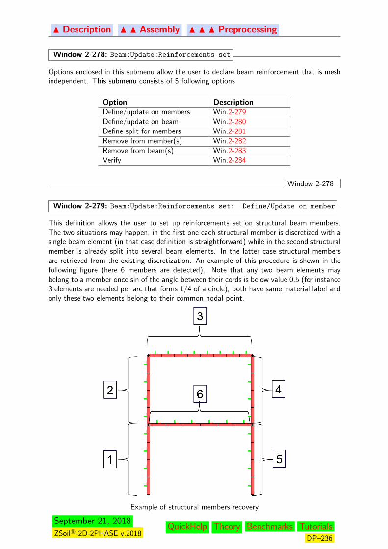
N Description N N Assembly N N N Preprocessing
Window 2-278: Beam:Update:Reinforcements set
Options enclosed in this submenu allow the user to declare beam reinforcement that is meshindependent. This submenu consists of 5 following options
Option DescriptionDefine/update on members Win.2-279Define/update on beam Win.2-280Define split for members Win.2-281Remove from member(s) Win.2-282Remove from beam(s) Win.2-283Verify Win.2-284
Window 2-278
Window 2-279: Beam:Update:Reinforcements set: Define/Update on member
This definition allows the user to set up reinforcements set on structural beam members.The two situations may happen, in the first one each structural member is discretized with asingle beam element (in that case definition is straightforward) while in the second structuralmember is already split into several beam elements. In the latter case structural membersare retrieved from the existing discretization. An example of this procedure is shown in thefollowing figure (here 6 members are detected). Note that any two beam elements maybelong to a member once sin of the angle between their cords is below value 0.5 (for instance3 elements are needed per arc that forms 1/4 of a circle), both have same material label andonly these two elements belong to their common nodal point.
Example of structural members recovery
September 21, 2018
ZSoilr-2D-2PHASE v.2018QuickHelp Theory Benchmarks Tutorials
DP–236
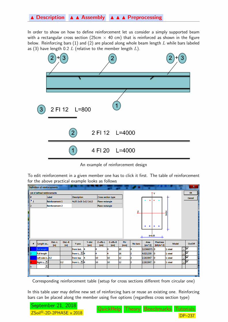
N Description N N Assembly N N N Preprocessing
In order to show on how to define reinforcement let us consider a simply supported beamwith a rectangular cross section (25cm × 40 cm) that is reinforced as shown in the figurebelow. Reinforcing bars (1) and (2) are placed along whole beam length L while bars labeledas (3) have length 0.2 L (relative to the member length L).
An example of reinforcement design
To edit reinforcement in a given member one has to click it first. The table of reinforcementfor the above practical example looks as follows
Corresponding reinforcement table (setup for cross sections different from circular one)
In this table user may define new set of reinforcing bars or reuse an existing one. Reinforcingbars can be placed along the member using five options (regardless cross section type)
September 21, 2018
ZSoilr-2D-2PHASE v.2018QuickHelp Theory Benchmarks Tutorials
DP–237
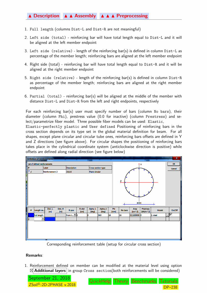
N Description N N Assembly N N N Preprocessing
1. Full length (columns Dist-L and Dist-R are not meaningful)
2. Left side (total) - reinforcing bar will have total length equal to Dist-L and it willbe aligned at the left member endpoint
3. Left side (relative) - length of the reinforcing bar(s) is defined in column Dist-L aspercentage of the member length; reinforcing bars are aligned at the left member endpoint
4. Right side (total) - reinforcing bar will have total length equal to Dist-R and it will bealigned at the right member endpoint
5. Right side (relative) - length of the reinforcing bar(s) is defined in column Dist-R
as percentage of the member length; reinforcing bars are aligned at the right memberendpoint
6. Partial (total) - reinforcing bar(s) will be aligned at the middle of the member withdistance Dist-L and Dist-R from the left and right endpoints, respectively
For each reinforcing bar(s) user must specify number of bars (column No bars), theirdiameter (column Phi), prestress value (0.0 for inactive) (column Prestress) and se-lect/parametrize fiber model. Three possible fiber models can be used: Elastic,Elastic-perfectly plastic and User defined Positioning of reinforcing bars in thecross section depends on its type set in the global material definition for beam. For allshapes, except plane circular and circular tube ones, reinforcing bars offsets are defined in Yand Z directions (see figure above). For circular shapes the positioning of reinforcing barstakes place in the cylindrical coordinate system (anticlockwise direction is positive) whileoffsets are defined along radial direction (see figure below)
Corresponding reinforcement table (setup for circular cross section)
Remarks:
1. Reinforcement defined on member can be modified at the material level using option� Additional layers in group Cross section(both reinforcements will be considered)
September 21, 2018
ZSoilr-2D-2PHASE v.2018QuickHelp Theory Benchmarks Tutorials
DP–238
N Description N N Assembly N N N Preprocessing
2. Reinforcement defined on a single beam element that belongs to the member replaces theone set up on member
3. Use option Verify in this submenu to check if reinforcement matches geometry of thecross section
4. Defined reinforcement can be applied to another member/beam element
5. This definition will not be accepted once local beam bases are not properly ordered. Inthat case user must use Reverse X-axis and/or Reverse direction options to adjustlocal bases.
Window 2-279
Window 2-280: Beam:Update:Reinforcements set: Define/Update on beam(s)
This option is fully compatible with the one designed for a beam member (see Win.(2-279)).It applies to a selected set of beam elements or to a single picked element.
Remarks:
1. Reinforcement defined on a beam replaces the one set up on a member
Window 2-280
September 21, 2018
ZSoilr-2D-2PHASE v.2018QuickHelp Theory Benchmarks Tutorials
DP–239
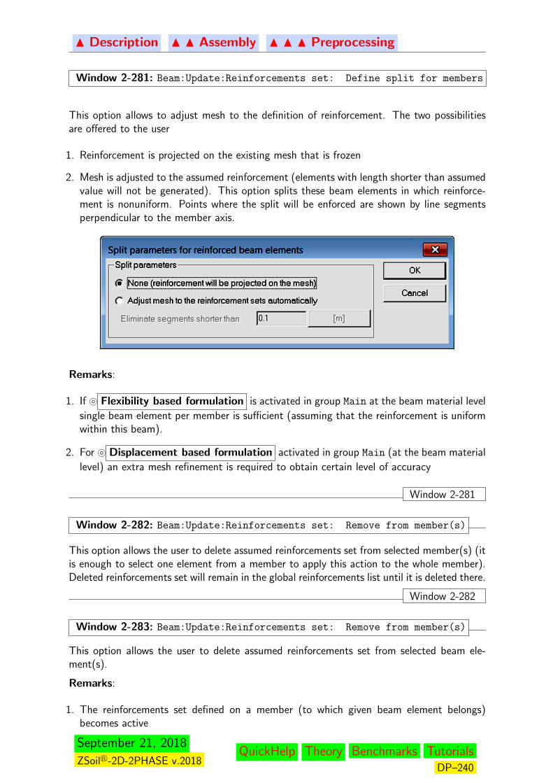
N Description N N Assembly N N N Preprocessing
Window 2-281: Beam:Update:Reinforcements set: Define split for members
This option allows to adjust mesh to the definition of reinforcement. The two possibilitiesare offered to the user
1. Reinforcement is projected on the existing mesh that is frozen
2. Mesh is adjusted to the assumed reinforcement (elements with length shorter than assumedvalue will not be generated). This option splits these beam elements in which reinforce-ment is nonuniform. Points where the split will be enforced are shown by line segmentsperpendicular to the member axis.
Remarks:
1. If } Flexibility based formulation is activated in group Main at the beam material level
single beam element per member is sufficient (assuming that the reinforcement is uniformwithin this beam).
2. For } Displacement based formulation activated in group Main (at the beam material
level) an extra mesh refinement is required to obtain certain level of accuracy
Window 2-281
Window 2-282: Beam:Update:Reinforcements set: Remove from member(s)
This option allows the user to delete assumed reinforcements set from selected member(s) (itis enough to select one element from a member to apply this action to the whole member).Deleted reinforcements set will remain in the global reinforcements list until it is deleted there.
Window 2-282
Window 2-283: Beam:Update:Reinforcements set: Remove from member(s)
This option allows the user to delete assumed reinforcements set from selected beam ele-ment(s).
Remarks:
1. The reinforcements set defined on a member (to which given beam element belongs)becomes active
September 21, 2018
ZSoilr-2D-2PHASE v.2018QuickHelp Theory Benchmarks Tutorials
DP–240

N Description N N Assembly N N N Preprocessing
2. Deleted reinforcements set will remain in the global reinforcements list until it is deletedthere.
Window 2-283
Window 2-284: Beam:Update:Reinforcements set: Verify
This option allows the user to check if declared reinforcement (its length and position) isconsistent with the beam element/member geometry and its cross section. This action isautomatically invoked during data verification.
Window 2-284
September 21, 2018
ZSoilr-2D-2PHASE v.2018QuickHelp Theory Benchmarks Tutorials
DP–241
N Description N N Assembly N N N Preprocessing
Window 2-285: Beam:Update:Tendon
Options enclosed in this submenu allow the user to add prestressed tendons to the selectedset of beam elements. This submenu consists of 4 following options
Option DescriptionDefine on members Win.2-286Define on sel. beams Win.2-287Update Win.2-288Remove Win.2-289
Window 2-285
Window 2-286: Beam:Update:Tendon:Define on members
This option allows to generate prestressed tendons coupled with beam elements forming chainof elements (called as a member). Precise definition of the member is given in Win.2-279.
To add a new tendons group click button Add . After adding new tendons group onecan edit geometry of each (in group) tendon ie. plane (B1), offsets in Y, Z local beamdirections (B2), trajectory (B3), tendon material (as for truss elements) (C1), existencefunction (C2), unloading function (C3) and prestress application data. The prestress dataconsists of the force value (D1), application way (D2) (at left endpoint, at right endpoint or atboth endpoints), friction (D3) and profile (D4) coefficients, prestress existence function (D5)and loading function (D6). Existence function (D5) applied to the prestressing enforces fullforce control in the assumed period of activity. After that period full compatibility betweenbeam nodes and tendon nodes is assumed. The load function (D6) allows modification of theprestress force in time in the active time period declared in the existence function. Locationof the tendon is shown in 3 projections in local beam coordinate axes (E1, E2).
September 21, 2018
ZSoilr-2D-2PHASE v.2018QuickHelp Theory Benchmarks Tutorials
DP–242

N Description N N Assembly N N N Preprocessing
Remarks:
1. One member may have only one tendons group (in one group any number of tendons canbe set)
2. Tendons can be straight or curved (via spline); to modify list of fit points use button ...in (B3); position X of the tendon is set as relative with respect to the member length whileY and Z as absolute (in cm)
3. Dialog box (F) includes list of all defined tendons
4. Tendon is split into set of truss elements connected with the beam axis via rigid artificialbeams; this operation is hidden to the user
Window 2-286
Window 2-287: Beam:Update:Tendon:Define on sel. beams
September 21, 2018
ZSoilr-2D-2PHASE v.2018QuickHelp Theory Benchmarks Tutorials
DP–243

N Description N N Assembly N N N Preprocessing
In more complex cases when tendons are added progressively to the member one may addthem precisely by selecting beams. Completing remaining part of the data is the same as forthe option on member (see Win.2-286).
Window 2-287
Window 2-288: Beam:Update:Tendon:Update
To update defined tendons click on the group label in the screen. See Win.2-286 for details.
Window 2-288
Window 2-289: Beam:Update:Tendon:Remove
This option allows to delete given tendons group by clicking the label in the screen.
Window 2-289
Window 2-290: Beam:Update:Split
By using this option user may split picked beam element or group of selected beam elementssetting split value in the dialog box as shown below. It is worth to mention that in purestructural applications, once the beam cross section is uniform along the length, single beamelement is enough to represent a structural member. To use this type of modeling activate} Flexibility based formulation option under parameters group Mainat the material level.
} Flexibility based formulation yields highly accurate results for both linear and nonlinearcases. For soil-structure interaction problems structural members have to be discretized topreserve mesh conformity between structure, interface and adjacent continuum. Thereforestandard } Displacement based formulation is sufficient. This split option does not takeinto account definition of reinforcements.
Remark:
Every new beam element inherits all the parameters from the parent element
Window 2-290
Window 2-291: Beam:Update:Scale
Using this option user may scale the size of the beam cross section and size of the local beamaxes.
September 21, 2018
ZSoilr-2D-2PHASE v.2018QuickHelp Theory Benchmarks Tutorials
DP–244

N Description N N Assembly N N N Preprocessing
Remark:
} Same size and } Same scale switches have no meaning here
Window 2-291
September 21, 2018
ZSoilr-2D-2PHASE v.2018QuickHelp Theory Benchmarks Tutorials
DP–245

N Description N N Assembly N N N Preprocessing
2.3.1.3.4 TRUSS/ANCHOR
Window 2-292: Options in menu Anchor
Option Method Toolbar DescriptionCreate 2 nodes/points — Window 2-296
2 nodes — Window 2-297Dialog — Window 2-293On edge(s) — Window 2-298On object(s) — Window 2-299On beam(s) — Window 2-300On beam(s) (remove
beam(s))
— Window 2-301
Copy with rotation Window 2-236
Copy with translation Window 2-237
Copy by symmetry Window 2-238Point+Vector+Length — Window 2-303Import (*.2n, *.nvd) — Window 2-303
Outline Box with 2 nodes Window 2-242
In zoom box Window 2-243
In zoom circle Window 2-244
Inside contour Window 2-245Sel. elements linked to
sel. anchors
— Window 2-304
Delete Delete Window 2-246Update Parameters — Window 2-305
Reverse direction — Window 2-309Reverse X axis — Window 2-310Prestress — Window 2-295Link to elements — Window 2-306Length — Window 2-311Inclination angle — Window 2-312
Split Window 2-313
Move Window 2-247
Rotate Window 2-248Scale — Window 2-314
Window 2-292
September 21, 2018
ZSoilr-2D-2PHASE v.2018QuickHelp Theory Benchmarks Tutorials
DP–246
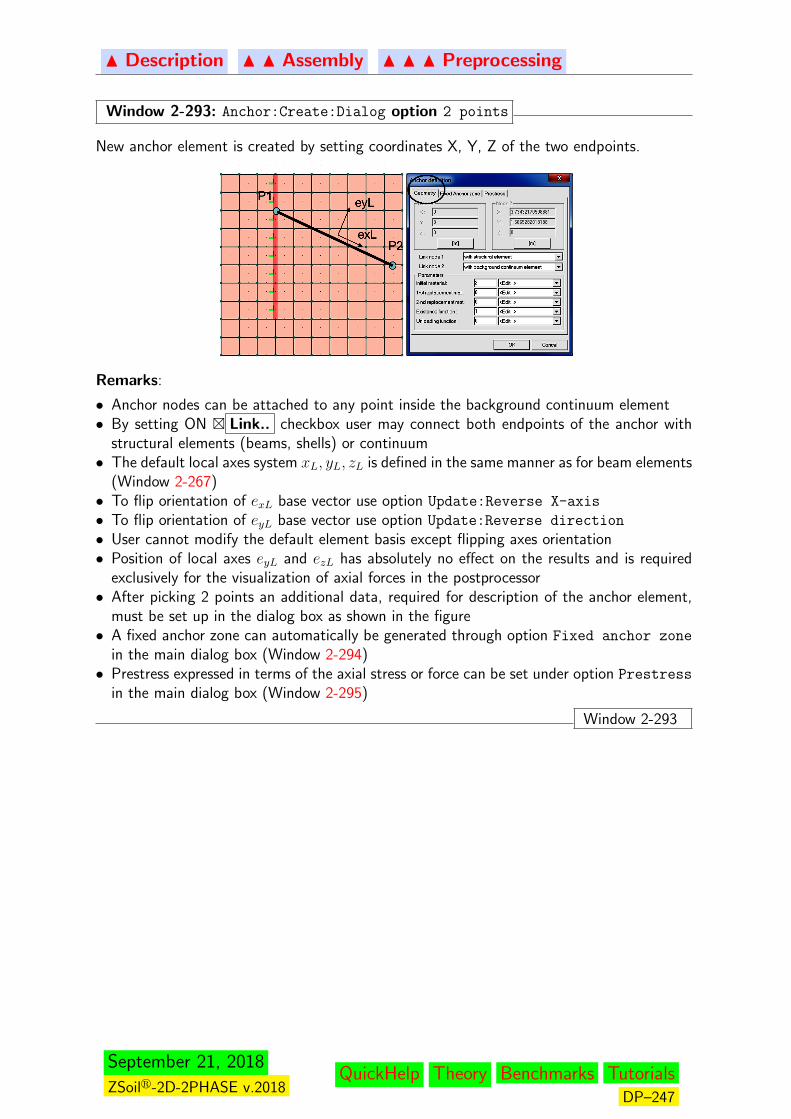
N Description N N Assembly N N N Preprocessing
Window 2-293: Anchor:Create:Dialog option 2 points
New anchor element is created by setting coordinates X, Y, Z of the two endpoints.
Remarks:
• Anchor nodes can be attached to any point inside the background continuum element• By setting ON � Link.. checkbox user may connect both endpoints of the anchor with
structural elements (beams, shells) or continuum• The default local axes system xL, yL, zL is defined in the same manner as for beam elements
(Window 2-267)• To flip orientation of exL base vector use option Update:Reverse X-axis
• To flip orientation of eyL base vector use option Update:Reverse direction
• User cannot modify the default element basis except flipping axes orientation• Position of local axes eyL and ezL has absolutely no effect on the results and is required
exclusively for the visualization of axial forces in the postprocessor• After picking 2 points an additional data, required for description of the anchor element,
must be set up in the dialog box as shown in the figure• A fixed anchor zone can automatically be generated through option Fixed anchor zone
in the main dialog box (Window 2-294)• Prestress expressed in terms of the axial stress or force can be set under option Prestress
in the main dialog box (Window 2-295)
Window 2-293
September 21, 2018
ZSoilr-2D-2PHASE v.2018QuickHelp Theory Benchmarks Tutorials
DP–247
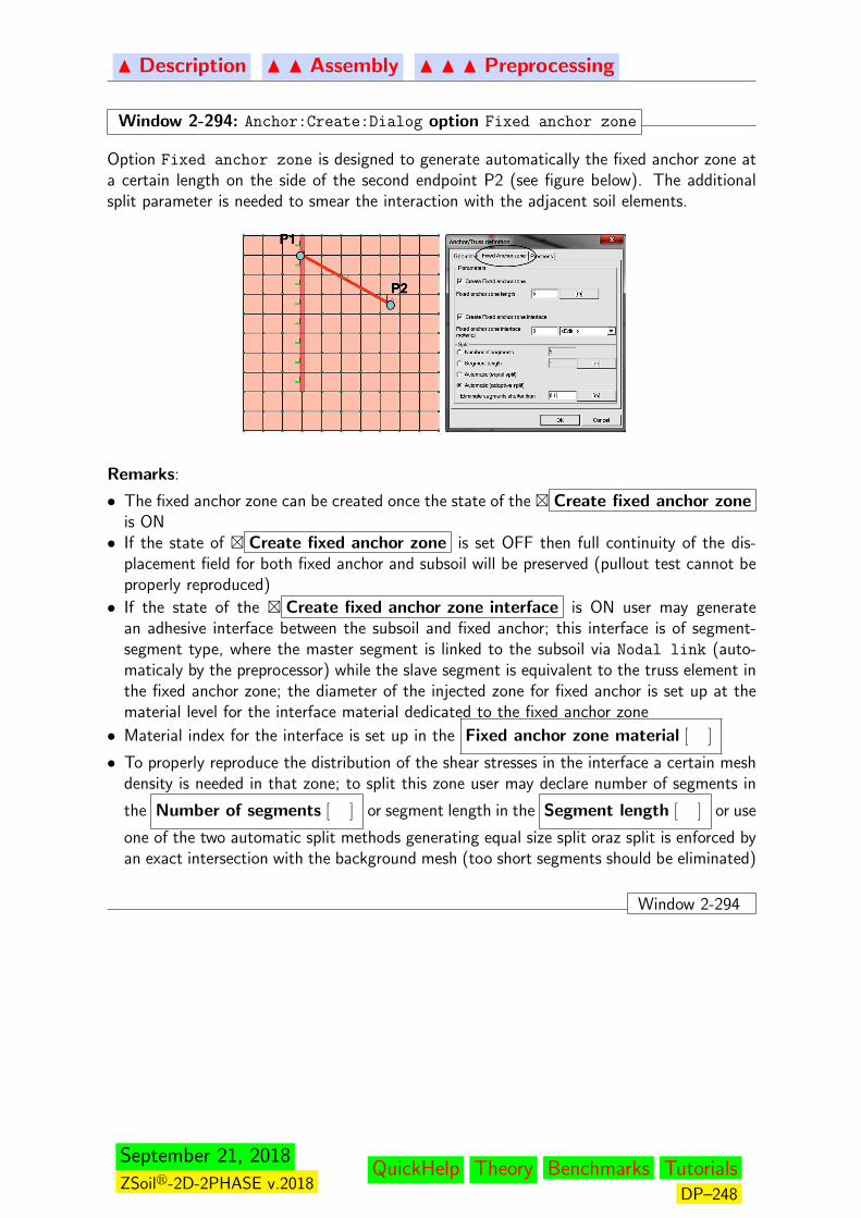
N Description N N Assembly N N N Preprocessing
Window 2-294: Anchor:Create:Dialog option Fixed anchor zone
Option Fixed anchor zone is designed to generate automatically the fixed anchor zone ata certain length on the side of the second endpoint P2 (see figure below). The additionalsplit parameter is needed to smear the interaction with the adjacent soil elements.
Remarks:
• The fixed anchor zone can be created once the state of the � Create fixed anchor zoneis ON• If the state of � Create fixed anchor zone is set OFF then full continuity of the dis-
placement field for both fixed anchor and subsoil will be preserved (pullout test cannot beproperly reproduced)
• If the state of the � Create fixed anchor zone interface is ON user may generatean adhesive interface between the subsoil and fixed anchor; this interface is of segment-segment type, where the master segment is linked to the subsoil via Nodal link (auto-maticaly by the preprocessor) while the slave segment is equivalent to the truss element inthe fixed anchor zone; the diameter of the injected zone for fixed anchor is set up at thematerial level for the interface material dedicated to the fixed anchor zone
• Material index for the interface is set up in the Fixed anchor zone material [ ]
• To properly reproduce the distribution of the shear stresses in the interface a certain meshdensity is needed in that zone; to split this zone user may declare number of segments in
the Number of segments [ ] or segment length in the Segment length [ ] or use
one of the two automatic split methods generating equal size split oraz split is enforced byan exact intersection with the background mesh (too short segments should be eliminated)
Window 2-294
September 21, 2018
ZSoilr-2D-2PHASE v.2018QuickHelp Theory Benchmarks Tutorials
DP–248

N Description N N Assembly N N N Preprocessing
Window 2-295: Anchor:Create:Dialog option Prestress
Option Prestress is designed to apply prestress force to the anchor. Its value expressed interms of the stress can be driven by the load time function and existence function. In activeperiods of the existence function prestress is kept under control and current stress will alwaysbe equal to the assumed prestress one; during inactive periods current stress in the anchormay deviate from the assumed value.
Window 2-295
Window 2-296: Anchor:Create: 2 Nodes/points
A 2-node anchor element is created by picking the two geometrical points or nodes in thegraphical pane. The two picked points will be first snapped to the existing nodes of the realmesh, then to the grid points. All other parameters required to complete anchor definitionare described in Window 2-293
Window 2-296
Window 2-297: Anchor:Create: 2 Nodes
New 2-node anchor element is created by picking the two existing nodes in the graphicalpane. It is strongly recommended to not to try to pick the node exactly (it is a difficultaction) but rather to select it by picking the existing element next to the one of its verticesthat coincides with the node.
All other parameters required to complete anchor definition are described in Window 2-293
Window 2-297
September 21, 2018
ZSoilr-2D-2PHASE v.2018QuickHelp Theory Benchmarks Tutorials
DP–249
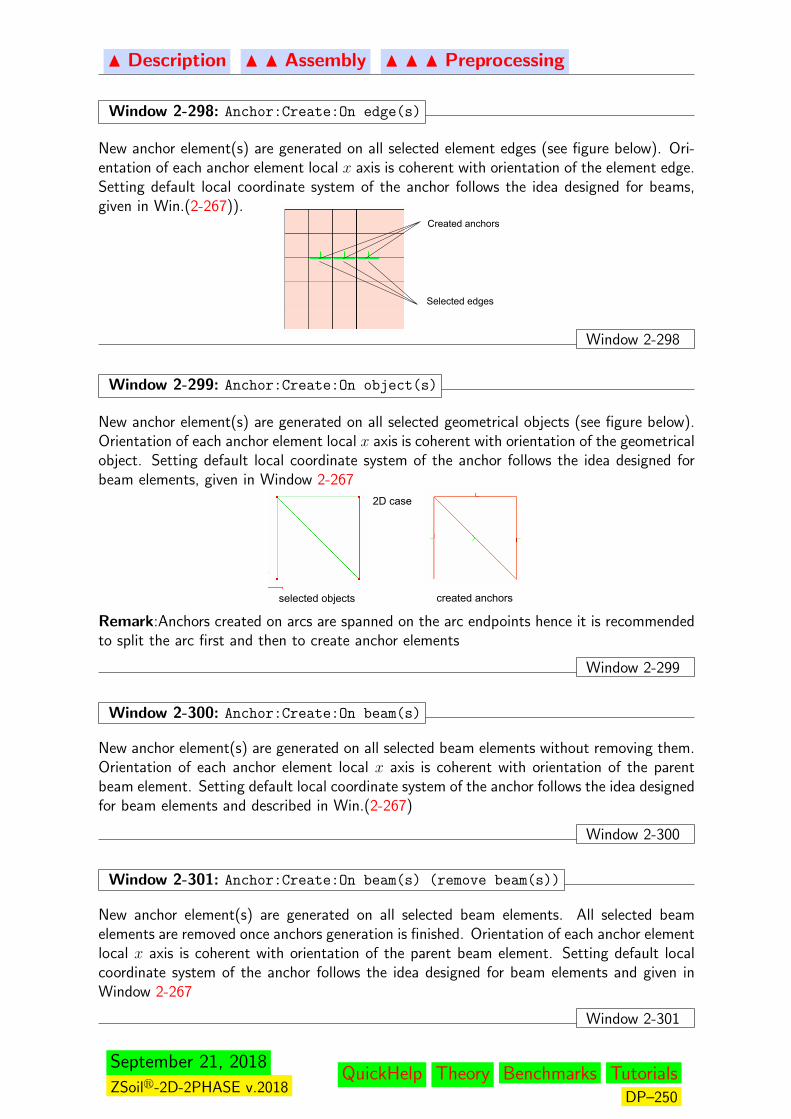
N Description N N Assembly N N N Preprocessing
Window 2-298: Anchor:Create:On edge(s)
New anchor element(s) are generated on all selected element edges (see figure below). Ori-entation of each anchor element local x axis is coherent with orientation of the element edge.Setting default local coordinate system of the anchor follows the idea designed for beams,given in Win.(2-267)).
Selected edges
Created anchors
Selected edges
Created anchors
Window 2-298
Window 2-299: Anchor:Create:On object(s)
New anchor element(s) are generated on all selected geometrical objects (see figure below).Orientation of each anchor element local x axis is coherent with orientation of the geometricalobject. Setting default local coordinate system of the anchor follows the idea designed forbeam elements, given in Window 2-267
selected objects created anchors
3D case
selected objects created anchors
2D case
Remark:Anchors created on arcs are spanned on the arc endpoints hence it is recommendedto split the arc first and then to create anchor elements
Window 2-299
Window 2-300: Anchor:Create:On beam(s)
New anchor element(s) are generated on all selected beam elements without removing them.Orientation of each anchor element local x axis is coherent with orientation of the parentbeam element. Setting default local coordinate system of the anchor follows the idea designedfor beam elements and described in Win.(2-267)
Window 2-300
Window 2-301: Anchor:Create:On beam(s) (remove beam(s))
New anchor element(s) are generated on all selected beam elements. All selected beamelements are removed once anchors generation is finished. Orientation of each anchor elementlocal x axis is coherent with orientation of the parent beam element. Setting default localcoordinate system of the anchor follows the idea designed for beam elements and given inWindow 2-267
Window 2-301
September 21, 2018
ZSoilr-2D-2PHASE v.2018QuickHelp Theory Benchmarks Tutorials
DP–250
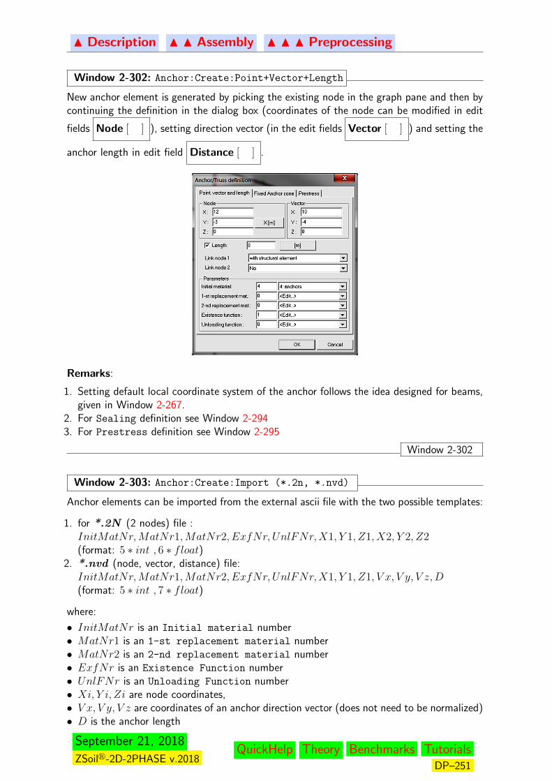
N Description N N Assembly N N N Preprocessing
Window 2-302: Anchor:Create:Point+Vector+Length
New anchor element is generated by picking the existing node in the graph pane and then bycontinuing the definition in the dialog box (coordinates of the node can be modified in edit
fields Node [ ] ), setting direction vector (in the edit fields Vector [ ] ) and setting the
anchor length in edit field Distance [ ] .
Remarks:
1. Setting default local coordinate system of the anchor follows the idea designed for beams,given in Window 2-267.
2. For Sealing definition see Window 2-2943. For Prestress definition see Window 2-295
Window 2-302
Window 2-303: Anchor:Create:Import (*.2n, *.nvd)
Anchor elements can be imported from the external ascii file with the two possible templates:
1. for *.2N (2 nodes) file :InitMatNr,MatNr1,MatNr2, ExfNr, UnlFNr,X1, Y 1, Z1, X2, Y 2, Z2(format: 5 ∗ int , 6 ∗ float)
2. *.nvd (node, vector, distance) file:InitMatNr,MatNr1,MatNr2, ExfNr, UnlFNr,X1, Y 1, Z1, V x, V y, V z,D(format: 5 ∗ int , 7 ∗ float)
where:
• InitMatNr is an Initial material number• MatNr1 is an 1-st replacement material number• MatNr2 is an 2-nd replacement material number• ExfNr is an Existence Function number• UnlFNr is an Unloading Function number• Xi, Y i, Zi are node coordinates,• V x, V y, V z are coordinates of an anchor direction vector (does not need to be normalized)• D is the anchor length
September 21, 2018
ZSoilr-2D-2PHASE v.2018QuickHelp Theory Benchmarks Tutorials
DP–251
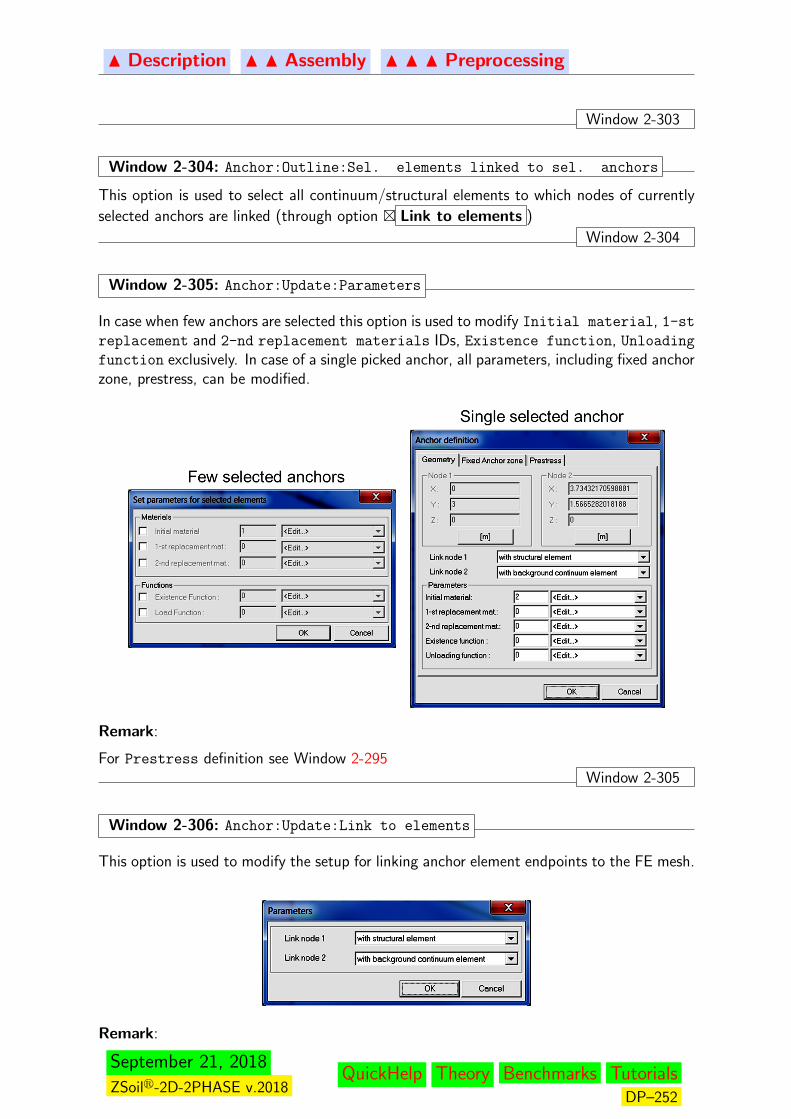
N Description N N Assembly N N N Preprocessing
Window 2-303
Window 2-304: Anchor:Outline:Sel. elements linked to sel. anchors
This option is used to select all continuum/structural elements to which nodes of currently
selected anchors are linked (through option � Link to elements )
Window 2-304
Window 2-305: Anchor:Update:Parameters
In case when few anchors are selected this option is used to modify Initial material, 1-streplacement and 2-nd replacement materials IDs, Existence function, Unloadingfunction exclusively. In case of a single picked anchor, all parameters, including fixed anchorzone, prestress, can be modified.
Remark:
For Prestress definition see Window 2-295Window 2-305
Window 2-306: Anchor:Update:Link to elements
This option is used to modify the setup for linking anchor element endpoints to the FE mesh.
Remark:
September 21, 2018
ZSoilr-2D-2PHASE v.2018QuickHelp Theory Benchmarks Tutorials
DP–252
N Description N N Assembly N N N Preprocessing
In the above example first node will be connected to the structural (beam) element (con-nection does not need to be set necessarily at the node) while the second endpoint will beconnected to the continuum element.
Window 2-306
Window 2-307: Anchor:Update:Fixed anchor zone length
This option allows the user to adjust fixed anchor zone length.
Window 2-307
Window 2-308: Anchor:Update:Prestress
This option is exclusively used to modify the prestress setup.
Remark:
Prestress is defined in terms of the stress or force and can be driven by the load time functionand existence function. In active periods of the existence function prestress is kept undercontrol and current axial stress/force will always be equal to the assumed value; duringinactive periods current stress/force in the anchor may deviate from the assumed value.
Window 2-308
Window 2-309: Anchor:Update:Reverse direction
This option is used to flip the local axis yL and in consequence local axis zL while xL remainsunchanged.Remarks:
September 21, 2018
ZSoilr-2D-2PHASE v.2018QuickHelp Theory Benchmarks Tutorials
DP–253
N Description N N Assembly N N N Preprocessing
• Proper setting of local anchor axes is important for visualization of normal force diagramsin the postprocessor• Local axis xL, by default, is drawn with red color, yL with green color and zL with a blue
color
Window 2-309
Window 2-310: Anchor:Update:Reverse X axis
This option is used to flip the local axis xL and in consequence local axis zL while yL remainsunchanged.Remarks:
• Proper setting of local anchor axes is very important for visualization of normal forcediagrams in the postprocessor• In case when anchors form a closed polygon their local xL axes should be oriented in one
direction• Local axis xL, by default, is drawn with red color, yL with green color and zL with a blue
color
Window 2-310
Window 2-311: Anchor:Update:Length
This option allows the user to adjust anchor length.
Window 2-311
Window 2-312: Anchor:Update:Inclination angle
This option allows the user to adjust anchor inclination angle in the vertical plane.
Window 2-312
Window 2-313: Anchor:Update:Split
Using this option user may split picked anchor element or group of selected anchor elementswith a split value set in the dialog box.
September 21, 2018
ZSoilr-2D-2PHASE v.2018QuickHelp Theory Benchmarks Tutorials
DP–254
N Description N N Assembly N N N Preprocessing
Remark:
Every new anchor element inherits all the parameters from the parent element
Window 2-313
Window 2-314: Anchor:Update:Scale
Using this option user may scale size of local anchor axes.
Remark:
} Same size and } Same scale switches have no meaning here
Window 2-314
September 21, 2018
ZSoilr-2D-2PHASE v.2018QuickHelp Theory Benchmarks Tutorials
DP–255
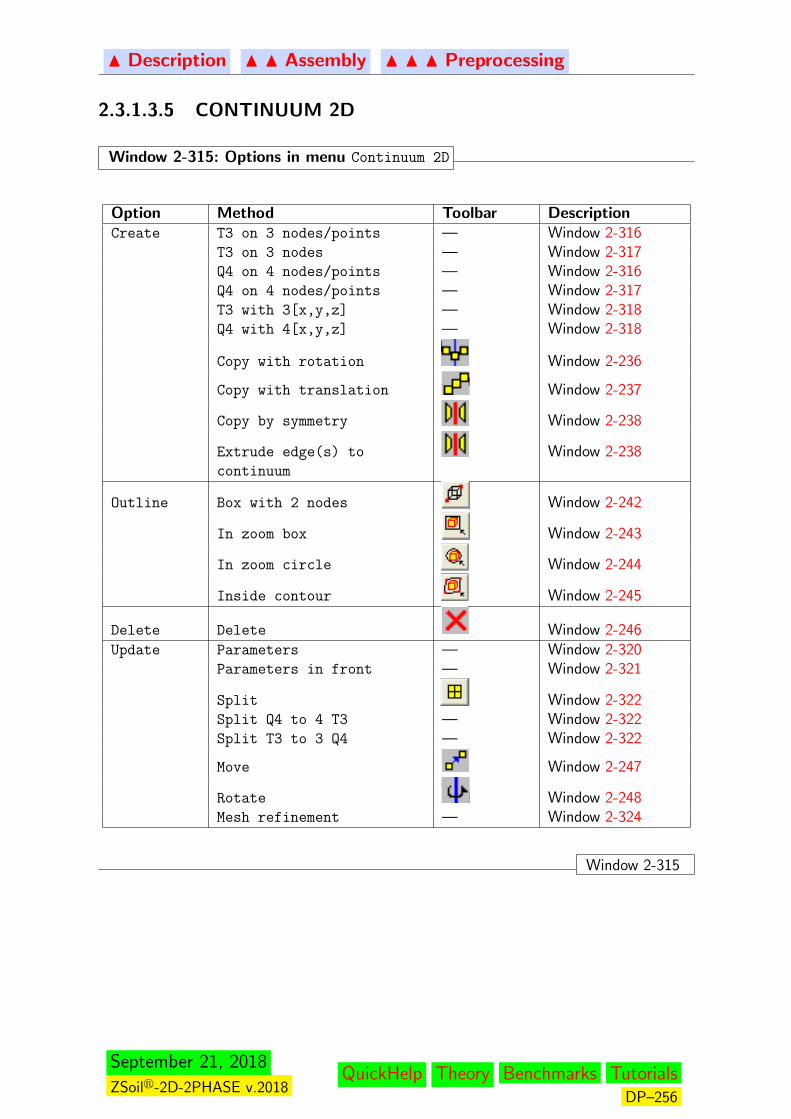
N Description N N Assembly N N N Preprocessing
2.3.1.3.5 CONTINUUM 2D
Window 2-315: Options in menu Continuum 2D
Option Method Toolbar DescriptionCreate T3 on 3 nodes/points — Window 2-316
T3 on 3 nodes — Window 2-317Q4 on 4 nodes/points — Window 2-316Q4 on 4 nodes/points — Window 2-317T3 with 3[x,y,z] — Window 2-318Q4 with 4[x,y,z] — Window 2-318
Copy with rotation Window 2-236
Copy with translation Window 2-237
Copy by symmetry Window 2-238
Extrude edge(s) to
continuum
Window 2-238
Outline Box with 2 nodes Window 2-242
In zoom box Window 2-243
In zoom circle Window 2-244
Inside contour Window 2-245
Delete Delete Window 2-246Update Parameters — Window 2-320
Parameters in front — Window 2-321
Split Window 2-322Split Q4 to 4 T3 — Window 2-322Split T3 to 3 Q4 — Window 2-322
Move Window 2-247
Rotate Window 2-248Mesh refinement — Window 2-324
Window 2-315
September 21, 2018
ZSoilr-2D-2PHASE v.2018QuickHelp Theory Benchmarks Tutorials
DP–256

N Description N N Assembly N N N Preprocessing
Window 2-316: Continuum-2D:Create:T3 on 3 nodes/pts, Q4 on 4 nodes/pts
New T3 or Q4 continuum 2D element is created by picking the three/four points in the graphpane. The picked points will be snapped first to the existing nodes of the real mesh projectedon the graph pane and then to the grid points, if snap options are set ON. This option must beused with care because close to the picked point in the graph pane there may appear severalprojected nodes/grid points and it may not be so easy to control the selection. So if onewants to create a continuum 2D element using the existing nodes it is recommended to usethe option Create:T3 on 3 nodes/Create:Q4 on 4 nodes described in Window 2-317.
Remark:Points/nodes can be picked in any order
Window 2-316
Window 2-317: Continuum-2D:Create:T3 on 3 nodes, Q4 on 4 nodes
New T3/Q4 continuum 2D element is created by picking the three/four existing nodes inthe graph pane. It is strongly recommended to not to try to pick the node exactly (it israther difficult action) but rather to select it by picking the existing element close to one ofits vertices that coincides with the node.
Remark:Nodes can be picked in any order
Window 2-317
Window 2-318: Continuum-2D:Create:T3 with 3 [x,y,z], Q4 with 4 [x,y,z]
New T3 or Q4 continuum 2D element is created by setting exact coordinates of 3 (for T3element) or 4 points (for Q4 element) in the dialog box.
Remark:
Points can be entered in any orderWindow 2-318
September 21, 2018
ZSoilr-2D-2PHASE v.2018QuickHelp Theory Benchmarks Tutorials
DP–257
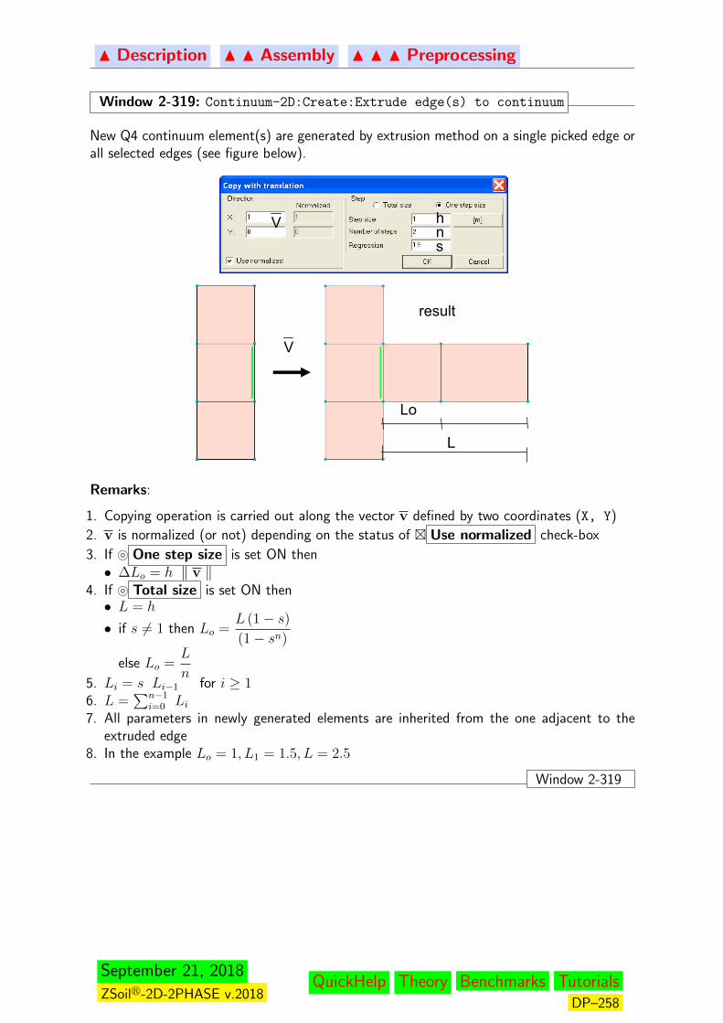
N Description N N Assembly N N N Preprocessing
Window 2-319: Continuum-2D:Create:Extrude edge(s) to continuum
New Q4 continuum element(s) are generated by extrusion method on a single picked edge orall selected edges (see figure below).
hns
Lo
L
V
V
result
Remarks:
1. Copying operation is carried out along the vector v defined by two coordinates (X, Y)
2. v is normalized (or not) depending on the status of � Use normalized check-box
3. If } One step size is set ON then• ∆Lo = h ‖ v ‖
4. If } Total size is set ON then• L = h
• if s 6= 1 then Lo =L (1− s)(1− sn)
else Lo =L
n5. Li = s Li−1 for i ≥ 16. L =
∑n−1i=0 Li
7. All parameters in newly generated elements are inherited from the one adjacent to theextruded edge
8. In the example Lo = 1, L1 = 1.5, L = 2.5
Window 2-319
September 21, 2018
ZSoilr-2D-2PHASE v.2018QuickHelp Theory Benchmarks Tutorials
DP–258
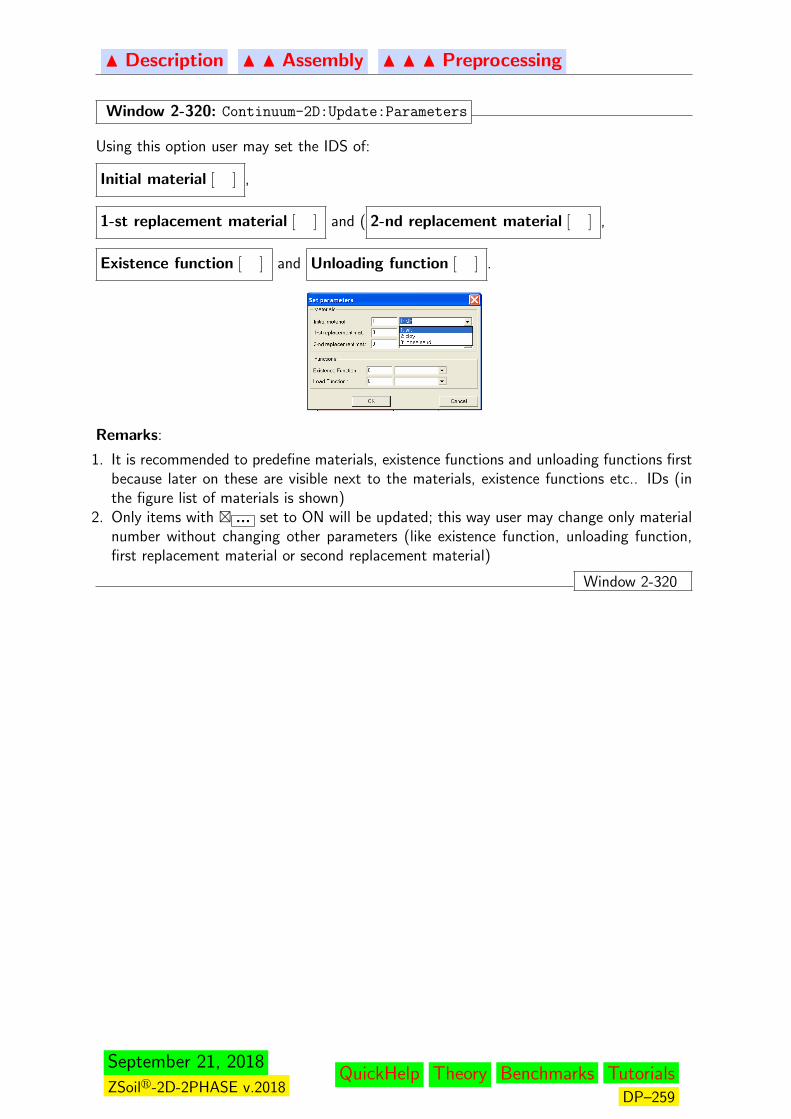
N Description N N Assembly N N N Preprocessing
Window 2-320: Continuum-2D:Update:Parameters
Using this option user may set the IDS of:
Initial material [ ] ,
1-st replacement material [ ] and ( 2-nd replacement material [ ] ,
Existence function [ ] and Unloading function [ ] .
Remarks:
1. It is recommended to predefine materials, existence functions and unloading functions firstbecause later on these are visible next to the materials, existence functions etc.. IDs (inthe figure list of materials is shown)
2. Only items with � ... set to ON will be updated; this way user may change only materialnumber without changing other parameters (like existence function, unloading function,first replacement material or second replacement material)
Window 2-320
September 21, 2018
ZSoilr-2D-2PHASE v.2018QuickHelp Theory Benchmarks Tutorials
DP–259
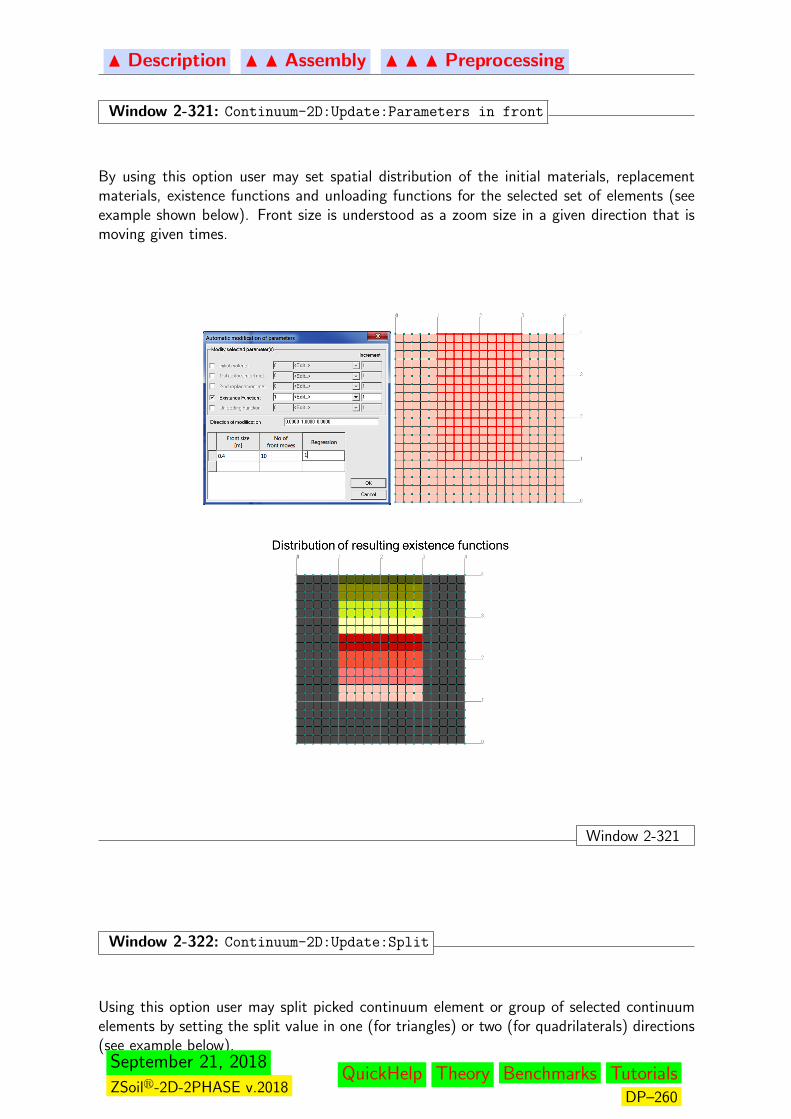
N Description N N Assembly N N N Preprocessing
Window 2-321: Continuum-2D:Update:Parameters in front
By using this option user may set spatial distribution of the initial materials, replacementmaterials, existence functions and unloading functions for the selected set of elements (seeexample shown below). Front size is understood as a zoom size in a given direction that ismoving given times.
Window 2-321
Window 2-322: Continuum-2D:Update:Split
Using this option user may split picked continuum element or group of selected continuumelements by setting the split value in one (for triangles) or two (for quadrilaterals) directions(see example below).
September 21, 2018
ZSoilr-2D-2PHASE v.2018QuickHelp Theory Benchmarks Tutorials
DP–260

N Description N N Assembly N N N Preprocessing
Q4T3
Remarks:
1. Every new element inherits all the parameters from the parent element2. If split is run for group of selected elements then the template split set for the first picked
element will be transferred to all adjacent elements to preserve mesh conformity
Window 2-322
Window 2-323: Continuum-2D:Update:Split Q4 to 4 T3, Split T3 to 3 Q4
Using this option user may split picked continuum element or group of selected continuumelements by setting the split value in one (for triangles) or two (for quadrilaterals) directions(see example below).
Remarks:
1. Every new element inherits all the parameters from the parent element2. Triangular elements can only be used in exceptional situations due to their inherent volu-
metric locking defect
Window 2-323
Window 2-324: Continuum-2D:Update:Mesh refinement
For detailed description of this option see Win.2-100.
Window 2-324
September 21, 2018
ZSoilr-2D-2PHASE v.2018QuickHelp Theory Benchmarks Tutorials
DP–261
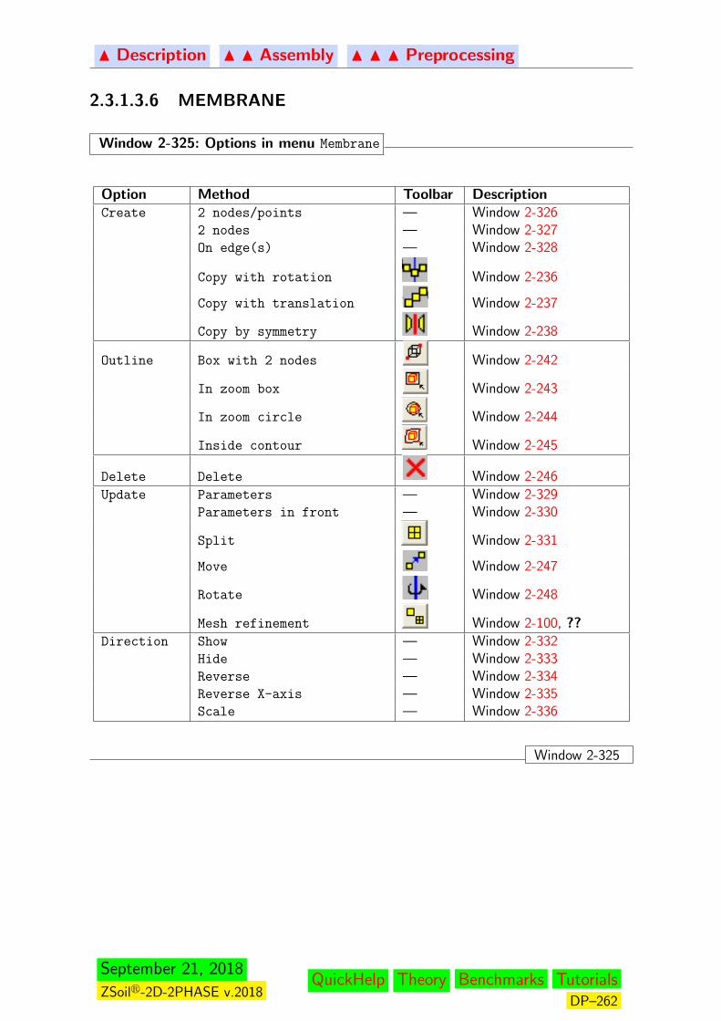
N Description N N Assembly N N N Preprocessing
2.3.1.3.6 MEMBRANE
Window 2-325: Options in menu Membrane
Option Method Toolbar DescriptionCreate 2 nodes/points — Window 2-326
2 nodes — Window 2-327On edge(s) — Window 2-328
Copy with rotation Window 2-236
Copy with translation Window 2-237
Copy by symmetry Window 2-238
Outline Box with 2 nodes Window 2-242
In zoom box Window 2-243
In zoom circle Window 2-244
Inside contour Window 2-245
Delete Delete Window 2-246Update Parameters — Window 2-329
Parameters in front — Window 2-330
Split Window 2-331
Move Window 2-247
Rotate Window 2-248
Mesh refinement Window 2-100, ??Direction Show — Window 2-332
Hide — Window 2-333Reverse — Window 2-334Reverse X-axis — Window 2-335Scale — Window 2-336
Window 2-325
September 21, 2018
ZSoilr-2D-2PHASE v.2018QuickHelp Theory Benchmarks Tutorials
DP–262
N Description N N Assembly N N N Preprocessing
Window 2-326: Membrane:2 nodes/points
New 2-node membrane element is created by picking the two points in the graph pane. Thetwo picked points will be first snapped to the existing nodes of the real mesh projected onthe graph pane and then to the grid points, if snap options are set ON. This option must beused with care because close to the picked point in the graph pane there may appear severalprojected nodes/grid points and it may not be so easy to control the selection. So if we wantto create an membrane between the two existing nodes it is recommended to use the optionCreate:2 nodes described in Window 2-327.
1. This definition is valid exclusively for the 2D models2. Positioning of the local axes follow the procedure designed for anchors and described in
Window 2-2933. Membrane elements are usually created on selected continuum element edges4. Direction of the external membrane normal vector should be verified before running com-
putation to avoid visualization problems (tensile force in the chain of membrane elementscan jump from top to the bottom side)
5. To reverse the normal use option Direction:Reverse
Window 2-326
Window 2-327: Membrane:2 nodes
New 2-node membrane element is created by picking the two existing nodes in the graphpane. It is strongly recommended to not to try to pick the node exactly (it is rather difficultaction) but rather to select it by picking the existing element close to one of its vertices thatcoincides with the node. For more information concerning setting local membrane axes seeWindow 2-326.
Window 2-327
Window 2-328: Membrane:On edges
New 2D membrane elements are created on a single picked edge or group of selected edges.
Remarks:
1. Membrane elements are usually created on selected continuum element edges2. Direction of the external membrane normal vector should be verified before running com-
putation to avoid visualization problems (tensile force in the chain of membrane elementscan jump from top to the bottom side)
3. To reverse the normal use option Direction:Reverse
Window 2-328
September 21, 2018
ZSoilr-2D-2PHASE v.2018QuickHelp Theory Benchmarks Tutorials
DP–263
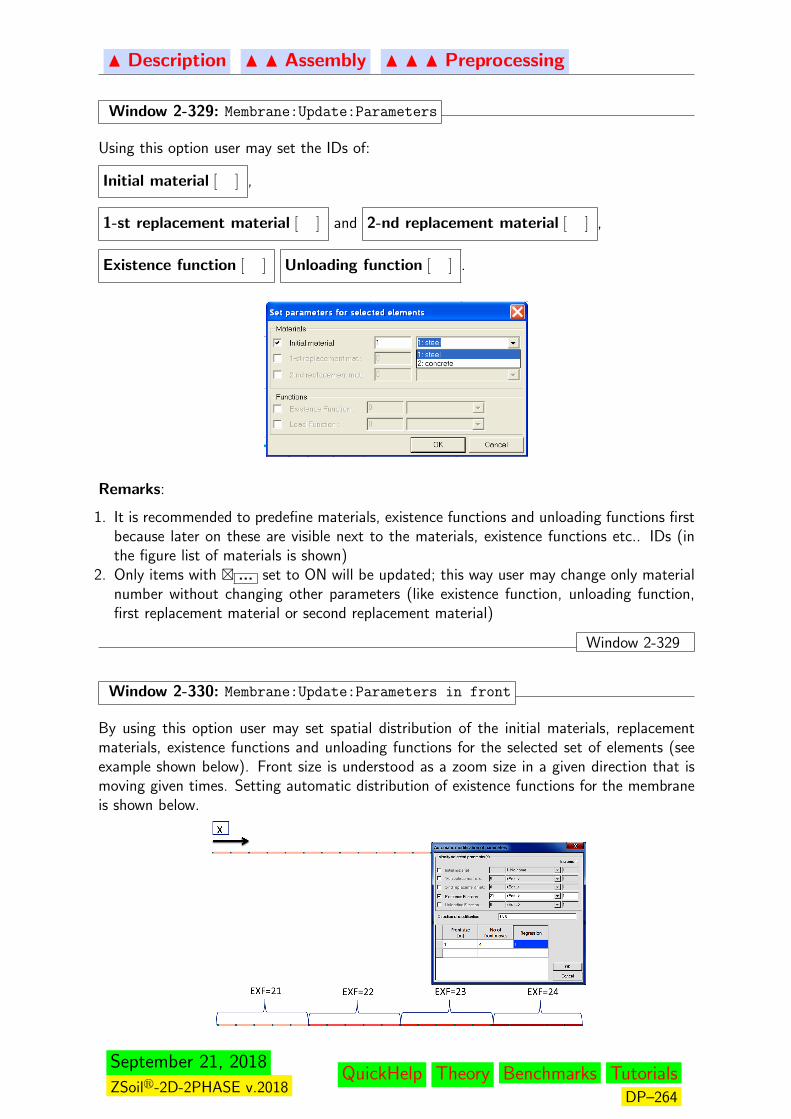
N Description N N Assembly N N N Preprocessing
Window 2-329: Membrane:Update:Parameters
Using this option user may set the IDs of:
Initial material [ ] ,
1-st replacement material [ ] and 2-nd replacement material [ ] ,
Existence function [ ] Unloading function [ ] .
Remarks:
1. It is recommended to predefine materials, existence functions and unloading functions firstbecause later on these are visible next to the materials, existence functions etc.. IDs (inthe figure list of materials is shown)
2. Only items with � ... set to ON will be updated; this way user may change only materialnumber without changing other parameters (like existence function, unloading function,first replacement material or second replacement material)
Window 2-329
Window 2-330: Membrane:Update:Parameters in front
By using this option user may set spatial distribution of the initial materials, replacementmaterials, existence functions and unloading functions for the selected set of elements (seeexample shown below). Front size is understood as a zoom size in a given direction that ismoving given times. Setting automatic distribution of existence functions for the membraneis shown below.
September 21, 2018
ZSoilr-2D-2PHASE v.2018QuickHelp Theory Benchmarks Tutorials
DP–264
N Description N N Assembly N N N Preprocessing
Window 2-330
Window 2-331: Membrane:Update:Split
In the 2D split of membrane element is same as for the anchor one ( see Window 2-313).
Window 2-331
Window 2-332: Membrane:Direction:Show
In the 2D this option activates visualization of the local base xL − yL in the same manneras for the anchor element.
Window 2-332
Window 2-333: Membrane:Direction:Hide
This option cancels visualization of membranes external normals.
Window 2-333
September 21, 2018
ZSoilr-2D-2PHASE v.2018QuickHelp Theory Benchmarks Tutorials
DP–265
N Description N N Assembly N N N Preprocessing
Window 2-334: Membrane:Direction:Reverse
Using this option user may reverse orientation of a single picked membrane element or groupof selected membrane elements.
For the 2D case this method is same as for the anchor element (see Window 2-309).
Window 2-334
Window 2-335: Membrane:Direction:Reverse X-axis
This option is valid only for the 2D cases and is equivalent to the one designed for anchorelement (see Window 2-310).
Window 2-335
Window 2-336: Membrane:Direction:Scale
Using this option user may enlarge or diminish size of the external normal vectors.
Window 2-336
September 21, 2018
ZSoilr-2D-2PHASE v.2018QuickHelp Theory Benchmarks Tutorials
DP–266
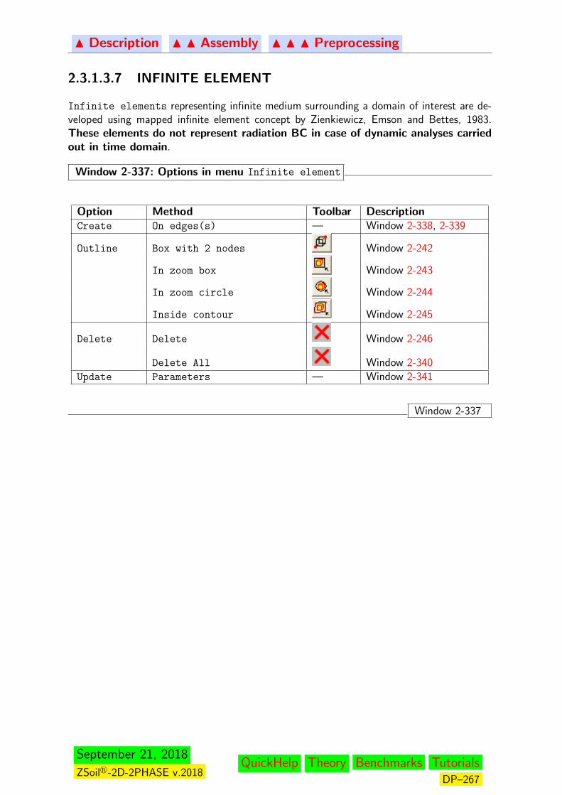
N Description N N Assembly N N N Preprocessing
2.3.1.3.7 INFINITE ELEMENT
Infinite elements representing infinite medium surrounding a domain of interest are de-veloped using mapped infinite element concept by Zienkiewicz, Emson and Bettes, 1983.These elements do not represent radiation BC in case of dynamic analyses carriedout in time domain.
Window 2-337: Options in menu Infinite element
Option Method Toolbar DescriptionCreate On edges(s) — Window 2-338, 2-339
Outline Box with 2 nodes Window 2-242
In zoom box Window 2-243
In zoom circle Window 2-244
Inside contour Window 2-245
Delete Delete Window 2-246
Delete All Window 2-340Update Parameters — Window 2-341
Window 2-337
September 21, 2018
ZSoilr-2D-2PHASE v.2018QuickHelp Theory Benchmarks Tutorials
DP–267
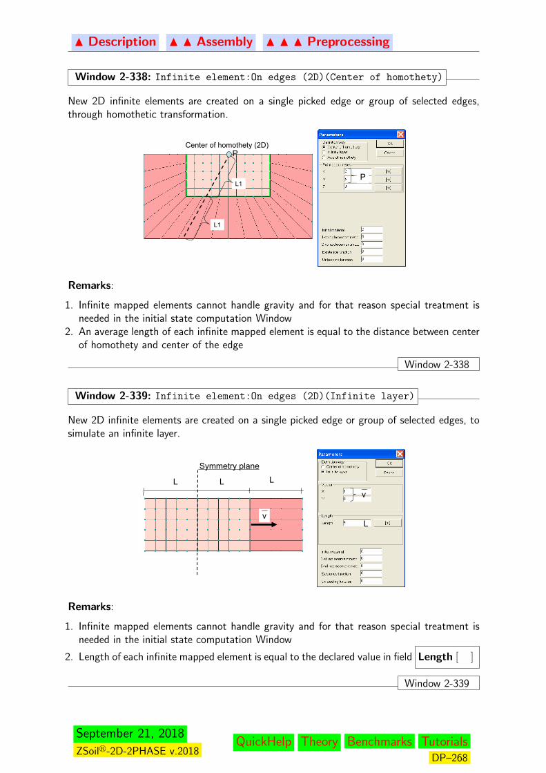
N Description N N Assembly N N N Preprocessing
Window 2-338: Infinite element:On edges (2D)(Center of homothety)
New 2D infinite elements are created on a single picked edge or group of selected edges,through homothetic transformation.
Center of homothety (2D)
L1
L1
P
P
Remarks:
1. Infinite mapped elements cannot handle gravity and for that reason special treatment isneeded in the initial state computation Window
2. An average length of each infinite mapped element is equal to the distance between centerof homothety and center of the edge
Window 2-338
Window 2-339: Infinite element:On edges (2D)(Infinite layer)
New 2D infinite elements are created on a single picked edge or group of selected edges, tosimulate an infinite layer.
v
L
L
v
L L
Symmetry plane
Remarks:
1. Infinite mapped elements cannot handle gravity and for that reason special treatment isneeded in the initial state computation Window
2. Length of each infinite mapped element is equal to the declared value in field Length [ ]
Window 2-339
September 21, 2018
ZSoilr-2D-2PHASE v.2018QuickHelp Theory Benchmarks Tutorials
DP–268
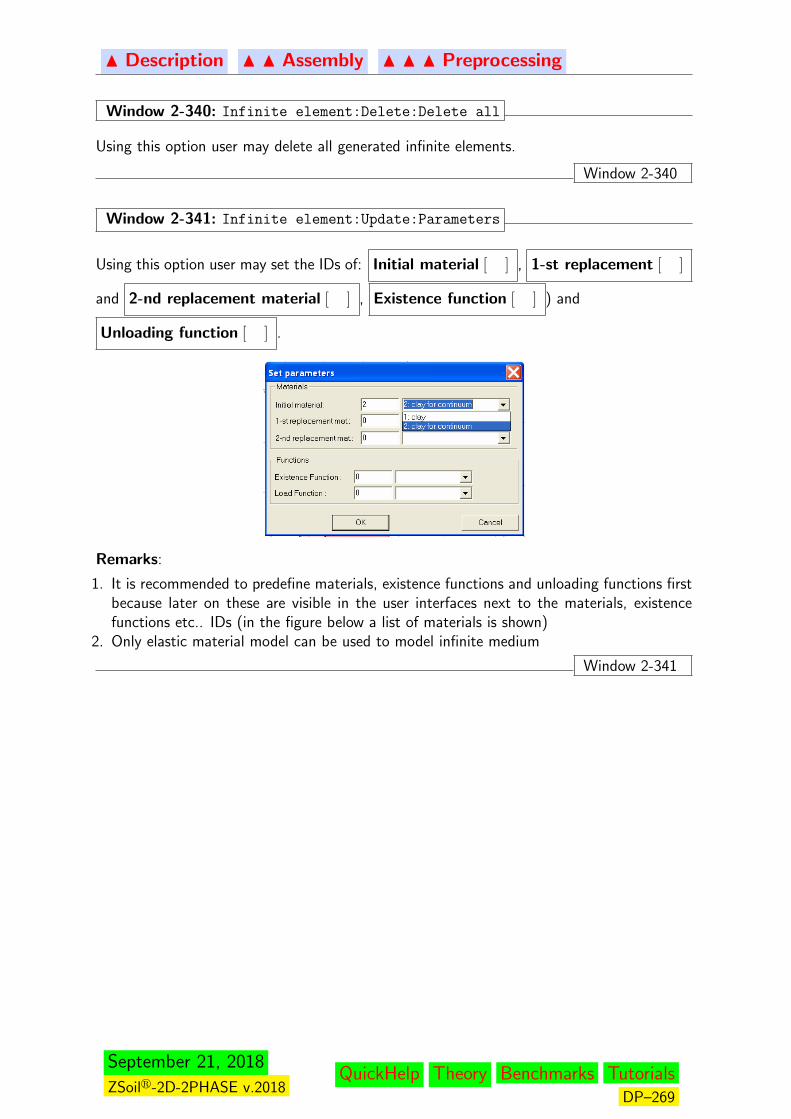
N Description N N Assembly N N N Preprocessing
Window 2-340: Infinite element:Delete:Delete all
Using this option user may delete all generated infinite elements.
Window 2-340
Window 2-341: Infinite element:Update:Parameters
Using this option user may set the IDs of: Initial material [ ] , 1-st replacement [ ]
and 2-nd replacement material [ ] , Existence function [ ] ) and
Unloading function [ ] .
Remarks:
1. It is recommended to predefine materials, existence functions and unloading functions firstbecause later on these are visible in the user interfaces next to the materials, existencefunctions etc.. IDs (in the figure below a list of materials is shown)
2. Only elastic material model can be used to model infinite medium
Window 2-341
September 21, 2018
ZSoilr-2D-2PHASE v.2018QuickHelp Theory Benchmarks Tutorials
DP–269

N Description N N Assembly N N N Preprocessing
Window 2-342: Infinite element:Handling initial state
As infinite mapped elements cannot handle gravity their presence must be cancelled in theinitial state computation. Hence the easiest way to manage that is as follows (see figure)
extra layer of elementswith EXF=1, UNLF=1
UNLF-11.0
1.0
t1.0
EXF-1
EXF=2
t1.0
EXF-2
t
1. Add additional layer of elements along the boundary at which infinite elements are to begenerated
2. Apply box-shaped boundary conditions and assume existence function to all fixities, sameas for the additional layer of elements
3. Apply a distinct existence function ID and unloading function ID for the additional layer ofelements• Existence function for additional layer of elements must be such that in the initial state
(t = 0) it is ON and then at time when infinite elements are activated it is switchedOFF• Unloading function for additional layer of elements starts at t = 0 from value zero (can
be any) and at time when the layer is switched OFF the function must be equal to 1.0up to infinity (this way all excavation forces will remain unchanged)
4. Apply a distinct existence function ID for infinite elements (inactive at t = 0)
Window 2-342
September 21, 2018
ZSoilr-2D-2PHASE v.2018QuickHelp Theory Benchmarks Tutorials
DP–270
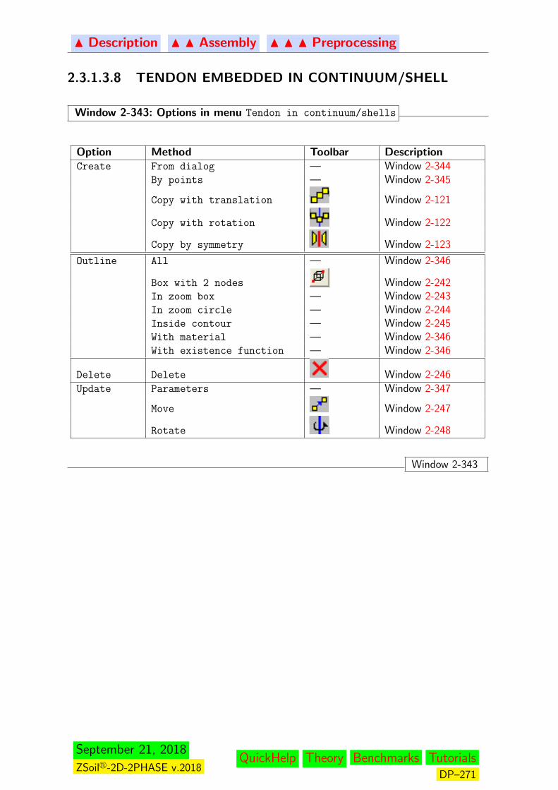
N Description N N Assembly N N N Preprocessing
2.3.1.3.8 TENDON EMBEDDED IN CONTINUUM/SHELL
Window 2-343: Options in menu Tendon in continuum/shells
Option Method Toolbar DescriptionCreate From dialog — Window 2-344
By points — Window 2-345
Copy with translation Window 2-121
Copy with rotation Window 2-122
Copy by symmetry Window 2-123
Outline All — Window 2-346
Box with 2 nodes Window 2-242In zoom box — Window 2-243In zoom circle — Window 2-244Inside contour — Window 2-245With material — Window 2-346With existence function — Window 2-346
Delete Delete Window 2-246Update Parameters — Window 2-347
Move Window 2-247
Rotate Window 2-248
Window 2-343
September 21, 2018
ZSoilr-2D-2PHASE v.2018QuickHelp Theory Benchmarks Tutorials
DP–271

N Description N N Assembly N N N Preprocessing
Window 2-344: Tendon in continuum/shells:Create:From dialog
A prestressed tendon is generated based on a given set of fit points put in list (A) of the dialog.Tendon passes exactly through all these points. Trace of the tendon is designed with aid of the2-nd or 3-rd order (most often) splines. Therefore number of fit points must be larger than
the spline order plus one. Spline order is defined int the edit Spline order [ ] . Material
id, existence and unloading functions are defined in sector (D) of the dialog. Whole set of thedata concerning prestress is given is sector (E) of the dialog. Prestress data consists of thevalue (in terms of force), two flags defining the way it is realized (from one left/right endpointor from both endpoints), friction µ and profile k coefficients (these coefficients influence lossof prestress along tendon length) but also the load function and existence function. Thelatter one defines time period in which prestress is equal to the assumed force value at oneor two endpoints. After real FE mesh generation tendon is converted to the set of trusselements (by an exact intersection with the FE mesh) that are linked to the background setof continuum/shell elements via Nodal link option (this is done automatically). Selectingbackground elements, in which tendon is embedded, is defined by means of selected materialsset in the list (C).
Window 2-344
Window 2-345: Tendon in continuum/shells:Create:By points
A prestressed tendon is generated by picking set of fit points (cable passes through thesepoints). This graphical operation after clicking few points can be ended up by clicking rightmouse cursor and then by selecting menu item Enter. The remaining part of the tendondefinition is the same as in option From dialog (see Window 2-344). In 2D one may pickany point on the screen once the snap option is set OFF but in 3D tendon fit points willalways be snapped to the grid, construction lines or other characteristic points.
Window 2-345
September 21, 2018
ZSoilr-2D-2PHASE v.2018QuickHelp Theory Benchmarks Tutorials
DP–272
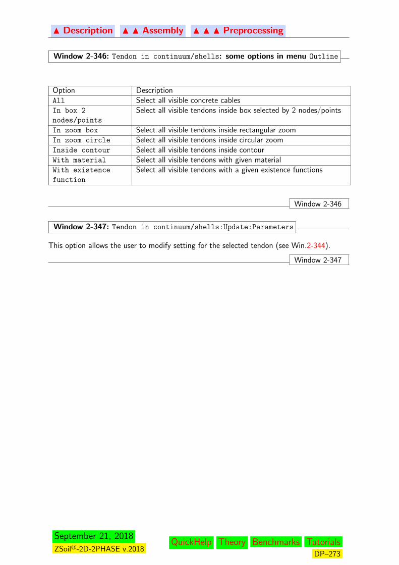
N Description N N Assembly N N N Preprocessing
Window 2-346: Tendon in continuum/shells: some options in menu Outline
Option DescriptionAll Select all visible concrete cablesIn box 2
nodes/points
Select all visible tendons inside box selected by 2 nodes/points
In zoom box Select all visible tendons inside rectangular zoomIn zoom circle Select all visible tendons inside circular zoomInside contour Select all visible tendons inside contourWith material Select all visible tendons with given materialWith existence
function
Select all visible tendons with a given existence functions
Window 2-346
Window 2-347: Tendon in continuum/shells:Update:Parameters
This option allows the user to modify setting for the selected tendon (see Win.2-344).
Window 2-347
September 21, 2018
ZSoilr-2D-2PHASE v.2018QuickHelp Theory Benchmarks Tutorials
DP–273

N Description N N Assembly N N N Preprocessing
2.3.1.3.9 INTERFACE (SMALL DEFORMATION)
Window 2-348: Options in menu Interface
Option Method Toolbar DescriptionCreate On Cont.elem.edges (2D) — Window 2-349
On Structural elements — Window 2-350, ??Outline All — Window 2-351
Box with 2 nodes Window 2-242With material — Window 2-352With existence function — Window 2-352With unloading function — Window 2-352With label — Window 2-352With attribute — Window 2-352On selected edges (2D) — Window 2-353
In zoom box Window 2-243
In zoom circle Window 2-244
Inside contour Window 2-245
Delete Delete Window 2-246Update Parameters — Window 2-354
Scale — Window 2-355Show direction — Window 2-356Hide direction — Window 2-357Standard view — Window 2-358Control view — Window 2-359Select singular interface
nodes
— Window 2-360
Link interface node(s) — Window 2-361Delete links Window 2-362Delete all links — Window 2-363Exclude elements — Window 2-364Disable excluded elements — Window 2-365Show excluded elements — Window 2-366
Window 2-348
September 21, 2018
ZSoilr-2D-2PHASE v.2018QuickHelp Theory Benchmarks Tutorials
DP–274

N Description N N Assembly N N N Preprocessing
Window 2-349: Interface:On edges
New 2D interface elements are created by selecting edges of continuum elements in theexisting real mesh (see example).
Selection of edges tocreate contact
Beam elements
A B
A, B – singular points
Remarks:
1. Note that beam elements will always be separated from the continuum at points A and B(as contact is ended in the inside of the domain); to enforce continuity in these points useoption Update:Link nodes
2. In cases like in this example it is recommended to create contact elements by parts to beable to apply a distinct label and to be able to apply different existence function, unloadingfunction and material ID, otherwise contact elements have to be selected from selectededges (2D) and then updated through Update:Parameters
3. Contact elements, disconnecting the real mesh along indicated segments, are generatedduring generation of the input file for calculation module (*.DAT file)
4. During contact generation user may set type of the contact behavior and an additionaldata in the dialog box (see Window 2-354) for details)
Window 2-349
September 21, 2018
ZSoilr-2D-2PHASE v.2018QuickHelp Theory Benchmarks Tutorials
DP–275

N Description N N Assembly N N N Preprocessing
Window 2-350: Interface:On Structural elements (2D)
New 2D interface elements are created by selecting structural elements (beams, membranes)in the existing real mesh (see example). In this definition contact interface may be created onany side of the structural element being in contact with continuum. It is important to care-fuly set contact properties concerning orientation of the structural element local coordinatesystem. The positive interface is located in contact zone continuum-top beam/membranefibers.
-++
Orientation of beamexternal normal
Remarks:
1. This definition may be useful when modeling reinforced soils using geotextiles; in suchcases this definition is optimal
2. One may create or not the interface on positive/negative side of the structural element3. Remarks in Win.(2-349) are valid for this option
Window 2-350
Window 2-351: Interface:Outline:All
Using this option user may select all contact interfaces.
Window 2-351
Window 2-352: Interface:Outline: material, existence/unloading function
September 21, 2018
ZSoilr-2D-2PHASE v.2018QuickHelp Theory Benchmarks Tutorials
DP–276

N Description N N Assembly N N N Preprocessing
Using this option user may select contact interfaces with a given material, existence function,unloading function ID or a given attribute or label. In case of a label or an attribute one mayselect a single item from combo-box.
Window 2-352
Window 2-353: Interface:Outline:On selected edges
Using this option user may select 2D contact elements which are overlapping with selectededges.
Window 2-353
September 21, 2018
ZSoilr-2D-2PHASE v.2018QuickHelp Theory Benchmarks Tutorials
DP–277
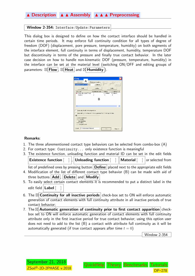
N Description N N Assembly N N N Preprocessing
Window 2-354: Interface:Update:Parameters
This dialog box is designed to define on how the contact interface should be handled incertain time periods. It may enforce full continuity condition for all types of degree offreedom (DOF) (displacement, pore pressure, temperature, humidity) on both segments ofthe interface element, full continuity in terms of displacement, humidity, temperature DOFbut discontinuity in terms of the pressure and finally true contact behavior. In the latercase decision on how to handle non-kinematic DOF (pressure, temperature, humidity) inthe interface can be set at the material level (switching ON/OFF and editing groups of
parameters: � Flow , � Heat and � Humidity ).
A
B
Remarks:
1. The three aforementioned contact type behaviors can be selected from combo-box (A)2. For contact type: Continuity... only existence function is meaningful3. The existence function, unloading function and material ID can be set in the edit fields
Existence function [ ] , Unloading function [ ] Material [ ] or selected from
list of predefined ones by pressing button Define placed next to the appropriate edit fields4. Modification of the list of different contact type behavior (B) can be made with aid of
three buttons Add , Delete and Modify5. To easily select certain contact elements it is recommended to put a distinct label in the
edit field Label [ ]
6. The � Continuity for all inactive periods check-box set to ON will enforce automaticgeneration of contact elements with full continuity attribute in all inactive periods of truecontact behavior;
7. The� Automatic generation of continuity prior to first contact apparition check-box set to ON will enforce automatic generation of contact elements with full continuityattribute only in the first inactive period for true contact behavior; using this option userdoes not need to add to the list (B) a contact with attribute full continuity as it will beautomatically generated (if true contact appears after time t = 0)
Window 2-354
September 21, 2018
ZSoilr-2D-2PHASE v.2018QuickHelp Theory Benchmarks Tutorials
DP–278

N Description N N Assembly N N N Preprocessing
Window 2-355: Interface:Update:Scale
Using this option user may enlarge or diminish size of the external normal vectors and openingof the interface in the Control view.
Window 2-355
Window 2-356: Interface:Update:Show direction
Using this option user visualize direction of external normal vectors to faces on which contactelements are created.
Window 2-356
Window 2-357: Interface:Update:Hide direction
Using this option user may hide external normal vectors to faces on which contact elementsare created.
Window 2-357
Window 2-358: Interface:Update:Standard view
With this option standard visualization of contact elements is activated.
Window 2-358
Window 2-359: Interface:Update:Control view
With this option special visualization of contact elements is activated. It makes easier recog-nition whether contact is properly set (see example below).Control view
Window 2-359
September 21, 2018
ZSoilr-2D-2PHASE v.2018QuickHelp Theory Benchmarks Tutorials
DP–279

N Description N N Assembly N N N Preprocessing
Window 2-360: Interface:Update:Select singular interface nodes
In case when structural elements are in contact with soil and their endpoints are locatedinside of the soil domain (bottom of the diaphragm wall for instance) the structural elementendpoints will be disconnected from soil by default when contact interface is created. OptionSelect singular interface nodes allows to select all nodes in which this effect is de-tected. To link these separated nodes use option Link interface nodes (Window 2-361).This situation is illustrated in the figure in Window 2-349.
Window 2-360
Window 2-361: Interface:Update:Link interface nodes
This option allows to link (enforce continuity) nodes separated by contact interface. In mostcases it is needed to handle the situation at points A, B as shown in the figure in Window2-349. Detection of such singular points can be made with aid of option Select singular
interface nodes (Window 2-360). Created links between two nodes are plot as light-greenbars.
Window 2-361
Window 2-362: Interface:Update:Delete link
Using this option one may cancel a single picked link of group of links at selected nodes.Hence to delete group of links selection of nodes is requested.
Window 2-362
Window 2-363: Interface:Update:Delete all links
Using this option one may delete all links.
Window 2-363
September 21, 2018
ZSoilr-2D-2PHASE v.2018QuickHelp Theory Benchmarks Tutorials
DP–280
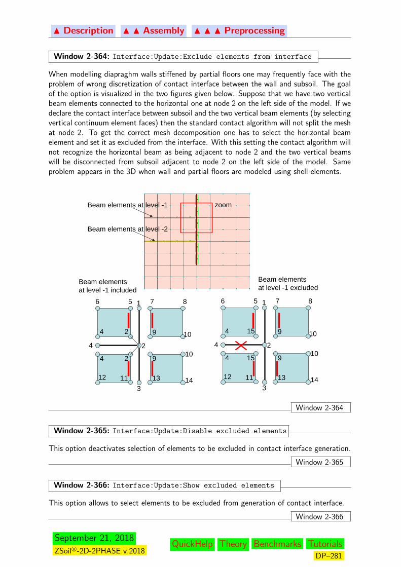
N Description N N Assembly N N N Preprocessing
Window 2-364: Interface:Update:Exclude elements from interface
When modelling diapraghm walls stiffened by partial floors one may frequently face with theproblem of wrong discretization of contact interface between the wall and subsoil. The goalof the option is visualized in the two figures given below. Suppose that we have two verticalbeam elements connected to the horizontal one at node 2 on the left side of the model. If wedeclare the contact interface between subsoil and the two vertical beam elements (by selectingvertical continuum element faces) then the standard contact algorithm will not split the meshat node 2. To get the correct mesh decomposition one has to select the horizontal beamelement and set it as excluded from the interface. With this setting the contact algorithm willnot recognize the horizontal beam as being adjacent to node 2 and the two vertical beamswill be disconnected from subsoil adjacent to node 2 on the left side of the model. Sameproblem appears in the 3D when wall and partial floors are modeled using shell elements.
1
2
3
4
56 7 8
2
2
4
4
9 10
9 10
1112 13 14
1
2
3
4
56 7 8
15
15
4
4
9 10
9 10
1112 13 14
zoomBeam elements at level -1
Beam elements at level -2
Beam elementsat level -1 excluded
Beam elementsat level -1 included
Window 2-364
Window 2-365: Interface:Update:Disable excluded elements
This option deactivates selection of elements to be excluded in contact interface generation.
Window 2-365
Window 2-366: Interface:Update:Show excluded elements
This option allows to select elements to be excluded from generation of contact interface.
Window 2-366
September 21, 2018
ZSoilr-2D-2PHASE v.2018QuickHelp Theory Benchmarks Tutorials
DP–281
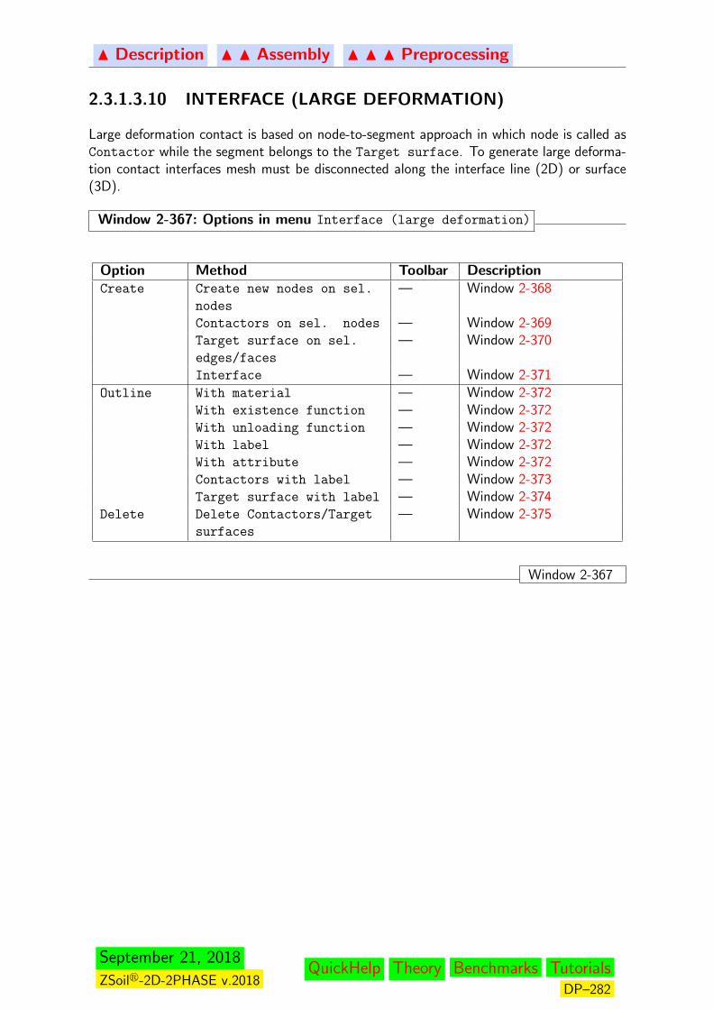
N Description N N Assembly N N N Preprocessing
2.3.1.3.10 INTERFACE (LARGE DEFORMATION)
Large deformation contact is based on node-to-segment approach in which node is called asContactor while the segment belongs to the Target surface. To generate large deforma-tion contact interfaces mesh must be disconnected along the interface line (2D) or surface(3D).
Window 2-367: Options in menu Interface (large deformation)
Option Method Toolbar DescriptionCreate Create new nodes on sel.
nodes
— Window 2-368
Contactors on sel. nodes — Window 2-369Target surface on sel.
edges/faces
— Window 2-370
Interface — Window 2-371Outline With material — Window 2-372
With existence function — Window 2-372With unloading function — Window 2-372With label — Window 2-372With attribute — Window 2-372Contactors with label — Window 2-373Target surface with label — Window 2-374
Delete Delete Contactors/Target
surfaces
— Window 2-375
Window 2-367
September 21, 2018
ZSoilr-2D-2PHASE v.2018QuickHelp Theory Benchmarks Tutorials
DP–282
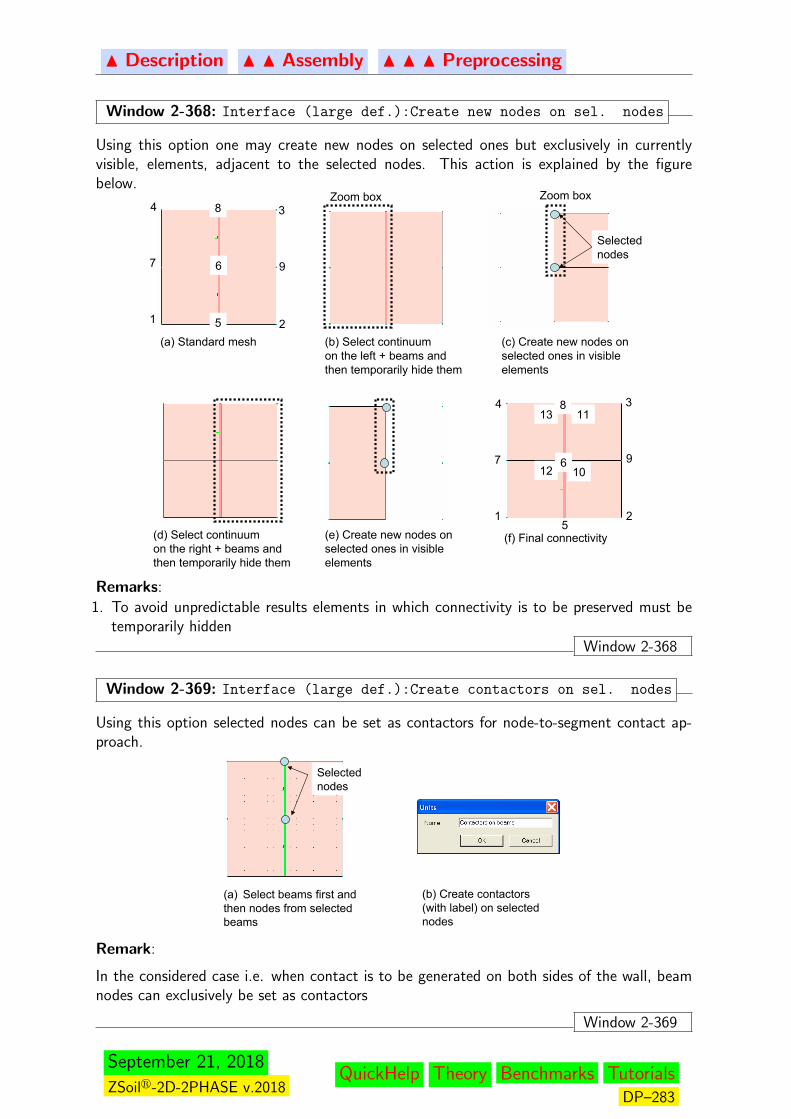
N Description N N Assembly N N N Preprocessing
Window 2-368: Interface (large def.):Create new nodes on sel. nodes
Using this option one may create new nodes on selected ones but exclusively in currentlyvisible, elements, adjacent to the selected nodes. This action is explained by the figurebelow.
(a) Standard mesh (b) Select continuum on the left + beams andthen temporarily hide them
(c) Create new nodes on selected ones in visibleelements
Zoom boxZoom box
Selectednodes
(d) Select continuum on the right + beams andthen temporarily hide them
(e) Create new nodes on selected ones in visibleelements
1
7
4
5
12
13
10
11
2
9
3
6
8
(f) Final connectivity
1
7
4
5 2
9
3
6
8
Remarks:
1. To avoid unpredictable results elements in which connectivity is to be preserved must betemporarily hidden
Window 2-368
Window 2-369: Interface (large def.):Create contactors on sel. nodes
Using this option selected nodes can be set as contactors for node-to-segment contact ap-proach.
(a) Select beams first andthen nodes from selectedbeams
(b) Create contactors(with label) on selectednodes
Selectednodes
Remark:
In the considered case i.e. when contact is to be generated on both sides of the wall, beamnodes can exclusively be set as contactors
Window 2-369
September 21, 2018
ZSoilr-2D-2PHASE v.2018QuickHelp Theory Benchmarks Tutorials
DP–283

N Description N N Assembly N N N Preprocessing
Window 2-370: Interface (large def.):Create target on sel. edges/faces
Using this option selected edges(2D)/faces(3D) can be set as target surface for node-to-segment contact approach.
(a) Create target surface on theleft side of the wall (on selectededges)
(b) Create target surface on theright side of the wall (on selectededges)
Remark:
In the considered case i.e. when contact is to be generated on both sides of the wall, adjacentto the wall, continuum element edges can exclusively be set as target surfaces
Window 2-370
Window 2-371: Interface (large def.):Interface
This option defines interfaces by combining pairs of contactors and target surfaces in thefollowing dialog box.
A B
C
Remarks:
1. Combo boxes (A) and (B) contain predefined sets of contactors and target surfaces ac-cordingly
2. New established interface can be added to the list (C) of interfaces through button ADD
3. Erroneous interface definition can be removed from list (C) with button Delete or modified
with button Update
4. Setting type of the contact behavior (same as for small deformation contact) can be
activated with button Modify Parameters (see Window 2-354) for detailed description)5. Interfaces do not need to be redefined after mesh refinement
Window 2-371
September 21, 2018
ZSoilr-2D-2PHASE v.2018QuickHelp Theory Benchmarks Tutorials
DP–284

N Description N N Assembly N N N Preprocessing
Window 2-372: Interface (large def.):Outline:Material, exist./unl.f., ...
This option allows to visualize certain interfaces identified by a given material, existencefunction, unloading function ID or a given attribute or label. Selected interface(s) are shownby highlighting target surface edges(2D)/faces(3D) and contactor nodes.
Window 2-372
Window 2-373: Interface (large def.):Outline:Contactors with label
This option selects contactor nodes with a given label.
Window 2-373
Window 2-374: Interface (large def.):Outline:Target surface with label
This option selects target surface (by highlighting target surface edges(2D)/faces(3D)) witha given label.
Window 2-374
Window 2-375: Interface (large def.):Delete:Contactors/Target surface
This option allows to delete some sets of contactor nodes or target surfaces through thefollowing dialog box.
A B
C
1. Combo boxes (A) and (B) contain predefined sets of contactors and target surfaces ac-cordingly
2. By deleting selected contactors set (from (A)) all the interfaces with this contactors setare cancelled from list (C)
3. By deleting selected target surface (from (B)) all the interfaces with this target surface arecancelled from list (C)
Window 2-375
September 21, 2018
ZSoilr-2D-2PHASE v.2018QuickHelp Theory Benchmarks Tutorials
DP–285
N Description N N Assembly N N N Preprocessing
2.3.1.3.11 SEEPAGE
Window 2-376: Options in menu Seepage
Option Method Toolbar DescriptionCreate 2 nodes — Window 2-378
On edge(s) — Window 2-377On Exc./Constr. front — Window 2-379
Outline All — Window 2-380
Box with 2 nodes Window 2-242With material — Window 2-381With existence function — Window 2-381With unloading function — Window 2-381With label — Window 2-381On selected edges (2D) — Window 2-382
In zoom box Window 2-243
In zoom circle Window 2-244
Inside contour Window 2-245
Delete Delete Window 2-246Update Parameters — Window 2-383Direction Show direction — Window 2-384
Hide direction — Window 2-385Scale — Window 2-386
Window 2-376
September 21, 2018
ZSoilr-2D-2PHASE v.2018QuickHelp Theory Benchmarks Tutorials
DP–286

N Description N N Assembly N N N Preprocessing
Window 2-377: Seepage:On edges
New 2D seepage elements are created by selecting continuum element edges in the existingreal mesh.
Standard nodes
Implicit layer with pressure dependent permeability i.e.:
, flow allowed, impermeable⎩
⎨⎧
≥−<−
=0)( if00)(if
EXT
EXTv
ppppk
k
Hiddennodes
Ω
Orientationmarkers
Remarks:
1. Seepage elements are meaningful for Flow and Deformation+Flow analyses2. Seepage elements are to be generated on edges/faces of continuum elements3. These elements are frequently used to simulate drains and to handle pressure/flux type of
the boundary condition in zones where free water surface intersects with domain boundary(see example); the penalty factor kv is automatically set by the calculation module andcan be modified by the user at the material level
4. An additional layer of external nodes is created automatically by the program and allpressure boundary conditions imposed on the seepage boundary are transferred to thesenodes
5. If seepage elements are conforming with the adjacent continuum elements then meshrefinement in the continuum will cause seepage refinement automatically
6. Direction marker helps to identify on which continuum element face given seepage elementin created; this is very important during stage construction analyses
Window 2-377
Window 2-378: Seepage:2 nodes
New 2D seepage elements are created along edges belonging to the line section defined bythe 2 picked nodes in the existing real mesh. This option, except the definition, is equivalentto the one described in Window 2-377.
Window 2-378
September 21, 2018
ZSoilr-2D-2PHASE v.2018QuickHelp Theory Benchmarks Tutorials
DP–287
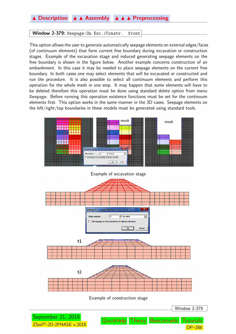
N Description N N Assembly N N N Preprocessing
Window 2-379: Seepage:On Exc./Constr. front
This option allows the user to generate automatically seepage elements on external edges/faces(of continuum elements) that form current free boundary during excavation or constructionstages. Example of the excavation stage and induced generating seepage elements on thefree boundary is shown in the figure below. Another example concerns construction of anembankment. In this case it may be needed to place seepage elements on the current freeboundary. In both cases one may select elements that will be excavated or constructed andrun the procedure. It is also possible to select all continuum elements and perform thisoperation for the whole mesh in one step. It may happen that some elements will have tobe deleted therefore this operation must be done using standard delete option from menuSeepage. Before running this operation existence functions must be set for the continuumelements first. This option works in the same manner in the 3D cases. Seepage elements onthe left/right/top boundaries in these models must be generated using standard tools.
Example of excavation stage
Example of construction stage
Window 2-379
September 21, 2018
ZSoilr-2D-2PHASE v.2018QuickHelp Theory Benchmarks Tutorials
DP–288
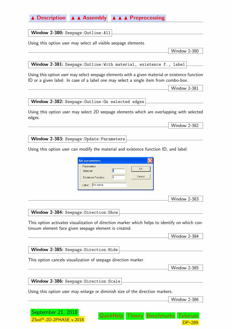
N Description N N Assembly N N N Preprocessing
Window 2-380: Seepage:Outline:All
Using this option user may select all visible seepage elements.
Window 2-380
Window 2-381: Seepage:Outline:With material, existence f., label
Using this option user may select seepage elements with a given material or existence functionID or a given label. In case of a label one may select a single item from combo-box.
Window 2-381
Window 2-382: Seepage:Outline:On selected edges
Using this option user may select 2D seepage elements which are overlapping with selectededges.
Window 2-382
Window 2-383: Seepage:Update:Parameters
Using this option user can modify the material and existence function ID, and label.
Window 2-383
Window 2-384: Seepage:Direction:Show
This option activates visualization of direction marker which helps to identify on which con-tinuum element face given seepage element is created.
Window 2-384
Window 2-385: Seepage:Direction:Hide
This option cancels visualization of seepage direction marker.
Window 2-385
Window 2-386: Seepage:Direction:Scale
Using this option user may enlarge or diminish size of the direction markers.
Window 2-386
September 21, 2018
ZSoilr-2D-2PHASE v.2018QuickHelp Theory Benchmarks Tutorials
DP–289
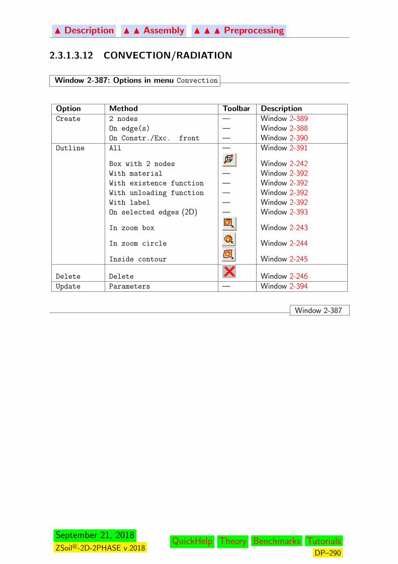
N Description N N Assembly N N N Preprocessing
2.3.1.3.12 CONVECTION/RADIATION
Window 2-387: Options in menu Convection
Option Method Toolbar DescriptionCreate 2 nodes — Window 2-389
On edge(s) — Window 2-388On Constr./Exc. front — Window 2-390
Outline All — Window 2-391
Box with 2 nodes Window 2-242With material — Window 2-392With existence function — Window 2-392With unloading function — Window 2-392With label — Window 2-392On selected edges (2D) — Window 2-393
In zoom box Window 2-243
In zoom circle Window 2-244
Inside contour Window 2-245
Delete Delete Window 2-246Update Parameters — Window 2-394
Window 2-387
September 21, 2018
ZSoilr-2D-2PHASE v.2018QuickHelp Theory Benchmarks Tutorials
DP–290
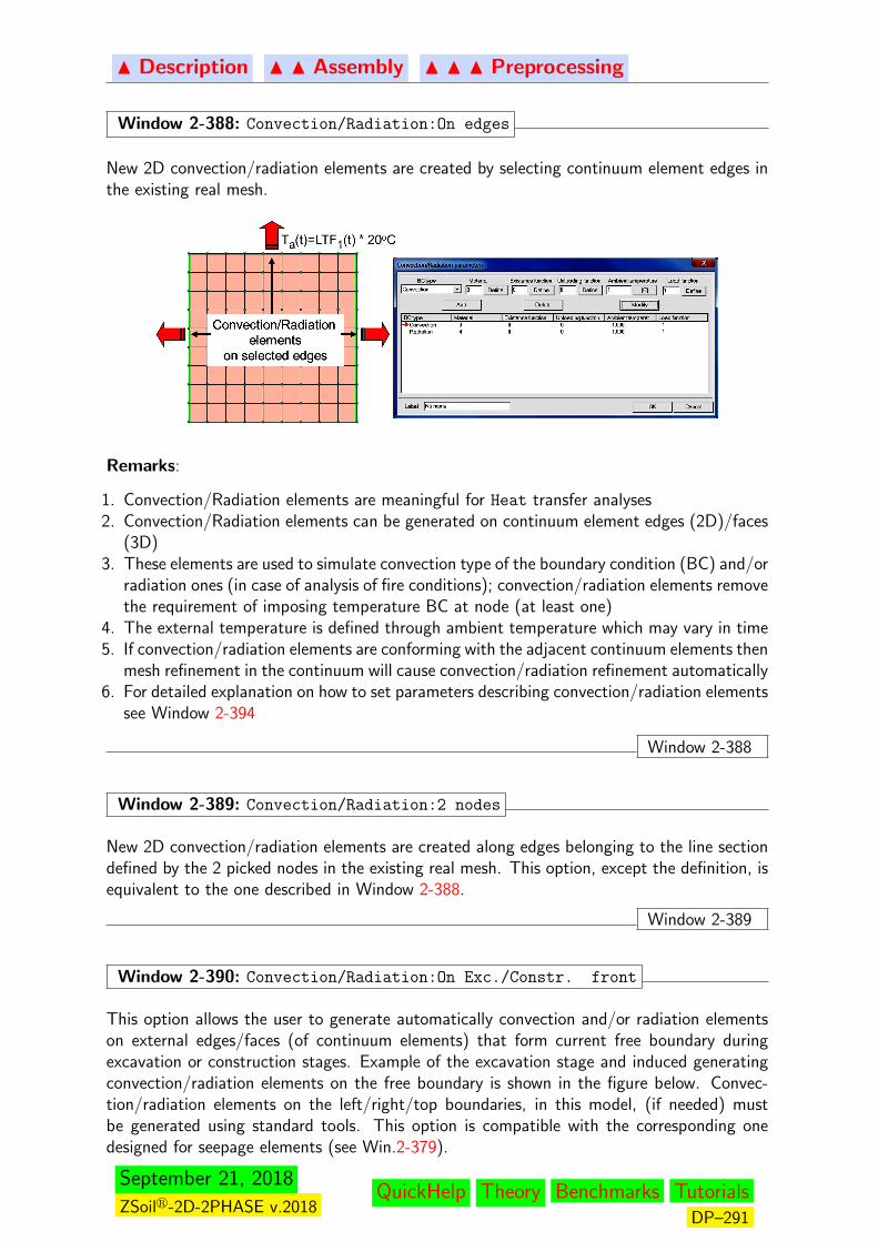
N Description N N Assembly N N N Preprocessing
Window 2-388: Convection/Radiation:On edges
New 2D convection/radiation elements are created by selecting continuum element edges inthe existing real mesh.
Remarks:
1. Convection/Radiation elements are meaningful for Heat transfer analyses2. Convection/Radiation elements can be generated on continuum element edges (2D)/faces
(3D)3. These elements are used to simulate convection type of the boundary condition (BC) and/or
radiation ones (in case of analysis of fire conditions); convection/radiation elements removethe requirement of imposing temperature BC at node (at least one)
4. The external temperature is defined through ambient temperature which may vary in time5. If convection/radiation elements are conforming with the adjacent continuum elements then
mesh refinement in the continuum will cause convection/radiation refinement automatically6. For detailed explanation on how to set parameters describing convection/radiation elements
see Window 2-394
Window 2-388
Window 2-389: Convection/Radiation:2 nodes
New 2D convection/radiation elements are created along edges belonging to the line sectiondefined by the 2 picked nodes in the existing real mesh. This option, except the definition, isequivalent to the one described in Window 2-388.
Window 2-389
Window 2-390: Convection/Radiation:On Exc./Constr. front
This option allows the user to generate automatically convection and/or radiation elementson external edges/faces (of continuum elements) that form current free boundary duringexcavation or construction stages. Example of the excavation stage and induced generatingconvection/radiation elements on the free boundary is shown in the figure below. Convec-tion/radiation elements on the left/right/top boundaries, in this model, (if needed) mustbe generated using standard tools. This option is compatible with the corresponding onedesigned for seepage elements (see Win.2-379).
September 21, 2018
ZSoilr-2D-2PHASE v.2018QuickHelp Theory Benchmarks Tutorials
DP–291
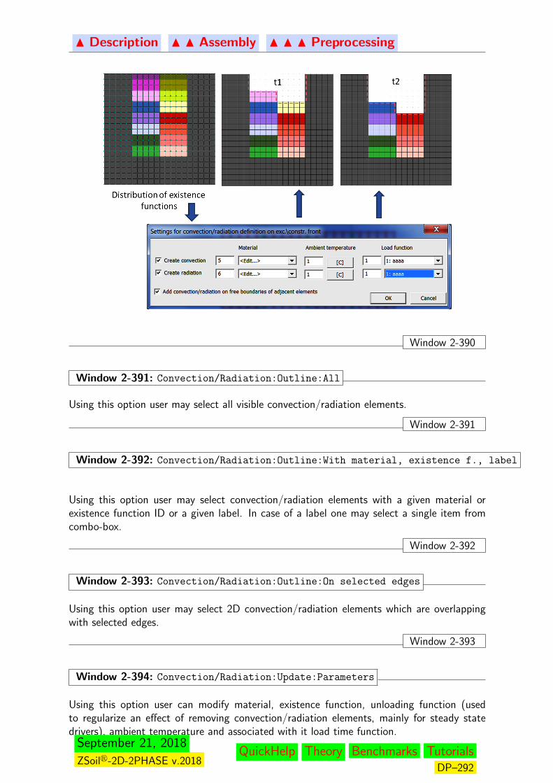
N Description N N Assembly N N N Preprocessing
Window 2-390
Window 2-391: Convection/Radiation:Outline:All
Using this option user may select all visible convection/radiation elements.
Window 2-391
Window 2-392: Convection/Radiation:Outline:With material, existence f., label
Using this option user may select convection/radiation elements with a given material orexistence function ID or a given label. In case of a label one may select a single item fromcombo-box.
Window 2-392
Window 2-393: Convection/Radiation:Outline:On selected edges
Using this option user may select 2D convection/radiation elements which are overlappingwith selected edges.
Window 2-393
Window 2-394: Convection/Radiation:Update:Parameters
Using this option user can modify material, existence function, unloading function (usedto regularize an effect of removing convection/radiation elements, mainly for steady statedrivers), ambient temperature and associated with it load time function.
September 21, 2018
ZSoilr-2D-2PHASE v.2018QuickHelp Theory Benchmarks Tutorials
DP–292
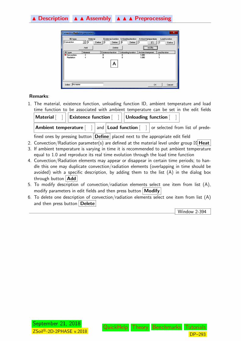
N Description N N Assembly N N N Preprocessing
Remarks:
1. The material, existence function, unloading function ID, ambient temperature and loadtime function to be associated with ambient temperature can be set in the edit fields
Material [ ] Existence function [ ] Unloading function [ ]
Ambient temperature [ ] and Load function [ ] or selected from list of prede-
fined ones by pressing button Define placed next to the appropriate edit field
2. Convection/Radiation parameter(s) are defined at the material level under group � Heat3. If ambient temperature is varying in time it is recommended to put ambient temperature
equal to 1.0 and reproduce its real time evolution through the load time function4. Convection/Radiation elements may appear or disappear in certain time periods; to han-
dle this one may duplicate convection/radiation elements (overlapping in time should beavoided) with a specific description, by adding them to the list (A) in the dialog box
through button Add5. To modify description of convection/radiation elements select one item from list (A),
modify parameters in edit fields and then press button Modify
6. To delete one description of convection/radiation elements select one item from list (A)
and then press button Delete
Window 2-394
September 21, 2018
ZSoilr-2D-2PHASE v.2018QuickHelp Theory Benchmarks Tutorials
DP–293
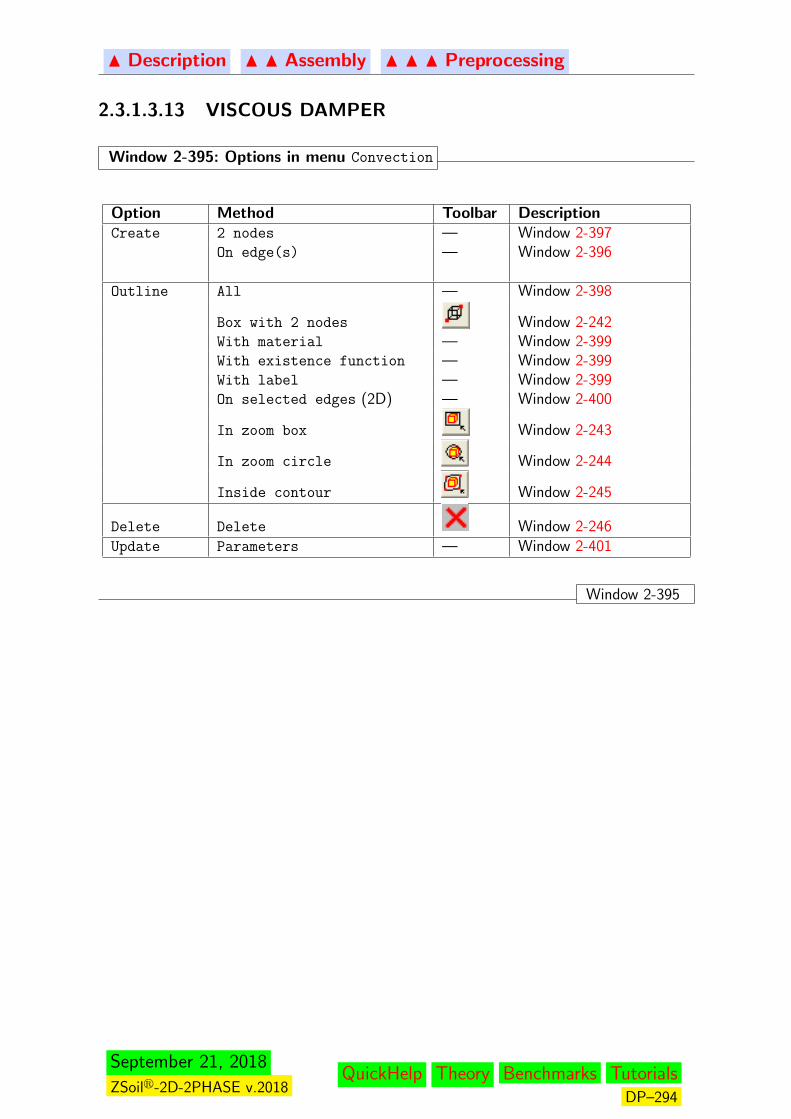
N Description N N Assembly N N N Preprocessing
2.3.1.3.13 VISCOUS DAMPER
Window 2-395: Options in menu Convection
Option Method Toolbar DescriptionCreate 2 nodes — Window 2-397
On edge(s) — Window 2-396
Outline All — Window 2-398
Box with 2 nodes Window 2-242With material — Window 2-399With existence function — Window 2-399With label — Window 2-399On selected edges (2D) — Window 2-400
In zoom box Window 2-243
In zoom circle Window 2-244
Inside contour Window 2-245
Delete Delete Window 2-246Update Parameters — Window 2-401
Window 2-395
September 21, 2018
ZSoilr-2D-2PHASE v.2018QuickHelp Theory Benchmarks Tutorials
DP–294
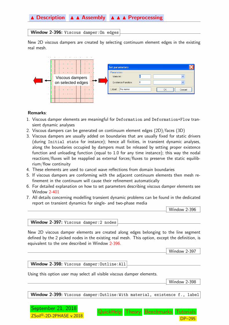
N Description N N Assembly N N N Preprocessing
Window 2-396: Viscous damper:On edges
New 2D viscous dampers are created by selecting continuum element edges in the existingreal mesh.
Viscous damperson selected edges
Remarks:
1. Viscous damper elements are meaningful for Deformation and Deformation+Flow tran-sient dynamic analyses
2. Viscous dampers can be generated on continuum element edges (2D)/faces (3D)3. Viscous dampers are usually added on boundaries that are usually fixed for static drivers
(during Initial state for instance); hence all fixities, in transient dynamic analyses,along the boundaries occupied by dampers must be released by setting proper existencefunction and unloading function (equal to 1.0 for any time instance); this way the nodalreactions/fluxes will be reapplied as external forces/fluxes to preserve the static equilib-rium/flow continuity
4. These elements are used to cancel wave reflections from domain boundaries5. If viscous dampers are conforming with the adjacent continuum elements then mesh re-
finement in the continuum will cause their refinement automatically6. For detailed explanation on how to set parameters describing viscous damper elements see
Window 2-4017. All details concerning modelling transient dynamic problems can be found in the dedicated
report on transient dynamics for single- and two-phase media
Window 2-396
Window 2-397: Viscous damper:2 nodes
New 2D viscous damper elements are created along edges belonging to the line segmentdefined by the 2 picked nodes in the existing real mesh. This option, except the definition, isequivalent to the one described in Window 2-396.
Window 2-397
Window 2-398: Viscous damper:Outline:All
Using this option user may select all visible viscous damper elements.
Window 2-398
Window 2-399: Viscous damper:Outline:With material, existence f., label
September 21, 2018
ZSoilr-2D-2PHASE v.2018QuickHelp Theory Benchmarks Tutorials
DP–295

N Description N N Assembly N N N Preprocessing
Using this option user may select viscous damper elements with a given material or existencefunction ID or a given label. In case of a label one may select a single item from combo-box.
Window 2-399
Window 2-400: Viscous damper:Outline:On selected edges
Using this option user may select 2D viscous damper elements which are overlapping withselected edges.
Window 2-400
Window 2-401: Viscous damper:Update:Parameters
Using this option user can modify material and existence function
Remarks:
1. Viscous damper elements can be used in transient dynamic analyses for the Deformation
and Deformation+Flow mode2. Viscous damper material parameters are defined at the material level under group� Elastic ,
� Unit weights and � Flow ; these material parameters can also be inherited from theadjacent continuum; this setting can be made at the material level
Window 2-401
September 21, 2018
ZSoilr-2D-2PHASE v.2018QuickHelp Theory Benchmarks Tutorials
DP–296
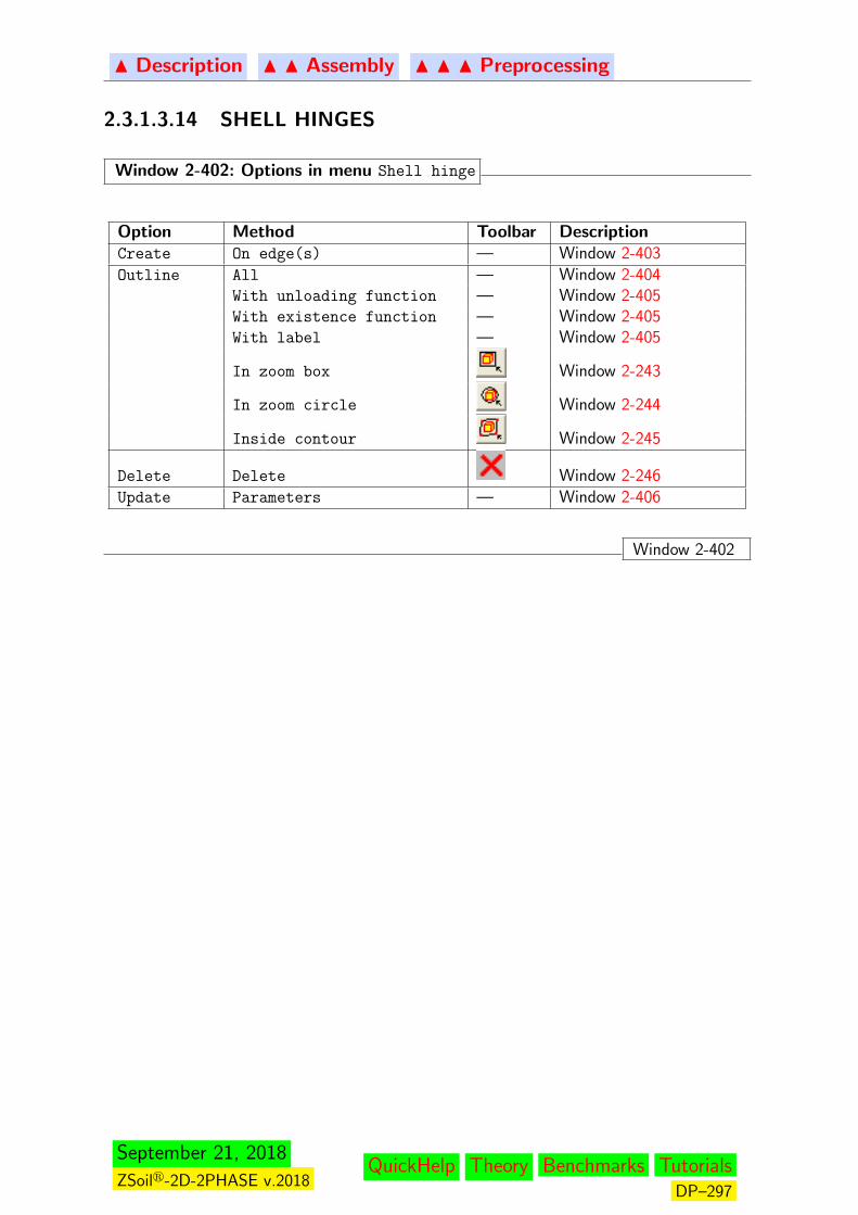
N Description N N Assembly N N N Preprocessing
2.3.1.3.14 SHELL HINGES
Window 2-402: Options in menu Shell hinge
Option Method Toolbar DescriptionCreate On edge(s) — Window 2-403Outline All — Window 2-404
With unloading function — Window 2-405With existence function — Window 2-405With label — Window 2-405
In zoom box Window 2-243
In zoom circle Window 2-244
Inside contour Window 2-245
Delete Delete Window 2-246Update Parameters — Window 2-406
Window 2-402
September 21, 2018
ZSoilr-2D-2PHASE v.2018QuickHelp Theory Benchmarks Tutorials
DP–297
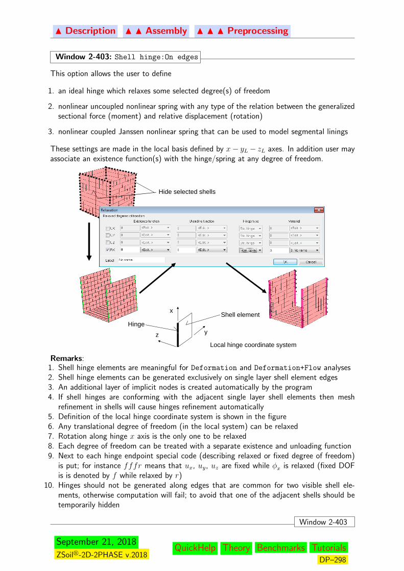
N Description N N Assembly N N N Preprocessing
Window 2-403: Shell hinge:On edges
This option allows the user to define
1. an ideal hinge which relaxes some selected degree(s) of freedom
2. nonlinear uncoupled nonlinear spring with any type of the relation between the generalizedsectional force (moment) and relative displacement (rotation)
3. nonlinear coupled Janssen nonlinear spring that can be used to model segmental linings
These settings are made in the local basis defined by x− yL− zL axes. In addition user mayassociate an existence function(s) with the hinge/spring at any degree of freedom.
Hide selected shells
x
y
Shell elementHinge
yzLocal hinge coordinate system
Remarks:1. Shell hinge elements are meaningful for Deformation and Deformation+Flow analyses2. Shell hinge elements can be generated exclusively on single layer shell element edges3. An additional layer of implicit nodes is created automatically by the program4. If shell hinges are conforming with the adjacent single layer shell elements then mesh
refinement in shells will cause hinges refinement automatically5. Definition of the local hinge coordinate system is shown in the figure6. Any translational degree of freedom (in the local system) can be relaxed7. Rotation along hinge x axis is the only one to be relaxed8. Each degree of freedom can be treated with a separate existence and unloading function9. Next to each hinge endpoint special code (describing relaxed or fixed degree of freedom)
is put; for instance fffr means that ux, uy, uz are fixed while φx is relaxed (fixed DOFis is denoted by f while relaxed by r)
10. Hinges should not be generated along edges that are common for two visible shell ele-ments, otherwise computation will fail; to avoid that one of the adjacent shells should betemporarily hidden
Window 2-403
September 21, 2018
ZSoilr-2D-2PHASE v.2018QuickHelp Theory Benchmarks Tutorials
DP–298

N Description N N Assembly N N N Preprocessing
Window 2-404: Shell hinge:Outline:All
Using this option user may select all visible seepage elements.
Window 2-404
Window 2-405: Shell hinge:Outline:With existence f., unloading f., label
Using this option user may select hinges with a given existence function, unloading functionID or a given label. In case of a label one may select a single item from combo-box.
Window 2-405
Window 2-406: Shell hinge:Update:Parameters
Using this option user can modify current set of relaxed degree of freedom and associatedwith them existence, unloading functions, and label. See Window 2-403 definition of thelocal hinge coordinate system.
Window 2-406
September 21, 2018
ZSoilr-2D-2PHASE v.2018QuickHelp Theory Benchmarks Tutorials
DP–299

N Description N N Assembly N N N Preprocessing
2.3.1.3.15 BOUNDARY CONDITIONS
The following types of boundary conditions can be created:
Solid BC Create kinematic BC on nodesTemperature BC Create temperature BC on nodesHumidity BC Create humidity BC on nodesPressure BC Create fluid pressure BC on nodesPeriodic BC Create periodic BC for pairs of nodes
September 21, 2018
ZSoilr-2D-2PHASE v.2018QuickHelp Theory Benchmarks Tutorials
DP–300
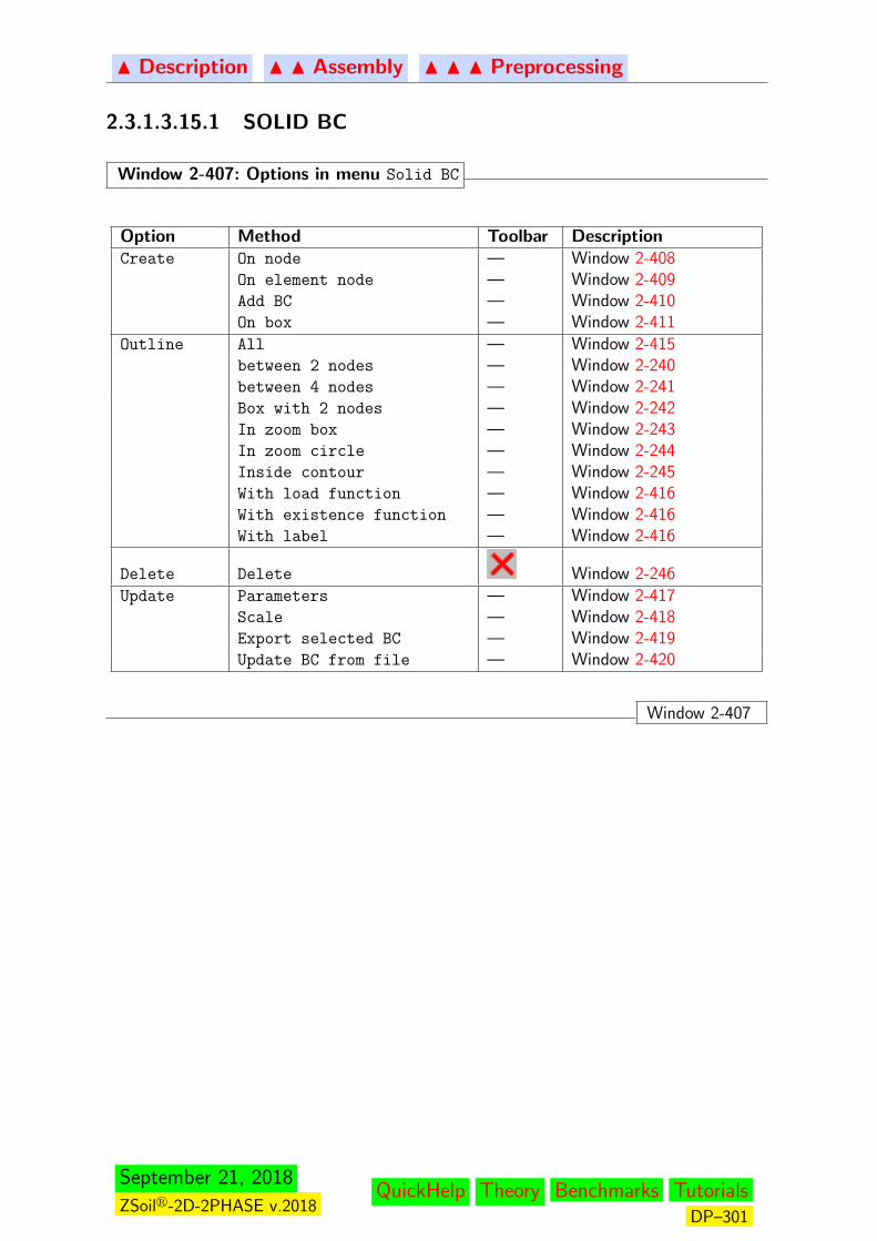
N Description N N Assembly N N N Preprocessing
2.3.1.3.15.1 SOLID BC
Window 2-407: Options in menu Solid BC
Option Method Toolbar DescriptionCreate On node — Window 2-408
On element node — Window 2-409Add BC — Window 2-410On box — Window 2-411
Outline All — Window 2-415between 2 nodes — Window 2-240between 4 nodes — Window 2-241Box with 2 nodes — Window 2-242In zoom box — Window 2-243In zoom circle — Window 2-244Inside contour — Window 2-245With load function — Window 2-416With existence function — Window 2-416With label — Window 2-416
Delete Delete Window 2-246Update Parameters — Window 2-417
Scale — Window 2-418Export selected BC — Window 2-419Update BC from file — Window 2-420
Window 2-407
September 21, 2018
ZSoilr-2D-2PHASE v.2018QuickHelp Theory Benchmarks Tutorials
DP–301
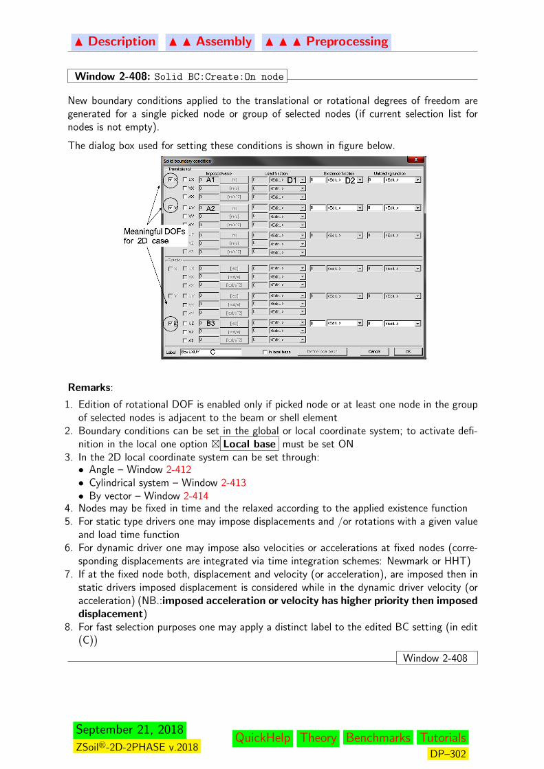
N Description N N Assembly N N N Preprocessing
Window 2-408: Solid BC:Create:On node
New boundary conditions applied to the translational or rotational degrees of freedom aregenerated for a single picked node or group of selected nodes (if current selection list fornodes is not empty).
The dialog box used for setting these conditions is shown in figure below.
Remarks:
1. Edition of rotational DOF is enabled only if picked node or at least one node in the groupof selected nodes is adjacent to the beam or shell element
2. Boundary conditions can be set in the global or local coordinate system; to activate defi-nition in the local one option � Local base must be set ON
3. In the 2D local coordinate system can be set through:• Angle – Window 2-412• Cylindrical system – Window 2-413• By vector – Window 2-414
4. Nodes may be fixed in time and the relaxed according to the applied existence function5. For static type drivers one may impose displacements and /or rotations with a given value
and load time function6. For dynamic driver one may impose also velocities or accelerations at fixed nodes (corre-
sponding displacements are integrated via time integration schemes: Newmark or HHT)7. If at the fixed node both, displacement and velocity (or acceleration), are imposed then in
static drivers imposed displacement is considered while in the dynamic driver velocity (oracceleration) (NB.:imposed acceleration or velocity has higher priority then imposeddisplacement)
8. For fast selection purposes one may apply a distinct label to the edited BC setting (in edit(C))
Window 2-408
September 21, 2018
ZSoilr-2D-2PHASE v.2018QuickHelp Theory Benchmarks Tutorials
DP–302

N Description N N Assembly N N N Preprocessing
Window 2-409: Solid BC:Create:On element node
Using this option one may set the BC on a selected element node(s). This is crucial incase when node belongs to the contact zone and the BC is to be set only at node at oneside of the interface. Further steps to define the BC are same as in the standard case (seeWindow 2-408)
Window 2-409
Window 2-410: Solid BC:Create:Add BC
Using this option one may add to the existing definition the new setting. It is very usefulespecially for operations on group of selected nodes. The previous and current setting arecombined by means of logical summation. It is however forbidden to modify the local basesetting. Further steps to define the BC are same as in the standard case (see Window 2-408)
Window 2-410
Window 2-411: Solid BC:Create:On box
Using this option one may generate standard in the geotechnical practice set of the BC. Anexample of such setting for 2D is shown in figure below.
Ux=Uy=0
Ux=0Ux=0
Φz=0
Φz=0
beams
Window 2-411
September 21, 2018
ZSoilr-2D-2PHASE v.2018QuickHelp Theory Benchmarks Tutorials
DP–303
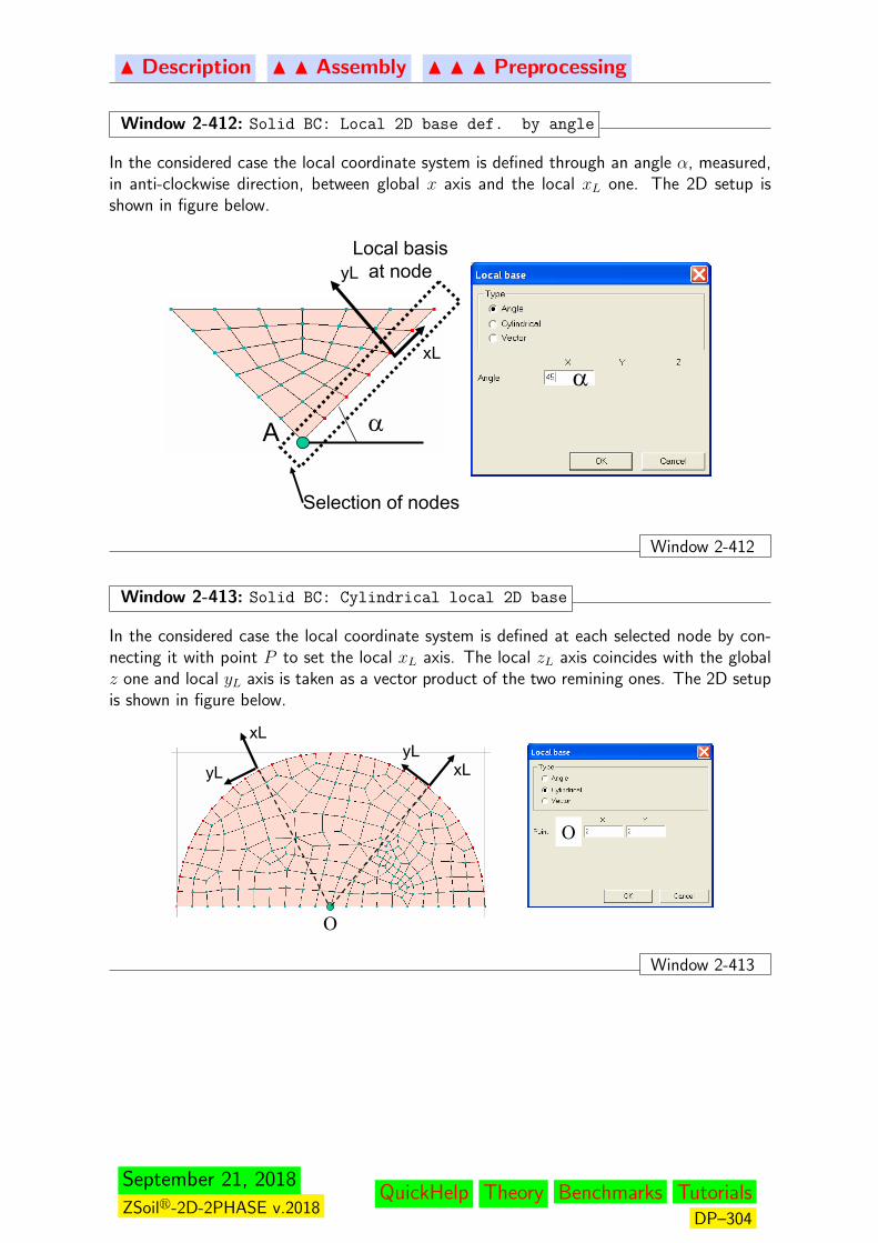
N Description N N Assembly N N N Preprocessing
Window 2-412: Solid BC: Local 2D base def. by angle
In the considered case the local coordinate system is defined through an angle α, measured,in anti-clockwise direction, between global x axis and the local xL one. The 2D setup isshown in figure below.
α
αxL
yLLocal basisat node
Selection of nodes
A
Window 2-412
Window 2-413: Solid BC: Cylindrical local 2D base
In the considered case the local coordinate system is defined at each selected node by con-necting it with point P to set the local xL axis. The local zL axis coincides with the globalz one and local yL axis is taken as a vector product of the two remining ones. The 2D setupis shown in figure below.
O
O
xLyL
xL
yL
Window 2-413
September 21, 2018
ZSoilr-2D-2PHASE v.2018QuickHelp Theory Benchmarks Tutorials
DP–304
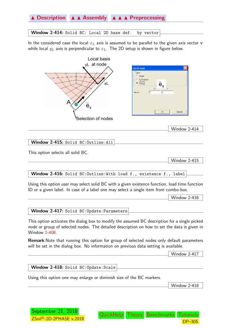
N Description N N Assembly N N N Preprocessing
Window 2-414: Solid BC: Local 2D base def. by vector
In the considered case the local xL axis is assumed to be parallel to the given axis vector vwhile local yL axis is perpendicular to xL. The 2D setup is shown in figure below.
xL
yLLocal basisat node
Selection of nodes
A ex
ex
Window 2-414
Window 2-415: Solid BC:Outline:All
This option selects all solid BC.
Window 2-415
Window 2-416: Solid BC:Outline:With load f., existence f., label
Using this option user may select solid BC with a given existence function, load time functionID or a given label. In case of a label one may select a single item from combo-box.
Window 2-416
Window 2-417: Solid BC:Update:Parameters
This option activates the dialog box to modify the assumed BC description for a single pickednode or group of selected nodes. The detailed description on how to set the data is given inWindow 2-408.
Remark:Note that running this option for group of selected nodes only default parameterswill be set in the dialog box. No information on previous data setting is available.
Window 2-417
Window 2-418: Solid BC:Update:Scale
Using this option one may enlarge or diminish size of the BC markers.
Window 2-418
September 21, 2018
ZSoilr-2D-2PHASE v.2018QuickHelp Theory Benchmarks Tutorials
DP–305

N Description N N Assembly N N N Preprocessing
Window 2-419: Solid BC:Update:Export sel. BC
Using this option user may export description of the selected BC to the external text file.This file can be read later on, and possibly modified, with aid of the Excel application.
Window 2-419
Window 2-420: Solid BC:Update/Update BC from file
This option is coupled with Solid BC:Update/Export sel. BC option (see Window 2-419). It allows to update description of exported BC, modified externally by Excel or anotherapplication.
Window 2-420
September 21, 2018
ZSoilr-2D-2PHASE v.2018QuickHelp Theory Benchmarks Tutorials
DP–306
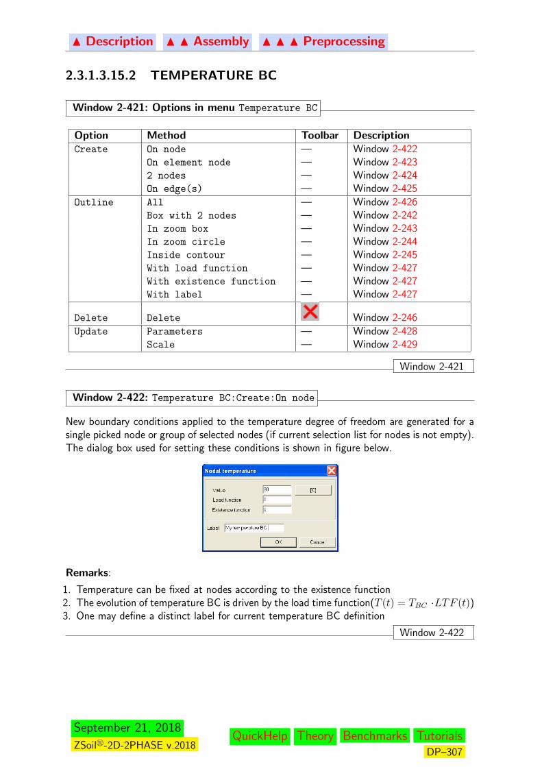
N Description N N Assembly N N N Preprocessing
2.3.1.3.15.2 TEMPERATURE BC
Window 2-421: Options in menu Temperature BC
Option Method Toolbar DescriptionCreate On node — Window 2-422
On element node — Window 2-4232 nodes — Window 2-424On edge(s) — Window 2-425
Outline All — Window 2-426Box with 2 nodes — Window 2-242In zoom box — Window 2-243In zoom circle — Window 2-244Inside contour — Window 2-245With load function — Window 2-427With existence function — Window 2-427With label — Window 2-427
Delete Delete Window 2-246Update Parameters — Window 2-428
Scale — Window 2-429
Window 2-421
Window 2-422: Temperature BC:Create:On node
New boundary conditions applied to the temperature degree of freedom are generated for asingle picked node or group of selected nodes (if current selection list for nodes is not empty).The dialog box used for setting these conditions is shown in figure below.
Remarks:
1. Temperature can be fixed at nodes according to the existence function2. The evolution of temperature BC is driven by the load time function(T (t) = TBC ·LTF (t))3. One may define a distinct label for current temperature BC definition
Window 2-422
September 21, 2018
ZSoilr-2D-2PHASE v.2018QuickHelp Theory Benchmarks Tutorials
DP–307
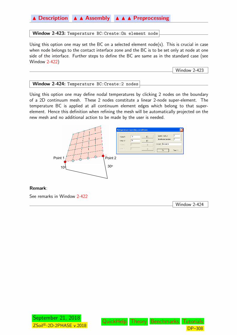
N Description N N Assembly N N N Preprocessing
Window 2-423: Temperature BC:Create:On element node
Using this option one may set the BC on a selected element node(s). This is crucial in casewhen node belongs to the contact interface zone and the BC is to be set only at node at oneside of the interface. Further steps to define the BC are same as in the standard case (seeWindow 2-422)
Window 2-423
Window 2-424: Temperature BC:Create:2 nodes
Using this option one may define nodal temperatures by clicking 2 nodes on the boundaryof a 2D continuum mesh. These 2 nodes constitute a linear 2-node super-element. Thetemperature BC is applied at all continuum element edges which belong to that super-element. Hence this definition when refining the mesh will be automatically projected on thenew mesh and no additional action to be made by the user is needed.
10o 30o
Point 1 Point 2
Remark:
See remarks in Window 2-422
Window 2-424
September 21, 2018
ZSoilr-2D-2PHASE v.2018QuickHelp Theory Benchmarks Tutorials
DP–308

N Description N N Assembly N N N Preprocessing
Window 2-425: Temperature BC:Create:On edge(s)
This option has a double meaning depending on whether selection list of edges in empty or not.If none of the edges is selected then user must pick the edge and generation procedure followsstrictly the one by 2 nodes described in Window refWin:-ASSEMB-PREPRO-MENU-FE-MODEL-BC-T-CREATE-2N. In all other cases user must pick the point at which he sets valueof the temperature To and to set temperature gradients in x and y directions. This definitionwhen refining the mesh will be automatically projected on the new mesh and no additionalaction to be made by the user is needed. Assuming that picked point coordinates are denotedby xP the temperature at any node (with coordinates denoted by x) belonging to the selectedset of edges is computed through the formula: T (x) = To + dTx · (x− xP ) + dTy · (y− yP ).This option is valid only for 2D models.
To=20o
2m
2m
To=0o
Selected edges
Window 2-425
Window 2-426: Temperature BC:Outline:All
This option selects all temperature BC.
Window 2-426
Window 2-427: Temperature BC:Outline:With load f., existence f., label
Using this option user may select temperature BC with a given existence function, load timefunction ID or a given label. In case of a label one may select a single item from combo-box.
Window 2-427
Window 2-428: Temperature BC:Update:Parameters
This option activates the dialog box to modify the assumed BC description. Each objectrepresenting temperature BC inherits the information on how it was initially set up. For thatreason updating the temperature BC corresponds strictly to its initial definition described ingroup of methods under general option Create.
Window 2-428
Window 2-429: Temperature BC:Update:Scale
Using this option one may enlarge or diminish size of the BC markers.
Window 2-429
September 21, 2018
ZSoilr-2D-2PHASE v.2018QuickHelp Theory Benchmarks Tutorials
DP–309
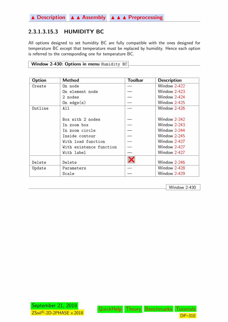
N Description N N Assembly N N N Preprocessing
2.3.1.3.15.3 HUMIDITY BC
All options designed to set humidity BC are fully compatible with the ones designed fortemperature BC except that temperature must be replaced by humidity. Hence each optionis referred to the corresponding one for temperature BC.
Window 2-430: Options in menu Humidity BC
Option Method Toolbar DescriptionCreate On node — Window 2-422
On element node — Window 2-4232 nodes — Window 2-424On edge(s) — Window 2-425
Outline All — Window 2-426
Box with 2 nodes — Window 2-242In zoom box — Window 2-243In zoom circle — Window 2-244Inside contour — Window 2-245With load function — Window 2-427With existence function — Window 2-427With label — Window 2-427
Delete Delete Window 2-246Update Parameters — Window 2-428
Scale — Window 2-429
Window 2-430
September 21, 2018
ZSoilr-2D-2PHASE v.2018QuickHelp Theory Benchmarks Tutorials
DP–310
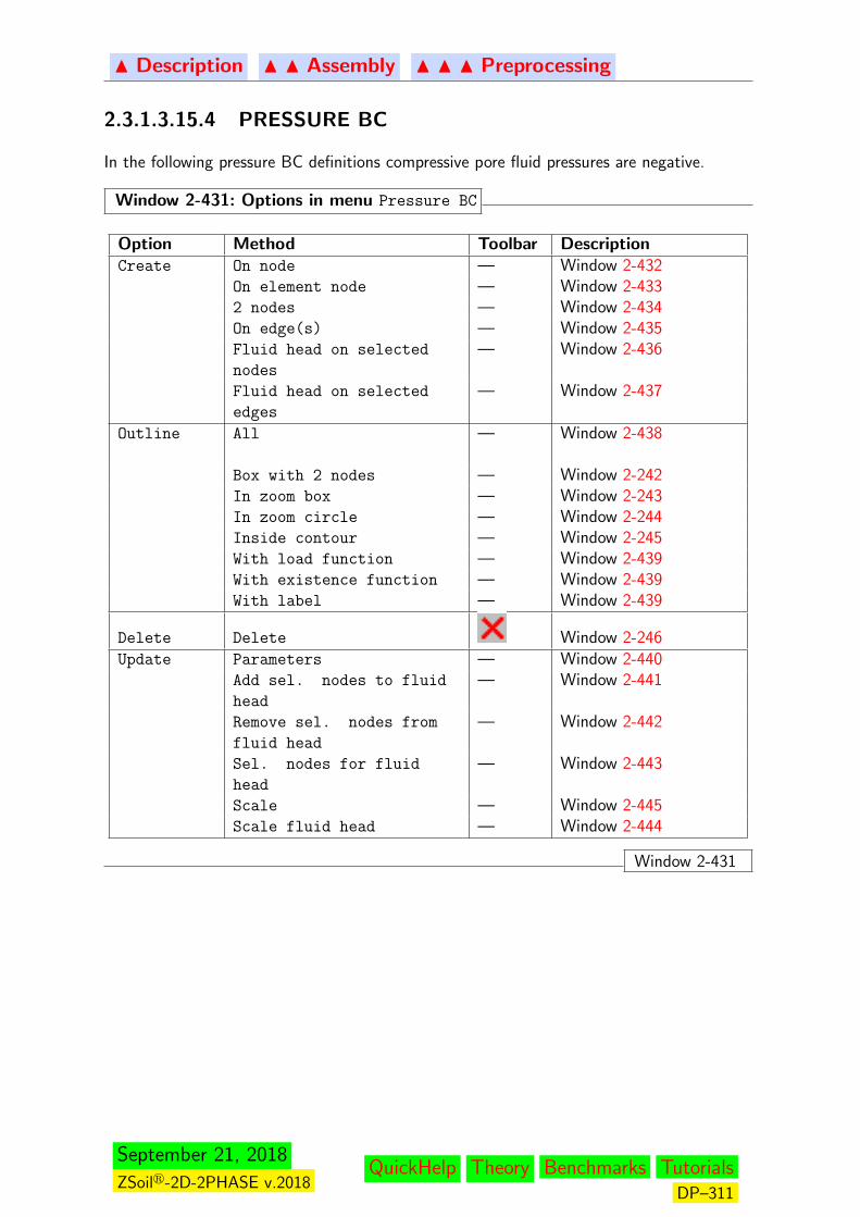
N Description N N Assembly N N N Preprocessing
2.3.1.3.15.4 PRESSURE BC
In the following pressure BC definitions compressive pore fluid pressures are negative.
Window 2-431: Options in menu Pressure BC
Option Method Toolbar DescriptionCreate On node — Window 2-432
On element node — Window 2-4332 nodes — Window 2-434On edge(s) — Window 2-435Fluid head on selected
nodes
— Window 2-436
Fluid head on selected
edges
— Window 2-437
Outline All — Window 2-438
Box with 2 nodes — Window 2-242In zoom box — Window 2-243In zoom circle — Window 2-244Inside contour — Window 2-245With load function — Window 2-439With existence function — Window 2-439With label — Window 2-439
Delete Delete Window 2-246Update Parameters — Window 2-440
Add sel. nodes to fluid
head
— Window 2-441
Remove sel. nodes from
fluid head
— Window 2-442
Sel. nodes for fluid
head
— Window 2-443
Scale — Window 2-445Scale fluid head — Window 2-444
Window 2-431
September 21, 2018
ZSoilr-2D-2PHASE v.2018QuickHelp Theory Benchmarks Tutorials
DP–311

N Description N N Assembly N N N Preprocessing
Window 2-432: Pressure BC:Create:On node
New boundary conditions applied to the pressure degree of freedom are generated for a singlepicked node or group of selected nodes (if current selection list for nodes is not empty). Thedialog box used for setting these conditions is shown in figure below.
Remarks:
1. Pressure can be fixed at nodes according to the existence function2. The evolution of pressure BC is driven by the load time function(T (t) = TBC · LTF (t))3. One may define a distinct label for current pressure BC definition
Window 2-432
Window 2-433: Pressure BC:Create:On element node
Using this option one may set the BC on a selected element node(s). This is crucial in casewhen node belongs to the contact interface zone and the BC is to be set only at node at oneside of the interface. Further steps to define the BC are same as in the standard case (seeWindow 2-432).
Window 2-433
Window 2-434: Pressure BC:Create:2 nodes
Using this option one may define nodal pressures by clicking 2 nodes on the boundary of a2D continuum mesh. These 2 nodes constitute a linear 2-node super-element. The pressureBC is applied at all continuum element edges which belong to that super-element. Hencethis definition when refining the mesh will automatically be projected on the new mesh andno additional action to be made by the user is needed.
1
2
p=-30 kPa
p=0 kPa
After split
Remark:
See remarks in Window 2-432
Window 2-434
September 21, 2018
ZSoilr-2D-2PHASE v.2018QuickHelp Theory Benchmarks Tutorials
DP–312
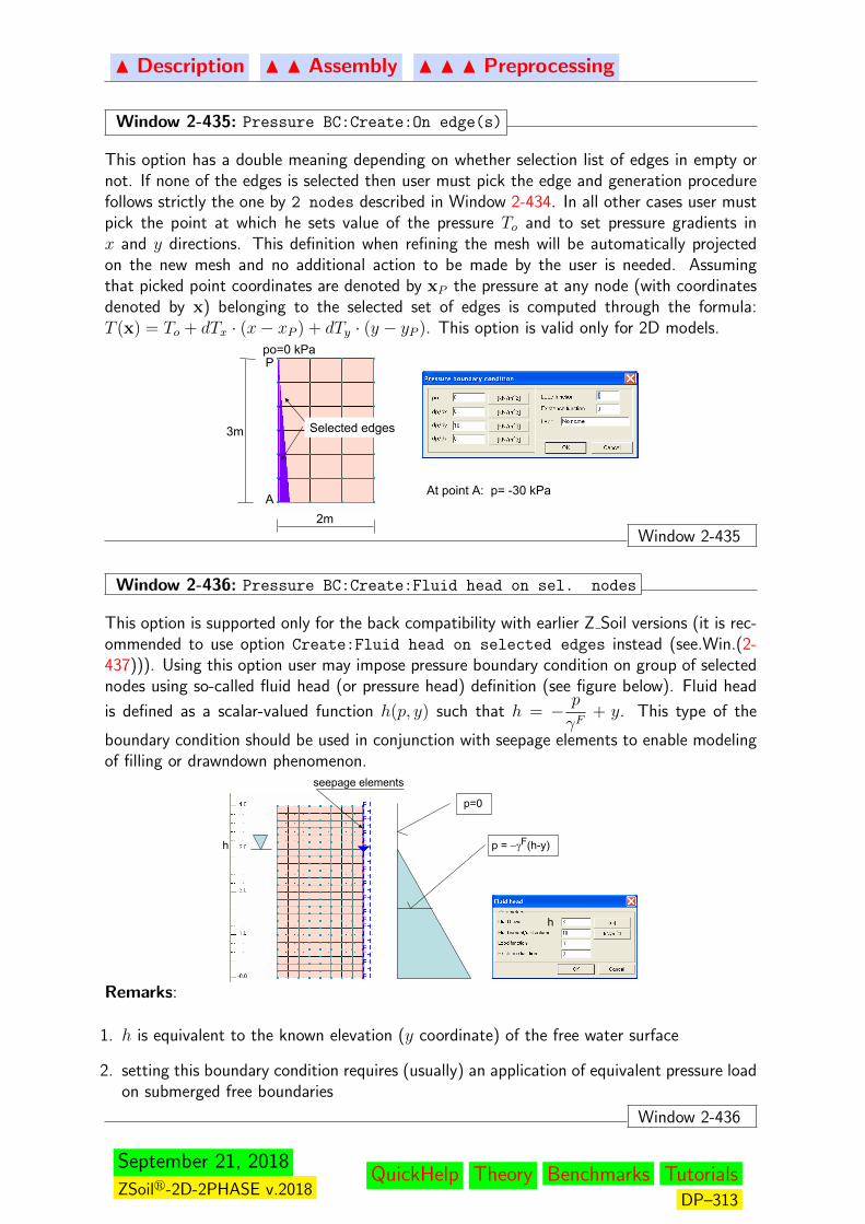
N Description N N Assembly N N N Preprocessing
Window 2-435: Pressure BC:Create:On edge(s)
This option has a double meaning depending on whether selection list of edges in empty ornot. If none of the edges is selected then user must pick the edge and generation procedurefollows strictly the one by 2 nodes described in Window 2-434. In all other cases user mustpick the point at which he sets value of the pressure To and to set pressure gradients inx and y directions. This definition when refining the mesh will be automatically projectedon the new mesh and no additional action to be made by the user is needed. Assumingthat picked point coordinates are denoted by xP the pressure at any node (with coordinatesdenoted by x) belonging to the selected set of edges is computed through the formula:T (x) = To + dTx · (x− xP ) + dTy · (y − yP ). This option is valid only for 2D models.
Selected edges
po=0 kPa
2m
3m
At point A: p= -30 kPa
P
A
Window 2-435
Window 2-436: Pressure BC:Create:Fluid head on sel. nodes
This option is supported only for the back compatibility with earlier Z Soil versions (it is rec-ommended to use option Create:Fluid head on selected edges instead (see.Win.(2-437))). Using this option user may impose pressure boundary condition on group of selectednodes using so-called fluid head (or pressure head) definition (see figure below). Fluid head
is defined as a scalar-valued function h(p, y) such that h = − p
γF+ y. This type of the
boundary condition should be used in conjunction with seepage elements to enable modelingof filling or drawndown phenomenon.
h
h
p = −γF(h-y)
p=0
seepage elements
Remarks:
1. h is equivalent to the known elevation (y coordinate) of the free water surface
2. setting this boundary condition requires (usually) an application of equivalent pressure loadon submerged free boundaries
Window 2-436
September 21, 2018
ZSoilr-2D-2PHASE v.2018QuickHelp Theory Benchmarks Tutorials
DP–313
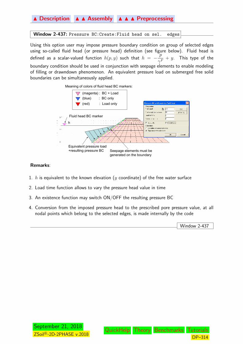
N Description N N Assembly N N N Preprocessing
Window 2-437: Pressure BC:Create:Fluid head on sel. edges
Using this option user may impose pressure boundary condition on group of selected edgesusing so-called fluid head (or pressure head) definition (see figure below). Fluid head is
defined as a scalar-valued function h(p, y) such that h = − p
γF+ y. This type of the
boundary condition should be used in conjunction with seepage elements to enable modelingof filling or drawndown phenomenon. An equivalent pressure load on submerged free solidboundaries can be simultaneously applied.
h
h
Seepage elements must be generated on the boundary
Fluid head BC marker
Equivalent pressure load+resulting pressure BC
Meaning of colors of fluid head BC markers:
(magenta) : BC + Load(blue) : BC only(red) : Load only
Remarks:
1. h is equivalent to the known elevation (y coordinate) of the free water surface
2. Load time function allows to vary the pressure head value in time
3. An existence function may switch ON/OFF the resulting pressure BC
4. Conversion from the imposed pressure head to the prescribed pore pressure value, at allnodal points which belong to the selected edges, is made internally by the code
Window 2-437
September 21, 2018
ZSoilr-2D-2PHASE v.2018QuickHelp Theory Benchmarks Tutorials
DP–314
N Description N N Assembly N N N Preprocessing
Window 2-438: Pressure BC:Outline:All
This option selects all pressure BC except Fluid head...Window 2-438
Window 2-439: Pressure BC:Outline:With load f., existence f., label
Using this option user may select pressure BC with a given existence function, load timefunction ID or a given label. In case of a label one may select a single item from combo-box.
Window 2-439
Window 2-440: Pressure BC:Update:Parameters
This option activates the dialog box to modify the assumed BC description. Each objectrepresenting pressure BC inherits the information on how it was initially set up. For thatreason updating the pressure BC corresponds strictly to its initial definition described ingroup of methods under general option Create.
Window 2-440
Window 2-441: Pressure BC:Update:Add sel. nodes to fluid head
This option allows to add selected nodes to the fluid head boundary condition representedon the screen as a blue triangle.
Window 2-441
Window 2-442: Pressure BC:Update:Remove sel. nodes from fluid head
This option allows to delete selected nodes from the fluid head boundary condition representedon the screen as a blue triangle.
Window 2-442
Window 2-443: Pressure BC:Update:Sel. nodes for fluid head
This option allows to select all nodes associated with the fluid head boundary conditionrepresented on the screen as a blue triangle.
Window 2-443
Window 2-444: Pressure BC:Update:Scale fluid head
This option allows to scale fluid head boundary condition marker.
Window 2-444
Window 2-445: Pressure BC:Update:Scale
Using this option one may enlarge or diminish size of the BC markers.Window 2-445
September 21, 2018
ZSoilr-2D-2PHASE v.2018QuickHelp Theory Benchmarks Tutorials
DP–315
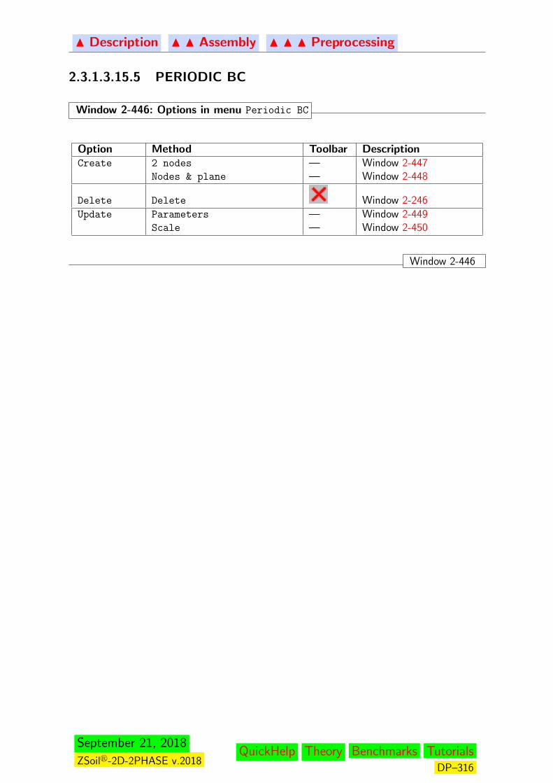
N Description N N Assembly N N N Preprocessing
2.3.1.3.15.5 PERIODIC BC
Window 2-446: Options in menu Periodic BC
Option Method Toolbar DescriptionCreate 2 nodes — Window 2-447
Nodes & plane — Window 2-448
Delete Delete Window 2-246Update Parameters — Window 2-449
Scale — Window 2-450
Window 2-446
September 21, 2018
ZSoilr-2D-2PHASE v.2018QuickHelp Theory Benchmarks Tutorials
DP–316

N Description N N Assembly N N N Preprocessing
Window 2-447: Periodic BC:Create:2 nodes
This option allows to tie selected degrees of freedom at two picked nodal points. It mayconcern any type of the degree of freedom (displacement, pressure, temperature, humidity).It is mainly used in dynamic applications to simulate motion of shear layer. The dialog boxused for setting these conditions is shown in the figure below.
P1 P2DOF’s to be tied
Remarks:
1. The tying can be made only in the global coordinate system2. This option does not apply to the fixed degree of freedom3. Each degree of freedom can be tied according to the declared existence function
Window 2-447
September 21, 2018
ZSoilr-2D-2PHASE v.2018QuickHelp Theory Benchmarks Tutorials
DP–317
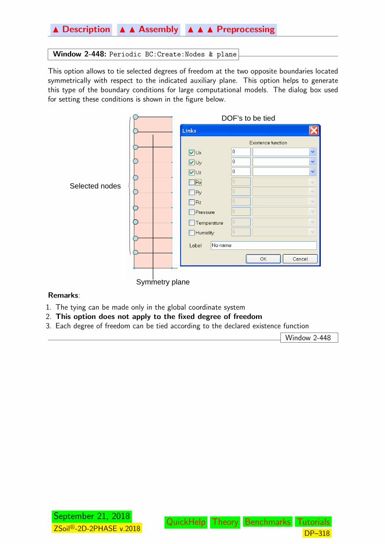
N Description N N Assembly N N N Preprocessing
Window 2-448: Periodic BC:Create:Nodes & plane
This option allows to tie selected degrees of freedom at the two opposite boundaries locatedsymmetrically with respect to the indicated auxiliary plane. This option helps to generatethis type of the boundary conditions for large computational models. The dialog box usedfor setting these conditions is shown in the figure below.
Symmetry plane
Selected nodes
DOF’s to be tied
Remarks:
1. The tying can be made only in the global coordinate system2. This option does not apply to the fixed degree of freedom3. Each degree of freedom can be tied according to the declared existence function
Window 2-448
September 21, 2018
ZSoilr-2D-2PHASE v.2018QuickHelp Theory Benchmarks Tutorials
DP–318
N Description N N Assembly N N N Preprocessing
Window 2-449: Periodic BC:Update:Parameters
This option activates the dialog box to modify the assumed periodic BC description for asingle picked node or group of selected nodes. The detailed description on how to set thedata is given in Window 2-447.
Remark:It has to be emphasized that this modification will be made too for allother nodes there were considered during creation of the Periodic BC
Window 2-449
Window 2-450: Periodic BC:Update:Scale
This option is not yet supported.
Window 2-450
September 21, 2018
ZSoilr-2D-2PHASE v.2018QuickHelp Theory Benchmarks Tutorials
DP–319

N Description N N Assembly N N N Preprocessing
2.3.1.3.16 LOADS
The following loads can be applied to the real mesh:
Body load Create body load on selected elements; this load will overwritethe global gravity setting
Nodal load Create concentrated forces on selected nodesSurface load Create surface loads on selected element faces/edgesBeam load Create surface loads on selected beams
September 21, 2018
ZSoilr-2D-2PHASE v.2018QuickHelp Theory Benchmarks Tutorials
DP–320
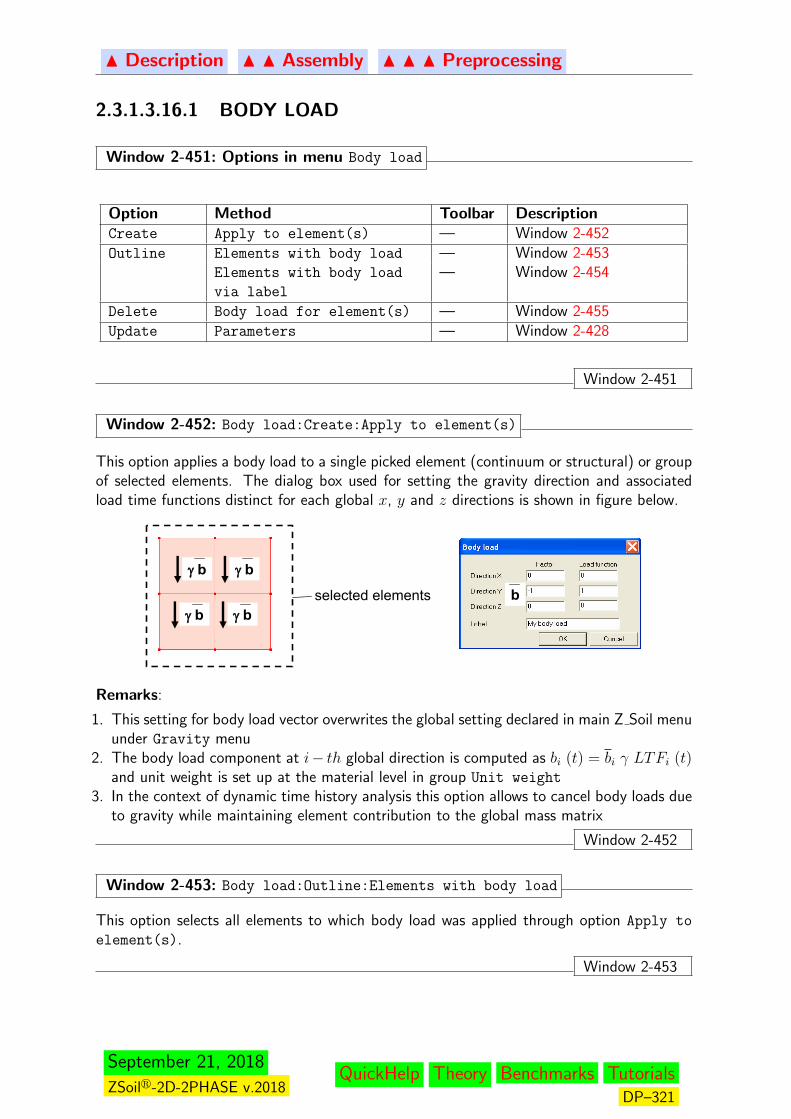
N Description N N Assembly N N N Preprocessing
2.3.1.3.16.1 BODY LOAD
Window 2-451: Options in menu Body load
Option Method Toolbar DescriptionCreate Apply to element(s) — Window 2-452Outline Elements with body load — Window 2-453
Elements with body load
via label
— Window 2-454
Delete Body load for element(s) — Window 2-455Update Parameters — Window 2-428
Window 2-451
Window 2-452: Body load:Create:Apply to element(s)
This option applies a body load to a single picked element (continuum or structural) or groupof selected elements. The dialog box used for setting the gravity direction and associatedload time functions distinct for each global x, y and z directions is shown in figure below.
selected elements b
γ b γ b
γ b γ b
Remarks:
1. This setting for body load vector overwrites the global setting declared in main Z Soil menuunder Gravity menu
2. The body load component at i− th global direction is computed as bi (t) = bi γ LTFi (t)and unit weight is set up at the material level in group Unit weight
3. In the context of dynamic time history analysis this option allows to cancel body loads dueto gravity while maintaining element contribution to the global mass matrix
Window 2-452
Window 2-453: Body load:Outline:Elements with body load
This option selects all elements to which body load was applied through option Apply to
element(s).
Window 2-453
September 21, 2018
ZSoilr-2D-2PHASE v.2018QuickHelp Theory Benchmarks Tutorials
DP–321
N Description N N Assembly N N N Preprocessing
Window 2-454: Body load:Outline:Elem. with body load via label
This option selects all elements to which body load, identified by a given label, was appliedthrough option Apply to element(s).
Window 2-454
Window 2-455: Body load:Delete:Body load for element(s)
This option selects all elements to which body load, identified by a given label, was appliedthrough option Apply to element(s).
Window 2-455
Window 2-456: Body load:Update:Parameters
This option activates the dialog box (see figure in Window 2-452) to update body loaddirection vector, load time functions and label for a single picked element or group of selectedelements.
Remark:In case when selection list of elements is not empty initial values in the dialog arefilled with default values.
Window 2-456
September 21, 2018
ZSoilr-2D-2PHASE v.2018QuickHelp Theory Benchmarks Tutorials
DP–322
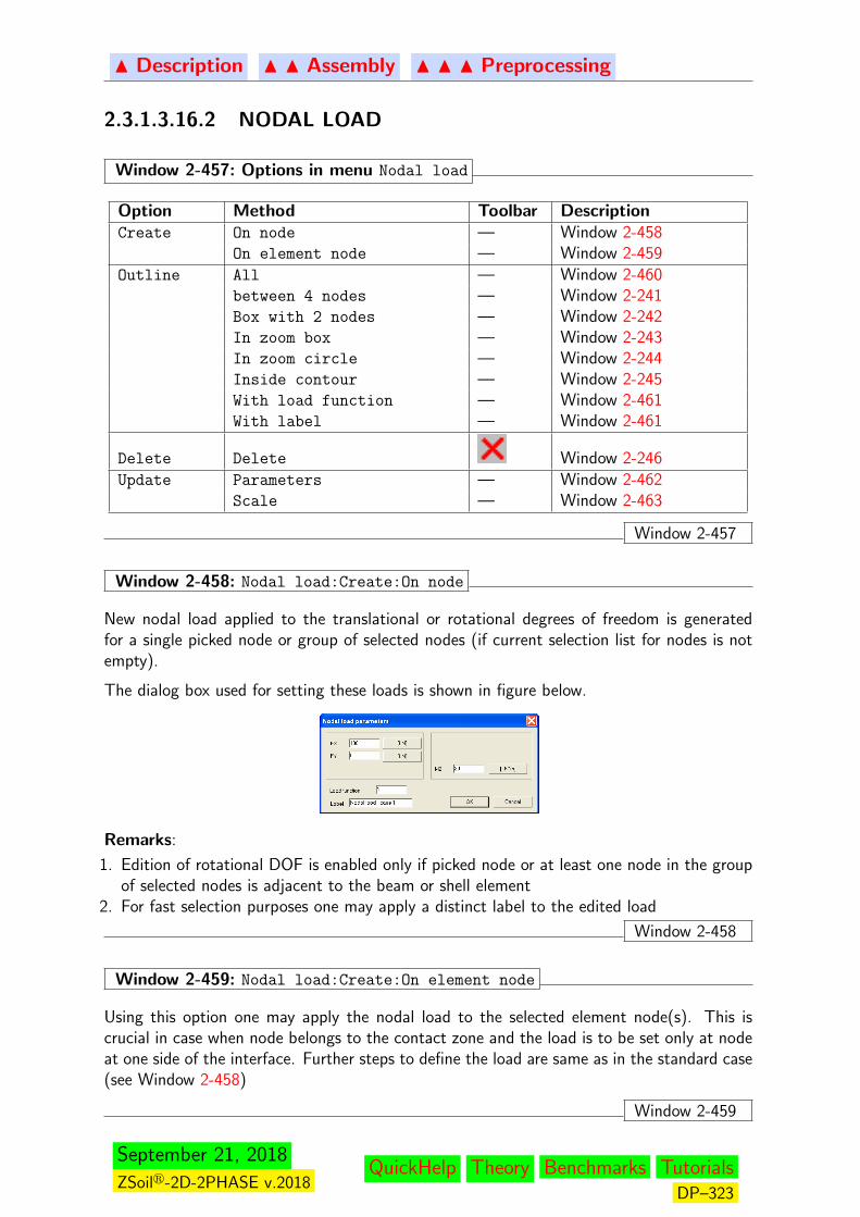
N Description N N Assembly N N N Preprocessing
2.3.1.3.16.2 NODAL LOAD
Window 2-457: Options in menu Nodal load
Option Method Toolbar DescriptionCreate On node — Window 2-458
On element node — Window 2-459Outline All — Window 2-460
between 4 nodes — Window 2-241Box with 2 nodes — Window 2-242In zoom box — Window 2-243In zoom circle — Window 2-244Inside contour — Window 2-245With load function — Window 2-461With label — Window 2-461
Delete Delete Window 2-246Update Parameters — Window 2-462
Scale — Window 2-463
Window 2-457
Window 2-458: Nodal load:Create:On node
New nodal load applied to the translational or rotational degrees of freedom is generatedfor a single picked node or group of selected nodes (if current selection list for nodes is notempty).
The dialog box used for setting these loads is shown in figure below.
Remarks:
1. Edition of rotational DOF is enabled only if picked node or at least one node in the groupof selected nodes is adjacent to the beam or shell element
2. For fast selection purposes one may apply a distinct label to the edited load
Window 2-458
Window 2-459: Nodal load:Create:On element node
Using this option one may apply the nodal load to the selected element node(s). This iscrucial in case when node belongs to the contact zone and the load is to be set only at nodeat one side of the interface. Further steps to define the load are same as in the standard case(see Window 2-458)
Window 2-459
September 21, 2018
ZSoilr-2D-2PHASE v.2018QuickHelp Theory Benchmarks Tutorials
DP–323
N Description N N Assembly N N N Preprocessing
Window 2-460: Nodal load:Outline:All
This option selects all nodal loads.
Window 2-460
Window 2-461: Nodal load:Outline:With load f., existence f., label
Using this option user may select nodal load with a given load time function ID or a givenlabel. In case of a label one may select a single item from combo-box.
Window 2-461
Window 2-462: Nodal load:Update:Parameters
This option activates the dialog box to modify the applied nodal load description, for a singlepicked node or group of selected nodes. The detailed description on how to set the data isgiven in Window 2-458.
Remark:When running this option for group of selected nodes only default parameters willbe set in the dialog box.
Window 2-462
Window 2-463: Nodal load:Update:Scale
Using this option one may enlarge or diminish size of nodal vectors, representing concentratedforces, or arcs, representing concentrated moments. markers.
Window 2-463
September 21, 2018
ZSoilr-2D-2PHASE v.2018QuickHelp Theory Benchmarks Tutorials
DP–324
N Description N N Assembly N N N Preprocessing
2.3.1.3.16.3 SURFACE LOAD
Window 2-464: Options in menu Surface load
Option Method Toolbar DescriptionUNIFORM On edge(s)(Uniform) — Window 2-465VARIABLE 2 nodes (Variable) — Window 2-466PRESSURE 2 nodes (P) — Window 2-467
On selected edges (HP) — Window 2-468PRESSURE
via Fluid
Head
On selected faces (SH) — Window ??
Outline All — Window 2-470between 4 nodes — Window 2-241Box with 2 nodes — Window 2-242In zoom box — Window 2-243In zoom circle — Window 2-244Inside contour — Window 2-245With load function — Window 2-471With label — Window 2-471
Delete Delete Window 2-246Update Parameters — Window 2-472
Scale — Window 2-473
Window 2-464
September 21, 2018
ZSoilr-2D-2PHASE v.2018QuickHelp Theory Benchmarks Tutorials
DP–325

N Description N N Assembly N N N Preprocessing
Window 2-465: Surface load:UNIFORM:On edge(s) (Uniform)
New uniform surface load is generated on a single picked edge or group of selected edges (ifcurrent selection list of edges is not empty). This option is valid only in 2D.
The dialog box used for setting this load is shown in figure below.
x
y
Remarks:
1. For fast selection purposes one may apply a distinct label to this definition2. This load is automatically split during mesh refinement
Window 2-465
Window 2-466: Surface load:VARIABLE:2 nodes (Variable)
New linearly varying surface load is generated on element edges belonging to the line sectiondesigned by the two picked points. This option is valid only in 2D.
An example for this setting is shown in figure below.
1
2
x
y
Remarks:
1. For fast selection purposes one may apply a distinct label to this definition2. This load is automatically split during mesh refinement
Window 2-466
September 21, 2018
ZSoilr-2D-2PHASE v.2018QuickHelp Theory Benchmarks Tutorials
DP–326

N Description N N Assembly N N N Preprocessing
Window 2-467: Surface load:PRESSURE:2 nodes
Using this option one may define variable surface pressure load by clicking 2 nodes on theboundary of a 2D mesh. These 2 nodes constitute a linear super-element. Pressure is appliedat all element edges which belong to that super-element. Hence this definition when refiningthe mesh will be automatically projected on the new mesh and no additional action to bemade by the user is needed. The dialog box used for setting this load is shown in figurebelow.
1
2
Remarks:
1. For fast selection purposes one may apply a distinct label to this definition2. Positive pressure is directed towards external element normals
Window 2-467
Window 2-468: Surface load:PRESSURE:On selected edges(HP)
Using this option one may apply distributed pressure load by picking the point at which valueof the pressure fo is defined, and setting pressure gradients in x and y directions. Thisdefinition when refining the mesh will be automatically projected on the new mesh and noadditional action to be made by the user is needed. Assuming that picked point coordinatesare denoted by xP the pressure at any node (with coordinates denoted by x) belonging to the
selected set of edges is computed through the formula: p(x) = fo+df
dx·(x−xP )+
df
dy·(y−yP ).
This option is valid only for 2D models.
P
x
y
Remarks:
1. For fast selection purposes one may apply a distinct label to this definition2. Positive pressure is directed towards external normal to the edges
Window 2-468
September 21, 2018
ZSoilr-2D-2PHASE v.2018QuickHelp Theory Benchmarks Tutorials
DP–327
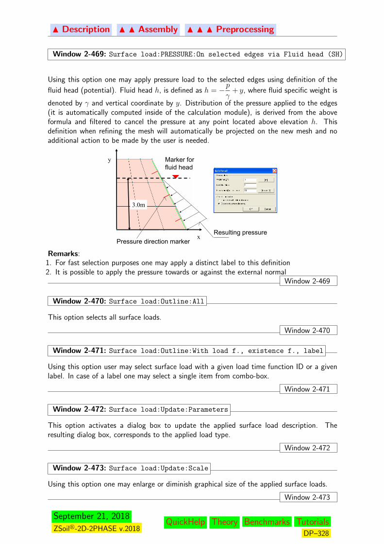
N Description N N Assembly N N N Preprocessing
Window 2-469: Surface load:PRESSURE:On selected edges via Fluid head (SH)
Using this option one may apply pressure load to the selected edges using definition of the
fluid head (potential). Fluid head h, is defined as h = −pγ
+ y, where fluid specific weight is
denoted by γ and vertical coordinate by y. Distribution of the pressure applied to the edges(it is automatically computed inside of the calculation module), is derived from the aboveformula and filtered to cancel the pressure at any point located above elevation h. Thisdefinition when refining the mesh will automatically be projected on the new mesh and noadditional action to be made by the user is needed.
x
y
3.0m
Marker forfluid head
Resulting pressurePressure direction marker
Remarks:1. For fast selection purposes one may apply a distinct label to this definition2. It is possible to apply the pressure towards or against the external normal
Window 2-469
Window 2-470: Surface load:Outline:All
This option selects all surface loads.
Window 2-470
Window 2-471: Surface load:Outline:With load f., existence f., label
Using this option user may select surface load with a given load time function ID or a givenlabel. In case of a label one may select a single item from combo-box.
Window 2-471
Window 2-472: Surface load:Update:Parameters
This option activates a dialog box to update the applied surface load description. Theresulting dialog box, corresponds to the applied load type.
Window 2-472
Window 2-473: Surface load:Update:Scale
Using this option one may enlarge or diminish graphical size of the applied surface loads.
Window 2-473
September 21, 2018
ZSoilr-2D-2PHASE v.2018QuickHelp Theory Benchmarks Tutorials
DP–328
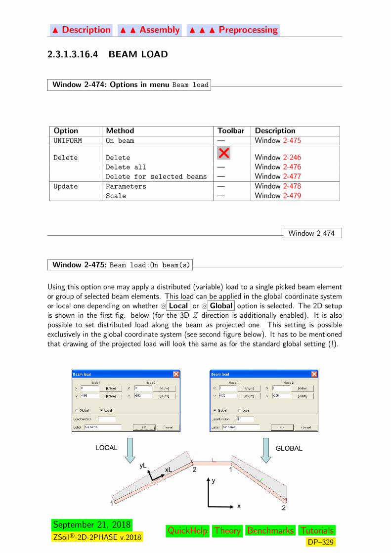
N Description N N Assembly N N N Preprocessing
2.3.1.3.16.4 BEAM LOAD
Window 2-474: Options in menu Beam load
Option Method Toolbar DescriptionUNIFORM On beam — Window 2-475
Delete Delete Window 2-246Delete all — Window 2-476Delete for selected beams — Window 2-477
Update Parameters — Window 2-478Scale — Window 2-479
Window 2-474
Window 2-475: Beam load:On beam(s)
Using this option one may apply a distributed (variable) load to a single picked beam elementor group of selected beam elements. This load can be applied in the global coordinate systemor local one depending on whether } Local or } Global option is selected. The 2D setupis shown in the first fig. below (for the 3D Z direction is additionally enabled). It is alsopossible to set distributed load along the beam as projected one. This setting is possibleexclusively in the global coordinate system (see second figure below). It has to be mentionedthat drawing of the projected load will look the same as for the standard global setting (!).
1
2 1
2
xLyL
x
y
GLOBALLOCAL
September 21, 2018
ZSoilr-2D-2PHASE v.2018QuickHelp Theory Benchmarks Tutorials
DP–329
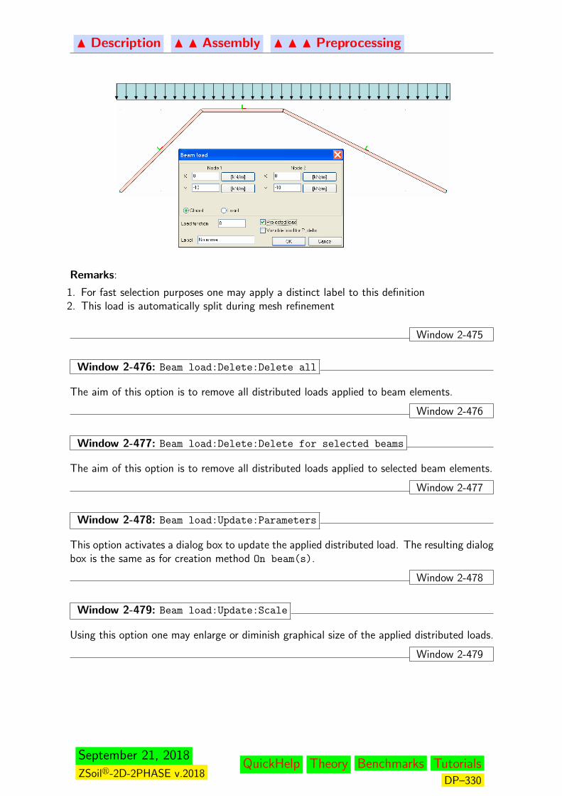
N Description N N Assembly N N N Preprocessing
Remarks:
1. For fast selection purposes one may apply a distinct label to this definition2. This load is automatically split during mesh refinement
Window 2-475
Window 2-476: Beam load:Delete:Delete all
The aim of this option is to remove all distributed loads applied to beam elements.
Window 2-476
Window 2-477: Beam load:Delete:Delete for selected beams
The aim of this option is to remove all distributed loads applied to selected beam elements.
Window 2-477
Window 2-478: Beam load:Update:Parameters
This option activates a dialog box to update the applied distributed load. The resulting dialogbox is the same as for creation method On beam(s).
Window 2-478
Window 2-479: Beam load:Update:Scale
Using this option one may enlarge or diminish graphical size of the applied distributed loads.
Window 2-479
September 21, 2018
ZSoilr-2D-2PHASE v.2018QuickHelp Theory Benchmarks Tutorials
DP–330

N Description N N Assembly N N N Preprocessing
2.3.1.3.17 ADDED MASSES
Added masses can be modeled using two options:
Nodal added masses Create masses on selected nodesDistributed added masses Create masses distributed on element boundaries
It is possible to filter added masses to eliminate interia terms along selected direction(s).This can be made in the global or local coordinate system (see paragraph FILTERING OFADDED MASSES )
September 21, 2018
ZSoilr-2D-2PHASE v.2018QuickHelp Theory Benchmarks Tutorials
DP–331
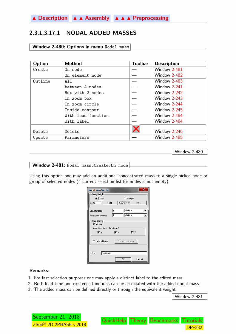
N Description N N Assembly N N N Preprocessing
2.3.1.3.17.1 NODAL ADDED MASSES
Window 2-480: Options in menu Nodal mass
Option Method Toolbar DescriptionCreate On node — Window 2-481
On element node — Window 2-482Outline All — Window 2-483
between 4 nodes — Window 2-241Box with 2 nodes — Window 2-242In zoom box — Window 2-243In zoom circle — Window 2-244Inside contour — Window 2-245With load function — Window 2-484With label — Window 2-484
Delete Delete Window 2-246Update Parameters — Window 2-485
Window 2-480
Window 2-481: Nodal mass:Create:On node
Using this option one may add an additional concentrated mass to a single picked node orgroup of selected nodes (if current selection list for nodes is not empty).
Remarks:
1. For fast selection purposes one may apply a distinct label to the edited mass2. Both load time and existence functions can be associated with the added nodal mass3. The added mass can be defined directly or through the equivalent weight
Window 2-481
September 21, 2018
ZSoilr-2D-2PHASE v.2018QuickHelp Theory Benchmarks Tutorials
DP–332
N Description N N Assembly N N N Preprocessing
Window 2-482: Nodal mass:Create:On element node
Using this option one may apply the additional mass to the selected element node(s). This iscrucial in case when node belongs to the contact zone and mass is to be set only at node atone side of the interface. Further steps to define the mass are same as in the standard case(see Window 2-481)
Window 2-482
Window 2-483: Nodal mass:Outline:All
This option selects all added nodal masses.
Window 2-483
Window 2-484: Nodal mass:Outline:With load f., existence f., label
Using this option user may select added nodal masses with a given load time function,existence function ID or a given label. In case of a label one may select a single item fromcombo-box.
Window 2-484
Window 2-485: Nodal mass:Update:Parameters
This option activates the dialog box to modify the applied added nodal masses description,for a single picked node or group of selected nodes. The detailed description on how to setthe data is given in Window 2-481.
Remark:When running this option for group of selected nodes only default parameters willbe set in the dialog box.
Window 2-485
September 21, 2018
ZSoilr-2D-2PHASE v.2018QuickHelp Theory Benchmarks Tutorials
DP–333
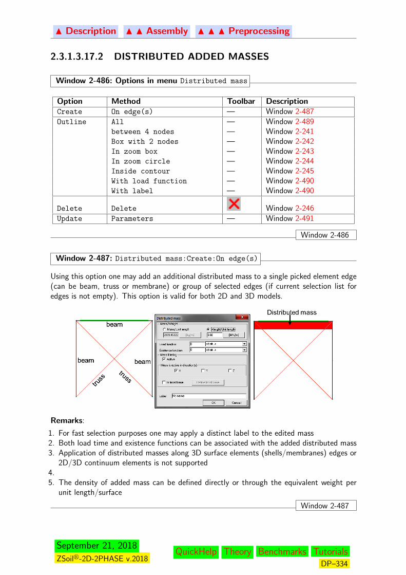
N Description N N Assembly N N N Preprocessing
2.3.1.3.17.2 DISTRIBUTED ADDED MASSES
Window 2-486: Options in menu Distributed mass
Option Method Toolbar DescriptionCreate On edge(s) — Window 2-487Outline All — Window 2-489
between 4 nodes — Window 2-241Box with 2 nodes — Window 2-242In zoom box — Window 2-243In zoom circle — Window 2-244Inside contour — Window 2-245With load function — Window 2-490With label — Window 2-490
Delete Delete Window 2-246Update Parameters — Window 2-491
Window 2-486
Window 2-487: Distributed mass:Create:On edge(s)
Using this option one may add an additional distributed mass to a single picked element edge(can be beam, truss or membrane) or group of selected edges (if current selection list foredges is not empty). This option is valid for both 2D and 3D models.
Remarks:
1. For fast selection purposes one may apply a distinct label to the edited mass2. Both load time and existence functions can be associated with the added distributed mass3. Application of distributed masses along 3D surface elements (shells/membranes) edges or
2D/3D continuum elements is not supported4.5. The density of added mass can be defined directly or through the equivalent weight per
unit length/surface
Window 2-487
September 21, 2018
ZSoilr-2D-2PHASE v.2018QuickHelp Theory Benchmarks Tutorials
DP–334

N Description N N Assembly N N N Preprocessing
Window 2-488: Distributed mass:Create:On face(s)
Using this option one may add an additional distributed mass to a single picked element face(can be shell or membrane in 3D) or group of selected faces (if current selection list for facesis not empty). This option is valid exclusively for 3D models.
Remarks:1. For fast selection purposes one may apply a distinct label to the edited mass2. Both load time and existence functions can be associated with the added distributed mass3. Applying distributed masses to faces of 3D continuum elements is not supported
Window 2-488
Window 2-489: Distributed mass:Outline:All
Using this option one may select all added distributed masses.
Window 2-489
Window 2-490: Distributed mass:Outline:With load f., existence f., label
Using this option user may select added distributed masses with a given load time function,existence function ID or a given label. In case of a label one may select a single item fromcombo-box.
Window 2-490
Window 2-491: Distributed mass:Update:Parameters
This option activates the dialog box to modify the applied added distributed masses descrip-tion, for a single picked edge/face or group of selected edges/faces. The detailed descriptionon how to set the data is given in Window 2-487 or Window 2-488.
Remarks:1. When running this option for group of selected edges/faces only default parameters will
be set in the dialog box2. If selection list contains added masses defined on both, edges and faces, then the operation
can exclusively be run for masses added on edges or on facesWindow 2-491
September 21, 2018
ZSoilr-2D-2PHASE v.2018QuickHelp Theory Benchmarks Tutorials
DP–335
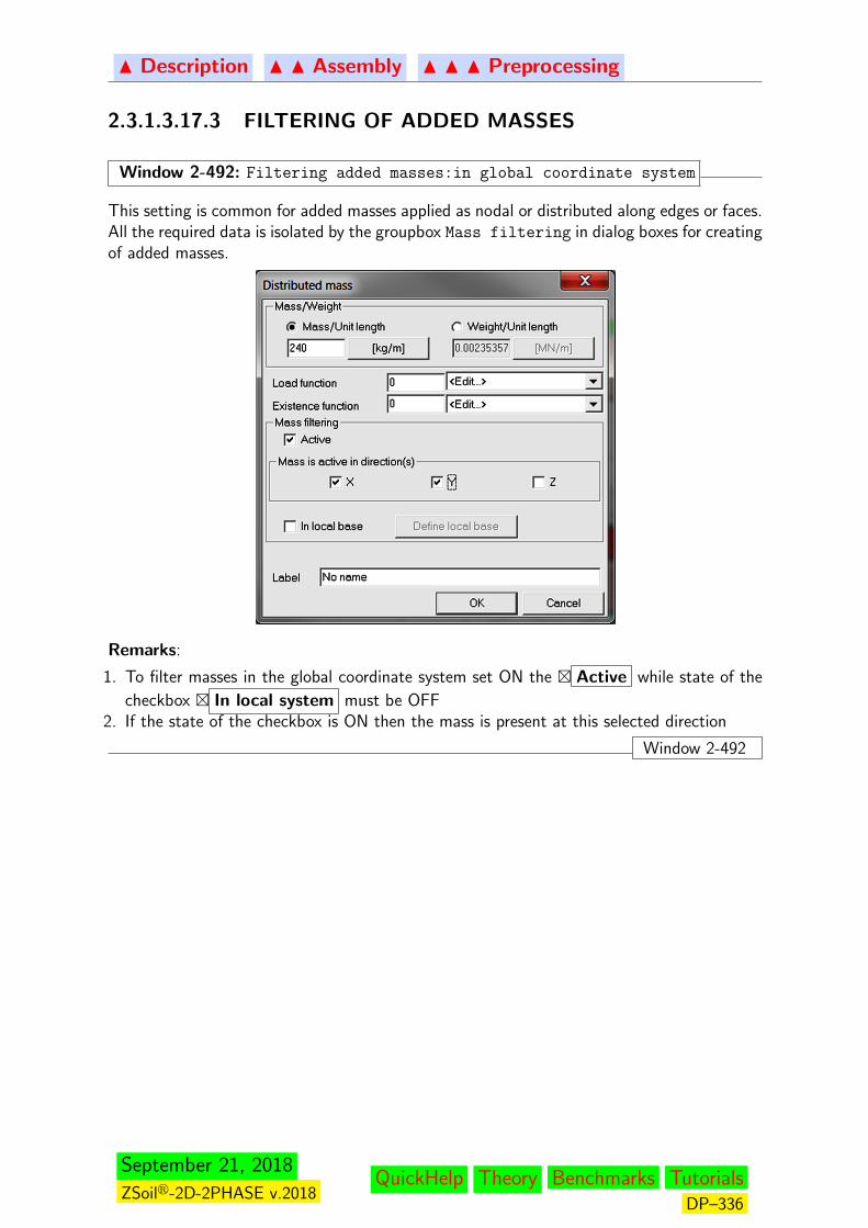
N Description N N Assembly N N N Preprocessing
2.3.1.3.17.3 FILTERING OF ADDED MASSES
Window 2-492: Filtering added masses:in global coordinate system
This setting is common for added masses applied as nodal or distributed along edges or faces.All the required data is isolated by the groupbox Mass filtering in dialog boxes for creatingof added masses.
Remarks:
1. To filter masses in the global coordinate system set ON the � Active while state of the
checkbox � In local system must be OFF2. If the state of the checkbox is ON then the mass is present at this selected direction
Window 2-492
September 21, 2018
ZSoilr-2D-2PHASE v.2018QuickHelp Theory Benchmarks Tutorials
DP–336
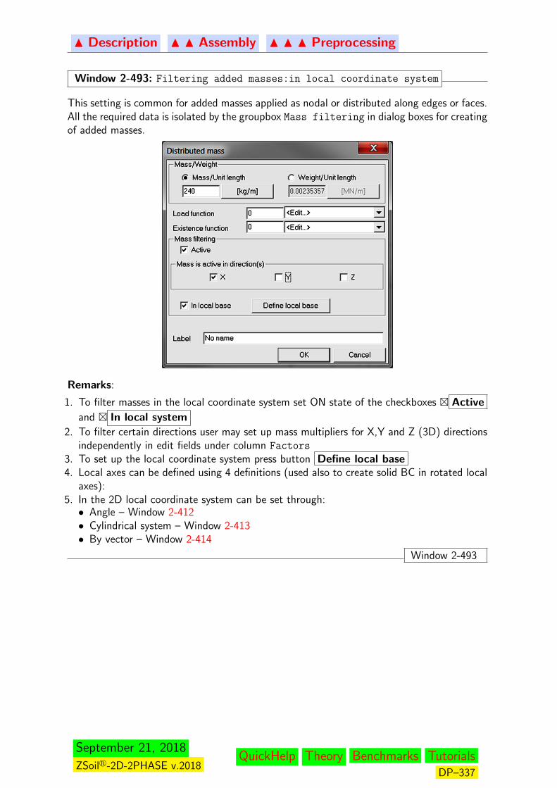
N Description N N Assembly N N N Preprocessing
Window 2-493: Filtering added masses:in local coordinate system
This setting is common for added masses applied as nodal or distributed along edges or faces.All the required data is isolated by the groupbox Mass filtering in dialog boxes for creatingof added masses.
Remarks:
1. To filter masses in the local coordinate system set ON state of the checkboxes � Active
and � In local system
2. To filter certain directions user may set up mass multipliers for X,Y and Z (3D) directionsindependently in edit fields under column Factors
3. To set up the local coordinate system press button Define local base4. Local axes can be defined using 4 definitions (used also to create solid BC in rotated local
axes):5. In the 2D local coordinate system can be set through:• Angle – Window 2-412• Cylindrical system – Window 2-413• By vector – Window 2-414
Window 2-493
September 21, 2018
ZSoilr-2D-2PHASE v.2018QuickHelp Theory Benchmarks Tutorials
DP–337

N Description N N Assembly N N N Preprocessing
2.3.1.3.18 DISTRIBUTED FLUX
Three groups of fluxes can be applied to elements in the real mesh
Fluid flux Create distributed fluid flux on selected elementsHeat flux Create distributed heat flux on selected elementsHumidity flux Create distributed humidity flux on selected elements
September 21, 2018
ZSoilr-2D-2PHASE v.2018QuickHelp Theory Benchmarks Tutorials
DP–338
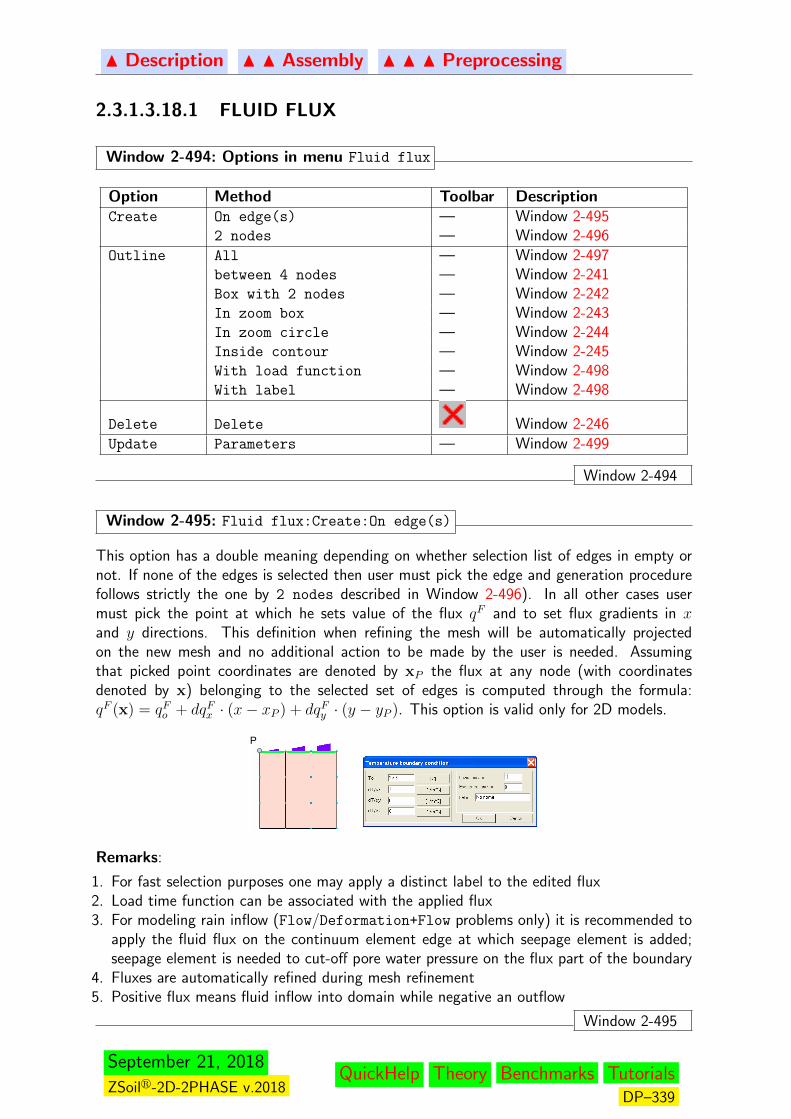
N Description N N Assembly N N N Preprocessing
2.3.1.3.18.1 FLUID FLUX
Window 2-494: Options in menu Fluid flux
Option Method Toolbar DescriptionCreate On edge(s) — Window 2-495
2 nodes — Window 2-496Outline All — Window 2-497
between 4 nodes — Window 2-241Box with 2 nodes — Window 2-242In zoom box — Window 2-243In zoom circle — Window 2-244Inside contour — Window 2-245With load function — Window 2-498With label — Window 2-498
Delete Delete Window 2-246Update Parameters — Window 2-499
Window 2-494
Window 2-495: Fluid flux:Create:On edge(s)
This option has a double meaning depending on whether selection list of edges in empty ornot. If none of the edges is selected then user must pick the edge and generation procedurefollows strictly the one by 2 nodes described in Window 2-496). In all other cases usermust pick the point at which he sets value of the flux qF and to set flux gradients in xand y directions. This definition when refining the mesh will be automatically projectedon the new mesh and no additional action to be made by the user is needed. Assumingthat picked point coordinates are denoted by xP the flux at any node (with coordinatesdenoted by x) belonging to the selected set of edges is computed through the formula:qF (x) = qFo + dqFx · (x− xP ) + dqFy · (y − yP ). This option is valid only for 2D models.
P
Remarks:
1. For fast selection purposes one may apply a distinct label to the edited flux2. Load time function can be associated with the applied flux3. For modeling rain inflow (Flow/Deformation+Flow problems only) it is recommended to
apply the fluid flux on the continuum element edge at which seepage element is added;seepage element is needed to cut-off pore water pressure on the flux part of the boundary
4. Fluxes are automatically refined during mesh refinement5. Positive flux means fluid inflow into domain while negative an outflow
Window 2-495
September 21, 2018
ZSoilr-2D-2PHASE v.2018QuickHelp Theory Benchmarks Tutorials
DP–339

N Description N N Assembly N N N Preprocessing
Window 2-496: Fluid flux:Create:2 nodes
Using this option one may apply a fluid flux to all continuum 2D element edges, belongingto the line section designed by the two picked points. This option is valid only for 2D modelsand is equivalent to the one On edge(s) (see Window 2-495).
1 2
Window 2-496
Window 2-497: Fluid flux:Outline:All
Using this option one may select all fluxes.
Window 2-497
Window 2-498: Fluid flux:Outline:With load f., label
Using this option user may select applied fluxes with a given load time function, or a givenlabel. In case of a label one may select a single item from combo-box.
Window 2-498
Window 2-499: Fluid flux:Update:Parameters
This option activates the dialog box to modify the applied fluid flux description, for a singlepicked edge/face or group of selected edges/faces. The detailed description on how to setthe data is given in Window 2-495 or Window ??.
Remarks:
1. When running this option for group of selected edges/faces only default parameters willbe set in the dialog box
Window 2-499
September 21, 2018
ZSoilr-2D-2PHASE v.2018QuickHelp Theory Benchmarks Tutorials
DP–340
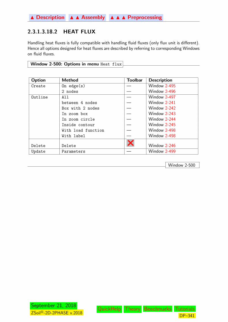
N Description N N Assembly N N N Preprocessing
2.3.1.3.18.2 HEAT FLUX
Handling heat fluxes is fully compatible with handling fluid fluxes (only flux unit is different).Hence all options designed for heat fluxes are described by referring to corresponding Windowson fluid fluxes.
Window 2-500: Options in menu Heat flux
Option Method Toolbar DescriptionCreate On edge(s) — Window 2-495
2 nodes — Window 2-496Outline All — Window 2-497
between 4 nodes — Window 2-241Box with 2 nodes — Window 2-242In zoom box — Window 2-243In zoom circle — Window 2-244Inside contour — Window 2-245With load function — Window 2-498With label — Window 2-498
Delete Delete Window 2-246Update Parameters — Window 2-499
Window 2-500
September 21, 2018
ZSoilr-2D-2PHASE v.2018QuickHelp Theory Benchmarks Tutorials
DP–341

N Description N N Assembly N N N Preprocessing
2.3.1.3.18.3 HUMIDITY FLUX
Handling humidity fluxes is fully compatible with handling fluid fluxes (only flux unit is differ-ent). Hence all options designed for humidity fluxes are described by referring to correspondingWindows on fluid fluxes.
Window 2-501: Options in menu Humidity flux
Option Method Toolbar DescriptionCreate On edge(s) — Window 2-495
2 nodes — Window 2-496Outline All — Window 2-497
between 4 nodes — Window 2-241Box with 2 nodes — Window 2-242In zoom box — Window 2-243In zoom circle — Window 2-244Inside contour — Window 2-245With load function — Window 2-498With label — Window 2-498
Delete Delete Window 2-246Update Parameters — Window 2-499
Window 2-501
September 21, 2018
ZSoilr-2D-2PHASE v.2018QuickHelp Theory Benchmarks Tutorials
DP–342

N Description N N Assembly N N N Preprocessing
2.3.1.3.19 INITIAL CONDITION
Initial conditions of any type can be applied with aid of super-elements of Q4 (for 2D models)or B8 (for 3D models) type. The idea is such that a given initial condition (like initialpressures, in situ effective stress components, etc..) is set at super-element vertices and thenit is interpolated, by means of standard Q4/B8 interpolation functions, to obtain assumedinitial condition at any node or integration point within the element (Gauss point) (seeWin.(2-502)).
Window 2-502: Concept of super-elements
12
3 4
P
FE mesh
Super-element
Remarks:
1. Any scalar, vectorial or tensorial data can be set at super-element vertices2. To recover the initial condition at a given node, or integration point, the following algorithm
is used• Compute vector of local coordinates xP of a given point P within the super-element
by solving the nonlinear equation: xP −∑NEN
i=1 Ni (ξP ) xi = 0 (here number ofsuper-element nodes is denoted by NEN)• Interpolate scalar, vectorial/tensorial (component by component) initial condition using
the formula: fP =∑NEN
i=1 Ni (ξP ) fi
Window 2-502
The following initial conditions can be set up:
Initial pressure Create initial pore fluid pressure via superelementsInitial temperature Create initial temperatures via superelementsInitial humidity Create initial humidity via superelementsInitial stress Create initial effective stresses in continuum via su-
perelementsInitial stresses on element(s) Create initial stresses in continuum/trusses/membranesInitial strain Create imposed strains via superelementsInitial strains on element(s) Create imposed strains on contin-
uum/trusses/membranesInitial displacement/velocity Create initial displacements and/or velocities on selected
nodesImposed strain on beams/shells Create imposed strains on beam/shell elements
September 21, 2018
ZSoilr-2D-2PHASE v.2018QuickHelp Theory Benchmarks Tutorials
DP–343
N Description N N Assembly N N N Preprocessing
2.3.1.3.19.1 INITIAL PRESSURE
In the definition of initial pressure compressive pore fluid pressures are negative incompression.
Window 2-503: Options in menu Initial pressure
Option Method Toolbar DescriptionCreate 4 nodes — Window 2-504
4 nodes/points — Window 2-505On bounding box — Window 2-506On bounding box of sel.
ele.
— Window 2-507
On construction front — Window 2-508Outline All — Window 2-509
In zoom box — Window 2-243In zoom circle — Window 2-244Inside contour — Window 2-245
Delete Delete Window 2-246Update Parameters — Window 2-510
Window 2-503
Window 2-504: Initial pressure:Create:4 nodes
Using this option one may define initial pore fluid pressure by setting quadrilateral super-element geometry (clicking 4 existing nodes) (see Window 2-502) and setting pressure valuesat 4 vertices in the following dialog box
Remarks:
1. Super-element vertices must be entered in order that prevents its distortion2. This initial condition is meaningful for Deformation, Deformation+Flow and Flow prob-
lems
Window 2-504
Window 2-505: Initial pressure:Create:4 nodes/points
Using this option one may define initial pore fluid pressure by setting quadrilateral super-element geometry (clicking 4 nodes/points) (see Window 2-502) and setting pressure valuesat 4 vertices in the following dialog box
September 21, 2018
ZSoilr-2D-2PHASE v.2018QuickHelp Theory Benchmarks Tutorials
DP–344
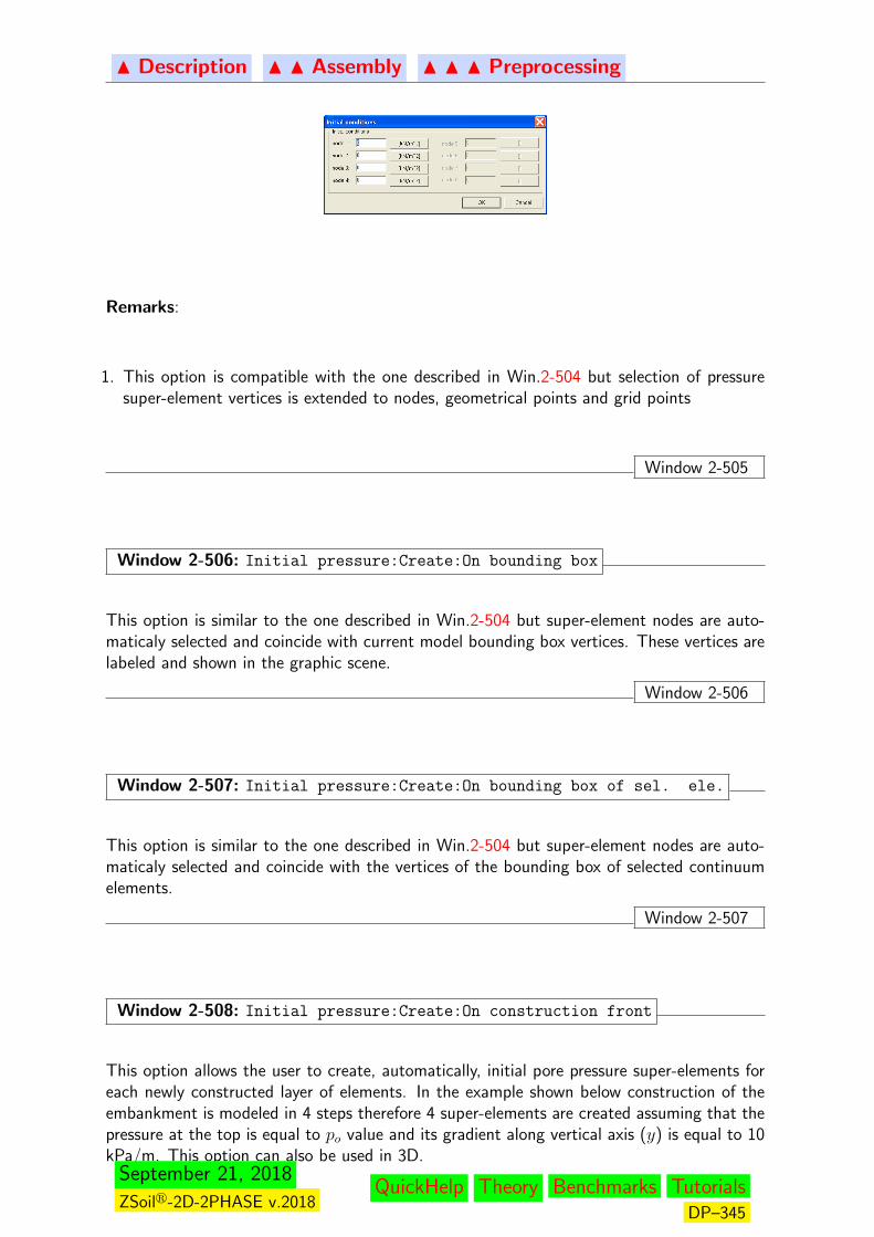
N Description N N Assembly N N N Preprocessing
Remarks:
1. This option is compatible with the one described in Win.2-504 but selection of pressuresuper-element vertices is extended to nodes, geometrical points and grid points
Window 2-505
Window 2-506: Initial pressure:Create:On bounding box
This option is similar to the one described in Win.2-504 but super-element nodes are auto-maticaly selected and coincide with current model bounding box vertices. These vertices arelabeled and shown in the graphic scene.
Window 2-506
Window 2-507: Initial pressure:Create:On bounding box of sel. ele.
This option is similar to the one described in Win.2-504 but super-element nodes are auto-maticaly selected and coincide with the vertices of the bounding box of selected continuumelements.
Window 2-507
Window 2-508: Initial pressure:Create:On construction front
This option allows the user to create, automatically, initial pore pressure super-elements foreach newly constructed layer of elements. In the example shown below construction of theembankment is modeled in 4 steps therefore 4 super-elements are created assuming that thepressure at the top is equal to po value and its gradient along vertical axis (y) is equal to 10kPa/m. This option can also be used in 3D.
September 21, 2018
ZSoilr-2D-2PHASE v.2018QuickHelp Theory Benchmarks Tutorials
DP–345
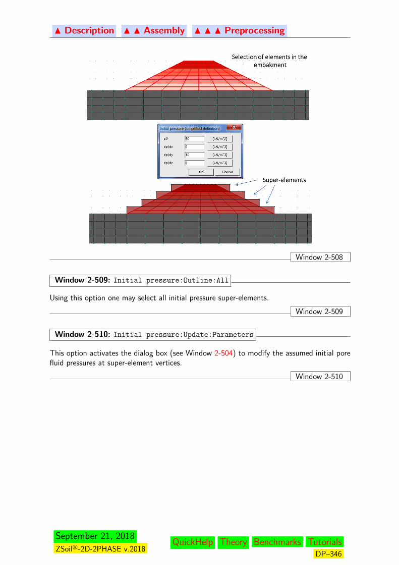
N Description N N Assembly N N N Preprocessing
Window 2-508
Window 2-509: Initial pressure:Outline:All
Using this option one may select all initial pressure super-elements.
Window 2-509
Window 2-510: Initial pressure:Update:Parameters
This option activates the dialog box (see Window 2-504) to modify the assumed initial porefluid pressures at super-element vertices.
Window 2-510
September 21, 2018
ZSoilr-2D-2PHASE v.2018QuickHelp Theory Benchmarks Tutorials
DP–346
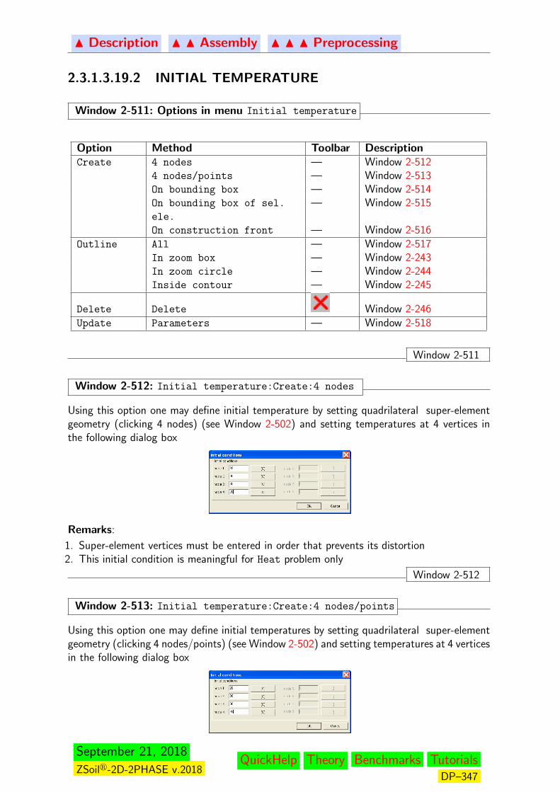
N Description N N Assembly N N N Preprocessing
2.3.1.3.19.2 INITIAL TEMPERATURE
Window 2-511: Options in menu Initial temperature
Option Method Toolbar DescriptionCreate 4 nodes — Window 2-512
4 nodes/points — Window 2-513On bounding box — Window 2-514On bounding box of sel.
ele.
— Window 2-515
On construction front — Window 2-516Outline All — Window 2-517
In zoom box — Window 2-243In zoom circle — Window 2-244Inside contour — Window 2-245
Delete Delete Window 2-246Update Parameters — Window 2-518
Window 2-511
Window 2-512: Initial temperature:Create:4 nodes
Using this option one may define initial temperature by setting quadrilateral super-elementgeometry (clicking 4 nodes) (see Window 2-502) and setting temperatures at 4 vertices inthe following dialog box
Remarks:
1. Super-element vertices must be entered in order that prevents its distortion2. This initial condition is meaningful for Heat problem only
Window 2-512
Window 2-513: Initial temperature:Create:4 nodes/points
Using this option one may define initial temperatures by setting quadrilateral super-elementgeometry (clicking 4 nodes/points) (see Window 2-502) and setting temperatures at 4 verticesin the following dialog box
September 21, 2018
ZSoilr-2D-2PHASE v.2018QuickHelp Theory Benchmarks Tutorials
DP–347
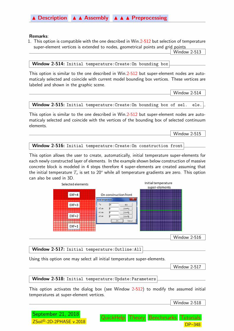
N Description N N Assembly N N N Preprocessing
Remarks:1. This option is compatible with the one described in Win.2-512 but selection of temperature
super-element vertices is extended to nodes, geometrical points and grid pointsWindow 2-513
Window 2-514: Initial temperature:Create:On bounding box
This option is similar to the one described in Win.2-512 but super-element nodes are auto-maticaly selected and coincide with current model bounding box vertices. These vertices arelabeled and shown in the graphic scene.
Window 2-514
Window 2-515: Initial temperature:Create:On bounding box of sel. ele.
This option is similar to the one described in Win.2-512 but super-element nodes are auto-maticaly selected and coincide with the vertices of the bounding box of selected continuumelements.
Window 2-515
Window 2-516: Initial temperature:Create:On construction front
This option allows the user to create, automatically, initial temperature super-elements foreach newly constructed layer of elements. In the example shown below construction of massiveconcrete block is modeled in 4 steps therefore 4 super-elements are created assuming thatthe initial temperature To is set to 20o while all temperature gradients are zero. This optioncan also be used in 3D.
Window 2-516
Window 2-517: Initial temperature:Outline:All
Using this option one may select all initial temperature super-elements.
Window 2-517
Window 2-518: Initial temperature:Update:Parameters
This option activates the dialog box (see Window 2-512) to modify the assumed initialtemperatures at super-element vertices.
Window 2-518
September 21, 2018
ZSoilr-2D-2PHASE v.2018QuickHelp Theory Benchmarks Tutorials
DP–348
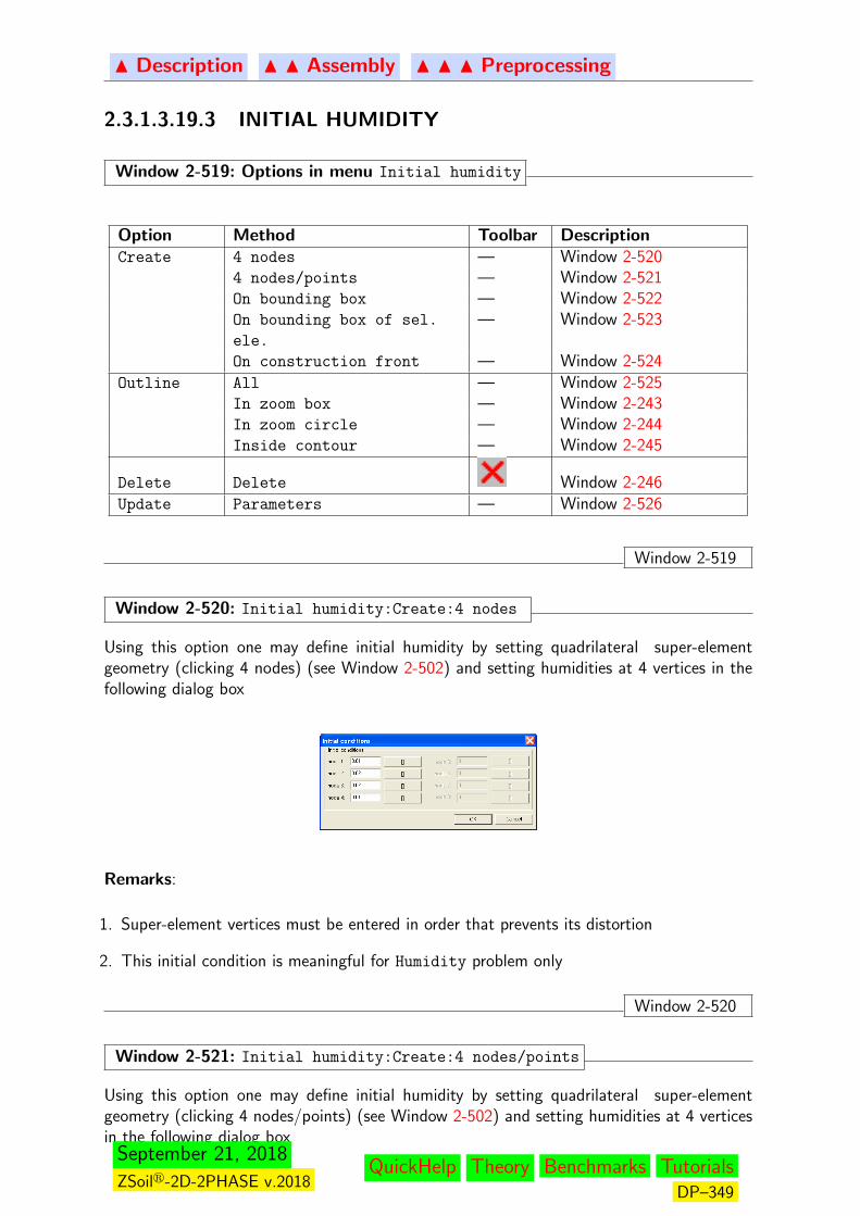
N Description N N Assembly N N N Preprocessing
2.3.1.3.19.3 INITIAL HUMIDITY
Window 2-519: Options in menu Initial humidity
Option Method Toolbar DescriptionCreate 4 nodes — Window 2-520
4 nodes/points — Window 2-521On bounding box — Window 2-522On bounding box of sel.
ele.
— Window 2-523
On construction front — Window 2-524Outline All — Window 2-525
In zoom box — Window 2-243In zoom circle — Window 2-244Inside contour — Window 2-245
Delete Delete Window 2-246Update Parameters — Window 2-526
Window 2-519
Window 2-520: Initial humidity:Create:4 nodes
Using this option one may define initial humidity by setting quadrilateral super-elementgeometry (clicking 4 nodes) (see Window 2-502) and setting humidities at 4 vertices in thefollowing dialog box
Remarks:
1. Super-element vertices must be entered in order that prevents its distortion
2. This initial condition is meaningful for Humidity problem only
Window 2-520
Window 2-521: Initial humidity:Create:4 nodes/points
Using this option one may define initial humidity by setting quadrilateral super-elementgeometry (clicking 4 nodes/points) (see Window 2-502) and setting humidities at 4 verticesin the following dialog box
September 21, 2018
ZSoilr-2D-2PHASE v.2018QuickHelp Theory Benchmarks Tutorials
DP–349
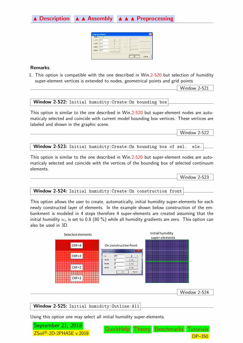
N Description N N Assembly N N N Preprocessing
Remarks:
1. This option is compatible with the one described in Win.2-520 but selection of humiditysuper-element vertices is extended to nodes, geometrical points and grid points
Window 2-521
Window 2-522: Initial humidity:Create:On bounding box
This option is similar to the one described in Win.2-520 but super-element nodes are auto-maticaly selected and coincide with current model bounding box vertices. These vertices arelabeled and shown in the graphic scene.
Window 2-522
Window 2-523: Initial humidity:Create:On bounding box of sel. ele.
This option is similar to the one described in Win.2-520 but super-element nodes are auto-maticaly selected and coincide with the vertices of the bounding box of selected continuumelements.
Window 2-523
Window 2-524: Initial humidity:Create:On construction front
This option allows the user to create, automatically, initial humidity super-elements for eachnewly constructed layer of elements. In the example shown below construction of the em-bankment is modeled in 4 steps therefore 4 super-elements are created assuming that theinitial humidity wo is set to 0.8 (80 %) while all humidity gradients are zero. This option canalso be used in 3D.
Window 2-524
Window 2-525: Initial humidity:Outline:All
Using this option one may select all initial humidity super-elements.
September 21, 2018
ZSoilr-2D-2PHASE v.2018QuickHelp Theory Benchmarks Tutorials
DP–350

N Description N N Assembly N N N Preprocessing
Window 2-525
Window 2-526: Initial humidity:Update:Parameters
This option activates the dialog box (see Window 2-520) to modify the assumed initialhumidities at super-element vertices.
Window 2-526
September 21, 2018
ZSoilr-2D-2PHASE v.2018QuickHelp Theory Benchmarks Tutorials
DP–351

N Description N N Assembly N N N Preprocessing
2.3.1.3.19.4 INITIAL STRESS
Window 2-527: Options in menu Initial stress
Option Method Toolbar DescriptionCreate 4 nodes — Window 2-528
4 nodes/points — Window 2-529On bounding box — Window 2-530On bounding box of sel.
ele.
— Window 2-531
On construction front — Window 2-532Outline All — Window 2-533
In zoom box — Window 2-243In zoom circle — Window 2-244Inside contour — Window 2-245
Delete Delete Window 2-246Update Parameters — Window 2-534Show XX — Window 2-535
YY — Window 2-535XY — Window 2-535ZZ — Window 2-535
Window 2-527
Window 2-528: Initial stress:Create:4 nodes
Using this option one may define initial effective stresses by setting quadrilateral super-element geometry (clicking 4 nodes) (see Window 2-502) and setting all effective stresscomponents at 4 vertices in the following dialog box
P1P2
P3 P4
Remarks:
1. The initial stresses can be generated by using a simplified procedure; all shear componentsare assumed to be zero while horizontal and out of the plane components are related to
the vertical one through the K in situo (to be set in the edit field Ko [ ] ) coefficient
• In the dialog box for simplified definition the value set in the Sig YY [ ] (σ∗y) is
assumed at the super-element vertex located at maximum y coordinate• At any point P (Gauss point) the vertical stress is computed as: σy(x) = σ∗y+γ (yP − y)
while the two remaining normal components are equal to: σx = K in situo σy, σz =
K in situo σy
September 21, 2018
ZSoilr-2D-2PHASE v.2018QuickHelp Theory Benchmarks Tutorials
DP–352
N Description N N Assembly N N N Preprocessing
2. Initial stresses are exclusively computed at the element center and then applied at allstandard Gauss points (note that stress generated from gravity is constant in low ordercontinuum finite element)
3. Super-element vertices must be entered in order that prevents its distortion4. This initial condition is meaningful for Deformation and Deformation+Flow problems5. Tensile stresses are positive6. The existence function is needed here to handle construction algorithm, mainly in the
situation when elements in certain zone appear then disappear and appear again (withpossibly new material properties); in such cases the initial stress super-element and finiteelements, to which these initial stresses are to be applied, must both have compatibleexistence functions
Window 2-528
Window 2-529: Initial stress:Create:4 nodes/points
This option is compatible with the one described in Win.2-528 but selection of stress super-element vertices is extended to nodes, geometrical points and grid points
Window 2-529
Window 2-530: Initial stress:Create:On bounding box
This option is similar to the one described in Win.2-528 but super-element nodes are auto-maticaly selected and coincide with current model bounding box vertices. These vertices arelabeled and shown in the graphic scene.
Window 2-530
Window 2-531: Initial stress:Create:On bounding box of sel. ele.
This option is similar to the one described in Win.2-528 but super-element nodes are auto-maticaly selected and coincide with the vertices of the bounding box of selected elements.
Window 2-531
Window 2-532: Initial stress:Create:On construction front
This option allows the user to create, automatically, initial effective stress super-elements foreach newly constructed layer of elements. In the example shown below construction of theembankment is modeled in 4 steps therefore 4 super-elements are created assuming that thevertical stress at the top is equal to σyy,o = 0 and its gradient along vertical axis (y) is equalto 20 kPa/m while Ko = 1. This option can also be used in 3D.
September 21, 2018
ZSoilr-2D-2PHASE v.2018QuickHelp Theory Benchmarks Tutorials
DP–353
N Description N N Assembly N N N Preprocessing
Window 2-532
Window 2-533: Initial stress:Outline:All
Using this option one may select all initial effective stress super-elements.
Window 2-533
Window 2-534: Initial stress:Update:Parameters
This option activates the dialog box (see Window 2-528) to modify the assumed initialeffective stress components at super-element vertices.
Window 2-534
Window 2-535: Initial stress:Show:XX,YY ...
With this option user may visualize color contours of the selected stress component.
Window 2-535
September 21, 2018
ZSoilr-2D-2PHASE v.2018QuickHelp Theory Benchmarks Tutorials
DP–354
N Description N N Assembly N N N Preprocessing
2.3.1.3.19.5 INITIAL STRESS ON ELEMENT(S)
Window 2-536: Options in menu Initial stresses on element(s)
Option Method Toolbar DescriptionCreate Apply to trusses — Window 2-537
Apply to membranes — Window 2-538Apply to continuum — Window 2-539
Outline Elem. with init.stress — Window 2-540Elem. with init.stress
via label
— Window 2-541
Delete Delete init. stress for
elements
Window 2-542
Update Parameters — Window 2-543
Window 2-536
Window 2-537: Initial stress:Create:Apply to trusses
Using this option one may define initial axial stress in selected or picked anchor/truss ele-ment(s) through the following dialog box
Selected truss elements
Remarks:
1. This initial condition is meaningful for Deformation and Deformation+Flow problems2. Tensile stresses are positive3. The load time function allows to analyze situations with variable (in time) initial axial stress4. This option can be useful for modeling cables where initial stresses are needed to start
computation
Window 2-537
September 21, 2018
ZSoilr-2D-2PHASE v.2018QuickHelp Theory Benchmarks Tutorials
DP–355
N Description N N Assembly N N N Preprocessing
Window 2-538: Initial stress:Create:Apply to membranes
Using this option one may define initial stresses in selected or picked membrane element(s)through the following dialog box
Selected membrane elements
Remarks:
1. This initial condition is meaningful for Deformation and Deformation+Flow problemsonly
2. Tensile stresses are positive3. The load time function allows to analyze situations with variable (in time) initial axial stress4. This option can be useful for modeling structural membranes where initial stresses are
needed to start the computation
Window 2-538
September 21, 2018
ZSoilr-2D-2PHASE v.2018QuickHelp Theory Benchmarks Tutorials
DP–356
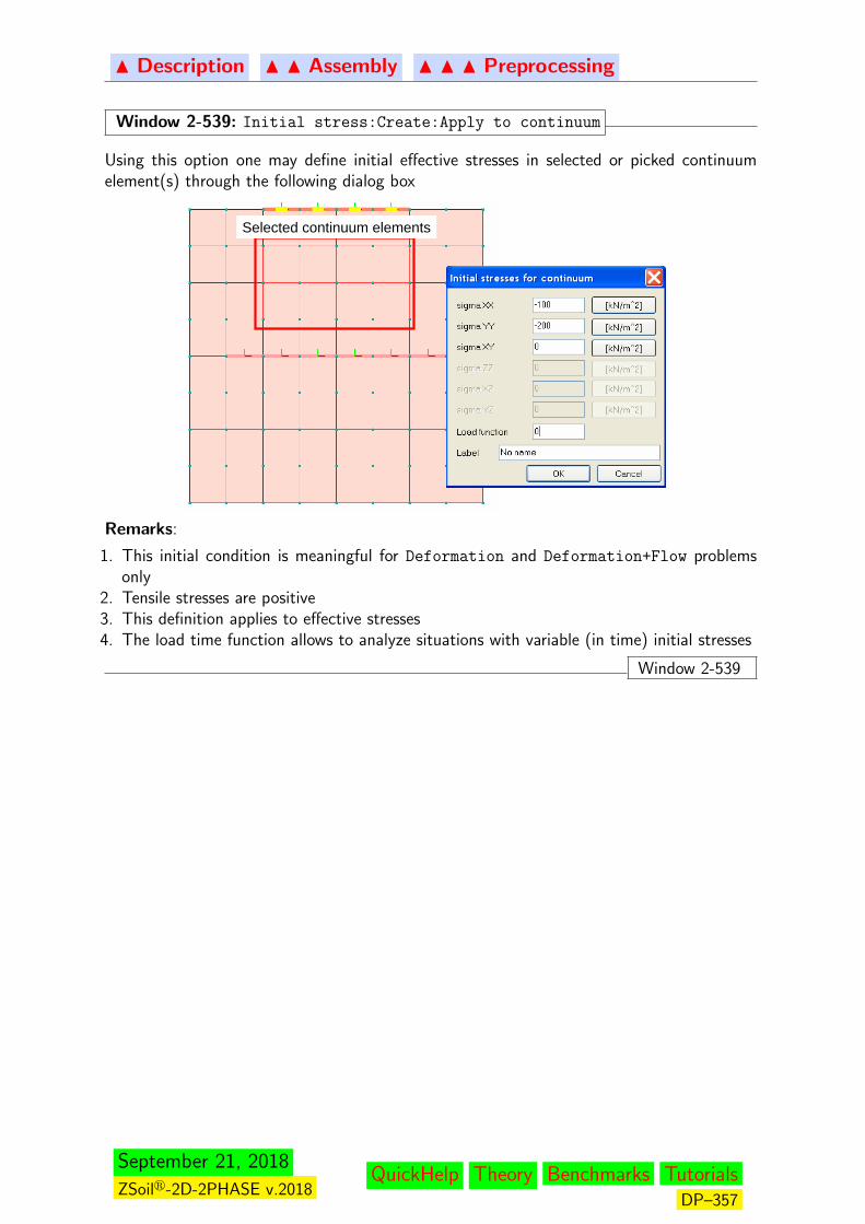
N Description N N Assembly N N N Preprocessing
Window 2-539: Initial stress:Create:Apply to continuum
Using this option one may define initial effective stresses in selected or picked continuumelement(s) through the following dialog box
Selected continuum elements
Remarks:
1. This initial condition is meaningful for Deformation and Deformation+Flow problemsonly
2. Tensile stresses are positive3. This definition applies to effective stresses4. The load time function allows to analyze situations with variable (in time) initial stresses
Window 2-539
September 21, 2018
ZSoilr-2D-2PHASE v.2018QuickHelp Theory Benchmarks Tutorials
DP–357

N Description N N Assembly N N N Preprocessing
Window 2-540: Initial stress:Outline:Elements with initial stress
This option allows to select all elements with the initial stresses defined under this menu.
Window 2-540
Window 2-541: Initial stress:Outline:Elements with initial stress via label
This option allows to select all elements with the initial stresses defined with a given label(under this general menu).
Window 2-541
Window 2-542: Initial stress:Delete:Initial stress for element(s)
This option allows to cancel initial stresses for selected elements.
Window 2-542
Window 2-543: Initial stress:Update:Parameters
This option activates the dialog box (see Window 2-537, Window 2-538, Window 2-539) tomodify the assumed initial stress components at selected elements.
Window 2-543
September 21, 2018
ZSoilr-2D-2PHASE v.2018QuickHelp Theory Benchmarks Tutorials
DP–358
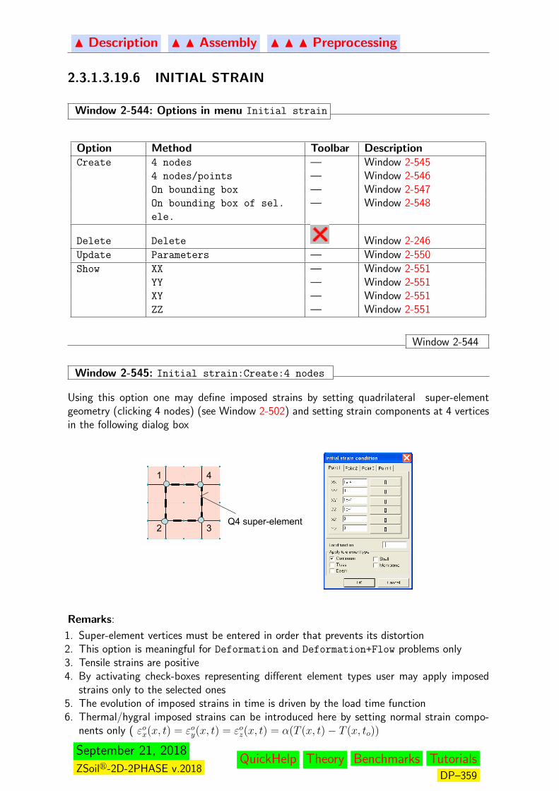
N Description N N Assembly N N N Preprocessing
2.3.1.3.19.6 INITIAL STRAIN
Window 2-544: Options in menu Initial strain
Option Method Toolbar DescriptionCreate 4 nodes — Window 2-545
4 nodes/points — Window 2-546On bounding box — Window 2-547On bounding box of sel.
ele.
— Window 2-548
Delete Delete Window 2-246Update Parameters — Window 2-550Show XX — Window 2-551
YY — Window 2-551XY — Window 2-551ZZ — Window 2-551
Window 2-544
Window 2-545: Initial strain:Create:4 nodes
Using this option one may define imposed strains by setting quadrilateral super-elementgeometry (clicking 4 nodes) (see Window 2-502) and setting strain components at 4 verticesin the following dialog box
Q4 super-element
1
2 3
4
Remarks:
1. Super-element vertices must be entered in order that prevents its distortion2. This option is meaningful for Deformation and Deformation+Flow problems only3. Tensile strains are positive4. By activating check-boxes representing different element types user may apply imposed
strains only to the selected ones5. The evolution of imposed strains in time is driven by the load time function6. Thermal/hygral imposed strains can be introduced here by setting normal strain compo-
nents only ( εox(x, t) = εoy(x, t) = εoz(x, t) = α(T (x, t)− T (x, to))
September 21, 2018
ZSoilr-2D-2PHASE v.2018QuickHelp Theory Benchmarks Tutorials
DP–359
N Description N N Assembly N N N Preprocessing
Window 2-545
Window 2-546: Initial strain:Create:4 nodes/points
This option is compatible with the one described in Win.2-545 but selection of strain super-element vertices is extended to nodes, geometrical points and grid points
Window 2-546
Window 2-547: Initial strain:Create:On bounding box
This option is similar to the one described in Win.2-545 but super-element nodes are auto-maticaly selected and coincide with current model bounding box vertices. These vertices arelabeled and shown in the graphic scene.
Window 2-547
Window 2-548: Initial strain:Create:On bounding box of sel. ele.
This option is similar to the one described in Win.2-545 but super-element nodes are auto-maticaly selected and coincide with the vertices of the bounding box of selected elements.
Window 2-548
Window 2-549: Initial strain:Outline:All
Using this option one may select all initial strain super-elements.
Window 2-549
Window 2-550: Initial strain:Update:Parameters
This option activates the dialog box (see Window 2-545) to modify the assumed imposedstrains components at super-element vertices.
Window 2-550
Window 2-551: Initial strain:Show:XX,YY ...
With this option user may visualize color contours of the selected strain component.
Window 2-551
September 21, 2018
ZSoilr-2D-2PHASE v.2018QuickHelp Theory Benchmarks Tutorials
DP–360

N Description N N Assembly N N N Preprocessing
2.3.1.3.19.7 INITIAL STRAIN ON ELEMENT(S)
Window 2-552: Options in menu Initial strains on element(s)
Option Method Toolbar DescriptionCreate Apply to element(s) — Window 2-553Outline Elem. with initial
strains
— Window 2-554
Elem. with initial
strains via label
— Window 2-555
Delete Delete initial strain for
elements
— —
Update Parameters — Window 2-553
Window 2-552
Window 2-553: Initial strain:Create:Apply to element(s)
Using this option one may define imposed strains (∆εxo = ∆εyo = ∆εzo = ∆εo) for pickedsingle element or group of selected elements.
Remarks:
1. In this setting thermal type induced strains can be generated only (for continuum or mem-branes all normal components are equal)
2. This option is meaningful for Deformation and Deformation+Flow problems only3. Tensile strains are positive4. The evolution of imposed strains in time is driven by the load time function
Window 2-553
September 21, 2018
ZSoilr-2D-2PHASE v.2018QuickHelp Theory Benchmarks Tutorials
DP–361
N Description N N Assembly N N N Preprocessing
Window 2-554: Initial strain:Outline:Elements with initial strain
This option selects all elements with defined initial strains (using exclusively the optionInitial strains on element(s)).
Window 2-554
Window 2-555: Initial strain:Outline:Elem.with initial strains via label
This option selects all elements with defined initial strains (using exclusively the optionInitial strains on element(s)), and given label.
Window 2-555
Window 2-556: Initial strain:Delete:Initial strains for elements
This option cancels initial strains, defined through the option Initial strains on element(s),for a single picked element or group of selected elements.
Window 2-556
September 21, 2018
ZSoilr-2D-2PHASE v.2018QuickHelp Theory Benchmarks Tutorials
DP–362
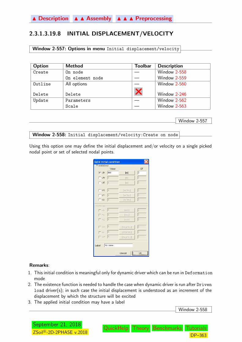
N Description N N Assembly N N N Preprocessing
2.3.1.3.19.8 INITIAL DISPLACEMENT/VELOCITY
Window 2-557: Options in menu Initial displacement/velocity
Option Method Toolbar DescriptionCreate On node — Window 2-558
On element node — Window 2-559Outline All options — Window 2-560
Delete Delete Window 2-246Update Parameters — Window 2-562
Scale — Window 2-563
Window 2-557
Window 2-558: Initial displacement/velocity:Create on node
Using this option one may define the initial displacement and/or velocity on a single pickednodal point or set of selected nodal points.
Remarks:
1. This initial condition is meaningful only for dynamic driver which can be run in Deformation
mode2. The existence function is needed to handle the case when dynamic driver is run after Driven
load driver(s); in such case the initial displacement is understood as an increment of thedisplacement by which the structure will be excited
3. The applied initial condition may have a label
Window 2-558
September 21, 2018
ZSoilr-2D-2PHASE v.2018QuickHelp Theory Benchmarks Tutorials
DP–363
N Description N N Assembly N N N Preprocessing
Window 2-559: Initial displacement/velocity:Create on element node
This option is equivalent to the one described in Window 2-558 but in this case the initialcondition is applied to a single picked element node. This way in case when at a givengeometrical point few nodes appear (due to contact interface for instance) one may applythe initial condition to the proper node.
Window 2-559
Window 2-560: Initial displacement/velocity:Options in menu Outline
All all initial conditions are selected; result of this action depends onthe status of Selection mode (see Window 2-81)
Between 2 nodes all initial conditions defined on nodes belonging to the sectionline defined by two picked points are selected; result of this ac-tion depends on the status of Selection mode in ribbon menuGlobal selection tools(see Window 2-81)
Between 4 nodes all initial conditions defined on nodes belonging to the surfacedefined by four picked points are selected; result of this action de-pends on the status of Selection mode in ribbon menu Global
selection tools(see Window 2-81)In zoom box if the zoom box is dragged from left to the right side then only
fully covered, by the zoom rectangle, initial conditions are selectedif the zoom box is dragged from right to the left side then evenpartially covered, by the zoom rectangle, initial conditions areselected
In zoom circle if the zoom circle is dragged from left to the right side then onlyfully covered, by the circle (cylinder in 3D), initial conditions areselectedif the zoom circle is dragged from right to the left side theneven partially covered, by the zoom circle (cylinder in 3D), initialconditions are selected
Inside contour all initial conditions being inside of the drawn closed contour areselected
With existence
function
all initial conditions with a given existence function are selected
With label all initial conditions with a given label are selected
Window 2-560
Window 2-561: Initial displacement/velocity:Delete:Delete
Using this option one may delete a single picked initial condition marker or group of selectedinitial conditions.
Window 2-561
Window 2-562: Initial displacement/velocity:Update:Parameters
September 21, 2018
ZSoilr-2D-2PHASE v.2018QuickHelp Theory Benchmarks Tutorials
DP–364
N Description N N Assembly N N N Preprocessing
This option activates the dialog box (see Window 2-558) to modify created initial conditions.
Window 2-562
Window 2-563: Initial displacement/velocity:Update:Scale
With this option one may increase or diminish the size of initial condition markers.
Window 2-563
September 21, 2018
ZSoilr-2D-2PHASE v.2018QuickHelp Theory Benchmarks Tutorials
DP–365
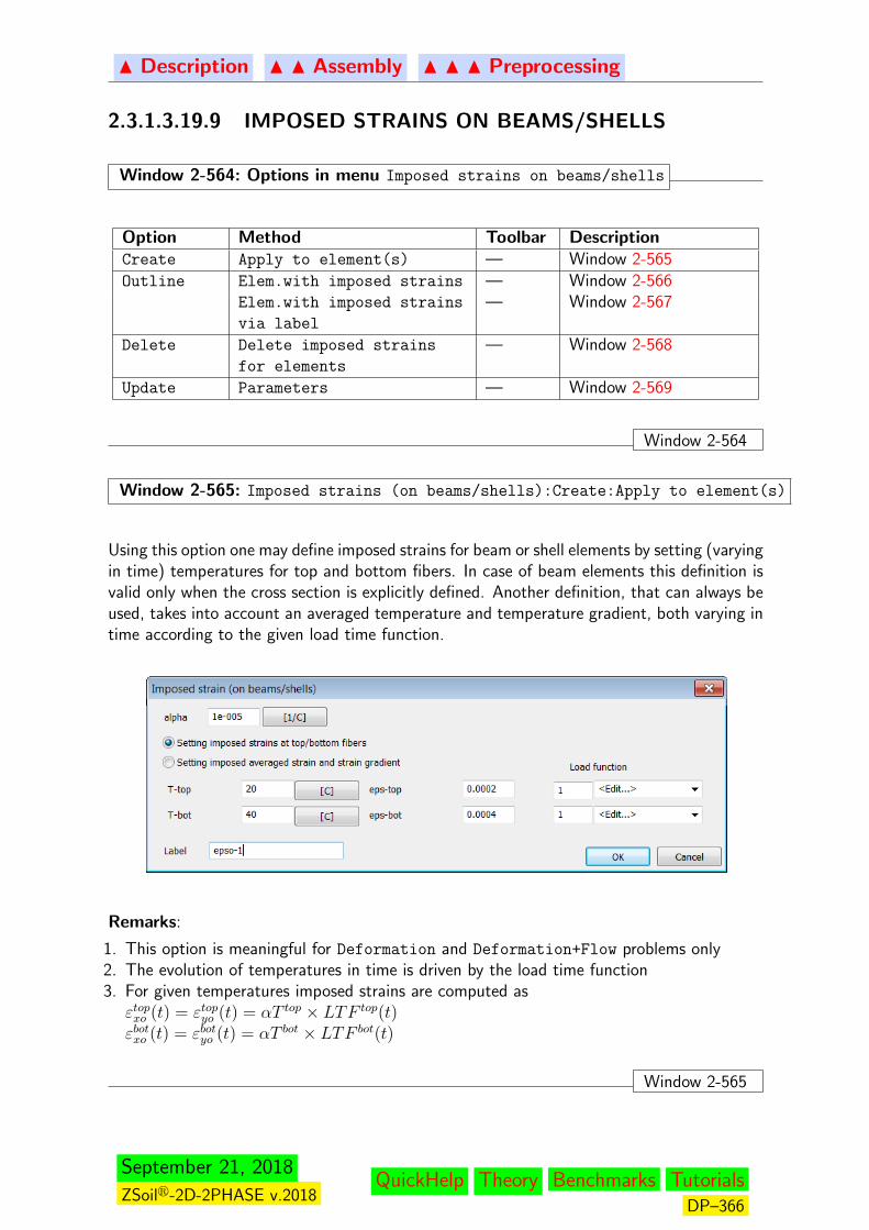
N Description N N Assembly N N N Preprocessing
2.3.1.3.19.9 IMPOSED STRAINS ON BEAMS/SHELLS
Window 2-564: Options in menu Imposed strains on beams/shells
Option Method Toolbar DescriptionCreate Apply to element(s) — Window 2-565Outline Elem.with imposed strains — Window 2-566
Elem.with imposed strains
via label
— Window 2-567
Delete Delete imposed strains
for elements
— Window 2-568
Update Parameters — Window 2-569
Window 2-564
Window 2-565: Imposed strains (on beams/shells):Create:Apply to element(s)
Using this option one may define imposed strains for beam or shell elements by setting (varyingin time) temperatures for top and bottom fibers. In case of beam elements this definition isvalid only when the cross section is explicitly defined. Another definition, that can always beused, takes into account an averaged temperature and temperature gradient, both varying intime according to the given load time function.
Remarks:
1. This option is meaningful for Deformation and Deformation+Flow problems only2. The evolution of temperatures in time is driven by the load time function3. For given temperatures imposed strains are computed asεtopxo (t) = εtopyo (t) = αT top × LTF top(t)εbotxo (t) = εbotyo (t) = αT bot × LTF bot(t)
Window 2-565
September 21, 2018
ZSoilr-2D-2PHASE v.2018QuickHelp Theory Benchmarks Tutorials
DP–366
N Description N N Assembly N N N Preprocessing
Window 2-566: Imposed strains on beams/shells:Outline:Elem.with imposed strain
This option selects all beam/shell elements with defined imposed strains.
Window 2-566
Window 2-567: Imposed strains on beams/shells:Outline:Elem.with imposed strain via label
This option selects all beam/shell elements with defined imposed strains under given label.
Window 2-567
Window 2-568: Imposed strains on beams/shells:Delete
This option allows the user to cancel imposed strains for single picked element (beam/shell)or group of selected elements.
Window 2-568
Window 2-569: Imposed strains on beams/shells:Update:Parameters
This option activates the dialog box (see Window 2-564) to modify the assumed temperaturesat top and bottom fibers, or averaged temperature and temperature gradient.
Window 2-569
September 21, 2018
ZSoilr-2D-2PHASE v.2018QuickHelp Theory Benchmarks Tutorials
DP–367
N Description N N Assembly N N N Preprocessing
2.3.1.3.20 DRM DOMAINS (DOMAIN REDUCTION METHOD)
Window 2-570: Options in menu DRM domains
Option Method Toolbar DescriptionCreate Exterior domain on
element(s)
— Window 2-571
Boundary domain on
element(s)
— Window 2-572
Outline Elements in exterior
domain
— Window 2-573
Elements in boundary
domain
— Window 2-574
Delete Delete exterior domain — Window 2-575Delete boundary domain — Window 2-576
Window 2-570
September 21, 2018
ZSoilr-2D-2PHASE v.2018QuickHelp Theory Benchmarks Tutorials
DP–368

N Description N N Assembly N N N Preprocessing
Window 2-571: DRM domains:Create: Exterior domain on element(s)
This option allows the user to define the exterior domain in Domain Reduction Method(DRM) for the set of selected continuum elements. This domain must not overlap with theboundary DRM layer.
Exterior domain
Viscous dampers Viscous dampers
Structure
Remarks:
1. On the external edges/faces viscous dampers should be generated to avoid spurious reflec-tions from finite boundaries
Window 2-571
Window 2-572: DRM domains:Create: Boundary domain on element(s)
This option allows the user to define the boundary layer of elements in Domain ReductionMethod (DRM) for the set of selected continuum elements. This domain must not overlapwith the exterior DRM layer.
Structure
Boundary layer
Interior domain
Exterior domain
Remarks:
1. The interior domain is detected automaticaly once the boundary and exterior domains areselected
2. In the boundary domain continuum must behave in the elastic manner; this is enforced bythe calculation module in an automatic manner for any constitutive model for continuum
Window 2-572
September 21, 2018
ZSoilr-2D-2PHASE v.2018QuickHelp Theory Benchmarks Tutorials
DP–369
N Description N N Assembly N N N Preprocessing
Window 2-573: DRM domains:Outline:Elements in exterior domain
This option selects all visible continuum elements that were selected in the exterior DRMdomain.
Window 2-573
Window 2-574: DRM domains:Outline:Elements in boundary domain
This option selects all visible continuum elements that were selected in the boundary DRMlayer .
Window 2-574
Window 2-575: DRM domains:Delete:Elements in exterior domain
This option removes all continuum elements from the set of elements in the exterior DRMdomain.
Window 2-575
Window 2-576: DRM domains:Delete:Elements in boundary domain
This option removes all continuum elements from the set of elements in the boundary DRMlayer .
Window 2-576
September 21, 2018
ZSoilr-2D-2PHASE v.2018QuickHelp Theory Benchmarks Tutorials
DP–370
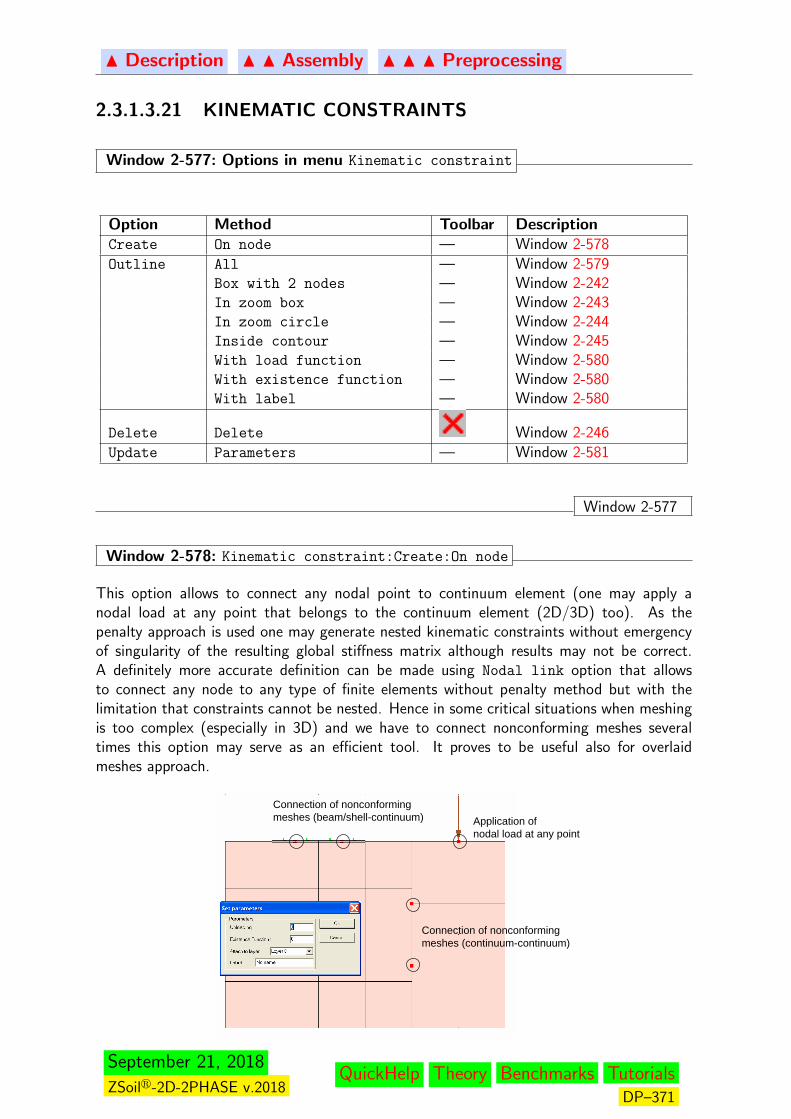
N Description N N Assembly N N N Preprocessing
2.3.1.3.21 KINEMATIC CONSTRAINTS
Window 2-577: Options in menu Kinematic constraint
Option Method Toolbar DescriptionCreate On node — Window 2-578Outline All — Window 2-579
Box with 2 nodes — Window 2-242In zoom box — Window 2-243In zoom circle — Window 2-244Inside contour — Window 2-245With load function — Window 2-580With existence function — Window 2-580With label — Window 2-580
Delete Delete Window 2-246Update Parameters — Window 2-581
Window 2-577
Window 2-578: Kinematic constraint:Create:On node
This option allows to connect any nodal point to continuum element (one may apply anodal load at any point that belongs to the continuum element (2D/3D) too). As thepenalty approach is used one may generate nested kinematic constraints without emergencyof singularity of the resulting global stiffness matrix although results may not be correct.A definitely more accurate definition can be made using Nodal link option that allowsto connect any node to any type of finite elements without penalty method but with thelimitation that constraints cannot be nested. Hence in some critical situations when meshingis too complex (especially in 3D) and we have to connect nonconforming meshes severaltimes this option may serve as an efficient tool. It proves to be useful also for overlaidmeshes approach.
Application ofnodal load at any point
Connection of nonconformingmeshes (beam/shell-continuum)
Connection of nonconformingmeshes (continuum-continuum)
September 21, 2018
ZSoilr-2D-2PHASE v.2018QuickHelp Theory Benchmarks Tutorials
DP–371

N Description N N Assembly N N N Preprocessing
Window 2-578
Window 2-579: Kinematic constraint:Outline:All
This option selects all kinematic constraints.
Window 2-579
Window 2-580: Kinematic constraint:Outline:With load f., exist.f., label
Using this option user may select assumed kinematic constraints with a given load timefunction ID, existence function or a given label. In case of a label one may select a singleitem from combo-box.
Window 2-580
Window 2-581: Kinematic constraint:Update:Parameters
This option activates the dialog box to modify the definition of kinematic constraint at agiven node. The detailed description on how to set the data is given in Window 2-578.
Window 2-581
September 21, 2018
ZSoilr-2D-2PHASE v.2018QuickHelp Theory Benchmarks Tutorials
DP–372
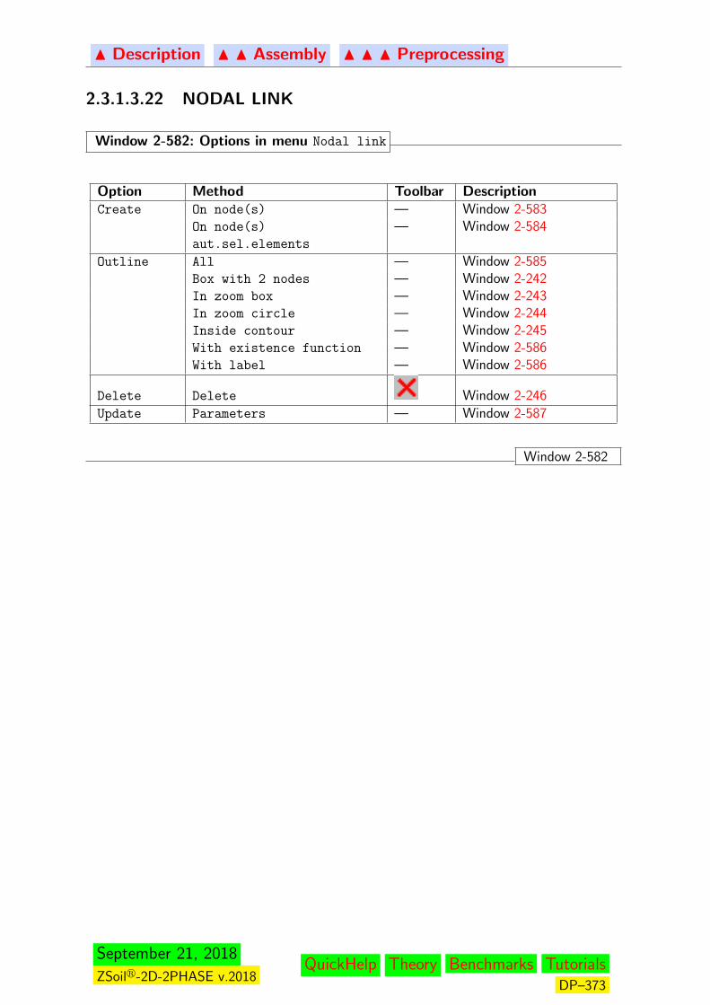
N Description N N Assembly N N N Preprocessing
2.3.1.3.22 NODAL LINK
Window 2-582: Options in menu Nodal link
Option Method Toolbar DescriptionCreate On node(s) — Window 2-583
On node(s)
aut.sel.elements
— Window 2-584
Outline All — Window 2-585Box with 2 nodes — Window 2-242In zoom box — Window 2-243In zoom circle — Window 2-244Inside contour — Window 2-245With existence function — Window 2-586With label — Window 2-586
Delete Delete Window 2-246Update Parameters — Window 2-587
Window 2-582
September 21, 2018
ZSoilr-2D-2PHASE v.2018QuickHelp Theory Benchmarks Tutorials
DP–373

N Description N N Assembly N N N Preprocessing
Window 2-583: Nodal link:Create:On node(s)
This option, valid for 2D and 3D, allows to link selected node(s) to selected elements (can becontinuum, shells, beams, trusses, membranes) in an exact manner (without penalty methodused in the option Kinematic constraint). It is obvious that a given node must be locatedin the interior of the element to which it is to be linked. This linking can be applied to selecteddegrees of freedom (DOFs). It has to be emphasized that linking is possible only for theseDOFs which are common for given node and element to be linked with(for instance whenbeam node is linked to the continuum then only translational DOFs can be constrained, ifwe link beam node to the shell element then all translational and rotational DOFs can beconstrained). Activating this option must be preceded by selection of nodes (the ones to belinked) and background elements. To select DOFs to be constrained user must also selectdegrees of freedom to be constrained (see picture below).
selected nodes
Selection of degrees of freedom to be constrained
Remarks:
1. Linking operation cannot be nested; it means that linking of a node to the element whoesenodes are already linked to another element is forbidden; in such cases to avoid multilevellinking one may use of standard kinematic constraints (option Kinematic constraint)enforced with aid of penalty method
2. This option can be used to apply nodal forces at any point (it is useful to apply nodalforces to large foundation rafts at any point)
Window 2-583
September 21, 2018
ZSoilr-2D-2PHASE v.2018QuickHelp Theory Benchmarks Tutorials
DP–374

N Description N N Assembly N N N Preprocessing
Window 2-584: Nodal link:Create:On node(s) aut. sel. elements
This option is equivalent to the one described in Win.2-583 but elements (the ones visiblein the graph pane) to which selected nodes are linked are selected automatically by thepreprocessor.
selected nodes
Selection of degrees of freedom to be constrained
Window 2-584
Window 2-585: Nodal link:Outline:All
This option selects all nodal links.
Window 2-585
Window 2-586: Nodal link:Outline:With exist.f., label
Using this option user may select nodal links with a given existence function ID (applied tosome constrained DOF) or a given label. In case of a label one may select a single item fromcombo-box.
Window 2-586
Window 2-587: Nodal link:Update:Parameters
This option activates the dialog box to modify the applied nodal link definition (degrees offreedom to be constrained), for a single picked nodal link or group of selected nodal links.The detailed description on how to set the data is given in Window 2-583.
Window 2-587
September 21, 2018
ZSoilr-2D-2PHASE v.2018QuickHelp Theory Benchmarks Tutorials
DP–375
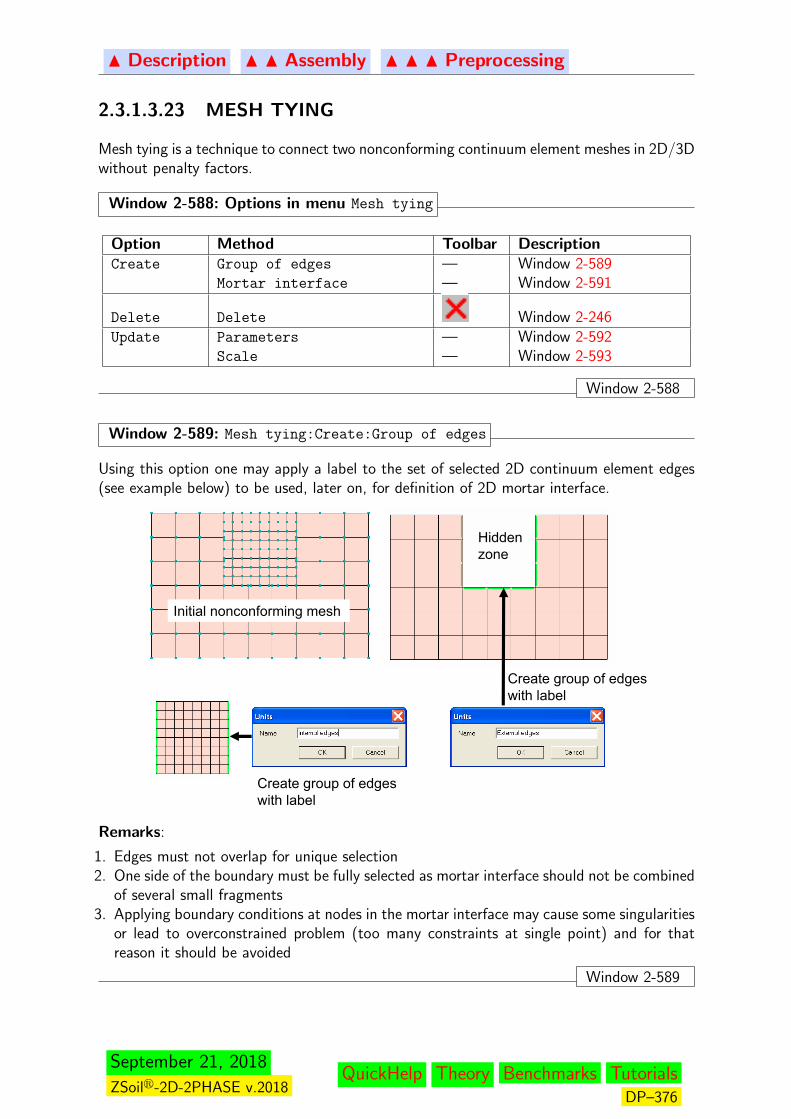
N Description N N Assembly N N N Preprocessing
2.3.1.3.23 MESH TYING
Mesh tying is a technique to connect two nonconforming continuum element meshes in 2D/3Dwithout penalty factors.
Window 2-588: Options in menu Mesh tying
Option Method Toolbar DescriptionCreate Group of edges — Window 2-589
Mortar interface — Window 2-591
Delete Delete Window 2-246Update Parameters — Window 2-592
Scale — Window 2-593
Window 2-588
Window 2-589: Mesh tying:Create:Group of edges
Using this option one may apply a label to the set of selected 2D continuum element edges(see example below) to be used, later on, for definition of 2D mortar interface.
Initial nonconforming mesh
Hiddenzone
Create group of edgeswith label
Create group of edgeswith label
Remarks:
1. Edges must not overlap for unique selection2. One side of the boundary must be fully selected as mortar interface should not be combined
of several small fragments3. Applying boundary conditions at nodes in the mortar interface may cause some singularities
or lead to overconstrained problem (too many constraints at single point) and for thatreason it should be avoided
Window 2-589
September 21, 2018
ZSoilr-2D-2PHASE v.2018QuickHelp Theory Benchmarks Tutorials
DP–376
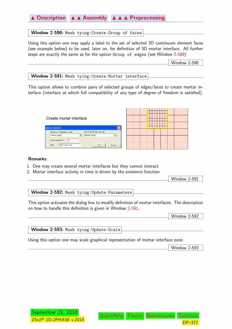
N Description N N Assembly N N N Preprocessing
Window 2-590: Mesh tying:Create:Group of faces
Using this option one may apply a label to the set of selected 3D continuum element faces(see example below) to be used, later on, for definition of 3D mortar interface. All furthersteps are exactly the same as for the option Group of edges (see Window 2-589)
Window 2-590
Window 2-591: Mesh tying:Create:Mortar interface
This option allows to combine pairs of selected groups of edges/faces to create mortar in-terface (interface at which full compatibility of any type of degree of freedom is satisfied).
Create mortar interface
Remarks:
1. One may create several mortar interfaces but they cannot interact2. Mortar interface activity in time is driven by the existence function
Window 2-591
Window 2-592: Mesh tying:Update:Parameters
This option activates the dialog box to modify definition of mortar interfaces. The descriptionon how to handle this definition is given in Window 2-591.
Window 2-592
Window 2-593: Mesh tying:Update:Scale
Using this option one may scale graphical representation of mortar interface zone.
Window 2-593
September 21, 2018
ZSoilr-2D-2PHASE v.2018QuickHelp Theory Benchmarks Tutorials
DP–377
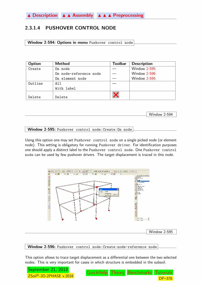
N Description N N Assembly N N N Preprocessing
2.3.1.4 PUSHOVER CONTROL NODE
Window 2-594: Options in menu Pushover control node
Option Method Toolbar DescriptionCreate On node — Window 2-595
On node-reference node — Window 2-596On element node — Window 2-595
Outline All —With label
Delete Delete
Window 2-594
Window 2-595: Pushover control node:Create:On node
Using this option one may set Pushover control node on a single picked node (or elementnode). This setting is obligatory for running Pushover driver. For identification purposesone should apply a distinct label to the Pushover control node. One Pushover control
node can be used by few pushover drivers. The target displacement is traced in this node.
Window 2-595
Window 2-596: Pushover control node:Create:node-reference node
This option allows to trace target displacement as a differential one between the two selectednodes. This is very important for cases in which structure is embedded in the subsoil.
September 21, 2018
ZSoilr-2D-2PHASE v.2018QuickHelp Theory Benchmarks Tutorials
DP–378
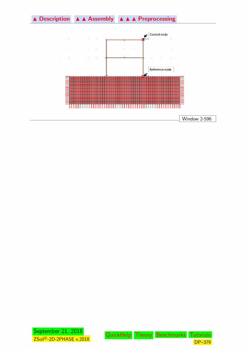
N Description N N Assembly N N N Preprocessing
Window 2-596
September 21, 2018
ZSoilr-2D-2PHASE v.2018QuickHelp Theory Benchmarks Tutorials
DP–379

N Preface N N Description N N N Assembly
2.3.2 MESH INFO
Window 2-597: Summary of computational model
Displays short reports on current data containing the number of:
... beam elements
... beams relaxation
... boundary conditions
... contact elements
... convection elements
... different materials
... existence functions
... heat boundary conditions
... humidity boundary conditions
... infinite elements
... initial conditions
... initial heat conditions
... initial humidity conditions
... initial stress conditions
... kinematic constrains
... load time functions
... loads for trusses
... membrane elements
... nodal forces
... nodes
... pressure heads loads
... quad elements
... seepage elements
... single layer shell elements
... shell elements
... surface loads
... truss elements
... volumic elements
... water boundary conditions
... water flux
Window 2-597
September 21, 2018
ZSoilr-2D-2PHASE v.2018QuickHelp Theory Benchmarks Tutorials
DP–380
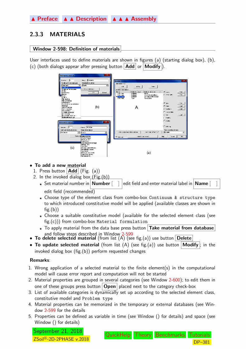
N Preface N N Description N N N Assembly
2.3.3 MATERIALS
Window 2-598: Definition of materials
User interfaces used to define materials are shown in figures (a) (starting dialog box), (b),
(c) (both dialogs appear after pressing button Add or Modify ).
• To add a new material1. Press button Add (Fig. (a))2. In the invoked dialog box (Fig.(b))
F Set material number in Number [ ] edit field and enter material label in Name [ ]
edit field (recommended)F Choose type of the element class from combo-box Continuum & structure type
to which introduced constitutive model will be applied (available classes are shown infig.(b))
F Choose a suitable constitutive model (available for the selected element class (seefig.(c))) from combo-box Material formulation
F To apply material from the data base press button Take material from databaseand follow steps described in Window 2-599
• To delete selected material (from list (A) (see fig.(a)) use button Delete
• To update selected material (from list (A) (see fig.(a)) use button Modify ; in the
invoked dialog box (fig.(b)) perform requested changes
Remarks:
1. Wrong application of a selected material to the finite element(s) in the computationalmodel will cause error report and computation will not be started
2. Material properties are grouped in several categories (see Window 2-600); to edit them in
one of these groups press button Open placed next to the category check-box3. List of available categories is dynamically set up according to the selected element class,
constitutive model and Problem type
4. Material properties can be memorized in the temporary or external databases (see Win-dow 2-599 for the details
5. Properties can be defined as variable in time (see Window () for details) and space (seeWindow () for details)
September 21, 2018
ZSoilr-2D-2PHASE v.2018QuickHelp Theory Benchmarks Tutorials
DP–381

N Preface N N Description N N N Assembly
6. For plastic damage model for concrete used in the continuum or shell elements extensionto fire problems (according to the Eurocode) is possible
7. Elastic-plastic 1D model for truss elements can also handle fire problems8. The default values of properties for few typical materials are given in Win.()
Window 2-598
September 21, 2018
ZSoilr-2D-2PHASE v.2018QuickHelp Theory Benchmarks Tutorials
DP–382

N Description N N Assembly N N N Materials
2.3.3.1 MATERIAL DATA BASE
Window 2-599: Material data base
Material data base is an user data bank created himself to collect material definitions, witha distinct label, for further use.
A
B
1. Defined databases combo-box (A) opens an access to the selected database
2. Create new database creates an empty and new database with a given label
3. Delete selected database removes database selected from combo-box (A)
4. Save selected database saves database selected from combo-box (A)
5. Save all selected databases saves all databases
6. Take selected material indicates which material (from list (B)) should be used by theparent dialog box used (see Window 2-598)
7. Remove selected material cancels material selected from list (B)in the selected databaseindicated in combo-box (A)
Window 2-599
September 21, 2018
ZSoilr-2D-2PHASE v.2018QuickHelp Theory Benchmarks Tutorials
DP–383
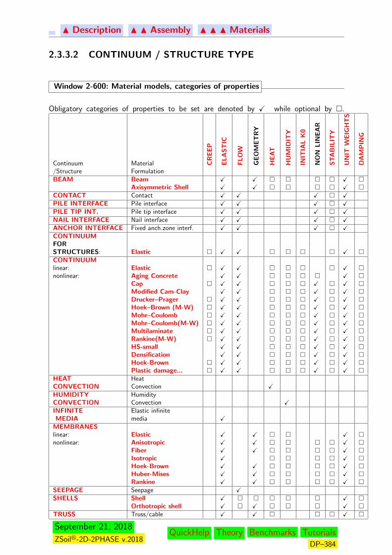
N Description N N Assembly N N N Materials
2.3.3.2 CONTINUUM / STRUCTURE TYPE
Window 2-600: Material models, categories of properties
Obligatory categories of properties to be set are denoted by X while optional by �.
Continuum Material CR
EE
P
EL
AS
TIC
FL
OW
GE
OM
ET
RY
HE
AT
HU
MID
ITY
INIT
IAL
K0
NO
NL
INE
AR
ST
AB
ILIT
Y
UN
ITW
EIG
HT
S
DA
MP
ING
/Structure FormulationBEAM Beam X X � � � � X �
Axisymmetric Shell X X � � � � X �CONTACT Contact X X X � XPILE INTERFACE Pile interface X X X � XPILE TIP INT. Pile tip interface X X X � XNAIL INTERFACE Nail interface X X X � XANCHOR INTERFACE Fixed anch.zone interf. X X X � XCONTINUUMFORSTRUCTURES: Elastic � X X � � � � X �CONTINUUMlinear: Elastic � X X � � � � X �nonlinear: Aging Concrete X X � � � � X �
Cap � X X � � � X � X �Modified Cam-Clay X X � � � X � X �Drucker–Prager � X X � � � X � X �Hoek–Brown (M-W) � X X � � � X � X �Mohr–Coulomb � X X � � � X � X �Mohr–Coulomb(M-W) � X X � � � X � X �Multilaminate � X X � � � X � X �Rankine(M-W) � X X � � � X � X �HS-small X X � � � X � X �Densification X X � � � X � X �Hoek-Brown � X X � � � X � X �Plastic damage... � X X � � � X � X �
HEAT HeatCONVECTION Convection XHUMIDITY HumidityCONVECTION Convection XINFINITE Elastic infiniteMEDIA media X
MEMBRANESlinear: Elastic X X � � X �nonlinear: Anisotropic X X � � � � X �
Fiber X X � � � � X �Isotropic X � � � � X �Hoek-Brown X X � � � � X �Huber-Mises X X � � � � X �Rankine X X � � � � X �
SEEPAGE Seepage XSHELLS Shell X � � � � � X �
Orthotropic shell X � X � � � X �TRUSS Truss/cable X X � � � X �
September 21, 2018
ZSoilr-2D-2PHASE v.2018QuickHelp Theory Benchmarks Tutorials
DP–384

N Description N N Assembly N N N Materials
Continuum Material CR
EE
P
EL
AS
TIC
FL
OW
GE
OM
ET
RY
HE
AT
HU
MID
ITY
INIT
IAL
K0
NO
NL
INE
AR
ST
AB
ILIT
Y
UN
ITW
EIG
HT
S
DA
MP
ING
/Structure FormulationBEAM NONL.HINGE Uncoupled axial X
Uncoupled tangent XUncoupled torsional XUncoupled flexural XCoupled flexural (Janssen) X X
SHELL NONL.HINGE Uncoupled axial XUncoupled tangent XUncoupled flexural XCoupled flexural (Janssen) X X
Window 2-600
September 21, 2018
ZSoilr-2D-2PHASE v.2018QuickHelp Theory Benchmarks Tutorials
DP–385

N Assembly N N Materials N N N Continuum/Structures
2.3.3.2.1 BEAMS AND AXISYMMETRIC SHELLS
Material model description, designed for beam or axisymmetric shell element, consists of :
• definition of cross section geometry• definition of material properties
The above data is specific for current analysis type ( 2D, 3D or axisymmetry), hence it isrecommended to select proper problem type in the initial pre-selection dialog box.
The two following models are available:
BEAM MODEL
AXISYMMETRIC SHELL
Related Topics
Theory:
• BEAMS THEORY
September 21, 2018
ZSoilr-2D-2PHASE v.2018QuickHelp Theory Benchmarks Tutorials
DP–386
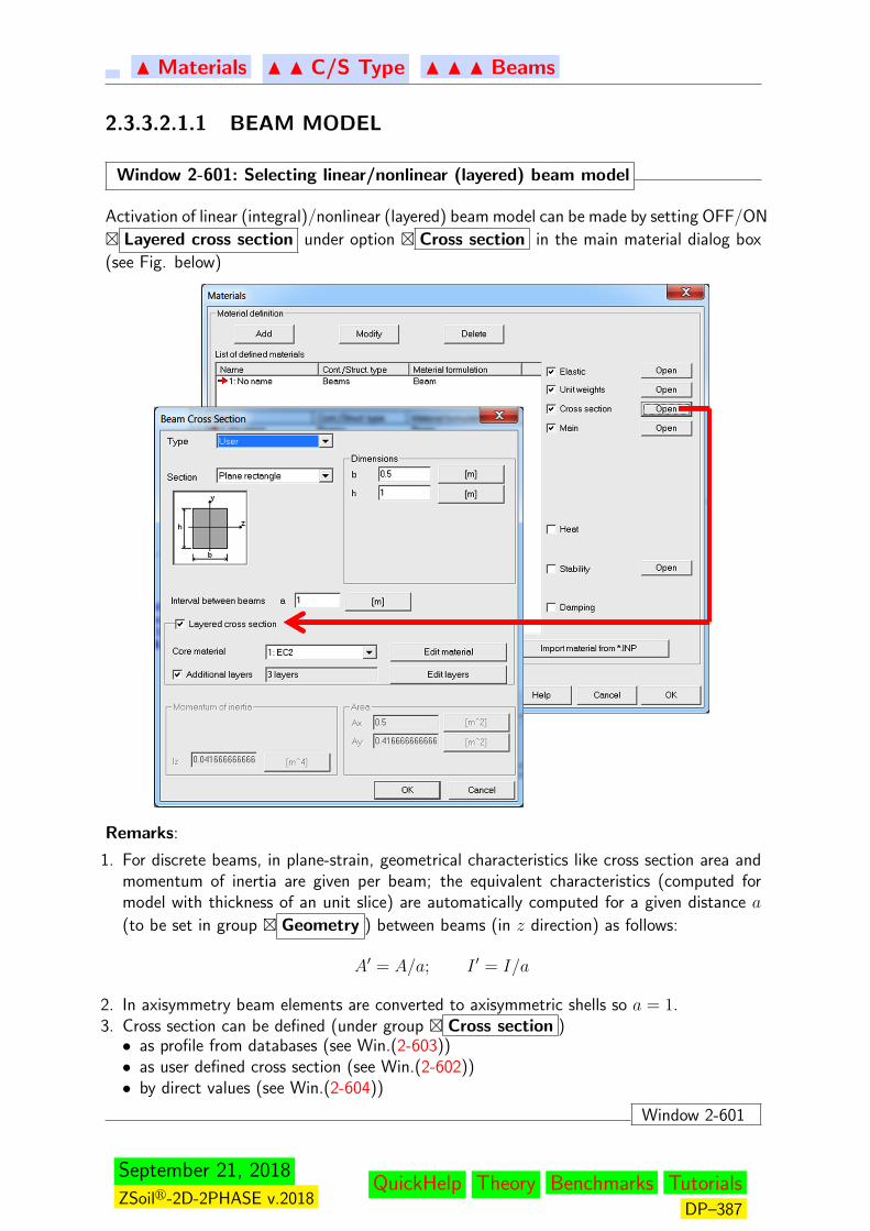
N Materials N N C/S Type N N N Beams
2.3.3.2.1.1 BEAM MODEL
Window 2-601: Selecting linear/nonlinear (layered) beam model
Activation of linear (integral)/nonlinear (layered) beam model can be made by setting OFF/ON
� Layered cross section under option � Cross section in the main material dialog box
(see Fig. below)
Remarks:
1. For discrete beams, in plane-strain, geometrical characteristics like cross section area andmomentum of inertia are given per beam; the equivalent characteristics (computed formodel with thickness of an unit slice) are automatically computed for a given distance a
(to be set in group � Geometry ) between beams (in z direction) as follows:
A′ = A/a; I ′ = I/a
2. In axisymmetry beam elements are converted to axisymmetric shells so a = 1.3. Cross section can be defined (under group � Cross section )• as profile from databases (see Win.(2-603))• as user defined cross section (see Win.(2-602))• by direct values (see Win.(2-604))
Window 2-601
September 21, 2018
ZSoilr-2D-2PHASE v.2018QuickHelp Theory Benchmarks Tutorials
DP–387
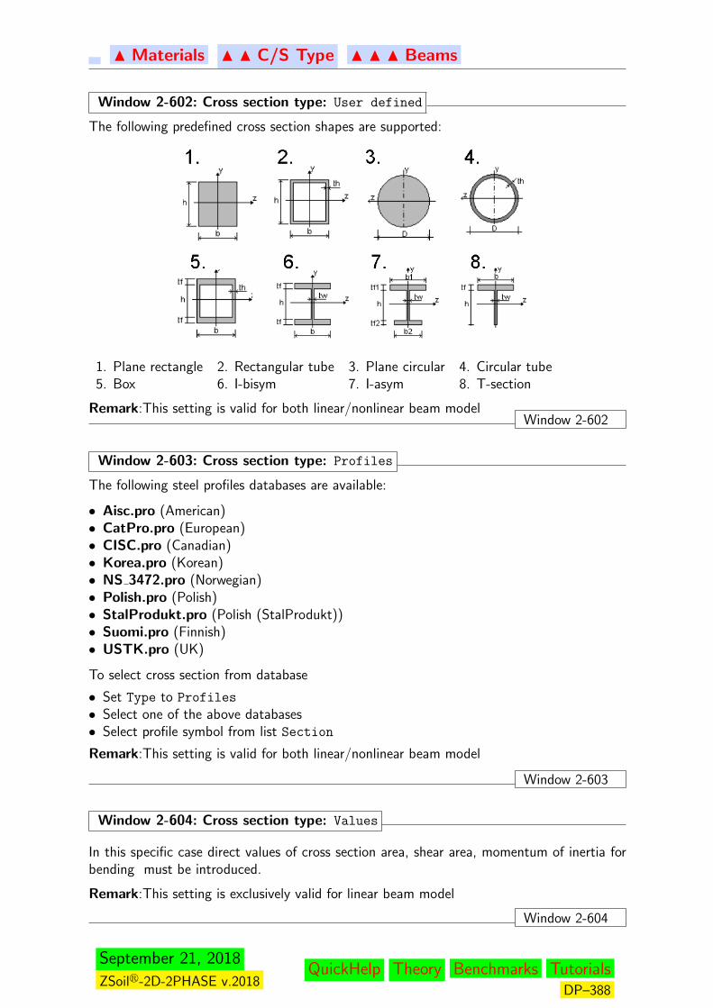
N Materials N N C/S Type N N N Beams
Window 2-602: Cross section type: User defined
The following predefined cross section shapes are supported:
1. Plane rectangle 2. Rectangular tube 3. Plane circular 4. Circular tube5. Box 6. I-bisym 7. I-asym 8. T-section
Remark:This setting is valid for both linear/nonlinear beam modelWindow 2-602
Window 2-603: Cross section type: Profiles
The following steel profiles databases are available:
• Aisc.pro (American)• CatPro.pro (European)• CISC.pro (Canadian)• Korea.pro (Korean)• NS 3472.pro (Norwegian)• Polish.pro (Polish)• StalProdukt.pro (Polish (StalProdukt))• Suomi.pro (Finnish)• USTK.pro (UK)
To select cross section from database
• Set Type to Profiles
• Select one of the above databases• Select profile symbol from list Section
Remark:This setting is valid for both linear/nonlinear beam model
Window 2-603
Window 2-604: Cross section type: Values
In this specific case direct values of cross section area, shear area, momentum of inertia forbending must be introduced.
Remark:This setting is exclusively valid for linear beam model
Window 2-604
September 21, 2018
ZSoilr-2D-2PHASE v.2018QuickHelp Theory Benchmarks Tutorials
DP–388
N Materials N N C/S Type N N N Beams
Window 2-605: Linear/nonlinear beam: common data groups
Data Use & Set up
Unit Weight optional;• γ, {[kNm−3]; [> 0]; 0} - weight of beam cross section per unit length
(averaged over the whole section);
• Density ρ =γ
gis automatically computed from γ (and vice versa)
• Multiplier for γ {[−]; [≥ 0]; 1.0}• Multiplier for ρ {[−]; [≥ 0]; 1.0}Setting γ multiplier to 0.0 will cancel body forces in all elements withthat material (unless body load definition is made at the element levelin the preprocessor) while setting ρ multiplier to 0.0 will cancel con-tribution of all elements with that material to the mass matrix; bothmultipliers are active if Dynamics or Pushover is set ON in the projectpreselection)
Main obligatory;• Beam FE formulation typeSelect one of } Displacement or } Flexibility based . The first oneis a classical displacement formulation in which beams are representedby a 2-node linear elements with a single integration point located at theelement center. A single member must be split into several beam ele-ments in order to get sufficient accuracy of results. In this case diagramof bending moment is postprocessed and its linear part is recovered byusing shear force value (M = Mo ± Q L/2). Other internal forces areplot as constant all over the element. The second formulation is a non-classical one in which any member can be represented by a single 2-nodebeam element with 5 Gauss-Lobatto integration points. This elementis highly accurate (practicaly exact for linear/nonlinear static problems)and recommended for pure structural applications where single beamelement is sufficient per structural member. Values of internal forcesat any integration point are exact. In case of soil-structure interactionproblems (sheet-pile walls, diaphragm walls etc..) beams adjacent tocontinuum must be split anyway (to preserve mesh conformity and toput contact among them) so standard displacement formulation is suf-ficient. The flexibility based formulation is more expensive in terms ofcomputational time.
Heat optional;α, {[C−1]; [> 0]; 1.0e−5} - thermal dilatancy coefficient. In case ofactive Data Group Heat and active associated Heat Transfer project(if α > 0), thermal strains will be evaluated at all integration points ofthe cross section.
Stability optional; Handle material strength parameters reduction, see:LOCAL STABILITY for the details.
Damping optional (same definition as in the global Control/Dynamics dialog)
Window 2-605
September 21, 2018
ZSoilr-2D-2PHASE v.2018QuickHelp Theory Benchmarks Tutorials
DP–389
N Materials N N C/S Type N N N Beams
Window 2-606: Linear beam: specific material data
Elastic beam model with an arbitrary cross section, is described by its integral characteristics(area and momentum of inertia) and by elastic constants. In that case the following data isrequired:
Data Use & Set up
Elastic obligatory; set:• Young’s elastic modulus E{[kPa]; [> 0]; 100000}• Poisons ratio ν{[−]; [0, 0.49999]; 0.3},Both will be used to compute shear Kirchoff modulus G =
E
2(1 + ν)
Cross section obligatory; cross–section characteristics, setting dependent onanalysis type:• a{[m]; [> 0]; 1} – the distance between members with given
section, for Plane Strain
• A {[m2]; [> 0]; 1} – cross–section area, for all Analysis
Type
• Iz {[m4]; [> 0]; 1} – momentum of inertia in bending aroundlocal ZL axis (i.e. in XY plane), for all Analysis Type
• Ay = κyA{[m2]; [> 0]; 1} – shear section area in YL direction(κy is a shear correction factor), for all Analysis Type
Remarks:
1. Hand setting of cross-sectional characteristics is possible only if Type is set to Values
(default on entry)2. For convenience, use provided utilities for setting cross section characteristics, setting Type
alternatively to:• Profiles - to set a typical manufactured (steel) section choosen form available data
base.• User - to enter geometrical data of predefined types.
3. In both cases all necessary cross section characteristics are automatically evaluated andshown in edit fields. After switching Type back to Values modifications of each data willbe again possible.
4. Large values of shear correction factor eliminate shear stiffness (switching to Kirchhoff–Bernoulli hypothesis instead of Timoshenko one).
Window 2-606
September 21, 2018
ZSoilr-2D-2PHASE v.2018QuickHelp Theory Benchmarks Tutorials
DP–390
N Materials N N C/S Type N N N Beams
Window 2-607: Nonlinear beam: specific material data
Nonlinear (layered) beam section model is represented by a set of layers, each described byits area and 1D elastic, elastic-perfectly plastic or user defined, model material data. In thatcase the following data is required:
Data Use & Set up
Elastic optionalIf Automatic evaluation of shear modulus is setX (de-fault), Kirchoff modulus G will be evaluated automatically bas-ing on E, ν of Core material. Otherwise set:• Young’s elastic modulus E{[kPa]; [> 0]; 100000},• Poisons ratio ν{[−]; [0, 0.49999]; 0.3}.Both will be used only to create shear Kirchhoff modulus G =
E
2(1 + ν), independently of Core material data.
In any case, elasticity modulus EX in axial direction has tobe entered via Cross section→ Core material → Edit
material
Cross section obligatorySelection between section Types has to be done. Use alterna-tively:• Profiles - to set a typical manufactured (steel) section
choosen form available data base.• User - to enter geometrical data of predefined types.In both cases cross section area will automatically be dividedinto layers with uni-axial elastic/elasto-plastic or user definedmodel marked as Core at each. In addition extra layers (possi-bly prestressed) can be added to the core material by activating
� Additional layers option. The latter option can be usedto model reinforced concrete, although setting beam reinforce-ment can be made much easier during preprocessing (underBeam use option Reinforcement sets). Reinforcement setsdefined at the preprocessing stage and extra layers defined atthe material level will be added. To edit data for core materialuse � Edit material and for extra layers use � Edit layers .Moreover, cross sectional characteristics, related to shear willbe automatically evaluated:• Ay = κyA{[m2]; [> 0]; 1} – shear section area in YL direction
(κy is a shear correction factor), for all Analysis Type
For Plane Strain set:• a{[m]; [> 0]; 1} – the interval between beams with given
section (leave a = 1 in case of a continues lining).
continued on next page
September 21, 2018
ZSoilr-2D-2PHASE v.2018QuickHelp Theory Benchmarks Tutorials
DP–391

N Materials N N C/S Type N N N Beams
continued from previous page
Heat optional; set:• α, {[C−1]; [> 0]; 1.0e−5} - thermal dilatancy coefficient. In
case of active Data Group Heat and active associated Heat
Transfer project (if α > 0), thermal strains will be evalu-ated at all integration points of the cross section.
Window 2-607
September 21, 2018
ZSoilr-2D-2PHASE v.2018QuickHelp Theory Benchmarks Tutorials
DP–392
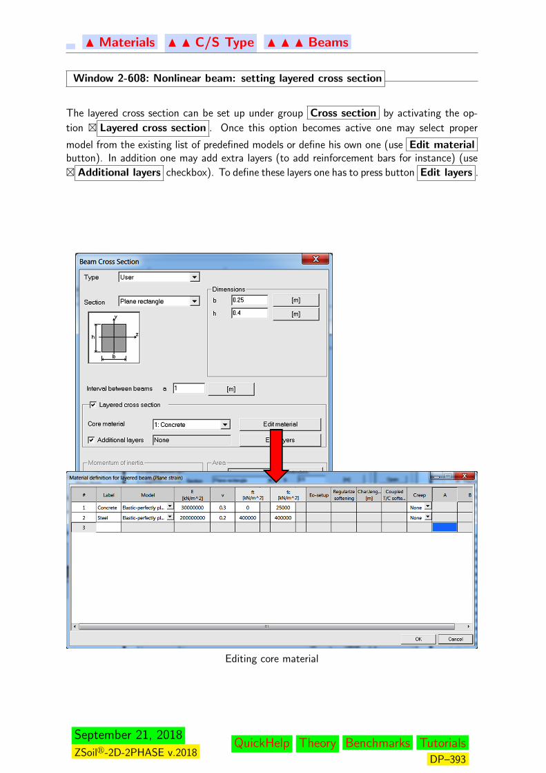
N Materials N N C/S Type N N N Beams
Window 2-608: Nonlinear beam: setting layered cross section
The layered cross section can be set up under group Cross section by activating the op-
tion � Layered cross section . Once this option becomes active one may select proper
model from the existing list of predefined models or define his own one (use Edit materialbutton). In addition one may add extra layers (to add reinforcement bars for instance) (use
� Additional layers checkbox). To define these layers one has to press button Edit layers .
Editing core material
September 21, 2018
ZSoilr-2D-2PHASE v.2018QuickHelp Theory Benchmarks Tutorials
DP–393

N Materials N N C/S Type N N N Beams
Adding extra layers
Remarks:
1. Only one core material may appear in the cross section2. The following three 1D fiber models can be used: linear, elasto-plastic and user defined;
for all of them creep can be activated (the exponential, power, logarithmic and hyperboliclaws can be used; if it is sufficient the exponential creep is recommended as it uses a singleKelvin dashpot instead of few ones as for another laws; creep in beam layers cannot bedelayed by means of the existence function;)
3. Extra layers can be prestressed4. Extra layers can be positioned in the cross section using Y, Z offsets (for all cross sections
except circular and circular tube ones, for which offset is set in the radial direction); thearea of each layer is the total one for all points representing this layer
5. Extra layers are added to the cross section no matter whether the reinforcement is defined,or not, at the beam level (using option Reinforcement sets under menu Beam in thepreprocessor)
Window 2-608
September 21, 2018
ZSoilr-2D-2PHASE v.2018QuickHelp Theory Benchmarks Tutorials
DP–394

N Materials N N C/S Type N N N Beams
Window 2-609: Linear/Nonlinear beam: general remarks
Remarks:
1. Terms Top, Bottom are related to the orientation of local element coordinate system YLaxis (positive YL points on Top). This in turns is related to:
node order (all 2D cases), as YL is set anticlockwise versus XL pointing from the 1stto 2nd node of a beam element
2. The model describing shear of the beam is assumed to remain purely elastic and uncoupledfrom its, in general, nonlinear bending and axial behavior.
3. The area of reinforcement layers will be neglected in evaluation of shear correctors κ
4. Geometry of layers related to base area of the section (i.e. Core) is fixed and can not bechanged.
5. For core material or extra layer elastic, elastic-perfectly plastic or user defined model hasto be set.
6. For the elastic/elastic-plastic Material definition the following data must be entered:
• E{[kPa]; [> 0]; 100000} – Young’s elastic modulus of the component material• Poisons ratio ν{[−]; [0, 0.49999]; 0.3}. This will be used exclusively for Core material,
only if under Elastic→ Automatic evaluation of shear modulus is set X (de-fault). Then Kirchoff modulus G for the whole section will be automatically evaluatedbasing on E, ν of Core material. In all other cases, i.e. for reinforcement layer ν isignored.• If Type is set to Elastic-perfectly plastic then additionally enter:F ft{[kPa], > 0, 1} – uniaxial tensile strength of the component materialF fc{[kPa], > 0, 1} – uniaxial compressive strength of the component material
7. For the User defined Material definition the tension and compression 1D char-acteristics must be defined via evolution functions (ε − σ relations)(stress/strain valuesare positive for both tensile and compressive branch); for softening laws set characteristiclength Lc to represent properly fracture energies (in tension and compression)
8. Material model data once entered will be stored in the job and may be reused for othersections or components.
Window 2-609
Related Topics
Theory
• BEAMS THEORY• UNI-AXIAL ELASTO–PLASTIC MODEL• UNI-AXIAL USER DEFINED MODEL
September 21, 2018
ZSoilr-2D-2PHASE v.2018QuickHelp Theory Benchmarks Tutorials
DP–395
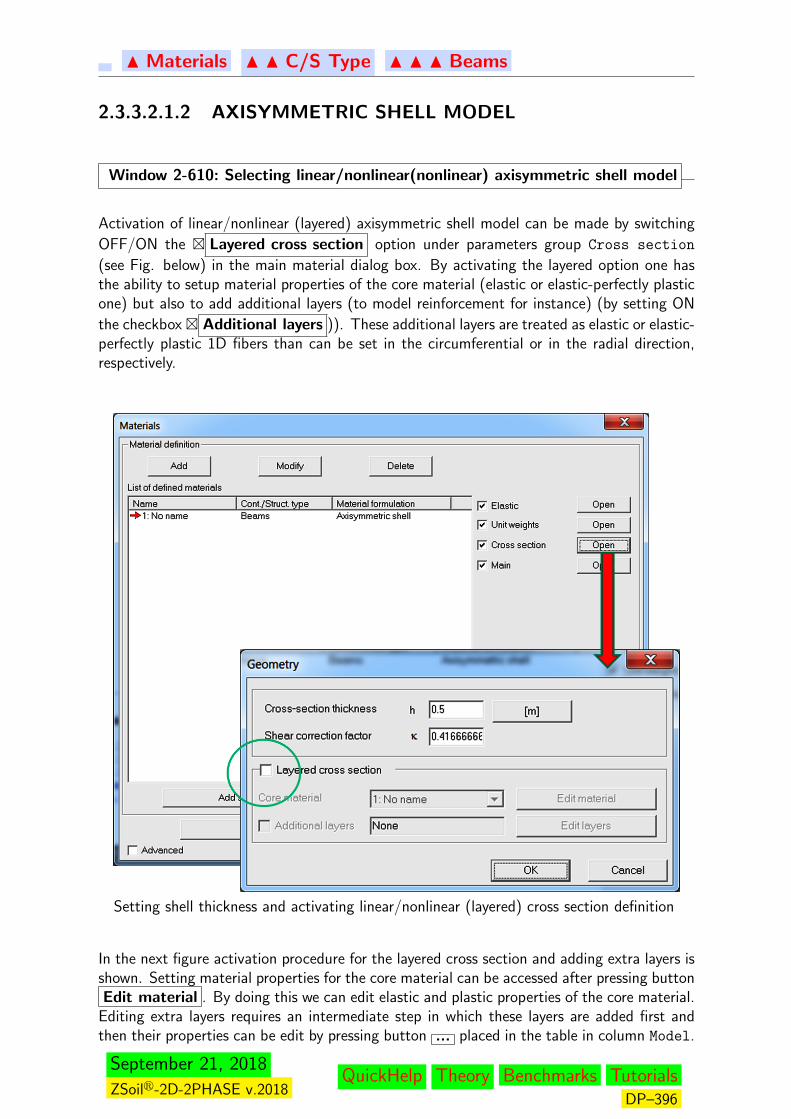
N Materials N N C/S Type N N N Beams
2.3.3.2.1.2 AXISYMMETRIC SHELL MODEL
Window 2-610: Selecting linear/nonlinear(nonlinear) axisymmetric shell model
Activation of linear/nonlinear (layered) axisymmetric shell model can be made by switching
OFF/ON the � Layered cross section option under parameters group Cross section
(see Fig. below) in the main material dialog box. By activating the layered option one hasthe ability to setup material properties of the core material (elastic or elastic-perfectly plasticone) but also to add additional layers (to model reinforcement for instance) (by setting ON
the checkbox � Additional layers )). These additional layers are treated as elastic or elastic-perfectly plastic 1D fibers than can be set in the circumferential or in the radial direction,respectively.
Setting shell thickness and activating linear/nonlinear (layered) cross section definition
In the next figure activation procedure for the layered cross section and adding extra layers isshown. Setting material properties for the core material can be accessed after pressing buttonEdit material . By doing this we can edit elastic and plastic properties of the core material.
Editing extra layers requires an intermediate step in which these layers are added first andthen their properties can be edit by pressing button ... placed in the table in column Model.
September 21, 2018
ZSoilr-2D-2PHASE v.2018QuickHelp Theory Benchmarks Tutorials
DP–396
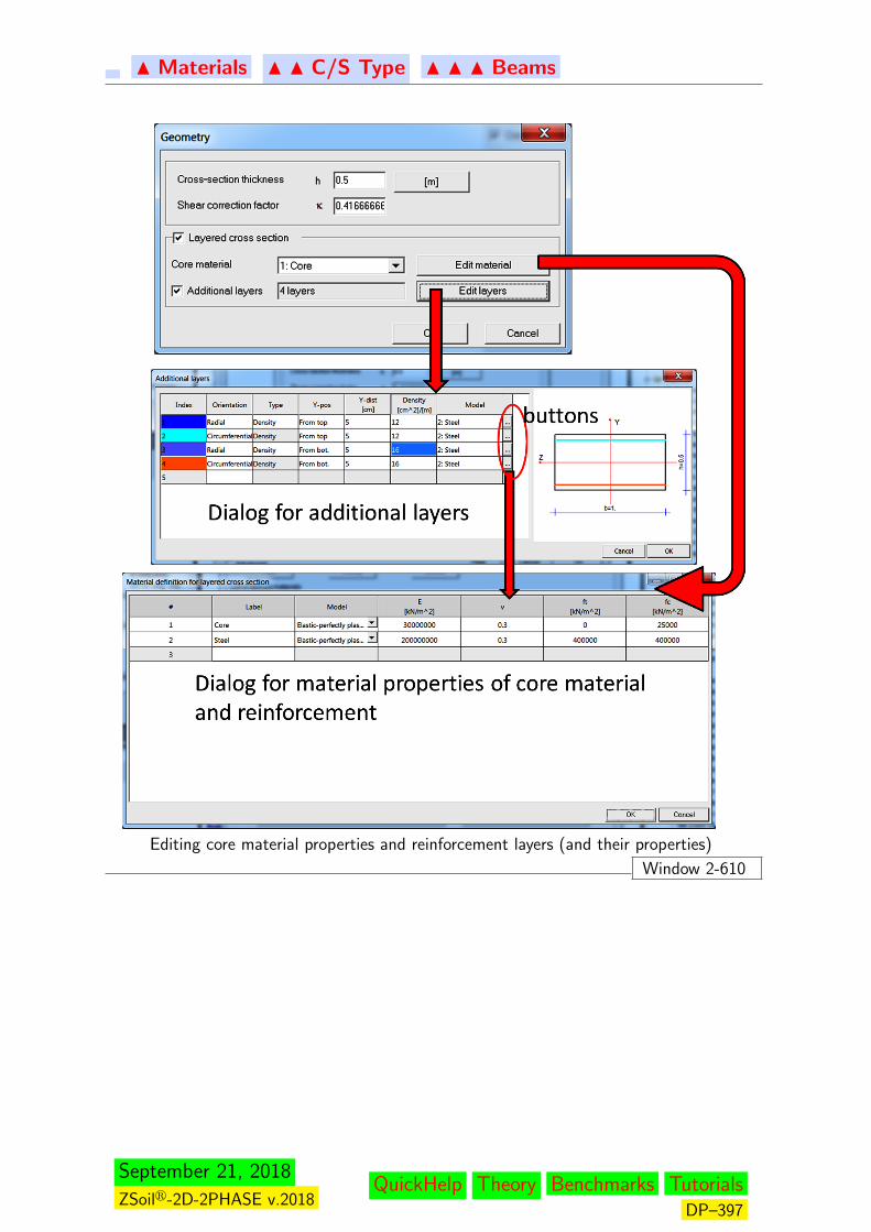
N Materials N N C/S Type N N N Beams
Editing core material properties and reinforcement layers (and their properties)
Window 2-610
September 21, 2018
ZSoilr-2D-2PHASE v.2018QuickHelp Theory Benchmarks Tutorials
DP–397
N Materials N N C/S Type N N N Beams
Window 2-611: Linear/nonlinear(layered) axisymmetric shell model: common data
The following groups of parameters are common for both linear and nonlinear (layered)axisymmetric shell models:
Data Use & Set up
Unit Weight optional;• γ, {[kNm−3]; [> 0]; 0} - unit weight of the shell (averaged
over the whole section);
• Density ρ =γ
gis automatically computed from γ (and vice
versa)• Multiplier for γ {[−]; [≥ 0]; 1.0}• Multiplier for ρ {[−]; [≥ 0]; 1.0}Setting γ multiplier to 0.0 will cancel body forces in all elementswith that material (unless body load definition is made at theelement level in the preprocessor) while setting ρ multiplier to0.0 will cancel contribution of all elements with that materialto the mass matrix; both multipliers are active if Dynamics orPushover is set ON in the project preselection).
Heat optionalα, {[C−1]; [> 0]; 1.0e−5} - thermal dilatancy coefficient.In case of active Data Group Heat and active associated Heat
Transfer project (if α > 0) thermal strains will be computed.
Stability optionalHandles material strength parameters reduction, see:LOCAL STABILITY for the details.
Damping Rayleigh damping factors αo (applies to the mass) {[s−1]; [≥0]; 0.0} and βo (applies to the stiffness) {[s]; [≥ 0]; 0.0}; dedi-cated calculator can be used if needed;
Window 2-611
September 21, 2018
ZSoilr-2D-2PHASE v.2018QuickHelp Theory Benchmarks Tutorials
DP–398
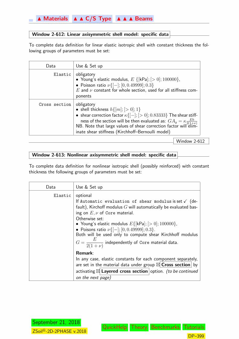
N Materials N N C/S Type N N N Beams
Window 2-612: Linear axisymmetric shell model: specific data
To complete data definition for linear elastic isotropic shell with constant thickness the fol-lowing groups of parameters must be set:
Data Use & Set up
Elastic obligatory• Young’s elastic modulus, E {[kPa]; [> 0]; 100000},• Poisson ratio ν{[−]; [0, 0.49999]; 0.3}E and ν constant for whole section, used for all stiffness com-ponents
Cross section obligatory• shell thickness h{[m]; [> 0]; 1}• shear correction factor κ{[−]; [> 0]; 0.83333} The shear stiff-
ness of the section will be then evaluated as: GAy = κ Eh2(1+ν)
NB. Note that large values of shear correction factor will elim-inate shear stiffness (Kirchhoff–Bernoulli model)
Window 2-612
Window 2-613: Nonlinear axisymmetric shell model: specific data
To complete data definition for nonlinear isotropic shell (possibly reinforced) with constantthickness the following groups of parameters must be set:
Data Use & Set up
Elastic optionalIf Automatic evaluation of shear modulus is setX (de-fault), Kirchoff modulus G will automatically be evaluated bas-ing on E, ν of Core material.Otherwise set:• Young’s elastic modulus E{[kPa]; [> 0]; 100000},• Poisons ratio ν{[−]; [0, 0.49999]; 0.3}.Both will be used only to compute shear Kirchhoff modulus
G =E
2(1 + ν)independently of Core material data.
Remark:In any case, elastic constants for each component separately,are set in the material data under group � Cross section by
activating � Layered cross section option. (to be continued
on the next page)
September 21, 2018
ZSoilr-2D-2PHASE v.2018QuickHelp Theory Benchmarks Tutorials
DP–399
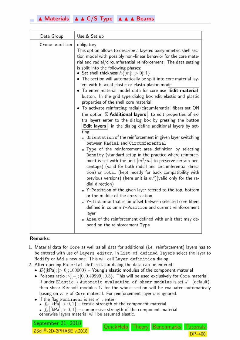
N Materials N N C/S Type N N N Beams
Data Group Use & Set up
Cross section obligatoryThis option allows to describe a layered axisymmetric shell sec-tion model with possibly non–linear behavior for the core mate-rial and radial/circumferential reinforcement. The data settingis split into the following phases:• Set shell thickness h{[m]; [> 0]; 1}• The section will automatically be split into core material lay-
ers with bi-axial elastic or elasto-plastic model• To enter material model data for core use Edit material
button. In the grid type dialog box edit elastic and plasticproperties of the shell core material.• To activate reinforcing radial/circumferential fibers set ON
the option � Additional layers ; to edit properties of ex-tra layers enter to the dialog box by pressing the buttonEdit layers ; in the dialog define additional layers by set-
tingF Orientation of the reinforcement in given layer switching
between Radial and Circumferential
F Type of the reinforcement area definition by selectingDensity (standard setup in the practice where reinforce-ment is set with the unit [m2/m] to preserve certain per-centage) (valid for both radial and circumferential direc-tion) or Total (kept mostly for back compatibility withprevious versions) (here unit is m2)(valid only for the ra-dial direction)
F Y-Position of the given layer refered to the top, bottomor the middle of the cross section
F Y-distance that is an offset between selected core fibersdefined in column Y-Position and current reinforcementlayer
F Area of the reinforcement defined with unit that may de-pend on the reinforcement Type
Remarks:
1. Material data for Core as well as all data for additional (i.e. reinforcement) layers has tobe entered with use of Layers editor. In List of defined layers select the layer toModify or Add a new one. This will call Layer definition dialog.
2. After opening Material definition dialog the data can be entered:• E{[kPa]; [> 0]; 100000} – Young’s elastic modulus of the component material• Poisons ratio ν{[−]; [0, 0.49999]; 0.3}. This will be used exclusively for Core material.
If under Elastic→ Automatic evaluation of shear modulus is set X (default),then shear Kirchoff modulus G for the whole section will be evaluated automaticalybasing on E, ν of Core material. For reinforcement layer ν is ignored.• If the flag Nonlinear is set X , enter:F ft{[kPa], > 0, 1} – tensile strength of the component materialF fc{[kPa], > 0, 1} – compressive strength of the component materialotherwise layers material will be assumed elastic.
September 21, 2018
ZSoilr-2D-2PHASE v.2018QuickHelp Theory Benchmarks Tutorials
DP–400
N Materials N N C/S Type N N N Beams
3. In contradiction to Plane Strain cases, material model for core shell in the axisymmetriccase is no longer uni-axial, as it has to deal with 2 normal components (longitudinaland circumferential) of stress and strain tensors. Based on the introduced ft, fc values,a smooth Hoek-Brown stress criterion is used to evaluate perfectly plastic constitutiveresponse of a medium. Additional (implicitly assumed) material data are eccentricity e =0.52 (optimal for concrete) and dilatancy angle ψ under uniaxial compression, i.e. anaverage between minimum and maximum values of y (see Theoretical Manual). In thecase when tensile yield stress is close to compressive one ( ft > 0.8fc), Huber-Missescriterion will be used instead of Hoek-Brown.
Window 2-613
September 21, 2018
ZSoilr-2D-2PHASE v.2018QuickHelp Theory Benchmarks Tutorials
DP–401
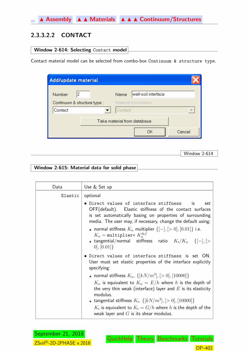
N Assembly N N Materials N N N Continuum/Structures
2.3.3.2.2 CONTACT
Window 2-614: Selecting Contact model
Contact material model can be selected from combo-box Continuum & structure type.
Window 2-614
Window 2-615: Material data for solid phase
Data Use & Set up
Elastic optional
• Direct values of interface stiffness is setOFF(default). Elastic stiffness of the contact surfacesis set automatically basing on properties of surroundingmedia. The user may, if necessary, change the default using:
F normal stiffness Kn multiplier {[−], [> 0], [0.01]} i.e.Kn = multiplier∗ Kdef
n
F tangential/normal stiffness ratio Kt/Kn {[−], [>0], [0.01]}
• Direct values of interface stiffness is set ON.User must set elastic properties of the interface explicitlyspecifying:
F normal stiffness Kn, {[kN/m3], [> 0], [10000]}Kn is equivalent to Kn = E/h where h is the depth ofthe very thin weak (interface) layer and E is its elasticitymodulus.
F tangential stiffness Kt, {[kN/m3], [> 0], [10000]}Kt is equivalent to Kt = G/h where h is the depth of theweak layer and G is its shear modulus.
September 21, 2018
ZSoilr-2D-2PHASE v.2018QuickHelp Theory Benchmarks Tutorials
DP–402
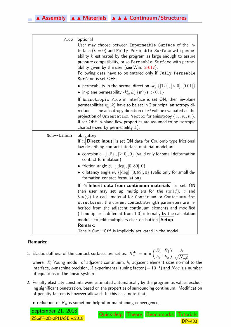
N Assembly N N Materials N N N Continuum/Structures
Flow optionalUser may choose between Impermeable Surface of the in-terface (k = 0) and Fully Permeable Surface with perme-ability k estimated by the program as large enough to assurepressure compatibility, or as Permeable Surface with perme-ability given by the user (see Win. 2-617).Following data have to be entered only if Fully Permeable
Surface is set OFF.
• permeability in the normal direction -k′z {[1/s], [> 0], [0.01]}• in-plane permeability -k′x, k
′y.{m2/s, > 0, 1}
If Anisotropic Flow in interface is set ON, then in–planepermeabilities k′x, k
′y have to be set in 2 principal anisotropy di-
rections. The anisotropy direction of x′ will be evaluated as theprojection of Orientation Vector for anisotropy {vx, vy, vz}.If set OFF in-plane flow properties are assumed to be isotropiccharacterized by permeability k′x.
Non--Linear obligatoryIf } Direct input is set ON data for Coulomb type frictionallaw describing contact interface material model are:
• cohesion c, {[kPa], [≥ 0], 0} (valid only for small deformationcontact formulation)
• friction angle φ, {[deg], [0, 89], 0}• dilatancy angle ψ, {[deg], [0, 89], 0} (valid only for small de-
formation contact formulation)
If } Inherit data from continuum materials is set ONthen user may set up multipliers for the tan(φ), c andtan(ψ) for each material for Continuum or Continuum for
structures; the current contact strength parameters are in-herited from the adjacent continuum elements and modified(if multiplier is different from 1.0) internally by the calculation
module; to edit multipliers click on button Setup .Remark:Tensile Cut--Off is implicitly activated in the model
Remarks:
1. Elastic stiffness of the contact surfaces are set as: Kdefn = min
(E1
h1,E2
h2
)A√Neqε
where: Ei Young moduli of adjacent continuum, hi adjacent element sizes normal to theinterface, ε-machine precision, A experimental tuning factor (= 10−4) and Neq is a numberof equations in the linear system
2. Penalty elasticity constants were estimated automatically by the program as values exclud-ing significant penetration, based on the properties of surrounding continuum. Modificationof penalty factors is however allowed. In this case note that:
• reduction of Kn is sometime helpful in maintaining convergence,
September 21, 2018
ZSoilr-2D-2PHASE v.2018QuickHelp Theory Benchmarks Tutorials
DP–403
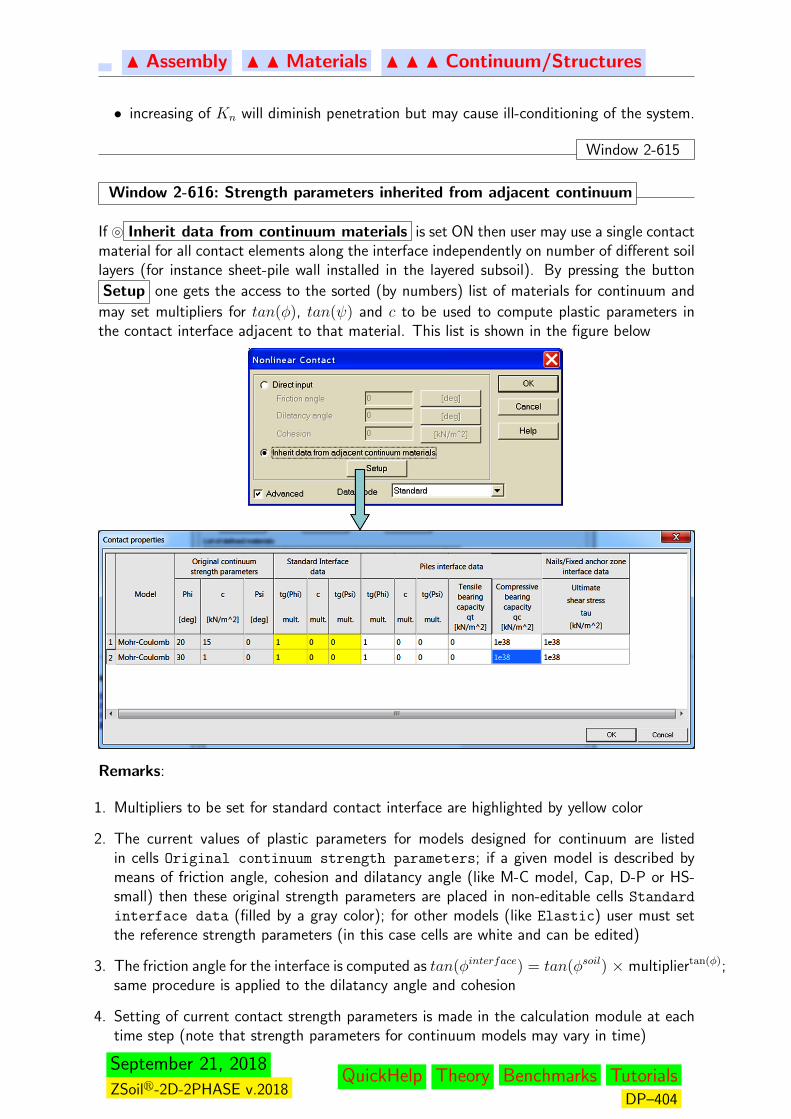
N Assembly N N Materials N N N Continuum/Structures
• increasing of Kn will diminish penetration but may cause ill-conditioning of the system.
Window 2-615
Window 2-616: Strength parameters inherited from adjacent continuum
If } Inherit data from continuum materials is set ON then user may use a single contactmaterial for all contact elements along the interface independently on number of different soillayers (for instance sheet-pile wall installed in the layered subsoil). By pressing the button
Setup one gets the access to the sorted (by numbers) list of materials for continuum and
may set multipliers for tan(φ), tan(ψ) and c to be used to compute plastic parameters inthe contact interface adjacent to that material. This list is shown in the figure below
Remarks:
1. Multipliers to be set for standard contact interface are highlighted by yellow color
2. The current values of plastic parameters for models designed for continuum are listedin cells Original continuum strength parameters; if a given model is described bymeans of friction angle, cohesion and dilatancy angle (like M-C model, Cap, D-P or HS-small) then these original strength parameters are placed in non-editable cells Standard
interface data (filled by a gray color); for other models (like Elastic) user must setthe reference strength parameters (in this case cells are white and can be edited)
3. The friction angle for the interface is computed as tan(φinterface) = tan(φsoil) × multipliertan(φ);same procedure is applied to the dilatancy angle and cohesion
4. Setting of current contact strength parameters is made in the calculation module at eachtime step (note that strength parameters for continuum models may vary in time)
September 21, 2018
ZSoilr-2D-2PHASE v.2018QuickHelp Theory Benchmarks Tutorials
DP–404

N Assembly N N Materials N N N Continuum/Structures
5. In the large deformations multiplier for cohesion is not meaningful
6. This list is common for all contact materials (including pile interfaces and pile tip interfaces)
Window 2-616
September 21, 2018
ZSoilr-2D-2PHASE v.2018QuickHelp Theory Benchmarks Tutorials
DP–405
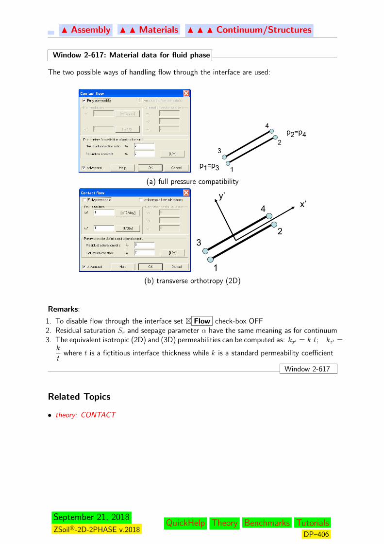
N Assembly N N Materials N N N Continuum/Structures
Window 2-617: Material data for fluid phase
The two possible ways of handling flow through the interface are used:
1
23
4
p1=p3
p2=p4
1
23
4 x’y’
1
23
4
p1=p3
p2=p4
1
23
4 x’y’
(a) full pressure compatibility
1
23
4
p1=p3
p2=p4
1
23
4 x’y’
1
23
4
p1=p3
p2=p4
1
23
4 x’y’
(b) transverse orthotropy (2D)
Remarks:
1. To disable flow through the interface set � Flow check-box OFF2. Residual saturation Sr and seepage parameter α have the same meaning as for continuum3. The equivalent isotropic (2D) and (3D) permeabilities can be computed as: kx′ = k t; kz′ =
k
twhere t is a fictitious interface thickness while k is a standard permeability coefficient
Window 2-617
Related Topics
• theory: CONTACT
September 21, 2018
ZSoilr-2D-2PHASE v.2018QuickHelp Theory Benchmarks Tutorials
DP–406
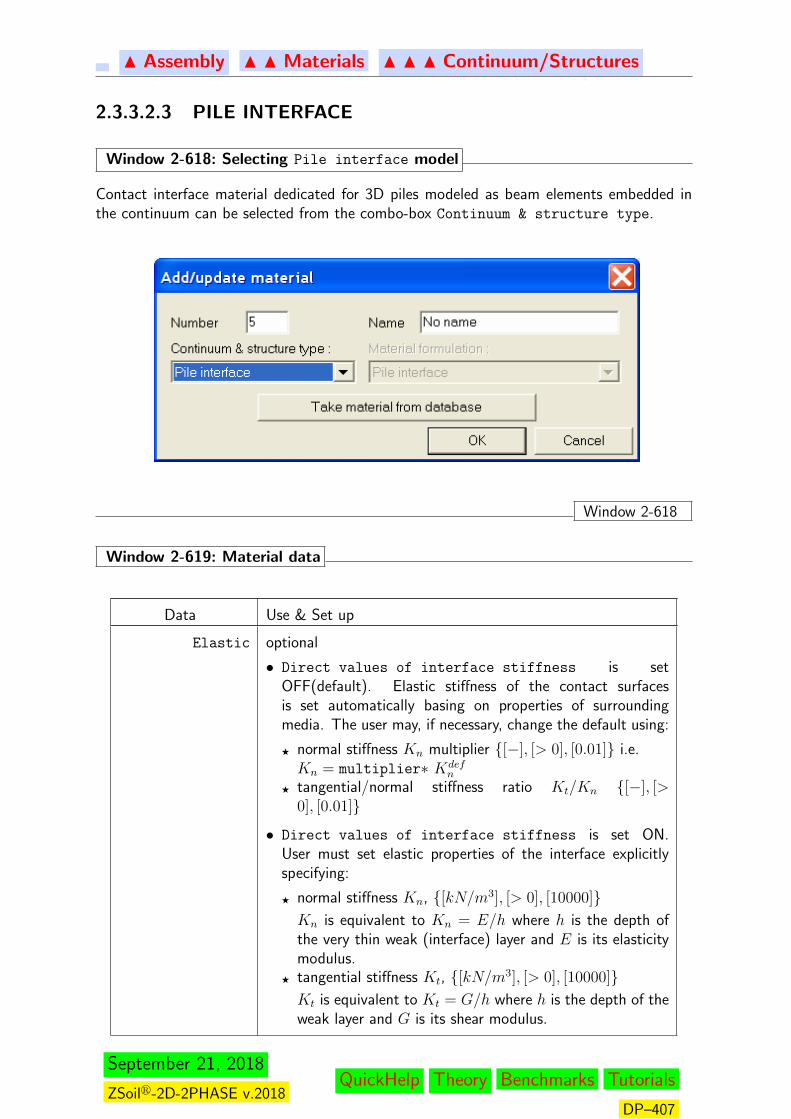
N Assembly N N Materials N N N Continuum/Structures
2.3.3.2.3 PILE INTERFACE
Window 2-618: Selecting Pile interface model
Contact interface material dedicated for 3D piles modeled as beam elements embedded inthe continuum can be selected from the combo-box Continuum & structure type.
Window 2-618
Window 2-619: Material data
Data Use & Set up
Elastic optional
• Direct values of interface stiffness is setOFF(default). Elastic stiffness of the contact surfacesis set automatically basing on properties of surroundingmedia. The user may, if necessary, change the default using:
F normal stiffness Kn multiplier {[−], [> 0], [0.01]} i.e.Kn = multiplier∗ Kdef
n
F tangential/normal stiffness ratio Kt/Kn {[−], [>0], [0.01]}
• Direct values of interface stiffness is set ON.User must set elastic properties of the interface explicitlyspecifying:
F normal stiffness Kn, {[kN/m3], [> 0], [10000]}Kn is equivalent to Kn = E/h where h is the depth ofthe very thin weak (interface) layer and E is its elasticitymodulus.
F tangential stiffness Kt, {[kN/m3], [> 0], [10000]}Kt is equivalent to Kt = G/h where h is the depth of theweak layer and G is its shear modulus.
September 21, 2018
ZSoilr-2D-2PHASE v.2018QuickHelp Theory Benchmarks Tutorials
DP–407
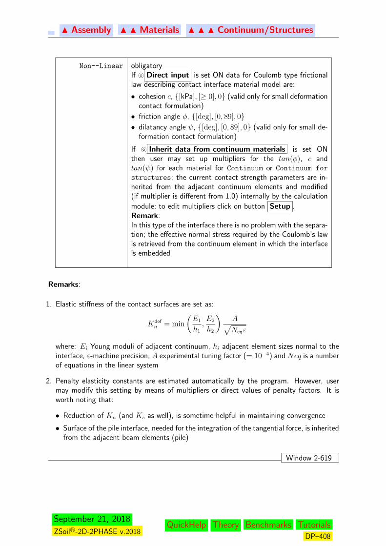
N Assembly N N Materials N N N Continuum/Structures
Non--Linear obligatoryIf } Direct input is set ON data for Coulomb type frictionallaw describing contact interface material model are:
• cohesion c, {[kPa], [≥ 0], 0} (valid only for small deformationcontact formulation)
• friction angle φ, {[deg], [0, 89], 0}• dilatancy angle ψ, {[deg], [0, 89], 0} (valid only for small de-
formation contact formulation)
If } Inherit data from continuum materials is set ONthen user may set up multipliers for the tan(φ), c andtan(ψ) for each material for Continuum or Continuum for
structures; the current contact strength parameters are in-herited from the adjacent continuum elements and modified(if multiplier is different from 1.0) internally by the calculation
module; to edit multipliers click on button Setup .Remark:In this type of the interface there is no problem with the separa-tion; the effective normal stress required by the Coulomb’s lawis retrieved from the continuum element in which the interfaceis embedded
Remarks:
1. Elastic stiffness of the contact surfaces are set as:
Kdefn = min
(E1
h1,E2
h2
)A√Neqε
where: Ei Young moduli of adjacent continuum, hi adjacent element sizes normal to theinterface, ε-machine precision, A experimental tuning factor (= 10−4) and Neq is a numberof equations in the linear system
2. Penalty elasticity constants are estimated automatically by the program. However, usermay modify this setting by means of multipliers or direct values of penalty factors. It isworth noting that:
• Reduction of Kn (and Ks as well), is sometime helpful in maintaining convergence
• Surface of the pile interface, needed for the integration of the tangential force, is inheritedfrom the adjacent beam elements (pile)
Window 2-619
September 21, 2018
ZSoilr-2D-2PHASE v.2018QuickHelp Theory Benchmarks Tutorials
DP–408

N Assembly N N Materials N N N Continuum/Structures
Window 2-620: Strength parameters inherited from adjacent continuum
If } Inherit data from continuum materials is set ON then user may use a single pileinterface material for all pile interface elements along the pile independently on number ofdifferent soil layers (for instance pile installed in the layered subsoil). By pressing the button
Setup one gets the access to the sorted (by numbers) list of materials for continuum and
may set multipliers for tan(φ), tan(ψ) and c to be used to compute plastic parameters inthe pile interface adjacent to that material. This list is shown in the figure below
Remarks:1. Multipliers to be set for pile interface are highlighted by yellow color2. The current values of plastic parameters for models designed for continuum are listed
in cells Original continuum strength parameters; if a given model is described bymeans of friction angle, cohesion and dilatancy angle (like M-C model, Cap, D-P or HS-small) then these original strength parameters are placed in non-editable cells Standard
interface data (filled by a gray color); for other models (like Elastic) user must setthe reference strength parameters (in this case cells are white and can be edited)
3. The friction angle for the interface is computed as tan(φinterface) = tan(φsoil) × multipliertan(φ);same procedure is applied to the dilatancy angle and cohesion
4. Setting current pile interface strength parameters is made in the calculation module ateach time step (note that strength parameters for continuum models may vary in time)
5. This list is common for all pile interface materials (including pile tip interfaces)Window 2-620
Related Topics
• theory: PILE INTERFACE
September 21, 2018
ZSoilr-2D-2PHASE v.2018QuickHelp Theory Benchmarks Tutorials
DP–409

N Assembly N N Materials N N N Continuum/Structures
2.3.3.2.4 PILE TIP INTERFACE
Window 2-621: Selecting Pile tip interface model
Contact material dedicated for 3D piles to model the interface between tip of the 3D pileand subsoil can be selected from the combo-box Continuum & structure type.
Window 2-621
Window 2-622: Material data
Data Use & Set up
Elastic optional
• Direct values of interface stiffness is setOFF(default). Elastic stiffness of the contact surfacesis set automatically basing on properties of surroundingmedia. The user may, if necessary, change the default using:
F normal stiffness Kn multiplier {[−], [> 0], [0.01]} i.e.Kn = multiplier∗ Kdef
n
• Direct values of interface stiffness is set ON.User must set elastic properties of the interface explicitlyspecifying:
F normal stiffness Kn, {[kN/m3], [> 0], [10000]}
September 21, 2018
ZSoilr-2D-2PHASE v.2018QuickHelp Theory Benchmarks Tutorials
DP–410
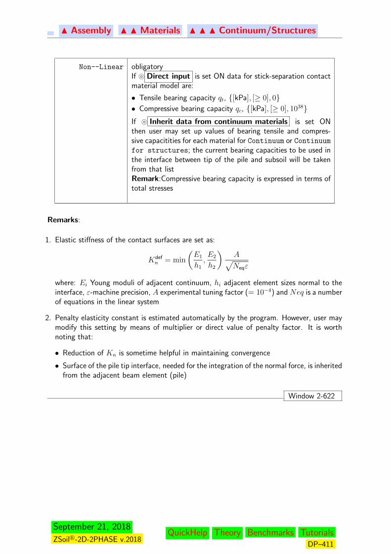
N Assembly N N Materials N N N Continuum/Structures
Non--Linear obligatoryIf } Direct input is set ON data for stick-separation contactmaterial model are:
• Tensile bearing capacity qt, {[kPa], [≥ 0], 0}• Compressive bearing capacity qc, {[kPa], [≥ 0], 1038}If } Inherit data from continuum materials is set ONthen user may set up values of bearing tensile and compres-sive capacitities for each material for Continuum or Continuumfor structures; the current bearing capacities to be used inthe interface between tip of the pile and subsoil will be takenfrom that listRemark:Compressive bearing capacity is expressed in terms oftotal stresses
Remarks:
1. Elastic stiffness of the contact surfaces are set as:
Kdefn = min
(E1
h1,E2
h2
)A√Neqε
where: Ei Young moduli of adjacent continuum, hi adjacent element sizes normal to theinterface, ε-machine precision, A experimental tuning factor (= 10−4) and Neq is a numberof equations in the linear system
2. Penalty elasticity constant is estimated automatically by the program. However, user maymodify this setting by means of multiplier or direct value of penalty factor. It is worthnoting that:
• Reduction of Kn is sometime helpful in maintaining convergence
• Surface of the pile tip interface, needed for the integration of the normal force, is inheritedfrom the adjacent beam element (pile)
Window 2-622
September 21, 2018
ZSoilr-2D-2PHASE v.2018QuickHelp Theory Benchmarks Tutorials
DP–411

N Assembly N N Materials N N N Continuum/Structures
Window 2-623: Strength parameters inherited from adjacent continuum
If } Inherit data from continuum materials is set ON then user may set up bearing ca-pacities (tensile and compressive) for tip of the pile embedded in a given continuum material.
By pressing the button Setup one gets the access to the sorted (by numbers) list of mate-
rials for continuum and may set up these values (qt and qc respectively). This list is shownin the figure below
Remarks:
1. qt and qc values to be set for the pile tip interface are highlighted by yellow color; thesevalues are usually available in codes for standard piles design
Window 2-623
Related Topics
• theory: PILE TIP INTERFACE
September 21, 2018
ZSoilr-2D-2PHASE v.2018QuickHelp Theory Benchmarks Tutorials
DP–412
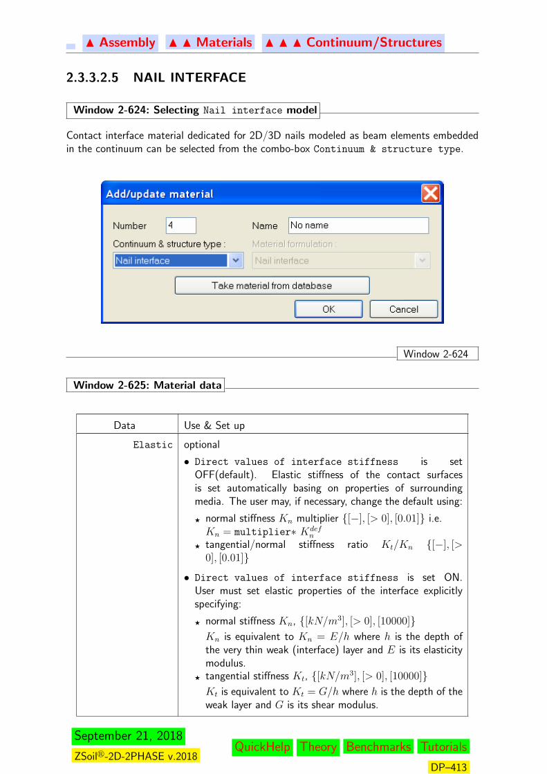
N Assembly N N Materials N N N Continuum/Structures
2.3.3.2.5 NAIL INTERFACE
Window 2-624: Selecting Nail interface model
Contact interface material dedicated for 2D/3D nails modeled as beam elements embeddedin the continuum can be selected from the combo-box Continuum & structure type.
Window 2-624
Window 2-625: Material data
Data Use & Set up
Elastic optional
• Direct values of interface stiffness is setOFF(default). Elastic stiffness of the contact surfacesis set automatically basing on properties of surroundingmedia. The user may, if necessary, change the default using:
F normal stiffness Kn multiplier {[−], [> 0], [0.01]} i.e.Kn = multiplier∗ Kdef
n
F tangential/normal stiffness ratio Kt/Kn {[−], [>0], [0.01]}
• Direct values of interface stiffness is set ON.User must set elastic properties of the interface explicitlyspecifying:
F normal stiffness Kn, {[kN/m3], [> 0], [10000]}Kn is equivalent to Kn = E/h where h is the depth ofthe very thin weak (interface) layer and E is its elasticitymodulus.
F tangential stiffness Kt, {[kN/m3], [> 0], [10000]}Kt is equivalent to Kt = G/h where h is the depth of theweak layer and G is its shear modulus.
September 21, 2018
ZSoilr-2D-2PHASE v.2018QuickHelp Theory Benchmarks Tutorials
DP–413
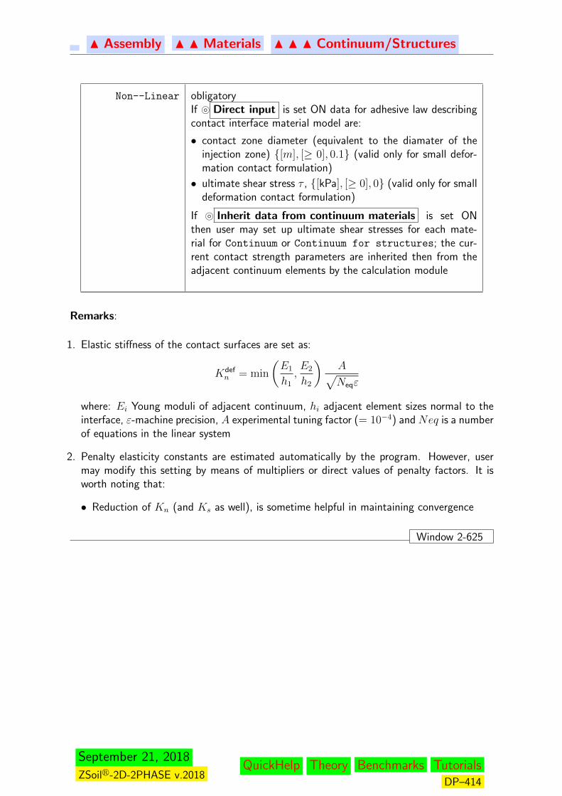
N Assembly N N Materials N N N Continuum/Structures
Non--Linear obligatoryIf } Direct input is set ON data for adhesive law describingcontact interface material model are:
• contact zone diameter (equivalent to the diamater of theinjection zone) {[m], [≥ 0], 0.1} (valid only for small defor-mation contact formulation)
• ultimate shear stress τ , {[kPa], [≥ 0], 0} (valid only for smalldeformation contact formulation)
If } Inherit data from continuum materials is set ONthen user may set up ultimate shear stresses for each mate-rial for Continuum or Continuum for structures; the cur-rent contact strength parameters are inherited then from theadjacent continuum elements by the calculation module
Remarks:
1. Elastic stiffness of the contact surfaces are set as:
Kdefn = min
(E1
h1,E2
h2
)A√Neqε
where: Ei Young moduli of adjacent continuum, hi adjacent element sizes normal to theinterface, ε-machine precision, A experimental tuning factor (= 10−4) and Neq is a numberof equations in the linear system
2. Penalty elasticity constants are estimated automatically by the program. However, usermay modify this setting by means of multipliers or direct values of penalty factors. It isworth noting that:
• Reduction of Kn (and Ks as well), is sometime helpful in maintaining convergence
Window 2-625
September 21, 2018
ZSoilr-2D-2PHASE v.2018QuickHelp Theory Benchmarks Tutorials
DP–414
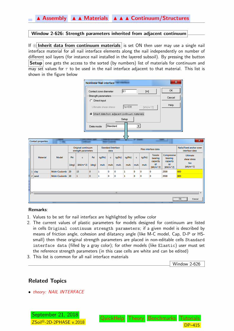
N Assembly N N Materials N N N Continuum/Structures
Window 2-626: Strength parameters inherited from adjacent continuum
If } Inherit data from continuum materials is set ON then user may use a single nailinterface material for all nail interface elements along the nail independently on number ofdifferent soil layers (for instance nail installed in the layered subsoil). By pressing the button
Setup one gets the access to the sorted (by numbers) list of materials for continuum andmay set values for τ to be used in the nail interface adjacent to that material. This list isshown in the figure below
Remarks:
1. Values to be set for nail interface are highlighted by yellow color2. The current values of plastic parameters for models designed for continuum are listed
in cells Original continuum strength parameters; if a given model is described bymeans of friction angle, cohesion and dilatancy angle (like M-C model, Cap, D-P or HS-small) then these original strength parameters are placed in non-editable cells Standard
interface data (filled by a gray color); for other models (like Elastic) user must setthe reference strength parameters (in this case cells are white and can be edited)
3. This list is common for all nail interface materials
Window 2-626
Related Topics
• theory: NAIL INTERFACE
September 21, 2018
ZSoilr-2D-2PHASE v.2018QuickHelp Theory Benchmarks Tutorials
DP–415
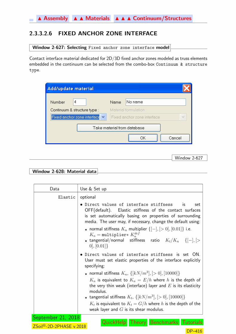
N Assembly N N Materials N N N Continuum/Structures
2.3.3.2.6 FIXED ANCHOR ZONE INTERFACE
Window 2-627: Selecting Fixed anchor zone interface model
Contact interface material dedicated for 2D/3D fixed anchor zones modeled as truss elementsembedded in the continuum can be selected from the combo-box Continuum & structure
type.
Window 2-627
Window 2-628: Material data
Data Use & Set up
Elastic optional
• Direct values of interface stiffness is setOFF(default). Elastic stiffness of the contact surfacesis set automatically basing on properties of surroundingmedia. The user may, if necessary, change the default using:
F normal stiffness Kn multiplier {[−], [> 0], [0.01]} i.e.Kn = multiplier∗ Kdef
n
F tangential/normal stiffness ratio Kt/Kn {[−], [>0], [0.01]}
• Direct values of interface stiffness is set ON.User must set elastic properties of the interface explicitlyspecifying:
F normal stiffness Kn, {[kN/m3], [> 0], [10000]}Kn is equivalent to Kn = E/h where h is the depth ofthe very thin weak (interface) layer and E is its elasticitymodulus.
F tangential stiffness Kt, {[kN/m3], [> 0], [10000]}Kt is equivalent to Kt = G/h where h is the depth of theweak layer and G is its shear modulus.
September 21, 2018
ZSoilr-2D-2PHASE v.2018QuickHelp Theory Benchmarks Tutorials
DP–416

N Assembly N N Materials N N N Continuum/Structures
Non--Linear obligatoryIf } Direct input is set ON data for adhesive law describingcontact interface material model are:
• contact zone diameter (equivalent to the diamater of theinjection zone) {[m], [≥ 0], 0.1} (valid only for small defor-mation contact formulation)
• ultimate shear stress τ , {[kPa], [≥ 0], 0} (valid only for smalldeformation contact formulation)
If } Inherit data from continuum materials is set ONthen user may set up ultimate shear stresses for each mate-rial for Continuum or Continuum for structures; the cur-rent contact strength parameters are inherited then from theadjacent continuum elements by the calculation module
Remarks:
1. Elastic stiffness of the contact surfaces are set as:
Kdefn = min
(E1
h1,E2
h2
)A√Neqε
where: Ei Young moduli of adjacent continuum, hi adjacent element sizes normal to theinterface, ε-machine precision, A experimental tuning factor (= 10−4) and Neq is a numberof equations in the linear system
2. Penalty elasticity constants are estimated automatically by the program. However, usermay modify this setting by means of multipliers or direct values of penalty factors. It isworth noting that:
• Reduction of Kn (and Ks as well), is sometime helpful in maintaining convergence
Window 2-628
September 21, 2018
ZSoilr-2D-2PHASE v.2018QuickHelp Theory Benchmarks Tutorials
DP–417
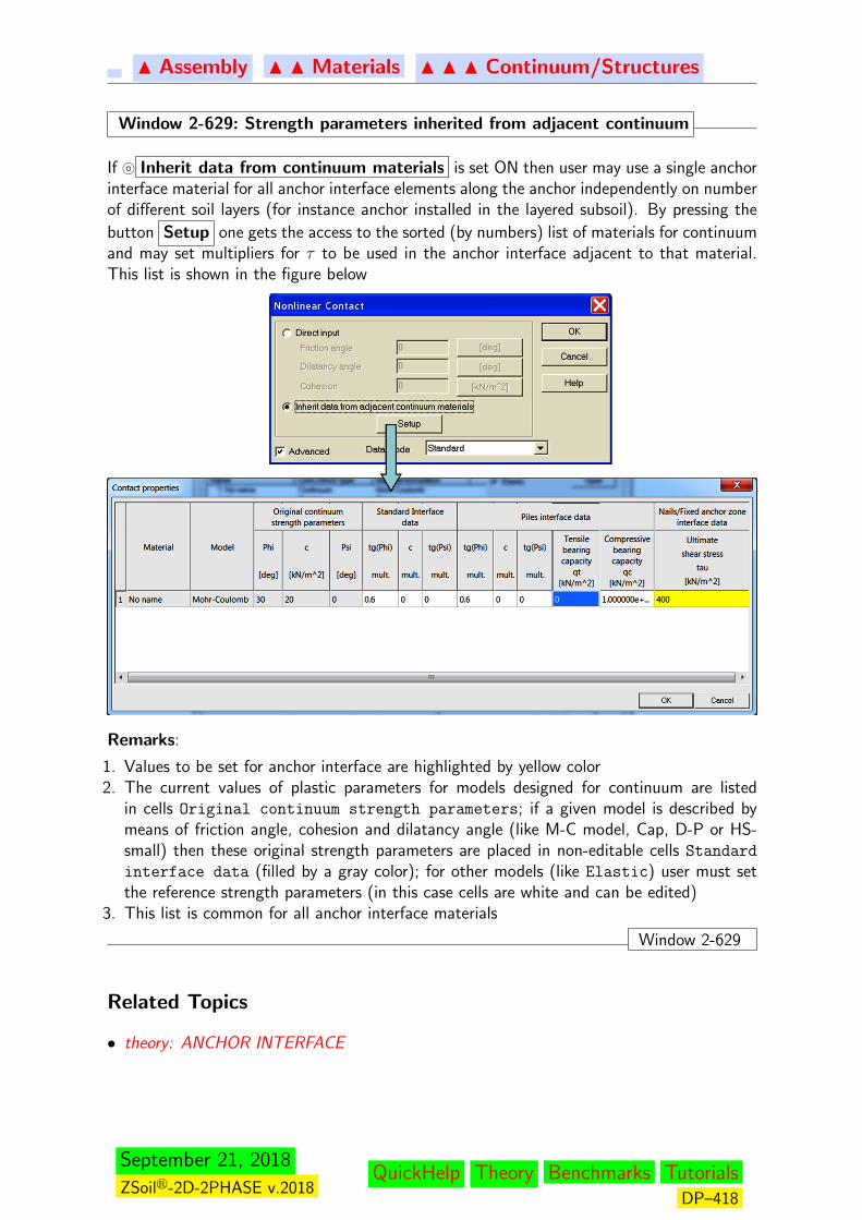
N Assembly N N Materials N N N Continuum/Structures
Window 2-629: Strength parameters inherited from adjacent continuum
If } Inherit data from continuum materials is set ON then user may use a single anchorinterface material for all anchor interface elements along the anchor independently on numberof different soil layers (for instance anchor installed in the layered subsoil). By pressing the
button Setup one gets the access to the sorted (by numbers) list of materials for continuumand may set multipliers for τ to be used in the anchor interface adjacent to that material.This list is shown in the figure below
Remarks:
1. Values to be set for anchor interface are highlighted by yellow color2. The current values of plastic parameters for models designed for continuum are listed
in cells Original continuum strength parameters; if a given model is described bymeans of friction angle, cohesion and dilatancy angle (like M-C model, Cap, D-P or HS-small) then these original strength parameters are placed in non-editable cells Standard
interface data (filled by a gray color); for other models (like Elastic) user must setthe reference strength parameters (in this case cells are white and can be edited)
3. This list is common for all anchor interface materials
Window 2-629
Related Topics
• theory: ANCHOR INTERFACE
September 21, 2018
ZSoilr-2D-2PHASE v.2018QuickHelp Theory Benchmarks Tutorials
DP–418
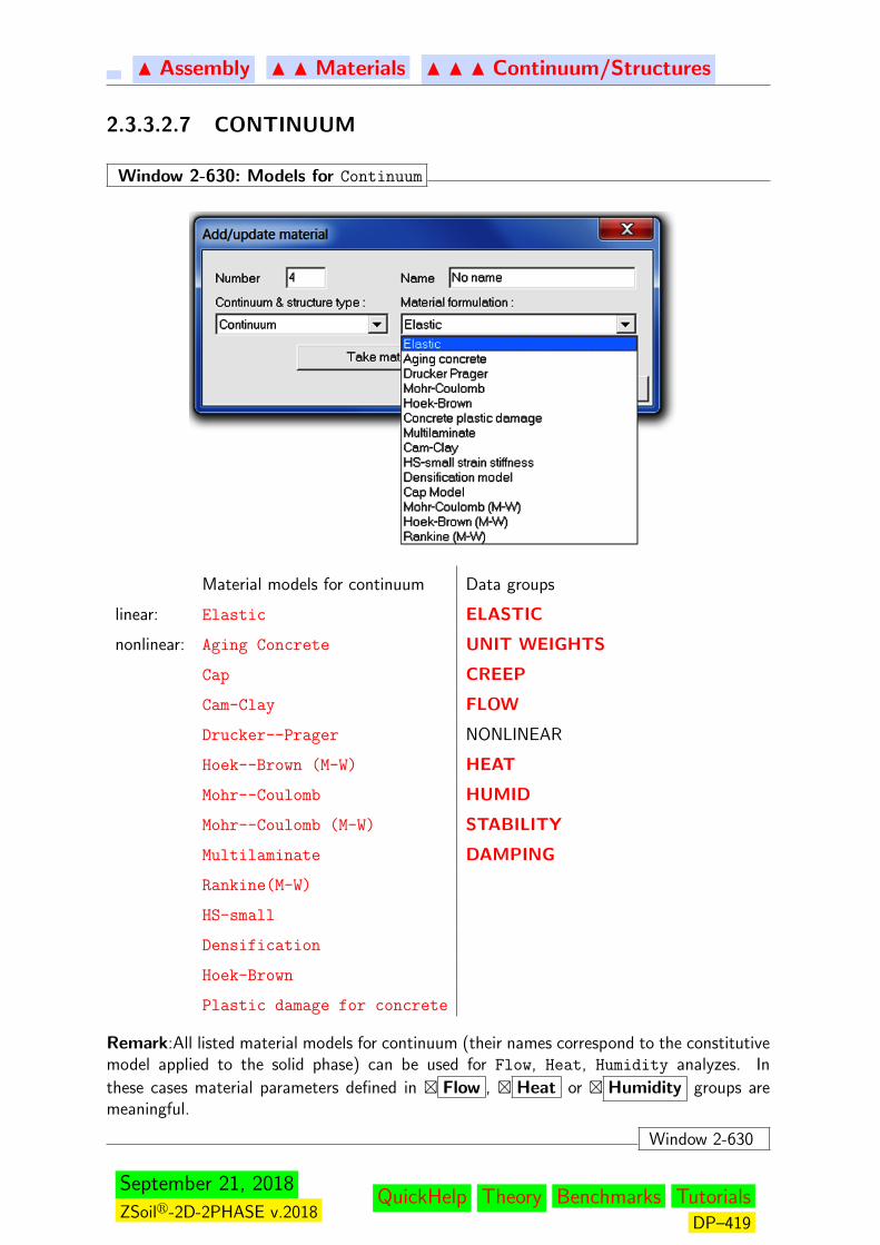
N Assembly N N Materials N N N Continuum/Structures
2.3.3.2.7 CONTINUUM
Window 2-630: Models for Continuum
Material models for continuum Data groups
linear: Elastic ELASTIC
nonlinear: Aging Concrete UNIT WEIGHTS
Cap CREEP
Cam-Clay FLOW
Drucker--Prager NONLINEAR
Hoek--Brown (M-W) HEAT
Mohr--Coulomb HUMID
Mohr--Coulomb (M-W) STABILITY
Multilaminate DAMPING
Rankine(M-W)
HS-small
Densification
Hoek-Brown
Plastic damage for concrete
Remark:All listed material models for continuum (their names correspond to the constitutivemodel applied to the solid phase) can be used for Flow, Heat, Humidity analyzes. In
these cases material parameters defined in � Flow , � Heat or � Humidity groups aremeaningful.
Window 2-630
September 21, 2018
ZSoilr-2D-2PHASE v.2018QuickHelp Theory Benchmarks Tutorials
DP–419
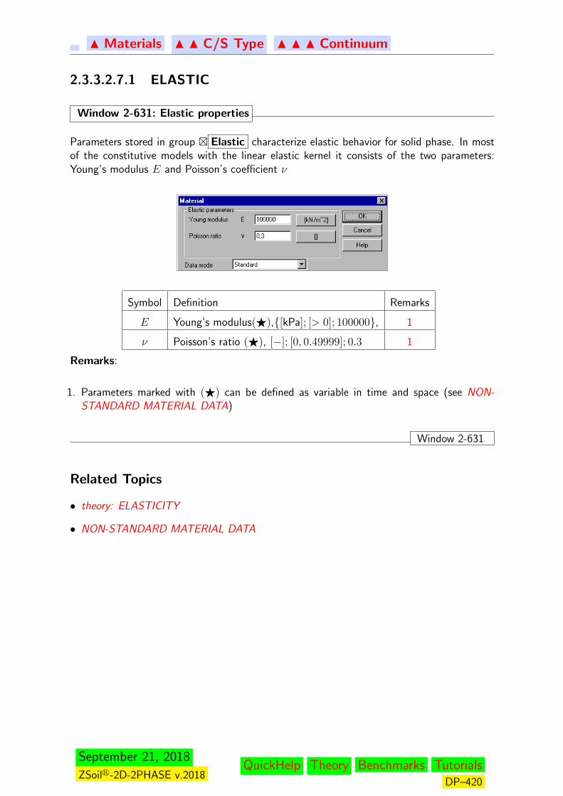
N Materials N N C/S Type N N N Continuum
2.3.3.2.7.1 ELASTIC
Window 2-631: Elastic properties
Parameters stored in group � Elastic characterize elastic behavior for solid phase. In mostof the constitutive models with the linear elastic kernel it consists of the two parameters:Young’s modulus E and Poisson’s coefficient ν
Symbol Definition Remarks
E Young’s modulus(F),{[kPa]; [> 0]; 100000}, 1
ν Poisson’s ratio (F), [−]; [0, 0.49999]; 0.3 1
Remarks:
1. Parameters marked with (F) can be defined as variable in time and space (see NON-STANDARD MATERIAL DATA)
Window 2-631
Related Topics
• theory: ELASTICITY
• NON-STANDARD MATERIAL DATA
September 21, 2018
ZSoilr-2D-2PHASE v.2018QuickHelp Theory Benchmarks Tutorials
DP–420
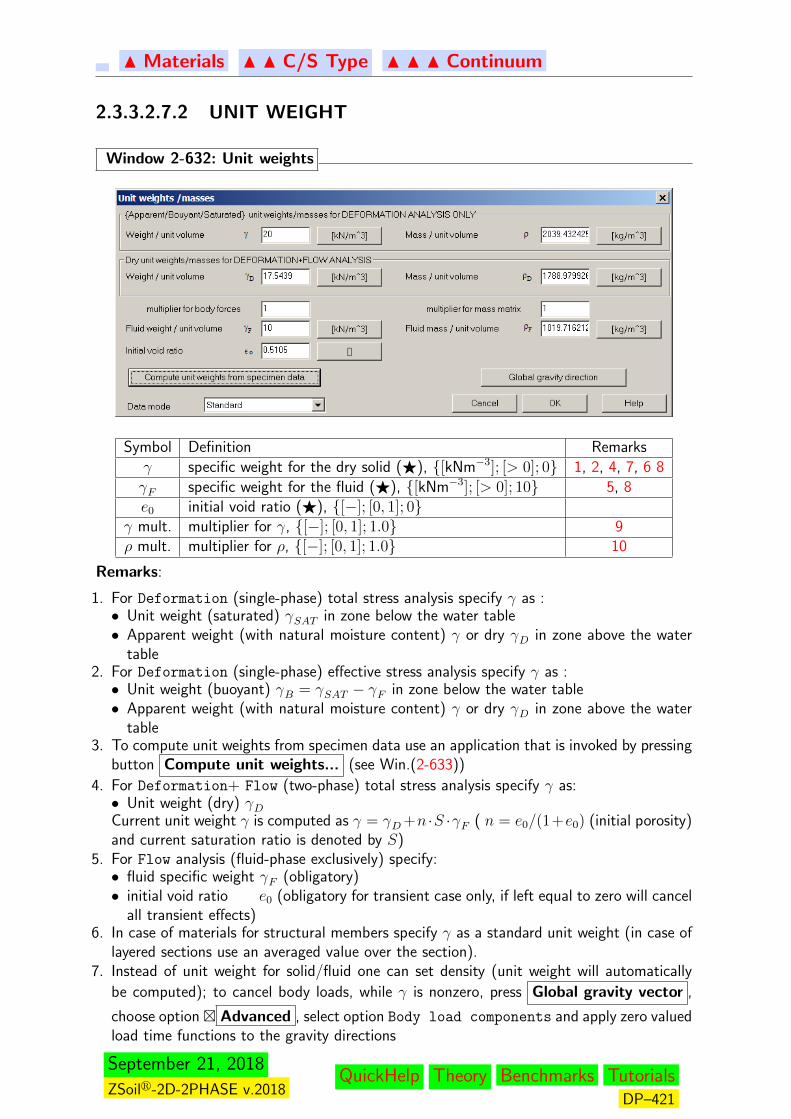
N Materials N N C/S Type N N N Continuum
2.3.3.2.7.2 UNIT WEIGHT
Window 2-632: Unit weights
Symbol Definition Remarksγ specific weight for the dry solid (F), {[kNm−3]; [> 0]; 0} 1, 2, 4, 7, 6 8γF specific weight for the fluid (F), {[kNm−3]; [> 0]; 10} 5, 8e0 initial void ratio (F), {[−]; [0, 1]; 0}
γ mult. multiplier for γ, {[−]; [0, 1]; 1.0} 9ρ mult. multiplier for ρ, {[−]; [0, 1]; 1.0} 10
Remarks:
1. For Deformation (single-phase) total stress analysis specify γ as :• Unit weight (saturated) γSAT in zone below the water table• Apparent weight (with natural moisture content) γ or dry γD in zone above the water
table2. For Deformation (single-phase) effective stress analysis specify γ as :• Unit weight (buoyant) γB = γSAT − γF in zone below the water table• Apparent weight (with natural moisture content) γ or dry γD in zone above the water
table3. To compute unit weights from specimen data use an application that is invoked by pressing
button Compute unit weights... (see Win.(2-633))
4. For Deformation+ Flow (two-phase) total stress analysis specify γ as:• Unit weight (dry) γDCurrent unit weight γ is computed as γ = γD+n ·S ·γF ( n = e0/(1+e0) (initial porosity)and current saturation ratio is denoted by S)
5. For Flow analysis (fluid-phase exclusively) specify:• fluid specific weight γF (obligatory)• initial void ratio e0 (obligatory for transient case only, if left equal to zero will cancel
all transient effects)6. In case of materials for structural members specify γ as a standard unit weight (in case of
layered sections use an averaged value over the section).7. Instead of unit weight for solid/fluid one can set density (unit weight will automatically
be computed); to cancel body loads, while γ is nonzero, press Global gravity vector ,
choose option � Advanced , select option Body load components and apply zero valuedload time functions to the gravity directions
September 21, 2018
ZSoilr-2D-2PHASE v.2018QuickHelp Theory Benchmarks Tutorials
DP–421
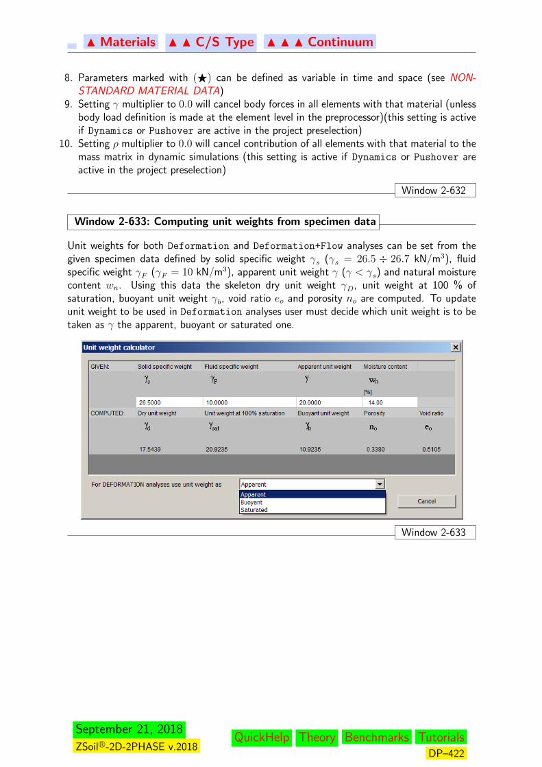
N Materials N N C/S Type N N N Continuum
8. Parameters marked with (F) can be defined as variable in time and space (see NON-STANDARD MATERIAL DATA)
9. Setting γ multiplier to 0.0 will cancel body forces in all elements with that material (unlessbody load definition is made at the element level in the preprocessor)(this setting is activeif Dynamics or Pushover are active in the project preselection)
10. Setting ρ multiplier to 0.0 will cancel contribution of all elements with that material to themass matrix in dynamic simulations (this setting is active if Dynamics or Pushover areactive in the project preselection)
Window 2-632
Window 2-633: Computing unit weights from specimen data
Unit weights for both Deformation and Deformation+Flow analyses can be set from thegiven specimen data defined by solid specific weight γs (γs = 26.5 ÷ 26.7 kN/m3), fluidspecific weight γF (γF = 10 kN/m3), apparent unit weight γ (γ < γs) and natural moisturecontent wn. Using this data the skeleton dry unit weight γD, unit weight at 100 % ofsaturation, buoyant unit weight γb, void ratio eo and porosity no are computed. To updateunit weight to be used in Deformation analyses user must decide which unit weight is to betaken as γ the apparent, buoyant or saturated one.
Window 2-633
September 21, 2018
ZSoilr-2D-2PHASE v.2018QuickHelp Theory Benchmarks Tutorials
DP–422

N Materials N N C/S Type N N N Continuum
2.3.3.2.7.3 FLOW
This group of parameters is meaningful only for Flow or Deformation + Flow problems. Ifgroup � Flow is set OFF then the considered material is treated as impermeable 2.
Window 2-634: Flow properties (2D case)
Symbol Definition RemarksβF Fluid bulk modulus {[kPa]; [> 0]; 1.0e+ 38}, 3
kx, ky(F) Permeability coefficients {[ms−1]; [> 0]; 1.0} 1,4,5β Inclination angle measured from x axis to 5
x′ permeability direction {[deg]; [0, 90]; 0}Sr Residual saturation {[−]; [0, 1]; 0}α Seepage parameter {[m−1]; [> 0]; 2.0} 6
� Skip .. Skip gravity term in Darcy’s law {OFF} 7
� Undr... Allow undrained behavior {ON} 8KF
KPenalty factor {[−]; [105 ÷ 107]; 106} 8
pcut−off Suction cut-off value {[kN/m3]; [≥ 0]; 100} 8
Window 2-634
September 21, 2018
ZSoilr-2D-2PHASE v.2018QuickHelp Theory Benchmarks Tutorials
DP–423

N Materials N N C/S Type N N N Continuum
Window 2-635: General remarks on flow properties
Remarks:
1. Parameters marked with (F) can be defined as variable in time and space (see NON-STANDARD MATERIAL DATA)
2. Avoid situation when seepage elements are adjacent to impermeable material (� Flow isset OFF)
3. Large value of βF yields fluid quasi-incompressibility4. Permeability coefficients are set up in principal directions5. For isotropic media set kx = ky. In that case setting direction is meaningless6. Large value of α reduces the thickness of the transition zone from the saturated to un-
saturated, as shown in Window 2-636. It will also slow down convergence.7. This flag allows to cancel the gravity term in Darcy law. This option may be useful when
modeling nonhydrostatic initial distribution of the presure field.8. Pure undrained behavior of soils can be modeled by using Driven load-undrained driver
that is available for Deformation+Flow analyses. Any material for continuum that hasthis flag set to ON will undergo undrained behavior when undrained driver is currentlyrun. The undrained behavior is implemented through penalty approach assuming that theratio between the artifficial bulk modulus of fluid and soil skeleton (the current elastic bulkmodulus) is a relatively large value from range 105 ÷ 107. In addition one may controlthe evolution of the suction pressure that can be generated during excavations. However,special care must be taken here. If the undrained driver follows any other like Driven
load+Steady state, Driven load+Transient or Consolidation then the conditionfor the suction pressure is verified for pressure p = S(po) po + ∆p where po is the pressurevalue produced from full two-phase theory, S(po) is the saturation ratio corresponding tothe po pressure (according to the van Genuchten’s law) and the undrained excess porepressure ∆p is produced exclusively by the undrained driver.
Window 2-635
September 21, 2018
ZSoilr-2D-2PHASE v.2018QuickHelp Theory Benchmarks Tutorials
DP–424

N Materials N N C/S Type N N N Continuum
Window 2-636: Saturation ratio
Saturation ratio in partially saturated zone as a function of h = pF /γF for different α
Window 2-636
Related Topics
• PROBLEM STATEMENT: TWO-PHASE MEDIA
• NUMERICAL IMPLEMENTATION: TWO-PHASE MEDIA
• MATERIAL MODELS: DARCY LAW
• NON-STANDARD MATERIAL DATA
September 21, 2018
ZSoilr-2D-2PHASE v.2018QuickHelp Theory Benchmarks Tutorials
DP–425
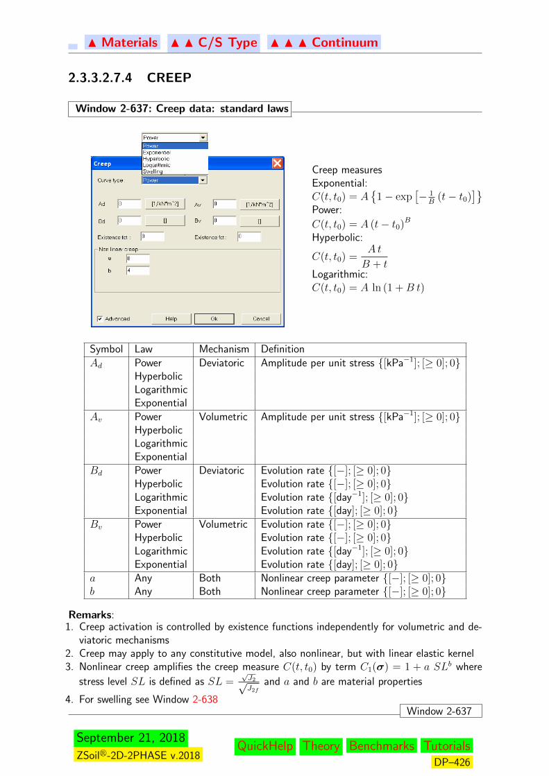
N Materials N N C/S Type N N N Continuum
2.3.3.2.7.4 CREEP
Window 2-637: Creep data: standard laws
Creep measuresExponential:C(t, t0) = A
{1− exp
[− 1B
(t− t0)]}
Power:
C(t, t0) = A (t− t0)BHyperbolic:
C(t, t0) =A t
B + tLogarithmic:C(t, t0) = A ln (1 +B t)
Symbol Law Mechanism DefinitionAd Power Deviatoric Amplitude per unit stress {[kPa−1]; [≥ 0]; 0}
HyperbolicLogarithmicExponential
Av Power Volumetric Amplitude per unit stress {[kPa−1]; [≥ 0]; 0}HyperbolicLogarithmicExponential
Bd Power Deviatoric Evolution rate {[−]; [≥ 0]; 0}Hyperbolic Evolution rate {[−]; [≥ 0]; 0}Logarithmic Evolution rate {[day−1]; [≥ 0]; 0}Exponential Evolution rate {[day]; [≥ 0]; 0}
Bv Power Volumetric Evolution rate {[−]; [≥ 0]; 0}Hyperbolic Evolution rate {[−]; [≥ 0]; 0}Logarithmic Evolution rate {[day−1]; [≥ 0]; 0}Exponential Evolution rate {[day]; [≥ 0]; 0}
a Any Both Nonlinear creep parameter {[−]; [≥ 0]; 0}b Any Both Nonlinear creep parameter {[−]; [≥ 0]; 0}
Remarks:1. Creep activation is controlled by existence functions independently for volumetric and de-
viatoric mechanisms2. Creep may apply to any constitutive model, also nonlinear, but with linear elastic kernel3. Nonlinear creep amplifies the creep measure C(t, t0) by term C1(σ) = 1 + a SLb where
stress level SL is defined as SL =√J2√J2f
and a and b are material properties
4. For swelling see Window 2-638Window 2-637
September 21, 2018
ZSoilr-2D-2PHASE v.2018QuickHelp Theory Benchmarks Tutorials
DP–426
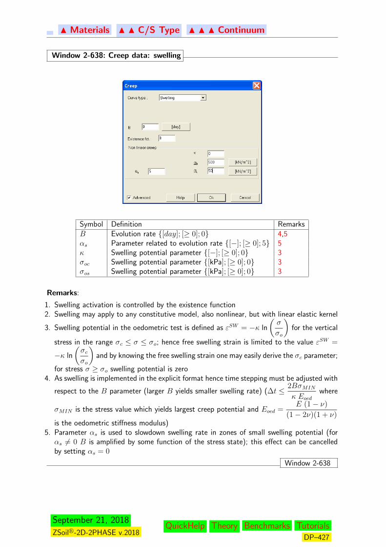
N Materials N N C/S Type N N N Continuum
Window 2-638: Creep data: swelling
Symbol Definition RemarksB Evolution rate {[day]; [≥ 0]; 0} 4,5αs Parameter related to evolution rate {[−]; [≥ 0]; 5} 5κ Swelling potential parameter {[−]; [≥ 0]; 0} 3σoc Swelling potential parameter {[kPa]; [≥ 0]; 0} 3σos Swelling potential parameter {[kPa]; [≥ 0]; 0} 3
Remarks:
1. Swelling activation is controlled by the existence function2. Swelling may apply to any constitutive model, also nonlinear, but with linear elastic kernel
3. Swelling potential in the oedometric test is defined as εSW = −κ ln
(σ
σo
)for the vertical
stress in the range σc ≤ σ ≤ σo; hence free swelling strain is limited to the value εSW =
−κ ln
(σcσo
)and by knowing the free swelling strain one may easily derive the σc parameter;
for stress σ ≥ σo swelling potential is zero4. As swelling is implemented in the explicit format hence time stepping must be adjusted with
respect to the B parameter (larger B yields smaller swelling rate) (∆t ≤ 2BσMIN
κ Eoedwhere
σMIN is the stress value which yields largest creep potential and Eoed =E (1− ν)
(1− 2ν)(1 + ν)is the oedometric stiffness modulus)
5. Parameter αs is used to slowdown swelling rate in zones of small swelling potential (forαs 6= 0 B is amplified by some function of the stress state); this effect can be cancelledby setting αs = 0
Window 2-638
September 21, 2018
ZSoilr-2D-2PHASE v.2018QuickHelp Theory Benchmarks Tutorials
DP–427

N Materials N N C/S Type N N N Continuum
Window 2-639: Creep data: EC2 creep with aging
Symbol Definition RemarksA Creep amplitude 3B Creep rate 4Initial age Age of analyzed concrete 5Equivalent time flag Flag whether to use temperature adjusted time 7, 6Q
RRatio between activation energy and universal gas constant 8
Tref Reference temperatures Strength evolution parameter 9t28 Time of 28 days in formula for βcc (EC2) 10n Exponent in expression for stiffness modulus 11
Remarks:
1. This creep law is aplicable exclusively to the plastic damage for concrete2. The EC2 creep model is implemented in the modified framework of aging visco-elasticity3. A = A1 = φRHβ(fcm)/E (see EC2 or dedicated report on plastic damage model for
concrete)4. B = βH (see EC2 or dedicated report on plastic damage model for concrete)5. when age of analyzed concrete is larger than t28 then concrete is treated as fully matured
6. tT (t) =∫ tt1
exp(−QR
(1
273 + T (τ)− 1
273 + Tref
)dτ
7. In case of uncoupled thermo-mechanical analysis evolution of creep and aging can beamplified when temperature is larger than Tref ; this option is valid only when thermal fieldis defined
September 21, 2018
ZSoilr-2D-2PHASE v.2018QuickHelp Theory Benchmarks Tutorials
DP–428

N Materials N N C/S Type N N N Continuum
8. Q/R = 4000 [K]
9. according to EC2 βcc =
{exp(s(1−
√t28/t)) for t ≤ t28 days
1 for t > t28 days10. in the EC2 standard t28 = 28 days11. in the EC2 standard evolution of Young modulus in time is expressed as E = E28 β
ncc
Window 2-639
Related Topics
Theory:
• CREEP
September 21, 2018
ZSoilr-2D-2PHASE v.2018QuickHelp Theory Benchmarks Tutorials
DP–429

N Materials N N C/S Type N N N Continuum
2.3.3.2.7.5 INITIAL K0 STATE
Window 2-640: Initial Ko state data (2D)
Symbol Definition RemarksKox Earth pressure coefficient in x′ direction {[−]; [> 0]; 0}, 1,3Koz Earth pressure coefficient in x′ direction {[−]; [> 0]; 0}, 1,3β Angle between x and x′ axes 2
Remarks:
1. This setting overwrites the global one (see Window 2-691)2. In most cases Kox = Koz and inclination angle is equal to zero3. The assumed Ko values are meaningful only for the initial state analysis4. In case of HS model one may reuse the data concerning stress history (OCR or qPOP ); in
this case at each element a distinct value of Ko coefficient will be computed (see Win.2-641for more details)
Window 2-640
Window 2-641: Automatic setting Ko for HS model
In case of cohesive soils the Ko coefficient is strongly related to the stress history defined bymeans of the OCR or preoverburden pressure (qPOP ). For shallow layers in subsoil the seconddefinition (via qPOP ) is usually recommended and it yields a variable OCR profile with depth(y coordinate) according to the formula:
OCR(y) =σ′y,o + qPOP
σ′y,oThe resulting Ko value at a given depth is set using the formula:
Ko(y) = KNCo (OCR)sinφ
′
where:KNCo = 1− sinφ′
The Ko(y) value is limited by the passive pressure coefficient Kp =1 + sinφ′
1− sinφ′
For sands we usually assume OCR=1 and therefore Ko = KNCo .
Window 2-641
September 21, 2018
ZSoilr-2D-2PHASE v.2018QuickHelp Theory Benchmarks Tutorials
DP–430

N Materials N N C/S Type N N N Continuum
Related Topics
Theory:
• GEOTECHNICAL ASPECT - INITIAL STATE
• NUMERICAL IMPLEMENTATION - INITIAL STRESS
September 21, 2018
ZSoilr-2D-2PHASE v.2018QuickHelp Theory Benchmarks Tutorials
DP–431
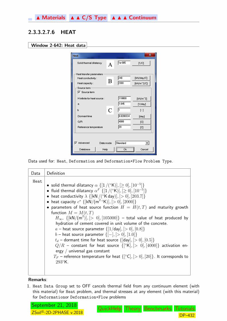
N Materials N N C/S Type N N N Continuum
2.3.3.2.7.6 HEAT
Window 2-642: Heat data
Data used for: Heat, Deformation and Deformation+Flow Problem Type.
Data Definition
Heat• solid thermal dilatancy α {[1 /(◦K)], [≥ 0], [10−5]}• fluid thermal dilatancy αF {[1 /(◦K)], [≥ 0], [10−5]}• heat conductivity λ {[kN /(◦K day)], [> 0], [203.7]}• heat capacity c∗ {[kN/(m2 ◦K)], [> 0], [2000]}• parameters of heat source function H = H(t, T ) and maturity growth
function M = M(t, T )H∞, {[kN/(m2)], [> 0], [105000]} – total value of heat produced byhydration of cement covered in unit volume of the concrete.a – heat source parameter {[1/day], [> 0], [0.8]}b – heat source parameter {[−], [> 0], [1.0]}td – dormant time for heat source {[day], [> 0], [0.5]}Q/R – constant for heat source {[◦K], [> 0], [4000]} activation en-ergy / universal gas constantTF – reference temperature for heat {[◦C], [> 0], [20]}. It corresponds to293◦K.
Remarks:
1. Heat Data Group set to OFF cancels thermal field from any continuum element (withthis material) for Heat problem, and thermal stresses at any element (with this material)for Deformationor Deformation+Flow problems
September 21, 2018
ZSoilr-2D-2PHASE v.2018QuickHelp Theory Benchmarks Tutorials
DP–432

N Materials N N C/S Type N N N Continuum
2. α and αF are needed exclusively for Deformation or Deformation+Flow problems andapply to any solid material model
3. λ is obligatory for steady and transient heat transfer drivers4. c∗ is obligatory only for transient heat transfer drivers; c∗ = cρ (specific heat is denoted
by c and density of the medium by ρ)5. hydration source parameters are optional and needed for• Heat problem if transient driver(s) are used• Deformation or Deformation+Flow problems when, Aging concrete model is used
in conjunction with supplied nonstationary temperature field declared in Analysis &
Drivers dialog (based on supplied thermal solution and given heat source parametersso-called maturity growth function M(T (t), t) is integrated in time; this function valueis an argument of the current stiffness modulus for Aging concrete model• heat source is described by the following formula
H(t, T ) = H∞(aM)b
1 + (aM)b
• a and b parameters need to be optimized for given cement class; for b = 1 the dH/dt(t)function is monotonicaly decreasing in time while for b > 1 it starts from zero thenreaches the maximum and then it is monotonicaly decreasing; for the cement class CEMI 42.5R optimal parameters are a = 1.645 [1/day] and b = 1.605 [-] while for cementclass CEM I 32.5R a = 1.517 [1/day] and b = 1.553 [-]; for other cement classes bestfit procedures must be used• H∞ is computed by multiplying the total heat produced from 1kg of a given cement
(for CEM I 42.5R it is 360 kJ/kg and for CEM I 32.5R 350 kJ/kg) by mass of cementin unit concrete volume
6. αF ,λ, c∗ and hydration source parameters apply exclusively to material models coherentwith continuum finite elements
7. One may use certain sets of parameters from database by pressing Database button8. Parameters λ, c∗,α can be assumed as temperature dependent by using evolution functions
(at the material level in group Heat use Evolution function in Data mode)
Window 2-642
Related Topics
• MATERIAL MODELS: HEAT TRANSFER
• PROBLEM STATEMENT: HEAT TRANSFER
September 21, 2018
ZSoilr-2D-2PHASE v.2018QuickHelp Theory Benchmarks Tutorials
DP–433

N Materials N N C/S Type N N N Continuum
2.3.3.2.7.7 HUMIDITY
Window 2-643: Humidity data
Data Definition
Humidity• Hygral dilatancy parameter β, {[−], [> 0], [0.01]}• Parameters for nonlinear function of diffusion coefficientF a, {[−], [> 0], [0.05]}F W1, {[−], [0 ≥ w1 ≤ 1], [0.75]]} - moisture potential at which the
diffusion coefficient is equal to 12D1(1 + a)
F D1, {[m2/s], [> 0], [3.6−7]} - diffusion coefficient for a moisture po-tential W = 1
Remarks:
1. Humidity Data Group set to OFF cancels moisture diffusion (in each continuum ele-ment with this material) for Humidity problem, and stresses due to moisture variation forDeformation or Deformation+Flow problems
2. β is needed exclusively for Deformation or Deformation+Flow problems and applies toany solid material model
3. Diffusion coefficient is defined as D(W ) = D1
a+1− a
1 +
(1−W1 +W1
)4
4. Constant moisture diffusion coefficient can be obtained assuming a = 1
Window 2-643
Related Topics
• PROBLEM STATEMENT: HUMIDITY TRANSFER
September 21, 2018
ZSoilr-2D-2PHASE v.2018QuickHelp Theory Benchmarks Tutorials
DP–434
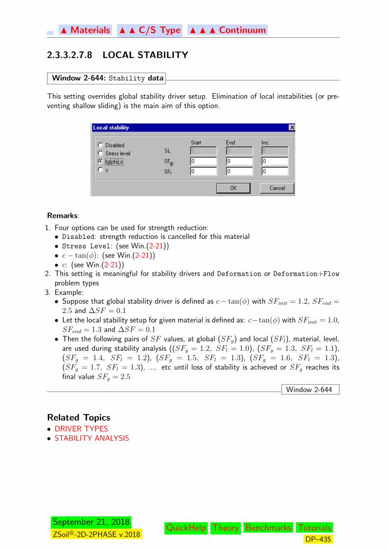
N Materials N N C/S Type N N N Continuum
2.3.3.2.7.8 LOCAL STABILITY
Window 2-644: Stability data
This setting overrides global stability driver setup. Elimination of local instabilities (or pre-venting shallow sliding) is the main aim of this option.
Remarks:
1. Four options can be used for strength reduction:• Disabled: strength reduction is cancelled for this material• Stress Level: (see Win.(2-21))• c− tan(φ): (see Win.(2-21))• c: (see Win.(2-21))
2. This setting is meaningful for stability drivers and Deformation or Deformation+Flow
problem types3. Example:• Suppose that global stability driver is defined as c− tan(φ) with SFinit = 1.2, SFend =
2.5 and ∆SF = 0.1• Let the local stability setup for given material is defined as: c−tan(φ) with SFinit = 1.0,SFend = 1.3 and ∆SF = 0.1• Then the following pairs of SF values, at global (SFg) and local (SFl), material, level,
are used during stability analysis ((SFg = 1.2, SFl = 1.0), (SFg = 1.3, SFl = 1.1),(SFg = 1.4, SFl = 1.2), (SFg = 1.5, SFl = 1.3), (SFg = 1.6, SFl = 1.3),(SFg = 1.7, SFl = 1.3), .... etc until loss of stability is achieved or SFg reaches itsfinal value SFg = 2.5
Window 2-644
Related Topics• DRIVER TYPES• STABILITY ANALYSIS
September 21, 2018
ZSoilr-2D-2PHASE v.2018QuickHelp Theory Benchmarks Tutorials
DP–435
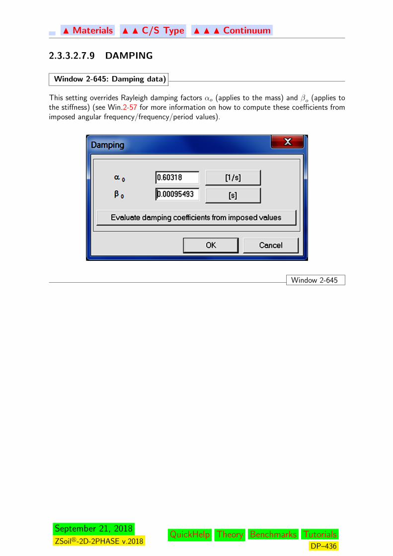
N Materials N N C/S Type N N N Continuum
2.3.3.2.7.9 DAMPING
Window 2-645: Damping data)
This setting overrides Rayleigh damping factors αo (applies to the mass) and βo (applies tothe stiffness) (see Win.2-57 for more information on how to compute these coefficients fromimposed angular frequency/frequency/period values).
Window 2-645
September 21, 2018
ZSoilr-2D-2PHASE v.2018QuickHelp Theory Benchmarks Tutorials
DP–436
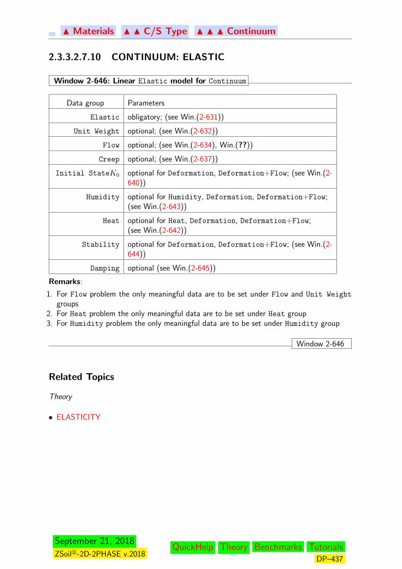
N Materials N N C/S Type N N N Continuum
2.3.3.2.7.10 CONTINUUM: ELASTIC
Window 2-646: Linear Elastic model for Continuum
Data group Parameters
Elastic obligatory; (see Win.(2-631))
Unit Weight optional; (see Win.(2-632))
Flow optional; (see Win.(2-634), Win.(??))
Creep optional; (see Win.(2-637))
Initial StateK0 optional for Deformation, Deformation+Flow; (see Win.(2-640))
Humidity optional for Humidity, Deformation, Deformation+Flow;(see Win.(2-643))
Heat optional for Heat, Deformation, Deformation+Flow;(see Win.(2-642))
Stability optional for Deformation, Deformation+Flow; (see Win.(2-644))
Damping optional (see Win.(2-645))
Remarks:
1. For Flow problem the only meaningful data are to be set under Flow and Unit Weight
groups2. For Heat problem the only meaningful data are to be set under Heat group3. For Humidity problem the only meaningful data are to be set under Humidity group
Window 2-646
Related Topics
Theory
• ELASTICITY
September 21, 2018
ZSoilr-2D-2PHASE v.2018QuickHelp Theory Benchmarks Tutorials
DP–437
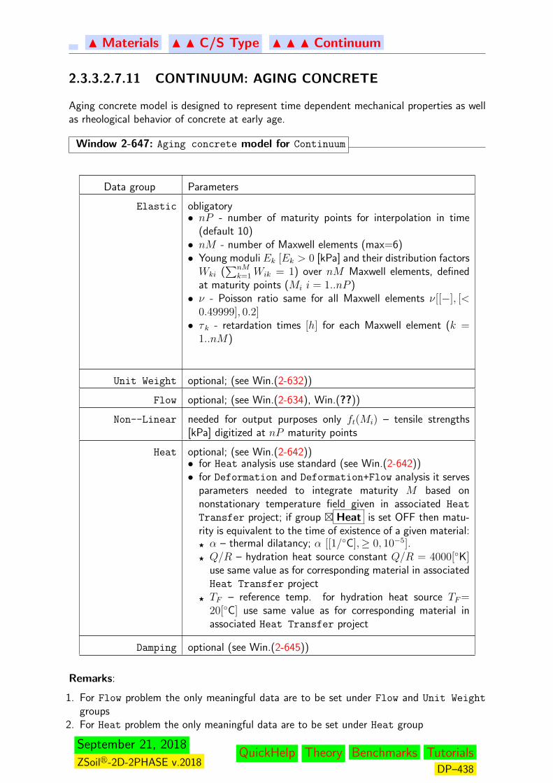
N Materials N N C/S Type N N N Continuum
2.3.3.2.7.11 CONTINUUM: AGING CONCRETE
Aging concrete model is designed to represent time dependent mechanical properties as wellas rheological behavior of concrete at early age.
Window 2-647: Aging concrete model for Continuum
Data group Parameters
Elastic obligatory• nP - number of maturity points for interpolation in time
(default 10)• nM - number of Maxwell elements (max=6)• Young moduli Ek [Ek > 0 [kPa] and their distribution factorsWki (
∑nMk=1Wik = 1) over nM Maxwell elements, defined
at maturity points (Mi i = 1..nP )• ν - Poisson ratio same for all Maxwell elements ν[[−], [<
0.49999], 0.2]• τ k - retardation times [h] for each Maxwell element (k =
1..nM)
Unit Weight optional; (see Win.(2-632))
Flow optional; (see Win.(2-634), Win.(??))
Non--Linear needed for output purposes only ft(Mi) – tensile strengths[kPa] digitized at nP maturity points
Heat optional; (see Win.(2-642))• for Heat analysis use standard (see Win.(2-642))• for Deformation and Deformation+Flow analysis it serves
parameters needed to integrate maturity M based onnonstationary temperature field given in associated Heat
Transfer project; if group � Heat is set OFF then matu-rity is equivalent to the time of existence of a given material:F α – thermal dilatancy; α [[1/◦C],≥ 0, 10−5].F Q/R – hydration heat source constant Q/R = 4000[◦K]
use same value as for corresponding material in associatedHeat Transfer project
F TF – reference temp. for hydration heat source TF=20[◦C] use same value as for corresponding material inassociated Heat Transfer project
Damping optional (see Win.(2-645))
Remarks:
1. For Flow problem the only meaningful data are to be set under Flow and Unit Weight
groups2. For Heat problem the only meaningful data are to be set under Heat group
September 21, 2018
ZSoilr-2D-2PHASE v.2018QuickHelp Theory Benchmarks Tutorials
DP–438

N Materials N N C/S Type N N N Continuum
3. For Humidity problem the only meaningful data are to be set under Humidity group
Window 2-647
September 21, 2018
ZSoilr-2D-2PHASE v.2018QuickHelp Theory Benchmarks Tutorials
DP–439
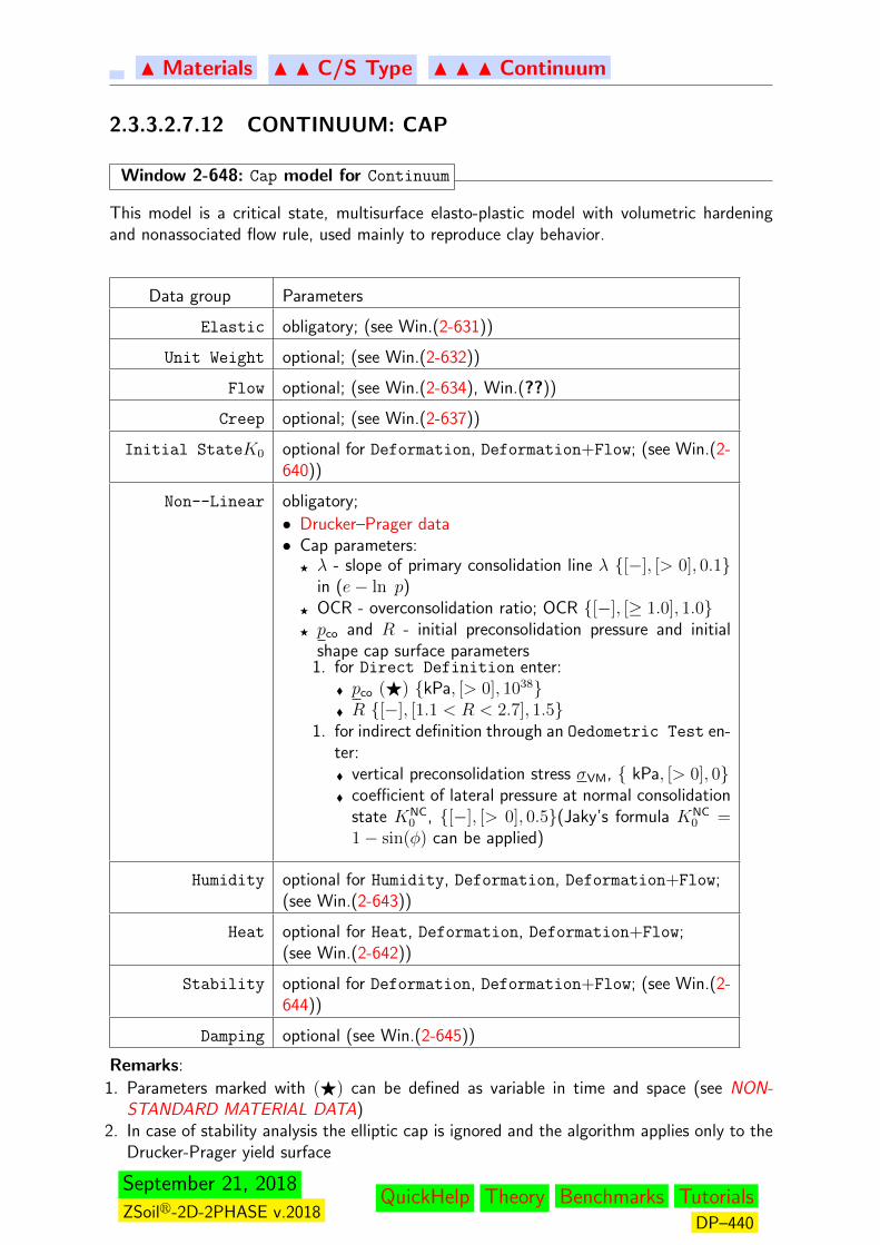
N Materials N N C/S Type N N N Continuum
2.3.3.2.7.12 CONTINUUM: CAP
Window 2-648: Cap model for Continuum
This model is a critical state, multisurface elasto-plastic model with volumetric hardeningand nonassociated flow rule, used mainly to reproduce clay behavior.
Data group Parameters
Elastic obligatory; (see Win.(2-631))
Unit Weight optional; (see Win.(2-632))
Flow optional; (see Win.(2-634), Win.(??))
Creep optional; (see Win.(2-637))
Initial StateK0 optional for Deformation, Deformation+Flow; (see Win.(2-640))
Non--Linear obligatory;
• Drucker–Prager data• Cap parameters:F λ - slope of primary consolidation line λ {[−], [> 0], 0.1}
in (e− ln p)F OCR - overconsolidation ratio; OCR {[−], [≥ 1.0], 1.0}F pco and R - initial preconsolidation pressure and initial
shape cap surface parameters1. for Direct Definition enter:
� pco (F) {kPa, [> 0], 1038}� R {[−], [1.1 < R < 2.7], 1.5}
1. for indirect definition through an Oedometric Test en-ter:� vertical preconsolidation stress σVM, { kPa, [> 0], 0}� coefficient of lateral pressure at normal consolidation
state KNC0 , {[−], [> 0], 0.5}(Jaky’s formula KNC
0 =1− sin(φ) can be applied)
Humidity optional for Humidity, Deformation, Deformation+Flow;(see Win.(2-643))
Heat optional for Heat, Deformation, Deformation+Flow;(see Win.(2-642))
Stability optional for Deformation, Deformation+Flow; (see Win.(2-644))
Damping optional (see Win.(2-645))
Remarks:
1. Parameters marked with (F) can be defined as variable in time and space (see NON-STANDARD MATERIAL DATA)
2. In case of stability analysis the elliptic cap is ignored and the algorithm applies only to theDrucker-Prager yield surface
September 21, 2018
ZSoilr-2D-2PHASE v.2018QuickHelp Theory Benchmarks Tutorials
DP–440

N Materials N N C/S Type N N N Continuum
3. Note that the initial preconsolidation pressure is not a material but rather a state parameter;for extended handling the initial preconsolidation pressure via OCR see Window 2-649,2-650
Window 2-648
September 21, 2018
ZSoilr-2D-2PHASE v.2018QuickHelp Theory Benchmarks Tutorials
DP–441

N Materials N N C/S Type N N N Continuum
Window 2-649: Setting pco via OCR if Initial state driver is active
User defined pco
is assumed to be the minimum allowed value of preconsolidation pressure(p
co-min). During the initial state computation hardening is deactivated and model behaves
as an ideal elasto-plastic one. Once the initial state is terminated the code estimates auto-matically, at each integration point, the initial pco, based on computed initial stress state σo,user defined OCR value and p
co-min. This algorithm is summarized below.
• For given stress state σo compute the p∗c
such that F (σ,p∗c) = 0 (cap plasticity condition)
• Correct the p∗c
by current OCR ratio: p∗∗c
= p∗c
OCR• IF p∗∗
c< p
co-minset: p
co= p
co-minELSE p
co= p∗∗
c
Remark:
To force the code to accept user defined pco-min
as an initial value for preconsolidation pressureOCR=1 must be assumed; however if given p
co-minvalue is too small at a given integration
point its value will automatically be enlarged to satisfy plastic admissibility condition F (..) ≤0
Window 2-649
Window 2-650: Setting pco if Initial state driver is not active
In this case the two possibilities are considered by the code to set up the initial pco
value
1. If the initial guess for the initial stress σ∗o is defined by the user (through the Initial
stress super-elements) then during the initialization phase the initial value of the pco
is set in the same manner as in Window 2-649 assuming σo=σ∗o.
2. If the initial guess for the initial effective stress state is not given explicitly by the user thenthe OCR factor is not interpreted and the initial preconsolidation pressure is set directly tothe value of p
coas declared in the user interface
Window 2-650
Related Topics
Theory:
• CAP MODEL
September 21, 2018
ZSoilr-2D-2PHASE v.2018QuickHelp Theory Benchmarks Tutorials
DP–442
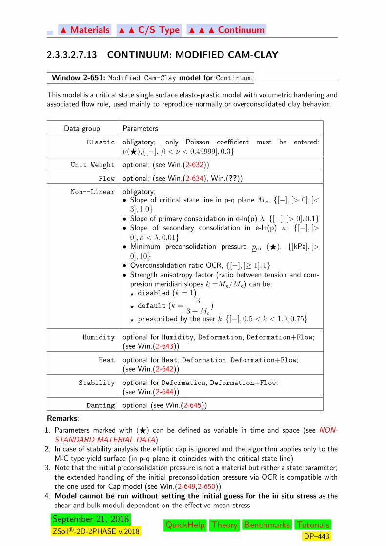
N Materials N N C/S Type N N N Continuum
2.3.3.2.7.13 CONTINUUM: MODIFIED CAM-CLAY
Window 2-651: Modified Cam-Clay model for Continuum
This model is a critical state single surface elasto-plastic model with volumetric hardening andassociated flow rule, used mainly to reproduce normally or overconsolidated clay behavior.
Data group Parameters
Elastic obligatory; only Poisson coefficient must be entered:ν(F),{[−], [0 < ν < 0.49999], 0.3}
Unit Weight optional; (see Win.(2-632))
Flow optional; (see Win.(2-634), Win.(??))
Non--Linear obligatory;• Slope of critical state line in p-q plane M c, {[−], [> 0], [<
3], 1.0}• Slope of primary consolidation in e-ln(p) λ, {[−], [> 0], 0.1}• Slope of secondary consolidation in e-ln(p) κ, {[−], [>
0], κ < λ, 0.01}• Minimum preconsolidation pressure pco (F), {[kPa], [>
0], 10}• Overconsolidation ratio OCR, {[−], [≥ 1], 1}• Strength anisotropy factor (ratio between tension and com-
presion meridian slopes k =M e/M c) can be:F disabled (k = 1)
F default (k =3
3 +Mc
)
F prescribed by the user k, {[−], 0.5 < k < 1.0, 0.75}
Humidity optional for Humidity, Deformation, Deformation+Flow;(see Win.(2-643))
Heat optional for Heat, Deformation, Deformation+Flow;(see Win.(2-642))
Stability optional for Deformation, Deformation+Flow;(see Win.(2-644))
Damping optional (see Win.(2-645))
Remarks:
1. Parameters marked with (F) can be defined as variable in time and space (see NON-STANDARD MATERIAL DATA)
2. In case of stability analysis the elliptic cap is ignored and the algorithm applies only to theM-C type yield surface (in p-q plane it coincides with the critical state line)
3. Note that the initial preconsolidation pressure is not a material but rather a state parameter;the extended handling of the initial preconsolidation pressure via OCR is compatible withthe one used for Cap model (see Win.(2-649,2-650))
4. Model cannot be run without setting the initial guess for the in situ stress as theshear and bulk moduli dependent on the effective mean stress
September 21, 2018
ZSoilr-2D-2PHASE v.2018QuickHelp Theory Benchmarks Tutorials
DP–443

N Materials N N C/S Type N N N Continuum
5. In case of overconsolidated soils problem of mesh dependency may appear and thus theresults should be analyzed carefully
Window 2-651
Related Topics
Theory
• NON-STANDARD MATERIAL DATA• CAM-CLAY MODEL• MODIFIED-CAM CLAY MODEL – STRESS RETURN ALGORITHM
September 21, 2018
ZSoilr-2D-2PHASE v.2018QuickHelp Theory Benchmarks Tutorials
DP–444

N Materials N N C/S Type N N N Continuum
2.3.3.2.7.14 CONTINUUM: DRUCKER–PRAGER
Window 2-652: Drucker-Prager model for Continuum
This model is a multisurface (due to optional cut-off condition), perfect, elasto-plastic modelwith a nonassociated flow rule, adjusted with respect to the Mohr-Coulomb criterion.
Data group Parameters
Elastic obligatory; (see Win.(2-631))
Unit Weight optional; (see Win.(2-632))
Flow optional; (see Win.(2-634), Win.(??))
Creep optional; (see Win.(2-637))
Initial StateK0 optional for Deformation, Deformation+Flow; (see Win.(2-640))
Non--Linear obligatory ;• Cohesion C (F), {kPa, [> 0], 20}• Friction angle ϕ (F), {[deg], [0, 89], 30}• Dilatancy angle ψ (F), {[deg], [0, 89], 0} Set ψ = 0 for
incompressible behavior• Tensile cut–off(F); optional, ignore if not konwlegable of
effects• Size adjustment with respect to the Mohr-Coulomb crite-
rion: (see Window 2-653: External Edges, Internal
Edges, Elastic, Plane Strain (default for plane strain),Intermediate (default for axisymmetry)
Humidity optional for Humidity, Deformation, Deformation+Flow;(see Win.(2-643))
Heat optional for Heat, Deformation, Deformation+Flow;(see Win.(2-642))
Stability optional for Deformation, Deformation+Flow; (see Win.(2-644))
Damping optional (see Win.(2-645))
Remarks:
1. Parameters marked with (F) can be defined as variable in time and space (see NON-STANDARD MATERIAL DATA)
2. φ− ψ ≥ 30o may yield convergence problems due to strain localization effects (caused bynonassociated flow rule)
3. Huber-Misses criterion is obtained setting φ = 0, C = 2√
3fy4. ψ = 0 corresponds to the incompressible plastic flow rule while ψ > 0 yields always
dilatancy5. Tensile Cut--Off condition reduces the maximum stress ratio: (
√J2/I1t) ≤ 1/
√3 or
equivalently p/q ≤ 3.
Window 2-652
September 21, 2018
ZSoilr-2D-2PHASE v.2018QuickHelp Theory Benchmarks Tutorials
DP–445
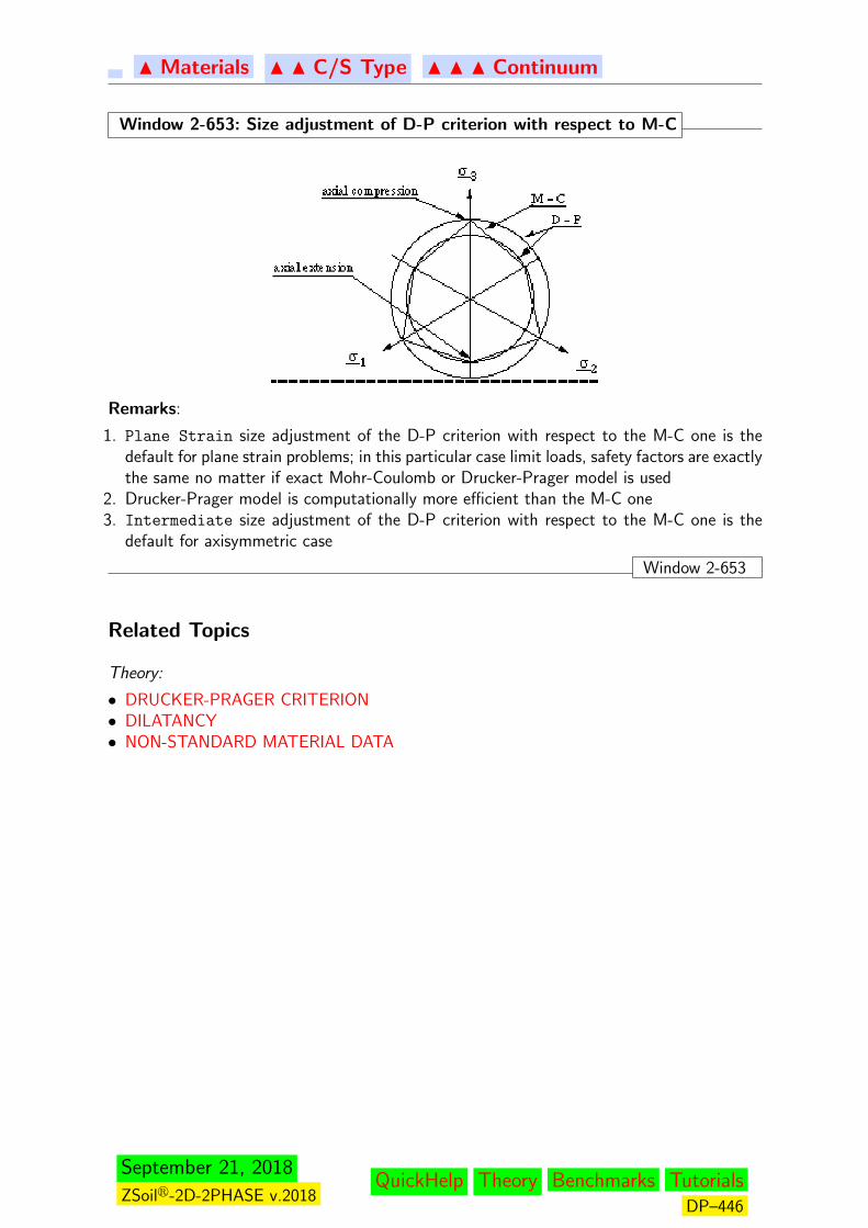
N Materials N N C/S Type N N N Continuum
Window 2-653: Size adjustment of D-P criterion with respect to M-C
Remarks:
1. Plane Strain size adjustment of the D-P criterion with respect to the M-C one is thedefault for plane strain problems; in this particular case limit loads, safety factors are exactlythe same no matter if exact Mohr-Coulomb or Drucker-Prager model is used
2. Drucker-Prager model is computationally more efficient than the M-C one3. Intermediate size adjustment of the D-P criterion with respect to the M-C one is the
default for axisymmetric case
Window 2-653
Related Topics
Theory:
• DRUCKER-PRAGER CRITERION• DILATANCY• NON-STANDARD MATERIAL DATA
September 21, 2018
ZSoilr-2D-2PHASE v.2018QuickHelp Theory Benchmarks Tutorials
DP–446
N Materials N N C/S Type N N N Continuum
2.3.3.2.7.15 CONTINUUM: HOEK–BROWN (M-W)
Window 2-654: Hoek-Brown model for Continuum
This model is a multi-surface (due to I1 type of the cut-off condition) elasto-plastic model withsoftening (optional) and nonassociated flow rule, used to reproduce concrete or rock behavior.The yield surface is described by a general Menetrey-Willam criterion with noncircular formin the deviatoric plane and parabolic shape of meridians in the
√J2 − I1 plane.
Data group Parameters
Elastic obligatory; (see Win.(2-631))
Unit Weight optional; (see Win.(2-632))
Flow optional; (see Win.(2-634), Win.(??))
Creep optional; (see Win.(2-637))
Initial StateK0 optional for Deformation, Deformation+Flow; (see Win.(2-640))
Non--Linear obligatory;• Compressive uni-axial strength fc, {[kPa], [> 0, >ft], 15000}• Tensile uni-axial strength ft, {[kPa], [> 0, < ft], 1000}• Biaxial compressive/uniaxial compressive strength ratiofb/fc, {[−], [> 1], 1.16}• Tensile Cut--Off flag ON/OFF
first stress invariant I1t (if Cut--Off is ON), {[kPa], [>0], 0}• Plastic flow type Deviatoric, Drucker--Prager, TensileMeridian, Hoek--Brown (M--W),• Dilatancy angle at uniaxial compressive strength ψc
(if Drucker--Prager or Hoek--Brown (M--W) flow is
ON), {[deg], [arctan
(ft√2fc
)≤ 35.3◦], 0}
• Softening flag ON/OFF7. This option must be used withcaution. If activated, introduce:F Crack opening at failure wr, {[m], [> 0], 0.0001]}F Steepness parameter a, {[−], [> 0], 5.0]}F Fictitious number of cracks for compression b, {[−], [>
1], 10.0]}
Humidity optional for Humidity, Deformation, Deformation+Flow;(see Win.(2-643))
Heat optional for Heat, Deformation, Deformation+Flow;(see Win.(2-642))
Stability optional for Deformation, Deformation+Flow; (see Win.(2-644))
Damping optional (see Win.(2-645))
September 21, 2018
ZSoilr-2D-2PHASE v.2018QuickHelp Theory Benchmarks Tutorials
DP–447

N Materials N N C/S Type N N N Continuum
Remarks:
1. Typical values of yield surface parameters for concrete and rock are:units rock concrete
ft kPa (2− 30) · 103 4 · 103
fc kPa (5− 400) · 103 40 · 103
e – 0.5-0.6 0.52
2. Exponential softening law 8 is driven by norm of tensile part of plastic strain tensor asstated below:
F (σ)− c = 0, c = exp(−a wwr
), ∆w = he ·∆q 1
N(b, σ), ∆q = ‖< ∆εp >‖
where: c is a softening function, w and q are softening parameters, he is an elementsize, N(b, σ) is a function describing fictitious number of cracks(=1 for tension, b forcompression) and principal tensile plastic strain is denoted by εp
Window 2-654
Related Topics
Theory:
• HOEK–BROWN CRITERION
• MOHR–COULOMB MODEL
• DILATANCY
8concerns versions: ACADEMIC, PROFESSIONAL, EXPERT only
September 21, 2018
ZSoilr-2D-2PHASE v.2018QuickHelp Theory Benchmarks Tutorials
DP–448

N Materials N N C/S Type N N N Continuum
2.3.3.2.7.16 CONTINUUM: MOHR–COULOMB (M-W)
Window 2-655: Mohr-Coulomb (M-W) (smooth version) model for Continuum
This model is a multi-surface (due to I1 type of the cut-off condition) elasto-plastic modelwith nonassociated flow rule, used to reproduce soil or rock behavior. The yield surface isdescribed by a general Menetrey-Willam criterion specialized here to the smooth version ofMohr-Coulomb one.
Data group Parameters
Elastic obligatory; (see Win.(2-631))
Unit Weight optional; (see Win.(2-632))
Flow optional; (see Win.(2-634), Win.(??))
Creep optional; (see Win.(2-637))
Initial StateK0 optional for Deformation, Deformation+Flow; (see Win.(2-640))
Non--Linear obligatory;• Cohesion c, {[kPa], [> 0], 20}• Friction angle φ, {[deg], [0, 89], 30}• Cut--Off flag ON/OffFlg• Tensile strength ft {{[kPa], [0, c/ tan(φ)], 0}
(if Cut--Off flag is ON),• Plastic flow type Deviatoric, Drucker--Prager• Dilatancy angle ψ, {[deg], [0, 89], 0}
(if Drucker--Prager flow is ON, set ψ = 0 for incompress-ible behavior• Size adjustment flag ON/OFF
Humidity optional for Humidity, Deformation, Deformation+Flow;(see Win.(2-643))
Heat optional for Heat, Deformation, Deformation+Flow;(see Win.(2-642))
Stability optional for Deformation, Deformation+Flow; (see Win.(2-644))
Damping optional (see Win.(2-645))
Remarks:
1. Deviatoric sections of smooth M-C surface are shown in fig. below
September 21, 2018
ZSoilr-2D-2PHASE v.2018QuickHelp Theory Benchmarks Tutorials
DP–449

N Materials N N C/S Type N N N Continuum
2. φ− ψ ≥ 30o may yield convergence problems due to strain localization effects (caused bynonassociated flow rule)
3. Plastic flow is driven by a Drucker–Prager type plastic potential (circular in the deviatoricplane); hence even for ψ = φ plastic flow is non-associated; ψ = 0 results in deviatoricplastic flow while 0 < ψ ≤ φ yields dilatancy
4. Tensile Cut--Off condition imposes: I1 ≤ I ′1t5. To achieve same limit loads and safety factors when applying standard M-C model and
M-C (M-W), in the plane strain (exclusively), � Size adjustment has to be set ON; for
φ = 0 (Huber–Misses criterion) size reduction factor is of order 0.866;
Window 2-655
Related Topics
Theory:
• MOHR–COULOMB• DILATANCY
September 21, 2018
ZSoilr-2D-2PHASE v.2018QuickHelp Theory Benchmarks Tutorials
DP–450
N Materials N N C/S Type N N N Continuum
2.3.3.2.7.17 CONTINUUM: MULTILAMINATE
Window 2-656: Multilaminate model for Continuum
Data group Parameters
Elastic obligatory; (see Win.(2-631))
Unit Weight optional; (see Win.(2-632))
Flow optional; (see Win.(2-634), Win.(??))
Creep optional; (see Win.(2-637))
Initial StateK0 optional for Deformation, Deformation+Flow; (see Win.(2-640))
Non--Linear obligatory;for each active weakness plane set:
• for 2D models:F Inclination angle α measured in anti-clockwise direction,{[deg], [−90 ≤ α ≤ 90], 0}
• Cohesion c, {[kPa], [> 0], 0}• Friction angle φ, {[deg], [0, 89], 0}• Dilatancy angle ψ, {[deg], [0, 89], 0}; set ψ = 0 for incom-
pressible behavior.• Cut--Off flag ON/OFF• Tensile strength ft, {[kPa], [0, c/ tan(φ)], 0}
(if Cut--Off flag is ON)
• Matrix material model ( elastic if � Advanced is OFF ) orMohr-Coulomb (M-W)/ Rankine (M-W)/Hoek-Brown
Humidity optional for Humidity, Deformation, Deformation+Flow;(see Win.(2-643))
Heat optional for Heat, Deformation, Deformation+Flow;(see Win.(2-642))
Stability optional for Deformation, Deformation+Flow; (see Win.(2-644))
Damping optional (see Win.(2-645))
Remarks:
1. To deactivate weakness plane set: φ = ψ = c = 0.02. Matrix material is assumed as elastic by default; if � Advanced mode is set ON one may
apply an elasto-plastic model described by Rankine (M-W) (see Win.(2-657)), Drucker-Prager (see Win.(2-652)) or Mohr-Coulomb (M-W) (smooth) (see Win.(2-655)) yield sur-face
Window 2-656
September 21, 2018
ZSoilr-2D-2PHASE v.2018QuickHelp Theory Benchmarks Tutorials
DP–451

N Materials N N C/S Type N N N Continuum
Related Topics
Theory:
MULTILAMINATE MODEL
September 21, 2018
ZSoilr-2D-2PHASE v.2018QuickHelp Theory Benchmarks Tutorials
DP–452
N Materials N N C/S Type N N N Continuum
2.3.3.2.7.18 CONTINUUM: RANKINE (M-W)
Window 2-657: Rankine (M-W) model for Continuum
This model is a single surface, strain softening (optional) elasto-plastic model with a nonas-sociated flow rule, derived from general Menetrey-Willam criterion.
Data group Parameters
Elastic obligatory; (see Win.(2-631))
Unit Weight optional; (see Win.(2-632))
Flow optional; (see Win.(2-634), Win.(??))
Creep optional; (see Win.(2-637))
Initial StateK0 optional for Deformation, Deformation+Flow; (see Win.(2-640))
Non--Linear obligatory; set:• Tensile strength (uni-axial) ft, {[kPa], [> 0], 0}• Softening flag; if � Softening is set ON defineF Crack opening at failure wr, {[m], [> 0], 0.0001]}F Steepness parameter a, {[−], [> 0], 5.0]}F Fictitious number of cracks for compression b, {[−], [>
1], 10.0]}
Humidity optional for Humidity, Deformation, Deformation+Flow;(see Win.(2-643))
Heat optional for Heat, Deformation, Deformation+Flow;(see Win.(2-642))
Stability optional for Deformation, Deformation+Flow; (see Win.(2-644))
Damping optional (see Win.(2-645))
Remarks:
1. Plastic flow is governed by a DP type plastic potential (hence flow rule is nonassociated)2. Strain softening option must be used with caution
Window 2-657
Related Topics
Theory:
• MOHR–COULOMB• HOEK–BROWN CRITERION
September 21, 2018
ZSoilr-2D-2PHASE v.2018QuickHelp Theory Benchmarks Tutorials
DP–453
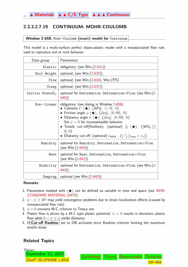
N Materials N N C/S Type N N N Continuum
2.3.3.2.7.19 CONTINUUM: MOHR-COULOMB
Window 2-658: Mohr-Coulomb (exact) model for Continuum
This model is a multi-surface perfect elasto-plastic model with a nonassociated flow rule,used to reproduce soil or rock behavior.
Data group Parameters
Elastic obligatory; (see Win.(2-631))
Unit Weight optional; (see Win.(2-632))
Flow optional; (see Win.(2-634), Win.(??))
Creep optional; (see Win.(2-637))
Initial StateK0 optional for Deformation, Deformation+Flow; (see Win.(2-640))
Non--Linear obligatory; (see dialog in Window 2-658)• Cohesion C (F), {[kPa], [> 0], 0}• Friction angle ϕ (F), {[deg], [0, 89], 0}• Dilatancy angle ψ (F), {[deg], [0, 89], 0}
Set ψ = 0 for incompressible behavior• Tensile cut–off(Rankine); (optional) ft (F), {[kPa], [≥
0], 0}• Dilatancy cut-off; (optional) eMAX , {[−], [emax > eo]}
Humidity optional for Humidity, Deformation, Deformation+Flow;(see Win.(2-643))
Heat optional for Heat, Deformation, Deformation+Flow;(see Win.(2-642))
Stability optional for Deformation, Deformation+Flow; (see Win.(2-644))
Damping optional (see Win.(2-645))
Remarks:
1. Parameters marked with (F) can be defined as variable in time and space (see NON-STANDARD MATERIAL DATA)
2. φ− ψ ≥ 30o may yield convergence problems due to strain localization effects (caused bynonassociated flow rule)
3. φ = 0 converts M-C criterion to Tresca one4. Plastic flow is driven by a M-C type plastic potential; ψ = 0 results in deviatoric plastic
flow while 0 < ψ ≤ φ yields dilatancy5. � Cut-off Rankine set to ON activates strict Rankine criterion limiting the maximum
tensile stress
Related Topics
Theory:September 21, 2018
ZSoilr-2D-2PHASE v.2018QuickHelp Theory Benchmarks Tutorials
DP–454

N Materials N N C/S Type N N N Continuum
• MOHR–COULOMB• DILATANCY• NON-STANDARD MATERIAL DATA
September 21, 2018
ZSoilr-2D-2PHASE v.2018QuickHelp Theory Benchmarks Tutorials
DP–455
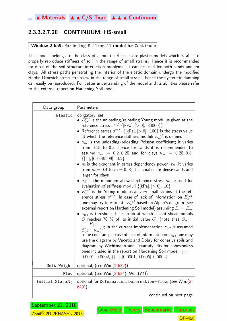
N Materials N N C/S Type N N N Continuum
2.3.3.2.7.20 CONTINUUM: HS-small
Window 2-659: Hardening Soil-small model for Continuum
This model belongs to the class of a multi-surface elasto-plastic models which is able toproperly reproduce stiffness of soil in the range of small strains. Hence it is recommendedfor most of the soil structure-interaction problems. It can be used for both sands and forclays. All stress paths penetrating the interior of the elastic domain undergo the modifiedHardin-Drnevich stress-strain law in the range of small strains, hence the hysteretic dampingcan easily be reproduced. For better undertsanding of the model and its abilities please referto the external report on Hardening Soil model.
Data group Parameters
Elastic obligatory; set• Eref
ur is the unloading/reloading Young modulus given at thereference stress σref {[kPa], [> 0], 80000})• Reference stress σref , {[kPa], [> 0], 100} is the stress value
at which the reference stiffness moduli Erefur is defined
• νur is the unloading/reloading Poisson coefficient; it variesfrom 0.15 to 0.3, hence for sands it is recommended toassume νur = 0.2..0.25 and for clays νur = 0.25..0.3,{[−], [0, 0.49999], 0.2}• m is the exponent in stress dependency power law; it varies
from m = 0.4 to m = 0..8; it is smaller for dense sands andlarger for clays• σL is the minimum allowed reference stress value used for
evaluation of stiffness moduli {[kPa], [> 0], 10}• Eref
o is the Young modulus at very small strains at the ref-erence stress σref ; In case of lack of information on Eref
o
one may try to estimate Erefo based on Alpan’s diagram (see
external report on Hardening Soil model) assuming Es = Eur• γ0.7 is threshold shear strain at which secant shear modulsG reaches 70 % of its initial value Go (note that Go =
Eo2(1 + νur)
); in the current implementation γ0.7 is assumed
to be constant; in case of lack of information on γ0.7 one mayuse the diagram by Vucetic and Dobry for cohesive soils anddiagram by Wichtmann and Triantafyllidis for cohesionlessones included in the report on Hardening Soil model; γ0.7 =0.0001..0.0002, {[−], [0.0001, 0.0005], 0.0002}
Unit Weight optional; (see Win.(2-632))
Flow optional; (see Win.(2-634), Win.(??))
Initial StateK0 optional for Deformation, Deformation+Flow; (see Win.(2-640))
continued on next page
September 21, 2018
ZSoilr-2D-2PHASE v.2018QuickHelp Theory Benchmarks Tutorials
DP–456
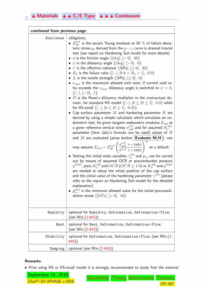
N Materials N N C/S Type N N N Continuum
continued from previous page
Nonlinear obligatory;
• Eref50 is the secant Young modulus at 50 % of failure devia-
toric stress qf derived from the q−ε1 curve in drained triaxialtest (see report on Hardening Soil model for more details)• φ is the friction angle {[deg], [> 0], 30}• ψ is the dilatancy angle {[deg], [> 0], 0}• c′ is the effective cohesion {[kPa], [≥ 0], 20}• Rf is the failure ratio {[−], [0.8 < Rf < 1], 0.9}• ft is the tensile strength {[kPa], [≥ 0], 0}• emax is the maximum allowed void ratio; if current void ra-
tio exceeds the emax dilatancy angle is switched to ψ = 0,{[−], [> 0], 1}• D is the Rowe’s dilatancy multiplier in the contractant do-
main, for standard HS model {[−], [0 ≤ D ≤ 1], 0.0} whilefor HS-small {[−], [0 ≤ D ≤ 1], 0.25}• Cap surface parameter M and hardening parameter H are
derived by using a simple calculator which simulates an oe-dometric test; for given tangent oedometric modulus Eoed ata given reference vertical stress σrefoed and for assumed KNC
o
parameter (here Jaky’s formula can be used) values of H
and M are evaluated (press button Evaluate M,H ); one
may assume Eoed = Eref50
(σrefoed + c cotφ
σref + c cotφ
)m
as a default
• Setting the initial state variables γPSo and pco can be carriedout by means of assumed OCR or preoverburden pressureqPOP ; pairs KSR
o and OCR (OCR ≥ 1.0) or KSRo and qPOP
are needed to setup the initial position of the cap surfaceand the initial value of the hardening parameter γPS (pleaserefer to the report on Hardening Soil model for the detailedexplanation)• pminco is the minimum allowed value for the initial preconsoli-
dation stress {[kPa], [> 0], 10}
Humidity optional for Humidity, Deformation, Deformation+Flow;(see Win.(2-643))
Heat optional for Heat, Deformation, Deformation+Flow;(see Win.(2-642))
Stability optional for Deformation, Deformation+Flow; (see Win.(2-644))
Damping optional (see Win.(2-645))
Remarks:
• Prior using HS or HS-small model it is strongly recommended to study first the external
September 21, 2018
ZSoilr-2D-2PHASE v.2018QuickHelp Theory Benchmarks Tutorials
DP–457

N Materials N N C/S Type N N N Continuum
report on Hardening Soil model
Window 2-659
Related Topics
Theory: Technical report on HS-small model
September 21, 2018
ZSoilr-2D-2PHASE v.2018QuickHelp Theory Benchmarks Tutorials
DP–458

N Materials N N C/S Type N N N Continuum
2.3.3.2.7.21 CONTINUUM: Densification model
Window 2-660: Densification model for Continuum
This model, derived directly from HSs model, is designed to reproduce loose soil depositsbehavior subject to cylic loading. Hence it is to be used mainly in dynamic predictions. It isable to reproduce cyclic compaction for single-phase problems and liquefaction for two-phaseones. This model can also be customized to nonlinear Mohr-Coulomb one (with nonlinearelasticity inside yield surface) by switching off deviatoric plastic mechanism and deactivatingdensification mechanism.
Data group Parameters
Elastic obligatory; set• Eref
ur is the unloading/reloading Young modulus given at thereference stress σref {[kPa], [> 0], 80000}); note that theelastic stiffness moduli depend on p rather on σ3 value inthis model• Reference stress σref , {[kPa], [> 0], 100} is the stress value
at which the reference stiffness moduli Erefur is defined
• νur is the unloading/reloading Poisson coefficient; it variesfrom 0.15 to 0.3, hence for sands it is recommended toassume νur = 0.2..0.25 and for clays νur = 0.25..0.3,{[−], [0, 0.49999], 0.2}• m is the exponent in stress dependency power law; for loose
sands m ≈ 0.5• σL is the minimum allowed reference stress value used for
evaluation of stiffness moduli {[kPa], [> 0], 10}• Eref
o is the Young modulus at very small strains at the ref-erence stress σref ; note that the current very small strainstiffness modulus Eo depends on p rather than σ3 (as in theHS model)• γ0.7 is threshold shear strain at which secant shear modulsG reaches 70 % of its initial value Go (note that Go =
Eo2(1 + νur)
); in the current implementation γ0.7 is assumed
to be constant; in case of lack of information on γ0.7 one mayuse the diagram by Wichtmann and Triantafyllidis included inthe report on Hardening Soil model; γ0.7 = 0.0001..0.0002,{[−], [0.0001, 0.0005], 0.0002}
Unit Weight optional; (see Win.(2-632))
Flow optional; (see Win.(2-634), Win.(??))
Initial StateK0 optional for Deformation, Deformation+Flow; (see Win.(2-640))
continued on next page
September 21, 2018
ZSoilr-2D-2PHASE v.2018QuickHelp Theory Benchmarks Tutorials
DP–459
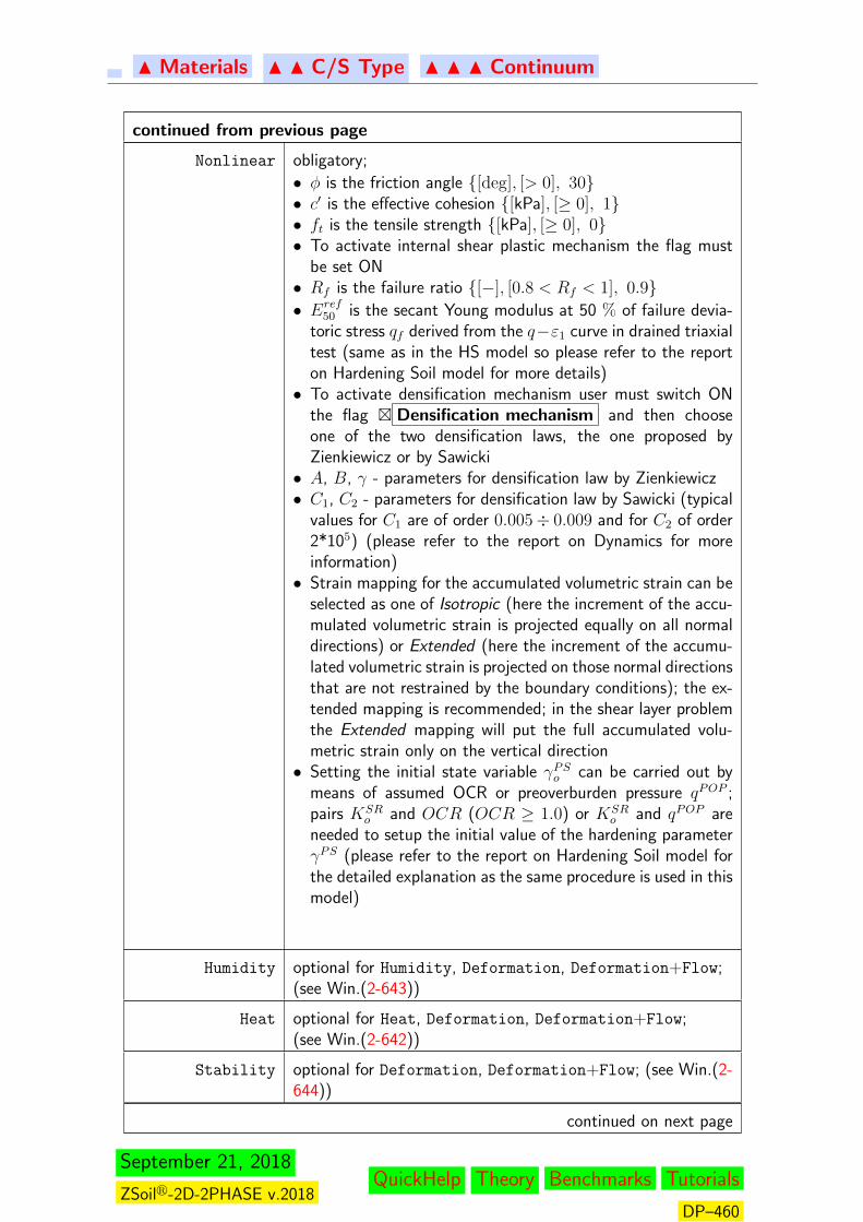
N Materials N N C/S Type N N N Continuum
continued from previous page
Nonlinear obligatory;
• φ is the friction angle {[deg], [> 0], 30}• c′ is the effective cohesion {[kPa], [≥ 0], 1}• ft is the tensile strength {[kPa], [≥ 0], 0}• To activate internal shear plastic mechanism the flag must
be set ON• Rf is the failure ratio {[−], [0.8 < Rf < 1], 0.9}• Eref
50 is the secant Young modulus at 50 % of failure devia-toric stress qf derived from the q−ε1 curve in drained triaxialtest (same as in the HS model so please refer to the reporton Hardening Soil model for more details)• To activate densification mechanism user must switch ON
the flag � Densification mechanism and then chooseone of the two densification laws, the one proposed byZienkiewicz or by Sawicki• A, B, γ - parameters for densification law by Zienkiewicz• C1, C2 - parameters for densification law by Sawicki (typical
values for C1 are of order 0.005÷ 0.009 and for C2 of order2*105) (please refer to the report on Dynamics for moreinformation)• Strain mapping for the accumulated volumetric strain can be
selected as one of Isotropic (here the increment of the accu-mulated volumetric strain is projected equally on all normaldirections) or Extended (here the increment of the accumu-lated volumetric strain is projected on those normal directionsthat are not restrained by the boundary conditions); the ex-tended mapping is recommended; in the shear layer problemthe Extended mapping will put the full accumulated volu-metric strain only on the vertical direction• Setting the initial state variable γPSo can be carried out by
means of assumed OCR or preoverburden pressure qPOP ;pairs KSR
o and OCR (OCR ≥ 1.0) or KSRo and qPOP are
needed to setup the initial value of the hardening parameterγPS (please refer to the report on Hardening Soil model forthe detailed explanation as the same procedure is used in thismodel)
Humidity optional for Humidity, Deformation, Deformation+Flow;(see Win.(2-643))
Heat optional for Heat, Deformation, Deformation+Flow;(see Win.(2-642))
Stability optional for Deformation, Deformation+Flow; (see Win.(2-644))
continued on next page
September 21, 2018
ZSoilr-2D-2PHASE v.2018QuickHelp Theory Benchmarks Tutorials
DP–460

N Materials N N C/S Type N N N Continuum
continued from previous page
Damping optional (see Win.(2-645))
Remarks:
• Prior using Densification model it is strongly recommended to study first the externalreport on Dynamics where a dedicated section is devoted to that model, its theory andbenchmarks
Window 2-660
Related Topics
Theory: Technical report on dynamics
September 21, 2018
ZSoilr-2D-2PHASE v.2018QuickHelp Theory Benchmarks Tutorials
DP–461
N Materials N N C/S Type N N N Continuum
2.3.3.2.7.22 CONTINUUM: HOEK–BROWN (true)
Window 2-661: Hoek-Brown model for Continuum
This model is a 2002 edition of the true Hoek-Brown one. It can be calibrated based on thegiven GSI index or directly through the σci, mb, s, a parameters. In addition the dilatancylaw includes the two versions i.e. with constant and with stress dependent dilatancy. Formore detailed information on that model please refer to the dedicated report.
Data group Parameters
Elastic obligatory; (see Win.(2-631))
Unit Weight optional; (see Win.(2-632))
Flow optional; (see Win.(2-634), Win.(??))
Creep optional; (see Win.(2-637))
Initial StateK0 optional for Deformation, Deformation+Flow; (see Win.(2-640))
continued on next page
September 21, 2018
ZSoilr-2D-2PHASE v.2018QuickHelp Theory Benchmarks Tutorials
DP–462
N Materials N N C/S Type N N N Continuum
continued from previous page
Non--Linear obligatory;• GSI index, {[−], [0 ≤ GSI ≤ 100], 100} (inactive for Direct
definition of mb,s,a parameters)(based on GSI E moduluscan be defined)• Disturbance factor D, {[−], [0 ≤ D ≤ 1], 0} (to be set only
when definition through GSI index is used) (for undisturbedrock use 0.0 and for highly disturbed one use 1.0) (inactivefor Direct definition of mb,s,a parameters)• Parameter mi (ratio of compressive to tensile strength for
intact rock) mi, {[−], [mi > 1], 10.0} (to be set only whendefinition through GSI index is used) (inactive for Direct def-inition of mb,s,a parameters)• Intact rock compressive strength σci, {[kPa], [σci >
0], 15000.0}• Parameter mb, {[−], [mb > 0, 10} (to be set only when Di-
rect definition is used)• Parameter s, {[−], [s > 0.0, 1.0} (to be set only when Direct
definition is used)• Parameter a, {[−], [0.5 ≤ s ≤ 0.67, 0.5} (to be set only
when Direct definition is used)• Constant dilatancy/Stress dependent dilatancy flag (default
is constant)• Dilatancy angle for constant dilatancy ψ, {[deg], [0.0 ≤ ψ ≤
90.0, 0.0}• Dilatancy cut-off stress σψ for stress dependent dilatancy,{[kPa], [σψ ≥ 0.0]}• Equivalent shear strain γr at peak on q − ε1 curve in uni-
axial compression test (this value is needed only for straindependent dilatancy and active hardening/softening)• Equivalent shear strain γres at reasidual state on q−ε1 curve
in uniaxial compression test (this value is needed only forstrain dependent dilatancy and active hardening/softening)
continued on next page
September 21, 2018
ZSoilr-2D-2PHASE v.2018QuickHelp Theory Benchmarks Tutorials
DP–463
N Materials N N C/S Type N N N Continuum
continued from previous page
• Weighting factors fψ (can be negative in pre-failure stage) atgiven characteristic equivalent shear strain magnitudes (γo,γr, γres)• Pre-peak hardening and hardening law type (standard,
parabolic and with stiffening effect)• For standard hardening law parameters mbo, so and ao are de-
scribing the initial position of the yield surface; (it is stronglyrecommended to assume ao = a)); certain restrictions areput on values of these parameters; for detailed informationsee dedicated report on HB model• For parabolic law set ro parameter {[−], [ro > 0, 1} (see
dedicated report for details)• For hardening that includes stiffening effect set two pairsξ1 − r1 and ξ2 − r2 of parameters {[−], [r1, r2 > 0, 1},{[−], [ξ1, ξ2 > 0, 1}, ξ1 < ξ2, r1 < r2 (see dedicated re-port for details)• Post-peak softening flag• Once softening is activated parameters mbres, sres and ares
are the values of mb, s and a at residual state; they describeresidual strength envelope (it is strongly recommended toassume ares = a)• Parameter αR describes the softening law for tensile stress
paths controled by the Rankine yield surface• Softening cut-off stress σsf : softening will be cancelled onceσ3 ¿ σsf , {[kPa], [σsf ≥ 0.0]}• Type of softening regularization: Local/Softening scaling;
the later one must be used in practical computations; thelocal one is used only for single element tests; local softeningmay lead to lack of convergence or mesh-dependent solutions• Parameter Lc - characteristic length required for soften-
ing scaling (must be set up based on experimental data){[m], [Lc ≥ 0.0]}; it is of order of milimiters; decides whetherpost-peak path in σ − ε curve is brittle or ductile
Humidity optional for Humidity, Deformation, Deformation+Flow;(see Win.(2-643))
Heat optional for Heat, Deformation, Deformation+Flow;(see Win.(2-642))
Stability optional for Deformation, Deformation+Flow; (see Win.(2-644))
Damping optional (see Win.(2-645))
September 21, 2018
ZSoilr-2D-2PHASE v.2018QuickHelp Theory Benchmarks Tutorials
DP–464

N Materials N N C/S Type N N N Continuum
Related Topics
Theory:
• Technical report on HB model
September 21, 2018
ZSoilr-2D-2PHASE v.2018QuickHelp Theory Benchmarks Tutorials
DP–465
N Materials N N C/S Type N N N Continuum
2.3.3.2.7.23 CONTINUUM: Plastic damage model for concrete
Window 2-662: Plastic damage model for Continuum
Current implementation of plastic damage model for concrete (CPDM) is based on the for-mulation proposed by Lee and Fenves with certain improvements introduced by the ZSoildevelopers. This model couples single surface elasto-plasticity with hardening and an en-hanced scalar damage allowing for description of stiffness degradation and stiffness recoveryin cyclic tension-compression tests. This model is also able to describe aging, creep (ac-cording to the EC2 standard) and damage at early stage of concrete maturing. The recentdevelopment (since version 2018) includes model extension to high temperatures. All detailsconcerning this model can be found in the report on Plastic damage model for concrete andConcrete structures at high temperatures.
Data group Parameters
Elastic obligatory; (see Win.(2-631)); this parameter can be modifiedby the predefined set of thermal evolution functions to carry outfire analyses (see the report on reinforced concrete structuressubject to elevated temperatures)
Unit Weight optional; (see Win.(2-632))
Flow optional; (see Win.(2-634), Win.(??))
Creep optional (two creep models can be used in this model; the firstone is the dedicated creep model following the EC2 standardwhile the second one describes thermal creep during fire; onlyone of them can be used during the analysis); (see Win.(2-639))
Initial StateK0 optional for Deformation, Deformation+Flow; (see Win.(2-640))
continued on next page
September 21, 2018
ZSoilr-2D-2PHASE v.2018QuickHelp Theory Benchmarks Tutorials
DP–466
N Materials N N C/S Type N N N Continuum
continued from previous page
Nonlinear obligatory;• f
c- uniaxial compressive strength (positive in compression);
use according to the EC2 standard; these parameter can bemodified by the predefined set of thermal evolution func-tions to carry out fire analyses (see the report on reinforcedconcrete structures subject to elevated temperatures)• f
co/f
c- initial to peak compressive strength ratio (0.4÷0.8)
• fcbo/f
co- initial biaxial to uniaxial strength ratio (1.1÷1.2)
• σc,D/f c - stress level at which damage starts to occur(σc,D/f c ≥ f
co/f
c)(0.4÷0.9); these parameter is internally
modified in fire analyses (see the report on reinforced con-crete structures subject to elevated temperatures)• σc/fc - stress level for damage calibration in compression (on
post-peak branch)(≤ 1.0)• Dc - damage parameter in uniaxial compression at the as-
sumed reference stress level (≥ 0.3); these parameter can bemodified by the user supplied thermal evolution functions tocarry out fire analyses (see the report on reinforced concretestructures subject to elevated temperatures)• Gc - fracture energy in compression (50 Gf ≤ Gc ≤ 100 Gf )• ft - uniaxial tensile strength (positive in tension); use accord-
ing to the EC2 standard; these parameter can be modified bythe predefined set of thermal evolution functions to carry outfire analyses (see the report on reinforced concrete structuressubject to elevated temperatures)• σt/ft - stress level for damage calibration (on post-peak
branch) (< 1)• Dt - damage parameter in uniaxial tension at the assumed
reference stress level (≥ 0.3)• Gt - fracture energy in tension; can be estimated as 73 f 0.18
c ∗10−6 (use MPa as strength unit here) (50∗10−6÷150∗10−6
MN/m)• s - stiffness recovery factor due to crack closure for tension-
compression cycles (0.1÷ 0.3)• Dilatancy type - Constant/Variable• αp - Dilatancy parameter value for Constant option or dila-
tancy parameter in uniaxial compression when option Vari-able is used (0.1÷ 0.5)• αpo - dilatancy parameter in uniaxial tension option Variable
is used (0.1÷ 0.4)• σc,dil/f c - activation of dilatancy in compression when Vari-
able option is used; σc,dil/f c ≥ fco/f
c; (0.4÷ 1.0)
• αd - smoothing factor for plastic potential; value 1.0 is rec-ommended (0.2÷ 2.0)• Char. length (RC) flag - enforced characteristic length flag
for reinforced concrete (ON/OFF)• lRCc - characteristic length to be used for reinforced concrete
when Char. length (RC) flag is ON (> 0)• Secant stiffness flag - use secant elastic stiffness
(mathbfDe(1 − D)) when ON or consistent tangent whenOFF (secant stiffness is recommended for cases with poorconvergence)
continued on next page
September 21, 2018
ZSoilr-2D-2PHASE v.2018QuickHelp Theory Benchmarks Tutorials
DP–467
N Materials N N C/S Type N N N Continuum
continued from previous page
Humidity optional for Humidity, Deformation, Deformation+Flow;(see Win.(2-643))
Heat optional for Heat, Deformation, Deformation+Flow;(see Win.(2-642)) parameters λ, c∗ and α can be modified bythe predefined set of thermal evolution functions to carry outfire analyses (see the report on reinforced concrete structuressubject to elevated temperatures)
Stability optional for Deformation, Deformation+Flow; (see Win.(2-644))
Damping optional (see Win.(2-645))
Window 2-662
Related Topics
Reports:Technical report on plastic damage model for concreteTechnical report on concrete structures subject to elevated temperatures
September 21, 2018
ZSoilr-2D-2PHASE v.2018QuickHelp Theory Benchmarks Tutorials
DP–468

N Assembly N N Materials N N N Continuum/Structures
2.3.3.2.8 CONTINUUM FOR STRUCTURES
Window 2-663: Models for Continuum for structures
Material models for continuum for structures Data groups
linear: Elastic ELASTIC
UNIT WEIGHTS
CREEP
FLOW
INITIAL K0 STATE
HEAT
HUMIDITY
DAMPING
Remarks:
1. List of material models applicable to continuum for structures (beams, shells) is limitedonly to the linear elastic model
2. This material cannot be attached to the triangular continuum elements3. All continuum finite elements declared as continuum for structures will be converted to
EAS elements with enhanced bending and shear representation (EAS-7 in plane-strain,EAS-5 in axisymmetry and EAS-9 in 3D)
4. Use more than 1 element across the thickness of beam/shell (to enable veryaccurate super-convergent patch recovery of stresses and stress resultants)
Window 2-663
September 21, 2018
ZSoilr-2D-2PHASE v.2018QuickHelp Theory Benchmarks Tutorials
DP–469
N Assembly N N Materials N N N Continuum/Structures
2.3.3.2.9 HEAT CONVECTION
Window 2-664: Heat convection model
This model is applicable exclusively to Heat Problem TypeIt is used to describe convectiveproperties of the boundary and surrounding media (with ambient temperature), in orderto control heat exchange through the boundary. It may exclusively be attached to Heat
Convection elements.
Data group Parameters
Heat obligatory
• Heat convection coefficient hT {[kN/(m · ◦K · s)], > 0, 10}(see the report on reinforced concrete structures subject toelevated temperatures to set up proper value of this parameterin case of fire analyses)
Window 2-664
Related Topics
Theory: HEAT TRANSFERReports: Technical report on concrete structures subject to elevated temperatures
September 21, 2018
ZSoilr-2D-2PHASE v.2018QuickHelp Theory Benchmarks Tutorials
DP–470
N Assembly N N Materials N N N Continuum/Structures
2.3.3.2.10 HEAT RADIATION
Window 2-665: Heat radiation model
This model is applicable exclusively to Heat Problem TypeIt is used to describe radiationboundary condition during fire. It may exclusively be attached to Heat Radiation elements.
Data group Parameters
Heat obligatory
• configuration factor φ {[−], > 0, 1}• surface emissivity of the member εm {[−], > 0, 0.8}• emissivity of the fire εf {[−], > 0, 1.0}• Boltzmann constant σ {[kN/m3/s/C4], > 0, 5.67e− 11}(see the report on reinforced concrete structures subject toelevated temperatures for more detailed information)
Window 2-665
Related Topics
Theory:
HEAT TRANSFERReports:
Technical report on concrete structures subject to elevated temperatures
September 21, 2018
ZSoilr-2D-2PHASE v.2018QuickHelp Theory Benchmarks Tutorials
DP–471

N Assembly N N Materials N N N Continuum/Structures
2.3.3.2.11 HUMIDITY CONVECTION
Window 2-666: Humidity convection model
The model is applicable exclusively to Humidity Problem Type 9.
It is used to describe convective properties of the boundary and surrounding media (withambient relative humidity), in order to control humidity exchange through the boundary. Itmay be attached to Humidity Convection elements exclusively.
Data group Parameters
Humidity obligatory;
• Humidity convection coefficient hW {[1/(m2 · d)], > 0, 10}
Window 2-666
9concerns versions: ACADEMIC, PROFESSIONAL, EXPERT only
September 21, 2018
ZSoilr-2D-2PHASE v.2018QuickHelp Theory Benchmarks Tutorials
DP–472

N Assembly N N Materials N N N Continuum/Structures
2.3.3.2.12 INFINITE MEDIA
Window 2-667: Infinite media model
Infinite medium can be represented exclusively by a linear elastic material.
Data group Parameters
Elastic obligatory; (see Win.(2-631))
Window 2-667
Related Topics
Theory:
FAR FIELD
September 21, 2018
ZSoilr-2D-2PHASE v.2018QuickHelp Theory Benchmarks Tutorials
DP–473
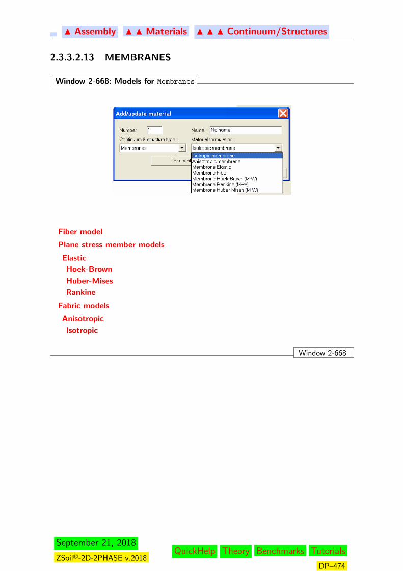
N Assembly N N Materials N N N Continuum/Structures
2.3.3.2.13 MEMBRANES
Window 2-668: Models for Membranes
Fiber model
Plane stress member models
Elastic
Hoek-Brown
Huber-Mises
Rankine
Fabric models
Anisotropic
Isotropic
Window 2-668
September 21, 2018
ZSoilr-2D-2PHASE v.2018QuickHelp Theory Benchmarks Tutorials
DP–474
N Materials N N C/S Type N N N Membranes
2.3.3.2.13.1 FIBER MODEL
Window 2-669: Fiber model for Membranes
This model represents a layer of equally spaced reinforcement bars.
Data groups Parameters
Elastic obligatory;Young’s elastic modulus, E {[kPa]; [> 0]; 100000}
Unit Weight optional;• γ, {[kNm−2]; [> 0]; 0} - unit weight of fiber material
• Density ρ =γ
gis automatically computed from γ (and vice versa)
• Multiplier for γ {[−]; [≥ 0]; 1.0}• Multiplier for ρ {[−]; [≥ 0]; 1.0}Setting γ multiplier to 0.0 will cancel body forces in all elements withthat material (unless body load definition is made at the elementlevel in the preprocessor) while setting ρ multiplier to 0.0 will cancelcontribution of all elements with that material to the mass matrix;both multipliers are active if Dynamics or Pushover is set ON in theproject preselection).
Creep not supported
Heat optional;α, {[C−1]; [> 0]; 1.0e−5} - thermal dilatancy coefficient
In case when group � Heat is active and preprocessed Heat
Transfer project is declared (if α > 0) thermal strains will be com-puted.
Humidity optional;β, {[−]; [≥ 0]; 0.01} - hygral dilatancy coefficient;
In case when group � Humidity is active and preprocessed
Humidity Transfer project is declared (if β > 0) hygral strainswill be computed.
Non--Linear optional• Uniaxial tensile strength ft, {[kPa]; [ft > 0]; 1}• Uniaxial compressive strength fc, {[kPa]; [fc ≥ 0]; 1}
Geometry obligatory• For Plane Strain:F Area per unit length A, {[m2/m=m], [> 0], [1]}• For Axisymmetry:F Direction: one of: } Circumferential or } Longitudinal
F Area per unit length A, {[m2/m=m], [> 0], [1]}
Damping optional (same definition as in the global Control/Dynamics dialog)
Window 2-669
Related Topics
Theory:September 21, 2018
ZSoilr-2D-2PHASE v.2018QuickHelp Theory Benchmarks Tutorials
DP–475

N Materials N N C/S Type N N N Membranes
• MEMBRANE ELEMENTS• UNI-AXIAL ELASTO-PLASTIC MODEL
September 21, 2018
ZSoilr-2D-2PHASE v.2018QuickHelp Theory Benchmarks Tutorials
DP–476

N Materials N N C/S Type N N N Membranes
2.3.3.2.13.2 PLANE STRESS MODELS
Window 2-670: Plane stress models for Membranes
The following models are used to represent membrane behavior under the plane-stress con-ditions:
ElasticHoek-Brown (M-W)Huber-MisesRankine (M-W)
Data groups Parameters
Elastic obligatory (same as for continuum); see Win.(2-631)
Unit Weight optional;• γ, {[kNm−3]; [> 0]; 0} - unit weight
• Density ρ =γ
gis automatically computed from γ (and vice versa)
• Multiplier for γ {[−]; [≥ 0]; 1.0}• Multiplier for ρ {[−]; [≥ 0]; 1.0}Setting γ multiplier to 0.0 will cancel body forces in all elements withthat material (unless body load definition is made at the element levelin the preprocessor) while setting ρ multiplier to 0.0 will cancel con-tribution of all elements with that material to the mass matrix; bothmultipliers are active if Dynamics or Pushover is set ON in the projectpreselection).
Geometry obligatory;Thickness t, {[m]; [> 0]; 0.1}
Creep not supported
Heat optional;α, {[C−1]; [> 0]; 1.0e−5} - thermal dilatancy coefficient
In case when group � Heat is active and preprocessed Heat Transfer
project is declared thermal strains will be computed (if β > 0).
Humidity optional;β, {[−]; [≥ 0]; 0.01} - hygral dilatancy coefficient;
In case when group � Humidity is active and preprocessed Humidity
Transfer project is declared hygral strains will be computed (if β > 0).
Non--Linear set:• For Huber--Mises and Rankine (M--W) (obligatory):F Uniaxial tensile strength ft, {[kPa]; [≥ 0]; 1}• For Hoek--Brown (M--W) (obligatory):F Uniaxial tensile strength ft, {[kPa]; [≥ 0]; 1}F Uniaxial compressive strength fc, {[kPa]; [fc > ft ≥ 0]; 1}
Damping optional (same definition as in the global Control/Dynamics dialog)
Window 2-670
September 21, 2018
ZSoilr-2D-2PHASE v.2018QuickHelp Theory Benchmarks Tutorials
DP–477

N Materials N N C/S Type N N N Membranes
Related Topics
Theory: MEMBRANES THEORY
September 21, 2018
ZSoilr-2D-2PHASE v.2018QuickHelp Theory Benchmarks Tutorials
DP–478
N Materials N N C/S Type N N N Membranes
2.3.3.2.13.3 MEMBRANE - FABRIC MODELS
Window 2-671: Fabric models for Membranes
The two following models are supported: Anisotropic and Isotropic
These models can represent different types of geo-textiles, geo-grids and similar products.The important point is that thickness parameter is included within the definition of stiffnessand strength parameters. Both isotropic and anisotropic models can be used.
Anisotropic and Isotropic membrane models: common data.
Data groups Parameters
Unit Weight optional; (see Win.(2-669))
Creep not supported
Heat optional;α, {[C−1]; [> 0]; 1.0e−5} - thermal dilatancy coefficient
In case when group � Heat is active and preprocessed Heat
Transfer project is declared thermal strains will be computed (ifβ > 0).
Humidity optional;β, {[−]; [≥ 0]; 0.01} - hygral dilatancy coefficient;
In case when group � Humidity is active and preprocessedHumidity Transfer project is declared hygral strains will be com-puted (if β > 0).
Damping optional (same definition as in the global Control/Dynamics dialog)
Isotropic membrane: specific data.
Data Use & Set up
Elastic obligatory;• Elastic stiffness K (equivalent to E×thickness) {[kN/m]; [>
0]; 100000},• Poisson ratio ν, {[−]; [0, 0.49999]; 0.3}Resulting elasticity matrix for the plane stress state will takeform:
D(3x3) =
K νK 0
νK K 0
0 0K
2(1 + ν)
,Non--Linear optional
If not activated elastic membrane with unlimited strength willbe considerd• Uniaxial tensile strength ft, {[kN/m]; [> 0]; 1}• Uniaxial compressive strength fc, {[kN/m]; [> 0]; 1}
September 21, 2018
ZSoilr-2D-2PHASE v.2018QuickHelp Theory Benchmarks Tutorials
DP–479

N Materials N N C/S Type N N N Membranes
Anisotropic membrane: specific data.
Data Use & Set up
Elastic obligatory;• Elastic stiffness in anisotropy direction KXX , KY Y , KXY {[kN/
m]; [> 0]; 100000},Resulting elasticity matrix for the plane stress state will take form:
D(3x3) =
Kxx Kxy 0
Kxy Kyy 0
0 0 0
,i.e. no shear stiffness is assumed in the model.
Geometry obligatoryX, Y , Z the coordinates of an arbitrary direction vector in 3D space.It determines anisotropy axis X
Non--Linear optionalIf not activated elastic membrane with unlimited strength will be con-sidered• Uniaxial tensile strength in anisotropy direction X,Y: ftX, ftY ,{[kN/m]; [≥ 0]; 1}• Uniaxial compressive strength in anisotropy direction X,Y: fcX,fcY , {[kN/m]; [≥ 0]; 1}
Remarks:
1. As a particular case no-tension material may be analyzed if fc = 0 (isotropic case) orfcX = fcY = 0 (anisotropic case)
2. No shear stiffness is assumed in the anisotropic model
Window 2-671
Related Topics
Theory:
MEMBRANES THEORY
September 21, 2018
ZSoilr-2D-2PHASE v.2018QuickHelp Theory Benchmarks Tutorials
DP–480
N Assembly N N Materials N N N Continuum/Structures
2.3.3.2.14 SEEPAGE
Window 2-672: Seepage model
This fictitious material model is associated with seepage surface elements simulating anautomatic switch from zero flux to pressure boundary condition (useful to model drains orfilling/drawdown effects). Behavior of this artificial interface is driven by a single parameter
Kv. Its reference value for the isotropic case is equal to Krefv =
k
gammaF hewhere k is
the seepage coefficient and he is the continuum element size adjacent to the seepage surfaceelement. In the standard case Kv = Kref
v ε where epsilon is a large number (penalty format),but there are also two other possibilities (since version 2018) to set this value. User may setdirect value of Kv parameter or may set his own multiplier to the Kref
v .
Data Use & Set up
Flow obligatory;• Multiplierto Kref
v ε, {[−], [> 0], 1}• Direct value of Kv {[m3/(kN s)], [> 0], 1}• Multiplierto Kref
v , {[−], [> 0], 1}Use standard option with multiplier 1.0 unless computed porepressure fields do not satisfy the assumed pressure boundaryconditions with required order of accuracy; in such cases try toenlarge the Multiplier; this may however lead to convergenceproblems. In special cases when modeling drains with limitedinflux use second (direct value of Kv) or third setting (usergiven multiplier to the reference value Kref
v )
Remark:
If continuum elements adjacent to seepage surface have impermeable material (group� Flowis set OFF), the error, caused by singularity of the resulting system of equations, will be re-ported.
Window 2-672
Related Topics
Theory:
• TWO-PHASE PARTIALLY SATURATED MEDIUM
September 21, 2018
ZSoilr-2D-2PHASE v.2018QuickHelp Theory Benchmarks Tutorials
DP–481

N Assembly N N Materials N N N Continuum/Structures
2.3.3.2.15 VISCOUS DAMPERS
Window 2-673: Viscous dampers model
This fictitious material model is attached to viscous damping elements that prevent wavereflections from domain boudaries. In most practical cases this data should be equivalentwith the one set up for adjacent continuum elements.
By default the flag � Inherit properties from adjacent continuum is set ON. However,user may set up the data himself in the same way as for the standard continuum.
Window 2-673
Related Topics
Theory:
• ABSORBING BOUNDARIES-SINGLE PHASE
• ABSORBING BOUNDARIES-TWO PHASE
September 21, 2018
ZSoilr-2D-2PHASE v.2018QuickHelp Theory Benchmarks Tutorials
DP–482
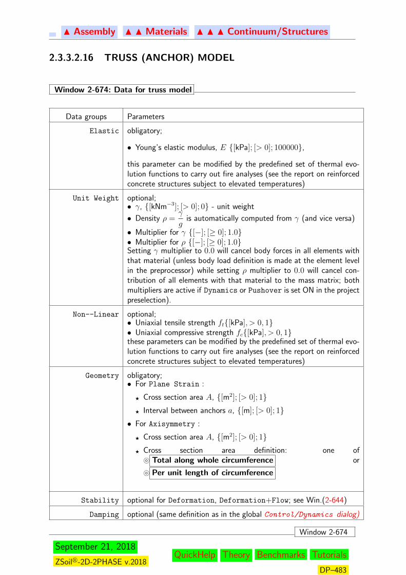
N Assembly N N Materials N N N Continuum/Structures
2.3.3.2.16 TRUSS (ANCHOR) MODEL
Window 2-674: Data for truss model
Data groups Parameters
Elastic obligatory;
• Young’s elastic modulus, E {[kPa]; [> 0]; 100000},
this parameter can be modified by the predefined set of thermal evo-lution functions to carry out fire analyses (see the report on reinforcedconcrete structures subject to elevated temperatures)
Unit Weight optional;• γ, {[kNm−3]; [> 0]; 0} - unit weight
• Density ρ =γ
gis automatically computed from γ (and vice versa)
• Multiplier for γ {[−]; [≥ 0]; 1.0}• Multiplier for ρ {[−]; [≥ 0]; 1.0}Setting γ multiplier to 0.0 will cancel body forces in all elements withthat material (unless body load definition is made at the element levelin the preprocessor) while setting ρ multiplier to 0.0 will cancel con-tribution of all elements with that material to the mass matrix; bothmultipliers are active if Dynamics or Pushover is set ON in the projectpreselection).
Non--Linear optional;• Uniaxial tensile strength ft{[kPa], > 0, 1}• Uniaxial compressive strength fc{[kPa], > 0, 1}these parameters can be modified by the predefined set of thermal evo-lution functions to carry out fire analyses (see the report on reinforcedconcrete structures subject to elevated temperatures)
Geometry obligatory;• For Plane Strain :
F Cross section area A, {[m2]; [> 0]; 1}F Interval between anchors a, {[m]; [> 0]; 1}• For Axisymmetry :
F Cross section area A, {[m2]; [> 0]; 1}F Cross section area definition: one of} Total along whole circumference or
} Per unit length of circumference
Stability optional for Deformation, Deformation+Flow; see Win.(2-644)
Damping optional (same definition as in the global Control/Dynamics dialog)
Window 2-674
September 21, 2018
ZSoilr-2D-2PHASE v.2018QuickHelp Theory Benchmarks Tutorials
DP–483

N Assembly N N Materials N N N Continuum/Structures
Remarks:
1. Perfect elasto-plastic model is used
Related Topics
Reports: Technical report on concrete structures subject to elevated temperatures
September 21, 2018
ZSoilr-2D-2PHASE v.2018QuickHelp Theory Benchmarks Tutorials
DP–484
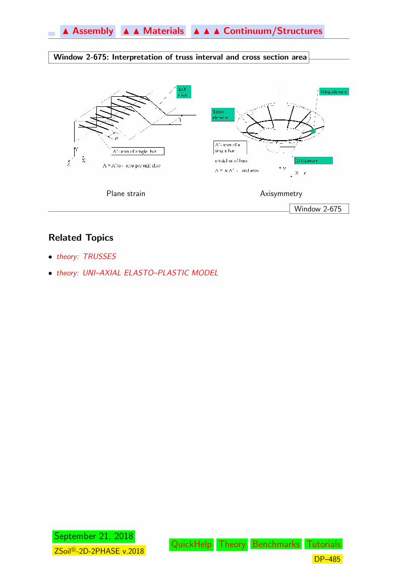
N Assembly N N Materials N N N Continuum/Structures
Window 2-675: Interpretation of truss interval and cross section area
Plane strain Axisymmetry
Window 2-675
Related Topics
• theory: TRUSSES
• theory: UNI–AXIAL ELASTO–PLASTIC MODEL
September 21, 2018
ZSoilr-2D-2PHASE v.2018QuickHelp Theory Benchmarks Tutorials
DP–485
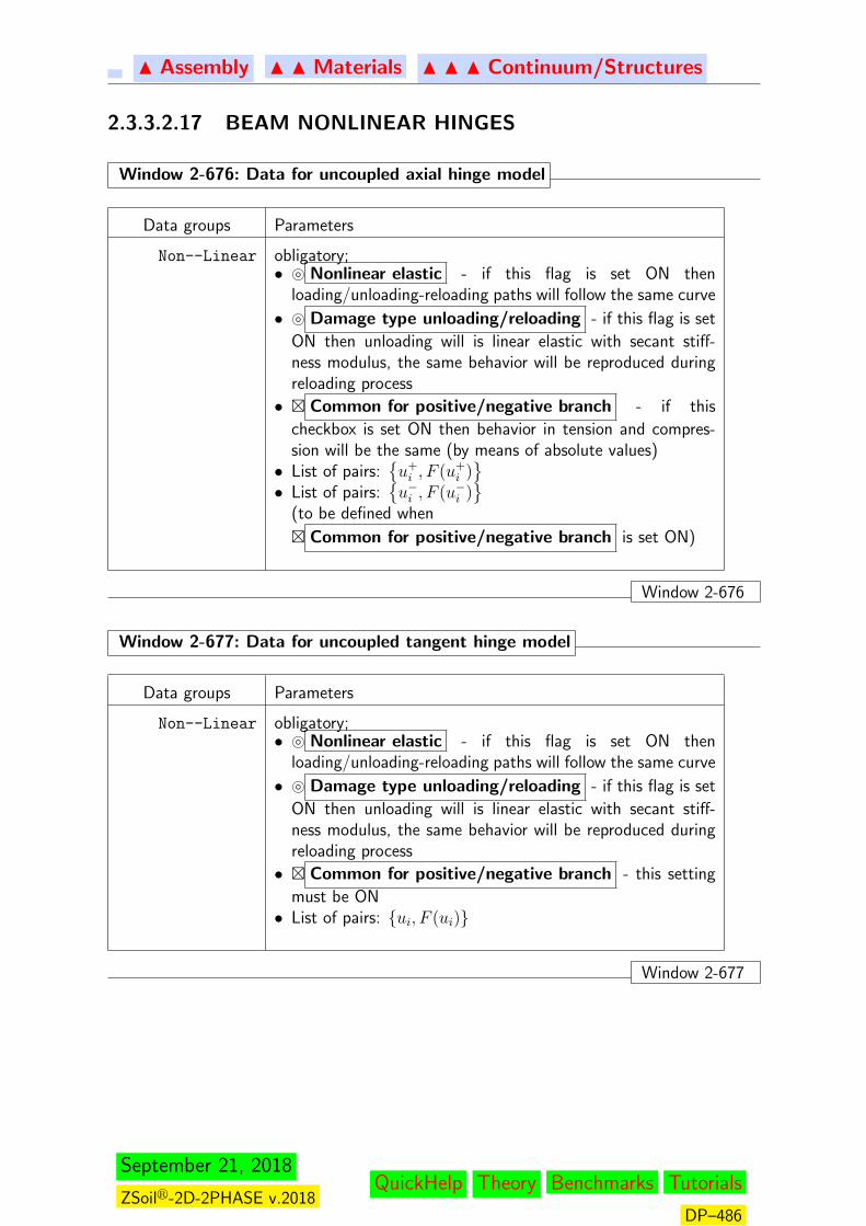
N Assembly N N Materials N N N Continuum/Structures
2.3.3.2.17 BEAM NONLINEAR HINGES
Window 2-676: Data for uncoupled axial hinge model
Data groups Parameters
Non--Linear obligatory;• } Nonlinear elastic - if this flag is set ON then
loading/unloading-reloading paths will follow the same curve
• } Damage type unloading/reloading - if this flag is set
ON then unloading will is linear elastic with secant stiff-ness modulus, the same behavior will be reproduced duringreloading process
• � Common for positive/negative branch - if this
checkbox is set ON then behavior in tension and compres-sion will be the same (by means of absolute values)• List of pairs:
{u+i , F (u+i )
}• List of pairs:
{u−i , F (u−i )
}(to be defined when
� Common for positive/negative branch is set ON)
Window 2-676
Window 2-677: Data for uncoupled tangent hinge model
Data groups Parameters
Non--Linear obligatory;• } Nonlinear elastic - if this flag is set ON then
loading/unloading-reloading paths will follow the same curve
• } Damage type unloading/reloading - if this flag is set
ON then unloading will is linear elastic with secant stiff-ness modulus, the same behavior will be reproduced duringreloading process
• � Common for positive/negative branch - this setting
must be ON• List of pairs: {ui, F (ui)}
Window 2-677
September 21, 2018
ZSoilr-2D-2PHASE v.2018QuickHelp Theory Benchmarks Tutorials
DP–486
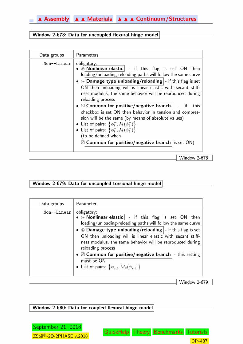
N Assembly N N Materials N N N Continuum/Structures
Window 2-678: Data for uncoupled flexural hinge model
Data groups Parameters
Non--Linear obligatory;• } Nonlinear elastic - if this flag is set ON then
loading/unloading-reloading paths will follow the same curve
• } Damage type unloading/reloading - if this flag is set
ON then unloading will is linear elastic with secant stiff-ness modulus, the same behavior will be reproduced duringreloading process
• � Common for positive/negative branch - if this
checkbox is set ON then behavior in tension and compres-sion will be the same (by means of absolute values)• List of pairs:
{φ+i ,M(φ+
i )}
• List of pairs:{φ−i ,M(φ−i )
}(to be defined when
� Common for positive/negative branch is set ON)
Window 2-678
Window 2-679: Data for uncoupled torsional hinge model
Data groups Parameters
Non--Linear obligatory;• } Nonlinear elastic - if this flag is set ON then
loading/unloading-reloading paths will follow the same curve
• } Damage type unloading/reloading - if this flag is set
ON then unloading will is linear elastic with secant stiff-ness modulus, the same behavior will be reproduced duringreloading process
• � Common for positive/negative branch - this setting
must be ON• List of pairs:
{φx,i,Mx(φx,i)
}Window 2-679
Window 2-680: Data for coupled flexural hinge model
September 21, 2018
ZSoilr-2D-2PHASE v.2018QuickHelp Theory Benchmarks Tutorials
DP–487
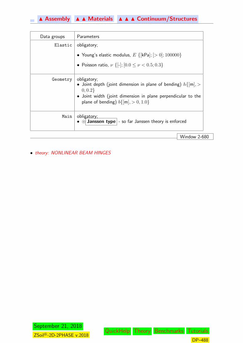
N Assembly N N Materials N N N Continuum/Structures
Data groups Parameters
Elastic obligatory;
• Young’s elastic modulus, E {[kPa]; [> 0]; 100000}
• Poisson ratio, ν {[-]; [0.0 ≤ ν < 0.5; 0.3}
Geometry obligatory;• Joint depth (joint dimension in plane of bending) h{[m], >
0, 0.2}• Joint width (joint dimension in plane perpendicular to the
plane of bending) b{[m], > 0, 1.0}
Main obligatory;• } Janssen type - so far Janssen theory is enforced
Window 2-680
• theory: NONLINEAR BEAM HINGES
September 21, 2018
ZSoilr-2D-2PHASE v.2018QuickHelp Theory Benchmarks Tutorials
DP–488
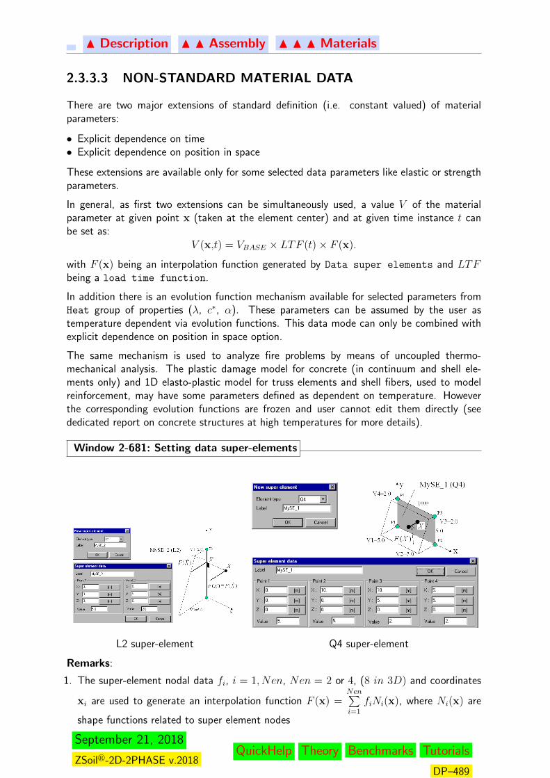
N Description N N Assembly N N N Materials
2.3.3.3 NON-STANDARD MATERIAL DATA
There are two major extensions of standard definition (i.e. constant valued) of materialparameters:
• Explicit dependence on time• Explicit dependence on position in space
These extensions are available only for some selected data parameters like elastic or strengthparameters.
In general, as first two extensions can be simultaneously used, a value V of the materialparameter at given point x (taken at the element center) and at given time instance t canbe set as:
V (x,t) = VBASE × LTF (t)× F (x).
with F (x) being an interpolation function generated by Data super elements and LTFbeing a load time function.
In addition there is an evolution function mechanism available for selected parameters fromHeat group of properties (λ, c∗, α). These parameters can be assumed by the user astemperature dependent via evolution functions. This data mode can only be combined withexplicit dependence on position in space option.
The same mechanism is used to analyze fire problems by means of uncoupled thermo-mechanical analysis. The plastic damage model for concrete (in continuum and shell ele-ments only) and 1D elasto-plastic model for truss elements and shell fibers, used to modelreinforcement, may have some parameters defined as dependent on temperature. Howeverthe corresponding evolution functions are frozen and user cannot edit them directly (seededicated report on concrete structures at high temperatures for more details).
Window 2-681: Setting data super-elements
L2 super-element Q4 super-element
Remarks:
1. The super-element nodal data fi, i = 1, Nen, Nen = 2 or 4, (8 in 3D) and coordinates
xi are used to generate an interpolation function F (x) =Nen∑i=1
fiNi(x), where Ni(x) are
shape functions related to super element nodes
September 21, 2018
ZSoilr-2D-2PHASE v.2018QuickHelp Theory Benchmarks Tutorials
DP–489

N Description N N Assembly N N N Materials
2. In case of a 4-node super element (a quad), the interpolation will be performed only forelements with central point placed inside the super element; for points being outside thesuper-element, base values of the material data are preserved
3. In case of L2 super-element, center of the finite element is orthogonally projected on thedefined line segment, and value of the data multiplier is linearly interpolated based onvalues defined at segment vertices
Window 2-681
September 21, 2018
ZSoilr-2D-2PHASE v.2018QuickHelp Theory Benchmarks Tutorials
DP–490
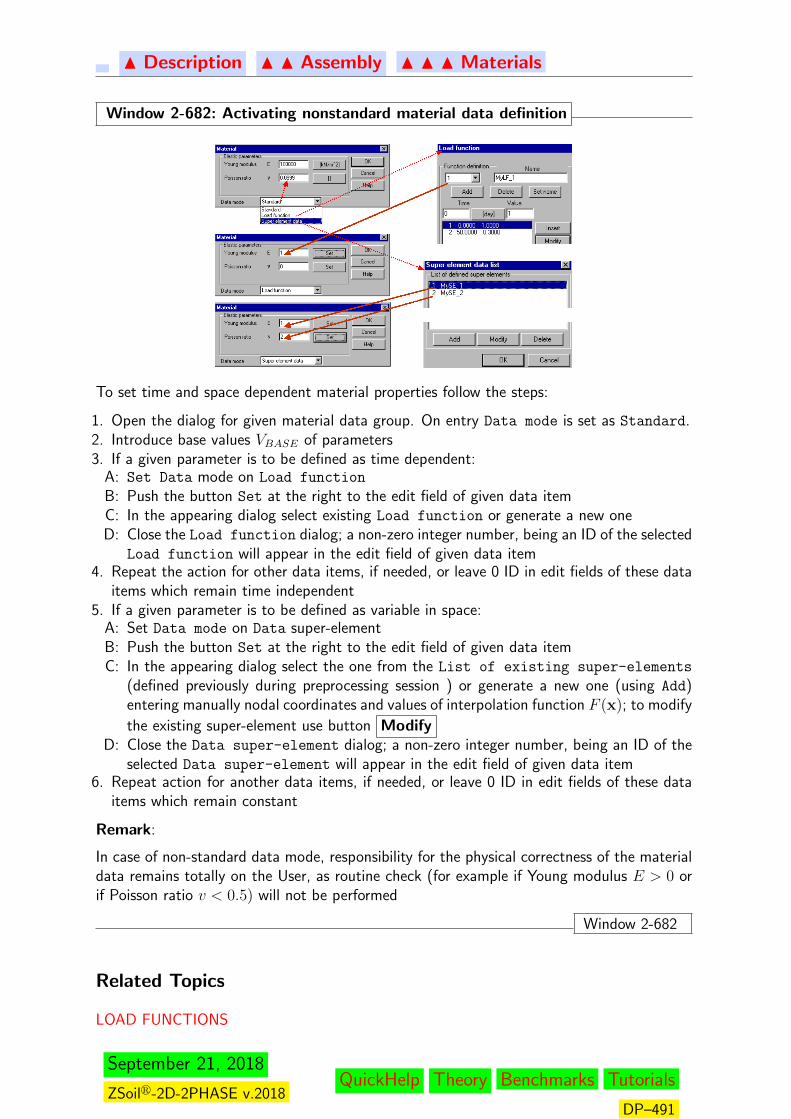
N Description N N Assembly N N N Materials
Window 2-682: Activating nonstandard material data definition
To set time and space dependent material properties follow the steps:
1. Open the dialog for given material data group. On entry Data mode is set as Standard.2. Introduce base values VBASE of parameters3. If a given parameter is to be defined as time dependent:
A: Set Data mode on Load function
B: Push the button Set at the right to the edit field of given data itemC: In the appearing dialog select existing Load function or generate a new oneD: Close the Load function dialog; a non-zero integer number, being an ID of the selected
Load function will appear in the edit field of given data item4. Repeat the action for other data items, if needed, or leave 0 ID in edit fields of these data
items which remain time independent5. If a given parameter is to be defined as variable in space:
A: Set Data mode on Data super-elementB: Push the button Set at the right to the edit field of given data itemC: In the appearing dialog select the one from the List of existing super-elements
(defined previously during preprocessing session ) or generate a new one (using Add)entering manually nodal coordinates and values of interpolation function F (x); to modify
the existing super-element use button ModifyD: Close the Data super-element dialog; a non-zero integer number, being an ID of the
selected Data super-element will appear in the edit field of given data item6. Repeat action for another data items, if needed, or leave 0 ID in edit fields of these data
items which remain constant
Remark:
In case of non-standard data mode, responsibility for the physical correctness of the materialdata remains totally on the User, as routine check (for example if Young modulus E > 0 orif Poisson ratio v < 0.5) will not be performed
Window 2-682
Related Topics
LOAD FUNCTIONS
September 21, 2018
ZSoilr-2D-2PHASE v.2018QuickHelp Theory Benchmarks Tutorials
DP–491

N Description N N Assembly N N N Materials
2.3.3.4 MATERIAL DATA VALUES
Summary of material data
Window 2-683: Summary of material data
The following table summarizes the most important material data
Data concerning Item Symbol Unit
UNIT WEIGHTS Unit weight for solid γ [kN/m3]
ELASTICITY Young modulus E [kPa]
Poisson ratio ν [-]
M-C PLASTICITY Friction angle φ [◦]
Cohesion c [kPa]
CUT-OFF Tensile strength ft [kPa]
DILATANCY Dilatancy angle ψ [◦]
CAP Initial void ratio eo [-]
Yield surface shape parameter R [-]
Slope of virgin consolidation
line in e-ln(p) λ [-]
Preconsolidation press. pc [kPa]
CREEP Parameters A,B units dependent
on creep law
CONSOLIDATION & FLOW Permeability (Darcy coeff.) k [m/s]
Fluid bulk modulus βF [kPa]
Fluid specific weight γF [k/m3]
Residual saturation Sr [-]
Regularization param. α [m−1]
Initial void ratio eo [-]
HEAT TRANSFER Heat conductivity λ [kN h/◦K]
Heat capacity c∗ [kN/(m2◦K]
Remarks:
Units are indicated in square brackets [..].
Window 2-683
September 21, 2018
ZSoilr-2D-2PHASE v.2018QuickHelp Theory Benchmarks Tutorials
DP–492
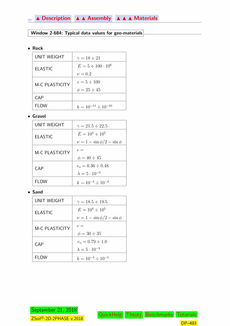
N Description N N Assembly N N N Materials
Window 2-684: Typical data values for geo-materials
• Rock
UNIT WEIGHT γ = 18÷ 21
ELASTICE = 5÷ 100 · 106
ν = 0.2
M-C PLASTICITYc = 5÷ 100
φ = 25÷ 45
CAP
FLOW k = 10−14 ÷ 10−10
• Gravel
UNIT WEIGHT γ = 21.5÷ 22.5
ELASTICE = 104 ÷ 105
ν = 1− sinφ/2− sinφ
M-C PLASTICITYc =
φ = 40÷ 45
CAPeo = 0.36÷ 0.48
λ = 5 · 10−3
FLOW k = 10−4 ÷ 10−2
• Sand
UNIT WEIGHT γ = 18.5÷ 19.5
ELASTICE = 104 ÷ 105
ν = 1− sinφ/2− sinφ
M-C PLASTICITYc =
φ = 30÷ 35
CAPeo = 0.79÷ 1.0
λ = 5 · 10−3
FLOW k = 10−4 ÷ 10−5
September 21, 2018
ZSoilr-2D-2PHASE v.2018QuickHelp Theory Benchmarks Tutorials
DP–493

N Description N N Assembly N N N Materials
• Silt
UNIT WEIGHT γ = 19.0÷ 20.0
ELASTICE = 104 ÷ 105
ν = 1− sinφ/2− sinφ
M-C PLASTICITYc = 10÷ 20
φ = 25÷ 35
CAPλ = 0.4÷ 0.9 · 10−2
eo = 0.70÷ 0.89
FLOWk = 10−7 ÷ 10−9
• Clay
UNIT WEIGHT γ = 18.0÷ 19.0
ELASTICE = 103
ν = 1− sinφ/2− sinφ
M-C PLASTICITYc = 0÷ 10
φ = 20÷ 30
CAPλ = 0.9÷ 2 · 10−3
R = 1÷ 1.5
FLOW0.89÷ 1.1
k = 10−7 ÷ 10−9
Window 2-684
Window 2-685: Common reference material data
Item: Unit Steel Concrete Soils Rocks Water
Specific weight γ kNm−3 78.0 24.0 18÷ 22 18÷ 25 10.0
Elastic modulus E kPa 2.1 · 108 1÷ 3 · 108 103 ÷ 105 5÷ 100 · 106 −
Tensile strength ft kPa − 4 · 103 − 2÷ 30 · 103 −
Compression s. fc kPa − 4 · 104 − 5÷ 400 · 103 −
Poisson ratio ν − 0.3 0.2 0.2÷ 0.5 0.2 −
Bulk modulus βF kPa − − − − 2 · 105
Heat conductivity λ W/(mK) 40÷ 80 2.4 1.0÷ 2.0 1.0÷ 2.0 0.060
Heat capacity c∗ kN/(m2K) 0.4 · 103 2 · 103 103 1÷ 3 · 103 4.2 · 103
Window 2-685
September 21, 2018
ZSoilr-2D-2PHASE v.2018QuickHelp Theory Benchmarks Tutorials
DP–494
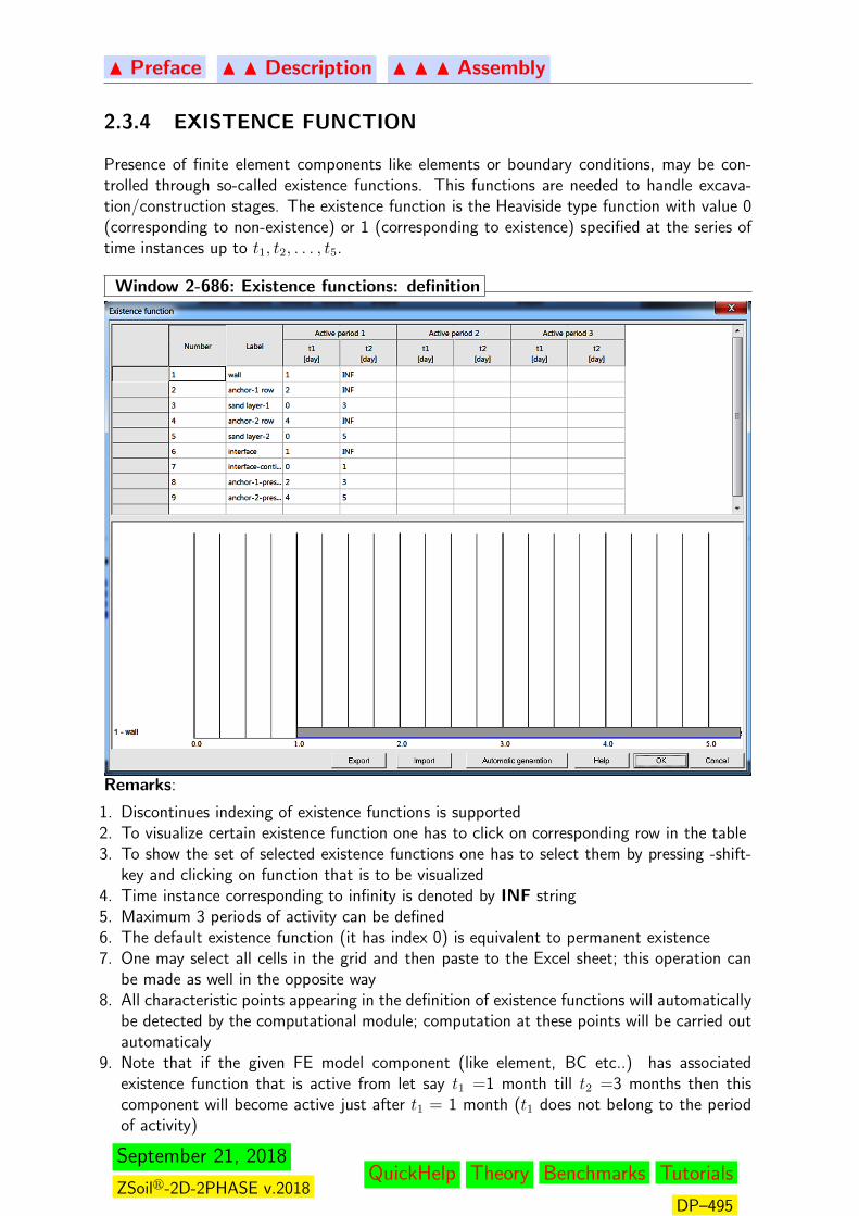
N Preface N N Description N N N Assembly
2.3.4 EXISTENCE FUNCTION
Presence of finite element components like elements or boundary conditions, may be con-trolled through so-called existence functions. This functions are needed to handle excava-tion/construction stages. The existence function is the Heaviside type function with value 0(corresponding to non-existence) or 1 (corresponding to existence) specified at the series oftime instances up to t1, t2, . . . , t5.
Window 2-686: Existence functions: definition
Remarks:
1. Discontinues indexing of existence functions is supported2. To visualize certain existence function one has to click on corresponding row in the table3. To show the set of selected existence functions one has to select them by pressing -shift-
key and clicking on function that is to be visualized4. Time instance corresponding to infinity is denoted by INF string5. Maximum 3 periods of activity can be defined6. The default existence function (it has index 0) is equivalent to permanent existence7. One may select all cells in the grid and then paste to the Excel sheet; this operation can
be made as well in the opposite way8. All characteristic points appearing in the definition of existence functions will automatically
be detected by the computational module; computation at these points will be carried outautomaticaly
9. Note that if the given FE model component (like element, BC etc..) has associatedexistence function that is active from let say t1 =1 month till t2 =3 months then thiscomponent will become active just after t1 = 1 month (t1 does not belong to the periodof activity)
September 21, 2018
ZSoilr-2D-2PHASE v.2018QuickHelp Theory Benchmarks Tutorials
DP–495
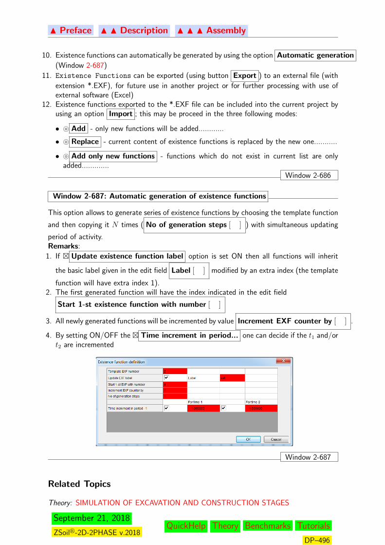
N Preface N N Description N N N Assembly
10. Existence functions can automatically be generated by using the option Automatic generation
(Window 2-687)
11. Existence Functions can be exported (using button Export ) to an external file (with
extension *.EXF), for future use in another project or for further processing with use ofexternal software (Excel)
12. Existence functions exported to the *.EXF file can be included into the current project byusing an option Import ; this may be proceed in the three following modes:
• } Add - only new functions will be added............
• } Replace - current content of existence functions is replaced by the new one...........
• } Add only new functions - functions which do not exist in current list are onlyadded.............
Window 2-686
Window 2-687: Automatic generation of existence functions
This option allows to generate series of existence functions by choosing the template function
and then copying it N times ( No of generation steps [ ] ) with simultaneous updating
period of activity.Remarks:
1. If � Update existence function label option is set ON then all functions will inherit
the basic label given in the edit field Label [ ] modified by an extra index (the template
function will have extra index 1).2. The first generated function will have the index indicated in the edit field
Start 1-st existence function with number [ ]
3. All newly generated functions will be incremented by value Increment EXF counter by [ ] .
4. By setting ON/OFF the � Time increment in period... one can decide if the t1 and/ort2 are incremented
Window 2-687
Related Topics
Theory: SIMULATION OF EXCAVATION AND CONSTRUCTION STAGES
September 21, 2018
ZSoilr-2D-2PHASE v.2018QuickHelp Theory Benchmarks Tutorials
DP–496
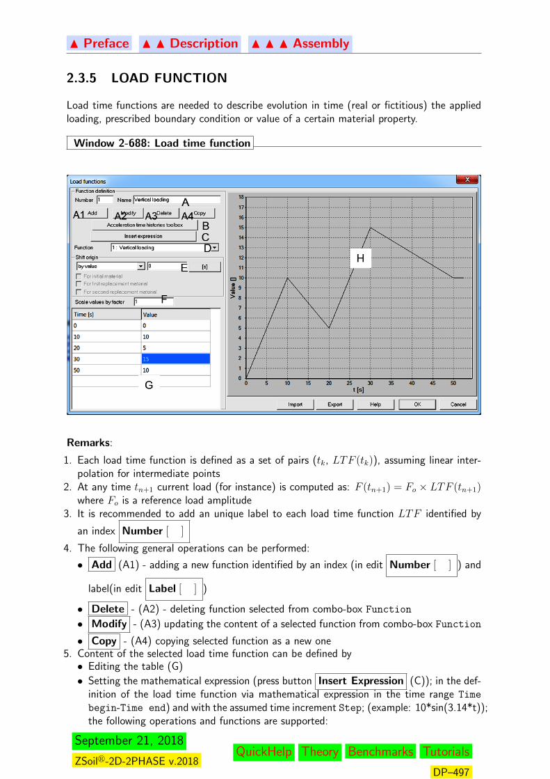
N Preface N N Description N N N Assembly
2.3.5 LOAD FUNCTION
Load time functions are needed to describe evolution in time (real or fictitious) the appliedloading, prescribed boundary condition or value of a certain material property.
Window 2-688: Load time function
Remarks:
1. Each load time function is defined as a set of pairs (tk, LTF (tk)), assuming linear inter-polation for intermediate points
2. At any time tn+1 current load (for instance) is computed as: F (tn+1) = Fo × LTF (tn+1)where Fo is a reference load amplitude
3. It is recommended to add an unique label to each load time function LTF identified by
an index Number [ ]
4. The following general operations can be performed:
• Add (A1) - adding a new function identified by an index (in edit Number [ ] ) and
label(in edit Label [ ] )
• Delete - (A2) - deleting function selected from combo-box Function
• Modify - (A3) updating the content of a selected function from combo-box Function
• Copy - (A4) copying selected function as a new one5. Content of the selected load time function can be defined by• Editing the table (G)
• Setting the mathematical expression (press button Insert Expression (C)); in the def-inition of the load time function via mathematical expression in the time range Time
begin-Time end) and with the assumed time increment Step; (example: 10*sin(3.14*t));the following operations and functions are supported:
September 21, 2018
ZSoilr-2D-2PHASE v.2018QuickHelp Theory Benchmarks Tutorials
DP–497

N Preface N N Description N N N Assembly
F arithmetic operators of the type: sum +, subtraction -, multiplication *, division /,parenthesis ( )
F trigonometric functions: SIN, COS, TG, ARCTG(arguments of trigonometric functions may be declared degrees or radians)
F square root function SQRT
F power function ˆ
• Importing the acceleration time history from earthquake data bases (press button (B))6. One may shift the origin of given load time function by a value indicated in edit field
Shift origin [ ] ; this operation can be made by declaring time shift value (by value),
by associating time shift value with the element activation (for the initial material, 1-st/2-nd replacement one) (this is useful when defining time dependent material properties) ordeactivation (for the initial material, 1-st/2-nd replacement one) (this is very useful whendefining unloading functions for several soil/rock excavated layers).
7. One may scale the load time function values (LTF (t)) by a value indicated in edit field
Scale values by factor [ ]
8. To inspect the evolution of the function in time one may zoom (with mouse) the diagram(G)
9. Discontinues numbering is supported10. The load time function that is not defined will yield value 0.0 at any time instance; user
will be warned when such undefined function is used11. For each function, value set at the last point is maintained until infinity12. During computation extra time steps are generated to trace all characteristic time instances
appearing at any load time function definition
Window 2-688
September 21, 2018
ZSoilr-2D-2PHASE v.2018QuickHelp Theory Benchmarks Tutorials
DP–498
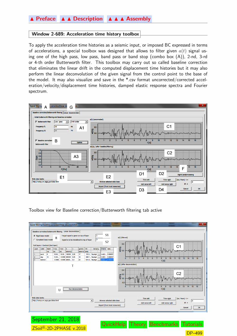
N Preface N N Description N N N Assembly
Window 2-689: Acceleration time history toolbox
To apply the acceleration time histories as a seismic input, or imposed BC expressed in termsof accelerations, a special toolbox was designed that allows to filter given a(t) signal us-ing one of the high pass, low pass, band pass or band stop (combo box (A)), 2-nd, 3-rdor 4-th order Butterworth filter. This toolbox may carry out so called baseline correctionthat eliminates the linear drift in the computed displacement time histories but it may alsoperform the linear deconvolution of the given signal from the control point to the base ofthe model. It may also visualize and save in the *.csv format uncorrected/corrected accel-eration/velocity/displacement time histories, damped elastic response spectra and Fourierspectrum.
Toolbox view for Baseline correction/Butterworth filtering tab active
September 21, 2018
ZSoilr-2D-2PHASE v.2018QuickHelp Theory Benchmarks Tutorials
DP–499
N Preface N N Description N N N Assembly
Toolbox view for Linear deconvolution tab active
Remarks:
1. To perform baseline correction press button Update ; the result of the correction will be
shown in diagram (C2)2. To add an additional signal filtering one may use a Butterworth filter; for low pass filter set
value f1 that will cancel frequencies higher than f1 (the gain function (A3) shows how theFourier amplitudes are scaled); for high pass set again value f1 that will cancel frequencieslower than f1, and for band pass and band stop set values f1 and f2 that give the rangeof frequencies that are to be maintained or canceled.
3. Three formats of data bases can be imported: the US data bank published at http://nsmp.wr.usgs.gov/data.html, the European one published at http://www.isesd.hi.is/ESD Local/frameset.htm and the free format where pairs (t, a(t)/g) are stored (E1); user may browse
one of the mentioned data banks by pressing button Browse..4. One may trim the acceleration record from the left and right side (use buttons (D1), (D2))5. One may add quiet zone at the beginning and end of the given record (use buttons (D3),
(D4))6. After downloading the acceleration records user may store them at his own directory; by
clicking the button (E3) user may select one of the stored records7. To export filtered, uncorrected/corrected (through baseline correction) acceleration time
histories, and corresponding undamped/damped Fourier spectra, to the Excel, press button(F); for long records this operation is time consuming.
8. To perform deconvolution of the signal switch to the Linear deconvolution tab (G),choose proper model (rigid base or compliant base)(R), edit data for soil layers in table(T), define where the target signal is given (S1) and where it should be transfered (S2),run deconvolution with button (U); result will be shown in window (C2); more details andtheory can be found in dedicated report on dynamics
Window 2-689
Related Topics
Theory:
LOAD FUNCTIONS
September 21, 2018
ZSoilr-2D-2PHASE v.2018QuickHelp Theory Benchmarks Tutorials
DP–500
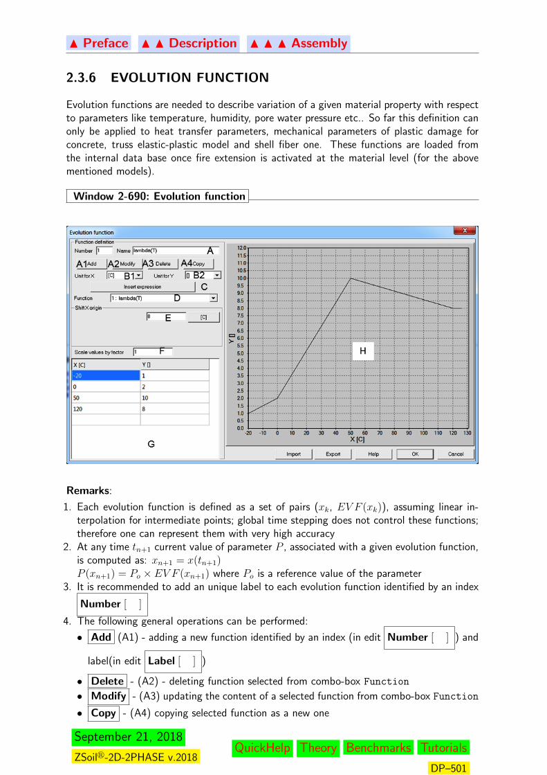
N Preface N N Description N N N Assembly
2.3.6 EVOLUTION FUNCTION
Evolution functions are needed to describe variation of a given material property with respectto parameters like temperature, humidity, pore water pressure etc.. So far this definition canonly be applied to heat transfer parameters, mechanical parameters of plastic damage forconcrete, truss elastic-plastic model and shell fiber one. These functions are loaded fromthe internal data base once fire extension is activated at the material level (for the abovementioned models).
Window 2-690: Evolution function
Remarks:
1. Each evolution function is defined as a set of pairs (xk, EV F (xk)), assuming linear in-terpolation for intermediate points; global time stepping does not control these functions;therefore one can represent them with very high accuracy
2. At any time tn+1 current value of parameter P , associated with a given evolution function,is computed as: xn+1 = x(tn+1)P (xn+1) = Po × EV F (xn+1) where Po is a reference value of the parameter
3. It is recommended to add an unique label to each evolution function identified by an index
Number [ ]
4. The following general operations can be performed:
• Add (A1) - adding a new function identified by an index (in edit Number [ ] ) and
label(in edit Label [ ] )
• Delete - (A2) - deleting function selected from combo-box Function
• Modify - (A3) updating the content of a selected function from combo-box Function
• Copy - (A4) copying selected function as a new one
September 21, 2018
ZSoilr-2D-2PHASE v.2018QuickHelp Theory Benchmarks Tutorials
DP–501

N Preface N N Description N N N Assembly
5. Content of the selected evolution function can be defined by• Editing the table (G)
• Setting the mathematical expression (press button Insert Expression (C)); in the
definition of the evolution function via mathematical expression in the range xo-xend)and with the assumed increment ∆x; (example: 10 ∗ sin(3.14 ∗ t) (use always t as afunction argument));the following operations and functions are supported:
F arithmetic operators of the type: sum +, subtraction -, multiplication *, division /,parenthesis ( )
F trigonometric functions: SIN, COS, TG, ARCTG(arguments of trigonometric functions may be declared degrees or radians)
F square root function SQRT
F power function ˆ6. One may shift given evolution function in time scale by a value indicated in edit field
Shift time origin [ ] ;
7. One may scale the evolution function values (EV F (t)) by a value indicated in edit field
Scale values by factor [ ]
8. To inspect the evolution of the function in time one may zoom (with mouse) the diagram(H)
9. Discontinues numbering is supported10. The evolution function that is not defined will yield value 0.0 at any time instance; user
will be warned when such undefined function is used11. For each function, value set at the last point is maintained until infinity12. None of characteristic instances, appearing in definition of an evolution function, is
traced during computation
Window 2-690
Related Topics
Theory:
EVOLUTION FUNCTIONS
September 21, 2018
ZSoilr-2D-2PHASE v.2018QuickHelp Theory Benchmarks Tutorials
DP–502

N Preface N N Description N N N Assembly
2.3.7 GRAVITY
Window 2-691: Gravity
Remarks:
1. Gravity direction can be set up using two definitions:A: Gravity vector
• Using this definition user may declare gravity vector b (default is (0,-1,0))
• This vector b is used to compute current body load vector b = γ b at each fi-nite element (body load definition may be overwritten, at the element level, duringpreprocessing stage, using option Body load)
• In addition to that option user may set a global initial state Ko coefficient; this globalKo setup can be overwritten at the material level by activating � Initial state Ko
group of parameters
B: Body load components (only in the � Advanced mode)
• Using this definition user may declare gravity vector b (default is (0,-1,0)) plus loadtime functions independently for all directions
• In this case gravity direction vector is not normalized
• Vector b is used to compute current body load components bi = γ bi LTFi(t) ateach finite element (body load definition may be overwritten, at the element level,during preprocessing stage, using option Body load)
2. For pseudo-seismic stability analysis the option Body load components has to be used(for instance in 2D models one may assume b = (0.1,−1.0))
3. Using the option Body load components one may cancel gravity loads, but not mass, inthe dynamic time history analysis; the easiest way, however, to cancel body loads or mass(in dynamic analyses), is to define the two independent multipliers, one for γ and one for ρat the material level in the setup for Unit weight. Setting γ multiplier to 0.0 will cancelbody forces in all elements with that material (unless body load definition is made at theelement level in the preprocessor) and setting ρ multiplier to 0.0 will cancel contributionof all elements with that material to the mass matrix.
4. Gravity direction influences also the hydraulic flow potential
Window 2-691
September 21, 2018
ZSoilr-2D-2PHASE v.2018QuickHelp Theory Benchmarks Tutorials
DP–503

N Preface N N Description N N N Assembly
Related Topics• data preparation: INITIAL K0 STATE• theory: GEOTECHNICAL ASPECT - INITIAL STATE• theory: NUMERICAL IMPLEMENTATION - INITIAL STRESS
September 21, 2018
ZSoilr-2D-2PHASE v.2018QuickHelp Theory Benchmarks Tutorials
DP–504

N Preface N N Description N N N Assembly
2.3.8 SEISMIC INPUT
Window 2-692: Seismic input
Seismic input option allows the user to apply the earthquake in the finite element model
• in the relative format for rigid base model; here seismic input is given as an imposed acceler-
ation ag =··ug of the ground that is global to the whole structure; the corresponding inertia
forces are shifted to the right hand side F(t) = −Mag(t) (set } Rigid base model ON)
• in the absolute format for compliant base model; here seismic input is given as an imposed
acceleration ag =··ug that is integrated to velocities (via Newmark method) and applied
at the base of the model where viscous dashpots must be added; this way the accelerationrecord is converted to the traction time history and applied to the bottom boundary of themodel (the bottom boundary is identified as a line segment (2D) or surface (3D), sharedby viscous boundary located at y = yMIN = const) (compliant base model circumvents
waves reflections) (set } Compliant base model ON)
Seismic input dialog window
Remarks:
1. Each acceleration record describes a time dependent acceleration vector that can be set inone of global X, Y or Z directions, or in the direction defined by a given vector
• for global X direction : ag(t) = ao (1, 0, 0)T · LTF (t)
• for global Y direction : ag(t) = ao (0, 1, 0)T · LTF (t)
• for global X direction : ag(t) = ao (0, 0, 1)T · LTF (t)
• for given vector v: ag(t) = aov · LTF (t)
where ao is the value set in the edit field Acceleration [ ]
September 21, 2018
ZSoilr-2D-2PHASE v.2018QuickHelp Theory Benchmarks Tutorials
DP–505

N Preface N N Description N N N Assembly
2. Acceleration values can be set as:A: relative to gravity acceleration g = 9.81[m/s2]B: absolute
3. Seismic input may consist of collection of acceleration records. At given time instanceglobal acceleration will be created as a sum of all records
4. Each record may have a different Load Function
5. To perform baseline correction/Butterworth filtering or linear deconvolution of the givenrecord use acceleration time history toolbox that can be activated at the Load time
function level6. Activate } Compliant base model option if seismic signal was transformed by linear
deconvolution procedure7. } Compliant base model / } Rigid base model switch is common for all applied
earthquake records
Related Topics• data preparation: TRANSIENT DYNAMICS• data preparation: LOAD FUNCTIONS
Window 2-692
September 21, 2018
ZSoilr-2D-2PHASE v.2018QuickHelp Theory Benchmarks Tutorials
DP–506
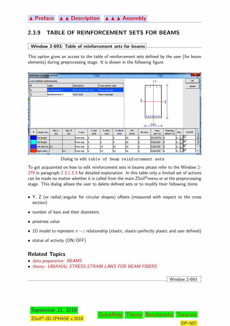
N Preface N N Description N N N Assembly
2.3.9 TABLE OF REINFORCEMENT SETS FOR BEAMS
Window 2-693: Table of reinforcement sets for beams
This option gives an access to the table of reinforcement sets defined by the user (for beamelements) during preprocessing stage. It is shown in the following figure
Dialog to edit table of beam reinforcement sets
To get acquainted on how to edit reinforcement sets in beams please refer to the Window 2-279 in paragraph 2.3.1.3.3 for detailed explanation. In this table only a limited set of actionscan be made no matter whether it is called from the main ZSoilrmenu or at the preprocessingstage. This dialog allows the user to delete defined sets or to modify their following items
• Y, Z (or radial/angular for circular shapes) offsets (measured with respect to the crosssection)
• number of bars and their diameters
• prestress value
• 1D model to represent σ−ε relationship (elastic, elastic-perfectly plastic and user defined)
• status of activity (ON/OFF)
Related Topics• data preparation: BEAMS• theory: UNIAXIAL STRESS-STRAIN LAWS FOR BEAM FIBERS
Window 2-693
September 21, 2018
ZSoilr-2D-2PHASE v.2018QuickHelp Theory Benchmarks Tutorials
DP–507
N Preface N N Description
2.4 ANALYSIS
Three computation modes are available:
Run Analysis This option consists of the following actions:• Saving the *.inp file• Generation of the *.dat file• Running calculation module starting from the first driver in the list
declared under Analysis and Drivers
Restart This option allows to restart computation from the last last convergedconfiguration of equilibriumSee: Window 2-694 : General remarksWindow 2-695 : Allowed and prohibited model modifications beforerestart
Batch processing This option is designed to allow the User to prepare a list of projects(*.inp files), to store them in the *.bat file and then to execute themin batch mode.See Window 2-696 : Handling batch processing
September 21, 2018
ZSoilr-2D-2PHASE v.2018QuickHelp Theory Benchmarks Tutorials
DP–508
NPreface NNDescription NNNAnalysis
2.4.1 RESTART
Window 2-694: Restart: General remarks
1. In case when at a given time step of the Time dependent Driver computation fails toconverge user may introduce the following modifications:• Change time step to diminish applied load increments• Modify Control data, i.e. convergence tolerances, nonlinear solver by switching full
Newton-Raphson method to the BFGS one (for instance) or the initial stiffnessand then to restart the computation
2. In case when at a given stability analysis step computation fails to converge, and no clearfailure mechanism is detected, user may introduce the following modifications:• Change safety factor increment (usually reduction is needed)• Modify Control data, i.e. convergence tolerances, nonlinear solver by switching full
Newton-Raphson method to the BFGS one (for instance) or the initial stiffnessand then to restart the computation
3. If user did not declare some material property as time dependent (which is recommended)and at certain time he wants to change its value then restart must be enforced. To handlethat case the following actions have to be performed:• Modification of the material property• Insertion of the next driver to continue computation starting from certain time instance• Executing computation restart
Window 2-694
Window 2-695: Restart: Allowed and prohibited model modifications
The following model modifications are allowed:
• Modification of Control data• Change of Driver list (only not yet executed drivers can be deleted)• Change of Driver parameters (time stepping)• Modification of Load time function in time ranges not completed yet, including time
points and function values• Modification of Existence function in time ranges not completed yet, including time
points and existence status• Loads (i.e. forces, fluxes) can be added / deleted• Load values can be modified (reference values as well as load time functions)• Boundary conditions can be added / deleted• Material model parameters can be changed
The following model modifications are prohibited:
• Changing Problem type in the sequence of Drivers• Changing Analysis type
• Adding / deleting nodes• Adding / deleting elements• Changing assignment of the material model to the elements• Changing material formulation for the material
Window 2-695
September 21, 2018
ZSoilr-2D-2PHASE v.2018QuickHelp Theory Benchmarks Tutorials
DP–509
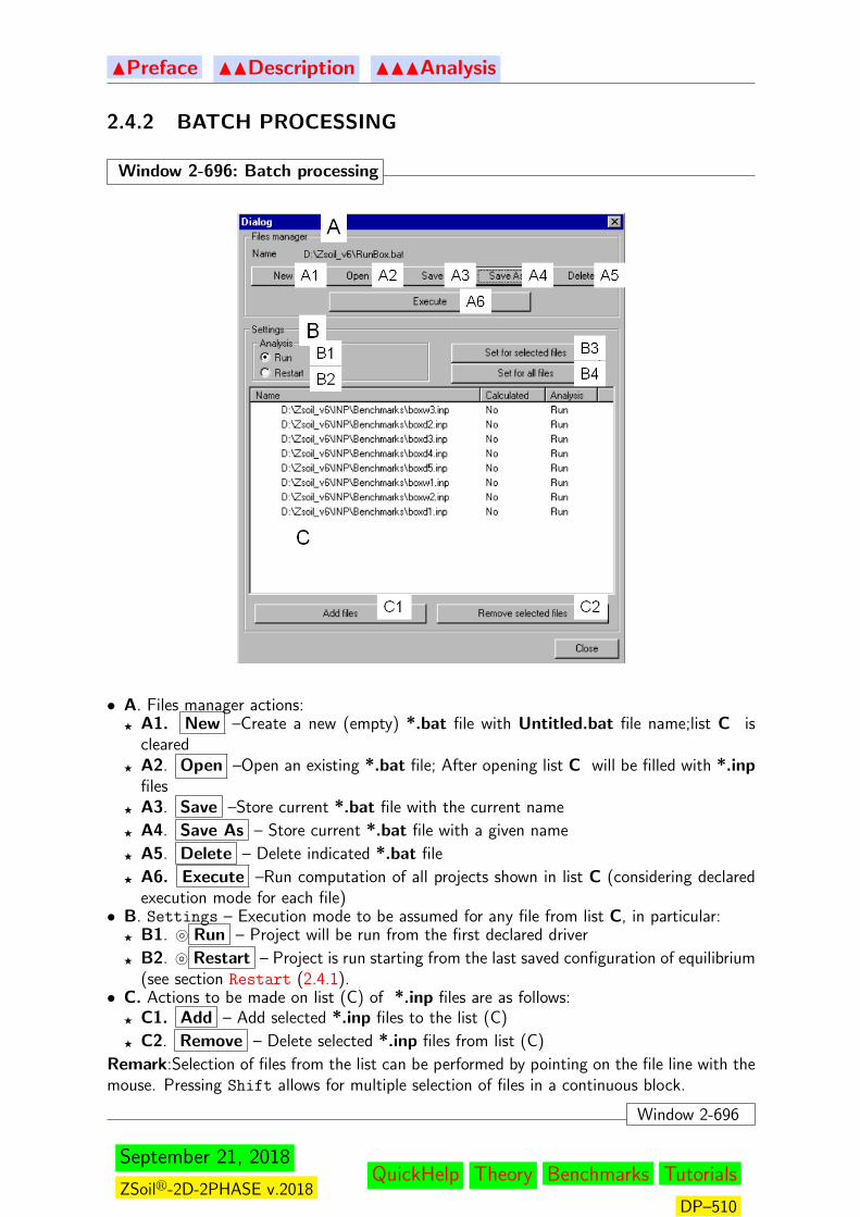
NPreface NNDescription NNNAnalysis
2.4.2 BATCH PROCESSING
Window 2-696: Batch processing
• A. Files manager actions:F A1. New –Create a new (empty) *.bat file with Untitled.bat file name;list C is
clearedF A2. Open –Open an existing *.bat file; After opening list C will be filled with *.inp
filesF A3. Save –Store current *.bat file with the current name
F A4. Save As – Store current *.bat file with a given name
F A5. Delete – Delete indicated *.bat file
F A6. Execute –Run computation of all projects shown in list C (considering declaredexecution mode for each file)
• B. Settings – Execution mode to be assumed for any file from list C, in particular:F B1. } Run – Project will be run from the first declared driver
F B2. } Restart – Project is run starting from the last saved configuration of equilibrium(see section Restart (2.4.1).
• C. Actions to be made on list (C) of *.inp files are as follows:F C1. Add – Add selected *.inp files to the list (C)
F C2. Remove – Delete selected *.inp files from list (C)
Remark:Selection of files from the list can be performed by pointing on the file line with themouse. Pressing Shift allows for multiple selection of files in a continuous block.
Window 2-696
September 21, 2018
ZSoilr-2D-2PHASE v.2018QuickHelp Theory Benchmarks Tutorials
DP–510
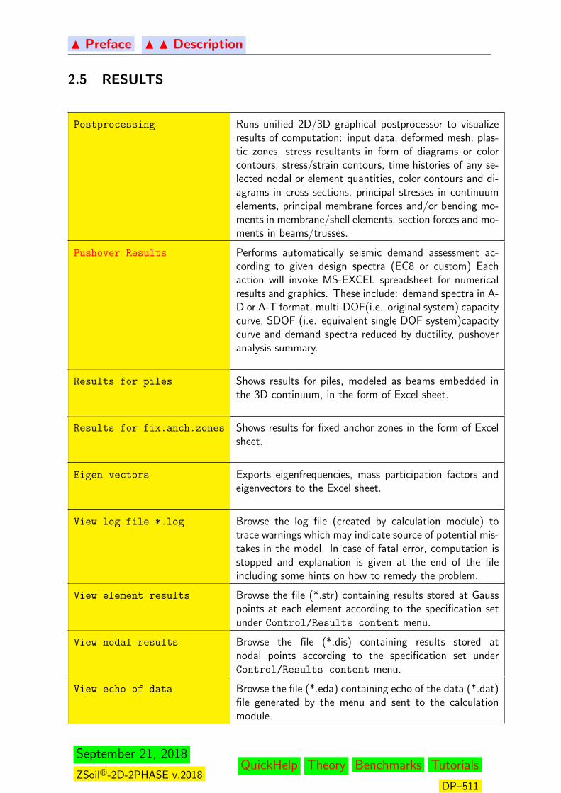
N Preface N N Description
2.5 RESULTS
Postprocessing Runs unified 2D/3D graphical postprocessor to visualizeresults of computation: input data, deformed mesh, plas-tic zones, stress resultants in form of diagrams or colorcontours, stress/strain contours, time histories of any se-lected nodal or element quantities, color contours and di-agrams in cross sections, principal stresses in continuumelements, principal membrane forces and/or bending mo-ments in membrane/shell elements, section forces and mo-ments in beams/trusses.
Pushover Results Performs automatically seismic demand assessment ac-cording to given design spectra (EC8 or custom) Eachaction will invoke MS-EXCEL spreadsheet for numericalresults and graphics. These include: demand spectra in A-D or A-T format, multi-DOF(i.e. original system) capacitycurve, SDOF (i.e. equivalent single DOF system)capacitycurve and demand spectra reduced by ductility, pushoveranalysis summary.
Results for piles Shows results for piles, modeled as beams embedded inthe 3D continuum, in the form of Excel sheet.
Results for fix.anch.zones Shows results for fixed anchor zones in the form of Excelsheet.
Eigen vectors Exports eigenfrequencies, mass participation factors andeigenvectors to the Excel sheet.
View log file *.log Browse the log file (created by calculation module) totrace warnings which may indicate source of potential mis-takes in the model. In case of fatal error, computation isstopped and explanation is given at the end of the fileincluding some hints on how to remedy the problem.
View element results Browse the file (*.str) containing results stored at Gausspoints at each element according to the specification setunder Control/Results content menu.
View nodal results Browse the file (*.dis) containing results stored atnodal points according to the specification set underControl/Results content menu.
View echo of data Browse the file (*.eda) containing echo of the data (*.dat)file generated by the menu and sent to the calculationmodule.
September 21, 2018
ZSoilr-2D-2PHASE v.2018QuickHelp Theory Benchmarks Tutorials
DP–511
N Preface N N Description
2.5.1 POSTPROCESSING
The detailed explanation on how to use graphical postprocessor is given in form of video filmsrecorded for all prepared tutorials. Some specific topics in form How do I... are given in nextsections.
How do I ... Explanations for some specific options
How to use macro Explanation on how to use macros to create an automatic out-put
Parametric analysis Explanation on how to plot nodal/element results vs varyingmaterial properties at a given time step
September 21, 2018
ZSoilr-2D-2PHASE v.2018QuickHelp Theory Benchmarks Tutorials
DP–512

N Preface N N Description N N N How do I .....
2.5.1.1 HOW DO I......1. paste a picture to text editor or Powerpoint
There are three possibilities:
• through File / Save As selecting *.bmp format;then under text editor you can import this bitmap,• through Ctrl-C and then Ctrl-V (here white background is recommended),
2. set a local system for nodal results and results for continuum elementsUse Settings/Local coord. system/continuum, nodal quantities menu to open a dialog.This dialog allows you to define a new X’-Y’-Z’ local coordinate system or cylindricalsystem. For X’-Y’-Z’ you have to define the two orthogonal basis vectors (normalizationis not required) and the third one will be set as vector product of first two. You may getan error message which says that the orthogonality check has failed. All results in nodesand continuum elements will be transformed to this new system.For cylindrical system you have to define a point and orientation vector coinciding with axisof axial symmetry. All nodal results and results for continuum elements will be transformedto this system.In all cases you want to change the local system just press Modify button and then OK. Ifyou want to see this local basis please activate it Visibility setup.
3. set a local system for shells/membranes/contactUse Settings/Local coord. system/shells,membranes/contact menu to open a dialog.This dialog allows you to define a vector V in reference system X − Y − Z used forshell/membrane/contact element local basis setup. The definition of the local coordinatesystem (where Π is a plane tangent to the midsurface) is show in figure below Local axisXL coincides with e
′1, axis y with e
′2. Note, that axis XL of that system, in each point
separately, is determined as the closest possible to the vector V , among all directionstangent to to the element. If V is tangent to the element itself, XL will coincide with V.The detailed procedure of evaluating {e′i} is given in Theroretical section under ??It may happen that for complex shell structures this definition leads to the situation thatvector V is parallel to the normal local axis e3. In that case new local basis setup isnonunique and hence results for these elements will not be displayed. Additionally thefollowing warning is shown : ”No way to define a local system for shell/contact for givenvector”.To remedy this situation please use mechanism of selections and work on groups of ele-ments.If you want to see this local axes please activate them in Visibility setup.
User defined shell-membrane-contactcoordinate system
September 21, 2018
ZSoilr-2D-2PHASE v.2018QuickHelp Theory Benchmarks Tutorials
DP–513

N Preface N N Description N N N How do I .....
4. set local basis for 3D section of continuumWhen making a 3D section of continuum element we need to define a local basis for resultstransformation. A normal vector to the section plane is assumed to be ”N” axis while thetwo axes ”T1” and ”T2”, in the section plane, have to be set using additional information.Through Settings/T1 axis for sections 3D we open a dialog box in which we can set avector, such that ”T1” axis coincides always with projection of this vector on section planeΠ.If you want to see this local basis please activate it Visibility setup.It may happen that running Graph Option/Sectional quantities you get a warning ”TheT1 axis will be adjusted automatically so please modify it if necessary”. It means thatthe default vector (for positioning of the T1 axis) was such that normal to the sectionplane was parallel to this vector. In that case program automatically changes this vectorto avoid a conflict but its position is random so please verify it especially if you analyzetensorial/vectorial components with index T1,T2.
5. save/ read graphical settings for projectPlease use Graph Option/Save Settings, Graph Option/Read Settings.
6. compute integrals for results shown in Color MapsPlease use Misc./Maps/Integral:INT(rsl) dA or Misc./Maps/Time history of INT(rsl) dA.This second possibility use with caution as it may take along time.
7. compute integrals for results shown in Sectional quantitiesPlease use Misc./Sections 3D/Integral:INT(rsl) dA or Misc./Sections 3D/Time history ofINT(rsl) dA. This second possibility use with caution as it may take along time.
September 21, 2018
ZSoilr-2D-2PHASE v.2018QuickHelp Theory Benchmarks Tutorials
DP–514

N Preface N N Description N N N How to use macro
2.5.1.2 HOW TO USE MACRO
Option Macro is designed to perform the following:
• to generate a template sequence of plots and store them in external *.BMP files• to generate a template sequence of numerical results and store them in external *.CSV
files• to repeat a template action for selected time instants in one job.• to execute an action from the template previously executed and stored in another job
Remarks:
1. Produced output i.e. graphic (*.BMP) or text (*.CSV) files can be easily processed inan automated way by any suitable software like MS-Word, PowerPoint, Excel.
2. Note, that using the technique of ”linking” but not ”copying” objects allows you to gen-erate template documents which will be automatically actualized if only ZSoilr outputwill change.
To generate a template action:
• Activate a macro session by: Macro→ Record macro,• Execute any desired control sequence of the plot including:
F Time instance,
F its contents (i.e. Graph. option),
F detailed Settings including Visibility setup,
F position on the screen and zoom (under View),
F required Selection.
• Store current plot status in a macro file (*.mcr) by pressing CTRL-C or File→ Copy
to clipboard.• Generate and record next plots.• To end the macro session use Macro→ Save macro. Assign any name to the macro
(*.mcr) file proceeding in a standard MS-Windows way.
How to generate files resulting from the recorded action
Remark: Any time the macro is played, the plots previously activated by CTRL-C duringmacro recording are stored in *.BMP files. Names of these files are automatically created.Each name contains a full information on file contents. It consist of three parts separatedby ”-” concerning:
• plot contents identified by the label identical as the string appearing at the bottom ofthe PostPro frame• job name (i.e. of *.INP file)• time instant in the form ”t=x.y” , plot instance (in case of multiple plots of the same
origin)
See the example of automatically generated file name:
EFFECTIVE PRINCIPAL STRESSES-MyINPFileName-t=0.1.bmp
The *.BMP files will be created at the same directory where *.mcr file is located by theUser.
To generate files:
• Record and Save a macro, see the previous point.
September 21, 2018
ZSoilr-2D-2PHASE v.2018QuickHelp Theory Benchmarks Tutorials
DP–515
N Preface N N Description N N N How to use macro
• Use: Macro→ Play macro
• In appearing dialog Open the *.mcr file
How to repeat a template action for selected time steps
• Activate a macro session by: Macro→ Record macro
• Execute a template sequence of actions for given time instance• Use Macro→ Repeat action for selected time step
• In the appearing listbox select the time steps for which the action has to be performedagain (i.e point the time step lines with the mouse, marking them in dark blue).• Store the sequence of actions using Macro→ Save
• Use Macro→ Play to generate plots and store them in external files
To execute an action from the template previously executed and stored in another job
• Use Macro → Play macro
• Select and then Open related existing *.mcr file. This will generate the plots and/orresult files for the recent job with all settings identical as in the template session.
To execute Z POST3D with a macro
To execute any action recorded in a macro stored in the *.mcr file, without enteringZ POST3D type a command on a level of operating system or run it as a batch file:
Z POST3D [#@PRJ DatPath@#] [#@POST3D MCR McrPath@#]
where:
• DatPath is a full path to the *.DAT file containing compiled data• McrPath is a full path to the *.MCR file containing pre-recorded macro as described
above• [#@PRJ, [#@POST3D MCR, @#] are obligatory control sign sequences
September 21, 2018
ZSoilr-2D-2PHASE v.2018QuickHelp Theory Benchmarks Tutorials
DP–516
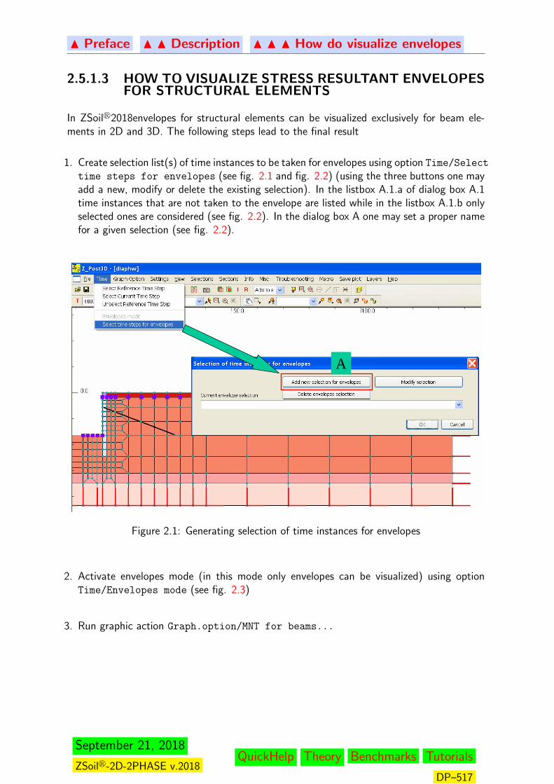
N Preface N N Description N N N How do visualize envelopes
2.5.1.3 HOW TO VISUALIZE STRESS RESULTANT ENVELOPESFOR STRUCTURAL ELEMENTS
In ZSoilr2018envelopes for structural elements can be visualized exclusively for beam ele-ments in 2D and 3D. The following steps lead to the final result
1. Create selection list(s) of time instances to be taken for envelopes using option Time/Select
time steps for envelopes (see fig. 2.1 and fig. 2.2) (using the three buttons one mayadd a new, modify or delete the existing selection). In the listbox A.1.a of dialog box A.1time instances that are not taken to the envelope are listed while in the listbox A.1.b onlyselected ones are considered (see fig. 2.2). In the dialog box A one may set a proper namefor a given selection (see fig. 2.2).
A
Figure 2.1: Generating selection of time instances for envelopes
2. Activate envelopes mode (in this mode only envelopes can be visualized) using optionTime/Envelopes mode (see fig. 2.3)
3. Run graphic action Graph.option/MNT for beams...
September 21, 2018
ZSoilr-2D-2PHASE v.2018QuickHelp Theory Benchmarks Tutorials
DP–517
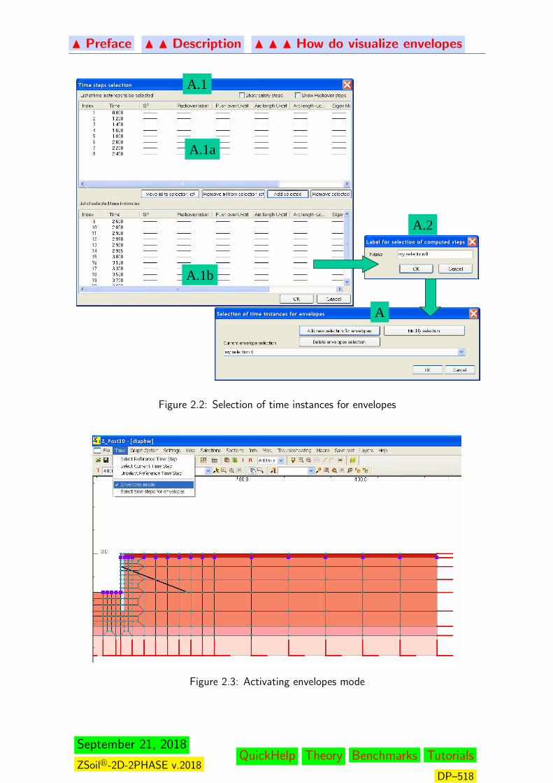
N Preface N N Description N N N How do visualize envelopes
A.1
A.1a
A.1b
A.2
A
Figure 2.2: Selection of time instances for envelopes
Figure 2.3: Activating envelopes mode
September 21, 2018
ZSoilr-2D-2PHASE v.2018QuickHelp Theory Benchmarks Tutorials
DP–518
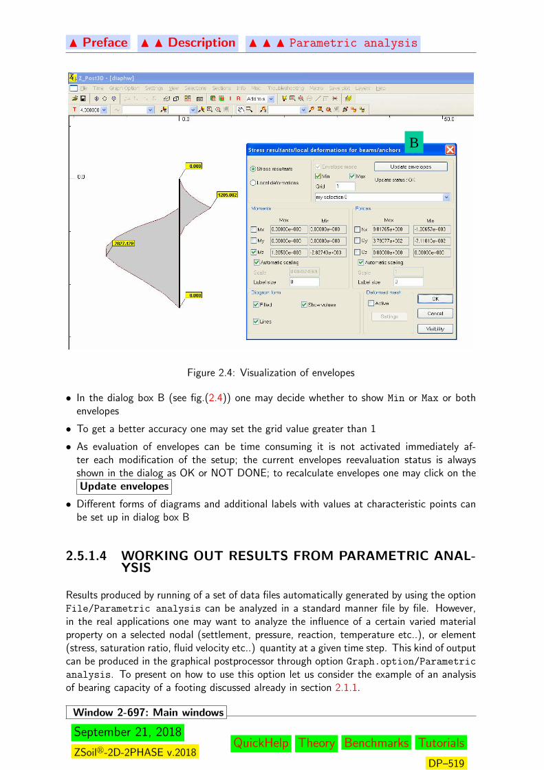
N Preface N N Description N N N Parametric analysis
B
Figure 2.4: Visualization of envelopes
• In the dialog box B (see fig.(2.4)) one may decide whether to show Min or Max or bothenvelopes
• To get a better accuracy one may set the grid value greater than 1
• As evaluation of envelopes can be time consuming it is not activated immediately af-ter each modification of the setup; the current envelopes reevaluation status is alwaysshown in the dialog as OK or NOT DONE; to recalculate envelopes one may click on theUpdate envelopes
• Different forms of diagrams and additional labels with values at characteristic points canbe set up in dialog box B
2.5.1.4 WORKING OUT RESULTS FROM PARAMETRIC ANAL-YSIS
Results produced by running of a set of data files automatically generated by using the optionFile/Parametric analysis can be analyzed in a standard manner file by file. However,in the real applications one may want to analyze the influence of a certain varied materialproperty on a selected nodal (settlement, pressure, reaction, temperature etc..), or element(stress, saturation ratio, fluid velocity etc..) quantity at a given time step. This kind of outputcan be produced in the graphical postprocessor through option Graph.option/Parametric
analysis. To present on how to use this option let us consider the example of an analysisof bearing capacity of a footing discussed already in section 2.1.1.
Window 2-697: Main windows
September 21, 2018
ZSoilr-2D-2PHASE v.2018QuickHelp Theory Benchmarks Tutorials
DP–519
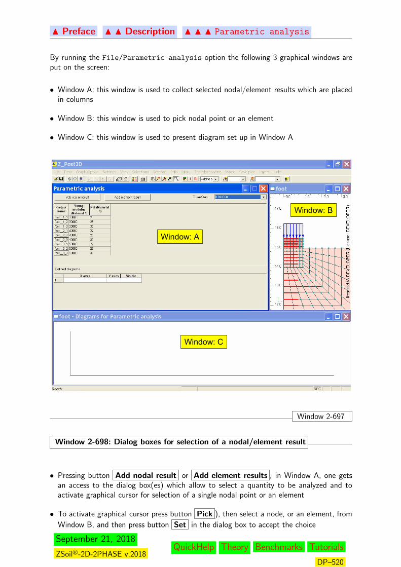
N Preface N N Description N N N Parametric analysis
By running the File/Parametric analysis option the following 3 graphical windows areput on the screen:
• Window A: this window is used to collect selected nodal/element results which are placedin columns
• Window B: this window is used to pick nodal point or an element
• Window C: this window is used to present diagram set up in Window A
Window: B
Window: C
Window: A
Window 2-697
Window 2-698: Dialog boxes for selection of a nodal/element result
• Pressing button Add nodal result or Add element results , in Window A, one getsan access to the dialog box(es) which allow to select a quantity to be analyzed and toactivate graphical cursor for selection of a single nodal point or an element
• To activate graphical cursor press button Pick ), then select a node, or an element, from
Window B, and then press button Set in the dialog box to accept the choice
September 21, 2018
ZSoilr-2D-2PHASE v.2018QuickHelp Theory Benchmarks Tutorials
DP–520
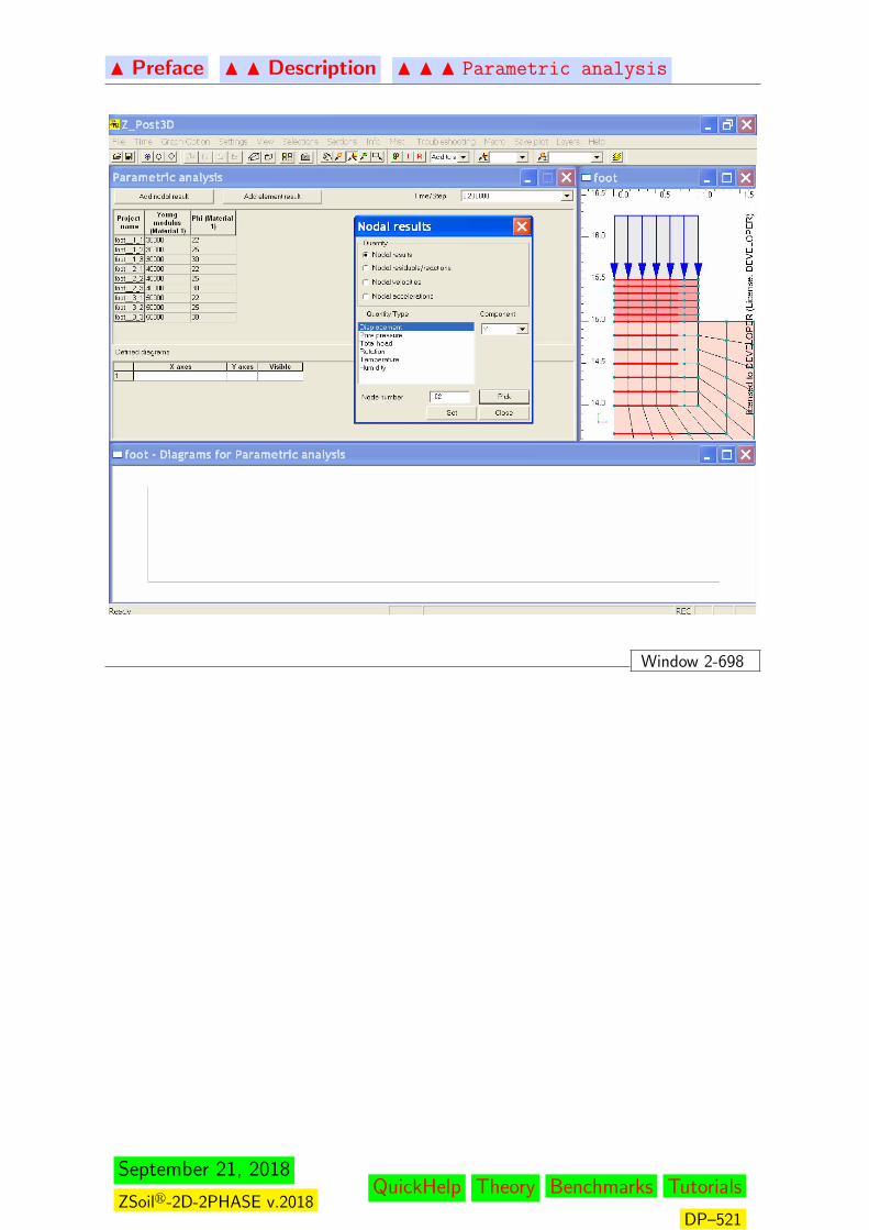
N Preface N N Description N N N Parametric analysis
Window 2-698
September 21, 2018
ZSoilr-2D-2PHASE v.2018QuickHelp Theory Benchmarks Tutorials
DP–521
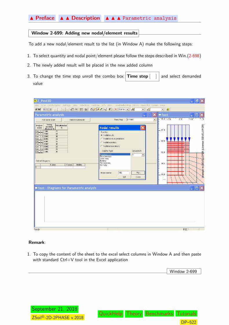
N Preface N N Description N N N Parametric analysis
Window 2-699: Adding new nodal/element results
To add a new nodal/element result to the list (in Window A) make the following steps:
1. To select quantity and nodal point/element please follow the steps described in Win.(2-698)
2. The newly added result will be placed in the new added column
3. To change the time step unroll the combo box Time step [ ] and select demanded
value
Remark:
1. To copy the content of the sheet to the excel select columns in Window A and then pastewith standard Ctrl+V tool in the Excel application
Window 2-699
September 21, 2018
ZSoilr-2D-2PHASE v.2018QuickHelp Theory Benchmarks Tutorials
DP–522
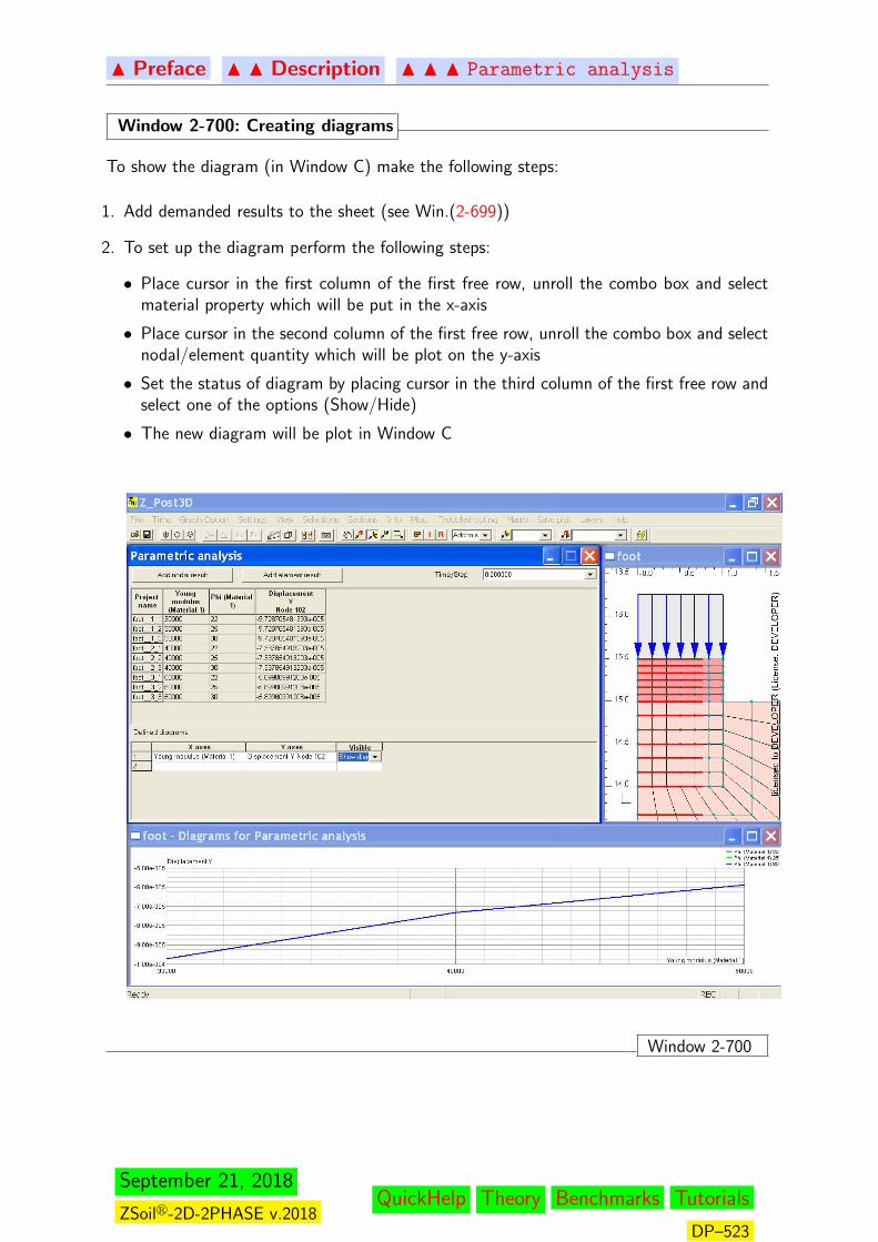
N Preface N N Description N N N Parametric analysis
Window 2-700: Creating diagrams
To show the diagram (in Window C) make the following steps:
1. Add demanded results to the sheet (see Win.(2-699))
2. To set up the diagram perform the following steps:
• Place cursor in the first column of the first free row, unroll the combo box and selectmaterial property which will be put in the x-axis
• Place cursor in the second column of the first free row, unroll the combo box and selectnodal/element quantity which will be plot on the y-axis
• Set the status of diagram by placing cursor in the third column of the first free row andselect one of the options (Show/Hide)
• The new diagram will be plot in Window C
Window 2-700
September 21, 2018
ZSoilr-2D-2PHASE v.2018QuickHelp Theory Benchmarks Tutorials
DP–523

N Preface N N Description
2.6 EXTRAS
Run Analysis Calls computational module without storing job file(*.inp) nor creating *.dat file. Use for *.dat file mod-ified by hand
Write *.dat Creates explicit data file without calling computation
View *.dat Edits *.dat file (only for very advanced users but incase of hand corrections hotline is not foreseen))
View *.inp Edits *.inp user data file (in case of hand correctionshotline is not foreseen)
View log file *.log Edits *.log file which contains echo of computationplus detected errors marked as warnings or fatal er-rors
Units conversion Invokes a dialog box to handle units conversion
Databases Gives an access to view:
• Databases containing steel profiles (in Excel for-mat)• User created material databases (see Window 2-
599)
Protection report Generates protection report
License Handles license upgrades
September 21, 2018
ZSoilr-2D-2PHASE v.2018QuickHelp Theory Benchmarks Tutorials
DP–524
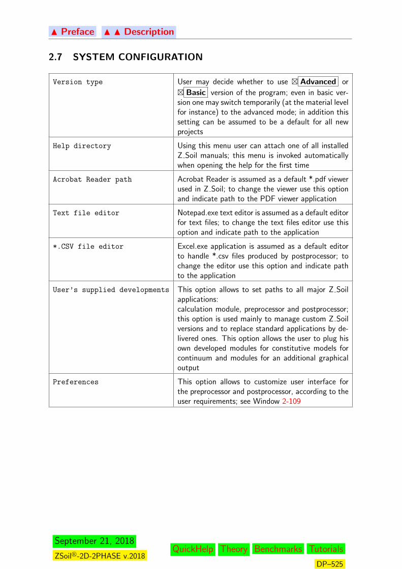
N Preface N N Description
2.7 SYSTEM CONFIGURATION
Version type User may decide whether to use � Advanced or
� Basic version of the program; even in basic ver-sion one may switch temporarily (at the material levelfor instance) to the advanced mode; in addition thissetting can be assumed to be a default for all newprojects
Help directory Using this menu user can attach one of all installedZ Soil manuals; this menu is invoked automaticallywhen opening the help for the first time
Acrobat Reader path Acrobat Reader is assumed as a default *.pdf viewerused in Z Soil; to change the viewer use this optionand indicate path to the PDF viewer application
Text file editor Notepad.exe text editor is assumed as a default editorfor text files; to change the text files editor use thisoption and indicate path to the application
*.CSV file editor Excel.exe application is assumed as a default editorto handle *.csv files produced by postprocessor; tochange the editor use this option and indicate pathto the application
User’s supplied developments This option allows to set paths to all major Z Soilapplications:calculation module, preprocessor and postprocessor;this option is used mainly to manage custom Z Soilversions and to replace standard applications by de-livered ones. This option allows the user to plug hisown developed modules for constitutive models forcontinuum and modules for an additional graphicaloutput
Preferences This option allows to customize user interface forthe preprocessor and postprocessor, according to theuser requirements; see Window 2-109
September 21, 2018
ZSoilr-2D-2PHASE v.2018QuickHelp Theory Benchmarks Tutorials
DP–525
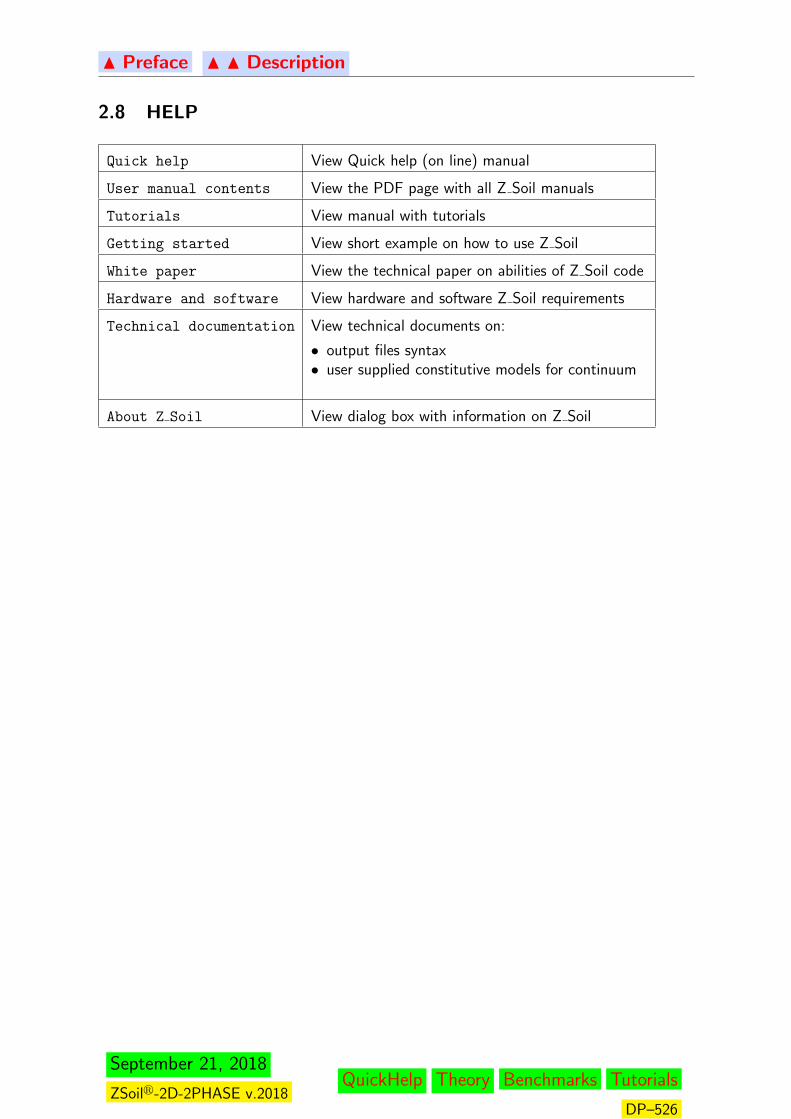
N Preface N N Description
2.8 HELP
Quick help View Quick help (on line) manual
User manual contents View the PDF page with all Z Soil manuals
Tutorials View manual with tutorials
Getting started View short example on how to use Z Soil
White paper View the technical paper on abilities of Z Soil code
Hardware and software View hardware and software Z Soil requirements
Technical documentation View technical documents on:
• output files syntax• user supplied constitutive models for continuum
About Z Soil View dialog box with information on Z Soil
September 21, 2018
ZSoilr-2D-2PHASE v.2018QuickHelp Theory Benchmarks Tutorials
DP–526

N Preface
Chapter 3
TROUBLESHOOTING
September 21, 2018
ZSoilr-2D-2PHASE v.2018QuickHelp Theory Benchmarks Tutorials
DP–527

N Preface N Troubleshooting
3.1 CALCULATION MODULE
Errors and warning handling
September 21, 2018
ZSoilr-2D-2PHASE v.2018QuickHelp Theory Benchmarks Tutorials
DP–528
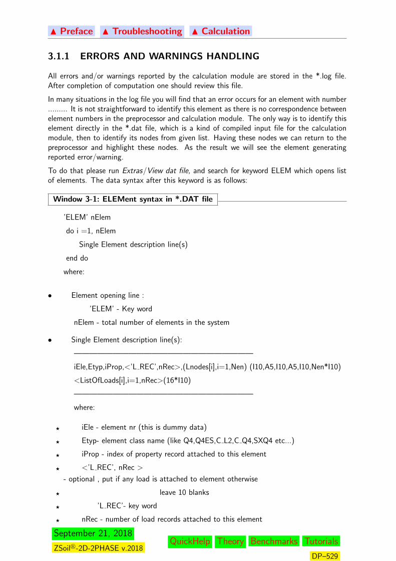
N Preface N Troubleshooting N Calculation
3.1.1 ERRORS AND WARNINGS HANDLING
All errors and/or warnings reported by the calculation module are stored in the *.log file.After completion of computation one should review this file.
In many situations in the log file you will find that an error occurs for an element with number......... It is not straightforward to identify this element as there is no correspondence betweenelement numbers in the preprocessor and calculation module. The only way is to identify thiselement directly in the *.dat file, which is a kind of compiled input file for the calculationmodule, then to identify its nodes from given list. Having these nodes we can return to thepreprocessor and highlight these nodes. As the result we will see the element generatingreported error/warning.
To do that please run Extras/View dat file, and search for keyword ELEM which opens listof elements. The data syntax after this keyword is as follows:
Window 3-1: ELEMent syntax in *.DAT file
’ELEM’ nElem
do i =1, nElem
Single Element description line(s)
end do
where:
• Element opening line :
’ELEM’ - Key word
nElem - total number of elements in the system
• Single Element description line(s):
———————————————————————
iEle,Etyp,iProp,<’L REC’,nRec>,(Lnodes[i],i=1,Nen) (I10,A5,I10,A5,I10,Nen*I10)
<ListOfLoads[i],i=1,nRec>(16*I10)
———————————————————————
where:
F iEle - element nr (this is dummy data)
F Etyp- element class name (like Q4,Q4ES,C L2,C Q4,SXQ4 etc...)
F iProp - index of property record attached to this element
F <’L REC’, nRec >
- optional , put if any load is attached to element otherwise
F leave 10 blanks
F ’L REC’- key word
F nRec - number of load records attached to this element
September 21, 2018
ZSoilr-2D-2PHASE v.2018QuickHelp Theory Benchmarks Tutorials
DP–529

N Preface N Troubleshooting N Calculation
F (Lnodes[i],i=1,Nen) - list of element node numbers where Nen is set by program
after recognizing of Etyp.
F <ListOfLoads[i],i=1,nRec>(16*I10)
if ’L REC’ was specified then from the beginning of the next line(s) , list of load
record indices should be given . It may be continued, in format (16*I10), in
following lines.
Window 3-1
September 21, 2018
ZSoilr-2D-2PHASE v.2018QuickHelp Theory Benchmarks Tutorials
DP–530
N Preface N Troubleshooting N Calculation
The following errors and warnings can be reported:
• CFG Cannot open configuration file for ZSOIL –>zsoil.cfg
The configuration file zsoil.cfg (in the Z SOIL root directory) has been damaged.
Check the existence of this file in your Z SOIL directory and if it does not exists reinstallyour Z SOIL system.
• DATA Data inconsistency has been detected ( see echo of data )
Some data inconsistencies have been detected. Please have a look to the *.eda file whichcovers echo of the input data.
• DATA To this element material model of inconsistent type is attached
.......................... (here some element number)
A wrong association of the material model and element class has been detected. You canidentify this element in the same way as for negative or zero Jacobian case.
• DATA Nodes of DSC element not found at this beam element:
....................... (here beam element number)
A special element, simulating relaxation/continuity between given beam element and theother, has unattached node(s).
• DATA Inadmissible material data group:
......................(here given group string)
This group of parameters is not allowed for material.
• DATA The seepage element is unattached to any element or is attached to the elementwith impermeable material; this may result in computation failure; If so delete in thepreprocessor all seepage elements attached to elements with impermeable materials.
....................(here given element number)
The explanation is given in the description of the warning.
• DATA This contact element is unattached to any element or is connected with elementswith impermeable materials; this may result in computation failure for flow or def.+flowproblems. If so make the contact material also impermeable.
....................(here given element number). The explanation is given in the description ofthe warning.
• DATA Following shell node is assigned as slave to more than 1 master
Use shell/direction show and flip in PrePro3D
....................(here given node number)
The explanation is given in the description of the warning.
• DATA Following shell node is assigned as both slave and master. Use shell/direction showand flip in PrePro3D
The explanation is given in the description of the warning.....................(here given nodenumber)
September 21, 2018
ZSoilr-2D-2PHASE v.2018QuickHelp Theory Benchmarks Tutorials
DP–531

N Preface N Troubleshooting N Calculation
• DATA There no exists any element attached to this contact element
A ”flying” contact element has been detected. Please verify the existence of this elementwith respect to the neighboring elements (continuum/ shells/membranes/beams).
• DATA No direction specified for infinite layer boundary element Return to Pre-Pro anddefine correct vector
• DATA For this variable thickness shell element ZERO thickness detected Return to Pre-Pro and define the thickness correctly
• DATA Too large gap for contact element
................ (here given contact element number)
A contact segment to segment element has been defined in such a way that correspondingnodes on the opposite faces do not coincide. This is a warning which does not break thecomputation. A tolerance for the geometrical gap has been assumed to be 0.05 * averagedelement size. You can identify this element in the *.dat file (contact elements are denotedas C L2 in 2D and C Q4 in 3D) similarly as for case of zero or negative Jacobian.
• DATA The internal node of penalty element is not inside domain
An element enforcing compatibility between two nonconforming continuum elements iswrongly defined.
• DATA Impossible to realize assumed prestress (probably Stress >Yield-Stress )
The assumed prestress in anchor element is possibly higher than yield stress.
• DATA This element reveal 0 or negative Jacobian
................. (here element number)
The indicated element reveals zero or negative Jacobian. This may happen only if theelement is highly distorted. Please identify the element in the *.dat file, as described inthe introductory part, and then return to the preprocessor to correct the data.
• DATA Gauss point radial coordinate <= 0.0 in axisymmetry
In the axisymmetric case any x-coordinate has to be greater than zero.
Return to the preprocessor and verify your data.
• DATA Invalid nr of layers in composite property set no. :
Nr of layers exceeds allowable maximum. Try to reduce nr of layers in composite section.
• DATA Fiber direction undetermined in layered shell element no. :
..................(here is given element number)
It is possible that the fiber direction vector is perpendicular to the shell midsurface.
• DATA Unconnected point outside demanded element in link element no. :
.............. (here is given element number)
One of the anchor element endpoints is unconnected.
Please look to the *.dat file (through View dat file option), find the element in the elementlist after keyword ELEM. Note that there is no correspondence between element numbers
September 21, 2018
ZSoilr-2D-2PHASE v.2018QuickHelp Theory Benchmarks Tutorials
DP–532
N Preface N Troubleshooting N Calculation
in the preprocessor and calculation module. The only way is to identify all nodes of theelement in the *.dat file and then to select them in the preprocessor.
• DATA For this beam element local base is undetermined due to incorrect position ofdirectional point.
.................(here is given element numbers)
A direction for given beam element is possibly parallel to the element axis. Return to thepreprocessor and correct it.
• I/O Cannot read/write file with optimized node/ele sequence
This error may appear in the following cases:
a) you tried to restart the analysis without having at least one converged step,
b) the auxiliary file *.opt has been deleted
To eliminate this error again Run Analysis
• I/O Error during file I/O operation
................... (here file no.)
An I/O error has occurred during read/write operation.
Your free disk space is possibly exhausted.
• I/O Lack of ZSOIL.TXT file
The file with system strings zsoil.txt (in the Z SOIL root directory) has been damaged.
Check the existence of this file in your Z SOIL directory and if it does not exists reinstallyour Z SOIL system.
• I/O Error while writing this binary result
............ (here file number)
An I/O error has occurred during results storage. Your free disk space is possibly exhausted.
• PIVOT Null pivot detected at :
..............(here there should be given node no. and degree of freedom)
There are following reasons which lead to such a situation:
a) insufficient number of boundary conditions
b) separation state along the whole contact interface (note that the effective stress conceptin contact holds),
c) a limit state has been reached,
d) boundary conditions are set in such a way that rigid body motion is not eliminated. Inthis case set proper BC.
• RAM Length of equation is greater than length of block
Try to enlarge the RAM size to be used by Z SOIL in System configuration
• RAM Too many blocks in given equation
Try to enlarge the RAM size to be used by Z SOIL in System configuration. Current RAMsize is insufficient for skyline block solver.
September 21, 2018
ZSoilr-2D-2PHASE v.2018QuickHelp Theory Benchmarks Tutorials
DP–533
N Preface N Troubleshooting N Calculation
• RAM Lack of free RAM to run a job (Note : RAM MAXIMUM >64 kB in zsoil.cfg !!)Try to close other running applications .
The amount of the RAM size in System configuration has to be greater than 64 kb. It ispossible that the declared RAM size is too large while concurrently using other Windowsapplications.
• RAM Dynamic memory allocation error; try to reduce the RAM size in zsoil.cfg to thefollowing size :
Please reduce your RAM size in System configuration to given value.
• RAM Lack of memory to allocate frontal solver
Your working memory space has been exhausted. Try to enlarge RAM size in Systemconfiguration.
• RAM Lack of free space detected while allocating this
In System configuration there is an edit box to define maximum RAM available for thecalculation module. However it may happen that for large problems assumed RAM size isinsufficient. Please enlarge it through System configuration but never exceed your platformlimitation.
• RUN Step not converged due to limitation of the absolute maximum nr of iterations
The maximum number of iterations has been overreached. If you want to enlarge thisnumber please do it through Control or try to reduce time step/ increment of safety factoror gravity multiplier.
• RUN Divergence of iteration process - can not continue calculations
Calculation process has been stopped due to divergence or lack of convergence.
Try to reduce gravity multiplier increment in the initial state analysis / time step for timedependent drivers or safety factor increment for stability analysis and then restart.
• RUN Restart is impossible
Please Run Analysis as the restart is impossible.
If appearing error message does not belong to the above list, or the message persistentlyappears despite an attempt to correct it, please contact hotline ZSOILZace.com
September 21, 2018
ZSoilr-2D-2PHASE v.2018QuickHelp Theory Benchmarks Tutorials
DP–534
N Preface N Troubleshooting N Calculation
Index
3Danalysis and drivers, DP: 15, 16, DP:
79
Analysisbatch processing, DP: 509restart computation, DP: 508run computation, DP: 507run computation without writing *.dat,
DP: 523Auxiliary planes, DP: 127Axisymmetry
analysis and drivers, DP: 15, 16, DP:79
Beamscreate/outline/update/delete elements,
DP: 229create/outline/update/delete subdomain
2D, DP: 158create/outline/update/delete subdomain
3D, DP: 158Reinforcement sets, DP: 506reinforcements set, DP: 236, DP: 242subdomain 2D parameters, DP: 161subdomain 3D parameters, DP: 161
Bearing capacity, DP: 30–32Boundary conditions
for humidity, DP: 193, DP: 309for humidity on macro-elements, DP:
193for pore pressure, DP: 188, DP: 310for pore pressure on macro-elements,
DP: 188for solid phase, DP: 300for temperature, DP: 191, DP: 306for temperature on macro-elements, DP:
191periodic, DP: 315
Construction algorithmanalysis and drivers, DP: 16
Continuum 2D elements, DP: 255Continuum 2D macromodel
Automatic mesh generation, DP: 172,173
Mesh morphing, DP: 174Semi-automatic mesh generation, DP:
170, 171Subdomain generation, DP: 157, 158Virtual mesh, DP: 169–171
Continuum 3D elements, DP: 261Convection 2D macromodel
Subdomain generation, DP: 178Convection 3D macromodel
Subdomain generation, DP: 178Convection elements, DP: 289Creep
standard properties, DP: 425swelling properties, DP: 425
Dynamicsadded masses, DP: 330consistent mass matrix, DP: 84control parameters, DP: 84Domain Reduction Method (DRM), DP:
368HHT scheme, DP: 84lumped mass matrix, DP: 84mass filtering, DP: 86Newmark scheme, DP: 84Reylaigh damping, DP: 84Seismic input, DP: 504
Elasticityconstants, DP: 7material properties, DP: 419
Elasto-plastic 1Dmodel, DP: 482
Evolution functions, DP: 500Existence functions, DP: 494
FE model preprocessingcommon methods to copy elements/nodes,
DP: 218
September 21, 2018
ZSoilr-2D-2PHASE v.2018QuickHelp Theory Benchmarks Tutorials
DP–535

N Preface N Troubleshooting N Calculation
common methods to delete elements/nodes,DP: 218
common methods to move elements/nodes,DP: 218
common methods to outline elements/nodes,DP: 218
common methods to rotate elements/nodes,DP: 218
Finite elementsselection strategy, DP: 94, DP: 96stabilization of pressure oscillations, DP:
96volumetric locking, DP: 95
Flowanalysis, DP: 15, 16, DP: 50flux boundary condition, DP: 51, DP:
195initial conditions, DP: 51initial state driver, DP: 50, DP: 53material data, DP: 50, DP: 422pressure boundary condition, DP: 51,
DP: 188steady state driver, DP: 50, DP: 54time dependent drivers, DP: 54transient driver, DP: 50, DP: 55
Fluxes on elementsfluid, DP: 338heat, DP: 340humidity, DP: 341
Fluxes on macromodelfluid, DP: 195heat, DP: 197humidity, DP: 199
Gravity, DP: 502body load components, DP: 502direction, DP: 502
Heatanalysis, DP: 15, 16, DP: 56flux boundary conditions, DP: 57, DP:
197initial conditions, DP: 57, 58initial state driver, DP: 56, DP: 58material properties, DP: 431steady state driver, DP: 56, DP: 59temperature boundary conditions, DP:
57, DP: 191thermal strains, DP: 80
time dependent drivers, DP: 56, DP:59
transient driver, DP: 56, DP: 60Hinges
in beam elements, DP: 235, DP: 485in shell elements, DP: 296
Humidityanalysis, DP: 15, 16, DP: 61flux boundary conditions, DP: 62, DP:
199humidity boundary conditions, DP: 62,
DP: 193hygral strains, DP: 61, DP: 80initial conditions, DP: 62, 63initial state driver, DP: 61, DP: 63material properties, DP: 61, DP: 433steady state driver, DP: 64time dependent drivers, DP: 61, DP:
64transient driver, DP: 65
Infinite elements, DP: 266Initial condition
for displacements, DP: 362for humidity, DP: 348, DP: 351for pore pressure, DP: 343for solid velocities, DP: 362for temperature, DP: 346
Initial state Komaterial properties, DP: 429
Interface 2D macromodelSubdomain generation, DP: 184
Interface 3D macromodelSubdomain generation, DP: 184
Interface elements, DP: 273Interface elements for large deformations,
DP: 281
Kinematic constraints, DP: 370
Large deformationsanalysis and drivers, DP: 16
Linear equation solvers, DP: 89skyline, DP: 89sparse, DP: 89
Load time functions, DP: 496Loads
body, DP: 320on beam elements, DP: 328on element surfaces, DP: 324
September 21, 2018
ZSoilr-2D-2PHASE v.2018QuickHelp Theory Benchmarks Tutorials
DP–536

N Preface N Troubleshooting N Calculation
on nodes, DP: 322on subdomain boundaries, DP: 207
Macromodeling2D mesh mapping, DP: 151Extrusion direction, DP: 154Fluid flux, DP: 195Heat flux, DP: 197Humidity BC, DP: 193Humidity flux, DP: 199Nails, DP: 201Objects, DP: 142Point, DP: 140Point loads, DP: 214Pressure BC, DP: 188Subdomain, DP: 155Subdomain parameters, DP: 160Surface load, DP: 207Temperature BC, DP: 191Virtual to real mesh conversion, DP:
175Macromodeling objects
Arc, DP: 145Circle, DP: 146common methods, DP: 143Delete methods, DP: 150DXF import, DP: 149Line, DP: 144Line(s) on edge(s), DP: 146Outline methods, DP: 150Point, DP: 144Split by plane, DP: 149Update methods, DP: 151
Main Z Soil menuAnalysis options, DP: 507Assembly options, DP: 99Control options, DP: 13, 14Control:analysis and drivers, DP: 16Extras, DP: 523File options, DP: 11Help, DP: 525Postpro, DP: 510System configuration, DP: v, DP: 524toolbars, DP: 10
Materialscreep properties group, DP: 425data groups, DP: 419databases, DP: 383elastic properties group, DP: 419
flow properties group, DP: 422handling, DP: 381heat properties group, DP: 431humidity properties group, DP: 433initial Ko properties group, DP: 429local stability properties group, DP: 434models, DP: 383properties varying in space, DP: 488properties varying in time, DP: 488Rayleigh damping parameters group, DP:
435unit weight properties group, DP: 420
Materials for axisymmetric shell elementslinear elastic model, DP: 395, DP: 399nonlinear (layered) model, DP: 395, DP:
399Materials for beam elements, DP: 385
linear elastic model, DP: 386, DP: 390nonlinear (layered) model, DP: 386, DP:
391, DP: 393Materials for contact elements, DP: 401
frictional contact model, DP: 402Materials for continuum elements, DP: 418
Aging concrete model, DP: 437Cap model, DP: 439Densification model, DP: 458Drucker-Prager model, DP: 445Hoek-Brown model, DP: 461Hoek-Brown(M-W) model, DP: 446HS-small model, DP: 455Linear elastic model, DP: 436Modified Cam Clay model, DP: 442Mohr-Coulomb (M-W) model, DP: 448Mohr-Coulomb model, DP: 453Multilaminate model, DP: 450Plastic damage for concrete, DP: 465Rankine(M-W) model, DP: 452
Materials for continuum elements for struc-tures, DP: 469
Materials for fixed anchor interface elementsadhesive contact model, DP: 416
Materials for fixed anchor zone interface el-ements, DP: 415
Materials for heat convection elementsconvection model, DP: 469
Materials for heat radiation elementsradiation model, DP: 470
Materials for humidity convection elementsconvection model, DP: 471
September 21, 2018
ZSoilr-2D-2PHASE v.2018QuickHelp Theory Benchmarks Tutorials
DP–537
N Preface N Troubleshooting N Calculation
Materials for infinite elementsLinear elastic model, DP: 472
Materials for membrane elements, DP: 473Anisotropic elasto-plastic model, DP:
478Fiber elasto-plastic model, DP: 474Isotropic elasto-plastic model, DP: 478Plane stress elastic model, DP: 477Plane stress Hoek-Brown model, DP:
477Plane stress Huber-Mises model, DP:
477Plane stress Rankine model, DP: 477
Materials for nail interface elements, DP:412
adhesive contact model, DP: 413Materials for pile interface elements, DP:
406frictional contact model, DP: 407, DP:
410Materials for pile tip interface elements, DP:
409Materials for seepage elements, DP: 480Membrane 2D macromodel
Subdomain generation, DP: 158Membranes, DP: 261Mesh tying, DP: 375
Nodal link, DP: 372Node, DP: 225Nonlinear solvers, DP: 82
Overlaid meshesgeneration, DP: 134
Plane strainanalysis and drivers, DP: 15, 16, DP:
79Postprocessing
envelopes for structural elements, DP:516
how do I...., DP: 512using macros, DP: 514
Preferences, DP: 139Preprocessing
FE model, DP: 101, DP: 217Macromodelling, DP: 101, DP: 139Main menu, DP: 102User interface, DP: 101
Preprocessor
construction lines, DP: 125copy by rotation selected objects, DP:
122copy by symmetry, DP: 122copy by translation selected objects, DP:
121grid, DP: 126import geometrical model, DP: 106move selected objects, DP: 120rotate selected objects, DP: 121selection of finite elements, DP: 117selection of nodes, DP: 118show distance, DP: 132show node coordinates, DP: 132show vector, DP: 132show volume of continuum element, DP:
132snap options, DP: 126
Preprocessor menuAssembly, DP: 109Draw, DP: 123Edges/Faces selection, DP: 113Edit, DP: 119Files, DP: 105Frequently used tools, DP: 134Global selection tools, DP: 115Mesh, DP: 130Overlaid meshes, DP: 132Parameters, DP: 122Settings, DP: 137Show construction/excavation steps, DP:
136Tools, DP: 132Undo, DP: 110View, DP: 111Windows, DP: 106
Preprocessor toolbars2D mesh refinement, DP: 131edges selection, DP: 114
Pushovercontrol parameters, DP: 86results, DP: 511
Pushover control node, DP: 377
Restartcontrol, DP: 82
Resultscontent, DP: 97for beam elements, DP: 98
September 21, 2018
ZSoilr-2D-2PHASE v.2018QuickHelp Theory Benchmarks Tutorials
DP–538
N Preface N Troubleshooting N Calculation
for continuum elements, DP: 98for shell/membrane elements, DP: 98nodal solid accelerations, DP: 99nodal solid velocities, DP: 99residuals at nodes, DP: 99standard nodal results, DP: 99storage frequency, DP: 82
Seepage 2D macromodelSubdomain generation, DP: 176
Seepage 3D macromodelSubdomain generation, DP: 176
Seepage elements, DP: 285Shell elements, DP: 261Shell elements with one layer of nodes, DP:
261Single phase
analysis, DP: 15, 16, DP: 21driven load driver, DP: 28effective stress analysis, DP: 21initial state driver, DP: 24time dependent drivers, DP: 28total stress analysis, DP: 21, DP: 27,
DP: 36Stability, DP: 33
analysis, DP: 35, 36driver, DP: 33–36local material setting, DP: 34, DP: 434
Strainsimposed, DP: 358, DP: 365thermal, DP: 56
Stresssign convention, DP: 3
SubdomainExcavation front, DP: 162
Swellingmaterial properties, DP: 425
Tendonsin continuum/shells, DP: 270
Truss 2D macromodelSubdomain generation, DP: 158
Truss 3D macromodelSubdomain generation, DP: 158
Truss elements, DP: 245Two phase
analysis, DP: 15, 16, DP: 37consolidation driver, DP: 44driven load+steady state flow driver,
DP: 42
driven load+transient flow driver, DP:43
initial state driver, DP: 40stability driver, DP: 46, 47time dependent drivers, DP: 42undrained driver, DP: 20, DP: 22, DP:
37, 38, DP: 67, DP: 423
Unit weightdefinitions, DP: 6in single phase problems, DP: 21, DP:
27in two phase problems, DP: 47material properties, DP: 420
Units, DP: 90basic, DP: 7, DP: 92compound, DP: 93conversion, DP: 91setting basic units, DP: 90
Viscous damper 2D macromodelSubdomain generation, DP: 181
Viscous damper 3D macromodelSubdomain generation, DP: 181
Viscous dampers, DP: 293, DP: 481
Warnings, DP: 138
September 21, 2018
ZSoilr-2D-2PHASE v.2018QuickHelp Theory Benchmarks Tutorials
DP–539