Technology adoption under uncertainty: Take up and

subsequent investment in Zambia

⇤

B. Kelsey JackTufts University and NBER

Paulina OlivaUCSB and NBER

Samuel BellShared Value Africa

Christopher SeverenUCSB

Elizabeth WalkerNERA Consulting

Abstract

Technology adoption often requires investments over time. As new informationabout the costs and benefits of investment is realized, agents may prefer to abandon atechnology that appeared profitable at the time of take-up. This re-optimization canreduce the cost-effectiveness of adoption subsidies. We use a field experiment with twostages of randomization to generate exogenous variation in the payoffs associated withtake-up and subsequent investment in a new technology: a tree species that providesprivate fertilizer benefits to adopting farmers. Our empirical results show high ratesof abandoning the technology, even after paying a positive price to take it up. Theexperimental variation offers a novel source of identification for a structural model ofintertemporal decision making under uncertainty. Estimation results indicate that thefarmers experience idiosyncratic shocks to net payoffs after take-up, which increase take-up but lower average per farmer tree survival. We simulate counterfactual outcomesunder different levels of uncertainty and observe that farmers with high returns areable to self-select at take-up only when the level of uncertainty is relatively low. Thus,uncertainty provides an additional explanation for why many subsidized technologiesmay not be utilized even when take-up is high.

⇤Helpful comments were received from Jim Berry, Chris Costello, Andrew Foster, Alex Pfaff, AndrewPlantinga, Stephen Ryan, Kenneth Train, Mushfiq Mobarak, Ryan Kellogg, Tavneet Suri and audiences atnumerous seminars and conferences. The authors thank the IGC, CDKN and Musika for financial support,and the Center for Scientific Computing at the CNSI and MRL at UC Santa Barbara (NSF MRSEC DMR-1121053 and NSF CNS-0960316) for use of its computing cluster. Field work was facilitated by Innovationsfor Poverty Action, with specific thanks to Jonathan Green, Farinoz Daneshpay, Mwela Namonje and MonicaBanda. The project was made possible by the collaboration and support of Shared Value Africa and DunavantCotton, Ltd.

1

1 Introduction

Many technology adoption decisions –in development, health and environmental policy–

consist of at least two parts, which occur at different points in time: an initial take-up

decision and a subsequent investment or follow-through decision. While subsidies are often

used to increase take-up, critics of subsidies for technology adoption worry that subsidizing

the initial take-up decision may lower subsequent follow-through, leading to a misallocation

of subsidized technologies to adopters who never use them.

The empirical evidence on whether the take-up price is correlated with follow-through is

mixed: some studies find a positive correlation (e.g., Ashraf et al. 2010) and others none (e.g.,

Cohen and Dupas 2010).1 The literature has put forward many reasons why follow-through

may or may not be affected by the initial cost of the technology, including screening effects,

learning, and psychological channels such as sunk costs or procrastination (Ashraf et al. 2010;

Cohen and Dupas 2010; Mahajan and Tarozzi 2011; Ashraf et al. 2013; Dupas 2014; Beaman

et al. 2014; Fischer et al. 2014; Carter et al. 2014; Cohen et al. 2015). With the exception

of learning, little attention has been paid to the role of dynamics and uncertainty in the

initial take-up decision.2 Specifically, at the time of take-up, many of the benefits and costs

associated with the follow-through decision may be unknown. New information may arrive

after take-up in the form of learning about the technology (Foster and Rosenzweig 1995;

Conley and Udry 2010) or in the form of transient shocks to the opportunity cost of follow-

through. If the new information is bad news about the profitability of the technology, then

adopters may opt for abandoning the technology. Adopters know that they can reoptimize

once new information is available and are likely to account for this at the time of take-up.

Thus, the take-up decision can be interpreted as the purchase of an option to follow-through.1Similar issues arise in cost sharing of medical treatment (e.g., Goldman et al. (2007)).2The dynamic effects of subsidies on subsequent demand for the same technology is investigated by Carter

et al. (2014), Dupas (2014) and Fischer et al. (2014), all of which find support for learning.

2

This paper identifies theoretically and empirically the role of uncertainty in the decision

to take-up and follow-through with a new technology in a setting where take-up may be

subsidized. We apply a dynamic conceptual model to farmer decisions to adopt a type of

fertilizer tree in Zambia. This technology requires both a one-time take-up decision (pur-

chasing seedlings) and a follow-through decision (planting and caring for the trees). Farmers

face potential shocks to the opportunity cost of following-through with the trees, including

illness of a household member, pests, drought or other factors that may affect (either posi-

tive or negative) other crops and/or the trees, and other events in the household or on the

farm that may be hard to define or measure. Our approach to identifying uncertainty in our

field setting circumvents the challenge of comprehensive measurement of all components of

opportunity cost, including those that are not realized, by extending a revealed preference

framework to the dynamic case: adoption-related choices by the same individual on the same

technology are made at different points in time and reveal the information that was acquired

in between. Our study proceeds in four steps: (1) a conceptual model of technology adoption

under uncertainty; (2) a field experiment with variation in adoption payoffs at two points in

time; (3) a structural model that builds on (1) and (2); and (4) counterfactual simulations

that vary the magnitude of uncertainty and show implications for adoption outcomes.

To develop intuition, we begin with a stylized model of intertemporal adoption under

uncertainty in the presence of subsidies, where individuals make binary take-up and follow-

through decisions at two different points in time.3 Between these two points in time new

information about the opportunity cost of follow-through is acquired. The theoretical model

generates clear predictions about the relationship between uncertainty and adoption out-

comes. First, a mean-preserving increase in uncertainty makes take-up more attractive

provided that abandoning the technology at a later stage is costless. This is because, re-3Our empirical model adds an intensive margin to the follow-through decision, similar to Ashraf et al.

2010; Cohen and Dupas 2010; Fischer et al. 2014 and others.

3

gardless of how costly following through turns out to be, profit is always bounded below

at zero by the option to abandon the technology. Thus, uncertainty can only increase the

upside of the take-up decision.4 Second, uncertainty undermines the screening effect of the

take-up price. Intuitively, if adopters know little about their net cost of follow-through when

they take-up, then a higher take-up price will not be effective at screening out those who

will end up having a high cost at follow-through. Our conceptual framework borrows heavily

from the literature on investment under uncertainty (Pindyck 1993; Dixit and Pindyck 1994)

and, like Fafchamps (1993), shows that choices that appear to lead to losses (like purchasing

a technology that is soon to be abandoned) can be rational ex-ante if their purpose is to

preserve flexibility.5

Next, we use a multi-period field experiment in rural Zambia to generate empirical evi-

dence for the presence of uncertainty. Farmers choose whether to adopt a tree species that

generates private soil fertility benefits over the long term, but carries short-run costs.6 We

observe whether the 1,314 farmers in the study take up a 50-tree seedling package at the start

of the agricultural cycle. The follow-through decision consists of the number of seedlings that

the farmer chooses to plant and care for (which we together refer to as tree cultivation) and

occurs over the course of the subsequent year. Shocks to the opportunity cost of follow-

through may cause farmers to abandon the technology, which they can do without penalty.

We measure follow-through as tree survival after one year, and assume that farmers can

guarantee tree survival for some level of costly effort.7

4This is true even in the presence of insurance, as the costless exit is still present in this case and thus thecontract becomes a substitute for insurance. See Giné and Yang (2009) for an example of how an uninsuredcredit contract may be more attractive than an insured one in the presence of limited liability.

5Other applications of dynamic decision making under uncertainty in the development and environmentalliterature include Bryan et al. (2014); Magnan et al. (2011); Arrow and Fisher (1974).

6Positive externalities, such as carbon sequestration and reduced soil erosion, further justify the subsidyfrom a policy perspective.

7The choice of minimum effort that guarantees survival is optimal under convexity of the survival riskfunction as a function of effort. The only source of uncertainty in tree survival in our model is the farmer’sendogenous choice of effort in response to new information about the costs of follow-through. This assumptionis examined in greater detail in Appendix A.3.

4

We introduce exogenous variation into this adoption decision at two different points in

time. First, we vary the take-up cost through a subsidy on the purchase of a seedling package.

Farmers’ response to this random variation helps characterize the heterogeneity in expected

costs across farmers.8 Second, we vary the payoff to follow-through by varying the size of a

reward that is conditional on the survival of at least 35 trees one year after take-up. The

tree cultivation choices farmers make in response to the reward help us characterize the

distribution of follow-through costs after potential shocks have been realized. Under the

assumption that shocks are independent across farmers, the difference in the variance of net

costs between the two points in time can be attributed to uncertainty.9 Note that, rather than

artificially varying the allocation of shocks across our study population, the reward creates

exogenous variation in the variance of possible outcomes faced by the farmers, and therefore

in the distribution of shocks. By offering a positive payoff, the performance reward varies the

distribution of shocks much in the way that varying the terms of an insurance contract has

a state-contingent effect on the distribution of outcomes.10 Together, the different sources

of variation at two points in time identify a structural model of intertemporal decisions that

can distinguish between static and dynamic explanations for the outcomes that we observe.

This is among the first papers to introduce multiple dimensions to the experimental design

to distinguish between adoption decisions and returns to investment (see Karlan and Zinman

(2009) and extensions of their design by Ashraf et al. (2010); Cohen and Dupas (2010) and

others), and the first to use this research design to explore time-varying returns to investment.

The reduced form responses to the randomized treatments are broadly consistent with the

predictions of our theoretical model in the presence of uncertainty: while farmers respond8Liquidity constraints could also affect the decision to take-up. To minimize the importance of cash-on-

hand, farmers receive a show-up fee sufficient to cover take-up costs. We also test for self-selection based onbroader forms of liquidity constraints: using random variation in the timing of the reward announcement.We discuss these tests for liquidity constraints and other confounds in Section 4 and Appendix A.4.

9The cross-farmer independence assumption rules out common shocks. In a model variant, discussed inSection 5, we relax the independence assumption by allowing for an unexpected common shock to all farmers.

10A similar approach is used by Einav et al. (2013); Bryan et al. (2014); Karlan et al. (2014), among others.

5

to economic incentives (they take-up at higher rates under higher subsidies and follow-

through at higher rates under higher rewards), the price at which each individual takes up

is not predictive of the follow-through outcome (i.e. we find no significant screening effect of

prices).11 In addition, a large share of farmers who paid a positive price end up abandoning

the technology altogether.12 Although these facts suggest that uncertainty plays a role in

farmers’ decisions, they do not allow us to quantify the amount of uncertainty farmers face

nor how important it is for farmers’ decisions versus other forms of heterogeneity that can

lead to similar behavior.

We turn next to our structural model to shed further light on the role and magnitude

of uncertainty in our setting, and the generalizability of our findings. We start by noting

that uncertainty is not the only plausible explanation for the absence of positive screening

effects of prices. When follow-through has an intensive margin, there may be heterogeneity

in both the level of the profit (for example, if there are fixed costs to adoption) and in the

number of trees that maximizes the profit (i.e. the interior solution to the farmers’ profit

maximization problem); moreover, these two types of heterogeneity may be positively or

negatively correlated. Only a positive correlation between the level of private profit and

privately optimal number of trees would generate higher follow-through rates among those

who participate at higher cost, yet a negative correlation is empirically plausible. Suri

(2011), for example, offers evidence of a negative correlation between optimal rates of usage

and fixed costs of adoption in the case of hybrid crop varieties. Our structural model allows11The lack of self-selection in our setting stands in contrast with Jack (2013), who provides evidence that

farmers self-select based on future costs into a tree planting incentive contract in Malawi. She studies adifferent context and different contract design. In addition, the pattern of selection effects over time in herstudy is consistent with a multi-year extension of our conceptual framework, which would predict strongerselection as the number of farmers who continue to cultivate trees shrinks.

12We rule out a number of alternative motives for this behavior. First, we rule out side-selling by exploitingcross-group variation in incentives to side-sell. Second, we test whether a desire to please the experimenter(social desirability bias) drives our results by allowing for a common “boost” to the attractiveness of take-upin our structural model, and find it has little effect on our estimates (Section 6). We also examine the effectof time inconsistent preferences (as in Mahajan and Tarozzi 2011) in Section 7 and Appendix table A.5.6.

6

for heterogeneity in the privately optimal number of trees as well as in the net cost of follow-

through, and allows these two known (to the farmer) components of private profit to be freely

correlated.13 We find that in our setting heterogeneity along the intensive margin of tree

survival operates in oposite direction to the extensive margin heterogeneity (similar to Suri

(2011)), thus weakening the screening effect of prices. In addition, our estimates find a large

variance in the unknown component of costs; i.e. a large amount of uncertainty. To illustrate

its magnitude, we calculate that 15 percent of farmers would change their ex ante decision

about meeting the threshold if they could take the new information into consideration.

Given that both uncertainty and heterogeneity along the intensive margin are contribut-

ing to the lack of screening coming from the take-up price, we implement counterfactual

simulations to better understand the relative importance of uncertainty in explaining our re-

sults. We find that at levels of uncertainty lower than those in our empirical setting, higher

prices for take-up do have a positive effect on follow-through. Reducing the variance of

shocks by 50 percent (everything else constant) would bring up follow-through rates among

those who take-up under full price by 15 percent, because of improved screening at take-up.

Our conceptual framework and simulations also highlight the different role for subsidies

in the presence of uncertainty. Greater uncertainty in the payoffs from follow-through makes

subsidies less important for take-up because the option value, which increases with uncer-

tainty, drives up the expected profit. However, with high uncertainty, the more modest effect

that subsidies may have on take-up may be (almost) free of adverse selection effects, making

subsidies less problematic for allocational efficiency.

Methodologically, our econometric framework is an example of sequential identification

of subjective and objective opportunity cost components in a dynamic discrete choice model

(Heckman and Navarro 2007, 2005). As described in Heckman and Navarro (2007), we can13This is akin to correlated random coefficient (CRC) models, where returns to the technology are allowed

to differ across potential adopters and therefore influence their decision to adopt (Heckman et al. 2010).

7

account for selection into treatment (in our case, take-up) when identifying the distribution of

the unobserved opportunity cost determinants. We do so by introducing two layers of random

variation in economic incentives, one of which produces a probability of take-up equal to one

for a randomly selected sub-population and a second of which produces an interior solution

in tree cultivation outcomes with probability one in the limit. The use of experimental

variation in treatments at two different points in time offers an alternative to a panel data

structure (used for example, in Einav et al. (2013)), since statistically independent samples

are exposed to each of the different treatment combinations. To our knowledge, this is the

first paper to introduce experimental variation in order to satisfy the exclusion restrictions

needed for sequential identification.

The paper proceeds as follows. We begin with a simple theoretical model to generate

intuition. Section 3 describes the empirical context and experimental design, and Section 4

shows reduced form results. We present the empirical model and its identification in Section

5 and show estimation results and simulations in Section 6. Section 7 discusses interpretation

and Section 8 concludes.

2 A simple model of intertemporal technology adoption

Consider a two period model, where each agent chooses whether to purchase (take-up) a

single unit of a technology in the first period (time 0) , and whether to follow-through with

implementation of the technology in the second period (time 1). The immediate cost of

taking up is c � A, where c is the market price of the technology and A is an exogenous

subsidy. The benefit of following-through is given by R � (F0 + F1), where F0 + F1 is the

“net private cost” of following through and R is an exogenous reward for doing so. Since

F0 + F1 is net of benefits, it can be positive or negative. The first component of the net

cost, F0, is known to the agent at the time of take-up, while F1 is unknown to the agent at

8

time 0 and its realization (which is revealed to the agent at time 1) has a known distribution

that is constant across agents. Note that although F0 is known at time 0, both F0 and F1

are incurred at time 1. Assume that c, A and R are constant across agents, while F0 varies

according to some cdf G0(f0). Assume further that

(i) F0 and F1 are independent, and

(ii) Et=0(F1) = Et=1(F1) = 0 (i.e. agents have rational expectations).

Under these assumptions, F0 represents the agent’s best guess at t = 0 about her specific

net cost of following through, and F1 represents any new information that emerges after the

take-up decision is made.

Following backward induction, the agent decides to follow-through at t = 1 if R�F0�F1 >

0. If this inequality does not hold, the agent receives a payoff of zero at t = 1. At t = 0, the

agent decides to take-up by purchasing the technology if

c� A� �EF1 max(R� F0 � F1, 0) < 0 (1)

where � is the one-period discount factor and the expectation in (1) is taken with respect to

the density of F1.

To simplify the exposition, assume that the distribution of F1 is such that F1 2 {fL, fH},

with fL < fH and Pr(F1 = fL) = pL. Thus we can represent a mean-preserving increase

in uncertainty as a symmetric widening of the distance between fL and fH .14 With this

assumption, we can classify individuals into three types: those who always follow through,

regardless of the realization of F1 (always follow-through types), those who follow through

only if the low net cost shock is realized (contingent follow-through types), and those who14This model simplifies our empirical setting in two key ways: first, it assumes a binary follow-through

decision and second, it assumes a discrete distribution on F1. As we show when we present our empiricalmodel, the propositions derived from this model are not an artifact of the distributional assumption on F1

nor of the binary decision that characterizes follow-through in this simple model.

9

never follow-through (never follow-through types). These three types of agents can be char-

acterized by whether their value of F0 is below R � fH , between R � fH and R � fL, and

above R�fL, respectively. Figure 1 graphically shows the proportions for each type of agent

using areas under a symbolic bell-shaped distribution for F0, separated by gray dashed lines.

Figure 1 also illustrates two thresholds (along the support of F0) for take-up in black dashed

lines. The first take-up threshold (labeled R� E(F1)� c�A�

) is only binding if it falls to the

left of the threshold that defines always adopters (R� fH). When this first take-up thresh-

old binds, only always follow-through types take-up. The second take-up threshold (labeled

R� fL � (c�A)� pL

) is perhaps more interesting. When binding, all always-follow through types

take-up, but only a share of contingent follow-through types take-up (those to the left of

the threshold). We use this figure to explain intuitively the results outlined by each of our

propositions below. The formal proofs of these propositions can be found in Appendix A.1.

Figure 1: Take-up and follow-through thresholds as a function of agent type

Notes: The figure shows the shares of always adopters, contingent adopters and non-adopters over a symbolicprobability density function of F0. The grey thresholds (R�fH and R�fL) correspond to the follow-throughthresholds, while the black thresholds correspond to the take-up thresholds.

10

Proposition 1 Follow-through conditional on take-up increases as a function of take-up

cost, i.e. there is a screening effect of the take-up cost.

To see this, note that as take-up cost increases (represented by c � A in Figure 1), the

second take-up threshold moves to the left, bringing down the overall share of contingent

follow-through types among the set of individuals who take-up. Since contingent adopters

follow-through with probability less than one (pL), this in turn increases the share of indi-

viduals who follow-through among those who take-up.15

Proposition 2 An increase in uncertainty reduces follow-through conditional on take-up.

This can also be appreciated from Figure 1: a widening of the distance between fL and fH

causes the share of contingent follow-through types to increase (as the two grey dashed lines

move further apart). Note that as uncertainty increases, the position of the second take-up

threshold does not change relative to the threshold that determines the upper bound for

contingent follow-through types. Thus, this group becomes a larger share of those who take

up, reducing average follow-through.

Corollary 2.1 Under no uncertainty, everyone who takes-up follows-through.

This is easy to see from Figure 1: under no uncertainty (where fL = fH) there would be

only always follow-through types and never follow-through types.

Proposition 3 An increase in uncertainty weakens the relationship between take-up cost

and conditional follow-through shown in Proposition 1.

To see this, consider the takeaways of Propositions 1 and 2 simultaneously. The share of

contingent adopters that are excluded by an increase in the take-up cost becomes a smaller15If the take-up cost, c � A, increases enough that the first take-up threshold is binding, follow-through

conditional on take-up reaches 100 percent and is constant for further increases in the take-up cost.

11

proportion of all those who take-up when uncertainty increases.

Proposition 4 The option value associated with take-up is increasing in uncertainty, which

results in higher take-up at all take-up cost levels.

This is shown formally in the appendix along with the formal definition of option value in

our context. Intuitively, the option value is the value of reoptimizing once new information

(the realization of F1) emerges. As the distance between fH and fL increases, the payoff

at t = 1 conditional on a low cost shock (fL) increases for contingent follow-through types.

Because agents can choose not to follow through, the payoff at t = 1 conditional on a high

cost (fH) stays constant at zero. Thus, the expected value of the contract at t = 0 increases

with uncertainty, and this increase emerges solely because of the possibility of reoptimizing

(i.e. choosing not to follow-through). This results in higher take-up.

A note on risk neutrality. We assume linear utility – or risk neutrality – throughout

the paper, including the empirical analysis. Assuming some degree of risk aversion would

not change our results qualitatively, although it would lower the value placed on extreme

positive profitability shocks at the time of take-up. This would make the expected value

of the contract at t = 0, and therefore take-up, less responsive to increases in uncertainty.

That said, the risk neutrality assumption is relatively innocuous and carries important ad-

vantages given our empirical context. Although risk aversion is an important component of

intertemporal decisions with costs or benefits that represent substantial shares of household

income, our specific technology adoption decision causes relatively small changes to income.

In addition, our framework (both theoretical and empirical) models decisions as a function

of the profits associated with adoption relative to the best alternative use of household re-

sources. Thus, a positive shock to the opportunity cost of adoption could correspond to

an increase or a decrease in overall household income. For example, an increase in prof-

12

itability of a competing economic activity and a labor shortage due to health could both

represent an increase in the opportunity cost of adoption, but would have opposite effects

on total income and thus on marginal utility of income. Incorporating risk aversion into our

theoretical model would require us to make modeling assumptions about the nature of the

opportunity cost of adoption. Hence, assuming risk neutrality allows us to leave the source

of the opportunity cost unspecified, which makes our framework generalizable to any source

of uncertainty regardless of its impact on overall income.

Transitory shocks and learning. So far, we have left open the question of whether F1

should be interpreted as a persistent or a transitory shock and our framework is consistent

with both interpretations. However, the distinction matters for future take-up decisions. If

the F1 component of the returns to the technology is persistent, future take-up decisions

will occur under a lower level of uncertainty. If F1 is transitory, future take-up decisions

will look similar to the first take-up decision. We cannot completely disentangle these two

interpretations of the model in our context, though we use survey data to provide suggestive

evidence on the extent of learning (see Section 7).

3 Context and experimental design

We bring the propositions from our conceptual model to a two-part technology adoption

problem, characterized by uncertainty in the costs and benefits of following through with the

technology. In the context of an ongoing project to encourage the adoption of agroforestry

trees (Faidherbia albida), we introduce exogenous variation in the payoffs to farmers at

the time of their take-up and follow-through decisions. We use the experimental variation

to uncover the existing levels of static heterogeneity and uncertainty in the population of

farmers, which we model as random parameters. This section describes the context and the

13

experimental design in detail.

The study was implemented in coordination with Dunavant Cotton Ltd., a large cotton

growing company with over 60,000 outgrower farmers in Zambia, and with an NGO, Shared

Value Africa. The project, based in Chipata, Zambia, targeted approximately 1,300 farmers

growing cotton under contract with Dunavant, alongside other subsistence crops. The project

is part of the NGO partner’s portfolio of carbon market development projects in Zambia.

3.1 The technology

Faidherbia albida is an agroforestry species endemic to Zambia that fixes nitrogen, a limiting

nutrient in agricultural production, in its roots and leaves. Optimal spacing of Faidherbia

is around 100 trees per hectare, or at intervals of 10 meters. The relatively wide spacing,

together with the fact that the tree sheds its leaves at the onset of the cropping season,

means that planting Faidherbia does not displace other crop production (Akinnifesi et al.

2010). Agronomic studies suggest significant yield gains from Faidherbia.16 However, these

private benefits take 7-10 years to reach their full value, and may be insufficient to justify

the up-front investment costs, particularly if farmers have high discount rates. We observe

low adoption rates at baseline: less than 10 percent of the study households reported any

Faidherbia on their land. This could be explained by low perceived private net-benefits,

by high costs associated with accessing inputs – there is no existing market for Faidherbia

seedlings – or cultivating the trees, or by a lack of information.17

Subsidies may therefore be necessary to increase take-up rates, and are justified by posi-

tive environmental externalities and market failures that contribute to high private discount16Estimates of yield increases range from 100 to 400 percent, relative to production without fertilizer

(Saka et al. 1994; Barnes and Fagg 2003). The benefits relative to optimal fertilizer application are less wellunderstood, but 30 percent of farmers in our baseline survey do not use any fertilizer and those who do useit primarily for cash crops.

17Informal land tenure presents an additional barrier to adoption. By focusing on landholders engaged incontract farming arrangements, the project targets households with relatively secure tenure.

14

rates. Environmental benefits include erosion control, wind breaks, and carbon sequestra-

tion. Based on allometric equations from Brown (1997), adapted to the growth curves for

Faidherbia, we estimate that over 30 years, a tree sequesters around 4 tons of carbon dioxide

equivalent. Discounting the annual sequestration at 15 percent leads to a present value of

around 0.48 tons per tree.

Both the private and the public benefits associated with adoption require that farmers

continue to invest in the technology after the initial take-up decision. To keep trees alive,

farmers must plant, water, weed and otherwise care for the trees, activities that are costly in

the short run. In addition, the opportunity cost of these investments may depend on shocks

to household labor supply, weather, pests and prices, all of which are realized after take-up.

Therefore, the technology maps clearly onto our conceptual framework.

3.2 Experimental design and data collection

The field experiment was implemented between November 2011 and December 2012 with

125 farmer groups and 1,314 farmers. Implementation of the study relied on Dunavant’s

outgrower infrastructure, which is organized around sheds, each of which serves several dozen

farmer groups. Each farmer group consists of 10-15 farmers and a lead farmer, who is trained

by Dunavant each year and in turn trains his or her own farmers on a variety of agricultural

practices. Implementation was concentrated at two points in the agricultural season, as

shown in Appendix figure A.5.1. First, farmer training, program enrollment, and a baseline

survey all occurred at the beginning of the planting season. As the figure shows, this is also

the time that farmers make decisions on other crops and technologies. Second, the endline

survey, tree survival monitoring and reward payment occurred at the end of our study period,

one year after program enrollment. In addition to these main stages, we performed mid-year

tree monitoring for a subsample of our farmers and a brief survey at the end of the planting

15

season.

At the training, farmers were provided with instructions on planting and caring for the

trees, information about the private fertilizer benefits and public environmental benefits of

the trees, and details on eligibility for the program.18 All farmers who attended the training

received a show up fee of 12,000 ZMK and lunch. Farmers were told the money received,

which was equivalent to about a day’s agricultural wages, was compensation for their time

and was theirs to keep. This design feature was intended to reduce the effect of immediate

liquidity constraints on take-up.

Enrollment occurred at the end of the training and consisted of farmers’ take-up decision.

Study enumerators explained the details of the enrollment choice: a take it or leave it offer of

a fixed number of seedlings (50, or enough to cover half a hectare) to be planted and managed

by the farmer and his or her household. The study design varied two major margins of the

farmer’s decision to adopt Faidherbia albida. First, the size of the take-up subsidy (A)

varied between 0, 4,000, 8,000, and 12,000 ZMK. At zero subsidy, farmers paid 12,000 ZMK

(approximately USD 2.60) for inputs, which is the cost recovery price for the implementing

organization, but is likely to fall below farmers’ full cost of accessing seeds or seedlings outside

of the program. Groups were randomly assigned to one of four take-up subsidy treatments

with equal probability using the min max T approach (Bruhn and McKenzie 2009), balanced

on Dunavant shed, farmer group size and day of the training. The subsidized price of the

inputs was announced to all farmers in the group at the end of training, before the take-up

decision was made.

Second, the program offered a threshold payment conditional on follow-through (tree

survival) after one year. The payment varied randomly across farmers. Farmers received

the reward if they kept 70 percent (35) of the trees alive through the first dry season (for 118Eligibility required that land must have been un-forested for 20 years, must be owned by the farmer,

and must not be under flood irrigation.

16

year). The threshold reward, as opposed to a per-tree incentive, allows us to draw a sharper

distinction between internal incentives and external incentives to cultivate the trees, which

aids identification of the structural model. To implement the individual-level randomization

of the rewards and allow participants to make their take-up decision in private, the study

enumerators called the farmers aside one by one and described the threshold nature of

the reward. The farmer then drew a scratch off card from a bucket, which revealed the

individual reward value, after which the take-up decision was recorded. The size of the

threshold performance reward (R) was varied in increments of 1,000 ZMK, ranging from

zero to 150,000 ZMK or approximately 30 USD.19 Variation in the reward was introduced

using a random draw at the time of the take-up decision. One-fifth of all draws were for zero

ZMK with the remaining four-fifths distributed uniformly over the range. The frequency of

treatment outcomes are shown in Appendix figure A.5.2.

We introduced an additional source of variation that allowed us to test for liquidity

constraints as a driver of selection outcomes: the timing of the reward draw was varied at

the individual level to occur either before or after the farmer’s take-up decision, with 52.5%

assigned to the surprise reward treatment. When the reward is known before take-up, it

affects both the type of farmer who takes-up and also the decision to follow-through; when

it is not known at take-up, it affects only follow-through. Varying when the reward was

revealed allows us to isolate its effect on selection, in a similar spirit to Karlan and Zinman

(2009).20

Following the take-up decision, all farmers were given a baseline survey that lasted for

approximately one hour. After the survey, participating farmers signed a contract indicating19At the time of the study, the exchange rate was just under 5000 ZMK = 1 USD. In piloting, the

distribution of payments extended to 200,000 but was scaled back prior to implementation. The scratchcards with values between 150,000 and 200,000 were removed from the prepared cards by hand, but six ofthem were missed. For the main analysis, we top-code payments at 150,000.

20We do not manipulate or measure beliefs about potential financial benefits from joining in the surprisereward treatment, and cannot therefore assume that farmers in the surprise reward treatment assumed R = 0at the time of take-up.

17

their agreement with the program terms, paid the take-up cost and collected their seedlings.

To minimize the effect of seedling quality on tree survival, farmers were not allowed to pick

their seedlings.

One year after the training, all farmers in the study sample were given an endline survey.

Approximately one week after the endline survey, farmers with contracts were visited for

field monitoring, during which the farmer and a study enumerator examined each tree,

and recorded whether it was sick, healthy or dead. Monitors also recorded indicators of

activities likely to affect survival outcomes: weeding, watering, constructing fire breaks, and

field burning (which, in contrast to the other three, threatens tree survival). All surviving

trees counted toward the tree survival threshold. Within a couple of days of the monitoring

visit, farmers with 35 or more surviving trees received their reward payment. Keeping the

payments separate from the monitoring was intended to improve monitors’ objectivity.21

In addition to the baseline and endline surveys, one-fifth of the farmers were randomly

sampled for ongoing data collection on activities and inputs associated with the trees and

with other crops. Farmers selected for this effort monitoring received a very short survey

(around 20 minutes) every two weeks, during which a project monitor asked the farmer about

agricultural activities, including those related to the trees, since the last visit. No information

was provided to the farmers about their performance and monitors were instructed not to

prompt specific activities or answer technical questions. We control for the effort monitoring

subsample in our analysis. The resulting data yield two important facts about the timing

of farmer investments. First, planting activities began immediately after the training for

some farmers, while other farmers chose to delay tree planting until other crops were planted

and the rainfall patterns were clearly established. Second, tree care activities spanned the21As a check for collusion between the monitors and farmers, we test whether individual monitors are

associated with a higher probability that a farmer passes the tree survival threshold. No single monitor indi-cator is significantly correlated with reaching the threshold, nor are the monitor indicators jointly predictive.Given differences in career concerns across monitors (some had higher paid jobs as survey supervisors whennot engaged in monitoring), similar levels of cheating by all monitors is unlikely.

18

entire agricultural season and tapered off before the tree survival monitoring one year after

training, consistent with the need for ongoing investments on the part of the farmer.

A note on the timing of farmers’ decisions and information. Because the program

offered rewards and measured outcomes for one year, farmers’ take-up and follow-through

decisions are based on their perceptions about costs and benefits during the first year only.

The rationale for the reward design is that the costs associated with planting and caring

for the trees are highest during the first year when the trees are vulnerable and require

attention in the form of watering, weeding and protection from pests. After they survive the

first dry season, costs decrease substantially. The follow-through decision we observe is more

accurately described as the cumulative outcome from numerous follow-through decisions

made over the course of the year after take-up. New information may reveal itself starting

immediately after the take-up decision is made, or at different points in time, as family

members fall ill, crops fail, or input and output prices change.22 When new information

arrives that affects the opportunity cost of caring for the trees, farmers may reoptimize on

the number of trees they continue to cultivate (if any). Note that our empirical model imposes

a simplified version of the timing, where we assume there are only two decision periods (take-

up and follow-through) as opposed to many. This simplified timing assumption corresponds

well to the empirical setting if the bulk of the information arrives shortly after take-up or

with a series of shocks that are highly correlated. On the benefit side, we expect to see little

change in information within the first year since the private benefits take considerably longer

than the costs to materialize. Of course, farmers may still face uncertainty about the costs

and benefits of keeping trees alive, even after follow-through is measured.22The take-up decision is made at the beginning of the planting season, as shown in Appendix figure

A.5.1. This is the natural timing of take-up decisions for other crops and technologies. Therefore, our designallows for an amount of time between take-up and follow-through that is similar to many other agriculturaltechnologies.

19

4 Summary statistics and reduced form results

Appendix table A.5.1 shows baseline summary statistics by treatment and treatment balance.

Around 70 percent of participants are heads of household and 13 percent of households are

female-headed. Respondents have, on average, just over 5 years of education and live in

households with just over 5 members. Households have around 3 hectares of land spread

across just under 3 fields, which are an average of around 20 minutes away from their dwelling.

Around 10 percent of households state that soil fertility is one of the major challenges that

their household faces. Households have worked with Dunavant Cotton for an average of over

4 years and over 40 percent interact regularly with their lead farmer. Almost 70 percent of

respondents report familiarity with the technology but only around 10 percent had adopted

prior to the program, likely due in part to the absence of a market for Faidherbia albida

seeds or seedlings.

We test for balance in the randomization outcomes by correlating observable characteris-

tics with treatment levels and assignment. Appendix table A.5.1 tests balance for the take-up

subsidy, threshold performance reward, and surprise reward treatment. Larger households

with more non-agricultural assets are more likely to receive lower take-up subsidies on av-

erage. Older respondents with larger households and better self-reported soil fertility are

marginally more likely to be assigned to the surprise reward treatment. The table consists of

51 separate regressions. Five significant coefficients is therefore consistent with significance

threshold of 10 percent.

We also examine whether non-random attrition at any stage of data collection affects

internal validity (Appendix table A.5.2).23 The baseline survey covered over 98 percent of

trained farmers, while the end line included over 95 percent of baseline respondents. We23Selection into treatment is also a threat to the experiment’s internal validity. By design, this is unlikely:

group level participation subsidy treatments were revealed only after individuals arrived for training, andindividual-level reward treatments were assigned in a one-on-one interaction with study enumerators.

20

see some evidence that farmers who received lower take-up subsidies were marginally less

likely (p < 0.10) to participate in the surveys. Otherwise, survey attrition is balanced across

treatments. For the tree survival monitoring, over 95 percent of the 1,092 households that

took up the program were located.24

Finally, spillovers across treatments pose a threat to the experimental design. Because the

take-up subsidy treatment was assigned at the group level, spillovers are relatively unlikely.

The value of the threshold reward, on the other hand, varied at the individual level. By

revealing the reward value privately to each farmer before the take-up decision, we mitigate

the potential that take-up is affected by rewards received by others. However relative reward

values may still affect performance since farmers can share information after they leave the

training. We test for spillovers associated with the take-up subsidy and the threshold reward

and observe little evidence that they affected outcomes (these tests and their findings are

reported in Appendix A.4.2).

4.1 Reduced form results

We examine the data for three pieces of reduced form evidence. First, we examine how the

incentive offered by the threshold reward affects tree survival outcomes and also indicators

of farmer investments in the trees. Second, we look for reduced form evidence consistent

with the presence of uncertainty. Third, we briefly address alternative explanations including

liquidity constraints and behavioral decision-making.

The effect of economic incentives on follow-through and farmer investments.

Table 1 displays means and standard deviations for several program outcomes: take-up,

follow-through (tree survival � 35), zero surviving trees and the number of trees conditional24Of the farmers eligible for monitoring, we were unable to locate 9 of them and thus assume zero tree

survival in the analysis.

21

on positive survival rates. These statistics are broken down by treatment and show clear

patterns in responses to the incentives offered in the experiment.

The reward amount has a positive effect on follow-through, both in the likelihood that

farmers reach the 35-tree threshold and in the absolute number of trees. This can be seen

first in Panel C of Table 1, which in column 2 shows that the share of farmers that reached

the 35-tree threshold increases from 0.13 to 0.32 across reward groups in ascending order,

and in column 3 shows a similarly monotonic relationship between the number of trees and

the reward amount. Column 4 also shows that the share of farmers with zero surviving trees

falls monotonically with the reward. We also look at the linear relationship between these

three outcomes and the reward when we compare our data with the structural estimates (see

Table 3). For example, the reward amount (in ’000 ZMK) has a marginal effect of 0.044

surviving trees that is significant at the 1 percent level (column 7 of Panel A, Table 3).25

Consistent with the follow-through results, we find evidence that farmers’ investment

choices are responsive to the reward (Appendix table A.5.3). Specifically, enumerators

recorded signs of weeding, fire breaks, watering and burning during field monitoring vis-

its at the end of the project. All of these activities are costly to the farmer and are likely to

affect tree survival, the first three positively and the last negatively. A linear regression of the

probability that the enumerator observed weeding, fire breaks and watering on the threshold

reward value shows a positive effect on weeding, fire breaks and watering, with p-values of

0.059, 0.129, and 0.041 respectively. The coefficient on field burning, which threatens tree

survival, is negative and statistically insignificant.

25The relationship between follow-through and the reward is unaffected by selection into the programbased on reward amounts. We can show this by comparing the response to the reward across farmers wholearned about the reward after choosing to take-up and farmers that knew about the reward before taking-up.The marginal effect of the reward is statistically similar in the two groups (see Appendix table A.4.1).

22

Table 1: Summary statistics

(1) (2) (3) (4)

Take-up 35-tree threshold

# trees | # trees> 0 Zero trees

mean 0.83 0.25 27.42 0.36sd 0.38 0.44 14.31 0.48

A = 0mean 0.71 0.26 27.60 0.37sd 0.46 0.44 14.31 0.48

A = 4000mean 0.76 0.29 28.86 0.36sd 0.43 0.45 13.67 0.48

A = 8000mean 0.86 0.27 29.30 0.38sd 0.35 0.44 14.19 0.49

A = 12000mean 0.97 0.22 24.93 0.33sd 0.17 0.41 14.52 0.47

R = 0 mean 0.90 0.13 22.00 0.49sd 0.31 0.34 14.70 0.50

R = (0,70000]mean 0.90 0.21 25.45 0.40sd 0.30 0.41 14.62 0.49

R = (70000,150000]mean 0.93 0.32 29.53 0.30sd 0.25 0.47 13.67 0.46

Panel C: by reward treatment

Panel B: by take up subsidy treatment

Panel A: full sample

Notes: Means and standard deviations of take-up (column 1) and follow-through (columns 2-4) outcomes, by experimental treatment. Column 1includes all farmers (N=1314). Columns 2-4 are conditional on take-up(N=1092). Column 2 reports the number of farmers who reached theperformance reward threshold.

23

Reduced form evidence of uncertainty. We use the means and standard deviations

presented in Table 1 to provide evidence for the presence of uncertainty, consistent with

our conceptual model. Regression-based results are shown, for ease of comparison with

simulations from the structural model, in Table 3. First, notice that take-up rates are

increasing across values of the take-up subsidy. Take-up rates are high, on average, even in

the zero subsidy condition, where over 70 percent of farmers take-up. This could be due to

high known payoffs from follow-through, on average, or to high expected values driven by

option value (see Proposition 4).

Second, we observe that follow-through rates vary considerably within treatment and are

low, on average, with only 25 percent of farmers reaching the 35-tree threshold (column 2).

This holds even in the zero subsidy condition, ruling out that farmers were certain about

high payoffs associated with cultivating a large number of trees at the time of take-up. Low

follow-through conditional on take-up is consistent with Proposition 2.26

Third, a large number of farmers abandon the technology altogether (have a survival of

zero trees), even conditional on taking up with zero subsidy (37 percent, column 4). This

rules out that farmers were certain about positive payoffs from a small number of trees at

the time of take-up, as in Corollary 2.1 of our conceptual model.

Finally, we see no reduced form effect of the subsidy treatment on the likelihood of

reaching the 35-tree threshold or of abandoning the technology (zero trees). We implement

a two-sample t-test for equal means between the highest and lowest subsidy condition. For

continuous tree survival, the probability of reaching the threshold (� 35 trees) and zero trees,

the p-values are 0.63, 0.25 and 0.32, respectively. The linear regression test of the effect of the

take-up subsidy on tree survival outcomes (shown in Table 3) is also statistically insignificant.

This is consistent with Proposition 3, which states that the selection effect of subsidies will26Behavioral explanations such as over-optimism or procrastination might also be consistent with high take-

up and low-follow through, even at positive take-up prices. We discuss behavioral explanations consistentwith the reduced form results, as well as the interpretation of the type of new information, in Section 7.

24

be diminished by high levels of uncertainty in the net benefits of follow-through.

We also examine whether outcomes can be explained by observables. Appendix table

A.5.4 shows that, overall, observables explains relatively little of the variation in outcomes:

the R-squared from a regression of outcomes on observables is 0.0296, 0.0297 and 0.0314 for

take-up, reaching the 35-tree threshold and tree survival, respectively. Adding the treatment

variables improves the explanatory power substantially (even numbered columns). The low

explanatory power of observables further motivates our use of a structural model to estimate

the heterogeneity across farmers at both take-up and follow-through.

Alternative mechanisms. In Appendix 4, we investigate potential alternative mecha-

nisms underlying the reduced form evidence. First, we test whether liquidity constraints

had an effect on take-up or self-selection. Second, we investigate psychological channels that

may affect both the decision to take-up and to follow-through with the technology. We find

little support for the empirical relevance of either explanation.

5 Model, identification and estimation

The reduced form results in Section 4 provide evidence that is consistent with uncertainty in

the opportunity costs of follow-through. However, they do not rule out that, in addition to

uncertainty, other sources of heterogeneity in costs may explain the lack of screening effect

of the take-up cost. For instance, a zero or even negative correlation between follow-through

rates and the take-up cost could emerge if there is a negative correlation between the privately

optimal number of trees and the total profit farmers derive from them.27 In addition, the27A correlation (positive or negative) between the optimal scale and the level of profit can emerge from

the joint distribution of the primitive parameters that govern a profit function (e.g. marginal costs, fixedcosts, marginal benefits, etc.). For instance, Suri (2011) finds that low adoption rates of hybrid maize amongfarmers who seem to have high returns from adoption can be traced to a positive correlation between fixedcosts and marginal benefits from adoption using a random coefficients model.

25

reduced form results do not offer any insight into the magnitude of the uncertainty that

farmers face. To address these remaining questions, we adapt our simple theoretical model

described in Section 2 to our empirical setting and explicitly estimate the distribution of

random parameters governing a quasi-profit function (a “reduced form” profit function of

sorts).

5.1 Farmer net benefits

General profit function. We begin with a general characterization of a farmer profits

at time t = 1 as a function of the number of trees she decides to plant and care for:

⇧(N) =

"

TX

t=7

1

(1 + r)t�

↵0N � ↵1N2�

#

� �0N � �1N2 � �2 ⇥ 1(N > 0) (2)

where N is the number of trees, the term in brackets corresponds to the discounted flow of

benefits, and the remaining terms represent variable and fixed cost. Equation (2) describes

a convex function in the number of trees cultivated provided that all parameters are positive

and ⌧↵0 � �0 � 0, where ⌧ =

PTt=7

1(1+r)t

.

The solution to the profit maximization problem defined by (2) is:

N⇤=

8

>

>

<

>

>

:

⌧↵0��02(⌧↵1+�1)

if (⌧↵0��0)2

4(⌧↵1+�1)� �2 > 0

0 if (⌧↵0��0)2

4(⌧↵1+�1)� �2 0

where ⌧ =

PTt=7

1(1+r)t

. The existence of interior and corner solutions to this function is

consistent with two empirical observations: many farmers choose to cultivate zero trees and

a number of them find it optimal to cultivate between zero and 50 trees (the number of

seedlings they receive) in the absence of an external incentive.28

28See Appendix figure A.3.1

26

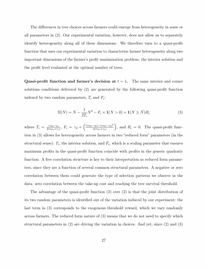
The differences in tree choices across farmers could emerge from heterogeneity in some or

all parameters in (2). Our experimental variation, however, does not allow us to separately

identify heterogeneity along all of these dimensions. We therefore turn to a quasi-profit

function that uses our experimental variation to characterize farmer heterogeneity along two

important dimensions of the farmer’s profit maximization problem: the interior solution and

the profit level evaluated at the optimal number of trees.

Quasi-profit function and farmer’s decision at t = 1. The same interior and corner

solutions conditions delivered by (2) are generated by the following quasi-profit function

indexed by two random parameters, Ti and Fi:

⇧(N) = N � 1

2Ti

N2 � Fi ⇥ 1(N > 0) + 1(N � ¯N)Ri (3)

where Ti =

⌧↵0��02(⌧↵1+�1)

, Fi = �2 +⇣

(⌧↵0��0)�(⌧↵0��0)2

4(⌧↵1+�1)

⌘

, and Ri = 0. The quasi-profit func-

tion in (3) allows for heterogeneity across farmers in two “reduced form” parameters (in the

structural sense): Ti, the interior solution, and Fi, which is a scaling parameter that ensures

maximum profits in the quasi-profit function coincide with profits in the generic quadratic

function. A free correlation structure is key to their interpretation as reduced form parame-

ters, since they are a function of several common structural parameters. A negative or zero

correlation between them could generate the type of selection patterns we observe in the

data: zero correlation between the take-up cost and reaching the tree survival threshold.

The advantage of the quasi-profit function (3) over (2) is that the joint distribution of

its two random parameters is identified out of the variation induced by our experiment: the

last term in (3) corresponds to the exogenous threshold reward, which we vary randomly

across farmers. The reduced form nature of (3) means that we do not need to specify which

structural parameters in (2) are driving the variation in choices. And yet, since (2) and (3)

27

share the same value at the optimal solution, we can still use (3) to evaluate welfare under

the more general profit function (2).

Tree survival as a farmer decision. Throughout our estimation, we assume that tree

survival is deterministic conditional on farmers’ costly effort. As we explain in greater detail

in Appendix 3, this assumption is also consistent with a model where survival is probabilistic

and the probability of survival is a convex continuous function of effort, e, up to e, where

it attains one. Farmers would respond to such probability profile by investing the minimum

effort that guarantees survival, e, in all trees they choose to plant.29 Empirically, the small

bunching of tree survival at 35 (the reward threshold) we observe in the data is consistent

with this assumption (see Appendix 3).

5.2 Dynamics and take-up decision

As in the conceptual model, we assume the farmer makes adoption-related decisions in two

periods: t = 0, 1. The random parameter Fi, which largely determines the magnitude of

optimized profits, is divided into two additive components: F0i and F1i, where F0i is known

at all periods and F1i is known at t = 1 but not at t = 0.30 In addition, we assume that

Ti is known to the farmer at all times. This amounts to assuming that there is uncertainty

about the net returns to tree cultivation, but not about the optimal scale of the technology.

The advantage of this particular structure of information is that it allows us to nest a model

without uncertainty (i.e., Var(F1i) = 0) that could also deliver no screening effects (or even

negative screening effects) within our more general model.

At t = 0, the farmer decides whether or not to pay to take-up the technology. At this

point in time, the farmer has partial information about her net benefits from the contract.29Except, perhaps, on one of them, as is explained in Appendix 3.30See the last paragraph of Section 3.2 for a discussion on our two-period assumption.

28

Assuming the farmer knows the distribution of F1i conditional on F0i and Ti at t = 0, the

farmer chooses to take-up if

�EF1i|F0i,Ti

h

max

N⇧(N |Ti, F0i, F1i, Ti, Ri)

i

� c+ Ai � 0 (4)

where c is the cost of the seedlings, Ai is the randomly determined subsidy, and � is the

discount factor, assumed equal to 0.6.31 Note that this representation of the NPV of farmer’s

profits from trees maintains the risk neutrality assumption from Section 2.32

5.3 Identification and estimation

Identification of the structural model consists of uniquely identifying the joint distribution of

unobservables Ti, F0i and F1i. In addition to the above described assumptions on the timing

of information, we maintain assumptions (i) and (ii) on the components of Fi from Section

2, and add the following assumptions

(iii) No common shocks: F1i ? F1j 8i 6= j

(iv) Normality: F0i ⇠ n�

µF , �2F0

�

, F1i ⇠ n�

0, �2F1

�

(v) Joint normality: (Fi, lnTi) ⇠ n(µ,⌃)

Below we explain the role that each of these assumptions plays for identification. In what

follows, we denote the randomized values of Ai and Ri as ai and ri to emphasize their role

as known (to the farmer and researcher) and exogenous.31Like Stange (2012), we note that in the context of stochastic dynamic structural models the discount

factor is not separately identified from the scale parameter of future period shocks. We used survey dataon time preferences to inform our choice of 0.6, which is in line with observed interest rates in our settingand elicited individual discount rates in other rural developing country settings (Conning and Udry 2007;Cardenas and Carpenter 2008).

32As discussed in Section 2, this assumption is innocuous to the extent that the changes in income producedby our program are small relative to total income. The highest reward from our program is roughly 3.5 percentof average annual income.

29

With no assumptions other than profit-maximizing behavior on behalf of the farmer and

a quadratic profit function that allows for corner solutions, the joint distribution of Fi and

Ti can be non-parametrically identified in the subset of the support such that ¯N < Ti < 50.

To see this, consider the follow-through decision of the subset of the sample for which

lim

a!A1

Pr

⇣

Eh

max

N⇧(N |Ti, F0i, F1i, Ti, ri)

�

�

�

F0i, Ti

i

� c� ai⌘

= 1,

such that there is no selection on take-up. Within this subset of the sample, we can use the

variation in ri to identify the joint distribution of (Fi, Ti). For this group, the probability of

cultivating N⇤= n > ¯N trees when R = ri can be written as

Pr(N⇤= n;R = ri) = Pr

✓

Fi < ri +1

2

n

�

�

�

�

Ti = n

◆

Pr (Ti = n) (5)

Because the left hand side of (5) is empirically observable, increments in ri, holding n con-

stant, trace out the conditional distribution of Fi given Ti. The same expression can then be

used to recover the marginal distribution of Ti by varying n and dividing by the conditional

distribution of Fi. Since non-parametric identification of the joint distribution of Fi and

Ti occurs only in the subset of the support such that ¯N < Ti < 50, additional paramet-

ric assumptions are required to fully characterize these distributions. We therefore adopt

assumption (v) for the estimation.

We use farmers’ take-up decisions in combination with assumptions (i)-(iv) in order to

separately identify the distributions of F0i and F1i, once the joint distribution of Fi and

Ti has been identified. Under these assumptions, the decision to take-up in response to ri

and ai provides independent identification of the distribution of the known component of

Fi, F0i. More formally, identification of the distribution of F0i is obtained from the decision

to take-up, which is characterized by the inequality in (4). The left side of (4) is a known

30

function of the random variable F0i. Note that parameters µF , �2F , µT , �2

T , and ⇢T,F can be

treated as known since they are identified from tree survival as described above. Denote this

function h(F0i; ri), so we can rewrite (4) as

h(F0i; ri) � c� ai (6)

The right side of (6) can take one of four known values, as ai 2 {0, 4000, 8000, 12000}. The

left hand side of (6) is known up to F0i and varies across individuals in response to the known

cost determinant, ri. Provided that h(F0i; ri) is invertible,33 we can identify the distribution

of F0i, from the random variation in ai and ri:

Pr

�

F0i h�1(c� ai, ri)|µF , �

2F , µT , �

2T , ⇢T,F

�

= Pr(TakeUpi|ai, ri) (7)

Common shocks and mean shift model. Assumption (iii) plays an important role for

identification, as it implies that the variance of Fi across farmers is the sum of the variances

of its two components: �2F0

+ �2F1

.34 The variance of shocks is thus partially identified

from subtracting the variance estimate of F0i, identified from (7), from the variance of

Fi, identified from tree choices. Shocks that are common across farmers do not translate

into variance in tree choices, and would lead to an underestimate of �2F1i

. In our context,

much of the uncertainty farmers face appears to be from idiosyncratic shocks. According

to our survey, two-thirds of respondents list health problems as their greatest challenge,

almost 50 percent of households report losing cattle or livestock to death or theft during

the past year, and 10 percent of households report the death or marriage of a working age

member.35 However, given that farmers are also likely affected by common shocks such as33It can be shown that there exists some f s.t. h(F0i; ri) is strictly monotonically decreasing on (�1, f).34Assumption (iii) is also present in Fafchamps (1993), and is necessary for maximum likelihood estimation.35This is consistent with a literature that documents, in most cases, a disproportionate share of income

risk from idiosyncratic factors in rural developing country settings (summarized in Dercon 2002).

31

rainfall patterns and commodity prices, we estimate a variant of our model that allows for a

specific type of common shock: one that is completely unforeseen at the time of take-up and

is common across all farmers. This model variant can be estimated by relaxing assumption

(ii), i.e. allowing for subjective and objective expectations about the mean of the shock to

differ. Thus we refer to this model as the mean shift model. The mean shift – or difference

between the subjective mean of the shock distribution at take-up and its objective mean –

is identified because the random variation in ri and ai allows us to identify µF in (7) from

the take-up decisions independently of the estimate from tree choices. Besides allowing us

to incorporate a type of common shock, the mean shift also captures any over-optimism or

experimenter demand effects that are common across farmers. These behaviors will share

the same structure as the unforseen common shock: the subjective mean will differ from the

objective mean of the opportunity cost distribution.

Estimation. We estimate the model using simulated maximum likelihood. The log-likelihoodfunction is over observations of the number of planted trees, N = 0, ..., 50, and the partici-pation decision, DP = 0, 1. The sample includes the 1,314 farmers who made a take-up de-cision. Because there are no trees planted whenever the individual chooses not to participate,the support of this bivariate vector is given by the 52 (DP,N) pairs: (0, 0), (1, 0), (1, 1), (1, 2), ..., (1, 50).

l(⇠;DP,N) =PM

i=1

n

(1−DPi) ln(1−⇡P,i) +DPi ln(⇡P,i) +DPi

P50j=0 1(Ni = j)lnPr(N = j)

o (8)

where ⇠ = (µF , �2F0, �2

F1, µT , �2

T , ⇢T,F ).

We use numerical methods to minimize the negative of the simulated log-likelihood.

For each likelihood evaluation, we use 1,500 draws of (Ti, F0i, F1i). Within each likelihood

evaluation and for each draw of (Ti, F0i, F1i), the expectation on the right hand side of

equation (4) is numerically computed using 100 draws of (Ti, F1i) conditional on the draw of

F0i.36 Standard errors for the estimated parameters are obtained as the inverse of the inner36Simulated methods often result in stepwise objective functions which work poorly with gradient-based

32

product of the simulated scores.37

6 Structural estimates and simulation results

In this section, we describe the structural estimates and carry out counterfactual simulations.

6.1 Structural estimates and model fit

Table 2 shows the point estimates for the main parameters described in Section 5.3.38 Panel A

shows the estimates of our baseline model, which assumes that farmers’ expectations about F

are correct and consistent over time. Panel B shows the results of allowing for an unexpected

common shock to all farmers at t = 1 (a mean shift). Because point estimates are somewhat

hard to interpret (e.g. the µT and �T parameters do not correspond to the mean and standard

deviation of the log-normally distributed parameter T ), we convert the estimated parameters

numerical optimization algorithms. To facilitate the numerical optimization, we “smooth” the objectivefunction by computing the multilogit formula for each decision over participation and the number of trees.We assume a relatively small variance parameter of the logistic error term: 0.5. However, we experimentwith different values for this parameter. We find that smoothing does not significantly affect the pointestimates and does improve substantially the curvature of our objective function. A further discussion ofthe estimation algorithm can be found in Appendix A.2.

37See Appendix A.2 for a more detailed description of our standard error calculation.38There are two remaining parameters that are omitted from Table 2 but discussed in Appendix A.2 for the

sake of brevity: these are the surprise treatment parameter, ↵S , and the monitoring treatment parameter,↵m. Recall that farmers in the surprise reward treatment made a take-up decision before learning theirreward. We model this aspect of the design by assuming individuals expect a threshold reward of 0 whentheir participation decision is made, but incorporate the reward value they draw in their follow-throughdecision. Because our reduced form results show that individuals in the surprise treatment had higherparticipation rates than those individuals who drew a reward of zero ZMK, we allowed the surprise rewardtreatment to have an independent effect on the participation decision. The structural estimates suggest thatthe boost to participation is equivalent to offering them between 92 and 54 ZMK (in the base and meanshifter models, respectively). Appendix A.2 describes these results in more detail.

In all models, we allow the regular visits to collect data on program implementation that were administeredto one-fifth of farmers to independently affect the tree survival decision (but not the participation decision).The estimated parameter is -238.40 (s.e. 73.887) in Panel A and -229.53 (s.e. 74.444) in Panel B. In otherwords, regular monitoring visits appears to be reducing the fixed costs of tree cultivation, which is consistentwith the positive effect of monitoring on tree survival that we find in the reduced form results.

33

into more easily interpretable outcomes using simulation.39 The estimated joint distribution

of T and F shown in Panel A is such that the mean ex-post privately optimal number of

trees is 8.46 (s.d. 14.64), with about 59 percent of farmers choosing to plant no trees.40

Table 2: Structural parameter estimates

μT σT ρ μF σF0 σF1 αs αm μFs

3.539 1.401 0.818 107.58 307.87 211.42 -91.79 -238.40 -(0.057) (0.066) (0.066) (11.822) (93.278) (49.953) (16.222) (73.887) -

3.579 1.392 0.835 74.48 290.06 193.05 -54.42 -229.53 53.29(0.071) (0.075) (0.073) (15.47) (84.622) (45.427) (20.47) (74.444) (26.761)

Parameters in F

Panel B. Allowing for Mean Shift

Panel A. No Mean Shift

Parameters in T

Notes: Parameters fitted by simulated maximum likelihood using 1500 draws of the random vector (F0i, F1i, Ti), with

smoothing (lambda is 0.5) and tolerance (1e-15). The baseline model (Panel A) restricts the mean of Fi to be the same

in both time periods. The mean shift model (Panel B) allows the mean of Fi to differ between the two periods, and the

parameter F_shift to capture this difference. The log-likelihood value for the baseline model is 11142.064, while it is11138.996 for the mean shift model.

This joint distribution also implies that the average ex-post private profit from the opti-

mal number of trees is 108.39 thousand ZMK. However, ex-post private profits vary widely

across farmers: the s.d. is 185.47. Importantly, the model estimates that about 39 percent

of the variance in ex-post profits is due to new information that emerges after the take-up

decision is made. To put this magnitude into perspective, among farmers whose expected

number of trees is above the reward threshold at the time of take-up, around 15 percent

prefer a number below the threshold after new information is revealed.

The variance of shocks is partially identified out of the difference in the variances of39The point estimates in Table 2 can be used to simulate farmer’s draws of F and T . These draws are

then used to compute optimal tree cultivation decisions that account for interior and corner solutions, whichare then be plugged back into the profit function to compute maximized profit. The statistics presented herecorrespond to means and variances from 10,000 simulated draws.

40These statistics assume that farmers can plant a maximum of 50 trees. Although we allow for thedistribution of T to be unbounded, we present statistics of the bounded distribution because we fit theeconometric model using only this range of outcomes. According to our estimates, about 6 percent of thefarmers would choose a private optimum of 50 or more trees.

34

expected profits at take-up (t = 0) and ex-post profits at the time the follow-through decision

is made (t = 1) and partially identified out of its non-linear effect on the mean level of the

expected profits at take-up.41 The presence of common shocks will generate a tug-of-war

between these two sources of identification: the expected value of the profits will pull the

variance of shocks parameter, �F1, up while the ex-post variance in profits will not reflect

the variance of common shocks and thus will pull �F1 down. Our mean shift model helps us

explore the importance of the bias in �F1 generated by the presence of common shocks, by

allowing the mean level of profits to be different at t = 0 and t = 1.

The corresponding results from the mean shift model are presented in Panel B of Table

2. The estimated difference in means between the two periods, the mean shift, is given

by parameter µFS . A non-zero value for this estimated parameter has a couple of plausible

interpretations. First, it can represent a single common shock whose possibility was unknown

at the time of take-up and affected all farmers equally. Second, it can pick up a common

update in the value for the technology that occurred after the take-up decision was made.

The latter interpretation is a useful test for the presence of experimenter demand effects

on take-up: the perceived obligation of potential adopters to take-up in the presence of the

experimenter. Our estimate of the value for µFS is positive but small and not significantly

different from zero at standard confidence levels. The positive value is consistent with either

the presence of a common shock of the specific type described above or an experimenter

demand effect. Note, however, that in either case, it is small compared to the standard

deviation of the shocks, �F1 . And, importantly, allowing for this effect induces a small

change in the variance of the shocks: �F1, falls moderately from 211.42 to 193.05, which is

consistent with a positive bias in our baseline model stemming from the presence of common

shocks.42 This suggests that uncertainty in the form of idiosyncratic shocks is important and41Recall that a higher variance in shocks results in a larger option value for the contract.42Unfortunately, we cannot calculate the share of the variance attributed to common shocks using model

estimates since we are not explicitly modeling random common shocks with a known distribution at the time

35

that experimenter demand effects are not driving our results.

We now turn to the interpretation of the parameters that govern the distribution of known

(at the time of take-up) sources of heterogeneity across farmers. We estimate a high positive

correlation between F and lnT , ⇢T,F = 0.81 (⇢T,F = 0.83 in the mean shift model).43 Because

F enters negatively in the profit function, this translates into a negative correlation between

the privately optimal number of trees and the level of profits. This negative correlation

generates low, but strictly positive, follow-through rates (as in low numbers of trees planted)

among farmers whose expected value from the contract is high and thus take-up under a

high price. In other words, the static heterogeneity identified by the model contributes

to undermining the effect of high prices at take-up on positive (high follow-through) self-

selection of farmers.

Because F and T are reduced form parameters (see Section 5.1), the positive correlation

between them could stem from two sources: a positive correlation between farmers’ fixed

costs and farmers’ interior solution to the maximization problem (a component of the reduced

form random parameter, F , is the fixed cost of the generic quadratic profit function), or a

high mean and high variance in the linear term of net marginal returns (the term ⌧↵0��0 in

the reduced form expression for T and F ), which enters linearly in T and non-linearly in F ,

and in high ranges may generate a negative relationship between them.44 Our model predicts

well some simple observations in the data. For example, our baseline model predicts that

1,104 farmers (1,112 under the mean shift model), out of a total of 1,314, will take-up; our

data show 1,092 participants. Our model also predicts that 173 out of the 963 farmers that

faced a strictly positive take-up cost (i.e. a subsidy less than 12,000 ZMK) will choose to

cultivate zero trees (180 in the mean shift model), while the observed number of farmers in

of take-up.43F1 is assumed to be orthogonal to F0 and T . Thus, the correlation between F and T stems solely from

the correlation between F0 (the known component of F ) and T .44We verified this is the case for plausible distributions of the deep structural parameters via simulation.

36

this category is 112. That is, the dynamics in our model replicate an observation that seems

at odds with rationality in a static framework: some farmers who purchase the trees choose

not to cultivate them. In this sense, our result parallels the result by Fafchamps (1993) in

that individuals make costly choices to maximize future flexibility.

Next, we further examine the model fit by comparing the reduced form treatment effects

using simulated outcomes from the estimated model and the observed data. Most of the

magnitudes and signs between the treatments and outcomes are well matched by our model

estimates. Panel A of Table 3 shows results with the observed data, while Panels B and C

show the corresponding simulations using the estimates from Table 2. Columns 1-4 estimate

the effect of a thousand ZMK increase in the subsidy on take-up and follow-through outcomes.

Columns 5-8 repeat the regressions with the reward (in ’000 ZMK) on the righthand side.

The effect of the subsidy and the reward on take-up (columns 1 and 5) and whether the

farmer reached the 35-tree threshold (columns 2 and 4, conditional on take-up) are similar

across the observed and simulated data. The effect of the reward on zero tree survival is also

very similar in the observed and simulated data.

There are, however, some discrepancies between what our model predicts and the ob-

served data. Columns 3 and 7 show the effect of the take-up subsidy and reward on the

number of surviving trees, excluding zeros (which are shown in columns 4 and 8). Interest-

ingly, the sign of the coefficient on the subsidy is different between the observed and simulated

data, though standard errors are relatively large. The effect of the reward on the number

of trees (column 7) is larger in the simulated data, consistent with the effects on reaching

the 35-tree threshold. Finally, we see evidence that the take-up subsidy selects for farmers

more likely to keep zero trees alive (column 4) in the simulated but not in the observed data,

indicating some selection effect on abandoning the technology altogether in the simulated

data only. Using simulations, we explore whether some of the discrepancies between our

estimated model and the data stem from the assumption of deterministic survival of the

37

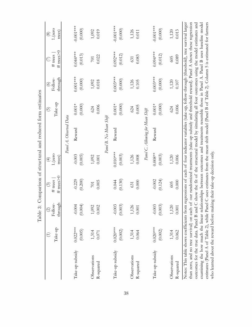
Tabl

e3:

Com

paris

onof

stru

ctur

alan

dre

duce

dfo

rmes

timat

es

(1)

(2)

(3)

(4)

(5)

(6)

(7)

(8)

Take

-up

Follo

w-

thro

ugh

# tr

ees

|#

tree

s>0

1.(z

ero

tree

s)Ta

ke-u

pFo

llow

-th

roug

h#

tree

s |

# tr

ees>

01.

(zer

otr

ees)

Take

-up

subs

idy

0.02

2***

-0.0

04-0

.229

-0.0

03R

ewar

d0.

001*

0.00

1***

0.04

4***

-0.0

01**

*(0

.005

)(0

.004

)(0

.200

)(0

.005

)(0

.000

)(0

.000

)(0

.013

)(0

.000

)

Obs

erva

tions

1,31

41,

092

701

1,09

262

41,

092

701

1,09

2R

-squ

ared

0.07

10.

002

0.00

50.

001

0.00

60.

018

0.02

20.

019

Take

-up

subs

idy

0.02

0***

-0.0

030.

044

0.01

0***

Rew

ard

0.00

1*0.

003*

**0.

092*

**-0

.001

***

(0.0

02)

(0.0

03)

(0.1

30)

(0.0

03)

(0.0

00)

(0.0

00)

(0.0

12)

(0.0

00)

Obs

erva

tions

1,31

41,

126

631

1,12

662

41,

126

631

1,12

6R

-squ

ared

0.06

40.

001

0.00

00.

008

0.00

50.

105

0.08

30.

011

Take

-up

subs

idy

0.02

0***

-0.0

03-0

.002

0.00

8**

Rew

ard

0.00

1*0.

003*

**0.

094*

**-0

.001

***

(0.0

02)

(0.0

03)

(0.1

24)

(0.0

03)

(0.0

00)

(0.0

00)

(0.0

12)

(0.0

00)

Obs

erva

tions

1,31

41,

120

605

1,12

062

41,

120

605

1,12

0R

-squ

ared

0.06

20.

001

0.00

00.

006

0.00

60.

107

0.08

90.

013

Pane

l A. O

bser

ved

Dat

a

Pane

l C. A

llowi

ng fo

r Mea

n Sh

ift

Pane

l B. N

o M

ean

Shift

Not

es:T

his

tabl

esh

ows

coef

ficie

nts

from

regr

essi

ons

ofea

chof

four

indi

cato

rvar

iabl

es(ta

ke-u

p,fo

llow

-thr

ough

(thre

shol

d),t

ree

surv

ival

larg

erth

anze

ro,a

ndno

tree

surv

ival

)on

each

ofou

rra

ndom

ized

trea

tmen

ts(ta

ke-u

psu

bsid

yan

dth

resh

old

rew

ard)

.Pan

elA

show

sth

ese

regr

essi

onou

tcom

esfo

rth

etr

ueda

ta.P

anel

Ban

dC

show

the

fitof

the

stru

ctur

alm

odel

bysi

mul

atin

gal

lfou

rou

tcom

esus

ing

the

mod

eles

timat

esan

dex

amin

ing

the

how

muc

hth

elin

ear

rela

tions

hips

betw

een

outc

omes

and

trea

tmen

tsre

sem

ble

thos

ein

Pane

lA

.Pa

nel

Bus

esba

selin

em

odel

estim

ates

(Pan

elA

ofTa

ble

2),w

hile

Pane

lCus

eses

timat

esfr

omth

em

ean

shift

mod

el(P

anel

Bof

Tabl

e2)

.Col

umn

5is

estim

ated

for

farm

ers

who

lear

ned

abou

t the

rew

ard

befo

re m

akin

g th

eir t

ake-

up d

ecis

ion

only.

38

trees conditional on effort by introducing a stochastic component to tree survival outcomes,

taking parameter estimates as given. We find little to no improvement when stochasticity is

introduced into the tree survival outcomes (see Appendix A.3).

6.2 The effect of uncertainty on farmer profit and program out-

comes

We use estimates from the structural model to perform counterfactual simulations of farmer

profits and program outcomes (take-up and tree survival) under different levels of uncertainty.

For these analyses, we use the results from the model with the mean shift parameter, such

that both the mean and the standard deviation of Fi may vary over time (Panel B in Table

2). In the simulated results below, we set the mean shift for t = 1, µFs , equal to zero, so

that we can equate the expected benefits with the true average discounted benefits from the

program.45 Results from using our baseline model estimates are qualitatively similar.

Farmer profits

We begin by examining the effect of uncertainty on the average per-farmer expected private

profit (right hand side of inequality 1) implied by the empirical model. In order to do so,

we simulate the value of the expected profit for each farmer at different values of �F1. The

relationship between the mean expected profit and �F1 corresponds to the solid black curves

in Figure 2. Panel A shows the relationship for a reward of zero and Panel B for the largest

reward offered (150 thousand ZMK). Both are shown at a full subsidy, so that take-up is 100

percent (i.e. there is no selection on the take-up price).45This treatment of the mean shift parameter is consistent with the common-shock interpretation of this

parameter.

39

Expected farmer profits are increasing in uncertainty. This result is analogous to

the theoretical result discussed in Proposition 4: the option value from the contract increases

with uncertainty and thus drives a positive relationship between the expected profit and

uncertainty. The option value, as defined in Appendix 1, is shown by the dashed lines in

Figure 2 for different values of the reward. The option value is always non-negative, and is

also the only component of the expected private profit that varies with uncertainty. Recall

that this result stems from the asymmetric response of the expected profit to positive and

negative shocks: if the realization of the random component of the profit drives it below

zero, the farmer will respond by not cultivating any trees at all (effectively bounding the

profit realizations at zero). This optimizing behavior turns the high variance of the shocks

into an asset of the contract, which in turn results in higher take-up.

The positive relationship between expected private profit and uncertainty has implica-

tions for take-up decisions: under higher uncertainty, more farmers are ex ante attracted to

the contract, even though its ex post expected value is unchanged. A high enough level of

uncertainty may result in an expected profit that exceeds even an unsubsidized take-up cost.

Hence, the ability of the take-up cost to “tease out” those who will be more likely to reach

the tree survival threshold decreases with uncertainty. This can be observed more directly

when looking at take-up and follow-through outcomes as a function of uncertainty, which we

turn to next.

40

Figure 2: Farmer expected profit as a function of uncertainty

Notes: This figure shows a counterfactual simulation of farmers’ mean expected profit as we vary the level ofuncertainty (the standard deviation of F1). For the simulations, we use the estimated parameters from PanelB of 2, except for �F1 , which we vary along the horizontal axis. The mean per-farmer profit is shown in asolid black line for low (Panel A, R = 0) and high (Panel B, R = 150) reward values. Profits, the subsidy(A) and the reward (R) are expressed in thousand ZMK. The dashed lines show the mean option value forthe two different reward levels. We define the option value as the value of re-optimizing the number of treesto cultivate after F1 is realized relative to the value of a static choice.

Program outcomes

Figure 3 plots average take-up at low and high subsidies (dashed and solid lines) and low

(Panel A) and high (Panel B) rewards as a function of uncertainty. Panels C and D show

the share of individuals who reach the 35-tree threshold conditional on take-up for the same

combinations of subsidies and rewards. Figure 4 shows the effects of uncertainty on the

average number of trees for different values of the subsidy (A) and reward (R). Panels A

and B show the average tree survival, unconditional on take-up (non-participants have zero

surviving trees). Panels C and D show average tree survival conditional on take up. Because

41

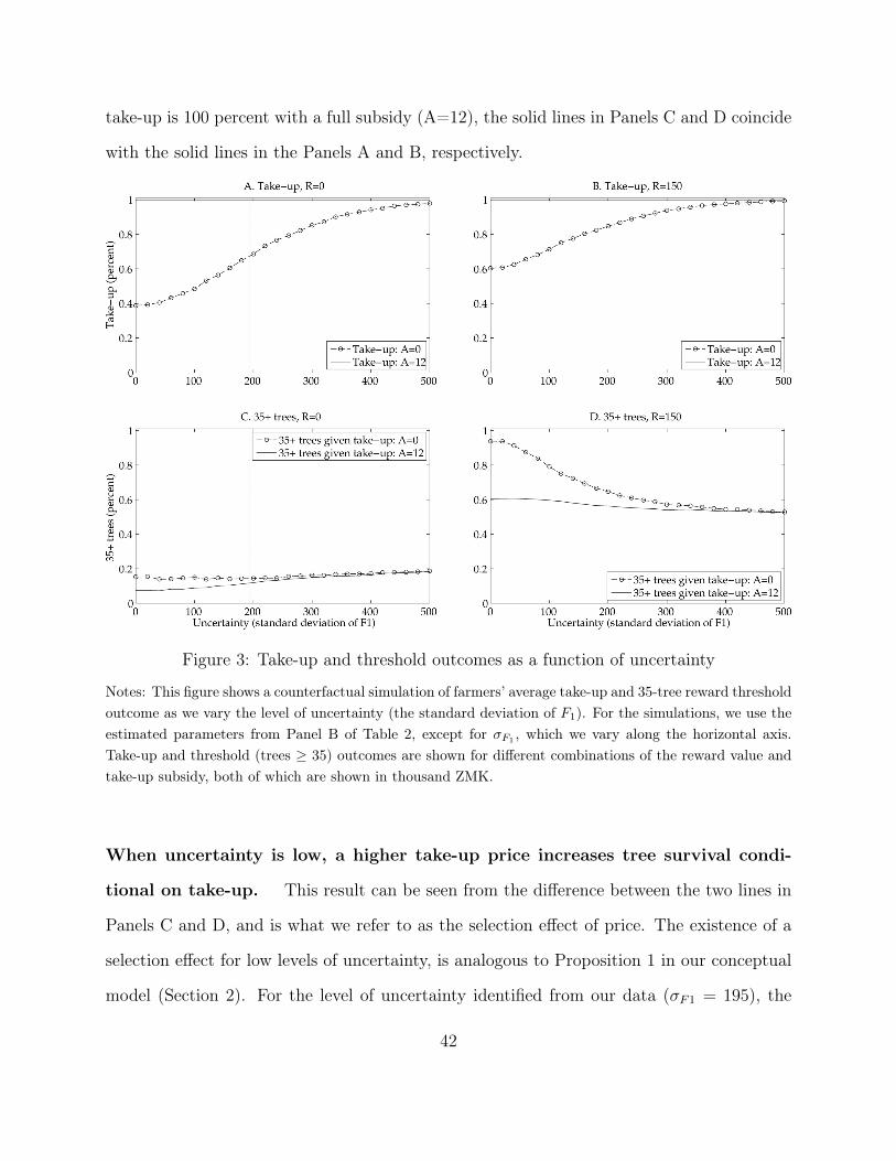
take-up is 100 percent with a full subsidy (A=12), the solid lines in Panels C and D coincide

with the solid lines in the Panels A and B, respectively.

Figure 3: Take-up and threshold outcomes as a function of uncertainty

Notes: This figure shows a counterfactual simulation of farmers’ average take-up and 35-tree reward thresholdoutcome as we vary the level of uncertainty (the standard deviation of F1). For the simulations, we use theestimated parameters from Panel B of Table 2, except for �F1 , which we vary along the horizontal axis.Take-up and threshold (trees � 35) outcomes are shown for different combinations of the reward value andtake-up subsidy, both of which are shown in thousand ZMK.

When uncertainty is low, a higher take-up price increases tree survival condi-

tional on take-up. This result can be seen from the difference between the two lines in

Panels C and D, and is what we refer to as the selection effect of price. The existence of a

selection effect for low levels of uncertainty, is analogous to Proposition 1 in our conceptual

model (Section 2). For the level of uncertainty identified from our data (�F1 = 195), the

42

gain in tree survival from charging more at take-up is modest – less than 5 trees – and it

continues falling as uncertainty increases. The reduction in the selection effect as uncertainty

increases is analogous to Proposition 3 in our conceptual model.

When the price for take-up is high, uncertainty lowers follow-through conditional

on take-up. This result is shown by the downward slope of the dashed line with circles

in Panels C and D in Figure 4. This reduction in tree survival is driven by the selection

effect of the take-up price decreasing as uncertainty increases: as shown by Panels A and B in

figure 3, take-up converges to 100 percent as uncertainty increases, making the pool of takers

ever more similar to the overall pool. This is broadly consistent with Proposition 2 from

our conceptual model, although the result in this richer model is qualified by an additional

competing effect: the variance of shocks can have a positive or negative effect on the number

of farmers that choose zero trees depending on whether the sign of this corner solution

threshold is to the right or to the left of the mean of F . We call this effect the corner

solution effect. It is positive whenever the threshold reward is 150 ZMK, and negative

whenever the threshold reward is zero. Thus, when the reward is zero, we see that the

unconditional average number of trees increases slightly with uncertainty (both lines in Panel

A and the solid line in Panel C increase with �F1).46 Thus, in this richer model, the effect

of uncertainty on follow-through conditional on take-up carries both effects: the selection

effect, which lowers follow-through; and the corner solution effect, which has an ambiguous

effect on follow-through. In our context, the selection effect dominates the corner solution

effect, and thus follow-through falls with uncertainty conditional on take-up. That average46This effect holds whenever the distribution of shocks is continuous and symmetric around the mean. To

see this, denote the standard normal cdf as �(.) and the threshold along the support of F above which theprivate profit associated with the interior solution is negative as F . The probability of choosing to plantzero trees takes the form 1� �

⇣

F�µF

�F0+�F1

⌘

. Note that the derivative of this probability with respect to �F1

has the same sign as the numerator of the argument of �(.). When R = 0, F = 12Ti. Given that µF is above

100 and the mode of Ti is 8.9, the numerator tends to be negative. However, when R = 150 and N⇤ � 35,F = N⇤ � 1

2TiN⇤2 + 150; and, thus, the numerator tends to be positive.

43

follow-through conditional on take-up falls with uncertainty has implications for technologies

whose benefits kick in above a certain “usage” level: under low levels of uncertainty about

implementation costs, a high cost of take-up will help select those individuals who are likely

to engage in more intensive usage of the technology.

The effect of a high subsidy on take-up may dominate its effects on selection.

This result is most clearly seen by comparing unconditional tree survival (Panels A and B of

Figure 4) with tree survival conditional on take-up, which excludes the take-up effect (Panels

C and D). The boost associated with the selection effect observed at low levels of uncertainty

in Panels C and D is more than offset by the take-up effect: many more farmers take-up

when subsidies are high (see Panels A and B in Figure 3). The two counteracting effects

lead to similar average tree survival across subsidy levels, unconditional on take-up (Panels

A and B). Hence, for technologies whose benefits kick in with total follow-through (whether

or not follow-through is spread about few or many adopters), subsidies may increase the

benefits of adoption. Note, however, that uncertainty also lowers the take-up advantage of

high subsidies, as take-up increases with uncertainty for all subsidy levels.

When uncertainty is high, a reward conditional on follow-through is more effec-

tive at inducing tree survival than a subsidy. This result can be appreciated when

comparing the effect of moving from a lower R to a higher R as compared to moving from

a low A to a high A. Even with the optimal (in our setting) combination of a low take-up

subsidy and high threshold reward, uncertainty can bring down the number of farmers that

reach the 35-tree threshold.

44

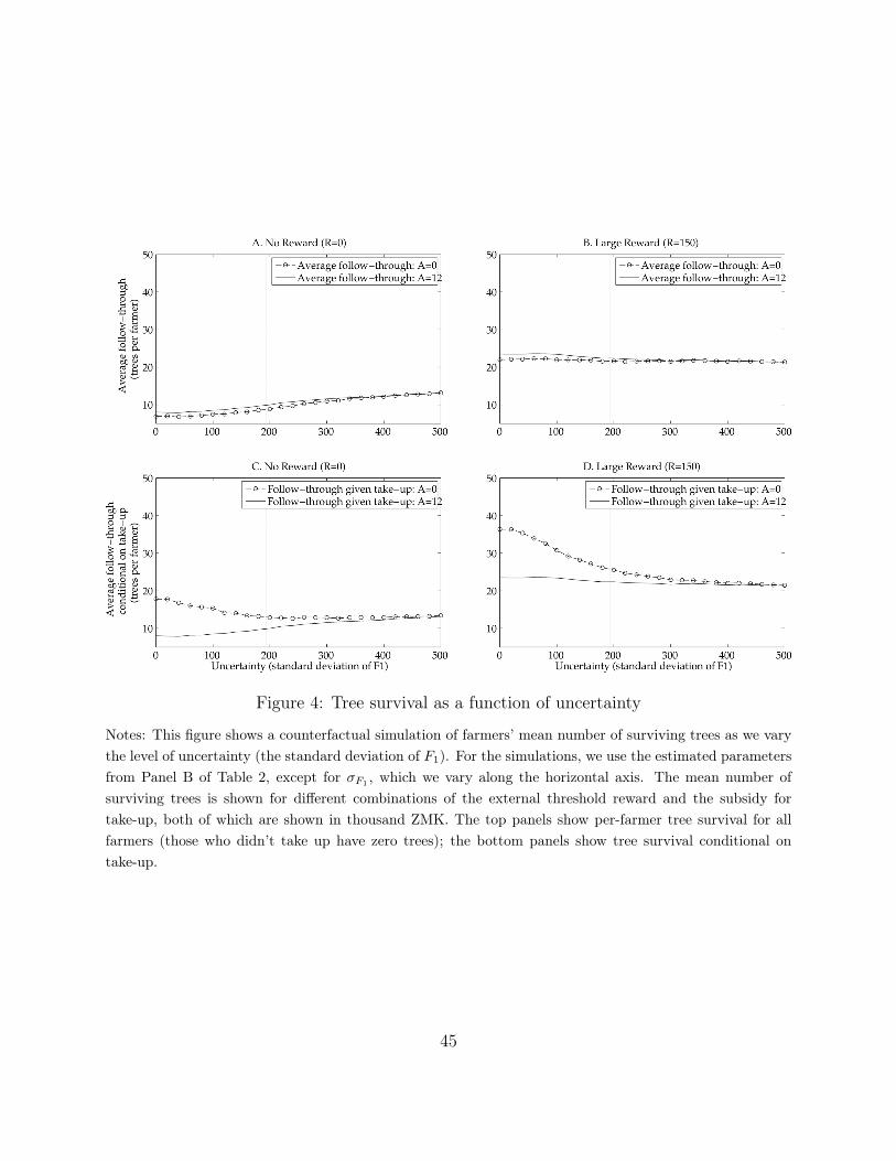
Figure 4: Tree survival as a function of uncertainty

Notes: This figure shows a counterfactual simulation of farmers’ mean number of surviving trees as we varythe level of uncertainty (the standard deviation of F1). For the simulations, we use the estimated parametersfrom Panel B of Table 2, except for �F1 , which we vary along the horizontal axis. The mean number ofsurviving trees is shown for different combinations of the external threshold reward and the subsidy fortake-up, both of which are shown in thousand ZMK. The top panels show per-farmer tree survival for allfarmers (those who didn’t take up have zero trees); the bottom panels show tree survival conditional ontake-up.

45

7 Discussion and interpretation

Our model and results are consistent with several interpretations of intertemporal adoption

decisions and the nature of the uncertainty that farmers face. Our preferred interpretation is

one of idiosyncratic and common shocks to the opportunity cost of follow-through with the

technology, with idiosyncratic shocks playing a relatively more important role. We describe

supplementary evidence on alternative interpretations and explanations in this section.

7.1 Learning

Our theoretical and empirical models are similar, from an ex ante perspective, if the infor-

mation that arrives between t = 0 and t = 1 is a persistent (learning) or transient shock

to opportunity cost, provided that both types of new information are independent across

farmers. In addition, to the extent that learning shocks are common across all farmers and

unexpected, the mean shift model could account for learning. Interpreted this way, the pos-

itive mean shift estimate is consistent with farmers systematically underestimating the costs

of follow-through at the time of take-up. The small estimated magnitude of the mean shift

parameter would then imply little systematic updating across all farmers. Learning shocks

that are independent across farmers and whose distribution is known by the farmers ex ante

would show up in the variance of F1. Thus, we cannot distinguish between persistent and

transitory shocks to the opportunity costs of cultivating trees.

The potential for learning about the value of the technology during the first year of tree

cultivation is limited given that tree survival benefits are not realized until several years

after the end of the study, and planting and caring for trees resembles activities that farmers

undertake regularly. Thus, if learning occurs, it is likely related to the opportunity costs of

cultivating the trees, rather than the benefits. We use survey data to explore the extent to

which baseline knowledge of the technology affects the results. Specifically, we expect that

46

farmers who had more baseline knowledge have less to learn and are therefore less likely to

end up with zero surviving trees if they take-up under a positive price.

We construct three baseline knowledge measures: (1) whether the farmer had any Faid-

herbia albida on their land at baseline, (2) whether anyone in the farmer group had Faidherbia

albida on their land at baseline, and (3) whether the farmer could name at least one risk

to tree survival at baseline. Appendix table A.5.5 shows the results from a linear regression

of the likelihood of having zero surviving trees on a knowledge variable, an indicator for

paying a positive price and their interaction, conditional on take-up. Learning would predict

a negative and significant interaction. We observe a negative and statistically insignificant

interaction for the first two knowledge variables, and a positive and significant interaction

for the third. In other words, we find no clear evidence that learning explains the pattern of

take-up under a positive price coupled with zero surviving trees, which can be explained by

transient shocks that arrive after take-up.

7.2 Procrastination

An alternative explanation that would violate our identifying assumptions is procrastination

or hyperbolic time preferences. Sustained effort choices are frequently associated with time

inconsistent behavior, in which the individuals initially takes up, intending to follow-through.

But when the time comes to act, costs loom larger (or benefits smaller) than anticipated

at the time of initial take-up decision. Mahajan and Tarozzi (2011) document time incon-

sistent technology adoption for insecticide treated bednets in India, with low rates of net

re-treatment.

We examine evidence for procrastination or hyperbolic time preferences by constructing

two measures of procrastination from the survey data (see Appendix Table A.5.6), which

differentiate to some degree between naive and sophisticated procrastinators. We begin by

47

examining whether these measures of procrastination are correlated with contract take-up

or tree survival conditional on take-up, controlling for other characteristics. They are not.

We next investigate the insight that farmers prone to procrastination may be differentially

sensitive to a contract structure that requires them to pay more upfront for inputs if the

potential rewards arrive only after a year of effort. We regress take-up on an interaction

of each of the two procrastination measures and the subsidy level. For the self-aware (so-

phisticated) procrastinators, there is a weakly greater likelihood of take-up at higher subsidy

levels. However, the interaction is insignificant with the measure more likely to capture naive

procrastinators. These results suggest a relatively minor role for procrastination in driving

take-up or follow-through outcomes.

8 Conclusion

This paper shows that uncertainty can play an important role in the adoption of technologies

that require costly effort over time. We provide a broad framework for adoption decisions

that allows for both time-invariant and time-varying heterogeneity as well as multiple di-

mensions of static heterogeneity across potential adopters. This framework applies to many

adoption decisions in agriculture, development, environment, and health research (for exam-

ple, the adoption and adherence to medical treatments). In our conceptual model, we show

that uncertainty in the opportunity cost of adoption can increase take-up rates at the cost of

reducing average follow-through rates. Uncertainty at the time of take-up provides an addi-

tional explanation to what has been discussed in the technology adoption literature for why

charging higher prices may be ineffective at selecting for adopters likely to follow-through at

the time of take-up.

Findings from our field experiment show reduced form evidence that is consistent with

our conceptual model, in the context of agricultural technology adoption. In Zambia, farmers

48

decide whether to take-up a nitrogen fixing tree under considerable uncertainty about the

benefits and costs of following through to keep the trees alive. The experimental variation

is used to identify a structural model of intertemporal decision making under uncertainty,

which explains our field results and quantifies the uncertainty that the farmers face at the

time of take-up. The structural model also helps distinguish between static and time-varying

sources of heterogeneity that may explain the absence of screening effects of prices. We find

that, in our setup, both static and time-varying heterogeneity reduce the screening effect of

the take-up price. Counterfactual simulations indicate that reducing the uncertainty in our

setting by half would increase the number of farmers that reach tree survival threshold by

18 percentage points (36 percent).

Like all empirical case studies, our data are specific to our setting. However, the com-

bination of the experimental data with a structural model allows us to simulate adoption

outcomes under different levels of uncertainty. Our results are consistent with more than one

interpretation of what changes for farmers between the time of the take-up and the follow-

through decisions. First, farmers may experience shocks, such as an illness in the household

or the arrival of agricultural pests, that affect the opportunity cost of following through with

the technology. Second, farmers may acquire additional information about the net costs of

tree cultivation after take-up through learning by doing or learning from peers. From an

ex ante modeling perspective, our general framework is agnostic about which explanation is

correct. Though we cannot distinguish among them using our experimental design, supple-

mentary evidence suggests that idiosyncratic shocks are important in our setting and that

learning opportunities, while present, are minimal.

Our study is an example of how experimental variation can be used to identify dynamic

structural models. The use of experimental variation in treatments at two different points in

time offers an alternative to a panel data structure, since statistically independent samples

are exposed to different treatment combinations. To our knowledge, this is the first paper

49

to introduce experimental variation in order to satisfy the exclusion restrictions needed for

sequential identification. One caveat of our basic identification strategy is that it relies on

shocks being independent across farmers. Therefore, a variant of our model allows for a

uniform common shock to farmers, provided that it is completely unanticipated (i.e. the

subjective probability assigned by farmers is zero).

From a policy standpoint, uncertainty has the effect of lowering adoption outcomes per

dollar of subsidy invested, while increasing the expected private profits to the adopter, be-

cause the downside risk of take-up is bounded at zero. To the extent that subsidies rely

on public funds, an increase in uncertainty represents an ex ante transfer from the public

to the private domain, driven entirely by the adopter’s ability to re-optimize follow-through

once new information becomes available. While stronger contracts that force adopters to

follow-through once they take-up a subsidized technology would address the problem of high

take-up coupled with low follow-through, they would do so at a clear cost to the adopter.

Future research to explore more innovative solutions to encouraging both take-up and follow-

through in the presence of uncertainty offers a promising direction for both environmental

and development policies. For example, cheaper monitoring solutions that facilitate rewards

for follow-through outcomes can have positive effects on both take-up and follow-through,

as shown in our setting.

50

References

Akinnifesi, F. K., O. Ajayi, Sileshi, P. W. Chirwa, and J. Chianu (2010). Fertiliser treesfor sustainable food security in the maize-based production systems of East and SouthernAfrica: A review. Agronomy for Sustainable Development 30 (3), 615–629.

Arrow, K. J. and A. C. Fisher (1974). Environmental preservation, uncertainty, and irre-versibility. Quarterly Journal of Economics 88 (2), 312–319.

Ashraf, N., J. Berry, and J. M. Shapiro (2010). Can higher prices stimulate product use?Evidence from a field experiment in Zambia. American Economic Review 100 (5), 2383–2413.

Ashraf, N., B. K. Jack, and E. Kamenica (2013). Information and subsidies: Complementsor substitutes? Journal of Economic Behavior & Organization 88, 133–139.

Barnes, R. and C. Fagg (2003). Faidherbia albida: Monograph and annotated bibliography.Beaman, L., D. Karlan, B. Thuysbaert, and C. Udry (2014). Self-selection into credit mar-

kets: Evidence from agriculture in mali. Working Paper .Brown, S. (1997). Estimating biomass and biomass change of tropical forests: a primer,

Volume 134. Food & Agriculture Org.Bruhn, M. and D. McKenzie (2009). In pursuit of balance: Randomization in practice in

development field experiments. American Economic Journal: Applied Economics 1 (4),200–232.

Bryan, G., S. Chowdhury, and A. M. Mobarak (2014). Underinvestment in a profitabletechnology: The case of seasonal migration in bangladesh. Econometrica 82 (5), 1671–1748.

Cardenas, J. C. and J. Carpenter (2008). Behavioural development economics: Lessons fromfield labs in the developing world. Journal of Development Studies 44 (3), 311–338.

Carter, M. R., R. Laajaj, and D. Yang (2014). Subsidies and the persistence of technologyadoption: Field experimental evidence from mozambique. Working Paper .

Cohen, J. and P. Dupas (2010). Free distribution or cost-sharing? Evidence from a random-ized malaria prevention experiment. Quarterly Journal of Economics 125 (1), 1–45.

Cohen, J., P. Dupas, and S. Schaner (2015). Price subsidies, diagnostic tests, and targeting ofmalaria treatment: Evidence from a randomized controlled trial. The American EconomicReview 105 (2), 609–645.

Conley, T. G. and C. R. Udry (2010). Learning about a new technology: Pineapple in ghana.The American Economic Review , 35–69.

Conning, J. and C. Udry (2007). Rural financial markets in developing countries. In Handbookof Agricultural Economics, Volume Volume 3, pp. 2857–2908. Elsevier.

Dercon, S. (2002). Income risk, coping strategies, and safety nets. The World Bank ResearchObserver 17 (2), 141–166.

Dixit, A. and R. Pindyck (1994). Investment under uncertainty. Princeton University Press.Dupas, P. (2014). Short-run subsidies and long-run adoption of new health products: Evi-

dence from a field experiment. Econometrica 82 (1), 197–228.Einav, L., A. Finkelstein, S. P. Ryan, P. Schrimpf, and M. R. Cullen (2013). Selection on

51

moral hazard in health insurance. American Economic Review 103 (1), 178–219.Fafchamps, M. (1993). Sequential labor decisions under uncertainty: An estimable household

model of west-african farmers. Econometrica, 1173–1197.Fischer, G., D. Karlan, M. McConnell, and P. Raffler (2014). To charge or not to charge:

Evidence from a health products experiment in uganda. Working Paper .Foster, A. D. and M. R. Rosenzweig (1995). Learning by doing and learning from others:

Human capital and technical change in agriculture. Journal of Political Economy, 1176–1209.

Giné, X. and D. Yang (2009). Insurance, credit, and technology adoption: Field experimentalevidence from malawi. Journal of Development Economics 89 (1), 1–11.

Goldman, D. P., G. F. Joyce, and Y. Zheng (2007). Prescription drug cost sharing: Associ-ations with medication and medical utilization and spending and health. Journal of theAmerican Medical Association 298 (1), 61–69.

Heckman, J. J. and S. Navarro (2005). Empirical estimates of option values of educationand information sets in a dynamic sequential choice model. Working paper .

Heckman, J. J. and S. Navarro (2007). Dynamic discrete choice and dynamic treatmenteffects. Journal of Econometrics 136 (2), 341–396.

Heckman, J. J., D. Schmierer, and S. Urzua (2010). Testing the correlated random coefficientmodel. Journal of Econometrics 158 (2), 177–203.

Jack, B. K. (2013). Private information and the allocation of land use subsidies in malawi.American Economic Journal: Applied Economics 5, 113–35.

Karlan, D., R. Osei, I. Osei-Akoto, and C. Udry (2014). Agricultural decisions after relaxingcredit and risk constraints. The Quarterly Journal of Economics 129 (2), 597–652.

Karlan, D. and J. Zinman (2009). Observing unobservables: Identifying information asym-metries with a consumer credit field experiment. Econometrica 77 (6), 1993–2008.

Magnan, N., T. J. Lybbert, R. Mrabet, and A. Fadlaoui (2011). The quasi-option value ofdelayed input use under catastrophic drought risk: the case of no-till in morocco. AmericanJournal of Agricultural Economics 93 (2), 498–504.

Mahajan, A. and A. Tarozzi (2011). Time inconsistency, expectations and technology adop-tion: The case of insecticide treated nets. Working Paper .

Pindyck, R. (1993). Investments of uncertain cost. Journal of Financial Economics 34 (1),53–76.

Saka, A., W. Bunderson, O. Itimu, H. Phombeya, and Y. Mbekeani (1994). The effects ofacacia albida on soils and maize grain yields under smallholder farm conditions in Malawi.Forest Ecology and Management 64, 217–230.

Stange, K. M. (2012). An empirical investigation of the option value of college enrollment.American Economic Journal: Applied Economics 4 (1), 49–84.

Suri, T. (2011). Selection and comparative advantage in technology adoption. Economet-rica 79 (1), 159–209.

52