
TECHNISCHE UNIVERSITÄT MÜNCHEN Coding for Relay Networks and Effective Secrecy for Wire-Tap...
132
TECHNISCHE UNIVERSITÄT MÜNCHEN Lehrstuhl für Nachrichtentechnik Coding for Relay Networks and Effective Secrecy for Wire-Tap Channels Jie Hou Vollständiger Abdruck der von der Fakultät für Elektrotechnik und Informationstechnik der Technischen Universität München zur Erlangung des akademischen Grades eines Doktor–Ingenieurs genehmigten Dissertation. Vorsitzender: Univ.-Prof. Dr.-Ing. Dr. rer. nat. Holger Boche Prüfer der Dissertation: 1. Univ.-Prof. Dr. sc. techn. ETH Zürich Gerhard Kramer 2. Prof. Young-Han Kim, Ph.D. University of California, San Diego, USA Die Dissertation wurde am 08.05.2014 bei der Technischen Universität München eingereicht und durch die Fakultät für Elektrotechnik und Informationstechnik am 02.08.2014 angenom- men.
Transcript of TECHNISCHE UNIVERSITÄT MÜNCHEN Coding for Relay Networks and Effective Secrecy for Wire-Tap...

TECHNISCHE UNIVERSITÄT MÜNCHEN
Lehrstuhl für Nachrichtentechnik
Coding for Relay Networks andEffective Secrecy for Wire-Tap Channels
Jie Hou
Vollständiger Abdruck der von der Fakultät für Elektrotechnik und Informationstechnikder Technischen Universität München zur Erlangung des akademischen Grades eines
Doktor–Ingenieurs
genehmigten Dissertation.
Vorsitzender: Univ.-Prof. Dr.-Ing. Dr. rer. nat. Holger Boche
Prüfer der Dissertation: 1. Univ.-Prof. Dr. sc. techn. ETH Zürich Gerhard Kramer2. Prof. Young-Han Kim, Ph.D.
University of California, San Diego, USA
Die Dissertation wurde am 08.05.2014 bei der Technischen Universität München eingereichtund durch die Fakultät für Elektrotechnik und Informationstechnik am 02.08.2014 angenom-men.


iii
Acknowledgements
I thank Professor Gerhard Kramer for his generous support and guidance during my
time at LNT, TUM. Whether for a cup of coffee or for a technical meeting, Gerhard’s
door is always open, for he has genuine interest in his students and research. I also thank
Gerhard for his effort and care in shaping my thinking and approach to research: solve
problems in the simplest way and present results in the most concise way. I am surely
going to benefit more from this motto in the future. I further thank Gerhard for the
many opportunities he created for me, especially the trip to USC. Thank you Gerhard!
At the beginning of my Ph.D. study, I had the honor to work with the late Professor
Ralf Kötter. Thank you Ralf, for giving me the opportunity to pursue a Dr.-Ing. degree
and for providing valuable advises.
I thank Professor Young-Han Kim for acting as the co-referee of my thesis and for
his suggestions. Special thanks go to Professor Hagenauer and Professor Utschick for
their support during the difficult times at LNT. I would like to thank the colleagues at
LNT for having created a pleasant atmosphere over the course of my Ph.D.. Several
people contributed to it in a special way. Hassan Ghozlan, a true “Trojan”, shared the
moments of excitement and disappointment in research. I very much enjoyed the con-
versations with Hassan, both technical and non-technical, on some of the “long” days.
My office-mate Tobias Lutz became a good friend and we had good times on and off work.
Finally, I am most indebted to my family who shared my ups and downs and who
always stood by my side: my late father Gongwei and my mother Jianning. Without
their love and support, I would not be where I am. The last word of thanks goes to
Miao and Baobao for their love and for making my life a pleasant one.
München, May 2014 Jie Hou

v
Contents
1. Introduction 1
2. Preliminaries 5
2.1. Random Variables . . . . . . . . . . . . . . . . . . . . . . . . . . . . . . . 5
2.2. Information Measures and Inequalities . . . . . . . . . . . . . . . . . . . 6
3. Short Message Noisy Network Coding 7
3.1. System Model . . . . . . . . . . . . . . . . . . . . . . . . . . . . . . . . . 9
3.1.1. Memoryless Networks . . . . . . . . . . . . . . . . . . . . . . . . . 9
3.1.2. Flooding . . . . . . . . . . . . . . . . . . . . . . . . . . . . . . . . 10
3.1.3. Encoders and Decoders . . . . . . . . . . . . . . . . . . . . . . . . 11
3.2. Main Result and Proof . . . . . . . . . . . . . . . . . . . . . . . . . . . . 12
3.2.1. Encoding . . . . . . . . . . . . . . . . . . . . . . . . . . . . . . . 13
3.2.2. Backward Decoding . . . . . . . . . . . . . . . . . . . . . . . . . . 15
3.3. Discussion . . . . . . . . . . . . . . . . . . . . . . . . . . . . . . . . . . . 19
3.3.1. Decoding Subsets of Messages . . . . . . . . . . . . . . . . . . . . 19
3.3.2. Choice of Typicality Test . . . . . . . . . . . . . . . . . . . . . . . 19
3.3.3. Optimal Decodable Sets . . . . . . . . . . . . . . . . . . . . . . . 21
3.3.4. Related Work . . . . . . . . . . . . . . . . . . . . . . . . . . . . . 23
3.4. SNNC with a DF option . . . . . . . . . . . . . . . . . . . . . . . . . . . 25
vi Contents
3.5. Gaussian Networks . . . . . . . . . . . . . . . . . . . . . . . . . . . . . . 28
3.5.1. Relay Channels . . . . . . . . . . . . . . . . . . . . . . . . . . . . 29
3.5.2. Two-Relay Channels . . . . . . . . . . . . . . . . . . . . . . . . . 32
3.5.3. Multiple Access Relay Channels . . . . . . . . . . . . . . . . . . . 33
3.5.4. Two-Way Relay Channels . . . . . . . . . . . . . . . . . . . . . . 36
3.6. Concluding Remarks . . . . . . . . . . . . . . . . . . . . . . . . . . . . . 38
4. Multiple Access Relay Channel with Relay-Source Feedback 39
4.1. System Model . . . . . . . . . . . . . . . . . . . . . . . . . . . . . . . . . 40
4.2. Main Result and Proof . . . . . . . . . . . . . . . . . . . . . . . . . . . . 41
4.3. The Gaussian Case . . . . . . . . . . . . . . . . . . . . . . . . . . . . . . 45
5. Resolvability 51
5.1. System Model . . . . . . . . . . . . . . . . . . . . . . . . . . . . . . . . . 52
5.2. Main Result and Proof . . . . . . . . . . . . . . . . . . . . . . . . . . . . 53
5.2.1. Typicality Argument . . . . . . . . . . . . . . . . . . . . . . . . . 54
5.2.2. Error Exponents . . . . . . . . . . . . . . . . . . . . . . . . . . . 57
5.2.3. Converse . . . . . . . . . . . . . . . . . . . . . . . . . . . . . . . . 60
5.3. Discussion . . . . . . . . . . . . . . . . . . . . . . . . . . . . . . . . . . . 61
6. Effective Secrecy: Reliability, Confusion and Stealth 63
6.1. Wire-Tap Channel . . . . . . . . . . . . . . . . . . . . . . . . . . . . . . 65
6.2. Main result and Proof . . . . . . . . . . . . . . . . . . . . . . . . . . . . 67
6.2.1. Achievability . . . . . . . . . . . . . . . . . . . . . . . . . . . . . 67
6.2.2. Converse . . . . . . . . . . . . . . . . . . . . . . . . . . . . . . . . 71
6.2.3. Broadcast Channels with Confidential Messages . . . . . . . . . . 73
6.2.4. Choice of Security Measures . . . . . . . . . . . . . . . . . . . . . 74
6.3. Hypothesis Testing . . . . . . . . . . . . . . . . . . . . . . . . . . . . . . 75
6.4. Discussion . . . . . . . . . . . . . . . . . . . . . . . . . . . . . . . . . . . 79

Contents vii
7. Conclusion 81
A. Proofs for Chapter 3 83
A.1. Treating Class 2 Nodes as Noise . . . . . . . . . . . . . . . . . . . . . . . 83
A.2. SNNC with joint Decoding . . . . . . . . . . . . . . . . . . . . . . . . . . 85
A.3. Backward Decoding for the Two-Relay Channel without Block Markov
Coding . . . . . . . . . . . . . . . . . . . . . . . . . . . . . . . . . . . . . 88
A.4. Rates and Outage for Gaussian Networks . . . . . . . . . . . . . . . . . . 91
A.4.1. Relay Channels . . . . . . . . . . . . . . . . . . . . . . . . . . . . 91
A.4.2. Two-Relay Channels . . . . . . . . . . . . . . . . . . . . . . . . . 93
A.4.3. Multiple Access Relay Channels . . . . . . . . . . . . . . . . . . . 99
A.4.4. Two-Way Relay Channels . . . . . . . . . . . . . . . . . . . . . . 103
B. Proofs for Chapter 5 109
B.1. Proof of Lemma 5.2: Non-Uniform W . . . . . . . . . . . . . . . . . . . . 109
B.2. Proof of Lemma 5.3 . . . . . . . . . . . . . . . . . . . . . . . . . . . . . . 111
C. Abbreviations 115


ix
Zusammenfassung
Diese Arbeit untersucht zwei Probleme in Netzwerk-Informationstheorie: Codierung
für Relaisnetzwerke und (präzise) Approximationen der Wahrscheinlichkeitsverteilungen
basierend auf nicht-normalisierter Kullback-Leibler Divergenz und deren Anwendungen
zur sicheren Kommunikation in Netzen.
Im Rahmen der ersten Problemstellung wird zuerst Netzcodierung in rauschbehafteten
Netzen mit kurzen Nachrichten (SNNC) untersucht. SNNC ermöglicht Rückwärtsde-
codierung, die einfach zu analysieren ist und die gleichen Raten wie SNNC mit Sliding-
Window Decodierung und Netzcodierung mit längen Nachrichten (LNNC) mit gemein-
samer Decodierung liefert. SNNC ermöglicht auch den Relais die frühzeitige Decodierung,
wenn die Kanalqualität gut ist. Dies führt zu gemischten Strategien, die die Vorteile von
SNNC und decode-forward (DF) vereinigen. Wir präsentieren einen iterativen Algorith-
mus, der diejenigen Nutzer findet, deren Nachrichten als Rauschen behandeltet werden
sollten, um die besten Raten zu gewährleisten. Anschließend wird der Vielfachzugriff-
Relaiskanal (MARC) mit Relais-Quelle Rückkopplung untersucht. Wir leiten mit einer
neuen DF Codierung die Ratenregionen her, die die Kapazitätsregion des MARC ohne
Rückkopplung einschließen. Dies zeigt, dass Rückkopplungen die Kapazitätsregionen in
Mehrnutzernetzwerken vergrößen können.
Im Rahmen der zweiten Problemstellung zeigen wir zuerst, dass die minimale Rate, um
eine Verteilung präzis zu approximieren, eine Transinformation ist. Die Genauigkeit ist
mit Hilfe der nicht-normalisierten Kullback-Leibler Divergenz gemessen. Anschließend
wenden wir das Ergebnis auf Kommunikationssicherheit in Netzen an und definieren
ein neues effektives Sicherheitsmaß, das starke Sicherheit und Heimlichkeit beinhal-
tet. Dieses effektive Maß stellt sicher, dass der Lauscher nichts von der Nachricht mit-
bekommt und auch nicht in der Lage ist, die Präsenz der bedeutsamen Kommunikation
zu detektieren.
x Contents
Abstract
This thesis addresses two problems of network information theory: coding for relay
networks and (accurate) approximations of distributions based on unnormalized infor-
mational divergence with applications to network security.
For the former problem, we first consider short message noisy network coding (SNNC).
SNNC differs from long message noisy network coding (LNNC) in that one transmits
many short messages in blocks rather than using one long message with repetitive encod-
ing. Several properties of SNNC are developed. First, SNNC with backward decoding
achieves the same rates as SNNC with offset encoding and sliding window decoding for
memoryless networks where each node transmits a multicast message. The rates are the
same as LNNC with joint decoding. Second, SNNC enables early decoding if the channel
quality happens to be good. This leads to mixed strategies that unify the advantages
of decode-forward and noisy network coding. Third, the best decoders sometimes treat
other nodes’ signals as noise and an iterative method is given to find the set of nodes
that a given node should treat as noise sources. We next consider the multiple access
relay channel (MARC) with relay-source feedback. We propose a new decode-forward
(DF) coding scheme that enables the cooperation between the sources and the relay to
achieve rate regions that include the capacity region of the MARC without feedback.
For the latter problem, we show that the minimum rate needed to accurately ap-
proximate a product distribution based on an unnormalized informational divergence
is a mutual information. This result subsumes results of Wyner on common informa-
tion and Han-Verdú on resolvability. The result also extends to cases where the source
distribution is unknown but the entropy is known. We then apply this result to net-
work security where an effective security measure is defined that includes both strong
secrecy and stealth communication. Effective secrecy ensures that a message cannot be
deciphered and that the presence of meaningful communication is hidden. To measure
stealth we use resolvability and relate this to binary hypothesis testing. Results are
developed for wire-tap channels and broadcast channels with confidential messages.

1Introduction
Network information theory extends Shannon’s seminal work [1] and seeks answers for
two questions: what are the ultimate limits for
⊲ reliable and secure data transmission
⊲ data compression with fidelity criteria
in multi-user networks? For some special networks, the solutions are known, e.g., the
capacity region of the two-user multiple access channel (MAC) [2,3] and the Slepian-Wolf
problem [4] (compressing two correlated sources). However, the solutions for general
multi-user networks remain elusive. For instance, the capacity for the relay channel is
open for over 40 years.
In order to deepen our understanding in theory and gain insight for practical imple-
mentations, we address two topics in network information theory in this thesis, namely:
⊲ Short message noisy network coding (SNNC)
⊲ Resolvability with applications to network security.

2 Chapter 1. Introduction
SNNC is a coding scheme for relay networks where every node forwards a quantized
version of its channel output along with its messages. SNNC combined with appropriate
decoding methods [5–9], for instance backward decoding, achieves the same rates as its
long message counterpart (LNNC) [10, 11] with joint decoding and provides a simpler
analysis since per-block processing is possible. The rate bounds have a nice cut-set
interpretation and generalize the results in [12–15] in a natural way. Also, SNNC allows
the relays to switch between decode-forward (DF) and quantize-forward (QF) depending
on the quality of the channels, thereby achieving a boost in performance.
On the other hand, resolvability addresses the minimal rate needed to mimic a target
distribution with some distance measure. Wyner considered this problem based on
normalized informational divergence [16] and Han-Verdú studied it based on variational
distance [17]. The same minimal rate, which is a Shannon mutual information, was
shown to be necessary and sufficient to produce good approximations for both measures
in [16,17]. We show that the same rate is also necessary and sufficient to generate good
approximations based on unnormalized informational divergence. We then apply this
result to establish a new and stronger security measure termed effective secrecy that
includes both strong secrecy and stealth. The effective secrecy measure includes hiding
the messages and hiding the presence of meaningful communication.
The thesis is organized as follows.
Chapter 2 introduces notation and useful definitions as well as inequalities that will
be used throughout this thesis.
Chapter 3 discusses SNNC for networks with multiple multi-cast sessions. We show
that SNNC with backward decoding achieves the same rates as SNNC with sliding
window decoding and LNNC with joint decoding. Backward decoding also provides a
simpler analysis since per-block processing is enabled. More importantly, we show that
SNNC enables the relays to choose the best strategy, DF or QF, depending on the
channel conditions which leads to mixed strategies that unify the advantages of both
DF and QF. Numerical results show that mixed strategies provide substantial gains
compared to SNNC (LNNC) and other strategies in rates and outage probabilities for
networks without and with fading, respectively.
Chapter 4 deals with the multiple access relay channel (MARC) with relay-source
feedback. We introduce a new DF coding scheme with feedback and establish an achiev-

3
able rate region that includes the capacity region of the MARC. We compare this region
with the achievable SNNC rates developed in Chapter 3. The results show how coop-
eration improves rates and how network geometry affects the choice of coding strategy.
In Chapter 5, we consider the resolvability problem based on unnormalized infor-
mational divergence. Our result subsumes that in [17, 18] when restricting attention to
product distributions and the proof is simpler.
In Chapter 6, we apply the resolvability result in Chapter 5 to network security
and establish a new and stronger security measure, effective secrecy, that includes strong
secrecy and stealth. We also relate stealth to binary hypothesis testing. Results are
developed for wire-tap channels and broadcast channels with confidential messages.
Finally, Chapter 7 summarizes the results and discusses open research problems that
are related to the work in this thesis.


2Preliminaries
2.1. Random Variables
Random variables are written with upper case letters such as X and their realizations
with the corresponding lower case letters such as x. Bold letters refer to random vectors
and their realizations (X and x). Subscripts on a variable/symbol denote the vari-
able/symbol’s source and the position in a sequence. For instance, Xki denotes the
i-th output of the k-th encoder. Superscripts denote finite-length sequences of vari-
ables/symbols, e.g., Xnk = (Xk1, . . . , Xkn). Calligraphic letters denote sets, e.g., we
write K = {1, 2, . . . , K}. The size of a set S is denoted as |S| and the complement set
of S is denoted as Sc. Set subscripts denote vectors of letters, e.g., XS = [Xk : k ∈ S].
A random variable X has distribution PX and the support of PX is denoted as
supp(PX). We write probabilities with subscripts PX(x) but we often drop the sub-
scripts if the arguments of the distributions are lower case versions of the random vari-
ables. For example, we write P (x) = PX(x). If the Xi, i = 1, . . . , n, are independent
and identically distributed (i.i.d.) according to PX , then we have P (xn) =∏n
i=1 PX(xi)
6 Chapter 2. Preliminaries
and we write PXn = P nX . We often also use Qn
X to refer to strings (or sequences) of i.i.d.
random variables. For X with finite alphabet X we write PX(S) =∑
x∈S PX(x) for any
S ⊆ X .
We use T nǫ (PX) to denote the set of letter-typical sequences of length n with respect
to the probability distribution PX and the non-negative number ǫ [19, Ch. 3], [20], i.e.,
we have
T nǫ (PX) =
{xn :
∣∣∣∣∣N(a|xn)
n− PX(a)
∣∣∣∣∣ ≤ ǫPX(a), ∀a ∈ X}
(2.1)
where N(a|xn) is the number of occurrences of a in xn.
2.2. Information Measures and Inequalities
The entropy of a discrete random variable X is defined as
H(X) =∑
x∈supp(X)
(−P (x) log P (x)) . (2.2)
Let X and Y be two discrete variables with joint distribution PXY . We write the mutual
information between X and Y as
I(X; Y ) =∑
(x,y)∈supp(PXY )
P (x, y) logP (x, y)
P (x)P (y). (2.3)
The informational divergence and variational distance between two distributions PX and
QX are respectively denoted as
D(PX ||QX) =∑
x∈supp(PX)
P (x) logP (x)
Q(x)(2.4)
||PX − QX ||TV =∑
x∈X
|P (x) − Q(x)|. (2.5)
Pinsker’s inequality [21, Theorem 11.6.1] states that
D(PX ||QX) ≥ 1
2 ln 2||PX − QX ||2TV. (2.6)

3Short Message Noisy Network
Coding
Noisy Network Coding (NNC) extends network coding from noiseless to noisy networks.
NNC is based on the compress-forward (CF) strategy of [21] and there are now two
encoding variants: short message NNC (SNNC) [5–9, 22–27] and long message NNC
(LNNC) [10, 11, 15]. Both variants achieve the same rates that include the results of
[12–14] as special cases.
For SNNC, there are many decoding variants: step-by-step decoding [21–24], sliding
window decoding [5, 6], backward decoding [7–9, 25, 26] and joint decoding [26]. There
are also several initialization methods. The papers [5, 6, 24] use delayed (or offset)
encoding, [7] uses many extra blocks to decode the last quantization messages and [9]
uses extra blocks to transmit the last quantization messages by multihopping. We remark
that the name of the relaying operation should not depend on which decoder (step-by-
step, sliding window, joint, or backward decoding) is used at the destination but is a
generic name for the processing at the relays, or in the case of SNNC and LNNC, the
8 Chapter 3. Short message noisy network coding
overall encoding strategy of the network nodes.
More explicitly, SNNC has
⊲ Sources transmit independent short messages in blocks.
⊲ Relays perform CF but perhaps without hashing (or binning) which is called
quantize-forward (QF).
⊲ Destinations use one of the several decoders. For instance, SNNC with CF and
step-by-step decoding was studied for relay networks in [22, Sec. 3.3.3], [23, Sec.
V], and [24]. The papers [5, 6] studied SNNC with sliding window decoding. The
papers [7–9, 25, 26] considered SNNC with backward decoding. SNNC with joint
decoding was studied in [26].
We prefer backward decoding because it permits per-block processing and gives the most
direct way of establishing rate bounds. However, we remark that the sliding window
decoder of [5,6] is preferable because of its lower decoding delay, and because it enables
streaming.
LNNC uses three techniques from [15]:
⊲ Sources use repetitive encoding with long messages.
⊲ Relays use QF.
⊲ Destinations decode all messages and all quantization bits jointly.
One important drawback of long messages is that they inhibit decode-forward (DF)
even if the channel conditions are good [8]. For example, if one relay is close to the source
and has a strong source-relay link, then the natural operation is DF which removes the
noise at the relay. But this is generally not possible with a long message because of its
high rate.
Our main goals are to simplify and extend the single source results of [7, 8, 25] by
developing SNNC with backward decoding for networks with multiple multicast sessions
[9]. We also introduce multihopping to initialize backward decoding. This method
reduces overhead as compared to the joint decoder initialization used in [7]. The method
3.1. System Model 9
W1 → (X1, Y1)W2 → (X2, Y2)
W3 → (X3, Y3)
Wk → (Xk, Yk)
WK → (XK , YK)
......
· · ·
P (y1, . . . , yK |x1, . . . , xK)
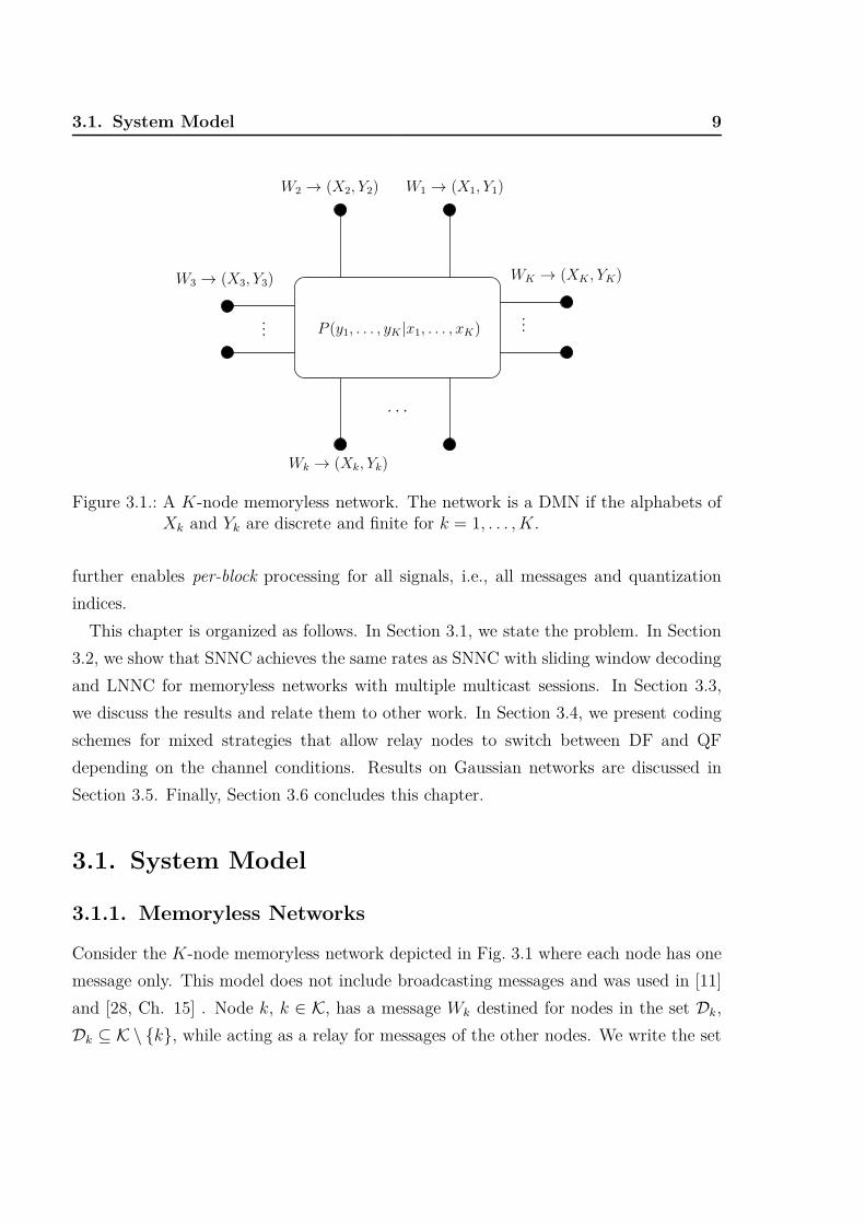
Figure 3.1.: A K-node memoryless network. The network is a DMN if the alphabets ofXk and Yk are discrete and finite for k = 1, . . . , K.
further enables per-block processing for all signals, i.e., all messages and quantization
indices.
This chapter is organized as follows. In Section 3.1, we state the problem. In Section
3.2, we show that SNNC achieves the same rates as SNNC with sliding window decoding
and LNNC for memoryless networks with multiple multicast sessions. In Section 3.3,
we discuss the results and relate them to other work. In Section 3.4, we present coding
schemes for mixed strategies that allow relay nodes to switch between DF and QF
depending on the channel conditions. Results on Gaussian networks are discussed in
Section 3.5. Finally, Section 3.6 concludes this chapter.
3.1. System Model
3.1.1. Memoryless Networks
Consider the K-node memoryless network depicted in Fig. 3.1 where each node has one
message only. This model does not include broadcasting messages and was used in [11]
and [28, Ch. 15] . Node k, k ∈ K, has a message Wk destined for nodes in the set Dk,
Dk ⊆ K \ {k}, while acting as a relay for messages of the other nodes. We write the set

10 Chapter 3. Short message noisy network coding
of nodes whose signals node k must decode correctly as Dk = {i ∈ K : k ∈ Di}. The
messages are mutually statistically independent and Wk is uniformly distributed over
the set {1, . . . , 2nRk}, where 2nRk is taken to be a non-negative integer.
The channel is described by the conditional probabilities
P (yK|xK) = P (y1, . . . , yK |x1, . . . , xK) (3.1)
where Xk and Yk, k ∈ K, are the respective input and output alphabets, i.e., we have
(x1, . . . , xK) ∈ X1 × · · · × XK
(y1, . . . , yK) ∈ Y1 × · · · × YK .
If all alphabets are discrete and finite sets, then the network is called a discrete memory-
less network (DMN) [29], [30, Ch.18]. Node k transmits xki ∈ Xk at time i and receives
yki ∈ Yk. The channel is memoryless and time invariant in the sense that
P (y1i, . . . , yKi|w1, . . . , wK , xi1, . . . , xi
K , yi−11 , . . . , yi−1
K )
= PY K |XK (y1i, . . . , yKi|x1i, . . . , xKi) (3.2)
for all i. As usual, we develop our random coding for DMNs and later extend the results
to Gaussian channels.
3.1.2. Flooding
We can represent the DMN as a directed graph G = {K, E}, where E ⊂ K × K is a set
of edges. Edges are denoted as (i, j) ∈ E , i, j ∈ K, i 6= j. We label edge (i, j) with the
non-negative real number
Cij = maxxK\i
maxPXi
I(Xi; Yj|XK\i = xK\i) (3.3)
called the capacity of the link, where I(A; B|C = c) is the mutual information between
the random variables A and B conditioned on the event C = c. Let Path(i,j) be a path
that starts from node i and ends at node j. Let Γ(i,j) to be the set of such paths. We
3.1. System Model 11
1 2 3 4C32C21 C43
C34C12 C23
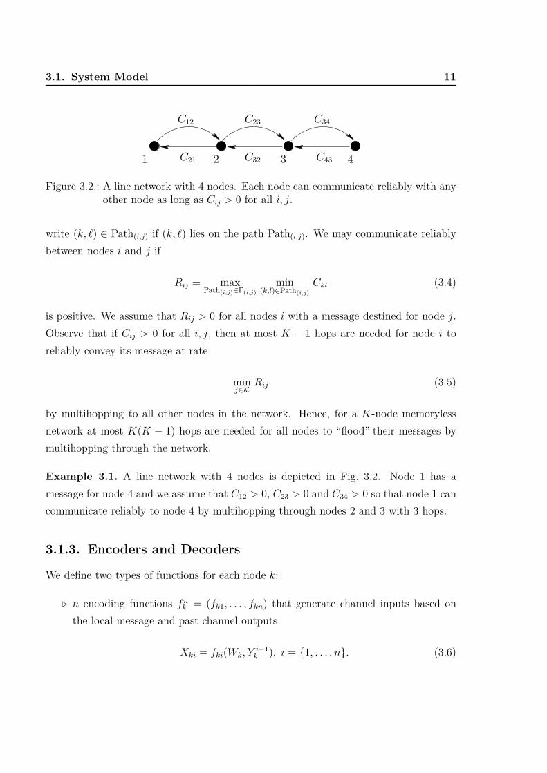
Figure 3.2.: A line network with 4 nodes. Each node can communicate reliably with anyother node as long as Cij > 0 for all i, j.
write (k, ℓ) ∈ Path(i,j) if (k, ℓ) lies on the path Path(i,j). We may communicate reliably
between nodes i and j if
Rij = maxPath(i,j)∈Γ(i,j)
min(k,l)∈Path(i,j)
Ckl (3.4)
is positive. We assume that Rij > 0 for all nodes i with a message destined for node j.
Observe that if Cij > 0 for all i, j, then at most K − 1 hops are needed for node i to
reliably convey its message at rate
minj∈K
Rij (3.5)
by multihopping to all other nodes in the network. Hence, for a K-node memoryless
network at most K(K − 1) hops are needed for all nodes to “flood” their messages by
multihopping through the network.
Example 3.1. A line network with 4 nodes is depicted in Fig. 3.2. Node 1 has a
message for node 4 and we assume that C12 > 0, C23 > 0 and C34 > 0 so that node 1 can
communicate reliably to node 4 by multihopping through nodes 2 and 3 with 3 hops.
3.1.3. Encoders and Decoders
We define two types of functions for each node k:
⊲ n encoding functions fnk = (fk1, . . . , fkn) that generate channel inputs based on
the local message and past channel outputs
Xki = fki(Wk, Y i−1k ), i = {1, . . . , n}. (3.6)

12 Chapter 3. Short message noisy network coding
⊲ One decoding function
gk(Y nk , Wk) = [W
(k)i , i ∈ Dk] (3.7)
where W(k)i is the estimate of Wi at node k.
The average error probability for the network is defined as
P (n)e = Pr
⋃
k∈K
⋃
i∈Dk
{W(k)i 6= Wi}
. (3.8)
A rate tuple (R1, . . . , RK) is achievable for the DMN if for any ξ > 0, there is a sufficiently
large integer n and some functions {fnk }K
k=1 and {gk}Kk=1 such that P (n)
e ≤ ξ. The capacity
region is the closure of the set of achievable rate tuples. For each node k we define
Kk = {k} ∪ Dk ∪ Tk, Tk ⊆ Dck \ {k} (3.9)
where Tk has the nodes whose messages node k is not interested in but whose symbol
sequences are included in the typicality test in order to remove interference. We further
define, for any S ⊂ L ⊆ K, the quantities
ILS (k) = I(XS ; YScYk|XSc) − I(YS ; YS|XLYScYk) (3.10)
ILS (k|T ) = I(XS ; YScYk|XScT ) − I(YS ; YS|XLYScYkT ) (3.11)
where Sc in (3.10) and (3.11) is the complement of S in L. We write RS =∑
k∈S Rk.
3.2. Main Result and Proof
The following theorem is the main result of this chapter.
Theorem 3.1. For a K-node memoryless network with one multicast session per node,
SNNC with backward decoding achieves the same rate tuples (R1, . . . , RK) as SNNC
with sliding window decoding [5, 6] and LNNC with joint decoding [10, 11]. These are

3.2. Main Result and Proof 13
the rate tuples satisfying
0 ≤ RS < IKk
S (k|T ) (3.12)
for all k ∈ K, all subsets S ⊂ Kk with k ∈ Sc and S∩Dk 6= ∅, where Sc is the complement
of S in Kk, and for joint distributions that factor as
P (t)
[K∏
k=1
P (xk|t)P (yk|yk, xk, t)
]P (yK|xK). (3.13)
Remark 3.1. The set Kk (see (3.9)) represents the set of nodes whose messages are
known or decoded at node k. In other words, from node k’s perspective the network has
nodes Kk only.
Example 3.2. If D = D1 = · · · = DK , then the bound (3.12) is taken for all k ∈ K and
all subsets S ⊂ Kk with k ∈ Sc and S ∩ D 6= ∅, where Sc is the complement of S in Kk.
Example 3.3. Consider K = {1, 2, 3, 4} and suppose node 1 has a message destined for
node 3, and node 2 has a message destined for node 4. We then have D3 = {1} and
D4 = {2}. If nodes 3 and 4 choose T3 = {2} and T4 = {∅} respectively, then we have
K3 = {1, 2, 3} and K4 = {2, 4}. In this case the rate bounds (3.12) are:
Node 3:
R1 < I(X1; Y2Y3Y3|X2X3T ) (3.14)
R1 + R2 < I(X1X2; Y3Y3|X3T ) − I(Y1Y2; Y1Y2|X1X2X3Y3Y3T ) (3.15)
Node 4:
R2 < I(X2; Y4Y4|X4T ) − I(Y2; Y2|X2X4Y4Y4T ) (3.16)
3.2.1. Encoding
To prove Theorem 3.1, we choose Kk = K for all k for simplicity. We later discuss the
case where these sets are different. For clarity, we set the time-sharing random variable T

14 Chapter 3. Short message noisy network coding
Block 1 · · · B B + 1 · · · B + K · (K − 1)X1 x11(w11, 1) · · · x1B(w1B, l1(B−1))
Y1 y11(l11|w11, 1) · · · y1B(l1B|w1B, l1(B−1)) Multihop K messages...
......
... to K − 1 nodesXK xK1(wK1, 1) · · · xKB(wKB, lK(B−1)) in K · (K − 1) · n′ channel uses
YK yK1(lK1|wK1, 1) yKB(lKB|wKB, lK(B−1))
Table 3.1.: SNNC for one multicast session per node.
to be a constant. Table 3.1 shows the SNNC encoding process. We redefine Rk to be the
rate of the short messages in relation to the (redefined) block length n. In other words,
the message wk, k ∈ K, of nBRk bits is split into B equally sized blocks, wk1, . . . , wkB,
each of nRk bits. Communication takes place over B + K · (K − 1) blocks and the true
rate of wk will be
Rk,true =nBRk
nB + [K · (K − 1) · n′](3.17)
where n′ is defined in (3.20) below.
Random Code: Fix a distribution∏K
k=1 P (xk)P (yk|yk, xk). For each block j = 1, . . . , B
and node k ∈ K, generate 2n(Rk+Rk) code words xkj(wkj, lk(j−1)), wkj = 1, . . . , 2nRk, lk(j−1) =
1, . . . , 2nRk , according to∏n
i=1 PXk(x(kj)i) where lk0 = 1 by convention. For each wkj and
lk(j−1), generate 2nRk reconstructions ykj(lkj|wkj, lk(j−1)), lkj = 1, . . . , 2nRk , according to∏n
i=1 PYk|Xk(y(kj)i|x(kj)i(wkj, lk(j−1))). This defines the codebooks
Ckj = {xkj(wkj, lk(j−1)), ykj(lkj|wkj, lk(j−1)),
wkj = 1, . . . , 2nRk , lk(j−1) = 1, . . . , 2nRk , lkj = 1, . . . , 2nRk} (3.18)
for j = 1, . . . , B and k ∈ K.
The codebooks used in the last K(K − 1) blocks with j > B are different. The blocks
j = B + (k − 1) · (K − 1) + 1, . . . , B + k · (K − 1) (3.19)
are dedicated to flooding lkB through the network, and for all nodes k ∈ K we gen-
erate 2n′Rk independent and identically distributed (i.i.d.) code words xkj(lkB), lkB =

3.2. Main Result and Proof 15
1, . . . , 2n′Rk , according to∏n′
i=1 PXk(x(kj)i). We choose
n′ = maxk
nRk
mink∈K
Rkk
(3.20)
that is independent of k and B. The overall rate of user k is thus given by (3.17) which
approaches Rk as B → ∞.
Encoding: Each node k upon receiving ykj at the end of block j, j ≤ B, tries to find
an index lkj such that the following event occurs:
E0(kj)(lkj) :(ykj(lkj|wkj, lk(j−1)), xkj(wkj, lk(j−1)), ykj
)∈ T n
ǫ
(PYkXkYk
)(3.21)
If there is no such index lkj, set lkj = 1. If there is more than one, choose one. Each
node k transmits xkj(wkj, lk(j−1)) in block j = 1, . . . , B.
In the K − 1 blocks (3.19), node k conveys lkB reliably to all other nodes by multi-
hopping xkj(lkB) through the network with blocks of length n′.
3.2.2. Backward Decoding
Let ǫ1 > ǫ. At the end of block B + K · (K − 1) every node k ∈ K has reliably recovered
lB = (l1B, . . . , lKB) via the multihopping of the last K(K − 1) blocks.
For block j = B, . . . , 1, node k tries to find tuples w(k)j = (w
(k)1j , . . . , w
(k)Kj) and l(k)
j−1 =
(l(k)1(j−1), . . . , l
(k)K(j−1)) such that the following event occurs:
E1(kj)(w(k)j ,l(k)
j−1, lj) :(x1j(w
(k)1j , l
(k)1(j−1)), . . . , xKj(w
(k)Kj, l
(k)K(j−1)),
y1j(l1j|w(k)1j , l
(k)1(j−1)), . . . , yKj(lKj|w(k)
Kj, l(k)K(j−1)), ykj
)∈ T n
ǫ1
(PXKYKYk
)(3.22)
where lj = (l1j , . . . , lKj) has already been reliably recovered from the previous block
j + 1.
Error Probability: Let 1 = (1, . . . , 1) and assume without loss of generality that wj = 1
and lj−1 = 1. In each block j, the error events at node k are:
E(kj)0 : ∩lkjEc
0(kj)(lkj) (3.23)
16 Chapter 3. Short message noisy network coding
E(kj)1 : Ec1(kj)(1, 1, 1) (3.24)
E(kj)2 : ∪(wj ,lj−1)6=(1,1) E1(kj)(wj , lj−1, 1) (3.25)
The error event Ekj = ∪2i=0E(kj)i at node k in block j thus satisfies
Pr[Ekj
]≤
2∑
i=0
Pr[E(kj)i] (3.26)
where we have used the union bound. Pr[E(kj)0
]can be made small with large n, as
long as (see [20])
Rk > I(Yk; Yk|Xk) + δǫ(n) (3.27)
where δǫ(n) → 0 as n → ∞. Similarly, Pr[E(kj)1
]can be made small with large n.
To bound Pr[E(kj)2
], for each wj and lj−1 we define
M(wj) = {i ∈ K : wij 6= 1} (3.28)
Q(lj−1) = {i ∈ K : li(j−1) 6= 1} (3.29)
S(wj , lj−1) = M(wj) ∪ Q(lj−1) (3.30)
and write S = S(wj , lj−1). The important observations are:
⊲ (XS , YS) is independent of (XSc, YSc, Ykj) in the random coding experiment;
⊲ The (Xi, Yi), i ∈ S, are mutually independent.
For k ∈ Sc and (wj, lj−1) 6= (1, 1), we thus have
Pr[E1(kj)(wj , lj−1, lj)
]≤ 2−n(IS−δǫ1(n)) (3.31)
where δǫ1(n) → 0 as n → ∞ and
IS =
[∑
i∈S
H(XiYi)
]+ H(XScYScYk) − H(XSYSXScYScYk)
= I(XS ; YScYk|XSc) +
[∑
i∈S
H(Yi|Xi)
]− H(YS|XKYScYk). (3.32)

3.2. Main Result and Proof 17
By the union bound, we have
Pr[E(kj)2
]≤
∑
(wj ,lj−1)6=(1,1)
Pr[E1(kj)(wj, lj−1, 1)
]
(a)
≤∑
(wj ,lj−1)6=(1,1)
2−n(IS(wj,lj−1)−δǫ1 (n))
(b)=
∑
S:k∈Sc
S6=∅
∑
(wj ,lj−1):
S(wj ,lj−1)=S
2−n(IS−δǫ1 (n))
(c)=
∑
S:k∈Sc
S6=∅
∑
M⊆S,Q⊆SM∪Q=S
∏
i∈M
(2nRi − 1)∏
i∈Q
(2nRi − 1)
· 2−n(IS−δǫ1 (n))
<∑
S:k∈Sc
S6=∅
∑
M⊆S,Q⊆SM∪Q=S
2nRM2nRQ2−n(IS−δǫ1 (n))
(d)
≤∑
S:k∈Sc
S6=∅
3|S|2n(RS+RS−(IS−δǫ1 (n)))
=∑
S:k∈Sc
S6=∅
2n
[RS−(IS−RS−
|S| log2 3n
−δǫ1 (n))
]
(3.33)
where
(a) follows from (3.31)
(b) follows by collecting the (wj , lj−1) 6= (1, 1) into classes where S = S(wj , lj−1)
(c) follows because there are
∏
i∈M
(2nRi − 1)∏
i∈Q
(2nRi − 1) (3.34)
different (wj , lj−1) 6= (1, 1) that result in the same M and Q such that M ⊆ S,
Q ⊆ S and S = M ∪ Q
(d) is because for every node i ∈ S, we must have one of the following three cases occur:
1) i ∈ M and i /∈ Q2) i /∈ M and i ∈ Q3) i ∈ M and i ∈ Q

18 Chapter 3. Short message noisy network coding
so there are 3|S| different ways of choosing M and Q.
Since we require Rk ≥ I(Yk; Yk|Xk) + δǫ(n), we have
IS − RS ≤ IS −∑
i∈S
I(Yi; Yi|Xi) − δǫ(n)
= IKS (k) − δǫ(n). (3.35)
Combining (3.26), (3.27), (3.33) and (3.35) we find that we can make Pr[Ekj
]→ 0 as
n → ∞ if
0 ≤ RS < IKS (k) (3.36)
for all subsets S ⊂ K such that k ∈ Sc and S 6= ∅. Of course, if IKS (k) ≤ 0, then we
require that RS = 0.
We can split the bounds in (3.36) into two classes:
Class 1 : S ∩ Dk 6= ∅ (3.37)
Class 2 : S ∩ Dk = ∅ or equivalently S ⊆ Dck (3.38)
LNNC requires only the Class 1 bounds. SNNC requires both the Class 1 and Class 2
bounds to guarantee reliable decoding of the quantization indices lj−1 for each backward
decoding step. With the same argument as in [5, Sec. IV-C], we can show that the Class
2 bounds can be ignored when determining the best SNNC rates. For completeness, the
proof is given in Appendix A.1. SNNC with backward decoding thus performs as well
as SNNC with sliding window decoding and LNNC with joint decoding. Adding a time-
sharing random variable T completes the proof of Theorem 3.1 for Kk = K for all k.
The proof with general Kk follows by having each node k treat the signals of nodes in
K \ Kk as noise
3.3. Discussion 19
3.3. Discussion
3.3.1. Decoding Subsets of Messages
From Theorem 3.1 we know that if node k decodes messages from nodes in Kk and some
of the Class 2 constraints in (3.38) are violated, then we should treat the signals from
the corresponding nodes as noise. In this way, we eventually wind up with some
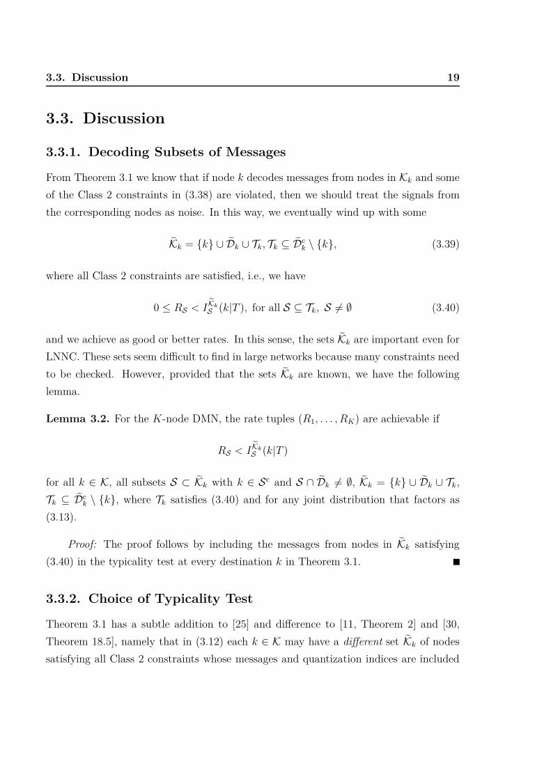
Kk = {k} ∪ Dk ∪ Tk, Tk ⊆ Dck \ {k}, (3.39)
where all Class 2 constraints are satisfied, i.e., we have
0 ≤ RS < IKk
S (k|T ), for all S ⊆ Tk, S 6= ∅ (3.40)
and we achieve as good or better rates. In this sense, the sets Kk are important even for
LNNC. These sets seem difficult to find in large networks because many constraints need
to be checked. However, provided that the sets Kk are known, we have the following
lemma.
Lemma 3.2. For the K-node DMN, the rate tuples (R1, . . . , RK) are achievable if
RS < IKk
S (k|T )
for all k ∈ K, all subsets S ⊂ Kk with k ∈ Sc and S ∩ Dk 6= ∅, Kk = {k} ∪ Dk ∪ Tk,
Tk ⊆ Dck \ {k}, where Tk satisfies (3.40) and for any joint distribution that factors as
(3.13).
Proof: The proof follows by including the messages from nodes in Kk satisfying
(3.40) in the typicality test at every destination k in Theorem 3.1.
3.3.2. Choice of Typicality Test
Theorem 3.1 has a subtle addition to [25] and difference to [11, Theorem 2] and [30,
Theorem 18.5], namely that in (3.12) each k ∈ K may have a different set Kk of nodes
satisfying all Class 2 constraints whose messages and quantization indices are included
20 Chapter 3. Short message noisy network coding
1
2
3
(a) Both nodes 1 and 2are sources and relays
1
2
3
(b) Node 2 acts as a re-lay for node 1
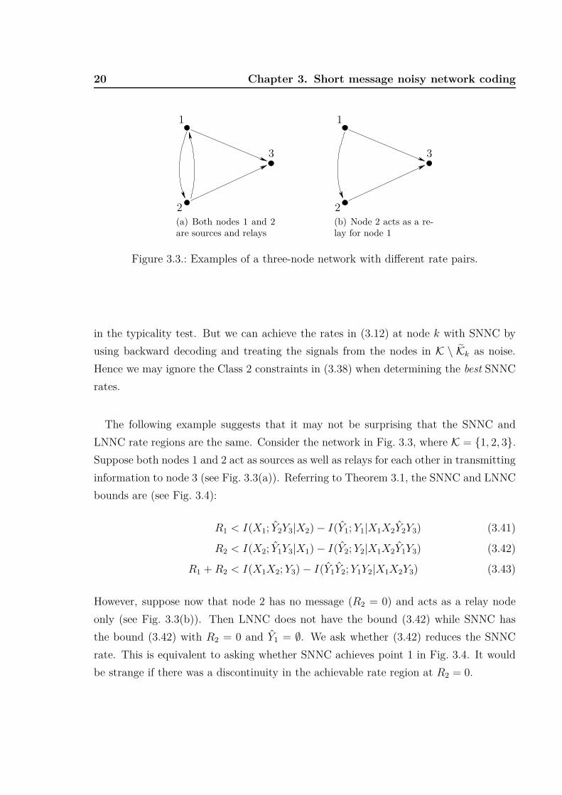
Figure 3.3.: Examples of a three-node network with different rate pairs.
in the typicality test. But we can achieve the rates in (3.12) at node k with SNNC by
using backward decoding and treating the signals from the nodes in K \ Kk as noise.
Hence we may ignore the Class 2 constraints in (3.38) when determining the best SNNC
rates.
The following example suggests that it may not be surprising that the SNNC and
LNNC rate regions are the same. Consider the network in Fig. 3.3, where K = {1, 2, 3}.
Suppose both nodes 1 and 2 act as sources as well as relays for each other in transmitting
information to node 3 (see Fig. 3.3(a)). Referring to Theorem 3.1, the SNNC and LNNC
bounds are (see Fig. 3.4):
R1 < I(X1; Y2Y3|X2) − I(Y1; Y1|X1X2Y2Y3) (3.41)
R2 < I(X2; Y1Y3|X1) − I(Y2; Y2|X1X2Y1Y3) (3.42)
R1 + R2 < I(X1X2; Y3) − I(Y1Y2; Y1Y2|X1X2Y3) (3.43)
However, suppose now that node 2 has no message (R2 = 0) and acts as a relay node
only (see Fig. 3.3(b)). Then LNNC does not have the bound (3.42) while SNNC has
the bound (3.42) with R2 = 0 and Y1 = ∅. We ask whether (3.42) reduces the SNNC
rate. This is equivalent to asking whether SNNC achieves point 1 in Fig. 3.4. It would
be strange if there was a discontinuity in the achievable rate region at R2 = 0.

3.3. Discussion 21
R1
R2
Point 1
Point 2
Figure 3.4.: Illustration of the achievable rates for the network of Fig. 3.3(b).
3.3.3. Optimal Decodable Sets
SNNC was studied for relay networks in [7]. For such networks there is one message
at node 1 that is destined for node K. We thus have DK = {1} and DcK \ {K} =
{2, . . . , K − 1}. The authors of [7] showed that for a given random coding distribution
P (t)P (x1|t)∏
k∈DcK
P (xk|t)P (yk|yk, xk, t) (3.44)
there exists a unique largest optimal decodable set T ∗, T ∗ ⊆ DcK \{K}, of the relay nodes
that provides the same best achievable rates for both SNNC and LNNC [7, Theorem 2.8].
We now show that the concept of optimal decodable set extends naturally to multi-source
networks.
Lemma 3.3. For a K-node memoryless network with a fixed random coding distribution
P (t)K∏
k=1
P (xk|t)P (yk|yk, xk, t) (3.45)
there exists for each node k a unique largest set T ∗k among all subsets Tk ⊆ Dc
k \ {k}satisfying (3.40). The messages of the nodes in T ∗
k should be included in the typicality
test to provide the best achievable rates.
Proof: We prove Lemma 3.3 without a time-sharing random variable T . The proof
with T is similar. We show that T ∗k is unique by showing that the union of any two sets
T 1k and T 2
k satisfying all constraints also satisfies all constraints and provides as good or
22 Chapter 3. Short message noisy network coding
better rates. Continuing taking the union, we eventually reach a unique largest set T ∗k
that satisfies all constraints and gives the best rates.
Partition the subsets Tk ⊆ Dck \ {k} into two classes:
Class 1: RS < IKk
S (k) for all S ⊆ Tk;
Class 2: There exists one S ⊆ Tk such that RS ≥ IKk
S (k).
We may ignore the Tk in Class 2 because the proof of Theorem 3.1 shows that we can
treat the signals of nodes associated with violated constraints as noise and achieve as
good or better rates. Hence, we focus on Tk in Class 1.
Suppose T 1k and T 2
k are in Class 1 and let T 3k = T 1
k ∪ T 2k . We define
K1k = {k} ∪ Dk ∪ T 1
k (3.46)
K2k = {k} ∪ Dk ∪ T 2
k (3.47)
K3k = {k} ∪ Dk ∪ T 3
k . (3.48)
Further, for every S ⊆ K3k, define S1 = S ∩K1
k and S2 = S ∩(K3k \S1). We have S1 ⊆ K1
k,
S2 ⊆ K2k, S1 ∪ S2 = S and S1 ∩ S2 = ∅. We further have
RS(a)= RS1 + RS2
(b)< I
K1k
S1(k) + I
K2k
S2(k)
(c)= I(XS1; Y
K1k
\S1Yk|X
K1k\S1
) − I(YS1; YS1|XK1k
YK1
k\S1
Yk)
+ I(XS2; YK2
k\S2
Yk|XK2
k\S2
) − I(YS2; YS2|XK2k
YK2
k\S2
Yk)
(d)
≤ I(XS1; YK3
k\S
Yk|XK3
k\S
) − I(YS1; YS1|XK1k
YK1
k\S1
Yk)
+ I(XS2; YK3
k\S
Yk|XK3
k\S2
) − I(YS2; YS2|XK2k
YK2
k\S2
Yk)
(e)
≤ I(XS1 ; YK3
k\S
Yk|XK3
k\S
) − I(YS1; YS1|XK3k
YK3
k\S
Yk)
+ I(XS2; YK3
k\S
Yk|XK3
k\S2
) − I(YS2; YS2|XK3k
YK3
k\S2
Yk)
(f)= I(XS ; Y
K3k\S
Yk|XK3
k\S
) − I(YS ; YS|XK3
k
YK3
k\S
Yk)
(g)= I
K3k
S (k) (3.49)

3.3. Discussion 23
where
(a) follows from the definition of S1 and S2
(b) follows because both T 1k and T 2
k are in Class 1
(c) follows from the definition (3.10)
(d) follows because all Xk are independent and conditioning does not increase entropy
(e) follows because conditioning does not increase entropy and by the Markov chains
XK3
k\S1
YK3
k\S
Yk − YS1XS1 − YS1 (3.50)
XK3
k\S2
YK3
k\S2
Yk − YS2XS2 − YS2 (3.51)
(f) follows from the chain rule for mutual information and the Markov chains (3.50)
and (3.51)
(g) follows from the definition (3.10).
The bound (3.49) shows that T 3k is also in Class 1. Moreover, by (3.49) if k includes the
messages of nodes in K3k in the typicality test, then the rates are as good or better than
those achieved by including the messages of nodes in K1k or K2
k in the typicality test.
Taking the union of all Tk in Class 1, we obtain the unique largest set T ∗k that gives the
best achievable rates.
Remark 3.2. There are currently no efficient algorithms for finding an optimal decod-
able set. Such algorithms would be useful for applications with time-varying channels.
3.3.4. Related Work
Sliding Window Decoding
SNNC with sliding window decoding was studied in [5, 6] and LNNC [11] and achieves
the same rates as in [5]. SNNC has extra constraints that turn out to be redundant [5,
Sec. IV-C], [6, Sec. V-B]. The sliding window decoding in [5] resembles that in [31]

24 Chapter 3. Short message noisy network coding
where encoding is delayed (or offset) and different decoders are chosen depending on
the rate point. The rates achieved by one decoder may not give the entire rate region
of Theorem 3.1, but the union of achievable rates of all decoders does [6, Theorem 1].
The advantage of sliding window decoding is a small decoding delay of K + 1 blocks as
compared to backward decoding that requires B + K(K − 1) blocks, where B ≫ K.
Backward Decoding
SNNC with backward decoding was studied in [7] for single source networks. For these
networks, [7] showed that LNNC and SNNC achieve the same rates. Further, for a
fixed random coding distribution there is a subset of the relay nodes whose messages
should be decoded to achieve the best LNNC and SNNC rates. Several other interesting
properties of the coding scheme were derived. It was also shown in [27] that SNNC
with a layered network analysis [15] achieves the same LNNC rates for single source
networks. In [32], SNNC with partial cooperation between the sources was considered
for multi-source networks.
Joint Decoding
It turns out that SNNC with joint decoding achieves the same rates as in Theorem 3.1.
Recently, the authors of [26] showed that SNNC with joint decoding fails to achieve
the LNNC rates for a specific choice of SNNC protocol. However, by multihopping the
last quantization indices and then performing joint decoding with the messages and
remaining quantization bits, SNNC with joint decoding performs as well as SNNC with
sliding window or backward decoding, and LNNC. This makes sense, since joint decoding
should perform at least as well as backward decoding. Details are given in Appendix A.2.
Multihopping
We compare how the approaches of Theorem 3.1 and [7, Theorem 2.5] reliably convey
the last quantization indices lB. Theorem 3.1 uses multihopping while Theorem 2.5 in [7]
uses a QF-style method with M extra blocks after block B with the same block length
n. In these M blocks every node transmits as before except that the messages are set
to a default value. The initialization method in [7] has two disadvantages:

3.4. SNNC with a DF option 25
⊲ Both B and M must go to infinity to reliably decode lB [7, Sec.IV-A, Equ. (34)].
The true rate of node k’s message wk is
R′k,true =
nBRk
nB + nM=
B
B + M· Rk (3.52)
and we choose B ≫ M so that R′k,true → Rk as B → ∞.
⊲ Joint rather than per-block processing is used.
Multihopping seems to be a better choice for reliably communicating lB, because the
QF-style approach has a large decoding delay due to the large value of M and does not
use per-block processing.
3.4. SNNC with a DF option
One of the main advantages of SNNC is that the relays can switch between QF (or CF)
and DF depending on the channel conditions. If the channel conditions happen to be
good, then the natural choice is DF which removes the noise at the relays. This not
possible with LNNC due to the high rate of the long message. On the other hand, if a
relay happens to experience a deep fade, then this relay should use QF (or CF).
In the following, we show how mixed strategies called SNNC-DF work for the multiple-
relay channel. These mixed strategies are similar to those in [23, Theorem 4]. However,
in [23] the relays use CF with a prescribed binning rate to enable step-by-step decoding
(CF-S) instead of QF. In Section 3.5 we give numerical examples to show that SNNC-DF
can outperform DF, CF-S and LNNC.
As in [23], we partition the relays T = {2, . . . , K − 1} into two sets
T1 = {k : 2 ≤ k ≤ K1}T2 = T \ T1
where 1 ≤ K1 ≤ K − 1. The relays in T1 use DF while the relays in T2 use QF. Let
π(·) be a permutation on {1, . . . , K} with π(1) = 1 and π(K) = K and let π(j : k) =
{π(j), π(j + 1), . . . , π(k)}, 1 ≤ j ≤ k ≤ K. Define Ti(π) = {π(k), k ∈ Ti}, i = 1, 2. We

26 Chapter 3. Short message noisy network coding
have the following theorem.
Theorem 3.4. SNNC-DF achieves the rates satisfying
RSNNC-DF < maxπ(·)
maxK1
min{
min1≤k≤K1−1
I(Xπ(1:k); Yπ(k+1)|Xπ(k+1:K1)
),
I(X1XT1(π)XS ; YScYK|XSc) − I(YS ; YS|X1XT YScYK)
}(3.53)
for all S ⊆ T2(π), where Sc is the complement of S in T2(π), and where the joint distri-
bution factors as
P (x1xT1(π))·[
∏
k∈T2(π)
P (xk)P (yk|yk, xk)
]· P (y2, . . . , yK |x1, . . . , xK−1). (3.54)
Remark 3.3. As usual, we may add a time-sharing random variable to improve rates.
Proof Sketch: For a given permutation π(·) and K1, the first mutual information
term in (3.53) describes the DF bounds [23, Theorem 1] (see also [33, Theorem 3.1]). The
second mutual information term in (3.53) describes the SNNC bounds. Using a similar
analysis as for Theorem 3.1 and by treating (X1XT1(π)) as the “new” source signal at the
destination, we have the SNNC bounds
RSNNC-DF < I(X1XT1(π)XS ; YScYK |XSc) − I(YS ; YS|X1XT YScYK) (3.55)
0 ≤ I(XS ; YScYK |X1XT1(π)XSc) − I(YS ; YS|X1XT YScYK) (3.56)
for all S ⊆ T2(π). The same argument used to prove Theorem 3.1 shows that if any of
the constraints (3.56) is violated, then we get rate bounds that can be achieved with
SNNC-DF by treating the signals from the corresponding relay nodes as noise. Thus we
may ignore the constraints (3.56).
Example 3.4. Consider K = 4 and K1 = 2. There are two possible permutations π1(1 :
4) = {1, 2, 3, 4} and π2(1 : 4) = {1, 3, 2, 4}. For π1(1 : 4) = {1, 2, 3, 4}, Theorem 3.4
states that SNNC-DF achieves any rate up to
RSNNC-DF = min
{I(X1; Y2|X2), I(X1X2; Y3Y4|X3),
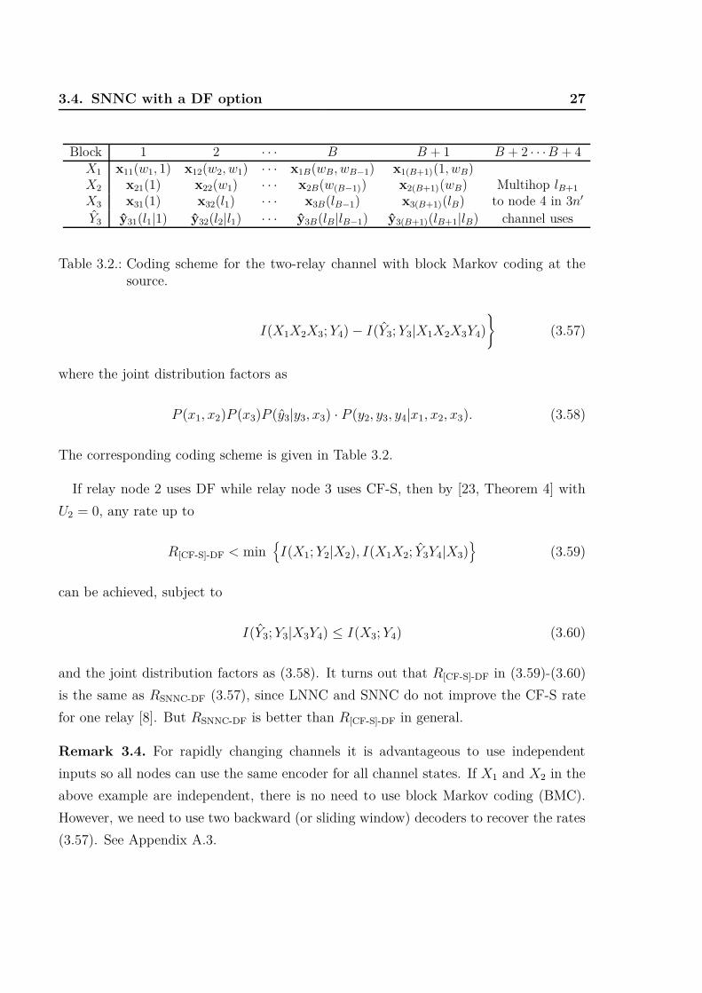
3.4. SNNC with a DF option 27
Block 1 2 · · · B B + 1 B + 2 · · · B + 4X1 x11(w1, 1) x12(w2, w1) · · · x1B(wB, wB−1) x1(B+1)(1, wB)X2 x21(1) x22(w1) · · · x2B(w(B−1)) x2(B+1)(wB) Multihop lB+1
X3 x31(1) x32(l1) · · · x3B(lB−1) x3(B+1)(lB) to node 4 in 3n′
Y3 y31(l1|1) y32(l2|l1) · · · y3B(lB|lB−1) y3(B+1)(lB+1|lB) channel uses
Table 3.2.: Coding scheme for the two-relay channel with block Markov coding at thesource.
I(X1X2X3; Y4) − I(Y3; Y3|X1X2X3Y4)
}(3.57)
where the joint distribution factors as
P (x1, x2)P (x3)P (y3|y3, x3) · P (y2, y3, y4|x1, x2, x3). (3.58)
The corresponding coding scheme is given in Table 3.2.
If relay node 2 uses DF while relay node 3 uses CF-S, then by [23, Theorem 4] with
U2 = 0, any rate up to
R[CF-S]-DF < min{I(X1; Y2|X2), I(X1X2; Y3Y4|X3)
}(3.59)
can be achieved, subject to
I(Y3; Y3|X3Y4) ≤ I(X3; Y4) (3.60)
and the joint distribution factors as (3.58). It turns out that R[CF-S]-DF in (3.59)-(3.60)
is the same as RSNNC-DF (3.57), since LNNC and SNNC do not improve the CF-S rate
for one relay [8]. But RSNNC-DF is better than R[CF-S]-DF in general.
Remark 3.4. For rapidly changing channels it is advantageous to use independent
inputs so all nodes can use the same encoder for all channel states. If X1 and X2 in the
above example are independent, there is no need to use block Markov coding (BMC).
However, we need to use two backward (or sliding window) decoders to recover the rates
(3.57). See Appendix A.3.
28 Chapter 3. Short message noisy network coding
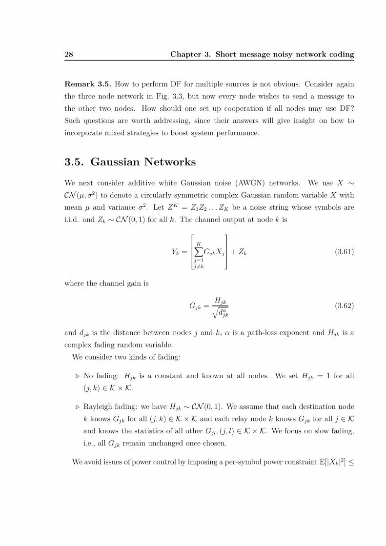
Remark 3.5. How to perform DF for multiple sources is not obvious. Consider again
the three node network in Fig. 3.3, but now every node wishes to send a message to
the other two nodes. How should one set up cooperation if all nodes may use DF?
Such questions are worth addressing, since their answers will give insight on how to
incorporate mixed strategies to boost system performance.
3.5. Gaussian Networks
We next consider additive white Gaussian noise (AWGN) networks. We use X ∼CN (µ, σ2) to denote a circularly symmetric complex Gaussian random variable X with
mean µ and variance σ2. Let ZK = Z1Z2 . . . ZK be a noise string whose symbols are
i.i.d. and Zk ∼ CN (0, 1) for all k. The channel output at node k is
Yk =
K∑
j=1j 6=k
GjkXj
+ Zk (3.61)
where the channel gain is
Gjk =Hjk√
dαjk
(3.62)
and djk is the distance between nodes j and k, α is a path-loss exponent and Hjk is a
complex fading random variable.
We consider two kinds of fading:
⊲ No fading: Hjk is a constant and known at all nodes. We set Hjk = 1 for all
(j, k) ∈ K × K.
⊲ Rayleigh fading: we have Hjk ∼ CN (0, 1). We assume that each destination node
k knows Gjk for all (j, k) ∈ K × K and each relay node k knows Gjk for all j ∈ Kand knows the statistics of all other Gjl, (j, l) ∈ K × K. We focus on slow fading,
i.e., all Gjk remain unchanged once chosen.
We avoid issues of power control by imposing a per-symbol power constraint E[|Xk|2] ≤

3.5. Gaussian Networks 29
Pk. We choose the inputs to be Gaussian, i.e., Xk ∼ CN (0, Pk), k ∈ K.
In the following we give numerical examples for four different channels
⊲ the relay channel;
⊲ the two-relay channel;
⊲ the multiple access relay channel (MARC);
⊲ the two-way relay channel (TWRC).
We evaluate performance for no fading in terms of achievable rates (in bits per channel
use) and for Rayleigh fading in terms of outage probability [34] for a target rate Rtar.
Relay node k chooses
Yk = Yk + Zk (3.63)
where Zk ∼ CN (0, σ2k). For the no fading case, relay node k numerically calculates the
optimal σ2k for CF-S and SNNC, and the optimal binning rate Rk(bin) for CF-S, in order
to maximize the rates. For DF, the source and relay nodes numerically calculate the
power allocation for superposition coding that maximizes the rates. For the Rayleigh
fading case, relay node k knows only the Gjk, j ∈ K, but it can calculate the optimal
σ2k and Rk(bin) based on the statistics of Gjl, for all (j, l) ∈ K × K so as to minimize
the outage probability. For DF, the fraction of power that the source and relay nodes
allocate for cooperation is calculated numerically based on the statistics of Gjk, for all
(j, k) ∈ K × K, to minimize the outage probability. Details of the derivations are given
in Appendix A.4.
3.5.1. Relay Channels
The Gaussian relay channel (Fig. 3.5) has
Y2 = G12X1 + Z2
Y3 = G13X1 + G23X2 + Z3 (3.64)
and source node 1 has a message destined for node 3.

30 Chapter 3. Short message noisy network coding
1
2
3
d12d23 = 1 − d12
d13 = 1
Figure 3.5.: A relay channel.
0 0.2 0.4 0.6 0.8 10
0.5
1
1.5
2
2.5
3
3.5
4
4.5
5
Source−Relay Distance d12
Rat
e R
(bi
ts/c
hann
el u
se)
SNNC−DFCut−Set Bound
DF
No Relay
CF−S LNNC (SNNC)
Figure 3.6.: Achievable rates R (in bits per channel use) for a relay channel with nofading.
No Fading
Fig. 3.5 depicts the geometry and Fig. 3.6 depicts the achievable rates as a function of
d12 for P1 = 4, P2 = 2 and α = 3. DF achieves rates close to capacity when the relay
is close to the source while CF-S dominates as the relay moves towards the destination.
For the relay channel, CF-S performs as well as SNNC (LNNC). SNNC-DF unifies the
advantages of both SNNC and DF and achieves the best rates for all relay positions.
Slow Rayleigh Fading
Fig. 3.7 depicts the outage probabilities with Rtar = 2, P1 = 2P, P2 = P , d12 = 0.3,
d23 = 0.7, d13 = 1 and α = 3.

3.5. Gaussian Networks 31
5 7 9 11 13 1510
−4
10−3
10−2
10−1
100
P in dB
Out
age
Pro
babi
lity
No Relay
CF−S
LNNC (SNNC)
DF
SNNC−DF
Cut−Set Bound
Figure 3.7.: Outage probabilities f or a relay channel with Rayleigh fading.
1
2
3
4
d12 = 0.2
d13 = 0.8
d14 = 1
d23 = 0.75
d24 = 0.8
d32 = 0.75
d34 = 0.2
Figure 3.8.: A two-relay channel.
Over the entire power range CF-S gives the worst outage probability. This is because
CF-S requires a reliable relay-destination link so that both the bin and quantization
indices can be recovered. Both DF and SNNC improve on CF-S. DF performs better
at low power while SNNC is better at high power. SNNC-DF has the relay decode if
possible and perform QF otherwise, and gains 1 dB over SNNC and DF.
32 Chapter 3. Short message noisy network coding
−5 0 5 10 150
1
2
3
4
5
6
7
8
9
P in dB
Rat
e R
(bi
ts/c
hann
el u
se)
Cut−Set Bound
SNNC−DF
DF
LNNC (SNNC)
CF−S
No Relay
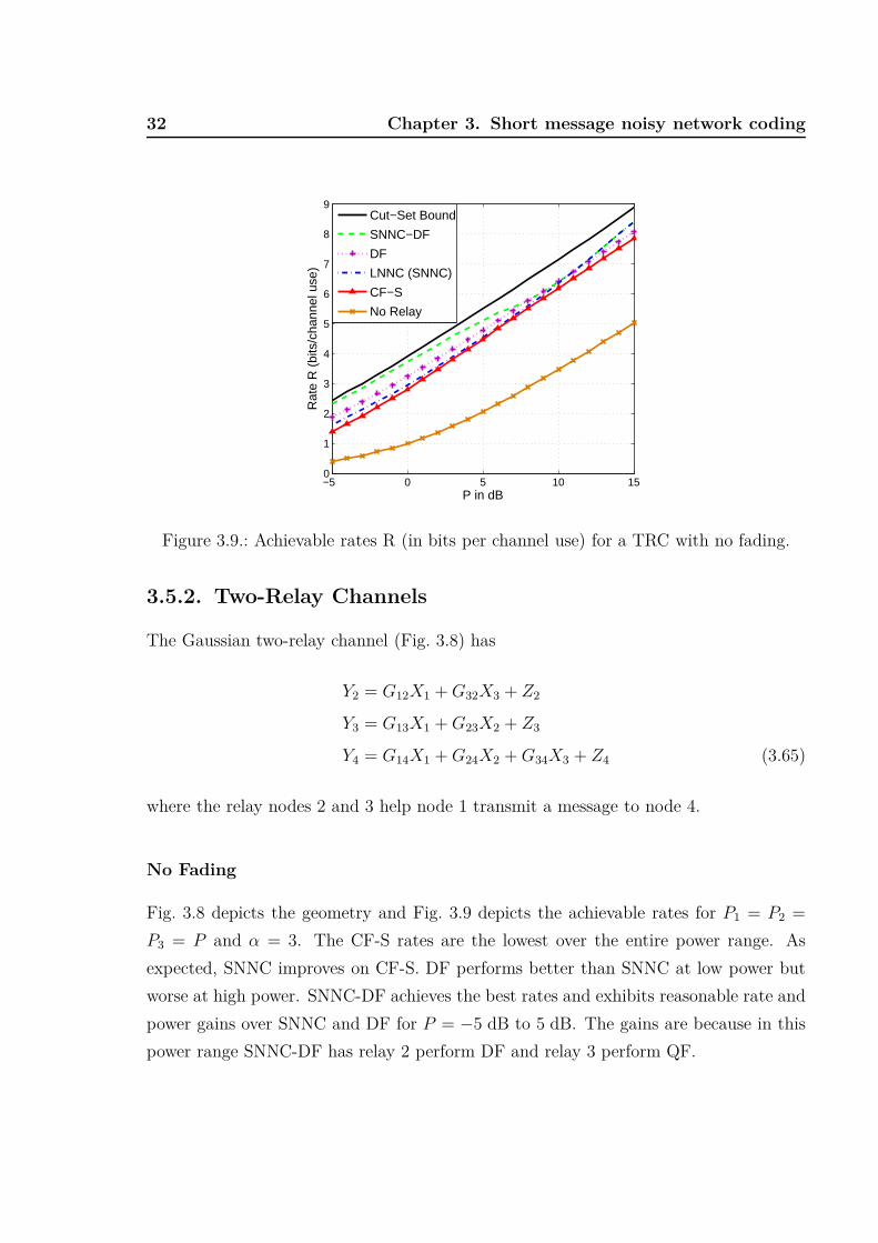
Figure 3.9.: Achievable rates R (in bits per channel use) for a TRC with no fading.
3.5.2. Two-Relay Channels
The Gaussian two-relay channel (Fig. 3.8) has
Y2 = G12X1 + G32X3 + Z2
Y3 = G13X1 + G23X2 + Z3
Y4 = G14X1 + G24X2 + G34X3 + Z4 (3.65)
where the relay nodes 2 and 3 help node 1 transmit a message to node 4.
No Fading
Fig. 3.8 depicts the geometry and Fig. 3.9 depicts the achievable rates for P1 = P2 =
P3 = P and α = 3. The CF-S rates are the lowest over the entire power range. As
expected, SNNC improves on CF-S. DF performs better than SNNC at low power but
worse at high power. SNNC-DF achieves the best rates and exhibits reasonable rate and
power gains over SNNC and DF for P = −5 dB to 5 dB. The gains are because in this
power range SNNC-DF has relay 2 perform DF and relay 3 perform QF.
3.5. Gaussian Networks 33
0 2 4 6 8 1010
−4
10−3
10−2
10−1
100
P in dB
Out
age
Pro
babi
lity
No Relay
CF−S
DF
LNNC (SNNC)
SNNC−DF
Cut−Set Bound
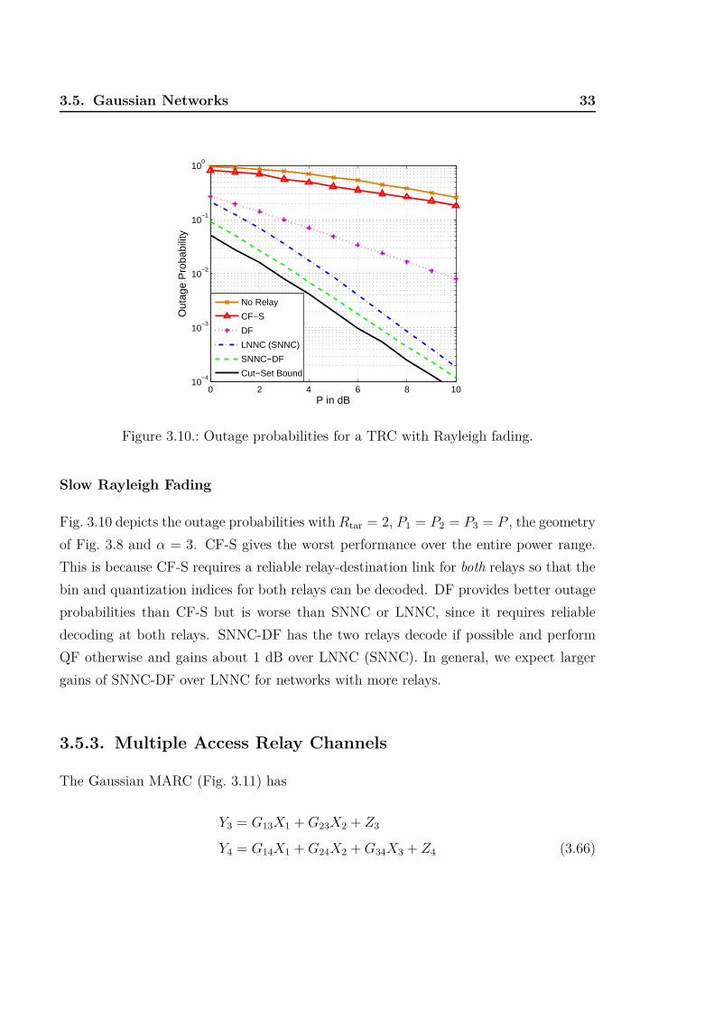
Figure 3.10.: Outage probabilities for a TRC with Rayleigh fading.
Slow Rayleigh Fading
Fig. 3.10 depicts the outage probabilities with Rtar = 2, P1 = P2 = P3 = P , the geometry
of Fig. 3.8 and α = 3. CF-S gives the worst performance over the entire power range.
This is because CF-S requires a reliable relay-destination link for both relays so that the
bin and quantization indices for both relays can be decoded. DF provides better outage
probabilities than CF-S but is worse than SNNC or LNNC, since it requires reliable
decoding at both relays. SNNC-DF has the two relays decode if possible and perform
QF otherwise and gains about 1 dB over LNNC (SNNC). In general, we expect larger
gains of SNNC-DF over LNNC for networks with more relays.
3.5.3. Multiple Access Relay Channels
The Gaussian MARC (Fig. 3.11) has
Y3 = G13X1 + G23X2 + Z3
Y4 = G14X1 + G24X2 + G34X3 + Z4 (3.66)

34 Chapter 3. Short message noisy network coding
1
2
34
d13 = 0.75
d14 = 1
d23 = 0.55
d24 = 1
d34 = 0.45
Figure 3.11.: A MARC.
and nodes 1 and 2 have messages destined for node 4.
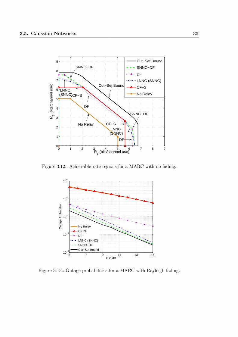
No Fading
Fig. 3.11 depicts the geometry and Fig. 3.12 depicts the achievable rate regions for
P1 = P2 = P3 = P , P = 15 dB and α = 3. The SNNC rate region includes the CF-S
rate region. Through time-sharing, the SNNC-DF region is the convex hull of the union
of DF and SNNC regions. SNNC-DF again improves on LNNC (or SNNC) and DF.
Slow Rayleigh Fading
Fig. 3.13 depicts the outage probabilities with Rtar1 = Rtar2 = 1, P1 = P2 = P3 = P ,
d13 = 0.3, d23 = 0.4, d14 = d24 = 1, d34 = 0.6 and α = 3. CF-S has the worst outage
probability because it requires a reliable relay-destination link to decode the bin and
quantization indices. DF has better outage probability than CF-S, while LNNC (or
SNNC) improves on DF over the entire power range. SNNC-DF has the relay perform
DF or QF depending on channel quality and gains 1 dB at low power and 0.5 dB at
high power over SNNC.
Remark 3.6. The gain of SNNC-DF over SNNC is not very large at high power. This is
because the MARC has one relay only. For networks with more relays we expect larger
gains from SNNC-DF.
3.5. Gaussian Networks 35
0 1 2 3 4 5 6 7 8 90
1
2
3
4
5
6
7
8
9
R1 (bits/channel use)
R2 (
bits
/cha
nnel
use
)
Cut−Set Bound
SNNC−DF
DF
LNNC (SNNC)
CF−S
No Relay
SNNC−DF
DF
No Relay
SNNC−DF
DF
CF−S
CF−S LNNC
(SNNC)
LNNC (SNNC)
Cut−Set Bound
Figure 3.12.: Achievable rate regions for a MARC with no fading.
5 7 9 11 13 1510
−4
10−3
10−2
10−1
100
P in dB
Out
age
Pro
babi
lity
No Relay
CF−S
DF
LNNC (SNNC)
SNNC−DF
Cut−Set Bound
Figure 3.13.: Outage probabilities for a MARC with Rayleigh fading.
36 Chapter 3. Short message noisy network coding
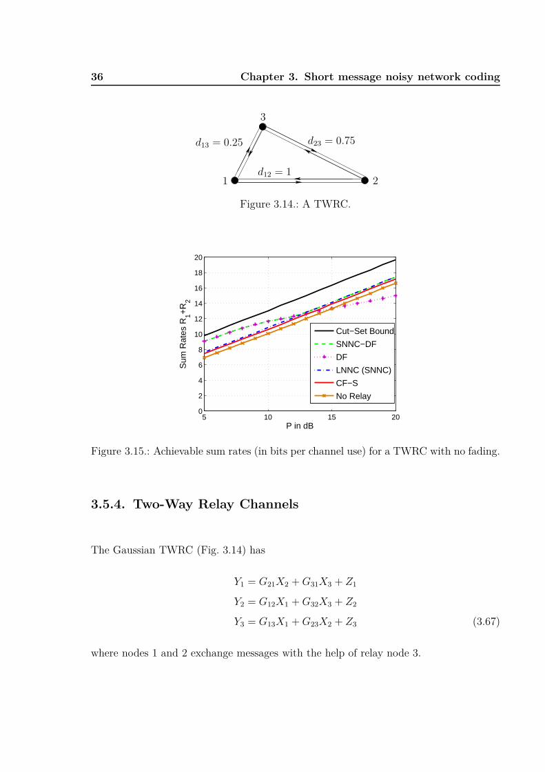
1 2
3
d12 = 1
d13 = 0.25 d23 = 0.75
Figure 3.14.: A TWRC.
5 10 15 200
2
4
6
8
10
12
14
16
18
20
P in dB
Sum
Rat
es R
1+R
2
Cut−Set Bound
SNNC−DF
DF
LNNC (SNNC)
CF−S
No Relay
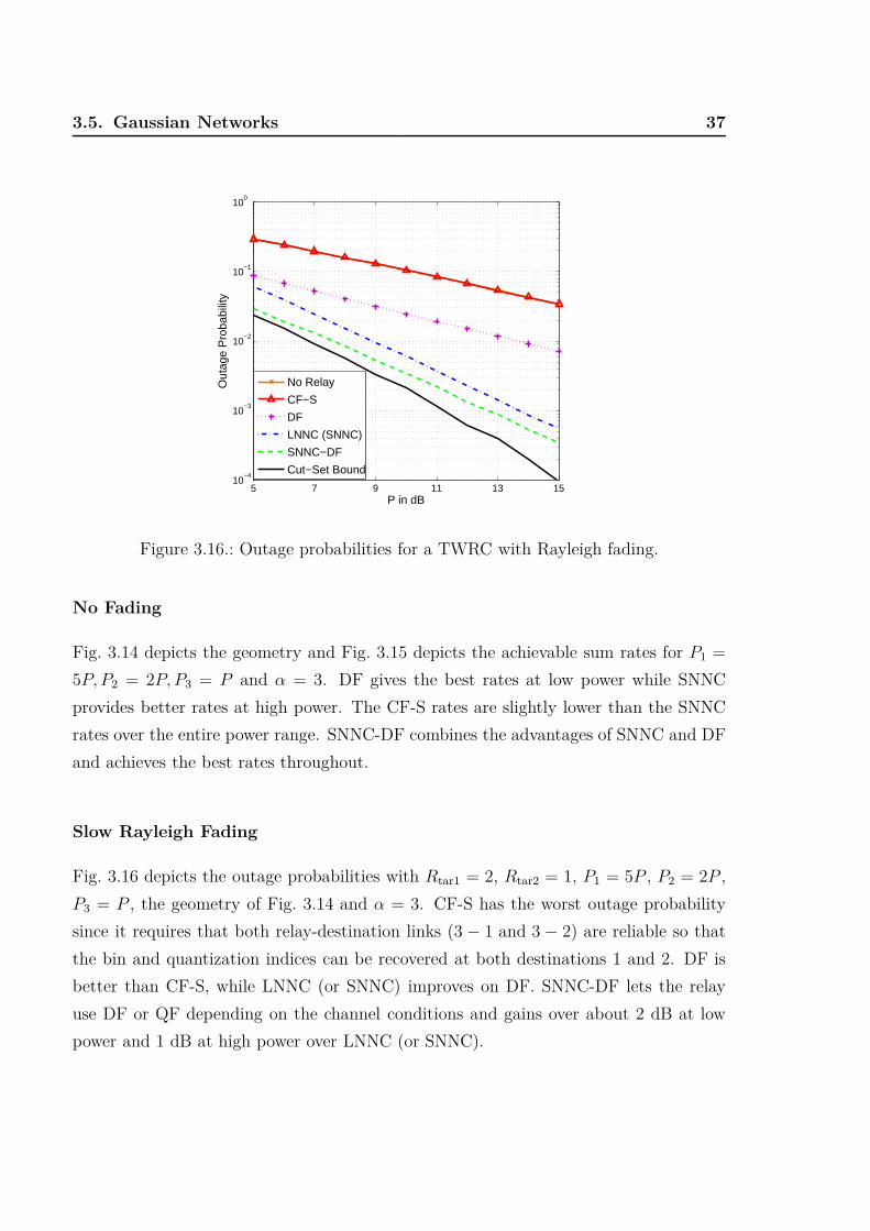
Figure 3.15.: Achievable sum rates (in bits per channel use) for a TWRC with no fading.
3.5.4. Two-Way Relay Channels
The Gaussian TWRC (Fig. 3.14) has
Y1 = G21X2 + G31X3 + Z1
Y2 = G12X1 + G32X3 + Z2
Y3 = G13X1 + G23X2 + Z3 (3.67)
where nodes 1 and 2 exchange messages with the help of relay node 3.
3.5. Gaussian Networks 37
5 7 9 11 13 1510
−4
10−3
10−2
10−1
100
P in dB
Out
age
Pro
babi
lity
No Relay
CF−S
DF
LNNC (SNNC)
SNNC−DF
Cut−Set Bound
Figure 3.16.: Outage probabilities for a TWRC with Rayleigh fading.
No Fading
Fig. 3.14 depicts the geometry and Fig. 3.15 depicts the achievable sum rates for P1 =
5P, P2 = 2P, P3 = P and α = 3. DF gives the best rates at low power while SNNC
provides better rates at high power. The CF-S rates are slightly lower than the SNNC
rates over the entire power range. SNNC-DF combines the advantages of SNNC and DF
and achieves the best rates throughout.
Slow Rayleigh Fading
Fig. 3.16 depicts the outage probabilities with Rtar1 = 2, Rtar2 = 1, P1 = 5P , P2 = 2P ,
P3 = P , the geometry of Fig. 3.14 and α = 3. CF-S has the worst outage probability
since it requires that both relay-destination links (3 − 1 and 3 − 2) are reliable so that
the bin and quantization indices can be recovered at both destinations 1 and 2. DF is
better than CF-S, while LNNC (or SNNC) improves on DF. SNNC-DF lets the relay
use DF or QF depending on the channel conditions and gains over about 2 dB at low
power and 1 dB at high power over LNNC (or SNNC).

38 Chapter 3. Short message noisy network coding
3.6. Concluding Remarks
SNNC with joint or backward decoding was shown to achieve the same rates as LNNC
for multicasting multiple messages in memoryless networks. Although SNNC has extra
constraints on the rates, these constraints give insight on the best decoding procedure.
SNNC enables early decoding at nodes, and this enables the use of SNNC-DF. Numerical
examples demonstrate that SNNC-DF shows reasonable gains as compared to DF, CF-S
and LNNC in terms of rates and outage probabilities.

4Multiple Access Relay Channel with
Relay-Source Feedback
The multiple access relay channel (MARC) [35] has multiple sources communicate with
one destination with the help of a relay node (Fig. 3.11). Results on coding strategies
for the MARC were discussed in [23, 31, 35–38]. In all previous work, the information
flow from the sources to the relay and the destination was considered. However, no
information flow in the opposite direction (feedback from the relay or the destination to
the sources) was considered. It turns out [39–41] that feedback can increase capacity of
the multiple-access channel (MAC) [2, 3].
In this chapter, we incorporate feedback from the relay (Fig. 4.1) and establish an
achievable rate region that includes the capacity region of the MARC without feedback
[35]. We use a DF coding scheme where the sources cooperate with one another and with
the relay due to the feedback. As a result, the relay can serve the sources simultaneously
rather than separately [35–37] and higher rates are achieved. We also compare these
results with the achievable SNNC rates developed in Chapter 3 with and without the

40 Chapter 4. Multiple Access Relay Channel with Relay-Source Feedback
1
2
3 4
d13
d23
d14
d24
d34
Direction of the information flow
Figure 4.1.: A two-source MARC with relay-source feedback.
relay feedback and show that cooperation improves rates, and that network geometry
influences the choice of coding strategies.
This chapter is organized as follows. In Section 4.1 we state the problem. In Section
4.2 we derive an achievable rate region for the MARC with relay-source feedback. Section
4.3 discusses Gaussian cases and shows that feedback can increase the capacity region
of the MARC.
4.1. System Model
We use the notation developed in Sec. 3.1. We study the two-user discrete memoryless
MARC with feedback (Fig. 4.1); the results extend naturally to multi-user and Gaussian
cases. The node k, k ∈ {1, 2}, has a message Wk destined for node 4. The messages
are statistically independent and Wk is uniformly distributed over 1, . . . , 2nRk , k = 1, 2,
where 2nRk is taken to be a non-negative integer. The relay node 3 assists the commu-
nication by forwarding information to node 4 and feeding back its channel outputs to
nodes 1 and 2. The channel is described by
P (y3, y4|x1, x2, x3) (4.1)

4.2. Main Result and Proof 41
and the feedback link is assumed to be noiseless.
We define the following functions:
⊲ n encoding functions fnk = (fk1, . . . , fkn), k = 1, 2, 3, that generate channel inputs
based on the local messages and past relay channel outputs
Xki = fki(Wk, Y i−13 ), i = {1, . . . , n} (4.2)
where W3 = ∅.
⊲ One decoding function that puts out estimates of the messages
g4(Yn
4 ) = [W1, W2]. (4.3)
The average error probability is
P (n)e = Pr
[(W1, W2) 6= (W1, W2)
]. (4.4)
The rate pair (R1, R2) is said to be achievable for the MARC with feedback if for any
ξ there is a sufficiently large n and some functions {fnk }3
k=1 and g4 such that P (n)e ≤ ξ.
The capacity region is the closure of the set of all achievable rate pairs (R1, R2).
4.2. Main Result and Proof
We have the following theorems.
Theorem 4.1. The capacity region of the MARC with feedback is contained in the set
⋃
(R1, R2) :
0 ≤ R1 ≤ I(X1; Y3Y4|X2X3)
0 ≤ R2 ≤ I(X2; Y3Y4|X1X3)
R1 + R2 ≤ min{I(X1X2; Y3Y4|X3), I(X1X2X3; Y4)}
(4.5)
where the union is taken over all joint distributions PX1X2X3Y3Y4 .
Proof: Theorem 1 is a special case of the cut-set bound [28, Theorem 15.10.1].

42 Chapter 4. Multiple Access Relay Channel with Relay-Source Feedback
Theorem 4.2. An achievable rate region of the MARC with relay-source feedback is
⋃
(R1, R2) :
0 ≤ R1 ≤ I(X1; Y3|UX2X3)
0 ≤ R2 ≤ I(X2; Y3|UX1X3)
R1 + R2 ≤ min {I(X1X2; Y3|UX3), I(X1X2X3; Y4)}
(4.6)
where the union is taken over joint distributions that factor as
P (u)3∏
k=1
P (xk|u)P (y3, y4|x1, x2, x3). (4.7)
Proof: In every block, the sources and the relay cooperate through the feedback
to help the receiver resolve the remaining uncertainty from the previous block. At the
same time, the sources send fresh information to the relay and the receiver.
Random Code: Fix a distribution P (u)∏3
k=1 P (xk|u)P (y3, y4|x1, x2, x3). For each
block j = 1, . . . , B, generate 2n(R1+R2) code words uj(wj−1), wj−1 = (w1(j−1), w2(j−1)),
w1(j−1) = 1, . . . , 2nR1, w2(j−1) = 1, . . . , 2nR2, using∏n
i=1 P (uji) . For each wj−1, gener-
ate 2nRk xkj(wkj|wj−1), wkj = 1, . . . , 2nRk, k = 1, 2, using∏n
i=1 P (x(kj)i|uji(wj−1)) and
generate an x3j(wj−1) using∏n
i=1 P (x(3j)i|uji(wj−1)). This defines the codebooks
Cj = {uj(wj−1), x1j(w1j|wj−1), x2j(w2j|wj−1), x3j(wj−1),
wj−1 = (w1(j−1), w2(j−1)), w1(j−1) = 1, . . . , 2nR1 , w2(j−1) = 1, . . . , 2nR2,
w1j = 1, . . . , 2nR1, w2j = 1, . . . , 2nR2
}(4.8)
for j = 1, . . . , B.
Encoding: In blocks j = 1, . . . , B, nodes 1 and 2 send x1j(w1j |wj−1) and x2j(w2j|wj−1),
and node 3 sends x3j(wj−1) where w0 = w1B = w2B = 1. The coding scheme is depicted
in Table 4.1.
Decoding at the relay: For block j = 1, . . . , B, knowing wj−1 the relay node 3 puts out
(w1j, w2j) if there is a unique pair (w1j, w2j) satisfying the typicality check
(x1(w1j |wj−1), x2(w2j |wj−1),u(wj−1), x3j(wj−1), y3j) ∈ T nǫ (PUX1X2X3Y3). (4.9)

4.2. Main Result and Proof 43
Block 1 2 3 · · · BU u1(1) u2(w1) u3(w2) · · · uB(wB−1)
X1 x11(w11|1) x12(w12|w1) x13(w13|w2) · · · x1B(1|wB−1)X2 x21(w21|1) x22(w22|w1) x23(w23|w2) · · · x2B(1|wB−1)X3 x31(1) x32(w1) x33(w2) · · · x3B(wB−1)
Table 4.1.: Coding scheme for MARC with feedback.
Otherwise it puts out (w1j , w2j) = (1, 1). Node 3 can decode reliably as n → ∞ if
(see [20])
R1 < I(X1; Y3|UX2X3)
R2 < I(X2; Y3|UX1X3)
R1 + R2 < I(X1X2; Y3|UX3). (4.10)
Decoding at the sources: For block j = 1, . . . , B − 1, assuming knowledge of wj−1,
source 1 puts out w2j if there is a unique w2j satisfying the typicality check
(x1(w1j|wj−1), x2(w2j|wj−1),u(wj−1), x3(wj−1), y3j) ∈ T nǫ (PUX1X2X3Y3). (4.11)
Otherwise it puts out w2j = 1. Node 1 can reliably decode w2j if (see [20])
R2 < I(X2; Y3|UX1X3) (4.12)
and n is sufficiently large. Similarly, source 2 can reliably decode w1j if
R1 < I(X1; Y3|UX2X3) (4.13)
and n is sufficiently large. Both sources then calculate wj = (w1j, w2j) for the cooperation
in block j + 1. The constraints (4.12)-(4.13) are already included in (4.10) and do not
further constrain the rates. This is because the sources observe the relay’s channel
outputs and have knowledge about their own messages.
Backward decoding at the receiver: For block j = B, . . . , 1, assuming correct decoding
of (w1j, w2j), the receiver puts out wj−1 if there is a unique wj−1 satisfying the typicality

44 Chapter 4. Multiple Access Relay Channel with Relay-Source Feedback
check
(x1(w1j |wj−1), x2(w2j|wj−1), x3(wj−1), y4j) ∈ T nǫ (PX1X2X3Y4). (4.14)
Otherwise it puts out wj−1 = 1. The receiver can decode reliably as n → ∞ if (see [20])
R1 + R2 < I(X1X2X3; Y4) (4.15)
which yields the reliable estimate wj−1 = (w1(j−1), w2(j−1)). Continuing in this way, the
receiver successively finds all (w1j, w2j). This completes the proof.
Remark 4.1. In (4.2), instead of three destination bounds, we have only one since the
receiver needs only one joint decoding to recover both sources’ messages. Without feed-
back, a common approach is to use successive interference cancellation, i.e., first decode
one source’s message while treat the other source’s message as noise. The resulting rate
region is smaller and time-sharing between different decoding orders is useful.
Remark 4.2. The rate region (4.6) is achieved with backward decoding which incurs
a substantial decoding delay. With offset encoding [31] we may enable sliding window
decoding to achieve the same region as in (4.6) and enjoy a reduced delay.
Corollary 4.3. An achievable SNNC rate region of the MARC is
⋃
(R1, R2) :
0 ≤ R1 ≤ I(X1; Y3Y4|X2X3)
0 ≤ R1 ≤ I(X1X3; Y4|X2) − I(Y3; Y3|X1X2X3Y4)
0 ≤ R2 ≤ I(X2; Y3Y4|X1X3)
0 ≤ R2 ≤ I(X2X3; Y4|X1) − I(Y3; Y3|X1X2X3Y4)
R1 + R2 ≤ I(X1X2; Y3Y4|X3)
R1 + R2 ≤ I(X1X2X3; Y4) − I(Y3; Y3|X1X2X3Y4)
(4.16)
Proof: Apply Theorem 3.1.

4.3. The Gaussian Case 45
Corollary 4.4. An achievable SNNC rate region of the MARC where the sources use
the feedback from the relay is
⋃
(R1, R2) :
0 ≤ R1 ≤ I(X1; Y2Y3Y4|X2X3) − I(Y1; Y3|X1X2X3Y2Y3Y4)
0 ≤ R1 ≤ I(X1X3; Y2Y4|X2) − I(Y1Y3; Y3|X1X2X3Y2Y4)
0 ≤ R2 ≤ I(X2; Y1Y3Y4|X1X3) − I(Y2; Y3|X1X2X3Y1Y3Y4)
0 ≤ R2 ≤ I(X2X3; Y1Y4|X1) − I(Y2Y3; Y3|X1X2X3Y1Y4)
R1 + R2 ≤ I(X1X2; Y3Y4|X3) − I(Y1Y2; Y3|X1X2X3Y3Y4)
R1 + R2 ≤ I(X1X2X3; Y4) − I(Y1Y2Y3; Y3|X1X2X3Y4)
(4.17)
Proof: Apply Theorem 3.1.
4.3. The Gaussian Case
The Gaussian MARC with feedback from the relay has
Y3 = G13X1 + G23X2 + Z3
Y4 = G14X1 + G24X2 + G34X3 + Z4 (4.18)
where Z3 ∼ CN (0, 1), Z4 ∼ CN (0, 1) and Z3 and Z4 are statistically independent, and
the channel gain is
Gjk =1√dα
jk
(4.19)
where djk is the distance between nodes j and k, and α is a path-loss exponent. We
impose a per-symbol power constraint E[|Xk|2] ≤ Pk and choose the inputs to be
X1 =√
α1P1 · U +√
α1P1 · X ′1
X2 =√
α2P2 · U +√
α2P2 · X ′2
X3 =√
P3 · U (4.20)

46 Chapter 4. Multiple Access Relay Channel with Relay-Source Feedback
where U, X ′1, X ′
2 are independent Gaussian CN (0, 1), 0 ≤ αk ≤ 1 and αk = 1 − αk,
k = 1, 2. In blocks j, j = 1 . . . , B, the two sources devote a fraction αk of the power,
k = 1, 2, to resolving the residual uncertainty from block j − 1 and the remaining
fraction αk to sending fresh information. The residual uncertainty can be resolved with
an effective power
Peff =(
G14
√α1P1 + G24
√α2P2 + G34
√P3
)2
(4.21)
while it in [35] can be resolved only with an effective power
P ′eff =
(G14
√α1P1 + G34
√α3P3
)2
+(
G24
√α2P2 + G34
√α3P3
)2
(4.22)
where 0 ≤ α3 ≤ 1, α3 = 1 − α3, because the relay splits its power to serve the sources
separately rather than simultaneously. Let C(x) = log2(1 + x), x ≥ 0. Referring to
Theorem 4.2, an achievable rate region of the Gaussian MARC with feedback is
⋃
(R1, R2) :
0 ≤ R1 ≤ C (α1G213P1)
0 ≤ R2 ≤ C (α2G223P2)
R1 + R2 ≤ C (α1G213P1 + α2G2
23P2)
R1 + R2 ≤ C (α1G214P1 + α2G2
24P2 + Peff)
(4.23)
where the union is over αk satisfying 0 ≤ αk ≤ 1, k = 1, 2. Referring to Corollary 4.3,
an achievable SNNC rate region of the Gaussian MARC is
⋃
(R1, R2) :
0 ≤ R1 ≤ C(
G213P1
1+σ23
+ G214P1
)
0 ≤ R1 ≤ C (G214P1 + G2
34P3) − C(
1σ2
3
)
0 ≤ R2 ≤ C(
G223P2
1+σ23
+ G224P2
)
0 ≤ R2 ≤ C (G224P2 + G2
34P3) − C(
1σ2
3
)
R1 + R2 ≤ C(G2
14P1 + G224P2 +
G213P1+G2
23P2+P1P2(G13G24−G14G23)2
1+σ23
)
R1 + R2 ≤ C (G214P1 + G2
24P2 + G234P3) − C
(1
σ23
)
(4.24)

4.3. The Gaussian Case 47
where the union is over σ23 satisfying σ2
3 > 1G2
34P3. Referring to Corollary 4.4, an achievable
SNNC rate region of the Gaussian MARC with feedback is
⋃
(R1, R2) :
0 ≤ R1 ≤ C(
G213P1(σ2
2+σ23)
σ22+σ2
3+σ22 σ2
3+ G2
14P1
)− C
(σ2
2 σ23
σ21(σ2
2+σ23)+σ2
1 σ22 σ2
3
)
0 ≤ R1 ≤ C(
G213P1(1+G2
34P3)
1+σ22
+ G214P1 + G2
34P3
)− C
(σ2
2(σ21+σ2
3)
σ21 σ2
3(1+σ22)
)
0 ≤ R2 ≤ C(
G223P2(σ2
1+σ23)
σ21+σ2
3+σ21 σ2
3+ G2
24P2
)− C
(σ2
1 σ23
σ22(σ2
1+σ23)+σ2
1 σ22 σ2
3
)
0 ≤ R2 ≤ C(
G223P2(1+G2
34P3)
1+σ21
+ G224P2 + G2
34P3
)− C
(σ2
1(σ22+σ2
3)
σ22 σ2
3(1+σ21)
)
R1 + R2 ≤ C(
G213P1+G2
23P2+P1P2(G13G24−G14G23)2
1+σ23
+ G214P1 + G2
24P2
)
−C(
σ23(σ2
1+σ22)
σ21 σ2
2(1+σ23)
)
R1 + R2 ≤ C (G214P1 + G2
24P2 + G234P3) − C
(1
σ21
+ 1σ2
2+ 1
σ23
)
(4.25)
where the union is over all (σ21 , σ2
2, σ23) such that (R1, R2) is non-negative.
Remark 4.3. The rate region in (4.25) recovers that in (4.24) when both σ21 and σ2
2 go to
infinity, i.e., both nodes 1 and 2 quantize so coarsely that Y1 and Y2 become statistically
independent of X1, X2 and Y3. This implies that better rates can be achieved if all nodes
in the network cooperate by quantizing the feedback (channel outputs) and forwarding
extra information to the other nodes. The cooperation incurs no additional cost in terms
of power but requires more sophisticated encoders and decoders. More importantly, it
relies on the non-selfish behavior of the nodes. For example, in the MARC case, nodes 1
and 2 could just ignore the feedback Y3, because they are not obliged to help each other.
But when they do, they both gain.
Fig. 4.2 depicts the rate regions of the MARC with and without feedback for P1 =
P2 = P3 = 15 dB, d13 = d23 = 0.2, d14 = d24 = 1, d34 = 0.8 and α = 3. The DF
region with feedback is larger than that without feedback [35]. Also, the DF region with
feedback includes the cut-set region without feedback which confirms that feedback can
indeed increase the capacity of the MARC. Further, the SNNC region with feedback
includes that without feedback. This shows that cooperation helps. Note that the
DF region with feedback is larger than the SNNC regions with and without feedback
suggesting that DF is preferable for a network geometry where the relay is close to
the sources. Fig. 4.3 depicts the rate regions for P1 = P2 = P3 = 15 dB, d13 = 0.7,

48 Chapter 4. Multiple Access Relay Channel with Relay-Source Feedback
0 1 2 3 4 5 6 7 8 90
1
2
3
4
5
6
7
8
9
R1 (bits/channel use)
R2 (
bits
/cha
nnel
use
)
DF Region with Feedback
Cut−Set Region without Feedback
DF Region without Feedback
SNNC Region with Feedback
SNNC Region without Feedback
Figure 4.2.: Rate regions for MARC with and without feedback for P1 = P2 = P3 = 15dB, d13 = d23 = 0.2, d14 = d24 = 1, d34 = 0.8 and α = 3.
0 1 2 3 4 5 6 7 8 90
1
2
3
4
5
6
7
8
9
R1 (bits/channel use)
R2 (
bits
/cha
nnel
use
)
Cut−Set Region without Feedback
SNNC Region with and without Feedback
DF Region with Feedback
DF Region without Feedback
Figure 4.3.: Rate regions for MARC with and without feedback for P1 = P2 = P3 = 15dB, d13 = 0.7, d23 = 0.75, d14 = d24 = 1, d34 = 0.25 and α = 3.

4.3. The Gaussian Case 49
d23 = 0.75, d14 = d24 = 1, d34 = 0.25 and α = 3. The cut-set region without feedback is
the largest. The DF region with feedback is larger than the DF region without feedback,
but is included by the SNNC regions with and without feedback which overlap in this
case. Thus, for a geometry where the relay is close to the destination, SNNC provides
better rates. In any case, DF with feedback performs at least as well as DF without
feedback.


5Resolvability
What is the minimal rate needed to generate a good approximation of a target distri-
bution with respect to some distance measure? Wyner considered such a problem and
characterized the smallest rate needed to approximate a product distribution accurately
when using the normalized informational divergence as the distance measure between two
distributions. The smallest rate is a Shannon mutual information [16]. Han-Verdú [17]
showed that the same rate is necessary and sufficient to generate distributions arbitrarily
close to an information stable distribution in terms of variational distance. Note that
normalized informational divergence and variational distance are not necessarily larger
or smaller than the other.
The main contributions of this chapter are to develop a simple and direct proof to
show that the minimal rate needed to make the unnormalized informational divergence
between a target product distribution and the approximating distribution arbitrarily
small is the same Shannon mutual information as in [16, 17] and we extend the proof
to cases where the encoder has a non-uniform input distribution. Our result implies
results in [16] and [17] when restricting attention to product distributions (in particular

52 Chapter 5. Resolvability
PW
W = {1, . . . , M} UnV n
QnV |U PV nEncoder
Figure 5.1.: Coding problem with the goal of making PV n ≈ QnV .
Theorem 6.3 in [16] and Theorem 4 in [17]). We remark that Hayashi developed closely
related theory via Gallager’s error exponent in [42] and Bloch and Kliewer considered
non-uniform distributions for secrecy in [43]. We also refer to results by Csiszar [44,
p. 44, bottom] who treats strong secrecy by showing that a variational distance exhibits
an exponential behavior with block length n [44, Prop. 2]. This result implies that
an unnormalized mutual information expression can be made small with growing n
via [44, Lemma 1]. Finally, Winter states such a result in [45] but provides no proof.
This chapter is organized as follows. In Section 5.1, we state the problem. In Section
5.2 we state and prove the main result. Section 5.3 discusses related work and extensions.
5.1. System Model
Consider the system depicted in Fig. 5.1. The random variable W is uniformly dis-
tributed over {1, . . . , M}, M = 2nR, and is encoded to the sequence
Un = f(W ). (5.1)
The sequence V n is generated from Un through a memoryless channel QnV |U and has
distribution PV n . A rate R is achievable if for any ξ > 0 there is a sufficiently large n
and an encoder such that the informational divergence
D(PV n||QnV ) =
∑
vn∈supp(PV n )
P (vn) logP (vn)
QnV (vn)
(5.2)
is less than ξ. We wish to determine the smallest achievable rate.

5.2. Main Result and Proof 53
PWW Un(·) Un(W )
QnV |U
V n
Un(1) Un(2) Un(M)
· · ·
· · ·
QnU Qn
UQnU
Encoder
PV n
Figure 5.2.: The random coding experiment.
5.2. Main Result and Proof
Theorem 5.1. For a given target distribution QV , the rate R is achievable if R >
I(V ; U), where I(V ; U) is calculated with some joint distribution QUV that has marginal
QV and |supp(QU)| ≤ |V|. The rate R is not achievable if R < I(V ; U) for all QUV with
|supp(QU)| ≤ |V|.
We provide two proofs, one with Shannon’s typicality argument and the other with
Gallager’s error exponent [46] where we extend results in [42]. Consider the random
coding experiment in Fig. 5.2. Suppose U and V have finite alphabets U and V,
respectively. Let QUV be a probability distribution with marginals QU and QV . Let
UnV n ∼ QnUV , i.e., for any un ∈ Un, vn ∈ Vn we have
Q(un, vn) =n∏
i=1
QUV (ui, vi) = QnUV (un, vn) (5.3)
Q(vn|un) =n∏
i=1
QV |U(vi|ui) = QnV |U(vn|un). (5.4)
Let C = {Un(1), Un(2), . . . , Un(M)} be a random codebook, where the Un(w), w =
1, . . . , M , are generated in an i.i.d. manner using QnU and occur with probability 1
M. V n
is generated from Un(W ) through the channel QnV |U (see Fig. 5.2) and we have
P (vn|C) =M∑
w=1
1
M· Qn
V |U(vn|Un(w)). (5.5)

54 Chapter 5. Resolvability
Note that if for a vn we have
QnV (vn) =
∑
un∈supp(QnU
)
QnU(un)Qn
V |U(vn|un) = 0 (5.6)
then we have
QnV |U(vn|un) = 0, for all un ∈ supp(Qn
U). (5.7)
This means P (vn|C) = 0 and supp(PV n|C
) ⊆ supp(QnV ) so that D(P
V n|C||Qn
V ) < ∞. We
further have
E
[Qn
V |U(vn|Un)
QnV (vn)
]=∑
un
QnU(un) ·
QnV |U(vn|un)
QnV (vn)
= 1. (5.8)
5.2.1. Typicality Argument
The informational divergence averaged over W , C and V n is (recall that P (w) = 1M
, w =
1, . . . , M):
E[D(PV n|C
||QnV )]
(a)= E
[log
∑Mj=1
1M
· QV n|Un(V n|Un(j))
QnV (V n)
]
=M∑
w=1
1
M· E
log
∑Mj=1 Qn
V |U(V n|Un(j))
MQnV (V n)
∣∣∣∣∣∣∣∣W = w
(b)
≤M∑
w=1
1
M· E
log
(Qn
V |U(V n|Un(w))
MQnV (V n)
+M − 1
M
)∣∣∣∣∣∣∣∣W = w
≤M∑
w=1
1
M· E
log
(Qn
V |U(V n|Un(w))
MQnV (V n)
+ 1
)∣∣∣∣∣∣∣∣W = w
(c)= E
[log
(Qn
V |U(V n|Un)
M · QnV (V n)
+ 1
)](5.9)
where
(a) follows by taking the expectation over W , V n and Un(1), . . . , Un(M);

5.2. Main Result and Proof 55
(b) follows by the concavity of the logarithm and Jensen’s inequality applied to the
expectation over the Un(j), j 6= w, and by using (5.8);
(c) follows by choosing UnV n ∼ QnUV .
Alternatively, we can make the steps (5.9) more explicit:
E[D(PV n|C
||QnV )]
(a)=
∑
un(1)
· · ·∑
un(M)
M∏
k=1
QnU(un(k))
∑
vn
M∑
w=1
1
M· Qn
V |U(vn|un(w))
log
∑Mj=1 Qn
V |U(vn|un(j))
M · QnV (vn)
=M∑
w=1
1
M
∑
vn
∑
un(w)
QnUV (un(w), vn)
M∑
k 6=w
∑
un(k)
M∏
l 6=w
QnU (un(l))
log
∑Mj=1 Qn
V |U(vn|un(j))
M · QnV (vn)
(b)
≤M∑
w=1
1
M
∑
vn
∑
un(w)
QnUV (un(w), vn)
log
Qn
V |U(vn|un(w))
M · QnV (vn)
+M∑
j 6=w
∑
un(j)
[Qn
UV (un(j), vn)
M · QnV (vn)
]
=M∑
w=1
1
M
∑
vn
∑
un(w)
QnUV (un(w), vn)
[log
(Qn
V |U(vn|un(w))
M · QnV (vn)
+M − 1
M
)]
≤M∑
w=1
1
M
∑
vn
∑
un(w)
QnUV (un(w), vn)
[log
(Qn
V |U(vn|un(w))
M · QnV (vn)
+ 1
)]
(c)= E
[log
(Qn
V |U(V n|Un)
M · QnV (V n)
+ 1
)]. (5.10)
We remark that the identity after (a) is valid for M = 1 by interpreting the empty sum
followed by an empty product to be 1. We may write (5.9) or (5.10) as
E
[log
(Qn
V |U(V n|Un)
M · QnV (V n)
+ 1
)]= d1 + d2 (5.11)
where
d1 =∑
(un,vn)∈T nǫ (QUV )
Q(un, vn) log
(Q(vn|un)
M · Q(vn)+ 1
)
d2 =∑
(un,vn)/∈T nǫ (QUV )
(un,vn)∈supp(QnUV
)
Q(un, vn) log
(Q(vn|un)
M · Q(vn)+ 1
).
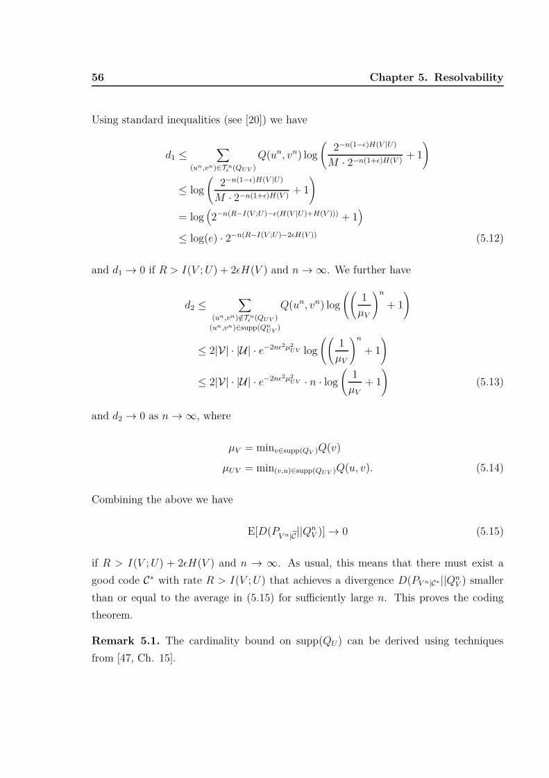
56 Chapter 5. Resolvability
Using standard inequalities (see [20]) we have
d1 ≤∑
(un,vn)∈T nǫ (QUV )
Q(un, vn) log
(2−n(1−ǫ)H(V |U)
M · 2−n(1+ǫ)H(V )+ 1
)
≤ log
(2−n(1−ǫ)H(V |U)
M · 2−n(1+ǫ)H(V )+ 1
)
= log(2−n(R−I(V ;U)−ǫ(H(V |U)+H(V ))) + 1
)
≤ log(e) · 2−n(R−I(V ;U)−2ǫH(V )) (5.12)
and d1 → 0 if R > I(V ; U) + 2ǫH(V ) and n → ∞. We further have
d2 ≤∑
(un,vn)/∈T nǫ (QUV )
(un,vn)∈supp(QnUV
)
Q(un, vn) log
((1
µV
)n
+ 1
)
≤ 2|V| · |U| · e−2nǫ2µ2UV log
((1
µV
)n
+ 1
)
≤ 2|V| · |U| · e−2nǫ2µ2UV · n · log
(1
µV+ 1
)(5.13)
and d2 → 0 as n → ∞, where
µV = minv∈supp(QV )Q(v)
µUV = min(v,u)∈supp(QUV )Q(u, v). (5.14)
Combining the above we have
E[D(PV n|C
||QnV )] → 0 (5.15)
if R > I(V ; U) + 2ǫH(V ) and n → ∞. As usual, this means that there must exist a
good code C∗ with rate R > I(V ; U) that achieves a divergence D(PV n|C∗||QnV ) smaller
than or equal to the average in (5.15) for sufficiently large n. This proves the coding
theorem.
Remark 5.1. The cardinality bound on supp(QU) can be derived using techniques
from [47, Ch. 15].

5.2. Main Result and Proof 57
Remark 5.2. If V = U , then we have R > H(V ).
Theorem 5.1 is proved using a uniform W which represents strings of uniform bits.
If we use a non-uniform W for the coding scheme, can we still drive the unnormalized
informational divergence to zero? We give the answer in the following lemma.
Lemma 5.2. Let W = BnR be a bit stream with nR bits that are generated i.i.d. with
a binary distribution PX with PX(0) = p, 0 < p ≤ 12. The rate R is achievable if
R >I(V ; U)
H2(p)(5.16)
where H2(·) is the binary entropy function.
Proof: The proof is given in Appendix B.1.
Remark 5.3. Lemma 5.2 states that even if W is not uniformly distributed, the in-
formational divergence can be made small. This is useful because if the distribution of
W is not known exactly, then we can choose R large enough to guarantee the desired
resolvability result. A similar result was developed in [43] for secrecy.
5.2.2. Error Exponents
We provide a second proof using Gallager’s error exponent [46] by extending [42, Lemma
2] to asymptotic cases. Consider −12
≤ ρ ≤ 0 and define
En0 (ρ, Qn
UV ) = ln∑
vn
{E[P
V n|C(vn|C)
11+ρ ]
}1+ρ(5.17)
E0(ρ, QUV ) = ln∑
v
{∑
u
Q(u)Q(v|u)1
1+ρ
}1+ρ
(5.18)
EG(R, QUV ) = inf− 1
2≤ρ<0
{E0(ρ, QUV ) + ρR} . (5.19)
Due to [42, Lemma 2], we have the following properties concerning En0 (ρ, Qn
UV ) and
E0(ρ, QUV ):
Property 1:
En0 (0, Qn
UV ) = E0(0, QUV ) = 0 (5.20)

58 Chapter 5. Resolvability
Property 2:
∂En0 (ρ, Qn
UV )
∂ρ
∣∣∣∣∣ρ=0
= −E[D(PV n|C
||QnV )]
∂E0(ρ, QUV )
∂ρ
∣∣∣∣∣ρ=0
= −I(V ; U) (5.21)
Property 3:
∂2En0 (ρ, Qn
UV )
∂ρ2≥ 0
∂2E0(ρ, QUV )
∂ρ2≥ 0 (5.22)
Due to [46, Theorem 5.6.3], we have
EG(R, QUV ) < 0 if R > I(V ; U)
EG(R, QUV ) = 0 if R ≤ I(V ; U)(5.23)
By extending [42, Sec. III, Inequality (15)] to asymptotic cases, we have the following
lemma.
Lemma 5.3. We have
En0 (ρ, Qn
UV ) ≤ enEG(R,QUV ). (5.24)
Proof: The proof is given in Appendix B.2.
Combining Properties 1-3, we have En0 (ρ, Qn
UV ) and E0(ρ, QUV ) are convex in ρ, for
−12
≤ ρ ≤ 0 and (see Fig. 5.3)
ρ · (−E[D(PV n|C
||QnV )]) ≤ En
0 (ρ, QnUV ) (5.25)
which means
E[D(PV n|C
||QnV )] ≤ En
0 (ρ, QnUV )
−ρ

5.2. Main Result and Proof 59
En0 (ρ, Qn
UV )ρ · (−E[D(PV n|C
||QnV )])
E0(ρ, QUV )
ρ · (−I(V ; U))
0 ρ−12
Figure 5.3.: An example of En0 (ρ, Qn
UV ) and E0(ρ, QUV ).
(a)
≤ enEG(R,QUV )
−ρ(5.26)
where (a) follows from Lemma 5.3. The right hand side of (5.26) goes to 0 as n → ∞as long as (see (5.23))
R > I(V ; U). (5.27)
Remark 5.4. This proof applies to continuous random variables by replacing the sums
in the proof of Lemma 5.3 with integrals.
Remark 5.5. The average divergence E[D(PV n|C
||QnV )] can be viewed as the mutual
information I(C; V n) from the random codebook C to the output V n [42, Sec. III]. To
show this, denote C as a realization of C and we have (see (5.10))
I(C; V n) =∑
C
P (C)∑
vn
P (vn|C) logP (vn|C)
QnV (vn)
=∑
un(1)
· · ·∑
un(M)
M∏
k=1
QnU(un(k))
∑
vn
M∑
w=1
1
M· Qn
V |U(vn|un(w)) log
∑Mj=1
1M
QnV |U(vn|un(j))
QnV (vn)
= E
log
∑Mj=1
1M
QnV |U(V n|Un(j))
QnV (V n)
= E[D(PV n|C
||QnV )]. (5.28)
60 Chapter 5. Resolvability
Thus, as E[D(PV n|C
||QnV )] → 0 we have I(C; V n) → 0 which means that C and V n
are (almost) independent. This makes sense, since as PV n|C
→ QnV one is not able to
distinguish which codebook is used to generate the output.
5.2.3. Converse
The converse follows by removing the normalization factor 1n
in [16, Theorem 5.2] . We
here provide a direct and simpler proof. Consider a given target distribution QV and any
code C with rate R and code words of length n. Using the requirement D(PV n ||QnV ) < nξ,
for some ξ > 0, we have
nξ > D(PV n ||QnV )
=
[∑
vn
P (vn)n∑
i=1
log1
QV (vi)
]− H(V n) (5.29)
=
[∑
vn
P (vn)n∑
i=1
log1
QV (vi)
]−
n∑
i=1
H(Vi|V i−1)
(a)
≥[
n∑
i=1
∑
v
PVi(v) log
1
QV (v)
]−
n∑
i=1
H(Vi)
=n∑
i=1
D(PVi||QV )
(b)
≥ nD(PV ||QV ) (5.30)
where PV = 1n
∑ni=1 PVi
, (a) follows because conditioning does not increase entropy, and
(b) follows by the convexity of D(PX ||QX) in PX . We also have
nR ≥ I(V n; Un)
≥ I(V n; Un) + D(PV n ||QnV ) − nξ
(a)= H(V n) − H(V n|Un) +
[n∑
i=1
∑
v
PVi(v) log
1
QV (v)
]− H(V n) − nξ
(b)
≥[
n∑
i=1
∑
v
PVi(v) log
1
Q(v)
]−[
n∑
i=1
H(Vi|Ui)
]− nξ
=
[n∑
i=1
∑
v
PVi(v) log
1
QV (v)
]+
n∑
i=1
∑
(u,v)
PUiVi(u, v) log QV |U(v|u)
− nξ

5.3. Discussion 61
= n
∑
(u,v)
PU(u)Q(v|u) logQ(v|u)
Q(v)
− nξ
(c)
≥ n
∑
(u,v)
PU(u)Q(v|u) logQ(v|u)
Q(v)
− nξ − nD(PV ||QV )
= n
∑
(u,v)
PU(u)Q(v|u) logQ(v|u)
Q(v)
− n
∑
(u,v)
PU(u)Q(v|u) logPV (v)
Q(v)
− nξ
= nI(V ; U) − nξ (5.31)
where PU = 1n
∑ni=1 PUi
, (a) follows by (5.29), (b) follows because conditioning does
not increase entropy, and (c) follows by D(PV ||QV ) ≥ 0. We further require that
D(PV ||QV ) → 0 as ξ → 0. Hence, we have
R ≥ minPU :PV =QV
I(V ; U) (5.32)
where P (v) =∑
u P (u)Q(v|u).
5.3. Discussion
Hayashi studied the resolvability problem using unnormalized divergence and he derived
bounds for nonasymptotic cases [42, Lemma 2]. We have outlined his proof steps in
Sec. 5.2.2. Theorem 5.1 can be derived by extending [42, Lemma 2] to asymptotic
cases (see 5.2.2) and it seems that such a result was the underlying motivation for [42,
Lemma 2]. Unfortunately, Theorem 5.1 is not stated explicitly in [42] and the ensuing
asymptotic analysis was done for normalized informational divergence. Hayashi’s proofs
(he developed two approaches) were based on Shannon random coding.
Theorem 5.1 implies [16, Theorem 6.3] which states that for R > I(V ; U) the normal-
ized divergence 1nD(PV n ||Qn
V ) can be made small. Theorem 5.1 implies [17, Theorem 4]
for product distributions through Pinsker’s inequality (Equ. (2.6)).Moreover, the speed
of decay in (5.26) is exponential with n. We can thus make
α(n) · E[D(P
V n|C||Qn
V )]
(5.33)

62 Chapter 5. Resolvability
vanishingly small as n → ∞, where α(n) represents a sub-exponential function of n that
satisfies,
limn→∞
α(n)
eβn= 0 (5.34)
where β is positive and independent of n (see also [42]). For example, we may choose
α(n) = nm for any integer m. We may also choose α(n) = eγn where γ < β.
Since all achievability results in [48] are based on [17, Theorem 4], Theorem 5.1 ex-
tends the results in [48] as well. Theorem 5.1 is closely related to strong secrecy [49,50]
and provides a simple proof that Shannon random coding suffices to drive an unnormal-
ized mutual information between messages and eavesdropper observations to zero (see
Chapter 6 below).
Theorem 5.1 is valid for approximating product distributions only. However extensions
to a broader class of distributions, e.g., information stable distributions [17], are clearly
possible.
Finally, an example code is as follows (courtesy of F. Kschischang). Consider a chan-
nel with input and output alphabet the 27 binary 7-tuples. Suppose the channel maps
each input uniformly to a 7-tuple that is distance 0 or 1 away, i.e., there are 8 channel
transitions for every input and each transition has probability 18. A simple “modula-
tion” code for this channel is the (7, 4) Hamming code. The code is perfect and if we
choose each code word with probability 116
, then the output V 7 of the channel is uni-
formly distributed over all 27 values. Hence I(V ; U) = 4 bits suffice to “approximate”
the product distribution (here there is no approximation).

6Effective Secrecy: Reliability,
Confusion and Stealth
Wyner [51] derived the secrecy capacity for degraded wire-tap channels (see Fig. 6.1).
Csiszár and Körner [52] extended the results to broadcast channels with confidential
messages. In both [51] and [52], secrecy was measured by a normalized mutual in-
formation between the message M and the eavesdropper’s output Zn under a secrecy
constraint
1
nI(M ; Zn) ≤ S (6.1)
which is referred to as weak secrecy. Weak secrecy has the advantage that one can trade
off S for rate. The drawback is that even S ≈ 0 is usually considered too weak because
the eavesdropper can decipher nS bits of M , which grows with n. Therefore, [49] (see
also [44]) advocated using strong secrecy where secrecy is measured by the unnormalized

64 Chapter 6. Effective Secrecy: Reliability, Confusion and Stealth
mutual information I(M ; Zn) and requires
I(M ; Zn) ≤ ξ (6.2)
for any ξ > 0 and sufficiently large n.
In related work, Han and Verdú [17] studied resolvability based on variational distance
that addresses the number of bits needed to mimic a marginal distribution of a prescribed
joint distribution. Bloch and Laneman [43] used the resolvability approach of [17] and
extended the results in [52] to continuous random variables and channels with memory.
The main contribution of this chapter is to define and justify the usefulness of a new
and stronger security measure for wire-tap channels that includes not only reliability
and (wiretapper) confusion but also stealth. The measure is satisfied by random codes
and by using the simplified proof of resolvability based on unnormalized informational
divergence developed in Chapter 5 (see also [45, Lemma 11]). In particular, we measure
secrecy by the informational divergence
D(PMZn||PMQZn) (6.3)
where PMZn is the joint distribution of MZn, PM is the distribution of M , PZn is the
distribution of Zn, and QZn is the distribution that the eavesdropper expects to observe
when the source is not communicating useful messages. We call this security measure
effective secrecy.
One can easily check that (see (6.7) below)
D(PMZn||PMQZn) = I(M ; Zn)︸ ︷︷ ︸
Non-Confusion
+ D(PZn||QZn)︸ ︷︷ ︸
Non-Stealth
(6.4)
where we interpret I(M ; Zn) as a measure of “non-confusion” and D(PZn||QZn) as a
measure of “non-stealth”. We justify the former interpretation by using error probability
in Sec. 6.2 and the latter by using binary hypothesis testing in Sec. 6.3. Thus, by making
D(PMZn||PMQZn) → 0 we not only keep the message secret from the eavesdropper but
also hide the presence of meaningful communication.
We remark that the choice of default behavior QZn in (6.3) will depend on the appli-
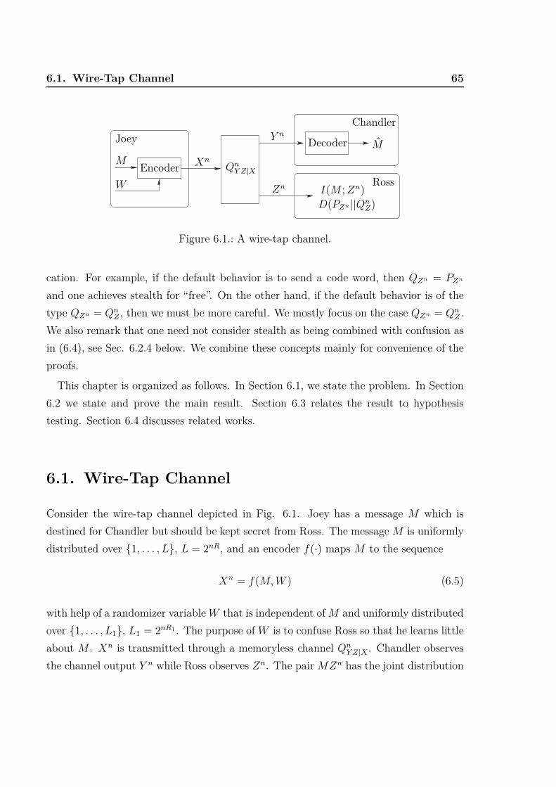
6.1. Wire-Tap Channel 65
Joey
Chandler
Ross
M
W
Xn
Y n
Zn
M
QnY Z|XEncoder
Decoder
I(M ; Zn)
D(PZn||QnZ)
Figure 6.1.: A wire-tap channel.
cation. For example, if the default behavior is to send a code word, then QZn = PZn
and one achieves stealth for “free”. On the other hand, if the default behavior is of the
type QZn = QnZ , then we must be more careful. We mostly focus on the case QZn = Qn
Z .
We also remark that one need not consider stealth as being combined with confusion as
in (6.4), see Sec. 6.2.4 below. We combine these concepts mainly for convenience of the
proofs.
This chapter is organized as follows. In Section 6.1, we state the problem. In Section
6.2 we state and prove the main result. Section 6.3 relates the result to hypothesis
testing. Section 6.4 discusses related works.
6.1. Wire-Tap Channel
Consider the wire-tap channel depicted in Fig. 6.1. Joey has a message M which is
destined for Chandler but should be kept secret from Ross. The message M is uniformly
distributed over {1, . . . , L}, L = 2nR, and an encoder f(·) maps M to the sequence
Xn = f(M, W ) (6.5)
with help of a randomizer variable W that is independent of M and uniformly distributed
over {1, . . . , L1}, L1 = 2nR1 . The purpose of W is to confuse Ross so that he learns little
about M . Xn is transmitted through a memoryless channel QnY Z|X. Chandler observes
the channel output Y n while Ross observes Zn. The pair MZn has the joint distribution
66 Chapter 6. Effective Secrecy: Reliability, Confusion and Stealth
PMZn. Chandler estimates M from Y n and the average error probability is
P (n)e = Pr
[M 6= M
]. (6.6)
Ross tries to learn M from Zn and secrecy is measured by
D(PMZn||PMQnZ)
=∑
(m,zn)∈supp(PMZn )
P (m, zn) log
(P (m, zn)
P (m) · QnZ(zn)
· P (zn)
P (zn)
)
=∑
(m,zn)∈supp(PMZn )
P (m, zn)
(log
P (zn|m)
P (zn)+ log
P (zn)
QnZ(zn)
)
= I(M ; Zn)︸ ︷︷ ︸
Non-Confusion
+ D(PZn||QnZ)
︸ ︷︷ ︸Non-Stealth
(6.7)
where PZn is the distribution Ross observes at his channel output and QnZ is the default
distribution Ross expects to observe if Joey is not sending useful information. For
example, if Joey transmits Xn with probability QnX(Xn) through the channel, then we
have
QnZ(zn) =
∑
xn∈supp(QnX
)
QnX(xn)Qn
Z|X(zn|xn) = PZn(zn). (6.8)
When Joey sends useful messages, then PZn and QnZ are different. But a small D(PMZn||PMQn
Z)
implies that both I(M ; Zn) and D(PZn||QnZ) are small which in turn implies that Ross
learns little about M and cannot recognize whether Joey is communicating anything
meaningful. A rate R is achievable if for any ξ1, ξ2 > 0 there is a sufficiently large n and
an encoder and a decoder such that
P (n)e ≤ ξ1 (6.9)
D(PMZn||PMQnZ) ≤ ξ2. (6.10)
The effective secrecy capacity CS is the supremum of the set of achievable R. We wish
to determine CS.

6.2. Main result and Proof 67
6.2. Main result and Proof
We prove the following result.
Theorem 6.1. The effective secrecy capacity of the wire-tap channel is the same as the
weak and strong secrecy capacity, namely
CS = supQV X
[I(V ; Y ) − I(V ; Z)] (6.11)
where the supremum is taken over all joint distributions QV X satisfying
QZ(z) =∑
v,x
QV X(v, x)QZ|X(z|x) (6.12)
and the Markov chain
V − X − Y Z (6.13)
where QZ is the default distribution at the eavesdropper’s channel output.
One may restrict the cardinality of V to |V| ≤ |X | .
6.2.1. Achievability
We use random coding and the proof technique of Sec. 5.2.1.
Random Code: Fix a distribution QX and generate L · L1 code words xn(m, w), m =
1, . . . , L, w = 1, . . . , L1 using∏n
i=1 QX(xi(m, w)). This defines the codebook
C = {xn(m, w), m = 1, . . . , L, w = 1, . . . , L1} (6.14)
and we denote the random codebook by
C = {Xn(m, w)}(L,L1)(m,w)=(1,1). (6.15)
Encoding: To send a message m, Joey chooses w uniformly from {1, . . . , L1} and
transmits xn(m, w). Hence, for a fixed codebook C = C every xn(m, w) occurs with

68 Chapter 6. Effective Secrecy: Reliability, Confusion and Stealth
probability
PXn(xn(m, w)) =1
L · L1(6.16)
rather than QnX(xn(m, w)) (see (6.8)) and Qn
Z may not be the same as PZn. Further, for
every pair (m, zn) we have
P (zn|m) =L1∑
w=1
1
L1· Qn
Z|X(zn|xn(m, w)) (6.17)
P (zn) =L∑
m=1
L1∑
w=1
1
L · L1
· QnZ|X(zn|xn(m, w)). (6.18)
Chandler: Chandler puts out (m, w) if there is a unique pair (m, w) satisfying the
typicality check
(xn(m, w), yn) ∈ T nǫ (QXY ). (6.19)
Otherwise he puts out (m, w) = (1, 1).
Analysis: Define the events
E1 : {(M, W ) 6= (M, W )}E2 : D(PMZn||PMQn
Z) > ξ2. (6.20)
Let E = E1 ∪ E2 so that we have
Pr[E] ≤ Pr[E1] + Pr[E2] (6.21)
where we have used the union bound. Pr[E1] can be made small with large n as long as
R + R1 < I(X; Y ) − δǫ(n) (6.22)
where δǫ(n) → 0 as n → ∞ (see [20]) which implies that P (n)e is small.

6.2. Main result and Proof 69
Pr[E2] can be made small with large n as long as (Theorem 5.1)
R1 > I(X; Z) + δ′ǫ(n) (6.23)
where δ′ǫ(n) → 0 as n → ∞. This is because the divergence averaged over M , W , C and
Zn satisfies (see Equ. (5.9) )
E[D(PMZn|C
||PMQnZ)]
(a)= E[D(PM ||PM) + D(P
Zn|M C||Qn
Z|PM)]
(b)= E
log
∑L1j=1 Qn
Z|X(Zn|Xn(M, j))
L1 · QnZ(Zn)
=L∑
m=1
L1∑
w=1
1
L · L1E
log
∑L1j=1 Qn
Z|X(Zn|Xn(m, j))
L1 · QnZ(Zn)
∣∣∣∣∣∣∣∣M = m, W = w
(c)
≤L∑
m=1
L1∑
w=1
1
L · L1E
log
(Qn
Z|X(Zn|Xn(m, w))
L1 · QnZ(Zn)
+ 1
)∣∣∣∣∣∣∣∣M = m, W = w
(d)= E
[log
(Qn
Z|X(Zn|Xn)
L1 · QnZ(Zn)
+ 1
)](6.24)
where
(a) follows by the chain rule for informational divergence;
(b) follows by (6.17) and by taking the expectation over M, W, Xn(1, 1), . . . , Xn(L, L1), Zn;
(c) follows by the concavity of the logarithm and Jensen’s inequality applied to the
expectation over the Xn(m, j), j 6= w for a fixed m;
(d) follows by choosing XnZn ∼ QnXZ .
Next we can show that the right hand side (RHS) of (6.24) is small if (6.23) is valid
by splitting the expectation in (6.24) into sums of typical and atypical pairs (see Equ.
(5.11)-(5.14)]). But if the RHS of (6.24) approaches 0, then using (6.7) we have
E[I(M ; Zn|C) + D(P
Zn|C||Qn
Z)]
→ 0. (6.25)
70 Chapter 6. Effective Secrecy: Reliability, Confusion and Stealth
Combining (6.21), (6.22) and (6.23) we can make Pr[E] → 0 as n → ∞ as long as
R + R1 < I(X; Y ) (6.26)
R1 > I(X; Z). (6.27)
which means that there must exist one good code C∗ satisfying the above conditions and
achieves an error probability smaller than or equal to the average error probability (see
(6.22) and (6.23)). We hence have the achievability of any R satisfying
0 ≤ R < supQX
[I(X; Y ) − I(X; Z)]. (6.28)
where the supremum is taken over all QX such that
QZ(z) =∑
x
QX(x)QZ|X(z|x). (6.29)
Of course, if the RHS of (6.28) is non-positive, then we require R = 0. Now we prefix a
channel QnX|V to the original channel Qn
Y Z|X and obtain a new channel QnY Z|V where
QnY Z|V (yn, zn|vn) =
∑
xn∈supp(QnX|V
(·|vn))
QnX|V (xn|vn)Qn
Y Z|X(yn, zn|xn). (6.30)
Using a similar analysis as above, we have the achievability of any R satisfying
0 ≤ R < supQV X
[I(V ; Y ) − I(V ; Z)] (6.31)
where the supremum is taken over all QV X satisfying (6.12) and (6.13). Again, if the
RHS of (6.31) is non-positive, then we require R = 0. As usual, the purpose of adding
the auxiliary variable V is to potentially increase R. Note that V = X recovers (6.28).
Hence, the RHS of (6.28) is always smaller than or equal to the RHS of (6.31).
Remark 6.1. The steps (6.24) imply that secrecy and stealth are attained for every
message m and not just for the average over all messages. This gives a guarantee for a
good worst case performance.
Remark 6.2. The average divergence E[D(PMZn|C
||PMQnZ)] is the sum of I(M C; Zn)
6.2. Main result and Proof 71
and D(PZn||QnZ) [42, Sec. III] (see also Remark 5.5). To see this, consider
E[D(PMZn|C
||PMQnZ)]
= D(PMZn|C
||PMQnZ |P
C)
(a)= D(P
Zn|M C||Qn
Z |PMPC)
= D(PZn|M C
||PZn|PMPC) + D(PZn||Qn
Z)
= I(M C; Zn) + D(PZn||QnZ) (6.32)
where (a) follows by the independence of M and the code words. Thus, as E[D(PMZn|C
||PMQnZ)] →
0 we have I(M C; Zn) → 0 which means that M C and Zn are (almost) independent. This
makes sense, since for effective secrecy the adversary learns little about M and the pres-
ence of meaningful transmission.
6.2.2. Converse
The converse follows as in [52, Theorem 1]. We provide an alternative proof using the
telescoping identity [53, Sec. G]. Consider any code C with rate R and code words of
length n satisfying (6.9) and (6.10) for some ξ1, ξ2 > 0. We have
log2 L = nR
= H(M)
= I(M ; Y n) + H(M |Y n)
(a)
≤ I(M ; Y n) + (1 + ξ1 · nR)
(b)
≤ I(M ; Y n) − I(M ; Zn) + ξ2 · n + (1 + ξ1 · nR) (6.33)
where (a) follows from Fano’s inequality and (b) follows from (6.7) and (6.10). Using
the telescoping identity [53, Equ. (9) and (11)] we have
1
n[I(M ; Y n) − I(M ; Zn)]
=n∑
i=1
[I(M ; Zni+1Y
i) − I(M ; Zni Y i−1)]

72 Chapter 6. Effective Secrecy: Reliability, Confusion and Stealth
=1
n
n∑
i=1
[I(M ; Yi|Y i−1Zni+1) − I(M ; Zi; |Y i−1Zn
i+1)]
(a)= I(M ; YT |Y T −1Zn
T +1T ) − I(M ; ZT |Y T −1ZnT +1T )
(b)= I(V ; Y |U) − I(V ; Z|U)
(c)
≤ maxQUV X :QZ(z)=
∑u,v,x
QUV X(u,v,x)QZ|X (z|x)[I(V ; Y |U) − I(V ; Z|U)]
≤ maxu
maxQV X|U=u:QZ(z)=
∑v,x
QV X|U (v,x|u)QZ|X(z|x)[I(V ; Y |U = u) − I(V ; Z|U = u)] (6.34)
(d)= max
QV X :QZ(z)=∑
u,v,xQV X(v,x)QZ|X (z|x)
[I(V ; Y ) − I(V ; Z)] (6.35)
where
(a) follows by letting T be independent of all other random variables and uniformly
distributed over {1, . . . , n};
(b) follows by defining
U = Y T −1ZnT +1T, V = MU,
X = XT , Y = YT , Z = ZT ; (6.36)
(c) follows from (6.10) (see also Sec. 5.2.3)
(d) follows because if the maximum in (6.34) is achieved for U = u∗ and QV X|U=u∗ , then
the same can be achieved in (6.35) by choosing a QV X = QV X|U=u∗ .
Combining (6.33) and (6.35) we have
R ≤supQV X
[I(V ; Y ) − I(V ; Z)]
1 − ξ1+
ξ2 · n + 1
(1 − ξ1)n. (6.37)
where the supremum is taken over all QV X satisfying (6.12) and (6.13). Letting n → ∞,
ξ1 → 0, and ξ2 → 0, we have
R ≤ supQV X
[I(V ; Y ) − I(V ; Z)] (6.38)

6.2. Main result and Proof 73
JoeyChandler
Ross
M
M0
W
Xn
Y n
Zn
M
M0
M0
QnY Z|XEncoder
Decoder 1
Decoder 2
Figure 6.2.: A broadcast channel with a confidential message.
where the supremum is taken over all QV X satisfying (6.12) and (6.13). The cardinality
bound in Theorem 1 was derived in [30, Theorem 22.1].
6.2.3. Broadcast Channels with Confidential Messages
Broadcast channels with confidential messages (BCC) [52] are wire-tap channels with
common messages. For the BCC (Fig. 6.2), Joey has a common message M0 destined
for both Chandler and Ross which is independent of M and uniformly distributed over
{1, . . . , L0}, L0 = 2nR0. An encoder maps M0 and M to
Xn = f(M0, M, W ) (6.39)
which is sent through the channel QnY Z|X. Chandler estimates (M0, M) from Y n while
Ross estimates M0 from Zn. The average error probability is
P ∗(n)e = Pr
[{(M0, M) 6= (M0, M)
}∪{
M0 6= M0
}](6.40)
and non-secrecy is measured by D(PMZn||PMQnZ). A rate pair (R0, R) is achievable if,
for any ξ1, ξ2 > 0, there is a sufficiently large n, an encoder and two decoders such that
P ∗(n)e ≤ ξ1 (6.41)
D(PMZn||PMQnZ) ≤ ξ2. (6.42)

74 Chapter 6. Effective Secrecy: Reliability, Confusion and Stealth
The effective secrecy capacity region CBCC is the closure of the set of achievable (R0, R).
We have the following theorem.
Theorem 6.2. CBCC is the same as the weak and strong secrecy capacity region
CBCC =⋃
(R0, R) :
0 ≤ R0 ≤ min {I(U ; Y ), I(U ; Z)}0 ≤ R ≤ I(V ; Y |U) − I(V ; Z|U)
(6.43)
where the union is over all distributions QUV X satisfying
QZ(z) =∑
u,v,x
QUV X(u, v, x)QZ|X(z|x) (6.44)
and the Markov chain
U − V − X − Y Z. (6.45)
One may restrict the alphabet sizes to
|U| ≤ |X | + 3; |V| ≤ |X |2 + 4|X | + 3. (6.46)
Proof: The proof is omitted due to the similarity to the proof of Theorem 6.1.
6.2.4. Choice of Security Measures
Effective secrecy includes both strong secrecy and stealth communication. One may ar-
gue that using only I(M ; Zn) or D(PZn||QnZ) would suffice to measure secrecy. However,
we consider two examples where secrecy is achieved but not stealth, and where stealth
is achieved but not secrecy.
Example 6.1. I(M ; Zn) → 0, D(PZn||QnZ) = D > 0. Suppose that Joey inadvertently
uses QX rather than QX for codebook generation, where (6.23) is still satisfied. For
example, QX might represent no energy while QX must have positive energy. The new

6.3. Hypothesis Testing 75
QX could result in a different expected QnZ 6= Qn
Z . Hence, as n grows large we have
D(PMZn||PMQnZ) = I(M ; Zn) + D(Qn
Z||QnZ) (6.47)
where I(M ; Zn) → 0 but we have
D(QnZ ||Qn
Z) = D, for some D > 0. (6.48)
Ross thus recognizes that Joey is transmitting useful information even though he cannot
decode.
Example 6.2. I(M ; Zn) = I > 0, D(PZn||QnZ) → 0. Note that E[D(PZn||Qn
Z)] → 0 as
n → ∞ as long as (see [54, Theorem 1])
R + R1 > I(X; Z). (6.49)
If Joey is not careful and chooses R1 such that (6.23) is violated and (6.49) is satisfied,
then D(PZn||QnZ) can be made small but we have
I(M ; Zn) = I for some I > 0. (6.50)
For example, Joey might choose R1 = 0. Thus, although the communication makes
D(PZn||QnZ) small, Ross can learn
I(M ; Zn) ≈ n[I(X; Z) − R1] (6.51)
bits about M if he is willing to pay a price and always tries to decode (see Sec. 6.3).
6.3. Hypothesis Testing
The reader may wonder how D(PZn||QnZ) relates to stealth. We consider a hypothesis
testing framework and show that as long as (6.49) is satisfied, the best Ross can do to
detect Joey’s action is to guess.
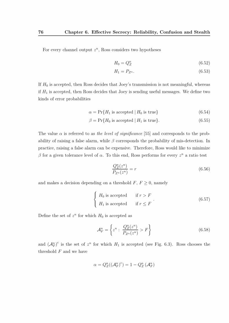
76 Chapter 6. Effective Secrecy: Reliability, Confusion and Stealth
For every channel output zn, Ross considers two hypotheses
H0 = QnZ (6.52)
H1 = PZn. (6.53)
If H0 is accepted, then Ross decides that Joey’s transmission is not meaningful, whereas
if H1 is accepted, then Ross decides that Joey is sending useful messages. We define two
kinds of error probabilities
α = Pr{H1 is accepted | H0 is true} (6.54)
β = Pr{H0 is accepted | H1 is true}. (6.55)
The value α is referred to as the level of significance [55] and corresponds to the prob-
ability of raising a false alarm, while β corresponds the probability of mis-detection. In
practice, raising a false alarm can be expensive. Therefore, Ross would like to minimize
β for a given tolerance level of α. To this end, Ross performs for every zn a ratio test
QnZ(zn)
PZn(zn)= r (6.56)
and makes a decision depending on a threshold F , F ≥ 0, namely
H0 is accepted if r > F
H1 is accepted if r ≤ F. (6.57)
Define the set of zn for which H0 is accepted as
AnF =
{zn :
QnZ(zn)
PZn(zn)> F
}(6.58)
and (AnF )c is the set of zn for which H1 is accepted (see Fig. 6.3). Ross chooses the
threshold F and we have
α = QnZ((An
F )c) = 1 − QnZ (An
F )

6.3. Hypothesis Testing 77
AnF (An
F )c
QnZ
(zn)
PZn(zn)> F
QnZ
(zn)
PZn (zn)≤ F
H0 = QnZ H1 = PZn
Figure 6.3.: Example of the decision regions AnF and (An
F )c.
β = PZn(AnF ). (6.59)
The ratio test in (6.56) is the Neyman-Pearson test which is optimal [55, Theorem 3.2.1]
in the sense that it minimizes β for a given α. We have the following lemma.
Lemma 6.3. If D(PZn||QnZ) ≤ ξ2, ξ2 > 0, then with the Neyman-Pearson test we have
1 − g(ξ2) ≤ α + β ≤ 1 + g(ξ2) (6.60)
where
g(ξ2) =√
ξ2 · 2 ln 2 (6.61)
which goes to 0 as ξ2 → 0.
Proof: Since D(PZn||QnZ) ≤ ξ2, we have
||PZn − QnZ ||TV ≤
√ξ2 · 2 ln 2 = g(ξ2) (6.62)
where the inequality follows by (2.6). We further have
||PZn − QnZ ||TV
=∑
zn∈AnF
|PZn(zn) − QnZ(zn)| +
∑
zn∈(AnF )
c
|PZn(zn) − QnZ(zn)|

78 Chapter 6. Effective Secrecy: Reliability, Confusion and Stealth
α
β
0
1
1
1 − g(ξ2)
1 − g(ξ2)
Stealth
No Stealth
Figure 6.4.: Optimal tradeoff between α and β.
≥∑
zn∈AnF
|PZn(zn) − QnZ(zn)|
(a)
≥∣∣∣∣∣∣
∑
zn∈AnF
[PZn(zn) − QnZ(zn)]
∣∣∣∣∣∣
= |PZn(AnF ) − Qn
Z(AnF )|
= |β − (1 − α)| (6.63)
where (a) follows by the triangle inequality. Combining (6.62) and (6.63), we have the
bounds (6.60).
Fig. 6.4 illustrates the optimal tradeoff between α and β for stealth communication,
i.e., when (6.49) is satisfied. As n → ∞ and ξ2 → 0, we have
D(PZn||QnZ) → 0 (6.64)
(α + β) → 1. (6.65)
If Ross allows no false alarm (α = 0), then he always ends up with mis-detection (β = 1).
If Ross tolerates no mis-detection (β = 0), he pays a high price (α = 1). Further, for
any given α, the optimal mis-detection probability is
βopt = 1 − α. (6.66)

6.4. Discussion 79
But Ross does not need to see Zn or perform an optimal test to achieve βopt. He may
randomly choose some A′ such that
QnZ((A′)c) = α (6.67)
and achieves β ′opt = 1 − α. The best strategy is thus to guess. On the other hand, if
limn→∞
D(PZn||QnZ) > 0 (6.68)
then Ross detects Joey’s action and we can have
α + β = 0. (6.69)
We thus operate in one of two regimes in Fig. 6.4, either near (α, β) = (0, 0) or near the
line α + β = 1.
6.4. Discussion
Our resolvability proof differs from that in [43] in that we rely on unnormalized informa-
tional divergence [54] instead of variational distance [17]. Our proof is simpler and the
result is stronger than that in [43] when restricting attention to product distributions
and memoryless channels because a small D(PMZn||PMQnZ) implies small I(M ; Zn) and
D(PZn||QnZ) while a small ||PXn − Qn
X ||TV implies only a small I(M ; Zn) [44, Lemma 1].
Hayashi studied strong secrecy for wire-tap channels using resolvability based on un-
normalized divergence and he derived bounds for nonasymptotic cases [42, Theorem 3].
We remark that Theorem 1 can be derived by extending [42, Lemma 2] to asymptotic
cases. However, Hayashi did not consider stealth but focused on strong secrecy, although
he too noticed a formal connection to (6.7) [42, p. 1568].


7Conclusion
We have addressed two problems in network information theory: short message noisy
network coding (SNNC) and resolvability based on unnormalized informational diver-
gence with applications to network security. SNNC with backward decoding simplifies
the analysis and enables mixed strategies of DF and QF that provide better rates and
outage probabilities. Resolvability based on informational divergence gives a stronger
result with a simpler proof that also applies to establish a new and stronger effective
secrecy measure. This measure includes strong secrecy and the hiding of the presence of
meaningful communication.
There are several open research problems worth addressing:
1. In [11], the authors characterized the gap between the cut-set bound and the
achievable LNNC (SNNC) rates under the assumption that all network nodes
quantize at the noise level. The resulting gap increases linearly with the number
of nodes K in the network. Recently, the papers [56–58] showed that if the quan-
tization noise level is proportional to the number of nodes K at all nodes, then
the gap increases logarithmically with K.

82 Chapter 7. Conclusion
However, we may improve the gap by letting the nodes quantize at individual noise
levels depending on the network geometry rather than quantizing at the same noise
level. Suppose we have a network with several sources, destinations and two classes
of relay nodes:
Class 1: close to the sources but far from the destinations
Class 2: close to the destinations but far from sources
Then, the Class 1 relays should quantize coarsely, because their relay-destination
links are weak and may not support fine details. For the Class 2 relays the situation
is the other way around: they should quantize finely to exploit the strong relay-
destination links. In this way, we may get a better gap.
2. The investigation of wire-tap channels with effective secrecy was done information-
theoretically. It would be interesting to find explicit codes with rate close to the
secrecy capacity that achieve strong secrecy and stealth at the same time. Recently,
the paper [59] showed that polar coding achieves strong secrecy for degraded binary
symmetric wire-tap channels. It’s worth checking whether polar coding can also
achieve effective secrecy for a broader class of wire-tap channels.

AProofs for Chapter 3
A.1. Treating Class 2 Nodes as Noise
If all Class 2 bounds in (3.38) are satisfied, then SNNC achieves the same rates as NNC.
In this case the decoder recovers the signals from the nodes in Dck and thereby removes
interference from these nodes.
Now suppose that an S in Class 2 has RS ≥ IKS (k). We use the argument presented
in [25] (see also [5]): for any J satisfying S ⊂ J ⊂ K such that J ∩ Dk 6= ∅ and k ∈ J c
we have
RJ \S < IKJ (k) − RS
(a)
≤ IKJ (k) − IK
S (k)
(b)= I(XJ ; YJ cYk|XJ c) − I(YJ ; YJ |XKYJ cYk) − I(XS ; YScYk|XSc) + I(YS ; YS|XKYScYk)
(c)= I(XJ ; YJ cYk|XJ c) − I(XS ; YScYk|XSc) − I(YJ \S ; YSYJ \S |XKYJ cYk)
− I(YS ; YSYJ \S |XKYScYk) + I(YS ; YS|XKYScYk)

84 Appendix A. Proofs for Chapter 3
(d)= I(XJ ; YJ cYk|XJ c) − I(XS ; YScYk|XSc) − I(YJ \S ; YSYJ \S |XKYJ cYk)
(e)= I(XJ \S ; YJ cYk|XJ c) + I(XS ; YJ cYk|XSc) − I(XS ; YScYk|XSc) − I(YJ \S ; YJ \S |XKYJ cYk)
(f)= I(XJ \S ; YJ cYk|XJ c) − I(XS ; YJ \S |XScYJ cYk) − I(YJ \S ; YJ \S |XKYJ cYk)
(g)= I(XJ \S ; YJ cYk|XJ c) − I(YJ \S ; XSYJ \S |XScYJ cYk)
(h)= I(XJ \S ; YJ cYk|XJ c) − I(YJ \S ; YJ \S |XScYJ cYk)
(i)= I
K\SJ \S(k) (A.1)
where
(a) follows because RS ≥ IKS (k) by assumption
(b) follows from the definition (3.10)
(c) follows from the chain rule for mutual information
(d) follows from the Markov chain
XScYJ \S YScYk − YSXS − YS (A.2)
(e)-(h) follow from the chain rule for mutual information and the Markov chain
XK\J XSYS YJ cYk − YJ \SXJ \S − YJ \S (A.3)
(i) follows from the definition (3.10).
The rates satisfying (A.1) are the NNC rates for the nodes in K \ S while treating the
signals from the nodes in S as noise. This shows that if any of the constraints in Class
2 is violated for NNC or SNNC, then the destination node should treat the signals from
the corresponding nodes as noise rather than decoding them.
Now repeat the above argument for the nodes in K \ S, until we reach a set Kk ⊂ K,
for which
0 ≤ RS < IKk
S (k) (A.4)
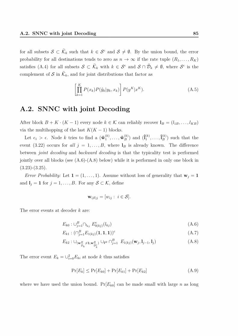
A.2. SNNC with joint Decoding 85
for all subsets S ⊂ Kk such that k ∈ Sc and S 6= ∅. By the union bound, the error
probability for all destinations tends to zero as n → ∞ if the rate tuple (R1, . . . , RK)
satisfies (A.4) for all subsets S ⊂ Kk with k ∈ Sc and S ∩ Dk 6= ∅, where Sc is the
complement of S in Kk, and for joint distributions that factor as
[K∏
k=1
P (xk)P (yk|yk, xk)
]P (yK|xK). (A.5)
A.2. SNNC with joint Decoding
After block B + K · (K − 1) every node k ∈ K can reliably recover lB = (l1B, . . . , lKB)
via the multihopping of the last K(K − 1) blocks.
Let ǫ1 > ǫ. Node k tries to find a (w(k)1 , . . . , w(k)
B ) and (l(k)1 , . . . , l(k)
B ) such that the
event (3.22) occurs for all j = 1, . . . , B, where lB is already known. The difference
between joint decoding and backward decoding is that the typicality test is performed
jointly over all blocks (see (A.6)-(A.8) below) while it is performed in only one block in
(3.23)-(3.25).
Error Probability: Let 1 = (1, . . . , 1). Assume without loss of generality that wj = 1
and lj = 1 for j = 1, . . . , B. For any S ⊂ K, define
w(S)j = [wij : i ∈ S].
The error events at decoder k are:
Ek0 : ∪Bj=1∩lkj
Ec0(kj)(lkj) (A.6)
Ek1 : (∩Bj=1E1(kj)(1, 1, 1))c (A.7)
Ek2 : ∪(wB
Dk
6=1,wB
Dck
) ∪lB ∩Bj=1 E1(kj)(wj, lj−1, lj) (A.8)
The error event Ek = ∪2i=0Eki at node k thus satisfies
Pr[Ek] ≤ Pr[Ek0] + Pr[Ek1] + Pr[Ek2] (A.9)
where we have used the union bound. Pr[Ek0] can be made small with large n as long

86 Appendix A. Proofs for Chapter 3
as (see (3.27))
Rk > I(Yk; Yk|Xk) + δǫ(n). (A.10)
Also, we have
Pr[Ek1] = Pr[(∩Bj=1E1(kj)(1, 1, 1))c]
= Pr[∪Bj=1E
c1(kj)(1, 1, 1)]
≤B∑
j=1
Pr[Ec1(kj)(1, 1, 1)]
(a)
≤ B · δǫ1(n)
= δǫ1(n, B) (A.11)
where (a) follows because Pr[Ec1(kj)(1, 1, 1)] ≤ δǫ1(n), which goes to zero as n → ∞, for
j = 1, . . . , B [20].
To bound Pr[Ek2
], for each (wj, lj−1), we define
Sj(wj, lj−1) = {i ∈ K : wij 6= 1 or li(j−1) 6= 1} (A.12)
and write Sj = Sj(wj, lj−1). Observe that for j = 1, . . . , B :
⊲ (XSj, YSj
) is independent of (XScj, YSc
j, Ykj) in the random coding experiment;
⊲ the (Xij, Yij), i ∈ Sj , are mutually independent.
We have (see (3.31) and (3.32)):
Pr[E1(kj)(wj, lj−1, lj)
]≤ P(kj)(Sj) (A.13)
where
P(kj)(Sj) =
2−n(ISj−δǫ1 (n)) if Sj 6= ∅
1 otherwise(A.14)
and δǫ1(n) → 0 as n → ∞.

A.2. SNNC with joint Decoding 87
By the union bound, we have
Pr[Ek2] ≤∑
(wB
Dk
6=1,wB
Dck
)∑
lB−1
Pr[∩Bj=1E1(kj) (wj, lj−1, lj)]
(a)=
∑(
wB
Dk
6=1,wB
Dck
)∑
lB−1
B∏
j=1
Pr[E1(kj) (wj, lj−1, lj)]
(b)
≤ ∑
wB ,lB−1
B∏
j=1
Pr[E1(kj) (wj, lj−1, lj)]
−
B∏
j=1
Pr[E1(kj) (1, 1, 1)]
(c)
≤ ∑
wB,lB−1
B∏
j=1
P(kj)(Sj)
− (1 − δǫ1(n, B))
(d)=
B∏
j=1
∑
wj ,lj−1
P(kj)(Sj)
− (1 − δǫ1(n, B))
(e)<
B∏
j=1
1 +∑
S:k∈Sc
S6=∅
∑
(wj ,lj−1)6=(1,1):
Sj(wj ,lj−1)=S
2−n(IS−δǫ1 (n))
− (1 − δǫ1(n, B))
(f)<
1 +
∑
S:k∈Sc
S6=∅
3|S|2n(RS+RS)−(IS−δǫ1 (n)))
B
− (1 − δǫ1(n, B)) (A.15)
where
(a) follows because the codebooks are independent and the channel is memoryless
(b) follows by adding(
wBDk
= 1, wBDc
k
)to the sum
(c) follows from (A.13) and because (see (A.11))
Pr[∩Bj=1E1(kj)(1, 1, 1)]
= 1 − Pr[(∩Bj=1E1(kj)(1, 1, 1))c]
≥ 1 − δǫ1(n, B) (A.16)
(d) follows because P(kj)(Sj) depends only on Sj which in turn depends only on (wj, lj−1)

88 Appendix A. Proofs for Chapter 3
(e) follows from (A.14)
(f) follows from (3.33).
Performing the same steps as in (3.35) and (3.36), we require
RS < IKS (k) (A.17)
for all subsets S ⊂ K such that k ∈ Sc and S 6= ∅. We can again split the bounds in
(A.17) into two classes:
Class 1 : S ∩ Dk 6= ∅ (A.18)
Class 2 : S ∩ Dk = ∅ or equivalently S ⊆ Dck (A.19)
and show that the constraints in (A.19) at node k are redundant with the same argu-
ment used for backward decoding. By the union bound, the error probability for all
destinations tends to zero as n → ∞ if the rate tuple (R1, . . . , RK) satisfies (3.12) for all
subsets S ⊂ K such that k ∈ Sc and S 6= ∅, and for any joint distribution that factors
as (3.13).
A.3. Backward Decoding for the Two-Relay
Channel without Block Markov Coding
The coding scheme is the same as in Example 3.4, except that no BMC is used (see
Table A.1). We show how to recover the rate (3.57) with independent inputs and with
2 different backward decoders.
Decoding at Relays:
1) Node 2. For block j = 1, . . . , B, node 2 tries to find a wj that satisfies
(x1 (wj), x2(wj−1), y2j) ∈ T nǫ (PX1X2Y2) . (A.20)
Node 2 can reliably decode wj as n → ∞ if (see [20])
R < I(X1; Y2|X2). (A.21)

A.3. Backward Decoding for the Two-Relay Channel without Block
Markov Coding89
Block 1 2 · · · B B + 1X1 x11(w1) x12(w2) · · · x1B(wB) x1(B+1)(1)X2 x21(1) x22(w1) · · · x2B(w(B−1)) x2(B+1)(wB)X3 x31(1) x32(l1) · · · x3B(lB−1) x3(B+1)(lB)
Y3 y31(l1|1) y32(l2|l1) · · · y3B(lB|lB−1) y3B+1(lB+1|lB)
Table A.1.: Coding scheme for the two-relay channel without block Markov coding atthe source.
2) Node 3. For block j = 1, . . . , B + 1, node 3 finds an lj such that
(y3j(lj |lj−1),x3j(lj−1), y3j) ∈ T nǫ (PY3X3Y3
) (A.22)
as n → ∞ if (see [20])
R > I(Y3; Y3|X3). (A.23)
Backward Decoding at the destination: Let ǫ1 > ǫ.
Decoder 1: 1) Multihop lB+1 to node 4 in blocks B + 2 to B + 3.
2) For block j = B, . . . , 1, node 4 puts out (wj , lj), if there is a unique pair (wj , lj)
satisfying the following typicality checks in both blocks j + 1 and j:
(x1(j+1)(wj+1), x2(j+1)(wj), x3(j+1)(lj), y3(j+1)(lj+1|lj), y4(j+1)
)∈ T n
ǫ1
(PX1X2X3Y3Y4
)
(A.24)
and
(x1j(wj), y4j) ∈ T nǫ1
(PX1Y4) (A.25)
where wj+1 and lj+1 have already been reliably decoded from the previous block j + 1.
Otherwise it puts out (wj, lj) = (1, 1).
Similar analysis as in Theorem 3.1 shows that node 4 can reliably recover (wj, lj) if
R < I(X1; Y4) + I(X2; Y3Y4|X1X3) (A.26)

90 Appendix A. Proofs for Chapter 3
R < I(X1X2X3; Y4) − I(Y3; Y3|X1X2X3Y4) (A.27)
0 ≤ I(X3; Y4|X1X2) − I(Y3; Y3|X1X2X3Y4) (A.28)
If the constraint (A.28) is violated, then the rate bound (A.27) becomes
R < I(X1X2; Y4) (A.29)
which is a stronger bound than (A.26) and can be achieved with SNNC-DF by treating
X3 as noise. Thus, we may ignore (A.28).
Decoder 2:
1) Multihop lB+1 and lB to node 4 in blocks B + 2 to B + 5.
2) For block j = B, . . . , 1, node 4 puts out (wj, lj−1) if there is a unique pair (wj, lj−1)
satisfying the following typicality checks in both blocks j + 1 and j:
(x1(j+1)(wj+1), x2(j+1)(wj), x3(j+1)(lj), y3(j)(lj+1|lj), y4(j+1)) ∈ T nǫ1
(PX1X2X3Y3Y4
)(A.30)
and
(x1j(wj), x3j(lj−1), y3j(lj|lj−1), y4j
)∈ T n
ǫ1
(PX1X3Y3Y4
)(A.31)
where wj+1, lj and lj+1 have already been reliably decoded from the previous block j +1.
Otherwise it puts out (wj, lj−1) = (1, 1).
Node 4 can reliably recover (wj, lj−1) if
R < I(X1X2; Y3Y4|X3) (A.32)
R < I(X1X2X3; Y4) − I(Y3; Y3|X1X2X3Y4) (A.33)
0 ≤ I(X3; Y4|X1) − I(Y3; Y3|X1X3Y4) (A.34)
If the constraint (A.34) is violated, then the rate bound (A.33) becomes
R < I(X1; Y4) + I(X2; Y3Y4|X1X3) (A.35)
and the resulting R can be achieved by using decoder 1 (see (A.26)). Thus, with the
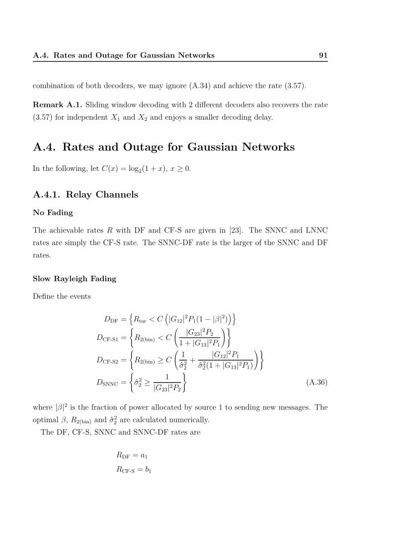
A.4. Rates and Outage for Gaussian Networks 91
combination of both decoders, we may ignore (A.34) and achieve the rate (3.57).
Remark A.1. Sliding window decoding with 2 different decoders also recovers the rate
(3.57) for independent X1 and X2 and enjoys a smaller decoding delay.
A.4. Rates and Outage for Gaussian Networks
In the following, let C(x) = log2(1 + x), x ≥ 0.
A.4.1. Relay Channels
No Fading
The achievable rates R with DF and CF-S are given in [23]. The SNNC and LNNC
rates are simply the CF-S rate. The SNNC-DF rate is the larger of the SNNC and DF
rates.
Slow Rayleigh Fading
Define the events
DDF ={
Rtar < C(|G12|2P1(1 − |β|2)
)}
DCF-S1 =
{R2(bin) < C
(|G23|2P2
1 + |G13|2P1
)}
DCF-S2 =
{R2(bin) ≥ C
(1
σ22
+|G12|2P1
σ22(1 + |G13|2P1)
)}
DSNNC =
{σ2
2 ≥ 1
|G23|2P2
}(A.36)
where |β|2 is the fraction of power allocated by source 1 to sending new messages. The
optimal β, R2(bin) and σ22 are calculated numerically.
The DF, CF-S, SNNC and SNNC-DF rates are
RDF = a1
RCF-S = b1

92 Appendix A. Proofs for Chapter 3
RSNNC = c1
RSNNC-DF =
RDF if DDF occurs
RSNNC otherwise(A.37)
where
a1 = min{C(|G12|2P1(1 − |β|2)
),
C(
|G13|2P1 + |G23|2P2 + 2ℜ{βG13G∗23}√
P1P2
)}
b1 =
C(
|G12|2P1
1+σ22
+ |G13|2P1
)if DCF-S1 ∩ DCF-S2
C (|G13|2P1) if DCF-S1 ∩ DcCF-S2
C(
|G13|2P1
1+|G23|2P2
)otherwise
c1 =
min{C (|G13|2P1 + |G23|2P2) − C( 1
σ22),
C(
|G12|2P1
1+σ22
+ |G13|2P1
)}if DSNNC
C(
|G13|2P1
1+|G23|2P2
)otherwise
(A.38)
and ℜ{x} is the real part of x and x∗ is the complex conjugate of x.
Remark A.2. For SNNC, event DSNNC means that
I(X2; Y3|X1) − I(Y2; Y2|X1X2Y3) ≥ 0 (A.39)
and the destination can reliably recover X2 and Y2 jointly which helps to decode X1.
Otherwise the destination should treat X2 as noise to get a better rate (see Theorem 3.1).
Similarly, for CF-S the events DCF-S1 and DCF-S2 mean that both X2 and Y2 can be
decoded in a step-by-step fashion [21]. If DCF-S1 and DcCF-S2 occur, then X2 can be
recovered which removes interference at the receiver. Otherwise the relay signal should
be treated as noise.
As recognized in [60], one drawback of DF is that if the source-relay link happens to be
weak and the relay tries to decode, then the rate suffers. Hence the relay should decode
only if the source-relay link is strong enough to support Rtar, i.e., if event DDF occurs.
Otherwise, the relay should perform CF-S or QF. Different choices of relay operations

A.4. Rates and Outage for Gaussian Networks 93
depending on the channel conditions lead to the achievable rates with SNNC-DF.
The outage probabilities are as follows:
P outDF = Pr[RDF < Rtar]
P outCF-S = Pr[RCF-S < Rtar]
P outSNNC = Pr[RSNNC < Rtar]
P outSNNC-DF = Pr[RSNNC-DF < Rtar] (A.40)
A.4.2. Two-Relay Channels
No Fading
The achievable DF rates are [23, Theorem 1]
RDF < max {RDF1, RDF2} (A.41)
where
RDF1 = min {a21, a22, a23}RDF2 = min {b21, b22, b23} (A.42)
with
a21 = C(|β1|2|G12|2P1
)
a22 = C(
(1 − |β3|2)|G13|2P1 + |γ1|2|G23|2P2 + 2ℜ{β2G13(γ1G23)∗}√
P1P2
)
a23 = C(|G14|2P1 + |G24|2P2 + |G34|2P3
+ (2ℜ{β2G14(γ1G24)∗} + 2ℜ{β3G14(γ2G24)∗})
√P1P2
+2ℜ{β3G14G∗34}√
P1P3 + 2ℜ{γ2G24G∗34}√
P2P3
)
b21 = C(|β1|2|G13|2P1
)
b22 = C(
(1 − |β3|2)|G12|2P1 + |γ1|2|G32|2P3 + 2ℜ{β2G12(γ1G32)∗}√
P1P3
)

94 Appendix A. Proofs for Chapter 3
b23 = C(|G14|2P1 + |G24|2P2 + |G34|2P3
+ (2ℜ{β2G14(γ1G34)∗} + 2ℜ{β3G14(γ2G34)∗})√
P1P3
+2ℜ{β2G14G∗24}√
P1P2 + 2ℜ{γ1G24G∗34}√
P2P3
)(A.43)
where∑3
i=1 |βi|2 = 1 and∑2
i=1 |γi|2 = 1 and the optimal power allocation parameters
are calculated numerically.
The CF-S rates are (see [23, Theorem 2] with Ui = 0, i = 2, 3)
RCF-S < c21 (A.44)
subject to
g2 ≤ d2, h2 ≤ e2, i2 ≤ f2
where
c21 = C
(|G12|2P1
1 + σ22
+|G13|2P1
1 + σ23
+ |G14|2P1
)
d2 = C
(|G24|2P2
1 + |G14|2P1
)
e2 = C
(|G34|2P3
1 + |G14|2P1
)
f2 = C
(|G24|2P2 + |G34|2P3
1 + |G14|2P1
)
g2 = C
1
σ22
+|G12|2P1
σ22(1 + |G13|2P1
(1+σ23)
+ |G14|2P1)
h2 = C
1
σ23
+|G13|2P1
σ23(1 + |G12|2P1
1+σ22
+ |G14|2P1)
i2 = C
(1 + σ2
2 + σ23
σ22 σ2
3
+|G12|2P1(1 + σ2
3) + |G13|2P1(1 + σ22)
σ22σ2
3(1 + |G14|2P1)
). (A.45)
The optimal σ22 and σ2
3 are calculated numerically.

A.4. Rates and Outage for Gaussian Networks 95
Referring to Theorem 3.1, the achievable SNNC rates are
RSNNC < min {c21, j21, j22, j23} (A.46)
where
j21 = C
(|G14|2P1 + |G24|2P2 +
|G13|2P1 + |G23|2P2
1 + σ23
+P1P2(|G13|2|G24|2 + |G14|2|G23|2)
1 + σ23
−2ℜ{G13G24G∗14G∗
23}P1P2
1 + σ23
)− C
(1
σ22
)
j22 = C
(|G14|2P1 + |G34|2P3 +
|G12|2P1 + |G32|2P3
1 + σ23
+P1P3(|G12|2|G34|2 + |G14|2|G32|2)
(1 + σ22)
−2ℜ {G12G34G∗14G∗
32} P1P3
(1 + σ22)
)− C
(1
σ23
)
j23 = C(|G14|2P1 + |G24|2P2 + |G34|2P3
)− C
(1 + σ2
2 + σ23
σ22σ2
3
). (A.47)
where c21 is defined in (A.45). The optimal σ22 and σ2
3 are calculated numerically.
If one relay uses DF and the other uses QF, rates satisfying
RDQF < max {RDQF1, RDQF2} (A.48)
can be achieved, where
RDQF1 = min {k21, k22, k23}RDQF2 = min {l21, l22, l23}
with
k21 = C
(|G12|2P1(1 − |θ|2)
1 + |G32|2P3
)

96 Appendix A. Proofs for Chapter 3
k22 = C(
|G14|2P1 + |G24|2P2 + 2ℜ{θG14G∗24}√
P1P2
+|G13|2P1 + |G23|2P2 + 2ℜ{θG13G
∗23}√
P1P2
1 + σ23
+(1 − |θ|2)P1P2(|G13|2|G24|2 + |G14|2|G23|2 − 2ℜ{G13G24G∗
14G∗23})
1 + σ23
)
k23 = C(
|G14|2P1 + |G24|2P2 + |G34|2P3 + 2ℜ{θG14G∗24}√
P1P2
)− C
(1
σ23
)(A.49)
and
l21 = C
(|G13|2P1(1 − |θ|2)
1 + |G23|2P2
)
l22 = C(
|G14|2P1 + |G34|2P3 + 2ℜ{θG14G∗34}√
P1P3
+|G12|2P1 + |G32|2P3 + 2ℜ{θG12G
∗32}√
P1P3
1 + σ22
+(1 − |θ|2)P1P3(|G12|2|G34|2 + |G14|2|G32|2 − 2ℜ{G12G34G∗
14G∗32})
1 + σ22
)
l23 = C(
|G14|2P1 + |G24|2P2 + |G34|2P3 + 2ℜ{θG14G∗34}√
P1P3
)− C
(1
σ22
)(A.50)
where 0 ≤ |θ|2 ≤ 1 and the optimal θ, σ22 and σ2
3 for RDQF1 and RDQF2 are calculated
numerically.
Referring to Theorem 3.4, SNNC-DF achieves rates satisfying
RSNNC-DF < max {RDF, RDQF, RSNNC}. (A.51)
Slow Rayleigh Fading
Define the events
DDFV =
Rtar < V21
Rtar < V22
DDF1 = { Rtar < k21}DDF2 = { Rtar < l21}
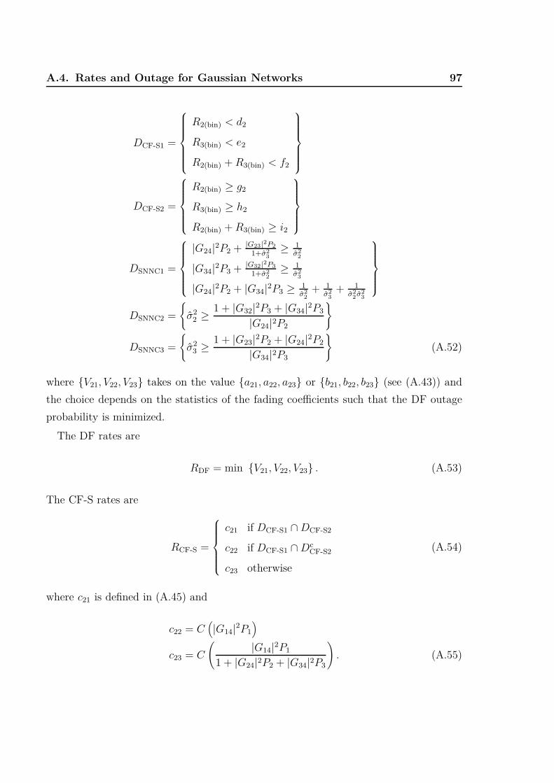
A.4. Rates and Outage for Gaussian Networks 97
DCF-S1 =
R2(bin) < d2
R3(bin) < e2
R2(bin) + R3(bin) < f2
DCF-S2 =
R2(bin) ≥ g2
R3(bin) ≥ h2
R2(bin) + R3(bin) ≥ i2
DSNNC1 =
|G24|2P2 + |G23|2P2
1+σ23
≥ 1σ2
2
|G34|2P3 + |G32|2P3
1+σ22
≥ 1σ2
3
|G24|2P2 + |G34|2P3 ≥ 1σ2
2+ 1
σ23
+ 1σ2
2 σ23
DSNNC2 =
{σ2
2 ≥ 1 + |G32|2P3 + |G34|2P3
|G24|2P2
}
DSNNC3 =
{σ2
3 ≥ 1 + |G23|2P2 + |G24|2P2
|G34|2P3
}(A.52)
where {V21, V22, V23} takes on the value {a21, a22, a23} or {b21, b22, b23} (see (A.43)) and
the choice depends on the statistics of the fading coefficients such that the DF outage
probability is minimized.
The DF rates are
RDF = min {V21, V22, V23} . (A.53)
The CF-S rates are
RCF-S =
c21 if DCF-S1 ∩ DCF-S2
c22 if DCF-S1 ∩ DcCF-S2
c23 otherwise
(A.54)
where c21 is defined in (A.45) and
c22 = C(|G14|2P1
)
c23 = C
(|G14|2P1
1 + |G24|2P2 + |G34|2P3
). (A.55)

98 Appendix A. Proofs for Chapter 3
Observe that if both DCF-S1 and DCF-S2 occur, then both the bin and quantization indices
can be decoded. If only DCF-S1 occurs, then only the bin index can be recovered.
Referring to Theorem 3.1 the SNNC rates are
RSNNC =
min {c21, j21, j22, j23} if DSNNC1
min {m21, m22} if DcSNNC1 ∩ DSNNC2
min {q21, q22} if DcSNNC1 ∩ DSNNC3
c23 otherwise
(A.56)
where
m21 = C
(P1(|G12|2 + (1 + σ2
2)|G14|2) + P1P3|G14|2|G32|2|G32|2P3 + (1 + σ2
2) (1 + |G34|2P3)
+P1P3(|G12|2|G34|2 − 2ℜ{G12G34G∗
14G∗32})
|G32|2P3 + (1 + σ22) (1 + |G34|2P3)
)
m22 = C
(|G14|2P1 + |G24|2P2
1 + |G34|2P3
)− C
(1
σ22
+|G32|2P3
σ22 (1 + |G34|2P3)
)
q21 = C
(P1(|G13|2 + (1 + σ2
3)|G14|2) + P1P2|G14|2|G23|2|G23|2P2 + (1 + σ2
3) (1 + |G24|2P2)
+P1P2(|G13|2|G24|2 − 2ℜ{G13G24G∗
14G∗23})
|G23|2P2 + (1 + σ23) (1 + |G24|2P2)
)
q22 = C
(|G14|2P1 + |G34|2P3
1 + |G24|2P2
)− C
(1
σ23
+|G23|2P2
σ23 (1 + |G24|2P2)
). (A.57)
The event DSNNC1 means that both quantization indices can be recovered. The events
DSNNC2 and DSNNC3 mean that only one of the two quantization indices can be decoded.
The SNNC-DF rates are
RSNNC-DF =
RDF if DDFV
RDQF1 if DcDFV ∩ DDF1
RDQF2 if DcDFV ∩ DDF2
RSNNC otherwise
(A.58)
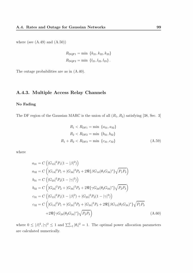
A.4. Rates and Outage for Gaussian Networks 99
where (see (A.49) and (A.50))
RDQF1 = min {k21, k22, k23}RDQF2 = min {l21, l22, l23} .
The outage probabilities are as in (A.40).
A.4.3. Multiple Access Relay Channels
No Fading
The DF region of the Gaussian MARC is the union of all (R1, R2) satisfying [38, Sec. 3]
R1 < RDF1 = min {a31, a32}R2 < RDF2 = min {b31, b32}
R1 + R2 < RDF3 = min {c31, c32} (A.59)
where
a31 = C(|G13|2P1(1 − |β|2)
)
a32 = C(
|G14|2P1 + |G34|2P3 + 2ℜ{βG14(θ1G34)∗}√
P1P3
)
b31 = C(|G23|2P2(1 − |γ|2)
)
b32 = C(
|G24|2P2 + |G34|2P3 + 2ℜ{γG24(θ2G34)∗}√
P2P3
)
c31 = C(|G13|2P1(1 − |β|2) + |G23|2P2(1 − |γ|2)
)
c32 = C(
|G14|2P1 + |G24|2P2 + |G34|2P3 + 2ℜ{βG14(θ1G34)∗}√
P1P3
+2ℜ{γG24(θ2G34)∗}√
P2P3
)(A.60)
where 0 ≤ |β|2, |γ|2 ≤ 1 and∑2
i=1 |θi|2 = 1. The optimal power allocation parameters
are calculated numerically.

100 Appendix A. Proofs for Chapter 3
The achievable CF-S rate region is the union of all (R1, R2) satisfying [38, Sec. 3]
R1 < d31
R2 < e31
R1 + R2 < f31 (A.61)
where
d31 = C
(|G13|2P1
1 + σ23
+ |G14|2P1
)
e31 = C
(|G23|2P2
1 + σ23
+ |G24|2P2
)
f31 = C
(|G14|2P1 + |G24|2P2 +
|G13|2P1 + |G23|2P2
1 + σ23
+P1P2(|G13|2|G24|2 + |G14|2|G23|2 − 2ℜ{G13G24G∗
14G∗23})
1 + σ23
)(A.62)
for some
σ23 ≥ 1 + (|G13|2 + |G14|2)P1 + (|G23|2 + |G24|2)P2
|G34|2P3
+P1P2(|G13|2|G24|2 + |G14|2|G23|2 − 2ℜ{G13G24G∗
14G∗23})
|G34|2P3
.
Referring to Theorem 3.1, the SNNC rate region is the union of pairs (R1, R2) satisfying
R1 < min {d31, g31}R2 < min {e31, h31}
R1 + R2 < min {f31, i31} (A.63)
where d31, e31 and f31 are defined in (A.62) and
g31 = C(|G14|2P1 + |G34|2P3
)− C
(1
σ23
)
h31 = C(|G24|2P2 + |G34|2P3
)− C
(1
σ23
)

A.4. Rates and Outage for Gaussian Networks 101
i31 = C(|G14|2P1 + |G24|2P2 + |G34|2P3
)− C
(1
σ23
)
for some σ23 > 1
|G34|2P3. The SNNC-DF rate region is the union of the SNNC and DF
rate regions.
Slow Rayleigh Fading
Define the events
DDF =
Rtar1 < a31
Rtar2 < b31
Rtar1 + Rtar2 < c31
DCF-S1 =
{R3(bin) < C
(|G34|2P3
1 + |G14|2P1 + |G24|2P2
)}
DCF-S2 =
{R3(bin) ≥ C
(1
σ23
+|G13|2P1 + |G23|2P2
σ23 (1 + |G14|2P1 + |G24|2P2)
+P1P2(|G13|2|G24|2 + |G14|2|G23|2 − 2ℜ{G13G24G∗
14G∗23})
σ23 (1 + |G14|2P1 + |G24|2P2)
)}
DSNNC =
{σ2
3 ≥ 1
|G34|2P3
}. (A.64)
The DF rate region of the Gaussian MARC is the union of all (R1, R2) satisfying (A.59).
The CF-S rate region is the union of all (R1, R2) satisfying [38]
R1 < RCF1 =
d31 if DCF-S1 ∩ DCF-S2
d32 if DCF-S1 ∩ DcCF-S2
d33 otherwise
(A.65)
R2 < RCF2 =
e31 if DCF-S1 ∩ DCF-S2
e32 if DCF-S1 ∩ DcCF-S2
e33 otherwise
(A.66)
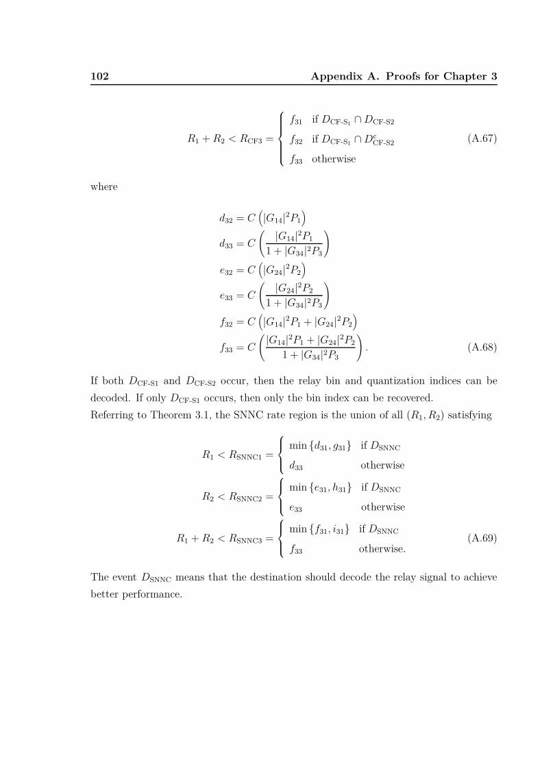
102 Appendix A. Proofs for Chapter 3
R1 + R2 < RCF3 =
f31 if DCF-S1 ∩ DCF-S2
f32 if DCF-S1 ∩ DcCF-S2
f33 otherwise
(A.67)
where
d32 = C(|G14|2P1
)
d33 = C
(|G14|2P1
1 + |G34|2P3
)
e32 = C(|G24|2P2
)
e33 = C
(|G24|2P2
1 + |G34|2P3
)
f32 = C(|G14|2P1 + |G24|2P2
)
f33 = C
(|G14|2P1 + |G24|2P2
1 + |G34|2P3
). (A.68)
If both DCF-S1 and DCF-S2 occur, then the relay bin and quantization indices can be
decoded. If only DCF-S1 occurs, then only the bin index can be recovered.
Referring to Theorem 3.1, the SNNC rate region is the union of all (R1, R2) satisfying
R1 < RSNNC1 =
min {d31, g31} if DSNNC
d33 otherwise
R2 < RSNNC2 =
min {e31, h31} if DSNNC
e33 otherwise
R1 + R2 < RSNNC3 =
min {f31, i31} if DSNNC
f33 otherwise.(A.69)
The event DSNNC means that the destination should decode the relay signal to achieve
better performance.

A.4. Rates and Outage for Gaussian Networks 103
The SNNC-DF rate region is the union of all (R1, R2) satisfying
R1 < RSNNC-DF1 =
RDF1 if DDF
RSNNC1 otherwise
R2 < RSNNC-DF2 =
RDF2 if DDF
RSNNC2 otherwise
R1 + R2 < RSNNC-DF3 =
RDF3 if DDF
RSNNC3 otherwise.(A.70)
If DDF occurs, then the relay should decode which will remove interference at the relay.
Otherwise, the relay should perform QF to avoid unnecessarily lowering the rates.
Let Rtar3 = Rtar1 + Rtar2. The outage probabilities are:
P outDF = Pr[{RDF1 < Rtar1} ∪ {RDF2 < Rtar2} ∪ {RDF3 < Rtar3}]
P outCF-S = Pr[{RCF-S1 < Rtar1} ∪ {RCF-S2 < Rtar2} ∪ {RCF-S < Rtar3}]
P outSNNC = Pr[{RSNNC1 < Rtar1} ∪ {RSNNC2 < Rtar2} ∪ {RSNNC3 < Rtar3}]
P outSNNC-DF = Pr[{RSNNC-DF1 < Rtar1} ∪ {RSNNC-DF2 < Rtar2} ∪ {RSNNC-DF3 < Rtar3}]
(A.71)
A.4.4. Two-Way Relay Channels
No Fading
The DF rate region for the Gaussian TWRC is the union of all (R1, R2) satisfying
R1 < RDF1 = min {a41, a42}R2 < RDF2 = min {b41, b42}
R1 + R2 < RDF3 = c41 (A.72)
where
a41 = C(|G13|2P1(1 − |β|2)
)

104 Appendix A. Proofs for Chapter 3
a42 = C(
|G12|2P1 + |G32|2P3(1 − |θ1|2) + 2ℜ{βG12(θ1G32)∗}√
P1P3
)
b41 = C(|G23|2P2(1 − |γ|2)
)
b42 = C(
|G21|2P2 + |G31|2P3(1 − |θ1|2) + 2ℜ{γG21(θ2G31)∗}√
P2P3
)
c41 = C(|G13|2P1(1 − |β|2) + |G23|2P2(1 − |γ|2)
)(A.73)
where 0 ≤ |β|2, |γ|2 ≤ 1 and∑2
i=1 |θi|2 = 1. The optimal power allocation parameters
are calculated numerically.
The CF-S rate region [61, Proposition 4] is the union of all (R1, R2) satisfying
R1 < d41
R2 < e41 (A.74)
where
d41 = C
(|G12|2P1 +
|G13|2P1
1 + σ23
)
e41 = C
(|G21|2P2 +
|G23|2P2
1 + σ23
)
for some
σ23 ≥ max {f41, f42, f43, f44}
where
f41 =1 + |G12|2P1 + |G13|2P1
|G32|2P3
f42 =|G21|2P2 + 1
|G31|2P3
+|G13|2P1(|G21|2P2 + 1)
|G31|2P3(|G12|2P1 + 1)
f43 =1 + |G21|2P2 + |G23|2P2
|G31|2P3,
f44 =|G12|2P1 + 1
|G32|2P3+
|G23|2P2(|G12|2P1 + 1)
|G32|2P3(|G21|2P2 + 1).

A.4. Rates and Outage for Gaussian Networks 105
Referring to Theorem 3.1, the SNNC rate region is the union of all (R1, R2) satisfying
R1 < min {d41, g41}R2 < min {e41, h41} (A.75)
where
g41 = C(|G12|2P1 + |G32|2P3
)− C
(1
σ23
)
h41 = C(|G21|2P2 + |G31|2P3
)− C
(1
σ23
)
for some σ23 > 0. The SNNC-DF rate region is the union of the DF and SNNC rate
regions.
Slow Rayleigh Fading
Define the events
DDF =
Rtar1 < a41
Rtar2 < b41
Rtar1+ Rtar2
< c41
DCF-S11 =
{R3(bin) < C
(|G31|2P3
1 + |G21|2P2
)}
DCF-S12 =
{R3(bin) ≥ C
(1
σ23
+|G23|2P2
σ23 (1 + |G21|2P2)
)}
DCF-S21 =
{R3(bin) < C
(|G32|2P3
1 + |G12|2P1
)}
DCF-S22 =
{R3(bin) ≥ C
(1
σ23
+|G13|2P1
σ23 (1 + |G12|2P1)
)}
DSNNC1 =
{σ2
3 ≥ 1
|G32|2P3
}
DSNNC2 =
{σ2
3 ≥ 1
|G31|2P3
}.

106 Appendix A. Proofs for Chapter 3
The DF region is the union of all (R1, R2) satisfying (A.72). The CF-S region is the
union of all (R1, R2) satisfying
R1 < RCF-S1 =
d41 if DCF-S21 ∩ DCF-S22
d42 if DCF-S21 ∩ DcCF-S22
d43 otherwise
(A.76)
R2 < RCF-S2 =
e41 if DCF-S11 ∩ DCF-S12
e42 if DCF-S11 ∩ DcCF-S12
e43 otherwise
(A.77)
where
d42 = C(|G12|2P1
)
d43 = C
(|G12|2P1
1 + |G32|2P3
)
e42 = C(|G21|2P2
)
e43 = C
(|G21|2P2
1 + |G31|2P3
).
The optimal R3(bin) and σ23 are calculated numerically.
Referring to Theorem 3.1, SNNC achieves all pairs (R1, R2) satisfying
R1 < RSNNC1 =
min {d41, g41} if DSNNC1
d43 otherwise(A.78)
R2 < RSNNC2 =
min {e41, h41} if DSNNC2
e43 otherwise.(A.79)
The SNNC-DF rate region is the union of the (R1, R2) satisfying
R1 < RSNNC-DF1 =
RDF1 if DDF
RSNNC1 otherwise(A.80)

A.4. Rates and Outage for Gaussian Networks 107
R2 < RSNNC-DF2 =
RDF2 if DDF
RSNNC2 otherwise.(A.81)
The outage probabilities are:
P outDF = Pr[{RDF1 < Rtar1} ∪ {RDF2 < Rtar2}]
P outCF-S = Pr[{RCF-S1 < Rtar1} ∪ {RCF-S2 < Rtar2}]
P outSNNC = Pr[{RSNNC1 < Rtar1} ∪ {RSNNC2 < Rtar2}]
P outSNNC-DF = Pr[{RSNNC-DF1 < Rtar1} ∪ {RSNNC-DF2 < Rtar2}] (A.82)


BProofs for Chapter 5
B.1. Proof of Lemma 5.2: Non-Uniform W
Observe that H(W ) = H(BnR) = nR · H2(p). Following the same steps as in (5.9) we
have
E[D(PV n|C
||QnV )] = E
[log
∑Mj=1 P (j)QV n|Un(V n|Un(j))
QnV (V n)
]
=∑
w
P (w) · E
log
∑Mj=1 P (j)Qn
V |U(V n|Un(j))
QnV (V n)
∣∣∣∣∣∣∣∣W = w
≤∑
w
P (w) · E
[log
(P (w)Qn
V |U(V n|Un(w))
QnV (V n)
+ 1 − P (w)
)]
≤∑
w
P (w) · E
[log
(P (w)Qn
V |U(V n|Un(w))
QnV (V n)
+ 1
)]
= d1 + d2 + d3 (B.1)

110 Appendix B. Proofs for Chapter 5
where
d1 =∑
w∈T nǫ (P n
X)
P (w)∑
(un(w),vn)∈T nǫ (Qn
UV)
QnUV (un(w), vn)
[log
(P (w)Qn
V |U(vn|un(w))
QnV (vn)
+ 1
)]
d2 =∑
w∈T nǫ (P n
X)
P (w)∑
(un(w),vn)/∈T nǫ (QUV )
(un(w),vn)∈supp(QnUV
)
QnUV (un(w), vn)
[log
(P (w)Qn
V |U(vn|un(w))
QnV (vn)
+ 1
)]
d3 =∑
w /∈T nǫ (P n
X)
w∈supp(P nX
)
P (w)∑
(un(w),vn)∈supp(QnUV
)
QnUV (un(w), vn)
[log
(P (w)Qn
V |U(vn|un(w))
QnV (vn)
+ 1
)].
(B.2)
We can bound d1 as follows (see (5.12))
d1 ≤∑
w∈T nǫ (P n
X)
P (w)
[log
(2n(I(V ;U)+2ǫH(V ))
2n(1−ǫ)R·H2(p)+ 1
)]
≤ log(2−n(R·H2(p)−I(V ;U)−ǫ(2H(V )+R·H2(p))) + 1
)
≤ log(e) · 2−n(R·H2(p)−I(V ;U)−δǫ(n)) (B.3)
which goes to zero if R > I(V ;U)+δǫ(n)H2(p)
and n → ∞, where δǫ(n) = ǫ(2H(V ) + R · H2(p)).
We also have
d2 ≤∑
w∈T nǫ (P n
X)
P (w)∑
(un(w),vn)/∈T nǫ (QUV )
(un(w),vn)∈supp(QnUV
)
QnUV (un(w), vn)
[log
((1
µV
)n
+ 1
)]
≤ 2|V| · |U| · e−2nǫ2µ2UV log
((1
µV
)n
+ 1
)(B.4)
which goes to zero as n → ∞ (see (5.13)). We further have
d3 ≤∑
w /∈T nǫ (P n
X)
w∈supp(P nX
)
P (w)∑
(un(w),vn)∈supp(QnUV
)
QnUV (un(w), vn)
[log
((1
µV
)n
+ 1
)]
≤∑
w /∈T nǫ (P n
X)
w∈supp(P nX
)
P (w)
[log
((1
µV
)n
+ 1
)]

B.2. Proof of Lemma 5.3 111
≤ 4 · e−2nǫ2p2
log
((1
µV
)n
+ 1
)(B.5)
which goes to zero as n → ∞ (see (5.13)).
Combining the above for non-uniform W we have
E[D(PV n|C
||QnV )] → 0 (B.6)
if R > I(V ;U)+δn(ǫ)H2(p)
and n → ∞.
B.2. Proof of Lemma 5.3
We extend the proof of [42, Sec. III, Inequality (15)] to asymptotic cases to establish
Lemma 5.3. Recall that −12
≤ ρ ≤ 0. Let s = −ρ1+ρ
so we have
0 ≤ s ≤ 1
1 + s =1
1 + ρ(B.7)
We also have for any a, b ≥ 0 and 0 ≤ x ≤ 1
(a + b)x ≤ ax + bx. (B.8)
Observe that for any vn we have
E[P (vn|C)] = E
[M∑
w=1
1
M· Qn
V |U(vn|Un(w))
]
= E[Qn
V |U(vn|Un(1))]
= E
[n∏
i=1
QV |U(vi|Ui(1))
]
=n∏
i=1
E[QV |U(vi|Ui(1))
]
=n∏
i=1
[∑
u
Q(u)QV |U(vi|u)
]

112 Appendix B. Proofs for Chapter 5
=n∏
i=1
QV (vi) = QnV (vn). (B.9)
We further have
eEn0 (ρ,Qn
UV) =
∑
vn
{E[P (vn|C)
11+ρ ]
}1+ρ
(a)=∑
vn
{E[P (vn|C)1+s]
} 11+s
=∑
vn
E
(
M∑
w=1
1
M· Qn
V |U(vn|Un(w))
)1+s
11+s
=1
M
∑
vn
E
M∑
w=1
QnV |U(vn|Un(w))
Qn
V |U(vn|Un(w)) +M∑
j 6=w
QnV |U(vn|Un(j))
s
11+s
(B.10)
where (a) follows from (B.7). Applying (B.8) to (B.10) we have
eEn0 (ρ,Qn
UV) ≤ 1
M
∑
vn
{E
[M∑
w=1
QnV |U(vn|Un(w))
(Qn
V |U(vn|Un(w)))s
+
M∑
j 6=w
QnV |U(vn|Un(j))
s
11+s
(a)=
1
M
∑
vn
{E
[M∑
w=1
(Qn
V |U(vn|Un(w)))1+s
]
+M∑
w=1
(E[Qn
V |U(vn|Un(w))])
· E
M∑
j 6=w
QnV |U(vn|Un(j))
s
11+s
(b)
≤ 1
M
∑
vn
ME
[(Qn
V |U(vn|Un))1+s
]+ MQn
V (vn) ·E
M∑
j 6=w
QnV |U(vn|Un(j))
s
11+s
(c)=
1
M
∑
vn
{ME
[(Qn
V |U(vn|Un))1+s
]+ MQn
V (vn) ((M − 1)QnV (vn))s
} 11+s
≤ 1
M
∑
vn
{ME
[(Qn
V |U(vn|Un))1+s
]+ (MQn
V (vn))1+s} 1
1+s
(B.11)
where

B.2. Proof of Lemma 5.3 113
(a) follows because Un(w) is independent of Un(j), j 6= w
(b) follows by choosing UnV n ∼ QnUV , by the concavity of xa for 0 ≤ a ≤ 1 and by (B.9)
(c) follows by (B.9)
Applying (B.8) again to (B.11) we have
eEn0 (ρ,Qn
UV) ≤ 1
M
∑
vn
{(ME
[(Qn
V |U(vn|Un))1+s
]) 11+s
+ MQnV (vn)
}
(a)= 1 + Mρ
∑
vn
(E[(
QnV |U(vn|Un)
) 11+ρ
])1+ρ
= 1 + Mρ∑
vn
(∑
un
QnU(un)
(Qn
V |U(vn|un)) 1
1+ρ
)1+ρ
(b)= 1 + enρR
∑
v
(∑
u
Q(u) (Q(v|u))1
1+ρ
)n(1+ρ)
= 1 + en(E0(ρ,QUV )+ρR) (B.12)
where
(a) follows from (B.7)
(b) follows because the UiVi are i.i.d., i = 1, . . . , n
Optimizing over ρ, we have
En0 (ρ, Qn
UV ) ≤ ln(1 + enEG(R,QUV )
)
≤ enEG(R,QUV ). (B.13)


CAbbreviations
List of Abbreviations
AWGN additive white Gaussian noise
BCC broadcast channel with confidential messages
BMC block Markov coding
CF compress-forward
CF-S compress-forward with step-by-step decoding
DF decode-forward
DMN discrete memoryless network
i.i.d. independent and identically distributed
LNNC long message noisy network coding
MAC multiple access channel
MARC multiple access relay channel
NNC noisy network coding
QF quantize-forward

116 List of Abbreviations
RHS right-hand side
SNNC short message noisy network coding
TWRC two-way relay channel
117
Bibliography
[1] C. E. Shannon, “A mathematical theory of communication,” Bell Syst. Tech. Jour-
nal, vol. 27, pp. 379–423, 623–656, July, October 1948.
[2] H. Liao, “Multiple-access channels,” Ph.D. dissertation, University of Hawaii, Hon-
olulu, 1972.
[3] R. Ahlswede, “Multi-way communication channels,” in IEEE Int. Symp. Inf. The-
ory, Tsahkadsor, Armenia, Sept. 1971, pp. 23–51.
[4] D. Slepian and J. Wolf, “Noiseless coding of correlated information sources,” IEEE
Trans. Inf. Theory, vol. 19, no. 4, pp. 471–480, July 1973.
[5] M. Yassaee and M. Aref, “Slepian-Wolf coding over cooperative networks,” in IEEE
Int. Symp. Inf. Theory, Seoul, Korea, June 2009, pp. 879–883.
[6] ——, “Slepian-Wolf coding over cooperative relay networks,” IEEE Trans. Inf. The-
ory, vol. 57, no. 6, pp. 3462–3482, 2011.
[7] X. Wu and L.-L. Xie, “On the optimal compressions in the compress-and-forward
relay schemes,” IEEE Trans. Inf. Theory, vol. 59, no. 5, pp. 2613–2628, 2013.
[8] G. Kramer and J. Hou, “Short-message quantize-forward network coding,” in 2011
8th Int. Workshop on Multi-Carrier Systems Solutions (MC-SS), Herrsching, Ger-
many, May 2011, pp. 1–3.
[9] J. Hou and G. Kramer, “Short message noisy network coding for multiple sources,”
in IEEE Int. Symp. Inf. Theory, Boston, USA, July 2012, pp. 1677–1681.
[10] S. Lim, Y.-H. Kim, A. El Gamal, and S.-Y. Chung, “Noisy network coding,” in
IEEE Inf. Theory Workshop (ITW), Cairo, Egypt, Jan. 2010, pp. 1–5.
118 Bibliography
[11] ——, “Noisy network coding,” IEEE Trans. Inf. Theory, vol. 57, no. 5, pp. 3132–
3152, May 2011.
[12] R. Ahlswede, N. Cai, S.-Y. Li, and R. Yeung, “Network information flow,” IEEE
Trans. Inf. Theory, vol. 46, no. 4, pp. 1204–1216, July 2000.
[13] A. Dana, R. Gowaikar, R. Palanki, B. Hassibi, and M. Effros, “Capacity of wireless
erasure networks,” IEEE Trans. Inf. Theory, vol. 52, no. 3, pp. 789–804, March
2006.
[14] N. Ratnakar and G. Kramer, “The multicast capacity of deterministic relay net-
works with no interference,” IEEE Trans. Inf. Theory, vol. 52, no. 6, pp. 2425–2432,
June 2006.
[15] A. Avestimehr, S. Diggavi, and D. Tse, “Wireless network information flow: A
deterministic approach,” IEEE Trans. Inf. Theory, vol. 57, no. 4, pp. 1872–1905,
April 2011.
[16] A. Wyner, “The common information of two dependent random variables,” IEEE
Trans. Inf. Theory, vol. 21, no. 2, pp. 163–179, March 1975.
[17] T. Han and S. Verdú, “Approximation theory of output statistics,” IEEE Trans.
Inf. Theory, vol. 39, no. 3, pp. 752–772, May 1993.
[18] A. Wyner and J. Ziv, “The rate-distortion function for source coding with side
information at the decoder,” IEEE Trans. Inf. Theory, vol. 22, no. 1, pp. 1–10, Jan.
1976.
[19] J. L. Massey, Applied Digital Information Theory, ETH Zurich, Zurich, Switzerland,
1980-1998.
[20] A. Orlitsky and J. Roche, “Coding for computing,” IEEE Trans. Inf. Theory,
vol. 47, no. 3, pp. 903–917, March 2001.
[21] T. Cover and A. E. Gamal, “Capacity theorems for the relay channel,” IEEE Trans.
Inf. Theory, vol. 25, no. 5, pp. 572–584, Sept. 1979.
[22] B. Schein, “Distributed coordination in network information theory,” Ph.D. disser-
tation, MIT, Cambridge, MA, USA, 2001.

Bibliography 119
[23] G. Kramer, M. Gastpar, and P. Gupta, “Cooperative strategies and capacity theo-
rems for relay networks,” IEEE Trans. Inf. Theory, vol. 51, no. 9, pp. 3037–3063,
Sept. 2005.
[24] M. Yassaee and M. Aref, “Generalized compress-and-forward strategy for relay net-
works,” in IEEE Int. Symp. Inf. Theory, Toronto, Canada, July 2008, pp. 2683–
2687.
[25] G. Kramer and J. Hou, “On message lengths for noisy network coding,” in IEEE
Inf. Theory Workshop (ITW), Paraty, Brazil, Oct. 2011, pp. 430–431.
[26] P. Zhong, A. Haija, and M. Vu, “On compress-forward without Wyner-Ziv
binning for relay networks,” submitted to IEEE Trans. Inf. Theory, 2011. [Online].
Available: http://arxiv.org/abs/1111.2837/
[27] A. Raja and P. Viswanath, “Compress-and-forward scheme for a relay network:
Approximate optimality and connection to algebraic flows,” submitted to IEEE
Trans. Inf. Theory. [Online]. Available: http://arxiv.org/abs/1012.0416/
[28] T. Cover and J. Thomas, Elements of Information Theory, 2nd ed. New York:
Wiley, 2006.
[29] G. Kramer, “Capacity results for the discrete memoryless network,” IEEE Trans.
Inf. Theory, vol. 49, no. 1, pp. 4–21, Jan. 2003.
[30] A. El Gamal and Y.-H. Kim, Network Information Theory. Cambridge University
Press, 2011.
[31] L. Sankar, G. Kramer, and N. B. Mandayam, “Offset encoding for multiple-access
relay channels,” IEEE Trans. Inf. Theory, vol. 53, no. 10, pp. 3814–3821, 2007.
[32] J. Du, M. Xiao, M. Skoglund, and S. Shamai (Shitz), “Short-message noisy network
coding with partial source cooperation,” in IEEE Inf. Theory Workshop (ITW),
Lausanne, Switzerland, Sept. 2012, pp. 144–147.
[33] L.-L. Xie and P. Kumar, “An achievable rate for the multiple-level relay channel,”
IEEE Trans. Inf. Theory, vol. 51, no. 4, pp. 1348–1358, April 2005.
120 Bibliography
[34] L. Ozarow, S. Shamai, and A. Wyner, “Information theoretic considerations for
cellular mobile radio,” IEEE Trans. on Veh. Technol., vol. 43, no. 2, pp. 359–378,
May 1994.
[35] G. Kramer and A. van Wijngaarden, “On the white gaussian multiple-access relay
channel,” in IEEE Int. Symp. Inf. Theory, Sorrento, Italy, June 2000, p. 40.
[36] L. Sankaranarayanan, G. Kramer, and N. Mandayam, “Capacity theorems for the
multiple-access relay channel,” in 42nd. Allerton Conf. Communications, Control,
and Computing, Sept. 2004.
[37] G. Kramer, P. Gupta, and M. Gastpar, “Information-theoretic multihopping for
relay networks,” in Int. Zurich Seminar on Communications, Zurich, Switzerland,
Feb. 2004, pp. 192–195.
[38] L. Sankaranarayanan, G. Kramer, and N. Mandayam, “Hierarchical sensor net-
works: capacity bounds and cooperative strategies using the multiple-access relay
channel model,” in 2004 First Annual IEEE Commun. Soc. Conf. on Sensor and
Ad Hoc Commun. and Networks, Santa Clara, Oct. 2004, pp. 191–199.
[39] N. Gaarder and J. Wolf, “The capacity region of a multiple-access discrete mem-
oryless channel can increase with feedback (corresp.),” IEEE Trans. Inf. Theory,
vol. 21, no. 1, pp. 100–102, Jan. 1975.
[40] T. Cover and C. Leung, “An achievable rate region for the multiple-access channel
with feedback,” IEEE Trans. Inf. Theory, vol. 27, no. 3, pp. 292–298, May 1981.
[41] L. Ozarow, “The capacity of the white gaussian multiple access channel with feed-
back,” IEEE Trans. on Inf. Theory, vol. 30, no. 4, pp. 623–629, 1984.
[42] M. Hayashi, “General nonasymptotic and asymptotic formulas in channel resolv-
ability and identification capacity and their application to the wiretap channel,”
IEEE Trans. Inf. Theory, vol. 52, no. 4, pp. 1562–1575, April 2006.
[43] M. Bloch and J. Kliewer, “On secure communication with constrained randomiza-
tion,” in IEEE Int. Symp. Inf. Theory, Boston, MA, USA, July 2012, pp. 1172–1176.
[44] I. Csiszár, “Almost independence and secrecy capacity,” Prob. of Inf. Transmission,
vol. 32, no. 1, pp. 40–47, Jan.–March 1996.

Bibliography 121
[45] A. Winter, “Secret, public and quantum correlation cost of triples of random vari-
ables,” in IEEE Int. Symp. Inf. Theory, Adelaide, Australia, Sept. 2005, pp. 2270–
2274.
[46] R. G. Gallager, Information Theory and Reliable Communication. Wiley, 1968.
[47] I. Csiszár and J. Körner, Information Theory: Coding Theorems for Discrete Mem-
oryless Systems. New York: Academic, 1981.
[48] P. Cuff, H. Permuter, and T. Cover, “Coordination capacity,” IEEE Trans. Inf.
Theory, vol. 56, no. 9, pp. 4181–4206, Sept. 2010.
[49] U. Maurer and S. Wolf, “Information-theoretic key agreement: From weak to strong
secrecy for free,” in Advances in Cryptology - Eurocrypt 2000. Lecture Notes in
Computer Science, Springer-Verlag, 2000, pp. 351–368.
[50] M. Bloch and J. Barros, Physical Layer Security From Information Theory to Se-
curity Engineering. Cambridge University Press, 2011.
[51] A. Wyner, “The wire-tap channel,” Bell Syst. Tech. Journal, vol. 54, no. 8, pp.
1355–1387, Oct. 1975.
[52] I. Csiszár and J. Körner, “Broadcast channels with confidential messages,” IEEE
Trans. Inf. Theory, vol. 24, no. 3, pp. 339–348, May 1978.
[53] G. Kramer, “Teaching IT: An identity for the Gelfand-Pinsker converse,” IEEE Inf.
Theory Society Newsletter, vol. 61, no. 4, pp. 4–6, Dec. 2011.
[54] J. Hou and G. Kramer, “Informational divergence approximations to product dis-
tributions,” in 13th Canadian Workshop on Inf. Theory (CWIT), Toronto, Canada,
June 2013, pp. 76–81.
[55] E. L. Lehmann and J. P. Romano, Testing Statistical Hypotheses, 3rd ed. New
York: Springer, 2005.
[56] B. Chern and A. Ozgur, “Achieving the capacity of the n-relay gaussian dia-
mond network within logn bits,” in IEEE Inf. Theory Workshop (ITW), Lausanne,
Switzerland, Sept. 2012, pp. 377–380.
122 Bibliography
[57] R. Kolte and A. Ozgur, “Improved capacity approximations for gaussian relay net-
works,” in IEEE Inf. Theory Workshop (ITW), Seville, Spain, Sept. 2013, pp. 1–5.
[58] ——, “Optimized noisy network coding for gaussian relay networks,” in Int. Zurich
Seminar on Communications, Zurich, Switzerland, Feb. 2014, pp. 140–143.
[59] H. Mahdavifar and A. Vardy, “Achieving the secrecy capacity of wiretap channels
using polar codes,” IEEE Trans. Inf. Theory, vol. 57, no. 10, pp. 6428–6443, Oct.
2011.
[60] J. Laneman, D. Tse, and G. Wornell, “Cooperative diversity in wireless networks:
Efficient protocols and outage behavior,” IEEE Trans. Inf. Theory, vol. 50, no. 12,
pp. 3062–3080, Dec. 2004.
[61] B. Rankov and A. Wittneben, “Achievable rate regions for the two-way relay chan-
nel,” in IEEE Int. Symp. Inf. Theory, Seattle, USA, July 2006, pp. 1668–1672.