Techniques for Fisheye Lens Calibration using a Minimal Number of Measurements

T. Nathan Mundhenk, Michael J. Rivett, Xiaoqun Liao, Ernest L. Hall1

University of Cincinnati Center for Robotics Research

Dept. of Mech. Ind. and Nuc. Eng. University of Cincinnati

Mail Location 72, Cincinnati, Ohio 45221

ABSTRACT A method is discussed describing how different types of Omni-Directional “fisheye” lenses can be calibrated for use in robotic vision. The technique discussed will allow for full calibration and correction of x,y pixel coordinates while only taking two uncalibrated and one calibrated measurement. These are done by finding the observed x,y coordinates of a calibration target. Any Fisheye lens that has a roughly spherical shape can have its distortion corrected with this technique. Two measurements are taken to discover the edges and centroid of the lens. These can be done automatically by the computer and does not require any knowledge about the lens or the location of the calibration target. A third measurement is then taken to discover the degree of spherical distortion, This is done by comparing the expected measurement to the measurement obtained and then plotting a curve that describes the degree of distortion. Once the degree of distortion is known and a simple curve has been fitted to the distortion shape, the equation of that distortion and the simple dimensions of the lens are plugged into an equation that remains the same for all types of lenses. The technique has the advantage of needing only one calibrated measurement to discover the type of lens being used.

Keywords: omni, vision, fisheye, circular, regression, correction, distortion, nikon

1. INTRODUCTION The omni-directional lens or as it is also called, a fisheye lens can have many advantages over traditional lenses when used for such things as tracking and surveillance. However, use of the fisheye lens brings with it its own problems. A fisheye lens is able to see half of the world. It can give a camera a complete view of 180° along the horizon and 180° vertically when pointed forward. However, this supreme view of the world comes with a price. The image taken from an omni-directional lens is distorted. The picture below shows what a picture taken from a fisheye lens looks like. As mentioned, this picture shows half of the world. To make these fisheye images a Nikon Nikkor 8mm 1:2.8 243304 lens was used

1Corrispondance:

T. Nathan Mundhenk nathan@mundhenk.com Michael Rivett rivettmj@rivett.org Xiaoqun Liao liaoxn@email.uc.edu Ernest L. Hall ernie.hall@uc.edu Center for Robotics Research http://www.robotics.uc.edu

Figure 1.1 A picture taken from a fisheye lens of the University of Cincinnati’s “Main Quad”

2. APPARATUS To study the distortion made by the fisheye lens, a device was constructed to measure various points and compare where the point was observed to where the point was actually located. To do this, the fisheye lens and CCD camera were mounted on a swivel, which could report the angle of its swivel. The camera and lens were mounted such that the lens was positioned exactly over the swivel point and was pointed forward. A 4’ metal ruler was placed vertically in front of the camera swivel mount. Onto the ruler was projected a laser beam. As the swivel was turned it could be noted on the swivel base what the angular direction to the beam point on the ruler was in terms of degrees along the horizon. This could then be compared with what was observed. Any measure could be taken along the horizontal angle from 90° to -90°. If the lens was moved very close to the ruler, measures could be taken as high as 80° vertically. This limited the measurable field of view to 90° by 80°. Figure 2.1 shows how the apparatus was set up. An ISCAN RK-446-R automatic video tracker was used to determine the pixel coordinates of the target on the observed video image taken from the fisheye lens.

Figure 2.1 This is the apparatus used to measure the target coordinates verses the observed coordinates. This picture includes the fisheye lens, laser point and ruler.

3. GENERAL DISTORTION MODEL

Using the apparatus described, the distortion was studied. A general non-linear model was developed which works this way: if you take a horizontal cross section of any part of the fisheye distorted image, from the left edge to the right edge of that cross section is 180°. A target viewed on each edge is 90° along the horizon from the center. The picture below shows how this works. Any target that lies on one of the lines on Figure 3.1 below is at the same angle along the horizon from the lens as another target that also lies on that same line.

Figure 3.1 The curved lines show how a target can fall at the same angle from the lens if it falls on the same line Ideally when measuring the angle to a target along the horizon, its true angle can be found by taking the x and y coordinates observed. You then take the distance of the target to be measured in pixels along the x and y axis from the center point. This yields the observed distance of the target in pixels from the center in the fisheye image. The next thing you need to know is the radius in pixels of the image. The ratio of the distance in pixels of the target from the center to its radius will determine the angle to the target only if the vertical angle to the target is 0° above the center point. That is, if the radius is 90 pixels for the image and the target lies 90 pixels down from the top of the image on the y center point but is 45 pixels to the left of the center point on the x axis, then the target is 45° from the lens along the horizon. However, this simple relationship decays as the target is moved higher or lower along the y-axis. The correction for this decay may be seen as this: if you move up the image the distance from the y-axis to the edge of the image decreases in pixels. However, the angle to a target that lies on this new y can still be from –90° to 90° from the lens along the horizon. What this means is that if the distance from the x center point to the edge is 60 pixels and an object is 30 pixels from the center point, then the object is again 45° from the lens along the horizon. Thus, to find the horizontal angle to a target from the lens you need to know the distance of the edge from the x center point. This can be found using the Pythagorean

theorem where the width x is unknown but the distance of the target from the center point in pixels y is known and the radius of the image in pixels z is known. Figure 3.2 below shows what this looks like.

Figure 3.2 The distance between the edge of the viewable area and the x center can be found using the Pythagorean theorem Having calculated the distance in pixels from the x center to the edge of the lens image you then can tell the real angle to the target by knowing the ratio of the distance from the x center to the distance of the edge to the x center.

(1) θ = the angle to target, in this case in degrees u = units, in this case it is set to 90 to represent 90 degrees. You can set u to the number of pixels in the radius for pixel to pixel conversion rx = the pixel radius in x, this is usually equal to ry

2 xd = the distance from the x center of the target in pixels ry = the pixel radius in y, this is usually equal to rx

2 yd = the distance from the y center of the target in pixels The image can also be corrected using the following code in C++

Mult = sqrt(1-pow((AbsY/YRad),2));

2 The ISCAN device uses rectangular pixels such that the pixel radius in y and x are not equal. This may not be the same in all cases.

Theta = XDist/(XRad*Mult); Theta = 90*Theta;

Mult is a holder variable. AbsY is the absolute distance in pixels of the target from the y center. YRad is the radius in y (Is usually equal to XRad except here when the ISCAN tracker was used) XDist is the distance of the target in pixels from the x center XRad is the radius in x Theta is the corrected angle to the target along the horizon

This example was broken into three lines to make it easier to understand. It should also be noted that this same system can correct the distortion vertically as well as horizontally merely by replacing the x factors with y factors.

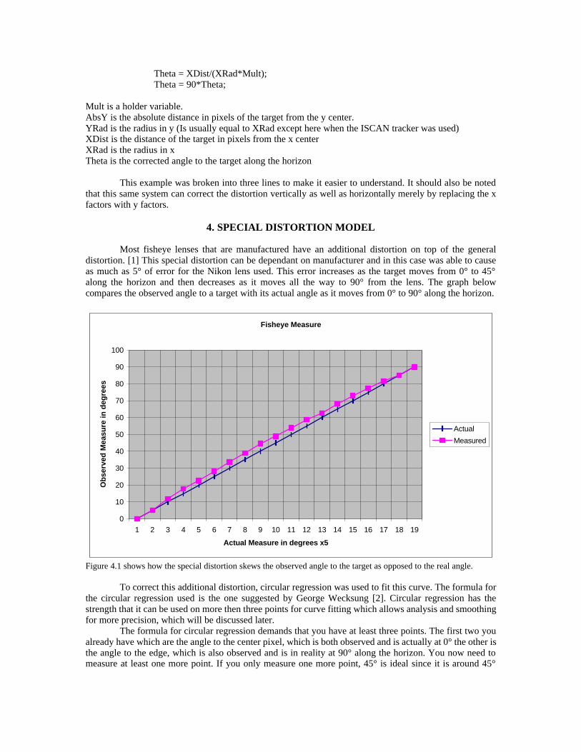
4. SPECIAL DISTORTION MODEL Most fisheye lenses that are manufactured have an additional distortion on top of the general distortion. [1] This special distortion can be dependant on manufacturer and in this case was able to cause as much as 5° of error for the Nikon lens used. This error increases as the target moves from 0° to 45° along the horizon and then decreases as it moves all the way to 90° from the lens. The graph below compares the observed angle to a target with its actual angle as it moves from 0° to 90° along the horizon.

Fisheye Measure

0

10

20

30

40

50

60

70

80

90

100

1 2 3 4 5 6 7 8 9 10 11 12 13 14 15 16 17 18 19

Actual Measure in degrees x5

Ob

serv

ed M

easu

re in

deg

rees

Actual

Measured

Figure 4.1 shows how the special distortion skews the observed angle to the target as opposed to the real angle. To correct this additional distortion, circular regression was used to fit this curve. The formula for the circular regression used is the one suggested by George Wecksung [2]. Circular regression has the strength that it can be used on more then three points for curve fitting which allows analysis and smoothing for more precision, which will be discussed later. The formula for circular regression demands that you have at least three points. The first two you already have which are the angle to the center pixel, which is both observed and is actually at 0° the other is the angle to the edge, which is also observed and is in reality at 90° along the horizon. You now need to measure at least one more point. If you only measure one more point, 45° is ideal since it is around 45°

where the special distortion is greatest. You can then plot the observed and real degrees to the target on 2D coordinates. This can then have a circle fitted to it. The process for the circular regression is as follows: (1) Given a circle with center at (h,k) and radius r and N boundary points (xi, yi) for I = 1, …, N, the mean square radial error may be expressed as:

∑=

−−+−=N

iii rkyhx

NE

1

2222 ))()((1

(2)

(2) By expanding the inner terms, E, may be written as:

22222

1

2 )22(1

rkhkyhxyxN

E iii

N

ii −++−−+= ∑

=

(3)

(3) The key step is to now let:

)( 222 khrc +−= (4) and

222iii yxz += (5)

(4) The error may now be written as a linear function of the parameters, h, k and c.

∑=

−−−=N

iiii ckyhxz

NE

1

22 )22(1

(6)

(5) We find h, k and c with the following linear system

∑∑∑∑====

=++N

iii

N

ii

N

iii

N

ii zxxcyxkxh

1

2

111

2 )2()2()2( (7)

∑∑∑∑====

=++N

iii

N

ii

N

ii

N

iii zyycykyxh

1

2

11

2

1

)2()2()2( (8)

∑∑∑===

=++N

ii

N

ii

N

ii zcNykxh

1

2

11

)2()2( (9)

(6) For a given set of N data points, a matrix inverse program may be written to solve for h,k and c. The radius, r, may then be found using:

22 khcr ++= (10) (7) To formulate the linear equations as a matrix equation, let

=

∑∑

∑∑∑

∑∑∑

==

===

===

Nyx

yyyx

xyxx

A

N

ii

N

ii

N

ii

N

ii

N

iii

N

ii

N

iii

N

ii

11

11

2

1

111

2

22

22

22

=

c

k

h

B

=

∑

∑

∑

=

=

=

N

ii

N

iii

N

iii

z

zy

zx

C

1

2

1

2

1

2

(12)

Then the linear equation is:

CAB = (13) and the solution for C is simply:

CAB 1−= (14)

The process yields an extremely good fit with an average error in this case of .041° .

C o m p a r i s o n s o f E r r o r s

0

1 0

2 0

3 0

4 0

5 0

6 0

7 0

8 0

9 0

1 0 0

1 2 3 4 5 6 7 8 9 1 0 1 1 1 2 1 3 1 4 1 5 1 6 1 7 1 8 1 9

A c t u a l D e g r e e s o n h o r i z o n x 5

Mea

sure

d D

egre

es o

n H

ori

zon

A c t u a lM e a s u r e dN e w E s t i m a t e

Figure 4.2 shows the fit of the circle to the special distortion observed. When the circle is found that fits the special distortion, it can be used to correct the distortion using the following formula:

(15)

θreal is the corrected angle to the target, θobs is the observed angle to the target. h, k and r are the static definitions of the circle obtained earlier using the circular regression technique. The formula can be plugged into C++ as follows

ModTheta = -(sqrt(-pow((Theta-k),2)+pow(r,2))-h);

Where ModTheta is the output corrected angle and Theta is the uncorrected angle. h, k and r are the static definitions of the circle.

5. EXPERIMENTAL RESULTS To determine the validity of the system, measurements were taken and the observed horizontal degree to the target was compared with the actual horizontal degrees using the apparatus previously described. Measurements were taken with the target at 0,15,30,45,60,75 and 85 degrees horizontally with the target moved vertically in increments of 10 degrees. In all, 63 measurements were taken, that is 7 at each of the 9 vertical levels. Along the horizontal, the farthest measurement taken was 85° instead of 90° due to the fact that it was extremely difficult to track the target at this extreme edge of the lens. The results below show the error chart. As can be seen, when the target does not move above 50° vertical, error stays below 3 degrees. However, error did reach as high as 12.67° at the extreme of 80° vertical by 45° horizontal. The average error at the 80° vertical is it’s highest at 6.12°

Horizontal Degrees to Target Degrees per

0 15 30 45 60 75 85 Pixel

Vertical 0 0 0.02 0.07 0.38 -1.8 1.2 0.6 0.5625

Degrees 10 0.45 -0.36 -0.266 0.226 0.593 1.4 1.48 0.567218

To Target 20 -0.5 -0.52 -0.536 -0.089 0.82 0.48 0.63 0.580566

30 0.099 -0.91 -1.774 -0.116 0.087 1.26 2.44 0.607108

40 0.087 -0.52 -1.72 -2.21 -0.82 1.944 3.133 0.647396

50 0.075 -1.68 -2.64 -2.587 -2.93 0.9169 2.26 0.712554

60 0 -3.35 -5.69 -7.886 -6.14 -1.52 -0.27 0.802088

70 0.87 -3.19 -7.49 -10.35 -10.27 -2.62 7 0.987185 80 2.56 -4.52 -9.8 -12.67 -5.79 2.5 5 1.537721Table 5.1 The amount of error in degrees is shown for each measurement. Also shown at the far right is the amount of coverage each pixel has in degrees.

1

4

7 0

30

60-15-10-50510

Error (Degrees)

Horizontal Degrees (x 10)

Vertical Degrees

Error of Measure in Degrees

5-10

0-5

-5-0

-10--5

-15--10

Figure 5.1 This is a visual representation of the data in figure 5.1 The error observed increases to as much as 12° at the extremities of the viewable area.

6. DISCUSSION

Of the error, much of it can be explained in several different ways. The first is that, as you move

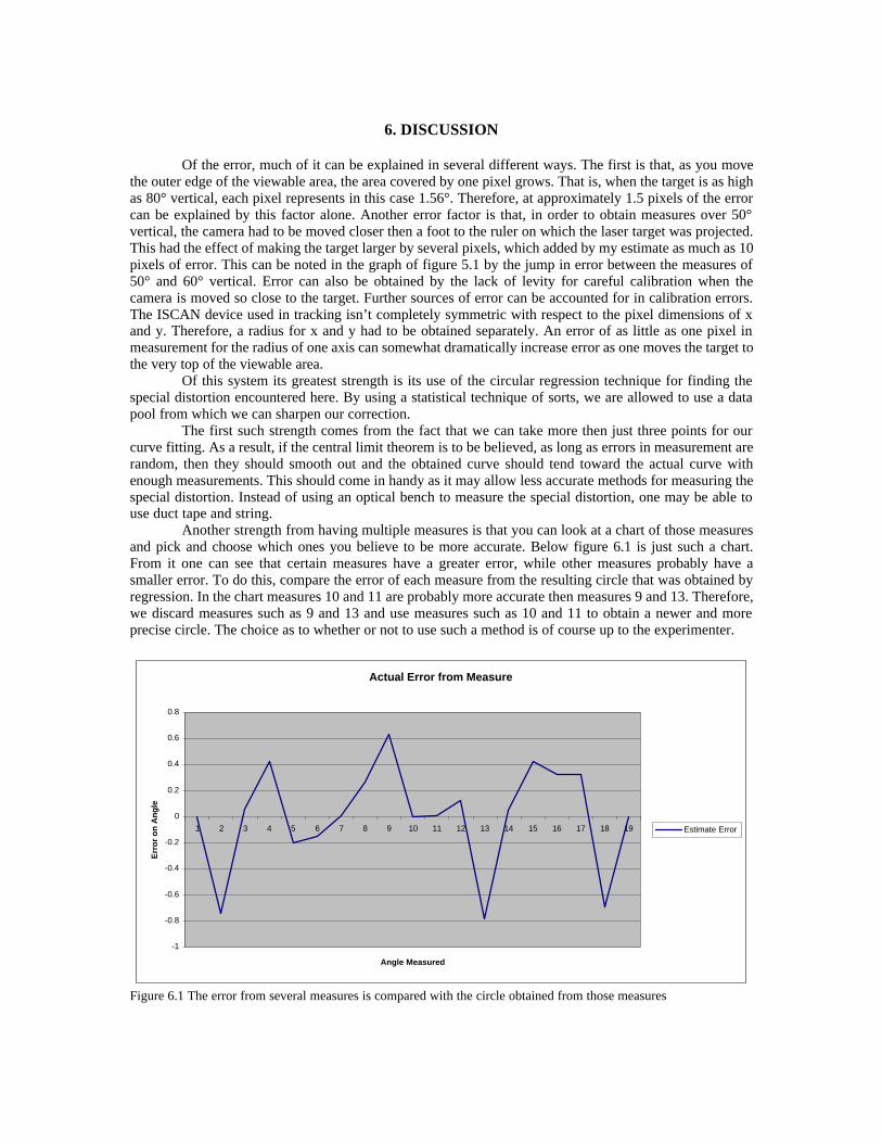
the outer edge of the viewable area, the area covered by one pixel grows. That is, when the target is as high as 80° vertical, each pixel represents in this case 1.56°. Therefore, at approximately 1.5 pixels of the error can be explained by this factor alone. Another error factor is that, in order to obtain measures over 50° vertical, the camera had to be moved closer then a foot to the ruler on which the laser target was projected. This had the effect of making the target larger by several pixels, which added by my estimate as much as 10 pixels of error. This can be noted in the graph of figure 5.1 by the jump in error between the measures of 50° and 60° vertical. Error can also be obtained by the lack of levity for careful calibration when the camera is moved so close to the target. Further sources of error can be accounted for in calibration errors. The ISCAN device used in tracking isn’t completely symmetric with respect to the pixel dimensions of x and y. Therefore, a radius for x and y had to be obtained separately. An error of as little as one pixel in measurement for the radius of one axis can somewhat dramatically increase error as one moves the target to the very top of the viewable area. Of this system its greatest strength is its use of the circular regression technique for finding the special distortion encountered here. By using a statistical technique of sorts, we are allowed to use a data pool from which we can sharpen our correction. The first such strength comes from the fact that we can take more then just three points for our curve fitting. As a result, if the central limit theorem is to be believed, as long as errors in measurement are random, then they should smooth out and the obtained curve should tend toward the actual curve with enough measurements. This should come in handy as it may allow less accurate methods for measuring the special distortion. Instead of using an optical bench to measure the special distortion, one may be able to use duct tape and string. Another strength from having multiple measures is that you can look at a chart of those measures and pick and choose which ones you believe to be more accurate. Below figure 6.1 is just such a chart. From it one can see that certain measures have a greater error, while other measures probably have a smaller error. To do this, compare the error of each measure from the resulting circle that was obtained by regression. In the chart measures 10 and 11 are probably more accurate then measures 9 and 13. Therefore, we discard measures such as 9 and 13 and use measures such as 10 and 11 to obtain a newer and more precise circle. The choice as to whether or not to use such a method is of course up to the experimenter.

Actual Error from Measure

-1

-0.8

-0.6

-0.4

-0.2

0

0.2

0.4

0.6

0.8

1 2 3 4 5 6 7 8 9 10 11 12 13 14 15 16 17 18 19

Angle Measured

Err

or

on

An

gle

Estimate Error

Figure 6.1 The error from several measures is compared with the circle obtained from those measures

Another thing worth noting about the use of circular regression is the fact that its computation is in fact quite simple. All circular regression computations for this experiment were performed on a Texas Instruments TI-92 calculator, which is available at almost any department store. Circular regression calculations can also be performed using MathCAD, MATLAB or any other standard mathematical package.

7. CONCLUSION

The system described is viable for the correction of fisheye distortion. It should also be noted how easy it is to obtain errors in measurements from the fisheye lens even with careful calibration. The system is also simple to use. The first equation needs only knowledge of the lens radius and center in order to correct for distortion while the second equation needs only a third measure to make the final correction. All of these can be done with widely available mathematical packages.

8. REFERENCES

[1] Yalin Xiong, Ken Turkowski, “Creating Image-Based VR Using a Self-Calibrating Fisheye Lens”,

1998, http://www.cs.cmu.edu/~yx/papers/Fisheye97.pdf [2] E.L. Hall, Computer Image Processing and Recognition, Academic Press, New York, 1979.