Technical Note: Seasonality in alpine water resources management – a regional assessment

Hydrol. Earth Syst. Sci., 12, 91–100, 2008www.hydrol-earth-syst-sci.net/12/91/2008/© Author(s) 2008. This work is licensedunder a Creative Commons License.

Hydrology andEarth System

Sciences

Technical Note: Seasonality in alpine water resources management –a regional assessment

D. Vanham1, E. Fleischhacker2, and W. Rauch1

1Unit of Environmental Engineering, Inst. of Infrastructure, Univ. Innsbruck, Technikerstrasse 13, 6020 Innsbruck, Austria2Wasser Tirol – Wasserdienstleistungs-GmbH, Salurnerstrasse 6, 6020 Innsbruck, Austria

Received: 17 August 2007 – Published in Hydrol. Earth Syst. Sci. Discuss.: 28 August 2007Revised: 22 November 2007 – Accepted: 18 December 2007 – Published: 25 January 2008

Abstract. Alpine regions are particularly affected by sea-sonal variations in water demand and water availability. Es-pecially the winter period is critical from an operational pointof view, as being characterised by high water demands due totourism and low water availability due to the temporal stor-age of precipitation as snow and ice. The clear definition ofsummer and winter periods is thus an essential prerequisitefor water resource management in alpine regions. This pa-per presents a GIS-based multi criteria method to determinethe winter season. A snow cover duration dataset serves asbasis for this analysis. Different water demand stakeholders,the alpine hydrology and the present day water supply infras-tructure are taken into account. Technical snow-making and(winter) tourism were identified as the two major seasonalwater demand stakeholders in the study area, which is theKitzbueheler region in the Austrian Alps. Based upon dif-ferent geographical datasets winter was defined as the periodfrom December to March, and summer as the period fromApril to November. By determining potential regional wa-ter balance deficits or surpluses in the present day situationand in future, important management decisions such as wa-ter storage and allocation can be made and transposed to thelocal level.

1 Introduction

1.1 Seasonality in alpine water resources management

Integrated management of water resources requires to bal-ance water utilisation from various stakeholders againstavailable resources at the catchment level (Frederick, 1997).In case of constant demand and resources such an assessmentcan be made easily on the basis of an annual water balance.

Correspondence to:D. Vanham([email protected])

However, typically both the water utilisation and the avail-able resources are fluctuating over time, with cyclic varia-tions on a daily, weekly and seasonal basis. The integratedmanagement of water resources has to take these temporalvariations into account and water mass balances have to bemade over the relevant periods.

Alpine areas are particularly affected by seasonal varia-tions, that is by differences between the summer and the win-ter period. Reason is that both the natural hydrology as wellas the demand differs significantly during winter. First theavailability of water resources (both surface and spring wa-ter) is generally lowest during this period due to the storageof water in form of snow and ice. On the other hand this pe-riod of minimal water availability is met by the peak waterdemand from stakeholders, due to winter tourism and waterdemand for technical snow production. The effect of climatechange is contributing further to this problem as mountainousareas are particularly vulnerable to temperature and precipi-tation changes (Beniston, 2003).

Based on the above it is clear that a water balance analysisin alpine catchments must be performed at least on the sea-sonal level. A clear distinction between summer and winterperiods is thus a must for any integrated assessment. Un-til now seasonality has been addressed in the literature notgeneric, but only with specific focus and for specific loca-tions. E.g. Tappeiner et al. (2001) defined the winter seasonfor the alpine upper Passeier Valley in Italy from Novemberto May. Christensen and Lettenmaier (2007) defined winterfrom October to March, and summer from April to Septem-ber.

The aim of this paper is a generic approach to define thewinter season in an alpine catchment from the point of viewof an integrated assessment of water resources.

Published by Copernicus Publications on behalf of the European Geosciences Union.

92 D. Vanham et al.: Seasonality in alpine water resources management

!

!

!!

!

!!

!!!

!

!

!980

760

763595 830

770 950

750

495 780

670

590

1760

Altitude (m a.s.l.)

! observation station

border municipality

border study area

2533

4500 5 102,5Kilometers

Station Hahnenkamm

Fig. 1. Topography and snow observation stations (with indicationof elevation) in the study area Kitzbueheler Region, Province ofTyrol, Austrian Alps.

Fig. 2. Average monthly number of tourist overnight stays (in Mio.)recorded for the years 2000 to 2006 in the Kitzbueheler region.

1.2 Water supply

In Austria, especially in alpine Regions, drinking water sup-ply systems are characterised by a local, small structured in-frastructure. In general, water supply is organised on a mu-nicipality basis. A total of 7600 public water supply under-takings provide the national population of 8.1 Mio. inhabi-tants with drinking water (Schoenback et al., 2004). In theproject area of the greater Kitzbueheler region, a typical ru-ral Alpine region, each of the 20 municipalities has its owndrinking water supply infrastructure. Additional to the largermunicipal water supply organisations a high number of smallwater co-operatives serve about 10% of the inhabitants. Wa-ter pipe connections between the different supply systems arerare.

1.3 Water resources

The seasonality of hydrological elements in alpine regionsis highly dependent on altitude (Merz and Bloeschl, 2003).

Jansson et al. (2003) stated that snow and ice significantlyaffect catchment hydrology by temporarily storing and re-leasing water. The seasonal snow cover causes a time lagbetween the precipitation event and runoff of typically sev-eral months. The alpine character of the study area resultsnot only in a temporal seasonality, but also in a high spatialvariability of the snow cover. Schoener and Mohnl (2003)state that the duration of snow cover influences the groundwater recharge. The availability of alpine water resources istherefore generally lowest in winter, the period where typ-ically low flows occur. Lahaa and Bloeschl (2006) dividedAustria into an alpine region with low flows dominated bywinter processes and into flatlands and hilly terrain with lowflows dominated by summer processes.

1.4 Water demand

Winter tourism is one of the most important industries in theAlps (Elsasser and Messerli, 2001). In the Austrian Provinceof Tyrol a total of 41.8 Mio. tourist overnight stays have beenrecorded for the year 2006, of which 52% occur in the wintermonths from December to March. The main requirement forsuccessful winter sports is the reliability of snow occurrencein the winter sports resorts. In recent years, the productionof technical snow has become an important issue in most skiareas of the world and is likely to increase due to climatechange (OECD, 2007). Water, air, energy and temperaturesbelow freezing are required to produce technical snow.

2 Study area

As case study the greater Kitzbueheler Region (Fig. 1), lo-cated in the Province of Tyrol, Austria, was chosen. The areaencompasses 20 municipalities located in the Eastern Alps,of which two – Kitzbuehel and Sankt Johann – are of ur-ban character, and the remaining municipalities are of a ruralcharacter. The highest mountain peak reaches 2533 m a.s.l.According to the land use dataset of CORINE only 2.5% ofthe study area is urbanised (Table 1). There are no glaciersin the area. Tourism is by far the largest industry, with anannual average of 6.5 Mio. tourist overnight stays recordedfor the years 2000 to 2006, of which 54% occur in the wintermonths from December to March (Fig. 2). The total popula-tion (principal residence) of the region is 60 632 inhabitants(Table 2). Typical for the alpine region, the public drinkingwater demand is covered by spring water to a rate of 80%,and by ground water to a rate of 20%. Surface water is notused for drinking water purposes.

Hydrol. Earth Syst. Sci., 12, 91–100, 2008 www.hydrol-earth-syst-sci.net/12/91/2008/

D. Vanham et al.: Seasonality in alpine water resources management 93

3 Methodology

3.1 Base and seasonal water demand

Urban water use typically consists of residential, industrial,commercial, and public uses, as well as some minor use forother purposes such as fire fighting. In the study area industryis of minor importance. In order to calculate the public drink-ing water demand in the 20 municipalities, a methodology(Vanham et al., 2007) based upon on the one hand the num-ber of inhabitants and persons employed in different sectorsas rasterdata, and on the other hand the number of tourists(recorded as overnight stays) is used. As this analysis usesspecific population census data in a GIS-raster format onlyavailable for the year 2001, the public water demand is cal-culated for the year 2001. These values are calibrated withoperating data of the drinking water supply systems, as col-lected by means of a questionnaire. These operating datashow only small variations in annual water demand over thepast 10 years. It can therefore be reasonably assumed thatthe public water demand stayed stable during this period.The calculations resulted in a total annual water demand ofabout 5 million m3 (Table 3), of which overnight stays ac-count for 1.5 million m3 (30%). The public drinking waterdemand can therefore be divided in firstly a base water de-mand (70%), which is in general constant when consideredon an annual basis, and secondly a seasonal water demand(30%), which depends on the number and the temporal dis-tribution of overnight stays. Of the base water demand of3.5 million m3, population attributes to about 80% of thisvalue. Although assumed constant, the base water is still tobe included in the seasonality analysis, due to the seasonalbehaviour of the water resources providing the water supplysystems.

Apart of the public water demand (with its both constantand seasonal shares), technical snow production is to be re-garded as second seasonal water demand factor. Proebstl(2006) evaluated the water demand for snowing in differentBavarian and Tyrolean ski regions in similar altitudes as theproject area of this study. In terms of temporal water demandit is to be differentiated between base snowing at the begin-ning of the winter season and improvement snowing duringthe remaining winter season. As a ground rule it is statedthat 2.4 m3 of snow is generated from 1 m3 of water. Forbase snowing, a snow height of 20 to 35 cm is required (70to 120 l water pro m2). For improvement snowing about 50to 120 percent of the base snowing is required, depending onthe local situation. In this study a base snowing of 35 cm isassumed, as well as an improvement snowing of 120 percent.A geographical dataset of all ski runs with the specificationof areas with technical snow making (total area 882 ha) isavailable. A calculated water demand of 2.3 million m3 isneeded for snow-making (Table 3).

Table 1. Land use in the Kitzbueheler region.

Description Percentage of total area

Urbanised areas 2.5Broad-leaved and mixed forest 19.1Coniferous forest 30.9Natural grassland 25.8(predominately alpine meadows)Pastures (predominately 17.9located in the valleys)Crops 0.1Sparsely vegetated areas 2.3Bare rock 1.3Water bodies 0.1

3.2 Snow cover start and end date

The fundamental dataset for the seasonality analysis is asnow cover duration map of the area. Reason being that allthree water demands (base water demand, water demand fortourism/overnight stays, technical snow production) are af-fected by the snow cover. The relation is obvious for tech-nical snow production and also for winter tourism (as snowcoverage is fundamental for winter sports). The base wa-ter demand is affected indirectly as snow cover indicates thatavailability of water resources decreases.

The snow cover duration map is generated based upon1) snow measurements at different weather stations and 2)a digital elevation model (DEM) using a spatial interpola-tion by means of conventional GIS-software. According toSlatyer et al. (1984) the duration of the snow cover correlateswith elevation and exposure. This is confirmed by Schoenerand Mohnl (2003), who generated a snow cover map (250 mresolution) for the entire Austrian area, based upon a spatialinterpolation of daily snow depth measurements at 835 cli-matological stations for the WMO’s climate normal periodfrom 1961 to 1990. The authors defined a day as a snowcover day if a complete snow cover of 1 cm (or more) isobserved at the measurement site. A correction of the re-sulting snow cover was made taking into account expositionand slope. The authors differentiated between snow coverand winter cover, with the latter defined as the longest con-tinuously existing snow cover of a winter season (minimumdepth 1 cm). In Alpine regions the duration of winter cover isessentially shorter than snow cover, as occasional snow coverdays are likely to occur in autumn or spring.

The analysis for the Kitzbueheler study area is based onthe winter cover, but in the remaining text this term will be re-ferred to as snow cover. A spatial interpolation of mean dailysnow cover duration is made for the period 1961 to 1990 for13 observation stations. The definition of a snow cover dayis taken from Schoener and Mohnl (2003). Of these stations,12 are located in the valleys at an altitude between 495 m

www.hydrol-earth-syst-sci.net/12/91/2008/ Hydrol. Earth Syst. Sci., 12, 91–100, 2008


Table 2. Basic data of the 20 municipalities in the Kitzbueheler region for the year 2001.

municipality area inhabitants overnight overnight public drinking water supply (%)(km2) stays stays per spring water groundwater

inhabitant (%) (%)

Aurach 54 1203 70 773 59 80 20Brixen 31 2574 251 173 98 100 0Fieberbrunn 76 4180 422 983 101 100 0Going 21 1730 306 132 177 100 0Hochfilzen 33 1109 48 620 44 100 0Hopfgarten 166 5266 337 044 64 95 5Itter 10 1060 74 202 70 100 0Jochberg 88 1540 63 938 42 100 0Kirchberg 98 4958 861 551 174 80 20Kirchdorf 114 3490 334 221 96 80 20Kitzbuehel 58 8571 767 259 90 80 20Oberndorf 18 1944 190 349 98 40 60Reith 16 1595 114 056 72 0 100St. Jakob 10 635 82 591 130 20 80St. Johann 59 7959 517 857 65 80 20Westendorf 95 3454 418 244 121 100 0Bad Haering 9 2265 149 975 66 70 30Ellmau 36 2524 662 712 263 100 0Scheffau 31 1211 246 248 203 100 0Soell 46 3364 449 624 134 80 20

total 1070 60 632 6 369 552 105 80 20

and 980 m a.s.l. and 1 is located in the mountains (StationHahnenkamm) at an altitude of 1760 m a.s.l. (Fig. 1). Thelatter is used for a linear regression with altitude, by meansof the interpolation algorithm GRADGRID (Bucher et al.,2004). In the same way a spatial interpolation of the meanstart and end date of the snow cover for the period 1961 to1990 is made, with the first day of the year defined as 1September. The 3 resulting geodatasets (250m resolution)are a mean snow cover duration and a mean snow cover startdate (SCOV6190S) and end date (SCOV6190E) raster. Thelatter 2 geodatasets, which comprise daily information, areused in the seasonality analysis.

3.3 GIS-multicriteria method

For computing the seasonality in alpine water resources man-agement, a GIS-multicriteria approach is chosen to make itpossible to account for on the one hand the base water de-mand and on the other hand the two principal seasonal wa-ter demand stakeholders snow-making and tourism in rela-tionship to their claimed water resources. The fundamentaldatasets for this analysis are the mean snow cover start date(SCOV6190S) and end date (SCOV6190E) rasters. Mul-ticriteria decision making is defined as choosing among al-ternatives based on a set of evaluation criteria (Malczewski,1999). Multicriteria decision analysis using GIS applies a

set of weight factors to each data characteristic. In thisstudy, the evaluation criteria for all three water demand fac-tors are the snow cover start date (SCOV6190S) and enddate (SCOV6190E rasters). Weight factors are applied inrelation to the demand quantity.

In the study the start and the end of the snow-making sea-son are assumed to collide with the start and the end of thesnow cover duration, as a temperature below zero is a ba-sic necessity for both natural and technical snow. Therefore,the start and the end date of the snow cover are taken asthe temporal change between the summer and winter sea-son with regard to the water demand stakeholder of snow-making. This assumption is a simplification, as in realitysnow-making starts already before snow cover as soon as thetemperature is sufficiently low. How much earlier a ski op-erator starts snow-making depends on the one hand on cli-matic factors and on the other hand on the legislation regard-ing the start date. However, there is no common legislationto all Alpine countries or even regions within certain coun-tries governing the use of technical snow-making (Proebstl,2006; OECD, 2007). Legal start dates of the snow-makingseason tend to differ among ski-regions of the Kitzbuehelerstudy area – even with their slope base at similar altitudes.The choice of the start of the snow cover as a conservativeindicator for temperatures below zero can therefore imply a



Table 3. Total water demand for the 20 municipalities in the Kitzbueheler region.

definition yearly waterdemand inmillion m3

Water sources

Public base water demand 3.5 springs (80%) and ground water (20%)feeding the public water infrastructure

Public seasonal water demand 1.5Seasonal snow-making water demand 2.3 springs, groundwater and surface water,

not attached to the public water infras-tructure

!

!

!

!!

(Eq.1) Ti for SCOV6190_S = 7 Dec and Ai =90ha




) Ti for SCOV6190_S = 17 Dec and Ai =84ha

0 2 41Kilometers ! Lowest ski slope zone

Ski slopes without snow-making

Ski slopes with snow-makingBuildings and road infrastructure

Ski lifts

Mean snow cover start date (SCOV6190_S)

21 December

18 October

Fig. 3. Location of the interconnected ski region “skiwelt Wilder Kaiser-Brixental” in the study area, with indication of ski slopes with snow-making and their lowest topographic zone. The values forTi andAi in Eq. (1) for the mean snow cover start date raster (SCOV6190S) aregiven.

shortening of the realistic snow-making season. On the otherhand, snow-making is likely to stop before the end of thesnow cover in spring, as snow cover usually persists for sometime under melting conditions – when snow making is notpossible anymore. The length of this period depends uponair temperature, topography and snow cover characteristics(Kling et. al., 2005). This assumption therefore can implya lengthening of the snow-making season. Nevertheless, thestart and end date of the snow cover were chosen as the deter-mining factor for defining the snow-making season in orderto simplify the analysis and constrain data requirements.

The different ski regions are weighted by their area ofslopes with snow-making in relation to the total area ofslopes with snow-making in the study area. Because the de-

cisive zone of the ski slope for the seasonality analysis isthe lowest zone, this area is selected for the analysis. ThisGIS-based analysis is exemplarily visualised in Fig. 3 andsummarised in the equation

Tsnow =

∑Ti(Ai/Asnow) (1)

whereTsnow is the weighted day for all ski regions andTi theselected day for a specific ski region i in the snow cover startdate (SCOV6190S) or end date (SCOV6190E) raster. Ai

represents the ski slope area with snow making for a specificski regioni. Asnow is the ski slope area with snow makingfor all ski regions within the study area.

In order to evaluate the impact of tourism in the formof overnight stays on the seasonality analysis, the seasonal



!!

!

!!!

!

!

!

!

!

Rastbuchquelle(Eq.2 and 3) Tj for SCOV6190_S = 24 Nov

Qj = 1 l/s Qk = 31,03 l/s Qj/Qk = 0,03

Luegeggquelle(Eq.2 and 3) Tj for SCOV6190_S = 30 Nov

Qj = 8,3 l/s Qk = 31,03 l/s Qj/Qk = 0,27

Oberangerquelle(Eq.2 and 3) Tj for SCOV6190_S = 26 Nov

Qj = 10 l/s Qk = 31,03 l/s Qj/Qk = 0,32

Bärenruhquellen 1+2(Eq.2 and 3) Tj for SCOV6190_S = 2 Dec

Qj = 2 l/s Qk = 31,03 l/s Qj/Qk = 0,06

Felderbrandquellen 1+2(Eq.2 and 3) Tj for SCOV6190_S = 6 Dec

Qj = 1 l/s Qk = 3,5 l/s Qj/Qk = 0,29

Blaufeldquellen 1+2(Eq.2 and 3) Tj for SCOV6190_S = 27 Nov

Qj = 2,5 l/s Qk = 3,5 l/s Qj/Qk = 0,71Ehrenbachquellen 1+2

(Eq.2 and 3) Tj for SCOV6190_S = 15 NovQj = 0,5 l/s Qk = 31,03 l/s Qj/Qk = 0,02

untere Oberfeldquellen 1-3(Eq.2 and 3) Tj for SCOV6190_S = Currently not used

Qj = 0 l/s Qk = 0 l/s Qj/Qk = 0

TB Gundhabing

Grundwasserbrunnen Langau

Municipality Kitzbuehel

Municipality Aurach

0 2 41Kilometers

Water supply infrastructure (pipelines)Border municipality !

Springs ("Quelle") and groundwater ("Grundwasser") used by the municipal water supply system

Buildings and road infrastructure


21 December

18 October

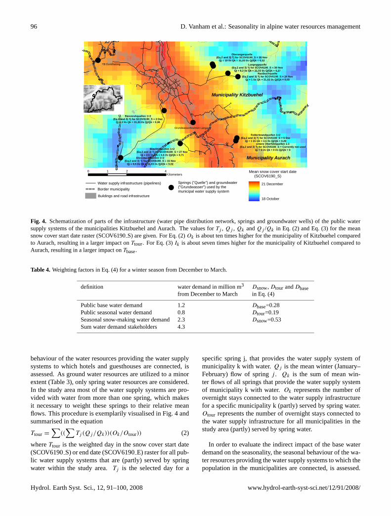
Fig. 4. Schematization of parts of the infrastructure (water pipe distribution network, springs and groundwater wells) of the public watersupply systems of the municipalities Kitzbuehel and Aurach. The values forTj , Qj , Qk andQj /Qk in Eq. (2) and Eq. (3) for the meansnow cover start date raster (SCOV6190S) are given. For Eq. (2)Ok is about ten times higher for the municipality of Kitzbuehel comparedto Aurach, resulting in a larger impact onTtour. For Eq. (3)Ik is about seven times higher for the municipality of Kitzbuehel compared toAurach, resulting in a larger impact onTbase.

Table 4. Weighting factors in Eq. (4) for a winter season from December to March.

definition water demand in million m3 Dsnow, Dtour andDbasefrom December to March in Eq. (4)

Public base water demand 1.2 Dbase=0.28Public seasonal water demand 0.8 Dtour=0.19Seasonal snow-making water demand 2.3 Dsnow=0.53Sum water demand stakeholders 4.3

behaviour of the water resources providing the water supplysystems to which hotels and guesthouses are connected, isassessed. As ground water resources are utilized to a minorextent (Table 3), only spring water resources are considered.In the study area most of the water supply systems are pro-vided with water from more than one spring, which makesit necessary to weight these springs to their relative meanflows. This procedure is exemplarily visualised in Fig. 4 andsummarised in the equation

Ttour =

∑((

∑Tj (Qj/Qk))(Ok/Otour)) (2)

whereTtour is the weighted day in the snow cover start date(SCOV6190S) or end date (SCOV6190E) raster for all pub-lic water supply systems that are (partly) served by springwater within the study area.Tj is the selected day for a

specific spring j, that provides the water supply system ofmunicipality k with water.Qj is the mean winter (January–February) flow of springj . Qk is the sum of mean win-ter flows of all springs that provide the water supply systemof municipality k with water.Ok represents the number ofovernight stays connected to the water supply infrastructurefor a specific municipality k (partly) served by spring water.Otour represents the number of overnight stays connected tothe water supply infrastructure for all municipalities in thestudy area (partly) served by spring water.

In order to evaluate the indirect impact of the base waterdemand on the seasonality, the seasonal behaviour of the wa-ter resources providing the water supply systems to which thepopulation in the municipalities are connected, is assessed.



0 10 20 30 405Kilometers

(a) (b)

16 to 31 October

1 to 15 November

16 to 30 November

1 to 15 December

16 to 31 December

Mean snow cover start date Mean snow cover end date

1 to 15 March

16 to 31 March

1 to 15 April

16 to 30 April

1 to 15 May

16 to 31 May

1 to 15 June

16 to 30 June

Fig. 5. Interpolated raster datasets (resolution 250 m×250 m) mean snow cover start date (SCOV6190S) (a) and mean snow cover end date(SCOV6190E) (b) for the World Meteorological Organization’s climate normal period from 1961 to 1990.

0

50

100

150

200

250

300

07.10.1999 06.12.1999 04.02.2000 04.04.2000 03.06.2000

Date

Flow

(l/s

)

Interpolated end date snow cover

No data available upto 16.11.1999

Fig. 6. Example of interaction between the hydrological regime(flow) of the spring “Schreiende Brunnen” (995 m a.s.l.), located inthe municipality of Fieberbrunn, with the interpolated snow coverend date for the winter 1999–2000 (15 April).

This approach is similar to the approach for tourist overnightstays. Only population (Table 2) is taken into account, as itamounts for the largest proportion of base water demand inthis area. The procedure is exemplarily visualised in Fig. 4and summarised in the equation

Tbase=∑

((∑

Tj (Qj/Qk))(Ik/Ibase)) (3)

whereTbaseis the weighted day in the snow cover start date(SCOV6190S) or end date (SCOV6190E) raster for all pub-lic water supply systems that are (partly) served by springwater within the study area.

∑Tj (Qj /Qk) represents the

same factor as in Eq. (2). Ik represents the number of in-habitants connected to the water supply infrastructure for aspecific municipalityk (partly) served by spring water.Ibase

represents the number of inhabitants connected to the watersupply infrastructure for all municipalities in the study area(partly) served by spring water.

Based upon the Eqs. (1), (2) and (3), the seasonality withregards to a water balance analysis for the study area can beanalysed according to the equation

Twbal = DsnowTsnow+ DtourTtour + DbaseTbase (4)

where Twbal is the weighted day in the snow cover start(SCOV6190S) or end date (SCOV6190E) raster. Dsnow,Dtour and Dbase represent respectively the relative amountof water demand of the seasonal stakeholder snow-making,tourism in the form of overnight stays and the base water de-mand in relation to the total water demand of all 3 assessedstakeholders. The definition of these amounts poses a prob-lem for Dtour and Dbase, as they have to be related to thewinter season – which has not been defined yet and is onlythe result of Eq. (4). Therefore a first estimation of the winterseason should be made. These values have then to be adaptediteratively, after analysing the results in Eq. (4). A good ref-erence can be the seasonality in overnight stays (Fig. 2), inwhich a winter season from December to March can be iden-tified. The weighting factorsDsnow, Dtour andDbasefor thisfirst estimation of the winter season are 0.53, 0.19 and 0.28respectively (Table 4).

4 Results

The interpolated mean snow cover duration raster(SCOV6190) is characterised by a minimum (respectively



Buildings and road infrastructure

Ski slopes

(a) (b)

0 10 20 30 405Kilometers

Mean snow cover end date (SCOV6190_E)

High : 296

Low : 184

23 June

3 March29 March


21 December

18 October

5 December

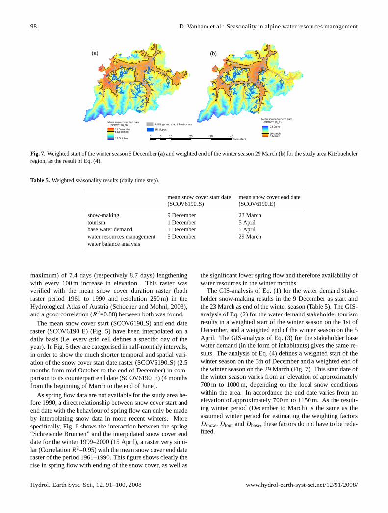
Fig. 7. Weighted start of the winter season 5 December(a) and weighted end of the winter season 29 March(b) for the study area Kitzbuehelerregion, as the result of Eq. (4).

Table 5. Weighted seasonality results (daily time step).

mean snow cover start date mean snow cover end date(SCOV6190S) (SCOV6190E)

snow-making 9 December 23 Marchtourism 1 December 5 Aprilbase water demand 1 December 5 Aprilwater resources management – 5 December 29 Marchwater balance analysis

maximum) of 7.4 days (respectively 8.7 days) lengtheningwith every 100 m increase in elevation. This raster wasverified with the mean snow cover duration raster (bothraster period 1961 to 1990 and resolution 250 m) in theHydrological Atlas of Austria (Schoener and Mohnl, 2003),and a good correlation (R2=0.88) between both was found.

The mean snow cover start (SCOV6190S) and end dateraster (SCOV6190E) (Fig. 5) have been interpolated on adaily basis (i.e. every grid cell defines a specific day of theyear). In Fig. 5 they are categorised in half-monthly intervals,in order to show the much shorter temporal and spatial vari-ation of the snow cover start date raster (SCOV6190S) (2.5months from mid October to the end of December) in com-parison to its counterpart end date (SCOV6190E) (4 monthsfrom the beginning of March to the end of June).

As spring flow data are not available for the study area be-fore 1990, a direct relationship between snow cover start andend date with the behaviour of spring flow can only be madeby interpolating snow data in more recent winters. Morespecifically, Fig. 6 shows the interaction between the spring“Schreiende Brunnen” and the interpolated snow cover enddate for the winter 1999–2000 (15 April), a raster very simi-lar (CorrelationR2=0.95) with the mean snow cover end dateraster of the period 1961–1990. This figure shows clearly therise in spring flow with ending of the snow cover, as well as

the significant lower spring flow and therefore availability ofwater resources in the winter months.

The GIS-analysis of Eq. (1) for the water demand stake-holder snow-making results in the 9 December as start andthe 23 March as end of the winter season (Table 5). The GIS-analysis of Eq. (2) for the water demand stakeholder tourismresults in a weighted start of the winter season on the 1st ofDecember, and a weighted end of the winter season on the 5April. The GIS-analysis of Eq. (3) for the stakeholder basewater demand (in the form of inhabitants) gives the same re-sults. The analysis of Eq. (4) defines a weighted start of thewinter season on the 5th of December and a weighted end ofthe winter season on the 29 March (Fig. 7). This start date ofthe winter season varies from an elevation of approximately700 m to 1000 m, depending on the local snow conditionswithin the area. In accordance the end date varies from anelevation of approximately 700 m to 1150 m. As the result-ing winter period (December to March) is the same as theassumed winter period for estimating the weighting factorsDsnow, Dtour andDbase, these factors do not have to be rede-fined.



5 Conclusions

This study presents a GIS-based multi criteria approach todefine a winter and summer season with respect to the anal-ysis of a water balance between available water resourcesand water demand in the Kitzbueheler region in the AustrianAlps. The fundamental geodatasets for this analysis are amean snow cover start date raster and a mean snow coverend date raster.

Public base water demand (3.5 Mio. m3 on a yearly basis)has to be taken into account in such analysis although beinga constant demand. Tourism and snow-making were definedas the two most important seasonal water demand stakehold-ers. Tourism was quantified in the number of overnight stays,and accounted for an annual water demand of 1.5 Mio. m3,connected to the water supply systems of the municipalitiesin the region. Not connected to the public system is the waterdemand for technical snow production which accounts for anannual demand of 2.3 Mio. m3. The GIS-analysis of the sea-sonality of these three stakeholders in the case study givesa rather similar result. This is due to the characteristics ofthe study area, where most ski regions have their ski slopesreaching the valleys, and the municipalities are provided to asignificant extent with water from resources located close tothe valleys. A weighted analysis results in the 5 Decemberand the 29 March as key dates for differentiating betweenwinter and summer. For practical reasons, it can be statedthat the winter months are December to March, and the sum-mer months April to November.

As stated in the methodology, this approach simplifies thedefinition of the actual seasonal water demand period regard-ing snow-making. However, other approaches taking into ac-count frost days – or better hours – or a snow model are defi-nitely more complex and still to be regarded with caution, asthe actual first snowing date is dependent on local legislation.The start of the snowing season is notwithstanding very im-portant, as base snowing accounts for 40% of water volumes.Although the study area currently does not have a regionalwater management plan for the present and future situation,a total reservoir volume - divided over about 20 reservoirs -of 0.9 Mio. m3 for snowmaking water storage is installed inthe region, capable of providing the total base water demandin the current situation (40% of 2.3 Mio. m3).

With the definition of a winter period of four months forthe study area, it is expected that the presented methodol-ogy will define longer winter periods for many alpine regionsthat are located at higher elevations and in similar climate re-gions. This methodology can also result in a significant dif-ferent seasonality for alpine regions with a larger variabilityin topography or hydrogeology, or in different climate zones.

This methodology also provides the possibility to defineseasonality for water resource management for future condi-tions. Breiling and Charamza (1999), for example, forecastan increase of the snowline of 100 m in the Kitzbueheler re-gion. An analysis of the seasonality will probably result in a

shortening of the winter period, due to the upward shift of thesnowline (the lowest zone of ski slopes in Eq. (1) will shiftupwards). This means that a water balance (water resources– water demand) for the winter period will be analysed overa shorter period of time compared with the existing situation.Another implication of climate change can be a rise in thearea with snowmaking facilities and a resulting increase inwater demand (OECD, 2007), implying different weightingfactorsDsnow, Dtour andDbasein Eq. (4). A shift in overnightstays from regions with low snow reliability to higher regions(OECD, 2007) is accounted for in the Eqs. (2) and (4). Pop-ulation increase (or decrease respectively) will have an effecton the seasonality due to different values in Eqs. (3) and (4).

It is to be noted that the relationship between overnightstays and inhabitants is an important issue in this method-ology. The Kitzbueheler region shows an average of 105overnight stays per inhabitant (Table 2). In contrast theski region of Soelden has recorded a total number of 2.1Mio. overnight stays for a population of 3128 resulting to676 overnight stays per inhabitant. The city of Innsbruck onthe other hand records 1.2 Mio. overnight stays in 2006 witha population of 117 000 which results to 10 overnight staysper inhabitant. In case such a large city is incorporated inthe presented seasonality analysis of a certain region, its im-pact will be significant due to its base water demand in theEqs. (3) and (4).

Acknowledgements.The authors would like to express theirgratitude to all members of the project team of the WaterpoolCompetence Network (http://www.waterpool.org) for the supportof this work.

Edited by: A. Montanari

References

Beniston, M.: Climatic change in mountain regions: a review ofpossible impacts, Climatic Change, 59, 5–31, 2003.

Breiling, M. and Charamza, P.: The impact of global warming onwinter tourism and skiing: a regionalised model for Austriansnow conditions, Reg. Environ. Change, 1, 4–14, 1999.

Bucher, K., Kerschner, H., Lumasegger, M., Mergili, M., and Rast-ner, P.: Spatial Precipitation Modelling for the Tyrol Region,http://tirolatlas.uibk.ac.at, 2004.

Christensen, N. S. and Lettenmaier, D. P.: A multimodel ensembleapproach to assessment of climate change impacts on the hydrol-ogy and water resources of the Colorado River Basin, Hydrol.Earth Syst. Sci., 11, 1417–1434, 2007,http://www.hydrol-earth-syst-sci.net/11/1417/2007/.

Elsasser, H. and Messerli, P.: The vulnerability of the snow industryin the Swiss Alps, Mt. Res. Dev., 21, 335–339, 2001.

Frederick, K. D.: Adapting to climatic impacts on the supply anddemand for water, Climatic Change, 37, 141–156, 1997.

Jansson, P., Hock, R., and Schneider, T.: The concept of glacierstorage – a review, J. Hydrol., 282, 116–129, 2003.

Laaha, G. and Bloeschl, G.: Seasonality indices for regionalizinglow flows, Hydrol. Process., 20, 3851–3878, 2006.


http://www.waterpool.org

http://tirolatlas.uibk.ac.at

http://www.hydrol-earth-syst-sci.net/11/1417/2007/


Kling, H., Fuerst, J., and Nachtnebel, H. P.: Seasonal, spatially dis-tributed modelling of accumulation and melting of snow for com-puting runoff in a long-term, large-basin water balance model,Hydrol. Process., 20, 2141–2156, 2005.

Malczewski, J.: GIS and Multicriteria Decision Analysis, John Wi-ley and Sons, New York, 1999.

Merz, R. and Bloeschl, G.: Saisonalitaet hydrologischer Groessenin Oesterreich, Mitteilungsblatt des Hydrographischen Dienstesin Oesterreich, 82, 2003.

OECD: Climate Change in the European Alps – Adapting wintertourism and natural hazards management, OECD – Organisationfor Economic Co-operation and Development, Paris, 2007.

Proebstl, U.: Kunstschnee und Umwelt. Entwicklung undAuswirkungen der technischen Beschneiung, Haupt Verlag,Bern, Stuttgart, Wien, 2006.

Schoener, W. and Mohnl, H.: Schneehoehen und Schneebedeckung[Snow depth and snow cover], Hydrologischer Atlas Oesterre-ichs, BMLFUW (Ed.), Oesterreichischer Kunst- und Kulturver-lag, Wien, 2003.

Schoenback, W., Oppolzer, G., Kraemer, R. A., Hansen, W., andHerbke, N.: International Comparison of Water Sectors. Com-parison of Systems against a Background of European and Eco-nomic Policy, Federal Chamber of Labour and Association ofAustrian Cities and Towns, Vienna, 2004.

Slatyer, R., Cochrane, P., and Galloway, R.: Duration and extentof snow cover in the Snowy Mountains and a comparison withSwitzerland, Search, 15, 327-331, 1984.

Tappeiner, U., Tappeiner, G., Aschenwald, J., Tasser, E., and Osten-dorf, B.: GIS-based modelling of spatial pattern of snow coverduration in an alpine area, Ecol. Model., 138, 265–275, 2001.

Vanham, D., Millinger, S., Heller, A., Pliessnig, H., Moederl,M., and Rauch, W.: Gis-gestuetztes Verfahren zur Erhebungund Analyse der Trinkwasserversorgungsinfrastruktur im alpinenRaum am Beispiel des Grossraumes Kitzbuehel, in: Proceed-ings of the 19th AGIT symposium on applied geo-informatics,Salzburg, Austria, 3–6 July 2007, 832–837, 2007.


Technical Note: Seasonality in alpine water resources management – a regional assessment

Documents

Transcript of Technical Note: Seasonality in alpine water resources management – a regional assessment