Task 1: Year 1 Annual Report Phase I: Design and Analysis of a Process for Melt Casting Metallic...
52
18 Task 1: Year 1 Annual Report Phase I: Design and Analysis of a Process for Melt Casting Metallic Fuel Pins Incorporating Volatile Actinides Submitted to Advanced Accelerator Applications Program Technical Focus Area Fuel Development Research ATTN: Dr. Anthony Hechanova Harry Reid Center University of Nevada Las Vegas Submitted by Dr. Yitung Chen, Principal Investigator, [email protected] Dr. Randy Clarksean, Co-Principal Investigator, [email protected] Dr. Darrell W. Pepper, Co-Principal Investigator, [email protected] Department of Mechanical Engineering University of Nevada Las Vegas 4505 Maryland Parkway, Box 454027 Las Vegas, NV 89154-4027 Phone: (702) 895-1202 Fax: (702) 895-3936 Collaborators Dr. Mitchell K. Meyer, Leader of Fabrication Development Group Dr. Steven L. Hayes, Manager of Fuels & Reactor Materials Section Nuclear Technology Division Argonne National Laboratory, Idaho Falls, ID Phase I Project Dates: 5/1/01 – 4/30/02 July 1, 2002
-
Upload
independent -
Category
Documents
-
view
0 -
download
0
Transcript of Task 1: Year 1 Annual Report Phase I: Design and Analysis of a Process for Melt Casting Metallic...
18
Task 1: Year 1 Annual Report
Phase I: Design and Analysis of a Process for Melt Casting Metallic Fuel Pins Incorporating Volatile Actinides
Submitted to
Advanced Accelerator Applications Program Technical Focus Area
Fuel Development Research ATTN: Dr. Anthony Hechanova
Harry Reid Center University of Nevada Las Vegas
Submitted by
Dr. Yitung Chen, Principal Investigator, [email protected] Dr. Randy Clarksean, Co-Principal Investigator, [email protected]
Dr. Darrell W. Pepper, Co-Principal Investigator, [email protected] Department of Mechanical Engineering
University of Nevada Las Vegas 4505 Maryland Parkway, Box 454027
Las Vegas, NV 89154-4027 Phone: (702) 895-1202 Fax: (702) 895-3936
Collaborators
Dr. Mitchell K. Meyer, Leader of Fabrication Development Group Dr. Steven L. Hayes, Manager of Fuels & Reactor Materials Section
Nuclear Technology Division Argonne National Laboratory, Idaho Falls, ID
Phase I Project Dates: 5/1/01 – 4/30/02
July 1, 2002

19
Table of Contents 1. Introduction - - - - - - - - - - - - - - - - - - - - - - - - - - - - - - - - - - - - - - - - - - - - - - - - - - - 20 2. Project Overview - - - - - - - - - - - - - - - - - - - - - - - - - - - - - - - - - - - - - - - - - - - - - - - 21 3. Furnace Design Selection - - - - - - - - - - - - - - - - - - - - - - - - - - - - - - - - - - - - - - - - - - 22 4. Furnace Models - - - - - - - - - - - - - - - - - - - - - - - - - - - - - - - - - - - - - - - - - - - - - - - - 28
4.1 Casting Rod Heat Transfer Model - - - - - - - - - - - - - - - - - - - - - - - - - - - - - 28 4.1.1 Physical And Numerical Model - - - - - - - - - - - - - - - - - - - - - - - - - - - - 28 4.1.2 Governing Equations - - - - - - - - - - - - - - - - - - - - - - - - - - - - - - - - - - - 30 4.1.3 FIDAP Details - - - - - - - - - - - - - - - - - - - - - - - - - - - - - - - - - - - - - - - - 32 4.1.4 Volume of Fluid (VOF) Method - - - - - - - - - - - - - - - - - - - - - - - - - - - 33 4.1.5 Results - - - - - - - - - - - - - - - - - - - - - - - - - - - - - - - - - - - - - - - - - - - - - 35
4.1.5.1 Results – Copper Molds - - - - - - - - - - - - - - - - - - - - - - - - - - - - - 37 4.1.5.1.1 Temperature Profile With Heat Transfer Coefficient 2000 W/m2K And Initial Filling Velocity1.0 m/s - - - - - - 37
4.1.5.1.2 Temperature Profile With Heat Transfer Coefficient 2000 W/m2K And Initial Filling Velocity 2.0 m/s - - - - - - 43 4.1.5.1.3 Impact Of The Initial Velocity On The Cooling Of
The Melt - - - - - - - - - - - - - - - - - - - - - - - - - - - - - - - - - - 49 4.1.5.1.4 Impact Of The Heat Transfer Coefficient On The
Cooling Of The Melt - - - - - - - - - - - - - - - - - - - - - - - - - 51 4.1.5.2 Results – Quartz Molds - - - - - - - - - - - - - - - - - - - - - - - - - - - - - - 55
4.2 Induction Heating Model - - - - - - - - - - - - - - - - - - - - - - - - - - - - - - - - - - - - 58 4.3 Mass Transfer Model - - - - - - - - - - - - - - - - - - - - - - - - - - - - - - - - - - - - - - - 62
5. Summary - - - - - - - - - - - - - - - - - - - - - - - - - - - - - - - - - - - - - - - - - - - - - - - - - - - - - 65 6. References - - - - - - - - - - - - - - - - - - - - - - - - - - - - - - - - - - - - - - - - - - - - - - - - - - - - 65

20
1. Introduction The AAA/ATW program requires a non-fertile actinide form to serve as the “fuel” for the transmuter blanket. The currently proposed candidates for this fuel form still include a metallic alloy fuel, a cermet fuel, and a nitride fuel. Each of these candidates has been proposed based on known performance of the fertile fuel (i.e., uranium) analogue. Of primary concern to the program is the requirement for fabrication of the selected fuel form in a remote, hot cell environment. This requires the selection of an acceptable furnace design from a remote handling standpoint in addition to its ability to produce fuel. For metal fuels, the key to assessing their viability is in the ability to demonstrate fabrication in the presence of a volatile constituent. This research effort is to assist in determining if a casting process can be developed by which volatile actinide elements (i.e., americium) can be incorporated into metallic alloy fuel pins. The traditional metal fuel casting process uses an inductively heated crucible. The process involves evacuation of the furnace. The evacuation of the furnace also evacuates quartz rods used as fuel pin molds. Once evacuated the open ends of the molds are lowered into the melt; the casting furnace is then rapidly pressurized, forcing the molten metal up into the evacuated molds where solidification occurs. This process works well for the fabrication of metal fuel pins traditionally composed of alloys of uranium and plutonium, but does not work well when highly volatile actinides are included in the melt. The problem occurs both during the extended time period required to superheat the alloy melt as well as when the chamber must be evacuated. The high vapor pressure actinides, particularly americium, are susceptible to rapid vaporization and transport throughout the casting furnace, resulting in only a fraction of the charge being incorporated into the fuel pins as desired. This is undesirable both from a materials accountability standpoint as well as from the failure to achieve the objective of including these actinides in the fuel for transmutation. The proposed research would be conducted in 3 phases. Each of the phases would be carried out over a one-year period. Phase I includes model development, analysis, and the selection of a new casting furnace design. The work discussed in this report was completed as Phase I. Phase II of the program will lead to more modeling and validation to evaluate the proposed furnace concept. Phase III would be a joint effort between UNLV and Argonne National Laboratory (ANL) to demonstrate the acceptable use of the new furnace in a simulated remote environment. The Phase III work would include the design and modification/fabrication of a small test furnace for remote operation. Some of the casting furnace techniques that will be evaluated include an induction skull melter, continuous casting, and the modification of the present process to operate at higher pressures. The groundwork laid this past year developed a set of modeling tools to assist in the design of a realistic fabrication technique. The primary technical hurdle to overcome in the fabrication of a

21
metallic alloy fuel is that of efficiently including the highly volatile actinide elements (i.e., americium). A comprehensive model for the mass transport has been developed and will be implanted in year two of the project. This report will overview the project, discuss the models developed for the project, and present modeling results.
2. Project Overview There were three research objectives for this past year. These objectives were to: 1. Document volatile actinides transport properties and issues, 2. Parametrically model/evaluate volatile actinide transport, and 3. Select a melt casting process suitable for casting metallic fuel pins that contain volatile
actinide elements. The key to the success of this project is to clearly define and understand the transport of the volatile actinides of interest (i.e. americium). Successfully completing each of the research objectives will insure a clear understanding of the physics controlling the volatilization and transport of the actinide elements. By understanding these transport issues, one can more effectively evaluate potential casting processes. This evaluation process will allow the determination of which process has the most potential to successfully cast metallic fuel pins that contain volatile actinides. The documentation of the transport issues is important to clearly define the scope of the problem. Work in support of this activity included literature research and proposed numerical models for the estimation of these physical properties. Experiments will be needed to completely evaluate the proposed property models. Parametric models will be used to assess the impact of process parameters on the transport of the volatile actinides. Varying process parameters (temperatures, pressures, alloying elements, etc.) in general process models will determine which process parameters are critical in retaining the volatile actinides in the metallic fuel pins. Year one has seen the development of a model for the casting of molten fuel into a chill mold. These detailed process models will incorporate heat transfer, mass transfer, and induction heating to assess casting furnace designs and operating conditions. The thorough analysis of these modeling results will assist in the final selection of a melt casting process. All of this work continues to be conducted in close cooperation with the research staff at ANL. Their experience and expertise is crucial in the selection of the next generation melt casting furnace suitable for fabricating metallic alloy actinide transmutation fuels.
22
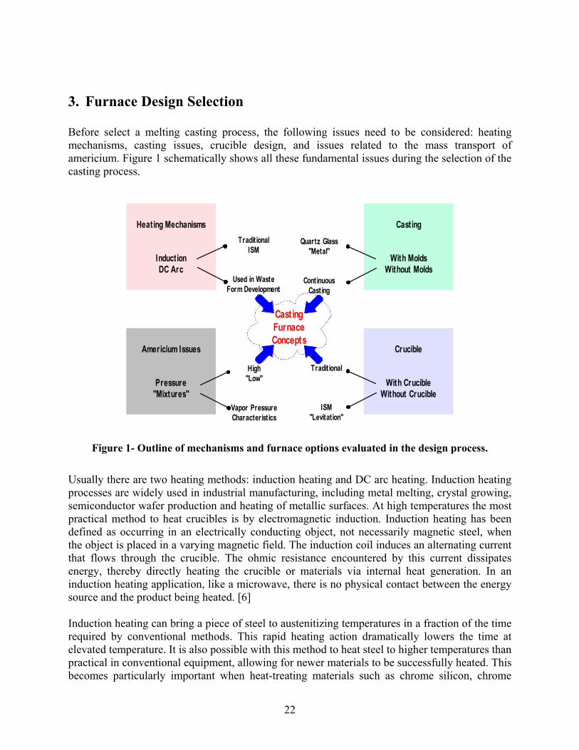
3. Furnace Design Selection Before select a melting casting process, the following issues need to be considered: heating mechanisms, casting issues, crucible design, and issues related to the mass transport of americium. Figure 1 schematically shows all these fundamental issues during the selection of the casting process.
CastingFurnaceConcepts
Casting
With MoldsWithout Molds
Crucible
With CrucibleWithout Crucible
Quartz Glass"Metal"
ContinuousCasting
Traditional
ISM"Levitation"
Heating Mechanisms
InductionDC Arc
Americium Issues
Pressure"Mixtures"
High"Low"
Vapor PressureCharacteristics
TraditionalISM
Used in WasteForm Development
Figure 1- Outline of mechanisms and furnace options evaluated in the design process.
Usually there are two heating methods: induction heating and DC arc heating. Induction heating processes are widely used in industrial manufacturing, including metal melting, crystal growing, semiconductor wafer production and heating of metallic surfaces. At high temperatures the most practical method to heat crucibles is by electromagnetic induction. Induction heating has been defined as occurring in an electrically conducting object, not necessarily magnetic steel, when the object is placed in a varying magnetic field. The induction coil induces an alternating current that flows through the crucible. The ohmic resistance encountered by this current dissipates energy, thereby directly heating the crucible or materials via internal heat generation. In an induction heating application, like a microwave, there is no physical contact between the energy source and the product being heated. [6] Induction heating can bring a piece of steel to austenitizing temperatures in a fraction of the time required by conventional methods. This rapid heating action dramatically lowers the time at elevated temperature. It is also possible with this method to heat steel to higher temperatures than practical in conventional equipment, allowing for newer materials to be successfully heated. This becomes particularly important when heat-treating materials such as chrome silicon, chrome

23
vanadium, or similar alloys that are known to be difficult to properly heat-treat. It’s also possible to have intense stirring of molten material in the crucible as a result of the inducted field, which results in high alloy uniformity. This can be controlled by adjusting the numbers and position of the induction coils, along with the frequency of the electrical field in the coils. [7] A number of industries also use DC arc heating. There may be one or more electrodes. Here the charge is heated by means of an electric arc produced between opposed electrodes (indirect arc furnaces) or between an electrode and the charge (direct arc furnaces). Using DC arc heating can achieve high temperatures and lower maintenance costs. The graphite electrodes do not have to be cooled compared to metal electrodes. Short DC arcs are effective in transferring thermal energy into the materials to be processed. But the high temperature region around the arc (gases may be exposed to the arc temperature) will destroy organic species and vapors that evolve from the material being processed. [8][9] The fuel rods can be formed through the use of molds or continuous casting. Argonne National Laboratory has extensive experience in using molds for casting, but this approach does produce a waste stream, the shattered quartz glass rods. In addition, it requires rapid pressurization and possibly some preheating of the molds. [10] Continuous casting means the solidified shape of the rod is produced as it leaves a mold region. It may be difficult to control the tight tolerances necessary to make fuel rods through the use of this technique. Many traditional casting furnaces have a crucible for containing the molten material. Other furnaces, such as the induction skull melter, do not rely on a traditional crucible. The “crucible” in the induction skull melter is the “skull” of material formed within a set of copper molds that are internally cooled. This cooling process forms a crucible region referred to as a “skull” region. [11][12] The contamination of molten metal by tramp elements which form the crucible which is made of refractory materials. Any reaction between metal and the crucible make it difficult to produce a high purity melt. In addition, there are some materials that have a higher melting point than typical crucible materials. For these reasons, a new casting method, levitation melting has been developed to resolve these difficulties. [13] In this situation, magnetic fields are used to maintain molten fluid within a specified region. The last mechanism deals with factors that can impact the transport of americium. The pressure could be increased to deter the evaporation of americium. Another technique might be to react the americium with another material to form a material that has a lower vapor pressure. An evaluation process was undertaken to select a concept that should have the greatest chance of success for casting americium into a fuel pin. After several sessions with the assistance of ANL-West staff, six conceptual designs were developed. They are each shown in the following six figures.

24
Inductively HeatedPressurized ChamberVacuum Cast (Molds)
Figure 2 - Inductively heated pressurized chamber vacuum cast (Molds).
Inductively HeatedPressurized Chamber
Figure 3 - Inductively heated pressurized “local” chamber.
Coils
Melt
Mold
Crucible
Chamber
Molds
Coils
Melt
Crucible
Chamber
25
Inductively HeatedContinuous Casting
Figure 4 - Inductively heated continuous casting
DC Arc
DC Arc Melting
Figure 5 - DC arc melting with pressurized/gravity molds.
Crucible
Coils
Molds
Chamber
Melt
Interface control between crucible
and molds
Chamber
Crucible
Molds
Electrode
Charge

26
Semi - Levitation Melting
Figure 6 - Semi-levitation melting.
"Cover"
Coils
"Chill Mold"
ResistanceHeaters
CoolantFlow
Figure 7 - Induction skull melting (ISM) with pressurized/gravity molds. Figure 2 illustrates the inductively heated-pressurized/vacuum molds. This model uses induction heating. After the charge was heated and melts, then it will be magnetically stirred to make sure
Coils
Molds
Charge
27
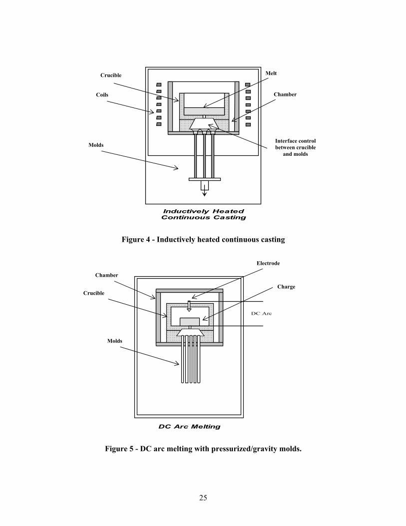
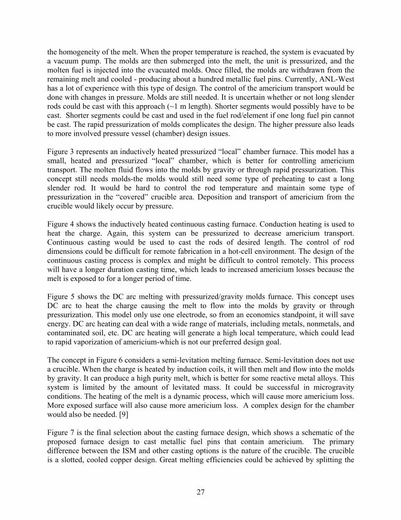
the homogeneity of the melt. When the proper temperature is reached, the system is evacuated by a vacuum pump. The molds are then submerged into the melt, the unit is pressurized, and the molten fuel is injected into the evacuated molds. Once filled, the molds are withdrawn from the remaining melt and cooled - producing about a hundred metallic fuel pins. Currently, ANL-West has a lot of experience with this type of design. The control of the americium transport would be done with changes in pressure. Molds are still needed. It is uncertain whether or not long slender rods could be cast with this approach (~1 m length). Shorter segments would possibly have to be cast. Shorter segments could be cast and used in the fuel rod/element if one long fuel pin cannot be cast. The rapid pressurization of molds complicates the design. The higher pressure also leads to more involved pressure vessel (chamber) design issues. Figure 3 represents an inductively heated pressurized “local” chamber furnace. This model has a small, heated and pressurized “local” chamber, which is better for controlling americium transport. The molten fluid flows into the molds by gravity or through rapid pressurization. This concept still needs molds-the molds would still need some type of preheating to cast a long slender rod. It would be hard to control the rod temperature and maintain some type of pressurization in the “covered” crucible area. Deposition and transport of americium from the crucible would likely occur by pressure. Figure 4 shows the inductively heated continuous casting furnace. Conduction heating is used to heat the charge. Again, this system can be pressurized to decrease americium transport. Continuous casting would be used to cast the rods of desired length. The control of rod dimensions could be difficult for remote fabrication in a hot-cell environment. The design of the continuous casting process is complex and might be difficult to control remotely. This process will have a longer duration casting time, which leads to increased americium losses because the melt is exposed to for a longer period of time. Figure 5 shows the DC arc melting with pressurized/gravity molds furnace. This concept uses DC arc to heat the charge causing the melt to flow into the molds by gravity or through pressurization. This model only use one electrode, so from an economics standpoint, it will save energy. DC arc heating can deal with a wide range of materials, including metals, nonmetals, and contaminated soil, etc. DC arc heating will generate a high local temperature, which could lead to rapid vaporization of americium-which is not our preferred design goal. The concept in Figure 6 considers a semi-levitation melting furnace. Semi-levitation does not use a crucible. When the charge is heated by induction coils, it will then melt and flow into the molds by gravity. It can produce a high purity melt, which is better for some reactive metal alloys. This system is limited by the amount of levitated mass. It could be successful in microgravity conditions. The heating of the melt is a dynamic process, which will cause more americium loss. More exposed surface will also cause more americium loss. A complex design for the chamber would also be needed. [9] Figure 7 is the final selection about the casting furnace design, which shows a schematic of the proposed furnace design to cast metallic fuel pins that contain americium. The primary difference between the ISM and other casting options is the nature of the crucible. The crucible is a slotted, cooled copper design. Great melting efficiencies could be achieved by splitting the
28
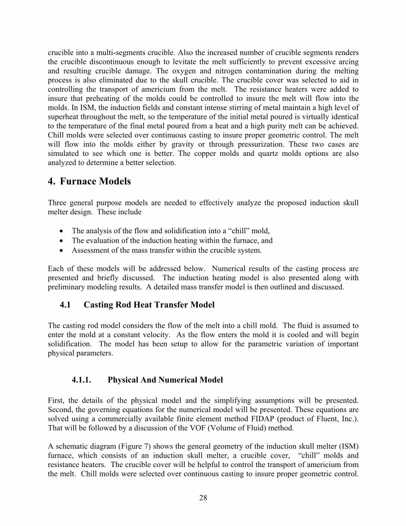
crucible into a multi-segments crucible. Also the increased number of crucible segments renders the crucible discontinuous enough to levitate the melt sufficiently to prevent excessive arcing and resulting crucible damage. The oxygen and nitrogen contamination during the melting process is also eliminated due to the skull crucible. The crucible cover was selected to aid in controlling the transport of americium from the melt. The resistance heaters were added to insure that preheating of the molds could be controlled to insure the melt will flow into the molds. In ISM, the induction fields and constant intense stirring of metal maintain a high level of superheat throughout the melt, so the temperature of the initial metal poured is virtually identical to the temperature of the final metal poured from a heat and a high purity melt can be achieved. Chill molds were selected over continuous casting to insure proper geometric control. The melt will flow into the molds either by gravity or through pressurization. These two cases are simulated to see which one is better. The copper molds and quartz molds options are also analyzed to determine a better selection.
4. Furnace Models Three general purpose models are needed to effectively analyze the proposed induction skull melter design. These include
• The analysis of the flow and solidification into a “chill” mold, • The evaluation of the induction heating within the furnace, and • Assessment of the mass transfer within the crucible system.
Each of these models will be addressed below. Numerical results of the casting process are presented and briefly discussed. The induction heating model is also presented along with preliminary modeling results. A detailed mass transfer model is then outlined and discussed.
4.1 Casting Rod Heat Transfer Model The casting rod model considers the flow of the melt into a chill mold. The fluid is assumed to enter the mold at a constant velocity. As the flow enters the mold it is cooled and will begin solidification. The model has been setup to allow for the parametric variation of important physical parameters.
4.1.1. Physical And Numerical Model First, the details of the physical model and the simplifying assumptions will be presented. Second, the governing equations for the numerical model will be presented. These equations are solved using a commercially available finite element method FIDAP (product of Fluent, Inc.). That will be followed by a discussion of the VOF (Volume of Fluid) method. A schematic diagram (Figure 7) shows the general geometry of the induction skull melter (ISM) furnace, which consists of an induction skull melter, a crucible cover, “chill” molds and resistance heaters. The crucible cover will be helpful to control the transport of americium from the melt. Chill molds were selected over continuous casting to insure proper geometric control.

29
We use resistance heaters to control the molds preheating temperature, which makes sure the melt will flow into the molds. This section of the report addresses the flow and heat transfer associated with the melt entering the chill molds. The important physics of this process includes
• Heat transfer from the melt into the mold, • Mold size, shape and material, • Preheating of the molds, • Mechanism to force the flow into the molds (pressure injection vs. gravity), and • Phase change characteristics of the melt.
As the crucible heats up, the plutonium, americium, and zirconium feedstock melts. The melt is then magnetically stirred to assure homogeneity of the melt before casting. When the proper temperature is reached, the melt will flow into the molds. A number of different velocities will be assumed to study how rapidly the melt must flow into the molds in order to prevent solidification prior to reaching the end of the mold. It is assumed that the melt flows out of the crucible and down into the molds. Figure 8 shows the geometry of the mold model with one end closed. The total length of the mold varies in the simulations, but ranges from 0.5 to 1.0 meter to see what range of length we can produce with low americium loss. The inner radius of the mold is 4 millimeters and the outer radius is 8 millimeters. The molds are preheated before the molten fluid fills the molds. The molds are preheated to insure that the melt flows nearly the full length of the mold, giving the desired rod length.
Inlet Flow
Outlet
Moldr
z
Figure 8 - The Schematic of fuel rod casting model
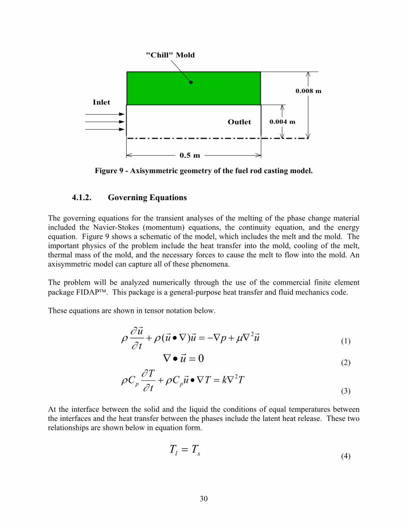
The molds have a cylindrical shape, which can be reduced to axisymmetric geometry involving radial and axial components. Figure 9 shows the simplified geometry. Whenever possible, the use of an axisymmetric geometry reduces the computational times. The variables that will affect mold filling are the average fill velocity of melt, initial mold temperatures and the heat transfer coefficient between the melt and the mold. The filling process happens only within a few seconds. The heat transfer coefficient between the melt and the mold is an important factor affecting the heat transfer.
30
Outlet
"Chill" Mold
0.5 m
0.008 m
0.004 m
Inlet
Figure 9 - Axisymmetric geometry of the fuel rod casting model.
4.1.2. Governing Equations The governing equations for the transient analyses of the melting of the phase change material included the Navier-Stokes (momentum) equations, the continuity equation, and the energy equation. Figure 9 shows a schematic of the model, which includes the melt and the mold. The important physics of the problem include the heat transfer into the mold, cooling of the melt, thermal mass of the mold, and the necessary forces to cause the melt to flow into the mold. An axisymmetric model can capture all of these phenomena. The problem will be analyzed numerically through the use of the commercial finite element package FIDAP. This package is a general-purpose heat transfer and fluid mechanics code. These equations are shown in tensor notation below.
2( )u u u p u
t∂ρ ρ µ∂
+ •∇ = −∇ + ∇r
r r r (1)
0u∇• =r
(2)
2p p
TC C u T k Tt
∂ρ ρ∂
+ •∇ = ∇r
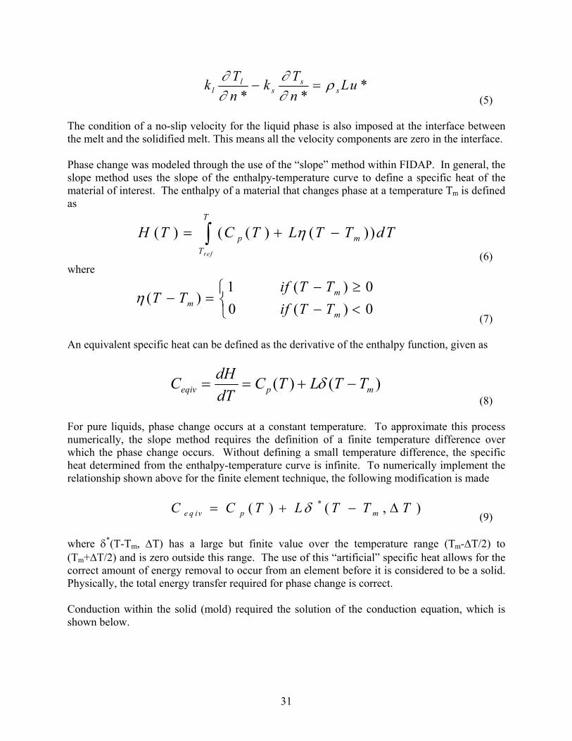
(3) At the interface between the solid and the liquid the conditions of equal temperatures between the interfaces and the heat transfer between the phases include the latent heat release. These two relationships are shown below in equation form.
l sT T= (4)
31
*
* *l s
l s sT Tk k Lun n
∂ ∂ ρ∂ ∂
− = (5)
The condition of a no-slip velocity for the liquid phase is also imposed at the interface between the melt and the solidified melt. This means all the velocity components are zero in the interface. Phase change was modeled through the use of the “slope” method within FIDAP. In general, the slope method uses the slope of the enthalpy-temperature curve to define a specific heat of the material of interest. The enthalpy of a material that changes phase at a temperature Tm is defined as
( ) ( ( ) ( ))ref
T
p mT
H T C T L T T dTη= + −∫ (6)
where
1 ( ) 0( )
0 ( ) 0m
mm
if T TT T
if T Tη
− ≥− = − < (7)
An equivalent specific heat can be defined as the derivative of the enthalpy function, given as
( ) ( )eqiv p m
dHC C T L T TdT
δ= = + − (8)
For pure liquids, phase change occurs at a constant temperature. To approximate this process numerically, the slope method requires the definition of a finite temperature difference over which the phase change occurs. Without defining a small temperature difference, the specific heat determined from the enthalpy-temperature curve is infinite. To numerically implement the relationship shown above for the finite element technique, the following modification is made
*( ) ( , )e q iv p mC C T L T T Tδ= + − ∆
(9) where δ*(T-Tm, ∆T) has a large but finite value over the temperature range (Tm-∆T/2) to (Tm+∆T/2) and is zero outside this range. The use of this “artificial” specific heat allows for the correct amount of energy removal to occur from an element before it is considered to be a solid. Physically, the total energy transfer required for phase change is correct. Conduction within the solid (mold) required the solution of the conduction equation, which is shown below.
32
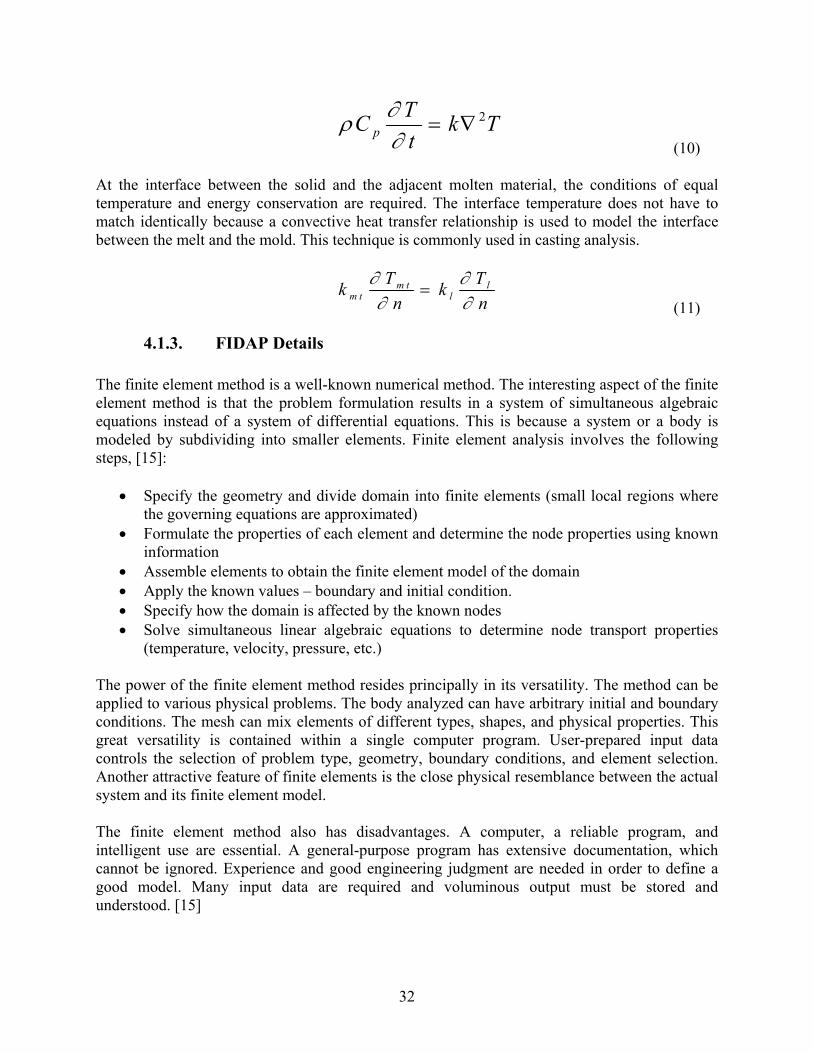
2p
TC k Tt
∂ρ∂
= ∇ (10)
At the interface between the solid and the adjacent molten material, the conditions of equal temperature and energy conservation are required. The interface temperature does not have to match identically because a convective heat transfer relationship is used to model the interface between the melt and the mold. This technique is commonly used in casting analysis.
m t l
m t lT Tk kn n
∂ ∂∂ ∂
= (11)
4.1.3. FIDAP Details The finite element method is a well-known numerical method. The interesting aspect of the finite element method is that the problem formulation results in a system of simultaneous algebraic equations instead of a system of differential equations. This is because a system or a body is modeled by subdividing into smaller elements. Finite element analysis involves the following steps, [15]:
• Specify the geometry and divide domain into finite elements (small local regions where the governing equations are approximated)
• Formulate the properties of each element and determine the node properties using known information
• Assemble elements to obtain the finite element model of the domain • Apply the known values – boundary and initial condition. • Specify how the domain is affected by the known nodes • Solve simultaneous linear algebraic equations to determine node transport properties
(temperature, velocity, pressure, etc.) The power of the finite element method resides principally in its versatility. The method can be applied to various physical problems. The body analyzed can have arbitrary initial and boundary conditions. The mesh can mix elements of different types, shapes, and physical properties. This great versatility is contained within a single computer program. User-prepared input data controls the selection of problem type, geometry, boundary conditions, and element selection. Another attractive feature of finite elements is the close physical resemblance between the actual system and its finite element model. The finite element method also has disadvantages. A computer, a reliable program, and intelligent use are essential. A general-purpose program has extensive documentation, which cannot be ignored. Experience and good engineering judgment are needed in order to define a good model. Many input data are required and voluminous output must be stored and understood. [15]
33
An iterative solution technique for a FEM solver was employed to solve the set of equations sequentially and separately for each active degree of freedom. This approach is referred to as a segregated solver. This method is used because it substantially reduces the memory requirement compared to the other solvers used, such as the fully coupled method. FIDAP uses the VOF (Volume of Fluid) technique to model transient flows involving free surfaces of arbitrary shape. The capabilities constitute a powerful tool in simulating complex free surface deformations including folding and breakup. FIDAP was used to solve the fluid and heat flow inside the molds. A “mapped” type mesh was used to discretize the geometry. The general purpose pre-processor GAMBITTM was used for the mesh generation. A mapped mesh is a regular “checkerboard” mesh for surface areas that are typically used for more regular geometries. The complete finite element mesh for the heat transfer problem was constructed from a collection of mapped mesh areas. This technique is not automatic, as the geometry must be decomposed into regions that are suited to a mapped mesh. A backward Euler (implicit) scheme was used to solve the three transient equations. Segregated iterative method was used to obtain the solution at each time step using fixed time step. Although one can generally obtain high order accuracy, when convection is strong compared to the diffusion and sharp gradients of the flow variables are encountered in the computational grid, unstable results are likely to occur. Streamline upwinding is used to stabilize the oscillations in the computations. There are two general approaches that could be used to model the flow of the molten material into the melt. The first is to move the mesh with the melt. This approach requires the mesh to be continually recalculated and it requires a technique to couple the heat transfer to the solid. The second choice is to have the fluid move through a fixed mesh. This latter technique is the approach FIDAP uses and it will briefly be discussed next.
4.1.4. Volume of Fluid (VOF) Method Free boundaries are considered to be surfaces on which discontinuities exist in one or more variables. Examples are free surfaces of fluids (open channel flow), material interfaces, shock waves, or interface between a fluid and deformable structures. Three types of problems arise in the numerical treatment of free boundaries: (1) their discrete representation, (2) their evolution in time, and (3) the manner in which boundary conditions are imposed on them. The process of embedding a discontinuous surface in a matrix of computational cells involves three separate tasks. First, it is necessary to devise a means of numerically describing the location and shape of the boundary. Second, an algorithm must be given for computing the time evolution of the boundary. Finally, a scheme must be provided for imposing the desired surface boundary conditions on the surrounding computational mesh. [16] FIDAP uses the Volume of Fluid (VOF) method as a technique to simulate free surface flows. [17] This tool is a filling process, which allows the simulation of complex free surface flows

34
with an arbitrary shape in any situation including folding or break-up. The filling process is computed as follows:
• A Galerkin finite element method is used to resolve Navier-Stokes equations. • Free surfaces are characterized by a VOF type representation on the mesh, advection of
the fluid is followed by a volume tracking method. • On the basis of a given velocity field, a new fluid boundary is determined with the
volume method. When the new fluid boundary is obtained, the Reynolds Average Navier-Stokes equations are solved using a finite element method. These two methods are thus applied in alternating deformations and decoupled in order to predict transient deformations.
The VOF technique relies on the definition of a variable F whose value is unity at any point occupied by fluid and zero otherwise. The average value of F in a cell would then represent the fractional volume of the cell occupied by fluid. In particular, a unit value of F would correspond to a cell full of fluid, while a zero value would indicate that the cell contained no fluid. Cells with F values between zero and one must then contain a free surface. VOF method only requires one storage word for each mesh cell, which is consistent with the storage requirements for all other dependent variables. The indicator function F represents the fluid volume, which is moved by the flow field. So the advection of the this function is governed by:
0Ft V F∂∂ + ⋅∇ =
v (12)
The sharp interfaces are maintained by ensuring a sharp gradient of F. The value of this function is 1 when the cell of the meshing volume is filled and is equal to 0 when this cell is emptied. A steep gradient of F represents a free surface location.
=VoidFluid
txF01
),( v
(13) The function F can be discretized as follows:
∫= iVi FdVfi
1
for element I (14) The limits of integration are restricted to the volume of an element Vi. The value of fi corresponds to a filled state, an emptied state, or fractional filled state. Thus fi varies between 0 and 1. An element whose fi = 1 is referred to as a filled element. An emptied element is denoted by fi = 0. The value of fi between 0 and 1 means a fractional fill or a free surface. [17][18]
35
The VOF method offers a region-following scheme with smaller storage requirements. Furthermore, because it follows regions rather than surface, all logic problems associated with intersecting surfaces are avoided with the VOF technique. The method is also applicable to three-dimensional computations, where its conservative use of stored information is highly advantageous. In principle, the method can be used to track surfaces of discontinuity in materials properties, in tangential velocity, or any other property. The particular case being represented determines the specific situations that must be applied at the location of the boundary. For situations where the surface does not remain fixed in the fluid, but has some additional relative motion, the equation of motion must be modified. Examples of such applications are shock waves, chemical reaction fronts, and boundaries between single-phase and two-phase fluid regions. [16]
4.1.5. Results In order to test the impact of process parameters (temperature, pressure, alloying elements, etc.) on the casting process, a parametric study of the casting model was performed on different parameters to determine which process parameters are critical in manufacturing a suitable metallic fuel pin. Parameters study efforts centered around model development and the analysis of the impact of mold preheating on heat transfer into the mold. The inner radius is estimated from discussions with ANL staff. Normally, the way the heat flows across the metal and mold surfaces directly affects the evolution of solidification, and plays a notable role in determining the freezing conditions within the metal. When metal and mold surfaces are brought into contact an imperfect junction is formed. While uniform temperature gradients can exist in both metal and mold, the junction between the two surfaces creates a temperature drop, which is dependent upon the thermophysical properties of the contacting materials, the casting and mold geometry, the roughness of the mold surface, the presence of the gaseous and non-gaseous interstitial media, the melt superheat, contact pressure and initial temperature of the mold. Because the two surfaces in contact are not perfectly flat, when the interfacial contact pressure is reasonably high, most of the energy passed through a limited number of actual contact spots. [19] The heat flow across the casting-mold interface can be characterized by a macroscopic average metal-mold interfacial heat transfer coefficient (hi), given by
)( 11 Mc TTAq
ih −= (15)
The heat transfer coefficient shows a high value in the initial stage of solidification, the result of good surface conformity between the liquid core and the solidified shell. As solidification progresses the mold expands due to the absorption of heat and the solid metal shrinks during cooling and as a result a gap develops because pressure becomes insufficient to maintain a conforming contact at the interface. Once the air gaps form, the heat transfer across the interface decreases rapidly and a relatively constant value of hi is attained. The ways of heat transfer here
36
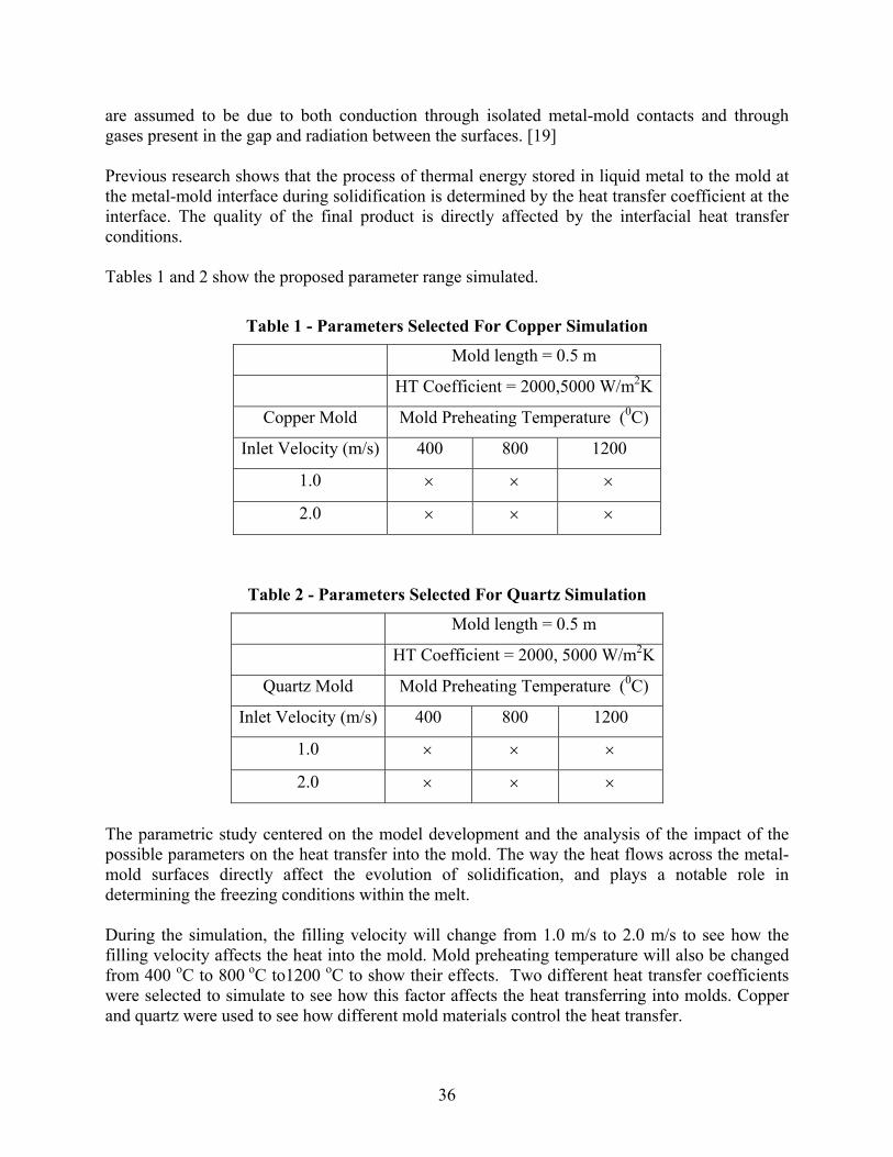
are assumed to be due to both conduction through isolated metal-mold contacts and through gases present in the gap and radiation between the surfaces. [19] Previous research shows that the process of thermal energy stored in liquid metal to the mold at the metal-mold interface during solidification is determined by the heat transfer coefficient at the interface. The quality of the final product is directly affected by the interfacial heat transfer conditions. Tables 1 and 2 show the proposed parameter range simulated.
Table 1 - Parameters Selected For Copper Simulation
Mold length = 0.5 m
HT Coefficient = 2000,5000 W/m2K
Copper Mold Mold Preheating Temperature (0C)
Inlet Velocity (m/s) 400 800 1200
1.0 × × ×
2.0 × × ×
Table 2 - Parameters Selected For Quartz Simulation
Mold length = 0.5 m
HT Coefficient = 2000, 5000 W/m2K
Quartz Mold Mold Preheating Temperature (0C)
Inlet Velocity (m/s) 400 800 1200
1.0 × × ×
2.0 × × ×
The parametric study centered on the model development and the analysis of the impact of the possible parameters on the heat transfer into the mold. The way the heat flows across the metal-mold surfaces directly affect the evolution of solidification, and plays a notable role in determining the freezing conditions within the melt. During the simulation, the filling velocity will change from 1.0 m/s to 2.0 m/s to see how the filling velocity affects the heat into the mold. Mold preheating temperature will also be changed from 400 oC to 800 oC to1200 oC to show their effects. Two different heat transfer coefficients were selected to simulate to see how this factor affects the heat transferring into molds. Copper and quartz were used to see how different mold materials control the heat transfer.
37
4.1.5.1 Results – Copper Molds The conditions for each model included:
• Melt temperature of 1500 oC. • Average fill velocity of 1.0 m/s • Mold thermal properties assumed to be similar to copper • Pin diameter of 0.008 m • Mold outside diameter of 0.016 m • Mold length of 0.50 m • Properties of melt assumed to be dependent on plutonium, americium, and zirconium • Heat transfer coefficient between the melt and the mold assumed to be 2,000 W/m2K,
unless otherwise noted • Initial mold temperatures were varied (1200 oC, 800 oC, or 400 oC)
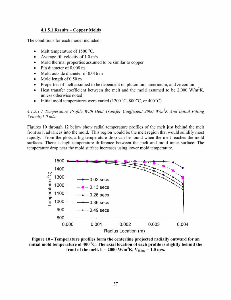
4.1.5.1.1 Temperature Profile With Heat Transfer Coefficient 2000 W/m2K And Initial Filling Velocity1.0 m/s: Figures 10 through 12 below show radial temperature profiles of the melt just behind the melt front as it advances into the mold. This region would be the melt region that would solidify most rapidly. From the plots, a big temperature drop can be found when the melt reaches the mold surfaces. There is high temperature difference between the melt and mold inner surface. The temperature drop near the mold surface increases using lower mold temperature.
800
900
1000
1100
1200
1300
1400
1500
0.000 0.001 0.002 0.003 0.004Radius Location (m)
Tem
pera
ture
(0 C)
0.02 secs
0.13 secs
0.26 secs
0.36 secs
0.49 secs
Figure 10 - Temperature profiles form the centerline projected radially outward for an
initial mold temperature of 400 oC. The axial location of each profile is slightly behind the front of the melt. h = 2000 W/m2K, Vfilling = 1.0 m/s.

38
800
900
1000
1100
1200
1300
1400
1500
0.000 0.001 0.002 0.003 0.004
Radius Location (m)
Tem
pera
ture
(0 C)
0.02 secs0.13 secs0.26 secs0.36 secs0.49 secs
Figure 11 - Temperature profiles form the centerline projected radially outward for an
initial mold temperature of 800 oC. h = 2000 W/m2K, Vfilling = 1.0 m/s.
800
900
1000
1100
1200
1300
1400
1500
0.000 0.001 0.002 0.003 0.004Radius Location (m)
Tem
pera
ture
(0 C)
0.02 secs0.13 secs0.26 secs0.36 secs0.49 secs
Figure 12 - Temperature profiles form the centerline projected radially outward for an initial
mold temperature of 1200 oC. h = 2000 W/m2K, Vfilling = 1.0 m/s.

39
Figures 13 and Figure 14 show the mold preheating effect on the heat transfer from melt into the mold. Figure 13 shows the temperature profile at 0.13 seconds in the radial direction during different preheating temperature condition. Higher preheating temperature will prevent the heat transferring into mold, which means it will take more time to reach the same location. Figure 14 shows the radial temperature profile at 0.36 seconds during different mold preheating temperature.
1000
1100
1200
1300
1400
1500
0.000 0.001 0.002 0.003 0.004Radius Location (m)
Tem
pera
ture
(0 C)
400 oC800 oC1200 oC
Figure 13 - Temperature profiles from the centerline projected radially outward at 0.13 seconds. Lower to upper curves represent mold temperature of 400oC, 800oC
and 1200 oC. h = 2000 W/m2K, Vfilling = 1.0 m/s
1000
1100
1200
1300
1400
1500
0.000 0.001 0.002 0.003 0.004Radius Location (m)
Tem
pera
ture
(0 C)
400 oC800 oC1200 oC
Figure 14 - Temperature profiles from the centerline projected radially outward at 0.36
seconds. Lower to upper curves represent mold temperature of 400 oC, 800 oC and 1200 oC. h = 2000 W/m2K, Vfilling = 1.0 m/s.
40
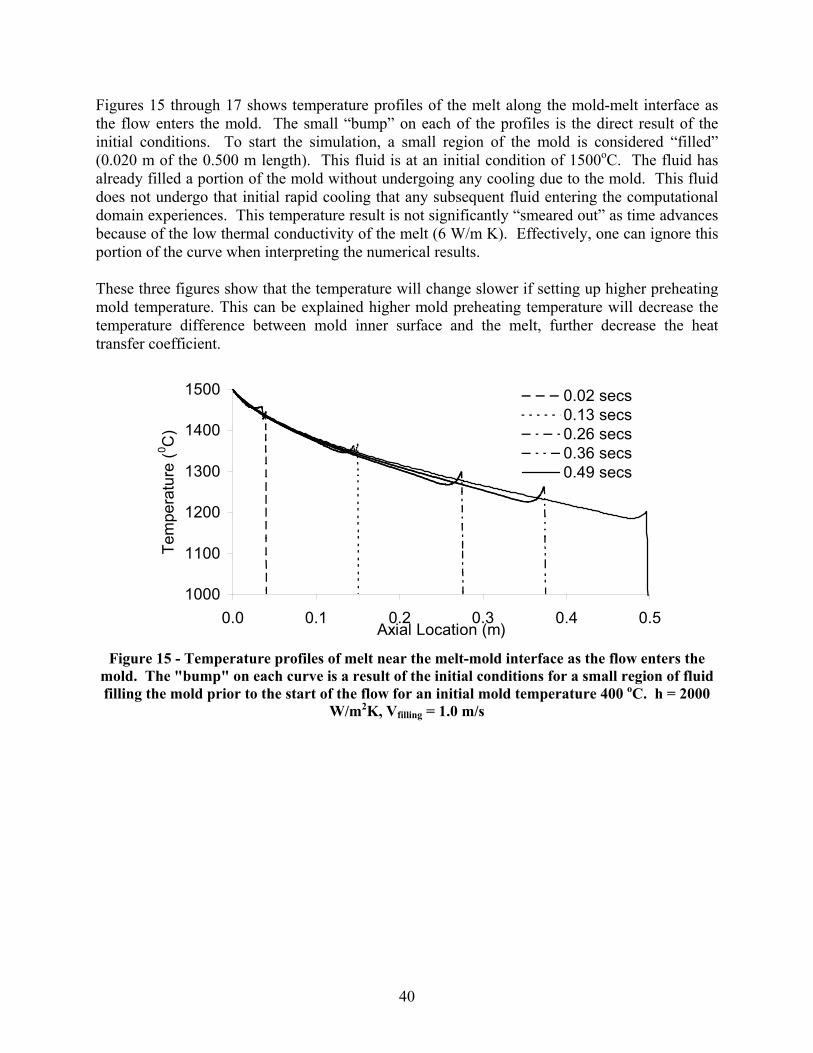
Figures 15 through 17 shows temperature profiles of the melt along the mold-melt interface as the flow enters the mold. The small “bump” on each of the profiles is the direct result of the initial conditions. To start the simulation, a small region of the mold is considered “filled” (0.020 m of the 0.500 m length). This fluid is at an initial condition of 1500oC. The fluid has already filled a portion of the mold without undergoing any cooling due to the mold. This fluid does not undergo that initial rapid cooling that any subsequent fluid entering the computational domain experiences. This temperature result is not significantly “smeared out” as time advances because of the low thermal conductivity of the melt (6 W/m K). Effectively, one can ignore this portion of the curve when interpreting the numerical results. These three figures show that the temperature will change slower if setting up higher preheating mold temperature. This can be explained higher mold preheating temperature will decrease the temperature difference between mold inner surface and the melt, further decrease the heat transfer coefficient.
1000
1100
1200
1300
1400
1500
0.0 0.1 0.2 0.3 0.4 0.5Axial Location (m)
Tem
pera
ture
(0 C)
0.02 secs0.13 secs0.26 secs0.36 secs0.49 secs
Figure 15 - Temperature profiles of melt near the melt-mold interface as the flow enters the
mold. The "bump" on each curve is a result of the initial conditions for a small region of fluid filling the mold prior to the start of the flow for an initial mold temperature 400 oC. h = 2000
W/m2K, Vfilling = 1.0 m/s

41
1000
1100
1200
1300
1400
1500
0.00 0.10 0.20 0.30 0.40 0.50Axial Locations (m)
Tem
pera
ture
(0 C)
0.02 secs0.13 secs0.26 secs0.36 secs0.49 secs
Figure 16 - Temperature profiles of melt near the melt-mold interface as the flow enters the mold with an initial mold temperature 800 oC. h = 2000 W/m2K, Vfilling = 1.0 m/s
1000
1100
1200
1300
1400
1500
0.0 0.1 0.2 0.3 0.4 0.5Axial Locations (m)
Tem
pera
ture
(0 C)
0.02 secs0.16 secs0.26 secs0.36 secs0.49 secs
Figure 17 - Temperature profiles of melt near the melt-mold interface as the flow enters the
mold with an initial mold temperature 1200 oC. h = 2000 W/m2K, Vfilling = 1.0 m/s Figures 18 and 19 are the temperature profiles along the melt-mold interface during different initial preheating mold preheating temperature 400 oC, 800 oC and 1200 oC. From the plots, it is not surprising that the mold preheating temperature greatly impacts the cooling rate of the melt as it flows into the mold.

42
800
900
1000
1100
1200
1300
1400
1500
0.0 0.1 0.2 0.3 0.4
Axial Location (m)
Tem
pera
ture
(0 C)
Figure 18 - Temperature profiles of melt material near the melt-mold interface at 0.49 seconds. Lower to upper curves represent mold temperature of 400 oC, 800 oC
and 1200 oC. h = 2000 W/m2K, Vfilling = 1.0 m/s
800
900
1000
1100
1200
1300
1400
1500
0.0 0.1 0.2 0.3Axial Locations (m)
Tem
pera
ture
(0 C)
Figure 19 - Temperature profiles of melt material near the melt-mold interface at 0.36 seconds. Lower to upper curves represent mold temperature of 400 oC, 800 oC
and 1200 oC. h = 2000 W/m2K, Vfilling = 1.0 m/s
Table 3 and Table 4 show the temperature of the melt material near the melt-mold interface at the 0.36 seconds and 0.49 seconds under different mold preheating temperature.
43
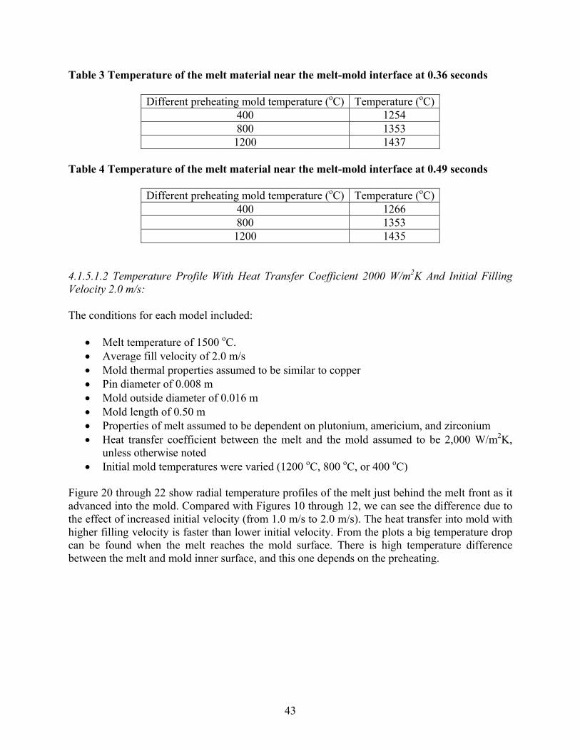
Table 3 Temperature of the melt material near the melt-mold interface at 0.36 seconds
Different preheating mold temperature (oC) Temperature (oC) 400 1254 800 1353 1200 1437
Table 4 Temperature of the melt material near the melt-mold interface at 0.49 seconds
Different preheating mold temperature (oC) Temperature (oC) 400 1266 800 1353 1200 1435
4.1.5.1.2 Temperature Profile With Heat Transfer Coefficient 2000 W/m2K And Initial Filling Velocity 2.0 m/s: The conditions for each model included:
• Melt temperature of 1500 oC. • Average fill velocity of 2.0 m/s • Mold thermal properties assumed to be similar to copper • Pin diameter of 0.008 m • Mold outside diameter of 0.016 m • Mold length of 0.50 m • Properties of melt assumed to be dependent on plutonium, americium, and zirconium • Heat transfer coefficient between the melt and the mold assumed to be 2,000 W/m2K,
unless otherwise noted • Initial mold temperatures were varied (1200 oC, 800 oC, or 400 oC)
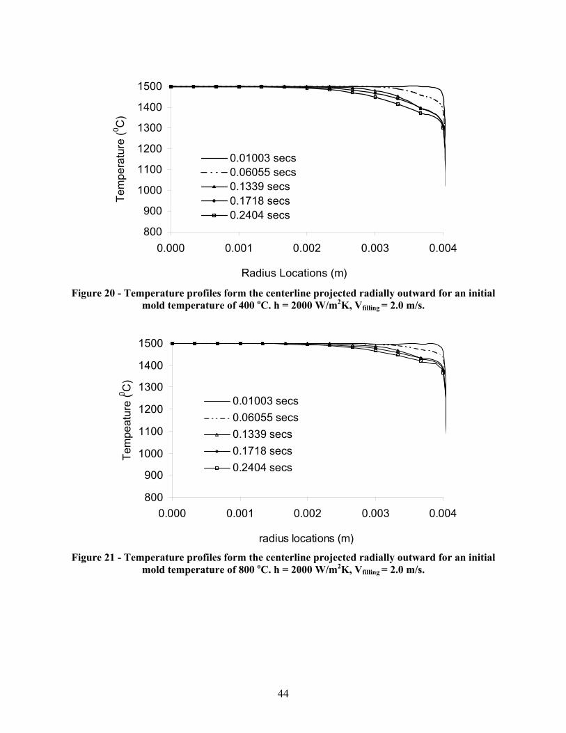
Figure 20 through 22 show radial temperature profiles of the melt just behind the melt front as it advanced into the mold. Compared with Figures 10 through 12, we can see the difference due to the effect of increased initial velocity (from 1.0 m/s to 2.0 m/s). The heat transfer into mold with higher filling velocity is faster than lower initial velocity. From the plots a big temperature drop can be found when the melt reaches the mold surface. There is high temperature difference between the melt and mold inner surface, and this one depends on the preheating.
44
800
900
1000
1100
1200
1300
1400
1500
0.000 0.001 0.002 0.003 0.004
Radius Locations (m)
Tem
pera
ture
(0 C)
0.01003 secs0.06055 secs0.1339 secs0.1718 secs0.2404 secs
Figure 20 - Temperature profiles form the centerline projected radially outward for an initial
mold temperature of 400 oC. h = 2000 W/m2K, Vfilling = 2.0 m/s.
800
900
1000
1100
1200
1300
1400
1500
0.000 0.001 0.002 0.003 0.004
radius locations (m)
Tem
peat
ure
(0 C)
0.01003 secs0.06055 secs0.1339 secs0.1718 secs0.2404 secs
Figure 21 - Temperature profiles form the centerline projected radially outward for an initial
mold temperature of 800 oC. h = 2000 W/m2K, Vfilling = 2.0 m/s.
45
800
900
1000
1100
1200
1300
1400
1500
0.000 0.001 0.002 0.003 0.004Radius Locations (m)
Tem
pera
ture
(0 C)
0.01003 secs0.06055 secs0.1339 secs0.1718 secs0.2404 secs
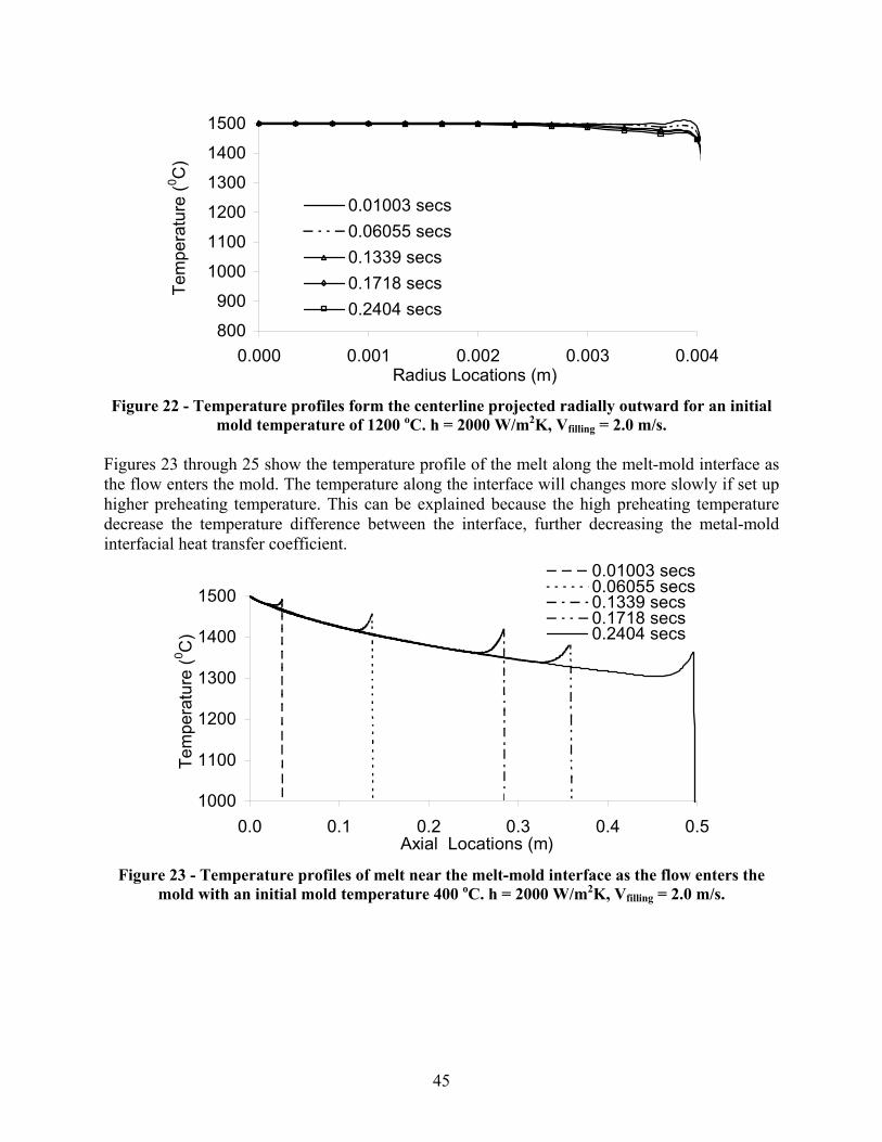
Figure 22 - Temperature profiles form the centerline projected radially outward for an initial
mold temperature of 1200 oC. h = 2000 W/m2K, Vfilling = 2.0 m/s. Figures 23 through 25 show the temperature profile of the melt along the melt-mold interface as the flow enters the mold. The temperature along the interface will changes more slowly if set up higher preheating temperature. This can be explained because the high preheating temperature decrease the temperature difference between the interface, further decreasing the metal-mold interfacial heat transfer coefficient.
1000
1100
1200
1300
1400
1500
0.0 0.1 0.2 0.3 0.4 0.5Axial Locations (m)
Tem
pera
ture
(0 C)
0.01003 secs0.06055 secs0.1339 secs0.1718 secs0.2404 secs
Figure 23 - Temperature profiles of melt near the melt-mold interface as the flow enters the
mold with an initial mold temperature 400 oC. h = 2000 W/m2K, Vfilling = 2.0 m/s.

46
1000
1100
1200
1300
1400
1500
0.0 0.1 0.2 0.3 0.4 0.5Axial Locations (m)
Tem
pera
ture
(0 C)
0.01003 secs0.06055 secs0.1339 secs0.1718 secs0.2404 secs
Figure 24 - Temperature profiles of melt near the melt-mold interface as the flow enters the
mold with an initial mold temperature 800 oC. h = 2000 W/m2K, Vfilling = 2.0 m/s.
1000
1100
1200
1300
1400
1500
0.0 0.1 0.2 0.3 0.4 0.5Axial Locations (m)
Tem
pera
ture
(0 C)
0.01003 secs0.06055 secs0.1339 secs0.1718 secs0.2404 secs
Figure 25 - Temperature profiles of melt near the melt-mold interface as the flow enters the
mold with an initial mold temperature 1200 oC. h = 2000 W/m2K, Vfilling = 2.0 m/s. Figures 26 and Figure 27 show the mold preheating effect on the heat transfer from the melt into the mold. Figure 26 shows the temperature profiles at 0.06 seconds in the radial direction during

47
different preheating temperature condition. The heat transferring into mold will be slower if using higher preheating temperature. Figure 27 shows the radial temperature profile at 0.18 seconds during different mold preheating temperature. Table 5 and Table 6 show the temperature from the centerline projected radially outward at the 0.06 seconds and 0.18 seconds under different mold preheating temperature.
Table 5 Temperature from centerline projected radially outward at 0.06 seconds
Different preheating mold temperature (oC) Temperature (oC) ∆(Ti – T400) oC 400 1498 800 1498 0.04 1200 1499 1.38
Table 6 Temperature from centerline projected radially outward at 0.18 seconds
Different preheating mold temperature (oC) Temperature (oC) ∆(Ti – T400) oC
400 1345 800 1401 56.2 1200 1458 56.3
1000
1100
1200
1300
1400
1500
0.000 0.001 0.002 0.003 0.004Radius Locations (m)
Tem
pera
ture
(0 C)
400 oC800 oC1200 oC
Figure 26 - Temperature profiles from the centerline projected radially outward for copper
mold 0.06 seconds. Lower to upper curves represent mold temperature of 400 oC, 800 oC and 1200 oC. h = 2000 W/m2K, Vfilling = 2.0 m/s.

48
1000
1100
1200
1300
1400
1500
0.000 0.001 0.002 0.003 0.004Radius Locations (m)
Tem
pera
ture
(0 C)
400 oC800 oC1200 oC
Figure 27 - Temperature profiles from the centerline projected radially outward for copper
mold 0.18 seconds. Lower to upper curves represent mold temperature of 400 oC, 800 oC and 1200 oC. h = 2000 W/m2K, Vfilling = 2.0 m/s.
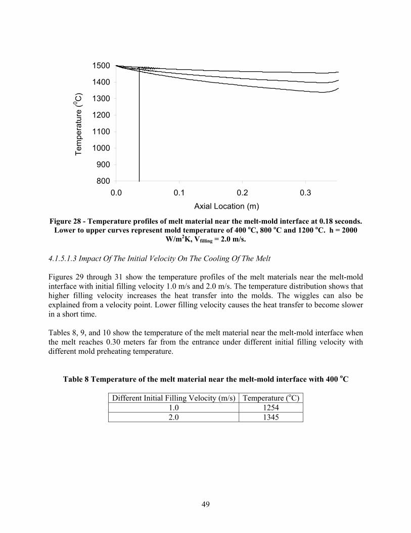
Figures 28 shows the temperature profiles along the melt-mold interface during different initial preheating mold temperature 400 oC, 800 oC and 1200 oC. There are more wiggles near the filling entrance when the preheating temperature is higher. These wiggles indicate that the heat transfer will be slower if the preheating mold temperature is higher. The cooling of the melt using 2.0 m/s is faster than using 1.0m/s, as compared with Figure 29. Table 7 shows the temperature of the melt material near the melt-mold interface at the 0.18 seconds far from the entrance under different mold preheating temperature.
Table 7 Temperature of the melt material near the melt-mold interface at 0.18 seconds
Different preheating mold temperature (oC) Temperature (oC) ∆(Ti – T400) oC400 1345 800 1401 56.2 1200 1458 56.3
49
800
900
1000
1100
1200
1300
1400
1500
0.0 0.1 0.2 0.3
Axial Location (m)
Tem
pera
ture
(0 C)
Figure 28 - Temperature profiles of melt material near the melt-mold interface at 0.18 seconds.
Lower to upper curves represent mold temperature of 400 oC, 800 oC and 1200 oC. h = 2000 W/m2K, Vfilling = 2.0 m/s.
4.1.5.1.3 Impact Of The Initial Velocity On The Cooling Of The Melt Figures 29 through 31 show the temperature profiles of the melt materials near the melt-mold interface with initial filling velocity 1.0 m/s and 2.0 m/s. The temperature distribution shows that higher filling velocity increases the heat transfer into the molds. The wiggles can also be explained from a velocity point. Lower filling velocity causes the heat transfer to become slower in a short time. Tables 8, 9, and 10 show the temperature of the melt material near the melt-mold interface when the melt reaches 0.30 meters far from the entrance under different initial filling velocity with different mold preheating temperature.
Table 8 Temperature of the melt material near the melt-mold interface with 400 oC
Different Initial Filling Velocity (m/s) Temperature (oC) 1.0 1254 2.0 1345

50
Table 9 Temperature of the melt material near the melt-mold interface with 800 oC
Different Initial Filling Velocity (m/s) Temperature (oC) 1.0 1356 2.0 1404
Table 10 Temperature of the melt material near the melt-mold interface with 1200 oC
Different Initial Filling Velocity (m/s) Temperature (oC) 1.0 1437 2.0 1458
1000
1100
1200
1300
1400
1500
0.0 0.1 0.2 0.3
Axial Location (m)
Tem
pera
ture
(0C
)
Figure 29 - Examination of the impact of initial filling velocity on the cooling of the melt. Mold preheating temperature = 400 oC. h = 2000 W/m2K

51
1000
1100
1200
1300
1400
1500
0.0 0.1 0.2 0.3Axial Location (m)
Tem
pera
ture
(0 C)
Figure 30 - Examination of the impact of initial filling velocity on the cooling of the melt. Mold preheating temperature = 800 oC. h = 2000 W/m2K
1000
1100
1200
1300
1400
1500
0.0 0.1 0.2 0.3Axial Location (m)
Tem
pertu
re (0 C
)
Figure 31 - Examination of the impact of initial filling velocity on the cooling of the melt. Mold preheating temperature = 1200 oC. h = 2000 W/m2K
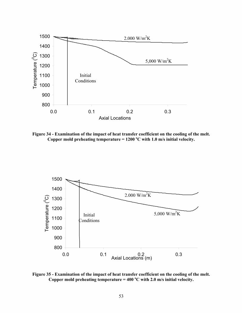
4.1.5.1.4 Impact Of The Heat Transfer Coefficient On The Cooling Of The Melt Figures 32 through 37 show the impact of the assumed heat transfer coefficient on the cooling of the melt. Depending on the theoretical research, the interfacial heat transfer coefficient is the most import factor affecting the heat transfer into the molds. The results clearly show this trend. The effect of higher heat transfer rate will obvious during lower filling velocity. The effect of
V = 2.0 m/sV = 1.0 m/s
Initial Conditions
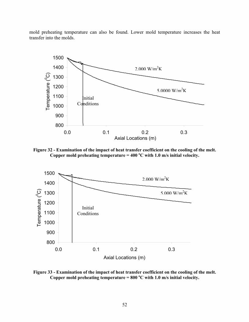
52
mold preheating temperature can also be found. Lower mold temperature increases the heat transfer into the molds.
800
900
1000
1100
1200
1300
1400
1500
0.0 0.1 0.2 0.3Axial Locations (m)
Tem
pera
ture
(0 C)
Figure 32 - Examination of the impact of heat transfer coefficient on the cooling of the melt. Copper mold preheating temperature = 400 oC with 1.0 m/s initial velocity.
800
900
1000
1100
1200
1300
1400
1500
0.0 0.1 0.2 0.3
Axial Locations (m)
Tem
pera
ture
(0 C)
Figure 33 - Examination of the impact of heat transfer coefficient on the cooling of the melt. Copper mold preheating temperature = 800 oC with 1.0 m/s initial velocity.
2,000 W/m2K
5,0000 W/m2K
5,000 W/m2K
2,000 W/m2K
Initial Conditions
Initial Conditions
53
800
900
1000
1100
1200
1300
1400
1500
0.0 0.1 0.2 0.3Axial Locations
Tem
pera
ture
(0 C)
Figure 34 - Examination of the impact of heat transfer coefficient on the cooling of the melt. Copper mold preheating temperature = 1200 oC with 1.0 m/s initial velocity.
800
900
1000
1100
1200
1300
1400
1500
0.0 0.1 0.2 0.3Axial Locations (m)
Tem
pera
ture
(0 C)
Figure 35 - Examination of the impact of heat transfer coefficient on the cooling of the melt.
Copper mold preheating temperature = 400 oC with 2.0 m/s initial velocity.
2,000 W/m2K
5,000 W/m2K
Initial Conditions
2,000 W/m2K
5,000 W/m2K Initial Conditions

54
800
900
1000
1100
1200
1300
1400
1500
0.0 0.1 0.2 0.3Axial Locations (m)
Tem
pera
ture
(0 C)
Figure 36 - Examination of the impact of heat transfer coefficient on the cooling of the melt. Copper mold preheating temperature = 800 oC with 2.0 m/s initial velocity.
800
900
1000
1100
1200
1300
1400
1500
0.0 0.1 0.2 0.3
Axial Locations (m)
Tem
pera
ture
(0 C)
Figure 37 - Examination of the impact of heat transfer coefficient on the cooling of the melt. Copper mold preheating temperature = 1200 oC with 2.0 m/s initial velocity.
2,000 W/m2K
5,000 W/m2K
5,000 W/m2K2,000 W/m2K
Initial Conditions
Initial Conditions

55
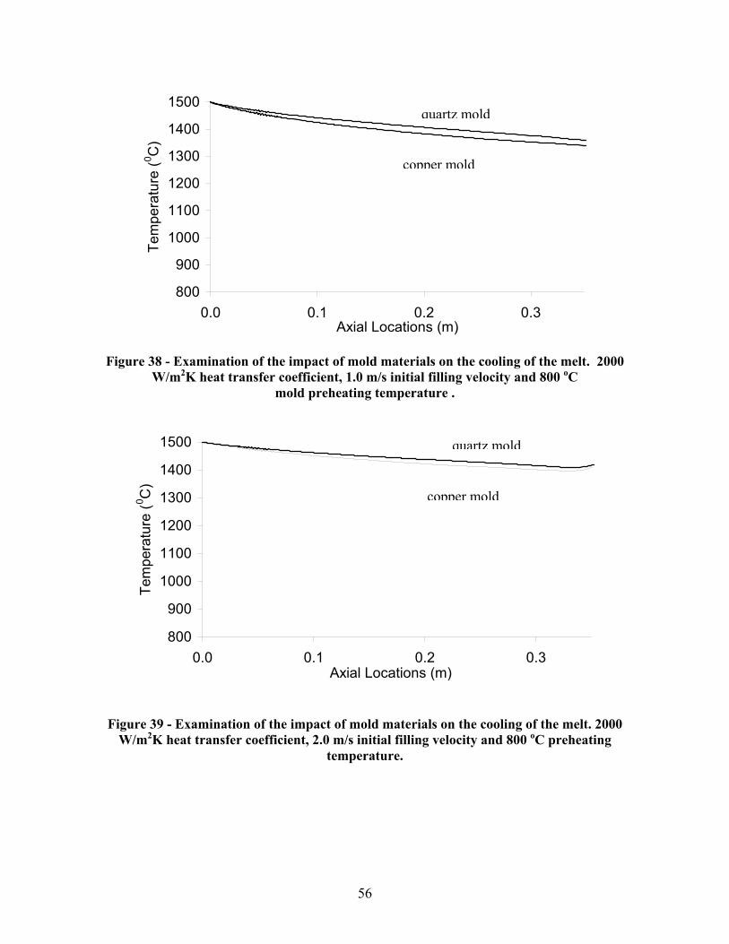
4.1.5.2 Results – Quartz Molds Figures 38 through 40 show the impact of different mold materials on the cooling of the melt. Heat transfer into the mold is faster using copper mold compared to quartz. The effect becomes more obvious during lower filling velocity. Figure 40 shows the wiggle phenomena. A lower heat transfer coefficient decreases the velocity of the heat transfer into the molds. Tables 11 through 14 show the temperature located at the 0.3 meters from the entrance, which are corresponding to the Figures 38 through 41.
Table 11 Temperature of the melt material near the melt-mold interface at 0.36 seconds
Different Mold Material Temperature (oC) ∆(Ti – Tcopper) oC Copper 1353 Quartz 1377 24
Table 12 Temperature of the melt material near the melt-mold interface at 0.18 seconds
Different Mold Material Temperature (oC) ∆(Ti – Tcopper) oC Copper 1401 Quartz 1416 15
Table 13 Temperature of the melt material near the melt-mold interface at 0.36 seconds
Different Mold Material Temperature (oC) ∆(Ti – Tcopper) oC Copper 1222 Quartz 1301 79
Table 14 Temperature of the melt material near the melt-mold interface at 0.18 seconds
Different Mold Material Temperature (oC) ∆(Ti – Tcopper) oC Copper 1299 Quartz 1352 53
56
800
900
1000
1100
1200
1300
1400
1500
0.0 0.1 0.2 0.3Axial Locations (m)
Tem
pera
ture
(0 C)
Figure 38 - Examination of the impact of mold materials on the cooling of the melt. 2000 W/m2K heat transfer coefficient, 1.0 m/s initial filling velocity and 800 oC
mold preheating temperature .
800
900
1000
1100
1200
1300
1400
1500
0.0 0.1 0.2 0.3Axial Locations (m)
Tem
pera
ture
(0 C)
Figure 39 - Examination of the impact of mold materials on the cooling of the melt. 2000 W/m2K heat transfer coefficient, 2.0 m/s initial filling velocity and 800 oC preheating
temperature.
quartz mold
copper mold
copper mold
quartz mold

57
800
900
1000
1100
1200
1300
1400
1500
0.0 0.1 0.2 0.3Axial Locations (m)
Tem
pera
ture
(0 C)
Figure 40 - Examination of the impact of mold materials on the cooling of the melt. 5000 W/m2K heat transfer coefficient, 1.0 m/s initial filling velocity and 800oC mold preheating
temperature.
800
900
1000
1100
1200
1300
1400
1500
0.0 0.1 0.2 0.3
Axial Locations (m)
Tem
pera
ture
(0C
)
Figure 41 - Examination of the impact of mold materials on the cooling of the melt. 5000
W/m2K heat transfer coefficient, 2.0 m/s initial filling velocity and 800 0C mold preheating temperature.
Glass
Copper
Glass
Copper

58
4.2 Induction Heating Model An important component in the development of an inductively heated casting furnace is the determination of the amount of heating produced by the system. Traditionally, detailed models of the electromagnetic field are used to evaluate the performance of the coil design. For the present problem, it is important to couple the produced field, heating, and fluid flow to insure proper mixing and to understand the mass transport from the melt into the gas space above the melt. Induction heating is commonly used in furnaces to melt metals for a number of metallurgical processes. This section of the report briefly discusses the governing equations of induction heating and presents some preliminary modeling results. The modeling efforts have centered around the development of the governing equations, developing a method to incorporate then into FIDAP, setting up a test problem, and making preliminary calculations for a geometry of interest. The test problem and derivations have been taken from previous publications (see References). The resulting governing equations are shown below and are for a cylindrical geometry, but the equations are similar to a Cartesian coordinates form. In tensor notation the equations are reduced to those shown below.
1( )
1( ) 0
oC Jr CoilSr
µ ∇ ⋅ ∇ = −
∇ ⋅ ∇ = (16)
1( )
1( )
C Sr r ConductorS Cr r
µσω
µσω
∇⋅ ∇ = ∇ ⋅ ∇ = − (17)
1( ) 0
1( ) 0
Cr ElsewhereSr
∇ ⋅ ∇ =
∇ ⋅ ∇ = (18) where
C, S = real and complex components of function substituted into governing equations to simplify solution process
r = radial coordinate Jo = current density µ = permeability ω = frequency σ = electrical conductivity
59
Using the appropriate relationships and integrating gives the heat deposition as a function of position.
22 2
2( , )2
Q r z S Cr
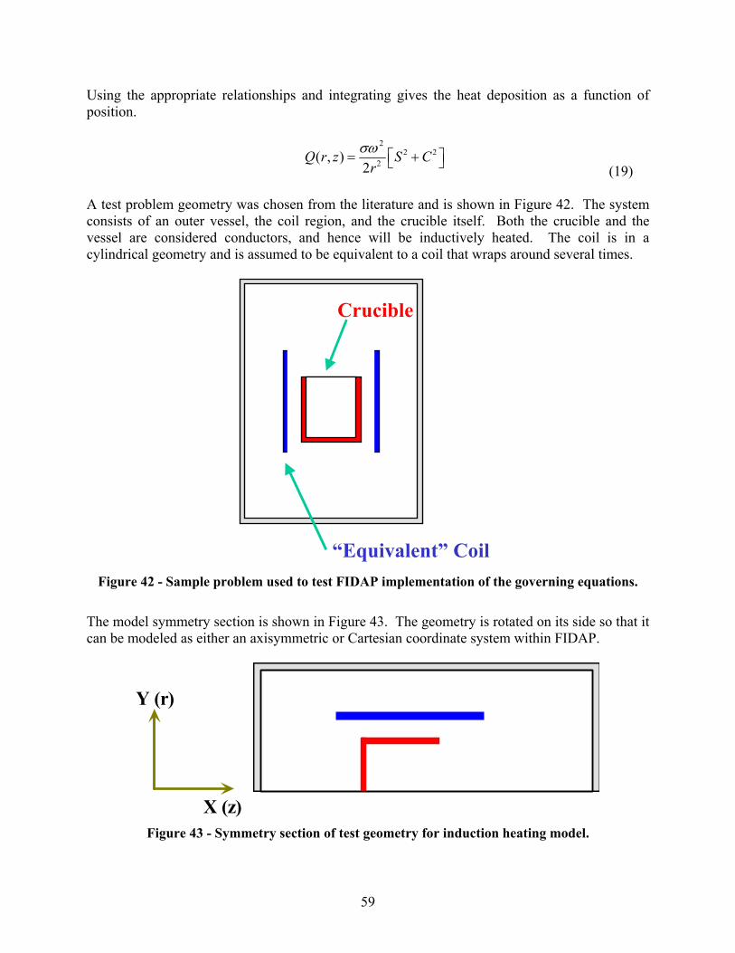
σω = + (19) A test problem geometry was chosen from the literature and is shown in Figure 42. The system consists of an outer vessel, the coil region, and the crucible itself. Both the crucible and the vessel are considered conductors, and hence will be inductively heated. The coil is in a cylindrical geometry and is assumed to be equivalent to a coil that wraps around several times.
“Equivalent” Coil
Crucible
Figure 42 - Sample problem used to test FIDAP implementation of the governing equations.
The model symmetry section is shown in Figure 43. The geometry is rotated on its side so that it can be modeled as either an axisymmetric or Cartesian coordinate system within FIDAP.
X (z)
Y (r)
Figure 43 - Symmetry section of test geometry for induction heating model.

60
Simulations were run with approximately 10,000 or 20,000 elements. In general, both simulations produced identical results, indicating that the solution was independent of the mesh. 4 node quads were used in all simulations and only two species equations were solved. The two equations were used to solve for the variables C and S as identified in the governing equations above. Surface plots of each of the functions, C and S, are shown in Figures 44 and 45 for a test problem. The test problem was taken from work previously reported in the literature. The domain consists of a crucible, a coil region, and a surrounding vessel. The regions of compressed mesh represent the crucible or coil regions. Figure 44 is the C variable and its greatest value occurs in the coil region. The right hand side image is the S variable and should be largest in the crucible region. Physically, each of these plots shows the proper trends and relationships for each of the variables in each of the regions of the mesh. Further work will be conducted to verify the solution and to calculate the power densities. The figures shown below are for the physical properties of 6 61.7 10 ; 1.3 10cruc vessσ σ= × = × .
Figure 44 - Surface plots of the solution variable C for the analysis of the induction heating
within an inductively heated furnace.
The results indicate that the variable C is highest in the coil region, while the variable S is highest in the crucible region. The sharp gradients exist as a result of the air gap and material properties. The combination of C and S effectively results in heating in a thin surface area near the surface of the crucible. These results agree with the trends and predictions presented in the literature. Future numerical work will attempt to verify the method used to implement these equation within FIDAP and to make direct comparisons to other numerical results.

61
Figure 45 - Surface plots of the solution variables C and S for the analysis of the induction
heating within an inductively heated furnace
The physical properties for the test case shown below are 6 65 10 ; 2 10cruc vessσ σ= × = × .
Figure 46 - Surface plot of the variable C for physical properties of 6 65 10 ; 2 10cruc vessσ σ= × = ×
(crucible and vessel respectively).
Other researchers have reported the sharp peaks shown in Figure 47. These peaks are real and not a numerical error that exists only during the solution process. These peaks become more prevalent when there is a larger difference in material properties between the crucible and the vessel (subscripts cruc and vess).

62
Figure 47 - Surface plot of the variable S for physical properties of 6 65 10 ; 2 10cruc vessσ σ= × = ×
(crucible and vessel respectively). Sharp peaks are reported in the literature by previous researchers.
Additional model benchmarking and evaluation will occur in year 2 of the project. The modeling effort developed here has shown that it is possible to model the field within a heat transfer code. Model development will continue and include heat transfer and fluid mechanic effects.
4.3 Mass Transfer Model The mass transfer of the americium from the melt is an important consideration in the complete project. The mass transfer is best described by the schematic shown in Figure 48. References 20 through 45 were used for the development of the mass transfer model as it is presented here. The model requires the consideration and interaction of three phenomena.
• Mass transport within the melt to the interface region (item 1 in Figure 48). This effectively reduces to transport through a thin boundary layer type region at the surface of the melt. The mass transport coefficient is defined as βm (cm/sec).
• Vaporization across the interface (item 2 in Figure 48). The mass transfer coefficient for this step is defined as Km (cm/sec).
• Mass transport within the gas phase above the melt (item 3 in Figure 48). The mass transport coefficient for this step is defined as βg (cm/sec).
The liquid boundary layer is step 1 is assumed to follow Machlin’s model and can be defined as 2 2 /m D rβ ν π= (20) where
D = diffusion coefficient ν = speed of melt in boundary layer. r = Machlin mode.
Each of these values can be estimated for the present system of interest.

63
Gas / Vapor
Melt .
Interface
1
2
3
Figure 48 - Mass transport consists of (1) transport within the melt, (2) vaporization at the
interface, and (3) transport in the gas phase. The mass transfer rate across the interface (2) can be written as ( ) ( ) ( )( ) /m m ms i L e i g i i msN K C K P P M Tε= = − (21) Accordingly, this allows the mass transfer coefficient to be written as
( ) ( )
( )
( ) /L e i g i i msm
ms i
K P P M TK Cε −
= (22)
where
Tms = temperature of the evaporating surface. Pe(i) = equilibrium partial pressure of component i at temperature Tms Pg(i) = partial pressure of component i in the gas space. KL = Langmuir constant. Cms(i) = average content of component i on the surface of the melt. Mi = atomic weight of component i. ε = condensation coefficient ( 1 for metals).
64
The components equilibrium partial pressure is defined as ( )o
e i i i iP x Pγ= , where Pio is the
equilibrium pressure of pure substance i and xi is the mole fraction of component i. The challenge for americium in our system is to evaluate γi , the activity coefficient. In i-j binary system, the relationship between the activity coefficient γi of the component i and its partial mole excess free energy
EiG can be written as
lnEi iG RT γ= (23)
in which
( )1
EE ijEi ij i
i
GG G x
x∂
= + −∂ (24)
where E
ijG is the system’s excess free energy and is given by
E Eij ij ijG H TS= ∆ − (25)
An approximate relationship between the heat formation of the binary system ijH∆ and its
excess entropy EijS will be calculated in the year two task.
0.1 mi mjE
ij ijmi mj
T TS H
T T +
= ∆ (26)
where Tmi and Tmj are the melt points of components I and j, respectively. If we define
1 0.1 mi mj
ijmi mj
T TT
T Tβ
+= −
(27) Then
Eij ij ijG Hβ= ∆ (28)
The activities of Am in molten U-Am and Pu-Am will be calculated. The controlling steps of mass transfer process will also be studied in year two. Previous research efforts were focused on the transport to the melt surface and the evaporation at that interface. The additional two stages of transport are also important in the present work. The transport of the vapor through the gas phase and eventual deposition on surrounding surfaces is important. Knowing where the americium will deposit or where it will be transported is a major concern.

65
5. Summary The phase I work shows the process of evaluating the important steps of casting fuel rods. A conceptual design of the next generation metallic casting furnace has been proposed and the models necessary to analyze its performance are being developed. The furnace concept is an induction skull melter, covered crucible region, chill molds, and resistance heaters to control the preheating of the molds. The design allows for control of the americium transport and control over the length of the fuels pins that can be cast. Fundamental issues related to the selection of a metallic fuel casting furnace design are studied and discussed. These issues include heating mechanisms, casting issues, crucible design, and issues related to the mass transport of americium. The process of evaluating all of these different criteria was undertaken to select a concept that would have the greatest chance of success for casting americium in a metallic fuel rod. Based on this evaluation process, a concept for the casting of metallic fuel pins containing high vapor pressure materials is selected and discussed. The important physics of this concept include the mass transport of americium from the melt, the induction heating and stirring of the melt, plus the casting of long slender fuel rods. The model considers the flow of the melt into the molds, heat transfer into the molds, and the impact of process parameters on the formation of the fuel rod. The development of a model for the casting of molten fuel into a chill mold has been studied in the first year. Three general models are in development. A model of the casting process has been developed and a parametric study has been performed. In addition, models for the induction heating field and for the mass transport of the americium are being developed and will be implemented for more detailed analyses of the casting process.
6. References
1. Dynamic Analysis of An overhead Crane Carrying A Canister By Finite Element Method –Musukula, University of Nevada, Las Vegas, 1993.
2. http://apt.lanl.gov/atw/index.htmal, (March 21, 2002).
3. http://www.nuc.berkeley.edu/designs/ifr, (Aril 4, 2002). 4. Compilation of Information on Modeling of Inductively Heated Cold Crucible Melters,
D.L. Lessor, March 1996. 5. Injection casting of U-Zr_Mn, surrogate alloy for U-Pu-Zr-Am-Np, C.L., Journal of
Nuclear Materials 224(1995) 305-306. 6. The Induct slag Melting Process, P.G. Clites, (Bulletin/United States Department of the
Interior, Bureau of Mines, 673), 1982. 7. Induction Skull Melting of Titanium Aluminides, P.G. Breig and S.W. Scott, the Duriron
Company, Inc. 1989
66
8. Hazardous waste & Hazardous materials, Volume 11, Number 1, 1994 (what is the title
of the article? The author? 9. The ABB DC arc furnace: Past, present, future, S.E. Stenkvist (ABB Process
Automation), June 1992 10. A Simplified Thermal Analysis of an Inductively Heated Casting Furnace, Randy
Clarksean and Charles Solbrig, ASME Heat Transfer Division, Vol. 317-1, pp. 433-441 11. Crucible for Induction Melting, Wilfried Guy, Kelsterbach, Germany, July, 1995
Journal? 12. Crucible for The Inductively Melting of Metals, Matthias Blum, Bodingen Wilfried Goy,
Kelsterbach, Frauz Hage, Germany, Oct., 1996 13. Cold Crucible Type Levitation Melting of Reactive Metals, A. Fukuzawa Chemical
Processing Division (this is not a complete reference)
14. The Further Development of the Semilevitation Melting Technique for The Production of Casting in Reactive Alloys, R A Harding and X R Zhu, University of Birmingham, UK.
15. Cook, R. D., Malkus, D.S. and Plesha, M.E., “Concepts and applications of finite
element analysis”, John Wiley & Sons, New York, 1989, Third edition. 16. Hirt, C.W. and Nichols, B.D., "Volume of Fluid (VOF) Method for the Dynamics of
Free Boundaries," Journal of Computational Physics 39, 201, 1981. 17. S.Kvicinsky, F. Longatte, J.-L. Kueny and F. Avellan, “Free Surface Flows:
Experimental Validation of Volume of Fluid (VOF) Method in the Plane Wall Case”, Proceedings of the 3rd ASME/JSME Joint Fluids Engineering Conference, July 18-23 1999, San Francisco, California
18. Nichols, B.D. and Hirt, C.W., "Methods for Calculating Multi-Dimensional, Transient
Free Surface Flows Past Bodies," Proc. First Intern. Conf. Num. Ship Hydrodynamics, Gaithersburg, ML, Oct. 20-23, 1975
19. C.A. Santos, J.M.V. Quaresma, A. Garcia, “Determination of transient interfacial heat
transfer coefficient in chill mold castings”, Journal of Alloys and Compounds 319 (2001), 174-186.
20. Harris, R., and Davenport, W.G., 1982, “Vacuum Distillation of Liquid Metals: Part 1.
Theory and Experimental Study," Metallurgical Transactions B, vol. 13B, December, pp. 581-88.
67
21. Harris, R., and Davenport, W.G., 1982, “Vacuum Distillation of Liquid Metals: Part 1. Photographic Study," Metallurgical Transactions B, vol. 13B, December, pp. 589-91.
22. Ozberk, E., and Guthrie, R.I.L., 1985, “Evaluation of Vacuum Induction Melting of
Copper Refining," Transactions of the Institution of Mining and Metallurgy Section C Mineral Processing and Extractive Metallurgy, vol 94, September, pp. C146-C157.
23. Ozberk, E., and Guthrie, R.I.L., 1986, “A Kinetic Model for the Vacuum Refining of
Inductively Stirred Copper Melts," Metallurgical Transactions B, vol. 17B, March, pp. 87-103.
24. Hino, M., Wand, S., Nagasaka, T., and Ban-ya, S., 1994, “Evaporation Rate of Zinc in
Liquid Iron," ISIJ International, vol. 34, no. 6, pp. 491-97. 25. Li, L., Tu, S., and Janke, D., 1995, “Kinetics of Zn and Pb Evaporation from Liquid
Iron," Steel Research, vol. 66, no. 5, pp. 188-93. 26. Guo, J., Yuan, L. Yanquing, S., Hongsheng, D., and Jun, J., 1998, “Evaporation
Behavior of Components in Ti-15-3 Melt During ISM Process," Transactions of Nonferrous Metals Society of China, vol. 8, no. 4, pp. 539-43.
27. Guo, J., Liu, Y., Su, Y., Ding, H., Liu, G., and Jia, J., 1999, “Evaporation Behavior of
Aluminum During the Cold Crucible Induction Skull Melting of Titanium Aluminum Alloys," Metallurgical and Materials Transactions B, vol 31B, August, pp. 837-44.
28. Savov, L. and Janke, D., 2000, “Evaporation of Cu and Sn from Induction-Stirred Iron-
Based Melts Treated at Reduced Pressure," ISIJ International, vol. 40, no. 2, pp. 95-104. 29. Guo, J., Liu, G., Su, Y., Liu, Y., Ding, H.S., and Jia, J, 2000, “Control of Al Content
during ISM Process of $Nb_3Al$," Transactions of Nonferrous Metals Society of China, vol. 10, no. 5, pp. 571-75.
30. Bellot, J.P., Duval, H., Ritchie, M., Mitchell, A., and Ablitzer, D., 2001, “Evaporation of
Fe and Cr from Induction-Stirred Austenitic Stainless Steel. Influence of Inert Gas Pressure," ISIJ International, vol. 41, no. 7, pp. 696-705.
31. Gokcen, N.A., 1986, Statistical Thermodynamics of Alloys, Plenum Press, New York. 32. Saito, T. (editor), 1999, Computational Materials Design, Springer, London. 33. Ilegbusi, O.J., Iguchi, M., and Wahnsiedler, W., 2000, Mathematical and Physical
Modeling of Materials Processing Operations, Champan and Hall (CRC), Boca Raton, Florida.
34. Liw, H. and Bouchard, M., 1997, “Evaluation of Interaction Coefficient in Al-Cu-H
Alloy," Metallurgical and Materials Transactions B, vol. 28B, August, pp. 625-632.

68
35. Waseda, Y., Ueno, S., and Toguri, J.M., 1989, “Theoretical Calculation of Solute
Activity Coefficient at Infinite Dilution in Metallic Solution," Zeitschrift fur Metallkunde, vol. 80, no. 6, pp. 406-12.
36. Ogawa, T., 1993, “Alloying Behavior Among U, Np, Pu, and Am Predicted with the
Brewer Valence Bond Model," Journal of Alloys and Compounds, vol. 194, pp. 1-7. 37. Dubinin, N.E., Yuryev, A.A., and Vatolin, N.A., 1995, “Thermodynamic Properties of
Ternary Liquid Metal Alloys," High Temperature Materials and Processes, vol. 14, no. 4, pp. 285-290.
38. Wang, F.M., Li, X.P., Han, Q.Y., and Zhang, N.X., 1997, “A Model for Calculating
Interation Coefficients Between Elements in Liquid and Iron-Base Alloy," Metallurgical and Materials Transactions B, vol. 28B, February, pp. 109-113.
39. Ueno, S., Waseda, Y., Jacob, K.T., and Tamaki, S., 1988, “Theoretical Treatment of
Interaction Parameters in Multicomponent Metallic Solutions," Steel Research, vol 59, no. 11, pp. 474-83.
40. Toop, G.W., 1965, “Predicting Ternary Activities Using Binary Data," Transactions of
the Metallurgical Society of AIME, vol. 233, pp. 850-55. 41. Sherwood, T.K., and Cooke, N.E., 1957, “Mass Transfer at Low Pressures," A.I.Ch.E.
Journal, vol. 3, no. 1, pp. 37-42. 42. Tanaka, T., Gokcen, N.A., and Morita, Z., 1990, “Relationship Between Enthalpy of
Mixing and Excess Entropy in Liquid Binary Alloys," Zeitschrift fur Metallkunde, vol. 81, no. 1, pp. 49-54.
43. Tanaka, T., Gokcen, N.A., Spencer, P.J., Morita, Z., and Iida, T., 1993, “Evaulation of
Interaction Parameters in Dilute Liquid Ternary Alloys by a Solution Method Based on the Free Volume Theory," Zeitschrift fur Metallkunde, vol. 84, no. 2, pp. 100-05.
44. Pehlke, R.D., 1973, Unit Processes of Extractive Metallurgy, American Elsevier
Publishing Company, Inc., New York. 45. Turkdogan, E.T., 1980, Physical Chemistry of High Temperature Technology, Academic
Press, New York. 46. Akinlade, O., and Sommer, F., 2001, “Concentration Fluctuations and Thermodynamic
Properties of Ternary Liquid Alloys," Journal of Alloys and Compounds, vol. 316, pp. 226-235.
69
47. Su, Y., Guo, J., Ding, H., Liu, S., Liu, Y., Liu, G., and Jia, J., 2001, “Component Evaporation of Ti-15-3 Melt During ISM Processing," Journal of Materials Science and Technology, vol. 17, no. 1, pp. 83-4.
48. Gokcen, N.A., 1997, “Thermodynamics of Solutions: A Unified Concept," J Chim Phys,
vol. 94, pp. 817-843. 49. Maeda, M., Kiwake, T., Shibuya, K., and Ikeda, T., 1997, “Activity of Aluminum in
Molten Ti-Al Alloy," Materials Science and Engineering, vol. A239-240, pp. 276-80. 50. Ma, Z., 2000, “Thermodynamic Description for Concentrated Metallic Solutions Using
Interaction Parameters," Metallurgical and Materials Transactions B, vol 32B, February, pp. 87-103
51. Ding, X., Fan, P., and Wang, W., 1999, “ Thermodynamic Calculation for Alloy
Systems," Metallurgical and Materials Transactions B, vol. 30B, April, pp. 271-77. 52. Gokcen, N.A., Tanaka, T., and Morita, Z., 1993, “Atomic Theories on Energetics of
Alloy Formation," J Chim Phys, vol. 90, pp. 233-248. 53. Turkdogan, E.T., Grieveson, P., and Darken, L.S., 1963, “Enhancement of Diffusion-
Limited Rates of Vaporization of Metals," J. Phys. Chem., vol. 67, August, pp. 1647-54. 54. Miedema, A.R., de Chatel, P.F., de Boer, F.R., 1980, “Cohesion in Alloys -
Fundamentals of a Semi-Empirical Model," Physica, vol. 100B, pp. 1-28.
55. Ferro, R., Cacciamani, G., Saccone, A., and Borzone, G., “Systematics of Lanthanide and Actinide Compound Formation: Remarks on the Americium Alloying Behaviour," Journal of Alloys and Compounds, vol. 320, pp. 326-40.
56. Ogawa, T., Ohmichi, T., Maeda, A., Arai, Y., and Suzuki, Y., 1995, “Vaporization
Behaviour of (Pu, Am)N," Journal of Alloys and Compounds, vol 224, pp. 55-59.