IEEE JOURNAL OF SELECTED TOPICS IN SIGNAL PROCESSING, VOL. 4, NO. 1, FEBRUARY 2010 79

Target Velocity Estimation and Antenna Placementfor MIMO Radar With Widely Separated Antennas

Qian He, Student Member, IEEE, Rick S. Blum, Fellow, IEEE, Hana Godrich, Member, IEEE, andAlexander M. Haimovich, Member, IEEE

Abstract—This paper studies the velocity estimation perfor-mance for multiple-input multiple-output (MIMO) radar withwidely spaced antennas. We derive the Cramer–Rao bound (CRB)for velocity estimation and study the optimized system/configura-tion design based on CRB. General results are presented for anextended target with reflectivity varying with look angle. Thendetailed analysis is provided for a simplified case, assuming anisotropic scatterer. For given transmitted signals, optimal antennaplacement is analyzed in the sense of minimizing the CRB ofthe velocity estimation error. We show that when all antennasare located at approximately the same distance from the target,symmetrical placement is optimal and the relative position oftransmitters and receivers can be arbitrary under the orthogonalreceived signal assumption. In this case, it is also shown that forMIMO radar with optimal placement, velocity estimation accu-racy can be improved by increasing either the signal time durationor the product of the number of transmit and receive antennas.

Index Terms—Antenna placement, Cramer–Rao bound (CRB),multiple-input multiple-output (MIMO) radar, maximum-likeli-hood (ML) estimate, velocity estimation.

I. INTRODUCTION

R ESEARCH on multiple-input multiple-output (MIMO)radar has been drawing more and more attention from

both the communication and radar communities. Most studieson MIMO radar can be classified into two categories. The firstcategory [1]–[8] employs widely separated antennas at both thetransmit and receive ends. Among these studies, both coherentand non-coherent processing has been considered [1]. Non-co-herent MIMO radar requires time synchronization between thesensors. Besides time synchronization, coherent MIMO radar

Manuscript received January 26, 2009; revised July 20, 2009. Current versionpublished nulldate. The work of Q. He and R. S. Blum were supported in partby the Air Force Research Laboratory under Agreement FA9550-09-1-0576, inpart by the National Science Foundation under Grant CCF-0829958, in part bythe U.S. Army Research Office under Grant W911NF-08-1-0449, and in part bythe China Scholarship Council. The work of H. Godrich and A. M. Haimovichwere supported in part by the U.S. Air Force Office of Scientific Research underagreement FA9550-09-1-0303. The associate editor coordinating the review ofthis manuscript and approving it for publication was Prof. Jian Li.

Q. He is with the Electrical Engineering Department, University of Elec-tronic Science and Technology of China, Chengdu, Sichuan 611731, China, andalso with Lehigh University, Bethlehem, PA 18015 USA (e-mail: qianhe@uestc.edu.cn; qih207@lehigh.edu).

R. S. Blum is with the Electrical and Computer Engineering Department,Lehigh University, Bethlehem, PA 18015 USA (e-mail: rblum@eecs.lehigh.edu).

H. Godrich and A. M. Haimovich are with the Electrical and Computer En-gineering Department, New Jersey Institute of Technology, Newark, NJ 07102USA (e-mail: hg44@njit.edu; haimovich@njit.edu).

Color versions of one or more of the figures in this paper are available onlineat http://ieeexplore.ieee.org.

Digital Object Identifier 10.1109/JSTSP.2009.2038974

requires additional phase synchronization. The second category[9]–[16] uses closely spaced antennas.

Widely dispersed antennas enable MIMO radar to view thetarget from several different angles simultaneously. This lowersthe chance that all antennas measure low Doppler shifts. Re-cently, we have begun to study the detection of moving tar-gets using MIMO radar [7]. We showed that MIMO radar withwidely separated antennas enjoys both the diversity gain and thegeometry gain. The diversity gain is similar to that uncovered in[3], so we do not focus on this in the current paper. The geom-etry gain is a different type of gain that results from viewing thetarget from different directions. While a single antenna may beblind to a target moving in a direction orthogonal to the line to-wards the antenna, a group of widely spaced antennas will notbe. This is the essence of geometry gain. In the current paper wefocus on geometry gain in our numerical results, since it is lesswell understand. To complete [7] and answer some remainingquestions, we focus here on the ultimate velocity estimation per-formance obtainable through MIMO radar with widely spacedantennas by studying the Cramer–Rao bound (CRB). We showthe utility of these results by using them to study proper antennaplacement.

Various CRB studies for MIMO radar performance have ap-peared in the literature. For example, the CRB for target local-ization in a coherent MIMO radar is presented in [4], [8]. Theaverage CRB for bearing estimation in MIMO radar is analyzedin [2]. In [6], the outage CRB is introduced to evaluate MIMOradar direction finding performance. In [16], range compressionand waveform optimization problems for MIMO radar are in-vestigated based on the CRB matrix. None of these papers con-sider target velocity estimation performance, which is anotherimportant issue for radar systems [17]–[20].

MIMO radar systems optimization has also been investigated.Most existing publications concentrate on waveform optimiza-tion. For example, in [21], waveform design methods for maxi-mizing the conditional mutual information (MI) or minimizingthe mean-square error (MMSE) are discussed. The two criterialead to the same solution under the same total power constraint.In [22], the uncertainty of the target power spectrum is consid-ered and the MI and MMSE criteria lead to different minimaxrobust waveforms. Different from this work, in [23] and [24],waveform optimization for target parameter estimation based onthe CRB is studied. In [25] the MIMO radar ambiguity functionis used for designing good waveforms. In this paper, the CRBis used to study target velocity estimation in MIMO radar withwidely dispersed antennas. We present an optimization strategyfor transmit/receive antenna placement.

Considering a target moving with constant velocity and amodel which includes Gaussian noise and path loss, we calcu-

1932-4553/$26.00 © 2010 IEEE

80 IEEE JOURNAL OF SELECTED TOPICS IN SIGNAL PROCESSING, VOL. 4, NO. 1, FEBRUARY 2010

late the CRB for velocity estimation using MIMO radar. Thederived CRB provides an effective way for finding the optimalvalue for certain parameters. With the other system parametersfixed, we focus on the optimal antenna placement. Assumingall antennas are located equidistant from the target, it is shownthat symmetrically placing the transmit and receive antennas isthe best choice, and the optimal achievable performance is notaffected by the relative position of the transmit and receive an-tennas under an orthogonal received signal assumption. This re-sult is also extended to a more general case without the equidis-tance assumption. This optimal placement result justifies someof our numerical findings, which also show that larger sensorseparations, corresponding to larger angular spreads, lead tobetter performance. We develop the maximum-likelihood (ML)estimator, compare the mean square error (MSE) of the MLestimate with the CRB result for some specific examples, andshow the ML estimate and the CRB agree for sufficiently largesignal-to-noise ratio (SNR). While initially, we focus on a targetwhose reflectivity is the same during the observation, we showhow to extend our results for more general models. For com-pleteness, the extreme sensor placements resulting in a singularFisher information matrix, which means one cannot accuratelyestimate the desired quantities, are briefly discussed.

The paper is organized as follows. The signal model is pre-sented in Section II. Section III derives the ML estimate ofthe velocity and calculates the corresponding CRB for a casewith an extended target whose reflectivity varies with angle. InSection IV, we start to concentrate on a special case, assumingan isotropic scatter, which simplifies the analysis and enablesus to provide useful insight. Then, Section V describes a gen-eral optimization based on the derived CRB, with optimal an-tenna placement studied as a particular example. Numerical re-sults are provided in Section VI. Finally, Section VII describesextensions to cases outside the original assumptions and alsoprovides conclusions for this paper.

II. SIGNAL MODEL

Consider a coherent MIMO radar that has transmit andreceive antennas. The elements at both the transmit and re-

ceive ends are widely dispersed, see [1], [7] for motivation.The set of transmitted signals expressed in low-pass equivalentform is given by , , where is thetotal transmitted energy. Each of the waveforms is nor-malized and satisfies , where is the ob-servation interval. Assume a narrowband signal such that thecommon complex envelope notation can be applied to the trans-mitted signal,1, i.e., . Each of these signalsis emitted by an individual transmit antenna. Note that the sig-nals , are expressed in a completely generalform, other than normalization, so that for example, either singlepulse or multiple pulse waveforms can be assumed. In addition,it is assumed that the target returns do not fluctuate during theobservation interval.

Consider a target moving with an unknown constant velocity, where and are velocity components in

a two-dimensional Cartesian coordinate system, as shown in

1Note that the actual transmitted signal is the real part, but we use complexenvelope description so we deal with complex signals.

Fig. 1. Location of transmitters and receivers with respect to the target and itsmotion.

Fig. 1. Since the focus of this paper is target velocity estima-tion, we assume that through the observation interval, the targetis known to be present in a resolution cell with nominal coordi-nates . Let the transmitters and receivers be locatedat , , and , , respec-tively. The low-pass equivalent of the signal received by the threceiver due to the transmissions from all transmitters andthe reflection from the target is given by

(1)

where is the unknown complex target reflec-tivity for the th path2 denotes the time delay of the thpath, and is the Doppler frequency detected by the threceiver due to the th transmitter. The observation interval isassumed long enough so that all transmitted signals can be ob-served, irrespective of their delay. The terms

(2)

in (1) represent the propagation coefficients, where

, with representingthe path length from the th transmitter to the target, and

representing the path lengthfrom the target to the th receiver. Note that the path loss isassumed to be inversely proportional to . We also have

, where is the speed of light. The phase shiftinduced by the carrier frequency is captured in the exponent of

.The noise at the th receiver is denoted by in (1). The

noise components , at different receivers arespatially independent, and temporally each is a zero-meanwhite complex Gaussian process with power spectral density(PSD) . If the noise is colored3 with PSD ,then a whitening filter is needed at each re-ceiver to remove the correlation of the noise.

The positions of the transmit and receive antennas with re-spect to the target motion are shown in Fig. 1. The transmitter

2Here we assume the target reflectivity is different for each transmit-to-re-ceive antenna path. If this is not the case we can reduce the number of unknownparameters as discussed later.

3For simplicity, ���� is assumed known. In practice it may have to be es-timated. For further details, the reader is referred to the extensive literature onspace-time adaptive processing (STAP).

HE et al.: TARGET VELOCITY ESTIMATION AND ANTENNA PLACEMENT FOR MIMO RADAR 81

and receiver view the target from different anglesand ,

where and . The Doppler shiftobserved at the th receiver due to the signal transmitted

by the th transmitter is given by

(3)

where denotes the carrier wavelength and

(4)

define two position matrices, and ,for and . These matrices are de-termined by the placement of the transmit and receive antennaswith respect to the target of interest.

The signals received from all the receivers are collected ina vector4 . The joint probabilitydensity function (pdf) of the observations (time samples at mul-tiple receive antennas) parameterized by the unknown param-eter vector

(5)

is given by [26]

(6)

Taking the logarithm of the probability density function, we ob-tain the log-likelihood function

(7)

where is some constant independent of the parameters col-lected in .

III. CRB AND ML ESTIMATE FOR

TARGET VELOCITY ESTIMATION

In this section, the CRB and the ML estimate of the targetvelocity are discussed for MIMO radar.

4The superscript � denotes transposition.

A. Cramer–Rao Bound for Velocity Estimation

In this subsection, we compute the CRB for the model intro-duced previously. The variance of the th element of any un-biased estimator for an unknown parameter vector satisfies[28], [30]

where is the Fisher information matrix (FIM) defined as

(8)

and the gradient operation is

. The CRB matrix is the inverse of the Fisherinformation matrix, . Note that here thereflection coefficients are assumed to be deterministicunknown. Using the approach described in [6], the CRBs forthe reflection coefficients modeled as random variables areprovided in Appendix I.

Since is a function of the Doppler frequency shifts, , , we introduce the param-

eter vector

(9)

which is a column vector with elements containing theobserved Doppler shifts from every transmit–receive path aswell as the real and imaginary parts of the target complex re-flectivities. Using the chain rule, the FIM can be expressed as

(10)

The term can be calculated from (3) and (9) as

where

and and are the all zero matrix and the identity matrix,respectively, with dimensions given in the corresponding sub-scripts.

We now calculate , which is a matrix,using (8) with replacing . Considering the structure ofhas to do with the order of the elements arranged in , it isconvenient to divide it into four block submatrices

The upper left submatrix involves derivatives of theDoppler frequencies. Consider the th components of such

82 IEEE JOURNAL OF SELECTED TOPICS IN SIGNAL PROCESSING, VOL. 4, NO. 1, FEBRUARY 2010

that , as per (9), and assume the th componentcorresponds to , and the th component corresponds to

. Then

for

where5

(11)

where and . When ,the integral term in (11) represents the square of the effectivepulse width of the th transmitted signal plus the square of thepulse center of the th received signal (see (34) for more detail),scaled by the squared magnitude of the propagation coefficientfor the th path. Note that in this calculation, the received sig-nals are delayed by a certain amount of time (the delay for thepath from the th transmit antenna to the th receive antenna),and the observation interval is chosen so that the received sig-nals are visible with this delay. When , then the integralterm in (11) is related to the squared average of the overlap timebetween the signals transmitted from the th and th transmitantennas when received at the th receive antenna. Note that dueto the complex signals involved, a conjugate enters into the cal-culation, as found normally in cross-correlation of complex sig-nals. For each , we can arrange for different , into an

matrix , the th entry of which is .The lower right submatrix involves derivatives of the target

complex reflectivities. Consider the th components of suchthat , as per (9), and assume the thcomponent corresponds to or , and the th componentcorresponds to or . Then we have

,

and

5The superscript � denotes conjugation, and � and � denotes the real andimaginary operators.

where

(12)The integral term in (12) represents the cross-correlation be-tween two signals as received at the th receive antenna whentransmitted from the th and th transmit antennas ,or the self-correlation when both transmitted signals comefrom the th transmit antenna . Note that the receivedDoppler shifts and propagation coefficients enter into thesecalculations as expected.

The upper right submatrix involves derivatives related toboth the Doppler frequency and the target complex reflectivities.Consider the th components of such that ,

, as per (9), and assume the th compo-nent corresponds to , and the th component corresponds to

or . Then we compute

and

where

(13)The integral term in (13) is similar to that in (12), except foran additional in the integrand. This makes it implement an ef-fective center of mass type calculation for the cross-correlatedsignals to estimate the time at which the center of this cross-cor-related signal resides. When , the integral term representsthe time center of the th transmitted signal when received at theth receiver.

Plugging and in (10), the FIM is obtained

(14)

In order to get the CRB matrix, we need to invert the FIM.Usually, and are invertible, and one can apply thematrix inversion lemma [33] to (14) to calculate the inverse ofthe FIM as in (15), shown at the bottom of the page. Here, we areinterested only in the estimates of and , whose variancesare bounded by

CRB (16)

(15)

HE et al.: TARGET VELOCITY ESTIMATION AND ANTENNA PLACEMENT FOR MIMO RADAR 83

CRB (17)

Thus, it is sufficient to calculate the upper-left 2 2 submatrixof , called

CRBCRB

(18)

The two diagonal elements of determine the CRBsof the estimates of and . They are dependent on severalparameters, such as the wavelength, the energy used per trans-mitter, the PSD of the noise, the target reflectivity, the range cellof interest, the terms , and related to the trans-mitted signals, and the number and placement of the radar an-tennas implied in the position matrices and .

B. ML Estimate of Velocities

ML estimation is an asymptotically optimal method [28]. Forsignal-in-noise problems, the ML estimator achieves the CRBfor sufficiently large SNRs. In our problem, the ML estimate isgiven by

where .Note that contains unknown parameters that need

to be estimated simultaneously, although only and areof interest. Since the closed-form solution for the ML estimateseems not available, numerical evaluation is needed. The com-putational complexity for a -dimensional search is veryhigh, especially for large . A practical approach is to useiterative optimization procedures such as the space alternatinggeneralized expectation–maximization (SAGE) algorithm [29].

C. Optimized System/Configuration Design Based on CRB

The results of Section III-A show that the CRBs of the es-timates of and are dependent on several parameters. Werequire the optimized system/configuration design with respectto a parameter vector to minimize a metricformed by the sum of the CRBs of the estimates of and .The value that optimizes this metric is given by

CRB CRB

(19)where denotes the objective function dependent on param-eter , and denotes the feasible set of . Numerical methodsare usually resorted to for solving this problem.

IV. VELOCITY ESTIMATION ANALYSIS

FOR AN ISOTROPIC SCATTERER

To simplify the analysis and provide useful insight, we con-sider the isotropic scatter, which gives the same reflectivity forall directions, and hence are the same for all paths, i.e.,

, for all . Note that the discussions in therest of the paper are based on this simplification.

A. Cramer–Rao Bound

For an isotropic scatter, the log-likelihood function can bewritten as

(20)

The dimensions of the unknown parameter vectors are greatlyreduced

and

which yields

and

where the submatrices and are the same as previously, butand have much fewer elements than their former versions,and . In the submatrix , involving the th components

of for we have

and

where

(21)

84 IEEE JOURNAL OF SELECTED TOPICS IN SIGNAL PROCESSING, VOL. 4, NO. 1, FEBRUARY 2010

In the submatrix , involving the th components of for, we find

and

where

(22)

Plugging and in (10), the FIM matrix is obtainedand given in (23), shown at bottom the of the page, where thematrix is defined after (11), and and , arethe th row of the position matrices and . The upper-left 2

2 submatrix of related to the velocity estimates is

CRBCRB

(24)

where , and are defined as

(25)

(26)

and

(27)

B. ML Estimate of Velocities

Based on the log-likelihood function in (20), the ML estimateof is

For any , the likelihood function is maximizedby letting

and

(23)

HE et al.: TARGET VELOCITY ESTIMATION AND ANTENNA PLACEMENT FOR MIMO RADAR 85

Then the ML estimate of the target complex reflectivityis obtained

where is defined in (21). Substituting back into the log-likelihood function, the ML estimate of the target velocities canbe derived

(28)

As further simplification seems not available for the ML esti-mator, needs to be determined numerically. In the numer-ical study, we adopt a two-dimensional grid search followed byan iterative optimization to obtain the maximum-likelihood es-timate.

Assuming the received signals satisfy an orthogonality cri-teria, we show later that the terms in are zero, andhence is a constant independent of velocity, which simplifies(28). Then the optimal estimator selects the velocity vectorin the phase term that maximizes the output of a matched filter,which is matched to a shifted version of the transmitted signal.A bank of matched filters that covers the allowable velocity re-gion can be used to produce an approximation to this optimalestimator. However, if the orthogonal received signal assump-tion does not hold, then the terms enter in . Note that thevalues of the terms are affected by the velocity vector.In this case, a more complicated optimal estimator is required.The more complicated estimate still employs a matched filter,but the quantity maximized is the matched filter divided by aterm that characterizes the impact of the interference one getsbetween signals originating from different transmit antennas, asmight be expected with non-orthogonal signals.

V. OPTIMIZED SYSTEM/CONFIGURATION DESIGN BASED ON

CRB AND AN ISOTROPIC SCATTERER

Using the CRB submatrix (24), for fixed wavelength and SNR(so that is fixed), the CRBs can be expressed as afunction of the quantities (25), (26), and (27). PluggingCRB and CRB into (19), the objective function becomes

(29)

and thus the optimal parameter should satisfy

(30)

A. Optimal Antenna Placement With Orthogonal Signals andan Isotropic Scatterer

In the rest of this section, we consider the case of orthogonalsignals, formulated in Assumption 1, which follows.

Assumption 1 (Orthogonal Signals): We assume that thetransmitted signals are orthogonal

ifif

and maintain orthogonality for a variety of allowed time delays, and Doppler frequency shifts , , i.e.,

ifif .

See Appendix II for further discussion.Given Assumption 1, we can simplify (see Appendix III) the

results in (11), (21), and (22) as

,(31)

(32)

(33)

where

(34)

, is the effective pulse width of thetransmitted signal, and represents the timecenter of the transmitted signal [35]. Plugging , , andback into (24)–(27), the CRB submatrix is obtained.

Before discussing the optimal antenna placement, we definesymmetrical antenna placement.

Definition 1 (Symmetrical Antenna Placement): Symmetricalantenna placement satisfies

,(35)

where and are arbitrary constant angles.Next, we introduce an equidistance assumption.Assumption 2 (Equidistance): We assume all antennas are

placed around the area being monitored, such that they haveroughly the same distance from the target.

In this case, the antenna placement variableis an vector consisting

of the transmit and receive antenna directions with respectto the target. The feasible set is , where

.Under Assumptions 1–2, (without

loss of generality, we normalize this term to in thesequel for simplicity), , and are the same for

86 IEEE JOURNAL OF SELECTED TOPICS IN SIGNAL PROCESSING, VOL. 4, NO. 1, FEBRUARY 2010

all and ( , ), and hence the terms, , (25)–(27) can be simplified to

(36)

(37)

and

(38)

It can be proved that for a MIMO radar system withwidely separated transmitters and widely separatedreceivers, , , and . See Appendix IV.

In this case, the optimal solution in (30) can be determinedby the necessary condition that it makes the gradient of the ob-jective function equal to zero

(39)

or more precisely

(40)

Plugging , , (36)–(38) in , the elements of the gradientcan be calculated. See Appendix V.

The following theorem indicates that there is only one kindof solution to (40), which therefore provides the solution to theoptimization problem (30) and leads to the best achievable ve-locity estimation performance.

Theorem 1: Assume a MIMO radar system withwidely separated transmitters and widely separatedreceivers satisfies Assumptions 1–2, then for waveforms witharbitrary and from (34), only symmetrical placement canbe optimum.

The proof of Theorem 1 is obvious based on the followingtwo lemmas.

Lemma 1: Assume a MIMO radar system withwidely separated transmitters and widely separatedreceivers satisfies Assumptions 1–2, then no solution other thana symmetric antenna placement will solve the zero gradient con-dition (40) for waveforms with arbitrary and from (34).

Proof of Lemma 1: See Appendix VI.Lemma 2: Assume a MIMO radar system with

widely separated transmitters and widely separatedreceivers satisfies Assumptions 1–2, then any symmetrical an-tenna placement will solve the zero gradient condition (40).

Proof of Lemma 2: See Appendix VII.Lemma 3: Assume a MIMO radar system with

widely separated transmitters and widely separatedreceivers satisfies Assumptions 1–2, then all symmetric antennaplacements give exactly the same performance.

Proof of Lemma 3: Under the assumptions given in Lemma3, according to (103) in Appendix VII, at all symmetrical place-ments, the quantities , , (36)–(38) are given by

(41)

The value of the objective function is the same for all symmetricantenna placements

(42)

Consequently, all symmetric antenna placements give exactlythe same performance.

Theorem 2: Assume a MIMO radar system withwidely separated transmitters and widely separatedreceivers satisfies Assumptions 1–2, then for waveforms witharbitrary and from (34), any symmetric antenna placementis optimal, assuming an optimum placement exists. The relativepositions between the transmit and receive antennas have noimpact on the performance.

Proof of Theorem 2: According to Theorem 1, no solutionsother than symmetric placements can be optimal, and accordingto Lemma 3, all symmetric placements give exactly the sameperformance. Therefore, any symmetric placement must be op-timal.

If you substitute the placements of the form given in (35),one finds the resulting expression is independent of and .Therefore, the relative positions between the transmit and re-ceive antennas have no impact on the performance.

We further conclude from (42) that for a MIMO radar systemwith symmetric (optimal) placement, the velocity estimation ac-curacy can be improved by increasing or the product of thenumber of the transmit and receive antennas .

Singular FIM Cases: When an FIM is singular, one cannotaccurately estimate the desired quantities without additionalconstrains. To understand the problems that can result, considera single pair of collocated transmit and receive antennas. Sincethey can measure, at most, only a single Doppler frequency,they cannot possibly measure a two-dimensional velocity.Further, if the target is moving in a direction perpendicular tothe vector between the antennas and the target, then no velocitymeasurement can be made.

Improper antenna placements could result in singular FIMs,if they make any row or column of from (14) a linear com-bination of the others. To simplify matters, we focus on the caseof orthogonal signals. Investigations for other cases follow sim-ilar steps. Plugging (31)–(33) into (23), under Assumptions 1–2,a singular FIM appears when the first two rows/columns of theFIM are proportional to each other, that is

(43)

For example, when a radar system has one transmitter andone receiver

HE et al.: TARGET VELOCITY ESTIMATION AND ANTENNA PLACEMENT FOR MIMO RADAR 87

Fig. 2. MSE of ML estimate and CRB for a 3 � 3 MIMO radar with �� �

�� � � � �� � � � ��� �, �� � �� � � � �� � � � �� �, �� �

����� � ������ � �����m, �� � ������ � ����� � �����m.

thus (43) is satisfied, resulting in a singular FIM. For anotherexample that leads to singular FIM, consider a radar system withmultiple transmit and receive antennas, but all the transmittersand/or receivers are co-located, then andfor all and . Hence, (43) is achieved by

Intuitively, these two systems provide only one propagationpath, from which only one Doppler frequency can be ob-served. This provides essentially a single observation, which iscertainly not enough to estimate the two-dimensional quantity

.

VI. NUMERICAL RESULTS

In this section, the CRBs are computed for some exampleMIMO radar systems. In Figs. 2–4, the empirical MSE of theML estimate is compared to the CRB. The figures are distin-guished by different antenna placements and different numbersof antennas.

We use Monte Carlo simulations with 2000 iterations perSNR value to obtain the MSE. We vary in (1), and labelour plots using a scaled version of . In particular, we use

, where is the maximum dis-tance between the target and radar antennas. Assume a movingtarget with velocity m/s is in the resolution

Fig. 3. MSE of ML estimate and CRB for a 3 � 3 MIMO radar with �� �

� � � � ��� � � � ��� �, �� � �� � � � � � � � ��� �, �� �

����� � ������ � �����m, �� � ������ � ����� � �����m.

Fig. 4. MSE of ML estimate and CRB for a 2 � 2 MIMO radar with �� �

�� � � � �� �, �� � �� � � � �� �, �� � ����� � ����� m,�� � ����� � ����� m.

cell of interest. Suppose the signal time duration6 is sand the carrier frequency is GHz. A set of pulsed sinu-soidal signals ,with frequency increment Hz are employed fortransmission (see Appendix II). The sampling frequency usedis KHz.

In Figs. 2 and 3, an MIMO radar is consideredwith two different antenna placements. In Fig. 2, the trans-mitters are located atwhile the receivers are located at

. In Fig. 3, the transmitters are located atand the receivers are

6The signal time duration is set to a large number to shorten the simulationtime for getting the MSE curve of the ML estimates.

88 IEEE JOURNAL OF SELECTED TOPICS IN SIGNAL PROCESSING, VOL. 4, NO. 1, FEBRUARY 2010

Fig. 5. Antenna positions corresponding to Figs. 2–4. Triangles represent trans-mitters while circles represent receivers. (a) Antenna positions in Fig. 2. (b) An-tenna positions in Fig. 3. (c) Antenna positions in Fig. 4.

located at . The distancebetween the transmit antennas and the target are assumedto be m, whilethe distance between the receive antennas and the target are

m.In Fig. 4, a 2 2 MIMO radar, with fewer transmit and re-

ceive antennas, is considered. The angles defining the transmitand receive antenna positions are and

, respectively. The transmitters andreceivers are located at m and

m away from the target.The simulation results show that the MSE of the ML estimates

approach the CRBs as SNR becomes large. This is consistentwith the theoretical asymptotic efficiency of ML estimates, andalso supports the correctness of the CRB derived in the previoussection.

It can be observed that the CRBs in Figs. 2 and 3 are smallerthan those in Fig. 4. This indicates that MIMO radars with moreantennas can achieve better performance. It is also found that theestimated error bounds (variance) for are larger than those for

in Figs. 2 and 4, while the estimated error bounds (variance)for are larger than that for in Fig. 3. These results showthat the estimation accuracy for and are quite different anddepend on the chosen antenna positions. The corresponding an-tenna positions in these examples are illustrated in Fig. 5, wheretriangles represent transmitters and circles represent receivers.Projecting the antenna locations to the and axes we find thatin (a) and (c) the antennas are more widely spread along the

-dimension. In this case, the antennas are more sensitive to thetarget motion in the -direction, thus the estimation accuracy of

is more accurate than that for in Figs. 2 and 4. On thecontrary, in (b), the antennas are more widely spread along the

-dimension, for the same reason the estimation accuracy foris more accurate than that for in Fig. 3. Thus, the results inFigs. 2–4 show that, generally, the more we spread out the an-tennas, the better the performance. Such findings are partiallyexplained by our optimum placement results from Section V,which also suggest it is best to spread out the antennas as muchas possible.

A. Cramer–Rao Bound Analysis

In this subsection, we provide some further analysis usingthe CRB result in (24). For simplicity, we assume all an-tennas are located at approximately the same distance fromthe target, and let m for all and .

Fig. 6. CRB for a 4 � 3 MIMO radar system with non/symmetric placement.� � � � ���� m; Nonsymmetric placement 1 (nonsym 1) �� ��� � � � ��� � � � �� � � � � �, �� � � � � � ��� � � ���� �. Nonsymmetric placement 2 (nonsym 2) �� � ��� � � ���� � � � �� � � � ��� �, �� � ��� � � � �� � � � ��� �.Symmetric placement (sym) �� � � � � � � � � �� � � � �� � � � � � � ,�� � � � � � � �� � ��� � ��� � � � .

Assume the velocity of the target is m/s.The transmitted signals employ pulsed sinusoidal signals

, with fre-quency increment for their low-pass equivalent, timeduration ms. The carrier frequency is GHz andthe sampling frequency is KHz.

In Fig. 6, we plot the CRBs for a 4 3 MIMO radarsystem with different placements. Let KHz.We first allocate the antennas non-symmetrically. The di-rections of the transmit and receive antennas in case 1are and

. In case 2, they arelocated atand . Then we considersymmetric placement, where the transmit antennas are at

and the receiveantennas are at , whereand are arbitrary. Fig. 6 shows that case 1 has the highestCRB. When the antennas are symmetrically placed, the CRBachieves the lowest value.7

In Fig. 7, we consider the CRBs for a 4 4 MIMO radarsystem with optimally (symmetrically) placed antennas trans-mitting orthogonal signals. In this example, we also usepulsed sinusoidal signals ,

. The frequency increment is chosen asKHz, such that the signals are approximately

orthogonal. All antennas have the same distance to the targetm, , . We

vary the signal time duration from to , and to , wherems. The sampling frequency is KHz. As

7Note that with antenna positions fixed, one can compute the CRBs for dif-ferent target positions. The results seem not very sensitive to the target positionin cases we looked at.

HE et al.: TARGET VELOCITY ESTIMATION AND ANTENNA PLACEMENT FOR MIMO RADAR 89

Fig. 7. Signal time duration effect on velocity estimation (using optimal place-ment). Signal time duration varies from � to �� , and to �� . � � ��� ms.

shown in the figure, the estimation accuracy is improved byincreasing the signal time duration. It is found that for all casesin this example, the CRB curves for and estimates fall ontop of each other. This is not surprising if we take a look at (41),which implies that the accuracies of the velocity estimation inthe and axes are equal when the antennas are optimallyplaced.

Fig. 8 compares the CRBs for MIMO radar systems using adifferent number of transmit and receive antennas . As-suming orthogonal signals and optimal placement are adopted,the parameter settings in this example are the same as in Fig. 7,while the signal time duration is fixed at . It is seen that thelarger the product of , the lower the CRB values. For ex-ample, the 8 8 system with has the highestvalue of the four, hence the lowest CRB curve. It is noticed thatthe 5 5 system performs better than the 7 3 system, eventhough both cases have a total of ten antennas. Also, the 88 system having a total of 16 antennas outperforms the 316 system with 19 antennas in all. Realizing the fact that it isthe product of transmitter and receiver numbers that determinesthe estimation accuracy is significant. It enables a MIMO radarsystem to achieve better performance with lower complexity(fewer antennas).

Finally, in Fig. 9, we give an example to show that our resultsare also valid for multiple pulse waveforms. The transmittedwaveforms are given by

, , where is the pulsewidth, is the pulse repetition time, is the number of pulsesduring one coherent processing interval (CPI), is thetime duration of one CPI, denotes the duty cycle,and is the rectangular window func-tion. Here, we choose s, ms, ,

ms, MHz, and GHz. Consider a 43 MIMO radar system. Suppose all antennas have the same

distance to the target m, ,. The CRB curves are plotted for both symmet-

rical (S) and nonsymmetrical (N) placement. In the nonsymmet-

Fig. 8. Effect of transmitter and receiver numbers �� ��� on velocity esti-mation (using optimal placement).

Fig. 9. CRB for a 4 � 3 MIMO radar applying multiple pulse signals with� � � �s, � � ���ms,� � �, � � ���ms, � � � MHz, � � � GHz;� � � � ���� m. Antennas angles are either nonsymmetrical (N) � ���� � ��� � �� � ��� �, � � �� � �� ��� � or symmetrical (S) � � �� �� ��� ��� � ,� � �� ��� ��� � , where and can take on any values.

rical cases, the angles defining the transmit and receive antennapositions areand , respectively. Thefigure shows similar results as we already discussed in the pre-vious pulsed sinusoidal signal cases.

VII. DISCUSSIONS AND CONCLUSION

In the signal model considered, the unknown target reflec-tivities are assumed to be constant during the observationinterval. As an extension, one may assume that the target re-flectivity fluctuates during the observation interval (from pulseto pulse), such that each varies with pulse number, whichgives , where , and denotes the numberof pulses in the observation interval. In this case, the parameter

90 IEEE JOURNAL OF SELECTED TOPICS IN SIGNAL PROCESSING, VOL. 4, NO. 1, FEBRUARY 2010

vector is a column vector given by. The di-

mension of the resulting FIM is then. The extension involves similar calculations to those given in

this paper for simpler cases, whereas for large values ofthe computation complexity increases greatly.

As another extension to the analysis in Section V-A, supposewe no longer constrain all antennas to be the same distancefrom the target. Suppose the possible region for us to place radarantennas is the outside of a circle with diameter , which sur-rounds the target. Since we often cannot get too close to a target,this is a reasonable scenario. In order to use minimum power, itis easy to see we should place all the antennas at the same dis-tance from the target. If Assumptions 1 and 2 are also satis-fied, then the results in Section V apply for this scenario if wereplace with .

In this paper, the CRB for the target velocity estimation hasbeen derived when a MIMO radar is deployed with widely dis-persed antennas. A signal model was formulated. The equationsspecifying the ML estimates of target velocity were developed,and the mean square error of the estimates was compared to theCRB for some examples. These comparisons substantiate theCRB results.

Optimization strategies were discussed for MIMO radarvelocity estimation. The conditions for optimal antenna place-ment were derived. For MIMO radar transmitting orthogonalsignals, symmetrically placing all the transmitters and all thereceivers gives the best achievable performance. The relativeposition between the transmitters and receivers does not affectthe results under orthogonal signals. The symmetric placementresult shows that larger sensor separations, corresponding toangular spreads, lead to better performance, which also justifiessome of our numerical findings. It was shown by both analysisand simulation that for any MIMO radar system with optimalplacement, it is possible to improve the velocity estimationaccuracy by increasing the effective signal time duration or theproduct of the number of transmit and receive antennas.

APPENDIX ICAMERA-RAO BOUND FOR RANDOM REFLECTIVITY

USING THE APPROACH FROM [6]

In this section, we derive the CRB for velocity es-timation when the reflectivity coefficients are as-sumed as random variables. Denote and

, then in(5) can be written as . The FIM conditioned on is

(44)

where . Plugging (3) into (7) and takingderivative with respect to and we find

(45)

where

and

The CRB conditioned on reflectivity is

CRB

CRBCRB

(46)

Further, we introduce several approaches to get rid of thedependence on the nuisance parameter from the CRBs. Fol-lowing the discussion in [6], we can compute the average CRB(ACRB) by averaging (46) with respect to

ACRB CRB (47)

ACRB CRB (48)

where the expectation is taken with respect to the pdf .We can also compute the outage CRB (OCRB) [6] for a given

probability based on (46), considering the CRBs in (46) de-pend on the realization of

OCRB CRB (49)

OCRB CRB (50)

Another approach is to compute the modified CRB (MCRB)[31] based on (45)

MCRB (51)

MCRB (52)

Note that since (according to Jensen’s in-equality or [32]), the ACRB is tighter than the MCRB.

The true CRB (TCRB) is tighter than the above CRBs dis-cussed, although it is very hard to evaluate

TCRB (53)

TCRB (54)

Note that the inner expectation in (53) or (54) is taken with re-spect to the pdf , and the outer expectation is taken withrespect to the pdf .

HE et al.: TARGET VELOCITY ESTIMATION AND ANTENNA PLACEMENT FOR MIMO RADAR 91

Fig. 10. Frequency spectrum for transmitted signals (solid curves) and the ef-fective parts of their time delayed versions (dotted curves).

APPENDIX IIFREQUENCY SPREAD SIGNALS

In this appendix, we describe one class of signals which couldbe employed. Under appropriate assumptions, these signals ap-proximately satisfy the conditions of Assumption 1 for orthog-onal signals. We discuss these assumptions. These assumptionsessentially ignore small sidelobes in the Fourier transform ofthese signals to approximate them with truncated (in frequencydomain) signals. After discussing the assumptions, we computethe CRB using the untruncated signals and also by assumingideal orthogonal signals and show the two CRBs are extremelyclose in cases of practical interest.

Consider a set of pulsed sinusoidal signals8

otherwise(55)

where , denotes the signal time duration, andis the frequency increment between

and . The approximate bandwidth of each signal is. The spectrum of and , and , are

shown in Fig. 10. Note that in this section, it is always assumedthat . According to Parseval’s theorem

(56)

By observing the spectrum, we see that when, the main lobes of and are sufficiently sep-

arated, so that and (56) approximates 0, whichmakes and approximately orthogonal. Here, we areignoring contributions from small sidelobes which is similar totruncating the signals in the frequency domain. As ,if the frequency increment satisfies

(57)

then any two signals from the signal setare approximately orthogonal.

Assume that and are time delayed by and. The nonzero part of the delayed signal occupies

, and the nonzero part of occupies. Hence, the time duration of the overlap be-

tween them is , where denotes the

8Windowing can be applied in practice but we omit discussion of this wellstudied topic.

time delay difference. Note that when is greater than orapproximates , the overlap part of these two signals vanishes,which implies (56) is close to 0 and the signals can be consid-ered as orthogonal. Therefore, it is possible for the two delayedsignals to be nonorthogonal only if , which makesthe following discussion necessary.

We denote the overlap interval as . Thus,

where and represent the overlapping parts ofand , the time duration of which are both

. More specifically, suppose , then wehave

The spectrum of and , i.e., and , areplotted by dotted curves in Fig. 10. In a similar way, for the timedelayed signals, the orthogonality is approximately maintainedif

(58)

Since , the inequality is maintained by requiring. As , the condition be-

comes , which is the same as in (57). Hence, therequirement for (57) guarantees (58). That is, if (57) is met, thetime delayed signals are orthogonal.

Next, we further discuss the Doppler shift restrictionfor orthogonality. The effective time delayed and Dopplershifted signals are given by and

. The frequency spectrum of the ef-fective time delayed signals and , i.e., and

, are replotted in Fig. 11 using solid curves, the center fre-quency of which are and . After Doppler frequency shift,the spectrum of the effective time delayed and Doppler shiftedsignals are and .They are shown in Fig. 11 using dashed curves. Thus, thecenter frequency of the effective signal is , whilethe center frequency of becomes . Clearly,provided , that is

or

(59)

the overlapping part between andcan be ignored. Thus, the orthogonality is

well approximated. Note that since (58) is satisfied, we have. Hence, the term

92 IEEE JOURNAL OF SELECTED TOPICS IN SIGNAL PROCESSING, VOL. 4, NO. 1, FEBRUARY 2010

Fig. 11. Frequency spectrum for the time-delayed equivalent signals (solidcurves) and their Doppler shifted versions (dotted curves).

Fig. 12. CRBs for frequency spread signals (FS) and ideal orthogonal approx-imation (orth), where (a) �� � �, (b) �� � ���� , (c) �� � ��� , (d)�� � ��� , (e) �� � ���� , and (f) �� � ���� .

in (59) can be ignored, resulting inor .

Numerical Investigations: We now examine the perfor-mance of a system using frequency spread signals by com-paring its exact CRB results with the CRBs obtained usingideal orthogonal signals as an approximation. We assume thefollowing system parameters: carrier frequency GHz,target velocity (7.75,13.42) m/s (in the resolution cell of in-terest), distances between transmit antennas and the targetarem, distances between receive antennas and the target are

m, directions fromthe transmit and receive antenna positions to the target are

and. Suppose the signal time

duration is ms. In Fig. 12, the CRB results for thefrequency spread signals (FS) are plotted to compare with thoseobtained using ideal orthogonal signals (orth). In this example,

is true for every . In (a), the frequency increment, which means all the transmitted signals are the same.

As shown in the figure, the resulting two CRB curves are farapart for this identical signals case. In (b), we set .Condition (57) is still not met and the transmitted signals arenonorthogonal. It can be observed that the CRB curves are notclose in this case either. In (c) to (f), the frequency incrementvaries from to , , and . We find that

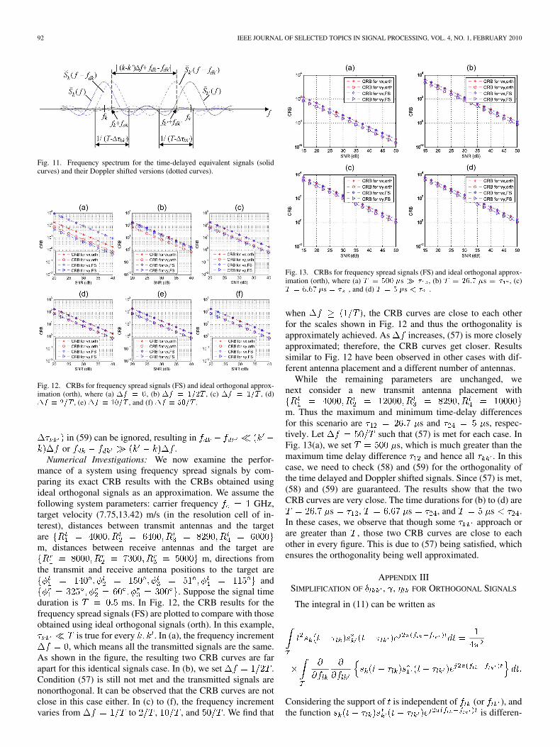
Fig. 13. CRBs for frequency spread signals (FS) and ideal orthogonal approx-imation (orth), where (a) � � ��� �s � � , (b) � � ���� �s � � , (c)� � ���� �s � � , and (d) � � � �s � � .

when , the CRB curves are close to each otherfor the scales shown in Fig. 12 and thus the orthogonality isapproximately achieved. As increases, (57) is more closelyapproximated; therefore, the CRB curves get closer. Resultssimilar to Fig. 12 have been observed in other cases with dif-ferent antenna placement and a different number of antennas.

While the remaining parameters are unchanged, wenext consider a new transmit antenna placement with

m. Thus the maximum and minimum time-delay differencesfor this scenario are s and s, respec-tively. Let such that (57) is met for each case. InFig. 13(a), we set s, which is much greater than themaximum time delay difference and hence all . In thiscase, we need to check (58) and (59) for the orthogonality ofthe time delayed and Doppler shifted signals. Since (57) is met,(58) and (59) are guaranteed. The results show that the twoCRB curves are very close. The time durations for (b) to (d) are

s , s , and s .In these cases, we observe that though some approach orare greater than , those two CRB curves are close to eachother in every figure. This is due to (57) being satisfied, whichensures the orthogonality being well approximated.

APPENDIX IIISIMPLIFICATION OF , , FOR ORTHOGONAL SIGNALS

The integral in (11) can be written as

Considering the support of is independent of (or ), andthe function is differen-

HE et al.: TARGET VELOCITY ESTIMATION AND ANTENNA PLACEMENT FOR MIMO RADAR 93

tiable with respect to (or ), we can interchange the orderof integration and differentiation [34] to get

When the orthogonal signals assumption (Assumption 1) holds,the above integral equals zero for , and therefore

for

For , it is straightforward to get

Observing (21), is composed of a bunch of weighted inte-grals terms. The one for are zero under Assumption 1.Thus,

The integral in (22) can be written as

Interchanging the order of integration and differentiation gives

which equals zero under Assumption 1 for . Therefore,all summands on the right-hand side of (22) vanish except thatfor . Therefore,

APPENDIX IVTHE PROOF OF , , AND

In this section, we prove some inequalities related to (36),(37), and (38) in Section V.In the first step, we prove by comparing the size of

the minuend and the subtrahend of (36). We first examine the

summation terms contained in the minuend and the subtrahend.Assume ,9 then

and (60)

According to Jensen’s Inequality, we have

(61)

where the equality holds if and only if .Plugging (60) into (61) we obtain

(62)

where the equality holds if and only if

(63)

Since , (63) is equivalent to

and (64)

For a MIMO radar system with widely separatedtransmitters and widely separated receivers,

and , where, thus (64) cannot be met. Therefore, the equality condi-

tion in (62) cannot be satisfied and the equal sign is eliminated.Further considering the square of any real number is non-nega-tive, we obtain

(65)

Now we consider the other parts of (36). As discussed inSection V-A, (34) with (positive pulsewidth ) and (from their definitions) so

(66)

From (65) and (66) we find

and therefore

(67)

Similarly, we can prove

(68)

9The symbol ������� denotes the matrix vectorization operator.

94 IEEE JOURNAL OF SELECTED TOPICS IN SIGNAL PROCESSING, VOL. 4, NO. 1, FEBRUARY 2010

Finally, we prove . Looking back at (24), we findthat is a positive multiple of a variance ,which is always non-negative, so

(69)

According to (67) and (69), we obtain

(70)

APPENDIX VELEMENTS OF THE GRADIENT

Under the assumptions given in Section V, we calculate theelements of the gradient .

Focusing first on the th transmit antenna yields

(71)

where the terms , , and are computedas follows. Plugging and

in , , (36)–(38) and taking derivative with respect to, we can obtain

(72)

(73)

and

(74)

where

(75)

(76)

and

(77)

Substituting (72)–(74) into (71) and after some manipulation,we obtain

(78)

where

(79)In the same way, we can calculate the elements of the gradient

with respect to the th receive antenna

where

HE et al.: TARGET VELOCITY ESTIMATION AND ANTENNA PLACEMENT FOR MIMO RADAR 95

and

Consequently, every element of can be obtained.

APPENDIX VIPROOF OF LEMMA 1

In this section, we show that under the assumptions given inLemma 1, symmetric placement is the necessary condition forthe gradient being equal to zero, i.e., no other placement willsolve the zero gradient condition.

The gradient being zero requiresfor and for .We first investigate the derivatives with respect to transmit

antennas. The derivative with respect to the th transmit antennais given in (78). Since it has been shown that in(70), is equivalent to

(80)

Plugging , , and from (75)–(77) into (79), can bewritten as

(81)

where

(82)

and

(83)

Substitute (81) into (80), thus is equivalent to

(84)

Note that for a certain placement, the coefficients ,, , and in (84) do not vary with . Next, we will show by

contradiction that the zero gradient condition requires all thesecoefficients equal to zero.

Let us assume that the gradient is equal to zero but the coeffi-cients in (84) are not all equal to zero. For example, we assume

, , , and . In this case,(84) is equivalent to

(85)

Zero gradient means that holds for. Equivalently, it implies (85) holds for all

. That is

(86)

Note that as and do not vary with , for a certain placement,they are fixed for all the equations in (86). As is assumed inLemma 1, the transmit antennas are widely separated, thus

. The range of each is . Hence, (86)implies that the following equation:

(87)

with respect to has at least distinct solutions in. This leads to a contradiction, since with fixed nonzero

coefficients and , the trigonometric equation (87) has onlytwo solutions in [36]. Therefore, for any , theplacement with , , , andcannot have zero gradient.

Similarly, we can show that other cases, when any one orsome of the terms , , , and are not equal tozero, will lead to a contradiction and thus fail to solve the zerogradient condition for any .

The analysis for the derivatives with respect to receive an-tennas is similar.

Therefore, for MIMO radar with any transmit an-tennas and any receive antennas, the placement that en-sures zero gradient must simultaneously satisfy

(88)

(89)

and (90)

Applying (88)–(90) to (82) and (83), we have

(91)

96 IEEE JOURNAL OF SELECTED TOPICS IN SIGNAL PROCESSING, VOL. 4, NO. 1, FEBRUARY 2010

where and are tunable parameters for radarwaveforms. To make sure (91) holds for arbitrary and , fol-lowing the similar analysis as discussed above, it is required that

(92)

Hence, the placement with zero gradient must satisfy all theequations in (92). It can be shown that for odd and , onlysymmetric placement satisfy (92); for even or , eithersymmetric placement or nonsymmetric placement with anglepairs that differ by (i.e.,or ) will satisfy (92). Tosee this, we can imagine drawing pictures in the complexplane. Consider (take the transmit antennas for ex-ample) as a vector on the unit circle. Using Euler’s formula

[37], the sum of these vectors beingequal to zero (i.e., ) ensuresand .

Next we will show that the possible nonsymmetric placementwith angle pairs that differ by can be ruled out, thus only sym-metric placement can solve the zero gradient condition. Plug-ging , and (92)into , , (36)–(38), we have

and

Since (67) and (68) (See Appendix IV), the con-ditions (88) and (89) giveand . That is

(93)

According to summation formulas (see Appendix VIII for aproof)

for (94)

for (95)

where is an arbitrary constant, symmetric placement ensures(93). However, the nonsymmetric placement with angle pairsthat differ by does not satisfy (93) for any andshould be ruled out.

As a consequence, for any , the placement withzero gradient must satisfy the equations in both (92) and (93),and thus symmetric placement (35) is the only solution.

APPENDIX VIIPROOF OF LEMMA 2

In this section, we prove that under the assumptions givenin Lemma 2, symmetric placement is a sufficient condition forthe gradient being equal to zero, i.e., symmetric placement willsolve the zero gradient condition.

HE et al.: TARGET VELOCITY ESTIMATION AND ANTENNA PLACEMENT FOR MIMO RADAR 97

Assume symmetric placement is used such that ,where the transmit and receive antenna positions and

are given in (35).We first observe the derivative with respect to the th transmit

antenna (78). Based on the expression in (78), weare going to prove by showing that ,

, and for symmetric placement.In the first step, we calculate the terms , , and in

(75)–(77) contained in (79). Use the summation formula(see Appendix VIII for a proof)

for (96)

where is an arbitrary constant, then for ,and in (35) satisfy

(97)

Thus, the corresponding terms in , , (75)–(77) areequal to zero, and we obtain

and (98)

Substituting (98) into (79), we obtain

(99)

Next we compute and . Pluggingand into , , and in (36)–(38),

we obtain

(100)

(101)

and

(102)

For symmetric placement , where and, the summation terms in (100)–(102) can be treated by

using the summation formulas (94)–(96). It can be derived that,for

(103)

and hence

(104)

Thus, we have proved that (99),(104), and (103). Plugging them in

(78), we find the derivative with respect to any transmit antennais equal to zero for symmetric placement

for (105)

Similarly, we can show that the derivative with respect to anyreceive antenna is equal to zero for symmetric placement

for (106)

The gradient of the objective function at the symmetric place-ment, which is made up of these terms in (105) and (106), istherefore equal to zero

(107)

Consequently, the symmetric placement does make the gradientequal to zero.

98 IEEE JOURNAL OF SELECTED TOPICS IN SIGNAL PROCESSING, VOL. 4, NO. 1, FEBRUARY 2010

APPENDIX VIIISUMMATION FORMULAS

In this section, we give proofs for some useful summationformulas. First, we introduce two basic formulas derived from[38]

and (108)

Let , , and , where integer .According to (108), we have

and

Therefore, for arbitrary

(109)

and

(110)

Let , , and , where integer .According to (108), we have

and

Therefore, for arbitrary

(111)

(112)

and

(113)

REFERENCES

[1] A. M. Haimovich, R. S. Blum, and L. Cimini, “MIMO radar withwidely separated antennas,” IEEE Signal Process. Mag., vol. 25, no.1, pp. 116–129, Jan. 2008.

[2] E. Fishler, A. M. Haimovich, R. S. Blum, D. Chizhik, L. Cimini, andR. Valenzuela, “MIMO radar: An idea whose time has come,” in Proc.IEEE Radar Conf., Apr. 2004, pp. 71–78.

[3] E. Fishler, A. M. Haimovich, R. S. Blum, L. Cimini, D. Chizhik, andR. Valenzuela, “Spatial diversity in radars—Models and detection per-formance,” IEEE Trans. Signal Process., vol. 54, no. 3, pp. 823–838,Mar. 2006.

[4] N. Lehmann, A. M. Haimovich, R. S. Blum, and L. Cimini, “Highresolution capabilities of MIMO radar,” in Proc. 40th Asilomar Conf.Signal, Syst. Comput., Nov. 2006, pp. 25–30.

[5] A. De Maio and M. Lops, “Design principles of MIMO radar detec-tors,” IEEE Trans. Aerosp. Electron. Syst., vol. 43, no. 3, pp. 886–898,Jul. 2007.

[6] N. Lehmann, E. Fishler, A. M. Haimovich, R. S. Blum, L. Cimini,and R. Valenzuela, “Evaluation of transmit diversity in MIMO radardirection finding,” IEEE Trans. Signal Process., vol. 55, no. 5, pp.2215–2225, May 2007.

[7] Q. He, N. Lehmann, R. S. Blum, and A. M. Haimovich, “MIMO radarmoving target detection in homogeneous clutter,” IEEE Trans. Aerosp.Electron. Syst., 2010, to be published.

[8] H. Godrich, A. M. Haimovich, and R. S. Blum, “Concepts and Applica-tions of a MIMO Radar System With Widely Separated Antennas,” inMIMO Radar Signal Processing, J. Li and P. Stoica, Eds. New York:Wiley, 2008.

[9] J. Li and P. Stoica, “MIMO radar with colocated antennas,” IEEESignal Process. Mag., vol. 24, no. 5, pp. 106–114, Sep. 2007.

[10] C.-Y. Chen and P. P. Vaidyanathan, “MIMO radar space-time adap-tive processing using prolate spheroidal wave functions,” IEEE Trans.Signal Process., vol. 56, no. 2, pp. 623–635, Feb. 2008.

[11] A. Leshem, O. Naparstek, and A. Nehorai, “Information theoretic adap-tive radar waveform design for multiple extended targets,” IEEE J. Sel.Topics Signal Process., vol. 1, no. 1, pp. 42–55, Jun. 2007.

HE et al.: TARGET VELOCITY ESTIMATION AND ANTENNA PLACEMENT FOR MIMO RADAR 99

[12] T. Aittomaki and V. Koivunen, “Low-complexity method for transmitbeamforming in MIMO radars,” in IEEE Int. Conf. Acoust., Speech,Signal Process., Apr. 2007, vol. 2, pp. 15–20.

[13] D. W. Bliss and K. W. Forsythe, “Multiple-input multiple-output(MIMO) radar and imaging: Degrees of freedom and resolution,” inProc. 37th Asilomar Conf. Signal, Syst., Comput., Nov. 2003, pp.54–59.

[14] D. J. Rabideau and P. Parker, “Ubiquitous MIMO digital array radar,”in Proc. 37th Asilomar Conf. Signal, Syst., Comput., Nov. 2003, pp.1057–1064.

[15] F. C. Robey, S. Coutts, D. Werikle, C. McHarg, and K. Cuomo, “MIMOradar theory and experimental results,” in Proc. 38th Asilomar Conf.Signal, Syst., Comput., Nov. 2004, pp. 300–304.

[16] J. Li, L. Xu, P. Stoica, K. W. Forsythe, and D. W. Bliss, “Range com-pression and waveform optimization for MIMO radar: A CRB basedstudy,” IEEE Trans. Signal Process., vol. 56, no. 1, pp. 218–232, Jan.2008.

[17] J. Ward, “Cramer–Rao bounds for target angle and Doppler estima-tion with space-time adaptive processing radar,” in Proc. 29th AsilomarConf. Signal, Syst., Comput., Nov. 1995, pp. 1198–1202.

[18] S. R. Dooley and A. K. Nandi, “Adaptive time delay and Doppler shiftestimation for narrowband signals,” IEE Proc. Radar, Sonar Navig.,vol. 146, no. 5, pp. 243–250, Oct. 1999.

[19] A. Dogandzic and A. Nehorai, “Estimating range, velocity, and direc-tion with a radar array,” in Proc. IEEE Int. Conf. Acoust., Speech, SignalProcess. (ICASSP), Mar. 1999, pp. 2773–2776.

[20] A. Dogandzic and A. Nehorai, “Cramer–Rao bounds for estimatingrange, velocity, and direction with an active array,” IEEE Trans. SignalProcess., vol. 49, no. 6, pp. 1122–1137, Jun. 2001.

[21] Y. Yang and R. S. Blum, “MIMO radar waveform design based on mu-tual information and minimum mean-square error estimation,” IEEETrans. Aerosp. Electron. Syst., vol. 43, no. 1, pp. 330–343, Jan. 2007.

[22] Y. Yang and R. S. Blum, “Minimax robust MIMO radar waveform de-sign,” IEEE J. Sel. Topics Signal Process., vol. 1, pp. 147–155, Jun.2007.

[23] L. Xu, J. Li, P. Stoica, K. W. Forsythe, and D. W. Bliss, “Waveformoptimization for MIMO radar: A Cramer–Rao bound based study,”in Proc. 2007 IEEE Int. Conf. Acoust., Speech, Signal Process., Apr.2007, pp. 917–920.

[24] K. W. Forsythe and D. W. Bliss, “Waveform correlation and optimiza-tion issues for MIMO radar,” in Proc. 39th Asilomar Conf. Signal, Syst.,Comput., Nov. 2005, pp. 1306–1310.

[25] G. San Antonio, D. R. Fuhrmann, and F. C. Robey, “MIMO radar am-biguity functions,” IEEE J. Sel. Topics Signal Process., vol. 1, no. 1,pp. 167–177, Jun. 2007.

[26] H. V. Poor, An Introduction to Signal Detection and Estimation, 2nded. New York: Dowden & Culver, 1994.

[27] S. Coutts, K. Cuomo, J. McHarg, F. Robey, and D. Weikle, “Distributedcoherent aperture measurements for next generation BMD radar,” inProc. IEEE Workshop Sens. Array Multichannel Signal Process., 2006,pp. 390–393.

[28] S. M. Kay, Fundamentals of Statistical Signal Processing: EstimationTheory, 1st ed. Englewood Cliffs, NJ: Prentice-Hall, 1993.

[29] J. A. Fessler and A. O. Hero, “Space-alternating generalized expecta-tion-maximization algorithm,” IEEE Trans. Signal Process., vol. 42,no. 10, pp. 2664–2677, Oct. 1994.

[30] H. L. Van Trees, Optimum Array Processing. New York: Wiley, 2002.[31] A. N. D’Andrea, U. Mengali, and R. Reggiannini, “The modified

Cramer–Rao bound and its application to synchronization problems,”IEEE Trans. Commun., vol. 42, no. 2, pp. 1391–1399, Feb. 1994.

[32] B. Z. Bobrovsky, E. Mayer-Wolf, and M. Zakai, “Some classesof global Cramer–Rao bounds,” Ann. Statist., vol. 15, no. 4, pp.1421–1438, 1987.

[33] W. J. Duncan, “Some devices for the solution of large sets of simulta-neous linear equations,” London, Edinburgh, Dublin Philosoph. Mag.J. Sci., vol. 7, no. 35, pp. 660–670, 1944.

[34] E. W. Weisstein, CRC Concise Encyclopedia of Mathematics. BocaRaton, FL: CRC, 2003.

[35] H. L. Van Trees, Detection, Estimation and Modulation Theory: PartIII. New York: Wiley, 1971.

[36] W. R. Ransom, “Solutions of a trigonometric equation,” Amer. Math.Monthly, vol. 56, no. 6, pp. 402–403, Jun. 1949.

[37] M. A. Moskowitz, DA Course in Complex Analysis in One Variable.Singapore: World Scientific, 2002.

[38] K. S. Kunz, Numerical Analysis. New York: McGraw-Hill, 1957.

Qian He (S’09) received the B.Eng. degree inelectronic engineering from the University of Elec-tronic Science and Technology of China (UESTC),Chengdu, in 2004. She is currently working towardsthe Ph.D. degree in the Electronic EngineeringDepartment, UESTC.

From 2007 to 2009, she was a Visiting Scholarin the Electrical and Computer Engineering De-partment, Lehigh University, Bethlehem, PA. Hercurrent research interests include statistical signalprocessing, array signal processing, and their appli-

cations in radar and communication systems.Ms. He is a member of Sigma Xi. She was awarded the Distinguished Grad-

uate of UESTC Award in 2004. She was awarded a scholarship under the StateScholarship Fund from 2007 to 2009.

Rick S. Blum (S’83–M’84–SM’94–F’05) receivedthe B.S. degree in electrical engineering from thePennsylvania State University, State College, in1984 and the M.S. and Ph.D. degrees in electricalengineering from the University of Pennsylvania,Philadelphia, in 1987 and 1991.

From 1984 to 1991, he was a Member of Tech-nical Staff at General Electric (GE) Aerospace,Valley Forge, PA, and he graduated from the GE’sAdvanced Course in Engineering. Since 1991,he has been with the Electrical and Computer

Engineering Department at Lehigh University, Bethlehem, PA, where he iscurrently a Professor and holds the Robert W. Wieseman Chaired Professorshipin Electrical Engineering. His research interests include communications,sensor networking, sensor processing, and related topics in the areas of signalprocessing and communications.

Dr. Blum is currently an Associate Editor for the IEEE COMMUNICATIONS

LETTERS and he is on editorial board for the Journal of Advances in InformationFusion of the International Society of Information Fusion. He was an AssociateEditor for the IEEE TRANSACTIONS ON SIGNAL PROCESSING and edited specialissues for this journal and for JSAC. He was a member of the Signal Processingfor Communications Technical Committee of the IEEE Signal Processing So-ciety and is a member of the Communications Theory Technical Committee ofthe IEEE Communication Society. He is also on the awards Committee of theIEEE Communication Society. He is an IEEE Third Millennium Medal winner,a member of Eta Kappa Nu and Sigma Xi, and holds several patents. He wasawarded an ONR Young Investigator Award in 1997 and an NSF Research Ini-tiation Award in 1992. His IEEE Fellow Citation “for scientific contributions todetection, data fusion, and signal processing with multiple sensors” acknowl-edges some early contributions to the field of sensor networking.

Hana Godrich (S’91–M’04) received the B.Sc. de-gree in electrical engineering from The Technion–Is-raeli Institute of Technology, Haifa, in 1987, and theM.Sc. degree in electrical engineering from Ben-Gu-rion University, Beer-Sheva, Israel, in 1993. She iscurrently working towards the Ph.D. degree in elec-trical engineering at the New Jersey Institute of Tech-nology (NJIT), Newark.

From 1987 to 1990, she was a Research Engineerwith the IAF. From 1993 to 1996, she served as theATE Manager of Scitex, Herzelia, Israel. From 1997

to 2003, she was a partner and consultant at Enetpower, Israel, focusing on mis-sion-critical facilities design. Her research interests include multiple-input mul-tiple-output systems, statistical signal processing, communication, and informa-tion theory.

100 IEEE JOURNAL OF SELECTED TOPICS IN SIGNAL PROCESSING, VOL. 4, NO. 1, FEBRUARY 2010

Alexander M. Haimovich (S’82–M’87) receivedthe B.Sc. degree in electrical engineering from TheTechnion–Israeli Institute of Technology, Haifa, in1977, the M.Sc. degree in electrical engineeringfrom Drexel University, Philadelphia, in 1983, andthe Ph.D. degree in systems from the University ofPennsylvania, Philadelphia, in 1989.

He is a Professor of Electrical and Computer En-gineering at the New Jersey Institute of Technology,Newark. His research interests include MIMO radarand communication systems, wireless networks, and

source localization.Prof. Haimovich is currently a Guest Editor for the Special Issue on MIMO

Radar of the IEEE JOURNAL FOR SPECIAL TOPICS IN SIGNAL PROCESSING.