
Tailored graph ensembles as proxies or null models for real networks I: tools for quantifying...
25
arXiv:0908.1759v2 [cond-mat.dis-nn] 13 Aug 2009 Tailored graph ensembles as proxies or null models for real networks I: tools for quantifying structure A Annibale † , ACC Coolen †‡ , LP Fernandes ‡ , F Fraternali ‡ and J Kleinjung § † Department of Mathematics, King’s College London, The Strand, London WC2R 2LS, United Kingdom ‡ Randall Division of Cell and Molecular Biophysics, King’s College London, New Hunt’s House, London SE1 1UL, United Kingdom § Medical Research, The Ridgeway, Mill Hill, London NW7 1AA, United Kingdom Abstract. We study the tailoring of structured random graph ensembles to real networks, with the objective of generating precise and practical mathematical tools for quantifying and comparing network topologies macroscopically, beyond the level of degree statistics. Our family of ensembles can produce graphs with any prescribed degree distribution and any degree-degree correlation function, its control parameters can be calculated fully analytically, and as a result we can calculate (asymptotically) formulae for entropies and complexities, and for information-theoretic distances between networks, expressed directly and explicitly in terms of their measured degree distribution and degree correlations. PACS numbers: E-mail: [email protected],[email protected] 1. Introduction In the study of natural or synthetic signaling networks, one of the key questions is how network structure relates to the execution of the process which it supports. This is especially true in systems biology, where, for instance, our understanding of how the structure of protein- protein interaction networks (PPIN) relates to their biological functionality is vital in the design of a new generation of intelligent and personalized medical interventions. In recent years, high-throughput proteomics has allowed for the drafting of large PPIN data sets, for different organisms, and with different experimental techniques and degrees of accuracy. With this accumulation of information, we now face the challenge of analyzing these data from a complex networks perspective, and using them optimally in order to increase our understanding of how PPIN control the functioning of cells, both in healthy and in diseased conditions. A prerequisite for achieving this is the availability of precise mathematical tools with which to quantify topological structure in large observed networks, to compare network instances and distinguish between meaningful and ‘random’ structural features. These tools have to be both systematic, i.e. with a sound statistical or information-theoretic basis, but also practical, i.e. preferably formulated in terms of explicit formulae as opposed to tedious numerical simulations.
Transcript of Tailored graph ensembles as proxies or null models for real networks I: tools for quantifying...
arX
iv:0
908.
1759
v2 [
cond
-mat
.dis
-nn]
13
Aug
200
9 Tailored graph ensembles as proxies or null models
for real networks I: tools for quantifying structure
A Annibale†, ACC Coolen†‡, LP Fernandes‡,
F Fraternali‡ and J Kleinjung§
† Department of Mathematics, King’s College London, The Strand, London WC2R
2LS, United Kingdom
‡ Randall Division of Cell and Molecular Biophysics, King’s College London, New
Hunt’s House, London SE1 1UL, United Kingdom
§ Medical Research, The Ridgeway, Mill Hill, London NW7 1AA, United Kingdom
Abstract. We study the tailoring of structured random graph ensembles to real
networks, with the objective of generating precise and practical mathematical tools
for quantifying and comparing network topologies macroscopically, beyond the level
of degree statistics. Our family of ensembles can produce graphs with any prescribed
degree distribution and any degree-degree correlation function, its control parameters
can be calculated fully analytically, and as a result we can calculate (asymptotically)
formulae for entropies and complexities, and for information-theoretic distances
between networks, expressed directly and explicitly in terms of their measured degree
distribution and degree correlations.
PACS numbers:
E-mail: [email protected],[email protected]
1. Introduction
In the study of natural or synthetic signaling networks, one of the key questions is how network
structure relates to the execution of the process which it supports. This is especially true
in systems biology, where, for instance, our understanding of how the structure of protein-
protein interaction networks (PPIN) relates to their biological functionality is vital in the
design of a new generation of intelligent and personalized medical interventions. In recent
years, high-throughput proteomics has allowed for the drafting of large PPIN data sets, for
different organisms, and with different experimental techniques and degrees of accuracy. With
this accumulation of information, we now face the challenge of analyzing these data from a
complex networks perspective, and using them optimally in order to increase our understanding
of how PPIN control the functioning of cells, both in healthy and in diseased conditions. A
prerequisite for achieving this is the availability of precise mathematical tools with which to
quantify topological structure in large observed networks, to compare network instances and
distinguish between meaningful and ‘random’ structural features. These tools have to be both
systematic, i.e. with a sound statistical or information-theoretic basis, but also practical, i.e.
preferably formulated in terms of explicit formulae as opposed to tedious numerical simulations.
Tailored graph ensembles as proxies or null models for real networks 2
Many quantities have been proposed for characterizing the structure of networks, such
as degree distributions [1], degree sequences [2], degree correlations [3] and assortativity
[4], clustering coefficients [5], and community structures [6]. To assess the relevance of
an observed topological feature in a network, a common strategy is to compare it against
similar observations in so-called ‘null models’, defined as randomized versions of the original
network which retain some features of the original one. The choice of which topological
features to conserve in the randomized models was mostly limited to degree distributions and
degree sequences. Such null models were used to assess the statistical relevance of network
motifs in real networks, viz. patterns which were observed significantly more often in the
real networks than in their randomized counterparts [7, 8, 9]. Whether any such proposed
motif is indeed functionally important and/or represent (evolutionary) arisen principles, is
however not obvious; topological deviations from randomized networks could also be merely
irrelevant consequences of some neglected structural property of the network, i.e. the result of
an inappropriate null hypothesis rather than of a distinctive feature of the process [10, 11]. The
definition and generation of good null models for benchmarking topological measures of real
world graphs (and the dynamical processes which they enable) is a nontrivial issue. Similarly,
in comparing observed networks (which, as a result of experimental noise, will usually not
even have identical nodes), one would seek to focus on the values of macroscopic topological
observables, and know the typical properties of networks with the observed features.
In recent years there have been efforts to define and generate random graphs whose
topological features can be controlled and tailored to experimentally observed networks. In
[12] a parametrized random graph ensemble was defined where graphs have a prescribed degree
sequence, and links are drawn in a way that allows for preferential attachment on the basis of
arbitrary two-degree kernels. In this paper we generalize the definition of this ensemble, and
show that it can be tailored asymptotically to the generation of graphs with any prescribed
degree distribution and any prescribed degree correlation function (and that it is a maximum
entropy ensemble, given the degree correlations). Moreover, in spite of its parameter space
being in principle infinitely large, in contrast to most random graph ensembles used to mimic
real networks, we can derive explicit analytical formulae for the parameters of the ensemble,
to leading order in system size, expressed directly in terms of the observed characteristics of
the network given. Graphs from this ensemble are thus ideally suited to be used as either
proxies or null models for observed networks, depending on the question to be answered.
Statistical mechanics approaches have been proposed to quantify the information content
of network structures. Especially the (Shannon or Boltzmann) entropy has been instrumental
in characterizing the complexity of network ensembles [13, 14, 15]. Here, the crucial availability
of analytical expressions for the parameters of our ensemble will enable us to derive explicit
formulae, in the thermodynamic limit (based on combinatorial and saddle-point arguments),
for our ensemble’s Shannon entropy, and hence also for the complexity of its typical graphs.
These formulae are compact and transparent, and expressed solely and explicitly in terms of
the degree distribution and the degree correlations that our ensemble is targeting. Finally,
along similar lines we can obtain an information theoretic distance between networks, again
expressed solely in terms of their degree distributions and degree correlations. A companion
paper [16] will be devoted to large scale applications to PPIN data of these complexity and
distance measures; here we focus on their mathematical derivation. Although there is no need
for numerical sampling in our derivations (all results can be obtained analytically), we note
that exact algorithms for generating random graphs from the proposed ensemble exist [17].
Tailored graph ensembles as proxies or null models for real networks 3
2. Definitions and properties of network topology characterizations
2.1. Networks, degree distributions, and degree correlation functions
We study networks (or graphs) of N nodes (or vertices), labeled by Roman indices i, j, . . . etc,
where every vertex can be connected to other vertices by undirected links (or ‘edges’). The
microscopic structure of such a network is defined in full by an N×N matrix of binary variables
cij ∈ 0, 1, where the nodes i and j are connected by a link if and only if cij = 1. We define
cij = cji and cii = 0 for all (i, j), and we abbreviate c = cij. Henceforth, unless indicated
otherwise, any summation over Roman indices will always run over the set 1, . . . , N.A standard way of characterizing the topology of a network c, as e.g. observed in
a biological or physical system under study, is to measure for each vertex i the degree
ki(c) =∑
j cij , the number of the links to this vertex. From these numbers then follow
the empirical degree distribution p(k|c) and the observed average connectivity k(c):
p(k|c) =1
N
∑
i
δk,ki(c), k(c) =1
N
∑
i
ki(c) (1)
(using the Kronecker δ-symbol for n,m ∈ IN, defined as δnm = 1 for n = m and δnm = 0
otherwise). Objects such as p(k|c) have the advantage of being macroscopic in nature, allowing
for size-independent characterization of network topologies, and for comparing networks
that differ in size. However, networks with the same degree distribution can still differ
profoundly in their microscopic structures. We need observables that capture additional
topological information, in order to discriminate between different networks with the same
degree distribution (1).
To construct macroscopic observables that quantify network topology beyond the level of
degree statistics, it is natural to consider how the likelihood for two nodes of a network c to
be connected depends on their degrees, which is measured by the degree correlation function
Π(k, k′|c) =P[conn|c, k, k′]
P[conn|c] (2)
Here P[conn|c, k, k′] is the probability for two randomly drawn nodes with degrees (k, k′) to
be connected, and P[conn|c] is the overall probability for two randomly drawn nodes to be
connected, irrespectively of their degrees, viz.
P[conn|c, k, k′] =
∑
i6=j cij δk,ki(c)δk′,kj(c)∑
i6=j δk,ki(c)δk′,kj(c)(3)
P[conn|c] =1
N(N−1)
∑
i6=j
cij =k(c)
N−1(4)
By definition, Π(k, k′|c) is symmetric under exchanging k and k′. For simple networks c0,
with some degree distribution p(k) but without any micro-structure beyond that required by
p(k)‡, it is known (see e.g. [18] and references therein) that in the limit N → ∞ one finds
Π(k, k′|c0) = kk′/ k2(c). (5)
It follows that those topological properties of a given (large) network c, that manifest
themselves at the level of degree correlations and cannot be attributed simply to its degree
‡ In section 2 we will give a precise and more general mathematical definition of ‘simple networks’,
relative to some imposed macroscopic feature such as the degree distribution p(k).

Tailored graph ensembles as proxies or null models for real networks 4
statistics, can be quantified by a deviation from the simple law (5); see also [7, 19, 20]. One
is therefore led in a natural way to the introduction of the relative degree correlations
Π(k, k′|c) =Π(k, k′|c)Π(k, k′|c0)
=P[conn|c, k, k′]
P[conn|c]k
2(c)
kk′. (6)
By definition, Π(k, k′|c0) = 1 for sufficiently large simple networks c0, whereas any statistically
relevant deviation from Π(k, k′|c) = 1 signals the presence in network c of underlying criteria
for connecting nodes beyond its degrees. Just like p(k|c), Π(k, k′|c) is again a macroscopic
observable that can be measured directly and at low computation cost. It is therefore a natural
tool for quantifying and comparing network structures beyond the level of degree statistics.
2.2. Properties of the relative degree correlation function
To prepare the ground for proving some asymptotic mathematical properties of the relative
degree correlation function Π(k, k′|c), we first simplify the denominator of (3):∑
i6=j
δk,ki(c)δk′,kj(c) =∑
ij
δk,ki(c)δk′,kj(c) − δkk′
∑
i
δk,ki(c)
= N2[p(k|c)p(k′|c) − N−1δkk′p(k|c)] (7)
Upon inserting the result for (4) together with (3) into (6) we then find that
Π(k, k′|c) =N−1∑
i6=j cijδk,ki(c)δk′,kj(c)
[p(k|c) − N−1δkk′]p(k′|c)k(c)
kk′(1−N−1) (8)
and hence, using cii = 0 for all i,
limN→∞
Π(k, k′|c) = limN→∞
k(c)∑
ij cijδk,ki(c)δk′,kj(c)
Np(k|c)p(k′|c)kk′. (9)
We are now in a position to establish three identities obeyed by Π(k, k′|c). The first two of
these, viz. (10,12), are the main ones; they are used frequently in mathematical manipulations
of subsequent sections. The third provides the physical intuition behind (10,12). It is assumed
implicitly in all proofs that k(c) remains finite for N → ∞ and that the limits N → ∞ exist.
• Linear constraints:
∀k ∈ IN : limN→∞
∑
k′
k′p(k′|c)k(c)
Π(k, k′|c) = 1 (10)
These are easily verified for simple graphs c0, for which Π(k, k′|c0) = 1 ∀k, k′. However,
they turn out to hold for any graph c, as can be proven using (9) as follows:
limN→∞
∑
k′
k′p(k′|c)k(c)
Π(k, k′|c) = limN→∞
∑
k′
∑
ij cijδk,ki(c)δk′,kj(c)
Np(k|c)k
= limN→∞
∑
i ki(c)δk,ki(c)
Np(k|c)k = 1. (11)
• Normalization:
limN→∞
∑
kk′
kp(k|c)k(c)
k′p(k′|c)k(c)
Π(k, k′|c) = 1 (12)
This follows directly from (10) upon multiplying both sides by kp(k)/〈k〉, followed by
summation over all k.
Tailored graph ensembles as proxies or null models for real networks 5
• Interpretation of the linear constraints:
limN→∞
∑
k′
k′p(k′|c)k(c)
Π(k, k′|c) = limN→∞
N
kP[conn|c, k] (13)
Here P[conn|c, k] is defined as the probability that two randomly drawn nodes, one having
degree k, are connected:
P[conn|c, k] =
∑
i6=j cijδk,ki(c)∑
i6=j δk,ki(c)=
∑
ij cijδk,ki(c)
N2p(k|c) (1 + O(N−1)) (14)
The proof is elementary:
limN→∞
∑
k′
k′p(k′|c)k(c)
Π(k, k′|c) = limN→∞
N
k
∑
ij cijδk,ki(c)
N2p(k|c) = limN→∞
N
kP[conn|c, k] (15)
We conclude that our first (proven) identity (10) boils down to the claim that for large N
one has P[conn|c, k] = k/N (modulo irrelevant orders in N), which is easily understood.
We end this section with two further observations. First, the relations (10) involve the degree
distribution, so one must expect that the possible values for Π(k, k′|c) are dependent upon (or
constrained by) p(k|c). Second, several other useful properties of the kernel Π(k, k′|c) can be
extracted from (10). For instance, the only separable kernel Π is Π(k, k′|c) = 1 for all (k, k′):
a separable kernel is of the form Π(k, k′|c) = G(k|c)G(k′ |c) for some function G(k|c) (Π being
symmetric), and insertion of this form into (10) leads immediately to G(k|c) = 1 for all k, c.
3. Random graphs with controlled macroscopic structure
3.1. Definition of the random graph ensembles
To study the signalling properties of real-world networks, or generate ‘null models’ to assess
the relevance of observed topological features, one needs random graph ensembles in which
one can control the topological characteristics one is interested in and ‘tune’ these to match
the characteristics of the observed networks. Most ensembles studied in literature so far have
focused on producing graphs with controlled degree statistics. The suggestion that (6) can
be used for identifying network complexity beyond degree statistics goes back at least to
[7, 18, 19, 20]. In contrast to these earlier studies, which were mostly limited to measuring (6)
for real networks, here we take further mathematical steps that will allow us to use (6) as a
systematic tool for quantifying complexity and distances in network structure beyond degree
statistics. This requires generating random graphs in which we can control at will both the
degree distribution p(k) and the relative degree correlations Π(k, k′).
It will turn out that we can achieve our objectives with the following random graph
ensembles, in which all degrees ki are drawn randomly and independently from p(k), and
where in addition the edges are drawn in a way that allows for preferential attachment on the
basis of an arbitrary symmetric function Q(k, k′) of the degrees of the two vertices concerned:
Prob(c|p,Q) =∑
k
Prob(c|Q,k)∏
i
p(ki) (16)
Prob(c|k, Q) =1
Z(k, Q)
∏
i<j
[
k
NQ(ki, kj)δcij ,1 +
(
1− k
NQ(ki, kj)
)
δcij ,0
]
∏
i
δki,ki(c) (17)
Here Z(k, Q) is a normalization constant that ensures∑
c Prob(c|k, Q) = 1 for all (k, Q), k =
N−1∑
i ki, and the function Q must obey Q(k, k′) ≥ 0 for all (k, k′) and N−2∑
ij Q(ki, kj) = 1.

Tailored graph ensembles as proxies or null models for real networks 6
The ensemble (17) with prescribed degrees k = (k1, ..., kN ) was defined and studied in [12, 21].
We note that in the above ensemble one will have k =∑
k p(k)k + O(N−1/2).
Upon making the simplest choice Q(k, k′) = 1 for all (k, k′) one retrieves from (16) the
‘flat’ ensemble, where once the individual degrees are drawn randomly from p(k), all graphs c
with the prescribed degrees carry equal probability:
Prob(c) =∑
k
[
∏
i
p(ki)]
∏
i δki,ki(c)∑
c′
∏
i δki,ki(c′). (18)
This follows from the property that for Q(k, k′) = 1 the factor∏
i<j[. . . δcij ,1 + . . . δcij ,0] in (16)
depends on c via the degrees ki(c) only, and will consequently drop out of the measure (17):
∏
i<j
[ 〈k〉N
δcij ,1 + (1 − 〈k〉N
)δcij ,0
]
=(
1 − k
N
)12N(N−1)
e∑
i<jcij log [ k
N(1− k
N)−1]
=(
1 − k
N
)12N(N−1)
e12Nk log [ k
N(1− k
N)−1] (19)
3.2. Asymptotic properties of the ensembles
One should expect that macroscopic physical observables such as p(k|c) (1) and Π(k, k′|c) (8)
are self-averaging, and can therefore be calculated, to leading order in N , in terms of their
expectation values over the ensemble (16)§. We should therefore find that each graph drawn
from (16) will for sufficiently large N have as its degree distribution p(k) and will have relative
degree correlations identical to
Π(k, k′) = limN→∞
∑
c
Prob(c|p,Q)Π(k, k′|c)
=〈k〉
p(k)p(k′)kk′lim
N→∞
1
N
∑
c
Prob(c|p,Q)∑
ij
cijδk,ki(c)δk′,kj(c) (20)
It turns out that (20) can be calculated analytically, and expressed in terms of p(k) and
Q(k, k′). The first published result related to this connection in an appendix of [12] was
unfortunately subject to an error; see the corrigendum [21] for the correct relation as given
below, of which the actual derivation is given in Appendix A of this present paper:
Π(k, k′) =Q(k, k′)
F (k|Q)F (k′|Q)(21)
where the function F (k|Q) is calculated self-consistently, for any Q(k, k′), as the solution of
∀k : F (k|Q) =1
〈k〉∑
k′
p(k′)k′ Q(k, k′)
F (k′|Q). (22)
It is satisfactory to observe, upon eliminating Q(k, k′) from (22) via (21), that (22) becomes
identical to the set of relations (10) that we derived earlier for Π(k, k′) solely on the basis of
the latter’s microscopic definition. Clearly, (10) must indeed hold for every single graph of the
ensemble (16), provided N is sufficiently large. On the other hand, for finite N a typical graph
of the ensemble (16) will display deviations from (21) that are at least of order O(N−1) (the
difference between definition (8) and its asymptotic form (9)), but possibly of order O(N−1/2)
(the typical finite size corrections in empirical averages over O(N) independent samples).
§ Proving this self-averaging property explicitly for the ensemble (16) is trivial in the case of p(k|c),and nontrivial but feasible in the case of Π(k, k′|c)

Tailored graph ensembles as proxies or null models for real networks 7
Expression (21) also provides en passant the explicit proof that for graphs in which
the only structure is that imposed by the degree sequence, viz. those generated from (18)
corresponding to Q(k, k′) = 1 for all (k, k′), one indeed finds Π(k, k′) = 1 for N → ∞. Upon
inserting Q(k, k′) = 1 into condition (22) we find that F 2(k) = 1 for all k, upon which the
desired result follows directly from (21).
Asymptotically (i.e. in leading relevant orders in N), the probabilities (16) to find graphs
c with the correct degree statistics, i.e. with degrees drawn randomly from p(k), depends on
c via the degree distribution p(k|c) and the kernel Π(k, k′|c) only. To see this we study the
following function for large N ,
Ω(c|p,Q) = − N−1 log Prob(c|p,Q) = −N−1 log∑
k
∏
i
[
p(ki)δki,ki(c)
]
e−NΩ(c|k,Q)
= − 1
N
∑
i
log p(ki(c)) + Ω(c|k(c), Q) (23)
The leading order in Ω(c|k, Q) = −N−1 log p(c|k, Q) was studied in [12]. If k(c) 6= k one has
Ω(c|k, Q) = ∞ (the degrees are imposed as strict constraints), whereas for k = k(c) one has
Ω(c|k, Q) =1
2k log N +
1
2k[log k − 1] − N−1
∑
i
log ki! + N−1∑
i
ki log F (ki|Q)
− N−1∑
i<j
cij log Q(ki, kj) + O(N−1)
=1
2k log N +
1
2k[log k − 1] − N−1
∑
i
log ki! + N−1∑
i
ki log F (ki|Q)
− 1
2
∑
kk′
log Q(k, k′)1
N
∑
ij
cijδk,kiδk′,kj
+ O(N−1) (24)
where k = N−1∑
i ki. We introduce the further short-hand p(k) = N−1∑
i δk,ki, as well as
the notation o(1) to denote finite size corrections that obey limN→∞ o(1) = 0 (to determine
the exact scaling with N of these corrections we would have to inspect e.g. the finite size
corrections to (21)). We write the leading orders of (24) in terms of the kernel Π(k, k′|c),using (9) and (21), and substituting into (21) the present degree distribution p(k), and find
Ω(c|k, Q) =1
2k log N +
1
2k[log k − 1] −
∑
k
p(k) log k! +∑
k
p(k)k log F (k|Q)
− 1
2
∑
kk′
log Q(k, k′)N−1∑
ij
cijδk,ki(c)δk′,kj(c) + o(1)
=1
2k log N +
1
2k[log k − 1] −
∑
k
p(k) log k! +∑
k
p(k)k log F (k|Q)
−∑
kk′
p(k)p(k′)kk′
2kΠ(k, k′|c) log[Π(k, k′)F (k|Q)F (k′|Q)] + o(1)
=1
2k log N +
1
2k[log k − 1] −
∑
k
p(k) log k!
+∑
k
p(k)k log F (k|Q)[
1 −∑
k′
p(k′)k′
kΠ(k, k′|c)
]
−∑
kk′
p(k)p(k′)kk′
2kΠ(k, k′|c) log Π(k, k′) + o(1)
Tailored graph ensembles as proxies or null models for real networks 8
=1
2k log N +
1
2k[log k − 1] −
∑
k
p(k) log k!
−∑
kk′
p(k)p(k′)kk′
2kΠ(k, k′|c) log Π(k, k′) + o(1) (25)
where in the last step we used the identities (10). It subsequently follows (23) as
Ω(c|p,Q) =1
2k(c) log N +
1
2k(c)[log k(c) − 1] −
∑
k
p(k|c) log k! (26)
− Ω[p(c),Π(c); p,Π] + o(1) (27)
Ω[p(c),Π(c); p,Π] =∑
kk′
p(k|c)p(k′|c)kk′
2k(c)Π(k, k′|c) log Π(k, k′) (28)
+∑
k
p(k|c) log p(k) (29)
with k(c) =∑
k kp(k|c), Π(c) = Π(k, k′|c), and p(c) = p(k|c). The leading order12k(c) log N in Ω(c|Q, p) reflects the property that the number of finitely connected graphs
grows asymptotically with N as exp[∼N log N ]. The next order is found to depend only on
the macroscopic characterization p(c),Π(c) of the specific graph c, and on the macroscopic
characterization p,Π of typical graphs from (16), with Π calculated for the kernel Q via (21).
3.3. Existence and uniqueness of tailored ensembles
We will now prove that for each degree distribution p(k) and each relative degree correlation
function Π(k, k′) there exist kernels Q(k, k′) such that their associated ensembles (16) will
for large N be tailored to the production of random graphs with precisely these statistical
features. We identify these kernels and show that they all correspond in leading order in N to
the same random graph ensemble.
• Existence of a family of tailored kernels:
For each non-negative function φ(k) such that p(k)φ(k)Π(k, k′)φ(k′)p(k′) is nonzero for
at least one combination (k, k′), the following kernel satisfies all conditions required to
define a random graph ensemble of the family (16) that generates graphs with degree
distribution p(k) and relative degree correlation function Π(k, k′) as N → ∞:
Q(k, k′) =φ(k)Π(k, k′)φ(k′)
Z, Z =
∑
kk′
p(k)φ(k)Π(k, k′)φ(k′)p(k′) (30)
Q(k, k′) is by construction non-negative, symmetric, and correctly normalized. Also we
will always find Z > 0 due to Π(k, k′) ≥ 0 in combination with our conditions on φ(k)
and the normalization (12). Recovering the correct degree distribution is built into the
ensemble (16) via the degree constraints. To prove that equations (21,22) are satisfied
we define F (k|Q) = φ(k)/√
Z, and use the fact that by virtue of (21) the condition (22)
reduces to (10), and is therefore guaranteed to hold, provided Π(k, k′) indeed represents
a relative degree correlation function.
What remains is to show that there exist functions φ(k) that meet the relevant conditions.
The simplest candidate is φ(k) = k/〈k〉, for which we find Z = 1 via (12) and which is
easily confirmed to meet all criteria. It gives what we will call the canonical kernel:
Q⋆(k, k′) = Π(k, k′)kk′/〈k〉2 (31)
Tailored graph ensembles as proxies or null models for real networks 9
• Completeness of the family of tailored kernels:
The set of kernels defined by (30) is complete: if a kernel Q(k, k′) generates random
graphs with statistics p(k) and Π(k, k′), then is must be of the form (30).
The proof is simple. If Q(k, k′) generates graphs with relative degree correlation function
Π(k, k′), according to (21) it must be of the form Q(k, k′) = F (k)Π(k, k′)F (k′) for some
function F (k). Since both Π(k, k′) and Q(k, k′) must be non-negative, the same must be
true for F (k). Hence Q(k, k′) is also of the form (30), with φ(k) =√
ZF (k) and with the
formula for Z in (30) satisfied automatically due to Q(k, k′) having to be normalized.
A further corollary is that all kernels tailored to the generation of graphs with statistics
p(k) and Π(k, k′) are related to the canonical kernel (31) via separable transformations,
with suitably normalized non-negative functions G(k):
Q(k, k′) = G(k)Q⋆(k, k′)G(k′) (32)
• Asymptotic uniqueness of the canonical ensemble:
The random graph ensembles of all kernels of the family (30), tailored to generating
random graphs with statistical properties p(k) and Π(k, k′), are asymptotically (i.e. for
large enough N) identical: if all ki are drawn randomly from p(k), and Q(k, k′) belongs
to the family (30) with canonical member Q⋆(k, k′) defined in (31), then
[Prob(c|p,Q)]1/N = [Prob(c|p,Q⋆)]1/Neo(1) (33)
This follows from (27), which tells us that in the two leading orders in N the probabilities
of graphs generated from (30) depend on the kernel Q(k, k′) of the ensemble only via its
associated function Π(k, k′), so that N−1 log Prob(c|p,Q)−N−1 log Prob(c|p,Q⋆) = o(1).
The above results imply that we may regard the random graph ensemble (16), equipped
with the kernel (31), as the natural ensemble for generating large random graphs with
topologies controlled strictly by a prescribed degree distribution p(k) and prescribed relative
degree correlations Π(k, k′). We will call p(c|p,Q⋆), with Q⋆(k, k′) = Π(k, k′)kk′/〈k〉2, the
canonical ensemble for graphs with p(k) and Π(k, k′). Note that for Π(k, k′) = 1 one has
Q⋆(k, k′) = kk′/〈k〉2, which is indeed equivalent to the trivial choice Q(k, k′) = 1 (as it is
related to the latter by a separable transformation).
We can now also define what we mean by ‘null models’. Given the hypothesis that a
network c has no structure beyond that imposed by its degree statistics, the appropriate null
model is a random graph generated by the canonical ensemble with degree distribution p(k) =
p(k|c) and relative degree correlations Π(k, k′) = 1 (giving the trivial kernel Q(k, k′) = 1; these
are usually referred to as ‘simple graphs’). Similarly, given the hypothesis that a network has
no structure beyond that imposed by its degree statistics and its degree-degree correlations,
the appropriate null model is a random graph generated by the canonical ensemble with degree
distribution p(k) = p(k|c) and relative degree correlations Π(k, k′) = Π(k, k′|c).
Finally, self-consistency demands that p(k) and the canonical kernel (or a member of
its equivalent family, related by separable transformations) are also the most probable pair
p,Q in a Bayesian sense. The probability Prob(p,Q|c) that a pair p,Q was the ‘generator’
of c via (16) can be expressed, via standard Bayesian relations, in terms of the probability
Prob(c|p,Q) of drawing c at random from (16):
Prob(p,Q|c) =Prob(c, p,Q)
Prob(c)=
Prob(c|p,Q)Prob(p,Q)∑
Q′
∑
p′ Prob(c|p′, Q′, )Prob(p′, Q′)(34)
Tailored graph ensembles as proxies or null models for real networks 10
The most probable pair p,Q is the one that maximizes log Prob(p,Q|c) = log Prob(p,Q) +
log Prob(c|p,Q) (modulo terms independent of p,Q), so in the absence of any prior bias,
i.e. if Prob(p,Q) is independent of p,Q, it is the kernel that maximizes Prob(c|p,Q). Since∑
c Prob(c|p,Q) = 1 for any p,Q, finding the most probable p,Q for a graph c boils down
to finding the smallest ensemble of graphs compatible with the structure of c. Intuitively this
makes sense: a more detailed characterization of the topology of an observed graph allows for
more information being carried over from the graph to the ensemble, reducing the number
of potential graphs allowed for by the ensemble. The smaller the number of graphs in the
ensemble, the more accurate will these graphs be when used as proxies for the observed one.
Maximizing Prob(c|p,Q) over p,Q means minimizing Ω(c|p,Q) in (23), of which the
leading orders in N are given in (27). Demonstrating Bayesian self-consistency of our canonical
graph ensemble for large N hence boils down to proving that the maximum of (29) over p,Π(subject to the relevant constraints) is obtained for p,Π = p(c),Π(c). The constraints
include the set (10). There are clearly more, e.g. Π(k, k′) ≥ 0 for all (k, k′), however we show
below that maximizing (29) over p,Π subject only to (10) and∑
k p(k) = 1 already generates
the desired result: p,Π = p(c),Π(c). Extremizing (29) with the Lagrange formalism, leads
to the following equations, which are to be solved in combination with (10) and∑
k p(k) = 1:
∀(k, k′) :∂
∂Π(k, k′)Ω[p(c),Π(c); p,Π] =
∑
ℓ≥0
λ(ℓ)∂
∂Π(k, k′)
(
1
〈k〉∑
ℓ′
ℓ′p(ℓ′)Π(ℓ, ℓ′)−1
)
(35)
∀k :∂
∂p(k)Ω[p(c),Π(c); p,Π] =
∑
ℓ≥0
λ(ℓ)∂
∂p(k)
(
1
〈k〉∑
ℓ′
ℓ′p(ℓ′)Π(ℓ, ℓ′)−1
)
+ µ∂
∂p(k)
(
∑
k′
p(k′)−1
)
(36)
in which λ(ℓ) and µ are Lagrange multipliers. Working out (35) gives
∀(k, k′) :p(k)Π(k, k′)p(k′)
〈k〉 =p(k|c)Π(k, k′|c)p(k′|c)
k(c)
p(k)k
2λ(k)(37)
Since both Π(k, k′) and Π(k, k′|c) must satisfy the constraints (10), with degree distributions
p(k) and p(k|c), respectively, it follows from (37) that
λ(k) =1
2p(k)k (38)
With this expression we eliminate λ(k) from (37) to find
∀(k, k′) :p(k)Π(k, k′)p(k′)
〈k〉 =p(k|c)Π(k, k′|c)p(k′|c)
k(c)(39)
Next we work out (36) and substitute (38) into the result. This gives, using symmetry of Π:
∀k : p(k|c) = µp(k) +p(k)
2〈k〉∑
k′
p(k′)k′Π(k′, k) =(
µ +1
2
)
p(k) (40)
The normalization conditions∑
k p(k|c) =∑
k p(k) = 1 then tell us that µ = 12 , so
p(k) = p(k|c) for all k, and finally also (via (39)):
∀(k, k′) : Π(k, k′) = Π(k, k′|c) (41)
Hence, the choice p,Π = p(c),Π(c) indeed extremizes the leading two orders in N of (27),
subject to (10) and to normalization of p(k). The above extremum must be a maximum, since
by making pathological choices for p,Π (viz. choices inconsistent with the structure of c) we
can make prob(c|p,Q) arbitrary small, and hence Ω[p(c),Π(c); p,Π] arbitrarily small. Hence
our canonical ensembles are indeed self-consistent in a Bayesian sense, as expected.
Tailored graph ensembles as proxies or null models for real networks 11
3.4. The random graphs ensemble as a conditioned maximum entropy ensemble
In this section we show that our canonical ensemble gives the maximum entropy within
the subspace of graphs with prescribed degrees and upon imposing as a constraint the
average values Π(k, k′) = 〈Π(k, k′|c)〉 of the relative degree correlations. First we define our
constraining observables, i.e. the degree sequence and the re-scaled degree correlation:
ki(c) = ki (∀i) (42)
q(k, k′|c) = N−1∑
ij
cijδk,ki(c)δk′,kj(c) (k, k′ > 0) (43)
Note that if N−1∑
i δk,ki(c) = p(k) and 〈k〉 =∑
k p(k), then
Π(k, k′|c) =〈k〉
p(k)p(k′)kk′q(k, k′|c) for N → ∞ (44)
We are interested in the maximum entropy random graph ensemble p(c) (limited to symmetric
graphs without self-interactions) such that q(k, k′) =∑
c p(c)q(k, k′|c) for all (k, k′) and
ki = ki(c) for all i. This is given by the ensemble p(c) for which the Shannon entropy
S[k, q] =∑
c
p(c|k, q) log p(c|k, q) (45)
is maximal subject to our constraints. Extremization of (45) with Lagrange multipliers gives,
without enforcing p(c) ≥ 0 explicitly,
∀c :∂
∂p(c)
∑
c′
p(c′)[
log p(c′) + Λ0 +∑
kk′
λ(k, k′)q(k, k′|c′)]
= 0 (46)
∀c : log p(c) + Λ0 +∑
kk′
λ(k, k′)q(k, k′|c) + 1 = 0 (47)
∀c : p(c) =1
Z e−∑
kk′λ(k,k′)q(k,k′|c) (48)
∀c : p(c) =1
Z e−N−1
∑
ijcijλ(ki(c),kj(c)) (49)
with Z such that∑
c p(c) = 1. As expected for an ensemble of random graphs with maximum
entropy, where a set of averages of obervables are constrained to assume prescribed values,
the result of the extremization gives an exponential family, where the parameters λ(ki, kj)are to be calculated from the equations for the constraints. What is left is to show that the
exponential family can be reduced to the micro-canonical ensemble (17), where degrees are
prescribed, by a simple redefinition of the Lagrange multipliers. Let us first rewrite (49)
∀c : p(c) =1
Z(
∏
i<j
e−N−1cij [λ(ki,kj)+λ(kj ,ki)])(
∏
i
δki,ki(c)
)
(50)
∀c : p(c) =1
Z(
∏
i<j
[
e−N−1[λ(ki,kj)+λ(kj ,ki)]δcij ,1 + δcij ,0
])(
∏
i
δki,ki(c)
)
(51)
We can then redefine our Langrange multipliers in terms of the function Q(k, k′) via
〈k〉N
Q(k, k′) =e−N−1[λ(ki,kj)+λ(kj ,ki)]
1 + e−N−1[λ(ki,kj)+λ(kj ,ki)]
This results in
p(c) =1
Z∏
i<j
(
1 − 〈k〉Q(ki, kj)
N
)−1
×∏
i<j
[ 〈k〉N
Q(ki, kj)δcij ,1 +(
1 − 〈k〉N
Q(ki, kj))
δcij ,0
]
.∏
i
δki,ki(c) (52)
Tailored graph ensembles as proxies or null models for real networks 12
The first product in (52) only depends on the constrained degrees ki (in fact, to leading order
this dependence is only via their average 〈k〉, since∏
i<j(1−〈k〉Q(ki, kj)/N)−1 = eN〈k〉/2+O(1)),
so it drops out of the measure, and hence (52) can be rewritten as
p(c) =1
Z(k, Q)
∏
i<j
[〈k〉N
Q(ki, kj)δcij ,1 +
(
1−〈k〉N
Q(ki, kj)
)
δcij ,0
]
∏
i
δki,ki(c) (53)
Z(k, Q) =∑
c
∏
i<j
[〈k〉N
Q(ki, kj)δcij ,1 +
(
1−〈k〉N
Q(ki, kj)
)
δcij ,0
]
∏
i
δki,ki(c) (54)
which indeed reduces to (17), as claimed.
3.5. Shannon entropy
The (rescaled) Shannon entropy of the canonical ensemble Prob(c|Q⋆, p), as defined by
Q⋆(k, k′) = Π(k, k′)kk′/〈k〉2 in combination with (16), is an important quantity as it allows us
to define and calculate the effective number of graphs N [p,Π] in the ensemble:
S[p,Π] = − 1
N
∑
c
Prob(c|p,Q⋆) log Prob(c|p,Q⋆) (55)
N [p,Π] = eNS[p,Π] (56)
In (55) one defines as always 0 log 0 = limǫ↓0 ǫ log ǫ = 0. For large N we can use our earlier
results (23,27,29) to find the leading orders of the entropy, since
S[p,Π] =∑
c
Prob(c|p,Q⋆)Ω(c|p,Q⋆)
=1
2〈k〉[
log[N〈k〉]−1]
−∑
k
p(k) log k!
−∑
c
Prob(c|p,Q⋆)Ω[Π(c), p(c);Π, p] + o(1)
=1
2〈k〉[
log[N〈k〉]−1]
−∑
k
p(k) log k! −∑
k
p(k) log p(k)
−∑
kk′
p(k)p(k′)kk′
2〈k〉 Π(k, k′) log Π(k, k′) + o(1)
=1
2〈k〉[
log[N/〈k〉]+1]
−∑
k
p(k) log[p(k)/π(k)]
− 1
2〈k〉∑
kk′
p(k)p(k′)kk′Π(k, k′) log Π(k, k′) + o(1) (57)
where π(k) denotes the Poissonian degree distribution with average degree 〈k〉, viz. π(k) =
e−〈k〉〈k〉k/k!. To prove various properties of the above expression for the entropy it will be
convenient to introduce a new (symmetric) quantity W (k, k′), defined as the probability that a
randomly drawn link in a graph that has Π(k, k′|c) = Π(k, k′) connects two nodes with degrees
k and k′. It can be shown to be related to Π(k, k′) via
W (k, k′) = p(k)p(k′)kk′Π(k, k′)/〈k〉2 (58)
Irrespective of its exact meaning, the crucial mathematical advantage here of working with
W (k, k′|p,Π) is that it represents a probability distribution: W (k, k′) ≥ 0 and∑
kk′ W (k, k′) =
1 (normalization follows from (10)). One also verifies explicitly that W (k) =∑
k′ W (k, k′) =
Tailored graph ensembles as proxies or null models for real networks 13
p(k)k/〈k〉 for all k. If we use (58) to eliminate Π(k, k′) from (57) in favour of W (k, k′) we get
S[p,Π] =1
2〈k〉[
log[N/〈k〉]+1]
−∑
k
p(k) log[p(k)/π(k)]
− 1
2〈k〉
∑
kk′
W (k, k′) log[
W (k, k′)/W (k)W (k′)]
+ o(1) (59)
The term in (59) with W (k, k′) is seen to be proportional to minus the mutual information
between two connected sites, and is therefore non-positive, vanishing if and only if Π(k, k′) = 1
for all (k, k′). Furthermore, the term in (59) involving π(k) is minus a KL-divergence, and
therefore also non-positive, vanishing if and only if p(k) = π(k) for all k. Our result (59)
therefore has a clear and elegant interpretation:
• For the simplest graphs of the Erdos-Renyi type, where only the average degree 〈k〉is imposed, one has p(k) = π(k) for all k and Π(k, k′) = 1 for all (k, k′). This gives
W (k, k′) = W (k)W (k′), and the entropy takes its maximal value:
S[p,Π] =1
2〈k〉[
log[N/〈k〉]+1]
(60)
• For graphs where the degree distribution p(k) is imposed, but without further
structure (i.e. still Π(k, k′) = 1 for all (k, k′)), the entropy decreases by an amount∑
k p(k) log[p(k)/π(k)] which is the KL-distance between the imposed p(k) and the
Poissonian degree distribution with the same average connectivity:
S[p,Π] =1
2〈k〉[
log[N/〈k〉]+1]
−∑
k
p(k) log[p(k)/π(k)] (61)
• For the more sophisticated graphs where both a degree distribution p(k) and
nontrivial degree correlations defined via Π(k, k′) are imposed, one no longer
has W (k, k′) = W (k)W (k′) and the entropy decreases further by an amount12〈k〉
∑
kk′ W (k, k′) log [W (k, k′)/W (k)W (k′)], which is proportional to the mutual
information regarding degrees of connected nodes:
S[p,Π] =1
2〈k〉[
log[N/〈k〉]+1]
−∑
k
p(k) log[p(k)/π(k)]
− 1
2〈k〉
∑
kk′
W (k, k′) log[
W (k, k′)/W (k)W (k′)]
(62)
4. Quantitative tools for networks
The availability for any given/observed network c of a well-defined canonical random graph
ensemble, that produces random graphs with microscopic topologies controlled solely by the
observed degree statistics and degree correlations of the given c, allows us to develop practical
quantitative tools with which to analyze and compare (structure in) real networks. Here we
focus on three such tools.
4.1. Quantifying structural network complexity
The natural definition of the complexity of a given network c is based on the number N [p,Π]
of graphs in its canonical ensemble p,Π, and hence on the entropy per node S[p,Π] given in
Tailored graph ensembles as proxies or null models for real networks 14
(59). It makes sense to write this entropy for large N as S[p,Π] = S0 − C[p,Π] + o(1), with a
first (positive) contribution S0 = 12〈k〉[ log[N/〈k〉+1] that originates simply from counting the
total number of bonds and would also be found for structureless Erdos-Renyi graphs (where
only the average degree is prescribed), minus a second term C[p,Π] which acts to reduce the
entropy as soon as there is structure in the graph beyond a prescribed average degree. This
latter quantity C[p,Π] can be identified as the complexity of graphs in the canonical ensemble
associated with c, and hence as the complexity of c:
C[p,Π] =∑
k
p(k) log[p(k)/π(k)] +1
2〈k〉∑
kk′
p(k)p(k′)kk′Π(k, k′) log Π(k, k′) (63)
where π(k) is the Poissonian distribution with average degree 〈k〉:π(k) = e−〈k〉〈k〉k/k! (64)
The larger C[p,Π], the more ‘rare’ or ‘special’ are graphs with characteristics p,Π. For every
N , the complexity is bounded from above by (60); at this value the network undergoes an
entropy ‘crisis’, as (62) vanishes and the degree distribution ceases to be graphical, i.e. no
network can be found with this degree distribution (see [22] for the notion of graphicality).
Note, however, that our results were obtained in the limit 〈k〉 ≪ N ; they no longer apply
for degree distributions with an average connectivity of the order of the system size. For e.g.
fully connected graphs, where the complexity is maximal, the entropy should vanish, whereas
(62) indeed yields an incorrect O(N) result. As an illustration one may check how close to the
entropy crisis are PPIN of different species (PPIN typically meet the requirements 〈k〉 ≪ N
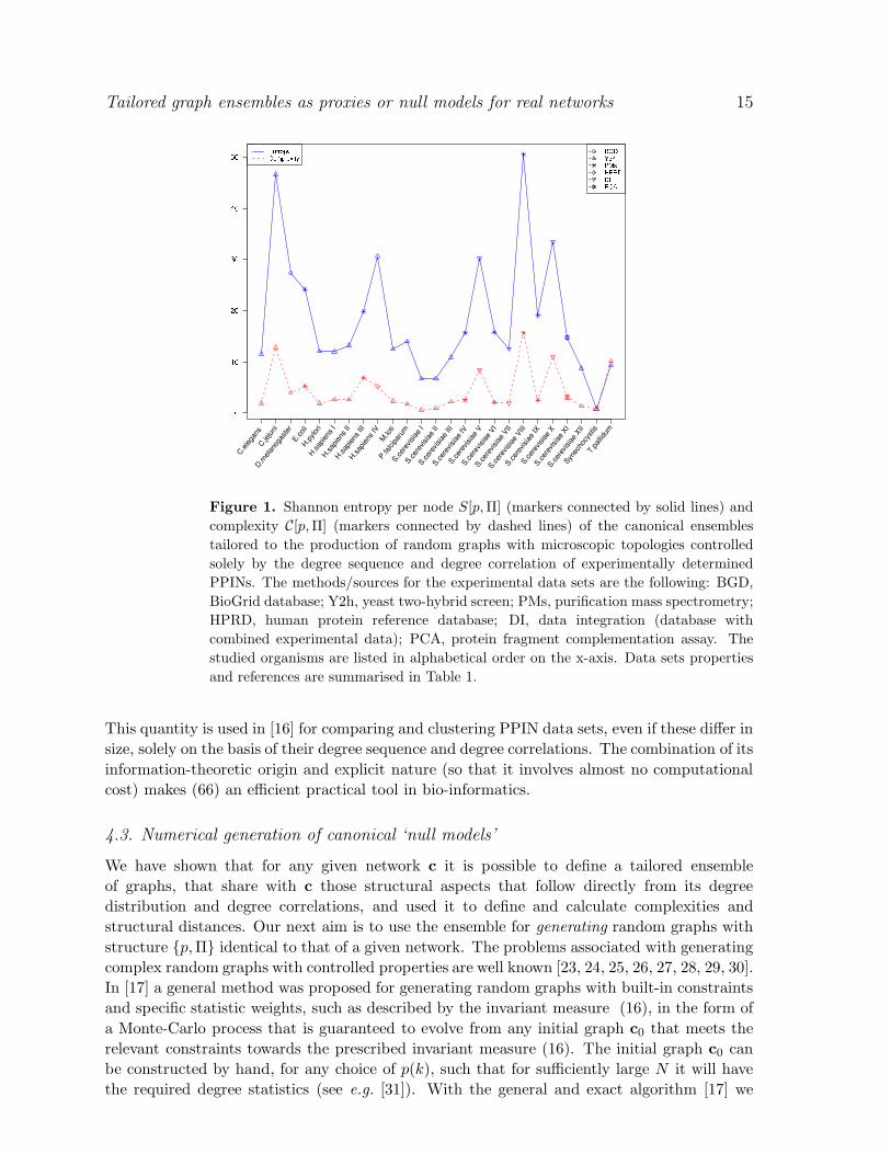
for our theory to apply). For this purpose we have computed the (62) for protein interaction
networks of different species and show the results in Fig. 1. A more systematic and extensive
application of our tools to PPIN will be published in [16].
4.2. Quantifying structural distance between networks
In the same spirit we can now also use our tailored graph ensembles to define an information-
theoretic distance DAB between any two networks cA and cB , based solely on the macroscopic
structure statistics as captured by their associated (observed) structure function pairs pA,ΠAand pB,ΠB. The natural definition would be in terms of the Jeffreys divergence (i.e. the
symmetrized KL-distance) between the two associated canonical ensembles, which is non-
negative and equals zero if and only if pA,ΠA = pB ,ΠB, i.e. if the graphs cA and cB
belong to the same canonical ensemble:
DAB =1
2N
∑
c
Prob(c|pA, QA) log[Prob(c|pA, QA)
Prob(c|pB , QB)
]
+1
2N
∑
c
Prob(c|pB , QB) log[Prob(c|pB , QB)
Prob(c|pA, QA)
]
(65)
Working out this formula, using (27) and (59), gives for large N :
DAB =1
2
∑
c
Prob(c|pA, QA)Ω(c|pB , QB) − 1
2S[pA,ΠA]
+1
2
∑
c
Prob(c|pB , QB)Ω(c|pA, QA) − 1
2S[pB ,ΠB ]
=1
2
∑
k
pA(k) log[pA(k)
pB(k)
]
+∑
kk′
pA(k)pA(k′)kk′
4〈k〉AΠA(k, k′) log
[ΠA(k, k′)
ΠB(k, k′)
]
(66)
+1
2
∑
k
pB(k) log[pB(k)
pA(k)
]
+∑
kk′
pB(k)pB(k′)kk′
4〈k〉BΠB(k, k′) log
[ΠB(k, k′)
ΠA(k, k′)
]
+ o(1)
Tailored graph ensembles as proxies or null models for real networks 15
Figure 1. Shannon entropy per node S[p, Π] (markers connected by solid lines) and
complexity C[p, Π] (markers connected by dashed lines) of the canonical ensembles
tailored to the production of random graphs with microscopic topologies controlled
solely by the degree sequence and degree correlation of experimentally determined
PPINs. The methods/sources for the experimental data sets are the following: BGD,
BioGrid database; Y2h, yeast two-hybrid screen; PMs, purification mass spectrometry;
HPRD, human protein reference database; DI, data integration (database with
combined experimental data); PCA, protein fragment complementation assay. The
studied organisms are listed in alphabetical order on the x-axis. Data sets properties
and references are summarised in Table 1.
This quantity is used in [16] for comparing and clustering PPIN data sets, even if these differ in
size, solely on the basis of their degree sequence and degree correlations. The combination of its
information-theoretic origin and explicit nature (so that it involves almost no computational
cost) makes (66) an efficient practical tool in bio-informatics.
4.3. Numerical generation of canonical ‘null models’
We have shown that for any given network c it is possible to define a tailored ensemble
of graphs, that share with c those structural aspects that follow directly from its degree
distribution and degree correlations, and used it to define and calculate complexities and
structural distances. Our next aim is to use the ensemble for generating random graphs with
structure p,Π identical to that of a given network. The problems associated with generating
complex random graphs with controlled properties are well known [23, 24, 25, 26, 27, 28, 29, 30].
In [17] a general method was proposed for generating random graphs with built-in constraints
and specific statistic weights, such as described by the invariant measure (16), in the form of
a Monte-Carlo process that is guaranteed to evolve from any initial graph c0 that meets the
relevant constraints towards the prescribed invariant measure (16). The initial graph c0 can
be constructed by hand, for any choice of p(k), such that for sufficiently large N it will have
the required degree statistics (see e.g. [31]). With the general and exact algorithm [17] we
Tailored graph ensembles as proxies or null models for real networks 16
(a) (b)
(c)
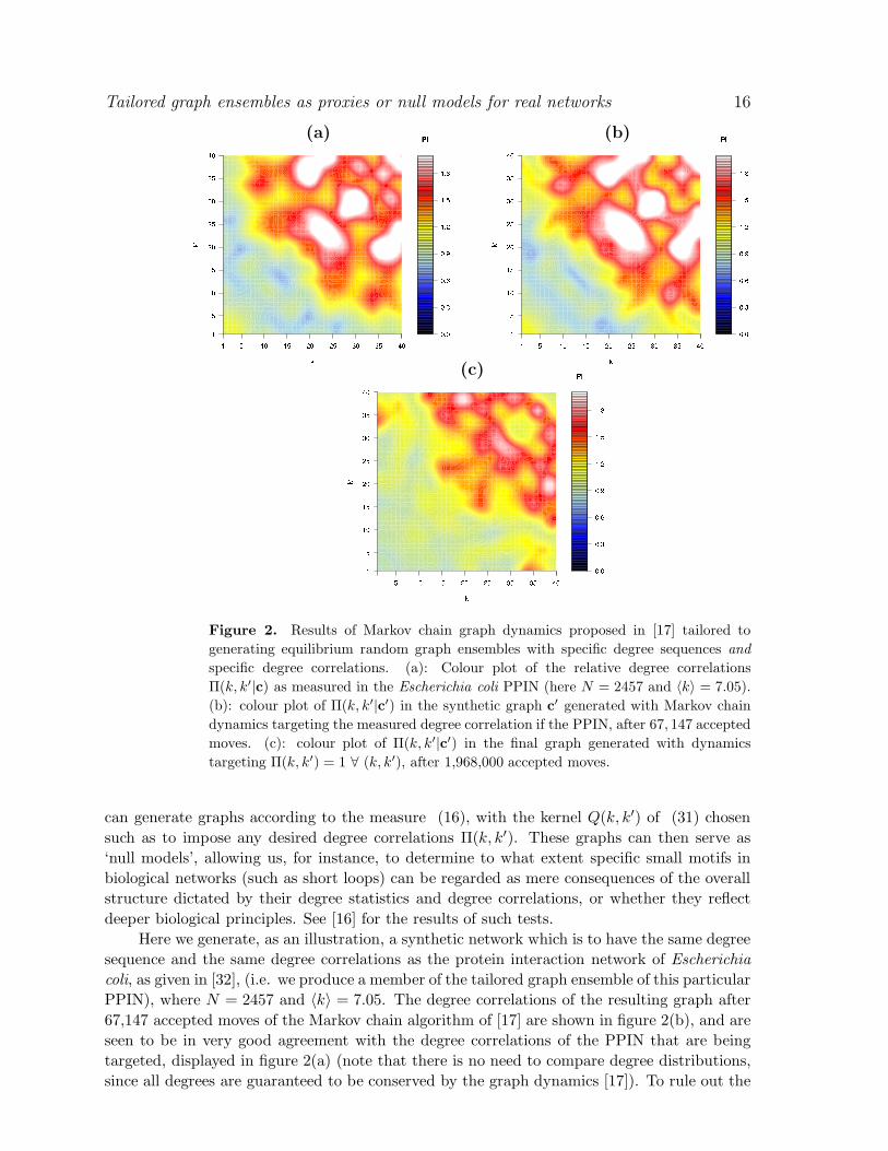
Figure 2. Results of Markov chain graph dynamics proposed in [17] tailored to
generating equilibrium random graph ensembles with specific degree sequences and
specific degree correlations. (a): Colour plot of the relative degree correlations
Π(k, k′|c) as measured in the Escherichia coli PPIN (here N = 2457 and 〈k〉 = 7.05).
(b): colour plot of Π(k, k′|c′) in the synthetic graph c′ generated with Markov chain
dynamics targeting the measured degree correlation if the PPIN, after 67, 147 accepted
moves. (c): colour plot of Π(k, k′|c′) in the final graph generated with dynamics
targeting Π(k, k′) = 1 ∀ (k, k′), after 1,968,000 accepted moves.
can generate graphs according to the measure (16), with the kernel Q(k, k′) of (31) chosen
such as to impose any desired degree correlations Π(k, k′). These graphs can then serve as
‘null models’, allowing us, for instance, to determine to what extent specific small motifs in
biological networks (such as short loops) can be regarded as mere consequences of the overall
structure dictated by their degree statistics and degree correlations, or whether they reflect
deeper biological principles. See [16] for the results of such tests.
Here we generate, as an illustration, a synthetic network which is to have the same degree
sequence and the same degree correlations as the protein interaction network of Escherichia
coli, as given in [32], (i.e. we produce a member of the tailored graph ensemble of this particular
PPIN), where N = 2457 and 〈k〉 = 7.05. The degree correlations of the resulting graph after
67,147 accepted moves of the Markov chain algorithm of [17] are shown in figure 2(b), and are
seen to be in very good agreement with the degree correlations of the PPIN that are being
targeted, displayed in figure 2(a) (note that there is no need to compare degree distributions,
since all degrees are guaranteed to be conserved by the graph dynamics [17]). To rule out the
Tailored graph ensembles as proxies or null models for real networks 17
possibility that the observed similarity in degree correlations between the synthetic graph and
the original PPIN could have arisen from poor sampling of the microscopic configurations (and
just reflect direct similarities in the connectivity matrices), we also calculated the Hamming
distance between the connectivity matrices c and c′ of the original PPIN and the synthetic
graph,
ρ(c, c′) =1
2N〈k〉∑
ij
|cij − c′ij |, (67)
(the prefactor is chosen such that when the two matrices differ in all the 2N〈k〉 entries which
could be different, then ρ(c, c′) = 1). The Hamming distance vanishes if the two matrices are
identical. In the present case we find ρ = 0.90, which implies that although our two graphs
have similar macroscopic structure, their microscopic realizations are indeed very different.
For comparison, we also show in figure 2(c) the degree correlations of a synthetic graph
obtained via the Markov chain dynamics of [17], starting from the same initial graph, but now
targeting degree correlations described by Π(k, k′) = 1 for all (k, k′). All residual deviations in
the bottom plot of figure 2 from the objective Π(k, k′) = 1 ∀(k, k′) are due to finite size effects.
Again we also calculate the Hamming distance between the original and the synthetic matrix,
giving ρ = 0.93. This value is similar to the one found previously, but now the macroscopic
structure of the synthetic graph in terms of the degree correlations is considerably different
from the underlying PPIN.
It has been noted by several authors that most PPINs are disassortative, i.e. nodes
with high degrees tend to connect with nodes with low degrees [4]. Measures of degree
assortativity have been proposed in [3, 4, 33]. A conventional measure of assortativity is
the correlation coefficient (〈kk′〉− 〈k〉〈k′〉)/(〈k2〉 − 〈k〉2), calculated over the joint distribution
W (k, k′) in (58). Degree-assortativity has been shown to have important consequences on
both the topology of a network and the process which it supports. In particular, it was shown
that assortative networks are more resistant to random attacks, i.e. random vertex removal,
whereas disassortative networks are less resistant [4]. It may be useful from a practical point of
view to generate networks with a prescribed assortative character. This can again be achieved
by using the measure (16), where the kernels Q(k, k′) are now chosen to produce assortative
or disassortative graphs. In [17] it was shown that the kernel
Q(k, k′) =|k − k′|2
2(〈k2〉 − 〈k〉2)(68)
tailors the ensemble (16) to the production, for large N , of graphs with degree correlations
Π(k, k′) =〈k〉(k − k′)2
[α3 − 2α2k + α1k2][α3 − 2α2k′ + α1k′2](69)
where the three coefficients αℓ are to be solved numerically from
αℓ =∑
k
kℓp(k)
α3 − 2α2k + α1k2(70)
This degree correlation has a disassortative character. In fact, any kernel of the form
Q(k, k′) = C−1|k − k′|n, n = 1, 2, . . . (71)
with C such that∑
k,k′ p(k)p(k′)Q(k, k′) = 1 will tailor the ensemble (16), for large N , to
the production of graphs with increasingly negative assortative coefficients as n increases. A
prototype of an assortative kernel would be
Q(k, k′) =1
C
1
1 + |k − k′|n (72)
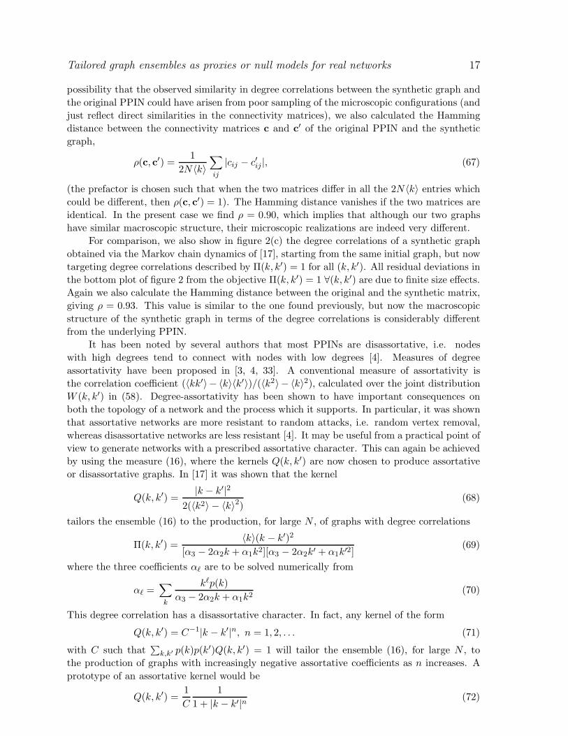
Tailored graph ensembles as proxies or null models for real networks 18
where C =∑
k,k′ p(k)p(k′)[1 + |k − k′|n]. For sufficiently large N , the predicted values for
Π(k, k′) follow from (21), where F (k) is to be solved numerically from (22). As an example
we generated two synthetic graphs, both with the same degree sequence as the PPIN of Homo
sapiens (the experimental data used was taken from the human protein reference database
(HPRD), [34]). In the first graph we enforced an assortative connectivity using (72) with
n = 1, and in the second one a disassortative connectivity using (71) with n = 1. Both graphs
were generated with the algorithm of [17], starting from the actual Homo sapiens PPIN. In
Fig. 3(a) we show the colour plot of the relative degree correlations Π(k, k′) as measured in
the Homo sapiens PPIN, and in Fig. 3(c) and 3(e) we show the same quantity in the two
synthethic graphs generated. For comparison we also show (Fig. 3(b) and 3(d), respectively)
the functional Π(k, k′) that are being targeted, via the kernels in (72) and (71).
5. Discussion
In this paper we have studied the tailoring of a particular structured random graph ensemble
to real-world networks. We have first derived several mathematical properties of this ensemble,
including information-theoretic properties, its Shannon entropy, and the relation between its
control parameters and the statistics and correlations of the degrees in the network to which
the ensemble is tailored. We were then able to use the mathematical results in order to
derive explicit and transparent mathematical tools with which to quantify structure in large
real networks, define rational distance measures for comparing networks, and for generating
controlled null models as benchmark graphs. These tools are precise and based on information-
theoretic principles, yet they take the form of fully explicit formulae (as opposed to implicit
equations that require equilibration of extensive graph simulations). We therefore hope and
anticipate that they will be particularly useful in bio-informatics; indeed a subsequent paper
will be fully devoted to their application to a broad range of protein-protein interaction
networks, involving multiple organisms and multiple experimental protocols [16].
Let us turn to the limitations of this study. Our work so far has focused on characterizing
network structure macroscopically at the level of degree distributions and degree-degree
correlations, and was limited to undirected networks and graphs. We therefore envisage two
main directions in which the present theory could and should be developed further. The
first, and relatively straightforward, one is generalization of the analysis to tailored directed
random graph ensembles. Here one does not envisage insurmountable obstacles, and it would
in bio-informatics open up the possibility of application to e.g. gene regulation networks.
The second direction is towards the inclusion of measures of macroscopic structure that take
account of loops, such as the distribution of length-three loops in which individual network
nodes participate. Here the mathematical task is much more challenging, since in entropy
calculations it is no longer clear whether and how one can achieve factorization over nodes.
Acknowledgements
ACCC would like to thank Conrad Perez-Vicente for stimulating discussions and the
Engineering and Physical Sciences Research Council (UK) for support in the form of a
Springboard Fellowship.
Tailored graph ensembles as proxies or null models for real networks 19
(a)
(b) (c)
(d) (e)
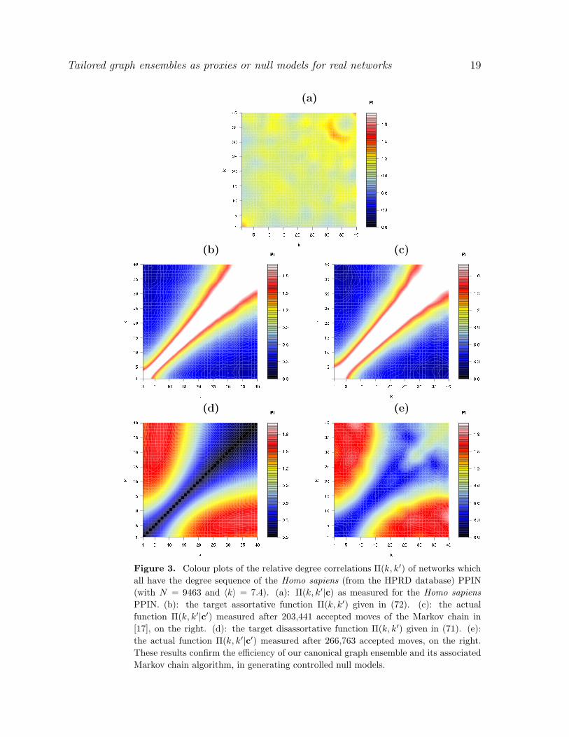
Figure 3. Colour plots of the relative degree correlations Π(k, k′) of networks which
all have the degree sequence of the Homo sapiens (from the HPRD database) PPIN
(with N = 9463 and 〈k〉 = 7.4). (a): Π(k, k′|c) as measured for the Homo sapiens
PPIN. (b): the target assortative function Π(k, k′) given in (72). (c): the actual
function Π(k, k′|c′) measured after 203,441 accepted moves of the Markov chain in
[17], on the right. (d): the target disassortative function Π(k, k′) given in (71). (e):
the actual function Π(k, k′|c′) measured after 266,763 accepted moves, on the right.
These results confirm the efficiency of our canonical graph ensemble and its associated
Markov chain algorithm, in generating controlled null models.
Tailored graph ensembles as proxies or null models for real networks 20
Species kmax Method Reference
C.elegans 99 Y2h [35]
C.jejuni 207 Y2h [36]
D.melanogaster 176 BGD [37]
E.coli 641 PMs [32]
H.pylori 55 Y2h [38]
H.sapiens I 125 Y2h [39]
H.sapiens II 95 Y2h [40]
H.sapiens III 314 PMs [41]
H.sapiens IV 247 HPRD [34]
M.loti 401 Y2h [42]
P.falciparum 51 Y2h [43]
S.cerevisiae I 24 Y2h [44]
S.cerevisiae II 55 Y2h [45]
S.cerevisiae III 279 Y2h [45]
S.cerevisiae IV 62 PMs [46]
S.cerevisiae V 118 DI [47]
S.cerevisiae VI 53 PMs [48]
S.cerevisiae VII 32 DI [49]
S.cerevisiae VIII 955 PMs [50]
S.cerevisiae IX 141 PMs [51]
S.cerevisiae X 127 DI [52]
S.cerevisiae XI 58 PCA [53]
S.cerevisiae XII 86 Y2h-PCA [54]
Synechocystis 51 Y2h [55]
T.pallidum 285 Y2h [56]
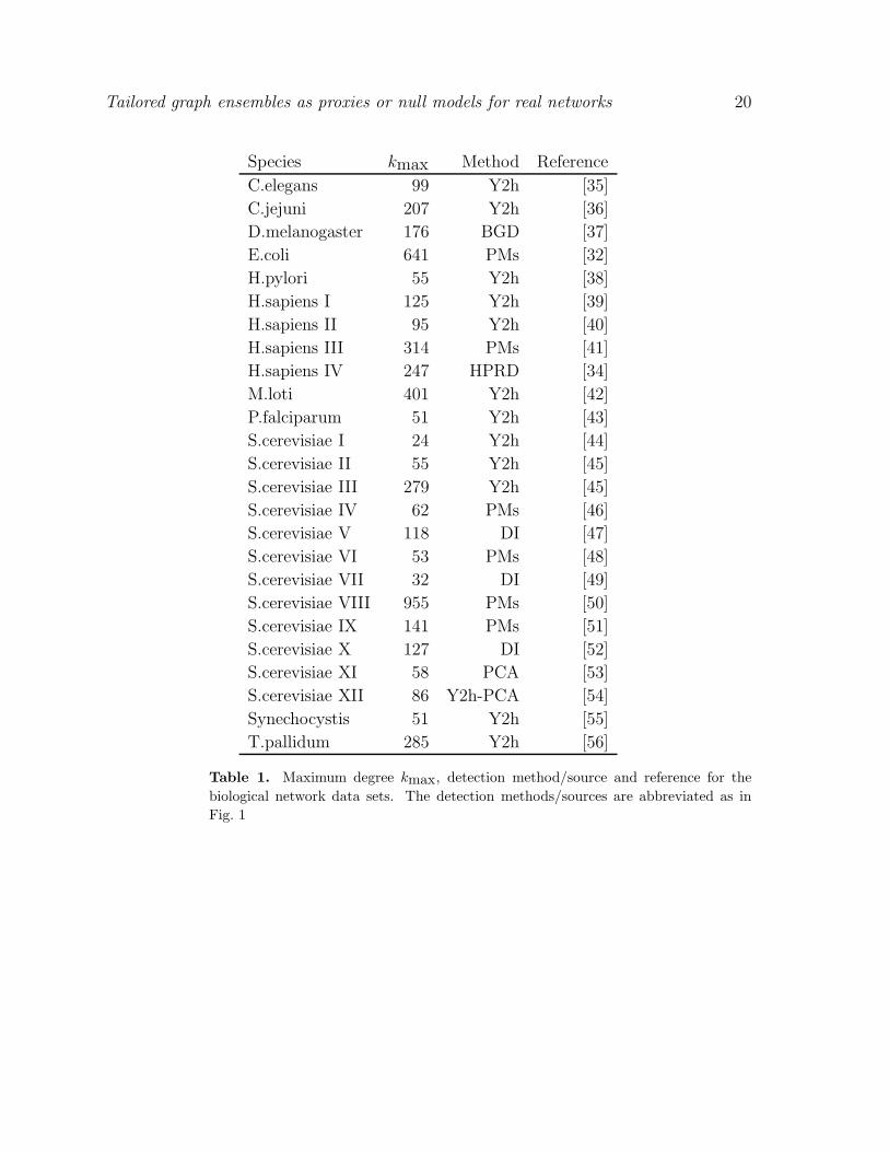
Table 1. Maximum degree kmax, detection method/source and reference for the
biological network data sets. The detection methods/sources are abbreviated as in
Fig. 1

Tailored graph ensembles as proxies or null models for real networks 21
6. References
[1] Albert R and Barabassi A L 2002 Reviews of Modern Physics 74 47-97
[2] Barabasi A L and Albert R 1999 Science 286 509
[3] Pastor-Satorras R, Vazquez A and Vespignani A 2001 Phys. Rev. Lett. 87 258701
[4] Newman M E J 2002 Phys. Rev. Lett. 89 208701
[5] Watts D J and Strogatz S H 1998 Nature 4 393
[6] Newman M E J and Leich E A 2007 Proc. Natl. Acad. Sci. U.S.A. 104 0364
[7] Maslov S and Sneppen K 2002 Science 296 5569
[8] Maslov S, Sneppen K and Zaliznyak A 2004 Physica A 333 529-540
[9] Shen-Orr S S, Milo R, Mongan S and Alon U 2002 Nature Genetics 31 64-68
[10] Junker B H and Schreiber F 2008 Analysis of biological networks (New York: Wiley Series on
Bioinformatics)
[11] Artzy-Randrup Y, Fleishman S J, Ben-Tal N and Stone L 2004 Science 305 5687
[12] Perez-Vicente C J and Coolen A C C 2008 J. Phys. A: Math. Theor. 41 255003
[13] Bianconi G 2008 EPL 81 28005
[14] Bianconi G, Coolen A C C and Vicente C J P 2008 Phys. Rev. E 78 016114
[15] Bianconi G 2009 Phys. Rev. E 79 036114
[16] Fernandes L P, Annibale A, Kleinjung J, Coolen A C C and Fraternali F in preparation
[17] Coolen A C C, De Martino A and Annibale A 2009 preprint arXiv:0905.4155
[18] Dorogovtsev S N and Mendes J F 2003 Evolution of networks (Oxford: Oxford University Press)
[19] Ivanic J, Wallqvist A and Reifman J 2008 BCM System Biology 2:11
[20] Ivanic J, Wallqvist A and Reifman J 2008 PLoS Computational Biology 4 7
[21] Perez-Vicente C J and Coolen A C C 2009, J. Phys. A: Math. Theor. 42 169801
[22] Erdos P and Gallai T 1960 Mat. Lapok 11 264-274
[23] Rao A R, Jana R, and Bandyopadhya S 1996 Indian J. of Statistics 58 225
[24] Gkantsidis C, Mihail M and Zegura E 2003 in Proc. 5th workshop on algorithm engineering and
experiments (ALENEX), Siam
[25] Viger F and Latapy M 2005 in COCOON 2005, The eleventh international computing and
combinatorics conference, LNCS 440-449
[26] Chen Y, Diaconis P, Holmes S and Liu J S 2005 J. Amer. Statistical Assoc. 100 109
[27] Catanzaro M, Boguna M, and Pastor-Satorras R 2005 Phys. Rev. E 71 027103
[28] Serrano M A and Boguna M 2005 Phys. Rev. E 72 036133
[29] Foster J G, Foster D V, Grassberger P and Paczuski M 2007 Phys. Rev. E 76 046112
[30] Verhelst N D 2008 Psychometrika 73 705
[31] Newman M E J, Strogatz S H and Watts D J 2001 Phys. Rev. E 64 026118
[32] Arifuzzaman M et al. 2006 Genome Res 16 686-691
[33] Newman M E J 2003 Phys. Rev. Lett. 67 026126
[34] Keshava Prasad T S et al. 2009 Nucleic Acids Research 27 (Database issue)
[35] Simonis N et al. 2008 Nature Methods 6(1):47-54
[36] Parrish J R et al. 2007 Genome Biology 8(7)
[37] Stark C et al. 2006 Nucleic Acids Res 34 (Database issue)
[38] Rain J C et al. 2001 Nature 409(6817):211-215
[39] Rual J-F F et al. 2005 Nature 437(7062):1173-1178
[40] Stelzl U et al. 2005 Cell 122(6):957-968
[41] Ewing R M et al. 2007 Molecular systems biology 3:89
[42] Shimoda Y et al. 2008 DNA Res 15(1):13-23
[43] Lacount D J et al. 2005 Nature 438(7064):103-107
[44] Uetz P et al. 2000 Nature 403(6770):623-627
[45] Ito T et al. 2001 Proc Natl Acad Sci U S A 98(8):4569-4574
[46] Ho Y et al. 2002 Nature 415(6868):180-183

Tailored graph ensembles as proxies or null models for real networks 22
[47] von Mering et al. 2002 Nature 417(6887):399-403
[48] Gavin A C et al. 2002 Nature 415(6868):141147
[49] Han J D J et al. 2004 Nature 430(6995):88-93
[50] Gavin A C C et al. 2006 Nature 440(7084):631-636
[51] Krogan N J et al. 2006 Nature 440(7084):637-643
[52] Collins S R et al. 2007 Mol Cell Proteomics MCP6(3), 439-450
[53] Tarassov K et al. 2008 Science 320(5882):1465-1470
[54] Yu H et al. 2008 Science 322(5898):104-110
[55] Sato S et al. 2007 DNA Res 14(5), 207-216
[56] Titz B et al. 2008 PLoS ONE 3(5)
Appendix A.
Degree correlations in the random graph ensemble
In this appendix we prove the validity of the crucial relation (21), with Π(k, k′) as defined in
(20) for the random graph ensemble (16):
Π(k, k′) =〈k〉
p(k)p(k′)kk′lim
N→∞
∑
rs
∑
k
[
∏
ℓ
p(kℓ)]
δk,krδk′,ks
1
N
∑
c
Prob(c|k, Q)crs (A.1)
Let us work out the sum over the graphs c in (A.1), using the integral representation
δnm = (2π)−1∫ 2π0 dω eiω(n−m) to deal with the N degree constraints δki,ki(c). This introduces
and N -fold integration over ω = (ω1, . . . , ωN ) ∈ [0, 2π]N . With a modest amount of foresight
we introduce the two abbreviations ω · k =∑
i ωiki and
W (ω,k) =∏
i<j
1 +k
NQ(ki, kj)[e
−i(ωi+ωj)−1]
(A.2)
These allow us to write
∑
c
Prob(c|k, Q)crs =
∑
c crs∏
i<j
[
kN Q(ki, kj)δcij ,1+
(
1− kN Q(ki, kj)
)
δcij ,0
]
.∏
i δki,ki(c)
∑
c
∏
i<j
[
kN Q(ki, kj)δcij ,1+
(
1− kN Q(ki, kj)
)
δcij ,0
]
.∏
i δki,ki(c)
=
∫
dω eiω·k∑
c crs∏
i<j
[
kN Q(ki, kj)δcij ,1+
(
1− kN Q(ki, kj)
)
δcij ,0
]
e−icij(ωi+ωj)
∫
dω eiω·k∑
c
∏
i<j
[
kN Q(ki, kj)δcij ,1+
(
1− kN Q(ki, kj)
)
δcij ,0
]
e−icij(ωi+ωj)
=
∫
dω W (ω,k)eiω·k[ k
NQ(kr ,ks)e−i(ωr+ωs)
1+ kN
Q(kr,ks)[e−i(ωr+ωs)−1]
]
∫
dω W (ω,k)eiω·k
=k
NQ(kr, ks)[1 + O(N−1)]
∫
dω W (ω,k)eiω·k−i(ωr+ωs)
∫
dω W (ω,k)eiω·k(A.3)
We next expand the function W (ω,k), as defined in (A.2), in leading orders for large N , using
the abbreviation P (q, ω|ω,k) = N−1∑
i δq,kiδ(ω − ωi):
W (ω,k) =∏
i<j
exp k
NQ(ki, kj)[e
−i(ωi+ωj)−1] + O(N−2)
= exp k
2N
∑
ij
Q(ki, kj)[e−i(ωi+ωj)−1] + O(1)
= exp1
2kN
∑
qq′
∫
dωdω′ P (q, ω|ω,k)P (q′, ω′|ω,k)Q(q, q′)[e−i(ω+ω′)−1] + O(1)
(A.4)

Tailored graph ensembles as proxies or null models for real networks 23
We now insert the following representation of unity, for each combination of (q, ω),
1 =
∫
dP (q, ω)δ[P (q, ω) − P (q, ω|ω,k)]
=
∫
dP (q, ω)dP (q, ω)
2π/NeiNP (q,ω)[P (q,ω)−P (q,ω|ω,k)] (A.5)
and convert the previous expression for W (ω,k) into the form of a functional integral, with
a path integral measure dP =∏
q,ω[dP (q, ω)∆ω/√
2π] (where the values of ω ∈ [0, 2π] are
first discretized, with the discretization spacing ∆ω sent to zero as soon as this is possible):
W (ω,k) =
∫
dPdPeiN∑
q
∫
dω P (q,ω)P (q,ω)−i∑
iP (ki,ωi)+O(1)
× e12kN∑
qq′
∫
dωdω′ P (q,ω)P (q′,ω′)Q(q,q′)[e−i(ω+ω′)−1]
=
∫
dPdPeN(Ψ[P,P]+Φ[P])−i∑
iP (ki,ωi)+O(1) (A.6)
with
Ψ[P, P] = i∑
q
∫ 2π
0dω P (q, ω)P (q, ω) (A.7)
Φ[P] =1
2k∑
qq′
∫ 2π
0dωdω′ P (q, ω)P (q′, ω′)Q(q, q′)[e−i(ω+ω′) − 1] (A.8)
We can now integrate over the N -fold angles ω ∈ [0, 2π]N , and obtain∫
dω W (ω,k)eiω·k′
=
∫
dPdPeN(Ψ[P,P]+Φ[P])+O(1)∫
dω eiω·k′−i∑
iP (ki,ωi)
=
∫
dPdPeN(Ψ[P,P]+Φ[P])+O(1)∏
i
∫
dω ei[ωk′
i−P (ki,ω)] (A.9)
and write the ratio of integrals in (A.3) as∫
dω eiω·k−i(ωr+ωs)W (ω,k)∫
dω eiω·kW (ω,k)=
∫ dPdPeN(Ψ[P,P]+Φ[P]+Ω[P|k])+O(1) [∫
dω eiω(kr−1)−iP (kr,ω)][∫
dω eiω(ks−1)−iP (ks,ω)][∫
dωeiω kr−iP (kr,ω)][∫
dω eiωks−iP (ks,ω)]
∫ dPdP eN(Ψ[P,P]+Φ[P]+Ω[P|k])+O(1)
(A.10)
with
Ω[P|k] =1
N
∑
i
log
∫
dω ei[ωki−P (ki,ω)] (A.11)
Therefore we find upon combining the previous intermediate results that the quantity of
interest (A.1) can be written in the following form:
Π(k, k′) =〈k〉2Q(k, k′)
p(k)p(k′)kk′lim
N→∞
∑
k
[
∏
ℓ
p(kℓ)][ 1
N
∑
r
δk,kr
][ 1
N
∑
s
δk′,ks
]
×
×
∫ dPdPeN(Ψ[P,P]+Φ[P]+Ω[P|k])+O(1) [∫
dω ei[ω(k−1)−P (k,ω)]][∫
dω ei[ω(k′−1)−P (k′,ω)]][∫
dωei[ω k−P (k,ω)]][∫
dω ei[ωk′−P (k′,ω)]]
∫ dPdPeN(Ψ[P,P]+Φ[P]+Ω[P|k])+O(1)
=〈k〉2Q(k, k′)
kk′×

Tailored graph ensembles as proxies or null models for real networks 24
limN→∞
∫ dPdPeN(Ψ[P,P]+Φ[P]+Ω[P])+O(1) [∫
dω ei[ω(k−1)−P (k,ω)]][∫
dω ei[ω(k′−1)−P (k′,ω)]][∫
dωei[ω k−P (k,ω)]][∫
dω ei[ωk′−P (k′,ω)]]
∫ dPdPeN(Ψ[P,P]+Φ[P]+Ω[P])+O(1)
(A.12)
where
Ω[P] =∑
k′′
p(k′′) log
∫
dω ei[ωk′′−P (k′′,ω)] (A.13)
We conclude from (A.12), in which the functional integrals can be done by steepest descent
in the limit N → ∞, that Π(k, k′) takes the form
Π(k, k′) = Q(k, k′)/F (k|Q)F (k′|Q) (A.14)
with
1
F (k|Q)=
〈k〉k
∫
dω eiω(k−1)−iP (k,ω)
∫
dω eiωk−iP (k,ω)(A.15)
and where the functions P (k, ω) and P (k, ω) are to be solved from extremization of Ψ[P, P]+Φ[P] + Ω[P], with the three functions given in (A.7,A.8,A.13), leading to the two coupled
functional saddle-point equations δ[Ψ + Φ]/δP = 0 and δ[Ψ + Ω]/δP = 0.
The last step in this appendix is to derive from the saddle-point equations an equation for
the function F (k|Q) in (A.14). Upon transforming exp[−iP (k, ω)] = R(k, ω), our saddle-point
equations simplify to
R(k, ω) = exp
〈k〉∑
k′
∫
dω′ P (k′, ω′)Q(k, k′)[e−i(ω+ω′)−1]
(A.16)
P (k, ω) = p(k)R(k, ω)eiωk
∫
dω′ R(k, ω′)eiω′k(A.17)
Elimination of P (k, ω) from this set gives, using the identity∫
dω P (k, ω) = p(k),
R(k, ω) = exp
〈k〉∑
k′
p(k′)Q(k, k′)
[
e−iω
∫
dω′ R(k′, ω′)eiω′(k′−1)
∫
dω′ R(k′, ω′)eiω′k′− 1
]
= exp
∑
k′
p(k′)Q(k, k′)e−iωk′/F (k′|Q) − G(k|Q)
(A.18)
in which F (k|Q) is defined in (A.15), and G(k|Q) = 〈k〉∑k′ p(k′)Q(k, k′). Insertion of our
expression for R(k, ω) into (A.15), using exp[−iP (k, ω)] = R(k, ω), leaves us with an equation
for F (k|Q) only, from which the object G(k|Q) simply drops out since it gives an identical pre-
factor exp[−G(k|Q)] in both the numerator and the denominator of the formula for F (k|Q):
1
F (k|Q)=
〈k〉k
∫
dω eiω(k−1)R(k, ω)∫
dω eiωkR(k, ω)
=〈k〉k
∑
m≥01
m!
[
∑
k′ p(k′)Q(k, k′)k′/F (k′|Q)]m ∫
dω eiω(k−1)−imω
∑
m≥01
m!
[
∑
k′ p(k′)Q(k, k′)k′F (k′|Q)]m ∫
dω eiωk−imω
=〈k〉k
∑
m≥01
m!δm,k−1
[
∑
k′ p(k′)Q(k, k′)k′F (k′|Q)]m
∑
m≥01
m!δmk
[
∑
k′ p(k′)Q(k, k′)k′/F (k′|Q)]m
=〈k〉
∑
k′ p(k′)Q(k, k′)k′/F (k′|Q)(A.19)

Tailored graph ensembles as proxies or null models for real networks 25
Equivalently:
F (k|Q) = 〈k〉−1∑
k′
p(k′)k′Q(k, k′)F−1(k′|Q) (A.20)
Note that the present derivation of the combined result (A.14,A.20) also serves as the explicit
proof of the validity of corrigendum [21].