Synchronous Problem-Based e-Learning (ePBL) in Interprofessional Health Science Education
Upload
khangminh22Category
view
0download
0

Systems Science and Population Health


1
Systems Science and Population Health
Edited by
AbdulrAhmAn m. el- SAyed
Executive Director and Health Officer, Detroit Health Department, City of Detroit
SAndro GAleA
Robert A. Knox Professor and Dean, Boston University School of Public Health

1
Oxford University Press is a department of the University of Oxford. It furthersthe University’s objective of excellence in research, scholarship, and educationby publishing worldwide. Oxford is a registered trade mark of Oxford UniversityPress in the UK and certain other countries.
Published in the United States of America by Oxford University Press198 Madison Avenue, New York, NY 10016, United States of America.
© Oxford University Press 2017
All rights reserved. No part of this publication may be reproduced, stored ina retrieval system, or transmitted, in any form or by any means, without theprior permission in writing of Oxford University Press, or as expressly permittedby law, by license, or under terms agreed with the appropriate reproductionrights organization. Inquiries concerning reproduction outside the scope of theabove should be sent to the Rights Department, Oxford University Press, at theaddress above.
You must not circulate this work in any other formand you must impose this same condition on any acquirer.
Library of Congress Cataloging- in- Publication DataNames: El- Sayed, Abdulrahman M., editor. | Galea, Sandro, editor.Title: Systems science and population health / edited by Abdulrahman M. El- Sayed, Sandro Galea.Description: Oxford ; New York : Oxford University Press, [2016] | Includesbibliographical references and index.Identifiers: LCCN 2016034543 (print) | LCCN 2016036314 (ebook) | ISBN 9780190492397 (pbk. : alk. paper) | ISBN 9780190492403 (ebook) | ISBN 9780190492410 (ebook) Subjects: | MESH: Systems Theory | Public Health | Regional Health Planning | Health Information Systems | Models, TheoreticalClassification: LCC RA418 (print) | LCC RA418 (ebook) | NLM WA 100 | DDC 362.1— dc23LC record available at https:// lccn.loc.gov/ 2016034543
This material is not intended to be, and should not be considered, a substitute for medical or other professional advice. Treatment for the conditions described in this material is highly dependent on the individual circumstances. And, while this material is designed to offer accurate information with respect to the subject matter covered and to be current as of the time it was written, research and knowledge about medical and health issues is constantly evolving, and dose schedules for medications are being revised continually, with new side effects recognized and accounted for regularly. Readers must therefore always check the product information and clinical procedures with the most up-to-date published product information and data sheets provided by the manufacturers and the most recent codes of conduct and safety regulation. The publisher and the authors make no representations or warranties to readers, express or implied, as to the accuracy or completeness of this material. Without limiting the foregoing, the publisher and the authors make no representations or warranties as to the accuracy or efficacy of the drug dosages mentioned in the material. The authors and the publisher do not accept, and expressly disclaim, any responsibility for any liability, loss, or risk that may be claimed or incurred as a consequence of the use and/or application of any of the contents of this material.
Oxford University Press is not responsible for any websites (or their content) referred to in this book that are not owned or controlled by the publisher.
9 8 7 6 5 4 3 2 1
Printed by LSC Communications, United States of America

CONTENTS
Acknowledgments viiContributors ix
1. Introduction 1Abdulrahman M. El- Sayed
SECTION 1 Simplicity, Complexity, and Population Health
2. Reductionism at the Dawn of Population Health 9Kristin Heitman
3. Wrong Answers: When Simple Interpretations Create Complex Problems 25David S. Fink and Katherine M. Keyes
4. Complexity: The Evolution Toward 21st- Century Science 37Anton Palma and David W. Lounsbury
5. Systems Thinking in Population Health Research and Policy 49Stephen J. Mooney
SECTION 2 Methods in Systems Population Health
6. Generation of Systems Maps: Mapping Complex Systems of Population health 61Helen de Pinho
vi C O N T E N T S
7. Systems Dynamics Models 77Eric Lofgren
8. Agent- Based Modeling 87Brandon D. L. Marshall
9. Microsimulation 99Sanjay Basu
10. Social Network Analysis 113Douglas A. Luke, Amar Dhand, and Bobbi J. Carothers
SECTION 3 Systems Science Toward a Consequential Population Health
11. Machine Learning 129James H. Faghmous
12. Systems Science and the Social Determinants of Population Health 139David S. Fink, Katherine M. Keyes, and Magdalena Cerdá
13. Systems Approaches to Understanding How the Environment Influences Population Health and Population Health Interventions 151Melissa Tracy
14. Systems of Behavior and Population Health 167Mark G. Orr, Kathryn Ziemer, and Daniel Chen
15. Systems Under Your Skin 181Karina Standahl Olsen, Hege Bøvelstad, and Eiliv Lund
16. Frontiers in Health Modeling 191Nathaniel Osgood
17. Systems Science and Population Health 217Abdulrahman M. El- Sayed and Sandro Galea
Index 221

ACKNOWLEDGMENTS
We are indebted to the editorial assistance of Claire Salant and Eric DelGizzo, without whom this book would not have been possible. We thank our fami-lies always for their support as we took on this book as just one of many other ongoing projects. Abdul in particular thanks Dr. Sarah Jukaku, Drs. Mohamed and Jacqueline El- Sayed, and Dr. Fatten Elkomy, and Sandro thanks Isabel Tess Galea, Oliver Luke Galea, and Dr. Margaret Kruk.


CONTRIBUTORS
Sanjay Basu, Stanford Prevention Research Center, Stanford University, Palo Alto, CA.
Hege Bøvelstad, Department of Community Medicine, University of Tromsø– The Arctic University of Norway, Tromsø, Norway.
Bobbi J. Carothers, Center for Public Health Systems Science, Washington University in St. Louis, St. Louis, MO.
Magdalena Cerdá, Department of Emergency Medicine, Violence Prevention Research Program, University of California, Davis, Sacramento, CA.
Daniel Chen, Social and Decision Analytics Laboratory, Biocomplexity Institute, Virginia Tech, Blacksburg, VA.
Helen de Pinho, Population and Family Health at the Columbia University Medical Center, Mailman School of Public Health, New York, NY.
Amar Dhand, Department of Neurology, Washington University School of Medicine in St. Louis, St. Louis, MO.
Abdulrahman M. El- Sayed, Detroit Health Department, City of Detroit, Detroit, MI.
James H. Faghmous, Arnhold Institute for Global Health, Icahn School of Medicine at Mount Sinai, New York, NY.
David S. Fink, Department of Epidemiology, Mailman School of Public Health, Columbia University, New York, NY.
Sandro Galea, School of Public Health, Boston University, Boston, MA.
Kristin Heitman, Independent Scholar, Bethesda, MD.

x C O N T R I B U T O R S
Katherine M. Keyes, Department of Epidemiology, Mailman School of Public Health, Columbia University, New York, NY.
Eric Lofgren, Paul G. Allen School for Global Animal Health, Washington State University, Pullman, WA.
David W. Lounsbury, Department of Epidemiology and Population Health, Department of Family and Social Medicine, Albert Einstein College of Medicine, New York, NY.
Douglas A. Luke, Center for Public Health Systems Science, George Warren Brown School of Social Work, Washington University in St. Louis, St. Louis, MO.
Eiliv Lund, Department of Community Medicine, University of Tromsø– The Arctic University of Norway, Tromsø, Norway.
Brandon D. L. Marshall, Department of Epidemiology, Brown University School of Public Health, Providence, RI.
Stephen J. Mooney, Harborview Injury Prevention & Research Center, University of Washington, Seattle, WA.
Karina Standahl Olsen, Department of Community Medicine, University of Tromsø– The Arctic University of Norway, Tromsø, Norway.
Mark G. Orr, Social and Decision Analytics Laboratory, Biocomplexity Institute, Virginia Tech, Blacksburg, VA.
Nathaniel Osgood, Department of Computer Science, Department of Community Health and Epidemiology, Bioengineering Division, University of Saskatchewan, SK, Canada.
Anton Palma, Department of Epidemiology, Mailman School of Public Health, Columbia University, New York, NY.
Melissa Tracy, Department of Epidemiology and Biostatistics, University at Albany School of Public Health, Albany, NY.
Kathryn Ziemer, Social and Decision Analytics Laboratory, Virginia Bioinformatics Institute, Virginia Tech, Blacksburg, VA.
1
Introduction
A B D U L RA H MA N M . E L - S AY E D
1. WHY SYSTEMS SCIENCE?
Population health is complex, involving dynamic interactions between cells, soci-eties, and everything in between. Our modal approach to studying population health, however, remains oriented around a reductionist approach to conceptual-izing, empirically analyzing, and intervening to improve population health.
Health scientists are concerned with identifying individual “risk factors” or “determinants” of disease in populations. This approach assumes that population health interventions can be designed by understanding each of these determi-nants individually, ultimately decreasing the risk of poor health outcomes they determine. Both population scientists and policymakers assume these interven-tions have direct, linear effects that do not extend beyond the outcomes they are meant to influence and that are consistent across different places in different times.
Sometimes these interventions work as expected. For this reason, popula-tion health science founded on simple understandings of the world can count many victories: germ theory, the health hazards of smoking, and a more nuanced understanding of the etiology of cardiovascular disease— all of which have vastly improved human health.
The trouble, however, is that interventions founded on simplifying a complex world often do not work, yielding failure, or worse, harm. The motivations for this book emerge from the truth that “silver bullet” health science often fails. And understanding why and how it fails can help us improve our approach to health science, and, ultimately, population health.
There are a number of examples from the population health science literature that illustrate the folly of oversimplification in population health. Many have had dramatic consequences for public health. Early evidence from observational studies

2 S Y S T E M S S C I E N C E A N D P O P U L A T I O N H E A LT H
suggested that hormone replacement therapy (HRT) could reduce cardiovascular disease risk among post- menopausal women. This evidence ultimately informed clinical guidelines that recommended HRT to millions of women over several decades [1, 2]. However, it was only after a series of randomized trials were per-formed that HRT was actually shown to increase cardiovascular disease (as well as breast cancer risk) among women [3– 5].
Yet randomized trials— the gold standard of population health science— have also led to policy failure. Consider the use of conditional cash transfer (CCT) to improve health. The Progresa- Oportunidades study showed improvements in the use of various health services and subsequent health outcomes in families that received cash transfers conditional on nutrition supplement, nutrition edu-cation, and health- care service use in Mexico [6, 7]. Several other randomized trials and literature reviews have shown that CCTs in low- and middle- income countries (LMICs) can improve the use of health services, nutritional status, and various health outcomes, including HIV and sexually transmitted infections [8– 10]. This evidence has moved policy: CCT programs feature prominently in health policies in over 30 LMICs across South and Central America, Asia, and sub- Saharan Africa [11].
However, CCT programs have also failed. One CCT program to prevent HIV/ AIDS in rural Malawi provides a telling example [12]. CCT did not prevent HIV status or diminish reported risky sexual behavior overall. Worse, men who received the benefit were actually more likely to engage in risky sexual behav-ior just after having received the cash. Another CCT program in New York City, which aimed to improve academic achievement among socioeconomically disad-vantaged youth, provides an additional example. A program evaluation showed that the achievement benefits were concentrated among academically prepared teenagers, prompting the cancellation of the program. In each case, these pro-grams were built from simplistic understandings of population health science that transported the evidence about CCTs from other contexts, without regard for how particular differences in context or time might influence the results.
Over the past 20 years, systems science has grown in influence and impor-tance across several scientific disciplines. Across diverse disciplines, systems sci-ence has yielded insights that have illuminated our understanding of complex human systems. Complexity and systems science have often cogently and coher-ently explained why “silver bullet” policies have sometimes failed to produce desired outcomes, or created paradoxical outcomes on these parameters— or unexpected outcomes on seemingly unrelated parameters.
However, few population health scientists or policymakers understand the precepts of complexity or systems science, let alone how to apply them to their work. Conversely, few systems scientists understand the applications of their work to population health. This book aims to bridge the gap between systems

Introduction 3
and population health sciences. We aim to unite contributions from leading authorities in the field to describe how complex systems science contributes to population health and to demonstrate how methodological approaches in sys-tems science can sharpen population health science. Throughout, we rely on examples from the emerging literature at the nexus between complex systems and population health.
2. COMPLEXITY FOR POPULATION HEALTH
Systems science— a conceptual framework that emphasizes the relationships that connect constituent parts of a system rather than the parts themselves— has advanced a number of scientific disciplines over the past two decades. From eco-nomics to ecology to cancer biology, scientists and practitioners have embraced systems science, yielding profound insights that have improved our understand-ing of important phenomena, including financial markets, herd behavior, and the biology of metastasis. Population health, too, is a complex system, wherein indi-viduals interact to produce collectives within varying environments, all of which feed back upon one another to shape the health and well- being of populations.
Systems science emphasizes relationships and scale. It is only appropriate that a book about systems science in population health should also emphasize relationships and scale between various concepts in epidemiology and popula-tion health. In that respect, we begin with a focus on simplicity, articulating why reductionism has formed the core of science and population health over the past century. The first section “Simplicity, Complexity, and Population Health” will walk the reader through the intellectual and conceptual history of systems sci-ence as it intersects with population health. It will begin with a discussion of the import of reductionism at the advent of epidemiology and public health. Next, it will explore challenges to reductionism in population health, considering both the intractability of a number of problems in the absence of systems approaches, as well as situations where a failure to appreciate complexity led to harm. The dis-cussion will then follow the evolution and maturation of systems science. Finally, the authors will consider exemplar systems of population health to set the stage for the next several sections.
The second section, “Methods in Systems Population Health,” will provide the reader with clear, concise overviews of several important and emerging systems science methodological tools, including systems dynamics, agent- based model-ing, microsimulation, social network analysis, and machine learning with rele-vant examples drawn from the population health literature.
The third section, “Systems Science Toward a Consequential Population Health,” synthesizes the previous two sections to explore the implications of sys-tems science for our understanding of broad issue areas in population health.

4 S Y S T E M S S C I E N C E A N D P O P U L A T I O N H E A LT H
Population health is ripe for systems science. We hope that this book will seed a future generation of population health scientists and thinkers with the concep-tual tools and methodological understanding needed to frame population health through complexity and systems science. In an applied science such as ours, the responsibility for action is paramount and must guide our scientific efforts [13]. Therefore, answers to our most pressing scientific questions must be both cor-rect and actionable. Our hope is that by incorporating complexity and systems thinking into population health, we might yield more correct and more action-able answers that ultimately improve the efficacy, efficiency, and equity of popu-lation health.
3. REFERENCES
1. Nabulsi AA, et al. Association of hormone- replacement therapy with various car-diovascular risk factors in postmenopausal women. New England Journal of Medicine. 1993; 328(15): 1069– 1075.
2. Stampfer MJ, Colditz GA. Estrogen replacement therapy and coronary heart dis-ease: a quantitative assessment of the epidemiologic evidence. Preventive Medicine. 1991; 20(1): 47– 63.
3. Vickers MR, et al. Main morbidities recorded in the women’s international study of long duration oestrogen after menopause (WISDOM): A randomised controlled trial of hormone replacement therapy in postmenopausal women. The BMJ. 2007; 335(7613): 239.
4. Chlebowski RT, et al. Influence of estrogen plus progestin on breast cancer and mammography in healthy postmenopausal women: The women’s health initiative randomized trial. JAMA: The Journal of the American Medical Association. 2003; 289(24): 3243– 3253.
5. Hernán MA, et al. Observational studies analyzed like randomized experiments: An application to postmenopausal hormone therapy and coronary heart disease. Epidemiology. 2008; 19(6): 766.
6. Rivera JA, Sotres- Alvarez D, Habicht J, Shamah T, Villalpando S. Impact of the mexi-can program for education, health, and nutrition (progresa) on rates of growth and anemia in infants and young children: A randomized effectiveness study. JAMA: The Journal of the American Medical Association. 2004; 291(21): 2563– 2570.
7. Gertler P. Do conditional cash transfers improve child health? Evidence from PROGRESA’s control randomized experiment. American Economic Review. 2004: 336– 341.
8. Lagarde M, Haines A, Palmer N. The impact of conditional cash transfers on health outcomes and use of health services in low and middle income countries. The Cochrane Database of Systematic Reviews. 2009; 4(4): 1– 49.
9. Ranganathan M, Lagarde M. Promoting healthy behaviours and improving health outcomes in low and middle income countries: A review of the impact of conditional cash transfer programmes. Preventive Medicine. 2012; 55: S95– S105.

Introduction 5
10. Baird S, Chirwa E, McIntosh C, Özler B. The short‐term impacts of a schooling conditional cash transfer program on the sexual behavior of young women. Health Economics. 2010; 19(S1): 55– 68.
11. Angrist J, Pischke JS. The credibility revolution in empirical economics: How better research design is taking the con out of econometrics. National Bureau of Economic Research. 2010: 1– 38.
12. Kohler HP, Thornton RL. Conditional cash transfers and HIV/ AIDS preven-tion: Unconditionally promising? The World Bank Economic Review. 2012; 26(2): 165– 190.
13. Galea S. An argument for a consequential epidemiology. American Journal of Epidemiology. 2013; 178(8): 1185– 1191.


SECTION 1
Simplicity, Complexity,
and Population Health


2
Reductionism at the Dawn
of Population Health
K R I ST I N H E I T MA N *
What we now think of as the field of population health emerged over the course of four and a half centuries. That transition from traditional understanding to modern science was less a triumph of rationality than an attempt to gain traction in a struggle with a host of complex problems, many of which are still with us. Near the turn of the 20th century, reductionists in medicine and public health managed to establish, as definitively scientific, their characteristic commitment to simple, unified, universal explanations of health and disease consistent with the standards and theories of chemistry and physics. Nonetheless, other camps with different practical and ontological concerns often put up legitimate resis-tance, in part because reductionist theories often simplified away phenomena with significant, observable, real- world consequences.
This chapter outlines the shifting concerns and constraints through that tran-sition. Many of the most enduring insights arose from the combined efforts of several intellectual communities that wrestled simultaneously with the same phe-nomena. I begin by describing the conceptual tools, interests, and assumptions of classically educated intellectuals through the late 19th century. The second sec-tion reviews the initial emergence of population thinking via early attempts to collect and analyze quantitative data about populations and their health during
*I am grateful for the generous support and critical encouragement of the editors, Martha Faraday, Alfredo Morabia, Sheila Muldoon, Martyn Noss, Kim Pelis, Claire Salant, and Suzanne Senay. Some of the material in this chapter was first developed for lectures presented at the National Library of Medicine; the New York Academy of Medicine; and the American Association for the History of Medicine 2015 Annual Meeting in New Haven, Connecticut.

10 S I M P L I C I T Y, C O M P L E x I T Y, A N D P O P U L A T I O N H E A LT H
the 16th, 17th, and early to mid- 18th centuries, while the third traces the devel-opment of stable diagnostic categories over the same period. The fourth section looks at key developments during a “long” 19th century (approximately 1780 to 1920) to illustrate the shift toward the reductionist approach that yielded mod-ern views about science, health, disease, and populations. To end, I discuss the uses and challenges of complexity in current efforts to construct a better under-standing of human health and disease at the population level.
1. TRADITIONAL APPROACHES
Through the mid- 19th century, most private intellectuals, physicians, and poli-cymakers were grounded in a broadly Aristotelian view of nature and a broadly Hippocratic approach to healing and health. Indeed, even as late 19th- century advocates of new, scientifically-driven theories increasingly characterized both traditions as opaque clutter, many still found an inclusive, flexible, holistic approach much more reliable in their attempts to understand observed events, anticipate developments, and manage their everyday challenges.
1.1. Understanding Natural Phenomena
Aristotelianism lay at the heart of a classical education. Where the “new phi-losophy” of the early modern era aimed to generate consensus through shared experimental methods, shared or reproducible observations, and (sometimes) the rigor and precision of mathematics, the Aristotelians began with consensus in a much broader sense: what we might deem “common sense,” and they often called “common opinion” [1] . They typically analyzed, critiqued, refined, shored up, and extended specific positions by invoking common experience, observa-tion of individual cases, and their typically rigorous common training.
Aristotelian analysis relied on both formal logic and a powerful set of rhe-torical techniques that included post- hoc inference, observation and selection biases, and confusions of part and whole [2] . However, even Aristotelian logic was driven less by an expectation of absolute universality than by a commitment to reflecting observed complexity. Aristotle himself had stipulated that universal statements should be expected to hold “usually or for the most part,” and later Aristotelians cultivated a willingness to investigate and explain exceptions, espe-cially in dramatic instances that they termed “monsters” or “miracles” [3, 4]. While the conceptual structures they developed were often normative, they embraced the idea that Nature itself included both deviation and complexity.
Aristotelian analysis was also explicitly qualitative. Aristotle had acknowl-edged the value of quantitative reasoning but set it aside because his logical
Reductionism at the Dawn of Population Health 11
system was purely binary and, as he put it, “there is no single denial of fifteen” [3] . That decision became an essential element of formal education through most of the early modern era. While classical geometry and arithmetic were part of the Aristotelian quadrivium (advanced curriculum), even in the late 1800s only a small minority of Western students were trained as deeply in mathematical meth-ods as they were in the logic, rhetoric, and grammar that had made up the basic trivium [1, 5, 6, 7].
1.2. Understanding Health and Healing
Hippocratic medicine likewise focused on individual instances organized into broad patterns that recognized significant variation. Its primary commitment was to keeping each individual patient’s body in its own functional, dynamic bal-ance with the environment in which it was embedded. Nearly all diseases were understood in terms of symptoms that signified that the body was somehow out of balance. But “balance” was not a simple concept. It was both individual-ized and essentially dynamic, although discernibly influenced by age, sex, and physiological type. An individual constitution, the Hippocratics taught, was best determined not via algorithms or abstract principles but through close obser-vation of the individual’s response to various influences, preferably over a long period of time and in good health as well as illness. Although the Hippocratics had a well- known interest in patterns and characteristics brought on by climate and environment, they were committed not to studying the health of populations but to using those broad, observable patterns in determining how best to help individual patients in the face of a huge array of unknowns, largely uncontrollable conditions, and the constant possibility of a therapeutic dead end [8– 11].
Traditional medicine was usually more Galenic than simply Hippocratic. Galen (ca. 130 ce– ca. 200 ce), a Hippocratic revisionist, distilled the diversity of the Hippocratic tradition into a single, unified theory [8– 9]. He kept the symptom- driven approach but devised a rigorously organized system of underly-ing principles, including an explanatory system of mechanisms drawn from his own extensive program of reading and animal dissection. The initial rich range of observation and opinion thus became a single, normative system of four humors (blood, phlegm, yellow bile (“choler”) and black bile) and six “non- naturals” (diet, atmosphere, excretions, exercise, sleep, and stress). Galen had no more interest in population health than his ancestors had, but he did insist that all observed varia-tions and complexities resulted from interactions of his simpler principles and mechanisms, which he laid down as universal in the Aristotelian sense [8, 11, 12].
Command of those principles was the distinguishing mark of learned Western medicine from the foundation of the first European universities in the 12th
12 S I M P L I C I T Y, C O M P L E x I T Y, A N D P O P U L A T I O N H E A LT H
century [12, 13]. Despite a series of significant additions and amendments, most Western medical faculties continued to find Galen’s works eminently suitable for lectures and the examinable mastery of texts through the 1800s [12, 14, 15, 16]. The shift to modern medicine was more often transition than revolution. Medical practitioners and even many scientists typically retained Galen’s architecture of humors, environment, and balance even as they replaced more specific content [12, 15]. Conversely, most new medical discoveries were quite focused and piecemeal. Even taken together, they could provide little integrated understand-ing of human physiology, health, or healing. Nor could the principles of medical science guide physicians in most of what they encountered in the course of their actual practice.
2. CONSTRUCTING POPULATIONS
Many view the Scientific Revolution as beginning with Francis Bacon (1561– 1626), who proposed a “Great Instauration” to strip away all the old theoretical jargon and complications. For Bacon, genuine knowledge of natural phenomena consisted of singular, direct observations organized, via induction, to disclose an underlying structure of natural kinds and their relations. Further observation was supposed to organize those kinds and relations into ever- higher levels of gener-ality until the whole of humanly possible natural knowledge had been realized. But for those conducting the investigations, the challenge was not just to “carve Nature at its joints,” as Plato had put it [17]. They had to create their own tools and metrics even when the questions they sought to answer were not yet clearly formulated. The actual shift in scientific inquiry was thus less a unified, coordi-nated effort than a pattern of change seen most readily in retrospect.
2.1. Counting and Calculating
In Europe, organized disease surveillance began with the plague epidemics at the turn of the 15th century. Most cities identified each victim individually, typically by name, trade or social status, and location of death [18]. With few maps and measurements in hand, civic authorities interpreted their plague rolls in light of what they already knew or believed about local conditions.
Strictly numerical tracking seems to have begun in Tudor London, whose day- to- day management was run by its merchant- aldermen [19– 21]. As early as 1532, London returned not socioeconomic information, nor even the names of the dead, but simply the number of burials in each parish each week, both from plague and in total [22]. More detailed mortality counts began in 1555, when London’s aldermen ordered its Company of Parish Clerks (a city guild) to count

Reductionism at the Dawn of Population Health 13
up every death every week, together with its cause, whether plague was present or not [21, 23]. Although we have no specific evidence about how the alder-men used those data, counts of deaths and their causes were useful metrics in an era when burial was controlled by the Established Church and living persons strongly resisted sharing their personal information. Counts of baptisms, divided into male and female, were added over the next two decades [21, 24].
From those weekly reports were born the London Bills of Mortality, which were in turn the basis for John Graunt’s seminal Natural and Political Observations on the Bills of Mortality (1662) [25]. Graunt provided a master table constructed from several decades of published annual summaries and worked through a struc-tured series of questions to show how to mine their data. He identified trends, exposed inexplicable outliers as likely errors, demonstrated divergence and cova-riance among causes of death, and suggested where additional data would help answer questions of clear civic value [26]. The newly founded Royal Society of London promptly elected Graunt a fellow (FRS) and others took up his sugges-tion of constructing mortality tables from parish records in cities such as Dublin, Amsterdam, Paris, and Norfolk (Britain’s second- largest port) [27, 28]. However, retrospective data for locations outside of London could capture only counts of all baptisms (sometimes male and female) and all burials. Except in London, causes of death had never been tracked.
2.2. Local vs. Universal
The Observations also presented the first- ever life table. Graunt drew on the mortality counts for specific diseases and common knowledge about London life to develop techniques for estimating quantities for which he lacked data, particularly ages at death. It was an effective proof of concept despite its short-comings: over the next two centuries, particularly as mathematics became an important element of university curricula, educated clergymen and interested gentlemen compiled life and mortality tables for parishes outside of London, sharing them via personal correspondence and intellectual organizations such as the Royal Society, both in Britain and on the Continent [29– 32]. Some looked for ways to improve upon Graunt’s methods, but many looked for connections between their results and the local climate, hoping to find Hippocratic implica-tions about environment, longevity, and native constitutions.
The search for a universal Law of Mortality began when the astronomer Edmond Halley, FRS (1656– 1742), published a life table1 based on four years of data (1687– 1691) compiled by a clergyman in the town of Breslau, in what
1. As Major Greenwood later pointed out [56], Halley had actually constructed a population table.
14 S I M P L I C I T Y, C O M P L E x I T Y, A N D P O P U L A T I O N H E A LT H
is now Poland [32– 34]. Halley used an approach characteristic of the Royal Society’s work in physics and chemistry [35, 36]. Where Graunt had looked for patterns in his data and developed techniques to clean up obvious errors with-out throwing out important clues about London’s complexities, Halley sought to sidestep complexity entirely by identifying a standard case with no known confounding factors. That case was expected to establish an unadulterated uni-versal mortality rate, as a norm against which variations could be identified and empirical explanations constructed. Halley’s analysis relied upon the fact that whereas the populations of cities like London and Dublin were both notoriously varied and demonstrably subject to in- migration, Breslau was a small town with a stable, homogenous population engaged almost entirely in light manufactur-ing. Equally important, the Breslau data included ages at death, so Halley could use observations instead of relying on Graunt’s estimation techniques.2
Halley used only arithmetic and tabulation to present his argument. Pierre Fermat (1601– 1665), Blaise Pascal (1623– 1662) and Christiaan Huygens (1629– 1695) had all published their seminal works on probability. The prolif-eration of mortality tables had enticed many other eminent mathematicians, and Nicholas Bernoulli had even offered a probabilistic rendition of London tables [29, 37]. But Halley saw his work as both groundbreaking and empirical. Probability theory still turned on problems taken from games of chance, where rules were known a priori and outcomes stipulated by type and relation to each other [38]. By contrast, those interested in the social and environmental condi-tions of health acknowledged at least four major challenges. First, the informa-tion required to frame and answer questions was qualitative, patchy, and scarce. Until Sweden established the first universal census in the 1730s, no numerically significant programs collected causes of death outside of London— and even London had never attempted to count its entire living population. Second, dis-ease categories were neither precise nor stable, even as used by MDs. That con-cern became increasingly important as attention shifted to diseases and more causes of death. Third, each set of records represented a mathematically self- contained population, and the search for local factors and variations kept that issue at the forefront. Finally, the significance of population- level results was not well understood. Both politicians and the demographically-inclined struggled to identify useful properties of a population as distinct from those of its mem-bers, and especially to identify the proper role of population thinking in debates about national policies, economics, and social changes [37]. These factors were
2. Graunt was exposed as a Catholic shortly before his death in 1674, which prompted the Royal Society’s conservative Anglicans to reassign the whole of the Observations to Graunt’s friend and sometime collaborator, Sir William Petty… Halley participated in that effort, as is apparent in the way he described the Observations in his own publications.
Reductionism at the Dawn of Population Health 15
mutually reinforcing. The lack of data made it difficult to develop sound quantita-tive methods— or even appropriate categories and metrics— yet harnessing the social power needed to gather a significant range of reliable data required some promise of socially useful results.
3. METHODS AND STANDARDS
For at least the next 250 years, universalists and localists saw themselves less as engaged with different aspects of a single problem than as locked in battle over whose questions and methods were correct. It is crucial to recognize— as the warring proponents did not— that the two communities pursued significantly different projects. Mathematicians, particularly those who began in astronomy, tended to dominate universalist inquiry: they used selected empirical data but assumed a priori that an objective, univocal set of universal laws mostly awaited the discovery of appropriate mathematical techniques. Mucking about in dirty data, they held, would never advance their objectives. The localists, meanwhile, generally examined a broader range of data looking for patterns elicited via induc-tion. While they might adopt the mathematicians’ tools, they insisted that con-structing allegedly universal laws based on artificially selected, simple cases failed to answer the questions that mattered. Both camps felt the constraints of limited quantitative data, but each fully expected that better methods and more of the right sort of data would prove them correct.
The scarcity of quantitative socioeconomic data set strict limits on the range of problems anyone could consider. Useful information could sometimes be gleaned from tax records, but until the mid- 1800s no government institution was charged with collecting information beyond the usual requirements of taxation, inheritance, muster, and poor relief [29, 37]. Registries for births, marriages, and deaths established at the turn of the 18th century served not demography but legal concerns. Even those employed by a national government, including Britain’s Gregory King (1648– 1712) and William Farr (1807– 1883), con-ducted their demographic and epidemiological work as private individuals or by extending their official duties without legal authorization [29, 37]. As long as Europeans continued to resist what they saw as intrusions into their private lives, reliable quantitative data could be gathered only about populations whose lives were already subject to external scrutiny and control: the military, com-mercial sailors, prisoners, orphans, and sometimes the urban poor.
3.1. Disease Categories
Finding consistent classification of diseases became increasingly important in the late 17th century, as diagnostic criteria were recognizably inconsistent even among

16 S I M P L I C I T Y, C O M P L E x I T Y, A N D P O P U L A T I O N H E A LT H
MDs [12, 29, 37, 39]. In the 1660s, the English physician Thomas Sydenham (1624– 1689) began to revise traditional nosology by replacing Galenic con-structs with characteristic patterns of observable symptoms, paying particular attention to the order and timing of their emergence [40– 42]. Like Bacon, he argued for compiling a huge array of observations: individual cases were to be carefully described and shared by trained observers— in this case, experienced physicians. But like his Hippocratic forbearers, Sydenham viewed disease mostly in terms of an individual body’s interaction with its local environment [12, 16, 40– 43].
Encouraged by first the eminent medical professor Herman Boerhaave, MD (1668– 1738) at the University of Leiden, and then by several distinguished medical faculty at universities in Scotland, Western physicians committed to Sydenham’s program collected cases into the 1800s [15, 44]. Like the demog-raphers, they drew upon their own records and experience, correspondence with colleagues, and local learned societies to compile relatively small sets of mostly local data. Such efforts became more frequent and better organized as the first Industrial Revolution (circa 1760– 1890) created both conditions that made health concerns much more acute and a financial incentive to manage the health of workers. British industrialists and charitable elites opened dispensa-ries and small hospitals to care for the working poor in London, Edinburgh, Glasgow, and the new industrial cities of northern England [12, 16, 44]. Those institutions also served as training centers staffed by volunteer physicians and surgeons committed to the principles of Sydenham, Boerhaave, and the Scots: qualified practitioners conducted rounds with their students in order to demonstrate techniques in diagnosis and treatment. Some staff published monographs on their successes and on patterns they observed, but their reports admittedly amounted only to case series that might contribute to better clinical judgment.
Those looking for patterns accepted quantification only gradually. Boerhaave and the early Scottish medical faculty counted and calculated little more than Sydenham had [45]. But with the rising influence of physician- statisticians like Thomas Percival, MD, FRS (1740– 1804), more hospitals and dispensaries kept systematic treatment records. The members of local statistical societies eagerly analyzed those records, looking for useful patterns. By the end of the century, a vocal contingent of physicians demanded the evidence of “mass” results instead of an author’s clinical judgment or theoretical justifications. Yet as learned medical discussions increasingly used quantitative analyses, arguments about diagnosis and treatment increasingly came down to one man’s numbers versus another’s. The entire effort faced the clear challenge of analyzing several small series with no empirical reason for preferring one set of disease criteria over another.

Reductionism at the Dawn of Population Health 17
3.2. A “calculus of observations”
Between 1750 and 1850, most significant developments in population think-ing relied on an analogy between astronomy and demographics. As a series of prominent mathematician- astronomers developed and refined what became the method of least squares, the applications in demography were immedi-ately obvious [29]. One can likewise treat a population as an objective, physi-cal entity so extended in space and time that it is observable only in discrete samples by many individuals. The homogeneity of observations remained a stumbling block. But with the development of increasingly rigorous methods, many variations across observers could also be defensibly smoothed out in analysis.
The analogy came apart in the 1850s, as the European Enlightenment made more social intervention possible. Much like Graunt, the influential Belgian astronomer Adolphe Quetelet (1796– 1874) found his interest piqued in look-ing through published records, in his case, late- Napoleonic crime reports, which exhibited stable regularities in population- level data about clearly independent human acts such as murders and suicides [29, 37]. The Scottish physician- mathematician John Arbuthnot (1677– 1735) had noted stabilities in mar-riages and the mortality rates of men and women, but Quetelet was intrigued by regularities in socially disruptive human behavior.3 Encouraged by the pro-gressive regime of Napoleon III, he began a study of “moral statistics,” hoping to identify environmental causes of crime that society could move to limit or eliminate [29].
Francis Galton (1822– 1911), who also began as an astronomer, was equally interested in correlations and natural convergence. But he soon rejected the wide-spread practice of dismissing deviations as either trivial or signs of observational error [29, 37]. Instead, deeply influenced by the evolutionary theory of his cousin Charles Darwin, he argued that capturing the diversity evident in exceptions and variations was crucial to understanding a complex, evolving natural order, espe-cially in matters such as human intelligence, psychology, and behavior. In emphasiz-ing the advantages in valuing diversity and its potential as a tool for social progress, Galton advocated not a swing back to fascination with individual Aristotelian monsters and miracles but rather a move away from understanding diversity and natural variation purely as deviation from a set of humanly constructed norms.4
3. Like many of his time, Arbuthnot saw such stabilities as evidence that certain practices were favored by Nature, and thus intended by a Creator.
4. Unfortunately, Galton is now best remembered for his interest in eugenics. However, in line with the individualistic elitism of his time, he advocated not constraints on “substandard”
18 S I M P L I C I T Y, C O M P L E x I T Y, A N D P O P U L A T I O N H E A LT H
4. REDEFINING “HEALTH” AND “DISEASE”
The “long” 19th century (here, approximately 1780 to 1920) saw a profound transformation of the understanding of health and disease, even as the social pro-grams of the Enlightenment brought yet another dimension to the battles over the nature and significance of health statistics. Class- based resistance to universal gov-ernment censuses applied equally in medical care: those who could afford to pay for care expected to be treated as unique individuals in the Hippocratic manner, and their physicians were equally reluctant to use population- level results in their private practices [46, 47]. The growing use of statistics in deciding public policy sharpened that sense of division. As Western governments began to build social programs for their less powerful classes, statistical methods increasingly drove public debates about what government programs should offer the poor and the standards for effectiveness [12, 29, 37]. Then, toward the end of the 19th cen-tury, as interventional research began to yield an avalanche of powerful practical results, its successes reshaped the expectations of policymakers, statisticians, sci-entists, medical practitioners, and the public, both moneyed and otherwise. Public health efforts sensibly shifted to take advantage of them, towing population- level studies in their wake.
4.1. “Counting is not Easy” [48]
The Paris Hospitals and Schools, founded in the wake of the French Revolution, were designed to provide institutionalized support for high- quality medical research as well as the best patient care possible [12]. Their collective arrange-ments directly addressed the problem of small samples. From the French Republic forward, everyone was offered health care in a single, egalitarian sys-tem. French hospitals and their clinics likewise trained all physicians, surgeons, and midwives in a single program and established unified systems of records for the care of their patients. Thus, throughout the long 19th century, it was pos-sible both to track thousands of individual patients from first visit to postmortem in hospital morgues and to compare patient outcomes across several different methods of diagnosis and treatment within a single system. The Paris approach emphasized not just observation but measurement, including unified, organized efforts to determine what measures were clinically significant and how best to interpret and use them.
individuals but rather efforts to enhance the overall creativity and intelligence of a population by encouraging creative, intelligent individuals to choose their mates in order to preserve and extend the benefits of both nature and nurture, including valuation of intelligent, educated, com-mitted mothering.
Reductionism at the Dawn of Population Health 19
The champion of the numerical method was Pierre- Charles- Alexandre Louis, MD (1787– 1872), who reviewed thousands of patient records and performed hundreds of autopsies [12, 48, 49]. Using mathematical techniques developed by LaPlace, Gauss, and others, Louis identified stable categories for diseases such as tuberculosis, typhoid fever, and pneumonia; determined the relative effective-ness of therapies; and even identified non- disease similarities among patients that affected the course of their diseases and treatments. Although his numbers were still too small even for moral certainty, within the Paris system his findings could be incorporated into the new clinical methods and techniques of other faculty and stu-dents. Subsequent patient records and diagnostic or treatment innovations could then be assessed numerically to yield another round of numerical indications for diagnosis, prognosis, prevention, and treatment. Quantitative analyses outside the hospital setting were also undertaken, generally with the support of first the French Republic and then Napoleon I and III. Louis- René Villermé (1782– 1863), for instance, mapped 1820s health outcomes for individual patients onto their Paris neighborhoods to expose socioeconomic patterns in health and recovery.
In Britain, relations were not so cordial. William Farr studied with Louis in Paris and then returned to London, where he eventually joined the newly founded General Register Office (GRO) as a compiler of mortality abstracts. He immediately saw two needs: (1) to standardize the categories used to iden-tify cause of death and (2) to identify diseases in the context of a complex social environment. Farr’s ideal was to construct mortality categories that would be exclusive, exhaustive, and disclose important empirical relations à la Louis [12, 29, 50, 51]. His efforts led to a very public clash with the reformer Edwin Chadwick (1800– 1890), who was equally bent on implementing the policies of Britain’s new poor laws, and conscious of the new power of statistics [52]. In 1839, Farr published a GRO report that included a conclusion that hunger was a significant contributing factor in both mortality and disease among the poor. Chadwick insisted that few in England or Wales starved— and those only by choice, since his new workhouses provided what he regarded a basic diet [50, 52, 53]. Political or not, the debate turned on what should be counted as death by starvation: Farr counted any sort of significant privation, including the long- term effects of poverty, whereas Chadwick would admit nothing except clear evidence that the person had eaten too little at the end of life.
4.2. From Induction to Reduction
Interventional physiology, in the tradition of Andreas Vesalius, MD (1514– 1564) and William Harvey, MD (1578– 1657) flourished across Europe, particularly in Italy, Germany, Britain, and France. The Paris faculty included interventional research from its foundation. Perhaps the most influential were the physiologist
20 S I M P L I C I T Y, C O M P L E x I T Y, A N D P O P U L A T I O N H E A LT H
François Magendie, MD (1783– 1855) and his protégé and successor, Claude Bernard, MD (1813– 1878). Bernard in particular advocated an a priori convic-tion that living things functioned via physical mechanisms governed entirely by the universal laws of physics and chemistry. He and his mentors trained as physicians but soon left patient care to focus on research. They employed a wide range of investigational techniques on a variety of non- human animals in order to understand diseases that they viewed as entities ontologically independent of who might be sick [9, 10]. Laboratory conditions were designed to provide scientific medicine with standards in Halley’s sense: the interventionists con-structed controlled conditions stripped of confounding factors in order to reveal the underlying universal laws. Universality was essential, Bernard held, for the mark of fully scientific medicine was the ability to cure every case of a disease, without exception [12, 54]. Even without a viable conceptual framework that did not draw on Galen’s individualized, balance- based approach, the task of medi-cal science was to discover universal physical mechanisms and their functions by framing and testing hypotheses and then deducing consequences from the results.
Much like Bacon, Bernard was a visionary whose strategies could never be fully realized. Until the turn of the 20th century, his approach was only rarely viable even as a means of improving standards of care. Interventionists typically produced only piecemeal results that medical practitioners found neither unified by coherent explanations nor useful in caring for humans in their self- evident diversity [12, 15]. Bernard had readily admitted that until scientific medicine was achieved, medical decisions grounded in population- level studies were a practical necessity. But he and his successors did not foresee that that this would then lead to encountering further complexities on every level they investigated. Instead, their successes deepened their faith that their methods would ultimately lead to complete success.
Initially, the pursuit of a unified, robust germ theory deepened the separation of medical research from medical practice. Much of that work was conducted in cutting- edge French and German laboratories of the late 1800s, which relied heavily on non- physician PhDs trained extensively in experimental medical sci-ence but not in medicine [12]. In the last years of the 19th century, the prin-ciples enunciated by Jakob Henle (1809– 1885) and Robert Koch (1843– 1910) ensured that isolated microbes and mechanisms could be confidently identified as causative. Given that knowledge, lab scientists began to develop new vaccines, discover antimicrobials, and refine the active ingredients in effective natural treatments even for non- infectious diseases such as diabetes and hypothyroid-ism. Medical practitioners then began to find that modern interventions, increas-ingly produced in industrial labs, had a consistency of effect that vastly outpaced both natural materia medica and patent medicines. With modern diagnosis and
Reductionism at the Dawn of Population Health 21
treatment, people whom disease would have condemned to death a decade ear-lier could sometimes recover in a matter of days. At the population level, it sud-denly became possible to limit the spread of the most devastating diseases and in some cases to deliver a cure.
Germ theory also led to aseptic surgical techniques that allowed surgeons to develop procedures to operate on regions of the body previously seen as too dangerous even to cut open. Greater surgical exploration and success produced better mechanistic explanations of human physiology and metabolism, with new definitions of metabolic and cardiovascular diseases based in structure and function based in biochemistry and modern physics. At the start of the 20th cen-tury, medical education began to incorporate courses in laboratory science and graduates increasingly sought hospital residencies where they learned to conduct laboratory tests as well as provide clinical care. Expanding public health services likewise incorporated the new science in investigating and addressing popula-tion- level challenges, particularly in contagious diseases. Even in studies of nutri-tion, exercise, sleep, and environment, mechanistic explanations of normalized physiology generally pushed aside any felt need to consider sleep, stress, or envi-ronmental factors [55].
5. SIMPLICITY AND COMPLEXITY
By the 1920s modern medicine could promise sweeping solutions to the chal-lenges of health and disease. Its rapid, widespread success over the next half- century transformed the way that researchers, healthcare providers, policymakers, and the public all understood health and disease. Its promise, however, has faded in the face of more recent challenges such as AIDS, MRSA, autism, and Alzheimer’s.
The difficulties arise in part because complexity comes in several forms. To be sure, the conditions of human health and disease have themselves become increasingly complex. More goods and people move more freely and rapidly about the world, spreading diseases in ways rarely imagined a century ago. New diseases emerge through processes that we sometimes struggle to iden-tify. In Western countries, where infectious diseases are no longer the primary causes of death, biopsychosocial predictors of health and illness— including poor food choices, too little physical activity, and smoking— require atten-tion to complexities of yet another sort. The causal influences of culture, gen-der, ethnicity, and socioeconomic status have proven to be significant factors in a heterogeneous host of health concerns, and even the study of genetics has turned out to require significant attention to environmental triggers and modifications.
How can the field of population health best handle such complexity? Much of the challenge stems from the way we conceive of simplicity itself. Even simple

22 S I M P L I C I T Y, C O M P L E x I T Y, A N D P O P U L A T I O N H E A LT H
laws and principles can act together to produce complex effects. Such phenom-ena are particularly evident in fields that must integrate many kinds of science, looking at indirect and nonlinear relations, mutual influences, and changes over time and across contexts. Indeed, the history of population- level investigations suggests that the differences among intellectual approaches can generate a rich range of new questions and results.
6. REFERENCES
1. Dear P. Discipline & Experience: The mathematical way in the Scientific Revolution. Chicago, IL: University of Chicago; 1995.
2. Skinner Q. Reason and Rhetoric in the Philosophy of Hobbes. Cambridge, UK: Cambridge University Press; 1995.
3. Aristotle. Categories, in The Basic Works of Aristotle, R. McKeon, Editor. New York, NY; 1941.
4. Daston L, Park K. Wonders and the Order of Nature, 1150- 1750. New York, NY: Zone Books; 2001.
5. Ball WWR. A History of the Study of Mathematics at Cambridge. Cambridge, UK: Cambridge University Press; 1889.
6. Curtis MH. Oxford and Cambridge in Transition, 1558- 1642: An essay on the changing relations between the English universities and English society. Oxford, UK: Clarendon Press; 1959.
7. Grattan- Guiness I, Editor. Companion Encyclopedia of the History and Philosophy of the Mathematical Sciences Vol. 2. Johns Hopkins University Press: Baltimore, MD; 1994.
8. Nutton V. Ancient Medicine. London, UK and New York, NY: Routledge, Taylor & Francis; 2004.
9. Temkin O. The Double Face of Janus and Other Essays in the History of Medicine. Baltimore, MD: The Johns Hopkins University; 1977.
10. Rosenberg C. What is disease? In memory of Owsei Temkin. Bulletin of the History of Medicine. 2003; 77(3): 491– 505.
11. Jouanna J. Hippocrates. Baltimore, MD and London, UK: The Johns Hopkins University Press; 1999.
12. Porter R. The Greatest Benefit to Mankind: A medical history of humanity. New York, NY and London, UK: WW Norton & Company; 1998.
13. Rosenberg C. Epilogue: Airs, waters, places. A status report. Bulletin of the History of Medicine. 2012; 86(4): 661– 670.
14. Cook HJ. The new philosophy and medicine in seventeenth- century England, in Reappraisals of the Scientific Revolution, D.C.a.R.S.W. Lindberg, Editor. Cambridge University Press: Cambridge, UK; 1990.
15. Starr P. The Social Transformation of American Medicine. New York, NY: Basic Books; 1982.
16. Wear A. Knowledge & Practice in English Medicine, 1550- 1680. Cambridge, UK: Cambridge University Press; 2000.

Reductionism at the Dawn of Population Health 23
17. Plato. Phaedrus, In The Collected Dialogues of Plato, Hamilton E, Cairns H, Editors. Princeton, NJ: Princeton University Press; 1961.
18. Cipolla C. Fighting the Plague in Seventeenth- Century Italy. Madison, WI: University of Wisconsin Press; 1981.
19. Barron CM. London in the Late Middle Ages: Government and People, 1200- 1500. Oxford, UK: Oxford University Press; 2004.
20. Thrupp SL. The Merchant Class of Medieval London: 1300- 1500. Ann Arbor Paperbacks. Ann Arbor, MI: University of Michigan Press; 1989.
21. Heitman K. On Deaths and Civic Management: A Prehistory of the London Bills of Mortality, in American Association for the History of Medicine 2015 Annual Meeting. New Haven, CT; 2015.
22. Egerton. MS 2303, f. undated (16- 23 November circa 1532), British Library. 23. Repertory of the Board of Alderman (London), v., fol. 258. 1555, London Metropolitan
Archives: London, UK. 24. Mortality Bill for 25 November to 2 December, 1591, F.S. Library, Editor. London,
UK; 1591. 25. Graunt J. Natural and Political Considerations Made Upon the Bills of Mortality. 1st ed.
London, UK; 1662. 26. Heitman K. Calculating with Mortalities in Restoration London: John Graunt and his
Natural and Political Observations on the Bills of Mortality, in National Library of Medicine History of Medicine Lecture Series. Bethesda, MD; 2013.
27. Hunter M. The Royal Society and Its Fellows: A morphology of an early scientific institution. 2nd ed. Chalfont St. Giles: British Society of the History of Science Monographs; 1994.
28. Graunt J. Natural and Political Observations upon the Bills of Mortality, in The Economic Writings of Sir William Petty, together with the Observations upon the Bills of Mortality, more probably by Captain John Graunt, Hull CH, Editor. Cambridge University Press: Cambridge, UK; 1676.
29. Porter TM. The Rise of Statistical Thinking, 1820- 1900. Princeton, NJ: Princeton University Press; 1986.
30. Bellhouse DR. A new look at Halley’s life table. Journal of the Royal Statistical Society A. 2011; 174(3): 823– 832.
31. Hald A. On the early history of life insurance mathematics. Scandinavian Actuarial Journal. 1987: 4– 18.
32. Hald A. A History of Probability and Statistics and their Applications before 1750. New York, NY: Wiley; 1990.
33. Halley E. An estimate of the degrees of mortality of mankind, drawn from curious tables of the births and funerals at the city of Breslaw; with an attempt to ascertain the price of annuities upon lives. Philosophical Transactions. 1693; 17: 596– 610.
34. Halley E. Some further considerations on the Breslaw bills of mortality. By the same hand &c. Philosophical Transactions. 1693; 17: 654– 656.
35. Hunter M. Science and the Shape of Orthodoxy: Intellectual Change in Late Seventeenth- Century Britain. Rochester, NY: The Boydell Press; 1995.
36. Shapin S, Schaffer S. Leviathan and Air- Pump: Hobbes, Boyle and the Experimental Life. Princeton, NJ: Princeton University Press; 1985.

24 S I M P L I C I T Y, C O M P L E x I T Y, A N D P O P U L A T I O N H E A LT H
37. Stigler SM. The History of Statistics: The measurement of uncertainty before 1900. Cambridge, MA: Belknap Press; 2003.
38. Hacking I. The Emergence of Probability: A philosophical study of early ideas about probability, induction and statistical inference. Cambridge, UK: Cambridge University Press; 2006.
39. Rusnock AA. Vital Accounts: Quantifying health and population in eighteenth- century England and France. Cambridge, UK: Cambridge University Press; 2002.
40. Sydenham T. Methodus Curandi Febres Propriis Observationibus Superstructura. The Latin text of the 1666 and 1668 editions with English translation (1848) ed. Kent, UK: Winterdown Books; 1987.
41. Bates DG. Thomas Sydenham: The development of his thought, 1666- 1676, in History of Science. The Johns Hopkins University: Baltimore, MD; 1975.
42. Dewhurst K. Dr. Thomas Sydenham (1624- 1689): His life and original writings. Berkeley and Los Angeles, CA: University of California Press; 1666.
43. Heitman K. John Locke, Thomas Sydenham and the Cultivation of Medical Judgement, in Worshipful Society of Apothecaries. London, UK; 2014.
44. Trohler U. “To Improve the Evidence of Medicine”: The 18th century British origins of a critical approach. Edinburgh, UK: Royal College of Physicians of Edinburgh; 2000.
45. Trohler U. The introduction of numerical methods to assess the effects of medical interventions during the 18th century: A brief history. Journal of the Royal Society of Medicine. 2011; 104(11): 465– 474.
46. Buck P. The people who counted: Political arithmetic in the eighteenth century. Isis. 1982; 73: 28– 45.
47. Trohler U. “To improve the evidence of medicine”: Arithmetic observation in clini-cal medicine in the eighteenth and early nineteenth centuries. History and Philosophy of the Life Sciences. 1988; 10, supplement: Medicine and Epistemology: Health, Disease and Transformation of Knowledge. 31– 40.
48. Morabia A. PCA Louis and the birth of clinical epidemiology. Journal of Clinical Epidemiology. 1996; 49(12): 1327– 1333.
49. Daston L. Classical Probability in the Enlightenment. Princeton, NJ: Princeton University Press; 1988.
50. Hamlin C. Could you starve to death in England in 1839? The Chadwick- Farr controversy and the loss of the “social” in public health. American Journal of Public Health. 1995; 85(6): 856– 866.
51. Eyler JM. William Farr on the cholera: The Sanitarian’s disease theory and the statis-tician’s method. Journal of the History of Medicine. 1973; 28(2): 79– 100.
52. Glass DV. Numbering the People. 1973, Farnborough, Hampshire, UK: Saxon House. 53. Stone R. Some British Empiricists in the Social Sciences, 1650- 1900. Cambridge,
UK: Cambridge University Press; 1997. 54. Bernard C. An Introduction to the Study of Experimental Medicine. New York,
NY: Dover Publications; 1957. 55. Kraut AM. Goldberger’s War: The life and work of a public health crusader. New York,
NY: Hill and Wang; 2004. 56. Greenwood M. Medical statistics from Graunt to Farr. Biometrika. 1941; 32, 101–
127, 203– 225.
3
Wrong Answers
When Simple Interpretations Create Complex Problems
DAV I D S. F I N K A N D K AT H E R I N E M . K EY E S
1. INTRODUCTION
Information regarding the causes of health and illness influence nearly every part of our daily lives, from the foods we eat (or avoid) to the seatbelts we wear, and to the speed limits we observe while driving on our highways. Due to ethical and other concerns, such information often relies on observational studies of individ-uals who choose health behaviors, rather than randomized studies. The complex-ity of using observational data to inform public health initiatives is perhaps most often recognized after randomized controlled trials (RCTs) contradict observa-tional studies [1, 2] or when simple interpretations of complex phenomena have led to ineffective, or even harmful, interventions [3] . The roots of these problems lie, in part, in basic processes of confounding and bias in observational studies. However, they also lie in the application of methodological reduction to better understand population health. While part of the process of scientific inquiry is often to reduce series of observations and hypotheses in order to describe more general processes, theories, or principles, such approaches can lead to inefficiency in building a knowledge base if complexity or context- specific effects are driv-ing the data- generating process. Observational and experimental studies often abstract complex systems in order to understand the effects of changing discrete elements of that process. Underappreciating that societies form a complex adap-tive system can result in wrong answers to arguably our most important research questions: those related to population health. In this chapter, we will discuss sev-eral examples of when simple interpretations have created complex problems in science. In particular, we will use the current reproducibility problems in science

26 S I M P L I C I T Y, C O M P L E x I T Y, A N D P O P U L A T I O N H E A LT H
to illustrate how ignoring complexity can create inferential errors, specifically within public health.
The scientific community has become increasingly concerned with the lim-ited reproducibility of study findings [4– 6]. Our preeminent scientific journals [1– 4] have published several editorials highlighting these concerns and propos-ing strategies to improve reproducibility and replication. The United States (US) National Institutes of Health (NIH), in the wake of reports that only a fraction of landmark biomedical findings could be reproduced, issued a white paper titled “Principles and Guidelines for Reporting Preclinical Research” that focused on rigorous statistical analysis, transparency in reporting, data and material sharing, and consideration of refutations. Although much of this literature has focused on the reproducibility of preclinical research, the fields of psychology [5] , ecol-ogy [7], and field biology [8] have also begun to grapple with reproducibility. Although there are many ways in which observational studies and RCTs can come to different conclusions, complexity of a system is one such process through which results that seem robust in observational studies, and valid to editors and referees of journals, do not stand the test of further studies [e.g., 9] or interven-tions [e.g., 3]. When should we expect reproducibility in population health stud-ies? This is the question we will attempt to answer throughout this chapter.
The issue of reproducibility highlights a broader issue in population health science, which is how to consider the classical experimental paradigm simulta-neously with the well- known contextual shifts and dynamic interactions among individuals in populations in which exposures occur. That is, experiments and reproducibility grew out of lab sciences. In population health studies, however, we are engaged outside of the lab and thus need to contend with the variables under which people function that are not laboratory defined. One way to confront this is to try to replicate the precision of the lab in the environment. Another way to confront this is to model the environment itself and examine how the variation in effect measures across it. This chapter will highlight both of these approaches and discuss their relation.
2. THE LIMITS OF RISK FACTOR ASSESSMENT AND ISOLATING CAUSES
Basic ideas of cause and effect fit well within human inquiry, and everyday causal inference is necessary for us to grow and function as humans (e.g., if I touch a stove when it is hot, I will get burned, therefore touching hot surfaces causes pain). The experimental paradigm, in turn, has carried on this tradition of isolat-ing the effects of causes, which is a process that is certainly necessary for a robust science. However, the study of human populations, observed outside of the labo-ratory, makes such inference difficult unless there are substantially large effects

Wrong Answers: When Simple Interpretations Create Complex Problems 27
[10], such as those observed between smoking and lung cancer [11], diethylstil-bestrol and cervical or vaginal cancer [12], or vaccine and immunity.
Epidemiological studies of health have focused on applying the ideas of the experimental paradigm, to the extent possible, in observational settings. This is done to tease out causes of human disease under conditions where humans cannot be randomized to potential exposures. Because that effort is fraught with potential confounding influences, the field has innovated substantially through the years with methods for confounder control, while simultaneously arriving at increasingly precise and elegant methods to estimate relatively small effect sizes of single exposures on a variety of outcomes. We do so partly because we think that if we just get it right, we will discover something about the natural process of disease and be able to reduce our observations to a general set of laws or theo-rems that govern the process of disease incidence. Yet as a field, epidemiology has been mired in small risk ratios with diffuse effects and methodological challenges regarding the assumptions we need to make in order to estimate such effects [13].
Reproducing effect measures is important to assuring that our science is strong, but the lack of reproducibility could indicate several different underlying processes. On the one hand, it could indicate that confounding, bias, and ran-dom error generated a set of findings. On the other hand, it could indicate that our effect estimates themselves are context and time specific, rather than general and unwavering. Indeed, even if the risk of disease among the exposed remains constant, a change in the base rate of disease can alter a relative effect measure.
Often, we study what happened to a particular sample over time, and use that information about what happened to make recommendations for future popula-tions. This is a two- part process, consisting of causal description and causal expla-nation [14]. In this section, we will discuss the assumptions we need in order to estimate a valid causal effect within a study sample (i.e., causal description). Second, we will discuss whether a causal effect that is measured in one study should be expected to remain valid across various other populations, places, and times (i.e., causal explanation). Finally, we will examine the magnitude of effect measures that are necessary to predict future events.
2.1. Assumptions of a Valid Causal Effect
Causal description is the process of identifying a causal effect. An exposure is a cause if both the exposure and disease occurred and, all things being equal, the outcome would not have occurred if the exposure had not occurred, at least not when and how it did [15, 16]. A causal effect, then, is the hypothetical difference in the future health state of a person after that person is exposed versus what would have happened if that person had not been exposed [17, 18]. However,
28 S I M P L I C I T Y, C O M P L E x I T Y, A N D P O P U L A T I O N H E A LT H
because we can only observe a person under a single exposure state, we must make several strong assumptions to estimate causal effects from averaging across groups of exposed and unexposed individuals.
We estimate associations between exposed and unexposed in our data using group comparison; such effects will equal a causal effect when we have, among other assumptions, exchangeability between the exposure groups and stable unit treatment value assumption (SUTVA) [19]. Exchangeability assumes that the probability of disease in the unexposed group equals the counterfactual risk among the exposed (i.e., probability of disease in the exposed if they were unex-posed). The likelihood of the validity of this assumption varies greatly between randomized and nonrandomized studies. In theory, randomized studies can control the exposure mechanism that determines which study participants are exposed and unexposed and, in expectation, people with different baseline prob-abilities of disease become balanced through randomization between the two groups. In nonrandomized studies, however, a researcher does not control the exposure mechanism that determines which study participants are exposed and unexposed. This loss of control over the exposure assignment mechanism can cause the baseline probability of disease in the unexposed group to vary from the counterfactual risk among the exposed, violating the exchangeability assumption.
A violation of the exchangeability assumption is typically referred to as “con-founding,” and residual confounding in observational studies is one of the main reasons why some findings from observational studies are later overturned by evidence from RCTs. Examples of such contradictory findings between nonran-domized and randomized studies are vitamin C for the treatment of advanced cancer [1] and the protective effect of hormone replacement therapy on coro-nary heart disease [2]. These examples provoked epidemiologists, and the public alike, to question how epidemiologic results can sometimes be so contradic-tory. The most likely reason for contradictory findings between randomized and nonrandomized studies is violation of the exchangeability assumption. A factor that is a common cause of both exposure and disease among those being stud-ied can create differences in the probability of disease in the unexposed, thus creating nonexchangeability. Whereas randomization of exposure would bal-ance, in expectation, the baseline risk in both exposure groups, nonrandomized studies must control or statistically adjust for any common antecedents of both the exposure and the outcome to reach the same balance. Such an approach is appropriate whenever a researcher can comfortably make the exchangeability assumption. However, there is more to observational studies versus experiments than exchangeability, which gets at the heart of why systems science methods are needed and why reproducibility is perhaps not optimal in all circumstances.
SUTVA is the a priori assumption that a person’s potential outcome will be the same (i) no matter how that person was exposed and (ii) no matter what
Wrong Answers: When Simple Interpretations Create Complex Problems 29
exposures other people received [20]. Whereas the former explains treatment variation irrelevance, the latter defines interference. Interference, in most epide-miological contexts, refers to the process through which an individual’s exposure status in the study influences another’s outcome value; however, interference is also common among social exposures. Indeed, several studies have documented that peer networks contribute substantially to the effectiveness of interventions [21– 24]. For example, the US Food and Drug Administration used a simula-tion study to show that raising the minimum legal age (MLA) from 18 to 21 to purchase tobacco increased the social distance between persons under age 18 and persons legally able to purchase tobacco, and it decreased initiation rates of smoking among persons under age 18 by over 25% [25]. Thus, modeling pro-cesses of inference— rather than assuming they do not exist— can give us greater insight not only into the mechanisms through which interventions can have an effect but also into the transportability of interventions across different settings and populations.
2.2. Assumptions of a Transportable Causal Effect
Causal explanation is about understanding how causal effects might vary as a function of time, space, or population (i.e., transportability, external valid-ity), and the mechanisms through which particular causes influence outcomes. Transportability, or external validity, occurs when causal effects found in one population will hold in various other times, settings, and populations [26]. Because effect measures are as much an assessment of the prevalence of compo-nent causes (i.e., those causes that interact with the exposure of interest) as they are a measure of a causal effect of an exposure, any given effect measure between an exposure and an outcome will vary among populations as a function of each population’s underlying distribution of component causes. For example, smokers in more recent cohorts have been documented to have a higher burden of psy-chopathology than in previous cohorts [27, 28], suggesting that, for example, the efficacy of smoking cessation programs may vary if such programs are less effica-cious among those facing significant psychiatric morbidity. Previous studies have suggested that the association between smoking and psychopathology changed over time as a function of how deviant a behavior smoking was considered in a particular place and at a particular time [27]. Because social norms are ubiqui-tous exposures to a certain time and place, we must vary the time and place to identify both the causal partners for and the transportability of the causal effect between smoking and psychopathology.
Cross- population studies exploit differences in causal structures among popu-lations to create variability in factors that are ubiquitous in any particular popula-tion [29]. As such, potential differences in causal structures can elucidate causes
30 S I M P L I C I T Y, C O M P L E x I T Y, A N D P O P U L A T I O N H E A LT H
that are otherwise hidden under a cloak of ubiquity. Through modeling the struc-tures that underlie our constructs, we can further understand the complex inter-play among person, place, and time. Through modeling systems, we are forced to confront the interactions among causes across levels that may be ignored when we reduce our vision to specific risk factors and causal effects that comprise the larger system.
2.3. Causal Effects and Prediction
Large odds ratios and other measures of association are required to overcome the differences in causal structures among populations and predict future dis-ease. For example, Barker [30] recommended that a risk factor (e.g., biomarker) must correctly identify over 50% of cases and falsely identify no more than 2% of cases to have utility as a screening tool for prostate cancer. However, most of the “usual suspect” exposures that we measure (diet, substance use, toxins) render an increased odds or risk of about 2 to 3 fold. Pepe and colleagues [10] showed that an exposure with an odds ratio of 3, correctly detecting 50% of cases, must mis-label over 25% of controls as cases, which is far above the recommended 2% of false positives necessary to constitute a useful screening tool for prostate cancer. In fact, we would need an odds ratio that exceeds 171 to meet the recommenda-tions for a useful screener (i.e., true positive ≥ 50% and false positive ≤ 2%) [30]. Therefore, a cause will produce a causal effect sufficient to predict future events only under rare circumstances.
However, we do not aim only to estimate causal effects for prediction but also to understand disease mechanisms and inform interventions. Unfortunately, it is well known that causal effects do not equal intervention effects [26, 31], because when isolating a causal effect we create a controlled world, absent of confounding factors, to isolate a single effect measure. In most cases, however, there is a com-plex interplay among different levels of exposures that bring about disorder over time. Therefore, we must again ask whether and when we should expect repro-ducibility in population health studies.
3. SYSTEMS THINKING IN A CONSEQUENTIALIST POPULATION HEALTH APPROACH
Over the second half of the 20th century, modern epidemiology consolidated a set of methods that often rendered a “risk factors” science focused on the behav-ioral and biological determinants of disease [32]. Although biological changes are likely to precipitate each individual’s transition from a healthy state to a dis-eased state, the way in which biology becomes embedded to cause disease reflects

Wrong Answers: When Simple Interpretations Create Complex Problems 31
population- level patterns that span the lifecourse and social roles. As such, it is difficult to understand the dynamics of populations fully, in terms of both health and disease, from the biological changes that occur at the individual level.
A focus on individual- versus population- level influences on health makes the assumption that although social and environmental influences might originate upstream, they ultimately manifest as risk factors at the level of the individual. Although this process may be true for certain exposures, Link and Phelan [33] have documented another class of exposures (i.e., “funda-mental causes”) that “embody access to important resources, affect multiple disease outcomes through multiple mechanisms, and consequently main-tain an association with disease even when intervening mechanisms change.” Fundamental causes represent one class of exposures that are not amicable to a “risk factor” epidemiology, given the often long latency periods between exposure and outcome, the intervening mechanistic factors that need to be measured and conceptualized, and the network and dynamic processes through which these exposures are often embedded. This provided a blue-print for systems thinking to address a number of prevalent conceptual and analytical limitations that accompanied a science attempting to explain social phenomenon with an analytical armamentarium that was not equipped to investigate such phenomena.
Epidemiologic perspectives, such as ecosocial theory [34], eco- epidemiology [35], or social- ecological systems perspective [32], provide the framework to understand the causes and processes within a larger system of risks that drive variations in population health and disorder. What these perspectives share in common is an explicit multilevel, dynamic process, whereby population health is shaped by the social structures that contain it. Therefore, differences in disease burden represent the different health distributions of their respective populations. Under this paradigm, populations, like individuals, display observ-able manifestations of disorder in the mechanisms of a larger whole, the larger whole here being populations. Geoffrey Rose articulated this point when he stated that “[d] ifferences in the prevalence of ‘mental illness’ reflect the different states of mental health of the parent communities. The visible part of the iceberg [prevalence] is a function of its total mass (the population average)” [36, p. 72]. Population distributions of health emerge from the complex interplay of health- related factors at multiple levels.
Our goal in population health science is to understand the distribution and determinants of diseases in populations, so that we can intervene to improve health. A consequentialist approach reminds us to consider the public health implications of our science [37]; however, we must contend with the limitations of our current methods— specifically the fact that causal effects do not equal intervention effects. For example, people exposed to interventions that target a

32 S I M P L I C I T Y, C O M P L E x I T Y, A N D P O P U L A T I O N H E A LT H
single, proximal risk behavior have been found to change their behavior to com-pensate for the intervention and mitigate the intervention’s effect. Intervention studies that have randomized smokers to either low- yield nicotine cigarettes or normal cigarettes have observed participants randomized to low- yield cigarettes smoke more cigarettes than participants randomized to normal cigarettes, com-pensating for the smaller amount of nicotine delivered in each cigarette [38]. Likewise, after several recent studies reported a link between sedentary behavior and mortality, sit- to- stand workstations have been implemented to reduce the long hours of sitting time that is common in some work environments. Whereas the early RCTs that focused only on sitting time during the work day found that sit- to- stand workstations decreased time spent sitting during work hours, a recent study observed that the reduction in sitting time during the work day is offset by increased time spent sitting and decreased light activity during nonworking hours [39]. These examples illustrate how some interventions that fail to con-sider a risk behavior within a larger system of risk can suggest wrong answers to important health problems.
4. CONCLUSION
Population health science has entered a new era. It is aware of the limits of reduc-tionism in population health and is building tools that manifest what systems thinking can bring to understanding how exposure can cause disease. Although the application of methodological reductionism has been useful for answering certain causal questions about “downstream” exposures, our dominant meth-ods remain best suited to identifying what the causal effect was in a particu-lar study. Indeed, we can expect internally valid effect estimates when there is both exchangeability and SUTVA; however, variations in causal effects across populations are generated as much from the causal effect of the exposure as the population prevalence of other causes of disease. Therefore, we can expect repro-ducibility in population health studies when there is both internal validity (i.e., exchangeability and SUTVA) and when the prevalence of other causes of disease (other than the exposure) remains constant across populations. It is the latter case that is most often not met in populations, and methods beyond risk fac-tor isolation can be informative tools to explain these causal processes. In sum, some causal effects are not reproducible because the original study got it wrong; however, other causal effects are not reproducible because there is variation in the causal effects across systems. Science that aims to understand causal varia-tion is necessary to explain the context- specific ways in which exposures become embedded and vary across space and time.
The application of methodological reductionism has compelled population health scientists to prioritize individual- level causes over factors that drive the
Wrong Answers: When Simple Interpretations Create Complex Problems 33
dynamics of population health— as such dynamics are often not reproducible. The past few decades have seen several theoretical frameworks designed to gen-erate population- level paradigms that integrate societal to biological processes that interact both between and within levels over time and area, explicitly link-ing social factors to biological processes of health and disorder. Systems adapt to compensate for interventions in ways that are often unpredictable at onset. Systems thinking is the process of understanding how the individual constitu-ent parts of an entire system influence one another within a complete entity or larger system. The consequences of failing to consider the system will often lead to simple— and perhaps errant— interventions.
5. ACKNOWLEDGMENTS
The work in this chapter was supported in part by a research grant from the US National Institute on Drug Abuse of the National Institute of Health (grant num-ber T32DA031099).
6. REFERENCES
1. Cameron E, Pauling L. Supplemental ascorbate in the supportive treatment of cancer: Reevaluation of prolongation of survival times in terminal human cancer. Proceedings of the National Academy of Sciences of the United States of America. 1978; 75(9): 4538– 4542.
2. Grodstein F, et al. Postmenopausal estrogen and progestin use and the risk of cardio-vascular disease. New England Journal of Medicine. 1996; 335(7): 453– 461.
3. Berkman LF, et al. Effects of treating depression and low perceived social support on clinical events after myocardial infarction: The Enhancing Recovery in Coronary Heart Disease Patients (ENRICHD) Randomized Trial. JAMA: The Journal of the American Medical Association. 2003; 289(23): 3106–3 116.
4. Begley CG, Ellis LM. Drug development: Raise standards for preclinical cancer research. Nature. 2012; 483(7391): 531– 533.
5. Yong E. Replication studies: Bad copy. Nature News. 2012: 298– 300. 6. McNutt M. Journals unite for reproducibility. Science. 2014; 346(6210): 679. 7. Huang x. Reproducibility in ecological research. Science. 2014; 346(6215): 1307. 8. Ryan MJ. Replication in field biology: The case of the frog- eating bat. Science. 2011;
334(6060): 1229– 1230. 9. Rossouw JE, et al. Risks and benefits of estrogen plus progestin in healthy post-
menopausal women: Principal results from the Women’s Health Initiative random-ized controlled trial. JAMA: The Journal of the American Medical Association. 2002; 288(3): 321– 333.
10. Pepe MS. Limitations of the odds ratio in gauging the performance of a diagnos-tic, prognostic, or screening marker. American Journal of Epidemiology. 2004; 159(9): 882– 890.

34 S I M P L I C I T Y, C O M P L E x I T Y, A N D P O P U L A T I O N H E A LT H
11. Brownson RC, Chang JC, Davis JR. Gender and histologic type variations in smoking- related risk of lung cancer. Epidemiology. 1992; 3(1): 61– 64.
12. Verloop J, et al. Cancer risk in DES daughters. Cancer Causes Control. 2010; 21(7): 999– 1007.
13. Rockhill B. Theorizing about causes at the individual level while estimating effects at the population level. Epidemiology. 2005; 16(1): 124– 129.
14. Shadish WR, Cook TD, Campbell DT. Experimental and Quasi- Experimental Designs for Generalized Causal Inference. Boston, MA: Houghton Mifflin Company; 2002.
15. Mackie JL. Causes and conditions. American Philosophical Quarterly 1965: 245– 264. 16. Rothman KJ, Greenland S. Causation and causal inference in epidemiology.
American Journal of Public Health. 2005; 95 (Supplement 1): S144– S150. 17. Holland PW. Statistics and causal inference. Journal of the American Statistical
Association. 1986; 81(396): 945– 960. 18. Hernan MA. Invited commentary: Hypothetical interventions to define causal
effects— afterthought or prerequisite? American Journal of Epidemiology. 2005; 162(7): 618– 620; discussion 21– 22.
19. Greenland S, Robins JM. Identifiability, exchangeability and confounding revisited. Epidemiologic Perspectives & Innovations. 2009; 6:4.
20. Rubin DB. Statistics and causal inference: Comment: Which ifs have causal answers. Journal of the American Statistical Association. 1986; 81(396): 961– 962.
21. Yang Y, et al. Examining the impact of the walking school bus with an agent- based model. American Journal of Public Health. 2014; 104(7): 1196– 1203.
22. Yang Y, Diez- Roux AV. Using an agent- based model to simulate children’s active travel to school. International Journal of Behavioral Nutrition and Physical Activity. 2013; 10: 67.
23. Christakis NA, Fowler JH. The spread of obesity in a large social network over 32 years. New England Journal of Medicine. 2007; 357(4): 370– 379.
24. Fowler JH, Christakis NA. Estimating peer effects on health in social net-works: A response to Cohen- Cole and Fletcher; and Trogdon, Nonnemaker, and Pais. Journal of Health Economics. 2008; 27(5): 1400– 1405.
25. Bonnie R, Stratton K, Kwan L, Editors. Public Health Implications of Raising the Minimum Age of Legal Access to Tobacco Products. Washington, DC: The National Academies Press; 2015.
26. Schwartz S, Gatto NM, Campbell UB. Transportability and causal generalization. Epidemiology. 2011; 22(5): 745– 746.
27. Chassin L, et al. “Deviance proneness” and adolescent smoking 1980 versus 2001: Has there been a “hardening” of adolescent smoking? Journal of Applied Developmental Psychology. 2007; 28(3): 264– 276.
28. Talati A, et al. Smoking and psychopathology increasingly associated in recent birth cohorts. Drug and Alcohol Dependence. 2013; 133(2): 724– 732.
29. Keyes K, Galea S. What matters most: Quantifying an epidemiology of consequence. Annals of Epidemiology. 2015; 25(5): 305– 311.
30. Baker SG. Identifying combinations of cancer markers for further study as triggers of early intervention. Biometrics. 2000; 56(4): 1082– 1087.
31. Schwartz S, Gatto N, Cambell U. What would have been is not what would be: Counterfactuals of the past and potential outcomes of the future. In: Shrout PE,

Wrong Answers: When Simple Interpretations Create Complex Problems 35
Keyes KM, Ornstein K, Editors. Causality and Psychopathology: Finding the determi-nants of disorders and their cures. New York: Oxford, 2011: 25– 46.
32. McMichael AJ. Prisoners of the proximate: Loosening the constraints on epidemiol-ogy in an age of change. American Journal of Epidemiology. 1999; 149(10): 887– 897.
33. Link BG, Phelan J. Social conditions as fundamental causes of disease. Journal of Health and Social Behavior. 1995; 35(extra issue): 80– 94. https:// www.jstor.org/ stable/ 2626958?seq=1#page_ scan_ tab_ contents
34. Krieger N. Epidemiology and the web of causation: Has anyone seen the spider? Social Science & Medicine. 1994; 39(7): 887– 903.
35. Susser M, Susser E. Choosing a future for epidemiology: II. From black box to Chinese boxes and eco- epidemiology. American Journal of Public Health. 1996; 86(5): 674– 677.
36. Rose G. The Strategy of Preventive Medicine. Oxford: Oxford University Press; 1992.
37. Galea S. An argument for a consequentialist epidemiology. American Journal of Epidemiology. 2013; 178(8): 1185– 1191.
38. Kozlowski LT, Pillitteri JL. Compensation for nicotine by smokers of lower yield cigarettes. Smoking and Tobacco Control Monograph 7. 1996: 161– 171.
39. Mansoubi M, et al. Using sit- to- stand workstations in offices: Is there a compensa-tion effect? Medicine & Science in Sports & Exercise. 2016; 48(4): 720– 725.

4
Complexity
The Evolution Toward 21st- Century Science
A NTON PA L MA A N D DAV I D W. L O U N S B U RY
Complexity is so common a characteristic in nature that ascribing it to any prob-lem often feels trite. Ensuring national security, practicing equitable university admissions, and even parenting a child can all be considered complex problems. Hence, recognizing complexity must not simply mean conceding the difficulties in solving these problems but rather eliciting the means to understand and address the properties that make them complex. Though numerous in nature, these prop-erties are largely unified by their dependency on context. Thus, we cannot reduce complex problems to simplistic relationships while ignoring the contexts they arise in.
Yet, reductionism is central to the scientific method and indeed to everyday life. Reducing causal mechanisms to small, decontextualized components has arguably many virtues: it enables generalizable inference, facilitates communica-tion, and lends support for specific, implementable action. However, a narrow, prescriptive, problem- solving approach often fails to produce desired results. In Developmental Evaluation, Michael Quinn Patton invokes the example of parent-ing as a “highly variable and situational” problem and an intuitive metaphor for approaching other context- dependent problems [1] . A parent choosing from the myriad disciplinary techniques available recognizes that children learn and adapt, diminishing the effectiveness of previously successful techniques over time; prior failures take emotional tolls on the parent, affecting future implementation; and children’s behavioral development requires coherent messages from their teach-ers and peers over time and across circumstances. Thus, behavior cannot be reduced to isolated causes. Accordingly, parenting requires “effective principles” tailored to the situation rather than “best practices” [1].
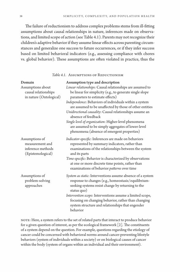
38 S I M P L I C I T Y, C O M P L E x I T Y, A N D P O P U L A T I O N H E A LT H
The failure of reductionism to address complex problems stems from ill- fitting assumptions about causal relationships in nature, inferences made on observa-tions, and limited scope of action (see Table 4.1). Parents may not recognize their children’s adaptive behavior if they assume linear effects across parenting circum-stances and generalize one success to future occurrences, or if they infer success based on limited behavioral indicators (e.g., assessing compliance with chores vs. global behavior). These assumptions are often violated in practice, thus the
Table 4.1. Assumptions of Reductionism
Domain Assumption type and descriptionAssumptions about
causal relationships in nature (Ontological)
Linear relationships: Causal relationships are assumed to be linear for simplicity (e.g., to generate single slope parameters to estimate effects)
Independence: Behaviors of individuals within a system are assumed to be unaffected by those of other entities
Unidirectional causality: Causal relationships assume an absence of feedback
Single level of organization: Higher- level phenomena are assumed to be simply aggregates of lower- level phenomena (absence of emergent properties)
Assumptions of measurement and inference methods (Epistemological)
Indicator- specific: Inferences are made on behaviors represented by summary indicators, rather than examinations of the relationships between the system and its parts
Time- specific: Behavior is characterized by observations at one or more discrete time points, rather than examinations of behavior patterns over time
Assumptions of problem- solving approaches
System as static: Interventions assume absence of a system response to changes (e.g., homeostasis/ equilibrium- seeking systems resist change by returning to the status quo)
Intervention scope: Interventions assume a limited scope, focusing on changing behavior, rather than changing system structure and relationships that engender behavior
Note: Here, a system refers to the set of related parts that interact to produce behavior for a given question of interest, as per the ecological framework [2]. The constituents of a system depend on the question. For example, questions regarding the etiology of cancer could be concerned with behavioral norms around cancer- preventing lifestyle behaviors (system of individuals within a society) or on biological causes of cancer within the body (system of organs within an individual and their environment).

Complexity: The Evolution Toward 21st-Century Science 39
challenge is to determine when and how to account for complexity. Observing limited success, a parent could attribute their child’s disobedience to fluctuations in disposition, or to permanent, learned responses to prior parenting. Either interpretation reasonably suggests different action. In this chapter, we present examples across three scientific disciplines where a complex problem ultimately proved to be insurmountable using reductionist approaches. In each example, scientists addressed complexity directly in order to better solve these problems.
1. ECONOMICS
For centuries, economists struggled to fully understand market behavior. They observed that markets generally followed large- scale trends but only under-stood the underlying processes and the role of constituent consumers and businesses in isolation [3] . Prevailing economic theories described individual behaviors predominantly as a function of personal preference and/ or extrinsic society- level factors (e.g., market demands and the effects of political climates and scientific innovations on economic productivity). For example, neoclassi-cal economists maintained free market views, theorizing that businesses selling products designed their products with characteristics that are in demand, such as durability or low price. However, this theory had trouble predicting behaviors under competitive conditions (e.g., when multiple businesses lose profits if they provide similar products [their outcomes are non- independent]). Purely free- market views disregarding non- independent decision making resulted in over- simplistic predictions [4].
Recognizing the fundamentally interactive nature of decision making, mathematicians worked separately to understand decision making in social settings more broadly. Drawing parallels from recreational games such as chess and poker, game theory posited that individuals predict how others’ actions affect their own outcomes. This game concept readily extended to economics, where businesses predict their competitors’ behaviors to maxi-mize payoffs. Game theory was first applied to economic theory in Theory of Games and Economic Behavior, in which John Von Neumann and Oskar Morgenstern expanded established utility- based decision- making theories to incorporate interdependence explicitly [5] . To illustrate, classical marginal utility theory (MUT) states that businesses choose from a set of alternatives (product designs) by assigning each alternative an expected utility (say, end- of- year profits). While MUT allows for variation in personal preferences (e.g., prioritizing sustainable materials), it ignores interaction between decision makers. Utility is derived not only from consumer and personal preferences but also from competitors’ designs and how they compete for demand. Game theory formalized this decision- making process by defining the mixed strategy

40 S I M P L I C I T Y, C O M P L E x I T Y, A N D P O P U L A T I O N H E A LT H
Nash equilibrium, the set of actions each player would choose under each pos-sible set of circumstances, assuming other players’ actions are held fixed— no business would change their design, assuming their competitors’ designs are unchanged [6]. John Nash proved that there exists at least one Nash equilib-rium in every finite game and devised a method for computing it, allowing economists to model business and consumer behaviors mathematically.
A well- known counterintuitive example is the Prisoner’s Dilemma, where two prisoners, A and B, must choose between confessing or keeping silent, and their punishment depends on the unknown choice of the other prisoner [7] . If both keep silent, both receive minor punishment, and if both con-fess, both receive moderate punishment. If A confesses and B keeps silent, A goes free while B receives severe punishment. Assuming B’s choice is fixed, A would always confess (likewise for B). Whereas the best outcome occurs when both prisoners keep silent, the Nash equilibrium predicts that both con-fess. This paradox arises partly because keeping silent requires trust in others to cooperate, and each prisoner possesses imperfect knowledge, fearing dire consequences if the other prisoner confesses. The paradox manifests in analo-gous problems across disciplines. Businesses choosing to split their consumer base by differentiating their products must trust their competitors to comply. In population health, health- service providers attempting to serve a commu-nity’s unmet health needs risk overinvestment if other providers expand ser-vices into the same area [8].
Game theory also has implications for long- term decision making. Using simulation, Robert Axelrod examined how various strategies performed over consecutive Prisoner’s Dilemma iterations, finding a “tit- for- tat” strategy was most successful. This strategy replicated an opponent’s previous actions, thereby rewarding previous cooperators and punishing previous competitors [9] . In contrast, humans exhibited forgiving tendencies, favoring cooperation even after it backfired, possibly due to ethical considerations (morally valuing col-laboration) or cognitive fallacy (presuming others must inevitably cooperate). Similarly, stock market investors often sell in direct response to sudden drops in stock values, causing collective harm when mass stock sales jeopardize the entire economy. As evinced by the mantra to avoid “market timing,” investors often mutually benefit by holding falling stocks, yet holding requires that other investors will cooperate in the long term. These insights show the complexity of economic behavior owing to the fundamentally social nature of decision making. Economies cannot be understood by assuming independence among their con-stituent consumers and businesses, since their decisions involve personal factors (e.g., moral values and risk tolerance) and their anticipation of others’ actions in the long term. These social interdependencies also exist between different spe-cies, as shown in the next example.

Complexity: The Evolution Toward 21st-Century Science 41
2. ECOLOGY
Ecologists are turning increasing attention toward human impacts on the natu-ral environment, aiming to identify negative impacts early and minimize harm. Archetypal examples include carbon emissions, forestry, and energy use, for which understanding the complex interdependency of human populations and their ecosystems is essential [10] . One application tackled the problem of over-fishing— specifically, the declining salmon harvest in the Pacific Northwest’s Tucannon River region during the mid- twentieth century [11, 12]. Fisheries recognized the need to understand salmon populations to maintain sustainable harvesting practices, yet annual trends proved unpredictable. Despite efforts to restrict overfishing, salmon populations declined 90% by the 1980s.
Ecologists hypothesized why salmon populations were unresponsive to these efforts, attributing persistent declines to overinvestment in fishing gear and local agricultural development, which permanently impacted salmon spawning habi-tats [13, 14]. Further, they observed that salmon survival was dependent on suf-ficient species diversity, which helps salmon adapt to unexpected environmental changes (e.g., climate and predators). Prior theories of marine populations assumed a stable environment (neglecting human influences on the landscape) and a homogeneous marine population that poorly represented the region’s five coexisting salmon species (underestimating the role diversity played in salmon survival). Lastly, given the four- year salmon lifespan and migration cycle, they speculated that observing annual changes in salmon populations was inadequate to detect effects.
Ecologists simulated salmon population trends over several decades in order to estimate the maximum sustainable yield (MSY), the largest annual harvesting fraction that would avoid permanent population declines [14, 15]. They applied known population growth rates, which reached a natural carrying capacity due to the limited number of feeding sites [13, 16]. They hypothesized that the MSY leveraged the salmon population’s natural resilience but was sensitive to the riv-er’s carrying capacity, species diversity, and human impacts. Further, estimating the MSY would be possible only after observing at least four years.
Simulations showed a four- year cyclical pattern and S- shaped growth over a ten- year period, as predicted by the salmon lifecycle and the river’s carrying capacity. A 95% harvesting policy showed little impact until four years out, where the population of returning adults dropped by 50% and exhibited marked drops every four years thereafter. The MSY ranged from 50% to 80% per year, account-ing for uncertainty in model parameters, which was much lower than earlier pre-dictions. The MSY was also affected by overfishing of any one species, such that species- naïve strategies caused greater long- term declines compared to diversity- maintaining strategies, even at the same harvesting fraction. Salmon populations

42 S I M P L I C I T Y, C O M P L E x I T Y, A N D P O P U L A T I O N H E A LT H
were resilient to species uniformity until sufficiently severe environmental shocks could no longer be sustained, thus the impacts remained unobserved until after several years. They also assessed the effects of agriculture and hydroelectric plant development on the salmon’s habitat, hypothesizing that heavy erosion from dry cropland, cattle grazing, and runoff from new hydroelectric plants reduces water quality, further decreasing the carrying capacity [17]. Moreover, agricultural development increased demand for these resources, prompting further develop-ment. Simulating these impacts showed sharp population declines to less than 20% within a few generations, mediated by decreases in the carrying capacity, further compounding the effect of high- harvesting fractions.
The dynamics of overfishing and development gleaned from the Tucannon salmon fishing model generalize to other ecosystems around the world [18]. Animal populations naturally exhibit dramatic decline and recovery; however, co- mingling with humans reveals interdependent, co- evolutionary relationships that are insufficiently explained by reductionist approaches that assume static eco-systems and assess species survival by numbers alone. Ecologists’ insights from complexity theory allowed fisheries to refine harvesting practices to ensure spe-cies diversity, balance human demand with the ecosystem’s natural tendencies, and acknowledge the long delay in observing effects. Analogous examples exist in population health. A health clinic providing diverse medical care and supportive services to its patient population demands an equally diverse and competent team of providers, which can be frequently overburdened due to understaffing and fre-quent turnover. While temporary staffing shortages can be absorbed by sharing responsibilities among other providers, long- term strain can be physically and emotionally taxing and reduce the team’s “carrying capacity” to provide future services. This type of worker fatigue will be explored in the next section.
3. PSYCHOLOGY
In the 1980s, burgeoning evidence in the psychology literature linked stress to poor psychological and behavioral outcomes. Work is a potentially major source of stress, but employers noted that some stressed workers suffered decaying job performance and economic productivity, while others benefited from stress as a motivator. The relationship between work stress and productivity was under-explored. Psychologists hypothesized that the negative effects of stress were mediated by worker burnout, states of severe exhaustion induced by prolonged, excessive work- related demands [19]. While variations in stress coping mecha-nisms influence the likelihood of developing burnout, it manifests when indi-viduals become overcommitted to frustrating work and perceive a differential between work goals and performance, often unfolding slowly and remaining unrecognized until too late [20, 21, 22].

Complexity: The Evolution Toward 21st-Century Science 43
Strategies to prevent or remedy worker burnout had so far proved ineffective. Employers turned to reducing worker expectations or shifting tasks (actively diminishing sources of stress), training workers to manage stress (curbing its effects), or providing rewards and relaxation time (balancing stress with relief ), yet no single strategy worked consistently [23]. Some workers also coped by engaging in addictive and damaging behaviors, such as drinking and gambling, which further undermined their physical health and exacerbated their intolerance for stress [24, 25]. Psychologists identified a need to under-stand the underlying psychological process causing burnout to uncover effec-tive solutions.
Jack Homer explored the phenomenon of worker burnout, hypothesizing that the “workaholic syndrome” itself was sufficient to produce burnout, inde-pendent of extrinsic factors [26]. In other words, one’s working conditions and individual skills may contribute to but are unnecessary to produce burnout. If so, workers could prevent burnout via managing the workaholic syndrome itself. Homer posited that when work performance equals or exceeds expectations, work-aholics raise their expectations and increase their workload to meet these new expectations. However, a high workload undermines their productivity, which is further aggravated by the inevitable frustration from failing to meet their new goals. These discrepancies finally compel the worker to decrease their expecta-tions [26]. This intuitive structure produces a dynamic cycle of stress buildup and burnout, illustrating how burnout may inevitably develop if effective stress- management strategies are not embraced.
Homer simulated the natural burnout cycle to identify leverage points for prevention. Glaringly familiar to psychologists for treating other disorders, he suggested controlling burnout by recognizing one’s workaholic syndrome and maintaining realistic work expectations [26, 27]. He found that an essential com-ponent of the burnout cycle is the dynamic setting of work expectations, where workaholics increase their workload even when performance meets expec-tations— symbolic of the archetypal workaholic attitude that is perpetually dissatisfied. Such workaholics tend to delay the recovery process (resetting real-istic work expectations) until catastrophic failure, which amplifies and prolongs burnout. Homer found that by restraining the tendency to increase expectations when meeting goals, and by setting a maximum workload even when failing to meet goals, the burnout cycle is blunted and overall productivity is improved over many burnout cycles [26]. Despite the model’s simplicity, it provided a rational intuition for the failures of common stress- reduction techniques. If an unrecognized workaholic tendency exists, measures to reduce external sources of stress or provide relief would not address the intrinsic motivations that trigger the burnout cycle. Importantly, extended burnout periods with low productivity counterbalance temporary increases in productivity during stress buildup. Thus,
44 S I M P L I C I T Y, C O M P L E x I T Y, A N D P O P U L A T I O N H E A LT H
employers should promote supportive work environments, and workers should learn to recognize harmful workaholic tendencies.
Homer’s model demonstrated the complexity of a pervasive psychological problem and its short- term and long- term solutions. In particular, Homer’s appli-cation of causal feedback synthesized existing knowledge of burnout and recov-ery and affirmed a plausible underlying structure of burnout. Although there is no single way to control burnout, examining feedback facilitated the cultivation of solutions targeting its intrinsic source, a process that can be extended more broadly [28]. Conceptually, burnout could be applied to higher units of analysis, such as a family, team, organization, community, or entire society. For example, one could ascertain the interdependent effects of burnout risk between work-ers and their team members and upper management. When collective workload, available resources, and expectations are poorly aligned, and workers face impos-sible deadlines, burnout may lead to mass employee attrition or strikes.
Aside from the health consequences of burnout on the worker, these insights can be generalized to other health problems. For example, in population vac-cination programs, inoculating sufficient proportions of a population achieves herd immunity, proffering protection to those who cannot be vaccinated (e.g., children and elderly). Yet, as shown by the resurgence of local outbreaks of vac-cine- preventable illness in the mid- 2010s, low risk perception due to prior vac-cine success, and misinformation about the dangers of vaccines, triggered many individuals to opt out. Losses in herd immunity caused thousands of preventable cases of measles, pertussis, and other illnesses worldwide [29, 30]. After these outbreaks, epidemiologists pushed efforts to expel misconceptions and expand vaccine uptake. The cyclical pattern is caused by incongruent risk perception and reality, prompting the need to understand the process driving risk percep-tion. Analogous to Homer’s burnout study, characterizing the complex feedback between vaccine success and risk perception is crucial to interrupting the cycle to reduce vaccination loss and curb outbreaks.
4. CONCLUSION
As these examples illustrate, complexity is ubiquitous and inextricable from nature— yet ignoring complexity via reductionism remains the dominant method for scientific inquiry. However, while the simplicity of reductionism is attractive, its strict simplifying assumptions are mismatched to many problems in nature whose complexity cannot be ignored. It is not surprising then that many scientific disciplines have converged upon complexity theory. Unfettered by a simplistic focus on singular causative factors, these complex approaches permit scientists to explore the dynamics of context- driven causality, which has implications for both causal inference and intervention. Scientists across

Complexity: The Evolution Toward 21st-Century Science 45
disciplines have criticized reductionism’s fixation on narrow causes, even calling for a paradigmatic revolution to address complexity [31, 32, 33, 34]. In popula-tion health, this is embodied in criticisms of randomized controlled trials as the gold standard for causal inference. These criticisms condemn the trials’ reliance on strict inclusion criteria and narrow, manipulable causes as constraints to population health science— rendering them limited to studying “downstream” causes and too “politically conservative” to effect meaningful change [35, 36].
In response, population health scientists have advanced methods to incor-porate contexts, including multilevel analysis to model influences from higher- level constructs, and simulation modeling to directly model complex systems. The latter gained popularity with the advent of increased computing capacity but has been fairly criticized for relying on data gleaned from reductionist tech-niques, thus suffering similar limitations [37]. Nonetheless, population health scientists who wish to disabuse themselves from the restrictions of reduction-ism may benefit from additional tools in their scientific toolbox that help them address complexity in complement with established reductionist approaches. These systems science approaches will be described in Part II of this book.
5. REFERENCES
1. Patton MQ. Developmental Evaluation: Applying Complexity Concepts to Enhance Innovation and Use. New York, NY: Guilford Press; 2011.
2. Bronfenbrenner U. The Ecology of Human Development: Experiments by Nature and Design. Cambridge, MA: Harvard University Press; 1979.
3. Ekelund R., Jr., Hebert R. A History of Economic Theory and Method. Sixth ed. Longgrove, IL: Waveland Press; 1975.
4. Kreps D. A Course in Microeconomic Theory. Princeton, NJ: Princeton University Press; 1990.
5. Von Neumann J, Morganstern O. Theory of Games and Economic Behavior. Princeton, NJ: Princeton University Press; 1944.
6. Nash J. Non- cooperative games. Annals of Mathematics. 1951; 54(2): 286– 295. 7. Tucker A. A Two- Person Dilemma: The Prisoner’s Dilemma. In: Rasmusen E, ed.
Readings in Games and Information. Hoboken: Wiley- Blackwell, 1950: 7– 8. 8. Westhoff W, et al. Cooperation or competition: Does game theory have rel-
evance for public health? American Journal of Health Education. 2012; 43(3): 175– 183.
9. Axelrod R. The Evolution of Cooperation. New York: Basic Books; 1984. 10. Cavana R, Ford A. Environmental and resource systems: Editors’ introduction.
System Dynamics Review. 2004; 20: 89– 98. 11. Paulik G, Greenough J. Management analysis for a salmon resource system. In: Watt
K, Editor. Systems Analysis in Ecology. New York: Academic Press; 1966. 12. Watt K. Ecology and Resource Management: A Quantitative Approach. New York:
McGraw- Hill; 1968.
46 S I M P L I C I T Y, C O M P L E x I T Y, A N D P O P U L A T I O N H E A LT H
13. Bjornn T. A model for predicting production and yield of Tucannon River salmon and steelhead stocks in relation to land management practices. In: Unit IFaWR, ed. Technical Report. Moscow, ID; 1987.
14. Ford A. The Tucannon Salmon. Modeling the Environment: An Introduction to System Dynamics Models of Environmental Systems. Washington, DC: Island Press; 1999.
15. Botkin D, Keller E. Environmental Science. New York: Wiley; 1995. 16. Ricker W. Computation and interpretation of biological statistics of fish popula-
tions. Bulletin. Ottawa, Canada: Department of Environment; 1975. 17. Harrison J. Tackling the Tucannon. Northwest Energy News. Portland, OR; 1992. 18. Clark C. Bioeconomic Modelling and Fisheries Management. New York: Wiley; 1985. 19. Freudenberger H, Richelson G. Burn- Out: The High Cost of High Achievement.
Garden City, NY: Anchor Press; 1980. 20. Alarcon G, Eschleman K, Bowling N. Relationships between personality variables
and burnout: A meta- analysis. Work & Stress. 2009; 23(3): 244– 263. 21. Routsalainen J, et al. Preventing occupational stress in healthcare workers. The
Cochrane Database of Systematic Reviews. 2006; 4: CD002892. 22. Swider B, Zimmerman R. Born to burnout: A meta- analytic path model of personal-
ity, job burnout, and work outcomes. Journal of Vocational Behavior. 2010; 76(3): 487– 506.
23. Machlowitz M. Workaholics: Living With Them, Working With Them. Reading, MA: Addison- Wesley; 1980.
24. Greenwood J, Greenwood J. Managing Executive Stress. New York, NY: Wiley; 1979. 25. Maslach C. Job burnout: How people cope. Public Welfare. 1978; 36(2): 56– 58. 26. Homer J. Worker burnout: A dynamic model with implications for prevention and
control. System Dynamics Review. 1985; 1(1): 42– 62. 27. Cameron R, Meichenbaum D. The nature of effective coping and the treatment
of stress- related problems: A cognitive- behavioral perspective. Handbook of Stress, 1982.
28. Stovya J, Anderson C. A coping- rest model of relaxation and stress management. In Goldberger L, Breznitz S, eds. Handbook of Stress: theoretical and clinical aspects. New York: The Free Press, 1982: 724– 756.
29. Abad C, Safdar N. The reemergence of measles. Current Infectious Disease Reports. 2015; 17(12): 51.
30. Gabutti G, Rota M. Pertussis: A review of disease epidemiology worldwide and in Italy. International Journal of Environmental Research and Public Health. 2012; 9(12): 4626– 4638.
31. Hassard J. Sociology and Organization Theory: Positivism, Paradigm and Postmodernity. Cambridge, UK: Cambridge University Press; 1993.
32. Kuhn T. The Structure of Scientific Revolutions. Chicago, IL: University of Chicago Press; 1962.
33. Levins R. When science fails us. Forests, Trees and People Newsletter. 1996; 72(32/ 33): 4– 13.
34. Mainzer K. Thinking in Complexity: The Computational Dynamics of Matter, Mind, and Mankind. Berlin, Germany: Springer; 1994.

Complexity: The Evolution Toward 21st-Century Science 47
35. McMichael A. Prisoners of the proximate: Loosening the constraints on epide-miology in an age of change. American Journal of Epidemiology. 1999; 149(10): 887– 897.
36. Schwartz S, et al. Is the “well- defined intervention assumption” politically conserva-tive? Social Science & Medicine. 2016;166:254–7.
37. Diez Roux A. Invited commentary: The virtual epidemiologist- promise and peril. American Journal of Epidemiology. 2014; 181(2): 100– 102.

5
Systems Thinking in Population Health
Research and Policy
ST E P H E N J. M OON EY
1. INTRODUCTION
This chapter illustrates how incorporating systems thinking into population health science helps to clarify key concepts, elaborate specific and testable hypotheses, and integrate findings from specific studies into policy decisions. We will discuss how policies designed to reduce environmental tobacco smoke have been more successful at preventing heart attacks than a naïve analysis might sug-gest, how eliminating endemic infectious disease through vaccination requires understanding the workings of social privilege, and the controversy surrounding whether liberalization of marijuana laws results in fewer traffic accidents.
2. SECOND- HAND SMOKE, SMOKING BANS, AND MYOCARDIAL INFARCTION
By the early 1980s, it was well understood that smoking tobacco causes heart disease [1] . Public health advocates became concerned that tobacco smoke exposure due to others’ smoking (sometimes called “second- hand smoke” or “environmental tobacco smoke”) might also cause heart disease [2, 3].
Epidemiologic studies showed a modestly (20%– 30%) elevated lifetime risk of myocardial infarction among those whose spouses smoked [4] . Because envi-ronmental tobacco smoke was thought to result in much less inhalation of harm-ful components of tobacco smoke than active smoking [5, 6], even this modest elevation of risk was larger than had been expected. Working from this evidence,
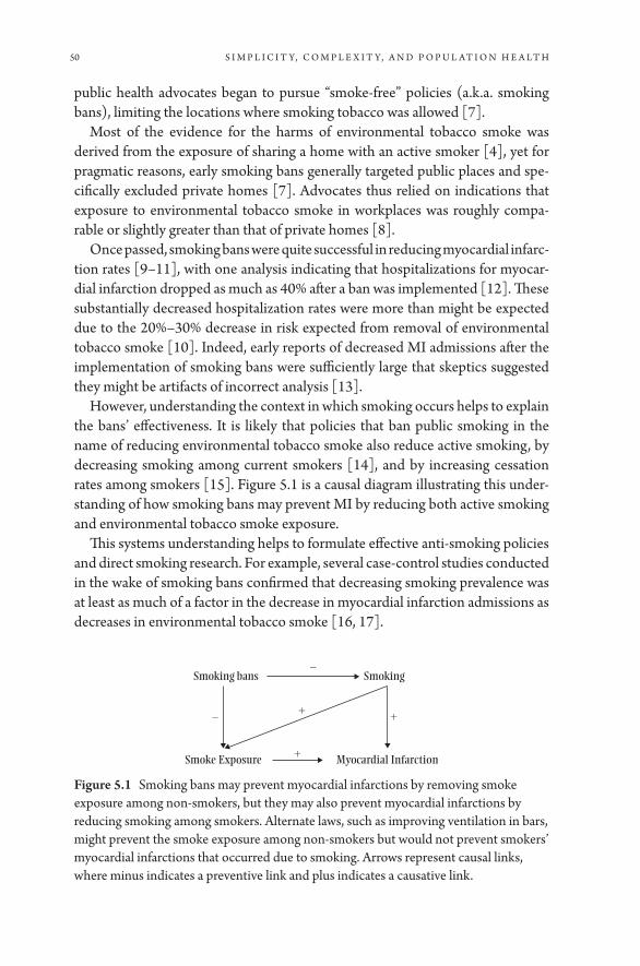
50 S I M P L I C I T Y, C O M P L E x I T Y, A N D P O P U L A T I O N H E A LT H
public health advocates began to pursue “smoke- free” policies (a.k.a. smoking bans), limiting the locations where smoking tobacco was allowed [7].
Most of the evidence for the harms of environmental tobacco smoke was derived from the exposure of sharing a home with an active smoker [4] , yet for pragmatic reasons, early smoking bans generally targeted public places and spe-cifically excluded private homes [7]. Advocates thus relied on indications that exposure to environmental tobacco smoke in workplaces was roughly compa-rable or slightly greater than that of private homes [8].
Once passed, smoking bans were quite successful in reducing myocardial infarc-tion rates [9– 11], with one analysis indicating that hospitalizations for myocar-dial infarction dropped as much as 40% after a ban was implemented [12]. These substantially decreased hospitalization rates were more than might be expected due to the 20%– 30% decrease in risk expected from removal of environmental tobacco smoke [10]. Indeed, early reports of decreased MI admissions after the implementation of smoking bans were sufficiently large that skeptics suggested they might be artifacts of incorrect analysis [13].
However, understanding the context in which smoking occurs helps to explain the bans’ effectiveness. It is likely that policies that ban public smoking in the name of reducing environmental tobacco smoke also reduce active smoking, by decreasing smoking among current smokers [14], and by increasing cessation rates among smokers [15]. Figure 5.1 is a causal diagram illustrating this under-standing of how smoking bans may prevent MI by reducing both active smoking and environmental tobacco smoke exposure.
This systems understanding helps to formulate effective anti- smoking policies and direct smoking research. For example, several case- control studies conducted in the wake of smoking bans confirmed that decreasing smoking prevalence was at least as much of a factor in the decrease in myocardial infarction admissions as decreases in environmental tobacco smoke [16, 17].
SmokingSmoking bans
Smoke Exposure Myocardial Infarction
+
+
+–
–
Figure 5.1 Smoking bans may prevent myocardial infarctions by removing smoke exposure among non- smokers, but they may also prevent myocardial infarctions by reducing smoking among smokers. Alternate laws, such as improving ventilation in bars, might prevent the smoke exposure among non- smokers but would not prevent smokers’ myocardial infarctions that occurred due to smoking. Arrows represent causal links, where minus indicates a preventive link and plus indicates a causative link.

Systems Thinking in Population Health Research and Policy 51
An analytic approach to smoking bans that failed to incorporate a systems perspective might incorrectly conflate the impact of reducing environmen-tal smoke with the impact of removing smoking, leading to an overesti-mate of the risks of environmental tobacco smoke. By contrast, the systems approach incorporates the pathways through which smoking bans function and can identify why working to improve ventilation in bars, as proposed by the tobacco industry [18, 19], would be less effective from a public health standpoint.
3. THE DECISION TO VACCINATE
Widespread vaccination is among the most successful initiatives ever to improve population health [20]. Prior to the extensive deployment of vaccination in the mid- 20th century, infectious disease caused about half of all deaths among US residents aged 5– 44, and a substantial proportion at other ages as well [21]. After childhood vaccination became normative, the burden of infectious disease fell to about 4% of disability- adjusted life years, even accounting for the late 20th- century emergence of HIV [21]. For example, measles was common enough to infect 90% of American children before they were 15 years old [22].With the introduction of the measles vaccination program in 1963, measles was eventually eliminated as an endemic disease in the United States [23, 24].
Over much of the history of infectious disease control, the primary barrier to vaccination has been access to the vaccine itself [25]. However, in recent years, vaccination rates for common childhood diseases such as measles have fallen in the United States, particularly among privileged groups who typically do not lack access to the vaccine [26]. Indeed, one high- profile outbreak in late 2014 in which measles was transmitted at the Disneyland theme park [27] was likely vastly increased in scale due to substandard vaccination rates among relatively privileged children visiting the park [28]. A systems understanding of vaccina-tion and socioeconomic privilege helps to explain this.
The reduction in disease risk conferred by any given vaccination is determined in part by the prevalence of vaccination among others. In particular, as a cam-paign successfully vaccinates more individuals, it decreases the probability that any given unvaccinated child will be exposed to and ultimately infected with the targeted disease [29].
One component of socioeconomic privilege is the capacity to leverage flex-ible resources such as money and social connections in pursuit of health [30]. Because vaccination carries risk, albeit minimal, of adverse events [31], in a con-text where measles is exceedingly rare and where clinical care can minimize harm in the event that a child does develop measles, scientifically informed parents may still feel the minimal risk outweighs the potential harms.
52 S I M P L I C I T Y, C O M P L E x I T Y, A N D P O P U L A T I O N H E A LT H
Indeed, opposing vaccination has been described as an expression of privi-lege [32]. Yet after the 2009– 2010 emergence of the H1N1 strain of influenza, during which fears about the severity of symptoms reported among the infected stoked a general increase in interest in vaccination [33], vaccine uptake was much more common among upper socioeconomic status individuals than lower [34]. Considering how disease prevalence and access to care affect risk and risk perception, and taking a systems perspective, clarifies the rationale behind the decision to vaccinate.
In the absence of a systems perspective, public health officials might simply assume anti- vaccination sentiment was driven by distrust of authorities. While qualitative studies do indicate that distrust of authorities also plays a role in the decision [35], the systems perspective helps to illustrate the difference between uptake of measles and H1N1 vaccines. These differences may be vital in con-structing messaging to maximize vaccine uptake [36].
4. MARIJUANA LIBERALIZATION AND TRAFFIC SAFETY
Starting with the 1996 passage of California’s Compassionate Use Act, several states have liberalized regulations affecting marijuana, which was already North America’s most widely used illegal drug [37]. By the end of 2014, 23 states and the District of Columbia (DC) had legalized the medical use of marijuana [38], and several had decriminalized or legalized non- medical use as well. Laboratory studies have established that intoxication with Tetrahydrocannabinol, the psy-choactive component of marijuana, leads to slowed reaction times, distracted driving, and failure to react to challenging driving situations [39]. Epidemiologic studies confirm that driving in real- world conditions while intoxicated elevates risk of crashing [40]. Finally, a large proportion of college- age students have reported driving after consuming marijuana [41, 42]. Public health and traf-fic safety officials have therefore expressed concern that liberalizing marijuana laws may increase marijuana consumption and consequent traffic injuries and fatalities [43].
Yet in practice, states that have liberalized marijuana laws have not had sub-stantial increases in traffic injuries and fatalities. Indeed, some early evidence suggests the opposite— that marijuana liberalization has led to decreased traf-fic fatalities [44]. This result may seem counterintuitive: can making it easier to access a substance that increases risk lead to decreased risk?
By considering the system in which marijuana is used, we can identify sev-eral factors that may explain this finding. First, while reported use of marijuana is higher in the states in which medical marijuana was legalized [45, 46], it remains unclear whether increases in marijuana use have followed liberaliza-tions or an atmosphere of marijuana tolerance has encouraged public support

Systems Thinking in Population Health Research and Policy 53
for liberalization. Indeed, several longitudinal analyses have suggested marijuana laws have no effect on consumption [47] or even that legal medical marijuana may prevent marijuana use among teens [48].
Second, while marijuana consumption increases crash risk when compared to not consuming marijuana [49, 50], in practice, liberalization of marijuana laws allows marijuana to substitute for other psychoactive substances that increase crash risk more than marijuana consumption does. For example, marijuana may substitute for opiates in pain management [51, 52], which may decrease crash risk because driving under the influence of opiates is even riskier than driving under the influence of marijuana [53]. Similarly, recreational marijuana use may substitute for alcohol use [44], which is associated with much greater risk of crashing at typical levels of intoxication [54].
Third, marijuana may elevate the risk of crashing while decreasing the severity of crashes, thereby preventing fatalities. Whereas alcohol users are often overcon-fident and drive at unsafe speeds, marijuana users frequently overestimate their impairment and drive more slowly [54]. Because the probability that a crash will result in a driver or pedestrian fatality increases greatly at high vehicle speeds [55, 56], decreasing the average speed of a collision should decrease fatality rates.
Fourth, while many young adults report driving under the influence of canna-bis [41], it is possible that marijuana use may prevent crashes by deterring driv-ing at a higher rate than the commensurate elevation of crash risk. Most estimates suggest that cannabis intoxication approximately doubles the risk of a crash [53]. Yet psychotropic effects of marijuana frequently include sluggishness and a feel-ing of detachment from surroundings [57]. If such effects decrease a marijuana consumer’s desire to drive such that more than twice as much driving is avoided, then the total number of crashes may drop even if any given instance of driving is riskier.
Finally, because legal changes surrounding marijuana use have taken place in political climates aware of crash risks, it may be that the changes have led to more police awareness of driving under the influence of marijuana and to public ser-vice announcements oriented at deterring driving after ingesting marijuana [43]. These policies may be responsible for increased traffic safety.
Figure 5.2 illustrates the system in which marijuana laws may affect traffic safety, highlighting points in the system described here. We caution that the impact of marijuana laws is very much an area of active research [58].
An analytic approach to marijuana and traffic safety that failed to incorporate a systems perspective might incorrectly infer from consistent lab- based studies showing marijuana consumption decreasing driver safety that liberalized mari-juana laws would necessarily elevate collision rates. Similarly, such an approach might commit the “ecologic fallacy,” inferring from the preliminary evidence showing liberalization decreasing collision rates either that the finding was a

54 S I M P L I C I T Y, C O M P L E x I T Y, A N D P O P U L A T I O N H E A LT H
priori in error due to its contradiction of lab- based evidence or, equally falsely, that marijuana improves individual driver safety.
5. SUMMARY
Population health is a product of dynamic interrelated mechanisms. Most health researchers implicitly or explicitly consider this complexity in formulating spe-cific study hypotheses. As these examples illustrate, holistic understanding of systems is a key component of identifying the optimal targets for study. Engaging with systems science principles can help investigators do the best science and identify the best interventions to protect population health.
6. REFERENCES
1. Kannel WB. Update on the role of cigarette smoking in coronary artery disease. American Heart Journal. 1981; 101(3): 319– 328.
2. Taylor AE, Johnson DC, Kazemi H. Environmental tobacco smoke and cardiovas-cular disease. A position paper from the Council on Cardiopulmonary and Critical Care, American Heart Association. Circulation. 1992; 86(2): 699– 702.
3. Kawachi I, Pearce N, Jackson R. Deaths from lung cancer and ischaemic heart dis-ease due to passive smoking in New Zealand. The New Zealand Medical Journal. 1989; 102(871): 337– 340.
4. Law MR, Morris J, Wald NJ. Environmental tobacco smoke exposure and ischaemic heart disease: An evaluation of the evidence. The BMJ. 1997; 315(7114): 973– 980.
5. Wald N, et al. Urinary cotinine as marker of breathing other people’s tobacco smoke. The Lancet. 1984; 323(8370): 230– 231.
6. Scherer G, Conze C, Tricker AR, Adlkofer F. Uptake of tobacco smoke constituents on exposure to environmental tobacco smoke (ETS). The Clinical Investigator. 1992; 70(3- 4): 352– 367.
Marijuana laws Marijuana use Driving Under theIn�uence of Cannabis
+ (?)
– (?)
Driving Under theIn�uence of Alcoholor Opiates
+
Crashing
Dying
–
+
+
+++
Figure 5.2 An illustration of the possible causal relationships linking marijuana laws to motor vehicle fatalities. Arrows represent causal links, where the number of pluses indicates the strength of the causal connection.

Systems Thinking in Population Health Research and Policy 55
7. Joossens L. Smoking policy in the workplace and other public places. Lung. 1990; 168(1): 437– 444.
8. Hammond SK. Exposure of US workers to environmental tobacco smoke. Environmental Health Perspectives. 1999. 107(Supplement 2): 329.
9. Herman PM, Walsh ME. Hospital admissions for acute myocardial infarction, angina, stroke, and asthma after implementation of Arizona’s comprehensive state-wide smoking ban. American Journal of Public Health. 2011; 101(3): 491.
10. Sargent RP, Shepard RM, Glantz SA. Reduced incidence of admissions for myocar-dial infarction associated with public smoking ban: Before and after study. The BMJ. 2004; 328(7446): 977– 980.
11. Juster HR, et al. Declines in hospital admissions for acute myocardial infarction in New York state after implementation of a comprehensive smoking ban. American Journal of Public Health. 2007; 97(11): 2035– 2039.
12. Glantz SA. Meta- analysis of the effects of smokefree laws on acute myocardial infarc-tion: An update. Preventive Medicine. 2008; 47(4): 452– 453.
13. Gasparrini A, Gorini G, Barchielli A. On the relationship between smoking bans and incidence of acute myocardial infarction. European Journal of Epidemiology. 2009; 24(10): 597– 602.
14. Fichtenberg CM, Glantz SA. Effect of smoke- free workplaces on smoking behav-iour: Systematic review. The BMJ. 2002; 325(7357): 188.
15. Fowkes FJ, et al. Scottish smoke‐free legislation and trends in smoking cessation. Addiction. 2008; 103(11): 1888– 1895.
16. Seo DC, Torabi MR. Reduced admissions for acute myocardial infarction associated with a public smoking ban: Matched controlled study. Journal of Drug Education. 2007; 37(3): 217– 226.
17. Khuder SA, et al. The impact of a smoking ban on hospital admissions for coronary heart disease. Preventive Medicine. 2007; 45(1): 3– 8.
18. Drope J, Bialous S, Glantz S. Tobacco industry efforts to present ventilation as an alternative to smoke- free environments in North America. Tobacco Control. 2004; 13(Supplement 1): i41– i47.
19. Bialous S, Glantz S. ASHRAE Standard 62: Tobacco industry’s influence over national ventilation standards. Tobacco Control. 2002; 11(4): 315– 328.
20. Centers for Disease Control and Prevention, Ten great public health achievements– United States, 1900- 1999. MMWR. Morbidity and mortality weekly report. 1999; 48(12): 241.
21. Armstrong GL, Conn LA, Pinner RW. Trends in infectious disease mortality in the United States during the 20th century. JAMA: The Journal of the American Medical Association. 1999; 281(1): 61– 66.
22. Langmuir AD. Medical importance of measles. American Journal of Diseases of Children. 1962; 103(3): 224– 226.
23. Papania MJ, et al. Elimination of endemic measles, rubella, and congenital rubella syndrome from the Western hemisphere: The US experience. JAMA Pediatrics. 2014; 168(2): 148– 155.
24. Orenstein WA, Papania MJ, Wharton ME. Measles elimination in the United States. Journal of Infectious Diseases. 2004; 189(Supplement 1): S1– S3.
25. Simons E, et al. Assessment of the 2010 global measles mortality reduction goal: Results from a model of surveillance data. The Lancet. 2012; 379(9832): 2173– 2178.
56 S I M P L I C I T Y, C O M P L E x I T Y, A N D P O P U L A T I O N H E A LT H
26. Diekema DS. Improving childhood vaccination rates. New England Journal of Medicine. 2012; 366(5): 391– 393.
27. Zipprich J, et al. Measles outbreak- California, December 2014- February 2015. MMWR (Morbidity and Mortality Weekly Report). 2015; 64: 153– 154.
28. Majumder MS, et al. Substandard vaccination compliance and the 2015 measles out-break. JAMA Pediatrics. 2015; 169(5): 494– 495.
29. Fu F, Rosenbloom DI, Wang L, Nowak MA. Imitation dynamics of vaccination behaviour on social networks. Proceedings of the Royal Society of London B: Biological Sciences. 2011; 278(1702): 42– 49.
30. Link BG, Phelan J. Social conditions as fundamental causes of disease. Journal of Health and Social Behavior. 1995: 80– 94.
31. Rosenthal S, Chen R. The reporting sensitivities of two passive surveillance sys-tems for vaccine adverse events. American Journal of Public Health. 1995; 85(12): 1706– 1709.
32. Kamadjeu R. Anti- vaxxing: A privilege of the fortunate. The Lancet Infectious Diseases. 2015; 15(7): 766– 767.
33. Centers for Disease Control and Prevention. Intent to receive influenza A (H1N1) 2009 monovalent and seasonal influenza vaccines- two counties, North Carolina, August 2009. MMWR. Morbidity and Mortality Weekly Report. 2009; 58(50): 1401.
34. Galarce EM, Minsky S, Viswanath K. Socioeconomic status, demographics, beliefs and A (H1N1) vaccine uptake in the United States. Vaccine. 2011. 29(32): 5284– 5289.
35. Mills E, Jadad AR, Ross C, Wilson K. Systematic review of qualitative studies explor-ing parental beliefs and attitudes toward childhood vaccination identifies common barriers to vaccination. Journal of Clinical Epidemiology. 2005; 58(11): 1081– 1088.
36. Nyhan B, Reifler J, Richey S, Freed G. Effective messages in vaccine promo-tion: A randomized trial. Pediatrics. 2014; 133(4): e835– e842.
37. Degenhardt L, Hall W. Extent of illicit drug use and dependence, and their contribu-tion to the global burden of disease. The Lancet. 2012; 379(9810): 55– 70.
38. Pollini RA, Romano E, Johnson M, Lacey J. The impact of marijuana decriminaliza-tion on California drivers. Drug and Alcohol Dependence. 2015; 150: 135– 140.
39. Hartman RL, Huestis MA. Cannabis effects on driving skills. Clinical Chemistry. 2013; 59(3): 478– 492.
40. Li MC, et al. Marijuana use and motor vehicle crashes. Epidemiologic Reviews. 2012; 34(1): 65– 72.
41. Whitehill JM, Rivara FP, Moreno MA. Marijuana- using drivers, alcohol- using driv-ers, and their passengers: Prevalence and risk factors among underage college stu-dents. JAMA Pediatrics. 2014; 168(7): 618– 624.
42. Asbridge M. Driving after marijuana use: The changing face of “impaired” driving. JAMA Pediatrics. 2014; 168(7): 602– 604.
43. Ghosh T, et al. The Public Health Framework of Legalized Marijuana in Colorado. American Journal of Public Health. 2015; e1– e7.
44. Anderson DM, Hansen B, Rees DI. Medical marijuana laws, traffic fatalities, and alcohol consumption. Journal of Law and Economics. 2013; 56(2): 333– 369.
45. Cerdá M, Wall M, Keyes KM, Galea S, Hasin D. Medical marijuana laws in 50 states: Investigating the relationship between state legalization of medical marijuana

Systems Thinking in Population Health Research and Policy 57
and marijuana use, abuse and dependence. Drug and Alcohol Dependence. 2012; 120(1): 22– 27.
46. Wall M, et al. Adolescent marijuana use from 2002 to 2008: Higher in states with medical marijuana laws, cause still unclear. Annals of Epidemiology. 2011; 21(9): 714– 716.
47. Lynne- Landsman SD, Livingston MD, Wagenaar AC, Effects of state medical mari-juana laws on adolescent marijuana use. American Journal of Public Health. 2013; 103(8): 1500– 1506.
48. Harper S, Strumpf EC, Kaufman JS. Do medical marijuana laws increase mari-juana use? Replication study and extension. Annals of Epidemiology. 2012; 22(3): 207– 212.
49. Ramaekers JG, Robbe H, O’Hanlon J. Marijuana, alcohol and actual driving per-formance. Human Psychopharmacology Clinical and Experimental. 2000; 15(7): 551– 558.
50. Asbridge M, Hayden JA, Cartwright JL. Acute cannabis consumption and motor vehicle collision risk: Systematic review of observational studies and meta- analysis. The BMJ. 2012; 344: e536.
51. Kim, JH, Santaella J, Cerdá M, Martins S. Medical marijuana laws and annual opioid analgesic sales in the United States. Drug and Alcohol Dependence. 2015; 156: e111.
52. Lucas P. Cannabis as an adjunct to or substitute for opiates in the treatment of chronic pain. Journal of Psychoactive Drugs. 2012; 44(2): 125– 133.
53. Elvik R. Risk of road accident associated with the use of drugs: A systematic review and meta- analysis of evidence from epidemiological studies. Accident Analysis & Prevention. 2013; 60: 254– 267.
54. Sewell RA, Poling J, Sofuoglu M. The effect of cannabis compared with alcohol on driving. American Journal on Addictions. 2009; 18(3): 185– 193.
55. Joksch HC. Velocity change and fatality risk in a crash— a rule of thumb. Accident Analysis & Prevention. 1993; 25(1): 103– 104.
56. Rosen E, Sander U. Pedestrian fatality risk as a function of car impact speed. Accident Analysis & Prevention. 2009; 41(3): 536– 542.
57. Azorlosa JL, Heishman SJ, Stitzer ML, Mahaffey JM. Marijuana smoking: Effect of varying delta 9- tetrahydrocannabinol content and number of puffs. Journal of Pharmacology and Experimental Therapeutics. 1992; 261(1): 114– 122.
58. Wilkinson ST, et al. Marijuana legalization: Impact on physicians and public health. Annual Review of Medicine. 2016; 67: 453– 466.


SECTION 2
Methods in Systems
Population Health

6
Generation of Systems Maps
Mapping Complex Systems of Population Health
H E L E N DE P I N H O
1. INTRODUCTION
Population health problems are messy.1 This “messiness” is characterized by inter-dependent factors, uncertainty as to how these factors will behave in relation to each other over time, and uncertainty as to how the problems should be resolved. Multiple and conflicting perspectives and assumptions about the problem situa-tion abound. In other words, these are complex adaptive problems.
If our thinking fails to recognize the complexity of the problem situation, then we risk being caught up in two traps: the trap of reductionism, avoiding the interconnectivity between variables; and the trap of dogmatism, working on the basis of a single unquestioning and limited perspective [1] . Such reductionist and dogmatic thinking leads to inadequate formulation of the problems; hence solutions, no matter how well designed, fail to address the right population health problems— a situation all too familiar.
To address these type three errors (the right answer to the wrong question) [2] , we need to move beyond simply “thinking about systems” (for example, health systems, political systems, financial systems, and legal and regulatory systems) and start using “systems thinking” approaches that regard systems as conceptual constructs that we select and use to inquire into, and engage with, situations of real- world complexity [3, 1]. A systems thinking approach requires that we use methods like systems diagrams to effectively organize thinking about problem situations so that action to bring about improvement can be taken [4].
1. The term “mess” in systems thinking is synonymous with Russell Ackoff [24].
62 M E T H O D S I N S Y S T E M S P O P U L A T I O N H E A LT H
Depending upon context, these actions may be to use these maps as the basis for further modeling, or to guide further data collection, discover new questions, illuminate core uncertainties, challenge the robustness of prevailing theories, and strengthen policy dialogue [5].
This chapter outlines an approach to creating these conceptual maps that facil-itates systems thinking. It begins with a discussion of stakeholder participation in the mapping process, then puts forward frameworks for problem articulation and critiquing boundary judgments, and discusses the development of a dynamic hypothesis. The final part of the chapter outlines three systems thinking tools that specifically focus on exposing the relationships amongst factors in a problem situation (a focus on the forest so that we can see the trees in context), and serves to make explicit multiple perspectives and assumptions— necessary to manage the complex realities that characterize population health problems— avoiding reductionism and dogmatism.
2. STAKEHOLDERS AND PARTICIPATION
Collaboration among stakeholders in the co- creation and use of systems maps is essential to building a community of systems thinkers able to engage with com-plex issues [6] . Population health decisions often involve tradeoffs and are char-acterized by conflicting values, and these decisions, once taken, may be difficult to implement. Effective participation by stakeholders in systems thinking pro-cesses reduces conflict, builds trust and long- term relationships, and increases the legitimacy of decisions. Not only is the quality of decisions improved, but there is also an increased likelihood that the decisions will be implemented [7].
Who the stakeholders are and who should be involved in the mapping process is context specific, but there are generally three categories of stakeholders present [3, 6]. The first category, issue owners, are people who are affected by the situation and who would be affected by the outcomes of any interventions. While they may not have the power to implement change, issue owners are vital to informing the map- building process, and we should take care not to speak on their behalf. Clients are the second group of stakeholders. They are the driving force behind the map building process and are able to effect change based on the outcome of the mapping process. Clients may be issue owners, or they may come from out-side organizations. It is important to know who they are and to understand their motivation and how they interact with the issue owners. The final category, gate-keepers, are stakeholders with the power to block or support map building and subsequent inquiry using the maps. They should be identified early in the process and brought on board, and they may also be issue owners or clients. Like all com-plex systems, stakeholder engagement should be viewed as a dynamic process, with stakeholders moving in and out of the process.
Generation of Systems Maps: Mapping Complex Systems of Population Health 63
An additional group of people engaged in the process are of course the systems practitioners, facilitators, and/ or modelers. The success of any participatory map building exercise relies on their skillful, reflective facilitation, and trust in and tol-erance for the process. Systems practitioners must make sure that there is trans-parency of information, that assumptions and uncertainties are made explicit, and that the process is iterative to accommodate new information.
3. PROBLEM ARTICULATION
In a complex situation, there are multiple and competing perspectives on the “problem” and how this problem is changing over time. Establishing a clear artic-ulation of the problem and overall purpose of the systems inquiry among stake-holders is therefore a vital step in the development of a systems map [8] .
Peter Hovmand has identified a series of questions that systems thinking prac-titioners should ask at the beginning of any system mapping process in order to refine the problem [6] . The purpose of these questions are twofold: to establish a common understanding of the problem among all stakeholders, and to decide if a systems thinking approach is appropriate to address the problem. The questions begin by first asking stakeholders about their understanding of the problem to be addressed and the overall purpose of engaging in a systems thinking process. If, after discussion, a lack of clarity remains, this may well be reason to pause or stop the map building process.
Once a problem has been identified, the next question establishes whether the problem is dynamic. Is it possible to draw a graph with the desired and feared behavior over a defined period of time? These behaviors over time graphs form reference modes and serve to focus the systems thinking process. Additional questions focus on understanding the nature of the problem and how this under-standing informs the kind of necessary systems analysis. For example, would a systems- rich picture suffice, or is the development of a simulation model needed in order to take action? Having decided upon the type of systems thinking analy-sis, the final question focuses on what would be the added value of this approach above existing tools [6] .
Working through these questions in collaboration with stakeholders serves to distill the description of the problem to be examined using a systems thinking approach and may even determine whether there is merit in proceeding with sys-tems mapping, especially if there is no clarity on the problem definition.
4. BOUNDARY CRITIQUE
Even when there is clarity regarding the problem definition and purpose of the inquiry, the elements we select as relevant for consideration of the problem
64 M E T H O D S I N S Y S T E M S P O P U L A T I O N H E A LT H
situation implicitly set boundaries [9] . These boundary judgments are inevitable. No assessment, action, description or map can fully capture a situation and align it with everyone’s perceptions [10]. What is included, excluded, and marginal-ized in the investigation of the complex problem reflects our values, mental mod-els, and worldview.
How to bound or delineate a system for the problem situation under consid-eration is a subjective decision and does not have to correspond to any real- life barriers or limits of an organization. From a critical point of view, what matters is not the comprehensiveness of our boundary judgments but rather “how care-fully we manage and reflect on the inevitable lack of comprehensiveness of our judgments” ([9] p. 15).
Critical systems heuristics (CSH) [11], provides a practical focus for assess-ing and discussing boundary judgments among stakeholders. It is a systematic framework of boundary categories, and twelve questions applied to problem situ-ations in order to unfold multiple perspectives and promote reflective practice. We can use these questions, presented in Table 6.1, to understand the assump-tions behind how boundaries are drawn and to explore the sources of values and motivation, power structures and control, knowledge, and legitimacy of the information used to determine boundaries.
Application of the CSH framework provides an opportunity to make judg-ments explicit, improve communication among stakeholders engaged in the mapping process, and promote a sense of mutual tolerance as we realize that “nobody has a monopoly for getting their facts, and values right” [11].
5. DEVELOPMENT OF DYNAMIC HYPOTHESIS
The end product of any systems thinking process when applied to a problem situ-ation is not the map or model itself but rather an accumulation of insights gained through the mapping or modeling process. These insights, made explicit, are formulated into a dynamic hypothesis. In the context of systems modeling, the process of analysis leading to a dynamic hypothesis is not meant to enumerate “unlimited details of a ‘system’ ” ([12] p. 348). Rather, the dynamic hypothesis provides a working theory of how the problem situation arose, postulating an initial explanation of the dynamics characterizing the observed system behavior in terms of the underlying causal relationships, feedback, delays, and structure of the system [13].
This explanation can be expressed verbally, but given the complexity of the interactions it is usefully communicated through systems maps such as causal loop diagrams (CLDs) and stock and flow diagrams. The dynamic hypothesis is refined, or at times abandoned, as these diagrams or maps are further explored
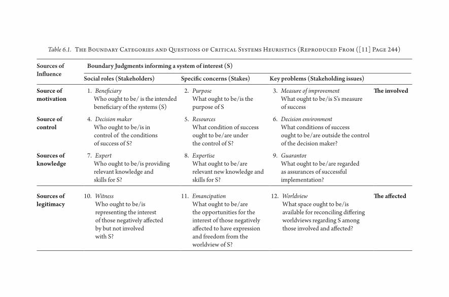
Table 6.1. The Boundary Categories and Questions of Critical Systems Heuristics (Reproduced From ([11] Page 244)
Sources of Influence
Boundary Judgments informing a system of interest (S)
Social roles (Stakeholders) Specific concerns (Stakes) Key problems (Stakeholding issues)
Source of motivation
1. BeneficiaryWho ought to be/ is the intended beneficiary of the systems (S)
2. PurposeWhat ought to be/ is the purpose of S
3. Measure of improvementWhat ought to be/ is S’s measure of success
The involved
Source of control
4. Decision makerWho ought to be/ is in control of the conditions of success of S?
5. ResourcesWhat condition of success ought to be/ are under the control of S?
6. Decision environmentWhat conditions of success ought to be/ are outside the control of the decision maker?
Sources of knowledge
7. ExpertWho ought to be/ is providing relevant knowledge and skills for S?
8. ExpertiseWhat ought to be/ are relevant new knowledge and skills for S?
9. GuarantorWhat ought to be/ are regarded as assurances of successful implementation?
Sources of legitimacy
10. WitnessWho ought to be/ is representing the interest of those negatively affected by but not involved with S?
11. EmancipationWhat ought to be/ are the opportunities for the interest of those negatively affected to have expression and freedom from the worldview of S?
12. WorldviewWhat space ought to be/ is available for reconciling differing worldviews regarding S among those involved and affected?
The affected
66 M E T H O D S I N S Y S T E M S P O P U L A T I O N H E A LT H
through the application of modeling techniques, or deeper engagement with key stakeholders in the real world.
6. GENERATION OF SYSTEMS MAPS
While much of the focus lies with the refinement of the dynamic hypotheses and subsequent models, there is limited attention paid to the actual creation of the initial systems maps. A scan of the literature focused on systems dynamic modeling and other simulation approaches provides limited insight into how the initial systems maps and dynamic models are developed, and the decisions taken regarding which elements are included in the maps. Instead, the focus lies on the refinement of the maps, models, and subsequent hypothesis once they are developed [14].
To avoid the two traps in thinking about problem situations, namely reduc-tionism and dogmatism, we need a more systematic and transparent approach to building up a dynamic hypothesis for a given situation. This approach can be divided into three phases, and while there is variation among systems practitio-ners about how these three phases are labeled, there is agreement about what each phase sets out to achieve [15, 16]. The first phase, referred to as “searching” or “creativity,” acts to sweep in multiple issues and perspectives— “to see the world through the eyes of another” [17]. During this phase there is an iterative exami-nation of the problem situation, describing structural, functional, and behav-ioral aspects of the elements in the situation. The second phase, “connectivity” or “mapping,” synthesizes the issues raised in the first phase, identifies relation-ships among these issues, and exposes existing assumptions. The third and final phase, “communication” or “telling the story,” draws upon the first two phases to integrate insights into a map that facilitates systems thinking. This three- phased approach allows us to challenge mental models, include multiple perspectives, reflect critically upon boundary judgments, and ultimately develop a dynamic hypothesis that can be tested through a modeling process.
There are a number of systems thinking tools that can be used for each of these three phases. For the purposes of this chapter, three tools are described: rich pic-tures, interrelationship diagraphs, and causal loop diagrams. Each can be used on their own but are most effective when used as a sequence toward the develop-ment of a hypothesis to explain the structure and potential dynamics driving a problem issue.
7. RICH PICTURES
Rich pictures support the first phase of developing a dynamic hypothesis. The rich picture is a drawing that reflects a concern or problem situation identified by
Generation of Systems Maps: Mapping Complex Systems of Population Health 67
key stakeholders, including the clients, gatekeepers, and issue owners. The pic-tures are ideally built through an iterative process of engagement: collaborative drawing and reflection with a group of key stakeholders. If working in a large group, it is sometimes helpful for smaller groups to develop their own rich pic-ture and then have the group come together to discuss the different rich pictures.
Rich pictures serve to “sweep- in” multiple perspectives, expose existing men-tal models, and make tacit knowledge and assumptions explicit, as stakeholders work together to develop a more complex understanding of a situation. The pic-ture should not be generic but clearly reflect contextual issues including existing resources and assets in the situation as well as problems.
The quality of the art is not important. Instead, what matters is that all ele-ments, relationships, emotions, and interactions relevant to the issue at hand are included. This is detailed in Box 6.1. Symbols and images are used instead of words to facilitate exploration of thoughts not yet verbalized. The richness of the picture is based upon the experience of all the stakeholders engaged in the draw-ing process, and enhanced by additional quantitative and qualitative data from interviews and the literature.
The rich picture is particularly useful when working with a diverse stakeholder group with various power relationships. Not only is it an effective medium through which to communicate complex relationships, but the act of drawing has a leveling effect within a group. It is often easier for stakeholders to draw an issue rather than state it out loud.
Box 6.1
What Should Be Included in a Rich Picture?
• Issues and concerns– what are the motivations and perceptions of each of the key stakeholders in this situation? What values are driving stakeholder actions?
• Structure– this refers to both formal structures like organizational structure, geographic location, physical layout, and all the people who are affected by the situation, as well as informal hierarchies and networks that exist in the system.
• Process— this refers to flows or transformations that occur within the struc-tures over time— such as flows of goods, information, resources, and com-munication patterns. It is also useful to include “behavior over time” graphs as tools to illustrate trends over time.
• Outcomes— include some of the outcomes of the system, both those that are intended and unintended. [18]

Box 6.2
Using Rich Pictures
A team looking to improve the availability of human resource for health data in a country developed the Rich Picture depicted in Figure 6.1. The group con-sisted of participants from the Ministry of Health as well as collaborating donor partners. It was only when they began drawing the flow of information from the ground up and from the Ministry of Health down that they realized that the two “routes” were quite separate from each other— accounting for the lack of coordi-nation and poor quality of data. This was then used as the basis for developing a proposal to strengthen the overall system.
Figure 6.1 Rich Picture exploring a concern about the availability of human resources for health data.
Generation of Systems Maps: Mapping Complex Systems of Population Health 69
While it is possible to use rich pictures as a standalone tool when working with a diverse group of stakeholders with widely different perspectives, they also pro-vide a useful starting point to surface the different factors influencing a problem situation and to use these in the next phase of systems map development. Box 6.2 provides an example of using rich pictures.
8. INTERRELATIONSHIP DIGRAPH
The interrelationship digraph (IRD) is a visual tool that builds on the rich picture and is used to explore all possible interactions among the key variables in a situ-ation. In the three- stage process of developing a dynamic hypothesis described earlier, the IRD supports the second stage, as it examines the relationships and connectivity among factors in the problem situation. The process of creating the IRD challenges existing mental models about the relationships among the variables and prevents coming to a quick conclusion about the structure of the system driving a particular problem situation. In the absence of hard data, it is a useful tool to explore complex relationships and surface key drivers and out-comes in a situation. The process of creating an IRD is summarized in Box 6.3.
IRDs can be used as a systems tool without going on to develop a causal loop diagram. When used as part of a group exercise, IRDs encourage team members to think in multiple directions rather than linearly and systematically explore the cause and effect relationships among all the key variables. This process will often surface basic assumptions and reasons for disagreements among team members, allowing key issues to emerge naturally rather than be forced by a dominant or powerful team member. Box 6.4 provides an example of using an IRD to explore a complex problem. The IRD also provides a useful starting point to begin the construction of the causal loop diagram.
9. CAUSAL LOOP DIAGRAMS
The third systems mapping tool is the causal loop diagram. Like the IRD, the CLD also aids in synthesizing issues and identifying the relationships among these issues and is then used by stakeholders and systems practitioners to communicate the hypothesized understanding of the system’s structure driving the problem.
Transforming an IRD into a CLD is an iterative and collaborative process. Rather than rely on their mental models of what they think is happening in a system, the model developer(s)/ systems practitioners work with stakeholders and use the IRD (and rich pictures) to surface the CLD. This process is summarized in Box 6.5.
Although there is no such thing as a “final” CLD, the completed map should tell a clear story about the structure of the problem situation without being overly complex (and not too simple!). The CLD is considered “done” when it

70 M E T H O D S I N S Y S T E M S P O P U L A T I O N H E A LT H
reflects the problem situation as perceived by those affected by the situation, the issue owners, and those wanting to improve the situation— the clients [20]. It is also considered “done” when the CLD reflects a potentially plausible explanation (prior to systems dynamics modeling) for the reference modes identified during problem articulation and included in the rich pictures. Box 6.6. summarizes the process of identifying the feedback loops in a CLD.
Box 6.3
How to Develop an Interrelationship Digraph
Before beginning an IRD, make sure that all involved in the process understand and agree on the problem statement (which would be the same statement that informed the rich picture). This done, step one is to identify ten to twelve key variables from the rich picture. These variables represent elements in the situa-tion that may act or be acted upon, where their value can vary up or down over time, and should be measurable, at least in theory. They should be neutrally defined, distinguish between perceived and actual states, and should include the desired outcome(s) of interest. When working with a group of stakeholders, it is useful to develop a reference list of variable definitions capturing the key con-struct depicted by the variable name.
Arrange the selected variables in a circle, pick one of the variables to begin, and consider the relationship between this variable and each of the other variables in the circle. For each pair of variables, decide if there is an “influence” between the two variables and where there is a direct relationship, and use an “influence” arrow to connect the two related variables. The arrows should be drawn from the variable that influences to the one that is influenced. If two elements influence each other, the arrow should be drawn to reflect the stronger influence in the given context. Arrows can only be drawn in one direction.
Move on to the next variable in the circle and consider where there is a rela-tionship between that variable and all others in the circle. Consider the relation-ships in pairs— a relationship need not exists between all variables. Continue until you have explored potential relationships amongst all variables.
The relationship should be a direct relationship and not via another vari-able. Where possible, base decisions on existing evidence, or consensus among experts. Always be aware of assumptions.
Once all possible relationships have been examined, the main drivers and out-come variables are determined by simply counting the number of arrows coming into and going out of a variable. Variables with more arrows coming in than going out are outcomes; those with more arrows going out are drivers.
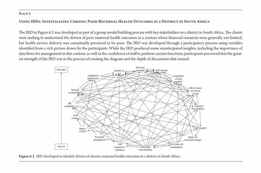
Box 6.4
Using IRDs: Investigating Chronic Poor Maternal Health Outcomes in a District in South Africa
The IRD in Figure 6.2 was developed as part of a group model building process with key stakeholders in a district in South Africa. The clients were seeking to understand the drivers of poor maternal health outcomes in a context where financial resources were generally not limited, but health service delivery was consistently perceived to be poor. The IRD was developed through a participatory process using variables identified from a rich picture drawn by the participants. While the IRD produced some unanticipated insights, including the importance of data flows for management in this context, as well as the confidence of staff to perform certain functions, participants perceived that the great-est strength of the IRD was in the process of creating the diagram and the depth of discussions that ensued.
Quality ofcare
Maternalmortality Staff attitude
Availabilityof drug
supplies
Effectivenessof referral
system
Transportavailability
Staff support
Impact ofstructural changes
Use of data formanagementLeadership/
team building
Staffcompetence/con�dence
Personnelmanagement
Impactof NGO
Stafftraining
HRavailability
Equipment/maintenance
Outcomes
Drivers
Internalaccountability
Figure 6.2 IRD developed to identify drivers of chronic maternal health outcomes in a district in South Africa.
Box 6.5
How to Develop a Causal Loop Diagram
The development and level of detail of the CLD should be informed by the following [19]:
• the problem statement or issue driving the creation of the CLD; • boundary decisions including whose voices and issues are included or
excluded; and • an assessment of the stakeholders, issue owners, clients and gatekeepers,
and their sphere of influence to affect change in the system.
A useful starting point for building a CLD is to surface a seed model from a related IRD. At least one key outcome of interest and driver of that outcome, and one or two variables that link the driver to the outcome, are identified from the IRD and transferred to a new sheet to begin the CLD.1 The variables selected for the seed model should fall within the appropriate sphere of influence. For example, if the map is being built to effect change at a facility level, then beginning with a distal variable such as “socio- economic class” is not useful, as this is beyond the immediate sphere of influence. This is not to say that the distal variables cannot be included in the final CLD. The seed model is simply a useful starting place to begin surfacing the CLD.
Working between the IRD and seed model, start adding in the variables that are linked to the outcome and driver(s) in the seed model to build up the CLD. Through this process, smaller loops in the IRD may become redundant with respect to larger, more encompassing loops. It may also be necessary to add new links, including some that feedback between variables (not permitted during the creation of the IRD), as well as new variables to better explain the relationship between existing variables. It is not necessary to incorporate all possible variables in the CLD. In some cases there are external elements that do not change or change very slowly, or whose changes are irrelevant to the problem situation. Including these can unnecessarily complicate the map, particularly if there is no or little con-trol over these variables [20]. Where appropriate, identify any links that have sig-nificant delays relative to the rest of the map. It is important to identify these delays, as they are often the source of imbalances that accumulate in the system.
There are some conventions to be followed when building a CLD [8] . Do not duplicate variable names, and avoid putting circles, boxes, or hexagons around the variables. Use curved lines to better reflect feedback loops, and as far as possible avoid crossed lines, although this is not always possible. The goal is to produce a map that effectively represents the structure and relationships among key factors giving rise to the outcome(s) of interest. The decision to include additional variables and causal links should be based on information received from stakeholder interviews and
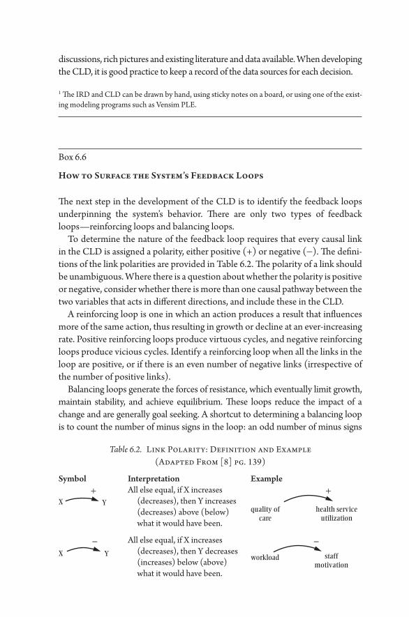
discussions, rich pictures and existing literature and data available. When developing the CLD, it is good practice to keep a record of the data sources for each decision.
1 The IRD and CLD can be drawn by hand, using sticky notes on a board, or using one of the exist-ing modeling programs such as Vensim PLE.
Box 6.6
How to Surface the System’s Feedback Loops
The next step in the development of the CLD is to identify the feedback loops underpinning the system’s behavior. There are only two types of feedback loops— reinforcing loops and balancing loops.
To determine the nature of the feedback loop requires that every causal link in the CLD is assigned a polarity, either positive (+) or negative (− ). The defini-tions of the link polarities are provided in Table 6.2. The polarity of a link should be unambiguous. Where there is a question about whether the polarity is positive or negative, consider whether there is more than one causal pathway between the two variables that acts in different directions, and include these in the CLD.
A reinforcing loop is one in which an action produces a result that influences more of the same action, thus resulting in growth or decline at an ever- increasing rate. Positive reinforcing loops produce virtuous cycles, and negative reinforcing loops produce vicious cycles. Identify a reinforcing loop when all the links in the loop are positive, or if there is an even number of negative links (irrespective of the number of positive links).
Balancing loops generate the forces of resistance, which eventually limit growth, maintain stability, and achieve equilibrium. These loops reduce the impact of a change and are generally goal seeking. A shortcut to determining a balancing loop is to count the number of minus signs in the loop: an odd number of minus signs
Table 6.2. Link Polarity: Definition and Example (Adapted From [8] pg. 139)
Symbol Interpretation Example
X Y
+ All else equal, if x increases (decreases), then Y increases (decreases) above (below) what it would have been.
quality ofcare
health serviceutilization
+
X Y
– All else equal, if x increases (decreases), then Y decreases (increases) below (above) what it would have been.
workload staffmotivation
–
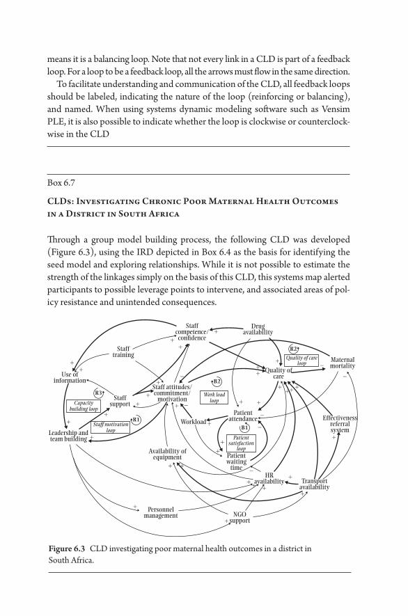
Box 6.7
CLDs: Investigating Chronic Poor Maternal Health Outcomes in a District in South Africa
Through a group model building process, the following CLD was developed (Figure 6.3), using the IRD depicted in Box 6.4 as the basis for identifying the seed model and exploring relationships. While it is not possible to estimate the strength of the linkages simply on the basis of this CLD, this systems map alerted participants to possible leverage points to intervene, and associated areas of pol-icy resistance and unintended consequences.
means it is a balancing loop. Note that not every link in a CLD is part of a feedback loop. For a loop to be a feedback loop, all the arrows must flow in the same direction.
To facilitate understanding and communication of the CLD, all feedback loops should be labeled, indicating the nature of the loop (reinforcing or balancing), and named. When using systems dynamic modeling software such as Vensim PLE, it is also possible to indicate whether the loop is clockwise or counterclock-wise in the CLD
Staffcompetence/
con�dence
Stafftraining
Use ofinformation
Staffsupport
Leadership andteam building
Staff attitudes/commitment/
motivation
Drugavailability
Maternalmortality
Quality of careloop
Work loadloopCapacity
building loop
Staff motivationloop
Patientsatisfaction
loop
Quality ofcare
Effectivenessreferralsystem
Transportavailability
HRavailability
Patientwaiting
time
PatientattendanceWorkload
Availability ofequipment
+ +
+
+
+ +
+ +
+++ +
++
++
+
+
+
+
+
+
++ +
R2
B2
B1
R1
R3
+
+
+
+
+
–
–
–
–
–
–
–
++
+
+
NGOsupport
Personnelmanagement
Figure 6.3 CLD investigating poor maternal health outcomes in a district in South Africa.

Generation of Systems Maps: Mapping Complex Systems of Population Health 75
An examination of the complex systems structure and intersection of feedback loops and relationships among the variables in a CLD can reveal points of poten-tial policy resistance, particularly in the presence of balancing feedback loops; identify possible leverage points where micro changes in the system could result in macro results; alert stakeholders to potential unintended consequences fol-lowing an intervention; and through this elaboration of the problem situation, inform the formulation of appropriate research questions [5] .
In recent years, a plethora of articles has appeared that utilize systems map-ping and CLDs qualitatively, in addition to parameterizing the maps to develop systems dynamics models [14]. This has given rise to concerns that a failure to understand that a CLD does not provide an indication of the strength of the relationships between variables, nor any accumulations, could result in inap-propriate application of CLDs to complex population health issues [21, 22]. For this reason, close attention must be paid to the process of systems mapping, including stakeholder engagement, approach to boundary decisions, the source of the data used to construct the CLD, and the interpretation of causality based on the CLD.
10. CONCLUSION
Systems mapping, through rich pictures, IRDs, or CLDs should not be regarded as the endpoint of the systems thinking process but rather the starting point for ongoing conversations, as well as systems dynamic modeling to facilitate policy experimentation not possible in the field. Each of these tools serves to make explicit and communicate an understanding of the structure of the com-plex web of factors driving a particular problem— in other words, the dynamic hypothesis.
Ultimately, if we are to avoid the traps of dogmatism and reductionism as we navigate a path through messy, complex population health issues, then we need both to expand and refine our practice of systems thinking. This will allow us to consistently challenge assumptions, test our understanding of the nature of these problems [23] and ultimately strengthen the models that we use to make sound population health decisions.
11. REFERENCES
1. Reynolds M, Holwell S. Systems Approaches to Managing Change: A Practical Guide. London, Springer; 2010.
2. Schwartz S, Carpenter KM. The right answer for the wrong question: Consequences of type III error for public health research. American Journal of Public Health. 1999; 89(8): 1175– 1180.

76 M E T H O D S I N S Y S T E M S P O P U L A T I O N H E A LT H
3. Checkland P. Soft systems methodology: A thirty year retrospective. Systems Research and Behavioural Science. 2000; 17: S11– S58.
4. Checkland P, Poulter J. Learning for Action: A Short Definitive Account of Soft Systems Methodology and its use for Practitioners: Wiley; 2006.
5. Epstein JM. Why model? Journal of Artificial Societies and Social Simulation. 2008; 11(4), http:// jasss.soc.surrey.ac.uk/ 11/ 4/ 12.html.
6. Hovmand P. Community Based System Dynamics: Springer; 2014. 7. Stave K. Participatory system dynamics modeling for sustainable environmental
management: Observations from Four Cases. Sustainability. 2010; 2(9): 2762. 8. Sterman J. Business Dynamics: Systems Thinking and Modeling for a Complex World:
The McGraw- Hill Companies, Inc; 2000. 9. Ulrich W. The quest for competence in systemic research and practice. Systems
Research and Behavioural Science. 2001; 18: 3– 28. 10. Reynolds M. Getting a grip: A critical systems framework for corporate responsibil-
ity. Systems Research and Behavioural Science. 2008; 25(3): 383– 395. 11. Ulrich W, Reynolds M. Critical Systems Heuristics. In Reynolds M, Holwell S,
Editors. Systems Approaches to Managing Change: A Practical Guide (243– 292). London: Springer; 2010.
12. Homer J, Oliva R. Maps and models in system dynamics: A response to Coyle. System Dynamics Review. 2001; 17(4): 347– 355.
13. Sterman J. Business Dynamics: Systems Thinking and Modeling for a Complex World: The McGraw- Hill Companies, Inc; 2000.
14. Carey G, et al. Systems science and systems thinking for public health: A systematic review of the field. BMJ Open e009002. 2015.
15. Gharajedaghi J. Systems Thinking Managing Chaos and Complexity: A Platform for Designing Business Architecture (Third ed.). Boston: Morgan Kaufmann; 2012.
16. Hudson J. Using diagrams in systems thinking. 1998. http:// johnrhudson.me.uk/ systems/ Using_ diagrams_ in_ systems_ thinking.pdf
17. Churchman CW. The Systems Approach: Delacorte Press; 1968. 18. Lane A, et al. Systems diagramming O. University. www.open.edu/ openlearn 19. Kim D. Guidelines For Drawing Causal Loop Diagrams. The Systems Thinker. 1992;
3(1): 5– 6. 20. Goodman M. Systems thinking: What, why, when, where, and how? The Systems
Thinker. 1997; 8(2). 21. Lane DC. The emergence and use of diagramming in system dynamics: A critical
account. Systems Research and Behavioral Science. 2008; 23: 3– 23. 22. Schaffernicht M. Causal loop diagrams between structure and behaviour: A critical
analysis of the relationship between polarity, behaviour and events. Systems Research and Behavioral Science. 2010; 27: 653– 666.
23. Peters DH. The application of systems thinking in health: Why use systems think-ing? Health Research Policy and Systems. 2014; 12: 51.
24. Ackoff RL. Re- creating the corporation: A design of organization for the 21st century. New York: Oxford University Press; 1999.
7
Systems Dynamics Models
E R IC L O F G R E N
1. INTRODUCTION
Systems dynamics models are representations of the real world made by dividing the population up into categories, with accompanying mathematical representa-tions of how these categories interact with each other and how members of one category move to another. These models have a long history of use in epidemiol-ogy, appearing in rudimentary form in work by Bernoulli, before Ross, Kermack, and McKendrick refined them in the early 20th century [1, 2]. By virtue of their age and mathematical tractability, these models became the foundational tool of public health modeling and continue to be one of the main tools in the modeling of human health. Many other types of models, such as agent- based or network models, stem from trying to address the assumptions behind systems dynamics models, which are discussed below.
In this chapter, we first consider how to construct a systems dynamics model and how to solve these models computationally. Then we explore some of the key insights that come from these models and how these models can be com-bined with observational data. Finally, we explore a more complex example of a systems dynamics model, discuss some of the assumptions inherent to this model type, and touch on some basic extensions that aim to address these assumptions.
2. MODEL COMPOSITION AND THE SIR MODEL
The key to understanding a systems dynamics model lies in the equations that govern it. As such, understanding how these models are composed is an essential first step. The examples used in this chapter focus on infectious processes because

78 M E T H O D S I N S Y S T E M S P O P U L A T I O N H E A LT H
these models were initially intended to study infectious diseases, but they are by no means exclusively useful for infectious diseases. Systems dynamics models can be used for anything from chronic disease progression to estimating patient recruitment and retention in treatment programs.
Often called “compartmental models,” these models are made of a series of compartments that represent distinct subpopulations. These can include health states, demographic characteristics, or other categories. Equations describe the flow between these compartments, including which transitions are allowed and at what rate. Graphically, this is represented as a flow diagram (Figure 7.1).
This model, known as the SIR model, is the most commonly used model in public health. Additional compartments and interactions between them can be added to give these models almost infinite variety. These schematics are help-ful for providing a quick overview of the model, but just as the model itself is a simplified representation of reality, the flow diagram is a simplified version of the model. It does not say how one transitions from one compartment to another. In order to answer this, we need a precise way to describe the model: mathematical equations.
Differential equations are used for most of these models. Each is made up of variables, represented as italicized capital letters, and parameters, represented by lowercase Greek letters. Variables are the compartments (such as S) whose value will change. Parameters are constants used to connect these variables together— for example, the rate of movement from I to R. Working from the graphical rep-resentation of a model, each compartment needs one variable, and each arrow needs at least one parameter.
An equation is created for each variable. The left side of the equation, for the variable I, is written as dI dt/ , or “the derivative of I with respect to t.” This is the change seen in I with an infinitesimally small change in time, t. The right side of the equation describes this rate as a combination of parameters and variables. For example, if a proportion of individuals γ leave I per unit time, this would be expressed as –γ I, for a full equation dI dt I= −γ .
S I R
Figure 7.1 The population is divided up into three compartments: those susteptible to infection (S), those infected (I), and those who have recovered or died from the infection (R).

Systems Dynamics Models 79
The model begins to take shape when we link the equations together. For example, γ people leave I per unit time (subtracting γI people) and go to R (add-ing γI people). We now have the basis for two equations:
dIdt
I
dRdt
I
= −
=
γ
γ
The people leaving I are now accounted for in the equation for R.Rather than occurring at a fixed rate, the transition from S to I is governed by
the number of people currently in I. This makes intuitive sense for an infectious disease— with more people to transmit the infection, it is more likely that a suscep-tible person will come into contact with them. Risk of disease being a function of the current prevalence of disease is known as “dependent happenings.” Modeling these dependent happenings is the primary use of systems dynamics models.
We use a contact rate, β, which takes into account the number of contacts an individual encounters per unit time, as well as the probability of contact between a susceptible and infectious individual resulting in the transmission of disease [3] . The full equations for the SIR model are:
dSdt
SIN
Idt
SIN
I
dRdt
I
= −
= −
=
β
β γ
γ
d
Where the total number, N = S + I + R. The I N term is often simplified to I
when dealing with proportions of the population (N = 1), rather than a number
of individuals. For convenience, we use this formulation. Everyone is accounted for in the model and all the arrows in the flow diagram are represented in the equations— we have a fully formed model. But what do we do with it?
These models support a broad range of mathematical analysis, from determin-ing the impact of parameter values on system dynamics to analytical proofs. For further information on these methods, readers are referred to more specialized texts [3, 4]. We focus on one particular type of analysis useful in public health research, known as numerical integration, which focuses on a set of parameters specific to a disease and setting. The behavior of the system is approximated by solving for the values of the variables over very small increments of time. Libraries
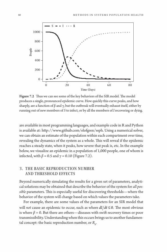
80 M E T H O D S I N S Y S T E M S P O P U L A T I O N H E A LT H
are available in most programming languages, and example code in R and Python is available at: http:// www.github.com/ elofgren/ ssph. Using a numerical solver, we can obtain an estimate of the population within each compartment over time, revealing the dynamics of the system as a whole. This will reveal if the epidemic reaches a steady state, when it peaks, how severe that peak is, etc. In the example below, we visualize an epidemic in a population of 1,000 people, one of whom is infected, with β = 0.5 and γ = 0.10 (Figure 7.2).
3. THE BASIC REPRODUCTION NUMBER AND THRESHOLD EFFECTS
Beyond numerically simulating the results for a given set of parameters, analyti-cal solutions may be obtained that describe the behavior of the system for all pos-sible parameters. This is especially useful for discovering thresholds— where the behavior of the system will change based on which values the parameters take.
For example, there are some values of the parameters for an SIR model that will not cause an epidemic to occur, such as where dI dt ≤ 0. The most obvious is where β = 0. But there are others— diseases with swift recovery times or poor transmissibility. Understanding when this occurs brings us to another fundamen-tal concept: the basic reproduction number, or R0.
0 20 40 60 80
0
200
400
600
800
1000
Time (Days)
Peop
le
S I R
Figure 7.2 Thus we can see some of the key behaviors of the SIR model. The model produces a single, pronounced epidemic curve. How quickly this curve peaks, and how sharply, are a function of β and γ, but the outbreak will eventually exhaust itself, either by running out of new members of S to infect, or by all the members of I recovering or dying.

Systems Dynamics Models 81
R0 is defined as the average number of cases caused by a single infective indi-vidual in an entirely susceptible population. R0 varies by both disease and setting, from 14- 18 in the case of Measles, 3.5– 6 for Smallpox, and 1.5– 2.5 for the West African Ebola outbreak [6, 7, 8]. This number needs to be above one for an epi-demic to occur— any lower and an infective person will not replace themselves before recovering or dying of the disease.
The methods to calculate R0 are myriad and will vary with each model [5] . For the SIR model R0 = β γ . Additionally, other thresholds are related to R0, such as the proportion of the population that must be vaccinated or immune in order for herd immunity to work, given as 1 1 0−( ).R
R0 is not without limitations. The foremost is the assumption of a fully suscep-tible population. For emerging pathogens, this may be justifiable, but for more established pathogens, it is problematic. This has lead to alternatives, such as the effective reproduction number, RE, which is the average number of cases caused by an infective individual in the current population, or Rt, a measurement that varies with time over the course of the outbreak. Similarly, while R0 is frequently viewed as an inherent property of a disease, this isn’t the case. An estimate of R0 is not necessarily portable between settings.
4. FITTING MODELS TO DATA
In an ideal world, the parameters needed for a model would be available in the literature, but this is rarely the case. In these circumstances, you must fit the model to data, statistically estimating the likely value of one or more parameters, in order to obtain a numerical solution. As with regression in observational epi-demiology, there are a number of ways to fit models to data— from least squares to maximum likelihood and Markov Chain Monte Carlo (MCMC). The means to do so are available in most programming languages, though the details are beyond the scope of this chapter. Instead, this section will focus on some of the limitations and caveats behind model fitting.
The first, and most important, is the recognition of what a model fitting the data does— and does not— mean. Formulating a model and fitting it to a time series is often referred to as “validating” a model, which implies that it is “right.” This is incorrect. The capability to fit a model to data only implies that that model can describe the observed data, not that it is the best or only description.
Second, the desirability of parsimony is less clear than it is for statistical mod-els. There is no general agreement as to the desired level of complexity for a sys-tems dynamics model. Simple models lend themselves to mathematical analysis

82 M E T H O D S I N S Y S T E M S P O P U L A T I O N H E A LT H
but may fail to represent the complexities of the real world. Complex models may be difficult to find parameter values for (and are often difficult to interpret) with combinations of parameters influencing the outcome of the model. Finding the balance between the two is one of the challenges of successfully modeling a disease system.
The availability of data places an additional constraint on complexity. Especially with emerging diseases, there is often scarce data, with few studies available to provide parameter estimates. In this circumstance, several vari-ables must be estimated from the same data, and the model may become non- identifiable, meaning two or more possible sets of parameter values are equally likely, and estimating the true value of a parameter is impossible. This means that the model can give several (or many) different answers, all of which are equally supported by the available data. As with the balance between complexity and simplicity, it is challenging to balance the desire to model a system fully with the availability of data.
5. EXPANDING THE SIR MODEL: PERTUSSIS AND WANING IMMUNITY
To explore some of the concepts and problems outlined above, we turn to a pre-viously published example. It is easy to build off the framework of the SIR model, adding new compartments and interactions to better represent a specific disease. In this case, we examine the impact of waning and naturally boosted immunity on the dynamics of pertussis [9] . The model is shown in Figure 7.3.
The model also includes a number of new interactions. Vaccination is modeled as the movement of people directly from S to R, and while R retains the same immunity to new infections as it did in the ordinary SIR model, individuals can now move out of R to a new class W, representing those whose immunity has begin to wane. Coming in contact with an infectious individual may challenge the immune systems of these individuals. Rather than developing an infection and moving to I, they move back to R as their immune system responds. In time, if not challenged, they move back to S. This model also incorporates births and
S I R W
Figure 7.3 This schematic is a simplification of the model described in Lavine, King, and Bjørnstad, 2011, as there are S, I, R and W compartments for many age groups. Adding an age structure is a common extension of the SIR model, although it requires parameters for every age group.

Systems Dynamics Models 83
deaths. Births replenish the population of S, allowing for multiple outbreaks (not shown). The full equations and parameters describing the model can be found in the referenced paper.
This model shows the flexibility and power that can be obtained with straight-forward modifications of the SIR model. It captures the immune dynamics of per-tussis, including the post- vaccine era shift in the incidence of pertussis towards teens, the reemergence of the disease even when the proportion of vaccinated
individuals was above the 1 1 0−( )R threshold, and impermanent immunity, a
shift from the type of dynamics one would expect in a SIR model sometimes called a “SIRS” model.
6. SYSTEMS DYNAMICS MODELS: ASSUMPTIONS AND EXTENSIONS
These models rely on two major assumptions: random mixing and large popula-tions. The basic systems dynamics model assumes the entire population mixes at random. This is not the case— people assort non- randomly by demographics, social relationships, and geographic proximity. This assumption is often accept-able in large- scale models and can be addressed by creating different compart-ments for different groups of people, where the assumption that people mixing randomly within their group is more tenable. However, this modification requires parameters on how each group interacts. For some characteristics, such as age, well- conducted studies provide this information [10]. For others, the evidence will be far less strong.
It may be necessary to model different contact patterns entirely. For exam-ple, changing the transmission term from βS I N( ) to simply βSI in a model with individuals changes the transmission from frequency dependent to density dependent— that is, it allows the contact rate to increase with population density, allowing progressively more contacts in larger populations. More complicated expressions exist to model more sophisticated forms of mixing [11].
The second assumption behind these models is that they are taking place in a large population, where the role of random chance is ignored. These models are known as deterministic models. Consider, for example, a disease with an R0 of 2.0. In the models we have been discussing, this disease will invariably cause an epidemic. However, in the real world, the very first case may not cause two new cases. They may cause no new cases, or dozens. In small populations, these dif-ferences can matter quite a bit— the difference between no new cases and dozens could have profound implications for the fortunes of a village. In a large popula-tion (generally populations in the thousands), it may be safe to ignore this when studying the behavior of a system, but even larger populations are vulnerable to

84 M E T H O D S I N S Y S T E M S P O P U L A T I O N H E A LT H
randomness [12]. Models that take this randomness into account are called sto-chastic models.
A variety of tools are available when working with stochastic models. Similar to the numerical solutions obtained earlier in this chapter, a technique known as Gillespie’s Direct Method can be used to simulate the model’s dynamics [14]. This algorithm calculates the next time an event will take place, advances the sim-ulation to that time step, randomly draws which event occurs (weighted by the frequency by which they occur) and moves a single individual from one com-partment to another, before repeating the procedure. This method both takes into account random chance and allows only integer- numbers of individuals in compartments, useful for small models where deterministic models may result in fractions of people in a compartment, which is uninterpretable, at the cost of being considerably more computationally intensive.
Use of various techniques to mitigate aspects of the SIR model can add sub-stantial complexity to the underlying system, but the core principles still apply. For example, the model found in Lofgren et al., 2014, is both stochastic and has a more complex mixing pattern. In this model of Clostridium difficile in a 12- patient intensive care unit, patients do not mix with one another [13]. Instead, their contact is indirect, through shared contact with healthcare workers. This type of indirect transmission is commonly used to model vector- borne diseases. While departing from a familiar form, and attempting to mitigate some of the assump-tions of a deterministic SIR model, this model is still clearly a systems dynamics model, governed by equations that describe population compartments and the parameters that govern transitions between them.
Systems dynamics models combine flexibility, computational approach-ability, and an amenability to more advanced analytical techniques. While admittedly limited in the way they can represent the complexity of human interactions, they have proven remarkably powerful at providing insight into the dynamics of both infectious and non- infectious diseases. Understanding how these models work is a good first step in exploring modeling in public health.
7. REFERENCES
1. Kermack W, McKendrick A. A Contribution to the Mathematical Theory of Epidemics. Proceedings of the Royal Society of London, Series A. 1927; 115(772): 700– 721.
2. Smith DL, et al. Ross, Macdonald, and a Theory for the Dynamics and Control of Mosquito- Transmitted Pathogens. 2012; 8.
3. Keeling M, Rohani P. Modeling Infectious Diseases in Humans and Animals. Princeton: Princeton University Press; 2008.

Systems Dynamics Models 85
4. Castillo- Chavez C, Brauer F. Mathematical Models in Population Biology and Epidemiology. Marsden JE, Sirovich L, Golubitsky M, Editors. New York: Springer; 2001.
5. Heffernan JM, Smith RJ, Wahl LM. Perspectives on the basic reproductive ratio. Journal of The Royal Society Interface. 2005; 2(4): 281– 293.
6. Orenstein WA, Gay NJ. The theory of measles elimination: Implications for the design of elimination strategies. The Journal of Infectious Diseases. 2004; 89, (Supplement 1): S27– S35
7. Gani R, Leach S. Transmission potential of smallpox in contemporary populations. Nature. 2001; 414(6865): 748– 751.
8. Van Kerkhove MD, et al. A review of epidemiological parameters from Ebola out-breaks to inform early public health decision- making. Scientific Data. 2015; 2: article number: 150019.
9. Lavine JS, King AA, Bjørnstad ON. Natural immune boosting in pertussis dynamics and the potential for long- term vaccine failure. Proceedings of the National Academy of Sciences of the United States of America. 2011; 108(17): 7259– 7264.
10. Mossong J, et al. Social contacts and mixing patterns relevant to the spread of infec-tious diseases. PLOS Medicine. 2008; 5(3): e74.
11. McCallum H, Barlow N. How should pathogen transmission be modelled? Trends in Ecology & Evolution. 2001; 295– 300.
12. Campillo F, Lobry C. Effect of population size in a predator– prey model. Ecological Modelling. 2012; 246: 1– 10.
13. Lofgren ET, et al. A mathematical model to evaluate the routine use of fecal microbi-ota transplantation to prevent incident and recurrent clostridium difficile infection. Infection Control & Hospital Epidemiology. 2014; 35(1): 18– 27.
14. Gillespie DT. Exact stochastic simulation of coupled chemical reactions. Journal of Physical Chemistry. 1977; 81(25): 2340– 2361.

8
Agent- Based Modeling
B RA N D ON D. L . MA R S HA L L
1. INTRODUCTION
The objective of this chapter is to convey the key concepts, overarching meth-ods, and common applications of agent- based modeling in population health sci-ence. I aim to provide the reader with a foundational understanding of how and why agent- based models (ABMs) are increasingly employed to address pressing public health challenges of the 21st century. I will demonstrate these concepts with an example from my own work using an ABM to simulate HIV transmission dynamics in high- risk populations. Readers interested in gaining a more in- depth appreciation for the design, construction, and validation of ABMs are referred to several excellent texts on the subject [4, 5]. I conclude this chapter with a discussion of two promising avenues for the continued adoption of agent- based modeling approaches to improve population health: the evaluation of policy experiments and evidence synthesis.
1.1. What are Agent- Based Models?
ABMs are individual- based microsimulations that simulate the behaviors and interactions of autonomous “agents.” In most epidemiological applications, agents represent people who interact with each other to form an artificial soci-ety, thus simulating a hypothetical population of interest. However, an ABM can represent any discrete set of units that interact with each other (e.g., hospitals, schools, or governments).
The evolution of an ABM is determined by pre- programmed agent characteris-tics and by rules that regulate how agents behave, relate with each other, and inter-act with the simulated environment [7] . Even models with simple rules governing

88 M E T H O D S I N S Y S T E M S P O P U L A T I O N H E A LT H
agent behavior can result in complex, unanticipated population phenomena [8]. By comparing model output under different rule sets, hypothetical public health programs and policies can be implemented and tested. Interventions that change agent behavior, alter contact networks through which risk factors or diseases are transmitted, and/ or modify environments in which health is produced can all be interrogated. Thus, ABMs serve as a highly flexible modeling laboratory in which a wide variety of interventions can be evaluated across populations and contexts. Although agent- based modeling within population health science has its roots in the study of infectious disease dynamics [9, 10], ABMs are increasingly used to explore the etiology and prevention of non- communicable diseases [11], social “contagions” (e.g., obesity, incarceration) [12– 14], and the effects of place on health [15, 16].
1.2. Strengths and Challenges of Agent- Based Modeling
Like ant colonies, traffic jams, and stock markets, population health outcomes emerge from local interactions between autonomous units (i.e., people) and their environments [17]. Agent- based modeling, in which population- level phenom-ena arise as a result of micro- level interactions among the agents, is thus well suited to the study of many population health systems [18] (Box 8.1). In fact, the ability to simulate emergence— the appearance of larger entities and patterns from interactions among smaller or simpler entities that themselves do not exhibit such properties— is a key strength of agent- based modeling approaches [19]. In systems epidemiology, the unique contribution of ABMs and other “bottom up” simulation tools stems from their capacity to reproduce (and thus understand) the processes through which group- level phenomena are generated. For this rea-son, ABMs are commonly used to elucidate the origins and determinants of pop-ulation- level protective factors (e.g., herd immunity) and harms (e.g., clustering of disease susceptibility) in human populations [20– 22].
A second strength of agent- based modeling techniques arises from the fact that agent- level outcomes are, by definition, non- independent. In most ABMs, an agent’s state is explicitly influenced by the status or behavior of other agents. Similarly, in infectious disease epidemiology and in many other health appli-cations, an individual’s health status is influenced by the outcome(s) and/ or exposure(s) of other people in the population. In contrast, many standard causal inference methods assume that the effect of the exposure on an individual is independent of the exposure of other individuals [23]. This assumption has been extensively characterized and is widely known as the stable unit treatment value assumption (SUTVA) [24]. The paucity of methods to identify causal effects in circumstances when SUTVA is violated has led to challenges in identifying the individual- and population- level effect of vaccines [25], and neighborhood- level
Box 8.1
HIV Transmission in High- risk Populations: An Agent- Based Model
Agent- based modeling has several distinct advantages over other mathematical modeling approaches. First, agents can take on a multitude of time- varying char-acteristics, which permits the simulation of heterogeneous, adaptive, and com-plex behavior in human populations. Second, agents interact with one another to form dynamic networks. Modeling these “relationships” permits the simulation and analysis of network effects (e.g., partner concurrency, epidemiologic bridg-ing) that are difficult to capture with compartmental models [1] . We constructed an ABM to examine HIV transmission dynamics and the effectiveness of com-bination HIV prevention programs to reduce HIV incidence among high- risk populations [2, 3]. In this model, agents form sexual and drug- using relation-ships, which results in an evolving “risk network” through which HIV is transmit-ted. The model simulates an artificial society of 100,000 agents, representative of the sociodemographic characteristics, epidemiological profile, and risk behav-ior patterns of the adult population of New York City. This setting was originally selected because of the rich demographic, HIV surveillance, drug- using behavior, and social network data available. The model is coded in Python™ and simulates the passage of time in discrete monthly time steps.
Over the course of the simulation, partnerships are formed, maintained or bro-ken, resulting in a dynamic sexual and drug- injecting network. The number of partners at each time step for each class of agent was specified by random sam-pling procedures from negative binomial distributions, using parameters from previously published estimates. Assortative mixing is incorporated by weight-ing the formation of partnerships between agents with similar characteristics. A snapshot of the agent network is shown in Figure 8.1.
In the ABM, the probability of HIV transmission depends on the infected agent’s HIV disease stage, HIV treatment status and adherence to therapy, the number of exposures (i.e., unprotected intercourse or syringe sharing) with an uninfected partner per time step, and the type of exposure (e.g., parenteral, sex between men, heterosexual). Moreover, interventions present in the agent envi-ronment modulate the likelihood of engaging in risk behavior and the probability that an HIV- diagnosed agent initiated antiretroviral therapy. For example, injec-tion drug- using agents who are engaged with a needle and syringe program have fewer risk acts with their partners, compared with other agents.
First, the ABM was calibrated to reproduce empirically observed HIV epi-demic trends observed in New York between 1992 and 2002. Then, HIV inci-dence trajectories from a “status quo” scenario (in which 2012 intervention coverage remains stable) were compared to those under hypothetical scenarios
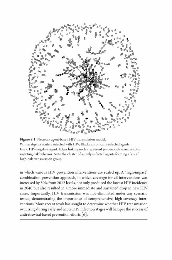
in which various HIV prevention interventions are scaled up. A “high- impact” combination prevention approach, in which coverage for all interventions was increased by 50% from 2012 levels, not only produced the lowest HIV incidence in 2040 but also resulted in a more immediate and sustained drop in new HIV cases. Importantly, HIV transmission was not eliminated under any scenario tested, demonstrating the importance of comprehensive, high- coverage inter-ventions. More recent work has sought to determine whether HIV transmission occurring during early and acute HIV infection stages will hamper the success of antiretroviral- based prevention efforts [6] .
Figure 8.1 Network agent- based HIV transmission model.White: Agents acutely infected with HIV; Black: chronically infected agents; Gray: HIV- negative agent. Edges linking nodes represent past- month sexual and/ or injecting risk behavior. Note the cluster of acutely- infected agents forming a “core” high- risk transmission group.

Agent-Based Modeling 91
effects on health [26], among other areas. Agent- based models are not so con-strained; disaggregating the influence of non- independence between units (i.e., “spillover effects”) from individual exposures (i.e., “direct effects”) is a useful and practical application of agent- based modeling in epidemiology [27].
Like all simulation models, the validity of ABMs depends on the strength and validity of assumptions made during the model development process. The avail-ability (and accuracy) of empirical data with which to parameterize the model is also critical in many population health studies employing ABMs. The number of frameworks upon which to base the construction, calibration, and validation of ABMs continues to grow [28, 29]. Guidelines for reporting ABMs, including their key assumptions and more detailed elements, are also available [30, 31]. Nonetheless, agent- based modeling rests on the fundamental assumption that, for any given research question, people and their relevant health states, interac-tions, and environments can be credibly modeled at a reasonable level of abstrac-tion [28]. Meeting this assumption carries at least two important challenges. First, the researcher must decide which minimal set of characteristics defining the agents, their relationships, and their environments are needed to accurately capture the processes being modeled. Second, data or prior knowledge must exist to inform the specific structure and parameterization of the model processes. In the sections that follow, we describe the most commonly employed methods to help ensure that an ABM has internal validity, and that the model’s results have relevance to solving real- world problems.
2. AGENT- BASED MODELING METHODOLOGIES
2.1. Implementation of agent- based models
For an ABM to run, the model developer must identify, define, and program agent behaviors, agent- agent interactions, and the relationship between agents and their environments. The first step in this process is to specify a “target”— the phe-nomena the model is intended to represent, reproduce, and simulate [4] . Since no model can capture all possible characteristics, behaviors, and environments that may influence a health outcome of interest, building a model for the target requires a theoretically motivated and conceptually grounded process of abstrac-tion [29]. The goal is not to construct an all- encompassing representation of real-ity, but a highly simplified depiction that nonetheless provides valid insights into real- world phenomena and improves scientific understanding [32]. Commonly employed conceptual frameworks in population health, including the social- ecological model of health behavior and the syndemic theory of disease produc-tion [33, 34], can be helpful in identifying the core components of an ABM as employed in epidemiology. Given that simplification is a necessary step in all
92 M E T H O D S I N S Y S T E M S P O P U L A T I O N H E A LT H
models used in epidemiology, existing tools, including causal diagraming [35], may also be helpful in determining the key processes to be modeled in an ABM.
An ABM requires a set of code and a computational engine to be executed. Many ABMs are designed from scratch using all- purpose programming languages such as Python™, Java™ and C++. A number of modeling services (with preloaded libraries of commonly employed routines and functions) are also available. Among the most common programs are NetLogo (https:// ccl.northwestern.edu/ netlogo) and Repast (http:// repast.sourceforge.net); other software has been reviewed elsewhere [28]. Once the model has been developed, the simula-tion is run by having agents repeatedly execute their behaviors and interactions according to pre- programmed rules. Most ABMs simulate the passage of time in steps that are either discrete or activity based.
In an ABM, agents are endowed with static or dynamic behaviors that can depend on everything from simple “if- then” rules to complex adaptive processes. The model developer must also define which agents are (or could be) connected to whom and the dynamics of these interactions. The way in which agents are connected is referred to as an ABM topology. Common typologies include a spa-tial grid, a more complicated spatial geography (e.g., agents can only interact with other agents who are nearby), or a social network. The typology of an ABM can also evolve over time. For example, in one study that used an ABM to evaluate policies to reduce influenza transmission in the workplace, agents were assigned to and moved between specific geographic locations representing schools or workplaces [36]. During each simulated day, agents could only interact with other agents who shared the same social activity location.
Agents can be entirely passive (i.e., purely responsive to exogenous stimuli) or seek to actively alter other agent characteristics or the environ-ment. Therefore, unlike many socio- ecological models of health production which assume that health outcomes are determined by immutable upstream forces, ABMs allow individuals to not only interact with, but change, their environment(s). The environment may represent a set of geographic char-acteristics (e.g., pollutants, crime, or other aspects of the physical or built environment), venues (e.g., homes, bars, workplaces), or institutions (e.g., hospitals, prisons). An agent’s location in the simulated landscape is usually recorded as a dynamic attribute as they move in space. Different types of envi-ronments may promote, facilitate, or constrain agent behaviors. For example, in one ABM that simulated walking behaviors within a city, the agent envi-ronment was composed of 400 equal- sized neighborhoods, each with two properties: safety and aesthetics [37]. A walking index (representing each person’s walking experience) was a function of both individual agents’ char-acteristics (e.g., age, walking ability) and the safety and aesthetic quality of
Agent-Based Modeling 93
all neighborhoods along a walking route. Each agent’s walking index in turn affected how much she/ he would walk in the subsequent day.
2.2. Verification and Validation of Agent- Based Models
Model verification and validation are essential components of the ABM design process. Model verification asks the question, “Does the ABM work as intended?” while model validation seeks to determine whether the “right” model has been built. While there is no universal approach or consensus on how to conduct veri-fication and validation in agent- based modeling, a number of principles and over-all techniques are available [38– 40].
The goal of verification is to determine whether the programming imple-mentation of the conceptual model is correct. This process includes debugging, verification of all model calculations, and determining whether equations in the model are solved correctly. Some common verification methods include de- bugging procedures, code “walk- throughs” (a form of software peer review), and boundary testing (i.e., determining whether the model performs as expected at the parameter boundaries).
Broadly, model validation is a process through which the research team assesses the extent to which the model is a credible representation of the real world. Several techniques are available to demonstrate a model’s validity. For example, a model is said to have face validity if content experts believe the model behaves reasonably well by making subjective judgments about its performance. Most ABMs also go through a procedure known as empirical validation. Here, the developer determines whether the model is a good representation of the target by comparing whether model output is consistent with observed data. Model calibration refers to an iterative process through which unmeasured or poorly measured parameters are adjusted until the model output is in agreement with empirical data. A number of different approaches to conduct calibration and empirical validation have been developed and are reviewed elsewhere [41]. A variety of statistical tests can be used to determine if the model’s behavior has an acceptable level of consistency with observed data [42].
2.3. Interpretation of Results from Agent- Based Models
Interpreting the output of an ABM has distinct challenges from other mathemat-ical modeling approaches. First, isolating the causal mechanisms and effects of one parameter can be difficult in models with a high degree of agent heterogene-ity and many interdependent processes. For this reason, conducting parameter

94 M E T H O D S I N S Y S T E M S P O P U L A T I O N H E A LT H
sweeps over multiple variables (frequently simultaneously) to understand model behavior is recommended.
Second, ABMs can be highly sensitive to initial conditions. In complex and chaotic systems, even small perturbations in initial conditions can lead to large differences in model output. We have previously shown that the identification of causal effects is only possible in models that meet a regularity assumption called “ergodicity” (for any given set of initial conditions, the model output can be repre-sented by an ensemble average as the number of model iterations increases) [27]. If non- ergodic behavior is present, the mean of model output across runs is not well defined, and casual effects comparing two counterfactual scenarios cannot be estimated.
Third, precise prediction of real- world phenomena under different inputs can be problematic when many assumptions are made regarding agent behavior and interactions. Given the complexity of many ABMs, the objective should not nec-essarily be to predict specific population outcomes under different scenarios per se, but to conduct a robust policy analysis, such that recommendations consist of an ensemble of policy options which perform well under plausible model specifi-cations and are robust to model assumptions.
3. AGENT- BASED MODELS AND THE FUTURE OF EPIDEMIOLOGY
Epidemiology is, at its heart, a pragmatic discipline that identifies opportuni-ties to control and prevent disease [43]. As such, epidemiologists must concern themselves not only with the isolation of causal effects but also with the identifi-cation of effective ways to intervene. Doing so necessitates more than an under-standing of the causal mechanics that link an exposure with a health outcome. One must also consider the population context (i.e., the underlying prevalence of the health condition and related risk factors) and how multifactorial causal structures interact to produce disease [44].
Agent- based modeling represents one (but not the only) method to synthe-size prior knowledge of a population— and the causal structures that act on this population— to understand how an intervention could affect the public’s health. In this manner, agent- based modeling is a science of evidence synthesis. Specifically, ABMs (and other simulation approaches) represent a platform for the integration of diverse evidence sources, including inconsistent or inconclu-sive scientific information, to support decision making for complex public health problems. Formalized methods and frameworks for the integration of diverse data streams into simulation models (and their implications for evidence- based
Agent-Based Modeling 95
policy analysis) have recently been proposed for population health sciences [45, 46]. Continued adoption of these methods is warranted.
I wish to conclude this chapter by noting that, although systems science in epidemiology and public health has clearly “arrived,” more work is needed. Agent- based modeling of population health systems and the impact of hypotheti-cal policy changes on health have led to novel scientific insights. However, the actual uptake of programs and policies informed by ABMs, and their subsequent evaluation in real- world settings, are lacking. A multidisciplinary and iterative science, in which model developers work collaboratively with interventionists and policymakers to implement, evaluate, and improve public health programs, is needed. Further stymieing the uptake of agent- based modeling is the fact that systems science methods are not currently featured in much public health cur-ricula or training [7] . Thus, the capacity for agent- based modeling to enhance the health of populations requires understanding and appreciation of the method among not just epidemiologists, but also public health practitioners and popula-tion health scientists broadly.
4. ACKNOWLEDGMENTS
I wish to thank Dean Sandro Galea for his feedback and critical insights on early drafts of this chapter. This work was supported by an “Avenir” new investigator award from the National Institute on Drug Abuse (DP2- DA040236).
5. REFERENCES
1. Garnett GP, Cousens S, Hallett TB, Steketee R, Walker N. Mathematical models in the evaluation of health programmes. The Lancet. 2011; 378(9790): 515– 525.
2. Marshall BDL, et al. Prevention and treatment produced large decreases in HIV inci-dence in a model of people who inject drugs. Health Affairs. 2014; 33(3): 401– 409.
3. Marshall BDL, et al. A complex systems approach to evaluate HIV prevention in metropolitan areas: Preliminary implications for combination intervention strate-gies. PLOS ONE. 2012; 7(9): e44833.
4. Gilbert N. Agent- Based Models. Thousand Oaks, CA: SAGE Publications; 2008. 5. Railsback SF, Grimm V. Agent- based and individual- based modeling: A practical intro-
duction. Princeton, NJ: Princeton University Press; 2012. 6. Escudero D, et al. Acute HIV infection transmission among people who inject drugs
in a mature epidemic setting. AIDS. 2016;30(16):2537–2544. 7. Luke DA, Stamatakis KA. Systems science methods in public health: Dynamics, net-
works, and agents. Annual Review of Public Health. 2012; 33: 357– 376.

96 M E T H O D S I N S Y S T E M S P O P U L A T I O N H E A LT H
8. Bonabeau E. Agent- based modeling: methods and techniques for simulating human systems. Proceedings of the National Academy of Sciences of the United States of America. 2002; 99(Supplement 3): 7280– 7287.
9. Zanette DH, Risau- Gusman S. Infection spreading in a population with evolving contacts. Journal of Biological Physics. 2008; 34(1- 2): 135– 148.
10. Perez L, Dragicevic S. An agent- based approach for modeling dynamics of conta-gious disease spread. International Journal of Health Geographics. 2009; 8:50.
11. Nianogo RA, Arah OA. Agent- based modeling of noncommunicable diseases: A sys-tematic review. American Journal of Public Health. 2015; 105(3): e20– e31.
12. Lum K, Swarup S, Eubank S, Hawdon J. The contagious nature of imprisonment: An agent- based model to explain racial disparities in incarceration rates. Journal of the Royal Society Interface. 2014; 11(98): 20140409.
13. Basu S, et al. Averting obesity and type 2 diabetes in India through sugar- sweetened beverage taxation: An economic- epidemiologic modeling study. PLOS Medicine. 2014; 11(1): e1001582.
14. El- Sayed AM, Seemann L, Scarborough P, Galea S. Are network- based inter-ventions a useful antiobesity strategy? An application of simulation models for causal inference in epidemiology. American Journal of Epidemiology. 2013; 178(2): 287– 295.
15. Auchincloss AH, Riolo RL, Brown DG, Cook J, Diez Roux AV. An agent- based model of income inequalities in diet in the context of residential segregation. American Journal of Preventive Medicine. 2011; 40(3): 303– 311.
16. Blok DJ, de Vlas SJ, Bakker R, van Lenthe FJ. Reducing income inequalities in food consumption: Explorations with an agent- based model. American Journal of Preventive Medicine. 2015; 49(4): 605– 613.
17. Reidpath DD. Population health. More than the sum of the parts? Journal of Epidemiology and Community Health. 2005; 59(10): 877– 880.
18. Epstein JM. Generative Social Science: Studies in Agent- Based Computational Modeling. Princeton, NJ: Princeton University Press; 2006.
19. Oakes JM. Invited commentary: Rescuing Robinson Crusoe. American Journal of Epidemiology. 2008; 168(1): 9– 12.
20. Galea S, Riddle M, Kaplan GA. Causal thinking and complex system approaches in epidemiology. International Journal of Epidemiology. 2010; 39(1): 97– 106.
21. Liu F, et al. The role of vaccination coverage, individual behaviors, and the public health response in the control of measles epidemics: An agent- based simulation for California. BMC Public Health. 2015; 15: 447.
22. El- Sayed AM, Scarborough P, Seemann L, Galea S. Social network analysis and agent- based modeling in social epidemiology. Epidemiologic Perspectives and Innovations. 2012; 9(1): 1.
23. Tchetgen Tchetgen EJ, VanderWeele TJ. On causal inference in the presence of inter-ference. Statistical Methods in Medical Research. 2012; 21(1): 55– 75.
24. Little RJ, Rubin DB. Causal effects in clinical and epidemiological studies via poten-tial outcomes: Concepts and analytical approaches. Annual Review of Public Health. 2000; 21: 121– 145.
25. Hudgens MG, Halloran ME. Toward causal inference with interference. Journal of the American Statistical Association. 2008; 103(482): 832– 842.

Agent-Based Modeling 97
26. Oakes JM. The (mis)estimation of neighborhood effects: Causal inference for a practi-cable social epidemiology. Social Science and Medicine. 2004; 58(10): 1929– 1952.
27. Marshall BDL, Galea S. Formalizing the role of agent- based modeling in causal infer-ence and epidemiology. American Journal of Epidemiology. 2015; 181(2): 92– 99.
28. Macal CM, North MJ. Tutorial on agent- based modelling and simulation. Journal of Simulation. 2010; 4: 151– 162.
29. Gilbert N, Terna P. How to build and use agent- based models in social science. Mind & Society. 2000; 1(1): 57– 72.
30. Grimm V, et al. A standard protocol for describing individual- based and agent- based models. Ecological Modelling. 2006; 198(1- 2): 115– 126.
31. Abuelezam NN, Rough K, Seage GR. Individual- based simulation models of HIV transmission: Reporting quality and recommendations. PLOS ONE. 2013; 8(9): e75624.
32. Heesterbeek H, et al. Modeling infectious disease dynamics in the complex land-scape of global health. Science. 2015; 347(6227): aaa4339.
33. Sallis JF, Owen N, Fisher EB. Ecological Models of Health Behavior. In: Glanz K, Rimer BK, Viswanath K, Editors. Health Behavior and Health Education: Theory, Research, and Practice, 4th edition. San Francisco: Wiley; 2008: 465– 486.
34. Singer M, Clair S. Syndemics and public health: Reconceptualizing disease in bio- social context. Medical Anthropology Quarterly. 2003; 17(4): 423– 441.
35. Greenland S, Pearl J, Robins JM. Causal diagrams for epidemiologic research. Epidemiology. 1999; 10(1): 37– 48.
36. Kumar S, Grefenstette JJ, Galloway D, Albert SM, Burke DS. Policies to reduce influ-enza in the workplace: Impact assessments using an agent- based model. American Journal of Public Health. 2013; 103(8): 1406– 1411.
37. Yang Y, Diez Roux AV, Auchincloss AH, Rodriguez DA, Brown DG. A spatial agent- based model for the simulation of adults’ daily walking within a city. American Journal of Preventive Medicine. 2011; 40(3): 353– 361.
38. Ormerod P, Rosewell B. Validation and Verification of Agent- Based Models in the Social Sciences. In: Squazzoni F, Editor. Epistemological Aspects of Computer Simulation in the Social Sciences. New York: Springer Berlin Heidelberg, 2010: 130– 140.
39. Khattak AS, Khiyal MSH, Rizvi SS. Verification and validation of agent- based model using e- VOMAS approach. International Journal of Computer Science and Network Security. 2015; 15(3): 29– 35.
40. Helbing D. Social Self- Organization: Agent- Based Simulations and Experiments to Study Emergent Social Behavior (Understanding Complex Systems). Zurich: Springer- Verlag Berlin Heidelberg; 2012.
41. Windrum P, Fagiolo G, Moneta A. Empirical validation of agent- based models: Alternatives and prospects. Journal of Artificial Societies and Social Simulation: JASSS. 2007; 10(2): 8.
42. xiang x, Kennedy R, Madey G, Cabaniss S. Verification and validation of agent- based scientific simulation models. Proceedings of the 2005 Agent- Directed Simulation Symposium, April 2005. The Society for Modeling and Simulation International, 47– 55.
43. Susser M. What is a cause and how do we know one? A grammar for pragmatic epi-demiology. American Journal of Epidemiology. 1991; 133(7): 635– 648.

98 M E T H O D S I N S Y S T E M S P O P U L A T I O N H E A LT H
44. Keyes K, Galea S. What matters most: Quantifying an epidemiology of consequence. Annals of Epidemiology. 2015; 25(5): 305– 311.
45. Atkinson JA, Page A, Wells R, Milat A, Wilson A. A modelling tool for policy analy-sis to support the design of efficient and effective policy responses for complex pub-lic health problems. Implementation Science. 2015; 10: 26.
46. Baguelin M, et al. Assessing optimal target populations for influenza vaccination programmes: An evidence synthesis and modelling study. PLOS Medicine. 2013; 10(10): e1001527.
9
Microsimulation
S A N JAY BAS U
A microsimulation is a model that simulates individuals within a population. The goal of microsimulation is to understand how variations in disease- relevant characteristics among individuals produce a population distribution of health outcomes. Microsimulation models therefore differ from models that simulate a population average rate of disease; microsimulation models, by focusing on indi-vidual risks of disease, enable modelers to pay particular attention to the tail ends of population distributions: for example, identifying those individuals at unusu-ally high risk of illness.
In this chapter, we discuss how to determine if a microsimulation modeling approach may be relevant in terms of addressing a given problem in popula-tion health. We detail the microsimulation modeling process through a series of examples, which reveal common applications of the method, pitfalls, and solu-tions adopted by researchers constructing and utilizing microsimulation models, as well as scenarios that may be amenable to microsimulation to address popula-tion health dilemmas. We identify key opportunities for the application of micro-simulation methods to population health research.
1. AN ILLUSTRATIVE EXAMPLE
Suppose we wish to study strategies to reduce the incidence of cardiovascular disease events (myocardial infarctions and strokes) in a population of patients treated at a local medical clinic. A new initiative focuses on finding individuals at the highest risk for cardiovascular disease and providing them with a home- based health intervention: visits from a nurse to help the patients take complex medica-tions to lower their risk of cardiovascular disease events. The risk of cardiovascular

100 M E T H O D S I N S Y S T E M S P O P U L A T I O N H E A LT H
disease events is related to many underlying risk factors such as high blood pres-sure, high cholesterol, type II diabetes, tobacco smoking, age, and sex [1] . These underlying risk factors are correlated; for instance, if an individual has high blood pressure, they are likely to also have high cholesterol [2]. As a result of these cor-relations, some individuals in the population are at much greater risk for cardio-vascular disease events than others, and the population “average” rate of risk may be less important for targeting an intervention to the most needy group than the question of which people are at highest risk. Furthermore, the individuals who have multiple risk factors for cardiovascular disease are also known to experience the greatest relative benefits from treatment [3]. Hence, the clinic hopes that pro-viding a home- based nursing intervention will help the individuals at greatest risk for disease avoid a future myocardial infarction or stroke. Prior randomized studies have indicated that this intervention improves adherence to medications significantly, such that the full benefits of the medications should accrue over time [4].
The physicians in the program choose which patients to enroll into the pro-gram using Framingham “risk equations,” which are equations that estimate the risk of myocardial infarction and stroke over the next 10 years for a given indi-vidual [1] . The risk equations take into account a person’s age, sex, his or her history of tobacco smoking, and whether the patient has type 2 diabetes, high blood pressure, and/ or high cholesterol, among other factors. The equations use regression coefficients derived from a longitudinal study of cardiovascular dis-ease to estimate how different values of these risk factors would be expected to increase or decrease the overall risk of cardiovascular disease events over the next decade.
Suppose the physicians who perform this calculation assign nurses to visit the homes of patients who have at least a 10% risk of myocardial infarction or stroke over the next decade, per the Framingham risk calculator. We wish to estimate the potential impact and cost- effectiveness of the nursing program over the next decade; over this period of time, we would expect the long- term benefits of the medication treatment program to manifest as a significant reduction in the rate of cardiovascular disease events. Because the time course of observing benefits is typically long [5] , a randomized trial may be costly to perform, and several decisions for the clinic (such as whether to expand the program to individuals at slightly lower risk than 10%) are of great interest to the staff. Hence, the clinic officials elect to employ a modeling strategy to study their program. If they construct a typical cohort model (e.g., the model illustrated in Figure 1A), they might substantially misestimate the impact and cost- effectiveness of the nursing program. In particular, a cohort- level model simulates a population by examining the average rate of disease within the population. In this case, a cohort model might estimate the average rate of
Microsimulation 101
events predicted by the Framingham equation among the treated population receiving home nursing and compare that rate to the average rate of events pre-dicted by the Framingham equation among the same population not receiving home nursing. The model would specifically apply the Framingham equations to the average blood pressure, cholesterol level, and average values of other risk factors among the treated population, and calculate the difference in pre-dicted event rates between the simulated population receiving nursing visits and the simulated population not receiving nursing visits. A problem with this approach to studying the intervention is that the rate of disease among the extremely high- risk subgroup of the population may drive the real- world out-comes from the program. Even if we repeatedly sampled from the probabil-ity distributions of each risk factor to capture uncertainty around the average values (Figure 9.1A), we would arrive at a Gaussian (normal) distribution of estimated risk. If we constructed the cohort model by dividing the treated population into smaller subpopulations— say, a higher- risk and a lower- risk subpopulation of the treated group— the cohort model would still not accu-rately estimate the benefits of the program, as the model would generate an estimate of the average risk among the two subgroups and not account for the very skewed nature of the cardiovascular disease risk distribution. The extreme high- risk subgroup of the higher- risk population will accrue more benefits than the average subgroup in the higher- risk group, and therefore more and more subgroups would be needed to accurately estimate the ben-efits of the program.
In breaking down the cohort model into smaller and more specific subgroups, we arrive at a natural limit: defining the model to the individual level, which pro-duces a microsimulation. A microsimulation model, depicted in Figure 9.1B, simulates each individual to account fully for the skewed nature of the probabil-ity distributions of cardiovascular disease events and treatment benefits among individuals. As illustrated in Figure 9.1B, a microsimulation model departs from a traditional cohort model because it does not simply take into account the aver-age blood pressure, average cholesterol, and average values of risk factors among each subpopulation. Rather, each individual in the model is provided with a spe-cific value for their blood pressure, cholesterol level, and so on— by sampling from correlated probability distributions of these factors, which captures the truly skewed nature of the risk distribution. By applying the Framingham equations to each individual in the model with and without the nursing intervention, the full benefits of the intervention (driven by the very high- risk individuals who benefit the most) can be captured. Furthermore, the model can be utilized to identify how changes to the criteria for intervention— for example, enrolling those with a 5% risk of cardiovascular events over a decade, or 15% risk, instead of the original 10% risk threshold— could change the outcomes of the program.

Calculateaverage risk ofdisease from
average values ofrisk factors w/intervention
0.04Pr
obab
ilit
y
0.02
0.00
100Blood pressure
(systolic, mmHg)
140 180
0.04
Prob
abil
ity
0.02
0.00
100Blood pressure
(systolic, mmHg)
140 180
0.20
Prob
abil
ity
0.10
0.00
Cholesterol(total, mmol/L)
0 5 10 15
0.20
Prob
abil
ity
0.10
0.00
Cholesterol(total, mmol/L)
0 5 10 15
15
10
5
0Pe
ople
Probability of event
0.00 0.10 0.20
15
Peop
le 10
5
0
0.00 0.10
Probability of event
0.20
Calculateaverage risk ofdisease from
average values ofrisk factors w/o
intervention
Difference inprobability
distributions =estimated impact
of intervention
With NursingIntervention
A
Simulatepopulation
Without NursingIntervention
Difference inprobability
distributions =estimated impact
of intervention
Calculate eachindividual’s risk
of disease bysampling from
correlateddistributions of
risk factor valuesw/ intervention
B
Calculate eachindividual’s risk
of disease bysampling from
correlateddistributions of
risk factor valuesw/o intervention
Simulatepopulation
Without NursingIntervention
With NursingIntervention
7
Cho
lest
erol
(tota
l, m
mol
/L)
5
3
1
120
Blood pressure(systolic, mmHg)
140
8
Cho
lest
erol
(tota
l, m
mol
/L)
6
4
2
120Blood pressure
(systolic, mmHg)
140 160
25
Peop
le 15
0
0.00 0.10
Probability of event
0.20
5
0.00 0.10
Probability of event
0.20
25
Peop
le 15
0
5
Microsimulation 103
2. METHODOLOGICAL FRAMEWORKS
As illustrated by the above example of cardiovascular disease microsimulation, the scientific questions that may be appropriate for microsimulation modeling are those that require us to consider differential risks among individuals within a complex, heterogeneous population. In the public health context, micro-simulation models are increasingly used for two common tasks: the optimiza-tion of screening or treatment strategies for chronic diseases, and the study of population- wide health policies that may differentially affect individuals within a population. We consider each of these two cases in turn.
Microsimulation modeling is particularly helpful for optimizing screening or treatment strategies for chronic diseases, because it allows a modeler to identify how including or excluding different individuals in a screening or treatment pro-gram can alter the expected population- level effectiveness of the program. For example, suppose we wish to develop an optimal strategy to screen people who may have a high risk for cardiovascular disease events, by posting community health- care workers at local supermarket parking lots to ask shoppers screening questions and refer “high risk” shoppers to a local health clinic for further evalua-tion. We could choose from many different questions that could be administered verbally by community health- care workers to identify who might be at high risk: whether a person has a family history of myocardial infarctions or strokes, whether they have been previously diagnosed with high blood pressure or high cholesterol or type 2 diabetes, or whether they currently smoke tobacco, for instance. These screening questions are non- invasive but attempt to identify indi-viduals who likely have biomarkers predisposing them to cardiovascular disease, which cannot be assessed without a further examination or laboratory assessment.
A microsimulation model could help identify the links between the factors that can be assessed through non- invasive screening questions and the underly-ing biomarkers for cardiovascular disease. Specifically, as shown in Figure 9.2, a
Figure 9.1 Conceptual diagram of microsimulation modeling Differences when constructing (A) a standard cohort model, versus (B) a microsimulation model of a nursing intervention to lower the risk of cardiovascular disease events. A cohort model is typically run by sampling independently from estimates of the average value of each input parameter. Hence, it fails to capture the skewed distribution of outcomes, as repeated sampling from the independent distributions of input parameters produces a Gaussian, or normal, distribution. The cohort approach would therefore underestimate the benefit of the intervention by failing to take into account the benefits of the program for high- risk individuals among whom the distribution of risk factors is correlated. Note that most risk calculation approaches take into account several risk factors, but only systolic blood pressure and total cholesterol are illustrated here for simplicity.
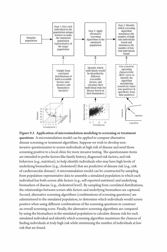
Simulatepopulation
Step 1: Give eachindividual in the
population uniquefeatures to make
the simulatedpopulation
representative ofthe target
population
Step 3: Identifywhich screening
algorithmmaximizes the
number of high-risk individuals
found andminimizes thenumber of low-risk individuals
found
Use a receiveroperating
characteristic(ROC) curve to
identify thealgorithm
maximizingsensitivity (mosttrue positives) &speci�city (leastfalse positives)
Identify whichindividuals would
be identi�ed bydifferent
screenablefactors, and
calculate theirindividual risks for
disease based ontheir biomarkers
Sample fromcorrelated
distributions ofboth screenable
factors (non-invasive) andbiomarkers(invasive)
35
7
5
3
1500
400300
200100
0
30
Biom
arke
r
Biom
arke
r-ba
sed
risk
Sens
itiv
ity
Scre
enin
g fa
ctor
2
25201510
1 2 3 4 5 60 5 15 25
Optimum
1-speci�cityScreening score
Screening factor 1
Step 2: Applyalternativescreening
algorithms to thesimulated
population
Figure 9.2 Application of microsimulation modeling to screening or treatment questions A microsimulation model can be applied to compare alternative disease screening or treatment algorithms. Suppose we wish to develop non- invasive questionnaires to screen individuals at high risk of disease and send those screening positive to a local clinic for more invasive testing. The questionnaire items are intended to probe factors like family history, diagnosed risk factors, and risk behaviors (e.g., nutrition), to help identify individuals who may have high levels of underlying biomarkers (e.g., cholesterol) that are predictive of disease risk (e.g., risk of cardiovascular disease). A microsimulation model can be constructed by sampling from population- representative data to assemble a simulated population in which each individual has both screen- able factors (e.g., self- reported nutrition) and underlying biomarkers of disease (e.g., cholesterol level). By sampling from correlated distributions, the relationships between screen- able factors and underlying biomarkers are captured. Second, alternative screening algorithms (combinations of screening questions) are administered to the simulated population, to determine which individuals would screen positive when using different combinations of the screening questions to construct an overall screening score. Finally, the alternative screening algorithms are compared by using the biomarkers in the simulated population to calculate disease risk for each simulated individual and identify which screening algorithm maximizes the chances of finding individuals at truly high risk while minimizing the number of individuals at low risk that are found.
Microsimulation 105
microsimulation of the population could be constructed by sampling from the correlated distributions of both factors assessed through non- invasive screening and underlying biological risk factors for disease (both of which are found in population- representative data sets such as the National Health and Nutrition Examination Survey in the United States [6] ). Hence, individuals in the simu-lated population could be assigned both screening question responses (what the community health- care workers would be able to assess in a supermarket park-ing lot) and biomarkers of disease (what the community health- care workers would not be able to assess in a supermarket parking lot) by repeatedly sampling from the correlated distributions among these factors (illustrated graphically in Figure 9.2). The microsimulation could then be used to identify which subset of the population would be found through alternative combinations of screening questions administered via the health- care workers. The optimal combination of questions could be found through simulations in which alternative combinations of screening questions would be compared, to identify which screening question combinations maximize the chances of finding high- risk individuals (true posi-tives) and minimize the risks of subjecting low- risk individuals to further evalua-tion (false positives) [7].
A second use of microsimulation modeling is to study population- wide health policies that may differentially affect individuals. Continuing with the theme of applying microsimulation to cardiovascular disease, suppose we wish to study the impact of a national program to reduce the sodium content in processed foods, under the premise that sodium is related to elevated blood pressures and subsequent cardiovascular disease. Most sodium intake in the United States is from processed foods (i.e., added by a manufacturer) rather than from table salt (i.e., added by the consumer) [8] . A large- scale program to reduce sodium in the food supply may affect people in different ways: some individuals may have high blood pressure that becomes lower, which decreases the risk of cardiovas-cular disease events and associated deaths; conversely, some individuals with low blood pressure could experience extremely low blood pressure, which can perversely increase their risk of death [9]. A microsimulation could help inform whether the program would be expected to benefit the population overall and among whom potential perversities might occur. Such a microsimulation model would first simulate the pre- intervention levels of sodium intake and blood pres-sure among individuals in the population (i.e., sampling from the sodium intake and blood pressure data in the National Health and Nutrition Examination Survey, if studying a US population [6]). The model would then estimate how much less sodium would be consumed after the intervention, given the amount of sodium that is withdrawn from the food supply and the amount added back in table salt by consumers. The model would finally use the results of major trials that related lower sodium intake to lower blood pressure to estimate how each

DEMOGRAPHICS
AgeSex
RaceIncome
A
SodiumIntake
Changein CVD
risk
Change inSBP withreducedsodiumintake
Daily sodium intake
Non-NSRIfood items
NSRI food items
• Bread: –25%• Cold cuts: –25%• Canned soup: –30%• Chips: –21%• Cheeseburger: –15%• Pizza: –13%• etc...
SBP
HtnStatus
CVDHistory
SODIUM CONSUMPTION
Probabilitydistributions
speci�c to eachcohort
CVD Risk
Male. White
B
Female. White
Female. Mexican
Female. Black
–7.5 –5.0 –2.5 0.0 2.5
% change in incident MI
Male. MexicanAge
18–39
40–59
60–85
Male. Black
Figure 9.3 Exploring potential benefits and perversities of a population health measure using microsimulation Simulation results from a microsimulation of the National Salt Reduction Initiative (NSRI) in the United States (11). The microsimulation involved (A) simulating the sodium intake, systolic blood pressure (SBP) levels of the US population and associated hypertension (Htn) and cardiovascular disease (CVD) history using data from the National Health and Nutrition Examination Survey, then estimating the reduction in blood pressure given the reduction in daily sodium intake among each person given the sodium reduction in foods published by the NSRI and data relating sodium reduction to blood pressure reduction from randomized trials of low sodium diets (10). The blood pressure levels were then related to CVD risk given observational data revealing a J- shaped relationship between sodium intake and mortality (9). As shown in (B), young Mexican women might experience a perverse increase in incident myocardial infarction (MI) risk due to excessively low blood pressure following the sodium reduction program.
Microsimulation 107
individual in the model would experience a blood pressure change based on their change in sodium intake, and estimate the change in risk of mortality given the J- shaped relationship between blood pressure and mortality gleaned from prior observational studies [10, 9]. As shown in Figures 9.3A and B., a microsimulation model performing these tasks to simulate the National Salt Reduction Initiative in the United States (which reduced sodium content in many processed food products) observed that most populations could benefit from the sodium reduc-tion, while young Mexican females might be at risk for perversely low blood pressures following the initiative. The model was then used to identify which foods might be best to target, given the vast differences in consumption patterns and types of foods consumed by young Mexican women as compared to other populations [11].
3. PRACTICAL DETAILS FOR MICROSIMULATION MODELING
To construct a microsimulation model, three steps are generally required: (i) con-structing a simulated population; (ii) sampling from correlated input data to assign relevant risk factors and other relevant attributes to each simulated indi-vidual in the population; and (iii) estimating the incidence of disease among the population using the assigned risk factors and attributes.
A simple way to conceptualize a microsimulation model is to imagine the model as a large table. Each row is an individual. Each column is a property of that individual— for example, their age, sex, race/ ethnicity, blood pressure, cho-lesterol, diabetes status (a 0/ 1 dummy variable), and so on. To “fill in” the table, we populate the columns by constructing a multidimensional joint probability distribution that can be defined by two features: a copula (the correlation among properties), and a marginal distribution for each individual property (the popu-lation distribution of that property) [12]. Figure 9.4 illustrates the copulas and marginal distributions between cardiovascular risk factor data for a microsimula-tion model of myocardial infarctions and strokes. We construct the copula and marginal distributions from population data on the distributions of each prop-erty and the correlation matrix between the properties; if such data are unavail-able, a microsimulation is essentially impossible to construct, and without the correlation matrix, a microsimulation would collapse into the same structure as a traditional cohort model.
Using these individual properties, we calculate a hazard of disease— which is specific to the disease process being simulated. In our cardiovascular disease examples, a Framingham risk score is employed, which involves multiplying each risk factor (e.g., systolic blood pressure) by coefficients estimated through logis-tic regression from a longitudinal cohort study of cardiovascular disease (e.g.,
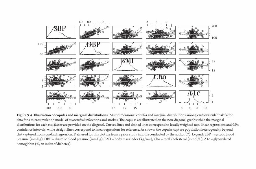
SBP
DBP
BMI
Cho
A1c
60 80 110 2 4 6
100
200
60
120
15
35
2
100 140 180 15 25 35 4 6 8 10
4
8
5
Figure 9.4 Illustration of copulas and marginal distributions Multidimensional copulas and marginal distributions among cardiovascular risk factor data for a microsimulation model of myocardial infarctions and strokes. The copulas are illustrated on the non- diagonal graphs while the marginal distributions for each risk factor are provided on the diagonal. Curved lines and dashed lines correspond to locally weighted non- linear regressions and 95% confidence intervals, while straight lines correspond to linear regressions for reference. As shown, the copulas capture population heterogeneity beyond that captured from standard regression. Data used for this plot are from a prior study in India conducted by the author (7). Legend: SBP = systolic blood pressure (mmHg), DBP = diastolic blood pressure (mmHg), BMI = body mass index (kg/ m2), Cho = total cholesterol (mmol/ L), A1c = glycosylated hemoglobin (%, an index of diabetes).

Microsimulation 109
each 1 mmHg increase in systolic blood pressure relates to a particular increase in the risk of myocardial infarction or stroke). In the case of other diseases, lon-gitudinal data from observed cohorts with a given disease will be necessary to define how the properties of a simulated person would be combined to define the risk of the specific disease being studied. If studying the potential impact or cost- effectiveness of an intervention is the purpose of the simulation, then the microsimulation will be run twice: once using estimated distributions of input parameters from individuals who receive the intervention, and a second time (a counterfactual case) using estimated distributions of input parameters from indi-viduals who do not receive the intervention.
There are at least three major challenges faced by modelers who attempt to implement such a microsimulation model. First, the question arises as to how many times to sample from input probability distributions to produce a rea-sonable estimate of outcomes from the model. At the present time, there is no “rule” for how many times the sampling should be repeated; greater sampling typically produces a more stable estimate of the mean outcome and an overall sense of the distribution of the outcome around the mean. Just as in a random-ized trial, however, one can use a power calculation to estimate what minimum amount of sampling is necessary to detect a certain degree of effect size between the counterfactual and intervention cases; one essentially treats the intervention and counterfactual simulation as matched pairs, such that the power calculation is the same as performing a t- test to detect the difference between two dependent means [13].
A second challenge is the question of how to validate a microsimulation model. External validation can be performed if we have data from a longitudinal cohort study that is independent from our input data. We can enter the risk factor values for every individual in the independent cohort and compare the individ-ual’s simulated outcomes to their actually observed outcomes over the period of the study duration, providing a sense of how well the microsimulation performs among people at varied levels of risk. When such an external data set is unavail-able, microsimulation modelers will frequently resort to out- of- sample internal validation: input data for two- thirds of an input sample are used to produce the input probability distributions, then the model is applied to the other one- third of the sample to estimate the degree of error between the modeled outcomes and observed outcomes [14].
4. IMPLICATIONS FOR POPULATION HEALTH
Overall, the microsimulation approach offers an opportunity to bridge the philosophical divide between “precision medicine” and population health. Precision medicine aims to identify how individual features may result in tailored

110 M E T H O D S I N S Y S T E M S P O P U L A T I O N H E A LT H
interventions for individuals [15]. The precision approach, however, appears fundamentally at odds with public health evidence suggesting that most popula-tion health disparities and avoidable causes of premature mortality are not due to individual features but misdistribution of health opportunities and resources, as well as disparities in adverse exposures [16]. Yet the population critique may need to address the circumstances of individuals who may be unassisted or even harmed if public health interventions do not consider the variations in risk within a population, as suggested by the sodium reduction example discussed above.
We may meld the two perspectives of precision medicine and population health with microsimulation: identifying how unequal exposures and risk fac-tors lead to differential risk among individuals within populations, permitting a public health approach that attempts to maximize population benefits while minimizing individual- level risks. Hence, microsimulation may bring large- scale analytic tools to users who require direct policy comparisons of alternative pol-icy strategies that are intended for deployment across complex, heterogeneous populations of people. As the field of microsimulation remains in its early stages, the next step for modelers is to share their experiences applying microsimula-tion models to new population health questions, both to identify what chal-lenges remain to ensuring the usefulness of the technique to emerging public health problems of interest, and to detail strategies to enhance the approach as it becomes increasingly used to provide insights into complex problems that are not easily addressed through traditional study designs.
5. REFERENCES
1. Anderson KM, Odell PM, Wilson PW, Kannel WB. Cardiovascular disease risk pro-files. American Heart Journal. 1991; 121(1): 293– 298.
2. Lim SS, et al. Prevention of cardiovascular disease in high- risk individuals in low- income and middle- income countries: Health effects and costs. The Lancet. 2007; 370(9604): 2054– 2062.
3. Gaziano TA, Opie LH, Weinstein MC. Cardiovascular disease prevention with a multidrug regimen in the developing world: A cost- effectiveness analysis. The Lancet. 2006; 368(9536): 679– 686.
4. McAlister FA, Stewart S, Ferrua S, McMurray JJ. Multidisciplinary strategies for the management of heart failure patients at high risk for admission: A systematic review of randomized trials. Journal of the American College of Cardiology. 2004; 44(4): 810– 819.
5. Gaziano T, Srinath Reddy K, Paccaud F, Horton S, Chaturvedi V. Cardiovascular dis-ease. In: Disease Control Priorities in Developing Countries. World Bank Publications; 2006. www.ncbi.nlm.nih.gov/ books/ NBK11728/ . Accessed May 11, 2015.
6. Centers for Disease Control and Prevention. National Health and Nutrition Examination Survey, 1999- 2012. Atlanta: HHS; 2012.

Microsimulation 111
7. Basu S, et al. The health system and population health implications of large- scale dia-betes screening in India: A microsimulation model of alternative approaches. PLOS Medicine. 2015; 12(5): e1001827.
8. Institute of Medicine. Sodium Intake in Populations: Assessment of Evidence. Washington D.C.: National Academies Press; 2013.
9. O’Donnell M, et al. Urinary sodium and potassium excretion, mortality, and cardio-vascular events. New England Journal of Medicine. 2014; 371(7): 612– 623.
10. Sacks FM, et al. Effects on blood pressure of reduced dietary sodium and the Dietary Approaches to Stop Hypertension (DASH) diet. New England Journal of Medicine. 2001; 344(1): 3– 10.
11. Choi SE, Brandeau ML, Basu S. Expansion of the national salt reduction initia-tive: A mathematical model of benefits and risks of population- level sodium reduc-tion. Medical Decision Making. 2016 Jan; 36(1): 72– 85.
12. Hofert M, Mächler M. Nested archimedean copulas meet R: The nacopula package. Journal of Statistical Software. 2011; 39(9): 1– 20.
13. Cohen J. A power primer. Psychological Bulletin. 1992; 112(1): 155. 14. Eddy DM, et al. Model transparency and validation: A report of the ISPOR- SMDM
modeling good research practices task force– 7. Medical Decision Making. 2012; 32(5): 733– 743.
15. Ashley EA. The precision medicine initiative: A new national effort. JAMA: The Journal of the American Medical Association. 2015; 313(21): 2119– 2120.
16. Bayer R, Galea S. Public health in the precision- medicine era. New England Journal of Medicine. 2015; 373(6): 499– 501.

10
Social Network Analysis
D O U G L AS A . L U K E , A MA R D HA N D, A N D B O B B I J. CA ROT H E R S
Network science has been developed over the last century as a scientific para-digm that explores human and other types of complex systems as socially struc-tured. Network analysis is the set of analytic tools that allow this exploration. Population health is driven in part by network characteristics and dynamics. This chapter attempts to answer the following five questions: (1) What is network science and social network analysis? (2) Why are networks important for study-ing, understanding, and influencing population health? (3) What do we know about how social networks influence population health, especially infectious and chronic diseases and their associated risk factors? (4) What are the primary methods used by network scientists when studying health? (5) What are some important challenges and opportunities for social network analysis and popula-tion health?
Two definitions are particularly useful for this chapter. First, network science is the use of relational and structural theories to study network representations of complex physical, biological, and social systems. Network science is inherently multidisciplinary, spread across many disciplines including genetics, biology, psychology, sociology, political science, public health, engineering, and com-puter science. Second, social network analysis is the set of analytic tools used to explore and model network data, made up of network members (nodes) related to one another via some type of social relationship (tie).
1. WHAT IS NETWORK SCIENCE AND SOCIAL NETWORK ANALYSIS?
Networks are all around us. Networked systems can be found at every level of organization, from genes, proteins, and cells at the lower end, to networks of

114 M E T H O D S I N S Y S T E M S P O P U L A T I O N H E A LT H
organizations, nations, and cultures at the higher end. “Below- the- skin” net-works of genes, protein interactions, and intercellular communication account for much of human development, physiology, and human disease. The human brain is now viewed as a complex network, or connectome [1] . Similarly, human diseases and their underlying genetic roots are connected as a diseasome [2]. Humans naturally organize themselves in “above- the- skin” networked systems. Families, broader kinship ties, neighborhoods, and communities organize them-selves in networked systems of relationships. Businesses and other social insti-tutions operate via complex interorganizational systems of trade, influence, and partnerships [3]. Networks are a fundamental means by which the universe is organized and humans function and thrive.
Exploring and influencing human networks requires alternative scientific the-ories, methods, and data. Network science is a multidisciplinary set of biological, social, and health theories that view human behavior, health, and disease through relational and structural lenses. Moreover, traditional data collection and analytic approaches are inadequate for studying networked systems. Network data are comprised of information about the relationships (ties) that connect the mem-bers (e.g., people, organizations, proteins, etc.) of the network. This implies that networked data are inherently non- independent. Customary statistical assump-tions of independence of observations mean that traditional statistical modeling (e.g., general and generalized linear models) cannot be used to analyze network data. Instead, analytic approaches that are appropriate to study dyads, local net-work structures, network subgroups, and entire networks must be developed and used.
2. WHY ARE NETWORKS IMPORTANT FOR STUDYING, UNDERSTANDING, AND INFLUENCING POPULATION HEALTH?
Social networks mediate and moderate the influence of broader cultural, socio-economic, and physical contexts— and in turn shape a wide variety of psycho-social mechanisms and psychophysical pathways leading to health conditions and outcomes. This can be seen in Figure 10.1, which has been adapted from Berkman’s original model [4, 5]. More specifically, social networks influence their members in two broad ways [6] . First, the networks serve to shape the flow of some resource to the individual members. The resource could be money, health information, social support, etc. Second, the structural position of a person within a social network is important. For example, persons who are in more isolated posi-tions in a network are at greater risk for certain types of health outcomes (e.g., earlier death after a cancer diagnosis). In the rest of this chapter, we will review the

Social-structuralConditions
(Macro)
Culture Social networkstructure Social support
Social in�uence
Social engagementPhysiological
pathways
Psychologicalpathways
Health behavioralpathways
Chronic diseases
Infectious diseases
Person-to-personcontact
Person-to-personcommunication
Access to resources & material goods
Characteristics ofnetwork ties
Social networkdynamics
Socioeconomicfactors
Politics
Social change
SocialNetworks(Mezzo)
PsychosocialMechanisms
(Micro)Pathways Disease
Outcomes
Figure 10.1 Conceptual model linking social networks to population health (adapted from [4] ).
116 M E T H O D S I N S Y S T E M S P O P U L A T I O N H E A LT H
relationship between social networks, human disease, and population health, and present an overview of important network analytic approaches and tools.
Network analysis grew out of many disciplines, including anthropology, soci-ology, psychology, political science, computer science, and mathematics. What we now recognize as network analysis started in the 1930s, with Jacob Moreno’s invention of sociometry and sociograms (network diagrams) [7] . From the beginning, network analytic methods were applied to study human behavior and health. Early applications examined family and genealogical systems, friend-ship and peer- support networks, and the role of social support on health. Over the last several decades, health, public health, and public policy researchers have increasingly used network approaches to study structural and systemic factors related to population health, with special emphasis on infectious and chronic diseases.
3. WHAT DO WE KNOW ABOUT HOW SOCIAL NETWORKS INFLUENCE POPULATION HEALTH?
3.1. Networks and Infectious Disease
Human relationships are essential to the spread of disease. Social aspects of disease transmission have been well studied in infectious diseases because of the relative ease of defining affected and unaffected individuals in a popu-lation. Traditional epidemic models of infectious disease such as the S- I- R (Susceptible, Infected, Removed) model and others function well when there are relatively clear mechanisms of transmission, infectivity, and outcomes [8] . These models are particularly useful for predicting the life course of an epidemic: when it started, how long it will last, and how many people will be affected by it. However, most of the research using S- I- R models assumes ran-dom mixing within a population; i.e., social structure is ignored. Starting in the 1970s, epidemiologists began adding structural and relational concepts into both their models and methods (e.g., contact tracing). More recent empiri-cal and computational modeling studies have begun to demonstrate the need for— and advantages of— incorporating network information into epidemio-logic models [9]. Instead of a traditional epidemic outbreak curve, diagram-ming the network growth of the spread of infection is more revealing of the underlying disease process [10].
The HIV/ AIDS epidemic in the 1980s accelerated the adoption of network methods into infectious disease research and control. These methods were adapted and extended to study other types of STDs, including syphilis [11], as well as IV drug use and other risky behavior [12]. These studies identified how various structural aspects of the networks were related to disease incidence,
Social Network Analysis 117
propagation, and maintenance, as well as suggesting effective new ways to inter-vene and treat infectious and behavioral diseases [13].
This work extends to understanding and controlling large- scale global pan-demics. In recent years, network information derived from global airline trans-portation data, as well as intra- and international commuting patterns, have been used to develop accurate models of infectious disease outbreaks [14]. These net-work models allow for accurate real- time forecasting of global infectious diseases such as H1N, as well as helping to design surveillance systems for foodborne ill-nesses [15, 16, 17]. It is no longer a radical idea to understand infectious diseases as being driven by social and relational processes; network analysis is a primary tool for understanding those relationships.
3.2. Networks and Chronic Disease and Disease Prevention
At first glance, the mechanisms underlying the connection between social net-works and chronic disease (and hence, population health) are a little harder to elucidate than those for infectious diseases. In a highly visible and influential set of studies, Christakis and Fowler have suggested that chronic diseases such as obesity and smoking may be “contagious” and influenced through peer and fam-ily social network processes [18, 19]. Referring back to the earlier conceptual model (Figure 10.1), we can see that networks can shape a variety of social sup-port, social influence, and social engagement processes that can in turn influence behavioral, psychological, and physical pathways that are implicated in chronic diseases.
Starting as early as the Alameda County study in the 1970s, a number of stud-ies have identified social isolation as a predictor of poorer morbidity and mortal-ity outcomes from a wide variety of chronic conditions, including heart disease, cancer, and respiratory diseases [20]. Social support and larger social networks have been linked to longer survival times after cancer diagnosis [21]. Most of these and similar studies have used fairly general or crude measures of network characteristics. One exception is a recent study by Villingshoj and colleagues that included actual measures of social network contact frequency and related them to colorectal cancer survival [22].
Of all chronic diseases, smoking and tobacco use has received the most attention from network scientists. Smoking behavior, especially smoking ini-tiation, is inherently relational and has a network aspect. Almost all people who start smoking do so before they are 18, and when they start they typi-cally get their first cigarettes from another person, usually a friend or family member [23]. Ennett and Bauman were among the first to study smoking with a network framework, showing that adolescents who were most isolated
118 M E T H O D S I N S Y S T E M S P O P U L A T I O N H E A LT H
from their peers were more likely to smoke [24]. More recent network studies of tobacco use have started to use more sophisticated methods, which allow testing of richer structural and causal hypotheses. For example, Alexander and colleagues conducted an important study that demonstrated an interac-tion between social network characteristics and school context on the like-lihood of smoking. Specifically, they found that popular students (defined in network terms) were more likely to smoke in schools with high smok-ing prevalence and less likely to smoke in schools with low smoking preva-lence [25]. This body of work has started to elucidate more precisely the mechanisms by which networks influence smoking initiation and cessation, including isolation and risk accumulation, diffusion of cultural norms, and structuring flows of emotional support [26, 27, 28]. Finally, using innova-tive new network modeling techniques (exponential random graph models, see below), Mercken and colleagues have shown that both social selection and social influence are important processes that shape adolescent smoking behavior [29].
There are relatively fewer network analytic studies of obesity and physical activity than for smoking. However, there is a growing body of research that sug-gests obesity and its related risk factors are in part socially determined. Valente and colleagues found that friendship ties were significantly more likely to occur between teenagers who were of the same weight, compared to those with differ-ent weights [30]. In a similar vein, but using more sophisticated stochastic net-work modeling techniques, Schaefer and colleagues analyzed the network data in the National Longitudinal Study of Adolescent to Adult Health and found that non- overweight adolescents (as measured by BMI) tended to avoid forming friendship ties with overweight peers [31].
Although it is challenging to study network effects on obesity, it is somewhat easier to assess how networks influence the behavioral risk factors for obesity, viz., physical activity and diet. For example, adolescents who report spending more time with friends in physical activity are more likely themselves to be physically active [32]. At the other end of the age spectrum, adults in their seventies who have more social ties show less functional decline and greater physical activity [33]. In general, physical activity and exercise to reduce obesity can be enhanced via social networks— for example, participating in a carpool social network has been shown to predict exercise adherence [34].
4. WHAT ARE THE PRIMARY METHODS USED BY NETWORK SCIENTISTS WHEN STUDYING HEALTH?
Network analysis comprises a wide variety of analytic techniques. Like any other rich analytic tradition, these network analytic tools can be used for exploratory

Social Network Analysis 119
data analysis, hypothesis building and testing, and more formal model devel-opment. Most network analysis techniques fall into one of three broad catego-ries: visualization, network description, and network modeling.
4.1. Visualization
A primary product of network analysis, and often the first step of network exploration, is the network diagram. Network diagrams are information graph-ics that depict the network members (often called “nodes”) and the relation-ships that connect them to one another (called “ties”). Network diagrams are not just pretty pictures; they are analytic tools that can convey important struc-tural properties of a system. For example, consider Figure 10.2, which depicts the sexual transmission network in the early days of the HIV/ AIDS epidemic [35, 36]. The pattern of ties displays the transmission route of the outbreak, and judicious use of node labeling and coloring tells a rich story of biology, sexual-ity, disease, and transportation. These types of disease transmission network
PA 1
GA 1
FL 2 FL 1
LA 1LA 2
LA 3
LA 9
TX 1
NY 3
0
NY 4
NY 9 NY 1
NY 6
NY 7NY 17
NY 14NY 16
NY 11
NY 13
NY 12
NY 2
NY 5
NY 19
NY 21
NY 8
NJ 1
NY 22
NY 10
NY 20
NY 18
LA 4
LA 5 LA 7
Kaposi sarcoma
0 = Index patient1-21 = Sequence of onset
Pneumocystis carinil pneumonia
Other opportunistic infection
Multiple diagnoses (KS and PCP)
City LA-Los Angeles, NY-New York City, SF-San FranciscoFL-Florida, GA-Georgia, NJ-New Jersey, PA-Pennsylvania, TX-TexasState
LA 6
SF 1
NY 15
LA 8
GA 2
Figure 10.2 HIV/ AIDS sexual transmission network.

120 M E T H O D S I N S Y S T E M S P O P U L A T I O N H E A LT H
visualizations revolutionized how epidemiologists both modeled and observed disease outbreaks, starting in the mid- 1980s.
4.2. Network Description
Network scientists have developed a multitude of network descriptive statistics that are used to summarize important characteristics and aspects of social net-works. These characteristics fall into a few broad categories, including network position (e.g., centrality), local network structure (e.g., transitivity), network subgroups and communities (e.g., modularity), and overall network structure (e.g., density) [37].
Figure 10.3 is a schematic that illustrates the rich diversity of descriptive meth-ods that can be used by network scientists. In addition to the more basic network descriptions of node location, local structure, subgroups, and overall network characteristics, network analysts can use more advanced techniques to study multiple networks, multiple types of network ties within the same network (e.g., examining trust, friendship, and sexual contact ties within a school), multilevel networks, and how networks change over time.
4.3. Network Modeling
Until recently, network analysis was restricted to visualization and simple description, due to limitation in statistical network theory and computational power. However, in the past few decades there has been rapid development and application of mathematical, statistical, and dynamic network modeling tech-niques. Theoretical and mathematical models have been developed that help explain fundamental structural properties of real- world social networks, as well as how those networks form. A particularly important theoretical development is the discovery that many real- world networks have heavy- tailed degree distri-butions that approximately follow a power law. These are typically called scale- free networks. Scale- free networks have a distinctive pattern where most nodes have small degree (number of connections), while a few nodes have much larger degrees. For example, sexual contacts in human social networks are scale- free [38]. Figure 10.4 is a good illustration of the distinctive “hub- and- spoke” struc-ture in a scale- free network [39]. This shows the large connected component of a high- school romantic contact network; while most members are connected to just one or two other students, a small number of students have dramatically more romantic partners.
New advances in statistical modeling of social networks have been one of the most important aids to empirical network research. Exponential random graph

Basic Network Description Advanced Network Description
Actor Location
Local Network Structure
Network Subgroup
Entire Network
TIME
Change in Networks Over Time
Multiple Types of Network Ties
Multiple Networks
Multilevel Networks
Contact
Class 1 Class 2
Friendship
Figure 10.3 Schematic of potential network analysis approaches.
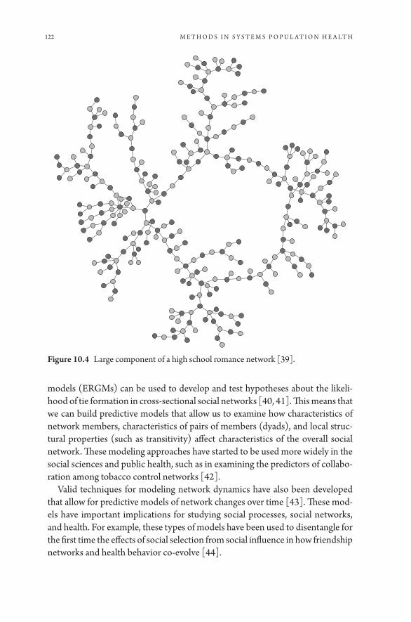
122 M E T H O D S I N S Y S T E M S P O P U L A T I O N H E A LT H
models (ERGMs) can be used to develop and test hypotheses about the likeli-hood of tie formation in cross- sectional social networks [40, 41]. This means that we can build predictive models that allow us to examine how characteristics of network members, characteristics of pairs of members (dyads), and local struc-tural properties (such as transitivity) affect characteristics of the overall social network. These modeling approaches have started to be used more widely in the social sciences and public health, such as in examining the predictors of collabo-ration among tobacco control networks [42].
Valid techniques for modeling network dynamics have also been developed that allow for predictive models of network changes over time [43]. These mod-els have important implications for studying social processes, social networks, and health. For example, these types of models have been used to disentangle for the first time the effects of social selection from social influence in how friendship networks and health behavior co- evolve [44].
Figure 10.4 Large component of a high school romance network [39].

Social Network Analysis 123
5. WHAT ARE SOME IMPORTANT CHALLENGES AND OPPORTUNITIES FOR SOCIAL NETWORK ANALYSIS AND POPULATION HEALTH?
In early 2000 Stephen Hawking called the next century “the century of complexity.” If his prediction proves true, then we will need new theories, methods, and types of data to study these complex social systems. Network science and network analysis provides some of these new approaches and tools. If network science, however, is to benefit our understanding and enhance population health fully, there is one impor-tant challenge to address. Unlike some of the other methods covered in this book (e.g., system dynamics, agent- based modeling), network analysis is predominately an empirical analysis approach. Population health network models need high- quality health- relevant network data. There are no large- scale health surveillance systems that currently collect health- relevant complete network data. Add Health (The National Longitudinal Study of Adolescent to Adult Health) is one important source of whole network data, but that ended new data collection in 2008.
One important opportunity to consider is greater integration of network data and network methods into other types of computational models. In particular, agent- based models of health- related complex systems often incorporate social network data and information. However, these ABMs tend to use simple network structures or data, and there is an opportunity to integrate ABMs with richer and more sophisticated social network data [45].
In summary, it is helpful here to remind ourselves of a call to action from soci-ologist Allen Barton in 1968:
If our aim is to understand people’s behavior rather than simply to record it, we want to know about primary groups, neighborhoods, organizations, social circles, and communities; about interaction, communication, role expectations, and social control [46].
With the rapid integration of network science theories and the widespread use of network data, we are making good progress toward Barton’s vision, thus lead-ing to a more evidence- based population health science.
6. REFERENCES
1. Sporns O. Discovering the human connectome. MIT Press; 2012. 2. Barabasi AL. Network medicine— From obesity to the ‘diseasome.’ New England
Journal of Medicine. 2007; 357: 404– 407. 3. Luke DA, Harris JK. Network analysis in public health: History, methods and appli-
cations. Annual Review of Public Health. 2007; 28: 69– 93.
124 M E T H O D S I N S Y S T E M S P O P U L A T I O N H E A LT H
4. Berkman LF, Glass T, Brissette I, Seeman TE. From social integration to health: Durkheim in the new millennium. Social Science & Medicine. 2000; 51(6): 843– 857.
5. Luke DA, Schoen MW. (in press). Social networks in human disease. In Loscalzo J, Silverman EK, Barabasi AL, Editors. Network Medicine, Complex Systems in Human Disease and Therapeutics.
6. Borgatti SP, Halgin DS. On network theory. Organization Science. 2011; 22: 1168– 1181.
7. Freeman L. The development of social network analysis: A study in the sociology of science. Empirical Press; 2004.
8. Hethcote HW. The mathematics of infectious diseases. SIAM Review. 2000; 42(4): 599– 653.
9. Keeling MJ, Eames KT. Networks and epidemic models. Journal of the Royal Society Interface. 2005; 2(4): 295– 307.
10. Read JM, Eames KT, Edmunds WJ. Dynamic social networks and the implications for the spread of infectious disease. Journal of The Royal Society Interface. 2008; 5(26): 1001– 1007.
11. Rothenberg RB, et al. Using social network and ethnographic tools to evaluate syph-ilis transmission. Sexually Transmitted Diseases. 1998; 25(3): 154– 160.
12. Wylie JL, Cabral T, Jolly AM. Identification of networks of sexually transmitted infec-tion: A molecular, geographic, and social network analysis. The Journal of Infectious Diseases. 2005; 191(6): 899– 906.
13. Valente TW. Network interventions. Science. 2012; 337(6090): 49– 53. 14. Hufnagel L, Brockmann D, Geisel T. Forecast and control of epidemics in a glo-
balized world. Proceedings of the National Academy of Sciences. 2004; 101(42): 15124– 15129.
15. Tizzoni M, et al. Real- time numerical forecast of global epidemic spreading: Case study of 2009 A/ H1N1pdm. BMC Medicine. 2012; 10(165): 1– 31.
16. Brockmann D, Helbing D. The hidden geometry of complex, network- driven conta-gion phenomena. Science. 2013; 342(1337): 1337– 1342.
17. Convertino M, Hedberg C. Optimal surveillance system design for outbreak source detection maximization: A vol model. Proceedings of the 7th International Congress on Environmental Modelling and Software. San Diego, CA; 2014.
18. Christakis NA, Fowler JH. The spread of obesity in a large social network over 32 years. New England Journal of Medicine. 2007; 357(4): 370– 379.
19. Christakis NA, Fowler JH. 2008. The collective dynamics of smoking in a large social network. New England Journal of Medicine. 2008; 358: 2249– 2258.
20. Berkman LF, Syme SL. Social networks, host resistance, and mortality: A nine- year follow- up study of Alameda County residents. American Journal of Epidemiology. 1979; 109(2): 186– 204.
21. Pinquart M, Duberstein PR. Associations of social networks with cancer mortal-ity: A meta- analysis. Critical Reviews in Oncology/ Hematology. 2010; 75(2): 122– 137.
22. Villingshoj M, Ross L, Thomsen BL, Johansen C. Does marital status and altered contact with the social network predict colorectal cancer survival? European Journal of Cancer. 2006; 42 (17): 3022– 3027.

Social Network Analysis 125
23. Flay BR, et al. Differential influence of parental smoking and friends’ smoking on adolescent initiation and escalation of smoking. Journal of Health and Social Behavior. 1994; 35(3): 248– 265.
24. Ennett ST, Bauman KE. Peer group structure and adolescent cigarette smok-ing: A social network analysis. Journal of Health and Social Behavior. 1993; 34 (3): 226– 236.
25. Alexander C, Piazza M, Mekos D, Valente T. Peers, schools, and adolescent cigarette smoking. Journal of Adolescent Health. 2001; 29(1): 22– 30.
26. Pearson M, West P. Drifting smoke rings. Connections. 2003; 25(2): 59– 76. 27. Valente TW, Gallaher P, Mouttapa M. Using social networks to understand and pre-
vent substance use: A transdisciplinary perspective. Substance Use & Misuse. 2004; 39 (10- 12): 1685– 1712.
28. Lakon CM, Hipp JR, Timberlake DS. The social context of adolescent smoking: A systems perspective. American Journal of Public Health. 2010; 100 (7): 1218– 1228.
29. Mercken L, Snijders TA, Steglich C, Vertiainen E, de Vries H. Smoking- based selec-tion and influence in gender- segregated friendship networks: A social network anal-ysis of adolescent smoking. Addiction. 2010; 105(7): 1280– 1289.
30. Valente TW, Fujimoto K, Chou CP, Spruijt- Metz D. Adolescent affiliations and adiposity: A social network analysis of friendships and obesity. Journal of Adolescent Health. 2009; 45(2): 202– 204.
31. Schaefer DR, Simpkins SD. Using social network analysis to clarify the role of obesity in selection of adolescent friends. American Journal of Public Health. 2014; 104: 1223– 1229.
32. Voorhees CC, et al. The role of peer social network factors and physical activity in adolescent girls. American Journal of Health Behavior. 2005; 29(2): 183– 190.
33. Unger JB, McAvay G, Bruce ML, Berkman L, Seeman T. Variation in the impact of social network characteristics on physical functioning in elderly persons: MacArthur Studies of Successful Aging. Journals of Gerontology. Series B: Psychological Sciences and Social Sciences. 1999; 54(5): S245– S251.
34. Gillett PA. Self- reported factors influencing exercise adherence in overweight women. Nursing Research. 1988; 37(1): 25– 29.
35. Luke DA, Stamatakis KA. Systems science methods in public health: Dynamics, net-works, and agents. Annual Review of Public Health. 2012; 33: 357– 376.
36. Auerbach DM, Jaffe HW, Curran JW, Darrow WW. Cluster of cases of the acquired immune- deficiency syndrome— patients linked by sexual contact. The American Journal of Medicine. 1984; 76: 487– 492.
37. Newman MEJ. Networks: An introduction. Oxford University Press; 2010. 38. Liljeros F, Edling CR, Amaral LAN, Stanley HE, Aberg Y. The web of human sexual
contacts. Nature. 2001; 411: 907– 908. 39. Bearman PS, Moody J, Stovel K. Chains of affections: The structure of adolescent
romantic and sexual networks. American Journal of Sociology. 2004; 110: 44– 91. 40. Goodreau SM. Advances in exponential random graph (p*) models applied to a
large social network. Social Networks. 2007; 29: 231– 248. 41. Harris JK. An Introduction to Exponential Random Graph Modeling. Sage
Publications; 2013.

126 M E T H O D S I N S Y S T E M S P O P U L A T I O N H E A LT H
42. Luke DA, et al. Systems analysis of collaboration in 5 national tobacco control networks. American Journal of Public Health. 2010; 100: 1290– 1297. PMCID: PMC2882404
43. Snijders RAB, van de Bunt GG, Teglich CEG. Introduction to actor- based models for network dynamics. Social Networks. 2010; 32: 44– 60.
44. Mercken L, Snijders TA, Vartiainen E, de Vries H. Dynamics of adolescent friend-ship networks and smoking behavior. Social Networks. 2010; 32: 72– 81.
45. IOM (Institute of Medicine). Assessing the use of agent-based models for tobacco regu-lation. Washington, DC: The National Academies Press; 2015.
46. Barton AH. Bringing society back in: Research and macro- methodology. The American Behavioral Scientist. 1968; 12(2): 1– 9.

SECTION 3
Systems Science Toward a
Consequential Population Health


11
Machine Learning
JA M E S H . FAG H M O U S
1. INTRODUCTION
Machine learning has become one of the fastest growing technical fields of the last few decades, aided by an unprecedented ability to create and store data at massive scales, as well as increased computational capabilities such as distributed and cloud computing. Machine learning has shown great promise in domains where data are abundant and the problems lend themselves to classification or regression, and as a result, an increasing number of scientific fields are interested in adopting machine learning techniques to take advantage of their own data del-uge. This chapter introduces non- computational scientists to the general field of machine learning and its methods. We begin by outlining the common structure of machine learning applications. We will then discuss a case study at the inter-section of machine learning and epidemiology: Google Flu Tends. We conclude the chapter with steps on how to begin creating practical machine learning algo-rithms for population health.
2. OVERVIEW
In his classic text, Tom Mitchell defines machine learning as “the study of algo-rithms that improve automatically through experience” [1] . More concretely, the field of machine learning develops algorithms that improve their perfor-mance at a predefined task as more data are observed. There are three parts to this definition. First, machine learning focuses on algorithms and not necessar-ily explanatory models. Second, these algorithms have a clear task whose perfor-mance is measurable. Third, performance is associated mainly with more data.

130 S Y S T E M S S C I E N C E T O W A R D A C O N S E Q U E N T I A L P O P U L A T I O N H E A LT H
An example of a learning problem is predicting hospital re- admissions. The task is to assign a label of re- admission or no re- admission to any given hospital visit record. The performance metric to be improved might be the accuracy of this re- admission classifier, and the training experience might consist of a collection of historical hospital admission records, each labeled in retrospect as leading to a re- admission or not. Alternatively, we might define a different performance metric that assigns a higher penalty when a “re- admission” case is labeled “no re- admission” by the algorithm, compared to when a “no re- admission” is incor-rectly labeled as “re- admission.”
This algorithmic focus is a fundamental departure from statistics, arguably the first science to formalize learning from data. In the statistical sciences, we are interested in descriptive models that can explain the observed data. These models tend to be interpretable especially on reasonable sample sizes. The algo-rithmic approach in machine learning assumes no knowledge about the data generation process and is not concerned with understanding what information leads to statistical skill. Instead, the focus is on maximizing predictive accuracy by optimizing a performance metric (Table 11.1).1
Generally speaking, a learning algorithm searches through a large space of hypotheses, guided by the data, to find a hypothesis that optimizes the perfor-mance metric the task is evaluated on. In practice, a learning algorithm is con-cerned with first selecting the family of hypotheses to search (e.g., mathematical functions, trees, etc.) and then choosing an approach to search through the selected set of hypotheses (e.g., optimization, simulations, etc.).
The rise of machine learning coincided with three major trends. First, the Internet democratized the production, storage, and distribution of data on unprecedented scales, which gave anyone with an Internet connection access to more data than most statisticians ever had in the 1990s. The data explosion enabled learning by examples on a scale that was not possible before the Internet and made the algorithmic approach a valid alternative to mainstream statistical modeling. The second trend was that the Internet not only created new data,
Table 11.1 The Difference Between the Modeling and Algorithmic Approaches to “Learning from Data”
Modeling approach Algorithmic approachFocus Understanding PredictionGoal Understand phenomena Statistical accuracyPriority Interpretability Flexibility (black- box)
1. The late Leo Breiman has a great discussion of the modeling and algorithmic approaches to learn-ing from data in [2] .

Machine Learning 131
it also created a host of problems to be addressed; chief among them was how we manage, annotate, and study the massive amounts of data created on a daily basis (of course, there are other problems such as spam filtering, product recom-mendations, and image annotation, etc.). Finally, the focus on general objective, yet abstract, performance metrics greatly facilitated comparing new methods, which accelerated innovation. This was further aided with the launch of the UCI Machine Learning Repository [3] , which hosts various benchmark data sets that researchers can use to objectively compare algorithm performance. While these focused developments led to rapid growth of machine learning, they also nar-rowed the types of problems it tackled. The algorithmic and learning by example approaches lead machines to focus mainly on classification, regression, and rank-ing problems, as opposed to traditional artificial intelligence tasks such as reason-ing or semantics [4]. Similarly, machine learning does not focus on inference as much as other sciences.
To summarize, machine learning is a field that seeks to learn from large- scale data sets with a large number of observations and numerous dimensions in each observation. The focus of learning algorithms is to produce a formula that maps new data (input) to a correct output based on input- output examples used to train the model. More recently, thanks to advances in cloud and dis-tributed computing, we are able to learn from these large data sets and deploy algorithms in real- world settings, such as self- driving cars. As a result, there has been an increasing focus on scalability and operational performance of such methods, as opposed to understanding the formal properties of the resulting input- to- output formula. It is important to note the differences between prob-lems traditionally tackled in machine learning and those that emerge in pop-ulation health. Not every data- driven investigation within population science will warrant a machine learning approach. Instead, we must focus on problems where relevant and abundant data are available, where the goal is to forecast an outcome as opposed to estimating the effect of an intervention, and where there is a premium on creating a real- world working system as opposed to a traditional research study.
3. MACHINE LEARNING PRINCIPLES
3.1. Anatomy of a machine learning application
We begin by broadly defining a machine learning problem and the steps that are commonly taken to produce a machine learning application. Given a data set, we need to split it into training and testing data sets. The training data set is used to build the model independent of the testing data. The testing data is used to objectively evaluate the quality of the learned model. It is important

132 S Y S T E M S S C I E N C E T O W A R D A C O N S E Q U E N T I A L P O P U L A T I O N H E A LT H
that the training and testing data sets be independent but representative of the overall data distribution. Next, the researcher chooses a family of models to fit (e.g., linear regression). Each model is governed by a set of parameters (e.g., slope and intercept for linear regression), and a model is fit to the data, by estimating its parameters using the training data set. Model parameters are fit through an iterative process where the parameters are slightly modified until a parameter choice that minimizes an objective function is identified (optimiza-tion [5] is an active field of research dedicated to this iterative process). The trained or fit model is then tested using the independent training data set to see how well the model generalizes to unseen data. If the model performs well on the training data, but poorly on the testing data, the model is said to have overfit the data. Overfitting is similar to brute force memorization instead of learning the general concepts of a problem. The final model and parameters are often referred to as a hypothesis.
It is important to note that machine learning can only estimate a function from observations. This is because it is assumed that any observation used to train the model is obtained using the true function we wish to estimate and an independent error that is unrelated to the observation (e.g., measurement error in an instrument; this is also known as irreducible error). The exact way that an algorithm executes the above- mentioned procedure depends on a few factors we discuss below.
3.2. Learning
One aspect that is unique to machine learning is the notion of learning. A broad view of learning is the assumption that given enough observations, we can learn an underlying process behind the data. Depending on the data we have, there are several variations of this learning process. Supervised learn-ing refers to settings where we have access to both the data and target labels and the data come in explicit input- output pairs. This can be thought of as learning by example. Unsupervised learning refers to the setting when no labels are given to the user (e.g., in the hospital example, we do not know who got readmitted in the past). In this setting, exploratory tasks are usually favored. Active learning refers to the setting where there is a small set of training exam-ples, but the algorithm has the opportunity to get new examples at a cost (e.g., ask an expert to create a new input- output pair). Finally, in reinforcement learn-ing, instead of having input- output pairs, the algorithm only knows for a given input whether the output is correct or not. If the output is incorrect, the algo-rithm still needs to identify the correct output. This approach is commonly used in the autonomous solving of puzzles and adversarial games [6] .

Machine Learning 133
3.3. Model Evaluation
For much of this chapter we will focus on supervised learning problems, where we assume we are given input- output pairs to learn a mapping between inputs and outputs. As mentioned earlier, a learning algorithm will search for a set of hypotheses that maximizes an evaluation metric or minimizes the error of a task. How do we know if the algorithm has learned? The concept of learning comes from the theory of generalization, where we measure the error on unseen (out- of- sample) data and compare it to the error on the examples used to train the model. Specifically, an algorithm is said to have learned if the difference between the in- sample and out- of- sample errors is small (known as Hoeffding’s Inequality).
3.4. Flexibility Versus Interpretability
We introduced the notions of in- sample and out- of- sample errors because they are critical in practical design decisions. Specifically, as we train a model to learn from (in- sample) data, we seek to minimize the error within this sam-ple. However, solely focusing on minimizing the in- sample error will lead us to choose increasingly complex hypotheses that will indeed minimize the in- sample error by “fitting” the data very well. However, fitting the training too well usu-ally means that the model is learning about the peculiarities of the training data (e.g., noise, or what we referred to earlier as irreducible error) as opposed to the underlying process. This results in poorly generalizable hypotheses, where the difference between the out- of- sample error and the in- sample error are too large. On the other hand, a less complex hypothesis set would give a better chance of generalizing to unseen data. As a result, a central concept in machine learning is that of maximizing model complexity while minimizing out- of- sample error, known as the bias- variance tradeoff. This notion is also important from a popula-tion health (and interdisciplinary) perspective. As algorithms are able to model increasingly complex functions (i.e., they are more flexible to fit the data), they become harder and harder to interpret from a domain perspective. Hence, in practice, a model might be statistically accurate but scientifically uninterpretable. In these settings, we would seek to maximize statistical accuracy while maintain-ing a minimum level of scientific interpretability.
3.5. Challenges in Machine Learning Applications
While machine learning offers a wide range of methods and approaches that are appropriate for numerous settings, including regression methods, artificial neu-ral network approaches, and decision tree methods, there are notable challenges
134 S Y S T E M S S C I E N C E T O W A R D A C O N S E Q U E N T I A L P O P U L A T I O N H E A LT H
that we must be aware of before embarking on a machine learning project in population health.
3.6. Data Empathy
A fundamental assumption in machine learning is that there is a process generat-ing observations on hand and that the data are representative of such a process. These assumptions usually hold for when the data are large and observations are independent of each other. However, in practical settings we cannot take these assumptions for granted. Thus, a level of data empathy [7] is needed to under-stand why and how the data were collected. Recently, we have seen efforts in open science to create “data descriptors” to afford users a more nuanced understanding of data they are about to analyze. In addition to lack of familiarity with the data, another challenge is that numerous data sets are collected without any consulta-tion with machine learning experts to advise on the types of data required to perform the needed analysis. As a result, a large number of data sets that currently exist in the sciences are ill- suited to tackle traditional machine learning problems. This design flaw of thinking about the machine learning steps only after data col-lection are common across disciplines and industries. However, the biggest dis-advantage science faces is that data collection tends to be a time- consuming and expensive process. This is in contrast to Internet applications, where if a design flaw is identified, we could deploy a new data collection initiative and begin col-lecting samples within minutes.
3.7. Multiple Hypothesis Testing
One of the challenges we face in complex high dimensional settings is the abil-ity of our model to generalize to unseen data and other settings. A common challenge in exploratory research is to ensure that, as we adaptively design our model (by repetitively training and testing it), our test data remain independent from the training data. This iterative approach to model tuning based on repeti-tive testing is known as adaptability, or “the garden of forking paths” [8] , and is an implicit multiple hypothesis testing problem that is not easily captured in traditional significance tests or techniques that control for false discovery rate [9]. The most appropriate way to address this challenge is to list in advance the hypotheses and experiments that will be undertaken; once the experiments are run, the data should no longer be used. This is not feasible in exploratory settings or where new data are not readily available. Thus, we need more robust mecha-nisms to partition the data into training and testing sets that are independent but also representative. Recent work has suggested new approaches to safely reuse a
Machine Learning 135
holdout data set without affecting the generalizability of the resulting model [10]. However, in other instances we will need to ensure that the training and testing data maintain the overall context of the data. For example, it has been shown that certain adverse health outcomes cluster over distinct spatial locations. There is a high likelihood that a uninformed split of the data may cause the training data to only have the spatial bias and not the test data set (or vice versa) that would lead to a poorly generalizable model.
3.8. Beyond Accurate Models
Based on the survey of the machine learning methods available to population health researchers, there remains a question of the utility of such methods for core population health research tasks. In order to create intervenable insights, more work is needed beyond the world of data and algorithms. Issues of communica-tion, persuasion, and mobilization become nearly as critical as the science itself. There are some avenues for intervention (or at least suggesting interventions) by creating interpretable models where we can understand the impact of covari-ates and their interactions on a target outcome. Furthermore, we can leverage advances in microsimulations, so that once the model is fit we can impose changes to a covariate and simulate the output’s response to such change. Finally, as more complex questions beyond “understanding” are sought in Internet domains, new research efforts are emerging on how to identify causal effects from observational data [11].
4. CASE STUDY: GOOGLE FLU TRENDS
Machine learning has rapidly become a valuable tool in the toolkit of most data- driven researchers. Its recent success has even pushed some to call for the “End of Theory” [12], where one could forgo scientific theory if there are sufficient data available.
A good example at the intersection of machine learning and epidemiology is Google Flu Trends. In 2009, a team of Google researchers reported being able to predict the incidence of flu outbreaks by analyzing the millions of flu- related search queries that are input into the Google search engine. The model worked so well that it accurately detected outbreaks much quicker than the Centers for Disease Control and Prevention [13]. More recently [14, 15], however, it has been shown that for consecutive years Google made more bad predictions than good ones. This raises questions about the usefulness of big data in population health and other settings. It is important to point out that there is nothing fun-damentally wrong about what the Google team did— thousands of machine
136 S Y S T E M S S C I E N C E T O W A R D A C O N S E Q U E N T I A L P O P U L A T I O N H E A LT H
learning teams take the same prediction- based approach. Because of the high visibility of Google as well as that of the initial publication (Nature), what we witnessed was the messy iterative process of machine learning unfolding in the public eye. There were, however, some problems with the approach taken. First, as is the case with any machine learning algorithm, its success hinges on the qual-ity of the data available. This is why data empathy is so important. However, in Google’s case, the algorithm had no control over the data or search queries, and there might have been significant sampling biases. Furthermore, the relation-ship between the inputs and the outputs is not obvious. For instance, while it is perfectly plausible that people might search for flu symptoms because they are feeling ill, it is also possible that populations search for flu symptoms because of timely media coverage. Finally, it seemed like there was no scientific hypoth-esis as to why the algorithm worked well in practice— were there other metrics beyond statistical accuracy that would provide additional evidence to the power of this approach? Could the authors verify the accuracy of their model by com-paring the predicted spatio- temporal spread of the disease to more traditional epidemiological models?
In hindsight, the Google Flu Trends approach suffers, like many data- driven scientific endeavors, from the siloed approach to data collection, scientific enquiry, and algorithmic techniques— all of which are developed almost inde-pendently of one another. Instead, what we must see in the future are diverse teams coming together to form a homogeneous unit of data collection, algo-rithmic design, and scientific hypothesis generation/ verification. Interestingly, Google recently announced that it will provide its model to various scientific institutions, including the Centers for Disease Control and Prevention. This is a more prudent approach, more in line with the collaborative spirit, that we believe is necessary to make machine learning actionable in the sciences.
5. THE ROAD AHEAD
In this chapter, we introduced the main principles of machine learning and highlighted unique aspects of the field compared to statistics and other quan-titative fields of study. It is important to remember that machine learning is a relatively new field. Many new advances will emerge in the near future, some of which will have transformational impact across disciplines. However, in order to fully take advantage of the state- of- the- art in machine learning, population health researchers must develop a basic understanding of the discipline and create deep bonds with practitioners. The platonic collaborations (consultan-cies) between scientists and machine learning experts are not conducive to the level of integration necessary to fully leverage the deep insights developed over decades of scientific research and the multiplicative potential of machine
Machine Learning 137
learning. In the near future, we hope to see a seamless integration of machine learning advances with deep population health knowledge, where the product of the two would be an inseparable process of data- driven scientific discovery.
6. ACKNOWLEDGMENTS
The author would like to acknowledge the generous support of the National Science Foundation (Award 1464297).
7. REFERENCES
1. Mitchell TM. Machine Learning. McGraw Hill; 1997. 2. Breiman L, et al. Statistical modeling: The two cultures (with comments and a
rejoinder by the author). Statistical Science. 2001; 16: 199– 231. 3. Asuncion A, Newman D. UC Irvine machine learning repository. 4. Langley P. The changing science of machine learning. Machine Learning. 2011;
82: 275– 279. 5. Bennett KP, Parrado- Hernández E. The interplay of optimization and machine learn-
ing research. The Journal of Machine Learning Research. 2006; 7: 1265– 1281. 6. Silver D, et al. Mastering the game of go with deep neural networks and tree search.
Nature. 2016; 529, 484– 489. 7. Faghmous JH, Kumar V. A big data guide to understanding climate change: The case
for theory- guided data science. Big Data 2. 2014; 155– 163. 8. Gelman A, Loken E. The garden of forking paths: Why multiple comparisons can be
a problem, even when there is no fishing expedition or p- hacking and the research hypothesis was posited ahead of time; 2013.
9. Gelman A, Loken E. The statistical crisis in science. American Scientist. 2014; 102: 460.
10. Dwork C, et al. The reusable holdout: Preserving validity in adaptive data analysis. Science. 2015; 349: 636– 638.
11. Brodersen KH, et al. Inferring causal impact using bayesian structural time- series models. The Annals of Applied Statistics. 2015; 9: 247– 274.
12. Anderson C. The end of theory: The data deluge makes the scientific method obsolete; 2008.
13. Ginsberg J, et al. Detecting influenza epidemics using search engine query data. Nature. 2009; 457: 1012– 1014.
14. Cook S, Conrad C, Fowlkes AL, Mohebbi MH. Assessing google flu trends perfor-mance in the United States during the 2009 influenza virus a (h1n1) pandemic. PLOS ONE 6. 2011; e23610.
15. Lazer D, Kennedy R, King G, Vespignani A. The parable of google flu: Traps in big data analysis. Science. 2014; 343.


12
Systems Science and the Social Determinants
of Population Health
DAV I D S. F I N K , K AT H E R I N E M . K EY E S, A N D MAG DA L E NA C E R D Á
1. INTRODUCTION
The distribution of health, both within and between populations, is often described with three statistics that communicate a measure of the central ten-dency, spread, and shape of that distribution. Mean life expectancy at birth, to take one measure of the central tendency, averaged 71 years worldwide in 2013 [1] . However, the mean can conceal the distribution’s spread: while the average world-wide life expectancy at birth is 70 years, the spread between countries is 38 years, from 46 years in Sierra Leone to 84 years in Japan. Finally, the shape of a distri-bution communicates the symmetry of the distribution. For example, mean life expectancy at birth is left skewed among the World Health Organization regions, such that the African region’s mean life expectancy is 58 years, which is 10 years below the next lowest regions (i.e., Southeast Asia and Eastern Mediterranean) and nearly 13 years below the worldwide mean of 71 years. The global distribu-tion of life expectancy reveals that lower life expectancy is found among people who are born into poverty, afflicted by political upheaval, or marginalized within their own countries [2]. Both within and between populations, the differences in the distribution of health reveal what Paul Farmer called the “biological reflec-tions of social fault lines” [3].
The distribution of health within and across populations is driven by a com-bination of factors that lie above the individual and shape their actions and interactions within societies. Examples of these factors include the social struc-ture, the economy and corporate practices, and political factors (e.g., taxation, environmental regulation). These macrosocial factors create differential access

140 S Y S T E M S S C I E N C E T O W A R D A C O N S E Q U E N T I A L P O P U L A T I O N H E A LT H
to resources and opportunities and influence the level and the distribution of health and disease across and within populations. In population health, we aim to identify the upstream factors that shape health and to understand how we might intervene in effective ways both to improve population health overall and to reduce health inequality. The health inequalities that arise from an unequal distribution of such macrosocial factors are of particular interest to population health sciences.
The drive to understand the processes that shape population health, and to identify the pathways that connect macrosocial factors to patterns of health and to health inequalities, has traditionally relied on a range of archival and survey data on social factors and health conditions at multiple levels— and on the use of analytic approaches such as multilevel models for the investigation of linear relationships between these factors and individual health states. Yet the relation between macrosocial factors and population health often arises from the collec-tive actions of individuals, social structures, and population dynamics, in addi-tion to the influence of individuals who comprise populations, requiring analytic strategies that take account of such a complex system of non- linear dynamics.
Systems science approaches have provided the methodological armamentar-ium to examine the complex processes that drive population health and produce inequalities in health. In this chapter, we will review three critical contributions that systems science approaches have made to population health science. First, a systems science approach has helped us model how health inequalities shape population health. Second, it has elucidated how feedback cycles between micro- and macro- level processes produce population health. Third, it has been used to identify targets for intervention in order to reduce inequalities in health. These contributions are not exclusive to systems science but rather steps that can be taken by population health scientists who employ systems science approaches to identify health inequalities, determine what causes them, and provide informed prevention strategies to ameliorate such health inequalities.
Systems science approaches are varied and include agent- based models, systems dynamic models, and network models, among others. In this chap-ter, we focus on agent- based models (ABM) but include other systems science approaches as relevant in order to complement the discussion. In brief, ABMs consist of simulations that follow prescribed rules about the characteristics of agents, their networks, contexts, and behaviors. By running simulations, we can observe how rules specified at the individual level produce population- level pat-terns. ABMs allow us to specify interdependence between agents and the spread of agent behaviors. Agent interactions can be a function of spatial proximity to other agents or based on a social network structure. Agents can also be placed within larger contexts such as workplaces, neighborhoods, and cities.

Systems Science and the Social Determinants of Population Health 141
2. IDENTIFYING HEALTH INEQUALITIES
Systems science approaches have made two important contributions to under-standing the drivers of health inequalities. First, in systems thinking, macro- level patterns of health emerge from the characteristics and behaviors of individuals embedded in different contexts and defined by their relations to each other. In this way, systems approaches force us to identify the processes at multiple levels that generate observed patterns of inequality. For example, in the United States, black men are over 6 times more likely to be incarcerated than their white coun-terparts. Kristian Lum and colleagues [4] have argued that the process of incar-ceration can be conceptualized similarly to a virus, one that is spread through social networks, and highlight several potential mechanisms for this process, including that an individual’s incarceration can expose his or her family to a net-work of criminals [5] and expose both their friends and family to closer police scrutiny [6, 7]. Furthermore, blacks are significantly more likely to be both sen-tenced [8] and receive longer sentences [9] than whites, even after controlling for legal factors and social context. Therefore, Lum and colleagues [4] employed an ABM to show how the social spread of incarceration through social networks, combined with modest racial differences in sentencing (i.e., blacks sentenced on average 3 months more than whites over a period of 25 years for the same crime), could produce the racial disparities that are currently observed in the United States. This study illustrated how small disturbances (i.e., likelihood and length of incarceration) in one part of a system can generate substantial changes in another part of the system (i.e., blacks are 6 times more likely to be incarcer-ated than whites), replicating the mechanisms whereby social inequalities can generate health inequalities.
Second, in systems science analytics (e.g., ABMs), we can change either one aspect of the initial conditions or multiple aspects of the initial conditions to identify causal effects and causal mechanisms, respectively [10]. By doing so, we can identify contextual factors that have the potential to modify an interven-tion’s effect on population health, amplifying or reducing inequalities in health. A recent study we conducted on the impact of universal versus targeted inter-ventions on health inequalities illustrated how fundamental causes of population health, such as residential segregation, might modify the effectiveness of inter-ventions in reducing inequalities [11]. As a test case to investigate this point, we created an ABM that simulated whether a universal (citywide) or targeted (to the most violent neighborhoods) increase in collective efficacy could reduce racial/ ethnic inequalities in homicides in New York City (see Figure 12.1). From 2009 through 2013, the annual rate of homicide in the United States among blacks was over five times higher than whites [12]. Robert J. Sampson and colleagues [13] have argued that lower levels of collective efficacy (defined as “social cohesion

Other
200
A
150
100
50
0
0 50 100 150 200
$75
k+$4
0k–
$74
k$2
0k–
$39
k<
$20
k
Hispanic Black White
200B
150
100
50
0
0 50 100 150 200
Figure 12.1 Agent locations in a grid of neighborhoods, with agents (a) segregated in neighborhoods by race and income, or (b) assigned random locations [11].Note. Each racial/ ethnic group is represented by a different shade of gray (black: other non- Hispanic; medium gray: Hispanic; light gray: black non- Hispanic; lightest gray: white non- Hispanic). Darker circles reflect higher income levels within each racial/ ethnic group.
Systems Science and the Social Determinants of Population Health 143
among neighbors combined with their willingness to intervene on behalf of the common good”) present in economically disadvantaged neighborhoods place residents at higher risk of violence. Using this ABM, we observed that a univer-sal strategy lowered overall rates of violent victimization; however, neither the universal nor the targeted prevention strategy reduced racial/ ethnic inequalities in victimization. We were concerned that this failure to reduce inequalities in homicides may be due to segregation of blacks into low- income neighborhoods, which would, in the long term, reduce collective efficacy and continue to drive higher rates of homicide. We thus simulated the same interventions under three alternative scenarios: (1) complete racial/ ethnic residential segregation across the city; (2) intermediate segregation; and (3) no segregation. Racial/ ethnic inequalities in victimization were only reduced through the elimination of resi-dential segregation (i.e., scenario 3). This study illustrates how, by using a system science approach to simulate a series of different interventions under a range of counterfactual scenarios of segregation (something impossible to observe in the real world), we were able to visualize how targeting proximal risk factors such as collective efficacy could fail to reduce health inequalities if we do not address the fundamental drivers of health inequalities [14].
3. UNDERSTANDING FEEDBACK
Systems science analytics are particularly well suited to help us understand the influence of feedback between micro- and macro- level processes that drive popu-lation health and health inequalities. James Ladyman and colleagues [15] explain that “(a) part of a system receives feedback when the way its neighbors interact with it at a later time depends on how it interacts with them at an earlier time.” Consider a series of neighborhoods, comprising heterogeneous households, where each household prefers to live near neighbors that share a recognizable characteristic (e.g., race/ ethnicity). Each household’s decision either to stay in their current neighborhood or relocate to a new neighborhood depends on the characteristics of their current neighbors, but after the household makes their decision to stay or relocate, each neighbor will make a similar decision in response to their neighbors’ movements. An early example of the application of systems science approaches to the generation of residential segregation dynamics illus-trated this process [16], showing how household preferences about location can give rise collectively to population segregation and neighborhood tipping points. In this model, every unit was assigned membership into one of two permanent and recognizable groups (i.e., black and white ethnicity). Through a series of dis-crete intervals each unit evaluated their current situation and decided whether to stay in their current location or relocate to a new area based on whether the color mixture in their current space was acceptable (i.e., half or more of the eight

144 S Y S T E M S S C I E N C E T O W A R D A C O N S E Q U E N T I A L P O P U L A T I O N H E A LT H
adjacent neighbors were of a similar color). This study contributed two impor-tant findings about the drivers of residential segregation. First, each unit is con-stantly affected by the decisions of others; irrespective of a unit’s decision to stay or relocate, everybody else’s movements will affect each unit’s location prior to the next interval, precipitating future movement. This chain of cause- and- effect between movement at the individual level and neighborhood composition at the group level produces a feedback loop. Second, it is through this feedback that the behavior of micro- level units give rise to macro- level phenomena (segregation).
More advanced ABMs have considered multiple contemporaneous feedback processes to understand the influence of place- related factors on creating health inequalities [17– 19]. An illustrative example relates to the influence of place- related factors on food preferences. It has been proposed that reduced access to healthy and affordable foods in low- income neighborhoods likely helps shape dif-ferences in food preferences between low- and high- income households [17, 18], forming a feedback loop between individual behavior and neighborhood mar-kets whereby availability drives preferences, which then affect availability. To identify the drivers of income inequalities in diet, Amy H. Auchincloss and col-leagues [19] employed an ABM that assigned households and stores behaviors based on their access to healthy foods and customers, respectively. In this model, each household’s decision to shop at a store was driven by food price, distance, and preferences for healthy foods, whereas stores decided to change location and food type in response to their customer base. Through these feedback processes, Auchincloss and colleagues found that the currently observed patterns of income differentials in access to healthy foods arise from the total segregation of high- income households and health food venues from low- income and unhealthy food venues. This finding refuted the hypothesis that inequalities in diet reflect difference in food preferences between low- and high- income households. Next, using the segregation scenario where income differentials in diet emerged (i.e., total segregation), Auchincloss and colleagues examined under what conditions healthy food prices and preferences could overcome or exacerbate the effects of segregation on healthy diet. In this series of experiments, the currently patterned segregation of healthy food stores to high- income areas could be reversed by simultaneously changing food preferences among low- income households and reducing food prices. Although these models do not require the explicit specifi-cation of interventions that can simultaneously shift both food preferences and prices, they provide evidence that synergistic interventions will be required to ameliorate the currently patterned health inequalities.
This in silico experiment by Auchincloss and colleagues [19] examined the interdependencies between household choices and business decisions, and how dynamic feedback over time between the changes in household choices and business decisions gave rise to either salubrious or deleterious household health
Systems Science and the Social Determinants of Population Health 145
behaviors. In addition, studies have documented that these reenforcing feedback cycles produce and maintain contextual factors that influence violent victimiza-tion and racial/ ethnic segregation [11], physical activity and built environment [20, 21], and alcohol consumption and density of alcohol retailers [22]. As these examples illustrate, systems science methods can be used to ask questions about the dynamic mechanisms through which macrosocial determinants of popula-tion health produce health inequalities.
4. IMPROVING INTERVENTIONS
Finally, systems science approaches have helped us identify targets for interven-tion to reduce health inequalities. While many of the previous examples have tested manipulable factors that could inform policy interventions to target health inequalities, the following models were explicitly built to optimize interventions and inform future policy decisions. Although several models have been built to represent a very specific population or geographic area [23], this specificity comes at a cost to generalizability— that is, the closer a model is built to represent a specific population or location, the less likely its findings will be generalizable to other societies with different mobility patterns, structural factors, and distribu-tions of individual- level risk factors. As such, some studies aim to examine more fundamental processes to increase their generalizability.
Systems science approaches can be used to identify hypothetical points of intervention that will obtain optimum improvement in population health. Previous models have compared individual- versus structural- level interventions [23– 25], active versus passive interventions [26], and primary versus tertiary prevention [27– 29]. In one study, we investigated whether a population- level violence prevention intervention (i.e., hot- spot policing) or an individual- level treatment intervention (i.e., cognitive behavioral therapy [CBT]) could produce a greater reduction in the burden of violence- related posttraumatic stress disor-der in urban areas [27]. In this model, we observed an equally slight reduction in the annual prevalence of violent victimization from implementing either hot- spot policing for 10 years or increasing CBT by 100% for 30 years; however, the joint implementation of hot- spot policing and a 50% increase in CBT resulted in a similar reduction in just five years. Much systems science literature has rep-licated our observation that interventions can work synergistically to obtain optimum improvement in population health [19, 20, 28]. Because the develop-ment, implementation, and long- term evaluation of community health interven-tions can be costly, ABMs have provided a particularly attractive opportunity to sequentially evaluate several competing intervention approaches to determine those most likely to provide population health benefits.

146 S Y S T E M S S C I E N C E T O W A R D A C O N S E Q U E N T I A L P O P U L A T I O N H E A LT H
Systems science approaches can also be used to simulate the effect of inter-ventions within a context of social transmission of health- related behaviors and interference. Interference refers to the process through which an individual’s exposure status in the study influences another’s outcome. Because the deci-sion to consume tobacco is partly social [30], and because an intervention on tobacco use affects not only the smoker but also others around the smoker, issues of interference [30, 31] influence the effect of tobacco control interventions on smoking. In 2003 the National Cancer Institute (NCI) began the Initiative on the Study and Implementation of Systems (ISIS) project that aimed “to use sys-tems thinking approaches and theory to address previously intractable issues, to improve the health outcomes associated with tobacco control and, by corol-lary, to improve all of public health” [32]. Furthermore, the Center for Tobacco Products (CTP) at the US Food and Drug Administration (FDA) employed two population models, SimSmoke and the Cancer Intervention and Surveillance Modeling Network (CISNET), to examine whether increasing the minimum legal age (MLA) to purchase tobacco from 18 to 19, 21, or 25 decreased ini-tiation rates among persons under 18 [33]. As the majority of underage per-sons rely on social contacts (e.g., acquaintances, friends, family) to get tobacco, the study hypothesized that raising the MLA to age 21 or above, compared to 19 years, would produce the greatest social distance between underage persons and potential sources that could legally purchase tobacco. Indeed, in these mod-els, raising the MLA from 18 to 19, 21, or 25 would result in respectively about a 10%, 25%, or 30% decrease in initiation rates of smoking among 15– 17 year olds. Further, this study found that raising the MLA to 21 or above reduced the likelihood that persons under age 18 would be in the same social networks as those who can legally obtain tobacco and, consequently, reduce tobacco initia-tion rates among persons under 18. By applying the intervention to persons aged 19 or older and measuring the outcome in those under 18, this study showed how modeling interference among agents can be exploited to both identify and maximize intervention effects.
The utility of systems science methods to evaluate a broad range of pub-lic health interventions is clear. Policymaking is difficult, but system science approaches can be used to weigh the costs and benefits paid and accrued by dif-ferent groups under multiple counterfactual interventions [10], while simulta-neously considering intervention effects on both the entire population and the sub- groups that comprise that population. Indeed, much research has docu-mented that individual- based medical interventions disproportionately favor the health of people occupying higher socioeconomic positions within societies, act-ing to perpetuate and exacerbate extant health inequalities. As such, taking an equity- focused approach to policymaking is particularly important to reduce the growing health inequalities that exist within our societies.

Systems Science and the Social Determinants of Population Health 147
5. CONCLUSIONS
Traditionally in public health and other sciences we have looked to behavioral risk factors that vary within populations as potential manipulable exposures that cause poor health, and there have been calls to move even further “downstream” to examine individual differences in biological factors. Yet such approaches make it more difficult to grapple with the macrosocial determinants and processes that create and maintain health inequalities. Systems science approaches provide both the theory and the tools to examine structural and macrosocial factors, allowing us to hypothesize about the fundamental drivers that shape health and how we might intervene on them in effective ways both to improve population health overall and to reduce health inequality. The years to come will be an exciting time for complex systems modeling in population health science, as more scholars are trained in these methods and technical and methodological innovation contin-ues to push the field forward. Increasing recognition that the systems that under-lie the generation of our data are critical to answer questions regarding how to improve population health will benefit our science and our ability to intervene for a healthier society.
6. ACKOWLEDGEMENTS
Parts of this paper are adapted from Fink DS, Keyes KM, Cerdá M. Social Determinants of Population Health: A Systems Sciences Approach. Current Epidemiologic Reports. 2016; 3(1): 98– 105. The work in this chapter was sup-ported in part by a research grant from the US National Institute on Drug Abuse of the National Institute of Health (grant number T32DA031099).
7. REFERENCES
1. World Health Organization. World Health Statistics 2015. Geneva, Switzerland: WHO Press; 2015.
2. United Nations. The International Forum for Social Development: Social Justice in an Open World; The Role of the United Nations. New York, NY: United Nations, Department of Economic and Social Affairs. Division for Social Policy and Development; 2006.
3. Farmer P. Infections and Inequalities: The Modern Plagues. Berkeley and Los Angeles, CA: University of California Press; 2001.
4. Lum K, Swarup S, Eubank S, Hawdon J. The contagious nature of imprisonment: An agent- based model to explain racial disparities in incarceration rates. Journal of the Royal Society, Interface/ the Royal Society. 2014; 11(98): 20140409.
5. Sutherland E, Cressey D. Criminology. 9th ed. Philadelphia, PA: Lippincott; 1974. 6. Farrington DP, Jolliffe D, Loeber R, Stouthamer- Loeber M, Kalb LM. The concen-
tration of offenders in families, and family criminality in the prediction of boys’ delinquency. Journal of Adolescent Health. 2001; 24(5): 579– 596.

148 S Y S T E M S S C I E N C E T O W A R D A C O N S E Q U E N T I A L P O P U L A T I O N H E A LT H
7. Besemer S, Farrington DP, Bijleveld CC. Official bias in intergenerational transmis-sion of criminal behaviour. British Journal of Criminology. 2013; 53(3): 438– 455.
8. Mitchell O. A meta- analysis of race and sentencing research: Explaining the incon-sistencies. Journal of Quantitative Criminology. 2005; 21(4): 439– 466.
9. Tonry M. The social, psychological, and political causes of racial disparities in the American criminal justice system. Crime and Justice. 2010; 39(1): 273– 312.
10. Marshall BD, Galea S. Formalizing the role of agent- based modeling in causal infer-ence and epidemiology. American Journal of Epidemiolgy. 2015; 181(2): 92– 99.
11. Cerdá M, Tracy M, Ahern J, Galea S. Addressing population health and health inequalities: The role of fundamental causes. American Journal of Public Health. 2014; 104 (Supplement 4): S609– S619.
12. Centers for Disease Control NCFHS. Underlying cause of death 1999- 2013 on CDC WONDER online database, released 2015. Data are from the Multiple Cause of Death File, 1999- 2013, as compiled from data provided by the 57 vital statistics jurisdictions through the Vital Statistics Cooperative Program. 2015.
13. Sampson RJ, Raudenbush SW, Earls F. Neighborhoods and violent crime: A multi-level study of collective efficacy. Science. 1997; 227(5328): 918– 924.
14. Link BG, Phelan J. Social conditions as fundamental causes of disease. Journal of Health and Social Behavior. 1995; Spec No: 80– 94.
15. Ladyman J, Lambert J, Wiesner K. What is a complex system? European Journal for Philosphy of Science. 2013; 3(1): 33– 67.
16. Schelling TC. Dynamic models of segregation. Journal of Mathematical Sociology. 1971; 1: 143– 186.
17. Story M, Kaphingst KM, Robinson- O’Brien R, Glanz K. Creating healthy food and eating environments: Policy and environmental approaches. Annual Review of Public Health. 2008; 29: 253– 272.
18. Leonard T, McKillop C, Carson JA, Shuval K. Neighborhood effects on food con-sumption. Journal of Behavioral and Experimental Economics. 2014; 51: 99– 113.
19. Auchincloss AH, Riolo RL, Brown DG, Cook J, Diez Roux AV. An agent- based model of income inequalities in diet in the context of residential segregation. American Journal of Preventive Medicine. 2011; 40(3): 303– 311.
20. Yang Y, Diez Roux AV, Auchincloss AH, Rodriguez DA, Brown DG. A spatial agent- based model for the simulation of adults’ daily walking within a city. American Journal of Preventive Medicine. 2011; 40(3): 353– 361.
21. Yang Y, Diez Roux AV, Auchincloss AH, Rodriguez DA, Brown DG. Exploring walk-ing differences by socioeconomic status using a spatial agent- based model. Health & Place. 2012; 18(1): 96– 99.
22. Gruenewald PJ. The spatial ecology of alcohol problems: Niche theory and assorta-tive drinking. Addiction. 2007; 102(6): 870– 878.
23. Blok DJ, de Vlas SJ, Bakker R, van Lenthe FJ. Reducing income inequalities in food consumption: Explorations with an agent- based model. American Journal of Preventive Medicine. 2015; 49(4): 605– 613.
24. Yang Y, Diez- Roux AV. Using an agent- based model to simulate children’s active travel to school. International Journal of Behavioral Nutrition and Physical Activity. 2013; 10: 67.

Systems Science and the Social Determinants of Population Health 149
25. Mahamoud A, Roche B, Homer J. Modelling the social determinants of health and simulating short- term and long- term intervention impacts for the city of Toronto, Canada. Social Science & Medicine. 2013; 93:247– 255.
26. Dray A, et al. Are drug detection dogs and mass- media campaigns likely to be effective policy responses to psychostimulant use and related harm? Results from an agent- based simulation model. International Journal of Drug Policy. 2012; 23(2): 148– 153.
27. Cerdá M, Tracy M, Keyes KM, Galea S. To Treat or to Prevent?: Reducing the popu-lation burden of violence- related post- traumatic stress disorder. Epidemiology. 2015; 26(5): 681– 689.
28. Marshall BD, et al. A complex systems approach to evaluate HIV prevention in met-ropolitan areas: Preliminary implications for combination intervention strategies. PLOS ONE. 2012; 7(9): e44833.
29. El- Sayed AM, Seemann L, Scarborough P, Galea S. Are network- based interventions a useful antiobesity strategy? An application of simulation models for causal infer-ence in epidemiology. American Journal of Epidemiolgy. 2013; 178(2): 287– 295.
30. Christakis NA, Fowler JH. The collective dynamics of smoking in a large social net-work. New England Journal of Medicine. 2008; 358(21): 2249– 2258.
31. Oberg M, Jaakkola MS, Woodward A, Peruga A, Pruss- Ustun A. Worldwide bur-den of disease from exposure to second- hand smoke: A retrospective analysis of data from 192 countries. The Lancet. 2011; 377(9760): 139– 146.
32. National Cancer Institute. Greater Than the Sum: Systems Thinking in Tobacco Control. Bethesda, MD: U.S. Department of Health and Human Services, National Institute of Health, National Cancer Institute; 2007.
33. Institute of Medicine. Public Health Implications of Raising the Minimum Age of Legal Access to Tobacco Products. Washington, DC: The National Academies Press; 2015.

13
Systems Approaches to Understanding How
the Environment Influences Population Health
and Population Health Interventions
M E L I S S A T RAC Y
Population health is determined through a multitude of interrelated factors, including features of the social and physical environment. Although a large body of research has examined relations between aspects of the environment and population health, it is only more recently that attempts have been made to understand the dynamic interrelations between the environment and population health using systems science approaches.
In this chapter, I describe the utility of systems approaches for furthering our understanding of how the physical and social environment influences population health, as well as the effectiveness of population health interventions. This includes a brief review of some of the evidence for the complex and reciprocal relations between environmental features and health, and the influence of environmental characteristics on the outcomes of population health interventions. I then discuss the advantages of systems approaches over traditional analytic methods for cap-turing the complex influences of the environment on health. Finally, I use several examples from the public health literature to illustrate best practices for develop-ing and applying systems science models to the study of environmental influences on health and on the effectiveness of population health interventions.
1. THE ENVIRONMENT AND POPULATION HEALTH
The increase in multilevel research over the past few decades has demonstrated the influence of a variety of characteristics of the social and physical environment
152 S Y S T E M S S C I E N C E T O W A R D A C O N S E Q U E N T I A L P O P U L A T I O N H E A LT H
on mental and physical health [1] . Under the multilevel framework, this research has attempted to quantify the influence of a particular environmental character-istic on health, independent of individual- level characteristics and in isolation from other environmental features, at least in theory. However, given the connec-tions between diverse environmental features and the patterning of individual behaviors and experiences by environmental characteristics, estimating indepen-dent effects may not be possible, or even desirable, as an approach to understand-ing population health [2].
An alternative approach seeks to understand the whole system in which popu-lation health develops, including representations of individual behaviors, social networks, health- related resources, and environmental influences. Rather than attempting to isolate the effects of a particular environmental characteristic on health, this approach aims to characterize the pathways through which the envi-ronment influences health and the dynamic relations between the components of the system that give rise to healthy and unhealthy states of being. Understanding the complex and diverse ways in which the environment may shape population health becomes of central importance in this paradigm, along with recognizing that the environment may also be influenced by population health, both directly and indirectly.
1.1. Complex and Reciprocal Relations Between the Environment and Health
The environment may shape population health in a variety of ways, including serving as a direct threat to health, influencing health behaviors, shaping inter-actions between individuals, and determining the availability of resources like health care. Individual aspects of these relations have been studied in depth, though appraising their joint effect on health has proved challenging. In addi-tion, the potential for population health to influence the environment as well, and the implications of that reciprocity, have not been fully explored. Below are some examples of the relations between different environmental characteristics and health that have been established.
A large body of literature has assessed the negative effects of direct environ-mental threats to health. These environmental exposures include pollutants and other toxic contaminants in the air, water, and soil, as well as natural disasters like tornadoes and hurricanes. They have been linked to a variety of outcomes— from mental health problems to cancer to respiratory problems and asthma— using a range of observational study designs, natural experiments, and study populations. Prevalent health conditions and perceived health risks may also directly impact environmental features, highlighting the reciprocal nature of these relationships.
Systems Approaches to Understanding 153
For example, health concerns have influenced building design and acceptable materials for use in residential dwellings (e.g., see the eradication of lead paint and asbestos). High rates of prescription drug use among the population, includ-ing antidepressants, have also begun to alter aquatic life in creeks and rivers [3] .
In addition to direct associations between environmental features and health, the environment in which one lives, works, goes to school, or otherwise spends time may influence one’s health behaviors, including physical activity, healthy or unhealthy eating, moderate or immoderate alcohol or drug use, and participa-tion in or exposure to violence. A number of studies have examined aspects of the environment in relation to health behaviors, including residence in a “food desert” in relation to eating habits and neighborhood educational inequality in relation to alcohol consumption, for example [4, 5]. These health behaviors in turn have important influences on health outcomes, including the development of chronic conditions like cardiovascular disease, thus providing an indirect pathway between the environment and health. Furthermore, health behaviors may also shape environmental features; for example, increased walking and physical activity among area residents may encourage relocation of businesses to high- trafficked areas and the development of safer and better- cared- for public spaces [6] .
Besides influencing health outcomes and health behaviors, the environment also shapes the social network structures and interactions through which health behaviors and disease risks may be transmitted. The most straightforward exam-ple of this relates to infectious disease, in which the patterning of social contacts is directly relevant to the spread of disease throughout the population. Models of infection transmission dynamics have analyzed these social network influences in order to identify the optimal infection control strategies under different sce-narios [7] . Recent studies have also emphasized the “contagious” nature of other health conditions, like obesity and violence, extending the importance of social network interactions to health outcomes not traditionally thought of as infec-tious [8, 9]. However, the role of the environment in shaping social contacts has received less attention, as has the influence of social interactions on changes in the environment.
These are just a few illustrations of the complex pathways between different features of the environment and population health. Many other examples can be found, including the spatial patterning of health- related resources, including hos-pitals, clinics, doctors’ offices, and businesses or facilities that promote or discour-age healthy living, with more positive resources generally found in more affluent areas with greater proportions of white residents, with important implications for access to needed services [10]. In addition, the effectiveness of population health interventions may be strongly influenced by environmental characteristics.
154 S Y S T E M S S C I E N C E T O W A R D A C O N S E Q U E N T I A L P O P U L A T I O N H E A LT H
1.2. Population Health Interventions in a Complex Environment
The outcomes of population health interventions are notoriously difficult to pre-dict. Interventions that address environmental features (e.g., housing conditions) often exhibit inconsistent improvements in health outcomes because of the inter-play of other factors that also influence health to different degrees and are pres-ent to different extents in different settings [11]. Structural and social features that aggregate risk factors in certain groups or areas may influence the effective-ness of health interventions or policies focused on one particular risk [12]. The underlying level of risk in the population also determines the choice of optimal health interventions, including whether interventions should be applied broadly or targeted more specifically to certain subgroups [13]. Rigorous evaluations of community- level interventions are difficult to conduct, with financial and time costs being prohibitive for randomized controlled trials and methodologic issues inhibiting inferences from observational studies.
Systems approaches have been touted as one possible way to compare inter-vention strategies in a simulated environment in order to gain insight into what approaches may be most effective in reality [14, 13]. The challenges of identify-ing the effects of population health interventions across varying environments, together with the complex and reciprocal pathways between environmental fea-tures and health, emphasize the need for a systems approach to fully understand the processes through which the environment influences health and how best to design and implement population health interventions.
2. SYSTEMS APPROACHES TO UNDERSTANDING THE INFLUENCE OF THE ENVIRONMENT ON HEALTH
Complex systems approaches include a variety of computational models that use computer- based algorithms to simulate dynamic processes, including interactions between individuals and between individuals and their environment [15, 16]. Two types of systems approaches are agent- based models and system dynamics mod-els. In agent- based models, heterogeneous agents with specified characteristics interact with each other over time according to predefined rules, updating their behaviors based on their past experiences and influences from other agents and their spatial environment [14]. By contrast, system dynamics models use a series of differential equations to reflect stock variables (e.g., population subgroups) and flows into and out of stocks, including bidirectional relationships [17, 18]. In both approaches, population- level patterns can be compared under different scenarios.
Systems Approaches to Understanding 155
2.1. Advantages of Systems Approaches for Studying Environmental Influences on Health
There are several advantages of using systems science approaches to under-stand relations between the social and physical environment and health. First, conceptualizing population health as arising from a complex system with explicit interrelations between different environmental features, social net-work characteristics, and individual behaviors allows for a more comprehen-sive assessment of the dynamic effects of environmental conditions on health. This approach allows for the possibility of joint environmental influences on multiple outcomes, reciprocal relations between the environment and health, and unintended health consequences of environmental changes. This is a clear advantage over traditional analytic approaches, which essentially attempt to isolate the health effect of one among many highly correlated area- level characteristics.
Second, systems approaches can compare the results of simulated interven-tions, policies, and changes in environmental features, keeping other aspects of the model constant in a way that is exceedingly challenging to accomplish with observational studies in real life. One particular advantage of systems approaches is the removal of issues related to constraints on where individuals can live given their circumstances (e.g., household income), which can make it hard to untangle health effects of the environmental context vs. attributes of area residents [6, 19]. In agent- based or system dynamics models, the health effects of environmental features themselves can thus be identified more clearly.
Third, the model can be calibrated to a variety of different initial scenarios, including simulations of different geographic locations and social groups, allow-ing for tests of health interventions and policies across diverse settings. Finally, the process of developing an agent- based or system dynamics model often helps bring together stakeholders in the community with academic researchers, and assists in the identification of empirical information needed to specify the rel-evant system fully.
Of course, a number of assumptions must be made to draw inferences from these simulated models about the real- life systems they are made to repre-sent. Simulation models are also reliant on past, existing data, which may not allow for accurate prediction of future trends. Given the very real possibility of model misspecification, these models should not necessarily be treated as quantifying intervention effects precisely [2, 17]. However, these models do have much to offer in the study of environmental influences on health, as illus-trated by the following examples demonstrating best practices for a systems science approach.
156 S Y S T E M S S C I E N C E T O W A R D A C O N S E Q U E N T I A L P O P U L A T I O N H E A LT H
2.2. Best Practices for Systems Approaches to Understanding the Environment and Health
I now use four examples from the public health literature to illustrate systems approaches incorporating the complex associations between the environment and health. Each example is described briefly, with additional information pro-vided in Table 13.1. Together, these examples highlight best practices in applying systems approaches to the study of environmental influences on health.
The first example, a system dynamics model of land use, transport, and health developed by Roderick J. McClure and colleagues, highlights the direct health consequences of environmental conditions [20]. Rather than using traditional methods to quantify relations between different features of the environment (e.g., length of road networks) and particular outcomes (e.g., traffic injuries or fatali-ties) in different settings, McClure et al. used this system dynamics model to gain a better understanding of the dynamics and interrelations between economic development, population wealth, car ownership, land- use patterns, and transport norms and how those dynamics influence population health in six major cities. In particular, while increased mobility may exacerbate certain health risks like transport- related injuries, increased access to transportation may also have posi-tive health consequences through improved access to health- related resources, improved health through the use of active transport modalities, and improved quality of life as a result of the increased economic development and wealth that often goes along with increased mobility. The authors simulated a series of trans-port policies aimed at reducing risk of injuries and encouraging modes of active transport as well as public transportation in order to maximize the health of the population.
In the second example, which focuses on environmental influences on walk-ing behaviors, Yong Yang and colleagues described an agent- based model in which individuals with heterogeneous characteristics were embedded in social networks and neighborhood environments that influenced their actions [6] . Agents could choose to walk to work, for leisure, or for basic needs like shopping in a simulated city; walking ability was a function of age, while walking prefer-ences were influenced by previous walking experiences, seeing others walking, and the walking attitudes of friends and family members. In this way, the model incorporated multiple levels of influence on individual behaviors, including feed-back from past experiences. Walking behaviors, including inequalities in walking behaviors across socioeconomic status (SES), were then observed under differ-ent distributions of land use and safety throughout the environment.
The study by Bruce V. Lee and colleagues used an agent- based model simu-lating the actions of every resident of Norfolk, Virginia, over a one- year period to observe outcomes of a theoretical influenza epidemic [21]. One strength of
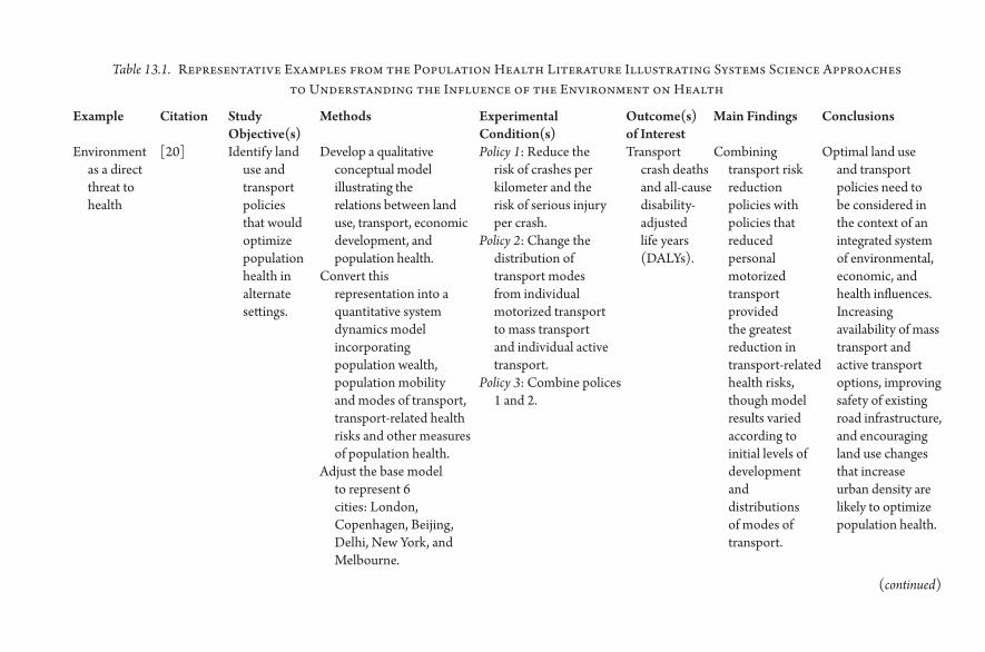
Table 13.1. Representative Examples from the Population Health Literature Illustrating Systems Science Approaches to Understanding the Influence of the Environment on Health
Example Citation Study Objective(s)
Methods Experimental Condition(s)
Outcome(s) of Interest
Main Findings Conclusions
Environment as a direct threat to health
[20] Identify land use and transport policies that would optimize population health in alternate settings.
Develop a qualitative conceptual model illustrating the relations between land use, transport, economic development, and population health.
Convert this representation into a quantitative system dynamics model incorporating population wealth, population mobility and modes of transport, transport- related health risks and other measures of population health.
Adjust the base model to represent 6 cities: London, Copenhagen, Beijing, Delhi, New York, and Melbourne.
Policy 1: Reduce the risk of crashes per kilometer and the risk of serious injury per crash.
Policy 2: Change the distribution of transport modes from individual motorized transport to mass transport and individual active transport.
Policy 3: Combine polices 1 and 2.
Transport crash deaths and all- cause disability- adjusted life years (DALYs).
Combining transport risk reduction policies with policies that reduced personal motorized transport provided the greatest reduction in transport- related health risks, though model results varied according to initial levels of development and distributions of modes of transport.
Optimal land use and transport policies need to be considered in the context of an integrated system of environmental, economic, and health influences. Increasing availability of mass transport and active transport options, improving safety of existing road infrastructure, and encouraging land use changes that increase urban density are likely to optimize population health.
(continued)

Environment as a determinant of health behaviors
[6] Evaluate how the built and social environments influence social inequalities in walking.
Develop an agent- based model simulating walking behavior in a hypothetical city, including walking to work, for basic needs, and for leisure. Walking ability is a function of age and attitude toward walking is influenced by walking experiences as well as the walking behaviors of friends and family. Residential segregation was represented by the location of lower socioeconomic status (SES) households in the center of the city, with higher SES households located on the periphery.
Four scenarios were compared, with different combinations of the spatial distribution of non- household locations and of safety: (1) randomly distributed non- household locations and random safety level; (2) randomly distributed non- household locations and lower safety level in the city center; (3) more non- household locations in the city center and random safety level; and (4) more non- household locations and lower safety level in the city center.
Average number of walking trips per day per person, by SES.
Known SES gradients in walking behaviors, with lower- income individuals more likely to walk to work and higher- income individuals more likely to walk for leisure, were replicated by the model.
Patterning of walking behaviors by SES is a function of the co- location of residential segregation, land use, and safety.
Example Citation Study Objective(s)
Methods Experimental Condition(s)
Outcome(s) of Interest
Main Findings Conclusions
Table 13.1. Continued

Environment as a determinant of social interactions
[21] Simulate a theoretical influenza epidemic in Norfolk, Virginia.
Develop an agent- based model that simulates every resident of Norfolk, VA and includes detailed city- level features including geographic characteristics, weather, and locations of homes, schools, and workplaces. Agent movements and interactions are also simulated, including health- care- seeking behaviors, including after 200 cases of influenza are introduced into the population.
The model was repeated multiple times, varying key parameters: the influenza transmission rate (i.e., the probability an infected agent transmits influenza to a non- infected agent with whom it interacts); the incubation period; the contagious period; and the percent of the population who were immune to influenza.
Epidemic curves, overall and by age and race; reproductive rates (R0); and number of health- care visits.
Cyclical variations in influenza incidence were observed, with increases on weekdays and decreases on weekends. The number of influenza cases peaked earlier and the prevalence of influenza remained high for longer among individuals aged 65 years and older than among other age groups.
Social distancing measures like school and workplace closures may be critical to reducing the spread of an influenza epidemic; the elderly may act as a “reservoir” for influenza during an epidemic and thus may be an important target of vaccination campaigns.
(continued)
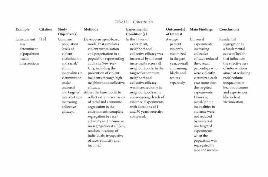
Environment as a determinant of population health interventions
[13] Compare population levels of violent victimization and racial/ ethnic inequalities in victimization under universal and targeted interventions increasing collective efficacy.
Develop an agent- based model that simulates violent victimization and perpetration in a population representing adults in New York City, including the prevention of violent incidents through high neighborhood collective efficacy.
Adjust the base model to reflect extreme scenarios of racial and economic segregation in the environment: complete segregation by race/ ethnicity and income vs. no segregation at all (i.e., random locations of individuals, irrespective of race/ ethnicity and income.)
In the universal experiment, neighborhood collective efficacy was increased by different increments across all neighborhoods. In the targeted experiment, neighborhood collective efficacy was increased only in neighborhoods with above- average levels of violence. Experiments with durations of 1 and 30 years were also compared.
Average percent violently victimized in the past year, overall and among blacks and whites separately.
Universal experiments increasing collective efficacy reduced the overall percentage who were violently victimized each year more than the targeted experiments. However, racial/ ethnic inequalities in violence were not reduced by universal nor targeted experiments when the population was segregated by race and income.
Residential segregation is a fundamental cause of health that influences the effectiveness of interventions aimed at reducing racial/ ethnic inequalities in health outcomes and experiences like violent victimization.
Example Citation Study Objective(s)
Methods Experimental Condition(s)
Outcome(s) of Interest
Main Findings Conclusions
Table 13.1. Continued

Systems Approaches to Understanding 161
this model was its detailed social network (including family members, neigh-bors, coworkers, classmates, and friends) and explicit opportunities for interac-tions between agents. Importantly, the model environment included simulated weather conditions and geographic features that restricted or promoted social interactions throughout the model run. In this way, environmental features con-tributed to the spread of disease through their influence on social networks and interactions. Influenza incidence was then observed under scenarios with vary-ing transmission probabilities, incubation periods, contagious periods, and level of immunity in the population.
The final example, using a systems science approach to anticipate environmen-tal influences on the effectiveness of a population health intervention, comes from Magdalena Cerdá and colleagues, who developed an agent- based model of violent victimization among adults in New York City [13]. The objective of this model was to compare universal vs. targeted experiments increasing neigh-borhood collective efficacy in order to reduce experiences of violence, as well as racial/ ethnic inequalities in violent victimization, where the universal experi-ment was characterized by a small increase in collective efficacy across the whole city and the targeted experiment comprised a more concerted effort to increase collective efficacy but only in high- violence neighborhoods. As in previous models ([6, 20]) the experimental conditions were compared under different hypothetical scenarios, in this case contrasting complete racial and economic res-idential segregation with a complete lack of segregation in the city. The authors found that the universal experiment led to greater reductions in violent victim-ization across all groups, but racial/ ethnic inequalities in violence persisted in the presence of racial and economic residential segregation. Only by reducing residential segregation through an artificial random distribution of individuals across the spatial environment were racial/ ethnic inequalities in violence elimi-nated through increased neighborhood collective efficacy.
What can we learn from these examples? These models share a number of fea-tures that are critically important to any assessment of environmental influences on health, including detailed representations of a variety of environmental char-acteristics; consideration of multiple outcomes and unintended consequences of experimental manipulations; examination of results under alternate scenarios; and caution against treating model results as inviolate predictions of reality.
The influenza epidemic model by Lee et al. best illustrates the importance of detailed empirical representations of multiple features of the environment, includ-ing population characteristics, geographic boundaries, businesses and work-places that operate at expected times of day, social networks linking individuals, and behaviors that mimic daily experiences [21]. Although simple models also have their advantages, the social interactions simulated in this model, which were realistically constrained by geography, weather, and individual routines, allowed

162 S Y S T E M S S C I E N C E T O W A R D A C O N S E Q U E N T I A L P O P U L A T I O N H E A LT H
epidemic patterns to emerge in a way that hadn’t been captured by less detailed models. Of course, including this level of detail required empirical information to parameterize individual behaviors as well as geographic and other environmental features; however, detailed data sources are available, including synthetic popula-tions and the General Social Survey and Environmental Protection Agency Time Usage Survey, and geographic information systems (GIS) data can be incor-porated into systems science programs as a matter of routine [22, 21, 23]. The models by Yang et al. and Cerdá et al. reflect a more modest reliance on empiric data, with populations simulated to represent a particular city and agent behav-iors based on available data but without quite the level of detail and fine- tuned daily experiences of Lee et al.’s model (2008) [6, 13, 21]. Importantly, however, interactions between individuals were still of central importance to individual behaviors in these models, with interactions constrained by the spatial environ-ment (e.g., walking behaviors were influenced by observing others walking in Yang et al. and violence exposures were determined by spatial contact between victims and perpetrators in Cerdá et al. [6, 13]).
McClure et al.’s land- use model and Cerdá et al.’s model of violence best dem-onstrate the utility of systems science approaches in considering unintended consequences, as well as opposing outcomes of health policies and interventions [20, 13]. By explicitly including both positive (increased active transport) and negative (increased transport injuries and fatalities) potential effects of land- use and transport policies, McClure et al. were able to assess the overall benefits of different policies for population health [20]. By considering both overall levels of violent victimization as well as racial/ ethnic inequalities in violence, Cerdá et al. recognized that experimental manipulations of neighborhood collective efficacy were not able to reduce inequalities in violence when residential segregation was high, even though overall levels of violence declined [13]. These examples high-light the importance of considering multiple outcomes in systems science mod-els in order to detect any unintended consequences or areas not benefitting from public health efforts and thus identify optimal policies to maximize population health.
All four models demonstrate the usefulness of observing model results under a variety of scenarios. In Yang et al., four different spatial patterns of safety and land use were generated, reflecting combinations of non- household locations clustered in the center of the spatial environment vs. randomly spatially distrib-uted, and lower safety levels in the center of the spatial environment vs. random safety levels throughout the environment [6] . These alternate scenarios had important implications for socioeconomic disparities in walking behaviors under the assumption that lower SES individuals tend to live in the city center [6]. Similarly, in their study of the effects of alternate transport policies, McClure and colleagues applied their model to representations of six major cities: London,

Systems Approaches to Understanding 163
Copenhagen, Beijing, Delhi, New York, and Melbourne [20]. This approach acknowledged that different settings are starting with different distributions of land use, road infrastructure, and risks of traffic injuries and thus stand to benefit from land- use and transport policies in different ways. Lee et al. examined pat-terns of influenza incidence assuming different levels of population immunity, different transmission rates, and different incubation and contagious periods, in order to characterize the full range of potential public health consequences of plausible influenza epidemics [21]. Cerdá et al. contrasted two extreme scenarios of racial and economic segregation to show that inequalities in violent victim-ization persist despite effective violence prevention interventions because, in unequal societies, the benefits of population health interventions accrue to those with more resources [13]. Being able to repeat experimental scenarios under alternate environmental conditions is a major strength of systems science mod-els with the potential for important insight into fundamental causes of health and appropriate targets of interventions.
Finally, the authors of all four models were transparent about the assumptions and limitations underlying their approaches and were careful to caution against using model results as predictions of quantifiable reductions or improvements to be expected, a caution that has been repeated by many public health researchers using these approaches [2, 17]. Rather than replacing real- world evaluations of interventions, these models are meant to serve as a sort of “virtual laboratory,” enabling a better understanding of the system as a whole, including the relations between different aspects of the environment that may be disturbed through interventions, and thus the potential system- wide implications of those distur-bances [21, 2].
3. CONCLUSIONS
As discussed throughout this chapter, a variety of mechanisms link environ-mental features to health outcomes and behaviors, both directly and indirectly. Systems science approaches that incorporate dynamic relations between the physical and social environment in producing and modifying health- related risks, behaviors, and resources hold great promise for advancing our understanding of the many environmental influences on population health. Although systems science models have numerous limitations and require strong assumptions, by following best practices, they allow testing of alter-nate intervention strategies for improving health, including consideration of how environmental features may impede or facilitate intervention effective-ness. Using these systems science approaches in concert with other research strategies represents an integrated approach that can be applied to a variety of population health problems.
164 S Y S T E M S S C I E N C E T O W A R D A C O N S E Q U E N T I A L P O P U L A T I O N H E A LT H
4. REFERENCES
1. Kaplan GA. What’s wrong with social epidemiology, and how can we make it better? Epidemiologic Reviews. 2004; 26: 124– 135.
2. Diez Roux AV. Health in cities: Is a systems approach needed? Cadernos de Saúde Pública. 2015; 31: Sup: S9– S23.
3. Ramirez AJ, et al. Occurrence of pharmaceuticals and personal care products in fish: Results of a national pilot study in the United States. Environmental Toxicology and Chemistry. 2009; 28(12): 2587– 2597.
4. Moore LV, Diez Roux AV, Nettleton JA, Jacobs DR, Jr. Associations of the local food environment with diet quality— a comparison of assessments based on surveys and geographic information systems: The multi- ethnic study of atherosclerosis. American Journal of Epidemiology. 2008; 167(8): 917– 924.
5. Lê F, Ahern J, Galea S. Neighborhood education inequality and drinking behavior. Drug and Alcohol Dependence. 2010; 112(1- 2): 18– 26.
6. Yang Y, Diez Roux AV, Auchincloss AH, Rodriguez DA, Brown DG. A spatial agent- based model for the simulation of adults’ daily walking within a city. American Journal of Preventive Medicine. 2011; 40(3): 353– 361.
7. Lipsitch M, et al. Transmission dynamics and control of severe acute respiratory syn-drome. Science. 2003; 300(5627): 1966– 1970.
8. Christakis NA, Fowler JH. The spread of obesity in a large social network over 32 years. New England Journal of Medicine. 2007; 357: 370– 379.
9. Institute of Medicine. Contagion of Violence: Workshop Summary. Washington, DC: The National Academies Press, 2013.
10. Smiley MJ, et al. A spatial analysis of health- related resources in three diverse metro-politan areas. Health Place. 2010; 16(5): 885– 892.
11. Northridge ME, Sclar ED, Biswas P. Sorting out the connections between the built environment and health: A conceptual framework for navigating pathways and plan-ning healthy cities. Journal of Urban Health. 2003; 80(4): 556– 568.
12. Phelan JC, Link BG, Tehranifar P. Social conditions as fundamental causes of health inequalities: Theory, evidence, and policy implications. Journal of Health and Social Behavior. 2010; 51: S28– S40.
13. Cerdá M, Tracy M, Ahern J, Galea S. Addressing population health and health inequalities: The role of fundamental causes. American Journal of Public Health. 2014; 104(S4): S609– S619.
14. Auchincloss AH, Diez Roux AV. A new tool for epidemiology: The usefulness of dynamic- agent models in understanding place effects on health. American Journal of Epidemiology. 2008; 168(1): 1– 8.
15. Tracy M, Cerdá M, Galea S. Causal thinking and complex systems approaches for understanding the consequences of trauma. In: Trauma, Psychopathology, and Violence. Widom CS, Editor. New York: Oxford University Press; 2012.
16. Galea S, Hall C, Kaplan GA. Social epidemiology and complex system dynamic modelling as applied to health behavior and drug use research. International Journal of Drug Policy. 2009; 20(3): 209– 216.

Systems Approaches to Understanding 165
17. Hirsch G, Homer J, Evans E, Zielinski A. A system dynamics model for planning cardiovascular disease interventions. American Journal of Public Health. 2010; 100(4): 616– 622.
18. Ip EH, et al. Reconciling statistical and systems science approaches to public health. Health Education & Behavior 2013; 40(1S): 123S– 131S.
19. Diez Roux AV. Multilevel analysis in public health research. Annual Review of Public Health. 2000; 21: 171– 192.
20. McClure RJ, et al. Simulating the dynamic effect of land use and transport polices on the health of populations. American Journal of Public Health. 2015; 105(S2): S223– S229.
21. Lee BY, Bedford VL, Roberts MS, Carley KM. Virtual epidemic in a virtual city: Simulating the spread of influenza in a US metropolitan area. Translational Research. 2008; 151(6): 275– 287.
22. Wheaton WD, et al. Synthesized Population Databases: A US Geospatial Database for Agent- Based Models. RTI Press publication No. MR- 0010- 0905. RTI International; Research Triangle Park, NC: 2009.
23. North MJ, et al. Complex adaptive systems modeling with Repast Simphony. Complex Adaptive Systems Modeling 2013; 1:3.

14
Systems of Behavior and Population Health
MA R K G . OR R , K AT H RY N Z I E M E R , A N D DA N I E L C H E N
1. INTRODUCTION
The purpose of this chapter is to bring meaning to the idea of systems of behavior in the context of population health. Systems of behavior are the mental apparatus (thoughts, beliefs, memory, emotion, motivation, etc.) that drive behavior. The emphasis on systems is decisive because it bounds the nature of explanations, mechanisms, and factors under consideration to dynamic processing models of behavior. Furthermore, we consider systems of behavior in the service of systems of populations, a topic that is rarely covered within either population health or the behavioral and neural sciences. Thus, ultimately, this chapter aims to pro-voke thinking about how to embed systems in systems, where behavior is nested within populations.
One approach to building systems of behavior might be to co- opt the men-tal apparatus from related fields such as behavioral medicine, health behavior, and health education— fields that have adopted theories of behavior to drive intervention and prevention approaches. However, this is not fully satisfactory because the theoretical approaches are less oriented toward a systems approach of behavior (we will describe what we mean by systems of behavior in detail below) than toward serving as frameworks for choosing measures of interest (for intervention) and capturing risk factors (for study). In a similar way, the addic-tion literature is limited in what it offers for building systems of behavior.
In what follows, we start with defining what we mean by systems of behavior and put forth a set of minimal criteria to help define it. Our approach reflects our training in cognitive science, a field that has specialized in building systems of

168 S Y S T E M S S C I E N C E T O W A R D A C O N S E Q U E N T I A L P O P U L A T I O N H E A LT H
human behavior since the 1950s [1] , and is thus ultimately constrained by what is known about humans (as opposed to any computation that solves a particular task). Then we provide an example from our recent work of a systems model of health behavior along with a critique of the model and some preliminary attempts to embed this system into a system of a population. Finally, we provide some thoughts and suggestions on the practicalities of embedding behavioral systems within population systems, thus addressing to some extent how to move forward.
We cannot emphasize strongly enough that what is presented below is about systems of populations, not developing systems of behavior for the purpose of informing intervention or prevention needs at the level of the individual. We will save the latter topic, an important one, for another discussion.
2. SYSTEMS OF BEHAVIOR
Figure 14.1 is a schematic of a well- known and influential system of behavior— a model of an individual human’s memory— whereby the circles represent mental constructs and the solid lines represent interactions among them [2] . Underlying this schematic is a set of detailed, formal assumptions, some capturing learning and some dictating the processing of information— all of which were imple-mented in a computer program. The conceptual development of this model was in response to a large body of experimental evidence on the nature of human memory. Equally important, the criteria for judging confidence in the model was determined by virtue of the matching between experimental data and data gener-ated by the model during simulations. The similarities to agent- based modeling are obvious; the differences are only of scale— the interacting parts are mental constructs in place of people.
Figure 14.1 A classic system of behavior (from [2]; adapted with permission). See the text for a description of its components and operations.

Systems of Behavior and Population Health 169
We will not venture to rigorously define what is and is not a system of behav-ior but will instead explore three broad classes of criteria for gauging the extent to which a model of behavior represents a system. Table 14.1 describes these classes in detail. Operations is a class referring to the parts of a system: how they interact internally, the potential interactions external to the system, and how the system adapts over time via learning mechanisms. Variation captures the notion of differences in behavior across implementations of the system as a function of values of the parameters that define the operations of the system. A simple example would be the speed at which new information is learned— the operation of learning is not changed, just its rate. Development focuses on how the model was conceptualized, how it is compared to empirical findings, and the degree to which the system is implemented in a usable computational formalism. Ideally, this last criterion satisfies the need for embedding the system of behavior into a system of the population.
An issue that is not represented in Table 14.1 is how to define what counts as behavior. For the purposes of this discussion, overt behavior is not required for a
Table 14.1. Criteria for Qualifying as a System of Behavior
Criterion Description ClassProcess- Oriented/
MechanisticPostulates mental constructs and their
interactionsOperations
Dynamic Representation of change over time and, potentially, interfaces dynamically with social contexts and environment
Learning Aspects of the model can change permanently over time
Individual Differences
Has the capacity to represents systematic and theoretically important variation in behavior across individuals
Variation
Theoretical Grounding
Processes and constructs are grounded and constrained by neuroscientific, psychological, or behavior economic theory
Development
Empirical Grounding
Proper comparison to empirical (most likely experimental) data to include testing of novel predictions. Ideally, a wide variety of experimental conditions would be considered
Computational Implementation
A formal model of the operations and drivers of variation that also represents its theoretical basis in a way that is empirically comparable to human experiment and observation
170 S Y S T E M S S C I E N C E T O W A R D A C O N S E Q U E N T I A L P O P U L A T I O N H E A LT H
model of behavior (e.g., picking up a cup of coffee). Thoughts and other mental processes alone qualify as behavior (e.g., recognizing that one wants coffee and planning to get it are both behaviors).
3. A SYSTEM OF HEALTH BEHAVIOR
We now show a system of health behavior— derived from some of our recent work [3, 4]— based on a well- understood formalism used extensively in cognitive science called “artificial neural networks” (henceforth “neural networks”). This formalism has been used repeatedly to represent important perceptual, cogni-tive, and social phenomena (see [5] for a review; [6] for more recent work). The import for population health is the natural analogy between the socio- cognitive aspects of health behavior (e.g., beliefs, attitudes, intention, and social learning) and the kinds of mental processes that neural networks are good at represent-ing (see [7] for a review). Specifically, neural networks are able to capture social processes that can be conceptualized as a dynamic human memory process, both taking into account what has been learned from past experience and the potential for more immediate influences such as current social and environmental contexts [2, 8– 10].
It is precisely these features that make neural networks useful for modeling health behavior— to capture the simultaneous influence of prior learning from past social contexts and the more current (or immediate) social context. For illus-tration, Figure 14.2 shows one of our systems models of the Theory of Reasoned Action [11] using the neural network formalization [4] . This model conceptu-alizes intention toward a behavior as driven by a dynamic, on- the- fly memory process called “constraint satisfaction”— the set of beliefs, cued by the social con-text external to the model, become activated, and then the system settles into a state (the intention state in this case) that has maximized how well it has satisfied the many constraints in the model. The constraints are the positive and negative relations between beliefs that encode belief structures from past experience via learning (e.g., exposure to peers’ beliefs over the past year).
The constraint satisfaction process used in the model is a hill- climbing algo-rithm. That is, the final state of the model, once cued by a social context, is the end path of a trajectory on a goodness surface that seeks increased goodness (larger goodness means more constraints were satisfied). Figure 14.3 is an ideal-ized representation of the goodness surfaces for two instantiations of the model (given a cue from the social context). Panel A suggests that the model will settle in a separate state compared to Panel B (the highest point on the goodness sur-face is the settling point).
The differences between the two panels in Figure 14.3 represent three dis-tinct scenarios: (1) the difference between two people given an identical social
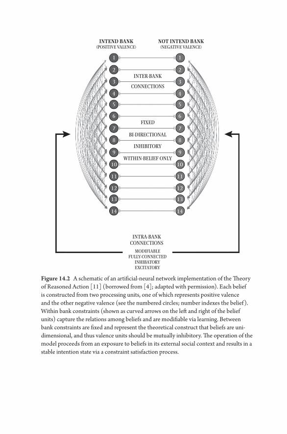
INTEND BANK(POSITIVE VALENCE)
NOT INTEND BANK(NEGATIVE VALENCE)
INTER-BANK
1
2
3
4
5
6
7
8
9
10
11
12
13
14
1
2
3
4
5
6
7
8
9
10
11
12
13
14
CONNECTIONS
FIXED
BI-DIRECTIONAL
INHIBITORY
WITHIN-BELIEF ONLY
INTRA-BANKCONNECTIONS
MODIFIABLEFULLY-CONNECTED
INHIBATORYEXCITATORY
Figure 14.2 A schematic of an artificial- neural network implementation of the Theory of Reasoned Action [11] (borrowed from [4] ; adapted with permission). Each belief is constructed from two processing units, one of which represents positive valence and the other negative valence (see the numbered circles; number indexes the belief). Within bank constraints (shown as curved arrows on the left and right of the belief units) capture the relations among beliefs and are modifiable via learning. Between bank constraints are fixed and represent the theoretical construct that beliefs are uni- dimensional, and thus valence units should be mutually inhibitory. The operation of the model proceeds from an exposure to beliefs in its external social context and results in a stable intention state via a constraint satisfaction process.

172 S Y S T E M S S C I E N C E T O W A R D A C O N S E Q U E N T I A L P O P U L A T I O N H E A LT H
context, where the differences are driven by variable social histories or differ-ent past exposures to social context features, or (2) the difference between two social contexts for the same person, or (3) the same context, the same person, but before and after the model had significant time to learn from past contexts. In short, end states, driven by hill climbing, vary because of learning (changes in the constraints) or differences in current social context.
Our prior work with this model, some of it using human data, illustrated the fol-lowing via a series of simulations: (1) its predictive power with respect to intentions toward behavior and (2) a formalization that accounts, simultaneously, for both past experience via learning and a person’s more immediate social contexts [3, 4].
How does this example model fair against the criteria presented in Table 14.1? Is it a system of behavior? The operations of the model are clearly mechanis-tic (beliefs and their attendant constraints serve as the mental constructs and their interactions), dynamic (through the constraint satisfaction process), and enable learning over time from exposure to social contexts. Although variation in the model across individuals was not explicitly explored to date, it is some-thing that the model could easily afford. For example, the rate of learning in the system (slower, faster) and the degree to which positive and negative valences inhibit one another (see [12, 13] regarding ambivalence in attitudes) might serve as explanations of variation across individuals. Finally, the development of the model was grounded in the Theory of Reasoned Action [11] (a highly influen-tial theory both in health behavior and in social psychology), was tested against empirical data, and was formalized using a well- understood computational for-malism. Thus, all of the criteria in Table 14.1 were met.
End States
0.0
–0.2
–0.4
–0.6
–0.8
–1.0
1.0
0.8
0.6
0.4
0.2
0.01.00.80.6
0.40.20.0
0.0
0.2
0.4
0.6
0.8
1.0
1.0
0.8
0.6
0.4
0.2
0.01.00.80.6
0.40.20.0
A B
Goo
dnes
s
Goo
dnes
s
Figure 14.3 A stylized goodness surface across possible states of a hypothesized neural network that uses constraint satisfaction as a settling mechanism. The x- and y-axes represent the full range of values for two units in the neural network (the full goodness surface for the model in Figure 2 is 28 dimensions, one per network node). See text for interpretation and comparison of Panels A & B and for additional details.

Systems of Behavior and Population Health 173
4. SYSTEMS OF BEHAVIOR IN A SYSTEM OF A POPULATION
A fundamental goal for population health is to have a clear understanding of the relation between models of individuals and models of populations, both in the service of scientific understanding and intervention/ prevention needs. Under the i.i.d. (independent and identically distributed) assumption, statistical models offer an appropriate realization of this goal, especially when data are longitudinal in nature. Multilevel hierarchical modeling can accommodate non– i.i.d. condi-tions within a statistical framework but do not capture bi- directional feedback across levels of a system. Agent- based modeling addresses the question of bi- directional feedback in a flexible dynamic way, but has yet to incorporate systems of behavior, instead relying on extra- simple assumptions regarding individuals’ behavior [14– 17]. Little, if any, work approaches this goal in the context of sys-tems of behavior.
Next, we will present new preliminary work of our own that begins to explore questions about the relation between individuals and populations using a systems of behavior approach. Specifically, we address the following question: to what degree do the parameters of a model of intention within individuals affect the diffusion of intention across a population? This question aligns with work over the past decade on the diffusion of health behaviors on social networks [18– 25] in that it is primarily concerned with diffusion dynamics of behavior. The differ-ence lies in how the individual is represented.
Using our newly developed modeling platform called MANN (Multi- Agent Neural Networks, see https:// github.com/ chendaniely/ multi- agent- neural- network accessed 3/ 25/ 16) we explored the diffusion of intention toward a behavior on a social network as a function of two parameters related to how intention operates within the individual. That is, over a large set of simulations, we varied the parameters of a neural network representing the Theory of Reasoned Action [11] while fixing the social network parameters, thus providing an experimental test, in- silico, of whether variation in the neu-ral network parameters affected the diffusion dynamics of intention on the social network.
Specifically, the parameterization of the neural network focused on two com-peting aspects, illustrated in Figure 14.2, that are dictated by the nature of the constraints built into the model. The within- bank constraints represent the degree of excitation within intention units (or not intention units) such that as these constraints become stronger in magnitude, the likelihood is increased that a small degree of activation within each bank will lead to amplification within the same bank. The between- bank constraints are similar but inverse, so as these increase in magnitude, each bank inhibits more the degree to which the other

174 S Y S T E M S S C I E N C E T O W A R D A C O N S E Q U E N T I A L P O P U L A T I O N H E A LT H
bank will become activated. Both of these constraints are reflected in the hill- climbing procedure that is described above and illustrated in Figure 14.3.
A single simulation consisted of instantiating a small world network (specified in [26]; our parameter values for the social network were 250 vertices, 10 near-est neighbors and a 0.02 probability of rewiring per each network edge, using bidirectional edges) in which each vertex was represented as a neural network (similar to Figure 14.2) that had the within- bank and between- bank constraints set to a value dictated by the experimental design (described below). A simu-lation was initialized so that all vertices were identical in terms of the value of the within and between bank constraints (with some purposeful random noise added). After initialization, five of the vertices were exposed randomly to one of three social contexts (high intention, high not intend, or ambivalence). Then, the simulation ran for 100 time steps. During each time step all vertices were updated in a random sequential order. A vertex was updated by using one of its neighbors’ last intention states, a portion of which was directly accessible to the updating vertex and thus served as a constraint on the updating vertex. In this way, inten-tion states had the chance to propagate through the social network. Figure 14.4 compares an early to later state of a single simulation.
Figure 14.5, a heat map, presents the full results of the simulations across the neural network parameter space (there were 25 levels of the between bank con-straints and 31 levels of the within- bank constraints totaling 775 points in param-eter space). Each cell in the heat map, representing one point in parameter space, is the average over approximately 10 simulations. (Figure 14.5, thus, captures
A B
Figure 14.4 Example of the time course of the diffusion of intention on a small- world graph with 250 vertices. Each vertex represents a recurrent neural network instantiation of the Theory of Reasoned Action [11]. The black vertices represent a state of not intending, the white intending, and the gray, ambivalent. Panels A & B illustrate the state of the network early and late in the diffusion process, respectively.

Systems of Behavior and Population Health 175
approximately 7750 simulations.) The metric represented in Figure 14.5 is the average amount of assortativity with respect to intention state at the final time step (t = 100) of each simulation. That is, roughly, it captures how much clustering of intention is present on the social network at the end of the simulation. As a point of reference, Figure 14.4, Panel B shows a high degree of clustering on intention.
The pattern shown in Figure 14.5 suggests that, although there are two regions of the parameter space in which changes in the neural network parameters have little consequence, the two regions are very distinct— one exhibits a large degree of assortativity with respect to the intention state; the other does not. This type of phase transition is characteristic of complex systems.
In sum, by constructing a simulation environment in which systems of behav-ior were nested within a population, we illustrated, experimentally, that the
0.80.790.780.770.760.750.740.730.720.71
0.70.690.680.670.660.650.64W
ithi
n
0.630.620.61
0.60.590.580.570.560.550.540.530.520.51
Between
0.0
0.2
0.4
0.6
0.8Assortativity
0.5
–0.21–0.2
2–0.2
3–0.2
4–0.2
5–0.2
6–0.2
7–0.2
8–0.2
9–0.3
–0.31–0.3
2–0.3
3–0.3
4–0.3
5–0.3
6–0.3
7–0.3
8–0.3
9–0.4
–0.41–0.4
2–0.4
3–0.4
4–0.4
5
Figure 14.5 A heat map representing 7750 diffusion of intention simulations (Figure 4 represents one of these). The axes represent two parameters of the recurrent neural network instantiation of the Theory of Reasoned Action [11]. The value of each cell in the heat map represents the average network assortativity (on the small- world graph) on intention of approximately 10 simulations for one point in the parameter space. See text for further details.

176 S Y S T E M S S C I E N C E T O W A R D A C O N S E Q U E N T I A L P O P U L A T I O N H E A LT H
parameters of the system of behavior affected the population dynamics, even when holding the social network parameters constant.
5. LOOKING FORWARD
Thus far we have (1) suggested criteria for a system of behavior, coming largely from work in cognitive science and computational psychology (see Table 14.1), and (2) provided an example of a system of health behavior and a glimpse of what insights might be gleaned when implementing said system into a system of a population. We will now focus on some core issues to consider as we move forward with further development of the systems of behavior approach in the domain of population health.
The most basic consideration is to recognize the conditions under which a system of behavior model is desirable, while appreciating that much work using systems science has yielded useful insights into population health phenomena without implementing systems of behavior [15– 18, 27]. In some cases, the research question itself will require a systems of behavior approach, like the work shown above in which we explored the effect of variation in the param-eters of a system of behavior on the diffusion dynamics in a population. Beyond such obvious cases, however, the need for a systems of behavior model will be less clear.
One unmistakable situation in which systems of behavior will be desirable is when intervention/ prevention levers under question implicate a set of com-plex mental processes such as those described in Table 14.1 (e.g., changes in dietary habits). By implementing a system of behavior in a model of a popula-tion, the insights will be in terms of the actual mental processes that should be targeted in order to see changes in the population. To date, however, there is a dearth of work, if any, that addresses interventions using a system of behavior (as outlined in Table 14.1) embedded in a system of a population. Although Figure 14.5 represents this notion directly, it is only in the abstract as proof- of- concept.
Another core consideration is feasibility. Although there exist many sys-tems of behavior already in computational form, covering many aspects of human behavior [28], it is uncertain to what extent these are directly applica-ble to population health needs. To gauge this will require both exploration of existing models and, most likely, extension of existing theory (computational or not) to include processes that are yet postulated but relevant for popu-lation health. Consider the system of behavior for the Theory of Reasoned Action [11] presented in Figure 14.2. We co- opted a general model used for attitude formation and reconceptualized the Theory of Reasoned Action to fit. In the process, we extended the Theory of Reasoned Action by implementing

Systems of Behavior and Population Health 177
additional mechanisms (e.g., how beliefs of one person are communicated to another, learning, and constraint satisfaction), none of which were empirically grounded. Only now are we in the process of developing social experiments to provide empirical grounding.
One intriguing idea is to leverage the extensive work on what are called archi-tectures in cognitive science [29– 31]. Architectures attempt to capture several core aspects of human behavior that are general across tasks and can account for individual differences. This might serve as a useful approach for understanding difficult issues such as behavioral comorbidity (e.g., smoking and unhealthy diet behavior) and could incorporate a general set of individual difference mecha-nisms that are directly related to health behaviors (e.g., delayed discounting [32]; self- regulation [33]).
A final consideration is the appreciation that common risk factors (e.g., gender, age, race/ ethnicity, geography, socioeconomic status) cannot be represented in a direct way in a system of behavior. It is not that these factors are negligible, only that they are placeholders for the direct processes represented in Table 14.1— e.g., differences in attitudes between two genders/ racial ethnic groups can only be explained by the operations and individual difference parameters of a system of attitude formation. A useful heuristic is this: to the extent that a risk factor can be conceptualized in terms of Table 14.1, it can be considered as a system of behavior or a part thereof.
6. CONCLUSION
The main point of this work was to introduce the feasibility of integrating systems of behavior with systems of populations for further understanding, practice, and policy in population health. Paradoxically, this notion is not only foreign to those in population health but also to those who focus on human behavior. In part, the latter group doesn’t see the purpose; studying individ-uals is sufficient. However, it is the former group for whom this chapter is targeted.
In any event, it is clear that much work is to be done in such a novel enterprise. Mostly, this work will require highly interdisciplinary teams, the generation of novel theory for application, and mostly, evidence and buy- in that this effort will, in fact, help to drive improvements in population health. We are hopeful that the work in this chapter begins a fruitful discussion.
7. ACKNOWLEDGMENTS
This work was funded in part by NSF Grant #1520359.

178 S Y S T E M S S C I E N C E T O W A R D A C O N S E Q U E N T I A L P O P U L A T I O N H E A LT H
8. REFERENCES
1. Newell A, Simon HA. Computer simulation of human thinking. Science. 1961; 134: 2011– 2017.
2. McClelland JL, Rumelhart DE. Distributed memory and the representation of gen-eral and specific information. Journal of Experimental Psychology: General. 1985; 114: 159– 188.
3. Orr M, Plaut DC. Complex systems and health behavior change: Insights from cog-nitive science. American Journal of Health Behavior. 2014; 38: 404– 413.
4. Orr MG, Thrush R, Plaut DC. The theory of reasoned action as parallel constraint satisfaction: Towards a dynamic computational model of health behavior. PLOS ONE. 2013; 8: e62409.
5. Read SJ, Miller LC, Editors. Connectionist models of social reasoning and social behavior. Mahwah, NJ: Lawrence Erlbaum Associates; 1998.
6. Read SJ, et al. A neural network model of the structure and dynamics of human per-sonality. Psychological Review. 2010; 117: 61– 92.
7. Thomas MSC, McClelland JL. Connectionist models of cognition. Sun R, Editor. The Cambridge Handbook of Computational Psychology. New York: Cambridge University Press; 2008.
8. Monroe BM, Read SJ. A general connectionist model of attitude structure and change: The ACS (Attitudes as Constraint Satisfaction) Model. Psychological Review. 2008; 115: 733– 759.
9. Shoda Y, LeeTiernan S, Mischel W. Personality as a dynamical system: Emergence of stability and distinctiveness from intra- and interpersonal interactions. Personality and Social Psychology Review. 2002; 6: 316– 325.
10. Shoda Y, Mischel W. Personality as a stable congitive- affective activation net-work: Characteristic patterns of behavior variation emerge from a stable personality structure. In: Read SJ, Miller LC, Editors. Connectionist Models of Social Reasoning and Social Behavior. Mahwah, NJ: Lawrence Erlbaum Associates; 1998.
11. Fishbein M, Ajzen I. Predicting and Changing Behavior: The Reasoned Action Approach. New York, NY: Psychology Press/ Taylor and Fancis; 2010.
12. de Liver Y, van der Pligt J, Wigboldus D. Positive and negative associations underlying ambivalent attitudes. Journal of Experimental Social Psychology. 2007; 43: 319– 326.
13. Thompson MM, Zanna MP. The conflicted individual: Personality- based and domain- specific antecedents of ambivalent social attitudes. Journal of Personality and Social Psychology. 1995; 63: 259– 288.
14. Orr MG, Merrill JA. Diffusion of innovation across a national local health depart-ment network: A simulation approach to policy development using agent- based modeling. Frontiers in Public Health Services and Systems Research. 2013; 2(5). DOI: 10.13023/ FPHSSR.0205.03.
15. Orr MG, Galea SG, Riddle M, Kaplan GA. Reducing racial disparities in obe-sity: Simulating the effects of improved education and social network influence on diet behavior. Annals of Epidemiology. 2014; 24: 563– 569.
16. Orr MG, Galea SG, Kaplan GA (In Press). Neighborhood food, physical activity, and educational environments and black/ white disparities in obesity: A complex systems simulation analysis. Journal of Epidemiology and Community Health.
Systems of Behavior and Population Health 179
17. Orr MG, Evans CR. Understanding long- term diffusion dynamics in the prevalence of adolescent sexual initiation: A first investigation using agent- based modeling. Research in Human Development. 2011; 8: 48– 66.
18. Bearman PS, Moody J, Stovel K. Chains of affection: The structure of adolescent romantic and sexual networks. American Journal of Sociology. 2004; 110: 44– 91.
19. Christakis NA, Fowler JH. The spread of obesity in a large social network over 32 years. New England Journal of Medicine. 2007; 357: 370– 379.
20. Christakis NA, Fowler JH. The collective dynamics of smoking in a large social net-work. New England Journal of Medicine. 2008; 358: 2249– 2258.
21. Galea S, Hall C, Kaplan GA. Social epidemiology and complex system dynamic modelling as applied to health behaviour and drug use research. International Journal of Drug Policy. 2009; 20: 209– 216.
22. Hill AL, Rand DG, Nowak MA, Christakis NA. Emotions as infectious diseases in a large social network: the SISa model. Proceedings of the Royal Society B- Biological Sciences. 2010; 277: 3827– 3835.
23. Smith KP, Christakis NA. Social networks and health. Annual Review of Sociology. 2008; 34: 405– 429.
24. Ueno K. The effects of friendship networks on adolescent depressive symptoms. Social Science Research. 2005; 34: 484– 510.
25. VanderWheele TJ. Sensitivity analysis for contagion effects in social networks. Sociological Methods and Research. 2011; 40: 240– 255.
26. Watts DJ, Strogatz SH. Collective dynamics of ‘small- world’ networks. Nature. 1998; 393: 440– 442.
27. Morris M, Kretzschmar M. Concurrent partnerships and transmission dynamics in networks. Social Networks. 1995; 17: 299– 318.
28. Sun R, Editor. The Cambridge Handbook of Computational Psychology. New York: Cambridge University Press; 2008.
29. Newell A. Unified Theories of Cognition. Cambridge, MA: Harvard University Press; 1990.
30. Anderson JR, Lebiere C. The Atomic Components of Thought. Mahwah, NJ: LEA; 1998.
31. Anderson JR. How Can the Human Mind Occur in the Physical Universe. Oxford: Oxford University Press; 2007.
32. Bickel WK, Koffarnus MN, Moody L, Wilson AG. The behavioral- and neuro- economic process of temporal discounting: A candidate behavioral marker of addic-tion. Neuropharmacology. 2014; 76: 518– 527.
33. Timms KP, Rivera DE, Collins LM, Piper ME. A dynamical systems approach to understanding self- regulation in smoking cessation behavior change. Nicotine & Tobacco Research. 2014; 16: S159– S168.


15
Systems Under Your Skin
K A R I NA STA N DA H L O L S E N, H E G E B Ø V E L STA D, A N D E I L I V L U N D
1. INTRODUCTION
Due to the differing focus of medical researchers, the question of what causes a certain disease can receive distinct and diverse answers. For example, when asked what causes cancer, an epidemiologist will focus on exposures to harmful sub-stances or lifestyle factors, but a molecular biologist may focus on mutational processes and alterations of cellular pathways. Even though the methods and explanatory models may differ, both epidemiologists and molecular biologists are searching for causes of disease. Hence, they are conceptually, albeit not meth-odologically, related. In a systems medicine approach, this relatedness becomes clear— and it holds promise of greater insights into disease processes at many levels [1] .
The research field of molecular epidemiology evolved in the 1980s as an attempt to combine epidemiology and molecular biology. In 1982 Perera and Weinstein described molecular epidemiology as “the use of advanced labora-tory methods in combination with analytic epidemiology to identify at the bio-chemical or molecular level, specific factors that play a role in human disease causation” [2] . With these advances, the traditional epidemiologist had to look inside “the black box,” and the molecular biologists had to look outside of the box. During the 1970s, 1980s, and 1990s, the topic of “genes versus environ-ment,” or nature versus nurture, was heavily debated by geneticists, biologists, psychologists, and social scientists, but it is only recently that technologies have been developed to enable explorative investigations of molecular mechanisms of disease in an epidemiological scale and framework. The revolution of molecular
182 S Y S T E M S S C I E N C E T O W A R D A C O N S E Q U E N T I A L P O P U L A T I O N H E A LT H
epidemiology came with the sequencing of the human genome published in 2001 [3, 4], and the concurrent development of – omics technologies for the efficient study of the total genome and other – omes like the transcriptome, metabolome, proteome, etc. Technology paved the way for new study designs searching for associations between genetic variability and diseases at the popu-lation level, the genome- wide association studies (GWAS). In some cases, this new approach resulted in great insight and identified potential for public health benefits: DNA from the human papilloma virus was found in virtually all cervi-cal cancers, and certain variants of the BRCA genes lead to highly increased risk of breast cancer. However, findings of such magnitude have been rare: there are very few genes with big effects [5].
This chapter will discuss, with some brief historical background, how – omics analyses in population research help to bring us closer to a more functional view of causal associations and how systems science is an essential tool in our arma-mentarium toward this understanding. We will discuss some prerequisites of this new emerging field: aspects of study design, human sample material, data analysis, and biological interpretation of – omics data in population research. In conclusion, we discuss challenges for the future and emerging directions in the field.
2. CAUSALITY IN EPIDEMIOLOGY
The epidemiological research tradition studies statistical associations between lifestyle factors and disease and aims to identify causal associations in the face of any confounding factors. Originally, studies were based on questionnaires to gain information about exposures, and diagnostic information about outcomes, diseases, or deaths. To improve the precision of the exposure estimates, biologi-cal tissue like blood began to be collected to allow measurements of biomark-ers: biochemical substances that reflect either the exposure itself, or a biological/ biochemical event during absorption, metabolism, or interaction with target tis-sues [6] . In addition to improved exposure information, more detailed classifica-tion of diseases using molecular markers enables stratified analyses in molecular subgroups and revelations of previously un- detectable differences of statistical associations.
Even though the use of biomarkers improves assessment of exposures, and new technology enables more detailed classification of disease, the statistical analyses of associations between exposure and disease have been straightfor-ward, using well- known statistical methods. A set of nine guidelines published by Bradford Hill in 1965 is the most frequently used tool to evaluate the causal-ity of statistical associations between exposures and outcomes in epidemiologi-cal studies [7] . Briefly, the guidelines address nine aspects, known collectively as
Systems Under Your Skin 183
“Hill’s criteria of causality”: strength of the association, consistency, specificity, temporality, biological gradient, biological plausibility, coherence, experiment, and analogy. At the time of Hill’s publication, the biological mechanisms of many diseases were unknown: this was only 12 years after the description of the DNA double- helix, and 35 years before the sequencing of the human genome [8]. Among Hill’s criteria is that of biological plausibility, which refers to the use of existing knowledge of biological mechanisms to lend strength to a statisti-cal association between exposure and outcome. At any given time, this criterion thus rests on the current state of knowledge. It follows from this that as long as the current knowledge of disease mechanisms is derived mainly from cell line or animal studies, the true causal mechanisms that are at play in humans may remain obscure. It is increasingly evident that mice studies have limited trans-ferability to human conditions and that they fail to capture the complexity of human disease etiologies and mechanisms [9, 10]. Systems medicine holds the promise of improving causal thinking by adding mechanistic information derived from human studies to the statistical associations found in epidemiolog-ical studies. Ultimately, advances in the field may enable disease models based on human observational data.
3. THE – OMICS IN POPULATION RESEARCH: TOWARD FUNCTIONAL UNDERSTANDING AND SYSTEMS MEDICINE
The first applications of – omics studies at the population level were the GWAS, large- scale studies searching for gene variants associated with increased risk of diseases. One example is a multicenter study of lung cancer patients and con-trols that identified two genetic variants (single nucleotide polymorphisms, SNP) associated with increased risk [11]. One of the SNP loci was situated in the gene coding for nicotinic acetylcholine receptor subunit 5, a gene that binds nicotine and nicotine derivatives. The finding raised the question of how the genetic variant affected the biological mechanisms that led to increased disease risk. However, this type of static genetic data is only marginally helpful in elu-cidating functional chains of events. On the other hand, – omics data like DNA methylation and gene expression provide an opportunity to understand, from a systems dynamics point of view, the functional, dynamic mechanisms that explain the observed phenomena. For example, it has been shown that smok-ing induces methylation changes in the DNA of blood cells, and that some of these changes remain even 30 years after smoking cessation [12]. The persistent smoking- dependent change is in line with the fact that smoking may still increase lung cancer risk up to 20 years after cessation [13]. Furthermore, DNA methyla-tion changes have now been linked to future lung cancer risk independently of
184 S Y S T E M S S C I E N C E T O W A R D A C O N S E Q U E N T I A L P O P U L A T I O N H E A LT H
smoking status [14]. The same study showed that the smoking- induced hypo- methylation was significantly inversely correlated with expression levels of the corresponding genes and that these genes were relevant to lung cancer etiology [14]. This illustrates how functional genomics may help to elucidate the causal pathways between exposure and disease.
Importantly, several enabling factors are prerequisites for exploring the func-tional aspects of disease- related molecular mechanisms that are at play at the pop-ulation level. The following enabling factors are further discussed below: access to human sample material, adequate study design, preferably with repeated mea-surements, and advanced data analysis and management.
4. SAMPLE MATERIAL FOR FUNCTIONAL GENOMICS
Two practical and ethical constraints limit the nature of the human sample mate-rial that is available to researchers: the tissue of interest may not be easily acces-sible, and it is not ethically acceptable to impose harm on study participants in order to investigate the molecular chains of events in the etiology of a disease that may be associated with exposure to a harmful substance. As an example, col-lection of blood samples from healthy individuals in a prospective cohort design is relatively non- invasive and feasible in epidemiological studies, and provides access to analysis of systemic processes [1] . However, adequate sample handling at all stages is paramount to preserving the biological information of interest. In combination with exposure information (questionnaires or biomarkers), func-tional genomics analysis of human sample material may provide snap shots of etiological disease mechanisms.
5. STUDY DESIGN OPPORTUNITIES
Functional genomics analyses in combination with prospective studies enable more sophisticated study designs and analytical approaches. As an example, the prospective globolomic study design has been developed to describe the systems epidemiology approach to disease causation [1] . The many aspects of this design are illustrated in Figure 15.1. The design incorporates multi- omics data sets collected repeatedly from different tissues of healthy persons and incorporates questionnaire information to enable stratified analyses. In a nested case- control study, a change in status from healthy to diseased enables analyses of functional disease mechanisms that may be present before any clinical manifestation of disease. Knowledge of these mechanisms holds promise of improved disease prevention, early detection of disease, and may provide new targets for treatment.
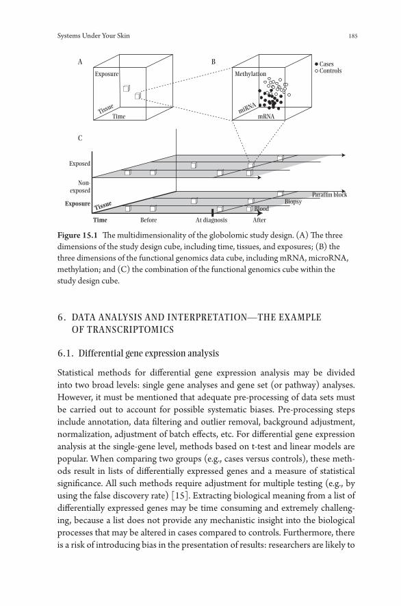
Systems Under Your Skin 185
6. DATA ANALYSIS AND INTERPRETATION— THE EXAMPLE OF TRANSCRIPTOMICS
6.1. Differential gene expression analysis
Statistical methods for differential gene expression analysis may be divided into two broad levels: single gene analyses and gene set (or pathway) analyses. However, it must be mentioned that adequate pre- processing of data sets must be carried out to account for possible systematic biases. Pre- processing steps include annotation, data filtering and outlier removal, background adjustment, normalization, adjustment of batch effects, etc. For differential gene expression analysis at the single- gene level, methods based on t- test and linear models are popular. When comparing two groups (e.g., cases versus controls), these meth-ods result in lists of differentially expressed genes and a measure of statistical significance. All such methods require adjustment for multiple testing (e.g., by using the false discovery rate) [15]. Extracting biological meaning from a list of differentially expressed genes may be time consuming and extremely challeng-ing, because a list does not provide any mechanistic insight into the biological processes that may be altered in cases compared to controls. Furthermore, there is a risk of introducing bias in the presentation of results: researchers are likely to
Exposure
A B
C
Before After
BloodBiopsy
Paraf�n block
At diagnosis
Exposure
Exposed
Non-exposed
Time
Methylation
mRNA
CasesControls
miRNA
Time
Tissue
Tissue
Figure 15.1 The multidimensionality of the globolomic study design. (A) The three dimensions of the study design cube, including time, tissues, and exposures; (B) the three dimensions of the functional genomics data cube, including mRNA, microRNA, methylation; and (C) the combination of the functional genomics cube within the study design cube.
186 S Y S T E M S S C I E N C E T O W A R D A C O N S E Q U E N T I A L P O P U L A T I O N H E A LT H
focus on genes and processes that are familiar to them, even though other pro-cesses may be more pronounced. The risk of researcher bias contrasts the very nature of transcriptomic analyses: it offers the opportunity to let the results speak for themselves in a non- hypothesis driven approach, whereas relying solely on the researcher’s previous knowledge may greatly reduce the degree to which the results are exploited.
6.2. Extracting Biological Information Using Pathway Analysis
To avoid the pitfalls mentioned above, several methods for gene set- or pathway- level analyses have been developed [16]. Their overall aim is to reduce the bio-logical complexity by analyzing genes in groups (gene sets or pathways), thereby reaching a higher explanatory power and reducing researcher bias in the inter-pretation of results. How the groups of genes are defined will have great impact on the information that such analyses provide. The groups of genes (gene sets) may be any list of genes with some relation to each other. Examples include biological pathways derived from comprehensive databases like KEGG [17] or Gene Ontology [18]. Another example is gene sets (lists of genes) derived from experimental literature. A biological pathway may be characterized as one of the following: (1) a metabolic pathway, which involves the enzyme- catalyzed step- by- step modification of an initial chemical or molecule to form another product; (2) a protein interaction pathway, which describes the interaction of proteins that may work alone or together in large complexes to perform cellular and physi-ological processes; (3) a gene regulatory pathway, which describes how exter-nal cellular stimuli are sensed, then transduced through the cellular interior into the DNA in the cell nucleus, where gene transcription into mRNA takes place; (4) the term signaling pathways, which may describe the same processes as the previous example but might also be used to describe similar pathways that do not lead to the transcription of a gene but to some other cellular alteration. Finally, the term “molecular pathway” is defined as a series of actions among molecules in a cell that leads to a certain end point or cell function (National Cancer institute).
A comprehensive overview of statistical methods to identify significantly dif-ferentially expressed pathways is beyond the scope of this chapter, but we will provide an introduction to the main approaches. All methods are based on the general scheme depicted in Figure 15.2 (modified from [19]). The first genera-tion of methods, over- representation analysis [20], starts with a list of differen-tially expressed genes after running single- gene level analysis to compare cases and controls. Then, the number of differentially expressed genes that are pres-ent in each pathway is counted, and finally, that number is compared to what you would expect to find by chance. The first generation methods rely on the

Systems Under Your Skin 187
assumptions that genes and pathways are independent of each other, which is highly questionable. Furthermore, the significance cutoff value for defining the input list of differentially expressed genes is arbitrary. If you use an FDR thresh-old of 0.05 and fold change cutoff of 2, all genes with a fold change of 1.95 or FDR 0.051 will be disregarded. These genes are arguably just as biologically impor-tant as the genes just under the arbitrary significance cutoff. Finally, the methods ignore how strongly the genes are associated with the phenotype (case/ control status). In spite of these limitations, first generation resources like MSigDB and GenMAPP provide an easily accessible first glimpse of gene set- level insights.
Second generation methods (e.g., Gene Set Enrichment Analysis [21] and Global Test [22]) are based on the hypothesis that weaker but coordinated changes in sets of functionally related genes (i.e., pathways) can also have sig-nificant effects [16, 23]. The general approach is to first calculate the differential expression and significance level. Then, for genes in Pathway A, the gene- level statistic is combined using univariate or multivariate approaches. Lastly, the pathway- level significance is assessed. Second generation methods consider the proportion of differentially expressed genes in the pathway, the size of the path-way, and the degree of correlation between genes in the pathway. Also, accessory biochemical measurements or clinical information may be included. An impor-tant difference from first generation methods is that all genes are considered, not just the most significant ones.
Methods that consider pathway topology are not easily generalizable, but collectively they may be considered a third generation of gene set- level analy-sis methods. With these methods, pathways are viewed as graphs and/ or net-works with nodes (genes) and edges (interactions) [16]. The same main steps as second generation methods may be employed, but the key difference is that information on pathway topology— the type of interaction and position of the gene in the pathway— is combined with the gene expression change in order to compute a gene- level statistic. These are further combined into a pathway- level statistic. A main limitation to these methods is the fact that biological pathways are not static— they are cell- type specific, condition- dependent, and dynamic.
Annotationdatabase
Algorithmsand statistics
User input:a list of genes
Results Interpretation
Figure 15.2 General scheme of pathway analysis methods.
188 S Y S T E M S S C I E N C E T O W A R D A C O N S E Q U E N T I A L P O P U L A T I O N H E A LT H
Currently, no database holds comprehensive information regarding the condi-tional interactions between any two genes. Still untackled by method develop-ers is the fact that not only are genes dependent, but pathways are also mutually dependent on each other.
7. CHALLENGES
Advances in technology for functional genomics analyses, as well as comput-ing and statistics, have allowed researchers to approach the true complexity of human disease etiology. However, numerous challenges remain, often related to design of studies and availability of human sample material. A review of nutrig-enomics studies revealed generally small sample sizes, which hinders generaliz-ability of the results and increases the chance of false positive findings [24]. The problem of false positive results can be reduced by increasing the number of participants in each study, by applying a test- retest design, or by using repeated measurements from each individual. Statistical analysis of multi- omics data sets face challenges related to mass significance testing and functional interpretation, and there are few established methods available for analysis of time- dependent changes.
In addition, despite the great progress in the biological interpretation of gene expression data sets, there are also still challenges in the process of extracting meaningful information from – omics data. There is a lack of human- derived in vivo data describing gene function dependent on regulatory mechanisms like DNA methylation. Furthermore, comprehensive information on functional effects of splicing variants and SNP variations, as well as information on condi-tion- and tissue- specific mechanisms is scarce. Importantly, modeling dynamic systems remains difficult, and there is not enough information on dependency between multiple molecular pathways.
8. EMERGING DIRECTIONS
Over the last two decades, the introduction of – omics technologies has changed epidemiology. Traditional epidemiology was focused on single- disciplinary interpretation of statistical associations, but now the focus has shifted toward more challenging multidisciplinary approaches to causality. This multidisci-plinary work demands a mutual understanding of many research traditions and methods and depends on collaborative efforts. There is a strong momentum to form larger groups or research centers for the exploration of functional genomics as part of systems medicine.
Equally important is the challenge of building new studies with biobanks con-taining material eligible for functional genomics analyses, with a particular focus
Systems Under Your Skin 189
on gene expression or other responsive molecules that are present in both blood and other tissues. The complexity of multilevel analyses is directly transferable to a need for increased size of studies, in order to handle statistical power and enable retest studies.
By using blood samples, results from – omics analyses will provide insight into immunological processes of the body. In recent years, the ubiquitous relevance of these processes has become clearer, and the immune system is no longer regarded only as the body’s defense system. Rather, immunological processes are major regulators of homeostasis, and the importance for etiology and causation of chronic diseases is increasingly apparent. For example, in cancer research, the systemic, immunological regulation of cancer progression includes all steps from primary tumor growth to metastasis [25].
This insight is likely to be relevant for many other diseases and highlights the need for prospective, preclinical studies with the collection of high- quality bio-logical material. When available, such studies will provide ample opportunity to investigate and establish causal chains of events, and as such they hold promise of discovering new targets for disease prevention, detection, and treatment.
9. REFERENCES
1. Lund E, Dumeaux V. Towards a more functional concept of causality in cancer research. International Journal of Molecular Epidemiology and Genetics. 2010; 1(2): 124– 133.
2. Perera FP, Weinstein IB. Molecular epidemiology and carcinogen- DNA adduct detection: New approaches to studies of human cancer causation. Journal of Chronic Diseases. 1982; 35(7): 581– 600.
3. Lander ES and International Human Genome Sequencing Consortium. Initial sequencing and analysis of the human genome. Nature. 2001; 409(6822): 860– 921.
4. Venter JC, et al. The sequence of the human genome. Science. 2001; 291(5507): 1304– 1351.
5. Manolio TA. Genomewide association studies and assessment of the risk of disease. New England Journal of Medicine. 2010; 363(2): 166– 176.
6. Vineis P, Chadeau- Hyam H. Integrating biomarkers into molecular epidemiological studies. Current Opinion in Oncology. 2011; 23(1): 100– 105.
7. Hill AB, The environment and disease: Association or causation? Proceedings of the Royal Society of Medicine. 1965; 58: 295– 300.
8. Fedak KM, et al. Applying the Bradford Hill criteria in the 21st century: How data integration has changed causal inference in molecular epidemiology. Emerging Themes in Epidemiology. 2015; 12(1): 1– 9.
9. Hayden EC. Misleading mouse studies waste medical resources, Nature. 2014. 10. Editorial, Of men, not mice. Nature Medicine. 2013. 19(4): 379– 379. 11. Hung RJ, et al. A susceptibility locus for lung cancer maps to nicotinic acetylcholine
receptor subunit genes on 15q25. Nature. 2008; 452(7187): 633– 637.

190 S Y S T E M S S C I E N C E T O W A R D A C O N S E Q U E N T I A L P O P U L A T I O N H E A LT H
12. Guida F, et al. Dynamics of smoking- induced genome- wide methylation changes with time since smoking cessation. Human Molecular Genetics. 2015; 24(8): 2349–2359.
13. Ebbert JO, et al. Lung cancer risk reduction after smoking cessation: Observations from a prospective cohort of women. Journal of Clinical Oncology. 2003; 21(5): 921– 926.
14. Fasanelli F, et al. Hypomethylation of smoking- related genes is associated with future lung cancer in three prospective cohorts. Nature Communications. 2015; 6(10192). Doi: 10.1038/ ncomms10192.
15. Benjamini Y, Hochberg Y. Controlling the False Discovery Rate: A practical and powerful approach to multiple testing. Journal of the Royal Statistical Society. Series B (Methodological). 1995. 57(1): 289– 300.
16. Khatri P, M Sirota, Butte AJ. Ten years of pathway analysis: Current approaches and outstanding challenges. PLOS Computational Biology. 2012: 8(2): e1002375.
17. Kanehisa M, Goto S. KEGG: Kyoto encyclopedia of genes and genomes. Nucleic Acids Research. 2000. 28(1): 27– 30.
18. Ashburner M, et al. Gene Ontology: Tool for the unification of biology. Nature Genetics. 2000; 25(1): 25– 29.
19. Huang da W, Sherman BT, Lempicki RA. Bioinformatics enrichment tools: Paths toward the comprehensive functional analysis of large gene lists. Nucleic Acids Research. 2009; 37(1): 1– 13.
20. Goeman JJ, Buhlmann P. Analyzing gene expression data in terms of gene sets: Methodological issues. Bioinformatics. 2007; 23(8): 980– 987.
21. Subramanian A, et al. Gene set enrichment analysis: A knowledge- based approach for interpreting genome- wide expression profiles. Proceedings of the National Academy of Sciences of the United States of America. 2005; 102(43): 15545– 15550.
22. Goeman JJ, et al. A global test for groups of genes: Testing association with a clinical outcome. Bioinformatics. 2004; 20(1): 93– 99.
23. Dinu I, et al. Gene- set analysis and reduction. Briefings in Bioinformatics. 2009; 10(1): 24– 34.
24. Olsen KS, Skeie G, Lund E. Whole- blood gene expression profiles in large- scale epidemiological studies: What do they tell. Current Nutrition Reports. 2015; 4(4): 377– 386.
25. McAllister SS, Weinberg RA. The tumour- induced systemic environment as a critical regulator of cancer progression and metastasis. Nature Cell Biology. 2014; 16(8): 717– 772.
16
Frontiers in Health Modeling
NAT HA N I E L O S G OOD
1. INTRODUCTION
A rapid evolution is taking place in the character of health applications of sys-tem science. Much of this change reflects its embedding of such applications within a rapidly changing scientific and technology landscape but also a grow-ing appreciation for how systems science methods fit into the policy and health science milieu and the emergence of practitioners trained in several modeling approaches. While such nascent trends are just starting to exert notable depar-tures from past practice, they seem likely to thoroughly reshape the field in com-ing decades. In this chapter, we briefly survey six such trends and discuss their implications for health modeling.
2. HYBRID VIGOR: THE RISE OF HYBRID SYSTEMS SCIENCE
Systems science techniques in general— and dynamic modeling techniques in particular— have long been fragmented into distinct and largely independently pursued traditions dating back many decades, with their origins in, and focus on, different types of questions. The community of practitioners in each of these tra-ditions have generally pursued their work with little interaction with— and often little awareness of— the techniques and communities of the other traditions. On occasion, however, practitioners have bridged those communities of practice and advanced models that fall on the boundaries between two different traditions. For example, System Dynamics models have since the inception of the approach been articulated at the level of individual actors (e.g., firms) [1] , an approach that has included some of the most widely known such models, such as the Beer

192 S Y S T E M S S C I E N C E T O W A R D A C O N S E Q U E N T I A L P O P U L A T I O N H E A LT H
Game [5]. In recent years, this has been expanded to consider the interaction of large numbers of such actors [3, 4]. Methodologists have also advanced research frameworks combining the approaches [52, 2]. However, it has not been until the past decade that adequate support has been available for the interweaving of several system science approaches within a given model [59]. With the resulting awareness of the potential of hybrid modeling, support for hybrid modeling has been incorporated in platforms with their origins in the agent- based modeling [59, 6], System Dynamics [60] and Discrete Event [61] traditions.
2.1. Motivations for Hybrid Modeling
There are a number of distinct motivations for application of hybrid modeling in general, with some of those motivations enjoying particular relevance to the health context. We discuss some of the most compelling here.
2.2. Competitive Advantages
Each type of modeling offers distinct competitive advantages. The most broadly recognized such advantages relate to ease of characterization of certain types of system behavior— for example, the fact that agent- based modeling exhibits pronounced advantages when it comes to capturing agent- agent interactions involving heterogeneous actors, or that Discrete Event Modeling provides an exceptional economy in specification of resource- constrained workflows, or System Dynamics in depicting the dynamics of regulatory systems involving con-tinuous variables. The capacity to weave together formalisms offering differing natural domains of expressiveness permits exploitation of metalinguistic abstrac-tion [8] — the capacity to choose the appropriate language (and associated ana-lytic lens) for particular areas of the system or problem of interest. For example, in a model of chronic disease and health- care processes in a demographically diverse aging population, the representation of agent characteristics and the natural history of disease for various comorbid conditions could be expressed using agent- based modeling, while progression of such agents through various primary and specialist care pathways could be best captured using Discrete Event Modeling. It bears emphasizing that such advantages are not reflective of inher-ent capacity. Each such modeling technique is computationally universal, mean-ing that models built with each such tradition could in principle be represented into the other traditions. However, it will often be far more economical, transpar-ent, and convenient to represent such logic in one particular domain.
A second area of comparative advantage relates to ease of stakeholder under-standing for and appreciation of modeling using different approaches. For

Frontiers in Health Modeling 193
example, clinicians often find it far easier to relate to a depiction of a system at an individual level. Those involved in health service delivery may find a representa-tion that offers a visualization and supports ready reporting of resource use far more important for enhancing confidence in a model. By contrast, demographers can often find an aggregate- level representation of a system familiar and intuitive. When we seek to build models that actually get used and are persuasive to deci-sion makers, such stakeholder- centric considerations can be important for the success of a project.
Like the second, the third area of competitive advantage is pragmatic: com-putational burden and latency. Models built in the different modeling traditions covered in this volume— and particularly individual- based models when com-pared to aggregate models— can exhibit profoundly different levels of computa-tional effort to simulation. While heavier computational burdens can currently take exploration with certain types of models (e.g., those with large synthetic populations) out of the hands of many researchers, this problem is decreasing with the advent of cloud- based computational engines. However, what is likely to remain a major differentiator in future years is the latency associated with the latency of model operation— the time between starting a model run and when practically useful results are at hand. Although techniques such as large- scale parallel computation and preexecution of model scenarios are likely to ame-liorate this significantly, such latency is likely to remain far higher for complex individual- based models with larger populations for at least a decade. This differ-ence in latency imposes, in turn, a considerable opportunity cost, particularly in terms of shortchanging the prospects for learning through interactive exploration of model behavior.
2.3. Flexibility in Response to Model- Based Learning
The effects of the competitive advantages are enhanced by a second funda-mental motivation for use of hybrid approaches: the flexibility they provide to nimbly evolve the model design and level of detail captured in response to learning during the modeling process. Specifically, hybrid modeling provides the capacity to reshape which sections of the model are captured using what modeling approach. This advantage reflects the status of models as “learning tools,” as living artifacts that help make a team’s learning faster, deeper, and more robust and evolve in response to that learning. As modeling continues, sensitivity analyses, observations of inconsistencies between model results and empirical data, demonstration of model results to stakeholders, and other experiences coming through simulation- based model exploration commonly identify needs for refining areas of the model. Often these recognized needs
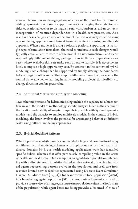
194 S Y S T E M S S C I E N C E T O W A R D A C O N S E Q U E N T I A L P O P U L A T I O N H E A LT H
involve elaboration or disaggregation of areas of the model— for example, adding representation of social support networks, changing the model to con-sider educational level or to distinguish rural vs. suburban vs. urban contexts, incorporation of resource dependencies in a health- care process, etc. As a result of these changes, an area of the model that was originally couched using one modeling approach may benefit from respecification using an alternate approach. When a modeler is using a software platform supporting just a sin-gle type of simulation formalism, the need to undertake such changes would typically entail an entire rewrite of the model in a new formalism— and a cor-respondingly different modeling package. Even in those comparatively rare cases where available skill sets make such a rewrite feasible, it is nevertheless likely to impose a high opportunity cost. By contrast, in the context of hybrid modeling, such a change can be supported by simply altering the boundaries between regions of the model that employ different approaches. Because of the central value attached to learning in many modeling projects, this flexibility to change direction confers great value.
2.4. Additional Motivations for Hybrid Modeling
Two other motivations for hybrid modeling include the capacity to subject cer-tain areas of the model to methodology- specific analyses (such as the analysis of the location and stability of long- term equilibria possible with System Dynamics models) and the capacity to employ multiscale models. In the context of hybrid modeling, the latter involves the potential for articulating behavior at different scales using different modeling approaches.
2.5. Hybrid Modeling Patterns
While a previous contribution has enumerated a large and combinatorial array of different hybrid modeling schemes with applications across them that span diverse domains [44], our health modeling applications work has identified specific hybrid schemes that offer particularly compelling value in the arena of health and health care. One example is an agent- based population interact-ing with a discrete event simulation- based service network, in which individ-ual agents representing persons evolve in the population and seek care from resource- limited service facilities represented using Discrete Event Simulation (Figure 16.1, drawn from [12, 54]). In the individuated focal population [ABM] in a broader aggregate population [SD] pattern, System Dynamics is used to provide a coarse view of an aggregate upstream population (often the lion’s share of the population), while agent- based modeling provides a “zoomed in” view of
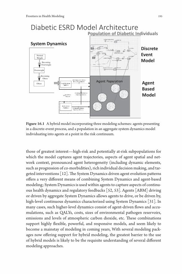
Frontiers in Health Modeling 195
those of greatest interest— high- risk and potentially at- risk subpopulations for which the model captures agent trajectories, aspects of agent spatial and net-work context, pronounced agent heterogeneity (including dynamic elements, such as progression of co- morbidities), rich individual decision making, and tar-geted interventions [12]. The System Dynamics driven agent evolution patterns offers a very different means of combining System Dynamics and agent- based modeling; System Dynamics is used within agents to capture aspects of continu-ous health dynamics and regulatory feedbacks [52, 53]. Agents [ABM] driving or driven by aggregate System Dynamics allows agents to drive, or be driven by, high- level continuous dynamics characterized using System Dynamics [31]. In many cases, such higher- level dynamics consist of agent- driven flows and accu-mulations, such as QALYs, costs, sizes of environmental pathogen reservoirs, emissions and levels of atmospheric carbon dioxide, etc. These combinations support highly flexible, powerful, and responsive models, and seem likely to become a mainstay of modeling in coming years, With several modeling pack-ages now offering support for hybrid modeling, the greatest barrier to the use of hybrid models is likely to be the requisite understanding of several different modeling approaches.
NormalWeight
BecomingOverweight
Overweight
BecomingObese
Obese
Figure 16.1 A hybrid model incorporating three modeling schemes: agents presenting in a discrete- event process, and a population in an aggregate system dynamics model individuating into agents at a point in the risk continuum.

196 S Y S T E M S S C I E N C E T O W A R D A C O N S E Q U E N T I A L P O P U L A T I O N H E A LT H
3. AGILE MODELING FOR LEARNING ACROSS TEAMS AND COMMUNITIES
A second major modeling trend is a reflection less of the technical artifacts deliv-ered by a modeling endeavor than of the modeling processes and practices. For many modelers, the goal is not only to build a useful model but also to see that model be put into actual use— in shaping policy, in informing understanding of and learning from incoming epidemiological data on the part of stakeholders, in shaping intervention implementation and scale- up plans, thinking through care system redesign, prioritizing data collection, and operational decision making. A central factor in determining the degree to which models get used in practice is the degree to and capacity in which modeling projects engage stakeholders. A discussion of the issue of stakeholder engagement in modeling projects look-ing forward bears consideration of some historic context. From the perspective of modeler- end user interaction, it is broadly fair to view dynamic modeling as having witnessed two historic eras, with a third era just starting to emerge. In the first era (“Bring us your problem, and we’ll tell you what decision is best”) [13], modeling projects were overwhelmingly conducted inside academic or specialist organizations, with the primary deliverable to the knowledge users being findings from model explorations conducted by such specialists. Elements of that first era of modeling remain widespread, but increasingly it was replaced by a second era in which models are commonly delivered to the knowledge users and stakeholder team for use— but often in a fairly “black box” fashion. Within this context, the team of stakeholders may interact with the model (for example, through a web- based or desktop interface), but only for prespecified scenarios, and only by viewing certain tightly circumscribed outputs. More importantly, within this second era of modeling, the internals of that model, including the assumptions made, typically remain opaque to end users, and cannot be modi-fied by them. Even in those cases in which the modeler is embedded within the end user team, requests to evolve the model— even for modest changes to the assumptions, or to add certain outputs or new types of scenarios— must be referred to the modeler(s). The inaccessibility of the model to the end users and the bottleneck around the modeler not only inhibit the speed of model evolution but also leave that evolution and those model assumptions notably vulnerable to misunderstandings. More critically, the model opacity and bottleneck around the modeler slows down the learning process and the speed of iteration toward improved understanding.
A combination of factors— evolution of modeling technologies to include more transparent and declarative model specifications (Figure 16.2), participa-tory modeling efforts, understanding of contemporary software development best practices and processes— are beginning to reshape how modeling is pursued
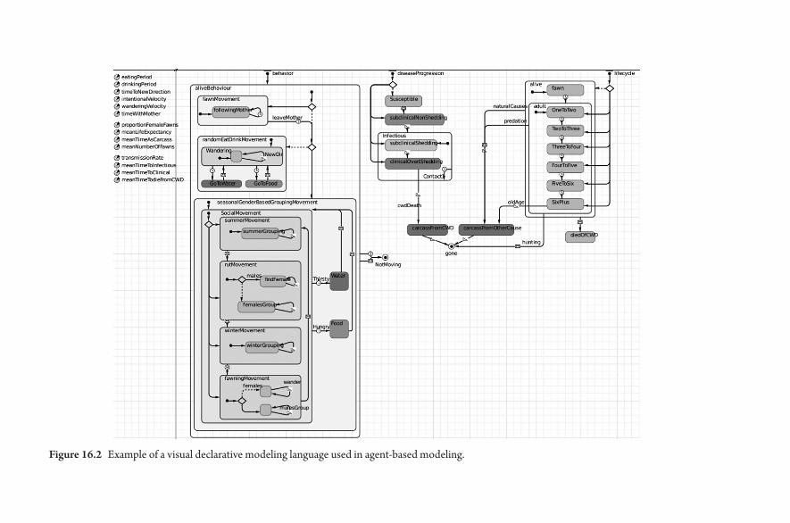
Figure 16.2 Example of a visual declarative modeling language used in agent- based modeling.
198 S Y S T E M S S C I E N C E T O W A R D A C O N S E Q U E N T I A L P O P U L A T I O N H E A LT H
and to usher in a third modeling era. In this emerging era of “Agile Modeling,” such modeling is increasingly embedded within interdisciplinary teams. Although modeling experts are still required, modeling is no longer purely the domain of such experts; models within such Agile Modeling contexts are designed in a fash-ion to be broadly accessible across team members. This environment supports team members in being able to proactively inspect— and thereby critique— the assumptions of a model, locally modify those assumptions, run the model, and increasingly to supplement previously defined model outputs with those of their own devising. Such broader access to the model will support faster model evolu-tion and learning, particularly in identifying discrepancies between model results and empirical observations or knowledge concerning the world and in helping to refine mental models [5] across the team.
More significantly, this emergence of “Agile Modeling” aids in realizing the potential for models to serve as learning tools. Rather than being viewed as “crys-tal balls” that are either accurate and successful or flawed and a failure, models are increasingly realizing their potential to enhance the rapidness, depth, and robust-ness of organizational learning. Although dynamic models most certainly do not directly confer reliable understanding of processes in the world, they can help us more quickly identify inconsistencies between our best understanding of that world and empirical evidence. The importance of models as “learning prosthe-ses” reflects the fact that unaided humans are notoriously poor at perceiving the implications of their understanding concerning underlying processes of a system on systems behavior as a whole [7] ; by contrast, given an unambiguous model specified on a computer, computers are extremely effective at playing out the logical implications of the assumptions captured within that model. From this perspective, the discovery of an inconsistency between what the model suggests in simulation results (often the logical but previously unrecognized consequence of erstwhile tacit organizational assumptions) and empirical knowledge is not a failure of the model, but a success of the modeling process— and a success of organizational learning, in that it helps refine that understanding, and render it more robust. Within this third and “Agile” era of modeling, embedded transpar-ent models within teams help harness knowledge across the breadth of the team and greatly accelerates the team’s ability to identify areas where that knowledge falls short, and contribute to making it more robust. Such modeling can further aid in identification of key uncertainties that will make that knowledge more firm and in planning interventions that will use that knowledge to offer high- leverage and cost- effective improvements for the health of the population. The results of such evidence gathering and from interventions can then further serve to help test the model and to refine the understanding captured therein, thereby refin-ing the team’s knowledge. Like Agile software development processes [9, 10, 11], such modeling will take place incrementally and embedded among stakeholders.
Frontiers in Health Modeling 199
This is a process in which ongoing learning and observation takes place— and in which the plan adapts to such learning and to evolving stakeholder prioritiza-tions of possible model extensions. Fully appreciating the benefits of Agile mod-eling requires appreciation for the implications of stakeholder involvement in modeling projects, a topic about which the space constraints only allow for a few words. Benefits of rich stakeholder involvement include informing and ground-ing the understanding going into and captured in the model, the potential for shaping stakeholder cooperation and capacity, to enhance a sense of buy- in— and sometimes ownership— over the model. Within this area, and particularly in the practice of “group model building” and “participatory modeling” [15, 14, 16, 17, 18, 19, 20], there has been a widespread recognition of the value of models as “boundary objects” [14]— that is, to serve as mutually understood concrete focal points for discussion concerning the underlying system by parties who otherwise speak very different languages. By concretizing the discussion around commonly understood elements that can be literally pointed at, the models not only help bring diverse parties to the table, but can further help foster communication between parties who lack the common abstract language to communicate readily about the system being structured.
Success in this area will benefit much from the ongoing strengthening of the visual, declarative specification of models (Figure 16.2) such that they are trans-parent to stakeholders not trained in modeling, as well as support for interactive, collaborative software for geographically disparate stakeholders to interact with a model. While the transition is in its nascent phase [46, 45], coming years are likely to see simulation follow the trend in many other areas of information tech-nology toward collaboratively oriented cloud- based support, similar to what is seen in Google Docs and Microsoft Office 365.
4. SYSTEMS SCIENCE IN THE AGE OF BIG DATA
A third major trend affecting health applications of systems science relates to the emerging synergies between electronically sourced health data and dynamic modeling. While large components of health information have long been stored and manipulated electronically, many such representations were largely under-taken for day- to- day operational purposes (e.g., billing, clinical workflow, to enable mandated reporting formats, etc.); when data was retained for research, planning, and administrative decision making purposes, such data was com-monly fragmented between information silos, including separate databases, spreadsheets, and separate files for tools such as SAS, SPSS, STATA, etc.
The past half- decade has witnessed a sea change within the health field in terms of the emergence of new data collection modalities, of interlinking previ-ously balkanized data sets, and in terms of processes and infrastructure to make

200 S Y S T E M S S C I E N C E T O W A R D A C O N S E Q U E N T I A L P O P U L A T I O N H E A LT H
such electronically sourced data available for decision- making purposes. This data comes in diverse forms, and relates to different areas of health behavior, contexts, status, and exposures. Several classes and types of such widely available health- related information are discussed below.
4.1. Important Classes of “Big Data” in Health
A first major class of health- related “big data” consists of physical measures of health behavior and status via sensor data from wearable devices and consumer electronics— for example, smartwatch- collected accelerometry, heart rate and heart rate variability, electrodermal activity, similar information and orientation from smartphones, and measures from devices supporting wireless data trans-port such as weight scales (potentially with adiposity measurement), glucom-eters, and blood pressure cuffs. This information can be of exceptional value in areas where self- reported data is often unreliable— such as with respect to nutri-tional intake, physical activity, contact, and mobility patterns.
The second major class of health- related “big data” captures aspects of con-text. Geospatial environmental information can lend an understanding of mobility, location, duration and occurrence of exposure to particular indoor and outdoor environments. Such information can particularly be gleaned from the strength of WiFi, GPS, Bluetooth, RFID, cellphone tower signals and certain sensors, which are commonly available on smartphones and some other consumer elec-tronic devices. Environmental information concerning those contexts— such as are present in GIS systems, databases collected from environmental sensors, or from building control systems— can provide an understanding of the character of these exposures. Some of such environmental information comes directly via wearables and consumer electronic devices carried by the subject (e.g., humidity, temperature, barometric pressure, magnetometers). Other information comes from cross- linking data on location with other data sources. Some of this data can be linked in real time— for example, measurements from proximate envi-ronmental sensors associated with infrastructure, such as in building control systems, municipal infrastructure, and weather stations. Other such linkages are reliant on retrospective databases, including GIS databases and historical data-bases compiled from monitoring infrastructure (e.g., weather records). Network context can be information used to detect dynamic interpersonal contact patterns and degree of proximity between participants can be derived from technologies such as Bluetooth and RFID.
A third broad class of health- related “big data” information consists of infor-mation shared with others, or self- reported by participants to surveillance ini-tiatives, research studies, or other health or health- care actors, as facilitated

Frontiers in Health Modeling 201
by use of electronic technologies. A first such type of information has older roots but has been substantially enhanced by synergy with other types of col-lected information: Responses to on- device questionnaires and ecological momen-tary assessments (EMAs). Tools such as the EpiCollect [21], mEMA [62] and DREAM [57] systems provide easy ways of gathering health information via personal mobile devices (and soon via wearables), with the iEpi system [32, 33] additionally supporting triggering of such ecological momentary assess-ments, based on sensed aspects of context or participant history (e.g., ques-tionnaire triggering at recreational locations, fast food restaurants, or following periods of sedentary behavior, in certain social contexts [47], or other aspects of sensed data). Such triggering can elicit place- or exposure- specific informa-tion and enhance likelihood of participant response. A second major type of self- reported information is the growing volume of electronically mediated crowdsourced information. A growing amount of public online health data is vol-unteered by individuals, either as part of community efforts, as a side effect of operational needs, or for personal insight. Examples include information submitted by parties using services such as Endomondo, Google Fit, and those using Apple Health, fitness- oriented apps such as FindSports, via FitBit shar-ing, etc.— interactions which also fall into the class of health- related commu-nicational behavior covered below. Tools such as iEpi/Ethica Health [32, 33] further support easy collection of study-specifc participantreported informa-tion on exposures, subclinical symptomology, etc., in a way that can be adapted without programming (Figure 16.3).
An overlapping class of information consists of health- related communicational behavior, which is key for informing understanding of health- related beliefs, cog-nitions and decision making. Such information includes information shared via social media, such as Facebook status updates, twitter feeds, blogs, chatrooms, etc. In a surveillance and research context, there can also be monitoring of addi-tional communicational browsing behavior (including URLs visited and page contents— particularly to health- related information and community sites), use of health- related apps, text messages occurrence and content, and phone calls.
Is Smoking Vaping
Report
FOOD_HOME
FOOD_OTHER
FOOD_SICKNESS
ID
vapingsmoking
Dec 6, 15
20 Jan 25 Jan 30 Jan 4 Feb 9 Feb 14 Feb 19 Feb 24 Feb 29 Feb 5 Mar
525
525
525
Dec 11, 15 Dec 16, 15 Dec 21, 15Hour of Timestamp
Dec 26, 15 Dec 31, 15
vapingsmoking
Is Smoking Vaping
Figure 16.3 High temporal density longitudinal data of the sort that could be used for model calibration.
202 S Y S T E M S S C I E N C E T O W A R D A C O N S E Q U E N T I A L P O P U L A T I O N H E A LT H
The growing use of technologies to identify affect and stress from voice commu-nicational behavior can enhance the data available.
Beyond the above classes of health information, there are a variety of important additional types of information. For example, electronic information on purchas-ing behavior can provide insight into health- related personal protective behaviors, risk behaviors, and concerns. Sources for such data include point of sale data from stores, online purchase transaction data, data preserved through use of purchase functionality (increasingly integrated with smartphones, etc.). Electronic clinical data is of great interest in the clinical and health- care management sphere but can also offer great value in terms of understanding the interaction between care- seeking and underlying population health concerns. Such clinical data is present in electronic health records, providing information on care- seeking, laboratory test outcomes, diagnoses, imaging results, physical measurements concerning diverse quantities such as patient height, weight, blood pressure, reflexes, etc.
Collectively, the “Four Vs” characteristic of “big data” [22] offer much to enhance the prospect of building dynamic models. The volume offers much evi-dence, the velocity (Figure 16.1) can help parameterize and calibrate fine- grained dynamic models, as well as aid in theory building. Given that dynamic models commonly characterize many aspects of human behavior, the variety can help simultaneously ground many elements of individual state and behavior (includ-ing location and obility, social network context, and diverse health behaviors), and the veracity can often considerably elevate accuracy in grounding certain elements more so than would be possible with self- reporting (particularly when compared to self- reporting in areas such as nutritional intake, physical activity, weight dynamics, contact patterns, and spatial mobility; see Figure 16.4).
4.2. Hierarchy of Data Science Models
Absent models to make sense of them, the electronic data discussed above offers simply a cacophony of numbers. Models to secure insight from such data come in a variety of forms and serve different purposes— for example, to classify, infer, estimate, filter, or smooth. Before incorporating elements of “big data” into dynamic models, it is frequently necessary to apply several such models in a suc-cessive fashion. For example, we often first need to screen out patently spurious sensor values (e.g., recognizable GPS artifacts), aggregate to lessen the effects of noise, and then analyze the underlying data in order to identify features in the empirical data that correspond to elements of the simulation model— high- level elements that are merely implicit in the “raw” data, such as “visit to park,” “con-tact between a child and their mother,” “visit to convenience store,” “period of sedentary behavior,” “use of a sidewalk.” After passing through several layers of

Figure 16.4 Example of variety of information often received in big data, combining temporal and geographic context plus survey answers, and audio recordings (from Ethica iEpi/Ethica Health system).
204 S Y S T E M S S C I E N C E T O W A R D A C O N S E Q U E N T I A L P O P U L A T I O N H E A LT H
model- based filtering and classification methods, the data may be suitable for use with a dynamic model. We discuss that combination below.
4.3. Combining Big Data and Dynamic Models
Dynamic models can be informed by the big data discussed above in several ways. Perhaps the most notable and direct way that “big data” can work with dynamic models is by serving as a source for model parameter estimates. In some cases, this estimate is more direct— for example, emerging from analysis of the frequency of some event clearly marked by the previous classifiers (e.g., visits to a convenience store or a park, contact with another participant, uses of an e- cigarette). Another more direct case is seen in [34, 35, 36], where measured proximity data directly drives network connectivity in the model. In other cases, derivation of this parameter estimate may require further statistical analysis, such as for hazard rates derived through survival, recurrent event or competing risk analysis. In another more indirect estimation example, the empirical data could function as revealed preference data for estimating preferences in discrete choice theory models [23].
In an alternative set of cases— of nearly equal significance to the above— “big data” informs the model in another way: through calibration. In this process, rather than being used directly to derive estimates for particular parameters, the empirical data is systematically compared against emergent behavior from the model as certain little- known parameter values in the model are tuned. We then assume as the value of those underinformed parameters the parameter value vector that minimizes the discrepancy between dynamic model output and empirical data.
Another important case focuses on the handling of incoming temporal sequences of data. Within this “filtering” case, rather than simply being used by the dynamic model, the incoming data is combined with model estimates of states derived from the simulation, forming a single or distribution of consensus values. For example, [37] demonstrated the use of the venerable Kalman Filtering technique for combining model estimates with incoming data, including sensor- based data from dynamic networks. Additional elements of this approach are dis-cussed in the section below on sequential Monte Carlo approaches.
In other cases, the data flow between machine learning and dynamic models is reversed, and dynamic models serve as a source for “synthetic ground truth” to test machine learning models or study designs involving big data. These approaches take key advantage of the fact that a dynamic modeler has complete access to information concerning the state of the simulation at any given time. Recourse to this true state of the model allows it to be compared with estimates

Frontiers in Health Modeling 205
or classifications of that state derived from machine learning methods, or from other analytics being evaluated as elements of the planned study design. For example, [56, 35] used synthetic ground truth from an agent- based model to identify contact network sampling rates (at different levels of specificity) required for reliable inferences to be drawn concerning the spread of information across those contact networks.
Another key way in which “big data” and modeling fit together lies in sup-port of validation and learning. Here, electronically sourced empirical data is compared with corresponding items from a simulation model in a particular context— for example, following an intervention. Frequently, the different ele-ments and subsets of such “big data” can help elucidate dynamics of distinct pathways hypothesized to drive outcomes of interest. For example, Figure 16.5 depicts hypothesized pathways by which a move of a low- income family to a mixed neighborhood might affect health and social outcomes (such as obesity) in that family. The “variety” component of “big data” can help shed light on the operation of such pathways, and the degree to which they are affected by the intervention. For example, GPS- and WiFi- based location sensors over time could pick up the degree to which significant changes in the use of recreational space occur before and after the move, the degree to which there is a change in the use of grocery stores (as compared to convenience stores) pre- and post- intervention, and changes in the amount of time that children are spending
Move to MixedIncome
Neighbourhood
Recreational SpaceAvailaibilty
+
++
+
+
+
+
+
++
+
+
+
+
+
+
+
––
–
––
–
–
– –
–
PerceivedSafety
NeighborhoodWalkability Sedentary
BehaviourObesityLevels
Pro-CriminalInvolvement
Risk ofPro-CriminalAssociation
SchoolPerformance
Healthiness ofDiet
Time Spent atHome
Likelihood ofUnsupervised Travel to
Old Neighbourhoods
Healthy FoodAvailability
SchoolQuality
Strength of Localex-Familial Social
Network
Likelihood of HighSchool Graduation
BMI
Moderative-VigorousPhysical Activity
Figure 16.5 Hypothesized pathways by which an intervention might affect outcomes of interest. Dynamics associated with such different pathways can often be measured by different subsets of sensor information.

206 S Y S T E M S S C I E N C E T O W A R D A C O N S E Q U E N T I A L P O P U L A T I O N H E A LT H
at time or are returning to their old neighborhood. Such location- based sen-sors together with accelerometers could help quantify the degree to which changes in walking intensity, the level of sedentary behavior, and moderate- vigorous physical activity that apply between old and new neighborhoods. On integrated sensor- crowdsourcing- EMA smartphone platforms such as Ethica iEpi [32, 33], EMAs could moreover be used to elicit attitudes and percep-tions (such as perception of safety, of walkability, etc.), shedding light on their dynamics pre- and post- intervention. While such sensor- based mechanisms provide an admirably multifaceted view of the effects of intervention, often they are well matched in richness by a corresponding simulation model. Such a simulation model will also include a diversity of such causal pathways within its representation, with the parallel character of these representations raising the opportunity for great insight via side- to- side comparison. Specifically, in the event of an intervention being put into place, empirical data collected from such smartphone- based mechanisms over time can be compared against the model’s expectations concerning the dynamics of corresponding pathways. Discrepancies can be used to refine the model or data collection strategies, and— even more importantly— to sharpen the research team’s understanding of the effects of such interventions.
5. COMBINING BAYESIAN MONTE CARLO APPROACHES AND DYNAMIC MODELS
The section on big data above briefly noted the joint roles played by dynamic models and their machine learning/ computational statistical and dynamic cous-ins in the specific context of big data, with dynamic models being informed and grounded by findings from machine learning models, and dynamic models being used to evaluate and refine machine learning models.
While the combinations of models drawn separately from each domain is of great value, the modes of cooperation of the methods of machine learning/ com-putational statistics (henceforth “machine learning”) and dynamic modeling are not limited to their use in distinct models. Although traditionally pursued by dis-tinct communities, each with a depth of methodological knowledge, we can use machine learning methods with a given dynamic model in several ways. We focus here on the powerful prospects extending from combining dynamic modeling approaches with one specific class of machine learning approaches— Bayesian Monte Carlo methods. This combination provides for modeling approaches sup-porting a capacity to readily incorporate new information as it becomes available and that is more robust by virtue of not only complex system behavior but also statistical variability and probabilistic model structure. In this section, we sketch

Frontiers in Health Modeling 207
the combination of two specific Bayesian Monte Carlo methods with dynamic models: Markov Chain Monte Carlo methods and Sequential Monte Carlo Methods (in the form of the particle filter) and note their combination in the form of Particle Markov Chain Monte Carlo methods.
While the three types of Bayesian Monte Carlo methods covered here dif-fer in their specifics, when combined with dynamic models they share several important features of relevance: (1) explicit probabilistic models relating obser-vations and other quantities (e.g., parameters), (2) the incorporation of dynamic model results to be incorporated into the likelihood functions employed, (3) the capacity to readily deal with estimation of latent quantities— quantities for which direct observations are not available, (4) a shared (Monte Carlo) goal of repeat-edly sampling (drawing) from posterior distributions associated with model quantities— once such samples are drawn, they can be used in many powerful ways, and (5) as Bayesian approaches, these methods support specification of prior distributions over the model quantities being sampled— distributions that allow characterizing prior beliefs about such parameters (beliefs possibly drawn as posterior distributions emerging from earlier data).
We now briefly characterize the role of such methods when combined with dynamic modeling.
5.1. Markov Chain Monte Carlo Methods
Dynamic modelers have long relied heavily on model calibration to estimate model parameters by matching simulation model data against empirical obser-vations. While valuable, calibration exhibits some notable shortcomings: it fre-quently yields just point estimates with unclear uncertainty. Even when such uncertainty is estimated by a covariance matrix, it fails to account for multimodal distributions and cannot be translated into similar bounds for model outputs, and differences between outputs for model scenarios, etc. A rapidly growing lit-erature [24, 25, 38, 40, 41] has applied Markov Chain Monte Carlo (MCMC) methods to deterministic dynamic models, particularly in the methodologically sophisticated area of mathematical epidemiology of infectious disease, and a handbook chapter by Osgood and Liu [40] provides a systematic introduction to the use of such models, while [26] provides a video tutorial designed to intro-duce viewers to the use of such models at a very elementary level. Given a prior distribution over a (vector of) model parameters θ, one or more observations y, and a likelihood function p(y|θ), MCMC methods seek to sample (i.e., draw particular parameter vectors in turn) from the joint posterior distribution p(θ|y) of those parameters. When combining MCMC methods with dynamic mod-els, some of the θ parameters are typically associated with the dynamic model,
208 S Y S T E M S S C I E N C E T O W A R D A C O N S E Q U E N T I A L P O P U L A T I O N H E A LT H
others are associated instead with the probabilistic model. Within this context, the dynamic model typically plays a central role in calculating the likelihood function p(y|θ)— particularly in translating one or more parameters within θ into dynamic model outputs that can be compared directly or indirectly to the empirical observations y. The capacity to compute this likelihood function and the prior likelihood function allows for (jointly) sampling parameters θ from the posterior distribution. Once each parameter is sampled, it can then be used for a variety of types of analyses, including sampling from the posterior distributions of model states, of future trajectories of the system under different intervention scenarios, of differences in outcome between two scenarios (e.g., between base-line scenario and an intervention), from a cost effectiveness ratio, or estimating the probability of a given occurrence, etc.
5.2. Sequential Monte Carlo Methods
A second and more recent approach to combining of machine learning and dynamic modeling methods can be found in the use of sequential Monte Carlo methods, specifically in the form of particle filtering. In contrast to MCMC approaches— which sample from the joint distribution of parameter values of the dynamic and probabilistic models— particle filtering samples from joint dis-tributions of latent states of the dynamic model. This approach is specifically well suited to “online” planning that takes into account incoming data streams while balancing the fact that both the simulation model and the data are error- prone. As a result of performing particle filtering with a dynamic and probabilistic model, we can sample from the distribution of model state over time, both during the period when new data is recurrently available as well as looking forward. This distribution reflects both uncertainty concerning how the underlying state of the model evolves forward over time (reflecting model stochastics) and uncertainty with regard to the measurements.
Reflecting its focus on stochastic models, Sequential Monte Carlo methods secure great computational efficiency by virtue of an incremental and recursive approach with use or arrival of each new observation updating the samples drawn on the basis of earlier observations. As with MCMC, particle filtering using a given (stochastic) dynamic model requires that the modeler specify a prior distribution— here, over initial latent states x0 of the dynamic model— and a likelihood function p(yt|xt), which specifies the likelihood that empirical obser-vation yt would be obtained given some posited state xt of the model at time t. Based on this, the system samples from the posterior distribution p(xt|yt) for all t. Moreover, far from being limited to sampling from the state vector at each time point in isolation, particle filtering allows for sampling from the distribution of latent state trajectories over the timeframe of the model, as well as dynamically

Frontiers in Health Modeling 209
evolving parameter values. Sampling jointly from both the latent state over time and the values of θ, by contrast, requires Particle MCMC (see Figure 16.6).
As a technique, particle filtering raises the extraordinary prospects of “learn-ing” models— modeling in a fashion that limits model uncertainty by recurrently regrounding a model’s estimate of its current state (including any evolving dynamic values) by reference to (recognizably noisy) external observations. This technique fits the needs of modeling emergent situations, such as outbreaks of new pathogens when many epidemiological parameters— and potentially some aspects of the natural history of infection or transmission pathways— remain uncertain. Indeed, particle filtering has been applied notably to H1N1 [27, 41] and for TB [41], and has demonstrated its effectiveness in correcting model state estimates for diverse networks using synthetic ground truth data [42]. By virtue of its ability to balance uncertainty about a model with uncertainty regarding empirical observations, its close support for automatic handling of incoming data streams, and the capacity to “learn” (in terms of state and evolving parameters) from repeated observations even in the context of an uncertain model, it seems likely that particle filtering will constitute a prominent staple of real- time decision making using dynamic models in coming years, despite acutely limited current software support [43].
The Particle Markov Chain Monte Carlo (PMCMC) technique represents a recent contribution in the literature that combines the essential elements of Markov Chain Monte Carlo techniques and particle filtering within a single algo-rithm. When used in conjunction with a dynamic model, PMCMC can be used to sample from a joint distribution over both parameter values and latent states of that dynamic model. Despite tremendous potential, the technique is encum-bered by high computational load and complexity and has yet to see widespread application to dynamic models.
Figure 16.6 Particle filtering for an aggregate transmission model applied to incoming data until day 35, with projection forward following that time. Empirical data on incident cases shown in darker horizontal markers, samples from the distribution of model predictions over incident cases shown in lighter color.

210 S Y S T E M S S C I E N C E T O W A R D A C O N S E Q U E N T I A L P O P U L A T I O N H E A LT H
6. REPRESENTATIONS OF COGNITIVELY PLAUSIBLE SITUATED HUMAN BEHAVIOR
In systems science models in the health area, representation of human health behaviors and decision making has long been of interest. Since the inception of dynamic modeling of vector- borne diseases with Ross [28, 29] and person- to- person spread of communicable diseases by Kermack and McKendrick in the 1920s [30], dynamic models have sought to represent aspects of human health behavior. Recent decades have seen increasing use of individual- based models (and particularly agent- based models) depicting situated decision making by actors based on aspects of local context in geographic space and within networks. However, traditional representations of behavior in such models have often been highly stylized— for example, positing utility maximization, fixed responses to the external stimuli, or even behavior dictated by fixed probabilities.
Similarly, when examining the impacts of interventions on population health outcomes, modelers have often made the simplifying assumption that parameter values would change in a defined fashion, for example by lowering the hazard rate associated with relapsing to smoking by 10%, or the probability of electing to take a convenience store meal by 20%. Models and model scenarios making use of these simple representations can contribute much insight— for example, in understanding the distal impacts of an intervention or other scenario on down-stream health outcomes, such as incidence of diabetes or heart disease— but often beg the question as to exactly how and how quickly such behavior change can be realized. For many purposes, use of more evolved behavioral representations can open notable opportunities. Rather than representing behavior as occurring with fixed probabilities, consisting of a fixed rule in response to observed external circumstance, or positing fixed changes to such behavior in response to interven-tions, for the sake of model- based learning, it is advantageous to see how changes to behavior emerge endogenously in response to a novel choice environment, or in the context of changed incentives, including those brought about by policies.
In addition to the desire for enhanced flexibility in examining behavioral assumptions, there is often a sense of a yawning gap between the types of behav-ioral representations commonly depicted in today’s models and what is sug-gested by evidence from empirical choice theories and cognitive science. One example concerns scientific recognition of widespread use of heuristic strategies in place of rational deliberation for many decisions in day- to- day life, which has been well documented by Kahneman, Tversky and others [49]. Several lines of evidence also suggest a tiered process in which strikingly different decision strat-egies are employed to perform a rough shakedown of possible choices (on the one hand) and to select among the strategies so chosen (on the other). Failure to adequately capture the impact of such heuristics on decision making in the
Frontiers in Health Modeling 211
context of changed choice environments may yield to systematic mis- estimates of the relative gains to be expected through different interventions [55].
Based on these gaps between traditional approaches and research findings, some leading researchers have advanced strategies to incorporate more cog-nitively plausible decision strategies within agent behavior, based on modern discrete choice theory [48, 31] or on connectionist approaches drawn from cog-nitive science [50, 51]. Models embracing such strategies can capture agents’ decision behavior that is simultaneously more cognitively realistic and also capa-ble of generating far more endogenized behavioral response to interventions than is possible with most of today’s modeling (in which such behavioral responses are often presupposed, or are more directly implied by the rules obtained). By virtue of such endogenization, models investing in more realistic representations of behavior, the door is opened to a greater ability to examine concerns regard-ing the intervention science. In contrast to traditional models in which behavior change is directly posited, the dynamics of intervention implementation can be simulated within the model, better capturing the delays associated with securing intervention effects on both behavior and on distal outcomes.
In the context of the emerging “big data” milieu discussed above, discrete choice theory is notable in its association with techniques for eliciting preference information from both stated and revealed preference data. For the former, the approach offers refined strategies for crafting instruments that will lower both the number of required respondents and the burden of questions on those respon-dents; the growing proliferation of wearables and mechanisms for smartphone- based EMAs can ease delivery of such questionnaires. While revealed preference data has most traditionally been associated with analyzing point of sale data, within the health area it is notable for being positioned to make use of the high- velocity longitudinal sensor data discussed above. While stated preference data will remain important for understanding certain types of counterfactuals, the prospects are strong for using revealed preference methods to exploit evidence collected via the growing number of low- burden, automatically collected elec-tronic data sources within the health area.
7. AN EMERGING TRANSFORMATION OF SYSTEMS SCIENCE
The trends discussed above are working to make the insights extending from health applications of systems science more widespread and accessible, deeper, more grounded, more impactful, less siloed, more easily conducted and shared, and more robust in light of the uncertainties present. The trends above and others not covered here— such as the growth of cloud- based computing— will draw systems science closer to computational statistics, the
212 S Y S T E M S S C I E N C E T O W A R D A C O N S E Q U E N T I A L P O P U L A T I O N H E A LT H
behavioral sciences, and policymakers, while allowing for a broader apprecia-tion and dissemination of its findings. The coming decades are likely to sig-nificantly reshape for the better the practice of health systems science in terms of project goals, technologies, social environment and team composition, and day- to- day operation. At the same time, some factors will remain invari-ant: key challenges in the education and training area, the need to embrace both rigor and relevance, and to break down barriers both within systems sci-ence communities and between systems science and cognate areas. If those challenges can be overcome, the contributions of health systems science are likely to multiply greatly.
8. REFERENCES
1. Forrester JW. Industrial Dynamics. Cambridge, MA. MIT Press; 1961. 2. Duggan, J. A Simulator for Continuous Agent- Based Modelling. 25th International
Conference of the Systems Dynamics Society Boston; 2007. 3. Tuckwell H, Toubiana L, Vibert J. Spatial epidemic network models with viral
dynamics. Physical Review E. 1998, 57: 2163– 2169. 4. Kostova T. Persistence of viral infections on the population level explained by an
immunoepidemiological model. Mathematical Biosciences. 2007; 206: 2309– 2319. 5. Sterman J. Business Dynamics. Boston, MA: McGraw- Hill Higher Education; 2000. 6. North MJ, et al. Complex adaptive systems modeling with Repast Simphony. Complex
adaptive systems modeling. 1(1): 1– 26; 2013. 7. Sterman JD. Modeling managerial behavior: Misperceptions of feedback in a
dynamic decision making experiment. Management Science. 1989; 35(3): 321– 339. 8. Abelson H, Sussman GJ. Structure and Interpretation of Computer Programs. MIT
Press, Cambridge, MA; 1996. 9. Martin RC. Agile software development: Principles, patterns, and practices. Prentice
Hall PTR; 2003. 10. Beck K, et al. Manifesto for Agile Software Development; 2001. 11. Fowler M, Highsmith J. The agile manifesto. Software Development. 2001;
9(8): 28– 35. 12. Gao A, Osgood N, An W, Dyck R. A Tripartite Hybrid Model Architecture for
Investigating Health and Cost Impacts and Intervention Tradeoffs for Diabetic End- Stage Renal Disease. Oral Presentation and Full Paper in Proceedings of the 2014 Winter Simulation Conference. December 7- 10, 2014, Savannah, GA; 2014.
13. Richmond B. System Dynamics/ Systems Thinking: Let’s Just Get On With It. In International Systems Dynamics Conference, Sterling, Scotland; 1994.
14. Hovmand P. Community Based System Dynamics. New York, NY: Springer; 2014. 15. Vennix JA. Group Model Building: Facilitating Team Learning Using System Dynamics.
Wiley; 1996. 16. Stave KA. A system dynamics model to facilitate public understanding of water man-
agement options in Las Vegas, Nevada. Journal of Environmental Management. 2003; 67(4): 303– 313.

Frontiers in Health Modeling 213
17. Stave K. Participatory system dynamics modeling for sustainable environmental management: Observations from four cases. Sustainability. 2010; 2(9): 2762– 2784.
18. Beall A, Zeoli L. Participatory modeling of endangered wildlife systems: Simulating the sage- grouse and land use in Central Washington. Ecological Economics. 2008; 68(1): 24– 33.
19. Langsdale SM, et al. Exploring the implications of climate change on water resources through participatory modeling: Case study of the Okanagan Basin, British Columbia. Journal of Water Resources Planning and Management. 2009; 135(5): 373– 381.
20. Langsdale S, et al. Collaborative modeling for decision support in water resources: Principles and best practices. Journal of the American Water Resources Association. 2013; 49(3): 629– 638.
21. Aanensen DM, Huntley DM, Feil EJ, Spratt BG. EpiCollect: Linking smartphones to web applications for epidemiology, ecology and community data collection. PLOS ONE. 2009; 4(9): e6968.
22. International Business Machines Corporation. The Four V’s of Big Data. Accessed on May 22, 2016. Infographic at http:// www.ibmbigdatahub.com/ infographic/ four- vs- big- data.
23. Train KE. Discrete Choice Methods with Simulation. Cambridge University Press; 2009. 24. Dorigatti I, Cauchemez S, Pugliese A, Ferguson NM. A new approach to characteris-
ing infectious disease transmission dynamics from sentinel surveillance: Application to the Italian 2009- 2010 A/ H1N1 influenza pandemic. Epidemics. 2012; 4(1): 9– 21.
25. Coelho FC, Codeço CT, Gomes MGM. A bayesian framework for parameter estima-tion in dynamical models. PLOS ONE. 2011; e19616.
26. Osgood N. 2013. Using Bayesian MCMC for Dynamic Model Parameter Estimation 1—Basic concepts. URL of https:// www.youtube.com/ watch?v=jK9T6H6SVIc
27. Ong J, et al. Real- time epidemic monitoring and forecasting of H1N1- 2009 using influenza- like illness from general practice and family doctor clinics in Singapore. PLOS ONE. 2010; 5: e10036– e10046.
28. Ross R. An application of the theory of probabilities to the study of a priori pathom-etry. Part I. Proceedings of the Royal Society of London. Series A, Containing papers of a mathematical and physical character. 1916; 204– 230.
29. Ross R, Hudson HP. An application of the theory of probabilities to the study of a pri-ori pathometry. Part II. In Proceedings of the Royal Society of London A: Mathematical, Physical and Engineering Sciences. 1917; 93(650): 212– 225.
30. Kermack WO, McKendrick AG. A contribution to the mathematical theory of epi-demics. In Proceedings of the Royal Society of London A: Mathematical, Physical and Engineering Sciences. 1927; 115(772): 700– 721.
31. Flynn T, et al. Discrete choice, agent based and system dynamics simulation of health profession career paths. Oral Presentation and Paper in Proceedings of the 2014 Winter Simulation Conference. Savannah, GA; 2014.
32. Knowles DL, Stanley KG, Osgood N. A field- validated architecture for the collection of health- relevant behavioural Data. Oral presentation and full paper publication in Proceedings of the IEEE International Conference on Healthcare Informatics 2014 (ICHI 2014). 79– 88. Verona, Italy; September 15– 17, 2014.

214 S Y S T E M S S C I E N C E T O W A R D A C O N S E Q U E N T I A L P O P U L A T I O N H E A LT H
33. Hashemian M, et al. 2012. iEpi: An end to end solution for collecting, condition-ing and utilizing epidemiologically relevant data. In Proceedings, The 2nd ACM International Workshop on Pervasive Wireless Healthcare. Hilton Head, South Carolina; June 11– 14, 2012.
34. Hashemian M, Stanley KG, Knowles DL, Calver J, Osgood N. 2011. Human net-work data collection in the wild: The epidemiological utility of micro- contact and location data. Full paper in Proceedings of the ACM SIGHIT International Health Informatics Symposium (IHI 2012). Miami, FL; 2012.
35. Hashemian M, Qian W, Stanley KG, Osgood N. Temporal aggregation impacts on epidemiological simulations employing microcontact data. BMC Medical Informatics and Decision Making. 2012; (12)132: 20 (plus figures).
36. Hashemian M, Stanley K, Osgood N. Leveraging H1N1 infection transmission modeling with proximity microdata. BMC Medical Informatics and Decision Making. 2012; 12(36): 39.
37. Qian W, Osgood N, Stanley KG. Integrating epidemiological modeling and surveil-lance data feeds: A Kalman filter based approach. Oral presentation and publication in Proceedings of the 2014 International Social Computing, Behavioral Modeling and Prediction Conference (SBP14), Washington DC; April 2– 4, 2014.
38. Osgood N, Liu J. Bayesian Parameter Estimation of System Dynamics Models Using Markov Chain Monte Carlo Methods: An Informal Introduction. Verbal and poster presentation and Full paper in Proceedings, The 30th International Conference of the System Dynamics Society, Cambridge, MA. 19pp. July 22– 24, 2013.
39. Qian W, Stanley KG, Osgood N. The impact of spatial resolution and representation on human mobility predictability. In Web and Wireless Geographical Information Systems. Springer Berlin Heidelberg, 2013. Paper presented in the 12th International Symposium on Web and Wireless Geographical Information Systems (W2GIS 2013), Springer Lecture Notes in Computer Science, 25– 40. April 4– 5, 2013, Banff, Alberta, Canada.
40. Osgood N, Liu J. “Combining Markov Chain Monte Carlo Approaches and Dynamic Modeling” in Rahmandad H, et al. Analytical Handbook for Dynamic Modelers. Cambridge, MA. MIT Press. November 13; 2015.
41. Safarishahrbijari A, et al. Particle filtering in a SEIRV simulation model of H1N1 influenza. Accepted June 8, 2015. To appear in Proceedings of the 2015 Winter Simulation Conference. December 6– 9, 2015. Huntington Beach, CA.
42. Osgood N, Liu J. Towards Closed Loop Modeling: Evaluating the Prospects for Creating Recurrently Regrounded Aggregate Simulation Models. Oral presentation and full paper publication in Proceedings of the 2014 Winter Simulation Conference, Savannah Georgia. December 7– 10, 2014.
43. Kreuger K, Osgood N. Particle Filtering Using Agent- Based Transmission Models. Accepted June 14, 2015. Full Paper to appear in Proceedings of the 2015 Winter Simulation Conference. December 6– 9, 2015. Huntington Beach, CA. 11pp.
44. Borschev A. 2013. The Big Book of Simulation Modeling. Multimethod Modeling with AnyLogic 6. AnyLogic Corporation; 2013.
45. Osgood N, McDonnell G. 2016 Supporting Rich Participatory Mapping for Hybrid and Agent- Based Models: A Collaborative Web- Based Modeling Platform. Accepted
Frontiers in Health Modeling 215
March 2, 2016 for presentation at Innovations in Collaborative Modeling, June 14– 15, 2016, Lansing, Michigan.
46. Dilsner S, Erker E, Osgood N. A Collaborative Web- Based Modeling Platform for Causal Loop Diagramming. Accepted March 2, 2016 for presentation at Innovations in Collaborative Modeling, June 14– 15, 2016, Lansing, Michigan.
47. Aiello AE, et al. Design and methods of a social network isolation study for reduc-ing respiratory infection transmission: The ex- FLU Cluster Randomized Trial. Accepted by Epidemics, January 19, 2016.
48. Bruch E, Swait J. A Cognitively Plausible Model of Neighborhood Choice; 2013. 49. Kahneman, D. Thinking, Fast and Slow. New York: Macmillan; 2011. 50. Orr MG, Thrush R, Plaut DC, The theory of reasoned action as parallel constraint
satisfaction: Towards a dynamic computational model of health behavior. PLOS ONE. 2013, 8(5): e62490.
51. Orr MG, Plaut DC, Complex systems and health behavior change: Insights from cognitive science. American Journal of Health Behavior. 2014, 38(3): 404– 413.
52. Vickers D, Osgood N. A unified framework of immunological and epidemiological dynamics for the spread of viral infections in a simple network- based population. Theoretical Biology and Medical Modelling. 2007; 4: 26.
53. Vickers D, Osgood N. The arrested immunity hypothesis in an immunoepidemio-logical model of chlamydia transmission. Theoretical Population Biology. 2014; 93: 52– 62.
54. Day TE, Ravi N, xian H, Brugh A. Sensitivity of diabetic retinopathy associated vision loss to screening interval in an agent- based/ discrete event simulation model. Computers in Biology and Medicine. 2014; 47: 7– 12.
55. Bruch EE, Mare RD. Neighborhood choice and neighborhood change. American Journal of Sociology. 2006; 112(3): 667– 709.
56. Osgood N. “Sensor Informed Computational Epidemiology.” Annual Meeting of the Society for Epidemiological Research,” June 30, 2012.
57. Pennsylvania State University Survey Research Centre, DREAM Software. http:// www.survey.psu.edu/ dream, Accessed May 23, 2016.
58. Oraji R, Safarishahrbijari A, Hoeppner V, Osgood N. 2016. Combining Particle Filtering and Transmission Modeling for TB Control. Submitted April 29, 2016 to the International Conference on Health Informatics, October 4- 7, 2016.
59. AnyLogic Corporation. AnyLogic 7 software system. St. Petersburg, Russia, 2016. 60. Ventana Systems. Vensim software. Harvard, MA; 2016. 61. Simul8 Corporation. Simul8 software. Boston, MA; 2016. 62. ilumivu, Inc. mEMA software. Cambridge, MA; 2016

17
Systems Science and Population Health
A B D U L RA H MA N M . E L - S AY E D A N D S A N D RO G A L EA
This book is mainly concerned with the health of populations and with under-standing the determinants of the distribution of health within and between pop-ulations. Our concern with the health of populations extends beyond academic considerations. We are interested in understanding the health of populations so that we may intervene and identify solutions that shift population curves and that produce healthier populations both in the present and over time. We came to systems science because of a recognition that our dominant approaches to under-standing population health frequently fall short. This is because populations are the quintessential complex system, and understanding the production of health in populations must, almost by definition, lean on methods that can grapple with this complexity to illuminate levers of action that can serve to improve popula-tion health.
In this book we have presented sixteen chapters that trace the evolution of systems thinking in population health, articulate methods that hold promise for systems analysis of population health, and consider how specific approaches can guide our thinking toward a population health science of consequence. We con-clude the book by tackling one specific question: what is the role of systems sci-ence approaches in population health science? In closing, we offer three thoughts on this, building on the chapters that have preceded this conclusion, with an eye toward the field’s evolution and emergence.
First, we suggest that populations are, inevitably, complex systems, and any approach to understanding populations must adopt a systems science approach. Specifically, this means the adoption of a systems science framework and per-spective, recognizing that there are a multitude of factors that influence a given population’s health and also recognizing that these factors interrelate— and

218 S Y S T E M S S C I E N C E T O W A R D A C O N S E Q U E N T I A L P O P U L A T I O N H E A LT H
further, these interrelations are spatially and temporally dependent, character-ized by feedback, reciprocity, non- linearity, and stochasticity. At some level there is nothing surprising about this statement; that populations of heterogeneous, networked, unpredictable individuals represent complex systems should sur-prise no one. However, at another level, saying that all population health thinking must rest on complex systems thinking upends how we currently do the busi-ness of population health science. Systems science has had to elbow its way into the mainstream of population health science thinking, and is far from accepted as a dominant paradigm. This relative marginalization simply reflects the evolu-tion of the field, and an embrace of deterministic methods that aim to isolate causes, encouraging us to focus on the identification of single “silver bullets” whereby we can intervene to effect change. An understanding that population health is the product of a set of complex interrelations positions systems science and population health as twinned approaches. The former is a mechanistic rep-resentation of the latter, and systems science is an indispensable approach if we are to understand population health. This provides us with a lens through which to understand the health of populations and a frame through which many other observations may be viewed. It suggests that we are better served not by looking for isolated causes but by understanding the causal architecture that shapes the health of populations and potential levers within that architecture that can be manipulated toward improving health.
This is not a trivial distinction: it gets us down the path of understanding causal interrelations and away from causal isolation. It also suggests that several of the methods discussed in this book may have utility to the population health analyst, providing an organizing frame for our approaches as much as they may provide particular analytic approaches to tackle specific questions.
Centrally, though, this suggests that adopting a systems science lens toward population health sets up our approaches differently, asks different questions, and accepts different answers than would a more reductionist approach. This does not make for easier answers, and it demands perhaps greater tolerance of complicated answers that call for creative solutions. But they can be solutions that can inflect the trajectory of population health toward fulfilling the central goal of the population health enterprise.
Second, perhaps one of the sentinel challenges of a systems science approach to population health is the temptation to always think “big” and to embrace approaches that aim to be everything for all problems. This runs the risk of embracing everything at all times, making it difficult to understand anything. After all, the health of populations in the present is produced by influences across generations, combining forces that extend from the pre- , peri- and post- natal period through to adulthood, that include behaviors of individuals, char-acteristics of their social networks, features of their neighborhood physical and

Systems Science and Population Health 219
social environments, municipal policies, and overriding national forces including but certainly not limited to politics, laws, and policies. It would be hard not to articulate mechanisms that link any of these factors to any given health indica-tor and not to articulate mechanisms that link these factors to one another. This centrally reinforces that what matters for population health is the product of a very complex system. It also, however, runs the risk of expanding our universe to thousands of analytic options and approaches, where we recognize that every-thing matters; in so doing we set ourselves up for failure if we are to identify any tractable approaches that can make a difference.
In the face of complexity, the population health scientist must be disciplined. She must take a hardheaded analytic approach that focuses on what matters most, even as we recognize that, yes, everything might matter at some level. Such an approach therefore builds on the point we are making above ( i.e., starting from a recognition that all populations are complex systems and that a systems lens can help articulate the core drivers of health in populations), and then using the conceptual and analytic tools of systems science to focus on the aspects of the system that may be most important for the health indicators under consid-eration. It is this balance between complexity and reduction of that complexity to its digestible elements that is, to our mind, the most promising approach to population health thinking and analysis. It is a balance that requires a concep-tual frame that is consistent with a complex systems perspective, facility with the armamentarium of systems science analytic methods, and confidence to use the simplest methods possible, but not simpler ones.
Third, recognizing that systems science approaches are an inevitable lens for population health science nudges our frame for communicating and teaching population health science, for the identification of questions and the articula-tion of answers in the field. The field of population health is bedeviled by com-peting narratives that emerge as study after study produces conflicting results. These results often emerge from internally valid state- of- the- science studies that fall short only insofar as they are producing answers that are valid within a par-ticular narrow definition of the system factors of interest. Other studies, similarly well conducted, but similarly concerned with narrow (but different) definitions of underlying complex systems, then inevitably yield different answers. This chal-lenge is not new. It is a challenge to the external validity of any study that cites its identification of factors of interest narrowly. A systems science approach to popu-lation health aims to do away with this problem by carefully and systematically situating our studies within the full complex system that produces a particular health indicator and articulating the answers we identify within the constraints of the system elements studied. This approach, however, requires both discipline and humility on the part of the population health analyst. It requires us to teach our students how to ground all observations within the broader complex system
220 S Y S T E M S S C I E N C E T O W A R D A C O N S E Q U E N T I A L P O P U L A T I O N H E A LT H
of interest, to communicate our findings as such, and to have the humility to rec-ognize that what we do discover is limited by the frame we adopt— and subject to reconsideration if we can grapple with more underlying complexity than any particular analysis takes into consideration. This may be a particular challenge to health communication, accustomed as we are to communicating health informa-tion as the sum of many individual “risk factors” (more blueberries, more steps walked a day) that dominate both the news cycle and countless sources of health information that characterize the health and medical landscape.
When we consider these three roles for systems science: its provision of an overall frame for our thinking about population health, the clarity of balance about the fullness of the systems at hand and the specific system aspects that we must take into consideration to identify tractable solutions, and the implications of both these perspectives for how we teach and communicate the science, one cannot help but feel that the task ahead is formidable. In some respects, it is noth-ing short of a rethink of how we approach population health, and the integration of systems science approaches into population health education, practice, and communication in all aspects of our work in the field.
And yet we remain optimistic. The field has come far in a relatively short period of time. Systems science and population health were strangers a decade ago but are now featured regularly in scientific meetings, in academic papers, and now in books. A new generation of population health scientists are embracing systems science, and a new generation of systems scientists are learning about the potential to make a contribution to population health. It is our aspiration that this book be one part of that emerging conversation between these fields and that subsequent books and scholarly contributions improve on what we have done. Then we can continue to move the field forward, toward a more consequential population health scholarship.
INDEX
active learning, 132adaptability, 134Add Health (National Longitudinal Study
of Adolescent Health), 118, 123agent- based modeling, 197f
strengths and challenges of, 88– 91agent- based modeling
methodologies, 91– 94agent- based models (ABMs), 87, 141
ABM topology, 92agent locations in a grid of
neighborhoods, 141, 142fand the future of epidemiology, 94– 95implementation, 91– 93interpretation of results from, 93– 94nature of, 87– 91verification and validation, 93
agile modeling for learning across teams and communities, 196, 198– 199
algorithms, 129– 130architectures (cognitive science), 177Aristotle, 10– 11Auchincloss, Amy H., 144Axelrod, Robert, 40
Bacon, Francis, 12balancing loops, 73basic reproduction number (R0), 80– 81Bernard, Claude, 20bias- variance tradeoff, 133big data, 203f, 211
combining dynamic models and, 204– 206
“Four Vs” characteristic of, 202important classes of health- related,
200– 202systems science in the age of, 200– 202,
204– 206biological pathways, 186blood pressure, 100, 102f– 104f, 103, 105,
106f, 107, 108f, 109Boerhaave, Herman, 16boundary categories and boundary
critique, 63– 64, 65tboundary critique, 63– 64, 65tBritain, 12– 13, 19burnout, worker, 42– 44
cardiovascular disease (CVD), 99– 101, 102f, 103, 104f, 105, 106f, 107. See also myocardial infarction
causal effectassumptions of a transportable, 29– 30assumptions of a valid, 27– 29and prediction, 30
causalityin epidemiology, 182– 183Hill’s criteria of, 182– 183
causal loop diagrams (CLDs), 64, 69– 70conventions to follow when
building, 72– 73bhow to develop, 69, 72– 73b
causal relationships in nature, assumptions about, 38t
Chadwick, Edwin, 19clients (category of stakeholders), 62
222 I N D E x
cognitive behavioral therapy (CBT) for PTSD prevention, 145
cognitively plausible situated behavior, representations of, 210– 211
collective efficacy, 141, 143communicational behavior,
health- related, 201communities, agile modeling for learning
across, 196, 198– 199compartmental models, 78complexity, 25, 61, 123. See also
specific topicsfor population health, 3– 4, 61simplicity and, 21– 22
complex systems, mapping. See system maps
computational statistics. See machine learning
conditional cash transfer (CCT), 2confounding, 20, 25, 27, 28connectome, 114constraint satisfaction, 170copulas, 107
illustration of, 107, 108f“counting is not easy,” 18– 19critical systems heuristics (CSH), 64
questions of, 64, 65t
data, healthavailability of human resources for,
68f, 68bmodeling vs. algorithmic approaches to
learning from, 130, 130tdata empathy, 134, 136data science models, hierarchy of,
202, 204dependent happenings, 79deterministic models, 83– 84development (systems of behavior),
169, 169tDiscrete Event Modeling, 192disease. See also specific topics
identifying determinants of, 7redefining “health” and, 18– 21social networks and chronic, 117– 118
disease categories, 14– 16
diseasome, 114DNA methylation, 183– 184dogmatism, 61, 62, 66, 75
defined, 61dynamic models. See also systems
dynamics modelscombining big data and, 204– 206
eco- epidemiology and ecosocial theory, 31
ecological momentary assessments (EMAs), 201, 206
ecology, 41– 42economics, 39– 40electronic clinical data, 201– 202empirical validation, 93End Theory, 135environmental effects on health,
151– 152, 163systems approaches to understanding,
154– 156, 161– 163advantages of, 155best practices for, 156, 161– 163examples from population health
literature, 156, 157– 160t, 161environmental information, 200environment and population health,
151– 152, 163complex and reciprocal relations
between, 152– 153population health interventions in a
complex environment, 154epidemiologic perspectives, 31epidemiology. See also molecular
epidemiology; specific topicsagent- based models and the future
of, 94– 95causality in, 182– 183
epistemological assumptions, 38tergodicity, 94error
irreducible, 132, 133type three, 61
exchangeability assumption, 28exponential random graph models
(ERGMs), 120, 122

I N D E x 223
face validity, 93Farr, William, 19feedback, understanding, 143– 145fish. See salmon populationsflexibility vs. interpretability, 133formalism, 170Framingham risk score and Framingham
equations, 100– 101, 107
Galen, 11, 12Galton, Francis, 17game theory, 39– 40gatekeepers (category of stakeholders), 62gene expression analysis, differential,
185– 186generalization, theory of, 133gene regulatory pathways, 186genomics, functional. See also - omics
challenges in, 188emerging directions in, 188– 189sample material for, 184study design opportunities, 184, 185f
geospatial environmental information, 200
germ theory, 20– 21Gillespie’s direct method/ Gillespie’s
algorithm, 84globolomic study design, 184
multidimensionality, 184, 185fGoogle Flu Trends, 135– 136Graunt, John, 13, 14group model building, 199
H1N1 strain of influenza, 52Halley, Edmond, 13– 14Hawking, Stephen, 123health. See also specific topics
redefining “disease” and, 18– 21understanding healing and, 11– 12
health behavior and status, physical measures of, 200
health inequalities, 140, 147contributions of systems science
approaches to understanding the drivers of, 143, 145
identifying, 141, 143
systems science approaches identifying targets for intervention to reduce, 145– 147
herd immunity, 44Hill, Bradford, 182Hill’s criteria of causality, 182– 183Hippocratic medicine, 11HIV/ AIDS epidemic, 116, 119HIV/ AIDS prevention, 2HIV/ AIDS sexual transmission network,
119, 119fHIV transmission in high- risk
populations, 89– 90bagent- based model of, 89– 90b, 90f
Hoeffding’s inequality, 133Homer, Jack, 43– 44hormone replacement
therapy (HRT), 2hybrid modeling, motivations for,
192– 194hybrid modeling patterns, 194– 195hybrid systems science
competitive advantages, 192– 193rise of, 191– 195
hypertension (Htn), 106f. See also blood pressure
hypothesis testing, multiple, 134– 135
immunity. See also vaccinationherd, 44pertussis and waning, 82– 83
inequalities. See also health inequalitiesin violence and violent victimization,
160t, 161– 163infectious disease, 20– 21. See also
vaccination; specific diseasessocial networks and, 116– 117
inference methods. See measurement and inference methods
influenza, 52, 156, 159t, 161interference, 29, 146
defined, 29, 146interrelationship diagraphs (IRDs),
69, 71fhow to develop an IRD, 69, 70busing, 71b
224 I N D E x
irreducible error, 132, 133issue owners (category of
stakeholders), 62
Ladyman, James, 143land use, transport, and health
system dynamics model of, 156, 157t, 162
learning, 132, 133modeling vs. algorithmic approaches to
learning from data, 130, 130tsupervised vs. unsupervised, 132, 133
logic and analysis, Aristotelian, 10– 11London, 12– 13Louis, Pierre- Charles- Alexandre, 19Lum, Kristian, 141
machine learning, 129– 130, 206case study, 135– 136defined, 129and the future, 136– 137
machine learning application(s)anatomy of a, 131– 132challenges in, 133– 134
machine learning principles, 131– 135
MANN (Multi- Agent Neural Networks), 173
mapping complex systems of population health. See system maps
marginal distributions, 107illustration of, 107, 108f
marginal utility theory (MUT), 39marijuana liberalization and traffic safety,
52– 54, 54fMarkov Chain Monte Carlo (MCMC)
methods, 207– 208maternal health outcomes in South Africa,
69, 71f, 74f, 74bmaximum sustainable
yield (MSY), 41measurement and inference methods,
assumptions of, 38tmetabolic pathways, 186microsimulation, 99, 135
example of, 99– 103f
exploring benefits and perversities of a population health measure using, 105, 106f, 107
implications for population health, 109– 110
methodological frameworks, 103, 105, 107
microsimulation modeling, 100– 101application to screening or treatment
questions, 103, 104f, 105challenges in, 109conceptual diagram of, 102– 103fpractical details for, 107, 109
Mitchell, Tom, 129mixed strategy Nash
equilibrium, 39– 40model- based learning, flexibility in,
193– 194model evaluation, 133models. See also specific topics
beyond accurate, 135model validation, 93molecular epidemiology, 181– 182
defined, 181molecular pathways, 186Monte Carlo methods, combining
dynamic models and Bayesian, 206– 209
Multi- Agent Neural Networks (MANN), 173
multiple hypothesis testing, 134– 135myocardial infarction (MI), 99– 100, 106f,
107, 108f, 109second- hand smoke, smoking bans,
and, 49– 51, 50f
Nash, John, 40Nash equilibrium, 40
mixed strategy, 39– 40National Longitudinal Study of
Adolescent Health (Add Health), 118, 123
National Salt Reduction Initiative (NSRI), 106f
Natural and Political Observations on the Bills of Mortality (Graunt), 13

I N D E x 225
natural phenomena, understanding, 10– 11
negative reinforcing loops, 73b, 74bnetwork analysis approaches, schematic of
potential, 120, 121fnetworks. See also social networks
below- vs. above- the- skin, 114neural, 170, 171f, 172f
network sciencedefined, 113nature of, 113, 114
network scientists. See also social networks
methods they use when studying health, 118– 119
network description, 120, 121fnetwork modeling, 120, 122visualization, 119– 120
neural networks, 170, 171f, 172fnumerical method, 18– 19
obesity, 118observations, a calculus of, 17occupational burnout, 42– 44- omics. See also genomics
challenges in, 188emerging directions in, 188– 189in population research, 183– 184
ontological assumptions, 38toperations (systems of behavior), 169, 169t
parameters, 78– 80participatory modeling, 199Particle Markov Chain Monte Carlo
(PMCMC) technique, 109pathway analysis, extracting biological
information using, 186– 187Patton, Michael Quinn, 37Percival, Thomas, 16Perera, F. P., 181performance, 129– 130
algorithms to measure, 129, 130pertussis and waning immunity, 82– 83Plato, 12population average (rate of disease), 99population health, history of, 9– 10
constructing populations, 12– 15methods and standards, 15– 17redefining “health” and “disease,” 18– 21simplicity and complexity, 21– 22traditional approaches, 10– 12
populations, constructing, 12counting and calculating, 12– 13local vs. universal, 13– 15
population size, 83and the assumption of large
populations, 83positive reinforcing loops, 73b, 74bposttraumatic stress disorder
(PTSD), 145precision medicine, 109– 110Prisoner’s Dilemma, 40problem articulation, 63problem- solving approaches, assumptions
of, 38tprotein interaction pathways, 186psychology, 42– 44purchasing behavior, 201
Quetelet, Adolphe, 17
racial segregation. See segregationrandomized controlled trials (RCTs), 25,
26, 28, 32policy failure resulting from, 2
random mixing, assumption of, 83reasoned action. See Theory of
Reasoned Actionreduction, from induction to, 19– 21reductionism, 32– 33, 37, 38, 61, 66
assumptions of, 38t, 38– 39defined, 61dogmatism and, 61, 62, 66, 75
reinforcement learning, 132reinforcing loops, 73reproducibility, 25– 28, 30, 32, 33reproduction number. See basic
reproduction numberresidential segregation. See segregationrich picture(s), 66– 67, 67b, 69, 70b
using, 68b, 69what should be included in a, 67, 67b
226 I N D E x
risk factors (for disease), 30, 31, 177. See also specific topics
identifying, 7limits of risk factor assessment and
isolating causes, 26– 30risk perception, 44Rose, Geoffrey, 31
salmon populations, 41– 42Sampson, Robert J., 141– 142scale- free networks, 120second- hand smoke, smoking bans,
and myocardial infarction, 49– 51, 50f
seed model, 72b, 74bsegregation, residential, 141, 142f,
143, 144and health inequalities, 141, 143, 144and violence, 141, 143, 145, 160t,
161– 163Sequential Monte Carlo methods,
208– 209single- nucleotide polymorphisms
(SNPs), 183SIR (Susceptible, Infected, Removed)
model, 77– 80, 78f, 80f, 84, 116expanding the, 82– 83
situated behavior, representations of cognitively plausible, 210– 211
smoking, 32, 117– 118, 146second- hand smoke, smoking bans, and
myocardial infarction, 49– 51, 50fsocial determinants of population
health, systems science and, 139– 140, 146
identifying health inequalities, 141, 143improving interventions, 145– 146understanding feedback, 143– 145
social- ecological systems perspective, 31social network analysis
challenges and opportunities for population health and, 123
defined, 113nature of, 113, 114
social networks. See also network scientists
conceptual model linking them to population health, 114, 115f
importance for studying, understanding, and influencing population health, 114, 116
and prevention of disease, 117– 118what we know about how they
influence population health, 116– 118
stable unit treatment value assumption (SUTVA), 28– 29, 32, 88
stakeholderscategories of, 62– 63and participation, 62– 63
stochastic models, 84stress, effects of, 41– 42. See also burnoutsupervised learning, 132, 133surgery, 21Sydenham, Thomas, 16system behavior, characterization of
various types of, 192system maps, generation of, 61– 62, 66,
75. See also causal loop diagramsboundary critique, 63– 64, 65tdevelopment of dynamic
hypothesis, 64, 66how to surface the system’s feedback
loops, 70, 73– 74binterrelationship diagraph, 69phases in, 66problem articulation, 63rich pictures, 66– 67, 67bstakeholders and participation, 62– 63
system of health behavior, 170, 172Systems Dynamics, 195systems dynamics models, 66, 74, 75,
77. See also dynamic models; SIR model
assumptions and extensions, 83– 84basic reproduction number (R0 ) and
threshold effects, 80– 81fitting models to data, 81– 82model composition and the SIR model,
77– 80, 78f, 80fsystems medicine, 183– 184system(s) of behavior, 167– 170, 168f, 177

I N D E x 227
a classic, 168fcriteria for qualifying as a, 169t,
169– 170feasibility, 176– 177and the future, 176– 177in a system of a population, 173– 176
systems practitioners/ systems facilitators/ systems modelers, 63
systems science. See also specific topicsan emerging transformation of,
211– 212overview and nature of, 3roles in population health, 140,
217– 220systems thinking, 61– 62
in a consequentialist population health approach, 30– 32
teams, agile modeling for learning across, 196, 198– 199
term signaling pathways, 186Theory of Reasoned Action, 172,
176– 177neural network implementation of the,
170, 171f, 174f, 175f
threshold effects, 80, 81transportable causal effect, assumptions of
a, 29– 30trauma, 145. See also violent victimizationTudor London, 12– 13type three errors, 61
vaccination, 44, 51the decision to vaccinate, 51– 52
validation, model, 93validity, external, 29– 30variables, 78variation (systems of behavior), 169, 169tviolent victimization
agent- based model of, 160t, 161, 162residential segregation and, 141, 143,
145, 160t, 161– 63
walking behaviors, environmental influences on, 156, 158t
Weinstein, I. B., 181workaholic syndrome, 43worker burnout, 42– 44workload, maximum, 43work performance and expectations, 43


Copyright © 2022 FDOKUMEN