JRC Digital Economy Working Paper 2021-01

Economies of scope in the aggregation of health-related data

Seyit Höcük

Pradeep Kumar

Joris Mulder

Patricia Prüfer

Bertin Martens, editor

2021

This publication is a report by the Joint Research Centre (JRC), the European Commission’s science and knowledge service. It aims to provide evidence-based scientific support to the European policymaking process. The scientific output expressed does not imply a policy position of the European Commission. Neither the European Commission nor any person acting on behalf of the Commission is responsible for the use that might be made of this publication. For information on the methodology and quality underlying the data used in this publication for which the source is neither Eurostat nor other Commission services, users should contact the referenced source. The designations employed and the presentation of material on the maps do not imply the expression of any opinion whatsoever on the part of the European Union concerning the legal status of any country, territory, city or area or of its authorities, or concerning the delimitation of its frontiers or boundaries. Contact information Name: Bertin Martens Address: Inca Garcilaso 3, 41092 Seville (Spain) Email: Bertin.Martens@ec.europa.eu EU Science Hub https://ec.europa.eu/jrc JRC125767 Seville: European Commission, 2021 © European Union, 2021 The reuse policy of the European Commission is implemented by the Commission Decision 2011/833/EU of 12 December 2011 on the reuse of Commission documents (OJ L 330, 14.12.2011, p. 39). Except otherwise noted, the reuse of this document is authorised under the Creative Commons Attribution 4.0 International (CC BY 4.0) licence (https://creativecommons.org/licenses/by/4.0/). This means that reuse is allowed provided appropriate credit is given and any changes are indicated. For any use or reproduction of photos or other material that is not owned by the EU, permission must be sought directly from the copyright holders. All content © European Union, 2021

How to cite this report: Seyit Höcük, Pradeep Kumar, Joris Mulder and Patricia Prüfer, Economies of scope in the aggregation of health-related data, Digital Economy working paper 2021-01, Seville, European Commission, 2021, JRC125767.

i

Contents

Abstract ....................................................................................................................................................................................................................................................................... 1

1 Introduction..................................................................................................................................................................................................................................................... 2

2 Technical background ........................................................................................................................................................................................................................... 5

2.1 The datasets..................................................................................................................................................................................................................................... 5

2.2 Data architecture ......................................................................................................................................................................................................................... 7

2.3 Longitudinal data ........................................................................................................................................................................................................................ 8

3 Data processing ....................................................................................................................................................................................................................................... 10

3.1 Data cleaning ............................................................................................................................................................................................................................... 10

3.2 Data transformation.............................................................................................................................................................................................................. 11

3.3 Data coupling ............................................................................................................................................................................................................................... 11

4 Modelling ........................................................................................................................................................................................................................................................ 12

4.1 Classification techniques .................................................................................................................................................................................................. 12

4.1.1 Logistic Regression (LR) ................................................................................................................................................................................... 12

4.1.2 Random Forest (RF) .............................................................................................................................................................................................. 13

4.2 Model building pipeline ....................................................................................................................................................................................................... 15

4.3 Labels .................................................................................................................................................................................................................................................. 16

4.4 Model evaluation ...................................................................................................................................................................................................................... 16

4.4.1 F1-score .......................................................................................................................................................................................................................... 17

4.4.2 K-fold cross-validation...................................................................................................................................................................................... 18

5 The parameter space ......................................................................................................................................................................................................................... 19

5.1 96 models ....................................................................................................................................................................................................................................... 19

5.2 Correlation thresholds ......................................................................................................................................................................................................... 19

5.3 Target variables ......................................................................................................................................................................................................................... 21

6 Results .............................................................................................................................................................................................................................................................. 23

6.1 Quantifying economies of scope ............................................................................................................................................................................... 25

7 Conclusions .................................................................................................................................................................................................................................................. 27

List of figures ..................................................................................................................................................................................................................................................... 28

List of tables ........................................................................................................................................................................................................................................................ 29

Annex 1. All results ............................................................................................................................................................................................................................... 30

ii

1

Abstract

Economies of scale in data aggregation is a widely accepted concept. It refers to improved prediction accuracy when the number of observations on variables in a dataset increases. By contrast, economies of scope in data is more ambiguous. The classic economic interpretation refers to cost savings in the re-use of data for other purposes. Here, we introduce another interpretation of economies of scope, in data aggregation. It refers to improvements in prediction accuracy when the number of complementary variables in a dataset increases, not the number of observations on these variables. If economies of scope in data aggregation exist, the value of aggregated data pools of complementary variables is higher than the sum of values of the disaggregated datasets because more and better insights can be extracted from the aggregated dataset.

Economies of scope in data aggregation is controversial in the economic research literature, also because there is so far little empirical evidence for their existence. The objective of this project is to fill that gap. For this purpose we create an aggregated data pool of health and health-related variables. We run machine learning models on this data pool to predict health outcomes. We gradually increase the number of independent variables in the model to estimate the magnitude of economies of scope in the aggregation of variables. Our findings confirm the existence of economies of scope in the aggregation of health and health-related variables in order to improve the prediction accuracy of health outcomes. The evidence is based on a nation-wide household survey and medical consumption data from the Netherlands.

This study was carried out by the Centerdata research institute1 on behalf of the Joint Research Centre (JRC) under contract JRC/SVQ/2020/LVP/1587 “Economies of scope in the aggregation of health-related data”. This report is the final deliverable for this project.

1 Centerdata is an independent non-profit research institute, located on the campus of Tilburg University

(Netherlands). Answering research questions in the area of people and society has been its mission since 1997. It collects, analyzes and disseminates reliable data for the academic community, government and private sector to support and contribute to scientific, social and policy-relevant research. It also develop models and draw up forecasts for a better future. For more information, see Home - Centerdata EN

2

1 Introduction The classic concept of economies of scope dates back to the 1980s. It originates in the literature on joint production of several goods by a single firm and the reuse of the same input to produce multiple outputs (Teece, 1980, 1981; Panzar and Willig, 1981)2. In this interpretation, economies of scope occur when a single product or asset can be (re)used for several purposes. For example, the same car engine can be used in several car models. For rival physical goods like engines, reuse implies reproduction of the same good at a positive marginal cost. Rival goods can only be used by one party at the same time. However, for non-rival immaterial products, reuse comes at zero marginal cost. Non-rival products can be used by many parties and purposes at the same time. The design of an engine, for example, can be reused to produce an endless series of copies of that engine. The reuse of designs does not involve reproducing a physical good. This results in cost savings. At best it requires copying a set of papers or electrons that constitute the underlying information file. This interpretation applies to the data economy.

Data are non-rival: many parties can use the same dataset for a variety of purposes without functional loss to the original data collector (OECD, 2016; Jones and Tonetti, 2019)3. Data only have to be collected once in order to be used many times. To illustrate the power of this idea, imagine that cars would be non-rival goods like digital data. It would suffice to produce a single car, rather than millions of cars, to enable any consumer to use it for any trip. This reasoning underpins the widely held view that more data access and sharing is beneficial for society (OECD, 2015). It multiplies data use benefits for the same single-shot data collection cost. Palfrey & Grasser (2012)4 warned that this is a biased perception. Society can benefit but also suffer from wider access and sharing of data. People do not want their private data to be publicly available and firms want to keep their commercial data confidential. While non-rivalry implies that the original use of data is not functionally affected by reuse for another purpose, the original data collector and user may face economic opportunity costs from reuse by other users. A better formulation of the policy implications of non-rivalry would be to ask what is the optimal degree of access to data that maximizes social welfare? Most likely, it will neither be zero nor full data sharing, but somewhere in between.

This research project is not about the classic concept of economies of scope in the reuse of data. Here, we focus on a new interpretation of economies of scope in data aggregation. When two complementary datasets are merged or aggregated into a single data pool, the aggregated dataset may produce more insights and economic value than the sum of insights and values of the individual datasets. Instead of using a single data input to produce several data outputs, economies of scope in data aggregation imply the use of several data inputs to create a single data output. Economies of scope in the reuse of data result from cost savings because it avoids re-collection of data and benefits from reuse at zero marginal cost for the production of another service. By contrast, the benefits of economies of scope in data aggregation stem from extracting new or additional insights from the merged dataset that cannot be obtained from the separate datasets.

This interpretation of economies of scope can be traced back to the economics of learning. Rosen (1983)5 observed that when a person has a choice between learning two skills, specialisation in one skill is always beneficial when the costs of learning both skills are entirely separable and not complementary. However, when costs are not separable and learning one skill decreases the cost of learning another, than there are

Panzar, J and R D Willig (1981) Economies of Scope, American Economic Review Vol. 71, No. 2, pp. 268-272. Teece,

David (1980), Economies of scope and the scope of the enterprise, Journal of economic behaviour and organisation, 1980. Teece, David (1982) Towards an economic theory of the multi-product firm, Journal of economic behaviour and organisation, 1982, pp 39-63.

2 Jones, Charles and Christopher Tonetti, Nonrivalry and the economics of data, NBER Working Paper nr 26260, September 2019. OECD Maximizing the economic and social value of data, understanding the Benefits and Challenges of Enhanced Data Access, Directorate for Science and Technology, Committee on Digital Economic Policy, Paris, November 2016.

2 Palfrey, John and Urs Gasser, Interop: The Promise and Perils of Highly Interconnected Systems, 2012.2 Panzar, J and R D Willig (1981) Economies of Scope, American Economic Review Vol. 71, No. 2, pp. 268-272. Teece, David (1980), Economies of scope and the scope of the enterprise, Journal of economic behaviour and organisation, 1980. Teece, David (1982) Towards an economic theory of the multi-product firm, Journal of economic behaviour and organisation, 1982, pp 39-63.

3 Jones, Charles and Christopher Tonetti, Nonrivalry and the economics of data, NBER Working Paper nr 26260, September 2019. OECD Maximizing the economic and social value of data, understanding the Benefits and Challenges of Enhanced Data Access, Directorate for Science and Technology, Committee on Digital Economic Policy, Paris, November 2016.

4 Palfrey, John and Urs Gasser, Interop: The Promise and Perils of Highly Interconnected Systems, 2012. 5 Rosen, Sherwin (1983) Specialisation and human capital, Journal of Labor Economics, Volume 1, Number 1 Jan., 1983.

3

economies of scope in learning both skills, provided that the benefits from interaction are sufficiently large to overcome the increased marginal costs of learning. In other words, the benefits from learning both skills jointly are higher compared to learning them separately. The magnitude of economies of scope depends on the degree of complementarity between the datasets. Without complementarity, there are no economies of scope in the aggregation of datasets.

There is a lot of confusion about economies of scope in data, not only because of the two different interpretations of economies of scope, but also because economies of scope and economies of scale are often mixed up. Economies of scale in the aggregation of data refers to an increase in model accuracy, and thus the model quality, when the number of observations of the independent variables increase. Economies of scope in data aggregation refers to an increase in model accuracy when the number of independent variables increase. Adding more variables is only helpful when they are complementary and neither entirely correlated nor completely unrelated. The marginal costs of applying analytics to the merged dataset should be lower than the marginal benefits. Therefore, the cost involved in setting up data collection, processing, and algorithmic implementation of the aggregated dataset should be lower than the potential benefits.

A convenient way to distinguish economies of scale and scope is to consider a dataset as a two-dimensional spreadsheet. Here, the number of columns represents the number of independent variables and the number of rows represent the number of observations of these variables. When this two-dimensional dataset is used in a model to predict a given outcome, economies of scale in data aggregation would result in higher prediction accuracy due to an increase in the number of rows (observations on variables), while economies of scope in data aggregation would improve prediction accuracy due to an increase in the number of columns (explanatory variables). Economies of scope will occur only if additional variables bring complementary information. Adding highly correlated variables would only increase the number of substitute variables without adding complementary information. Adding totally unrelated variables would not increase the information content either. Both economies of scale and scope can run into diminishing returns with increasing number of observations and variables.

While economies of scale is a widely accepted concept, economies of scope in data aggregation remains controversial, partly because there is little empirical evidence for their existence. A number of empirical studies on the prediction accuracy of larger datasets focus on economies of scale rather than economies of scope in data aggregation. Chiou and Tucker (2017)6, for example, find no decrease in search engine accuracy when time series of consumers’ historical searches are shortened because of EU privacy regulation. However, this result does not relate to economies of scale or scope in data as the anonymization did not reduce the amount of clicking data the search engines could access. Neumann, Tucker and Whitfield (2018) show that large data brokers do not necessarily perform better in consumer profiling than data brokers with fewer consumer profile data. Claussen, Peukert and Sen (2019)7 find that more individual user data helps algorithms to outperform human news editors, but decreasing returns to user engagement sets in rapidly. On the other hand, Safi and Schaefer (2019) find that the quality of search engine results do improve with more data on previous searches. This is in line with McAfee et al (2015) who find that Google Search outperforms Microsoft Bing in long-tail searches because of a higher number of users. Klein et al. (2021) conducted an experiment with a small search engine. They find that a small search engine can produce equally good search results as the largest search engine (Google) for popular queries, but not for infrequent long-tail queries. This suggests that differences in search engine quality are largely driven by the amount of data a search engine has collected from its users in the past. 8 Bajari et al (2018)9 come close to economies of scope in data aggregation. They find that product sales forecasts do not become more accurate when historical data from several products markets are aggregated. However, weak complementarity between product markets results in separable datasets and thus in weak economies of scope. There is also some anecdotal evidence that supports economies of scope in data aggregation. For example, McNamee (2019)10 mentions that Google gradually improved its targeted advertising by combining personal data from several sources, starting from web searches and later adding email and maps (location) data. 6 Chiou L and C Tucker (2017) Search engines and data retention, implications for privacy and antitrust. NBER working

paper nr 23815. 7 Claussen, Jörg and Peukert, Christian and Sen, Ananya, The Editor vs. the Algorithm: Targeting, Data and Externalities in

Online News (2019). 8 Klein, T., Kurmangaliyeva , M., Prüfer, J. and Prüfer P. (2021), The dependence of search result quality on user-generated data: evidence from an experiment, mimeo, Tilburg University 9 Bajari, P and V Chernozhukov, A Hortaçu and J Suzuki (2018) The impact of big data on firm performance, an empirical

investigation, NBER working paper nr 24334. 10 McNamee, Roger (2019) Zucked: waking up to the Facebook catastrophe.

4

The objective of this project is twofold. First, it seeks to find evidence for the existence of economies of scope in data aggregation. Second, it relies on economies of scope in data aggregation to improve prediction accuracy of health outcomes using health and non-health data. The findings of improved model predictions in health outcomes will confirm the existence of economies of scope in data aggregation. . Data aggregation is achieved by adding more independent variables to a health prediction model that uses machine learning techniques.

There have been other research projects that focus on the benefits of data aggregation in the health sector. The increased use of electronic medical records has promoted research in medical prognosis, producing models that can predict the future health of an individual. Larabee (2008)11 showed that aggregating multiple indicators improved the detection of malingering, invoking health reasons to stay away from work. Colbaugh and Glass (2017)12 proposed a novel machine learning methodology that facilitates accurate individual-level prediction models to be learned from aggregated data.

The focus on the prediction of health outcomes is important because health issues are of strong public interest and have a social welfare dimension on top of a private dimension. There may be significant benefits for society from health data aggregation. At the same time, health data are sensitive personal data that require strong data protection. This may complicate the pooling and aggregation of personal health data with other personal datasets, unless anonymization techniques can guarantee privacy and data protection.

11 Larrabee GJ. Aggregation across multiple indicators improves the detection of malingering: relationship to likelihood

ratios. Clin Neuropsychol. 2008 Jul;22(4):666-79. Epub 2007 Sep 17. 12 “Learning about individuals’ health from aggregate data”, Rich Colbaugh & Kristin Glass, IEE (2017).

5

2 Technical background Recent research in various sectors such as healthcare, retail, telecommunications, and online business has empirically shown that aggregation of datasets helps machine learning models to generalize well over training datasets and allow for better predictions. Generally, when datasets comprise less information (few variables) about each data instance, the aggregation of related datasets will provide more variables. This can boost the predictive performance of machine learning models. Agarwal et al. (2011) found a noticeable drop in the performance of their proposed model on a subsample of an advertising dataset and they achieved better results by using the entire dataset. Sometimes the aggregation of large numbers of datasets also results in sparse and high dimensional data. Junque de Fortuny et al. (2013), for example, proposed a modified version of multivariate Naive Bayes which achieved marginal increases in performance of the model as training datasets continue to grow.

For this study, our proposition was to combine longitudinal data from a representative household panel of the Dutch population, the so-called Longitudinal Internet studies for the Social Sciences (LISS) panel, with administrative microdata from Statistics Netherlands (CBS). This provides us with a substantial dataset containing many observations on a considerable number of variables, which can be segmented across data sources, years, variables, and observations into many smaller datasets. This way, we can analyze the impact of data aggregation by studying the (aggregation of) subsets of the larger dataset. This enables us to assess to what extent economies of scope in the aggregation of data result in increased prediction accuracy due to an increase in the number of columns (i.e., variables). Adding more variables is only helpful when they are complementary and not entirely unrelated.

2.1 The datasets

Centerdata manages and operates the LISS panel which was established in 2007 for scientific, social, and policy-relevant research. The LISS panel is ideally suited for research that requires a representative sample.13 It is a probability-based panel (no self-selection) and currently (May 2021) counts 5,000 Dutch households, comprising approximately 7,000 individuals who complete online surveys every month. The address samples to recruit households are randomly selected from the Dutch population register in collaboration with CBS. If a selected household does not have a broadband internet connection or a computer, Centerdata loans out the required equipment to enable the household to participate in the panel. This is what sets the LISS panel apart from other online panels: people without internet access are able to participate and there is no self-selection.

Since 2007, LISS panel members have been completing online questionnaires every month, which adds up to over 250 questionnaires. These questionnaires vary greatly in terms of subject matter (politics, finances, culture), but also in terms of clients for whom we carry out the survey (academics, social, and policy researchers). Every year, a fixed set of questionnaires are fielded in the panel covering a broad range of topics, such as health, personality, income and assets, spending leisure time, and politics and religion in the panel, known as the longitudinal LISS Core Studies14.

To be specific, for the current research we use the following longitudinal questionnaires from the LISS Core Study:

1. Health (also contains the outcome variables)

2. Family and Household

3. Work and Schooling

4. Personality

5. Economic Situation: Income

In addition to the data from these longitudinal questionnaires, we use a sixth dataset from the LISS panel. This dataset contains all the available demographic15 information of the LISS panel members and households.

Remarkably, the LISS panel has high response rates for years on end. Over the past few years, the response rate averaged 79% on the individual panel member level. This high response rate is achieved by offering an attractive range of questionnaires, but also by providing an effective monetary incentive. Respondents receive

13 For further details about the setup and composition of the LISS panel, please refer to section 6.2. 14 https://www.dataarchive.lissdata.nl/study_units/view/1 15 https://www.dataarchive.lissdata.nl/study_units/view/322

6

€7.50 for a questionnaire that takes 30 minutes to complete. Each fieldwork period lasts one month and respondents receive a reminder twice during this period. Everyone, from young to old, employed, unemployed, or on leave, is given the opportunity to complete the questionnaires. The response and panel members’ reactions throughout the fieldwork period are closely monitored.

Another unique feature of the LISS panel is the associated LISS Data Archive. This archive offers access to all the research data collected since 2007. By linking the unique ID of panel members, the data from different questionnaires can be combined (over time) and subsequently can be merged with data from other studies.16

Moreover, given that the composition of the LISS panel is based on a sample of the Dutch population drawn by CBS, the data from the LISS panel can be merged and enriched with CBS administrative microdata based on unique identifiers.

CBS microdata are linkable data at the level of individuals, companies, and addresses that can be made available to Dutch universities, scientific organizations, planning agencies and statistical authorities within the EU under strict conditions for statistical research. The guiding principle here is safeguarding privacy and preventing disclosure of persons or companies.

To gain access to CBS microdata, several steps must be completed. Once authorization is provided and access is granted, the CBS microdata can be analyzed in a remote environment via a secure internet connection. External datasets can be uploaded to the CBS remote environment and linked to the CBS microdata. All microdata, together with the uploaded external data, remain within this secure CBS environment.

The CBS microdata catalogue contains data on the following main subject areas:

Labor and social security

Enterprises

Population

Construction and dwellings

Financial and business services

Health and wellbeing

Trade, hotels, and restaurants

Income and expenditure

International trade

Manufacturing industry and energy

Agriculture

Macroeconomics

Nature and environment

The Netherlands, regional

Education

Government and politics

Prices

System of Social Statistical Datasets

Security and justice

Traffic and transport

Leisure and culture

16 Provided that the relevant LISS data user statement has been signed: https://statements.centerdata.nl/liss-panel-data-

statement

7

More details on the main subject areas and their underlying microdata datasets can be found on the CBS website17.

For the current research, we requested five microdata datasets from the main subject area “Health and wellbeing”. We selected these datasets to have maximum overlap with the LISS panel data participants when aggregated. All selected datasets from CBS have relevance to our topic and each dataset contains multiple variables, which is about 10 on average. CBS pseudonymizes the uploaded LISS panel data in the same fashion as their own data, such that it will become possible to merge all datasets by a unique key variable.

2.2 Data architecture

Both Centerdata’s LISS panel data (survey data) and CBS microdata (registry data) are considered rich sources of data, comprising information on an individual level with many independent variables. Since our focus is on health data, we concentrated on health-related categories from each data source, which were collected and compiled in the first phases of the project.

After merging the individual datasets, the integral final dataset is a high volume, multivariable, longitudinal, and mixed source dataset (i.e., numerical, ordinal, nominal, and textual), containing both objective and subjective information.

The goal of this final dataset was to create a comprehensive set of independent variables to predict selected outcome (or dependent) variables, which we will refer to as target variables from hereon. The next step is training and optimizing supervised machine learning models on individual datasets to objectively compare the performances of trained models, based on their learning curve and predictive power on new and unseen data. This provides us with the opportunity to measure effectiveness of data aggregation on the predictive power of machine learning models.

We grouped the independent datasets in three distinct categories: two are from the LISS panel and one from the CBS. Here we explain the selection, structure, and composition of each of these groups and their respective sizes.

LISS health

Our fiducial (main) dataset is the LISS core questionnaire about health. This is called LISS health from here on. Our main target variables are selected from this dataset, since they provide insight into people’s health through the questions posed in the health surveys. These can be either subjective question answers, such as “How good is your health?”, or objective question answers, such as “Do you currently smoke?”

LISS background

Combining a selection of other relevant LISS core questionnaires, that is, including socio-economic, socio-demographic, family and household, work, schooling, and personality comprises our second LISS dataset. We call this LISS background from here on.

CBS medicine

The CBS dataset that is used in this work is the prescribed medicine dataset for the whole population of the Netherlands. This dataset falls under the major theme ‘Health and Welfare’, as categorized by the CBS. We call this CBS medicine from here on.

Other CBS datasets that were originally selected to be used in this study are, however, excluded from the analyses. This was because of a very low overlap found with respect to the LISS panel participants. These other CBS datasets contained data on mental healthcare treatments and products, used facilities and received support from the Dutch social support act (WMO), and received disability benefits. The percent overlap between the non-included datasets and the LISS participants ranged from 1.5% to 6%. These overlap scores are too low to include them in the analyses. Even when aggregated to a higher level, that is, grouping multiple variables and/or multiple years together, the overlap scores proved to be insufficient for modelling purposes. Therefore, only the prescribed medicine dataset is included from the CBS categories.

17 https://www.cbs.nl/nl-nl/onze-diensten/maatwerk-en-microdata/microdata-zelf-onderzoek-doen/catalogus-microdata. This

page is in Dutch, with links to the subcategories and documents.

8

The medicine dataset is, however, by far the largest among the CBS datasets in terms of both observations and the number of variables. The percent overlap of the CBS medicine dataset with the LISS participants is 92%, as calculated on the whole set basis, that is, ranging over multiple years. On a single year basis, the overlap fluctuates between 70-75%.

Each of the three major group datasets, that is, LISS health, LISS background, and CBS medicine, gives us many new and independent variables when aggregated. We utilized these datasets to study the impact of economies of scope on data aggregation. Figure 1 depicts the composition and size of the aggregated dataset used for the economies of scope.

Figure 1: Composition of the aggregated dataset, including individual dataset sizes.

2.3 Longitudinal data

In addition to the three types of independent datasets, we have annual longitudinal data at our disposal, comprising multiple years. In the LISS panel, these are called ‘waves’. 13 waves have been administered between the years 2007 and 2020 (with only one wave between the years 2013 and 2016 due to funding limitations at that time).

For the CBS medicine dataset, the data registration dates back to the year 2006, while the data for the year 2020 is not yet published. The following table (Table 1) shows the range in years for each of the independent datasets.

Table 1: Availability of historical datasets

Dataset starting year final year

LISS health 2007 2020

LISS background 2007 2020

CBS medicine 2006 2019

We note that the CBS medicine dataset covers the entire range of the LISS panel data except for the year 2020. The year 2020 is not yet published at the time of writing.

9

Since the LISS data are collected near the end of the year (around November), the year 2020 may not be very a representative year due to the COVID19 pandemic. Similarly, the starting year of 2007 may also be subject to some differences. These two boundaries will later on be excluded from the analyses. The remaining overlapping years among all datasets is 2008-2019.

10

3 Data processing After obtaining all the datasets (LISS and CBS), data processing steps commenced. This involved data cleaning, data transformation, variable selection, noise removal, and data coupling (not necessarily in that order). Prior to coupling, data pre-processing must be done on the individual datasets. After coupling, some post processing is also required. We first start with the data cleaning.

3.1 Data cleaning

The first phase of data cleaning is done before the data is submitted to the CBS secure environment where the LISS datasets Health and Background can be coupled to the CBS dataset Medicine. This cleaning phase is needed because the LISS core questionnaires can have some intrinsic differences among them that have to be resolved first (see also the first interim report). We completed this step by combining all the longitudinal data of the relevant core questionnaires.

The second cleaning phase commenced within the CBS secure environment. This phase encompasses rigorous cleaning of all the data by considering data variance, data correlation, data imputation, data normalization, and data encoding, and while doing that, dealing with the various data types that exist in the combined dataset.

Table 2: Cleaning steps on LISS panel data

Cleaning step description Dropped variables

Dropped observations

1. Removed all (free) text data 74

2. Excluded the years < 2008 and 2020 from the analyses 16,272

3. Removed completely unfilled questionnaire questions 80

4. Removed questions that were all uniformly answered (e.g., all answered ‘yes’) 44

5. Merged the same questions appearing in multiple questionnaires 6

6. Removed variables containing 70% or more missing (e.g., many follow-up questions are not relevant to many people) 1189

7. Removed variables that showed very little variability 31

8. Removed highly correlated variables (P. coefficient > 0.9) 22

9. Removed nonsensical variables (e.g., month of survey) 34

10. Removed variables with too many or unrelated categories (e.g., “which insurance company are you registered to?”) 14

11. Discarded the variables used for coupling datasets 3

Table 2 shows the cleaning steps that are performed during this second phase together with the number of variables that are removed from consideration for the analyses. The starting total number of variables was

11

2,007, that is, the raw LISS panel data right after the initial submission to the CBS secure environment, and the number of observations was 89,611.

The CBS data did not require any deep cleaning as they are registry data that are extensively checked and to this purpose specifically prepared. They are not subjective in nature.

3.2 Data transformation

The next step comprised the transformation of categorical (nominal) data to a type that is suitable for

modelling. After a thorough process, from the remaining 512 variables 35 nominal variables are identified.18 These variables are then encoded using the one-hot encoding technique.

One-hot encoding essentially converts each category of a variable into a new variable. For example, for the hypothetical question “Which color do you like?” with the selectable answer categories ‘green’, ‘blue’, and ‘red’, one-hot encoding will make three new dummy variables where each new encoded variable represents a new question, such as, ‘do you like the color green?’ (yes/no), ‘do you like the color blue?’ (yes/no), and ‘do you like the color red?’ (yes/no). Each of these new variables are now in a format that is suitable for modelling.

Encoding always results in the increase of the total number of variables, often significantly if there are many categories to start with. Encoding also makes the data sparser (more cells containing zeros). However, it makes nominal data variables usable by making all datatypes uniform.

In this case, our 35 nominal categories became 143 new one-hot encoded variables, thereby growing the total number of variables by 108. After all these steps, the total number of variables of the LISS panel that we were left with was:

620 independent variables (columns) and

73.3k observations (rows)

The CBS medicine dataset was provided in a long format and it needed to be transformed to be usable. Every individual person has a list of prescribed medicine (ATC4) categories given as observations. We converted each of the medicine categories to new variables, in essence also creating dummy variables per medicine category. The original long-format single variable of prescribed medicine categories after conversion became 187 new independent variables.

3.3 Data coupling

After the cleaning and transformation steps, we finally coupled the processed LISS panel data with the processed CBS data. Only the people who gave consent to CBS coupling or did not object to this, which is one of the questions in the questionnaires, were considered in the coupling with CBS. The total number of participants that can be used for the analyses decreases somewhat because of this.

The total number of observations of the coupled dataset also depends on the selected range in years. For the last five years (2015-2019), the total number of observations amounted to 22,792. The total number of variables from the final merger ended up as 807 (620 + 187).

18 Except binary categories since binary categories can simply be used after numerical encoding.

12

4 Modelling

We employ two types of machine learning algorithms. These are Logistic Regression (LR) and Random Forest (RF). Both types of algorithms are transparent models. A conscious choice. This means that from model outputs, insights into model behavior can be gained and the variable importance lists can be extracted. With these lists, one is able to determine which variables are the main causes for an improved model performance.

Next to feature importance, also the direction of importance of a variable can sometimes be obtained. To give an example, if age is an important predictor for high blood pressure, the question can be if higher age or lower age causes the high blood pressure. Often common sense will lead you to an answer, but this is not always obvious. With LR, one has the coefficients for each of the variables that leads to the decision boundary. The coefficients are the multipliers of the features, the same as in linear regression. From the value of these coefficients, one is able to extract the importance of a variable and from the sign of the coefficients one can tell in which direction it points.

With RF, there is the Gini index. The Gini index is a commonly used metric in RF, which is a measure of variance, and is used for determining the decision boundary. The higher the variance, the more misclassification there is. Therefore, lower values of the Gini index yield better classification. An RF model typically returns the normalized Gini indexes per variable. Using this, one can immediately find the order of relevance of the variables given a model prediction. Since an RF is a collection of decision trees, and the majority voting is selected as the final answer, the direction of a variable is lost in the final outcome. By running a lower-level algorithm like a decision tree or even an LR on the main indicators, one can still obtain the direction of variable importance.

In this work, we do not focus on the direction of variable importance, but we provide insight into the absolute and relative importance of the predictor variables. A notable limitation of these models is that causality is not captured, neither from variable importance nor directionality.

4.1 Classification techniques

There are many different types of models for predictive analyses. Some models are more descriptive and exploratory while others are more powerful and accurate. The predictive power of a model is often related to how transparent and interpretable a model is. The general statement ‘the more transparent a model, the less powerful its prediction’ can be made. In this work, we are more interested explainability and interpretability of model outcomes.

The focus here is on supervised machine learning, since, by choice, we have the dependent (target) variables. Supervised machine learning models can be divided into two separate groups, that is, regression models and classification models. Since most of the LISS panel data are categorical in nature, especially the dependent variables, we employ classification models for this work. With the points made above, our list was shortened to two selected models, that is, LR and RF.

In the next sections, we briefly explain the selected two classification models for this work.

4.1.1 Logistic Regression (LR)

Logistic regression is a type of regression analysis. Although the method resembles a linear regression technique, Logistic Regression is actually a classification technique. Logistic Regression is an algorithm used to assign observations to a separate set of two or more classes. With it one is able to predict the class of a dependent variable (often a binary outcome) using a set of independent variables. A popular example of a binary classification problem is the prediction of whether a received email is spam or not.

13

In general, Logistic Regression uses a linear combination of multiple explanatory variables (X1, X2,… Xn), just like linear regression does (i.e., Y = b0 + b1X1 + b2X2 +… bnXn). But now, the linear combination of variables is used as an argument to the sigmoid function instead.

The sigmoid function can be given as = ଵ

ଵାషೊ

The corresponding output of the sigmoid function is a number between 0 and 1. An input that returns 0.5 or more is counted as class 1, while an output lesser than 0.5 is counted as class 0. Unlike linear regression analysis, where the dependent variable is a continuous variable, in Logistic Regression the dependent variable is a categorical (discrete) variable. Figure 2 highlights the method of the Logistic Regression technique.

Figure 2: Example of the Logistic Regression technique and a comparison to linear regression.

One downside of LR is that it underperforms in the presence of too many independent variables. Independent variables are also known as features in data science. To deal with this problem, regularizations are introduced in Logistic Regression. These techniques impose a penalty on the model's coefficients to regulate their influence on the model. Regularization is an important addition to LR that is often used to avoid the overfitting of a model.

There are two main-stream regularization techniques, these are Ridge and Lasso. The Ridge regression technique (or L2-regularization) squares the coefficients in the penalty term of the OLS loss function and tends to drive the coefficients of minor variables close to zero, but not quite to zero. The Lasso regression technique (or L1-regularization), on the other hand, penalizes the absolute values of the coefficients and shrinks some coefficients all the way to zero. In this way, the method also helps to reduce the number of dependent variables, improving model performance. In this work, we employed Lasso (L1) regularization.

Logistic Regression for more than two classes is called multiclass classification. Multiple classes can be treated via the one-vs-rest scheme (OVR), in which each class is still regarded as a binary classification problem. Some of our employed models used the OVR scheme.

4.1.2 Random Forest (RF)

14

Random Forest is a popular tree-based supervised machine learning technique, in which many decision trees are combined to arrive at the final prediction. We speak of an ensemble method when several models are combined into one large model. Decision trees are therefore the building blocks of a Random Forest. Combining many separate decision trees into an ensemble model results in a higher precision and in more stable model predictions. A Random Forest therefore generally gives much better predictions than a single Decision Tree.

A single decision tree is an easily interpretable classification method. It is one of the more commonly used classification methods because of the high level of transparency it provides. Decision trees are often considered fun, insightful, and management friendly. A graphical representation is quickly made, and it gives a clear overview of the route to the forecast.

With Random Forest, where many decision trees are used, the collection of trees is called random because each tree is trained on a random selection of variables and observations (with replacements). Each individual tree spews out a prediction. If the target variable for the prediction is categorical in nature, the final outcome is determined by majority voting. In other words: the outcome of most trees counts as the final outcome. Figure 3 depicts the hierarchy of an RF model.

Figure 3: Schematic representation of the Random Forest algorithm.

(Image credit: TIBCO Software)

The fundamental concept behind Random Forest is simple yet powerful - the wisdom of multitudes. All the trees together form an entity that is greater than the sum of its parts. The method can produce ensemble predictions that are more accurate than all the individual predictions. The reason for this amazing effect is that the trees protect each other from their individual faults, as long as they are no systematic errors. Some trees may be wrong, but many other trees are right.

15

In this work, we selected to use 500 decision trees for our Random Forest algorithm. The maximum allowed tree depth is set to 7 and the minimum samples per leaf is set to 2. The remainder are standard settings for the Scikit-Learn Random Forest algorithm.

4.2 Model building pipeline

When a data-driven research is started, it is useful to follow a detailed plan. In a general sense, there are five steps that must be followed to obtain good model performance, see Figure 4. The steps are:

1. Get the data

2. Process the data

3. Train a model

4. Test and evaluate

5. Optimize the model

Figure 4: The five steps of a data-driven research.

(Image credit: Data Science Initiative)

The sequence of the step-by-step plan may deviate somewhat and depends on the research objective or the type of model. The step-by-step plan is often also an iterative process. For example, after testing, evaluation, and optimization (steps 4 and 5), it is often wise to go back and retrain the model (step 3) or go back even further to better preprocess the data (step 2) in order to improve model results.

The steps we followed while building our predictive model are listed below:

We merged all LISS panel data into one file.

We pre-cleaned the data. This phase only involved the cleaning of LISS panel data. In this, the unrelated, non-filled, low variance, and highly similar survey question answers were removed from the dataset.

We combined all the datasets. In the simplest terms, these are the major datasets LISS health & background and CBS medicine. In non-simple terms, the major datasets also contained many sub-groups.

We split the data year wise and took random samples of the independent variables.

We selected the target (dependent) variables. There are four target variables, ranging from very subjective health-related questions to highly objective health outcomes.

16

We perform the final stage processing on the created subsets. This involves cleaning using automatic correlation dropping, regrouping the classes of the target variables, and the removal of the other target variables from the selected target variable set.

We impute the missing values. We do this in two ways: imputing by mode for categorical data and imputing by median for numerical data.

We normalize the data using MinMax normalizer such that every value will be within a range of 0 and 1. Normalizing is not necessary for some type of algorithms but is required for other algorithms. Staying consistent is always preferable.

We set-up our machine learning models. Some hyperparameters must be selected, like the number of trees in Random Forest (see also section 4.1).

We then run all the combinations in the parameter space with two different machine learning algorithms, that is, Logistic Regression and Random Forest.

We evaluate the models using the k-fold cross-validation technique. This means that the data is split into a training set and a test set. The percentage wise split is taken as 80/20, training and testing, respectively. The test set is used to evaluate model performance. More on k-fold cross-validation technique in section 4.4.2.

We optimize the models. For this, one must go back to the second step and start the cycle anew. Optimizing is done until an acceptable model performance is achieved. In this work, the optimization of models has not been a major focus, since our goal is not to create the best possible model, but rather to see how model performances improve with increasing dataset size.

4.3 Labels

In machine learning, the target variables are also known as ‘labels’. These are the known variables on which a supervised machine learning model is ‘trained’. Basically, the smart algorithm learns how to get to the known outputs (labels) by figuring out the importance of each of the independent variables. It weighs them, connects them to one another, and does this in a multi-dimensional space, where each variable/feature can be considered as another dimension.

Instead of performing the analyses on a single target (dependent) variable, we have decided to select four target variables and run all models for all variables separately. The reason for doing this is that the choice of a target variable may have an impact on results. Some target variables may be more susceptible to data aggregation, while others may actually be less prone. Furthermore, some target variables can be more subjective in nature, whereas others are very objective. Since the goal here is to study the impact of data aggregation on predictive modelling on health-related data, there is not a clear research question at hand. By taking more than one target variable, assuring some diversity, and by taking the average of the model outcomes, we can say something about the general impact of data aggregation on predictive modelling.

For each chosen target variable, we drop the others from the list of dependent variables to mitigate their impact on the analyses. Our target variables are further detailed in section 5.2.

4.4 Model evaluation

As soon as the models generate outcomes, it is fundamental to know how well the models are performing. To assess the performance of a model and to be able to compare it to other models, various evaluation metrics can be used. There are many ways to this.

Model evaluation metrics quantify model performances. The choice of an evaluation metric depends on a particular machine learning task (such as classification, regression, ranking, clustering, or topic modelling). Some metrics, such as Precision and Recall, are useful for multiple tasks. Others are highly specific to a cause, such as the False Negative Rate or Gini coefficient. The most used performance metrics in supervised machine learning are:

17

Accuracy

Precision

Recall (also known as sensitivity)

Confusion matrix

F1-score

Receiver Operating Characteristic Area Under Curve (ROC-AUC)

Accuracy is the part of the observations that is correctly predicted. It is often described as the number of correctly predicted observations over the total number of observations. This is also formulated as (TP+TN)/(TP+TN+FP+FN), where TP stands for true positive, TN for true negative, FP for false positive, and FN for false negative.

Recall or sensitivity is the part of the observations that was correctly predicted for that class. This can be done per class or averaged over all classes. For example, for a given class 1 of a dichotomous variable, the formula would be: Recall = the number of 'true positives' over the number of actual positives = TP/(TP+FN).

Precision is the part of the predictions that is correctly classified for the given class. This can again be done per class or averaged over all classes. For example, for class 1 of a dichotomous variable, the formula would be: Precision = the number of true positives over the number of predicted positives = TP/(TP+FP).

In a confusion matrix, for a binary target variable, the predicted class is compared to the actual class in a way that is given in Figure 5.

Predicted class

0 1

Actual class

0 True Negative (TN) False Positive (FP)

1 False Negative (FN) True Positive (TP)

Figure 5: An example of a confusion matrix

4.4.1 F1-score

The F1-score measures a model's performance as the harmonic mean between precision and sensitivity (Provost & Fawcett, 2013). The result is a value between zero and one, where a value of one would imply perfect precision and sensitivity. The F1 score is calculated by the following formula:

F1-score = 2 * (Precision * Sensitivity) / (Precision + Sensitivity)

The F1-score is a much better measure than accuracy, precision, or recall individually, especially in the case if the data is imbalanced. This is in fact the case most of the time in this work.

The formula above is given for the case of two classes in the target variable. When there are more than two classes in the target variable, the macro average F1-score is considered. The macro average is simply calculated as the sum of the F1-scores for each of the classes divided by the number of classes.

18

Before evaluation by the F1-score can be done, the data must first be split into a part used for training the algorithm and a part for model evaluation. The splitting of the data must be done before training the model or imputing any of the variables.

4.4.2 K-fold cross-validation

Cross-validation is a statistical resampling method used together with the evaluation of machine learning models. This method is often implemented when dealing with limited or imbalanced data sets. In applied machine learning, it is commonly used to compare and select the better model for a given predictive modelling problem, because it is easy to understand and easy to implement. The procedure has a single parameter "k" that refers to the number of groups into which a given data sample is to be split, or also known as folds. Therefore, the procedure is often referred to as k-fold cross-validation.

In a practical sense, the data is first shuffled and then split into k-groups. Each group is, in turn, reserved as a test set, while the remainder of the dataset is used for training. The model is then trained on the training set. In this way, each group gets its turn to become part of training and part of testing. This approach allows the optimal use of the whole dataset for testing and evaluating, which offers a great benefit over the regular train-test splitting, where one is basically forced to reduce the dataset size for testing purposes. Especially for the smaller datasets this is ideal, where you cannot afford to lose any of your data. The only downside with this approach is that one does not have a truly ‘unseen’ test set on which one bases the model evaluation, thereby sacrificing some generalization of the model.

A typical value of k is taken as 5, resulting in an 80% train and 20% test sample, which is then run five times. Sometimes k=10 is also used for larger datasets. We choose k to be 5 in our models. One can choose to re-shuffle every time a new split/fold is made (this is called the “ShuffleSplit” method), resulting in more randomness. While this can be seen as fairer, it comes at the cost of not optimally using the whole dataset. It can sometimes also lead to identical sets, however highly rare. We do not adopt this method because we prefer reproducibility of the results and wish to involve less randomness into the equation in order to better explain the results.

One can also choose to stratify the data (this is called the “Stratified Kfold” method), meaning that all target classes must be (about) equally represented in each k-group. This allows for good training and testing of the models, but a limitation is imposed, that is, not all possible k-groups are allowed. While this can be a necessary thing for very small and imbalanced datasets, since you do not want to have a k-group with missing samples to test for, for the larger datasets it can be avoided, even if it helps model performance.

K-fold cross-validation is independent on the choice of an evaluation metric. Any evaluation metric can be applied together with the k-fold cross-validation. Some popular ones include the ones mentioned in the previous section, such as accuracy, precision, recall, and F1-score. We apply the macro average F1-score in our models as the evaluation metric.

The output of the k-fold cross-validation method is k evaluations of the whole dataset. The final result is taken as the average of all these evaluations (i.e., in our case, the mean F1-score).

19

5 The parameter space

5.1 96 models

We ran our predictive models for a wide range of parameter space. This is done to make the model results independent of a varied range of parameters, such as the chosen machine learning model or the (random) sampling method. We first explain the parameter space in which the models are run.

We used two different machine learning algorithms, LR and RF, for our model predictions. This makes the results model agnostic to a certain degree. In order to measure economies of scope in data aggregation we ran each of the algorithms 20 times, each time increasing the randomly sampled number of independent variables (columns), from 5% to 100% with increments of 5%.

We also ran the models for two different time series ranges, 2018 to 2019 and 2015 to 2019. This increases the size of the dataset in rows (instead of columns) by having more observations of the same participants. The further we go back in time, the more data we have per participant. The number of participants does not change, however.

In the machine learning models as well as in the sampling method there is randomness involved. To make the model results reproducible, fixed seed randomness is selected for all models and the data sampling methods. In order to eliminate any potential dependence on the selected random seed, all model combinations were also run for two different, but fixed, random number seeds.

The other parameters are described in the following sections. Together, varying all parameters results in a combination of 96 models. Table 3 gives a complete overview of the used parameter space.

Table 3: Chosen parameters and their descriptions

Parameter Combinations Description

Machine learning algorithms 2 Logistic Regression, Random Forest

Range in years 2 2018-2019, 2015-2019

Randomness 2 Used seeds #3, #30

Correlation thresholds 3 0.5, 0.7, 0.9. See section 5.2

Target variables 4 See section 5.3

5.2 Correlation thresholds

Prior to running any models, we compute the pairwise correlation between all variables of the data (excluding null values). This results in a large matrix of dimension N x N, where N is the number of variables. We use each individual correlation coefficient to decide if a variable is too strongly correlated with another. Too correlated variables are then discarded from the analysis.

An example of a matrix of highly correlated variables (with Pearson’s r > 0.9) in shown by a triangle graph in Figure 6. In this figure, some of the variables are encoded, but age (leeftijd) and birth year first child (cf456) or size of household (aantalhh) and number of kids (aantalki) are typical examples of strong (anti)correlations.

20

Figure 6: A correlation triangle graph showing correlated variables of Pearson’s r > 0.9.

The correlation check step is automated, that is, one of the two correlated variables has to be removed from analysis and the algorithm selects which one. This is done in a consistent and reproducible way. The sampling for dataset size is performed at a later stage, such that the removal of variables due to correlation is not affecting the size and composition of the subsets.

To compute the pairwise correlation, we use the Pearson method, also referred to as Pearson’s r or bivariate correlation. It is essentially a normalized measurement of the covariance. Pearson’s correlation coefficient ranges from -1 to 1, but we take the absolute value, now ranging between 0 and 1, to determine the level of (anti)correlation. Anything above a selected threshold level is marked for removal. The choice of the threshold is somewhat arbitrary. We therefore selected three threshold levels to study the impact of removing correlated variables from the analysis. These are thresholds 0.5, 0.7, and 0.9. Changing correlation thresholds can also be perceived as the amount of cleaning and processing performed on the data prior to the analyses (lower threshold means more cleaning).

21

5.3 Target variables

Finally, we have to choose the target variables (aka dependent variables) for the supervised machine learning models. This study aims to give a general result for the impact of data aggregation in the prediction health-related outcomes. Any chosen dependent variable might result in a bias toward that target variable. Since it is not inconceivable that some variables might be more prone to data aggregation than others, any choice of a target variable may have an important impact on results.

Hence, to be choice independent, we selected four inherently different variables, ranging from highly subjective to highly objective ones, as our target variables. The proof of a similar behavior for each of the variables with dataset size, or at least the trend of the average prediction of the four target variables, will allow us to justify the general result for the impact of data aggregation in the prediction health-related outcomes.

Our choices in the target variables are:

A. Perceived health. The exact question for this in the LISS health questionnaire is “How would you describe your health, generally speaking?” Possible answers scale from 1 to 5, where 1 is ‘poor’ and 5 is ‘excellent’. This variable is very subjective.

B. Functional disability. There are three related survey questions for this. These are based on the following: “To what extent did your physical health or emotional problems hinder your xxx over the past month?”, where xxx is either ‘daily activities’, ‘social activities’, or ‘work’. Possible answers scale from 1 to 5, where 1 is ‘not at all’ and 5 is ‘very much’. These variables are more objective, but still fairly subjective.

C. Chronic lung disease. The question for this in the LISS health questionnaire is “Has a physician told you this last year that you suffer from: a chronic lung disease such as chronic bronchitis or emphysema?” Possible answers are 0 ‘no’ and 1 ‘yes’. This variable is objective.

D. Prescribed medicine for respiratory system (ATC-R). This data is taken from the CBS registry. The data is based on the medicine prescribed that are reimbursed according to entitlement to pharmaceutical care under the basic healthcare insurance to persons who are registered in the Personal Records Database (BRP). The value range is a scaled number on the count of how many ATC-R19 sub-categories are prescribed over the course of one year. This variable is based on facts.

For target variable A., the number of people answering 1 or 5 are much less in comparison to the other answers, especially 3. Good models always benefit from a balanced dataset. Following good modelling practice, for improvement in model predictions, we grouped the given answers of categories 1 and 2 to the category ‘bad’ and the answers of categories 4 and 5 to the category ‘good’. We now have only three, more balanced categories that are classified as ‘bad’, ‘normal’, and ‘good’.

For target variable B., We merged the three questions into a single variable. For this, we took the mean of all three answers. We then combined the answer categories ‘hardly’ and ‘a bit’ into one category and the categories ‘quite a lot’ and ‘very much’ into another. This reduced the five categories into three, more balanced categories. We then removed the original variables from the analysis. The new variable has essentially become a general question about functional disability in daily life. It is more objective in relation to perceived health. However, it remains a question to the participants and thus is prone to one’s personal view of functional disability.

For target variable C., we already have only two classes, either 0 or 1. While imbalanced, that is more people answered 0 ‘no’ than 1 ‘yes’, no adjustments to this variable were made.

19 The Anatomical Therapeutic Chemical (ATC) code is a drug classification system that classifies the active ingredients of drugs according

to the organ or system on which they act and their therapeutic, pharmacological, and chemical properties. ATC-R is the Respiratory system main anatomy group.

22

For target variable D., we merged the ATC4-R sub-groups into this single variable. The sub-groups contain a 0 (a medicine is prescribed in that sub-category) or 1 (no medicine is prescribed in that sub-category). The ATC-R respiratory group category now has an integer number representing the number of sub-categories in which one had medicine prescribed for a given year. No further adjustments were made.

23

6 Results We present the results in the form of graphs of model performance versus the dataset size for each combination of the parameter space. As described in section 5.1, there are in total 96 combinations. This comprises 48 different models with each model performed twice (changing randomness). We show the results for the four target variables in this section. The complete set of figures for all combinations of the parameter space, for one fixed seed randomness, are presented in Appendix A.

In this section, we present the model performance results (prediction value according to the F1 score) for each of the four target variables. The target variables are in function of the size of the explanatory variables dataset, as a percentage of total number of available variables, for the two types of machine learning algorithms (LR and RF). We also plot the average result of both algorithm performance scores combined in the same figure. The selected correlation threshold (0.7 or 0.9) and data range (years 2015-19 or 2018-19) are given in the image captions. The full set of results is presented in the appendix.

Figure 7: Prediction F1-scores of perceived health versus dataset size for two independent machine learning algorithms. Correlation threshold is 0.7 and year range is 2018-19.

30.0%

35.0%

40.0%

45.0%

50.0%

55.0%

60.0%

Predicting perceived health

Logistic Regression Random Forest average

24

Figure 8: Prediction F1-scores of functional disability versus dataset size for two independent machine learning algorithms. Correlation threshold is 0.7 and year range is 2015-19.

Figure 9: Prediction F1-scores of prescribed medicine for the respiratory anatomy group (ATC-R) versus dataset size for two independent machine learning algorithms. Correlation threshold is 0.9 and year range is 2018-19.

30.0%

35.0%

40.0%

45.0%

50.0%

55.0%

60.0%

Predicting functional disability

Logistic Regression Random Forest average

35.0%

40.0%

45.0%

50.0%

55.0%

60.0%

65.0%

70.0%

Predicting prescribed medicine (ATC-R)

Logistic Regression Random Forest average

25

Figure 10: Prediction F1-scores of chronic lung disease versus dataset size for two independent machine learning algorithms. Correlation threshold is 0.9 and year range is 2018-19.

All results show a decreasing trend toward smaller number of explanatory variables. This confirms the presence of economies of scope in data aggregation across variables: prediction accuracy increases with a higher number of explanatory variables.

There are sometimes jumps in model performance and prediction does not always follow a smooth line with respect to dataset size. These can especially be noticed from figures 9 and 10. The addition of some (key) variables to the dataset sometimes improves model performance significantly. This is another indication in favor of economies of scope in the aggregation of data. Such behavior is more often observed with the more objective variables, such as ATC-R and chronic lung disease. It seems that the predictive models of objective target variables are more reliant on direct information from individual (relevant) sources, whereas the more subjective target variables show a more smooth behavior and are rather dependent on a combination of variables that lead to the final prediction.

Model performance can also sometimes decrease with increasing number of variables. This can especially be noticed from the figures A1, A3, A9, and A13 in the appendix. We attribute this to the condition that sometimes the addition of new data rather acts as noise to the models, thereby reducing performance, albeit slightly. This behaviour may be overcome if more time and effort is spent on data (pre-)processing of the subsets, such as cleaning, transforming, and imputing.

6.1 Quantifying economies of scope

The graphs above give a first visual confirmation of the existence of economies of scope in data aggregation. We continue to quantify the magnitude of economies of scope. For this, we run 48 linear regressions on the prediction outcomes:

35.0%

40.0%

45.0%

50.0%

55.0%

60.0%

65.0%

70.0%

Predicting chronic lung disease

Logistic Regression Random Forest average

26

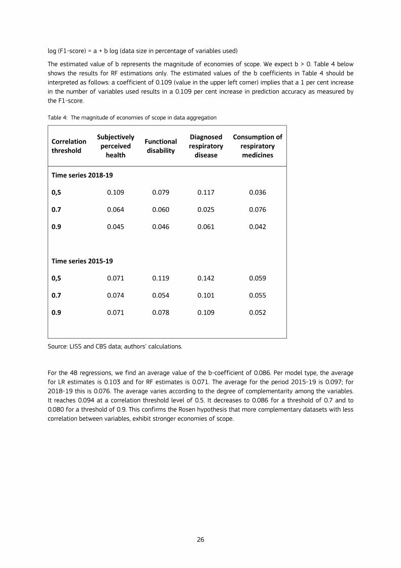
log (F1-score) = a + b log (data size in percentage of variables used)

The estimated value of b represents the magnitude of economies of scope. We expect b > 0. Table 4 below shows the results for RF estimations only. The estimated values of the b coefficients in Table 4 should be interpreted as follows: a coefficient of 0.109 (value in the upper left corner) implies that a 1 per cent increase in the number of variables used results in a 0.109 per cent increase in prediction accuracy as measured by the F1-score.

Table 4: The magnitude of economies of scope in data aggregation

Correlation threshold

Subjectively perceived

health

Functional disability

Diagnosed respiratory

disease

Consumption of respiratory medicines

Time series 2018-19

0,5 0.109 0.079 0.117 0.036

0.7 0.064 0.060 0.025 0.076

0.9 0.045 0.046 0.061 0.042

Time series 2015-19

0,5 0.071 0.119 0.142 0.059

0.7 0.074 0.054 0.101 0.055

0.9 0.071 0.078 0.109 0.052

Source: LISS and CBS data; authors’ calculations.

For the 48 regressions, we find an average value of the b-coefficient of 0.086. Per model type, the average for LR estimates is 0.103 and for RF estimates is 0.071. The average for the period 2015-19 is 0.097; for 2018-19 this is 0.076. The average varies according to the degree of complementarity among the variables. It reaches 0.094 at a correlation threshold level of 0.5. It decreases to 0.086 for a threshold of 0.7 and to 0.080 for a threshold of 0.9. This confirms the Rosen hypothesis that more complementary datasets with less correlation between variables, exhibit stronger economies of scope.

27

7 Conclusions There is considerable controversy and confusion about economies of scale and scope in data. While economies of scale may be intuitively clear, the interpretation of economies of scope when applied to data is ambiguous. We introduce a conceptual distinction between the traditional interpretation of economies of scope in the reuse of data and a new interpretation of economies of scope in data aggregation. Economies of scope in reuse constitutes an argument in favour of lowering access barriers and wider sharing and diffusion of data. Economies of scope in data aggregation put a premium on concentration of data in large pools. Apart from conceptual ambiguity, the absence of empirical evidence has contributed to doubts about the existence of economies of scope in data aggregation.

The existing confusion about economies of scale and scope in data in the economic literature is not only due to conceptual ambiguities but also to the absence of empirical evidence on the existence of economies of scope in data aggregation. In the second part of this paper, we present empirical evidence from the aggregation of Dutch health and health-related datasets for the prediction of health outcomes. We find that more aggregation across a wider set of independent and complementary variables significantly increases the prediction accuracy of health outcomes.

These findings suggest that the aggregation of health and non-health personal and socio-economic data may lead to better insights in health outcomes. It would be an argument in favour of opening up health data silos and merging them with other sources into large multi-domain data pools in order to produce better health research outcomes. Companies with access to large and very diverse consumer data pools should have an advantage if they manage to combine this with personal health data. Since health data are particularly sensitive from a personal data protection point of view, merging or aggregating personal health data into wider data pools should be subject to strict data protection procedures.

28

List of figures

Figure 1: Composition of the aggregated dataset, including individual dataset sizes. ............................ 8

Figure 2: Example of the Logistic Regression technique and a comparison to linear regression. ...............13

Figure 3: Schematic representation of the Random Forest algorithm. ............................................14

Figure 4: The five steps of a data-driven research. .................................................................15

Figure 5: An example of a confusion matrix .........................................................................17

Figure 6: A correlation triangle graph showing correlated variables of Pearson’s r > 0.9. .......................20

Figure 7: Prediction F1-scores of perceived health versus dataset size for two independent machine learning algorithms. Correlation threshold is 0.7 and year range is 2018-19. .............................................23

Figure 8: Prediction F1-scores of functional disability versus dataset size for two independent machine learning algorithms. Correlation threshold is 0.7 and year range is 2015-19. ...................................24

Figure 9: Prediction F1-scores of prescribed medicine for the respiratory anatomy group (ATC-R) versus dataset size for two independent machine learning algorithms. Correlation threshold is 0.9 and year range is 2018-19. ...............................................................................................................24

Figure 10: Prediction F1-scores of chronic lung disease versus dataset size for two independent machine learning algorithms. Correlation threshold is 0.9 and year range is 2018-19. ...................................25

29

List of tables

Table 1: Availability of historical datasets ............................................................................ 8

Table 2: Cleaning steps on LISS panel data .........................................................................10

Table 3: Chosen parameters and their descriptions .................................................................19

Table 4: The magnitude of economies of scope in data aggregation .............................................26

30

Annexes

Annex 1. All results

Here, we show the resulting graphs from the modelling for all the combinations of the parameter space. The raw data from which the figures are made are provided as separate Excel files.

Correlation threshold 0.5, range in years 2018-2019.

Figure 1 Target variable: ATC-R

40.35

40.4

40.45

40.5

40.55

40.6

40.65

LR F1-scores

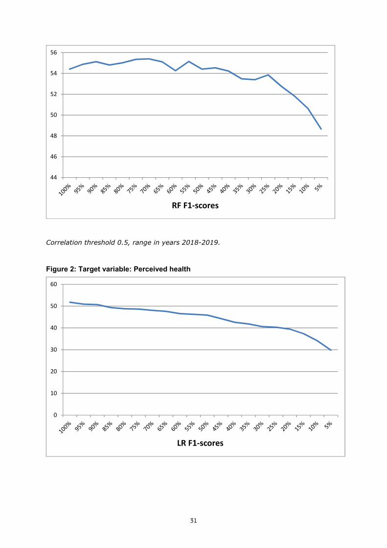
31

Correlation threshold 0.5, range in years 2018-2019.

Figure 2: Target variable: Perceived health

44

46

48

50

52

54

56

RF F1-scores

0

10

20

30

40

50

60

LR F1-scores

32

Correlation threshold 0.5, range in years 2018-2019.

Figure 3: Target variable: Chronic lung disease

0

10

20

30

40

50

60

RF F1-scores

0

10

20

30

40

50

60

70

LR F1-scores

33

Correlation threshold 0.5, range in years 2018-2019.

Figure 4: Target variable: Functional disability

0

10

20

30

40

50

60

70

80

RF F1-scores

0

5

10

15

20

25

30

35

40

45

LR F1-scores

34

Correlation threshold 0.7, range in years 2018-2019.

Figure 5: Target variable: ATC-R

0

10

20

30

40

50

60

RF F1-scores

0

10

20

30

40

50

60

70

LR F1-scores

35

Correlation threshold 0.7, range in years 2018-2019.

Figure 6: Target variable: Perceived health

0

10

20

30

40

50

60

70

RF F1-scores

0

10

20

30

40

50

60

LR F1-scores

36

Correlation threshold 0.7, range in years 2018-2019.

Figure 7: Target variable: Chronic lung disease

0

10

20

30

40

50

60

RF F1-scores

0

10

20

30

40

50

60

70

LR F1-scores

37

Correlation threshold 0.7, range in years 2018-2019.

Figure 8 Target variable: Functional disability

61

62

63

64

65

66

67

68

69

RF F1-scores

0

5

10

15

20

25

30

35

40

45

50

LR F1-scores

38

Correlation threshold 0.9, range in years 2018-2019.

Figure 9: Target variable: ATC-R

0

10

20

30

40

50

60

RF F1-scores

0

10

20

30

40

50

60

70

LR F1-scores

39

Correlation threshold 0.9, range in years 2018-2019.

Figure 10 Target variable: Perceived health

48

50

52

54

56

58

60

62

64

66

RF F1-scores

0

10

20

30

40

50

60

LR F1-scores

40

Correlation threshold 0.9, range in years 2018-2019.

Figure 11: Target variable: Chronic lung disease

42

44

46

48

50

52

54

56

58

RF F1-scores

0

10

20

30

40

50

60

70

LR F1-scores

41

Correlation threshold 0.9, range in years 2018-2019.

Figure 12: Target variable: Functional disability

0

10

20

30

40

50

60

70

80

RF F1-scores

0

5

10

15

20

25

30

35

40

45

50

LR F1-scores

42

Correlation threshold 0.5, range in years 2015-2019.

Figure 13: Target variable: ATC-R

40

42

44

46

48

50

52

54

56

RF F1-scores

39.5

40

40.5

41

41.5

42

42.5

LR F1-scores

43

Correlation threshold 0.5, range in years 2015-2019.

Figure 14: Target variable: Perceived health

46

48

50

52

54

56

58

60

62

RF F1-scores

0

10

20

30

40

50

60

LR F1-scores

44

Correlation threshold 0.5, range in years 2015-2019.

Figure 15: Target variable: Chronic lung disease

0

10

20

30

40

50

60

RF F1-scores

0

10

20

30

40

50

60

70

80

LR F1-scores

45

Correlation threshold 0.5, range in years 2015-2019.

Figure 16: Target variable: Functional disability

0

10

20

30

40

50

60

70

80

RF F1-scores

0

5

10

15

20

25

30

35

40

45

50

LR F1-scores

46

Correlation threshold 0.7, range in years 2015-2019.

Figure 17: Target variable: ATC-R

0

10

20

30

40

50

60

RF F1-scores

0

10

20

30

40

50

60

70

LR F1-scores

47

Correlation threshold 0.7, range in years 2015-2019.

Figure 18: Target variable: Perceived health

50

52

54

56

58

60

62

64

66

RF F1-scores

0

10

20

30

40

50

60

LR F1-scores

48

Correlation threshold 0.7, range in years 2015-2019.

Figure 19: Target variable: Chronic lung disease

0

10

20

30

40

50

60

RF F1-scores

0

10

20

30

40

50

60

70

LR F1-scores

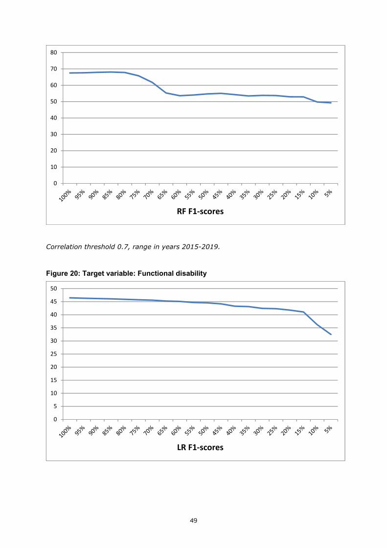
49

Correlation threshold 0.7, range in years 2015-2019.

Figure 20: Target variable: Functional disability

0

10

20

30

40

50

60

70

80

RF F1-scores

0

5

10

15

20

25

30

35

40

45

50

LR F1-scores

50

Correlation threshold 0.9, range in years 2015-2019.

Figure 21 Target variable: ATC-R

38

40

42

44

46

48

50

52

RF F1-scores

0

10

20

30

40

50

60

70

LR F1-scores

51

Correlation threshold 0.9, range in years 2015-2019.

Figure 22: Target variable: Perceived health

50

52

54

56

58

60

62

64

66

RF F1-scores

0

10

20

30

40

50

60

LR F1-scores

52

Correlation threshold 0.9, range in years 2015-2019.

Figure 23: Target variable: Chronic lung disease

0

10

20

30

40

50

60

RF F1-scores

0

10

20

30

40

50

60

70

80

LR F1-scores

53

Correlation threshold 0.9, range in years 2015-2019.

Figure 24: Target variable: Functional disability

0

10

20

30

40

50

60

70

80

RF F1-scores

0

5

10

15

20

25

30

35

40

45

50

LR F1-scores

54

0

10

20

30

40

50

60

RF F1-scores

55

List of figures in the appendix

Figure 1 Target variable: ATC-R ......................................................................................30

Figure 2: Target variable: Perceived health ..........................................................................31

Figure 3: Target variable: Chronic lung disease .....................................................................32

Figure 4: Target variable: Functional disability ......................................................................33

Figure 5: Target variable: ATC-R ......................................................................................34

Figure 6: Target variable: Perceived health ..........................................................................35

Figure 7: Target variable: Chronic lung disease .....................................................................36

Figure 8 Target variable: Functional disability .......................................................................37

Figure 9: Target variable: ATC-R ......................................................................................38

Figure 10 Target variable: Perceived health .........................................................................39

Figure 11: Target variable: Chronic lung disease ....................................................................40

Figure 12: Target variable: Functional disability.....................................................................41

Figure 13: Target variable: ATC-R ....................................................................................42

Figure 14: Target variable: Perceived health ........................................................................43

Figure 15: Target variable: Chronic lung disease ....................................................................44

Figure 16: Target variable: Functional disability.....................................................................45

Figure 17: Target variable: ATC-R ....................................................................................46

Figure 18: Target variable: Perceived health ........................................................................47

Figure 19: Target variable: Chronic lung disease ....................................................................48

Figure 20: Target variable: Functional disability.....................................................................49

Figure 21 Target variable: ATC-R .....................................................................................50

Figure 22: Target variable: Perceived health ........................................................................51

Figure 23: Target variable: Chronic lung disease ....................................................................52

Figure 24: Target variable: Functional disability.....................................................................53

GETTING IN TOUCH WITH THE EU

In person

All over the European Union there are hundreds of Europe Direct information centres. You can find the address of the centre nearest you at: https://europa.eu/european-union/contact_en

On the phone or by email

Europe Direct is a service that answers your questions about the European Union. You can contact this service:

- by freephone: 00 800 6 7 8 9 10 11 (certain operators may charge for these calls),

- at the following standard number: +32 22999696, or

- by electronic mail via: https://europa.eu/european-union/contact_en

FINDING INFORMATION ABOUT THE EU

Online

Information about the European Union in all the official languages of the EU is available on the Europa website at: https://europa.eu/european-union/index_en

EU publications You can download or order free and priced EU publications from EU Bookshop at: https://publications.europa.eu/en/publications. Multiple copies of free publications may be obtained by contacting Europe Direct or your local information centre (see https://europa.eu/european-union/contact_en).