
Epidemiology and virulence of Clostridium difficile - ThinkIR
Upload
khangminh22Category
view
3download
0
Systems analysis of the host response toClostridium difficile toxins
A Dissertation
presented to the faculty of the School of Engineering and Applied Sciencein partial fullfillment of the requirements for the degree of
Doctor of Philosophy
by Kevin Michael D’AuriaMay 2014
Department of Biomedical Engineering

ii
APPROVAL SHEET
This dissertation is in partial fulfillment of the requirements for the degree of Doctor ofPhilosophy in Biomedical Engineering
Kevin Michael D’AuriaAuthor
This dissertation has been read and approved by the examining committee:
Jason Papin, Ph.D.Dissertation Advisor
Department of Biomedical Engineering
Shayn Peirce-Cottler, Ph.D.Committee Chair
Department of Biomedical Engineering
Erik Hewlett, M.D.Committee Member, Division of Infectious
Diseases and International Health
Alison Criss, Ph.D.Committee Member
Department of Microbiology
Kevin Janes, Ph.D.Committee Member
Department of Biomedical Engineering
Accepted for the School of Engineering and Applied Science:
Jaymes H. Aylor, Ph.D.Dean, School of Engineering and Applied Science

Contents
Acknowledgements xi
Preface xiii0.1 Me, a biomedical engineer . . . . . . . . . . . . . . . . . . . . . . . . . . . . . . . . . xiii0.2 Me, a computational systems biologist . . . . . . . . . . . . . . . . . . . . . . . . . . xiii0.3 My dissertation as systems biologist . . . . . . . . . . . . . . . . . . . . . . . . . . . xiv
1 Introduction 11.1 Abstract . . . . . . . . . . . . . . . . . . . . . . . . . . . . . . . . . . . . . . . . . . . 11.2 A preview of this dissertation . . . . . . . . . . . . . . . . . . . . . . . . . . . . . . . 2
2 Choosing transcriptomics analyses 42.1 Background . . . . . . . . . . . . . . . . . . . . . . . . . . . . . . . . . . . . . . . . . 4
2.1.1 mRNA as a measure of cell state . . . . . . . . . . . . . . . . . . . . . . . . . 42.1.2 Measuring mRNA levels with microarrays . . . . . . . . . . . . . . . . . . . . 5
2.2 Microarray preprocessing . . . . . . . . . . . . . . . . . . . . . . . . . . . . . . . . . 62.2.1 Steps of data preprocessing . . . . . . . . . . . . . . . . . . . . . . . . . . . . 6
2.3 Choosing preprocessing techniques . . . . . . . . . . . . . . . . . . . . . . . . . . . . 82.3.1 What are the best preprocessing steps? . . . . . . . . . . . . . . . . . . . . . 82.3.2 Which workflow do I use? . . . . . . . . . . . . . . . . . . . . . . . . . . . . . 12
2.4 Differential expression . . . . . . . . . . . . . . . . . . . . . . . . . . . . . . . . . . . 122.4.1 Types of statistical tests . . . . . . . . . . . . . . . . . . . . . . . . . . . . . . 132.4.2 What test should I use? . . . . . . . . . . . . . . . . . . . . . . . . . . . . . . 16
2.5 Caveats of microarrays and alternatives . . . . . . . . . . . . . . . . . . . . . . . . . 172.6 Reproducibile analyses . . . . . . . . . . . . . . . . . . . . . . . . . . . . . . . . . . . 17
2.6.1 Why bother? . . . . . . . . . . . . . . . . . . . . . . . . . . . . . . . . . . . . 172.6.2 Are microarrays reproducible? . . . . . . . . . . . . . . . . . . . . . . . . . . 18
2.7 Transcriptomics analyses in this dissertation . . . . . . . . . . . . . . . . . . . . . . . 19
3 miRNA Transcriptomics of melanoma 203.1 Motivation . . . . . . . . . . . . . . . . . . . . . . . . . . . . . . . . . . . . . . . . . 203.2 Introduction . . . . . . . . . . . . . . . . . . . . . . . . . . . . . . . . . . . . . . . . . 213.3 Methods . . . . . . . . . . . . . . . . . . . . . . . . . . . . . . . . . . . . . . . . . . . 22
3.3.1 miRNA quantification . . . . . . . . . . . . . . . . . . . . . . . . . . . . . . . 223.4 Results . . . . . . . . . . . . . . . . . . . . . . . . . . . . . . . . . . . . . . . . . . . . 23
3.4.1 miRNA expression of all samples . . . . . . . . . . . . . . . . . . . . . . . . . 233.4.2 miRNA expression changes after treatment . . . . . . . . . . . . . . . . . . . 253.4.3 Different miRNA expression changes between responders and non-responders 25
iii
iv CONTENTS
3.5 Conclusions . . . . . . . . . . . . . . . . . . . . . . . . . . . . . . . . . . . . . . . . . 28
4 Functional transcriptomics of toxin response 294.1 C. difficile: a dangerous pathogen . . . . . . . . . . . . . . . . . . . . . . . . . . . . . 30
4.1.1 Historical significance . . . . . . . . . . . . . . . . . . . . . . . . . . . . . . . 304.1.2 Toxin molecular biology . . . . . . . . . . . . . . . . . . . . . . . . . . . . . . 314.1.3 Physiological toxin responses . . . . . . . . . . . . . . . . . . . . . . . . . . . 31
4.2 Functional transcriptomics: enrichment . . . . . . . . . . . . . . . . . . . . . . . . . 324.2.1 Gene set enrichment analysis . . . . . . . . . . . . . . . . . . . . . . . . . . . 33
5 Toxins A and B disrupt the cell cycle 355.1 Synopsis . . . . . . . . . . . . . . . . . . . . . . . . . . . . . . . . . . . . . . . . . . . 355.2 Background . . . . . . . . . . . . . . . . . . . . . . . . . . . . . . . . . . . . . . . . . 365.3 Methods . . . . . . . . . . . . . . . . . . . . . . . . . . . . . . . . . . . . . . . . . . . 37
5.3.1 Cell Culture . . . . . . . . . . . . . . . . . . . . . . . . . . . . . . . . . . . . . 375.3.2 Microarrays . . . . . . . . . . . . . . . . . . . . . . . . . . . . . . . . . . . . . 375.3.3 Flow Cytometry . . . . . . . . . . . . . . . . . . . . . . . . . . . . . . . . . . 385.3.4 Quantitative real time PCR . . . . . . . . . . . . . . . . . . . . . . . . . . . 395.3.5 Western Blots . . . . . . . . . . . . . . . . . . . . . . . . . . . . . . . . . . . . 39
5.4 Results . . . . . . . . . . . . . . . . . . . . . . . . . . . . . . . . . . . . . . . . . . . . 405.4.1 Transcriptional Responses . . . . . . . . . . . . . . . . . . . . . . . . . . . . . 405.4.2 Functions associated with differentially expressed genes . . . . . . . . . . . . 425.4.3 Effects of TcdA and TcdB on the Regulation of Cell Cycle . . . . . . . . . . . 47
5.5 Discussion . . . . . . . . . . . . . . . . . . . . . . . . . . . . . . . . . . . . . . . . . . 505.6 Conclusion . . . . . . . . . . . . . . . . . . . . . . . . . . . . . . . . . . . . . . . . . 525.7 Acknowledgements . . . . . . . . . . . . . . . . . . . . . . . . . . . . . . . . . . . . . 52
6 In vivo toxin responses 536.1 From in vitro to in vivo host responses . . . . . . . . . . . . . . . . . . . . . . . . . . 536.2 Synopsis . . . . . . . . . . . . . . . . . . . . . . . . . . . . . . . . . . . . . . . . . . . 546.3 Introduction . . . . . . . . . . . . . . . . . . . . . . . . . . . . . . . . . . . . . . . . . 546.4 Methods . . . . . . . . . . . . . . . . . . . . . . . . . . . . . . . . . . . . . . . . . . . 57
6.4.1 Cecal injection . . . . . . . . . . . . . . . . . . . . . . . . . . . . . . . . . . 576.4.2 Cell culture . . . . . . . . . . . . . . . . . . . . . . . . . . . . . . . . . . . . 586.4.3 Blood counts . . . . . . . . . . . . . . . . . . . . . . . . . . . . . . . . . . . 586.4.4 Histology . . . . . . . . . . . . . . . . . . . . . . . . . . . . . . . . . . . . . 586.4.5 Isolation of cells from cecal tissue . . . . . . . . . . . . . . . . . . . . . . . . 596.4.6 Flow cytometry . . . . . . . . . . . . . . . . . . . . . . . . . . . . . . . . . . 596.4.7 Antibody-mediated neutralization of chemokines . . . . . . . . . . . . . . . . 596.4.8 Microarray procedure . . . . . . . . . . . . . . . . . . . . . . . . . . . . . . 606.4.9 Statistical analysis . . . . . . . . . . . . . . . . . . . . . . . . . . . . . . . . 606.4.10 Microarray preprocessing . . . . . . . . . . . . . . . . . . . . . . . . . . . . 606.4.11 Determining differentially expressed genes . . . . . . . . . . . . . . . . . . . . 616.4.12 Gene set enrichment . . . . . . . . . . . . . . . . . . . . . . . . . . . . . . . . 626.4.13 Cytopathic effects on a mouse, cecal, epithelial cell line . . . . . . . . . . . . 64
6.5 Results . . . . . . . . . . . . . . . . . . . . . . . . . . . . . . . . . . . . . . . . . . . . 656.5.1 Dose-response to TcdA cecal injection . . . . . . . . . . . . . . . . . . . . . . 656.5.2 Survival after cecal injection . . . . . . . . . . . . . . . . . . . . . . . . . . . 66

CONTENTS v
6.5.3 Physiological results of toxin cecal injection . . . . . . . . . . . . . . . . . . 666.5.4 Host transcription altered by toxin injection . . . . . . . . . . . . . . . . . . 696.5.5 Comparisons of gene and protein expression of cytokines . . . . . . . . . . . . 786.5.6 CXCL1 and CXCL2 neutralization alters the host response to TcdA cecal
injection . . . . . . . . . . . . . . . . . . . . . . . . . . . . . . . . . . . . . . . 806.5.7 In vivo transcriptome response versus in vitro transcriptome and proteome
responses . . . . . . . . . . . . . . . . . . . . . . . . . . . . . . . . . . . . . . 826.6 Discussion . . . . . . . . . . . . . . . . . . . . . . . . . . . . . . . . . . . . . . . . . . 846.7 Acknowledgements . . . . . . . . . . . . . . . . . . . . . . . . . . . . . . . . . . . . . 89
7 Responses of multiple cell types 917.1 From transcriptomics of the epithelial-layer to the roles of different cell types in the
epithelial layer . . . . . . . . . . . . . . . . . . . . . . . . . . . . . . . . . . . . . . . 917.2 Synopsis . . . . . . . . . . . . . . . . . . . . . . . . . . . . . . . . . . . . . . . . . . . 927.3 Introduction . . . . . . . . . . . . . . . . . . . . . . . . . . . . . . . . . . . . . . . . . 937.4 Methods . . . . . . . . . . . . . . . . . . . . . . . . . . . . . . . . . . . . . . . . . . . 95
7.4.1 Cell Culture . . . . . . . . . . . . . . . . . . . . . . . . . . . . . . . . . . . . . 957.4.2 Electrical impedance assay . . . . . . . . . . . . . . . . . . . . . . . . . . . . 957.4.3 Analyses . . . . . . . . . . . . . . . . . . . . . . . . . . . . . . . . . . . . . . . 96
7.5 Results . . . . . . . . . . . . . . . . . . . . . . . . . . . . . . . . . . . . . . . . . . . . 967.5.1 Quantification of the cytopathic effects elicited by TcdA and TcdB . . . . . . 967.5.2 Epithelial and endothelial cells: similar characteristic responses but different
sensitivities to TcdA and TcdB . . . . . . . . . . . . . . . . . . . . . . . . . . 987.5.3 Macrophages: rapid, sensitive, complex concentration-dependent responses
to TcdA and TcdB . . . . . . . . . . . . . . . . . . . . . . . . . . . . . . . . . 997.5.4 Glucosyltransferase-deficient TcdB alters the effects of TcdA and TcdB on
macrophages and epithelial cells . . . . . . . . . . . . . . . . . . . . . . . . . 1007.6 Discussion . . . . . . . . . . . . . . . . . . . . . . . . . . . . . . . . . . . . . . . . . . 1047.7 Acknowledgements . . . . . . . . . . . . . . . . . . . . . . . . . . . . . . . . . . . . . 109
8 Multi-well time course analyses 1108.1 Concise annotation of multiple wells . . . . . . . . . . . . . . . . . . . . . . . . . . . 1108.2 Selecting and modifying wells . . . . . . . . . . . . . . . . . . . . . . . . . . . . . . . 1118.3 Visualization . . . . . . . . . . . . . . . . . . . . . . . . . . . . . . . . . . . . . . . . 1138.4 Independent wells . . . . . . . . . . . . . . . . . . . . . . . . . . . . . . . . . . . . . . 1148.5 Data transformations . . . . . . . . . . . . . . . . . . . . . . . . . . . . . . . . . . . . 1158.6 Interpolation and smoothers . . . . . . . . . . . . . . . . . . . . . . . . . . . . . . . . 1178.7 Custom metrics . . . . . . . . . . . . . . . . . . . . . . . . . . . . . . . . . . . . . . . 1198.8 Future plans . . . . . . . . . . . . . . . . . . . . . . . . . . . . . . . . . . . . . . . . . 121
9 Future directions: toxin responses and metabolism 1229.1 Toxins alter expression of many metabolic genes . . . . . . . . . . . . . . . . . . . . 1229.2 Integrating and visualizing transcriptional changes within a metabolic network . . . 1229.3 Synopsis . . . . . . . . . . . . . . . . . . . . . . . . . . . . . . . . . . . . . . . . . . . 1239.4 Glossary . . . . . . . . . . . . . . . . . . . . . . . . . . . . . . . . . . . . . . . . . . . 1239.5 Systems biology and pathogen metabolism . . . . . . . . . . . . . . . . . . . . . . . . 1269.6 Reconstructing metabolic networks . . . . . . . . . . . . . . . . . . . . . . . . . . . . 1299.7 Drug targets in metabolic networks . . . . . . . . . . . . . . . . . . . . . . . . . . . . 136

vi CONTENTS
9.7.1 Metabolite essentiality . . . . . . . . . . . . . . . . . . . . . . . . . . . . . . . 1409.7.2 Combination gene and reaction perturbations . . . . . . . . . . . . . . . . . . 1409.7.3 Groups of targets and network topology . . . . . . . . . . . . . . . . . . . . . 1419.7.4 Environment and conditional essentiality . . . . . . . . . . . . . . . . . . . . 141
9.8 From target to drug and the development of model guided pipelines for drug discovery1429.9 A host cell perspective . . . . . . . . . . . . . . . . . . . . . . . . . . . . . . . . . . . 1439.10 Next steps . . . . . . . . . . . . . . . . . . . . . . . . . . . . . . . . . . . . . . . . . . 1459.11 Concluding remarks . . . . . . . . . . . . . . . . . . . . . . . . . . . . . . . . . . . . 1469.12 Acknowledgements . . . . . . . . . . . . . . . . . . . . . . . . . . . . . . . . . . . . . 147
Appendices 181
A Reproducing in vivo analyses 182A.1 Introduction . . . . . . . . . . . . . . . . . . . . . . . . . . . . . . . . . . . . . . . . . 182A.2 Preparing software, files, and folders . . . . . . . . . . . . . . . . . . . . . . . . . . . 182
A.2.1 Directory structure . . . . . . . . . . . . . . . . . . . . . . . . . . . . . . . . . 182A.2.2 R and R packages . . . . . . . . . . . . . . . . . . . . . . . . . . . . . . . . . 183A.2.3 Downloading the microarray data . . . . . . . . . . . . . . . . . . . . . . . . . 183
A.3 Loading and organizing microarray data . . . . . . . . . . . . . . . . . . . . . . . . . 183A.4 Preprocessing microarray data . . . . . . . . . . . . . . . . . . . . . . . . . . . . . . 184A.5 Microarray and gene annotation . . . . . . . . . . . . . . . . . . . . . . . . . . . . . 184
A.5.1 Background . . . . . . . . . . . . . . . . . . . . . . . . . . . . . . . . . . . . . 184A.5.2 Annotation sources . . . . . . . . . . . . . . . . . . . . . . . . . . . . . . . . . 185A.5.3 Generating annotation lists in R . . . . . . . . . . . . . . . . . . . . . . . . . 186A.5.4 Transitive mapping . . . . . . . . . . . . . . . . . . . . . . . . . . . . . . . . . 188A.5.5 Many probes to many genes mapping . . . . . . . . . . . . . . . . . . . . . . 189
A.6 Analyzing differential expression . . . . . . . . . . . . . . . . . . . . . . . . . . . . . 190A.7 Gene set enrichment . . . . . . . . . . . . . . . . . . . . . . . . . . . . . . . . . . . . 191
A.7.1 Competitive . . . . . . . . . . . . . . . . . . . . . . . . . . . . . . . . . . . . . 191A.7.2 Self-contained . . . . . . . . . . . . . . . . . . . . . . . . . . . . . . . . . . . . 192
A.8 Analysis of previous in vitro data . . . . . . . . . . . . . . . . . . . . . . . . . . . . . 193A.9 Comparisons to other transcriptomic and proteomic data . . . . . . . . . . . . . . . 193A.10 Cytotoxicity assay . . . . . . . . . . . . . . . . . . . . . . . . . . . . . . . . . . . . . 194A.11 Scripts for generating figures and tables . . . . . . . . . . . . . . . . . . . . . . . . . 194A.12 Notes on formatting . . . . . . . . . . . . . . . . . . . . . . . . . . . . . . . . . . . . 194A.13 Acknowledgements . . . . . . . . . . . . . . . . . . . . . . . . . . . . . . . . . . . . . 195
B Reproducing time-course analyses 196B.1 Introduction . . . . . . . . . . . . . . . . . . . . . . . . . . . . . . . . . . . . . . . . . 196B.2 References from Chapter 7 . . . . . . . . . . . . . . . . . . . . . . . . . . . . . . . . 196
B.2.1 Reference 1 . . . . . . . . . . . . . . . . . . . . . . . . . . . . . . . . . . . . 196B.2.2 Reference 2 . . . . . . . . . . . . . . . . . . . . . . . . . . . . . . . . . . . . 197
B.3 Reproducing Figures . . . . . . . . . . . . . . . . . . . . . . . . . . . . . . . . . . . 197B.3.1 Figure 1 . . . . . . . . . . . . . . . . . . . . . . . . . . . . . . . . . . . . . . 198B.3.2 Figure 2 . . . . . . . . . . . . . . . . . . . . . . . . . . . . . . . . . . . . . . 198B.3.3 Figure 3 . . . . . . . . . . . . . . . . . . . . . . . . . . . . . . . . . . . . . . 201B.3.4 Figure 4 . . . . . . . . . . . . . . . . . . . . . . . . . . . . . . . . . . . . . . 202B.3.5 Figure 5 . . . . . . . . . . . . . . . . . . . . . . . . . . . . . . . . . . . . . . 203

CONTENTS vii
B.4 Exploring the data . . . . . . . . . . . . . . . . . . . . . . . . . . . . . . . . . . . . 204B.4.1 Plate summaries . . . . . . . . . . . . . . . . . . . . . . . . . . . . . . . . . . 205B.4.2 HCT8 cells . . . . . . . . . . . . . . . . . . . . . . . . . . . . . . . . . . . . . 206B.4.3 CHO cells . . . . . . . . . . . . . . . . . . . . . . . . . . . . . . . . . . . . . . 209B.4.4 IMCE cells . . . . . . . . . . . . . . . . . . . . . . . . . . . . . . . . . . . . . 210B.4.5 HUVECs . . . . . . . . . . . . . . . . . . . . . . . . . . . . . . . . . . . . . . 210B.4.6 T84 cells . . . . . . . . . . . . . . . . . . . . . . . . . . . . . . . . . . . . . . 211B.4.7 J774 cells . . . . . . . . . . . . . . . . . . . . . . . . . . . . . . . . . . . . . . 211B.4.8 PMN leukocytes . . . . . . . . . . . . . . . . . . . . . . . . . . . . . . . . . . 213B.4.9 Plate Layouts . . . . . . . . . . . . . . . . . . . . . . . . . . . . . . . . . . . . 216

List of Figures
3.1 miRNA expression profiles pre- and post-treatment . . . . . . . . . . . . . . . . . . . 243.2 Effect size and statistical significance of post- versus pre-treatment miRNA expression 263.3 Different miRNA expression between responders and non-responders . . . . . . . . . 27
4.1 An oversimplified view of C. difficile infection . . . . . . . . . . . . . . . . . . . . . . 304.2 Sequence, structure, and functioin of TcdA and TcdB . . . . . . . . . . . . . . . . . 32
5.1 Overall transcriptional response of HCT-8 cells to TcdA and TcdB . . . . . . . . . . 415.2 qRT-PCR validation of and genes with high differential expression . . . . . . . . . . 425.3 Gene ontology categories associated with differentially expressed genes . . . . . . . . 435.4 Gene set enrichment of biological processes and cellular components . . . . . . . . . 445.5 The altered gene expression of G1 phase cell cycle regulators at 6h and changes in
the distribution of cells within the cell cycle . . . . . . . . . . . . . . . . . . . . . . . 465.6 Timing of RAC1 glucosylation and expression of cyclin-related genes and proteins
in subconfluent and confluent cultures. . . . . . . . . . . . . . . . . . . . . . . . . . . 475.7 Distribution of apoptotic versus non-apoptotic cells within the cell cycle and char-
acteristics of G2/M phase, toxin-treated cells . . . . . . . . . . . . . . . . . . . . . . 49
6.1 Study workflow . . . . . . . . . . . . . . . . . . . . . . . . . . . . . . . . . . . . . . . 556.2 Cytopathic effects of TcdA and TcdB on a mouse epithelial cell line. . . . . . . . . . 646.3 Histopathology 6h after cecal injection with TcdA. . . . . . . . . . . . . . . . . . . . 666.4 Physiological and gene expression changes post toxin injection . . . . . . . . . . . . . 686.5 The concentration of circulating blood cells was altered during intoxication . . . . . 696.6 Cell type proportions as determined by flow cytometry . . . . . . . . . . . . . . . . . 716.7 Gene expression changes post toxin injection . . . . . . . . . . . . . . . . . . . . . . 726.8 Biological functions associated with gene-expression changes . . . . . . . . . . . . . . 766.9 Expression changes of inflammation associated and immune regulatory genes . . . . 776.10 Cytokine gene and protein expression . . . . . . . . . . . . . . . . . . . . . . . . . . 796.11 Antibody neutralization of CXCL1 and CXCL2 . . . . . . . . . . . . . . . . . . . . . 816.12 Cxcl1 and Cxcl2 expression after Cxcl1 & Cxcl2 neutralization . . . . . . . . . . . . 826.13 Neutrophil infiltration 6h after TcdA cecal injection of mice pretreated with neutral-
izing antibodies . . . . . . . . . . . . . . . . . . . . . . . . . . . . . . . . . . . . . . . 836.14 Correlations between in vitro and in vivo responses to toxins . . . . . . . . . . . . . 836.15 Similarly expressed genes in vitro and in vivo . . . . . . . . . . . . . . . . . . . . . . 84
7.1 Measurement of toxins’ cytopathic effects by tracking electrical impedance acrossthe surface of a cell culture . . . . . . . . . . . . . . . . . . . . . . . . . . . . . . . . 97
7.2 SQuantification of cytopathic effects . . . . . . . . . . . . . . . . . . . . . . . . . . . 98
viii

LIST OF FIGURES ix
7.3 Macrophage responses to TcdA and TcdB . . . . . . . . . . . . . . . . . . . . . . . . 1017.4 Response of HCT8 epithelial cells to gdTcdB, TcdA+gdTcdB, and TcdB+gdTcdB . 1027.5 Response of J774 macrophages to gdTcdB, TcdA+gdTcdB, and TcdB+gdTcdB . . . 103
9.1 The iterative process of model building and refinement . . . . . . . . . . . . . . . . . 1289.2 Drug targeting in metabolic networks . . . . . . . . . . . . . . . . . . . . . . . . . . 138
A.1 Batch corrected HCT8 transcriptional data . . . . . . . . . . . . . . . . . . . . . . . 194

List of Tables
3.1 Patient outcomes and availability of miRNA data . . . . . . . . . . . . . . . . . . . . 22
6.1 Survival in cecal injection experiments . . . . . . . . . . . . . . . . . . . . . . . . . . 676.2 Infiltration of immune cells 6h and 16h after cecal injection . . . . . . . . . . . . . . 706.3 Genes with significantly altered expression 2h after TcdA or TcdB injection . . . . . 736.4 Biological functions and gene sets associated with gene expression changes 2h after
TcdA or TcdB injection . . . . . . . . . . . . . . . . . . . . . . . . . . . . . . . . . . 746.5 Molecular functions associated with gene expression changes 16h after TcdA injection 75
8.1 Example metadata file . . . . . . . . . . . . . . . . . . . . . . . . . . . . . . . . . . . 111
9.1 Drug targeting-related analysis of pathogen metabolic networks . . . . . . . . . . . . 127
A.1 Annotation scripts and variables. “Affy”=Affymetrix Mouse 430 2.0 probeset ID.“Entrez”=Entrez gene ID, “Ensembl”=Ensembl gene ID . . . . . . . . . . . . . . . . 187
A.2 Annotation scripts and variables for Hgu133 Plus 2.0 chip . . . . . . . . . . . . . . . 188A.3 Scripts for producing tables and figures . . . . . . . . . . . . . . . . . . . . . . . . . 195
x

Acknowledgements
First and foremost, I would like to thank my family for their love and continued support during
my graduate education. Throughout my work in the past few years, I have finally begun to realize
the extent of the dedication of my parents, Mike and Jennifer, to my sister and me. I thank my
sister and best friend, Wendy, for showing me how to survive and always keeping my spirits up.
I would not be adequately equipped for my research if it weren’t for the faculty, students, and
researchers in Biomedical Engineering and the Biomedical Sciences at UVa. As an engineer, I
have had the incredible opportunity to work day in and day out with biologists, learning how to
develop and contextualize my work. At the same time, the faculty in Biomedical Engineering have
developed my intuition for applying models to practical problems. I’ve been fortunate to “grow
up” in this multilingual scientific community, unknowingly becoming fluent in different “scientific
languages”.
My dissertation would not exist if it wasn’t for collaborations and help from colleagues and
friends. The students with whom I’ve worked with the longest—Arvind, Edik, Paul, Phil, Anna,
Jennie and Matt—have provided constant critical feedback that has improved my work and kept
me focused. I’d especially like to thank Arvind Chavali, a colleague with whom I collaborated
with many times, but even more a friend who showed me the ropes, and has and I’m sure will
continue to provide advice for years to come. I’ve been very fortunate to have fellow students that
have made these past five years so enjoyable, whether it be cheering for the ’Hoos or discovering
Charlottesville’s most interesting locations.
I’m indebted to the handful of researchers with whom I have worked most closely since my first
day of graduate school. Mary Gray and Gina Donato, who always happily answered my many
questions, taught me most everything I know at the bench. Without their instruction, I would
xi

xii ACKNOWLEDGEMENTS
surely have spent many months of frustration troubleshooting every problem I encountered. Cirle
Warren, in our group’s weekly meetings, has helped me put my research into clinical context. Glynis
Kolling has been a tremendous resource, showing me what is and is not possible experimentally and
helping me choose the best path to follow based on my many crazy ideas. I’ve had the privilege to
work side by side with this group of researchers, at the bench and at the whiteboard hammering
out ideas and manuscripts.
Finally, I’d like to thank those on my dissertation committee: Shayn Peirce-Cottler, Kevin
Janes, Alison Criss, Erik Hewlett, and Jason Papin. My discussions with them have shown me
their genuine interest in my career. They have pushed me far beyond my comfort zone as only a
clever engineering to become a better thinker, to step back and understand the broader goals.
Erik Hewlett has graciously been an unofficial secondary advisor. After every experiment,
presentation, and paper, he has been right there excited to hear how things are going, ready to
provide encouragement and criticism. As someone from an engineering background, he has helped
me contextualize my work. I am also appreciative for his introductions that have allowed me to
work with many other great people.
Jason Papin has been a great mentor and advisor, helping me develop as a scientist and leader.
I try to emulate him as I mentor others. I credit much of my progression from a fault-finding cynic
to more of a forward-thinking optimist to his influence. I am most thankful for his genuine interest
in my personal and career goals. He has given me the freedom to think independently, to fail and
to succeed on my own.

Preface
0.1 Me, a biomedical engineer
I don’t label myself an engineer in the traditional sense; I don’t design things to be manufactured.
I also dislike being called a scientist because of the visual it may provoke; most of my time isn’t
spent in a long white coat at a bench. Though others might think me one, I don’t consider myself
a statistician, computer scientist, or biologist either.
I am a scientist in that I’m curious about nature, especially health and medicine. I’m an engineer
in that I’m curious about translating scientific understanding to ideas and tools that will improve
others’ quality of life. To do this, I use and invent tools in mathematics, statistics, computer science,
and the biological sciences. There is no formal and universally accepted definition of a “biomedical
engineer” and likely never will be. However, these dual interests in basic and translational science
and medicine are what, I believe, defines a biomedical engineer, and I think many would agree.
0.2 Me, a computational systems biologist
As a biomedical engineer in the information age, trillions of data points are available. In this
dissertation alone, I gather data from dozens of expression states of the 3.3-billion letter human
genome or 2.8-billion letter mouse genome. Tens of thousands of megapixel images of individual
cells are captured at different wavelengths of light. Tissue and blood samples from hundreds of mice
under different stresses are analyzed microscopically and by molecular assays to quantify pathology,
the proportion of different cells (e.g., epithelial, white blood cell, etc.), and the amounts of dozens
of proteins.
However, these data points independent of each other are of little use. As an example, consider
xiii
xiv PREFACE
a mouse that ingests a toxin. If we then observe inflammation in the mouse’s intestine, we wonder
about the cause. After dissecting tissue sections, we then find that a particular gene is expressed
prior to inflammation. Is this gene responsible for inflammation? Are there other genes whose
regulation is linked to this gene of interest? How does expression of this gene translate to the
amount of its gene product, the protein that physically interacts with the cells’ environment? Is
this inflammation only due to local events? What about the brain and the nervous system? What
happens after inflammation? Are there any changes throughout the body from the local injury in
the intestine (e.g., in the blood)? Where did the toxin go? The questions go on, but it is apparent
that there are many levels of data and interactions, a system, that determine the apparent clinical
manifestation. Systems biology aims to consider biological systems as a whole and answer how
one or many changes affects the state or output of the entire system.
Systems biology requires computational tools just so data can be managed, so the term compu-
tational systems biology is somewhat redundant. The term’s definition will change from person
to person. As I use it in this dissertation, it is distinct from “systems biology” in that computa-
tional tools are used to make insights and comparisons that would be experimentally impossible,
or would at least be prohibitively difficult. Computational systems biology may take well-designed,
simple, comparative experiments that are the core of good scientific research (e.g., think null versus
alternate hypotheses and p-values) and then go one step further by presenting the data in novel
ways and by making formal, rigorous predictions.
0.3 My dissertation as a biomedical engineer and computational
systems biologist
As I described above, Biomedical Engineering and Computational Systems Biology include aspects
of many different fields (biology, medicine, engineering, etc.). Therefore, this dissertation includes
new contributions and tools to these fields, allowing for better descriptions and reliable, repeatable
predictions from biological data. The unifying element to these contributions and tools is one
research question: why do a bacterium’s toxins make us sick and what are ways to make us better
once we’re sick? More specifically, I show how multi-level, systems biology data improves our
understanding of host cell responses to the two principal virulence factors of Clostridium difficile,

0.3. MY DISSERTATION AS SYSTEMS BIOLOGIST xv
toxins A and B. This understanding suggests new treatments and diagnostics, but also reveals
entirely new ways of thinking that offer leads to promising targets for future treatments.

Chapter 1
Introduction
1.1 Abstract
Toxins A and B, two highly potent protein toxins, are the essential virulence factors of C. difficile,
a bacterium which infects 300,000+ people in the US every year [1]. Since the extent to which
a persons body overreacts to the toxins determines disease severity, controlling the host response
is critical for improving treatments. Given the manifestations of diarrhea and colitis, nearly all
research to date has predictably focused on known inflammatory pathways and related cellular
responses. However, 40 years after the toxins’ discovery, the fatality rate has continued to rise.
A different approach is needed. In this dissertation, I present a holistic approach, profiling the
physiological and transcriptional changes of host cells to toxins in vitro and in vivo. I determine
the most appropriate statistical methods for identifying genes and pathways affected by toxins,
leading to discovery of an unrecognized cell-cycle disruption of epithelial cells treated with toxins.
I then extend the approach to investigate epithelial-layer cells in mice with toxin injected into their
intestines, identifying pathways altered only in vivo. These pathways offer new therapeutic targets,
as is shown by antibody neutralization experiments showing that the levels of two cytokines are
predictive of survival. I again extend the systems approach to analyze toxin sensitivity and dynamic,
morphological changes of cell types in addition to epithelial cells. Sensitivities of macrophages,
epithelial, and endothelial cells indicate that epithelial cells may not be the critical cell type for
initiating disease and show that the most well-studied toxin molecular activity (glucosylation) is
not required for all toxin-induced cellular responses. In addition to these novel findings, this work
1

2 CHAPTER 1. INTRODUCTION
presents new ways of thinking about host responses to C. difficile toxins that can be investigated
in the future with mechanistic models and reductionist experiments.
1.2 A preview of this dissertation
In Chapter 2, I explain the experimental and computational methods at the core of the findings in all
subsequent chapters. A short primer explains the biological concepts of mRNA and transcriptomics
studies. The advantages and pitfalls of the many possible data processing techniques that together
form the analytical workflow are described in context of the data presented in Chapter 5 and
Chapter 6. The importance of reproducibility, a special concern of mine, is also discussed. Chapter 3
presents my transcriptomics analysis of samples from a clinical trial for a combination melanoma
therapy. These methods set the stage for the primary focus of this dissertation, the host response
to C. difficile toxins.
Chapter 4 gives the scientific background and clinical significance of C. difficile infections,
the known roles of C. difficile toxins in infection, and the importance of the host response to
pathogenesis. The basic concepts, advantages, and pitfalls of functional genomics and systems
biology methods such as gene set enrichment that come after the methods in Chapter 2 are briefly
described. These systems biology methods are then used in Chapter 5 to analyze the transcriptional
responses of an epithelial cell line, revealing disruptions in cell cycle that block cell growth without
inducing complete cell death.
Chapter 6 presents physiological and transcriptional responses to C. difficile toxins in a mouse
intoxication model. Changes in the expression of pathways and gene sets that are characteristic
of the response are described and compared to the in vitro responses in Chapter 5. Follow-up
experiments neutralizing two cytokines within these gene sets proved that the systemic levels of
the two cytokines correlated with disease severity and could be used to predict survival.
Epithelial cells are the focus of the in vitro and in vivo transcriptional studies, yet the data
indicate that other cell types are also important. Therefore, in Chapter 7 the dynamic, morpholog-
ical changes responses of macrophage, endothelial cells, and epithelial cells are measured precisely
with electrical impedance. With this experimental framework, I also investigate the necessity of
the toxins’ glucosyltransferase activity to these responses. Software that I developed for managing

1.2. A PREVIEW OF THIS DISSERTATION 3
and visualizing time course data from multi-well data is presented in Chapter 8.
The last chapter, Chapter 9, reviews metabolic network analyses. Although not directly related
to the methods in the previous chapters, it is presented as an example of additional analyses that
could be performed to gain more mechanistic insight.

Chapter 2
Reliable, reproducible transcriptomics
analyses
Throughout this dissertation, I present analyses of the expression of the genomes of human cells
or tissues of mice that have been treated with C. difficile toxins A and B (TcdA and TcdB) in
order to determine the pathogenic responses of the host at the cellular level. In deciding how to
process this type of data, I encountered many limitations and misunderstandings in common gene
expression analyses. In this chapter, I summarize the principles of these analyses that form the
base of this dissertation, and explain some important considerations for interpreting sometimes
very different results produced by different data analyses, an overlooked problem in the majority
of gene expression studies.
2.1 Background
2.1.1 mRNA as a measure of cell state
Our genomes are a sequence of ∼3-billion “letters” from a four-letter alphabet of nucleobase
molecules (bases) [2]. Each of our ∼20,000 genes is pieced together from, on average, 5 physi-
cally separate sequences called exons. Exons, which range from ∼20 to 1,600 bases, are contained
within one of the 46 strands of DNA in our cells [3].
The central dogma of molecular biology is DNA → RNA → protein [4]. In each cell, exons are
4

2.1. BACKGROUND 5
copied (transcribed) and spliced into portable messenger RNA (mRNA). mRNA is then translated
to strings of amino acids that arrange themselves into shapes with chemical properties that perform
specific tasks. These amino acid strings, or proteins, are the primary functional units that execute
the instructions in our DNA.
When a protein is needed, a cell’s “circuitry” triggers a gene (the DNA encoding that protein)
to be transcribed to mRNA that is then translated to the protein. Specific amounts of proteins are
produced in response to different stimuli. Since the proteins will alter the physical state of cells and
consequently the body’s overall physiological responses, many scientists have striven to understand
the arrangement and logic of this regulatory circuitry.
Most of this circuit’s components were identified soon after the sequencing of the human genome
in 2003 [5, 6]. This and decades of previous biological research provided a very basic view of
connections within the cell, yet many of the studies delineating functions were limited to small sets
of genes and proteins. To be able to understand how all the components affect each other, there
had to be a way to take snapshots of the levels of thousands more mRNAs or proteins.
In 1982, technology to simultaneously measure genome-wide gene expression (i.e., the levels of
mRNA in a cell) from a collection of cells was already being developed [7]. Current RNA sequencing
technologies can now count individual mRNA molecules (transcripts) from a collection of cells for
$1000 or less.
2.1.2 Measuring mRNA levels with microarrays
DNA molecules consist of two, connected, parallel strands, each strand containing a sequence of
nucleobases along a sugar backbone. The four bases (adenosine (A), thymine (T), cytosine (C),
guanine (G)) join to each other by hydrogen bonds. A only pairs with T; C only pairs with G. Two
strands hybridize when their base pairs are aligned.
Strand-specific hybridization can be used to identify DNA sequences from uncharacterized sam-
ples. For example, single-stranded DNA with a known sequence can be fixed to a substrate or
surface, and DNA from an unknown source can then be labeled and washed over that surface. If
DNA from the two sources have matching strands (i.e., they complement one another), the labeled
DNA will hybridize and be detected. The first “gene arrays” that could detect multiple sequences
in this way were built by attaching DNA to hundreds of spots (probes) on glass plates or slides [7,

6 CHAPTER 2. CHOOSING TRANSCRIPTOMICS ANALYSES
8]. Each probe contained thousands or millions of DNA molecules with the same sequence so that
one gene was detected per probe.
Since hybridization requires two DNA samples, mRNA must be reverse transcribed back to
DNA if it is to be measured on a gene array. The resulting complementary DNA (cDNA) can then
be labeled and detected. Signal intensities from the probes indicate the relative amounts of each
mRNA in a sample.
Microarrays, very small gene arrays, were introduced in 1995 [9]. Although microarrays require
more sophisticated manufacturing, they are based on the principles of older gene arrays.
2.2 Microarray preprocessing techniques
The most commonly used microarrays over the past decade have been made by Affymetrix. I
described here many methods designed for these arrays, yet the principles can be extended to most
other microarray technologies and even sequencing data.
2.2.1 Steps of data preprocessing
Affymetrix microarrays
In less than one square inch, Affymetrix arrays fit over one million probes, enough to measure
genome-wide expression (the transcriptome). Since exons are longer than the 25-nucleotide probes,
probe sets of ten to fifteen probes are designed to hybridize one gene or exon.
Nonspecific hybridization
For each probe sequence, Affymetrix made a mismatch probe with the 13th base changed. The
mismatch probes are placed directly beside the corresponding mismatch probes and were intended
to measure how many other transcripts bind to a similar sequence as the targeted mRNA (the
perfect match probe sequence).
Hence, by subtracting the mismatch signal from the perfect-match signal, nonspecific hybridiza-
tion (cross-hybrdization from other transcripts) may be estimated (perfect-match correction). How-
ever, mismatch hybridization is complex. Usually, more than one third of mismatch probes have
a higher signal than their perfect match probes [10]. This should theoretically never happen, but

2.2. MICROARRAY PREPROCESSING 7
presumably is due to nonspecific binding of other transcripts or low signal to noise ratios. Several
have proposed hierarchical models with nonlinear terms that better account for mismatch probes
[11–14], yet algorithms that ignore mismatch probes perform equally well or better [10, 15, 16].
Background correction
Since mismatch probes cannot be used and there is no empty space on high-density arrays, back-
ground signals must be estimated from many probes. Affymetrix first proposed splitting an array
into zones and calculating background signals from low intensity probes. This approach systemati-
cally corrects large sections of the array, yet it does not address probe-specific background signals.
Irizarry et al. observed the distribution of all observed probe signals (O) could be approximated
by a mixture of an exponential distribution (S) and a normal distribution (B) [10]. S and B were
considered the true signal and background signal, respectively (O = S + B). After the mean and
variance of S and B are estimated from the data, the background-corrected signal can be calculated
as E[S|O = o] by the robust multi-array average (RMA) procedure in [10]. Wu et al. introduced
gcRMA, which improved upon RMA by accounting for sequence-specific probe affinities that were
determined from previous experiments (O = S+B+N where N is the differences in hybridization
due to sequence-specific probe affinities) [17]. gcRMA also modeled mismatch probes by making
two equations, one for Omismatch and one for Operfect, with one common term, the true signal S.
Similarly, other model-based expression value calculations have the option to include or ignore
mismatch probes (e.g.,[11, 12]).
Probe set summarization
To estimate a gene’s expression, the probes in a probe set must be summarized. Since outliers are
common, robust statistics (e.g., median) are preferred. Affymetrix first recommended the Tukey
bi-weight statistic, calculating probe set values one microarray at a time. However, many probes
have similar effects across all microarrays (e.g., different affinities), and these probe effects can be
modeled and removed as was shown by Li and Wong ([11, 18] is often called the “Li-Wong method”).
The most popular summarization, “median polish”, places a probe set’s expression values aij in a
matrix (i indicates the probe an j indicates the array). The row and column medians are iteratively
subtracted to estimate an error matrix. Probe effects and expression values are calculated from

8 CHAPTER 2. CHOOSING TRANSCRIPTOMICS ANALYSES
the sum of the subtracted row and column medians, respectively, minus the medians of both vector
sums [10, 19]. Chen et al.’s “distribution-free, weighted” summarization accounts for probe effects
primarily by assuming that low-variability probes are high-quality and should be weighted more
than other probes [15]. Hochreiter et al. assume perfect match probes are normally distributed,
enabling them to perform ‘factor analysis’ where the ‘factors’ are mRNA concentrations [16]. Even
more complex models may incorporate background correction, perfect-match correction, and probe
set summarization into one step (e.g. [13, 20]), yet each step is typically performed separately.
Normalization
Systematic differences between arrays must be normalized if they are to be compared. The simplest
normalization procedures center all array values by mean, median, or some other measure, yet
centering doesn’t account for different ranges of values. Quantile normalization forces two arrays
to have the exact same statistical distribution [21]. Li and Wong’s normalization iteratively searches
for a group of “housekeeping genes” (the invariant set of probes) that will be forced to the same
expression values in all arrays, and all other probes are adjusted accordingly [18]. Huber et al. found
that the inverse hypberbolic sine transformation made probe variance less dependent on probe mean
[22]. This variance stabilization—in combination with a nonlinear model fit to find scaling factors
and offsets for each microarray—is used for normalization. Loess normalization applies a smoother
to an ‘MA plot’ which plots the differences between two arrays (M = log2(x1/x2) = log2(x1) −
log2(x2)) versus the average signal of two arrays (A = 12 log2(x1x2) =
12(log2(x1) + log2(x2))). The
smoother is subtracted from each point so that the plot is centered around the A-axis. Loess
normalization thus makes offset adjustments that are dependent on the intensity of the signal.
2.3 Choosing preprocessing techniques
2.3.1 What are the best preprocessing steps?
Usually, the answer is “we’re not sure” or “it depends”. Hundreds of methods have been published.
Which ones are chosen depends on if the methods’ assumptions match the experimental design.
Selecting the full sequence of steps (the workflow) is daunting. The techniques in 2.2.1 are a
subset of the many choices. For each step (background correction, normalization, perfect-match

2.3. CHOOSING PREPROCESSING TECHNIQUES 9
correction, and probe set summarization), there are ten or more possible algorithms making at least
104 = 10, 000 possible workflows. However, each algorithm has at least one, sometimes three or
four arbitrarily or heuristically chosen parameters, making for over ten million possible workflows
(actually real number parameters make for infinite workflows). Since there are no general guidelines,
I present some illustrative examples below.
Background correction and perfect-match correction
Background correction algorithms decompose the observed signal into two signals: the noise and
true signal. They are most helpful then for low-signal probes where the signal to noise ratio is
lowest. If researchers are uninterested in low-abundance transcripts, they might consider skipping
background correction.
Background correction is the least understood step because “there is currently no way to de-
sign an oligonucleotide microarray such that the probes have fully predictable hybridization” [23].
gcRMA and PDNN use sequence data to try and infer complex probe affinities from sequence
data yet are not much better than some that do not [10, 17, 20]. Affymetrix’s MAS5.0 back-
ground correction and perfect-match corrections are not model based, making simple assumptions
on how low-intensity probes or mismatch probes should adjust surrounding perfect-match probes.
Although there is no clear, universal support of one method over another, it is commonly accepted
that mismatch signals should be ignored or modeled in some way as contributing to the observed
signal.
Normalization
If one is sure of impeccable sample isolation and reproducibility, they might decide against nor-
malization. However, since even the slightest differences in one of many experimental factors (e.g.,
scanner reproducibility, mRNA concentration calculations, hybridization temperatures) cause sys-
tematic errors, there should be strong justification for skipping normalization.
If researchers believe that only a few dozen of thousands of transcripts vary between arrays, then
the distribution of expression values should be similar among all arrays. Quantile normalization
would then be appropriate. If treatment systematically increases the total mRNA per cell, quantile
normalization would incorrectly mean-center all arrays (though uncommon, cells may need to be

10 CHAPTER 2. CHOOSING TRANSCRIPTOMICS ANALYSES
counted before RNA isolation [24]). Loess normalization might be better since it modifies each
array’s values according to similarly expressed probes on other arrays, allowing for slightly different
distributions. If the primary problem is high variance of low-signal probes, variance stabilization
may be best. If 10 “housekeeping” genes are known or can be trusted to be found algorithmically,
invariant set normalization would work. However, since invariant set normalization assumes probe
affinities are similar, probe values must be corrected in background correction. Treatment groups
may be so different that no normalization cannot be justified. The treatment groups might then
be separately normalized, although subsequent comparisons may be difficult to interpret.
Probe set summarization
There are no general rules for probe set summarization, yet there are mistakes to be avoided. Out-
liers are common in microarrays so robust measures of center are used. It is recommended to choose
summaries that “borrow” information from all arrays to identify probe effects. Though different
summarization techniques may produce significantly different expression values, no technique is
necessarily incorrect. However, the artifacts introduced by some techniques may cause incorrect
interpretations in downstream analyses (see 2.3.1).
Summarization reduces 10+ probes to one value, so 90% of the data is lost. Therefore, before
summarization, one might use the distribution of probe values to perform more powerful statistical
tests or to propogate error through subsequent steps [12, 13]. Nevertheless, probe set summarization
must eventually be performed at some level if one wants to study genes, not 25-nucleotide stretches
of DNA.
The order of steps
There is no required order for each step of the workflow, yet there are limitations. For instance,
if probe set summarization were done first, probe values would not be available to estimate the
background signal. Perfect-match correction also wouldn’t be possible. Normalization can be
applied before and/or after summarization. There is no strong evidence supporting one choice over
the other. It is also unclear if normalization should be done for all arrays at once or separately for
subsets (e.g., control and treatment groups).
With few exceptions, each preprocessing method is modular, compatible with any other method.

2.3. CHOOSING PREPROCESSING TECHNIQUES 11
However, very few have explored the effects effects of combining algorithms. For example, it may be
the case that a background correction invalidates assumptions for some normalization procedures.
Different choices for different goals
Different analyses work better for different problems. For example, Zhang et al claimed their PDNN
model was superior to dChip (”Li-Wong” method) and MAS5.0 (Affymetrix default) [20]. However,
Wu and Irizzary commented that their RMA and gcRMA methods performed as well or better for
predicting mRNA concentrations [25]. Zhang et al. responded that their concentration predictions
are off by a predictable scale factor, and that the ability to detect differentially expressed genes
was better than RMA and gcRMA [26]. They were also unable to reproduce results supporting
Wu and Irizarry’s claims. It was unclear what the goal should be: accurate predictions of mRNA
levels or differentially expressed genes?
If the goal of a study is to compare the profiles of many genes or samples, one must be aware
of artifacts introduced by probe set summarization algorithms that severely overestimate correla-
tions. Lim et al. observed, with gcRMA, an average correlation coefficient of 0.4 among randomly
generated, uncorrelated arrays [27]. Since correlation measures are essential for reverse engineering
regulatory networks, previous network studies that used gcRMA were flawed. Giorgi et al. iden-
tified that the median polish algorithm introduces high inter-sample correlations among randomly
generated arrays [28]. Their solution was to transpose the matrix of probe intensities for each
probe set, thereby transferring the error so that probes would be overly correlated, not samples.
Therefore, if a study’s goal is to classify patients by a clustering algorithm, one should use the
median polish algorithm very carefully. If the goal is only to detect differentially expressed genes,
then the algorithm will not cause critical errors.
Gold standards?
To once and for all determine the best preprocessing methods, Choe et al. spiked in 5,700 transcripts
at various concentrations on 18 arrays (called “Golden Spike” [29]) By quantifying the accuracy of
predicted differentially expressed genes, they defined one best performing workflow, though several
others performed similarly well. Several authors noted flaws in the experimental design and analysis
causing unrealistic conclusions [30–35], and a “Platinum Spike” data set was generated to address

12 CHAPTER 2. CHOOSING TRANSCRIPTOMICS ANALYSES
the flaws [36]. Conflicting recommendations from various authors that stemmed from these data
suggests that there will likely never be one “best” workflow, yet the analyses made possible by these
data sets highlighted advantages and pitfalls each method (many of which are discussed in 2.3.1)
and led to the invention of new techniques.
2.3.2 Which workflow do I use?
The previous sections have shown that I or anyone else cannot definitively choose the right workflow.
Instead, I would recommend an exploratory approach tailored for each data set. For example, one
could analyze there data set with ten or more different workflows and compare the results using
diagnostic tools (e.g., correlation matrices, clustering, principal components analysis (PCA), and
MA plots). For example, one may find, as I did in one case, that invariant set normalization causes
outlier arrays (identified by PCA) because of the automatically selected “housekeeping genes”.
Using an MA plot, they may then notice extraordinarily high variance in the fold changes of
low-signal probes, and then decide on a workflow (e.g., mmGmos) that propagates this error to
statistical tests for differential expression. If expression levels from arrays will be used as parameters
in another model (e.g., a model of metabolic flux where expression levels indicate the presence
of different enzymes), then the high-variance, low-signal expression values might all be set to a
common threshold. Interactive, easy-to-use diagnostic visualizations that allow for these decisions
are desperately lacking. Although developing visualizations is a tremendous technical challenge,
there is a great opportunity for improvement in this area.
2.4 Detecting differentially expressed genes
After preprocessing, it is common to identify genes that are differentially expressed (DEGs) between
two treatment groups. Like preprocessing, there are many methods with different assumptions
(reviewed in [37–45]). This further expands the number of possible workflows to well over 100
million.
Conceptually, significance tests for DEGs are simple. For each gene, two groups can be com-
pared with a t-test. However, significant p-values are usually found for too many lowly expressed
transcripts with small effect sizes because of very small variances near the microarray detection

2.4. DIFFERENTIAL EXPRESSION 13
limit. Therefore, filtering of low-abundance transcripts is common, yet newer statistical tests can
adjust for errors in low-signal probes without excluding the probes from subsequent analyses.
2.4.1 Types of statistical tests
Modified t-tests
In Student’s t-test, a t statistic is the difference in expression between conditions (effect size)
divided by the amount of variability in the data (standard error). The distribution of t-statistics
with different sample sizes is known, so how unusual (or how significant) a t-statistic is can be
calculated as a p-value. Since the standard error of probes is what causes too many significant
transcripts, a simple solution is to add a “fudge factor” to the standard error, thus making a
modified t-statistic.
tmodified =Effect size
fudge factor+ standard error (2.1)
The goal of several bioinformatics studies has been to how to best estimate the fudge factor.
Tusher et al. heuristically chose a constant that minimized the variation of the standard error
across all expression values [46]. Efron et al. chose the constant to be the 90th percentile of the
standard error for all transcripts [47, 48]. Baldi and Speed’s cyberT method adds “pseudo-replicate”
arrays for which the standard deviation is estimated as the average standard deviation of similarly
expressed genes on the real arrays [49]. The variance of expression values is therefore “shrunk”
towards the variance of similarly expressed genes. Fox et al. instead calculate the variance of
pseudoreplicates using the sum-squared differences of similarly expressed genes [50]. Demissie et
al. show how to use a similar fudge factor but for a Welch test (a t-test where groups have unequal
variance) [51].
Bayesian statistics
cyberT improves upon a regular t-test by incorporating information we know (or guessed) to be true,
namely that the sample variance of low-signal probes is usually greater than observed. “Bayesian
statistics” is the field of statistics that allows one to make such prior assumptions (called priors)
in a mathematically rigorous way to reduce the set of possible outcomes (the sample space). The

14 CHAPTER 2. CHOOSING TRANSCRIPTOMICS ANALYSES
reduced sample space allows us to make new, posterior probabilities given the prior information.
For example, my guess of the average height of people in a room (perhaps 5’6”) would change
dramatically if I were told prior that everyone was 2 years old (a subset of the population–the
reduced sample space). Bayesian statistics are common in microarray analyses. Since formulas for
prior and posterior probabilities can be esoteric, I will only mention the assumptions on which the
priors are based.
Lonnstedt et al. derived a statistic equal to the log of the probability a gene is a DEG divided
by the probability the gene is not a DEG [52]. To do so, they made the prior assumptions that (1)
only a small proportion, p, of genes are DEG, (2) all log fold changes of transcripts are normally
distributed, and (3) the variances of expression values follow an inverse gamma distribution. The
parameters for prior distributions (e.g. the mean and variance of the normal distribution) are
called hyperparameters. Lonnstedt et al. guessed p and estimated the other hyperparameters
using the data. Efron et al. assumed a prior distribution of a modified t-statistic based on random
permutations of microarrays. This “empirical Bayes” procedure has been used in several other
DEG tests [48]. As researchers have continued to learn about microarray chemistry so that we may
make better prior assumptions, Bayes statistics for DEG detection have continued to be published.
See the aforementioned reviews and citations for more examples [53–61].
Linear models
Linear models are a natural extension to t-tests when an experiment has multiple factors that
describe the samples (e.g., treatment group, gender, RNA isolation protocol). Analysis of variance
(ANOVA) is used to estimate how much of the experiment-wide variance is due to each factor. In-
stead of a t-statistic, ANOVA finds an F-statistic which compares these variances. Like the modified
t-tests in 2.4.1 , there are several modified F-tests, some of which use Bayesian statistics to estimate
fudge factors (reviewed in [37]). For example, the IBMT method extends cyberT’s assumptions
to linear models [62]. Perhaps the most common DEG test, “linear models for microarray data”
(LIMMA), builds a linear model based on multiple factors that are then reduced to another linear
model calculating specific contrasts (effect sizes) [63, 64]. Limma extends the bayesian moderated
t-statistic from Lonnstedt et al. to calculate the signifcance of the contrasts for each gene [52].

2.4. DIFFERENTIAL EXPRESSION 15
Rank-based metrics
t-tests and linear models (types of parametric tests) assume the expression values for each gene
are normally distributed. However, the assumption may not be justified; there usually aren’t
enough samples to know. Additionally, the assumption required by the t-test that the mean and
variance are independent is usually not true in microarray data. Nevertheless, parametric tests are
often chosen for practical reasons. Expensive microarray experiments have small sample sizes, and
parametric tests are needed to gain enough statistical power to find DEGs.
However, several non-parametric tests have been developed which make fewer assumptions [65].
The Wilcoxan rank sums test uses combinatorics to calculate how unusual the rankings of microar-
rays are for each gene. In another approach called RankProd, genes are ranked by fold change
for all two-array treatment group comparisons (e.g., 3 × 3 = 9 comparisons for triplicate samples
in two treatment groups) [66–68]. For each gene, the product of its ranking in all comparisons
is calculated. To determine if a rank product is unusual (significant), samples are permuted be-
tween treatment groups many times to estimate the usual distribution of rank products (the null
distribution).
Permutation tests
Many other statistical tests use permutations to avoid making inappropriate assumptions about
the data (e.g., [48, 69]). The most popular DEG test (by citation count) is Significant Analysis of
Microarrays (SAM) [46]. SAM calculates moderated t-statistics for each permutation and compares
this to the actual moderated t-statistic to estimate which genes fall below a specified false discovery
rate (FDR). The greatest limitation of permutation tests is that they require much larger sample
sizes than is typical in costly microarray experiments. For example, the minimum two-sided p-
value for an 8-sample permutation test with quadruplicates is only 2/(84
)= 0.03. Hence although
permutation tests are possible with moderate sample sizes, it is better to have at least ten arrays
where the minimum p-value is 0.008.

16 CHAPTER 2. CHOOSING TRANSCRIPTOMICS ANALYSES
Machine learning-based tests
Many of the previously introduced statistics such as the modified t-statistic violate the assumptions
on which the significance tests are based, or the test statistics are no longer in forms that can be
used in statistical tests. Although these methods depart from the statistical theory, they are still
useful for ranking and prioritizing genes. In this spirit, some statisticians have used machine
learning algorithms to prioritize genes even though the numbers from the algorithms are difficult
to interpret. For example, Lu et al performed PCA on the probes in a probe set to determine
which probe sets to filter as as not differentially expressed [70]. They used the loading on the
first principal component relative to all other loadings to set a filtering cutoff. Clark et al. use
linear discriminant analysis to find a hyperplane in n-dimensional space (where n is the number of
transcripts) that separates treatment groups [71]. The angle between each transcript’s axis and the
hyperplane is used to define how much that gene contributes to the overall differential expression
between treatment groups.
Fold change-based tests
The MAQC project found that irreproducibility between microarrays was largely due to the anal-
yses, not due to the technology or experimental variability [72]. The most basic ranking statistic
they tested, the fold change, was the most consistent between laboratories performing the same
protocols. Other statistics they used such as limma have the problem discussed in the previous
sections that many low-signal probes are ranked among the most significant DEGs. It may be that
many complex significance tests are biased to the data sets on which they were tested. Several
statistical methods that are based on fold change, yet do not disregard the variability in the data,
are potential compromises (e.g. [43, 73–79]).
2.4.2 What test should I use?
Like with preprocessing, I recommend an exploratory approach with significance testing, looking
at the results from several tests. The different gene rankings from the same data will put into
perspective the confidence one should have in any follow-up experiments. Since probes with low
signals are problematic (see previous sections), I also recommend reporting expression values and

2.5. CAVEATS OF MICROARRAYS AND ALTERNATIVES 17
fold changes along with any p-values or statistical measures.
2.5 Caveats of microarrays and alternatives
As discussed, many of the problems with microarrays are low-intensity probes (low-abundance
transcripts). The number of statistical tests to correct for this problem is exasperating, yet very
few studies have focused on experimental methods to improve the dynamic range of arrays.
Next generation sequencing of RNA (RNA-seq) is the next step to improving variability. RNA-
seq offers great potential for reducing the uncertainty in transcript levels because transcripts are
counted. With microarrays, relative abundances can only be estimated indirectly. However, RNA-
seq presents new challenges. For instance, many of the sequenced reads cannot be mapped to the
genome. There also is not a standard way to quantify expression levels of entire genes based off of
many different transcripts.
A major hindrance to any research with microarrays or sequencing is the availability and repro-
ducibility of analyses. I have taken a special interest in reproducible research and will now discuss
it briefly.
2.6 Reproducibile analyses
2.6.1 Why bother?
Irreproducible analyses are dangerous, perhaps bordering on unethical negligence. Dave et al. in
the New England Journal of Medicine reported a marker for follicular lymphoma [80]. In letters
to the editor, Tibshirani and Hong et al. stated they could not reproduce the analyses [81]. Dave
et al. rectified the discrepancy as a misunderstanding in how their data was interpreted. This
is just one of a handful of public disputes in the literature about gene expression analyses (two
mentioned in previous paragraphs). Authors of disputed studies are most always well-intentioned,
yet irreproducible analyses or poorly presented data raise suspicions.
In my opinion, analysts shouldn’t fear being wrong. As researchers, we must speculate and make
hypotheses that, when tested, are very often found to be wrong. Instead, researchers should fear
being overconfident or misleading. By making data and code open to criticism, scientists protect

18 CHAPTER 2. CHOOSING TRANSCRIPTOMICS ANALYSES
their integrity and intellectual property in the same way that lab notebooks do. They protect
their colleagues whose careers are dependent on their analyses as well as the patients whose health
decisions are affected by their research. Finally, they increase their chance for mutually beneficial
collaborations.
2.6.2 Are microarrays reproducible?
Thre has been great concern about inter-lab repeatability of gene expression experiments (see ex-
ample of poor reproducibility in [82–85]). Rather than discrediting microarray analysis, one should
also consider that microarrays may reveal differences in seemingly identical experimental protocols.
For example, with the data presented in this dissertation, arrays from replicate experiments on
different days were clearly different when visualized with principal components analysis. However,
the differences were systematic and could be corrected.
Problems may also arise from overexpectations and misunderstandings of what expression values
can predict. For example, comparisons of microarray classification studies (e.g., [86–98]) with non-
microarray studies have indicated predictive cancer markers or profiles may not be as reliable as
hoped [99–102]. Hundreds or even thousands of microarrays may be necessary to accurately predict
cancer outcomes [103–106]. However, a more rigorous re-evaluation of a pessimistic study claiming
that microarray studies cannot predict cancer markers found that markers can indeed be found
(see [104, 107–109] for the debate). One shouldn’t jump to conclusions from any one or even
a few analytical workflows. For instance, two studies may find very different list of differentially
expressed genes, yet the correlation between the data sets may be strong. Alternatively, two studies
may predict two different results that are both correct [110, 111].
Several studies raise concerns about experimental reproducibility between experimental plat-
forms [112–118]. Many irreproducibility claims were incorrect, first dismissed by scientists at the
FDA [119]. The FDA and EPA coordinated a Microarray Quality Control (MAQC) project to
set standards and resolve outstanding questions [120–123]. With careful quality assurance and
analyses, microarray data were similar between laboratories [124–129] and platforms [130–138].

2.7. TRANSCRIPTOMICS ANALYSES IN THIS DISSERTATION 19
2.7 Transcriptomics analyses in this dissertation
In my dissertation, the first set of challenges have been solving engineering problems—ensuring the
reliability and reproducibility of all analyses. This behind the scenes work is not highlighted in all of
the following chapters, yet it is central to achieving the goals of each chapter. In developing the best
analytical strategies, I worked through several previous publications. The greatest challenge I and
others have faced is reproducing these results. I have made special efforts to make all computational
analyses repeatable.
The next chapter describes a transcriptomics analysis where that I have included to ensure
reproducibility of a clinical trial for which I analyzed the results.
As the hundreds of publications about microarray preprocessing and significance tests have
shown, engineers and statisticians have been very interested in techniques and optimization. How-
ever, the most difficult part of microarray studies comes after the data processing, when biological
interpretations need to be made. For example, new techniques may improve the accuracy of DEG
detection from 80% to 90%, but is that better accuracy more helpful? Would a biologist find it
useful that 9/10 of genes in a list are correct, not just 8/10? Maybe. Maybe not.
The following chapters focus on this transition from statistics to biological understanding. In
particular, transcriptomics analyses of host cells to C. difficile toxins are used to elucidate changes
in the replication of cells and proteins that contribute to or are markers of pathogenesis.

Chapter 3
Transcriptomics characterize
responses to melanoma treatment
3.1 Motivation
Computational models that use millions of data points often require complex, multi-step analyses
that few can implement or understand completely, yet the end goal is most always to find simple,
fundamental relationships that anyone can intellectually grasp. Simple, well-designed summaries
and descriptions of the data are, arguably, of equal importance if not more important than a pre-
dictive or mechanistic model. Transitioning from a computer and data to logic and understanding
is a bottleneck for the sharing ideas with a larger community that can derive new interpretations
to advance medicine. Visual summaries allow us to take advantage of the best analytical tool we
have, the human intellect. Here, I present a phase II clinical trial in which I guided the analyses
and presentation of the data after the completion of the treatment period [139]. Through this
example, I show how appropriate visualizations identified errors in previous analyses and enabled
new interpretations and new hypotheses to be generated.
The clinical trial was directed by Dr. Craig Slingluff at the University of Virginia. Aubrey
Wagenseller, the first author on the associated publication [139], drafted the manuscript and led
follow-up experiments. A more general and briefer background of that given in the manuscript is
provided below. My analysis as presented in the publication (figures and results) are also presented
20

3.2. INTRODUCTION 21
in this section. In addition, a more in depth description of the methods are also presented. This
important addition allows one to understand the choice of methods and also reproduce the results
shown in the publication, a process which is not possible from the supplemental data provided in
the published manuscript.
3.2 Introduction
Ametastatic melanoma (more formally ‘stage IV melanoma’) is a type of cancer in which melanocytes
(cells that produce the pigment melanin that is found in the skin, eye, inner ear, etc.) grow im-
properly or uncontrollably and spread to other parts of the body. Even with current treatments,
the two-year survival rate is under 20%, so there is a need for new therapeutics or improvements
upon current therapies [140, 141]. To find more potent, target-specific drugs, several studies have
targeted molecular pathways known to be disregulated in many melanomas [142]. Clinical trials
with many of these monotherapies have had variable results: 3% response rate in a Temsirolimus
(targeting PI3K-AKT-mTOR pathway) trial and 0% and 17% response rates in two Bevaczimub
(targeting VEGF) trials [143–145]. However, combination therapies that simultaneously target
multiple pathways have potential to succeed where single drugs have failed. For example, Molhoek
et al. found that dual targeting of VEGF and mTOR with bevacizumab and sirolimus synergisti-
cally reduced growth and caused death in VEGFR-2+, patient-derived, melanoma cell lines [146].
In a follow-up phase II trial with 17 patients treated with temsirolimus+bevaczimub, three patients
partially responded, nine had stable disease after eight weeks, four had progressive disease, and
one patient could not be evaluated (Table 3.1) [147]. In this clinical study, additional miRNA data
was taken from patients before and after treatment. This analysis aimed to identify (1) if pre-
treatment miRNA expression profiles correlate with treatment response or (2) if any post- versus
pre-treatment changes in miRNA expression correlate with the treatment effectiveness.

22 CHAPTER 3. MIRNA TRANSCRIPTOMICS OF MELANOMA
Patient Pre-tx Post-tem Post-combo BRAFV600E Outcome1 + ND Stable disease2 + + + Y Stable disease3 + + ND Y Stable disease4 + + + Y Stable disease5 + + + Y Progressive disease6 + + ND N Partial response7 + + + N Progressive disease8 + + + Y Progressive disease9 + + + N Partial response10 + + + N Not evaluable11 + + ND N Stable disease12 + + + N Stable disease
Table 3.1: Patient outcomes and availability of miRNA data. A ‘+’ indicates that miRNAwas measured from biopsies before treatment (Pre-tx), after temsirolimus treatment (Post-tem),or after bevacizumab+temsirolimus treatment (Post-combo). All patients received each treatmentunless denoted with ND (not done). Blank entries indicate where ample RNA could not be obtained.
3.3 Methods
3.3.1 miRNA quantification
500 ng of total RNA was extracted from formalin-fixed, paraffin-embedded tissue sections and
labeled with the dye Hy3. A universal reference sample was labeled with Hy5. After image pro-
cessing, the local median background signal was subtracted from the median signal of each spot
on the array. The log of the ratio of these background-corrected signals (log(Hy3/Hy5)) was then
normalized using LOWESS fits (fitting log(Hy3/Hy5) versus log(Hy3×Hy5)/2 ). These intra-array
normalized ratios were denoted as the ‘log median ratio’ (LMR). Inter-array normalization was not
performed because of the built-in normalization provided by the universal reference sample. The
LMR metric will be unfamiliar to most researchers who use popular single-channel, high-density
RNA microarrays (e.g. Affymetrix). However, the universal reference sample in this experimental
design better accounts for errors from cross-hybridization or probe-specific affinities. The raw data
processing was performed by the manufacturer of the arrays. The images of the scanned arrays
are not publicly available. The raw data files publicly available online (GEO #GSE37131) only
include the signal intensities for one channel, which makes it impossible to reproduce the data
normalization. The processed data (the LMR values provided to me) are available online as an

3.4. RESULTS 23
XML file. The code for parsing and analyzing this XML file is provided online in my public code
repository. For more information about experimental methods, see Wagenseller et al. [139].
3.4 Results
3.4.1 miRNA expression of all samples
Figure 3.1 summarizes the miRNA data from tumors that could be bioposied and profiled (14 of the
17 patients). The row of colors above the heatmap indicate the patient from which miRNA samples
came. The shapes above each column of the heatmap represent the time at which the sample was
obtained. Lines indicate pre-treatment samples. Filled circles represent samples from patients one
day after temsirolimus treatment (day 1). Patients then received bevacizumab+temsirolimus (day
8) and then temsirolimus (day 15). “Double-circles” indicate post-combination treatment samples
that were obtained on day 23. The heatmap colors show the expression of each miRNA relative to
a universal reference sample.
The dendrogram in Figure 3.1 shows a hierarchical clustering of miRNA samples based on
correlation coefficients. This clustering shows that the strongest factor distinguishing the tumors
is the patient. In other words, patient to patient variability is greater than variability from any
other factor such as pre- versus post-treatment. The tight clustering of technical replicates (shaded
gray) showed that variations were due experimental or human error. In the initial analysis, there
were only four samples from patient 7 (there are five samples shown in Figure 3.1). However, the
clustering suggested that one of the pre-treatment samples for patient 7, which had been annotated
as patient 6, was mislabeled. After checking lab notebooks and shipping documents, we rectified the
problem. After correcting the annotations, the variance of samples from patients 6 and 7 decreased
greatly. This, in turn, increased statistical power so that additional differentially expressed miRNAs
could be detected.
This initial profiling provided a general understanding of the structure and scale of the data.
However, because the patient-to-patient variability so strongly dominated the overall variability,
we performed statistical tests to focus on treatment effects.

24 CHAPTER 3. MIRNA TRANSCRIPTOMICS OF MELANOMA
4 6 11 5 9 2 8 3 1 9 2 710 12
hsa−miR−451hsa−miR−1290hsa−miR−3182hsa−miR−1274ahsa−miRPlus−A1086hsa−miR−142−3phsa−miR−142−5phsa−miR−223hsa−miR−125bhsa−miR−100hsa−miR−10bhsa−miR−205hsa−let−7chsa−let−7bhsa−miR−199a−3p/hsa−miR−199b−3phsa−miR−199a−5phsa−miR−126hsa−miR−143hsa−miR−221hsa−miR−222hsa−miR−101hsa−miR−26bhsa−let−7ahsa−let−7ihsa−let−7ghsa−miR−93hsa−miR−29ahsa−miR−29bhsa−miR−27bhsa−miR−27ahsa−miR−23ahsa−miR−24hsa−miR−22hsa−miR−21hsa−miR−23bhsa−miR−211hsa−miR−509−3phsa−miR−130ahsa−miR−3647−3phsa−miR−3607−3phsa−miR−3607−5phsa−miR−146b−5phsa−miR−146ahsa−miR−30dhsa−miR−30bhsa−miR−19ahsa−miR−19bhsa−miR−20ahsa−miR−106ahsa−miR−17
Pre-treatment miRNA expressionLog Median Ratio
Technical replicates
Post-temsirolimus treatmentPost-combination treatment (temsirolimus + bevacizumab)
patient treatment
−4
−2
0
2
4
Figure 3.1: miRNA expression profiles pre- and post-treatment The 50 miRNAs with thegreatest variance across all samples are shown.

3.4. RESULTS 25
3.4.2 miRNA expression changes after treatment
To identify differentially expressed miRNAs, paired t-tests were performed by comparing pre- and
post-treatment groups (samples from the same patient were paired). Figure 3.2 plots the p-values
from these tests against the effect size (shown as dLMR = LMRpost-treatment − LMRpre-treatment).
These “volcano plots” helps identify differences that are statistically significant (y-axis) while the
x-axis helps identify large effects sizes that are often interpreted as more biologically significant.
miRNAs with low p-values and large effects sizes are in the upper left and upper right corners
of the plot. The samples used in the comparisons can be seen in Figure 3.1 or Table 3.1. This
visualization revealed a technical error in previous analyses that was to be used for publication
before I joined the study. There was an unusual distribution of p-values with an overabundance of
values close to 1.0, which appeared to be an artifact of the code used to calculate the statistics.
The volcano plots were used to select miRNAs of interest, with the cutoffs being |dLMR| > 0.5
and p < 0.01 (gray lines in Figure 3.2). No miRNAs met these cutoffs in the post-temsirolimus
treatment versus pre-treatement comparison. However, there were 15 miRNAs of interest when
comparing post-combination treatment versus pre-treatment. One concern from this analysis may
be that the t-test is inappropriate if the effect sizes are not normally distributed. I therefore
performed a permutation based statistical test (‘Significant Analysis of Microarrays’) and found
the same 15 miRNAs as the most significant. Such close agreement between statistical tests is rare.
The same findings with two statistical tests further supports these miRNAs as truly differentially
expressed. The expression of the 15 miRNAs was validated by qRT-PCR. Several of the selected
miRNAs have predicted targets that are known to be oncogenic. For a discussion of these targets,
see Wagenseller et al. [139].
3.4.3 Different miRNA expression changes between responders and non-responders
Last, we investigated if there are miRNAs or sets of miRNAs whose pre-treatment expression would
separate the responders from the non-responders (patients with ‘progressive disease’). This is a
two-class classification problem (10 total samples) with 1,300 features (1,300 miRNAs). Any linear
model with 10 of the miRNAs will be guaranteed to perfectly predict responders. The problem is
then to identify which 10 or fewer miRNAs most reliably predict responders versus non-responders.

26 CHAPTER 3. MIRNA TRANSCRIPTOMICS OF MELANOMA
00
0
1
2
3
4
1
2
3
4
0.5-0.5-1.0-1.5 1.0 1.5
0 0.5-0.5-1.0-1.5 1.0 1.5
-log 10
(p-v
alue
)-lo
g 10(p
-val
ue)
dLMR (pre-treatment vs. temsirolimus alone)
dLMR (pre-treatment vs. tem/bev combination)
A
B
Figure 3.2: Effect size and statistical significance of post- versus pre-treatment miRNAexpression Black circles represent individual miRNAs. Red circles indicate miRNAs of interest.Closed red circles are putative tumor suppressors.
Backwards subtraction selection of features finds many possible sets of miRNAs that perfectly
predict responders. The problem of many possible models remains. Often, miRNAs are correlated
to each other so that the independence assumption of linear models are violated. I investigated
regularized linear models (lasso and ridge regression), yet there was still no clear best set of miRNAs
that predicted responders. Cross-validation of many models worked 100% of the time. Other
predictive models (e.g. support vector machines and decision trees) had similar problems. After
conceding that there is no ‘best’ model given the miRNA data, I decided to present the four miRNAs
with p < 0.01 and |dLMR| > 0.5 (Figure 3.3A). The heatmap shows that any one of these miRNAs,
with an appropriately selected cutoff, are capable of predicting responders versus non-responders.
Figure 3.3B shows miRNAs with |dLMR| > 0.5 and p < 0.04 when comparing post-combination
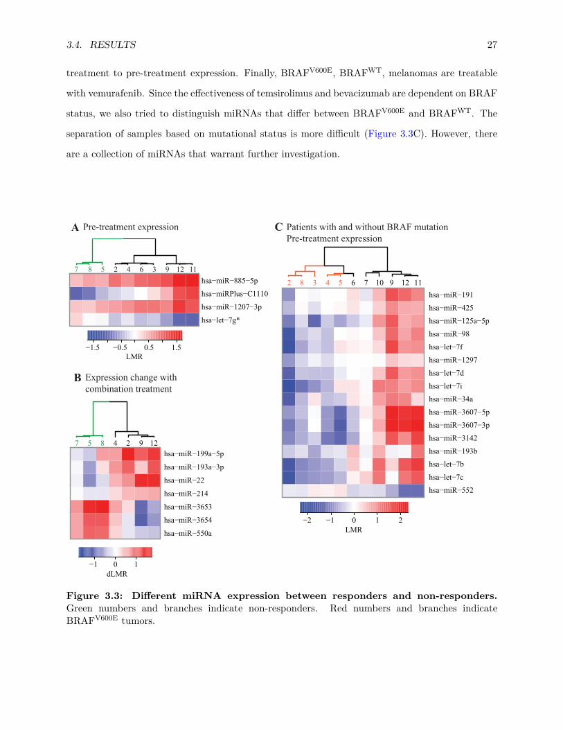
3.4. RESULTS 27
treatment to pre-treatment expression. Finally, BRAFV600E, BRAFWT, melanomas are treatable
with vemurafenib. Since the effectiveness of temsirolimus and bevacizumab are dependent on BRAF
status, we also tried to distinguish miRNAs that differ between BRAFV600E and BRAFWT. The
separation of samples based on mutational status is more difficult (Figure 3.3C). However, there
are a collection of miRNAs that warrant further investigation.
7 5 8 4 2 9 12
hsa−miR−550a
hsa−miR−3654
hsa−miR−3653
hsa−miR−214
hsa−miR−22
hsa−miR−193a−3p
hsa−miR−199a−5p
−1 0 1
hsa−let−7g*
hsa−miR−1207−3p
hsa−miRPlus−C1110
hsa−miR−885−5p
−1.5 −0.5 0.5LMR
dLMR
1.5
1293642587 11
2 8 3 4 5 6 7 10 9 12 11
hsa−miR−552
hsa−let−7c
hsa−let−7b
hsa−miR−193b
hsa−miR−3142
hsa−miR−3607−3p
hsa−miR−3607−5p
hsa−miR−34a
hsa−let−7i
hsa−let−7d
hsa−miR−1297
hsa−let−7f
hsa−miR−98
hsa−miR−125a−5p
hsa−miR−425
hsa−miR−191
−2 −1 0LMR
1 2
A Pre-treatment expression
B Expression change with combination treatment
C Patients with and without BRAF mutationPre-treatment expression
Figure 3.3: Different miRNA expression between responders and non-responders.Green numbers and branches indicate non-responders. Red numbers and branches indicateBRAFV600E tumors.

28 CHAPTER 3. MIRNA TRANSCRIPTOMICS OF MELANOMA
3.5 Conclusions
Proper use of simple statistical tests and well-designed visualizations corrected for small, but critical
errors in the analyses of high throughput biological data obtained from a clinical trial (Figure 3.1).
Bevacizumab+temsirolimus treatment affects miRNA expression more than temsirolimus treat-
ment alone, suggesting that the two drugs are at least additive in their effects on melanoma miRNA
expression (Figure 3.2). This is in line with their synergistic growth-reducing effects in melanoma
cell lines [146].
The pre-treatment expression of small sets of miRNA predicted the success of bevacizumab+temsirolimus
treatment (Figure 3.3A). The expression changes of 7 miRNAs could classify responders versus non-
responders; these miRNAs may play a role in the response to treatment (Figure 3.3B).

Chapter 4
Functional transcriptomics of the host
response to C. difficile toxins
C. difficile causes 300,000+ reported infections and ∼20,000 deaths in the US every year, indi-
rectly costing the healthcare system over $8 billion [1]. Infections indicate worsened health due to
Clostridium difficile, not normal colonization of C. difficile that occurs in healthy individuals. C.
difficile strains are only pathogenic if they release toxin A or toxin B (TcdA and TcdB). The basic
structure and enzymatic activities of the toxins are understood but the complex host response to
the toxins is not [148–153]. Since the severity of illness is determined by the the host and not the
extent of infection or the number of bacteria in the host, it is critical to understand detrimental
host responses [154].
Taking a systems biology approach, I show how transcriptomics can be used to infer previously
unidentfied host cell responses. The field of functional genomics (or functional transcriptomics)
overlaps with systems biology. They both aim to determine functions from genetic data and char-
acterize interactions between genes and proteins. In this chapter’s last section, I discuss the concept
of “enrichment” to identify groups of genes or pathways that are altered.
29

30 CHAPTER 4. FUNCTIONAL TRANSCRIPTOMICS OF TOXIN RESPONSE
4.1 C. difficile: a dangerous pathogen
4.1.1 Historical significance
In 1935, Hall and O’Toole isolated a novel gram-positive bacterium from infants which they named
Bacillus difficilis because it was a rod (Bacillus) and was an anaerobe that was difficult to grow
(difficilis). They also identified a B. difficilis toxin that killed mice. In 1943, the first rodent model
of infection was made unintentionally when penicillin induced inflammation in the cecum [155].
Remarkably, these findings from 70 years ago summarize much of what we now know: C. difficile
infection occurs when the flora is disrupted by antibiotics and the pathogenic effects are due to
toxins. Even more interesting, several studies over 50 years ago suggested that the most effective
treatment could be the restoration of the bacterial flora, which in the past few years has proved to
be the most effective treatment (reviewed in [156]).
Figure 4.1: An oversimplified view of C. difficile infection
After the advent of antibiotics, “pseudomembranous colitis” (PMC), a condition manifesting as
inflammation and diarrhea, became associated with antibiotic treatment [156, 157]. The etiology

4.1. C. DIFFICILE: A DANGEROUS PATHOGEN 31
of PMC remained unknown for several years until a rapid succession of experiments between 1977
and 1981 found C. difficile and its two large protein toxins (TcdA and TcdB) to be the primary
cause of PMC [158–167]. With increased antibiotic usage and improved surveillance, the incidience
of C. difficile infections has increased nearly every year since [1]. From 1981 to 1995, studies
characterized the broad physiological toxin effects, many of which are discussed in the following
chapters.
4.1.2 Toxin molecular biology
TcdA and TcdB are extremely potent. They are not small molecules like other toxins such as
arsenic or cyanide. As proteins, they are more similar to other toxins such as ricin, anthrax toxin,
tetanus toxin, and botulinum toxin (Botox).
The enzymatic activity of TcdA and TcdB which is responsible for their cytopathic effects
was discoverd in 1995 by Just et al. [151, 152]. Both TcdA and TcdB, with 63% amino acid
homology [168], have N-terminal domains that glucosylate Rho family proteins, disabling them
from entering their GTP-bound, active state [151, 152]. The C-terminal of both toxins consists
of many “clostridial repetitive oligopeptides” (CROPs) that are present in other clostridial and
streptococcal species [169, 170] that are important for cell binding and entry [171–173]. However,
it is unclear if the CROPs are entirely necessary for cell entry or if the CROPs can alone cause
cytopathic effects [174, 175]. Both toxins enter cells by endocytosis and rearrange structurally in
the acidic endosome [176, 177]. After translocating N-terminal domains to the cytosol through
self-formed pore in the endosome, a cysteine protease domain cleaves off the glucosyltransferase
domain into the cytosol [150, 178, 179]. Although much remains to be understood about the toxins’
functions on the molecular level (e.g., no toxin receptors are known and a large middle portion of
the toxins has no known function), there are even more unknowns about the disease pathogenesis
that is most critical to clinical outcome.
4.1.3 Physiological toxin responses
The external manifestations of C. difficile infection are diarrhea, abdominal pain, and sometimes
fever. Internally, pseudomembranous colitis is characterized by an inflamed colon covered with
yellow, volcano-shaped pseudomembranes made of cellular debris, exudate, and inflammatory cells

32 CHAPTER 4. FUNCTIONAL TRANSCRIPTOMICS OF TOXIN RESPONSE
Figure 4.2: Sequence, structure, and functioin of TcdA and TcdB
[157]. Histology reveals an abundance of neutrophils and loss of epithelial barrier integrity [180,
181]. Accordingly, many of the hypotheses for C. difficile and toxin studies have been centered
around known inflammatory markers. However, how these markers interact together is unknown.
It is also unknown if any other cell functions (e.g., regulation of metabolism) contribute to the
pathogenesis or the healing process.
4.2 Functional transcriptomics: enrichment
This dissertation presents a systems biology approach to the host response to C. difficile toxins,
using genome-wide expression to reveal altered cellular functions. Appropriate data processing

4.2. FUNCTIONAL TRANSCRIPTOMICS: ENRICHMENT 33
techniques were chosen to calculate expression values and differentially expressed genes (Chapter 2).
Many network based algorithms can be used to reconstruct regulatory networks and gene in-
teractions. However, many of these methodologies are unproven or still in the formative stages.
The approach in this dissertation is to present the differentially expressed genes using exploratory
analyses that enable novel hypotheses.
4.2.1 Gene set enrichment analysis
One of the simplest yet most helpful questions from transcriptomics data is ‘what types of genes
changed’. For example, is the number of differentially expressed chemokines greater than expected?
If so, then one could say that the data set is enriched with highly expressed chemokines. Alterna-
tively, it is common to say that chemokine genes or chemokine functions are enriched.
These questions lead to a hypothesis tests in which the significance of the difference between
two different proportions is determined. For example, is there a significantly greater proportion of
chemokines in the list of DEGs compared to the list of non-DEGs? The Fisher exact test calculates
the significance of such proportions, and it is ubiquitous in gene expression studies. The enrichment
of hundreds of predefined sets of genes from public biological databases can be used.
The Fisher test as well as the χ2 and other tests of proportions require a threshold to define
DEGs, and the results of the test are very sensitive to the threshold chosen. A handful of algorithms
have tried to solve the problem by scanning many thresholds, but they have had little success. These
proportion tests usually assume that genes within the gene set are independent, which usually
incorrect.
Like with DEG significance tests, the choices are numerous. In trying to find the appropriate
test, I evaluated over 130 articles introducing new tests and software tools to perform enrichment
tests, and there are probably one hundred more. Reviews of these methods can usually discuss a
portion of the possible tests [182–186]. Also similar to DEG tests, there are many different cate-
gories (e.g., parametric tests, permutation tests, machine learning algorithms) that make different
statistical assumptions.
Enrichment methods are even more complicated because the hypotheses are ill defined. For
instance, are there more genes in a gene set than all genes outside the gene set? Is the fold change
of gene in a gene set, on average, different than 1? The first question is more restrictive than the

34 CHAPTER 4. FUNCTIONAL TRANSCRIPTOMICS OF TOXIN RESPONSE
second, but neither are wrong questions to ask.
In later chapters, I describe some more details of different tests and give reasoning to the
enrichment tests chosen for the transcriptomics data. The tests were chosen based on exploration
of many methods to find the most consistent lists of highly ranked gene sets.

Chapter 5
Toxins A and B disrupt the cell cycle
5.1 Synopsis
Toxins A and B (TcdA and TcdB) are Clostridium difficile’s principal virulence factors, yet the
pathways by which they lead to inflammation and severe diarrhea remain unclear. Also, the relative
role of either toxin during infection and the differences in their effects across cell lines is still
poorly understood. To better understand their effects in a susceptible cell line, we analyzed the
transciptome-wide gene expression response of human ileocecal epithelial cells (HCT-8) after 2, 6,
and 24 hr of toxin exposure. We show that toxins elicit very similar changes in the gene expression
of HCT-8 cells, with the TcdB response occurring sooner. The high similarity suggests differences
between toxins are due to events beyond transcription of a single cell-type and that their relative
potencies during infection may depend on differential effects across cell types within the intestine.
We next performed an enrichment analysis to determine biological functions associated with changes
in transcription. Differentially expressed genes were associated with response to external stimuli and
apoptotic mechanisms and, at 24 hr, were predominately associated with cell-cycle control and DNA
replication. To validate our systems approach, we subsequently verified a novel G1/S and known
G2/M cell-cycle block and increased apoptosis as predicted from our enrichment analysis. This
study shows a successful example of a workflow deriving novel biological insight from transcriptome-
wide gene expression. Importantly, we do not find any significant difference between TcdA and TcdB
besides potency or kinetics. The role of each toxin in the inhibition of cell growth and proliferation,
an important function of cells in the intestinal epithelium, is characterized.
35

36 CHAPTER 5. TOXINS A AND B DISRUPT THE CELL CYCLE
5.2 Background
C. difficile, a Gram-positive, spore-forming anaerobe, colonizes the human gut and causes infections
leading to pseudomembranous colitis. This opportunistic pathogen flourishes in antibiotic-treated
and immunocompromised patients and is frequently spread in hospitals, although community-
acquired Clostridium difficile infection (CDI) cases have also increased [187]. The emergence of
hypervirulent strains that possess more robust toxin production and increased sporulation has
been correlated with outbreaks across Europe and North America [188]. In most areas, the number
of cases has increased in the past decade. The number of patients hospitalized in the US with CDI
doubled to approximately 250,000/year (from year 2000 to 2003) and fatalities increased at a similar
rate [189]. The US healthcare costs for CDI are estimated to be over $1 billion/year [190]. As TcdA
and TcdB appear to be responsible for many of the clinical manifestations of CDI, understanding
the intracellular and systemic effects of each toxin is critical to developing and improving strategies
for treatment and prevention.
In light of the multiple events and pathways involved in the development of CDI, we chose
to examine the toxins’ effects from a systems perspective, focusing on epithelial cells in vitro.
Both TcdA and TcdB bind to cells [173], enter an endosome by clathrin-mediated endocytosis
[176], translocate and then cleave their catalytic domain into the cytosol which glucosylates and so
inactivates Rho family proteins [178]. The disruption of these crucial signaling regulators begins to
explain cytotoxic effects such as deregulation of the cytoskeleton and the breakdown of the epithelial
barrier [191]. However, other processes are likely affected by the trafficking and processing of these
toxins. In addition, secondary effects of Rho glucosylation in relation to pathologies of CDI have
not been fully elucidated.
We therefore investigated the transcriptional profile of HCT-8 [192] cells treated with TcdA or
TcdB and identified pathways and cellular functions associated with differentially expressed genes.
With respect to toxins, in vitro analyses of gene expression in host cells have been performed with
type A botulinum neurotoxin, lethal toxin [193] and edema toxin [194] from Bacillus anthracis,
pertussis toxin [195], Shiga toxin type 1 [196], and several others. Such studies provide lists of
differentially expressed genes or classes of genes that serve as a resource for the generation of new
hypotheses. In this regard, we used bioinformatics analyses to identify cellular functions altered

5.3. METHODS 37
by TcdA and TcdB that are relevant to pathogenicity. The correct identification of the majority of
functions found to be affected in previous research regarding TcdA and TcdB confirmed our analysis
and experimental design, and experiments reported herein validated changes in cell function that
were suggested by altered gene expression.
Among the genes that TcdA and TcdB affect, many are involved in the regulation of the
cell cycle and induction of apoptosis. Bacterial factors such as cytotoxic necrotizing factor and
cytolethal distending toxins that disrupt normal cell cycle progression have been described as
“cyclomodulins” [197]. In addition to effects of TcdA and TcdB on cells in the G2/M phase which
have been described previously [198–201], we found that TcdA and TcdB affect expression of cyclins
and cyclin-dependent kinase (CDK) inhibitors controlling the G1– S transition. Our experiments
establish that alterations of cell cycle implicated in our analysis of gene expression do, in fact,
occur in toxin-treated cells. In addition to effects on cell cycle, we also present the other cellular
functions associated with differentially expressed genes, some of which enable novel hypotheses on
the cellular activity and function of these toxins.
5.3 Methods
5.3.1 Cell Culture
HCT-8 cells were cultured in RPMI-1640 supplemented with 10% heat-inactivated fetal bovine
serum (Gibco) and 1mM sodium pyruvate (Gibco). The cultures were maintained at 37°C/5%
CO2 up to passage 35. Toxin A and Toxin B, isolated from strain VPI-10643, were a generous gift
from David Lyerly (TECHLAB Inc., Blacksburg, VA).
5.3.2 Microarrays
HCT-8 cells (5 x 10⁶/flask) were grown overnight at 37°C/5% CO2. Media were replaced with 2.5
ml fresh media and toxin was added (100 ng/ml). At the end of the indicated incubation period,
cells were washed with 5 ml PBS (Sigma) and total RNA was isolated using the QIAshredder and
RNeasy mini kits (Qiagen), according to the manufacturer’s instructions. An RNase inhibitor was
added (RNasin, Promega) and samples were stored at -80°C. RNA integrity was assessed using
an Agilent 2100 BioAnalyzer prior to cDNA synthesis and RNA labeling using either the 3′ IVT

38 CHAPTER 5. TOXINS A AND B DISRUPT THE CELL CYCLE
expression or one-cycle target labeling methods (Affymetrix). Biotin-labeled RNA was hybridized
to Human Genome U133 Plus 2.0 chips, washed, stained and scanned using a GeneChip System
3000 7G (Affymetrix). Data from three independent microarray experiments were deposited into
the NCBI Gene Expression Omnibus repository (GSE29008).
Microarray signal intensities were normalized using the gcrma package [17]. Treatment and
control groups were contrasted with linear models; a Benjamini-Hochberg correction was applied
across all the probes and the nestedF method within the limma software package was used for
multiple testing across all contrasts [63, 64]. The Gene Ontology (GO) annotation database was
used to map gene symbols to GO categories [202]. A gene symbol was considered differentially
expressed if at least one of the probe sets annotated to it was significant. A probe set was considered
significant if the p<0.1 and the magnitude of the fold change was above 1.5. Enriched GO categories
were identified with the topGO package using Fisher’s exact test to calculate p-values and the elim
algorithm [203].
5.3.3 Flow Cytometry
HCT-8 cells were grown overnight to 50% confluence, media were removed and replaced with fresh
media, and toxin was added at the concentrations denoted in the text and figures. At 24h and 48h,
non-adherent cells were removed and saved on ice. Adherent cells were treated with 1mL of 0.25%
trypsin and 1 mL of Accutase with EDTA for 30 min at room temperature and joined with the non-
adherent cells in 5 mL PBS. After centrifugation, resuspension for counting cells, and another round
of centrifugation, the dissociated cells were resuspended to 2×10⁶ cells/mL and 0.5 mL was added
to 5mL of 70% ice-cold ethanol for fixation. Afterward, the fixed cells were resuspended in 5 ml
PBS with 2% Bovine Serum Albumin and then resuspended and incubated for 30 min in a solution
to stain DNA (PBS with 10% Triton X-100, 2% DNasefree RNase, 0.02% propidium iodide(PI)).
Single-cell fluorescence was measured with a Becton Dickinson FACSCalibur flow cytometer. The
proportion of cells in each stage of the cell cycle was calculated using ModFit cell cycle analyzer. The
24h-samples were imaged with an Amnis Imagestream imaging flow cytometer, which photographs
the bright field and fluorescent channels from every cell individually [204]. Using Amnis software,
a bivariate gate—based on the contrast of the brightfield image and the area of nuclear stain—
differentiated apoptotic and non-apoptotic cells [205]. All other image features were taken from
5.3. METHODS 39
the Amnis software.
5.3.4 Quantitative real time PCR
For each gene examined, primers were designed from the target sequences retrieved from the Ref-
Seq Sequence Database, using the Primer Express 3.0 software (Applied Biosystems). Primers
were then custom made through Invitrogen Oligo Program. RNA quality control was carries out
using an Agilent 2100 BioAnalyzer. Approximately 2 μg of each RNA sample was converted to
cDNA. Quantitative PCRs were carried out in triplicates using equal amounts of each cDNA sam-
ple approximately equivalent to 50 ng of starting total RNA. Power SYBR Green Master Mix
(Applied Biosystems, PN 4367660) was used with the respective forward and reverse primers at
the optimized concentrations. Amplifying PCR and monitoring of the fluorescent emission in real
time were performed in the ABI Prism 7900HT Sequence Detection System (Applied Biosystems)
as described (ABI SYBR Green Protocol). To verify that only a single PCR product was ampli-
fied per transcript, dissociation curve data was analyzed through the 7900HT Sequence Detection
Software (SDS). To account for differences in starting material, quantitative PCR was also carried
out for each cDNA sample using housekeeping genes synthesized in-house, human glyceraldehyde-3-
phosphate dehydrogenase (GAPDH) and hypoxanthine phosphoribosyltransferase I (HPRT1). The
data collected from these quantitative PCRs defined a threshold cycle number (Ct) of detection
for the target or housekeeping genes in each cDNA sample. The relative quantity (RQ) of target,
normalized to geometric means of the housekeeping genes and relative to a calibrator (the Rox
reference dye in this case), is given by RQ = 2–∆∆Ct where ∆∆Ct represents the difference in Ct
between the transcript and the housekeeping gene for the same RNA sample. The ratio of the RQs
for the treated sample and the experiment sample was used to derive the fold change.
5.3.5 Western Blots
After toxin treatment, non-adherent cells were removed and centrifuged. The adherent cells were
then treated with 200 μL of homogenization buffer: 10 mM HEPES pH 7.4, 150 mM NaCl, 10
mM sodium pyrophosphate, 10 mM NaF, 10 mM EDTA, 4mM EGTA, 0.1 mM PMSF, 2 �g/mL
CLAP (Chymostatin, Leupeptin, Antipain, and Pepstatin), and 1% Triton X-100. Each well was
scraped and the sample with homogenization buffer was added to the resuspended non-adherent

40 CHAPTER 5. TOXINS A AND B DISRUPT THE CELL CYCLE
cells. This was centrifuged at 15,000 rpm for 5 min at 4°C and the supernatant was boiled for
5 min, placed on ice for 5 min, boiled again for 5 min, and stored at -20°C. Samples containing
equal amounts of protein were loaded into each lane of a 12.5% polyacrylamide gel. Gels were
electrophoresed, transferred to PVDF, and the membranes were blocked with 5% skim milk in
PBS, 0.1% Tween-20 for 2h. Primary antibodies (Cyclin D1 #2922, Cyclin E2 #4132, p57 Kip2
#2557, p27 Kip1 #2552 from Cell Signaling and Cyclin A sc-751 from Santa Cruz Biotechnology)
were added to the blocking solution and membranes were incubated overnight at 4°C on a platform
shaker. The membranes were then washed six times in PBS-Tween 20. The appropriate secondary
antibodies, either anti-mouse or anti-rabbit HRP-linked antibodies (#7076, #7074, Cell Signaling),
were added and the membranes were incubated for 2h on a platform shaker. The membranes were
subsequently washed 6 times and proteins were detected by chemiluminescence with ECL reagents
(Amersham). To strip antibodies, the membranes were incubated in 50 mM Tris, 2% SDS, 0.7%
�-mercaptoethanol at 50°C for 30 min. The membranes were then washed 6 times, blocked, and
reprobed with a GAPDH antibody (ab8245 from Abcam) as described above.
5.4 Results
5.4.1 Transcriptional Responses
Overall, the changes in gene expression are consistent as time progresses, but the number of dif-
ferentially expressed genes increases (Figure 5.1A). Specifically, at 2h and 6h, there are 4 and 134
probe sets differentially expressed (relative to control) for TcdA and 57 and 294 for TcdB, respec-
tively (Figure 5.1C). Many more are differentially expressed by 24h—1,155 and 1,205 in TcdA- and
TcdB-treated cells, respectively. In order to validate these data, qRT-PCR was performed on 10
representative genes (r=0.89 by Pearson correlation; Figure 5.2A). Since the glucosylation of Rho
family proteins occurs within one hour of toxin treatment [206], many of the differentially expressed
genes at 24h may reflect secondary effects from the initial toxin action or possibly other unknown
activities and processing of the toxin.
Though the transcriptional responses to the two toxins are similar overall, a notable difference
between the two toxins is that TcdB-induced changes occur more rapidly (Figure 5.1A). At the later
time points, however, the overall transcriptional response induced by TcdA becomes more similar

5.4. RESULTS 41
0 4-4-16 16 64-64
A, 2 hr
B, 2 hr
A, 6 hr
B, 6 hr
A, 24 hr
B, 24 hr
A, 2 hr
B, 2 hr
A, 6 hr
B, 6 hr
A, 24 hr
B, 24 hr
A, 2 hr
B, 2 hr
A, 6 hr
B, 6 hr
A, 24 hr
B, 24 hr
4 57134
Di�erentiallyexpressed probesets
294
1,155 1,205
A, 2 hr
B, 2 hr
A, 6 hr
B, 6 hr
A, 24 hr
B, 24 hr
−0.04 0.09 0.28 0.38 0.91 1.00
−0.04 0.10 0.24 0.37 1.00 0.91
−0.04 0.25 0.86 1.00 0.37 0.38
0.01 0.30 1.00 0.86 0.24 0.28
0.56 1.00 0.30 0.25 0.10 0.09
1.00 0.56 0.01 −0.04−0.04−0.04
Fold change
Mic
roar
ray
prob
e se
ts
Correlation Coe�cients ( r )
A B
C
Figure 5.1: Overall transcriptional response of HCT-8 cells to TcdA and TcdB. (A)A heatmap shows the number of differentially expressed probe sets at 2h, 6h, and 24h. The colorscale represents the fold change (binary log scale) of genes relative to untreated cells at the sametime point. “A, 2hr” indicates the gene expression of cells after 2h of TcdA treatment. TcdA andTcdB concentration is 100 ng/ml. (B) The correlation of transcriptional profiles between TcdAand TcdB at the indicated time points are displayed in a correlation matrix. The values representthe Pearson correlation coefficient calculated from the fold change of all the probe sets withinthe microarray. (C) The number of differentially expressed genes used to identify enriched GOcategories was determined from a linear model (see 5.3.2).
to the TcdB-induced transcriptional changes (see correlations in Figure 5.1B). Among the most
affected genes, immediate early-response genes such as JUN, KLF2, and RHOB are upregulated 2h
after toxin treatment and remain increased compared to untreated cells through 24 hr (Figure 5.2B).
While identification of the most-affected genes provides important insight, focusing on a small
subset risks overlooking other toxin effects key to the disease process. We therefore analyzed the
expression data in the context of broad functional categories.

42 CHAPTER 5. TOXINS A AND B DISRUPT THE CELL CYCLE
1.1−1.71.31.21.31.21.21.22.83.8
CTGFDUSP6CCNA2CCNE2CDC25ACCND1CDKN1BCDKN1CRHOBJUN
Array PCRA, 2 hr B, 2h r A, 6 hr B, 6 hr A, 24 hr B, 24 hr
Array PCR Array PCR Array PCR Array PCR Array PCR
−1.11.01.21.31.71.11.21.01.41.5
−4.5−14.7
1.31.21.1
−1.41.73.28.4
27.9
−2.7−3.91.01.0
−1.1−1.31.1
−1.63.73.7
−28.2−12.6
1.1−1.4−1.5−2.81.43.2
18.339.7
−11.2−5.4−1.0−1.5−1.6−2.11.63.2
11.810.4
−31.9−22.1
1.1−4.9−4.2−5.21.56.0
21.637.5
−25.1−21.6
1.2−3.0−2.7−5.42.5
11.912.316.4
−98.4−4.3
−61.0−68.6−11.7−1.51.73.3
14.137.7
−35.2−3.3
−17.9−8.3−4.41.12.12.0
16.446.5
−95−2.5−32
−13.2−6.2−1.51.51.6
13.844.9
−29.9−1.8
−19.4−5.8−2.61.32.41.0
23.268.0
EGR1CTGF
RHOBKLF2JUN
A, 2 hr
B, 2 hr
A, 6 hr
B, 6 hr
A, 24 hr
B, 24 hr
−1.9−1.3−1.51.1
−1.5−1.1−1.72.83.93.8
cystein-rich angiogenic inducer, 61angiomotin like 2early growth response 1connective tissue growth factortumor necrosis factor (ligand) superfamily, member 15EPH receptor A2dual speci�city phosphatase 6ras homolog gene family, member BKruppel-like factor 2 (lung)jun proto-oncogene
CYR61AMOTL2
TNFSF15EPHA2DUSP6
NameSymbol
−8.1−7.5−4.0−4.5−4.0−5.3
−14.78.4
14.527.9
−8.7−12.9−11.5−28.2−6.2−8.4
−12.618.310.539.7
−10.9−13.0−23.4−31.9−9.7
−15.4−22.121.612.037.5
−25.8−19.5−8.9
−98.4−2.8−5.4−4.314.111.037.7
−23.7−19.9−22.2−95.0−1.5−2.3−2.513.89.4
44.9
A
B
Figure 5.2: qRT-PCR validation of and genes with high differential expression (A)Fold changes of gene expression relative to controls as measured by microarray were validated byqRT-PCR. To summarize multiple probe sets within a microarray that were annotated to the samegene, the value for the probe set with the greatest fold change is shown. The notation “A, 2hr”indicates the expression of genes treated with TcdA for 2 hr. (B) This list consists of genes thatwere among the top 25 differentially expressed genes (according to fold change) in at least 3 of the6 conditions.
5.4.2 Functions associated with differentially expressed genes
We employed the GO database, which contains extensive annotation of biological functions associ-
ated with specific genes, to identify cellular phenotypes associated with changes in gene expression.
The terms in this database are separated into three ontologies: Molecular Functions, Cellular Com-
ponents, and Biological Processes (detailed descriptions at http://www.geneontology.org). A GO
category—here defined as all the genes associated with a single GO term—with a proportion of
differentially expressed genes greater than would be expected by chance is considered overrepre-

5.4. RESULTS 43
negative regulation of phosphyorylationinactivation of MAPK activityregulation of cyclin-dependent protein kinase activitynucleosome assemblyrelease of cytochrome c from mitochondriaactivation of caspase activityresponse to hydrogen peroxideresponse to cytokine stimulusresponse to lipopolysaccharideagingangiogenesisovarian follicle development
A
0 .004 .032 .108 .256 0.5
Toxin
Toxin
2 hr
p-value
6 hr 24 hrB A B A B
cell cycle checkpointS phase of mitotic cell cycleG1/S transition of mitotic cell cyclemitotic prometaphasemitosisnucleosome assemblytelomere maintenance via semi-conservative replicationtelomere maintenance via recombinationDNA strand elongation during DNA replicationDNA replicationcell divisionnegative regulation of megakaryocyte di�erentiation
A2 hr 6 hr
B A BA
B
Figure 5.3: Gene ontology categories associated with differentially expressed genes.(A) The most significantly enriched GO categories (Fisher Exact Test, topGO elim algorithm [203],see 5.3.2) at 2h and 6h are displayed in a heat map. The color intensity in each cell correspondsto the p-value (Fisher Exact Test) for the GO category that is enriched. The dendrograms weregenerated from a hierarchical clustering of GO Groups according to Resnik similarity [207]. (B)The most significantly enriched GO categories at 24h were determined similarly
sented or enriched (see 5.3.2). While some enriched categories might have been anticipated, others
provide novel insights. Within the Biological Processes ontology, the most significantly enriched
categories at 2 and 6 hr are listed in Figure 5.3A. Within the Cellular Component ontology, the
mitochondrial outer membrane and the apical junction complex category are enriched most signif-
icantly at 6h (Figure 5.4A). Interestingly, many of the functions related to the enriched categories

44 CHAPTER 5. TOXINS A AND B DISRUPT THE CELL CYCLE
0.004
.032.108
.2560.5 p-value
AToxin
2 hr6 hr
24 hrB
AB
AB
condensed chromosom
econdensed nuclear chrom
osome
condensed nuclear chromosom
e, centromeric region
outer kinetochore of condensed chromosom
econdensed chrom
osome kinetochore
nucleosome
chromatin
cohesin complex
chromosom
e, centromeric region
chromosom
al partchrom
osome, telom
eric regionnuclear replisom
ereplication forknuclear chrom
osme part
nuclear origin of replication recognition complex
centrosome
centriolespindle m
icrotubulespindlespindle polem
icrotubule associated complex
cytoplasmic m
icrotubulem
icrotubulecytosolm
itochondrial outer mem
branenucleoplasmpronucleusnucleusapical junction com
plexm
idbody
AA
Toxin2 hr
6 hr24 hr
BA
BA
Btelom
ere maintenance
telomere m
aintenance via semi-conservative replication
telomere m
aintenance via recombination
nucleotide-excision repair, DN
A gap �lling
DN
A replication
DN
A strand elongation during D
NA
replicationD
NA
replication initiationG
1/S transition of mitotic cell cycle
regulation of transcription involved in G1/S-phase of m
itotic cell cycleM
/G1 transition of m
itotic cell cycleS phase of m
itotic cell cycleG
2/M transition of m
itotic cell cyclem
itotic sister chromatid segregation
mitotic prom
etaphasem
itosiscell cycle checkpointcell cyclecell divisionnegative regulation of m
egakaryocyte di�erentiationphosphoinositide-m
ediated signalingCenH
3-containing nucleosome assem
bly at centromere
nucleosome assem
blym
icrotubule-based movem
entm
itotic spindle organizationspindle organization
B
Figure
5.4:G
eneset
enrichment
ofbiological
processesand
cellularcom
ponents.(A
)Cellular
Com
ponentGO
categorieswith
p<
10−3across
alltimepoints
areshow
n.Criteria
forcalculating
pvalues
andGO
categorieswere
thesam
eas
inFigure
2.(B
)The
25most
significantGO
BiologicalProcessesat
24hr
wereselected
bythe
criteriadescribed
inFigure
5.3.

5.4. RESULTS 45
have been linked with toxin treatment in previous work. One or both of the toxins induce activation
of caspases [200, 208–210], damage mitochondria and cause the release of cytochrome c [211, 212],
increase oxygen radicals and expression of cytokines [213–215], alter MAPK signaling [216–218],
and disrupt the organization of tight junctions [191]. Hence, our analysis of gene expression as
summarized in Figure 5.3 is consistent with the previously reported cellular responses to these
toxins.
The most significantly enriched categories for each toxin at the later time points are related
to cell cycle and DNA replication (Figure 5.3B). Categories such as telomere maintenance and
nucleosome assembly provide more specific connections between the toxins and changes in DNA
replication. A more extensive list reveals that several categories related to microtubule organization
during cell division are also enriched (Figure 5.4B). By 24 hr, there are changes related to virtually
all elements of the cell cycle, but those controlling G1 and S phases are more significantly affected.
Though many of the genes within the enriched categories were not among the most differentially
expressed genes, the abundance of differentially expressed genes involved in the same functions
provides evidence for toxin effects on control of cell cycle at the G1 phase. Cyclins and other proteins
necessary for progression from the G1 phase into and through the S phase are downregulated
(Figure 5.5A). Cyclin proteins expressed at different points are central in coordinating entry into
or exit from different phases. They specifically bind and activate particular CDKs which then
phosphorylate downstream targets effecting progression [219]. Inhibitors of cyclin-CDK complexes
from the INK4 family (p15, p16, p18, and p19) and Cip/Kip family (p21, p27, and p57) may
suppress cyclin-CDK signaling [220]. Expression of many of these and other genes, such as CDC6
and CDC25A that are required for progression from G1 to the S phase, is altered by TcdA and
TcdB. The decreased expression of G1 cyclins along with the increased expression of inhibitors of
G1-associated cyclin-CDK complexes suggest altered regulation of the cell cycle specifically in G1.
We also measured expression of genes and proteins (Figure 5.6) after 6 and 24 hr of treatment with
0.1, 1, and 10 ng/ml of TcdA or TcdB in confluent and subconfluent cultures, which confirmed a
consistent alteration of cell cycle genes and proteins across a variety of conditions.

46 CHAPTER 5. TOXINS A AND B DISRUPT THE CELL CYCLE
Figure 5.5: The altered gene ex-pression of G1 phase cell cycleregulators at 6h and changes inthe distribution of cells withinthe cell cycle. (A) A schematicof cell cycle regulation with proteinsplaced next to the phase of cell cy-cle with which they are associated(p19 and p21 are the products of theCDKN2D and CDKN1A genes, re-spectively). Gray, blue, and red indi-cate genes with unchanged, increased,or decreased expression, respectively,post toxin treatment. (B) Cells ina subconfluent culture were treatedwith the indicated concentrations oftoxin for 24h. The DNA content ofcells in each condition was quantifiedby PI fluorescence. The histogramsof the area of PI fluorescence are nor-malized to the total number of cells(denoted as normalized cell count) inthe sample such that the area undereach histogram is equal to 1. In thisway, the proportions of cells in eachphase of the cell cycle may be com-pared for different size samples. Thescale of the vertical axis is the same ineach histogram. (C) The percentageof cells in each phase of the cell cy-cle was calculated using ModFit LTsoftware. Sub-G0/G1 cells were notincluded in the calculations.
CDC25A
CDC6
Cyclin ECDK2
Untreated
TcdA TcdB TcdA and TcdB
G0/G1
S
100%
70%
Untreat
ed 0.1 1
0.1 0.1 1110
G2/MNor
mal
ized
cel
l cou
nt
Area of PI �uorescence (DNA content)
TcdB0.1 ng/ml
TcdB1 ng/ml
CDK1
CDK4
CDK6
Cyclin D
Cyclin D
Cyclin A
CDKN1A
CDKN1A
CDKN2D
CDKN1B
CDKN1B
CDKN1C
CDKN1C
CDK2Cyclin A
UpregulatedGene expresssion relative to untreated cells. TcdB, 6hr (microarray)
S
A
B
C
M
G2
G1
Downregulated
Unchanged
CDK1Cyclin B
Cyclin D
Cyclin A
Cycl
in E
Cyclin
BG2/M
S
G0/G1

5.4. RESULTS 47
−1.31.1
−1.61.01.22.1
−1.3−1.11.51.11.0
−1.21.31.21.21.11.01.1
−1.41.0
−0.51.11.01.01.01.0
−1.11.21.01.1
2.22.02.74.15.4
12.33.54.26.14.14.02.91.71.71.74.34.14.53.53.85.13.64.04.33.84.03.91.51.81.6
−1.34−1.34−31.2
1.53.38.1
−1.21.84.3
−1.1−1.4−6.71.21.2
−1.71.11.31.8
−1.1−1.13.21.0
−1.1−1.1−1.1−1.1−1.91.0
−1.1−2.9
1.9−4.0
−11.16.0
29.334.23.79.6
11.03.3
−1.5−4.62.41.3
−1.23.14.64.94.7
18.151.64.24.34.32.82.41.41.1
−1.9−4.2
−1.01.0
−3.51.01.76.31.22.08.9
−1.11.01.11.01.0
−2.0−1.11.01.11.31.22.3
−1.11.0
−1.41.11.0
−1.91.11.0
−1.5
−1.1−1.3
−22.7−1.13.1
10.2−1.12.9
14.3−1.11.1
−2.31.1
−1.1−3.6−1.11.31.81.01.33.21.2
−1.1−3.3−1.2−1.3−3.7−1.3−1.3−2.1
−1.1−5.4
−38.12.18.1
15.92.4
11.826.11.0
−1.4−2.3−1.1−2.2−6.1−1.21.22.01.02.53.81.0
−1.5−11.7−1.1−2.1−6.81.0
−1.4−1.4
−7.1−30.9−20.1
6.016.519.17.9
34.437.1−1.4
−1.76−1.2−1.5−7.9−4.91.42.62.82.44.11.9
−1.4−13.4−8.9−2.2−3.6−3.1−1.9−1.8−1.4
0.11
10
0.11
10
0.11
10
0.11
10
0.11
10
0.11
10
0.11
10
0.11
10
0.11
10
0.11
10
CCND1
Con�uence HighA, 6 hr B, 6 hr A, 24 hr B, 24 hr
Low High Low High Low High Low ng/ml
CCNE2
CCNA2
CDKN1C
CDKN1B
CDC25A
DUSP6
JUN
RHOB
CTGF
1
A B
Cyclin A2GAPDH
Cyclin D1GAPDH
Cyclin E2GAPDH
p27GAPDH
p57
non-glucosylated Rac1
non-glucosylated Rac1
Toxinng/ml
Time
GAPDH
1.2 1.0 0.9 1.0 0.8 0.7 1 <0.1 0.6 <0.1 <0.1
1 0.3 0.7 1.1 0.3 0.3 0.5 1 0.1 0.7 0.3 0.4
1 0.6 0.7 1.0 0.5 0.5 0.5 1 <0.1 0.3 <0.1 <0.1
1 1.3 1.0 1.0 2.2 1.7 1.8 1 2.2 1.3 2.1 2.5
1
30 min
52 2.4 2.3 125 97 63 1 2.9 <0.1 0.9 3.3
- A A A B B B - A A B B- 1000 100 10
6 hr 24 hr1000 100 10 - 1000 100 1000 10
Cduration of Toxin A exposure
15 min
duration of Toxin B exposure
1 hr
untreated
15 min30 m
in
30 min
1 hr2 hr
2 hr
4 hr
4 hr
6 hr
6 hr
8 hr
8 hr
12 hr
12 hr
24 hr
24 hr
Figure 5.6: Timing of RAC1 glucosylation and expression of cyclin-related genes andproteins in subconfluent and confluent cultures. (A) The expression of 10 genes in bothsubconfluent and confluent toxin-treated cells was measured by qRT-PCR. Fold changes shownare relative to untreated samples. (B) Densitometry was performed on immunoblots of lysatesfrom toxin-treated, confluent cells. The intensity of each band was normalized to the intensity ofGAPDH, the loading control. The values above each row indicate the amount of protein relative tothe amount in untreated cells. The relative intensity for p57 was not calculated because the proteinwas not detectable in untreated cells. The blots show the presence of p57 after toxin treatment.(C) A Rac1 antibody (BD#610650) that recognizes non-glucosylated Rac1 (protein that has notbeen glucosylated by either toxin) shows the activity of TcdA and TcdB in HCT-8 cells.
5.4.3 Effects of TcdA and TcdB on the Regulation of Cell Cycle
The functional changes suggested by altered gene and protein expression were then investigated by
quantifying the proportion of cells in each phase of the cell cycle before and after toxin treatment.
To focus on actively growing cells and avoid the effects of contact inhibition, subconfluent cultures
were used. After 24 hr of 0.1 or 1 ng/ml TcdB treatment, the distribution of cells across the cell
cycle changes significantly, with only a small increase in the proportion of cells with less than a
G0/G1 amount of DNA—cells that are presumably dead or dying (Figure 5.5B). In agreement with
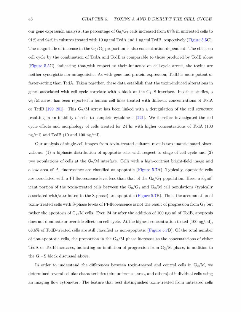
48 CHAPTER 5. TOXINS A AND B DISRUPT THE CELL CYCLE
our gene expression analysis, the percentage of G0/G1 cells increased from 67% in untreated cells to
91% and 94% in cultures treated with 10 ng/ml TcdA and 1 ng/ml TcdB, respectively (Figure 5.5C).
The magnitude of increase in the G0/G1 proportion is also concentration-dependent. The effect on
cell cycle by the combination of TcdA and TcdB is comparable to those produced by TcdB alone
(Figure 5.5C), indicating that,with respect to their influence on cell-cycle arrest, the toxins are
neither synergistic nor antagonistic. As with gene and protein expression, TcdB is more potent or
faster-acting than TcdA. Taken together, these data establish that the toxin-induced alterations in
genes associated with cell cycle correlate with a block at the G1–S interface. In other studies, a
G2/M arrest has been reported in human cell lines treated with different concentrations of TcdA
or TcdB [199–201]. This G2/M arrest has been linked with a deregulation of the cell structure
resulting in an inability of cells to complete cytokinesis [221]. We therefore investigated the cell
cycle effects and morphology of cells treated for 24 hr with higher concentrations of TcdA (100
ng/ml) and TcdB (10 and 100 ng/ml).
Our analysis of single-cell images from toxin-treated cultures reveals two unanticipated obser-
vations: (1) a biphasic distribution of apoptotic cells with respect to stage of cell cycle and (2)
two populations of cells at the G2/M interface. Cells with a high-contrast bright-field image and
a low area of PI fluorescence are classified as apoptotic (Figure 5.7A). Typically, apoptotic cells
are associated with a PI fluorescence level less than that of the G0/G1 population. Here, a signif-
icant portion of the toxin-treated cells between the G0/G1 and G2/M cell populations (typically
associated with/attributed to the S-phase) are apoptotic (Figure 5.7B). Thus, the accumulation of
toxin-treated cells with S-phase levels of PI-fluorescence is not the result of progression from G1 but
rather the apoptosis of G2/M cells. Even 24 hr after the addition of 100 ng/ml of TcdB, apoptosis
does not dominate or override effects on cell cycle. At the highest concentration tested (100 ng/ml),
68.6% of TcdB-treated cells are still classified as non-apoptotic (Figure 5.7B). Of the total number
of non-apoptotic cells, the proportion in the G2/M phase increases as the concentrations of either
TcdA or TcdB increases, indicating an inhibition of progression from G2/M phase, in addition to
the G1– S block discussed above.
In order to understand the differences between toxin-treated and control cells in G2/M, we
determined several cellular characteristics (circumference, area, and others) of individual cells using
an imaging flow cytometer. The feature that best distinguishes toxin-treated from untreated cells
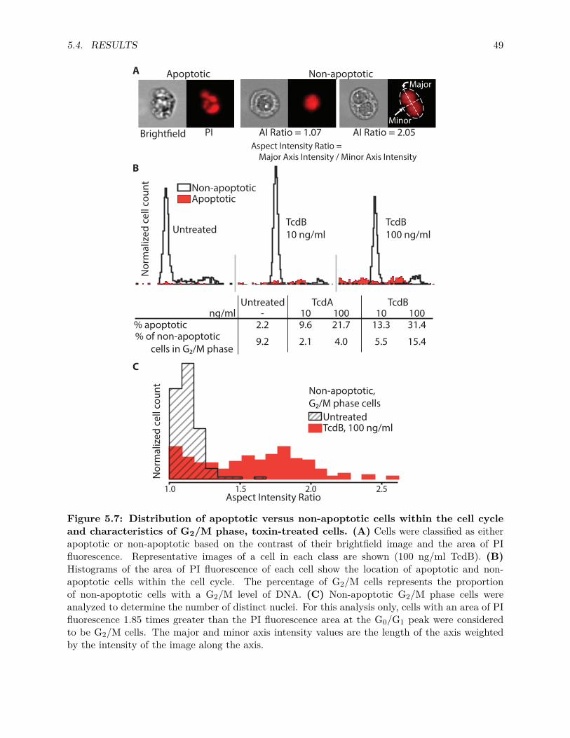
5.4. RESULTS 49
Major
Minor
Untreated
Untreated TcdAng/ml
% apoptotic% of non-apoptotic cells in G2/M phase
2.2-
9.2
9.610
2.1
21.7100
4.0
TcdB
13.310
5.5
31.4100
15.4
Aspect Intensity Ratio = Major Axis Intensity / Minor Axis Intensity
Non-apoptotic
1.0 1.5 2.0 2.5
Apoptotic
Non-apoptotic,G2/M phase cells
TcdB10 ng/ml
TcdB100 ng/ml
Nor
mal
ized
cel
l cou
ntN
orm
aliz
ed c
ell c
ount
AI Ratio = 1.07 AI Ratio = 2.05PI
Non-apoptoticA
B
C
UntreatedTcdB, 100 ng/ml
Bright�eld
Apoptotic
Aspect Intensity Ratio
Figure 5.7: Distribution of apoptotic versus non-apoptotic cells within the cell cycleand characteristics of G2/M phase, toxin-treated cells. (A) Cells were classified as eitherapoptotic or non-apoptotic based on the contrast of their brightfield image and the area of PIfluorescence. Representative images of a cell in each class are shown (100 ng/ml TcdB). (B)Histograms of the area of PI fluorescence of each cell show the location of apoptotic and non-apoptotic cells within the cell cycle. The percentage of G2/M cells represents the proportionof non-apoptotic cells with a G2/M level of DNA. (C) Non-apoptotic G2/M phase cells wereanalyzed to determine the number of distinct nuclei. For this analysis only, cells with an area of PIfluorescence 1.85 times greater than the PI fluorescence area at the G0/G1 peak were consideredto be G2/M cells. The major and minor axis intensity values are the length of the axis weightedby the intensity of the image along the axis.

50 CHAPTER 5. TOXINS A AND B DISRUPT THE CELL CYCLE
is the intensity-weighted aspect ratio of the PI fluorescence image. When an ellipse is fit around
the image, an aspect ratio near one indicates a circular nucleus and a higher aspect ratio indicates
an elliptical nucleus or multiple nuclei (Figure 5.7A). Upon visual inspection, a high aspect ratio
is due typically to binucleation. The higher proportion of binucleated cells in toxin-treated cells
(Figure 5.7C) indicates that the G2/M block is attributable to a failure to complete cytokinesis
[221]. Therefore, in addition to demonstration of a G1– S block, our results show an inhibition
of progression at the G2 –M transition, which is congruent with previous findings [198–201] in
other cell types treated with different toxin concentrations. Importantly, these G2/M effects were
observed at the same concentration of toxin used for microarray analysis (100 ng/ml). Again, TcdA
elicited a similar response to TcdB at the same concentration, yet to a lesser extent, thus showing
consistency from gene and protein expression to cell function.
5.5 Discussion
Understanding the differences between these two toxins is particularly relevant in determining their
roles in C. difficile infection. Toxin A appears to be the dominant virulence factor in animal studies,
yet Toxin B has higher enzymatic activity in vitro and is more potent when injected into Don cells
and for human cells studied in vitro [206, 222]. In a hamster model, Kuehne et al. found that
strains of C. difficile producing only TcdA or TcdB are comparable in their virulence, while Lyras
et al used a TcdA mutant to show that TcdB was the key virulence factor [223, 224]. In this
study, we used a systems approach to understand the effects of TcdA and TcdB on a human colonic
epithelial cell line. We observed that the responses to these two toxins are strikingly similar, with
the response to TcdB occurring more rapidly. Investigation of one of the biological consequences of
these changes in gene expression revealed toxin effects at both the G1– S and the G2 –M transitions.
In order to explore the interactions between C. difficile and intestinal epithelial cells, Janvilisri
et al. examined the transcriptional responses of Caco-2 cells and C. difficile organisms during an in
vitro infection [225]. Because expression was measured at no more than 2 hr post-infection, most
of the changes in gene expression were slight, yet they identified functions such as cell metabolism
and transport associated with affected genes. We focused on cells treated with TcdA or TcdB at
a concentration and time course in which the cell morphology is strongly affected. The effects of

5.5. DISCUSSION 51
TcdA and TcdB on gene expression in host cells have been interrogated in other studies focusing
on individual pathways, but until now, an analysis of the comprehensive global transcriptional
response induced by either TcdA or TcdB alone had not been performed.
Our systems approach identified a disruption of the cell cycle not readily apparent from a ranked
list of genes. This approach overcame difficulties in deciphering the particular relevance of genes
known to be induced by several stimuli or genes whose expression leads to many possible cellular
phenotypes. JUN is overall the most differentially expressed gene in our data, and, considering
TcdA or TcdB as a cellular stress, its dramatic increase in expression is consistent with it being
characterized as a stress-response gene. However, increased JUN expression has also been associated
with the promotion of G1 progression, protection from apoptosis after ultraviolet radiation, and even
induction of apoptosis [226]. Clearly, multiple events may lead to the same changes in expression
of an individual gene. The identification of functions associated with many of the differentially
expressed genes thus provides better evidence of actual biological functions important to the toxin
response.
These results have clarified the effects of TcdA and TcdB at each stage of the cell cycle. In
studying Rho signaling, Welsh et al. showed that combined Rho, Rac, and Cdc42 inhibition by
TcdA (200 ng/ml) in fibroblasts led to decreased cyclin D1 expression and an inability of serum-
starved cells, stimulated with fetal calf serum and treated with toxin, to progress past the G1
phase [227]. Importantly, we show that a strong G1 arrest occurs in unsynchronized, proliferating
epithelial cells. Only when treated with higher concentrations (100 ng/ml TcdA, 10 ng/ml TcdB)
of toxin did we begin to observe the inhibition of cell division at the G2/M phase in a significant
proportion of cells. With regard to cell death, others have shown an increased susceptibility of
S-phase cells to toxin treatment [228]. We did observe an increase in the proportion of apoptotic
S or G2/M phase cells. At low concentrations (10 ng/ml TcdA, 1 ng/ml TcdB), the decrease in
the proportion of S-phase cells, however, could not be entirely accounted for by death of cells at
a particular point in the growth cycle. Rather, many non-apoptotic cells remained in the G0/G1
phase.

52 CHAPTER 5. TOXINS A AND B DISRUPT THE CELL CYCLE
5.6 Conclusion
Our results have several implications in reference to the role of these toxins in pathogenicity. In
a host, the gut epithelial cells normally turn over every 2-3 days [229]. Disruption of this cellular
renewal process, and therefore cell cycle, impairs the maintenance of the epithelial barrier. The
ability of both TcdA and TcdB to arrest growth at the G0/G1 phase and the G2 –M transition, by
likely different mechanisms (G1 arrest occurs even at low toxin concentrations and is associated with
altered protein signaling; G2 arrest is likely associated with disorganization of the cytoskeleton),
places each toxin in the category of cyclomodulins. As has been previously shown however, control
of cell proliferation is certainly not their only or necessarily primary effect (e.g., inflammation,
disruption of tight junctions). The high similarity in the gene expression induced by these two
toxins indicates that, qualitatively, their effects and the overall cellular responses are comparable.
The rate of internalization and/or the rapidity of inactivation of Rho-family proteins in different
hosts may partially account for the different rates in the onset of gene expression. Though we did not
observe synergy or antagonism between the two toxins, it is possible that each could differentially
bind various cell types and therefore act synergistically within a host. Clearly, the response to each
toxin is a complex process involving the activation and inhibition of several pathways in different
cell types. The integration and use of the data we present here have and will continue to aid the
organization of these multiple effects into a central framework for interrogating toxin activity.
5.7 Acknowledgements
This entire chapter is taken from Kolling, G. L., D’Auria, K. M., Donato, G. M., Gray, M. C.,
Warren, C. A., Cave, L. M., Solga, M. D., Lannigan, J. A., Papin, J. A. & Hewlett, E. L. Systems
analysis of the transcriptional response of human ileocecal epithelial cells to Clostridium difficile
toxins and effects on cell cycle control. BMC Systems Biology 6, 2 (2012). I would like to thank
all the co-authors. I am also grateful to David Lyerly, Ph.D., and TechLab, Inc., Blacksburg, VA,
for the generous gift of Toxins A and B.

Chapter 6
In vivo physiological and
transcriptional profiling of Toxins A
and B
6.1 From in vitro to in vivo host responses
The cell cycle is disrupted in HCT8 epithelial cells, but does something a similar thing happen
to epithelial cells in the intestines? To answer this, we isolated epithelial cells from mice injected
with toxins. There was no significant difference in the proportions of cells in each stage of the cell
cycle when comparing treatment groups (data not shown). This may have been because most of
the epithelial cells in the intestines are no longer growing. The cell cycle is already stopped. We
therefore performed immunohistochemistry for changes in cell growth markers Ki67 and PCNA
at the base of intestinal crypts (the locations where cells are still dividing). The results were
not definitive (data not shown), but did indicate that their might be changes in cell cycle for the
small minority of epithelial cells that are actively dividing and growing. Better techniques will be
required to isolate changes in specific cell types [231, 232]. For example, one could use transgenic
Fucci mice, whose cells fluoresce red or green depending on their stage in the cell cycle [233]. In
addition to cell cycle regulators, many other genes were altered in HCT8 cells, but their relevance
in the pathogenesis of disease could not be assessed in vitro. In this chapter, I present altered
53

54 CHAPTER 6. IN VIVO TOXIN RESPONSES
gene expression induced by TcdA and TcdB in a mouse intoxication model. Several novel responses
were identified, and comparisons between in vitro and in vivo experiments are discussed in the last
sections.
6.2 Synopsis
Toxin A (TcdA) and toxin B (TcdB) of Clostridium difficile cause gross pathologic changes (e.g.,
inflammation, secretion, and diarrhea) in the infected host, yet the molecular and cellular pathways
leading to observed host responses are poorly understood. To address this gap, we evaluated the
effects of single doses of TcdA and/or TcdB injected into the ceca of mice and several endpoints
were analyzed, including tissue pathology, neutrophil infiltration, epithelial-layer gene expression,
chemokine levels, and blood-cell counts—2, 6, and 16h after injection. In addition to confirming
TcdA’s gross pathologic effects, we found that both TcdA and TcdB resulted in neutrophil infiltra-
tion. Bioinformatics analyses identified altered expression of genes associated with the metabolism
of lipids, fatty acids, and detoxification; small GTPase activity; and immune function and inflamma-
tion. Further analysis revealed transient expression of several chemokines (e.g., Cxcl1 and Cxcl2).
Antibody neutralization of CXCL1 and CXCL2 did not affect TcdA-induced local pathology or
neutrophil infiltration, but it did decrease the peripheral blood neutrophil count. Additionally, low
serum levels of CXCL1 and CXCL2 corresponded with greater survival. Though TcdA induced
more pronounced transcriptional changes than TcdB and the upregulated chemokine expression
was unique to TcdA, the overall transcriptional responses to TcdA and TcdB were strongly corre-
lated, supporting differences primarily in timing and potency rather than differences in the type of
intracellular host response. In addition, the transcriptional data revealed novel toxin effects (e.g.,
altered expression of GTPase-associated and metabolic genes) underlying observed physiological
responses to C. difficile toxins.
6.3 Introduction
The toxins TcdA and TcdB are two key virulence factors of C. difficile, an intestinal, opportunistic
pathogen responsible for more than 300,000 infections in the US per year (2009 data) with several
estimates of annual cost between $433 million and $8.2 billion [1, 234–236]. Clinical manifestations

6.3. INTRODUCTION 55
0
3
6
9
b. Inject TcdA, TcdB, TcdA+B, or saline
Incubate2, 6, or16 hours
Collect blood
Systemic blood cells
Cell isolation
Cecaltissuesections
Samples
Measurements
Analysis
a. Laparotomy
c. Close incision
Cecal injection
Wash contents
a. Digest tissue
b. Filter
c. Centrifuge �ltrate
Chemokine levels
Gene expression
Histopathologyscoring of tissue sections
by complete blood counts
by cardiac puncture
Cell type proportions
by cytometric bead array
Genome-wideexpression measured by microarray.
Immune cell in�ltrationby immunostaining
Di�erentiallyexpressed genes
Pathway &gene set analysis
Propose and validate mediators of the host response to TcdA and TcdB
Section tissue
Cecum
Cell pellet
by flow cytometry
Collect ceca
Figure 6.1: Study workflow.
include leukocytosis and diarrhea. The importance of TcdA and TcdB is underlined by the facts that
strains without either toxin colonize but do not cause disease and that intoxication causes similar
manifestations as infection [223, 224, 237]. TcdA and TcdB are similar in size, amino acid sequence,
and enzymatic specificity, yet exhibit different enzymatic activities and in vivo potencies [163, 168,
206]. Furthermore, much remains unknown about common and divergent cellular pathways leading
to toxin-mediated host responses [238, 239].
Determining the relative roles of TcdA and TcdB in pathogenesis has proven difficult in part
because of variable findings within and between animal models as well as species-specific responses.
Clinically, strains lacking TcdA are commonly isolated from infected patients, and no TcdA+/TcdB-
clinical strain has ever been reported [240]. Toxin effects in the context of infection have typically
been studied using animal models in which an antibiotic regimen and subsequent disruption of
intestinal flora must precede infection with C. difficile [165, 241]. By generating mutant strains,
Lyras et al. found that TcdB but not TcdA was essential for hamster infection, yet Kuehne et al.
found, in a similar hamster infection model, that either toxin was sufficient [223, 224]. Investigating
56 CHAPTER 6. IN VIVO TOXIN RESPONSES
toxin effects more directly, multiple intoxication models have demonstrated TcdA to be enterotoxic,
while TcdB caused little to no pathology [163, 237, 242]. However, epithelial damage in human
xenografts in mice is greater with TcdB than TcdA, suggesting that many differences in toxin
effects may be species-specific [243]. The ability of either toxin to bind, enter, and/or activate
intestinal cells may also explain differential effects of TcdA and TcdB. The sequences differ most in
the C-terminal binding domain. TcdB has been shown to be incapable of binding the brush border
membranes of hamsters, although TcdB has been found to further damage bruised ceca, synergize
with TcdA, and contribute to pathogenesis during infection [224, 242, 244]. Multiple receptors
for TcdA have been proposed or identified, yet the roles of these receptors in different organisms,
animal models, and cell types are unclear [245–250]. TcdB weakly binds various trisaccharides and
oligosaccharides, yet no functional receptor for TcdB has been identified [251]. It is also possible
that differences in intracellular actions of TcdA versus TcdB are responsible for differences in the
host response. Though a similar dose of TcdA or TcdB may result in different gross pathologies, it
is unclear if entirely different pathways are activated or repressed or if the same overall functions
are affected to different degrees. We previously analyzed the transcriptional response of a human,
ileocecal, epithelial cell line (HCT8) to TcdA and TcdB and showed that the toxins induce very
similar transcriptional signatures, yet the effects of TcdB occurred earlier [230]. In addition, we
found altered regulation of many genes involved in cell growth and division but no overwhelming
expression of inflammatory markers or other genes associated with physiological changes in vivo.
The in vivo effects of these toxins have not been investigated by measuring genome-wide responses,
and many of the links between cellular responses and physiological changes remain unknown. We
therefore used an in vivo system, intracecal injection of toxin into mice, and collected samples to
characterize the genome-wide cellular responses and gross physiological effects of each toxin over a
16h time course.
It has been difficult to tease apart the aspects of the host response to TcdA and TcdB because of
the important interactions among the many tissues, cell types, and signals involved [153, 252]. The
intestinal epithelium, the initial barrier to these toxins, continuously interacts with surrounding cells
throughout the development and resolution of disease. We therefore focused on the transcriptional
response of epithelial-layer cells to toxin and other toxin-related effects. Given the importance of
surrounding tissues and with recent evidence of systemic dissemination of toxins, we chose cecal
6.4. METHODS 57
injection of toxin, an open system, as opposed to closed ileal loop models or ex vivo systems that
may restrict toxin to a limited area [253]. Additionally, previous studies have focused on separate
facets of the host response, typically with only one toxin per study [181, 254–259]. To address these
deficits in the knowledge of this illness, we measured genome-wide expression from epithelial-layer
cells exposed to TcdA and TcdB to simultaneously capture effects of each toxin.
Using this approach, we identify several genes differentially expressed after toxin treatment
that serve as specific candidates to investigate further. Additionally, we employ currently available
bioinformatic methods and also introduce novel methods to identify groups of regulated genes
associated with known biological functions. Our measurements were taken on several biological
levels to link changes in one set of variables (e.g., gene expression) to changes in others (e.g.,
pathology and blood counts). These linkages serve as tools to validate previous findings as well as
identify novel functions affected by TcdA or TcdB. Of the many linkages that could be explored,
we further investigated chemokine expression and the role of two chemokines in the response to
TcdA cecal injection with respect to changes in pathology, neutrophil recruitment, and survival. In
addition to the comparison between toxins and identification of differentially expressed genes, these
associations and concepts serve as a basis for further probing the host response to these toxins in
the context of C. difficile infection.
6.4 Methods
6.4.1 Cecal injection
All procedures involving animals were conducted in accordance with the guidelines of the University
of Virginia IACUC (Protocol #3626). Purified TcdA and TcdB were generously provided by Dr.
David Lyerly at TECHLAB, Inc. Mice (male C57BL/6J, 8 w.o. from Jackson Laboratories)
were anesthetized with ketamine/xylazine in preparation for surgery. A midline laparotomy was
performed to locate the cecum, and 20 μg of toxin in 100 μL of 0.9% normal saline was injected into
the distal tip. Incisions were sutured, and animals were monitored during recovery. Sham injected
animals received only 100 μL of saline. If an animal became moribund (i.e., hunched posture, ruffled
coat, or little to no movement), they were immediately euthanized.

58 CHAPTER 6. IN VIVO TOXIN RESPONSES
6.4.2 Cell culture
An immortalized, C57BL/6 mouse, cecal epithelial cell line (passage 9) was provided from the lab-
oratory of Dr. Eric Houpt and maintained as described by Becker et al. [260]. Toxin cytopathicity
was assessed by measuring changes in cell adherence and morphology using a multi-well, contin-
uous, electrical impedance assay (xCelligence; ACEA Biosciences). In each well, 20x solutions of
TcdA or TcdB (prepared in media) were added 34h after seeding 21,000 cells yielding the indicated
concentrations.
6.4.3 Blood counts
Blood was collected using cardiac puncture and complete blood counts were measured using a
HEMAVET 950FS (Drew Scientific). Serum was analyzed for levels of systemic chemokines using
MILLIPLEX MAP beads, and the signal was measured using a Luminex 100 IS System (UVA Flow
Cytometry Core Facility).
6.4.4 Histology
A cross section from the middle of each cecum was dissected and fixed. The tissues were paraffin-
embedded, sectioned, and stained by the UVA histology core. H&E sections were coded and scored
by a blinded observer using parameters to assess inflammation, luminal exudates, mucosa thicken-
ing, edema, and epithelial erosions [261]. Each of these five parameters was scored between zero and
three yielding total pathology scores between zero and fifteen. Eosinophils were detected in tissue
using Congo Red Staining [262]. Tissues for H&E, MPO, and eosinophil staining were fixed in
Bouin’s solution; tissues for other measurements were fixed in 4% paraformaldehyde. Immunohis-
tochemistry was performed by the Biorepository and Tissue Research Facility at the University of
Virginia. Monocytes/macrophages, dendritic cells, and neutrophils were separately identified using
the markers F4/80 (clone CI:A3-1; AbD Serotec), Ly75 (EPR5233; Abcam), and myeloperoxidase
(MPO; rabbit-anti-MPO; Novus Biologicals), respectively. The presence of neutrophils was quan-
tified by averaging the number of positive cells associated with epithelial and subepithelial layers in
ten random fields (40x objective). Monocytes/macrophages and dendritic cell staining was scored
by analyzing each section for the number of positive cells and overall staining intensity. Samples

6.4. METHODS 59
were assigned scores of 1 (few cells/weak staining), 2 (moderate staining), or 3 (many cells/intense
staining).
6.4.5 Isolation of cells from cecal tissue
The remaining two sections of each cecum were opened longitudinally, rinsed with Hank’s Balanced
Salt Solution (HBSS, Gibco), and shaken at 250 rpm for 30 minutes at 37°C in HBSS containing
50mM EDTA and 1mM DTT in order to remove epithelial layer cells. The digested tissue was
strained with a 100-μm cell strainer, and the filtrate was centrifuged (1,000×g, 4°C, 10 min). Cells
were resuspended in red-cell lysis buffer (150 mM NH4Cl, 10mM NaHCO3, 0.1 mM EDTA) and
centrifuged again. The pelleted cells were used immediately for flow cytometry or stored at -
80°C until RNA isolation. RNA was isolated using the RNeasy mini kit (Qiagen) with on-column
DNase digestion according to manufacturer’s instructions. Protein was collected from cell lysate
supernatants, which were made using a lysis buffer containing 50 mM HEPES, 1% Triton-X100,
and HALT protease inhibitor. The lysate was incubated on ice for 30 minutes and centrifuged
(13,000×g, 4°C, 10 min). Clarified supernatants were stored at -80°C.
6.4.6 Flow cytometry
Epithelial layer cells were isolated from mice 16h after injection with TcdA (n=2), TcdB (n=3),
or saline control (n=3). The cell preparations were stained with markers including CD3� (BV421;
BioLegend), cytokeratin (PE; Novus Biologicals), CD11b (APC-Cy7; BioLegend), B220 (FITC;
BD Bioscience), and CD45 (V500; BD Bioscience) to detect different populations. Samples were
analyzed on the CyAn ADP analyzer; 50,000 events were collected and subsequently analyzed using
FlowJo software.
6.4.7 Antibody-mediated neutralization of chemokines
For each antibody, 100 μg was administered by intraperitoneal injection 16h before sham/toxin
injection. Mice received a combination of anti-CXCL1 (clone 48415) and anti-CXCL2 (clone 40605)
or the relevant isotype controls (clones 54447 and 141945). All antibodies were purchased from R&D
systems and resuspended according to the manufacturer’s directions. Decreased levels of CXCL1

60 CHAPTER 6. IN VIVO TOXIN RESPONSES
and CXCL2 in the serum of mice receiving neutralizing antibody (compared to isotype controls)
were indicative that the neutralization was successful.
6.4.8 Microarray procedure
An Agilent 2100 BioAnalyzer was used to assess RNA integrity. cDNA was synthesized, biotin
labeled, and hybridized to Affymetrix Mouse Genome 430 2.0 GeneChip according to the manu-
facturer’s instructions. Arrays were scanned with a GeneChip System 3000 7G (Affymetrix).
6.4.9 Statistical analysis
Unless otherwise stated, each two-sample test is a two-sided Mann-Whitney U test.
6.4.10 Microarray preprocessing
Multiple steps are involved in processing the raw data of microarrays to a matrix of signal intensity
values. We first introduce the usual steps and then describe the methods we chose for each step.
Possible steps in processing microarrays
Except for probe set summarization, each one of the steps below is optional. The order of some
steps may be alternated, though this is not typical.
1. Background correction: Each array is corrected for background intensity.
2. Probe level normalization: All arrays are normalized to each other based on the probe level
data.
3. Mismatch correction: The signal intensity of perfect-match probes is corrected based on the
signal from corresponding mismatch probes.
4. Probe set summarization: The probes in each probe set are summarized into one probe set
signal intensity
Each step has about four to ten different computational methods that can be used. Many of
the methods have several optional parameters. Hence, the number of ways to process microarrays
is vast.

6.4. METHODS 61
Steps taken in processing microarrays
In the list below are the computatonal methods we chose for the microarray processing steps
described in the last section. Instead of presenting the lengthy comparative analysis of the many
sequences of methods that we examined, we provide only a brief description of either why a method
was chosen or why others were not.
1. Background correction [10]: gcRMA[17] was not used since it has been shown to cause ar-
tificially high gene-gene correlation which would affect our gene set enrichment tests [27].
Instead, RMA normalization was used.
2. Probe level normalization: Cyclic loess normalization was used over quantile normalization
because of quantile normalization’s assumption that the probes on each microarray have the
exact same distribution [263]. Invariant set normalization caused some microarrays to become
outliers, which we observed using principal components analysis [18]. A second cyclic loess
normalization was applied at the probe set level.
3. Perfect match correction: Only perfect match probes were used. Although several model-
based processing techniques have shown that mismatch probes provide useful information,
the precise way in which mismatch probes should be used to correct for the signal from the
corresponding perfect match probes remains unclear [264].
4. Probe set summarization: Median polish was used as opposed to Tukey’s Bi-Weight algorithm
to better account for differences in probe affinities [265, 266].
6.4.11 Determining differentially expressed genes
As with processing raw microarray data, there are many methods and options for determining the
significance of a probe set’s change in expression between two sample groups. We analyzed the
results from many available methods, but only briefly explain some of the findings that led us
to the statistical test which we chose. Though permutation tests such as significance analysis of
microarrays are advantageous because they are less sensitive to outliers, we did not use such tests
because our low sample numbers did not allow many permutations to be generated [46]. We did not
use simple fold change cutoffs because they do not account for variation among replicates. We also
62 CHAPTER 6. IN VIVO TOXIN RESPONSES
considered limma’s moderated t-statistic [64]. We found that many of the significant probe sets
identified by limma had low intensity values but very small expression differences between sample
groups. This was due to the near zero standard errors of some probe sets which we believed to
occur for mostly technical, not biological reasons. We therefore used cyberT, which, in practice,
adjusts the standard deviation for a probe set depending on the signal intensity of that probe set
[49].
The next problem is deciding what p-value cutoff to use for determining which probe sets are
“significant”. To help with this, various “p-value adjustments” or “FDR corrections” use the p-value
distribution to estimate the false discovery rate (FDR). FDR corrections generate q values that
describe the false discovery rate for a group of genes. For instance, if the tenth ranked gene has
a q value of 0.2, then 2 of the top ten genes should be false positives and the other 8 should be
true positives. We chose to use the Benjamini-Hochberg p-value adjustment instead of other more
conservative methods such as the Bonferroni correction which controls the family-wise error rate
[267]. This helps conceptually, yet still leaves an arbitrary choice of what q-value cutoff to use. We
chose a cutoff of q<0.01 for mostly the practical reason that the number of significant genes it led
to was manageable.
Of the many statistical tests that we analyzed, we found that the number of differentially
expressed genes varied from test to test. However, for each test, the number of differentially
expressed genes for one comaparison relative to another comparison was similar. For instance,
if statistical test A, relative to test B, found double the number of differentially expressed genes
for the TcdA versus sham comparison at 2h, then test A also found about double the number of
differentially expressed genes in all other comparisons. Also, the ranking of the genes was fairly
consistent for different statistical tests. Hence, in our next analysis of gene set enrichment, we
sought enrichment methods which use expression values or test statistics, not those that require
genes to be set as “differentially expressed” or “not differentially expressed”.
6.4.12 Gene set enrichment
As briefly mentioned in the manuscript, gene set enrichment methods help to understand the
biological functions associated with changes in gene expression data. To define gene sets, we used
gene function annotations from the Gene Ontology and Reactome databases.

6.4. METHODS 63
Much of the bioinformatics literature has categorized different enrichment methods by the type
of hypothesis tested [182].
Competitive
One possible hypothesis tested in the “competitive” gene set enrichment method CAMERA, de-
veloped by Wu et al., is whether the mean t-statistic for the genes in a gene set is significantly
different than the genes not in the gene set [268]. In other words, it tests whether or not the genes
in a gene set are more differentially expressed than the genes outside of the gene set. As this type of
test compares the differential expression of two competing groups of genes (genes in the set versus
not in the set), it has come to be named a “competitive” test. CAMERA was written to use the
moderated t-statistic from limma [64]. We wrote a modified version of CAMERA to instead use
the cyberT t statistic, the same statistic used in our differential gene expression analysis [49].
Self-contained
Another important and common null hypothesis is that the genes in the gene set are not differen-
tially expressed at all. Since this type of test requires only data from genes in the gene set, it has
been coined a “self-contained” test. Our self-contained method tests whether the avearge t-statistic
for the genes in a gene set is zero.
To describe our self-contained test, we use the notations from the CAMERA manuscript [268].
Consider a gene-wise statistic, zi for gene i in a gene set with m genes. In our self-contained test,
this statistic is the standard normal deviate which has the same quantile as the cyberT t-statistic;
a similar transformation is also performed with CAMERA. Under the null hypothesis that the
average of the gene expression differences between the two sample groups is zero, the gene set’s
mean test statistic, z̄, is normally distributed with µ = 0 and
V ar(z̄) =1
m2
m∑i=1
σ2i +
∑i<j
σiσjρij
. (6.1)
Since zi ∼ N (0, 1) for all i,
V ar(z̄) =1
m+
m− 1
mρ̄ (6.2)

64 CHAPTER 6. IN VIVO TOXIN RESPONSES
where ρ̄ is the average correlation between genes in the gene set. Note for large m, V ar(z) ≈ ρ̄.
If z̄k is the mean test statistic for gene set k calculated from the data, then a p-value is calculated
using location of z̄k in the cumulative distribution function of z̄. This novel method improves upon
another published, parametric gene set enrichment method, namely PAGE [269].
6.4.13 Cytopathic effects on a mouse, cecal, epithelial cell line
The cytopathic effects (e.g. cell rounding) of TcdA and TcdB were confirmed using an immortalized,
mouse, cecal epithelial cell line (Methods). These effects were quantified by continuously measuring
Figure 6.2: Cytopathic effects of TcdA and TcdB on a mouse epithelial cell line.

6.5. RESULTS 65
the impedance across the surface of electrode-embedded wells (ACEA Biosciences). Similar methods
and instrumentation have been used previously in an ultrasensitive assay to detect TcdA and TcdB.
[270] Changes in impedance represent changes in cell adherence, morphology, and number. Our
visual observations of cell rounding corresponded with changes in impedance.
Figure 6.2 shows impedance before and after toxin addition. All readings are normalized to
the impedance at the time the toxin was added. Gray ribbons surrounding the lines represent the
standard deviation (n=2 per concentration, n=3 for control). If ribbons are not visible, this is
because the replicates are highly similar. An impedance of zero is the impedance of media before
cells were seeded.
The minimum concentration of TcdA needed to alter an impedance profile (as shown in Fig-
ure 6.2) is between 10 and 100 pg/ml (in a volume of 210.5 μl); the concentration for TcdB is
approximately 10 fg/ml. Hence, TcdB is at least 1,000 times more potent than TcdA in vitro with
immortalized epithelial cells from a mouse cecum. Interestingly, our results clearly show that TcdA
more potently induces inflammation and tissue damage in vivo. The initial concentration in our
cecal injection experiments was 20μg/100μl=200μg/ml. Nevertheless, the preparations of TcdA and
TcdB used in this study affect mouse cells rapidly (e.g. <10min for TcdB at 100 ng/ml, Figure 6.2)
at concentrations comparable to and even far lower than the initial concentrations in our in vivo
experiments.
6.5 Results
6.5.1 Dose-response to TcdA cecal injection
To understand the potency of TcdA in a cecal injection system, a dose-response experiment was
performed with histopathology as the measured outcome. Five histopathology parameters were
scored from zero to three, for a total possible score between zero and fifteen (Methods). Excluding
the largest dose (40 μg), TcdA dose was positively correlated with the parameters “Architecture
and epithelial erosions”, “Congestion and luminal exudates”, and “Inflammation” (Figure 6.3). The
total histopathology score was similarly correlated. The 20 μg dose led to the highest scores; the
scores with the 40 μg dose were similar to the scores for the 5 or 10 μg dose. A slight correlation
between toxin dose and the “Edema” and ”Mucosal thickening” parameters may be observed from

66 CHAPTER 6. IN VIVO TOXIN RESPONSES
Figure 6.3, yet this possible correlation is unclear due to Sham mice scoring similar to all other
toxin doses. TcdA thus affects aspects of histopathology at 5 μg, the lowest dose tested. Maximal
effects occur with 20 μg, the dose used in all our other experiments.
5Sham 10 20 40 μg5Sham 10 20 40 μg 5
1
2
3
1
2
3
1
2
3
1
2
3
1
2
3
3
6
9
12
15
Sham 10 20 40 μg
5Sham 10 20 40 μg 5Sham 10 20 40 μg 5Sham 10 20 40 μg
Architecture and epithelial erosionsTotal histopathology score
In�ammation
Mucosal thickeningCongestion and luminal exudates Edema
Figure 6.3: Histopathology 6h after cecal injection with TcdA.
6.5.2 Survival after cecal injection
In addition to the dose-response experiment, three cecal injection experiments were performed,
each on different days (Table 6.1).
6.5.3 Physiological results of toxin cecal injection
TcdA, TcdB, or TcdA and TcdB (TcdA+B) were injected into the cecum to study an anatomical
site affected during infection (Figure 6.1). The TcdA dose (20 μg/animal) and incubation periods
(2, 6, and 16h) were chosen based on our in vitro data and dose-response experiments (Figure 6.3)
in order to capture the early effects from a single dose of toxin [230]. The biological activities of
TcdA and TcdB were confirmed using an immortalized, mouse, cecal epithelial cell line (Figure 6.2).
Relative to sham controls, TcdA-challenged mice had greater total pathology scores (more

6.5. RESULTS 67
2 hours 6 hours 16 hours TcdA TcdBToxin: A B A+B Sham A B A+B Sham A B Sham Lot # Lot #
Dose-response — — — — 15/16* — — 3/3 — — — 0810123 —Exp. 1 3/3 5/5 3/3 3/3 3/3 3/3 1/3 3/4 3/3 2/3 3/3 0909101 0209165Exp. 2 3/4 4/4 — 4/4 3/4 3/4 — 3/4 5/5 4/5 5/5 0909101 0209165Exp. 3 — — — — — — — — 2/5 3/4 3/3 0810123 0209165Totals 6/7 9/9 3/3 7/7 10/11 6/7 1/3 9/11 10/13 9/12 11/11
86% 100% 100% 100% 91% 86% 33% 82% 77% 75% 100%
Table 6.1: Survival in cecal injection experiments The “15/16*” in the table are the miceshown in Figure 6.3. Only four of these mice were given 20 μg, and only these four are included inthe “Totals”. The one mouse that did not survive in the dose-response experiment was given 5μgof TcdA. The TECHLAB® lot numbers of the toxins used are given in the last two columns. Miceused for microarrays and all protein measurements were from experiments 1 and 2. The numbersgive the fraction of survivors in each sample group (# survivors/total mice).
severe pathology) at 2, 6, and 16h (Figure 6.4A and Figure 6.4B), with higher scores for all five
measured parameters at 16h (p<0.01), all but mucosa thickening at 6h (p<0.03), and all but luminal
exudates at 2h (p<0.02). In contrast, the average total pathology score for TcdB-challenged mice
was significantly higher than sham mice at only 16h (p<0.05). At 2h, TcdA+B led to mucosal
thickening, inflammation, and edema (p<0.04). Mice challenged with TcdA experienced diarrhea
at intermediate and late time points based on visual observations of wet tail and clumped cage
bedding. We also examined the colons of mice 16h after TcdA, TcdB, or sham challenge in order
to determine if there are distant effects from the cecal injection. Using the same scoring system, no
significant differences in histopathology scores were noted throughout the colon (data not shown).
The complete blood counts and infiltration of immune cells are also altered by TcdA and TcdB.
In blood drawn by cardiac puncture 16h after injection of TcdB, there was an increased concen-
tration of several cell types (Figure 6.5). At 16h, TcdA slightly increased the concentration of
monocytes (p<0.1), but decreased the concentrations of lymphocytes and platelets (p<0.05). The
increased systemic concentration of monocytes after TcdA challenge is reflected in their infiltration
into the cecal submucosa 6 and 16h after injection (based on immunohistochemistry staining using
F4/80, Table 6.2). In addition, increases in dendritic cells were also evident in the submucosa 6h
and 16h after TcdA challenge. Relative to sham, TcdA and TcdB increased neutrophil infiltration
at 16h (p≤0.02, using MPO staining), and at 6h, neutrophil infiltration in four of the six animals
challenged with TcdA was greater than neutrophil infiltration in any sham mouse (Figure 6.4C).

68 CHAPTER 6. IN VIVO TOXIN RESPONSES
Figure 6.4: Physiologicalchanges post toxin injection.Panels A, B, and C include datacombined from four independentexperiments with 7, 39, 36, and 12mice. In total, 10 of 94 mice did notsurvive until the experimental endpoint: one TcdA-treated mouse didnot survive to 2h, six mice did notsurvive to 6h (1 TcdA, 2 TcdA+B,1 TcdB, 2 Sham), and six mice didnot survive to 16h (3 TcdB, 3 TcdA;Table 6.1). The data points displayedin the figure were used for each statis-tical test. The horizontal lines abovethe bar charts which connect twosample groups indicate a two-samplestatistical tests. The p-values forthese tests are indicated beside thelines. (A) Representative examplesof H&E-stained cecal tissue sectionsfrom the eleven indicated samplegroups. (B) Total histopathologyscore (see 6.4.4) from cecal-tissuesections. Except for the two miceinjected with TcdA+B (two mice notused for microarrays), histopathologyscores were not measured for micethat did not survive. Since two ofthree mice injected with TcdA+Bdid not survive to six hours in ourfirst experiment, we dedicated moremice for TcdA and TcdB at 16h sothat no samples were obtained forTcdA+B at 16h. All subsequentexperiments also excluded the 16htime point for injection of TcdA+B.(C) The number of cells within themucosa and immediate submucosawhich were positive for MPO af-ter immunohistochemical staining.*p=0.055 by the two-sided t test.
2h0
5
10
6h
A. Cecal tissue sections
B. Histopathology
C. Neutrophil in�ltration
Tota
l his
topa
thol
ogy
scor
e (0
-15)
16h
TcdAChallenge
2h 6h
Sham
TcdA
TcdB
TcdA
+B
16h
TcdB
Sham
Black outlinesindicate miceused for microarrays
TcdA + TcdB
p<0.03 p<0.01
p<0.01
p<0.05
2h0
10
20
6h
MPO
pos
itive
cel
ls/4
0x �
eld
16h
p<0.01p=0.13* p<0.05
0.1 mm

6.5. RESULTS 69
2 h 6 h 16 h
2.5
5.0
7.5
2
4
1234
Lymphocytes
Neutrophils
TcdATcd
BSha
mTcd
ATcd
BSha
mTcd
ATcd
BSha
mTcd
ATcd
BSha
mTcd
ATcd
BSha
mTcd
ATcd
BSha
mTcd
ATcd
BSha
mTcd
ATcd
BSha
mTcd
ATcd
BSha
m
2 h 6 h 16 h
0.5
1.0
0.2
0.4
Thou
sand
s pe
r mic
rolit
er Thou
sand
s pe
r
mic
rolit
ergr
ams
per
dec
ilete
r
Thou
sand
s pe
r mic
rolit
er
0.6
0.050.100.150.20
Monocytes
EosinophilsBasophils
2 hp < 0.1
p < 0.01p < 0.05 6 h 16 h
250
500
750
5
10
15
10%20%30%40%50%
PlateletsH
emoglobin
Hem
atocrit
White blood cells
Figure 6.5: The concentration of circulating blood cells is altered during intoxicationBlood was drawn by cardiac puncture immediately after mice were euthanized. Only measurementsfor mice which survived to the end point are represented in the figure. Sufficient blood to measurecomplete blood counts was not capable of being drawn from every mouse. The mean corpuscularvolume (MCV), mean corpuscular hemoglobin (MCH), MCH concentration (MCHC), red blood celldistribution width (RDW), and mean platelet volume (MPV) were similar across all three samplegroups and are not shown.
6.5.4 Host transcription altered by toxin injection
We evaluated gene expression changes in the epithelial layer to characterize the host-cell responses
to TcdA and TcdB. To determine the proportions of cell types within our epithelial-layer isolation,
we used flow cytometry to analyze cells from mice 16h after TcdA, TcdB, and sham challenge
(Figure 6.6). The percentage of epithelial cells (cytokeratin+) was similar across all experimental
conditions, averaging 85%. Approximately half of the remaining non-epithelial fraction in each
experimental condition was leukocytes (CD45+). However, the number of leukocytes was slightly
greater for TcdA-challenged mice over sham controls (p=0.06). Within the leukocyte fraction,
there was no significant difference between experimental conditions in the percentage of CD3+
cells (average of 40%, T cell marker) or CD11b+ cells (average of 59%, marker for myeloid lineage).
However, the percentage of leukocytes positive for B220, a common B cell marker, was greater

70 CHAPTER 6. IN VIVO TOXIN RESPONSES
Cell type: Macrophages Dendritic Cells EosinophilsMarker: F4/80 Ly75 Congo Red n
Sham, 6h: + + + 4TcdA, 6h: +++ ++ + 8 (4 for F4/80)
Sham, 16h: + + + 4TcdA, 16h: +++ +++ + 7
Table 6.2: Infiltration of immune cells 6h and 16h after cecal injection To determine ifmonocytes/macrophages, dendritic cells, and eosinophils infiltrate the epithelial layer after cecalinjection of toxin, we used immunohistochemistry markers (Methods). Cecal tissue sections werescored by analyzing each section for the number of positive cells and overall staining intensity.Samples were assigned scores of + (few cells/weak staining), ++ (moderate staining), or +++(increased cell/intense staining).
in TcdB samples than sham samples (60% versus 34%, p<0.01). The remaining non-epithelial
fraction, an average of 7.5% of all cells, was not characterized by the markers used. The same
epithelial-layer isolation procedure was used for all gene expression measurements.
For both toxins, a small set of genes is affected at 2h and, at 6h and 16h, hundreds or thousands
are differentially expressed. A more pronounced TcdA transcriptional response, compared to TcdB,
is consistent with TcdA’s greater pathophysiological effects in vivo (Figure 6.4B). However, many of
the expression changes induced by TcdA and TcdB are similar. Over 50% and 90% of the genes that
are differentially expressed after TcdB treatment, at 6h and 16h respectively, are also differentially
expressed after TcdA treatment (Figure 6.7A). Comparing challenge with individual toxins versus
TcdA+B challenge, the transcriptional response induced by TcdA+B is very similar to that induced
by TcdA alone. For instance, at 2h, 12 of the 20 genes with a significant change in expression after
TcdA challenge were also differentially expressed after TcdA+B challenge. Although the degree of
pathology and magnitude of transcriptional changes are significantly different between TcdA and
TcdB, the overall transcriptional responses to TcdA and TcdB are highly correlated (Figure 6.7B).
Hence, in general, gene expression that is affected by TcdA is also affected by TcdB but to a lesser
extent, suggesting broadly similar in vivo cellular responses to TcdA and TcdB.
For an initial perspective of which genes are affected, we present genes differentially expressed
2h post toxin challenge (Table 6.3). These include several transcription factors (Atf3, Egr1, and
Jun) and an mRNA binding protein (Zfp36). Consistent with the observed pathology, several of
the affected genes at 2h are related to the regulation of inflammation (C3, Cxcl1, Cxcl10, Dusp1,
Egr1, etc.). Increased expression of Sprr1a and Atf3, markers of neuronal damage, is interesting

6.5. RESULTS 71
% o
f cyt
oker
atin
− cel
lspo
sitiv
e fo
r CD
45%
of C
D45
+ cel
lspo
sitiv
e fo
r CD
3%
of t
otal
cel
ls
% o
f tot
al c
ells
% o
f tot
al c
ells
% o
f tot
al c
ells
Cell group (% of total cells)
Visual representation of average cell typeproportions for TcdA-treated mice
Epithelial (87.8%)
EpithelialNonepithelial
Non
epith
elia
l (12
.2%
)
CD45
+ (6
.9%
)
CD3+
Panel 1 Panel 2
Legend
Colors distinguish experimental conditions
0
5
10
15
20
0
25
50
75
0
20
40
60
0
10
20
30
40
50
0
2.5
5
7.5
10
12.5
0
25
50
75
0
20
40
60
80
0
20
40
60
0
20
40
60
% o
f tot
al c
ells
0
25
50
75
% o
f non
epith
elia
l cel
lspo
sitiv
e fo
r CD
45%
of C
D45
+ cel
lspo
sitiv
e fo
r CD
11b
% o
f CD
45+ c
ells
posi
tive
for B
220
EpithelialNonepithelial
CD45+ CD45+
CD11b+ B220+
Subset of CD45+Subset of CD45+Subset of CD45+
Sham
TcdA
TcdB
Each shape ( , , ) corresponds to the same mouse in each experimental condition across cell markers
Cells from mice 16h after cecal injectionTwo panels run with same cell isolations
Subset of nonepithelial
p<0.01
Subset of nonepithelialCD
3+ (3
.1%
)
p<0.05p<0.1
Figure 6.6: Cell type proportions as determined by flow cytometry The cell type pro-portions within the epithelial-layer cell isolation were determined by flow cytometry. Two separateflow cytometry panels were used. For each sample, 50,000 events, or particles, were captured. Forboth panels, all particles were initially gated using pulse width and forward scatter-area to selectfor single cells, or singlets. Events in this gate were then separated by forward scatter and sidescatter to identify epithelial and non-epithelial fractions. Epithelial cells were then validated usingcytokeratin positivity in the first panel. The non-epithelial fractions from both panels were furthercharacterized with CD45, a leukocyte marker. Finally, the leukocytes were further characterizedusing CD3 (a T cell marker), CD11b (a myeloid lineage marker), and B220 (a primarily B cellmarker).
with respect to previous findings implicating involvement of the enteric nervous system in the
host response [271, 272]. Rhob, upregulated in our and others’ previous in vitro studies, is also

72 CHAPTER 6. IN VIVO TOXIN RESPONSES
Figure 6.7: Gene expressionchanges post toxin injection..(D) Venn diagrams show the over-lap of which microarray probe sets aredifferentially expressed (comparingtoxin-challenged mice versus Sham-challenged mice using a cutoff ofq<0.01, see 6.4.10). All microar-ray probes are annotated into 45,501probe sets, each of which representsthe expression of one gene or multi-ple similarly related genes. Since onlyone microarray was used for TcdA+Bat 6h, statistical tests could not beused to determine differentially ex-pressed genes for that sample group.(E) All probe sets which were dif-ferentially expressed for at least onetime point were included in the heatmap. The Pearson correlation co-efficients below the heat map aregenerated by comparing the log foldchanges between each sample group.The dendrogram above the heatmapis a hierarchical clustering of the sam-ple groups, using the correlation coef-ficients as the distance metric.
A. Di�erentially expressed genes
B. Change in gene expression of toxin treated mice relative to sham mice
2h
BToxin: A A+B B A B AA+B
6h 16h
6 hours
4714 290345
16 hours
4974 56558
TcdA TcdBTcdA TcdB
12
26831
3157
23604
3
TcdA
16h
0
5602
540
740
1
TcdB2h 6h
2h 6h
16h
Mic
roar
ray
prob
e se
ts
0
18
215
212
0
2 hours
TcdA TcdB
TcdA + TcdB
-1 0 1
Correlation coe�cients
.04.22
.33.30
.61.58
.72
.00.07
.18.41
.47.44
.04.26
.40.42
.88
-.02.32
.49.50
-.26-.03
.13.34
.64.35
A2
AB2
B6
A6
AB6
B16
A16 B2
A2
AB2
B6
A6
AB6
B16
-6
-4
-2
0
2
4
6
Log2 fold change

6.5. RESULTS 73
upregulated in these experiments [230, 273]. Manually scanning large lists of differentially expressed
genes provides novel and interesting findings, yet is impractical when the list includes thousands
of genes as is the case at 6 and 16h. This manual approach also overlooks groups of genes that
are only slightly regulated, but in a coordinated fashion. Therefore, we performed bioinformatics
analyses to identify other potentially important yet not readily apparent associations that could
reflect important functional relationships.
Time 2 hours 6 hours 16 hoursToxin A B A+B A B A+B A BDifferentially expressed genes after TcdA challengeDusp1 4.8 1.3 4.4 6.4 -1.0 10.1 1.9 1.1Rhob 4.2 1.2 3.8 4.0 1.5 4.8 2.2 1.3Atf3 4.0 1.4 3.5 2.7 -1.2 4.0 1.2 2.0Sprr1a 3.4 1.5 3.7 4.9 -1.1 8.8 -1.6 -1.4C3 2.8 1.6 1.2 2.2 1.6 3.2 5.7 1.9Areg 2.6 -1.1 2.5 12.8 2.4 15.5 14.9 5.1Cxcl10 2.6 2.0 6.8 11.3 1.3 13.3 4.7 2.2Insig1 2.5 1.5 1.8 -1.9 -1.1 -1.4 -2.3 -1.5Errfi1 2.5 1.1 2.2 3.4 -1.0 5.5 -1.2 -1.4Egr1 2.3 -1.1 1.5 2.5 1.9 5.0 3.7 1.4Zfp36 2.2 1.1 2.0 2.9 1.8 3.4 2.2 1.2Hmgcs1 1.8 1.2 1.6 -1.2 1.0 -1.1 2.4 1.5Jun 1.8 1.3 1.6 1.4 1.2 1.6 -1.9 -1.1Gm11545 1.6 1.1 1.7 7.3 1.9 8.2 5.6 3.81700006J14Rik -1.8 -1.3 -1.2 -1.3 1.4 -1.1 -1.6 -1.1H3f3b -2.0 -1.5 -1.3 1.1 2.0 1.4 1.8 1.4Lrrtm1 -2.3 -2.0 -2.2 -2.3 -1.5 -2.5 -1.9 -1.9Slc8a1 -2.3 -1.3 -1.7 -3.4 1.4 -2.7 -2.9 1.0Differentially expressed genes after TcdB challengeCxcl1 4.4 2.2 6.5 9.7 1.1 8.1 3.3 1.6Mtch2 -1.5 -2.0 -1.7 -1.1 2.0 -1.6 -1.5 -1.2Slc20a1 -1.9 -2.1 -2.5 -2.5 1.7 -2.7 -4.4 -1.5
Table 6.3: Genes with significantly altered expression 2h after TcdA and TcdB in-jection Average fold changes relative to sham are shown (values of -1.1 and +1.1 imply a 10%decrease and increase, respectively, in gene expression). The cutoff for determining a differentiallyexpressed gene is q<0.01 (see 6.4.10).
Many statistical tools, termed “enrichment methods”, can be used to determine if the tran-
scription of predefined sets of genes is significantly altered or “enriched”; this approach allows for
the characterization of cellular processes (instead of individual genes) that are affected. Given
our experimental design, we carefully chose two enrichment methods. In our implementation of a

74 CHAPTER 6. IN VIVO TOXIN RESPONSES
“competitive” enrichment method named CAMERA, which was developed by Wu et al., we test
whether the genes in a set are more differentially expressed than those outside the set [268]. We
also developed a “self-contained” test, inspired by CAMERA, to determine if the average change in
gene expression within each gene set is different than zero. Whereas the “competitive” hypothesis
may find a gene set (with several differentially expressed genes) to be insignificant because many
genes outside the set are also differentially expressed, the self-contained hypothesis would find the
same set to be significant. The self-contained test identified enriched functions for all samples; for
TcdA and TcdB samples at 2h, which have few differentially expressed genes, multiple gene sets are
enriched (Table 6.4). Using the competitive test for TcdA samples, no functions are enriched at 6h
(q<0.2) but several are enriched at 16h (Table 6.5). The genes within these groups are presented
below.
TcdA −log10(p) q DatabaseInterleukin-1-mediated signaling pathway 5.3 0.003 BPCellular response to hydrogen peroxide 5.1 0.003 BPPositive regulation of fatty acid biosynthetic process 4.0 0.026 BPCholesterol metabolic process 3.7 0.042 BPHormone activity 4.2 0.021 MFInnate immunity signaling 3.9 0.047 Reactome
TcdBNegative regulation of the Notch signaling pathway 5.7 0.002 BPNuclear envelope lumen 3.6 0.045 CCGenes involved in apoptotic cleavage of cellular proteins 4.0 0.037 ReactomeMembrane trafficking 3.6 0.043 Reactome
Table 6.4: Biological functions and gene sets associated with gene expression changes2h after TcdA or TcdB injection Our self-contained enrichment test was run on multipledatabases separately, and gene sets with q<0.05 are shown. The logarithms of the p-values fromthe enrichment test are shown. The Gene Ontology database is separated into three ontologies:molecular functions (MF), biological processes (BP), and cellular components (CC). Mouse geneswere mapped to human orthologs so that the Reactome database could be used.
One of the most striking upregulated sets of genes includes those encoding proteins which bind to
GTP or GTPases (Table 6.5). These expression changes are most evident for TcdA at 16h, though
a similar pattern is observed at earlier time points and with TcdB (Figure 6.8A). The expression
of interferon-inducible GTPase genes is increasingly affected from 2h to 16h with either toxin. To
a lesser extent, the expression of several small GTPase genes, not directly tied to interferons or

6.5. RESULTS 75
TcdA −log10(p) qCell surface binding 3.5 0.102Rho GTPase binding 3.3 0.102GTPase activity 3.1 0.107GTP binding 2.9 0.107Protein N-terminus binding 2.5 0.205Glutathione transferase activity 2.3 0.205Steroid binding 2.3 0.205Carboxylase activity 2.2 0.205RNA polymerase II core promoter sequence-specific DNA binding 2.2 0.205Protein complex binding 2.1 0.205Heme binding 2.1 0.205Thiolester hydrolase activity 2.1 0.205Fibronectin 2.1 0.205Cholesterol binding 2.1 0.205Histone deacetylase activity 2.1 0.205Triglyceride lipase activity 2.0 0.210Selenium binding 2.0 0.210Aromatase activity 2.0 0.210Beta-tubulin binding 1.9 0.210Actin binding 1.9 0.210
Table 6.5: Molecular functions associated with gene expression changes 16h after TcdAinjection. The top 20 competitively enriched gene sets from the molecular function ontology ofthe Gene Ontology database are shown.
immune function, is also altered. These small GTPases include members of several subfamilies
from the Ras protein superfamily. Genes encoding proteins which interact or bind with Rho family
proteins were also upregulated. Hence, in addition to the toxins’ glucosylation of small GTPases,
the in vivo transcription of many GTP and GTPase binding proteins with a wide range of functions
is clearly altered in response to TcdA and TcdB.
We also found an abundance of differentially expressed genes associated with cell metabolism
(Table 6.4 and Table 6.5). More specifically, many enzymes involved in fatty acid breakdown and
beta-oxidation were downregulated. Four other classes of enzymes were also downregulated: cy-
tochrome P450 enzymes, glutathione S-transferases, carboxylesterases, and sulfotransferases (Fig-
ure 6.8B). These genes span several metabolic pathways, yet there is a strong commonality in
their substrates, most of which include lipid and fatty acids or related compounds; xenobiotics;
or both. In addition to the conspicuous toxin-induced pathology and inflammation, recognition of
the altered expression of detoxification enzymes and fatty acid metabolic enzymes introduces an

76 CHAPTER 6. IN VIVO TOXIN RESPONSES
Toxin: A AB B A A2 hr 6 hr 16 hr
AB B B Toxin: A AB B A A2 hr 6 hr 16 hr
AB B B
Toxin: A AB B A A2 hr 6 hr 16 hr
AB B B Toxin: A AB B A A2 hr 6 hr 16 hr
AB B B
Toxin: A AB B A A2 hr 6 hr 16 hr
AB B BToxin: A AB B A A
2 hr 6 hr 16 hrAB B B Toxin: A AB B A A
2 hr 6 hr 16 hrAB B B Toxin: A AB B A A
2 hr 6 hr 16 hrAB B B
Cyp20a1Cyp2d9
Cyp2d34Cyp4f14Cyp2d10Cyp4f13 Mgst3
Gstt3Mgst2Cyp3a25
Cyp2s1
Sult1b1
Cyp4v3Cyp2d26
Cyp4f15Cyp3a13
Gstm2
Cyp2c68Cyp2c40
Gstm7
Gstk1
Ces2c
Gstt1Gstm6
Ces1fCes2e
Gstm1Cyp2d22
Ces2b
Gstm3
Ces1gCes1e
Cyp2w1
Ces2a
Sult1a1
Cyp4b1
Fabp6Acot9Acsl4
Acot10Dgat1Acot11Fabp4
AasdhDgat2Lipg
Acox1Pnpla6Acot2Acot1Plin2
Acsm3Fabp2Cpt1aMgll
Echs1AcadmAspgAcads
Acsf2Hsd17b4Adipor2
Ech1Lpin2Acaa2HadhAadac
EhhadhAcsl3Hao2Acer1
Slc27a2Acaa1bAcaa1aCes1d
Rasl11bRab40cRap2aRala
RhodRab17Arl4aRras2Rhov
Rap2bRap1bRasefRhofRhob
Rac2Rnd1
Rasl2-9Ran
Rab27aRab8bKras
Arl5bRab31Arf2
Irgm1Irgm2Gbp3Igtp
Tgtp1Gbp2Iigp1Interferon inducible GTPases
Fatty acid metabolism
Cytochrome P450 enzymes
Toxin: A AB B A A2 hr 6 hr 16 hr
AB B B
Glutathione S-transferases
Sulfotransferases
Carboxylesterases
Small GTPases
Rho binding proteins
A. Di�erentially expressed GTPase genes
1.2 2 5 15 50Fold change
DownregulatedLegend
Upregulated
Area is proportional to fold change (log2 scale). Examples:
B. Di�erentially expressed metabolic genes
Cyp2c55
C. Immune regulatory genes and in�ammation associated genes
Fold changes at 2, 6, and 16hCircles indicate genes. Color indicatesgene clusters.
Expr
essi
on c
hang
e (
1 =
100%
)
Expr
essi
on c
hang
e
Expr
essi
on c
hang
e
Expr
essi
on c
hang
e
Expr
essi
on c
hang
e
TcdB
TcdB
TcdB
TcdB
TcdB
TcdBTcdA
TcdATcdA
TcdA
2h 6h 16h
2h 6h 16h
2h 6h 16h
2h 6h 16h
2h 6h 16h
FlnaFmnl2Diap3
Akap13Inf2
TcdA-induced changes in black lines with genes labeledTcdB-induced changes in brown lines; genes are unlabeled.
0
5
10
0
5
10
15
0
25
50
75
100
0.0
2.5
5.0
7.5
10.0
−7.5
−5.0
−2.5
0.0
Ccl3Cxcl10
Cxcl1
Ptgs2
Cxcl3
Cxcl2
TnfIcam1
Dusp6Chst4 Clec4d
Cd55Tnfsf9
Srgn
Tnfaip3
Adam8Il1rn
Fpr2Tac1
Tmem173
Il1b
Reg3bChi3l3
AregS100a8
Reg3gS100a9
Gbp6
Cxcl9Tgtp1
Ecm1
Cd177EcscrIgtpEreg
Lcn2Gbp2
Iigp1
Il33Ido1
OsmrGbp10
Gm4951
Serping1Gata3Gbp3
Zbp1 Reg3aIrgm1
Irgm2C3
I�tm1
Tgm2
Cd274Slc7a9
Nlrc5
Pycard
Map2k6
Afap1l2
Agxt2Prlr
Cmtm8
Il15
Edn1Bmp8a
Il1r1Ephx2
Gas6
Il18
Grb7
MertkBmp2Edn2
−2
0
2
4
6
−2 0 2 4
6 hr
16 h
r
Log 2 fo
ld c
hang
e
−2
0
2
−2 0 2 4
6 hr
16 h
r
TcdA
TcdA
Figure 6.8: Biological functions associated with gene-expression changes. The expressiondata was generated from the mice indicated in Figure 6.4B. (A) The fold changes of differentiallyexpressed GTPase and GTPase-binding genes. Only genes with greater than a two-fold change inexpression are shown. (B) Similar to (A), but instead showing genes associated with metabolicfunctions associated with gene expression changes. (C) Expression changes and clustering of genesannotated as being associated with immune regulation or inflammation. Genes were clustered basedon expression changes 6 and 16h after TcdA injection. In the scatterplots, black circles indicategenes with low expression changes; these genes are not included in the line plots.
unexplored aspect of the host response to TcdA and TcdB.
Inflammation is a clear pathophysiological manifestation of toxin injection, and many inflammation-
associated genes are differentially expressed (Table 6.3, Figure 6.8C). However, at 6 and 16h, genes

6.5. RESULTS 77
−2
0
2
4
6
−2 0 2 4
−2
0
2
4
6
−2 0 2 4
6 hr
Toxin A Toxin B
16 h
r
6 hr
16 h
r
Log 2 fo
ld c
hang
e
Log2 fold changeLog2 fold change
Log 2 fo
ld c
hang
e
Ptgs2
Ccl3
Cxcl10
Cxcl3
Cxcl2
Cxcl1
TnfIcam1
Dusp6Chst4 Clec4d
Cd55Tnfsf9
Srgn
Tnfaip3
Adam8Il1rn
Fpr2Tac1
Tmem173
Il1b
Reg3bChi3l3
AregS100a8
Reg3gS100a9
Tnf
Icam1
Dusp6
Chst4
Clec4d
Cd55
Tnfsf9
Srgn
Tnfaip3Adam8
Il1rn
Fpr2
Tac1
Tmem173
Il1b
Reg3b
Chi3l3
Areg
S100a8
Reg3g
S100a9
Gbp6
Cxcl9Tgtp1
Ecm1
Cd177EcscrIgtpEreg
Lcn2Gbp2
Iigp1
Il33Ido1
Gbp6
Cxcl9
Tgtp1
Ecm1Cd177
Ecscr
IgtpEreg
Lcn2Gbp2
Iigp1
Il33
Ido1
OsmrGbp10
Gm4951
Serping1Gata3Gbp3
Zbp1 Reg3aIrgm1
Irgm2C3
I�tm1
Tgm2
Cd274Slc7a9
Nlrc5
OsmrGbp10Gm4951
Serping1
Gata3Gbp3Zbp1
Reg3aIrgm1
Irgm2C3
I�tm1
Tgm2
Cd274
Slc7a9
Nlrc5
Pycard
Map2k6
Afap1l2
Agxt2Prlr
Cmtm8
Il15
Edn1Bmp8a
Il1r1Ephx2
Gas6
Il18
Grb7
MertkBmp2Edn2 Pycard Map2k6
Afap1l2
Agxt2Prlr
Cmtm8Il15
Edn1Bmp8aIl1r1
Ephx2Gas6
Il18
Grb7
Mertk
Bmp2
Edn2
0
5
10
0.0
0.4
0.8
1.2
0
5
10
15
0
1
2
3
4
0
25
50
75
100
0
3
6
9
0.0
2.5
5.0
7.5
10.0
0
1
2
3
4
−7.5
−5.0
−2.5
0.0
−3
−2
−1
0
Ccl3Cxcl10
Cxcl1
Ptgs2
Cxcl3
Cxcl2
2h 6h 16h
2h6h
16h
Expr
essi
on c
hang
e (
1 =
100%
)
Expr
essi
on c
hang
e (
1 =
100%
)
Figure 6.9: Expression changes of inflammation associated and immune regulatorygenes This figure extends Figure 6.8C to also show TcdB-induced and TcdA-induced expressionchanges on separate, side-by-side plots.

78 CHAPTER 6. IN VIVO TOXIN RESPONSES
associated with inflammation are not expressed to a greater extent than genes associated with sev-
eral other functions (see Table 6.5). Competitive enrichment tests did find “inflammatory response”
and “chemotaxis” among the top six enriched functions for TcdA at 6h, but the enrichment of these
groups is not significant (q=0.32). Given the importance of inflammation in our physiological mea-
surements at 6 and 16h, yet no remarkable regulation of only inflammation-associated genes at
these times, we further investigated the expression of genes known to be linked with inflammation
and related physiological effects.
To identify temporal expression patterns, we clustered genes associated with immune regula-
tion and inflammation according to their change in expression over time (Figure 6.8C). Several of
these genes are upregulated at 6h and still at 16h, which may represent transcription that per-
petuates the inflammatory response or has anti-inflammatory effects. For TcdA, expression of five
chemokine genes (Cxcl1, Cxcl2, Cxcl3, Cxcl10, and Ccl3) is strongly upregulated at 6h (coinciding
with increased neutrophil infiltration) but subsides by 16h. The gene expression of several of these
chemokines also correlates with protein expression (r=0.67, TcdA at 6h, Figure 6.10). Though the
6h peak in chemokine gene expression does not occur with TcdB, TcdA-induced and TcdB-induced
gene expression changes are correlated for all other inflammatory genes (Figure 6.9). Hence, except
for the aforementioned chemokines, TcdA and TcdB similarly regulate inflammation-associated
and immune-regulatory genes, although TcdA-induced changes are on average two and three times
greater at 6 and 16h, respectively.
6.5.5 Comparisons of gene and protein expression of cytokines
To test the common assumption that gene expression correlates with protein expression, we com-
pared the microarray data for chemokines to the intracellular protein expression. After mapping
microarray probes to the appropriate Ensembl gene IDs, we found that TcdA-induced changes in
gene expression correlated to changes in protein expression (r=0.67, Figure 6.10A).
Figure 6.10B compares our measurements of changes in the gene expression of cecal epithelial
cells (Toxin A+B versus Sham at 6h; cecal injection) to protein concentration changes in mouse
colonic tissue lysates as measured by Hirota et al. (Toxin A+B versus Sham at 4h; intrarectal
instillation) [274]. Figure 6.10C compares cecal epithelial layer protein expression (Toxin A versus
Sham at 6h) to the same Hirota et al. data. Overall, the changes in the protein concentrations of

6.5. RESULTS 79
0.0 0.5 1.0 1.5 2.0 2.5 3.0
−10
12
34A B
C D
Ccl11Lif
Cxcl10
Cxcl1
Ccl2
Ccl3
Cxcl2
Cxcl9
Ccl5
0 1 2 3 4
02
46
8 Ccl2
Ccl3
Ccl4
Ccl5
Cxcl1
Cxcl9
Cxcl10Ifng
Il1a
Il1b
Il2Il3
Il5
Il6
Il7Il9
Il10
Il12b
Il13
Il17a
Lif Tnf
Csf3
Csf1 Vegfa
0.0 0.5 1.0 1.5 2.0 2.5 3.0
02
46
8
Lif
Cxcl10
Cxcl1
Ccl2
Ccl3
Cxcl9
Ccl5
0 1 2 3 4 5 6
02
46
8
Lif
Cxcl10
Cxcl1
Ccl2
Ccl3
Ccl4Cxcl9
Ccl5
Toxin A, 6h cecal injectionCecal epithelial layer cells
intracellular mRNA
Toxin A+B, 6h cecal injectionCecal epithelial layer cells
intracellular mRNA
Toxi
n A
, 6 h
cec
al in
ject
ion
Ceca
l epi
thel
ial l
ayer
cel
lsin
trac
ellu
lar p
rote
in
Toxin A, 6 h cecal injectionCecal epithelial layer cells
intracellular protein
Toxin A, 6 h cecal injectionBlood serum
extracellular protein
All axes are log2 fold change of treatment relative to control. Data points are at the center of protein and gene symbols.
Comparisons of gene and protein expression in cecal epithelial layer cells (this study), blood serum (this study), and colonic tissue lysates (intrarectal instillation of toxin, Hirota et al.)
Toxi
n A
+B, 4
h in
trar
ecta
l ins
tilla
tion
Colo
nic
tissu
e ly
sate
s (H
irota
et a
l.)in
trac
ellu
lar +
ext
race
llula
r pro
tein
Toxi
n A
+B, 4
h in
trar
ecta
l ins
tilla
tion
Colo
nic
tissu
e ly
sate
s (H
irota
et a
l.)in
trac
ellu
lar +
ext
race
llula
r pro
tein
Toxi
n A
+B, 4
h in
trar
ecta
l ins
tilla
tion
Colo
nic
tissu
e ly
sate
s (H
irota
et a
l.)in
trac
ellu
lar +
ext
race
llula
r pro
tein
1:1 line
1:1 line
1:1 line
1:1 line
r=0.36correlation coe�cient
r=0.68correlation coe�cient
r=0.50correlation coe�cient
r=0.67correlation coe�cient
Figure 6.10: Cytokine gene and protein expression Our data for Ccl4 is not shown inFigure 6.10A because the protein concentration measurements were at or below the detection limitof our assay. The Ccl4 concentration from three mice treated with toxin A were 0.8, 0.8, and 4.8pg/ml; the concentrations from three sham mice were 0.8, 0.8, and 14.72 pg/ml. Cell lysates wereobtained as described in the Methods of the Manuscript. Cytokine levels in serum and lysates weremeasured by using MILLIPLEX® MAP beads and the signal was measured using a Luminex 100IS System.

80 CHAPTER 6. IN VIVO TOXIN RESPONSES
colonic tissue were greater than measurements of gene or protein expression from cecal cells.
In addition to differences in the location of the intestine and differences in the biological
molecules being measured, the Hirota et al. samples were obtained from a different source, colonic
tissue. The colonic tissue presumably includes proteins from intracellular and extracellular pro-
teins, while many of our measurements included only intracellular protein or mRNA. Nevertheless,
Figure 6.10B and Figure 6.10C show correlation between the colonic tissue data and cecal epithelial
layer gene expression (r=0.5) and protein expression (r=0.36). Additionally, our measurements of
changes in blood serum cytokines after 6h of TcdA injection correlated best with the data from
Hirota et al. (Figure 6.10D).
6.5.6 CXCL1 and CXCL2 neutralization alters the host response to TcdA cecal
injection
To investigate the role of these acutely expressed chemokine genes in response to TcdA challenge,
we administered neutralizing antibodies against CXCL2 and the closely related CXCL1. In addi-
tion to the high expression of Cxcl2, we also chose Cxcl1 because it is another important primary
neutrophil chemoattractant. Anti-CXCL1 and anti-CXCL2 (or corresponding isotypes) were ad-
ministered by intraperitoneal injection (100 μg/antibody/animal) 16h prior to TcdA cecal injection.
TcdA-induced increases in the serum levels of CXCL1 and CXCL2 is significantly reduced in mice
pretreated with anti-CXCL1 and anti-CXCL2, demonstrating that systemic levels were effectively
neutralized compared to isotype controls (Figure 6.11A; p<0.01 for CXCL1, p<0.02 for CXCL2).
To test if neutralization of CXCL1 and CXCL2 alters expression of Cxcl1 and Cxcl2, we isolated
mRNA from epithelial-layer cells. We found that neutralization does not eliminate the 6h-peak
in Cxcl1 and Cxcl2 expression caused by TcdA (Figure 6.12). In addition, pathology and neu-
trophil infiltration in the cecum is not affected by administration of anti-CXCL1 and anti-CXCL2
(Figure 6.11C, Figure 6.13). However, 16h after TcdA injection, systemic neutrophil levels are
reduced by neutralization (Figure 6.11B). A larger percentage of mice survived after CXCL1 and
CXCL2 neutralization, though the experiment was not designed to assess survival and more sam-
ples would be necessary to determine statistical significance (Figure 6.11D). However, higher sera
levels of CXCL1 and CXCL2 correlate with a moribund state and administration of anti-CXCL1
and anti-CXCL2 reduces those chemokine elevations.

6.5. RESULTS 81
C. Cecal histopathology D. Survival
A. Serum Cxcl1 & Cxcl2 levels 6h post TcdA injection B. Systemic neutrophils
Tota
l his
topa
thol
ogy
scor
e (0
-15)
Cxcl1 Cxcl2p<.01
p<.02
Anti-Cxcl1+Anti-Cxcl2
Isotypeantibodies
7/8
4/85/5
5/5
0
3
6
9
Prot
ein
(ng/
ml)
thou
sand
s/μL
of b
lood
TcdA TcdA
Nonsurvivor
Pretreatment
Anti-Cxcl1 +Anti-Cxcl2
Isotypeantibodies
Sham Sham
*
PretreatmentAntibody
6h
TcdASham
3/4
2/4
Survived/Total
2/2
2/2
16h
TcdASham
0.0
5.0
10.0
6h 16h
TcdA TcdASham Sham
0.0
6h 16h
TcdA TcdASham Sham
2.5
5.0
7.5
10.0
Figure 6.11: Antibody neutralization of CXCL1 and CXCL2. In each panel, the foursample groups are defined by two binary factors: (1) TcdA injection or sham injection and (2)pretreatment with isotype antibodies or anti-CXCL1 and anti-CXCL2 antibodies. The data in allpanels are combined from two independent experiments, one with 24 mice and another with 14mice (??). Missing values in panels A and B are due to the limited volume of blood that couldbe drawn from some mice. The data points displayed in the figure were used for each statisticaltest. Statistical tests are indicated with horizontal lines as described in the caption to Figure 6.4.(A) Concentration of CXCL1 and CXCL2 in the sera of mice 6h after cecal injection of TcdA.(B) Concentration of neutrophils in blood obtained by cardiac puncture. *p=0.057 by the Mann-Whitney U test; using this nonparametric, two-sided test with three samples in one group andfour in the other, the minimum possible p-value is 0.057. p<0.02 by the two-sided t test. (C)Total histopathology score (see 6.4.4) from cecal tissue sections. (D) Survival of mice after cecalinjection. Mice were monitored so that moribund mice were sacrificed and are counted as havingnot survived (nonsurvivors).

82 CHAPTER 6. IN VIVO TOXIN RESPONSES
Cxcl1
Cxcl2
6h 16h
6h 16h
0
10
20
30
0
25
50
75
100
125
Nonsurvivor
Pretreatment
Anti-Cxcl1 +Anti-Cxcl2
Isotypeantibodies
Expr
essi
on r
elat
ive
to“h
ouse
keep
ing”
gen
es
(1=1
00%
cha
nge)
Expr
essi
on r
elat
ive
to“h
ouse
keep
ing”
gen
es
(1=1
00%
cha
nge)
Figure 6.12: Cxcl1 and Cxcl2 expression after Cxcl1 & Cxcl2 neutralization Asidefrom any possible feedback and regulatory mechanisms, i.p. administration of anti-Cxcl1 and anti-Cxcl2 were predicted to neutralize extracellular proteins and not directly affect Cxcl1 and Cxcl2expression. Using qRT-PCR to measure mRNA in epithelial-layer cells, we found that antibodyneutralization did not block the transient increase in Cxcl1 and Cxcl2 expression that we previouslymeasured by microarray. Actb and Hprt were used as “housekeeping” genes. The quantity of eachtranscript was calculated as 2−∆∆Ct where ∆∆Ct is the difference in cycle threshold between thetranscript and the geometric mean of the housekeeping genes).
6.5.7 In vivo transcriptome response versus in vitro transcriptome and pro-
teome responses
In previous studies with epithelial cell lines, the response to TcdA and/or TcdB has been analyzed
with transcriptomic and proteomic techniques. In order to merge the data in this present study
to our previous data from a human ileocecal epithelial cell line (HCT8 cells) treated with TcdA or
TcdB, we mapped orthologous mouse and human genes [230]. These genes were further mapped to
human proteins in order to be compared to a recent proteomics study by Zeiser et al. who treated
Caco-2 cells with TcdA [275].
The fold changes of sample groups relative to control groups were compared using nonpara-
metric correlation coefficients (Figure 6.14). The values in cells of the figure are the correlation
coefficients squared (the square of the Pearson correlation coefficient is the coefficient of determi-
nation, or R2 value). The colors of the cells correspond to the correlation coefficients. Negative

6.5. RESULTS 83
MPO
pos
tive
cells
/40x
�el
d
TcdASham0
3
6
9
Nonsurvivor
Pretreatment
Anti-Cxcl1 +Anti-Cxcl2
Isotypeantibodies
Figure 6.13: Neutrophil infiltration 6h after TcdA cecal injection of mice pretreatedwith neutralizing antibodies We hypothesized that neutralization of Cxcl1 and Cxcl2 wouldinhibit neutrophil infiltration in the cecum. We found that our neutralization did not affect theamount of infiltration after injection of TcdA (Figure 6.13). The high variability for these limitedsamples, however, makes it difficult to claim that isotype, anti-Cxcl1, and anti-Cxcl2 antibodies door do not have an effect on neutrophil infiltration 6h after cecal injection—at least with the methodin which we administered the antibodies.
correlations are blue; positive correlations are red. One-to-one orthologs were used to compare the
two transcriptional data sets (19,643 genes). The proteomics data set was merged separately since
data is available for many fewer proteins than genes (4,090 gene-protein pairs).
As seen above, there is little correlation between different studies and experimental systems. In
Figure 6.15, we show 13 of the most differentially expressed genes that were similarly expressed in
both our in vivo and in vitro data sets.
A B A+BA B A+BA B A B A B A B
A
BABABABAA+BBAA+B
In vivo transcriptome
Cecal, epithelial layerIn vitro transcriptom
eH
CT8 cells
In vitro proteomeCaco-2 cells
BA
16
6
6 616 24
2
2Hours: 2
ToxinHours
.63
.08
1
.01
0
0.01
.02
.02
0
0
0
0
.01
0
1
.63
.07
.02
0
0
.01
.01
0
0
0
0
0
0
0
0
.01
.01
0
0
.03
.06
.06
0
.06
.34
.13
1
0
0
.01
0
0
0
0
0
0
0
.03
0
.14
1
.13
0
0
0
0
0
0
0
.05
.11
.12
.03
.16
1
.14
.34
0
0
0
0
0
0
0
.17
.31
.71
.29
1
.16
0
.06
0
0
0
0
0
0
0
.09
.08
.23
1
.29
.03
.03
0
0
0
0
.01
0
0
0
.15
.28
1
.23
.71
.12
0
.06
0
.01
.02
.01
0
0
.01
.48
1
.28
.08
.31
.11
0
.06
0
.01
.02
.01
0
0
.01
1
.48
.15
.09
.17
.05
0
.03
0
0
.01
0
0
.23
1
.01
.01
0
0
0
0
0
0
0
0
0
.01
.02
1
.23
0
0
0
0
0
0
0
0
0
.02
.01
.62
1
.02
0
0
0
0
0
0
0
0
.01
0
.07
.08
1
.62
.01
0
.01
.01
.01
0
0
0
0
.01
0 0 0
−1
-0.5
0
Spearman correlation coe�
cient (R)Colors scaled by R; N
umbers show
n are R2
0.5
1
2
6
24
24
In vivo transcriptome Cecal, epithelial layer
In vitro transcriptomeHCT8 cells
Figure 6.14: Correlations between in vitro and in vivo responses to toxins

84 CHAPTER 6. IN VIVO TOXIN RESPONSES
Edn1Bmp2AlpiJunKlf2RhobDusp1Gdf15Bcl2l15Hspa1aKlf6Cd44Gpx2
-1.5
-1.3
1.1
1.9
2.3
4.2
4.8
4.4
-1.1
-1.6
1.6
-1
1.1
1.1
-1.2
-1
1.3
-1
1.2
1.3
1
-1.4
-2.3
1.1
1
1.1
-1.5
-1.3
1.2
1.7
1.8
3.8
4.4
4.5
1.6
-1.7
1.6
1.3
1.1
-2.8
-2.7
-1.3
1.6
2.4
4
6.4
7.5
1.9
1.3
2.6
3.1
1.9
-1.6
-1.7
-1.3
1.2
1
1.5
-1
1.1
1.1
1.5
1.1
1.1
1.3
-3.6
-2.7
-2.3
1.9
2.6
4.8
9.9
11.5
-1.5
4.2
2.3
4.7
2.1
-5
-2.6
-3.7
-1.8
4.4
2.1
1.9
4.3
18.8
2.2
1.4
2.3
3.2
-1.9
-1.4
-2.1
-1.3
1.1
1.2
1.1
1.1
1.1
1
1.1
-1
1.9
-1.3
-1.1
-1.1
2.3
2.7
2.1
-1.1
1
1.1
-1.7
1.5
1
1
-2.9
-1.5
-1.3
9
7.9
4.9
1.7
2
-1.1
-1.4
2.9
1.1
1.1
-1.9
-1.3
-1.9
10.9
6.1
4.2
1.4
1.3
1.4
2
2.9
1.5
1.2
-2.2
-1.6
-2
10.3
6.7
4.6
1.5
1.1
1.6
1.6
3.1
1.8
1.4
-2.1
-2.1
-7.6
13.5
7.8
6
1.7
1.7
3.8
1.3
4
2
3.9
-2.5
-1.7
-6.3
14.8
6.8
6.1
2.2
3.4
3.7
1.6
4.7
2.7
5.3
-16
-4
0
4
16
A B A+BA B A+BA B A B A B A B
24Hours:
Toxin:
621662
In vivo response Cecal, epithelial layer
In vitro responseHCT8 cells
Fold change relative to Sham/Control (Log
2 scale)
Figure 6.15: Similarly expressed genes in vitro and in vivo
6.6 Discussion
This is the first study to characterize the genome-wide transcriptional response to TcdA and TcdB
in vivo. Additionally, several other parallel measurements were assessed to quantify changes at the
cellular and tissue levels. The overall dynamics of the host responses to TcdA include rapid changes
in cecal pathology, neutrophil infiltration, and gene expression. Conversely, TcdB elicits a delayed
transcriptional response and causes significantly less pathology yet still recruits neutrophils and
induces histopathological changes by 16h. The combined effects of TcdA and TcdB (20 μg/toxin)
on histopathology at 2h and the overall transcriptional response at 2h and 6h are not additive.
However, two of three mice injected with TcdA+B did not survive to our 6h time point, so we do
not rule out potential synergism at later times. For example, Hirota et al., using lower doses (5
μg/toxin), found that TcdA and TcdB may act synergistically 4h after both toxins are introduced
intrarectally [274]. As for TcdB alone, several studies have found that TcdB does not damage
hamster or mouse intestines, nor does TcdB bind to hamster brush border membranes [242, 244].
However, Lyerly et al. showed that, when the cecum was bruised before intragastric administration
of TcdB, all mice became ill [242]. Hence, it is possible that the experimental procedure of cecal
injection may allow or enhance the TcdB-induced pathology we observe at 16h. In line with our
findings that TcdB has pathologic effects, Libby et al. found that 16 of 16 hamsters died within
36h of cecal injection of 60 μg of TcdB and found that 35 μg of TcdA resulted in epithelial lesions,
edema, and neutrophil infiltration [237]. We were able to quantify separate aspects of these host

6.6. DISCUSSION 85
responses over time, revealing the relative responses to TcdA and TcdB, individually altered genes
and markers of intoxication, and regulated gene sets associated with pathways that function at the
intracellular and extracellular levels.
This study builds on our previous analysis of the transcriptional response of a human ileocecal,
epithelial cell line (HCT8) to TcdA or TcdB (2, 6, and 24h after toxin treatment). After mapping
all orthologous genes, we found that the overall transcriptional response of HCT8 cells is poorly
correlated to the responses of the cecal epithelial layer cells in vivo (r2 < 0.03 for all comparisons,
Figure 6.14). Some of these dissimilarities are presumably due to the different experimental systems
and mRNA sources (in vitro vs. in vivo and human vs. mouse). Many differences may also represent
important responses primarily observed in an in vivo experimental system. For instance, transient
expression of chemokines and increased expression of several other cytokines was not observed in
HCT8 cells. Also, the altered expression of many metabolic genes did not occur in HCT8 cells.
Conversely, cell-cycle and DNA damage-associated gene sets were not enriched in vivo as they
were with HCT8 cells. Selecting for expression that is similar between the data sets, ten genes
are commonly upregulated (Rhob, Klf2, Klf6, Jun, Dusp1, Gdf15, Hspa1a, Dusp1, Bcl2l15, and
Gpx2) and a few are commonly downregulated (Edn1, Alpi, and Bmp2; Figure 6.15). In another
high-throughput analysis of the host cell response to TcdA, Zeiser et al. analyzed the changes in
the proteome of Caco2 cells 24h after TcdA exposure [275]. By mapping transcripts to proteins,
we found that the proteomics data was poorly correlated with transcriptional changes in HCT8
cells and our in vivo data (r2 < 0.01 for all comparisons). However, similar to our previous study
and this current study, Zeiser et al. did note changes in the amount of many cell-cycle associated
proteins and several proteins involved in lipid and cholesterol metabolism.
Aside from the quantitative and temporal differences of the physiological responses, many tran-
scriptional similarities exist between the host response to TcdA and TcdB. For both toxins, the
immediate transcriptional response, indicative of initial or acute toxin effects, is represented by
altered expression of a small set of genes. By 6h, the number of differentially expressed genes for
both toxins increases 200 fold, coinciding with changes in pathology including neutrophil infiltra-
tion. TcdA challenge leads to approximately ten-fold more differentially expressed genes at 2, 6,
and 16h; however, there is significant overlap in the genes affected by TcdA and TcdB (Figure 6.7).
Though TcdA-induced changes were greater in magnitude, correlation coefficients (which are scale

86 CHAPTER 6. IN VIVO TOXIN RESPONSES
invariant) between TcdA and TcdB demonstrate strong overall similarity in gene expression signa-
tures (Figure 6.7B). This difference in scale between the toxin responses may result from differences
in molecular functions and/or the number, type, and sensitivity of cells affected. Which and how
many cells are affected might also originate from the differential abilities of TcdA and TcdB to
bind and enter intestinal cells. In line with our results showing that TcdB caused significantly less
pathology than TcdA, Rolfe found little to no TcdB adsorption relative to TcdA on hamster brush
border membranes [244]. The location and transport of toxins within the gut, which is very poorly
understood, may also partly explain the extent of pathology in intoxicated mice. After cecal injec-
tion of TcdA or TcdB, we did not observe any significant pathology in the colon. Hence, the effects
of the toxins which we measured were restricted to the cecum. Nevertheless, other systemic effects
emanating from local insult may contribute to overall pathology. Multiple animal studies have
observed increased mucosal permeability after TcdA intoxication, and Steele et al. demonstrated
systemic dissemination of both TcdA and TcdB during severe infection in mice and piglets [253].
Despite the various explanations for the lesser effects we observe with TcdB, a change in transcrip-
tion after injection of TcdB is distinct even at 2h and 6h when changes in histopathology and many
other variables are not apparent. Furthermore, this transcriptional response is highly correlated
with the response to TcdA. Hence, the transcriptional analysis reveals that overall intracellular
responses of epithelial-layer cells to TcdA and TcdB are largely similar though the magnitudes of
the gross observed pathologies may differ.
Beyond piecemeal identification of genes with altered expression, the transcriptional data as
a whole reflects the cellular responses to underlying molecular interactions. Our analyses identi-
fied the upregulation of several genes encoding Rho binding proteins and small GTPases that are
known to be affected by TcdA and TcdB. We also identified strong upregulation of many interferon-
inducible GTPases. These interferon-inducible GTPases have been implicated in several mecha-
nisms of cell-autonomous immunity such as inflammasome activation, recognition of pathogens in
vacuoles, assembly of defense complexes, and autophagy [276]. Though the transcription of inter-
feron genes is unaltered in the epithelial-layer cells we isolated, the GTPase upregulation suggests
the functional presence of interferons. Consistent with this, Ishida et al. found increased transcrip-
tion of IFN-γ in whole tissue and increased production of IFN-γ by infiltrating neutrophils after
injection of TcdA into ligated ileal loops of mice [256]. In the same analysis, “beta-tubulin binding”

6.6. DISCUSSION 87
and “histone deacytelase activity” were also enriched. Though the relevance of these associations
may seem at first unclear, Nam et al. have recently shown that inhibition of histone deacytelase 6
blocks TcdA-induced tubulin acetylation and subsequent mucosal damage [277]. Hence, our anal-
ysis corroborates previous data and suggests that our transcriptional data reflects other functions
that are affected in parallel with or prior to transcription. For example, a novel set of toxin-induced
genes identified in our analysis includes several metabolic genes. At 2h, multiple genes associated
with cholesterol and steroid synthesis (specifically the mevalonate pathway) are slightly upregu-
lated, whereas, at 6 and 16h, genes associated with fatty acid metabolism and detoxification of
xenobiotics are downregulated. The expression of several of these genes is known to be controlled
directly or indirectly by nuclear receptors. In light of the finding that gp96 (a paralogue to heat
shock protein 90, Hsp90) serves as a receptor for TcdA in vitro, these transcriptional changes may
also result from Hsp90 interactions (e.g. Hsp90 proteins bind xenobiotic response elements and
steroid hormone receptors) [250].
In addition to the above intracellular effects, several genes previously associated with toxin-
mediated pathophysiology are altered. For instance, our self-contained enrichment test identified
the “interleukin-1 mediated signaling pathway” as the most enriched gene set 2h after TcdA injec-
tion. More specifically, TcdA increases proinflammatory Il1b expression by 80% at 2h and then over
500% at 16h; TcdB causes no such change. In addition to Il1b, concomitant increases in the IL-1
receptor antagonist, Il1rn, suggest a natural feedback mechanism. These findings are in line with a
previous study demonstrating that recombinant IL1RN pretreatment attenuated TcdA+B-induced
inflammation [278]. Expression of Il33, an IL-1 family cytokine involved in mucosal signaling, also
dramatically increases in response to TcdA (28- and 95-fold at 6 and 16h, respectively). Similarly,
in mice infected with C. difficile (VPI10463), intestinal levels of IL-33 increase at the peak of infec-
tion (data not shown), suggesting that this cytokine is responsive in part to toxin effects. In another
study, Hirota et al. measured cytokine levels in colonic tissue lysates four hours after intrarectal
instillation of TcdA+TcdB. The data published by Hirota et al. are correlated to our measured
cecal, epithelial-layer gene expression (r=0.5, TcdA+B at 6h) and intracellular protein expression
(r=0.36, TcdA at 6h, Figure 6.10). Six hours after cecal injection of TcdA, serum cytokine con-
centrations correlate even more strongly with Hirota et al.’s data (r=0.68). Hence, our data from
cecal cells and serum after cecal injection of TcdA and/or TcdB are in agreement with findings

88 CHAPTER 6. IN VIVO TOXIN RESPONSES
from colonic tissue after intrarectal instillation of TcdA+TcdB. Additionally, our data show the
expression changes of many other genes over a 16h time course for each toxin individually.
Although the expression and/or release of chemokines and cytokines are known responses to C.
difficile toxins, the full profile of the transcription of cytokines in response to toxins has not been
investigated. Previously, the role of many chemokines and proinflammatory mediators in TcdA-
induced enteritis has been studied individually with ileal loops or in vitro [153]. For example,
Morteau et al. found increased Ccl3 and Ccl5 transcription in whole tissue one hour after TcdA
injection, and showed that Ccl3 knockout mice were less susceptible to TcdA [254]. Castagliuolo et
al. identified increased expression of Cxcl2 in rat epithelial cells after injection of TcdA into ligated
ileal loops [257]. Our results identify additional chemokines which are transiently expressed and
provide insight into the response of the epithelial layer over a time course covering the development
of toxin-mediated pathogenesis. Additionally, our data includes the expression of all cytokines in
response to TcdA and TcdB separately and in combination. We found that overall cytokine expres-
sion in response to TcdA and TcdB is correlated, yet TcdA-induced changes are more pronounced.
However, TcdB does not increase the expression of several inflammation-associated chemokines as
TcdA does. This difference between toxins is particularly interesting in light of the fact that TcdB
cecal injection causes less tissue damage and inflammation than injection of TcdA. Our data also
show that the chemokine expression in response to TcdA is transient, yet many other cytokines
continue to be expressed even after chemokine expression returns towards basal levels. The early
chemokine expression may be involved in the acute toxin effects. However, since C. difficile infec-
tion typically last several days, the continued expression of several other cytokines is potentially
interesting and an unexplored area of research.
In order to characterize the timing and the effects of the acute response after toxin exposure,
we investigated the early effects of CXCL1 and CXCL2 in the same cecal injection system. The
increased expression of chemokine genes involved in neutrophil recruitment (e.g. Cxcl1 and Cxcl2)
was coincident with neutrophil infiltration. Local epithelial damage and neutrophil infiltration were
not attenuated by neutralization of CXCL1 and CXCL2. Similar findings in pathology between
neutralizing antibodies and isotype controls could be due to insufficient levels of antibody near the
site of toxin injection or the method of antibody administration. In another neutralization study,
Castagliuolo et al. injected anti-CXCL2 intravenously into fasted rats 15 minutes prior to injec-

6.7. ACKNOWLEDGEMENTS 89
tion of TcdA into ileal loops; this neutralization attenuated TcdA-induced fluid secretion, mucosal
permeability, and MPO activity [257]. Other ileal loop experiments with TcdA have revealed that
pathology and neutrophil infiltration become evident one to three hours after intoxication [256,
257]. Hence, it is unlikely the effects we measured in this study would have been discernible prior
to our earliest 2h time point. On the other hand, few studies have examined the host responses after
the initial acute response; most have focused on responses within the first 6 hours [181, 254–256,
258, 259, 279]. Our latest time point, 16h, did reveal attenuation of the TcdA-induced increase
in systemic neutrophils for anti-CXCL1 and anti-CXCL2-treated animals. Moreover, serum levels
of CXCL1 and CXCL2 were predictors for survival. This result also suggests that surviving mice
are poor responders in terms of Cxcl1 and Cxcl2 expression and production. Related to this, a
recent study by Feghaly et al. showed that inflammatory markers in stool, not the number of C.
difficile colony forming units, correlated with clinical outcomes [154]. In a hamster infection model,
Steele et al. showed that serum levels of CXCL1, IL6, TNF�, and IL1� are increased in cases of
severe, systemic infection [253]. Our results demonstrating that high CXCL1 and CXCL2 corre-
late with mortality are supportive of these infection studies and suggest that the release of these
and perhaps other inflammatory markers in serum is primarily toxin-mediated. Our experiments
with anti-CXCL1 and anti-CXCL2 thus emphasize the importance of the locale of toxin effects and
chemokine expression systemically and/or throughout the intestine.
The multilevel measurements and our analysis have revealed important aspects of the relative
host responses to TcdA versus TcdB intoxication, novel changes in transcription underlying observed
physiological changes, and many aspects of the early time course and dynamics of the host response
near the site of injection and in circulating blood. These extensive data and experimental framework
also provide a basis for comparisons and future investigations with mutant toxins and mutant mouse
strains. Furthermore, these data may be used to identify diagnostic markers or novel targets to
attenuate host responses to TcdA and TcdB.
6.7 Acknowledgements
This chapter was taken from D’Auria, K. M., Kolling, G. L., Donato, G. M., Warren, C. A., Gray,
M. C., Hewlett, E. L. & Papin, J. A. In vivo physiological and transcriptional profiling reveals host

90 CHAPTER 6. IN VIVO TOXIN RESPONSES
responses to Clostridium difficile toxin A and toxin B.. Infection and Immunity 81, 3814–3824 (Oct.
2013). I thank the co-primary author Glynis Kolling and all other co-authors. We thank David
Bolick for his technical expertise; David Lyerly at TECHLAB, Inc., for providing purified TcdA
and TcdB; and Stephen Becker and Dr. Eric Houpt for providing immortalized mouse epithelial
cells.

Chapter 7
High temporal resolution of the
responses of multiple cell types and
the necessity of toxin glucosylation
7.1 From transcriptomics of the epithelial-layer to the roles of
different cell types in the epithelial layer
Localizing toxins
The gene expression changes in vitro and in vivo showed the many changes during pathogenesis, yet
it is difficult to determine if specific responses are a direct reaction to toxin or a secondary response.
To help elucidate this, I aimed to characterize the location of toxin within the intestine. Presumably,
toxins enter epithelial cells in order to damage the epithelial barrier. However, other cell types such
as macrophages, neurons, and dendritic cells drive inflammatory responses. Unfortunately, there
is no antibody for TcdB that has proven to work in immunohistochemistry. Therefore, I directly
labeled TcdA and TcdB with a fluor by amine conjugation. The concentration required to detect
the labeled TcdB was approximately 1μm. With this limit, much of the labeled toxins would go
undetected. Therefore, I here take an indirect approach, looking at the responses of different cell
types to wide ranges of toxin concentrations.
91

92 CHAPTER 7. RESPONSES OF MULTIPLE CELL TYPES
Precise quantification of toxin responses
To compare the response in a reproducible and consistent manner, I decided to track broad struc-
tural changes by measuring how electrical impedance across the surface of a cell culture as described
in this chapter. From this method, the potency of toxins can be determined. The “potency” and
“rapidity of onset” of the toxins are linked. In the way I use the terms here, high potency means
faster acting effects in cells. Since the toxins are enzymes, they can continue their activity until
all Rho proteins are glucosylated. This was indeed the case for nearly all experiments. TcdA and
TcdB, at all concentrations, eventually caused the same degree of cytopathic effects. The couple
of exceptions where only a proportion of cells were affected may indicate limiting concentrations
of toxins in which not all cells are intoxicated. This precise quantification system had the added
benefit as a quality control to compare the potency of labeled versus unlabeled toxin as well as
different toxin purifications.
The glucosyltransferase, the primary pathogenic activity?
The glucosyltransferase domains of TcdA and TcdB have long been considered the primary molec-
ular mechanisms of pathogenesis. However, recent studies have challenged this line of thought. In
this chapter, I take advantage of the precise assay mentioned above and the profiling of multiple
cell types to undestand the necessity of glucosyltransferase activity.
7.2 Synopsis
Clostridium difficile toxins A and B (TcdA and TcdB), homologous proteins essential for C. difficile
infection, affect the behavior and morphology of several cell types with different potency and timing.
However, precise morphological changes over various time scales, which help explain the roles of
cell types, are poorly characterized. The toxins’ glucosyltransferase domains are critical to their
deleterious effects, and cell responses to glucosyltransferase-independent activities are incompletely
understood. By tracking morphological changes of multiple cell types to C. difficile toxins with
high temporal resolution, newly characterized cellular responses to TcdA, TcdB, and a mutant,
glucosyltransferase-deficient TcdB (gdTcdB) are elucidated. Human umbilical vein endothelial
cells, J774 macrophage-like cells, and four epithelial cell lines were treated with TcdA, TcdB, and

7.3. INTRODUCTION 93
gdTcdB. Impedance changes across cell cultures were measured to track changes in cell morphology.
Metrics from impedance data, developed to quantify rapid and long-lasting responses, were used
to build standard curves with wide dynamic ranges that defined cell line-specific toxin sensitivities.
Except for T84 epithelial cells, all cell lines were more sensitive to TcdB than TcdA. Macrophages
rapidly stretched and arborized, and then increased in size in response to TcdA and TcdB but
not gdTcdB. High concentrations of TcdB and gdTcdB (>10 ng/ml) resulted in loss of intact
macrophages. In HCT8 epithelial cells, gdTcdB (1000 ng/ml) elicited a cytopathic effect only after
several days, yet it was capable of delaying TcdA and TcdB’s rapid effects. gdTcdB did not delay
TcdA’s stimulation of macrophages. Epithelial and endothelial cells have similar responses to toxins
yet differ in timing and degree. Relative potencies of TcdA and TcdB in mouse epithelial cells in
vitro do not correlate with potencies in vivo. gdTcdB is not entirely benign in HCT8 cells. TcdB
requires glucosyltransferase activity to stimulate macrophages, but cell death from high TcdB
concentrations is glucosyltransferase-independent. Competition experiments with gdTcdB show
TcdA or TcdB round HCT8 cells through common mechanisms, yet macrophages are stimulated
through potentially different pathways. This first-time, precise quantification of multiple cell lines
provides a comparative framework for contextualizing previous research and delineating the roles
of different cell types and toxin-host interactions.
7.3 Introduction
Clostridium difficile infections, with an annual occurrence in the US of over 300,000, cause po-
tentially fatal diarrhea and colitis [1]. These pathologies arise from the release of two potent,
homologous, protein toxins—TcdA and TcdB—into the host gut. The toxins’ interactions with
many cell types lead to disease, yet the relative sensitivities and roles of different cell types remain
poorly understood. Both toxins disrupt the epithelial barrier by causing epithelial cells to round
and detach [281]. Neutrophil infiltration and activation of other immune cells, driven by inflam-
matory signals, are also key to toxin-induced enteritis [181]. Though several molecular mediators
of disease have been identified, little is understood about the host cell dynamics and the role of
each cell type involved [153, 282]. To explore the toxins’ effects on different cells, facets of the
host response have been studied using cell lines treated with TcdA and/or TcdB (e.g., release of

94 CHAPTER 7. RESPONSES OF MULTIPLE CELL TYPES
cytokines [153, 257, 283], changes in cell morphology [284, 285], gene expression [230, 273], and
cell death [200, 286]). Most of these assays used in previous studies are limited to few time points,
and since both toxins affect cells rapidly (in less than one hour), it is unknown if either toxin has
additional effects on finer time scales and if any of these effects are consistent across cell lines at
comparable concentrations.
We and others have tracked temporal changes in cell morphology and attachment in response to
TcdA or TcdB by continuously measuring electrical impedance across the surface of a cell culture
[270, 280, 287]. When cells grow or increase their footprint or adherence, impedance rises. In
contrast, cell rounding, shrinking, and/or death correspond to decreased impedance. This assay
has primarily been used as a sensitive diagnostic—as a more quantitative replacement of assays that
are dependent on visualization of cell rounding. In this study, we recognize that this impedance
data, in addition to indirectly detecting the amount of toxin in samples, can further be analyzed
to reveal previously unrecognized, dynamic responses of host cells. Our analyses and associated
metrics also allow precise comparisons between the effects of TcdA and TcdB and between different
cell types. Using epithelial and endothelial cells, these analyses identify characteristics such as the
minimal effective toxin concentrations and the shortest time to measurable toxin effects; standard
curves with wide dynamic ranges can also be derived. Impedance changes of other cells, such as
macrophages, are not as easily linked to known cell functions, but the data reveal toxin effects that
would not otherwise be observed at lower temporal resolution. This knowledge contextualizes the
potential roles and relative abilities of different cell types to respond directly to toxin during an
infection.
Impedance curves that profile cell responses also provide insight into the toxins’ molecular func-
tions. TcdA and TcdB have glucosyltransferase domains that inactivate small GTPases (see 4.1.2
for a discussion of other domains and molecular activities). With the use of engineered mutant
toxins, glucosyltransferase activity has been found necessary for cell rounding [288]. However, ev-
idence that some glucosyltransferase-deficient mutants of TcdB (gdTcdB) are cytotoxic has raised
questions about whether there are other, previously unknown toxin activities [289]. The mutant
in particular has two amino acids in the “DxD” motif that is important for the toxins binding
to their UDP-glucose substrate [288]. Teichert et al. showed that the gluocysltransferase activity
of the DxD motif in a solution with all necessary substrates was reduced 6,900-fold. In cells, no

7.4. METHODS 95
cytopathic effects could be detected [288]. In order to identify changes dependent and indepen-
dent of glucosyltransferase activity, we use gdTcdB to evaluate the dynamics of the response of
macrophage and epithelial cell lines to gdTcdB, elucidating changes dependent and independent
of glucosyltransferase activity. We also leverage the unique response profiles to TcdA, TcdB, and
gdTcdB in order to investigate synergy or antagonism between toxins.
The cell response profiles define the dynamics of basic changes in cell physiology (e.g., cell
rounding) across multiple cell types in response to TcdA, TcdB, and gdTcdB. This understanding
identifies those times most representative of the entire cell response, delineates the contribution of
glucosyltransferase activity to overall toxin effects, and suggests the relative roles of various cell
during toxin-mediated disease.
7.4 Methods
7.4.1 Cell Culture
HCT-8 cells were cultured in RPMI-1640 supplemented with 10% heat-inactivated fetal bovine
serum (HI-FBS) and 1 mM sodium pyruvate. J774A.1 cells were cultured in DMEM high glucose
media supplemented with 10% HI-FBS, 1 mM, and MEM nonessential amino acids (Gibco 11140).
HUVEC cells (passage 3) were cultured in endothelial growth medium (EGM-Bullet Kit CC-3124,
Lonza group). T84 cells were grown in an equal mixture of Ham’s F12 and Dulbecco’s modified
Eagle’s media supplemented with 2.5 mM L-glutamine and 5% HI-FBS. All cells were incubated
at 37°C/5% CO2. In our analyses, we include our previous data from immortalized, mouse, cecal
epithelial cells (hereon referred to as IMCE cells) which were derived by Becker et al. and incubated
at 33°C as described by Becker et al. [260, 280]. TcdA and TcdB, isolated and purified from
strain VPI-10643, were a generous gift from David Lyerly (TECHLAB Inc., Blacksburg, VA).
Recombinant gdTcdB and TcdB were a generous gift from the laboratory of Aimee Shen.
7.4.2 Electrical impedance assay
Impedance was measured using the xCELLigence RTCA system (ACEA Biosciences), which con-
sists of an RTCA DP Analyzer and 16-well E-plates. PBS was added around all wells to prevent
evaporation. In each well, 100 μL media was incubated at room temperature for 30 minutes, and

96 CHAPTER 7. RESPONSES OF MULTIPLE CELL TYPES
one baseline reading was taken. Cells in 100 μL media were then added and allowed to settle at
room temperature for 30 minutes. Plates were then moved inside the RTCA DP Analyzer inside
a CO2 incubator at 37°C. Subsequent readings were taken at frequencies ranging between every 4
seconds to every 10 minutes, with higher frequency measurements reserved for times directly before
toxin addition to at least 6 hours after addition (complete protocols and data files available in the
Supplemental Material).
Since the impedance measurements are sensitive to slight movements or vibrations, the method
by which toxin was added to cells was an important consideration. In our initial experiments,
mechanical agitation and replacement of media sometimes caused small, sharp spikes in electrical
impedance. To minimize disturbances, plates were not removed from the RTCA Analyzer once
seated. Toxins prepared in media (10x) were gently pipetted using only one to two depressions.
Media was not replaced after the addition of toxin.
7.4.3 Analyses
The protocols, data, computer code, and instructions for running the code that reproduce all results
and figures are provided in Appendix B.
7.5 Results
7.5.1 Quantification of the cytopathic effects elicited by TcdA and TcdB
In order to assess the cytopathic effects of TcdA and TcdB, we measured changes in impedance
across the surface of electrode-embedded wells (Methods). Impedance is dependent upon cell
number, adherence, and morphology. It increases as cells proliferate or spread and decreases when
toxin is added and cells round up (Figure 7.1). The rate at which impedance decreases is dependent
on the toxin, toxin concentration, and cell type (Figure 7.2A and Figure 7.2B). To summarize the
data-rich “impedance curves”, we calculated simple metrics: the area between the curves of control
and toxin-treated cells (ABC, gray area in inset of Figure 7.1), the maximum slope of a curve
(MaxS), and time for a curve to decrease by 50% (TD50, Figure 7.1). A negative ABC indicates
that the impedance curves of toxin-treated cells are below the curves of untreated cells. Blue, dashed
lines in Figure 2C show the variability of the ABC of control cells from their average impedance

7.5. RESULTS 97
curve. Standard curves relating TD50 to toxin concentration have been generated before [290], and
we found that our metrics, ABC and MaxS, also produce log-linear calibration curves (Figure 7.2C).
Among replicates, differences in timing translated to differences in TD50, as expected, whereas MaxS
values were more similar. In simpler terms, for replicates within and between experiments, the time
required to observe a change in impedance was more variable than the rate of the change. For this
reason, we found that MaxS, instead of TD50, better quantified rapidity of the cell response to high
toxin concentrations. The other metric, ABC, captures long-term effects by integrating readings
over several hours. The minimal concentration to induce a change in impedance from control is
denoted as the minimal cytopathic concentration (MCC; Figure 7.2C). When ABC and MaxS are
considered together, toxin concentration can be determined with a dynamic range spanning six
orders of magnitude or more (depending on toxin and cell type). Together, these metrics allow for
millions of data points and hundreds of wells to be simultaneously visualized and summarized to
dozens of numbers or fewer that can be easily interpreted (e.g., Figure 7.2D and Appendix B).
Figure 7.1: Measurement of toxins’ cytopathic effects by tracking electrical impedanceacross the surface of a cell culture. All impedance readings were normalized to the impedanceat the time toxin was added. Shaded regions above and below lines represent the standard deviationof technical replicates (n=2). Readings were taken as quickly as every four seconds (Methods). Thebrightness of each photograph was adjusted digitally (uniformly across an entire photograph) tomake the overall brightness across all photographs similar.

98 CHAPTER 7. RESPONSES OF MULTIPLE CELL TYPES
Figure 7.2: Quantification of cytopathic effects. (A and B) The cytopathic effects betweencell types and toxins can easily be distinguished. (C) The impedance curves can be analyzed toproduce two metrics, ABC and MaxS, which can then be used to define the minimal cytopathicconcentration (MCC). (D) The MCC of TcdA and TcdB for five cell lines define cell line specificsensitivities.
7.5.2 Epithelial and endothelial cells: similar characteristic responses but dif-
ferent sensitivities to TcdA and TcdB
In the first set of comparisons, we chose four well-characterized cell types or cell lines—one en-
dothelial (HUVECs) and three epithelial (CHO, HCT8, and T84)—and one immortalized, cecal,
mouse epithelial cell line (IMCE, see Methods). For these five cell lines, the MCC for TcdA and
TcdB varied over ranges of 0.1-1 ng/ml and 0.1-100 pg/ml, respectively (Figure 7.2D). We did

7.5. RESULTS 99
not find a maximal effective concentration of either toxin (1 �g/ml was the highest concentration
tested). TcdB was consistently 100-1000 times more potent than TcdA, except in T84 cells, which
were equally sensitive to TcdA and TcdB (as measured by MCC). The curves were largely similar
in that they all consisted of a short delay followed by a sharp decrease that then leveled off (Fig-
ure 7.2A); differences were primarily in scale. Determining the time to the onset of the first toxin
effects was complicated slightly by the physical process of adding toxins to wells—a process which
caused disturbances that temporarily affected impedance (note the early “bump” in Figure 7.2A).
Nevertheless, differences between control and toxin-treated cells can be distinguished. Across all
cell types, the time required for an impedance curve to diverge from control was more than ten
minutes. Nothing clearly suggested an immediate response to toxin binding. Morphological changes
might not occur until after toxins enter cells and glucosylate Rho proteins. We next examined early
effects of toxins on macrophages and investigated the contribution of glucosyltransferase activity
to the dynamics of cell responses.
7.5.3 Macrophages: rapid, sensitive, complex concentration-dependent responses
to TcdA and TcdB
J774 mouse macrophages were as sensitive and responsive to TcdA and TcdB as epithelial cells.
The impedance of macrophages treated with TcdA (300 ng/ml) and TcdB (10 ng/ml) diverged from
controls in 10 and 20 minutes, respectively (Appendix B). In contrast to epithelial cells, however,
the impedance of macrophages increased after toxin addition (Figure 7.3), and the responses of
J774 cells to TcdA and TcdB differed in shape and scale. TcdA caused a rise in impedance at 0.1
ng/ml, and the magnitude and speed of this rise increased until TcdA concentration reached 100
ng/ml (Figure 7.3A). At higher concentrations (300 and 1000 ng/ml), the slope of the rise continued
to increase, yet the rise was inhibited, as if stopped prematurely before reaching its peak, and then
impedance dropped below that of control cells (Figure Figure 7.3A and Appendix B). Considering
now TcdB, 0.1, 1, and 10 ng/ml caused impedance to rise and stabilize at approximately double
the initial value; only the slope of the rise (not the final height) was affected by toxin concentration
(Figure 3A and Appendix B). These curves allowed us to resolve time points that would be of
most interest for cell imaging. Increases in impedance, for TcdA and TcdB, correlated with rapid
stretching and arborization of cells (appearance of many filopodia in Figure 7.3B) that suggest
100 CHAPTER 7. RESPONSES OF MULTIPLE CELL TYPES
macrophage activation. Over the next 48 hours, cells increased in size and became more circular
(Figure 7.3B). Subsequently for TcdA, decreased impedance correlated with a decrease in intact
cells (Figure 7.3B). These results support complex dynamic responses of J774 cells to different toxin
concentrations or a response driven by two or more cellular functions (e.g. activation and apoptosis
are known to occur in monocytes and macrophages in response to TcdA and TcdB [286, 291–293].
At 100, 300, and 1000 ng/ml of TcdB, the impedance curves were entirely different than lower
concentrations. Instead of rising, impedance fell (see loss of intact cells in bottom row of images of
Figure 7.3B). Hence, at a concentration between 10 and 100 ng/ml, the response of macrophages to
TcdB switches from cell stretching to a degradation of normal cell structure. We hypothesized that
the glucosyltransferase activity of TcdB, when at or above 100 ng/ml, is not necessary to induce
the loss of intact cells. To investigate this, we used gdTcdB. First, to better understand the effects
of gdTcdB, we examined its ability to induce the well-known cytopathic effects of TcdA and TcdB
in epithelial cells.
7.5.4 Glucosyltransferase-deficient TcdB alters the effects of TcdA and TcdB
on macrophages and epithelial cells
Since the cytopathic effects of TcdA and TcdB have been attributed to their glucosyltransferase
activities, we expected that gdTcdB would not cause cell rounding. Indeed, the impedances of
HCT8 cells treated with gdTCB (100 and 1000 ng/ml) and untreated cells were indiscernible in
the first ten hours after toxin addition (Figure 7.4A). However, gdTcdB caused an unexpected
slow rise in impedance above that of control cells (Figure 7.4A). During this rise, imaging revealed
continued growth, elongation, and close apposition of untreated cells, while cells treated with 100
or 1000 ng/ml of gdTcdB rounded slightly but remained attached (Figure 7.4A). The increased
impedance elicited by gdTcdB was followed by a slow decrease towards that of TcdB-treated cells.
This decrease, which took more than six days, was due to detachment of cells and disruption of
cell morphology (Figure 7.4A). Hence, though gdTcdB does not round cells quickly as with TcdB,
it still has unexplained, slow effects that alter the morphology of HCT8 epithelial cells.
To investigate if TcdA and TcdB have overlapping activity, we performed experiments with
gdTcdB plus TcdA or TcdB. We anticipated that gdTcdB would attenuate or delay the effects of
TcdB and perhaps TcdA. Indeed, a tenfold excess gdTcdB delayed the onset of the effects of TcdA

7.5. RESULTS 101
Figure 7.3: Macrophage responses to TcdA and TcdB (A) Impedance curves from a selec-tion of toxin concentrations for TcdA and TcdB. Both graphs represents one multi-well experimentwhere confluent cells were treated with toxin. (B) Pairing of impedance data with photographs toshow the morphological changes represented in the impedance data. Since wells with electrodes areopaque, technical replicates in transparent wells were used for microscopy. Sub-confluent cultureswere used so that structural changes in individual cells could more easily be observed.
and TcdB in HCT8 cells (Figure 7.4B and Figure 7.4C). Competition for shared substrates (Rho
family proteins) of gdTcdB with TcdA and TcdB likely account for the delay, although other factors

102 CHAPTER 7. RESPONSES OF MULTIPLE CELL TYPES
Figure 7.4: Response of HCT8 epithelial cells to gdTcdB, TcdA+gdTcdB, andTcdB+gdTcdB. (A) Impedance curves of HCT8 cells treated with gdTcdB and correspondingphotographs. (B) HCT8 cells treated with TcdB or gdTcdB and TcdB in combination. (C) HCT8cells treated with TcdA or gdTcdB and TcdA in combination. The three graphs are from the samemulti-well experiment but are representative of three independent experiments.
such as shared receptors may be responsible.
We next determined glucosyltransferase-dependent toxin effects on J774 macrophages. Low
gdTcdB concentrations did not cause macrophages change their morphology as did TcdB (Fig-
ure 7.5A). However, gdTcdB at 100 and 1000 ng/ml resulted in a loss of intact macrophages, similar
to TcdB at 100 ng/ml (Figure 7.5A). Hence, glucosyltransferase activity is required for macrophage
stretching and arborization but not required for the loss of intact cells for concentrations of TcdB
at or above 100 ng/ml.

7.5. RESULTS 103
Figure 7.5: Response of J774 macrophages to gdTcdB, TcdA+gdTcdB, andTcdB+gdTcdB. (A) Impedance curves of J774 cells treated with gdTcdB and correspondingphotographs. Concentrations at or below 10 ng/ml are denoted as “low”, and other concentrationsare denoted as “high”. This data is derived from the same experiment shown in Figure 3B. (Band C) J774 cells treated with TcdB; gdTcdB and TcdB in combination; or gdTcdB and TcdA incombination. The data in the three graphs are derived from three independent experiments.
Since TcdA and TcdB caused different effects at and above 100 ng/ml, we hypothesized that
TcdA and TcdB have one or more distinct activities in macrophages. As expected, gdTcdB delayed
the effects of TcdB on J774 cells (Figure 7.5B). However, gdTcdB did not clearly attenuate or delay

104 CHAPTER 7. RESPONSES OF MULTIPLE CELL TYPES
the response of J774 cells to TcdA, suggesting that the prominent responses to TcdA and TcdB in
these cells are due to distinct toxin activities or substrates (Figure 7.5C).
7.6 Discussion
In this study we systematically profiled the dynamic responses of epithelial, endothelial, and
macrophage cell lines to TcdA and TcdB, revealing relative sensitivities and complex concentration-
dependent cell responses. While comparing results from different experimental systems is difficult,
our data have allowed quantitative comparisons between cell types and between toxins under sim-
ilar conditions, distinguishing which cell types may respond most quickly or most intensely when
exposed directly to toxins. The impedance “response profiles” provide continuous readouts repre-
senting external changes in morphology and adherence that occur from several possible functions
within the cell. We began to explore the mechanisms of these changes by using glucosyltransferase
deficient TcdB (gdTcdB), revealing which molecular functions of the toxin contribute to different
aspects of response profiles. The response profiles also raise many questions about the mechanisms
for the novel differences we observed. Although addressing each of these in detail is beyond the
scope of this study, we highlight, in the following text, the findings that bring about these ques-
tions, discuss their relevance to previous studies, and so explain how they improve our current
understanding of host cell responses to TcdA and TcdB.
The cytopathic effects of TcdA and TcdB that led to their discovery are still used as the gold
standard diagnostic for infection [294, 295]. Since most cytotoxicity assays are endpoint assays,
the kinetics of these effects that are key to scientific research and clinical practice have not been
characterized. With a continuous assay, we were better able to observe immediate effects of toxin.
Although toxins may interact immediately with the toxin surface, the morphological differences
(represented by impedance) occurred after a delay of ten minutes or more. Since TcdA (2.65
μg/ml) has been found to enter HT29 cells in 5-10 minutes, the delay we observed is likely because
toxins must enter HCT8 cells to alter their morphology [296].
Epithelial and endothelial cell lines had the same characteristic changes in morphology, yet the
rapidity of the changes distinguished different cell types, toxin concentrations, and TcdA versus
TcdB. These differences could be summarized by condensing the data into metrics that represented

7.6. DISCUSSION 105
the greatest rate of the change (MaxS) and the cumulative amount of change over several hours
(ABC). When these metrics are considered together, standard curves over many orders of magnitude
can be used to measure toxin concentration and determine the minimal amount of toxin necessary
to induce an effect (MCC, Figure 2D). The CHO cell line was second-most sensitive to TcdB,
making CHO cells a good choice for toxin detection. Indeed, a modified CHO cell line was used in
the development of an ultrasensitive assay of toxin activity [270]. T84 cells, the least sensitive to
TcdB, were similarly sensitive to TcdA and TcdB, as has been found previously [206]. For TcdB,
the two rodent cell lines (CHO and IMCE) were more sensitive than the three human cell lines
(HCT8, HUVEC, and T84), although more cell lines would be needed to confirm any species-specific
sensitivity. For TcdA, cell line sensitivities were less variable than for TcdB, indicating that factors
that make cells vulnerable to TcdA may be more consistent between cell lines.
Comparisons between TcdA and TcdB have often been a prominent research focus. TcdB is
more cytotoxic in cell culture; TcdA is more enterotoxic in animal intoxication models [242, 280];
and there are varying results about which toxin is essential for C. difficile infection [223, 224].
Identifying which toxin contributes most to disease helps prioritize therapeutics. Comparisons
between toxins are also valuable scientific tools. Differences in the toxins’ effects provide clues
about their molecular activities. Also, by correlating differences in host cell responses to differences
in disease severity, particular cell types or toxin activities can be prioritized. For instance, TcdA
is more enterotoxic than TcdB in mice and hamster ceca, damaging the epithelial barrier [237,
280]. This agrees with findings that TcdB binds weakly in the hamster intestine, and TcdA binds
epithelial cells [244, 297]. One might then expect that cecal epithelial cells from mice of the same
genetic background as those used in the aforementioned in vivo studies (IMCE cells) would be more
sensitive to TcdA than TcdB. Instead, IMCE cells were over 100 times more sensitive to TcdB than
TcdA, suggesting that factors in addition to the cytopathic effects on epithelial cells are important
in explaining the pathologies of toxins in vivo. The extracellular environment or other cell types
may be the key mediators determining disease severity.
Macrophages are likely exposed to toxin after epithelial damage and play an important part
in disease, changing morphology and releasing molecules that exacerbate inflammation [292, 298].
Previous studies have quantified the viability either TcdA- or TcdB-treated macrophages at one
or two time points [291, 293, 299]. We characterized the effects of both toxins on macrophages,

106 CHAPTER 7. RESPONSES OF MULTIPLE CELL TYPES
and the other cell types already presented, over many more concentrations and time points. J774
macrophages, HUVECs, and epithelial cells had similar sensitivity to toxins, indicating that all
may be affected directly by toxins during disease. TcdA or TcdB rapidly stretched and arborized
macrophages, which was reflected in increased macrophage impedance. However, the timing and
concentration-dependent effects of TcdA and TcdB were different, as discussed below.
TcdA increased macrophage impedance, and a subsequent decrease from the peak of the increase
towards the impedance of control cells correlated with a loss of intact cells. This agrees in part
with Melo Filo et al. who reported that TcdA and TcdB killed 30% and 60%, respectively, of
primary mouse macrophages (1 μg/ml at 24h) [293]. The balance of activation and death may
therefore account for the rise and fall of impedance of TcdA-treated macrophages. At 100 ng/ml
(the concentration at which the rise in impedance was greatest), two effects appear to be balanced.
At higher concentrations, the stimulatory effect that raised the impedance occurred more rapidly
but did not reach the same height, indicating that higher concentrations move the balance away
from stimulation towards death and decreased adherence.
TcdB caused two distinct responses in J774 macrophages: stretching (with “low” concentrations
at or below 10 ng/ml) or a loss of intact structure (with “high” concentrations at or above 100
ng/ml). Siffert et al. showed TcdB-treated, human macrophages arborize with little loss of viability
(1μg/ml at 3h and 24h) [291]. This arborization corresponds with the morphological responses of
J774 macrophages to low TcdB concentrations. It is possible that TcdB also causes two distinct
response in human macrophages, but Siffert et al. only reported results at one concentration.
Although much remains to be determined about the mechanisms of these effects, we have identified
new characteristics of the dynamic responses of macrophages and these effects help to explain the
role of macrophages during disease. In the intestine, macrophages likely respond to several signals
begun during intoxication, and given their high sensitivity, may also respond directly to toxin in the
intestine. Early stimulation of macrophages may contribute to acute inflammation, while eventual
death correlates with macrophage depletion and neutrophil accumulation in C. difficile associated
diarrhea [300].
The cell responses described above prompted questions about toxin mechanisms. For instance,
microinjection of TcdB’s glucosyltransferase domain is sufficient to induce cytopathic effects, yet
are there changes in cell structure independent of glucosyltransferase activity [301]? We found

7.6. DISCUSSION 107
that 100 or 1,000 ng/ml of gdTcdB raised the impedance of epithelial cells above controls two days
after toxin addition, and this difference was observed by tightly packed, visibly distinct control
cells versus a smoother monolayer and slightly rounded gdTcdB-treated cells. The mechanisms for
these differences are unclear. It is possible another toxin activity is unmasked when the strong
cytopathic activity is removed or that the mutant glucosyltransferase affects substrates differently.
After several days, gdTcdB causes cytotoxic or cytopathic effects. Chumbler et al. found that
glucosyltransferase mutants were cytotoxic to HeLa cells after only 2.5h [289]. The different cell
types (HCT8 versus HeLa) and different glucosyltransferase mutants may account for the differences
in timing. It is also possible that any residual glucosyltransferase activity of the mutant toxin is not
revealed until several days after treatment. The effects of mutant toxins have never been assessed
over such long time scales with such great sensitivity.
The relatively benign effects of gdTcdB in the first hours after addition to HCT8 cells allowed
us to investigate the effects of gdTcdB in combination with TcdA and TcdB. Since TcdA and
TcdB are homologous, one might expect that gdTcdB should interfere with TcdA. Indeed, gdTcdB
delayed the cytopathic effects of TcdA and TcdB. A first interpretation of this result is that TcdA
and TcdB compete for cell entry. However, two studies using truncated toxins found that (1) the
C-terminal domain (which is believed to be necessary for toxin internalization) of TcdA does not
inhibit the effects of TcdB and (2) the TcdB C-terminus inhibits neither TcdA or TcdB-induced
cell rounding [173, 302]. Hence, at the point of cell entry, TcdA and TcdB likely do not interfere
with one another. Since the glucosyltransferase domains of TcdA and TcdB have many of the
same Rho-family proteins as substrates, another interpretation is that the toxins compete after
internalization. In this scenario, our results would indicate that gdTcdB is processed by the host
cell, and its glucosyltransferase domain is still capable of binding Rho proteins or is at least close
enough to interfere with TcdA. Although gdTcdB-mediated changes have the potential to reveal
interesting mechanisms independent of glucosyltransferase activity, the results overall confirm the
central role of the glucosyltransferase domains in eliciting the rapid, full effects of TcdA and TcdB
in epithelial cells. However, as described later, glucosyltransferase activity may not be required for
all toxin effects in all cell types.
gdTcdB often delayed the onset of cytopathic effects by one hour or less. Without high temporal
resolution, we would have likely missed the time window in which TcdB+gTcdB was different than
108 CHAPTER 7. RESPONSES OF MULTIPLE CELL TYPES
TcdB alone. This has implications in other studies that wish to identify other host factors that
enhance or attenuate toxin effects. Without precisely tracking changes in cell structure, several
potential inhibitors of toxin effects could be missed.
Since macrophages detect a variety of antigens, one might expect that the responses to toxin
might not be entirely dependent on glucosyltransferase activity. The stretching of macrophages
with low TcdB concentrations required glucosyltransferase activity. However, high TcdB concen-
trations destroyed intact macrophage structure by an unknown, glucosyltransferase-independent
mechanism.
The high sensitivity of epithelial cells, endothelial cells, and macrophages to TcdA and TcdB
suggests that all of these cells could be damaged by direct toxin interaction in the host. However, the
amount and location of toxin during infection is very poorly understood. With sensitivities of cells
reaching as low as 100 pg/ml, tracking toxins by immunohistochemistry is technically challenging.
Antibody labeling has only detected toxin on fixed, toxin-treated tissues with concentrations greater
than 1 μg/ml [297]. Assessing sensitivities in vitro provides an indirect measure of the roles of
different cell types in isolation. In addition to their direct effects, TcdA and TcdB initiate a cascade
of deleterious events involving multiple cells. Neuronal signals have been implicated in beginning
the disease process, stimulating mast cells or macrophages that may then recruit other cells [279,
303–305]. Neutrophil infiltration is a hallmark of intoxication, yet neutrophils in vitro require
much higher toxin concentrations than all other cell types to be affected or recruited (>1 �g/ml)
[181, 285, 306–308]. Hence, it is thought that neutrophils may be primarily recruited by signals
secondary to toxin damage [153, 181, 309]. To confirm the low toxin-sensitivity of neutrophils, we
did attempt to measure impedance changes of neutrophils in response to toxins, yet the variability
in these primarily non-adherent cells (impedance largely measures adherence) was too high to
identify differences (Appendix B). Elements of the toxin responses of other cell types (e.g., mast
cells [216, 310, 311], dendritic cells [312, 313], neurons [314, 315], fibroblasts [316, 317], etc.) have
been studied, yet the dynamics of their responses—and in many cases concentration-dependent
effects—are unknown. In the future, precisely capturing the time and concentration-dependent
responses to TcdA and TcdB will better contextualize their potential roles in the host. Our analyses
of endothelial cells, epithelial cells, and macrophages in the same experimental framework set
a precedent for such comparisons. Furthermore, we show how data from sensitive, continuous

7.7. ACKNOWLEDGEMENTS 109
assays, could be used to gain insight into cell function and molecular mechanisms and generate
new hypotheses. The framework and simple analyses may also be used to investigate synergy,
antagonism, or interactions between bacterial toxins and other host factors that affect cells over a
wide range of time scales.
7.7 Acknowledgements
This chapter is a manuscript in preparation, and I would like to thank all co-authors: Meghan
Bloom, Yesenia Reyes, Mary Gray, Edward van Opstal, Jason Papin, and Erik Hewlett. We are
exceedingly grateful to David Lyerly and TECHLAB Inc. for providing purified TcdA and TcdB
as well as Aimee Shen for providing recombinant TcdB and gdTcdB.
Chapter 8
Software for analyzing time course
data from multi-well experiments
The data in the previous chapter was generated from thousands of wells in multi-well plates. For
each well, thousands of data points were recorded. To manage these data, I wrote software to
organize and visualize the data. This software is written in the free, open source R programming
language so that it is easily accessible and extensible. Here, I briefly describe its key features.
8.1 Concise annotation of multiple wells
The meta data for all the wells can be input as a spreadsheet or table as in Table 8.1. The format
and notation was chosen to minimize the amount of effort. All blank cells use the value of the next
non-blank cell above it. The well identifier also allows shorthand (e.g., A-B1-2 refers to wells A1,
A2, B1, and B2). Each row of the table represents an experimental action that occurred directly
after the ith data point. The “ID” labels that action so that it can be referenced in future data
transformations and alignments. “rmVol” and “adVol” are the volume removed, respectively, during
an action. “name” and “concentration” indicate the compounds in the solution being added to each
well. Comma-separated values are matched with the “wells” column. In the “type” column, ”final”
indicates that the indicated concentration is the concentration after the action is performed; “start”
indicates the concentration referse to the solution before it is added to the well.
This file is parsed and stored in an object in R.
110

8.2. SELECTING AND MODIFYING WELLS 111
file wells ID i rmVol adVol name concentration (ng/ml) type solventT84-TcdB.txt A-H5-6 start 1 0 100 - - - media
A-H5-6 cellSeed 2 T84 30000 totalB-F6, C5, E-F5 toxinAdd 1429 22.2 TcdB 1000, 300, 100, 30, 10, 3, 1, 0.1 finalD5 - - -
CecalCells.txt A-H3-6 start 1 100 - - -A-H3-6 cellSeed 2 IMCE 30000 totalA-B3, D-H3 toxinAdd 449 22.2 TcdA 1000, 100, 10, 1, 0.1, 0.01, 0.001 finalC3 - - -A-B3, D-H3 449 TcdB 100, 10, 1, 0.1, 0.01, 0.001, 0.0001 final
Table 8.1: Example metadata file
# Parse and load the datawells = parse.RTCAanalyze(metadata = "./MasterSheet2.csv", data.dir = "./Data2")
# Show a summary of the first 8 wellsprint(wells[1:8])
## file points hours well totals ID.soln## 1 CHO.txt 3,461 184 A01 CHO-9000 TcdA-1000## 2 - - - B01 -## 3 - - - C01 - TcdA-100## 4 - - - D01 - TcdA-1## 5 - - - E01 - TcdA-0.1## 6 - - - F01 - TcdA-0.01## 7 - - - G01 - TcdA-0.001## 8 - - - H01 - TcdA-1e-04
# Show a summary for the first wellprint(wells[[1]])
## Well: CHO.txt, A01## 3,461 data points over 184 hours#### ID t1 t2 rmVol notes solution status## 1 start 0 1 0 100, lis.... 100, lis....## 2 cellSeed 2 3 0 100, lis.... 100, lis....## 3 move1 285 286 0 NA, list.... 100, lis....## 4 mediaReplace 307 308 100 100, lis.... 100, lis....## 5 toxinAdd 611 612 0 100, lis.... 100, lis....
8.2 Selecting and modifying wells
Each well contains several actions. Each action contains a solution object.

112 CHAPTER 8. MULTI-WELL TIME COURSE ANALYSES
# Select wells based off metadatasubset = retrieveWells(wells, file = "IMCE.txt",
compounds = "TcdB", max.concentrations = 50,controls = TRUE )
print(subset)
## file points hours well totals ID.soln## 1 IMCE.txt 5,376 119.9 C03 IMCE-30000## 2 - - - B04 - TcdB-10## 3 - - - C04 - TcdB-1## 4 - - - D04 - TcdB-0.1## 5 - - - E04 - TcdB-0.01## 6 - - - F04 - TcdB-0.001## 7 - - - G04 - TcdB-1e-04## 8 - - - H04 - TcdB-1e-05## 9 - - - C05 -## 10 - - - A06 - TcdB-10## 11 - - - B06 - TcdB-1## 12 - - - C06 - TcdB-0.1## 13 - - - D06 - TcdB-0.01## 14 - - - E06 - TcdB-0.001## 15 - - - F06 - TcdB-1e-04## 16 - - - G06 - TcdB-1e-05## 17 - - - H06 -
# Quick look at the actions in the first wellprint(subset[[1]])
## Well: IMCE.txt, C03## 5,376 data points over 119.9 hours#### ID t1 t2 rmVol notes solution status## 1 start 0 1 0 100, lis.... 100, lis....## 2 cellSeed 2 3 0 100, lis.... 100, lis....## 3 toxinAdd 449 450 0 100, lis.... 100, lis....
# The solution objects for each actionsolutions = subset[[1]]$timeline$solutionprint(solutions)
## [[1]]## 100 uL media#### [[2]]## 100 uL## Solvent: media## IMCE 30000 total.##

8.3. VISUALIZATION 113
## [[3]]## 22.2 uL media
# Solutions have compounds and solventssolutions[[3]]$compounds
## [1] name conc type## <0 rows> (or 0-length row.names)
# Adding and subtracting solutionssolutions[[2]] + solutions[[3]]
## 122.2 uL## Solvent: media## IMCE 30000 total.
solutions[[2]] + solutions[[3]] - solutions[[1]]
## 22.2 uL## Solvent: media## IMCE 30000 total.
8.3 Visualization
Lists of well objects can be visualized and plot features can be linked to metadata.
plot(subset, color = "by.concentrations", linetype = "by.compounds", replicates = FALSE)

114 CHAPTER 8. MULTI-WELL TIME COURSE ANALYSES
Diagnostic plots can also be made.
plot(subset, color = "by.concentrations", replicates = FALSE, diagnostic = 1)
8.4 Independent wells
The software was written to be modular so that it can be easily extended. Each well is an inde-
pendent object. Functions are written for well objects so they can easily be applied to a list of
unrelated wells. Unless the wells in the data in a well is modified, the data is passed by reference
(a copy of the data that would take more memory does not need to be created).
# Wells from any experiment can be combined. For examplewell.list.1 = subset[2]well.list.2 = subset[10:13]new.list = c(well.list.1, well.list.2)print(new.list)
## file points hours well totals ID.soln## 1 IMCE.txt 5,376 119.9 B04 IMCE-30000 TcdB-10## 2 - - - A06 - -## 3 - - - B06 - TcdB-1## 4 - - - C06 - TcdB-0.1## 5 - - - D06 - TcdB-0.01

8.5. DATA TRANSFORMATIONS 115
8.5 Data transformations
Replicates can be averaged, either directly or in the plot function.
subset.averaged = averageReplicates(subset)print(subset.averaged)
## file points hours well totals ID.soln## 1 IMCE.txt 5,376 119.9 C03+C05+H06 IMCE-30000## 2 - - - B04+A06 - TcdB-10## 3 - - - C04+B06 - TcdB-1## 4 - - - D04+C06 - TcdB-0.1## 5 - - - E04+D06 - TcdB-0.01## 6 - - - F04+E06 - TcdB-0.001## 7 - - - G04+F06 - TcdB-1e-04## 8 - - - H04+G06 - TcdB-1e-05
subset.transformed = transform(subset,c("tcenter","normalize"),ID="toxinAdd")plot(subset.transformed,color="by.concentrations",xlim=c(-2,10))
Because experimental protocols cannot be carried simultaneously on all wells, wells can be
aligned according to the actions defined in the metadata. Data can then be normalized or trans-
formed using times defined in the metadata.

116 CHAPTER 8. MULTI-WELL TIME COURSE ANALYSES
subset2 = retrieveWells(wells,compounds="HUVEC")new.list = c(subset[1:2],subset2[3:4])print(new.list)
## file points hours well totals ID.soln## 1 IMCE.txt 5,376 119.9 C03 IMCE-30000## 2 - - - B04 - TcdB-10## 3 HUVEC-a.txt 4,979 250.5 C03 HUVEC-5000 TcdA-100## 4 - - - D03 -
# plot1 - raw datacustomplot = function(...) plot(...,color="by.concentrations",
linetype="by.total.compounds")plot1 = customplot(new.list)
# plot2 - aligned datacentered.wells = transform(new.list,"tcenter",ID="toxinAdd")plot2 = customplot(centered.wells)
# plot3 - normalized datanorm.wells = transform(new.list,c("tcenter","normalize"),ID="toxinAdd")plot3 = customplot(norm.wells)
# plot4 - take out just a slice of the time coursesliced.wells = transform(new.list,c("tcenter","normalize","slice"),
ID="toxinAdd",xlim=c(-1,10))plot4 = customplot(sliced.wells)
grid.arrange(plot1,plot2,plot3,plot4,ncol=2)
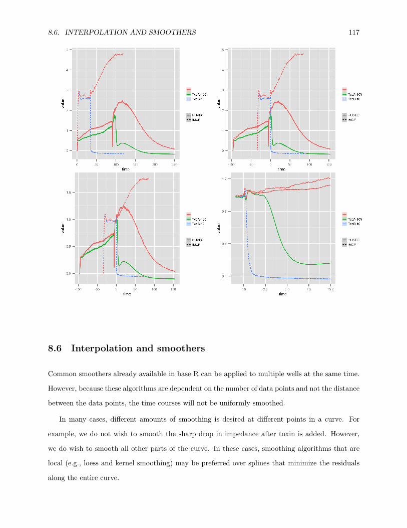
8.6. INTERPOLATION AND SMOOTHERS 117
8.6 Interpolation and smoothers
Common smoothers already available in base R can be applied to multiple wells at the same time.
However, because these algorithms are dependent on the number of data points and not the distance
between the data points, the time courses will not be uniformly smoothed.
In many cases, different amounts of smoothing is desired at different points in a curve. For
example, we do not wish to smooth the sharp drop in impedance after toxin is added. However,
we do wish to smooth all other parts of the curve. In these cases, smoothing algorithms that are
local (e.g., loess and kernel smoothing) may be preferred over splines that minimize the residuals
along the entire curve.

118 CHAPTER 8. MULTI-WELL TIME COURSE ANALYSES
In some cases, smoothing with R code took several minutes, so I wrote or attached open source
C++ and Fortran functions that calculate smoothers in less than one millisecond.
• smoother_curfit fits a cubic spline so that the sum of the residuals matches a user-defined
value (calls Fortran code from the DIERCKX package)
• smoother_bin bins the data and averages each bin to reduce the size of the data set
• smoother_maverage calculates a moving average in C++
• smoother_smooth.spline is the cubic smoothing spline in the R ‘stats’ package
• smoother_lokern performs “kernel regression smoothing with local plug-in bandwidth” as
described by Herrman using the ‘lokern’ R package developed by Herrman [318].
• interpolate_linear performs linear interpolation
• smooth.pchip calculates a piecewise cubic hermitian interpolating function. This function is
used when aligning two curves.
• smoother_composite is a multi-step smoother that I found was particularly useful for the
impedance data in this chapter. First, the derivative of the curve is estimated from smoother_bin.
smoother_maverage of the absolute value of the derivative is used to weight each data point
so that rapidly changing parts of the curve are fit more tightly. The weights are translated
to bandwidths with user-defined limits. Using these bandwidths, local polonymials are fit
with smoother_lokern in order to estimate the residuals that are used in smoother_curfit.
This composite smoother requires more user-defined parameters than any other, but it is very
consistent between different curves and different experiments.
The polynomial smoothers can be used to calculate derivatives and integrals. Smoothers also
have the added benefit of data compression, sometimes reducing 10,000+ data points to a spline
with less than 20 knots.
huvecs.a = retrieveWells(subset2, compounds = "TcdA")huvecs.norm = transform(huvecs.a, c("tcenter","normalize","slice"),
ID="toxinAdd", xlim=c(-1,Inf))

8.7. CUSTOM METRICS 119
huvecs.smth = add_smoother(huvecs.norm, method="composite", x.scale=2/3, y.scale=1,noise.scale=1/60, deriv.cutoffs=c(0.05,0.25) )
plot(huvecs.smth[c(1,8,10,17)],xlim=c(-1,3),showpoints=TRUE,smoother=TRUE)
8.7 Custom metrics
With this framework, it is easy for one to define new functions that calculate metrics from the
curves. Below is an example of a function (max.rate) that calculates the maximum slope of
curves. The slopes are then plotted versus toxin concentrations.
subset = retrieveWells(wells, compounds="IMCE")subset.norm = transform(subset, c("tcenter","normalize","slice"),
ID="toxinAdd", xlim=c(-1,Inf))subset.smth = add_smoother(subset.norm, method="composite", x.scale=2/3, y.scale=1,
noise.scale=1/60, deriv.cutoffs=c(0.05,0.25) )subset.rate = max.rate(subset.smth, ID = "toxinAdd", min.diff = 10/60/60,
ylim = 0.8, xlim = 2)MaxS = groupMetric(subset.rate, ID = "toxinAdd", metric = "max.rate")

120 CHAPTER 8. MULTI-WELL TIME COURSE ANALYSES
plotMetric(MaxS)
Here is the code for the function
print(max.rate.Well)
## function (well, ID, duration = Inf, nbw = 10, min.diff = NULL,## ylim = 0.75, xlim = 2, smoother = TRUE)## {## dwell = spline_interpolate(well, deriv = 1, nbw = nbw, smooth = smoother,## min.diff = min.diff)## times = timesdata(dwell)## dm.deriv = datamat(dwell)## dwell = spline_interpolate(well, deriv = 0, nbw = nbw, smooth = FALSE,## min.diff = min.diff)## vals = welldata(dwell)## sweep = getrows.by.ID(dwell, ID)$t1## idx = which(sweepdata(dwell) == sweep)## tstart = times[idx]## idx.range = times > tstart & times < (tstart + duration)## idx.spike = times < (tstart + xlim) & vals > ylim## dm.deriv = dm.deriv[idx.range & !idx.spike, ]## id = which.min(dm.deriv$values)## rate = dm.deriv[id, c("time", "values")]

8.8. FUTURE PLANS 121
## colnames(rate) = c("time", "value")## well$metrics$max.rate = as.data.frame(as.list(rate))## return(well)## }
8.8 Future plans
After approval from the maintainers of R packages, this will be a standard R package accessible
from the Comprehensive R Archive Network (CRAN).

Chapter 9
Future directions: toxin responses
and metabolism
9.1 Toxins alter expression of many metabolic genes
As discussed in a previous chapter, many genes encoding enzymes in lipid and fatty acid pathways
were differentially expressed after toxin treatment. We therefore hypothesized that metabolism
of lipids and fats will alter the host responses to TcdA. To test this, we placed mice on a high
fat diet and performed cecal injection experiments as described previously. When the two factors
were accounted for (western diet versus regular diet and toxin-treated versus sham), there was no
significant effects caused by a high fat diet 16h after toxin injection (data not shown). Nevertheless,
many metabolic genes were altered. Since the greatest expression differences occurred at 16 hours,
it is possible that these changes reflect upstream changes in central regulators known to control the
expression of many of these genes (e.g., nuclear receptors).
9.2 Integrating and visualizing transcriptional changes within a
metabolic network
Since well-curated, genome-scale networks have been constructed for human and mouse, it is possi-
ble to overlay the transcriptional data in this dissertation onto these networks to visualize modules
or entire pathways that are altered. In addition, the transcription may be used to turn enzymes
122

9.3. SYNOPSIS 123
on or off in these models in order to determine shifts in metabolism during pathogenesis or repair
from TcdA and TcdB.
Integration of transcription data with metabolic is therefore are a potential future direction
that could identify novel host responses to toxin. Although this dissertation does not use metabolic
models, I have had significant experience with them while working with colleagues. In this chapter, I
present a review of methods for identifying drug targets from metabolic reconstructions of microbes.
However, the last section is dedicated to how the host metabolism can be controlled or modified
for new treatment strategies.
9.3 Synopsis
For many infectious diseases, novel treatment options are needed in order to address problems
with cost, toxicity and resistance to current drugs. Systems biology tools can be used to gain
valuable insight into pathogenic processes and aid in expediting drug discovery. In the past decade,
constraint-based modeling of genome scale metabolic networks has become widely used. Focusing
on pathogen metabolic networks, we review in silico strategies used to identify effective drug targets
and highlight recent successes as well as limitations associated with such computational analyses.
We further discuss how accounting for the host environment and even targeting the host may offer
new therapeutic options. These systems-level approaches are beginning to provide novel avenues
for drug targeting against infectious agents.
9.4 Glossary
biomass
an objective reaction consisting of important metabolites that the cell needs in order to grow
(e.g. amino acids, lipids and carbohydrates). Correlated reaction sets: groups of reactions
whose fluxes always change in relation to one another. 129–137, 145
exchange reaction
a reaction that transports metabolites into or out of the system. 138

124 CHAPTER 9. FUTURE DIRECTIONS: TOXIN RESPONSES AND METABOLISM
flux balance analysis (FBA)
the possible combination of allowable fluxes given a defined set of constraints which bound
reaction fluxes, for example reversible and irreversible reactions. 125, 126, 128–132, 134–140,
145
feasible flux space
the possible combination of allowable fluxes given a defined set of constraints which bound
reaction fluxes, for example reversible and irreversible reactions. 129
flux distribution
the set of all reaction fluxes within a metabolic network. 131, 133, 134
flux variability analysis (FVA)
a linear programming-based method which determines the minimum and maximum reaction
fluxes that allow for optimal or near-optimal flux through the objective reaction. 128, 137–139
gene-protein-reaction relationship (GPR)
the combination of proteins or protein components sufficient to carry out an enzymatic reac-
tion and the combination of genes sufficient to express each of the protein components. 125,
128, 129, 134, 136
in silico
in contrast to in vivo or in vitro, the term indicates a computational process in a simulated
environment. 123, 129, 135, 140
linear programming
also termed linear optimization, an area of mathematics developed for maximizing a linear
combination of variables (e.g. Av1 + Bv2 + Cv3), such that the variables are constrained by
many linear equalities and inequalities (e.g. the constraint v1 − v2 = 0 implies that flux v1 is
constrained to be twice flux v2). 124, 129, 131

9.4. GLOSSARY 125
mass balance
a requirement that the mass entering the system or any pathway within the system equals
the mass exiting the system or pathway; a crucial characteristic of metabolic reconstructions
from which functional mathematical models can be derived. 129, 134
metabolic network reconstruction
a manually-curated computational network of the metabolism of an organism with all the
gene-protein-reaction relationships(GPRs) assembled from a functionally annotated genome,
biochemical data, and literature, that are compiled into a stoichiometric matrix, which serves
as the framework for further computational analysis. 125, 126, 128–130, 134, 136–142, 144–
146
objective flux
the flux through the objective reaction. 131, 132, 137–139
objective reaction
a reaction which sets a demand for particular metabolites in the network. The typical goal in
formulating this reaction is to simulate a biological objective, whether it be growth, energy,
virulence, or a combination of other factors. 125, 129–131, 133, 134, 136–142
reaction flux
moles consumed in a reaction per unit time. 123–125, 129–131, 133–139, 141, 142, 144
steady state
with respect to flux, a key assumption in flux balance analysis (FBA) that the reaction fluxes
within the system, and therefore the amounts of each metabolite, do not change over time,
an assumption often justified by the very short time-scale of metabolic reactions compared
to the time necessary for changes in cell phenotype. 130
stoichiometric matrix (S matrix)
a mathematical formalization of a metabolic reconstruction; a matrix in which each element
contains the stoichiometric coefficient for a metabolite (row) participating in the correspond-

126 CHAPTER 9. FUTURE DIRECTIONS: TOXIN RESPONSES AND METABOLISM
ing reaction (column). 125, 129, 130, 140
Clicking on a glossary term within this chapter returns you to its definition in this section.
9.5 Systems biology and pathogen metabolism
Systems biology methods have been applied extensively to the study of infectious diseases across
multiple scales of biological organization to generate predictions ranging from pathogen gene lethal-
ity in particular microenvironments [319, 320] to dynamics involved in the host immune response
to infection [321]. Utilizing the predictive power of computational modeling and systems analysis,
wideranging questions related to pathogen virulence, disease progression and host response can be
explored to generate hypotheses for more thorough experimental investigation.
The increasing availability of high-quality genome-scale metabolic reconstructions [322] presents
an opportunity for the rational and systematic identification of metabolic drug targets in a pathogen
of interest. Built bottom-up from functional genome annotations (and a variety of other data
sources) and analyzed with computational methods such as FBA, these biochemical networks can
account for hundreds to thousands of metabolites participating in enzymatic reactions across a range
of metabolic subsystems (e.g. carbohydrate, amino acid, lipid, nucleotide and energy metabolism)
and cellular localizations (e.g. extracellular space, cytosol and compartments specific to particular
organisms) (Figure 9.1A) [323]. Since the initial genome-scale reconstructions of Escherichia coli
[324, 325] and Haemophilus influenzae [326, 327], the metabolic networks of over 50 organisms
(bacteria, archaea and eukaryotes) have been reconstructed (reviewed in [322]). Elements of this
network reconstruction process have been automated, allowing the preliminary analysis of hundreds
of draft network reconstructions [328]. Among these, metabolic networks have been reconstructed
for several pathogenic organisms (Table 9.1). Indeed, the study of pathogen metabolism-for the
elucidation of highpriority drug targets and metabolic factors contributing to pathogenicity—is an
exciting application for metabolic network modeling and systems biology.
In this review, we explore several techniques and approaches used to predict antimicrobial drug
targets from metabolic network modeling using FBA. Where possible we present examples that have
led to novel data, drug targets, or drugs. Metabolic network modeling is still in its infancy, but
has allowed for predictions that align with previous data and has provided many hypotheses that

9.5. SYSTEMS BIOLOGY AND PATHOGEN METABOLISM 127
Dru
gta
rget
-rel
ated
anal
ysis
Val
id-
atio
n
Pat
hoge
n
Gene/reactionessentiality
Minimalmediaprediction
Conditionalessentiality
Syntheticlethality
Fluxvariabilityanalysis
Enzymerobustness
Metaboliteessentiality
Correlatedreactionsets
Literaturederived
Novelexperimentalvalidation
Novelcompoundsidentified
Dis
ease
Ref
sAc
inet
obac
ter
baum
anni
iOpp
ortunistic;c
epacia
synd
rome
[329]
Burk
hold
eria
ceno
cepa
cia
Opp
ortunistic;n
osocom
ialinfectio
n[330]
Fran
cise
llatu
lare
nsis
Tularemia
[331]
Hae
mop
hilu
sin
fluen
zae
Otit
ismedia
andrespira
tory
infections
[326,3
27]
Hel
icob
acte
rpy
lori
Gastritis;
peptic
ulceratio
n;ga
stric
cancer
[332,3
33]
Kle
bsie
llapn
eum
onia
eKlebsiella
pneumon
ia;u
rinarytractinfection
[334]
Myc
obac
teri
umtu
berc
ulos
isMeningitis
;meningo
coccal
septicem
ia[319,3
20,3
35]
Nei
sser
iam
enin
gitid
isOpp
ortunistic;c
epacia
synd
rome
[336]
Porp
hyro
mon
asgi
ngiv
alis
Perio
dontal
disease
[337]
Pseu
dom
onas
aeru
gino
saOpp
ortunistic;n
osocom
ialinfectio
n[338]
Salm
onel
laTy
phim
urium
Gastroenteritis;
diarrhea
[339–3
41]
Stap
hylo
cocc
usau
reus
Opp
ortunistic;n
osocom
ialinfectio
n[342–3
44]
Vibr
iovu
lnifi
cus
Bubo
nic,
pneumon
ic,a
ndsepticem
icplag
ue[345]
Yers
inia
pest
isOpp
ortunistic;n
osocom
ialinfectio
n[346]
Cry
ptos
pori
dium
hom
inis
Cryptospo
ridiosis
[347]
Leis
hman
iam
ajor
Leish
man
iasis
[348]
Plas
mod
ium
falc
ipar
umMalaria
[349,3
50]
Tryp
anos
oma
cruz
iCha
gasdisease
[351]
Tabl
e9.
1:Drugtargeting-relatedan
alysis
ofpa
thog
enmetab
olic
netw
orks

128 CHAPTER 9. FUTURE DIRECTIONS: TOXIN RESPONSES AND METABOLISM
Identify andtest drugs
Modeling andanalysis
Literature andexperimentalvalidation
Iterativemodelbuilding
Reconstruction ofreaction network
Flux balance analysis
Identify potentialdrug targets
Improve and Data reconciliationand assembly
max vbiomass
S v = 0
Omics
Association of drugs and targets
(structural bioinformatics, drug databases, etc.)
S =
b
Gene
Protein
Reactiona
ANDOR
A
B
Figure 9.1: The iterative process of model building and refinement. (A) A function-ally annotated genome together with data from the biochemical literature are used to assemble anetwork reconstruction. FBA allows for modeling and simulation of the reconstructed network. Ad-vanced network analyses (such as gene essentiality or flux variability) allow for identifying potentialantimicrobial drug targets. These targets can then be associated with drugs using bioinformaticsapproaches and obtaining target drug information from a variety of publicly available databases(e.g. STITCH or DrugBank). Predictions involving targets and drugs can be experimentally val-idated. Any discrepancies between computational predictions and experimental validation can beinformative to improving upon and refining the original reconstruction and modeling platform. (B)GPRs, central to the assembly of a metabolic reconstruction, define the genes and gene productsneeded for each enzymatic reaction. Isozymes can be represented with ’OR’ statements, whereasenzyme subunits required to function together to catalyze a particular reaction can be representedwith ’AND’ statements.

9.6. RECONSTRUCTING METABOLIC NETWORKS 129
continue to be developed. We first discuss the fundamental aspects of network analysis and FBA in
particular. Subsequently, we delve into how computational metabolic reconstructions can be used
to prioritize drug target predictions. Furthermore, we review recent developments on model-guided
pipelines for drug target discovery against pathogens. Finally, we extend the discussion to include
host cell metabolism and propose directions for future modeling efforts in infectious disease.
9.6 Reconstructing the metabolic network and defining an objec-
tive
A metabolic network reconstruction is assembled piece-by-piece by compiling data on known en-
zymes, genes encoding these enzymes, and the stoichiometry of the reactions catalyzed by these
enzymes (see [352] for a list of databases containing such data). GPRs, in the form of Boolean logic
statements, define which genes are necessary for each enzyme and which enzymes are necessary for
each reaction [323] (Figure 9.1B). The information for all the reactions in a network reconstruction
with m metabolites and n reactions can be stored in an m by n table or matrix, the stoichiometric
matrix. Each element or cell in this matrix corresponds to the stoichiometric coefficient of one
particular metabolite in one particular reaction [323, 353]. The stoichiometric matrix enables strict
accounting for the underlying biochemistry and allows a quantitative description of complex in-
teractions between metabolites that are responsible for driving a cellular phenotype. This matrix
formalism facilitates interrogation of the structural and functional properties of the network.
The application of FBA to a network reconstruction results in the identification of combinations
of reaction fluxes that correspond to a maximum flux through a targeted reaction (an objective)
while requiring that constraints are satisfied, for example that the mass entering the network is
equal to the mass exiting the network (mass balance). In more mathematical terms, FBA involves
the use of a linear programming formulation wherein an objective is optimized subject to a set
of governing constraints (Box 1) [322, 353, 354]. In addition to requiring mass balance for every
reaction, thermodynamic, topological, environmental, and regulatory data may provide additional
constraints that dictate the feasible flux space [355]. An objective often used with FBA is biomass
production, which is represented in silico as a drain capturing crucial metabolites necessary for
growth of the organism [356, 357]. With the ultimate goal of identifying antimicrobial drug targets

130 CHAPTER 9. FUTURE DIRECTIONS: TOXIN RESPONSES AND METABOLISM
(and associated drugs) to slow or stop the growth of a pathogen, a biomass objective is often
very appropriate for computational modeling efforts. Network reconstructions of most pathogenic
organisms have incorporated biomass reactions as their objectives (Table 9.1).
Box 1. A brief primer on FBANutrient availability, restrictions on surrounding environmental pH, and temperature are
examples of basic constraints that, when imposed upon cells, can affect the resulting pheno-
types [353]. Such constraints can be mathematically described, and they serve to narrow the
operating range of the cell and yield a set of feasible reaction fluxes for a metabolic network.
In other words, the constraints (which can be physicochemical, topological, environmental
and regulatory) restrict the number of possible phenotypes, which then allows the function
of the biochemical network to be characterized [353, 355].
FBA is one constraint-based method that has been extensively applied in the study of
prokaryotic and eukaryotic metabolic networks [338, 358]. First, reactions of a metabolic net-
work are assembled into a stoichiometric matrix, whose elements correspond to the stoichio-
metric coefficients describing the conversions from reactants to products (see figure below)
[323, 353]. This simple matrix formalism permits quantitative description of the complex
interactions between metabolites. Following network reconstruction, the concentrations of
metabolites and fluxes through reactions can be represented as follows:
dC
dt= Sv (9.1)
Here, C is a vector of concentrations of metabolites, t is time, S is the stoichiometric matrix
consisting of m rows of metabolites and n columns of reactions, and v is a vector of fluxes
through the corresponding reactions. Invoking the steady state assumption so that the rate
of production of every metabolite equals its rate of consumption yields the following:
Sv = 0 (9.2)
Limits can be applied to individual fluxes as follows:

9.6. RECONSTRUCTING METABOLIC NETWORKS 131
vmin ≤ v ≤ vmax
Particular reactions can have set upper limits (vmax) that may align closely with experimental
enzyme capacity measurements, whereas other irreversible reactions will have vmin set to 0.
The principle physicochemical constraints in Equation 9.2 represents a set of m linear
equations. Because there are typically more unknown variables (m reaction fluxes) than
equations (n steady state equations for each metabolite), the system of equations is “inde-
terminate” [353]. In other words, there may be many sets of fluxes (many flux distributions)
that can satisfy the steady state constraints as well as the vmin and vmax of each reac-
tion. The goal then is to use linear programming to identify which of these feasible flux
distributions allow for the greatest flux through the objective reaction.
Traditionally, maximization of biomass has been chosen as the objective of choice in
FBA [353]. A set of metabolites (e.g. amino acids, lipids, nucleotides and carbohydrates)
that are necessary for the cell or organism to grow are typically included in the biomass
reaction. Therefore, the optimization problem can be summarized as simply:
maximize vbiomass
subject to Sv = 0
vmin ≤ vi ≤ vmax for i = 1...n
Even with these constraints, linear programming does not guarantee that the set of fluxes that
allow for the maximal objective flux are unique. What is guaranteed is that the objective flux
(vbiomass) found is the highest possible flux through the objective reaction that the network
can allow, under any state. There are often are many possible flux distributions that achieve
the maximal objective flux. See Box 4 for a method that helps investigate the many possible
solutions.

132 CHAPTER 9. FUTURE DIRECTIONS: TOXIN RESPONSES AND METABOLISM
A
A
R1T1
T2
R3Robj
R4R2
C
CR1 A + AR2 A + BR3 CR4 D
EE
C D
DE
E
B
B R1ABS =CDE
-20
+100
-1-10
+10
00-10
+1
000-1+1
+10000
0+1000
0000-1
R2 R3 R4 T1 T2 Robj
Sv = 0-2vR1 - vR2 + vT1
-vR2 + vT2
vR1 - vR3
vR2 - vR4
vR3 + vR4 - vRobj
= 0
= 0= 0= 0= 0
Objective Maximize vRobj
Constraints S v = 0vT1 ≤ 5vT2 ≤ 5
(Steady state)
(Limited
in�ux)
SolutionvRobj = 5vR1 = vR3 = 0
(Optimal solution doesnot allow �ux through R1 or R3)
Metabolites Reactions
Flux balance analysis
Stoichiometric matrix
D
Steady state assumption Mathematical optimization
Transport reactions
Objectivereaction
The inability of the metabolic network model to synthesize even one metabolite of the biomass
reaction will result in a predicted value of zero for the objective flux (biomass), and analogously no
growth. Therefore, growth predictions are sensitive to metabolites that are placed in the biomass
reaction reaction. FBA can be used to investigate the ability of the model to produce each metabo-
lite within biomass. In the Porphyromonas gingivalis metabolic network, the ability of the model
to produce each of the 52 metabolites within the biomass reaction was evaluated after system-
atic reaction deletions [337]. Crucial groups of reactions were identified that were responsible for
lipopolysaccharide (LPS) production, coenzyme A production, glycolysis, or purine and pyrimidine
biosynthesis [337]. Corresponding enzymes that are essential for growth, as well as for the pro-
duction of important bacterial components such as LPS, could serve as potential drug targets. In
addition, in a study of Leishmania major metabolism, the contribution of minimal media compo-
nents to the synthesis of individual biomass reaction constituents was analyzed [348]. The study
found that the absence of cysteine and oxygen in the minimal media had a drastic impact on
the overall metabolic network, limiting the generation of 30 of the 40 biomass constituents [348].
9.6. RECONSTRUCTING METABOLIC NETWORKS 133
Network analyses as delineated in these examples of P. gingivalis and L. major may permit the
formulation of a hypothesis for the role of specific metabolites and their influence on growth. There-
fore, defining an appropriate biomass reaction (Box 2 and Box 3) is crucial for useful predictions
and identification of vulnerable parts of the metabolism of a pathogen.
Box 2. Cellular objectives of pathogenic organismsA biomass reaction is not applicable under all conditions, and very often growth alone may
not be a realistic objective. Other objective such as maximizing or minimizing ATP or
maximizing the production of particular cellular by-products (e.g. lactate or pyruvate) can
also be used.
The metabolism of an organism may be adapted for increased virulence or pathogenic-
ity. Pathogens and host cells may also temporarily opt for alternative objectives while under
selective pressures (e.g. changes in nutrients or environmental influences of secreted toxins).
In addition, different morphological stages of a pathogen (e.g. the sporozoite stage of Plas-
modium falciparum in mosquitoes vs the merozoite stage in humans) may be characterized
by varying metabolic requirements. Consequently, the objective function must be appropri-
ately defined to find relevant enzyme targets crucial in particular stages of infection and/or
environmental conditions.
To explore the effects of targeted perturbations (pharmacological or genetic), different
objectives can be explored. It may be that the evolutionary pressures that dictate wild-type
cells are different for knockout mutants. Additionally, mutants may not have the ability
for immediate regulation of fluxes that allow for optimal growth. Based on these ideas,
an approach termed minimization of metabolic adjustment (MOMA) was developed. The
requirement for optimal growth is relaxed for gene deletions in MOMA. Instead, MOMA
assumes that the overall flux distribution of a gene-knockout mutant will probably not change
significantly from that of the corresponding wild type [359]. In terms of flux values, the
gene-knockout mutant will remain as close as possible (in Euclidean distance) to the wild-
type optimal flux distribution. MOMA aided in correcting gene essentiality predictions
associated with knockouts of fructose-1,6-bisphosphatate aldolase, triosephosphate isomerase

134 CHAPTER 9. FUTURE DIRECTIONS: TOXIN RESPONSES AND METABOLISM
and phosphofructokinase in the E. coli central metabolic model [359]. These genes were
predicted to be nonessential when biomass was used as the objective for E. coli growth
on glucose, which was inconsistent with supporting literature evidence. MOMA yielded a
suboptimal flux distribution for a knockout mutant that would not necessarily equal the
optimum as dictated by traditional FBA [359].
Approaches such as MOMA that consider alternate hypotheses for the objective
of metabolic networks provide a basis for understanding a potential biological goal for
pathogenic organisms, especially considering the complexity of the environment surrounding
the pathogen of interest.
Box 3. Knowledge gaps and caveats to metabolic network
analysisMultiple steps in the model-building process and subsequent analyses are prone to errors that
may greatly affect flux and growth predictions and, consequently, predicted drug targets.
FBA provides a quality-assurance check that ensures mass balance. Growth rates and gene
essentiality predictions are validated against experimental data to ensure the model truly
reflects biological processes. Gene essentiality predictions (commonly between 55% and
90%) provide confidence that downstream analyses are based on a high-quality model [319,
360]. To ensure the usefulness of any computational pipeline, drug target predictions should
be compared to known targets from the literature. Below we discuss more of the particular
difficulties and limitations encountered when using metabolic models to identify drug targets.
Genome annotation
In any metabolic reconstruction, there may be hundreds of putative metabolic enzymes with
no experimentally identified function. These reactions and associated GPRs may be assem-
bled strictly based on existing functional annotations of the genome or based on evidence
from related organisms. Even some very well characterized enzymes may have other unex-

9.6. RECONSTRUCTING METABOLIC NETWORKS 135
pected activities. In such cases, misannotated enzymes may yield incorrect model predictions
leading to errors in drug targeting. For instance, an enzyme may be incorrectly predicted
to be essential if the activity of another enzyme, which is not included in the network, can
account for the same function. Therefore, this represents one important knowledge gap in
the assembly of metabolic networks, and the inclusion of more refined enzyme annotations
will directly improve drug target predictions [361, 362].
Nutrient availability
An important challenge in reconstructing and modeling metabolic networks is determining
the composition of in silico media. Nutrients available in host environments are poorly char-
acterized. In addition, for any nutrients that are identified, quantitative data on uptake rates
are unavailable. Knowledge of the transporters of an organism elucidates which metabolites
are transported into the cell. However, information on transporters is particularly limited
and, in general, transport reactions lack any experimental evidence or gene associations sup-
porting their presence. Instead, transport reactions are added for proper functioning of the
computational model. Because model predictions are dependent on the media environment,
nutrients and transporters must be carefully defined.
Objective function
As stated previously, in FBA-based modeling of microbial organisms, a biomass reaction has
often been used. The purpose of the reaction is to ensure a drain of metabolites that are
deemed essential to support the growth of the organism. Starting with the estimated weight
fraction of important macromolecular components of the cell (e.g. protein, lipid, RNA, DNA
and carbohydrate), the relative abundance of metabolites comprised in each group (e.g.
amino acids, phospholipids, nucleotides) can be computed [356]. Among several available,
a few experimental methods to measure biomass components include chloroform–methanol
extraction (lipids), colorimetric protein assays, and gas chromatography–mass spectrometry
(protein content) [363]. Fluxes measured directly by metabolic flux analysis, which tracks

136 CHAPTER 9. FUTURE DIRECTIONS: TOXIN RESPONSES AND METABOLISM
the movement of 13C from an initial 13C-labeled substrate, may also help to define the
objective function [364, 365].
An objective function is most likely to cause errors if metabolites are entirely missing
or incorrectly included; the relative amounts of each metabolite in the objective reaction
(i.e. the stoichiometric coefficients) do not greatly affect FBA results [357, 366]. Therefore,
logically deducing a biomass reaction is often adequate to estimate the growth of an organism.
However, additional experimental data can reveal interesting peculiarities that may be used
to design a specific biomass reaction for a particular organism. Data on growth- and non-
growth-associated ATP maintenance can be included in the biomass reaction [367]. Under
in vivo conditions when a pathogen is interacting with its host, an aspect that is often
unclear is which biomass component(s) to include in the reaction. The composition of the
biomass reaction is likely to vary under different physiological conditions, and the choice of
metabolites can directly influence model predictions regarding drug targets. For example,
failure to include a particular cell-wall component will not necessarily direct flux through
reactions that may be crucial in vivo, and therefore the associated enzymes will not be
targeted.
9.7 The quest for drug targets in metabolic networks of pathogens
Gene essentiality analysis
The most common method to identify potential drug targets has been through the prediction of
essential genes (Table 9.1). The enzymes encoded by essential genes are typically hypothesized as
drug targets. Gene knockouts might lead to a redistribution of flux through the network if the
perturbed gene or gene product affects the removal of a particular flux-carrying reaction [322]. A
GPR aids in mapping the effects of a genetic (or pharmacological) perturbation on the associated
reactions, and thus the network. Gene-level perturbations that result in reduced or zero flux
through a biomass reaction correspond to growth-reducing or lethal gene knockouts, respectively
(Figure 9.2). For example, in a reconstruction of Mycobacterium tuberculosis, five previously known

9.7. DRUG TARGETS IN METABOLIC NETWORKS 137
drug targets were encoded by genes predicted to be essential from computational analysis [335].
For metabolic reconstructions of pathogens, enzymes that are predicted to be essential will offer
new experimental hypotheses and avenues for drug discovery. In the following subsections we
discuss several other approaches for drug targeting using metabolic network analysis. These other
approaches may provide a separate list of potential targets; however, they can also be used in
tandem with gene essentiality analysis for step-by-step prioritization of drug targets.
Enzyme robustness and flux variability
In addition to an analysis of gene essentiality, assessing enzyme robustness could identify vulnerable
or sensitive portions of a metabolic network suitable for drug targeting. To determine the robustness
of a metabolic network to the inhibition of an enzyme-catalyzed reaction, the flux of a reaction
may be constrained to a fraction of its wild type flux (simulating partial to complete inhibition),
and the effects on an objective flux (e.g. biomass production) can be evaluated [368] (Figure 9.2).
Such an approach was used in analyzing the network reconstruction of Francisella tularensis, which
revealed that the growth rate was sensitive to changes in H+ and NH4 flux in a simulated in vitro
medium but not in a simulated in vivo medium that mimicked the environment during infection
[331]. Analyzing enzyme robustness with different constraints provides a detailed view of possibly
nonlethal reactions whose change in flux has a strong effect on the objective of a network under
different environmental conditions, therefore suggesting important reactions during an infection or
perturbations for drug targeting.
Alternatively, the objective function could be constrained to a fixed percentage of its wild
type flux and the allowable range of flux for each reaction can be determined using an approach
termed flux variance analysis (FVA) (Box 4) [369]. A recognized shortcoming of FBA is that the
typical implementation calculates only one of many possible solutions that optimize flux through
the objective reaction. Consequently, there may be many possible routes through the network
that achieve the same optimal flux for a given objective [355, 369]. In an effort to circumvent
this shortcoming, FVA was developed to determine the range of fluxes over which a particular
reaction operates, while still allowing for optimal, or near-optimal, objective flux [369]. FVA
also identifies blocked reactions (reactions incapable of carrying any flux in a given model under
specified constraints) or reactions with different flux ranges in various media. Enzymes that catalyze

138 CHAPTER 9. FUTURE DIRECTIONS: TOXIN RESPONSES AND METABOLISM
Intracellular
Objectivereaction
InputMedia
Gene/Reaction EssentialityReactions whose knockout causes zero �ux through an objective
Conditional EssentialityGenes, reaction, or metabolites onlyessential in speci�c environments
NE E
NENE
Flux variabilityRobust reactions allow near-optimal objective �ux over a large range of �ux.Sensitive reactions are potential targets.
Reaction �ux
Robust
SensitiveObj
ectiv
e �u
x
Metabolite EssentialityRemoval of a metabolite disables alldirectly connected reactions.
E
Synthetic LethalityTwo indvidually non-essential genes/reactions whose knockout causes zero �ux through an objective
SL
SL
Sample Network
Non-essentialEssentialE
NEMetabolite
Reaction
E
Figure 9.2: Drug targeting in metabolic networks. Various strategies are illustrated foridentifying drug targets by performing FBA on metabolic reconstructions. The sample networkshows an input media that represents the environment and exchange reactions, intracellular reac-tions, and an objective reaction that drains metabolites out of the system. An essential reactionand metabolite that, when removed, block any flux through the objective are highlighted in red.In the conditionally essential panel, the absence of the metabolite highlighted in blue causes thehighlighted reaction to become essential in the selected media. One of the synthetic lethal pairs ofthe network is denoted by ‘SL’. The dashed line in the flux variability illustration may represent‘near-optimal’ objective flux. A robust reaction maintains near-optimal objective flux over a largerrange of reaction fluxes.

9.7. DRUG TARGETS IN METABOLIC NETWORKS 139
reactions with little to no variability in flux for a given objective could be selected as potential
drug targets given that the network may be sensitive to even modest inhibition of its activity. In
analyzing the reconstruction of M. tuberculosis, the average of the highest and lowest allowable
flux for each reaction was used as a point of comparison for the model under constraints for two
growth rates [335]. In the study, the reaction catalyzed by isocitrate lyase—an enzyme important
for persistence in a host—was predicted to have increased flux during slow growth, and the activity
of the enzyme was experimentally confirmed to be greater in slow-growing cells of the closely related
Mycobacterium bovis [335]. Hence, flux variability and enzyme robustness aid in further prioritizing
drug targets identified from other methods such as gene essentiality.
Box 4. A brief primer on FVAAfter the application of various constraints on the biochemical network, the number of al-
lowable network states (or possible phenotypes) is typically large. Depending on the size and
interconnectedness of the cellular network, there may be several alternative optimal pheno-
types [355]. FBA calculates one of many feasible solutions that result in the same optimal
value of the cellular objective.
FVA calculates the range of flux in each reaction that allows for the same optimal
flux through the objective reaction. The objective flux of the reaction is specified as an
additional constraint and multiple optimizations are performed to compute the maximum
and minimum flux for every reaction in the network:
Max/Min vi
subject to Sv = 0
vbiomass = Zobj
vmin ≤ vi ≤ vmax for i = 1...n
Here, n refers to the number of reactions in the biochemical network, and Zobj is the optimal
value of the cellular objective (vbiomass) as obtained by FBA [369].

140 CHAPTER 9. FUTURE DIRECTIONS: TOXIN RESPONSES AND METABOLISM
9.7.1 Metabolite essentiality
Many current drugs have high similarity to natural metabolites and compete for and/or inhibit
normal enzymatic activity [370]. Therefore, another very interesting avenue towards identifying
drug targets in metabolic networks is via the prediction of essential metabolites. In contrast to the
more traditional individual gene knockouts mentioned previously, metabolites in the stoichiometric
matrix can also be systematically removed. Consequently, all reactions in which a given metabolite
participates are removed, and the resultant effects on the objective are assessed (Figure 9.2). A
total of 211 essential metabolites in the Acinetobacter baumanii reconstruction were narrowed to 9
following removal of (i) currency metabolites (ATP, NADH, H2O, etc.); (ii) metabolites present in
the human metabolic network; and (iii) metabolites participating in reactions catalyzed by enzymes
with human homologs [329]. Enzymes that catalyze reactions involved in the consumption or
production of these essential metabolites may be considered as drug targets. Moreover, structural
analogs of essential metabolites may be considered as test compounds for experimental evaluation,
thus sidestepping extensive screening or computational predictions [345].
9.7.2 Combination gene and reaction perturbations
Many anti-infectives on the market act on multiple targets. This multiplicity of targets was ex-
emplified in a network analysis of 890 FDA-approved drugs targeting 394 human proteins (derived
from the DrugBank database), where approximately 38% of the drugs were associated with more
than one protein target, and a few drugs were associated with as many as 14 targets [371]. In that
regard, a drug discovery strategy incorporating compounds known to act simultaneously on multiple
targets can be adopted for microbial pathogens. FBA allows predictions involving the perturbation
of multiple genes or reactions in a rapid timeframe (minutes or hours)—a single in silico combina-
tion taking only a fraction of a second [372]. In a reconstruction of M. tuberculosis that accounted
for features specific to an in vivo environment, all non-trivial double-deletion mutants (synthetic
lethal pairs) were tested for in silico growth using FBA [320]. Of two experimentally-characterized
double gene deletions, the model accurately predicted reduced in silico growth in both in vitro and
in vivo environmental conditions [320]. A combination of drugs that affect synthetic lethal targets
may act synergistically to inhibit growth of a pathogen, thereby paving the way for model-guided

9.7. DRUG TARGETS IN METABOLIC NETWORKS 141
predictions of drug synergy. Experimentally screening for all possible drug combinations against a
particular pathogen is costly and is often not feasible. Therefore, predicted combinations of drugs
associated with synthetic lethal targets can direct more specific experiments and perhaps reveal
entirely novel treatment strategies.
9.7.3 Groups of targets and network topology
Other approaches characterizing the structure of a genome-scale network reconstruction identify
sets of reactions that act together and therefore may be targeted as an entire pathway. Sets
of correlated reactions (or Co-sets) consist of groups of reactions whose fluxes are linked, and
which represent functional modules within a biochemical network [373]. Co-sets, which can aid in
suggesting alternative drug targets by identifying reactions that are functionally related to each
other, can be divided into several categories. A perfect Co-set consists of a group of reactions such
that, for any given pair in the group, a non-zero flux in one reaction implies a non-zero flux in
the other, with a fixed ratio . Other categories include partial Co-sets (pairs of linked reactions,
but with a variable flux ratio) and directional Co-sets (a non-zero flux in one reaction implies a
nonzero flux in the other, but the converse is not true) [374]. By calculating hard-coupled reaction
(HCR) sets—a subgroup of perfect Co-sets where sets of reactions are defined by participating
metabolites sharing a consumption to production connectivity of 1:1 (i.e. two reactions are linked
by a metabolite that is connected to no other reaction)—one study found 25 of 147 HCR sets
contained previously identified drug targets in M. tuberculosis [319]. Because an altered flux in
one reaction results in an altered flux of all reactions within a HCR set, only one enzyme needs
to be targeted. This approach aids in prioritizing the list of potential drug targets by identifying
linked enzymatic reactions. Hence, analyses of the topology of a metabolic network can reveal key
local and structural features that may be important drug targets when data related to environment
fluxes or appropriate objective are not necessarily available.
9.7.4 Environment and conditional essentiality
Finally, the metabolic phenotype is dependent on the media environment and the exchange of
metabolites into and out of the system (see Box 3 for discussion of knowledge gaps associated with
nutrient availability). By constraining uptake or secretion fluxes, a minimal set of metabolites

142 CHAPTER 9. FUTURE DIRECTIONS: TOXIN RESPONSES AND METABOLISM
that allows flux through the objective can be computed [348]. Moreover, enzymes or metabolites
that are necessary for growth in various environments (e.g. minimal media, defined media, or rich
media with an abundance of nutrients and carbon sources) can be predicted. In the reconstruction
of F. tularensis, genes that were essential in a simulated macrophage environment and five other
environmental conditions were considered to be unconditionally essential genes (in other words, they
represented a core set of genes that were essential regardless of the medium). Of the 17 virulence
factors cataloged from previous literature, eight were unconditionally essential genes [331]. By
contrast, enzymes that may be necessary for growth under one condition, but not another, are
conditionally essential (Figure 9.2). With a careful consideration of an objective and appropriate
nutrient uptake, gene essentiality analysis may reveal new drug targets specific to particular growth
conditions and environments in which a pathogen must survive. Such an analysis can also inform
strategies for manipulating the environment of the pathogen that could be effective as a treatment
option.
9.8 From target to drug and the development of model guided
pipelines for drug discovery
Computational analysis of metabolic processes in pathogens can yield a ranking of predicted drug
targets. Bioinformatics and network analyses were performed to yield a high-confidence list of
targets against M. tuberculosis [375]. By implementing a multilayered approach, targets that did
not pass sequential cut-off values were removed (e.g. elimination of enzymes with human homologs or
targets with no computationally predicted binding pocket) [375]. In another proof-of-concept study
it was noted that essential type II fatty acid biosynthesis (FAS II) reactions in the E. coli MG1655
metabolic network were also essential in several Staphylococcus aureus strains [376]. Following
network analysis, a virtual screening strategy was employed whereby small molecules from a library
of approximately 106 compounds were docked to enzymes catalyzing essential reactions, and 41
inhibitors of FAS II enzymes were selected for experimental validation [376]. In cell viability assays,
six of the inhibitors had growth-retarding effects against E. coli and S. aureus strains in standard
LB agar plates [376]. Finally, following the identification of 163 essential metabolites, a third study
used a layered approach to prioritize five essential metabolites in the metabolic network of the
9.9. A HOST CELL PERSPECTIVE 143
opportunistic pathogen Vibrio vulnificus [345]. Currency metabolites, metabolites consumed by a
single reaction, metabolites present in the human metabolic network, and metabolites associated
with enzymes with human homologs were removed. The study screened 352 compounds found to
be structurally similar to one of the five essential metabolites and identified one compound that
most potently inhibited growth, more so than a currently used drug [345]. These studies provide
various examples of model-guided pipelines to drug discovery by primarily using network analyses
to identify and prioritize drug targets. Additional constraints such as enzyme druggability and
elevated gene expression can also be used to prioritize drug targets, which can then guide the
screening and selection of compounds.
A common approach in proposing drug targets using metabolic networks has been to rule out
targets that overlap with host cell metabolism—the idea being that offtargets can be minimized
and drug interference plus subsequent complications with the host can be avoided. However, there
are arguments to be made in favor of retaining targets that overlap with human metabolism. First,
accounting for the drug selectivity between host and pathogen targets at the respective binding
sites may preclude off-target influences [377]. Second, if the goal is to discover drugs against
infectious diseases quickly, then the best option may be to focus on finding new clinical indications
for existing FDA-approved drugs (i.e. pursuing drug repurposing strategies) instead of developing
new investigational compounds that are subject to regulatory hurdles [378]. Also, the majority
of FDA-approved drugs target human proteins. Hence, eliminating pathogen targets that overlap
with human proteins reduces the number of potential drugs that could be evaluated experimentally.
9.9 A host cell perspective
Interaction with a host cell is often crucial to the metabolism and survival of a pathogen. For
instance, the kinetoplastid parasite L. major is unable to synthesize several essential amino acids
and therefore obtains them from the host macrophage [379]. As another example, Legionella
pneumophila, the bacterium responsible for Legionnaire’s disease, ceases to replicate inside a host
macrophage when it cannot access or process threonine [380]. Consequently, identifying the partic-
ular niche of nutrients and resources in the host cell required by a pathogen is vital to discovering
treatment options that specifically target host-pathogen interactions [381].

144 CHAPTER 9. FUTURE DIRECTIONS: TOXIN RESPONSES AND METABOLISM
A systems-level analysis of pathogen metabolism interfaced with cell type-specific host metabolic
networks can also be conducted. Because P. falciparum invades mature erythrocytes to establish
infection in its human host, a metabolic model of the human erythrocyte was built in conjunction
with the P. falciparum reconstruction to make predictions which aligned closer to known condi-
tions in the infected erythrocyte [349]. This model, modifying an existing approach from Shlomi
et al. [382], integrated previous gene expression data where several enzymes were constrained to
be ’on’ and ’off’ during specific life-cycle stages. The combined erythrocyte-blood stage P. falci-
parum network correctly predicted metabolite exchanges between the microbe and host [349]. A
recently active area of research has been the development of algorithms to create cell type-specific
metabolic networks by integrating gene and protein expression data with existing human metabolic
reconstructions [382–384]. Inclusion of host-specific factors into pathogen metabolic-network recon-
structions or developing systems-level models of host and pathogen networks will continue to enable
investigations into the complexities of the host-pathogen interplay.
Finally, inhibiting host pathways and perturbing the flux of metabolites in the host cell may
alter the ambient environment and require pathogens to adapt their metabolic needs. Therefore,
targeting the machinery of a host cell at the host-pathogen interface can provide new therapeutic
approaches [385]. For example, host proteins hijacked for viral replication are potentially important
drug targets. Recently, a high-throughput screening assay identified a lipophilic compound–NA255–
that inhibits the host serine palmitoyltransferase, an enzyme needed for association of hepatitis C
virus (HCV) with host lipid rafts [386]. Moreover, to characterize transformations in host functions,
data specific to the host cell preand post-infection must be obtained. The analysis of transcription
profiles is one approach that has been successfully implemented to identify genes in the host cell
that are differentially regulated due to pathogenic infection [387, 388]. Similarly, profiling the
proteome and lipidome of a hepatocyte over the time-course of infection and integrating these data
with protein-protein interaction networks revealed multiple lipids and enzymes differentially regu-
lated in HCV-infected cells [389]. A third approach for identifying factors in the host necessary for
establishing infection involves the use of genetic screens in which largescale insertional mutagenesis
is performed to develop null mutants in a human cell line [390]. Ultimately, the use of new exper-
imental technologies along with metabolic modeling will be vital to discovering host components
crucial to the survival of a pathogen.

9.10. NEXT STEPS 145
9.10 Next steps
Advanced meta-network analyses, such as comparative modeling of metabolic reconstructions across
multiple strains and species or community-based modeling of metabolism across differing pathogenic
organisms, have broad implications for understanding and investigating infectious diseases. Below,
we highlight several future directions in this realm and provide a few examples of efforts already
underway.
The recent completion of metabolic reconstructions of the pathogen Pseudomonas aeruginosa
[338] and the related nonpathogen Pseudomonas putida [391] creates new opportunities for in-
vestigating species-specific differences in metabolism and the metabolic basis for virulence of P.
aeruginosa. Towards that end, a reconciliation of the two reconstructions was completed such that
any differences in the metabolic networks of P. aeruginosa and P. putida would be indicative of
true biological variations as opposed to artifacts of the reconstruction and modeling process [392].
In the reconciliation study, the model for each organism was analyzed to characterize the tradeoffs
of producing biomass versus the production of individual metabolites. Compared to P. putida, P.
aeruginosa was able to produce a small proportion of the shared virulence factor precursors with
only a slight decrease in biomass production. In general, the metabolic flexibility analysis suggested
that the virulence of P. aeruginosa is complex and highly multifactorial, and has more flexibility
than P. putida in many metabolic pathways. This computational analysis paves the way for future
modeling efforts of other infectious disease-causing agents and their basis for establishing virulence.
As another example, syntrophic mutualism between a sulfate-reducing bacterium, Desulfovibrio
vulgaris, and a methanogen, Methanococcus maripaludis, was investigated by performing FBA
on a compartment-based model involving the metabolic reconstructions of both organisms and a
culture medium [393]. In another study, gene expression data were integrated with the genome-
scale metabolic reconstruction of P. aeruginosa in the context of a chronic cystic fibrosis lung
infection over a 44-month time-course [394]. This analysis provided a systems-level view of bacterial
adaptations in a cystic fibrotic lung environment over time. Subsequent studies can shed light on
the interactions between multiple organisms over the time course of an infection.
Finally, automated reconstruction platforms such as ModelSEED permit the rapid reconstruc-
tion of hundreds of draft bacterial metabolic networks [395, 396]. Integration of many such re-
146 CHAPTER 9. FUTURE DIRECTIONS: TOXIN RESPONSES AND METABOLISM
constructed networks may help elucidate interactions within the host microbiome and partially
explain the development of opportunistic infections that occur primarily because of an altered bac-
terial flora and environment. For example, an integrative metabolic analysis of organisms in the
human gut microbiome could aid understanding of the intricate balance between non-pathogenic
and potentially pathogenic organisms during healthy and infectious states in the gastrointestinal
tract. An expected outcome of such analyses could result in the selection of drugs or drug cocktails
that specifically target pathogens without eliminating non-pathogenic members.
9.11 Concluding remarks
As reconstructions of metabolic networks become more standard and automated [323], the need
for computational tools to characterize these networks becomes more apparent. In addition, the
generation and management of large datasets pertaining to both host cell and pathogen intracellular
processes of metabolism, signal transduction or regulation has necessitated a systems approach
and, therefore, the computational methods used to analyze these data are becoming increasingly
important. Experimental methods will continue to improve, thereby generating data that have
so far been either impossible or prohibitively laborious to obtain, and which have constrained
the value of some model predictions. For example, TraDIS (a new experimental method used
to identify all essential genes simultaneously) directly measures gene essentiality that the model
could only predict [397]. However, the iterative relationship between modeling and experiment
will always permit the generation of novel hypotheses and the contextualization of large datasets,
often in a quicker and more cost-efficient manner (e.g. rapid essentiality prediction of all double
gene knockouts). Network-based approaches such as genome-scale metabolic reconstructions have
been effective in drug target prediction and will continue to expand in scope and applicability. In
addition, integration of networks and data into more standard pipelines that traverse the spectrum
from computational prediction to experimental evaluation and back again will speed the process
dramatically. By including many types of data sources that have yet to be coupled, entirely new
classes of drug targets or treatment strategies may be found. The already enormous amount of
data is only increasing, and the use of systems biology approaches will be vital to driving future
research of drug and drug target discovery against infectious diseases.

9.12. ACKNOWLEDGEMENTS 147
9.12 Acknowledgements
The majority of this chapter was taken from Chavali, A. K., D’Auria, K. M., Hewlett, E. L.,
Pearson, R. D. & Papin, J. A. A metabolic network approach for the identification and prioritization
of antimicrobial drug targets. Trends in Microbiology 20, 113–123 (Mar. 2012). I was co-primary
author on this paper and would like to thank Dr. Chavali, the other primary author, and all
other co-authors. We would like to thanks Glynis Kolling and Erwin Gianchandani for reading the
manuscript and providing insightful feedback.

Bibliography
1. Lucado, J., Gould, C. & Elixhauser, A. Clostridium Difficile Infections (CDI) in HospitalStays, 2009: Statistical Brief #124 (Agency for Health Care Policy and Research (US),Rockville (MD), Feb. 2012) (cit. on pp. 1, 29, 31, 54, 93).
2. Johnson, D. L., Lander, E. S., Bailey, J. A., Linton, L. M., Birren, B., Nusbaum, C., Zody,M. C., Baldwin, J., Devon, K., Dewar, K., Doyle, M., FitzHugh, W., Funke, R., Gage,D., Harris, K., Heaford, A., Howland, J., Kann, L., Lehoczky, J., LeVine, R., McEwan, P.,McKernan, K., Meldrim, J., Mesirov, J. P., Miranda, C., Morris, W., Naylor, J., Raymond,C., Rosetti, M., Santos, R., Sheridan, A., Sougnez, C., Stange-Thomann, N., Stojanovic,N., Subramanian, A., Wyman, D., Rogers, J., Sulston, J., Ainscough, R., Beck, S., Bentley,D., Burton, J., Clee, C., Carter, N., Coulson, A., Deadman, R., Deloukas, P., Dunham, A.,Dunham, I., Durbin, R., French, L., Grafham, D., Gregory, S., Hubbard, T., Humphray,S., Hunt, A., Jones, M., Lloyd, C., McMurray, A., Matthews, L., Mercer, S., Milne, S.,Mullikin, J. C., Mungall, A., Plumb, R., Ross, M., Shownkeen, R., Sims, S., Waterston,R. H., Wilson, R. K., Hillier, L. W., McPherson, J. D., Marra, M. A., Mardis, E. R., Fulton,L. A., Chinwalla, A. T., Pepin, K. H., Gish, W. R., Chissoe, S. L., Wendl, M. C., Delehaunty,K. D., Miner, T. L., Delehaunty, A., Kramer, J. B., Cook, L. L., Fulton, R. S., Minx, P. J.,Clifton, S. W., Hawkins, T., Branscomb, E., Predki, P., Richardson, P., Wenning, S., Slezak,T., Doggett, N., Cheng, J. F., Olsen, A., Lucas, S., Elkin, C., Uberbacher, E., Frazier, M.,Gibbs, R. A., Muzny, D. M., Scherer, S. E., Bouck, J. B., Sodergren, E. J., Worley, K. C.,Rives, C. M., Gorrell, J. H., Metzker, M. L., Naylor, S. L., Kucherlapati, R. S., Nelson,D. L., Weinstock, G. M., Sakaki, Y., Fujiyama, A., Hattori, M., Yada, T., Toyoda, A.,Itoh, T., Kawagoe, C., Watanabe, H., Totoki, Y., Taylor, T., Weissenbach, J., Heilig, R.,Saurin, W., Artiguenave, F., Brottier, P., Bruls, T., Pelletier, E., Robert, C., Wincker, P.,Smith, D. R., Doucette-Stamm, L., Rubenfield, M., Weinstock, K., Lee, H. M., Dubois, J.,Rosenthal, A., Platzer, M., Nyakatura, G., Taudien, S., Rump, A., Yang, H., Yu, J., Wang,J., Huang, G., Gu, J., Hood, L., Rowen, L., Madan, A., Qin, S., Davis, R. W., Federspiel,N. A., Abola, A. P., Proctor, M. J., Myers, R. M., Schmutz, J., Dickson, M., Grimwood,J., Cox, D. R., Olson, M. V., Kaul, R., Shimizu, N., Kawasaki, K., Minoshima, S., Evans,G. A., Athanasiou, M., Schultz, R., Roe, B. A., Chen, F., Pan, H., Ramser, J., Lehrach, H.,Reinhardt, R., McCombie, W. R., de la Bastide, M., Dedhia, N., Blocker, H., Hornischer, K.,Nordsiek, G., Agarwala, R., Aravind, L., Bateman, A., Batzoglou, S., Birney, E., Bork, P.,Brown, D. G., Burge, C. B., Cerutti, L., Chen, H. C., Church, D., Clamp, M., Copley, R. R.,Doerks, T., Eddy, S. R., Eichler, E. E., Furey, T. S., Galagan, J., Gilbert, J. G., Harmon,C., Hayashizaki, Y., Haussler, D., Hermjakob, H., Hokamp, K., Jang, W., Johnson, L. S.,Jones, T. A., Kasif, S., Kaspryzk, A., Kennedy, S., Kent, W. J., Kitts, P., Koonin, E. V.,Korf, I., Kulp, D., Lancet, D., Lowe, T. M., McLysaght, A., Mikkelsen, T., Moran, J. V.,Mulder, N., Pollara, V. J., Ponting, C. P., Schuler, G., Schultz, J., Slater, G., Smit, A. F.,
148

BIBLIOGRAPHY 149
Stupka, E., Szustakowski, J., Thierry-Mieg, D., Thierry-Mieg, J., Wagner, L., Wallis, J.,Wheeler, R., Williams, A., Wolf, Y. I., Wolfe, K. H., Yang, S. P., Yeh, R. F., Collins, F.,Guyer, M. S., Peterson, J., Felsenfeld, A., Wetterstrand, K. A., Patrinos, A., Morgan, M. J.,de Jong, P., Catanese, J. J., Osoegawa, K., Shizuya, H., Choi, S., Chen, Y. J., Szustakowki,J. & International Human Genome Sequencing Consortium. Initial sequencing and analysisof the human genome. Nature 409, 860–921 (Feb. 2001) (cit. on p. 4).
3. Michael, D. & Manyuan, L. Intron—exon structures of eukaryotic model organisms. NucleicAcids Research (1999) (cit. on p. 4).
4. Crick, F. Central dogma of molecular biology. Nature 227, 561–563 (Aug. 1970) (cit. on p. 4).5. International Human Genome Sequencing Consortium. Finishing the euchromatic sequence
of the human genome. Nature 431, 931–945 (Oct. 2004) (cit. on p. 5).6. Grafham, D., Hunt, A., Bentley, D., Carter, N., Jones, M., Gregory, S., Barlow, K. F.,
McLay, K. E., Kaul, R., Swarbreck, D., Dunham, A., Scott, C. E., Howe, K. L., Woodfine,K., Spencer, C. C. A., Gillson, C., Searle, S., Zhou, Y., Kokocinski, F., McDonald, L., Evans,R., Phillips, K., Atkinson, A., Cooper, R., Jones, C., Hall, R. E., Andrews, T. D., Lloyd,C., Ainscough, R., Almeida, J. P., Ambrose, K. D., Anderson, F., Andrew, R. W., Ashwell,R. I. S., Aubin, K., Babbage, A. K., Bagguley, C. L., Bailey, J. A., Beasley, H., Bethel, G.,Bird, C. P., Bray-Allen, S., Brown, J. Y., Brown, A. J., Buckley, D., Burton, J., Bye, J.,Carder, C., Chapman, J. C., Clark, S. Y., Clarke, G., Clee, C., Cobley, V., Collier, R. E.,Corby, N., Coville, G. J., Davies, J., Deadman, R., Dunn, M., Earthrowl, M., Ellington, A. G.,Errington, H., Frankish, A., Frankland, J., French, L., Garner, P., Garnett, J., Gay, L., Ghori,M. R. J., Gibson, R., Gilby, L. M., Gillett, W., Glithero, R. J., Griffiths, C., Griffiths-Jones,S., Grocock, R., Hammond, S., Harrison, E. S. I., Hart, E., Haugen, E., Heath, P. D., Holmes,S., Holt, K., Howden, P. J., Hunt, S. E., Hunter, G., Isherwood, J., James, R., Johnson, C.,Johnson, D. L., Joy, A., Kay, M., Kershaw, J. K., Kibukawa, M., Kimberley, A. M., King, A.,Knights, A. J., Lad, H., Laird, G., Lawlor, S., Leongamornlert, D. A., Lloyd, D. M., Loveland,J., Lovell, J., Lush, M. J., Lyne, R., Martin, S., Mashreghi-Mohammadi, M., Matthews, L.,Matthews, N. S. W., McLaren, S., Milne, S., Mistry, S., Moore, M. J. F., Nickerson, T.,O’Dell, C. N., Oliver, K., Palmeiri, A., Palmer, S. A., Parker, A., Patel, D., Pearce, A. V.,Peck, A. I., Pelan, S., Phelps, K., Phillimore, B. J., Plumb, R., Rajan, J., Raymond, C.,Rouse, G., Saenphimmachak, C., Sehra, H. K., Sheridan, E., Shownkeen, R., Sims, S., Skuce,C. D., Smith, M., Steward, C., Subramanian, S., Sycamore, N., Tracey, A., Tromans, A.,Van Helmond, Z., Wall, M., Wallis, J. M., White, S., Whitehead, S. L., Wilkinson, J. E.,Willey, D. L., Williams, H., Wilming, L., Wray, P. W., Wu, Z., Coulson, A., Vaudin, M.,Sulston, J. E., Durbin, R., Hubbard, T., Wooster, R., Dunham, I., McVean, G., Ross, M. T.,Harrow, J., Olson, M. V., Beck, S., Rogers, J., Banerjee, R., Bryant, S. P., Burford, D. C.,Burrill, W. D. H., Clegg, S. M., Dhami, P., Dovey, O., Faulkner, L. M., Gribble, S. M.,Langford, C. F., Pandian, R. D., Porter, K. M. & Prigmore, E. The DNA sequence andbiological annotation of human chromosome 1. Nature 441, 315–321 (May 2006) (cit. onp. 5).
7. Augenlicht, L. H. & Kobrin, D. Cloning and screening of sequences expressed in a mousecolon tumor. Cancer Research 42, 1088–1093 (Mar. 1982) (cit. on p. 5).
8. Maskos, U. & Southern, E. M. Oligonucleotide hybridisations on glass supports: a novel linkerfor oligonucleotide synthesis and hybridisation properties of oligonucleotides synthesised insitu. Nucleic Acids Research 20, 1679–1684 (Apr. 1992) (cit. on p. 5).

150 BIBLIOGRAPHY
9. Schena, M., Shalon, D., Davis, R. W. & Brown, P. O. Quantitative monitoring of geneexpression patterns with a complementary DNA microarray. Science 270, 467–470 (Oct.1995) (cit. on p. 6).
10. Irizarry, R. a., Hobbs, B., Collin, F., Beazer-Barclay, Y. D., Antonellis, K. J., Scherf, U. &Speed, T. P. Exploration, normalization, and summaries of high density oligonucleotide arrayprobe level data. Biostatistics 4, 249–264 (Apr. 2003) (cit. on pp. 6–9, 61).
11. Li, C. & Wong, W. H. Model-based analysis of oligonucleotide arrays: expression index com-putation and outlier detection. Proceedings of the National Academy of Sciences of the UnitedStates of America 98, 31–36 (Jan. 2001) (cit. on p. 7).
12. Milo, M., Fazeli, A., Niranjan, M. & Lawrence, N. D. A probabilistic model for the extractionof expression levels from oligonucleotide arrays. Biochemical Society Transactions 31, 1510–1512 (Dec. 2003) (cit. on pp. 7, 10).
13. Liu, X., Milo, M., Lawrence, N. D. & Rattray, M. A tractable probabilistic model forAffymetrix probe-level analysis across multiple chips. Bioinformatics 21, 3637–3644 (Sept.2005) (cit. on pp. 7, 8, 10).
14. Ambler, G. K., Hein, A.-M. K., Richardson, S., Causton, H. C. & Green, P. J. BGX: a fullyBayesian integrated approach to the analysis of Affymetrix GeneChip data. Biostatistics 6,349–373 (July 2005) (cit. on p. 7).
15. Chen, Z., McGee, M., Liu, Q. & Scheuermann, R. H. A distribution free summarizationmethod for Affymetrix GeneChip arrays. Bioinformatics 23, 321–327 (Feb. 2007) (cit. onpp. 7, 8).
16. Hochreiter, S., Clevert, D.-A. & Obermayer, K. A new summarization method for Affymetrixprobe level data. Bioinformatics 22, 943–949 (Apr. 2006) (cit. on pp. 7, 8).
17. Wu, Z., Gentleman, R. C., Irizarry, R. A., Murillo, F. M. & Spencer, F. A model basedbackground adjustment for oligonucleotide expression arrays tech. rep. (2004) (cit. on pp. 7,9, 38, 61).
18. Li, C. & Wong, W. Model-based analysis of oligonucleotide arrays: model validation, designissues and standard error application. Genome Biology 2, RESEARCH0032 (2001) (cit. onpp. 7, 8, 61).
19. Mosteller, F. & Tukey, J. W. Data analysis and regression (Addison-Wesley, 1977) (cit. onp. 8).
20. Zhang, L., Aldape, K. D. & Miles, M. F. A model of molecular interactions on short oligonu-cleotide microarrays. Nature Biotechnology 21, 818–821 (July 2003) (cit. on pp. 8, 9, 11).
21. Bolstad, B. M., Irizarry, R. A., Astrand, M. & Speed, T. P. A comparison of normalizationmethods for high density oligonucleotide array data based on variance and bias. Bioinfor-matics 19, 185–193 (Jan. 2003) (cit. on pp. 8, 183).
22. Huber, W., von Heydebreck, A., Sueltmann, H., Poustka, A. & Vingron, M. Parameterestimation for the calibration and variance stabilization of microarray data. Statistical Ap-plications in Genetics and Molecular Biology 2, Article3 (2003) (cit. on p. 8).
23. Pozhitkov, A. E., Tautz, D. & Noble, P. A. Oligonucleotide microarrays: widely applied–poorly understood. Briefings in Functional Genomics & Proteomics 6, 141–148 (June 2007)(cit. on p. 9).
BIBLIOGRAPHY 151
24. Loven, J., Burge, C. B., Orlando, D. A., Sigova, A. A., Lin, C. Y., Rahl, P. B., Levens, D. L.,Lee, T. I. & Young, R. A. Revisiting global gene expression analysis. Cell 151, 476–482 (Oct.2012) (cit. on p. 10).
25. Wu, Z. & Irizarry, R. a. Preprocessing of oligonucleotide array data. Nature Biotechnology22, pages (June 2004) (cit. on p. 11).
26. Zhang, L., Baggerly, K., Wu, C., Carta, R. & Coombes, K. R. Response to Preprocessing ofoligonucleotide array data. Nature Biotechnology 22, 658 (June 2004) (cit. on p. 11).
27. Califano, A., Lim, W. K., Wang, K. & Lefebvre, C. Comparative analysis of microarraynormalization procedures: effects on reverse engineering gene networks. Bioinformatics 23,i282–8 (July 2007) (cit. on pp. 11, 61).
28. Bolger, A. M., Giorgi, F. M., Lohse, M. & Usadel, B. Algorithm-driven artifacts in medianPolish summarization of microarray data. BMC Bioinformatics 11, 553 (2010) (cit. on p. 11).
29. Choe, S. E., Boutros, M., Michelson, A. M., Church, G. M. & Halfon, M. S. Preferredanalysis methods for Affymetrix GeneChips revealed by a wholly defined control dataset.Genome Biology 6, R16 (2005) (cit. on p. 11).
30. Pearson, R. D. A comprehensive re-analysis of the Golden Spike data: towards a benchmarkfor differential expression methods. BMC Bioinformatics 9, 164 (2008) (cit. on p. 11).
31. Schuster, E. F., Blanc, E., Partridge, L. & Thornton, J. M. Estimation and correction ofnon-specific binding in a large-scale spike-in experiment. Genome Biology 8, R126 (2007)(cit. on p. 11).
32. Storey, J. D. & Dabney, A. R. A reanalysis of a published Affymetrix GeneChip controldataset. Genome Biology 7, 401 (2006) (cit. on p. 11).
33. Irizarry, R. a., Cope, L. M. & Wu, Z. Feature-level exploration of a published AffymetrixGeneChip control dataset. Genome Biology 7, 404 (2006) (cit. on p. 11).
34. Gaile, D. P. & Miecznikowski, J. C. Putative null distributions corresponding to tests ofdifferential expression in the Golden Spike dataset are intensity dependent. BMC Genomics8, 105 (2007) (cit. on p. 11).
35. Fodor, A. A., Tickle, T. L. & Richardson, C. Towards the uniform distribution of null Pvalues on Affymetrix microarrays. Genome Biology 8, R69 (2007) (cit. on p. 11).
36. Zhu, Q., Miecznikowski, J. C. & Halfon, M. S. Preferred analysis methods for AffymetrixGeneChips. II. An expanded, balanced, wholly-defined spike-in dataset. BMC Bioinformatics11, 285 (2010) (cit. on p. 12).
37. Cui, X., Churchill, G. A. & Churchill, G. A. Statistical tests for differential expression incDNA microarray experiments. Genome Biology 4, 210 (2003) (cit. on pp. 12, 14).
38. Murie, C., Woody, O., Lee, A. Y. & Nadon, R. Comparison of small n statistical tests ofdifferential expression applied to microarrays. BMC Bioinformatics 10, 45 (2009) (cit. onp. 12).
39. Storey, J. D. & Tibshirani, R. Statistical methods for identifying differentially expressed genesin DNA microarrays. Methods in Molecular Biology 224, 149–157 (2003) (cit. on p. 12).
40. Sreekumar, J. & Jose, K. K. Statistical tests for identification of differentially expressed genesin cDNA microarray experiments. Indian Journal of Biotechnology (2008) (cit. on p. 12).

152 BIBLIOGRAPHY
41. Pan, W. A comparative review of statistical methods for discovering differentially expressedgenes in replicated microarray experiments. Bioinformatics 18, 546–554 (Apr. 2002) (cit. onp. 12).
42. Hong, F. & Breitling, R. A comparison of meta-analysis methods for detecting differentiallyexpressed genes in microarray experiments. Bioinformatics 24, 374–382 (Feb. 2008) (cit. onp. 12).
43. Bickel, D. R. & Yanofsky, C. M. Validation of differential gene expression algorithms: appli-cation comparing fold-change estimation to hypothesis testing. BMC Bioinformatics 11, 63(2010) (cit. on pp. 12, 16).
44. Kadota, K. & Shimizu, K. Evaluating methods for ranking differentially expressed genesapplied to microArray quality control data. BMC Bioinformatics 12, 227 (2011) (cit. onp. 12).
45. Jeffery, I. B., Higgins, D. G. & Culhane, A. C. Comparison and evaluation of methods forgenerating differentially expressed gene lists from microarray data. BMC Bioinformatics 7,359 (2006) (cit. on p. 12).
46. Tusher, V. G., Tibshirani, R. & Chu, G. Significance analysis of microarrays applied to theionizing radiation response. Proceedings of the National Academy of Sciences 98, 5116–5121(Apr. 2001) (cit. on pp. 13, 15, 61).
47. Tusher, V. G., Tibshirani, R. & Chu, G. Significance analysis of microarrays applied to theionizing radiation response. Proceedings of the National Academy of Sciences 98, 5116–5121(Apr. 2001) (cit. on p. 13).
48. Efron, B., Tibshirani, R. & Storey, J. D. Empirical Bayes analysis of a microarray experiment.Journal of the American Statistical Association (2001) (cit. on pp. 13–15).
49. Long, A. D. A Bayesian framework for the analysis of microarray expression data: regularizedt-test and statistical inferences of gene changes. Bioinformatics (2001) (cit. on pp. 13, 62,63, 190).
50. Fox, R. J. & Dimmic, M. W. A two-sample Bayesian t-test for microarray data. BMC Bioin-formatics 7, 126 (2006) (cit. on p. 13).
51. Demissie, M., Calza, S., Mascialino, B. & Pawitan, Y. Unequal group variances in microarraydata analyses. Bioinformatics 24, 1168–1174 (May 2008) (cit. on p. 13).
52. Lonnstedt, I. & Speed, T. P. Replicated microarray data. Statistica Sinica, 31–46 (2002)(cit. on p. 14).
53. Newton, M. A., Kendziorski, C. M., Richmond, C. S., Blattner, F. R. & Tsui, K. W. On dif-ferential variability of expression ratios: improving statistical inference about gene expressionchanges from microarray data. Journal of Computational Biology 8, 37–52 (2001) (cit. onp. 14).
54. Murie, C. & Nadon, R. A correction for estimating error when using the Local Pooled ErrorStatistical Test. Bioinformatics 24, 1735–1736 (Aug. 2008) (cit. on p. 14).
55. Jain, N., Thatte, J., Braciale, T., Ley, K. & O’Connell, M. Local-pooled-error test for iden-tifying differentially expressed genes with a small number of replicated microarrays. Journalof Bacteriology (2003) (cit. on p. 14).
56. Yu, L., Gulati, P., Fernandez, S., Pennell, M., Kirschner, L. & Jarjoura, D. Fully moderatedT-statistic for small sample size gene expression arrays. Statistical Applications in Geneticsand Molecular Biology 10 (2011) (cit. on p. 14).

BIBLIOGRAPHY 153
57. Astrand, M., Mostad, P. & Rudemo, M. Empirical Bayes models for multiple probe typemicroarrays at the probe level. BMC Bioinformatics 9, 156 (2008) (cit. on p. 14).
58. Newton, M. A., Noueiry, A., Sarkar, D. & Ahlquist, P. Detecting differential gene expressionwith a semiparametric hierarchical mixture method. Biostatistics 5, 155–176 (Apr. 2004)(cit. on p. 14).
59. Gottardo, R., Pannucci, J. A., Kuske, C. R. & Brettin, T. Statistical analysis of microarraydata: a Bayesian approach. Biostatistics 4, 597–620 (Oct. 2003) (cit. on p. 14).
60. Efron, B. & Tibshirani, R. Empirical bayes methods and false discovery rates for microarrays.Genetic Epidemiology 23, 70–86 (June 2002) (cit. on p. 14).
61. Townsend, J. P. & Hartl, D. L. Bayesian analysis of gene expression levels: statistical quantifi-cation of relative mRNA level across multiple strains or treatments. Genome Biology (2002)(cit. on p. 14).
62. Sartor, M. A., Tomlinson, C. R., Wesselkamper, S. C., Sivaganesan, S., Leikauf, G. D. &Medvedovic, M. Intensity-based hierarchical Bayes method improves testing for differentiallyexpressed genes in microarray experiments. BMC Bioinformatics 7, 538 (2006) (cit. on p. 14).
63. Smyth, G. K. in Bioinformatics and Computational Biology Solutions Using R and Biocon-ductor (Springer, New York, Jan. 2006) (cit. on pp. 14, 38, 183).
64. Smyth, G. K. Linear models and empirical bayes methods for assessing differential expressionin microarray experiments. Statistical Applications in Genetics and Molecular Biology 3,Article3 (2004) (cit. on pp. 14, 38, 62, 63).
65. Qi, Y., Sun, H., Sun, Q. & Pan, L. Ranking analysis for identifying differentially expressedgenes. Genomics 97, 326–329 (May 2011) (cit. on p. 15).
66. Breitling, R., Amtmann, A., Armengaud, P. & Herzyk, P. Rank products: a simple, yetpowerful, new method to detect differentially regulated genes in replicated microarray ex-periments. FEBS Letters 573, 83–92 (Aug. 2004) (cit. on p. 15).
67. Breitling, R. & Herzyk, P. Rank-based methods as a non-parametric alternative of the T-statistic for the analysis of biological microarray data. Journal of Bioinformatics and Com-putational Biology 3, 1171–1189 (Oct. 2005) (cit. on p. 15).
68. Hong, F., Breitling, R., McEntee, C. W., Wittner, B. S., Nemhauser, J. L. & Chory, J.RankProd: a bioconductor package for detecting differentially expressed genes in meta-analysis. Bioinformatics 22, 2825–2827 (Nov. 2006) (cit. on p. 15).
69. Yan, X., Deng, M., Fung, W. K. & Qian, M. Detecting differentially expressed genes byrelative entropy. Journal of Theoretical Biology 234, 395–402 (June 2005) (cit. on p. 15).
70. Lu, J., Bushel, P. R., Kerns, R. T. & Peddada, S. D. Principal component analysis-basedfiltering improves detection for Affymetrix gene expression arrays. Nucleic Acids Research39, e86–e86 (July 2011) (cit. on p. 16).
71. Clark, N. R., Hu, K. S., Feldmann, A. S., Kou, Y., Chen, E. Y., Duan, Q. & Ma’ayan, A.The characteristic direction: a geometrical approach to identify differentially expressed genes.BMC Bioinformatics 15, 79 (2014) (cit. on p. 16).

154 BIBLIOGRAPHY
72. MAQC Consortium, Schena, M., Frueh, F. W., Thierry-Mieg, D., Canales, R. D., Puri, R.,Kawasaki, E., Shi, L., Reid, L. H., Jones, W. D., Shippy, R., Warrington, J. A., Baker,S. C., Collins, P. J., de Longueville, F., Lee, K. Y., Luo, Y., Sun, Y. A., Willey, J. C.,Setterquist, R. A., Fischer, G. M., Tong, W., Dragan, Y. P., Dix, D. J., Herman, D., Jensen,R. V., Johnson, C. D., Lobenhofer, E. K., Schrf, U., Thierry-Mieg, J., Wang, C., Wilson, M.,Wolber, P. K., Zhang, L., Amur, S., Bao, W., Barbacioru, C. C., Lucas, A. B., Bertholet,V., Boysen, C., Bromley, B., Brown, D., Brunner, A., Cao, X. M., Cebula, T. A., Chen,J. J., Cheng, J., Chu, T.-M., Chudin, E., Corson, J., Corton, J. C., Croner, L. J., Davies,C., Davison, T. S., Delenstarr, G., Deng, X., Dorris, D., Eklund, A. C., Fan, X.-h., Fang,H., Fulmer-Smentek, S. B., Fuscoe, J. C., Gallagher, K., Ge, W., Guo, L., Guo, X., Hager,J., Haje, P. K., Han, J., Han, T., Harbottle, H. C., Harris, S. C., Hatchwell, E., Hauser,C. A., Hester, S., Hong, H., Hurban, P., Jackson, S. A., Ji, H., Knight, C. R., Kuo, W. P.,LeClerc, J. E., Levy, S., Li, Q.-Z., Liu, C., Liu, Y., Lombardi, M. J., Ma, Y., Magnuson, S. R.,Maqsodi, B., McDaniel, T., Mei, N., Myklebost, O., Ning, B., Novoradovskaya, N., Orr, M. S.,Osborn, T. W., Papallo, A., Patterson, T. A., Perkins, R. G., Peters, E. H., Peterson, R.,Philips, K. L., Pine, P. S., Pusztai, L., Qian, F., Ren, H., Rosen, M., Rosenzweig, B. A.,Samaha, R. R., Schroth, G. P., Shchegrova, S., Smith, D. D., Staedtler, F., Su, Z., Sun, H.,Szallasi, Z., Tezak, Z., Thompson, K. L., Tikhonova, I., Turpaz, Y., Vallanat, B., Van, C.,Walker, S. J., Wang, S.-J., Wang, Y., Wolfinger, R., Wong, A., Wu, J., Xiao, C., Xie, Q.,Xu, J., Yang, W., Zhang, L., Zhong, S., Zong, Y. & Slikker, W. The MicroArray QualityControl (MAQC) project shows inter- and intraplatform reproducibility of gene expressionmeasurements. Nature Biotechnology 24, 1151–1161 (Sept. 2006) (cit. on p. 16).
73. Dembele, D. & Kastner, P. Fold change rank ordering statistics: a new method for detectingdifferentially expressed genes. BMC Bioinformatics 15, 14 (2014) (cit. on p. 16).
74. Farztdinov, V. & McDyer, F. Distributional fold change test - a statistical approach fordetecting differential expression in microarray experiments. Algorithms for Molecular Biology7, 29 (2012) (cit. on p. 16).
75. Theilhaber, J., Bushnell, S., Jackson, A. & Fuchs, R. Bayesian estimation of fold-changes inthe analysis of gene expression: the PFOLD algorithm. Journal of Computational Biology 8,585–614 (2001) (cit. on p. 16).
76. McCarthy, D. J. & Smyth, G. K. Testing significance relative to a fold-change threshold is aTREAT. Bioinformatics 25, 765–771 (Mar. 2009) (cit. on p. 16).
77. Aston, K. I., Bell, J. L., Stevens, J. R. & White, K. L. A comparison of probe-level andprobeset models for small-sample gene expression data. BMC Bioinformatics 11, 281 (2010)(cit. on p. 16).
78. Deng, X., Xu, J., Hui, J. & Wang, C. Probability fold change: a robust computational ap-proach for identifying differentially expressed gene lists. Computer Methods and Programsin Biomedicine 93, 124–139 (Feb. 2009) (cit. on p. 16).
79. Hein, A.-M. K. & Richardson, S. A powerful method for detecting differentially expressedgenes from GeneChip arrays that does not require replicates. BMC Bioinformatics 7, 353(July 2006) (cit. on p. 16).
80. Dave, S. S., Greiner, T. C., Armitage, J. O., Wright, G., Tan, B., Rosenwald, A., Gascoyne,R. D., Chan, W. C., Fisher, R. I., Braziel, R. M., Rimsza, L. M., Grogan, T. M., Miller,T. P., LeBlanc, M., Weisenburger, D. D., Lynch, J. C., Vose, J., Smeland, E. B., Kvaloy, S.,Holte, H., Delabie, J., Connors, J. M., Lansdorp, P. M., Ouyang, Q., Lister, T. A., Davies,
BIBLIOGRAPHY 155
A. J., Norton, A. J., Muller-Hermelink, H. K., Ott, G., Campo, E., Montserrat, E., Wilson,W. H., Jaffe, E. S., Simon, R., Yang, L., Powell, J., Zhao, H., Goldschmidt, N., Chiorazzi, M.& Staudt, L. M. Prediction of survival in follicular lymphoma based on molecular featuresof tumor-infiltrating immune cells. New England Journal of Medicine 351, 2159–2169 (Nov.2004) (cit. on p. 17).
81. Tibshirani, R. Immune signatures in follicular lymphoma. New England Journal of Medicine352, pages (Apr. 2005) (cit. on p. 17).
82. Evsikov, A. V. & Solter, D. Comment on ” ’Stemness’: transcriptional profiling of embryonicand adult stem cells” and ”a stem cell molecular signature”. Science 302, 393–author reply393 (Oct. 2003) (cit. on p. 18).
83. Comment on ” ’Stemness’: transcriptional profiling of embryonic and adult stem cells” and”a stem cell molecular signature”. Science 302, 393–author reply 393 (Oct. 2003) (cit. onp. 18).
84. Ivanova, N. B., Dimos, J. T., Schaniel, C., Hackney, J. A., Moore, K. A., Ramalho-Santos,M., Yoon, S., Matsuzaki, Y., Mulligan, R. C., Melton, D. A. & Lemischka, I. R. Response toComments on ” ’Stemness’: Transcriptional Profiling of Embryonic and Adult Stem Cells”and ”A Stem Cell Molecular Signature”. 302, 393d–393 (Oct. 2003) (cit. on p. 18).
85. Mulligan, R. C., Ramalho-Santos, M., Yoon, S., Matsuzaki, Y. & Melton, D. A. ”Stemness”:transcriptional profiling of embryonic and adult stem cells. Science 298, 597–600 (Oct. 2002)(cit. on p. 18).
86. Van ’t Veer, L. J., Dai, H., van de Vijver, M. J., He, Y. D., Hart, A. A. M., Mao, M., Peterse,H. L., van der Kooy, K., Marton, M. J., Witteveen, A. T., Schreiber, G. J., Kerkhoven, R. M.,Roberts, C., Linsley, P. S., Bernards, R. & Friend, S. H. Gene expression profiling predictsclinical outcome of breast cancer. Nature 415, 530–536 (Jan. 2002) (cit. on p. 18).
87. Yeoh, E.-J., Ross, M. E., Shurtleff, S. A., Williams, W. K., Patel, D., Mahfouz, R., Behm,F. G., Raimondi, S. C., Relling, M. V., Patel, A., Cheng, C., Campana, D., Wilkins, D.,Zhou, X., Li, J., Liu, H., Pui, C.-H., Evans, W. E., Naeve, C., Wong, L. & Downing, J. R.Classification, subtype discovery, and prediction of outcome in pediatric acute lymphoblasticleukemia by gene expression profiling. Cancer Cell 1, 133–143 (Mar. 2002) (cit. on p. 18).
88. Alizadeh, A. A., Eisen, M. B., Davis, R. E., Ma, C., Lossos, I. S., Rosenwald, A., Boldrick,J. C., Sabet, H., Tran, T., Yu, X., Powell, J. I., Yang, L., Marti, G. E., Moore, T., Hudson, J.,Lu, L., Lewis, D. B., Tibshirani, R., Sherlock, G., Chan, W. C., Greiner, T. C., Weisenburger,D. D., Armitage, J. O., Warnke, R., Levy, R., Wilson, W., Grever, M. R., Byrd, J. C.,Botstein, D., Brown, P. O. & Staudt, L. M. Distinct types of diffuse large B-cell lymphomaidentified by gene expression profiling. Nature 403, 503–511 (Feb. 2000) (cit. on p. 18).
89. Golub, T. R., Slonim, D. K., Tamayo, P., Huard, C., Gaasenbeek, M., Mesirov, J. P., Coller,H., Loh, M. L., Downing, J. R., Caligiuri, M. A., Bloomfield, C. D. & Lander, E. S. Molecularclassification of cancer: class discovery and class prediction by gene expression monitoring.Science 286, 531–537 (Oct. 1999) (cit. on p. 18).
90. Perou, C. M., Jeffrey, S. S., Van De Rijn, M., Rees, C. A., Eisen, M. B., Ross, D. T.,Pergamenschikov, A., Williams, C. F., Zhu, S. X., Lee, J. C., Lashkari, D., Shalon, D., Brown,P. O. & Botstein, D. Distinctive gene expression patterns in human mammary epithelial cellsand breast cancers. Proceedings of the National Academy of Sciences 96, 9212–9217 (Aug.1999) (cit. on p. 18).
156 BIBLIOGRAPHY
91. Wang, Y., Klijn, J. G. M., Zhang, Y., Sieuwerts, A. M., Look, M. P., Yang, F., Talantov, D.,Timmermans, M., Meijer-van Gelder, M. E., Yu, J., Jatkoe, T., Berns, E. M. J. J., Atkins,D. & Foekens, J. A. Gene-expression profiles to predict distant metastasis of lymph-node-negative primary breast cancer. Lancet 365, 671–679 (Feb. 2005) (cit. on p. 18).
92. Van de Vijver, M. J., He, Y. D., van’t Veer, L. J., Dai, H., Hart, A. A. M., Voskuil, D. W.,Schreiber, G. J., Peterse, J. L., Roberts, C., Marton, M. J., Parrish, M., Atsma, D., Witteveen,A., Glas, A., Delahaye, L., van der Velde, T., Bartelink, H., Rodenhuis, S., Rutgers, E. T.,Friend, S. H. & Bernards, R. A gene-expression signature as a predictor of survival in breastcancer. New England Journal of Medicine 347, 1999–2009 (Dec. 2002) (cit. on p. 18).
93. Rosenwald, A., Armitage, J. O., Greiner, T. C., Wright, G., Chan, W. C., Connors, J. M.,Campo, E., Fisher, R. I., Gascoyne, R. D., Muller-Hermelink, H. K., Smeland, E. B., Giltnane,J. M., Hurt, E. M., Zhao, H., Averett, L., Yang, L., Wilson, W. H., Jaffe, E. S., Simon,R., Klausner, R. D., Powell, J., Duffey, P. L., Longo, D. L., Weisenburger, D. D., Sanger,W. G., Dave, B. J., Lynch, J. C., Vose, J., Montserrat, E., Lopez-Guillermo, A., Grogan,T. M., Miller, T. P., LeBlanc, M., Ott, G., Kvaloy, S., Delabie, J., Holte, H., Krajci, P.,Stokke, T., Staudt, L. M. & Lymphoma/Leukemia Molecular Profiling Project. The use ofmolecular profiling to predict survival after chemotherapy for diffuse large-B-cell lymphoma.New England Journal of Medicine 346, 1937–1947 (June 2002) (cit. on p. 18).
94. Beer, D. G., Kardia, S. L. R., Huang, C.-C., Giordano, T. J., Levin, A. M., Misek, D. E.,Lin, L., Chen, G., Gharib, T. G., Thomas, D. G., Lizyness, M. L., Kuick, R., Hayasaka, S.,Taylor, J. M. G., Iannettoni, M. D., Orringer, M. B. & Hanash, S. Gene-expression profilespredict survival of patients with lung adenocarcinoma. Nature medicine 8, 816–824 (Aug.2002) (cit. on p. 18).
95. Bhattacharjee, A., Richards, W. G., Staunton, J., Li, C., Monti, S., Vasa, P., Ladd, C., Be-heshti, J., Bueno, R., Gillette, M., Loda, M., Weber, G., Lander, E. S., Wong, W., Johnson,B. E., Golub, T. R., Sugarbaker, D. J. & Meyerson, M. Classification of human lung carcino-mas by mRNA expression profiling reveals distinct adenocarcinoma subclasses. Proceedingsof the National Academy of Sciences of the United States of America 98, 13790–13795 (Nov.2001) (cit. on p. 18).
96. Ramaswamy, S., Ross, K. N., Lander, E. S. & Golub, T. R. A molecular signature of metas-tasis in primary solid tumors. Nature genetics 33, 49–54 (Jan. 2003) (cit. on p. 18).
97. Mukherjee, S., Califano, A., Pomeroy, S. L., Tamayo, P., Gaasenbeek, M., Sturla, L. M.,Angelo, M., McLaughlin, M. E., Kim, J. Y. H., Goumnerova, L. C., Black, P. M., Lau,C., Allen, J. C., Zagzag, D., Olson, J. M., Curran, T., Wetmore, C., Biegel, J. A., Poggio,T., Rifkin, R., Stolovitzky, G., Louis, D. N., Mesirov, J. P., Lander, E. S. & Golub, T. R.Prediction of central nervous system embryonal tumour outcome based on gene expression.Nature 415, 436–442 (Jan. 2002) (cit. on p. 18).
98. Iizuka, N., Oka, M., Yamada-Okabe, H., Nishida, M., Maeda, Y., Mori, N., Takao, T.,Tamesa, T., Tangoku, A., Tabuchi, H., Hamada, K., Nakayama, H., Ishitsuka, H., Miyamoto,T., Hirabayashi, A., Uchimura, S. & Hamamoto, Y. Oligonucleotide microarray for predictionof early intrahepatic recurrence of hepatocellular carcinoma after curative resection. Lancet361, 923–929 (Mar. 2003) (cit. on p. 18).
99. Miklos, G. L. G. & Maleszka, R. Microarray reality checks in the context of a complex disease.Nature Biotechnology 22, 615–621 (May 2004) (cit. on p. 18).

BIBLIOGRAPHY 157
100. Michiels, S., Koscielny, S. & Hill, C. Interpretation of microarray data in cancer. BritishJournal of Cancer 96, 1155–1158 (Apr. 2007) (cit. on p. 18).
101. Koscielny, S. Why most gene expression signatures of tumors have not been useful in theclinic. Science translational medicine 2, 14ps2–14ps2 (Jan. 2010) (cit. on p. 18).
102. Eden, P., Ritz, C., Rose, C., Ferno, M. & Peterson, C. ”Good Old” clinical markers havesimilar power in breast cancer prognosis as microarray gene expression profilers. EuropeanJournal of Cancer 40, 1837–1841 (Aug. 2004) (cit. on p. 18).
103. Ioannidis, J. P. A. Microarrays and molecular research: noise discovery? Lancet 365, 454–455(Feb. 2005) (cit. on p. 18).
104. Koscielny, S., Michiels, S. & Hill, C. Prediction of cancer outcome with microarrays: a multiplerandom validation strategy. Lancet 365, 488–492 (Feb. 2005) (cit. on p. 18).
105. Ein-Dor, L., Zuk, O. & Domany, E. Thousands of samples are needed to generate a robustgene list for predicting outcome in cancer. Proceedings of the National Academy of Sciencesof the United States of America 103, 5923–5928 (Apr. 2006) (cit. on p. 18).
106. Frantz, S. An array of problems. Nature Reviews Drug Discovery 4, 362–363 (May 2005)(cit. on p. 18).
107. Fan, X., Shi, L., Fang, H., Cheng, Y., Perkins, R. & Tong, W. DNA microarrays are predictiveof cancer prognosis: a re-evaluation. Clinical Cancer Research 16, 629–636 (Jan. 2010) (cit.on p. 18).
108. Tong, W. & Fan, X. Statistical Evaluation of Clinical Usefulness of Microarrays for CancerPrognosis Needs to be Placed in the Context of Clinical Reality—Response. Clinical CancerResearch (2010) (cit. on p. 18).
109. Koscielny, S. & Michiels, S. Clinical usefulness of microarrays for cancer prognosis in 2010–letter. Clinical Cancer Research 16, 6180–author reply 6181 (Dec. 2010) (cit. on p. 18).
110. Zhang, M., Yao, C., Guo, Z., Zou, J., Zhang, L., Xiao, H., Wang, D., Yang, D., Gong, X., Zhu,J., Li, Y. & Li, X. Apparently low reproducibility of true differential expression discoveriesin microarray studies. Bioinformatics 24, 2057–2063 (Sept. 2008) (cit. on p. 18).
111. Zhang, M., Zhang, L., Zou, J., Yao, C., Xiao, H., Liu, Q., Wang, J., Wang, D., Wang, C. &Guo, Z. Evaluating reproducibility of differential expression discoveries in microarray studiesby considering correlated molecular changes. Bioinformatics 25, 1662–1668 (July 2009) (cit.on p. 18).
112. Tan, P. K., Downey, T. J., Spitznagel, E. L., Xu, P., Fu, D., Dimitrov, D. S., Lempicki, R. A.,Raaka, B. M. & Cam, M. C. Evaluation of gene expression measurements from commercialmicroarray platforms. Nucleic Acids Research 31, 5676–5684 (Oct. 2003) (cit. on p. 18).
113. Kuo, W. P., Jenssen, T.-K., Butte, A. J., Ohno-Machado, L. & Kohane, I. S. Analysis ofmatched mRNA measurements from two different microarray technologies. Bioinformatics18, 405–412 (Mar. 2002) (cit. on p. 18).
114. Mah, N., Thelin, A., Lu, T., Nikolaus, S., Kuhbacher, T., Gurbuz, Y., Eickhoff, H., Kloppel,G., Lehrach, H., Mellgard, B., Costello, C. M. & Schreiber, S. A comparison of oligonucleotideand cDNA-based microarray systems. Physiological genomics 16, 361–370 (Feb. 2004) (cit.on p. 18).
115. Rogojina, A. T., Orr, W. E., Song, B. K. & Geisert, E. E. Comparing the use of Affymetrix tospotted oligonucleotide microarrays using two retinal pigment epithelium cell lines. MolecularVision 9, 482–496 (Oct. 2003) (cit. on p. 18).

158 BIBLIOGRAPHY
116. A comparison of cDNA, oligonucleotide, and Affymetrix GeneChip gene expression microar-ray platforms. Journal of Biomolecular Techniques 15, 276–284 (Dec. 2004) (cit. on p. 18).
117. Li, J., Pankratz, M. & Johnson, J. A. Differential gene expression patterns revealed byoligonucleotide versus long cDNA arrays. Toxicological Sciences (2002) (cit. on p. 18).
118. Kothapalli, R., Yoder, S. J. & Mane, S. Microarray results: how accurate are they? BMCBioinformatics (2002) (cit. on p. 18).
119. Shi, L., Goodsaid, F., Frueh, F. W., Puri, R., Tong, W., Fang, H., Scherf, U., Han, J.,Guo, L., Su, Z., Han, T., Fuscoe, J. C., Xu, Z. A., Patterson, T. A., Hong, H., Xie, Q.,Perkins, R. G., Chen, J. J. & Casciano, D. A. Cross-platform comparability of microarraytechnology: intra-platform consistency and appropriate data analysis procedures are essential.BMC Bioinformatics 6 Suppl 2, S12 (July 2005) (cit. on p. 18).
120. Lesko, L. J. & Woodcock, J. Translation of pharmacogenomics and pharmacogenetics: aregulatory perspective. Nature Reviews Drug Discovery 3, 763–769 (Sept. 2004) (cit. onp. 18).
121. Frueh, F. W. Impact of microarray data quality on genomic data submissions to the FDA.Nature Biotechnology 24, 1105–1107 (Sept. 2006) (cit. on p. 18).
122. Dix, D. J., Benson, W. H., Gallagher, K., Groskinsky, B. L., McClintock, J. T., Dearfield,K. L. & Farland, W. H. A framework for the use of genomics data at the EPA. NatureBiotechnology 24, 1108–1111 (Sept. 2006) (cit. on p. 18).
123. Shi, L., Tong, W., Goodsaid, F. & Frueh, F. W. QA/QC: challenges and pitfalls facingthe microarray community and regulatory agencies. Expert Review of Molecular Diagnostics(2004) (cit. on p. 18).
124. Beer, D. G., Dobbin, K. K., Meyerson, M., Yeatman, T. J., Gerald, W. L., Jacobson, J. W.,Conley, B., Buetow, K. H., Heiskanen, M., Simon, R. M., Minna, J. D., Girard, L., Misek,D. E., Taylor, J. M. G., Hanash, S., Naoki, K., Hayes, D. N., Ladd-Acosta, C., Enkemann,S. A., Viale, A. & Giordano, T. J. Interlaboratory comparability study of cancer gene ex-pression analysis using oligonucleotide microarrays. Clinical Cancer Research 11, 565–572(Jan. 2005) (cit. on p. 18).
125. Irizarry, R. a., Warren, D., Spencer, F., Kim, I. F., Biswal, S., Frank, B. C., Gabrielson,E., Garcia, J. G. N., Geoghegan, J., Germino, G., Griffin, C., Hilmer, S. C., Hoffman, E.,Jedlicka, A. E., Kawasaki, E., Martinez-Murillo, F., Morsberger, L., Lee, H., Petersen, D.,Quackenbush, J., Scott, A., Wilson, M., Yang, Y., Ye, S. Q. & Yu, W. Multiple-laboratorycomparison of microarray platforms. Nature Methods 2, 345–350 (May 2005) (cit. on p. 18).
126. Larkin, J. E., Frank, B. C., Gavras, H., Sultana, R. & Quackenbush, J. Independence andreproducibility across microarray platforms. Nature Methods 2, 337–344 (May 2005) (cit. onp. 18).
127. Ulrich, R. G., Rockett, J. C., Gibson, G. G. & Pettit, S. D. Overview of an interlaboratorycollaboration on evaluating the effects of model hepatotoxicants on hepatic gene expression.Environmental Health Perspectives 112, 423–427 (Mar. 2004) (cit. on p. 18).
128. Beekman, J. M., Waring, J. F., Ulrich, R. G., Flint, N., Morfitt, D., Kalkuhl, A., Staedtler,F., Lawton, M. & Suter, L. Interlaboratory evaluation of rat hepatic gene expression changesinduced by methapyrilene. Environmental Health Perspectives 112, 439–448 (Mar. 2004) (cit.on p. 18).

BIBLIOGRAPHY 159
129. Bammler, T., Bushel, P. R., Beyer, R. P., Bhattacharya, S., Boorman, G. A., Boyles, A.,Bradford, B. U., Bumgarner, R. E., Chaturvedi, K., Choi, D., Cunningham, M. L., Deng,S., Dressman, H. K., Fannin, R. D., Farin, F. M., Freedman, J. H., Fry, R. C., Harper,A., Humble, M. C., Hurban, P., Kavanagh, T. J., Kaufmann, W. K., Kerr, K. F., Jing, L.,Lapidus, J. A., Lasarev, M. R., Li, J., Li, Y.-J., Lobenhofer, E. K., Lu, X., Malek, R. L.,Milton, S., Nagalla, S. R., O’malley, J. P., Palmer, V. S., Pattee, P., Paules, R. S., Perou,C. M., Phillips, K., Qin, L.-X., Qiu, Y., Quigley, S. D., Rodland, M., Rusyn, I., Samson,L. D., Schwartz, D. A., Shi, Y., Shin, J.-L., Sieber, S. O., Slifer, S., Speer, M. C., Spencer,P. S., Sproles, D. I., Swenberg, J. A., Suk, W. A., Sullivan, R. C., Tian, R., Tennant, R. W.,Todd, S. A., Tucker, C. J., Van Houten, B., Weis, B. K., Xuan, S., Zarbl, H. & Membersof the Toxicogenomics Research Consortium. Standardizing global gene expression analysisbetween laboratories and across platforms. Nature Methods 2, 351–356 (May 2005) (cit. onp. 18).
130. Kawasaki, E., Petersen, D., Chandramouli, G. V. R., Geoghegan, J., Hilburn, J., Paarlberg,J., Kim, C. H., Munroe, D., Gangi, L., Han, J., Puri, R., Staudt, L., Weinstein, J., Barrett,J. C. & Green, J. Three microarray platforms: an analysis of their concordance in profilinggene expression. BMC Genomics 6, 63 (2005) (cit. on p. 18).
131. Yauk, C. L., Berndt, M. L., Williams, A. & Douglas, G. R. Comprehensive comparison ofsix microarray technologies. Nucleic Acids Research 32, e124–e124 (2004) (cit. on p. 18).
132. Park, P. J., Cao, Y. A., Lee, S. Y., Kim, J.-W., Chang, M. S., Hart, R. & Choi, S. Currentissues for DNA microarrays: platform comparison, double linear amplification, and universalRNA reference. Journal of Biotechnology 112, 225–245 (Sept. 2004) (cit. on p. 18).
133. Yuen, T., Wurmbach, E., Pfeffer, R. L., Ebersole, B. J. & Sealfon, S. C. Accuracy and calibra-tion of commercial oligonucleotide and custom cDNA microarrays. Nucleic Acids Research30, e48 (May 2002) (cit. on p. 18).
134. Goodsaid, F., Austermiller, B., Canales, R. D., Luo, Y., Willey, J. C., Barbacioru, C. C.,Boysen, C., Hunkapiller, K., Jensen, R. V., Knight, C. R., Lee, K. Y., Ma, Y., Maqsodi, B.,Papallo, A., Peters, E. H., Poulter, K., Ruppel, P. L., Samaha, R. R., Shi, L., Yang, W. &Zhang, L. Evaluation of DNA microarray results with quantitative gene expression platforms.Nature Biotechnology 24, 1115–1122 (Sept. 2006) (cit. on p. 18).
135. Shippy, R., Thierry-Mieg, D., Fulmer-Smentek, S. B., Jensen, R. V., Jones, W. D., Wolber,P. K., Johnson, C. D., Pine, P. S., Boysen, C., Guo, X., Chudin, E., Sun, Y. A., Willey, J. C.,Thierry-Mieg, J., Setterquist, R. A., Wilson, M., Lucas, A. B., Novoradovskaya, N., Papallo,A., Turpaz, Y., Baker, S. C., Warrington, J. A., Shi, L. & Herman, D. Using RNA sampletitrations to assess microarray platform performance and normalization techniques. NatureBiotechnology 24, 1123–1131 (Sept. 2006) (cit. on p. 18).
136. Patterson, T. A., Tikhonova, I., Fulmer-Smentek, S. B., Kawasaki, E., Lobenhofer, E. K.,Collins, P. J., Chu, T.-M., Bao, W., Fang, H., Hager, J., Walker, S. J., Zhang, L., Hurban,P., de Longueville, F., Fuscoe, J. C., Tong, W., Shi, L. & Wolfinger, R. D. Performancecomparison of one-color and two-color platforms within the MicroArray Quality Control(MAQC) project. Nature Biotechnology 24, 1140–1150 (Sept. 2006) (cit. on p. 18).
137. Tong, W., Fan, X., Lucas, A. B., Shippy, R., Fang, H., Hong, H., Orr, M. S., Chu, T.-M.,Guo, X., Collins, P. J., Sun, Y. A., Wang, S.-J., Bao, W., Wolfinger, R. D., Shchegrova, S.,Guo, L., Warrington, J. A. & Shi, L. Evaluation of external RNA controls for the assessmentof microarray performance. Nature Biotechnology 24, 1132–1139 (Sept. 2006) (cit. on p. 18).

160 BIBLIOGRAPHY
138. Guo, L., Goodsaid, F., Lobenhofer, E. K., Wang, C., Shippy, R., Harris, S. C., Zhang, L.,Mei, N., Chen, T., Herman, D., Hurban, P., Phillips, K. L., Xu, J., Deng, X., Sun, Y. A.,Tong, W., Dragan, Y. P. & Shi, L. Rat toxicogenomic study reveals analytical consistencyacross microarray platforms. Nature Biotechnology 24, 1162–1169 (Sept. 2006) (cit. on p. 18).
139. Wagenseller, A. G., Shada, A., D’Auria, K. M., Murphy, C., Sun, D., Molhoek, K. R., Papin,J. A., Dutta, A. & Slingluff, C. L. MicroRNAs induced in melanoma treated with combinationtargeted therapy of Temsirolimus and Bevacizumab. Journal of Translational Medicine 11,218 (2013) (cit. on pp. 20, 23, 25).
140. Robert, C., Thomas, L., Bondarenko, I., O’Day, S., M D, J. W., Garbe, C., Lebbe, C.,Baurain, J.-F., Testori, A., Grob, J.-J., Davidson, N., Richards, J., Maio, M., Hauschild,A., Miller, W. H., Gascon, P., Lotem, M., Harmankaya, K., Ibrahim, R., Francis, S., Chen,T.-T., Humphrey, R., Hoos, A. & Wolchok, J. D. Ipilimumab plus dacarbazine for previouslyuntreated metastatic melanoma. New England Journal of Medicine 364, 2517–2526 (June2011) (cit. on p. 21).
141. Hodi, F. S., O’Day, S., McDermott, D. F., Weber, R. W., Sosman, J. A., Haanen, J. B.,Gonzalez, R., Robert, C., Schadendorf, D., Hassel, J. C., Akerley, W., van den Eertwegh,A. J. M., Lutzky, J., Lorigan, P., Vaubel, J. M., Linette, G. P., Hogg, D., Ottensmeier, C. H.,Lebbe, C., Peschel, C., Quirt, I., Clark, J. I., Wolchok, J. D., Weber, J. S., Tian, J., Yellin,M. J., Nichol, G. M., Hoos, A. & Urba, W. J. Improved survival with ipilimumab in patientswith metastatic melanoma. New England Journal of Medicine 363, 711–723 (Aug. 2010)(cit. on p. 21).
142. Ko, J. M. & Fisher, D. E. A new era: melanoma genetics and therapeutics. The Journal ofPathology 223, 241–250 (Jan. 2011) (cit. on p. 21).
143. Margolin, K., Baratta, T., Margolin, K. A., Longmate, J., Longmate, J., Synold, T., Syn-old, T., Christensen, S., Weber, J., Gajewski, T., Quirt, I. & Doroshow, J. H. CCI-779 inmetastatic melanoma: a phase II trial of the California Cancer Consortium. Cancer … 104,1045–1048 (Sept. 2005) (cit. on p. 21).
144. Biber, J. E., Varker, K. A., Kefauver, C., Jensen, R., Lehman, A., Young, D., Wu, H.,Lesinski, G. B., Kendra, K., Chen, H. X., Walker, M. J. & Carson, W. E. A randomizedphase 2 trial of bevacizumab with or without daily low-dose interferon alfa-2b in metastaticmalignant melanoma. Annals of Surgical Oncology 14, 2367–2376 (Aug. 2007) (cit. on p. 21).
145. Schuster, C., Eikesdal, H. P., Puntervoll, H., Geisler, J., Geisler, S., Heinrich, D., Molven,A., Lonning, P. E., Akslen, L. A. & Straume, O. Clinical efficacy and safety of bevacizumabmonotherapy in patients with metastatic melanoma: predictive importance of induced earlyhypertension. PLoS ONE 7, e38364 (2012) (cit. on p. 21).
146. Molhoek, K. R., Griesemann, H., Shu, J., Gershenwald, J. E., Brautigan, D. L. & Slingluff,C. L. Human melanoma cytolysis by combined inhibition of mammalian target of rapamycinand vascular endothelial growth factor/vascular endothelial growth factor receptor-2. CancerResearch 68, 4392–4397 (June 2008) (cit. on pp. 21, 28).
147. Slingluff, C. L., Petroni, G. R., Molhoek, K. R., Brautigan, D. L., Chianese-Bullock, K. A.,Shada, A. L., Smolkin, M. E., Olson, W. C., Gaucher, A., Chase, C. M., Grosh, W. W., Weiss,G. R., Wagenseller, A. G., Olszanski, A. J., Martin, L., Shea, S. M., Erdag, G., Ram, P.,Gershenwald, J. E. & Weber, M. J. Clinical activity and safety of combination therapy withtemsirolimus and bevacizumab for advanced melanoma: a phase II trial (CTEP 7190/Mel47).Clinical Cancer Research 19, 3611–3620 (July 2013) (cit. on p. 21).

BIBLIOGRAPHY 161
148. Pruitt, R. N., Chambers, M. G., Ng, K. K. S., Ohi, M. D. & Lacy, D. B. Structural organi-zation of the functional domains of Clostridium difficile toxins A and B. Proceedings of theNational Academy of Sciences 107, 13467–13472 (July 2010) (cit. on p. 29).
149. Pruitt, R. N., Chumbler, N. M., Rutherford, S. A., Farrow, M. A., Friedman, D. B., Spiller,B. & Lacy, D. B. Structural determinants of Clostridium difficile toxin A glucosyltransferaseactivity. The Journal of Biological Chemistry 287, 8013–8020 (Mar. 2012) (cit. on p. 29).
150. Genisyuerek, S., Aktories, K., Papatheodorou, P., Guttenberg, G., Schubert, R. & Benz,R. Structural determinants for membrane insertion, pore formation and translocation ofClostridium difficile toxin B. Molecular Microbiology 79, 1643–1654 (Mar. 2011) (cit. onpp. 29, 31).
151. Wilm, M., Eichel-Streiber, C. v., Selzer, J. & Rex, G. The enterotoxin from Clostridiumdifficile (ToxA) monoglucosylates the Rho proteins. The Journal of Biological Chemistry(1995) (cit. on pp. 29, 31).
152. Just, I., Eichel-Streiber, C. v., Selzer, J., Wilm, M., Mann, M. & Aktories, K. Glucosylationof Rho proteins by Clostridium difficile toxin B. Nature 375, 500–503 (June 1995) (cit. onpp. 29, 31).
153. Savidge, T., Sun, X. & Feng, H. The enterotoxicity of Clostridium difficile toxins. Toxins 2,1848–1880 (July 2010) (cit. on pp. 29, 56, 88, 93, 94, 108).
154. El Feghaly, R. E., Haslam, D., Stauber, J. L., Deych, E., Gonzalez, C. & Tarr, P. I. Markers ofintestinal inflammation, not bacterial burden, correlate with clinical outcomes in Clostridiumdifficile infection. Clinical Infectious Diseases 56, 1713–1721 (June 2013) (cit. on pp. 29, 89).
155. Hamre, D. M., Rake, G. & McKee, C. M. The toxicity of penicillin as prepared for clinicaluse. The American Journal of Medical Sciences (1943) (cit. on p. 30).
156. Bartlett, J. G. Historical perspectives on studies of Clostridium difficile and C. difficile in-fection. Clinical Infectious Diseases 46 Suppl 1, S4–11 (Jan. 2008) (cit. on p. 30).
157. Tedesco, F. J., Barton, R. W. & Alpers, D. H. Clindamycin-associated colitisa prospectivestudy. Annals of Internal Medicine (1974) (cit. on pp. 30, 32).
158. Lusk, R. H., Fekety, R., Silva, J., Browne, R. A., Ringler, D. H. & Abrams, G. D. Clindamycin-induced enterocolitis in hamsters. The Journal of Infectious Diseases 137, 464–475 (Apr.1978) (cit. on p. 31).
159. Chang, T. W., Bartlett, J. G., Gorbach, S. L. & Onderdonk, A. B. Clindamycin-inducedenterocolitis in hamsters as a model of pseudomembranous colitis in patients. Infection andImmunity 20, 526–529 (May 1978) (cit. on p. 31).
160. Browne, R. A., Fekety, R., Silva, J., Boyd, D. I., Work, C. O. & Abrams, G. D. The protectiveeffect of vancomycin on clindamycin-induced colitis in hamsters. The Johns Hopkins MedicalJournal 141, 183–192 (Oct. 1977) (cit. on p. 31).
161. Fekety, R., Silva, J., Toshniwal, R., Allo, M., Armstrong, J., Browne, R., Ebright, J. & Rifkin,G. Antibiotic-associated colitis: effects of antibiotics on Clostridium difficile and the diseasein hamsters. Reviews of infectious diseases 1, 386–397 (Mar. 1979) (cit. on p. 31).
162. Ebright, J., Fekety, R. & Silva, J. Evaluation of eight cephalosporins in hamster colitis model.Antimicrobial Agents and Chemotherapy (1981) (cit. on p. 31).
163. Taylor, N. S., Thorne, G. M. & Bartlett, J. G. Comparison of two toxins produced byClostridium difficile. Infection and Immunity 34, 1036–1043 (Dec. 1981) (cit. on pp. 31, 55,56).
162 BIBLIOGRAPHY
164. Bartlett, J. G., Chang, T. W., Gurwith, M., Gorbach, S. L. & Onderdonk, A. B. Antibiotic-associated pseudomembranous colitis due to toxin-producing clostridia. New England Journalof Medicine 298, 531–534 (Mar. 1978) (cit. on p. 31).
165. Bartlett, J. G., Onderdonk, A. B., Cisneros, R. L. & Kasper, D. L. Clindamycin-associatedcolitis due to a toxin-producing species of Clostridium in hamsters. The Journal of InfectiousDiseases 136, 701–705 (Nov. 1977) (cit. on pp. 31, 55).
166. Lusk, R. H., Fekety, F. R., Silva, J., Bodendorfer, T., Devine, B. J., Kawanishi, H., Korff,L., Nakauchi, D., Rogers, S. & Siskin, S. B. Gastrointestinal side effects of clindamycin andampicillin therapy. The Journal of Infectious Diseases 135 Suppl, S111–9 (Mar. 1977) (cit.on p. 31).
167. Keighley, M. R., Burdon, D. W., Arabi, Y., Williams, J. A., Thompson, H., Youngs, D.,Johnson, M., Bentley, S., George, R. H. & Mogg, G. A. Randomised controlled trial of van-comycin for pseudomembranous colitis and postoperative diarrhoea. British Medical Journal2, 1667–1669 (Dec. 1978) (cit. on p. 31).
168. Eichel-Streiber, C. v., Laufenberg-Feldmann, R., Sartingen, S., Schulze, J. & Sauerborn, M.Comparative sequence analysis of the Clostridium difficile toxins A and B. Molecular andGeneral Genetics 233, 260–268 (May 1992) (cit. on pp. 31, 55).
169. Eichel-Streiber, C. v. & Sauerborn, M. Clostridium difficile toxin A carries a C-terminalrepetitive structure homologous to the carbohydrate binding region of streptococcal glyco-syltransferases. Gene 96, 107–113 (Nov. 1990) (cit. on p. 31).
170. Eichel-Streiber, C. v., Sauerborn, M. & Kuramitsu, H. K. Evidence for a modular structureof the homologous repetitive C-terminal carbohydrate-binding sites of Clostridium difficiletoxins and Streptococcus mutans glucosyltransferases. Journal of Bacteriology 174, 6707–6710 (Oct. 1992) (cit. on p. 31).
171. Ho, J. G. S., Greco, A., Rupnik, M. & Ng, K. K. S. Crystal structure of receptor-bindingC-terminal repeats from Clostridium difficile toxin A. Proceedings of the National Academyof Sciences of the United States of America 102, 18373–18378 (Dec. 2005) (cit. on p. 31).
172. Greco, A., Ho, J. G. S., Lin, S.-J., Palcic, M. M., Rupnik, M. & Ng, K. K. S. Carbohydraterecognition by Clostridium difficile toxin A. Nature Structural & Molecular Biology 13, 460–461 (May 2006) (cit. on p. 31).
173. Frisch, C., Hoffmann, F., Gerhard, R. & Aktories, K. The complete receptor-binding do-main of Clostridium difficile toxin A is required for endocytosis. Biochemical and BiophysicalResearch Communications (2003) (cit. on pp. 31, 36, 107).
174. Yeh, C.-Y., Lin, C.-N., Chang, C.-F., Lin, C.-H., Lien, H.-T., Chen, J.-Y. & Chia, J.-S. C-terminal repeats of Clostridium difficile toxin A induce production of chemokine and adhesionmolecules in endothelial cells and promote migration of leukocytes. Infection and Immunity76, 1170–1178 (Mar. 2008) (cit. on p. 31).
175. Castagliuolo, I., Anderluh, G., Zemljic, M., Rupnik, M., Scarpa, M. & Palu, G. Repetitivedomain of Clostridium difficile toxin B exhibits cytotoxic effects on human intestinal epithelialcells and decreases epithelial barrier function. Anaerobe 16, 527–532 (Oct. 2010) (cit. onp. 31).
176. Aktories, K., Papatheodorou, P., Zamboglou, C., Genisyuerek, S. & Guttenberg, G. Clostridialglucosylating toxins enter cells via clathrin-mediated endocytosis. PLoS ONE 5, e10673(2010) (cit. on pp. 31, 36).
BIBLIOGRAPHY 163
177. Qa’Dan, M., Spyres, L. M. & Ballard, J. D. pH-Induced Conformational Changes inClostrid-ium difficile Toxin B. Infection and Immunity (2000) (cit. on p. 31).
178. Egerer, M., Aktories, K., Giesemann, T., Jank, T. & Satchell, K. J. F. Auto-catalytic cleavageof Clostridium difficile toxins A and B depends on cysteine protease activity. The Journal ofBiological Chemistry 282, 25314–25321 (Aug. 2007) (cit. on pp. 31, 36).
179. Barth, H., Pfeifer, G., Busch, C., Aktories, K., Schirmer, J., Leemhuis, J. & Meyer, D. K.Cellular uptake of Clostridium difficile toxin B. Translocation of the N-terminal catalyticdomain into the cytosol of eukaryotic cells. The Journal of Biological Chemistry 278, 44535–44541 (Nov. 2003) (cit. on p. 31).
180. Lyerly, D. M., Krivan, H. C. & Wilkins, T. D. Clostridium difficile: its disease and toxins.Clinical Microbiology Reviews (1988) (cit. on p. 32).
181. Kelly, C., Becker, S., Linevsky, J. K., Joshi, M. A., O’Keane, J. C., Dickey, B. F., LaMont,J. T. & Pothoulakis, C. Neutrophil recruitment in Clostridium difficile toxin A enteritis inthe rabbit. Journal of Clinical Investigation 93, 1257–1265 (Mar. 1994) (cit. on pp. 32, 57,89, 93, 108).
182. Ackermann, M. & Strimmer, K. A general modular framework for gene set enrichment anal-ysis. BMC Bioinformatics 10, 47 (2009) (cit. on pp. 33, 63).
183. Huang, D. W., Sherman, B. T. & Lempicki, R. A. Bioinformatics enrichment tools: pathstoward the comprehensive functional analysis of large gene lists. Nucleic Acids Research 37,1–13 (Jan. 2009) (cit. on p. 33).
184. Abatangelo, L., Maglietta, R., Distaso, A., D’Addabbo, A., Creanza, T. M., Mukherjee, S.& Ancona, N. Comparative study of gene set enrichment methods. BMC Bioinformatics 10,275 (2009) (cit. on p. 33).
185. Van den Berg, B. H. J., Thanthiriwatte, C., Manda, P. & Bridges, S. M. Comparing geneannotation enrichment tools for functional modeling of agricultural microarray data. BMCBioinformatics 10 Suppl 11, S9 (2009) (cit. on p. 33).
186. Adewale, A. J., Dinu, I., Liu, Q., Potter, J. D., Jhangri, G. S., Mueller, T., Einecke, G.,Famulsky, K., Halloran, P. & Yasui, Y. A biological evaluation of six gene set analysis methodsfor identification of differentially expressed pathways in microarray data. Cancer Informatics6, 357–368 (2008) (cit. on p. 33).
187. Freeman, J., Bauer, M. P., Baines, S. D., Corver, J., Fawley, W. N., Goorhuis, B., Kuijper,E. J. & Wilcox, M. H. The changing epidemiology of Clostridium difficile infections. ClinicalMicrobiology Reviews 23, 529–549 (July 2010) (cit. on p. 36).
188. Warny, M., Pepin, J., Fang, A., Killgore, G. E., Thompson, A., Brazier, J., Frost, E. &Mcdonald, L. C. Toxin production by an emerging strain of Clostridium difficile associatedwith outbreaks of severe disease in North America and Europe. Lancet 366, 1079–1084 (Sept.2005) (cit. on p. 36).
189. Zilberberg, M. D., Shorr, A. F. & Kollef, M. H. Increase in adult Clostridium difficile-relatedhospitalizations and case-fatality rate, United States, 2000-2005. Emerging Infectious Dis-eases 14, 929–931 (June 2008) (cit. on p. 36).
190. Dubberke, E. R. & Wertheimer, A. I. Review of current literature on the economic burden ofClostridium difficile infection. Infection Control and Hospital Epidemiology 30, 57–66 (Jan.2009) (cit. on p. 36).
164 BIBLIOGRAPHY
191. Eichel-Streiber, C. v., Nusrat, A., Turner, J. R., Verkade, P., Madara, J. L. & Parkos,C. A. Clostridium difficile toxins disrupt epithelial barrier function by altering membranemicrodomain localization of tight junction proteins. Infection and Immunity 69, 1329–1336(Mar. 2001) (cit. on pp. 36, 45).
192. Tompkins, W. A., Watrach, A. M., Schmale, J. D., Schultz, R. M. & Harris, J. A. Culturaland antigenic properties of newly established cell strains derived from adenocarcinomas ofthe human colon and rectum. Journal of the National Cancer Institute 52, 1101–1110 (Apr.1974) (cit. on p. 36).
193. Comer, J. E., Galindo, C. L., Chopra, A. K. & Peterson, J. W. GeneChip analyses of globaltranscriptional responses of murine macrophages to the lethal toxin of Bacillus anthracis.Infection and Immunity 73, 1879–1885 (Mar. 2005) (cit. on p. 36).
194. Bush, K. L., Comer, J. E., Galindo, C. L., Zhang, F., Wenglikowski, A. M., Garner, H. R.,Peterson, J. W. & Chopra, A. K. Murine macrophage transcriptional and functional responsesto Bacillus anthracis edema toxin. Microbial Pathogenesis 41, 96–110 (Aug. 2006) (cit. onp. 36).
195. Blankenhorn, E. P., Lu, C., Pelech, S., Zhang, H., Bond, J., Spach, K., Noubade, R. &Teuscher, C. Pertussis toxin induces angiogenesis in brain microvascular endothelial cells.Journal of Neuroscience Research 86, 2624–2640 (Sept. 2008) (cit. on p. 36).
196. Leyva-Illades, D., Cherla, R. P., Galindo, C. L., Chopra, A. K. & Tesh, V. L. Global tran-scriptional response of macrophage-like THP-1 cells to Shiga toxin type 1. Infection andImmunity 78, 2454–2465 (June 2010) (cit. on p. 36).
197. Nougayrede, J.-P., Taieb, F., De Rycke, J. & Oswald, E. Cyclomodulins: bacterial effectorsthat modulate the eukaryotic cell cycle. Trends in Microbiology 13, 103–110 (Mar. 2005)(cit. on p. 37).
198. Fiorentini, C., Fabbri, A., Falzano, L., Fattorossi, A., Matarrese, P., Rivabene, R. & Donelli,G. Clostridium difficile toxin B induces apoptosis in intestinal cultured cells. Infection andImmunity 66, 2660–2665 (June 1998) (cit. on pp. 37, 50).
199. Kim, H., Pothoulakis, C., LaMont, J. T., Savidge, T., Rhee, S. H., Kokkotou, E., Na,X. & Moyer, M. P. Clostridium difficile toxin A regulates inducible cyclooxygenase-2 andprostaglandin E2 synthesis in colonocytes via reactive oxygen species and activation of p38MAPK. The Journal of Biological Chemistry 280, 21237–21245 (June 2005) (cit. on pp. 37,48, 50).
200. Just, I., Gerhard, R., Nottrott, S., Schoentaube, J., Tatge, H. & Olling, A. Glucosylation ofRho GTPases by Clostridium difficile toxin A triggers apoptosis in intestinal epithelial cells.Journal of Medical Microbiology 57, 765–770 (June 2008) (cit. on pp. 37, 45, 48, 50, 94).
201. Nottrott, S., Just, I., Gerhard, R., Schoentaube, J. & Genth, H. Clostridium difficile toxinA-induced apoptosis is p53-independent but depends on glucosylation of Rho GTPases. Apop-tosis 12, 1443–1453 (Aug. 2007) (cit. on pp. 37, 48, 50).
202. Apweiler, R., Binns, D., Barrell, D., Dimmer, E., Huntley, R. P. & O’Donovan, C. The GOAdatabase in 2009–an integrated Gene Ontology Annotation resource. Nucleic Acids Research37, D396–403 (Jan. 2009) (cit. on p. 38).
203. Alexa, A., Rahnenfuhrer, J. & Lengauer, T. Improved scoring of functional groups from geneexpression data by decorrelating GO graph structure. Bioinformatics 22, 1600–1607 (July2006) (cit. on pp. 38, 43).

BIBLIOGRAPHY 165
204. Basiji, D., Hall, B. E., George, T. C., Lynch, D. H., Ortyn, W. E., Perry, D. J., Seo, M. J.,Zimmerman, C. A. & Morrissey, P. J. Distinguishing modes of cell death using the Im-ageStream multispectral imaging flow cytometer. Cytometry. Part A. 59, 237–245 (June2004) (cit. on p. 38).
205. George, T. C., Henery, S., Basiji, D., Hall, B. E., Ortyn, W. & Morrissey, P. Quantitativeimage based apoptotic index measurement using multispectral imaging flow cytometry: acomparison with standard photometric methods. Apoptosis 13, 1054–1063 (Aug. 2008) (cit.on p. 38).
206. Eichel-Streiber, C. v., Chaves-Olarte, E., Weidmann, M. & Thelestam, M. Toxins A andB from Clostridium difficile differ with respect to enzymatic potencies, cellular substratespecificities, and surface binding to cultured cells. Journal of Clinical Investigation 100,1734–1741 (Oct. 1997) (cit. on pp. 40, 50, 55, 105).
207. Resnik, P. Semantic similarity in a taxonomy: An information-based measure and its applica-tion to problems of ambiguity in natural language. Journal of Artificial Intelligence Research11, 95–130 (1999) (cit. on p. 43).
208. Ballard, J. D., Qa’Dan, M., Ramsey, M., Daniel, J., Spyres, L. M., Safiejko-Mroczka, B. &Ortiz-Leduc, W. Clostridium difficile toxin B activates dual caspase-dependent and caspase-independent apoptosis in intoxicated cells. Cellular Microbiology 4, 425–434 (2002) (cit. onp. 45).
209. Alcantara-Warren, C., Brito, G. A. C., Carneiro, B. A., Fujii, J., Oria, R. B., Lima, A. A. M.,Obrig, T. & Guerrant, R. L. Caspase and bid involvement in Clostridium difficile toxin A-induced apoptosis and modulation of toxin A effects by glutamine and alanyl-glutamine invivo and in vitro. Infection and Immunity 74, 81–87 (Jan. 2006) (cit. on p. 45).
210. Brito, G. A. C., Carneiro-Filho, B. A., Fujji, J., Lima, A. A. M., Obrig, T. & Guerrant, R. L.Mechanism of Clostridium difficile toxin A-induced apoptosis in T84 cells. The Journal ofInfectious Diseases 186, 1438–1447 (Nov. 2002) (cit. on p. 45).
211. Falzano, L., Matarrese, P., Popoff, M. R., Fabbri, A., Gambardella, L., Frank, C., Geny, B.,Malorni, W. & Fiorentini, C. Clostridium difficile toxin B causes apoptosis in epithelial cellsby thrilling mitochondria. Involvement of ATP-sensitive mitochondrial potassium channels.The Journal of Biological Chemistry 282, 9029–9041 (Mar. 2007) (cit. on p. 45).
212. Hagen, S., He, D., Pothoulakis, C., Chen, M., Medina, N. D., Warny, M. & LaMont, J. T.Clostridium difficile toxin A causes early damage to mitochondria in cultured cells. Gastroen-terology 119, 139–150 (July 2000) (cit. on p. 45).
213. He, D., Sougioultzis, S., Hagen, S., Liu, J. & Keates, S. Clostridium difficile toxin A triggershuman colonocyte IL-8 release via mitochondrial oxygen radical generation. Gastroenterology(2002) (cit. on p. 45).
214. Qiu, B., Pothoulakis, C., Castagliuolo, I., Nikulasson, S. & LaMont, J. T. Participation ofreactive oxygen metabolites in Clostridium difficile toxin A-induced enteritis in rats. TheAmerican Journal of Physiology 276, G485–90 (Feb. 1999) (cit. on p. 45).
215. Flegel, W. A., Muller, F., Daubener, W., Fischer, H. G., Hadding, U. & Northoff, H. Cytokineresponse by human monocytes to Clostridium difficile toxin A and toxin B. Infection andImmunity 59, 3659–3666 (Oct. 1991) (cit. on p. 45).

166 BIBLIOGRAPHY
216. Gerhard, R., Meyer, G. K. A., Just, I., Neetz, A., Brandes, G., Tsikas, D. & Butterfield,J. H. Clostridium difficile toxins A and B directly stimulate human mast cells. Infection andImmunity 75, 3868–3876 (Aug. 2007) (cit. on pp. 45, 108).
217. Lee, J. Y., Park, H. R., Oh, Y.-K., Kim, Y.-J., Youn, J., Han, J.-S. & Kim, J. M. Effects oftranscription factor activator protein-1 on interleukin-8 expression and enteritis in responseto Clostridium difficile toxin A. Journal of Molecular Medicine 85, 1393–1404 (Dec. 2007)(cit. on p. 45).
218. Na, X., Zhao, D., Koon, H. W., Kim, H., Husmark, J. & Moyer, M. P. Clostridium difficiletoxin B activates the EGF receptor and the ERK/MAP kinase pathway in human colono-cytes. Gastroenterology (2005) (cit. on p. 45).
219. Murray, A. W. Recycling the cell cycle: cyclins revisited. Cell 116, 221–234 (Jan. 2004) (cit.on p. 45).
220. Denicourt, C. & Dowdy, S. F. Cip/Kip proteins: more than just CDKs inhibitors. Genes &Development 18, 851–855 (Apr. 2004) (cit. on p. 45).
221. Inhibition of cytokinesis by Clostridium difficile toxin B and cytotoxic necrotizing factors–reinforcing the critical role of RhoA in cytokinesis. Cell Motility and the Cytoskeleton 66,967–975 (Nov. 2009) (cit. on pp. 48, 50).
222. Riegler, M., Sedivy, R., Pothoulakis, C., Hamilton, G., Zacherl, J., Bischof, G., Cosentini,E., Feil, W., Schiessel, R. & LaMont, J. T. Clostridium difficile toxin B is more potent thantoxin A in damaging human colonic epithelium in vitro. Journal of Clinical Investigation 95,2004–2011 (May 1995) (cit. on p. 50).
223. Kuehne, S. A., Cartman, S. T., Heap, J. T., Kelly, M. L., Cockayne, A. & Minton, N. P.The role of toxin A and toxin B in Clostridium difficile infection. Nature 467, 711–713 (Oct.2010) (cit. on pp. 50, 55, 105).
224. Lyras, D., O’Connor, J. R., Howarth, P. M., Sambol, S. P., Carter, G. P., Phumoonna, T.,Poon, R., Adams, V., Vedantam, G., Johnson, S., Gerding, D. N. & Rood, J. I. Toxin B isessential for virulence of Clostridium difficile. Nature 458, 1176–1179 (Apr. 2009) (cit. onpp. 50, 55, 56, 105).
225. Janvilisri, T., Scaria, J. & Chang, Y.-F. Transcriptional profiling of Clostridium difficile andCaco-2 cells during infection. Journal of Infectious Diseases 202, 282–290 (July 2010) (cit. onp. 50).
226. Ameyar, M., Wisniewska, M. & Weitzman, J. B. A role for AP-1 in apoptosis: the case forand against. Biochimie 85, 747–752 (Aug. 2003) (cit. on p. 51).
227. Welsh, C. F., Roovers, K., Villanueva, J., Liu, Y., Schwartz, M. A. & Assoian, R. K. Timingof cyclin D1 expression within G1 phase is controlled by Rho. Nature Cell Biology 3, 950–957(Nov. 2001) (cit. on p. 51).
228. Huelsenbeck, J., Just, I., Gerhard, R., Barth, H., Dreger, S. & Genth, H. Difference in thecytotoxic effects of toxin B from Clostridium difficile strain VPI 10463 and toxin B fromvariant Clostridium difficile strain 1470. Infection and Immunity 75, 801–809 (Feb. 2007)(cit. on p. 51).
229. Kim, M., Ashida, H., Ogawa, M., Yoshikawa, Y., Mimuro, H. & Sasakawa, C. Bacterialinteractions with the host epithelium. Cell Host & Microbe 8, 20–35 (July 2010) (cit. onp. 52).

BIBLIOGRAPHY 167
230. Kolling, G. L., D’Auria, K. M., Donato, G. M., Gray, M. C., Warren, C. A., Cave, L. M., Solga,M. D., Lannigan, J. A., Papin, J. A. & Hewlett, E. L. Systems analysis of the transcriptionalresponse of human ileocecal epithelial cells to Clostridium difficile toxins and effects on cellcycle control. BMC Systems Biology 6, 2 (2012) (cit. on pp. 52, 56, 66, 73, 82, 94, 193).
231. Blanpain, C. & Simons, B. D. Unravelling stem cell dynamics by lineage tracing. NatureReviews Molecular Cell Biology 14, 489–502 (Aug. 2013) (cit. on p. 53).
232. Barker, N., van Oudenaarden, A. & Clevers, H. Identifying the stem cell of the intestinalcrypt: strategies and pitfalls. Cell Stem Cell 11, 452–460 (Oct. 2012) (cit. on p. 53).
233. Sakaue-Sawano, A., Kurokawa, H., Morimura, T., Hanyu, A., Hama, H., Osawa, H., Kashi-wagi, S., Fukami, K., Miyata, T., Miyoshi, H., Imamura, T., Ogawa, M., Masai, H. &Miyawaki, A. Visualizing spatiotemporal dynamics of multicellular cell-cycle progression.Cell 132, 487–498 (Feb. 2008) (cit. on p. 53).
234. Ghantoji, S. S., Sail, K., Lairson, D. R., DuPont, H. L. & Garey, K. W. Economic healthcarecosts of Clostridium difficile infection: a systematic review. The Journal of Hospital Infection74, 309–318 (Apr. 2010) (cit. on p. 54).
235. McGlone, S. M., Bailey, R. R., Zimmer, S. M., Popovich, M. J., Tian, Y., Ufberg, P., Muder,R. R. & Lee, B. Y. The economic burden of Clostridium difficile. Clinical Microbiology andInfection 18, 282–289 (Mar. 2012) (cit. on p. 54).
236. Dubberke, E. R. & Olsen, M. A. Burden of Clostridium difficile on the healthcare system.Clinical Infectious Diseases 55 Suppl 2, S88–92 (Aug. 2012) (cit. on p. 54).
237. Libby, J. M., Jortner, B. S. & Wilkins, T. D. Effects of the two toxins of Clostridium difficilein antibiotic-associated cecitis in hamsters. Infection and Immunity 36, 822–829 (May 1982)(cit. on pp. 55, 56, 84, 105).
238. Jank, T. & Aktories, K. Structure and mode of action of clostridial glucosylating toxins: theABCD model. Trends in Microbiology 16, 222–229 (May 2008) (cit. on p. 55).
239. Carter, G. P., Rood, J. I. & Lyras, D. The role of toxin A and toxin B in the virulence ofClostridium difficile. Trends in Microbiology 20, 21–29 (Jan. 2012) (cit. on p. 55).
240. Drudy, D., Fanning, S. & Kyne, L. Toxin A-negative, toxin B-positive Clostridium difficile.International Journal of Infectious Diseases 11, 5–10 (Jan. 2007) (cit. on p. 55).
241. Small, J. D. Fatal enterocolitis in hamsters given lincomycin hydrochloride. Laboratory Ani-mal Care 18, 411–420 (Aug. 1968) (cit. on p. 55).
242. Lyerly, D. M., Saum, K. E., MacDonald, D. K. & Wilkins, T. D. Effects of Clostridiumdifficile toxins given intragastrically to animals. Infection and Immunity 47, 349–352 (Feb.1985) (cit. on pp. 56, 84, 105).
243. Savidge, T., Pothoulakis, C., O’Brien, M., Pan, W.-H., Newman, P. & Anton, P. M. Clostrid-ium difficile toxin B is an inflammatory enterotoxin in human intestine. Gastroenterology 125,413–420 (Aug. 2003) (cit. on p. 56).
244. Rolfe, R. D. Binding kinetics of Clostridium difficile toxins A and B to intestinal brush bordermembranes from infant and adult hamsters. Infection and Immunity 59, 1223–1230 (Apr.1991) (cit. on pp. 56, 84, 86, 105).
245. Krivan, H. C., Clark, G. F., Smith, D. F. & Wilkins, T. D. Cell surface binding site forClostridium difficile enterotoxin: evidence for a glycoconjugate containing the sequence Galalpha 1-3Gal beta 1-4GlcNAc. Infection and Immunity 53, 573–581 (Sept. 1986) (cit. onp. 56).
168 BIBLIOGRAPHY
246. Tucker, K. D. & Wilkins, T. D. Toxin A of Clostridium difficile binds to the human carbo-hydrate antigens I, X, and Y. Infection and Immunity 59, 73–78 (Jan. 1991) (cit. on p. 56).
247. Rolfe, R. D. & Song, W. Immunoglobulin and non-immunoglobulin components of humanmilk inhibit Clostridium difficile toxin A-receptor binding. Journal of Medical Microbiology42, 10–19 (Jan. 1995) (cit. on p. 56).
248. Kelly, C., Pothoulakis, C., Gilbert, R. J., Cladaras, C., Castagliuolo, I., Semenza, G., Hitti,Y., Montcrief, J. S., Linevsky, J., Nikulasson, S., Desai, H. P., Wilkins, T. D. & LaMont, J. T.Rabbit sucrase-isomaltase contains a functional intestinal receptor for Clostridium difficiletoxin A. Journal of Clinical Investigation 98, 641–649 (Aug. 1996) (cit. on p. 56).
249. Kelly, C., Pothoulakis, C., Galili, U. & Castagliuolo, I. A human antibody binds to alpha-galactose receptors and mimics the effects of Clostridium difficile toxin A in rat colon. Gas-troenterology (1996) (cit. on p. 56).
250. Na, X., LaMont, J. T., Pothoulakis, C., Kim, H. & Moyer, M. P. gp96 is a human colonocyteplasma membrane binding protein for Clostridium difficile toxin A. Infection and Immunity76, 2862–2871 (July 2008) (cit. on pp. 56, 87).
251. Armstrong, J., El-Hawiet, A., Kitova, E. N., Kitov, P. I., Eugenio, L., Ng, K. K. S., Mulvey,G. L., Dingle, T. C., Szpacenko, A. & Klassen, J. S. Binding of Clostridium difficile toxinsto human milk oligosaccharides. Glycobiology 21, 1217–1227 (Sept. 2011) (cit. on p. 56).
252. Madan, R. & Jr, W. A. P. Immune responses to Clostridium difficile infection. Trends inMolecular Medicine 18, 658–666 (Nov. 2012) (cit. on p. 56).
253. Steele, J., Chen, K., Sun, X., Zhang, Y., Wang, H., Tzipori, S. & Feng, H. Systemic dis-semination of Clostridium difficile toxins A and B is associated with severe, fatal disease inanimal models. Journal of Infectious Diseases 205, 384–391 (Feb. 2012) (cit. on pp. 57, 86,89).
254. Morteau, O., Pothoulakis, C., Gerard, N. P., Castagliuolo, I., Gerard, C., Mykoniatis, A.,Zacks, J., Wlk, M. & Lu, B. Genetic deficiency in the chemokine receptor CCR1 protectsagainst acute Clostridium difficile toxin A enteritis in mice. Gastroenterology 122, 725–733(Mar. 2002) (cit. on pp. 57, 88, 89).
255. Kokkotou, E., Espinoza, D. O., Torres, D., Karagiannides, I., Kosteletos, S., Savidge, T.,O’Brien, M. & Pothoulakis, C. Melanin-concentrating hormone (MCH) modulates C difficiletoxin A-mediated enteritis in mice. Gut 58, 34–40 (Jan. 2009) (cit. on pp. 57, 89).
256. Ishida, Y., Maegawa, T., Kondo, T., Kimura, A., Iwakura, Y., Nakamura, S. & Mukaida,N. Essential involvement of IFN-gamma in Clostridium difficile toxin A-induced enteritis.Journal of Immunology 172, 3018–3025 (Mar. 2004) (cit. on pp. 57, 86, 89).
257. Kelly, C., Castagliuolo, I., Keates, A. C., Wang, C. C., Pasha, A., Valenick, L., Nikulasson,S. T., LaMont, J. T. & Pothoulakis, C. Clostridium difficile toxin A stimulates macrophage-inflammatory protein-2 production in rat intestinal epithelial cells. Journal of Immunology160, 6039–6045 (June 1998) (cit. on pp. 57, 88, 89, 94).
258. Kelly, C., Warny, M., Keates, A. C., Keates, S., Castagliuolo, I., Zacks, J. K., Aboudola, S.,Qamar, A., Pothoulakis, C. & LaMont, J. T. p38 MAP kinase activation by Clostridium dif-ficile toxin A mediates monocyte necrosis, IL-8 production, and enteritis. Journal of ClinicalInvestigation 105, 1147–1156 (Apr. 2000) (cit. on pp. 57, 89).

BIBLIOGRAPHY 169
259. Brito, G. A. C., Alcantara-Warren, C., Carneiro-Filho, B. A., Jin, X. H., Barrett, L. J., Carey,R. M. & Guerrant, R. L. Angiotensin II subtype 1 receptor blockade inhibits Clostridiumdifficile toxin A-induced intestinal secretion in a rabbit model. Journal of Infectious Diseases191, 2090–2096 (June 2005) (cit. on pp. 57, 89).
260. Becker, S. M., Cho, K.-N., Guo, X., Fendig, K., Oosman, M. N., Whitehead, R., Cohn, S. M.& Houpt, E. R. Epithelial cell apoptosis facilitates Entamoeba histolytica infection in thegut. The American Journal of Pathology 176, 1316–1322 (Mar. 2010) (cit. on pp. 58, 95).
261. Pawlowski, S. W., Calabrese, G., Kolling, G. L., Platts-Mills, J., Freire, R., Alcantara-Warren,C., Liu, B., Sartor, R. B. & Guerrant, R. L. Murine model of Clostridium difficile infectionwith aged gnotobiotic C57BL/6 mice and a BI/NAP1 strain. Journal of Infectious Diseases202, 1708–1712 (Dec. 2010) (cit. on p. 58).
262. Albert, E. J., Duplisea, J., Dawicki, W., Haidl, I. D. & Marshall, J. S. Tissue eosinophilia ina mouse model of colitis is highly dependent on TLR2 and independent of mast cells. TheAmerican Journal of Pathology 178, 150–160 (Jan. 2011) (cit. on p. 58).
263. Ballman, K. V., Grill, D. E., Oberg, A. L. & Therneau, T. M. Faster cyclic loess: normalizingRNA arrays via linear models. Bioinformatics 20, 2778–2786 (Nov. 2004) (cit. on p. 61).
264. Wang, Y., Kawasaki, E., Miao, Z.-H., Pommier, Y. & Player, A. Characterization of mismatchand high-signal intensity probes associated with Affymetrix genechips. Bioinformatics 23,2088–2095 (Aug. 2007) (cit. on pp. 61, 184).
265. Tukey, J. W. Exploratory Data Analysis 1977 (cit. on p. 61).266. Affymetrix. Statistical Algorithms Description Document tech. rep. (Santa Clara, 2002) (cit.
on p. 61).267. Benjamini, Y. & Hochberg, Y. Controlling the false discovery rate: a practical and powerful
approach to multiple testing. Journal of the Royal Statistical Society (1995) (cit. on p. 62).268. Wu, D. & Smyth, G. K. Camera: a competitive gene set test accounting for inter-gene cor-
relation. Nucleic Acids Research 40, e133–e133 (Sept. 2012) (cit. on pp. 63, 74, 191).269. Kim, S.-Y. & Volsky, D. J. PAGE: parametric analysis of gene set enrichment. BMC Bioin-
formatics 6, 144 (2005) (cit. on p. 64).270. He, X., Wang, J., Steele, J., Sun, X., Nie, W., Tzipori, S. & Feng, H. An ultrasensitive rapid
immunocytotoxicity assay for detecting Clostridium difficile toxins. Journal of MicrobiologicalMethods 78, 97–100 (July 2009) (cit. on pp. 65, 94, 105).
271. Bradbury, E. J., Starkey, M. L., Davies, M., Yip, P. K., Carter, L. M., Wong, D. J. N.& McMahon, S. B. Expression of the regeneration-associated protein SPRR1A in primarysensory neurons and spinal cord of the adult mouse following peripheral and central injury.The Journal of Comparative Neurology 513, 51–68 (Mar. 2009) (cit. on p. 71).
272. Linhoff, M. W., Lauren, J., Cassidy, R. M., Dobie, F. A., Takahashi, H., Nygaard, H. B.,Airaksinen, M. S., Strittmatter, S. M. & Craig, A. M. An unbiased expression screen forsynaptogenic proteins identifies the LRRTM protein family as synaptic organizers. Neuron61, 734–749 (Mar. 2009) (cit. on p. 71).
273. Just, I., Gerhard, R., Tatge, H., Genth, H., Thum, T., Borlak, J. & Fritz, G. Clostridium dif-ficile toxin A induces expression of the stress-induced early gene product RhoB. The Journalof Biological Chemistry 280, 1499–1505 (Jan. 2005) (cit. on pp. 73, 94).

170 BIBLIOGRAPHY
274. Hirota, S. A., Al Bashir, S., Becker, H., Armstrong, J., Iablokov, V., Tulk, S. E., Schenck,L. P., Nguyen, J., Dingle, T. C., Laing, A., Liu, J., Li, Y., Bolstad, J., Mulvey, G. L.,MacNaughton, W. K., Muruve, D. A., Macdonald, J. A. & Beck, P. L. Intrarectal instillationof Clostridium difficile toxin A triggers colonic inflammation and tissue damage: developmentof a novel and efficient mouse model of Clostridium difficile toxin exposure. Infection andImmunity 80, 4474–4484 (Dec. 2012) (cit. on pp. 78, 84).
275. Gerhard, R., Zeiser, J., Just, I. & Pich, A. Substrate specificity of clostridial glucosylat-ing toxins and their function on colonocytes analyzed by proteomics techniques. Journal ofProteome Research 12, 1604–1618 (Apr. 2013) (cit. on pp. 82, 85, 193).
276. Kim, B.-H., Shenoy, A. R., Kumar, P., Bradfield, C. J. & Macmicking, J. D. IFN-inducibleGTPases in host cell defense. Cell Host & Microbe 12, 432–444 (Oct. 2012) (cit. on p. 86).
277. Ahn, K. J., Pothoulakis, C., Nam, H. J., Kang, J. K., Kim, S.-K., Seok, H., Park, S. J.,Chang, J. S., Lamont, J. T. & Kim, H. Clostridium difficile toxin A decreases acetylation oftubulin, leading to microtubule depolymerization through activation of histone deacetylase6, and this mediates acute inflammation. The Journal of Biological Chemistry 285, 32888–32896 (Oct. 2010) (cit. on p. 87).
278. Ng, J., Armstrong, J., Hirota, S. A., Gross, O., Li, Y., Ulke-Lemee, A., Potentier, M. S.,Schenck, L. P., Vilaysane, A., Seamone, M. E., Feng, H., Tschopp, J., Macdonald, J. A.,Muruve, D. A. & Beck, P. L. Clostridium difficile toxin-induced inflammation and intestinalinjury are mediated by the inflammasome. Gastroenterology 139, pages (Aug. 2010) (cit. onp. 87).
279. Castagliuolo, I., LaMont, J. T., Letourneau, R., Kelly, C., O’Keane, J. C., Jaffer, A., Theo-harides, T. C. & Pothoulakis, C. Neuronal involvement in the intestinal effects of Clostridiumdifficile toxin A and Vibrio cholerae enterotoxin in rat ileum. Gastroenterology 107, 657–665(Sept. 1994) (cit. on pp. 89, 108).
280. D’Auria, K. M., Kolling, G. L., Donato, G. M., Warren, C. A., Gray, M. C., Hewlett, E. L.& Papin, J. A. In vivo physiological and transcriptional profiling reveals host responses toClostridium difficile toxin A and toxin B. Infection and Immunity 81, 3814–3824 (Oct. 2013)(cit. on pp. 89, 94, 95, 105, 195).
281. Pothoulakis, C. Effects of Clostridium difficile toxins on epithelial cell barrier. Annals of theNew York Academy of Sciences 915, 347–356 (2000) (cit. on p. 93).
282. Shen, A. Clostridium difficile toxins: mediators of inflammation. Journal of Innate Immunity4, 149–158 (2012) (cit. on p. 93).
283. Kelly, C., Keates, S., Siegenberg, D., Linevsky, J. K., Pothoulakis, C. & Brady, H. R. IL-8secretion and neutrophil activation by HT-29 colonic epithelial cells. The American Journalof Physiology 267, G991–7 (Dec. 1994) (cit. on p. 94).
284. Grossmann, E. M., Longo, W. E., Kaminski, D. L., Smith, G. S., Murphy, C. E., Durham,R. L., Shapiro, M. J., Norman, J. G. & Mazuski, J. E. Clostridium difficile toxin: cytoskeletalchanges and lactate dehydrogenase release in hepatocytes. The Journal of Surgical Research88, 165–172 (Feb. 2000) (cit. on p. 94).
285. Brito, G. A. C., Sullivan, G. W., Ciesla, W. P., Carper, H. T., Mandell, G. L. & Guer-rant, R. L. Clostridium difficile toxin A alters in vitro-adherent neutrophil morphology andfunction. The Journal of Infectious Diseases 185, 1297–1306 (May 2002) (cit. on pp. 94,108).

BIBLIOGRAPHY 171
286. Solomon, K., Webb, J., Ali, N., Robins, R. A. & Mahida, Y. R. Monocytes are highly sensitiveto clostridium difficile toxin A-induced apoptotic and nonapoptotic cell death. Infection andImmunity 73, 1625–1634 (Mar. 2005) (cit. on pp. 94, 100).
287. Ryder, A. B., Huang, Y., Li, H., Zheng, M., Wang, X., Stratton, C. W., Xu, X. & Tang,Y.-W. Assessment of Clostridium difficile infections by quantitative detection of tcdB toxinby use of a real-time cell analysis system. Journal of Clinical Microbiology 48, 4129–4134(Nov. 2010) (cit. on p. 94).
288. Teichert, M., Gerhard, R., Just, I., Tatge, H. & Schoentaube, J. Application of mutatedClostridium difficile toxin A for determination of glucosyltransferase-dependent effects. In-fection and Immunity 74, 6006–6010 (Oct. 2006) (cit. on pp. 94, 95).
289. Haslam, D., Chumbler, N. M., Farrow, M. A., Lapierre, L. A., Franklin, J. L., Goldenring,J. R. & Lacy, D. B. Clostridium difficile Toxin B causes epithelial cell necrosis through anautoprocessing-independent mechanism. PLoS pathogens 8, e1003072 (2012) (cit. on pp. 94,107).
290. Xu, X. & Zheng, M. in, 151–175 (Springer US, Boston, MA, Aug. 2012) (cit. on p. 97).291. Siffert, J. C., Baldacini, O., Kuhry, J. G., Wachsmann, D., Benabdelmoumene, S., Faradji, A.,
Monteil, H. & Poindron, P. Effects of Clostridium difficile toxin B on human monocytes andmacrophages: possible relationship with cytoskeletal rearrangement. Infection and Immunity61, 1082–1090 (Mar. 1993) (cit. on pp. 100, 105, 106).
292. Linevsky, J. K., Kelly, C., Pothoulakis, C., Keates, S., Warny, M., Keates, A. C. & LaMont,J. T. IL-8 release and neutrophil activation by Clostridium difficile toxin-exposed humanmonocytes. The American Journal of Physiology 273, G1333–40 (Dec. 1997) (cit. on pp. 100,105).
293. Melo-Filho, A. A., Souza, M. H., Lyerly, D. M., Cunha, F. Q., Lima, A. A. & Ribeiro, R. A.Role of tumor necrosis factor and nitric oxide in the cytotoxic effects of Clostridium difficiletoxin A and toxin B on macrophages. Toxicon 35, 743–752 (May 1997) (cit. on pp. 100, 105,106).
294. Larson, H. E., Parry, J. V., Price, A. B., Davies, D. R., Dolby, J. & Tyrrell, D. A. Undescribedtoxin in pseudomembranous colitis. British Medical Journal 1, 1246–1248 (May 1977) (cit. onp. 104).
295. Planche, T. & Wilcox, M. Reference assays for Clostridium difficile infection: one or two goldstandards? Journal of Clinical Pathology, 1 (Jan. 2011) (cit. on p. 104).
296. Just, I., Olling, A., Goy, S., Hoffmann, F., Tatge, H. & Gerhard, R. The repetitive oligopep-tide sequences modulate cytopathic potency but are not crucial for cellular uptake of Clostrid-ium difficile toxin A. PLoS ONE 6, e17623 (2011) (cit. on p. 104).
297. Keel, M. K. & Songer, J. G. The distribution and density of Clostridium difficile toxinreceptors on the intestinal mucosa of neonatal pigs. Veterinary Pathology 44, 814–822 (Nov.2007) (cit. on pp. 105, 108).
298. Rocha, M. F., Soares, A. M., Flores, C. A., Steiner, T. S., Lyerly, D. M., Guerrant, R. L.,Ribeiro, R. A. & Lima, A. A. Intestinal secretory factor released by macrophages stimulatedwith Clostridium difficile toxin A: role of interleukin 1beta. Infection and Immunity 66,4910–4916 (Oct. 1998) (cit. on p. 105).

172 BIBLIOGRAPHY
299. He, X., Sun, X., Wang, J., Wang, X., Zhang, Q., Tzipori, S. & Feng, H. Antibody-enhanced,Fc gamma receptor-mediated endocytosis of Clostridium difficile toxin A. Infection and Im-munity 77, 2294–2303 (June 2009) (cit. on p. 105).
300. Johal, S. S., Lambert, C. P., Hammond, J., James, P. D., Borriello, S. P. & Mahida, Y. R.Colonic IgA producing cells and macrophages are reduced in recurrent and non-recurrentClostridium difficile associated diarrhoea. Journal of Clinical Pathology 57, 973–979 (Sept.2004) (cit. on p. 106).
301. Eichel-Streiber, C. v., Rupnik, M., Pabst, S., Rupnik, M., Urlaub, H. & Soling, H.-D. Char-acterization of the cleavage site and function of resulting cleavage fragments after limitedproteolysis of Clostridium difficile toxin B (TcdB) by host cells. Microbiology 151, 199–208(Jan. 2005) (cit. on p. 106).
302. Armstrong, J., Dingle, T., Wee, S., Mulvey, G. L., Greco, A., Kitova, E. N., Sun, J., Lin, S.,Klassen, J. S., Palcic, M. M. & Ng, K. K. S. Functional properties of the carboxy-terminal hostcell-binding domains of the two toxins, TcdA and TcdB, expressed by Clostridium difficile.Glycobiology 18, 698–706 (Sept. 2008) (cit. on p. 107).
303. Sorensson, J., Jodal, M. & Lundgren, O. Involvement of nerves and calcium channels in theintestinal response to Clostridium difficile toxin A: an experimental study in rats in vivo.Gut (2001) (cit. on p. 108).
304. Castagliuolo, I., LaMont, J. T. & Pothoulakis, C. Nerves and Intestinal Mast Cells ModulateResponses to Enterotoxins. News in Physiological Sciences 13, 58–63 (Apr. 1998) (cit. onp. 108).
305. Gerard, N. P., Castagliuolo, I., Riegler, M., Pasha, A., Nikulasson, S., Lu, B., Gerard, C.& Pothoulakis, C. Neurokinin-1 (NK-1) receptor is required in Clostridium difficile- inducedenteritis. Journal of Clinical Investigation 101, 1547–1550 (Apr. 1998) (cit. on p. 108).
306. Triadafilopoulos, G., Shah, M. H. & Pothoulakis, C. The chemotactic response of humangranulocytes to Clostridium difficile toxin A is age dependent. The American Journal ofGastroenterology 86, 1461–1465 (Oct. 1991) (cit. on p. 108).
307. Pothoulakis, C., Sullivan, R., Melnick, D. A., Triadafilopoulos, G., Gadenne, A. S., Meshulam,T. & LaMont, J. T. Clostridium difficile toxin A stimulates intracellular calcium release andchemotactic response in human granulocytes. Journal of Clinical Investigation 81, 1741–1745(June 1988) (cit. on p. 108).
308. Dailey, D. C., Kaiser, A. & Schloemer, R. H. Factors influencing the phagocytosis of Clostrid-ium difficile by human polymorphonuclear leukocytes. Infection and Immunity 55, 1541–1546(July 1987) (cit. on p. 108).
309. Voth, D. E. & Ballard, J. D. Clostridium difficile toxins: mechanism of action and role indisease. Clinical Microbiology Reviews 18, 247–263 (Apr. 2005) (cit. on p. 108).
310. Calderon, G. M., Torres-Lopez, J., Lin, T. J., Chavez, B., Hernandez, M., Munoz, O., Befus,A. D. & Enciso, J. A. Effects of toxin A from Clostridium difficile on mast cell activationand survival. Infection and Immunity 66, 2755–2761 (June 1998) (cit. on p. 108).
311. Gerhard, R., Just, I., Queisser, S., Tatge, H., Meyer, G., Dittrich-Breiholz, O., Kracht, M.& Feng, H. Down-regulation of interleukin-16 in human mast cells HMC-1 by Clostridiumdifficile toxins A and B. Naunyn-Schmiedeberg’s archives of pharmacology 383, 285–295 (Mar.2011) (cit. on p. 108).

BIBLIOGRAPHY 173
312. Kim, Y.-J., Lee, J. Y., Kim, H., Cha, M. Y., Park, H. G., Kim, I. Y. & Kim, J. M. Clostrid-ium difficile toxin A promotes dendritic cell maturation and chemokine CXCL2 expressionthrough p38, IKK, and the NF-kappaB signaling pathway. Journal of Molecular Medicine87, 169–180 (Feb. 2009) (cit. on p. 108).
313. Jafari, N. V., Kuehne, S. A., Bryant, C. E., Elawad, M., Wren, B. W., Minton, N. P.,Allan, E. & Bajaj-Elliott, M. Clostridium difficile modulates host innate immunity via toxin-independent and dependent mechanism(s). PLoS ONE 8, e69846 (2013) (cit. on p. 108).
314. Xia, Y., Hu, H. Z., Liu, S., Pothoulakis, C. & Wood, J. D. Clostridium difficile toxin A excitesenteric neurones and suppresses sympathetic neurotransmission in the guinea pig. Gut (2000)(cit. on p. 108).
315. Neunlist, M., Barouk, J., Michel, K., Just, I., Oreshkova, T., Schemann, M. & Galmiche,J. P. Toxin B of Clostridium difficile activates human VIP submucosal neurons, in part viaan IL-1beta-dependent pathway. American Journal of Physiology. Gastrointestinal and LiverPhysiology 285, G1049–55 (Nov. 2003) (cit. on p. 108).
316. Wedel, N., LaMont, J. T., Toselli, P., Pothoulakis, C., Faris, B., Oliver, P. & Franzblau, C.Ultrastructural effects of Clostridium difficile toxin B on smooth muscle cells and fibroblasts.Experimental Cell Research 148, 413–422 (Oct. 1983) (cit. on p. 108).
317. Chaves-Olarte, E., Popoff, M. R., Eichel-Streiber, C. v., Florin, I. & Thelestam, M. UDP-Glucose Deficiency in a Mutant Cell Line Protects against Glucosyltransferase Toxins fromClostridium difficile and Clostridium sordellii. The Journal of Biological Chemistry 271,6925–6932 (Mar. 1996) (cit. on p. 108).
318. Herrmann, E. Local bandwidth choice in kernel regression estimation. Journal of Computa-tional and Graphical Statistics (1997) (cit. on p. 118).
319. Jamshidi, N. & Palsson, B. O. Investigating the metabolic capabilities of Mycobacteriumtuberculosis H37Rv using the in silico strain iNJ661 and proposing alternative drug targets.BMC Systems Biology 1, 26 (2007) (cit. on pp. 126, 127, 134, 141).
320. Fang, X., Wallqvist, A. & Reifman, J. Development and analysis of an in vivo-compatiblemetabolic network of Mycobacterium tuberculosis. BMC Systems Biology 4, 160 (2010) (cit.on pp. 126, 127, 140).
321. Segovia-Juarez, J. L., Ganguli, S. & Kirschner, D. Identifying control mechanisms of gran-uloma formation during M. tuberculosis infection using an agent-based model. Journal ofTheoretical Biology 231, 357–376 (Dec. 2004) (cit. on p. 126).
322. Oberhardt, M. A., Palsson, B. O. & Papin, J. A. Applications of genome-scale metabolicreconstructions. Molecular Systems Biology 5, 320 (2009) (cit. on pp. 126, 129, 136).
323. Thiele, I. & Palsson, B. O. A protocol for generating a high-quality genome-scale metabolicreconstruction. Nature Protocols 5, 93–121 (Jan. 2010) (cit. on pp. 126, 129, 130, 146).
324. Edwards, J. S. & Palsson, B. O. The Escherichia coli MG1655 in silico metabolic genotype: Itsdefinition, characteristics, and capabilities. Proceedings of the National Academy of Sciences97, 5528–5533 (May 2000) (cit. on p. 126).
325. Reed, J. L., Vo, T. D., Schilling, C. H. & Palsson, B. O. An expanded genome-scale model ofEscherichia coli K-12 (iJR904 GSM/GPR). Genome Biology 4, R54 (2003) (cit. on p. 126).
326. Edwards, J. S. & Palsson, B. O. Systems properties of the Haemophilus influenzaeRd metabolicgenotype. The Journal of Biological Chemistry (1999) (cit. on pp. 126, 127).

174 BIBLIOGRAPHY
327. Schilling, C. H. & Palsson, B. O. Assessment of the metabolic capabilities of Haemophilusinfluenzae Rd through a genome-scale pathway analysis. Journal of Theoretical Biology 203,249–283 (Apr. 2000) (cit. on pp. 126, 127).
328. Henry, C. S., DeJongh, M., Best, A. A., Frybarger, P. M., Linsay, B. & Stevens, R. L. High-throughput generation, optimization and analysis of genome-scale metabolic models. NatureBiotechnology 28, 977–982 (Sept. 2010) (cit. on p. 126).
329. Kim, H. U., Kim, T. Y. & Lee, S. Y. Genome-scale metabolic network analysis and drugtargeting of multi-drug resistant pathogen Acinetobacter baumannii AYE. Molecular BioSys-tems 6, 339–348 (Feb. 2010) (cit. on pp. 127, 140).
330. Fang, K., Zhao, H., Sun, C., Lam, C. M. C., Chang, S., Zhang, K., Panda, G., Godinho, M.,Martins dos Santos, V. A. P. & Wang, J. Exploring the metabolic network of the epidemicpathogen Burkholderia cenocepacia J2315 via genome-scale reconstruction. BMC SystemsBiology 5, 83 (2011) (cit. on p. 127).
331. Raghunathan, A., Shin, S. & Daefler, S. Systems approach to investigating host-pathogeninteractions in infections with the biothreat agent Francisella. Constraints-based model ofFrancisella tularensis. BMC Systems Biology 4, 118 (2010) (cit. on pp. 127, 137, 142).
332. Thiele, I., Vo, T. D., Price, N. D. & Palsson, B. O. Expanded metabolic reconstruction ofHelicobacter pylori (iIT341 GSM/GPR): an in silico genome-scale characterization of single-and double-deletion mutants. Journal of Bacteriology 187, 5818–5830 (Aug. 2005) (cit. onp. 127).
333. Schilling, C. H., Covert, M. W., Famili, I., Church, G. M., Edwards, J. S. & Palsson, B. O.Genome-scale metabolic model of Helicobacter pylori 26695. Journal of Bacteriology 184,4582–4593 (Aug. 2002) (cit. on p. 127).
334. Liao, Y.-C., Huang, T.-W., Chen, F.-C., Charusanti, P., Hong, J. S. J., Chang, H.-Y., Tsai,S.-F., Palsson, B. O. & Hsiung, C. A. An experimentally validated genome-scale metabolicreconstruction of Klebsiella pneumoniae MGH 78578, iYL1228. Journal of Bacteriology 193,1710–1717 (Apr. 2011) (cit. on p. 127).
335. Beste, D. J. V., Hooper, T., Stewart, G., Bonde, B., Avignone-Rossa, C., Bushell, M. E.,Wheeler, P., Klamt, S., Kierzek, A. M. & McFadden, J. GSMN-TB: a web-based genome-scale network model of Mycobacterium tuberculosis metabolism. Genome Biology 8, R89(2007) (cit. on pp. 127, 137, 139).
336. Baart, G. J. E., Zomer, B., de Haan, A., van der Pol, L. A., Beuvery, E. C., Tramper, J.& Martens, D. E. Modeling Neisseria meningitidis metabolism: from genome to metabolicfluxes. Genome Biology 8, R136 (2007) (cit. on p. 127).
337. Mazumdar, V., Snitkin, E. S., Amar, S. & Segre, D. Metabolic network model of a humanoral pathogen. Journal of Bacteriology 191, 74–90 (Jan. 2009) (cit. on pp. 127, 132).
338. Oberhardt, M. A., Puchalka, J., Fryer, K. E., Martins dos Santos, V. A. P. & Papin, J. A.Genome-scale metabolic network analysis of the opportunistic pathogen Pseudomonas aerug-inosa PAO1. Journal of Bacteriology 190, 2790–2803 (Apr. 2008) (cit. on pp. 127, 130, 145).
339. AbuOun, M., Suthers, P. F., Jones, G. I., Carter, B. R., Saunders, M. P., Maranas, C. D.,Woodward, M. J. & Anjum, M. F. Genome scale reconstruction of a Salmonella metabolicmodel: comparison of similarity and differences with a commensal Escherichia coli strain.The Journal of Biological Chemistry 284, 29480–29488 (Oct. 2009) (cit. on p. 127).

BIBLIOGRAPHY 175
340. Allen, D. K., Thiele, I., Hyduke, D. R., Steeb, B., Fankam, G., Bazzani, S., Charusanti, P.,Chen, F.-C., Fleming, R. M. T., Hsiung, C. A., De Keersmaecker, S. C. J., Liao, Y.-C., Mar-chal, K., Mo, M. L., Ozdemir, E., Raghunathan, A., Reed, J. L., Shin, S.-I., Sigurbjornsdottir,S., Steinmann, J., Sudarsan, S., Swainston, N., Thijs, I. M., Zengler, K., Palsson, B. O., Ad-kins, J. N. & Bumann, D. A community effort towards a knowledge-base and mathematicalmodel of the human pathogen Salmonella Typhimurium LT2. BMC Systems Biology 5, 8(2011) (cit. on p. 127).
341. Raghunathan, A., Reed, J., Shin, S., Palsson, B. & Daefler, S. Constraint-based analysisof metabolic capacity of Salmonella typhimurium during host-pathogen interaction. BMCSystems Biology 3, 38 (2009) (cit. on p. 127).
342. Almaas, E., Lee, D.-S., Oltvai, Z. N., Barabasi, A.-L., Burd, H., Liu, J., Wiest, O. & Ka-patral, V. Comparative genome-scale metabolic reconstruction and flux balance analysis ofmultiple Staphylococcus aureus genomes identify novel antimicrobial drug targets. Journalof Bacteriology 191, 4015–4024 (June 2009) (cit. on p. 127).
343. Heinemann, M., Kummel, A., Ruinatscha, R. & Panke, S. In silico genome-scale reconstruc-tion and validation of the Staphylococcus aureus metabolic network. Biotechnology and Bio-engineering 92, 850–864 (Dec. 2005) (cit. on p. 127).
344. Becker, S. A. & Palsson, B. O. Genome-scale reconstruction of the metabolic network inStaphylococcus aureus N315: an initial draft to the two-dimensional annotation. BMC Mi-crobiology (2005) (cit. on p. 127).
345. Kim, H. U., Kim, S. Y., Jeong, H., Kim, T. Y., Kim, J. J., Choy, H. E., Yi, K. Y., Rhee,J. H. & Lee, S. Y. Integrative genome-scale metabolic analysis of Vibrio vulnificus for drugtargeting and discovery. Molecular Systems Biology 7, 460–460 (Jan. 2011) (cit. on pp. 127,140, 143).
346. Almaas, E. & Navid, A. Genome-scale reconstruction of the metabolic network in Yersiniapestis, strain 91001. Molecular BioSystems 5, 368–375 (Apr. 2009) (cit. on p. 127).
347. Vanee, N., Roberts, S. B., Fong, S. S., Manque, P. & Buck, G. A. A genome-scale metabolicmodel of Cryptosporidium hominis. Chemistry & Biodiversity 7, 1026–1039 (May 2010) (cit.on p. 127).
348. Chavali, A. K., Whittemore, J. D., Eddy, J. A., Williams, K. T. & Papin, J. A. Systems anal-ysis of metabolism in the pathogenic trypanosomatid Leishmania major. Molecular SystemsBiology 4, 177 (2008) (cit. on pp. 127, 132, 142).
349. Huthmacher, C., Hoppe, A., Bulik, S. & Holzhutter, H.-G. Antimalarial drug targets in Plas-modium falciparum predicted by stage-specific metabolic network analysis. BMC SystemsBiology 4, 120 (2010) (cit. on pp. 127, 144).
350. Plata, G., Hsiao, T.-L., Olszewski, K. L., Llinas, M. & Vitkup, D. Reconstruction and flux-balance analysis of the Plasmodium falciparum metabolic network. Molecular Systems Biol-ogy 6, 408 (Sept. 2010) (cit. on p. 127).
351. Roberts, S. B., Robichaux, J. L., Chavali, A. K., Manque, P. A., Lee, V., Lara, A. M., Papin,J. A. & Buck, G. A. Proteomic and network analysis characterize stage-specific metabolismin Trypanosoma cruzi. BMC Systems Biology 3, 52 (2009) (cit. on p. 127).
352. Durot, M., Bourguignon, P.-Y. & Schachter, V. Genome-scale models of bacterial metabolism:reconstruction and applications. FEMS Microbiology Reviews 33, 164–190 (Jan. 2009) (cit.on p. 129).

176 BIBLIOGRAPHY
353. Lee, J. M., Gianchandani, E. P. & Papin, J. A. Flux balance analysis in the era of metabolomics.Briefings in Bioinformatics 7, 140–150 (June 2006) (cit. on pp. 129–131).
354. Gianchandani, E. P., Chavali, A. K. & Papin, J. A. The application of flux balance analysis insystems biology. Wiley Interdisciplinary Reviews. Systems Biology and Medicine 2, 372–382(May 2010) (cit. on p. 129).
355. Price, N. D., Reed, J. L. & Palsson, B. O. Genome-scale models of microbial cells: evaluatingthe consequences of constraints. Nature Reviews Microbiology 2, 886–897 (Nov. 2004) (cit. onpp. 129, 130, 137, 139).
356. Feist, A. M. & Palsson, B. O. The biomass objective function. Current Opinion in Microbi-ology 13, 344–349 (June 2010) (cit. on pp. 129, 135).
357. Varma, A. & Palsson, B. O. Metabolic Capabilities of Escherichia coli: I. Synthesis of Biosyn-thetic Precursors and Cofactors. Journal of Theoretical Biology (1993) (cit. on pp. 129, 136).
358. Duarte, N. C., Becker, S. A., Jamshidi, N., Thiele, I., Mo, M. L., Vo, T. D., Srivas, R. &Palsson, B. O. Global reconstruction of the human metabolic network based on genomicand bibliomic data. Proceedings of the National Academy of Sciences of the United States ofAmerica 104, 1777–1782 (Feb. 2007) (cit. on p. 130).
359. Segre, D., Vitkup, D. & Church, G. M. Analysis of optimality in natural and perturbedmetabolic networks. Proceedings of the National Academy of Sciences of the United States ofAmerica 99, 15112–15117 (Nov. 2002) (cit. on pp. 133, 134).
360. Feist, A. M., Henry, C. S., Reed, J. L., Krummenacker, M., Joyce, A. R., Karp, P. D., Broad-belt, L. J., Hatzimanikatis, V. & Palsson, B. O. A genome-scale metabolic reconstruction forEscherichia coli K-12 MG1655 that accounts for 1260 ORFs and thermodynamic information.Molecular Systems Biology 3, 121 (2007) (cit. on p. 134).
361. Hsiao, T.-L., Revelles, O., Chen, L., Sauer, U. & Vitkup, D. Automatic policing of biochemicalannotations using genomic correlations. Nature Chemical Biology 6, 34–40 (Jan. 2010) (cit.on p. 135).
362. Szappanos, B., Kovacs, K., Szamecz, B., Honti, F., Costanzo, M., Baryshnikova, A., Gelius-Dietrich, G., Lercher, M. J., Jelasity, M., Myers, C. L., Andrews, B. J., Boone, C., Oliver,S. G., Pal, C. & Papp, B. An integrated approach to characterize genetic interaction networksin yeast metabolism. Nature genetics 43, 656–662 (July 2011) (cit. on p. 135).
363. Boyle, N. R. & Morgan, J. A. Flux balance analysis of primary metabolism in Chlamy-domonas reinhardtii. BMC Systems Biology 3, 4 (2009) (cit. on p. 135).
364. Chen, X., Alonso, A. P., Allen, D. K., Reed, J. L. & Shachar-Hill, Y. Synergy between (13)C-metabolic flux analysis and flux balance analysis for understanding metabolic adaptation toanaerobiosis in E. coli. Metabolic Engineering 13, 38–48 (Jan. 2011) (cit. on p. 136).
365. Blank, L. M., Kuepfer, L. & Sauer, U. Large-scale 13C-flux analysis reveals mechanisticprinciples of metabolic network robustness to null mutations in yeast. Genome Biology 6,R49 (2005) (cit. on p. 136).
366. Varma, A. & Palsson, B. O. Stoichiometric flux balance models quantitatively predict growthand metabolic by-product secretion in wild-type Escherichia coli W3110. Applied and Envi-ronmental Microbiology 60, 3724–3731 (Oct. 1994) (cit. on p. 136).
367. Forster, J., Famili, I., Fu, P., Palsson, B. O. & Nielsen, J. Genome-scale reconstruction ofthe Saccharomyces cerevisiae metabolic network. Genome Research 13, 244–253 (Feb. 2003)(cit. on p. 136).

BIBLIOGRAPHY 177
368. Edwards, J. S. & Palsson, B. O. Robustness analysis of the Escherichia coli metabolic network.Biotechnology Progress 16, 927–939 (Nov. 2000) (cit. on p. 137).
369. Mahadevan, R. & Schilling, C. H. The effects of alternate optimal solutions in constraint-based genome-scale metabolic models. Metabolic Engineering 5, 264–276 (Oct. 2003) (cit. onpp. 137, 139).
370. Dobson, P. D., Patel, Y. & Kell, D. B. ’Metabolite-likeness’ as a criterion in the design andselection of pharmaceutical drug libraries. Drug Discovery Today 14, 31–40 (Jan. 2009) (cit.on p. 140).
371. Yildirim, M. A., Barabasi, A.-L., Goh, K.-I., Cusick, M. E. & Vidal, M. Drug-target network.Nature Biotechnology 25, 1119–1126 (Oct. 2007) (cit. on p. 140).
372. Becker, S. A., Feist, A. M., Mo, M. L., Hannum, G., Palsson, B. O. & Herrgard, M. J.Quantitative prediction of cellular metabolism with constraint-based models: the COBRAToolbox. Nature Protocols 2, 727–738 (2007) (cit. on p. 140).
373. Papin, J. A., Reed, J. L. & Palsson, B. O. Hierarchical thinking in network biology: theunbiased modularization of biochemical networks. Trends in Biochemical Sciences 29, 641–647 (Dec. 2004) (cit. on p. 141).
374. Xi, Y., Chen, Y.-P. P., Qian, C. & Wang, F. Comparative study of computational methodsto detect the correlated reaction sets in biochemical networks. Briefings in Bioinformatics12, 132–150 (Mar. 2011) (cit. on p. 141).
375. Raman, K., Yeturu, K. & Chandra, N. targetTB: a target identification pipeline for Mycobac-terium tuberculosis through an interactome, reactome and genome-scale structural analysis.BMC Systems Biology 2, 109 (2008) (cit. on p. 142).
376. Shen, Y., Liu, J., Estiu, G., Isin, B., Ahn, Y.-Y., Lee, D.-S., Barabasi, A.-L., Kapatral,V., Wiest, O. & Oltvai, Z. N. Blueprint for antimicrobial hit discovery targeting metabolicnetworks. Proceedings of the National Academy of Sciences 107, 1082–1087 (Jan. 2010) (cit.on p. 142).
377. Hopkins, A. L. Network pharmacology: the next paradigm in drug discovery. Nature ChemicalBiology 4, 682–690 (Nov. 2008) (cit. on p. 143).
378. Chong, C. R. & Sullivan, D. J. New uses for old drugs. Nature 448, 645–646 (Aug. 2007)(cit. on p. 143).
379. McConville, M. J., de Souza, D., Saunders, E., Likic, V. A. & Naderer, T. Living in aphagolysosome; metabolism of Leishmania amastigotes. Trends in Parisitology 23, 368–375(Aug. 2007) (cit. on p. 143).
380. Sauer, J.-D., Bachman, M. A. & Swanson, M. S. The phagosomal transporter A couples threo-nine acquisition to differentiation and replication of Legionella pneumophila in macrophages.Proceedings of the National Academy of Sciences of the United States of America 102, 9924–9929 (July 2005) (cit. on p. 143).
381. Brown, S. A., Palmer, K. L. & Whiteley, M. Revisiting the host as a growth medium. NatureReviews Microbiology 6, 657–666 (Sept. 2008) (cit. on p. 143).
382. Shlomi, T., Cabili, M. N., Herrgard, M. J., Palsson, B. O. & Ruppin, E. Network-basedprediction of human tissue-specific metabolism. Nature Biotechnology 26, 1003–1010 (Sept.2008) (cit. on p. 144).

178 BIBLIOGRAPHY
383. Context-specific metabolic networks are consistent with experiments. PLoS ComputationalBiology 4, e1000082 (May 2008) (cit. on p. 144).
384. Jensen, P. A. & Papin, J. A. Functional integration of a metabolic network model andexpression data without arbitrary thresholding. Bioinformatics 27, 541–547 (Feb. 2011) (cit.on p. 144).
385. Schwegmann, A. & Brombacher, F. Host-directed drug targeting of factors hijacked bypathogens. Science Signaling 1, re8–re8 (2008) (cit. on p. 144).
386. Aoki, M., Sakamoto, H., Arisawa, M., Okamoto, K., Kato, H., Katsume, A., Ohta, A.,Tsukuda, T., Shimma, N., Aoki, Y., Kohara, M. & Sudoh, M. Host sphingolipid biosyn-thesis as a target for hepatitis C virus therapy. Nature Chemical Biology 1, 333–337 (Nov.2005) (cit. on p. 144).
387. Handley, S. A., Dube, P. H. & Miller, V. L. Histamine signaling through the H(2) receptorin the Peyer’s patch is important for controlling Yersinia enterocolitica infection. Proceedingsof the National Academy of Sciences of the United States of America 103, 9268–9273 (June2006) (cit. on p. 144).
388. Hossain, H., Tchatalbachev, S. & Chakraborty, T. Host gene expression profiling in pathogen-host interactions. Current Opinion in Immunology 18, 422–429 (Aug. 2006) (cit. on p. 144).
389. Diamond, D. L., Syder, A. J., Jacobs, J. M., Sorensen, C. M., Walters, K.-A., Proll, S. C.,McDermott, J. E., Gritsenko, M. A., Zhang, Q., Zhao, R., Metz, T. O., Camp, D. G., Wa-ters, K. M., Smith, R. D., Rice, C. M. & Katze, M. G. Temporal proteome and lipidomeprofiles reveal hepatitis C virus-associated reprogramming of hepatocellular metabolism andbioenergetics. PLoS pathogens 6, e1000719 (Jan. 2010) (cit. on p. 144).
390. Carette, J. E., Guimaraes, C. P., Varadarajan, M., Park, A. S., Wuethrich, I., Godarova, A.,Kotecki, M., Cochran, B. H., Spooner, E., Ploegh, H. L. & Brummelkamp, T. R. Haploidgenetic screens in human cells identify host factors used by pathogens. Science 326, 1231–1235 (Nov. 2009) (cit. on p. 144).
391. Puchalka, J., Oberhardt, M. A., Godinho, M., Bielecka, A., Regenhardt, D., Timmis, K. N.,Papin, J. A. & Martins dos Santos, V. A. P. Genome-scale reconstruction and analysis ofthe Pseudomonas putida KT2440 metabolic network facilitates applications in biotechnology.PLoS Computational Biology 4, e1000210 (Oct. 2008) (cit. on p. 145).
392. Oberhardt, M. A., Puchalka, J., Martins dos Santos, V. A. P. & Papin, J. A. Reconciliationof genome-scale metabolic reconstructions for comparative systems analysis. PLoS Compu-tational Biology 7, e1001116 (Mar. 2011) (cit. on p. 145).
393. Stolyar, S., Van Dien, S., Hillesland, K. L., Pinel, N., Lie, T. J., Leigh, J. A. & Stahl, D. A.Metabolic modeling of a mutualistic microbial community. Molecular Systems Biology 3, 92(2007) (cit. on p. 145).
394. Oberhardt, M. A., Goldberg, J. B., Hogardt, M. & Papin, J. A. Metabolic network analysis ofPseudomonas aeruginosa during chronic cystic fibrosis lung infection. Journal of Bacteriology192, 5534–5548 (Oct. 2010) (cit. on p. 145).

BIBLIOGRAPHY 179
395. Begley, T., Overbeek, R., Butler, R. M., Choudhuri, J. V., Chuang, H.-Y., Cohoon, M., deCrecy-Lagard, V., Diaz, N., Disz, T., Edwards, R., Fonstein, M., Frank, E. D., Gerdes, S.,Glass, E. M., Goesmann, A., Hanson, A., Iwata-Reuyl, D., Jensen, R., Jamshidi, N., Krause,L., Kubal, M., Larsen, N., Linke, B., McHardy, A. C., Meyer, F., Neuweger, H., Olsen, G.,Olson, R., Osterman, A., Portnoy, V., Pusch, G. D., Rodionov, D. A., Ruckert, C., Steiner,J., Stevens, R., Thiele, I., Vassieva, O., Ye, Y., Zagnitko, O. & Vonstein, V. The subsystemsapproach to genome annotation and its use in the project to annotate 1000 genomes. NucleicAcids Research 33, 5691–5702 (2005) (cit. on p. 145).
396. Olsen, G., Aziz, R. K., Bartels, D., Best, A. A., DeJongh, M., Disz, T., Edwards, R. A.,Formsma, K., Gerdes, S., Glass, E. M., Kubal, M., Meyer, F., Olson, R., Osterman, A. L.,Overbeek, R. A., McNeil, L. K., Paarmann, D., Paczian, T., Parrello, B., Pusch, G. D., Reich,C., Stevens, R., Vassieva, O., Vonstein, V., Wilke, A. & Zagnitko, O. The RAST Server: rapidannotations using subsystems technology. BMC Genomics 9, 75 (2008) (cit. on p. 145).
397. Langridge, G. C., Phan, M.-D., Turner, D. J., Perkins, T. T., Parts, L., Haase, J., Charles,I., Maskell, D. J., Peters, S. E., Dougan, G., Wain, J., Parkhill, J. & Turner, A. K. Simulta-neous assay of every Salmonella Typhi gene using one million transposon mutants. GenomeResearch 19, 2308–2316 (Dec. 2009) (cit. on p. 146).
398. Chavali, A. K., D’Auria, K. M., Hewlett, E. L., Pearson, R. D. & Papin, J. A. A metabolic net-work approach for the identification and prioritization of antimicrobial drug targets. Trendsin Microbiology 20, 113–123 (Mar. 2012) (cit. on p. 147).
399. Bolstad, B. M., Gentleman, R. C., Carey, V., Bates, D. M., Dettling, M., Dudoit, S., Ellis, B.,Gautier, L., Ge, Y., Gentry, J., Hornik, K., Hothorn, T., Huber, W., Iacus, S., Irizarry, R.,Leisch, F., Li, C., Maechler, M., Rossini, A. J., Sawitzki, G., Smith, C., Smyth, G., Tierney,L., Yang, J. Y. H. & Zhang, J. Bioconductor: open software development for computationalbiology and bioinformatics. Genome Biology 5, R80 (2004) (cit. on p. 182).
400. Bolstad, B. M., Gautier, L., Cope, L. & Irizarry, R. a. affy–analysis of Affymetrix GeneChipdata at the probe level. Bioinformatics 20, 307–315 (Feb. 2004) (cit. on p. 183).
401. Durinck, S., Spellman, P. T., Birney, E. & Huber, W. Mapping identifiers for the integrationof genomic datasets with the R/Bioconductor package biomaRt. Nature Protocols 4, 1184–1191 (2009) (cit. on p. 183).
402. Wickham, H. ggplot2 (Springer New York, New York, NY, 2009) (cit. on p. 183).403. Wickham, H. Reshaping Data with the reshape Package. Journal of Statistical Software
(2007) (cit. on p. 183).404. Huang, D. W., Sherman, B. T. & Lempicki, R. A. Systematic and integrative analysis of large
gene lists using DAVID bioinformatics resources. Nature Protocols 4, 44–57 (2009) (cit. onp. 185).
405. Kasprzyk, A. BioMart: driving a paradigm change in biological data management. Database2011, bar049 (2011) (cit. on p. 185).
406. Ashburner, M., Ball, C. A., Blake, J. A., Botstein, D., Butler, H., Cherry, J. M., Davis,A. P., Dolinski, K., Dwight, S. S., Harris, M. A., Hill, D. P., Issel-Tarver, L., Kasarskis, A.,Lewis, S., Matese, J. C., Richardson, J. E., Ringwald, M., Rubin, G. M. & Sherlock, G. Geneontology: tool for the unification of biology. The Gene Ontology Consortium. Nature genetics25, 25–29 (May 2000) (cit. on p. 185).

180 BIBLIOGRAPHY
407. Hermjakob, H., Matthews, L., Gopinath, G., Gillespie, M., Caudy, M., Croft, D., de Bono, B.,Garapati, P., Hemish, J., Jassal, B., Kanapin, A., Lewis, S., Mahajan, S., May, B., Schmidt,E., Vastrik, I., Wu, G., Birney, E., Stein, L. & D’Eustachio, P. Reactome knowledgebase ofhuman biological pathways and processes. Nucleic Acids Research 37, D619–22 (Jan. 2009)(cit. on p. 185).
408. Blake, J. A., Bult, C. J., Kadin, J. A., Richardson, J. E. & Mouse Genome Database Group.The Mouse Genome Database (MGD): comprehensive resource for genetics and genomics ofthe laboratory mouse. Nucleic Acids Research 40, D881–6 (Jan. 2012) (cit. on p. 185).
409. Harrow, J., Barrell, D., Kahari, A. K., Birney, E. & Fernandez-Suarez, X. M. Ensembl 2012.Nucleic Acids Research 40, D84–90 (Jan. 2012) (cit. on p. 186).
410. Xie, Y. knitr: A General-Purpose Tool for Dynamic Report Generation in R (2013) (cit. onp. 194).

Appendices
181

Appendix A
Instructions for reproducing in vivo
transcriptomics analysis
A.1 Introduction
To ensure that all computational analyses, tables, and figures presented are reproducible, we have
provided the necessary data files, scripts, and accompanying explanations. All analyses were per-
formed with the free, open source R programming language and R software packages within the
Bioconductor project [399]. In addition to the instructions included in this document, every script
file is well commented, providing further details. The supplemental figures and associated text are
in a separate document.
A.2 Preparing software, files, and folders
A.2.1 Directory structure
All of the scripts and data, except for the microarray data, are stored in a compressed folder that
can be accessed at http://bme.virginia.edu/csbl/downloads-cdiff. The scripts, without the
large annotation and data files in the ./data folder, are also accessible from an online version
control system at bitbucket.org.
Once extracted, this root folder serves as the working directory for all scripts. The folder is
heretofore referred to with the path ./ . Note that for path names on Windows operating systems,
182

A.3. LOADING AND ORGANIZING MICROARRAY DATA 183
backslashes are used instead of forward slashes. Several physiological measurements are included in
the tab delimited text file ./PhysiologyMeasurements.csv. Files associated with different steps
of the analysis are included in subfolders corresponding to subsequent sections of this document.
A.2.2 R and R packages
Version 2.15.2 of R was run on a x86_64-pc-linux-gnu platform. The following R packages were
used [21, 63, 400–403] :
affy_1.36.1 digest_0.6.2 MASS_7.3-23 reshape_0.8.4affyio_1.26.0 gcrma_2.30.0 Matrix_1.0-11 reshape2_1.2.2affyPLM_1.34.0 gdata_2.12.0 mouse4302cdf_2.11.0 RSQLite_0.11.2AnnotationDbi_1.20.3 ggplot2_0.9.3 mouse4302.db_2.8.1 scales_0.2.3Biobase_2.18.0 GO.db mouse4302probe_2.11.0 splines_2.15.2BiocGenerics_0.4.0 gplots_2.11.0 munsell_0.4 stats4_2.15.2BiocInstaller_1.8.3 grid_2.15.2 org.Mm.eg.db_2.8.0 stringr_0.6.2biomaRt_2.14.0 gtable_0.1.2 parallel_2.15.2 tcltk_2.15.2Biostrings_2.26.3 gtools_2.7.0 plyr_1.8 tools_2.15.2bitops_1.0-5 IRanges_1.16.4 preprocessCore_1.20.0 XML_3.95-0.1caTools_1.14 KernSmooth_2.23-8 proto_0.3-10 zlibbioc_1.4.0colorspace_1.2-1 labeling_0.1 qvalue_1.32.0DBI_0.2-5 lattice_0.20-13 RColorBrewer_1.0-5dichromat_2.0-0 limma_3.14.4 RCurl_1.95-3
A.2.3 Downloading the microarray data
The microarray data files are deposited in the NCBI GEO database as a data series with the
accession number GSE44091. The matrix of preprocessed data is also uploaded to GEO. However,
for the purposes of this analysis, the compressed folder of .CEL files must be downloaded. On the
GEO web page for GSE44091, there should be a link to download the compressed folder which is
probably in a tar format (i.e. with a tar file extension). Once extracted, all of the .CEL files should
be placed in the ./data/CEL.files/ folder. Each of the 32 files is approximately ten megabytes.
A.3 Loading and organizing microarray data
The script ./A-LoadingData/loadData.R parses the .CEL files into AffyBatch objects and and
saves them in the ./data/RData/abatches.RData file. There are four AffyBatch objects for four

184 APPENDIX A. REPRODUCING IN VIVO ANALYSES
groupings of the microarrays: 2hr, 6hr, 16hr, and all arrays. The endpoint and toxin injection
associated with each array are also labeled and can be accessed using the pData function on each
AffyBatch.
A.4 Preprocessing microarray data
./B-Preprocessing/preprocessData.R preprocesses the AffyBatch objects. Once preprocessed,
each AffyBatch object leads to an ExpressionSet object which contains the signal intensities for
every probe set on each microarray. The ExpressionSet objects are stored in ./data/RData/esets.RData.
A.5 Microarray and gene annotation
A.5.1 Background
On the Mouse 430 2.0 Affymetrix array used here, there are approximately 1002×1002 = 1,004,004
probes, each of which has a different 25 base pair oligomer. Affymetrix used the GenBank and
Unigene databases to choose the probe sequences that align with all the genes in the mouse genome.
Approximately half of the probes are “mismatch” probes, probes for which the sequence differs by
one nucleotide from the corresponding “perfect-match” probe. These mismatch probes are intended
to measure nonspecific binding. However, how to best use the readings from mismatch probes is
still unclear [264]. Several processing techniques successfully use only the “perfect match” probes;
we do the same here.
Affymetrix arranged probes into probe sets. Each probe set includes approximately 10-20 probes
and is intended to represent the sequence of a specific gene or transcript. The Affymetrix probe set
IDs can in turn be linked to databases of other identifiers (e.g. Entrez gene, Ensembl, MGI, etc.).
In order to understand and interpret the signal intensities of the probes in reference to commonly
used gene names (e.g. Jun, Rhob, etc.), the annotations from probe to probe set to gene name
are exceedingly important. Multiple databases, which we employ here, have arisen to address this
need.
A.5. MICROARRAY AND GENE ANNOTATION 185
A.5.2 Annotation sources
Sequence annotations are constantly updated as new experimental findings come to light. To ensure
our annotations and subsequent analyses using these annotations are repeatable, we have either
provided the version number of annotation packages used or downloaded annotation files from public
databases. All downloaded annotation files are in the ./data/RData/annotation.files folder;
the file names are made to be self explanatory. The parsed annotations files resulted in R variables
used in all further analyses. These variables are stored in the ./data/RData/annotation.RData
folder. One could therefore skip this section of the ths document and simply load these variables
into the R workspace.
Affymetrix probe set IDs
The Affymetrix probe to probe set mappings were taken from the mouse4302.db and mouse4302cdf
packages, version 2.8.1 and 2.11.0, respectively. The DAVID [404] and Biomart [405] databases
were used for linking Affymetrix probe set IDs to gene symbols (e.g. Rhob), gene names (e.g.
Ras homolog gene family, member B), MGI IDs (e.g. MGI:107949), and Entrez IDs (e.g. 11852).
Version 2.4.1 of the org.Mm.eg.db package was also used. The biomaRt package, version 2.14.0,
was used to access version 0.8 of the BioMart database.
Gene set annotations
Gene ontology gene associations with MGI gene IDs were downloaded from geneontology.org and are
saved in the annotation folder [406]. Gene assocations from the Reactome database (reactome.org)
with human Entrez gene IDs were also downloaded [407].
Orthology annotations
The Reactome database is built using Human Entrez IDs. To be able to use Reactome and other
databases with human data, annotations were downloaded from NCBI homologene and MGI’s flat
files in order to map mouse genes to their human orthologs [408]. In order to compare mouse
and human transcriptional date sets, Ensembl transcript IDs and gene IDs were mapped using the
Biomart database.

186 APPENDIX A. REPRODUCING IN VIVO ANALYSES
Additional annotations
The relationship between Affymetrix probe sets and gene IDs is typically many-to-many. In other
words, there are probe sets that map to many genes, and there are genes that map to many probe
sets. For example, there are two microarray probe sets (1418652_at and 1456907_at) that map
to Cxcl9. Which probe set should then be used to show the data for Cxcl9, or how should these
probe sets be combined into a single probe set? We address this selection/summarization problem
with functions described in section A.5.5 of this document.
As an alternative, we also aligned probe sequences to gene sequences from Ensembl [409] in
order to define custom probe sets with one-to-one mappings to Ensembl gene IDs. These Ensembl-
defined probe sets then made MGI-defined probe sets possible using a mapping from Ensembl to
MGI gene IDs. To map MGI IDs to Ensembl Gene IDs, the Biomart database was used and a
mapping file from MGI was also downloaded. Mappings from Ensembl transcript IDs to Ensembl
Gene IDs were downloaded from Ensembl. Probe sequences were taken from version 2.11.0 of
the mouse4302probe Bioconductor package and written to a FASTA file. NCBI BLAST-2.2.27+
was used to map probes which aligned 100% with Ensembl transcript IDs which then mapped to
Ensembl Gene IDs.
The strict requirements we set reduced the number of probes (310,467 from ∼450,000) and
probe sets (21,288 from 45,101). Redifining probe sets thus lost ∼30% of the microarray data.
Since this probe set redefinition did not greatly affect our overall analyses, we continued with the
Affymetrix defined probe sets. A parallel analysis to the one presented in this document (but with
our redefined probe sets) is contained in the ./DiffProbeSets folder yet is not discussed further.
A.5.3 Generating annotation lists in R
Several scripts generate the mappings from one type of ID to another. These mappings are contained
in nested list objects (hereon referred to as annotation lists).
# Examples of annotation listsload("./data/annotation.RData/MsAnn.RData")load("./data/annotation.RData/MsAnnGO.RData")head(MsAnn$MGI$Affy, 3)
## $`101757`

A.5. MICROARRAY AND GENE ANNOTATION 187
## [1] "1448346_at" "1455138_x_at"#### $`101758`## [1] "1421566_at"#### $`101759`## [1] "1415844_at" "1415845_at"
head(MsAnnGO$MGI$BP, 3)
## $`101757`## [1] "GO:0007010" "GO:0006928" "GO:0030010" "GO:0007015" "GO:0030030"## [6] "GO:0045792" "GO:0006468" "GO:0006606" "GO:0022604" "GO:0043200"## [11] "GO:0000910" "GO:0001755" "GO:0030836" "GO:0001842"#### $`101759`## [1] "GO:0006810" "GO:0007269" "GO:0048489" "GO:0017158"#### $`101760`## [1] "GO:0006396" "GO:0006355" "GO:0006397" "GO:0008380" "GO:0006351"## [6] "GO:0048025"
The scripts which parse annotation files and access annotation databases are within the ../C-Annotations/
folder. The script names, the mappings the scripts generate, and in what variable the mappings
(i.e. the annotation lists) are stored are shown in Table A.1. The variables are saved in similarly
named .RData files in the ./data/annotation.RData folder.
Script R variable ID mappingsProbeSetToOthers.R MsAnn Affy ↔ MGI, Entrez, Gene Symbol, Gene NameGOAnnotations.R MsAnnGO MGI ↔ Gene Ontology TermOtherGenesetAnnotations.R GSAnn Human Entrez ↔ REACTOMEOrthologAnnotations.R MsAnn Human Entrez ↔ Entrez, Affy
Human Ensembl ↔ EnsemblEnsemblToOthers.R MsAnn Ensembl gene ↔ MGINewProbeSets.R CustomPS Affy probe ↔ Ensembl, MGIGeneSymbols.R MsAnn MGI ↔ Gene Symbol
Table A.1: Annotation scripts and variables. “Affy”=Affymetrix Mouse 430 2.0 probeset ID.“Entrez”=Entrez gene ID, “Ensembl”=Ensembl gene ID
The data from our previous study of the HCT8 cell transcriptional response to TcdA and TcdB
was reanalyzed in the same way this in vivo data is analyzed. The annotation files are given in
Table A.2. The scripts are located in the ./InVitro/C-Annotations/ folder and the R variables

188 APPENDIX A. REPRODUCING IN VIVO ANALYSES
are saved to the ./InVitro/data/annotation.RData/ folder.
Script R variable ID mappingsmakeAnnotations.R HsAnn Affy ↔ Gene Symbol, Entrez, Gene Name
HsAnnGO Symbol ↔ Gene Ontology TermNewProbeSetsHS.R HsAnn Ensembl ↔ Probe, Entrez, Gene Symbol
Table A.2: Annotation scripts and variables for Hgu133 Plus 2.0 chip
A.5.4 Transitive mapping
Not all gene, probe, and probe set identifiers have direct mappings available. However, it is some-
times possible to map one identifier to another using intermediate mappings. In symbolic terms,
for IDs a,b, and c, if there are mappings a → b and b → c, then an a → c mapping can be made.
The TransitiveMapping function in the ./C-Annotations/TransitiveMapping.R script gener-
ates such “transitive mappings” when given two mappings related by one common ID. Annotation
lists or two-column matrices are taken as input. The function uses simple matrix multiplication for
efficient mapping, typically taking <5s for many genome-wide mappings.
# An example of transitive mappingsource("./C-Annotations/TransitiveMapping.R")head(TransitiveMapping(MsAnn$MGI$Affy, MsAnnGO$MGI$BP), 4)
## $`1415670_at`## [1] "GO:0006810" "GO:0006886" "GO:0015031" "GO:0016192" "GO:0072384"## [6] "GO:0051683"#### $`1415671_at`## [1] "GO:0006810" "GO:0006811" "GO:0006200" "GO:0015992" "GO:0034220"## [6] "GO:0015991"#### $`1415672_at`## [1] "GO:0006893"#### $`1415673_at`## [1] "GO:0008152" "GO:0008652" "GO:0006564" "GO:0006563"

A.5. MICROARRAY AND GENE ANNOTATION 189
A.5.5 Many probes to many genes mapping
As introduced in section A.5.2, the relationship between Affymetrix probe sets and gene IDs is
typically many-to-many. For example, one usually wants to report the expression of gene A, not
the expression of probe set 1, probe set 2, and probe set 3 that map to gene A. There are two
solutions to this many probe set to gene problem: (1) selecting only one of the several probe
sets for each gene (selection), and (2) combining all of the probe sets into a new probe set (gene
summarization).
Continuing with this example, a further problem may be that probe set 2 also maps to gene B.
Hence, it is possible that one probe set may represent or contribute to the measured expression of
many different genes. This probe set to many gene problem is more difficult to resolve. Perhaps the
most straightforward solution is complete reannotation of the microarray as discussed in section
A.5.2. We reannotated the microarray to contain only one-to-one relationships, yet found that
reducing the many-to-many relationship to only a many-to-one (not one-to-one) relationship led to
similar results. The many-to-one relationship also kept the data for many microarray probes that
must be discarded in the generation of one-to-one mappings.
The script ./C-Annotation/CollapseIDs.R contains functions which will “collapse” genes with
multiple probe sets into a single measurement, either by selection of a probe set or by gene sum-
marization. In other words, data with probe set IDs is converted to data with commonly used and
understandable gene IDs, even when given a many-to-many probe set to gene mapping. The criteria
for selecting which probe set represents a gene or the criteria by which several probe sets are sum-
marized into a gene are inputs to the collapseExprMatrix and collapseExprVector functions
defined in the CollapseIDs.R script. By default, the probe set with the largest interquartile range
is selected. For gene summarization, the mean of probe sets is taken to represent the expression
for a gene.
# An example of 'collapsing' an expression matrixlibrary(affy)source("./C-Annotations/CollapseIDs.R")load("./data/RData/esets.RData")data = exprs(esets[["6hr"]])head(data, 3)

190 APPENDIX A. REPRODUCING IN VIVO ANALYSES
## 213 214 215 216 217 218 221 223 224 232## 1415670_at 8.514 8.752 8.630 8.317 8.468 8.504 8.647 8.593 8.564 8.414## 1415671_at 9.748 9.626 9.627 9.763 9.804 9.859 9.668 9.823 9.929 9.950## 1415672_at 9.892 9.910 9.993 9.635 9.682 9.588 10.079 9.551 9.609 9.566
head(collapseExprMatrix(data, MsAnn$MGI$Affy, type = "select"), 3)
## 213 214 215 216 217 218 221 223 224 232## 101757 8.570 8.732 8.784 8.652 8.465 8.411 8.698 8.582 8.522 8.091## 101758 2.025 1.844 1.720 2.214 1.491 2.178 1.844 1.654 1.992 1.832## 101759 1.838 1.993 2.089 1.840 1.921 2.012 1.913 1.981 2.128 1.780
A.6 Analyzing differential expression
The CyberT statistical test [49] was used to generate p-values for the differential expression of probe
sets after toxin injection relative to sham injection. The CyberT R source code was downloaded
from http://cybert.ics.uci.edu; this source code is in the ./D-DiffExpression/bayesreg.R
script. We wrote the cybertWrapper function to automatically format ExpressionSet objects for
the bayesT function in the bayesreg.R script. The wrapper function automatically sets up toxin
versus sham comparisons according to the phenotype data within each ExpressionSet. Hence, the
wrapper function is highly customized for this study. The wrapper function outputs a list containing
matrices of parameters and p-values; the columns of each matrix represent the different two-class
comparisons. The ./D-DiffExpression/cybertRun.R script applies the cybertWrapper for all of
the toxin-sham comparisons and saves the results to ./data/RData/cyberT.results.RData.
# Part of the output from CyberT test for differential expressionload("./data/RData/cyberT.results.RData")head(cyberT.results$pval, 3)
## A2-Sham2 B2-Sham2 AB2-Sham2 A6-Sham6 B6-Sham6 AB6-Sham6## 1415670_at 0.1456 0.6577 0.2659 0.3397942 0.4228 2.696e-01## 1415671_at 0.4098 0.8156 0.4063 0.0174292 0.3247 9.285e-03## 1415672_at 0.0409 0.8617 0.2724 0.0007157 0.6105 3.125e-05## A16-Sham16 B16-Sham16## 1415670_at 0.0003463 0.08325## 1415671_at 0.2354018 0.79854## 1415672_at 0.3446540 0.16402
head(cyberT.results$tstats, 3)
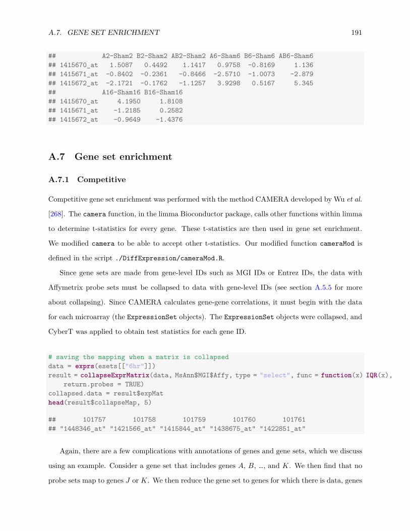
A.7. GENE SET ENRICHMENT 191
## A2-Sham2 B2-Sham2 AB2-Sham2 A6-Sham6 B6-Sham6 AB6-Sham6## 1415670_at 1.5087 0.4492 1.1417 0.9758 -0.8169 1.136## 1415671_at -0.8402 -0.2361 -0.8466 -2.5710 -1.0073 -2.879## 1415672_at -2.1721 -0.1762 -1.1257 3.9298 0.5167 5.345## A16-Sham16 B16-Sham16## 1415670_at 4.1950 1.8108## 1415671_at -1.2185 0.2582## 1415672_at -0.9649 -1.4376
A.7 Gene set enrichment
A.7.1 Competitive
Competitive gene set enrichment was performed with the method CAMERA developed by Wu et al.
[268]. The camera function, in the limma Bioconductor package, calls other functions within limma
to determine t-statistics for every gene. These t-statistics are then used in gene set enrichment.
We modified camera to be able to accept other t-statistics. Our modified function cameraMod is
defined in the script ./DiffExpression/cameraMod.R.
Since gene sets are made from gene-level IDs such as MGI IDs or Entrez IDs, the data with
Affymetrix probe sets must be collapsed to data with gene-level IDs (see section A.5.5 for more
about collapsing). Since CAMERA calculates gene-gene correlations, it must begin with the data
for each microarray (the ExpressionSet objects). The ExpressionSet objects were collapsed, and
CyberT was applied to obtain test statistics for each gene ID.
# saving the mapping when a matrix is collapseddata = exprs(esets[["6hr"]])result = collapseExprMatrix(data, MsAnn$MGI$Affy, type = "select", func = function(x) IQR(x),
return.probes = TRUE)collapsed.data = result$expMathead(result$collapseMap, 5)
## 101757 101758 101759 101760 101761## "1448346_at" "1421566_at" "1415844_at" "1438675_at" "1422851_at"
Again, there are a few complications with annotations of genes and gene sets, which we discuss
using an example. Consider a gene set that includes genes A, B, …, and K. We then find that no
probe sets map to genes J or K. We then reduce the gene set to genes for which there is data, genes

192 APPENDIX A. REPRODUCING IN VIVO ANALYSES
A, B, …, and I. Now consider that, in collapsing probe sets to genes, probe set 1 was selected as
the probe set to represent the closely related genes E, F , G, H, and I. If probe set 1 was strongly
differentially expressed, then the majority of genes in this gene set would be found to be differentially
expressed, which may or may not be the case. To avoid a probe set errantly making a gene set
significantly enriched, a probe set was not allowed to be repreated in a gene set. In this example,
the gene set would then be genes A, B, C, D, and one gene represented by probe set 1. When
gene set enrichment is performed on a collapsed matrix, it is thus necessary to save which probes
map to genes (note the return.probes option in the previous example of the collapseExprMatrix
function). Finally, gene sets with few genes are more likely to be enriched by one or two outliers,
and gene sets with several hundred genes are often too vague for interpretation. Hence, gene sets
with very few or several hundred genes were excluded. The function indexGeneSets accounts for
all the problems mentioned above; it also converts the format of the gene set annotation lists so
that they may be used with camera and cameraMod.
A wrapper function, cameraModWrapper in cameraModWrapper.R, uses the CyberT t statistic
as input to cameraMod. The wrapper function is used in the script runCAMERA.R and the results
are saved to ./data/RData/cameraMod.RData.
A.7.2 Self-contained
The function for the self contained test, cactus, is defined in the ./E-Enrichment/cactus.R
script. The runCactus.R script runs cactus for every toxin-sham comparison and saves the p-
values from each gene set enrichment in the ./data/RData/cactus.RData file. The annotation
problems mentioned for competitive gene set enrichment were addressed in the same way for self-
contained gene set enrichment.
# Example of p-values from gene set enrichmentsource("./E-Enrichment/cameraModWrapper.R")eset = esets[["16hr"]]result = cameraModWrapper(eset, MsAnnGO$MF$MGI, list(c("A16", "Sham16")), MsAnn$MGI$Affy)head(sort(result, decreasing = FALSE))
## GO:0043498 GO:0005525 GO:0003924 GO:0004364 GO:0005097 GO:0047485## 0.0002763 0.0021449 0.0022396 0.0031255 0.0038467 0.0043996

A.8. ANALYSIS OF PREVIOUS IN VITRO DATA 193
source("./E-Enrichment/cactus.R")
eset = esets[["2hr"]]
result = cactus(eset, MsAnnGO$BP$MGI, list(c("A2", "Sham2"), c("B2", "Sham2")),
MsAnn$MGI$Affy)
head(result, 4)
## A2-Sham2 B2-Sham2## GO:0000038 0.53392 0.3159## GO:0000045 0.07490 0.3596## GO:0000060 0.04644 0.3564## GO:0000070 0.65147 0.3277
A.8 Analysis of previous in vitro data
The analysis described in the previous sections was repeated for the transcriptional response of
HCT8 cells exposed to TcdA or TcdB [230]. The scripts and files for this analysis are in the
./InVitro/ folder. The directory structure is the same as for analysis of our in vivo data.
Our reanalysis of the in vitro data uncovered a clear batch effect between different runs of
microarrays. The batch effect had little effect on the ranking of genes or the gene set enrichment
results we have reported previously. Nevertheless, we corrected for this batch effect using a sim-
ple linear model. Factors for the three different runs were included in the model. A principal
components plot of all the microarrays before and after batch correction are shown in Figure A.1.
A.9 Comparisons to other transcriptomic and proteomic data
Proteomic data from Zeiser et al. was downloaded from the supplementary material of their
manuscript [275]. The transcriptional data with HCT8 cells was downloaded from NCBI GEO.
The scripts parsing these data are in the ./G-Comparisons folder. In merging the data between
mouse and human, only one-to-one mappings were used.
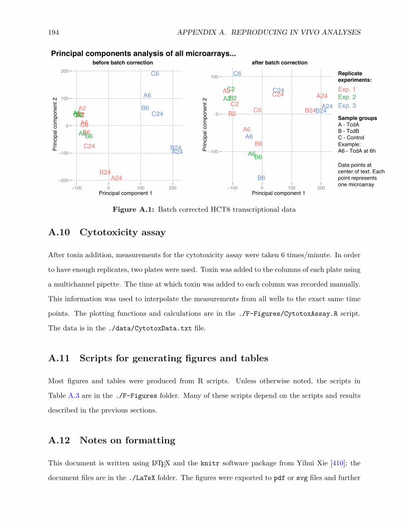
194 APPENDIX A. REPRODUCING IN VIVO ANALYSES
C2C2A2
A2B2B2C6
C6
A6A6
A6
B6B6
B6
C24
C24
A24
A24
B24
B24
−200
−100
0
100
200
−100 0 100 200Principal component 1
Prin
cipa
l com
pone
nt 2
Exp. 1Exp. 2Exp. 3C2
C2A2A2
B2
B2
C6
C6
A6
A6
A6B6
B6
B6
C24C24A24
A24B24B24
−100
0
100
−100 0 100 200Principal component 1
Replicateexperiments:
Principal components analysis of all microarrays...before batch correction after batch correction
Sample groupsA - TcdAB - TcdBC - Control
Prin
cipa
l com
pone
nt 2
Example:A6 - TcdA at 6h
Data points atcenter of text. Eachpoint representsone microarray
Figure A.1: Batch corrected HCT8 transcriptional data
A.10 Cytotoxicity assay
After toxin addition, measurements for the cytotoxicity assay were taken 6 times/minute. In order
to have enough replicates, two plates were used. Toxin was added to the columns of each plate using
a multichannel pipette. The time at which toxin was added to each column was recorded manually.
This information was used to interpolate the measurements from all wells to the exact same time
points. The plotting functions and calculations are in the ./F-Figures/CytotoxAssay.R script.
The data is in the ./data/CytotoxData.txt file.
A.11 Scripts for generating figures and tables
Most figures and tables were produced from R scripts. Unless otherwise noted, the scripts in
Table A.3 are in the ./F-Figures folder. Many of these scripts depend on the scripts and results
described in the previous sections.
A.12 Notes on formatting
This document is written using LATEX and the knitr software package from Yihui Xie [410]; the
document files are in the ./LaTeX folder. The figures were exported to pdf or svg files and further

A.13. ACKNOWLEDGEMENTS 195
Figure or Table ScriptTable 1 Table1.RTables 2 & 3 Tables2and3.RFigure 2 Figure2.RFigure 3 & S6 Figure3.RFigure 4 Figure4.RFigure S1, S3, S7, and S8 Supplement.RTables S1 & S2 Manually enteredFigure S2 CytotoxAssay.RFigure S4 flow.RFigure S5 ./G-Comparisons/Hirota-et-al/HirotaCytokines.RFigures S9 ./G-Comparisons/HCT8-cells/Sims.R
& S10 & ./G-Comparisons/Proteomics/loadData.R
Table A.3: Scripts for producing tables and figures
formatted with Adobe Illustrator.
A.13 Acknowledgements
This appendix is part of the supplement for D’Auria, K. M., Kolling, G. L., Donato, G. M., Warren,
C. A., Gray, M. C., Hewlett, E. L. & Papin, J. A. In vivo physiological and transcriptional profiling
reveals host responses to Clostridium difficile toxin A and toxin B.. Infection and Immunity 81,
3814–3824 (Oct. 2013).

Appendix B
Reproducing time-course analyses
B.1 Introduction
This document includes the supplemental data referred to in Chapter 7 as well as instructions for
how to reproduce our analyses and explore the data further. This is a functional document in that
scripts (written in the R programming languange with the knitr package) are embedded, and they
were run during PDF creation to produce the figures and output shown. Thus, the analyses can
be repeated by downloading the source of this document (with the data) or copy-pasting all of the
code into one’s own R console.
B.2 References from Chapter 7
B.2.1 Reference 1
“The impedance curves of cells treated with TcdA (300 ng/ml) and TcdB (10 ng/ml) diverged from
controls in 10 and 20 minutes, respectively (Appendix B).”
196
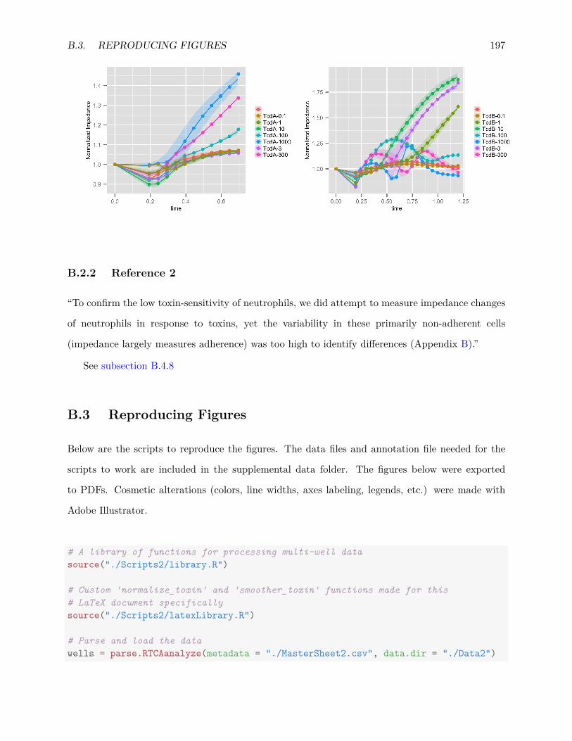
B.3. REPRODUCING FIGURES 197
B.2.2 Reference 2
“To confirm the low toxin-sensitivity of neutrophils, we did attempt to measure impedance changes
of neutrophils in response to toxins, yet the variability in these primarily non-adherent cells
(impedance largely measures adherence) was too high to identify differences (Appendix B).”
See subsection B.4.8
B.3 Reproducing Figures
Below are the scripts to reproduce the figures. The data files and annotation file needed for the
scripts to work are included in the supplemental data folder. The figures below were exported
to PDFs. Cosmetic alterations (colors, line widths, axes labeling, legends, etc.) were made with
Adobe Illustrator.
# A library of functions for processing multi-well datasource("./Scripts2/library.R")
# Custom 'normalize_toxin' and 'smoother_toxin' functions made for this# LaTeX document specificallysource("./Scripts2/latexLibrary.R")
# Parse and load the datawells = parse.RTCAanalyze(metadata = "./MasterSheet2.csv", data.dir = "./Data2")
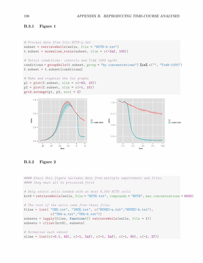
198 APPENDIX B. REPRODUCING TIME-COURSE ANALYSES
B.3.1 Figure 1
# Process data from file HCT8-4.txtsubset = retrieveWells(wells, file = "HCT8-4.txt")t.subset = normalize_toxin(subset, xlim = c(-Inf, 100))
# Select conditions: controls and TcdA 1000 ng/mlconditions = groupWells(t.subset, group = "by.concentrations") %in% c("", "TcdA-1000")f.subset = t.subset[conditions]
# Make and organize the two graphsp1 = plot(f.subset, xlim = c(-43, 10))p2 = plot(f.subset, xlim = c(-1, 10))grid.arrange(p1, p2, ncol = 2)
B.3.2 Figure 2
#### Since this figure includes data from multiple experiments and files,#### they must all be processed first
# Only select wells seeded with at most 6,000 HCT8 cellshct8 = retrieveWells(wells, file = "HCT8.txt", compounds = "HCT8", max.concentrations = 6000)
# The rest of the wells come from these filesfiles = list( "CHO.txt", "IMCE.txt", c("HUVEC-a.txt","HUVEC-b.txt"),
c("T84-a.txt","T84-b.txt"))subsets = lapply(files, function(f) retrieveWells(wells, file = f))subsets = c(list(hct8), subsets)
# Normalize each subsetxlims = list(c(-0.1, 43), c(-1, Inf), c(-1, Inf), c(-1, 60), c(-1, 27))

B.3. REPRODUCING FIGURES 199
n.subsets = mapply(normalize_toxin, subsets, xlim = xlims)
# Add a smoother to each subsetx.scales = c( 2/3, 1, 1, 2/3, 2/3 )s.subsets = mapply( smoother_toxin, n.subsets, x.scale=x.scales )
# Calculate ABC for each subset (with different integration limits)left = rep(0, 5)right = c(43, 40, 80, 80, 27)i.subsets = mapply(integrate, s.subsets, left, right)allwells = do.call(c, i.subsets)
# Calculate MaxS for each wellallwells = max.rate(allwells, ID = "toxinAdd", min.diff = 10/60/60,
ylim = 0.8, xlim = 2)
######### Panel A. Different cell types. Same concentrations. #########subset = retrieveWells(allwells, compounds = "TcdA", ID = "toxinAdd",
max.concentrations = 101, min.concentrations = 99)panelA = plot(subset, xlim = c(-1, 10), se = FALSE, color = "by.total.compounds",
linetype = "by.compounds")
######### Panel B. Same cell type. Different toxins ############subset = retrieveWells(allwells, compounds = "IMCE")subset2 = retrieveWells(subset, compounds = c("TcdA", "TcdB"), ID = "toxinAdd",
max.concentrations = c(101, 101), min.concentrations = c(99, 99))panelB = plot(subset2, xlim = c(-0.1, 2), se = FALSE)
######## Panel C. MaxS and ABC for IMCE cells ###########subset = retrieveWells(allwells, compounds = "IMCE")MaxS = groupMetric(subset, ID = "toxinAdd", metric = "max.rate")p1 = plotMetric(MaxS)ABC = groupMetric(subset, ID = "toxinAdd", metric = "integral")p2 = plotMetric(ABC)panelC = arrangeGrob(p1 + theme(legend.position = "none"),
p2 + theme(legend.position = "none"), ncol = 2)
####### Panel D. The MCC for each cell type ############### The MCC was found by plotting the ABC of each cell type over# a range of concentrations. The concentration diverging from# controls was considered the MCCABC = groupMetric(allwells, ID = "toxinAdd", metric = "integral")ABC$cells = groupWells(allwells, group = "by.total.compounds")plotMetric(ABC, file = FALSE) + facet_wrap(~cells, scales = "free_y")

200 APPENDIX B. REPRODUCING TIME-COURSE ANALYSES
After the processing, the four panels can be combined.
# Manually enter the MCC for each cell typed = data.frame(type = c("CHO", "HCT8", "HUVEC", "IMCE", "T84"), a = c(1, 1,
1, 0.1, 0.1), b = c(0.001, 0.01, 0.01, 1e-04, 0.1))panelD = ggplot(d, aes(x = log10(a), y = log10(b), label = type)) + geom_text() +
scale_x_reverse(limits = c(0, -4)) + scale_y_reverse(limits = c(0, -4)) +geom_abline(slope = 1, intercept = 0) + coord_equal() + geom_point(color = "red")
# Show the final plotgrid.arrange(panelA, panelB, panelC, panelD, ncol = 2)

B.3. REPRODUCING FIGURES 201
B.3.3 Figure 3
###### Panel Asubset = retrieveWells(wells, file = c("J774-a.txt", "J774-b.txt"))t.subset = normalize_toxin(subset, xlim = c(-Inf, 100))
# Toxin A curvesconditions = groupWells(t.subset, group = "by.concentrations") %in%
c("", paste0("TcdA-", c(0.1, 3, 100, 1000)))p1 = plot(t.subset[conditions], xlim = c(-0.01, 40))
# Toxin B curvesconditions = groupWells(t.subset, group = "by.concentrations") %in%
c("", paste0("TcdB-", c(0.1, 10, 100)))p2 = plot(t.subset[conditions], xlim = c(-0.01, 15))
# TcdA and TcdB curves side by sidegrid.arrange(p1, p2, ncol = 2)
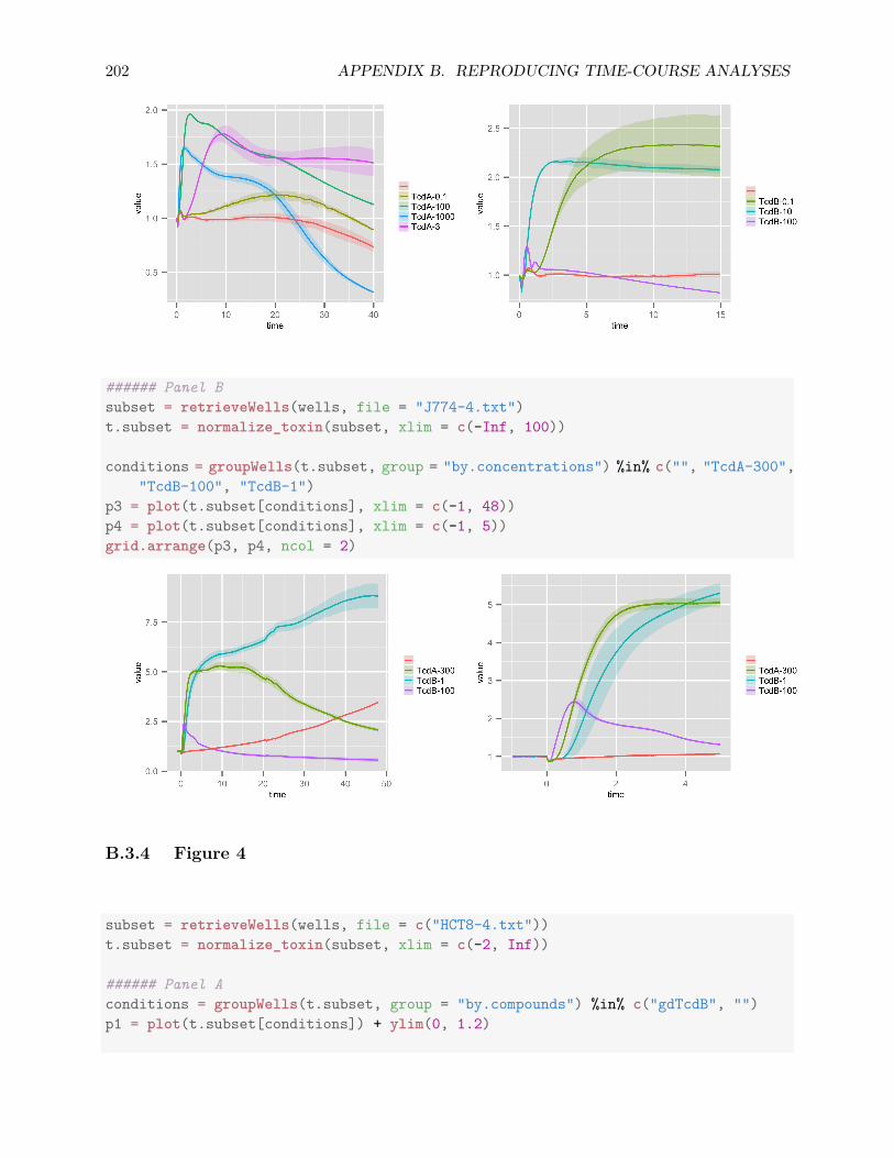
202 APPENDIX B. REPRODUCING TIME-COURSE ANALYSES
###### Panel Bsubset = retrieveWells(wells, file = "J774-4.txt")t.subset = normalize_toxin(subset, xlim = c(-Inf, 100))
conditions = groupWells(t.subset, group = "by.concentrations") %in% c("", "TcdA-300","TcdB-100", "TcdB-1")
p3 = plot(t.subset[conditions], xlim = c(-1, 48))p4 = plot(t.subset[conditions], xlim = c(-1, 5))grid.arrange(p3, p4, ncol = 2)
B.3.4 Figure 4
subset = retrieveWells(wells, file = c("HCT8-4.txt"))t.subset = normalize_toxin(subset, xlim = c(-2, Inf))
###### Panel Aconditions = groupWells(t.subset, group = "by.compounds") %in% c("gdTcdB", "")p1 = plot(t.subset[conditions]) + ylim(0, 1.2)

B.3. REPRODUCING FIGURES 203
###### Panel Bconditions = groupWells(t.subset, group = "by.concentrations") %in%
c("", "gdTcdB-100", "TcdB-10", "gdTcdB-100.TcdB-10")p2 = plot(t.subset[conditions], xlim = c(-0.2, 4)) + ylim(0, 1.2)
###### Panel Cconditions = groupWells(t.subset, group = "by.concentrations") %in%
c("", "gdTcdB-1000", "TcdA-1000", "gdTcdB-1000.TcdA-1000","TcdA-100", "gdTcdB-1000.TcdA-100")
p3 = plot(t.subset[conditions], xlim = c(-0.2, 10)) + ylim(0, 1.2)
grid.arrange(p1,p2,p3,ncol=2)
B.3.5 Figure 5
##### Panel Asubset = retrieveWells(wells, file = "J774-4.txt")t.subset = normalize_toxin(subset, xlim = c(-2, Inf))conditions = groupWells(t.subset, group = "by.compounds") %in%
c("", "TcdB", "gdTcdB")p1 = plot(t.subset[conditions], xlim = c(-1, 48))

204 APPENDIX B. REPRODUCING TIME-COURSE ANALYSES
##### Panel Bsubset = retrieveWells(wells, file = c("J774-3a.txt", "J774-3b.txt"))t.subset = normalize_toxin(subset, xlim = c(-2, Inf))conditions = groupWells(t.subset, group = "by.concentrations") %in%
c("", "TcdB-0.01", "gdTcdB-1.TcdB-0.01")p2 = plot(t.subset[conditions], xlim = c(-0.2, 5))
##### Panel Csubset = retrieveWells(wells, file = c("J774-5.txt"))t.subset = normalize_toxin(subset, xlim = c(-2, Inf))conditions = groupWells(t.subset, group = "by.concentrations") %in%
c("", "gdTcdB-10", "TcdA-1", "gdTcdB-10.TcdA-1")p3 = plot(t.subset[conditions], xlim = c(-0.2, 24))
grid.arrange(p1, p2, p3, ncol = 2)
B.4 Exploring the data
All experiments, each involving several experimental conditions, are summarized in the table be-
low. Independent experiments that occurred on different days are separated by horizontal lines.
Diagrams of the physical multi-well plates are displayed in B.4.9. The number of cells seeded and
all the incubation times can be found in the csv annotation file in the supplemental data or can be

B.4. EXPLORING THE DATA 205
accessed in the wells variable within R (as shown in B.3).
B.4.1 Plate summaries
Cell type File names Toxins (ng/ml) Notes
HCT8
HCT8.txt A (500, 100, 10, 1, 0.1)B (500, 100, 10, 1, 0.1)
HCT8-2a.txtHCT8-2b.txt
B (1), A (100)gdTcdB (100, 1000)B (1) + gdTcdB (100)B (1) + gdTcdB(1000)A (100) + gdTcdB (1000)
toxins + gdTcdB
HCT8-3.txt
B (1), A (100)gdTcdB (10, 100, 1000)B (1) + gdTcdB (10)B (1) + gdTcdB (100)A (100) + gdTcdB (1000)
toxins + gdTcdB
HCT8-4.txt
B (10, 100), A (100, 1000)gdTcdB (100, 1000)B (10) + gdTcdB (100)B (10) + gdTcdB (1000)B (100) + gdTcdB (100)B (100) + gdTcdB (1000)A (10) + gdTcdB (100)A (100) + gdTcdB (100)A (100) + gdTcdB (1000)A (1000) + gdTcdB (1000)
toxins + gdTcdB
CHO CHO.txt A (1000, 100, 1, 0.1, 0.01, 1e-3, 1e-4 )B (1000, 100, 1, 0.1, 0.01, 1e-3, 1e-4 )
IMCE IMCE.txt A (1000, 100, 10, 1, 0.1, 0.01, 0.001 )B (1000, 100, 10, 1, 0.1, 0.01, 0.001 )
HUVEC HUVEC-a.txtHUVEC-b.txt
A (1000, 300, 100, 30, 10, 1, 0.1)B (1000, 300, 100, 30, 10, 1, 0.1)
T84 T84-a.txtT84-b.txt
A (300, 100, 30, 10, 3, 1, 0.1)B (1000, 300, 100, 30, 10, 3, 1, 0.1)
J774
J774-a.txtJ774-b.txt
A (0.1, 1, 3, 10, 100, 300, 1000)B (0.1, 1, 3, 10, 100, 300, 1000)
J774-2.txt B (0.00001, 0.0001, 0.001, 0.01, 0.1, 1, 10)
J774-3a.txtJ774-3b.txt
A (10), B (0.01)gdTcdB (0.1, 1, 100)B (0.01) + gdTcdB (1)B (0.01) + gdTcdB (0.1)A (10) + gdTcdB (100)
toxins + gdTcdB
J774-4.txtA (3, 300), B (1, 100)gdTcdB (1, 100)A (10) + gdTcdB (100)
toxins + gdTcdB

206 APPENDIX B. REPRODUCING TIME-COURSE ANALYSES
J774-5.txt
A (1, 1000),gdTcdB (10, 100)A (1) + gdTcdB (10)A (1000) + gdTcdB (1000)B (10) + gdTcdB (100)
toxins + gdTcdB
PMN
PMN-a.txtPMN-b.txt
A (10000, 7000, 5000, 3000, 1000, 500, 100)B (10000, 7000, 5000, 3000, 1000, 500, 100) toxins + IL8
PMN-2a.txtPMN-2b.txt
A (1000, 100, 10, 1, 0.1, 0.01, 0.001)B (1000, 100, 10, 1, 0.1, 0.01, 0.001) toxins alone
PMN-3.txt A (10, 100, 1000)B (1, 10, 100, 1000)
toxins alone andtoxins + IL8
PMN-4.txt A (10, 100, 1000)B (10, 100, 1000)
toxins alone andtoxins + IL8
B.4.2 HCT8 cells
HCT8.txt
subset = retrieveWells(wells, file = "HCT8.txt", compounds = "HCT8", max.concentrations = 6000)t.subset = normalize_toxin(subset, xlim = c(-1, 10))p1 = plot(retrieveWells(t.subset, compounds = "TcdA"))p2 = plot(retrieveWells(t.subset, compounds = "TcdB"))grid.arrange(p1, p2, ncol = 2)
HCT8-2a.txt and HCT8-2b.txt
subset = retrieveWells(wells, file = c("HCT8-2a.txt", "HCT8-2b.txt"))t.subset = normalize_toxin(subset, xlim = c(-2, Inf))p1 = plot(t.subset, xlim = c(-2, 150))

B.4. EXPLORING THE DATA 207
t.subset = smoother_toxin(t.subset, x.scale = 1.1)t.subset = max.rate(t.subset, ID = "toxinAdd", min.diff = 10/3600, ylim = 0.88,
xlim = 2)maxs = getMetric(t.subset, metric = "max.rate")labels = factor(groupWells(t.subset, group = "by.concentrations", ID = "toxinAdd"),
levels = c("", "gdTcdB-100", "gdTcdB-1000", "gdTcdB-1000.TcdA-100", "TcdA-100","gdTcdB-100.TcdB-1", "gdTcdB-10.TcdB-1", "TcdB-1"))
p2 = qplot(labels, maxs$value, color = labels) + no_x_labels + labs(color = "Legend") +xlab("group") + ylab("MaxS")
grid.arrange(p1, p2, ncol = 2)
HCT8-3.txt
subset = retrieveWells(wells, file = c("HCT8-3.txt"))t.subset = normalize_toxin(subset, xlim = c(-2, 58))p1 = plot(t.subset)
t.subset = smoother_toxin(t.subset, x.scale = 1.1)t.subset = max.rate(t.subset, ID = "toxinAdd", min.diff = 10/3600, ylim = 0.88,
xlim = 2)maxs = getMetric(t.subset, metric = "max.rate")labels = factor(groupWells(t.subset, group = "by.concentrations", ID = "toxinAdd"),
levels = c("", "gdTcdB-10", "gdTcdB-100", "gdTcdB-1000", "gdTcdB-100.TcdB-1","gdTcdB-10.TcdB-1", "TcdB-1", "gdTcdB-1000.TcdA-100", "TcdA-100", "TcdAother-100",
"TcdAup-100"))p2 = qplot(labels, maxs$value, color = labels) + no_x_labels + labs(color = "Legend") +
xlab("group") + ylab("MaxS")grid.arrange(p1, p2, ncol = 2)

208 APPENDIX B. REPRODUCING TIME-COURSE ANALYSES
HCT8-4.txt
subset = retrieveWells(wells, file = c("HCT8-4.txt"))t.subset = normalize_toxin(subset, xlim = c(-2, 155))p1 = plot(t.subset)
t.subset = smoother_toxin(t.subset, x.scale = 1.1)t.subset = max.rate(t.subset, ID = "toxinAdd", min.diff = 10/3600, ylim = 0.88,
xlim = 2)t.subset = integrate(t.subset, lower = 0, upper = 10)
maxs = getMetric(t.subset, metric = "max.rate")labels = factor(groupWells(t.subset, group = "by.concentrations", ID = "toxinAdd"),
levels = c("", "gdTcdB-100", "gdTcdB-1000", "gdTcdB-100.TcdA-10", "TcdA-10","gdTcdB-1000.TcdA-100", "gdTcdB-100.TcdA-100", "TcdA-100", "gdTcdB-1000.TcdA-1000",
"TcdA-1000", "gdTcdB-1000.TcdB-10", "gdTcdB-100.TcdB-10", "TcdB-10","gdTcdB-1000.TcdB-100", "gdTcdB-100.TcdB-100", "TcdB-100"))
p2 = qplot(labels, maxs$value, color = labels) + no_x_labels + labs(color = "Legend") +xlab("group") + ylab("MaxS")
# MaxS metrics show unexpected results for TcdB at 100 ng/ml This plot shows# that gdTcdB appears to have only been added to one of the four wells?# Regardless, gdTcdB clearly delayed TcdB at 10 ng/mlaa = retrieveWells(t.subset, compounds = "TcdB", max.concentrations = 101, min.concentrations = 99)p3 = plot(aa, xlim = c(-1, 7), replicates = FALSE)
grid.arrange(arrangeGrob(p1, p3, ncol = 2), p2, nrow = 2)

B.4. EXPLORING THE DATA 209
B.4.3 CHO cells
CHO.txt
subset = retrieveWells(wells, file = "CHO.txt")t.subset = normalize_toxin(subset, c(-2, Inf))p1 = plot(retrieveWells(t.subset, compounds = "TcdA"), xlim = c(-1, 40))p2 = plot(retrieveWells(t.subset, compounds = "TcdB"), xlim = c(-1, 20))grid.arrange(p1, p2, ncol = 2)

210 APPENDIX B. REPRODUCING TIME-COURSE ANALYSES
B.4.4 IMCE cells
IMCE.txt
subset = retrieveWells(wells, file = "IMCE.txt")t.subset = normalize_toxin(subset, c(-2, Inf))p1 = plot(retrieveWells(t.subset, compounds = "TcdA"), xlim = c(-1, 80))p2 = plot(retrieveWells(t.subset, compounds = "TcdB"), xlim = c(-1, 80))grid.arrange(p1, p2, ncol = 2)
B.4.5 HUVECs
HUVEC-a.txt and HUVEC-b.txt
subset = retrieveWells(wells, file = c("HUVEC-a.txt", "HUVEC-b.txt"))t.subset = normalize_toxin(subset, c(-2, Inf))p1 = plot(retrieveWells(t.subset, compounds = "TcdA"), xlim = c(-1, 20))p2 = plot(retrieveWells(t.subset, compounds = "TcdB"), xlim = c(-1, 20))grid.arrange(p1, p2, ncol = 2)

B.4. EXPLORING THE DATA 211
B.4.6 T84 cells
T84-a.txt and T84-b.txt
subset = retrieveWells(wells, file = c("T84-a.txt", "T84-b.txt"))t.subset = normalize_toxin(subset, c(-2, Inf))p1 = plot(retrieveWells(t.subset, compounds = "TcdA"), xlim = c(-1, 20))p2 = plot(retrieveWells(t.subset, compounds = "TcdB"), xlim = c(-1, 20))grid.arrange(p1, p2, ncol = 2)
B.4.7 J774 cells
J774-a.txt and J774-b.txt
subset = retrieveWells(wells, file = c("J774-a.txt", "J774-b.txt"))t.subset = normalize_toxin(subset, c(-2, Inf))p1 = plot(retrieveWells(t.subset, compounds = "TcdA"), xlim = c(-1, 40))p2 = plot(retrieveWells(t.subset, compounds = "TcdB"), xlim = c(-1, 40))grid.arrange(p1, p2, ncol = 2)

212 APPENDIX B. REPRODUCING TIME-COURSE ANALYSES
J774-2.txt
subset = retrieveWells(wells, file = "J774-2.txt")t.subset = normalize_toxin(subset, c(-2, Inf))p1 = plot(t.subset, xlim = c(-1, 40))p2 = plot(t.subset, xlim = c(-1, 5))grid.arrange(p1, p2, ncol = 2)
J774-3a.txt and J774-3b.txt
subset = retrieveWells(wells, file = c("J774-3a.txt", "J774-3b.txt"))t.subset = normalize_toxin(subset, c(-2, Inf))p1 = plot(t.subset, xlim = c(-1, 24))p2 = plot(t.subset, xlim = c(-1, 5))grid.arrange(p1, p2, ncol = 2)
J774-4.txt

B.4. EXPLORING THE DATA 213
subset = retrieveWells(wells, file = "J774-4.txt")t.subset = normalize_toxin(subset, c(-2, Inf))p1 = plot(t.subset, xlim = c(-1, 48))p2 = plot(t.subset, xlim = c(-1, 5))grid.arrange(p1, p2, ncol = 2)
J774-5.txt
subset = retrieveWells(wells, file = "J774-5.txt")t.subset = normalize_toxin(subset, c(-2, Inf))p1 = plot(t.subset, xlim = c(-1, 48))p2 = plot(t.subset, xlim = c(-1, 5))grid.arrange(p1, p2, ncol = 2)
B.4.8 PMN leukocytes
Consistent response profiles of PMNs to TcdA or TcdB could not be obtained.

214 APPENDIX B. REPRODUCING TIME-COURSE ANALYSES
PMN-2a.txt and PMN-2b.txt
Only TcdA at 1,000 ng/ml was clearly different than control cells. Instead of normalizing the
impedance at the time toxin was added, the change in impedance from the time of toxin addition
is shown.
subset = retrieveWells(wells, file = c("PMN-2a.txt", "PMN-2b.txt"))t.subset = transform(subset, c("tcenter", "slice", "level"), xlim = c(-2, Inf),
ID = "toxinAdd")p1 = plot(retrieveWells(t.subset, compounds = "TcdA"), xlim = c(-1, 24))p2 = plot(retrieveWells(t.subset, compounds = "TcdB"), xlim = c(-1, 24))grid.arrange(p1, p2, ncol = 2)
PMN-a.txt and PMN-b.txt
Cells were seeded in the presence of 100 ng/ml (9.01 nM) of human recombinant IL-8 in an attempt
to increase impedance before adding toxin.
subset = retrieveWells(wells, file = c("PMN-a.txt", "PMN-b.txt"))t.subset = transform(subset, c("tcenter", "slice", "level"), xlim = c(-2, Inf),
ID = "toxinAdd")p1 = plot(retrieveWells(t.subset, compounds = "TcdA"), xlim = c(-1, 24))p2 = plot(retrieveWells(t.subset, compounds = "TcdB"), xlim = c(-1, 24))grid.arrange(p1, p2, ncol = 2)

B.4. EXPLORING THE DATA 215
PMN-3.txt
Cells were seeded in the presence of 25 nM (277.45 ng/ml) of IL-8.
subset = retrieveWells(wells, file = "PMN-3.txt")t.subset = transform(subset, c("tcenter", "slice", "level"), xlim = c(-2, Inf),
ID = "toxinAdd")p1 = plot(retrieveWells(t.subset, compounds = "TcdA"), xlim = c(-1, 48), replicates = FALSE)p2 = plot(retrieveWells(t.subset, compounds = "TcdB"), xlim = c(-1, 48), replicates = FALSE)grid.arrange(p1, p2, ncol = 2)
PMN-4.txt
Cells were seeded in the presence of 25 nM (277.45 ng/ml) of IL-8. The machine temporarily
stopped making impedance measurements from approximately five to 20 hours.
subset = retrieveWells(wells, file = "PMN-4.txt")t.subset = transform(subset, c("tcenter", "slice", "level"), xlim = c(-2, Inf),

216 APPENDIX B. REPRODUCING TIME-COURSE ANALYSES
ID = "toxinAdd")p1 = plot(retrieveWells(t.subset, compounds = "TcdA"), xlim = c(-1, 48))p2 = plot(retrieveWells(t.subset, compounds = "TcdB"), xlim = c(-1, 48))grid.arrange(p1, p2, ncol = 2)
B.4.9 Plate Layouts
Below are the layouts of all of the plates used.
fwells = split(wells, getfiles(wells))fwells = fwells[sort(names(fwells))]
options(xtable.print.results=FALSE)fwt = lapply(fwells, well_table, ID="toxinAdd")lt = lapply(fwt, print_well_table, scalebox=0.6, floating=FALSE)
do.call( cat, c("\\begin{adjustwidth}{0in}{3in}{",lt,"} \\end{adjustwidth}") )
1 2A TcdA-1000 TcdB-1000B TcdB-100C TcdA-100 TcdB-1D TcdA-1 TcdB-0.1E TcdA-0.1 TcdB-0.01F TcdA-0.01G TcdA-0.001 TcdB-0.001H TcdA-1e-04 TcdB-1e-04
CHO.txt
1 2A TcdB-1, gdTcdB-100 TcdB-1, gdTcdB-100B TcdB-1, gdTcdB-10 TcdB-1, gdTcdB-10C TcdA-100, gdTcdB-1000 TcdA-100, gdTcdB-1000D TcdB-1 TcdB-1E TcdA-100 TcdA-100F gdTcdB-1000 gdTcdB-1000G gdTcdB-100 gdTcdB-100H
HCT8-2a.txt3 4
A TcdB-1, gdTcdB-100 TcdB-1, gdTcdB-100B TcdB-1, gdTcdB-10 TcdB-1, gdTcdB-10C TcdA-100, gdTcdB-1000 TcdA-100, gdTcdB-1000D TcdB-1 TcdB-1E TcdA-100 TcdA-100F gdTcdB-1000 gdTcdB-1000G gdTcdB-100 gdTcdB-100H
HCT8-2b.txt
3 4 5 6A TcdA-100, gdTcdB-1000 TcdA-100 gdTcdB-10B gdTcdB-100 TcdA-100 TcdA-100, gdTcdB-1000 TcdAup-100C TcdA-100 gdTcdB-100 gdTcdB-10D TcdA-100, gdTcdB-1000 gdTcdB-100 TcdAup-100E TcdB-1 gdTcdB-1000 TcdB-1, gdTcdB-10 gdTcdB-10F TcdB-1, gdTcdB-100 TcdB-1, gdTcdB-10 TcdB-1 TcdAother-100G TcdB-1, gdTcdB-10 TcdB-1, gdTcdB-100 gdTcdB-1000 TcdAother-100H gdTcdB-1000 TcdB-1 TcdB-1, gdTcdB-100
HCT8-3.txt

B.4. EXPLORING THE DATA 217
1 2 3 4A TcdA-10 TcdB-10 TcdB-100, gdTcdB-1000 TcdB-100, gdTcdB-1000B TcdA-1000 TcdA-1000 TcdB-100 TcdB-10C TcdA-10, gdTcdB-100 TcdB-100, gdTcdB-100D gdTcdB-1000 gdTcdB-1000 TcdA-100, gdTcdB-100 TcdA-1000, gdTcdB-1000E gdTcdB-100 TcdA-100 TcdA-1000, gdTcdB-1000F TcdB-10, gdTcdB-100 gdTcdB-100 TcdA-10, gdTcdB-100 TcdA-100, gdTcdB-1000G TcdB-10, gdTcdB-100 TcdA-100 TcdB-10, gdTcdB-1000 TcdA-100, gdTcdB-1000H TcdB-10, gdTcdB-1000 TcdB-100 TcdA-100, gdTcdB-100 TcdB-100, gdTcdB-100
HCT8-4.txt3 4
A TcdA-100 TcdA-100B NA-NA NA-NAC TcdB-100D TcdA-500 TcdB-500E TcdA-100 TcdB-100F TcdA-10 TcdB-10G TcdA-1 TcdB-1H TcdA-0.1 TcdB-0.1
HCT8.txt
3 4A TcdA-1000 TcdB-1000B TcdA-300 TcdB-300C TcdA-100 TcdB-100DE TcdA-30 TcdB-30F TcdA-10 TcdB-10G TcdA-1 TcdB-1H TcdA-0.1 TcdB-0.1
HUVEC-a.txt
5 6A TcdA-1000 TcdB-1000B TcdA-300 TcdB-300C TcdA-100 TcdB-100DE TcdA-30 TcdB-30F TcdA-10 TcdB-10G TcdA-1 TcdB-1H TcdA-0.1 TcdB-0.1
HUVEC-b.txt3 4 5 6
A TcdA-1000 TcdB-100 TcdA-1000 TcdB-10B TcdA-100 TcdB-10 TcdA-100 TcdB-1C TcdB-1 TcdB-0.1D TcdA-10 TcdB-0.1 TcdA-10 TcdB-0.01E TcdA-1 TcdB-0.01 TcdA-1 TcdB-0.001F TcdA-0.1 TcdB-0.001 TcdA-0.1 TcdB-1e-04G TcdA-0.01 TcdB-1e-04 TcdA-0.01 TcdB-1e-05H TcdA-0.001 TcdB-1e-05 TcdA-0.001
IMCE.txt
5 6A TcdB-10 TcdB-10B TcdB-1 TcdB-1C TcdB-0.1 TcdB-0.1D TcdB-0.01 TcdB-0.01E TcdB-0.001 TcdB-0.001F TcdB-1e-04 TcdB-1e-04G TcdB-1e-05 TcdB-1e-05H
J774-2.txt1 2
A TcdB-0.01, gdTcdB-1 TcdB-0.01, gdTcdB-1B TcdB-0.01, gdTcdB-0.1 TcdB-0.01, gdTcdB-0.1C TcdA-10, gdTcdB-100 TcdA-10, gdTcdB-100D TcdB-0.01 TcdB-0.01E TcdA-10 TcdA-10F gdTcdB-100 gdTcdB-100G gdTcdB-1 gdTcdB-1H gdTcdB-0.1
J774-3a.txt
3 4A TcdB-0.01, gdTcdB-1 TcdB-0.01, gdTcdB-1B TcdB-0.01, gdTcdB-0.1 TcdB-0.01, gdTcdB-0.1C TcdA-10, gdTcdB-100 TcdA-10, gdTcdB-100D TcdB-0.01 TcdB-0.01E TcdA-10 TcdA-10F gdTcdB-100G gdTcdB-1H gdTcdB-0.1 gdTcdB-0.1
J774-3b.txt1 2
A TcdB-1 TcdB-1B TcdB-100 TcdB-100CD gdTcdB-1 gdTcdB-1E gdTcdB-100 gdTcdB-100F TcdA-3 TcdA-3G TcdA-300 TcdA-300H gdTcdB-100, TcdA-10 gdTcdB-100, TcdA-10
J774-4.txt
1 2A gdTcdB-100, TcdB-10 gdTcdB-100, TcdB-10B gdTcdB-10, TcdA-1 gdTcdB-10, TcdA-1C gdTcdB-100, TcdA-1000 gdTcdB-100, TcdA-1000D TcdA-1 TcdA-1E TcdA-1000 TcdA-1000F gdTcdB-10 gdTcdB-10G gdTcdB-100 gdTcdB-100H
J774-5.txt1 2
A TcdA-1000 TcdB-1000B TcdA-300 TcdB-300CD TcdA-100 TcdB-100E TcdA-10 TcdB-10F TcdA-3 TcdB-3G TcdA-1 TcdB-1H TcdA-0.1 TcdB-0.1
J774-a.txt
5 6A TcdA-1000 TcdB-1000B TcdA-300 TcdB-300C Other-100D TcdA-100 TcdB-100E TcdA-10 TcdB-10F TcdA-3 TcdB-3G TcdA-1 TcdB-1H TcdA-0.1 TcdB-0.1
J774-b.txt
3 4A TcdA-1000 TcdB-1000B TcdA-100 TcdB-100C TcdA-10 TcdB-10D TcdA-1 TcdB-1E TcdA-0.1 TcdB-0.1F TcdB-0.01G TcdA-0.01 TcdB-0.001H TcdA-0.001 NA-NA
PMN-2a.txt5 6
A TcdA-1000 TcdB-1000B TcdA-100 TcdB-100C TcdA-10 TcdB-10D TcdA-1 TcdB-1E TcdA-0.1 TcdB-0.1F TcdB-0.01G TcdA-0.01 TcdB-0.001H TcdA-0.001
PMN-2b.txt
3 4 5 6A IL8-110.98, TcdB-1 IL8-110.98, TcdB-1 TcdB-1 TcdB-1B IL8-110.98, TcdB-10 IL8-110.98, TcdB-10 TcdB-10 TcdB-10C IL8-110.98 IL8-110.98D IL8-110.98, TcdB-100 IL8-110.98, TcdB-100 TcdB-100 TcdB-100E IL8-110.98, TcdB-1000 IL8-110.98, TcdB-1000 TcdB-1000 TcdB-1000F IL8-110.98, TcdA-1000 IL8-110.98, TcdA-1000 TcdA-1000 TcdA-1000G IL8-110.98, TcdA-100 IL8-110.98, TcdA-100 TcdA-100 TcdA-100H IL8-110.98, TcdA-10 IL8-110.98, TcdA-10 TcdA-10 TcdA-10
PMN-3.txt

218 APPENDIX B. REPRODUCING TIME-COURSE ANALYSES
1 2 3 4A IL8-110.98, TcdA-10 IL8-110.98, TcdA-10 TcdA-10 TcdA-10B IL8-110.98, TcdA-100 IL8-110.98, TcdA-100 TcdA-100 TcdA-100C IL8-110.98 IL8-110.98D IL8-110.98, TcdA-1000 IL8-110.98, TcdA-1000 TcdA-1000 TcdA-1000E IL8-110.98, TcdB-1000 IL8-110.98, TcdB-1000 TcdB-1000 TcdB-1000F IL8-110.98, TcdB-100 IL8-110.98, TcdB-100 TcdB-100 TcdB-100G IL8-110.98, TcdB-10 IL8-110.98, TcdB-10 TcdB-10 TcdB-10
PMN-4.txt
1 2A TcdA-10000 TcdB-10000B TcdA-7000 TcdB-7000C TcdA-5000 TcdB-5000DE TcdB-3000 TcdA-3000F TcdB-1000 TcdA-1000G TcdB-500 TcdA-500H TcdB-100 TcdA-100
PMN-a.txt3 4
A TcdA-10000 TcdB-10000B TcdA-7000 TcdB-7000C TcdA-5000 TcdB-5000DE TcdB-3000 TcdA-3000F TcdB-1000 TcdA-1000G TcdB-500 TcdA-500H TcdB-100 TcdA-100
PMN-b.txt
3 4A NA-NA NA-NAB TcdA-300 TcdA-1C TcdA-100 TcdA-0.1D TcdA-30 NA-NAE TcdA-10F TcdA-3 NA-NAG NA-NA NA-NAH NA-NA NA-NA
T84-a.txt
5 6A NA-NA NA-NAB NA-NA TcdB-1000C TcdB-3 TcdB-300D TcdB-100E TcdB-1 TcdB-30F TcdB-0.1 TcdB-10G NA-NA NA-NAH NA-NA NA-NA
T84-b.txt
Copyright © 2022 FDOKUMEN