Synaptic and non-synaptic propagation of slow waves and ...
201
Synaptic and non-synaptic propagation of slow waves and their modulation by endogenous electric fields Beatriz Rebollo González ADVERTIMENT. La consulta d’aquesta tesi queda condicionada a l’acceptació de les següents condicions d'ús: La difusió d’aquesta tesi per mitjà del servei TDX (www.tdx.cat) i a través del Dipòsit Digital de la UB (diposit.ub.edu) ha estat autoritzada pels titulars dels drets de propietat intel·lectual únicament per a usos privats emmarcats en activitats d’investigació i docència. No s’autoritza la seva reproducció amb finalitats de lucre ni la seva difusió i posada a disposició des d’un lloc aliè al servei TDX ni al Dipòsit Digital de la UB. No s’autoritza la presentació del seu contingut en una finestra o marc aliè a TDX o al Dipòsit Digital de la UB (framing). Aquesta reserva de drets afecta tant al resum de presentació de la tesi com als seus continguts. En la utilització o cita de parts de la tesi és obligat indicar el nom de la persona autora. ADVERTENCIA. La consulta de esta tesis queda condicionada a la aceptación de las siguientes condiciones de uso: La difusión de esta tesis por medio del servicio TDR (www.tdx.cat) y a través del Repositorio Digital de la UB (diposit.ub.edu) ha sido autorizada por los titulares de los derechos de propiedad intelectual únicamente para usos privados enmarcados en actividades de investigación y docencia. No se autoriza su reproducción con finalidades de lucro ni su difusión y puesta a disposición desde un sitio ajeno al servicio TDR o al Repositorio Digital de la UB. No se autoriza la presentación de su contenido en una ventana o marco ajeno a TDR o al Repositorio Digital de la UB (framing). Esta reserva de derechos afecta tanto al resumen de presentación de la tesis como a sus contenidos. En la utilización o cita de partes de la tesis es obligado indicar el nombre de la persona autora. WARNING. On having consulted this thesis you’re accepting the following use conditions: Spreading this thesis by the TDX (www.tdx.cat) service and by the UB Digital Repository (diposit.ub.edu) has been authorized by the titular of the intellectual property rights only for private uses placed in investigation and teaching activities. Reproduction with lucrative aims is not authorized nor its spreading and availability from a site foreign to the TDX service or to the UB Digital Repository. Introducing its content in a window or frame foreign to the TDX service or to the UB Digital Repository is not authorized (framing). Those rights affect to the presentation summary of the thesis as well as to its contents. In the using or citation of parts of the thesis it’s obliged to indicate the name of the author.
-
Upload
khangminh22 -
Category
Documents
-
view
8 -
download
0
Transcript of Synaptic and non-synaptic propagation of slow waves and ...

Synaptic and non-synaptic propagation of slow waves and their modulation
by endogenous electric fields
Beatriz Rebollo González
ADVERTIMENT. La consulta d’aquesta tesi queda condicionada a l’acceptació de les següents condicions d'ús: La difusió d’aquesta tesi per mitjà del servei TDX (www.tdx.cat) i a través del Dipòsit Digital de la UB (diposit.ub.edu) ha estat autoritzada pels titulars dels drets de propietat intel·lectual únicament per a usos privats emmarcats en activitats d’investigació i docència. No s’autoritza la seva reproducció amb finalitats de lucre ni la seva difusió i posada a disposició des d’un lloc aliè al servei TDX ni al Dipòsit Digital de la UB. No s’autoritza la presentació del seu contingut en una finestra o marc aliè a TDX o al Dipòsit Digital de la UB (framing). Aquesta reserva de drets afecta tant al resum de presentació de la tesi com als seus continguts. En la utilització o cita de parts de la tesi és obligat indicar el nom de la persona autora. ADVERTENCIA. La consulta de esta tesis queda condicionada a la aceptación de las siguientes condiciones de uso: La difusión de esta tesis por medio del servicio TDR (www.tdx.cat) y a través del Repositorio Digital de la UB (diposit.ub.edu) ha sido autorizada por los titulares de los derechos de propiedad intelectual únicamente para usos privados enmarcados en actividades de investigación y docencia. No se autoriza su reproducción con finalidades de lucro ni su difusión y puesta a disposición desde un sitio ajeno al servicio TDR o al Repositorio Digital de la UB. No se autoriza la presentación de su contenido en una ventana o marco ajeno a TDR o al Repositorio Digital de la UB (framing). Esta reserva de derechos afecta tanto al resumen de presentación de la tesis como a sus contenidos. En la utilización o cita de partes de la tesis es obligado indicar el nombre de la persona autora. WARNING. On having consulted this thesis you’re accepting the following use conditions: Spreading this thesis by the TDX (www.tdx.cat) service and by the UB Digital Repository (diposit.ub.edu) has been authorized by the titular of the intellectual property rights only for private uses placed in investigation and teaching activities. Reproduction with lucrative aims is not authorized nor its spreading and availability from a site foreign to the TDX service or to the UB Digital Repository. Introducing its content in a window or frame foreign to the TDX service or to the UB Digital Repository is not authorized (framing). Those rights affect to the presentation summary of the thesis as well as to its contents. In the using or citation of parts of the thesis it’s obliged to indicate the name of the author.

Doctoral Thesis by Beatriz Rebollo González
PhD Supervisor: María Victoria Sánchez Vives2017


INSTITUT D’INVESTIGACIONS BIOMEDIQUES AUGUST PI I SUNYER
UNIVERSITY OF BARCELONA
THESIS FOR DOCTORAL DEGREE IN BIOMEDICINE
Synaptic and non-synaptic propagation of
slow waves and their modulation by
endogenous electric fields
Author:Beatriz Rebollo Gonzalez
Supervisor:Dra. Marıa V. Sanchez Vives
Systems NeuroscienceCortical Networks
2017


iii
A mis padres


v
“They did not know it was impossible so they did it. ”
Mark Twain


vii
AbstractDoctoral degree in Biomedicine
Synaptic and non-synaptic propagation of slow
waves and their modulation by endogenous electric
fieldsby Beatriz Rebollo Gonzalez
During deep sleep stage, neurons synchronize leading to a pattern of activitymanifested as slow oscillations (< 1 Hz rhythm). This recurrent synapticactivity is organized eliciting a wave that propagates in the cortex. In thisthesis I explore the spatiotemporal dynamics of the slow oscillations in thelocal cortical network, as well as the electric fields generated by these slowwaves. Using an in vitro preparation of cortical visual slices, we unraveledthat the propagation of slow oscillations is determined by the laminar corticalstructure and that the endogenous electric fields that they generate are able tomodulate the occurrence of these slow waves.


ix
This work was partially funded by the projects BFU-2011-27094 and BFU-2014-52467-Rfrom Spanish Ministry of Economy and Competitiveness (MINECO); the European
Union’s Horizon 2020 Research and Innovation Programme under Grant AgreementNo. 720270 (HBP SGA1); Slow-Dyn PCIN-2015-162-C02-01 [FLAG ERA]. Beatriz
Rebollo Gonzalez was supported by a predoctoral fellowship from Spanish Ministry ofEconomy and Competitiveness (FPI, BES-2012-053122).


xi
Publications by the author
1. Mattia D’Andola, Beatriz Rebollo, Adenauer G. Casali, Julia F. Weinert,Andrea Pigorini, Rosa Villa, Marcello Massimini and Maria V. Sanchez-Vives. Bistability, causality and complexity in cortical networks: an invitro perturbational study. Cerebral Cortex, 1-10 (2017).
2. Sancristobal, B., Rebollo, B., Boada, P., Sanchez-Vives, M. V., &Garcia-Ojalvo, J. Collective stochastic coherence in recurrent neuronalnetworks. Nature Physics 12, 881 - 887 (2016).
3. Gemma Gabriel, Xavi Illa, Anton Guimera, Beatriz Rebollo, JavierHernandez-Ferrer, Inigo Martin-Fernandez, Ma. Teresa Martınez,Philippe Godignon, Mavi Sanchez-Vives and Rosa Villa. Chaptertitle: Carbon nanotubes as suitable interface for improving neuralrecordings. Book title: Recent Progress in Carbon Nanotube Research/ Book 2 (ISBN 980- 953-307-485-1). INTECH Open Access Publisher(2013).
4. C. Capone, B. Rebollo, A. Munoz-Cespedes, P. Del Giudice, M.V. Sanchez-Vives, M. Mattia. Slow-waves in cortical slices: howspontaneous activity is shaped by laminar structure. Under review inCerebral Cortex.
5. S.L. Gonzalez Andino*, R. Grave de Peralta Menendez*, B. Rebollo,X. Villa and M. V. Sanchez-Vives. Ohmic quasistatic models fail todescribe the electrodynamic propagation of slow oscillations in thecortical network. Under review in Scientific Reports.
6. B. Rebollo, M. Perez-Zabalza, M. Ruiz-Mejias, MV. Sanchez-Vives.Increased high frequency oscillatory activity in the prefrontal cortex inan in vitro model of schizophrenia. In preparation.
7. B. Rebollo et la., Modulation of Slow Waves by Endogenous ElectricFields: an experimental and theoretical study. In preparation.


xiii
AcknowledgementsBefore getting into scientific details, let me introduce the people who havesupported and given me guidance during these years at Sanchez-Vives lab.
First and foremost, I would like to introduce my supervisor Dr. SanchezVives. Mavi, a scientist woman who has kept on going at the top of sciencedespite the scarce amount of national funding in current times. I speciallythank her for giving me the opportunity to pursue a PhD, and for her guidanceand advice to open doors for my future career.I also thank Vanessa, the lab manager, who has been the mother of the lab,always taking care of all resources needed, and making sure that everythinggoes smoothly both on bureaucracy and experimental logistics.
I am very grateful to have worked in collaboration with Maurizio Mattia andJordi Garcıa-Ojalvo with whom I discovered the computational modelingresearch. And Sara Gonzalez, thanks to who I expanded my knowledge inphysics.
It has been a real pleasure to start and finish the period of my thesiswith Nuria, a person who has always been willing to overcome challenges nomatter how difficult they are, what have made her a great researcher.Marcel and Marıa, I would like to express my gratitude for their immensepatience to teach me most of what I know about slow oscillations. Thanks toMarcel I have got my experience to keep the brain alive even with bubbles.Thanks to Marıa I learned to interpret the Matlab analysis, somethingcompletely new to me at that time. The combination of both of them hascontributed significantly to my progress as electrophysiologist.Julia, the efficient German with whom I have shared infinite hours at the invitro set ups, working through sleepless night that transformed the pumpsound in the music of a Brunch Electronik. Also infinite hours have been sharedwith Mattia, looking for complexity within a piece of cortex, although he is aperson not at all complex; I have always admired his ability to distinguishbetween work and friendship. To both of them I would like to thank forteaching me how to use the key that detects Up/Down states.Thanks to Pol for his plots, it was a pleasure to stochastically coincide at thelab.

xiv
Others who were not so close to my work but equally important at thelab, Juan who gave me useful advices at the beginning of my career that I onlyhave got to understand later during my PhD.Lorena, the second mother in the lab, has always been ready to analyze, andre-analyze data, and assist with informatics issues... she has always been thereto appreciate our experimental work.Patricia, a little girl full of essence, I hold in high regard her broad knowledgeand planning capacity.An unique character was Thomas, with his long talks and sense of humor hetaught me a lot about how to enjoy science.The most singular who has passed by the lab: Diego, with him I learned a lotabout happiness and love; and by the way, talking about happiness and love Ineed to mention also Marta Cosın from the Cuqui group. I am grateful for theirinvitations to Amasa la Masa, meetings where together with Marıa Jesus andothers from the lab we have enjoyed delicious dishes and talks, a great epochduring my PhD.Another person I would like to thank for sharing her happiness is Melody,with her infinite kindness she has managed to comb my craziness.I also feel really happy to have had the opportunity to share the last year ofmy thesis with Miguel, Pedro, Almudena, Alex, Cristina and Alvaro. Peoplewith an amazing sense of humor making every day more pleasant. Thanksto all of them for bringing new perspectives to the lab: to Miguel and Pedrofor sharing their valuable expertise as postdocs, to Almudena and Alex fortheir fresh inquietudes. Thanks to Cristina for improving our English. Andspecial thanks to Alvaro for making much more easier the ending of my thesisanalyzing huge amount of data keeping the good mood.
Fuera del lab ha estado Barcelona, una ciudad que no para si te rodeasde las personas adecuadas. Personas como Itsaso, icono del bien hacervasco, quiero darle las gracias por el diseno de la portada, y sobre todo porhaber estado siempre pendiente de si disfrutaba el momento. Personas comoMarta, de un valor incalculable, gracias por haber construido un hogar dondesentirme en paz durante las distintas fases de la tesis.
Caceres ha resultado el lugar perfecto de desconexion donde familiaresy amigas, me han dado oxıgeno para seguir adelante. A todos ellosquiero agradecerles por encontrar siempre un momento entre mis efımerasvisitas para verme y ponernos al dıa mientras disfrutabamos de la buena

xv
gastronomıa extremena. Dentro de este maravilloso grupo se incluyen mispadres, a quienes quiero agradecer por ayudarme a descubrir mi vocacion porla ciencia, por respetar mi decision de querer avanzar en mi carrera aunqueeso suponga seguir lejos, por estar siempre dispuestos a un encuentro enMadrid con obra de teatro y gin-tonics. Son simplemente geniales.
Finalmente, a pessoa mais proxima a esta aventura tem sido Marco, que,apesar da distancia conseguiu repor minhas energias e me guiar para mantero curso em uma viagem que acaba de comecar.
Thanks to all! Gracias a todos! Obrigado!


xvii
Contents
Abstract vii
Acknowledgements xiii
1 Introduction 11.1 The slow oscillation: a rhythmic pattern . . . . . . . . . . . . . . 2
1.1.1 How does the slow oscillation emerge? . . . . . . . . . . 31.1.2 Slow oscillations within the cortical structure . . . . . . . 5
1.2 From synaptic activity to electric fields . . . . . . . . . . . . . . . 81.2.1 How do electric fields emerge? . . . . . . . . . . . . . . . 91.2.2 Electric fields within the brain tissue . . . . . . . . . . . . 10
1.3 Synaptic activity and electric field dialogue . . . . . . . . . . . . 121.3.1 The slow oscillation as the key player . . . . . . . . . . . 14
2 Objectives 15
3 Materials and Methods 173.1 Experimental procedure . . . . . . . . . . . . . . . . . . . . . . . 17
3.1.1 Preparation and maintenance of slices . . . . . . . . . . . 17Complete cut of the slice . . . . . . . . . . . . . . . . . . . 18
3.1.2 Extracellular recordings . . . . . . . . . . . . . . . . . . . 183.1.3 Experimental protocols . . . . . . . . . . . . . . . . . . . 20
Drug applications . . . . . . . . . . . . . . . . . . . . . . . 20Inverted slices . . . . . . . . . . . . . . . . . . . . . . . . . 21Electric field stimulation . . . . . . . . . . . . . . . . . . . 22
3.1.4 Histology . . . . . . . . . . . . . . . . . . . . . . . . . . . 233.2 Data analysis . . . . . . . . . . . . . . . . . . . . . . . . . . . . . . 24
3.2.1 Multiunit Activity and Up/Down state detection . . . . 243.2.2 Slow wave propagation analysis . . . . . . . . . . . . . . 253.2.3 Analysis of non-synaptic propagation of slow waves . . 263.2.4 Statistics . . . . . . . . . . . . . . . . . . . . . . . . . . . . 28

xviii
4 Results 294.1 Propagation of slow waves . . . . . . . . . . . . . . . . . . . . . 30
4.1.1 Up/Down cycle propagation across visual cortical slices 314.1.2 Laminar structure shapes slow wave propagation . . . . 334.1.3 Excitability level for a regular propagation pattern . . . . 35
4.2 Electric field propagation of slow waves . . . . . . . . . . . . . . 384.2.1 Slow wave propagation between disconnected columns 384.2.2 EF propagation of slow waves to a TTX-blocked network 404.2.3 Distortion, delays and speed: characterizing
endogenous EF propagation . . . . . . . . . . . . . . . . 424.2.4 Slow wave activity and its EF propagation within a
disrupted laminar cortical structure . . . . . . . . . . . . 454.2.5 Influence of extracellular space on slow waves and its EF
propagation . . . . . . . . . . . . . . . . . . . . . . . . . . 474.2.6 Influence of external EF stimulation on slow waves and
their EF propagation . . . . . . . . . . . . . . . . . . . . . 514.3 Endogenous electric fields modulate the occurrence slow
oscillations . . . . . . . . . . . . . . . . . . . . . . . . . . . . . . . 534.3.1 Synchronizing two synaptically disconnected networks
with external EF stimulation . . . . . . . . . . . . . . . . 544.3.2 Modulation of subthreshold glutamate-induced
responses by endogenous EF . . . . . . . . . . . . . . . . 554.3.3 Frequency modulation of SO by endogenous EFs . . . . 56
5 Discussion 615.1 Propagation of slow oscillations . . . . . . . . . . . . . . . . . . . 61
5.1.1 Slow oscillations accommodate within layer 5 . . . . . . 625.1.2 Slow oscillations: a collective network phenomenon . . . 63
5.2 Endogenous electric fields generated by slow oscillations . . . . 645.2.1 Endogeneous EF propagation is damped and delayed . . 655.2.2 The cortical network as a non-homogeneous tissue . . . 65
5.3 Endogenous electric fields modulate the occurrence of slowoscillations . . . . . . . . . . . . . . . . . . . . . . . . . . . . . . . 68
5.4 Concluding remarks and perspectives . . . . . . . . . . . . . . . 70
6 Conclusions 73
Bibliography 75

xix
A Publications 85
B Manuscripts 95

xxi
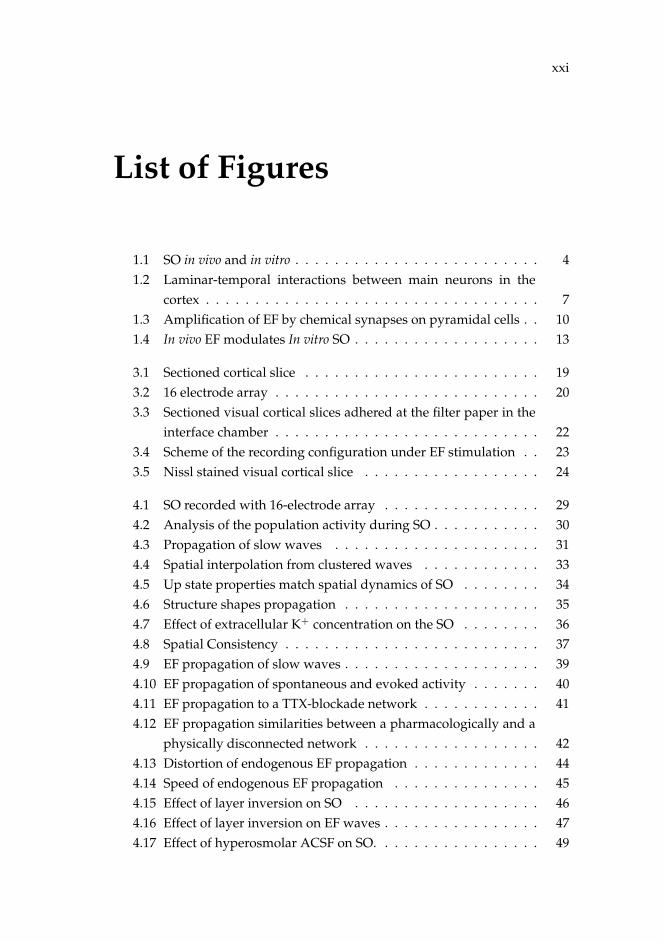
List of Figures
1.1 SO in vivo and in vitro . . . . . . . . . . . . . . . . . . . . . . . . . 41.2 Laminar-temporal interactions between main neurons in the
cortex . . . . . . . . . . . . . . . . . . . . . . . . . . . . . . . . . . 71.3 Amplification of EF by chemical synapses on pyramidal cells . . 101.4 In vivo EF modulates In vitro SO . . . . . . . . . . . . . . . . . . . 13
3.1 Sectioned cortical slice . . . . . . . . . . . . . . . . . . . . . . . . 193.2 16 electrode array . . . . . . . . . . . . . . . . . . . . . . . . . . . 203.3 Sectioned visual cortical slices adhered at the filter paper in the
interface chamber . . . . . . . . . . . . . . . . . . . . . . . . . . . 223.4 Scheme of the recording configuration under EF stimulation . . 233.5 Nissl stained visual cortical slice . . . . . . . . . . . . . . . . . . 24
4.1 SO recorded with 16-electrode array . . . . . . . . . . . . . . . . 294.2 Analysis of the population activity during SO . . . . . . . . . . . 304.3 Propagation of slow waves . . . . . . . . . . . . . . . . . . . . . 314.4 Spatial interpolation from clustered waves . . . . . . . . . . . . 334.5 Up state properties match spatial dynamics of SO . . . . . . . . 344.6 Structure shapes propagation . . . . . . . . . . . . . . . . . . . . 354.7 Effect of extracellular K+ concentration on the SO . . . . . . . . 364.8 Spatial Consistency . . . . . . . . . . . . . . . . . . . . . . . . . . 374.9 EF propagation of slow waves . . . . . . . . . . . . . . . . . . . . 394.10 EF propagation of spontaneous and evoked activity . . . . . . . 404.11 EF propagation to a TTX-blockade network . . . . . . . . . . . . 414.12 EF propagation similarities between a pharmacologically and a
physically disconnected network . . . . . . . . . . . . . . . . . . 424.13 Distortion of endogenous EF propagation . . . . . . . . . . . . . 444.14 Speed of endogenous EF propagation . . . . . . . . . . . . . . . 454.15 Effect of layer inversion on SO . . . . . . . . . . . . . . . . . . . 464.16 Effect of layer inversion on EF waves . . . . . . . . . . . . . . . . 474.17 Effect of hyperosmolar ACSF on SO. . . . . . . . . . . . . . . . . 49

xxii
4.18 Effect of hyperosmolar ACSF on EF propagation. . . . . . . . . . 504.19 Effect of EF stimulation on SO. . . . . . . . . . . . . . . . . . . . 524.20 Effect of external EF stimulation on endogenous EF waves. . . . 534.21 Synchrony between disconnected cortical columns at different
EF stimulations . . . . . . . . . . . . . . . . . . . . . . . . . . . . 544.22 Modulation of subthreshold glutamate-induced responses by
endogenous EFs. . . . . . . . . . . . . . . . . . . . . . . . . . . . 564.23 Frequency modulation of spontaneous SO by endogenous EFs . 574.24 Frequency modulation kinetics . . . . . . . . . . . . . . . . . . . 59

xxiii
List of Abbreviations
ACSF Artificial Cerebro-Spinal FluidAHP AfterhyperpolarizationBMI Bicuculline MethiodideCV Coefficient of VariationCSD Current Source DensityDC Direct CurrentEEG ElectrencephalogramsEF Electric FieldEPS Erly Propagation StripEPSP Excitatory Postsynaptic PotentialGABA Gamma-Aminobutyric AcidIG InfragranularLFP Local Field PotentialMEG MagnetoencephalogramMUA Multi Unit ActivityNMDA N-Methyl-D-AspartateND Normalized DifferencePC Peak CompressionPFC Prefrontal CortexPLV Phase Locking ValueREM Rapid Eye MovementSE StandardErrorSG SupragranularSO Slow OscillationsTTX Tetrodotoxin


1
Chapter 1
Introduction
The cerebral cortex is organized in complex circuits of neurons stronglyinterconnected in a conductive medium. During deep sleep stage, thisneuronal connectivity generates recurrent synchronized synaptic activityleading to transition states where periods of activity are interspersed withperiods of silence. This stereotyped pattern of alternate states is manifestedas slow oscillations (SO), <1 Hz rhythm that dominates the cortical networkduring slow wave sleep (Steriade et al., 1993b) becoming important formemory consolidation (Marshall et al., 2006), plasticity (Reig et al., 2006; Reigand Sanchez-Vives, 2007) and metabolic homeostasis (Xie et al., 2013). Thespatiotemporal dynamic of the SO is more complex than the simultaneousactivation of neurons in a local network. The SO travels with a pattern ofpropagation in the cortical network, with a preference in the anterior toposterior direction (Massimini et al., 2004; Ruiz-Mejias et al., 2011).This oscillatory rhythm, which can be observed at single neuronal level andat the population level, generates extracellular fields that are prominentenough to be measured extracellularly on the conductive medium (local fieldpotentials, LFP) or even from the skull surface (electroencephalograms, EEG).Many excellent studies have raised awareness of the mechanisms involved inthese extracellular signals generated by neuronal populations (Kajikawa andSchroeder, 2011; Buzsaki et al., 2012; Herreras, 2016; Telenczuk et al., 2017).Moreover, in the last years it has been proved how the electric fields (EFs)generated by neuronal activity, in turn, induce changes in such activity ofneurons (Frohlich and McCormick, 2010; Anastassiou et al., 2011). In otherwords, the electric environment generated by neuronal activity has a feedbackeffect on the synaptic activity. In this manner, exogenous electric fieldsused in non-invasive brain stimulation provide a broad scope of therapeuticapplications by modulating brain activity.
2 Chapter 1. Introduction
In this thesis, I will explore how the synaptic and non-synaptic componentsmodulate each other during the propagation of SO. For this purpose, I willdescribe the propagation pattern of SO across the cerebral cortex; then I willinvestigate the endogenous EFs generated by slow waves dissecting it fromthe synaptic components to further investigate the modulation that they mayinduce on the cortical SO.
1.1 The slow oscillation: a rhythmic pattern
Interconnected neuronal networks within the brain have the capacity tomaintain and process information, leading to different temporal dynamicswhich vary as a function of brain states. A clear example of this phenomenonappears during non-REM sleep, an unconscious state period during whichdifferent rhythms such as spindles (7-14 Hz) arise during the early state ofnon-REM sleep, and delta (1-4Hz) and SO (<1 Hz) during later stages.
The SO occurring during slow wave sleep represents one of the intrinsicdynamics of the brain network (Sanchez-Vives and Mattia, 2014). Generatedand maintained by neuronal activity synchronization, SO consists in apattern of recurrent activity in which active periods of neural activity (Upstates) intersperse with relative silence (Down states). Such synchronizedtransitions were first described in striatum (Wilson and Groves, 1981) to laterbe characterized in the cortex and thalamus (Steriade et al., 1993b,a). Pioneerstudies in anesthetized cats have shown that SO are associated with spindleand delta rhythms in the corticothalmocortical network. While spindlesare generated in the thalamus, independently of the slow rhythms, deltafrequency appears to be associated with the SO and is generated in boththalamus and cortex (Steriade et al., 1993c).Moreover, SO elicits fast oscillatory rhythms during Up states, similar tothose observed during awake states (Steriade et al., 1996; Destexhe et al.,1999; Hasenstaub et al., 2005; Compte et al., 2008). The presence of thesefast rhythms might induce synaptic plasticity by increasing the number ofconnections in the cortex, and therefore suggest an important role in memoryconsolidation (Marshall et al., 2006). On the other hand, synchronous silencesduring Down states have been associated with beneficial effects in preventingcellular damage and maintaining cellular processes (Vyazovskiy and Harris,

1.1. The slow oscillation: a rhythmic pattern 3
2013).
1.1.1 How does the slow oscillation emerge?
There has been a great interest in understanding the mechanisms that driveSO and their functional outcomes (Sanchez-Vives and McCormick, 2000;Timofeev et al., 2000; Bazhenov et al., 2002; Volgushev et al., 2006; Neske,2015). Although some SO features remain unexplored, many network andcellular mechanisms have already been established.
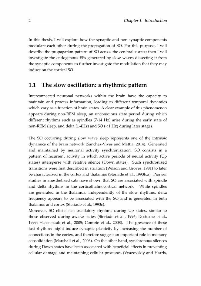
Regarding network mechanisms, already in 1993 Steriade and collaboratorsdescribed how the SO emerges as a local cortical phenomenon which resultsfrom the orchestration of excitatory and inhibitory components. Withexperiments performed under thalamic lesions they revealed the corticalorigin of SO. Later studies proved how such slow oscillatory pattern canbe spontaneously sustained in limited circuits for long periods of time (Fig.1.1), allowing a better exploration of the cellular and network mechanisticdetails involved (Sanchez-Vives and McCormick, 2000; Timofeev et al.,2000). However, certain controversy has arisen about the contribution ofthe thalamus in the origin of SO, which through its inputs to layer 4 mightinfluence the initiation of slow wave activity (David et al., 2013; Fiathet al., 2016). Recent studies justified the thalamocortical circuit as a uniquefunctional network where the thalamus also generates the SO (Crunelli andHughes, 2010; Crunelli et al., 2015).
Regarding cellular mechanisms, experiments in cortical slices (Sanchez-Vivesand McCormick, 2000) or deafferented cortical slabs (Timofeev et al., 2000)disclosed how the SO emerges as a cortical network phenomenon where mostneurons are involved. Excitatory pyramidal neurons seem to be responsible forthe electrical synchronization in cortical networks (Steriade et al., 1993b). Thissynchronization persists thanks to the synaptic excitation/inhibition balancewhich maintains active states over hundreds of milliseconds (Compte et al.,2009; Neske, 2015). Excitation at infragranular (IG) layers (see ”Propagationof slow oscillations within a cortical structure” section) causes the onset of Upstates while K+ currents lead to their offset (Sanchez-Vives and McCormick,2000; Compte et al., 2003). Recently, a combination of voltage-sensitive dyewith extracellular multielectrode recordings allowed specifying the temporal
4 Chapter 1. Introduction
FIGURE 1.1: SO in vivo and in vitro A. Intracellular recordingshowing depolarization and hyperoplarization of a singleneuron in the anesthetized cat. B. Depolarizations examplesfrom A. C. Autocorrelograms of the intracellular recordingsrepresenting the periodicity of the oscillation. D-F. Sameas A-C in a cortical ferret slice. (D, top) extracellularmultiunit-activity. Reproduced from Nature Neuroscience
(Sanchez-Vives and McCormick, 2000).
spike sequences during SO, revealing a larger contribution of inhibitory cellsduring Up states than during Down states on the barrel cortex of anesthetizedrats (Reyes-Puerta et al., 2016). Besides the neural components, it has beenproposed that astrocytes can also be involved in Up state generation bycontrolling extracellular glutamate in the cortical network (Poskanzer andYuste, 2011).
At the molecular level, a role of persistent Na+ currents andN-Methyl-D-Aspartate (NMDA)-mediated excitatory postsynaptic potential(EPSP) have been suggested in the initiation of active states (Steriade et al.,

1.1. The slow oscillation: a rhythmic pattern 5
1993b; Sanchez-Vives and McCormick, 2000). Likewise Ca+-dependentK+ currents on the long lasting hyperpolarization seem to be involvedin the Up states offset (Steriade et al., 1993b; Compte et al., 2003). Theseassumptions were reinforced in the slab studies (Timofeev et al., 2000)and slice preparations, where the blockade of non-NMDA glutamatergicreceptors abolished SO occurrence, and slow afterhyperpolarization (AHP)reversal potentials suggested an increase in K+ conductances (Sanchez-Vivesand McCormick, 2000). Moreover, blockade of GABAA led to shorter Upstates with increased AHP, concurring with the proposed mechanisms of K+
channels as the candidates for Up state termination (Sanchez-Vives et al., 2010).
1.1.2 Slow oscillations within the cortical structure
A large number of studies have focused on the anatomical organization ofneural networks in an attempt to infer functions from structures (Thomsonand Lamy, 2007; Stetter et al., 2013; Markram et al., 2015; Pielecka-Fortunaet al., 2015; Lee et al., 2016).Regarding the SO previously described, recent work on mouse prefrontalcortex (PFC) slices postulates that intrinsic properties of neurons, whichare critical to generate delta oscillatory rhythms, occasionally synchronizesmall cluster of neurons; and this synchronization arises due to the networkstructure that tends to connect proximal neurons (Blaeser et al., 2017).In addition, slow waves have been described as traveling waves within thewhole brain (Massimini et al., 2004; Ruiz-Mejias et al., 2011; Stroh et al., 2013).In anesthetized and sleeping humans and mice, SO can be originated at anycortical area and propagate in any direction, however there is preference to beoriginated in anterior regions to propagate to posterior areas.It is thus of interest to study to what extent the network structure determinesthe origin and propagation of SO.
The neocortex is shaped by columnar and laminar structures that arise dueto the anatomical and physiological arrangement of thousands of neurons, alayout that is conserved across different species. Many neuronal classificationscan be done based on morphology, electrophysiological properties, proteinexpression and connectivity (McCormick et al., 1985; Douglas and Martin,2004; Thomson and Lamy, 2007; Ascoli et al., 2008; Markram et al., 2015).Briefly, the massive cortical circuitry configuration can be simplified in

6 Chapter 1. Introduction
two main populations of neurons identified as pyramidal (excitatory) andinterneurons (inhibitory) neurons. Those are distributed heterogeneouslywithin six layers (supragranular, SG: layer 1-3; granular: layer 4; IG: layer5-6) that result from the neuronal migration during development (Arionet al., 2007). Under this structure neurons communicate through verticaland horizontal connections in the cortex (Lorente de No, 1934; Cajal, 1952;Bannister, 2005).
In a generalized view of the neocortical circuit, pyramidal cells mainlyconform the excitatory flow between layers: starting within layer 4 whichreceives input from the thalamus to further communicate with layer 2/3; thenlayer 2/3 projects to layer 5, which projects to layer 6, and has a feedbackconnection to layer 2/3. This feedback loop between layer 2/3 and layer5 seems to overcome the inhibition that superficial layers may cause to thecortex. At the same time, layer 6 returns the information to layer 4 closing theloop (Fig. 1.2). Also, intralaminar excitatory communication is present withinlayer 2/3 and layer 5, being stronger in the latter (Douglas and Martin, 2004;Thomson and Lamy, 2007; Wester and Contreras, 2012).
Whereas excitatory neurons establish most of their connections betweenlayers; inhibitory neurons mainly form synapses within their local layer(Douglas and Martin, 2004; Thomson and Lamy, 2007). Regarding inhibitorycircuitry, layer 1 which is composed primarily of interneurons together withapical dendrites and axon terminals, seems to confine the communicationbetween neurons. This layer seizes feedback projections from other areas aswell as receives subcortical inputs (Douglas and Martin, 2004). To the greatestextent, inhibitory circuits within the entire cortex regulate excitatory circuits,although recent studies point to a direct role of inhibition in contributing tofunctional networks (Ascoli et al., 2008; Maffei, 2017).
Considering the previously described massively interconnected wiringnetwork, many studies have explored how such cortical structure takespart on the origin and spreading of SO (Sanchez-Vives and McCormick,2000; Wester and Contreras, 2012; Beltramo et al., 2013; Reyes-Puerta et al.,2016). A recent in vivo study (Fiath et al., 2016) reported the contributionof different layers on this rhythmic activity. Briefly, the authors exploredthe spatial distribution of synaptic/transmembrane currents and spikingactivity along the laminar cortex during SO. As a result, current source density

1.1. The slow oscillation: a rhythmic pattern 7
FIGURE 1.2: Laminar-temporal interactions between mainneurons in the cortex Time towards the right displaying 5consecutive synaptic crossing. Gray circles, pyramidal cells.Black circles, interneurons. P: pyramidal cells. B: basketcells. Tax: thalamic afferents. L6Pax: Layer 6 pyramidalarbors projecting to layer 4. Reproduced from Annual Review
of Neuroscience (Douglas and Martin, 2004).
(CSD) analysis revealed the longer source on superficial layers, while a sinkappeared in the middle layers during Up states. Layer 4 displayed the higherdepolarization on LFP recording while the multiunit activity (MUA) wasmaximal at layer 5, exhibiting more frequent firing at the onset of Up states,and suggesting a possible initiating role of layer 4 and a major contribution oflayer 5 on Up state generation (Fiath et al., 2016).
Regarding layer 2/3 the probability of connection between neurons ishigher if they allocate a common input, nevertheless connectivity in this layeris weaker than in layer 5 in cortical slice preparations (Wester and Contreras,2012). It has been proved how layer 5, which communicates columns withlarger EPSPs than layer 2/3 (Douglas and Martin, 2004), resulted to bemore efficient to transfer excitation to other nearby cells under optogeneticactivation of pyramidal cells in in vivo mice (Beltramo et al., 2013); what ismore, layer 5 that depolarizes layer 2/3 during SO propagation, also receivesfeedback propagation from layer 2/3 to later spread the activity within thecortical columns (Wester and Contreras, 2012). In addition, simultaneous
8 Chapter 1. Introduction
recordings performed with voltage sensitive dye imaging and multielectrodesshowed shorter latencies between spike firing and Up state onset at IG layerthan at SG layers, confirming the upward propagation of SO from deep tosuperficial layers (Sanchez-Vives and McCormick, 2000; Reyes-Puerta et al.,2016). Thus, once the activity is recruited, the propagation occurs radiallyand homogeneously from deep to superficial layers without preference for thedirection (Reyes-Puerta et al., 2016).In spite of this combined neural activity between IG and SG layers, which caninduce spontaneous transmitter release in any neuron leading to depolarizedstates (Chauvette et al., 2010), the large amount of synapses arriving to layer5, as well as the presence of a subtype of pyramidal cells (low-frequencybursting) in this layer which might drive the Up states onsets (Lorincz et al.,2015), indicate that layer 5 mediates transitions from Down to Up states.Moreover, activity within layer 5 is able to hold and spread horizontally thecortical rhythm without the contribution of layer 2/3 (Sanchez-Vives andMcCormick, 2000; Wester and Contreras, 2012). Hence, a large amount ofevidence points to layer 5 as crucial for the generation and propagation of SO(Sanchez-Vives and McCormick, 2000; Wester and Contreras, 2012; Beltramoet al., 2013; Fiath et al., 2016; Reyes-Puerta et al., 2016; Blaeser et al., 2017).
Overall, it seems that SO start in layer 5 and spread radially to superficiallayers. The feedback projections from superficial layers to deep layers,together with the horizontal projection within layer 5 drive the propagationacross columns in the cortical network (Sakata and Harris, 2009; Okun andLampl, 2008). However, it has not yet been studied to what extent thespatiotemporal pattern of the SO is determined by the cortical structure,and how the global excitability of the neuronal population can modulate itsspatiotemporal dynamics.
1.2 From synaptic activity to electric fields
Synaptic activity is considered the most important component for a dynamicinteraction between neural networks. However, the electrical phenomenonthat arises when different charges move across neuronal membranesgenerating currents should not be dismissed. EEG measurements at thescalp surface indicate that synaptic and electric fields (EFs) coexist in neural

1.2. From synaptic activity to electric fields 9
tissue, and what is more they propagate within it (Buzsaki et al., 2012). Thus,synapses, together with other active mechanisms, contribute to extracellularelectric currents that, when superimposed at a specific position, generate fieldpotentials (Kajikawa and Schroeder, 2011; Herreras, 2016). In this manner, itremains a challenge to separate synaptic from non-synaptic components whenmeasuring neural activity.LFP is the low-pass component of the extracellular currents, and it is widelyused as an extracellular measure of brain activity. As long as the LFP is aremote rather than a local measurement (Kajikawa and Schroeder, 2011),there is a strong possibility that it reflects activity of structures far from therecording point (Herreras, 2016). Thus, many studies have explored its originin order to better understand the activity that it mirrors (Weiss and Faber,2010; Kajikawa and Schroeder, 2011; Buzsaki et al., 2012; Anastassiou et al.,2015; Herreras, 2016).
1.2.1 How do electric fields emerge?
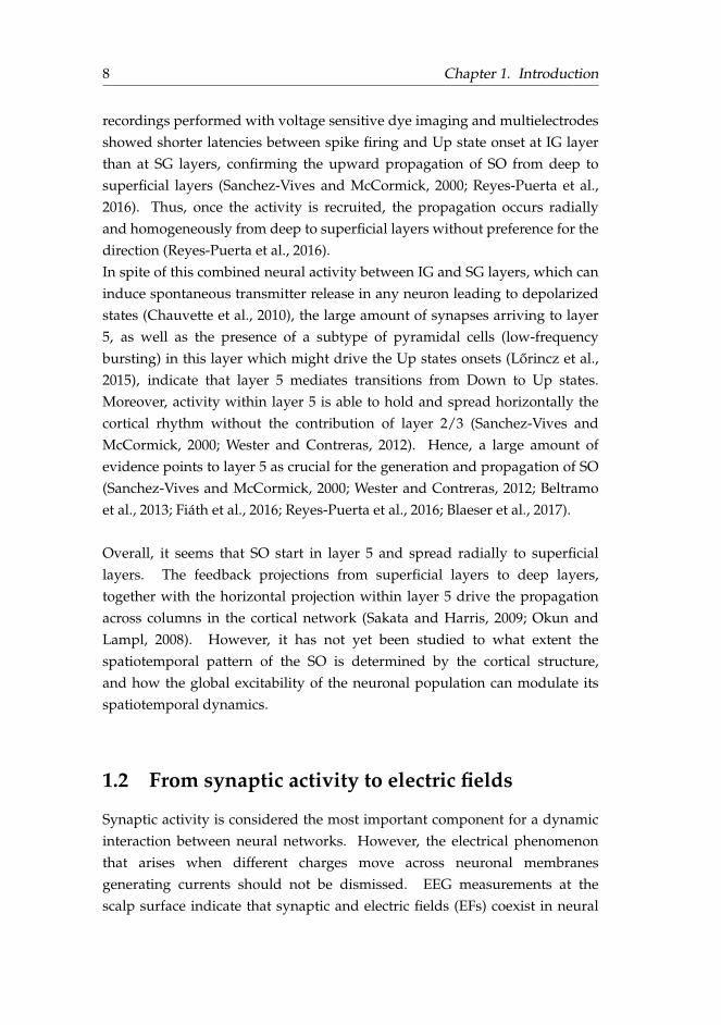
By and large, pyramidal cells are considered the major contributors toextracellular fields as a result of their shape (their long somatodendritic axisgenerates strong dipoles) and abundance in the cortex. In addition, theirspatial distribution and temporal synchrony determine the magnitude ofextracellular currents (Fig. 1.3A) (Weiss and Faber, 2010; Buzsaki et al., 2012).Current sources with neuronal origin present a dipolar structure (Herreras,2016); in addition, the large current fluctuations at the pyramidal somasoccurring when activity is synchronized leads to distinct polarity zones(positive and negative) (Buzsaki et al., 2012). This way, an extracellular dipoleis formed between IG and SG layers in the cortical network; the paralleldistribution of pyramidal cells causes a current flow perpendicular to theiraxis that when superimposed generates the active dipole. An outcome of thisis the polarity inversion observed at SG layers in the LFP when recording SOacross cortical layers (Fiath et al., 2016)(Fig. 4.1). Thus, the fact that both SGand IG layers reflect depolarization of neuronal populations during Up stateswith different polarities on the LFP (positive and negative, respectively), isin line with the idea that LFP polarity does not mirror the active currents ofsynapses (Kajikawa and Schroeder, 2011; Herreras, 2016).
Those current flows along the vertical axis of pyramidal neurons, which result
10 Chapter 1. Introduction
FIGURE 1.3: Amplification of EF by chemical synapses onpyramidal cells A, Schematic of pyramidal cells arranged ina parallel orientation. Color code indicate the extracellularpotential. B. Feedback effect between synaptic activity andits EF. Reproduced from Frontiers in Neural Circuits (Weiss and
Faber, 2010).
in a dipole on the cortical network, illustrate the variation along time of theEFs, in other words, they illustrate EF propagation (Buzsaki et al., 2012). Thetransmission of EF through biological tissue from a source to a measurementsensor defines the term volume conduction (Rutkove, 2007). The expansionof the volume conduction will be determined by the current dipole, alreadydescribed, and the conductivity of the medium (Buzsaki et al., 2012).
1.2.2 Electric fields within the brain tissue
Regarding the conductivity in the brain tissue, there is controversyabout whether we should consider the brain as a homogeneous or anon-homogeneous medium. On one hand, cortical impedances measured inthe visual cortex of in vivo monkeys described the tissue as a homogeneousmedium where the EF propagation is isotropic and permits an equitablepropagation of any frequency, meaning that tissue impedance is frequencyindependent. According to this, LFP dimension will be determined by the sizeof the signal rather than by tissue properties (Logothetis et al., 2007). On theother hand, frequency attenuation is observed when measuring extracellularpotentials, leading to higher spacial coherence in SO than in high frequencyoscillations (Destexhe et al., 1999). The homogeneous isotropic medium doesnot reflect the frequency dependent attenuation, so it is not adequate for

1.2. From synaptic activity to electric fields 11
modeling LFP signals. A non-homogeneous extracellular conductivity resultsin a low pass filter that makes the low frequency events attenuate less withdistance, generating the LFP/EEG signals. These frequency filtering propertiesof the tissue are determined by the structural composition of the medium,which requires considering the extracellular medium non-homogeneous andanisotropic (Bedard et al., 2004). This debate remains open the questionwhether the tissue has any influence on the EF propagation.
Considering the above, greater attention has been focused on the role ofvolume conduction and EF propagation in the brain tissue, as they are alsoreflected on extracellular signals toghether with the spiking activity.Good evidence that emphases the need to pay heed to non-synapticmechanisms when measuring LFP was reported in the study of Kajikawa andSchroeder, where sources (positive charges traveling to the extracellular space)and sinks (positive charges traveling to the intracellular space) obtained withcurrent source density analysis (CSD) could not reproduce the observed LFP.Besides, responses to different tones recorded at two different sites eliciteddifferent spatial propagation of LFP, CSD and MUA. While CSD and MUAdisappeared when moving the frequency tone from the best frequency tone,LFP measurement remained (the order of the spatial spread differences were:LFP >CSD >MUA) (Kajikawa and Schroeder, 2011). Therefore, volumeconduction may exert a greater impact on LFP than on MUA (or CSD).Hence, the neural activity reflected on LFP signals propagate not only throughsynaptic events, but also through non-synaptic mechanisms.
Indeed, recent work on an unfolded hippocampus preparation showedhow epileptiform activity propagates by EFs at surprisingly low speed(∼0.1 m/s) independently of synaptic activity (Zhang et al., 2014). Tofurther investigate the role of the extracellular medium on this propagation,osmolarity was increased in order to enlarge the distances between neuronsand widen the extracellular space (Traynelis and Dingledine, 1989). The resultwas a reduction of 46.8 % in speed propagation (Shahar et al., 2009; Qiu et al.,2015) revealing that extracellular space has an influence on EF propagation,particularly decreasing its velocity when increasing the space.

12 Chapter 1. Introduction
1.3 Synaptic activity and electric field dialogue
Under this scenario where synaptic and non-synaptic mechanisms coexist,there is a feedback effect between the structural neural activity and theendogenous EFs which shape and modulate the final network activity (Fig.1.3B) (Jefferys, 1995; Frohlich and McCormick, 2010; Weiss and Faber, 2010;Anastassiou et al., 2011; Schmidt et al., 2014; Anastassiou and Koch, 2015).The interactions of EF are shaped by the temporal dynamics of synapticactivity (Weiss and Faber, 2010). When these interactions lead to changesin the membrane potential of neurons, and consequently in spiking, it canyield a non-synaptic mechanism known as ephaptic coupling (Anastassiouand Koch, 2015). Ephaptic coupling mainly affects population activity underhypersynchronous states (Buzsaki et al., 2012); it can induce small but coherentchanges in the firing timing of neuronal populations, thus implying that fieldeffects can modulate oscillatory activity (Reato et al., 2010).
The three main components of neural activity (synapses, neurons andnetworks) are sensitive to extracellular EF (Anastassiou and Koch, 2015). EFcan alter the presynaptic membrane potential by inducing changes in the ionicflows. Also, EF can influence chemical synaptic transmission in a network byclearing negative glutamatergic charges or through changes in voltage gatedchannels, as well as by mediating neurotransmission and collaborating in fastrhythmogenesis (Weiss and Faber, 2010).
Researchers that have tried to address the effect of endogenous EF onneuronal activity by applying exogenous EF through two parallel electrodesoutside the tissue preparation (Radman et al., 2007; Frohlich and McCormick,2010; Reato et al., 2010; Schmidt et al., 2014), report a critical effect of weak EFstimulation on spiking neural activity due to its impact on membrane voltage.Besides, in a 12 pipette set up, where electrical stimulation was applied insideand outside individual cells while recording extracellular fields at differentspecific locations next to an active neuron, elicited ephaptic coupling atthe level of single cells. Extracellular EF was not able to induce any actionpotential, but it did entrain subthreshold activity and spike trains when itoscillated at slow rhythms (1 Hz) (Anastassiou et al., 2011).These results reinforce the idea that EF effects can be strong enough to bemagnified on the network dynamics. In particular, in vitro experiments onhippocampal slices, together with an in silico model supported that weak

1.3. Synaptic activity and electric field dialogue 13
applied EFs influenced oscillatory activity (Reato et al., 2010); in this manner,ephaptic coupling synchronizes networks with a stronger feedback effecton oscillatory patterns, specially on SO (Frohlich and McCormick, 2010;Anastassiou et al., 2011; Anastassiou and Koch, 2015).
It was the pioneering work of Frohlich and McCormick in 2010 whichclearly exhibited the effect of an endogenous (and not exogenous) EF onspontaneous oscillatory activity. In cortical ferret slices eliciting SO, theyapplied weak external EF stimulation (2-4 V/m) through two parallelelectrodes that mimicked the endogenous in vivo field activity recorded inanesthetized ferrets. This EF stimulation was able to modulated the oscillatorynetwork activity (Fig. 1.4), supporting the idea that endogenous EFs are not amere idling of the neural activity (Weiss and Faber, 2010). Further explorationof the feedback between EF and synaptic activity demonstrated that the stateof the targeted network is critical for the effect that EF might induce; so,only weak EF stimulations with frequencies similar to the ongoing oscillationinduced changes in the endogenous activity (Schmidt et al., 2014).
FIGURE 1.4: In vivo EF modulates In vitro SO Left: no fieldapplied (control). Right: in vivo field applied. Top: appliedin vivo field. Middle: multiunit activity recorded in corticalslices. Bottom: multiunit activity averaged from 20-30 trials.
Adapted from Neuron (Frohlich and McCormick, 2010).

14 Chapter 1. Introduction
Despite these experiments demonstrated the feedback interaction betweenEFs and synaptic activity, they did not address the modulation of synapticactivity by its authentic endogenous EF.
1.3.1 The slow oscillation as the key player
Considering the above, the SO represents a suitable testbed to study thesynaptic and non-synaptic propagation, as well as the interaction betweenboth components. First, the SO reflects an emergent property of the networkwhere the neural activity is synchronized in active and silent states (Steriadeet al., 1993b). Second, it can be spontaneously generated (and also induced) invitro preserving its fundamental properties (Sanchez-Vives and McCormick,2000) while easing specific manipulations (see Materials and Methods chapter)to better control the local cortical circuit, and thus explore its dynamicsalong the cortical structure. Third, as emergent property of the network, it ismore sensitive to the field effects than single neurons activity (Anastassiouand Koch, 2015); and at the same time, as oscillatory pattern, it will revealbetter the effect of endogenous EF in the neuronal activity (Weiss and Faber,2010). Fourth, SO has been proved to be the oscillatory rhythm producing thegreatest effect on ephaptic coupling (Anastassiou et al., 2011).
Moreover, the SO seems to be the default mode activity of the corticalmantle during deep sleep, anesthesia, or even in cortical slices preparation(Sanchez-Vives and Mattia, 2014; Sanchez-Vives et al., 2017b). Suchsynchronized cortical activity occurs during functional and anatomicaldisconnection from other inputs and is associated to a broad range ofdifferent functions, from metabolic homeostasis (Xie et al., 2013) and cellularmaintenance (Vyazovskiy and Harris, 2013), to plasticity recalibration (Reiget al., 2006; Reig and Sanchez-Vives, 2007) and memory consolidation(Marshall et al., 2006). Additionally, the SO has been suspected to be thebasal frequency needed to group other higher frequencies (spindle and delta)contributing to the reorganization of distant networks (Neske, 2015). Thus,elucidating the SO mechanisms will give information about the propertiesof the underlying network, and can be useful to develop mechanisticinvestigations for neurological disease were the functions just mentioned areimbalanced (Ruiz-Mejias et al., 2016; Castano-Prat et al., 2017).

15
Chapter 2
Objectives
The principal aim of this thesis is to determine the role of synaptic andnon-synaptic (endogenous electric fields) components in the generation andpropagation of slow waves.
Regarding the propagation of slow waves, the objectives are:
1. To explore the spatiotemporal patterns of slow wave propagation acrosscortical columns and layers.
2. To determine how excitability modulates the spatiotemporal regularityof the slow oscillatory activity in the cortical network.
Regarding the non-synaptic propagation of slow waves, the objectives are:
1. To explore the propagation of endogenous electric fields induced byslow waves in the cortical tissue, dissecting them from the synapticcomponents.
2. To study the influence that the laminar structure and the size of theextracellular space may exert on the electric field propagation of slowwaves.
3. To investigate the modulation that endogenous electric fields may induceon cortical slow waves.


17
Chapter 3
Materials and Methods
3.1 Experimental procedure
The main methods used during this doctoral thesis consisted of in vitroexperiments performed in 98 visual cortical slices from ferrets (Mustela putoriusfuro) (Sanchez-Vives and McCormick, 2000). Cortical slice preparation allowsus to explore and manipulate the local cortical microcircuit easily accessingall cortical layers. In addition, this preparation is well known for elicitingrobust spontaneous slow oscillations (SO) (Sanchez-Vives and McCormick,2000; Compte et al., 2008; Sanchez-Vives, 2012) similar to the ones observedduring slow-wave sleep (Steriade et al., 1993b). These advantages made the invitro preparation ideal to achieve the objectives mentioned above.Two different sets of experiments were done to study synaptic andnon-synaptic propagation of an active cortical circuit. Preparation andmaintenance of slices, as well as extracellular local field recordings werecommon along all experiments. Different protocols and analysis wereperformed, mainly for the non-synaptic propagation experiments, which willbe described in detail.
3.1.1 Preparation and maintenance of slices
Ferrets (4-10 months old, both sex) were anesthetized with sodiumpentobarbital (40 mg/kg) and decapitated. The entire forebrain was rapidlyremoved to oxygenated cold (4-10C) bathing medium (Sanchez-Vives, 2012).Ferrets were treated in accordance with the European Union guidelines onprotection of vertebrates used for experimentation (Strasbourg 3/18/1986). Allexperiments were approved by the local ethical committee.Coronal slices (0.4 mm thick) from visual cortex (areas 17, 18 and 19) were
18 Chapter 3. Materials and Methods
used. A modification of the sucrose-substitution technique (Aghajanianand Rasmussen, 1989) was used to increase tissue viability. During slicepreparation, the tissue was placed in a solution in which NaCl was replacedwith sucrose while maintaining osmolarity. After preparation, the slices wereplaced in an interface style recording chamber (Fine Sciences Tools, FosterCity, CA), where they were superfused with an equal mixture in volumeof the normal bathing medium, artificial cerebral spinal fluid (ACSF) andthe sucrose-substituted solution, for 15 minutes. Following this, normalbathing medium was switched into the recording chamber and the slices weresuperfused for 1 hour and 20 minutes; the normal bathing medium contained(in mM): NaCl, 126; KCl, 2.5; MgSO4, 2; Na2HPO4, 1; CaCl2, 2; NaHCO3,26; dextrose, 10; and was aerated with 95 % O2, 5 % CO2 to a final pH of 7.4.Then, a modified slice solution was used throughout the rest of the experiment;it was similar to the normal bathing medium except for different levels ofthe following (in mM): KCl, 4; MgSO4, 1; and CaCl2, 1 (Sanchez-Vives andMcCormick, 2000; Sanchez-Vives, 2012). Bath temperature was maintained at34-36C.
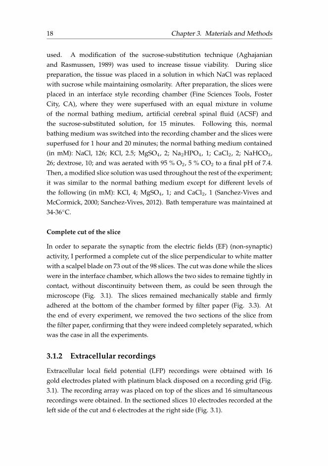
Complete cut of the slice
In order to separate the synaptic from the electric fields (EF) (non-synaptic)activity, I performed a complete cut of the slice perpendicular to white matterwith a scalpel blade on 73 out of the 98 slices. The cut was done while the sliceswere in the interface chamber, which allows the two sides to remaine tightly incontact, without discontinuity between them, as could be seen through themicroscope (Fig. 3.1). The slices remained mechanically stable and firmlyadhered at the bottom of the chamber formed by filter paper (Fig. 3.3). Atthe end of every experiment, we removed the two sections of the slice fromthe filter paper, confirming that they were indeed completely separated, whichwas the case in all the experiments.
3.1.2 Extracellular recordings
Extracellular local field potential (LFP) recordings were obtained with 16gold electrodes plated with platinum black disposed on a recording grid (Fig.3.1). The recording array was placed on top of the slices and 16 simultaneousrecordings were obtained. In the sectioned slices 10 electrodes recorded at theleft side of the cut and 6 electrodes at the right side (Fig. 3.1).

3.1. Experimental procedure 19
FIGURE 3.1: Sectioned cortical slice. A. Sectioned corticalslice picture with a 16 channel array positioned on the surface.Notice the tenuous line at the scissors level showing the cutwithout discontinuity between the resulting slice pieces. B.Schematic of the sectioned cortical slice with 10 electrodesrecording at the left side and 6 electrodes recording at the right
side. WM: white matter; L1-6: layers 1 to 6.
The grid including an array of holes was designed and fabricated usingSU-8 negative photoresist or polyamide (Fig. 3.2). The holes allowedoxygenation of the slices, they were used to provide mechanical stability andto allow pipettes to reach the slice for local drug applications (Fig. 3.3).In each of the recording points, there were 2-3 electrodes (separated by 200µm) (diodes or triodes, respectively). They were positioned such that half ofthem would record from supragranular (SG) and the other half would recordfrom infragranular (IG) layers (diodes / triodes were 750 µm apart in thevertical axis), as well as from 3 different cortical columns (1.5 mm apart in thehorizontal axis) (Fig. 3.1 and 3.2A).The electrodes were 50 µm in diameter, resulting in an impedance values of |Z|∼ 10MΩ at 1 kHz. The impedance was decreased 2-fold by electrochemicallycoating the electrodes with a layer of black platinum, what enhanced theelectrode behavior, resulting in electrode impedance values being two ordersof magnitude below the amplifiers input impedance over the whole frequencyrange. Electrode impedances and phases were tested with known signalsprior to the recordings for each array (Fig. 3.2B); this way we excluded thepossibility of phase delays or distortion that differences in electrode coatingcould induce.
Neural activity was referenced to an electrode placed at the bottom of thechamber in contact with the ACSF. Unfiltered signals were acquired withMultichannel System amplifier and digitized at 10 KHz with a Power1401

20 Chapter 3. Materials and Methods
FIGURE 3.2: 16 electrodes array. A. Customized recordinggrid with 16 electrodes (black dots) organized in 2 or 3groups with holes (white dots) between them. B. Impedancecharacterization before (gray line) and after (black line)coating with black platinum for the whole frequency range.
interface and Spike2 software (CED, Cambridge, UK). No filters were addedduring the recording stage to avoid signal distortion.
3.1.3 Experimental protocols
To study different excitability levels on the propagation of slow waves,the ionic composition of the ACSF was modified on 13 slices by varyingthe K+ concentration from 1 mM to 7 mM (Sancristobal et al., 2016), thesevalues are located at the same level as the one found in vivo (Amzica et al.,2002; Bazhenov et al., 2004). That modification changes the extracellular K+
concentration leading to variations in the excitatory network level.
To explore the influence of structure and extracellular space on thenon-synaptic propagation of slow waves, as well as the modulation betweenboth disconnected networks, different protocols and manipulations wereperformed on the sectioned slices, they are described below.
Drug applications
Different pharmacological agents were used: glutamic acid (glutamate) fromRBI, tetrodotoxin (TTX) from Tocris, bicuculline methiodide (BMI) from Sigmaand saccharose from Scharlau. Applications were either local or batheddepending on the purpose to achieve (explained below).
Glutamate (0.5 mM) and TTX (30 µM) were delivered locally through aglass micropipette. In both cases, borosilicate glass capillaries were pulled ona Sutter Instrument P-97, their tips were broken (1-4 µm diameter) and laterfilled with the drug. Brief pulses of pressure (ranging from 4 to 150 ms, and 5to 30 psi; adjusted depending on the response to evoke) were applied. Such

3.1. Experimental procedure 21
local applications were delivered at different positions within the slice.
Glutamic acid. Local applications of glutamate are widely known to evokehighly stable responses by activating glutamate receptors and recruitinglocal network activity (Sanchez-Vives and McCormick, 1997; Sanchez-Viveset al., 1997, 2008). Such applications allow us to better control the time andlocation where the Up states (or glutamate response) are originated to studytheir non-synaptic propagation. They were used, not only to study the EFpropagation across the cut, but also to investigate modulation between the twodisconnected networks by: (1) inducing small responses in one side to increaseexcitability and see if endogenous EF could trigger spontaneous Up statesin a more depolarized network; and (2) inducing suprathreshold responsesat different frequencies to be able to entrain the disconnected network in adesired frequency.Tetrodotoxin. TTX, selective inhibitor of Na+ channel conductance thatabolishes spontaneous multiunit activity. It was applied to rule out interactionsbetween synaptic and non-synaptic activity.
BMI (2.4 - 3 µM) and saccharose (40 mM) were bath applied. It shouldbe noted that in the interface chamber used it takes around 20 minutes to geta stable concentration in the bath, so all measurements were taken after thisperiod.
Bicuculline methiodide. BMI is a GABAA receptor blocker that acts as acompetitive inhibitor of GABA. It was used to transform the spontaneous SOin epileptiform activity (Sanchez-Vives et al., 2010), generating large responsesstrongly evident across the cut.Saccharose. Saccharose 40 mM was used to increase osmolarity and withit the extracellular space. A concentration of 40 mM saccharose causes anincrease of 40 mOsm (from 328 mOsm on control condition, to 368 mOsmunder hyperosmolar condition), that involves a 12% increment, what has beenproved to have an effect on the propagation of epileptiform activity (Shaharet al., 2009; Qiu et al., 2015).
Inverted slices
To further explore the influence of the laminar cortical structure in thenon-synaptic propagation of slow waves, one side of the cut slices was

22 Chapter 3. Materials and Methods
overturned, such that IG layers were next to SG layers and vice versa. Thismanipulation was done consecutively to the cut in the interface style recordingchamber, the bath flow was increased while gently rotating the right side of theslice with the forceps tips. The result was a sectioned cortical slice where oneside had an inverted laminar structure (Fig. 3.3).
FIGURE 3.3: Sectioned visual cortical slices adhered at thefilter paper in the interface chamber. A. Magnification ofan inverted slice. B. Same preparation with the array on topof the inverted slice and two glass pipettes used for local
applications passing through the array holes.
Electric field stimulation
In order to achieve synchronization between both disconnected networks,the excitability of the whole slice was increased by means of external EFmanipulations. Thus, direct current (DC) stimulation was applied as describedin Frohlich and McCormick, 2010 and Sanchez-Vives et al., 2017a. Briefly,two customized AgCl electrodes (1 mm diameter, 10 mm length) were placedparallel to the cortical surface, this arrangement allowed us to generate a

3.1. Experimental procedure 23
uniform EF parallel to the apical - dendrite axis of pyramidal cells. Thus,positive fields (oriented from IG layers to SG layers) depolarized pyramidalcells leading to an increase in the network excitability; while, negative fields(oriented from SG layers to IG layers) decreased the network excitability byhyperpolarizing pyramidal cells (Fig. 3.4). The different EF applied (±1-4V/m) were calibrated before every experiment. The current to generate thefield was produced with a stimulus isolator (360A, WPI, Aston, UK).
FIGURE 3.4: Scheme of the recording configuration under EFstimulation. Stimulation electrodes parallel to white matter(WM). Positive/negative EF parallel to the pyramidal neuronsaxis (red/gray, respectively). 16 electrodes recording from
supragranular (SG) and infragranular (IG) layers.
3.1.4 Histology
Nissl staining was used for visualizing lamination of the cortex and studyingslow wave propagation across columns and layers. After recording, 9 sliceswere marked where the array was positioned and fixed in paraformaldehyde(4%) for later Nissl staining. Slices 400 µm were washed during 4-5 days in0.1 M PB containing 30% saccharose. Then 50 µm thick slices were cut in aThermo Scientific MICROM HM 450 microtome and placed on gelatin-coatedglass slides. After drying overnight, slices were incubated 2 hours in ethanol70% for the subsequent double toluidine staining: first, nuclei were stainedby an incubation of 15 minutes on toluidine blue and afterward dehydratewith ascending alcohol series, 5 minutes incubation on xylene was done toclarify the tissue for the second staining. Second, similar incubations, 10-15minutes toluidine and different increasing alcohols, finishing with two xyleneincubations were used to stain cytoplasm. Finally, slices were mounted inDePeX medium. Images were visualized and taken with a confocal laser

24 Chapter 3. Materials and Methods
microscope.Layers were limited according to density and size of the observed cells(Homman-Ludiye et al., 2010) (Fig. 3.5).
FIGURE 3.5: Nissl stained visual cortical slice. A. Completevisual cortical slice Nissl stained with the 16 channelselectrode array superimposed (black circles) according to theobserved marks (white arrows). Layer limits displayed withdashed lines. B. Amplifications of A displaying differencesbetween layers. L1:the less dense layer, L2: the thinnest layerwith mainly bulky cells, L3: the thickest layer with mixture ofsmall and bulky cells; L4: layer with big pyramidal neurons(top arrow) mixed with smaller cells displaying a clearercolumnar pattern (dash circle); L5: layer less dense than L4and L6 with big pyramidal cells (arrow); L6: mixture of small
and big cells.
Nissl staining was performed in collaboration with Alberto Munoz Cespedes atJavier de Felipe laboratory (Instituto Cajal, Madrid).
3.2 Data analysis
All analysis were performed offline with either custom-written or Matlabtoolbox scripts (The MathWorks Inc. Natick, MA). Spike2 software was usedfor offline analysis when stated. All average values are presented as mean ±SE.
3.2.1 Multiunit Activity and Up/Down state detection
From all of the recordings multiunit activity (MUA) was estimated to furtherdetect Up and Down states from the SO as described in previous works

3.2. Data analysis 25
(Compte et al., 2008, 2009; Reig et al., 2010; Sanchez-Vives et al., 2010;Ruiz-Mejias et al., 2011; Mattia and Sanchez-Vives, 2012; D’Andola et al.,2017). Briefly, MUA was estimated as the change in power of the Fourier highfrequency components from the LFP signal. Later, population firing rate wasobtained from the MUA (Mattia and Del Giudice, 2002). To detect Up statesa threshold was set in the log(MUA) as described in Reig et al., 2010 andRuiz-Mejias et al., 2011 (Fig. 4.2).From the transformed log(MUA) signal different parameters were quantified:frequency of the SO, Up and Down state durations, mean and maximum firingrates in the Up states. Coefficients of variation (CV)(standard deviation/mean)were used to measure variability.
3.2.2 Slow wave propagation analysis
To study slow wave propagation within the slice the analysis was based in theUp/Down detection already described. Thus, times at which each electrodecrossed the threshold in the log(MUA) were taken and transformed into timelags. Next, these time lags were interpolated such that a wave-front could bedraw (Fig. 4.4) (Capone et al., under review; Sancristobal et al., 2016).Waves that propagated through every columns were considered and clusteredby Principal Component Analysis based on the origin, speed and direction todifferentiate types of propagation.These clustered waves allowed us to compute an early propagation strip (EPS)from the points where the wavefront tip occurred earlier. EPS plots wereoverlapped with their respective Nissl stained slice pictures to measure theportion of the EPS area included in each layer (Capone et al., in preparation).Also, for each clustered wave, percentages of correlations between them werecomputed for spatial consistency (SC) quantification to explore regularitypatterns under different excitability levels (Sancristobal et al., 2016).
Analysis in the propagation of slow waves were performed in collaboration withMaurizio Mattia (Instituto Superiore di Sanita, Rome, Italy). Specifically, EPSanalysis were performed by Cristiano Capone and spatial consistency analysis by PolBoada.

26 Chapter 3. Materials and Methods
3.2.3 Analysis of non-synaptic propagation of slow waves
To explore the propagation of slow waves in the absence of synaptic activitythe first step was to detect the EF waves in a synaptic disconnected network.With that purpose mean responses were obtained by averaging the signalacross repetitions of spontaneous (or evoked) Up states, triggered glutamateresponses or epileptiform responses, and tested for significant differencesfrom baseline values.Cases where the studied response on one side of the slice overlapped on timewith the spontaneous Up states (or epileptiform responses) of the other sidewere discarded from the averages.
To characterize the damping, distortion and delays on the endogenousEF waves a curve fitting was computed in a time window of 2.5 seconds onthe glutamate responses. Delays were quantified from the latency betweenthe waves peaks at both sides of the cut. Widening and compression weremeasured with respect to the original wave to evaluate the distortion. Thus,peak compression (PC) was defined as the duration difference between thewaves at both side of the cut (the wave reference -Dr -, where the waves areoriginated; and the waves recorded on electrodes at the other side - De -)divided by the reference duration (Gonzalez-Andino et al., under review).
PC =Dr −DeDr
(3.1)
Analysis to characterize the propagation of slow waves in the absence of synapticactivity were performed in collaboration with Sara L. Gonzalez Andino and RolandoGrave de Peralta Menendez (Electrical Neuroimaging Group, Geneva, Switzerland).
Once we were able to asses the presence of the EF responses, we proceededto study the modulation of SO by endogenous EF with different analysisdepending on the protocol performed (detailed below). In all the casesfrequency of Up/Down cycle was quantified at both sides of the cut based onthe log(MUA) detection, as described at the beginning of this section.
Correlations. On the slices where DC stimulation was applied wecomputed correlations between both sides of the cut to look for synchrony.Cross-covariation coefficients were computed on the log(MUA) signal with

3.2. Data analysis 27
Matlab toolbox.Also, phase locking values (PLV) (Lachaux et al., 1999) for SO were quantifiedbetween two different channels from both sides.
Exponential fitting. On the slices where glutamate puffers were deliveredat different frequencies to entrain the rhythmicity of the disconnected networkthe analysis was as follows.First, Up/Down detection was computed to obtained the SO frequency atboth sides. The frequency change of the glutamate release, was considered thereference time from which an exponential fit was adjusted on the frequencyincrease/decrease of the side where no glutamate was applied.
y = a(1− e− 1b t) (3.2)
y = a(e−1b t) (3.3)
Being b the time constant τ (63.2 %) that represents the time needed for thenon stimulated side to be modulated and to change its frequency. Cases whereτ reached values higher than 120 seconds (time period analyzed after thefrequency change) were discarded as outliers.
Then, normalized differences of frequencies (ND) were computed to bettercompare the frequency variation between both sides.
ND =
∣∣∣∣∣F2 − F1
F2+F1
2
∣∣∣∣∣ (3.4)
For the side where the frequency was induced, F1 and F2 were determined bythe local application glutamate periodicity. For the modulated side, F1 is themedian obtained in the 90 seconds previous to the frequency change, and F2
is the asymptotic value of the exponential.
Analysis to study the modulation of SO by endogenous EF were performed incollaboration with Lorena Perez and Alvaro Navarro from our laboratory.

28 Chapter 3. Materials and Methods
3.2.4 Statistics
Values are presented as mean ± SE. Either parametric (Student’s t-test) ornon parametric (Mann-Whitney U test or Wilconson sign-rank test) were useddepending on the properties of the samples to be compared.

29
Chapter 4
Results
Results reported in this thesis show the spatiotemporal dynamics of the slowoscillations (SO) in an in vitro preparation of ferret visual cortex. Specifically,spontaneous SO were recorded with 16-channel array (see Materials andMethods) covering different columns and layers within the cortical slices (Fig.4.1A). This is the first time that, to our knowledge, these 2D recordings are froma slice. A total of 98 slices spontaneously generating SO in most electrodes inthe array were used. Figure 4.1B displays a representative case eliciting thespontaneous rhythmic pattern in the 16 electrodes.
FIGURE 4.1: SO recorded with 16-electrode array. A. Picture(top) and scheme (bottom) of a 16-channel array over a visual
cortical slice. B. 16 channels eliciting spontaneous SO.

30 Chapter 4. Results
From each raw local field potential (LFP) the network relative firing rate wasestimated to further compute Up/Down state transitions and durations asillustrated in figure 4.2A with the red line. Also, the associated multiunitactivity (MUA) color coded in the raster plot and the waveform averageobtained from the relative firing rate were used to calculate transitions states(Fig. 4.2B-C) (see Materials and Methods).
FIGURE 4.2: Analysis of the population activity duringSO. A. Relative firing rate (black) and LFP recording (blue).Up and Down state detection is represented with a redline. B. Raster plot of 60 aligned Up states. C. Waveformaverage of the relative firing rate that is used to calculateDown-Up/Up-Down transitions and maximum firing rate.The shade represents the SD. LFP, local field potential; MUA,
multiunit activity.
4.1 Propagation of slow waves
To achieve the first objective regarding the propagation of slow waves acrosscolumns and layers, I recorded spontaneous SO traveling along the corticalvisual network on 12 slices. The first step was to identify the active and silentperiods that composed SO. Thus, estimation of the multiunit activity (MUA)was used to analyze population firing rate (see Materials and Methods). Fromthis estimation, Up and Down states were represented by the high and lowfiring rate peaks, respectively (Fig. 4.3B). Down peak standard deviation wasconsidered the threshold to further detect transitions between Up and Downstates; and from theses, Up/Down state durations and cycle frequency weremeasured (Fig. 4.3C).

4.1. Propagation of slow waves 31
Similar results to previous works performed with conventional extracellularrecordings were observed (Sanchez-Vives and McCormick, 2000;Sanchez-Vives et al., 2010; Reig et al., 2010): bimodal distribution of theMUA and state durations showing the differences between Up (∼ 310 ms)and Down (∼ 3 s) states activity. Also MUA time course for state transitionselicited an average oscillatory cycle frequency of ∼ 0.3 Hz (Fig. 4.3 B-D). Thisway, we proved the reliability of the new surface array recording spontaneousSO (Capone et al., under review).
FIGURE 4.3: Propagation of slow waves. Analysis ofpopulation activity in one slice recorded with a 16-channelarray. A. Nissl stained slice with layer limits (dashed whitelines) and 16 electrodes (circles, unused electrodes displayedin gray) superimposed. B-C. Bimodal distribution of the MUAand state duration (respectively) for Up (red) and Down (blue)states. Vertical dashed lines, mean values. D. Average MUA(top). Down-Up transitions (dashed line) and maximumfiring rate (MUA, color code). E. Time course of the MUAestimated from eleven channels. Horizontal dashed line
represents MUA threshold for detecting Up states onsets.
4.1.1 Up/Down cycle propagation across visual cortical slices
Thanks to the simultaneous recordings with the 16-electrode array, weobserved that spontaneous Up states were not isolated events, they

32 Chapter 4. Results
propagated across the slice in agreement with past studies (Sanchez-Viveset al., 2010; Wester and Contreras, 2012; Reyes-Puerta et al., 2016). To computepropagation within the slice we measured time lags between Up state onsetsof every channel, particular example is shown on figure 4.3 E-top, where slowwaves propagate in the horizontal direction from the left (blue traces) to theright (purple traces).
Results across experiments displayed different propagation patterns inthe horizontal direction. To further explore the spatiotemporal dynamics,full waves (waves propagating across the three columns of the array) wereclustered in a fixed number of 10 wave clusters (Fig. 4.4B). For each cluster,average Up state onsets were used to estimate the time course of waves alongthe rectangular area covered by the array, obtaining a spatial interpolation thatreflected the different wave profiles (Fig. 4.4C) (see Materials and Methods). Nopreference for the ignition site was found across experiments: ∼59 % of waveswere originated at the lateral columns of the array, while ∼34 % appearedfirst at the center (Fig. 4.4D). Besides, a confined shape perpendicular tothe cortical surface underlay the faster velocity along the vertical (depth)direction with respect to the horizontal (lateral). The time course obtainedfrom the interpolation previously described exhibited propagation speeds ofslow waves similar to previous studies: 5.8 ± 1.8 mm/s lateral (horizontaldirection) and 8.9 ± 3.4 mm/s in depth (vertical direction).(Fig. 4.4E).

4.1. Propagation of slow waves 33
FIGURE 4.4: Spatial interpolation from clustered waves.A. Clustered traveling waves from an example experimentdisplayed on a time lag matrix, gray areas failed Up statedetections. B. Same as A for full waves (waves propagatingacross the three columns of the array). C. Time course ofaverage wavefronts obtained from the interpolation of Upstate onsets for two different clusters. D. Average fraction offull and partial waves and electrodes from where Up statesare originated (n=12 slices). E. Box plots of the speed ofwaves traveling lateral (horizontal, X) and in depth (vertical,Y) directions. Dashed lines, extreme values; central mark,
median.
4.1.2 Laminar structure shapes slow wave propagation
Previous in vitro studies demonstrated the role of layer 5 in the originof spontaneous SO (Sanchez-Vives and McCormick, 2000; Wester andContreras, 2012). To investigate the link between the propagation of emergentspontaneous activity and cortical structure, we explored how the excitationfeatures of waves were preserved across the different obtained clusters.Specifically, an early propagation strip (EPS) was identified from the locationwhere Up state onset times appeared earlier along the horizontal direction(Fig. 4.5A) (see Materials and Methods). The EPS density obtained fromdifferent clustered waves of the same slice were similar, supporting the ideathat wavefronts shapes are independent of the origin site and the propagationdirection (Fig. 4.5B). To prove whether these EPS represented the part of the

34 Chapter 4. Results
slice with the highest excitability we interpolated the average durations ofUp states (TUp) (Fig. 4.5C) and the maximum MUA (Fig. 4.5D) of Up statesalong the area covered by the array. The outcome of these interpolations wascontinuous strips overlapping with the EPS density (Fig. 4.5E).
FIGURE 4.5: Up state properties match spatial dynamics ofSO. A. Same as in figure 4.4 C for two different examplewaves. Dotted lines, early propagation strip (EPS); arrowspropagation direction. B. Density of EPS. Gray lines, EPS ofeach wave cluster traveling along X direction. Brown thickline, average EPS from the wave clusters. C. Interpolationof Up state duration. Green thick line, maximum Up stateduration at different X. D. Interpolation of maximum MUAof Up state. Cyan thick line, maximum MUA at different X.E. Superimposed average EPS, maximum Up and maximum
MUA from plots B-D.
Altogether, these results elicited the maximum level of excitability atinfragranular (IG) layers, which should correspond with the role of layer 5 onleading the generation of SO (Sanchez-Vives and McCormick, 2000; Westerand Contreras, 2012, Capone et al., under review). To verify whether neurons inlayer 5 were the first to activate with respect to others within the same column,slices were Nissl stained and layer limits determined based on density andsize of cells bodies. Then, we overlapped the laminar structure and the EPSdensity to further quantify the area covered by the EPS. The result was a major

4.1. Propagation of slow waves 35
overlapped with layer 5, the area exhibiting the maximum MUA and longestUp states. When comparing EPS area overlapping the different layers, layer2/3 and layer 6 values were significantly lower than the ones obtained forlayer 4 and layer 5 (Fig. 4.6).
FIGURE 4.6: Structure shapes propagation. A. Particularexample of EPS density superimposed to the correspondingslice with layers limited. B. Average values of EPS area
covering every layer of the total slices stained (n=9).
These observations suggest that layer 5, together with layer 4 determine thepropagation across columns with its structure (Capone et al., under review).
4.1.3 Excitability level for a regular propagation pattern
The next objective was to determine how excitability modulates thespatiotemporal regularity of slow waves. To act on the excitability ofneuronal networks it is needed to modify the resting membrane potentialof neurons, which is mainly controlled by K+ equilibrium potential. Thus,variations in the extracellular K+ concentration lead to changes in the neuronalpopulation excitability. With that purpose I modified the extracellular K+
level from 1 mM to 7 mM on 13 slices. This variation in the extracellular K+
concentration led to an increase in the excitability of the network, which isrepresented by the standard deviation of the Down states log(MUA) (Fig.4.7A). In addition, this increase in the global excitability was associated withan increase in the occurrence of Up states as expected (Fig. 4.7B). Then, wequantified the variability induced on the Up/Down cycle by such increasedexcitability computing coefficient of variation (CV). In this case however,there was not an increase with increasing K+ levels, instead a minimumvariability appeared at intermediate levels of excitability for SO frequency

36 Chapter 4. Results
in all the slices (Fig. 4.7C). The concentration at which CV displayed theminimum value varied between K+ 3 and 4 mM, this variability was due todifferences in the basal excitability level across slices; for that reason valueswere normalized, we calculated z-score of the CVs and aligned the level ofK+ placing the minima at zero. Average values for Up/Down cycle CV andDown state duration CV showed the minimum variation for intermediateK+ concentrations, while Up states duration did not show any significantvariation with distinct K+ concentrations (Fig. 4.7D-E), meaning that it wasless dependent on the network excitability (Sancristobal et al., 2016).
FIGURE 4.7: Effect of extracellular K+ concentration on theSO. A. Standard deviation of log(MUA) during Down statesunder different K+ level. B. Example of log(MUA) tracesunder three different K+ concentrations. C. CV of SO cyclefrequency versus relative K+ concentration for 13 individualcases. D-E. Average CV of SO cycle frequency and Up/Downduration (red/blue), respectively. Error bars, standarddeviation. Adapted from Nature Physics (Sancristobal et al.,
2016).
Knowing that an intermediate excitability level originates regular rhythmicSO in vitro with a low temporal dispersion (i.e minor CV of cycle duration).Next, we took advantage of the simultaneous recording obtained with the16-electrode array, being able to explore spatial dynamics of slow wavesunder the same conditions. Thereby, for each K+ concentration we studied the

4.1. Propagation of slow waves 37
regularity of the Up state propagation, quantified here as spatial consistency(SC) (see Materials and Methods). This measure revealed an irregularpropagation of Up states for low and high K+ levels, while a well-definedspatial pattern appeared for intermediate concentrations. Color plots for aparticular example under three different K+ concentrations are shown onfigure 4.8A, clearly displaying more than 60% consistency (red areas) at 4 mMconcentration. Indeed, population average values showed that this spatialconsistency was negatively correlated with the temporal CV of the SO cycle(Fig. 4.8B).
FIGURE 4.8: Spatial Consistency. A. Spatial consistencyof the average wavefronts color-coded (percentage) for aparticular slice under three different excitability levels. B.Average z-score values for the spatial consistency (SC) and thecoefficient of variation (CV) from 8 slices. Error bars, standarddeviation. Adapted from Nature Physics (Sancristobal et al.,
2016).
These results point out that an intermediate level of excitability in the neuronalpopulation leads to the highest spatiotemporal regularity of slow waves, aphenomenon that is called stochastic coherence. Stochastic coherence has beendescribed in individual neurons but hardly as a network phenomenon, whichis a novelty reported here as a mechanisms for Up/Down cycle dynamics(Sancristobal et al., 2016).

38 Chapter 4. Results
4.2 Electric field propagation of slow waves
The previous section showed how synaptic transmission is the mainmechanism for the generation and spreading of SO in the cortical network.However, previous studies reveal that neural population activity generatesendogenous electric fields (EFs), which in turn have an effect on local anddistant neurons and their synaptic transmission (Frohlich and McCormick,2010; Anastassiou et al., 2011; Zhang et al., 2014). Thus, our next purpose wasto dissect the synaptic from the EF propagation of slow waves. We performeda complete cut of the slice perpendicular to cortical layers in 73 slices whileboth sides remained in close contact (Fig. 4.9A). Sectioning the slice oftenresulted in two independent networks with different oscillatory patterns ascan be observed on figure 4.9A. For this particular case, raw LFP traces fromthe left site (black), displayed slower oscillatory frequency than the ones fromthe right (red traces). Their respective autocorrelograms on the right representmore clearly the differences in periodicity between both sites.
4.2.1 Slow wave propagation between disconnected columns
The presence of two independent networks confirmed the existence ofinterrupted synaptic connectivity between cortical columns, along with thefact that at the end of the recording it was always checked that they were twototally independent pieces of cortex. Under this scenario, we observed thatspontaneous Up states could be recorded across the cut albeit with a largedecrease in amplitude (Fig. 4.9 B-C).Such decrease in amplitude representedthe dimensionless measure known as damping, a property shared by differentspontaneous and evoked responses when propagating across the twoindependent networks. We will refer to damping as the percentage remainingfrom the original Up state. Figure 4.10 exhibits four individual examples:a spontaneous Up state (black), an evoked Up state with glutamate (blue),an evoked glutamate response (green) and a spontaneous epileptiform event(red). Epileptiform activity was induced by bath applying the GABAA blockerbicuculline (2.4-3 µM)(see Materials and Methods). Blockade of inhibitionresulted in large events that, although they were reduced to less than a 10%due to the EF propagation, the waves at the other side of the cut were easilydetectable (Fig. 4.10A, bottom)(Gonzalez-Andino et al., under review).

4.2. Electric field propagation of slow waves 39
FIGURE 4.9: EF propagation of slow waves. A. Left, raw LFPtraces from supragranular (SG) and infragranular layers (IG)at the three different locations indicated on the top scheme.Right, autocorrelograms of the multiunit activity recordedat location 2 IG and 3 IG showing two different patterns ofactivity. Black, left side of the slice; red, right side of the slice.B. Top, 4 spontaneous Up states recorded at location 2 and thesimultaneous EFs originated at location 3 (the other side ofthe cut). Traces amplification on the most right. Bottom, fourwaves averaged of the shadowed periods (800ms). C. Same as
B for the opposite direction.
Voltage cross-correlations over time between the recorded signals at both sidesshowed their maximum values with delays (Fig. 4.10B). Besides, in caseswhere fast components occurred (Fig. 4.10A blue and red, asterisks), thesewere filtered clearly showing the distortion that characterized EF propagationacross disconnected networks. Delays and distortions represented on figure4.10 examples were consistent across repetitions and slices. In particular,mean cross-correlation for epileptiform responses, within the 250ms followingthe onset of the original signal, was low (mean max CC = 0.33 ± 26, n = 7

40 Chapter 4. Results
slices), corresponding to the damping that characterizes EF waves propagation(Gonzalez-Andino et al., under review).
FIGURE 4.10: EF propagation of spontaneous and evokedactivity. A. Four different responses originated at site 1and propagating across the cut to site 2 (spontaneous Upstates (black), evoked Up states with glutamate (blue), evokedglutamate responses (green) and spontaneous epileptiformevents (red). B. Cross-correlation of both signals overthe shadowed period (800ms, 300ms, 550ms and 320ms
respectively). Colour code as in A.
4.2.2 EF propagation of slow waves to a TTX-blocked network
Hitherto, the described EF propagation took place between two differentnetworks synaptically active. This could lead to interactions between EF andsynaptic activity. An example of this phenomenon is illustrated in figure4.11A, where the first Up state on site 1 (indicated with an asterisk) mightbe the synaptic reverberation blended with the EF wave of the glutamateresponse evoked at 2 (black traces). To avoid these episodes we appliedtetrodotoxin (TTX) (30 µM) locally on the side where the EF was recorded in

4.2. Electric field propagation of slow waves 41
7 slices. TTX prevents synaptic activity by blocking sodium conductances.The result was suprathreshold activity abolished on site 1 (green traces) whileglutamate responses kept on being evoked on site 2 (gray traces) (Fig. 4.11B).The associated EF waves remained with the same amplitude before and afterTTX application (mean p=0.21, t-test) (Fig. 4.11C-top). Moreover, averagecross-correlations value between EF waves before ana after TTX applicationwas highly significant (0.91 ± 0.6) without varying the delay with respect tothe evoked glutamate response at site 2.For the example illustrated in figure 4.11, EF waves propagated with a delayof 104 ms. Overall the 7 slices where synaptic activity was blocked, time lags(between the evoked glutamate responses and their respective EF waves) werepractically equal before and after TTX application (92.2 ± 17 ms and 96.4 ± 23ms, respectively; p=0.23, t-test).
FIGURE 4.11: EF propagation to a TTX-blockade network. A.Raw LFP recordings (top traces) and their respective multiunitactivity (MUA, bottom traces) at both sides of the slice (sites 1and 2 on the top scheme) while evoking glutamate responsesat site 2. B. Same as in A when applying TTX at site 1. Noticehow spontaneous SO and multiunit activity disappear only inone side due to the local synaptic blockade (green). C. Left,average responses from A and B recordings superimposed foreach side (standard errors overlaid). Right, delays between
site 1 and 2 after TTX application.
Additionally, to explore if the cut was acting on the damping and delayspreviously described, we blocked synaptic activity at the same side where theglutamate was evoked (Fig. 4.12). By doing this we could compare the EFpropagation within pharmacologically and physically synaptic-disconnected
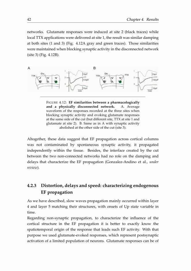
42 Chapter 4. Results
networks. Glutamate responses were induced at site 2 (black traces) whilelocal TTX applications were delivered at site 1, the result was similar dampingat both sites (1 and 3) (Fig. 4.12A gray and green traces). Those similaritieswere maintained when blocking synaptic activity in the disconnected network(site 3) (Fig. 4.12B).
FIGURE 4.12: EF similarities between a pharmacologicallyand a physically disconnected network. A. Averagewaveform of the responses recorded at the three sites whenblocking synaptic activity and evoking glutamate responsesat the same side of the cut (but different site, TTX at site 1 andglutamate at site 2). B. Same as in A with synaptic activity
abolished at the other side of the cut (site 3).
Altogether, these data suggest that EF propagation across cortical columnswas not contaminated by spontaneous synaptic activity, it propagatedindependently within the tissue. Besides, the interface created by the cutbetween the two non-connected networks had no role on the damping anddelays that characterize the EF propagation (Gonzalez-Andino et al., underreview).
4.2.3 Distortion, delays and speed: characterizing endogenousEF propagation
As we have described, slow waves propagation mainly occurred within layer4 and layer 5 matching their structures, with onsets of Up state variable intime.Regarding non-synaptic propagation, to characterize the influence of thecortical structure in the EF propagation it is better to exactly know thespatiotemporal origin of the response that leads such EF activity. With thatpurpose we used glutamate-evoked responses, which represent postsynapticactivation of a limited population of neurons. Glutamate responses can be of

4.2. Electric field propagation of slow waves 43
different amplitude depending on the amount applied, from a small responsethat recruits an Up state to a large response (Sanchez-Vives and McCormick,1997; Sanchez-Vives et al., 1997, 2008). These triggered events have theadvantages of being a controlled rather than a spontaneous event, and thusto measure them in a precise time window; as well as, to control the exactlocation where they have been generated.
We measured how different parameters of the mean EF-propagated glutamateresponses varied depending on the stimulated and the recorded layer (Fig.4.13A). Specifically, we computed duration, amplitude and distortion (peakcompression/widening), and speed. Significant differences were observedbetween EF waves recorded and coming from different layers (Fig. 4.13 and4.14).
EF waves recorded at SG layers (blue) were significantly narrower andsmaller than EF waves recorded at IG layer (red) in both cases: whenglutamate responses were evoked at SG (EF wave at SG: 4.86 ± 3.01 µV and0.33 ± 0.02 s; EF wave at IG: 15.31 ± 8.13 µV and 0.4 ± 0.02 s) (hollow bars)and when glutamate responses were evoked at IG layers (EF wave at SG: 3.94± 5.41 µV and 0.34 ± 0.01 s; EF wave at IG: 25.54 ± 6.10 µV and 0.41 ± 0.01 s)(full bars) (Fig. 4.13 B-D).Distortion was measured by computing the compression and widening of thepeak. Positive values represent compression of the wave when propagatingacross the cut, while negative values represent widening (see Materials andMethods section). Only when EF propagated from IG layers to synapticallydisconnected SG layers was there compression in the waves (0.05 ± 0.05) (Fig.4.13E). While when glutamate responses propagated across the cut from SGlayers to IG layers signals widened (Fig. 4.13E).Finally, significant differences were observed between duration, amplitudeand distortion of the EF wave propagation within SG layers (blue hollow bars)and IG layers (full red bars) (Fig. 4.13C-E).

44 Chapter 4. Results
FIGURE 4.13: Distortion of endogenous EF propagation. A.Schematic of the recording configuration. Top, glutamateresponses evoked at supragranular layers (Ev SG); bottom,glutamate responses evoked at infragranular layers (Ev IG).B. Average responses at the four sites indicated in A fora particular slice. C-E. Population averages displayingsignificant differences on duration, amplitude and distortion(respectively) of EF waves on 12 slices. Hollow and full barsindicate evoked responses at SG and IG layers, respectively.Blue and red indicate EF waves recorded at SG and IGlayers, respectively. ∗p≤0.05, ∗∗p≤0.01,∗∗∗p≤0.001;t-test or
Mann-Whitney U test.
Considering propagation speed, there was no significant differences betweenlocations where the glutamate responses were induced. But, when theglutamate response was originated at IG layers, it propagated significantlyfaster to the same layer across the cut than to SG layers (15.7 ± 10.15 mm/s toIG, 9.5 ± 19.57 mm/s to SG) (Fig. 4.14 C, bottom). Moreover, we observed thatEF velocity, despite showing significant difference with synaptic transmissionvelocity (EF: 18.3 ± 2.85 mm/s; synaptic: 13.6 ± 2.70 mm/s; p<0.001,Mann-Whitney U-text), was the same order of magnitude (mm/s) insteadthan instantaneous as volume conduction transmission (Gonzalez-Andino etal., under review).

4.2. Electric field propagation of slow waves 45
FIGURE 4.14: Speed of endogenous EF propagation. A-B.Same as in figure 4.13A-B, showing the time trigger ofthe glutamate application to better display delays. C.Speed population averages of the EF propagation wheninducing the glutamate response at supraganular (SG, top)and infragranular (IG, bottom) layers of 12 slices. Bar codeas in figure 4.13 ∗p≤0.05, ∗∗p≤0.01,∗∗∗p≤0.001; t-test or
Mann-Whitney U test
4.2.4 Slow wave activity and its EF propagation within adisrupted laminar cortical structure
To further explore whether changes in the laminar cortical structure influencethe interaction between synaptic and EF activity, one side of the slice wasrotated. Such manipulation was done after cutting the slice in the interfacechamber as previously described, and the right side of the slice was gentlyoverturned 180so that SG layers were next to IG layers and vice versa (Fig.3.3 and 4.15A), care was taken that there was close contact. This configurationcaused an abrupt change in the structure of the tissue, resulting in a sectionedcortical slice where one side had an inverted laminar structure. This was donein 6 slices where this protocol was performed.
Even when we investigated in detail any possible influence of the corticalstructure disruption on the SO parameters, we did not detect any influence onthe frequency oscillatory pattern from one side to the other. The main changeswere observed in the characteristics of Up states, which were inverted withrespect to layers on the right side. Interestingly, in the inverted side (site

46 Chapter 4. Results
2), there was a trend towards longer Up states in SG layer than in IG layers(SG: 0.42 ± 0.04 s; IG: 0.36 ± 0.05 s) (Fig. 4.15B), which is the opposite of avery consistent observation in physiological conditions where Up states at IGlayers are longer (SG: 0.37 ± 0.05; IG: 0.39 ± 0.05 s) (Fig. 4.17Bb-Cb gray bars).The same phenomenon occurred with mean firing rates, which trended to behigher in SG layers than in IG layers on the right side (SG: 0.40 ± 0.03; IG: 0.38± 0.01) (Fig. 4.15C), as well as with maximum firing rates (SG: 1.68 ± 0.18 IG:1.35 ± 0.25)(Fig. 4.15D). Although significant differences were not observed, atrend to elicit opposite behaviors can be noticed between both sides.
FIGURE 4.15: Effect of layer inversion on SO. A.Top, schematic of the recording configuration. Bottom,representative Up state at each recording site. (B-D) Meanaverage values of Up state duration, mean firing rate andmaximum firing rate from 6 slices. Mean and maximum firingrate are the absolute values of Up state computed from thetransform log MUA (see Materials and Methods) (∗∗p≤0.01;
Paired student t-test).
We next explored the influence of the cortical structure on the propagation ofendogenous EF waves. For this, we used spontaneous Up states at IG layeron site 2 (Fig. 4.16A) as the reference responses that led to EF waves at theother side of the cut (sites 3 and 4 in figure 4.16A). Interestingly, rotating theright side of the slice led to amplitude values of EF waves that trended to belarger in SG layers (site 4 in figure 4.16A) than in IG layers (site 3 in figure4.16A) (SG: 19.67 ± 9.2 µV; IG: 17.89 ± 11.23 µV) (Fig. 4.16A-B). This tendencyobserved in sectioned slices where one side was rotated (larger amplitude inSG than in IG layers) was the opposite to the tendency observed in sectionedslices where there was no rotation (larger amplitude in IG than in SG layers).Duration and peak compression of EF waves elicited a similar tendency inboth sectioned slices (with and without rotated side): IG layers showed EFwaves with longer duration than the EF waves in SG layers (Fig. 4.16C), and

4.2. Electric field propagation of slow waves 47
EF waves widened at IG layers and were compressed at SG layers (Fig. 4.16D).
The same tendency in the characteristics of EF waves were observed inthree slices (with the right side rotated) where glutamate responses wereinduced to better control the origin of the response. From these three caseswe could compute the speed of propagation from the peak to peak delaysthat turned out to be similar between layers (from SG to IG: 19.35 ± 9.45mm/s; from IG to SG: 18.98 ± 9.19 mm/s) (not shown), and in the same rangemeasured for the larger population presented in previous section (4.2.3).
FIGURE 4.16: Effect of layer inversion on EF waves A. Left,schematic of the recording configuration. Right, waveformaverage responses at the four indicated sites. B-D. Meanvalues of amplitude, duration and peak compression from 6slices. Blue, supragranular layer (SG); red, infragranular layer
(IG).
In summary, the reversion observed in the amplitude of the recorded EFwaves (larger in SG than IG layers), together with the resulting damping(29,06 ± 38,68 % from SG to IG, and 52.2 ± 18.07% from IG to SG) suggestssome dependence of these parameters on the local network where the EFwave is originated, and not only on the network where it is recorded.
4.2.5 Influence of extracellular space on slow waves and its EFpropagation
To study the influence of extracellular space on the synaptic and non-synapticmechanisms of SO, we increased the osmolarity of the ACSF, which is knownto expand the extracellular space (Traynelis and Dingledine, 1989).For this, saccharose (40 mM) was added to the ACSF solution to increase by

48 Chapter 4. Results
12% the osmolarity (from 328 to 368 mOsm). Similar increases with otheragents have been proved to decrease synaptic and non-synaptic activity(Shahar et al., 2009; Zhang et al., 2014; Qiu et al., 2015).
Spontaneous SO (<1Hz) in normal ACSF solution (328 mOsm) displayed Upstates, (0.39 ± 0.05 s duration) interspersed with Down states (3.47 ± 0.86 sduration) in IG layers. Up/Down cycle frequency was 0.33 ± 0.06 Hz.
Increases in osmolarity resulted in alterations in the Up and Down states at SGand IG layers (Fig. 4.17). Although significant differences were only observedin the oscillatory frequency, which decreased from 0.33 ± 0.06 Hz in controlcondition to 0.17 ± 0.02 in the hyperosmolar condition (p <0.05) (Fig. 4.17 Be),changes in other parameters were non significant but consistent (observed in6 out of 7 slices). Up and Down state durations tended to increase, from 0.39± 0.05 s to 0.54 ± 0.1 s; and from 3.47 ± 0.86 s to 6.31 ± 1.44 s, respectively(Fig. 4.17 Ba-c). These changes in the Up/Down cycle dynamics led to a moreirregular slow oscillatory pattern: the coefficient of variation (CV) of the SOfrequency increased (control: 7.03 ± 3.22, hyperosmolar: 31.89 ± 21.33) (Fig.4.17 Bd).In spite of this reduction in the capacity of the network to generate Up states,there was an increase in mean firing rate during Up states (from 0.45 ± 0.04under 328 mOsm, to 0.56 ± 0.09 under 368 mOsm), as well as in maximumfiring rate (from 1.89 ± 0.2 under 328mOsm, to 2.47 ± 0.28 under 368mOsm)(Fig. 4.17 Be-f). Up/Down cycle variations reported here, which refer to IGlayers, elicited similar variation as the ones obtained in SG layers (Fig. 4.17C).
These results suggest that slightly increasing osmolarity altered the excitabilityof the network, thereby decreasing the frequency of oscillations.

4.2. Electric field propagation of slow waves 49
FIGURE 4.17: Effect of hyperosmolar ACSF on SO. A. Oneexample under control (328 mOsm) (left) and hyperosmolar(368 mOsm) ACSF (right). Relative firing rate (top) andLFP recording (bottom). The red line represents the Up andDown states detection. B. Average population data for thetwo conditions (control: gray; hyperosmolar: red) showingvariations in the different parameters in infragranular (IG)layers when increasing osmolarity by 12% in 7 slices. a, Downstate duration. b, Up state duration. c, SO frequency. d,SO Frequency CV. e, Up state mean firing rate. f, Up statemaximum firing rate. C. Same as in B for supragranular (SG)layers in 6 slices. ∗p≤0.05; Paired student t-test vs. control).
Our main objective was to study the influence on the EF induced by Upstates across the cut. Regarding EF propagation of spontaneous Up statesin a hyperosmolar medium, we observed similar damping as previouslyreported (20.45%) in section 4.2.1. When computing average amplitude valuesof EF waves, these were significantly reduced with respect to the controlcondition (328mOsm, 15.24 ± 2.8 µV; 368 mOsm, 7.5 ± 1.9 µV at IG layers)(Fig. 4.18A-B). Such reduction was due to a decrease in amplitude of theoriginal LFP signal (328mOsm, 56.37 ± 9.4 µV; 368 mOsm, 37.47 ± 2.8 µV).Significant differences were also observed in peak compression: spontaneous

50 Chapter 4. Results
Up states were compressed when propagating across the cut under the controlcondition (0.39 ± 0.16 at SG, 0.27 ± 0.09 at IG), while they were widened inan expanded extracellular medium (-0.08± 0.11 at SG; -0.15 ± 0.05 at IG) (Fig.4.18D).When computing time delays from peak to peak in four slices, EF waves inSG layers displayed slower velocities under a hyperosmolar medium (10.22 ±3.9 mm/s with 328 mOsm versus 8.39 ± 3.21 mm/s with 368 mOsm) whileEF waves in IG layers remained similar (10.47 ± 4.09 mm/s with 328 mOsmversus 10.52 ± 1.98 mm/s with 368 mOsm) (Fig. 4.18E).A similar decrease in EF wave propagation was observed in three slicesunder a hyperosmolar medium where glutamate responses were evoked (notshown).
FIGURE 4.18: Effect of hyperosmolar ACSF on EFpropagation. A. Schematic of the recording configuration(top). Average responses at the four sites indicated in thescheme (middle and bottom). B-E. Mean values of amplitude,duration, peak compression and speed from 6 slices. (Hollowbars, supragranular layer (SG); full bars, infragranular layer
(IG).
By expanding the extracellular space we were able to decrease EF propagationof slow waves. Similar observations have been made with epileptiform burstscaused by 4-aminopyridine (Zhang et al., 2014; Qiu et al., 2015) or low-Mg2+
(Shahar et al., 2009) in hippocampal slices.

4.2. Electric field propagation of slow waves 51
4.2.6 Influence of external EF stimulation on slow waves andtheir EF propagation
Next, we explored the influence of external EF stimulation on the endogenousEF propagation of slow waves. Previous studies have used external EFstimulation to mimic endogenous fields (Frohlich and McCormick, 2010);here we have already disconnected the endogenous fields from the synapticactivity, thus we have used the exogenous EF to modulate the networkexcitability and affect the detectability of endogenous EFs.
Therefore, uniform external EFs were applied by direct current (DC)stimulations through two parallel AgCl electrodes in 8 sectioned slices (Fig.4.19B). It is widely known that positive DC stimulation induces somaticdepolarizations that lead to an increase in the excitability of neurons (Frohlichand McCormick, 2010; Schmidt et al., 2014). Thus, we applied DC stimulationwith increasing intensities (from -4 V/m to +4 V/m) which enhanced thefrequency of SO cycle at both sides of the cut without having any relevanteffect on spontaneous Up state properties (Fig. 4.19), as reported in previousstudies (Sanchez-Vives et al., 2017a).

52 Chapter 4. Results
FIGURE 4.19: Effect of EF stimulation on SO. A. One exampleof Up/Down state detection (red lines) under two differentintensities of EFs (left, right) and in a control condition (0V/m). Relative firing rate (top) and LFP recording (bottom).B. Schematic of the recording configuration with the two AgClelectrodes parallel to the apical surface. C. SO frequencyincrease for different EF stimulations (gray, individual cases;
black, average values from 8 slices).
Our hypothesis was that increasing DC stimulation would result in largerEF waves that could increase the probability of inducing suprathresholdresponses. According to the results described before (section 4.2.4 and 4.2.5)suggesting that the EF wave amplitude depends on the original signal whereit comes from, the absence of effect on Up states amplitude and durationwith DC stimulation led to no differences in EF waves traveling across thecut. Figure 4.20 shows the lack of a clear variation or tendency in amplitude,damping, duration and peak compression of EF waves with increasing DCstimulation (similar results observed with glutamate responses) (not shown).
According to our hypothesis (see above), DC stimulation could be drivingthe EF wave to induce suprathreshold responses, hence contributing to thegeneration of Up states in the disconnected network. In this case, thesesuprathreshold responses would have been discarded according to analysiscriteria (periods with Up states overlapped from both sides were removedfrom the averaged EF waves) (see Materials and Methods). However, we found

4.3. Endogenous electric fields modulate the occurrence slow oscillations 53
FIGURE 4.20: Effect of external EF stimulation onendogenous EF waves. A-D. Amplitude, damping, durationand peak compression of EF waves at site 3 shown in E(bottom). Insets, normalized data with respect to control(0 V/m) values. Blue, supragranular layers (SG); red,infragranular layers (IG). E. Top, line plot showing thepercentages of Up state detected at site 2 that led to EF waves(red), and that overlapped with Up states onset/offset at site
3 (blue). Bottom, schematic of the recording configuration.
that from all Up states recorded on site 2 the majority did not overlap withUp state onset or offset on site 3; in fact, most of them were recorded withsimilar damping at the other side of the cut (Fig. 4.20 E). Thus, against ourhypothesis, enhanced excitability did not result into higher probability ofinducing suprathreshold responses.
4.3 Endogenous electric fields modulate the
occurrence slow oscillations
So far, the results described previously in this thesis demonstrated thatpropagation activity of SO and the EFs that they generate coexist in theneural tissue. Past studies demonstrated that external EFs are able to entrain

54 Chapter 4. Results
neocortical network activity (Frohlich and McCormick, 2010; Anastassiouet al., 2011). Taking advantage of our sectioned in vitro preparation, wheresynaptic and endogenous EFs can be disassociated, we next explored theinteraction of activity across the two synaptically disconnected networks.
4.3.1 Synchronizing two synaptically disconnected networkswith external EF stimulation
Synchronous Up states at both sides of the cut could occur randomly. Wewanted to test whether enhancing excitability with exogenous EFs wouldincrease SO synchronization between both sides of the cut. To study whetherthere was any modulated synchronization across both disconnected networks,we computed cross-covariation coefficients between site 2 (IG) and site 3(IG) (Fig. 4.19B) under control conditions (no stimulation applied) and withdifferent intensities of DC stimulation (negative and positive) in 8 slices.Hence, we obtained the cross-covariation coefficient that corresponds to thecross-correlation between both sides where the mean had been subtracted.Even though DC stimulation increased the cross-covariation coefficient, theonly value significantly different from the control condition (0 V/m) was at -1V/m.
FIGURE 4.21: Synchrony between disconnectedcortical columns at different EF stimulations. A. Meancross-covariation coefficients between two selected channelsfrom both sides of the slice at different EF intensities in 8
slices. B. Same as A for phase-locking values (PLV).
As changes in the cross-covariation coefficient were too small, we looked fora more sensitive measurement such as the phase locking value (PLV), whichis a statistical measure used to study synchronization of neural activity. ThePLV computed between site 2 (IG) and site 3 (IG) led to similar results as thecross-covariation coefficient: higher values with DC stimulation however notsignificant (Fig. 4.21B).

4.3. Endogenous electric fields modulate the occurrence slow oscillations 55
Although, a linear relationship in average PLV was not observed withincreasing DC stimulation, it is worth to note the results for low EFstimulations (±1 V/m), which suggest that DC electric stimulation of lowintensity may be enough to synchronize two independent networks.
4.3.2 Modulation of subthreshold glutamate-inducedresponses by endogenous EF
We have shown above that DC stimulation on both sides of the slicemodulates excitability. However, the increase in excitability with increasingDC stimulation did not result in an enhanced synchronization of spontaneousSO between both disconnected networks. To further explore the possibilityof inducing SO in spite of the interrupted cortical synaptic connectivity, weused small local applications of glutamate to slightly increase the excitabilityonly in one side at a desired time without evoking an Up state. I will refer tothese as subthreshold responses that do not trigger Up states. This should bedifferentiated from the classical use of subthreshold responses referring to thosethat do not evoke action potentials.First, small local applications of glutamate were adjusted to inducedepolarization without evoking Up states on one side (side 2) (Fig. 4.22A, top: Off-On). Next, full blown Up states (or glutamate-evoked responses)were induced on the other side (side 1). Thus, two glutamate applicationswere applied at the same time on both sides of the slice (on the left side toinduce Up states, on the right side to locally increase excitability withoutevoking Up states) (Fig. 4.22 A, middle: On-On).With this strategy we wanted to amplify the potential effect of the endogenousEF across the cut. Although endogenous EFs could not induce SO in anon-synaptically connected network even when we locally increased theexcitability with small glutamate applications, they did significantly increaseamplitude (p<0.005) and duration (p<0.01) of the subthreshold inducedresponses (Fig. 4.22 C-D, mean values from 260 waves analyzed offlinewith Spike2 software: 20 waves x 13 slices). These increases were revertedto control values (i.e, same values presented when adjusting the glutamateapplication at side 2) when the glutamate application inducing Up states onthe left side stopped (Fig. 4.22 A, bottom; B-D), further confirming that thechanges observed were due to the endogenous EFs generated by evoked Upstates on the left side.

56 Chapter 4. Results
FIGURE 4.22: Modulation of subthresholdglutamate-induced responses by endogenous EFs. A.Induced wave responses by local glutamate application.Schematic of the recording configuration (left) and 20averaged waves obtained from the glutamate applicationsat site 1 and 2 (right). Top, subthreshold responses inducedat site 2 prior to glutamate response induction at site 1.Middle, responses from glutamate applications on bothsides (inducing glutamate responses at 1 and subthresholdresponses at 2). Bottom, subthreshold responses at site 2 afterthe induction at site 1. Most bottom, designated features.B,C,D. Mean values for latency, amplitude and duration(respectively) of the subtheshold response at site 2. Valuesare normalized to the first subthreshold response. ∗p≤0.05,
∗∗p≤0.01,∗∗∗p≤0.001; Paired student t-test vs. control).
4.3.3 Frequency modulation of SO by endogenous EFs
We have seen in the previous section how the endogenous EFs generated byevoked Up states modulate subthreshold glutamate-induced responses. Here,we used another strategy to detect the influence of endogenous EFs on thetemporal pattern of occurrence of spontaneous SO.
So, in order to further explore the impact of endogenous EFs on spontaneoussynaptic activity, we used glutamate-evoked Up states to modulate

4.3. Endogenous electric fields modulate the occurrence slow oscillations 57
non-synaptically the neural activity across disconnected networks. Byusing local glutamate applications we could control the periodicity of theUp state occurrence. Thus, different oscillatory frequencies were inducedon the left side of the slice (Fig. 4.23 A-top scheme). By doing this weexplored the impact on the spontaneous oscillatory frequency of the rightside. Interestingly, this manipulation resulted in a frequency variation inthe spontaneous SO on the right side of the cut. Increasing (decreasing)the glutamate application periodicity induced an increase (decrease) in thespontaneous SO frequency of the disconnected network (Fig. 4.23A-B).
FIGURE 4.23: Frequency modulation of spontaneous SOby endogenous EFs. A. Relative firing rate (black), LFPrecording (blue) and Up and Down state detection (red lines)for spontaneous activity (top) and two evoked oscillatoryfrequencies: 0.66 Hz and 0.33 Hz (middle and bottom,respectively). Left, left side on the slice; right, right side on theslice. B. Mean SO frequency from a 50-second period analyzedat four different frequencies (one control and three evoked in
the following order: 0.66, 0.33 and 0.4 Hz).
We next explored the kinetics of such entrainment. To explore the time course

58 Chapter 4. Results
of the interaction, we changed the frequency on the left side and we measuredthe evolution of the frequency on the right. We observed that the interactionfollowed an exponential time course. An exponential fit was adjusted (Fig.4.24 B - red line); the time constant τ (red dot) of this exponential fit wasconsidered as the time that the signal took to change the frequency on theright side depending on the glutamate application on the left side (averagevalues: 8.62 ± 5.18 s for increasing frequencies, n = 11 frequency variations - 1outlier discarded - ; 36.15 ± 17.71 s for decreasing frequencies, n = 6 frequencyvariations - 4 outliers discarded - ; from a total of 12 slices, 4 slices discarded)(see Materials and Methods).Because the SO cycle did not exactly reach the same frequency on both sidesof the slice with glutamate applications, normalized differences of frequencies(ND) (see Eq. 3.4) were quantified at each side of the slice to better comparethe frequency variations observed (see Material and Methods). The dispersionplot in figure 4.24 C represents the ND for the glutamate application frequencyversus the ND of the spontaneous SO frequency on the right side. The resultwas a linear relationship between both NDs: the induced on the left side andthe spontaneous modulated on the right side, with significant linear regressionvalues (R2 = 0.42, p = 0.01 for 22 variation in frequency; in a total of 13 slices; 3slices where no modulation was observed were discarded) (Fig. 4.24 D).
This entrainment was also explored after disrupting the cortical layer structureby rotating the right side (in 3 slices) or increasing the extracellular space byadding saccharose (40 mM) to the ACSF solution (in 2 slices). In these twocases a clear modulation was not observed: the evoked glutamate applicationon the left did not induce any influence on SO frequency on the right.
In summary, endogenous EFs were able to modulate the SO frequencyof a disconnected network when maintaining the physiological conditions.Disrupting the layer structure or expanding the extracellular space preventedthe modulation.

4.3. Endogenous electric fields modulate the occurrence slow oscillations 59
FIGURE 4.24: Frequency modulation kinetics. A. Raster plotsof three consecutive recordings from one representative slice(375 s) for a time window of 4 s (time period covering oneor two Up/Down cycles). Three frequency variations canbe observed (from 0.2 to 0.5 Hz, top; from 0.5 to 0.2 Hz,middle; from 0.2 to 0.33 Hz, bottom), on the left where it isinduced, perfectly defined; on the right, a clear modulationover time (from top to bottom) of the spontaneous SO. B.Exponential fit for a particular change in frequency (top inA) displaying: the glutamate application frequency (black);the spontaneous SO frequency of the disconnected network(blue) and its exponential fit displaying the τ (red dot). C.Dispersion plot of the ND at both sides of the slice. Increasesin frequencies, blue; decreases in frequencies, red. (n=22
frequency variations, 13 slices)


61
Chapter 5
Discussion
The two major aims of this PhD work were to explore the synaptic andnon-synaptic propagation of SO within the laminar cortical network. Theresults reported here illustrate that SO are generated spontaneously in thecortical network. Different excitability levels modulate the frequency and thespatiotemporal dynamics of the slow waves reaching the maximal regularitywith intermediate excitability levels. Moreover, the propagation of these slowwaves across the cortex is led by the region eliciting the maximum firingrate in the cortical structure. Further we showed that such cortical rhythmgenerates propagating endogenous EFs, opening the possibility to better studythe conductive properties of neural tissue. Finally, these endogenous EFs havein turn a feedback effect that can further modulate the synaptic activity.
5.1 Propagation of slow oscillations
To explore local and global dynamics of the cortical network I used a16-channel array over cortical slices which covered different cortical columnsand layers allowing to study the propagation of SO, one of the most spatiallysynchronized rhythmic patterns within the brain (Destexhe et al., 1999). Inour slice preparation different ignition sites along the cortical structure wereobserved, but a longitudinal strip with the maximum firing rate led to aconsistent parallel propagation to the cortical surface for all the differentcluster waves detected (Fig. 4.4). In humans, the slow wave propagation hasdifferent origin sites with different propagation directions within the cortex,drawing out a preference pattern of propagation from anterior to posteriorareas (Massimini et al., 2004). Thus in both, coronal slices and the full cortexsuperficial propagation, slow waves can start at any point but there are

62 Chapter 5. Discussion
prefered paths for their propagation.The propagation pattern led by layer 5 reported here agrees with thespreading of SO in deep layers described in previous studies (Sanchez-Vivesand McCormick, 2000; Wester and Contreras, 2012).
5.1.1 Slow oscillations accommodate within layer 5
The experimental recordings from slices that I obtained during the course ofthis PhD revealed that Up states were consistently originated in and spreadthrough deep layers of the cortical structure. Particularly, overlapping the EPSdensity with the anatomical slice reconstruction showed that the propagationpattern accommodated well with the structure of layer 5 and to some extentwith layer 4 (Fig. 4.6). Average values of the area covered by the EPS did notshow significant differences between layer 4 and layer 5, suggesting that evenif layer 5 had the major contribution to the generation of SO, the neuronalpopulation of layer 4 might also be involved in its spatiotemporal dynamics(Fiath et al., 2016).
Layer 5 comprises a large number of synaptic connections between columnsand layers within the cortex (Wester and Contreras, 2012; Beltramo et al.,2013), thus being more likely involved in the origin of SO (Sanchez-Vives andMcCormick, 2000; Chauvette et al., 2010). Indeed, most animal studies haveshown that layer 5 plays a key role in the origin and propagation of slowwaves (Sanchez-Vives et al., 2010; Beltramo et al., 2013; Neske, 2015; Blaeseret al., 2017). In contrast, a human study reported that the superficial layers arethe ones eliciting stronger multi- and single- unit activity (Csercsa et al., 2010)and thus endowing SG layers with a role in the genesis of SO. Assuming thatthe network structure determines how neurons synchronize with each otherto generate transition network states such as the SO pattern (Blaeser et al.,2017), the differences observed between humans and rodents regarding SOgeneration could be due to the differences in their cortical cytoarchitecture(DeFelipe, 2011). The human cortex is thicker than the rodent one, with SGlayers conforming half of the cortex, while in rodents more than half of thecortex corresponds to IG layer. If any layer can be involved in the initiationof Up states as far as its neurons have the ability to synchronize (Chauvetteet al., 2010), the neuronal density of each respective layer could explain whySO are originated at superficial layers in humans and at deep layers in rodent

5.1. Propagation of slow oscillations 63
preparations.
Results on the propagation speed across different columns (5.5 ± 1.5 mm/s)(Fig. 4.4E) are similar to the velocities reported in past works using the samepreparation, which yielded propagation speeds of 7.2 mm/s (Sanchez-Viveset al., 2010) and 10.9 mm/s (Sanchez-Vives and McCormick, 2000). However,other preparations eliciting SO in vitro in rat brain slices measured 20 mm/spropagation speed with voltage sensitive dye images (Wester and Contreras,2012). This higher speed might be due to the recording technique which alsoexamines subthreshold activity of neurons, while our LFP analysis, based onthe logMUA (Fig. 4.3), only reflects suprathreshold activity of those cells.Higher speeds appeared also in in vivo preparations: 23.4 mm/s in visualcortex of anesthetized mice (Ruiz-Mejias et al., 2011), and 37 mm/s withinthe whole cortex reported with calcium imaging (Stroh et al., 2013). Thelower velocities observed in in vitro experiments would be explained bythe elimination of long range cortico-cortical connectivity and also by thedisconnection from the thalamus.
5.1.2 Slow oscillations: a collective network phenomenon
To further explore the spatiotemporal dynamics of SO within the laminarcortex, I varied the extracellular K+ concentration to globally modulate theexcitability of neurons within the network. We observed that intermediate K+
levels maximized the temporal and spacial regularity of the SO (Sancristobalet al., 2016). Low excitability levels decreased the probability of Up stateoccurrence while increasing the variability of Down state duration. With highexcitability levels the occurrence of Up states increased also enhancing thevariability of the SO frequency (Fig. 4.7 and 4.8).Together these results showed the self-regulation of the cortical dynamicswith different excitability levels. An intermediate amount of synaptic noise,here determined by the neuronal excitability, is needed to maximized the SOregularity, what correspond to a collective stochastic coherence phenomenon(Sancristobal et al., 2016). A similar phenomenon has been observed incell cultures where random firing of neurons led to a cascade of activity inneuronal populations generating coherent spontaneous activity (Soriano andCasademunt, 2015).Also, evidence regarding SO as a network phenomenon increases when

64 Chapter 5. Discussion
endogenous fields are considered to be involved in the generation andmaintenance of neural oscillations (Weiss and Faber, 2010)(see next section).
5.2 Endogenous electric fields generated by slow
oscillations
SO have been regarded as a relevant experimental approach to investigatethe interactions between endogenous EFs and synaptic activity (Frohlich andMcCormick, 2010; Reato et al., 2010; Schmidt et al., 2014). The SO representsa large spatially synchronized activity which generates endogenous EFs that,in turn, might be involved in the orchestration of such oscillatory rhythm(Frohlich and McCormick, 2010) by inducing ephaptic coupling betweenneurons (Anastassiou et al., 2011).LFP, an accessible measure widely used to study mesoscopic brain activity,is an informative signal to experimentally explore the electrical activitymeasured in clinical applications with EEG, magnetoencephalogram (MEG)or electrocorticogram (Buzsaki et al., 2012). LFP provides insights notonly about the suprathreshold activity, but also about the subthresholdcomponents and the charges distribution within the tissue (Herreras, 2016),here manifested as EF waves. Additionally, LFP can reflect the activity ofnetworks that are far from the recording point (Kajikawa and Schroeder,2011; Herreras, 2016), enabling us to measure the propagation of signalswithin synaptically disconnected networks located several millimeters apart.Therefore, considering all the advantages just mentioned, LFP offers a suitableand reliable measure for studying the synaptic and non-synaptic componentsof slow waves.
In the experimental approach used here, cutting the cortical slice in two piecesperpendicularly to the white matter, while maintaining both sides tightly incontact, yielded two independent networks with different oscillatory patterns.Importantly, the independence between both networks meant that therewas no synaptic propagation of slow waves across the cut. This way, theactivity (Up states) originated in one side of the cut could be recorded as EFwaves at the other side. Thereby, the limitation of studying endogenous EFswith external field stimulation was overcome, and instead of measuring amimicked or induced activity (Frohlich and McCormick, 2010; Reato et al.,2010; Schmidt et al., 2014), we just recorded the endogenous EF generated by

5.2. Endogenous electric fields generated by slow oscillations 65
the spontaneous SO.
5.2.1 Endogeneous EF propagation is damped and delayed
Surprisingly, EF propagation of spontaneous and evoked activity eliciteddamping and delays when traveling across the cut between both disconnectednetworks (Fig. 4.10). This observation goes against the assumption thatneural tissue acts as a homogeneous ohmic conductor where EFs travel nearlyinstantaneously and undistorted from their origin. To rule out the possibilitythat the presence of the cut itself was acting on the observed damping anddelays, we compared the EF propagation between pharmacologically andphysically disconnected networks (Fig. 4.12). The similarity between bothrecorded waves confirmed that the interface created by the cut was not thecause of the observed damping and delays. Moreover, if the cut had hadany impact on the propagation, we would have then expected an increase,and not a decrease, in the conductivity of the medium; the remaining spacewould have been filled with ACSF mimicking better the isotropic propertiesof homogeneous ohmic mediums that do not account for damping and delays(Logothetis et al., 2007).
5.2.2 The cortical network as a non-homogeneous tissue
Accompanying the damping effects, propagation of EF waves travelingacross cortical columns and layers was characterized by distortions. As aconsequence of this, differences arose between EF waves recorded at IG andSG layers; EF waves at IG were wider and larger than EF waves at SG layers(Fig. 4.13). These results point out that the EF propagation is sensitive to thestructure and composition of the neural tissue. Thus, the knowledge collectedfrom our experimental model questions the assumption that neural tissue is ahomogeneous ohmic conductor, and rather suggests that the wiring corticalnetwork conforms a non-homogeneous medium. Our results are in agreementwith previous studies where impedance measurements of the tissue showednon-ohmic and filtering properties of the extracellular medium due to ionicdiffusion (Gomes et al., 2016).However, the conductive properties of the neural tissue still remainscontroversial. In a recent report, Gratiy and colleagues postulated that the

66 Chapter 5. Discussion
displacement of currents in the extracellular space (ionic diffusion) can beneglected on extracellular signals as CSD (Gratiy et al., 2017); therefore, tissuecould be considered as a homogeneous medium where EF propagation isisotropic (Logothetis et al., 2007). Within the framework of this debate, oneshould consider whether CSD can be used to infer conductivity propertiesof the neural tissue. There are numerous complex interactions taking placeduring network activity, such as synaptic activity, current distribution withinthe space, temporal dynamics of those currents, dipoles generations etc.that can be recorded with extracellular signals (Bedard et al., 2004; Buzsakiet al., 2012). Evidence that CSD does not totally reflect all those processesoccurring during neural activity as LFP signals do (Kajikawa and Schroeder,2011) awakes some pertinent doubts about the assumptions of CSD theoryrevisited by Gratiy and collaborators. Along this line of reasoning, even ifthe ionic diffusion could be neglected when interpreting CSD measurements(Gratiy et al., 2017), such disregard might not be an indicator of the ohmicand filtering properties of the tissue. Also, the possibility of ignoring ionicdiffusion cannot be generalized to every pattern of activity, and for instancealternative interpretations may account for slow rhythms (<1 Hz) whereionic diffusion exerts a larger contribution (Gratiy et al., 2017). Hence, in ourpresent study, damping and delays observed within the EF propagation ofslow waves might be an echo of the non-ohmic properties of the tissue, whereionic diffusion could be contributing (Gomes et al., 2016).
Further evidence about the inhomogeneities of the tissue were foundwhen we computed the EF propagation speed. Velocities measured from thedelays turned out to be very low (18.3 ± 2.85 mm/s) (Fig. 4.14), similar to thesynaptic propagation velocities (13.6± 2.7 mm/s) rather than instantaneous asexpected in a homogeneous medium. The speed we found (18.3 ± 2.85 mm/s)was similar to the electric propagation speed of epileptiform activity measuredin unfolded hippocampal slices (∼100 mm/s) where the endogenous fieldtransmission was independent of synaptic activity (Zhang et al., 2014).
In previous studies, spatial and temporal analysis of fast and slow rhythms inanesthetized and chronically implanted cats showed larger spatial correlationsfor slow waves than for fast oscillations (Destexhe et al., 1999). These datafurther suggest that the frequencies do not attenuate equally within the tissue:fast frequencies attenuate more than slow frequencies (Bedard et al., 2004).Hence, considering the existing variations in the attenuation of frequencies

5.2. Endogenous electric fields generated by slow oscillations 67
reported in activity patterns similar to ours (SO) (Bedard et al., 2004), itwould be reasonable to speculate that the damping and low speed reported inour study could result from a filtering of high frequencies within the tissue.This would accumulate more evidence to consider the cortical structure as anon-homogeneous medium with frequency dependence (Bedard et al., 2004),rather than as an ohmic conductor with a frequency independent impedance(Logothetis et al., 2007).
In this context, where the characteristics of the tissue might determinethe EF propagation, I further investigated whether the anatomical structurehas any repercussion in the EF propagation. For this purpose, I tested the effectthat an abrupt change in the laminar cortical structure would cause by rotatingone side of the slice. This experiment revealed that, EF waves traveling fromIG to SG layers were larger than the EFs traveling from SG to IG, the EF wavesdetected at SG exhibited larger amplitude than at IG, although there wereno significant differences (Fig. 4.16). This result was the opposite to the onereported on slices without rotation (longer wave amplitude at IG than at SG).Because IG layers caused larger EF waves than SG layers, disregarding therecording site, one could conclude that the EF wave depended on the networkwhere it was originated. This would be at odds with the previous idea that thetissue behaves as a non-ohmic and frequency-dependence conductor wherethe measured signals might not totally depend on their origin site. Conversely,considering that substrates with weak synaptic responses receive greaterimpact of the non-synaptic components occurring in the network (Kajikawaand Schroeder, 2011), SG layers should then reflect better responsiveness toEF waves originated at IG.However, our experimental procedure, consisting in rotating one side of theslice, involves certain limitations such as damaging the slice or hamperingthe position of the recording sites with the superficial arrays, that mightobscure a possible effect of the structure. Therefore, better approaches areneeded to understand to what extent the laminar cortical structure influencesEF propagation. In this regard, different tests could be done, for exampleone interesting experiment to address this matter would be to study EFpropagation in the reelin mutant mouse, which shows a disrupted pattern ofcortical lamination due to defective polarization and migration of neural cellsduring cortical development (Wagener et al., 2010; Pielecka-Fortuna et al.,2015; Guy et al., 2016). Therefore, if the laminar structure has any influenceon EF propagation, differences in the EF propagation reported here must be

68 Chapter 5. Discussion
absent in the cortex of those animals.
To further investigate the influence of the medium in the EF propagation, theextracellular space was increased by increasing the ACSF osmolarity. It iswell known that hyperosmolarity expands the extracellular space (Traynelisand Dingledine, 1989). This expansion creates more space between neuronsresulting in an increase in the conductivity of the medium. So, assuming thereis a contribution of ionic diffusion in the EF propagation of SO, the increasein space would make the charges to be more scattered within the mediumleading to smaller EF waves and slower EF propagation as observed in ourresults (Fig. 4.18). Such reduction in the EF propagation is in agreementwith previous in vitro and in silico studies in hippocampus where osmolaritychanges were explored (Shahar et al., 2009; Qiu et al., 2015), confirming thatthe extracellular space influences the endogenous EF activity.
5.3 Endogenous electric fields modulate the
occurrence of slow oscillations
Previous approaches to study the feedback loop between endogenous EFand synaptic activity have used external DC stimulation through parallelelectrodes (Radman et al., 2007; Frohlich and McCormick, 2010; Reato et al.,2010; Schmidt et al., 2014), without solving the experimental challenge ofisolating synaptic activity and its authentic endogenous EF. Our in vitropreparation has overcome this challenge, allowing a better exploration of theinteractions between endogenous EF and synaptic activity.
In this work, we used DC stimulation in an attempt to enhance the localexcitability and increase the chance that the EF would evoke suprthresholdresponses (Up state). Increasing EF stimulation led to faster SO at both sidesof the cut (Fig. 4.19), but did not promote the induction of suprathresholdactivity by endogenous EF (Fig. 4.20). This could be due to the DC stimulationinducing suprathreshold activity randomly. However, when I inducedcontrolled subthreshold responses with small local applications of glutamateto check if endogenous EF could convert them into proper Up states, nosuprathreshold activity was triggered either (Fig. 4.22). These results agreewith previous works, where EFs did not trigger action potentials but they

5.3. Endogenous electric fields modulate the occurrence of slow oscillations69
did have an effect on the spike timing (Radman et al., 2007; Reato et al., 2010;Anastassiou and Koch, 2015). Indeed, we observed an increase in synchronybetween the two disconnected networks with DC stimulation (4.21), whichmight be the result of a greater bidirectional effect of each endogenous EF overthe corresponding population activity timing on the disconnected networks.Moreover, the higher correlation between both networks was more notoriousfor weak EF stimulations (±1 V/m), stimulations that kept the oscillatoryrhythms close to their basal frequency (without extremely hyperpolarizing ordepolarizing the networks). These results concur with what has been observedin in vitro experiments and in silico, namely, that low EF stimulations have asignificant effect on oscillatory activity (Frohlich and McCormick, 2010; Reatoet al., 2010) and frequency shifts only appear with EF stimulations that matchthe intrinsic oscillations (Schmidt et al., 2014).
Even if the reported increases in synchrony with DC stimulation denotedentrainment of SO by EFs, it was difficult to know to what extent this wasdue to the exogenous EF applied through the parallel electrodes or to the pureendogenous EF originated by the slow waves. Simultaneously, there was adouble modulation from one network to the other that was difficult to teaseapart.To clarify the entrainment that the noise induced by external EF stimulationmight be masking, the frequency of SO was precisely controlled with localapplication of glutamate. Up states were induced only in one side of the slice atdifferent periodicities. Frequency changes in the glutamate application in onenetwork led to frequency changes in the spontaneous SO in the disconnectednetwork, unraveling an entrainment of slow wave rhythms by endogenous EF(Fig. 4.24). It should be noticed that the side modulated by the endogenousEF did not reach frequencies similar to the glutamate applications, meaningthat evoked Up states on one side did not directly trigger Up state occurrenceon the other. This is in line with the notion that endogenous EFs are able tosynchronize neural activity by modulating its timing but they cannot triggerany additional synaptic activity (Anastassiou et al., 2011).
Variations in the structure (cortical layer disruption) or the extracellularmedium (osmolarity increase) avoided the modulation, suggesting thatphysiological conditions under which SO are originated must be preserved tostudy ephaptic coupling between independent networks.
70 Chapter 5. Discussion
Why can endogenous EFs not trigger Up states but can induce variations inthe frequency of SO? The main reason would involve resonance of neuronsand networks. Resonance of a neuron is the propensity that it has torespond more strongly to an input, modulating either its spike probability orsubthreshold activity. Thus, resonance becomes the link between subthresholdand suprathreshold responses (Dwyer et al., 2012). Indeed, theta resonancein layer 5 pyramidal neurons has been described as one of the contributors todrive cortical network activity (Schmidt et al., 2016). Moreover, such resonancewas demonstrated in freely behaving animals to allow the entrainment of thecortex by the hippocampus through parvalbumin interneurons (Stark et al.,2013). Thus, the modulation observed between both disconnected networksin our experiments could be due to the resonance properties of neurons.Future research will hopefully shed light on how intrinsic properties ofneurons are affected by endogenous EFs, and to what extent such fields affectthe activity of individual neurons leading to changes in the global networkactivity.
5.4 Concluding remarks and perspectives
In summary, the findings exposed within this thesis have unraveled that slowwaves are not local events, they propagate along the cortical network. Thepropagation of SO within the cortex is largely influenced by the structureof the cortical tissue. Also, an intermediate excitability level controlledby extracellular K+ leads to the highest spatiotemporal regularity. Thisexcitability level represents the synaptic noise, revealing that a collectivestochastic coherence phenomenon leads to the maximal regularity of SO. Inaddition, slow waves generate EFs which travel independently of synaptictransmission within the cortical tissue, suggesting that cortical rhythmsemerge from interconnected networks and might be influenced by the EFsgenerated by these networks. Moreover, these EFs travel with dampingat a slow propagation speed, similar to the synaptic propagation velocities(18.3 ± 2.85 mm/s), rather than instantaneous as volume conduction,suggesting that neural tissue is non-homogeneous. All together, theseresults imply that interpretation of LFP, EEG/MEG needs to be reconsideredas most experimental and clinical approaches assume that neural tissueis a homogeneous ohmic conductor. Finally, endogenous fields modulate

5.4. Concluding remarks and perspectives 71
the SO frequency of a synaptically disconnected network, suggesting thatnon-synaptic mechanisms may be able to couple populations of neurons.Such coupling may affect information processing in the cortex and synapticplasticity; thus, the ability of EFs to modulate neuronal timing might beexplored as a promising therapeutical intervention to restore abnormal spiketiming that characterize many neurobiological disorders.


73
Chapter 6
Conclusions
1. Slow waves are not local events, but they propagate along cortical slicesparallel to the surface.
2. The slow wave propagation across cortical columns is variable ininitiation sites and speed. Our concrete measures suggest that underthe in vitro conditions that we work, it is a memoryless random process,similarly to what has been observed in deep anesthesia.
3. Slow wave propagation across columns is led by an early propagationstrip that is shaped by the structure of cortical layer 4 and layer 5,coinciding with the highest firing rate and longest Up states that act asleader of the propagating wave.
4. The neuronal population excitability can be modulated by extracellularK+ concentration, leading to changes in the background synaptic noise,and in the frequency and variability of slow oscillations.
5. Slow oscillations reach the highest spatiotemporal regularity with anintermediate excitability level, and thus noise level, similar to that inphysiological conditions, what is known as stochastic coherence.
6. Initiation and termination of Up states are a global network phenomenonled by a collective stochastic coherence regime.
7. Slow waves generate an endogenous electric field that travels withdamping and delays, suggesting that cortical rhythms emergingfrom synaptically interconnected networks may be influenced by theinteraction of the electric fields generated by these networks.
8. Local blockade of synaptic activity with TTX did not affect electricfield propagation, revealing that electric fields travel independently

74 Chapter 6. Conclusions
of synaptic activity across pharmacologically and physicallysynaptic-disconnected cortical networks.
9. Endogenous electric field propagation is characterized by distortionswhen traveling across cortical columns and layers, suggesting that EFpropagation is sensitive to the structure and the composition of theneural tissue.
10. Our measures of electric field propagation speeds are low (18.3 ±2.85 mm/s), being similar to synaptic propagation speeds rather thaninstantaneous as volume conduction transmission.
11. Experimental manipulation that changes the cortical structure, such aslayer inversion, suggest that electric fields have a critical influence inshaping emergent activity.
12. Increasing the extracellular space with a hyperosmolar solution reducesamplitude and increases duration of electric field waves with respect toa control condition, changing the distortion suffered by spontaneous Upstates when traveling across the cut (compression in control conditions,widening in hyperosmolar conditions).
13. External DC electric stimulation does not induce any variation onspontaneous Up states; in consequence no changes were observed in thecharacteristics of electric field waves generated by them.
14. External DC electric stimulations of low intensity, such as ±1 V/m, canbe enough to synchronize non-synaptically two independent networks.
15. Endogenous electric fields can hardly induce suprathreshold activityin a synaptically disconnected network, but they are able to enhancesubthreshold responses.
16. Endogenous electric fields modulate slow wave frequency of asynaptically disconnected network, suggesting that non-molecularmechanisms may be able to couple neurons non-synaptically.
17. Slow oscillations propagate in the cortical network shaped by thelaminar structure and generating electric fields that in turn modulate thefrequency of slow waves.

75
Bibliography
George K Aghajanian and Kurt Rasmussen. Intracellular studies in the facialnucleus illustrating a simple new method for obtaining viable motoneuronsin adult rat brain slices. Synapse, 3(4):331–338, 1989.
Florin Amzica, Marcello Massimini, and Alfredo Manfridi. Spatial bufferingduring slow and paroxysmal sleep oscillations in cortical networks of glialcells in vivo. Journal of Neuroscience, 22(3):1042–1053, 2002.
Costas A Anastassiou and Christof Koch. Ephaptic coupling to endogenouselectric field activity: why bother? Current opinion in neurobiology, 31:95–103,2015.
Costas A Anastassiou, Rodrigo Perin, Henry Markram, and Christof Koch.Ephaptic coupling of cortical neurons. Nature neuroscience, 14(2):217–223,2011.
Costas A Anastassiou, Rodrigo Perin, Gyorgy Buzsaki, Henry Markram, andChristof Koch. Cell type-and activity-dependent extracellular correlates ofintracellular spiking. Journal of neurophysiology, 114(1):608–623, 2015.
Dominique Arion, Travis Unger, David A Lewis, and Karoly Mirnics.Molecular markers distinguishing supragranular and infragranular layersin the human prefrontal cortex. European Journal of Neuroscience, 25(6):1843–1854, 2007.
Giorgio A Ascoli, Lidia Alonso-Nanclares, Stewart A Anderson, GermanBarrionuevo, Ruth Benavides-Piccione, Andreas Burkhalter, GyorgyBuzsaki, Bruno Cauli, Javier DeFelipe, Alfonso Fairen, et al. Petillaterminology: nomenclature of features of gabaergic interneurons of thecerebral cortex. Nature Reviews Neuroscience, 9(7):557–568, 2008.
A Peter Bannister. Inter-and intra-laminar connections of pyramidal cells inthe neocortex. Neuroscience research, 53(2):95–103, 2005.

76 BIBLIOGRAPHY
Maxim Bazhenov, Igor Timofeev, Mircea Steriade, and Terrence J Sejnowski.Model of thalamocortical slow-wave sleep oscillations and transitions toactivated states. Journal of neuroscience, 22(19):8691–8704, 2002.
Maxim Bazhenov, Igor Timofeev, Mircea Steriade, and Terrence J Sejnowski.Potassium model for slow (2-3 hz) in vivo neocortical paroxysmaloscillations. Journal of neurophysiology, 92(2):1116–1132, 2004.
Claude Bedard, Helmut Kroger, and Alain Destexhe. Modeling extracellularfield potentials and the frequency-filtering properties of extracellular space.Biophysical journal, 86(3):1829–1842, 2004.
Riccardo Beltramo, Giulia D’urso, Marco Dal Maschio, Pasqualina Farisello,Serena Bovetti, Yoanne Clovis, Glenda Lassi, Valter Tucci, Davide De PietriTonelli, and Tommaso Fellin. Layer-specific excitatory circuits differentiallycontrol recurrent network dynamics in the neocortex. Nature neuroscience, 16(2):227–234, 2013.
Andrew Stephen Blaeser, Barry W Connors, and Arto V Nurmikko.Spontaneous dynamics of neural networks in deep layers of prefrontalcortex. Journal of Neurophysiology, pages jn–00295, 2017.
Gyorgy Buzsaki, Costas A Anastassiou, and Christof Koch. The origin ofextracellular fields and currents - eeg, ecog, lfp and spikes. Nature reviewsneuroscience, 13(6):407–420, 2012.
S Ramon Y Cajal. Structure and connections of neurons. Bulletin of the LosAngeles Neurological Society, 17(1-2):5–46, 1952.
Patricia Castano-Prat, Maria Perez-Zabalza, Lorena Perez-Mendez, Rosa MEscorihuela, and Maria V Sanchez-Vives. Slow and fast neocorticaloscillations in the senescence-accelerated mouse model samp8. Frontiers inAging Neuroscience, 9:141, 2017.
Sylvain Chauvette, Maxim Volgushev, and Igor Timofeev. Origin of activestates in local neocortical networks during slow sleep oscillation. Cerebralcortex, 20(11):2660–2674, 2010.
Albert Compte, Maria V Sanchez-Vives, David A McCormick, and Xiao-JingWang. Cellular and network mechanisms of slow oscillatory activity (¡1 hz) and wave propagations in a cortical network model. Journal ofneurophysiology, 89(5):2707–2725, 2003.
BIBLIOGRAPHY 77
Albert Compte, Ramon Reig, Vanessa F Descalzo, Michael A Harvey, Gabriel DPuccini, and Maria V Sanchez-Vives. Spontaneous high-frequency (10–80hz) oscillations during up states in the cerebral cortex in vitro. Journal ofNeuroscience, 28(51):13828–13844, 2008.
Albert Compte, Ramon Reig, and Maria V Sanchez-Vives. Timing excitationand inhibition in the cortical network. In Coherent Behavior in NeuronalNetworks, pages 17–46. Springer, 2009.
Vincenzo Crunelli and Stuart W Hughes. The slow (<1 hz) rhythm of non-remsleep: a dialogue between three cardinal oscillators. Nature neuroscience, 13(1):9–17, 2010.
Vincenzo Crunelli, Francois David, Magor L Lorincz, and Stuart W Hughes.The thalamocortical network as a single slow wave-generating unit. Currentopinion in neurobiology, 31:72–80, 2015.
Richard Csercsa, Balazs Dombovari, Daniel Fabo, Lucia Wittner, Lorand Eross,Laszlo Entz, Andras Solyom, Gyorgy Rasonyi, Anna Szucs, Anna Kelemen,et al. Laminar analysis of slow wave activity in humans. Brain, page awq169,2010.
Mattia D’Andola, Beatriz Rebollo, Adenauer G Casali, Julia F Weinert, AndreaPigorini, Rosa Villa, Marcello Massimini, and Maria V Sanchez-Vives.Bistability, causality, and complexity in cortical networks: An in vitroperturbational study. Cerebral Cortex, pages 1–10, 2017.
Francois David, Joscha T Schmiedt, Hannah L Taylor, Gergely Orban,Giuseppe Di Giovanni, Victor N Uebele, John J Renger, Regis C Lambert,Nathalie Leresche, and Vincenzo Crunelli. Essential thalamic contributionto slow waves of natural sleep. Journal of Neuroscience, 33(50):19599–19610,2013.
Javier DeFelipe. The evolution of the brain, the human nature of corticalcircuits, and intellectual creativity. Frontiers in neuroanatomy, 5:29, 2011.
Alain Destexhe, Diego Contreras, and Mircea Steriade. Spatiotemporalanalysis of local field potentials and unit discharges in cat cerebral cortexduring natural wake and sleep states. Journal of Neuroscience, 19(11):4595–4608, 1999.
Rodney J Douglas and Kevan AC Martin. Neuronal circuits of the neocortex.Annu. Rev. Neurosci., 27:419–451, 2004.

78 BIBLIOGRAPHY
Jennifer Dwyer, Hyong Lee, Amber Martell, and Wim van Drongelen.Resonance in neocortical neurons and networks. European Journal ofNeuroscience, 36(12):3698–3708, 2012.
Richard Fiath, Balint Peter Kerekes, Lucia Wittner, Kinga Toth, PatrıciaBeregszaszi, Domonkos Horvath, and Istvan Ulbert. Laminar analysis ofthe slow wave activity in the somatosensory cortex of anesthetized rats.European Journal of Neuroscience, 44(3):1935–1951, 2016.
Flavio Frohlich and David A McCormick. Endogenous electric fields mayguide neocortical network activity. Neuron, 67(1):129–143, 2010.
Jean-Marie Gomes, Claude Bedard, Silvana Valtcheva, Matthew Nelson,Vitalia Khokhlova, Pierre Pouget, Laurent Venance, Thierry Bal, andAlain Destexhe. Intracellular impedance measurements reveal non-ohmicproperties of the extracellular medium around neurons. Biophysical journal,110(1):234–246, 2016.
Sergey L Gratiy, Geir Halnes, Daniel Denman, Michael J Hawrylycz, ChristofKoch, Gaute T Einevoll, and Costas A Anastassiou. From maxwell’sequations to the theory of current-source density analysis. European Journalof Neuroscience, 2017.
Julien Guy, Alexandra Sachkova, Martin Mock, Mirko Witte, Robin J Wagener,and Jochen F Staiger. Intracortical network effects preserve thalamocorticalinput efficacy in a cortex without layers. Cerebral Cortex, 2016.
Andrea Hasenstaub, Yousheng Shu, Bilal Haider, Udo Kraushaar, AlvaroDuque, and David A McCormick. Inhibitory postsynaptic potentials carrysynchronized frequency information in active cortical networks. Neuron, 47(3):423–435, 2005.
Oscar Herreras. Local field potentials: Myths and misunderstandings. Frontiersin Neural Circuits, 10, 2016.
Jihane Homman-Ludiye, Paul R Manger, and James A Bourne.Immunohistochemical parcellation of the ferret (mustela putorius) visualcortex reveals substantial homology with the cat (felis catus). Journal ofComparative Neurology, 518(21):4439–4462, 2010.
JG Jefferys. Nonsynaptic modulation of neuronal activity in the brain: electriccurrents and extracellular ions. Physiological reviews, 75(4):689–723, 1995.

BIBLIOGRAPHY 79
Yoshinao Kajikawa and Charles E Schroeder. How local is the local fieldpotential? Neuron, 72(5):847–858, 2011.
Jean-Philippe Lachaux, Eugenio Rodriguez, Jacques Martinerie, Francisco JVarela, et al. Measuring phase synchrony in brain signals. Human brainmapping, 8(4):194–208, 1999.
Wei-Chung Allen Lee, Vincent Bonin, Michael Reed, Brett J Graham, GregHood, Katie Glattfelder, and R Clay Reid. Anatomy and function of anexcitatory network in the visual cortex. Nature, 532(7599):370–374, 2016.
Nikos K Logothetis, Christoph Kayser, and Axel Oeltermann. In vivomeasurement of cortical impedance spectrum in monkeys: implications forsignal propagation. Neuron, 55(5):809–823, 2007.
Rafael Lorente de No. Studies on the structure of the cerebral cortex. ii.continuation of the study of the ammonic system. Journal fur Psychologieund Neurologie, 1934.
Magor L Lorincz, David Gunner, Ying Bao, William M Connelly, John TR Isaac,Stuart W Hughes, and Vincenzo Crunelli. A distinct class of slow (∼ 0.2–2hz) intrinsically bursting layer 5 pyramidal neurons determines up/downstate dynamics in the neocortex. Journal of Neuroscience, 35(14):5442–5458,2015.
Arianna Maffei. Fifty shades of inhibition. Current Opinion in Neurobiology, 43:43–47, 2017.
Henry Markram, Eilif Muller, Srikanth Ramaswamy, Michael W Reimann,Marwan Abdellah, Carlos Aguado Sanchez, Anastasia Ailamaki, LidiaAlonso-Nanclares, Nicolas Antille, Selim Arsever, et al. Reconstruction andsimulation of neocortical microcircuitry. Cell, 163(2):456–492, 2015.
Lisa Marshall, Halla Helgadottir, Matthias Molle, and Jan Born. Boosting slowoscillations during sleep potentiates memory. Nature, 444(7119):610–613,2006.
Marcello Massimini, Reto Huber, Fabio Ferrarelli, Sean Hill, and Giulio Tononi.The sleep slow oscillation as a traveling wave. Journal of Neuroscience, 24(31):6862–6870, 2004.
Maurizio Mattia and Paolo Del Giudice. Population dynamics of interactingspiking neurons. Physical Review E, 66(5):051917, 2002.

80 BIBLIOGRAPHY
Maurizio Mattia and Maria V Sanchez-Vives. Exploring the spectrum ofdynamical regimes and timescales in spontaneous cortical activity. Cognitiveneurodynamics, 6(3):239–250, 2012.
David A McCormick, Barry W Connors, James W Lighthall, and David APrince. Comparative electrophysiology of pyramidal and sparsely spinystellate neurons of the neocortex. Journal of neurophysiology, 54(4):782–806,1985.
Garrett T Neske. The slow oscillation in cortical and thalamic networks:mechanisms and functions. Frontiers in neural circuits, 9, 2015.
Michael Okun and Ilan Lampl. Instantaneous correlation of excitationand inhibition during ongoing and sensory-evoked activities. Natureneuroscience, 11(5):535–537, 2008.
Justyna Pielecka-Fortuna, Robin Jan Wagener, Ann-Kristin Martens, BiankaGoetze, Karl-Friedrich Schmidt, Jochen F Staiger, and Siegrid Lowel. Thedisorganized visual cortex in reelin-deficient mice is functional and allowsfor enhanced plasticity. Brain Structure and Function, 220(6):3449–3467, 2015.
Kira E Poskanzer and Rafael Yuste. Astrocytic regulation of cortical up states.Proceedings of the National Academy of Sciences, 108(45):18453–18458, 2011.
Chen Qiu, Rajat S Shivacharan, Mingming Zhang, and Dominique M Durand.Can neural activity propagate by endogenous electrical field? Journal ofNeuroscience, 35(48):15800–15811, 2015.
Thomas Radman, Yuzhuo Su, Je Hi An, Lucas C Parra, and Marom Bikson.Spike timing amplifies the effect of electric fields on neurons: implicationsfor endogenous field effects. Journal of Neuroscience, 27(11):3030–3036, 2007.
Davide Reato, Asif Rahman, Marom Bikson, and Lucas C Parra. Low-intensityelectrical stimulation affects network dynamics by modulating populationrate and spike timing. Journal of Neuroscience, 30(45):15067–15079, 2010.
Ramon Reig and Maria V Sanchez-Vives. Synaptic transmission and plasticityin an active cortical network. PLoS One, 2(8):e670, 2007.
Ramon Reig, Roberto Gallego, Lionel G Nowak, and Maria V Sanchez-Vives.Impact of cortical network activity on short-term synaptic depression.Cerebral Cortex, 16(5):688–695, 2006.

BIBLIOGRAPHY 81
Ramon Reig, Maurizio Mattia, Albert Compte, Carlos Belmonte, and Maria VSanchez-Vives. Temperature modulation of slow and fast cortical rhythms.Journal of neurophysiology, 103(3):1253–1261, 2010.
Vicente Reyes-Puerta, Jenq-Wei Yang, Magdalena E Siwek, Werner Kilb,Jyh-Jang Sun, and Heiko J Luhmann. Propagation of spontaneousslow-wave activity across columns and layers of the adult rat barrel cortexin vivo. Brain Structure and Function, 221(9):4429–4449, 2016.
Marcel Ruiz-Mejias, Laura Ciria-Suarez, Maurizio Mattia, and Maria VSanchez-Vives. Slow and fast rhythms generated in the cerebral cortex ofthe anesthetized mouse. Journal of neurophysiology, 106(6):2910–2921, 2011.
Marcel Ruiz-Mejias, Maria Martinez de Lagran, Maurizio Mattia, PatriciaCastano-Prat, Lorena Perez-Mendez, Laura Ciria-Suarez, Thomas Gener,Belen Sancristobal, Jordi Garcıa-Ojalvo, Agnes Gruart, et al. Overexpressionof dyrk1a, a down syndrome candidate, decreases excitability and impairsgamma oscillations in the prefrontal cortex. Journal of Neuroscience, 36(13):3648–3659, 2016.
Seward B Rutkove. Introduction to volume conduction. In The clinicalneurophysiology primer, pages 43–53. Springer, 2007.
Shuzo Sakata and Kenneth D Harris. Laminar structure of spontaneousand sensory-evoked population activity in auditory cortex. Neuron, 64(3):404–418, 2009.
Maria V Sanchez-Vives. Spontaneous rhythmic activity in the adult cerebralcortex in vitro. Isolated Central Nervous System Circuits, pages 263–284, 2012.
Maria V Sanchez-Vives and Maurizio Mattia. Slow wave activity as the defaultmode of the cerebral cortex. Arch Ital Biol, 152:147–155, 2014.
Maria V Sanchez-Vives and David A McCormick. Functional properties ofperigeniculate inhibition of dorsal lateral geniculate nucleus thalamocorticalneurons in vitro. Journal of Neuroscience, 17(22):8880–8893, 1997.
Maria V Sanchez-Vives and David A McCormick. Cellular and networkmechanisms of rhythmic recurrent activity in neocortex. Nature neuroscience,3(10):1027–1034, 2000.
82 BIBLIOGRAPHY
Maria V Sanchez-Vives, Thierry Bal, and David A McCormick. Inhibitoryinteractions between perigeniculate gabaergic neurons. Journal ofNeuroscience, 17(22):8894–8908, 1997.
Maria V Sanchez-Vives, Vanessa F Descalzo, Ramon Reig, NA Figueroa,Albert Compte, and Roberto Gallego. Rhythmic spontaneous activity in thepiriform cortex. Cerebral cortex, 18(5):1179–1192, 2008.
Maria V Sanchez-Vives, Maurizio Mattia, Albert Compte, MariaPerez-Zabalza, Milena Winograd, Vanessa F Descalzo, and Ramon Reig.Inhibitory modulation of cortical up states. Journal of neurophysiology, 104(3):1314–1324, 2010.
Maria V Sanchez-Vives, Mattia D’Andola, Pol Boada-Collado, M Giulioni,and Julia F Weinert. Electrical modulation of cerebral cortex activity:Mechanisms and applications. In Converging Clinical and Engineering Researchon Neurorehabilitation II, pages 1409–1411. Springer, 2017a.
Maria V Sanchez-Vives, Marcello. Massimini, and Maurizio Mattia. Shapingthe default activity pattern of the cortical network. Neuron, in press, 2017b.doi: NEURON-D-16-02060R2.
Belen Sancristobal, Beatriz Rebollo, Pol Boada, Maria V Sanchez-Vives, andJordi Garcia-Ojalvo. Collective stochastic coherence in recurrent neuronalnetworks. Nature Physics, 12(9):881–887, 2016.
Stephen L Schmidt, Apoorva K Iyengar, A Alban Foulser, Michael RBoyle, and Flavio Frohlich. Endogenous cortical oscillations constrainneuromodulation by weak electric fields. Brain stimulation, 7(6):878–889,2014.
Stephen L Schmidt, Christopher R Dorsett, Apoorva K Iyengar, and FlavioFrohlich. Interaction of intrinsic and synaptic currents mediate networkresonance driven by layer v pyramidal cells. Cerebral Cortex, 2016.
E Shahar, M Derchansky, and PL Carlen. The role of altered tissue osmolalityon the characteristics and propagation of seizure activity in the intactisolated mouse hippocampus. Clinical Neurophysiology, 120(4):673–678, 2009.
Jordi Soriano and Jaume Casademunt. Neuronal cultures: The brainscomplexity and non-equilibrium physics, all in a dish. Contributions toscience, 11:225–235, 2015.

BIBLIOGRAPHY 83
Eran Stark, Ronny Eichler, Lisa Roux, Shigeyoshi Fujisawa, Horacio GRotstein, and Gyorgy Buzsaki. Inhibition-induced theta resonance in corticalcircuits. Neuron, 80(5):1263–1276, 2013.
M Steriade, D Contreras, R Curro Dossi, and A Nunez. The slow ( <1 hz)oscillation in reticular thalamic and thalamocortical neurons: scenario ofsleep rhythm generation in interacting thalamic and neocortical networks.Journal of Neuroscience, 13(8):3284–3299, 1993a.
Mircea Steriade, A Nunez, and F Amzica. A novel slow ( <1 hz) oscillation ofneocortical neurons in vivo: depolarizing and hyperpolarizing components.Journal of neuroscience, 13(8):3252–3265, 1993b.
Mircea Steriade, Angel Nunez, and Florin Amzica. Intracellular analysisof relations between the slow ( <1 hz) neocortical oscillation and othersleep rhythms of the electroencephalogram. Journal of Neuroscience, 13(8):3266–3283, 1993c.
Mircea Steriade, Diego Contreras, Florin Amzica, and Igor Timofeev.Synchronization of fast (30-40 hz) spontaneous oscillations in intrathalamicand thalamocortical networks. Journal of Neuroscience, 16(8):2788–2808, 1996.
Olav Stetter, Jordi Soriano, Theo Geisel, Demian Battaglia, Pedro L Garrido,Joaquın Marro, Joaquın J Torres, and JM Cortes. From structure to function,via dynamics. In AIP Conference Proceedings, volume 1510, pages 64–73. AIP,2013.
Albrecht Stroh, Helmuth Adelsberger, Alexander Groh, Charlotta Ruhlmann,Sebastian Fischer, Anja Schierloh, Karl Deisseroth, and Arthur Konnerth.Making waves: initiation and propagation of corticothalamic ca 2+ wavesin vivo. Neuron, 77(6):1136–1150, 2013.
Bartosz Telenczuk, Nima Dehghani, Michel Le Van Quyen, Sydney S Cash, EricHalgren, Nicholas G Hatsopoulos, and Alain Destexhe. Local field potentialsprimarily reflect inhibitory neuron activity in human and monkey cortex.Scientific Reports, 7:40211, 2017.
Alex M Thomson and Christophe Lamy. Functional maps of neocortical localcircuitry. Frontiers in neuroscience, 1:2, 2007.
I Timofeev, F Grenier, M Bazhenov, TJ Sejnowski, and Mircea Steriade. Originof slow cortical oscillations in deafferented cortical slabs. Cerebral Cortex, 10(12):1185–1199, 2000.

84 BIBLIOGRAPHY
Stephen F Traynelis and Raymond Dingledine. Role of extracellular spacein hyperosmotic suppression of potassium-induced electrographic seizures.Journal of Neurophysiology, 61(5):927–938, 1989.
Maxim Volgushev, Sylvain Chauvette, Mikhail Mukovski, and Igor Timofeev.Precise long-range synchronization of activity and silence in neocorticalneurons during slow-wave sleep. Journal of Neuroscience, 26(21):5665–5672,2006.
Vladyslav V Vyazovskiy and Kenneth D Harris. Sleep and the single neuron:the role of global slow oscillations in individual cell rest. Nature ReviewsNeuroscience, 14(6):443–451, 2013.
Robin J Wagener, Csaba David, Shanting Zhao, Carola A Haas, andJochen F Staiger. The somatosensory cortex of reeler mutant mice showsabsent layering but intact formation and behavioral activation of columnarsomatotopic maps. Journal of Neuroscience, 30(46):15700–15709, 2010.
Shennan A Weiss and Donald S Faber. Field effects in the cns play functionalroles. Frontiers in neural circuits, 4:15, 2010.
Jason C Wester and Diego Contreras. Columnar interactions determinehorizontal propagation of recurrent network activity in neocortex. Journalof Neuroscience, 32(16):5454–5471, 2012.
Charles J Wilson and Philip M Groves. Spontaneous firing patterns ofidentified spiny neurons in the rat neostriatum. Brain research, 220(1):67–80,1981.
Lulu Xie, Hongyi Kang, Qiwu Xu, Michael J Chen, Yonghong Liao,Meenakshisundaram Thiyagarajan, John ODonnell, Daniel J Christensen,Charles Nicholson, Jeffrey J Iliff, et al. Sleep drives metabolite clearancefrom the adult brain. science, 342(6156):373–377, 2013.
Mingming Zhang, Thomas P Ladas, Chen Qiu, Rajat S Shivacharan, Luis EGonzalez-Reyes, and Dominique M Durand. Propagation of epileptiformactivity can be independent of synaptic transmission, gap junctions, ordiffusion and is consistent with electrical field transmission. Journal ofNeuroscience, 34(4):1409–1419, 2014.

85
Appendix A
Publications

86 Appendix A. Publications
ARTICLESPUBLISHED ONLINE: 2 MAY 2016 | DOI: 10.1038/NPHYS3739
Collective stochastic coherence in recurrentneuronal networksBelén Sancristóbal1†, Beatriz Rebollo2, Pol Boada2, Maria V. Sanchez-Vives2,3*and Jordi Garcia-Ojalvo1*
Recurrent networks of dynamic elements frequently exhibit emergent collective oscillations, which can show substantialregularity even when the individual elements are considerably noisy. How noise-induced dynamics at the local level coexistswith regular oscillations at the global level is still unclear. Here we show that a combination of stochastic recurrence-basedinitiation with deterministic refractoriness in an excitable network can reconcile these two features, leading to maximumcollective coherence for an intermediate noise level. We report this behaviour in the slow oscillation regime exhibited by acerebral cortex network under dynamical conditions resembling slow-wave sleep and anaesthesia. Computational analysis of abiologically realistic networkmodel reveals that an intermediate level of background noise leads to quasi-regular dynamics.Weverify this prediction experimentally in cortical slices subject to varying amounts of extracellular potassium, which modulatesneuronal excitability and thus synaptic noise. The model also predicts that this eectively regular state should exhibit noise-induced memory of the spatial propagation profile of the collective oscillations, which is also verified experimentally. Takentogether, these results allow us to construe the high regularity observed experimentally in the brain as an instance of collectivestochastic coherence.
Recurrent networks are directed graphs with cyclic paths thatcan exhibit self-sustained collective dynamics. When thenetwork nodes are threshold elements, a sufficiently large
background noise will render their activity stochastic. Yet, thecollective behaviour of the network is frequently highly regular intime. This raises the question of how the stochastic nature of thenetwork elements coexists with the quasi-deterministic character ofthe collective dynamics. Although coupling has long been proposedas a regularizing mechanism for interacting sloppy oscillators1,2,the situation is much less clear when the individual elements arenot intrinsic oscillators, but exhibit noise-driven pulsatile dynamics,such as in excitable elements. A relevant instance of this situation isgiven by neuronal networks.
Here we study the interplay between noise and collective dy-namics in networks of neurons from the cerebral cortex operatingin the state of slow oscillations, a dynamical regime that has beensuggested as the default activity of the cortex3. In this physiologicalstate, typical of slow-wave sleep and anaesthesia4, the membranepotential of cortical neurons alternates at frequencies of the order of1Hz between the so-called UP and DOWN states5,6. UP states arecharacterized by a depolarization of the membrane voltage towardsthe spiking threshold and a sustained firing activity of the neurons,similar to their dynamics during wakefulness. In contrast, in theDOWN states, neurons are mostly silent and exhibit a hyperpolar-ized membrane voltage. The fact that UP and DOWN states existspontaneously in vitro7,8, in the absence of external stimulation,suggests that this dynamical regime is self-sustained, appearinglocally without requiring either large-scale cortical interactions orexternal inputs. In other words, the recurrent connectivity betweenneurons is sufficient for the emergence of these slow oscillations9.
We examine the recurrent network dynamics exhibited in vitroby slices of the ferret cerebral cortex. In our experiments, noiseis determined by the level of neuronal excitability, which canbe controlled by the extracellular potassium concentration inthe medium. In contrast to previous studies10, no external time-dependent signals are applied to the system, which operatesspontaneously in a regime very close to what is observed in vivo7.The regularity of the slow oscillations decreases when the braincomes out of deep anaesthesia11, anticipating the loss of the slowoscillatory regime and the emergence of the sustained depolarizedstate characteristic of wakefulness12.
Theoretical work has shown that the sequence of UP andDOWNstates can be highly irregular in the presence of noisy inputs,provided inhibition is decreased13, for low AMPA conductancesof the connections between pyramidal neurons and inhibitoryinterneurons14, or more generally by changing the stability balancebetween metastable UP and DOWN attractors—for instance,through modulation of the fatigue- and adaptation-mediatedinhibitory feedback9. The nature of the more regular regimecharacteristic of the sleep state is, however, still under debate. Isit a deterministic or a noise-driven state? Here we explore thelatter possibility in an isolated network of the cerebral cortex.We observe that the cortical network generates slow oscillationsthat exhibit maximal regularity for an intermediate amount ofbackground synaptic noise, in what can be construed as an instanceof stochastic coherence.
In generic (uncoupled) excitable systems, stochastic coherencearises from the fact that the entry into the excited state is noise-driven, whereas the exit is basically controlled by deterministicprocesses and is followed by a refractory period, after which
1Department of Experimental and Health Sciences, Universitat Pompeu Fabra, Barcelona Biomedical Research Park, 08003 Barcelona, Spain. 2Institut deInvestigacions Biomèdiques August Pi i Sunyer, 08036 Barcelona, Spain. 3Institució Catalana de Recerca i Estudis Avançats (ICREA), 08010 Barcelona,Spain. †Present addresses: Physics Department and Center for Neural Dynamics, University of Ottawa, Ottawa, Ontario K1N 6N5, Canada; Mind, BrainImaging and Neuroethics Research Unit, Royal Ottawa Healthcare, Institute of Mental Health Research, Ottawa, Ontario K1Z 7K4, Canada.*e-mail: [email protected]; [email protected]
NATURE PHYSICS | ADVANCE ONLINE PUBLICATION | www.nature.com/naturephysics 1
© 2016 Macmillan Publishers Limited. All rights reserved

ARTICLES NATURE PHYSICS DOI: 10.1038/NPHYS3739
no reinitiation is possible for a certain time window undermoderate noise15,16. In those conditions, increasing noise leadsto more frequent initiations, which eventually pile up at therefractory period with strong regularity, whereas, for largernoise, refractoriness breaks down and the dynamics becomesirregular again. Here we conjecture that UP/DOWN oscillationsexhibit this behaviour, motivated by the realization that theneuronal networks underlying the phenomenon show thethree main requirements of stochastic coherence (stochasticinitiation, deterministic termination, and refractoriness) at thecollective level.
First, the initiation of theUP state is triggered by the spontaneous(noise-driven) simultaneous firing of a few excitatory neurons.Second, the termination of the UP state can be explained by anaccumulation of adaptation during the UP state, which can beexpected to be mainly deterministic9. The transition from theUP to the DOWN state can be accounted for by the activity-dependent adaptation of neurons caused by the activation ofpotassium channels that reduce the sensitivity to synaptic inputs7,17.This is a cumulative processes driven by the high (and well-defined) firing rate characteristic of the UP regime, and is thusessentially deterministic. Other cumulative mechanisms for UP-state termination have been proposed, including synapse fatiguecaused by depression18,19, but they are also mostly independent ofnoise at the network level. Importantly, all thesemechanisms requirea recovery of the network excitability following the UP state, leadingto refractoriness7.
We thus propose that stochastic coherence provides amechanismby which the natural excitability of the cortex determines theregularity of the UP/DOWN dynamics, by controlling the amountof background synaptic noise acting on the neurons. In that way, anintermediate level of excitability which coincides with physiologicalconditions20 would lead to maximally coherent slow oscillations.In that scenario, the variations in regularity that are characteristicof sleep-to-wake transitions21,22 would arise from regulated changesin cortical excitability. In contrast to previous studies of stochasticcoherence at the level of individual neurons15,23,24, the stochasticcoherence reported here is a purely collective phenomenon, becauseboth the initiation and the termination of the UP states ariseonly at the network level (initiation resulting from recurrentactivation, and termination emerging from potassium channel-mediated adaptation, which comes into effect only during network-driven, high-frequency UP-state activity).
Collective stochastic coherence in a spiking network modelFollowing Compte et al.17, we consider a network of excitatoryand inhibitory neurons described by conductance-based models(see Methods for a full description). Network clustering enablesrecurrence of neuronal activity, through which randomly occurringspikes lead to a cascade of neuronal firing events (UP state). This isshown in the top panel of Fig. 1a, which depicts the typical dynamicsof two neurons from the network, one excitatory and the otherinhibitory. The UP state terminates mainly via a potassium channeldependent on the intracellular sodium concentration, IKNa, which isknown to be expressed throughout the brain25. An increase in thesodium concentration due to the enhancement of the firing activityof the cell during the UP state activates this adaptive current, whichin turn renders the neuron insensitive to upcoming presynapticaction potentials26. This mechanism leads to a hyperpolarization ofthe neurons that increases in amplitude and duration with the firingrate27,28, and terminates the UP state17. To quantify the dynamics ofthe entire neuronal population we use themultiunit activity (MUA),whose value on a logarithmic scale is estimated as the averagespectral power of the local field potential (LFP) in a particularfrequency band, relative to the total power29 (see Methods). Thetime evolution of the LFP (Fig. 1a, middle) and of the log(MUA)
−80
−40
0
V (m
V)
−60
−30
0
LFP
(μV
)
0 1 2 3 4 5 6 7 80
5
10
Time (s)
log(
MU
A)
Inhibitory Excitatorya
2 3 4 5 6 7 80
5
10
15
20
Popu
latio
n av
erag
efir
ing
rate
(spi
kes
s−1)
b
−1.0
−0.5
0.0
0.5
1.0
1.5
2.0
z-sc
ore
[SD
log(
MU
A)]
c
[K+]o (mM)2 3 4 5 6 7 8
[K+]o (mM)
ExcitatoryInhibitory p-value < 0.0001
= 0.973ρ
Figure 1 | UP/DOWN oscillations in a cortical network model. a, Timetraces of two specific neurons in the network (top panel), including anexcitatory neuron (black line) and an inhibitory neuron (red line). The LFPand log(MUA) time traces of the full network are shown in the middle andbottom panels, respectively. Magenta lines in the bottom panel indicate theboundaries of the UP states computed from the log(MUA) signal.b, Average firing rate of the excitatory and inhibitory subpopulations of thecomplete network during the UP state for varying extracellular potassiumconcentration. c, z-score of the log(MUA) standard deviation in the DOWNstate for increasing extracellular potassium concentration. Error bars in band c represent the corrected sample standard deviation. Computations aremade across five dierent simulations with distinct realizations of theconnectivity matrix and external input. ρ denotes the Pearson correlationcoecient.
(Fig. 1a, bottom) exhibit clear slow oscillations, which reflect thecyclic time course of the synaptic currents flowing within thenetwork and, at the same time, the firing activity of neurons.
TheUP states shown in Fig. 1a are driven by background synapticactivity impinging stochastically on each neuron, coming from theirpresynaptic neighbours. The main way in which this backgroundsynaptic noise can vary is through changes in the excitability ofthe local network. To modify the excitability (ignoring externalinputs), and thus change the background synaptic noise, we variedthe resting membrane potential of all neurons by acting on theequilibrium potential of potassium, which plays the largest role inestablishing the neuron’s resting potential. This can be replicatedexperimentally by modifying the concentration of potassium inthe extracellular medium, [K+]o. In fact, recordings performed incats during transitions from slow-wave to REM sleep showed anenhancement of [K+]o (ref. 30), suggesting its influence in neuronalexcitability and network dynamics. In ourmodel we increased [K+]ofrom 2.4mM to 7.5mM, examining its effect on the dynamics ofthe individual neurons. The firing rate during the UP states, shownin Fig. 1b for both excitatory and inhibitory neurons, reveals thatthe firing activity of both neuron types increases with [K+]o. Notethat inhibition overcomes excitation for high excitability, preventingrunaway activity that would otherwise appear in this recurrentlyconnected model network.
2
© 2016 Macmillan Publishers Limited. All rights reserved
NATURE PHYSICS | ADVANCE ONLINE PUBLICATION | www.nature.com/naturephysics

NATURE PHYSICS DOI: 10.1038/NPHYS3739 ARTICLESTo establish the relationship between network excitability and the
initiation of UP states, we next quantify the activity of the networkduring the DOWN states (which is small but non-negligible). Thisactivity is estimated by the log(MUA), which is known to correlatewith spiking activity28,29. Variability in this quantity during theDOWN states can thus be associated with background synapticnoise. We compute the standard deviation of the log(MUA) duringtheDOWNstates as a function of [K+]o. The result, shown in Fig. 1c,reveals a clear increase of the standard deviation as the extracellularpotassium level rises (with a high linear correlation, ρ, and lowp-value) . We thus identify the excitability, controlled by [K+]o, withthe noise acting on the network.
The response of the network to an increase in excitability isshown in Fig. 2a. The figure depicts the temporal evolution ofthe membrane potential of a representative neuron of the modelnetwork for three different values of the extracellular potassiumconcentration. For low [K+]o (top panel) the excitability level issmall, and consequently the initiation of UP states is infrequent.As the excitability increases (middle and bottom panels of Fig. 2a)the UP events become more frequent, owing to higher noise levels,and the firing rate during the UP state also increases (in agreementwith Fig. 1b).
We next examine how the variability of the oscillatory dynamicsdepends on noise (excitability), by computing the coefficient ofvariation of the durations of the UP and DOWN events. As shownin Fig. 2b, for low excitability levels, the variability of the UP phaseduration is basically constant, in agreement with our assumptionthat termination is essentially deterministic unless noise is toolarge. In contrast, the variability of the DOWN phase durationdecreases sharply with noise for low noise levels, growing againwhen noise dominates the dynamics. The coefficient of variation(CV) of the full cycle duration (Fig. 2c) follows closely that of theDOWN state, showing a clear minimum for intermediate noise(excitability), which is the main hallmark of stochastic coherence.This behaviour is not due to the concomitant increase in firingrate arising from growing excitability (Fig. 1b): as shown in theSupplementary Section 3, increasing the external noise acting on theneurons produces the same effect, with essentially no variation inthe firing rate.
Evidence in cortical slicesTo validate experimentally the prediction made by ourcomputational model we turned to in vitro cortical slices offerret visual cortex, which generate UP/DOWN state transitionsspontaneously6,7,31. We studied the rhythmic activity patternsgenerated under various levels of synaptic noise by varying theextracellular potassium concentration [K+]o (Fig. 3a), as discussedin the previous section. Spontaneous slow oscillationswere recordedat extracellular potassium concentrations ranging from 1mM to7mM (ref. 7) (see Supplementary Section 2 for experimentaldetails). These values are of the same order of magnitude of thepotassium levels found typically in vivo, located around 3mM(refs 20,32,33).
First, we testedwhether an increase of the extracellular potassiumconcentration led to an increase in the background noise of thenetwork, as measured by the standard deviation of the log(MUA)during the DOWN states. Figure 3b confirms that this is indeedthe case. The response of the population firing rate, measuredagain in terms of the log(MUA), is shown in Fig. 3c for threedifferent potassium levels. As expected, higher potassium leads tomore frequent UP states. To quantify the variability in the durationof the complete UP/DOWN cycle, we evaluated the coefficient ofvariation of that quantity as a function of the potassium level.As shown in Fig. 3d, all the experimental trials (N = 13 slices)exhibit a minimum in the variability for an intermediate excitabilitylevel, although the minima occur at slightly different extracellular
−80
−40
0
V (m
V)
V (m
V)
V (m
V)
[K+]o = 2 .4 m M
[K+]o = 4 .5 m M
[K+]o = 7.5 m M
[K+]o (m M)[K+]o (m M)
−80
−40
0
0 5 10 15 20−80
−40
0
Time (s )
a
−2
0
2p-value = 0.015
2 3 4 5 6 7 8−2
0
2
z-sc
ore
[CV
]DOWN
b
2 3 4 5 6 7 8−2
−1
0
1
2
z-sc
ore
[CV
]
UP/DOWN cycle
c
UP
= 0. 809ρ
p-value = 0.002 = 0. 902ρ
Figure 2 | Stochastic coherence in a cortical network model. a, Temporalevolution of the membrane potential of a representative excitatory neuronof the network for three dierent values of the extracellular potassiumconcentration [K+]o. b, Coecient of variation (CV) of the duration of theUP and DOWN events (red and blue, respectively). The Pearson coecientρ and the p-value quantify the correlation between each CV and the oneshown in c, and the statistical significance of such correlation, respectively.c, CV of the duration of the full UP/DOWN cycle. Note that z-scores areshown in the y axes of b and c. In those panels, error bars denote correctedsample standard deviation.
potassium concentrations across slices. Differences across slicesand experiments may arise due to distinct basal excitability levelssecondary to intrinsic connectivity. To account for these differences,we aligned the level of potassium to place the minima of all trialsat zero, and calculated the average z-score of the CVs. The result,plotted in Fig. 3e, shows a minimum variability for an intermediatelevel of excitability, thus confirming the predicted existence ofstochastic coherence. Note that the normalization implicit in thez-score computation does not change the relationship between thedependent variables and [K+]o. The results also show that the CVof the UP state is much less dependent on the excitability levelthan that of the DOWN state for low excitability (Fig. 3f), inqualitative agreement with the modelling results. Taken together,our experiments confirm that the network activity acts as a collectiveorder parameter that controls the regularity of the global rhythm.
Noise-induced spatial memoryThe neuronal network underlying the emergence of UP/DOWNdynamics in our model is organized in space: the connectionprobability between pairs of neurons is higher the closer theneurons are to each other (see Methods). This gives the UP statesa propagative character: noise-driven initiation of the neuronalactivity occurs at a given point in the network, and propagates awayfrom it with a speed that depends on the strength of the synapticcoupling and on the excitatory/inhibitory balance17. We thus askwhat is the effect of background synaptic noise, and of the associatednoise-induced regularity, on the spatiotemporal organization ofthe UP/DOWN dynamics. In fact, previous theoretical studies34
NATURE PHYSICS | ADVANCE ONLINE PUBLICATION | www.nature.com/naturephysics
© 2016 Macmillan Publishers Limited. All rights reserved
3

ARTICLES NATURE PHYSICS DOI: 10.1038/NPHYS3739
a
LFP
K+
1 2 3 4 5 6 7−2
−1
0
1
2
z-sc
ore
[SD
log(
MU
A)]
= 0 .953ρ
= 0.296ρ
= 0.983ρ
p- value < 0.001
b
0
1
2
log(
MU
A)
[K+]o = 1 mM
0
1
2
log(
MU
A)
[K+]o = 4 mM
0 5 10 15 20
0
1
2
Time (s)lo
g(M
UA
)
[K+]o = 7 mM
c
−4 −2 0 2 4
−2
−1
0
1
2
z-sc
ore
[CV
]
−2
−1
0
1
2
z-sc
ore
[CV
]
d e
−2
0
2
−2
0
2
z-sc
ore
[CV
]p- value < 10−7
UP
DOWN
f
[K+]o (mM)
Relative [K+]o (mM)−4 −2 0 2 4
Relative [K+]o (mM)−4 −2 0 2 4
Relative [K+]o (mM)
Figure 3 | Experimental evidence of stochastic coherence in the cortical tissue. a, Illustration of the experimental procedure: three visual cortex slicesmaintained in an interface recording chamber in vitro. b, Eect of varying extracellular potassium concentration [K+]o on the standard deviation of thelog(MUA) during the DOWN states. c, Typical time traces of the log(MUA) for three dierent levels of [K+]o. d, CV of the UP/DOWN cycle durationversus [K+]o for all the experimental trials (N= 13 slices). e, Average CV of the UP/DOWN cycle duration. f, Average CV of the individual durations of theUP and DOWN states versus [K+]o. To account for variability across experiments, in d–f the curves are shifted horizontally so that the CV minima of theUP/DOWN cycle are aligned to relative [K+]o =0. Error bars in b,e,f correspond to the corrected sample standard deviation.
have suggested the existence of noise-induced memory in spatiallyextended systemswith non-collective excitability, when operating ina regime of stochastic coherence.
To test whether our system can exhibit noise-induced spatialmemory, we examined the spatiotemporal behaviour of ourneuronal networkmodel for increasing excitability levels. To captureclear UP wavefronts, we decreased the speed of propagation byreducing the spread of the excitatory connectivity in the model. Theresults are presented in Fig. 4a–c, which shows the wavefronts ofthe UP states exhibited by the model network (aligned horizontallyso that they are superimposed in time) for three different amountsof extracellular potassium concentration (corresponding to threelevels of excitability, and thus of background synaptic noise). Thewavefronts are shown as contour plots computed over the spike-time histograms of groups of 40 consecutive neurons spanning theentire array. These plots suggest that the propagation of UP states israther irregular for both low and high excitability (noise), whereasit follows a well-defined spatial pattern with clear initiation sitesfor intermediate noise levels. This is quantified in terms of thespatial consistency (SC) of the UP wavefronts, which is inverselyrelated to the amount of spatial dispersion among the wavefrontsshown in Fig. 4a–c (see Methods). This quantity exhibits a clearmaximum as the potassium concentration increases, as shown inFig. 4d. On the other hand, the temporal dispersion of the initiationevents (as quantified by the CV) shows a clear minimum as the
excitability increases. Therefore, our model predicts the existenceof noise-induced spatial memory in the propagation of UP statesfor intermediate levels of background synaptic noise, which concurswith the regularity of the collective dynamics.
To verify this theoretical prediction, we measured the electricalactivity of cortical slices with the electrode array shown in Fig. 5a–c(see Supplementary Section 2). This set-up allows us to monitorthe spatiotemporal dynamics of the LFP exhibited by the corticalslice, and we do so for varying levels of extracellular potassium.An example of the behaviour of the tissue for a given experimentaltrial is depicted in Fig. 5d, again for three different levels ofexcitability. As we did with the modelling results, we quantifiedthe spatial consistency of the UP wavefronts as described in theMethods. This measure is shown in the colour maps of Fig. 5dfor a given experiment. The plot reveals that the UP wavefrontsfollow more regular patterns of propagation (dark red areas) for anintermediate excitability level, as predicted by our computationalmodel. The behaviour of this spatial consistency for varyingextracellular potassium levels is negatively correlated with thetemporal dispersion (coefficient of variation) of the UP/DOWNcycle durations, as illustrated in Fig. 5e, in agreement with thetheoretical prediction. An analysis of the statistical significanceof the curves shown in Fig. 5e using mixed-effects modelling35allows us to reject the null hypothesis that potassium affects neitherCV (p< 10−10) nor SC (p< 0.005). This supports our conclusion
4
© 2016 Macmillan Publishers Limited. All rights reserved
NATURE PHYSICS | ADVANCE ONLINE PUBLICATION | www.nature.com/naturephysics

NATURE PHYSICS DOI: 10.1038/NPHYS3739 ARTICLES
−1 0 1
200
400
600
800
1,000
1,200
Time (s )−1 0 1
Time (s )−1 0 1
Time (s)
Neu
ron
200
400
600
800
1,000
1,200
Neu
ron
200
400
600
800
1,000
1,200
Neu
ron
[K+]o = 2 .5 m M [K+]o = 4 .5 m M [K+]o = 7.5 mMa b c
2 3 4 5 6 7 8−2
−1
0
1
2
3
z-sc
ore
SC
CV
d
[K+]o (m M)
Figure 4 | Noise-induced spatial memory of UP-state initiation in the model. a–c, UP wavefronts (grey) centred at the origin as they propagate through thenetwork, for three dierent excitability levels, controlled by the extracellular potassium concentration [K+]o. Specific wavefronts are highlighted in black.d, Spatial consistency (SC) of the UP waves and coecient of variation (CV) of the cycle duration for increasing [K+]o. Note that this plot diers fromFig. 2c, because the connectivity between excitatory neurons has been decreased to better capture the propagation of the UP state through the network.Error bars in d represent corrected sample standard deviation.
that potassium (noise) affects both the temporal and the spatialdispersion of the UP/DOWN dynamics.
Physiological implicationsIt is well known that excitable systems (of which neurons arean example) can tune noise to enhance the regularity of theirpulsing dynamics15,16,36 at a characteristic timescale that is intrinsicto the system37, instead of being imposed externally38–44. This effecthas been observed in single neurons45 and in the somatosensorypathway of anaesthetized cats46 in response to ad hoc noisy inputs.In contrast to these works, here we have studied a purely corticalin vitro system under the influence of its own intrinsic noise,operating in a dynamic regime of slow oscillations that mimic thoseduring slow-wave sleep and anaesthesia. Our results reveal that anintermediate amount of background noise maximizes the regularityof the UP/DOWN cycle. Modulating the regularity of these slowoscillations, which are an emerging property of the network, couldfacilitate the control of cortical information processing, by enablingmechanisms such as communication through coherence47,48, orin general any mechanism that requires a periodic informationcarrier. Differently from other studies23,49 that consider a white noise
added to the membrane voltage, in our model the source of noisearises within the network, in the form of irregular presynapticspike trains affecting all neurons of the network, and coming fromneighbouring areas. This noise can be tuned experimentally via themembrane excitability of the individual neurons, determined by thepotassium concentration [K+]o in the extracellular medium. In thisscenario, population activity appears as a collective phenomenonthat underlies the control of rhythmicity.
Both the network model and the experimental recordingsconfirm that slow UP/DOWN rhythms are modulated by randomfluctuations, and achieve a maximum periodicity at an intermediateamplitude of those fluctuations. At low excitability levels, theprobability of eliciting anUP state is low, and the occurrence of theseevents fluctuates strongly with time, giving rise to high variabilityin the durations of the DOWN states. On the other hand, forhigh levels of excitability, the refractory period can be overcomemore easily (that is, the system is re-excited sooner followingthe UP termination). This is in agreement with the behaviourobserved in the transition from sleep to awake, or from deepto light anaesthesia11, where the UP/DOWN transitions becomemore frequent and irregular. Between the two extremes, the UP
NATURE PHYSICS | ADVANCE ONLINE PUBLICATION | www.nature.com/naturephysics
© 2016 Macmillan Publishers Limited. All rights reserved
5

ARTICLES NATURE PHYSICS DOI: 10.1038/NPHYS3739
1.5 mm
692.8 µm
WM
SG
IGWM
a b c
Relative [K+]o (mM)
d
−4 −2 0 2 4−2
−1
0
1
2
z-sc
ore
SCCV
e[K+]o = 1 m M
0
20
40
60
80
100
[K+]o = 4 m M
[K+]o = 7 m M
Figure 5 | Noise-induced spatial memory of UP-state initiation events in cortical slices. a, Illustration of our flexible array with sixteen electrodes (blackdots) superimposed on a visual cortex slice. b, Scheme of the recording configuration showing the location of the dierent electrodes on the slice(supragranular layers, SG, and infragranular layers, IG) with respect to the white matter (WM). c, Scheme of the two-dimensional electrode array anddistances between groups of electrodes. d, Colour-coded spatial consistency of the UP wavefronts (as a percentage, see Methods) for three dierent levelsof extracellular potassium concentration in a typical slice. The grey circles indicate the location of the electrodes. e, z-score values of the spatialconsistency (SC) and temporal coecient of variation (CV) across the set of experiments (N=8). All [K+]o values are referred to the location of the CVminimum for each experiment before averaging. Error bars show the corrected sample standard deviation across experiments.
states are consistently evoked at a similar phase of the DOWNstate, and a recurrent collective period emerges. The specifics ofthis regular UP/DOWN regime depend on the balance betweenrecurrent excitation and inhibition28.
These results shed light on the self-regulation of corticaldynamics across different states of excitability, and reveal theexistence of a regime of collective stochastic coherence leading toa maximal regularity of the dynamics for intermediate excitability.This is an emerging behaviour reminiscent of the phenomenon ofcoherence resonance, which has been reported in a large varietyof physical and chemical excitable systems over the years16. Incontrast with those previous studies, however, the effect describedhere is an emerging property of the network, arising from thecollective interaction between the neurons. Given the stochastic andintrinsically emerging character of brain function, our results mightbe evidence of the functional benefits of noise in the activity of thecentral nervous system.
MethodsMethods and any associated references are available in the onlineversion of the paper.
Received 24 June 2015; accepted 23 March 2016;published online 2 May 2016
References1. Enright, J. T. Temporal precision in circadian systems: a reliable neuronal clock
from unreliable components? Science 209, 1542–1545 (1980).2. Garcia-Ojalvo, J., Elowitz, M. B. & Strogatz, S. H. Modeling a synthetic
multicellular clock: repressilators coupled by quorum sensing. Proc. Natl Acad.Sci. USA 101, 10955–10960 (2004).
3. Sanchez-Vives, M. V. &Mattia, M. Slow wave activity as the default mode of thecerebral cortex. Arch. Ital. Biol. 152, 147–155 (2014).
4. Steriade, M., Nuñez, A. & Amzica, F. A novel slow (<1Hz) oscillation ofneocortical neurons in vivo: depolarizing and hyperpolarizing components.J. Neurosci. 13, 3252–3265 (1993).
5. Stern, E. A., Kincaid, A. E. & Wilson, C. J. Spontaneous subthresholdmembrane potential fluctuations and action potential variability ofrat corticostriatal and striatal neurons in vivo. J. Neurophysiol. 77,1697–1715 (1997).
6. Shu, Y., Hasenstaub, A. & McCormick, D. A. Turning on and off recurrentbalanced cortical activity. Nature 423, 288–293 (2003).
7. Sanchez-Vives, M. V. & McCormick, D. A. Cellular and network mechanismsof rhythmic recurrent activity in neocortex. Nature Neurosci. 3,1027–1034 (2000).
8. Compte, A. et al . Spontaneous high-frequency (10–80Hz) oscillationsduring up states in the cerebral cortex in vitro. J. Neurosci. 28,13828–13844 (2008).
9. Mattia, M. & Sanchez-Vives, M. V. Exploring the spectrum of dynamicalregimes and timescales in spontaneous cortical activity. Cogn. Neurodynam. 6,239–250 (2012).
10. Gluckman, B. J. et al . Stochastic resonance in a neuronal network frommammalian brain. Phys. Rev. Lett. 77, 4098–4101 (1996).
11. Deco, G., Martí, D., Ledberg, A., Reig, R. & Sanchez-Vives, M. V. Effectivereduced diffusion-models: a data driven approach to the analysis of neuronaldynamics. PLoS Comput. Biol. 5, e1000587 (2009).
12. Steriade, M., Timofeev, I. & Grenier, F. Natural waking and sleep states: a viewfrom inside neocortical neurons. J. Neurophysiol. 85, 1969–1985 (2001).
13. Parga, N. & Abbott, L. F. Network model of spontaneous activity exhibitingsynchronous transitions between up and down states. Front. Neurosci. 1,57–66 (2007).
14. Bazhenov, M., Timofeev, I., Steriade, M. & Sejnowski, T. J. Model ofthalamocortical slow-wave sleep oscillations and transitions to activated states.J. Neurosci. 22, 8691–8704 (2002).
15. Pikovsky, A. S. & Kurths, J. Coherence resonance in a noise-driven excitablesystem. Phys. Rev. Lett. 78, 775–778 (1997).
16. Lindner, B., Garcia-Ojalvo, J., Neiman, A. & Schimansky-Geier, L. Effects ofnoise in excitable systems. Phys. Rep. 392, 321–424 (2004).
17. Compte, A., Sanchez-Vives, M. V., McCormick, D. A. &Wang, X.-J.Cellular and network mechanisms of slow oscillatory activity (<1Hz) andwave propagations in a cortical network model. J. Neurophysiol. 89,2707–2725 (2003).
18. Holcman, D. & Tsodyks, M. The emergence of up and down states in corticalnetworks. PLoS Comput. Biol. 2, e23 (2006).
19. Mejias, J. F., Kappen, H. J. & Torres, J. J. Irregular dynamics in up and downcortical states. PLoS ONE 5, e13651 (2010).
6
© 2016 Macmillan Publishers Limited. All rights reserved
NATURE PHYSICS | ADVANCE ONLINE PUBLICATION | www.nature.com/naturephysics

NATURE PHYSICS DOI: 10.1038/NPHYS3739 ARTICLES20. Amzica, F., Massimini, M. & Manfridi, A. Spatial buffering during slow and
paroxysmal sleep oscillations in cortical networks of glial cells in vivo.J. Neurosci. 22, 1042–1053 (2002).
21. McCormick, D. A. Cholinergic and noradrenergic modulation ofthalamocortical processing. Trends Neurosci. 12, 215–221 (1989).
22. Romcy-Pereira, R. N., Leite, J. P. & Garcia-Cairasco, N. Synaptic plasticityalong the sleep-wake cycle: implications for epilepsy. Epilepsy Behav. 14,47–53 (2009).
23. Han, S. K., Yim, T. G., Postnov, D. E. & Sosnovtseva, O. V. Interactingcoherence resonance oscillators. Phys. Rev. Lett. 83, 1771–1774 (1999).
24. Balenzuela, P. & García-Ojalvo, J. Role of chemical synapses in coupled neuronswith noise. Phys. Rev. E 72, 021901 (2005).
25. Bhattacharjee, A., von Hehn, C., Mei, X. & Kaczmarek, L. Localization of theNa-activated K channel slick in the rat central nervous system. J. Comp. Neurol.484, 80–92 (2005).
26. Wang, X.-J., Liu, Y., Sanchez-Vives, M. V. & McCormick, D. A. Adaptation andtemporal decorrelation by single neurons in the primary visual cortex.J. Neurophysiol. 89, 3279–3293 (2003).
27. Sanchez-Vives, M. V., Nowak, L. G. & McCormick, D. A. Cellular mechanismsof long-lasting adaptation in visual cortical neurons in vitro. J. Neurosci. 20,4286–4299 (2000).
28. Sanchez-Vives, M. V. et al . Inhibitory modulation of cortical up states.J. Neurophysiol. 104, 1314–1324 (2010).
29. Mattia, M. & Del Giudice, P. Population dynamics of interacting spikingneurons. Phys. Rev. E 66, 051917 (2002).
30. Satoh, T., Watabe, K. & Eguchi, K. Enhancement during REM sleep ofextracellular potassium ion activity in the reticular formation. Brain Res. 174,180–183 (1979).
31. Cossart, R., Aronov, D. & Yuste, R. Attractor dynamics of network up states inthe neocortex. Nature 423, 283–288 (2003).
32. Yamaguchi, T. Cerebral extracellular potassium concentration change andcerebral impedance change in short-term ischemia in gerbil. Bull. Tokyo Med.Dental Univ. 33, 1–8 (1986).
33. Bazhenov, M., Timofeev, I., Steriade, M. & Sejnowski, T. J. Potassium model forslow (2–3 hz) in vivo neocortical paroxysmal oscillations. J. Neurophysiol. 92,1116–1132 (2004).
34. Chialvo, D., Cecchi, G. & Magnasco, M. Noise-induced memory in extendedexcitable systems. Phys. Rev. E 61, 5654–5657 (2000).
35. Baayen, R. H., Davidson, D. J. & Bates, D. M. Mixed-effects modelingwith crossed random effects for subjects and items. J. Mem. Lang. 59,390–412 (2008).
36. Sagués, F., Sancho, J. & García-Ojalvo, J. Spatiotemporal order out of noise. Rev.Mod. Phys. 79, 829–882 (2007).
37. Gang, H., Ditzinger, T., Ning, C. & Haken, H. Stochastic resonance withoutexternal periodic force. Phys. Rev. Lett. 71, 807–810 (1993).
38. Bulsara, A., Jacobs, E., Zhou, T., Moss, F. & Kiss, L. Stochastic resonance in asingle neuron model. J. Theor. Biol. 152, 531–555 (1991).
39. Longtin, A. Stochastic resonance in neuron models. J. Stat. Phys. 70,309–327 (1993).
40. Douglass, J. K., Wilkens, L., Pantazelou, E. & Moss, F. Noise enhancement ofinformation transfer in crayfish mechanoreceptors by stochastic resonance.Nature 365, 337–340 (1993).
41. Levin, J. E. & Miller, J. P. Broadband neural encoding in the cricket cerealsensory system enhanced by stochastic resonance. Nature 380, 165–168 (1996).
42. Collins, J. J., Imhoff, T. T. & Grigg, P. Noise-enhanced information transmissionin rat SA1 cutaneous mechanoreceptors via aperiodic stochastic resonance.J. Neurophysiol. 76, 642–645 (1996).
43. Stacey, W. C. & Durand, D. M. Stochastic resonance improves signal detectionin hippocampal ca1 neurons. J. Neurophysiol. 83, 1394–1402 (2000).
44. McDonnell, M. D. &Ward, L. M. The benefits of noise in neural systems:bridging theory and experiment. Nature Rev. Neurosci. 12, 415–426 (2011).
45. Gu, H., Yang, M., Li, L., Liu, Z. & Ren, W. Experimental observation of thestochastic bursting caused by coherence resonance in a neural pacemaker.Neuro Rep. 13, 1657–1660 (2002).
46. Manjarrez, E. et al . Internal stochastic resonance in the coherence betweenspinal and cortical neuronal ensembles in the cat. Neurosci. Lett. 326,93–96 (2002).
47. Fries, P. Rhythms for cognition: communication through coherence. Neuron88, 220–235 (2015).
48. Barardi, A., Sancristóbal, B. & Garcia-Ojalvo, J. Phase-coherence transitionsand communication in the gamma range between delay-coupled neuronalpopulations. PLoS Comput. Biol. 10, e1003723 (2014).
49. Horikawa, Y. Coherence resonance with multiple peaks in a coupledFitzHugh-Nagumo model. Phys. Rev. E 64, 031905 (2001).
AcknowledgementsWe thank A. Compte for useful comments, and our colleagues from CSIC-CNM inBarcelona (X. Villa, R. Villa, G. Gabriel) for providing the recording arrays used in Fig. 5.This work was supported by the Ministerio de Economia y Competividad and FEDER(Spain, projects FIS2012-37655-C02-01, to J.G.-O., and BFU2014-52467-R, to M.V.S.-V.)and EU project CORTICONIC (contract number 600806, to M.V.S.-V.). B.R. wassupported by the FPI programme associated to BFU2011-27094 (Spain, Ministerio deEconomia y Competividad). J.G.-O. acknowledges support from the ICREA Academiaprogramme and from the Generalitat de Catalunya (project 2014SGR0974).
Author contributionsB.S., M.V.S.-V. and J.G.-O. conceived the research. B.S. implemented the mathematicalmodel. B.S. and P.B. analysed the data. B.R. performed the experiments. M.V.S.-V. andJ.G.-O. supervised the work. B.S., M.V.S.-V. and J.G.-O. wrote the manuscript. All authorsrevised and approved the text.
Additional informationSupplementary information is available in the online version of the paper. Reprints andpermissions information is available online at www.nature.com/reprints.Correspondence and requests for materials should be addressed to M.V.S.-V. or J.G.-O.
Competing financial interestsThe authors declare no competing financial interests.
NATURE PHYSICS | ADVANCE ONLINE PUBLICATION | www.nature.com/naturephysics
© 2016 Macmillan Publishers Limited. All rights reserved
7

ARTICLES NATURE PHYSICS DOI: 10.1038/NPHYS3739
MethodsDescription of the network model.We consider a network composed of 1,280neurons, 80% of which are excitatory whereas the remaining 20% are inhibitory50.The neurons, modelled as described in Supplementary Section 1, were arranged intwo open one-dimensional chains, one for the excitatory population and the otherfor the inhibitory population, with one inhibitory neuron placed every fouradjacent excitatory neurons. All connections between cells are chemical synapses(no gap junctions are considered), and each neuron connects with 20±5 otherneurons. The two chains are 5mm long, with no empty space between adjacentneurons. We use the coupling architecture introduced by ref. 17, in which theprobability that two neurons are connected is determined by the distance xbetween them, according to a Gaussian probability distributionP(x)=e−x2/2σ 2
/√2πσ 2, with no autapses being allowed. The standard deviation σ
is set to 250 µm for the excitatory connections, and 125 µm for the inhibitoryconnections. As a reference, the size of an excitatory neuron can be considered∼5 µm (50 times smaller than its σ ) and that of an inhibitory neuron ∼19 µm(about 13 times smaller than its σ ). The neurons are also driven by random spiketrains drawn from a Poisson distribution, representing the effect of neurons thatare not included explicitly in the network. Experimentally, this random inputcorresponds to fluctuations in the excitability of neurons neighbouring the areawhere the slow oscillation is taking place.
Estimation of the local field potential (LFP). The local field potential (LFP) iscomputed as the sum of the absolute values of the excitatory and inhibitorysynaptic currents acting on the excitatory neurons51–53:
LFP=Re
∑(|IAMPA|+|INMDA|+|IGABA|) (1)
The terms IAMPA and INMDA account for both the external excitatory heterogeneousPoisson spike train and the recurrent excitatory synaptic current due to networkconnectivity. In turn, IGABA corresponds to the recurrent inhibitory synapticcurrent. Re represents the resistance of a typical electrode used for extracellularmeasurements, here chosen to be 1M. The LFP is sampled at 1 kHz. Theinitiation and termination of the UP and DOWN states were identified by means ofthe log(MUA), a measure extracted from the power spectrum of the LFP(equation (1)) within the frequency range 0.2–0.5 kHz (see next section for acomplete description).
Estimation of the log(MUA). The multiunit activity (MUA) is estimated as thepower change in the Fourier components of the recorded (or simulated) LFP athigh frequencies. The time-dependent MUA is computed from the power spectrumin 50-ms windows, each frequency normalized by the corresponding amplitude ofthe power spectrum computed over the whole time series, and averaged within the0.2–1.5 kHz band (0.2–0.5 kHz in the simulations, except in Supplementary Fig. 1B,where the range 0.1–0.5 kHz was used). The MUA signal is then logarithmicallyscaled and smoothed by a moving average with a sliding window of 80ms (ref. 54).The UP and DOWN states were singled out by setting a threshold in the log(MUA)signal. The threshold was set between peaks of the bimodal distributions oflog(MUA), corresponding to the UP and DOWN states. The peak related to the
DOWN state was used as reference, setting there log(MUA)=0. The z-score of thelog(MUA) is computed by subtracting from each SD curve its mean value for allsimulations/experiments across the extracellular potassium range, normalizing itby its standard deviation, and averaging the results across replicates.
Spatial consistency analysis. To quantify the regularity of the UP waves weproceed as follows. First, after detection of every UP state, we compute the times atwhich each electrode crosses a given threshold (as mentioned in the section above).Electrodes whose signals are very noisy are not used for the analysis. On the otherhand, we consider only those UP states that are detected in all three columns inwhich the array is arranged (see Fig. 5a,b)—but not necessarily in all the electrodesin each column. This condition enables us to consider those waves that propagatethrough all three columns across the slice. We transform those first-passage timesinto time lags by subtracting the initial time at which the UP wave is first detectedsomewhere within the array. If one of the propagating UP states is not detected inone of the electrodes used for the analysis, we assign to that electrode, for thatparticular wave, a time lag that is an average from other time lags belonging to thefive most similar propagating wavefronts.
Next, we interpolate the time lags using a thin-plate spline by means of theMATLAB function tpaps. The new data points form a grid of 105×49 points.Hence we have as many grids as detected UP states. Each grid is further subdividedinto a coarse matrix of 15×7 cells. We then compute the correlation between eachone of these cells with the equivalent cell belonging to the other detected UP waves.Therefore, the correlation between two UP waves leads to 105(=15×7) correlationcoefficients, and the correlation between N UP waves leads to (N (N −1)/2)×105coefficients.
Finally, we compute the spatial consistency (SC) of the wavefronts in terms ofthe percentage of highly correlated matrix elements (>0.7) between all wave pairsfor each of the cells. The colour maps in Fig. 5d represent the spatial consistency forall cells in the 15×7 coarse matrix. The same approach is followed in ourone-dimensional model, where the time lags are obtained from 16 clusters ofconsecutive excitatory neurons covering the entire one-dimensional modelnetwork, and an interpolation is performed to generate a vector of 49 cells.
References50. Mountcastle, V. B. Perceptual Neuroscience: The Cerebral Cortex (Harvard Univ.
Press, 1998).51. Mazzoni, A., Panzeri, S., Logothetis, N. K. & Brunel, N. Encoding of
naturalistic stimuli by local field potential spectra in networks of excitatory andinhibitory neurons. PLoS Comput. Biol. 4, e1000239 (2008).
52. Berens, P., Logothetis, N. K. & Tolias, A. S. Local field potentials, BOLD andspiking activity–relationships and physiological mechanisms. Available athttp://precedings.nature.com/documents/5216/version/1 (2010).
53. Buzsáki, G., Anastassiou, C. A. & Koch, C. The origin of extracellular fieldsand currents - EEG, ECoG, LFP and spikes. Nature Rev. Neurosci. 13,407–420 (2012).
54. Reig, R., Mattia, M., Compte, A., Belmonte, C. & Sanchez-Vives, M. V.Temperature modulation of slow and fast cortical rhythms. J. Neurophysiol.103, 1253–1261 (2010).
© 2016 Macmillan Publishers Limited. All rights reserved
NATURE PHYSICS | www.nature.com/naturephysics

95
Appendix B
Manuscripts

96 Appendix B. Manuscripts

1
Slow-waves in cortical slices: how
spontaneous activity is shaped by
laminar structure
Running title: Shaping of slow waves by cortical layers.
Cristiano Capone1,2, Beatriz Rebollo3, Alberto Muñoz4, Xavi Illa5,6,
Paolo Del Giudice2, Maria V. Sanchez-Vives3,7, Maurizio Mattia2
1 Phd Program in Physics, Sapienza University, Rome, Italy 2 Istituto Superiore di Sanità, Rome, Italy 3 IDIBAPS (Institut d’Investigacions Biomèdiques August Pi i Sunyer), Barcelona,
Spain 4 Universidad Complutense de Madrid, Madrid, Spain 5 IMB-CNM-CSIC (Instituto de Microelectrónica de Barcelona), Universitat Autónoma
de Barcelona, Barcelona, Spain 6 CIBER-BBN, Networking Center on Bioengineering, Biomaterials and Nanomedicine,
Zaragoza, Spain 7 ICREA (Institucio Catalana de Recerca i Estudis Avançats), Barcelona, Spain
* Corresponding author: Maurizio Mattia, PhD
Istituto Superiore di Sanità
Viale Regina Elena 299
00161 Rome, Italy
Phone: + 39 06 49902513
E-mail: [email protected]
Figures: 8
Abstract (≤ 200 words): 200 words
Keywords (≥ 5): Slow waves; oscillations; cortical layers; in vitro
recordings; computer models.
Author contributions: MM, CC, MVSV designed research; BR performed and MVSV
supervised experimental research; CC performed and MM, PDG supervised simulations
and analyses; AM, BR performed histology; XI, co-designed and fabricated the new
electrode array; MM, PDG, CC, MVSV wrote the paper.

2
Abstract
Cortical slow oscillations (SO) of neural activity spontaneously emerge and propagate
during deep sleep and anesthesia and are also expressed in isolated brain slices and
cortical slabs. We lack full understanding of how SO integrate different structural levels
underlying local excitability of cell assemblies and their mutual interaction. Here, we
focus on ongoing slow waves (SWs) in ferret cortical slices reconstructed from a 16-
electrodes array, designed to probe the neuronal activity at multiple spatial scales. In
spite of the variable propagation patterns observed, we reproducibly found a smooth
strip of loci leading the SW fronts, overlapped with cortical layers 4 and 5, along which
Up states were the longest and displayed the highest firing rate. Propagation modes
were uncorrelated in time, signaling a memoryless generation of SWs. All these features
could be modeled by a multi-modular large-scale network of spiking neurons with a
specific balance between local and intermodular connectivity. Modules work as
relaxation oscillators with a weakly stable Down state and a peak of local excitability to
model layers 4 and 5. These conditions allow for both optimal sensitivity to the network
structure and richness of propagation modes, a potential neuronal substrate for
dynamic flexibility in more general contexts.

3
Introduction
Propagating waves are a natural strategy to transfer information across the cortical web
of neurons. For example, the processing of sensory stimuli by the brain is the result of a
coordinated activity of all its cellular components, which are huge in number and
distributed in space. Activation waves travelling across the cortical surface appears to
be one of the possible ways in which such orchestration takes place (Ermentrout and
Kleinfeld 2001; Sato et al. 2012). Travelling waves emerge in topologically organized
media (Cross and Hohenberg 1993), where the nonlinear dynamics of its interacting
elements contribute to generate complex and state-dependent responses to external
stimulations: a way to implement sensory information processing. A wide body of
literature supports this view, as activity waves elicited by sensory stimuli are invariantly
found to propagate across the cortex of anesthetized animals (Bringuier et al. 1999;
Jancke et al. 2004; Benucci et al. 2007; Xu et al. 2007; Stroh et al. 2013). This findings
are corroborated by the similar spatiotemporal patterns of cortical activity measured in
behaving animals (Rubino et al. 2006; Ferezou et al. 2007; Muller et al. 2014).
Remarkably, these stimulus-evoked waves are not only a mere echo of the incoming
input from the environment. Indeed, stimulus-evoked activations can continuously and
cyclically propagate across the visual cortex even when sensory information does not
change in time, as in the case of binocular rivalry induced by presenting to the two eyes
dissimilar patterns (Lee et al. 2007). Moreover, perceptual waves spread well beyond
primary sensory cortices giving rise to a self-sustained activity propagation which
eventually involves other cortical areas at higher hierarchical levels, and can persist in
time for fractions of seconds after stimulus presentation (Ferezou et al. 2007; Xu et al.
2007).
Hence it is not by chance that activation waves are spontaneously expressed by
the cortical tissue also when it is kept isolated from the environment, as it happens in
the intact brain of many species during slow-wave (SW) sleep (Cirelli and Tononi
2008; Siegel 2008) and under deep anaesthesia (Alkire et al. 2008). A default activity
mode (Sanchez-Vives and Mattia 2014) which invariantly emerges also in the extreme
condition of brain slices maintained in vitro (Sanchez-Vives and McCormick 2000;
Wester and Contreras 2012). Despite the reproducibility of this SW activity, the
ongoing spatiotemporal patterns composing this default mode display a high degree of
dynamical richness. Indeed, in vivo SWs are endowed with a remarkable balance
between stochastic and deterministic components. In this brain state, waves
preferentially initiates in frontal cortex and propagates backward to parietal/occipital
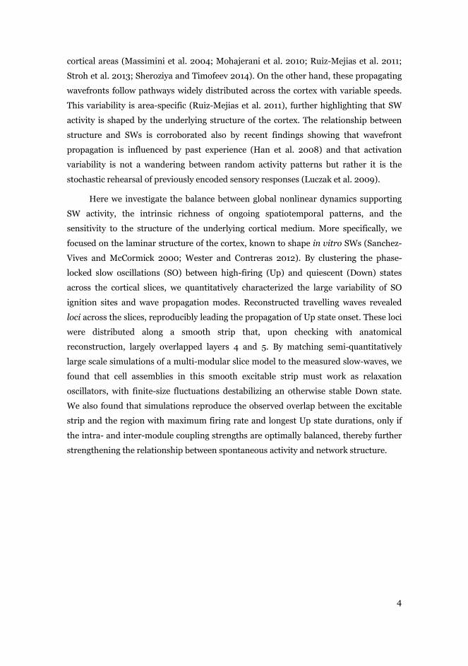
4
cortical areas (Massimini et al. 2004; Mohajerani et al. 2010; Ruiz-Mejias et al. 2011;
Stroh et al. 2013; Sheroziya and Timofeev 2014). On the other hand, these propagating
wavefronts follow pathways widely distributed across the cortex with variable speeds.
This variability is area-specific (Ruiz-Mejias et al. 2011), further highlighting that SW
activity is shaped by the underlying structure of the cortex. The relationship between
structure and SWs is corroborated also by recent findings showing that wavefront
propagation is influenced by past experience (Han et al. 2008) and that activation
variability is not a wandering between random activity patterns but rather it is the
stochastic rehearsal of previously encoded sensory responses (Luczak et al. 2009).
Here we investigate the balance between global nonlinear dynamics supporting
SW activity, the intrinsic richness of ongoing spatiotemporal patterns, and the
sensitivity to the structure of the underlying cortical medium. More specifically, we
focused on the laminar structure of the cortex, known to shape in vitro SWs (Sanchez-
Vives and McCormick 2000; Wester and Contreras 2012). By clustering the phase-
locked slow oscillations (SO) between high-firing (Up) and quiescent (Down) states
across the cortical slices, we quantitatively characterized the large variability of SO
ignition sites and wave propagation modes. Reconstructed travelling waves revealed
loci across the slices, reproducibly leading the propagation of Up state onset. These loci
were distributed along a smooth strip that, upon checking with anatomical
reconstruction, largely overlapped layers 4 and 5. By matching semi-quantitatively
large scale simulations of a multi-modular slice model to the measured slow-waves, we
found that cell assemblies in this smooth excitable strip must work as relaxation
oscillators, with finite-size fluctuations destabilizing an otherwise stable Down state.
We also found that simulations reproduce the observed overlap between the excitable
strip and the region with maximum firing rate and longest Up state durations, only if
the intra- and inter-module coupling strengths are optimally balanced, thereby further
strengthening the relationship between spontaneous activity and network structure.

5
Materials and Methods
Slice preparation and histology.
In vitro experiments were done on 0.4 mm thick visual cortical slices (areas 17, 18 and
19) from 5 to 10 month old male ferrets (Mustela putorius furo) that were anesthetized
with sodium pentobarbital (40 mg/kg) and decapitated. Their brain were removed and
placed in the cold (4-10ºC) cutting solution. Ferrets were cared in accordance with the
European Union guidelines on protection of vertebrates used for experimentation
(Strasbourg 3/18/1986) as well as approved by the local ethical committee. During
cutting of slices on a vibratome, the tissue was place in a solution in which the NaCl was
substituted with sucrose. Following transfer to the interface-style recording chamber
(Fine Sciences Tools, Foster City, CA), the slices were incubated in ‘traditional’ slice
solution containing 126 mM NaCl, 2.5 mM KCl, 2 mM MgSO4, 1 mM NaHPO4, 2 mM
CaCl2, 26 mM NaHCO3 and 10 mM dextrose, aerated with 95% O2, 5% CO2 to a final pH
of 7.4. After approximately 1 hour, the slice solution was modified to contain 1 mM
MgCl2, 1 mM CaCl2 and 4 mM KCl (Sanchez-Vives and McCormick 2000). Bath
temperature was maintained at 34-36oC.
Extracellular multiple unit recordings were obtained with flexible arrays of 16
electrodes arranged in columns as in Fig. 1A (Illa et al. 2015). The multi electrode array
(MEA) covered most of the area occupied by a cortical slice. It consisted of six groups of
electrodes positioned to record electrophysiological activity from supra- and infra-
granular layers (692µm apart) and from what should correspond to 3 different cortical
columns (1500µm apart). The unfiltered field potential (raw signal) was acquired at 20
kHz with Multichannel System amplifier and digitized with a 1401 CED acquisition
board and Spike2 software (Cambridge Electronic Design).
At the end of each experiment slices were fixed in paraformaldehyde (4%),
cryoprotected in 30% sucrose solution in phosphate buffer (0.1 M, pH7.4), frozen in dry
ice and cut in a Thermo Scientific MICROM HM 450 freezing sliding microtome. The
sections (50 µm thick) were mounted in glass slides and Nissl stained, dehydrated,
coverslipped and photographed. Layer limits were drawn according to the size and
density of observed cells and the MEA position was superimposed on the basis of the
identification of marks performed at the end of the recording session.
To check the reliability of the interpolation procedure introduced to investigate
the relationship between spontaneous electrophysiological activity and network
structure in the slice regions far from MEA position, we performed the same

6
experiments on 5 additional cortical slices including the simultaneous recordings from
an additional extra electrode placed sequencially in 5 different location within the area
covered by the MEA (see Supplementary Material for details).
MUA estimate and state detection
Up and Down states and multi-unit activity (MUA) were estimated from the recorded
raw signals as in (Reig et al. 2010; Sanchez-Vives et al. 2010). Briefly, the power spectra
from sliding windows of 5 ms of the raw signal were computed. MUA were estimated as
the relative change of the power in the frequency band [0.2, 1.5] kHz. Average MUA
following Up-to-Down transitions was used as reference value and set to 1. Such
spectral estimate of the MUA was not affected by the electrode filtering properties and
provided a good estimate of the relative firing rate of the pool of neurons nearby the
electrode tip. We then smoothed log(MUA) performing a moving average with a sliding
window of 80 ms. From the long-tailed histogram of log(MUA) (see Fig. 1B) an optimal
threshold separating Up and Down activity states was set at 4 times the standard
deviation (SD) of the Down peak. To avoid biases in the identification of wavefronts,
the same threshold was used for each recording in the same slice, as all having similar
Down peaks SD. This to avoid introducing biases among electrodes in the
characterization of activation and silencing wavefronts. The threshold was also the
same for detecting both Down-to-Up and Up-to-Down transitions.
Slow waves detection and reconstruction
Activation waves were detected when a Down-to-Up transition from multiple electrodes
occurred within a time window ∆T initially chosen to 1 s. Then ∆T was iteratively
reduced by a factor of 0.75, until each detected wave contained no more than one state
transition per electrode. In order to recompose waves involving a subset of columns of
electrodes wrongly detected as separated waves, a minimum inter-wave interval (IWI)
was chosen and waves occurring within the IWI were considered as composing a single
wave. The initial IWI was set to half the maximum time lag between initially detected
waves. Then IWI was iteratively reduced by the 25% if collected waves included the
same electrode columns more than once or if the number of time lags composing the
wave size is larger than the number of electrodes. After each IWI reduction, wave
recollection is recomputed. This iterative process ended once the IWI was neither
reduced nor increased, or when the number of waves including the same electrode
more than once was less than 10% of the total number of detected waves. The iteration
was stopped if the number of recomposed waves in the first step of iteration was higher

7
than a reasonable value of expected waves, that is the median number of transition for
each channel. Otherwise we may have an artefactual amplification of small waves.
Waves including the same electrode more than once and waves with state transitions in
less than 4 electrodes per column were rejected. Such constrain was dictated by the
necessity to fully sample the slice area covered by the MEA in order to have reliable
predictions about ongoing network activity also relatively far from the position of the
electrodes.
Each wave was associated to an array of relative time lags (where t = 1,…Wand
i = 1,…N are the wave and the electrode indices), resulting from the difference between
the detected state transition time in each electrode, and their average across electrodes.
Such arrays of relative time lags, in turn composed the rows of the time lag matrix
(TLM) showed in Figure 2A. TLM columns were grouped in 3 sets of electrodes, each
related to a different electrode column of the MEA. We computed the average
log(MUA) in each of these electrode column detecting Up/Down state transitions on
these pooled signals relying on the same detection adopted for single electrodes. Those
waves in which a Down-to-Up transition was detected in each of these columns was
classified as "full", to distinguish them for the other remaining "partial" waves. Unless
otherwise specified, only full waves were considered for the following analysis. In order
to infer the wavefront time lags T(x,y) in the slice regions not covered by the electrodes,
we interpolated without smoothing such times with a thin-plate spline. For each wave
only those electrodes with detected MUA state transitions were taken into account.
From T(x,y) the speed V(x,y) was computed as
, = 1 , + ,
Slow wave features characterization
We collected wave vectors describing full waves and clustered them using k-means
algorithm to separate different modes of propagations characterized by different origin,
speed and direction. In order to perform k-means clustering, we needed complete
transition time vectors. We filled each empty entry in the vectors, that corresponds to a
non recorded transition during a wave, with the average transition time recorded by the
same electrode in the most similar 5 waves. The median error in the time lag of the
“filled” elements estimated in this way was 30.0 ± 8.0 ms, one order of magnitude
smaller than the characteristic time scale of wave propagation which typically took

8
more than 600 ms to cross the whole slice (see Supplementary Material). For each
recording we grouped waves in 10 clusters. We rejected clusters, and relative waves,
with a mean speed lower than 2 mm/s. This threshold value has been chosen starting
from the observation that the distribution of the speed over all experiments (not
shown) is well fitted by the sum of two distributions. These distributions are peaked
just above and below such threshold, respectively. Of these two components, the one
corresponding to the highest speeds is related to propagating modes described in the
Results section. The other component with slowest speed seemed to be not associated
to traveling activation wavefronts and for this reason we did not analyzed them. On
average, 3 clusters for each experiment were rejected and the accepted ones were
composed of 15 waves.
For each wave from an accepted cluster, we computed the vertical (Vx) and
horizontal (Vy) components of the wavefront velocity from T(x,y) as
= , = ,.
In order to characterize the spatiotemporal complexity of the identified waves we
considered only in this case both full and partial waves described by the time series and partial waves and evaluated the correlation AC(n) as a function of delay n as
follows
= !∑ ∑ #$ −&''' −&'''()$*!* ,
with N the number of electrodes and W the number of detected waves. &''' = ∑ (* .
Note that, lag n did not explicitly relate to the time but rather to the ordinal number of
the detected wave.
Quantitative characterization of slow waves
For each wave an early propagation strip (EPS) was identified as the set of points where
the wavefront tip at different times first occurred in the horizontal direction. In other
words, EPS(x) was the vertical position y where the time-lag surface T(x,y) displayed a
minimum at fixed x: EPS = argmin , . EPSs were identified for all waves from
accepted clusters. All the strips were convolved with a Gaussian kernel along the
vertical direction and averaged to obtain a smoothed probability density function
p(x,y). A cut-off to this density was further adopted by setting p(x,y) = 0 for p(x,y) <
9
0.75 pmax(x), where pmax(x) was the maximum of p(x,y) at a given x. After renormalizing
this cut density average EPS = 4 5, 6. and its SD were finally computed.
For each electrode both the average Up state duration, and the maximum MUA
during the Up state were computed for each wave in an accepted cluster. As for the
time-lag surface T(x,y), these values were interpolated by a thin-plate spline allowing to
obtain TUP(x,y) and MUA(x,y), respectively. From these surfaces, the curves where
maximum Up duration and MUA can be found at different horizontal positions x
(argmax 89, and argmaxMUA, , respectively) were computed (see Figure
4C-E). The distances between these curves and EPS(x) at the horizontal locations of the
electrodes in the array (n = 8) were computed to estimate histograms in Figure 4F-G.
We repeated the same analysis in additional set of similar experiments (n = 5
slices) using an extra electrode placed subsequently in 5 different positions far from
other electrodes of the MEA (see Figure 2F and Supplementary Material), in which one
recording were discarded due to data acquisition instability bringing to have n = 24
samples in the data set. For each SW the propagating wavefronts were computed
relying on the thin-plate spline-based interpolation procedure described above. Such
wavefronts were estimated both with and without the extra electrode (see Fig.2F and
Supplementary Materials) to check the reliability by inspecting the resulting differences
giving a measure of their misalignment in time. The same approach was used to
estimate the measure error due to relying on the interpolation procedure in the
identification of the EPS, and the strips in the slices where the Up state duration and
the MUA are maximal (see Supplementary Material for further details).
To study the wave speed dependence of propagation modes (Fig. 4H-I), we
computed separately the average speeds VL(S) and VR(S) along the average EPS
curvilinear abscissa S in the leftward and rightward direction, respectively. We finally
computed an asymmetry index as the speed difference ∆V(S) = VR(S) − VL(S). Similarly
we also computed the gradient of Up state durations 689=/6=. All these measures
were sub-sampled in order to avoid spurious correlation effects. Decimated points were
selected at steps ∆S = 0,21 mm, a length always greater than the decay constant of the
autocorrelation of TUp(S).
To test the overlap between EPS and some specific laminar structures of the
cortical slices we considered the region where the EPS density p(x,y) > 0.05. Thus we
measured the portion of its area included in each layer (Fig. 7).

10
Where not specified averages across the n = 12 experiments are reported as mean
mean ± standard deviation (SD).
All off-line analyses were performed using MATLAB (The MathWorks, Natick,
MA).
Theory, models and simulations.
We used both network models of integrate-and-fire (IF) neurons and a minimal rate
model to set the simulation parameters. The in silico slice is a multi-modular
interconnected network of spiking neurons. Similarly to (Mattia et al. 2013), cortical
modules were composed of 350 leaky integrate-and-fire (LIF) excitatory (E, 80%) and
inhibitory (I, 20%) neurons with spike frequency adaptation (SFA). Membrane
potential V(t) of LIF neurons evolved according to ?@A?A =− @ABC + IEFGt − IIJKt,
where IEFGt was the synaptic incoming current and τα was the membrane decay
constant ( τE = 20 ms and τI = 10 ms). Spikes were emitted when V(t) crossed a 20 mV
threshold, after which a 15 mV reset potential was set for an absolute refractory period
of 10 ms (6 ms) for excitatory (inhibitory) neurons. IIJKt was the activity-dependent
after-hyperpolarizing potassium current acting as a fatigue mechanism modeling SFA
for excitatory neurons: ?LMNOA?A =− LMNOABMNO +gIJK∑ δt − tQQ , with τAHP = 1 s and gAHP =
0.06 mV/s. The δ(t-tk) were the spikes emitted by the neuron.
Synaptic transmission was instantaneous, and RS$T = ∑ UVVW XYT − TWV + XVZ +∑ U[,WXT − T[,WW . The k-th spike emitted at t = tjk by the local presynaptic neuron j
affected the postsynaptic membrane potential with a synaptic efficacy Jj after a
transmission delay δj. Synaptic efficacies were randomly chosen from a Gaussian
distribution with mean Jαβ and SD ∆Jαβ depending on the type of presynaptic (β = E,
I) and postsynaptic (α = E, I) neurons. We initially set JEE = 0.73 mV, JIE = 0.95 mV,
JEI = 2.55 mV, and JII = 2.55 mV, whereas ∆Jαβ = 0.25 Jαβ for any α and β. Intramodular
connectivity is \]^_ = 80% (probability to have synaptic contact between two neurons
of the same module) for any α and β, unless otherwise specified. Excitatory and
inhibitory synaptic transmission delays were drawn from an exponential distribution
with average 13.3 ms and 3.3 ms respectively. Each neuron receives also spikes coming
from neurons outside the cortical module it belongs to, collectively modeled as a
Poisson process with average spike frequency νext chosen to have under mean-field
approximation an average firing rate νE = 0.7 Hz and νI = 1.75 Hz. Synaptic efficacies

11
Jext,k were randomly chosen from a Gaussian distribution with the same moments as the
local excitatory connections.
The neurons in the excitatory population were grouped in two sub-populations,
25% in a foreground population (F) displaying Up/Down slow oscillations, and the
remaining 75% in a background population (B) always firing at a relatively low firing
rate (Fig. 5B). Oscillatory dynamics in the foreground population was obtained by
potentiating synaptic self-excitation Ucc = d#Uee, with a potentiation level d# = 1.8. To
keep fixed νF = 0.7 Hz and νB = 0.89 Hz, Ugc = Ucg were decreased accordingly.
In the in silico slice, modules were spatially arranged on a 2-dimensional grid
composed of H × B sites (generally H = 9, B = 20). The intermodular connectivity \h]^i
was set only between pairs of subpopulations with presynaptic excitatory neurons,
modeling cortico-cortical long-range synaptic connections. When not otherwise
specified \h]^i = 0.2. Inter-module spike delays were sampled from an exponential
distribution with 21 ms average. Connectivity decayed following a Gaussian function of
the distance with standard deviation λ = 0.7 IMD (inter-modules distance). The
resulting networks had a total size of Nneu = 63 000 neurons and Nsyn= 20 millions of
synapses. The modulation of in silico slice excitability (Fig. 7D) was performed by
changing the spike rate νExt of external spikes (νExt was multiplied by a factor ranging
from 0.89 to 1.00). The layered structure of the in silico slices (Fig. 6) was incorporated
by creating an excitable strip of modules with higher connectivity, such that modules
far from the strip had the lower values of connectivity: the inter- and intramodular
connectivity (\h]^i and \]^_, respectively) were reduced by a factor 0.8. Approaching the
excitable strip connectivity this factor was gradually increased till the maximum
connectivity strip (MCS) where \h]^i and \]^_ reach their maximum value,
independently chosen for inter- and intra-modular connectivity . Numerical
simulations of in silico slices were performed relying on an event-based approach
described in (Mattia and Del Giudice 2000), spanning network times of 100 s.
To use the same analytical approach developed for in vitro recordings to our in
silico slices, we estimated the instantaneous firing rates ν(t) from the simulated
population of excitatory neurons in each module, and used them as MUA after adding a
relatively weak white noise to emulate unspecific background fluctuations of
experimental recordings.
The optimal choice for maximum \h]^i and \]^_ (Fig. 7) was found performing
different simulation with different values of these parameters and looking for the

12
minimum value of the identification error between the EPS and the MCS. The
identification error was estimated as the average vertical distance between the 2 strips.
Simulations were evaluated on a grid of 9 × 9 points in the (max. \]^_, max. \h]^i) plane,
ranging from 0.8 to 1.1. For each point 4 simulations were performed. The resulting
surfaces were interpolated with a thin-plate spline with smoothing parameter p = 0.95.
The dynamical features of each module were set relying on a mean-field theory.
Mean-field (minimal rate) model had dynamics determined by the gain function Φ
(Wilson and Cowan 1972) as follows:
klm6n6T = onp, \p −nq6\6T = − \qr +sn
here np = n and \p = \, with i = F,B,I pointing out the excitatory foreground,
excitatory background and inhibitory populations composing the single model,
respectively. Since the single module includes multiple interacting neural populations,
the mean-field dynamics would be described by a multi-dimensional gain function. Our
gain function Φ was computed as an ‘effective’ gain function ot, along the lines proposed
by (Mascaro and Amit 1999). This approximation allows the reduction of the multi-
dimensional mean-field problem (Amit and Brunel 1997) to a two-dimensional one
corresponding to the dynamics of the firing rate (ν) and of the fatigue level (c) of the
foreground population of interest (Mattia and Sanchez-Vives 2012):
klm6n6T = otn, \ − nq6\6T = − \qr + sn
For this reduced dynamics of a single module nullclines (nu = 0 and \u = 0) can be
derived, whose intersections represent fixed points. Modules were set to have a weakly
stable Down state (meaning that low-firing rate intersection was on the lower branch of
the ν nullcline, rather close to the point where this branch ended, see Figure 5C).
Energy landscapes near the fixed point were defined by the integral of the function otn, \ − n, assuming for c its value in the same fixed point.
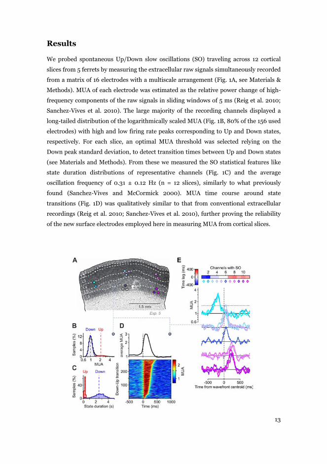
13
Results
We probed spontaneous Up/Down slow oscillations (SO) traveling across 12 cortical
slices from 5 ferrets by measuring the extracellular raw signals simultaneously recorded
from a matrix of 16 electrodes with a multiscale arrangement (Fig. 1A, see Materials &
Methods). MUA of each electrode was estimated as the relative power change of high-
frequency components of the raw signals in sliding windows of 5 ms (Reig et al. 2010;
Sanchez-Vives et al. 2010). The large majority of the recording channels displayed a
long-tailed distribution of the logarithmically scaled MUA (Fig. 1B, 80% of the 156 used
electrodes) with high and low firing rate peaks corresponding to Up and Down states,
respectively. For each slice, an optimal MUA threshold was selected relying on the
Down peak standard deviation, to detect transition times between Up and Down states
(see Materials and Methods). From these we measured the SO statistical features like
state duration distributions of representative channels (Fig. 1C) and the average
oscillation frequency of 0.31 ± 0.12 Hz (n = 12 slices), similarly to what previously
found (Sanchez-Vives and McCormick 2000). MUA time course around state
transitions (Fig. 1D) was qualitatively similar to that from conventional extracellular
recordings (Reig et al. 2010; Sanchez-Vives et al. 2010), further proving the reliability
of the new surface electrodes employed here in measuring MUA from cortical slices.

14
Figure 1. Multi-electrode recordings of slow Up/Down oscillations travelling across
ferret cortical slices. A, Matrix of 16 electrodes (filled circles) superimposed to the
histological slice of an example experiment. Gray circles, unused channels. B, Long-
tailed distribution of the MUA measured from an example electrode (histogram), fitted
to the sum of two Gaussian distributions (red and blue) representing the activity of the
Down and Up state, respectively. Vertical dashed lines, mean of the Gaussian
distributions. C, Histograms of the detected Up and Down state durations (red and
blue, respectively). Vertical dashed lines, average durations. D, Rastergram of MUA
(bottom) centered around the detection time of Down-to-Up transitions (0 ms). Up
states are sorted by duration. Top, average MUA. E, Example time course of the MUA
simultaneously estimated from used channels. Horizontal dotted line, MUA threshold
to detect Up state onset. Diamonds, crossing time of MUA threshold. Colors are as in
Panel A, and characterize different electrodes. Vertical dashed line, average time of Up
state onsets composing the same wavefront. The time lags of Down-to-Up transitions
from this wavefront centroid are represented as a horizontal color bar (top).
Diverse modes of wave propagation across cortical slices
Spontaneous Up state onsets at single channel level did not occur as isolated events. As
shown in Fig. 1E, Up states traveled across the cortical slice (Sanchez-Vives and
McCormick 2000; Sanchez-Vives et al. 2010; Wester and Contreras 2012), giving rise
to waves identifiable by the set of time lags between the MUA onsets occurring across
channels (Fig. 1E-top, see Materials and Methods), and the average time of such local
activations was used as reference time. In each experiment we found a wide variability
of the propagation patterns (Fig. 2A), the large majority of which involved at least two
of the three channel vertical columns composing the multi-electrode array (MEA) (96.7
± 3.4% of detected waves, average across all n = 12 slices). In order to uncover whether
such diversity hid some spatiotemporal organization of spontaneous slow oscillations,
we analyzed with a k-means clustering the subset of full waves, those which propagated
across all the three channel columns of the MEA (Fig. 2B, see Materials and Methods
for details, an average of 80 ± 19% of the detected waves per slice, n = 12). Using a fixed
number of 10 wave clusters, for each we estimated the time course of average activation
wavefronts across the rectangular field covered by the MEA, by performing a spatial
interpolation of the averaged time lags per channel (Fig. 2C, see Materials and Methods
for details).
From these wave profiles it was apparent that not only different directions in the
horizontal propagation spontaneously occurred, but also that across experiments there
was almost no preference in the ignition site (Fig. 2D): on average 59 ± 22 % of the

15
waves appeared first from the lateral columns of electrodes, while 34 ± 25 % originated
close to the central column of the MEA (n = 12). Adding complexity to the phenomenon
was also the evidence that more than one ignition site could contribute to the slice
activation, as it is apparent from the first wave cluster in Fig. 2B (bottom) where an
early Up state onset (blue matrix elements) occurred in the two most lateral electrode
columns. Besides, whatever the mode of propagation was, average wavefronts displayed
always a shape squeezed along the vertical axis, perpendicular to the pia of the cortical
slice. This highlighted a slower velocity along the horizontal (lateral) direction with
respect to the vertical (in depth) one (Fig. 2E): a difference confirmed at the population
level, since the average velocities were 5.8 ± 1.8 mm/s and 8.9 ± 3.4 mm/s, respectively
(n = 12), compatible with previous measures from similar experiments (Sanchez-Vives
and McCormick 2000; Sanchez-Vives et al. 2010).
As all these results rely on the interpolation procedure the region of slice
uncovered by the MEA, we performed an additional set of experiments including an
extra electrode placed in different locations far from the MEA electrode position to
check possible time shift artificially introduce by the adopted method (Fig. 2F, see
Materials and Methods, and Supplementary Material). Up state onset times measured
including the extra electrode was directly compared with those obtained without taking
it into account displayed a high degree of correlation (Fig.2G). At population level, the
average of the absolute error between real and extrapolated time lags resulted to have
across recordings a rather narrow distribution (Fig.2H), with a mean error of 51.0 ± 6.5
ms (n = 24 from different slices and extra electrode positions) which corresponded to a
shift of approximatively 10% the time taken by a wave to travel across the whole slice.
We remark here that this is a result per se, as confirming the smoothness of SW
propagation across cortical slices although dynamics underlying their generation is
expected to be intimately nonlinear.

16
Figure 2. Variability of propagation modes of Up state onsets. A, Time lag matrix of
detected Up state onsets from single traveling waves of an example experiment. Rows
are as the top horizontal bar in Fig. 1E. Gray pixels, failed detections of Down-to-Up
transition. Dashed vertical lines separate channels arranged in different vertical
columns of the MEA (see panel C). Wavefronts are sorted by number of columns
involved. Full and partial waves are those with 3 and 2 columns involved, respectively.
Right, number of channels detecting the Up onset in each wave. B, Time lag matrix of
full waves with failed detections of Up onsets replaced by estimates from similar
wavefronts (see text). Waves are pooled in 10 groups by k-means clustering, separated
by horizontal dashed lines. Gray-shading bar distinguishes different clusters. C, Time
course of average wavefronts from two example clusters. Color code as in panel B and
C. Consecutive wavefronts are separated by 50 ms. Time lags across the depicted area
are interpolated from the average Up onset times across a wave cluster, relying on thin-
plate splines (see text). D, Box plots of the fraction of full and partial waves (all =
partial + full) detected across experiments (n = 12), together with the column of
electrodes from where waves originated (side, from 1st and 3rd column; center, from 2nd

17
column). E, Box plots of the average absolute velocity of wave clusters across
experiments (n = 12) along the horizontal (X) and vertical (Y) direction of the electrode
array, parallel and perpendicular to the cortical surface, respectively. In each box plot,
whiskers (dashed lines) are extreme values of the distribution, edges are the 1st and 3rd
quartiles and the central mark is the median. Where shown, circles are average values
of the distribution. F, Example of interpolated activation wavefronts obtained
including or not data from an extra electrode (solid and dashed lines, respectively). Red
circle represent the location of extra electrode. G, Scatter plot for an example
slice/eleectrode position of Down-to-Up transition times measured from the extra
electrode (δtm) versus the interpolated ones estimated without taking account this
electrode (δti). H, Histogram of the average absolute error estimated for each
slice/electrode position (n = 24).
Memoryless generation of spontaneous waves
Traveling wavefronts of Up state onsets belong to the realm of phenomena occurring in
noisy excitable media, known to spontaneously express spatiotemporal patterns (Cross
and Hohenberg 1993; Sagués et al. 2007). Experimental evidence supports this view, as
local excitation in space elicit propagating self-sustained wavefronts of in vitro activity
(Wu et al. 1999; Wester and Contreras 2012). This phenomenon in slices displays a low
degree of complexity, as spontaneous propagation modes are unidirectional (Golomb
and Amitai 1997; Wu et al. 1999; Sanchez-Vives and McCormick 2000; Wester and
Contreras 2012), i.e. wavefronts mainly propagate in a direction parallel to the cortical
surface. Here, we characterized the dimensionality of the Up wavefronts by performing
a principal component analysis (PCA) of the time lag matrices (Fig. 3A). Detected
spatiotemporal patterns had low dimensionality (maximal dimensionality is 15 as the
electrodes in the MEA are 16 and we set to 0 the average time lag per wave), as the first
two principal components (PC) explained a large part of the time lag variance (Fig. 3B,
average variance explained 82% ± 16%, n = 12). This is consistent with the previous
reports on propagation patterns measured with optical imaging (Wu et al. 1999; Wester
and Contreras 2012). Moreover, in the (PC1,PC2) plane where each full wave
corresponded to a circle (Fig. 3A), two main clusters were often recognizable,
representing the preferred mode of propagations, hence further decreasing the degree
of complexity of spontaneous activity. This indeed corresponded to a rather stereotyped
activation of the slices when belonging to the same mode (wave cluster) of propagation
(see Supplementary Material). In the specific example shown in Fig. 3A, the two
preferred modes corresponded to those shown in Fig. 2C for the same experiment,
although other two smaller clusters were apparent in the first and third quadrant
representing waves with different numbers and positions of ignition sites.

18
To uncover possible complexity in the time domain, we inspected the similarity
degree between wavefronts occurring at different distances in time (see Materials and
Methods). Visual inspection of the time course of φ (Fig. 3C), the angle (phase)
associated in the plane (PC1,PC2) to each circle/wave in Fig. 3A, highlighted a rather
irregular nature in the selection of the next wave onset between the two preferred
propagation modes shown in Fig. 3A and 2C. This qualitative picture was confirmed at
the population level: average autocorrelation ACn of the time lag arrays characterizing
the waves at lag n (see Materials and Methods), was close to 0 (Fig. 3D). Also at single
slice level, wave selection was memoryless (ACn = 0), with only one exception (Fig. 3E,
red plot). In this experiment we found a significant positive correlation AC1 = 0.04
(Wilcoxon signed-rank test, P < 0.01). Intriguingly, there we measured the longest Up
state duration (540 ± 90 ms, more than 200 ms longer than the average duration of 310
± 110 ms across experiments), supporting the hypothesis that this cortical slice was in a
relatively more excitable state with respect to the others. The correlation between AC1
and Up state duration (Fig. 3D) confirmed that the memory degree in the next wave
selection was tighlty related to the excitability of the network, which in turn is expected
to be associated to longer high-firing states. From this perspective, spontaneous waves
in our basal excitability levels and frequencies between 0.11 and 0.40 Hz did not take
into account of past events as expected in a subexcitable state (Sagués et al. 2007).
Under this condition, endogenous fluctuations of the activity in the Down state were
expected to elicit in random locations the onset of different Up wavefronts explaining
the memoryless renewal origin of spontaneous waves in our in vitro model of SO.

19
Figure 3. Past modes of propagation do not influence next Up wavefronts. A, First two
principal components (PC1 and PC2) of the time lag matrix in Fig. 2B. Each circle is an
Up onset wavefront (an array of time lags), whose gray shading indicates the wave
cluster it belongs to (gray levels as in Fig. 2B). B, Box plot of variance explained by PC1
and the first two PCs across all experiments. C, Time course of the phase φ in the
(PC1,PC2) plane of full (filled circles) and partial (dots) waves.Gray filling and
experiment as in A. D, Scatterplot of the autocorrelation AC1 of the time lag arrays of
consecutive waves versus the average duration of the Up state from a reference channel
(that with the highest MUA in the Up state). Experiments included are those with a
fraction of full waves greater than 80% (n = 7 out of 12). E, Autocorrelation ACn of the
time lag arrays of waves at lag n. Black line and gray shading, average and SD of ACn
across all experiments shown in D, respectively. Red line, average ACn for a specific
outlier experiment, not included in the average.
Structure has a role in shaping Up state and onset wavefronts
If SO in cortical slices arose as in a subexcitable medium, we might expect that activity
reverberation did not completely overwhelm the underlying intracortical connectivity

20
structure. Under this hypothesis, spontaneous activity should be (at least partially)
shaped by the structure and excitability distribution of the cortical network, such that
wave propagation and SO in single electrodes should retain and share some of this
information. To investigate such possible interplay between structure and spontaneous
activity, we started looking for features of the excitation waves preserved across
different modes of propagation. More specifically, following each travelling Up onset
wavefront we identified an early propagation strip (EPS, see Materials and Methods),
the most advanced tip of Up onset times along X direction of the MEA (Fig. 4A, dotted
lines). This would likely represent the most excitable part of the slice, where neuronal
pools reacted first to the synaptic input provided by nearby active cortical regions.
Intriguingly, EPS extracted from excitation waves were remarkably similar in the same
experiment, irrespective from their mode of propagation (Fig. 4B), further supporting
the hypothesis that the underlying intracortical connectivity establishes preferred
routes across the slice, modeling the shape of wavefronts independently of ignition site
and direction of propagation.
A natural hypothesis is that EPS would correspond to sites of maximal
excitability, which in turn led us to predict that also local SO properties would be
different along the EPS. To test this hypothesis, we carried out the average Up state
durations TUp across the area covered by MEA, by interpolating the TUp measured from
the different MEA channels (Fig. 4C), similarly to what done for working out traveling
wavefronts (see Materials and Methods). Another mean feature of SO related to the
local excitability of neuronal assemblies was the maximum MUA during Up states
(Fig.4D), computed as above by resorting to interpolation. Most excitable pools were
expected to have the longest Up duration and maximum MUA, corresponding to a
maximally stable Up state (Mattia and Sanchez-Vives 2012), we found them at sites
composing continuous strips (green and cyan curves in Fig. 4C and D, respectively),
which in turn displayed a remarkable overlap with the EPS estimated from wave
propagation (Fig. 4E). This overlaps between excitable strips estimated from different
features of slow wave activity in slice was apparent across all experiments, as the
vertical distance between EPS (YEPS) and position of maximum MUA (Ymax. MUA in Fig.
4F) and maximum TUp (Ymax. Tup in Fig. 4G) were not significantly different from 0
(average distances were 47 ± 140 µm and 10 ± 90 µm, respectively; Wilcoxon sign-rank
test, P > 0.05; see Materials and Methods for details). As also EPS and the strips of
maximum MUA and TUp relied on the interpolation method introduced by commenting
Fig. 2, we investigated the introduced error by measuring the differences when the
extra electrode was or was not taken into account (see Materials and Methods, and

21
Supplementary Material). When computed as an average across all waves, EPSs
estimated with and without the extra electrode (solid and dashed line in Fig.4H,
respectively) widely overlapped. The average vertical distance had a narrow
distribution across slices and extra electrode position (Fig. 4I), with a relatively small
mean EPS location error of 39.5 ± 7.3 µm, approximatively about the 5% of the MEA
vertical extension. Similar results were obtained for the strips of maximum MUA and
TUp (see Supplementary Material). Finally, it is important to remark that all population
analyses were computed at the horizontal center of the electrode columns where
misalignment between interpolation and real measures was the smallest.
Figure 4. Global Up wavefront properties match local dynamical features of SO. A, Two example Up
wavefronts propagating in opposite directions as in Fig. 2C, from another example experiment. Gray
curves with arrows, early propagation strip (EPS). B, Density of EPS from all detected waves. Brown
thick line, weighted average of EPS density along X direction. Gray lines, EPSs of each cluster of
traveling waves computed as in Fig. 2. C, Average Up state duration (TUp) interpolated across the slice

22
area covered by the matrix of electrodes (circles). Green thick line, maximum Up duration found at
different X. D, Average maximum MUA during Up state interpolated as in panel C. Cyan thick line,
maximum MUA found at different X. E, Superimposed weighted average of EPS, maximum Up state
duration and MUA from panels B-D, respectively. F-G, Histograms of the vertical distance across all
experiments (n = 12) between EPSs and line of maximal Up duration (F) or MUA (G). H, EPS
estimated with and without the extra electrode (dashed and solid lines, respectively). Two example
different positions of the extra electrode are showed (top and bottom panels, see Supplementary
Material for details). I, Distributions of the average vertical error in interpolating the EPS across slice
and extra electrode locations (n=24). J, Correlation between speed difference and dTUp/dX, the change
per unit length of Up state duration along the EPS, in the same example experiment of panels A-E.
Speed difference is between median velocities of waves propagating in opposite directions (see
Materials and Methods for details). K, Histogram of the Pearson correlation ρ as in panel H for all
experiments (n = 12). To the right of the red dashed line, correlations ρ are significant (P < 0.05).
What shown here highlights a non-monotonic degree of excitability across the
cortical depth (vertical Y direction of MEAs), displaying a maximum at intermediate
layers where local populations emitted spikes at higher firing rates during Up state,
compatibly with the leading role of Layer 5 in the generation of SO found in previous in
vitro studies (Sanchez-Vives and McCormick 2000; Wester and Contreras 2012). On
the other hand, a heterogeneous degree of excitability was also apparent along the
direction parallel to the cortical surface (horizontal X direction of MEAs), as shown in
Fig. 4C and D, as both maximum MUA and TUp increased from left to right.
A gradient of maximum MUA and Up duration (TUp) along the excitable strip
(solid lines in Fig. 4C and D), would intuitively produce an acceleration of the waves
traveling in the same direction, while a deceleration should be measured for those
waves propagating towards less excitable region of the slice. These could imply
different speed profiles depending on the propagation mode, as acceleration in one way
can be higher than the absolute value of the deceleration in the opposite direction.
Indeed, accelerating waves would find a more excitable tissue, while in the other way
wavefront would be pushed ahead by less excitable cortical assemblies. According to
this, a correlation is expected between the gradient of the excitability (the change of TUp
per unit horizontal length dTUp/dX, see Materials and Methods) and the speed
difference between leftward and rightward propagating wave (Fig. 4J). This correlation,
related to the interplay between the spatiotemporal patterns and horizontal circuits of
the cortex, was found in the majority of the experiments (Fig. 4K, 7 out of 12
experiments had significant correlation, P < 0.05 with a Pearson correlation ρ > 0.5),
further supporting the evidence of an intimate relationship between spontaneous
activity and underlying cortical organization.

23
Weakly stable Down states behind slow oscillations
The analysis described so far shows that cortical slices spontaneously express waves
generated by nonlinear self-excitation; wave propagation exhibits a rich repertoire of
spatiotemporal patterns, which we have shown to be related to the structural
organization of the slice. Taken together, these observations suggest that the cortical
network behaves as a nonlinear excitable system, that is balanced such that it avoids
collapsing into stereotyped excited collective states (e.g. epileptic) while keeping
sensitivity to the connectivity spatial structure.
Figure 5. Slow-wave activity in a spiking neuronal network model of cortical slice. A,
Simulated networks are organized as a lattice of interacting modules (small black
circles). Top, each module is composed of two pools of excitatory (E) and inhibitory
(I) LIF neurons. Excitatory neurons receive an additional state-dependent self-
inhibition (purple link) modeling spike frequency adaptation (SFA). B, Example slow
oscillation in a simulated module. Top raster plot displays a subset of emitted spikes.
Recurrent connectivity between excitatory neurons is shaped in order to have only a
subset of them firing during Up states (depicted in panel A-top as a dashed circle in
the excitatory pool). Center, firing rates ν(t) of different pools, and fatigue level c(t)
proportional to self-inhibition inducing SFA. Bottom, raster of spikes emitted by
neurons from different excitatory modules along X axis of the modeled slice. C,
Nullclines (curves) and fixed-points (circles) of single module dynamics in the (ν,c)
plane, under mean-field approximation. Green curve, example trajectory of the
24
module in the (ν,c) plane, with initial condition on the right of the ν-nullcline. D,
Mean-field nullclines for the same module in (C) receiving two different inputs
obtained increasing external rate of spikes by 7% (dark gray) and 20% (light gray).
Superimposed are example trajectories for these two conditions, colored to encode
time (see top color bar). E, MUA in logarithmic scale estimated from the firing rate
ν(t) of the example cortical module in (B). Inset, histogram of Up and Down state
durations detected from the modeled MUA with the same analytical tools used for in
vitro recordings, as in Fig. 1C.
We therefore undertook to understand, in a theoretical model, the determinants
of such interplay between excitability and sensitivity to structural features. For this
purpose, we set up a large-scale model of cortical slice as a network of modules
arranged uniformly on a lattice, each of them exciting nearby modules which intensity
decreasing with distance (Fig. 5A, Materials and Methods). Modules were composed of
350 leaky integrate-and-fire (LIF) excitatory (80%) and inhibitory (20%) neurons each.
SO occurred as the interplay between recurrent synaptic excitation and a history-
dependent self-inhibition (Fig. 5B), analogously to previous works (Bazhenov et al.
2002; Compte et al. 2003; Holcman and Tsodyks 2006; Mattia and Sanchez-Vives
2012). During Down state activity fluctuations can drive the module through recurrent
excitation towards a high-firing Up state, self-sustained in time by local synaptic
reverberation involving a subset of both excitatory and inhibitory neurons (Fig. 5B-
top). Each excitatory neuron possesses an activity-dependent inhibitory current
modelling spike frequency adaptation (SFA) due to the influx of a hyperpolarizing
potassium current proportional to a fatigue level c(t), which increases each time a spike
is emitted (Koch 1999). During periods of high firing rate ν(t), fatigue c(t) accumulates
(Fig. 5B-middle, purple line), eventually crossing a threshold level which destabilizes
the Up state and determines the Up-to-Down transition and the beginning of the
recovery phase during the Down state. Excitatory intermodular connectivity promotes a
fast chain reaction following a local Down-to-Up transition, recruiting nearby inactive
modules after recovery from previous active states, eventually generating global SO as
in Figure 5B-bottom. A synthetic MUA from the firing rate of each module is computed
by adding a Gaussian white noise unavoidably affecting electrophysiological recordings
(Fig. 5E, Materials and Methods). This allow to analyze and compare experiments and
simulations with the same tools, as those to work out state duration distribution (Fig.
5E, inset).
In order to quantitatively reproduce the statistics of experimental SO, two
minimal requirements had to be met. Firstly, Down state should be weakly stable, such
that Down-to-Up transitions can occur with non negligible probability due only to

25
fluctuations of local activity ν(t); alternatively, Down-to-Up transitions can be primed
by the additional input due to the activation of nearby modules. Secondly, modules
must be excitable, such that small supra-threshold inputs could elicit the onset of an Up
state.
Cortical modules with these features can be designed by relying on mean-field
theory, where the module nonlinear dynamics can be fully depicted in the phase plane
(ν,c) (see Materials and Methods). Figure 5C shows the nullclines (loci of zero time
derivative) for ν (black) and c (red), for a parameters choice meeting the above
requirements: the (stable) Down state is the only intersection between the nullclines
(i.e. the only point attractor of the dynamics), and the green curve describes an example
trajectory followed by the system for an initial condition to the right of the ν nullcline.
As the Down state is very close to the knee of the ν nullcline, its stability is weak and
noise can promote an escape from this state. If endogenous fluctuations are taken into
account, while the system approaches the Down fixed point, it can fluctuate for long
time around it (Fig. 5D, colored curve), until a large enough fluctuation makes it jump
towards the upper branch of the ν nullcline (the Up state). If, at parity of other
parameters, the synaptic input from other modules is increased, the ν nullcline shifts to
the left (Fig. 5D gray curve), and an almost deterministic Down-to-Up transition is
elicited. The two illustrated scenarios address the requirements above, and would
represent i) the modules which due to fluctuations prime the activation wave onset
(black nullcline) and ii) those ones which receiving input from nearby active modules
contribute to the wave propagation (gray nullcline).
Heterogeneous excitability shapes spatiotemporal activity patterns
As the next step, the cortical slice model was employed to investigate the mentioned
interplay between local excitability and structural features suited to reproduce the
spatiotemporal properties of propagating waves found in our experiments (Figs. 2, 3
and 4). For this purpose, we differentially modulated the excitability level of the cortical
modules in the slice model, with the most excitable modules in a strip (dark inverted U
strip in Fig. 6A, Materials and Methods). Following (Mattia and Sanchez-Vives 2012),
the excitability of the cortical modules was regulated by changing the local connectivity \]^_ (probability to establish a synaptic contact between two excitatory neurons in the
same module) and/or the external input from other modules, here dependent on the
global connectivity \h]^i (probability of a connection with an excitatory neuron from
nearby modules). Increasing \]^_ raised the firing rate of the Up states and

26
strengthened its stability (upper branch of the ν nullcline became higher and wider,
gray to black curves in Fig. 6B). At the same time, Down state stability was weakened as
the corresponding attracting energy valley became shallower (in Fig. 6C-top, gray to
black curves).
In this cortical slice model, synchronized SO across the lattice of modules
collectively emerged as an activation wave (Fig. 6D). The spatiotemporal pattern
started with the Up state onset in a neuronal assembly close to the most excitable strip
(Fig. 6D, white dashed line), where modules with maximum \]^_ were located (MCS,
maximum connectivity strip). From there, the activation wave propagated horizontally
following the maximally excitable modules. Maximum MUA (dark red) occurred along
the MCS as the tip of the Up onset wavefront, consistently with what shown in Fig. 4.
More specifically, we characterized activation waves resorting to the cluster analysis
used for the experiments, recognizing also in simulation different modes of propagation
(Fig. 6E). Similar to what found in vitro, the in silico cortical slice displayed a
remarkable overlap between the MCS (dashed line), the EPS estimated from wave
propagation and the strip where maximum MUA and vw were measured from SO of
the single modules (Fig. 6F). This overlap did not depend on the particular shape of the
MCS, as we tested by performing simulations with different strip shapes (not shown).

27
Figure 6. Spiking cortical model with non-homogeneous structure. A, Simulated
networks have the same multi-modular arrangement as in Figure 5A, with the only
difference that modules have a different degree of intra- (local) and intermodular
(global) connectivity (see sketch above). Darkest circles (thickest synaptic link) are
those with the highest connectivity. B Nullclines (curves) and fixed-points (circles) of
single module dynamics in the (ν,c) plane, varying the connectivity level under mean-
field approximation. Gray levels code for connectivity, same as in (A). C, Energy
landscapes (top) around the fixed-points varying connectivity as in (C). Bottom, a
(rotated) zoom of the (ν,c) plane in (C). D, Snapshots at different times of the
propagation of an Up wavefront across the cortical slice model. White dashed line is
the maximum connectivity strip (MCS) corresponding to the region of the most
excitable modules as in (A). Color coded is the MUA from simulations. E, Two
examples of Up wavefronts propagating in opposite directions from the same
simulation, as in Fig. 4A. F, Comparison between estimated EPS (brown), and strips of
maximum Up state duration (green) and MUA (cyan), together with the exact position
of the MCS set in the modeled slice (black dashed line).

28
An optimal balance between short- and long-range connectivity
The capability to produce travelling waves of Up state onsets by assigning a pivotal role
to a subset of maximally excitable neuronal assemblies, which in turn shape these
spatiotemporal patterns does not offend intuition, and may appear as a rather
straightforward expectation. With this in mind, we explored the sensitivity of the wave
features expressed by the in silico slice to the choice of several key parameters of the
network.
The uniqueness of the dynamical regime needed to reproduce the collected in
vitro experimental evidence described in Fig. 5, emerged also by testing the model
network under the modulation of another critical parameter known to modulate the
nonlinear dynamics of networks expressing SO (Mattia and Sanchez-Vives 2012): the
intensity of an external excitatory input R[ modeling the incoming background activity
produced outside the modeled neuronal field (see Materials and Methods). By
increasing R[, SO in single modules displayed Up states with longer durations (Fig.
7D), which in turn positively correlated (Pearson correlation ρ = 0.56, P < 0.001) with
the autocorrelation between the time lag arrays representing wave propagation, the
same as the one measured in experiments (Fig. 3): the larger the excitability, the longer
the Up state and the higher the correlation between the mode of propagation of
successive waves (wave lag 1). Similarly to what found in experiments, on average no
memory was retained about the way waves propagated previously in time (Fig. 7E,
black line at $ ≅ 0). A positive autocorrelation of the time lag arrays occurred only
for those simulations with large enough R[ (red circles in Fig. 7D) representing the
most excitable model networks. In this case average correlation (Fig. 7E, red line) was
significantly different from 0 (Wilcoxon rank sum test, P < 0.01), in good agreement
with what found in vitro (Fig. 3D).
29
Figure 7. In silico optimal balance between global and local connectivity. A, Speed of
traveling wavefronts in cortical slice models varying local (\]^_) and global (\h]^i)
connectivity in the MCS. Connectivity of modules outside the MCS are adjusted
accordingly (see text for details). Dashed line, set of network parameters yielding to a
constant speed of waves of 9 mm/s compatible with experiments. B, Identification
error of MCS from EPS for the same parameter set as in (A). C, Comparison between
EPS and MCS for three different example slice models corresponding to the filled
circles in (B). D, Average Up state duration versus autocorrelation AC between time
lag arrays of consecutive Up wavefronts, computed as in Fig. 3. Each circle is a
simulated network with a different external excitatory input RzA to each excitatory
neuron, modulating the module excitability. Filling color codes for the changes ∆RzA of
the reference external input RzA in the network of panels (A-B) with \]^_ = \h]^i = 1. E,
Autocorrelation ACG of the time lag arrays at different wave lags, as in Fig. 3D. Black
line and gray shading depicts the average and SD over all simulations. Red line, ACG an
outlier slice model with the highest RzA. Middle cortical layers lead wave propagation and SO
Our matching observations from experiments and in silico slices strongly suggest that
the cortical slice structure determines the features of in vitro spontaneous SO and their
propagation across the tissue. A natural question follows up: does the most excitable
region of cortical slices inferred from their spontaneous activity correspond to a specific
anatomical structure? Previous in vitro studies highlighted a leading role of L5 in the
generation of SO (Sanchez-Vives and McCormick 2000). Neurons in this layer were the

30
first to activate with respect to the others located at different depths in the same
cortical column. However, the columnar interactions between supragranular and
infragranular layers (L2/3 and L5) were found to underlie the activity propagation of in
vitro SO (Wester and Contreras 2012). Here, we addressed the question by matching
the laminar organization characterized from histology and the excitable regions
inferred from the spontaneous activity of the slices (Fig. 8A). More specifically, in the
cortical slices where histology was available (n = 9 out of 12 experiments), we computed
the area covered by the distribution of EPS estimated from recorded waves in different
layers (see Materials and Methods for details). As a result, we found a major overlap
between L4 and L5 and EPS distribution (Fig. 8B), and hence with the slice region
where maximum MUA and Up duration were also found. Fractions of EPS in L2/3 and
L6 was significantly lower than those in L4 and L5 (Wilcoxon sign-rank test, P <
0.001). Although EPS area overlapping with L4 was on average lower than the one on
L5, the difference was not significant such that the functional identification of the most
excitable region of cortical slice highlighted a shared role between these two layers.
Figure 8. L4 and L5 overlap with the excitable cortical region predicted from
spontaneous activity propagation of in vitro SO. A, EPS density and area covered by
the MEA superimposed to the image of the corresponding cortical slice stained after
electrophysiological recordings. Dashed lines, boundaries between layers. EPS density
below 0.04 is not shown. B, Box plot of the area covered by EPS density higher than
0.04 in each layer of the cortical slices for which histological characterization was
performed (n = 9 out of 12).
31
Discussion
Our cross-cutting study of the spontaneous alternation between Up and Down states
propagating across cortical slices provides a novel perspective on the dynamical origin
of such a multiscale phenomenon. We relayed on a dedicated experimental setup in
which an array of multiple electrodes was arranged in small electrode clusters, thereby
providing a multi-resolution probe to investigate at the same time both local and global
network dynamics. By this means, we reproducibly found a rich repertoire of
propagation modes all sharing three distinctive features. Firstly, activation waves
systematically propagated parallel to the cortical surface, in agreement with previous
works (Wu et al. 1999; Sanchez-Vives and McCormick 2000; Wester and Contreras
2012), although a wide distribution of speeds and ignition sites was found within each
single experiment. Almost no local activity bumps were observed. Wavefronts of Up
state onset were mildly curved, corresponding to a measured vertical speed, along
columnar orientation, twice the horizontal one. Secondly, irrespective of their
variability, wavefronts revealed loci across the slices which reproducibly led SO
propagation, composing a longitudinal smooth strip. Upon checking against anatomical
reconstruction, this strip largely overlapped L4/L5, compatibly with the evidence that
the most excitable cell assemblies reside in L5 both in vitro (Sanchez-Vives and
McCormick 2000; Wester and Contreras 2012; Krause et al. 2014) and in vivo (Sakata
and Harris 2009; Chauvette et al. 2010; Amigó et al. 2015). Finally, wave onset was an
almost memoryless process, i.e. no correlations were found between propagation
modes of successive waves. Such composite evidence traced a narrow path for the
theoretical model we developed to understand its determinants: the prominent
excitable strip pointed towards a distribution of local excitability; the variability of wave
modes and their lack of memory hinted at an important role of noise.
In fact, we found that a multi-modular large-scale in silico model of the slice,
capable to reproduce all these features, must primarily incorporate a distribution of
excitability in the form of heterogeneous synaptic self-excitation of the single modules.
But we also found that local self-coupling must be optimally balanced with the mutual
excitation between modules. These conditions ensured that our in silico slice acted as a
structured sub-excitable medium in which each module displayed a marginally stable
Down state from which, thanks to maximal sensitivity to endogenous finite-size noise
and inter-modular input, relaxation oscillations could be generated. As a result, the
most excitable strip overlapped the sites with maximal duration of the Up states, and
with maximal firing during Up states, as confirmed by our experiments and further

32
highlighting the pivotal role of L4/L5 in leading SW activity. All findings support the
hypothesis that this default mode spontaneously expressed by the cerebral cortex
(Sanchez-Vives and Mattia 2014) is due to a privileged configuration of the network
allowing both dynamical richness and sensitivity to underlying structure.
Comparisons with previous studies
Horizontal intracortical connections play an important role in determining the speed of
activity propagation (Wadman and Gutnick 1993; Golomb and Amitai 1997; Sanchez-
Vives and McCormick 2000; Wester and Contreras 2012), together with the excitability
level modulated for instance by the balance between excitation and inhibition
(Sanchez-Vives et al. 2010), as also described in theoretical models of SW activity
(Bazhenov et al. 2002; Compte et al. 2003). In the specific framework of in vitro
spontaneous SO, the horizontal speed of SWs we measured (5.5 ± 1.5 mm/s) well
matches those from previous works which range from 7.2 mm/s (Sanchez-Vives et al.
2010) to 10.9 mm/s (Sanchez-Vives and McCormick 2000) in ferret cortical slices
(same preparation adopted here), up to the 20 mm/s measured in rat brain slices
(Wester and Contreras 2012). Note that, the high speed reported in the latter work may
be due not only to the different animals, but also to the use of voltage-sensitive dyes
(VSD) imaging, known to probe subthreshold membrane potential rather than the
suprathreshold MUA we recorded. An even higher horizontal velocity of 30 mm/s was
previously measured with VSD imaging in rat neocortical slices in low (0.1 mM)
magnesium (Wu et al. 1999). SO frequency under these conditions was 7 − 10 Hz,
significantly higher than that measured in our experiments (0.31 ± 0.12 Hz). If greater
speed is attributed to greater excitability, the above theoretical argument would also
imply: i) less variable wave propagation modes (due to reduced sensitivity to the
underlying structure) and ii) more correlated successive propagation modes. Indeed,
(Wu et al. 1999) also observed that waves usually propagated in the same direction.
These predictions which might be ideally tested in experiments in which slice
excitability is directly manipulated as in (Reig et al. 2010; Sanchez-Vives et al. 2010;
Sancristóbal et al. 2016).
Relations with in vivo slow-waves
In anesthetized rodents SW activity is well documented, and reported to be similar to
SWs during deep sleep (Alkire et al. 2008; Cirelli and Tononi 2008; Siegel 2008), thus
raising a question as to their possibly similar dynamic origin to SWs in vitro. A first
difference is that in vivo Down-to-Up wavefronts propagate faster, with a speed

33
tangential to the cortical surface which ranges from 25 to 40 mm/s (Fucke et al. 2011;
Ruiz-Mejias et al. 2011; Stroh et al. 2013; Sheroziya and Timofeev 2014). This is
irrespective on the adopted probe which in these works varied from intracellular and
extracellular recordings to two-photon calcium imaging. What we measured in our
slices experiments as the vertical speed of the Up state onset, in vivo was observed by
directly probing cortical columns during SO (Sakata and Harris 2009; Chauvette et al.
2010). Columnar activation in vivo was more asymmetric as deep layers (L5 and L6)
activated simultaneously, and the activity spreads towards superficial layers (L2/3)
with a speed of about 30 mm/s, as a depth of 700 µm was covered in about 25 ms
(Sakata and Harris 2009). Such quantitative differences in asymmetry and speeds may
be plausibly related to the known lack of long-range cortico-cortical connections in
vitro (Stepanyants et al. 2009; Schnepel et al. 2015), which is expected to be more
pronounced along the direction tangential the cortical surface. This would explain why
in the cortical slice the vertical speed is twice the horizontal one, while they are almost
the same as in the intact brain. We also remark that the mentioned differences may
affect the optimal balance between local excitability and inter-modular connectivity
which we have shown here to be a major determinant of the kinematics of slow waves.
Limitations of this study
Here, activation and silencing of wavefronts were reconstructed relying on an
interpolation procedure between the sparse electrodes of the MEA, and clustering
together similar waves in order to improve the signal-to-noise ratio of the estimated
state transition time lags. Under the assumption of reasonably smooth wavefronts, this
method allowed to recover information about the wavefronts in slice regions where no
electrodes were available. A failure of this assumption might imply a wrong
identification of the depth of the strip leading wave propagation. To test its range of
applicability, we performed simulations of the in silico slice with different shapes and
slopes of the most excitable strip (not shown). As expected, the error in estimating the
strip location from the measured EPS increased for steeper slopes. Nevertheless, its
magnitude was always remarkably small. Of course, having denser arrays of electrodes
would allow to relax the above assumption, without changing the analytic approach
here introduced, which is independent from the MEA size. The flexibility of the
approach would allow to apply it also to other experimental frameworks like the study
of in vivo quasi-planar waves.
Another possible limitation of this study is that we did not sort single units (SU)
from the MUA. Yet, we do not expect any qualitative change in the characterization of

34
in vitro SWs from relying on SU activity instead of MUA. Indeed, using rather different
methodologies with different spatial and temporal resolutions ranging from
intracellular and extracellular recordings, to calcium and VSD imaging, the observed
propagating modes shared in all cases similar features both in vivo (Fucke et al. 2011;
Ruiz-Mejias et al. 2011; Stroh et al. 2013; Sheroziya and Timofeev 2014) and in vitro
(Wu et al. 1999; Sanchez-Vives and McCormick 2000; Sanchez-Vives et al. 2010;
Wester and Contreras 2012).
Functional and dysfunctional implications
An appealing result of the modeling study was the recognition that for the model to
match the experimental it was critical a proper balance between local and mutual
modules excitation. This together with the need of a weakly stable Down state,
establishes a “sweet spot” of the network parameters where structure is influential but
at the same time allows for a wide variety of propagation modes. As travelling waves
have been proposed to contribute both to process and transfer information across
peripheral areas of the cerebral cortex (Rubino et al. 2006; Ferezou et al. 2007; Sato et
al. 2012; Muller et al. 2014), from a computational standpoint an intriguing implication
arises. It has been proposed that optimal sensitivity to structure can be a smart way to
implement “self-organized instability” (Solé et al. 2002). Whenever the environment
changes and new stimuli are sensed, the cortical network moves to a different working
point, likely no longer optimal. To bring the system back to an optimal working regime
a mechanism is needed allowing to recover the proper weak stability of the Down state.
A simple unspecific modulation of the network excitability would serve this purpose. As
a result, the variability of stimulus-evoked waves would not be purely random, but
rather sensitive to the network structure (Rabinovich et al. 2008). If such a self-
organization mechanism would exist, the emergence of a default mode made of
propagating SO should appear as a direct consequence of it.
On the other hand, pushing the cortical tissue outside this sweet spot likely
distorts the spontaneous activity yielding the network to display pathological dynamics,
which can persist if optimality is not recovered. For instance, a wrong balance between
excitation and inhibition is now known to influence the speed of the SWs travelling
across the frontal cortex of Down’s syndrome models (Ruiz-Mejias et al. 2016). An
underexpressed synaptic inhibition seems to underlie the break of long-range
coherence of SW activity in mouse models of the Alzheimer’s disease (Busche et al.
2015). In these cases our analytical approach, combined with properly tuned in silico
models, have a potential to help elucidate which combination of local excitability and

35
inter-modular synaptic coupling underlie SW activity changes, unraveling the
mechanistic roots of pathological dynamics.

36
Acknowledgements
This work was in part supported by CORTICONIC (EC FP7 grant 600806),
WaveScalES (EC FET Flagship HBP SGA1 720270), BFU2014-52467-R and FLAGERA-
PCIN-2015-162-C02-01, MINECO (Spain).

37
References
Alkire MT, Hudetz AG, Tononi G. 2008. Consciousness and anesthesia. Science (80- ).
322:876–880.
Amigó JM, Monetti R, Tort-Colet N, Sanchez-Vives M V. 2015. Layer 5 leads
information flow during slow oscillations according to information directionality
indicators. J Comput Neurosci. 38.
Amit DJ, Brunel N. 1997. Model of global spontaneous activity and local structured
activity during delay periods in the cerebral cortex. Cereb Cortex. 7:237–252.
Bazhenov M, Timofeev I, Steriade M, Sejnowski TJ. 2002. Model of thalamocortical
slow-wave sleep oscillations and transitions to activated States. J Neurosci.
22:8691–8704.
Benucci A, Frazor R a, Carandini M. 2007. Standing waves and traveling waves
distinguish two circuits in visual cortex. Neuron. 55:103–117.
Bringuier V, Chavane F, Glaeser L, Frégnac Y. 1999. Horizontal propagation of visual
activity in the synaptic integration field of area 17 neurons. Science (80- ).
283:695–699.
Busche MA, Kekuš M, Adelsberger H, Noda T, Förstl H, Nelken I, Konnerth A. 2015.
Rescue of long-range circuit dysfunction in Alzheimer’s disease models. Nat
Neurosci. 18:1623–1630.
Chauvette S, Volgushev M, Timofeev I. 2010. Origin of active states in local neocortical
networks during slow sleep oscillation. Cereb Cortex. 20:2660–2674.
Cirelli C, Tononi G. 2008. Is sleep essential? PLoS Biol. 6:1605–1611.
Compte A, Sanchez-Vives M V, McCormick DA, Wang X-J. 2003. Cellular and network
mechanisms of slow oscillatory activity (<1 Hz) and wave propagations in a
cortical network model. J Neurophysiol. 89:2707–2725.
Cross MC, Hohenberg PC. 1993. Pattern formation outside of equilibrium. Rev Mod
Phys. 65:851–1112.
Ermentrout GB, Kleinfeld D. 2001. Traveling electrical waves in cortex: insights from
phase dynamics and speculation on a computational role. Neuron. 29:33–44.
Ferezou I, Haiss F, Gentet LJ, Aronoff R, Weber B, Petersen CCH. 2007.
Spatiotemporal Dynamics of Cortical Sensorimotor Integration in Behaving Mice.
Neuron. 56:907–923.

38
Fucke T, Suchanek D, Nawrot MP, Seamari Y, Heck DH, Aertsen A, Boucsein C. 2011.
Stereotypical spatiotemporal activity patterns during slow-wave activity in the
neocortex. J Neurophysiol. 106:3035–3044.
Golomb D, Amitai Y. 1997. Propagating neuronal discharges in neocortical slices:
computational and experimental study. J Neurophysiol. 78:1199–1211.
Han F, Caporale N, Dan Y. 2008. Reverberation of recent visual experience in
spontaneous cortical waves. Neuron. 60:321–327.
Holcman D, Tsodyks M. 2006. The emergence of Up and Down states in cortical
networks. PLoS Comput Biol. 2:e23.
Illa X, Rebollo B, Gabriel G, Sánchez-Vives M V, Villa R. 2015. A SU-8-based flexible
microprobe for close and distal recordings from the cortical network. In: SPIE
Microtechnologies. International Society for Optics and Photonics. p. 951803.
Jancke D, Chavane F, Naaman S, Grinvald A. 2004. Imaging cortical correlates of
illusion in early visual cortex. Nature. 428:423–426.
Koch C. 1999. Biophysics of Computation: Information Processing in Single Neurons.
New York: Oxford University Press.
Krause BM, Raz A, Uhlrich DJ, Smith PH, Banks MI. 2014. Spiking in auditory cortex
following thalamic stimulation is dominated by cortical network activity. Front
Syst Neurosci. 8:1–24.
Lee S-H, Blake R, Heeger DJ. 2007. Hierarchy of cortical responses underlying
binocular rivalry. Nat Neurosci. 10:1048–1054.
Luczak A, Barthó P, Harris KD. 2009. Spontaneous events outline the realm of possible
sensory responses in neocortical populations. Neuron. 62:413–425.
Mascaro M, Amit DJ. 1999. Effective neural response function for collective population
states. Network. 10:351–373.
Massimini M, Huber R, Ferrarelli F, Hill SL, Tononi G. 2004. The sleep slow oscillation
as a traveling wave. J Neurosci. 24:6862–6870.
Mattia M, Del Giudice P. 2000. Efficient event-driven simulation of large networks of
spiking neurons and dynamical synapses. Neural Comput. 12:2305–2329.
Mattia M, Pani P, Mirabella G, Costa S, Del Giudice P, Ferraina S. 2013. Heterogeneous
attractor cell assemblies for motor planning in premotor cortex. J Neurosci.
33:11155–11168.

39
Mattia M, Sanchez-Vives M V. 2012. Exploring the spectrum of dynamical regimes and
timescales in spontaneous cortical activity. Cogn Neurodyn. 6:239–250.
Mohajerani MH, McVea D a, Fingas M, Murphy TH. 2010. Mirrored bilateral slow-
wave cortical activity within local circuits revealed by fast bihemispheric voltage-
sensitive dye imaging in anesthetized and awake mice. J Neurosci. 30:3745–3751.
Muller L, Reynaud A, Chavane F, Destexhe A. 2014. The stimulus-evoked population
response in visual cortex of awake monkey is a propagating wave. Nat Commun.
5:3675.
Rabinovich MI, Huerta R, Laurent G. 2008. Transient dynamics for neural processing.
Science (80- ). 321:48–50.
Reig R, Mattia M, Compte A, Belmonte C, Sanchez-Vives M V. 2010. Temperature
modulation of slow and fast cortical rhythms. J Neurophysiol. 103:1253–1261.
Rubino D, Robbins KA, Hatsopoulos NG. 2006. Propagating waves mediate
information transfer in the motor cortex. Nat Neurosci. 9:1549–1557.
Ruiz-Mejias M, Ciria-Suarez L, Mattia M, Sanchez-Vives M V. 2011. Slow and fast
rhythms generated in the cerebral cortex of the anesthetized mouse. J
Neurophysiol. 106:2910–2921.
Ruiz-Mejias M, Martinez de Lagran M, Mattia M, Castano-Prat P, Perez-Mendez L,
Ciria-Suarez L, Gener T, Sancristobal B, García-Ojalvo J, Gruart A, Delgado-
García JM, Sanchez-Vives M V, Dierssen M. 2016. Overexpression of Dyrk1A, a
Down Syndrome Candidate, Decreases Excitability and Impairs Gamma
Oscillations in the Prefrontal Cortex. J Neurosci. 36:3648–3659.
Sagués F, Sancho JM, García-Ojalvo J. 2007. Spatiotemporal order out of noise. Rev
Mod Phys. 79:829–882.
Sakata S, Harris KD. 2009. Laminar structure of spontaneous and sensory-evoked
population activity in auditory cortex. Neuron. 64:404–418.
Sanchez-Vives M V, Mattia M. 2014. Slow wave activity as the default mode of the
cerebral cortex. Arch Ital Biol. 152:147–155.
Sanchez-Vives M V, Mattia M, Compte A, Perez-Zabalza M, Winograd M, Descalzo VF,
Reig R. 2010. Inhibitory modulation of cortical up states. J Neurophysiol.
104:1314–1324.
Sanchez-Vives M V, McCormick DA. 2000. Cellular and network mechanisms of
rhythmic recurrent activity in neocortex. Nat Neurosci. 3:1027–1034.

40
Sancristóbal B, Rebollo B, Boada P, Sanchez-Vives M V., Garcia-Ojalvo J. 2016.
Collective stochastic coherence in recurrent neuronal networks. Nat Phys. 12:1–8.
Sato TK, Nauhaus I, Carandini M. 2012. Traveling waves in visual cortex. Neuron.
75:218–229.
Schnepel P, Kumar A, Zohar M, Aertsen A, Boucsein C. 2015. Physiology and Impact of
Horizontal Connections in Rat Neocortex. Cereb Cortex. 25:3818–3835.
Sheroziya M, Timofeev I. 2014. Global Intracellular Slow-Wave Dynamics of the
Thalamocortical System. J Neurosci. 34:8875–8893.
Siegel JM. 2008. Do all animals sleep? Trends Neurosci. 31:208–213.
Solé R V, Alonso D, McKane AJ. 2002. Self-organized instability in complex
ecosystems. Philos Trans R Soc London Ser B. 357:667–671.
Stepanyants A, Martinez LM, Ferecskó AS, Kisvárday ZF, Ferecsko AS. 2009. The
fractions of short- and long-range connections in the visual cortex. Proc Natl Acad
Sci USA. 106:3555–3560.
Stroh A, Adelsberger H, Groh A, Rühlmann C, Fischer S, Schierloh A, Deisseroth K,
Konnerth A. 2013. Making Waves: Initiation and Propagation of Corticothalamic
Ca2+ Waves In Vivo. Neuron. 77:1136–1150.
Wadman WJ, Gutnick MJ. 1993. Non-uniform propagation of epileptiform discharge in
brain slices of rat neocortex. Neuroscience. 52:255–262.
Wester JC, Contreras D. 2012. Columnar interactions determine horizontal
propagation of recurrent network activity in neocortex. J Neurosci. 32:5454–5471.
Wilson HR, Cowan JD. 1972. Excitatory and inhibitory interactions in localized
populations of model neurons. Biophys J. 12:1–24.
Wu J-Y, Guan L, Tsau Y. 1999. Propagating activation during oscillations and evoked
responses in neocortical slices. J Neurosci. 19:5005–5015.
Xu W, Huang X, Takagaki K, Wu J. 2007. Compression and reflection of visually
evoked cortical waves. Neuron. 55:119–129.

1
Title: Ohmic quasistatic models fail to describe the electromagnetic propagation of slow
oscillations and epileptiform activity in cortical tissue
Abstract
Macroscopic models ofthe propagation of electromagnetic fields in neural tissue (from
electroencephalography to local field potentials) assume the validity of the quasistatic
approximation (QSA) of the Maxwell equations. Upon this approximation, which is
extensively applied in both clinical (e.g. deep brain stimulation, electrical neuroimaging)
and experimental neuroscience (e.g. current source density computation via Laplacian of
Potentials), electromagnetic fields travel nearly instantaneously from the sources to the
sensors. Yet, recent estimates suggest that the propagation speed of epileptiform activity
within the hippocampal tissue is too low (~0.1m/s) to justify quasistatic assumptions. We
tested the assumptions of the QSA by studying the electromagnetic propagation of slow
wave oscillations (SWO) and epileptiform activity in neocortical slices after isolating
synaptic from electromagnetic transmission. Contrary to the damped, undistorted,
instantaneous propagation of SWOs (<1Hz) and epileptiform activity predicted by QSA over
short distances, we observed substantial deformations and delays compatible with
dispersion arising from ionic diffusion and/or polarization. Our results suggest that
accurate macroscopic models of propagation of electromagnetic fields in neural tissue
must consider the dispersive properties that account for the laminar and columnar
microstructure of the cortex.

2
Introduction
Macroscopic models of the propagation of electromagnetic fields (local field potential,
LFP; electroencephalography, EEG; magnetoencephalography, MEG) in neural tissue
assume the validity of the quasistatic approximation (QSA) of the Maxwell equations (1). In
these models, the gray matter is typically considered as a homogeneous conductor
described by a constant conductivity and therefore, dispersion, i.e. frequency-dependent
dielectric parameters (conductivity and permittivity), which is inherent to good
conductors (2), is ignored. With dispersion, the propagation speed of electromagnetic
phenomena varies with frequency; therefore, delays and distortion characterize signal
propagation.
In contrast, the most salient property of quasistatic in ohmic (resistive) conductors is the
absence of delays assuming that electric and magnetic fields travel instantaneously from
their sources to the sensors. Consequently, under the QSA, electromagnetic fields are
memoryless as they neither depend on their past values nor those of their sources. In this
view, electromagnetic signals propagating in neural tissue can only afford damping
(attenuation of the wave’s amplitude) but not delays or distortion.The QSA is not only
relevant for computational macroscopic models but also for clinical and experimental
neuroscience. Indeed, the design (3) and understanding of the effects of deep brain
stimulation devices (4) or the models underlying non-invasive electrical neuroimaging (5)
all rely on the QSA. Electrophysiological data analysis estimates the Current Source
Density by calculating the Laplacian of the measured potentials (6). This approach might
be invalid if the QSA is violated (7).
Several reasons cast doubts on the validity of such a simplified model to estimate the
behavior of electromagnetic fields in highly heterogeneous ionic conductors such as neural
tissue. First, the neural tissue preferentially filters some frequencies more than others

3
(8)and LFP/EEG/MEG signals show a 1/f spectrum that is compatible with the existence of
dispersion (9, 10). Second, ionic conductors are lossy materials in which absorption is
important. As a consequence of causality (2), lossy materials are necessarily dispersive.
Third, nearly all dielectric spectroscopy studies of cortical tissue report substantially high
dielectric permittivity values at low frequencies, which isincompatible with the purely
resistive (ohmic) model, as well as important low-frequency dispersion (11, 12).
Noticeably, the lack of dispersion reported by Logothetis (13) in vivo seems to contradict
the universal low-frequency dispersion that was experimentally observed and modeled by
Jonscher (14), Ngai (15) and Dissado and Hill (16) in non-biological materials with ionic
conductivity. Fourth, epileptiform activity in the hippocampus has been recently observed
to propagate by electric field effects at a speed of 0.1 m/s (17), which is far too slow to
justify the instantaneous propagation of the effects predicted by the QSA in the absence
of dispersion. Fifth, a recent experimental study from Gomes et al. (18) indicates the
necessity of revisiting the assumption of the extracellular space as a purely ohmic
medium.
Obtaining reliable estimates of the dielectric parameters in neural tissue via "broadband
dielectric spectroscopy" (19) would readily inform about the accuracy of QSA models to
describe electrophysiological phenomena. Unfortunately, the accuracy of dielectric
spectroscopy is substantially compromised in the low-frequency range of interest to study
neural rhythms. This compromise is a consequence of electrode polarization effects
appearing at the electrode-electrolyte interface that subsist (20) even if a four-electrode
system is used for estimation (13). Removal of polarization effects typically requires
theoretical or phenomenological assumptions on the specific behavior of the polarization
impedance (21, 22). Polarization effects, therefore, compromise the accuracy of dielectric
estimates below 100Hz (21) rendering them unavailable below 10Hz (21, 22).

4
An alternative approach is to evaluate whether substantial delays and distortion
accompany the propagation of the signals that we are interested in modeling, for
instance,those obtained in neural tissue using standard LFP recordings in vitro. Rather
than relying on current injection, which often enhances parasitic effects, one can inspect
the propagation of spontaneously occurring neural activity such as slow wave oscillations
(SWO), which are neural signals consistingof interspersed Up (with active neuronal firing)
and Down (silent) states, and which are similar to those observed during slow-wave sleep
and deep anesthesia(27). Alternatively, one can pharmacologically evoke natural signals
such as epileptiform activity or SWO. Also, it is possible to considerably reduce distortions
of artifactual origin by carefully avoiding filtering and by choosing the recording
electrodes and the amplifiers, making sure that electrode impedance remains negligible
relative to amplifier input impedance over the frequency range of interest (23). Ifdespite
these precautions,delays, and distortions still accompany the electromagnetic propagation
of natural signals, then cortical tissue should be treated as the lossy dispersive dielectric
that is predicted by the causality principle (24), which would be in agreement with the
behavior observed for ionic conductors (25).
We investigated the validity of the QSA by dissociating the electromagnetic from the
synaptic contributions to the propagation of slow wave oscillations and epileptiform
activity in cortical tissue. For this, we used ferret neocortical slices that spontaneously
generate SWO (26). SWO and epileptiform activity provide an excellent testbed since they
belong to the lowest frequency range of the electromagnetic spectrum where the QSA
should be most accurate.To test whether the electromagnetic propagation of SWO and
epileptiform activity can be explained by the QSA, we completely sectioned the cortical
slice into two pieces by making an entire cut perpendicular to the white matter but
allowing contact between the tissue on both sides. Three aspects of this
electromagnetically propagated neural activity were characterized: the attenuation with

5
distance of the signal (damping), the propagation speed, and the possible existence of
signal distortion.
Materials and Methods
General approach: Our main goal was to characterize how fields associated with
physiologically relevant activity (SWOs or epileptiform discharges) propagate in the
cortical tissue. We wanted to evaluate if distortion and delays accompany propagation
independently of synaptic transmission. Indeed, if the neural tissue can be assumed as an
ideal conductor operating under the QSA, then signal delays and distortions should be
absent during extrasynaptic (field-mediated) propagation to source-free regions. On the
contrary, substantial delays and distortion would provide indications of the need to
account for dispersion to model signal propagation. Dispersion, arising from either ionic
diffusion or polarization, would require replacing Poisson by Helmholtz equation (8) in
current models and considering frequency varying dielectric parameters as discussed next.
1. Theory
The Maxwell equations allow describing the propagation of electromagnetic fields in
biological tissue. For simplicity, we express here all equations in the frequency domain.
All fields are complex valued functions that depend on space (r) and frequency (w).
Temporal derivatives in the time domain are replaced by the multiplicative factor iw
where i = √−1and w is measured in rad/s. With this convention, the Maxwell equations
read:
∇xEr,w = −iwBr,w (1) ∇xHr,w = iwDr, w + Jr, w (2)
∇. Dr, w = ρr, w (3) ∇. Br, w = 0 (4)

6
where E is the electric field vector [V/m], H the magnetic field vector [A/m], D the
electric flux density (displacement) vector [As/m2], B the magnetic flux density
(displacement) vector [Tesla], Jfthe current density vector [A/m 2], and ρ the scalar
charge density [As/m 2]. The subscript f is used to indicate free charges and currents, i.e.,
to distinguish (ionic) charges that can move freely within the medium from bound charges.
The current density J consists of two parts:J = J + J, with Jdenoting a primary or
impressed source, independent of the field and delivering energy to carriers (ions), and
Jdenoting the conduction current.
The constitutive relations linking the flux densities (D and B) to the fields (E and H) for
linear isotropic materials read as:
Dr,w = ϵ1 + χr, wEr,w = ϵr,wEr, w (5)
Br,w = µ[Hr, w + χ!r, wHr,w] = µr, wHr,w (6)
Jr,w = σr, wEr,w (7)
Whereχe and χm are the electric and magnetic susceptibilities and ϵ, µ and σ are the
permittivity, permeability, and conductivity, respectively. Since neural tissue is non-
magnetic, its permeability can be considered identical to empty space permeability, i.e.,
µ = µ0.
To relate the Maxwell equations to electrophysiological measurements, it is more
convenient: 1) to express the electric and magnetic fields in terms of the auxiliary
potentials φ and A respectively, where A is the vector potential, and φ the scalar
potential of interest to electrophysiology; and 2) to rely on a formalism in which electric
and magnetic fields are uncoupled via the wave equation in the frequency domain, i.e.,
the Helmholtz equation. In the most general case of anisotropic and heterogeneous

7
materials,the Helmholtz equation can be writtenin terms of a complex permittivity ϵ
defined as: ϵ = ϵϵ# − j σ
% = ϵ − j σ
%, with ϵ# being the relative permittivity (dielectric
constant) F.m() of the material at frequency w. With this definition, the Helmholtz
equation reads (28):
∇. [ϵr,w∇φr,w] + jw∇. [ϵr, wAr, w] = ∇.+,#,%-% (8)
Eq. 8 is not easily solvable for arbitrary materials. In practice, it is common to
approximate materials as if their dielectric parameters ϵand σ are piecewise constants in
spacewhile keeping their frequency dependency.Electric properties, which fluctuate over
space in neural tissue, are averaged over microscopically large-volume elements and
summarized in the form of effective dielectric properties. These engineered variables,
which summarize fields due to neuronal boundaries and structural details, are determined
from dielectric spectroscopy as in Gabriel’s database (21). In this case, the problem is
reduced to the following non-homogeneous Helmholtz equation:
∇.φr,w + %/0,/ φr, w = ∇.+,#,%
-%12#,% (9)
The term %/0,/ = −γ., with γ = α + jβ, is the so-called propagation constant, a frequency-
dependent complex valued function expressed in terms of the attenuation (α, Np/mand
the phase (β, rad/mconstants given by (29):
α = %√µ
√. 891 + : σ
%∈<. − 1=
>/andβ = %√µ∈
√. 891 + : σ
%∈<. + 1=
>/ (10)

8
The attenuation constant defines the rate at which the different frequency components of
the signal attenuate during propagation. The phase constant defines the rate at which the
phase changes as the signal propagates.
In neural tissue, it is standard to compute the fields using the quasistatic approximation
(1), which practically amounts to:
1) Quasistatic: Neglects the second term on the left side of Eq. 9, which amounts
to assume that the propagation constant ? = 0.
2) Ohmic or resistive: Neglects capacitive effects, i.e., neglects the term @AB on
the denominator on the right-hand term in Eq. 9.
These assumptions lead to the Poisson equation with a frequency-independent real-valued
conductivity, which is solved in EEG/LFP modeling using appropriate boundary conditions
(but see (30)). Importantly, despite the generalized use of the term quasistatic in the
bioelectricity literature to refer to the Plonsey and Heppner approximation, it must be
noticed that the Poisson equation in ohmic conductors describes static fields rather than
electro-quasistatic phenomena. Nevertheless, for consistency with the literature in the
domain, we will continue to refer to this approximation as the quasistatic approximation
(QSA).
Assuming γ = 0inEq. 9is applicable for the low frequencies of interest to
electrophysiology if, and only if, the phase velocity GH, were sufficiently large so that the
second term becomes negligible. A common confusion is to imagine that the propagation
speed of electromagnetic phenomena is always very high, approaching the speed of light.
Indeed, this is true in a lossless dielectric medium, where the conductivity is assumed zero
and the propagation constant equals the phase constant (see e.g., (31)). In this case of

9
lossless dielectrics, the phase velocity is defined by v = )√J∈, coinciding with the speed of
light in the material. If the permittivity does not vary with frequency, the group and phase
velocity coincide and dispersion is absent.
Things are different in good conductors, in particular in the low-frequency range where
K%1 ≫ 1. Substitution in Eq. 9 of the attenuation and phase constants defined by Eq. 10 in
good conductors leads to:
α ≈ 9%µσ
. and N ≈ 9%µσ
. (11)
In good conductors, the real and imaginary parts of the propagation constant are
approximately equal both depending on frequency. Therefore, even if the dielectric
properties (ϵand σ)per se are relatively constant over a broad band of frequencies, a good
conductor is always dispersive.
In effect, the phase velocity GH, i.e., the speed at which each frequency component of
the original source travels, is given by:
GH =OP ≈ OQ ≈ )
√R∈ 9.O∈S = 9 .O
RTS = A9 .ORTS = AU[VW ] (12)
where δ is the skin depth, i.e., a measure of the depth at which the electric field and the
current density fall to 1/e of their value at the interface between the membrane (source)
and the extracellular space. For example, in copper at 10 Hz, the skin depth is just 21mm,
and the phase velocity is only 21 mm/s. With these estimates, it is hard to neglect the
second term on the left-hand side in Eq. 9 as to justify the so-called QSA in neuroscience
which, as previously mentioned, corresponds to static. Since in the most general case
dielectric parameters can vary with frequency, we will use, from now on, the term

10
electromagnetic (EM) propagation to refer to the dynamic aspects of the propagation of
fields in tissue that can be described by solutions to the Helmholtz (8) or approximated by
static solutions to the Poisson equations.
Under quasistatic, electrophysiological signals propagate unaltered in shape and with
infinite speed. The situation is completely different outside quasistatic. The lower
frequencies will travel further in a good conductor albeit at lower speeds than the high
frequencies. Thus, good conductors will always exhibit frequency-dependent propagation
speeds and will, therefore, show distortion and filtering even if the dielectric parameters
themselves do not vary with frequency.
1.1 Physical causality forces dispersion in good conductors
The causality principle describes the temporal relationship between cause and effect
stating that no effect can precede its cause. In electrodynamics, causality expresses that
the response of a material to an electromagnetic perturbation must be zero before the
onset of the perturbation. As a property specific to the material, causality cannot be
directly inferred from Maxwell equations (1-4). Developing causality-compliant
electromagnetic models implies that the dielectric parameters (conductivity and
permittivity) are linked by the dispersion or Kramers-Kronig (KK) relations. Dispersion
relations relate the imaginary part of ε, which characterizes the absorptive (damping)
properties of the medium in conductors (24), to the real part of ε, which characterizes its
dispersive (frequency-shifting) properties.
Intuitively, dispersion relations are analogous to linear filters. Causal filters, which
suppress some frequency components without leak of the signal into the past, lead to
distortions and delays. Likewise, in conductors, because of causality, electromagnetic
absorption of certain frequencies must be accompanied by phase shifts of other

11
frequencies. As phase shifts in the frequency domain imply delays in the time domain,
some of the components of the signal should propagate at lower speeds than others
(dispersion) to comply with causality. This results in distortions in the shape of the
temporal wave of the propagated signal. The filtering analogy, nicely illustrated in Toll
(24), reflects that in practice it is impossible to envision a physical system that is at the
same time strongly absorptive, causal and dispersionless (2).
Clearly, modeling dispersion effects is impossible under the QSA as the equations resulting
from neglecting propagation effects (γ. = 0) are the static equations of Poisson/Laplace,
which assume instantaneous and distortionless propagation. Consequently, if signal
propagation in neural tissue is accompanied by distortion and delays, this would require a
description based on the Helmholtz equation (Eq. 9).
2. Experimental procedures
Slice preparation: In vitro experiments were carried out on 400-µm-thick slices from the
ferret occipital cortex, including primary visual cortical areas. Adult ferrets (5–8 months
old, male) were anesthetized with sodium pentobarbital (40 mg/kg) and decapitated. The
entire forebrain was rapidly removed and placed in oxygenated cold (4-10oC) bathing
medium. Ferrets were cared forin accordance with the European Union guidelines on the
protection of vertebrates used for experimentation (Strasbourg 3/18/1986), and the
experiments were approved by the local ethical committee. Details on the preparation can
be found in (32). The bath temperature was constantly monitored and maintained at 34-
36°C.
Complete vertical cut of the cortical slice (Fig. 1):To separate the synaptic from the
electromagnetic (EM) propagation, we performed a complete cut of the slice
perpendicular to cortical layers using a scalpel blade. The cut was done while the slices
were in the interface chamber. The recordings were carried out in the following solution

12
Sanchez-Vives, 2000 #34(in mM): NaCl, 126; Na2HPO4, 1; NaHCO3, 26; KCl, 4; MgSO4, 1;
CaCl2, 1; dextrose, 10; and aerated with 95% O2, 5%CO2 to a final pH of 7.4 . The two sides
of the cut remained in close contact as could be seen through the microscope (Fig. 1C),
where no discontinuity was seen. This was allowed by maintaining the cut slices in an
interface chamber, where the slices remained mechanically stable and firmly adhered at
the bottom of the chamber consisting of filter paper.
Then, the recording grid was placed on top of the sectioned slice, and simultaneous
recordings were obtained from both sides by the same array for every experiment. Once
the experiment was finished, we removed the two sections of the slice from the filter
paper, confirming that they were indeed completely separated, which was the case in all
the experiments (n= 22, 15 control and glutamate-induced waves and seven epileptiform
activity induced by blocking GABAA-mediated inhibition with bicuculline).
Extracellular recordings (Fig. 1): Extracellular local field potential (LFP) recordings were
obtainedusingarrays containing 16 gold electrodes plated with platinum black disposed on
a recording grid (Fig. 1A). A microprobe including an array of holes was designed and
fabricated using SU-8 negative photoresist. The holes were used to allow oxygenation of
the slices, to provide mechanical stability and to allow other electrodes or pipettes to
reach the slice. In each of the recording points, we had 2-3 closely spaced
electrodes(separated by 200 µm) positioned such that they would record from supra and

13
Figure 1. Extracellular recordings from a 16-electrode array positioned in a visual cortex slice.
A. Customized microprobe consisting of 16electrodes (black dotsorganized into six groups
of 2 to 3 closely placed electrodes (black dots; 50µm diameter, separated by 200µm).
Holes in between the electrodes allow the contact between the slice and the oxygenated
and humidified environment. B. Impedance characterization of the array. Electrode-
electrolyte impedance modulus shift measured in 0.9% NaCl before (gray line, bare gold
sensors) and after (black line) modification of the sensors using platinum black. C. Flexible
microprobe array positioned in a sectioned cortical slice, with eight electrodes aimed at
supragranular layers (SG) and eight electrodes at infragranular layers (IG). D. Schematic of
the recording configuration from a sectioned cortical slice. (Left) Ten electrodes recording
from the left part of the slices and six from the right part.Dashed lines display layer limits.
(Right) The scheme represents a situation where glutamate was locally applied to one part
of the slice while applying TTX at the other part. Glu, glutamate; IG, infragranular layer;
L1-L6, layers 1 through 6; SG, supragranular layer; TTX, tetrodotoxin; WM,white matter; Z,
impedance.
infragranular layers (750 µm apart) and from what should correspond to 3 different
cortical columns (1.5 mm apart) (Fig.1A and 1C). In the array, ten electrodes recorded
from one side of the cut and six electrodes from the other side (Fig. 1C and 1D). The
electrodes were 50 µm in diameter, which resulted in high impedance values (at 1 kHz,
|Z|~10 MΩ). We further decreased the impedance by electrochemically coating the
electrode with a veryrough layer of black platinum. With this coating, a 2-fold decrease in
the impedance values was achieved (Fig. 1B), resulting in electrode impedance values
being two orders of magnitude below the amplifiers’ input impedance over the whole
frequency range. Neural activity was referenced to an electrode placed at the bottom of

14
the chamber in contact with the artificial cerebrospinal fluid (ACSF). To exclude the
possibility of phase delays or distortion induced by differences in electrode coating,
electrode impedances and phases were tested with known signals before the recordings
for each recording grid (Fig. 1B). Unfiltered signals were acquired with Multichannel
System amplifier (> 1012 Ω paralleled by ten pF input impedance) and digitized at 10 KHz
with a Power1401 interface and Spike2 software (CED, Cambridge, UK). No filters were
added during the recording stage to avoid signal distortion.
Drug application: Glutamate (0.5mM) and tetrodotoxin (TTX)(30µM) were delivered using
a brief pulse of nitrogen to a drug-containing micropipette (volumes of 10–20 pl, (26)), as
indicated in the text (Fig. 1D). Glutamate was released into different positions within the
slice every 4, 6 or 8 seconds, while TTX was applied to one specific location. The average
response triggered by the release of glutamate was then computed at each position to
cancel out spontaneous activity that was not synchronized to this event. Bicuculline
methiodide (bicuculline) (GABAA blocker; 2.4-3 µM) was bath applied to evoke epileptiform
activity.
3. Signal analysis and statistics
The analysis was based on the raw, unfiltered signals and was done using custom-built
Matlab functions (Matlab R2007b, The Mathworks, Natick, MA). The smoothing seen in the
figures is due to the process of averaging over stimulus repetitions.
Slow wave onset: The onset of the spontaneous SWO was determined following a
previously describedapproach (33). The onset was considered at the moment where the
first derivative of the low-pass (<100 Hz) filtered extracellular potential crossed the zero
line. The end was considered at the moment where the derivative of the signal crossed
the zero line after reaching its maximum. This is the only analysis where off-line filtering
was necessary, and filtering was based on zero-phase forward and reverse digital

15
filteringto minimize signal distortion or time delays. The slow wave onset determined from
this approach was then used to align the unfiltered responses.
Statistics: Both parametric and their equivalent non-parametric tests were used in all
statistical comparisons. All samples were tested for normality using the Lilliefors test (34).
When the test provided clear evidence for rejecting the null hypothesis of normality
(p<0.01) we relied on the nonparametric version of the two-samples t-test, the Mann–
Whitney U. Paired comparisons were preceded by ANOVA and its nonparametric version
(Friedman test) to assess overall differences between groups. Values are presented as
mean ± S.D.
Assessing the presence of response: Mean responses created by time-averaging the
unfiltered data in individual electrodes were tested for significant changes from baseline
(2s) values usingtwo samples, two-tailed t-test. Electrodes that showed a significant
(p<0.01) increase/decrease in signal power, defined as the square of the raw voltage
values with respect to the baseline distribution, were consideredto have a significant
mean response. To identify periods where mean responses significantly deviated from
baseline, we applied a sample-by-sample t-test comparing the distribution of values after
glutamate stimulation with the distribution of all values during the baseline interval. The
periods where the t-test was significant (p=0.001) were defined as periods of significant
responses. The same test was used to compare the responses before and after TTX, and
the responses after TTX were additionally compared to the baseline period.
Peak fitting to characterize damping, distortion, and delays: Statistics on the mean slice
responses evoked by glutamate were estimated from the position, height (amplitude) and
width (duration) of peaks by using an iterative least-square curve fitting. Curve fitting was
performed using the Peak Fitter toolbox (version 5), available from the Matlab user-
contributed section. For each electrode, we iteratively fitted the 2.5 s signal following

16
glutamate release with an increasing number of peaks, varying from two to five, until the
fitting error reached a minimum. Electrodes with poor fitting, indicated by fitting errors
above 10%, were discarded from the statistical analyses.
To evaluate distortion, we introduced a measure of peak compression (PC) defined as the
difference between the width estimated at the electrode with the largest response in the
stimulated triode (reference, Wr) and the width at all other electrodes (We), and all
divided by the reference width, i.e., PC=(Wr-We)/Wr. Note that positive values of the
peak compression denote peaks that are narrowed with respect to the reference, while
negative values denote peak widening. Delays were measured from the difference in
latency between the first peak detected at the reference electrode and the latency of the
first peak at all the other electrodes. The propagation speed of SWOs was computed by
dividing the inter-electrode distance by the estimated delay. To investigate the impact of
the laminated neural geometry on electromagneticpropagation, we computed population
statisticson the fitted peak parameters after splitting the data into four groups according
to the layer onto where glutamate was released (supra/infragranular) and the layer from
which the EM waves were recorded (supra/infragranular).
Results
We recorded from a total of 15 cortical slices that displayed spontaneous slow oscillatory
activity, each oscillation cycle consisting on an Up (active) and a Down (silent) state (as in
26). All of the slices were cut vertically (across layers) and the activity was recorded from
both sides of the cut, whichremained in physical contact.
Electromagnetic propagation of slow oscillations
Cutting the slice resulted in two independent networks on each side, each of them with its
slow oscillatory pattern of spontaneous oscillations (SWOs). We consistently observed that

17
the spontaneous SWOs that originated and propagated within one side of the slice could be
recorded across the cut albeit with strongly reduced amplitudes (Fig. 2A). Mean Up states
on one side of the cut, once aligned with the onset of spontaneous Up states on the other
side, were significantly different from baseline in 86% of the cases (p<0.01, t-test; n= 13
out of 15). Mean results on the 15 slices where spontaneous SWO were investigated
indicate that spontaneous SWOs lost on average more than 50% of their initial energy (51.2
± 34 % S.D.) over distances as short as 1.5 mm when propagated by EM effects without
synaptic connectivity. Averaging across repetitions was necessary to minimize the impact
of the spontaneous activity on the side where we assumed that time-locked events were
uniquely determined by EM propagation. In the next sections, we resorted to evoked
rather than spontaneous Up states for these reasons.
Signal distortion and delays characterize the propagation of activity
Triggered events such as Up states induced by local glutamate application (Fig. 2B) or
glutamate responses per se (Fig. 2C) presented the advantages of providing a well-defined
time window allowing to measure larger amplitudes across the cut. Moreover,
pharmacological stimulation has advantages over electrical stimulation, since it reduces
the risk of contaminating the data with capacitive electrode artifacts.
Local application of glutamate in this preparation has been previously proved to be useful
for evoking SWOs in a reliable way (26). The difference between Up states and glutamate
responses is that Up states are based on local synaptic reverberation (26, 35) while
glutamateresponses are a postsynaptic response of a local neuronal population.
Spontaneous epileptiform events induced by addition of the GABAA blocker bicucullineto
the bath led to rather large EM-propagated responses traveling across the cut (Fig. 2D).

18
Figure 2. Damping, delays, and distortion characterize the electromagnetic (EM) propagation of
both spontaneous and evoked activity.A-D. Four different recording examples of activity
originated at position 1 (IG) and its simultaneous EM activity recorded at position 2 (IG).
From top to bottom: A: spontaneous Up state (black); B: Up state evoked with glutamate
(blue); C: glutamate response (green); D: spontaneous (not triggered) epileptiform
discharge under 2.4µM bicuculline methiodide bath application. The rightmost panels show
the cross-correlations between the voltages at positions 1 and 2 computed over the periods
shadowed in A-D: 800ms, 300ms, 550ms, and 320ms, respectively. Asterisk on B and D, fast
frequency components. IG, infragranular layer; SG, supragranular layer; CC, cross-
correlation.
Damping was a shared property ofall EM-propagated events, independently ofthem being
spontaneous or evoked, physiological or epileptiform. For instance, epileptiform
discharges occurring by blocking inhibition withbicucullinewere large events (Fig. 2D) that

19
were well detectable across the cut. Yet, the slow component of epileptiform responses
lost on average more than 90% of itsamplitude during propagation across the cut, passing
from 500 µV at the site with the largest amplitude to 50 µV at the closest contact across
the cut (n=7 events, recorded under GABAA receptor blockade with bicuculline).
Cross-correlations between the propagated and the original signals never reached their
maximum at zero lag; instead, they clearly showed perceptible delays (Fig. 2A-D,
rightmost panels). Moreover, the strong filtering of the initial fast frequency components
propagating over 1.5 mm is evident from the traces, indicating distortion (asterisks in Fig.
2B and 2D).While the examples illustrated in Figure 2 correspond to the propagation of
single events, the presence of delays was systematic across repetitions. The delays
estimated from the mean cross-correlations (250 ms after event onset) over the seven
slices where propagation of epileptiform events was investigated (more than 191 events)
were on average 28.5 ± 20ms (i.e. 52 mm/s). Mean cross-correlation values of the seven
slices were relatively low (mean max CC = 0.33±26), suggesting that propagated signals
were distorted versions of the original epileptiform signal.
Ruling out potential confounds between synaptic and EM propagation
In Figure 3A we illustrate four examples of EM propagation of mean glutamate-induced
responses (black traces with asterisk)and their respective EM propagation across the cut
(red traces). Even though the responses are obviously damped across the cut, when
expanded, the shape of the responses can be observed (Fig. 3A, center).Glutamate-
induced responses and their EM-propagated signals across the cut were different
depending on the site where they had been generated (Fig. 3A), illustrating the
asymmetries present across cortical layers and suggesting an impact of the local cortical
structure on the EM propagation.

20
EM propagation across the cut was sometimes large enough to recruit the local neuronal
population and eventually generate enough local reverberation, resulting into a full-blown
Up state (e.g. Fig. 3B1). This is interesting in itself since it illustrates an interaction
between EM and synaptic propagation that probably takes place physiologically. However,
to properly quantify EM propagation, we need to separateEMfromsynaptic propagation. To
do this, we locally applied 30 µM TTX to the recording area on one side ofthe cut (n=7
slices; Fig. 3C, green). By doing this, we ensured that the observed response in this
location strictly corresponded to the EM-transmitted signal given that TTX blocks synaptic
transmission. We then evaluated the impact of TTX application on the EM-propagated
response across the cut, specifically, the impact on its amplitude as well as on any
existing delays or distortions.
Damping and delays in the propagated signals before (Fig. 3B) and after (Fig. 3C) blocking
the activity of local networks by TTX were comparable. TTX abolished spontaneous
oscillations and multiunit activity in the channels surrounding its application (Fig. 3C,
green) but it did not abolish the mean glutamate response significantly different from zero
(p=3e-4, t-test) on the other side of the cut (Fig. 3C, gray). Response timing and
amplitudes were assessed before and after TTX in the 2 s following the release of
glutamate. TTX application did not change the main negative component of the EM-
propagated response (response peak) (mean p=0.21, t-test). The cross-correlations
between the mean responses before and after TTX were highly significant (mean
0.91±0.6, n=7, p=2.5e-5) and peaked at zero lag. These findings suggest that the neural
response evoked by glutamate propagated across the cut even though synaptic
propagation was blocked, thus resulting in an EM-propagated signal.

21
Figure 3. Distortion and propagation delays measured on averaged responses are not due to
synaptic delays. A. Black traces depict the mean responses evoked by periodic releases of
glutamate (n=130) at different positions within the slice (indicated by an asterisk). Red
traces show the mean responses computed after EM propagation across the cut;expanded
vertical scale outside the slice schemes. B. Raw LFP (top traces) and MultiUnit activity
(MUA, bottom traces) recorded at IG layers on both sides of the cut (contact 1 and 2) in
response to glutamate release every 4 s on the right part (black). C. Local application of
TTX at contact 1 blocking synaptic activity (spontaneous SWO, green), but not glutamate
responses (gray). D. (Left) Superposition of the mean responses (standard errors overlaid)
to glutamate before (red) and after (green) blocking synaptic transmission with TTX at
contact 1 and across the cut at contact 2, before (black) and after(gray) TTX. (Right) Peak
to peak delays are seen between contacts 1 and 2 after TTX.Abbreviations as in Fig. 2.
The mean response of the non-stimulated side of the cut was similarly damped before and
after TTX application (Fig. 3D). In this particular example, damping was accompanied by a
delay of the propagated signal by 104 ms (Fig. 3D, right). Overall, signal delays between
the stimulated site and the closest contacts on the other side of the cut before and after
TTX were nearly identical (mean delay=92.2 ±17ms before TTX and mean delay=96.4±23ms

22
after TTX, p=0.23, t-test). Such similarities in peak to peak delays before and after TTX
rule out synaptic conduction delays as a potential explanation for the low propagation
speed of the EM effects on cortical tissue. In the shown example (Fig. 3D, right), the
speed at which the envelope of the signal propagated over the 1.5mm separating both
contacts resultedin a modest value of 14 mm/s. This speed is more than five orders of
magnitude lower than the one estimated (equation 12) from available dielectric
parameters (12) for 10 Hz (~200000 mm/s) but similar to the speed at which SWO typically
propagate under intact synaptic connectivity (26).
Distortion and delays characterize EM propagation
Local application of glutamate evokes neural activity generated by the postsynaptic
activation of glutamate receptors plus the subsequent recruitment of local networks.
Predicting the potential patterns to be measured at a source-free location (e.g., the non-
stimulated side of the slice) as a function of all potentials recorded in the stimulated site
would require knowing: 1) the currents arising everywhere, 2) the local geometry and 3)
dielectric parameters below 10 Hz (36). However, as illustrated in Figures 4 and 5, the
mean responses to glutamate, on which we based estimates of distortion and speed given
next, tended to be very local to the stimulated triode with amplitudes quickly decaying at
contacts potentially connected to the stimulated site (Fig. 4B, bottom row, and Fig. 5B
top row). Therefore, responses estimated at electrodes on the other side of the cut were
dominated by the responses at the stimulated contacts. In cases like this one, with a
relatively simple spatial pattern of potentials, delays and distortions were still observed
(Fig. 5B), suggesting that they progressively appearedbecause ofEM propagation in a
dispersive tissue.Similarly, during the propagation of epileptiform events spontaneously
generated in the left sectionof the cut, all electrodes on the left side showed the initial
fast component that was missing on the right side of the cut.

23
Figure 4. Damping, Compression, and Widening of the EM propagated responses in 12 slices. A.
Scheme showing the spatial distribution of channels and the corresponding cortical layers
stimulated by local application of glutamate. B.Event-triggered average waveforms
obtained from 102 repetitions of glutamate application to the location indicated in A. The
location of the recordings is indicated by the number. C, D, and E illustrate population
statistics of the damping and distortions of the EM-propagated waves. Statistics were
computed from the fitting of event-triggered average peaks using a minimum of 50
repetitions to compute each average. Population statistics (Mean & Standard Error)
summarize results from 64 releases of glutamate at one of the triodes/diodes on 12
different slices. *p<=0.05, **p<=0.01, ***p<=0.001 using t-test or Mann–Whitney U test. Stim
(stimulation), Rec (recording electrode), 1-4 (electrode position for each recording),
Hollow/full bars correspond to the application of glutamate at SG/IG, respectively.
Dark/light gray, SG/IG recording, respectively.Other abbreviations as in Fig. 2.
We also investigated if the presence of the cut played a major role in the observed delays
and distortions. To do so, we blocked synaptic transmission on the leftmost pairs of
electrodes (diodes) in five slices by locally applying TTX over them. This allowed us to
explore how the responses to glutamate locally applied to the contacts in the middle of
the slice propagated to a pharmacologically “synaptic-disconnected” rather than to a

24
physically “synaptic-disconnected” tissue. Delays and distortion during EM propagation to
TTX-blocked areas (not shown) were like those observed in the presence of the cut,
indicating that the artificial interface created by the cut was not the main source of
delays and distortion.
Propagation of glutamate-evoked slow waves as a function of local microstructure
Cortical microstructures are expected to play a major role in shaping LFP propagation
(37). We, therefore, evaluated if and how different parameters of the glutamate-evoked
mean propagated peaks (duration, amplitude, peak compression/widening and
propagation speed) varied as a function of both the stimulated and the recorded cortical
layers (Fig. 4 and 5). The plots summarize results of 62 cases, with each case defined as
the release of glutamate at a given triode (12 slices/6 triodes, 10out of 72 cases were
discarded because peak fitting errors were above 10%). Only sites not synaptically
connected to the stimulated site are summarized in the statistics. The responses were
divided according to the layer where the electrode recording the EM-propagated response
was positioned and the layer where the glutamate was released (Fig.4A,B, and 5A,B).
We observed significant differences in the EM propagation as a function of the layer. In
comparison to contacts within infragranular layers, those at supragranular layers showed
significantly narrower (Fig.4B,C, p<0.01, t-test) and smaller peaks (p<0.01, t-test) upon
both supragranular and infragranular stimulation. We quantified distortion using a measure
of the peak widening/compression (Fig. 4E) that provided information specific to the
nature of the distortion, positive values indicating compression and negative values
indicating widening(see Materials and Methods). Overall, we observed that distortion was
sensitive to the positions of the source (stimulated site) with respect to the receiver;
andhighlysensitive to the layers traversed by the signals during their propagation.

25
Figure 5. EM propagation speeds of glutamate responses are too slow to justify the quasistatic
approximation (QSA).A-B. Same as figure 4A-B. In this case, the onset of the glutamate
application is depicted. C. Mean EM propagation speeds computed as a function of the
stimulated layer (Stim). Electrodes such as 1 in the bottom plot in B where no significant
responses above/below baseline were detected (t-test)were excluded. Speed was
computed as the difference in latency between the peak fitted to the stimulated site and
the IG and SG sites on the other side of thecut divided by the distance between the
stimulated electrodes. Abbreviations as in Fig. 2 and Fig. 4 (*p<0.05 using t-test).
Application of glutamate to supragranular layers (Fig. 4E) led to significant peak widening
recorded in infragranular layers (p=0.046, U-test). On the contrary, application of
glutamate to infragranular stimulation led peak compression (p=0.0002, U-test) while
propagating across the columns to supragranular layers (Fig. 4E). In short, signal distortion
(peak widening/compression) was overall less severe when glutamate responses
propagated from supra to infragranular layers than when traveling from infra to
supragranular layers. The similar deformation of the responses between intact synaptic
connectivity and absent connectivity suggests a role for cortical microstructure in shaping
LFP responses.
Regarding propagation speed, the horizontal propagation speed was relatively stable
across layers since no significant differences were observed as a function of the stimulated

26
site (p=0.13, U-test) (Fig. 5). Propagation speeds were slightly faster when EM signals
propagated through infragranular layers (Fig. 5C). EM propagation speed was significantly
slower than propagation speed under intact synaptic connectivity (Mean intact
connectivity: 13.6 ± 2.70 SD mm/s, Mean EM: 18.3 ± 2.85 SD; p=0.0006, Mann-Whitney U-
test).
Discussion
In this study,we found that electromagnetic propagation of SWO and epileptiform activity
cannot be explained by the QSA.For this, we experimentally assessed the main
assumptions underlying macroscopic models currently in use in the neuroscience literature
(assumptions 1 and 2 in the theoretical section of the Methods) to describe the
propagation of LFP and EEG/MEG signals in cortical tissue. It is often assumed that neural
tissue behaves as an homogeneous ohmic conductor (i.e., neurons, membranes and
extracellular space taken as mixed into a continuous model characterized by a frequency-
independent unique conductivity value). In this model, signals with different frequency
content propagate without distortion and at infinite speeds from the sources to the
sensors. This assumption seems at odds with theoretical predictions for good conductors
(see equation 12) or with recent measurements of the dielectric properties (3, 21), which
attribute large permittivity values and strongly dispersive properties to neural tissue
within the electrophysiological range of interest in agreement with the theory (equations
11 and 12). Experimental evidence against low-frequency dispersion was later provided by
an in vivo study from Logothetis et al.(13), although results from Gomes et al. (18) which
considered the low-frequency range under 10 Hz seem to contradict this finding. Directly
estimating dielectric properties is particularly problematic within the low-frequency band
where the parasitic polarization effects at the interface between tissue and electrodes
seriously decrease the reliability of the estimates (20, 36), even if the four-electrode
system is used (20). These effects are particularly acute during electrical stimulation.

27
To partially overcome these limitations, we investigated here the propagation of signals
naturally evoked in neural tissue during physiological (SWOs) or pathological (epileptiform
activity) cortical activity. Noteworthy, the use of the term “wave” to refer to SWOs does
not refer to the physical concept of electromagnetic waves, but rather to the
neuroscience concept of wave cycle of neural oscillations. We searched for unequivocal
signs of low-frequency dispersion (signal distortion and delays) using pharmacological
manipulations and recording settings aimed at minimizing artifactual contributions from
the electrode-tissue interface. To isolate synaptic transmission (also responsible for signal
delays) from electromagnetic (which we call here electromagnetic—EM) propagation, we
performed a complete section of the cortical slice perpendicular to the cortical layers
while ensuring that both sides of the cut remained in contact.
In agreement with previous studies (18), we observed important deviations from
predictions of the non-dispersive quasistatic approximation (QSA), which is often used to
model the propagation of low-frequency SWO from intracranial, LFP and scalp (EEG/MEG)
recordings. Instead of the expected undistorted and nearly instantaneous propagation
predicted by the Poisson equation, SWOs underwent considerable distortion and delays
during their propagation across the interrupted cortical tissue. Non-synaptic propagation
speeds were strikingly low, approaching the values at which slow waves travel under
intact horizontal synaptic connections (26, 38-40). Our estimated EM mean propagation
speeds (~18mm/s) were, however, closer to the propagation speeds (~100mm/s) reported
in hippocampal tissue (17) during the electric propagation of epileptiform activity than to
quasistatic predictions. The large delays and the fact that our conclusions are based on
comparing unfiltered signals within the same frequency band using the same
instrumentation (23) makes it unlikely that electrode polarization was the source of the
distortions.
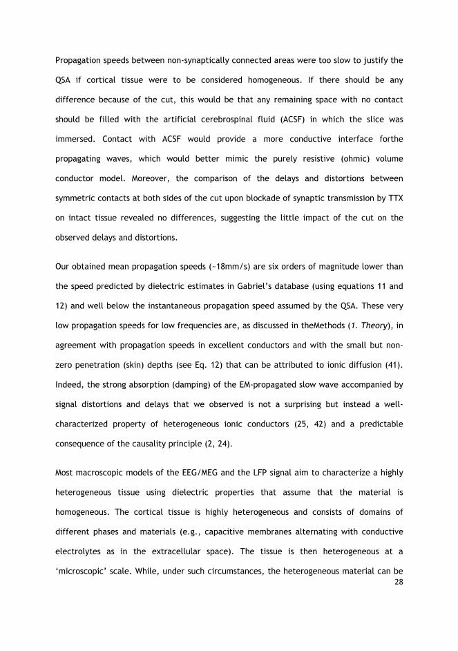
28
Propagation speeds between non-synaptically connected areas were too slow to justify the
QSA if cortical tissue were to be considered homogeneous. If there should be any
difference because of the cut, this would be that any remaining space with no contact
should be filled with the artificial cerebrospinal fluid (ACSF) in which the slice was
immersed. Contact with ACSF would provide a more conductive interface forthe
propagating waves, which would better mimic the purely resistive (ohmic) volume
conductor model. Moreover, the comparison of the delays and distortions between
symmetric contacts at both sides of the cut upon blockade of synaptic transmission by TTX
on intact tissue revealed no differences, suggesting the little impact of the cut on the
observed delays and distortions.
Our obtained mean propagation speeds (~18mm/s) are six orders of magnitude lower than
the speed predicted by dielectric estimates in Gabriel’s database (using equations 11 and
12) and well below the instantaneous propagation speed assumed by the QSA. These very
low propagation speeds for low frequencies are, as discussed in theMethods (1. Theory), in
agreement with propagation speeds in excellent conductors and with the small but non-
zero penetration (skin) depths (see Eq. 12) that can be attributed to ionic diffusion (41).
Indeed, the strong absorption (damping) of the EM-propagated slow wave accompanied by
signal distortions and delays that we observed is not a surprising but instead a well-
characterized property of heterogeneous ionic conductors (25, 42) and a predictable
consequence of the causality principle (2, 24).
Most macroscopic models of the EEG/MEG and the LFP signal aim to characterize a highly
heterogeneous tissue using dielectric properties that assume that the material is
homogeneous. The cortical tissue is highly heterogeneous and consists of domains of
different phases and materials (e.g., capacitive membranes alternating with conductive
electrolytes as in the extracellular space). The tissue is then heterogeneous at a
‘microscopic’ scale. While, under such circumstances, the heterogeneous material can be

29
viewed as a continuum on the microscopic scale and can be ascribed macroscopic or
‘effective’ properties (42), a proper theoretical formalism to do so is currently lacking. It
is however known from dielectric spectroscopy studies in heterogeneous media (42) that
water membrane heterogeneity exhibits a typical dispersive dielectric behavior
characterized by 1) a power law dependence of the effective electric conductivity at low
frequencies (called alpha dispersion), often ascribed to the longitudinal and tangential
diffusion of ions in the electrical double layer that surrounds charged membranes (43),
and 2) large effective permittivity values at very low frequencies that are seen when
interfaces with aqueous ionic substances are involved (44). Consequently, the large
permittivity values reported by Gabriel (1996) and confirmed in vivo by Wagner (22)and
the dispersion effects are neither unique to animal tissue nor necessarily artefactual in
origin. Instead, they are more likely a general property of the microstructure of
heterogeneous materials with ionic conduction and aqueous interfaces (45, 46). In support
of this view, detailed LFP models (47) that restrict the QSA to the extracellular space in a
purely ohmic medium, while incorporating neuronal geometries and membrane
capacitances into the cable model, can reproduce signal delays and distortion comparable
to ours (although see (48)). According to previous simulations that use a synaptic current
as input and a non-quasistatic modeling framework (cable equation), delays and distortion
are due to the intrinsic-dendritic filtering effect and therefore to tissue heterogeneities
(Torbjørn V Ness, Gaute Einenvoll, personal communication).
The modeling and simulation studies from Bedard et al. (49) or Lindén et al. (47) link the
heterogeneous microstructure of neural tissue with its filtering properties. As shown by
Bedard et al. (48), spatial gradients in the conductivity and permittivity induced by neural
microstructures results in the filtering of the high-frequency components of the
extracellular signals with distance. As previously discussed, filtering of some components
should result in phase shifts and delays of other components, hence leading to signal

30
delays and distortion. Therefore,our observations of distortion and delays seem in line
with previous modeling studies specific to neural tissue (47, 49), being in agreement with
the causality principle and likely reflectinga universal property inherent to highly
heterogeneous materials (42). These effects cannot be accountedfor within the
homogeneous quasistatic modeling framework currently in use in many macroscopic
models.
The experimental findings of the current study are compatible with the necessity to rely
on dispersive models (i.e., frequency varying dielectric properties) to build homogeneous
macroscopic models of cortical tissue. We describe the propagation of the
electromagnetic fields in a homogenized macroscopic model of neural tissue using
effective parameters (permittivity and conductivity), a situation in which there are no
divisions between cell membranes and extracellular space. As shown in the theoretical
section, dispersion is a property inherent to conductors rather than capacitors
(dielectrics). Consequently, the dispersive properties of neural tissue cannot be solely
ascribed tothe capacitive properties of the neuron membrane which is typically considered
as frequency independent. The microscopic origin of these dispersive properties within the
low-frequency range is probably influenced by multiple physical and physicochemical
effects including transport or ionic diffusion and polarization phenomena (37, 50, 51).
Unfortunately, appropriate models able to describe the universality of ionic conduction
laws in disordered materials (52) in the presence of aqueous charged interfaces are still
absent. Currently, theoretical models attribute low-frequency dispersion (below 1kHz) to
the longitudinal and tangential diffusion of ions within the electrical double layer that
surrounds charged particles or membranes (43). Ionic diffusion is one of the likely
microscopic mechanisms that can explain low propagation speeds and distortion (18),
thereby leading to a distribution of relaxation times and therefore to frequency-
dependent dielectric parameters (dispersion). Furthermore, since our cut slices are in
31
contact, we cannot rule out certain contribution of ionic diffusion e.g. potassium ions
traveling across the cut, to the described phenomena. However, further investigation on
the microscopic mechanisms underlying dispersion is required since alternative
mechanisms to ionic diffusion have been proposed(14, 50).
Overall, the observation of delays and distortions during the propagation of physiological
signals bears implications for the modeling, analysis, and interpretation of the LFP,
intracranial data or scalp-recorded EEG/MEG signals. The approach taken in this study to
investigate capacitive effects and dispersion for frequencies below 10 Hz (18, 22) is unable
to provide concrete estimates for the permittivity and conductivity needed to build
detailed macroscopic models. Therefore, it is not possible to fully appreciate the
magnitude of errors incurred by quasistatic ohmic considerations. However, the studies by
Wagner (22) or Butson and McIntyre (53), which evaluated the importance of including
capacitive effects (permittivity) within models for transcranial magnetic stimulation (TMS)
or deep brain stimulation (DBS) models, detected substantial differences.
While Butner or Wagner and McIntyre ignored dispersion, our results confined to the
extremelylow-frequency range below 10Hz are not necessarily relevant for DBS, which
typically relies on higher frequencies. However, the situation is different for TMS or
scalp/intracranial EEG models. In light of our study, modeling errors are to be expected
as well for head models used in electrical neuroimaging and particularly for those aimed
at localizing epileptic activity or SWOs given their frequency content below 10Hz.
Although a full quantitative assessment of the errors needs to await for more reliable
dielectric data, we can already anticipate some of methodological and clinical approaches
that might be impacted by our results. First, the fact that EMpropagationis delayed and
signals are distorted bears consequences on the qualitative assessment of
electrophysiological data. For instance, scalp measured epileptic spikes or slow waves are

32
not necessarily the instantaneous reflect of their intracerebral sources but might indeed
reflect generators acting a few milliseconds before. Consequently, epileptic source
localization needs to account for a temporal window preceding the scalp event to identify
betterthe epileptic focus. Second, delays between intracranially recorded events cannot
be anymore readily interpreted as neuronal transmission delays between circuit elements.
Third, causality or connectivity studies based on spectral features derived from LFPs,
intracranial recordings or scalp EEG signals should probably need to account for the strong
variation in frequency filtering properties of brain tissue that translates into delays and
eventual phase reversals of the propagated signals. At a certain distance from the source
generating the pulse, these combined effects (selective frequency filtering and phase
changes) might be wrongly interpreted as interrelationships between the phase and the
power of different oscillations or as some rhythms causally driving others. Fourth, we
observed phase reversals between contacts that were not synaptically connected in the
absence of any underlying source/sink. Therefore, the possibility that phase changes or
reversals arise from cortical microstructures (e.g., dendritic filtering or extracellular
impedances), rather than from current sources and sinks, needs to be considered in cases
where the goal is to localize the epileptic focus. In fact, with dispersion, a direct
relationship between the Current Source Density (CSD) and the Laplacian of the measured
potential cannot be anymore guaranteed, and new approaches to CSD estimation are thus
required (7).
Author Contributions:
SLGA, MVSV, BR and RGPM designed the study and wrote the paper. BR and MVSV
performed the experiments. RGPM, SLGA, and BR contributed analytic tools and analyzed
data. XV contributed analytic tools.

33
Acknowledgements:
SLGA and RGPM weresupported by the 3R Research Foundation Grant 119-10. The
experimental work was funded by Spanish Ministerio de Ciencia e Innovación (BFU2014-
52467-R) and by PCIN-2015-162-C02-01 (FLAG-ERA) and WaveScales #604102 (Human Brain
Project) to MVSV. BR had an FPI fellowship from the Spanish Ministerio de Ciencia e
Innovación. SAF2012-40227- C02-02, and IPT-2012-0438-010000 from Spanish Ministry of
Economy and Competitiveness and the European Regional Development Fund.

34
References
1. Plonsey, R., and D. B. Heppner. 1967. Considerations of quasi-stationarity in electrophysiological systems. Bull Math Biophys 29:657-664.
2. Yuffa, A. J., and J. A. Scales. 2012. Linear response laws and causality in electromagnetics. Eur J Phys 33:1635-1650.
3. Wagner, T., A. Valero-Cabre, and A. Pascual-Leone. 2007. Noninvasive Human Brain Stimulation. Annual Review of Biomedical Engineering 9:527-565.
4. Bossetti, C. A., M. J. Birdno, and W. M. Grill. 2008. Analysis of the quasi-static approximation for calculating potentials generated by neural stimulation. Journal of Neural Engineering 5:44-53.
5. Grave de Peralta Menendez, R., M. M. Murray, C. M. Michel, R. Martuzzi, and S. L. Gonzalez Andino. 2004. Electrical neuroimaging based on biophysical constraints. NeuroImage 21:527-539.
6. Nicholson, C., and J. A. Freeman. 1975. Theory of current source-density analysis and determination of conductivity tensor for anuran cerebellum. Journal of Neurophysiology 38:356-368.
7. Bédard, C., and A. Destexhe. 2011. Generalized theory for current-source-density analysis in brain tissue. Physical Review E 84:041909.
8. Buzsaki, G. 2004. Large-scale recording of neuronal ensembles. Nat Neurosci 7:446-451.
9. Bedard, C., and A. Destexhe. 2009. Macroscopic models of local field potentials and the apparent 1/f noise in brain activity. Biophys J 96:2589-2603.
10. Bazhenov, M., P. Lonjers, S. Skorheim, C. Bedard, and A. Dstexhe. 2011. Non-homogeneous extracellular resistivity affects the current-source density profiles of up-down state oscillations. Philos Trans A Math Phys Eng Sci 369:3802-3819.
35
11. Gabriel, S., R. W. Lau, and C. Gabriel. 1996. The dielectric properties of biological tissues: II. Measurements in the frequency range 10 Hz to 20 GHz. Physics in Medicine and Biology 41:2251-2269.
12. Gabriel, S., Lau, R.W. , Gabriel, C. . 1996. The dielectric properties of biological tissues: III. Parametric models for the dielectric spectrum of tissues. Phys. Med. Biol. 41:2271-2293.
13. Logothetis, N. K., C. Kayser, and A. Oeltermann. 2007. In vivo measurement of cortical impedance spectrum in monkeys: implications for signal propagation. Neuron 55:809-823.
14. Jonscher, A. K. 1995. An electrochemical model of low-frequency dispersion. J Mater Sci 30:2491-2495.
15. Ngai, K. L., A. K. Jonscher, and C. T. White. 1979. On the origin of the universal dielectric response in condensed matter. Nature 277:185-189.
16. Dissado, L. A., and R. M. Hill. 1984. Anomalous low-frequency dispersion. Near direct current conductivity in disordered low-dimensional materials. Journal of the Chemical Society, Faraday Transactions 2: Molecular and Chemical Physics 80:291-319.
17. Zhang, M., T. P. Ladas, C. Qiu, R. S. Shivacharan, L. E. Gonzalez-Reyes, and D. M. Durand. 2014. Propagation of Epileptiform Activity Can Be Independent of Synaptic Transmission, Gap Junctions, or Diffusion and Is Consistent with Electrical Field Transmission. The Journal of Neuroscience 34:1409-1419.
18. Gomes, J.-M., C. Bédard, S. Valtcheva, M. Nelson, V. Khokhlova, P. Pouget, L. Venance, T. Bal, and A. Destexhe. 2016. Intracellular Impedance Measurements Reveal Non-ohmic Properties of the Extracellular Medium around Neurons. Biophysical Journal 110:234-246.
19. Feldman, Y., A. Puzenko, and Y. Ryabov. 2005. Dielectric Relaxation Phenomena in Complex Materials. In Fractals, Diffusion, and Relaxation in Disordered Complex Systems. John Wiley & Sons, Inc. 1-125.
20. Sverre, G., and G. M. Ørjan. 2007. Sources of error in tetrapolar impedance measurements on biomaterials and other ionic conductors. Journal of Physics D: Applied Physics 40:9.
21. Gabriel, S., Lau, R.W., Gabriel, C. 1996. The dielectric properties of biological tissues: II. Measurements in the frequency range 10 Hz to 20 GHz. Phys. Med. Biol. 41:2251-2269.
22. Wagner, T., U. Eden, J. Rushmore, C. J. Russo, L. Dipietro, F. Fregni, S. Simon, S. Rotman, N. B. Pitskel, C. Ramos-Estebanez, A. Pascual-Leone, A. J. Grodzinsky, M. Zahn, and A. Valero-Cabre. 2014. Impact of brain tissue filtering on neurostimulation fields: a modeling study. NeuroImage 85:1048-1057.
23. Nelson, M. J., P. Pouget, E. A. Nilsen, C. D. Patten, and J. D. Schall. 2008. Review of signal distortion through metal microelectrode recording circuits and filters. J Neurosci Methods 169:141-157.

36
24. Toll, J. S. 1956. Causality and the Dispersion Relation - Logical Foundations. Phys Rev 104:1760-1770.
25. Jonscher, A. K., C. LÉOn, and J. Santamaria. 1998. Dynamic transport in ionic conductors. J Mater Sci 33:4485-4490.
26. Sanchez-Vives, M. V., and D. A. McCormick. 2000. Cellular and network mechanisms of recurrent rhythmic activity in neocortex. Nat Neurosci 3:1027-1034.
27. Steriade, M. 1993. Sleep oscillations in corticothalamic neuronal networks and their development into self-sustained paroxysmal activity. Rom J Neurol Psychiatry 31:151-161.
28. Grave de Peralta Menendez, R., and S. Gonzalez Andino. 2015. Electrical Neuroimaging with Irrotational Sources. Computational and Mathematical Methods in Medicine 2015:801037.
29. Ida, N. 2004. Engineering electromagnetics. Springer, Berlin.
30. Reimann, Michael W., Costas A. Anastassiou, R. Perin, S. L. Hill, H. Markram, and C. Koch. 2013. A Biophysically Detailed Model of Neocortical Local Field Potentials Predicts the Critical Role of Active Membrane Currents. Neuron 79:375-390.
31. Someda, C. G. 2006. Plane waves in isotropic media. In Electromagnetic Waves, Second Edition. CRC Press. 89-131.
32. Sanchez-Vives, M. V. 2012. Spontaneous rhythmic activity in the adult cerebral cortex in vitro. In Isolated Central Nervous System Circuits. H. Press, editor. 263-284.
33. Amzica, F., and M. Massimini. 2002. Glial and Neuronal Interactions during Slow Wave and Paroxysmal Activities in the Neocortex. Cerebral Cortex 12:1101-1113.
34. Lilliefors, H. W. 1967. On the Komogorov-Smirnov test for normality with mean and variance unknown. Journal of the American Statistical Association 62:399-402.
35. Compte, A., R. Reig, V. F. Descalzo, M. A. Harvey, G. D. Puccini, and M. V. Sanchez-Vives. 2008. Spontaneous high-frequency (10-80 Hz) oscillations during up states in the cerebral cortex in vitro. J Neurosci 28:13828-13844.
36. Gabriel, C., Peyman, A., Grant, E.H 1. 2009. Electrical conductivity of tissue at frequencies below 1 MHz. Phys. Med. Biol. 54 54:4863–4878.
37. Barsoukov, E., MacDonald, J.R. . 2005. Impedance Spectroscopy: Theory, Experiment, and Applications, 2nd Edition. Wiley, New York.
38. Massimini, M., Huber, R., Ferrarelli, F., Hill, S., Tononi, G. . 2004. The sleep slow oscillation as a traveling wave The Journal of Neuroscience 24:6862-6870.
.

37
39. Ruiz-Mejias, M., Ciria-Suarez, L., Mattia, M., & Sanchez-Vives, M. V. . 2011. Slow and fast rhythms generated in the cerebral cortex of the anesthetized mouse. Journal of Neurophysiology 106:2910-2921.
40. Stroh, A., H. Adelsberger, A. Groh, C. Rühlmann, S. Fischer, A. Schierloh, K. Deisseroth, and A. Konnerth. 2013. Making Waves: Initiation and Propagation of Corticothalamic Ca2+ Waves In Vivo. Neuron 77:1136-1150.
41. Hirose, A., Lonngren, K.E. 1995. Introduction to Wave Phenomena. Wiley Interscience, New York.
42. Torquato, S. 2002. Random heterogeneous materials : microstructure and macroscopic properties. Springer, New York.
43. Chew, W. C. 1984. Dielectric enhancement and electrophoresis due to an electrochemical double layer: A uniform approximation. The Journal of Chemical Physics 80:4541-4552.
44. Chelidze, T. L., Gueguen, Y. 1999. Electrical spectroscopy of porous rocks: a review.-I. Theoretical models. Geophys. J. Int 137:1-15.
45. Bedard, C., Destexhe, A 2012. Modeling local field potentials and their interaction with the extracellular medium. In Handbook of Neural Activity Measurement. R. Brette, Destexhe, A, editor. Cambridge University Press, Cambridge. 136-191.
46. Martinsen, O. G. G., S.; Schwan, H. P. 2002. Interface phenomena and dielectric properties of biological tissue. . In Encyclopedia of Surface and Colloid Science. A. T. Hubbard, editor. Taylor & Francis, CRC Press. 2643-2652.
47. Lindén, H., E. Hagen, S. Leski, E. S. Norheim, K. H. Pettersen, and G. T. Einevoll. 2014. LFPy: A tool for biophysical simulation of extracellular potentials generated by detailed model neurons. Frontiers in Neuroinformatics 7.
48. Bedard, C., S. Rodrigues, N. Roy, D. Contreras, and A. Destexhe. 2010. Evidence for frequency-dependent extracellular impedance from the transfer function between extracellular and intracellular potentials: intracellular-LFP transfer function. J Comput Neurosci 29:389-403.
49. Bedard, C., H. Kroger, and A. Destexhe. 2004. Modeling extracellular field potentials and the frequency-filtering properties of extracellular space. Biophys J 86:1829-1842.
50. Klösgen, B., C. Rümenapp, and B. Gleich. 2011. Bioimpedance Spectroscopy. In BetaSys: Systems Biology of Regulated Exocytosis in Pancreatic ß-Cells. B. Booß-Bavnbek, B. Klösgen, J. Larsen, F. Pociot, and E. Renström, editors. Springer New York, New York, NY. 241-271.
51. Martinsen, Ø. G., Grimnes, S., Schwan, H.P.:. 2002. Interface phenomena and dielectric properties of biological tissue. In Encyclopedia of Surface and Colloid Science. 2643-2652.
52. Dyre, J. C., and T. B. Schrøder. 2000. Universality of ac conduction in disordered solids. Reviews of Modern Physics 72:873-892.

38
53. Butson, C. R., and C. C. McIntyre. 2005. Tissue and electrode capacitance reduce neural activation volumes during deep brain stimulation. Clinical neurophysiology : official journal of the International Federation of Clinical Neurophysiology 116:10.1016/j.clinph.2005.1006.1023.
54. Fröhlich, F., and D. A. McCormick. 2010. Endogenous electric fields may guide neocortical network activity. Neuron. 67:129-143.