www.elsevier.com/locate/ynimg

NeuroImage 36 (2007) 69–87

Symmetrical event-related EEG/fMRI information fusion in avariational Bayesian framework

Jean Daunizeau,a,b,c,d,k,⁎ Christophe Grova,e Guillaume Marrelec,b,c,f,k Jérémie Mattout,a,g,h,k

Saad Jbabdi,b,i,k Mélanie Pélégrini-Issac,b,c,k Jean-Marc Lina,b,d,f,j,k and Habib Benalib,c,f,k

aWellcome Department of Imaging Neuroscience, London, UKbINSERM U678, Paris F-75013, FrancecUniversité Pierre et Marie Curie, Faculté de Médecine Pitié-Salpêtrière, Paris F-75013, FrancedCentre de Recherches Mathématiques, Montréal, Québec, CanadaeMontreal Neurological Institute, Montréal, Québec, CanadafUniversité de Montréal, MIC/UNF, Montreal, Canada H3W 1W5gCEA/SHFJ, Orsay, FrancehINSERM U821, Dynamique Cérébrale et Cognition, 69000, Lyon, FranceiFMRIB Lab., Oxford, UKjEcole de Technologie Supérieure, Montréal, Québec, CanadakIFR49, Paris, France

Received 21 April 2006; revised 12 December 2006; accepted 3 January 2007Available online 15 February 2007

In this work, we propose a symmetrical multimodal EEG/fMRIinformation fusion approach dedicated to the identification of event-related bioelectric and hemodynamic responses. Unlike existing, asym-metrical EEG/fMRI data fusion algorithms, we build a joint EEG/fMRIgenerative model that explicitly accounts for local coupling/uncouplingof bioelectric and hemodynamic activities, which are supposed to share acommon substrate. Under a dedicated assumption of spatio-temporalseparability, the spatial profile of the common EEG/fMRI sources isintroduced as an unknown hierarchical prior on both markers of cere-bral activity. Thereby, a devoted Variational Bayesian (VB) learningscheme is derived to infer common EEG/fMRI sources from a jointEEG/fMRI dataset. This yields an estimate of the common spatialprofile, which is built as a trade-off between information extracted fromEEG and fMRI datasets. Furthermore, the spatial structure of theEEG/fMRI coupling/uncoupling is learned exclusively from the data.The proposed data generative model and devoted VBEM learningscheme thus provide an un-supervised well-balanced approach for thefusion of EEG/fMRI information. We first demonstrate our approachon synthetic data. Results show that, in contrast to classical EEG/fMRIfusion approach, the method proved efficient and robust regardless ofthe EEG/fMRI discordance level. We apply the method on EEG/fMRIrecordings from a patient with epilepsy, in order to identify brain areasinvolved during the generation of epileptic spikes. The results arevalidated using intracranial EEG measurements.© 2007 Elsevier Inc. All rights reserved.

⁎ Corresponding author. The Wellcome Department of Imaging Neuro-science, Institute of Neurology, UCL, 12 Queen Square, London WC1N3BG, UK. Fax: +44 207 813 1445.

E-mail address: j.daunizeau@fil.ion.ucl.ac.uk (J. Daunizeau).Available online on ScienceDirect (www.sciencedirect.com).

1053-8119/$ - see front matter © 2007 Elsevier Inc. All rights reserved.doi:10.1016/j.neuroimage.2007.01.044

Introduction

Because of the complementary temporal and spatial resolutionsof electroencephalography (EEG) and functional magnetic reso-nance imaging (fMRI), combining measurements originating fromboth modalities may reveal fine spatio-temporal structures of neu-ronal activity that would otherwise remain undetected if the ana-lyses were conducted using data from only one modality. Thisfusion of information is essential to understand the physiologicalprocesses mediating the treatment of a cognitive task or spon-taneous brain activity.

The main cause of EEG measurements is likely to be the post-synaptic cortical currents associated to the large pyramidal neurons,which are oriented perpendicular to the cortical surface (Nunez,1981). Even though fMRI is believed to reveal some complementaryfeatures of neuronal activity (Nunez and Silberstein, 2000;Mukamelet al., 2005), it is only an indirect measure thereof, through meta-bolism, oxygenation and blood flow. Despite the increasing amountof literature in the field of neuro-vascular coupling (see, for a recentexample (Riera et al., 2006)), none of the existing biophysicalmodels specifies precisely what is meant by the “neural activity” thatdrives the hemodynamic response. Therefore, these models cannottell us what aspect of neural information processing is reflected bythe BOLD signal. As a matter of fact, neural information processingwithin a given cortical unit can be described along many differentdimensions, and its relationship with existing neurophysiologicalprocesses can be characterized on different scales, for example, localfield potentials versus spiking activity, excitatory versus inhibitorypostsynaptic potentials or different types of receptor at synapses(Stefan et al., 2004).

70 J. Daunizeau et al. / NeuroImage 36 (2007) 69–87

Sophisticated animal studies that combine multielectrode recor-dings with fMRI (Puce et al., 1997; Logothetis et al., 2001; Logo-thetis and Wandell, 2004) or with optical imaging techniques (Ma-thiesen et al., 1998; Martindale et al., 2003) have started to addressthese issues. However, the quantitative contribution of each of theneurophysiological processes that occur within the “active” areas toboth EEG and fMRI measurements is nowadays mostly unknown.As a consequence, the state-of-the-art (invasive) experimentalevidences are probably not understood so as to ground a robustneurophysiologically informed model of the neuro-vascular coupling(Gonzales et al., 2001; Stefan et al., 2004; Daunizeau et al., 2005a).

Nevertheless, we might define “neuronal activity” operationally:it is the set of dynamic processes that characterizes the nodesbelonging to the brain network specifically involved in the treatmentof a given event (e.g. a cognitive/sensory/motor task or spontaneousbrain activity) (Friston, 2005b). This allows us to consider event-related (ER) EEG and fMRI datasets as different measures of this“neuronal activity”, since the ER response is indeed defined as thereproducible EEG or fMRI signature that is systematicallyconsecutive to the appearance of a single event (Friston, 2005a).In that perspective, the bioelectric and metabolic activities (under-stood as ER responses), as detected by EEG and fMRI, do notnecessarily match.

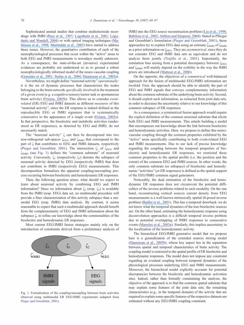
The “neuronal activity” ζ can then be decomposed into twonon-orthogonal sub-spaces ζEEG and ζfMRI that correspond to thepart of ζ that contributes to EEG and fMRI datasets, respectively(Pieger and Greenblatt, 2001). The intersection ζ1 of ζEEG andζfMRI (see Fig. 1) defines the “common substrate” of neuronalactivity. Conversely, ζ2 (respectively ζ3) denotes the subspace ofneuronal activity detected by EEG (respectively fMRI) that doesnot contribute to fMRI (respectively EEG) measurements. Thisdecomposition formalizes the apparent coupling/uncoupling pro-cess occurring between bioelectric and hemodynamic ER responses.

Then, the following question arises: what should we expect tolearn about neuronal activity by combining EEG and fMRIinformation? Since no information about ζ2 (resp. ζ3) is availablefrom the fMRI (resp. EEG) data set, no multimodal procedure willprovide a finer characterization of this activity subspace than a uni-modal EEG (resp. fMRI) data analysis. By contrast, it seemsreasonable to expect that such a multimodal approach should benefitfrom the complementarity of EEG and fMRI information about thesubspace ζ1 to refine our knowledge about the commonalities of thebioelectric and hemodynamic ER responses.

Most current EEG/fMRI fusion strategies mainly rely on theintroduction of constraints derived from a preliminary analysis of

Fig. 1. Formalization of the coupling/uncoupling between brain activitiesobserved using multimodal ER EEG/fMRI experiments (adapted fromPieger and Greenblatt, 2001).

fMRI into the EEG source reconstruction problem (Liu et al., 1998;Babiloni et al., 2003; Ahlfors and Simpson, 2004). Stated in Pfliegerand Greenblatt’s formulation (Pieger and Greenblatt, 2001), theseapproaches try to explain EEG data using an estimate ζ̂fMRI of ζfMRI

as a prior information on ζEEG. They are asymmetrical, since they donot consider EEG and fMRI data sets as equivalent and do notanalyze them jointly (Trujillo et al., 2001). Importantly, theestimation bias arising from a potential discrepancy between ζEEGand ζfMRI will mainly depend on the exibility in the way the fMRIpriors are introduced (Mattout et al., 2006).

On the opposite, the objectives of a symmetrical well-balancedapproach for the fusion of multimodal EEG/fMRI information aretwofold. First, the approach should be able to identify the part ofEEG and fMRI signals that conveys complementary informationabout the common substrate of the underlying brain activity. Second,it should exploit such information, as extracted from joint data sets,in order to decrease the uncertainty relative to our knowledge of thiscommon subspace of ER responses.

As a consequence, a symmetrical fusion approach would requirethe explicit definition of the common neuronal substrate that elicitsboth EEG and fMRI measurements. This entails building a modelthat encompasses our knowledge about the link between bioelectricand hemodynamic activities. Here, we propose to define this neuro-vascular coupling through the common properties exhibited by the“active” areas specifically contributing to both event-related EEGand fMRI measurements. Due to our lack of precise knowledgeregarding the coupling between the temporal properties of bio-electric and hemodynamic ER responses, we restricted thesecommon properties to the spatial profile (i.e. the position and theextent) of the common EEG and fMRI sources. In other words, theonly common substrate (or subspace) of bioelectric and hemody-namic “activities” (or ER responses) is defined as the spatial supportof the EEG/fMRI common signal generators.

Noticeably, the dual estimation of the bioelectric and hemo-dynamic ER responses does not circumvent the potential diffi-culties of the inverse problems related to each modality. On the onehand, reconstructing cortical sources current density from EEGmeasurements is a well known intrinsically spatial ill-posed inverseproblem (Baillet et al., 2001). This has a temporal drawback: we donot know what the temporal dynamics of the true bioelectric sourcesare. On the other hand, estimating the hemodynamic response usingdeconvolution approaches is a difficult temporal inverse problemdue to potential overlapping of fMRI responses to consecutiveevents (Marrelec et al., 2003a). Similarly, this implies uncertainty inthe localization of the hemodynamic activity.

The hierarchical EEG/fMRI generative model that we proposehere is a generalization of the extended sources mixing model(Daunizeau et al., 2005b), whose key aspect lies in the separationbetween spatial and temporal characteristics of brain activity. Thecoupling model is restricted to the spatial profile of ER bioelectric andhemodynamic responses. The model does not impose any constraintregarding an eventual coupling between temporal dynamics of thephysiological processes underlying EEG and fMRI measurements.Moreover, the hierarchical model explicitly accounts for potentialdiscrepancies between the bioelectric and hemodynamic activationsites. Indeed, rather than formally constraining the analysis, theobjective of the approach is to find the common spatial substrate thatmay explain some features of the joint data sets; the remainingcharacteristics (e.g., in the temporal domain) of the activity that arerequired to explain some specific features of the respective datasets areestimated without any EEG/fMRI coupling constraint.

1 This formulation does not refer to the standard GLM, as proposed in(Friston et al., 1995), where the design matrix is defined by regressors thatmodel the different types of stimuli and are constructed by convolution of thestimulus with a canonical hemodynamic response function, while regressioncoefficients represent effects sizes. Rather, this forward model is adiscretization of the unknown ER hemodynamic impulse response function.

71J. Daunizeau et al. / NeuroImage 36 (2007) 69–87

Despite its somewhat heuristic aspect, this joint EEG/fMRIinformation fusion approach is both robust to the lack ofinformation about the neuro-vascular coupling and flexible enoughto allow for later incorporation of further knowledge about thegeneration of bioelectric and hemodynamic ER responses.

This paper comprises various sections. In Model of spatially con-cordant ER responses, we show how to rely on the spatio-temporaldecomposition of cerebral activity to formalize the coupling/de-coupling of bioelectric and hemodynamic event-related responses(Separation of space and time). We also expose the statisticalassumptions required to specify the associated graphical generativemodel (Specification of the hierarchical model). In Learning themodel: variational Bayesian learning scheme, we describe theVariational Bayesian (VB) algorithm that we developed in order tomake statistical inference on the model. Evaluation presentselements of evaluation of the whole approach: (1) assessment ofthe method’s performance using simulated data and (2) illustration ofthe approach in the context of interictal spike localization from EEG/fMRI data simultaneously acquired on a patient with focal epilepsy.In Discussion, we discuss the main aspects of the model andassociated VB inference scheme and replace the whole approach inthe context of the general problem of information fusion.

Notations

In the following, XT;Xi;Xij and tr(X) indicate the transpose ofmatrix X, the ith vector column of X, the scalar element of the ithcolumn and jth row of X and the trace of X, respectively. (xi)1≤i≤ndenotes the n×1 vector whose entries are xi. In and 0n stand for then×n identity matrix and the n×1 null vector, respectively. For anyn×1 vector x, Diag(x) denotes the n×n diagonal matrix whosediagonal is x. By contrast, diag(X) denotes the n×1 vectorcontaining the diagonal entries of the n×n matrix X.⊗ denotes theKronecker product, ▵ denotes the Laplacian operator and “∝”relates two expressions that are proportional. The cardinal of anyset V is written card½V�. For two variables x and y, x|y stands for “xgiven y”, p(x) for the probability of x, ⟨x⟩ for its expectation and x̂for its estimate. Nðm;VÞ is the Gaussian probability densityfunction (pdf) with mean m and covariance matrix V and Gða; bÞ isthe Gamma pdf with a degrees of freedom (d.o.f.) and shapeparameter b. Given an a×b matrix X, let us also define an ab×1vector-valued function denoted by vec(X) such that

vecðXÞ ¼X1

X2

vXb

0BB@

1CCA:

Model of spatially concordant ER responses

In the following, we assume that a single type of event isinvolved in the experiment. We then provide a generative model thatcan account for both fMRI and EEG event-related data in ahierarchical fashion.

The EEG and fMRI forward problems

On the one hand, solving the EEG inverse problem within theso-called distributed framework amounts to finding a uniquesolution to the following linear system (Dale and Sereno, 1993):

M ¼ GJþ E; ð1Þ

where M stands for the p× t1 matrix of scalp (ER potential) EEGdata set (p∼102: number of sensors, t1∼102: number of timesamples), E is an additive measurement noise, J is the n× t1 matrixof the unknown time courses of the dipoles (n∼104: number ofdipoles distributed on the cortical surface) and G is the p×n gainmatrix (forward operator) associated with the position andorientation of the dipoles.

J is the voxelwise description of the bioelectric ER response. Gis obtained by solving the so-called forward problem (de Munck,1988) for a given set of dipoles with fixed position and orientation(distributed perpendicular to the cortical surface). Each column Gj

of G indicates the putative contribution of dipole j to the scalp data(its so-called forward field).

On the other hand, the general linear model (GLM) links thestimulation paradigm to the fMRI measurements through thehemodynamic response function (HRF) (Marrelec et al., 2001)1:

Y ¼ Bhþ F; ð2Þwhere Y is the t2×n matrix of voxelwise fMRI measurements(t2∼/ 102: number of time samples, n∼104: number of voxels),F is an additive measurement noise, h is the k×n matrix of theunknown HRF in each voxel (k: order of the convolution model),and B is the t2×k design matrix, consisting of the lagged stimulusonset covariates, i.e.:

B ¼xk N x1v

xt2þk�1 N xt2

0@

1A; ð3Þ

given that (xi)1≤i<t2+k is the event time course.

Separation of space and time

We further assume that cerebral activity is structured by a set ofactive areas (brain regions) that are characterized by their temporalcoherence. Therefore, let us consider a given parcelling of thecortical surface into q anatomically and functionally homogeneousclusters (see Appendix B). The so-called extended sources mixingmodel (see previous work (Daunizeau et al., 2005a)) then associateseach parcel Pi(i=1, …, q) with its single temporal dynamics usingthe following hierarchical model of bioelectric sources J:

J ¼ DiagðwEEGÞCXþ R; ð4Þwhere X is an unknown q× t1 matrix made of the q time courses ofthe q parcels, C is the known n×q matrix describing the cortexparcelling (Cji=1 if j∈Pi, and Cji=0 otherwise.), wEEG is a n×1unknown vector, and R is a residual bioelectric activity that cannotbe explained using the extended sources mixing model. In thisformulation, the temporal dynamics of the ith dipole is defined as thetime course of the parcel to which it belongs, weighted by a scalarwiEEG. The vector wEEG expresses the relative within-region

distribution of current intensity. It describes the (time-invariant)spatial profile of each active extended cortical source. On theopposite,X embodies the temporal features of the bioelectric sources

72 J. Daunizeau et al. / NeuroImage 36 (2007) 69–87

J. Eq. (4) thus enforces a spatio-temporal separability of thebioelectric activity by means of the parcelling C.

In a similar fashion, let us write the extended sources mixingmodel for the hemodynamic ER response:

h ¼ ZCTDiagðwfMRIÞ þ L; ð5Þ

where Z is an unknown k×q matrix containing the HRF temporalshape of the q parcels, wfMRI is an also unknown n×1 vectorassociated with the spatial profile of the hemodynamic activitysources, and L is the residual discrepancy from the extendedsources mixing model.

Furthermore, we assume that the common feature of bioelectricand hemodynamic ER responses is the spatial profile of the sourcesseen by both neuroimaging modalities. This assumption may beformalized using the following equation:

wEEG ¼ wfMRI ¼ w: ð6ÞHence, X (resp. Z) represents the bioelectric (resp. hemody-

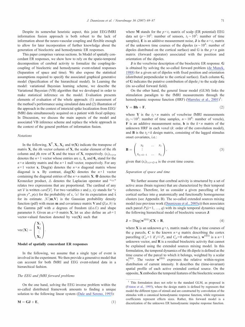
namic) temporal dynamics of activity sources common to EEG andfMRI, whereas residuals R and L are associated to the activitysources specific of EEG and fMRI, respectively. Since the physicalunits of bioelectric and hemodynamic activities are carried by thetime course variables X and Z, the common substrate of cerebralactivityw is a dimensionless quantity. Fig. 2 illustrates this “spatiallyconcordant” ER responses model.

Specification of the hierarchical model

In a Bayesian perspective, any uncertainty associated with anunknown quantity is to be modeled through a probability densityfunction (pdf). In the previous section, we described the hierarchical

Fig. 2. Schematic illustration of spatio-temporal decomposition entailed bythe spatially concordant ER responses model. Two active areas are depicted,with their (time invariant) spatial profile. These exhibit coherent bioelectricand hemodynamic ER responses (the colored time courses are associatedwith different voxels belonging to the same parcel), which are supposed tocontribute to EEG and fMRI measurements, respectively.

observation model. Now, we focus on additional assumptions aboutthe conditional dependencies between the differentmodel parameters.

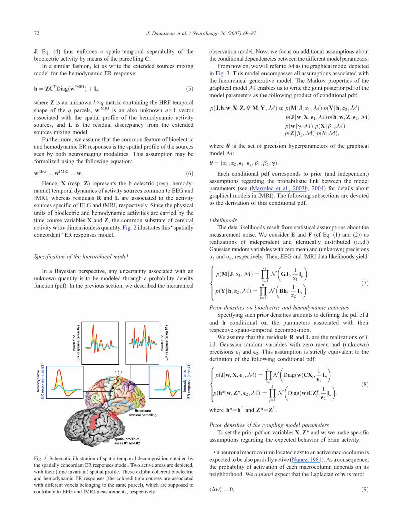
From now on, we will refer toM as the graphical model depictedin Fig. 3. This model encompasses all assumptions associated withthe hierarchical generative model. The Markov properties of thegraphical modelM enables us to write the joint posterior pdf of themodel parameters as the following product of conditional pdf:

pðJ;h;w;X;Z; q jM;Y;MÞ~ pðM jJ; a1;MÞ pðY jh; a2;MÞpðJ jw;X; ϵ1;MÞpðh jw;Z; ϵ2;MÞpðw jg;MÞ pðX jb1;MÞpðZ jb2;MÞ pðq jMÞ;

where θ is the set of precision hyperparameters of the graphicalmodel M:

q ¼ ða1; a2; ϵ1; ϵ2; b1; b2; gÞ:Each conditional pdf corresponds to prior (and independent)

assumptions regarding the probabilistic link between the modelparameters (see (Marrelec et al., 2003b, 2004) for details aboutgraphical models in fMRI). The following subsections are devotedto the derivation of this conditional pdf.

LikelihoodsThe data likelihoods result from statistical assumptions about the

measurement noise. We consider E and F (cf Eq. (1) and (2)) asrealizations of independent and identically distributed (i.i.d.)Gaussian random variables with zero mean and (unknown) precisionsα1 and α2, respectively. Then, EEG and fMRI data likelihoods yield:

p M jJ; a1;Mð Þ ¼Yt1i¼1

N GJi;1a1

Ip

� �

p Y jh; a2;Mð Þ ¼Ynj¼1

N Bhj;1a2

It2

� �:

8>>>><>>>>:

ð7Þ

Prior densities on bioelectric and hemodynamic activitiesSpecifying such prior densities amounts to defining the pdf of J

and h conditional on the parameters associated with theirrespective spatio-temporal decomposition.

We assume that the residuals R and L are the realizations of i.i.d. Gaussian random variables with zero mean and (unknown)precisions ϵ1 and ϵ2. This assumption is strictly equivalent to thedefinition of the following conditional pdf:

p Jjw;X; ϵ1;Mð Þ ¼Yt1i¼1

N Diag wð ÞCXi;1ϵ1

In

� �

p h4jw;Z4; ϵ2;Mð Þ ¼Ykj¼1

N Diag wð ÞCZj4;1ϵ2

In

� �;

8>>>><>>>>:

ð8Þ

where h4uhT and Z4uZT.

Prior densities of the coupling model parametersTo set the prior pdf on variables X, Z⁎ and w, we make specific

assumptions regarding the expected behavior of brain activity:

• a neuronalmacrocolumn located next to an activemacrocolumn isexpected to be also partially active (Nunez, 1981). As a consequence,the probability of activation of each macrocolumn depends on itsneighborhood. We a priori expect that the Laplacian of w is zero:

hDwi ¼ 0: ð9Þ

Fig. 3. Graph representing the hierarchical relations between the EEG/fMRIdata generative model parameters. w is the common spatial profile of thesources, X (respectively Z) is the temporal dynamics of the bioelectric(respectively hemodynamic) activity. J is the time course of the bioelectricactivity. h is the hemodynamic activity.M (resp. Y) contains the EEG (resp.fMRI) measurements. The other nodes are the precision parameters that areassociated with prior assumptions about the expected structure of brainactivity, and noise measurements.

73J. Daunizeau et al. / NeuroImage 36 (2007) 69–87

Under Gaussian assumption, this is strictly equivalent to thefollowing prior pdf for the spatial field w (Gössl et al., 2001):

p wjg;Mð Þ ¼ N 0n;1gðSTSÞ�1

� �; ð10Þ

where γ is the (unknown) precision of the Laplacian field ofw, and Sis the n×n discrete Laplacian operator defined as:

Sjj ¼ 1

Sjj V ¼ � 1card½V j� if j VϵV j

Sjj V ¼ 0 otherwise;

8><>: ð11Þ

where V j is the neighborhood of voxel j.

• EEG and fMRI are known to provide oversampled measures ofbioelectric and hemodynamic activities, respectively (Nunez, 1981;Heeger, 2002). This implies some temporal smoothness in the timecourses of bioelectric and hemodynamic activities of the corticalparcels. Here, we a priori expect that the second temporalderivatives ofX and Z are zero (Marrelec et al., 2001, 2003b, 2004):

�B2XBt2

�¼�B2ZBt2

�¼ 0: ð12Þ

Under Gaussian assumption, this is equivalent to the following priorpdf for X and Z (Marrelec et al., 2003a):

p vec Xð Þjb1;Mð Þ ¼ N 0qt1 ;

1b1

�TT1T1

��1!

p vec Z⁎ð Þjb2;Mð Þ ¼ N 0qk1 ;

1b2

�TT2T2

��1!;

8>>>>><>>>>>:

ð13Þ

where β1 and β2 are the (unknown) precisions of the secondtemporal derivatives of X and Z, and T1 (resp. T2) is a qt1×qt1(resp. kq×kq) matrix such that:

Tdii ¼ �2Tdij ¼ 1 if j ¼ iFðqþ 1ÞTdij ¼ 0 otherwise:

8<: ð14Þ

Prior densities on scaling hyperparametersAll precision hyperparameters are unknown quantities. There-

fore, in a full Bayesian approach, we need to specify prior densitieson each of them. These were chosen such that our graphical modelM belongs to conjugate exponential models, which are easier tomanipulate (Gelman et al., 1998).

As for the variances of the EEG/fMRI measurement noise, letus assume that we have at our disposal two data windows (M0, ofsize p× t3 in EEG, and Y0 of size n× t4 in fMRI) containing onlyi.i.d. noise. In practice, one can use scalp recordings precedingbioelectric responses in EEG, and fMRI data corresponding toregions that do not belong to grey matter. A direct consequenceof the assumption of Gaussian noise is that α1 given M0 (resp. α2given Y0) behaves as a Gamma variate. The definition of their re-spective prior pdf thus pertains to the derivation of the conditionalpdf p (α1|M0) and p (α2|Y0):

pða1jMÞ ¼ pða1jM0Þ ¼ Gða1; b1Þpða2jMÞ ¼ pða2jY0Þ ¼ Gða2; b2Þ; ð15Þ

where parameters (a1, b1) and (a2, b2) are such that:

a1 ¼ pt32

; b1 ¼ trðMT0M0Þ2

a2 ¼ nt42

; b2 ¼ trðYT0Y0Þ2

:

8>><>>: ð16Þ

Finally, since we have no prior information about the remainingprecision hyperparameters, we consider noninformative Jeffreys’priors (uniform pdf over the log-hyperparameter) (Kass andWassermann, 1996):

pðϵ1jMÞ~ðϵ1Þ�1

pðϵ2jMÞ~ðϵ2Þ�1

pðb1jMÞ~ðb1Þ�1

pðb2jMÞ~ðb2Þ�1

pðgjMÞ~ðgÞ�1:

8>>>><>>>>:

ð17Þ

All assumptions listed in Specification of the hierarchical modeland associated with the spatially concordant event-related responsemodel form the graphical (hierarchical) model that is summarizedby the graph represented in Fig. 3.

Learning the model: variational Bayesian learning scheme

There are two main goals in Bayesian learning. The first one isto provide the posterior distribution over the model parameters; thesecond one, to provide a quantitative feedback on the relevance of

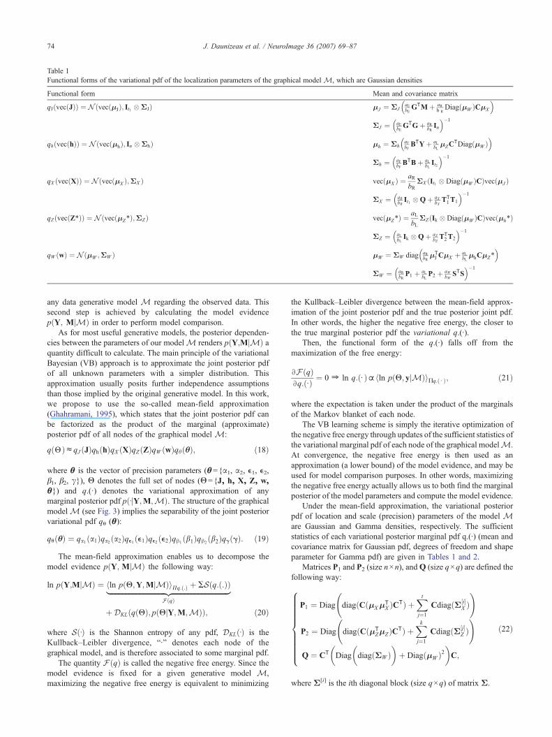
Table 1Functional forms of the variational pdf of the localization parameters of the graphical model M, which are Gaussian densities

Functional form Mean and covariance matrix

qJðvecðJÞÞ ¼ N ðvecðmJÞ; It1 �ΣJÞ mJ ¼ ΣJaEbEGTMþ aR

b RDiag mWð ÞCmX

� �ΣJ ¼ aE

bEGTGþ aR

bRIn

� ��1

qhðvecðhÞÞ ¼ N ðvecðmhÞ; In �ΣhÞ mh ¼ ΣhaFbFBTYþ aL

bLmZC

TDiag mWð Þ� �

Σh ¼ aFbFBTBþ aL

bLIt2

� ��1

qX ðvecðXÞÞ ¼ N ðvecðmX Þ;ΣX Þ vec mXð Þ ¼ aRbR

ΣX It1 � DiagðmW ÞCð Þvec mJð Þ

ΣX ¼ aRbRIt1 �Qþ aX

bXTT1T1

� ��1

qZðvecðZ4ÞÞ ¼ N ðvecðmZ4Þ;ΣZÞ vec mZ4ð Þ ¼ aLbL

ΣZ Ik � DiagðmW ÞCð Þvec mh4ð Þ

ΣZ ¼ aLbLIk �Qþ aZ

bZTT2T2

� ��1

qW ðwÞ ¼ N ðmW ;ΣW Þ mW ¼ ΣW diag aRbRmTJ CmX þ aL

bLmhCmZ4

� �ΣW ¼ aR

bRP1 þ aL

bLP2 þ aW

bWSTS

� ��1

74 J. Daunizeau et al. / NeuroImage 36 (2007) 69–87

any data generative model M regarding the observed data. Thissecond step is achieved by calculating the model evidencepðY; MjMÞ in order to perform model comparison.

As for most useful generative models, the posterior dependen-cies between the parameters of our modelM renders pðY;MjMÞ aquantity difficult to calculate. The main principle of the variationalBayesian (VB) approach is to approximate the joint posterior pdfof all unknown parameters with a simpler distribution. Thisapproximation usually posits further independence assumptionsthan those implied by the original generative model. In this work,we propose to use the so-called mean-field approximation(Ghahramani, 1995), which states that the joint posterior pdf canbe factorized as the product of the marginal (approximate)posterior pdf of all nodes of the graphical model M:

qðHÞcqJ ðJÞqhðhÞqX ðXÞqZðZÞqW ðwÞqhðqÞ; ð18Þ

where θ is the vector of precision parameters (θ={α1, α2, ϵ1, ϵ2,β1, β2, γ}), Θ denotes the full set of nodes (Θ={J, h, X, Z, w,θ}) and q.(·) denotes the variational approximation of anymarginal posterior pdf pðdjY;M;MÞ. The structure of the graphicalmodel M (see Fig. 3) implies the separability of the joint posteriorvariational pdf qθ (θ):

quðqÞ ¼ qa1ða1Þqa2ða2Þqϵ1ðϵ1Þqϵ2 ðϵ2Þqh1ðb1Þqh2

ðb2ÞqgðgÞ: ð19ÞThe mean-field approximation enables us to decompose the

model evidence pðY; MjMÞ the following way:

ln pðY;MjMÞ ¼ hln pðQ;Y;MjMÞiPq:ð:Þ þ ASðq:ð:ÞÞ|fflfflfflfflfflfflfflfflfflfflfflfflfflfflfflfflfflfflfflfflfflfflfflfflfflfflfflfflfflfflfflffl{zfflfflfflfflfflfflfflfflfflfflfflfflfflfflfflfflfflfflfflfflfflfflfflfflfflfflfflfflfflfflfflffl}FðqÞ

þ DKLðqðQÞ; pðQjY;M;MÞÞ; ð20Þ

where SðdÞ is the Shannon entropy of any pdf, DKLðdÞ is theKullback–Leibler divergence, “·” denotes each node of thegraphical model, and is therefore associated to some marginal pdf.

The quantity FðqÞ is called the negative free energy. Since themodel evidence is fixed for a given generative model M,maximizing the negative free energy is equivalent to minimizing

the Kullback–Leibler divergence between the mean-field approx-imation of the joint posterior pdf and the true posterior joint pdf.In other words, the higher the negative free energy, the closer tothe true marginal posterior pdf the variational q.(·).

Then, the functional form of the q.(·) falls off from themaximization of the free energy:

BFðqÞBq:ðd Þ ¼ 0 Z ln q: dð Þ~hln p Q; yjMð ÞiCq:ðd Þ; ð21Þ

where the expectation is taken under the product of the marginalsof the Markov blanket of each node.

The VB learning scheme is simply the iterative optimization ofthe negative free energy through updates of the sufficient statistics ofthe variational marginal pdf of each node of the graphical modelM.At convergence, the negative free energy is then used as anapproximation (a lower bound) of the model evidence, and may beused for model comparison purposes. In other words, maximizingthe negative free energy actually allows us to both find the marginalposterior of the model parameters and compute the model evidence.

Under the mean-field approximation, the variational posteriorpdf of location and scale (precision) parameters of the model Mare Gaussian and Gamma densities, respectively. The sufficientstatistics of each variational posterior marginal pdf q.(·) (mean andcovariance matrix for Gaussian pdf, degrees of freedom and shapeparameter for Gamma pdf) are given in Tables 1 and 2.

Matrices P1 and P2 (size n×n), andQ (size q×q) are defined thefollowing way:

P1 ¼ Diag diagðCðmXmTX ÞCTÞ þ

Xtj¼1

CdiagðΣ½i�X Þ

!

P2 ¼ Diag diagðCðmTZmZÞCTÞ þ

Xkj¼1

CdiagðΣ½j�Z Þ

!

Q ¼ CT Diag

�diagðΣW Þ

�þ DiagðmW Þ2

�C;

�

8>>>>>>>>><>>>>>>>>>:

ð22Þ

where Σ[i] is the ith diagonal block (size q×q) of matrix Σ.

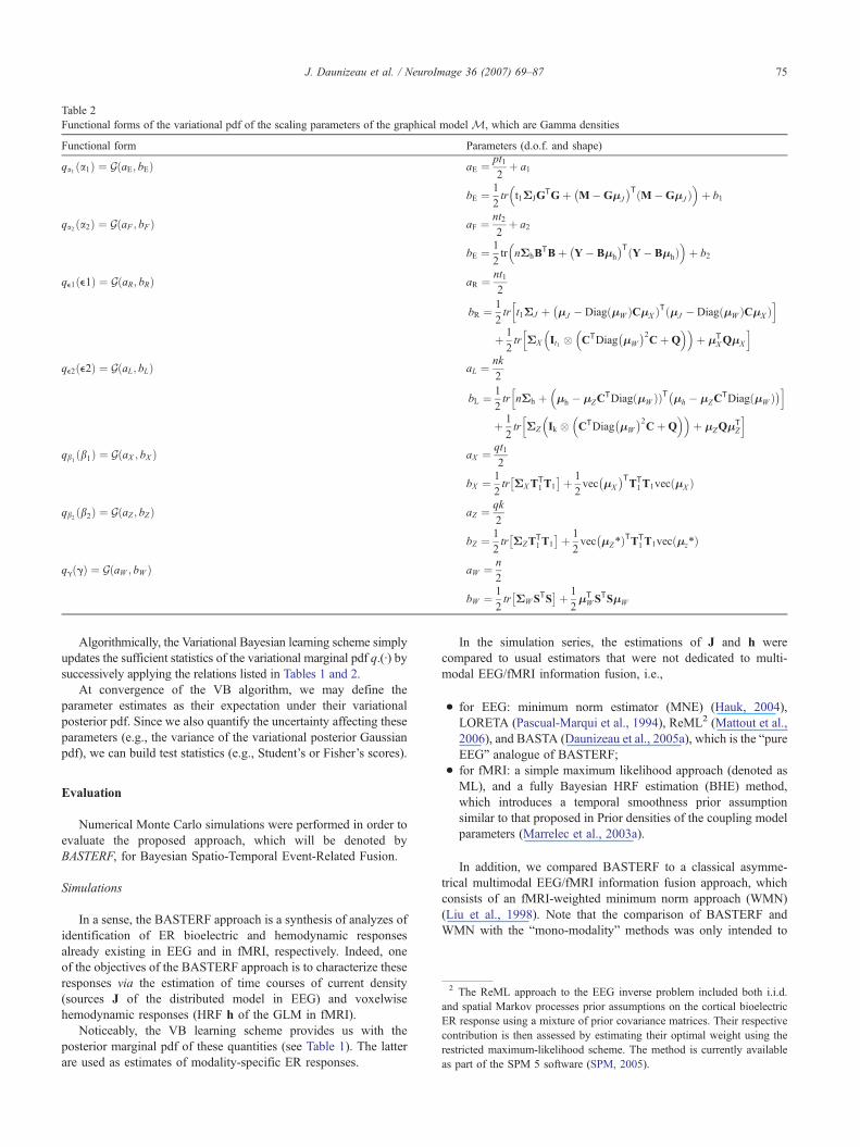
Table 2Functional forms of the variational pdf of the scaling parameters of the graphical model M, which are Gamma densities

Functional form Parameters (d.o.f. and shape)

qa1 ða1Þ ¼ GðaE; bEÞ aE ¼ pt12

þ a1

bE ¼ 12tr t1ΣJG

TGþ M�GmJ

TM�GmJð Þ

�þ b1

�qa2 ða2Þ ¼ GðaF ; bFÞ aF ¼ nt2

2þ a2

bE ¼ 12tr nΣhB

TBþ Y� Bmh

TY� Bmhð Þ

�þ b2

�qϵ1ðϵ1Þ ¼ GðaR; bRÞ aR ¼ nt1

2

bR ¼ 12tr t1ΣJ þ

mJ � Diag mWð ÞCmX ÞT mJ � Diag mWð ÞCmXð Þ

ihþ 12tr ΣX It1 � CTDiag

mW

2CþQ

�� �þ mT

XQmX

� ihqϵ2ðϵ2Þ ¼ GðaL; bLÞ aL ¼ nk

2

bL ¼ 12tr nΣh þ mh � mZC

TDiag mWð ÞÞT mh � mZCTDiag mWð Þ � ih

þ 12tr ΣZ Ik � CTDiag

mW

2CþQ

�� �þ mZQmT

Z

� ihqb1 ðb1Þ ¼ GðaX ; bX Þ aX ¼ qt1

2

bX ¼ 12tr ΣXT

T1T1

� �þ 12vecmX

TTT1T1vec mXð Þ

qb2 ðb2Þ ¼ GðaZ ; bZÞ aZ ¼ qk2

bZ ¼ 12tr ΣZT

T1T1

� �þ 12vecmZ4ÞTTT

1T1vec mz4ð Þ

qgðgÞ ¼ GðaW ; bW Þ aW ¼ n2

bW ¼ 12tr ΣWSTS� �þ 1

2mTWSTSmW

75J. Daunizeau et al. / NeuroImage 36 (2007) 69–87

Algorithmically, the Variational Bayesian learning scheme simplyupdates the sufficient statistics of the variational marginal pdf q.(·) bysuccessively applying the relations listed in Tables 1 and 2.

At convergence of the VB algorithm, we may define theparameter estimates as their expectation under their variationalposterior pdf. Since we also quantify the uncertainty affecting theseparameters (e.g., the variance of the variational posterior Gaussianpdf), we can build test statistics (e.g., Student’s or Fisher’s scores).

2 The ReML approach to the EEG inverse problem included both i.i.d.and spatial Markov processes prior assumptions on the cortical bioelectricER response using a mixture of prior covariance matrices. Their respectivecontribution is then assessed by estimating their optimal weight using therestricted maximum-likelihood scheme. The method is currently availableas part of the SPM 5 software (SPM, 2005).

Evaluation

Numerical Monte Carlo simulations were performed in order toevaluate the proposed approach, which will be denoted byBASTERF, for Bayesian Spatio-Temporal Event-Related Fusion.

Simulations

In a sense, the BASTERF approach is a synthesis of analyzes ofidentification of ER bioelectric and hemodynamic responsesalready existing in EEG and in fMRI, respectively. Indeed, oneof the objectives of the BASTERF approach is to characterize theseresponses via the estimation of time courses of current density(sources J of the distributed model in EEG) and voxelwisehemodynamic responses (HRF h of the GLM in fMRI).

Noticeably, the VB learning scheme provides us with theposterior marginal pdf of these quantities (see Table 1). The latterare used as estimates of modality-specific ER responses.

In the simulation series, the estimations of J and h werecompared to usual estimators that were not dedicated to multi-modal EEG/fMRI information fusion, i.e.,

• for EEG: minimum norm estimator (MNE) (Hauk, 2004),LORETA (Pascual-Marqui et al., 1994), ReML2 (Mattout et al.,2006), and BASTA (Daunizeau et al., 2005a), which is the “pureEEG” analogue of BASTERF;

• for fMRI: a simple maximum likelihood approach (denoted asML), and a fully Bayesian HRF estimation (BHE) method,which introduces a temporal smoothness prior assumptionsimilar to that proposed in Prior densities of the coupling modelparameters (Marrelec et al., 2003a).

In addition, we compared BASTERF to a classical asymme-trical multimodal EEG/fMRI information fusion approach, whichconsists of an fMRI-weighted minimum norm approach (WMN)(Liu et al., 1998). Note that the comparison of BASTERF andWMN with the “mono-modality” methods was only intended to

76 J. Daunizeau et al. / NeuroImage 36 (2007) 69–87

give an idea of the added-value (the gain or loss of information) ofthe “multi-modality” approaches.

BASTERF can be distinguished from established EEG orfMRI generative models by the number and diversity of its modelparameters. Therefore, we chose to define a very simplesimulation environment, in order to bring to light the behaviorof the BASTERF approach with respect to the main issue ofmultimodal EEG/fMRI information fusion: the possible mismatchbetween bioelectric and hemodynamic activities.

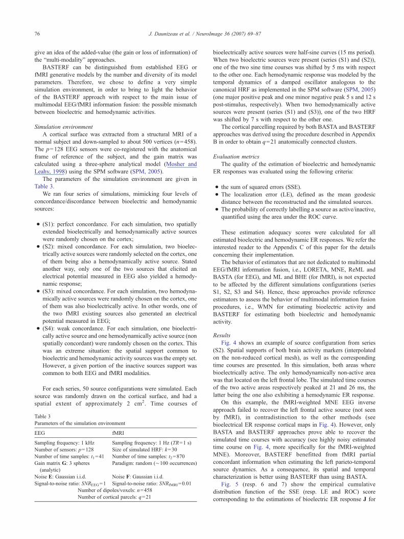
Simulation environmentA cortical surface was extracted from a structural MRI of a

normal subject and down-sampled to about 500 vertices (n=458).The p=128 EEG sensors were co-registered with the anatomicalframe of reference of the subject, and the gain matrix wascalculated using a three-sphere analytical model (Mosher andLeahy, 1998) using the SPM software (SPM, 2005).

The parameters of the simulation environment are given inTable 3.

We ran four series of simulations, mimicking four levels ofconcordance/discordance between bioelectric and hemodynamicsources:

• (S1): perfect concordance. For each simulation, two spatiallyextended bioelectrically and hemodynamically active sourceswere randomly chosen on the cortex;

• (S2): mixed concordance. For each simulation, two bioelec-trically active sources were randomly selected on the cortex, oneof them being also a hemodynamically active source. Statedanother way, only one of the two sources that elicited anelectrical potential measured in EEG also yielded a hemody-namic response;

• (S3): mixed concordance. For each simulation, two hemodyna-mically active sources were randomly chosen on the cortex, oneof them was also bioelectrically active. In other words, one ofthe two fMRI existing sources also generated an electricalpotential measured in EEG;

• (S4): weak concordance. For each simulation, one bioelectri-cally active source and one hemodynamically active source (nonspatially concordant) were randomly chosen on the cortex. Thiswas an extreme situation: the spatial support common tobioelectric and hemodynamic activity sources was the empty set.However, a given portion of the inactive sources support wascommon to both EEG and fMRI modalities.

For each series, 50 source configurations were simulated. Eachsource was randomly drawn on the cortical surface, and had aspatial extent of approximately 2 cm2. Time courses of

Table 3Parameters of the simulation environment

EEG fMRI

Sampling frequency: 1 kHz Sampling frequency: 1 Hz (TR=1 s)Number of sensors: p=128 Size of simulated HRF: k=30Number of time samples: t1=41 Number of time samples: t2=870Gain matrix G: 3 spheres

(analytic)Paradigm: random (∼100 occurrences)

Noise E: Gaussian i.i.d. Noise F: Gaussian i.i.d.Signal-to-noise ratio: SNREEG=1 Signal-to-noise ratio: SNRfMRI=0.01

Number of dipoles/voxels: n=458Number of cortical parcels: q=21

bioelectrically active sources were half-sine curves (15 ms period).When two bioelectric sources were present (series (S1) and (S2)),one of the two sine time courses was shifted by 5 ms with respectto the other one. Each hemodynamic response was modeled by thetemporal dynamics of a damped oscillator analogous to thecanonical HRF as implemented in the SPM software (SPM, 2005)(one major positive peak and one minor negative peak 5 s and 12 spost-stimulus, respectively). When two hemodynamically activesources were present (series (S1) and (S3)), one of the two HRFwas shifted by 7 s with respect to the other one.

The cortical parcelling required by both BASTA and BASTERFapproaches was derived using the procedure described in AppendixB in order to obtain q=21 anatomically connected clusters.

Evaluation metricsThe quality of the estimation of bioelectric and hemodynamic

ER responses was evaluated using the following criteria:

• the sum of squared errors (SSE).• The localization error (LE), defined as the mean geodesic

distance between the reconstructed and the simulated sources.• The probability of correctly labelling a source as active/inactive,

quantified using the area under the ROC curve.

These estimation adequacy scores were calculated for allestimated bioelectric and hemodynamic ER responses. We refer theinterested reader to the Appendix C of this paper for the detailsconcerning their implementation.

The behavior of estimators that are not dedicated to multimodalEEG/fMRI information fusion, i.e., LORETA, MNE, ReML andBASTA (for EEG), and ML and BHE (for fMRI), is not expectedto be affected by the different simulations configurations (seriesS1, S2, S3 and S4). Hence, these approaches provide referenceestimators to assess the behavior of multimodal information fusionprocedures, i.e., WMN for estimating bioelectric activity andBASTERF for estimating both bioelectric and hemodynamicactivity.

ResultsFig. 4 shows an example of source configuration from series

(S2). Spatial supports of both brain activity markers (interpolatedon the non-reduced cortical mesh), as well as the correspondingtime courses are presented. In this simulation, both areas wherebioelectrically active. The only hemodynamically non-active areawas that located on the left frontal lobe. The simulated time coursesof the two active areas respectively peaked at 21 and 26 ms, thelatter being the one also exhibiting a hemodynamic ER response.

On this example, the fMRI-weighted MNE EEG inverseapproach failed to recover the left frontal active source (not seenby fMRI), in contradistinction to the other methods (seebioelectrical ER response cortical maps in Fig. 4). However, onlyBASTA and BASTERF approaches prove able to recover thesimulated time courses with accuracy (see highly noisy estimatedtime course on Fig. 4, more specifically for the fMRI-weightedMNE). Moreover, BASTERF benefitted from fMRI partialconcordant information when estimating the left parieto-temporalsource dynamics. As a consequence, its spatial and temporalcharacterization is better using BASTERF than using BASTA.

Fig. 5 (resp. 6 and 7) show the empirical cumulativedistribution function of the SSE (resp. LE and ROC) scorecorresponding to the estimations of bioelectric ER response J for

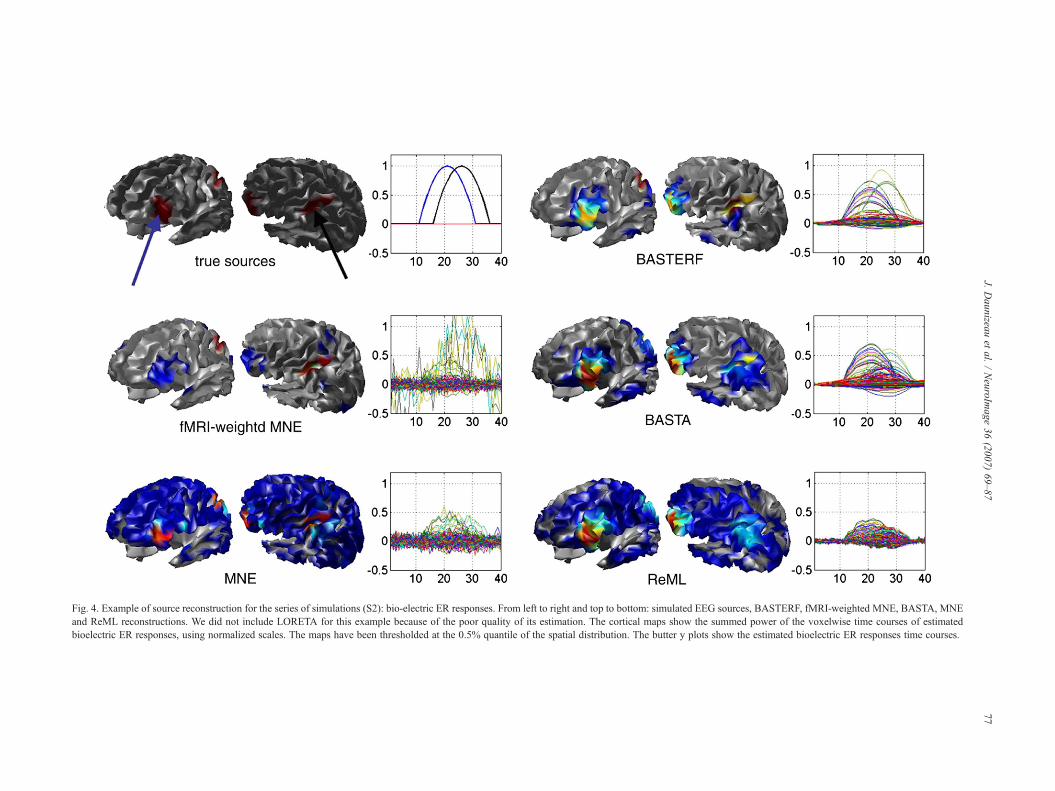
Fig. 4. Example of source reconstruction for the series of simulations (S2): bio-electric ER responses. From left to right and top to bottom: simulated EEG sources, BASTERF, fMRI-weighted MNE, BASTA, MNEand ReML reconstructions. We did not include LORETA for this example because of the poor quality of its estimation. The cortical maps show the summed power of the voxelwise time courses of estimatedbioelectric ER responses, using normalized scales. The maps have been thresholded at the 0.5% quantile of the spatial distribution. The butter y plots show the estimated bioelectric ER responses time courses.

77J.

Daunizeau

etal.

/NeuroIm

age36

(2007)69–87

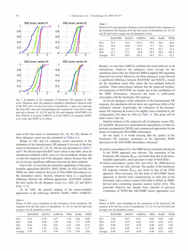
Fig. 5. Evaluation of the estimation of bioelectric ER response J: SSEscore. Diagrams show the empirical cumulative distribution function (cdf)of the SSE score over the four series of simulations. x- and y-axis representthe (log) SSE value and corresponding cdf, respectively. From left to rightand top to bottom: S1, S2, S3 and S4. On each diagram, BASTERF is inblue, BASTA is in green, LORETA is in red, MNE is in turquoise, ReMLis in violet and WMN is in yellow.

Table 5Means of LE score (geodesic distance in mm) calculated on the estimation ofthe bioelectric ER response J for the four series of simulations: S1, S2, S3and S4 (and total average over all simulation series)

BASTERF BASTA LORETA MNE ReML WMN

(S1) 56.5 74.8 107.2 78.8 78.6 60.4(S2) 55.8 68.0 113.8 71.3 74.5 84.8(S3) 18.7 31.3 101.1 35.5 36.7 21.4(S4) 27.7 27.5 84.0 39.5 30.8 102.2Average 39.7 50.4 101.5 56.3 55.1 67.2

78 J. Daunizeau et al. / NeuroImage 36 (2007) 69–87

each of the four series of simulations (S1, S2, S3, S4). Means ofthese adequacy scores are also presented in Tables 4–6.

Means of SSE and LE adequacy scores associated to theestimation of the hemodynamic ER response h for each of the fourseries of simulations (S1, S2, S3, S4) are also presented in Tables 7and 8. We did not report the ROC score values in any table, since allsimulations exhibited a ROC score of 1 for all methods. Neither didwe plot the empirical cdf of the adequacy indices because they didnot reveal any significant difference between the three methods.

First of all, we note that the estimation capabilities of the mono-modality approaches (BASTA, MNE, ReML for EEG and ML forfMRI) are stable whatever the level of EEG-fMRI discordance (i.e.the simulation series). Second, whenever there is a significantdifference between the different approaches, BASTERF exhibitsthe best results for all adequacy scores (i.e. SSE, LE and ROC)(Figs. 6−8).

As for EEG, the general ranking of the mono-modalityapproaches is the following: BASTA>ReML>MNE>LORETA.

Table 4Means of SSE score calculated on the estimation of the bioelectric ERresponse J for the four series of simulations: S1, S2, S3 and S4 (and totalaverage over all simulation series)

BASTERF BASTA LORETA MNE ReML WMN

(S1) 0.33 0.79 1.87 1.54 2.00 0.80(S2) 0.69 0.98 1.99 1.68 1.77 0.99(S3) 0.83 1.20 2.03 1.81 2.08 0.72(S4) 1.30 1.33 2.10 1.93 2.10 1.73Average 0.79 1.07 1.99 1.74 1.99 1.06

Besides, we note that LORETA exhibited the worst behavior in allsimulations, whatever the adequacy score (except for thesimulation series (S4), for which the fMRI-weighted MN algorithmbehaved even worst). Moreover, the three adequacy scores showeda significant difference between BASTERF and BASTA, exceptfor the simulation series (S4), where the two methods behavedsimilarly. These observations indicate that the improved localiza-tion properties of BASTERF are mainly due to the contribution ofthe fMRI information, whenever the latter is sufficientlyconcordant with the bioelectric ER response.

As for the adequacy of the estimation of the hemodynamic ERresponse, the simulations did not show any significant effect of theestimation scheme. Surprisingly, the estimation of the hemody-namic ER responses h seems to be slightly more perturbed by theconfiguration (S3) than for (S4) (cf Table 7). This point will bemade clearer later on.

Detailed analysis of the empirical cdf of adequacy scores SSE,LE and ROC allowed us to understand the dissimilarity of behaviorbetween asymmetrical (WMN) and symmetrical approaches for thefusion of multimodal EEG/fMRI information.

On one hand, it is worth noticing that the quality of thebioelectric ER response estimation of the algorithm WMNdecreased as the EEG/fMRI discordance increased:

• perfect concordance (S1): the fMRI-based constraint introducedin the WMN approach was relevant. The estimation of thebioelectric ER response ĴWMN was better than that of all mono-modality approaches, and equivalent to that of BASTERF;

• mixed concordance (series (S2) and (S3)): the fMRI-derivedconstraint was not fully relevant. The quality of the bioelectricER response estimate ĴWMN got closer to that of the MNEapproach. More precisely, for this kind of EEG/fMRI fusionapproach, it seemed more compromising to omit part of thebioelectric active sources (series (S2)) than to define an fMRI-derived prior containing spurious sources (series (S3)). Thisparticular behavior has already been reported in previousevaluations of WMN-like EEG/fMRI fusion approaches (Liu

Table 6Means of ROC score calculated on the estimation of the bioelectric ERresponse J for the four series of simulations: S1, S2, S3 and S4 (and totalaverage over all simulation series)

BASTERF BASTA LORETA MNE ReML WMN

(S1) 1.00 0.97 0.67 0.89 0.94 1.00(S2) 0.97 0.95 0.62 0.85 0.90 0.93(S3) 0.99 0.95 0.70 0.90 0.92 1.00(S4) 0.95 0.94 0.71 0.86 0.93 0.85Average 0.98 0.95 0.68 0.88 0.92 0.95

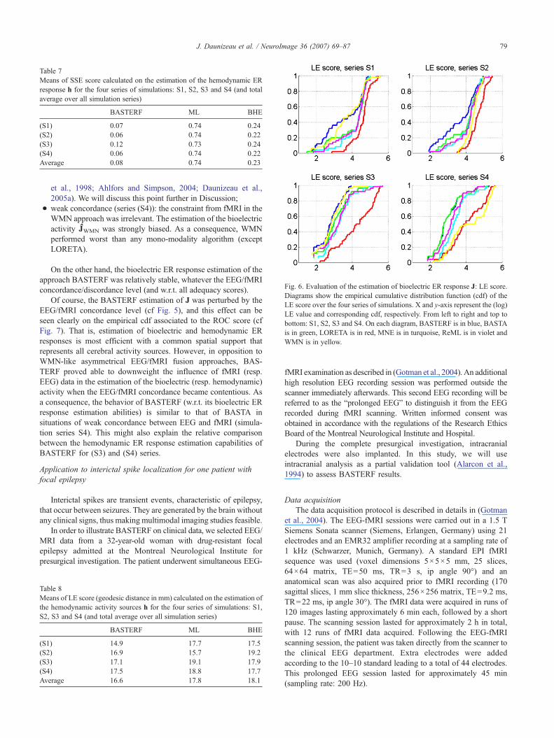
Table 7Means of SSE score calculated on the estimation of the hemodynamic ERresponse h for the four series of simulations: S1, S2, S3 and S4 (and totalaverage over all simulation series)

BASTERF ML BHE

(S1) 0.07 0.74 0.24(S2) 0.06 0.74 0.22(S3) 0.12 0.73 0.24(S4) 0.06 0.74 0.22Average 0.08 0.74 0.23

Fig. 6. Evaluation of the estimation of bioelectric ER response J: LE score.Diagrams show the empirical cumulative distribution function (cdf) of theLE score over the four series of simulations. X and y-axis represent the (log)LE value and corresponding cdf, respectively. From left to right and top tobottom: S1, S2, S3 and S4. On each diagram, BASTERF is in blue, BASTAis in green, LORETA is in red, MNE is in turquoise, ReML is in violet andWMN is in yellow.

79J. Daunizeau et al. / NeuroImage 36 (2007) 69–87

et al., 1998; Ahlfors and Simpson, 2004; Daunizeau et al.,2005a). We will discuss this point further in Discussion;

• weak concordance (series (S4)): the constraint from fMRI in theWMN approach was irrelevant. The estimation of the bioelectricactivity ĴWMN was strongly biased. As a consequence, WMNperformed worst than any mono-modality algorithm (exceptLORETA).

On the other hand, the bioelectric ER response estimation of theapproach BASTERF was relatively stable, whatever the EEG/fMRIconcordance/discordance level (and w.r.t. all adequacy scores).

Of course, the BASTERF estimation of J was perturbed by theEEG/fMRI concordance level (cf Fig. 5), and this effect can beseen clearly on the empirical cdf associated to the ROC score (cfFig. 7). That is, estimation of bioelectric and hemodynamic ERresponses is most efficient with a common spatial support thatrepresents all cerebral activity sources. However, in opposition toWMN-like asymmetrical EEG/fMRI fusion approaches, BAS-TERF proved able to downweight the influence of fMRI (resp.EEG) data in the estimation of the bioelectric (resp. hemodynamic)activity when the EEG/fMRI concordance became contentious. Asa consequence, the behavior of BASTERF (w.r.t. its bioelectric ERresponse estimation abilities) is similar to that of BASTA insituations of weak concordance between EEG and fMRI (simula-tion series S4). This might also explain the relative comparisonbetween the hemodynamic ER response estimation capabilities ofBASTERF for (S3) and (S4) series.

Application to interictal spike localization for one patient withfocal epilepsy

Interictal spikes are transient events, characteristic of epilepsy,that occur between seizures. They are generated by the brain withoutany clinical signs, thus making multimodal imaging studies feasible.

In order to illustrate BASTERF on clinical data, we selected EEG/MRI data from a 32-year-old woman with drug-resistant focalepilepsy admitted at the Montreal Neurological Institute forpresurgical investigation. The patient underwent simultaneous EEG-

Table 8Means of LE score (geodesic distance in mm) calculated on the estimation ofthe hemodynamic activity sources h for the four series of simulations: S1,S2, S3 and S4 (and total average over all simulation series)

BASTERF ML BHE

(S1) 14.9 17.7 17.5(S2) 16.9 15.7 19.2(S3) 17.1 19.1 17.9(S4) 17.5 18.8 17.7Average 16.6 17.8 18.1

fMRI examination as described in (Gotman et al., 2004). An additionalhigh resolution EEG recording session was performed outside thescanner immediately afterwards. This second EEG recording will bereferred to as the “prolonged EEG” to distinguish it from the EEGrecorded during fMRI scanning. Written informed consent wasobtained in accordance with the regulations of the Research EthicsBoard of the Montreal Neurological Institute and Hospital.

During the complete presurgical investigation, intracranialelectrodes were also implanted. In this study, we will useintracranial analysis as a partial validation tool (Alarcon et al.,1994) to assess BASTERF results.

Data acquisitionThe data acquisition protocol is described in details in (Gotman

et al., 2004). The EEG-fMRI sessions were carried out in a 1.5 TSiemens Sonata scanner (Siemens, Erlangen, Germany) using 21electrodes and an EMR32 amplifier recording at a sampling rate of1 kHz (Schwarzer, Munich, Germany). A standard EPI fMRIsequence was used (voxel dimensions 5×5×5 mm, 25 slices,64×64 matrix, TE=50 ms, TR=3 s, ip angle 90°) and ananatomical scan was also acquired prior to fMRI recording (170sagittal slices, 1 mm slice thickness, 256×256 matrix, TE=9.2 ms,TR=22 ms, ip angle 30°). The fMRI data were acquired in runs of120 images lasting approximately 6 min each, followed by a shortpause. The scanning session lasted for approximately 2 h in total,with 12 runs of fMRI data acquired. Following the EEG-fMRIscanning session, the patient was taken directly from the scanner tothe clinical EEG department. Extra electrodes were addedaccording to the 10–10 standard leading to a total of 44 electrodes.This prolonged EEG session lasted for approximately 45 min(sampling rate: 200 Hz).

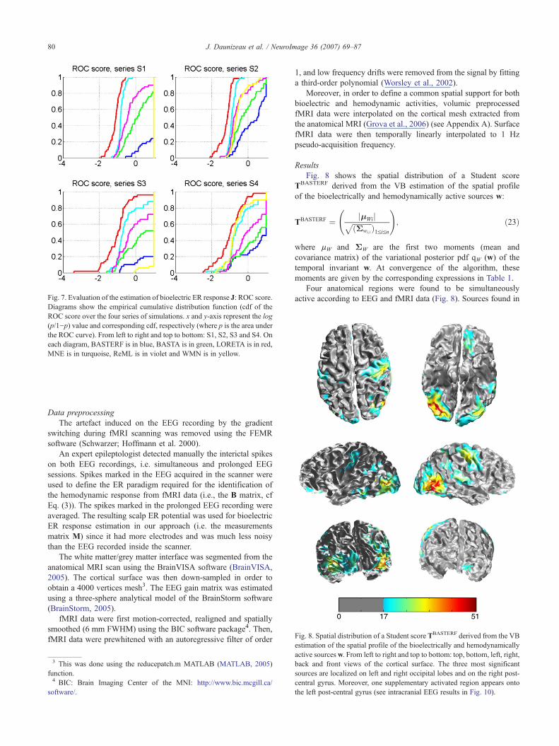
Fig. 7. Evaluation of the estimation of bioelectric ER response J: ROC score.Diagrams show the empirical cumulative distribution function (cdf of theROC score over the four series of simulations. x and y-axis represent the log(p/1−p) value and corresponding cdf, respectively (where p is the area underthe ROC curve). From left to right and top to bottom: S1, S2, S3 and S4. Oneach diagram, BASTERF is in blue, BASTA is in green, LORETA is in red,MNE is in turquoise, ReML is in violet and WMN is in yellow.

Fig. 8. Spatial distribution of a Student score TBASTERF derived from the VB

80 J. Daunizeau et al. / NeuroImage 36 (2007) 69–87

Data preprocessingThe artefact induced on the EEG recording by the gradient

switching during fMRI scanning was removed using the FEMRsoftware (Schwarzer; Hoffmann et al. 2000).

An expert epileptologist detected manually the interictal spikeson both EEG recordings, i.e. simultaneous and prolonged EEGsessions. Spikes marked in the EEG acquired in the scanner wereused to define the ER paradigm required for the identification ofthe hemodynamic response from fMRI data (i.e., the B matrix, cfEq. (3)). The spikes marked in the prolonged EEG recording wereaveraged. The resulting scalp ER potential was used for bioelectricER response estimation in our approach (i.e. the measurementsmatrix M) since it had more electrodes and was much less noisythan the EEG recorded inside the scanner.

The white matter/grey matter interface was segmented from theanatomical MRI scan using the BrainVISA software (BrainVISA,2005). The cortical surface was then down-sampled in order toobtain a 4000 vertices mesh3. The EEG gain matrix was estimatedusing a three-sphere analytical model of the BrainStorm software(BrainStorm, 2005).

fMRI data were first motion-corrected, realigned and spatiallysmoothed (6 mm FWHM) using the BIC software package4. Then,fMRI data were prewhitened with an autoregressive filter of order

3 This was done using the reducepatch.m MATLAB (MATLAB, 2005)function.4 BIC: Brain Imaging Center of the MNI: http://www.bic.mcgill.ca/

software/.

1, and low frequency drifts were removed from the signal by fittinga third-order polynomial (Worsley et al., 2002).

Moreover, in order to define a common spatial support for bothbioelectric and hemodynamic activities, volumic preprocessedfMRI data were interpolated on the cortical mesh extracted fromthe anatomical MRI (Grova et al., 2006) (see Appendix A). SurfacefMRI data were then temporally linearly interpolated to 1 Hzpseudo-acquisition frequency.

ResultsFig. 8 shows the spatial distribution of a Student score

TBASTERF derived from the VB estimation of the spatial profileof the bioelectrically and hemodynamically active sources w:

TBASTERF ¼ jmWijffiffiffiffiffiffiffiffiffiffiffiðΣwi;i

p Þ1ViVn

!; ð23Þ

where μW and ΣW are the first two moments (mean andcovariance matrix) of the variational posterior pdf qW (w) of thetemporal invariant w. At convergence of the algorithm, thesemoments are given by the corresponding expressions in Table 1.

Four anatomical regions were found to be simultaneouslyactive according to EEG and fMRI data (Fig. 8). Sources found in

estimation of the spatial profile of the bioelectrically and hemodynamicallyactive sourcesw. From left to right and top to bottom: top, bottom, left, right,back and front views of the cortical surface. The three most significantsources are localized on left and right occipital lobes and on the right post-central gyrus. Moreover, one supplementary activated region appears ontothe left post-central gyrus (see intracranial EEG results in Fig. 10).

81J. Daunizeau et al. / NeuroImage 36 (2007) 69–87

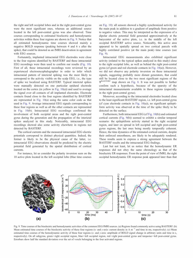
the right and left occipital lobes and in the right post-central gyruswere the most significant ones, whereas an additional sourcelocated in the left post-central gyrus was also observed. Timecourses corresponding to estimated bioelectric and hemodynamicactivities within these four regions are shown in Fig. 9. Notice thatall estimated hemodynamic time courses showed mainly anegative BOLD response (peaking between 4 and 6 s after thespike), that could be denoted as an fMRI deactivation in agreementwith EEG sources.

Fortunately, implanted intracranial EEG electrodes were closeto the four regions identified by BASTERF and these intracranialEEG recordings were then used to confirm our results (Fig. 10).First of all, these intracranial recordings were reviewed by anexperienced electroencephalographer in order to infer whichintracranial pattern of interictal spiking was the most likely tocorrespond to the activity visible on the scalp EEG, i.e., the typeof spike we localized using BASTERF. Typical interictal spikeswere manually detected on one particular epidural electrodelocated on the cortex (in yellow in Fig. 10(a)) and used to averagethe signal over all contacts of all implanted electrodes. Electrodecontacts found close to the four regions identified by BASTERFare represented in Fig. 10(a) using the same color code as thatused in Fig. 9. Average intracranial EEG signals corresponding tothese four regions as well as all the other contacts are representedin Fig. 10(b). Intracranial EEG recordings confirmed theinvolvement of both occipital areas and the right post-centralgyrus during the generation and the propagation of the interictalspikes analyzed in this study. Noticeably, intracranial EEGrecordings showed also some activity elsewhere in regions notdetected by BASTERF.

The cortical currents and the measured intracranial EEG electricpotentials correspond to distinct physical quantities. Indeed, theformer is likely to be the physical cause of the latter, i.e.intracranial EEG observations should be predicted by the electricpotential field generated by the spatial distribution of corticalcurrents.

For instance, let us consider the polarity inversion seen on the10 active plots located in the left occipital lobe (blue time courses

Fig. 9. Time courses of the bioelectric and hemodynamic activities of the common EMean estimated time courses of the bioelectric activity of these four regions (x- aestimated time courses of the hemodynamic activity of these four regions (x- andrespectively). On all subgyrus, green=right occipital region, blue= left occipitalErrorbars show half the standard deviation over the set of voxels belonging to the

on Fig. 10): all sensors showed a highly synchronized activity forthe main peak in addition to a gradient of amplitude from positiveto negative values. This may be interpreted as the expression of adipolar electric potential field generated approximatively at thebarycenter of the active plots, i.e. in the middle of the leftoccipital BASTERF active source. Noticeably, this active areaappeared to be spatially spread on two cortical parcels withhighly correlated positive (at the main peak) time courses (seeFig. 9).

Intracranial EEG measurements also exhibited significantactivity (related to the typical spikes analyzed in this study) closeto the right occipital lobe, as well as behind the right post-centralgyrus (cf green and red electrode contacts in Fig. 10(a)). However,we did not observe any polarity inversion on these intracranialsignals, suggesting probably more distant generators, that couldstill be located close to the two most significant regions of theTBASTERF map shown on Fig. 8. It was not possible to furtherconfirm such a hypothesis, because of the sparsity of theintracranial measurements available in these regions (especiallyin the right post-central gyrus).

Moreover, according to the intracranial electrodes located closeto the least significant BASTERF region, i.e. left post-central gyrus(cf cyan electrode contacts in Fig. 10(a)), no significant epilepti-form activity was observed at the time of the spike likely to bedetected on the surface.

Furthermore, both intracranial EEG (cf Fig. 10(b)) and estimatedcortical currents (Fig. 9(b)) seemed to exhibit a similar temporalscenario: the epileptiform activity started in the right occipitalregion, and later on spread in left occipital and right post-centralgyrus regions, the last ones being mostly temporally coherent.Hence, the time dynamics of the estimated cortical currents, despitetheir enforced smoothness, are likely to be adequately rendered.These results seem to express a strong agreement between theBASTERF results and the intracranial EEG findings.

Last but not least, let us notice that the hemodynamic ERresponses did not obey the same chronology as that of thebioelectric ER responses. From the point of view of fMRI, the rightoccipital hemodynamic ER response peak appeared later than that

EG/fMRI sources. (a) Regions found commonly active using BASTERF. (b)nd y-axis: current density in A m−3 and time in ms, respectively). (c) Meany-axis: amplitude of BOLD signal change in arbitrary units and time in s,region, red=right post-central gyrus and turquoise= left post-cental gyrus.four activated regions.

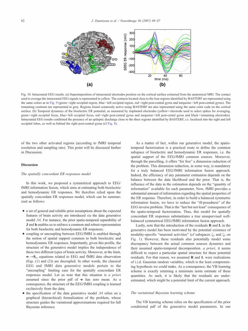
Fig. 10. Intracranial EEG results. (a) Superimposition of intracranial electrodes position on the cortical surface extracted from the anatomical MRI. The contactused to average the intracranial EEG signals is represented in yellow. The contacts located close to the four regions identified by BASTERF are represented usingthe same colors as in Fig. 9 (green=right occipital region, blue= left occipital region, red=right post-central gyrus and turquoise= left post-central gyrus). Theremaining contrasts are represented in grey. Regions found commonly active using BASTERF are also represented using the same color code on the corticalsurface. (b) Temporal dynamics of the bioelectric ER potential, as measured by implanted electrodes (yellow=electrode used to select spikes for averaging,green=right occipital focus, blue= left occipital focus, red=right post-central gyrus and turquoise= left post-cental gyrus and black=remaining electrodes).Intracranial EEG results confirmed the presence of an epileptic discharge close to the three regions identified by BASTERF, i.e. localized into the right and leftoccipital lobes, as well as behind the right post-central gyrus (cf Fig. 8).

82 J. Daunizeau et al. / NeuroImage 36 (2007) 69–87

of the two other activated regions (according to fMRI temporalresolution and sampling rate). This point will be discussed furtherin Discussion.

Discussion

The spatially concordant ER responses model

In this work, we proposed a symmetrical approach to EEG/fMRI information fusion, which aims at estimating both bioelectricand hemodynamic ER responses. We therefore relied upon thespatially concordant ER responses model, which can be summar-ized as follows:

• a set of general and reliable prior assumptions about the expectedfeatures of brain activity are introduced via the data generativemodel M. For instance, the prior spatio-temporal separability ofJ and h enables us to enforce a common and robust representationfor both bioelectric and hemodynamic ER responses;

• coupling or uncoupling between EEG/fMRI is enabled throughthe notion of spatial support common to both bioelectric andhemodynamic ER responses. Importantly, given this profile, thestructure of the generative model implies the independence ofthese two different types of brain activity. Moreover, at the limit,w→0n, equations related to EEG and fMRI data observation(Eqs. (1) and (2)) are decoupled. In other words, the classicalEEG and fMRI data generative models pertain to the“uncoupling” limiting case for the spatially concordant ERresponses model. Let us note that this situation is a prioriassumed since the prior pdf of w has zero mean. As aconsequence, the structure of the EEG/fMRI coupling is learnedexclusively from the data;

• the specification of the data generative model M relies on agraphical (hierarchical) formalization of the problem, whosestructure guides the variational approximations required for fullBayesian inference.

As a matter of fact, within our generative model, the spatio-temporal factorization is a practical route to define the commonsubspace of bioelectric and hemodynamic ER responses, i.e. thespatial support of the EEG/fMRI common sources. Moreover,through the parcelling, it offers “for free” a dimension reduction ofthe problem. This dimension reduction, in some way, is mandatoryfor a truly balanced EEG/fMRI information fusion approach.Indeed, the efficiency of any parameter estimation depends on thebalance between the data likelihood and the prior. That is, theinfluence of the data in the estimation depends on the “quantity ofinformation” available for each parameter. Now, fMRI provides asubstantial amount of information regarding the spatial properties ofthe ER response. Therefore, in order to build a balanced symmetricinformation fusion, we have to reduce the “ill-posedness” of theEEG inverse problem. That is the “last but not least” consequence ofthe spatio-temporal factorization. Thus, this model for spatiallyconcordant ER responses substantiates a true unsupervised well-balanced symmetrical EEG/fMRI information fusion approach.

Lastly, note that the introduction of the residuals R and L in thegenerative model has been motivated by the potential existence ofmodality-specific “neuronal activities” (cf subspaces ζ2 and ζ3 onFig. 1). However, these residuals also potentially model somediscrepancy between the actual common sources dynamics andtheir assumed spatio-temporal decomposition. a priori, it seemsdifficult to expect a particular spatial structure for these potentialresiduals. For that reason, we assumed R and L were realizationsof i.i.d. Gaussian random variables, which is the least compromis-ing hypothesis we could make. As a consequence, the VB learningscheme is exactly returning a minimum norm estimate of thesequantities. As such, it is likely that the residuals are under-estimated, which might be a potential limit of the current approach.

The variational Bayesian learning scheme

The VB learning scheme relies on the specification of the priorconditional pdf of the generative model parameters. In our

83J. Daunizeau et al. / NeuroImage 36 (2007) 69–87

generative model, we have made use of non-informative prior pdf(for instance, Jeffreys priors on precision hyperparameters). Indeed,the building of non-informative distributions is the heart of acontroversial debate: how should we parameterize our priorignorance? Jeffreys priors are derived from formal rules (invarianceprinciples) for choosing non-informative priors associated tofamilies of parameters (location, scale, …). Unfortunately, thesepriors are improper, i.e. unnormalized. The practical alternative toJeffreys-like priors is the use of diffuse but proper prior pdf. In ourcase, this pertains to specify vague Gamma prior pdf for all precisionparameters, which would embody the expected scale of magnitudeof all the unknown hidden states (J, h, w, X and Z). This wouldtheoretically prevent the posterior from its potential impropriety.However, when improper priors lead to badly behaved posteriors, itis a warning that the problem itself may be hard; in this situationdiffuse proper priors are likely to lead to similar difficulties (Kassand Wassermann, 1996).

A second argument in favor of our use of non-informativepriors for precision hyperparameters may come from both theintuitive understanding of the hierarchical generative model andthe simulation series. The observation Eqs. (1) and (2), combinedwith the informative (Gamma) prior on the measurement noises (cfEq. (15)) are very likely to enforce a certain scale of magnitude forthe estimated voxelwise dynamics J and h. Then, the conditionalpdf given by Eqs. (8), (10) and (13) can be rewritten as a zero meanprior pdf for J and h, with a given covariance structure. Thiscovariance structure is decomposed into spatial and temporalcomponents (through the spatio-temporal factorization), whichhave to match the (data) imposed scale of J and h. In other words,the spatial and temporal variability of J and h is parameterized by amixture of covariance matrices, which has to be “adjusted” throughthe estimation of the precision hyperparameters. Two limitingsituations may then occur: either there is enough information in thedata to fit the hyperparameters, or there is not. In the latter case,one may claim that the posterior Gamma hyperparameter pdfderived from the VB learning scheme may reflect any potentiallack of data information, by showing, for instance, a high posteriorvariance of the precision hyperparameters. However, the simula-tion series did not show any striking difference between theposterior variances of the measurement noise precisions (whosemarginal posterior are assured to be proper) and the other precisionhyperparameters (whose posterior might, a priori, be improper).

Another comment is to be made about the VB inversion of thegenerative model. The hierarchical prior on w is derived bymaking use of the discrete Laplacian operator S (cf Prior densitiesof the coupling model parameters), which is rank deficient (i.e. ofrank n−1). As a consequence, the prior Gaussian pdf of w isformally degenerate, i.e. one of the principal axis of its priorcovariance matrix has an infinite variance. Nevertheless, this doesnot lead to an improper posterior pdf, because its posteriorcovariance matrix is full-rank (see Table 1). An equivalent remarkcan be made for X and Z, whose hierarchical prior made use ofthe discrete second temporal derivative operators T1 and T2.Despite the fact that this rank-deficiency does not invalidate theuse of application of the VB framework, it may be a problem forthe actual calculation of the variational free energy, for which onemay have to resort to some full-rank approximation of the above-mentioned operators.

Furthermore, we should shed some light on the VB learning ofthe time invariant w, which is the EEG/fMRI coupling key quantity.The common spatial profile of brain activity w is estimated

according to a trade-off in fitting both the EEG and fMRI data.More precisely, the functional form of the variational marginalposterior pdf qW is such that:

• this trade-off between the two terms of attach to the bioelectricand hemodynamic activities, respectively, is related to a measureof uncertainty associated to these cerebral activity markers (viathe precision hyperparameters ϵ1 and ϵ2, cf Table 1). In otherwords, the influence of the EEG or fMRI datasets in theestimation of their common spatial profile w is an increasingfunction of the plausibility of the information they contain;

• the variational posterior covariance matrix of w is a decreasingfunction of the variational posterior covariance matrices ofX andZ (cf Table 2, Eq. (22)). This phenomenon illustrates theconservation of the total uncertainty associated with thesubsystem (w, X, Z), which is a commonly observedcharacteristic of dual variables. This enforces a weighting thatpenalizes the voxels/dipoles whose temporal (bioelectric and/orhemodynamic) characteristics are highly uncertain. In otherwords, the iterative estimation of w may be considered as aselecting process of brain areas whose characteristics are the leastuncertain given the observed EEG/fMRI datasets.

By construction, the estimated common spatial profile w shouldreveal the bioelectrically and hemodynamically active areas thatare characterized with no uncertainty by the joint EEG/fMRIdatasets. w then yields a quantitative image of the true fusion ofmultimodal information.

Indeed, the simulation series highlighted the expected behaviourof the invariant spatial profile w. Let us consider the differencebetween WMN-like and BASTERF fusion approaches, which ismost prominent for the simulation series (S4). These series havebeen described as “weak concordance” situations because despitethe fact that no active source was contributing to both EEG and fMRIdatasets, both datasets partially agree about the inactive sources.This puts into light another difference between the proposedapproach and the more classical fMRI-weighted minimum normapproach to the EEG inverse problem: the VB inference scheme isexplicitly estimating the uncertainty of the model parametersassociated to both EEG and fMRI data generative models. As aconsequence, the areas of the brain that do not contribute to any ofthe EEG and fMRI datasets are considered as certainly inactive.However, the areas that are expressed in one of the two datasets willbe associated to a higher local variance. Intuitively, the algorithm hasthen to choose between these less certainly inactive areas to explainthe respective datasets. This is not the case for fMRI-weightedminimum norm approaches, because these do not consider the localuncertainty of the fMRI prior.

The variational Bayesian learning scheme further enables us totest for the significance of the estimated common spatial profile w.Such a test might reveal the “common spatial support” of bioelectricand hemodynamic activities. By spatial support of activity, we meanthe infinite set of significantly activated voxels. Hence, the commonspatial support is the intersection of bioelectrically and hemodyna-mically active voxels. This classification would allow us to localizethe regions that exhibit a strong bioelectric/hemodynamic couplingfor a given subject and a given experiment.

However, the mean-field approximation implies an under-estimation of the degree of uncertainty associated to the estimationsof the graphical model parameters. For instance, this may explain thelarge T-values obtained in the epileptic patient study (cf Fig. 8). As a

84 J. Daunizeau et al. / NeuroImage 36 (2007) 69–87

consequence, it might be difficult to propose an absolute way ofthresholding the mapw. This particular point should be tackled withgreat care, and might benefit from an exhaustive comparison withclassical Bayesian sampling approaches (such as Gibbs sampling).

The cortical parcelling

Up to now, we did not discuss the specific influence of theparcelling (C), which constitutes, in this work, a fixed priorassumption about the structure of cortical activity.

As a matter of fact, the adequacy of the local spatio-temporalfactorization assumption (within the parcels dynamics) is definitelydependent on the cortical parcelling itself. Noticeably, thissensitivity has been evaluated when first proposing the spatio-temporal model for the EEG inverse problem in (Daunizeau et al.,2005b). The conclusions were the following: as long as each parceldynamics can be described using one approximated time course, themodel is actually fine. Moreover, even when at least one priorcortical parcel contains more than one active source, the subsequentperturbation on the estimated spatial profilew is “acceptable”, in thesense that the corresponding cortical source estimation (J=Diag(w)CX) is most of the time better than the standard LORETA (Pascual-Marqui et al., 1994), MN and WMN methods.

Nevertheless, the sensitivity of the whole approach to thepotential inadequacy of the prior cortical parcelling still remains tobe properly evaluated. The simulation series S1, S2, S3 and S4were conducted such that no cortical parcel contained more thanone active simulated source. Therefore, we did not evaluate thebehavior of the whole approach when the prior hypothesis oftemporal coherence of the parcels was mainly irrelevant. Althoughimportant, the question of estimating such a cortical parcel fallsbeyond the scope of this article. Several approaches have alreadybeen proposed to derive a cortical parcelling based on functionalneuroimaging data (see (Flandin et al., 2002; Bellec et al., 2004)for fMRI and (Daunizeau et al., 2004; Lapalme et al., 2006) forEEG). However, no multimodal approach has yet been proposed.We are currently investigating the putative usefulness of such anapproach, which, interestingly, might be consecutive to theinability of the model to describe properly the cortical voxelwiseER response. Indeed, in that case, the data itself will “require” amore adequate parcelling to be properly modelled.

Noticeably, the data generative model M introduces J and h asperturbations of their respective spatio-temporal decomposition (cfEqs. (4) and (5)). Hence, the residuals R and L enable us to relax theestimation of J and h and prevent it from inappropriate constraint oftemporal coherence. As a consequence, it is possible to explicitlylook for the parcelling that is associated with a maximal intra-parceltemporal coherence, according to both EEG and fMRI data. Thisoptimization scheme may be introduced during the iterations of theVB algorithm, by specifying a prior pdf 5 for the new unknownvariable C. Another practical alternative would be to comparedifferentmodels associated to a reduced set of given parcellings usingthe variational free energy (approximation of the model evidence).

Comments on the observed neurovascular coupling

The validation part of this work has involved the use ofmultimodal epilepsy data, and relied on the available intracranial

5 For example, this pdf could be a multinomial pdf (living in the labelsspace), whose mode might be defined as the Brodmann cortical parcelling.

EEG measurements to draw some conclusions regarding thebehavior of the whole approach. First of all, one must emphasizethe limitations of the intracranial EEG neuroimaging modality: it isbased on local measurements. As a consequence, intracranial EEGdoes not provides us with any information about any potentialactivity remote to the implanted electrodes. Moreover, a quantitativecomparison of intracranial EEG signals and reconstructed corticalcurrents would involve a dedicated forward model, exactlyequivalent to that underlying the calculation of the EEG gain matrix(Chang et al., 2005). Particularly, this model should inform us abouthow to distort the amplitude of the intracranial EEG signals byrendering the spatial shape of the electrical potential field that couldhave been generated by the cortical currents. Though highlyrelevant, such a quantitative analysis of the intracranial EEGmeasurements is beyond the scope of this article.

Nevertheless, despite these concerns, the intracranial EEGmeasurements allowed us to (partially) validate the results of theBASTERF analysis of the epilepsy data, and to compare thebioelectric and the hemodynamic ER responses in the (clinical)context of interictal spikes localization. The latter lead us to maketwo striking observations:

1. The local hemodynamic ER responses do not obey the samechronology as the bioelectric ER responses;

2. A significant bioelectric ER response is locally associated to anegative hemodynamic ER response, i.e. a local deactivation.

The concern related to the temporal precedence of the ERresponses has already been reported in (Bandettini et al., 1997). Thishas outstanding implications for any causality analysis within theactive network: one may draw complete opposite conclusions aboutthe causal relations of the nodes by relying on either bioelectric orhemodynamic ER responses. Since the hemodynamic response ispartly driven by biophysical processes that are independent of theunderlying neuronal activity (e.g., dynamics of the muscular cellswhich regulate the vasodilation), we are inclined to favor EEG-related analysis in any inference regarding the causal relations withinthe active network. In other words, one should always complementany fMRI analysis with EEG recordings in order to be able to inferboth the nodes and the links of the active network.

The second point brings to light the difficulty in linking thetemporal dynamics of bioelectric and hemodynamic activities. As amatter of fact, very few works have specifically focused onexperimental evidence for candidates processes to deactivation.Deactivation is commonly interpreted as a transient metabolismsuspension related to the event (Raichle et al., 2000). Relying onthe “sharp-slow wavy” pattern of the scalp ERP of this patient, thefMRI deactivation may be interpreted by an increase in theinhibitory activity, which is believed to reduce the net presynapticactivity (Arthurs and Boniface, 2003). One explanation is thatstrong local inhibition is playing a role in keeping these epilepticdischarges from spreading, and therefore could represent the mostprominent phenomenon from the metabolic point of view(Stefanovic et al., 2005). We have no evidence, however, forwhether this putative inhibitory activity is the cause or theconsequence of the observed epileptiform activity.

Noticeably, these results would have unlikely been obtained byusing a method enforcing a prior link between the time courses ofthe bioelectric and hemodynamic ER responses (e.g.: through anextension of the Balloon model (Riera et al., 2006)). This ismainly because the existing neurovascular coupling models do not

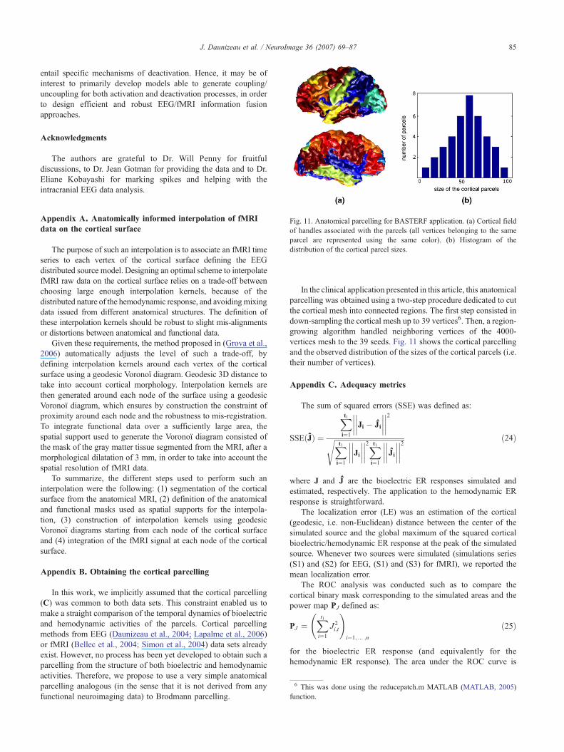
85J. Daunizeau et al. / NeuroImage 36 (2007) 69–87

entail specific mechanisms of deactivation. Hence, it may be ofinterest to primarily develop models able to generate coupling/uncoupling for both activation and deactivation processes, in orderto design efficient and robust EEG/fMRI information fusionapproaches.

Acknowledgments

The authors are grateful to Dr. Will Penny for fruitfuldiscussions, to Dr. Jean Gotman for providing the data and to Dr.Eliane Kobayashi for marking spikes and helping with theintracranial EEG data analysis.

Fig. 11. Anatomical parcelling for BASTERF application. (a) Cortical fieldof handles associated with the parcels (all vertices belonging to the sameparcel are represented using the same color). (b) Histogram of thedistribution of the cortical parcel sizes.

6 This was done using the reducepatch.m MATLAB (MATLAB, 2005)function.

Appendix A. Anatomically informed interpolation of fMRIdata on the cortical surface

The purpose of such an interpolation is to associate an fMRI timeseries to each vertex of the cortical surface defining the EEGdistributed source model. Designing an optimal scheme to interpolatefMRI raw data on the cortical surface relies on a trade-off betweenchoosing large enough interpolation kernels, because of thedistributed nature of the hemodynamic response, and avoidingmixingdata issued from different anatomical structures. The definition ofthese interpolation kernels should be robust to slight mis-alignmentsor distortions between anatomical and functional data.

Given these requirements, the method proposed in (Grova et al.,2006) automatically adjusts the level of such a trade-off, bydefining interpolation kernels around each vertex of the corticalsurface using a geodesic Voronoï diagram. Geodesic 3D distance totake into account cortical morphology. Interpolation kernels arethen generated around each node of the surface using a geodesicVoronoï diagram, which ensures by construction the constraint ofproximity around each node and the robustness to mis-registration.To integrate functional data over a sufficiently large area, thespatial support used to generate the Voronoï diagram consisted ofthe mask of the gray matter tissue segmented from the MRI, after amorphological dilatation of 3 mm, in order to take into account thespatial resolution of fMRI data.

To summarize, the different steps used to perform such aninterpolation were the following: (1) segmentation of the corticalsurface from the anatomical MRI, (2) definition of the anatomicaland functional masks used as spatial supports for the interpola-tion, (3) construction of interpolation kernels using geodesicVoronoï diagrams starting from each node of the cortical surfaceand (4) integration of the fMRI signal at each node of the corticalsurface.

Appendix B. Obtaining the cortical parcelling

In this work, we implicitly assumed that the cortical parcelling(C) was common to both data sets. This constraint enabled us tomake a straight comparison of the temporal dynamics of bioelectricand hemodynamic activities of the parcels. Cortical parcellingmethods from EEG (Daunizeau et al., 2004; Lapalme et al., 2006)or fMRI (Bellec et al., 2004; Simon et al., 2004) data sets alreadyexist. However, no process has been yet developed to obtain such aparcelling from the structure of both bioelectric and hemodynamicactivities. Therefore, we propose to use a very simple anatomicalparcelling analogous (in the sense that it is not derived from anyfunctional neuroimaging data) to Brodmann parcelling.

In the clinical application presented in this article, this anatomicalparcelling was obtained using a two-step procedure dedicated to cutthe cortical mesh into connected regions. The first step consisted indown-sampling the cortical mesh up to 39 vertices6. Then, a region-growing algorithm handled neighboring vertices of the 4000-vertices mesh to the 39 seeds. Fig. 11 shows the cortical parcellingand the observed distribution of the sizes of the cortical parcels (i.e.their number of vertices).

Appendix C. Adequacy metrics

The sum of squared errors (SSE) was defined as:

SSEðJ ̂Þ ¼

Xt1i¼1

��������Ji � Ĵi

��������2ffiffiffiffiffiffiffiffiffiffiffiffiffiffiffiffiffiffiffiffiffiffiffiffiffiffiffiffiffiffiffiffiffiffiffiffiffiffiffiffiXt1

i¼1

��������Ji��������2Xt1

i¼1

��������Ĵi

��������2

s ð24Þ

where J and Ĵ are the bioelectric ER responses simulated andestimated, respectively. The application to the hemodynamic ERresponse is straightforward.

The localization error (LE) was an estimation of the cortical(geodesic, i.e. non-Euclidean) distance between the center of thesimulated source and the global maximum of the squared corticalbioelectric/hemodynamic ER response at the peak of the simulatedsource. Whenever two sources were simulated (simulations series(S1) and (S2) for EEG, (S1) and (S3) for fMRI), we reported themean localization error.

The ROC analysis was conducted such as to compare thecortical binary mask corresponding to the simulated areas and thepower map PJ defined as:

PJ ¼Xt1i¼1

J 2i;t

!i¼1; N ;n

ð25Þ

for the bioelectric ER response (and equivalently for thehemodynamic ER response). The area under the ROC curve is

86 J. Daunizeau et al. / NeuroImage 36 (2007) 69–87

then the probability to correctly disambiguate between an activatedand an inactivated elementary dipole, on the basis of the powermap PJ. Note that this index provides an accurate estimation of theglobal spatial behavior of an estimator (in terms of both itslocalization and extent estimation capabilities).

References

Ahlfors, S.P., Simpson, G.U., 2004. Geometrical interpretation of fMRI-guided MEG/EEG. NeuroImage 22, 323–332.

Alarcon, G., Guy, C., Walker, S., Elwes, R., Polkey, C., 1994. Intracerebralpropagation of interictal activity in partial epilepsy: implications forsource localization. J. Neurol. Neurosurg. Psychiatry 57, 435–449.

Arthurs, O.J., Boniface, S.J., 2003. What aspect of the fMRI BOLD signalbest reflects the underlying electrophysiology in human somatosensorycortex? Clin. Neurophysiol. 114, 1203–1209.

Babiloni, F., Babiloni, C., Carduci, F., Romani, G.L., Rossini, P.M.,Angelone, L., Cincotti, F., 2003. Multimodal integration of high-resolution EEG and functional magnetic resonance imaging data: asimulation study. NeuroImage 19, 1–15.

Baillet, S., Mosher, J.C., Leahy, R.M., 2001. Electromagnetic brainmapping. IEEE Signal Process. Mag. 18, 14–30.

Bandettini, P.A., Kwong, K.K., Davis, T.L., Tootell, R.B.H., Wong, E.C.,Fox, P.T., Belliveau, J.W., Weissko, R.M., Rosen, B.R., 1997.Characterization of cerebral blood oxygenation and flow changes duringprolonged brain activation. Hum. Brain Mapp. 5, 93–109.

Bellec, P., Marrelec, G., Posé, C., Jolivet, O., Pélégrini-Issac, M., Doyon, J.,Benali, H., 2004. An assisted data-driven procedure to selectfunctionally connected brain regions in fMRI. Proceedings of the 10thInternational Conference on Functional Mapping of the Human Brain.Available on NeuroImage CD-Rom, volume 22, Budapest, Hungary.

BrainStorm, 2005. BrainStorm software. Available at http://neuroimage.usc.edu/brainstorm/.

BrainVISA, 2005. BrainVISA software. Available at http://brainvisa.info/.Chang, N., Gulrajani, R., Gotman, J., 2005. Dipole localization using

simulated intracerebral EEG. Clin. Neurophysiol. 116, 2707–2716.Dale, A.M., Sereno, M., 1993. Improved localization of cortical activity by

combining EEG and MEG with MRI surface reconstruction: a linearapproach. J. Cogn. Neurosci. 5, 162–176.

Daunizeau, J., Mattout, J., Goulard, B., Lina, J.M., Benali, H., 2004. Data-driven cortex parcelling: a regularization tool for the EEG/MEG inverseproblem. Second 2004 IEEE International Symposium on BiomedicalImaging: From Nano to Macro (ISBI’04), pp. 1343–1346. Arlington, VA.

Daunizeau, J., Grova, C., Mattout, J., Marrelec, G., Clonda, D., Goulard, B.,Lina, J.M., Benali, H., 2005a. Assessing the relevance of fMRI-basedprior in the EEG inverse problem: a Bayesian Model Comparisonapproach. IEEE Trans. Sign. Proc. 53, 3461–3472.

Daunizeau, J., Mattout, J., Clonda, D., Goulard, B., Benali, H., Lina, J.M.,2005b. Bayesian spatio-temporal approach for EEG source reconstruc-tion: conciliating ECD and distributed models. IEEE Trans. Biomed.Eng. 53, 503–516.

de Munck, J.C., 1988. The potential distribution in a layered spheroidalvolume conductor. J. Appl. Phys. 64, 464–470.

Flandin, G., Kherif, F., Pennec, X., Rivière, D., Ayache, N., Poline, J.B.,2002. Parcellation of brain images with anatomical and functionalconstraints for fMRI data analysis. Proc. IEEE ISBI, pp. 907–910.Washington, DC, USA, Juil.

Friston, K.J., 2005a. Models of brain function in neuroimaging. Annu. Rev.Psychol. 56, 57–87.

Friston, K.J., 2005b. A theory of cortical responses. Philos. Trans. R. Soc.360, 815–836.

Friston, K.J., Holmes, A.P., Poline, J.B., Grasby, P.J., Williams, S.C.,Frackowiak, R.S., Turner, R., 1995. Analysis of fMRI time-seriesrevisited. NeuroImage 2, 45–53.

Gelman, A., Carlin, J.B., Stern, H.S., Rublin, D.B., 1998. Bayesian DataAnalysis. Chapman and Hall, Londres.

Ghahramani, Z., 1995. Factorial learning and the EM algorithm. Adv. NeuralInf. Process. Syst. 7, 617–624.

Gonzales, A.S.L., Blanke, O., Lantz Thut, G., Grave de Peralta Merendez,R., 2001. The use of functional constraints for the neuromagnetic inverseproblem: alternatives and caveats. Int. J. Bioelectromagn. 3, 103–114.

Gössl, C., Auer, D., Fahrmeir, L., 2001. Bayesian spatiotemporal inferencein functional magnetic resonance imaging. Biometrics 57, 554–562.

Gotman, J., Benar, C.G., Dubeau, F., 2004. Combining EEG and fMRI inepilepsy: methodological challenges and clinical results. J. Clin.Neurophysiol. 21, 179–192.

Grova, C., Makni, S., Flandin, G., Ciuciu, P., Gotman, J., Poline, J.B., 2006.Anatomically informed interpolation of fMRI data on the corticalsurface. NeuroImage 31, 1475.

Hauk, O., 2004. Keep it simple: a case for using classical minimum normestimation in the analysis of EEG and MEG data. NeuroImage 21,1612–1621.

Heeger, D.J., 2002. What fMRI tells us about neuronal activity? Nature 3,142–151.

Kass, R.E., Wassermann, L., 1996. The selection of prior distributions byformal rules. J. Am. Stat. Assoc. 91, 1343–1370.

Lapalme, E., Lina, J.M., Mattout, J., 2006. Data-driven parceling andentropic inference in MEG. NeuroImage 30, 160–171.

Liu, A.K., Belliveau, J.W., Dale, A.M., 1998. Spatiotemporal imaging ofhuman brain activity using functional MRI constrained magnetoencepha-lographic data: Monte Carlo simulations. Proc. Natl. Acad. Sci. U. S. A.95, 8945–8950.

Logothetis, N.K., Wandell, B.A., 2004. Interpreting the BOLD signal. Annu.Rev. Physiol. 66, 735–769.

Logothetis, N.K., Pauls, J., Augath, M., Trinath, T., Oeltermann, A., 2001.Neuro-physiological investigation of the basis of the fMRI signal.Nature 412, 150–157.

Marrelec, G., Benali, H., Ciuciu, P., Poline, J.B., 2001. Bayesian estimationof the hemodynamic response function in functional MRI. In: Fry, R.(Ed.), Bayesian Inference and Maximum Entropy Methods in Scienceand Engineering. Workshop Proceedings. AIP, Melville, pp. 229–247.

Marrelec, G., Benali, H., Ciuciu, P., Pélégrini-Issac, M., Poline, J.B., 2003a.Robust Bayesian estimation of the hemodynamic response function inevent-related BOLD fMRI using basic physiological information. Hum.Brain Mapp. 19, 1–17.

Marrelec, G., Ciuciu, P., Pélégrini-Issac, M., Benali, H., 2003b. Estimationof the hemodynamic response function in event-related functional MRI:directed acyclic graphs for a general Bayesian inference framework. In:Taylor, C.J., Noble, J.A. (Eds.), Information Processing in MedicalImaging. Springer-Verlag, Berlin, pp. 635–646.

Marrelec, G., Ciuciu, P., Pélégrini-Issac, M., Benali, H., 2004. Estimation ofthe hemodynamic response function in event-related functional MRI:Bayesian networks as a framework for efficient Bayesian modelling andinference. IEEE Trans. Med. Imag. 23, 959–967.

Martindale, J., Mayhew, J., Berwick, J., Jones, M., Martin, C., Johnston,D., Redgrave, P., Zheng, Y., 2003. The hemodynamic impulseresponse to a single neural event. J. Cereb. Blood Flow Metab. 23,546–555.

Mathiesen, C., Caesar, K., Akgoren, N., Lauritzen, M., 1998. Modificationof activity-dependent increases of cerebral blood flow by excitatorysynaptic activity and spikes in rat cerebellar cortex. J. Physiol. 512,555–566.

MATLAB. MATLAB software, 2005. Available at http://www.mathworks.com/.

Mattout, J., Philipps, C., Rugg, M.D., Friston, K.J., 2006. MEG sourcelocalization under multiple constraints: an extended Bayesian frame-work. NeuroImage 30, 753–767.

Mosher, J.C., Leahy, R.M., 1998. Recursive MUSIC: a framework for EEGand MEG source localization. IEEE Trans. Biomed. Eng. 45,1342–1354.

Mukamel, R., Gelbard, H., Arieli, A., Hasson, U., Fried, I., Malach, R.,2005. Coupling between neuronal ring, field potentials, and fMRI inhuman auditory cortex. Science 5, 951–954.

87J. Daunizeau et al. / NeuroImage 36 (2007) 69–87

Nunez, P.L., 1981. Electric Fields of the Brain. New York Press, Oxford.Nunez, P.L., Silberstein, R.B., 2000. On the relationship of synaptic activity

to macroscopic measurements: does co-registration of EEG with fMRImake sense? Brain Topogr. 13, 79–96.

Pascual-Marqui, R.D., Michel, C.M., Lehmann, D., 1994. Low ResolutionElectromagnetic Tomography: a new method for localizing electricalactivity in the brain. Int. J. Psychophysiol. 18, 49–65.

Pieger, P.J., Greenblatt, R.E., 2001. Nonlinear analysis of multimodaldynamic brain imaging data. Int. J. Bioelectromagn. 3 (Available athttp://www.ijbem.org/volume3/number1/toc.htm).

Puce, A., Allison, T., Spencer, S.S., Spencer, D.D., McCarthy, G., 1997.Comparison of cortical activation evoked by faces measured byintracranial field potentials and functional MRI: two cases studies.Hum. Brain Mapp. 5, 298–305.

Raichle, M.E., MacLeod, A.M., Snyder, A.Z., Powers, W.J., Gusnard, D.A.,Schuman, G.L., 2000. A default mode of brain function. Proc. Natl.Acad. Sci. U. S. A. 98, 67–682.

Riera, J., Wan, X., Jimenez, J.C., Kawashima, R., 2006. Nonlinear local

electrovascular coupling: I. A theoretical model. Hum. Brain Mapp. 25,1025–1041.

Simon, O., Kherif, F., Flandin, G., Poline, J.B., Rivière, D., Mangin, J.F., LeBihan, D., Dehaene, S., 2004. Automatized clustering and functionalgeometry of human parietofrontal networks for language, space, andnumber. NeuroImage 23, 1192–1202.

SPM, 2005. SPM 5 software. Available at http://www.fil.ion.ucl.ac.uk/spm/.Stefan, K., Harrison, L.E., Penny, W.D., Friston, K., 2004. Biophysical

models of fMRI responses. Curr. Opin. Neurobiol. 14, 629–635.Stefanovic, B., Warnking, J.M., Kobayashi, E., 2005. Hemodynamic and

metabolic responses to activation, deactivation and epileptic discharges.NeuroImage 28, 205–215.

Trujillo, N.J., Martinez, E., Melie, L., Valdès-Sosa, P.A., 2001. Bayesianmodel for fMRI and EEG/MEG neuroimage fusion. Int. J. Bioelectro-magn. 3 (Available at http://www.ijbem.org/volume3/number1/toc.htm).

Worsley, K.J., Liao, C., Aston, J., Petre, V., Duncan, G.H., Morales, F.,Evans, A.C., 2002. A general statistical analysis for fMRI data.NeuroImage 15, 1–15.