arX

iv:1

104.

3348

v1 [

cs.G

T]

17 A

pr 2

011

Symbolic Algorithms for Qualitative Analysis ofMarkov Decision Processes with Buchi Objectives⋆

Krishnendu Chatterjee1, Monika Henzinger2, Manas Joglekar3, and Nisarg Shah3

1 IST Austria2 University of Vienna

3 IIT Bombay

Abstract. We consider Markov decision processes (MDPs) withω-regular spec-ifications given as parity objectives. We consider the problem of computing theset ofalmost-surewinning states from where the objective can be ensured withprobability 1. The algorithms for the computation of the almost-sure winning setfor parity objectives iteratively use the solutions for thealmost-sure winning setfor Buchi objectives (a special case of parity objectives). Our contributions are asfollows: First, we present the first subquadratic symbolic algorithm to computethe almost-sure winning set for MDPs with Buchi objectives; our algorithm takesO(n · √m) symbolic steps as compared to the previous known algorithm thattakesO(n2) symbolic steps, wheren is the number of states andm is the num-ber of edges of the MDP. In practice MDPs have constant out-degree, and then oursymbolic algorithm takesO(n ·√n) symbolic steps, as compared to the previousknown O(n2) symbolic steps algorithm. Second, we present a new algorithm,namelywin-losealgorithm, with the following two properties: (a) the algorithmiteratively computes subsets of the almost-sure winning set and its complement,as compared to all previous algorithms that discover the almost-sure winning setupon termination; and (b) requiresO(n ·

√K) symbolic steps, whereK is the

maximal number of edges of strongly connected components (scc’s) of the MDP.The win-lose algorithm requires symbolic computation of scc’s. Third, we im-prove the algorithm for symbolic scc computation; the previous known algorithmtakes linear symbolic steps, and our new algorithm improvesthe constants as-sociated with the linear number of steps. In the worst case the previous knownalgorithm takes5 ·n symbolic steps, whereas our new algorithm takes4 ·n sym-bolic steps.

1 IntroductionMarkov decision processes.The model of systems in verification of probabilistic sys-tems areMarkov decision processes (MDPs)that exhibit both probabilistic and non-deterministic behavior [11]. MDPs have been used to model and solve control prob-lems for stochastic systems [9]: there, nondeterminism represents the freedom of thecontroller to choose a control action, while the probabilistic component of the behav-ior describes the system response to control actions. MDPs have also been adoptedas models for concurrent probabilistic systems [5], probabilistic systems operating inopen environments [17], and under-specified probabilisticsystems [1]. Aspecification

⋆ This work was partially supported by FWF NFN Grant S11407-N23 (RiSE) and a Microsoftfaculty fellowship.

describes the set of desired behaviors of the system, which in the verification and con-trol of stochastic systems is typically anω-regular set of paths. The class ofω-regularlanguages extends classical regular languages to infinite strings, and provides a robustspecification language to express all commonly used specifications, such as safety, live-ness, fairness, etc [20]. Parity objectives are a canonicalway to define suchω-regularspecifications. Thus MDPs with parity objectives provide the theoretical framework tostudy problems such as the verification and control of stochastic systems.

Qualitative and quantitative analysis.The analysis of MDPs with parity objectivescan be classified into qualitative and quantitative analysis. Given an MDP with parityobjective, thequalitative analysisasks for the computation of the set of states fromwhere the parity objective can be ensured with probability 1(almost-sure winning). Themore generalquantitative analysisasks for the computation of the maximal probabilityat each state with which the controller can satisfy the parity objective.

Importance of qualitative analysis.The qualitative analysis of MDPs is an importantproblem in verification that is of interest irrespective of the quantitative analysis prob-lem. There are many applications where we need to know whether the correct behaviorarises with probability 1. For instance, when analyzing a randomized embedded sched-uler, we are interested in whether every thread progresses with probability 1 [7]. Evenin settings where it suffices to satisfy certain specifications with probabilityp < 1,the correct choice ofp is a challenging problem, due to the simplifications introducedduring modeling. For example, in the analysis of randomizeddistributed algorithms itis quite common to require correctness with probability 1 (see, e.g., [15,14,19]). Fur-thermore, in contrast to quantitative analysis, qualitative analysis is robust to numericalperturbations and modeling errors in the transition probabilities, and consequently thealgorithms for qualitative analysis are combinatorial. Finally, for MDPs with parity ob-jectives, the best known algorithms and all algorithms usedin practice first performthe qualitative analysis, and then performs a quantitativeanalysis on the result of thequalitative analysis [5,6,4]. Thus qualitative analysis for MDPs with parity objectives isone of the most fundamental and core problems in verificationof probabilistic systems.One of the key challenges in probabilistic verification is toobtain efficient and sym-bolic algorithms for qualitative analysis of MDPs with parity objectives, as symbolicalgorithms allow to handle MDPs with a large state space.

Previous results.The qualitative analysis for MDPs with parity objectives isachievedby iteratively applying solutions of the qualitative analysis of MDPs with Buchi objec-tives [5,6,4]. The qualitative analysis of an MDP with a parity objective withd prioritiescan be achieved byO(d) calls to an algorithm for qualitative analysis of MDPs withBuchi objectives, and hence we focus on the qualitative analysis of MDPs with Buchiobjectives. The classical algorithm for qualitative analysis for MDPs with Buchi objec-tives works inO(n · m) time, wheren is the number of states, andm is the numberof edges of the MDP [5,6]. The classical algorithm can be implemented symbolically,and it takes at mostO(n2) symbolic steps. An improved algorithm for the problem wasgiven in [3] that works inO(m · √m) time. The algorithm of [3] crucially depends onmaintaining the same number of edges in certain forward searches. Thus the algorithmneeds to explore edges of the graph explicitly and is inherently non-symbolic. In the

2

literature, there is no symbolic subquadratic algorithm for qualitative analysis of MDPswith Buchi objectives.

Our contribution. In this work our main contributions are as follows.

1. We present a new and simpler subquadratic algorithm for qualitative analysis ofMDPs with Buchi objectives that runs inO(m · √m) time, and show that the al-gorithm can be implemented symbolically. The symbolic algorithm takes at mostO(n · √m) symbolic steps, and thus we obtain the first symbolic subquadratic al-gorithm. In practice, MDPs often have constant out-degree:for example, see [8]for MDPs with large state space but constant number of actions, or [9,16] for ex-amples from inventory management where MDPs have constant number of actions(the number of actions correspond to the out-degree of MDPs). For MDPs withconstant out-degree our new symbolic algorithm takesO(n · √n) symbolic steps,as compared toO(n2) symbolic steps of the previous best known algorithm.

2. All previous algorithms for the qualitative analysis of MDPs with Buchi objectivesiteratively discover states that are guaranteed to be not almost-sure winning, andonly when the algorithm terminates the almost-sure winningset is discovered. Wepresent a new algorithm (namelywin-losealgorithm) that iteratively discovers bothstates in the almost-sure winning set and its complement. Thus if the problem is todecide whether a given states is almost-sure winning, and the states is almost-surewinning, then the win-lose algorithm can stop at an intermediate iteration unlike allthe previous algorithms. Our algorithm works in timeO(

√KE ·m) time, whereKE

is the maximal number of edges of any scc of the MDP (in this paper we write sccfor maximal scc). We also show that the win-lose algorithm can be implementedsymbolically, and it takes at mostO(

√KE · n) symbolic steps.

3. Our win-lose algorithm requires to compute the scc decomposition of a graph inO(n) symbolic steps. The scc decomposition problem is one of the most fundamen-tal problem in the algorithmic study of graph problems. The symbolic scc decom-position problem has many other applications in verification: for example, check-ing emptiness ofω-automata, and bad-cycle detection problems in model checking,see [2] for other applications. AnO(n · logn) symbolic step algorithm for scc de-composition was presented in [2], and the algorithm was improved in [10]. Thealgorithm of [10] is a linear symbolic step scc decomposition algorithm that re-quires at mostmin 5 · n, 5 ·D ·N +N symbolic steps, whereD is the diameterof the graph, andN is the number of scc’s of the graph. We present an improvedversion of the symbolic scc decomposition algorithm. Our algorithm improves theconstants of the number of the linear symbolic steps. Our algorithm requires at mostmin 3 ·n+N, 5 ·D∗+N symbolic steps, whereD∗ is the sum of the diametersof the scc’s of the graph. Thus, in the worst case, the algorithm of [10] requires5 ·nsymbolic steps, whereas our algorithm requires4 · n symbolic steps. Moreover, thenumber of symbolic steps of our algorithm is always bounded by the number ofsymbolic steps of the algorithm of [10] (i.e. our algorithm is never worse).

Our experimental results show that our new algorithms perform better than the previousknown algorithms both for qualitative analysis of MDPs withBuchi objectives andsymbolic scc computation.

3

2 DefinitionsMarkov decision processes (MDPs).A Markov decision process (MDP)G =((S,E), (S1, SP ), δ) consists of a directed graph(S,E), a partition(S1,SP ) of thefi-nite setS of states, and a probabilistic transition functionδ: SP → D(S), whereD(S)denotes the set of probability distributions over the statespaceS. The states inS1 aretheplayer-1 states, where player1 decides the successor state, and the states inSP arethe probabilistic (or random)states, where the successor state is chosen according tothe probabilistic transition functionδ. We assume that fors ∈ SP andt ∈ S, we have(s, t) ∈ E iff δ(s)(t) > 0, and we often writeδ(s, t) for δ(s)(t). For a states ∈ S, wewriteE(s) to denote the set t ∈ S | (s, t) ∈ E of possible successors. For technicalconvenience we assume that every state in the graph(S,E) has at least one outgoingedge, i.e.,E(s) 6= ∅ for all s ∈ S.

Plays and strategies.An infinite path, or aplay, of the game graphG is an infinitesequenceω = 〈s0, s1, s2, . . .〉 of states such that(sk, sk+1) ∈ E for all k ∈ N. Wewrite Ω for the set of all plays, and for a states ∈ S, we writeΩs ⊆ Ω for the set ofplays that start from the states. A strategyfor player1 is a functionσ: S∗ ·S1 → D(S)that chooses the probability distribution over the successor states for all finite sequencesw ∈ S∗ · S1 of states ending in a player-1 state (the sequence represents a prefix ofa play). A strategy must respect the edge relation: for allw ∈ S∗ and s ∈ S1, ifσ(w · s)(t) > 0, then t ∈ E(s). A strategy isdeterministic (pure)if it chooses aunique successor for all histories (rather than a probability distribution), otherwise itis randomized. Player1 follows the strategyσ if in each player-1 move, given that thecurrent history of the game isw ∈ S∗ · S1, she chooses the next state according toσ(w). We denote byΣ the set of all strategies for player1. A memorylessplayer-1strategy does not depend on the history of the play but only onthe current state; i.e., forall w,w′ ∈ S∗ and for alls ∈ S1 we haveσ(w ·s) = σ(w′ ·s). A memoryless strategycan be represented as a functionσ: S1 → D(S), and a pure memoryless strategy canbe represented asσ : S1 → S.

Once a starting states ∈ S and a strategyσ ∈ Σ is fixed, the outcome of the MDPis a random walkωσ

s for which the probabilities of events are uniquely defined, whereaneventA ⊆ Ω is a measurable set of plays. For a states ∈ S and an eventA ⊆ Ω,we writePrσs (A) for the probability that a play belongs toA if the game starts from thestates and player 1 follows the strategyσ.

Objectives.We specifyobjectivesfor the player 1 by providing a set ofwinningplaysΦ ⊆ Ω. We say that a playω satisfiesthe objectiveΦ if ω ∈ Φ. We considerω-regular objectives[20], specified as parity conditions. We also consider the special caseof Buchi objectives.

– Buchi objectives.Let T be a set of target states. For a playω = 〈s0, s1, . . .〉 ∈ Ω,we defineInf(ω) = s ∈ S | sk = s for infinitely manyk to be the set of statesthat occur infinitely often inω. The Buchi objectives require that some state ofTbe visited infinitely often, and defines the set of winning plays Buchi(T ) = ω ∈Ω | Inf(ω) ∩ T 6= ∅ .

– Parity objectives.For c, d ∈ N, we write [c..d] = c, c + 1, . . . , d . Let p:S → [0..d] be a function that assigns apriority p(s) to every states ∈ S,where d ∈ N. The parity objectiveis defined asParity(p) = ω ∈ Ω |

4

min(

p(Inf(ω)))

is even . In other words, the parity objective requires that theminimum priority visited infinitely often is even. In the sequel we will useΦ todenote parity objectives.

Qualitative analysis: almost-sure winning.Given a player-1 objectiveΦ, a strategyσ ∈ Σ is almost-sure winningfor player 1 from the states if Prσs (Φ) = 1. Thealmost-sure winning set〈〈1〉〉almost (Φ) for player 1 is the set of states from which player 1 hasan almost-sure winning strategy. The qualitative analysisof MDPs correspond to thecomputation of the almost-sure winning set for a given objectiveΦ. It follows from theresults of [5,6] that for all MDPs and all reachability and parity objectives, if there is analmost-sure winning strategy, then there is a memoryless almost-sure winning strategy.The qualitative analysis of MDPs with parity objectives is achieved by iteratively ap-plying the solutions of qualitative analysis for MDPs with Buchi objectives [6,4], andhence in this work we will focus on qualitative analysis for Buchi objectives.

Theorem 1 ([5,6]).For all MDPsG, and all reachability and parity objectivesΦ, thereexists a pure memoryless strategyσ∗ such that for alls ∈ 〈〈1〉〉almost (Φ) we havePrσ∗

s (Φ) = 1.

Scc and bottom scc.Given a graphG = (S,E), a setC of states is an scc if for alls, t ∈ C there is a path froms to t going through states inC. An sccC is a bottom sccif for all s ∈ C all out-going edges are inC, i.e.,E(s) ⊆ C.

Markov chains, closed recurrent sets.A Markov chain is a special case of MDPwith S1 = ∅, and hence for simplicity a Markov chain is a tuple((S,E), δ) with aprobabilistic transition functionδ : S → D(S), and(s, t) ∈ E iff δ(s, t) > 0. Aclosed recurrentsetC of a Markov chain is a bottom scc in the graph(S,E). LetC =

⋃

C is closed recurrentC. It follows from the results on Markov chains [13] that for alls ∈ S, the setC is reached with probability 1 in finite time, and for allC such thatC isclosed recurrent, for alls ∈ C and for allt ∈ C, if the starting state iss, then the statet is visited infinitely often with probability 1.

Markov chain from a MDP and memoryless strategy. Given a MDP G =((S,E), (S1, SP ), δ) and a memoryless strategyσ∗ : S1 → D(S) we obtain a MarkovchainG′ = ((S,E′), δ′) as follows:E′ = E ∩ (SP ×S)∪ (s, t) | s ∈ S1, σ∗(s)(t) >0 ; andδ′(s, t) = δ(s, t) for s ∈ SP , andδ′(s, t) = σ(s)(t) for s ∈ S1 andt ∈ E(s).We will denote byGσ∗

the Markov chain obtained from an MDPG by fixing a memo-ryless strategyσ∗ in the MDP.

Symbolic encoding of an MDP.All algorithms of the paper will only depend on thegraph(S,E) of the MDP and the partition(S1, SP ), and not on the probabilistic tran-sition functionδ. Thus the symbolic encoding of an MDP is obtained as the standardencoding of a transition system (with an OBDD [18]), with one additional bit, and thebit denotes whether a state belongs toS1 or SP .

3 Symbolic Algorithms for Buchi ObjectivesIn this section we will present a new improved algorithm for the qualitative analysisof MDPs with Buchi objectives, and then present a symbolic implementation of thealgorithm. Thus we obtain the first symbolic subquadratic algorithm for the problem.We start with the notion ofattractorsthat is crucial for our algorithm.

5

Random and player 1 attractor.Given an MDPG, letU ⊆ S be a subset of states. Therandom attractorAttrR(U) is defined inductively as follows:X0 = U , and fori ≥ 0,letXi+1 = Xi∪s ∈ SP | E(s)∩Xi 6= ∅∪s ∈ S1 | E(s) ⊆ Xi . In other words,Xi+1 consists of (a) states inXi, (b) player-1 states whose all successors are inXi and(c) random states that have at least one edge toXi. ThenAttrR(U) =

⋃

i≥0 Xi. Thedefinition ofplayer-1 attractorAttr1(U) is analogous and is obtained by exchangingthe role of random states and player 1 states in the above definition.

Property of attractors. Given an MDPG, and setU of states, letA = AttrR(U).Then fromA player 1 cannot force to avoidU , in other words, for all states inA and forall player 1 strategies, the setU is reached with positive probability. ForA = Attr1(U)there is a player 1 memoryless strategy to ensure that the setU is reached with certainty.The computation of random and player 1 attractor is the computation of alternatingreachability and can be achieved inO(m) time [12], and can be achieved inO(n)symbolic steps.

3.1 A new subquadratic algorithmThe classical algorithm for computing the almost-sure winning set in MDPs with Buchiobjectives hasO(n · m) running time, and the symbolic implementation of the algo-rithm takes at mostO(n2) symbolic steps. A subquadratic algorithm, withO(m · √m)running time, for the problem was presented in [3]. The algorithm of [3] uses a mix ofbackward exploration and forward exploration. Every forward exploration step consistsof executing a set of DFSs (depth first searches) simultaneously for a specified numberof edges, and must maintain the exploration of the same number of edges in each ofthe DFSs. The algorithm thus depends crucially on maintaining the number of edgestraversed explicitly, and hence the algorithm has no symbolic implementation. In thissection we present a new subquadratic algorithm to compute〈〈1〉〉almost (Buchi(T )).The algorithm is simpler as compared to the algorithm of [3] and we will show that ournew algorithm can be implemented symbolically. Our new algorithm has some similarideas as the algorithm of [3] in mixing backward and forward exploration, but the keydifference is that the new algorithm never stops the forwardexploration after a certainnumber of edges, and hence need not maintain the traversed edges explicitly. Thus thenew algorithm is simpler, and our correctness and running time analysis proofs are dif-ferent. We show that our new algorithm works inO(m ·√m) time, and requires at mostO(n · √m) symbolic steps.

Improved algorithm for almost-sure Buchi. Our algorithm iteratively removes statesfrom the graph, until the almost-sure winning set is computed. At iterationi, we denotethe remaining subgraph as(Si, Ei), whereSi is the set of remaining states,Ei is theset of remaining edges, and the set of remaining target states asTi (i.e.,Ti = Si ∩ T ).The set of states removed will be denoted byZi, i.e.,Si = S \ Zi. The algorithm willensure that (a)Zi ⊆ S \ 〈〈1〉〉almost (Buchi(T )); and (b) for alls ∈ Si ∩ SP we haveE(s) ∩ Zi = ∅. In every iteration the algorithm identifies a setQi of states such thatthere is no path fromQi to the setTi. Hence clearlyQi ⊆ S\〈〈1〉〉almost (Buchi(T )). Bythe random attractor property fromAttrR(Qi) the setQi is reached with positive prob-ability against any strategy for player 1. The algorithm maintains the setLi+1 of statesthat were removed from the graph since (and including) the last iteration of Case 1,and the setJi+1 of states that lost an edge to states removed from the graph since the

6

last iteration of Case 1. InitiallyL0 := J0 := ∅, Z0 := ∅, and leti := 0 and we de-scribe the iterationi of our algorithm, and we call our algorithm IMPRALGO (ImprovedAlgorithm) and the formal pseudocode is in the appendix.

1. Case 1.If ((|Ji| ≥√m) or i = 0), then

(a) LetYi be the set of states that can reach the current target setTi (this can becomputed inO(m) time by a graph reachability algorithm).

(b) LetQi := Si \ Yi, i.e., there is no path fromQi to Ti.(c) Zi+1 := Zi ∪ AttrR(Qi). The setAttrR(Qi) is removed from the graph.(d) The setLi+1 is the set of states removed from the graph in this iteration (i.e.,

Li+1 := AttrR(Qi)) andJi+1 be the set of states in the remaining graph withan edge toLi+1.

(e) If Qi is empty, the algorithm stops, otherwisei := i + 1 and go to the nextiteration.

2. Case 2.Else(|Ji| ≤√m), then

(a) We do a lock-step search from every states in Ji as follows: we do a DFS froms and (a) if the DFS tree reaches a state inTi, then we stop the DFS search froms; and (b) if the DFS is completed without reaching a state inTi, then we stopthe entire lock-step search, and all states in the DFS tree are identified asQi.The setAttrR(Qi) is removed from the graph andZi+1 := Zi∪AttrR(Qi). IfDFS searches from all statess in Ji reach the setTi, then the algorithm stops.

(b) The setLi+1 is the set of states removed from the graph since the last iter-ation of Case 1 (i.e.,Li+1 := Li ∪ AttrR(Qi), whereQi is the DFS treethat stopped without reachingTi in the previous step of this iteration) andJi+1 be the set of states in the remaining graph with an edge toLi+1, i.e.,Ji+1 := (Ji \AttrR(Qi)) ∪Xi, whereXi is the subset of states ofSi with anedge toAttrR(Qi).

(c) i := i+ 1 and go to the next iteration.

Correctness and running time analysis.We first prove the correctness of the algo-rithm.

Lemma 1. Algorithm IMPRALGO correctly computes the set〈〈1〉〉almost (Buchi(T )).

Proof. We consider an iterationi of the algorithm. Recall that in this iterationYi isthe set of states that can reachTi andQi is the set of states with no path toTi. Thusthe algorithm ensures that in every iterationi, for the set of statesQi identified bythe algorithm there is no path to the setTi, and hence fromQi the setTi cannot bereached with positive probability. Clearly, fromQi the setTi cannot be reached withprobability 1. Since fromAttrR(Qi) the setQi is reached with positive probabilityagainst all strategies for player 1, it follows that fromAttrR(Qi) the setTi cannot beensured to be reached with probability 1. Thus for the setZi of removed states we haveZi ⊆ S \ 〈〈1〉〉almost (Buchi(T )). It follows that all the states removed by the algorithmover all iterations are not part of the almost-sure winning set.

To complete the correctness argument we show that when the algorithm stops, theremaining set is〈〈1〉〉almost (Buchi(T )). When the algorithm stops, letS∗ be the set ofremaining states andT∗ be the set of remaining target states. It follows from above

7

thatS \ S∗ ⊆ S \ 〈〈1〉〉almost (Buchi(T )) and to complete the proof we showS∗ ⊆〈〈1〉〉almost (Buchi(T )). The following assertions hold: (a) for alls ∈ S∗ ∩ SP we haveE(s) ⊆ S∗, and (b) for all statess ∈ S∗ there is a path to the setT∗. We prove (a) asfollows: whenever the algorithm removes a setZi, it is a random attractor, and thus if astates ∈ S∗ ∩ SP has an edge(s, t) with t ∈ S \ S∗, thens would have been includedin S \ S∗, and thus (a) follows. We prove (b) as follows: (i) If the algorithm stops inCase 1, thenQi = ∅, and it follows that every state inS∗ can reachT∗. (ii) We nowconsider the case when the algorithm stops in Case 2: In this case every state inJi hasa path toTi = T∗, this is because if there is a states in Ji with no path toTi, thenthe DFS tree froms would have been identified asQi in step 2 (a) and the algorithmwould not have stopped. It follows that there is no bottom sccin the graph inducedby S∗ that does not intersect withT∗: because if there is a bottom scc that does notcontain a state fromJi and also does not contain a target state, then it would have beenidentified in the last iteration of Case 1. Since every state in S∗ has an out-going edge,it follows every state inS∗ has a path toT∗. Hence (b) follows. Consider a shortestpath (or the BFS tree) from all states inS∗ to T∗, and for a states ∈ S∗ ∩ S1, let s′

be the successor for the shortest path, and we consider the pure memoryless strategyσ∗ that chooses the shortest path successor for all statess ∈ (S∗ \ T∗) ∩ S1, and instates inT∗ ∩ S1 choose any successor inS∗. Let ℓ = |S∗| and letα be the minimumof the positive transition probability of the MDP. For all statess ∈ S∗, the probabilitythatT∗ is reached withinℓ steps is at leastαℓ, and it follows that the probability thatT∗ is not reached withink × ℓ steps is at most(1 − αℓ)k, and this goes to 0 askgoes to∞. It follows that for all s ∈ S∗ the pure memoryless strategyσ∗ ensuresthatT∗ is reached with probability 1. Moreover, the strategy ensures thatS∗ is neverleft, and hence it follows thatT∗ is visited infinitely often with probability 1. It followsthatS∗ ⊆ 〈〈1〉〉almost (Buchi(T∗)) ⊆ 〈〈1〉〉almost (Buchi(T )) and hence the correctnessfollows.

We now analyze the running time of the algorithm.

Lemma 2. Given an MDPG with m edges, AlgorithmIMPRALGO takesO(m · √m)time.

Proof. The total work of the algorithm, when Case 1 is executed, overall iterations isat mostO(

√m ·m): this follows because between two iterations of Case 1 at least

√m

edges must have been removed from the graph (since|Ji| ≥√m everytime Case 1 is

executed other than the case wheni = 0), and hence Case 1 can be executed at mostm/

√m =

√m times. Since each iteration can be achieved inO(m) time, theO(m ·√

m) bound for Case 1 follows. We now show that the total work of thealgorithm, whenCase 2 is executed, over all iterations is at mostO(

√m·m). The argument is as follows:

consider an iterationi such that Case 2 is executed. Then we have|Ji| ≤√m. LetQi

be the DFS tree in iterationi while executing Case 2, and letE(Qi) = ∪s∈QiE(s).

The lock-step search ensures that the number of edges explored in this iteration is atmost|Ji| · |E(Qi)| ≤

√m × |E(Qi)|. SinceQi is removed from the graph wecharge

the work of√m · |E(Qi)| to edges inE(Qi), charging work

√m to each edge. Since

there are at mostm edges, the total charge of the work over all iterations when Case 2is executed is at mostO(m · √m). Note that if instead of

√m we would have used a

8

boundk in distinguishing Case 1 and Case 2, we would have achieved a running timebound ofO(m2/k+m ·k), which is optimized byk =

√m. Our desired result follows.

This gives us the following result.

Theorem 2. Given an MDPG and a setT of target states, the algorithmIMPRALGO

correctly computes the set〈〈1〉〉almost (Buchi(T )) in timeO(m · √m).

3.2 Symbolic implementation ofIMPRALGO

In this subsection we will a present symbolic implementation of each of the steps ofalgorithm IMPRALGO. The symbolic algorithm depends on the following symbolic op-erations that can be easily achieved with an OBDD implementation. For a setX ⊆ S ofstates, let

Pre(X) = s ∈ S | E(s) ∩X 6= ∅ ; Post(X) = t ∈ S | t ∈ ⋃

s∈X E(s) ;CPre(X) = s ∈ SP | E(s) ∩X 6= ∅ ∪ s ∈ S1 | E(s) ⊆ X .

In other words,Pre(X) is the predecessors of states inX ; Post(X) is the successors ofstates inX ; andCPre(X) is the set of statesY such that for every random state inYthere is a successor inX , and for every player 1 state inY all successors are inY .

We now present a symbolic version of IMPRALGO. For the symbolic version thebasic steps are as follows: (i) Case 1 of the algorithm is sameas Case 1 of IMPRALGO,and (ii) Case 2 is similar to Case 2 of IMPRALGO, and the only change in Case 2is instead of lock-step search exploring the same number of edges, we have lock-stepsearch that executes the same number of symbolic steps. The details of the symbolicimplementation are as follows, and we will refer to the algorithm as SYMB IMPRALGO.

1. Case 1.In Case 1(a) we need to compute reachability to a target setT . The symbolicimplementation is standard and done as follows:X0 = T andXi+1 := Xi ∪Pre(Xi) untilXi+1 = Xi. The computation of the random attractor is also standardand is achieved as above replacingPre by CPre. It follows that every iteration ofCase 1 can be achieved inO(n) symbolic steps.

2. Case 2.For analysis of Case 2 we present a symbolic implementation of the lock-step forward search. The lock-step ensures that each searchexecutes the same num-ber of symbolic steps. The implementation of the forward search from a states initerationi is achieved as follows:P0 := s andPj+1 := Pj ∪ Post(Pj) unlessPj+1 = Pj orPj ∩Ti 6= ∅. If Pj ∩Ti 6= ∅, then the forward search is stopped froms. If Pj+1 = Pj andPj ∩Ti = ∅, then we have identified that there is no path fromstates inPj to Ti.

3. Symbolic computation of cardinality of sets.The other key operation required bythe algorithm is determining whether the size of setJi is at least

√m or not. Below

we describe the details of this symbolic operation.

Symbolic computation of cardinality. Given a symbolic description of a setX anda numberk, our goal is to determine whether|X | ≤ k. A naive way is to check foreach state, whether it belongs toX . But this takes time proportional to the size of state

9

space and also is not symbolic. We require a procedure that uses the structure of a BDDand directly finds the states which this BDD represents. It should also take into accountthat if more thank states are already found, then no more computation is required.We present the following procedure to accomplish the same. Acubeof a BDD is apath from root node to leaf node where the leaf node is the constant 1 (i.e. true). Thus,each cube represents a set of states present in the BDD which are exactly the statesfound by doing every possible assignment of the variables not occurring in the cube. Foran explicit implementation: consider a procedure that usesCuddForEachCube (fromCUDD package, see [18] for symbolic implementation) to iterate over the cubes of agiven OBDD in the same manner the successor function works on a binary tree. If l isthe number of variables not occurring in a particular cube, we get2l states from thatcube which are part of the OBDD. We keep on summing up all such states until theyexceedk. If it does exceed, we stop and say that|X | > k. Else we terminate whenwe have exhausted all cubes and we get|X | ≤ k. Thus we requiremin(k, |BDD(X)|)symbolic steps, whereBDD(X) is the size of the OBDD of X . We also note, thatthis method operates on OBDDs that represent set of states, and these OBDDs onlyuse log(n) variables compared to2 · log(n) variables used by OBDDs representingtransitions (edge relation). Hence, the operations mentioned are cheaper as comparedtoPre andPost computations.

Correctness and runtime analysis.The correctness of SYMB IMPRALGO is estab-lished following the correctness arguments for algorithm IMPRALGO. We now analyzethe worst case number of symbolic steps. The total number of symbolic steps executedby Case 1 over all iterations isO(n · √m) since between two executions of Case 1 atleast

√m edges are removed, and every execution is achieved inO(n) symbolic steps.

The work done for the symbolic cardinality computation is charged to the edges alreadyremoved from the graph, and hence the total number of symbolic steps over all itera-tions for the size computations isO(m). We now show that the total number of symbolicsteps executed over all iterations of Case 2 isO(n · √m). The analysis is achieved asfollows. Consider an iterationi of Case 2, and let the number of states removed in theiteration beni. Then the number of symbolic steps executed in this iteration for eachof the forward search is at mostni, and since|Ji| ≤

√m, it follows that the number of

symbolic steps executed is at mostni ·√m. Since we removeni states, wechargeeach

state removed from the graph with√m symbolic steps for the totalni ·

√m symbolic

steps. Since there are at mostn states, the total charge of symbolic steps over all itera-tions isO(n · √m). Thus it follows that we have a symbolic algorithm to computethealmost-sure winning set for MDPs with Buchi objectives inO(n · √m) symbolic steps.

Theorem 3. Given an MDPG and a setT of target states, the symbolic algorithmSYMB IMPRALGO correctly computes〈〈1〉〉almost (Buchi(T )) in O(n · √m) symbolicsteps.

Remark 1.In many practical cases, MDPs have constant out-degree and hence we ob-tain a symbolic algorithm that works inO(n · √n) symbolic steps, as compared to theprevious known (symbolic implementation of the classical)algorithm that takesO(n2)symbolic steps.

10

3.3 OptimizedSYMB IMPRALGO

In the worst case, the SYMB IMPRALGO algorithm takesO(n · √m) steps. However itis easy to construct a family of MDPs withn states andO(n) edges, where the classicalalgorithm takesO(n) symbolic steps, whereas SYMB IMPRALGO takesO(n ·√n) sym-bolic steps. One approach to obtain an algorithm that takes at mostO(n ·√n) symbolicsteps and no more than linearly many symbolic steps of the classical algorithm is todovetail (or run in lock-step) the classical algorithm and SYMB IMPRALGO, and stopwhen either of them stops. This approach will take time at least twice the minimumrunning time of the classical algorithm and SYMB IMPRALGO. We show that a muchsmarter dovetailing is possible (at the level of each iteration). We now present the smartdovetailing algorithm, and we call the algorithm SMDVSYMB IMPRALGO. The basicchange is in Case 2 of SYMB IMPRALGO. We now describe the changes in Case 2:

– At the beginning of an execution of Case 2 at iterationi such that the last executionwas Case 1, we initialize a setUi toTi. Every time a post computation (Post(Pj)) isdone, we updateUi byUi+1 := Ui∪Pre(Ui) (this is the backward exploration stepof the classical algorithm and it is dovetailed with the forward exploration step inevery iteration). For the forward exploration step, we continue the computation ofPj unlessPj+1 = Pj orPj∩Ui 6= ∅ (i.e., SYMB IMPRALGO checked the emptinessof intersection withTi, whereas in SMDVSYMB IMPRALGO the emptiness of theintersection is checked withUi). If Ui+1 = Ui (i.e., a fixpoint is reached), thenSi \ Ui and its random attractor is removed from the graph.

Correctness and symbolic steps analysis.Details are given in appendix and we havethe following result.

Theorem 4. Given an MDPG and a setT of target states, the symbolic algorithmSMDVSYMB IMPRALGO correctly computes〈〈1〉〉almost (Buchi(T )) and requires atmost

min 2 · SymbStep(SYMB IMPRALGO), 2 · SymbStep(CLASSICAL) +O(m)

symbolic steps, whereSymbStep is the number of symbolic steps of an algorithm.

Observe that it is possible that the number of symbolic stepsand running time ofSMDVSYMB IMPRALGO is smaller than both SYMB IMPRALGO and CLASSICAL (incontrast to a simple dovetailing of SYMB IMPRALGO and CLASSICAL, where the run-ning time and symbolic steps is twice that of the minimum). Itis straightforward to con-struct a family of examples where SMDVSYMB IMPRALGO takes linear (O(n)) sym-bolic steps, however both CLASSICAL and SYMB IMPRALGO take at leastO(n · √n)symbolic steps.

4 The Win-Lose AlgorithmAll the algorithms known for computing the almost-sure winning set (including the al-gorithms presented in the previous section) iteratively compute the set of states fromwhere it is guaranteed that there is no almost-sure winning strategy for the player. Thealmost-sure winning set is discovered only when the algorithm stops. In this section,

11

first we will present an algorithm that iteratively computestwo setsW1 andW2, whereW1 is a subset of the almost-sure winning set, andW2 is a subset of the complement ofthe almost-sure winning set. The algorithm hasO(K ·m) running time, whereK is thesize of the maximal strongly connected component (scc) of the graph of the MDP. Wethen present an improved version of the algorithm, using thetechniques to obtain IM-PRALGO from the classical algorithm, and finally present the symbolic implementationof the new algorithm.

4.1 The basic win-lose algorithm

The basic steps of the new algorithm are as follows. The algorithm maintainsW1 andW2, that are guaranteed to be subsets of the almost-sure winning set and its complementrespectively. InitiallyW1 = ∅ andW2 = ∅. We also maintain thatW1 = Attr1(W1)andW2 = AttrR(W2). We denote byW the union ofW1 andW2. We describe aniteration of the algorithm and we will refer to the algorithmas the WINLOSEalgorithm(formal pseudocode in the appendix).

1. Step 1.Compute the scc decomposition of the remaining graph of the MDP, i.e.,scc decomposition of the MDP graph induced byS \W .

2. Step 2.For every bottom sccC in the remaining graph: ifC ∩ Pre(W1) 6= ∅ orC ∩T 6= ∅, thenW1 = Attr1(W1 ∪C); elseW2 = AttrR(W2∪C), and the statesin W1 andW2 are removed from the graph.

The stopping criterion is as follows: the algorithm stops whenW = S. Observe that ineach iteration, a setC of states is included in eitherW1 or W2, and henceW grows ineach iteration.Correctness of the algorithm.Note that in Step 2 we ensure thatAttr1(W1) = W1

andAttrR(W2) = W2, and hence in the remaining graph there is no state of player 1with an edge toW1 and no random state with an edge toW2. We show by induction thatafter every iterationW1 ⊆ 〈〈1〉〉almost (Buchi(T )) andW2 ⊆ S \〈〈1〉〉almost (Buchi(T )).The base case (withW1 = W2 = ∅) follows trivially. We prove the inductive caseconsidering the following two cases.

1. Consider a bottom sccC in the remaining graph such thatC ∩ Pre(W1) 6= ∅ orC∩T 6= ∅. Consider the randomized memoryless strategyσ for the player that playsall edges inC uniformly at random, i.e., fors ∈ C we haveσ(s)(t) = 1

|E(s)∩C| fort ∈ E(s)∩C. If C∩Pre(W1) 6= ∅, then the strategy ensures thatW1 is reached withprobability 1, sinceW1 ⊆ 〈〈1〉〉almost (Buchi(T )) by inductive hypothesis it followsC ⊆ 〈〈1〉〉almost (Buchi(T )). HenceAttr1(W1 ∪ C) ⊆ 〈〈1〉〉almost (Buchi(T )). IfC ∩ T 6= ∅, then since there is no edge from random states toW2, it follows thatunder the randomized memoryless strategyσ, the setC is a closed recurrent setof the resulting Markov chain, and hence every state is visited infinitely often withprobability 1. SinceC ∩ T 6= ∅, it follows thatC ⊆ 〈〈1〉〉almost (Buchi(T )), andhenceAttr1(W1 ∪ C) ⊆ 〈〈1〉〉almost (Buchi(T )).

2. Consider a bottom sccC in the remaining graph such thatC ∩ Pre(W1) = ∅ andC ∩ T = ∅. Then consider any strategy for player 1: (a) If a play starting from astate inC stays in the remaining graph, then sinceC is a bottom scc, it followsthat the play stays inC with probability 1. SinceC ∩ T = ∅ it follows thatT is

12

never visited. (b) If a play leavesC (note thatC is a bottom scc of the remaininggraph and not the original graph, and hence a play may leaveC), then sinceC ∩Pre(W1) = ∅, it follows that the play reachesW2, and by hypothesisW2 ⊆ S \〈〈1〉〉almost (Buchi(T )). In either case it follows thatC ⊆ S\〈〈1〉〉almost (Buchi(T )).It follows thatAttrR(W2 ∪ C) ⊆ S \ 〈〈1〉〉almost (Buchi(T )).

The correctness of the algorithm follows as when the algorithm stops we haveW1 ∪W2 = S.Running time analysis.In each iteration of the algorithm at least one state is removedfrom the graph, and every iteration takes at mostO(m) time: in every iteration, thescc decomposition of step 1 and the attractor computation instep 2 can be achieved inO(m) time. Hence the naive running of the algorithm isO(n·m). The desiredO(K ·m)bound is achieved by considering the standard technique of running the algorithm onthe scc decomposition of the MDP. In other words, we first compute the scc of thegraph of the MDP, and then proceed bottom up computing the partition W1 andW2 foran sccC once the partition is computed for all states below the scc. Observe that theabove correctness arguments are still valid. The running time analysis is as follows: letℓ be the number of scc’s of the graph, and letni andmi be the number of states andedges of thei-th scc. LetK = max ni | 1 ≤ i ≤ ℓ . Our algorithm runs in timeO(m) +

∑ℓ

i=1 O(ni ·mi) ≤ O(m) +∑ℓ

i=1 O(K ·mi) = O(K ·m).

Theorem 5. Given an MDP with a Buchi objective, theWINLOSEalgorithm iterativelycomputes the subsets of the almost-sure winning set and its complement, and in theend correctly computes the set〈〈1〉〉almost (Buchi(T )) and the algorithm runs in timeO(KS · m), whereKS is the maximum number of states in an scc of the graph of theMDP.

4.2 Improved WINLOSEalgorithm and symbolic implementation

Improved WINLOSE algorithm. The improved version of the WINLOSE algorithmperforms a forward exploration to obtain a bottom scc like Case 2 of IMPRALGO. Atiteration i, we denote the remaining subgraph as(Si, Ei), whereSi is the set of re-maining states, andEi is the set of remaining edges. The set of states removed will bedenoted byZi, i.e.,Si = S \ Zi, andZi is the union ofW1 andW2. In every iterationthe algorithm identifies a setCi of states such thatCi is a bottom scc in the remain-ing graph, and then it follows the steps of the WINLOSE algorithm. We will considertwo cases. The algorithm maintains the setLi+1 of states that were removed from thegraph since (and including) the last iteration of Case 1, andthe setJi+1 of states thatlost an edge to states removed from the graph since the last iteration of Case 1. InitiallyJ0 := L0 := Z0 := W1 := W2 := ∅, and leti := 0 and we describe the iterationi of our algorithm. We call our algorithm IMPRWINLOSE (formal pseudocode in theappendix).

1. Case 1.If ((|Ji| ≥√m) or i = 0), then

(a) Compute the scc decomposition of the remaining graph.(b) For each bottom sccCi, if Ci ∩ T 6= ∅ or Ci ∩ Pre(W1) 6= ∅, thenW1 :=

Attr1(W1 ∪Ci), elseW2 := AttrR(W2 ∪ Ci).

13

(c) Zi+1 := W1 ∪W2. The setZi+1 \ Zi is removed from the graph.(d) The setLi+1 is the set of states removed from the graph in this iteration and

Ji+1 be the set of states in the remaining graph with an edge toLi+1.(e) If Zi isS, the algorithm stops, otherwisei := i+1 and go to the next iteration.

2. Case 2.Else(|Ji| ≤√m), then

(a) Consider the setJi to be the set of vertices in the graph that lost an edge to thestates removed since the last iteration that executed Case 1.

(b) We do a lock-step search from every states in Ji as follows: we do a DFS froms, until the DFS stops. Once the DFS stops we have identified a bottom sccCi.

(c) If Ci ∩ T 6= ∅ or Ci ∩ Pre(W1) 6= ∅, thenW1 := Attr1(W1 ∪ Ci), elseW2 := AttrR(W2 ∪ Ci).

(d) Zi+1 := W1 ∪W2. The setZi+1 \ Zi is removed from the graph.(e) The setLi+1 is the set of states removed from the graph since the last iteration

of Case 1 andJi+1 be the set of states in the remaining graph with an edge toLi+1.

(f) If Zi = S, the algorithm stops, otherwisei := i+1 and go to the next iteration.

Correctness and running time.The correctness of the algorithm follows from thecorrectness of the WINLOSE algorithm. The running time analysis of the algorithmis similar to IMPRALGO algorithm, and this shows the algorithm runs inO(m · √m)time. Applying the IMPRWINLOSE algorithm bottom up on the scc decomposition ofthe MDP gives us a running time ofO(m · √KE), whereKE is the maximum numberof edges of an scc of the MDP.

Theorem 6. Given an MDP with a Buchi objective, theIMPRWINLOSE algorithm it-eratively computes the subsets of the almost-sure winning set and its complement, andin the end correctly computes the set〈〈1〉〉almost (Buchi(T )) and the algorithm runs intimeO(

√KE ·m), whereKE is the maximum number of edges in an scc of the graph

of the MDP.

Symbolic implementation. The symbolic implementation of IMPRWINLOSE algo-rithm is obtained in a similar fashion as SYMB IMPRALGO was obtained from IM-PRALGO. The only additional step required is the symbolic scc computation. It followsfrom the results of [10] that scc decomposition can be computed in O(n) symbolicsteps. In the following section we will present an improved symbolic scc computationalgorithm.

Corollary 1. Given an MDP with a Buchi objective, the symbolicIMPRWINLOSE

algorithm (SYMB IMPRWINLOSE) iteratively computes the subsets of the almost-sure winning set and its complement, and in the end correctlycomputes the set〈〈1〉〉almost (Buchi(T )) and the algorithm runs inO(

√KE · n) symbolic steps, where

KE is the maximum number of edges in an scc of the graph of the MDP.

Remark 2.It is clear from the complexity of the WINLOSE and IMPRWINLOSE algo-rithms that they would perform better for MDPs where the graph has many small scc’s,rather than few large ones.

14

5 Improved Symbolic SCC AlgorithmA symbolic algorithm to compute the scc decomposition of a graph inO(n · logn)symbolic steps was presented in [2]. The algorithm of [2] wasbased on forward andbackward searches. The algorithm of [10] improved the algorithm of [2] to obtain analgorithm for scc decomposition that takes at most linear amount of symbolic steps. Inthis section we present an improved version of the algorithmof [10] that improves theconstants of the number of linear symbolic steps required. We first describe the mainideas of the algorithm of [10] and then present our improved algorithm. The algorithmof [10] improves the algorithm of [2] by maintaining the right order for forward sets.The notion ofspine-setsandskeleton of a forward setwas designed for this purpose.

Spine-sets and skeleton of a forward set.Let G = (S,E) be a directed graph. Con-sider a finite pathτ = (s0, s1, . . . , sℓ), such that for all0 ≤ i ≤ ℓ − 1 we have(si, si+1) ∈ E. The path ischordlessif for all 0 ≤ i < j ≤ ℓ such thatj − i > 1, thereis no edge fromsi to sj . LetU ⊆ S. The pair(U, s) is aspine-setof G iff G containsa chordless path whose set of states isU that ends ins. For a states, let FW(s) denotethe set of states that is reachable froms (i.e., reachable by a forward search froms).The set(U, t) is askeleton ofFW(s) iff t is a state inFW(s) whose distance froms ismaximum andU is the set of states on a shortest path froms to t. The following lemmawas shown in [10] establishing relation of skeleton of forward set and spine-set.

Lemma 3 ([10]).LetG = (S,E) be a directed graph, and letFW(s) be the forwardset ofs ∈ S. The following assertions hold: (1) If(U, t) is a skeleton of a forward-setFW(s), thenU ⊆ FW(s). (2) If (U, t) is a skeleton ofFW(s), then(U, t) is a spine-setin G.

The intuitive idea of the algorithm. The algorithm of [10] is a recursive algorithm, andin every recursive call the scc of a states is determined by computingFW(s), and thenidentifying the set of states inFW(s) having a path tos. The choice of the state to beprocessed next is guided by the implicit inverse order associated with a possible spine-set. This is achieved as follows: whenever a forward-setFW(s) is computed, a skeletonof such a forward set is also computed. The order induced by the skeleton is then usedfor the subsequent computations. Thus the symbolic steps performed to computeFW(s)is distributed over the scc computation of the states belonging to a skeleton ofFW(s).The key to establish the linear complexity of symbolic stepsis the amortized analysis.We now present the main procedure SCCFIND and the main sub-procedure SKELFWD

of the algorithm from [10].

ProceduresSCCFIND and SKELFWD. The main procedure of the algorithm is SC-CFIND that calls SKELFWD as a sub-procedure. The input to SCCFIND is a graph(S,E) and(A,B), where either(A,B) = (∅, ∅) or (A,B) = (U, s ), where(U, s)is a spine-set. IfS is ∅, then the algorithm stops. Else, (a) if(A,B) is (∅, ∅), then theprocedure picks an arbitrarys from S and proceeds; (b) otherwise, the sub-procedureSKELFWD is invoked to compute the forward set ofs together with the skeleton(U ′, s′)of such a forward set. The SCCFIND procedure has the following local variables:FWSet,NewSet,NewState andSCC. The variableFWSet that maintains the forwardset, whereasNewSet andNewState maintainU ′ and s′ , respectively. The variable

15

SCC is initialized tos, and then augmented with the scc containings. The partition ofthe scc’s is updated and finally the procedure is recursivelycalled over:

1. the subgraph of(S,E) is induced byS\FWSet and the spine-set of such a subgraphis obtained from(U, t ) by subtractingSCC;

2. the subgraph of(S,E) induced byFWSet \ SCC and the spine-set of such a sub-graph obtained from(NewSet,NewState) by subtractingSCC.

The SKELFWD procedure takes as input a graph(S,E) and a states, first it computesthe forward setFW(s), and second it computes the skeleton of the forward set. Theforward set is computed by symbolic breadth first search, andthe skeleton is computedwith a stack. The detailed pseudocodes are in the appendix. We will refer to this algo-rithm of [10] as SYMBOLIC SCC. The following result was established in [10]: for theproof of the constant 5, refer to the appendix of [10] and the last sentence explicitlyclaims that every state is charged at most 5 symbolic steps.

Theorem 7 ([10]).LetG = (S,E) be a directed graph. The algorithmSYMBOLIC SCC

correctly computes the scc decomposition ofG in min5·|S|, 5·D(G)·N(G)+N(G)symbolic steps, whereD(G) is the diameter ofG, andN(G) is the number of scc’s inG.

Improved symbolic algorithm. We now present our improved symbolic scc algorithmand refer to the algorithm as IMPROVEDSYMBOLIC SCC. Our algorithm mainly modi-fies the sub-procedure SKELFWD. The improved version of SKELFWD procedure takesan additional input argumentQ, and returns an additional output argument that is storedas a setP by the calling SCCFIND procedure. The calling function passes the setU asQ. The way the outputP is computed is as follows: at the end of the forward search wehave the following assignment:P := FWSet ∩ Q. After the forward search, the skele-ton of the forward set is computed with the help of a stack. Theelements of the stacksare sets of states stored in the forward search. The spine setcomputation is similar toSKELFWD, the difference is that when elements are popped of the stack, we check ifthere is a non-empty intersection withP , if so, we break the loop and return. Moreover,for the backward searches in SCCFIND we initializeSCC byP rather thans. We referto the new sub-procedure as IMPROVEDSKELFWD (detailed pseudocode in appendix).

Correctness.Sinces is the last element of the spine setU , andP is the intersectionof a forward search froms with U , it means that all elements ofP are both reachablefrom s (sinceP is a subset ofFW(s)) and can reachs (sinceP is a subset ofU ). Itfollows thatP is a subset of the scc containings. Hence not computing the spine-setbeyondP does not change the future function calls, i.e., the value ofU ′, since theomitted parts ofNewSet are in the scc containings. The modification of starting thebackward search fromP does not change the result, sinceP will anyway be includedin the backward search. So the IMPROVEDSYMBOLIC SCC algorithm gives the sameresult as SYMBOLIC SCC, and the correctness follows from Theorem 7.

Symbolic steps analysis.We present two upper bounds on the number of symbolicsteps of the algorithm. Intuitively following are the symbolic operations that need tobe accounted for: (1) when a state is included in a spine set for the first time in IM-PROVEDSKELFWD sub-procedure which has two parts: the first part is the forward

16

search and the second part is computing the skeleton of the forward set; (2) when astate is already in a spine set and is found in forward search of I MPROVEDSKELFWD

and (3) the backward search for determining the scc. We now present the number ofsymbolic steps analysis for IMPROVEDSYMBOLIC SCC.

1. There are two parts of IMPROVEDSKELFWD, (i) a forward search and (ii) a back-ward search for skeleton computation of the forward set. Forthe backward search,we show that the number of steps performed equals the size ofNewSet computed.One key idea of the analysis is the proof where we show that a state becomes partof spine-set at most once, as compared to the algorithm of [10] where a state canbe part of spine-set at most twice. Because, when it is already part of a spine-set, itwill be included inP and we stop the computation of spine-set when an element ofP gets included. We now split the analysis in two cases: (a) states that are includedin spine-set, and (b) states that are not included in spine-set.(a) We charge one symbolic step for the backward search of IMPROVEDSKELFWD

(spine-set computation) to each element when it first gets inserted in a spine-set. For the forward search, we see that the number of steps performed is thesize of spine-set that would have been computed if we did not stop the skeletoncomputation. But by stopping it, we are only omitting statesthat are part ofthe scc. Hence we charge one symbolic step to each state getting inserted intospine-set for the first time and each state of the scc. Thus, a state getting insertedin a spine-set is charged two symbolic steps (for forward andbackward search)of IMPROVEDSKELFWD the first time it is inserted.

(b) A state not inserted in any spine-set is charged one symbolic step for backwardsearch which determines the scc.

Along with the above symbolic steps, one step is charged to each state for theforward search in IMPROVEDSKELFWD at the time its scc is being detected.Hence each state gets charged at most three symbolic steps. Besides, for computingNewState, one symbolic step is required per scc found. Thus the total number ofsymbolic steps is bounded by3 · |S|+N(G), whereN(G) is the number of scc’sof G.

2. LetD∗ be the sum of diameters of the scc’s in aG. Consider a scc with diameterd. In any scc the spine-set is a shortest path, and hence the size of the spine-setis bounded byd. Thus the three symbolic steps charged to states in spine-set con-tribute to at most3 ·d symbolic steps for the scc. Moreover, the number of iterationsof forward search of IMPROVEDSKELFWD charged to states belonging to the sccbeing computed are at mostd. And the number of iterations of the backward searchto compute the scc is also at mostd. Hence, the two symbolic steps charged tostates not in any spine-set also contribute at most2 · d symbolic steps for the scc.Finally, computation ofNewSet takes one symbolic step per scc. Hence we have5 · d + 1 symbolic steps for a scc with diameterd. We thus obtain an upper boundof 5D∗ +N(G) symbolic steps.

It is straightforward to argue that the number of symbolic steps of IMPROVEDSCCFIND

is at most the number of symbolic steps of SCCFIND. The detailed pseudocode andrunning time analysis is presented in the appendix.

17

Theorem 8. LetG = (S,E) be a directed graph. The algorithmIMPROVEDSYMBOL -ICSCC correctly computes the scc decomposition ofG in min 3 · |S| + ·N(G), 5 ·D∗(G) +N(G) symbolic steps, whereD∗(G) is the sum of diameters of the scc’s ofG, andN(G) is the number of scc’s inG.

Remark 3.Observe that in the worst case SCCFIND takes5 ·n symbolic steps, whereasIMPROVEDSCCFIND takes at most4 · n symbolic steps. Thus our algorithm improvesthe constant of the number of linear symbolic steps requiredfor symbolic scc decom-position.

6 Experimental ResultsIn this section we present our experimental results. We firstpresent the results for sym-bolic algorithms for MDPs with Buchi objectives and then for symbolic scc decompo-sition.

Symbolic algorithm for MDPs with Buchi objectives. We implemented all the sym-bolic algorithms (including the classical one) and ran the algorithms on randomly gener-ated graphs. If we consider arbitrarily randomly generatedgraphs, then in most cases itgives rise to trivial MDPs. Hence we generated large number of MDP graphs randomly,first chose the ones where all the algorithms required the most number of symbolicsteps, and then considered random graphs obtained by small uniform perturbations ofthem. Our results of average symbolic steps required are shown in Table 1 and showthat the new algorithms perform significantly better than the classical algorithm. Therunning time comparison is given in Table 2.

Number of statesClassicalSYMB IMPRALGO SMDVSYMB IMPRALGO SYMB IMPRWINLOSE

5000 16508 3382 3557 400710000 57438 6807 7489 714620000 121376 11110 11882 12519

Table 1. The average symbolic steps required by symbolic algorithmsfor MDPs withBuchi objectives.

Number of statesClassicalSYMB IMPRALGO SMDVSYMB IMPRALGO SYMB IMPRWINLOSE

5000 29.8 8.5 8.9 10.710000 316.1 53.5 55.4 60.920000 1818.4 224.1 228.4 268.7

Table 2. The average running time required in sec by symbolic algorithms for MDPswith Buchi objectives.

Symbolic scc computation.We implemented the symbolic scc decomposition algo-rithm from [10] and our new symbolic algorithm. We ran the algorithms on randomly

18

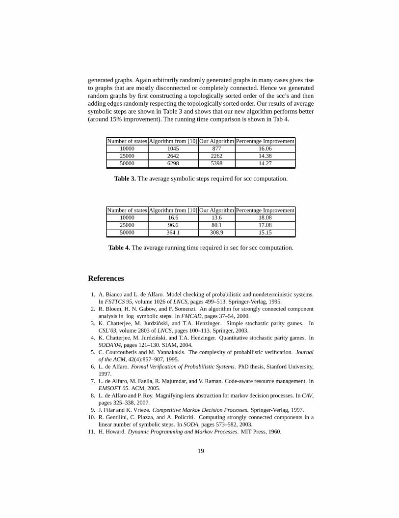
generated graphs. Again arbitrarily randomly generated graphs in many cases gives riseto graphs that are mostly disconnected or completely connected. Hence we generatedrandom graphs by first constructing a topologically sorted order of the scc’s and thenadding edges randomly respecting the topologically sortedorder. Our results of averagesymbolic steps are shown in Table 3 and shows that our new algorithm performs better(around 15% improvement). The running time comparison is shown in Tab 4.

Number of statesAlgorithm from [10] Our Algorithm Percentage Improvement10000 1045 877 16.0625000 2642 2262 14.3850000 6298 5398 14.27

Table 3.The average symbolic steps required for scc computation.

Number of statesAlgorithm from [10] Our Algorithm Percentage Improvement10000 16.6 13.6 18.0825000 96.6 80.1 17.0850000 364.1 308.9 15.15

Table 4.The average running time required in sec for scc computation.

References

1. A. Bianco and L. de Alfaro. Model checking of probabilistic and nondeterministic systems.In FSTTCS 95, volume 1026 ofLNCS, pages 499–513. Springer-Verlag, 1995.

2. R. Bloem, H. N. Gabow, and F. Somenzi. An algorithm for strongly connected componentanalysis in log symbolic steps. InFMCAD, pages 37–54, 2000.

3. K. Chatterjee, M. Jurdzinski, and T.A. Henzinger. Simple stochastic parity games. InCSL’03, volume 2803 ofLNCS, pages 100–113. Springer, 2003.

4. K. Chatterjee, M. Jurdzinski, and T.A. Henzinger. Quantitative stochastic parity games. InSODA’04, pages 121–130. SIAM, 2004.

5. C. Courcoubetis and M. Yannakakis. The complexity of probabilistic verification.Journalof the ACM, 42(4):857–907, 1995.

6. L. de Alfaro.Formal Verification of Probabilistic Systems. PhD thesis, Stanford University,1997.

7. L. de Alfaro, M. Faella, R. Majumdar, and V. Raman. Code-aware resource management. InEMSOFT 05. ACM, 2005.

8. L. de Alfaro and P. Roy. Magnifying-lens abstraction for markov decision processes. InCAV,pages 325–338, 2007.

9. J. Filar and K. Vrieze.Competitive Markov Decision Processes. Springer-Verlag, 1997.10. R. Gentilini, C. Piazza, and A. Policriti. Computing strongly connected components in a

linear number of symbolic steps. InSODA, pages 573–582, 2003.11. H. Howard.Dynamic Programming and Markov Processes. MIT Press, 1960.

19

12. N. Immerman. Number of quantifiers is better than number of tape cells.Journal of Com-puter and System Sciences, 22:384–406, 1981.

13. J.G. Kemeny, J.L. Snell, and A.W. Knapp.Denumerable Markov Chains. D. Van NostrandCompany, 1966.

14. M. Kwiatkowska, G. Norman, and D. Parker. Verifying randomized distributed algorithmswith prism. InWorkshop on Advances in Verification (WAVE’00), 2000.

15. A. Pogosyants, R. Segala, and N. Lynch. Verification of the randomized consensus algorithmof Aspnes and Herlihy: a case study.Distributed Computing, 13(3):155–186, 2000.

16. M. L. Puterman.Markov Decision Processes. J. Wiley and Sons, 1994.17. R. Segala.Modeling and Verification of Randomized Distributed Real-Time Systems. PhD

thesis, MIT, 1995. Technical Report MIT/LCS/TR-676.18. F. Somenzi. Colorado university decision diagram package.

http://vlsi.colorado.edu/pub/, 1998.19. M.I.A. Stoelinga. Fun with FireWire: Experiments with verifying the IEEE1394 root con-

tention protocol. InFormal Aspects of Computing, 2002.20. W. Thomas. Languages, automata, and logic. In G. Rozenberg and A. Salomaa, edi-

tors,Handbook of Formal Languages, volume 3, Beyond Words, chapter 7, pages 389–455.Springer, 1997.

20

Appendix

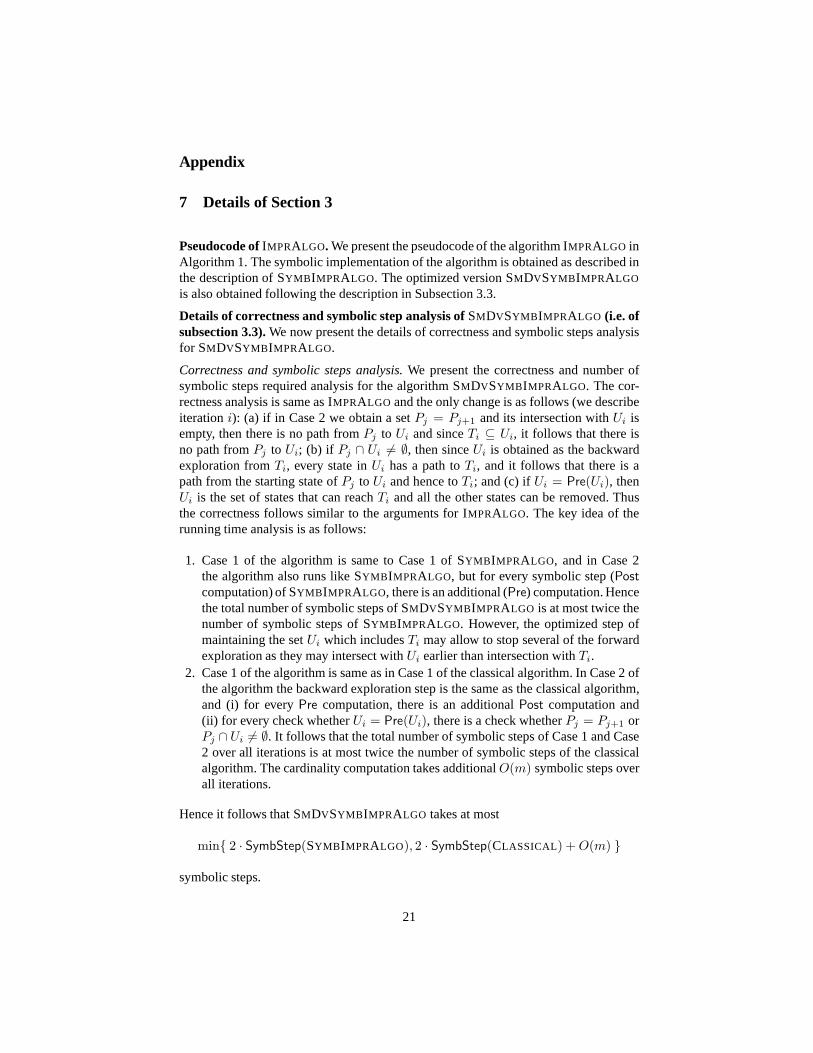
7 Details of Section 3

Pseudocode ofIMPRALGO. We present the pseudocode of the algorithm IMPRALGO inAlgorithm 1. The symbolic implementation of the algorithm is obtained as described inthe description of SYMB IMPRALGO. The optimized version SMDVSYMB IMPRALGO

is also obtained following the description in Subsection 3.3.

Details of correctness and symbolic step analysis ofSMDVSYMB IMPRALGO (i.e. ofsubsection 3.3).We now present the details of correctness and symbolic stepsanalysisfor SMDVSYMB IMPRALGO.

Correctness and symbolic steps analysis.We present the correctness and number ofsymbolic steps required analysis for the algorithm SMDVSYMB IMPRALGO. The cor-rectness analysis is same as IMPRALGO and the only change is as follows (we describeiterationi): (a) if in Case 2 we obtain a setPj = Pj+1 and its intersection withUi isempty, then there is no path fromPj to Ui and sinceTi ⊆ Ui, it follows that there isno path fromPj to Ui; (b) if Pj ∩ Ui 6= ∅, then sinceUi is obtained as the backwardexploration fromTi, every state inUi has a path toTi, and it follows that there is apath from the starting state ofPj to Ui and hence toTi; and (c) ifUi = Pre(Ui), thenUi is the set of states that can reachTi and all the other states can be removed. Thusthe correctness follows similar to the arguments for IMPRALGO. The key idea of therunning time analysis is as follows:

1. Case 1 of the algorithm is same to Case 1 of SYMB IMPRALGO, and in Case 2the algorithm also runs like SYMB IMPRALGO, but for every symbolic step (Postcomputation) of SYMB IMPRALGO, there is an additional (Pre) computation. Hencethe total number of symbolic steps of SMDVSYMB IMPRALGO is at most twice thenumber of symbolic steps of SYMB IMPRALGO. However, the optimized step ofmaintaining the setUi which includesTi may allow to stop several of the forwardexploration as they may intersect withUi earlier than intersection withTi.

2. Case 1 of the algorithm is same as in Case 1 of the classical algorithm. In Case 2 ofthe algorithm the backward exploration step is the same as the classical algorithm,and (i) for everyPre computation, there is an additionalPost computation and(ii) for every check whetherUi = Pre(Ui), there is a check whetherPj = Pj+1 orPj ∩ Ui 6= ∅. It follows that the total number of symbolic steps of Case 1 and Case2 over all iterations is at most twice the number of symbolic steps of the classicalalgorithm. The cardinality computation takes additionalO(m) symbolic steps overall iterations.

Hence it follows that SMDVSYMB IMPRALGO takes at most

min 2 · SymbStep(SYMB IMPRALGO), 2 · SymbStep(CLASSICAL) +O(m)

symbolic steps.

21

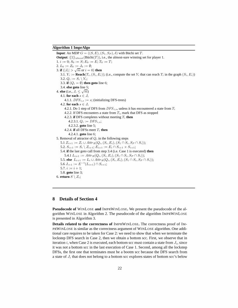
Algorithm 1 ImprAlgoInput : An MDP G = ((S,E), (S1, SP ), δ) with Buchi setT .Output : 〈〈1〉〉almost (Buchi(T )), i.e., the almost-sure winning set for player 1.1. i := 0; S0 := S; E0 := E; T0 := T ;2.L0 := Z0 := J0 := ∅;3. if (|Ji| >

√m or i = 0) then

3.1.Yi := Reach(Ti, (Si, Ei)); (i.e., compute the setYi that can reachTi in the graph(Si, Ei))3.2.Qi := Si \ Yi;3.3. if (Qi = ∅) then goto line 6;3.4.else gotoline 5;

4. else(i.e.,Ji ≤√m)

4.1. for each s ∈ Ji

4.1.1.DFS i,s := s; (initializing DFS-trees)4.2. for each s ∈ Ji

4.2.1. Do 1 step of DFS fromDFS i,s, unless it has encountered a state fromTi

4.2.2. If DFS encounters a state fromTi, mark that DFS as stopped4.2.3.if DFS completes without meetingTi then

4.2.3.1.Qi := DFS i,s;4.2.3.2.goto line 5;

4.2.4.if all DFSs meetTi then4.2.4.1.goto line 6;

5. Removal of attractor ofQi in the following steps5.1Zi+1 := Zi ∪AttrR(Qi, (Si, Ei), (S1 ∩ Si, SP ∩ Si));5.2.Si+1 := Si \ Zi+1; Ei+1 := Ei ∩ Si+1 × Si+1;5.4. if the last goto call from step 3.4 (i.e. Case 1 is executed)then

5.4.1Li+1 := AttrR(Qi, (Si, Ei), (S1 ∩ Si, SP ∩ Si));5.5.else Li+1 := Li ∪ AttrR(Qi, (Si, Ei), (S1 ∩ Si, SP ∩ Si));5.6Ji+1 := E−1(Li+1) ∩ Si+1;5.7.i := i+ 1;5.8.goto line 3;

6. return S \ Zi;

8 Details of Section 4

Pseudocode ofWINLOSE and IMPRWINLOSE. We present the pseudocode of the al-gorithm WINLOSE in Algorithm 2. The pseudocode of the algorithm IMPRWINLOSE

is presented in Algorithm 3.

Details related to the correctness ofIMPRWINLOSE. The correctness proof of IM-PRWINLOSE is similar as the correctness argument of WINLOSEalgorithm. One addi-tional care requires to be taken for Case 2: we need to show that when we terminate thelockstep DFS search in Case 2, then we obtain a bottom scc. First, we observe that initerationi, when Case 2 is executed, each bottom scc must contain a statefromJi, sinceit was not a bottom scc in the last execution of Case 1. Second,among all the lockstepDFSs, the first one that terminates must be a bootm scc becausethe DFS search froma state ofJi that does not belong to a bottom scc explores states of bottomscc’s below

22

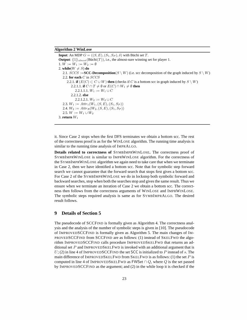
Algorithm 2 WinLoseInput : An MDP G = ((S,E), (S1, SP ), δ) with Buchi setT .Output : 〈〈1〉〉almost (Buchi(T )), i.e., the almost-sure winning set for player 1.1.W := W1 := W2 := ∅2. while(W 6= S) do

2.1.SCCS :=SCC-Decomposition(S \W ) (i.e. scc decomposition of the graph induced byS \W )2.2. for eachC in SCCS

2.2.1.if (E(C) ⊂ C ∪W ) then (checks ifC is a bottom scc in graph induced byS \W )2.2.1.1.if C ∩ T 6= ∅ or E(C) ∩W1 6= ∅ then

2.2.1.1.1.W1 := W1 ∪ C

2.2.1.2.else2.2.1.2.1.W2 := W2 ∪ C

2.3.W1 := Attr1(W1, (S,E), (S1, SP ))2.4.W2 := AttrR(W2, (S,E), (S1, SP ))2.5.W := W1 ∪W2

3. return W1

it. Since Case 2 stops when the first DFS terminates we obtain abottom scc. The restof the correctness proof is as for the WINLOSEalgorithm. The running time analysis issimilar to the running time analysis of IMPRALGO.

Details related to correctness ofSYMB IMPRWINLOSE. The correctness proof ofSYMB IMPRWINLOSE is similar to IMPRWINLOSE algorithm. For the correctness ofthe SYMB IMPRWINLOSEalgorithm we again need to take care that when we terminatein Case 2, then we have identified a bottom scc. Note that for symbolic step forwardsearch we cannot guarantee that the forward search that stops first gives a bottom scc.For Case 2 of the SYMB IMPRWINLOSE we do in lockstep both symbolic forward andbackward searches, stop when both the searches stop and gives the same result. Thus weensure when we terminate an iteration of Case 2 we obtain a bottom scc. The correct-ness then follows from the correctness arguments of WINLOSE and IMPRWINLOSE.The symbolic steps required analysis is same as for SYMB IMPRALGO. The desiredresult follows.

9 Details of Section 5

The pseudocode of SCCFIND is formally given as Algorithm 4. The correctness anal-ysis and the analysis of the number of symbolic steps is givenin [10]. The pseudocodeof IMPROVEDSCCFIND is formally given as Algorithm 5. The main changes of IM-PROVEDSCCFIND from SCCFIND are as follows: (1) instead of SKELFWD the algo-rithm IMPROVEDSCCFIND calls procedure IMPROVEDSKELFWD that returns an ad-ditional setP and IMPROVEDSKELFWD is invoked with an additional argument that isU ; (2) in line 4 of IMPROVEDSCCFIND the setSCC is initialized toP instead ofs. Themain difference of IMPROVEDSKELFWD from SKELFWD is as follows: (1) the setP iscomputed in line 4 of IMPROVEDSKELFWD asFWSet ∩ Q, whereQ is the set passedby IMPROVEDSCCFIND as the argument; and (2) in the while loop it is checked if the

23

element popped intersects withP and if yes, then the procedure breaks the while loop.The correctness argument from the correctness of SCCFIND is already shown in themain paper.

Symbolic steps analysis.We now present the detailed symbolic steps analysis of thealgorithm. As noted in Section 3.2, common symbolic operations on a set of states arePre, Post andCPre. We note that these operations involve symbolic sets of2 · log(n)variables, as compared to symbolic sets oflog(n) variables required for operations suchas union, intersection and set difference. Thus onlyPre, Post andCPre are counted assymbolic steps, as done in [10]. The total number of other symbolic operations is alsoO(|S|). We note that only lines 5 and 10 of IMPROVEDSCCFIND and lines 3.3 and 7.3of IMPROVEDSKELFWD involvePre andPost operations.

In the following, we charge the costs of these lines to statesin order to achieve the3 · |S| + N(G) bound for symbolic steps. We define subspine-set asNewSet returnedby IMPROVEDSKELFWD and show the following result.

Lemma 4. For any spine-setU and its end vertexu, T is a subspine-set iffU \ T ⊆SCC(u).

Proof. Note that while constructing a subspine-setT , we stop the construction whenwe find any statev in a subspine-set. Now clearly sincev ∈ U , there is a path fromv to u. Also, since we found this state inFW (u), there is a path fromu to v. Hence,v ∈ SCC(u). Also, each state that we are omitting by stopping construction of T hasthe property that there is a path fromu to that state and a path from that state tov. Thisimplies that all the states we are omitting in construction of T are inSCC(u).

Note that since we passNewSet \ SCC in the subsequent call to IMPROVEDSC-CFIND, it will actually be a spine set. In the following lemma we show that any statecan be part of subspine-set at most once, as compared to twicein the SCCFIND pro-cedure in [10]. This lemma is one of the key points that lead tothe improved symbolicsteps required analysis.

Lemma 5. Any statev can be part of subspine-set at most once.

Proof. In [10], the authors show that any state can be included in spine sets at mosttwice in SKELFWD. The second time it is included is in line 6 of SKELFWD when theSCC of that state is to be found. In contrast, IMPROVEDSKELFWD checks intersectionof the subspine-set being constructed with the setP that contains the states of thisSCCwhich are already in a subspine-set. When this happens, it stops the construction ofspine set. Now ifv is already included in the spine set, then it will be part ofP andwould not be included in subspine-set again. Hence,v can be part of subspine-set atmost once.

Lemma 6. States added inSCC by iteration of line 5 ofIMPROVEDSCCFIND are ex-actly the states which are not part of any subspine-set.

Proof. We see that in line 5 of IMPROVEDSCCFIND, we start fromSCC = P and thenwe find theSCC by backward search. Also,P has all the states fromSCC which arepart of subspine-set. Hence, the extra states that are addedin SCC are states which arenever included in a subspine-set.

24

Charging symbolic steps to states.We now consider three cases to charge symbolicsteps to states and scc’s.

1. Charging states included in subspine-set.First, we see that the number of timesthe loop of line 3 in IMPROVEDSKELFWD is executed is equal to the size of thespine set that SKELFWD would have computed. Using Lemma 4, we can chargeone symbolic step to each state of the subspine-set and each state of theSCC thatis being computed. Now, the number of times line 7.3 of IMPROVEDSKELFWD isexecuted equals the size of subspine-set that is computed. Hence, we charge onesymbolic step to each state of subspine-set for this line.

Now we summarize the symbolic steps charged to each state which is part of somesubspine-set. First time when a state gets into a subspine-set, it is charged two steps,one for line 3.3 and one for line 7.3 of IMPROVEDSKELFWD. If its SCC is not foundin the same call to IMPROVEDSCCFIND, then it comes into action once again whenits SCC is being found. By Lemma 5, it is never again included in a subspine set.Hence in this call to IMPROVEDSKELFWD, it is only charged one symbolic step forline 3.3 and none for line 7.3 as line 7.3 is charged to states that become part of thenewly constructed subspine-set. Also because of Lemma 6, since this state is in asubspine-set, it is not charged anything for line 5 of IMPROVEDSCCFIND. Hence,a state that occurs in any subspine-set is charged at most three symbolic steps.

2. Charging states not included in subspine-set.For line 5 of IMPROVEDSCCFIND,the number of times it is executed is the number of states thatare added toSCCafter initialization toSCC = P . Using Lemma 6, we charge one symbolic stepto each state of thisSCC that is never a part of any subspine-set. Also, we mighthave charged one symbolic step to such a state for line 3.3 of IMPROVEDSKELFWD

when we called it. Hence, each such state is charged at most two symbolic steps.3. ChargingSCCs. For line 10 of IMPROVEDSCCFIND, we see that it is executed

only once in a call to IMPROVEDSCCFIND that computes aSCC. Hence, the totalnumber of times line 10 is executed equalsN(G), the number ofSCCs of the graph.Hence, we charge eachSCC one symbolic step for this line.

The above argument shows that the number of symbolic steps that the algorithm IM-PROVEDSCCFIND requires is at most3 · |S|+N(G).

25

Algorithm 3 ImprWinLoseInput : An MDP G = ((S,E), (S1, SP ), δ) with Buchi setT .Output : 〈〈1〉〉almost (Buchi(T )), i.e., the almost-sure winning set for player 1.1. i := 0; S0 := S; E0 := E; T0 := T ;2.W1 := W2 := L0 := Z0 := J0 := ∅;3. if (|Ji| >

√m or i = 0) then

3.1.SCCS :=SCC-Decomposition(Si) (scc decomposition of graph induced bySi)3.2. for eachC in SCCS

3.2.1.if (Ei(C) ⊂ C) then (checks ifC is a bottom scc in graph induced bySi)3.2.1.1.if C ∩ T 6= ∅ or E(C) ∩W1 6= ∅ then

3.2.1.1.1.W1 := W1 ∪ C

3.2.1.2.else3.2.1.2.1.W2 := W2 ∪ C

3.3.goto line 54. else(i.e.,Ji ≤

√m)

4.1. for each s ∈ Ji

4.1.1.DFS i,s := s (initializing DFS-trees)4.2. for each s ∈ Ji

4.2.1. Do 1 step of DFS fromDFS i,s

4.2.2.if DFS completesthen4.2.2.1.C := DFS i,s

4.2.2.2.if C ∩ T 6= ∅ or E(C) ∩W1 6= ∅ then4.2.2.2.1.W1 := W1 ∪ C

4.2.2.3.else4.2.2.3.1.W2 := W2 ∪ C

4.2.2.4.goto line 55. Removal ofW1 andW2 states in the following steps

5.1.W1 := Attr1(W1, (Si, Ei), (S1 ∩ Si, SP ∩ Si))5.2.W2 := AttrR(W2, (Si, Ei), (S1 ∩ Si, SP ∩ Si))5.3.Zi+1 := Zi ∪W1 ∪W2

5.4.Si+1 := Si \ Zi+1; Ei+1 := Ei ∩ Si+1 × Si+1

5.5. if the lastgotocall was from line3.3 then5.5.1.Li+1 := Zi+1 \ Zi

5.6.else5.6.1.Li+1 := Li ∪ (Zi+1 \ Zi)

5.7.Ji+1 := E−1(Li+1) ∩ Si+1

5.8. if Zi+1 = S then5.8.1. goto line6

5.9.i := i+ 1; goto line 36. return W1

26

Algorithm 4 SCCFIND

Input: (S,E, 〈U, s〉), i.e., a graph(S,E) with spine set(U, s).Output: SCCPartition i.e. the set of SCCs of the graph(S,E)1. if (S = ∅) then

1.1 return ;2. if (U = ∅) then

2.1s := pick(S)3. 〈FWSet,NewSet,NewState〉 := SKELFWD(S,E, s)4. SCC = s

5. while (((Pre(SCC) ∩ FWSet) \ SCC) 6= ∅) do5.1SCC := SCC ∪ (Pre(SCC) ∩ FWSet)

6. SCCPartition := SCCPartition ∪ SCC(Recursive call onS \ FWSet)

7.S′ := S \ FWSet

8.E′ := E ∩ (S′ × S′)9.U ′ := U \ SCC10.s′ := Pre(SCC ∩ U) ∩ (S \ SCC)11.SCCPartition := SCCPartition∪ SCCFIND(S′, E′, 〈U ′, s′〉)

(Recursive call onFWSet \ SCC)12.S′ := FWSet \ SCC13.E′ := E ∩ (S′ × S′)14.U ′ := NewSet \ SCC15.s′ := NewState \ SCC16.SCCPartition := SCCPartition∪ SCCFIND(S′, E′, 〈U ′, s′〉)17. ReturnSCCPartition

ProcedureSKELFWD

Input: (S,E, s), i.e., a graph(S,E) with a states ∈ S.Output: 〈FWSet,NewSet,NewState〉,

i.e. forward setFWSet, new spine-setNewSet andNewState ∈ NewSet

1. Letstack be an empty stack of sets of nodes2.L := s

3. while (L 6= ∅) do3.1Push(stack, L)3.2FWSet := FWSet ∪ L

3.3L := Post(L) \ FWSet

4.L := Pop(stack)5.NewSet := NewState := pick(L)6. while (stack 6= ∅) do

6.1L := Pop(stack)6.2NewSet := NewSet ∪ pick(Pre(NewSet) ∩ L)

7. return 〈FWSet,NewSet,NewState〉

27

Algorithm 5 IMPROVEDSCCFIND

Input: (S,E, 〈U, s〉), i.e., a graph(S,E) with spine set(U, s).Output: SCCPartition, the set of SCCs of the graph(S,E)1. if (S = ∅) then

1.1 return ;2. if (U = ∅) then

2.1s := pick(S)3. 〈FWSet,NewSet,NewState, P 〉 := IMPROVEDSKELFWD(S,E,U, s)4. SCC = P

5. while (((Pre(SCC) ∩ FWSet) \ SCC) 6= ∅) do5.1SCC := SCC ∪ (Pre(SCC) ∩ FWSet)

6. SCCPartition := SCCPartition ∪ SCC(Recursive call onS \ FWSet)

7.S′ := S \ FWSet

8.E′ := E ∩ (S′ × S′)9.U ′ := U \ SCC10.s′ := Pre(SCC ∩ U) ∩ (S \ SCC)11.SCCPartition := SCCPartition∪ IMPROVEDSCCFIND(S′, E′, 〈U ′, s′〉)

(Recursive call onFWSet \ SCC)12.S′ := FWSet \ SCC13.E′ := E ∩ (S′ × S′)14.U ′ := NewSet \ SCC15.s′ := NewState \ SCC16.SCCPartition := SCCPartition∪ IMPROVEDSCCFIND(S′, E′, 〈U ′, s′〉)

Procedure IMPROVEDSKELFWD

Input: (S,E,Q, s), i.e., a graph(S,E) with a setQ and a states ∈ S.Output: 〈FWSet,NewSet,NewState, P 〉1. Letstack be an empty stack of sets of nodes2.L := s

3. while (L 6= ∅) do3.1Push(stack, L)3.2FWSet := FWSet ∪ L

3.3L := Post(L) \ FWSet

4.P := FWSet ∩Q

5.L := Pop(stack)6.NewSet := NewState := pick(L)7. while (stack 6= ∅) do

7.1L := Pop(stack)7.2 if (L ∩ P 6= ∅) then

7.2.1break while loop7.3elseNewSet := NewSet ∪ pick(Pre(NewSet) ∩ L)

8. return 〈FWSet,NewSet,NewState, P 〉

28