arX

iv:c

ond-

mat

/980

4131

v2 [

cond

-mat

.sta

t-m

ech]

15

Apr

199

8

Switching Boundary Conditions in the Many-Body Diffusion Algorithm

F. Luczak, F. Brosens ∗and J.T. Devreese †

Departement Natuurkunde, Universiteit Antwerpen (UIA),Universiteitsplein 1, B-2610 Antwerpen

L. F. LemmensDepartement Natuurkunde, Universiteit Antwerpen (RUCA),

Groenenborgerlaan 171, B-2020 Antwerpen(January 27, 1998)

In this paper we show how the transposition, the basic operation of the permutation group, canbe taken into account in a diffusion process of identical particles. Whereas in an earlier approachthe method was applied to systems in which the potential is invariant under interchanging theCartesian components of the particle coordinates, this condition on the potential is avoided here.In general, the potential introduces a switching of the boundary conditions of the walkers. [Thesetransitions modelled by a continuous–time Markov chain generate sample paths for the propagatoras a Feynman–Kac functional . A few examples , including harmonic fermions with an anharmonicinteraction, and the ground-state energy of ortho-helium are studied to elucidate the theoreticaldiscussion and to illustrate the feasibility of a sign-problem-free implementation scheme for therecently developed many-body diffusion approach.]

I. INTRODUCTION

In a previous paper [1], the present authors have shown that the many-body diffusion algorithm (MBDA) allowsfor a sign-problem-free simulation of excited antisymmetric states of interacting harmonic oscillators. The basicidea behind this approach has been to split the Euclidean-time propagator into a sum of independent propagatorswhich remain positive on the appropriate state space [2–5]. Each of the elementary propagators could be individuallysampled as a diffusion process for distinguishable particles on a state space with absorbing or reflecting boundaries.

In the present paper, the many-body diffusion formalism and its implementation are generalized to allow for theconstruction of interdependent diffusion processes. In this approach the propagator that governs the Euclidean timeevolution is split into two parts: the kinetic part is used to describe the evolution of the system with well-definedboundary conditions, the potential is used for branching and killing and rules transitions from one set of boundaryconditions to another set. The evolution is given by a Brownian motion or a random walk, but the boundary conditionscan change during the simulation according to a continuous-time Markov process. The transition rates of this processpartly or completely derive from the potential which determines also the killing or branching process.

This principle is illustrated with some test models. A limited number of degrees of freedom is considered to avoidlarge computation times and to allow for a visual control on the probability densities that are generated. The presentedalgorithm does not integrate smoothly with the previous one for harmonic fermions, in the sense that for this algorithmthe interchange of two identical particles is fully under control but in combination with the even permutations it isfar from trivial if more than two particles of parallel spin are present.

In the next section, the theoretical background of the method is discussed. In Sec. III, details on the diffusionin a reduced state space are provided. In Sec. IV, a sign-problem-free implementation is developed and applied totwo toy models to illustrate the concepts. Subsequently, anisotropic harmonic fermions are studied avoiding normalcoordinates in order to elucidate the role of the potential for the transitions between different sets of boundaryconditions. Finally, the MBDA is employed to calculate the ground-state energy of ortho-helium. Some concludingremarks are presented in Sec. V.

∗Senior Research Associate of the FWO-Vlaanderen.†Also at the Universiteit Antwerpen (RUCA) and Technische Universiteit Eindhoven, The Netherlands.

1

II. A SIGN-PROBLEM-FREE APPROACH

In this section, we describe the construction of a Feynman-Kac functional equipped with a process to generate thesample paths over which the exponential containing the interaction has to be averaged. This construction is basedon the many body diffusion approach introduced in [4] and illustrated in [1]. The procedure is sign-problem-free inthe strict sense, i.e. expectation values in the Feynman-Kac functional are obtained using transition probabilities ina Wiener-Poisson space. A mathematical account on the foundations of these compound processes can be found in[10]. The Wiener space is the support for the diffusion whereas a multivariate Poisson process counts the switches ofthe boundary condition as will be explained below.

A. Diffusion on a Domain

Let r be a 3N -dimensional point in the configuration space R3N of N distinguishable particles and assume that the

propagator for this system is given by:

KD[rf , τ ; ri, 0] =∑

k

(ψk(ri), exp(−τH)ψk(rf )) , (1)

where H describes the evolution in Euclidean time of the N particles. The subscript D denotes that at this stagethe particles are still considered to be distinguishable. This propagator can be easily written as a Feynman-Kacfunctional over all paths starting in ri and ending in rf a Euclidean time lapse τ later. The paths are constructed

by a 3N -dimensional Brownian motionR (τ) ; τ ≥ 0

with variance σ2 = ~τ/m

KD[rf , τ ; ri, 0] = Eri

I(R(τ)=rf) exp

−1

~

τ∫

0

V(R(ς)

)dς

. (2)

All integration paths in (2) start in ri as indicated by the averaging index Eriand satisfy the condition R (τ) = rf

as denoted by the indicator I(R(τ)=rf). Writing the propagator as an average over a Brownian motion is equivalent

to giving the evolution equation and the initial condition:

∂

∂τKD[rf ,τ ; ri, 0] =

(~

2m∇2

r − 1

~V (rf )

)KD[rf ,τ ; ri, 0] , (3)

limτ↓0

KD[rf , τ ; ri, 0] = δ (rf − ri ) . (4)

If a propagator containing two indistinguishable particles j and k has to be derived from (1), a projection on thesymmetric (anti-symmetric) irreducible representation of the permutation group has to be made for bosons (fermions):

KI [rf , τ ; ri, 0] =1

2!

∑

P

ξPKD[Prf , τ ; ri, 0] , (5)

where P represents the permutations of the particles j,k and ξ = ±1 is chosen according to the particle statisticsunder consideration. The evolution equation for the projected propagator is given by the same eq. (3), because ∇2

r

as well as the potential V (r) are invariant under all the permutations P . The initial condition obtained from theprojection (5) by taking the limit τ ↓ 0 is not the initial condition that is usually studied if one wants to solve apartial differential equation using probabilistic methods. [11] In order to obtain an initial condition which is given by

limτ↓0

KI [rf , τ ; ri, 0] = δ (rf − ri) with rf ,ri ∈ D32 ⊗ R

3(N−2) , (6)

one has to restrict the configuration space R3N to a domain D3

2 ⊗ R3(N−2). In this domain the identical-particle

coordinates ~rj , ~rk are linearly ordered. In D2, for example, the x–coordinates are ordered as follows: xj ≥ xk.Introducing a domain implies that one has to specify the boundary conditions; the specification appropriate forbosons or fermions moving freely or interacting harmonically has been proposed in [4] and analyzed in [1].

2

1. Boundary conditions

The ordering particles in a three–dimensional space can be performed by ordering the particles with respect to eachof the three independent Cartesian directions. This option has been chosen in the previous investigations and led [1–4]to the construction of an ordered state-space D. The symmetric irreducible representation implies four combinationsl = 0, 1, 2, 3. By definition, the (l = 0)–boundary condition causes reflection at the boundary ∂D in every directionx, y, z, whereas for l = 1, 2, 3 the boundary ∂D reflects in x, y, z-direction and absorbs in the two other two Cartesiandirections. For fermions, l = 0 means absorption at ∂D in all three directions, whereas for l = 1 absorption occursin the x-direction and reflection in the y- and z-direction. Similarly, l = 2 and l = 3 correspond to the appropriateabsorption and reflection conditions with respect to the y- and z-direction. It is clear that in order to study theevolution of the system in Euclidean time one has to give not only the starting point in the domain D3

2 but also theboundary conditions l. The propagator has to contain the information that a state, initially characterized by ri and

l, will end after a Euclidean time lapse τ in rf with boundary conditions l. The evolution in Euclidean time of thispropagator can be studied from its extension to R

3N , which gives

KI [rf , l,τ ; ri, l, 0] =

(1

2!

)3∑

Px

ξPx

l

∑

Py

ξPy

l

∑

Pz

ξPz

l KD[PxPyPz rf , τ ; ri, l, 0] , (7)

where Px, Py, Pz symbolize the permutations of the x, y, z-coordinates of the two indistinguishable particles j and kand where we imposed the initial condition

limτ↓0

KI [rf , l,τ ; ri, l, 0] = δl,lδ(rf − ri) , rf ,ri ∈ D3

2 ⊗ R3(N−2) . (8)

The boundary condition l determines the parity ξPx

l , ξPy

l , ξPz

l of the permutations Px, Py, Pz .

2. Evolution equations

A potential V (r) whose decomposition contains only one-dimensional irreducible representations with respect topermutations Qx, Qy, Qz of the coordinates is straightforward to analyze. Expanding the potential energy in thepossible symmetry combinations, described above, one may write:

V (r) =

3∑

l′=0

(1

2!

)3∑

Qx

ξQx

l′

∑

Qy

ξQy

l′

∑

Qz

ξQz

l′ V (QxQyQz r ) . (9)

Consider now the following decomposition

χ =

(1

2!

)3∑

Px

∑

Py

∑

Pz

ξPx

l ξPy

l ξPz

l V (PxPyPz rf ) KD[PxPyPz rf , τ ; ri, l, 0]

=

(1

2!

)6∑

l′

∑

PxQx

∑

PyQy

∑

PzQz

ξPx

l ξQx

l′ ξPy

l ξQy

l′ ξPz

l ξQz

l′ V (QxPxQyPyQzPz rf ) KD[PxPyPz rf , τ ; ri, l, 0] .

Introducing the permutations Si = QiPi with i = x, y, z, the quantity χ can be written as:

χ =

(1

2!

)6 ∑

PxSx

∑

PySy

∑

PzSz

∑

l′

ξPx

l ξSxP−1

x

l′ ξPy

l ξSyP−1

y

l′ ξPzl ξ

SzP−1

z

l′ V (SxSySz rf ) KD[PxPyPz rf , τ ; ri, l , 0] .

The permutation Pi and its inverse P−1i have the same parity and therefore ξ

SiP−1

i

l′ = ξSi

l′ ξPi

l′ . We furthermore define

ξPi

l≡ ξPi

l ξPi

l′ . This leads immediately to:

χ =∑

l

Vll(rf )KI [rf , l,τ ; ri, l , 0] , (10)

where we introduced the notation:

3

Vll(rf ) =

(1

2!

)3∑

Sx

∑

Sy

∑

Sz

ξSx

l ξSy

l ξSz

l V (SxSySz rf ) ξSx

lξ

Sy

lξSz

l. (11)

Using eq. (3) for the propagator (7) and the result obtained in (10), the evolution equation becomes:

∂

∂τKI [rf , l,τ ; ri, l , 0] =

~

2m∇2

r KI [rf , l,τ ; ri, l, 0] − 1

~

∑

l

Vll(rf ) KI [rf , l,τ ; ri, l, 0] , (12)

where use has been made of the invariance of ∇2r with respect to permutations of the coordinates x, y, z of the particle

positions.The study of the non-diagonal interaction contribution (12) is the main purpose of the present section. In some

cases, these non-diagonal terms are zero. For instance, if V (r) can be written as Vs (r) = V (x) + V (y) + V (z) , theinvariance under the permutations of the particles implies invariance under permutations of the coordinates, which inturn then implies that Vll′ (r) = δll′V (r). For harmonic interactions along the principal axes the many-body potentialcan be written as such a sum. The evolution equation is then diagonal in the quantum numbers l, meaning thatduring the evolution the boundary conditions do not change. The computational feasibility and efficiency of this typeof evolution equation has been demonstrated in [1].

3. Decomposition of the Potential

The potential V (~rj ;~rk) ≡ V (~r1, . . . , ~rj , . . . , ~rk, . . . , ~rN ) is invariant under the permutation of any two particles, andin particular for interchanging ~rj with ~rk

V (~rj ; ~rk) = V (~rk; ~rj) . (13)

For motion in 2D, one can decompose the potential as:

V (xj , yj ;xk, yk) = Vbb(xj , yj ;xk, yk) + Vff(xj , yj ;xk, yk) , (14)

with

Vbb(xj , yj;xk, yk) =1

4[V (xj , yj;xk, yk) + V (xk, yj ;xj , yk) + V (xk, yk;xj , yj) + V (xj , yk;xk, yj)]

and

Vff(xj , yj ;xk, yk) =1

4[V (xj , yj ;xk, yk) − V (xk, yj;xj , yk) + V (xk, yk;xj , yj) − V (xj , yk;xk, yj)] .

Introducing the operator σx, σy for interchanging the x, y -coordinates, and the operator ex, ey for leaving the x, y-coordinates unchanged, the decomposition of the potential can be written as:

Vbb(xj , yj ;xk, yk) =1

4(ex + σx) (ey + σy)V (xj , yj ;xk, yk) .

For motion in 3D the same principle can be used leading to the decomposition:

V (xj , yj, zj ;xk, yk, zk) = Vbbb(xj , yj , zj;xk, yk, zk) + Vbff(xj , yj , zj;xk, yk, zk) (15)

+Vfbf(xj , yj , zj ;xk, yk, zk) + Vffb(xj , yj, zj ;xk, yk, zk) ,

where typically Vfbf(xj , yj , zj;xk,yk, zk) is given by:

Vfbf(xj , yj, zj ;xk, yk, zk) =1

8(ex − σx) (ey + σy) (ez − σz)V (xj , yj, zj ;xk, yk, zk) (16)

and analogous definitions hold for the other matrix elements. It is interesting to note the similarity between thisprojection and quaternions:

1xyz =1

8

[(ex + σx) (ey + σy) (ez + σz) + (ex + σx) (ey − σy) (ez − σz)

+ (ex − σx) (ey + σy) (ez − σz) + (ex − σx) (ey − σy) (ez + σz)

]. (17)

Using this projection the formal decomposition (11) is achieved explicitly.

4

B. The Feynman-Kac functional

Given that the propagator indeed satisfies the evolution equation (12), it remains to be shown that a process canbe found to generate the sample paths and a Feynman-Kac functional.

1. Positivity and the process

To start the construction of the generator of the process consider the following identity:

∑

l

Vll ( r) =

(1

2!

)3∑

l

∑

Sx

∑

Sy

∑

Sz

ξSx

l ξSy

l ξSz

l V (SxSySz r) ξSx

lξ

Sy

lξSz

l(18)

= V (r) .

This is a direct consequence of eq. (9). Assume further, that the domain D32 is chosen in such a way that Vll (r) ≤ 0

for l 6= l . This allows to rewrite eq. (12) as follows:

∂

∂τKI [rf , l,τ ; ri, l, 0] =

~

2m∇2

r KI [rf , l,τ ; ri, l , 0] − 1

~V (rf )KI [rf , l,τ ; ri, l, 0] (19)

−Wl (rf )KI [rf , l,τ ; ri, l , 0] +∑

l

Wll (rf )KI [rf , l,τ ; ri, l , 0] ,

where Wll (rf ) denotes the non-diagonal part − 1~Vll (rf ) if l 6= l:

Wll (rf ) = −1

~Vll (rf ) (1 − δl,l) , (20)

and the quantity Wl (rf ) stands for:

Wl (rf ) =∑

l

Wll (rf ) (21)

In this situation, the Wll (rf ) can be interpreted as the rate that a walker in the position rf will change its boundary

condition from l to l . This means that the following terms of eq. (19) generate a diffusion together with a Markovprocess on the four possible boundary conditions:

∂

∂τK0

I [rf , l,τ ; ri, l, 0] =~

2m∇2

r K0I [rf , l,τ ; ri, l , 0] +

∑

l

Wll (rf )K0I [rf , l,τ ; ri, l , 0] (22)

−Wl (rf )K0I [rf , l,τ ; ri, l , 0],

where K0I [rf , l,τ ; ri, l , 0] satisfies a backward Kolmogorov equation, and there for it is the transition probability of a

compound stochastic process [10] that generates the sample paths in our state space.

2. Positivity and the functional

Above, we assumed that the domain D32 can be chosen such that Vll (r) ≤ 0 for l 6= l. This assumption is

necessary, because otherwise the introduced W–matrix would not represent a continuous-time Markov process. Fromits construction it is clear that it depends on the potential. Therefore a general analysis for any potential is beyond thescope of the present communication. Assuming that the system under consideration has a potential with this property(or can be transformed by a unitary transformation to a system with such a potential), the evolution (22) describesa diffusion triggering a continuous–time Markov chain that swithces boundary conditions in a Wiener–Poisson space.The switches do not induce discontinuities in the sample paths but allow for a change in boundary condition accordingto the rates defined by the W–matrix. The sign condition on the projections of the potential is necessary for theinterpretation of the non diagonal elements as rates. The evolution equation based on this assumption describes astochastic process in the strict mathematical sense. It can therefore be simulated sign-problem-free. The propagator

KI [rf ,l,τ ; ri, l, 0] with the initial condition (8) can be written as a Feynman-Kac functional

5

KI [rf , l,τ ; ri, l, 0] = Eri,l

I(R(τ)=rf ,Lτ=l) exp

−1

~

∑

l

τ∫

0

VLς l

(R(ς)

)dς

, (23)

where use has been made of the identity (18) to make explicit that the potential is diagonal in the label l.The sample paths are generated by a 3N -dimensional Brownian motion

R (τ) ; τ ≥ 0

with σ2 = ~τ/m and ab-

sorbing and reflecting boundary conditions as defined by the index l. After the transition, the boundary conditionsare adapted to agree with those from the Markov chain Lτ ; τ ≥ 0 where the (normalized) quantities Vll then deter-

mine the boundary-condition transition rates l → l . Repeated application of this procedure for all the subprocessesstarting with boundary conditions l generates the sample paths of the diffusion process of N − 2 distinguishable andtwo indistinguishable particles in three dimensions. The stochastic integration over the Feynman-Kac functional isthen done by killing and branching.

III. DIFFUSION ON A REDUCED STATE SPACE D

The positivity of the rates Wll(rf ) is a necessary ingredient to guarantee the interpretation of the Euclidean timeSchrodinger equation as a compound diffusion equation with killing and branching in a Wiener-Poisson space. Forsome potentials, the condition of negative definite Vll(rf ) may not be satisfied on the state spaceD3

2⊗R3(N−2). In these

cases, the definition of an alternative (reduced) state space is required in order to find purely positive transition ratesWll(rf ). The symmetry of the potential effects the structure of the adapted state space, which therewith is specific

for certain classes of applications. To illustrate the construction principle, the reduced state space D32 ⊗R

3(N−2) willbe considered, where

D32 ≡

(xj , xk, yj , yk, zj , zk)T

∣∣∣xj ≥ |xk|, yj ≥ |yk|, zj ≥ |zk|. (24)

This choice will be of relevance for the probabilistic sampling of the real ground-state wave function of ortho-helium.The procedures for the construction of an ordered state space xj ≥ xk, yj ≥ yk, zj ≥ zk, reported in [2–4], alone do

not induce the ordering on D32, and an additional set of boundary conditions must be supplied to impose the desired

ordering. In that framework, the separation of the multi-dimensional diffusion process into one-dimensional diffusionprocesses will again prove useful.

A. Free Diffusion of Indistinguishable Particles on D1

2

The free diffusion process of two indistinguishable particles on a line has been introduced in [2–4] as the diffusionprocess of two distinguishable particles on the ordered state space D1

2 with absorption (for fermions) or reflection (for

bosons) at the boundary ∂D12. The construction of the free diffusion process on the reduced state space D1

2 requires theextension of the stochastic process. (Anti)symmetrization again plays the major role in that approach: the diffusion

process of free indistinguishable particles on the state space D12 can be mapped onto D1

2 by the construction ofreflecting and absorbing boundaries. The starting point for the derivation of the required processes is the separation

of the state space into two non-intersecting subspaces D12 and PxD

12 of equal volume: D1

2 = D12 ∪ PxD

12 . The

mapping between both subspaces is realized by the permutation operator Px which models reflection at x1 = −x2,

i.e.: Px(x1, x2)T = (−x2,−x1)

T . Then, the transition probability density ρf,b(x, τ ;x′) that the system of two free

fermions/bosons evolves from x ′ to x during the Euclidean time interval τ , can be written as

ρf,b(x, τ ;x′) =

1

2

(ρff,b(x, τ ;x

′) + ρbf,b(x, τ ;x ′)

), (25)

where we defined

ρff,b(x, τ ;x

′) = ρf,b(x, τ ;x′) − ρf,b(Pxx, τ ;x

′) , ρbf,b(x, τ ;x

′) = ρf,b(x, τ ;x ′) + ρf,b(Pxx, τ ;x′) .

Each of the transition probability densities ρf,b(x, τ ;x′) consists of two density matrices, one—ρb

f,b(x, τ ;x′)—for

which the boundary x1 = −x2 acts reflecting, and one—ρff,b(x, τ ;x

′)—which induces absorption at x1 = −x2. With

an appropriate initial choice x ′ ∈ D12, free fermion/boson diffusion to any point x ∈ D1

2—and thus also to any

6

x ∈ R2—can be projected to the reduced state space D1

2 by means of reflecting and absorbing state-space boundaries.Each of the elementary density matrices ρb

f,b(x, τ ;x′) and ρf

f,b(x, τ ;x′) constitutes a diffusion process with the initial

condition

limτ↓0

ρbf,b(x, τ ;x

′) = limτ↓0

ρff,b(x, τ ;x

′) = δ(x− x ′) . (26)

To proof this statement, ρbf (x, τ ;x ′) and ρf

f(x, τ ;x′) must be shown to satisfy probability conservation and the semi-

group property. Both properties are derived taking into account the Markov properties for the free fermion/bosondiffusion density ρf,b(x, τ ;x

′) defined on the state space D12 with absorbing/reflecting boundaries. Probability con-

servation for the two-boson density ρbb(x, τ ;x ′) follows from

∫

D1

2

dx ρbb(x, τ ;x ′) =

1

2

∫

D1

2

dx∑

Px

ρbb(Pxx, τ ;x

′) =1

2

∫

D1

2

dx ρbb(x, τ ;x ′) =

1

2

∫

D1

2

dx(ρb(x, τ ;x ′) + ρb(Pxx, τ ;x

′))

= 1 .

As argued in [2], the free fermion diffusion density ρf(x, τ ;x′) is not automatically normalized on the state space D1

2.In contrast, normalization of the free fermion diffusion density ρf(x, τ ;x

′) requires the introduction of the absorbingboundary state [2] which comprises all transitions to the outside of the state spaceD1

2 . Also in the present analysis, theconstruction of a boundary state [8] [11] ensures the normalization of the probability densities ρf

b(x, τ ;x ′), ρbf (x, τ ;x ′)

and ρff(x, τ ;x

′). The density ρfb(x, τ ;x ′), for instance, associates an absorbing boundary x1 = −x2 to bear in mind the

probability for distinguishable-particle propagation to x1 ≤ −x2. The semigroup properties of ρff(x, τ ;x

′

), ρbf (x, τ ;x

′

),

ρfb(x, τ ;x

′

) and ρbb(x, τ ;x

′

) are derived by unfolding to the state space D12. Using their symmetry properties, they

can be retraced to the semigroup properties of ρf(x, τ ;x′

) and ρb(x, τ ;x′

). E.g.

∫

D1

2

dx ρff(x

′, τ ;x) ρff(x, σ;x ′′) =

1

2

∫

D1

2

dx∑

Px

ρff(x

′, τ ; Pxx) ρff(Pxx, σ;x ′′)

=1

2

∫

D1

2

dx(ρf(x

′, τ ;x) − ρf(x′, τ ; Pxx)

)(ρ f(x, σ;x ′′) − ρf(Pxx, σ;x ′′)

)

=

∫

D1

2

dx(ρf(x

′, τ ;x) ρf(x, σ;x ′′) − ρf(x′, τ ;x) ρf(x, σ; Pxx

′′))

= ρf(x′, τ + σ;x ′′) − ρf(x

′, τ + σ; Pxx′′) = ρf

f(x′, τ + σ;x ′′) .

As a consequence, the free diffusion process Xf,b(τ) of two indistinguishable particles on a line is characterized by the

combination of two adapted Wiener processes defined on the reduced state space D12:

Xb(τ) =1

2

(Xb

b (τ) + X fb(τ)

)for bosons, and

Xf(τ) =1

2

(Xb

f (τ) + X ff (τ)

)for fermions .

Since ρbb,f(x, τ ;x

′) and ρfb,f(x, τ ;x

′) are orthogonal, e.g.

∫

D1

2

dx ρff(x

′, τ ;x) ρbf (x, τ ;x ′′) =

∫

D1

2

dx ρff(x

′, τ ;x) ρbf (x, τ ;x ′′) +

∫

PxD1

2

dx ρff(x

′, τ ;x) ρbf (x, τ ;x ′′)

=

∫

D1

2

dx[ρff(x

′, τ ;x) ρbf (x, τ ;x ′′) − ρf

f(x′, τ ;x) ρb

f (x, τ ;x ′′)]

= 0 ,

each of the densities ρbb,f(x, τ ;x

′

), ρfb,f(x, τ ;x

′

) evolves independently and generates the corresponding Brownianmotion. We have used in the upper and the lower indices the same letter to characterize the boundary condition, thisis customarily done in supersymmetric models [12], it should be noted that these letters for b in the upper indicesindicate wether there is absorption or reflection on the boundary introduced by the (broken) symmetry requirementsfor the potential and they are independent of the f or b in the under indices introduced by the statistics of the particles.

In the sampling procedures, each of the processes X f,bf,b (τ) is constructed from the diffusion process Xd(τ) of two

distinguishable particles taking into account the corresponding boundary conditions: the process X fb(τ), for instance,

means reflection at the hypersurface x1 = x2 and absorption at x1 = −x2. For each of the composite processes,

7

absorption at the boundary defines a characteristic first exit time τ∂D1

2

[4] which specifies the adapted stochasticprocess, e.g.

X ff (τ) =

Xd(τ) for τ ≤ τ

∂D1

2

Xd(τ∂D1

2

) for τ > τ∂D1

2

.

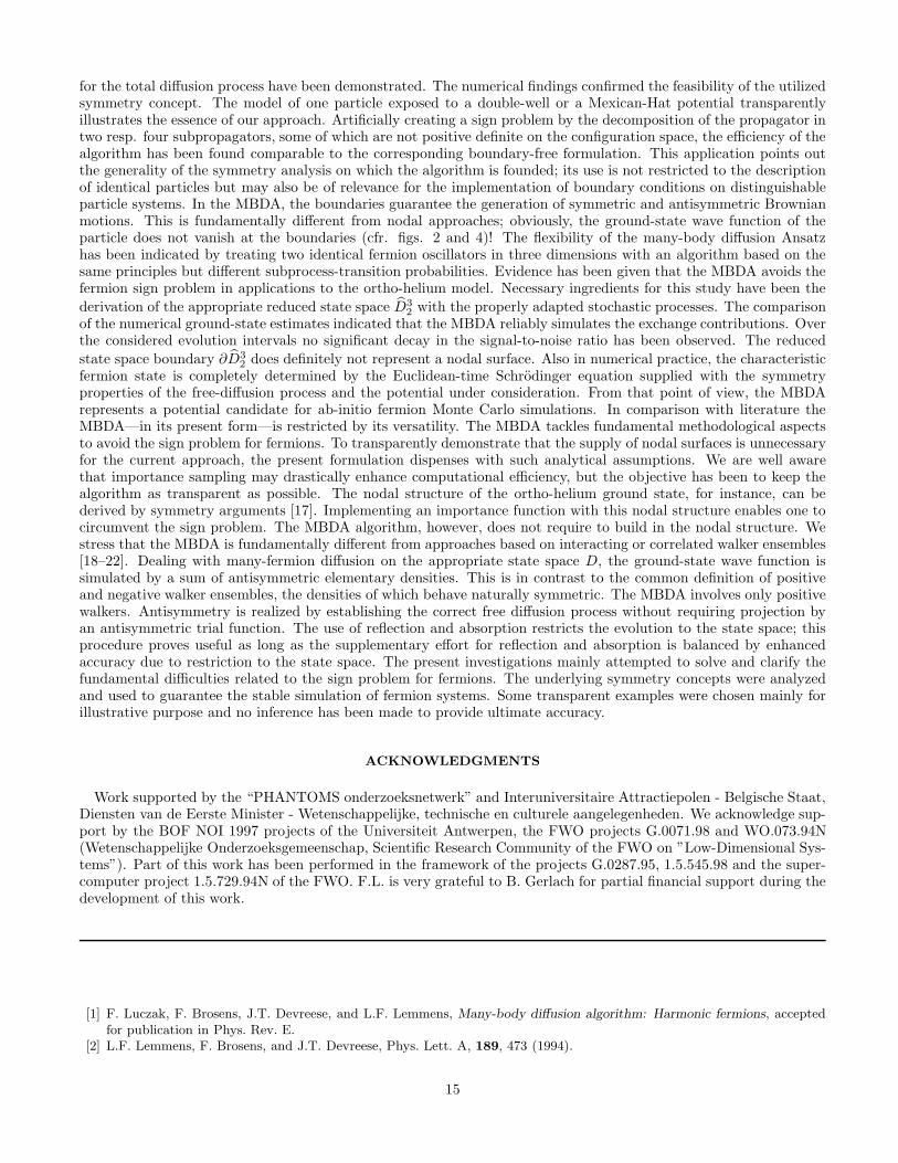
In fig. 1, the feasibility of the developed sampling technique is indicated by graphical comparison of the numericallysampled and rigorous transition probability densities ρb

f for a given initial x ′ denoted by the crosses.

B. Free Fermion and Free Boson Diffusion on D3

2

We now formulate the diffusion process of two free indistinguishable particles in three dimensions on the reduced

state space D32 by extending the symmetry analysis performed above. Following the basic principles outlined in [4],

the free diffusion of indistinguishable particles can be traced back to one-dimensional free diffusion processes. In

that framework, the transition probabilities X f,bf,b(τ) represent the elementary subprocesses combined to constitute the

overall free diffusion process in three dimensions. For free identical fermions in three dimensions, the density matrixcan be expressed as

ρ(r, τ ; r ′) =1

8

[ [ρff(x, τ ;x

′) + ρbf (x, τ ;x ′)

] [ρfb(y, τ ; y ′) + ρb

b(y, τ ; y ′)] [ρfb(z, τ ; z ′) + ρb

b(z, τ ; z ′)]

+[ρfb + ρb

b

] [ρff + ρb

f

] [ρfb + ρb

b

]+[ρfb + ρb

b

] [ρfb + ρb

b

] [ρff + ρb

f

]+[ρff + ρb

f

] [ρff + ρb

f

] [ρff + ρb

f

]]

whereas for the corresponding boson system the density matrix evaluates to

ρ(r, τ ; r ′) =1

8

[ [ρfb(x, τ ;x ′) + ρb

b(x, τ ;x ′)] [ρfb(y, τ ; y ′) + ρb

b(y, τ ; y′)] [ρfb(z, τ ; z ′) + ρb

b(z, τ ; z′)]

+[ρff + ρb

f

] [ρff + ρb

f

] [ρfb + ρb

b

]+[ρfb + ρb

b

] [ρff + ρb

f

] [ρff + ρb

f

]+[ρff + ρb

f

] [ρfb + ρb

b

] [ρff + ρb

f

]]

In this representation, the density matrix for identical particles contains 32 terms. Since each term factorizes into aproduct of three one-dimensional orthogonal density matrices, each of the 32 elementary three-dimensional density

matrices satisfies the Markov properties and generates a Wiener subprocess on the reduced state space D32. For

instance, the subprocess X fbffbb(τ)

X fbffbb(τ) = X f

f (τ) ⊗ Y bb (τ) ⊗ Z f

b(τ) ,

can be sampled as the diffusion process of two free distinguishable particles restricted to the reduced state space byreflection at the boundaries y1 = y2 and z1 = z2 and absorption at x1 = x2, x1 = −x2, y1 = −y2 and z1 = −z2. Thecombination of all the 64 Wiener subprocesses gives rise to the free diffusion process of two indistinguishable particles

in three dimensions defined on D32 . The symmetry properties of the elementary processes allow furthermore to unfold

the resulting probability density into the configuration space R6.

C. Evolution Equations and Decomposition of the Potential

The derivation of the evolution equation for the propagator proceeds along the same lines as for the two-dimensionalcase, as discussed in Sec. II.A.2. Without going into detail, we only mention the result

∂

∂τKI [rf , l,l

′,τ ; ri, l , l′, 0] =

~

2m∇2

r KI [rf , l,l′,τ ; ri, l, l

′, 0] − 1

~

∑

l,l′

V l′l′

ll(rf ) KI [rf , l,l

′,τ ; ri, l, l

′, 0] ,

where

KI [rf , l,l′,τ ; ri, l , l

′, 0] =

(1

2!

)6∑

Px

ξPx

l′

∑

Py

ξPy

l′

∑

Pz

ξPz

l′

∑

Px

ξPx

l

∑

Py

ξPy

l

∑

Pz

ξPz

l KD[PxPyPzPxPyPz rf , τ ; ri, l, 0] .

The components of the potential are given by

V l′l′

l l(rf ) =

(1

2!

)6∑

Sx

∑

Sy

∑

Sz

∑

Sx

∑

Sy

∑

Sz

ξSx

l ξSy

l ξSz

l ξSx

l′ ξSy

l′ ξSz

l′ V (SxSySzSxSySz rf ) ξSx

lξ

Sy

lξSz

lξSx

l′ξ

Sy

l′ξSz

l′,

it should be noted that if the range of the label l used to denoted the statistics is extented in such a way that it alsoindicates the boundary conditions on the reduced domain then the evolution equation for the propagator derived heretakes the same form as the equation (19).

8

IV. AN ALGORITHMIC APPROACH ON MODELS

In the previous section, we introduced a novel representation of the Euclidean-time propagator of systems containingtwo indistinguishable particles. This representation allows to sample the propagator sign-problem-free. We nowdevelop a numerically feasible sign-problem-free implementation scheme. Its efficiency in numerical practice is analyzedin applications to model systems. In all the cases, we use atomic units ~ = m = e = 1. Energy and Euclidean timeare measured in Hartrees (H) and H−1.

A. General Structure

The key elements of the many-body diffusion algorithm (MBDA) for the symmetry problems considered here are(i) an appropriately adapted free diffusion step, (ii) a routine to model subprocess transitions, and (iii) a branchingand killing procedure. Whilst some elements of the algorithm resemble Diffusion Monte Carlo, we stress that theunderlying principle of interdependent subprocess evolution is conceptually new. We are also aware that the efficiencyof the presented algorithm can be drastically enhanced by importance sampling methods. Although we can show thatthis expectation holds true, we do not dwell on these refinements, for major emphasis is on the realization of symmetryarguments. In the limit of infinitely long evolution τ → ∞, the stepwise application of the Euclidean time propagatoron a given sample leads in principle to the system’s lowest eigenstate compatible with the symmetry restrictionsmade. In numerical practice, this evolution occurs in discrete Euclidean time steps ∆τ . Since the assumption of suchtime steps is only exact for ∆τ → 0, the algorithm in principle suffers from a systematic time-step error. The latter,however, could be controlled in the considered applications. The main advantages of the developed approach are thesimplicity and convergence properties. In particular, it allows for the transparent implementation of reflecting andabsorbing boundaries to model the subprocesses derived above. Let us discuss the algorithm in some more detail.Having generated an initial population of walkers located at positions (r ′

i )i in the appropriate state space, each validwalker makes a free distinguishable particle move to (r ′

f )i. This is achieved by the construction of Gaussian deviates

with variance√

∆τ and mean r ′i . If a walker hits the state-space boundary by free distinguishable particle diffusion

it is either reflected or absorbed depending on its characteristic boundary conditions [1]. In numerical practice, theuse of non-zero Euclidean time steps ∆τ prevents the proper construction of reflecting and absorbing boundaries.In the mathematical literature, free diffusion in the presence of an absorbing boundary is realized by the so-calledSkohorod construction [8]. The latter reflects walker trajectories without changing the “momentum” of the walker.This is in contrast to the reflection experienced by a classical object at a hard wall. In the numerical procedures, thefinal reflected position r ′

f is obtained by reflection of the corresponding r ′f . The systematic error for inappropriate

reflection vanishes for ∆τ → 0; for the utilized time intervals ∆τ no significant error were observed. The efficientimplementation of fermionlike diffusion, in contrast, calls for numerical crossing-recrossing corrections. For twoidentical fermions j, k on a line the corrections for an absorbing boundary xj = xk have been discussed in [1]. Basedon the principle of images, we showed that an apparently valid walker move from (x′j , x

′k) to (xj , xk), both points inside

the state space, has to be rejected with the probability exp(−(xj −xk)(x′j −x′k)/∆τ). The symmetry properties of thepotentials discussed in this work require the generation of interdependent subprocesses. In succession to the adaptedfree diffusion step, a walker associated with the boundary condition of the subprocess l may change to the boundarycondition of a subprocess l′ with the probability pl→l′(rf ). Its actual structure is determined by the physical situation,e.g. the symmetry properties of both the potential and the eigenstate under consideration. The local dependence ofthe probabilities pl→l′(rf ) governs the relevance of subprocess transitions at a given position rf . The structure ofpl→l′(rf ) is fairly flexible as long as it harmonizes with the killing and branching procedure. For instance, pl→l′(rf )could be decoupled from the different kinds of boundary conditions. Then each subprocess transition occurs withequal probability 1/nl, where nl denotes the total number of subprocesses. Accordingly, both the normalization ratesand the probability for branching and killing become dependent on the subprocess transition performed on the walker.In what follows, we assume subprocess transition probabilities adapted to the branching and killing procedure dueto the potential. The third step, branching and killing, realizes the presence of the potential by the implementation

of the exponential path-integral weights w(r ′, r) = exp

(−

∆τ∫

0

V(R(ς)

)dς

)∣∣∣∣∣

R(∆τ)=r

R(0)=r ′

, where R(ς) denotes the paths

generated by the adapted free diffusion process. The principal lack of continuous trajectories in discrete time-stepevolution procedures induces the necessity for feasible approximations to w(r ′, r). For sufficiently smooth potentials,the Suzuki-Trotter formula [6] offers a reliable alternative. Then only the values of the potential at the initial and finalpoints of a move are taken into account: w(r ′, r) = exp−(V (r ′) + V (r))∆τ/2. Especially for singular potentials,improved approximations (for a detailed discussion see e.g. [7] and references therein) are recommended. Here, we

9

choose the semiclassical approximation suggested in [9]: w(r ′, r) = exp−∫ 1

0 dξ V (r ′ + ξ(r − r ′)). A branching andkilling technique serves to efficiently adapt the walkers to the weights w(r ′, r) by an acceptance/rejection procedure.To conserve the size of the walker population to within statistical fluctuations, an appropriate reference energy Eref

has been supplied to yield improved weights w(r ′, r) eEref∆τ . In [1], we derived an estimator for the ground-stateenergy E0. The key elements of this estimator are the potential average 〈V 〉D over the state space D and a surfaceterm 〈j〉∂D triggered by the non-zero gradient of the fermionlike subdensities at absorbing boundaries. The estimateis easily generalized to an ensemble of interdependent subdensities Ψ(r, l,τ)

E0 = limτ→∞

Eτ = limτ→∞

∑

l

[−

~2

2m

∫∂D2

dr ∇rΨ(r, l,τ)∫

D2dr Ψ(r, l,τ)

+

∫D2dr Ψ(r, l,τ)V (r)∫

D2dr Ψ(r, l,τ)

]=∑

l

[〈 j 〉l∂D2

+ 〈V 〉lD2

].

Alternatively, the growth estimates

E0 = limτ→∞

Eτ = − limτ→∞

1

τln

∫drf

∫dri

∑

l

K[rf , l,τ ; ri, 0] ,

may serve to predict the ground-state energy. Based on this general algorithmic structure, the ground-state wavefunction of several model systems is investigated below. The different types of potentials make a specific analysis ofthe appropriate state space necessary.

B. Double well and Mexican Hat

To start with, the symmetry principles underlying the many-body diffusion algorithm are illustrated for a quantum-mechanical particle in a double-well or a Mexican Hat potential. For these models, the utilization of (anti)symmetricsubprocesses is shown to provide a suitable technique for the numerical generation of the real ground-state wavefunction. Our study aims at revealing the role of symmetry arguments to sample a probability density on an ap-propriate part of the configuration space. Feasibility of the symmetry concept has been tested independently withstandard Monte Carlo techniques. Consider a single particle in a one-dimensional double-well potential, described bythe Hamiltonian

H = −1

2

∂2

∂x2+ V (x) with V (x) =

(x2 − a)2 − a2

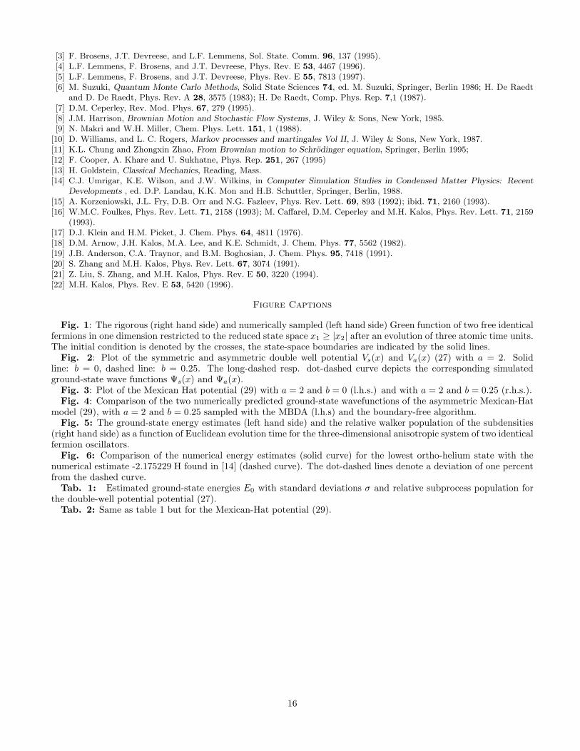
4+ b x3 , (27)

where a and b represent parameters. Fig. 2 depicts the potential values for two different parameter choices: a = 2, b = 0and a = 2, b = 0.25 in the following referred to as symmetric and asymmetric potential. According to the rulesoutlined above, the Euclidean time propagator K(x, τ ;x ′) associated with the Hamiltonian (27) can be formulatedas a sum of four subpropagators K(x, τ, ;x ′, ) with , ∈ 0, 1 denoting symmetric resp. antisymmetric behaviorunder the transformation Px : x → −x. This means that K(x, , τ ;x ′, 0) and K(x, , τ ;x ′, 1) are initially symmetricand antisymmetric with respect to the boundary x = 0 which separates the two half-spaces D− = x|x ≤ 0 andD+ = x|x ≥ 0. The (anti)symmetrized potentials Vs(x) and Va(x) are derived as

Vs(x) ≡ V(x) =V (x) + V (−x)

2=x2(x2 − 2a)

4; Va(x) ≡ V′(x) =

V (x) − V (−x)2

= b x3 , , ′ ∈ 0, 1, 6= ′

The matrix W (cfr. (20)) is calculated as W′ = −Va (1 − δ,′) with the total rate represented by W = −Va. TheEuclidean-time Schrodinger equation [cfr. (19)] can thus be written

∂

∂τK[x, ,τ ;x′, , 0] =

1

2

∂2

∂x2K[x, ,τ ;x′, , 0] − Vs(x)KI [x, ,τ ;x

′, , 0] −1∑

′=0

Va(x)K[x, ′,τ ;x′, , 0] (1 − δ,′) . (28)

Eq. (28) allows for a change of the boundary conditions of the propagator K[x, ,τ ;x′, , 0] during its evolution inEuclidean time. Written as a Feynman-Kac functional, the propagator K[x, ,τ ;x′, , 0] can be interpreted as a sumof two interdependent distinguishable-particle diffusion subprocesses. The numerical realization of the subprocesses occurs by means of ensembles (x

i)i=1,nof n walkers. Each of the n walkers satisfies the boundary conditions

for the subprocess and during the evolution a walker may change its subprocess to according to the normalizedtransition amplitudes p→′(rf ). To formulate a probability-based evolution scheme it is therefore required thatp→′(rf ) remains positive. Since

10

1∑

=0

exp (− τ V′ (rf )) = 2 exp

(− τ

(x2 − a)2 − a2

4

)[cosh

(− τ b x3

)δ′, + sinh

(− τ b x3

)(1 − δ′,)

],

the half-space D− represents the appropriate state space for probabilistic sampling. Walker transitions to x > 0 areprevented by the construction of a reflecting (for =0) or an absorbing (for =1) boundary. The major algorithmicsteps for the numerical evolution procedure are enlisted as follows:

1. Generate two distinct walker sets (xi)i=1,n

, =0, 1. The initial non-zero walker populations n are chosenrandomly.

2. Calculate for each walker the subprocess-transition probabilities pa(x) =[1 − exp

(−2∆τbx3

)]/2 and apply

them by comparison with uniform pseudo-random numbers η ∈ [0, 1]: if η ≤ pf(x) change the boundarycondition associated to the walker, else leave the condition unchanged.

3. Make an evolution step, as indicated in Sec. A.

4. Return to step 1. until the density has equilibrated; after a certain amount of repetitions, calculate the potentialaverage and the walker outflow to get an estimate for the ground-state energy.

5. To obtain an image of the sampled ground-state wave function, record the walker positions in small discretebins.

The results obtained for the ground-state energy E0 of the double-well system are shown in table 1. To test thealgorithm, the estimates EMBDA

0 have been compared with the numerical outcome Econf0 of a program with evolution

on the full configuration space. For both the symmetric and the asymmetric potential, the results agree withinthe estimated standard deviation σ. It is illuminating to examine the population sizes of the two subprocesses .For the symmetric potential the probability pa(x) is zero and independent subprocesses are simulated. Due to thehigher eigenenergy related to the fermion subprocess K[x, 0,τ ;x′, , 0], the antisymmetric process rapidly fades outand the ground state wave function is completely described by the symmetric process. For the asymmetric potentialin contrast, the antisymmetric subprocess is of crucial importance, since the asymmetric ground-state wave functioncannot be simply generated by a symmetric process. The faster decay of the antisymmetric density is counteractedby a net walker transition from the symmetric to the antisymmetric population. In equilibrium, almost half of thepopulation belongs to the antisymmetric density.

Econf0 σconf EMBDA

0 σMBDA∑

Ψs/∑

Ψ∑

Ψa/∑

Ψ

b = 0 -0.2996 0.0006 -0.2999 0.0006 100 % 0 %b = 0.25 -1.0251 0.0012 -1.0251 0.0011 53.7 % 46.3 %

Table 1

This example for a particle in one dimension can be transparently generalized to arbitrary spatial dimensions.Consider, e.g., a particle in two dimensions exposed to the Mexican-Hat potential

H = −1

2

∂2

∂x2− 1

2

∂2

∂y2+ V (x, y) with V (x, y) =

(x2 + y2 − a)2 − a2

4+ b x3 . (29)

The two parameter sets a = 2, b = 0 and a = 2, b = 0.25 were chosen as in one dimension to represent a symmetricand an asymmetric potential, as depicted in fig. 2. Consider the two operators P x : x → −x and P y : y → −y andintroduce the two boundaries x = 0 and y = 0. The construction of reflecting and absorbing boundary conditionsat these two boundaries calls for the definition of 16 Euclidean-time propagators K(x, τ, ;x ′, ) and four elementarystates Ψss, Ψsa, Ψas and Ψaa with their indices characterizing their properties under transformation with P x and P y,respectively. By imposing reflecting and absorbing boundary conditions the configuration space R

2 is split into foursubspaces with positive or negative x- or y-coordinates. Although the system’s evolution can be folded to any ofthese four subspaces, the analysis of the subprocess-transition amplitudes for the Mexican-Hat potential reveals thatonly two subspaces are associated with positive definite sampling. A sign analysis of the four subprocess-transitionamplitudes pss(rf ), psa(rf ), pas(rf ) and paa(rf )

pas(x) =1 − exp

(−2∆τbx3

)

2, pss(x) =

1 + exp(−2∆τbx3

)

2, psa(x) = 0 , paa(x) = 0 ,

indicates that they all may be interpreted as probabilities if the evolution is confined to either the subspace D+− ≡

x ≤ 0, y ≥ 0 or D−− ≡ x ≤ 0, y ≤ 0. The fact that psa(x) = 0 and paa(x) = 0 induces two independent sets of

11

subprocesses, namely [K(x, τ,ss;x ′, ), K(x, τ,as;x ′, )] and [K(x, τ,sa;x ′, ), K(x, τ,aa;x ′, )]. Only those subprocesstransitions are allowed which conserve the parity under P y. The formulation of the respective MBDA yields resultsfor the ground-state energy which are in good agreement with the results achieved without the introduction ofboundaries (see table 2). Since the characteristics of the model (29) allow for a distinguishable-particle treatment,the boundary-free algorithm reliably simulates the properties under investigation. The comparison of the estimatedground-state energies demonstrates the efficiency of the MBDA. Both energies Econf

0 and EMBDA0 have been obtained

with comparable numerical effort and standard deviations. The last four columns of table 2 show the relevance of thefour states Ψss , Ψsa, Ψas and Ψaa with as measure of their relative population sizes. Since psa(x) = 0 and paa(x) = 0,the states Ψsa and Ψaa fade out. In addition, for the symmetric potential pas(x) = 0. This means that also Ψas isirrelevant for the sampling of the ground-state wave function. The remaining state Ψss is symmetric under both P x

and P y. Clearly, evolution in the presence of the asymmetric potential cannot be simulated with a symmetric stateonly; the algorithm ensures the occurrence of the Ψas state by a steady transformation of walkers associated with thesubprocess K(x, τ,ss;x ′, ) to walkers propagating according to K(x, τ,as;x ′, ).

Econf0 σconf EMBDA

0 σMBDA∑

Ψss/∑

Ψ∑

Ψas/∑

Ψ∑

Ψsa/∑

Ψ∑

Ψaa/∑

Ψ

b = 0 -0.19865 0.00042 -0.19860 0.00037 100 % 0 % 0 % 0 %b = 0.25 -0.56129 0.00054 -0.56115 0.00050 60.5 % 39.5 % 0 % 0 %

Table 2

C. Anisotropic Harmonic Fermions

A system of two non-interacting anisotropic identical fermion oscillators in three dimensions serves as a transparenttesting ground for indistinguishable particles. We considered a system with the Hamiltonian

H =p 2

2+

Ω2x

2

(x2

1 + x22

)+

Ω2y

2

(y21 + y2

2

)+

Ω2z

2

(z21 + z2

2

), (30)

with ground-state energy

E0 = Ωx + Ωy + Ωz + Min[Ωx,Ωy,Ωz] . (31)

We now consider a rotated reference frame as the result of from the rotation by the two Euler angles φ and θ [13]

R =

cosφ sinφ 0

− sinφ cos θ cosφ cos θ 0sinφ sin θ − cosφ sin θ cos θ

r .

The objectives are clear: the symmetry of the potential under the interchange of Cartesian particle coordinates isavoided without losing the advantage of comparison with a rigorous analytical solution. A proper implementation ofthe propagator with the MBDA requires positive definite subprocess transition amplitudes

pll(rf ) =

∑Sx

∑Sy

∑SzξSx

l ξSy

l ξSz

l exp (−τV (SxSySz rf )) ξSx

lξ

Sy

lξSz

l∑l

∑Sx

∑Sy

∑SzξSx

l ξSy

l ξSz

l exp (−τV (SxSySz rf )) ξSx

lξ

Sy

lξSz

l

, (32)

where we used the notation introduced in Sec. II. If the numerator of eq. (32) is positive definite, pll(rf ) may

be interpreted as the probability for a subprocess transition l → l. Since the sign of pll(rf ) is determined by the

parity of the propagator K[rf ,l,∆τ ; ri, l,0] and the boundary condition l under Cartesian-coordinate permutation,four different subprocess-transition amplitudes occur. Their classification according to their symmetry propertiessuggests the following notation: pbbb(rf ), pffb(rf ), pfbf(rf ) and pbff(rf ). The probability pffb(rf ), e.g., stands fortransitions between subprocesses with even parity in the z-coordinate and odd parity in the x, y-coordinates, forinstance K[rf ,fbb,∆τ ; ri,bfb,0]. While the amplitude pbbb(~r) is always positive, positivity of the three remainingamplitudes is imposed (in first order of the Euclidean time step ∆τ) by the following conditions on the domain andthe parameters Ωx, Ωy, Ωz, φ and θ:

sinφ cosφ(Ω2

x − Ω2y cos2 θ + Ω2

z(cos2 θ − 1))

(x1 − x2) (y1 − y2) ≥ 0cosφ sin θ cos θ

(Ω2

y − Ω2z

)(y1 − y2) (z1 − z2) ≥ 0

− sinφ sin θ cos θ(Ω2

y − Ω2z

)(x1 − x2) (z1 − z2) ≥ 0

. (33)

12

For the present illustration, the evolution has been restricted to the state space D23 with a particular set of parameters:

x1 ≥ x2 , y1 ≥ y2 , z1 ≥ z2 , Ωx = 4 , Ωy = 3 , Ωz = 2 , φ = 130 , θ = 50 . (34)

Employing samples of approximately 20,000 walkers and Euclidean time steps of 0.001 H−1, the MBDA leads to thenumerical results visualized in fig. 5. The ground-state energy estimates (see left-hand side of fig. 5) oscillate ina small interval around their average of 10.9987±0.0056 H. They estimate the rigorous ground-state energy of 11.0H with a statistical inaccuracy of about half a per mil. After numerical thermalization, the population of each ofthe four subprocesses f,b,b, b,f,b, b,b,f and f,f,f remains approximately constant (see right-hand side of fig.5). In particular, contributions from the f,f,f-subprocess prove indispensable to correctly generate the propagator.Our numerical investigations manifested the occurrence of a net walker flow from the subdensities Ψfbb,Ψbfb,Ψbbf

to Ψfff. Without the inclusion of subprocess interdependencies, the subprocess K[rf ,fff,∆τ ; ri, l,0] would fade outexponentially in evolution time.

D. Application to Ortho Helium

To illustrate the feasibility of the reduced state space concept, we also used the MBDA to calculate the ground-state energy of ortho-helium. In the triplet states of ortho-helium, the two electrons carry equal spin. The occurrenceof additional repulsive forces due to exchange distinctly influences the energy spectrum, so that the simulation ofthe lowest ortho-helium state requires the accurate inclusion of Fermi statistics. In that context, the challenge ofnumerical implementation shows twofold. First, the lowest energy level should be reliably predicted and second,the converged energy estimates should be stable in time. In particular the second aspect concerns the fermionsign problem: the MBDA is demonstrated to exactly filter out possible interfering symmetric contributions. The

general evolution scheme on the reduced state space D 32 relies on the construction of 322 interdependent subprocesses

K[rf , l, l′,∆τ ; ri, l, l

′,0]. Here, each of the l,l may be one of the four boundary conditions fff,fbb,bfb or bbf, whereas

l′, l′ run over the eight conditions bbb,fbb,..,fff. Symmetry arguments allow to simplify the computational procedureby the prior rejection of certain classes of subprocesses. As the permutation operator P has the same effect on the

ortho-helium Hamiltonian as the permutation operator P , the ground-state wave function consists of substates with

equal parity under P and P . Consequently, the simulation of the ortho-helium ground-state wave function on the

reduced state space D 32 is accomplished by the construction of only 16 subprocesses with l = l, l′ = l′ specified as

fff,fbb,bfb or bbf. Although both - the general and the simplified - procedure in principle lead to the exact densities,the restriction to four subprocesses considerably improves the convergence of the algorithm. The next step in theformulation of an evolution scheme for the ortho-helium ground state is the consideration of the subprocess-transitionamplitudes

pl′l′

ll(rf ) =

∑Sx,Sy,Sz,Sx,Sy,Sz

ξSx

l ξSy

l ξSz

l ξSx

l′ ξSy

l′ ξSz

l′ e−τV (SxSySzSxSySz rf ) ξSx

lξ

Sy

lξSz

lξSx

l′ ξ

Sy

l′ ξ

Sz

l′

∑l,l

′

,Sx,Sy,Sz,Sx,Sy,SzξSx

l ξSy

l ξSz

l ξSx

l′ ξSy

l′ ξSz

l′ e−τV (SxSySzSxSySz rf ) ξSx

lξ

Sy

lξSz

lξSx

l′ ξ

Sy

l′ ξ

Sz

l′

(35)

controlling the interplay between the four single subprocesses. In order to derive the subspaces associated with

positive sums of exponentials e−τV (SxSySzSxSySz rf ), we focus on the short-time limits (1 − τV (SxSySzSxSySz rf ))of the exponentials, which contain all the essential symmetry characteristics necessary for the sign analysis of theamplitudes (35). Furthermore, it proves useful to separate the potential V (r) in two parts V1(r) and V2(r) with

V1(r) =−2

|~r1|+

−2

|~r2|, V2(r) =

1

|~r1 − ~r2|, V (r) = V1(r) + V2(r) .

To illustrate the need of a reduced state space, consider the corresponding many-body diffusion process on thestate space D 3

2 . The amplitudes pbbb(r), pffb(r), pfbf(r) and pbff(r) control the transitions between the 16 fermion

subprocesses K[rf , l,∆τ ; ri, l,0]. A detailed investigation of the amplitudes, however, discloses that some of them maybecome negative on the state space D 3

2. For instance, considering pffb(r), one derives

pffb(r)τ→0:−→ eτV ( r)

∑

Px,Py,Pz

(−)Px(−)Py (1 − V1(PxPyPzr))

∝ 4τ√π

∫ ∞

−∞

dt(e−x 2

1t2 − e−x 2

2t2)(

e−y 2

1t2 − e−y 2

2t2)(

e−z 2

1t2 + e−z 2

2t2)

13

which is positive definite on a subdomain of the state space, namely for |x1| ≥|x2| and |y1| ≥|y2|. Similar restrictionsfollow from pfbf(r) and pbff(r), whereas pbbb(r) is a sum of only positive elements. Strictly speaking, utilizing thestate space as the domain for evolution, the MBDA would incorrectly simulate the ortho-helium propagator. It is

at that point that the reduced state space D 32 as defined by (24) comes into play. By appropriate restriction of the

evolution to the reduced state space, the subprocess-transition amplitudes all remain positive and their probabilisticimplementation is justified. In what follows, we take over the results from Sec. III and adapt the general scheme tothe ortho-helium system.

Continuing with the investigation of the amplitudes p(r), let us first focus on the contributions of V1(r). In V1(r), the

coordinates x1, . . . , z2 are entangled such that the transformations P and P have the same effects; for our purpose,no distinction has to be made between P and P .With regard to amplitudes with identical sub- and superindices per coordinate, one obtains

pffbffb(r)

∣∣V1

= eτV ( r)∑

Px,Py,Pz,PxPy ,Pz

(−)Px(−)Py(−)Px(−)Py exp(PxPyPxPyr)

τ→0:−→ τ

2√πeτV1( r)

∫ ∞

−∞

dt(e−x 2

1t2 − e−x 2

2t2)(

e−y 2

1t2 − e−y 2

2t2)(

e−z 2

1t2 + e−z 2

2t2)

.

The remaining 28 amplitudes have in common that for at least one coordinate the permutations P and P inducedifferent parity. Each of these subprocess-transition amplitudes involves a sum composed of two parts of equal absolutevalue but opposite sign. Consequently, they are irrelevant for the evolution procedure.The potential V2(r) proves invariant under interchange of two coordinates. Its symmetry properties entail that only

those amplitudes p(r) contribute which in each direction involve equal positive (bosonlike) parity under P and P , i.e.

pbbbbbb(r)

∣∣V2

∝∑

Px,Py,Pz,PxPy,Pz

exp(−τ PxPyPzPxPyPz r)τ≪1:−→ exp (−τV2(r)) . (36)

Obviously, pbbbbbb(r) is positive on the reduced state space D 3

2 . By recombination of both potentials V1(r) and V2(r),the total evolution scheme is established. Its proper implementation guarantees accurate probabilistic sampling

of the ortho-helium propagator on the reduced state space D 32 . The sampled density consists of 4 subdensities

Ψfbbfbb(r, τ), Ψbfb

bfb(r, τ), Ψbbfbbf(r, τ) and Ψfff

fff(r, τ). Due to the symmetry properties of the ortho-helium potential V (r) =V1(r) + V2(r), certain classes of subprocess transitions are forbidden; each of the subprocesses undergoes one out offour possible transitions ruled by the probabilities pffb

ffb(r), pfbffbf(r), p

bffbff(r) and pbbb

bbb(r). During a time step ∆τ , thesubdensity Ψfbb

fbb(r, τ), for instance, branches into the subdensities Ψbfbbfb(r, τ + ∆τ), Ψbbf

bbf(r, τ + ∆τ), Ψffffff(r, τ + ∆τ)

and Ψfbbfbb(r, τ + ∆τ) according to the probabilities pffb

ffb(r), pfbffbf(r), p

bffbff(r) and pbbb

bbb(r). Notice that the analysis of thesubprocess transition amplitudes is consistent with the restriction to four subdensities in the sense that no transitionsoccur to subdensities different from the four specified ones. Fig. 6 illustrates the energy estimates for the lowest ortho-helium state achieved with a pre-thermalized sample. The numerical average -2.1744±0.0012 H is in good agreementwith the numerical energy estimate of -2.175229 H found in [14]. Systematic errors due to time discretization andimperfect sampling could be diminished by the use of total sample sizes of 100,000 walkers and time steps of 0.001H−1.

V. DISCUSSION AND CONCLUSIONS

It should be mentioned that the relation between fermi statistics and the elimination of paths at permutationhyperplanes has been put forward by Korzeniowski et al. [15]. This approach was subsequently criticized [16], becauseit left open a few fundamental questions. Studying the underlying mathematical Ansatz has lead us to an extensionof the recently reported many-body diffusion approach [2–5] in which it was the basic idea to rigorously separate themulti-dimensional free diffusion process of indistinguishable particles into one-dimensional free diffusion processes.The novelty of the outlined symmetry analysis for the simulation of indistinguishable particles is the construction ofnumerically implementable diffusion process with a switching of boundary conditions driven by a compound Markovchain . The continuous-time Markov chain, not considered before in that framework, has been set up to enable therealization of interdependent Brownian motions. The inclusion of transitions between a set of simultaneously evolvingdiffusion processes has been shown necessary to approach identical particles in potentials which are not invariantunder permutations of Cartesian coordinates. To transfer the recently reported MBDA sampling technique [1] to thosesystems, a symmetry analysis of the potential is necessary. In applications to different model systems, the consequences

14

for the total diffusion process have been demonstrated. The numerical findings confirmed the feasibility of the utilizedsymmetry concept. The model of one particle exposed to a double-well or a Mexican-Hat potential transparentlyillustrates the essence of our approach. Artificially creating a sign problem by the decomposition of the propagator intwo resp. four subpropagators, some of which are not positive definite on the configuration space, the efficiency of thealgorithm has been found comparable to the corresponding boundary-free formulation. This application points outthe generality of the symmetry analysis on which the algorithm is founded; its use is not restricted to the descriptionof identical particles but may also be of relevance for the implementation of boundary conditions on distinguishableparticle systems. In the MBDA, the boundaries guarantee the generation of symmetric and antisymmetric Brownianmotions. This is fundamentally different from nodal approaches; obviously, the ground-state wave function of theparticle does not vanish at the boundaries (cfr. figs. 2 and 4)! The flexibility of the many-body diffusion Ansatzhas been indicated by treating two identical fermion oscillators in three dimensions with an algorithm based on thesame principles but different subprocess-transition probabilities. Evidence has been given that the MBDA avoids thefermion sign problem in applications to the ortho-helium model. Necessary ingredients for this study have been the

derivation of the appropriate reduced state space D32 with the properly adapted stochastic processes. The comparison

of the numerical ground-state estimates indicated that the MBDA reliably simulates the exchange contributions. Overthe considered evolution intervals no significant decay in the signal-to-noise ratio has been observed. The reduced

state space boundary ∂D32 does definitely not represent a nodal surface. Also in numerical practice, the characteristic

fermion state is completely determined by the Euclidean-time Schrodinger equation supplied with the symmetryproperties of the free-diffusion process and the potential under consideration. From that point of view, the MBDArepresents a potential candidate for ab-initio fermion Monte Carlo simulations. In comparison with literature theMBDA—in its present form—is restricted by its versatility. The MBDA tackles fundamental methodological aspectsto avoid the sign problem for fermions. To transparently demonstrate that the supply of nodal surfaces is unnecessaryfor the current approach, the present formulation dispenses with such analytical assumptions. We are well awarethat importance sampling may drastically enhance computational efficiency, but the objective has been to keep thealgorithm as transparent as possible. The nodal structure of the ortho-helium ground state, for instance, can bederived by symmetry arguments [17]. Implementing an importance function with this nodal structure enables one tocircumvent the sign problem. The MBDA algorithm, however, does not require to build in the nodal structure. Westress that the MBDA is fundamentally different from approaches based on interacting or correlated walker ensembles[18–22]. Dealing with many-fermion diffusion on the appropriate state space D, the ground-state wave function issimulated by a sum of antisymmetric elementary densities. This is in contrast to the common definition of positiveand negative walker ensembles, the densities of which behave naturally symmetric. The MBDA involves only positivewalkers. Antisymmetry is realized by establishing the correct free diffusion process without requiring projection byan antisymmetric trial function. The use of reflection and absorption restricts the evolution to the state space; thisprocedure proves useful as long as the supplementary effort for reflection and absorption is balanced by enhancedaccuracy due to restriction to the state space. The present investigations mainly attempted to solve and clarify thefundamental difficulties related to the sign problem for fermions. The underlying symmetry concepts were analyzedand used to guarantee the stable simulation of fermion systems. Some transparent examples were chosen mainly forillustrative purpose and no inference has been made to provide ultimate accuracy.

ACKNOWLEDGMENTS

Work supported by the “PHANTOMS onderzoeksnetwerk” and Interuniversitaire Attractiepolen - Belgische Staat,Diensten van de Eerste Minister - Wetenschappelijke, technische en culturele aangelegenheden. We acknowledge sup-port by the BOF NOI 1997 projects of the Universiteit Antwerpen, the FWO projects G.0071.98 and WO.073.94N(Wetenschappelijke Onderzoeksgemeenschap, Scientific Research Community of the FWO on ”Low-Dimensional Sys-tems”). Part of this work has been performed in the framework of the projects G.0287.95, 1.5.545.98 and the super-computer project 1.5.729.94N of the FWO. F.L. is very grateful to B. Gerlach for partial financial support during thedevelopment of this work.

[1] F. Luczak, F. Brosens, J.T. Devreese, and L.F. Lemmens, Many-body diffusion algorithm: Harmonic fermions, acceptedfor publication in Phys. Rev. E.

[2] L.F. Lemmens, F. Brosens, and J.T. Devreese, Phys. Lett. A, 189, 473 (1994).

15

[3] F. Brosens, J.T. Devreese, and L.F. Lemmens, Sol. State. Comm. 96, 137 (1995).[4] L.F. Lemmens, F. Brosens, and J.T. Devreese, Phys. Rev. E 53, 4467 (1996).[5] L.F. Lemmens, F. Brosens, and J.T. Devreese, Phys. Rev. E 55, 7813 (1997).[6] M. Suzuki, Quantum Monte Carlo Methods, Solid State Sciences 74, ed. M. Suzuki, Springer, Berlin 1986; H. De Raedt

and D. De Raedt, Phys. Rev. A 28, 3575 (1983); H. De Raedt, Comp. Phys. Rep. 7,1 (1987).[7] D.M. Ceperley, Rev. Mod. Phys. 67, 279 (1995).[8] J.M. Harrison, Brownian Motion and Stochastic Flow Systems, J. Wiley & Sons, New York, 1985.[9] N. Makri and W.H. Miller, Chem. Phys. Lett. 151, 1 (1988).

[10] D. Williams, and L. C. Rogers, Markov processes and martingales Vol II, J. Wiley & Sons, New York, 1987.[11] K.L. Chung and Zhongxin Zhao, From Brownian motion to Schrodinger equation, Springer, Berlin 1995;[12] F. Cooper, A. Khare and U. Sukhatne, Phys. Rep. 251, 267 (1995)[13] H. Goldstein, Classical Mechanics, Reading, Mass.[14] C.J. Umrigar, K.E. Wilson, and J.W. Wilkins, in Computer Simulation Studies in Condensed Matter Physics: Recent

Developments , ed. D.P. Landau, K.K. Mon and H.B. Schuttler, Springer, Berlin, 1988.[15] A. Korzeniowski, J.L. Fry, D.B. Orr and N.G. Fazleev, Phys. Rev. Lett. 69, 893 (1992); ibid. 71, 2160 (1993).[16] W.M.C. Foulkes, Phys. Rev. Lett. 71, 2158 (1993); M. Caffarel, D.M. Ceperley and M.H. Kalos, Phys. Rev. Lett. 71, 2159

(1993).[17] D.J. Klein and H.M. Picket, J. Chem. Phys. 64, 4811 (1976).[18] D.M. Arnow, J.H. Kalos, M.A. Lee, and K.E. Schmidt, J. Chem. Phys. 77, 5562 (1982).[19] J.B. Anderson, C.A. Traynor, and B.M. Boghosian, J. Chem. Phys. 95, 7418 (1991).[20] S. Zhang and M.H. Kalos, Phys. Rev. Lett. 67, 3074 (1991).[21] Z. Liu, S. Zhang, and M.H. Kalos, Phys. Rev. E 50, 3220 (1994).[22] M.H. Kalos, Phys. Rev. E 53, 5420 (1996).

Figure Captions

Fig. 1: The rigorous (right hand side) and numerically sampled (left hand side) Green function of two free identicalfermions in one dimension restricted to the reduced state space x1 ≥ |x2| after an evolution of three atomic time units.The initial condition is denoted by the crosses, the state-space boundaries are indicated by the solid lines.

Fig. 2: Plot of the symmetric and asymmetric double well potential Vs(x) and Va(x) (27) with a = 2. Solidline: b = 0, dashed line: b = 0.25. The long-dashed resp. dot-dashed curve depicts the corresponding simulatedground-state wave functions Ψs(x) and Ψa(x).

Fig. 3: Plot of the Mexican Hat potential (29) with a = 2 and b = 0 (l.h.s.) and with a = 2 and b = 0.25 (r.h.s.).Fig. 4: Comparison of the two numerically predicted ground-state wavefunctions of the asymmetric Mexican-Hat

model (29), with a = 2 and b = 0.25 sampled with the MBDA (l.h.s) and the boundary-free algorithm.Fig. 5: The ground-state energy estimates (left hand side) and the relative walker population of the subdensities

(right hand side) as a function of Euclidean evolution time for the three-dimensional anisotropic system of two identicalfermion oscillators.

Fig. 6: Comparison of the numerical energy estimates (solid curve) for the lowest ortho-helium state with thenumerical estimate -2.175229 H found in [14] (dashed curve). The dot-dashed lines denote a deviation of one percentfrom the dashed curve.

Tab. 1: Estimated ground-state energies E0 with standard deviations σ and relative subprocess population forthe double-well potential potential (27).

Tab. 2: Same as table 1 but for the Mexican-Hat potential (29).

16

Fig.1

Ψs(x)

Ψa(x)Vs(x)

Va(x)x

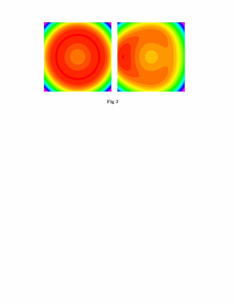
Fig.3

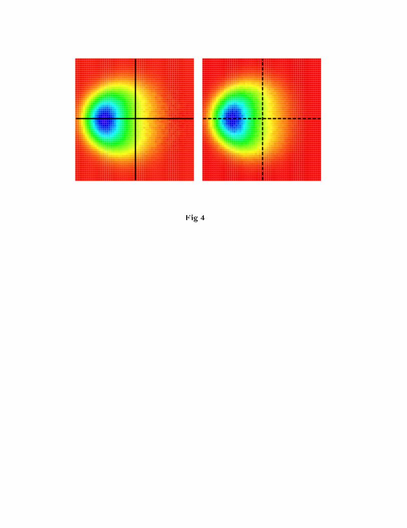
Fig.4

0

0

5

5

10

10

15

15

20

20

25

25

30

30

10.85 10.85

10.90 10.90

10.95 10.95

11.00 11.00

11.05 11.05

11.10 11.10

11.15 11.15

gro

un

d−

sta

te e

ne

rgy

evolution time0

0

5

5

10

10

15

15

20

20

25

25

30

30

0.0 0.0

0.2 0.2

0.4 0.4

0.6 0.6

0.8 0.8

1.0 1.0

evolution time

rel. po

pu

lation

f,b,b b,b,f b,f,b

f,f,f

Fig.5

0

0

4

4

8

8

12

12

16

16

20

20

24

24

−2.20 −2.20

−2.19 −2.19

−2.18 −2.18

−2.17 −2.17

−2.16 −2.16

−2.15 −2.15

−2.14 −2.14MBDAMBDA average num. res. [11]

evolution time

en

erg

y

Fig.6