Surface Color Estimation Based on Inter- and Intra-Pixel Relationshipsin Outdoor Scenes

Shun HiroseNara Institute of Science and Technology

8916-5, Takayama-cho, Ikoma, Nara, Japanshun-h@is.naist.jp

Tsuyoshi SuenagaNara Institute of Science and Technology

8916-5, Takayama-cho, Ikoma, Nara, Japantsuyo-s@is.naist.jp

Kentaro TakemuraNara Institute of Science and Technology

8916-5, Takayama-cho, Ikoma, Nara, Japankenta-ta@is.naist.jp

Rei KawakamiUniversity of Tokyo

4-6-1, Komaba, Meguro-ku, Tokyo, Japanrei@cvl.iis.u-tokyo.ac.jp

Jun TakamatsuNara Institute of Science and Technology

8916-5, Takayama-cho, Ikoma, Nara, Japanj-taka@is.naist.jp

Tsukasa OgasawaraNara Institute of Science and Technology

8916-5, Takayama-cho, Ikoma, Nara, Japanogasawar@is.naist.jp

Abstract

We propose a method for estimating inherent surfacecolor robustly against image noises from two registered im-ages taken under different outdoor illuminations. We formu-late the estimation based on maximum likelihood mannerwhile considering both inter-pixel and intra-pixel relation-ships. We define inter-pixel relationship based on stochas-tic behavior of image noises and properties of outdoor il-lumination chromaticity. We rely on the spatial continuityof both surface color and illumination to define intra-pixelrelationship. We also propose to maximize the estimationfunction in two step manner. Experimental results demon-strate the significant improvement of the proposed methodin estimation accuracy compared to previous methods.

1. IntroductionColor is one of the most important features on computer

vision algorithms, from object recognition to estimation ofphotometric properties. However, color information ob-servable by camera is multiplication of both illuminationand surface color, hence we must estimate illumination inthe scene to infer surface color, which is invariant to illumi-nation changes.

In general, this surface-color-estimation or color con-stancy problem is ill-posed, because it has to estimate twounknown parameters, i.e. surface color and illumination,

from one input pixel value. Most of the related methodsassume that a scene is lit by uniform illumination. But inactual situation a scene includes multiple illuminations likeshadow and direct sunlight.

Unlike the aforementioned methods, Finlayson etal. [11] solved this ill-posed problem by using the profileof outdoor illumination, which can be linearized. Thoughtheir algorithm is sensitive to inevitable image noises,Kawakami et al. [22] extended Finlayson’s algorithm [11]to remove the effect of the image noises in a deterministic,not probabilistic, manner.

We propose a method to robustly estimate surfacecolor and illumination from the same input as Finlayson’smethod: two registered images captured under differentoutdoor illuminations. We use both inter-pixel (i.e. pixel-wise) and intra-pixel (i.e. spatial) relationships to make themethod robust to image noise. First, we formulate inter-pixel relationship by exploiting knowledge of physics-basedvision and stochastic behavior of image noises. Next, weformulate intra-pixel relationship by assuming spatial con-tinuity in illumination as well as surface color. Then, weverify the effectiveness of considering inter- and intra-pixelrelationships.

The contributions of this paper are the following:

1. We formulate color constancy problem in the proba-bilistic framework. As a result, image noises can behandled more simply.

978-1-4244-6983-3/10/$26.00 ©2010 IEEE

2. We propose a method for estimating plausible solutionof the higher order, non-parametric Markov randomfield with complicated topology to solve this color con-stancy problem.

The rest of this paper is organized as follows: after re-viewing related work in Section 2, we describe the theoret-ical background about color constancy and outdoor illumi-nation in Section 3. In Section 4, we describe our surface-color-estimation method. In Section 5, we show actual im-plementation, such as modeling of image noises and out-door illumination, and the optimization method which weemploy. In Section 6, we show the experimental results toverify the effectiveness of the proposed method. Section 7concludes this paper.

2. Related WorkVarious methods for estimating an object’s surface color

have been proposed. Although several methods [24, 26, 33]rely on the Neutral-Interface-Reflection (NRI) assumption,that is, color of specular reflection assumes to be illumina-tion color, we only deal with diffuse objects, which do nothave any specular reflection. As mentioned above, most ofthe methods assume that a scene is lit by uniform illumina-tion. These methods are roughly classified into two classes:one class relies on heuristics and the other class uses train-ing data and machine learning.

In the former, the Gray-World algorithm [4] assumesthat the average color in a usual scene is gray. In thesame analogy, the Gray-Edge algorithm [36] assumes thatthe average edge difference in a scene is achromatic. TheScale-By-Max method [25] adjusts intensity range in eachcolor channel so that the maximum intensities are the same.Gijsenij and Gevers [16] proposed to adaptively select theabove color constancy algorithms depending on types of tar-get images.

In the latter, the normalization approach, which is anextension of the Scale-By-Max method, decides the scal-ing factor considering the distribution of outdoor illumi-nation [1, 14, 15]. Gamut mapping [15] maps the cur-rent gamut, i.e., convex hull of color samples, to the pre-learned gamut under standard illumination. Perspectivecolor constancy applies gamut mapping in the chromaticity,not RGB, space [10]. Color-By-Correlation uses the corre-lation between illumination and the observed color distri-bution [12, 2]. Neural networks [6, 8, 5, 17, 27, 29, 35] di-rectly learn and estimate the relationship between illumina-tion and the color distribution. However, since these meth-ods statistically estimate surface colors, images dissimilarfrom the training images are difficult to handled.

A few methods estimate multiple illuminations from an

image. Ebner [9] applies the Gray-World algorithm sepa-rately to each window on the image. Hsu et al. [18] assumesthat a scene consists of a small set of material colors. Unlikethese methods, our method estimates inherent surface colorand illumination in each pixel using maximum likelihood.

3. Theoretical Background3.1. Illumination, Surface Color, and Pixel Intensity

The pixel intensity of a diffuse object is generally de-scribed as:

IC =∫

Ω

S(λ)E(λ)qC(λ)dλ, (1)

where λ represents some spectral wavelength. IC is the sen-sor response and C (∈ R,G,B) indicates from whichfilter (red, green, or blue) the response is obtained. S(λ)is the surface spectral reflectance and E(λ) is the illumina-tion spectral power distribution. qC(λ) is the three-elementfunction of sensor sensitivity. The sensor response is calcu-lated by integrating over the visible spectrum Ω.

Like [11], by assuming that the camera’s sensitivity isvery narrow, i.e., regarded as the Dirac delta function, Equa-tion (1) can be written as:

Ic = ScEc. (2)

We define the vector (SR, SG, SB) as surface color.

3.2. Outdoor Illumination

In this paper, we rely on the fact that outdoor illumina-tion can be approximated by a black body radiator, whichhas already been proved in [20, 13]. Planckian locus is thepath or locus that the color of an incandescent black bodywould take in a particular chromaticity space as the blackbody temperature changes. The spectral power distributionof its radiation, B(λ), is formulated as Planck formula inEquation (3).

B(λ) =c1

λ5(e

c2λkT − 1)−1, (3)

where c1 = 3.7418 × 10−16 [Wm2], c2 = 1.4388 ×10−2 [mK], λ is wavelength [m], and T is temperature inKelvin. By combining it with Equation (2), we can obtain acamera response under outdoor illumination:

IC = aSCBC(T ), (4)

where a is a scaling value. Considering the inverse chro-maticity space,

ic =Ic

IB(c ∈ R,G), (5)

Input

Input Images

Surface Imageg

Illuminaiton Imagesg

Output

Optimization

Model

Image Noise Model

Intensity

Pro

ba

bilit

y

Illumination Model

1 / Red

1 / G

reen

Inter-pixel method

Intra-pixel method

IntensityIntensityIntensity1 / Red

pixel method

i

j1

j4

j3j2

Illumination (E) Intensity (I)Surface (S)

i

iGraphical Model

Figure 1. Overview of the proposed method. The two registered images taken under different outdoor illuminations are used as input. Themethod estimates surface color and illumination by considering inter-pixel and intra-pixel relationships based on the maximum likelihoodmanner.

which is employed in [11], the sensor response ic in thespace is formulated as:

ic = scbc(T ), (6)

where sc and bc(T ) are surface color and illumination in thechromaticity space.

The important point is that the outdoor illumination isparametrized by only one parameter T . We use the fact thatsimultaneous equation system for the estimation is solv-able, since there are four unknown variables (two illumina-tion temperatures and one two-DOF surface chromaticity)and four constraints obtained from the two registered im-ages [23].

4. Proposed Method

4.1. Inter-Pixel Relationship

In this method, surface color is estimated from two reg-istered images which are captured under different illumina-tions. Since the images have already been registered, thecorresponding pixel of two images are observations of thesurface lit by different illuminations. Thus, there are twoinputs, I1, I2 and there are three unknowns, surface color Sand two illumination colors E1, E2 in each pixel.

We estimate these unknowns by maximum likelihoodestimation, since the statistical behavior of image noises,rather than noise itself, is tractable. In detail, we max-imize the posterior probability of p(S,E1, E2|I1, I2) foreach pixel.

This probability density function can be decomposed asEquation (7) by Bayes’ theorem.

p(S,E1, E2|I1, I2)∝ p(I1, I2|S,E1, E2)p(S,E1, E2). (7)

Since we can assume the independence of all the variables,Equation (7) can be decomposed as Equation (8):

p(S,E1, E2|I1, I2)∝ p(I1|S,E1)p(E1)p(I2|S,E2)p(E2), (8)

where p(S) is assumed to be uniform distribution.The first and third terms in the right hand of Equation (8)

can be replaced with p(I|I(def= SE)). This means multipli-cation of surface color and illumination corresponds to thenoise-free intensity I . This likelihood represents the imagenoise profile, that is, the likelihood that the observed inten-sity is I when the noise-free intensity is I .

4.2. Intra-Pixel Relationship

In this section, we propose the estimation method ro-bust to image noise by using intra-pixel relationship. Inmany cases, surface color and illumination can be smoothlychanged in the image. To use this assumption of spatialcontinuity, we formulate the estimation as:

F = p(Si, E1i, E2i|I1i, I2i)=

∏i∈I

p(Si, E1i, E2i|I1i, I2i)∏

j∈N(i)

p(Si, Sj)

·∏

j∈N(i)

p(E1i, E1j)∏

j∈N(i)

p(E2i, E2j), (9)

where i, j are positions on image coordinates, I is the setof all the pixels on the image, N(i) is the set of four neigh-borhood pixels of i, and p(Si, Sj), etc. represent spatialdependency in either surface color or illumination space.

4.3. Maximization

Before estimating the surface color by maximizing theposterior likelihood (Equations (8) and (9)), we consider thefollowing issues:

Illumination1

Intensity1

Surface

Illumination2

Intensity2

i

i

i

i i

j1

j2

j3

j4

j1

j2

j3

j4

j1

j2

j3

j4

Figure 2. Graphical model of the estimation. The estimation of il-lumination E1i, E2i and surface color Si depends on input imagesI1i, I2i and the four neighbors E1j , E2j and Sj .

• Which color space to use?

• Which method to use to maximize Equation (9)?

Unlike methods [11, 22], which employ the chromaticityspace, we employ the RGB space, since image noises comeup in the RGB space. Also, ambiguity about the scales ofsurface color and illumination should be considered; the fol-lowing equation holds for all the real value a.

S′E′ = (aS)(1/aE) = SE.

To solve this ambiguity, we assume√

S2R + S2

G + S2B = 1.

Maximizing Equation (9) is equal to maximizing thesecond order non-parametric Markov random field (MRF)(Figure 2). And the number of variables is three times largerthan the number of pixels. Although to use the state-of-the-art maximization methods, such as [31, 19, 30], is one ofthe solutions, calculation time and memory consumption isheavy even when the size of image is moderate.

We use the Iterated Conditional Modes (ICM)method [3] to maximize Equation (9) in MRF. Theweakness of the ICM method is that it is easy to get trappedat the local minima. But this weakness can be solved bygiving the appropriate initial guess, which can be obtainedby using Equation (8), i.e., pixel-wise maximization.

5. Implementation5.1. Modeling of Outdoor Illumination

For modeling the distribution of outdoor illumination,we took pictures of white reflectance target from sunrise tosunset. White balance function of digital camera is turned

er

eg

Figure 3. Illumination distribution obtained by actual measure-ment. The distribution limits around the line.

off to prevent compensation of illumination. Figure 3 showsillumination distribution in the inverse chromaticity spacein Equation (5). It supports the validity of approximatingillumination using one-degree line of the Planckian locus.

The probability density function of outdoor illuminationis defined by non-parametric Kernel density estimation [7],as

p(E) = f(er, eg)

=1

Nh

N∑i=1

K

(er − eri

h

)K

(eg − egi

h

),

K(x) =1√2π

e−12 x2

, (10)

where K(x) is the kernel function, N is the total numberof illumination samples, and h is a smoothing parameter. Inthis paper, h is empirically set to 0.05. Figure 4 shows theprobability density of illumination. Note that when calcu-lating the probability density function, illumination parame-ters in the RGB space is converted to that in the chromaticityspace.

5.2. Noise Measurement

As shown in [34, 32], noise distribution and variance de-pend on levels of noise-free intensity. Thus, noise distribu-tion is estimated at each intensity value. Suppose we havea set of images of static scene taken from a fixed viewpointwith the same camera parameters as input. Fluctuation ineach pixel among the images originates from image noiseonly. Intensity histograms are made up at each pixel from aset of images. The most frequently appearing intensity canbe assumed as a noise-free intensity. Noise distribution inthe entire images is constructed by merging them. Figure 5shows noise distributions in several intensity levels. We ap-

er

eg

Figure 4. Probability density function of illumination.

0

0.05

0.1

0.15

0.2

0.25

0.3

0 50 100 150 200 250 0

0.05

0.1

0.15

0.2

0.25

0.3

0 50 100 150 200 250 0

0.05

0.1

0.15

0.2

0.25

0.3

0 50 100 150 200 250 0

0.05

0.1

0.15

0.2

0.25

0.3

0 50 100 150 200 250 0

0.05

0.1

0.15

0.2

0.25

0.3

0 50 100 150 200 250 0

0.05

0.1

0.15

0.2

0.25

0.3

0 50 100 150 200 250 0

0.05

0.1

0.15

0.2

0.25

0.3

0 50 100 150 200 250 0

0.05

0.1

0.15

0.2

0.25

0.3

0 50 100 150 200 250 0

0.05

0.1

0.15

0.2

0.25

0.3

0 50 100 150 200 250 0

0.05

0.1

0.15

0.2

0.25

0.3

0 50 100 150 200 250 0

0.05

0.1

0.15

0.2

0.25

0.3

0 50 100 150 200 250 0

0.05

0.1

0.15

0.2

0.25

0.3

0 50 100 150 200 250 0

0.05

0.1

0.15

0.2

0.25

0.3

0 50 100 150 200 250 0

0.05

0.1

0.15

0.2

0.25

0.3

0 50 100 150 200 250 0

0.05

0.1

0.15

0.2

0.25

0.3

0 50 100 150 200 250 0

0.05

0.1

0.15

0.2

0.25

0.3

0 50 100 150 200 250 0

0.05

0.1

0.15

0.2

0.25

0.3

0 50 100 150 200 250 0

0.05

0.1

0.15

0.2

0.25

0.3

0 50 100 150 200 250 0

0.05

0.1

0.15

0.2

0.25

0.3

0 50 100 150 200 250 0

0.05

0.1

0.15

0.2

0.25

0.3

0 50 100 150 200 250 0

0.05

0.1

0.15

0.2

0.25

0.3

0 50 100 150 200 250 0

0.05

0.1

0.15

0.2

0.25

0.3

0 50 100 150 200 250 0

0.05

0.1

0.15

0.2

0.25

0.3

0 50 100 150 200 250 0

0.05

0.1

0.15

0.2

0.25

0.3

0 50 100 150 200 250 0

0.05

0.1

0.15

0.2

0.25

0.3

0 50 100 150 200 250 0

0.05

0.1

0.15

0.2

0.25

0.3

0 50 100 150 200 250

Intensity

Probability

Figure 5. The noise distribution in the red channel. Noise profilesdepend on their intensity levels.

proximate the noise distribution as Gaussian distribution inthe estimation.

5.3. Spatial Dependency

As shown in Figure 2, we use the spatial dependencyof four neighborhood pixels in surface-color and illumina-tion images. We use Gaussian distribution to represent thisdependency. Thus, the parameters of the dependency aresmoothness of surface-color and illumination images.

5.4. Optimization

We sequentially optimize Equations (8) and (9). For op-timization of Equation (8), we use the Down-hill simplexmethod [28]. Initial value of parameters are set by Fin-layson’s estimation, or randomly.

For optimization of Equation (9), we begin with thepixel-wise estimation, i.e., Equation (8), as initial guess and

use the ICM method [3]. This method maximizes the en-ergy function by changing several (usually one) of the pa-rameters while keeping the others fixed. This partial maxi-mization is iterated until convergence of the function whilechanging the unfixed parameters.

We use the Newton method to maximize Equation (9)with one free parameter. We show the case in the maxi-mization using E1i. The other cases are dealt with in thesame manner. We take the logarithm of Equation (9) andthen calculate its derivative to estimate parameters of ex-tremum. All the terms but the third and fourth terms in righthand of Equation (11) are simple quadratic forms after tak-ing the logarithm and the derivative is easy to take. Thethird and fourth terms are approximated as Taylor series ofp(E1i) around Et

1i, the estimation at the t-th iteration. Themaximization with Et+1

1i is done by solving Equation (9).

∂ ln(F )∂E1i

=∑

j∈N(i)

Et+11i − Et

1j

σ2a

− Sti (I1i − St

iEt+11i )

σ2n

− P ′(Et1i)

P (Et1i)

− P ′′(Et+11i − Et

1i)P (Et+11i − Et

1i) − P ′(Et1i)

P (Et+11i − Et

1i)2

= 0. (11)

The superscript t indicates the estimation in the t-th itera-tion.

6. ExperimentsWe conducted experiments to quantitatively evaluate the

proposed method. We show the experimental results of thetwo proposed methods (using pixel-wise relationship only,and both pixel-wise and spatial relationships) compared tothe prior methods [11, 21] using images of the Gretag Mac-beth Color Checker. We also show the result of anotheroutdoor scene.

6.1. Quantitative Evaluation

Method We used the images which include the GretagMacbeth Color Checker and white reflectance target in thisexperiment. We took RAW images using DSLR cameraNikon D60 and developed them by Adobe Photoshop Light-room to uncompressed TIFF images without compensationof illumination. ISO sensitivity of the digital camera wasfixed, since the noise distribution differs with ISO sensitiv-ity.

For quantitative evaluation, we used 18 color patches ofthe color checker and white reflectance target. To obtain theground truth, we set up the situation where illumination isuniformly distributed and thus illumination effect are esti-mated from the white reflectance target. To reduce image

(a)

(b)

(c)

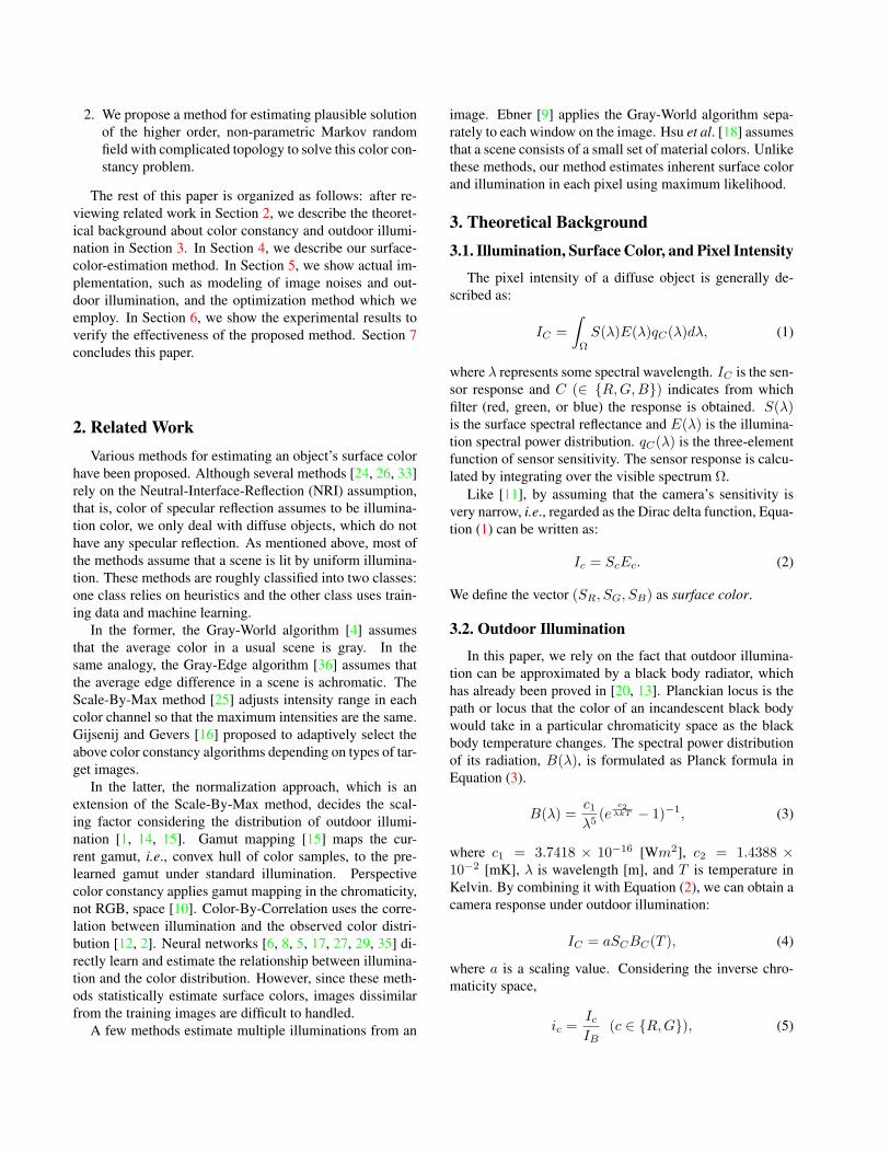
Figure 6. Input image pairs of the Macbeth Color Checker takenunder different outdoor illuminations.

noise effects, the ground-truth surface color is obtained byaveraging pixel values of each patches (30 × 30 pixels inthis experiment).

We define the difference between the estimated andground truth as the angular error in the RGB space:

RR + GG + BB√

R2 + G2 + B2√

R2 + G2 + B2.

R, G, B, R,G,B are respectively the ground truth and theestimated values in the RGB space. The angular error isusually used for the evaluation in this research area.

Result We conducted experiments using five pairs of im-ages which were taken under different illuminations. Fig-ure 6 are several examples of the pairs. Figure 7 shows oneof the result of surface-color-estimation. From top to bot-tom, rows of Figure 7 show the inputs, estimation by Fin-layson’s [11] and Kawakami’s methods [21], estimation bythe proposed methods, and ground truth.

In addition, we quantitatively evaluated them by usingthe average estimation error. As shown in Table 1, the es-timation results of our methods have better accuracy com-pared to the previous works [11, 21]. This result provesthat it is advantageous to handle image noises by maximumlikelihood manner and to handle spatial continuity by MRFframework in estimation of surface colors.

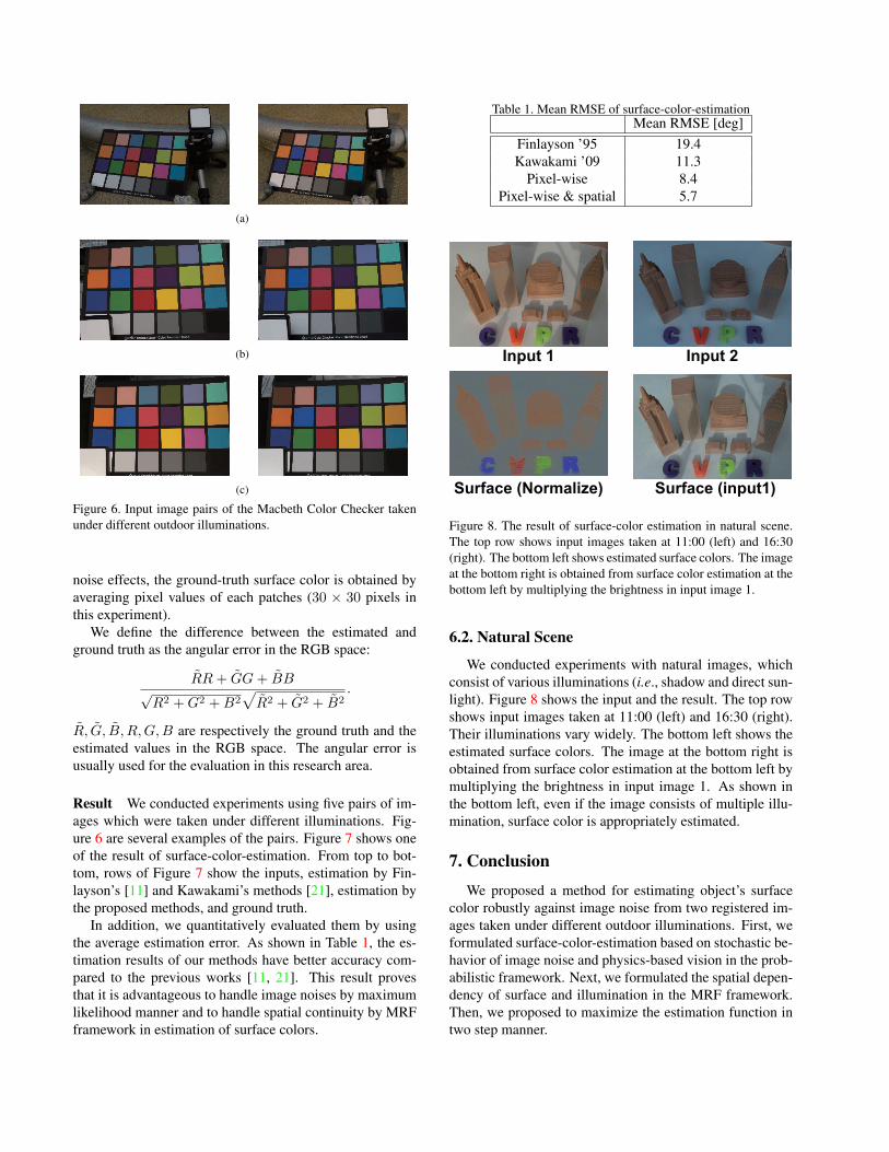
Table 1. Mean RMSE of surface-color-estimationMean RMSE [deg]

Finlayson ’95 19.4Kawakami ’09 11.3

Pixel-wise 8.4Pixel-wise & spatial 5.7

Input 2Input 1

Surface (input1)Surface (Normalize)

Figure 8. The result of surface-color estimation in natural scene.The top row shows input images taken at 11:00 (left) and 16:30(right). The bottom left shows estimated surface colors. The imageat the bottom right is obtained from surface color estimation at thebottom left by multiplying the brightness in input image 1.

6.2. Natural Scene

We conducted experiments with natural images, whichconsist of various illuminations (i.e., shadow and direct sun-light). Figure 8 shows the input and the result. The top rowshows input images taken at 11:00 (left) and 16:30 (right).Their illuminations vary widely. The bottom left shows theestimated surface colors. The image at the bottom right isobtained from surface color estimation at the bottom left bymultiplying the brightness in input image 1. As shown inthe bottom left, even if the image consists of multiple illu-mination, surface color is appropriately estimated.

7. Conclusion

We proposed a method for estimating object’s surfacecolor robustly against image noise from two registered im-ages taken under different outdoor illuminations. First, weformulated surface-color-estimation based on stochastic be-havior of image noise and physics-based vision in the prob-abilistic framework. Next, we formulated the spatial depen-dency of surface and illumination in the MRF framework.Then, we proposed to maximize the estimation function intwo step manner.

Ground truth

Input image 1

Input image 2

Pixel-wise & spatial

Pixel-wise

Kawakami ‘09

Finlayson ‘95

Figure 7. The result of surface-color estimation. From top to bottom, inputs, estimation by Finlayson’s [11] and Kawakami’s methods [21],estimation by the proposed methods, and ground truth are shown.

Our experimental results quantitatively demonstrated theeffectiveness of the proposed algorithm compared to theprevious methods. This result insists on the effectiveness ofconsidering both image noise effect and spatial consistencyto solve color constancy problem.

One of our future directions is to design a method to es-timate only from a single image. To prepare the two reg-istered images under different illuminations is sometimesdifficult. Another direction is to estimate surface color fromimages which include interreflection or specular reflection.We believe that the ability to estimate illumination at eachpixel is advantageous.

References[1] K. Barnard, G. Finlayson, and B. Funt. Color constancy for

scenes with varying illumination. In Proc. of European Conf.on Comp. Vis. (ECCV), pages 276–287, 2004. 2

[2] K. Barnard, L. Martin, and B. Funt. Colour by correlationin a three dimensional colour space. In Proc. of EuropeanConf. on Comp. Vis. (ECCV), pages 375–389, 2000. 2

[3] J. Besag. On the statistical analysis of dirty pictures. J. Roy.Stat. Soc. B, 48:259–302, 1986. 4, 5

[4] G. Buchsbaum. A spatial processor model for object colourperception. J. of The Franklin Institute 310, pages 1–26,1980. 2

[5] V. Cardei and B. Funt. Learning color constancy. In Proc.of Imaging Science and Technology / Society for Informa-tion Display Fourth Color Imaging Conference, pages 58–60, 1996. 2

[6] S. Courtney, L. Finkel, and G. Buchsbaum. A multistageneural network for color constancy and color induction.IEEE Trans. on Neural Networks, 6(6):972–985, 1995. 2

[7] R. Duda, D. Stork, and P. Hart. Pattern Classification. Wiley,John and Sons, 2000. 4

[8] P. Dufort and C. Lumsden. Color categorization and colorconstancy in a neural network model of v4. Biological Cy-bernetics, 65(4):293–303, 1991. 2

[9] M. Ebner. Color constancy using local color shifts. In Proc.of European Conf. on Comp. Vis. (ECCV), pages 276–287,2004. 2

[10] G. Finlayson. Color in perspective. IEEE Trans. on Patt.Anal. and Mach. Intell., 18(10):1034–1038, 1996. 2

[11] G. Finlayson, B. Funt, and K. Barnard. Color constancy un-der varying illumination. In Proc. of Int’l Conf. on Comp.Vis. (ICCV), pages 720–725, 1995. 1, 2, 3, 4, 5, 6, 7

[12] G. Finlayson, S. Hordley, and P. Hubel. Color by correlation:A simple, unifying framework for color constancy. IEEETrans. on Patt. Anal. and Mach. Intell., 23(11):1209–1221,2001. 2

[13] G. Finlayson and G. Schaefer. Solving for colour constancyusing a constrained dichromatic reflectionmodel. Int. J. ofComp. Vis., 42(3):127–142, 2002. 2

[14] D. Forsyth. A novel approach to colour constancy. In Proc.of Int’l Conf. on Comp. Vis. (ICCV), pages 9–18, 1988. 2

[15] D. Forsyth. A novel algorithm for color constancy. Int. J. ofComp. Vis., 5(1):5–36, 1990. 2

[16] A. Gijsenij and T. Gevers. Color constancy using naturalimage statistics. In Proc. of Comp. Vis. and Patt. Recog.(CVPR), pages 1–8, 2007. 2

[17] J. Herault. A model of colour processing in the retinaof vertebrates: From photoreceptors to colour oppositionand colour constancy phenomena. Neurocomputing, 12(2-3):113–129, 1996. 2

[18] E. Hsu, T. Mertens, S. Paris, S. Avidan, and F. Durand. Lightmixture estimation for spatially varying white balance. ACMTrans. on Graphics, 27(3):70–70, 2008. 2

[19] M. Isard. Pampas: real-valued graphical models for com-puter vision. In Proc. of Comp. Vis. and Patt. Recog. (CVPR),pages 613–620, 2003. 4

[20] D. Judd, D. MacAdam, and G. Wyszecki. Spectral distribu-tion of typical daylight as a function of correlated color tem-perature. J. of the Optical Society of America, 54(8), 1964.2

[21] R. Kawakami and K. Ikeuchi. Color estimation from a sin-gle surface color. In Proc. of Comp. Vis. and Patt. Recog.(CVPR), 2009. 5, 6, 7

[22] R. Kawakami, K. Ikeuchi, and R. Tan. Consistent surfacecolor for texturing large objects in outdoor scenes. In Proc.of Int’l Conf. on Comp. Vis. (ICCV), volume 2, pages 1200–1207, 2005. 1, 4

[23] R. Kawakami, J. Takamatsu, and K. Ikeuchi. Color con-stancy from blackbody illumination. J. of the Optical Societyof America, 24-7:1886–1893, 2007. 3

[24] G. J. Klinker, S. A. Shafer, and T. Kanade. The measurementof highlights in color images. Int. J. of Comp. Vis., 2(1):7–26,1992. 2

[25] E. Land and J. McCann. Lightness and retinex theory. J. ofthe Optical Society of America, 61(1):1–11, 1971. 2

[26] H. Lee. Method for computing the scene-illuminant chro-maticity from specular highlights. J. of the Optical Societyof America, 3(10):1694–1699, 1986. 2

[27] A. Moore, J. Allman, and R. Goodman. Real time neural sys-tem for color constancy. IEEE Trans. on Neural Networks,2(2):237–247, 1991. 2

[28] J. Nelder and R. Mead. The downhill simplex method. Com-puter Journal, 7:308–310, 1965. 5

[29] C. Novak and S. Shafer. Supervised color constancy for ma-chine vision. Jones and Bartlett Publishers, Inc., 1992. 2

[30] M. Park, Y. Liu, and R. Collins. Efficient mean shift beliefpropagation for vision tracking. In Proc. of Comp. Vis. andPatt. Recog. (CVPR), pages 1–8, 2008. 4

[31] E. Sudderth, T. Ihler, W. Freeman, and A. Willsky. Nonpara-metric belief propagation. In Proc. of Comp. Vis. and Patt.Recog. (CVPR), pages 605–612, 2003. 4

[32] J. Takamatsu, Y. Matsushita, and K. Ikeuchi. Estimatingcamera response functions using probabilistic intensity sim-ilarity. In Proc. of European Conf. on Comp. Vis. (ECCV),2008. 4

[33] R. Tan, K. Nishino, and K. Ikeuchi. Color constancy throughinverse-intensity chromaticity space. J. of the Optical Societyof America, 21(3):321–334, 2004. 2

[34] Y. Tsin, V. Ramesh, and T. Kanade. Statistical calibration ofccd imaging process. In Proc. of Int’l Conf. on Comp. Vis.(ICCV), pages 480–487, 2001. 4

[35] S. Usui and S. Nakauchi. A neurocomputational model forcolour constancy. In Selected Proceedings of the Interna-tional Conference, pages 475–482, 1997. 2

[36] J. van de Weijer, T. Gevers, and A. Gijsenij. Edge-based color constancy. IEEE Trans. on Neural Networks,16(9):2207–2214, 2007. 2