www.sciencemag.org/cgi/content/full/science.aab3884/DC1

Supplementary Material for

Genomic evidence for the Pleistocene and recent population history of Native Americans

Maanasa Raghavan, Matthias Steinrücken, Kelley Harris, Stephan Schiffels, Simon Rasmussen, Michael DeGiorgio, Anders Albrechtsen, Cristina Valdiosera, María C. Ávila-Arcos, Anna-Sapfo Malaspinas, Anders Eriksson, Ida Moltke, Mait Metspalu,

Julian R. Homburger, Jeff Wall, Omar E. Cornejo, J. Víctor Moreno-Mayar, Thorfinn S. Korneliussen, Tracey Pierre, Morten Rasmussen, Paula F. Campos, Peter de Barros

Damgaard, Morten E. Allentoft, John Lindo, Ene Metspalu, Ricardo Rodríguez-Varela, Josefina Mansilla, Celeste Henrickson, Andaine Seguin-Orlando, Helena Malmström,

Thomas Stafford Jr., Suyash S. Shringarpure, Andrés Moreno-Estrada, Monika Karmin, Kristiina Tambets, Anders Bergström, Yali Xue, Vera Warmuth, Andrew D. Friend, Joy

Singarayer, Paul Valdes, Francois Balloux, Ilán Leboreiro, Jose Luis Vera, Hector Rangel-Villalobos, Davide Pettener, Donata Luiselli,3 Loren G. Davis, Evelyne Heyer, Christoph P. E. Zollikofer, Marcia S. Ponce de León, Colin I. Smith, Vaughan Grimes, Kelly-Anne Pike, Michael Deal, Benjamin T. Fuller, Bernardo Arriaza, Vivien Standen, Maria F. Luz, Francois Ricaut, Niede Guidon, Ludmila Osipova, Mikhail I. Voevoda,

Olga L. Posukh, Oleg Balanovsky, Maria Lavryashina, Yuri Bogunov, Elza Khusnutdinova, Marina Gubina, Elena Balanovska, Sardana Fedorova, Sergey Litvinov, Boris Malyarchuk, Miroslava Derenko, M. J. Mosher, David Archer, Jerome Cybulski, Barbara Petzelt, Joycelynn Mitchell, Rosita Worl, Paul J. Norman, Peter Parham, Brian

M. Kemp, Toomas Kivisild, Chris Tyler-Smith, Manjinder S. Sandhu, Michael Crawford, Richard Villems, David Glenn Smith, Michael R. Waters, Ted Goebel, John R. Johnson, Ripan S. Malhi, Mattias Jakobsson, David J. Meltzer, Andrea Manica, Richard Durbin,

Carlos D. Bustamante, Yun S. Song,* Rasmus Nielsen,* Eske Willerslev,*

*Corresponding authors. E-mail: yss@berkeley.edu (Y.S.S.); rasmus_nielsen@berkeley.edu (R.N.); ewillierslev@snm.ku.dk

Published 21 July 2015 on Science Express

DOI: 10.1126/science.aab3884

This PDF file includes:

Materials and Methods Supplementary Text Figs. S1 to S41 Tables S1 to S15 Full Reference List

2

S1. Sample background and data generation (ancient & present-day samples) Data generation and analyses were performed with approval from The National Committee on Health Research Ethics, Denmark (H-3-2012-FSP21). We note the use of different laboratory protocols due to sample processing (modern and ancient) being conducted in multiple laboratories and ancient DNA facilities. Some of the differences in the methods also arise from the use of different tissues that warrant different treatments/protocols, as well as optimization of protocols over time within the same research group. Present-day Native American, Siberian and Oceanian genomes We sequenced present-day genomes from 5 Native Americans, 12 Siberians and 14 Oceanians to high depth and analyzed them together with previously published genomes to study the early peopling of the Americas (Table S1, Fig. S1). Siberia: a. Buryat: During the summer of 1998, peripheral blood samples (venipuncture) of western Buryat were collected from volunteers residing in Ghani. Ghani is a small community of 500 individuals on the Ust-Orda Buryat Okrug situated west of Lake Baikal in Siberia. Informed consent was administered in Russian by the team’s Russian geneticists and IRB approval was received from the University of Kansas IRB. Extraction was performed on two samples using the Super Quik-Gene extraction kit (Analytical Genetic Testing Center, USA). b. Koryak: During the summer of 2001, Koryak blood samples were collected from volunteers residing on Anavguy, Kamchatka. Informed consent was administered in Russian and IRB approval received from the University of Kansas IRB. Extraction was performed on two samples using the Super Quik-Gene extraction kit (Analytical Genetic Testing Center, USA). c. Sakha: Two unrelated and reportedly unadmixed Sakha were sampled upon receiving informed consent in geographically distant parts of Sakha Republic, Russian Federation. Self reported ethnicity of sample donors’ parents and grandparents is also Sakha. DNA was extracted from blood using standard proteinase K, phenol/chloroform procedure. d. Ket: Two unrelated and reportedly unadmixed Kets were sampled upon receiving informed consent in Kellogg settlement in Turukhansky rayon in Krasnoyarsky Krai, Russian Federation. DNA was extracted from blood using standard proteinase K, phenol/chloroform procedure. e. Altai: Two unrelated and reportedly unadmixed Altaians were sampled upon receiving informed consent in geographically distant parts of the Altay Republic in Russian Federation. One sample donor comes from Telengit-Sortogoy settlement in Kosh-Agachsky district and the other from Kulada settlement in Ongudaisky district. DNA was extracted from blood using standard proteinase K, phenol/chloroform procedure. All the above genome-sequenced individuals were previously single nucleotide polymorphism (SNP)-typed in: (29) (altai378k labeled as altai14; Buryats and Koryaks),

3

(4) (altai80) and (30) (Kets and Sakha). The individuals were selected for whole genome sequencing based on their ancestry profiles as revealed by ADMIXTURE (36) analysis. The samples were selected to best represent their respective populations and avoid recent genetic admixture from populations of western Eurasian origin. We also verified from genotype data that the individuals to be sequenced did not represent close relatives. Blunt-end Illumina libraries were constructed and amplified for the above samples as outlined for the Nivkh samples in (39). Briefly, two libraries were built for each of the samples, except altai378k for which only one library was constructed. Between 0.5-1.4 µg of sheared DNA (Bioruptor, NGS, Diagenode) was used as input per library and built into blunt-end libraries using NEBNext DNA Sample Prep Master Mix Set 2 (New England Biolabs, E6070). Amplification of the libraries was performed for 10 cycles using Phusion polymerase, as indicated in (39), and followed by size selection on a 2% agarose gel. Equimolar pools of the libraries were sequenced on the HiSeq 2000 and HiSeq 2500 in rapid run mode (paired-end, 100 cycles) at the Danish National High-Throughput DNA Sequencing Centre. f. Siberian Eskimo (Yupik): Whole blood samples were collected in June 1989 during fieldwork in Novoye Chaplino (New Chaplino), Chukotskiy Avtonomnyy Okrug (Chukchi Autonomous County), Russia from healthy, unrelated individuals from whom appropriate informed consent together with information about birthplace, parents and grandparents was obtained. All participants lacked non-native ancestors and had either been born or had derived from New Chaplino and a few other nearby, but no longer existing, villages. Genomic DNA was extracted from buffy coats by using standard phenol/chloroform procedure. Of the 19 Siberian Eskimo samples that were successfully genotyped previously with Illumina OmniExpress bead arrays, 13 samples passed the tests of relatedness at IBD < 0.125 (31). We estimated pairwise IBD iteratively using PLINK (65) (excluding fixed alleles) and removed individuals that had an IBD > 0.125 in each iteration. This process was repeated until no individuals had an IBD > 0.125. Two samples with the highest DNA concentration, Esk17B (male) and Esk20 (female) were chosen for whole genome sequencing. The PLINK (65) estimated PI_HAT value for the Esk17B and Esk20 pair was 0. Both Esk17B and Esk20 showed the presence of only one ancestry component in ADMIXTURE (36) analyses at K=4, revealing no detectable signature of European admixture. Two blunt-end Illumina libraries were built for each of the two samples as outlined above for the other Siberians. A test lane was initially run on MiSeq (paired-end, 100 cycles), after which the rest of the lanes were run on HiSeq 2000 at the Danish National High-Throughput DNA Sequencing Centre (single-read, 100 cycles). Americas: a-d. Pima, Huichol, Yukpa, Aymara: One Pima and one Huichol individual from Northern Mexico, and one Yukpa individual from near the Caribbean coast of Venezuela were selected from previously SNP-typed samples (32-34), while one Aymara individual from the Peruvian Andes was selected based on SNP chip genotyping performed in this study. Based on SNP array data, these samples did not show evidence of European admixture and thus were selected for whole genome sequencing. Genomic libraries were constructed using Nextera DNA Sample Preparation Kits (Epicentre, Chicago, IL, USA) and sequenced at the Stanford Center for Genomics and Personalized Medicine using

4

Illumina HiSeq 2000 sequencing platform (paired-end). e. Tsimshian: We sequenced one Tsimshian genome previously SNP-typed in (35), stemming from collaboration between authors R.S.M. and J.C. and the Tsimshian that began in 2009. Following consultation from the tribal councils and community meetings, we collected saliva samples using the DNA Genotek Saliva Sampling Kit. We visit the communities on a regular basis and provide community members the latest results of the research study and answer questions asked by the community members. Some community members attended the Summer Internship for Native Americans in Genomics (SING) workshop, to obtain a detailed understanding of genomic research. DNA was extracted from the Tsimshian individual using the DNA isolation kit from Oragene. Two blunt end libraries were constructed and amplified as indicated for the Siberians, except, for one of the libraries two parallel PCR reactions were set up using different indexes. Sequencing was performed on HiSeq 2000 in single-read mode (100 cycles) at the Danish National High-Throughput DNA Sequencing Centre. Oceania: a. Papuans: We sequenced the genomes of 14 Papuan individuals from the Human Genome Diversity Project-Centre de'Etude du Polymorphism Humain (HGDP-CEPH) panel (66). The DNA was derived from lymphoblastoid cell lines and was obtained from Fondation Jean Dausset-CEPH, Paris, France. A single library was constructed for each sample with a target insert size of 350 bp, and sequenced on the Illumina HiSeq X Ten platform (paired-end, 151 cycles) at the Wellcome Trust Sanger Institute. Ancient shotgun dataset I. Assessing genetic patterns within the Americas a. 939 This sample was previously analyzed and its mtDNA haplogroup presented in (67), referred to as XVII-B-939 (hereafter 939). Briefly, the Lucy Islands, British Columbia, Canada are an isolated cluster in Chatham Sound, 19 km west of the city of Prince Rupert and its inner harbour (Fig. S1). Traditionally, the Lucy Islands are included in the territory of the Gitwilgyots, a Tsimshian-speaking tribe that wintered in the Prince Rupert area at the time of European contact. On the largest island, a small rectangular house depression adjacent to a large shell midden site (archaeological site GbTp-1) is inferred to be a seasonal camp (68). Seven radiocarbon assays date the cultural deposits at this site from 7550 to 5280 calibrated years before present (cal BP) (68). The older dates are supported by the elevation of the cultural deposits above the shoreline. A sea level curve, created for neighboring islands, demonstrates that sea levels in the period between 8000 and 5000 radiocarbon years BP were higher than they are today (69). An incomplete lower jaw of a late middle-aged or older male (939) was found with other human remains, exposed on the shell midden deposit of GbTp-1 during the winter of 1984-1985 AD when two trees were felled by strong winds. The human remains were collected by personnel from the Museum of Northern British Columbia, Prince Rupert, and sent for

5

osteological analysis to the Canadian Museum of Civilization, Gatineau. A brief report was filed (70) and the remains were assigned catalog numbers and accessioned by the latter institution with the approval of the Metlakatla Indian Band. Measured collagen based radiocarbon age of 5710±40 BP was obtained for 939 (Beta-317343). Conventional age of 5930±40 BP was also reported by Beta Analytic Inc., along with a δ13C value of -11.6‰. This value indicates a diet high in marine protein according to a scale developed for Prince Rupert Harbour skeletal remains (71-73), and required compensation for a marine reservoir influence on the radiocarbon age estimate. The corrected two-sigma age range for sample 939 was 6260-5890 cal BP. DNA extraction: A DNA extraction from a tooth from the sample 939 was completed in an ancient DNA laboratory facility at the University of Illinois. Surface contamination from the tooth was removed by submerging it in 6% sodium hypochlorite (full strength Clorox bleach) for 6 minutes. The bleach was removed and the sample was then rinsed twice with DNA-free ddH2O and once with isopropanol to remove any remaining bleach. The sample was then placed in a UV crosslinker until dry. Approximately 0.20 grams of tooth powder was obtained using a Dremel tool at low speeds to minimize the production of heat. The tooth powder was then incubated in 4 ml of demineralization/lysis buffer (0.5 M EDTA, 33.3 mg/ml Proteinase K, 10% N-lauryl sarcosine) for 12-24 hours at 37°C. The digested sample was then concentrated to approximately 100 ml using Amicon centrifugal filter units. Following concentration, the digest was run through silica columns using the Qiagen PCR Purification Kit and eluted in 60 µl volume of DNA extract. Library preparation and sequencing: Approximately 50 µl of DNA extract was used to create a genomic library with adapters that contained a unique index for each library. The following modifications were made to the TruSeq DNA Sample Preparation V2 protocol. The DNA extract was not sheared as the DNA is expected to be fragmented due to taphonomic processes. A 1:20 dilution of adapters was used, as the DNA concentration in the extract is presumably low. Multiple Ampure Bead XP clean ups were completed in an attempt to remove adapter-dimers that may have developed. A PCR amplification of the genomic library was prepared in the ancient DNA laboratory (25 µl reaction with 10 µM primers, 5x PCR Buffer, 10 mM Kapa dNTPs, KapaHiFi polymerase, genomic library) and then transported to thermocyclers in the contemporary laboratory, across campus, in a sealed environment. The genomic library was amplified for 15 cycles, and was then cleaned with the Qiagen MinElute Purification Kit. The quality of the libraries were assessed on the Agilent 2100 Bioanalyzer using the High Sensitivity DNA kit and sequenced on HiSeq 2000 in single-read mode (100 cycles) at the Danish National High-Throughput DNA Sequencing Centre.

b. Enoque65 This sample originates from a left human femur, found in a cave called Toca do Enoque in Serra da Capivara, Piaui, Brazil (site number 951) (Fig. S1). It was recorded as skeleton 3 from burial 3. We carried out radiocarbon dating of this sample as part of this study and found it to date to ~ 3500 cal BP (Table S2). DNA extraction: All DNA extractions, library preparations and PCR set-ups were performed in a dedicated ancient DNA facility at the Centre for GeoGenetics

6

(Copenhagen). All subsequent molecular biology-based laboratory work, such as PCR amplification, Bioanalyzer runs and sequencing, was performed in a separate post-PCR DNA facility. Between 0.01 and 0.09 g of bone powder, obtained by drilling into the bone with Dremel drill, was incubated overnight at room temperature in 1.5 mL buffer consisting of 0.5 M EDTA and 25 mg/mL proteinase K. To pellet the nondigested powder, the solution was centrifuged at 12,000 rpm for 5 min. The liquid fraction was then transferred to a Centricon microconcentrator (30-kDa cutoff), and spun at 4,000 × g for 10 min. When the liquid was concentrated down to about 200 to 250 µL, the DNA was purified using a Qiagen MinElute PCR purification kit with the following modifications: a) spins were done at 8,000rpm with the exception of the final one at 13,000rpm, and b) in the elution step, spin columns were incubated in 40 µl buffer EB at 37ºC for 10 minutes, spun down, and repeated once more. The eluates from both rounds of elution were pooled. Library preparation and sequencing: Three double stranded DNA Illumina libraries were constructed from the extract. Blunt-end libraries were constructed on 21.25 µl of the DNA extract using NEBNext DNA Sample Prep Master Mix Set 2 (New England Biolabs, E6070). The protocols outlined in the kit manual and (39) were followed with the following modifications. Reaction volumes were cut down from the manufacturer’s protocol by a quarter in the end-repair step and by half in the ligation and fill-in steps. After the end-repair and ligation incubations, the reaction was purified through Qiagen MinElute spin columns and eluted in 15 µl and 21 µl, respectively, after a 5-minute incubation at 37°C with Qiagen EB buffer. Ligation reaction was performed for 25 minutes at 20º C using Illumina-specific adapters specified in (74). Fill-in reaction was performed for 20 minutes at 65º C. The purified libraries were amplified in a two-step manner, where 5 µl PCR product from the first amplification round was transferred into new 50 µl PCR reactions. To increase complexity, the second-round PCRs were set up as four parallel reactions. PCR products were then pooled and purified through a single Qiagen MinElute spin column, and eluted in 25 µl EB buffer following a 10-minute incubation at 37ºC. The purified libraries were amplified as follows: 25 µl DNA library, 1X High Fidelity PCR buffer, 2 mM MgSO4, 200 µM dNTPs each (Invitrogen, Carlsbad, CA), 200 nM Illumina Multiplexing PCR primer inPE1.0, 4 nM Illumina Multiplexing PCR primer inPE2.0, 200 nM Illumina Index PCR primer, 1 U of Platinum Taq DNA Polymerase (High Fidelity) (Invitrogen, Carlsbad, CA) and water to 50 µl. Cycling conditions were: initial denaturing at 94°C for 4 minutes, 8 cycles of 94°C for 30 seconds, 60°C for 30 seconds, 68°C for 40 seconds, and a final extension at 72°C for 7 minutes. PCR products were purified through Qiagen MinElute spin columns and eluted in 20 µl of Qiagen Buffer EB, following a 10-minute incubation at 37°C. A second round of PCR (four parallel reactions for each library) was set up as follows: 5 µl of purified product from first PCR round, 1X High Fidelity PCR buffer, 2 mM MgSO4, 200 µM dNTPs each, 200 nM each of Sol_bridge_P5 and Sol_bridge_P7 primers (75), 1 U of Platinum Taq DNA Polymerase (High Fidelity), and water to 50 µl. Cycling conditions included an initial denaturing at 94°C for 4 minutes, 10 cycles of 94°C for 30 seconds, 58°C for 30 seconds, 68°C for 40 seconds, and a final extension at 72°C for 7 minutes. The amplified libraries were run on Agilent 2100 Bioanalyzer High Sensitivity DNA chip. Samples were pooled and sequenced on HiSeq 2000 (100 cycles, single read mode) at the Danish National High-Throughput DNA Sequencing Centre.

7

c. Chinchorro The Chinchorro mummies originate from the northern sector of Arica, Chile and were excavated in 1990 (Fig. S1). The mummies were found in a shallow burial, in a terrace with sandy and rocky terrain. All bodies were fragmented, grouped together and presented artificial mummification (black style) (76). The sample processed in this study derives from the mummy Maderas Enco C2, a female over 25 years old, which was relatively dated to ~ 4800 BP by the type of body preparation. Funerary body treatment consisted of de-fleshing and modeling with clay, sticks and reeds. The body was completely modeled with whitish-grey clay. There was also evidence of a small hole in the skull to anchor the head to the rest of the body. The teeth did not present any cavities. Energy dispersive X-ray fluorescence (ED-XRF) analysis showed that the whitish-grey clay primarily contained SiO2 (68.9%) (77). Using EDXRF, the mineral composition of the modeling showed that this clay was mainly composed of quartz, albite, sanidine and muscovite. The physical properties show that the clay was very fine and of good quality to model the bodies. The complex mummification techniques, high quality of the clay and low head lice infestation in the wigs (78) clearly show that the morticians paid a great deal of attention to details while preparing the mummies. The mummy also presented camelid skin (fur) as part of the wrapping. We sampled bone from the mummy for DNA analysis and hair for radiocarbon dating, and the camelid skin to discern the marine reservoir offset. We dated the mummy sample to ~5800 cal BP after taking into account the marine reservoir effect (Table S2). DNA extraction: Sample processing for DNA analysis was undertaken in the dedicated clean laboratory and post-PCR facilities of Centre for GeoGenetics (Copenhagen). Bone material from the Maderas Enco-1C2 individual was sampled from Universidad de Tarapacá in Chile. Prior to powdering, the bone sample was slightly cleaned on the surface with a cloth drenched in 10% hypochlorite. Next, the outermost surface was drilled into powder with a Dremel drill-bit and discarded. The remaining powder was then distributed into two sterile tubes with approximately 350 mg of drilled bone powder in each. The bone powder was digested according to the procedures outlined in (79), in 4.7 mL buffer consisting of 0.5 M EDTA, 0.2 mg/ml Proteinase K, and 0.5% N-Laurylsarcosyl and incubated at 50ºC. The DNA was extracted from the digest using an in-solution silica approach. The binding solution was a guanidinium thiocyanate-based binding buffer containing 118.2 g guanidinium thiocyanate with 2.5 mM Tris, 25 mM NaCl, 20 mM EDTA, 1 g N-Lauryl-Sarcosyl and water, in a total volume of 200 mL. After DNA binding, the silica was centrifuged and washed twice with 80% cold ethanol, and the DNA eluted in 80 µl Qiagen EB Buffer. Library preparation and sequencing: Blunt-end, double-stranded Illumina sequencing libraries were built using the NEBNext DNA Library Prep Master Mix Set (E6070), according to protocols described in (79). A volume of 20 µl of DNA extract was used for each library, without prior nebulization, since ancient DNA is already highly fragmented. Library amplification followed a two-round PCR setup described previously (74). The amplifications were done in 50 µl reactions, consisting of 1X PCR buffer, 4 mM MgCl2, 0.4 mg/ml BSA, 125 µM dNTPs, 0.2 µM of each primer (Illumina Multiplexing PCR primer inPE1.0 and custom indexed reverse primer (5’-CAAGCAGAAGACGGCATACGAGATNNNNNNGTGACTGGAGTTC- 3’), and 5

8

U AmpliTaq Gold DNA Polymerase (Applied Biosystems). The first amplification was carried out as follows: 5 minutes at 94°C, followed by 12 cycles of 30 seconds at 94°C, 30 seconds at 60°C and 40 seconds at 72°C, ultimately with a 7 minutes elongation step at 72°C. Identical thermocycling conditions were used for the second amplification, with 12-16 amplification cycles and a PCR mix consisting of 1X PCR buffer, 4 mM MgCl2, 0.4 mg/ml BSA, 250 µM dNTPs, 0.4 µM of each primer (P5 and P7), 2.5 U AmpliTaq Gold DNA Polymerase, 5 µl of first amplified library and water up to 25 µl. The amplified libraries were purified with PB buffer on Qiagen MinElute columns, before being eluted in 30 µl EB and subsequently quantified on Agilent Bioanalyzer 2100. The library pools were sequenced on HiSeq 2000 (100 cycles, single-read) at the Danish National High-throughput DNA Sequencing Centre.

d. MARC1492 Old Mission Point (ClDq-1) is located on the banks of the Restigouche River, near the town of Atholville in northern New Brunswick, Canada (Fig. S1). The site represents the prehistoric village of Tjigog, the place of summer aggregation for the northern Mi’gmaq (80-83). Rediscovered in 1968 by Martijn’s (84) archaeological surveys of Gloucester and Restigouche counties, the site was only excavated in 1972 and 1973 by Turnbull (85, 86) after construction workers unearthed human remains in a nearby gravel pit. The discovery of the burials left the skeletal assemblage badly commingled and fragmented, however, Turnbull’s (85) report features several photographs of in situ graves representing both primary and secondary internments, specifically in the form of bundle burials (see 87 and 88 for bundle burial descriptions). Artifacts recovered from the burials include a toggling harpoon head, worked bone, copper tube and shell beads, an axe head, rare pieces of cordage and braided plant-fibre textile, as well as remnants of beaver fur and birch bark (86, 88). Turnbull’s excavations also uncovered possible domestic architecture near the burial area in the form of post moulds, as well as over a thousand ceramic sherds featuring punctate, dentate-stamped, and pseudo-scallop shell designs (85). A single charcoal sample taken from a hearth feature associated with the ceramic finds gave an uncalibrated radiocarbon date of 2030±130 BP (RL-343) (89). With permission from the Listuguj Mi’gmaq community, the human remains recovered from the site underwent bioarchaeological assessment beginning in 2011 at Memorial University, where it was determined that at least 5 adults and 9 juvenile individuals (MNI=14) were included within the skeletal assemblage. Samples from a loose tooth (right mandibular first premolar (RPM1) - MARC1492) associated with a middle adult female individual (Skeleton #4) within the Old Mission Point assemblage were taken for ancient DNA analysis. The mandible of this individual in question was well-preserved unlike many of the skeletal elements found elsewhere in the assemblage, however, the in situ right first, second, and third molars (RM1, RM2, RM3) all feature a great deal of occlusal dental wear. The only remaining left molar (LM3) does not feature occlusal wear to the same extent. It is surmised that this female individual preferentially chewed on the right side of the mandible, the reason for which may be explained by the presence of a moderately healed periapical abscess located in the area of the left mandibular first and second molars (LM1, LM2) resulting in antemortem tooth loss. Uncalibrated radiocarbon AMS dates obtained on ultrafiltered bone collagen from the right femorii of 4 of the adult skeletons, (UCIAMS-125912, UCIAMS-107245, UCIAMS-107246: Skeleton #4,

9

UCIAMS-107247) as well as the lower extremities of 4 of the juvenile skeletons (UCIAMS-125908, UCIAMS-125909, UCIAMS-125910, UCIAMS-125911) ranged from 2405-415 BP. This time range overlaps with the previous uncalibrated charcoal radiocarbon date (89), and along with the ceramic finds, suggests that Mi’gmaq individuals were living and being buried in the area as long ago as the early Middle Woodland period (ca. 2150-1650 BP) and up and until the Late Woodland (ca. 650-400 BP) or Early Historic (ca. 400-250 BP) periods (90). These findings lend support to the idea that Old Mission Point represents the oldest known long-term use Mi’gmaq cemetery in the Canadian Maritimes region to-date (88). The sampled individual was dated to ~400 BP after correcting for marine reservoir effect. (Table S2). DNA extraction: All laboratory procedures including pre-treatment, extraction, library construction and PCR set-ups were carried out in ancient DNA facilities at the Centre for GeoGenetics (Copenhagen). Fine drill heads were used with a Dremel drill operated on low-speed setting to obtain the powdered sample. The tooth was drilled by cutting off the end of the roots and drilling into the pulp chamber with special dental drill heads, thereby collecting ~50 mg of powder. The collected powder were digested overnight at 55°C in 1 ml of a buffer consisting of 1 M urea, 0.5 M EDTA and 0.3 mg/ml Proteinase K (modified from 91). Following digestion, the supernatant was concentrated using a 30 kDa centrifugal filter unit down to 100-200 µl and purified through a Qiagen MinElute spin column (using Qiagen PN binding buffer) following manufacturer’s instructions. In the elution step, the column was incubated in 45 µl of Qiagen EB buffer at 37°C for 30 minutes, spun down, and re-incubated in 30 µl of EB buffer at 37°C for 15 minutes. Library preparation and sequencing: Two blunt-end Illumina libraries were prepared using NEBNext DNA Sample Prep Master Mix Set 2 (New England Biolabs, E6070), as described in (39), with the following differences in the protocols. Ligation was performed for 15 minutes at 20°C using Illumina-specific adapters specified in (74) and the fill-in reaction was performed for 20 minutes at 37º C. The libraries were amplified as follows: 25 µl DNA library, 1X High Fidelity PCR buffer, 2 mM MgSO4, 200 µM dNTPs each (Invitrogen, Carlsbad, CA), 200 nM Illumina Multiplexing PCR primer inPE1.0, 4 nM Illumina Multiplexing PCR primer inPE2.0, 200 nM Illumina Index PCR primer, 1 U of Platinum Taq DNA Polymerase (High Fidelity) (Invitrogen, Carlsbad, CA) and water to 50 µl. Cycling conditions were: initial denaturing at 94°C for 4 minutes, 12 cycles of: 94°C for 30 seconds, 60°C for 30 seconds, 68°C for 40 seconds, and a final extension at 72°C for 7 minutes. PCR products were purified through Qiagen MinElute spin columns and eluted in 10 µl of Qiagen Buffer EB, following a 10-minute incubation at 37°C. A second round of PCR (two parallel reactions for each library) was set up as follows: 5 µl of purified product from first PCR round, 1X High Fidelity PCR buffer, 2 mM MgSO4, 200 µM dNTPs each, 500 nM Illumina Multiplexing PCR primer 1.0, 10 nM Illumina Multiplexing PCR primer 2.0, 500 nM Illumina Index PCR primer, 1 U of Platinum Taq DNA Polymerase (High Fidelity), and water to 50 µl. Cycling conditions included an initial denaturing at 94°C for 4 minutes, 10 cycles of: 94°C for 30 seconds, 60°C for 30 seconds, 68°C for 40 seconds, and a final extension at 72°C for 7 minutes. Both PCR products originating from one library were purified through one Qiagen MinElute spin column and eluted in 20 µl of Qiagen Buffer EB, following a 10-minute incubation at 37°C. The amplified libraries were pooled in equimolar quantities, run on Agilent Bioanalyzer 2100 and thereafter sequenced on HiSeq 2000 (100 cycles,

10

single-read) at the Danish National High-throughput DNA Sequencing Centre. II. Testing the Paleoamerican hypothesis a. Pericúes The Pericúes occupied the southern tip of the Baja California peninsula, Mexico (Fig. S1) and went extinct approximately 200 years ago (92). They are argued to be a relict group of ‘Paleoamericans’ (23) owing to their distinctive cranial form (24). We generated genome-wide sequence data from six Pericúes excavated from the cave site of Piedra Gorda (Fig. S1), associated with the Las Palmas culture dating from 800 to 300 years BP. All Pericú bone and teeth samples (BC23, BC25, BC27, BC28, BC29 and BC30) were collected at the Museo Nacional de Antropología (Dirección de Antropología Física) in Mexico City from the Massey collection. Appropriate permits to conduct DNA analysis on these remains were obtained by the Coordinación Nacional de Arqueología y Consejo de Arqueología, dependent on the Instituto Nacional de Antropología Física (INAH). The Pericú samples were from the site of Piedra Gorda in Baja California, and the mummies from Sierra Tarahumara, located in Northern Mexico (Fig. S1).

b. Fuego-Patagonians The Fuego-Patagonian hunter-gatherers inhabited the southernmost tip of South America. They included the Yaghan (Yámana) group in the coastal area around the Beagle Channel in Tierra del Fuego, the Kaweskar (Alacalúf) who occupied the islands and channels from the southern Chilean Pacific Coast, and the Selknam (Ona) from Isla Grande in Tierra del Fuego (Fig. S1). It is generally agreed that these populations differ morphologically from Amerindians, with some suggesting they are a relict Paleoamerican group, although the significance of that differentiation and its cause, whether due to distinctive ancestry or diversification owing to drift and local adaptations is debated (23, 26, 27, 93-95). We generated genome-wide sequence data from eleven Fuego-Patagonian individuals with representatives from each of three aforementioned groups from European museum collections originally obtained in the 1800s. Yaghan and Selknam: Hair samples (890, 894 and 895) from the Yaghan (Yámana) individuals were obtained from the Cape Horn mission (1882-1883) and bone samples (MA572, MA575 and MA577) from the Selknam (Ona) were obtained from the Emperaire (1946-1949) and Rousson & Willems mission collections. All the samples from Tierra del Fuego reported here are stored at the Musée de l´Homme in Paris, France. The Yaghan bone samples are from the Orange Bay collection, MA572 is from the Magellan Straits, while no location is available for MA575 and MA577 from within Tierra del Fuego (Fig. S1). The appropriate permits for sampling and conducting DNA analyses were obtained by the Musée de l´Homme. Kaweskar The bone and tooth samples (AM66, AM71, AM72, AM73 and AM74) belonging to the Kaweskar (Alacalúf) population and originating from Patagonia, Chile (Fig. S1) were collected from the osteological collection at the Anthropological Institute at the University of Zürich, Switzerland. These samples were part of the Carl Hagenbeck

11

expedition into the Americas in 1882, and have been under custody of the University of Zürich since the late 1800´s. The samples originate from Patagonia, Chile, and have been sent back and buried there in 2010. Appropriate permits were obtained by the University of Zurich to conduct DNA analysis on these samples.

c. Pre-Columbian mummies We sequenced two pre-Columbian mummies from northern Mexico (Sierra Tarahumara) (Fig. S1), which were used as morphological controls since they are expected to fall within the range of Amerindian morphological cranial variation. The mummies (F9 and MOM6) were also collected at the Museo Nacional de Antropología (Dirección de Antropología Física) in Mexico City from the Momias de Mexico collection and permits to conduct DNA analysis were obtained by the Coordinación Nacional de Arqueología y Consejo de Arqueología, dependent on the Instituto Nacional de Antropología Física (INAH).

DNA extractions: All samples were prepared in dedicated aDNA facilities at the Center for GeoGenetics (Copenhagen) and at the Evolutionary Biology Center (Uppsala). The first millimeter of the bones and teeth was abraded using a Dremel tool and then ground into powder using a multitool drill (Dremel) or a Freezer Mill 6870 SPEX sampleprep. Between two hundred and four hundred milligrams of this bone/tooth powder were used for DNA extraction following three different silica binding methods as in (79) for the Selknam samples and as in (96) and (97) for the Kaweskar, Pericúes and Mexican mummies. Approximately 100 mg of the Yaghan head hair shaft samples were decontaminated on the surface through soaking in 0.5% sodium hypochlorite solution, followed by rinsing in UV irradiated ddH20. DNA was extracted using phenol-chloroform combined with Qiagen MinElute columns as previously described (98). The silica-bound DNA was purified sequentially with AW1/AW2 wash buffers (Blood and Tissue Kit, Qiagen), Salton buffer (60% Guanidine Thiocyanate and 40% H2O) and Qiagen PE buffer, before being eluted in 60 µl Qiagen EB buffer. Library preparation and sequencing: Given the degraded nature of ancient DNA, we constructed DNA libraries by skipping the initial fragmentation step. In Uppsala, 20 µl of extracted DNA were converted into Illumina multiplex sequencing libraries (blunt end ligation method), following (74). DNA was enriched by amplifying six PCR reactions for each library in a final volume of 25 µl. Library amplification was carried out using AmpliTaq Gold DNA Polymerase (Life Technologies) with a final concentration of 1X Gold Buffer, 2.5 mM MgCl2, 250 µM dNTP (each), 3 µl of DNA library, 0.2 µM IS4 PCR primer (5’- AATGATACGGCGACCACCGAGATCTACACTCTTTCCCTACACGACGCTCTT 3’) and 0.2µM indexing primer (5’- CAAGCAGAAGACGGCATACGAGATxxxxxxxGTGACTGGAGTTCAGACGTGT, where x is one of 228 different 7bp indexes provided in (74) and 0.1 U/µl of AmpliTaq Gold. Cycling conditions were as follows: a 12 min activation step at 94ºC, followed by 8-15 cycles of 30 seconds at 94ºC, 30 seconds at 60ºC, 45 seconds at 72ºC, with a final extension of 10 minutes at 72ºC. The number of cycles was different for each sample and varied between 8 and 15. After amplification, the libraries were run on a Bioanalyzer 2100 using the High Sensitivity DNA chip (Agilent) for DNA visualization. All 6

12

amplification reactions were purified using the AMPure XP (Agencourt-Beckman Coulter A63881) following the manufacturer’s guidelines. In Copenhagen, 20 µl of each DNA extract was built into a blunt-end library using the NEBNext DNA Sample Prep Master Mix Set 2 (E6070) and Illumina specific adapters (74). The libraries were prepared according to manufacturer's instructions, with a few modifications outlined below. The end-repair step was performed in 25 µl reactions using 20 µl of DNA extract. This was incubated for 20 minutes at 12°C and 15 minutes at 37°C, and purified using PN buffer with Qiagen MinElute spin columns, and eluted in 15 µl. Next, Illumina-specific adapters (prepared as in 74) were ligated to the end-repaired DNA in 25 µl reactions. The reaction was incubated for 15 minutes at 20°C and purified with PB buffer on Qiagen MinElute columns, before being eluted in 20 µl EB Buffer. The adapter fill-in reaction was performed in a final volume of 25 µl and incubated for 20 minutes at 37°C followed by 20 minutes at 80°C to inactivate the Bst enzyme. The entire DNA library (25 µl) was then amplified and indexed in a 50 µl PCR reaction, with 1X PCR buffer, 4 mM MgCl2, 0.4 µg/µl BSA, 250 µM dNTPs (each), 200 nM of each primer (inPE forward primer + indexed reverse primer), and 0.1 U/µl AmpliTaq Gold DNA Polymerase (Applied Biosystems). Thermocycling conditions were 5 minutes at 94°C, followed by 12 cycles of 30 seconds at 94°C, 30 seconds at 60°C and 40 seconds at 72°C, and a final 7 minutes elongation step at 72°C. This was followed by a second PCR reaction (25 µl total and 13 cycles) using 5 µl of the amplified library and P5/P7 primers (75). The amplified library was purified using PB buffer on Qiagen MinElute columns, before being eluted in 30 µl EB. Initially, before switching to blunt end ligation for library construction, we used a T/A ligation method; this applies to libraries built for samples AM66, AM71, AM72, BC25, BC30, F9 and MOM6; libraries for all other samples were built using the blunt-end method. In the T/A method, extracted DNA from samples was used to build Illumina index libraries (T/A ligation method), using the Rapid Library kit from Roche-454 (Branford, CO), with the following modifications to the manufacturer’s protocol. For each library, the fragmentation step was excluded, 16 µl of DNA extract was used and mixed with 2.5 µl RL 10X PNK buffer, 2.5 µl RL ATP, 1 µl RL dNTP, 1 µl RL T4 polymerase, 1 µl RL PNK and 1 µl RL Taq polymerase. The mix was incubated at 25°C for 20 minutes, 72°C for 20 minutes and then placed at 4°C. We then added 1 µl of Illumina indexing adaptor mix and 1 µl RL ligase and incubated the sample for 10 minutes at 25°C. Finally, the library was purified on a Qiagen MiniElute spin column according to protocol and eluted in 30 µl of Qiagen Buffer EB. Amplification of purified libraries was performed using Platinum Taq DNA Polymerase High Fidelity polymerase (Invitrogen) with a final mixture of 1X High Fidelity PCR Buffer, 4 mM MgSO4, 0.2 mM dNTP (each), 0.5 µM Multiplexing PCR primer 1.0 (5’-AATGATACGGCGACCACCGAGATCTACACTCTTTCCCTACACGACGCTCTT CCGATCT), 0.01 µM Multiplexing PCR primer 2.0 (5’-GTGACTGGAGTTCAGACGTGTGCTCTTCCGATCT), 0.5 µM PCR primer Index X (5’- CAAGCAGAAGACGGCATACGAGATN6GTGACTGGAGTTC), where X is one of 12 different indexes, and N6 is the corresponding tag), 3% DMSO, 0.02 U/µl Platinum HiFi polymerase, 10-20 µl of template and water to 50 µl final volume. Primers are part of Illumina’s Multiplexing Sample Prep Oligo Kit. Cycling conditions were as follows: a 3 minute activation step at 94 ºC, followed by 20 cycles of 30 seconds at 94 ºC, 20

13

seconds at 60 ºC, 20 seconds at 68 ºC, with a final extension of 7 minutes at 72 ºC. A second PCR was performed using same conditions as the first one but with 16 cycles. PCR products were finally gel purified before sequencing using a Qiagen gel extraction kit, following manufactures guidelines. The concentration and size profiles of the purified libraries were determined on a Bioanalyzer 2100. All libraries were pooled at equimolar concentrations and sequenced on HiSeq 2000 platform (100bp, single end) at the Danish National High-throughput DNA Sequencing Centre or at BGI Europe. SNP chip genotype data from present-day worldwide populations We assembled a panel of present-day worldwide samples genotyped with several different Illumina (Human610- Quad, HumanHap650Y, Human660W-Quad, HumanOmniExpress 730K and HumanOmni1-Quad) and Affymetrix genotyping arrays, and additionally included two ancient genomes (Clovis/Anzick-1 and Saqqaq). The panel contains 3053 samples from 169 populations (plus, Anzick-1 and Saqqaq) and most of the data come from previous studies (Table S3) (4-6, 29-34, 99-109). Of these, 79 new samples were typed specifically for this study (Table S4). These samples are from 28 different populations (Table S4), collected over the years with appropriate informed consent, and in most cases belong to populations that were underrepresented in previous studies (e.g. North America). Majority of the new samples were genotyped using the Illumina iScan System following the manufacturer’s protocol on Human660W-Quad, HumanOmniExpress 730K and HumanOmni1-Quad genotyping arrays. Genotype data was evaluated using Illumina GenomeStudio, version 2011.1, making use of genome build GRCh37/hg19 and most up-do-date manifest files. The Aymara samples were genotyped on the Affy6.0 array. Here we describe the merging steps we took to arrive at the final dataset. We first merged the genotype data of the new samples (N=79) to the genotype panel of previously published samples done on similar Illumina genotyping arrays using PLINK (65). For the older data we merged raw data first by array version and lifted where necessary using the Liftover tool at the UCSC Genome Browser (110) to reflect physical positions of human genome build 37(GRCh37). Marker rs numbers were matched with dbSNP hg19 build 135 using SNAP (111), and the strand was set according to the 1000 Genomes Project. AT and GC markers were removed in order to minimize potential strand errors during the merging of the data from the different Illumina arrays. For better coverage of Native American populations we turned to datasets published by (6) and (35) and merged our dataset with these. (6) used another genotyping array of Illumina Inc., which contains about 360 thousand markers. The intersection of our genotyping panel data and that of (6) yielded a dataset of ca. 200,000 SNPs. For merging, we started from the full dataset used in (6) of 2351 individuals, which includes both samples genotyped in that study and data from published sources. We excluded 556 samples from that dataset that came from overrepresented populations from the Hapmap collection (ASW,CEU, CHB, CHD, JPT, LWK, MEX, TSI). We further excluded 16 individuals from this dataset based on relatedness (1st and 2nd degree) to other samples in

14

the final merged dataset. We used KING (112) to determine relatedness. We removed AT GC markers in order to minimize potential strand errors during the merging of the datasets. We then extracted the SNPs (according to rsNumber) that overlapped between the two datasets (our Illumina and (2)) from our Illumina dataset and merged these data to the (6) panel using PLINK. During merger we retained SNP physical positions and strand orientations from (6). To further increase the Native American coverage we merged data from (35). The (35) dataset used Illumina Human610- Quad chip and therefore merging this dataset did not lead to further loss of SNPs in the final merged dataset. We also merged 16 samples from the Andaman Islands (106, 113). The overlap of SNPs in that panel (Affymetrix) with the ca. 200,000 SNPs in our panel was 34,868 SNPs. Therefore, we opted to keep all SNP positions retaining the Andaman samples with considerable amount of missing data. We further merged the datasets in (33, 34, 102) containing Solomon Islanders and Native American populations Huichol and Yukpa (Stanford Affymetrix data). We first merged these datasets over rsNumbers using PLINK and took the Huichol dataset, as the biggest, as the base. The number of overlapping SNPs was 903, 800. These data were mapped against human reference sequence build 18 (hg18). We therefore used rsNumbers to merge these data to the rest, which were mapped against hg19. We used SNAP to identify rsNumbers present in the Stanford Affymetrix data, which have new aliases in the most current dbSNP build 135. We found 625 such SNPs and removed those in order to avoid potential confusion. We then intersected these rsNumbers with the ca. 200,000 in the merged data (see above) and found 62,125 SNPs. We merged those to the master dataset retaining physical positions and strand orientation of the latter. We kept all ca. 200,000 SNP positions in the whole dataset to increase power in several analyses. The genotype calls extracted from the Saqqaq (29) and Anzick-1 (5) genomes according to SNP physical positions in hg19 were also merged to the final dataset. We thus ended up with a dataset of 3053 samples and SNP information for 199,285 autosomal loci (Table S3). This dataset that was used to run ADMIXTURE analysis (Section S5). For SNP chip-data based D-statistics and outgroup f3 statistics (Section S6), we used a subset of this panel consisting of 2610 individuals. The excluded individuals are from the following populations, which were only used for ADMIXTURE analysis: Huichol (34), Yukpa (33), Aymara (this study), Mexican (109) and Maya (32). We further filtered the data based on individuals with very little Native American ancestry (Section S5), and relatedness between the remaining individuals. The latter was done by estimating the kinship coefficient using REAP (114), based on inferred admixture proportions and allele frequencies estimated using ADMIXTURE. This was done for all pairs of individuals within each continent. Individuals were sequentially removed until all pairs of individuals had a kinship coefficient lower than 0.18. Finally, 2,510 individuals were left for the D-statistics and outgroup f3 statistics analyses (Table S3). Testing the Paleoamerican hypothesis: To increase representation of Amerindian groups in the SNP chip genotype panel, the analyses evaluating the Paleoamerican hypothesis employed a separate merged genotype dataset. This employed two SNP chip reference panels, each containing a subset of different Native American populations. We refer to these datasets as ARL (6) and AME (34). The ARL dataset includes 2,351 individuals

15

from worldwide populations genotyped on different Illumina arrays yielding a total of 364,470 intersecting SNPs. The subset of Native Americans consists of 493 individuals from 52 populations. Because several Native American individuals in this study were admixed and had some European ancestry, we used a version of the dataset in which the non-Native American segments were masked genome wide (set to missing) (6). The AME dataset comprises genotype data for 228 individuals assayed on the Affymetrix 6.0 SNP array platform for a total of 827,995 sites (34). This dataset includes unrelated and unadmixed individuals from 14 indigenous groups in Mexico, namely the Seri (n = 14), Tarahumara (n = 16), Huichol (n = 24), Purépecha (n = 3), Totonac (n = 18), Nahua from Jalisco (n = 10), Nahua from Puebla (n = 9), Triqui (n = 24), Mazatec (n = 16), Zapotec (n = 21), Tzotzil (n = 21), Tojolabal (n = 20), Lacandon (n = 21) and Maya (n = 11). Before merging the genotype data with the low-depth aDNA sequencing data from the ancient Pericúes, Fuego-Patagonians and Mexican mummies, we processed and filtered the SNP chip data to avoid potential biases (115). The following steps were carried out using a combination of custom scripts and PLINK v1.07 (65): we removed A/T and G/C as well as monomorphic SNPs from the panel, identified SNPs reported in the negative strand and inverted them in order to have all SNPs in the panel in forward orientation, lifted over coordinates from hg18 to hg19 and, randomly selected one allele at each site and for each individual in the reference panel and turned it into a homozygous genotype for the sampled allele. The last step in the above list was carried out to render the reference panel more similar to the whole genome data. Certainly, given the low depth of our sequence data, most of the sites are covered by a single read; hence, only one allele is observed (115). After applying the above filters the number of sites remaining were 363,909 and 675,295 for the ARL and AME datasets, respectively. After filtering, the genomic coordinates of the SNPs in the reference panels were queried from each sample’s bam file using the samtools mpileup command with the –l option (116). If there was one read covering the queried site, and if that read had a base with base quality above 20 at that site that did not represent a third allele, then the site was selected for downstream analyses. When more than one read covered a queried site, one of the reads was randomly selected among those with base quality above 20 at the site of interest and the same filters applied. The coordinates of sites that passed filters were then used to extract a subset from the reference panel with those sites. Finally, the ancient genotypes and the corresponding data from the reference panel were merged using PLINK v1.07 (65).

16

S2. Whole genome read processing (ancient & present-day samples) Present-day genomes Read processing The Illumina data was basecalled using Illumina software CASAVA 1.8.2 and sequences were de-multiplexed with a requirement of full match of the 6 nucleotide index that was used for library preparation. Samples prepared using Nextera were hard clipped 13 nucleotides of the 5’ end. Adapter sequences and leading/trailing stretches of Ns were trimmed from the reads and additionally bases with quality 2 or less were removed using AdapterRemoval-1.1 (117). Trimmed reads were mapped to the human reference genome build 37 using bwa-0.6.2 and filtered for mapping quality 30 and sorted using Picard (http://picard.sourceforge.net) and samtools (116). Data was merged to library level and duplicates removed using Picard MarkDuplicates (http://picard.sourceforge.net) and hereafter merged to sample level. Sample level BAMs were re-aligned using GATK-2.2-3 and had the md-tag updated and extended BAQs calculated using samtools calmd (116). Read depth and coverage were determined using pysam (http://code.google.com/p/pysam/) and BEDtools (118). Statistics of the read data processing are shown in Tables S1 and S5 for modern and ancient samples, respectively. The sequence data and the alignments are available for most of the samples at http://www.cbs.dtu.dk/suppl/NativeAmerican/ and the reads also through ENA accession number PRJEB9733, except where indicated as being under data access agreement (Table S1). Genotyping Genotypes were called both per individual and in a multi-sample approach using samtools-0.1.18 and bcftools (116). In the multi-sample approach all genomes were called simultaneously in 10 Mb windows with all sites emitted (GATK option) and hereafter merged per chromosome. Variants were extracted, converted to vcf and annotated using GATK-2.3-9 VariantAnnotator for FisherStrand, MappingQualityRankSumTest, ReadPosRankSumTest, RMSMappingQuality, HaplotypeScore and QualByDepth (119). Hereafter, the annotations were used to recalibrate the variants by GATK-2.3-9 VariantRecalibrator using the HapMap 3.3, OmniChip 2.5 and dbSNP135 resources with priors 15, 12 and 2, respectively. Recalibrated variants were filtered using a truth-sensitivity threshold of 99.9. Because samtools/bcftools will assign homozygous reference calls for individuals with missing data we masked individual calls with no coverage and phased the calls using shapeit2-r727 (120). The phasing was performed per chromosome for the autosomes and the X chromosome using only bi-allelic sites and a window size of 0.5. Phased calls were hereafter hard-filtered for 10X depth per individual (Y chromosomes were filtered for 5X depth) and for sites that violated a one-tailed test for Hardy-Weinberg Equilibrium at a p-value < 1e-4 (121). Because the GATK Variant Quality Score Recalibration approach classifies all variants on the mitochondrial chromosome as false, the mitochondrial variants was filtered by individual genotype quality > 30 and 10X depth. All heterozygote calls on Y and mitochondrial chromosomes were masked as well. The non-reference calls

17

were masked for 10X and 5X (Y chromosome) depth per individual and a minimum posterior probability of 0.01 and combined with the filtered variants to create chromosomal multi-sample vcf files. Finally, these combined variants were filtered for regions described by (122) such as non-conserved human/chimpanzee synteny blocks, regions of recent segmental duplications, CpG islands, exons of protein-coding genes and annotated repeats (122). Genotype concordance was assayed using PLINK for the Greenlandic Inuit, Nivhks and Aleutian_2 and was observed to be between 99.62-99.98% using 477-479k common markers. This dataset was used in the climate-informed spatial genetic modelling analysis. In the per individual genotyping approach, each genome was called using -C50 in samtools mpileup and filtered for minimum depth of 1/3 average depth and a maximum depth of 2 times average depth except for the mitochondrial genome which were filtered for minimum 10 and maximum 10000 reads. The variant calls were subsequently filtered if there were two variants called within 5 bp of each other, for phred posterior probability of 30, strand bias and end distance bias of p<1e-4 and heterozygotes were additionally filtered if the allelic balance was <0.2 or >0.8. Calls were merged across all samples and sites filtered for if they deviate from Hardy-Weinberg Equilibrium with p<1e-4 (121). These calls were phased by shapeit2-r727 (120) using the 1000 Genomes phase 1 release 3 panel, an effective population size of 20,000. After phasing, the depth mask was re-applied to mask imputed sites and sites not overlapping with the reference panel were added as unphased sites. Additionally, as some of the analyses (IBS tract distribution analysis, diCal2.0, MSMC) required all sites to be phased, we produced a version of the dataset that was phased without using a reference panel. The phased single called datasets were then masked using a map-ability mask using a kmer of size 35 and stringency 0.5 (http://lh3lh3.users.sourceforge.net/snpable.shtml). We produced a more extensive call set for the D-statistic tests based on called genotypes, where the lower depth limit set to 10X if it was below that depth and sites were filtered if variants were called within 5bp of each other and if the allelic balance was <0.2 or >0.8. The call sets are available at http://www.cbs.dtu.dk/suppl/NativeAmerican/. Ancient genomes Basecalling was performed using CASAVA 1.8.2 in most cases, except for the BGI runs where it was done using CASAVA 1.7. In both cases, only reads with the correct indexes were kept. Fastq files for all libraries were trimmed using AdapterRemoval (117) for adapters, bases with quality of 2 or less from the 3’ and ambiguous bases at the ends of the reads. The minimum length allowed after trimming was 25 nucleotides. Filtered fastq files were mapped to build 37 of the human reference genome, with the mitochondrial sequence replaced by the Cambridge reference sequence (rCRS) (124). Reads were mapped to the reference using bwa-0.6.2 with the seed disabled to allow for better sensitivity (124), and alignments processed using samtools (116) and Picard (http://picard.sourceforge.net) for a minimum mapping quality of 30. Duplicates were removed using Picard MarkDuplicates (http://picard.sourceforge.net) and alignments were re-aligned using GATK-2.2-3 and had md-tags updated and BAQs calculated using samtools calmd. We identified a high amount of alignment errors for sequences shorter

18

than 30 bp and filtered the realigned alignments for these. The exception to this was the Chinchorro sample that had a comparatively short read length distribution (25-30 bp) and filtering out <30 bp reads would decrease the read depth substantially. Hence, to retain as many of the reads while ensuring accurate mapping (i.e. avoiding spurious mapping of short reads), we avoided filtering by read length and instead used the –i option in BWA while mapping to disallow indels. Read statistics per sample are shown in Table S1. Raw reads for all the ancient samples are available through ENA accession number PRJEB9733, and alignment files are available at http://www.cbs.dtu.dk/suppl/NativeAmerican/.

Sequencing strategy for the ancient Fuego-Patagonians and Pericúes Given the large number of samples and the variable endogenous content for individual libraries (from 0.6% to 65.1% of the total number of reads mapped to the human genome), we set on a sequencing strategy taking into account the samples’ origin and the molecular complexity of the libraries – where the complexity is defined as “the expected number of distinct molecules that can be observed in a given set of sequenced reads” (125). We first screened all the libraries by multiplexing them over a few lanes. Subsequently, we chose the one sample per Fuego-Patagonian subpopulation and Pericúes displaying the highest endogenous content and sequenced those libraries to saturation. To do so, we computed “saturation rates” that we define as the number of unique reads one expects to get for every newly sequenced read – or the slope of the complexity curve. We first computed complexity curves by running preseq (125) with default parameters except for the step size that was set to 1e6 for the Fuego-Patagonians and 1e5 for the Pericúes. We then estimated the slope of the curve at each point by taking the ratio of ∆x/∆y (to approximate the slope of the tangent at each point). We defined an ad hoc threshold of 0.1 for the saturation rate as a target. We then computed the theoretical number of lanes (by assuming 180e6 reads per HiSeq lane) needed to reach that level saturation and sequenced the selected libraries accordingly. Note that our predictions remain quite rough given, for example, the observed variability in number of reads per HiSeq lane. The samples with the ‘best’ libraries (that we define as the highest endogenous content libraries) are AM74 (Kaweskar), MA577 (Selknam), 895 (Yaghan) and BC29 (Pericúes). The achieved saturation rates (the slope of the curve at the y-intercept after sequencing) are 0.06 (AM74), 0.54 (MA577), 0.16 (895) and 0.05 (BC29) and, those libraries have a duplication rate - percentage of non-unique reads mapping to the human genome - of 80.9% (AM74), 26.8% (MA577), 62.4% (895) and 76.0% (BC29). This suggests that we essentially saturated the libraries as defined by our ad hoc target for all but MA577. In the case of MA577 the saturation curve suggests that 5 extra lanes would bring the sample from a depth of 1.7X to around 3X. We therefore decided not to sequence MA577 any further since the extra depth would still not allow confident genotype calling (three reads on average would cover every position of the genome).

19

S3. DNA damage, error rate and contamination analyses (ancient & present-day samples) DNA damage profiles It has been shown that ancient DNA is fragmented and chemically modified and hence both patterns can be used to assess the authenticity of ancient DNA data (e.g. 126, 127). We measured the fragment length distribution and the substitutions at each position of the sequenced reads compared to the reference genome for all the ancient samples sequenced in this study. We first looked at the read length distribution, since it has been shown that there is a correlation between the read length and the age of the samples (128). We define “read length” as the length of the reads after trimming and mapping to the human genome. The ancient dataset was produced on Illumina HiSeq 2000 sequencing machines with runs for up to 100 cycles. The average read length we report here is therefore biased downwards since reads longer than 100 can only be sequenced for the first 100 base pairs (or less). We observed that the DNA is fragmented, as expected, with average values between 36.1 bp (Chinchorro) and 88.6 bp (MARC1492) (Fig. S2). We note that some samples (895, MA577) had a distribution with several maxima (Fig. S2), which has been interpreted as “nucleosome protection” (129). A common type of chemical feature observed in ancient DNA is an increased frequency of cytosine (C) to thymine (T) substitutions close to the ends of the DNA fragments (126). This has been explained by a potential increase of deamination of C residues at single stranded overhangs. For ancient DNA fragments, we therefore expect an increased C->T at the 5’ end and an increased G->A at the 3’ end for double stranded libraries. We calculated the frequencies of observing a given nucleotide (e.g. T) conditioning on the reference allele (e.g. C) and the position along the read (from both 5’ and 3’). Comparing to other types of mismatches, we observed an increase rate of C->T mismatches near the 5’ end, and an increase rate of G->A mismatches near the 3’ end (Fig. S2). The rate of C->T (respectively G->A) ranged from around 4% (AM72) to 25% (Enoque65) at the 1st bp on the 5’ end (respectively 3’ end), similar to what has been observed before (e.g. 127). Error rates Error rates for the ancient and modern genomes sequenced in this study were estimated using ANGSD (130) in an approach almost identical to that used in (79). It makes use of a high quality genome and the rationale behind it is that all humans are expected to have the same number of derived alleles compared to an outgroup, in this case the chimpanzee. Hence, it is reasonable to assume that an excess of derived alleles (compared to the high quality genome) observed in a sample is due to errors. The model and the estimation methods are described in detail in (79). However, we note that unlike in that study, here we used all reads instead of a single randomly sampled read per site. For the chimpanzee, the multiway alignment that includes both chimpanzee and human (pantro2 from the hg19 multiz46) was used. For the high quality genome, sequencing

20

data from the individual NA12778 from the 2013 release of 1000 Genomes Project was used (131). Additionally, for this genome, all reads with read length less than 100 bases, all reads with a mapping quality score less than 35 and all bases with a base quality score less than 35 were excluded. For our genomes we estimated error rates for all reads, excluding reads with a mapping quality score less then 30 and all bases with a base quality score less than 20 prior to the error rates estimation. Estimates of both type-specific error rates and the overall error rates for all the modern and ancient genomes generated in this study can be seen in Figs. S3A and S3B, respectively. Most of the modern genomes have low error rates, however the two Siberian Yupik samples are exceptions to this, with error rates more than twice as high as all the other samples. For the ancient genomes, C to T and G to A transitions, typical of ancient DNA damage caused by cytosine deamination, form the bulk of the type-specific errors, as expected. Contamination estimation For ancient samples sequenced in this study with sufficient data for the analysis, we estimated the contamination fraction using two different methods. The rationale behind both methods is to consider polymorphic sites in the haploid mitochondrial genome (mtDNA) and on the X chromosome in males (also haploid). In these cases, a single allele is expected at each site (if one disregards heteroplasmy in the mitochondrial genome and the small part where the X chromosome is homologous with the Y chromosome). Reads that cover the same position but do not contain the same base must therefore either be due to errors (sequencing or mapping) or contamination, i.e., reads that derive from other individuals than the one sampled. The advantage in using mtDNA here is that cells generally have multiple copies of the organelle, leading to a higher depth of coverage. Hence, although this chromosome is fairly short, the number of reads covering each position is much higher, making it feasible to obtain a contamination estimate for data at low depth across the nuclear genome. In contrast, the X chromosome is much longer and contains more sites that can be informative/polymorphic sites in human populations. Moreover, the X chromosome estimate provides an autosomal-based estimate, which is more relevant for most downstream analyses.

MtDNA-based contamination estimates

To estimate the contamination fraction on the mtDNA, we used a method detailed in (132) that generates a moment-based estimate of the error rate and a Bayesian-based estimate of the posterior probability of the contamination fraction. We mapped the reads from each sample to the nuclear genome (genome build 37.1) as well as to the consensus mtDNA for each sample (see section ‘MtDNA haplogroups’ for a description of how we obtained the consensus). We only retained those reads that mapped best to the consensus mtDNA, which has the effect of eliminating most nuclear copies of mitochondrial genes (NUMTs). We ran three chains of 50,000 iterations for the Monte Carlo Markov Chain and discarded the first 10,000, as was done in (132). We assessed convergence of the

21

chains by visualizing the potential scale reduction factor (PSRF) and verifying that the median of PSRF is below 1.01 for all cases (133, 134). The results for the ancient samples with an average depth of coverage above 3X on the mtDNA are shown in Table S6. For the majority of the samples (18 out of 21) mtDNA-based contamination estimates had maximum a posteriori probabilities (MAP) below 5%. Sex determination

Prior to undertaking the X chromosome-based contamination analysis, we determined the sex of all the ancient samples to identify males. We used the ratio of reads mapping to the Y chromosome (chrY) and X chromosome (chrX) to determine the sex of each sample as described in (135). We ran the script provided with the publication with default parameters to calculate R_y (defined as the fraction of reads that map to chrY out of the total of reads mapping to both chrY and chrX), which in turn is used to assign the sample to either XX or XY. All Pericúes except BC25, both the Mexican mummies and five out of the eleven Fuego-Patagonians were determined to be males. Additionally, MARC1492, Chinchorro and 939 were assigned as females and Enoque65 as male. Table S6 summarizes the results of the sex assignment. Notably, in all but two cases, the sexing based on genetic data matched the sexing based on morphological data (available for all samples except Enoque65). The exceptions were an infant/adolescent (BC23) and inference based on an incomplete jaw (939), where morphological sex identification is difficult. X chromosome-based contamination estimates

In the case of MA577, the only male sample with a depth of coverage above 0.5X, we also estimated the contamination rate based on the X chromosome. To do so, we used a maximum likelihood based method, which is described in detail in previous work (105) and as implemented in ANGSD (130). To discern the extent to which the observed mismatches in the sample are caused by error versus contamination, we exploited the fact that contamination will have no detectable effect at sites at which the sample and the contamination source(s) share the same allele. Hence, it will never have an effect at sites that are monomorphic in humans. We identified sites that are polymorphic across 11 populations (ASW, CEU, CHB, CHD, GIH, JPT, LWK, MXL, TSI and YRI) by using the reference data made available by the HapMap phase II+III (109). Specifically, we downloaded the data from http://hapmap.ncbi.nlm.nih.gov/downloads/frequencies/2010-08_phaseII+III. We used two tests for contamination: one that assumes independent error rates both within and between sites (“test1”) and a second method that uses only a single randomly sampled read (“test 2”). Both methods produced similar results. The data was first filtered as follows: sites were removed based on mapability (100mer) so that no region will map to another region of the genome with an identity above 98%, reads with a mapping quality score of less than 30 and bases with a base quality score less than 20 were removed, and all sites with a read depth below 2 or above 40 were removed. The analysis was repeated for each of the HapMap populations. In all cases, we found that we could reject the null hypothesis of no contamination at a 1% level (with the

22

highest p-value being 4.777e-07). The contamination fraction was around 2% with standard errors around 0.3% for each reference population. For example, for the CEU population, the contamination fraction was found to be 2.1% with a standard error of 0.2% for test1, and 2.0% with a standard error of 0.3% for test2. The low fraction of contamination of MA577 on the X chromosome suggests that the downstream nuclear-based analyses will not be affected by contamination.

23

S4. MtDNA and Y-chromosome haplogroups (ancient & present-day samples) MtDNA haplogroups (hgs) Ancient samples For samples sequenced in this study, reads that mapped to the revised Cambridge Reference Sequence (rCRS) (123) were retrieved using samtools view (116) from the filtered and indexed bam files. Between 66% and 93% of the mtDNA sequence was covered by at least one read across samples (Table S6), while the average depth of coverage across samples ranged between 1.7X and 283X. Only reads with mapping quality above 30 and sites with base quality above 30 were used to call a consensus and identify the mtDNA hg. mtDNA bam files were searched for variants in relation to the rCRS using samtools and bcftools (116) specifying haploidy. The identified substitutions were analyzed using Haplogrep (136) with Phylotree build 16 (137), and the highest rank hg was retrieved for each sample. All the mtDNA hgs observed in the ancient individuals are commonly found in present-day Native American populations (19) (Table S6). Present-day samples We determined mtDNA hgs for all the Siberian and indigenous American genome-sequenced samples from Table S1, using the revised Cambridge Reference Sequence (rCRS; NCBI Reference Sequence: NC_012920.1). The hg affiliations reported in this analysis correspond to the current nomenclature of the mtDNA Tree Build 16, www.phylotree.org (137), which uses Reconstructed Sapiens Reference Sequence (RSRS) (138) as the reference sequence. We used the software programs FASTmtDNA and mtDNAble, provided by mtDNA Community (www.mtdnacommunity.org) (138) to assign mtDNA hgs and additionally performed manual checks to confirm the assignments. Results are presented in Table S7. The mtDNA hgs found in our samples derive primarily from eastern Eurasian nodes M (hgs D, C and G) and N (hgs A, B, Y), which are found in many present-day Siberian populations (101, 139, 140). Hg U, found in the Siberian Kets, belongs to present-day western Eurasian maternal gene pool, but has also been found in Siberia (101, 141-143) and the 24,000-year-old Mal’ta sample (4). Y chromosome haplogroups (present-day samples) We determined Y chromosome hgs for all the Siberian and indigenous American genome-sequenced males from Table S1, using 42385 SNPs (incuding the 965 routinely screened SNPs from Y Chromosome Consortium ISOGG). These sites were previously found to be variable in the 456 complete Y chromosomes and the hgs were determined according to the labeling in (144) (Table S7). For consistency, we also note previous haplogroup nomeclatures (145-147). The most prevalent hg in the samples from the Americas is hg Q, which is of Asian origin and links Asia to the Americas. It occurs in Central Asian, Indian and many Siberian populations and in high frequency among the

24

Siberian Kets and Selkups (148). The sublineage Q1a (Q-M3), carried here by five individuals, is reported to be specific to the Americas and widespread therein (149). The Pima individual and Anzick-1 carry its sister lineage Q1b. Except for one Aleutian individual showing admixture signal with the Y chromosome belonging to predominantly European hg I (150), all individuals represent the respective regional Y chromosome diversity (144).

25

S5. Admixture and ancestry painting analyses (present-day samples) Admixture analysis - SNP chip genotype data We used a STRUCTURE-like (151) maximum likelihood based approach assembled into ADMIXTURE (36) to visualize the genetic structure of the Native American populations in the context of worldwide reference populations. We used the full SNP chip dataset consisting of 3053 individuals (Section S1). Since several of the merged datasets had low SNP overlap with the bulk of the data, we did not use genotyping success filter. Indeed, several populations in the analysis are represented only by a fraction of the total of ca. 200,000 SNPs. However, it seems this does not have a marked effect on the results. For example, the Aymara samples originate from two different studies, and in the merged dataset one of these sets contains only about 30% of the ca. 200,000 SNPs. Nevertheless, such low overlap does not make this subset of Aymara look any different in the admixture plot (Fig. S4). We did, however, restrict our analysis to SNPs with minor allele frequency over 1%. We next pruned the data for LD as ADMIXTURE generally assumes unlinked loci. We used PLINK (65) to calculate an LD (r2) score for each pair of SNPs in a window of 200 SNPs and excluded one SNP from the pair if r2 > 0.4. The window was advanced by 25 SNPs at the time. The final dataset included 135,591 SNPs. We ran ADMIXTURE assuming 2 to 18 “ancestral “ populations (K=2 to K=18) in 100 replicates. We monitored convergence of individual ADMIXTURE runs at each K by looking at the maximum difference in log likelihood (LL) scores in fractions of runs with the highest LL scores at each K. We assume that a global LL maximum was reached at a given K if 10% of the runs with the highest LL score show minimal variation in LL scores. Previous studies (e.g. 100) have shown that a threshold of 5 LL units is conservative enough to assure identical results as assessed by CLUMPP (152). Accordingly, we concluded that the global LL maximum was reached in runs at K=2 to K=6 and K=15. It is known that high number of samples in the analysis makes it more difficult for ADMIXTURE to converge, that is, convergence of independent runs at around the same and highest possible LL. Therefore, non-convergence was expected at most higher Ks. ADMIXTURE includes a cross-validation (CV) procedure to help choose the “best” K, which is defined as the K that has the best predictive accuracy. Due to the large number of sample in the analysis, the lowest CV index was found at K=18. In Fig. S4A, we thus plot the best ADMIXTURE runs that converged close to the maximum LL at K=2 to 6 and K=15. Additional to the results reported in the main text, the Native American-specific genetic component at K=2-6 (Fig. S4A) is also found in Siberia among populations very close to the Bering Strait e.g. Chukchi, Siberian Eskimo and Naukan. It is not clear from this analysis if this is due to admixture postdating the peopling of the Americas or a vestige of the common genetic heritage. There is also widespread admixture of some of the Native Americans with western Eurasians (Europeans) (6). This is especially true for populations in North America (both Amerindians and Athabascans). The uneven distribution of the western Eurasian genetic components across individuals from Native American populations suggests that the admixture is relatively recent. For this reason, admixed

26

samples were masked for the western Eurasian (European) genetic component for several downstream analyses (see below). Moreover, we observe the Athabascan/northern Amerindian component (dark brown, K=15) among Inuit and also Chukchi, Siberian Eskimo and Naukan. Ancestry painting and admixture masking in indigenous Americans Present-day genomes We used a discriminative approach to identify regions of the indigenous American genomes presenting European, Asian, African or Native American ancestry, as implemented in the program RFMix (153). The method models the ancestry of each phased individual chromosome of admixed individuals using known ancestries from reference panels constituted by phased genotyped individuals of European, Asian, African and Native American origins. We used genotyped individuals from the HapMap project with the Affy 6.0 SNP chip as the reference panels. The sequenced and phased present-day genomes in this study (Table S1) were intersected with the reference panel rendering a total of 583,126 SNPs. Unusually long tracts of non-Native American ancestry, more specifically European, were determined by comparison with the distribution of ancestry tracts found in the high-coverage Saqqaq individual. Tracts of non-Native ancestry in the indigenous American genomes that are longer than 1.5e7 bp were not included in further analyses. The individuals that presented European admixture and were masked were: Tsimshian, Aleutian_2 and Mayan (HGDP00877). Results from this analysis are presented in Tables S8 and S9, while figures can be viewed at http://www.cbs.dtu.dk/suppl/NativeAmerican/. SNP chip genotype data Several indigenous American individuals used in this analysis contain some level of European or African admixture (Fig. S4), hence we masked any part of the genome that was not homozygous for Native American ancestry. This allowed us to focus fully on the Native American component of these individuals’ ancestry for downstream analyses (primarily D-statistics and outgroup f3 statistics). We performed ancestry painting and subsequent masking of the SNP chip genotype dataset using two slightly different methods outlined below. We considered the subset of the SNP chip panel that was created for D and outgroup f3 statistics analyses. This subset contained 638 indigenous American individuals, excluding several Huichol, Yukpa, Aymara, Mexican and Mayan individuals, and was further filtered for relatedness as described in Section S1. The results from this analysis are reported in Table S4. Descriptions of downstream analyses in the following sections specify which method was used for the particular analysis. Method 1: We masked three subsets of the panel independently. These included the indigenous Americans from (6), (35), and the remainder of the individuals. Each dataset was combined with three continental reference panels, representing European, African, and Native American ancestry. The European reference panel consisted of 75 CEU individuals and the African reference panel consisted of 75 YRI, both genotyped as part of the 1000 Genomes Project (131). The Native American reference panel consisted of 75

27

individuals with Maya and Tepehuano ancestry (34). The intersection of our datasets with the reference panel contained the following numbers of SNPs: the combined dataset from (6) had 346,867 SNPs, and the combined dataset from (35) had 466,073 SNPs, and the remainder of the dataset had 271,170 SNPs. First, phasing was performed using shapeit2 (120). Local ancestry estimation was performed using RFMix (153) with the reference panels described above representing their respective continental ancestries. RFMix was run with the phase correction option enabled, and two rounds of the expectation-maximization (EM) algorithm were performed. All other settings were the default settings for the program. Local ancestry calls with a forward-backward probability of less than 0.95 were set to unknown. Regions in each individual’s genome that did not contain homozygous high quality Native American ancestry calls were masked for downstream analyses. Additionally, we also identified samples that displayed very little Native American ancestry (<20% Native American ancestry on the basis of ADMIXTURE run with K=3) and removed these from downstream analyses: HAI003, STS007, TLI006, TLI007, aleut361, aleut376, JJ494Costanoan, JJ534Lumbee.

Method 2: We used the merged indigenous American dataset described above with a genotype reference panel representative of European, African and Native American ancestry. The reference panel contained 30 CEU individuals from (154), 30 YRI individuals from (154) and, 30 Native American individuals from (6). The 30 Native American individuals were chosen from a subset for which we were not able to detect any European or African ancestry from an ADMIXTURE run with K=3. The merged dataset was then phased using shapeit2 (120). The 1000 Genomes phased variant panel (Phase I v3) was used as a reference and the HapMap recombination rates were used as a proxy for the genetic map over the human genome. Local ancestry from the three ancestral populations (Europeans, Africans and Native Americans) was then inferred using RFMix (153) with the G parameter set to 15 generations and allowing for phase correction. Finally, for each individual, regions containing at least one African or European allele, according to the RFMix Viterbi calls, were masked for subsequent analyses. The same individuals noted in ‘Method 1’ were excluded due to very little Native American ancestry.

Finally, after filtering for relatives (Section S1) and individuals with low Native American ancestry as described above, the total count of individuals from the Americas (used for D-statistics and outgroup f3 statistics) was 580 (plus merged Anzick-1 and Saqqaq genome data).

28

S6. Population history of Native Americans: TreeMix, D-statistics and outgroup f3 statistics (ancient & present-day samples) TreeMix based on genomic sequence data A subset of the genomes in Table S1 was used for this analysis. Specifically, the populations included Yoruba (38), Sardinian (38), French (38), Dai (38), Han (38), Ket (this study), Nivkh (39), Buryat (this study), Altai (this study), Sakha (this study), Siberian Yupik (this study), Koryak (this study), Huichol (this study), Pima (this study), Karitiana (5, 38), Yukpa (this study), Aymara (this study), Athabascan, East and West Greenlandic Inuit (39). The ancient genomes included in the analysis were Saqqaq (29), Anzick-1 (5) and Mal’ta (MA-1) (4). All input datasets to TreeMix (37) required that each site was variable, biallelic, and that each population had at least one non-missing individual at the site. In addition, to guard against biases generated by post-mortem DNA damage, all C→T and G→A polymorphic sites were removed. TreeMix was applied to each dataset assuming Yoruba as the root population (with the –root option), accounting for linkage disequilibrium by grouping L nearby sites (using the –k option) so that a dataset with N sites had approximately N/L ≈ 20,000 independent sites, and performing a global optimization (with the –global option) at the end of the analysis. For each of a given number of migration events m, m = 0-10, 100 replicate analyses were performed and the replicate with the maximum likelihood score was chosen. For the low-coverage ancient MA-1 sample, reads with a mapping quality of 30 and nucleotides with a quality of 20 were retained. Furthermore, a single read was sampled uniformly at random at each site, which then represented the allele for the ancient sample at that site. Fig. S5 displays results obtained with TreeMix, assuming 0 to 10 migration events. In addition to the results discussed in the main text, we see a migration edge from MA-1 into the Greenlandic Inuit (m=3), which is in support of a common origin for all indigenous American groups, but does not exclude the possibility of independent admixture events between the Mal’ta lineage and the ancestors of Native Americans and Inuit, or later gene flow from Native American ancestors (post-MA-1 admixture) into the ancestors of the Greenlandic Inuit. In fact, a migration event is inferred from Athabascans into the {Yupik and Greenlandic Inuit} clade (m=5), which also provides an alternative explanation for a MA-1-like signal in the Inuit. We also observe gene flow between various Siberian populations, including the Koryak, Nivkhs and Yupik (m=6, 8), indicative of complex population histories of these neighbouring groups in northeast Siberia. Additionally, we observe admixture events that are indicative of some southern Siberians being intermediate to eastern and western Eurasians (m=2, 7). D-statistic tests based on sampled reads from genomic sequence data (ABBA-BABA) and SNP chip genotype data: Testing for Inuit admixture in Native Americans Inuit-Athabascan admixture: To further investigate the admixture history of the Native Americans analyzed in this study, an ABBA-BABA test, equivalent to the D-statistic

29

based test performed in (46) and (155), was applied to genomic sequencing data from a single genome from a subset of those listed in Table S1. If we let H1, H2 and H3 denote 3 populations, this was done to test if the data is consistent with the null hypothesis that tree (((H1, H2), H3), chimpanzee) is correct and there has been no gene flow between H3 and either H1 or H2, in which case the D-statistic is expected to be 0. There are several definitions of the D-statistic in the literature. We used the following definition from (156): D = (nABBA-nBABA)/(nABBA+nBABA), where nABBA is the number of diallelic sites in which H1 has the same allele as the chimpanzee and H2 and H3 have a different allele, and nBABA is the number of sites where H2 has the same allele as the chimpanzee and H1 and H3 have a different allele. Following (46) and (155), significance of the deviation from D=0 was assessed using a Z-score. The Z-score was obtained using the "delete-m Jackknife for unequal m" procedure described in (157) for 5 Mb blocks of the genome. As (46) and (155), we considered an absolute Z-value higher than 3 to indicate a significant deviation from the null hypothesis. For the chimpanzee outgroup, the multiway alignment that includes both chimpanzee and human (pantro2 from the hg19 multiz46) was used. Prior to calculating the D-statistics, we also masked European ancestry from the Aleutian, Mayan and Tsimshian genomes, as outlined in Section S5. Next, all the read data were quality filtered as in (79), by which the 50% lowest quality reads were removed. Finally, a single base was sampled for each site for each individual. We calculated D-statistics both with and without transitions since the ancient genomes have postmortem damage that strongly increases errors at transition sites, which can affect the test results. Results from the genomic sequencing data-based analysis show that the Greenlandic Inuit are significantly closer to the Athabascans than to southern North Americans and South and Central Americans (Fig. S6A), which is in support of gene flow between Athabascans and the Inuit shown above using TreeMix as well as ADMIXTURE analysis (Fig. S4). We found similar results when using Siberian Yupik as the outgroup/H3 instead of the Inuit (Fig. S6B), which implies either gene flow from the Inuit into the Athabascans (Yupik are sister group to the Inuit), or gene flow from the Athabascans into the common ancestors of Inuit and Yupik. The latter direction, that is, gene flow from Athabascans into both Inuit and Yupik, is seen consistently in the TreeMix analysis (Fig. S5). However, we also find a tendency for East Asians (including Siberians) to be closer to Athabascans than to Karitiana (Fig. S7), which supports gene flow into Athabascans from a source that carries higher East Asian-related ancestry than the Athabascans. As such, we cannot exclude bidirectional admixture between Athabascans and Inuit, and conclude that there is evidence of complex admixture between Athabascans and Arctic populations in both the Americas and northeast Siberia. Testing for Inuit admixture in northern Amerindians: We additionally investigated whether this gene flow was restricted to Athabascans in northern North America using D-statistics on a worldwide SNP chip panel, including several previously unrepresented Athabascan and Amerindian groups from North America. We used the reduced SNP chip panel described in Section S1, which was filtered for relatives as described in Section S1 and for individuals with too little Native American ancestry based on ancestry painting

30

‘Method 1’ (Section S5), as well as masked for non-Native American ancestry using ‘Method 1’ as outlined in Section S5. First, allele frequencies for each population in the worldwide panel were estimated from the SNP chip genotype data. Based on these allele frequency estimates, the D-statistic was estimated as:

where H1, H2, H3 and H4 represent populations in the tree (((H1, H2), H3),H4), with H4 being the outgroup, M is the number of sites included and is the allele frequency for population H1 at site i. Only sites with information for all 4 populations were included. As for the D-statistic based on sampled reads from genomic sequencing data, a Z score was obtained from the D-statistics using standard errors based on a “delete m jackknife for unequal m” procedure for 5Mb regions weighted according to the number of SNPs in each block (157). We used Yoruba as the outgroup in all the tests. We found a signal of admixture between the Inuit and all sampled Athabascans, including the broader Na Dene speaking group (Chipewyan, Tlingit, Northern Athabascans_1/2/3/4, Southern Athabascan_1, Haida) (Fig. S8A) and also northwestern Amerindian groups (Nisga’a, Coastal Tsimshian) (Fig. S8B), but were unable to find this admixture among the more centrally and easterly located northern Amerindians (Cree, Ojibwa, Algonquin) (Fig. S8C). We note that in many cases the results are not significant, but this trend in the data holds regardless. The admixture signal among all the Athabascans and the Amerindians along the Pacific Northwest coast also provides an explanation for Karitiana being closer to the north-central/northeastern Amerindians than to the Athabascans and northwestern Amerindians (Fig. S9), and in this case the gene flow direction would have to be from the Inuit into the latter populations. The admixture itself might have occurred due to geographic factors (e.g. the Pacific Northwest coast being close to ancestral Inuit origins in Alaska), irrespective of the linguistic affiliations recognized in present-day populations. Alternatively, the results might also be reflective of admixture between Athabascans and neighbouring Amerindians, whereby an Inuit signal would reach the northwestern Amerindians via the Athabascans. We also see evidence of admixture between Southern Athabascans and southern Native Americans in Fig. S9.

D-statistic tests based on SNP chip genotype data, and sampled reads and called genotypes from genomic sequencing data: Evidence of gene flow into some Native Americans from Old World populations As stated in the main text, we found a slight gradient in the D-statistics values across the Native Americans in the above SNP chip-based tests looking at Athabascan-Inuit gene flow. For instance, north-central and northeastern Amerindians such as Algonquin, Cree and Ojibwa as well as some southern Amerindians such as Yaqui and Arhuaco displayed more positive D-scores compared to other Amerindians such as Palikur and Surui in Fig. S8. Assuming no biases in the masking, if Inuit gene flow was restricted to the

31

northwestern Native Americans, then the expectation would be that the remainder of the Native Americans should show a homogenous signal in the above tests. A possible explanation for our results would be additional gene flow into some Amerindians e.g. Palikur and Surui from a source related to the Inuit (also see Section S7, ‘diCal analysis’ for Karitiana-Koryak and Athabascan-Koryak gene flow). To further investigate this signal, we used D-statistics on the masked SNP chip panel as in the previous sub-section to test candidate populations from Siberia (Koryak), East Asia (Han) and Australo-Melanesia (Papuan, non-Papuan Melanesian, Solomon Islanders and Aeta) as potential sources of such a gene flow event. We found that the tested Eurasian populations were consistently closer to the Surui from Brazil than to the majority of the Native Americans in the dataset, and present results for tests employing indigenous Americans as H1, Surui as H2 and Eurasians as H3 (Fig. S10). We again see a tendency for the Native Americans to show a gradual affiliation towards all tested Eurasians, with a similar set of Native Americans showing the strongest and weakest signals consistently. As in the main text, we acknowledge that most of the presented tests do not reach significance. Nevertheless, a few tests do show significant differences between certain Native Americans in their affinity to Siberians, East Asians and Australo-Melanesians, and implicates admixture from a source which contained ancestry components related to present-day East Asians/Siberians and Australo-Melanesians. Moreover, the Aleuts stand out as showing the strongest signal of the tested Eurasians compared to the rest of the American populations. We further investigated the Papuan-related signal in Native Americans using D-statistics based on both sampled reads and called genotypes from whole genomes. As before, the Aleutian, Mayan and Tsimshian genomes were masked for recent European admixture. Using Anzick-1 and the Native Americans as the ingroups (under the assumption that the admixture we observe is a later event as the signal is not homogenous throughout the southern Native Americans), and removing transitions due to the analysis containing an ancient sample, we tested for potential Papuan admixture in present-day Native Americans. Except for Karitiana (genome from (5) tested here) showing a weak affinity to the Papuan (genome from (38) tested here), none of the other Native Americans showed a Papuan-related signal in the tests using sampled reads (Fig. S11A). However, we still found a slightly stronger Papuan signal in the Aleut compared to the rest of the Native Americans (Fig. S11B). We also used called genotypes (Section S2) from the sequenced genomes (Table S1) for conducting D-statistic based tests to make it possible to merge data from multiple individuals from the same population and to thereby increase the power of the analysis. We used the 14 Papuan genomes generated in this study (Table S1), as well as previously published genomes from Karitiana (n=3), Yoruba (n=2), and Anzick-1 (Table S1). Again, we could not reject the topologies (((Anzick-1, Karitiana), Papuan), Yoruba) (D=0.004) or topologies (((Anzick-1, Merged southern North American/South & Central Americans), Papuan), Yoruba) (D=0.002), where the merged southern North American/South & Central Americans are represented by the three Karitiana, one Yukpa, one Pima, one Aymara, one Huichol and one Mixe genomes (Table S1).

32

Enhanced D-statistic comparisons We additionally calculated enhanced D-statistics (similar to 38) comparing the similarity of Aleut and Native American samples to a potential Melanesian source. We used the vcfs generated as outlined in Section S2, and filtered SNPs to be biallelic with QUAL ≥ 50 and REF = A, C, G or T. We required a minimum genotype quality score of 30 to make non-reference genotype calls and a minimum coverage of 10 for calling a homozygous reference genotype. Sites that did not meet these thresholds were treated as missing data. Then, we filtered the polymorphic sites to only include ones where all outgroup samples were homozygous for the same allele and the test Papuan sample, 13748_3 (Table S1), was homozygous for a different allele. At these sites, we then tabulated how many alleles the two test samples H1 and H2 had that were shared with the Papuan allele versus the outgroup allele. D-statistics were then calculated in the standard way. All comparisons used H2 = Aleut and H1 a Native American sample. For the Aleut, we restricted our analyses to portions of the genome for which we infer that both copies of Aleut genome are unadmixed (Section S5). We sub-divided these regions into non-overlapping 1 Mb sub-regions (486 total) for our analyses. Significance of D values was estimated by bootstrap resampling (i.e., sampling with replacement 486 total 1 Mb regions, 104 times). The first comparison used as outgroups 5 African samples (Mbuti, San, Yoruba, Mandenka, Dinka) and 2 European samples (French, Sardinian) (Table S1) (38). The goal was to exclude sites that represent ancestral or trans-continental genetic variation. We found that the Aleut sample is genetically more similar to Papuans than are Native American samples, and that this similarity is statistically significant for some comparisons (Table S10A). The second comparison used 9 outgroup samples, consisting of 5 Africans, 2 Europeans and 2 East Asians (Dai and Han) (Table S1) (38). While this more accurately represents Melanesian-specific genetic variation, the number of informative sites is much smaller leading to reduced statistical power to detect significant differences between samples. The D values in this analysis are generally less than the ones in the previous analysis. This suggests that East Asian ancestry (or ancestry from a related population) is a potentially confounding variable (Table S10B), which is supported by D-statistics based on both masked SNP chip (Fig. S10) and masked genomic sequencing data (D(((Aleutian, Karitiana), Han), YRI) = -0.026). The numbers of sites used for the comparisons are quite small (generally ~1,100), making it difficult to obtain statistical significance in comparisons. Nonetheless, the general qualitative conclusion (i.e. that the Aleut sample is more similar to Papuan samples than are the Native American samples) seems to be quite solid. Identifying Denisovan haplotypes We also used a separate approach for identifying potential East Asian/Australo-Melanesian admixture that uses the fact that the only populations with a substantial amount of Denisovan ancestry are from Melanesia (or Australia) (155). We hypothesize that if the Aleutians have any real genetic similarity with Australo-Melanesians, they will contain more putative Denisovan ancestry tracts than do Native American genomes. We scanned the unmasked Aleutian genome for haplotypes that are absent in the 5 African

33

samples, absent in the Neanderthal genome and present in the Denisovan genome. We require these haplotypes to contain at least 6 diagnostic SNPs (each in complete LD with the others, i.e., with r2 = 1), spanning at least 5 Kb. To account for lack of haplotypic phase and variable levels of missing data across samples, we identified genotypes with ≤ 20% missing data that are consistent with the presence of a putative Denisovan haplotype. We then tabulated the number of such putative Denisovan haplotypes contained in each genome, as well as their average length. Results are presented in Table S10C. These results provide suggestive evidence for more Denisovan ancestry (and thus, by proxy, more Melanesian-related ancestry) in the Aleut sample than in the 7 Native American samples, consistent with the D-statistic results presented above. As in the main text, we caution that all above results are based on analyses of a small fraction of the Aleut genome that was identified as unadmixed. It is possible that the local ancestry estimation is inaccurate due to lack of suitable reference populations, and this may bias the results. Outgroup f3 statistics based on genomic sequencing and SNP chip genotype data For this analysis, we assume that no admixture has occurred in a tree with topology (YRI; X, Y), and therefore, drift on the lineage leading to YRI (the outgroup) remains constant regardless of which are the remaining two populations. Thus, the value of f3 is proportional to the relatedness between the populations X and Y, that is, greater values of f3 imply that X and Y share a higher degree of genetic history. ADMIXTOOLS (47) with the qp3pop program was employed to calculate outgroup f3 statistics based on whole genome sequencing data from a subset of genomes listed in Table S1, sequenced in this study and in (4, 5, 29, 38, 39, 105). All input datasets required that each site was variable and biallelic in the set of sampled individuals. Additionally, genomic regions that appeared consistent with European admixture in the Mayan, Aleut, and Tsimshian samples were masked using the approach in Section S5. The results of the genomic sequencing-based outgroup f3 statistics are presented as scaled statistics in Fig. S12, focusing on a single population and, thereby, investigating its relative ancestry sharing with other populations. We use Yoruba as the outgroup in this analysis. Focusing on the Native American samples, the highest outgroup f3 statistics are with other Native American populations, indicating that, Native American populations have more shared ancestry amongst themselves relative to all other populations. Focusing on the Athabascans, the most sharing is with Native Americans, which is consistent with the TreeMix analysis. They also have some affinity to the Greenlandic Inuit and Yupik, which is again explained by the admixture event between these populations as predicted by TreeMix and D-statistics. Inuit share most ancestry with each other, but also substantial ancestry with Yupik. The Saqqaq shares most of its ancestry with Koryak, Yupik and Inuit, as shown previously (29). We similarly employed outgroup f3 statistics on the reduced SNP chip panel (Section S1) in order to discern the genetic patterns across the Americas over time by analyzing ten

34

ancient samples from across the Americas. We used the four samples outlined for this analysis in Section S1 (939, Enoque65, MARC1492 and Chinchorro), and also included the Anzick-1 genome as well as the highest-covered Fuego-Patagonian and Pericú (BC25 and MA577, respectively) (Section S1). The SNP chip dataset was filtered for relatives as described in Section SI and for individuals with too little Native American ancestry based on masking ‘Method 1’ (Section S5). We performed the same analysis in parallel using the masking information generated from both ‘Method 1’ and ‘Method 2’ (Section S5). For the ancient samples, reads with a minimum mapping quality of 30 and nucleotides with a minimum quality of 20 were retained. Further, at a given site, reads were only retained if a C→T or G→A transition with respect to the reference genome was not observed. For each of the ancient samples, a single read was sampled uniformly at random at each site. As before, we use Yoruba as outgroup in this analysis. Results from this analysis are shown in main text Fig. 4 and Figs. S13 and S14, and discussed in the main text. Overall, results from the two masking methods yield similar results.

35

S7. Timing early Native American migrations (present-day samples)

We employed three independent methods to date the divergence between pairs of Native Americans and East Asians/Siberians, and between the northern Native Americans and southern Native Americans. Method 1: diCal analysis An overall description of the method The key mathematical component of the method diCal (which stands for “Demographic Inference using Composite Approximate Likelihood”) is the conditional sampling distribution (CSD) πΘ , which describes the conditional probability of observing a new haplotype hm given a collection of already observed haplotypes h1,…,hm−1 under a given population genetics model with parameters Θ. This probability distribution underlies numerous analytical tools in population genomics and computational biology. Unfortunately, the true CSD πΘ under the full coalescent model with recombination is unknown, so various approximations have been proposed in the past. Paul and Song (158) developed a principled approach based on the Wright-Fisher diffusion process with recombination to derive improved CSDs directly from the underlying population genetics model. The resulting mathematical expressions admit intuitive genealogical interpretations, which were utilized (159) under the sequentially Markov coalescent approximation (160-162) to develop a coalescent hidden Markov model (HMM), yielding an algorithm with time complexity linear in both the number of loci and the number of haplotypes. This coalescent HMM framework was later extended to incorporate variable population sizes, and the method diCal was originally developed to infer piecewise-constant population size histories (41). The version of diCal used in this paper incorporates several algorithmic improvements and mathematical extensions, including the work of (42) to handle sub-divided population structure with migration. The method is quite general and it can use whole-genome data from multiple individuals to infer complex demographic models involving multiple populations, with population size changes, population splits, migration, and admixture. The CSD can be combined in several different ways to devise an approximate likelihood of a model Θ given a collection of haplotypes h1,…,hn . In our work, we utilize the leave-

one-out composite likelihood defined as L(Θ) = π̂Θ(hi | {h1,...,hn}− hi )i=1n∏ , where π̂Θ

denotes diCal’s CSD under model Θ. Mutation and recombination rates, and the average generation time We used 1.25×10−8 as the mutation rate per base pair per individual per generation. For recombination rates, we used the deCODE genetic maps (http://www.decode.com/addendum/) to calculate a chromosome-specific sex-averaged recombination rate between adjacent bases averaged over each chromosome. The average generation time was assumed to be 29 years.

36

A genetic algorithm for parameter optimization diCal utilizes the EM algorithm to optimize over the parameters of a specified demographic model. However, the log-likelihood functions for most of the demographic models we considered are not concave, and therefore the EM algorithm is guaranteed to converge to only a local optimum. To get around this issue, we developed the following search algorithm akin to a genetic algorithm. We start the optimization at 50 different points and run 6 iterations of the EM algorithm for each starting point. Then, we take 6 points with the highest likelihood values and let each of them spawn (on average) 3 new particles by introducing random perturbation to parameters. We repeat this procedure for 4 offspring generations. The demographic model for analyzing pairs of populations For analyzing a given pair of populations in our data, we consider the demographic model illustrated in Fig. 2A (main text). In this model, we assume that the ancient past consisted of a single panmictic population of effective size NA; this population represents the ancestral population in Africa. The out-of-Africa event occurred TB years before present (YBP), leading to a bottleneck in the migrant population; we assume that the effective size of this population remained constant at NB until TDIV YBP, when a pair of populations, labeled 1 and 2, split off. The effective population sizes of the two new populations are assumed to have remained constant at N1 and N2 until the present. This model allows for continuous gene flow between populations 1 and 2 starting from TDIV and ending at TM YBP. The backward probability of migration per individual per generation is denoted by m. Inference of clean split models We first carried out our analysis assuming clean population splits, i.e., m (see below for relaxing this assumption). In our analysis, we used the two phased genomes of a single individual from each tested population: Athabascan (Athabascan_1), Karitiana (BI16), Koryak (Kor1), Nivkh (Nivh1), Huichol (HUI03), Greenlandic Inuit (Greenlander_2) and Han Chinese (HGDP00778) (Section S2, Table S1). Using the first five chromosomes in the aforementioned optimization method, we obtained the following estimates:

NA = 20000, (1) TB = 70000, NAthabascan = 2600, NKaritiana = 1650, NKoryak = 3200, NNivkh = 4650, NHuichol = 2500, NInuit = 3500, NHan = 12000.

Then, we used all 22 autosomes to compute the likelihood surface as a function of the bottleneck size NB and the divergence time TDIV. The resulting likelihood surfaces for “Athabascan vs. Koryak”, “Athabascan vs. Koryak”, “Athabascan vs. Nivkh”, “Karitiana vs. Nivkh”, and “Athabascan vs. Karitiana” pairs are shown in Figs. S15 and S16. The

37

maximum likelihood estimates for various population pairs are summarized in Table S11A. Note that the maximum likelihood estimates of the bottleneck size NB and the divergence time TDIV are similar for “Athabascan vs. Koryak” and “Karitiana vs. Koryak” pairs, as are the results for “Athabascan vs. Nivkh” and “Karitiana vs. Nivkh” pairs.

To study the accuracy of our estimates in a clean split model, we carried out a parametric bootstrap analysis using 100 simulated datasets, each with 4 haplotypes of length 200 Mbp and with parameters NA = 20,000, NB,= 2,000, N1,= 2,000, N2,= 3,000, TB = 70,000, TDIV = 19.0 KYA in main text Fig. 2A. Box plots of log2(Estimated/Truth) values are shown in the left panel of Fig. S17. The mean of the estimates for the divergence time TDIV was around 18.3 KYA, while the median was 18.4 KYA. This suggests that our estimate of divergence time is biased downward by a few hundred years. Furthermore, the empirical 2.5% and 97.5% quantiles were 16.4 KYA and 20.3 KYA, implying a confidence interval of roughly +/- 1,900 years.

We also carried out a parametric bootstrap analysis for a more recent divergence scenario akin to the split between Athabascans and Karitiana. The parameters used in simulation were NA = 20,000, NB,= 1,700, N1,= 2,600, N2,= 1,600, TB = 70,000, TDIV = 13.0 KYA. The mean and the median of the estimated divergence time TDIV were 12.7 KYA years and 12.8 KYA years, respectively, which again suggests that our estimate is slightly biased downward. The empirical 2.5% and 97.5% quantiles of TDIV were 11.5 KYA and 14.1 KYA, respectively. Box plots of log2(Estimated/Truth) values are shown in the right panel of Fig. S17. To establish a more rigorous bias-corrected estimate and confidence interval for the divergence time between Athabascan and Karitiana, we performed an analysis of the simulated data from the previous paragraph that is more akin to the workflow we applied to the real datasets. For each of the 100 simulated datasets, we used the EM algorithm to estimate all 6 parameters (NA, NB, N1, N2, TB, TDIV). We then fixed NA, N1, N2, and TB to the estimated values and performed a grid search to obtain more precise MLEs for NB and TDIV. Again, treating all parameters but TDIV as nuisance parameters, this resulted in a mean (median) estimate for TDIV of 12.7 KYA (12.8 KYA), and the empirical 2.5% and 97.5% quantiles were 11.3 KYA and 14.0 KYA, respectively. These results imply that our method is biased downward by 300 years. Since the maximum of the surface in Fig. S16 is attained at 12.9 KYA, we obtain a bias corrected estimate of 13.2 KYA. A similar line of reasoning yields a 95% basic bootstrap confidence interval of [12.0, 14.7] KYA. Inference of models with gene flow after divergence We also performed inference while allowing for potential gene flows after splitting (i.e., m > 0 in main text Fig. 2A). In this analysis, we fixed NB = 1810 and used the parameter values shown in Equation 1. We first considered a model where gene flow continues until the present (i.e., TM = 0). We generated the likelihood surface as a function of the backward migration probability m and the divergence time TDIV. The results for various population pairs are summarized in Table S11B. Fig. S18 shows diCal’s likelihood surfaces for population splits between Siberians and Native Americans. Fig. S19 is for population splits involving Greenlandic

38

Inuit, while Fig. S20 is for population splits involving Huichol, a southern North American population. Likelihood surfaces for population splits between Han Chinese and Native Americans are shown in Fig. S21. For a subset of population pairs, we then considered a model with the stopping time TM of gene flow as a free parameter (see main text Fig. 2A). For this analysis, we fixed TDIV to 19, 20, 21, 22, and 23 KYA, and generated likelihood surfaces as a function of the migration probability m and the stopping time TM. The results for the Karitiana-Koryak and the Athabascan-Koryak pairs are summarized in Table S11C. For both population pairs, the highest likelihood was obtained for models with the divergence time TDIV = 22 KYA; the corresponding likelihood surfaces are shown in Fig. S22. However, the two pairs differed in the estimated gene flow rate and stopping time. For the Karitiana-Koryak pair, we estimated m = 2.2×10−4 and TM = 2 KYA, suggesting that gene flow occurred until recently, though we are not able to resolve whether it was direct gene flow between these populations or indirect gene flow through other populations. In contrast, gene flow between Athabascan and Koryak seems to have stopped much earlier, around 12 KYA, although the rate of gene flow is estimated to be much higher (m = 1.9×10−3), compared to the Karitiana-Koryak pair. Method 2: Identity by State (IBS) tract analysis Demographic analysis In addition to inferring demographic histories using diCal, we performed demographic analyses using tracts of identity by state (IBS) as described in two previous papers (43, 163). An IBS tract is a stretch of DNA lying between two consecutive heterozygous sites in a diploid sequence, or analogously, spanning a pair of consecutive differences between two haploid chromosomes sampled from different individuals. The length of an IBS tract contains information about the local coalescence time between the two haplotypes being compared; long IBS tracts only tend to occur in regions where the haplotypes share a relatively recent common ancestor. Harris and Nielsen (43) derived an approximate analytic formula for the expected length distribution of IBS tracts shared between two haploid genomes given a very general demographic history including divergence events, admixture pulses, and changes in effective population size. To infer the joint history of a pair of diverged populations P1 and P2, we first calculate the empirical length distribution of IBS tracts shared between two sequences drawn from P1. In the same way, a second IBS tract length distribution is calculated from pairs of sequences drawn from population P2. A third length distribution is calculated from comparisons of P1 sequences to P2 sequences. Expected IBS tract length distributions for each of these three comparisons are calculated as functions of divergence time, population sizes and population size change times, and these parameters are optimized to maximize a composite likelihood function using the Broydon-Fletcher-Goldfarb-Shanno (BFGS) algorithm. This optimization is repeated several times from randomly chosen starting points until it appears likely that the global optimum has been found multiple times. For the purpose of computing the composite likelihood function, IBS tract lengths are grouped into exponentially-spaced bins with endpoints (3/2)

n, the same binning used

39

by (163). To minimize the impact of read mapping errors and multinucleotide mutations on the inference of recent demographic history (43, 164), tracts shorter than 300 bp were excluded from the analysis. In addition, to minimize the confounding effect of mapping errors on this tract length distribution, we filtered away all IBS tracts lying within 10,000 base pairs of a region failing the map-ability filter (Section S2). Each IBS tract analysis requires pre-specification of the number of population size changes that occur before and after the divergence, as well as the number of allowed gene flow events and ghost admixture events. For the recent divergence events considered in this paper, no gene flow or ghost admixture events appeared necessary to achieve a good fit to the data. However, the model we utilized contains several effective population size changes: four prior to the divergence and one in each population post-divergence (Fig. S23). The distribution of IBS tracts shared between two populations has the potential to be confounded by phasing errors. For the dataset described in this paper, phased haplotypes were estimated from diploid genomes using the computational phasing algorithm shapeit2 (120) (Section S2). Phasing algorithms have the potential to make switch errors that can break up long IBS tracts or stitch together overlapping IBS tracts that occur on different chromosomes, and these errors can have potential downstream effects on demographic inference. Although we could do nothing to entirely eliminate potential switch errors, we made an effort to homogenize switch error frequencies within and between populations by using haplotypes from different individuals to compute the distribution of IBS tracts shared within P1 (never using the IBS tracts shared within a single diploid genome). Divergence results for Karitiana, Koryak, and Athabascans Using IBS tracts, joint histories were inferred for Karitiana vs. Koryak, Athabascan vs. Koryak, and Karitiana vs. Athabascan (Athabascans: Athabascan_1; Athabascan_2, Karitiana: BI16; HGDP00998, Koryak: Kor1; Kor2) (Table S1). The first two divergences serve to date the migration of Siberians into the Americans, whereas the third serves to date the divergence of northern Native Americans from southern Native South Americans (Table S12). Although the common ancestral histories do not superimpose perfectly, they all agree that the ancestral Siberian population experienced a strong bottleneck before the Native American lineage split from the Siberian lineage between 17 and 20 KYA. The northern and southern Native American lineages are inferred to diverge 13.5 KYA, with the southern Native Americans having a smaller recent effective population size. For the Karitiana vs. Koryak divergence history, the fit between real IBS tracts and those predicted by the model is shown in main text Fig. 2B. Fig. S24 shows IBS tract fits for the other two pairwise divergence models. Method 3: Multiple Sequentially Markovian Coalescent (MSMC) analysis We used the Multiple Sequentially Markovian Coalescent (MSMC) (44) to estimate population sizes over time using two individuals from each of the following populations: Athabascan (Athabascan_1, Athabascan_2), Karitiana (BI16, HGDP00998), Koryak

40

(Kor1, Kor2), Greenlandic Inuit (Greenlander_1, Greenlander_2) and Nivkh (Nivh1, Nivh2) (Table S1). Although MSMC can handle unphased sites to some extent, we chose to use the same data set that was used in the diCal and the IBS tract analysis, with haplotype phasing of all heterozygous sites generated by shapeit2 (120) without a reference panel, to make the comparison between the methods easier. We used a mutation rate of 1.25×10−8 per generation per basepair, and a generation time of 29 years. The recombination rate was fixed to 1.1 cM/Mb, and default parameters from the MSMC implementation were used (http://www.github.com/stschiff/msmc). Fig. S25 shows results from the analysis, with population size estimates between about 5 to KYA. We find that Karitiana has the smallest population size, around 1,200, and staying flat between 20 to ~5 KYA, when they increase again. Other populations have their lowest point around 25 KYA. Next, we used MSMC to estimate relative cross coalescence rates (CCR) from two outgroups, Han and Yoruba. The results are shown in Fig. S26. The divergence from Yoruba is very similar for all populations considered here, as expected, and occurs mostly between 50 and 70 KYA. Divergence from Han is spread mostly between 15 and 30 KYA, with the Native Americans (Athabascan, Karitiana and Huichol) splitting first, and the American Arctic and Siberian populations (Greenlandic Inuit, Nivkh and Koryak) splitting later. The seemingly later split of the latter populations from Han may also reflect post-split gene flow. We also analyzed relative CCR within the populations considered here, as shown in Fig. S27. Splits within the old and new world all occur around 10,000 years ago, with somewhat more recent splits of Karitiana/Huichol and Koryak/Greenlandic Inuit, again possibly reflecting post-split gene flow. Splits between the old and the new world are mostly around 20,000 years ago, with some notable exceptions: First, Greenlandic Inuit split much later from all new world populations, indicating post-split gene flow. Also, Athabascan/Koryak is a bit later, indicating gene flow. To compare MSMC divergence estimates with parameterized estimates from diCal and the IBS-tract method, we first generated simulated data sets under the diCal and IBS models, for both the Koryak/Karitiana and the Koryak/Athabascan divergence. Results are shown in main text Figs. 2C, D. Estimating Bias due to Phasing Errors As previously discussed, the IBS tract length distribution, MSMC, and diCal were used in this study to estimate divergence times and the strength of subsequent gene flow for a number of population pairs. These methods draw their power directly or indirectly from the amount and distribution of IBS sharing between the individuals in the sample under investigation. However, to be able to detect tracts of shared variability along the sequence (especially long tracts), these methods rely heavily on accurate haplotype information. As haplotype sequences for the dataset analyzed were not assessed experimentally, we had to apply statistical phasing algorithms to obtain estimates of the haplotypes. Errors in haplotype inference resulting from applying these statistical frameworks are unavoidable, and these errors potentially affect the fidelity of the demographic estimates obtained from

41

the IBS-based methods. In what follows we show that phasing errors (particularly switch errors) introduce no bias in MSMC and only mild bias in diCal. Estimating switch error rates We do not know the true underlying haplotypes for the dataset under investigation, and thus neither the true switch error rate. We estimated it by applying two different methods for phasing and computed the relative switch error rates. As detailed in Section S2, the dataset we used for the in-depth analysis of the demographic history of the populations involved in the peopling of the Americas was phased using only individuals from the dataset used in this study. While this phasing method does not draw power from external sources, it has the clear advantage that the whole genome of all individuals in the dataset is completely phased. We denote the dataset resulting from this phasing as the “no-panel” data. Additionally, we phased the same dataset, again, using the method shapeit2 (120) (Section S2) and, in addition, the phased individuals from the 1000 Genomes data as a reference panel. The advantage of this phasing is that it uses external information and thus results in a better phasing quality. However, we were not able to phase the complete genomes using this approach. It resulted in an average of 5% unphased SNPs, and, in addition, these unphased SNPs were enriched for genomic variation private to the individuals in the Americas. We denote the dataset resulting from this phasing as the “panel” data. As we are more confident of the phasing in the “panel” data (for the SNPs that were phased), we compute the mean distance between two consecutive haplotype-switch points for all individuals when comparing the “panel” haplotypes with the “no-panel” haplotypes, and argue that this gives a rough estimate of the true switch error rate in the “no-panel” data which is used for the in-depth analysis. Fig. S28 shows the mean distance of switch points for some of the individuals in the data set. The relative switch error rates range from ~30kb in the Siberian Yupik to ~80kb in Karitiana. Simulating data with switch errors For the simulations, we focused on a scenario of population divergence akin to the divergence between Karitiana and Koryak. We decided on a switch error rate of 70kb, which is between our empirical estimates of ~55kb for Koryak and ~80kb for Karitiana. First, we employed the program scrm (165) to simulate sequence data under the following two demographic models:

• Clean split at 18.5 KYA: A model of two populations diverging 18.5 KYA, with no gene flow after the split. This model was inferred from the real data for the divergence of Karitiana and Koryak using diCal when gene flow after the split was not allowed. The model is shown in main text Fig. 2A. We used the parameters:NA=20,000; NB=1810; N1=1650; N2=3200; TB=70,000; TDIV=18,500; m=0.

• Split at 22 KYA + migration [2k,22k]: A model of two populations diverging 22 KYA , with gene flow after the split which stops at 1.8 KYA. This model was inferred from the real data for the divergence of Karitiana and Koryak using diCal when gene flow after the population split is allowed. The model is shown in main

42

text Fig. 2A. We used the parameters: NA=20,000; NB=1810; N1=1650; N2=3200; TB=70,000; TDIV=22,000; m=0.00022; TM=1,800.

For each scenario, we simulated 8 haplotypes, 4 in each population. We simulated 16 “chromosomes” of size 150 Mbp. We used the clean simulated datasets as a reference (no error). Additionally, we introduced switch errors at a rate of 70kb. To this end, we paired the simulated haplotypes into pairs to form simulated diploid individuals. We then introduced switch-points in each individual according to a Poisson process with rate 1/70kb, and exchanged the haplotype tracks at each switch-point. Analysis of the simulated data Finally, we analyzed the simulated datasets with and without switch errors to estimate the bias introduced by the switch errors. Fig. S29 shows the relative CCR estimated using MSMC on the different simulated datasets. While the exact nature of the CCR curve changes in both cases, the divergence time, estimated as the time where the CCR crosses 50%, does not differ substantially between the simulations with and without switch errors. Table S13 shows the divergence times estimated from the different datasets using diCal, assuming a model of a clean population split (main text Fig. 2A, assuming m=0). Without switch errors, the divergence time estimates from the datasets simulated under a clean split are biased downwards by 1.5k years under a clean split and 3k years in the model with migration. Introducing switch errors at a rate of 70kb increases the estimates by 3.5k and 5k years, respectively, to some degree cancelling the existing downward bias in the method. In conclusion, we are confident that the divergence times reported in this manuscript are, at most, mildly affected by switch errors in the analyzed dataset. Comparative demographic inference using IBS tracts, diCal, and MSMC Native Americans and Siberians are genetically very close, and thus the genetic signal of differentiation between these populations is comparatively weak and especially susceptible to confounding by bioinformatic errors. We repeated many demographic analyses using both IBS tracts and diCal to combat this source of uncertainty and increase our confidence about the results. As a third source of information, we used the MSMC to estimate cross-coalescence rates between real and simulated sequences. Each individual demographic inference method employs different degrees of genomic data compression. Compared to diCal, IBS tract inference involves more data compression and requires more aggressive filtering of missing data. However, visual inspection of the fit between real IBS tracts and IBS tracts simulated under a demographic model provides a useful test as to whether that model adequately fits the data (as opposed to being the least poor choice of parameters for a model that does not fit the data). A second test of model fit can be obtained by looking at the site frequency spectrum (SFS), and both the IBS tract history and the diCal history provide good fits to the joint SFS of the two Koryak genomes and two Karitiana genomes (Fig. S30). CCR distributions estimated by the MSMC provide a third check of absolute model fit. To investigate accuracy and biases of the different demographic inference methods, we performed a simulation study where each method was used to infer demographic parameters from two separate simulated datasets, which were simulated under the diCal

43

clean split history and the IBS tract history inferred for the Koryak/Karitiana split. Each dataset was generated using the coalescent simulator scrm and consisted of 20 “chromosomes”, each 3e6 base pairs long, with 4 Koryak haplotypes and 4 Karitiana haplotypes being simulated. Most of the 6 resulting divergence time estimates were relatively unbiased, with the exception of the MSMC inference from data simulated under the IBS tract history. In this case, the sharp bottleneck in the ancestral Siberian population appeared to produce a downwardly biased divergence time estimate (Table S14). This case study illustrates the utility of employing multiple methods to obtain high-confidence inferences about recent demographic events.

44

S8. Climate-Informed Spatial Genetic Model (CISGeM) analysis (ancient & present-day samples) Rationale of the analysis We modeled the peopling of the Americas using a spatially explicit framework in which the local demography is informed by paleo-climatic and paleo-vegetation reconstructions. This approach was first used in (45), where it was shown to provide realistic reconstructions in terms of arrival times in different areas of the world based on archaeology. In this supplementary, we refer to this approach as CISGeM (Climate Informed Spatial Genetic Model). In CISGeM, the world is divided into regular hexagonal cells, approximately 100km wide. Population sizes change through time and space according to changes in available resources quantified by predictions of terrestrial Net Primary Productivity (NPP) based on paleoclimate reconstructions. Simulations of the peopling of the world by Anatomically Modern Humans (AMHs) start with a single cell inhabited in Sub-Saharan Africa, and allows AMHs to expand by peopling neighbouring cells once they reach the local carrying capacity, with subsequent migration among neighbours. Demographic parameters (population growth rate, migration and peopling rates, maximum carrying capacity and two parameters linking carrying capacity to NPP) are explored by random sampling, testing several billion parameter combinations, which are then fitted to the genetic data using the Approximate Bayesian Computation (ABC) framework. The spatially explicit nature of CISGeM allows us to make predictions about relationships between ancient and modern samples found at different locations, thus allowing simultaneously for the effects of isolation by time and distance. We tested whether northern Native Americans belonged to the initial wave into the Americas by fitting the model to southern North American and Central and South American populations, and then comparing the observed genetic difference between populations from the northern and southern parts of the continent against the predictions from the model. Our model required a modification to be able to fit the genomes from Greenland (the Greenlandic Inuit and Saqqaq). Fitting to non-Eskimo genomes identifies a narrow range of possible values for the lower NPP threshold (below which no hunter-gatherer population can exist) in our model. However, terrestrial NPP values at the locations on Greenland are below this threshold. For this reason, we had to allow for emergence of the Eskimo-like lifestyle (i.e. the ability to survive in Greenland and in the very northern part of Canada). This was achieved by giving a fixed “bonus” (NPPE) to the NPP at coastal locations in the Eskimo range (taken from the current extent of Eskimos), starting from 7 KYA. This allowed North American populations to migrate further north and people the north of Canada and Greenland at the time of the first appearance of Paleo-Eskimos in the archaeological record ca. 6 KYA (166). Genomes and summary statistics For our analysis, we used the following genomes from Table S1, including three ancient genomes: Dinka (38), Mandenka (38), Yoruba (38), French (38), Sardinian (38), Athabascan (39), Anzick-1 (5), Greenlandic Inuit (39), Saqqaq (29), Aymara (this study),

45

Huichol (this study), Karitiana (5, 38), Pima (this study), Yukpa (this study), Altai (this study), Avar (4), Buryat (this study), Dai (38), Han (38), Indian (4), Ket (this study), Koryak (this study), Nivkh (39), Siberian Yupik (this study), Tadjik (4), Sakha (this study), Papuan (38) and Australian Aborigine (105). Because of their large divergence from the other African genomes, we also did not consider the Africa pygmy genomes, San and Mbuti (as they are not directly involved in the out of Africa expansion, and would have required a complex demographic model for Africa). We estimated mean Time to Most Recent Common Ancestor (TMRCA) between pairs of genomes from the mean number of pairwise differences (between-genome π) assuming a constant mutation rate (m=3.9×10-10/year) calculated using the data from (167) and masked using the filters described in (122) (which remove coding regions and other problematic areas such as CpG sites) (Section S2). The low value of the mutation rate is a consequence of removing CpG sites from the analysis (167). For the ancient genomes, we generated summary statistics by first simulating complete deamination of all genomes (modern and ancient, by replacing all Gs with As and all Ts with Cs) and then computing the number of differences between pairs of the deaminated genomes (deaminated π) as we did for the modern genomes. Fitting the demographic modeling to the genomes Details of the demographic modeling, including how paleoclimatic reconstructions are used to inform carrying capacities, are given in (45). The same paleo-climatic and paleo-vegetation reconstructions presented in the original paper were used for this analysis, except for the adoption of improved reconstructions of the extent the ice sheets in North America over the last 20k years (168). To generate stochastic gene genealogies for individuals sampled at different locations, we proceed in two stages. First, the global population dynamics is simulated forward. In each generation, we record the number of individuals in each cell, and the number of migrants or colonizers moving from a cell to another. In the second stage, we simulate gene genealogies for each locus (independently, as they are considered unlinked). We simulate local random mating according to the Wright-Fisher dynamic, conditional on the population dynamics recorded in the first stage. Starting with the present, we trace the ancestral lines of our sampled individuals back through time, generation-by-generation, keeping track of which cell each line belongs to. Each line is randomly assigned to a gamete within the individuals in the cell. If the individual is a migrant or colonizer, the line moves to the cell of origin before mating. Whenever two lines are assigned to the same parental gamete, this is recorded, and the two lines coalesce into a single line, their common ancestor. This proceeds until there is only a single line left, corresponding to the common ancestors of the whole sample. We fitted our model in the ABC framework, using the ABC-GLM algorithm (169). For computational efficiency, we used a two-step approach to explore the demographic parameters that are compatible with the genetics. To fit the model, we only used Eurasian genomes and genomes from southern North America and Central and South America (in other words, from populations that we know to be descendents of the first wave into the Americas). We generated three summary statistics from the average pairwise TMRCA between continents: we treated Europe and Central Asia as one continent (Eurasia), and

46

East Asia as a separate continent. Our summary statistics are thus TAfrica,Eurasia, TEurasia,EastAsia, TEurasia,America. These quantities are an informative subset of those used in (45), selected to capture the most important features of the full matrix of pairwise TMRCA values. While there is a gradual decline in genetic diversity (and thus in pairwise TMRCA within populations) with increasing distance from Africa, the decrease is not linear (170) and there are some discontinuities between continents (171). Pairwise TMRCAs between adjacent pairs of continents capture both the overall shape of the decline (including the different slopes at different distances from Africa) and any discontinuity due to major bottlenecks during the initial spread into new continents, while also keeping the number of summary variables reasonably low as required by ABC (169). We started by randomly sampling 4 billion parameter values from the following ranges: Tstart ∈ [2.5, 200] (kyr ago),

€

r∈[0.01, 1],

€

cKmax ∈[2, 1000],

€

m∈[0.001, 1/6],

€

Kmax ∈[100, 10000] ,

€

KA ∈[100, 10000],

€

K0 ∈[100, 1000000] ,

€

NPPlow ∈[0, NPPmax ],

€

NPPhigh ∈[0, NPPmax ], and

€

NPPE ∈[0, NPPmax ] (where

€

NPPmax is the largest NPP value observed in the climate dataset). The parameters Tstart, NPPlow, NPPhigh, and NPPE were sampled according to a uniform distribution over the interval, while all other parameters were sampled from a uniform distribution of their log-transformed values. We further imposed (through rejection sampling) the constraints:

€

cKmax < Kmax /6 (cannot send out more colonists than individuals) and

€

NPPlow < NPPhigh . To identify good parameter combinations for ABC we first calculated the Euclidian square distances between predicted and observed statistics and restricted analysis to parameter combinations within 20% of the variance of summary statistics. We then ran ABC on the accepted parameter combinations to estimate posterior distributions of the model parameters.

When we fitted our model to describe a single wave into the Americas that reached the southern part of the continent, we found that both Anzick-1 and the Athabascans belong to this wave (main text Fig. 3). Saqqaq and present-day Greenlandic Inuit, on the other hand, do not belong to this wave, as expected from previous work on these Arctic populations (39). This latter result confirms the ability of our model to detect populations from different waves, strengthening our conclusion that the Athabascans belong to the same wave as Anzick-1 and the other southern North American and Central and South American populations. We can also visualize past migration routes by reconstructing through time the inferred locations of the most recent common ancestors (MRCAs) of the sequenced genomes. All southern North American and Central and South Amerindians, as well as the Anzick-1 and the Athabascan individual, descend from the early wave of humans into the Americas, which mostly followed a coastal route (Fig. S31).

47

S9. Testing the Paleoamerican model (ancient & present-day samples) Principal Components analysis and Procrustes transformation Principal components analysis (PCA) was carried out on genotype data PLINK files using smartpca from the EIGENSOFT 4.2 package (172, 173). While performing PCA, different subsets of the ARL (6) and AME (34) panels (Section S1) were generated to better depict, in PC space, the relationship of the ancient samples to modern populations at different levels of resolution. Each subset is described below.

Worldwide subset: We extracted a subset of 1,832 individuals from the total 2,351 in the ARL panel to place the ancient Fuego-Patagonian and Pericúes samples in a worldwide context. This selection excluded individuals of mixed ancestry, such as African Americans and Mexicans, as well as Middle Eastern and African populations. We therefore retained 493 Native American individuals (masked for non-Native American segments), 255 individuals from Central and South Asia, 502 East Asians, 353 Europeans, 26 individuals from Near Oceania (Papua NGH and Boungainville) and 203 individuals from Siberia. Native Americans subsets: To gain further insight into the genetic affinities within modern Native American populations, we generated two subsets from the ARL dataset. Because of the high levels of missing data in some Native American individuals we first removed all individuals with 10% of sites missing a SNP call.

i) Mexico and Central-South American populations The first subset consisted of 176 individuals from Mexico and Central and South American populations. This set included 95 individuals from Mexico (8 Maya, 17 Mixe, 4 Mixtec, 23 Pima, 16 Tepehuano and 27 Zapotec), and the remaining 81 were distributed across Argentina, Bolivia, Brazil, Chile, Colombia, Guatemala, Guiana, Paraguay, and Peru. Central and South American individuals comprise the following indigenous groups: Arara (1), Aymara (18), Chane (2), Guahibo (6), Guarani (5), Huilliche (1), Inga (1), Jamamadi (1), Kaqchikel (6), Palikur (3), Parakana (1), Piapoco (6), Quechua (16), Ticuna (5), Toba (4), Whichi (4), and Yaghan (1).

ii) South American populations

The second subset of the ARL reference panel included solely South American populations from Brazil, Argentina, Colombia, Guiana, Paraguay as well as from the Andean and Chilean Patagonia regions, adding to 70 individuals in total, distributed among the following populations: Arara (1), Aymara (18), Chane (2), Guahibo (6), Guarani (5), Huilliche (1), Inga (1), Jamamadi (1), Palikur (3), Parakana (1), Piapoco (6), Quechua (16), Toba (4), Whichi (4), and Yaghan (1).

Native Mexicans subset: We included 11 populations with 172 individuals: Tarahumara (16), Huichol (24), Purépecha (3), Totonac (18), Nahua from Jalisco (10), Nahua from Puebla (9), Triqui (24), Mazatec (16), Zapotec (21), Tzotzil (21) and Maya (11).

Extended Native American and Oceanian subset: We used the filtered subset of 140

48

Oceanians and 580 samples from the Americas (plus merged Anzick-1 and Saqqaq genome data), as described in Section S1 for outgroup f3 and D-statistics analyses. From the PLINK files containing the intersected reference genotype and the sample’s sequence data (Section S1), we selected the populations in each subset scheme and performed PCA to calculate the eigenvectors. In order to project all ancient samples in the same PC space, we applied a Procrustes transformation (115). We calculated the reference-only eigenvectors for the same subset of individuals using the PLINK files (using PLINK files described in Section S1 prior to merging with the genomic sequencing data). We then used the Procrustes function in the R ‘Vegan’ package (174), except for the plot in Fig. S32D for which we used the Procrustes function in R ‘MCMCpack’ package, to transform the calculated PC1 and PC2 for each intersected dataset to match the reference-only PC1 and PC2 (115). When transforming PC1 and PC2, the ancient individual was excluded so the function was only applied to the common set that comprised the reference panel individuals. The configuration of transformed PC1 and PC2 was then applied to the ancient individuals, and transformed coordinates were overlaid on the reference-only PC1 and PC2 plot. The results from this analysis are shown in main text Fig. 5 and S32 and revealed that all the Fuego-Patagonians, the Pericúes and the Mexican pre-Columbian mummies cluster well within modern-day Native American populations and outside the range of Near Oceanian genetic variation (Figs. 5A, S32D). To further investigate the genetic affinity of the samples at a sub-continental level, we conducted the same analysis using only the subset of the reference panels corresponding to Native American populations. By combining Mexican and South American reference groups, we found the Pericúes and pre-Columbian mummies cluster with Mexican populations and the Fuego-Patagonians with South and Central Americans (Fig. S32A). We further narrowed down the affinity of the Pericúes by considering a reference panel consisting solely of Native Mexican indigenous populations (34). All Pericúes and the two control mummies display highest affinity to Northern Mexican Tarahumara and Huichol (TAR, HUI) and Central Nahuas (NXP/NAJ) indigenous populations (Fig. S32C). Finally, employing a subset of individuals that includes different Native American populations from central and southern South America (6), we found that the three Fuego-Patagonian groups display highest genetic affinity to southern American populations from Chile (Huilliches), Tierra del Fuego (Yaghan) as well as Andeans and Patagonians (Fig. S32B). ADMIXTURE analysis We used the program ADMIXTURE (36) to evaluate the proportions of continental and sub-continental ancestries in the ARL (6) reference panel, and used the output information to calculate the respective proportions in each ancient sample. We ran ADMIXTURE on the ‘Worldwide’ subset of ARL as detailed above, which consists of 1,832 individuals typed at 363,909 sites. Similar to the approach in Section S5, running ADMIXTURE with the --cv option, we identified the value of K (number of clusters) that yielded the lowest CV error. CV error decreased with increasing Ks up to K=15. We then ran 100 ADMIXTURE replicates on the subset of the ARL dataset, changing the seed for a random value in each replicate, for each value of K between 6 and 13. We selected the run with the highest Log Likelihood score for each K and used R studio (175) to plot the

49

output Q matrices to illustrate ancestral proportions of each individual in the reference panel. The corresponding P matrices (ancestral allele frequencies) were then used to estimate the most likely ancestry distribution in each ancient sample as was done in (176). Results for K=6 and K=13 are shown in main text Fig. 5 and Fig. S33, respectively, and results for K=7 to K=12 are shown in Fig. S34. After K=7 new components within Native Americans start to emerge. There are two components restricted to Native Americans at K=7 and three at K=8, while the fourth and fifth emerge at K=10 and K=11, respectively. The distribution of these components differs between Pericúes/mummies and Fuego-Patagonians, but remains similar within the two Mexican groups and the three subpopulations of Fuego-Patagonians (Fig. S34), with the Pericúes/mummies displaying largely Native American (ivory) and Mexican (pink) components and the Fuego-Patagonians displaying Native American (ivory) and Central South American components (cyan, orange and dark orange). These results are consistent with the ancient samples being genetically similar to the present-day Native Americans in the respective sampling areas, as reflected in the heat maps based on outgroup f3 statistics (Section S6), and provide further evidence for the shared ancestry among Native Americans and the ancient Pericúes and Fuego-Patagonians. As our study involved the analysis of low depth genomes and damaged DNA, we explored the possible effects these could have on the estimation of ancestral components in the ancient individuals. We focused our analysis on the ancestry proportions at K=6, as the clustering in the reference panel at this value evidences a clear Native American component (ivory), along with well-defined European (green), Siberian (Indian red), East Asian (navy blue) and Near Oceania (Papua NGH and Bougainville, cyan) clusters (main text Fig. 5). Most of the ancestry (>96%) among the present-day Native Americans in the reference panel is attributed to the Native American and Siberian components, with the former contributing >92% of their ancestry, while the latter makes up around 5%.

Based on these observations in the modern data, we expected that most of the ancestry in the ancient Native American individuals (the Mexican mummies and Anzick-1) to be similarly distributed. However, this was not the case, with e.g. F9 displaying as little as 84% Native American + Siberian ancestry (main text Fig. 5). To our knowledge, the effects of increased error rate and low depth on clustering analyses have not been characterized systematically. We expect those effects to be impacted by the choice of the reference data as well. We, therefore, investigated whether there was a correlation between depth of coverage and/or error rate with the amount of “other” ancestry (East Asia, Europe, Near Oceania, Central and South Asia) in our case. Interestingly, we found a linear correlation between error rate and “other” ancestry fraction (R2 =0.6, Fig. S35A), such that higher error rates in the sequence data yielded higher estimates of “other” (non-Native American and Siberian) ancestry. On the other hand, the depth did not seem to have a clear effect on this feature (R2=0.093, Fig. S35B). We, therefore, conclude that the high fraction of “other” ancestry in Pericúes and Fuego-Patagonians was most likely the result of noise introduced as an effect of the high error rate. Having established depth has little effect, our analysis suggests that even individuals at a depth of 0.003X (e.g. F9 or AM572) can provide meaningful biological information for clustering analysis. This is in line with the observation that the similarly damaged

50

genome of the Anzick-1 individual, despite having an average depth of >14X, displayed comparable amounts of Native American + Siberian components (93%). Outgroup f3 statistics We used outgroup f3-statistics (47) to assess the genetic affinity of the ancient individuals to a set of present-day non-African populations included in the ARL and AME reference panels (Section S1). We computed outgroup f3-statistics of the form f3(YRI; ancient individual, population X) as described in Section S6, except that a minimum base quality of 30 was used. Results for the ARL and AME panels are shown in Figs. S36 and S37, respectively. We found that all ancient individuals are more closely related to present-day Native American populations than to any other population . While all eight ancient Mexican samples (Pericúes and Mexican mummies) have a greater affinity to central Native American populations, the eleven ancient Fuego-Patagonian samples are genetically closer to southern Native American populations; more specifically, they are closer to the Yaghan population from Tierra del Fuego, Chile. Moreover, note that all ancient samples are more closely related to East Asians than they are to Near Oceanians. These patterns suggest that these 19 ancient individuals fall within present-day Native American genetic variation. In order to determine genetic affinity patterns at a finer scale for all Mexican samples, we computed outgroup f3 statistics using the AME reference panel. We found that Pericúes are most closely related to native populations from Northern Mexico. Similarly, both mummies (F9 and MOM6) show a closer relationship to Northern Native Mexican populations. However, when taking into account the standard errors, all Pericúes seem equally related to the Mexican populations, suggesting that more data is necessary to reach a conclusion with this analysis. D-statistics We used D-statistics (46, 47) to test specific hypotheses regarding the evolutionary history of the Fuego-Patagonians and the Pericúes. We computed D-statistics based on allele frequencies from the ARL reference panel and computed D-statistics as described in (47) using admixtools. Standard errors were estimated using the block jackknife procedure implemented in admixtools. D-statistics for which |Z|>3 were regarded as statistically significant deviations from D=0 following (156). Note that unlike for the whole genome data, transitions were not excluded from the allele frequency-based D-statistics, since only ~1% of the sites included in the ARL reference panel involve transversions, corresponding to 4,856 sites. We also explored the relationship between ancient individuals and nine present-day complete genomes (Table S1): (1) a Huichol and an Aymara (this study), (2) Anzick-1 (5), (3) a Yoruban, a French, a Han, a Papuan and a Karitiana (38), and (4) an Athabascan (39). Since the demographic history of the American Arctic is complex (39), we did not include genomes from the region in our analyses. We computed D-statistics as described in (47) using ANGSD (130). Standard errors were estimated using block jackknife strategy with 5Mb blocks. Since the error rate is much higher for transitions for ancient DNA data, we excluded transitions for this

51

analysis. We used the same sampling strategy that was used for f3 statistics for each of the ancient samples. As mentioned above, the D-statistic can be found to be statistically different from 0 because the error rate is not uniform across samples. This is a particular concern in our case since error rates are higher for ancient individuals compared to all other modern individuals (Table S5, Fig.S3). Increased error rates in one of the samples placed in one inner branch (H1 or H2) will have the effect of artificially increasing the number of derived alleles in H1 or H2. Thus, the sample H1 or H2 with the highest error rate will be artificially "attracted" towards the outgroup (“outgroup attraction”), and consequently we might reject the null hypothesis. We computed the error rate for all modern genomes used in the analysis (Section S3, see Fig. S3 for Aymara and Huichol error rates, Yoruba=0.02%; French=0.02%; Han=0.02%; Papuan=0.02%; Karitiana=0.02%; Athabascan=0.04%) and discuss the expected effect of error rate in each case below. The average error rates in relevant whole genomes from present-day individuals range from 0.02% to 0.04% (Fig. S3). As expected, such values are lower than the error rates in ancient individuals, which range from 0.25% to 1.12 % (see Fig. S3 for error rates of samples sequenced in this study; Anzick-1=0.89%). Pericúes and Fuego-Patagonians and modern-day Native Americans are equally related to Near Oceanians To investigate the “Paleoamerican relict scenario” (see Fig. S38 for a schematic description, including the underlying population tree expected under this scenario), we used data from (1) Native American and Papuan populations included in the ARL SNP array data, (2) five Native American and one Papuan whole genome. We used D-statistics to test the tree topology (((Native American, ancient individual), Papuan), Yoruba). In this case, a significant deviation from D=0 would imply either that Native Americans and Papuans are more closely related to each other than they are to the ancient individual (D<0) or that the ancient individual and Papuans are more closely related to each other (D>0). Under the scenario in (29), we expect D>0. Failing to reject the null hypothesis can therefore be interpreted as no support for this scenario. Note that this remains true when gene flow is added in Asia or in the Americas. For all samples, we were not able to reject the proposed tree topology using SNP chip genotype data or whole genome data (Figs. S39A, B). Moreover, we observed similar D-statistics trends for the ancient Native American individual (Anzick-1). Therefore, we found no support for the scenario in (29) regarding the origin of Pericúes or ancient Fuego-Patagonians. In the above tests we placed the low depth ancient individual in H2. The effect of increased error rate would be a decrease in the D-statistic, i.e., we could artificially reject the null with D<0 for this test. Yet, this is not the case. We observe that the value of the D-statistic is close to 0 with little (e.g. BC25) to no (e.g. MA577) bias towards negative values for all comparisons suggesting that the increased error rate in the ancient samples in H2 has little effect in this case. No evidence of European admixture in Pericúes or ancient Fuego-Patagonians Since not all the ancient samples are pre-Columbian, we investigated if they bear European ancestry. To do so, we used for comparison all the Native Americans in the

52

ARL dataset, for which the European admixture has been masked (6) (Section S2) or Native American genomes with no reported European admixture (Huichol, Aymara, Karitiana, Athabascan and Anzick-1). We included the CEU population in the ARL dataset and a whole genome from a French individual to represent Europeans. We tested if we could reject the tree topology (((Native American, ancient individual), French), Yoruba). A significant deviation from D=0 would indicate gene flow between Europeans and Native Americans (D<0), or between Europeans and the ancient individual (D>0). We could not reject the null hypothesis for any of the cases, i.e., we find no statistical support for European admixture into any of the ancient samples for either the SNP chip genotype data or whole genome data (Figs. S39C, D). Again, we see no qualitative bias in the D-statistics values suggesting that the increased error rate in the ancient sample has little effect. Pericúes and ancient Fuego-Patagonians are equally related to Han Chinese We explored a scenario under which Pericúes and ancient Fuego-Patagonians are the result of a migration out-of-Asia separate from the Native American migration. Under such a scenario, we would expect Native Americans to be more closely related to East Asians than the ancient samples. To test this hypothesis, we used the Native American dataset and SNP chip genotype data from the CHB population, as well as a whole genome from a Han Chinese individual. We tested the tree topology (((Native American, ancient individual), Han), Yoruban). Assuming no gene flow occurred after the populations diverged, a significant deviation from D=0 would suggest that Native Americans are closer to East Asians (D<0) than Pericúes/Fuego-Patagonians are (D>0). For the whole genome data, we were not able to reject the null hypothesis of equal relatedness of Native Americans and Pericúes and ancient Fuego-Patagonians to East Asians (Fig. S40A-C). This was also true for the SNP chip genotype data for all ancient Fuego-Patagonians (see, e.g. Fig. S40B) and Pericúes (see, e.g. Fig. S40C) but two individuals: AM74 and BC25 (Fig. S40D). Rejecting the test for the SNP chip genotype data for one Pericú and one Fuego-Patagonian could be interpreted as support for a two-wave migration. Yet, our interpretation is that this is rather the result of outgroup attraction. Indeed we see that (1) we cannot replicate this result (reject H0 with D<0) with whole genome data that has been filtered for transitions, and (2) the two individuals for which we can reject the null hypothesis have almost the highest error rates when comparing all 19 samples. Note that this test is the one producing the D-statistics that are the most biased towards negative values (for the SNP chip genotype data). Our interpretation is that the internal branch for this comparison is shorter than for the other set ups discussed above (fewer ABBA and BABA sites), i.e., East Asians diverged from Native Americans more recently than Europeans or Papuans diverged. Yet this interpretation is complicated, among other things, by the ascertainment in the SNP array. We believe that more data is required to reach a conclusion in this instance. Pericúes are closer to Huichol and ancient Fuego-Patagonians are closer to Aymara We report above that our ancient samples bear different proportions of a northern Mexican and an Andean/Patagonian component (see above for admixture analysis). To get further insight into the relationship between the Pericúes and ancient Fuego-

53

Patagonians and, present-day Native American populations, we compared the ancient data to a northern Mexican (Huichol) genome and an Andean (Aymara) genome. We tested the tree topology (((Huichol, Aymara), ancient individual), Yoruban). For this test, a significant deviation from D=0 would suggest that the ancient individual is either more closely related (possibly due to gene flow) to the Huichol individual (D<0) or to the Aymara individual (D>0). This test should not be affected by outgroup attraction due to the ancient sample being placed in H3 position. We found a trend in which Pericúes are closer to the Huichol individual and ancient Fuego-Patagonians are closer to the Aymara individual (Fig. S40D). Although we were not able to reject the null hypothesis for all cases, the D-statistics were significantly different from 0 for the samples with the highest depth of coverage: 890, 895, BC25 and MA577. While more data is required, these results suggest that Pericúes and ancient Fuego-Patagonians are genetically closer to modern populations located nearby as observed in the PCA, the clustering analysis and the f3-based analysis. Craniometric affinities of Paleoamerican, Kaweskar, and Pericú populations

Aims and hypotheses The aim of this craniometric analysis is to re-assess phenotypic affinities between Paleoamerican populations, Amerindian populations, and a worldwide population reference sample, and to integrate new craniometric data from the Pericú and Kaweskar individuals that have been sequenced in this study. Various authors maintain that there are substantial differences in cranial morphology between Late Pleistocene/Early Holocene populations from the Americas (Paleoamericans) and modern populations from these continents (Amerindians) (23, 24, 59, 177-182). According to these studies, Paleoamerican populations tend to exhibit a dolichocephalic morphology (long but narrow neurocranium), while modern Amerindian populations are more brachycephalic (short but wide neurocranium). Moreover, Paleoamerican populations have been proposed to be similar in cranial morphology to the Late Pleistocene (Upper Paleolithic) populations from Eurasia (183, 184), and to modern populations from Sub-Saharan Africa and Sahul (24). On the other hand, modern Amerindian populations are generally recognized to be most similar craniometrically to modern Northeast Asian populations. Phenotypic differences between early and modern American populations have been interpreted in various ways (184-187). Some researchers propose that they reflect at least two distinct population dispersals into the Americas, possibly along coastal (early) and land (late) routes (two-wave model) (23, 59, 188). This model, however, has been difficult to match with mtDNA evidence (62, 181, 189-191). Others see no craniometric evidence for multi-wave scenarios, and propose a single Beringian founder population (out-of-Beringia model) (17). Still others reconcile these models by proposing that Paleoamerican and modern Amerindian morphologies represent opposite sides of a continuum of morphological variation. The full spectrum of variation might have been present in the Beringian founder population, and later modified through microevoluationary processes within the Americas, and through circum-Arctic dispersal

54

from America back to Asia during the Holocene (26). Alternatively, cranial diversity among modern Amerindian populations might have evolved locally (184). Methodological considerations Using craniometric data from Paleoamerican and archaeological Amerindian crania to test hypotheses about their population affinities faces several difficulties:

1) The actual number of specimens per population is typically limited, especially in North America, and many specimens are incomplete, such that only a fraction of the total phenotypic evidence is available for comparative analysis.

2) The number of independent (uncorrelated) phenotypic variables that can be acquired from a cranium is small compared to the number of independent genetic variables. Craniometric analyses thus tend to have less statistical power than genetic analyses of population differentiation.

3) Most craniometric data sets consist of linear and angular measurements, which are analysed with multivariate techniques. Compared to methods of geometric morphometrics, "classical" multivariate craniometry is less effective in characterizing complex patterns of three-dimensional shape variation, and in identifying effects of size allometry and sexual dimorphism (192).

4) Patterns of cranial variation among modern human populations are multifactorial, reflecting sexual dimorphism, neutral and non-neutral (adaptive) evolutionary processes, as well as environmental and lifestyle effects (193-196). It is also known that cranial sub-regions such as the braincase, cranial base, and face have been differentially modified by these factors (196).

5) Since Howells's pioneering studies (197, 198) it is well known that craniometric distances among individuals of a given human population tend to be larger than distances among population means. As an effect, evaluating population affinities of single individuals (e.g. archaeological specimens) with craniometric data typically remains inconclusive.

6) Various methods have been proposed to quantify phenotypic between-population distances (PST) in analogy to genotypic distances (FST). These measurements use estimates of within-population variation, and of the heritability of phenotypic variables. For small archaeological samples, within-population variation is difficult to estimate, and heritability is unknown.

7) Between-population craniometric distance matrices are often analyzed with agglomerative hierarchical clustering methods such as neighbour-joining and UPGMA (Unweighted Pair Group Method with Arithmetic Mean). These procedures are based on specific assumptions about underlying evolutionary mechanisms, which are typically unknown for empirical samples (see point 4 above).

These issues are addressed here as follows:

1) We concentrate on the best-preserved archaeological specimens. Fragmentary specimens are omitted because multiple regression-based estimation of missing data (179) tends to bias population-specific means toward the total sample mean. For slightly incomplete specimens (<10% of data loss), missing measurements are estimated via population/sex-specific regression-based prediction.

55

2) We use Principal Components Analysis (PCA) to partition the total variation in the sample into statistically independent components of craniometric variation. These serve as proxies for biologically independent phenotypic variables.

3) Since most previous studies of Paleoamerican and Amerindian populations are based on craniometric measurements defined by Howells (24), we use the same measurement system to facilitate comparisons.

4) Sexual dimorphism is taken into account by treating female and male subsamples of each population as independent groups (morphology-based sex determination of archaeological specimens is a well-established and reliable procedure). The influence of neutral versus non-neutral evolutionary processes on overall cranial shape remains unknown in our sample, and needs to be discussed in the light of the results of this analysis.

5) We analyse between-group craniometric distances rather than distances between individuals. Since archaeological sample sizes are small, we use resampling procedures to estimate mean values and distances. These procedures are explained in detail below.

6) We use Euclidean distances evaluated in PCA space as a measure of phenotypic similarity between group means. No correction for heritability h2 is used. Also, phenotypic distances are not scaled by group-specific and total variance estimates (σ2

S, σ2T). This is equivalent to the assumption that these unknown parameters

basically act as scaling factors, which do not distort the between-group phenotypic distance matrix (199).

7) For each group, we evaluate craniometric nearest-neighbour, second-nearest neighbour, and third-nearest neighbour relationships with other groups. This results in a web of between-group similarities rather than a hierarchical similarity tree.

Sample structure As a comparative modern sample we use the worldwide craniometric data set of W. W. Howells (200), which represents 28 populations, comprising populations from North America (Arikara, North Dakota; Santa Cruz Island, California), and from South America (Yauyo, Peru). One of the largest Paleoamerican population samples is that from Lagoa Santa, Brazil. The best-preserved specimens included here are MN 630, MN 807, MN 1959, HW 001, HW 005, HW 006, HW 010, SR1-1, SH-03, SH-05, SH-09, SH-16; craniometric data of these specimens are from (24). The sample also includes craniometric data for N=5 Pericúes (BC23, BC25, BC27, BC28 and BC30) and N=5 Kaweskar (AM66, AM71, AM72, AM73 and AM74) individuals whose genomes were sequenced in the present study. Craniometric data All data represent linear cranial dimensions, as defined by Howells (197, 198, 200). Howells provided precise instructions on how to measure each cranial variable. A comparison of Howells' original data with craniometric data from various studies on Paleoamerican and Amerindian crania (23, 24, 180, 201, 202), however, showed that there are subtle differences between observers in the way in which some of the variables have been measured. We thus used a subset of 29 Howells variables, which are least susceptible to potential inter-observer bias: GOL, NOL, BNL, BBH, XCB, XFB, ZYB,

56

AUB, WCB, ASB, MDH, STB, FRC, PAC, OCC, FOL, BPL, NPH, NLH, JUB, NLB, MAB, OBH, OBB, DKB, ZMB, FMB, EKB and IML. Craniometric analysis For each of the M=62 groups (i.e., sex/population-specific subsets), a subsample of N=3 specimens was selected randomly with replacement, group mean values were evaluated for the K=29 craniometric variables, and the resulting group mean matrix G (dimensions MxK) was submitted to Principal Components Analysis (PCA). PCA was performed on the covariance matrix of G to guarantee that all craniometric variables are weighted according to their actual physical dimensions in millimetres. The resulting PCs represent statistically independent phenotypic variables, which summarize largest, second-largest, etc., proportions of the total morphometric variation in the sample. The first 12 PCs, which comprise ~95% of the total sample variation, were used to evaluate a phenotypic distance matrix, D; higher-order PCs were omitted because they likely represent craniometric sampling noise. As a distance measure, we used the standardized Euclidean distance, which gives equal weights to all of the PCs (since PCs are statistically independent of each other, the standardized Euclidean distance is equivalent to the Mahalanobis distance). The resulting distance matrix D was used to evaluate the identity of each group's nearest-neighbour group. These procedures were repeated 1000 times, yielding 1000 resampled D-matrices, and resulting in a frequency distribution of nearest-neighbour groups. Finally, for each group, the most frequent, second-most frequent and third-most frequent nearest-neighbour groups were annotated. The 1000 resampled D-matrices were further used to evaluate a consensus UPGMA tree summarizing the hierarchical structure of craniometric affinities between groups. Finally, the mean D-matrix was evaluated, and multidimensional scaling was used to extract principal coordinates (PCOs) of shape variation in the sample. Among modern populations, nearest-neighbour relationships exhibit a fairly consistent pattern (Table S15): for most groups, the opposite sex constitutes the nearest neighbour, while second and third nearest neighbours typically are from the same geographic region. This general pattern has several exceptions. For example, our analyses reproduce the well-known phenetic affinities between African, Andamanese, and Australian populations, which is typically interpreted as an effect of adaptive convergence. The modern American populations (Arikara, Santa Cruz, Peru) show closest affinities with each other, and with populations from Asia. The Paleoamerican sample from Lagoa Santa shows closest affinities with populations from the Arctic region, and from Taiwan (Atayal), but no close similarity to African or Australian populations. The Kaweskar sample shows closest affinities with Arctic populations, and with the Paleoamerican sample. The Pericú females show closest affinities with populations from North America, the Arctic region and Northern Japan. The Pericú males are the only subsample among the so-called relict Paleoamericans that exhibits affinities with populations from Africa and Australia. The consensus UPGMA tree (Fig. S41A) also shows closest craniometric affinities between males and females of any given population. Furthermore, this tree highlights craniometric affinities between Paleoamericans, Pericúes and Kaweskar, as well as

57

between modern populations in close geographical vicinity. Relationships between these local clusters, however, are poorly resolved. The actual patterns of craniometric variation underlying these observations are graphed in Fig. S41B-C. The first few principal coordinates (PCOs) resulting from multidimensional scaling of the mean D-matrix are correlated with key craniometric features (Fig. S41B): PCO1 is correlated with cranial size (the geometric mean of all craniometric variables), PCO2 is correlated with the ratio of cranial width to length (a measure of the degree of dolichocephaly versus brachycephaly), and PCO3 is correlated with the ratio of cranial height to length (a measure of neurocranial "roundedness"). Plotting PCO3 versus PCO2 (Fig. S41C) shows wide intra-continental variation in these general cranial features, and overlap between continents. For any given population, females tend to have relatively higher crania than males. The graph also highlights conspicuous "outlier" groups such as the Buriats (extreme brachycephaly), and the Pericúes (extreme dolichocephaly). Combining the evidence from nearest-neighbour analysis (Table S15), tree analysis (Fig. S41A), and patterns of cranial shape variation (Fig. 41B-C) permits the following conclusions: The visually most conspicuous, generalized patterns of cranial shape variation (dolichocephaly versus brachycephaly; rounded versus elongated crania) are typically represented by the first few principal components of multivariate craniometric analyses. Inferring phenetic similarity relationships between populations from these components (23, 201), however, might be misleading, because there is wide variation even among closely related populations, and because there is considerable overlap between continental patterns of variation. The limitations of inferring population affinities from general patterns of cranial shape variation are best exemplified with the following observation: In the graph of Fig. S41C, male-female intra-population differences along PCO3 tend to be in the same range as between-population differences. However, multidimensional craniometric distances between males and females of any given population are smaller than between-population distances (Table S15, Fig. S41A). Overall, our analyses provide craniometric evidence for population continuity from Paleoamerican to modern Amerindian populations, and conserved craniometric affinities with Asian populations. Craniometric affinities of the Pericú male subsample with Australo-Melanesian populations indicate, in our view, convergence in terms of extreme dolichocephaly, probably as an effect of local adaptation/drift in a fairly isolated population, similar to what has been suggested for the Buryats, which represent a craniometric "outlier" population at the opposite (brachycephalic) end of variation (203).

58

Supplementary References 65. S. Purcell et al., PLINK: a tool set for whole-genome association and population-

based linkage analyses. Am. J. Hum. Genet. 81, 559-575 (2007). 66. H. M. Cann et al., A human genome diversity cell line panel. Science 296, 261-262

(2002). 67. Y. Cui et al., Ancient DNA analysis of Mid-Holocene individuals from the

Northwest Coast of North America reveals different evolutionary paths for mitogenomes. PLoS One 8, e66948 (2013).

68. D. Archer, The Lucy Island Archaeological Project. Unpublished report on file with the British Columbia Archaeology Branch, Victoria (2011).

69. D. McLaren, Sea level change and archaeological site locations on the Dundas Island Archipelago of North Coastal British Columbia. PhD dissertation, University of Victoria (2008).

70. J. S. Cybulski, Human Remains from Lucy Island, British Columbia, Site GbTp 1, 1984/85. Canadian Museum of Civilization Library Archives Ms. 2360, Gatineau (1986).

71. B. S. Chisholm, D. E. Nelson, H. P. Schwarz, Marine and terrestrial protein in prehistoric diets on the British Columbia coast. Curr. Anthropol. 24, 396-398 (1983).

72. J. S. Cybulski, in Human Variation in the Americas: The Integration of Archaeology and Biological Anthropology, B. M. Auerbach, Ed. (Center for Archaeological Investigations, Carbondale, 2010), pp. 77-112.

73. J. S. Cybulski, in Violence and Warfare Among Hunter-Gatherers, M. W. Allen, T. L. Jones, Eds., (Left Coast Press, Walnut Creek, 2014), pp. 333-350.

74. M. Meyer, M. Kircher, Illumina sequencing library preparation for highly multiplexed target capture and sequencing. Cold Spring Harb. Protoc. 2010, doi:10.1101/pdb.prot5448 (2010).

75. T. Maricic, M. Whitten, S. Pääbo, Multiplexed DNA sequence capture of mitochondrial genomes using PCR products. PLoS One 5, e14004 (2010).

76. B. Arriaza, Beyond Death: The Chinchorro Mummies of Ancient Chile (Smithsonian Insitiution Press, 1995).

77. B. T. Arriaza et al., Chemical and mineral characterization of gray sediments used to model Chinchorro bodies. Chungara 44, 177-194 (2012).

78. B. Arriaza et al., On head lice and social interaction in archaic Andean coastal populations. International Journal of Paleopathology 3, 257-268 (2013).

79. L. Orlando et al., Recalibrating Equus evolution using the genome sequence of an early Middle Pleistocene horse. Nature 499, 74-78 (2013).

80. P. D. Clarke, A la recherché de La Petite-Rochelle: Memory and Identity in Restigouche. Acadiensis XXVIII, 3-40 (1999).

59

81. P. D. Clarke, Land of East Wind: Mise en Forme d’une Memoire Mi’gmaq. Canadian Review of Sociology 37, 167-195 (2000).

82. K. Leonard, Archaeology of the Restigouche River, New Brunswick: A Summary. Wesgijinua’luet Research Title Project, Mi’gmawei Mawiomi Secretariat (2002).

83. K. Leonard, Archaeology of the New Brunswick Sites of Gespegewagji. Wesgijinua’luet Research Title Project, Mi’gmawei Mawiomi Secretariat (2002).

84. C. Martijn, An Archaeological Survey of the Northeast Coast of New Brunswick 1968 (Restigouche and Gloucester Counties). Historical Resources Administration, Fredericton, New Brunswick (1968).

85. C. J. Turnbull, in Old Mission Point 1973: Report for an Archaeological Survey of Canada Salvage Contract (Archaeological Survey of Canada, Ottawa, 1974).

86. C. J. Turnbull, The Richibucto Burial Site (CeDf-18), New Brunswick. Manuscript on file with Archaeological Services Unit, New Brunswick (1981).

87. T. N. Garlie, An Ethnohistorical and Archaeological Review regarding Aboriginal Mortuary Remains reported from Nova Scotia and New Brunswick and the Potential for Future Research. Unpublished Honours Essay, Memorial University (1992).

88. K. A. Pike, Bearing Identity: A Biocultural Analysis of Human Remains from Old Mission Point (ClDq-1), New Brunswick. Unpublished Master of Arts Thesis, Memorial University (2014).

89. C. J. Turnbull, S.W. Turnbull, in Preliminary Report of the 1973 Excavations at Old Mission Point (ClDq-1) New Brunswick (Archaeological Survey of Canada, Ottawa, 1973).

90. J. B. Petersen, D. Sanger, in Prehistory of the Maritime Provinces: Past and Present Research, M. Deal, S. Blair, Eds. (Council of Maritime Premiers, Fredericton, 1991), pp. 113-170

91. E. M. Svensson et al., Tracing genetic change over time using nuclear SNPs in ancient and modern cattle. Anim. Genet. 38, 378-383 (2007).

92. G. V. Pijoan, A. Romero, J. Mansilla., Los Pericues de Baja California Sur en Perspectiva Tafonómica. INAH Colección Científica 560. 2, 67 (2010).

93. J. Garcia-Bour et al., Early population differentiation in extinct aborigines from Tierra del Fuego-Patagonia: Ancient mtDNA sequences and Y-chromosome STR characterization. Am. J. Phys. Anthropol. 123, 361-370 (2004).

94. C. Lalueza-Fox, A. Pérez-Pérez, E. Prats, L. Cornudella, D. Turbón, Lack of founding Amerindian mitochondrial DNA lineages in extinct aborigines from Tierra del Fuego-Patagonia. Hum. Mol. Genet. 6, 41 (1997).

95. M. Moraga et al., Mitochondrial DNA polymorphisms in Chilean aboriginal populations: implications for the peopling of the southern cone of the continent. Am. J. Phys. Anthropol. 113, 19 (2000).

60

96. D. Y. Yang, B. Eng, J. S. Waye, J. C. Dudar, S. R. Saunders, Technical note: improved DNA extraction from ancient bones using silica-based spin columns. Am. J. Phys. Anthropol. 105, 539-543 (1998).

97. N. Rohland, M. Hofreiter, Ancient DNA extraction from bones and teeth. Nat. Protoc. 2, 1756-1762 (2007).

98. M. T. P. Gilbert et al., Ancient mitochondrial DNA from hair. Curr. Biol. 14, R463-R464 (2004).

99. D. M. Behar et al., The genome-wide structure of the Jewish people. Nature 466, 238 (2010).

100. D. M. Behar et al., No evidence from genome-wide data of a Khazar origin for the Ashkenazi Jews. Human biology 85, 859-900 (2013).

101. S. A. Fedorova et al., Autosomal and uniparental portraits of the native populations of Sakha (Yakutia): implications for the peopling of Northeast Eurasia. BMC Evol. Biol. 13, 127 (2013).

102. E. E. Kenny et al., Melanesian blond hair is caused by an amino acid change in TYRP1. Science 336, 554 (2012).

103. A. B. Migliano et al., Evolution of the pygmy phenotype: evidence of positive selection for genome-wide scans in African, Asian, and Melanesian pygmies. Human Biology 85, 251-284 (2013).

104. D. Pierron et al., Genome-wide evidence of Austronesian-Bantu admixture and cultural reversion in a hunter-gatherer group of Madagascar. Proc. Natl. Acad. Sci. U. S. A. 111, 936-941 (2014).

105. M. Rasmussen et al., An Aboriginal Australian Genome Reveals Separate Human Dispersals into Asia. Science 333, 94-98 (2011).

106. D. Reich, K. Thangaraj, N. Patterson, A. L. Price, L. Singh., Reconstructing Indian population history. Nature 461, 489 (2009).

107. P. Verdu et al., Patterns of admixture and population structure in native populations of Northwest North America. PLoS genetics 10, e1004530 (2014).

108. B. Yunusbayev et al., The Caucasus as an Asymmetric Semipermeable Barrier to Ancient Human Migrations. Molecular biology and evolution 29, 359-365 (2012).

109. International HapMap 3 Consortium, Integrating common and rare genetic variation in diverse human populations. Nature 467, 52-58 (2010).

110. W. J. Kent et al., The human genome browser at UCSC. Genome Res. 12, 996-1006 (2002).

111. A. D. Johnson et al., SNAP: A web-based tool for identification and annotation of proxy SNPs using HapMap. Bioinformatics 24, 2938-2939 (2008).

112. A. Manichaikul et al., Robust relationship inference in genome-wide association studies, Bioinformatics 26, 2867-2873 (2010).

113. P. Moorjani et al., Genetic evidence for recent population mixture in India. Am J Hum Genet 93, 422-438 (2013).

61

114. T. Thornton et al., Estimating kinship in admixed populations. Am. J. Hum. Genet. 91, 122-138 (2012).

115. P. Skoglund et al., Origins and Genetic Legacy of Neolithic Farmers and Hunter-Gatherers in Europe. Science 336, 466-469 (2012).

116. H. Li et al., The Sequence Alignment/Map format and SAMtools. Bioinforma. Oxf. Engl. 25, 2078-2079 (2009).

117. S. Lindgreen, AdapterRemoval: easy cleaning of next-generation sequencing reads. BMC Res. Notes 5, 337 (2012).

118. A. R. Quinlan, I. M. Hall, BEDTools: a flexible suite of utilities for comparing genomic features, Bioinformatics 26, 841-842 (2010).

119. M. A. DePristo et al., A framework for variation discovery and genotyping using next-generation DNA sequencing data, Nat Genet 43, 491-498 (2011).

120. O. Delaneau, J. Marchini, J.-F. Zagury, A linear complexity phasing method for thousands of genomes. Nat. Methods 9, 179-81 (2012).

121. J. E. Wigginton, D. J. Cutler, G. R. Abecasis, A note on exact tests of Hardy-Weinberg equilibrium, Am J Hum Genet 76, 887-893 (2005).

122. I. Gronau, M. J. Hubisz, B. Gulko, C. G. Danko, A. Siepel, Bayesian inference of ancient human demography from individual genome sequences. Nat.Genet. 43, 1031-1034 (2011).

123. R. M. Andrews et al., Reanalysis and revision of the Cambridge reference sequence for human mitochondrial DNA. Nat. Genet. 23, 147 (1999).

124. M. Schubert et al., Improving ancient DNA read mapping against modern reference genomes. BMC Genomics 13, 178 (2012).

125. T. Daley, A. D. Smith, Predicting the molecular complexity of sequencing libraries. Nat. Methods 10, 325-327 (2013).

126. A. W. Briggs et al., Patterns of damage in genomic DNA sequences from a Neandertal. Proc. Natl. Acad. Sci. 104, 14616-14621 (2007).

127. S. Sawyer, J. Krause, K. Guschanski, V. Savolainen, S. Paabo, Temporal Patterns of Nucleotide Misincorporations and DNA Fragmentation in Ancient DNA. PLoS ONE. 7, e34131 (2012).

128. M. E. Allentoft et al., The half-life of DNA in bone: measuring decay kinetics in 158 dated fossils. Proc. R. Soc. B Biol. Sci., doi:10.1098/rspb.2012.1745 (2012).

129. J. S. Pedersen et al., Genome-wide nucleosome map and cytosine methylation levels of an ancient human genome. Genome Res. 24, 454-466 (2014).

130. T. Korneliussen, A. Albrechtsen, R. Nielsen, ANGSD: Analysis of Next Generation Sequencing Data. BMC Bioinformatics 15, 356 (2014).

131. The 1000 Genomes Project Consortium. An integrated map of genetic variation from 1,092 human genomes. Nature 491, 56-65 (2012).

132. Q. Fu et al., A Revised Timescale for Human Evolution Based on Ancient Mitochondrial Genomes. Curr. Biol. 23, 553-59 (2013).

62

133. A. Gelman, D. B. Rubin, Inference from Iterative Simulation Using Multiple Sequences. Stat. Sci. 7, 457-472 (1992).

134. M. Plummer, N. Best, K. Cowles, K. Vines, CODA: convergence diagnosis and output analysis for MCMC. R News. 6, 7-11 (2006).

135. P. Skoglund, J. Storå, A. Götherström, M. Jakobsson, Accurate sex identification of ancient human remains using DNA shotgun sequencing. J. Archaeol. Sci. 40, 4477-4482 (2013).

136. A. Kloss-Brandstätter et al., HaploGrep: a fast and reliable algorithm for automatic classification of mitochondrial DNA haplogroups. Hum. Mutat. 32, 25-32 (2011).

137. M. van Oven, M. Kayser, Updated comprehensive phylogenetic tree of global human mitochondrial DNA variation. Hum. Mutat. 30, 386-394 (2009).

138. D.M. Behar et al., A “Copernican” reassessment of the human mitochondrial DNA tree from its root. Am. J. Hum. Genet. 90, 675-684 (2012).

139. M. V. Derenko, et al., Mitochondrial DNA variation in two South Siberian Aboriginal populations: implications for the genetic history of North Asia. Hum. Biol. 72, 945-73. (2000).

140. M. Derenko, et al., Phylogeographic analysis of mitochondrial DNA in northern Asian Populations. Am. J. Hum. Genet. 81, 1025-1041 (2007).

141. V. N. Pimenoff et al., Northwest Siberian Khanty and Mansi in the junction of West and East Eurasian gene pools as revealed by uniparental markers. Eur. J. Hum. Genet. 16, 1254-64 (2008).

142. O. A. Derbeneva, E. B. Starikovskaya, D. C. Wallace, R. I. Sukernik, Traces of early Eurasians in the Mansi of northwest Siberia revealed by mitochondrial DNA analysis. Am. J. Hum. Genet. 70, 1009-1114 (2002).

143. O. A. Derbeneva, E. B. Starikovskaya, N. V. Volodko, D. C. Wallace, R. I. Sukernik, Mitochondrial DNA variation in Kets and Nganasans and the early peoples of Northern Eurasia. Genetika 38, 1554-1560 (2002).

144. M. K. Karmin et al., A recent bottleneck of Y chromosome diversity coincides with a global change in culture. Genome Res. doi:10.1101/gr.186684.114 (2015).

145. M. van Oven, A. Van Geystelen, M. Kayser, R. Decorte, M. H. Larmuseau, Seeing the wood for the trees: a minimal reference phylogeny for the human Y chromosome. Human mutation 35, 187-191 (2014).

146. ISOGG (http://www.isogg.org) 147. T. M. Karafet et al., New binary polymorphisms reshape and increase resolution of

the human Y chromosomal haplogroup tree. Genome Res 18, 830-838 (2008). 148. T. M. Karafet et al., High levels of Y-chromosome differentiation among Native

Siberian populations and the genetic signature of a boreal hunter-gatherer way of life. Hum. Biol. 74, 761-789 (2002).

63

149. M. C. Dulik et al., Mitochondrial DNA and Y Chromosome Variation Provides Evidence for a Recent Common Ancestry between Native American and Indigenous Altaians. Am. J. Hum. Genet. 90, 229-246 (2012).

150. S. Rootsi et al., Phylogeography of Y-Chromosome Haplogroup I Reveals Distinct Domains of Prehistoric Gene Flow in Europe. Amer. Jour. of Hum. Genet. 75, 128-137 (2004).

151. J. K. Pritchard, M. Stephens, P. Donnelly, Inference of population structure using multilocus genotype data. Genetics 155, 945-959 (2000).

152. M. Jakobsson, N. A. Rosenberg, CLUMPP: a cluster matching and permutation program for dealing with label switching and multimodality in analysis of population structure. Bioinformatics 23, 1801-1806 (2007).

153. B. K. Maples, S. Gravel, E. E. Kenny, C. D. Bustamante, RFMix: a discriminative modeling approach for rapid and robust local-ancestry inference. Am. J. Hum. Genet. 93, 278-88 (2013).

154. K. A. Frazer et al., A second generation human haplotype map of over 3.1 million SNPs. Nature 449, 851–861 (2007).

155. D. Reich et al., Genetic history of an archaic hominin group from Denisova Cave in Siberia. Nature 468, 1053-1060 (2010).

156. E. Y. Durand, N. Patterson, D. Reich D, M. Slatkin, Testing for ancient admixture between closely related populations, Mol. Biol. Evol. 28, 2239-2252 (2011).

157. F. M. T. A. Busing, E. Meijer, R. van der Leeden, Delete-m Jackknife for Unequal m. Statistics and Computing 9, 3-8 (1999).

158. J. S. Paul, Y. S. Song, A principled approach to deriving approximate conditional sampling distributions in population genetics models with recombination. Genetics 186, 321-338 (2010).

159. J. S. Paul, M. Steinrücken, Y. S. Song, An accurate sequentially Markov conditional sampling distribution for the coalescent with recombination. Genetics 187, 1115-1128 (2011).

160. C. Wiuf, J. Hein, Recombination as a point process along sequences Theor. Popul. Biol. 55, 248-259 (1999).

161. G. A. McVean, N. J. Cardin, Approximating the coalescent with recombination. Philos. Trans. R. Soc. Lond. B Biol. Sci. 360, 1387-1393 (2005).

162. P. Marjoram, J. D. Wall, Fast “coalescent” simulation. BMC Genetics 7, 16 (2006). 163. S. Liu et al., Population genomics reveal recent speciation and rapid evolutionary

adaptation in polar bears. Cell 4, 785-794 (2014). 164. K. Harris, R. Nielsen, Error-prone polymerase activity causes multinucleotide

mutations in humans. Genome Res. 24, 1445-1454 (2014). 165. P. Staab, S. Zhu, D. Metzler, G. Lunter, scrm: efficiently simulating long sequences

using the approximated coalescent with recombination. Bioinformatics 861, doi: 10.1093/bioinformatics/btu861 (2015).

64

166. R. K. Harritt, Paleo-Eskimo beginnings in North America: A new discovery at Kuzitrin Lake, Alaska. Etud. Inuit 22, 61-81 (1998).

167. A. Kong et al., Fine-scale recombination rate differences between sexes, populations and individuals. Nature 467, 1099-1103 (2010).

168. A. S. Dyke, A. Moore, L. Robertson, Deglaciation of North America, Geological Survey of Canada Open File 1574 (2003).

169. D. Wegmann, C. Leuenberger, S. Neuenschwander, L. Excoffier, ABCtoolbox: A versatile toolkit for approximate Bayesian computations. BMC Bioinformatics 11, 116 (2010).

170. H. Liu, F. Prugnolle, A. Manica, F. Balloux, A geographically explicit genetic model of worldwide human-settlement history. Am. J. Hum. Genet. 79, 230-237 (2006).

171. N. A. Rosenberg et al., Clines, clusters, and the effect of study design on the inference of human population structure. PLoS Genet. 1, e70 (2005).

172. A. L. Price et al., Principal components analysis corrects for stratification in genome-wide association studies. Nat. Genet. 38, 904-909 (2006).

173. N. Patterson, A. L. Price, D. Reich, Population Structure and Eigenanalysis. PLoS Genet. 2, e190 (2006).

174. J. Oksanen et al., vegan: Community Ecology Package (2013; http://cran.r-project.org/web/packages/vegan/index.html).

175. Home. RStudio, (available at http://www.rstudio.com/). 176. M. Sikora et al., Population Genomic Analysis of Ancient and Modern Genomes

Yields New Insights into the Genetic Ancestry of the Tyrolean Iceman and the Genetic Structure of Europe. PLoS Genet. 10, e1004353 (2014).

177. W. Neves, The origin of the first Americans: an analysis based on the cranial morphology of early South American human remains. Am J Phys Anthr.. 81, 274 (1990).

178. W. Neves, M. Blum, “Luzia” is not alone: further evidence of a non-mongoloid settlement of the new world. Curr. Res. Pleistocene. 18, 73-77 (2001).

179. R. González-José et al., Late Pleistocene/Holocene craniofacial morphology in Mesoamerican Paleoindians: Implications for the peopling of the New World. Am. J. Phys. Anthropol.. 128, 772-780 (2005).

180. W. A. Neves, M. Hubbe, G. Correal, Human skeletal remains from Sabana de Bogotá, Colombia: A case of Paleoamerican morphology late survival in South America? Am. J. Phys. Anthropol. 133, 1080-1098 (2007).

181. S. I. Perez, V. Bernal, P. N. Gonzalez, M. Sardi, G. G. Politis, Discrepancy between Cranial and DNA Data of Early Americans: Implications for American Peopling. PLoS ONE. 4, e5746 (2009).

65

182. H. M. Pucciarelli, S. I. Perez, G. G. Politis, Early Holocene human remains from the Argentinean Pampas: Additional evidence for distinctive cranial morphology of early South Americans. Am. J. Phys. Anthropol.. 143, 298-305 (2010).

183. W. Neves, H. Pucciarelli, The Zhoukoudian Upper Cave skull 101 as seen from the Americas. J Hum Evol. 34, 219-222 (1998).

184. J. Powell, W. Neves, Craniofacial morphology of the first Americans: Pattern and process in the peopling of the New World. Am. J. Phys. Anthropol. 29, 153-188 (1999).

185. D. G. Steele, J. F. Powell, Paleobiology of the first Americans. Evol. Anthropol. Issues News Rev.. 2, 138-146 (1993).

186. J. F. Powell, The first Americans: race, evolution and the origin of native Americans (Cambridge University Press, Cambridge, 2005).

187. V. F. Gonçalves et al., Identification of Polynesian mtDNA haplogroups in remains of Botocudo Amerindians from Brazil. Proc. Natl. Acad. Sci. 110, 6465-6469 (2013).

188. W. Neves, H. Pucciarelli, Morphological affinities of the first Americans: an exploratory analysis based on early South American human remains. J Hum Evol. 21, 261-273 (1991).

189. T. D. Dillehay, Probing deeper into first American studies. Proc. Natl. Acad. Sci.. 106, 971-978 (2009).

190. G. N. Van Vark, D. Kuizenga, F. L. Williams, Kennewick and Luzia: lessons from the European upper Paleolithic. Am. J. Phys. Anthropol. 121, 181-184 (2003).

191. R. L. Jantz, D. W. Owsley, Reply to Van Vark et al.: Is European Upper Paleolithic cranial morphology a useful analogy for early Americans? Am. J. Phys. Anthropol.. 121, 185-188 (2003).

192. F. L. Bookstein, Morphometric Tools for Landmark Data (Cambridge University Press, Cambridge, 1991).

193. C. C. Roseman, T. D. Weaver, Multivariate apportionment of global human craniometric diversity. Am. J. Phys. Anthr. 125, 257-263 (2004).

194. L. Betti, F. Balloux, W. Amos, T. Hanihara, A. Manica, Distance from Africa, not climate, explains within-population phenotypic diversity in humans. Proc. R. Soc. B-Biol. Sci. 276, 809-814 (2009).

195. M. Hubbe, T. Hanihara, K. Harvati, Climate signatures in the morphological differentiation of worldwide modern human populations. Anat. Rec. 292, 1720-1733 (2009).

196. L. Betti, F. Balloux, T. Hanihara, A. Manica, The relative role of drift and selection in shaping the human skull. Am. J. Phys. Anthr. 141, 76-82 (2010).

197. W. W. Howells, Skull Shapes and the Map: Craniometric Analyses in the Dispersion of Modern Homo. (Harvard University Press, Cambridge, 1989), Peabody Museum of Archaeology and Ethnology.

66

198. W. W. Howells, Cranial Variation in Man: A Study by Multivariate Analysis of Patterns of Difference Among Recent Human Populations (Harvard University Press, 1973).

199. N. Morimoto, M. S. Ponce de León, C. P. Zollikofer, Phenotypic variation in infants, not adults, reflects genotypic variation among chimpanzees and bonobos. PLoS ONE. 9, e102074 (2014).

200. W. W. Howells, Howells’ craniometric data on the internet. Am J Phys Anthr. 101, 441-442 (1996).

201. W. A. Neves et al., A new early Holocene human skeleton from Brazil: implications for the settlement of the New World. J Hum Evol. 48, 403-414 (2005).

202. W. A. Neves, M. Hubbe, L. B. Piló, Early Holocene human skeletal remains from Sumidouro Cave, Lagoa Santa, Brazil: History of discoveries, geological and chronological context, and comparative cranial morphology. J. Hum. Evol. 52, 16-30 (2007).

203. C. C. Roseman, Detecting interregionally diversifying natural selection on modern human cranial form by using matched molecular and morphometric data. Proc. Natl. Acad. Sci. U. S. A. 101, 12824-12829 (2004).

204. K. Prüfer et al., The complete genome sequence of a Neanderthal from the Altai Mountains. Nature 505, 43-49 (2013).

205. J. H. Greenberg, C. G. Turner, S. L. Zegura, The settlement of the Americas: a comparison of the linguistic, dental, and genetic evidence. Curr. Anthropol. 27, 477– 497 (1986).

67

Table S1: Overview of present-day genomes generated in this study. Included are other published modern and ancient genomes used in various analyses in this study. ** and * denote pairs of same individuals sequenced in different studies. The genomes under access agreement can be requested by contacting author EW.

Sample Region Population Reference Gender Average Depth

Covered > 1X Library strategy Notes/alternate names

DNK02 Africa Dinka 38 Male 24.3 0.90 PE/100bp HGDP00456 Africa Mbuti 38 Male 20.3 0.90 PE/100bp HGDP00521 Europe French 38 Male 22.6 0.90 PE/100bp

HGDP00542** Oceania Papuan 38 Male 21.6 0.90 PE/100bp HGDP00665 Europe Sardinian 38 Male 19.9 0.90 PE/100bp HGDP00778 East Asia Han 38 Male 22.3 0.90 PE/100bp HGDP00927 Africa Yoruba 38 Male 26.7 0.90 PE/100bp HGDP00998 Americas Karitiana 38 Male 21.3 0.90 PE/100bp HGDP01029 Africa San 38 Male 26.9 0.90 PE/100bp HGDP01284 Africa Mandenka 38 Male 20.6 0.90 PE/100bp HGDP01307 East Asia Dai 38 Male 23.8 0.90 PE/100bp

BI16 Americas Karitiana 5 Female 23.4 0.89 PE/100bp HGDP00995 CEPH_11_D12 Americas Pima This study Male 19.0 0.89 PE/100bp HGDP01045

HUI03 Americas Huichol This study Female 23.2 0.89 PE/100bp Data access agreement TA6 Americas Aymara This study Male 20.6 0.89 PE/100bp Data access agreement

Y2040 Americas Yukpa This study Male 22.5 0.89 PE/100bp Data access agreement HGDP00877 Americas Mayan 5 Male 13.2 0.90 PE/100bp

Alt1 Siberia Altai This study Female 22.4 0.89 PE/100bp Alt2 Siberia Altai This study Male 26.5 0.90 PE/100bp Bur1 Siberia Buryat This study Male 21.4 0.90 PE/100bp Data access agreement Bur2 Siberia Buryat This study Male 25.8 0.90 PE/100bp Data access agreement Ket1 Siberia Ket This study Male 34.5 0.90 PE/100bp Ket2 Siberia Ket This study Male 23.5 0.90 PE/100bp Kor1 Siberia Koryak This study Female 21.4 0.89 PE/100bp Data access agreement Kor2 Siberia Koryak This study Male 20 0.90 PE/100bp Data access agreement Nivh1 Siberia Nivkh 39 Female 20.9 0.89 PE/100bp Nivh2 Siberia Nivkh 39 Male 22.6 0.90 PE/100bp Yak1 Siberia Sakha This study Male 23.1 0.90 PE/100bp Yak2 Siberia Sakha This study Female 21.1 0.89 PE/100bp

Aleutian_2 Americas Aleutian 39 Male 20.8 0.89 SE/100bp Athabascan_1 Americas Athabascan 39 Female 23.2 0.87 SE/100bp Athabascan_2 Americas Athabascan 39 Male 22 0.88 SE/100bp Greenlander_1 Greenland East Greenlandic Inuit 39 Female 44.2 0.88 SE/100bp Greenlander_2 Greenland West Greenlandic Inuit 39 Female 42.2 0.88 SE/100bp

Esk17 Siberia Siberian Yupik This study Male 21.4 0.83 SE+PE/100bp Esk20 Siberia Siberian Yupik This study Female 23.1 0.88 SE+PE/100bp Avar Caucasus Avar 4 Male 12.8 83.1 PE/100bp

Manny South Asia Indian 4 Female 15.9 89.1 PE/100bp

68

Sample Region Population Reference Gender Average Depth

Covered > 1X Library strategy Notes/alternate names

Mari Europe Mari 4 Male 12 87.3 PE/100bp Tajik Central Asia Tajik 4 Male 16.4 88.3 PE/100bp

AusAboriginal Oceania Australian Aboriginal 105 Male 6.3 0.5 SE/100bp Ancient genome Saqqaq Greenland Saqqaq 29 Male 14.4 0.79 SE/100bp Ancient genome

Anzick-1 Americas Clovis 5 Male 12.8 0.87 SE/100bp Ancient genome Tsimshian Americas Tsimshian This study NA 0.44 0.31 PE/100bp Data access agreement SS6004467 East Asia Dai 204 Male 33.2 0.92 PE/100bp HGDP01308 SS6004469 East Asia Han 204 Male 32 0.92 PE/100bp HGDP00775 SS6004470 Africa Mandenka 204 Male 33.4 0.92 PE/100bp HGDP01286 SS6004471 Africa Mbuti 204 Male 33.4 0.92 PE/100bp HGDP00982

SS6004472* Oceania Papuan 204 Male 38.6 0.92 PE/100bp HGDP00546 SS6004473 Africa San 204 Male 33.2 0.92 PE/100bp HGDP01036 SS6004475 Africa Yoruba 204 Male 35.6 0.92 PE/100bp HGDP00936 SS6004476 Americas Karitiana 204 Male 32 0.92 PE/100bp HGDP01015 SS6004477 Oceania Australian 204 Male 36.9 0.92 PE/100bp WON,M SS6004478 Oceania Australian 204 Female 38.4 0.92 PE/100bp BUR,E SS6004479 Americas Mixe 204 NA 36.3 0.92 PE/100bp MIXE 0007 SS6004480 Africa Dinka 204 Male 32.1 0.92 PE/100bp DNK07

13733_8 Oceania Papuan This study Male 16.9 0.90 PE/151bp HGDP00540 13748_1 Oceania Papuan This study Male 18.6 0.90 PE/151bp HGDP00541

13748_2** Oceania Papuan This study Male 18.8 0.90 PE/151bp HGDP00542 13748_3 Oceania Papuan This study Male 18.9 0.90 PE/151bp HGDP00543 13748_4 Oceania Papuan This study Female 18.9 0.90 PE/151bp HGDP00544 13748_5 Oceania Papuan This study Male 18.3 0.90 PE/151bp HGDP00545

13748_6* Oceania Papuan This study Male 18.3 0.90 PE/151bp HGDP00546 13748_7 Oceania Papuan This study Male 18.5 0.90 PE/151bp HGDP00547 13748_8 Oceania Papuan This study Male 17.7 0.90 PE/151bp HGDP00549 13784_1 Oceania Papuan This study Female 13.0 0.90 PE/151bp HGDP00550 13784_2 Oceania Papuan This study Male 18.0 0.90 PE/151bp HGDP00551 13784_3 Oceania Papuan This study Male 18.1 0.90 PE/151bp HGDP00553 13784_4 Oceania Papuan This study Male 14.2 0.90 PE/151bp HGDP00555 13784_5 Oceania Papuan This study Male 13.9 0.90 PE/151bp HGDP00556

Kennewick Americas Ancient North American 51 Male 0.9 0.52 SE+PE/94,101bp Ancient genome DenisovaPinky Siberia Denisova 38 Female 24.3 0.89 Archaic genome

AltaiNea Siberia Neanderthal 204 Female 40.8 0.89 Archaic genome

69

Table S2: Results of radiocarbon dating and marine reservoir correction analyses for three ancient samples sequenced in this study.

Sample d13C (‰)

d15N (‰) %C %N C:N

(Atomic) DeltaR error Fmarine Curve Lab code 14C date

(BP) Error Cal BP (1 sigma)

Cal BP (2 sigma)

MARC1492 (Skel 4) -15.6 18.1 43.6 15.3 3.3 254 119 0.62 Mixed marine and NH At. UCIAMS107246 740 20 308-451 258-516

Chinchorro mummy -12.9 23.1 40.7 12.2 3.9 675 25 1 Mixed marine

and Atm. UCIAMS147105 5480 25 5910-5834 5922-5756 Chinchorro camelid skin -20.4 16.1 32.9 9.1 4.2 - - - - UCIAMS147106 4805 25 5590-5485 5597-5475

Enoque65 -18.5 12.5 41.7 15.3 3.2 - - - - UCIAMS144538 3335 20 3610-3515 3635-3483

70

Table S3: Present-day SNP-typed populations used in the study. n refers to sample counts for ADMIXTURE analysis (ADM) and D/outgroup f3 statistics (Other). The latter is a subset of the panel used for ADMIXTURE analysis and is additionally filtered for relatives (section S1) and low Native American ancestry (section S1). For some North American populations, we have excluded the geographical coordinates to avoid identification.

n Population Source Latitude Longitude Linguistic family - Americas from reference 205 ADM Other

AFRICA Bantus 6 -14.3 30.7 17 17

Biaka_Pygmies 6 4 17 21 21 Mandenkas 6 12 -12 22 22

Mbuti_Pygmies 6 1 29 13 13 Mozabites 6 32 3 26 26

San 6 -21 20 5 4 Yorubas 6 8 5 21 21

YRI 6 8 5 109 109 Total (Africa) 234 233

AMERICAS Alaskan_Inuit This study Eskimo-Aleut 1 1

Aleutians 6, 29 52.0 -176.6 Eskimo-Aleut 9 6 Algonquin 6 48.4 -71.1 Northern Amerind 5 2

Arara 6 -4.0 -53.5 Ge-Pano-Carib 1 1 Arhuaco 6 11.0 -73.8 Chibchan-Paezan 5 1 Aymara 6 -16.5 -68.2 Andean 23 22 Bribri 6 9.4 -83.1 Chibchan-Paezan 4 4

Cabecar 6 9.5 -84.0 Chibchan-Paezan 31 26 CanAmerindian_1 This study Northern Amerind 1 1

Chane 6 -22.3 -63.7 Equatorial-Tucanoan 2 2 Chilote 6 -42.5 -73.9 Andean 8 8

Chipewyan This study, 6 57.6 -107.4 Na Dene 15 15 Chono 6 -45.0 -74.0 Andean 4 3

Chorotega 6 10.1 -85.5 Central-Amerind 1 1 Coastal_Tsimshian This study, 35 54.0 -130.3 Northern Amerind 27 27

Cochimi This study 23.8 -110.1 Northern Amerind 2 2 Cree This study, 6 52.0 -104.1 Northern Amerind 6 6

Cucupa This study 23.0 -110.0 Northern Amerind 1 1 Diaguita 6 -28.5 -65.8 Andean 5 5

East_Greenlandic_Inuit 6, 29, 39 67.5 -37.9 Eskimo-Aleut 12 7 Embera 6 7.0 -76.0 Chibchan-Paezan 5 3 Guahibo 6 5.8 -69.5 Equatorial-Tucanoan 6 4 Guarani 6 -23.0 -54.0 Equatorial-Tucanoan 6 6 Guaymi 6 8.5 -82.0 Chibchan-Paezan 5 4 Haida This study, 29, 35 55.9 -133.0 Na Dene 15 14 Huetar 6 9.7 -84.3 Chibchan-Paezan 1 1

Huichol This study 25.6 -107.2 Central-Amerind 2 2

71

n Population Source Latitude Longitude Linguistic family - Americas from reference 205 ADM Other

Hulliche 6 -41.0 -73.0 Andean 4 4 Inga 6 1.0 -77.0 Andean 9 9

Jamamadi 6 -8.5 -64.5 Equatorial-Tucanoan 1 1 Kaingang 6 -24.0 -52.5 Ge-Pano-Carib 2 1 Kaqchikel 6 15.0 -91.0 Northern Amerind 13 13 Karitiana 6 -10.0 -63.0 Equatorial-Tucanoan 13 13

Kogi 6 11.0 -74.0 Chibchan-Paezan 3 1 Kumiai This study 23.5 -110.0 Northern Amerind 1 1 Maleku 6 10.6 -84.8 Chibchan-Paezan 3 1 Maya1 6 20.3 -87.8 Northern Amerind 37 37 Maya2 6 19.6 -90.4 Northern Amerind 12 12 Mixe 6 17.0 -96.0 Northern Amerind 17 17

Mixtec This study, 6 17.0 -97.0 Central-Amerind 13 13 Nisga'a 35 55.0 -129.5 Northern Amerind 8 8

Northern_Athabascans_1 This study, 29 Na Dene 9 7 Northern_Athabascans_2 29 Na Dene 6 4 Northern_Athabascans_3 29 Na Dene 2 1 Northern_Athabascans_4 This study Na Dene 1 1

Ojibwa 6 46.5 -81.0 Northern Amerind 5 5 Palikur 6 98.909 99.5714 Equatorial-Tucanoan 3 1

Parakana 6 98.894 97.077 Equatorial-Tucanoan 1 1 Piapoco 6 3.0 -68.0 Equatorial-Tucanoan 7 4

Pima 6, 32 29.3 -108.8 Central-Amerind 33 32 Purepecha 6 19.0 -101.5 Chibchan-Paezan 1 1 Quechua 6 -14.5 -69.0 Andean 40 40

Southern_Athabascans_1 This study Na Dene 5 5 Splatsin 35 50.6 -119.1 Northern Amerind 9 9

Stswecem'c 35 51.6 -122.1 Northern Amerind 13 11 Surui 6 -11.0 -62.0 Equatorial-Tucanoan 19 18

Tepehuano 6 23.2 -104.5 Central-Amerind 25 25 Teribe 6 9.0 83.2 Chibchan-Paezan 3 3 Ticuna 6 -3.8 -70.0 Equatorial-Tucanoan 6 3 Tlingit This study, 62, 35 57.7 -134.9 Na Dene 23 21 Toba 6 -26.5 -59.3 Ge-Pano-Carib 4 4

USAmerindian_1 This study Northern Amerind 1 1 USAmerindian_2 This study Central-Amerind 1 1 USAmerindian_3 This study Central-Amerind 1 1 USAmerindian_4 This study Northern Amerind 1 1 USAmerindian_5 This study Northern Amerind 1 0 USAmerindian_6 This study Northern Amerind 1 0

Waunana 6 5.0 -77.0 Chibchan-Paezan 3 3

72

n Population Source Latitude Longitude Linguistic family - Americas from reference 205 ADM Other

Wayuu 6 11.0 -73.0 Equatorial-Tucanoan 11 11 West_Greenlandic_Inuit 6, 29, 39 65.3 -52.0 Eskimo-Aleut 11 10

Wichi 6 -22.5 -63.8 Ge-Pano-Carib 5 2 Yaghan 6 -55.0 -68.0 Andean 4 4 Yaqui 6 63.349 55.13 Central-Amerind 1 1

Zapotec1 6 16.5 -97.2 Central-Amerind 22 22 Zapotec2 6 17.4 -96.7 Central-Amerind 21 21

Total 638 580 For ADMIXTURE only

Aymara This study Andean 18 Huichol 34 Central-Amerind 350 Yukpa 33 Ge-Pano-Carib 25

Mexican 109 46 Maya 32 Northern Amerind 4

Total 443 Total (Americas) 1081

CAUCASUS Adygei 6 44 39 17 17 Balkars 108 43.6 43.4 22 22 Lezgins 99, 100 42.0 47.9 21 21

Total (Caucasus) 60 60 EAST ASIA Cambodians 6 12 105 10 10

Dai 6 21 100 10 10 Daur 6 48.5 124 9 9 Han 6 32.2 114 44 44

Hezhen 6 47.5 133.5 8 8 Japanese 6 38 138 28 28

Lahu 6 22 100 8 8 Miaozu 6 28 109 10 9

Mongola 6 45 111 7 7 Naxi 6 26 100 8 8

Oroqens 6 50.4 126.5 9 9 She 6 27 119 10 10 Tu 6 36 101 10 10

Tujia 6 29 109 10 10 Uygurs 6 44 81 10 10 Xibo 6 43.5 81.5 9 9 Yizu 6 28 103 10 10

Total (East Asia) 210 209

73

n Population Source Latitude Longitude Linguistic family - Americas from reference 205 ADM Other

EUROPE Chuvash 30, 99 55.6 47.1 19 19 Estonians 4 59 26 15 15

French 6 46 2 28 28 French_Basques 6 43 0 24 24

Hungarians 6 47.4 19.3 19 19 North_Italians 6 46 10 12 12

Orcadians 6 59 -3 15 15 Russians 6, 30, 100 61 40 58 58

Sardinians 6 40 9 28 28 Tuscans 6 43 11 8 8

Ukranians 108 49 32 20 20 Total (Europe) 246 246

NEAR EAST Bedouins 6 31 35 45 45

Druze 6 32 35 42 42 Palestinians 6 32 35 42 42

Total (Near East) 129 129 OCEANIA Melanesians 6 -6 155 10 10

Papuans 6, 103 -4 143 26 26 Papuans_pygmy 103 -7 145.9 16 16

Solomons 102 -9.3 159.5 89 88 Total (Oceania) 141 140

SIBERIA Altaian-Kizhi 31 50.9 84.6 12 11

Altaians This study, 6, 4, 29, 30 56.3 82.8 19 19 Buryats 6, 30, 31 52.6 104.3 45 45

Chukchis 6, 31, 29, 101 67.8 178.4 47 47 Dolgans 6, 4, 29, 101 69.8 88.1 11 10 Eskimo 31 66 172 17 13 Evenkis This study, 6, 29, 30, 31 64.1 95.4 46 45 Evens 4, 30, 31, 101 61.7 158.1 35 34 Kets 6, 30, 101 63.8 87.4 6 6

Khakases 101 53.3 90 17 17 Khanty 6 63 76.5 35 34 Koryaks 6, 29, 30, 31, 101 64.1 167.9 40 32

Mongolians 6, 29, 30 48 107 11 11 Naukan 6 65 188 16 15 Nenets 30 64.9 77.8 15 14

74

n Population Source Latitude Longitude Linguistic family - Americas from reference 205 ADM Other

Nganasan2 6 70 94 14 12 Nganasans 6, 29, 30 73.3 88 16 14

Nivkhs This study, 101 54.5 136.5 7 7 Sakha 6, 30, 31, 65, 101 63 130 64 64

Selkups This study, 4, 6, 29 66.4 84.9 20 20 Shors This study, 31, 101 54.6 87.1 31 31 Teleut 31 54.6 87.1 12 11

Tundra_Nentsi 6 66.1 76.5 3 3 Tuvinians This study, 6, 30 52 94.4 21 20 Yukaghirs 6, 29 68 150 19 19

Total (Siberia) 579 554 SOUTH ASIA

Balochi 6 30.5 66.5 21 21 Brahui 6 30.5 66.5 23 23

Burusho 6 36.5 74 25 25 Great_Andamanese 6 12.1 93 7 5

Gujaratis 6 23.1 72.4 82 82 Hazara 6 33.5 70 17 17 Kalash 6 36 71.5 23 23

Makrani 6 26 64 20 20 Malayan 99 8.5 77 2 2

North_Kannadi 99 13 77.6 9 8 Onge 106 10.3 92.3 9 1

Paniya 99 8.5 77 4 4 Pathan 6 33.5 70.5 22 22 Sakilli 99 8.5 77 4 4 Sindhi 6 25.5 69 22 22

Total (South Asia) 290 279 SOUTHEAST ASIA

Aeta 99 15.2 120.1 15 15 Agta 103 16.1 122 3 3 Bajo 104 -2 121 32 31 Batak 103 10 118.6 15 15

Kayah_Lebbo 104 1 114 16 14 Total (Southeast Asia) 81 78

GENOMES-AMERICA Saqqaq – WGS 29 1 1 1

Clovis/Anzick-1 – WGS 5 1 1 1

Totals (ADMIXTURE & f3/D-statistics, respectively) 3053 2510

75

Table S4: List of all present-day indigenous Americans included in outgroup f3 and D-statistics analyses (subset of the ADMIXTURE panel; see Section S1 and Table S3), and the corresponding results from ancestry painting analysis (Section S5). * refers to individuals excluded from downstream analyses due to very low Native American ancestry (< 20% estimated Native ancestry from K=3 ADMIXTURE analysis) and ** were filtered out during relatedness analysis. ^ refers to samples under data access agreement (with author EW). Additionally, we also list the Siberians and Native American Aymara that were sequenced in this study, although the Aymara (TA*) were only included in the ADMIXTURE analysis.

% homozygous for Native ancestry

Sample ID Population Continent Chip Reference Method 1 Method 2 AK149^ Alaskan_Inuit America 660k This study 92.097 51.11 aleut325 Aleutians America 660k 6 0.832 0.26

aleut361* Aleutians America 660k 6 5.666 3.13 aleut364 Aleutians America 660k 29 0.38 0.57

aleut376* Aleutians America 660k 6 1.324 0.45 aleut396** Aleutians America 660k 6 6.579 4.58

aleut400 Aleutians America 660k 6 14.54 11.05 aleut401 Aleutians America 660k 6 9.159 5.59 aleut420 Aleutians America 660k 6 6.16 2.21

aleutAK25 Aleutians America 660k 6 1.522 0.6 PT-GLFK** Algonquin America 364K 6 38.666 34.68 PT-GLGK** Algonquin America 364K 6 42.97 37.58 PT-GLGW Algonquin America 364K 6 41.431 36.85 PT-GLHL Algonquin America 364K 6 59.658 53.42

PT-GLHX** Algonquin America 364K 6 58.812 53.7 PT-GLG1 Arara America 364K 6 98.64 94.922

PT-91CT** Arhuaco America 364K 6 62.464 62.09 PT-91CV** Arhuaco America 364K 6 57.024 55.08 PT-91CX** Arhuaco America 364K 6 51.965 51.37 PT-GLHA** Arhuaco America 364K 6 64.904 64.63 PT-GLHM Arhuaco America 364K 6 55.026 53.28 PT-8ZV7 Aymara America 364K 6 93.778 93.658 PT-8ZV8 Aymara America 364K 6 87.645 85.93 PT-8ZV9 Aymara America 364K 6 95.984 95.902 PT-8ZVA Aymara America 364K 6 78.925 79.44 PT-8ZVB Aymara America 364K 6 67.501 67.48 PT-91YN Aymara America 364K 6 92.28 90.75 PT-91YO Aymara America 364K 6 93.204 93.161 PT-91YP Aymara America 364K 6 95.848 95.209 PT-91YQ Aymara America 364K 6 94.645 94.421 PT-91YR Aymara America 364K 6 95.516 96.102 PT-91YT Aymara America 364K 6 95.789 95.377 PT-91YU Aymara America 364K 6 89.155 88.91 PT-91YV Aymara America 364K 6 93.596 93.017 PT-91YW Aymara America 364K 6 96.934 97.195 PT-91YX Aymara America 364K 6 91.97 91.044 PT-91YY Aymara America 364K 6 96.312 95.717 PT-91YZ Aymara America 364K 6 86.67 85.53 PT-91Z1 Aymara America 364K 6 97.32 99.698 PT-91Z2 Aymara America 364K 6 94.26 94.544 PT-91Z3 Aymara America 364K 6 95.866 96.163

PT-91Z4** Aymara America 364K 6 97.223 97.808 PT-91Z5 Aymara America 364K 6 95.881 94.935 PT-91Z7 Aymara America 364K 6 96.159 96.364 TA11^ Aymara America Affy6.0 This study TA3^ Aymara America Affy6.0 This study TA2^ Aymara America Affy6.0 This study

TA29^ Aymara America Affy6.0 This study TA13^ Aymara America Affy6.0 This study TA10^ Aymara America Affy6.0 This study TA6^ Aymara America Affy6.0 This study TA7^ Aymara America Affy6.0 This study

TA34^ Aymara America Affy6.0 This study TA12^ Aymara America Affy6.0 This study TA14^ Aymara America Affy6.0 This study

76

Sample ID Population Continent Chip Reference Method 1 Method 2 TA15^ Aymara America Affy6.0 This study TA17^ Aymara America Affy6.0 This study TA9^ Aymara America Affy6.0 This study TA4^ Aymara America Affy6.0 This study

TA30^ Aymara America Affy6.0 This study TA1^ Aymara America Affy6.0 This study

TA16^ Aymara America Affy6.0 This study PT-918T Bribri America 364K 6 81.802 79.23 PT-918U Bribri America 364K 6 98.859 98.796 PT-918W Bribri America 364K 6 91.292 90.098 PT-918X Bribri America 364K 6 98.547 99.6827 PT-917K Cabecar America 364K 6 98.752 98.947 PT-917L Cabecar America 364K 6 98.76 99.8926 PT-917M Cabecar America 364K 6 98.841 99.7088 PT-917N Cabecar America 364K 6 73.793 73.09 PT-917O Cabecar America 364K 6 67.906 63.14 PT-917P Cabecar America 364K 6 87.744 88.67 PT-917R Cabecar America 364K 6 90.974 89.76 PT-917S Cabecar America 364K 6 95.933 95.517 PT-917T Cabecar America 364K 6 98.741 97.746 PT-917U Cabecar America 364K 6 98.715 99.99458 PT-917V Cabecar America 364K 6 98.61 99.6522 PT-917W Cabecar America 364K 6 98.617 99.4911 PT-917X Cabecar America 364K 6 98.795 99.4748

PT-917Y** Cabecar America 364K 6 96.97 97.076 PT-917Z** Cabecar America 364K 6 98.741 99.7709

PT-9181 Cabecar America 364K 6 98.753 99.6305 PT-9183 Cabecar America 364K 6 98.567 98.605 PT-9184 Cabecar America 364K 6 98.593 99.5064

PT-9185** Cabecar America 364K 6 98.214 99.9197 PT-9187 Cabecar America 364K 6 98.654 99.8364 PT-918A Cabecar America 364K 6 98.525 99.8749 PT-918B Cabecar America 364K 6 98.855 98.892 PT-918C Cabecar America 364K 6 98.596 92.348 PT-918D Cabecar America 364K 6 98.781 99.7093

PT-918F** Cabecar America 364K 6 98.771 82.98 PT-918H** Cabecar America 364K 6 98.797 99.8281

PT-918I Cabecar America 364K 6 97.963 99.97832 PT-918J Cabecar America 364K 6 91.361 99.99704 PT-918L Cabecar America 364K 6 98.87 99.99901 PT-918M Cabecar America 364K 6 86.671 99.735 PT-918N Cabecar America 364K 6 98.754 99.898

IndCanB1^ CanAmerindian_1 America 660k This study 82.65 73.61 PT-GLG7 Chane America 364K 6 98.124 98.194 PT-GLGJ Chane America 364K 6 97.608 96.946 PT-8ZX8 Chilote America 364K 6 32.303 30.07 PT-8ZXA Chilote America 364K 6 27.612 25.33 PT-8ZXB Chilote America 364K 6 28.631 25.88 PT-8ZXC Chilote America 364K 6 27.685 24.64 PT-8ZXD Chilote America 364K 6 37.422 35.31 PT-8ZXE Chilote America 364K 6 63.522 62.75 PT-8ZXF Chilote America 364K 6 36.481 34.43 PT-8ZXG Chilote America 364K 6 54.67 54.55

IndCanCRE12^ Chipewyan America 660k This study 61.891 49.2 NAD15 Chipewyan America 364K 6 53.856 44.96 NAD54 Chipewyan America 364K 6 56.354 47.55 NAD55 Chipewyan America 364K 6 47.868 40.81 NAD56 Chipewyan America 364K 6 56.625 48.17 NAD59 Chipewyan America 364K 6 89.169 74.55 NAD64 Chipewyan America 364K 6 49.259 40.74 NAD93 Chipewyan America 364K 6 85.919 72.01 NAD96 Chipewyan America 364K 6 61.533 54.77 NAD98 Chipewyan America 364K 6 35.494 29.27

77

Sample ID Population Continent Chip Reference Method 1 Method 2 PT-911I Chipewyan America 364K 6 88.473 73.88 PT-911J Chipewyan America 364K 6 52.673 42.89 PT-911K Chipewyan America 364K 6 54.645 47.03 PT-911L Chipewyan America 364K 6 47.288 40.05 PT-911M Chipewyan America 364K 6 48.269 40.11 PT-8ZXH Chono America 364K 6 34.401 31.37

PT-8ZXI** Chono America 364K 6 45.269 44.98 PT-8ZXK Chono America 364K 6 47.219 45.76 PT-8ZXL Chono America 364K 6 67.173 67.05 PT-918Z Chorotega America 364K 6 61.901 53.77

Clovis Clovis America WGS 5 IndCanTSC2^ Coastal_Tsimshian America 660k This study 0 0.45

TSI001 Coastal_Tsimshian America 610K 35 58.406 46.28 TSI002 Coastal_Tsimshian America 610K 35 49.98 41.89 TSI003 Coastal_Tsimshian America 610K 35 25.849 22.15 TSI004 Coastal_Tsimshian America 610K 35 30.209 26.2 TSI005 Coastal_Tsimshian America 610K 35 24.498 18.33 TSI006 Coastal_Tsimshian America 610K 35 27.819 20.36 TSI007 Coastal_Tsimshian America 610K 35 23.655 20.48 TSI008 Coastal_Tsimshian America 610K 35 71.861 60.27 TSI009 Coastal_Tsimshian America 610K 35 0.153 0.41 TSI010 Coastal_Tsimshian America 610K 35 68.044 56.78 TSI011 Coastal_Tsimshian America 610K 35 45.621 37.14 TSI012 Coastal_Tsimshian America 610K 35 56.668 46.79 TSI013 Coastal_Tsimshian America 610K 35 66.911 56.72 TSI014 Coastal_Tsimshian America 610K 35 18.74 14.79 TSI015 Coastal_Tsimshian America 610K 35 7.209 5.25 TSI016 Coastal_Tsimshian America 610K 35 31.898 25.08 TSI017 Coastal_Tsimshian America 610K 35 0.399 0.44 TSI018 Coastal_Tsimshian America 610K 35 54.018 44.99 TSI019 Coastal_Tsimshian America 610K 35 35.582 27.6 TSI020 Coastal_Tsimshian America 610K 35 23.811 20.13 TSI021 Coastal_Tsimshian America 610K 35 68.789 55.73 TSI022 Coastal_Tsimshian America 610K 35 84.867 70.45 TSI023 Coastal_Tsimshian America 610K 35 25.944 21.7 TSI024 Coastal_Tsimshian America 610K 35 68.08 57.42 TSI025 Coastal_Tsimshian America 610K 35 0.668 0.4 TSI026 Coastal_Tsimshian America 610K 35 30.046 23.62

Cochimi_CN12b^ Cochimi America 660k This study 22.842 37 Cochimi_CN5^ Cochimi America 660k This study 36.672 22.76 IndCanCRE11^ Cree America 660k This study 21.894 26.37 IndCanCRE6^ Cree America 660k This study 31.248 19.43

PT-911O Cree America 364K 6 41.567 34.61 PT-911P Cree America 364K 6 31.154 30.37 PT-911Q Cree America 364K 6 33.187 29.13 PT-911R Cree America 364K 6 37.963 31.58 Cucupa1^ Cucupa America 660k This study 48.315 50.36 PT-8ZV2 Diaguita America 364K 6 55.201 52.52 PT-8ZV3 Diaguita America 364K 6 40.102 37.41 PT-8ZV4 Diaguita America 364K 6 50.653 48.72 PT-8ZV5 Diaguita America 364K 6 70.002 66.99 PT-8ZV6 Diaguita America 364K 6 68.402 66.1

eastGreenland10** East_Greenlandic_Inuit America 660k 6 51.593 34.1 eastGreenland14 East_Greenlandic_Inuit America 660k 6 41.989 50.57 eastGreenland15 East_Greenlandic_Inuit America 660k 39 0.024 0.06

eastGreenland16** East_Greenlandic_Inuit America 660k 6 33.873 0.07 eastGreenland19** East_Greenlandic_Inuit America 660k 39 91.562 49.02

eastGreenland2 East_Greenlandic_Inuit America 660k 39 60.516 41.37 eastGreenland20** East_Greenlandic_Inuit America 660k 39 90.955 0.16

eastGreenland4 East_Greenlandic_Inuit America 660k 39 90.402 30.37 eastGreenland5 East_Greenlandic_Inuit America 660k 29 0 0.3 eastGreenland6 East_Greenlandic_Inuit America 660k 29 0.069 28.52

eastGreenland8** East_Greenlandic_Inuit America 660k 29 90.723 50.33

78

Sample ID Population Continent Chip Reference Method 1 Method 2 eastGreenland9 East_Greenlandic_Inuit America 660k 29 0.05 51.2

PT-91D9** Embera America 364K 6 98.012 98.639 PT-91DA Embera America 364K 6 98.834 99.1724

PT-91DC** Embera America 364K 6 98.756 99.162 PT-GLGQ Embera America 364K 6 98.859 98.905 PT-GLH3 Embera America 364K 6 98.432 99.2729

4256126387_A** Guahibo America 364K 6 98.705 98.803 4256126451_A Guahibo America 364K 6 98.899 99.98276 4256126566_A Guahibo America 364K 6 98.823 98.811 4256126568_A Guahibo America 364K 6 98.874 99.1837 4256126575_A Guahibo America 364K 6 97.883 97.676

4256126576_A** Guahibo America 364K 6 98.684 99.2763 PT-91EO Guarani America 364K 6 26.66 26.22 PT-GLFI Guarani America 364K 6 97.972 97.69 PT-GLFU Guarani America 364K 6 98.692 99.8808 PT-GLGV Guarani America 364K 6 98.133 97.43 PT-GLH7 Guarani America 364K 6 94.527 95.427 PT-GLHJ Guarani America 364K 6 94.139 93.936 PT-917E Guaymi America 364K 6 97.938 99.7763 PT-917F Guaymi America 364K 6 98.718 99.8926 PT-917G Guaymi America 364K 6 98.333 99.6394 PT-917H Guaymi America 364K 6 96.995 96.312

PT-917I** Guaymi America 364K 6 97.867 99.3034 AK116Haida^ Haida America 660k This study 56.718 51.97 AK156Haida^ Haida America 660k This study 22.647 18.4 athabaskHD2 Haida America 660k 29 38.576 36.04 athabaskHD3 Haida America 660k 29 26.198 21.56 athabaskHD4 Haida America 660k 29 0.334 0.94

HAI001 Haida America 610K 35 27.381 17.15 HAI002 Haida America 610K 35 0.581 0.11

HAI003* Haida America 610K 35 3.346 1.21 HAI004 Haida America 610K 35 48.742 39.62 HAI005 Haida America 610K 35 0.426 0.64 HAI006 Haida America 610K 35 0.702 0.37 HAI007 Haida America 610K 35 0.15 0.05 HAI008 Haida America 610K 35 31.698 23.24 HAI009 Haida America 610K 35 89.733 75.05 HAI010 Haida America 610K 35 0.281 0.53 PT-9193 Huetar America 364K 6 55.437 55.71

huichol01^ Huichol America 660k This study 93.323 93.592 huichol48^ Huichol America 660k This study 95.384 95.416 PT-8ZVD Hulliche America 364K 6 94.438 94.208 PT-8ZVE Hulliche America 364K 6 71.783 69.62 PT-8ZVF Hulliche America 364K 6 72.649 67.11 PT-8ZVG Hulliche America 364K 6 70.631 69.02 PT-919J Inga America 364K 6 86.89 70.59 PT-919P Inga America 364K 6 87.685 70.51 PT-91CH Inga America 364K 6 71.768 88.45 PT-91CL Inga America 364K 6 74.734 90.768 PT-91CM Inga America 364K 6 89.082 88.61 PT-91CN Inga America 364K 6 91.413 38 PT-91CO Inga America 364K 6 88.107 53.84 PT-91CP Inga America 364K 6 41.283 86.45 PT-91CS Inga America 364K 6 58.101 86.79 PT-9GRL Jamamadi America 364K 6 98.771 98.572

PT-91ET** Kaingang America 364K 6 74.12 70.31 PT-91EU Kaingang America 364K 6 66.179 65.53 PT-9143 Kaqchikel America 364K 6 97.019 92.132 PT-9147 Kaqchikel America 364K 6 56.066 94.353 PT-9148 Kaqchikel America 364K 6 79.183 83.62 PT-916Z Kaqchikel America 364K 6 92.654 92.606 PT-9171 Kaqchikel America 364K 6 76.013 96.434 PT-9172 Kaqchikel America 364K 6 97.197 43.22

79

Sample ID Population Continent Chip Reference Method 1 Method 2 PT-9173 Kaqchikel America 364K 6 88.716 77.42 PT-9174 Kaqchikel America 364K 6 50.357 74.4 PT-9176 Kaqchikel America 364K 6 95.23 96.17 PT-9179 Kaqchikel America 364K 6 85.872 87.11 PT-917A Kaqchikel America 364K 6 95.597 46.29 PT-917B Kaqchikel America 364K 6 85.79 95.379 PT-917C Kaqchikel America 364K 6 93.811 83.95

HGDP00995 Karitiana America 650k 6 98.852 99.98916 HGDP00998 Karitiana America 650k 6 98.784 99.98571 HGDP00999 Karitiana America 650k 6 98.889 99.8049 HGDP01001 Karitiana America 650k 6 98.743 99.6773 HGDP01003 Karitiana America 650k 6 98.778 99.6773 HGDP01006 Karitiana America 650k 6 98.715 99.7414 HGDP01010 Karitiana America 650k 6 98.685 99.8217 HGDP01012 Karitiana America 650k 6 98.744 99.8093 HGDP01013 Karitiana America 650k 6 98.752 99.7527 HGDP01014 Karitiana America 650k 6 98.794 99.4778 HGDP01015 Karitiana America 650k 6 98.821 99.7108 HGDP01018 Karitiana America 650k 6 98.889 99.98916 HGDP01019 Karitiana America 650k 6 98.851 99.99064 PT-91D6** Kogi America 364K 6 98.838 99.0142 PT-GLGL** Kogi America 364K 6 98.674 98.602 PT-GLGX Kogi America 364K 6 98.814 98.906

Kumiai_Kz10^ Kumlai America 660k This study 44.59 45.2 PT-9198** Maleku America 364K 6 98.701 83.98

PT-9199 Maleku America 364K 6 98.865 99.5207 PT-919B** Maleku America 364K 6 84.163 99.4064

HGDP00855 Maya1 America 650k 6 95.366 93.76 HGDP00856 Maya1 America 650k 6 89.792 87.24 HGDP00857 Maya1 America 650k 6 94.22 94.002 HGDP00858 Maya1 America 650k 6 88.059 85.56 HGDP00859 Maya1 America 650k 6 86.571 83.36 HGDP00860 Maya1 America 650k 6 44.417 42.65 HGDP00861 Maya1 America 650k 6 66.764 63.48 HGDP00862 Maya1 America 650k 6 79.946 78.52 HGDP00863 Maya1 America 650k 6 84.17 80.55 HGDP00864 Maya1 America 650k 6 89.868 87.96 HGDP00868 Maya1 America 650k 6 72.565 70.1 HGDP00869 Maya1 America 650k 6 65.773 62.6 HGDP00870 Maya1 America 650k 6 85.94 84.36 HGDP00871 Maya1 America 650k 6 50.556 48.49 HGDP00872 Maya1 America 650k 6 87.315 84.3 HGDP00876 Maya1 America 650k 6 51.623 49.85 HGDP00877 Maya1 America 650k 6 76.631 73.97

Maya_4003_041703 Maya1 America 364K 6 82.803 82.31 Maya_4003_042703 Maya1 America 364K 6 78.145 75.99 Maya_4009_041709 Maya1 America 364K 6 66.446 61.37 Maya_4012_041712 Maya1 America 364K 6 72.822 68.28 Maya_4012_042712 Maya1 America 364K 6 86.381 83.16 Maya_4014_041714 Maya1 America 364K 6 68.112 63.21 Maya_4014_042714 Maya1 America 364K 6 92.911 91.701 Maya_4016_041716 Maya1 America 364K 6 90.361 88.7 Maya_4016_042716 Maya1 America 364K 6 87.847 84.6 Maya_4017_041717 Maya1 America 364K 6 90.781 88.92 Maya_4017_042717 Maya1 America 364K 6 93.357 91.336 Maya_4018_041718 Maya1 America 364K 6 79.809 77.1 Maya_4018_042718 Maya1 America 364K 6 88.625 86.57 Maya_4026_042726 Maya1 America 364K 6 91.539 90.392 Maya_4031_041731 Maya1 America 364K 6 79.437 76.95 Maya_4032_041732 Maya1 America 364K 6 97.212 97.341 Maya_4032_042732 Maya1 America 364K 6 78.815 76.18 Maya_4034_042734 Maya1 America 364K 6 87.919 83.88 Maya_4037_041737 Maya1 America 364K 6 90.932 89.28

80

Sample ID Population Continent Chip Reference Method 1 Method 2 Maya_4037_042737 Maya1 America 364K 6 80.117 76.14 Maya_4000_041700 Maya2 America 364K 6 90.086 88.98 Maya_4000_042700 Maya2 America 364K 6 83.419 75.36 Maya_4001_042701 Maya2 America 364K 6 87.071 84.64 Maya_4005_041705 Maya2 America 364K 6 77.335 75.54 Maya_4005_042705 Maya2 America 364K 6 91.838 90.96 Maya_4009_042709 Maya2 America 364K 6 86.451 83.32 Maya_4010_042710 Maya2 America 364K 6 84.88 81.6

Maya_4010_c_041710_c Maya2 America 364K 6 87.345 83.54 Maya_4011_042711 Maya2 America 364K 6 88.181 86.15 Maya_4025_041725 Maya2 America 364K 6 79.774 75.89 Maya_4025_042725 Maya2 America 364K 6 87.565 82.35 Maya_4026_041726 Maya2 America 364K 6 83.914 82.15

PT-912T Mixe America 364K 6 97.641 96.486 PT-912U Mixe America 364K 6 96.433 95.475 PT-912V Mixe America 364K 6 96.192 95.473 PT-912W Mixe America 364K 6 98.698 98.318 PT-912X Mixe America 364K 6 95.704 94.134 PT-912Y Mixe America 364K 6 95.808 94.841 PT-912Z Mixe America 364K 6 98.205 99.9936 PT-9131 Mixe America 364K 6 91.171 96.456 PT-9132 Mixe America 364K 6 95.633 92.839 PT-9133 Mixe America 364K 6 97.405 88.42 PT-9134 Mixe America 364K 6 97.071 94.233 PT-9135 Mixe America 364K 6 97.575 97.107 PT-9136 Mixe America 364K 6 98.371 96.41 PT-9137 Mixe America 364K 6 96.78 96.514 PT-9139 Mixe America 364K 6 94.911 97.858 PT-913B Mixe America 364K 6 96.905 96.33 PT-913C Mixe America 364K 6 94.11 95.441

mixtec04^ Mixtec America 660k This study 90.376 90.032 mixtec05^ Mixtec America 660k This study 90.695 90.196 mixtec18^ Mixtec America 660k This study 90.549 90.721 mixtec22^ Mixtec America 660k This study 81.44 82.45 mixtec33^ Mixtec America 660k This study 91.254 91.433 mixtec39^ Mixtec America 660k This study 90.979 90.414 mixtec42^ Mixtec America 660k This study 89.434 88.6 mixtec45^ Mixtec America 660k This study 87.51 88.34 PT-912N Mixtec America 364K 6 93.272 90.216 PT-912O Mixtec America 364K 6 92.256 90.549 PT-912P Mixtec America 364K 6 93.288 91.744 PT-912Q Mixtec America 364K 6 82.667 80.55 PT-912R Mixtec America 364K 6 94.767 92.037 NIS001 Nisga'a America 610K 35 65.224 52.71 NIS002 Nisga'a America 610K 35 84.151 70.19 NIS003 Nisga'a America 610K 35 53.251 40.2 NIS004 Nisga'a America 610K 35 83.08 68.53 NIS005 Nisga'a America 610K 35 68.475 56.58 NIS006 Nisga'a America 610K 35 70.356 58.76 NIS007 Nisga'a America 610K 35 87.597 67.18 NIS008 Nisga'a America 610K 35 42.983 35.1

athabaskCA12 Northern_Athabascans_1 America 660k 29 96.656 54.55 athabaskCA13 Northern_Athabascans_1 America 660k 29 95.747 81.3

athabaskCA16** Northern_Athabascans_1 America 660k 29 95.659 81.21 athabaskCA24 Northern_Athabascans_1 America 660k 29 86.036 78.3 athabaskCA26 Northern_Athabascans_1 America 660k 29 33.381 71.16 athabaskCA6 Northern_Athabascans_1 America 660k 29 76.767 30.25

athabaskCA85** Northern_Athabascans_1 America 660k 29 95.047 78.68 athabaskCA93 Northern_Athabascans_1 America 660k 29 0.138 0.34 IndCanCRE8^ Northern_Athabascans_1 America 660k This study 46.069 39.81 athabaskCN15 Northern_Athabascans_2 America 660k 29 96.018 53.55 athabaskCN27 Northern_Athabascans_2 America 660k 29 79.6 82.89 athabaskCN36 Northern_Athabascans_2 America 660k 29 73.249 66.67

81

Sample ID Population Continent Chip Reference Method 1 Method 2 athabaskCN40** Northern_Athabascans_2 America 660k 29 89.739 62.22

athabaskCN42 Northern_Athabascans_2 America 660k 29 19.112 74.87 athabaskCN9** Northern_Athabascans_2 America 660k 29 65.053 16.52

athabaskSV3 Northern_Athabascans_3 America 660k 29 96.31 71.42 athabaskSV6** Northern_Athabascans_3 America 660k 29 84.243 66.03 IndCanSTO1^ Northern_Athabascans_4 America 660k This study 72.597 63.65

PT-911S Ojibwa America 364K 6 40.358 34.98 PT-911T Ojibwa America 364K 6 45.591 42.05 PT-911U Ojibwa America 364K 6 44.046 38.09 PT-911V Ojibwa America 364K 6 65.822 58.31 PT-911W Ojibwa America 364K 6 61.624 53.56

PT-8ZVJ** Palikur America 364K 6 98.736 97.389 PT-8ZVK Palikur America 364K 6 98.909 99.5714

PT-8ZVL** Palikur America 364K 6 89.835 90.671 PT-9GRW Parakana America 364K 6 98.894 97.077

HGDP00702 Piapoco America 650k 6 98.631 99.5886 HGDP00703 Piapoco America 650k 6 73.84 71.96

HGDP00704** Piapoco America 650k 6 98.602 99.0546 HGDP00706 Piapoco America 650k 6 98.678 98.891

HGDP00708** Piapoco America 650k 6 98.854 99.1359 HGDP00710** Piapoco America 650k 6 98.85 99.1497

HGDP00970 Piapoco America 650k 6 98.849 99.99212 4249815024_A Pima America 364K 6 73.035 70.09 4249815035_A Pima America 364K 6 98.335 97.124 4249815052_A Pima America 364K 6 97.322 96.542 4249815114_A Pima America 364K 6 95.694 94.884 4249815138_A Pima America 364K 6 89.71 88.21 4249815174_A Pima America 364K 6 83.81 82.49 4249815208_A Pima America 364K 6 90.868 90.706 4254930060_A Pima America 364K 6 90.351 88.72 4254930065_A Pima America 364K 6 82.782 81.45 4254930178_A Pima America 364K 6 97.862 97.076 4254930244_A Pima America 364K 6 96.386 94.433 4254930269_A Pima America 364K 6 89.4 88.17 4254930270_A Pima America 364K 6 97.532 97.062 4254930343_A Pima America 364K 6 84.144 81.83 4254930364_A Pima America 364K 6 92.065 91.03 4254930550_A Pima America 364K 6 78.907 78.3 4254930566_A Pima America 364K 6 93.085 91.628 4254930592_A Pima America 364K 6 94.795 92.725 4254930593_A Pima America 364K 6 74.275 71.73 4254930595_A Pima America 364K 6 97.738 95.449 4254930599_A Pima America 364K 6 74.751 73.09

HGDP01037 Pima America 650k 6 89.116 89.25 HGDP01043 Pima America 650k 6 98.461 96.16 HGDP01044 Pima America 650k 6 97.971 97.224 HGDP01047 Pima America 650k 6 97.214 96.211 HGDP01050 Pima America 650k 6 88.122 86.31

HGDP01051** Pima America 650k 6 91.585 89.6 HGDP01053 Pima America 650k 6 96.652 95.2 HGDP01055 Pima America 650k 6 86.377 84.44 HGDP01056 Pima America 650k 6 98.256 99.98768 HGDP01057 Pima America 650k 6 96.985 95.385 HGDP01058 Pima America 650k 6 85.992 83.83 HGDP01059 Pima America 650k 6 92.972 91.729 PT-GLHG Purepecha America 364K 6 70.157 66.41

4249815279_A Quechua America 364K 6 95.88 95.274 4249815287_A Quechua America 364K 6 95.843 95.055 4249815288_A Quechua America 364K 6 97.144 99.3694 4249815289_A Quechua America 364K 6 55.525 54.67 4249815296_A Quechua America 364K 6 86.031 84.32 4249815297_A Quechua America 364K 6 80.864 79.41 4254930355_A Quechua America 364K 6 61.443 60.7

82

Sample ID Population Continent Chip Reference Method 1 Method 2 4254930365_A Quechua America 364K 6 77.907 76.56 4254930366_A Quechua America 364K 6 74.645 75.05 4254930367_A Quechua America 364K 6 79.888 78.43 4254930391_A Quechua America 364K 6 94.607 93.424 4254930399_A Quechua America 364K 6 65.25 62.97 4254930420_A Quechua America 364K 6 62.005 62.27 4254930439_A Quechua America 364K 6 77.674 76.26 4254930451_A Quechua America 364K 6 75.476 76.16 4254930455_A Quechua America 364K 6 76.568 75.5 4254930482_A Quechua America 364K 6 69.461 68.35 4254930496_A Quechua America 364K 6 94.139 94.716 4254930531_A Quechua America 364K 6 86.341 85.13 4254930534_A Quechua America 364K 6 70.896 68.46 4254930537_A Quechua America 364K 6 88.876 87.92 4254930581_A Quechua America 364K 6 90.258 90.335

PT-91Z8 Quechua America 364K 6 81.608 81.27 PT-91Z9 Quechua America 364K 6 88.853 88.58 PT-91ZA Quechua America 364K 6 88.002 86.79 PT-91ZB Quechua America 364K 6 90.338 90.411 PT-91ZC Quechua America 364K 6 95.811 95.477 PT-91ZE Quechua America 364K 6 80.564 79.2 PT-91ZG Quechua America 364K 6 93.987 93.537 PT-91ZH Quechua America 364K 6 95.29 94 PT-91ZI Quechua America 364K 6 93.268 92.973 PT-91ZJ Quechua America 364K 6 88.237 87.94 PT-91ZK Quechua America 364K 6 89.647 88.98 PT-91ZL Quechua America 364K 6 93.721 92.735 PT-91ZM Quechua America 364K 6 93.754 94.011 PT-91ZN Quechua America 364K 6 89.179 88.78 PT-91ZO Quechua America 364K 6 90.941 89.97 PT-91ZP Quechua America 364K 6 58.011 55.17 PT-91ZQ Quechua America 364K 6 93.08 92.644 PT-91ZR Quechua America 364K 6 94.93 93.735 Saqqaq Saqqaq America WGS 29 438^ Southern_Athabascans_1 America 660k This study 97.171 88.19 492^ Southern_Athabascans_1 America 660k This study 88.021 81.51 511^ Southern_Athabascans_1 America 660k This study 78.181 75.54

IndCan1^ Southern_Athabascans_1 America 660k This study 90.728 81.75 JJ554^ Southern_Athabascans_1 America 660k This study 0.436 0.88 SPL001 Splatsin America 610K 35 56.348 25.51 SPL002 Splatsin America 610K 35 83.494 67.73 SPL003 Splatsin America 610K 35 86.223 65.11 SPL004 Splatsin America 610K 35 89.937 70.94 SPL005 Splatsin America 610K 35 25.375 21.76 SPL006 Splatsin America 610K 35 96.308 82 SPL007 Splatsin America 610K 35 86.652 66.69 SPL008 Splatsin America 610K 35 68.019 55.37 SPL009 Splatsin America 610K 35 48.964 21.02

STS001** Stswecem'c America 610K 35 77.167 65.53 STS002 Stswecem'c America 610K 35 59.166 44.62 STS003 Stswecem'c America 610K 35 62.559 51.36 STS004 Stswecem'c America 610K 35 77.165 64.91 STS005 Stswecem'c America 610K 35 65.255 55.21 STS006 Stswecem'c America 610K 35 0.248 0.42

STS007* Stswecem'c America 610K 35 0 0 STS008 Stswecem'c America 610K 35 61.046 51.36 STS009 Stswecem'c America 610K 35 68.447 55.19 STS010 Stswecem'c America 610K 35 71.87 42.6 STS011 Stswecem'c America 610K 35 13.666 8.93 STS012 Stswecem'c America 610K 35 0.418 0.31 STS013 Stswecem'c America 610K 35 72.921 59.57

4256126001_A Surui America 364K 6 98.811 99.94679 4256126002_A Surui America 364K 6 98.802 99.98867

83

Sample ID Population Continent Chip Reference Method 1 Method 2 4256126004_A Surui America 364K 6 98.787 99.90196 4256126007_A Surui America 364K 6 98.785 99.8852 4256126036_A Surui America 364K 6 98.707 99.9729

4256126086_A** Surui America 364K 6 98.808 99.8832 4256126171_A Surui America 364K 6 98.833 99.98867 4256126172_A Surui America 364K 6 98.84 99.90049 4256126173_A Surui America 364K 6 98.751 99.99409 4256126183_A Surui America 364K 6 98.713 99.99409 4256126202_A Surui America 364K 6 98.76 99.8882 4256126312_A Surui America 364K 6 98.778 99.9197 4256126330_A Surui America 364K 6 98.593 99.91773 4256126341_A Surui America 364K 6 98.789 99.8295 4256126376_A Surui America 364K 6 98.804 99.96551

HGDP00837 Surui America 650k 6 98.731 99.9128 HGDP00838 Surui America 650k 6 98.741 99.8744 HGDP00845 Surui America 650k 6 98.744 99.8759 HGDP00849 Surui America 650k 6 98.75 99.99261

Tepehuano_10000_101700 Tepehuano America 364K 6 90.734 88.56 Tepehuano_10000_102700 Tepehuano America 364K 6 94.299 91.819 Tepehuano_10003_101703 Tepehuano America 364K 6 92.936 91.319 Tepehuano_10003_102703 Tepehuano America 364K 6 81.731 77.02 Tepehuano_10007_102807 Tepehuano America 364K 6 88.966 86.2 Tepehuano_10009_101709 Tepehuano America 364K 6 86.12 82.54 Tepehuano_10009_102709 Tepehuano America 364K 6 92.488 90.61 Tepehuano_10018_101718 Tepehuano America 364K 6 84.409 80.51 Tepehuano_10018_102718 Tepehuano America 364K 6 82.93 79.13 Tepehuano_10023_101723 Tepehuano America 364K 6 93.716 91.886 Tepehuano_10023_102723 Tepehuano America 364K 6 91.798 88.71 Tepehuano_10026_102726 Tepehuano America 364K 6 98.013 96.108 Tepehuano_10027_101727 Tepehuano America 364K 6 94.528 92.632 Tepehuano_10028_101728 Tepehuano America 364K 6 95.778 92.762 Tepehuano_10028_102728 Tepehuano America 364K 6 94.401 91.852 Tepehuano_10030_101730 Tepehuano America 364K 6 89.963 88.74 Tepehuano_10030_102730 Tepehuano America 364K 6 87.619 85.34 Tepehuano_10035_101735 Tepehuano America 364K 6 89.594 85.74 Tepehuano_10038_102738 Tepehuano America 364K 6 94.034 92.419 Tepehuano_10039_101739 Tepehuano America 364K 6 81.912 78.56 Tepehuano_10039_102739 Tepehuano America 364K 6 91.483 89.08 Tepehuano_10040_101740 Tepehuano America 364K 6 97.878 95.175 Tepehuano_10040_102740 Tepehuano America 364K 6 94.583 92.304 Tepehuano_10098_101798 Tepehuano America 364K 6 96.44 94.03 Tepehuano_10099_101799 Tepehuano America 364K 6 89.135 86.85

PT-918O Teribe America 364K 6 96.262 96.161 PT-918P Teribe America 364K 6 98.923 99.4069 PT-918Q Teribe America 364K 6 98.702 99.5142

PT-91CY** Ticuna America 364K 6 97.878 96.307 PT-91CZ** Ticuna America 364K 6 98.944 99.5527

PT-91D3 Ticuna America 364K 6 85.123 82.14 PT-GLFP** Ticuna America 364K 6 98.729 99.8123 PT-GLG2 Ticuna America 364K 6 96.286 96.645 PT-GLGE Ticuna America 364K 6 96.389 96.487

AK118Tlingit^ Tlingit America 660k This study 39.476 46.62 AK187Tlingit^ Tlingit America 660k This study 97.145 32.58 AK209Tlingit^ Tlingit America 660k This study 84.935 83.64 AK219Tlingit^ Tlingit America 660k This study 85.009 74.79 AK224Tlingit^ Tlingit America 660k This study 40.345 72.78 AK28Tlingit^ Tlingit America 660k This study 53.949 35.22 athabaskTL1 Tlingit America 660k 29 94.211 78.33

TLI001 Tlingit America 610K 35 97.927 79.54 TLI002 Tlingit America 610K 35 97.4 78.47 TLI003 Tlingit America 610K 35 77.687 49.83 TLI004 Tlingit America 610K 35 52.627 39.54 TLI005 Tlingit America 610K 35 97.964 80.4

84

Sample ID Population Continent Chip Reference Method 1 Method 2 TLI006* Tlingit America 610K 35 0.202 0 TLI007* Tlingit America 610K 35 0 0.11 TLI008 Tlingit America 610K 35 25.084 19.78 TLI009 Tlingit America 610K 35 30.531 22.3 TLI010 Tlingit America 610K 35 26.176 13.11 TLI011 Tlingit America 610K 35 0.209 0.36 TLI012 Tlingit America 610K 35 0.598 0.48 TLI013 Tlingit America 610K 35 97.451 80.97 TLI014 Tlingit America 610K 35 48.372 19.75 TLI015 Tlingit America 610K 35 34.524 26.28 TLI016 Tlingit America 610K 35 0.725 0.34

PT-GLFJ Toba America 364K 6 98.358 97.661 PT-GLFV Toba America 364K 6 94.108 93.413 PT-GLG8 Toba America 364K 6 92.247 91.754 PT-GLH8 Toba America 364K 6 98.249 98.001

JJ491^ USAmerindian_1 America 660k This study 12.962 14.36 JJ275^ USAmerindian_2 America 660k This study 76.382 77.72 JJ535^ USAmerindian_3 America 660k This study 26.211 28.53

IndCanCV1^ USAmerindian_4 America 660k This study 39.164 35.75 JJ534*^ USAmerindian_5 America 660k This study 0 0 JJ494*^ USAmerindian_6 America 660k This study 0 0.39

PT-91DH Waunana America 364K 6 98.824 99.3773 PT-91DI Waunana America 364K 6 98.873 99.164 PT-GLFL Waunana America 364K 6 98.853 95.579 PT-91DL Wayuu America 364K 6 96.517 80.76 PT-91DQ Wayuu America 364K 6 98.035 91.4 PT-91DW Wayuu America 364K 6 98.023 72.28 PT-91DX Wayuu America 364K 6 51.733 97.692 PT-91E9 Wayuu America 364K 6 38.952 84.97 PT-91EF Wayuu America 364K 6 79.105 96.788 PT-9GS6 Wayuu America 364K 6 82.262 99.5453 PT-9GS8 Wayuu America 364K 6 93.217 96.129 PT-9GS9 Wayuu America 364K 6 75.608 45.51 PT-9GSB Wayuu America 364K 6 97.535 28.48 PT-9GSC Wayuu America 364K 6 86.554 74.81

westGreenland1** West_Greenlandic_Inuit America 660k 6 31.503 24.89 westGreenland12 West_Greenlandic_Inuit America 660k 39 0.22 0.28 westGreenland16 West_Greenlandic_Inuit America 660k 6 54.634 11.06 westGreenland17 West_Greenlandic_Inuit America 660k 29 0.104 11.61 westGreenland18 West_Greenlandic_Inuit America 660k 29 0.125 13.66 westGreenland19 West_Greenlandic_Inuit America 660k 39 32.266 0.06 westGreenland20 West_Greenlandic_Inuit America 660k 6 39.976 41.53 westGreenland3 West_Greenlandic_Inuit America 660k 39 0 0.29 westGreenland5 West_Greenlandic_Inuit America 660k 6 15.549 0.17 westGreenland6 West_Greenlandic_Inuit America 660k 6 16.394 16.72 westGreenland9 West_Greenlandic_Inuit America 660k 6 16.435 30.97

PT-GLFH Wichi America 364K 6 74.965 74.31 PT-GLFT** Wichi America 364K 6 98.755 98.728 PT-GLG6** Wichi America 364K 6 98.637 98.866 PT-GLGI** Wichi America 364K 6 98.89 98.773 PT-GLGU Wichi America 364K 6 98.926 99.0876 PT-91YI Yaghan America 364K 6 98.785 98.583 PT-91YJ Yaghan America 364K 6 51.937 49.18 PT-91YL Yaghan America 364K 6 50.034 48.52 PT-91YM Yaghan America 364K 6 72.994 70.84 PT-912H Yaqui America 364K 6 63.349 55.13 PT-8ZVR Zapotec1 America 364K 6 88.546 85.95 PT-8ZVS Zapotec1 America 364K 6 98.577 96.965 PT-8ZVZ Zapotec1 America 364K 6 97.199 93.246 PT-9128 Zapotec1 America 364K 6 79.714 84.63 PT-913D Zapotec1 America 364K 6 85.697 55.72 PT-913E Zapotec1 America 364K 6 59.536 81.47 PT-913F Zapotec1 America 364K 6 83.343 84.21

85

Sample ID Population Continent Chip Reference Method 1 Method 2 PT-913G Zapotec1 America 364K 6 85.609 79.75 PT-913H Zapotec1 America 364K 6 81.529 82.73 PT-913I Zapotec1 America 364K 6 85.581 79.74 PT-913J Zapotec1 America 364K 6 81.927 89.45 PT-913Q Zapotec1 America 364K 6 91.065 87.04 PT-913R Zapotec1 America 364K 6 89.804 85.76 PT-913S Zapotec1 America 364K 6 88.438 86.94 PT-913U Zapotec1 America 364K 6 88.699 69.94 PT-913V Zapotec1 America 364K 6 73.042 92.306 PT-913W Zapotec1 America 364K 6 92.288 88.97 PT-913X Zapotec1 America 364K 6 91.299 75.41 PT-913Y Zapotec1 America 364K 6 78.733 79.3 PT-913Z Zapotec1 America 364K 6 80.541 75.13 PT-9141 Zapotec1 America 364K 6 91.048 90.349 PT-9142 Zapotec1 America 364K 6 88.944 86.97

Zapotec_20002_202602 Zapotec2 America 364K 6 96.189 95.282 Zapotec_20004_201604 Zapotec2 America 364K 6 93.216 92.069 Zapotec_20006_201606 Zapotec2 America 364K 6 96.654 95.795 Zapotec_20007_201607 Zapotec2 America 364K 6 97.317 95.86 Zapotec_20009_202609 Zapotec2 America 364K 6 95.333 94.604 Zapotec_20013_202513 Zapotec2 America 364K 6 96.105 94.987 Zapotec_20016_201516 Zapotec2 America 364K 6 93.456 92.633 Zapotec_20019_201519 Zapotec2 America 364K 6 94.586 93.64 Zapotec_20020_201520 Zapotec2 America 364K 6 92.664 91.663 Zapotec_20029_201529 Zapotec2 America 364K 6 94.803 93.165 Zapotec_20034_202534 Zapotec2 America 364K 6 95.655 94.463 Zapotec_20040_202540 Zapotec2 America 364K 6 94.466 92.288 Zapotec_20042_202542 Zapotec2 America 364K 6 94.782 93.991 Zapotec_20043_201543 Zapotec2 America 364K 6 95.171 94.455 Zapotec_20045_202545 Zapotec2 America 364K 6 89.113 88.92 Zapotec_20048_202548 Zapotec2 America 364K 6 93.491 91.438 Zapotec_20055_201555 Zapotec2 America 364K 6 95.092 94.418 Zapotec_20059_201559 Zapotec2 America 364K 6 95.979 94.433 Zapotec_20060_202560 Zapotec2 America 364K 6 97.271 95.829 Zapotec_20066_202566 Zapotec2 America 364K 6 94.339 93.439 Zapotec_20069_201569 Zapotec2 America 364K 6 93.267 92.302

GRC12124554 Altaians Siberia 730K This study Evenk-012 Evenkis Siberia 730K This study Evenk-052 Evenkis Siberia 730K This study Evenk-069 Evenkis Siberia 730K This study Evenk-607 Evenkis Siberia 730K This study Evenk-686 Evenkis Siberia 730K This study Nivkh-032 Nivkhs Siberia 730K This study Nivkh-037 Nivkhs Siberia 730K This study Nivkh-039 Nivkhs Siberia 730K This study Nivkh-596 Nivkhs Siberia 730K This study Nivkh-614 Nivkhs Siberia 730K This study

selkupFar093_1m Selkups Siberia 1M This study selkupTK07_1m Selkups Siberia 1M This study selkupTK30_1m Selkups Siberia 1M This study

Shor-232 Shors Siberia 730K This study Shor-234 Shors Siberia 730K This study Shor-243 Shors Siberia 730K This study

GRC12124555 Tuvinians Siberia 730K This study GRC12124556 Tuvinians Siberia 730K This study GRC12124557 Tuvinians Siberia 730K This study

86

Table S5. Description and sequence data statistics for 23 ancient samples sequenced in this study.

Samples Tissue Age (BP) % endogenous (unique)

Average depth (X)

Error rate (%)

BC23 Tooth 800 - 300 1.8 0.01 0.91

BC25 Tooth 800 - 300 1.1 0.2 0.77

BC27 Bone 800 - 300 0.2 0.01 1.05

BC28 Bone 800 - 300 0.4 0.01 0.72

BC29 Bone 800 - 300 0.9 0.04 0.41

Pericúes

BC30 Tooth 800 - 300 1.4 0.1 0.68

F9 Tooth >500 0.2 0.01 0.73 Mummies

MOM6 Tooth >500 0.1 0.01 0.37

AM66 Bone 132 0.5 0.02 0.42

AM71 Bone 132 1.8 0.1 0.32

AM72 Bone 132 0.1 0.003 0.25

AM73 Bone 132 0.6 0.02 0.29

Fuego-Patagonian (Kaweskar)

AM74 Tooth 132 1.4 0.4 1.12

MA572 Bone ~200 3.8 0.01 0.87

MA575 Bone ~200 1.1 0.003 0.75 Fuego-

Patagonian (Selknam) MA577 Bone ~200 15.7 1.7 0.38

890 Hair ~200 17.7 0.5 0.33

894 Hair ~200 21.6 1.0 0.33 Fuego-

Patagonian (Yaghan) 895 Hair ~200 23.8 1.3 0.26

Enoque65 Bone 3635-3483* 1 0.1 0.71

Chinchorro Bone 5922-5756*^ 0.08 0.01 0.75

MARC1492 Tooth 258-516*^ 1.4 0.1 0.35 Others

939 Tooth 6260-5890*^ 11.8 0.4 0.34

*cal BP (two-sigma) ^corrected for marine reservoir effect (Table S2)

87

Table S6: Sex assignment, mtDNA data statistics, mtDNA haplogroup determination and mtDNA contamination estimates for 23 ancient samples.

X and Y chromosomes mtDNA Sample

NchrY+NchrX R_y Sex assignment

# mtDNA reads

Average length

Average depth

Fraction covered

mtDNA haplogroup

Contamination estimate (%)

BC23 9973 0.082 XY 862 62.9 3.2 0.77 B2g1 3.06(0.68, 8.80)

BC25 320573 0.0066 XX 6141 67.2 24.8 0.86 CZ 6.91(4.77, 10.91)

BC27 8876 0.0858 XY 3065 68.3 12.4 0.83 B2g1 0.62(0.06, 2.9)

BC28 8725 0.0832 XY 675 63.1 2.6 0.66 C1c1 -

BC29 47461 0.0883 XY 2976 66.1 11.8 0.85 CZ 5.18(3.02, 8.64)

Pericúes

BC30 119881 0.091 XY 4530 67.6 18.4 0.86 B2g1 3.69(2.05, 6.01)

F9 5439 0.0903 XY 2883 77.4 13.3 0.85 C 0.08(0.01, 1,56) Mummies

MOM6 8708 0.0861 XY 5460 84 27.2 0.89 C1b 1.02(0.22, 2.86)

AM66 21818 0.0939 XY 4061 65.8 16.1 0.85 D4h3a 1.22(0.44, 2.65)

AM71 156806 0.0068 XX 5715 84.8 29.2 0.87 D4h3a 0.78(0.34, 1.62)

AM72 5680 0.0114 XX 3178 77.4 14.8 0.86 D4h3a 0.85(0.23, 2.28)

AM73 29170 0.008 XX 896 76.3 4.1 0.77 D1g 2.54(0.61, 9.06)

Fuego-Patagonian (Kaweskar)

AM74 401786 0.0987 XY 49063 96.5 282.9 0.93 D4h3a 0.57(0.37, 0.84)

MA572 19700 0.0085 XX 1374 64.2 5.3 0.81 D4h3a 1.5(0.17, 5.63)

MA575 2767 0.0947 XY 370 80.1 1.7 0.67 C1b - Fuego-Patagonian (Selknam)

MA577 1953502 0.0922 XY 14990 80.3 72 0.91 D1g5 13.2(11.2, 15.7)

890 566802 0.0895 XY 46860 86.8 244.9 0.91 D4h3a 0.2(0.07, 0.4)

894 1847322 0.0059 XX 14925 72.8 65.5 0.88 D4h3a 0.53(0.23, 1.07) Fuego-Patagonian (Yaghan)

895 2227199 0.0054 XX 26099 93.5 147 0.91 C1b 1.64(1.18, 2.28)

Enoque65 108199 0.0862 XY 7278 20.1 46 0.79 A2e 2.65(1.15, 4.93)

Chinchorro 31082 0.0304 XX 50798 38 117.8 0.82 A2 1.91(1.13, 2.98)

MARC1492 163506 0.0079 XX 9536 90 51.7 0.89 A2+(64) 0.77(0.25, 1.92) Others

939 881407 0.0046 XX 7824 81 38.4 0.89 D4h3a7 0.90(0.30, 1.87)

88

Table S7. Mitochondrial DNA (mtDNA) and Y-chromosome haplogroup (hg) affiliations of present-day and ancient genome-sequenced individuals from the Americas and Siberia.

mtDNA haplogroups Y-chromosome haplogroups Sample ID

Population Reference mtDNA Hg Karmin et al. (152) ISOGG (154) VanOven et al. (153) Karafet et al (155)

Aleutian2 Aleutian 39 D2a1 I2a-B474 I2a1b3 I-L621* I2a* Alt1 Altai This study M11b Alt2 Altai This study C4b3 R1a2-Z93 R1a1a1b2* R1a R1a1

Athabascan1 Athabascan 39 A2-C64T Athabascan2 Athabascan 39 A2-C64T Q1a-B34 Q1a2a1a1 Q-M3 Q1a3a

BI16 Karitiana 5 D1e

Bur1 Buryat This study D4p N3a5-B199 N1c1a1a N-L392* NA Bur2 Buryat This study C4a1c2 N3a5-B199 N1c1a1a N-L392* NA

CEPH_11_D12 Pima This study C1b11 Q1b_M944 Q1a2a1b Q-Z780 Q1a3*

Anzick-1 Clovis 4 D4h3 Q1b_M944 Q1a2* Q-Z780 Q1a3* Esk17 Siberian Yupik This study A2a N3a5-B203 N1c1a1a N-L392* Esk20 Siberian Yupik This study A2b1

Greenlander1 Greenlandic Inuit 39 A2b1 Greenlander2 Greenlandic Inuit 39 A2b1 HGDP00877 Maya 4 A2w Q1a-M943 Q1a2a1a1 Q-M3 Q1a3a

HGDP00998 Karitiana 38 D1 Q1a-M825 Q1a2a1a1 Q-M3 Q1a3a HUI03 Huichol This study B4b Ket1 Ket This study U4a1 Q1c-B30 Q1a2a1c Q-L330 Q1a3*

Ket2 Ket This study U5a1 Q1c-B31 Q1a2a1c Q-L330 Q1a3* Kor1 Koryak This study A8 Kor2 Koryak This study A8 C3c2-B93 C3b2 C-M48 C3c

Nivkh1 Nivkh 39 G1 Nivkh2 Nivkh 39 Y1a C3c'h-L1373 C3* C-L1373* C3* Saqqaq Saqqaq 29 D2a Q2_B143 Q1a* Q1a1 Q1a*

TA6 Aymara This study B4b Q1a-B40 Q1a2a1a1 Q-M3 Q1a3a Tsimshian Tsimshian This study A2-C64T Q2b'c Q1a1 Q1a1 Q1a*

Y2040 Yukpa This study A2 Q1a-M848 Q1a2a1a1 Q-M3 Q1a3a

Yak1 Sakha This study C4a2 N3a2-M1984 N1c1a1 N3a-708* N1c1 Yak2 Sakha This study C4b1

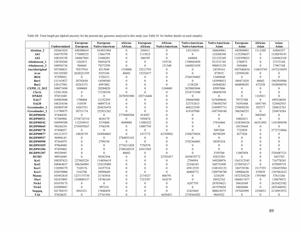
89

Table S8: Total length per diploid ancestry for the present-day genomes analyzed in this study (see Table S1 for further details on each sample).

Undetermined European-European

European-NativeAmerican

African-African

European-African

African-NativeAmerican

NativeAmerican-NativeAmerican

NativeAmerican-Asian

European-Asian

African-Asian

Asian-Asian

Aleutian_2 103661024 698500634 816951894 0 249413 0 143134431 360649061 692890903 1111569 63884357 Alt1 104578799 173098525 13863759 0 1115015 0 0 124208340 1125298657 0 1338870191 Alt2 108258758 244867965 33488201 0 380199 0 644684 221332349 1102599025 0 1169462105

Athabascan_1 128769266 1262872 58452678 0 0 319734 1749943850 912151745 2760973 0 27372168 Athabascan_2 108956736 504669 79272299 0 0 121340 1669921039 998833129 5456886 0 17967188 AusAboriginal 107540621 78537916 4513949 1334806 23213795 0 0 24359161 1057686834 110635765 1473210439

Avar 101329305 2628221395 9355186 48602 15253677 0 0 875015 125950106 0 0 BI16 97299022 0 3726213 0 0 0 2766538403 13469648 0 0 0 Bur1 131163827 38792650 14598560 0 0 0 0 143998833 589471828 48602 1962958986 Bur2 128127981 43261571 8997402 0 0 0 1138220 165840283 604898295 672558 1928096976

CEPH_11_D12 100873498 1890069 20284820 0 0 1184849 2670803044 85997006 0 0 0 Clovis 123011026 0 37230330 0 0 0 2534733580 186058350 0 0 0

DNK02 97651049 0 0 2678501980 103714446 0 0 0 0 1165811 0 Esk17 105885040 1788804 21352295 0 0 0 296043080 1676898641 79737388 0 699328038 Esk20 106234104 518559 60897318 0 0 0 323752413 1786502765 76393448 1691744 525042935

Greenlander_1 105884749 14267551 284476478 0 0 0 404232199 1549997713 270949256 392577 250832763 Greenlander_2 111788975 38751174 252921262 0 0 0 419107988 1497549348 306240255 0 254674284

HGDP00456 97446830 0 0 2779689304 814307 0 0 0 0 3082845 0 HGDP00521 97360904 2754716716 4636179 0 7456876 0 0 0 16862611 0 0 HGDP00542 104999300 112254914 3376880 4940988 11884322 0 0 37016866 1358304326 66351092 1181904598 HGDP00665 98246254 2745859267 3766358 0 15007743 0 0 0 18153664 0 0 HGDP00778 97494057 0 0 0 0 0 0 3097204 7723059 0 2772718966 HGDP00877 101212537 14828739 543084003 0 1473772 62769962 2108278456 46708389 2677428 0 0 HGDP00927 96980143 0 0 2784053143 0 0 0 0 0 0 0 HGDP00998 97564479 0 2799150 0 0 0 2742366403 38303254 0 0 0 HGDP01029 97064880 0 0 2776211828 7756578 0 0 0 0 0 0 HGDP01284 97459402 0 0 2740160319 43413565 0 0 0 0 0 0 HGDP01307 99529945 0 0 48602 0 0 0 5359760 11007858 0 2765087121

HUI03 98910449 0 50382544 0 0 25783437 2659670772 42832301 0 0 3453783 Ket1 108207623 227605224 114856619 0 0 0 2784954 349288076 1361512545 0 716778245 Ket2 108464637 306246984 124335888 0 0 0 23246343 368753498 1270476217 0 679509719 Kor1 132098379 7169176 16357334 0 0 0 45912529 1108183133 184739196 2117555 1384455984 Kor2 103070080 5162706 20994649 0 0 0 44404772 1209794788 109066620 676039 1387863632

Manny 103952818 1237175730 21743934 0 2174327 806791 0 3236295 1472338220 1791905 37813266 Mari 102419883 1520089337 19746169 0 7323707 434279 0 28922762 1066017477 0 136079672 Nivh1 101870175 0 0 0 0 0 6287759 287039621 50410349 0 2435425382 Nivh2 103009047 0 997216 0 0 0 0 267559656 54020446 0 2455446921

Saqqaq 101784353 8563231 17688458 0 0 0 33425665 400618575 197642999 2356033 2118953972 TA6 97624655 0 27761956 0 0 6438451 2739364302 9843922 0 0 0

90

Undetermined European-European

European-NativeAmerican

African-African

European-African

African-NativeAmerican

NativeAmerican-NativeAmerican

NativeAmerican-Asian

European-Asian

African-Asian

Asian-Asian

Tadjik 107169097 2223936164 43047238 0 2871179 0 0 1493055 495207697 0 7308856 Y2040 98251455 0 722259 0 0 0 2751693249 30366323 0 0 0 Yak1 108799608 28454520 12356844 0 0 0 1443908 278459672 470323061 0 1981195673 Yak2 105828941 20825063 22589208 0 0 0 0 214479531 630730996 145401 1886434146

91

Table S9: Proportions of diploid ancestry for the present-day genomes analyzed in this study (see Table S1 for further details on each sample).

Undetermined European-European

European-NativeAmerican

African-African

European-African

African-NativeAmerican

NativeAmerican-NativeAmerican

NativeAmerican-Asian

European-Asian

African-Asian

Asian-Asian

Aleutian_2 3.6 24.24 28.36 0 0.01 0 4.97 12.52 24.05 0.04 2.22 Alt1 3.63 6.01 0.48 0 0.04 0 0 4.31 39.06 0 46.47 Alt2 3.76 8.5 1.16 0 0.01 0 0.02 7.68 38.27 0 40.59

Athabascan_1 4.47 0.04 2.03 0 0 0.01 60.74 31.66 0.1 0 0.95 Athabascan_2 3.78 0.02 2.75 0 0 0 57.96 34.67 0.19 0 0.62 AusAboriginal 3.73 2.73 0.16 0.05 0.81 0 0 0.85 36.71 3.84 51.13

Avar 3.52 91.22 0.32 0 0.53 0 0 0.03 4.37 0 0 BI16 3.38 0 0.13 0 0 0 96.03 0.47 0 0 0 Bur1 4.55 1.35 0.51 0 0 0 0 5 20.46 0 68.13 Bur2 4.45 1.5 0.31 0 0 0 0.04 5.76 21 0.02 66.92

CEPH_11_D12 3.5 0.07 0.7 0 0 0.04 92.7 2.98 0 0 0 Clovis 4.27 0 1.29 0 0 0 87.98 6.46 0 0 0

DNK02 3.39 0 0 92.97 3.6 0 0 0 0 0.04 0 Esk17 3.68 0.06 0.74 0 0 0 10.28 58.2 2.77 0 24.27 Esk20 3.69 0.02 2.11 0 0 0 11.24 62.01 2.65 0.06 18.22

Greenlander_1 3.68 0.5 9.87 0 0 0 14.03 53.8 9.4 0.01 8.71 Greenlander_2 3.88 1.35 8.78 0 0 0 14.55 51.98 10.63 0 8.84

HGDP00456 3.38 0 0 96.48 0.03 0 0 0 0 0.11 0 HGDP00521 3.38 95.62 0.16 0 0.26 0 0 0 0.59 0 0 HGDP00542 3.64 3.9 0.12 0.17 0.41 0 0 1.28 47.15 2.3 41.02 HGDP00665 3.41 95.31 0.13 0 0.52 0 0 0 0.63 0 0 HGDP00778 3.38 0 0 0 0 0 0 0.11 0.27 0 96.24 HGDP00877 3.51 0.51 18.85 0 0.05 2.18 73.18 1.62 0.09 0 0 HGDP00927 3.37 0 0 96.63 0 0 0 0 0 0 0 HGDP00998 3.39 0 0.1 0 0 0 95.19 1.33 0 0 0 HGDP01029 3.37 0 0 96.36 0.27 0 0 0 0 0 0 HGDP01284 3.38 0 0 95.11 1.51 0 0 0 0 0 0 HGDP01307 3.45 0 0 0 0 0 0 0.19 0.38 0 95.98

HUI03 3.43 0 1.75 0 0 0.89 92.32 1.49 0 0 0.12 Ket1 3.76 7.9 3.99 0 0 0 0.1 12.12 47.26 0 24.88 Ket2 3.76 10.63 4.32 0 0 0 0.81 12.8 44.1 0 23.59 Kor1 4.59 0.25 0.57 0 0 0 1.59 38.46 6.41 0.07 48.05 Kor2 3.58 0.18 0.73 0 0 0 1.54 41.99 3.79 0.02 48.17

Manny 3.61 42.94 0.75 0 0.08 0.03 0 0.11 51.1 0.06 1.31 Mari 3.55 52.76 0.69 0 0.25 0.02 0 1 37 0 4.72 Nivh1 3.54 0 0 0 0 0 0.22 9.96 1.75 0 84.53 Nivh2 3.58 0 0.03 0 0 0 0 9.29 1.88 0 85.23

Saqqaq 3.53 0.3 0.61 0 0 0 1.16 13.91 6.86 0.08 73.55 TA6 3.39 0 0.96 0 0 0.22 95.08 0.34 0 0 0

92

Undetermined European-European

European-NativeAmerican

African-African

European-African

African-NativeAmerican

NativeAmerican-NativeAmerican

NativeAmerican-Asian

European-Asian

African-Asian

Asian-Asian

Tadjik 3.72 77.19 1.49 0 0.1 0 0 0.05 17.19 0 0.25 Y2040 3.41 0 0.03 0 0 0 95.51 1.05 0 0 0 Yak1 3.78 0.99 0.43 0 0 0 0.05 9.67 16.32 0 68.77 Yak2 3.67 0.72 0.78 0 0 0 0 7.44 21.89 0.01 65.48

93

Table S10. (A) and (B) Results of genomic sequence-data based enhanced D-statistics testing for Melanesian (Papuan) signal in Native Americans and Aleutian Islander. All comparisons used as H1 a Native American sample listed below, H2 = Aleut and H3 = Papuan. The difference between A and B is the outgroup used. (C) Results from an analysis indentifying Denisovan heplotypes in Aleut versus Native Americans, considered a direct result of potential East Asian/Australo-Melanesian signal. A) Outgroup = 5 African samples (Mbuti, San, Yoruba, Mandenka, Dinka) and 2 European samples (French, Sardinian)

H1 D p-value Athabascan1 0.062 0.0696 Athabascan2 0.033 0.1732

Karitiana (HGDP00998) 0.068 0.0345 Karitiana (BI16) 0.131 0.0003

Huichol 0.139 <.0001 Aymara 0.122 0.0007 Yukpa 0.06 0.1021

B) Outgroup = 5 Africans and 2 Europeans as in (A), as well as 2 East Asians (Dai and Han)

H1 D p-value Athabascan1 -0.009 0.5449 Athabascan2 0.014 0.4183

Karitiana (HGDP00998) 0.181 0.0043 Karitiana (BI16) 0.069 0.1805

Huichol 0.086 0.112 Aymara 0.084 0.1504 Yukpa 0.068 0.2336

C)

Sample # Denisovan regions

Average length (Kb)

Aleutian_2 111 34.9 Athabascan1 78 33 Athabascan2 100 28.7

Karitiana (HGDP00998) 84 26 Karitiana (BI16) 91 33.4

Huichol 71 24.4 Aymara 106 36.1 Yukpa 77 40

94

Table S11. (A) Divergence time estimates and bottleneck size for the clean split model. (B) Divergence time and migration probability estimates for pairs of populations assuming that gene flow continues between TDIV and the present (i.e. TM = 0). (C) Estimation of migration probability m and the gene flow stopping time, TM, for various fixed values of the divergence time, TDIV. A)

Populations compared Estimated divergence time, TDIV (KYA) Estimated Bottleneck Size, NB

Athabascan vs. Karitiana 12.9 1670 Athabascan vs. Koryak 19.7 1760 Athabascan vs. Nivkh 22 1810

Karitiana vs. Koryak 18.5 1810 Karitiana vs. Nivkh 21.2 1810

Huichol vs. Athabascan 13.4 1670

Huichol vs. Karitiana 8.4 1670 Huichol vs. Koryak 19 1790

Greenlandic Inuit vs. Athabascan 14.5 1790

Greenlandic Inuit vs. Karitiana 13.7 1930 Greenlandic Inuit vs. Huichol 13.7 1930 Greenlandic Inuit vs. Koryak 15 1930

Greenlandic Inuit vs. Nivkh 19.7 1930 Han vs. Athabascan 22.2 1790 Han vs. Karitiana 21.5 1790

B)

Populations compared Estimated divergence time, TDIV (KYA) Estimated migration probability, m (10-5)

Athabascan vs. Karitiana 12 5 Athabascan vs. Koryak 20.8 14 Athabascan vs. Nivkh 23.2 10 Karitiana vs. Koryak 22.4 20 Karitiana vs. Nivkh 23.2 10

Huichol vs. Karitiana 8.1 5 Huichol vs. Athabascan 12.6 3

Huichol vs. Koryak 20.9 14 Greenlandic Inuit vs. Athabascan 18.5 41 Greenlandic Inuit vs. Karitiana 18.5 28 Greenlandic Inuit vs. Huichol 18.5 28 Greenlandic Inuit vs. Koryak 21.4 91 Greenlandic Inuit vs. Nivkh 23.6 41

Han vs. Athabascan 22.9 7 Han vs. Karitiana 22.9 10

C)

Karitiana vs. Koryak Athabascan vs. Koryak

TDIV (KYA) TM (KYA) m (10-5) Log likelihood TM (KYA) m (10-5) Log likelihood

19 1.2 11 -15401448 12.2 82 -13535240

20 2 17 -15401391 11.8 110 -13535187 21 2.4 22 -15401360 11.4 140 -13535160 22 1.8 22 -15401353 (best) 11.8 190 -13535158 (best)

23 2.4 28 -15401363 11.8 230 -13535177

95

Table S12. Divergence times and effective population size histories inferred from pairs of populations using the IBS tract method. Kar: Karitiana, Kordn Koryak, Ath: Athabascan.

N00 N01 t0 N10 N11 ts N2 t2 N3 t3 N4 t4 N5 t5 N6

Kar v. Kor 565 1299 11.6 KYA 8894 5687 20.2 KYA 500 24.7 KYA 3357 76.6 KYA 10780 941.3 KYA 11940 1521 KYA 17510 Ath v. Kor 1750 1841 12.3 KYA 18590 4073 17.4 KYA 500 21.7 KYA 16028 41.0 KYA 547 49.7 KYA 10380 1391 KYA 15060 Ath v. Kar 1171 7680 4.14 KYA 29990 500 13.5 KYA 500 16.9 KYA 2107 62.0 KYA 9726 1214 KYA 13500 2709 KYA 23580

Table S13. Divergence time estimates from simulated data using diCal2.0 under a clean split model (main text Fig. 2B, m=0). We treated all parameters except the divergence time as nuisance parameters and did not report them.

Simulated scenario No Errors 70kb Switch Errors

Clean split @ 18.5k 17 KYA 20.5 KYA Split @ 22k + migration [2k, 22k] 16 KYA 21 KYA

Table S14. Validation of Koryak vs. Karitiana divergence results using a simulation study.

True divergence time IBS tract inference diCal inference MSMC inference

IBS tract history 20 KYA 17.6 18.3 14.3 diCal history 19.5 KYA 17.6 19.2 17.3

96

Table S15. Craniometric affinities of Paleoamerican, Kaweskar, and Pericú populations. Name: population name and sex. Region: AfS - Subsaharan Africa; AfN+E - Northern Africa and Europe; As - Asia; NAm/Sam - N/S America; Aus - Australia and Melanesia; Oce - Oceania. Frequency: frequency (nr. of cases / 1000 resamplings) with which reference group is most similar to nearest neighbor groups 1, 2, and 3.

Reference group Nearest neighbor 1 Nearest neighbor 2 Nearest neighbor 3

Name Region N Name Region Frequency Name Region Frequency Name Region Frequency

San F AfS 49 San M AfS 0.31 Australia F Aus 0.09 Teita F AfS 0.08 San M AfS 41 San F AfS 0.34 Tasman F Aus 0.09 Australia F Aus 0.08

Dogon F AfS 52 Andaman M As 0.16 Dogon M AfS 0.14 Andaman F As 0.13 Dogon M AfS 47 Dogon F AfS 0.23 Andaman M As 0.1 Zulu F AfS 0.08

Teita F AfS 50 Teita M AfS 0.19 Australia F Aus 0.07 Andaman M As 0.06 Teita M AfS 33 Teita F AfS 0.21 Zulu M AfS 0.08 Australia F Aus 0.07 Zulu F AfS 46 Zulu M AfS 0.27 Dogon F AfS 0.08 Ainu F As 0.07

Zulu M AfS 55 Zulu F AfS 0.36 Dogon M AfS 0.08 Teita M AfS 0.07 Berg F AfN+E 53 Berg M AfN+E 0.16 Zalavar F AfN+E 0.16 Norse F AfN+E 0.07 Berg M AfN+E 56 Berg F AfN+E 0.23 Zalavar M AfN+E 0.13 Norse M AfN+E 0.13

Egypt F AfN+E 53 Norse F AfN+E 0.21 Egypt M AfN+E 0.2 S Japan F As 0.11 Egypt M AfN+E 58 Egypt F AfN+E 0.21 Zalavar M AfN+E 0.13 Norse F AfN+E 0.12 Norse F AfN+E 55 Norse M AfN+E 0.17 Egypt F AfN+E 0.16 Zalavar F AfN+E 0.14

Norse M AfN+E 55 Norse F AfN+E 0.23 Zalavar M AfN+E 0.19 Egypt M AfN+E 0.13 Zalavar F AfN+E 45 Zalavar M AfN+E 0.12 Norse F AfN+E 0.09 Berg F AfN+E 0.09 Zalavar M AfN+E 53 Zalavar F AfN+E 0.14 Norse M AfN+E 0.14 Egypt M AfN+E 0.08

Andaman F As 35 Andaman M As 0.38 Dogon F AfS 0.21 Hainan F As 0.09 Andaman M As 35 Andaman F As 0.23 Dogon F AfS 0.12 Hainan F As 0.11 Anyang M As 42 Hainan M As 0.13 S Japan M As 0.12 Philippi M As 0.1

Atayal F As 18 Atayal M As 0.23 S Japan F As 0.1 Zalavar F AfN+E 0.08 Atayal M As 29 Atayal F As 0.14 Hainan M As 0.09 Anyang M As 0.07 Hainan F As 38 S Japan F As 0.15 Guam F Oce 0.11 Andaman M As 0.1

Hainan M As 45 Guam F Oce 0.14 Philippi M As 0.12 S Japan M As 0.09 N Japan F As 32 S Japan F As 0.22 Hainan F As 0.08 S Japan M As 0.07 N Japan M As 55 S Japan M As 0.19 Philippi M As 0.09 Hainan M As 0.08

Philippi M As 50 Hainan M As 0.12 Anyang M As 0.11 Guam F Oce 0.1

97

Reference group Nearest neighbor 1 Nearest neighbor 2 Nearest neighbor 3

Name Region N Name Region Frequency Name Region Frequency Name Region Frequency

S Japan F As 41 N Japan F As 0.15 Hainan F As 0.12 S Japan M As 0.07 S Japan M As 50 N Japan M As 0.13 S Japan F As 0.11 Hainan M As 0.1 Buriat F As 54 Buriat M As 0.17 Arikara F AmN 0.13 Santa Cr M AmN 0.12 Buriat M As 55 Buriat F As 0.33 Arikara M AmN 0.19 Santa Cr M AmN 0.1

Ainu F As 38 S Japan F As 0.08 Ainu M As 0.08 Zalavar F AfN+E 0.07 Ainu M As 48 Ainu F As 0.22 Zalavar M AfN+E 0.11 S Japan M As 0.09

Eskimo F As 55 Eskimo M As 0.3 Moriori F Oce 0.06 S Japan F As 0.06

Eskimo M As 53 Eskimo F As 0.38 Arikara M AmN 0.08 Atayal M As 0.05 Arikara F AmN 27 Arikara M AmN 0.16 Santa Cr F AmN 0.12 Guam F Oce 0.06 Arikara M AmN 42 Arikara F AmN 0.2 Santa Cr M AmN 0.09 Hainan M As 0.09

Santa Cr F AmN 51 Santa Cr M AmN 0.21 Peru F AmS 0.1 Arikara F AmN 0.1 Santa Cr M AmN 51 Santa Cr F AmN 0.33 Peru M AmS 0.09 Arikara M AmN 0.07 Pericu F AmN 2 Santa Cr F AmN 0.11 N Japan F As 0.08 Ainu F As 0.07

Pericu M AmN 3 Teita M AfS 0.26 Pericu F AmN 0.09 Australia M Aus 0.09 Kaweskar F AmS 3 Kaweskar M AmS 0.34 Moriori F Oce 0.14 Eskimo F As 0.07 Kaweskar M AmS 2 Kaweskar F AmS 0.3 Ainu F As 0.09 Lagoa Sa M AmS 0.08

Lagoa Sa F AmS 4 Lagoa Sa M AmS 0.34 Ainu F As 0.18 Atayal M As 0.08 Lagoa Sa M AmS 8 Lagoa Sa F AmS 0.32 Atayal M As 0.12 Eskimo F As 0.06

Peru F AmS 55 Peru M AmS 0.21 Santa Cr F AmN 0.11 S Japan F As 0.08

Peru M AmS 55 Peru F AmS 0.19 Hainan M As 0.06 Santa Cr M AmN 0.06 Australia F Aus 49 Australia M Aus 0.13 Tasman F Aus 0.13 Tolai F Aus 0.11 Australia M Aus 52 Australia F Aus 0.28 Tasman M Aus 0.17 Tolai M Aus 0.12

Tasmania F Aus 42 Tasman M Aus 0.23 Australia F Aus 0.16 Tolai F Aus 0.12 Tasmania M Aus 45 Tasman F Aus 0.32 Australia M Aus 0.17 Tolai M Aus 0.12

Tolai F Aus 54 Tolai M Aus 0.31 Tasman F Aus 0.11 Australia F Aus 0.1

Tolai M Aus 56 Tolai F Aus 0.4 Tasman M Aus 0.09 Australia M Aus 0.08 Easter I F Oce 37 Easter I M Oce 0.32 Mokapu F Oce 0.15 Moriori F Oce 0.06 Easter I M Oce 49 Easter I F Oce 0.3 Mokapu M Oce 0.19 N Maori M Oce 0.07

Guam F Oce 27 Hainan M As 0.13 Hainan F As 0.08 Philippi M As 0.08 Guam M Oce 30 Guam F Oce 0.15 Anyang M As 0.15 Mokapu M Oce 0.11

Mokapu F Oce 49 Mokapu M Oce 0.21 Easter I F Oce 0.1 Guam F Oce 0.09

98

Reference group Nearest neighbor 1 Nearest neighbor 2 Nearest neighbor 3

Name Region N Name Region Frequency Name Region Frequency Name Region Frequency

Mokapu M Oce 51 Mokapu F Oce 0.15 Guam M Oce 0.14 Easter I M Oce 0.13 Moriori F Oce 51 Moriori M Oce 0.17 Arikara F AmN 0.08 S Maori M Oce 0.07 Moriori M Oce 57 Moriori F Oce 0.28 N Maori M Oce 0.19 S Maori M Oce 0.16 N Maori M Oce 10 S Maori M Oce 0.39 Moriori M Oce 0.16 Moriori F Oce 0.08

S Maori M Oce 10 N Maori M Oce 0.38 Moriori M Oce 0.12 Guam M Oce 0.1

99

Fig. S1. Geographical locations of populations from the Americas that were analyzed in this study. See Section S1 and Tables S1, S3 and S4 for further information.

�

��

�

��

�

�

��

��

�

���

�

����

�Chipewyan

Alaskan Inuit

HaidaTlingit

Coastal Tsimshian

USAmer_4 CanAmer_1Nor_Ath_4,Splatsin

Nor.Ath_1 , Nor_Ath_2

�

�

USAmerindian_1-3,5,6 Southern_Ath_1

Cucupa,Cochimi,Kumiai

Cree

Mixtec

Pima ,Yaqui

���

�� Aymara

�Yukpa

� Chinchorro

�Enoque65

Fuego-Patagonians

�Pericues

� MARC1492�

939

�Aleutian

�Algonquin

�Arara

��

Palikur

Parakana

�

Yaghan

ChonoChilote

Huilliche

Diaguita Toba

GuaraniChaneWichi Kaingang

SuruiKaritiana

JamamadiTicuna

PiapocoGuahibo

IngaWaunanaEmbera

���

Quechua

����

���

��� �����

KogiArhuaco Wayuu

Chorotega, Huetar,Cabecar, Teribe, Guaymi, Bribri,Maleku

�Kaqchikel

� Maya, Maya1, Maya2�

MixeZapotec1, Zapotec2, Mexican

��

Purepecha

��West_Greenlandic_Inuit

East_Greenlandic_InuitNor_Ath_3Nisga'aStswecem'c

�Ojibwa

Mexican MummiesHuichol ,Tepehuano

Ancient - genome-sequenced (this study)

Present-day, SNP chip-typed (this study)

Present-day, genome-sequenced (this study)

Present-day, SNP chip-typed (this study+published)

Present-day, SNP chip-typed (published)

Present-day, genome-sequenced (published)

100

Fig. S2. DNA fragmentation and damage. On the left: DNA fragment length distributions of nine ancient samples (one per sub-population). Reads below 30bp were filtered out, expect in the case of Chinchorro where the mapping was instead performed by excluding indels near the read end (-i option in bwa). The maximum read length is 100 bp (HiSeq) so that the distribution appears truncated and the mean (indicated on each plot) is biased downwards. On the right: mismatch frequency relative to the reference as a function of read position (C to T in orange and G to A in light blue).

101

read length distribution

read length

frequ

ency

0.00.1

0.20.3

0.4

20 27 34 41 48 55 62 69 76 83 90 97

MARC 1492

average: 88.6

0 20 40 60 80

0.00

0.01

0.02

0.03

0.04

0.05

0.06

0.07

position from 5' end

frequ

ency

C�>AG�>AT�>A

A�>CG�>CT�>C

A�>GC�>GT�>G

A�>TC�>TG�>T

80 60 40 20 0

0.00

0.01

0.02

0.03

0.04

position from 3' end

frequ

ency

C�>AG�>AT�>A

A�>CG�>CT�>C

A�>GC�>GT�>G

A�>TC�>TG�>T

damage pattern 5' end damage pattern 3' end

read length

frequ

ency

FWFWFWFWFW

read length distribution

Enoque65

average: 43.5

0.00

0.01

0.02

0.03

0.04

0.05

20 27 34 41 48 55 62 69 76 83 90 97

Enoque65

average: 43.5

0 20 40 60 80

0.00

0.05

0.10

0.15

0.20

0.25

position from 5' end

frequ

ency

C�>AG�>AT�>A

A�>CG�>CT�>C

A�>GC�>GT�>G

A�>TC�>TG�>T

80 60 40 20 0

0.00

0.05

0.10

0.15

0.20

0.25

position from 3' end

frequ

ency

C�>AG�>AT�>A

A�>CG�>CT�>C

A�>GC�>GT�>G

A�>TC�>TG�>T

read length

frequ

ency

0.00.1

0.20.3

20 27 34 41 48 55 62 69 76 83 90 97

939

average: 81.5

0 20 40 60 80

0.000

0.005

0.010

0.015

position from 5' end

frequ

ency

C�>AG�>AT�>A

A�>CG�>CT�>C

A�>GC�>GT�>G

A�>TC�>TG�>T

80 60 40 20 0

0.00

0.05

0.10

0.15

position from 3' end

C�>AG�>AT�>A

A�>CG�>CT�>C

A�>GC�>GT�>G

A�>TC�>TG�>T

frequ

ency

read length

frequ

ency

0.00

0.02

0.04

0.06

0.08

20 27 34 41 48 55 62 69 76 83 90 97 0 20 40 60 80

0.00

0.05

0.10

0.15

C�>AG�>AT�>A

A�>CG�>CT�>C

A�>GC�>GT�>G

A�>TC�>TG�>T

80 60 40 20 0

0.00

0.05

0.10

0.15

position from 3' end

frequ

ency

C�>AG�>AT�>A

A�>CG�>CT�>C

A�>GC�>GT�>G

A�>TC�>TG�>T

Chinchorro

average: 36.1

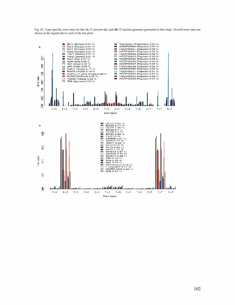
102

Fig. S3. Type-specific error rates for the (A) 31 present-day and (B) 23 ancient genomes generated in this study. Overall error rates are shown in the legend above each of the bar plots.

103

Fig. S4. Admixture proportions estimated using ADMIXTURE (36). Shown are plots with K=2-6 (A) and K=15 (B and C).

EskimoAleut

NaDene NorthernAmerind

Central-Amerind ChibchanPaezan

EquatorialTucanoan

Ge-PanoCarib

Andean

Mix

tec

Tepehuano

Yaqui

Zapote

c1

Zapote

c2

Choro

tega

Pure

pech

aB

ribri

Cabeca

r

Hu

eta

rM

ale

kuG

uaym

iTe

rib

eW

au

na

na

Arh

ua

coE

mb

era

Ko

gi

Gu

ah

ibo

Pia

poco

Wayu

uJa

mam

adi

Kari

tiana

Palik

ur

Para

kana

Suru

i

Tic

una

Guara

ni

Chane

Yukp

a

Ara

raK

ain

ga

ng

Tob

aW

ich

iIn

ga

Quech

ua

Aym

ara

Chilo

teC

hono

Dia

guita

Hulli

che

Yaghan

Mexi

can

Saqqaq

Clo

vis

East

Gre

enla

nders

West

Gre

enla

nders

Ale

utia

ns

Ala

skan

Inuit

Chip

ew

yan

Nort

hern

Ath

abasc

ans

2

Haid

a

South

ern

Ath

abasc

ans

1

Tlin

git

CanA

meri

ndia

n1

Alg

onquin

Coast

alT

sim

shia

n

Cre

eN

isga'a

Ojib

wa

Spla

tsin

Sts

wece

m'c

Lum

bee U

SA

meri

ndia

nC

och

imi

Cucu

pa

K

um

iai

Maya

Maya

1

Maya

2

Mix

e

Kaqch

ikel

US

Am

eri

ndia

n

Pim

a

Huic

hol

34 5146 321

Sa

nB

iaka

Pyg

mie

s

Mbu

tiP

ygm

ies

Ba

ntu

s

Ma

nd

en

kas

Yo

rub

as

YR

I

Mo

zab

ites

Be

do

uin

s

Pa

lest

inia

ns

Dru

ze

Orc

ad

ian

s

Fre

nch

Fre

nch

Ba

squ

es

Sa

rdin

ian

s

No

rth

Ita

lian

sTu

sca

ns

Hu

ng

ari

an

s

Ukr

an

ian

s

Ru

ssia

ns

Est

on

ians

Ch

uva

sh

Ba

lka

rs

Ad

yge

i

Le

zgin

s

Uyg

urs

Ha

zara

Ka

lash

Pa

tha

n

Bu

rush

o

Ba

loch

i

Bra

hu

i

Ma

kra

ni

Sin

dh

i

Gu

jara

tis

No

rth

Ka

nn

ad

iM

ala

yan

Pa

niy

aS

aki

lliO

ng

eG

rea

tA

nd

am

an

ese A

eta

Ag

taB

ata

kM

ela

ne

sia

ns

Pa

pu

an

s

Pa

pu

an

spyg

mie

s

So

lom

on

s

Ba

jo

Kaya

hL

ebb

oC

am

bo

dia

ns

Da

iL

ah

uM

iao

zuN

axi

Sh

eY

izu

Tujia

Ha

n TuX

ibo

Da

ur

He

zhe

nO

roq

en

sM

on

go

laM

on

go

lian

s

Jap

an

ese

Bu

rya

ts

Tuvi

nia

ns

Do

lga

ns

Ke

tsS

elk

up

s

Kh

an

ty

Ne

ne

tsTu

nd

raN

en

tsi

Ng

an

asa

ns

Ng

an

asa

n2

Alta

ians

Alta

ian

Kiz

hi

Tele

uts

Sh

ors

Kh

aka

ses

Yu

kag

hirs

Niv

khs

Sa

kha

Eve

nki

s

Eve

ns

Ko

rya

ks

Ch

ukc

his

Esk

imo

Na

uka

n

Africa NearEast Europe&Caucasus SouthAsia SEAsia&Oceania EastAsia SiberiaB

C

2

3

4

5

6

A m e r i c a sA f r i c a & E u r a s i a

A

104

Fig. S5. Admixture trees based on genomic sequence data from worldwide present-day and ancient populations. Plots were generated using TreeMix (37), and include whole genomes from 20 present-day individuals and three ancient samples. Shown are plots for migration edges m=0-10 and the corresponding residual matrices. We find all Native Americans, including southern Amerindians (from southern North America and Central and South America) and Athabascans, to be a monophyletic group.

105

106

107

108

Fig. S6. (A) Genomic sequence data-based D-statistics of the form ((Athabascan, X), Inuit), where X represents southern Amerindians (from southern North America and Central and South America), shows gene flow between Inuit and Athabascans. The Mayan genome has been masked for recent European admixture. The ancient Anzick-1 sample should be considered without transitions included in the analysis (circle). The thick and thin lines represent 1 and 3 standard errors, respectively. (B) We find similar results when the Inuit are replaced by the Siberian Yupik as the outgroup (H3) (next page).

109

B

Anzick�1

Mayan

Aymara

Karitiana

Yukpa

Pima

Huichol

�0.05 0.00 0.05 0.10 0.15 0.20

H1 = X, H2 = Athabascan, H3 = Yupik

D statistic

�

�

|Z|<3|Z|>3Without transitionsWith transitions

110

Fig. S7. Genomic sequence data-based D-statistics of the form ((Karitiana, Athabascan), X), where X represents East Asians, Siberians and the Inuit. All the tested populations (tests with transitions included - triangles) are slightly closer to Athabascans than to Karitiana.

Han

Buryat

Nivkh

Yakut

Dai

Altai

Ket

Koryak

East�Greenland

Yupik

West�Greenland

0.00 0.01 0.02 0.03 0.04

H1 = Karitiana, H2 = Athabascan, H3 = X

D statistic

�

�

|Z|<3|Z|>3Without transitionsWith transitions

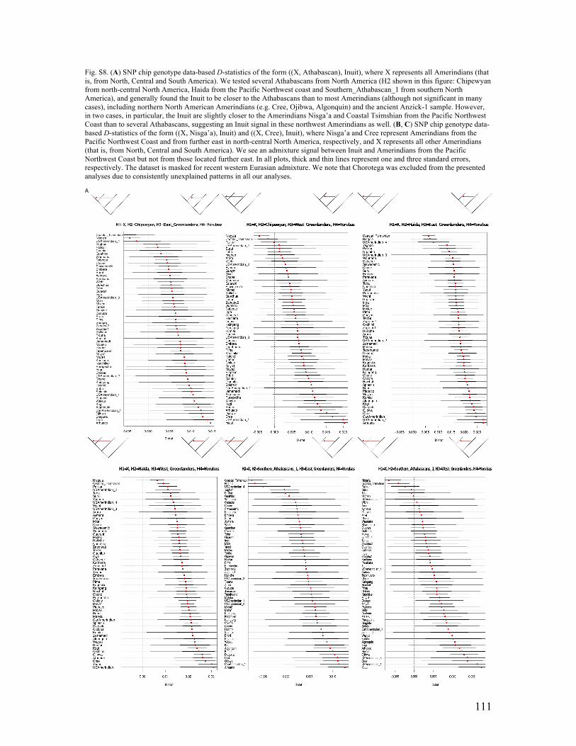
111

Fig. S8. (A) SNP chip genotype data-based D-statistics of the form ((X, Athabascan), Inuit), where X represents all Amerindians (that is, from North, Central and South America). We tested several Athabascans from North America (H2 shown in this figure: Chipewyan from north-central North America, Haida from the Pacific Northwest coast and Southern_Athabascan_1 from southern North America), and generally found the Inuit to be closer to the Athabascans than to most Amerindians (although not significant in many cases), including northern North American Amerindians (e.g. Cree, Ojibwa, Algonquin) and the ancient Anzick-1 sample. However, in two cases, in particular, the Inuit are slightly closer to the Amerindians Nisga’a and Coastal Tsimshian from the Pacific Northwest Coast than to several Athabascans, suggesting an Inuit signal in these northwest Amerindians as well. (B, C) SNP chip genotype data-based D-statistics of the form ((X, Nisga’a), Inuit) and ((X, Cree), Inuit), where Nisga’a and Cree represent Amerindians from the Pacific Northwest Coast and from further east in north-central North America, respectively, and X represents all other Amerindians (that is, from North, Central and South America). We see an admixture signal between Inuit and Amerindians from the Pacific Northwest Coast but not from those located further east. In all plots, thick and thin lines represent one and three standard errors, respectively. The dataset is masked for recent western Eurasian admixture. We note that Chorotega was excluded from the presented analyses due to consistently unexplained patterns in all our analyses. A

112

B

C

113

Fig. S9. SNP chip genotype data-based D-statistics of the form ((X, north-central/northeastern Amerindians), Karitiana), where X represents Athabascans and northern Amerindians residing in northwestern North America. Thick and thin lines represent one and three standard errors, respectively. The dataset is masked for recent western Eurasian admixture. We find some evidence for Karitiana being closer to the north-central (Cree and Chipewyan) and northeastern (Ojibwa) Amerindians than to the northwestern Amerindians (Nisga’a and Coastal Tsimshian). Southern Athabascans have likely admixed with neighbouring (southern branch) Amerindians in the recent past, given their geographical location in southern North America.

114

Fig. S10. SNP chip genotype data-based D-statistics of the form ((X, Surui), Old World), where X represents indigenous American populations. Thick and thin lines represent one and three standard errors, respectively. The dataset is masked for recent western Eurasian admixture. We observe a gradient in the genetic affiliation across the Americas to populations with East Asian, including Siberian, and Australo-Melanesian ancestry. We note that Chorotega was excluded from the presented analyses due to consistently unexplained patterns in all our analyses.

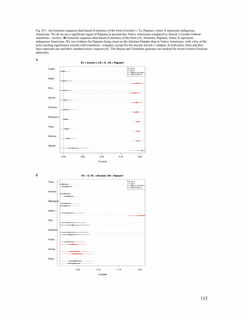
115

Fig. S11. (A) Genomic sequence data-based D-statistics of the form ((Anzick-1, X), Papuan), where X represents indigenous Americans. We do no see a significant signal of Papuans in present-day Native Americans compared to Anzick-1 (results without transitions - circles). (B) Genomic sequence data-based D-statistics of the form ((X, Aleutian), Papuan), where X represents indigenous Americans. We see evidence for Papuans being closer to the Aleutian Islander than to Native Americans, with a few of the tests reaching significance (results with transitions - triangles, except for the ancient Anzick-1 sample). In both plots, thick and thin lines represent one and three standard errors, respectively. The Mayan and Tsimshian genomes are masked for recent western Eurasian admixture. A B

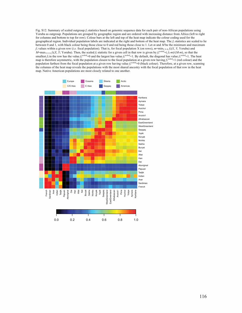
116

Fig. S12. Summary of scaled outgroup f3 statistics based on genomic sequence data for each pair of non-African populations using Yoruba as outgroup. Populations are grouped by geographic region and are ordered with increasing distance from Africa (left to right for columns and bottom to top for row). Colour bars at the left and top of the heat map indicate the colour coding used for the geographical region. Individual population labels are indicated at the right and bottom of the heat map. The f3 statistics are scaled to lie between 0 and 1, with black colour being those close to 0 and red being those close to 1. Let m and M be the minimum and maximum f3 values within a given row (i.e. focal population). That is, for focal population X (on rows), m=minY,Y≠X f3(X, Y; Yoruba) and M=maxY,Y≠X f3(X, Y; Yoruba). Then, the scaled f3 statistic for a given cell in that row is given by f3

scaled=( f3-m)/(M-m), so that the smallest f3 in the row has the value f3

scaled=0 and the largest has value f3scaled=1. By default, the diagonal has value f3

scaled=1. The heat map is therefore asymmetric, with the population closest to the focal population at a given row having f3

scaled=1 (red colour) and the population farthest from the focal population at a given row having value f3

scaled=0 (black colour). Therefore, at a given row, scanning the columns of the heat map reveals the populations with the most shared ancestry with the focal population of that row in the heat map. Native American populations are most closely related to one another.

Fren

ch

Sar

dini

an

Avar

Indi

an

Tadj

ik

Papu

an

Abo

rigin

al

Dai

Han

Alta

i

Ket

Bur

yat

Niv

hks

Kory

ak

Yupi

k

Saq

qaq

Wes

tGre

enla

nd

Eas

tGre

enla

nd

Ath

abas

can

Anz

ick1

Pim

a

Hui

chol

Yukp

a

Aym

ara

Kar

itian

a

French

Sardinian

Avar

Indian

Tadjik

Papuan

Aboriginal

Dai

Han

Altai

Ket

Buryat

Sakha

Nivhks

Koryak

Yupik

Saqqaq

WestGreenland

EastGreenland

Athabascan

Anzick1

Pima

Huichol

Yukpa

Aymara

Karitiana

0.0 0.2 0.4 0.6 0.8 1.0

Europe

C/S Asia

Oceania

E Asia

Siberia

Saqqaq

Arctic

AmericasS

akha

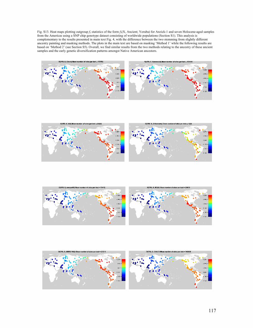
117

Fig. S13. Heat maps plotting outgroup f3 statistics of the form f3(X, Ancient; Yoruba) for Anzick-1 and seven Holocene-aged samples from the Americas using a SNP chip genotype dataset consisting of worldwide populations (Section S1). This analysis is complementary to the results presented in main text Fig. 4, with the difference between the two stemming from slightly different ancestry painting and masking methods. The plots in the main text are based on masking ‘Method 1’ while the following results are based on ‘Method 2’ (see Section S5). Overall, we find similar results from the two methods relating to the ancestry of these ancient samples and the early genetic diversification patterns amongst Native American ancestors.

118

Fig. S14. Ranked outgroup f3 statistics for the tests presented in main text Fig. 4 and Fig. S13. Results are presented for both the masking methods, ‘Method 1’ (left panels) and ‘Method 2’ (right panels). The errors bars represent one standard error of the f3 statistic. Overall, we get consistent results from the two methods.

�

�

�

�

�

�

�

�

�

Near EastEuropeCaucasusSouth AsiaSoutheastern AsiaOceaniaEast AsiaSiberiaAndeanCentral�AmerindChibchan�PaezanEquatorial�TucanoanEskimo�AleutGe�Pano�CaribNa DeneNorthern Amerind

0.12 0.14 0.16 0.18 0.20 0.22

f3(X, Anzick�1; Yorubas)

�Bedouins�Palestinians

�Druze�Makrani

�Sardinians�Brahui�Onge�Balochi�Tuscans�Papuans�Papuans pygmy�North Italians�Sakilli�Sindhi�French Basques�Adygei�Balkars�Lezgins�French�North Kannadi�Pathan�Paniya�Gujaratis�Kalash�Hungarians�Malayan�Melanesians�Orcadians�Ukranians�Great Andamanese�Burusho�Estonians�Russians�Solomons

�Aeta�Agta�Chuvash

�Hazara�Batak�Uygurs�Bajo�Cambodians�Kayah Lebbo�Teleut�Khakases�Shors�Altaians�Dai�Lahu�Khanty�Tu�Naxi�She�Selkups�Altaian�Kizhi�Mongolians�Tujia�Han�Yizu�Miaozu�Tuvinians�Dolgans�Xibo�Tundra Nentsi�Nenets�Japanese�Mongola�Buryats�Kets�Daur�Hezhen�Yakuts�Evenkis�Nganasans�Nivkhs�Oroqens�Evens�Yukaghirs�Nganasan2

�Koryaks�Chukchis

�Eskimo�Naukan

Alaskan InuitEast GreenlandersWest Greenlanders

AleutiansNorthern Athabascans 3

Algonquin�Chorotega

Northern Athabascans 4Chipewyan

Northern Athabascans 1Splatsin

TlingitCree

OjibwaStswecem'c

HaidaNorthern Athabascans 2

Coastal TsimshianNisga'a

CanAmerindian 1USAmerindian 4USAmerindian 1

Southern Athabascans 1Huetar

WichiCucupa

�YaquiArhuaco

BribriWayuu

Cochimi�Pima

DiaguitaMalekuChilote

�MixtecMaya2

WaunanaToba

�Zapotec1Yaghan

KaingangPurepecha

HullicheTeribeMaya1

�TepehuanoCabecar

KaqchikelQuechua

Embera�USAmerindian 3

TicunaMixe

GuaymiKogi

�Zapotec2Piapoco

Inga�Huichol

AymaraChane

KaritianaGuarani

ChonoPalikur

JamamadiKumlai

AraraGuahibo

Surui�USAmerindian 2

Parakana

�

�

�

�

�

�

�

�

�

Near EastEuropeCaucasusSouth AsiaSoutheastern AsiaOceaniaEast AsiaSiberiaAndeanCentral�AmerindChibchan�PaezanEquatorial�TucanoanEskimo�AleutGe�Pano�CaribNa DeneNorthern Amerind

0.10 0.15 0.20 0.25

f3(YRI; X, Anzick-1)

BedouinsPalestinians

DruzeMakrani

SardiniansNorth_Italians

TuscansBrahui

BalochiFrench_Basques

FrenchBalkarsAdygeiSindhi

LezginsHungarians

OrcadiansSakilli

UkraniansOnge

PathanPapuans

Papuans_pygmyKalash

GujaratisEstonians

North_KannadiPaniya

RussiansBurushoMalayan

MelanesiansChuvash

Great_AndamaneseSolomons

AgtaAeta

HazaraUygurs

BatakBajo

CambodiansTeleut

KhakasesKayah_Lebbo

ShorsAltaiansKhanty

LahuAltaian�Kizhi

SelkupsDaiTu

NaxiMongolians

DolgansTujia

NenetsShe

Tundra_NentsiTuvinians

BuryatsYizu

MongolaXiboHan

MiaozuKets

JapaneseNganasans

YakutsHezhenNivkhs

DaurEvenkis

OroqensEvens

YukaghirsNganasan2

KoryaksChukchis

EskimoNaukan

East_GreenlandersAleutians

Alaskan_InuitWest_Greenlanders

Northern_Athabascans_3Algonquin

ChipewyanNorthern_Athabascans_1

OjibwaCanAmerindian_1

CreeTlingit

Northern_Athabascans_2Northern_Athabascans_4

HaidaCoastal_Tsimshian

SplatsinNisgaa

StswecemcUSAmerindian_4

Southern_Athabascans_1Huetar

PimaYaqui

CucupaMaleku

BribriArara

WaunanaChorotega

KogiPalikurMixtec

CochimiWichi

KaingangPiapocoHuichol

USAmerindian_2Mixe

TeribeTepehuano

CabecarWayuu

EmberaZapotec1Zapotec2

ChonoChilote

HuillicheYaghanAymara

TobaInga

Maya2Guaymi

QuechuaKaritiana

TicunaMaya1

KaqchikelKumlai

JamamadiGuaraniArhuacoDiaguita

PurepechaGuahibo

ChaneSurui

USAmerindian_1Parakana

USAmerindian_3

BedouinsPalestinians

DruzeMakrani

SardiniansNorth_Italians

TuscansBrahui

BalochiFrench_Basques

FrenchBalkarsAdygeiSindhi

LezginsHungarians

OrcadiansSakilli

UkraniansOnge

PathanPapuans

Papuans_pygmyKalash

GujaratisEstonians

North_KannadiPaniya

RussiansBurushoMalayan

MelanesiansChuvash

Great_AndamaneseSolomons

AgtaAeta

HazaraUygurs

BatakBajo

CambodiansTeleut

KhakasesKayah_Lebbo

ShorsAltaiansKhanty

LahuAltaian�Kizhi

SelkupsDaiTu

NaxiMongolians

DolgansTujia

NenetsShe

Tundra_NentsiTuvinians

BuryatsYizu

MongolaXiboHan

MiaozuKets

JapaneseNganasans

YakutsHezhenNivkhs

DaurEvenkis

OroqensEvens

YukaghirsNganasan2

KoryaksChukchis

EskimoNaukan

East_GreenlandersAleutians

Alaskan_InuitWest_Greenlanders

Northern_Athabascans_3Algonquin

ChipewyanNorthern_Athabascans_1

OjibwaCanAmerindian_1

CreeTlingit

Northern_Athabascans_2Northern_Athabascans_4

Haida

SplatsinNisgaa

StswecemcUSAmerindian_4

HuetarPimaYaqui

CucupaMaleku

BribriArara

WaunanaChorotega

KogiPalikurMixtec

CochimiWichi

KaingangPiapocoHuichol

USAmerindian_2Mixe

TeribeTepehuano

CabecarWayuu

EmberaZapotec1Zapotec2

ChonoChilote

HuillicheYaghanAymara

TobaInga

Maya2Guaymi

QuechuaKaritiana

TicunaMaya1

KaqchikelKumlai

JamamadiGuaraniArhuacoDiaguita

PurepechaGuahibo

ChaneSurui

USAmerindian_1Parakana

USAmerindian_3

Coastal_Tsimshian

Southern_Athabascans_1

119

0.12 0.14 0.16 0.18 0.20 0.22

f3(X, Kennewick; Yorubas)

�Bedouins�Palestinians

�Druze�Makrani�Sardinians

�Brahui�Tuscans�North Italians�Balochi�Onge�French Basques�Lezgins�Adygei�Papuans�French�Sindhi�Papuans pygmy�Balkars�Sakilli�Great Andamanese�Hungarians�Kalash�Pathan�Orcadians�Paniya�Gujaratis�North Kannadi�Ukranians�Malayan�Estonians�Melanesians�Russians�Burusho

�Solomons�Agta�Chuvash�Aeta

�Hazara�Uygurs�Batak�Bajo

�Cambodians�Teleut�Kayah Lebbo�Khakases�Shors�Khanty�Lahu�Altaians�Dai�Tu�Altaian�Kizhi�Naxi�Selkups�She�Miaozu�Kets�Mongolians�Tundra Nentsi�Yizu�Tujia�Mongola�Xibo�Dolgans�Han�Buryats�Nenets�Tuvinians�Japanese�Daur�Yakuts�Evenkis�Hezhen�Oroqens�Nivkhs�Evens�Nganasans�Yukaghirs�Nganasan2

�Koryaks�Chukchis

�Eskimo�Naukan

East GreenlandersAlaskan Inuit

�ChorotegaWest Greenlanders

AleutiansNorthern Athabascans 3Northern Athabascans 4

CreeTlingit

CanAmerindian 1Chipewyan

Northern Athabascans 1ArhuacoNisga'aSplatsin

HaidaOjibwaHuetar

Coastal Tsimshian�Yaqui

Northern Athabascans 2Algonquin

WayuuStswecem'cPurepecha

Southern Athabascans 1�USAmerindian 3�Pima

Maya2�Tepehuano

DiaguitaTeribeMaya1

Guaymi�Huichol

KaqchikelKogi

�MixtecBribri

ChaneKaingangCabecar

�Zapotec1Wichi

ChiloteUSAmerindian 4

TicunaQuechuaKaritiana

WaunanaToba

MalekuInga

�USAmerindian 2Hulliche

MixeAymaraGuarani

Surui�Zapotec2

PalikurEmbera

GuahiboCucupaCochimiPiapoco

ParakanaKumlai

USAmerindian 1Jamamadi

YaghanChonoArara

�

�

�

�

�

�

�

�

�

Near EastEuropeCaucasusSouth AsiaSoutheastern AsiaOceaniaEast AsiaSiberiaAndeanCentral�AmerindChibchan�PaezanEquatorial�TucanoanEskimo�AleutGe�Pano�CaribNa DeneNorthern Amerind

�

�

�

�

�

�

�

�

�

Near EastEuropeCaucasusSouth AsiaSoutheastern AsiaOceaniaEast AsiaSiberiaAndeanCentral�AmerindChibchan�PaezanEquatorial�TucanoanEskimo�AleutGe�Pano�CaribNa DeneNorthern Amerind

0.10 0.15 0.20 0.25

f3(YRI; X, Kennewick)

BedouinsPalestinians

DruzeSardinians

MakraniTuscans

North_ItaliansFrench_Basques

BrahuiBalochiFrenchAdygei

LezginsBalkars

OngeOrcadians

HungariansSindhi

UkraniansPathanSakilli

EstoniansPapuans_pygmy

KalashGujaratisPapuansRussians

PaniyaNorth_Kannadi

BurushoMalayan

MelanesiansGreat_Andamanese

ChuvashAgta

SolomonsAeta

HazaraUygurs

BatakBajo

CambodiansTeleutShors

KhakasesKayah_Lebbo

KhantyAltaians

DaiSelkups

Altaian�KizhiLahu

YukaghirsKets

Tundra_NentsiTu

NaxiShe

NenetsTujia

MongoliansMongola

YizuMiaozuBuryatsDolgans

XiboTuvinians

HanJapanese

DaurYakutsYakut

NivkhsHezhenEvenkis

NganasansOroqens

EvensNganasan2

ChukchisYukaghirKoryaksEskimo

ChukchiNaukan

West_GreenlandersEast_Greenlanders

AleutiansCanAmerindian_1

ChorotegaAlaskan_Inuit

HuetarCree

Northern_Athabascans_3Chipewyan

Northern_Athabascans_1OjibwaTlingitHaida

Northern_Athabascans_4Kogi

Northern_Athabascans_2Nisgaa

Coastal_TsimshianAlgonquin

YaquiArhuaco

Southern_Athabascans_1Pima

KumlaiGuaymi

TepehuanoMixtecBribri

WayuuPalikur

CucupaPurepecha

WichiSplatsinChilote

CabecarChane

CochimiZapotec1

TeribeMaya2

KaritianaMaya1

EmberaKaqchikel

TicunaToba

JamamadiQuechua

MixeAymara

Zapotec2ParakanaGuahibo

SuruiHuichol

WaunanaInga

USAmerindian_2Huilliche

StswecemcPiapocoGuaraniMaleku

AraraKaingang

USAmerindian_3USAmerindian_4

YaghanDiaguita

USAmerindian_1Chono

BedouinsPalestinians

DruzeSardinians

MakraniTuscans

North_ItaliansFrench_Basques

BrahuiBalochiFrenchAdygei

LezginsBalkars

OngeOrcadians

HungariansSindhi

UkraniansPathanSakilli

EstoniansPapuans_pygmy

KalashGujaratisPapuansRussians

PaniyaNorth_Kannadi

BurushoMalayan

MelanesiansGreat_Andamanese

ChuvashAgta

SolomonsAeta

HazaraUygurs

BatakBajo

CambodiansTeleutShors

KhakasesKayah_Lebbo

KhantyAltaians

DaiSelkups

Altaian�KizhiLahu

YukaghirsKets

Tundra_NentsiTu

NaxiShe

NenetsTujia

MongoliansMongola

YizuMiaozuBuryatsDolgans

XiboTuvinians

HanJapanese

DaurYakutsYakut

NivkhsHezhenEvenkis

NganasansOroqens

EvensNganasan2

ChukchisYukaghirKoryaksEskimo

ChukchiNaukan

West_GreenlandersEast_Greenlanders

AleutiansCanAmerindian_1

ChorotegaAlaskan_Inuit

HuetarCree

Northern_Athabascans_3Chipewyan

Northern_Athabascans_1OjibwaTlingitHaida

Northern_Athabascans_4Kogi

Northern_Athabascans_2Nisgaa

Coastal_TsimshianAlgonquin

YaquiArhuaco

Southern_Athabascans_1Pima

KumlaiGuaymi

TepehuanoMixtecBribri

WayuuPalikur

CucupaPurepecha

WichiSplatsinChilote

CabecarChane

CochimiZapotec1

TeribeMaya2

KaritianaMaya1

EmberaKaqchikel

TicunaToba

JamamadiQuechua

MixeAymara

Zapotec2ParakanaGuahibo

SuruiHuichol

WaunanaInga

USAmerindian_2Huilliche

StswecemcPiapocoGuaraniMaleku

AraraKaingang

USAmerindian_3USAmerindian_4

YaghanDiaguita

USAmerindian_1Chono

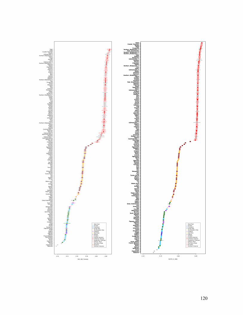
120

0.12 0.14 0.16 0.18 0.20 0.22

f3(X, 939; Yorubas)

�Bedouins�Palestinians

�Druze�Makrani

�Sardinians�Brahui�Tuscans�North Italians�French Basques�Balochi�Papuans�Balkars�Lezgins�Sindhi�Papuans pygmy�Hungarians�French�Adygei�Onge�Orcadians�Pathan�Malayan�Ukranians�Paniya�Kalash�Gujaratis�Sakilli�North Kannadi�Estonians�Russians�Burusho�Melanesians

�Agta�Chuvash�Solomons�Aeta�Great Andamanese

�Hazara�Batak�Uygurs�Bajo�Cambodians�Teleut�Kayah Lebbo�Khakases�Shors�Khanty�Altaians�Dai�Selkups�Lahu�Altaian�Kizhi�Tu�Miaozu�Dolgans�She�Yizu�Tundra Nentsi�Nenets�Mongolians�Naxi�Han�Tuvinians�Tujia�Xibo�Mongola�Buryats�Kets�Japanese�Evenkis�Yakuts�Daur�Hezhen�Nganasans�Oroqens�Nivkhs�Evens�Yukaghirs�Nganasan2

�Koryaks�Chukchis

�Eskimo�Chorotega�Naukan

Alaskan InuitEast Greenlanders

USAmerindian 1Aleutians

West Greenlanders�USAmerindian 3

ArhuacoAlgonquin

CanAmerindian 1Diaguita

OjibwaGuaymiWayuu

Northern Athabascans 4Huetar

CreeBribri

JamamadiTicuna

KaingangPiapocoMaleku

CabecarCucupaChilote

SplatsinKumlai

HullicheKaqchikel

Maya2Inga

�PimaTeribe

�Mixtec�Huichol

Southern Athabascans 1�Tepehuano

CochimiMaya1

Stswecem'cParakana

TobaWichi

WaunanaChane

PurepechaKogi

Northern Athabascans 3�Zapotec1

KaritianaAymara

MixeSurui

EmberaChono

QuechuaGuarani

ChipewyanYaghan

�Zapotec2Northern Athabascans 1

�USAmerindian 2Arara

GuahiboTlingit

PalikurNorthern Athabascans 2

USAmerindian 4Nisga'a

Coastal TsimshianHaida

�Yaqui

�

�

�

�

�

�

�

�

�

Near EastEuropeCaucasusSouth AsiaSoutheastern AsiaOceaniaEast AsiaSiberiaAndeanCentral�AmerindChibchan�PaezanEquatorial�TucanoanEskimo�AleutGe�Pano�CaribNa DeneNorthern Amerind

�

�

�

�

�

�

�

�

�

Near EastEuropeCaucasusSouth AsiaSoutheastern AsiaOceaniaEast AsiaSiberiaAndeanCentral�AmerindChibchan�PaezanEquatorial�TucanoanEskimo�AleutGe�Pano�CaribNa DeneNorthern Amerind

0.10 0.15 0.20 0.25

f3(YRI; X, 939)

BedouinsPalestinians

DruzeSardinians

MakraniBrahui

TuscansFrench_Basques

North_ItaliansOnge

BalochiFrench

HungariansBalkarsLezginsAdygei

OrcadiansSindhi

UkraniansPathan

EstoniansKalash

PapuansPapuans_pygmy

SakilliRussiansGujaratis

PaniyaMalayan

North_KannadiBurusho

MelanesiansChuvash

AgtaSolomons

AetaGreat_Andamanese

HazaraUygurs

BatakBajo

TeleutCambodians

KhakasesKayah_Lebbo

ShorsKhanty

AltaiansDai

SelkupsLahu

Altaian�KizhiTu

YizuNenets

DolgansMiaozu

Tundra_NentsiTujiaShe

MongoliansHanXiboNaxiKets

TuviniansBuryats

MongolaJapanese

DaurYakuts

NganasansEvenkisNivkhs

HezhenOroqens

EvensYukaghirs

Nganasan2Koryaks

ChukchisEskimoNaukan

ChorotegaCanAmerindian_1

PiapocoAlaskan_Inuit

JamamadiHuetarTicunaTeribe

IngaWichi

CabecarChono

DiaguitaUSAmerindian_1

ChiloteBribri

HuicholSurui

MixtecGuaymi

WaunanaCucupaWayuu

PimaGuarani

KogiKaritiana

AymaraKumlaiChane

EmberaAraraMixeToba

Zapotec1KaingangHuilliche

USAmerindian_2Maya1

TepehuanoMaya2

QuechuaZapotec2

East_GreenlandersKaqchikel

CochimiGuahibo

OjibwaSouthern_Athabascans_1

AlgonquinParakana

MalekuUSAmerindian_3

PalikurCree

Northern_Athabascans_4Yaghan

ChipewyanArhuaco

AleutiansUSAmerindian_4

StswecemcSplatsin

YaquiNorthern_Athabascans_1Northern_Athabascans_2

West_GreenlandersNorthern_Athabascans_3

PurepechaTlingit

NisgaaCoastal_Tsimshian

Haida

BedouinsPalestinians

DruzeSardinians

MakraniBrahui

TuscansFrench_Basques

North_ItaliansOnge

BalochiFrench

HungariansBalkarsLezginsAdygei

OrcadiansSindhi

UkraniansPathan

EstoniansKalash

PapuansPapuans_pygmy

SakilliRussiansGujaratis

PaniyaMalayan

North_KannadiBurusho

MelanesiansChuvash

AgtaSolomons

AetaGreat_Andamanese

HazaraUygurs

BatakBajo

TeleutCambodians

KhakasesKayah_Lebbo

ShorsKhanty

AltaiansDai

SelkupsLahu

Altaian�KizhiTu

YizuNenets

DolgansMiaozu

Tundra_NentsiTujiaShe

MongoliansHanXiboNaxiKets

TuviniansBuryats

MongolaJapanese

DaurYakuts

NganasansEvenkisNivkhs

HezhenOroqens

EvensYukaghirs

Nganasan2Koryaks

ChukchisEskimoNaukan

ChorotegaCanAmerindian_1

PiapocoAlaskan_Inuit

JamamadiHuetarTicunaTeribe

IngaWichi

CabecarChono

DiaguitaUSAmerindian_1

ChiloteBribri

HuicholSurui

MixtecGuaymi

WaunanaCucupaWayuu

PimaGuarani

KogiKaritiana

AymaraKumlaiChane

EmberaAraraMixeToba

Zapotec1KaingangHuilliche

USAmerindian_2Maya1

TepehuanoMaya2

QuechuaZapotec2

East_GreenlandersKaqchikel

CochimiGuahibo

OjibwaSouthern_Athabascans_1

AlgonquinParakana

MalekuUSAmerindian_3

PalikurCree

Northern_Athabascans_4Yaghan

ChipewyanArhuaco

AleutiansUSAmerindian_4

StswecemcSplatsin

YaquiNorthern_Athabascans_1Northern_Athabascans_2

West_GreenlandersNorthern_Athabascans_3

PurepechaTlingit

NisgaaCoastal_Tsimshian

Haida

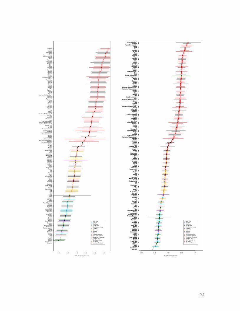
121

0.14 0.16 0.18 0.20 0.22 0.24

f3(X, Chinchorro; Yorubas)

�Bedouins�Palestinians

�Paniya�Makrani�Kalash�Agta�Aeta�Brahui�Tuscans�Papuans�Pathan�Druze�Papuans pygmy�Sardinians�North Kannadi�Sakilli�Gujaratis�Melanesians�Balkars�Malayan�Balochi�Sindhi�Lezgins�Hungarians�Hazara�Ukranians�Orcadians�North Italians�Adygei�Russians�Chuvash�French�French Basques�Burusho�Batak�Estonians�Uygurs�Teleut�Onge�She�Bajo

�Naxi�Dai�Cambodians�Altaians�Xibo�Kayah Lebbo�Khakases�Tu�Tuvinians�Buryats�Shors�Miaozu�Altaian�Kizhi�Kets�Nenets�Hezhen�Yizu�Han�Yakuts�Mongolians�Daur�Khanty�Yukaghirs�Dolgans�Oroqens�Solomons�Japanese�Mongola�Selkups�Nganasan2�Nganasans�Lahu�Tujia�Tundra Nentsi�Evenkis�Nivkhs�Evens

�Koryaks�Eskimo�Great Andamanese

AleutiansNorthern Athabascans 4

USAmerindian 1�Chukchis

Nisga'a�Naukan

West Greenlanders�USAmerindian 3

ChipewyanUSAmerindian 4

Coastal TsimshianKumlaiTlingit

Alaskan InuitNorthern Athabascans 2Northern Athabascans 1

East GreenlandersHaida

Stswecem'cKaingang

KogiAlgonquin

Northern Athabascans 3Splatsin

�HuicholInga

EmberaKaqchikel

�Zapotec2Chane

AymaraMaya1

�PimaParakana

�TepehuanoDiaguita

QuechuaSouthern Athabascans 1

OjibwaCree

�Mixtec�Zapotec1

MixeGuaymiMaya2HuetarTicuna

HullicheGuarani

PurepechaWayuu

CanAmerindian 1CucupaChiloteYaghan

PiapocoMaleku

WaunanaWichi

ArhuacoSuruiBribri

KaritianaCochimi

JamamadiCabecar

AraraChono

�USAmerindian 2Toba

Teribe�Chorotega

Palikur�Yaqui

Guahibo

�

�

�

�

�

�

�

�

�

Near EastEuropeCaucasusSouth AsiaSoutheastern AsiaOceaniaEast AsiaSiberiaAndeanCentral�AmerindChibchan�PaezanEquatorial�TucanoanEskimo�AleutGe�Pano�CaribNa DeneNorthern Amerind

�

�

�

�

�

�

�

�

�

Near EastEuropeCaucasusSouth AsiaSoutheastern AsiaOceaniaEast AsiaSiberiaAndeanCentral�AmerindChibchan�PaezanEquatorial�TucanoanEskimo�AleutGe�Pano�CaribNa DeneNorthern Amerind

0.10 0.15 0.20 0.25 0.30

f3(YRI; X, Chinchorro)

BedouinsPalestinians

TuscansDruze

MakraniBrahui

SardiniansBalkarsBalochi

North_ItaliansSakilli

PathanFrench

MelanesiansPapuansGujaratis

AdygeiKalash

UkraniansLezgins

RussiansSindhi

OrcadiansMalayan

OngeFrench_Basques

North_KannadiHungarians

PaniyaPapuans_pygmy

AetaHazara

BatakAgta

EstoniansUygurs

BurushoBajo

TuChuvashAltaians

SolomonsMongola

CambodiansShe

MiaozuHan

TeleutNganasans

DaiXibo

Tundra_NentsiKhanty

Kayah_LebboJapanese

KetsBuryats

NaxiHezhen

YizuAltaian�Kizhi

KhakasesDolgans

DaurYakutsNivkhs

OroqensTuvinians

NenetsShorsLahu

MongoliansNganasan2

TujiaSelkups

YukaghirsEvenkis

Alaskan_InuitEvens

KoryaksEskimo

ChukchisNaukan

AleutiansNorthern_Athabascans_1

CanAmerindian_1Kaingang

YaquiNisgaa

USAmerindian_4Stswecemc

KogiCucupaHuichol

ParakanaUSAmerindian_3

JamamadiOjibwa

ChipewyanTicuna

GuaraniCoastal_Tsimshian

IngaZapotec2

ChorotegaAlgonquin

HuetarSouthern_Athabascans_1

Maya1Cochimi

TlingitEmbera

Northern_Athabascans_3Arara

East_GreenlandersMixe

SplatsinPima

ChiloteDiaguita

Northern_Athabascans_4Northern_Athabascans_2

PiapocoMaleku

ArhuacoChane

Zapotec1Haida

GuaymiTepehuano

Great_AndamaneseCreeBribri

USAmerindian_2Aymara

HuillicheMixtec

PurepechaKaqchikelQuechua

Maya2Teribe

WayuuKaritiana

ChonoCabecar

PalikurSurui

KumlaiWaunana

TobaWichi

YaghanWest_Greenlanders

GuahiboUSAmerindian_1

BedouinsPalestinians

TuscansDruze

MakraniBrahui

SardiniansBalkarsBalochi

North_ItaliansSakilli

PathanFrench

MelanesiansPapuansGujaratis

AdygeiKalash

UkraniansLezgins

RussiansSindhi

OrcadiansMalayan

OngeFrench_Basques

North_KannadiHungarians

PaniyaPapuans_pygmy

AetaHazara

BatakAgta

EstoniansUygurs

BurushoBajo

TuChuvashAltaians

SolomonsMongola

CambodiansShe

MiaozuHan

TeleutNganasans

DaiXibo

Tundra_NentsiKhanty

Kayah_LebboJapanese

KetsBuryats

NaxiHezhen

YizuAltaian�Kizhi

KhakasesDolgans

DaurYakutsNivkhs

OroqensTuvinians

NenetsShorsLahu

MongoliansNganasan2

TujiaSelkups

YukaghirsEvenkis

Alaskan_InuitEvens

KoryaksEskimo

ChukchisNaukan

AleutiansNorthern_Athabascans_1

CanAmerindian_1Kaingang

YaquiNisgaa

USAmerindian_4Stswecemc

KogiCucupaHuichol

ParakanaUSAmerindian_3

JamamadiOjibwa

ChipewyanTicuna

GuaraniCoastal_Tsimshian

IngaZapotec2

ChorotegaAlgonquin

HuetarSouthern_Athabascans_1

Maya1Cochimi

TlingitEmbera

Northern_Athabascans_3Arara

East_GreenlandersMixe

SplatsinPima

ChiloteDiaguita

Northern_Athabascans_4Northern_Athabascans_2

PiapocoMaleku

ArhuacoChane

Zapotec1Haida

GuaymiTepehuano

Great_AndamaneseCreeBribri

USAmerindian_2Aymara

HuillicheMixtec

PurepechaKaqchikelQuechua

Maya2Teribe

WayuuKaritiana

ChonoCabecar

PalikurSurui

KumlaiWaunana

TobaWichi

YaghanWest_Greenlanders

GuahiboUSAmerindian_1

122

0.12 0.14 0.16 0.18 0.20 0.22 0.24 0.26

f3(X, Enoque65; Yorubas)

�Bedouins�Palestinians

�Druze�Sardinians�Makrani�Tuscans�Papuans pygmy�Brahui�French Basques�Papuans�North Italians�Lezgins�Balochi�French�Orcadians�Hungarians�Adygei�Balkars�Paniya�Sakilli�Sindhi�Malayan�Estonians�Pathan�Great Andamanese�Gujaratis�Ukranians�Russians�North Kannadi�Kalash�Solomons�Melanesians�Onge�Burusho�Chuvash�Aeta�Agta

�Uygurs�Hazara�Batak�Bajo�Teleut�Shors�Khanty�Khakases�Cambodians�Kayah Lebbo�Altaians�Altaian�Kizhi�Naxi�Dai�Selkups�Tu�Buryats�Mongolians�Xibo�Kets�Miaozu�Tundra Nentsi�Tujia�Dolgans�Tuvinians�Nenets�Han�Lahu�Yizu�Mongola�Oroqens�Yakuts�Evens�Nganasans�Japanese�Daur�She�Evenkis�Hezhen�Nivkhs�Yukaghirs�Nganasan2

�Koryaks�Chukchis

�Eskimo�Naukan

AleutiansEast GreenlandersWest Greenlanders

Alaskan Inuit�USAmerindian 3

KumlaiTlingit

ArhuacoChipewyan

HaidaSplatsin

Northern Athabascans 3Cree

Nisga'aStswecem'c

USAmerindian 1Coastal Tsimshian

Northern Athabascans 1CanAmerindian 1

OjibwaNorthern Athabascans 2

HuetarPurepecha

Northern Athabascans 4Southern Athabascans 1

Jamamadi�Chorotega

USAmerindian 4Algonquin

�PimaKogi

�USAmerindian 2�Tepehuano�Mixtec�Zapotec2�Zapotec1�Yaqui

KaqchikelMixe

ChiloteKaingang

CochimiQuechua

Maya2Maya1Wayuu

BribriHullicheTicuna

ParakanaDiaguita

WaunanaInga

CabecarTeribe

KaritianaAymaraPiapocoEmberaYaghan

�HuicholChane

GuahiboMalekuCucupa

TobaGuaraniGuaymi

WichiChono

SuruiPalikur

Arara

�

�

�

�

�

�

�

�

�

Near EastEuropeCaucasusSouth AsiaSoutheastern AsiaOceaniaEast AsiaSiberiaAndeanCentral�AmerindChibchan�PaezanEquatorial�TucanoanEskimo�AleutGe�Pano�CaribNa DeneNorthern Amerind

�

�

�

�

�

�

�

�

�

Near EastEuropeCaucasusSouth AsiaSoutheastern AsiaOceaniaEast AsiaSiberiaAndeanCentral�AmerindChibchan�PaezanEquatorial�TucanoanEskimo�AleutGe�Pano�CaribNa DeneNorthern Amerind

0.10 0.15 0.20 0.25 0.30

f3(YRI; X, enoque65)

BedouinsPalestinians

DruzeSardinians

TuscansMakrani

North_ItaliansBrahui

French_BasquesFrenchBalochi

HungariansLezginsBalkarsAdygeiSindhi

OrcadiansPapuans_pygmy

UkraniansPapuans

PathanRussiansGujaratis

EstoniansSakilli

PaniyaMalayan

OngeKalash

Great_AndamaneseNorth_Kannadi

MelanesiansBurushoChuvash

SolomonsAetaAgta

HazaraUygurs

BatakTeleut

BajoCambodians

Kayah_LebboShors

KhakasesKhanty

AltaiansSelkups

Altaian�KizhiTu

LahuTundra_Nentsi

NenetsNaxi

MongoliansDolgansBuryats

DaiYizu

TuviniansKetsTujia

HezhenHan

MiaozuYakuts

XiboJapanese

SheOroqensEvenkis

NganasansMongola

EvensDaur

YukaghirsNivkhs

Nganasan2Koryaks

ChukchisEskimo

AleutiansNaukan

Alaskan_InuitEast_GreenlandersWest_Greenlanders

Northern_Athabascans_1USAmerindian_1

HaidaCree

TlingitSplatsinOjibwa

CanAmerindian_1Chipewyan

KumlaiNisgaa

CochimiCoastal_Tsimshian

StswecemcAlgonquin

ArhuacoPima

Zapotec2Chorotega

Northern_Athabascans_4USAmerindian_4

Northern_Athabascans_2Jamamadi

USAmerindian_3Southern_Athabascans_1

PurepechaTepehuano

HuicholYaqui

HuetarZapotec1

ChiloteUSAmerindian_2

MixeMixtec

KaqchikelMalekuTeribe

KogiChono

HuillicheNorthern_Athabascans_3

QuechuaYaghanMaya1

DiaguitaWaunana

AymaraMaya2

CabecarPiapoco

KaritianaBribriWichi

WayuuEmbera

ParakanaInga

TicunaGuaraniGuaymi

GuahiboChane

SuruiCucupa

TobaKaingang

PalikurArara

BedouinsPalestinians

DruzeSardinians

TuscansMakrani

North_ItaliansBrahui

French_BasquesFrenchBalochi

HungariansLezginsBalkarsAdygeiSindhi

OrcadiansPapuans_pygmy

UkraniansPapuans

PathanRussiansGujaratis

EstoniansSakilli

PaniyaMalayan

OngeKalash

Great_AndamaneseNorth_Kannadi

MelanesiansBurushoChuvash

SolomonsAetaAgta

HazaraUygurs

BatakTeleut

BajoCambodians

Kayah_LebboShors

KhakasesKhanty

AltaiansSelkups

Altaian�KizhiTu

LahuTundra_Nentsi

NenetsNaxi

MongoliansDolgansBuryats

DaiYizu

TuviniansKetsTujia

HezhenHan

MiaozuYakuts

XiboJapanese

SheOroqensEvenkis

NganasansMongola

EvensDaur

YukaghirsNivkhs

Nganasan2Koryaks

ChukchisEskimo

AleutiansNaukan

Alaskan_InuitEast_GreenlandersWest_Greenlanders

Northern_Athabascans_1USAmerindian_1

HaidaCree

TlingitSplatsinOjibwa

CanAmerindian_1Chipewyan

KumlaiNisgaa

CochimiCoastal_Tsimshian

StswecemcAlgonquin

ArhuacoPima

Zapotec2Chorotega

Northern_Athabascans_4USAmerindian_4

Northern_Athabascans_2Jamamadi

USAmerindian_3Southern_Athabascans_1

PurepechaTepehuano

HuicholYaqui

HuetarZapotec1

ChiloteUSAmerindian_2

MixeMixtec

KaqchikelMalekuTeribe

KogiChono

HuillicheNorthern_Athabascans_3

QuechuaYaghanMaya1

DiaguitaWaunana

AymaraMaya2

CabecarPiapoco

KaritianaBribriWichi

WayuuEmbera

ParakanaInga

TicunaGuaraniGuaymi

GuahiboChane

SuruiCucupa

TobaKaingang

PalikurArara

123

0.12 0.14 0.16 0.18 0.20 0.22 0.24

f3(X, BC25; Yorubas)

0.10 0.15 0.20 0.25 0.30

f3(YRI; X, BC25)

BedouinsPalestinians

DruzeSardinians

MakraniTuscans

North_ItaliansFrench_Basques

BrahuiBalochiSindhi

AdygeiBalkarsFrench

LezginsOrcadians

HungariansKalash

UkraniansSakilli

PathanPapuansGujaratisRussians

EstoniansMalayan

Papuans_pygmyPaniya

BurushoNorth_Kannadi

OngeMelanesians

SolomonsChuvash

AgtaAeta

Great_AndamaneseHazaraUygurs

BatakTeleut

BajoCambodians

ShorsKayah_Lebbo

KhantyKhakases

AltaiansAltaian�Kizhi

TuLahuSheDai

SelkupsYizuNaxi

DolgansMiaozu

MongolaMongolians

Tundra_NentsiXiboHan

NenetsBuryats

TujiaTuvinians

KetsJapanese

DaurHezhenYakuts

NganasansNivkhs

EvenkisEvens

OroqensYukaghirs

Nganasan2Koryaks

ChukchisEskimoNaukan

USAmerindian_4Alaskan_Inuit

East_GreenlandersNorthern_Athabascans_1

West_GreenlandersHaidaTlingit

AleutiansNorthern_Athabascans_2Northern_Athabascans_4

ChipewyanUSAmerindian_1

CanAmerindian_1Coastal_Tsimshian

SplatsinCree

StswecemcNorthern_Athabascans_3

KaingangNisgaaOjibwa

ChorotegaSouthern_Athabascans_1

HuetarTicuna

JamamadiBribri

PalikurWaunanaAlgonquin

AymaraUSAmerindian_3

EmberaInga

ChonoKogi

QuechuaGuahiboCabecar

WichiGuaraniWayuu

HuillicheMaya1

DiaguitaArara

Maya2Surui

PiapocoChane

TobaParakana

GuaymiKaqchikelKaritiana

KumlaiTeribe

YaghanChilote

ArhuacoMaleku

Zapotec1Mixe

Zapotec2USAmerindian_2

MixtecPima

PurepechaHuichol

TepehuanoCucupa

YaquiCochimi

BedouinsPalestinians

DruzeSardinians

MakraniTuscans

North_ItaliansFrench_Basques

BrahuiBalochiSindhi

AdygeiBalkarsFrench

LezginsOrcadians

HungariansKalash

UkraniansSakilli

PathanPapuansGujaratisRussians

EstoniansMalayan

Papuans_pygmyPaniya

BurushoNorth_Kannadi

OngeMelanesians

SolomonsChuvash

AgtaAeta

Great_AndamaneseHazaraUygurs

BatakTeleut

BajoCambodians

ShorsKayah_Lebbo

KhantyKhakases

AltaiansAltaian�Kizhi

TuLahuSheDai

SelkupsYizuNaxi

DolgansMiaozu

MongolaMongolians

Tundra_NentsiXiboHan

NenetsBuryats

TujiaTuvinians

KetsJapanese

DaurHezhenYakuts

NganasansNivkhs

EvenkisEvens

OroqensYukaghirs

Nganasan2Koryaks

ChukchisEskimoNaukan

USAmerindian_4Alaskan_Inuit

East_GreenlandersNorthern_Athabascans_1

West_GreenlandersHaidaTlingit

AleutiansNorthern_Athabascans_2Northern_Athabascans_4

ChipewyanUSAmerindian_1

CanAmerindian_1Coastal_Tsimshian

SplatsinCree

StswecemcNorthern_Athabascans_3

KaingangNisgaaOjibwa

ChorotegaSouthern_Athabascans_1

HuetarTicuna

JamamadiBribri

PalikurWaunanaAlgonquin

AymaraUSAmerindian_3

EmberaInga

ChonoKogi

QuechuaGuahiboCabecar

WichiGuaraniWayuu

HuillicheMaya1

DiaguitaArara

Maya2Surui

PiapocoChane

TobaParakana

GuaymiKaqchikelKaritiana

KumlaiTeribe

YaghanChilote

ArhuacoMaleku

Zapotec1Mixe

Zapotec2USAmerindian_2

MixtecPima

PurepechaHuichol

TepehuanoCucupa

YaquiCochimi

�Bedouins�Palestinians

�Druze�Makrani�Sardinians�Brahui�Tuscans�Balochi�Papuans�Sindhi�North Italians�Papuans pygmy�Kalash�Lezgins�Adygei�French Basques�Malayan�Paniya�French�Balkars�Hungarians�Sakilli�Onge�Pathan�Gujaratis�North Kannadi�Orcadians�Ukranians�Estonians�Burusho�Russians�Melanesians�Great Andamanese�Solomons�Agta�Chuvash�Aeta

�Hazara�Uygurs�Batak

�Bajo�Teleut�Kayah Lebbo�Cambodians�Khakases�Tu�Shors�Khanty�Dai�She�Altaians�Lahu�Yizu�Naxi�Mongolians�Mongola�Altaian�Kizhi�Dolgans�Tujia�Han�Xibo�Miaozu�Selkups�Buryats�Nenets�Tuvinians�Tundra Nentsi�Japanese�Kets�Hezhen�Yakuts�Nivkhs�Oroqens�Daur�Evenkis�Nganasans�Evens�Yukaghirs�Nganasan2�Koryaks

�Chukchis�Eskimo

�NaukanAlaskan Inuit

AleutiansEast GreenlandersWest Greenlanders

USAmerindian 4TlingitHaida

Northern Athabascans 3Northern Athabascans 2

ChipewyanNorthern Athabascans 1

SplatsinNorthern Athabascans 4

Coastal TsimshianStswecem'c

CreeNisga'aOjibwa

�ChorotegaKaingang

PurepechaAlgonquin

CanAmerindian 1Wichi

PalikurArhuaco

Southern Athabascans 1Diaguita

HuetarBribriKogi

ParakanaMaya2Wayuu

KaqchikelWaunana

Maya1Cabecar

TicunaChilote

QuechuaGuaymiAymaraHullicheYaghanEmbera

SuruiGuaraniGuahibo

IngaAraraToba

USAmerindian 1Piapoco

KaritianaTeribe

Jamamadi�USAmerindian 3�Zapotec1

Chane�Mixtec�Zapotec2�Huichol

MixeMalekuChono

�Yaqui�Tepehuano�Pima

Cucupa�USAmerindian 2

KumlaiCochimi

�

�

�

�

�

�

�

�

�

Near EastEuropeCaucasusSouth AsiaSoutheastern AsiaOceaniaEast AsiaSiberiaAndeanCentral�AmerindChibchan�PaezanEquatorial�TucanoanEskimo�AleutGe�Pano�CaribNa DeneNorthern Amerind

�

�

�

�

�

�

�

�

�

Near EastEuropeCaucasusSouth AsiaSoutheastern AsiaOceaniaEast AsiaSiberiaAndeanCentral�AmerindChibchan�PaezanEquatorial�TucanoanEskimo�AleutGe�Pano�CaribNa DeneNorthern Amerind

124

0.12 0.14 0.16 0.18 0.20 0.22 0.24

f3(X, MARC1492; Yorubas)

�Bedouins�Palestinians

�Druze�Makrani�Sardinians�Brahui�Tuscans�Papuans pygmy�Papuans�Solomons�Balochi�French Basques�French�Balkars�North Italians�Lezgins�Sindhi�Adygei�Pathan�Gujaratis�Kalash�Hungarians�Orcadians�Malayan�Ukranians�Sakilli�Paniya�Estonians�North Kannadi�Burusho�Melanesians�Russians�Onge�Great Andamanese

�Chuvash�Agta�Aeta

�Hazara�Uygurs�Batak�Bajo�Cambodians�Teleut�Khanty�Khakases�Kayah Lebbo�Shors�Kets�Altaians�Selkups�Yizu�Nenets�Lahu�Dai�Dolgans�Altaian�Kizhi�Mongolians�Xibo�Tu�Tuvinians�Naxi�Tundra Nentsi�Buryats�Han�Mongola�Oroqens�She�Yakuts�Nganasans�Miaozu�Tujia�Evenkis�Nganasan2�Daur�Evens�Hezhen�Nivkhs�Japanese�Yukaghirs

�Koryaks�Chukchis

USAmerindian 1�Eskimo

�NaukanAlaskan Inuit

East Greenlanders�Chorotega

AleutiansWest Greenlanders

Northern Athabascans 4Stswecem'c

HaidaChonoTlingit

Nisga'aYaghan

BribriDiaguita

�HuicholNorthern Athabascans 2

HullicheWayuu

Coastal TsimshianKaqchikelJamamadi

Maya2Northern Athabascans 1

TicunaNorthern Athabascans 3

IngaMaya1

TobaChilote

PurepechaPiapoco

�MixtecSplatsin

CreeChipewyan

EmberaQuechua

�Zapotec1Guahibo

MalekuAymaraHuetar

KogiGuarani

CanAmerindian 1Cabecar

ParakanaChane

�TepehuanoWaunana

TeribeMixe

Karitiana�Zapotec2

CucupaSurui

�PimaGuaymi

Southern Athabascans 1KaingangArhuaco

USAmerindian 4�Yaqui

AraraWichi

AlgonquinCochimi

�USAmerindian 3PalikurOjibwaKumlai

�USAmerindian 2

�

�

�

�

�

�

�

�

�

Near EastEuropeCaucasusSouth AsiaSoutheastern AsiaOceaniaEast AsiaSiberiaAndeanCentral�AmerindChibchan�PaezanEquatorial�TucanoanEskimo�AleutGe�Pano�CaribNa DeneNorthern Amerind

�

�

�

�

�

�

�

�

�

Near EastEuropeCaucasusSouth AsiaSoutheastern AsiaOceaniaEast AsiaSiberiaAndeanCentral�AmerindChibchan�PaezanEquatorial�TucanoanEskimo�AleutGe�Pano�CaribNa DeneNorthern Amerind

0.10 0.15 0.20 0.25

f3(YRI; X, MARC1492)

BedouinsPalestinians

DruzeSardinians

MakraniTuscans

BrahuiNorth_Italians

French_BasquesBalochiFrenchBalkarsAdygei

OrcadiansLezgins

PapuansPapuans_pygmy

HungariansSindhi

UkraniansPathanSakilli

GujaratisEstonians

KalashNorth_Kannadi

RussiansMalayan

MelanesiansBurusho

PaniyaSolomons

OngeChuvash

Great_AndamaneseAetaAgta

HazaraUygurs

BatakBajo

TeleutKhakases

CambodiansShors

KhantyKayah_Lebbo

KetsAltaians

NaxiYizu

SelkupsDai

Altaian�KizhiLahu

DolgansTu

MongoliansXibo

BuryatsTundra_Nentsi

TuviniansNenets

HanTujia

MiaozuShe

MongolaDaur

EvenkisJapanese

YakutsNganasans

HezhenOroqens

EvensNivkhs

YukaghirsNganasan2

KoryaksChukchis

EskimoNaukan

USAmerindian_1East_Greenlanders

AleutiansAlaskan_Inuit

USAmerindian_4Chono

West_GreenlandersYaghan

ArhuacoKaingangHuilliche

BribriQuechuaDiaguita

MixtecNorthern_Athabascans_2

WaunanaGuahiboAymaraPiapoco

IngaStswecemc

TlingitMaya1

JamamadiMaya2NisgaaPalikur

KaqchikelKumlaiWayuu

TobaMixe

KaritianaTicuna

Northern_Athabascans_1Haida

ChiloteZapotec1

TeribeParakana

GuaraniKogi

CucupaSurui

EmberaCanAmerindian_1

Zapotec2Chane

Coastal_TsimshianTepehuano

CochimiHuichol

CabecarPima

ChorotegaSplatsinGuaymi

Northern_Athabascans_4Southern_Athabascans_1

AraraMaleku

WichiHuetar

AlgonquinChipewyan

Northern_Athabascans_3Ojibwa

USAmerindian_2Purepecha

YaquiCree

USAmerindian_3

BedouinsPalestinians

DruzeSardinians

MakraniTuscans

BrahuiNorth_Italians

French_BasquesBalochiFrenchBalkarsAdygei

OrcadiansLezgins

PapuansPapuans_pygmy

HungariansSindhi

UkraniansPathanSakilli

GujaratisEstonians

KalashNorth_Kannadi

RussiansMalayan

MelanesiansBurusho

PaniyaSolomons

OngeChuvash

Great_AndamaneseAetaAgta

HazaraUygurs

BatakBajo

TeleutKhakases

CambodiansShors

KhantyKayah_Lebbo

KetsAltaians

NaxiYizu

SelkupsDai

Altaian�KizhiLahu

DolgansTu

MongoliansXibo

BuryatsTundra_Nentsi

TuviniansNenets

HanTujia

MiaozuShe

MongolaDaur

EvenkisJapanese

YakutsNganasans

HezhenOroqens

EvensNivkhs

YukaghirsNganasan2

KoryaksChukchis

EskimoNaukan

USAmerindian_1East_Greenlanders

AleutiansAlaskan_Inuit

USAmerindian_4Chono

West_GreenlandersYaghan

ArhuacoKaingangHuilliche

BribriQuechuaDiaguita

MixtecNorthern_Athabascans_2

WaunanaGuahiboAymaraPiapoco

IngaStswecemc

TlingitMaya1

JamamadiMaya2NisgaaPalikur

KaqchikelKumlaiWayuu

TobaMixe

KaritianaTicuna

Northern_Athabascans_1Haida

ChiloteZapotec1

TeribeParakana

GuaraniKogi

CucupaSurui

EmberaCanAmerindian_1

Zapotec2Chane

Coastal_TsimshianTepehuano

CochimiHuichol

CabecarPima

ChorotegaSplatsinGuaymi

Northern_Athabascans_4Southern_Athabascans_1

AraraMaleku

WichiHuetar

AlgonquinChipewyan

Northern_Athabascans_3Ojibwa

USAmerindian_2Purepecha

YaquiCree

USAmerindian_3

125

0.12 0.14 0.16 0.18 0.20 0.22 0.24 0.26

f3(X, MA577; Yorubas)

�Bedouins�Palestinians

�Druze�Makrani�Sardinians�Tuscans�Brahui�North Italians�French Basques�Onge�Balochi�Papuans�Papuans pygmy�French�Adygei�Lezgins�Sakilli�Sindhi�Balkars�Hungarians�Orcadians�Pathan�Malayan�Kalash�Great Andamanese�Ukranians�North Kannadi�Gujaratis�Paniya�Estonians�Melanesians�Russians�Burusho�Solomons�Agta�Chuvash�Aeta�Hazara�Uygurs�Batak�Bajo�Cambodians�Teleut�Kayah Lebbo�Khakases�Shors�Dai�Lahu�Khanty�Altaians�Tu�Naxi�Altaian�Kizhi�Mongolians�Selkups�She�Yizu�Tujia�Miaozu�Xibo�Han�Kets�Mongola�Dolgans�Tuvinians�Buryats�Japanese�Nenets�Tundra Nentsi�Daur�Hezhen�Nivkhs�Oroqens�Yakuts�Evenkis�Nganasans�Evens�Nganasan2�Yukaghirs

�Koryaks�Chukchis

�Eskimo�Naukan

Alaskan InuitEast Greenlanders

AleutiansWest Greenlanders

Northern Athabascans 3Northern Athabascans 1

ChipewyanTlingit

SplatsinNorthern Athabascans 2

Stswecem'cNorthern Athabascans 4

AlgonquinCree

Nisga'aOjibwaHaida

CanAmerindian 1USAmerindian 4

Coastal Tsimshian�Chorotega

Southern Athabascans 1Purepecha

�Yaqui�USAmerindian 3�Pima

Cucupa�Tepehuano�Zapotec1

Maya2�Huichol�Mixtec

Kaqchikel�Zapotec2

HuetarMaya1Kumlai

MixeCochimi

USAmerindian 1Ticuna

�USAmerindian 2Arhuaco

WayuuKogi

CabecarBribri

DiaguitaMaleku

JamamadiWichi

TeribeGuaymiEmbera

WaunanaQuechuaPiapoco

KaritianaIngaToba

GuaraniParakana

AymaraKaingang

SuruiGuahibo

ChanePalikur

AraraChiloteChono

HullicheYaghan

�

�

�

�

�

�

�

�

�

Near EastEuropeCaucasusSouth AsiaSoutheastern AsiaOceaniaEast AsiaSiberiaAndeanCentral�AmerindChibchan�PaezanEquatorial�TucanoanEskimo�AleutGe�Pano�CaribNa DeneNorthern Amerind

�

�

�

�

�

�

�

�

�

Near EastEuropeCaucasusSouth AsiaSoutheastern AsiaOceaniaEast AsiaSiberiaAndeanCentral�AmerindChibchan�PaezanEquatorial�TucanoanEskimo�AleutGe�Pano�CaribNa DeneNorthern Amerind

0.10 0.15 0.20 0.25 0.30

f3(YRI; X, MA577)

BedouinsPalestinians

DruzeSardinians

MakraniTuscans

North_ItaliansFrench_Basques

BrahuiBalochiFrenchAdygeiBalkars

OrcadiansHungarians

LezginsSindhi

UkraniansSakilli

PathanKalash

PapuansPapuans_pygmy

EstoniansOnge

GujaratisRussiansMalayan

North_KannadiBurusho

PaniyaMelanesians

ChuvashGreat_Andamanese

SolomonsAgtaAeta

HazaraUygurs

BatakCambodians

BajoTeleut

KhakasesShors

Kayah_LebboKhanty

AltaiansLahu

Altaian�KizhiSelkups

DaiMongolians

NaxiTu

NenetsSheKetsYizuTujia

DolgansBuryats

HanTuvinians

XiboMongola

MiaozuJapanese

Tundra_NentsiHezhenNivkhs

DaurYakuts

NganasansEvenkis

OroqensEvens

YukaghirsNganasan2

KoryaksChukchis

EskimoNaukan

AleutiansAlaskan_Inuit

East_GreenlandersNorthern_Athabascans_4

West_GreenlandersCanAmerindian_1

Northern_Athabascans_1ChipewyanAlgonquin

Northern_Athabascans_3USAmerindian_4

Northern_Athabascans_2OjibwaTlingit

SplatsinNisgaa

StswecemcHaidaCree

Coastal_TsimshianSouthern_Athabascans_1

YaquiPima

TepehuanoPurepecha

MalekuZapotec1

CucupaUSAmerindian_2

HuicholMixtec

Zapotec2USAmerindian_3

MixeHuetar

CochimiTicunaKumlaiMaya1

KogiKaqchikel

TeribeMaya2

ChorotegaCabecar

KaingangKaritiana

BribriUSAmerindian_1

PiapocoGuaymi

WichiWaunana

IngaEmberaWayuu

ParakanaJamamadiQuechuaGuarani

SuruiChane

AymaraGuahibo

AraraDiaguita

PalikurArhuaco

TobaChonoChilote

HuillicheYaghan

BedouinsPalestinians

DruzeSardinians

MakraniTuscans

North_ItaliansFrench_Basques

BrahuiBalochiFrenchAdygeiBalkars

OrcadiansHungarians

LezginsSindhi

UkraniansSakilli

PathanKalash

PapuansPapuans_pygmy

EstoniansOnge

GujaratisRussiansMalayan

North_KannadiBurusho

PaniyaMelanesians

ChuvashGreat_Andamanese

SolomonsAgtaAeta

HazaraUygurs

BatakCambodians

BajoTeleut

KhakasesShors

Kayah_LebboKhanty

AltaiansLahu

Altaian�KizhiSelkups

DaiMongolians

NaxiTu

NenetsSheKetsYizuTujia

DolgansBuryats

HanTuvinians

XiboMongola

MiaozuJapanese

Tundra_NentsiHezhenNivkhs

DaurYakuts

NganasansEvenkis

OroqensEvens

YukaghirsNganasan2

KoryaksChukchis

EskimoNaukan

AleutiansAlaskan_Inuit

East_GreenlandersNorthern_Athabascans_4

West_GreenlandersCanAmerindian_1

Northern_Athabascans_1ChipewyanAlgonquin

Northern_Athabascans_3USAmerindian_4

Northern_Athabascans_2OjibwaTlingit

SplatsinNisgaa

StswecemcHaidaCree

Coastal_TsimshianSouthern_Athabascans_1

YaquiPima

TepehuanoPurepecha

MalekuZapotec1

CucupaUSAmerindian_2

HuicholMixtec

Zapotec2USAmerindian_3

MixeHuetar

CochimiTicunaKumlaiMaya1

KogiKaqchikel

TeribeMaya2

ChorotegaCabecar

KaingangKaritiana

BribriUSAmerindian_1

PiapocoGuaymi

WichiWaunana

IngaEmberaWayuu

ParakanaJamamadiQuechuaGuarani

SuruiChane

AymaraGuahibo

AraraDiaguita

PalikurArhuaco

TobaChonoChilote

HuillicheYaghan

126

Fig. S15. Likelihood surface as a function of the bottleneck size NB and the divergence time TDIV for a Native American population and a Siberian population. All 22 autosomes were used for this computation. In each plot, the red X symbol indicates the grid point where the likelihood is maximized. The likelihood was evaluated at grid points (NB, TDIV), where NB ∈ {1500, 1541, 1583, 1626, 1670, 1716, 1763, 1811, 1860, 1911, 1963, 2016, 2071, 2128, 2186, 2245, 2306, 2369, 2434, 2500}, and TDIV ∈{15000, 15229, 15461, 15697, 15937, 16180, 16427, 16677, 16932, 17190, 17452, 17718, 17989, 18263, 18542, 18825, 19112, 19403, 19699, 20000} for the pairs involving Koryak, and TDIV ∈{20000, 20236, 20475, 20717, 20962, 21210, 21460, 21714, 21970, 22230, 22492, 22758, 23027, 23299, 23574, 23853, 24135, 24420, 24708, 25000} for the pairs involving Nivkh.

15000 16000 17000 18000 19000 20000

1600

1800

2000

2200

2400

Athabascan vs. Koryak (clean split)

TDIV

NB

−13539250 −13539050

−13538850 −13538700 −13538650

−13538600 −13538550

−13538500 −13538450

−13538400 −13538350

−13538300

−13538250 −13538200

−13538150 −13538100 −13538050 −13538000 −13537950

−13537900

−13537850

−13537850

−13537800

−13537750

−13537700 −13537650

−13537600

−13537600 −13537550 −13537500

−13537450

−13537450

−13537400

−13537400

−13537350

−13537350

−13537300

−13537300

−13537250

−13537250

−13537200

−13537200

−13537150

−13537150

−13537100

−13537100

−13537050

−13537050

−13537000

−13537000

−13536950

−13536950

−13536900

−13536900

−13536850

−13536850

−13536800

−13536800

−13536750

−13536750

−13536700

−13536700

−13536650

−13536650

−13536600

−13536600

−13536550

−13536550

−13536500

−13536500

−13536450

−13536450

−13536400

−13536400

−13536350

−13536350

−13536300

−13536300

−13536250

−13536250

−13536200

−13536200

−13536150

−13536150

−13536100

−13536100

−13536050

−13536050

−13536000

−13536000

−13535950

−13535950

−13535900

−13535900

−13535850

−13535850

−13535800

−13535800

−13535750

−13535750

−13535700

−135

3570

0

−13535650 −13535600

−13535550

−13535500 −13535450

−13535400 −13535350

−13535300

19699

1763

20000 21000 22000 23000 24000 25000

1600

1800

2000

2200

2400

Athabascan vs. Nivkhs (clean split)

TDIV

NB

−13811900 −13811600

−13811400 −13811300 −13811200

−13811100 −13811000

−13810900

−13810800 −13810700

−13810600

−13810500 −13810400

−13810300 −13810200

−13810100 −13810000

−13809900 −13809800 −13809700 −13809600

−13809500

−13809400 −13809300 −13809200 −13809100 −13809000 −13808900

−13808800

−13808700

−13808700

−13808600

−13808500

−13808500 −13808400

−13808300

−13808300

−13808200

−13808200

−13808100

−13808100

−13808000

−13808000

−13807900

−13807900

−13807800

−13807800

−13807700

−13807700

−13807600

−13807600

−13807500

−13807500

−13807400

−13807400

−13807300

−13807300

−13807200

−13807200 −13807100

−13807000

21970

1811

15000 16000 17000 18000 19000 20000

1600

1800

2000

2200

2400

Karitiana vs. Koryak (clean split)

TDIV

NB

−15405550 −15405350

−15405150 −15405050

−15405000 −15404950

−15404900 −15404850

−15404800 −15404750

−15404700

−15404600 −15404550

−15404500 −15404450

−15404400 −15404350 −15404300 −15404250 −15404200

−15404150

−15404100

−15404050

−15404000

−15403950

−15403900

−15403900 −15403850 −15403800 −15403750

−15403700

−15403700 −15403650 −15403600

−15403550

−15403500

−15403500

−15403450

−15403450

−15403400

−15403400

−15403350

−15403350

−15403300

−15403300

−15403250

−15403250

−15403200

−15403200

−15403150

−15403150

−15403100

−15403100

−15403050

−15403050

−15403000

−15403000

−15402950

−15402950

−15402900

−15402900

−15402850

−15402850

−15402800

−15402800

−15402750

−15402750

−15402700

−15402700

−15402650

−15402650

−15402600

−15402600

−15402550

−15402550

−15402500

−15402500

−15402450

−15402450

−15402400

−15402400

−15402350

−15402350

−15402300

−15402300

−15402250

−15402250

−15402200

−15402200

−15402150

−15402150

−15402100

−15402100

−15402050

−15402050

−15402000

−15402000

−15401950

−15401950

−15401900

−15401900

−15401850 −15401800

−15401750

−15401700

−15401650

18542

1811

20000 21000 22000 23000 24000 25000

1600

1800

2000

2200

2400

Karitiana vs. Nivkhs (clean split)

TDIV

NB

−15435000 −15434700

−15434500

−15434400 −15434300

−15434200 −15434100 −15434000

−15433900

−15433800

−15433700 −15433600

−15433500 −15433400

−15433300 −15433200

−15433100

−15433000

−15432900 −15432800 −15432700 −15432600

−15432500

−15432400 −15432300 −15432200 −15432100 −15432000 −15431900

−15431800

−15431700

−15431600

−15431500

−15431400

−15431400

−15431300

−15431300

−15431200

−15431100

−15431100

−15431000

−15431000

−15430900

−15430900

−15430800

−15430800

−15430700

−15430700

−15430600

−15430600

−15430500

−15430500

−15430400

−15430400

−15430300

−15430300

−15430200

−15430100

−15430000

−15429900

21210

1811

127

Fig. S16. Likelihood surface as a function of the bottleneck size NB and the divergence time TDIV for Athabascan and Karitiana. The red X symbol indicates the grid point where the likelihood is maximized.

Fig. S17. Parametric bootstrap results for the clean-split model. The true parameter values used in simulation are shown on the x-axis.

Athabascan vs. Karitiana

T_DIV

N_B

−12011400

−12010700 −12010100

−12010000

−12009600

−12009400

−12009100

−12009000

−12008900 −12008600

−12008400

−12008300 −12008200

−12008100

−12008000 −12007900

−12007800

−12007700 −12007600

−12007500 −12007400

−12007300

−12007200

−12007100 −12007000

−12006900

−12006800

−12006700 −12006600

−12006500

−12006400

−12006300 −12006200 −12006100

−12006000

−12005900 −12005800 −12005700 −12005600

−12005500 −12005400 −12005300 −12005200

−12005100 −12005000 −12004900 −12004800

−12004700 −12004600

−12004500 −12004400

−12004300

−12004200 −12004100 −12004000

−12003900 −12003800

−12003700

−12003700 −12003600

−12003500

−12003500 −12003400

−12003300

−12003300

−12003200

−12003100

−12003000

−12002900

10000 15000 20000

1500

2000

2500

1670

12909

−1.0

−0.5

0.0

0.5

1.0

Accuracy

log 2(estimatetruth)

TD TB N1 N2 NB NA19000 70000 2000 3000 2000 20000

−1.5

−1.0

−0.5

0.0

0.5

1.0

1.5

Accuracy

log 2(estimatetruth)

TDIV TB N1 N2 NB NA13000 70000 2600 1600 1700 20000

128

Fig. S18. Population splits and gene flows involving Native Americans and Siberians. The plots show likelihood surface as a function of the migration rate m and the divergence time TDIV. All 22 autosomes were used for this computation.

15000 20000 25000 30000

2e−0

65e−0

62e−0

55e−0

52e−0

45e−0

42e−0

3Athabascan vs. Koryak (migration)

TDIV

Mig

ratio

n pr

obab

ility

m

20780

0.00

0136

15000 20000 25000 30000

2e−0

65e−0

62e−0

55e−0

52e−0

45e−0

42e−0

3

Athabascan vs. Nivkhs (migration)

TDIV

Mig

ratio

n pr

obab

ility

m23183

0.00

0095

15000 20000 25000 30000

2e−0

65e−0

62e−0

55e−0

52e−0

45e−0

42e−0

3

Karitiana vs. Koryak (migration)

TDIV

Mig

ratio

n pr

obab

ility

m

22353

0.00

0196

15000 20000 25000 30000

2e−0

65e−0

62e−0

55e−0

52e−0

45e−0

42e−0

3

Karitiana vs. Nivkhs (migration)

TDIV

Mig

ratio

n pr

obab

ility

m

23183

0.00

0095

129

Fig. S19. Population splits and gene flows involving the Greenlandic Inuit.

10000 15000 20000 25000

2e−0

65e−0

62e−0

55e−0

52e−0

45e−0

42e−0

3

Greenlander vs. Athabascan (migration)

TDIV

Mig

ratio

n pr

obab

ility

m

18479

0.00

0406

10000 15000 20000 25000

2e−0

65e−0

62e−0

55e−0

52e−0

45e−0

42e−0

3

Greenlander vs. Karitiana (migration)

TDIV

Mig

ratio

n pr

obab

ility

m

18479

0.00

0282

15000 20000 25000 30000

2e−0

61e−0

55e−0

52e−0

41e−0

35e−0

3

Greenlander vs. Koryak (migration)

TDIV

Mig

ratio

n pr

obab

ility

m

21425

0.00

0912

18000 20000 22000 24000 26000 28000 30000 32000

2e−0

65e−0

62e−0

55e−0

52e−0

45e−0

42e−0

3

Greenlander vs. Nivkhs (migration)

TDIV

Mig

ratio

n pr

obab

ility

m

23583

0.00

0406

10000 15000 20000 25000

2e−0

65e−0

62e−0

55e−0

52e−0

45e−0

42e−0

3

Greenlander vs. Huichol (migration)

TDIV

Mig

ratio

n pr

obab

ility

m

18479

0.00

0282

130

Fig. S20. Population splits and gene flows involving Huichol, a southern North American population.

7000 8000 9000 10000 11000 12000 13000

2e−0

65e−0

62e−0

55e−0

52e−0

45e−0

42e−0

3Huichol vs. Karitiana (migration)

TDIV

Mig

ratio

n pr

obab

ility

m

8080

0.00

0046

12000 14000 16000 18000 20000

2e−0

65e−0

62e−0

55e−0

52e−0

45e−0

42e−0

3

Huichol vs. Athabascan (migration)

TDIV

Mig

ratio

n pr

obab

ility

m

12574

0.00

0032

18000 20000 22000 24000 26000 28000 30000 32000

2e−0

65e−0

62e−0

55e−0

52e−0

45e−0

42e−0

3

Huichol vs. Koryak (migration)

TDIV

Mig

ratio

n pr

obab

ility

m

20892

0.00

0136

131

Fig. S21. Population splits and gene flows involving Han Chinese and Native Americans.

Fig. S22. Likelihood surfaces as a function of gene flow rate m and stopping time TM. These surfaces are for divergence time TDIV = 22 KYA. These results suggest that gene flow between the Karitiana and the Koryak (left) occurred until recently, possibly indirectly through other populations. In contrast, gene flow between the Athabascan and the Koryak (right) seems to have stopped much earlier, around 12 KYA.

18000 20000 22000 24000 26000 28000 30000 32000

2e−0

65e−0

62e−0

55e−0

52e−0

45e−0

42e−0

3Han vs. Athabascan (migration)

TDIV

Mig

ratio

n pr

obab

ility

m

22879

0.00

0066

18000 20000 22000 24000 26000 28000 30000 32000

2e−0

65e−0

62e−0

55e−0

52e−0

45e−0

42e−0

3

Han vs. Karitiana (migration)

TDIV

Mig

ratio

n pr

obab

ility

m

22879

0.00

0095

Karitiana vs. Koryak (T_DIV = 22 kya)

TM

Mig

ratio

n pr

obab

ility

m

−15403050

−15402900 −15402800

−15402750 −15402650

−15402600

−15402550

−15402500

−15402450

−15402400

−15402350

−15402300 −15402250

−15402200

−15402150

−15402100

−15402050

−15402000

−15

4020

00

−15401950

−154

0195

0

−15401900

−154

0190

0

−15401850

−15401850

−15401800

−15401800 −15401750

−15401750

−15401700

−15401700

−15401650

−15401650

−15401600

−15401600

−15401550

−15401550

−15401500

−15401450

−15401400

1000 2000 5000 10000 15000

5e−0

51e−0

42e−0

45e−0

40.

001

0.00

2

1764

0.00

0221

Athabascan vs. Koryak (T_DIV = 22 kya)

TM

Mig

ratio

n pr

obab

ility

m

−13

5355

15

−13

5355

05

−13

5355

00

−135

3549

5

−13

5354

90

−135

3548

5

−135

3548

0

−135

3547

5

−13

5354

70

−13

5354

65

−135

3546

0

−135

3545

5 −

1353

5450

−13535445

−135

3544

0 −1

3535

435

−13535430

−135

3542

5

−135

3542

0

−13535415

−13535410

−135

3540

5

−13535400

−13535395

−135

3539

0

−135

3538

5

−13535380

−13535375

−13535370

−13535365

−135

3536

0

−13535355

−13535350

−13535345

−135

3534

0

−13535335

−13535330 −13535325

−13535320

−13535315

−13535310

−13535305 −13535300

−13535295

−13535290 −13535285

−13535280 −1

3535275 −1

3535270

−135

3527

0

−13535265 −13535260

−13535255 −1

3535250

−135

3525

0

−13535245

−13535240 −13535235

−13535230

−135

3523

0

−13535225

−135

3522

5

−13535220

−13535215

−13535210

−13535210

−13535205

−135

3520

5

−13535200 −13535195

−13535190

−13535190

−13535185

−135

3518

5

−13535180

−135

3518

0

−13535175

−13535175

−13535170

−135

3517

0

−13535165

−13535165

−13535160

−13535160

10000 15000

5e−0

40.

001

0.00

20.

005

11812

0.00

1909

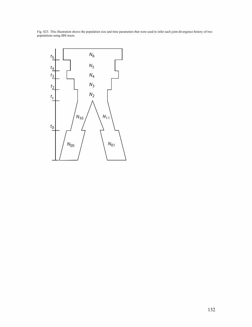
132

Fig. S23. This illustration shows the population size and time parameters that were used to infer each joint divergence history of two populations using IBS tracts.

133

Fig. S24. Real and predicted IBS tracts shared between Athabascan and Koryak/Karitiana. A1 shows real IBS tracts shared within the Athabascan, within the Koryak and between Athabascan and Koryak. Similarly, B1 shows real IBS tracts shared within the Athab-scan, within the Karitiana and between Athabascan and Karitiana. Each of the remaining panels shows a single real IBS tract length distribution compared to the IBS tract distribution predicted under the appropriate model from Table S12.

134

Fig. S25. MSMC population size estimates based on 2 diploid samples per population.

Fig. S26. Relative cross coalescence rate estimates between 6 populations of this study from two outgroups, Han and Yoruba.

AthabascanKaritianaKoryakGreenlanderNivkh

effe

ctiv

e po

pula

tion

size

1000

2000

5000

10000

20000

years ago [mu=1.25×10-8, gen=29 years]5000 10000 20000 50000 100000

Yoruba/AthabascanYoruba/KaritianaYoruba/KoryakYoruba/GreenlanderYoruba/NivkhYoruba/Huichol

Han/AthabascanHan/KaritianaHan/KoryakHan/GreenlanderHan/NivkhHan/Huichol

rela

tive

cros

s co

ales

cenc

e ra

te

0

0,2

0,4

0,6

0,8

1,0

rela

tive

cros

s co

ales

cenc

e ra

te

0

0,2

0,4

0,6

0,8

1,0

time [years ago]5000 10000 20000 50000

135

Fig. S27. Relative cross coalescence rates across American and Eurasian populations.

Fig. S28. Switch errors in the different populations. The plot shows the mean distance between to haplotype-switches for each individual when comparing the haplotypes from the “panel”-phased and “no-panel”-phased datasets. We report this mean distance for the chromosomes 1-11. Two lines are shown for Koryak (Kor1, Kor2), Karitiana (BI16, HGDP00998), Athabascan (Athabascan_1, Athabascan_2), Siberian Yupik (Esk17, Esk20), and Nivkhs (Nivh1, Nivh2), since the dataset contained two individuals for each of these populations. The IDs for the single sample (Table S1) are: East Greenland (Greenlander_1), West Greenland, (Greenlander_2) Han (HGDP00778), Dai (HGDP01307) and Huichol (HUI03).

Karitiana/KoryakAthabascan/KoryakHuichol/KoryakKaritiana/NivkhAthabascan/NivkhHuichol/NivkhKaritiana/GreenlanderAthabascan/GreenlanderHuichol/Greenlander

Old world / New world splits:

Athabascan/KaritianaAthabascan/HuicholKaritiana/Huichol

New world splits:

Koryak/NivkhKoryak/GreenlanderNivkh/Greenlander

Old world splits:

rel. c

ross c

oal. r

ate

0

0,5

1,0

rel. c

ross c

oal. r

ate

0

0,5

1,0

rel. c

ross c

oal. r

ate

0

0,5

1,0

years ago0 10000 20000 30000 40000

136

Fig. S29. CCR-rates estimated from the simulated data using MSMC. The upper panel shows the results from the “Clean split @ 18.5k” simulation, whereas the lower panel shows the results from the “Split @ 22k + migration [2k,22k]” simulation. The time when the CCR-curve crosses 50% is reported as the divergence time and does not seem to be affected by introducing switch errors.

18.5k split18.5k split with s.e.22k split with mig.22k split+mig, with s.e.

rela

tive

CC

R

0

0,5

1,0

rela

tive

CC

R

0

0,5

1,0

time [years ago]0 10000 20000 30000 40000

137

Fig. S30. Here, each point on the X-axis represents an entry of the folded 2-D Site Frequency Spectrum (SFS) of the Koryak and Karitiana, with four haplotypes sampled from each population. The label (m, n) describes sites for which m Karitiana haplotypes have some allelic type A, the remaining 4 − m Karitiana have a different type B, and exactly n of the Koryak have allelic type A. For each of these types, the y axis plots the fraction of variable sites that fall into category (m, n), one curve each describing the real data, the model inferred by diCal2.0 and the model inferred using IBS tracts.

138

Fig. S31. Routes of gene flow during the expansion represented by the distribution of coalescence events; 100 gene trees were sampled from each of the best fitting combinations of demographic parameters. The two panels show coalescence events for (left) Anzick-1 versus Amerindians from southern North America and Central and South America and (right) Athabascans (coalescences within the population).

139

Fig. S32. Procrustes transformation PCA plots of samples combined with different reference panels. For the PCA plot with the worldwide panel from (6), see main text Fig. 5. (A) PCA of samples (key in figure) projected on a subset of the worldwide reference panel including only individuals from Mexico (blue filled circles) and Central America (purple triangles). (B) PCA of Fuego-Patagonian samples and a subset of the reference panel in panel A including only South American individuals. (C) PCA of Pericúes and Mexican mummies (key in figure) plotted with a reference panel that contains only Mexican individuals (34). Population labels are TAR: Tarahumara, HUI: Huichol, PUR: Purepecha, TOT: Totonac, NAJ: Nahua Jalisco, NXP: Nahua Puebla, TRQ: Triqui, MAZ: Mazatec, ZAP: Zapotec, TZT: Tzotzil, MYA: Maya Q.Roo. (D) PCA of all 23 ancient samples sequenced in this study, and Anzick-1, plotted with the extended reference panel compiled in this study, only including individuals from Oceanians and the Americas (Table S3).

�0.20 �0.15 �0.10 �0.05 0.00 0.05 0.10

�0.3

�0.2

�0.1

0.0

0.1

PC1 (1.72%)

PC

2 (

1.3

4%

)

TAR

HUI

PURTOT

NAJ

NAP

TRQ

MAZ

ZAP

TZT

MYA

North

Central West

Central East

South

Southeast

�0.05 0.00 0.05 0.10 0.15 0.20 0.25

�0.1

5�0

.10

�0.0

50

.00

0.0

50

.10

0.1

5

PC1 (2.93%)

PC

2 (

1.8

2%

)

Mexico

Central�South America

AM71

Nr66

Nr72

Nr73

Nr74

MA572

MA575

MA577

890

894

895

Fuego-Patagonians

F9

MOM6

Mummies

BC23

BC25

BC27

BC28

BC29

BC30

Pericúes

F9

MOM6

Mummies

BC23

BC25

BC27

BC28

BC29

BC30

Pericúes

�0.1 0.0 0.1 0.2

�0.4

�0.3

�0.2

�0.1

0.0

0.1

0.2

PC1 (3.52%)

PC

2 (

2.8

1%

)

Brazil

Argentina

Colombia

Andes (Colombia Bolivia Peru Chile)

Chile�Patagonia

Guiana

Paraguay(&Argentina)

AM71

Nr66

Nr72

Nr73

Nr74

MA572

MA575

MA577

890

894

895

Fuego-Patagonians

PCA Americas PCA South America

PCA Mexico

�0.10 �0.05 0.00

�0.0

50.0

00.0

50.1

0

PC1 (5.66%)

PC

2 (

1.0

6%

)

Solomons

Papuans

Melanesians

Native

Americans

�

��

890

894

895

939

AM71

BC23

BC25

BC27

BC28

BC29

BC30

Chinchorro

Anzick-1

F9

MA572

MA575

MA577

MARC1492

MOM6

Nr66

Nr72

Nr73

Nr74

enoque65

���

PCA Americas/Oceania (extended dataset)

A B

C D

140

Fig. S33. Population structure in ancient Pericúes, Mexican mummies and Fuego-Patagonians from this study and worldwide populations. Ancestry proportions are shown when assuming 13 genetic components (K=13). The top bars show the ancestry proportions (represented as different colors) of the 19 ancient individuals sequenced in this study, Anzick-1 (5), and two present-day genomes from this study (Huichol and Aymara). The plot at the bottom illustrates the ancestry proportions for 1,823 individuals from the worldwide panel from (6). There is a clear differentiation in northern Mexican (pink) and Central South American ancestry (brown). For plots showing six components (K=6), see main text Fig. 5.

Tarahumara, HUI: Huichol, PUR: Purepecha, TOT: Totonac, NAJ: Nahua Jalisco, NXP: Nahua Puebla, TRQ: Triqui, MAZ: Mazatec, ZAP: Zapotec, TZT: Tzotzil, MYA: Maya Q.Roo. E, PCA of Fuego-Patagonian samples and a subset of the reference panel in c including only South American individuals.

Fig. 2. Population structure in ancient Pericú, Mexican mummy and Fuego-Patagonian individuals from this study and worldwide populations. A, Ancestry proportions are shown when when assuming 6 genetic components (K=6) and B, when assuming 13 genetic components (K=13). The top bars in each panel show the ancestry proportions (represented as different colors) of the 19 ancient individuals in this study, for Anzick-1(4), and two modern genomes from this study (Huichol and Aymara). The plot at the bottom of each panel illustrates the ancestry proportions for 1,823 individuals from the worldwide panel from Reich et al(28) (same subset depicted in Figure 1b). In A (K=6) our samples show mainly (>92%) “Native American” (Ivory) and “Siberian” (Indian Red) ancestry, in B (K=13) there is a clear differentiation in northern Mexican (pink) and Central South American ancestry (brown).

141

Fig. S34. Examples of population structures from this study alongside ADMIXTURE results for worldwide populations. Ancestry proportions are shown for K=7 to 12 (see main text Fig. 5 for K=6 and Fig. S33 for K=13) for whole genome data obtained in this study and a worldwide reference panel from (6). The whole genome data is represented on the left with wide bars for one Pericú individual, one Mexican mummy, three Fuego-Patagonian, the Anzick-1 genome and the two modern genomes sequenced in this study. On the top, the ancestry proportions as obtained by running ADMIXTURE for the reference panel. This data has been filtered for recent European admixture in the Native American populations (labelled Mexico, Chile-Patagonia, Central South Am, Canada, Greenland, Aleut) by (6).

142

Fig. S35. Linear regression of (A) error rate and (B) depth of coverage versus combined European, Near Oceania and Central South Asian admixture fractions. For each ancient sample we plotted error rate and depth of coverage against the cumulative ancestry proportions corresponding to the “European” “Near Oceanian” and “Central South Asian” fractions (green, light blue and purple clusters in main text Fig. 5) at K=6. Linear regression and the coefficient of (R2) are shown on both plots. The Anzick-1, the Aymara and the Huichol genomes are shown on the graph as well for comparison but were not used to perform the linear regression.

143

Fig. S36. Outgroup f3 statistics using SNP chip genotype data from modern-day non-African populations. We computed outgroup f3 statistics of the form f3 (YRI; X, ancient individual) where X corresponds to the 116 non-African populations in the (6) reference panel. Horizontal lines correspond to one standard error obtained through a block-jackknife procedure. Results are shown for the individuals with the highest depth of coverage from each subpopulation.

144

Fig. S37. Genetic affinities (shared drift) of ancient Pericúes, Mummies and Fuego-Patagonians with worldwide populations. Left plots show the f3 statistic point estimates (with one standard error) for the topology f3(YRI; X, Ancient), where X represents one of the populations from the Americas, Near Oceania, or the Han Chinese (CHB) from the reference panel used for Fig. S32. The heat maps to the right indicate geographically how the samples compare to the global populations, with the point color indicating the f3 statistic values. The results shown here correspond to one ancient individual (with the highest depth of genome coverage) per subpopulation (qualitatively similar results for all individuals within subpopulations were observed). (A) Pericúes, (B) Mummies, (C) Kaweskar, (D) Selknam, (E) Yaghan. All samples show higher f3 values for modern day Native Americans.

145

Fig. S38. Simplified schematic of the scenario proposed by (23) where the Americas are peopled by two waves of migration. Under this hypothesis, the first migration (1, indicated in green) consists of the “Paleoamericans”, a population that shares a recent common ancestor with Papuans. The second wave of migration (2, indicated in blue) occurs later by the morphologically different Amerindians that share recent common ancestry with East Asians. The Amerindians largely replaced the Paleoamericans, however, some populations (e.g. the Pericúes/Fuego-Patagonians) have been described as relict Paleoamericans on morphological grounds. The expected tree topology is given (centre) and key locations (including our sample sites) are labeled. Potential gene flow between the arrows is omitted.

146

Fig. S39. D-statistics using SNP chip genotype data and whole genome data from Native Americans, Papuans and Europeans. We tested a tree topology of the form (((Native American, ancient individual), X), YRI) where X corresponds to Papuans (A and B) and Europeans (C and D). For each figure, the top sub-panel shows results for SNP chip genotype data, and the bottom sub-panel shows results for whole genome data. Results are shown for the Pericú (A and D) and the Fuego-Patagonian (B and C) with the highest depth of coverage. We obtain qualitatively identical results for all samples. One and three standard errors are shown for each result.

147

Fig. S40. D-statistics using SNP chip genotype data and whole genome data from Native Americans and East Asians. We tested a tree topology of the form (((Native American, ancient individual), East Asian), YRI). We show results for the Pericú (A) and the ancient Fuego-Patagonian (B) with the highest depth of coverage. We also show results for the Pericú with the lowest error rate, BC29, for the same test (C). For each figure, the top sub-panel shows results for SNP chip genotype data, and the bottom sub-panel shows results for whole genome data. We used Native American whole genomes to test a tree topology of the form (((Huichol, Aymara), ancient individual), YRI) (D). D<0 implies a closer relationship of the ancient individual and the north Mexican Huichol and D>0 implies that the ancient individual is more closely related to the Andean Aymara. One and three standard errors are shown for each result.

148

Fig. S41. Craniometric affinities of Paleoamericans, Kaweskar, and Pericú populations. (A) UPGMA tree of craniometric similarity between groups. (B) Patterns of craniometric variation. The first three principal coordinates of craniometric shape variation account for cranial size (PCO1), cranial width/length (PCO2; dolichocephaly versus brachycephaly), and cranial height/length (elongated versus rounded crania). (C) Cranial shape variation along PCO2 and PCO3. Cranial outline drawings illustrate actual amount of variation in relative cranial width (PCO2) and height (PCO3). Note wide intra-continental variation, overlap of patterns of variation between continents, and conspicuous differences between males and females of any given population. Continent abbreviations as in Table S15.