Supplemental appendix to "Household Portfolios and Implicit Risk Preference" by

Supplemental appendix to “Household Portfolios and Implicit

Risk Preference” by Alessandro Bucciol and Raffaele Miniaci, Review of Economics and Statistics, Vol. 93, No. 4

(November 2011), pp. 1235–1250.

URL: http://www.mitpressjournals.org/doi/abs/10.1162/REST_a_00138

HOUSEHOLD PORTFOLIOS

AND IMPLICIT RISK PREFERENCE

ALESSANDRO BUCCIOL RAFFAELE MINIACI

University of Verona,

University of Amsterdam, and Netspar

University of Brescia

Supplementary Appendix

– NOT FOR PUBLICATION –

S2

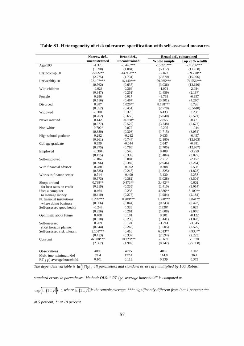
S.1. Specification with self-assessed measures

In this exercise we use the benchmark estimates of risk tolerance and replicate the

regression analysis of Table 5 in the main text, with a richer specification that includes two

self-assessed measures on risk attitude and time horizon.

The first measure is based on the SCF question:

«Which of the following statements comes closest to describing the amount of

financial risk that you [and your husband/wife/partner] are willing to take when

you save or make investments?»

1. Take substantial financial risks expecting to earn substantial returns

2. Take above average financial risks expecting to earn above average returns

3. Take average financial risks expecting to earn average returns

4. Not willing to take any financial risks

where we code as “self-assessed risk tolerant” households responding 1 or 2.

The second measure is based on the SCF question:

«In planning (your/your family’s) saving and spending, which of the following

is most important to [you/you and your (husband/wife/partner)]: the next few

months, the next year, the next few years, the next 5 to 10 years, or longer than

10 years? »

1. Next few months

2. Next year

3. Next few years

4. Next 5-10 years

S3

5. Longer than 10 years

where we code as “self-assessed short-horizon planner” households responding 1 or 2.

Results from this analysis are shown in Table S1.

S4

S.2. Results using different asset moments

In this exercise we estimate risk tolerance for each household, taking the same definition of

portfolio as in the benchmark case but changing the asset returns.

S.2.1. Numeraire

We compute asset return moments from the same series of risky asset returns as in the

benchmark case, where now returns are in excess from yields to i) 10-year bonds and ii)

real 3-month T-bills (computed as nominal yields net of inflation growth, with inflation

measured as the variation in the CPI index for all urban consumers, all items). In the

benchmark case we instead use returns in excess from yields to nominal 3-month T-bills.

The time series cover quarterly the sample 1980-2004 (100 observations); the 20

observations for real estate returns between 1980 and 1984 are imputed as in the benchmark

case following Stambaugh (1997).

Results from this analysis are shown in Tables S2-S5, and in Figures S1-S2.

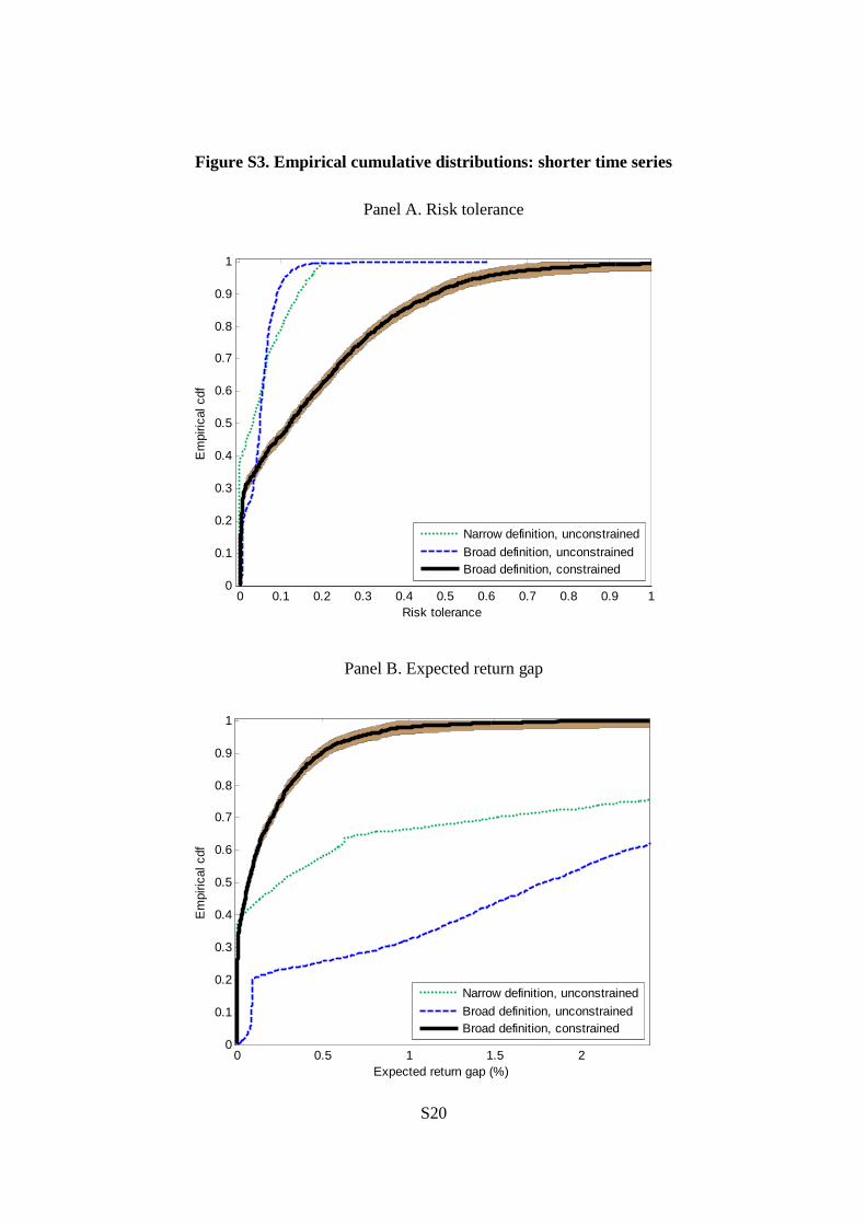
S.2.2. Time series period coverage

We compute asset return moments from the same series of risky and risk free asset returns

as in the benchmark case, but using a shorter period coverage.

The time series cover quarterly the sample period 1990-2004 (60 observations).

Results from this analysis are shown in Tables S6-S7, and in Figure S3.

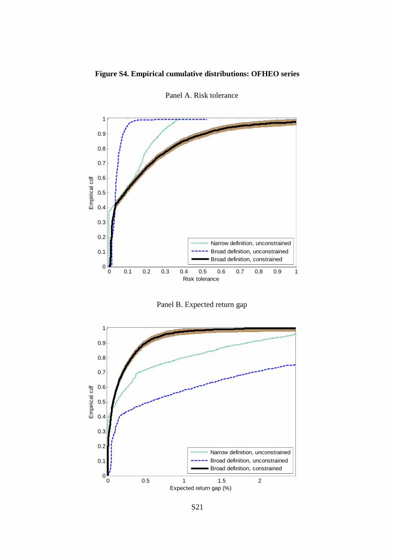
S.2.3. Time series for real estate returns

We compute asset return moments from the same series of risky and risk free asset returns

as in the benchmark case, with the exception of real estate returns. Here we use the repeat-

S5

sale, purchase-only index calculated for the whole of the US by the Office of Federal

Housing Enterprise Oversight (OFHEO) from data provided by Fannie Mae and Freddie

Mac (the two biggest mortgage lenders in the US). To account for imputed rents, we

increase returns by a constant factor of 5% as in Flavin and Yamashita (2002) and Pelizzon

and Weber (2008).

The time series cover quarterly the sample 1980-2004 (100 observations); in this case no

imputation of real estate returns is needed.


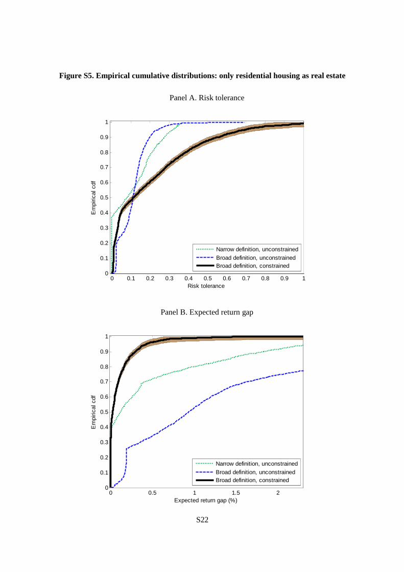
S.3. Results using a different definition of portfolio

In this exercise we estimate risk tolerance for each household, taking the same asset returns

as in the benchmark case, but changing the definition of portfolio. The new definition

includes only (owner-occupied) residential housing as real wealth; consistently, we exclude

from the portfolio other real estate properties and related loans.

Under the new definition, the inequality constraint imposed on real estate in the

benchmark analysis (the optimal holding of real estate has to be not lower than the

observed holding of residential housing) becomes an equality constraint (the optimal

holding of real estate coincides with the observed holding of residential housing). Since the

composition of the observed portfolio has changed, three further constraints are also

different from the benchmark analysis: the equality constraints on human capital and real

estate, and the inequality constraint on bonds (for which the optimal holding has to be not

lower than the opposite of the observed holding on real estate).

The number of observations in the new dataset is slightly different than in the

benchmark analysis (4,100 observations rather than 4,095) as we exclude from the original

S6

sample 20 observations (rather than 25) whose portfolios do not respect our constraints. It

is also worth pointing out that, while the median wealth is virtually unchanged relative to

the benchmark case (including human capital, it is 142,322 USD as opposed to 141,300

USD), the distribution of wealth in the sample changes, and the top 20% wealthiest

households considered in the last column of Table S11 are not the same as the ones

considered in the last column of Table 5 in the main text.


S7

Table S1. Heterogeneity of risk tolerance: specification with self-assessed measures

Narrow def., unconstrained

Broad def., unconstrained

Broad def., constrained Whole sample Top 20% wealth Age/100 -1.375

(1.390) -5.445***

(1.084) -15.228***

(5.112) -37.206***

(11.768) Ln(income)/10 -5.922**

(2.275) -14.983***

(1.731) -7.873

(7.870) -39.770** (15.926)

Ln(wealth)/10 22.107*** (0.762)

16.140*** (0.637)

29.035*** (3.036)

71.556*** (13.610)

With children -0.023 (0.347)

0.366 (0.251)

-1.074 (1.459)

-2.084 (2.187)

Female 0.286 (0.516)

0.017 (0.497)

-3.763 (3.501)

-6.957 (4.280)

Divorced 0.387 (0.552)

1.026** (0.451)

8.138*** (2.770)

0.726 (3.5610)

Widowed -0.301 (0.762)

0.375 (0.656)

6.433 (5.040)

3.298 (5.521)

Never married 0.142 (0.577)

-0.988* (0.522)

2.855 (3.248)

-0.471 (5.677)

Non-white -0.702* (0.380)

0.072 (0.308)

-0.205 (1.715)

-1.944 (3.051)

High school graduate 0.282 (0.861)

-0.282 (0.744)

0.635 (2.180)

-6.457 (12.963)

College graduate 0.959 (0.875)

-0.044 (0.786)

2.647 (2.705)

-0.981 (12.967)

Employed -0.304 (0.475)

0.546 (0.339)

0.489 (1.404)

-3.259 (3.077)

Self-employed -0.867 (0.596)

0.004 (0.387)

2.712 (2.946)

-2.457 (3.264)

With financial advisor 0.288 (0.335)

-0.002 (0.218)

0.308 (1.325)

0.598 (1.823)

Works in finance sector 0.714 (0.573)

-0.490 (0.382)

3.130 (3.028)

2.258 (3.501)

Shops around for best rates on credit

0.788** (0.319)

0.473** (0.235)

3.442** (1.410)

0.602 (2.014)

Uses a computer to manage money

0.464 (0.410)

0.233 (0.277)

4.386** (1.984)

5.100** (2.184)

N. financial institutions where doing business

0.209*** (0.066)

0.209*** (0.044)

1.398*** (0.343)

0.841** (0.423)

Self-assessed good health -0.248 (0.356)

0.326 (0.261)

2.828* (1.608)

0.629 (2.076)

Optimistic about future 0.408 (0.310)

0.101 (0.233)

0.201 (1.441)

-0.122 (1.878)

Self-assessed short horizon planner

0.269 (0.344)

0.124 (0.266)

-1.214 (1.505)

-3.345 (2.579)

Self-assessed risk tolerant 2.101*** (0.413)

0.410 (0.337)

6.513** (2.594)

4.933** (2.223)

Constant -6.308*** (2.367)

10.229*** (1.902)

-6.699 (8.247)

-1.570 (25.968)

Observations 4095 4095 4095 1602 Mult. imp. minimum dof 74.4 172.4 114.8 36.4 RT ( )γ average household 0.101 0.113 0.239 0.373

The dependent variable is ( )ln 1 γ+ ; all parameters and standard errors are multiplied by 100. Robust

standard errors in parentheses. Method: OLS. “ RT ( )γ average household” is computed as

( ){ }exp ln 1 1γ+ − where ( )ln 1 γ+ is the sample average. ***: significantly different from 0 at 1 percent; **:

at 5 percent; *: at 10 percent.

S8

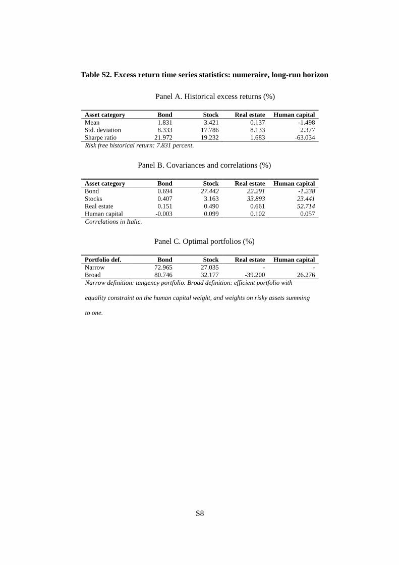
Table S2. Excess return time series statistics: numeraire, long-run horizon

Panel A. Historical excess returns (%)

Asset category Bond Stock Real estate Human capital Mean 1.831 3.421 0.137 -1.498 Std. deviation 8.333 17.786 8.133 2.377 Sharpe ratio 21.972 19.232 1.683 -63.034 Risk free historical return: 7.831 percent.

Panel B. Covariances and correlations (%)

Asset category Bond Stock Real estate Human capital Bond 0.694 27.442 22.291 -1.238 Stocks 0.407 3.163 33.893 23.441 Real estate 0.151 0.490 0.661 52.714 Human capital -0.003 0.099 0.102 0.057 Correlations in Italic.

Panel C. Optimal portfolios (%)

Portfolio def. Bond Stock Real estate Human capital Narrow 72.965 27.035 - - Broad 80.746 32.177 -39.200 26.276 Narrow definition: tangency portfolio. Broad definition: efficient portfolio with

equality constraint on the human capital weight, and weights on risky assets summing

to one.

S9

Table S3. Heterogeneity of risk tolerance: numeraire, long-run horizon




(1.375) -5.399***

(1.006) -15.757***

(4.733) -37.042***

(11.348) Ln(income)/10 -5.310**

(2.248) -13.431***

(1.588) -3.982

(7.213) -35.092** (14.587)

Ln(wealth)/10 22.327*** (0.736)

15.420*** (0.570)

27.741*** (2.615)

68.072*** (12.400)


0.390* (0.236)

-1.408 (1.347)

-2.522 (1.999)

Female 0.075 (0.516)

0.015 (0.457)

-4.515 (3.391)

-6.806* (3.888)

Divorced 0.615 (0.549)

0.991** (0.423)

7.742*** (2.686)

0.957 (3.043)

Widowed -0.028 (0.755)

0.366 (0.598)

7.009 (4.901)

4.071 (4.938)


-0.993** (0.485)

3.486 (3.194)

0.949 (5.850)

Non-white -0.718* (0.375)

0.051 (0.285)

0.561 (1.674)

-1.421 (2.638)


-0.326 (0.684)

0.961 (2.061)

-1.981 (11.811)


-0.112 (0.725)

3.185 (2.671)

1.994 (11.758)

Employed -0.278 (0.471)

0.581* (0.315)

0.411 (1.259)

-3.414 (2.756)


0.024 (0.362)

1.590 (2.384)

-2.231 (2.949)


0.009 (0.205)

0.236 (1.231)

0.266 (1.657)


-0.474 (0.360)

3.320 (2.903)

2.954 (3.532)


0.780** (0.317)

0.460** (0.219)

2.788** (1.259)

0.984 (1.740)


0.592 (0.406)

0.234 (0.260)

4.588** (1.900)

4.434** (1.940)


0.246*** (0.065)

0.207*** (0.041)

1.408*** (0.339)

0.943** (0.443)


0.306 (0.242)

2.706* (1.511)

0.814 (1.883)


0.115 (0.214)

0.384 (1.334)

0.250 (1.641)

Constant -6.398*** (2.343)

9.498*** (1.743)

-8.246 (7.635)

-5.278 (23.271)


The dependent variable is ( )ln 1 γ+ , and is normalized to produce the same RT for the average household as

the benchmark case. All parameters and standard errors are multiplied by 100. Robust standard errors in

parentheses. Method: OLS. “ RT ( )γ average household” is computed as ( ){ }exp ln 1 1γ+ − where ( )ln 1 γ+

is the sample average. ***: significantly different from 0 at 1 percent; **: at 5 percent; *: at 10 percent.

S10

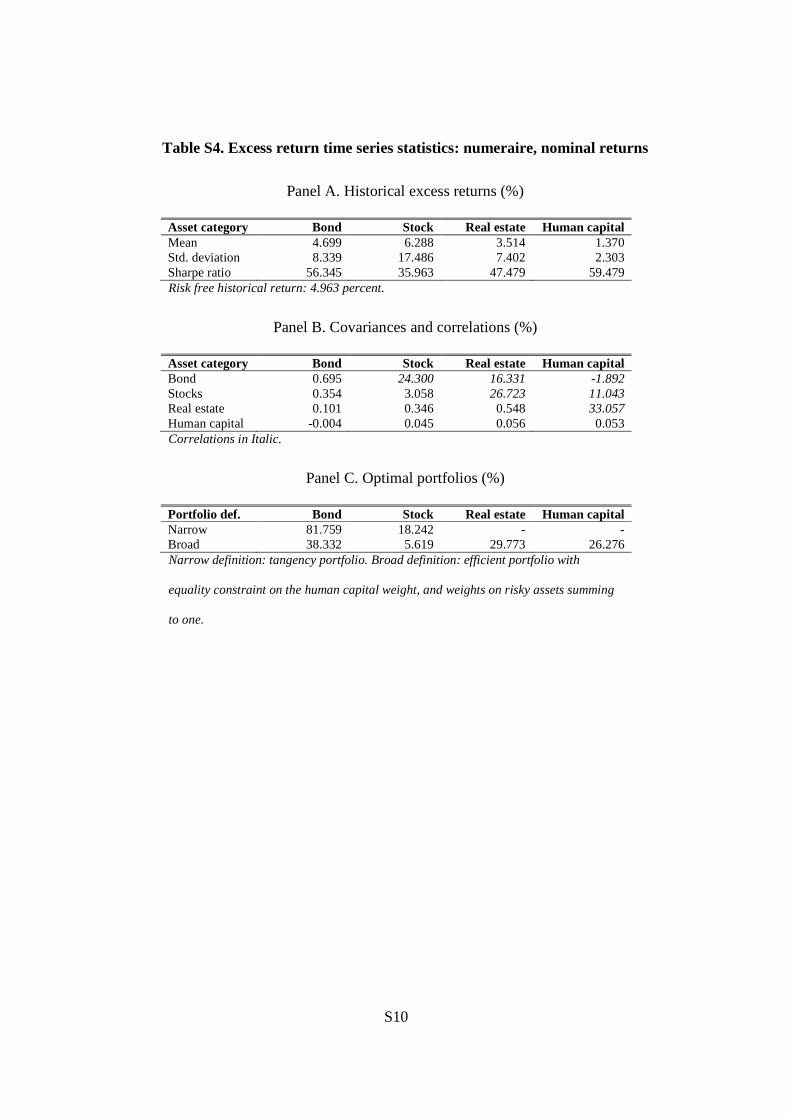
Table S4. Excess return time series statistics: numeraire, nominal returns


Asset category Bond Stock Real estate Human capital Mean 4.699 6.288 3.514 1.370 Std. deviation 8.339 17.486 7.402 2.303 Sharpe ratio 56.345 35.963 47.479 59.479 Risk free historical return: 4.963 percent.


Asset category Bond Stock Real estate Human capital Bond 0.695 24.300 16.331 -1.892 Stocks 0.354 3.058 26.723 11.043 Real estate 0.101 0.346 0.548 33.057 Human capital -0.004 0.045 0.056 0.053 Correlations in Italic.


Portfolio def. Bond Stock Real estate Human capital Narrow 81.759 18.242 - - Broad 38.332 5.619 29.773 26.276 Narrow definition: tangency portfolio. Broad definition: efficient portfolio with


to one.

S11

Table S5. Heterogeneity of risk tolerance: numeraire, nominal returns




(1.405) -6.472***

(1.192) -18.969***

(4.820) -39.905***

(11.324) Ln(income)/10 -5.386**

(2.311) -15.836***

(1.925) -2.427

(7.638) -32.982** (14.877)

Ln(wealth)/10 22.488*** (0.754)

17.167*** (0.691)

30.618*** (2.684)

71.542*** (13.010)


0.399 (0.280)

-1.311 (1.361)

-2.663 (2.131)

Female 0.063 (0.529)

-0.066 (0.573)

-3.984 (3.432)

-7.025 (4.256)

Divorced 0.650 (0.565)

1.231** (0.510)

8.454*** (2.718)

0.765 (3.590)

Widowed -0.007 (0.775)

0.532 (0.763)

6.618 (4.966)

3.904 (5.462)


-1.036* (0.593)

2.998 (3.147)

-0.879 (5.386)

Non-white -0.714* (0.383)

0.066 (0.345)

-0.542 (1.619)

-1.739 (2.946)


-0.356 (0.841)

1.210 (2.113)

-2.715 (12.570)


-0.054 (0.896)

3.634 (2.729)

2.902 (12.520)

Employed -0.271 (0.484)

0.624* (0.377)

0.667 (1.356)

-2.869 (3.012)


0.000 (0.430)

2.849 (2.746)

-2.326 (3.148)


-0.019 (0.244)

0.464 (1.254)

0.426 (1.799)


-0.530 (0.426)

2.687 (2.751)

2.020 (3.332)


0.806** (0.325)

0.516* (0.263)

3.415*** (1.301)

1.027 (1.958)


0.618 (0.418)

0.305 (0.308)

4.556** (1.818)

5.404** (2.124)


0.242*** (0.067)

0.244*** (0.050)

1.517*** (0.330)

0.844** (0.413)


0.373 (0.289)

2.696* (1.492)

0.885 (2.048)


0.123 (0.258)

0.536 (1.332)

0.469 (1.839)

Constant -6.477*** (2.400)

10.439*** (2.103)

-12.719 (7.792)

-11.178 (24.385)






S12

Table S6. Excess return time series statistics: shorter time series




Asset category Bond Stock Real estate Human capital Bond 0.313 -7.560 6.827 12.085 Stocks -0.073 3.005 19.824 10.621 Real estate 0.028 0.255 0.552 31.449 Human capital 0.014 0.037 0.047 0.040 Correlations in Italic.


Portfolio def. Bond Stock Real estate Human capital Narrow 84.877 15.123 - - Broad 44.105 6.129 23.490 26.276 Narrow definition: tangency portfolio. Broad definition: efficient portfolio with


to one.

S13

Table S7. Heterogeneity of risk tolerance: shorter time series



Broad def., constrained Whole sample Top 20% wealth Age/100 -3.078**

(1.541) -6.498***

(1.183) -18.304***

(3.392) -31.032***

(8.679) Ln(income)/10 -4.394*

(2.609) -16.198***

(1.996) -10.670*

(5.899) -32.488***

(9.732) Ln(wealth)/10 23.037***

(0.835) 17.905***

(0.691) 39.016***

(1.878) 77.964***

(9.303) With children -0.280

(0.396) 0.477* (0.277)

-2.346*** (0.822)

-3.740** (1.822)

Female -0.134 (0.589)

-0.074 (0.575)

-2.376 (1.800)

-4.417 (3.677)

Divorced 0.910 (0.635)

1.280** (0.507)

4.857*** (1.529)

1.627 (3.174)

Widowed 0.161 (0.852)

0.549 (0.780)

2.110 (2.750)

0.970 (4.791)


-1.061* (0.588)

0.469 (1.729)

-2.496 (3.966)

Non-white -0.954** (0.416)

0.138 (0.340)

-0.601 (0.912)

0.159 (2.510)

High school graduate -0.052 (0.811)

-0.502 (0.838)

0.298 (1.850)

-0.038 (9.847)


-0.182 (0.895)

4.031* (2.074)

5.369 (9.808)

Employed -0.174 (0.539)

0.682* (0.377)

-0.083 (1.158)

-0.355 (2.356)


0.148 (0.437)

1.785 (1.545)

-0.719 (2.460)


-0.046 (0.244)

1.561* (0.807)

1.372 (1.551)


-0.520 (0.424)

1.105 (1.281)

0.699 (2.300)


0.908** (0.366)

0.527** (0.261)

1.864** (0.778)

0.873 (1.627)


0.811* (0.480)

0.273 (0.305)

3.325*** (0.999)

3.766** (1.677)


0.271*** (0.077)

0.237*** (0.049)

1.246*** (0.194)

0.399 (0.284)


0.400 (0.286)

1.332 (0.867)

-0.540 (1.664)


0.054 (0.256)

0.698 (0.785)

0.098 (1.548)

Constant -7.769*** (2.663)

10.114*** (2.136)

-9.262 (5.882)

-26.290 (17.968)






S14

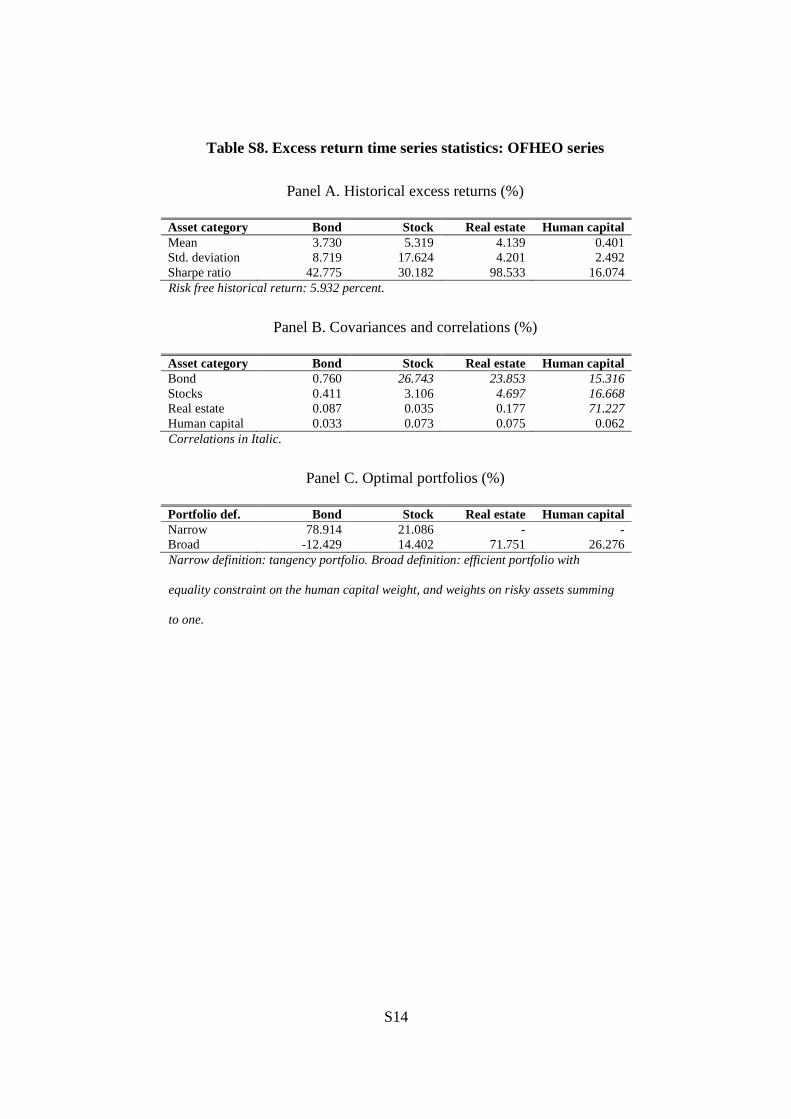
Table S8. Excess return time series statistics: OFHEO series




Asset category Bond Stock Real estate Human capital Bond 0.760 26.743 23.853 15.316 Stocks 0.411 3.106 4.697 16.668 Real estate 0.087 0.035 0.177 71.227 Human capital 0.033 0.073 0.075 0.062 Correlations in Italic.


Portfolio def. Bond Stock Real estate Human capital Narrow 78.914 21.086 - - Broad -12.429 14.402 71.751 26.276 Narrow definition: tangency portfolio. Broad definition: efficient portfolio with


to one.

S15

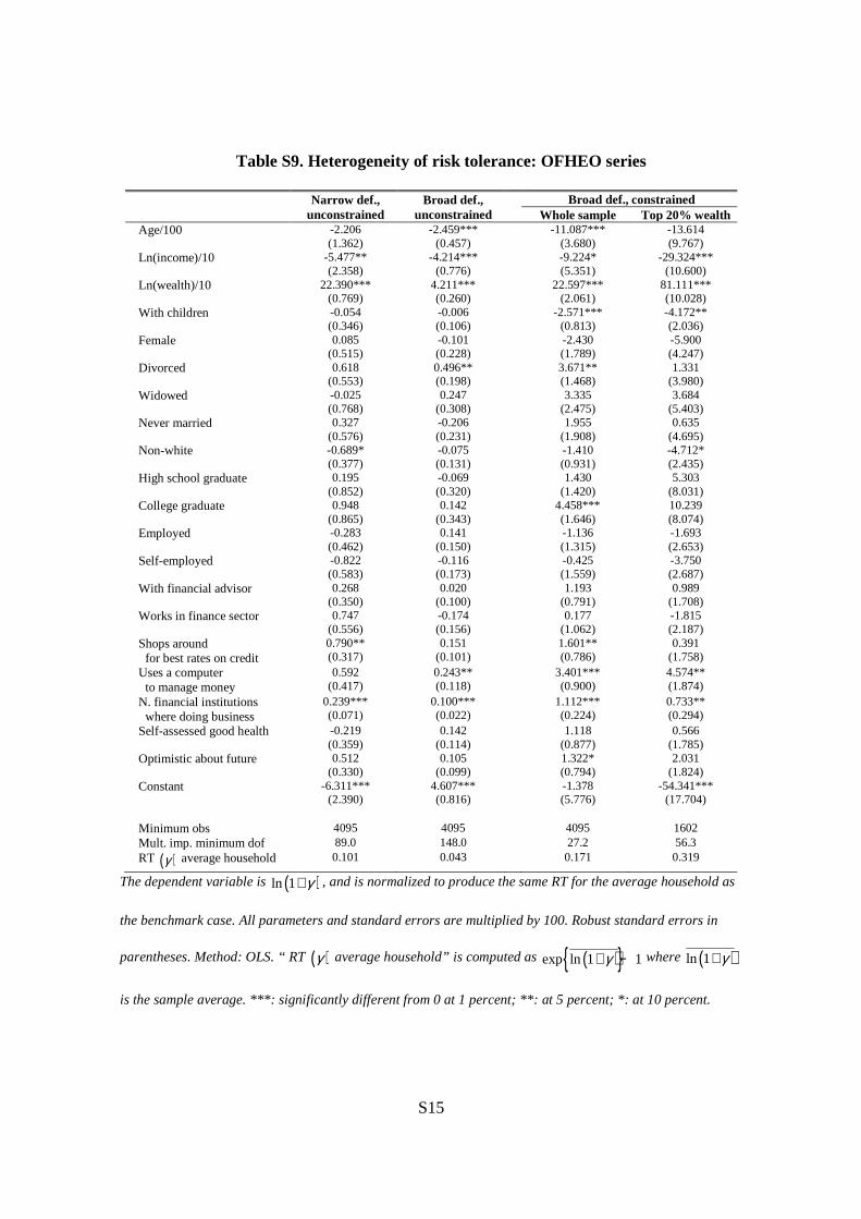
Table S9. Heterogeneity of risk tolerance: OFHEO series




(1.362) -2.459***

(0.457) -11.087***

(3.680) -13.614 (9.767)

Ln(income)/10 -5.477** (2.358)

-4.214*** (0.776)

-9.224* (5.351)

-29.324*** (10.600)

Ln(wealth)/10 22.390*** (0.769)

4.211*** (0.260)

22.597*** (2.061)

81.111*** (10.028)


-0.006 (0.106)

-2.571*** (0.813)

-4.172** (2.036)

Female 0.085 (0.515)

-0.101 (0.228)

-2.430 (1.789)

-5.900 (4.247)

Divorced 0.618 (0.553)

0.496** (0.198)

3.671** (1.468)

1.331 (3.980)

Widowed -0.025 (0.768)

0.247 (0.308)

3.335 (2.475)

3.684 (5.403)


-0.206 (0.231)

1.955 (1.908)

0.635 (4.695)

Non-white -0.689* (0.377)

-0.075 (0.131)

-1.410 (0.931)

-4.712* (2.435)


-0.069 (0.320)

1.430 (1.420)

5.303 (8.031)


0.142 (0.343)

4.458*** (1.646)

10.239 (8.074)

Employed -0.283 (0.462)

0.141 (0.150)

-1.136 (1.315)

-1.693 (2.653)


-0.116 (0.173)

-0.425 (1.559)

-3.750 (2.687)


0.020 (0.100)

1.193 (0.791)

0.989 (1.708)


-0.174 (0.156)

0.177 (1.062)

-1.815 (2.187)


0.790** (0.317)

0.151 (0.101)

1.601** (0.786)

0.391 (1.758)


0.592 (0.417)

0.243** (0.118)

3.401*** (0.900)

4.574** (1.874)


0.239*** (0.071)

0.100*** (0.022)

1.112*** (0.224)

0.733** (0.294)


0.142 (0.114)

1.118 (0.877)

0.566 (1.785)


0.105 (0.099)

1.322* (0.794)

2.031 (1.824)

Constant -6.311*** (2.390)

4.607*** (0.816)

-1.378 (5.776)

-54.341*** (17.704)

Minimum obs 4095 4095 4095 1602 Mult. imp. minimum dof 89.0 148.0 27.2 56.3 RT ( )γ average household 0.101 0.043 0.171 0.319





S16

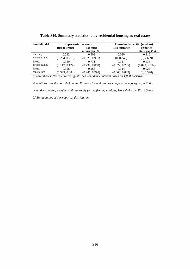
Table S10. Summary statistics: only residential housing as real estate

Portfolio def. Representative agent Household-specific (median) Risk tolerance Expected

return gap (%) Risk tolerance Expected

return gap (%) Narrow, unconstrained

0.212 (0.204, 0.219)

0.903 (0.823, 0.991)

0.080 (0, 0.345)

0.116 (0, 2.669)

Broad, unconstrained

0.120 (0.117, 0.124)

0.771 (0.737, 0.808)

0.111 (0.022, 0.285)

0.935 (0.073, 7.304)

Broad, constrained

0.356 (0.329, 0.384)

0.268 (0.245, 0.290)

0.114 (0.008, 0.822)

0.026 (0, 0.598)

In parentheses: Representative agent: 95% confidence interval based on 1,000 bootstrap

simulations over the household units. From each simulation we compute the aggregate portfolio

using the sampling weights, and separately for the five imputations; Household-specific: 2.5 and

97.5% quantiles of the empirical distribution.

S17

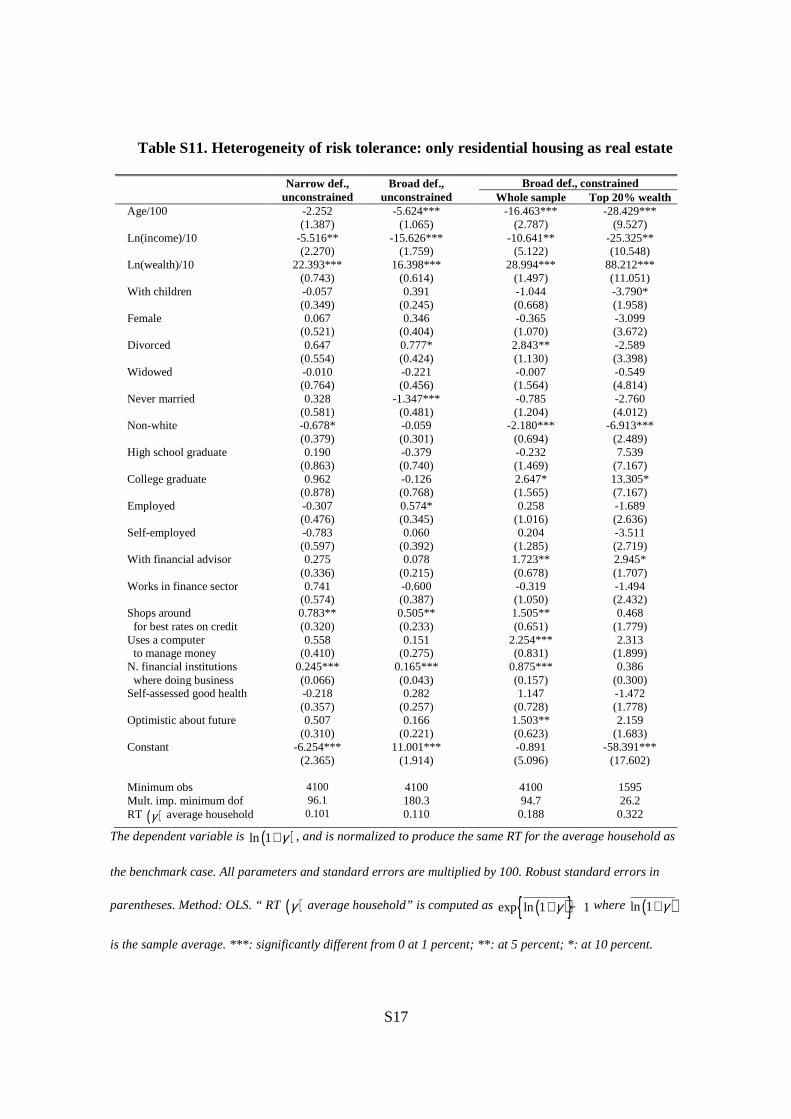
Table S11. Heterogeneity of risk tolerance: only residential housing as real estate




(1.387) -5.624***

(1.065) -16.463***

(2.787) -28.429***

(9.527) Ln(income)/10 -5.516**

(2.270) -15.626***

(1.759) -10.641**

(5.122) -25.325** (10.548)

Ln(wealth)/10 22.393*** (0.743)

16.398*** (0.614)

28.994*** (1.497)

88.212*** (11.051)


0.391 (0.245)

-1.044 (0.668)

-3.790* (1.958)

Female 0.067 (0.521)

0.346 (0.404)

-0.365 (1.070)

-3.099 (3.672)

Divorced 0.647 (0.554)

0.777* (0.424)

2.843** (1.130)

-2.589 (3.398)

Widowed -0.010 (0.764)

-0.221 (0.456)

-0.007 (1.564)

-0.549 (4.814)


-1.347*** (0.481)

-0.785 (1.204)

-2.760 (4.012)

Non-white -0.678* (0.379)

-0.059 (0.301)

-2.180*** (0.694)

-6.913*** (2.489)


-0.379 (0.740)

-0.232 (1.469)

7.539 (7.167)


-0.126 (0.768)

2.647* (1.565)

13.305* (7.167)

Employed -0.307 (0.476)

0.574* (0.345)

0.258 (1.016)

-1.689 (2.636)


0.060 (0.392)

0.204 (1.285)

-3.511 (2.719)


0.078 (0.215)

1.723** (0.678)

2.945* (1.707)


-0.600 (0.387)

-0.319 (1.050)

-1.494 (2.432)


0.783** (0.320)

0.505** (0.233)

1.505** (0.651)

0.468 (1.779)


0.558 (0.410)

0.151 (0.275)

2.254*** (0.831)

2.313 (1.899)


0.245*** (0.066)

0.165*** (0.043)

0.875*** (0.157)

0.386 (0.300)


0.282 (0.257)

1.147 (0.728)

-1.472 (1.778)


0.166 (0.221)

1.503** (0.623)

2.159 (1.683)

Constant -6.254*** (2.365)

11.001*** (1.914)

-0.891 (5.096)

-58.391*** (17.602)

Minimum obs 4100 4100 4100 1595 Mult. imp. minimum dof 96.1 180.3 94.7 26.2 RT ( )γ average household 0.101 0.110 0.188 0.322





S18

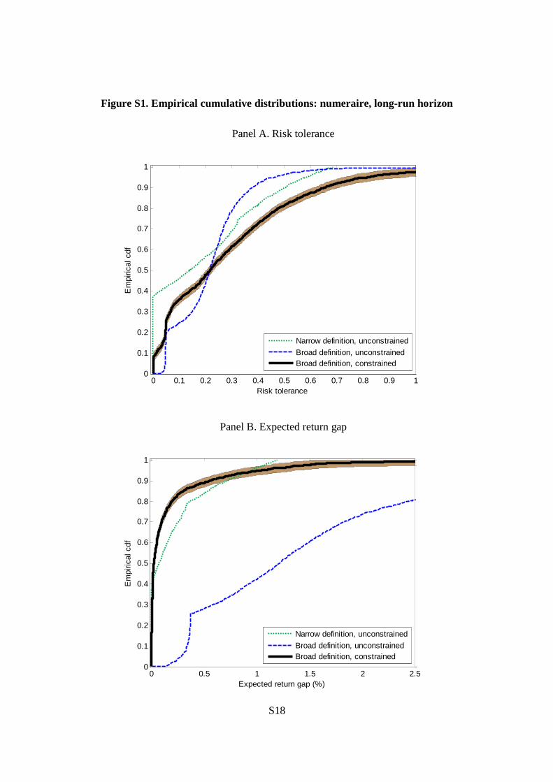
Figure S1. Empirical cumulative distributions: numeraire, long-run horizon

Panel A. Risk tolerance

0 0.1 0.2 0.3 0.4 0.5 0.6 0.7 0.8 0.9 10

0.1

0.2

0.3

0.4

0.5

0.6

0.7

0.8

0.9

1

Risk tolerance

Em

piric

al c

df

Narrow definition, unconstrained

Broad definition, unconstrainedBroad definition, constrained

Panel B. Expected return gap

0 0.5 1 1.5 2 2.50

0.1

0.2

0.3

0.4

0.5

0.6

0.7

0.8

0.9

1

Expected return gap (%)

Em

piric

al c

df



S19

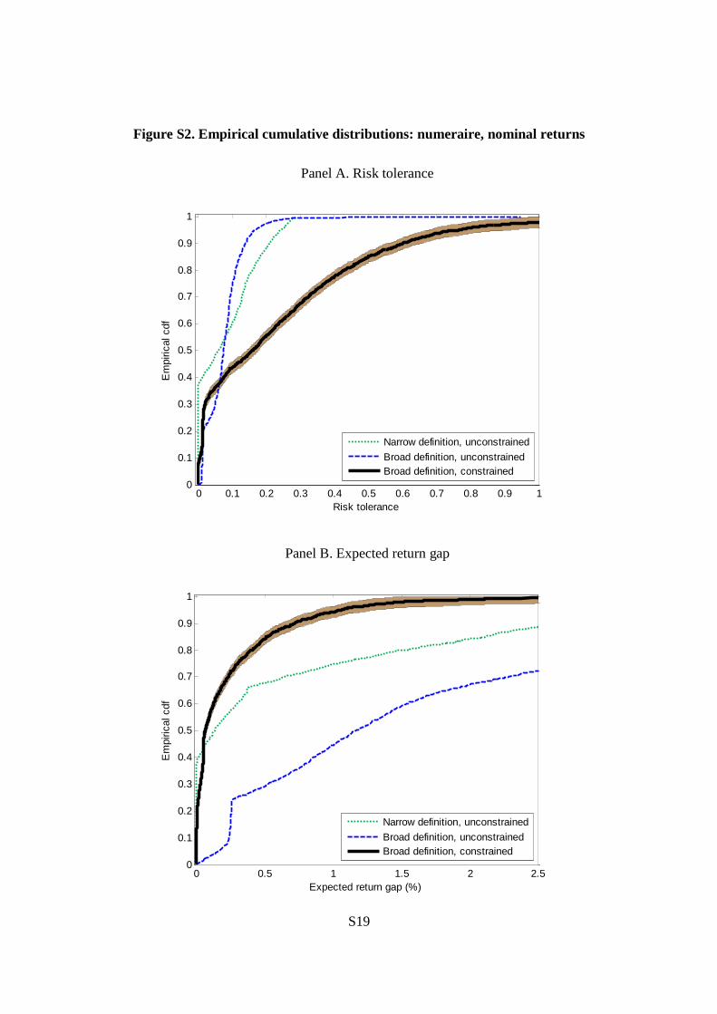
Figure S2. Empirical cumulative distributions: numeraire, nominal returns


0 0.1 0.2 0.3 0.4 0.5 0.6 0.7 0.8 0.9 10

0.1

0.2

0.3

0.4

0.5

0.6

0.7

0.8

0.9

1

Risk tolerance

Em

piric

al c

df




0 0.5 1 1.5 2 2.50

0.1

0.2

0.3

0.4

0.5

0.6

0.7

0.8

0.9

1


Em

piric

al c

df



S20

Figure S3. Empirical cumulative distributions: shorter time series


0 0.1 0.2 0.3 0.4 0.5 0.6 0.7 0.8 0.9 10

0.1

0.2

0.3

0.4

0.5

0.6

0.7

0.8

0.9

1

Risk tolerance

Em

piric

al c

df




0 0.5 1 1.5 20

0.1

0.2

0.3

0.4

0.5

0.6

0.7

0.8

0.9

1


Em

piric

al c

df



S21

Figure S4. Empirical cumulative distributions: OFHEO series


0 0.1 0.2 0.3 0.4 0.5 0.6 0.7 0.8 0.9 10

0.1

0.2

0.3

0.4

0.5

0.6

0.7

0.8

0.9

1

Risk tolerance

Em

piric

al c

df




0 0.5 1 1.5 20

0.1

0.2

0.3

0.4

0.5

0.6

0.7

0.8

0.9

1


Em

piric

al c

df



S22

Figure S5. Empirical cumulative distributions: only residential housing as real estate


0 0.1 0.2 0.3 0.4 0.5 0.6 0.7 0.8 0.9 10

0.1

0.2

0.3

0.4

0.5

0.6

0.7

0.8

0.9

1

Risk tolerance

Em

piric

al c

df




0 0.5 1 1.5 20

0.1

0.2

0.3

0.4

0.5

0.6

0.7

0.8

0.9

1


Em

piric

al c

df



Supplemental appendix to "Household Portfolios and Implicit Risk Preference" by

Documents

Transcript of Supplemental appendix to "Household Portfolios and Implicit Risk Preference" by