Efficient Trading in Taxable Portfolios1

Sanjiv R. DasDennis Yi DingVincent Newell

Daniel N. Ostrov

Santa Clara UniversitySanta Clara, CA 95053

July 23, 2015

1We thank Ananth Madhavan and other participants at the Journal of Investment Man-agement conference, San Diego 2015 for their comments. Correspondence may be addressedto the authors at the Department of Mathematics and Computer Science, Santa Clara Uni-versity; 500 El Camino Real, Santa Clara, CA 95053, USA. Email: dostrov@scu.edu.Telephone: 408-554-4551. Fax: 408-554-2370.

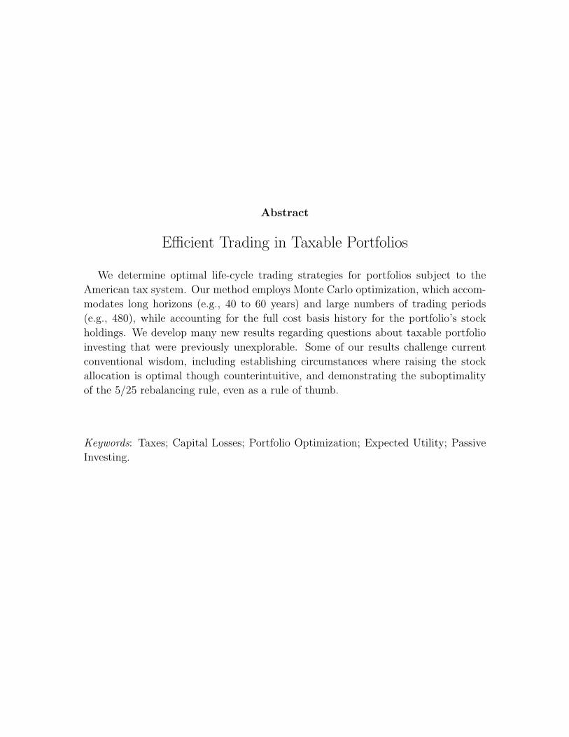
Abstract

Efficient Trading in Taxable Portfolios

We determine optimal life-cycle trading strategies for portfolios subject to the

American tax system. Our method employs Monte Carlo optimization, which accom-

modates long horizons (e.g., 40 to 60 years) and large numbers of trading periods

(e.g., 480), while accounting for the full cost basis history for the portfolio’s stock

holdings. We develop many new results regarding questions about taxable portfolio

investing that were previously unexplorable. Some of our results challenge current

conventional wisdom, including establishing circumstances where raising the stock

allocation is optimal though counterintuitive, and demonstrating the suboptimality

of the 5/25 rebalancing rule, even as a rule of thumb.

Keywords: Taxes; Capital Losses; Portfolio Optimization; Expected Utility; Passive

Investing.

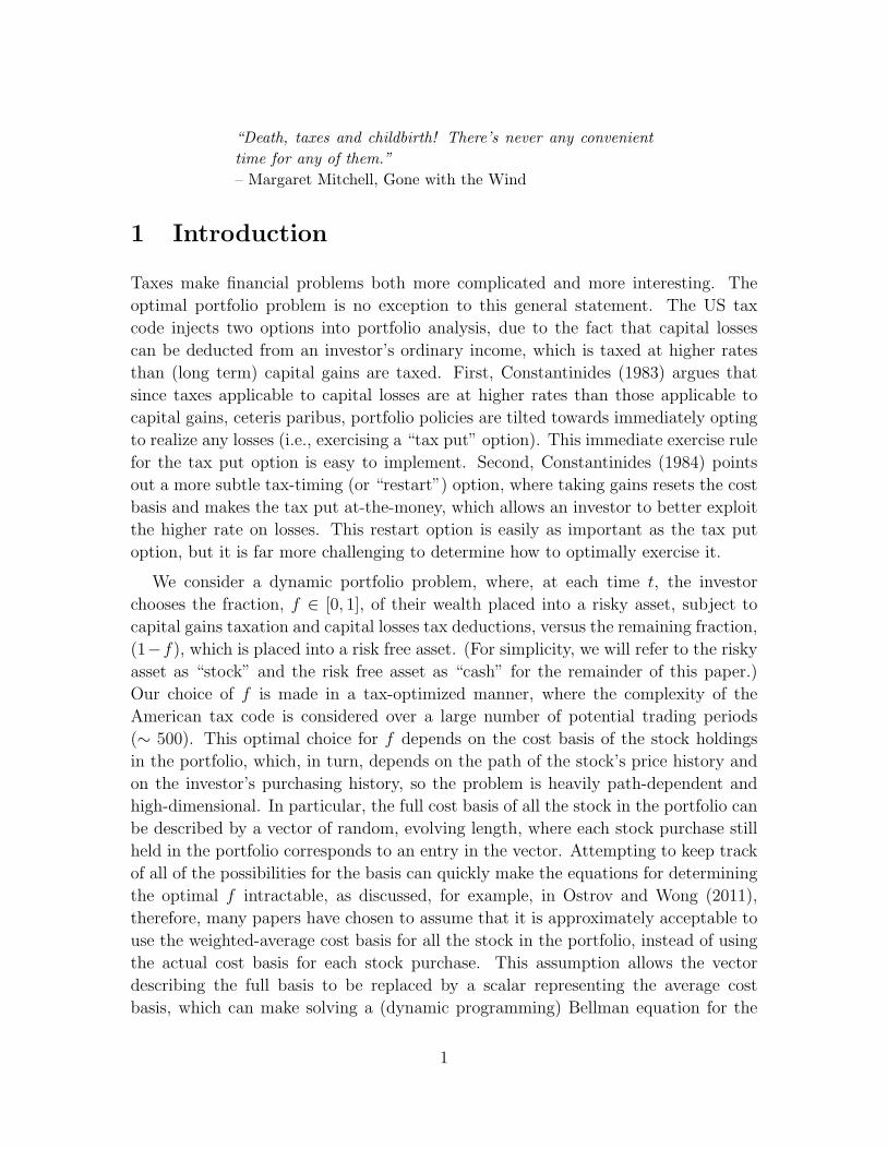
“Death, taxes and childbirth! There’s never any convenienttime for any of them.”– Margaret Mitchell, Gone with the Wind

1 Introduction

Taxes make financial problems both more complicated and more interesting. The

optimal portfolio problem is no exception to this general statement. The US tax

code injects two options into portfolio analysis, due to the fact that capital losses

can be deducted from an investor’s ordinary income, which is taxed at higher rates

than (long term) capital gains are taxed. First, Constantinides (1983) argues that

since taxes applicable to capital losses are at higher rates than those applicable to

capital gains, ceteris paribus, portfolio policies are tilted towards immediately opting

to realize any losses (i.e., exercising a “tax put” option). This immediate exercise rule

for the tax put option is easy to implement. Second, Constantinides (1984) points

out a more subtle tax-timing (or “restart”) option, where taking gains resets the cost

basis and makes the tax put at-the-money, which allows an investor to better exploit

the higher rate on losses. This restart option is easily as important as the tax put

option, but it is far more challenging to determine how to optimally exercise it.

We consider a dynamic portfolio problem, where, at each time t, the investor

chooses the fraction, f ∈ [0, 1], of their wealth placed into a risky asset, subject to

capital gains taxation and capital losses tax deductions, versus the remaining fraction,

(1−f), which is placed into a risk free asset. (For simplicity, we will refer to the risky

asset as “stock” and the risk free asset as “cash” for the remainder of this paper.)

Our choice of f is made in a tax-optimized manner, where the complexity of the

American tax code is considered over a large number of potential trading periods

(∼ 500). This optimal choice for f depends on the cost basis of the stock holdings

in the portfolio, which, in turn, depends on the path of the stock’s price history and

on the investor’s purchasing history, so the problem is heavily path-dependent and

high-dimensional. In particular, the full cost basis of all the stock in the portfolio can

be described by a vector of random, evolving length, where each stock purchase still

held in the portfolio corresponds to an entry in the vector. Attempting to keep track

of all of the possibilities for the basis can quickly make the equations for determining

the optimal f intractable, as discussed, for example, in Ostrov and Wong (2011),

therefore, many papers have chosen to assume that it is approximately acceptable to

use the weighted-average cost basis for all the stock in the portfolio, instead of using

the actual cost basis for each stock purchase. This assumption allows the vector

describing the full basis to be replaced by a scalar representing the average cost

basis, which can make solving a (dynamic programming) Bellman equation for the

1

optimal f tractable.1 Examples of papers that have used the average cost basis include

Dammon, Spatt, and Zhang (2001), Dammon, Spatt, and Zhang (2004), Gallmeyer,

Kaniel, and Tompaidis (2006), and Tahar, Soner, and Touzi (2010).

Dybvig and Koo (1996) implemented a model with the full cost basis, but were

limited to four periods before the problem became intractable. DeMiguel and Up-

pal (2005) subsequently used nonlinear programming (the SNOPT algorithm of Gill,

Murray, and Saunders (2002)) with linear constraints to extend the model to ten pe-

riods. For their ten period model, they found that using the full cost basis provided a

1% certainty equivalent advantage over using the average cost basis, which is robust

to various parameterizations.

In contrast to these previous models, we use a simulation algorithm with opti-

mization that runs very fast. Our algorithm uses the nonlinear optimizer in the R

programming language, which calls a simulation run in compiled C for 50,000 paths

of portfolio wealth and policy. We generally will run our algorithm for 40 year port-

folio horizons with quarterly trading, i.e., 160 potential trading periods. However,

we will also implement the model for longer horizons, e.g., 60 years, or for monthly

trading, i.e., 480 periods, which takes marginally longer to run. Our approach has

the advantage of being both simple and flexible, which yields a number of benefits,

such as allowing us to 1) determine solutions using the full cost basis, even if the basis

is large and complicated; 2) address a number of complex features of the American

tax code that are generally difficult to accommodate; and 3) work with any desired

stochastic processes to simulate the stock movement, although, for simplicity, we use

geometric Brownian motion in this paper.

Our model keeps track of the entire tax basis, however, we can also implement a

simplification to accommodate the average basis, which will allow us to compare the

effect of using the average cost basis versus the full cost basis. This is key for under-

standing whether or not it is justified to use the average cost basis approximation that

current dynamic programming (Bellman equation) approaches implement. DeMiguel

and Uppal (2005) argue that using the average tax basis is reasonable, since, in their

simulations, most stock holdings comprise a single basis, and only 4% of the holdings

comprise additional bases. However, their conclusion is based on a ten-period model,

where there are few periods for new purchases. With many more periods and more

complex tax code features, as in our model, there is more potential for the difference

in optimality between the full tax basis problem and the average tax basis problem

1The state space for the dynamic programming problem comprises the current wealth of theinvestor and the tax basis. If the weighted-average tax basis is used, then the state space is two-dimensional. If the complete tax basis is used, then the dimension of the state space has no definiteupper bound.

2

to become large. Having a large number of periods is more like a Bellman model,

where potential sales and purchases occur in continuous time or over multiple periods

in discrete time.

A comprehensive paper by Dammon, Dunn, and Spatt (1989) examines both the

tax put option and the restart option.2 Their paper shows that the value of these

options depends on the pattern of gains, the length of the portfolio’s time horizon, T ,

and whether, at this horizon, the investor is alive and liquidates their portfolio or is

deceased. (In the latter case, taxes are lower as all capital gains are forgiven at death

and the basis is reset.) We will also explore the effect of the investor being alive or

deceased at the horizon T and show that it leads to substantially different optimal

strategies, even when T is large. Unlike our paper, Dammon, Dunn, and Spatt (1989)

do not determine an optimal trading policy. Instead they compare three trading rules

suggested by Constantinides (1984) and compare the performance of these rules to

a buy and hold strategy. They find that the restart option value is lower than that

suggested by Constantinides (1984) for high volatility stocks, because such stocks also

tend to have higher capital gains. They conclude that offset rules matter, hence in

our model, we account for tax loss offsets and carry-forwards exactly as per the US

tax code.

It is well established (see, for example, Dai, Liu, and Zhong (2011), Davis and

Norman (1990), or, in the asymptotic case, Atkinson and Mokkhavesa (2002); Good-

man and Ostrov (2010); Janacek and Shreve (2004); Rogers (2004); Shreve and Soner

(1994); and Whaley and Wilmott (1997)) that, in the absence of taxes, the optimal

trading strategy is to maintain the stock fraction within a specific “no-transaction

region” (also referred to as a “hold region”). When the portfolio’s stock fraction is

in the interior of this no-transaction region, there is no trading. Trading only oc-

curs to rebalance the portfolio so that it does not escape the no-transaction region.

The same logic applies to the optimal strategy for taxable portfolios, but with one

tweak: the optimal strategy, as per Constantinides (1983) and Ostrov and Wong

(2011), requires realizing any capital losses as soon as possible (that is, exercising

the “tax-put” option) — no matter where we are in the region — and then rebuying

an essentially equivalent stock or index while avoiding wash sale rules, as discussed

further in Subsection 2.1. This process collects the tax advantages of realized losses

without rebalancing the portfolio. We only rebalance, as before, to prevent the port-

folio from escaping our region. Because we transact to realize losses in the interior of

our region, we refer to any region using this optimal strategy in the presence of taxes

as a “no-rebalancing region” instead of a “no-transaction region.” In the case of a

single stock, as in this paper, the region is an interval.

2See also the review by Dammon and Spatt (2012).

3

Using our optimization algorithm, we find many new results about the optimal

no-rebalancing interval for the stock fraction. Some of our results confirm statements

in the current literature, while others contradict previous claims, but many of our

results provide insight into questions hitherto uncovered in the extant literature. The

main findings of this paper are as follows:

First, as noted, we provide a simulation based method that quickly generates an

optimal portfolio trading strategy. Our method utilizes the full cost basis history, a

complex, realistic tax model, and many more trading periods (we implemented 480)

than has been considered in the literature so far when using the full cost basis history

(20 periods in Haugh, Iyengar, and Wang (2014)). Our model can be extended in a

number of directions, including accommodating just about any stochastic model for

stock price evolution and any utility function applied to the portfolio worth at the

horizon time, T . Our model can be applied to multiple stocks, however, assumptions

would have to be made about the geometric nature of the no-rebalancing region. In

contrast, the approach used in DeMiguel and Uppal (2005) for the multiple stock

question required no a priori knowledge about the geometry of the no-rebalancing

region, although it was computationally limited to seven trading periods for two

stocks and four trading periods for four stocks.

Second, our portfolio rule comprises an optimal no-rebalancing interval for the

stock fraction, which can be specified by the interval’s center, denoted by f ∗, and

the interval’s width, denoted by ∆f . We show that optimality is reduced much more

by movement away from the optimal center than movement away from the optimal

width. When the optimal interval width is positive, as opposed to zero, the reduction

in optimality due to perturbations of the interval width from its optimal value is

particularly small.

Third, as in Dammon, Dunn, and Spatt (1989), we find that materially different

optimal portfolio choices are made depending on whether the investor is assumed

to be alive or to expire when the portfolio is liquidated at the horizon time, T .

Moreover, our results indicate that this optimal strategy difference does not vanish

as T increases, even though the tax treatment is only different at time T , suggesting

that these strategies have long memory.

Fourth, counterintuitively, the optimal stock fraction in a taxable portfolio (or

more specifically, f ∗, the interval’s center, if the interval width ∆f > 0) is often

higher, not lower, than the optimal stock fraction for a portfolio without taxes. This

is the case whether or not the investor is assumed to be alive or dead when the

portfolio is liquidated at time T . Because there are generally more capital gains than

capital losses, it is intuitive to think that taxes should make the stock less desirable.

However, the tax rate used to credit losses is generally significantly higher than the

4

tax rate for gains, which can often be exploited to make the taxable stock more, not

less, desirable. We analyze when this is the case.

Fifth, our analyses show that static band rules that are commonly used in practice

to determine the no-rebalancing region are generally problematic. The “5/25” rule

of thumb, for example, generally suggests for our stock-cash scenario that we should

use a no-rebalancing interval with a width ∆f = 0.10, since that corresponds to ±5

percentage points for the portfolio’s stock fraction. Our results, however, show that

the optimal width of the no-rebalancing interval can vary dramatically (and is often

zero), depending on a number of parameters. Specifically, the optimal width increases

as we increase the stock’s expected return, the capital gains tax rate, or the size of

the portfolio, and it decreases as we increase the risk free return, the capital losses

tax rate, or the time horizon, T , of the portfolio. The optimal width is also increased

if the investor is assumed to expire at time T . (Surprisingly, in our results, the

optimal width does not appear to be sensitive to stock’s volatility, when intuitively

one might expect it to be. See, for example, the trading range in Section 3.2.1.)

Further, we explain why, as a rule of thumb when we roughly average the effect of all

these parameters, it is better to choose ∆f = 0 (that is, continually rebalance) than

to choose ∆f = 0.10 as suggested by the 5/25 rule.

Sixth, counterintuitively, as the tax rate on gains increases, generally more, not

less, investment in the stock is optimal in the case when the investor is assumed to

expire at the portfolio horizon. This is because the amount of rebalancing (along with

the associated capital gains) needed to maintain a desired fraction, f , of the portfolio

in stock decreases as f increases from f = 0.5 to f = 1. Indeed, to maintain f = 1,

no rebalancing is needed, so no capital gains are generated.

Seventh, we assessed monthly, quarterly, and semi-annual trading schemes and

found that the choice among these three trading frequencies has no material effect on

the optimal allocation strategy. This assessment is novel in comparison to the extant

literature, which was unable to assess this issue due to limitations in the number of

periods it was possible to consider.

Eighth, using a large collection of scenarios, mostly with a 40 year time horizon,

we find that, on average, using the full cost basis provides only a 0.65% certainty

equivalent advantage over using the average cost basis if the investor is alive at the

portfolio horizon time, T . This advantage reduces even further to 0.27% when the

investor is assumed to expire at time T . These numbers are a bit lower than the 1%

figure reported by DeMiguel and Uppal, giving more support to the validity of using

the average cost basis approximation in optimization models like the Bellman models

that require the approximation for tractability.

Ninth, for completeness and comparison with Leland (2000), we also re-optimize

5

the taxable portfolio in the presence of proportional transactions costs. We confirm

Leland’s result that transactions costs reduce portfolio churn (i.e., they increase the

optimal width ∆f), but unlike Leland, we do not find that transaction costs materially

reduce the optimal fraction of the portfolio in the stock position. (That is, they do

not reduce the optimal f ∗.)

In the following section (Section 2), we present our modeling approach, explicitly

accounting for the features of the tax code and for the evolving cost basis of all stock

in the portfolio. This is followed by numerical simulations of the model in Section

3, where we report and explain the effect on the optimal trading strategy caused by

varying the values of the stock’s expected return, the cash interest rate, the stock’s

volatility, the investor’s risk aversion, the tax rate on losses, the tax rate on gains, the

initial portfolio worth, the portfolio’s time horizon, and the period between trading

opportunities. We then report and explain the effect on the optimal trading strategy

of letting the strategy change halfway to liquidation (at time T2), of using the average

cost basis in place of the full cost basis, and of incorporating transaction costs into

the model. Section 4 concludes.

2 Model

In this section we present the assumptions behind our model and the details of our

simulation of the model.

2.1 Assumptions and Notation

We have two assets in our portfolio model, stock and cash. The return on the stock

is risky; the return on the cash is certain. Our model applies two sets of assumptions:

those for the stock and cash positions and those for the tax model.

For the stock and cash positions, we make the following assumptions:

1. We assume the stock evolves by geometric Brownian motion with a constant

expected return, µ, and a constant volatility, σ.

2. The tax-free continuously compounded interest rate for the cash position, r, is

assumed to be constant. We note that cash positions with constant interest

taxed at a constant rate can be converted to an equivalent tax-free rate, r,

and, of course, periodically compounded interest at a constant rate can also be

converted to a continuously compounded rate, r.

6

3. Except where otherwise specified, we assume that stock and cash can be bought

and sold in any quantity, including non-integer amounts, with negligible trans-

action costs.

In portfolios subject to tax, the impact of taxes on the optimal strategy is gener-

ally much stronger than the impact of transactions costs. At the same time, tax

codes are generally more complex than models for transactions costs. For tax-

free portfolios like 401(k)s and Roth IRAs where transaction costs take center

stage, there is an extensive literature on portfolio optimization, such as Akian,

Menaldi, and Sulem (1996); Atkinson and Ingpochai (2006); Bichuch (2012);

Goodman and Ostrov (2010); Leland (2000); Liu (2004); and Muthuraman and

Kumar (2006).

4. For simplicity, we do not consider dividends for the stock, although the model

can easily be altered to approximate the effect of dividends by adjusting µ, the

growth rate of the stock.

For the tax model, we make the following assumptions:

1. As stipulated by the tax code in the United States, we assume a limit of no

more than $3000 in net losses can be claimed at the end of each year. Net

losses in excess of this amount are carried over to subsequent years. Should the

investor expire when the portfolio is liquidated at time T , all remaining carried

over capital losses are lost. We encode all these features into our portfolio

simulation program.

2. For simplicity, we assume that for all times prior to the portfolio being liqui-

dated, the capital gains tax rate, τg, is constant and applies to both long term

and short term gains. When the portfolio is liquidated, we use the capital gains

rate τ liq = τg if the investor is alive, while τ liq = 0 if the investor is dead to

reflect the fact that capital gains are forgiven in the U.S. tax system when an

investor expires. Similarly, for both short term and long term capital losses that

are claimed prior to the portfolio being liquidated, we assume a constant rate,

τl, which corresponds to the marginal income tax rate of the investor.

Our model can be altered to accommodate different rates for short term and

long term gains and losses, but optimizing with this short term/long term model

poses difficulties, unless one restricts the strategy to something reasonable, but

possibly suboptimal, such as assuming that short term gains will never be real-

ized.

3. We allow for wash sale rules, but make an additional assumption, so that they

have no effect. Specifically, we assume the presence of other stocks or stock

7

indexes in our market with essentially the same value of µ and σ. For a loss

to qualify for tax credit, wash sale rules in the U.S. require that the investor

wait at least 31 days before repurchasing a stock that was sold at a loss. But

if the investor sells all of a stock that is at a loss and then immediately buys

a different stock with the same µ and σ, the investor will avoid triggering a

wash sale, while still taking full advantage of the loss for tax purposes. This

sell/repurchase strategy for any stock with losses lowers the cost basis, but

because it allows for earlier use of the losses for taxes, it is always superior to

the strategy of buying and holding when transaction costs are negligible (see,

for example, Constantinides (1983) or Ostrov and Wong (2011)).

2.2 Trading Strategy

We implement the following trading strategy:

For simplicity, we start with a strictly cash portfolio, although initial portfolios

containing stock positions with various cost bases could just as easily be accommo-

dated. We then immediately buy stock so that the portfolio’s stock allocation attains

a selected fraction, f init, of the total portfolio’s worth.

After each time period of length h years passes in the simulation, we consider three

types of trades. We first sell and repurchase any stock with a loss, while avoiding wash

sale rules as described above, to generate money from these capital losses.3 Next, if

f , the fraction of the portfolio’s value in the stock position, is below a selected lower

threshold, f l (which is constant over time), we purchase stock until f = f l. Finally,

if f is above a selected upper threshold, fu (which is also constant over time), then

stock with the highest cost basis is sold until f = fu. Choosing to sell the highest

cost basis stock is optimal, since it minimizes capital gains.

At the end of each year, taxes on any net capital gains are paid from the cash

position, and any net losses that can be realized are used to purchase additional

stock.

We keep track of the cost basis of all stock purchases, which makes the problem and

portfolio value path dependent, ruling out any easy dynamic programming approaches

to determining the optimal stock proportions at each point in time for the portfolio,

as explained in the introduction.

Our goal is to determine the three values for f init, f l, and fu that optimize the

expected utility of the portfolio at a specified final portfolio liquidation time, T . Our

3This assumes that the investor has non-investment income, so the losses can be used to lowerthe tax on the income, which is equivalent to generating money from tax shields.

8

model can easily accommodate any utility function, however, in our simulations, we

have chosen power law utility functions (i.e., constant relative risk aversion). Nor-

mally, power law utilities lead to results that are independent of the initial portfolio

worth, however this will not be the case here due to the $3000 limit on losses that

can be claimed per year.

2.3 The Algorithm for Simulating a Single Run over T Years

For a given f init, f l, and fu, our algorithm works by Monte Carlo simulation over a

large number of runs. For each run, we proceed with the following algorithm:

We start by purchasing stock so that our initially all-cash portfolio attains the

given initial stock fraction, f init, at t = 0.

We simulate the market over each time period h. From time t to time t + h, the

stock price, S, advances by geometric Brownian motion, so

St+h = St exp

[(µ− σ2

2

)h+ σ

√hZ

],

where Z is a standard normal random variable. The cash position, C, advances by

Ct+h = Ct exp(rh).

As we buy and sell stocks over time, we develop a portfolio with stock positions

purchased at various prices. We keep track of each of these separately to determine

the correct basis for computing gains or losses when we sell the stock. We let J be

the number of different purchase prices (corresponding to various purchase times)

for the stock. Define Bj, where j = 1, 2, ..., J , be these J purchase prices in order

of purchase times, and let Nj be the number of stocks purchased at each of these

prices.4 Since we sell and repurchase any stock that has a loss, we are guaranteed

that B1 ≤ B2 ≤ ... ≤ BJ . In the initial (t = 0) stock purchase, for example, we have

that J = 1, since there is only one stock position; B1 = S0, the stock price at t = 0;

and the number of shares bought is N1 = f initW0

S0, where W0 is the initial worth of the

portfolio.

After each time period h elapses, we consider our three possible trades in the

following order:

1. Collect any losses: Define k such that positions k, k + 1, ..., J are the only

positions with losses. That is, Bk, Bk+1, ..., BJ are the only values of Bj that

4Should our model be altered to distinguish between short term and long term gains and losses,the time of purchase, tj , must also be recorded.

9

are greater than the current stock price, S. We sell all of these positions and

then immediately buy them back, recalling that we are actually buying back

other stocks or stock indexes that have the same µ and σ to avoid wash sale

restrictions. We subtract these losses from our current gains, so the new value

for the gains, denoted G, is

G = Gold −J∑j=k

Nj(Bj − S).

Since the positions k through J have all been repurchased at the current stock

price, we now have that Nk = N oldk + N old

k+1 + ... + N oldJ , where Bk = S, and we

reduce J to equal k, since positions k + 1 through Jold no longer exist.

2. Buy stock if the current stock fraction, f , is below f l: We buy stock until

f = f l. Since we buy stock, we must create a new position at the current

purchase price, so we increase J by one. For this new J position, we have

BJ = S and NJ equals the number of stocks needed to make f = f l.

3. Sell stock if the current stock fraction, f , is above fu: We begin selling position

J , then position J − 1, etc., until we have f = fu. We add these gains to G.

They must be gains, because all losses were already collected. If any positions

are liquidated by this procedure, we reduce the value of J to reflect this.

This trading strategy of buying and selling stock so as to stay just within the interval

[f l, fu] is a standard optimizing strategy when there are either no transaction costs

or proportional transaction costs, as is the case here. (See Davis and Norman (1990),

for example.)

At the end of each year, we pay taxes or collect tax credits, depending on the

sign of G. If G > 0, we have gains and so we remove G · τg from the cash account

and then set G = 0. If G < 0, we have losses, which we use to buy stock. Since

we are buying stock, we increase J by one and then set BJ = S, the current stock

price. If the losses, −G, are less than the annual limit of $3000, they generate −G · τldollars, which purchases NJ = −G·τl

Sshares of stock, and we then set G = 0. If the

losses are more than $3000, we purchase NJ = 3000·τlS

shares of stock, and then we set

G = Gold + 3000, so the excess losses are carried over to the next year.

At the end of T years, we liquidate all the stock positions in the portfolio. If we

assume the portfolio’s owner is alive, capital gains from this liquidation are paid. If

we assume the owner has expired, no capital gains are paid. Any carried over losses

are lost.

10

As detailed in the next subsection, we will look to average the utility of the final

portfolio worth over all of our Monte Carlo runs to determine an approximation for the

expected utility. We use the same simulated stock runs for comparing the expected

utilities for different f init, f l, and fu combinations. This allows us to converge to

the values of f init, f l, and fu that optimize the expected utility for this fixed set of

simulations. We then use different sets of simulations to check for consistency in the

optimal values determined for f init, f l, and fu.

2.4 The Expected Utility Estimator and The OptimizationProgram

Working with our model is quite computationally intensive. We generally chose a

base case liquidation time, T , of forty years. Each forty year run is computed using

the complex algorithm from the previous section, and we needed to average the utility

at liquidation over a high number (eventually 50,000) of these runs to estimate the

expected utility of the terminal wealth, E[U(WT )], corresponding to any specific

values of f init, f l, and fu. On top of this, the optimization algorithm requires several

calls to this expected utility estimator for various values of f init, f l, and fu.

Given this approach, we required both very fast computation for the expected

utility estimator and an efficient optimizer. We therefore programmed the expected

utility estimator in the C programming language, and compiled it and linked it to

be callable from the R programming language so as to use the optimizer in R, which

is stable, fast, and accurate. The optimization function in R is constrOptim, which

is a constrained optimizer, as we need to restrict the values of f init, f l, fu so that

0 ≤ f l ≤ f init ≤ fu ≤ 1.

We applied a power utility function,

U(W ) =W 1−α

1− α, (1)

to the terminal wealth, although we can easily accommodate any other utility function

in our simulation program. The power law utility, however, is particularly suited to

our model where f l and fu are constant with respect to time because, in the absence

of taxes, Merton (1992) showed that, for the power law utility, the optimal fraction

of the portfolio in stock is

fMerton =µ− rα · σ2

,

which is also constant with respect to time.

Given our choice of the power law utility, our estimate of the expected utility at

11

time T becomes

E[U(WT )] ≈ 1

M

M∑m=1

1

1− α· (WT (m))1−α,

where α is the coefficient of relative risk aversion for the investor, m indexes each

simulated run, M is the total number of runs, and WT (m) is the terminal wealth for

run m generated in the simulation.

Optimization is run in two stages. In the first stage, we find the values of f init,

f l, and fu that are optimum over a case with only M = 1000 runs, which is fast,

since M is small. We then use these three values as starting guesses for the optimum

f init, f l, and fu in the second stage, where we optimize over M = 50, 000 runs. This

two step process has the benefit of speed from the first stage and precision from the

second stage. We used standard computing hardware for this simulated optimization

procedure, and each optimization runs in under 5 minutes. We obtained similar

results when using other sets of 50,000 sample paths generated using independent

sets of random numbers.

3 Results and Analysis

In this section we present and analyze numerical results obtained from the simulation

model described in the previous section. We begin in Subsection 3.1 with a discussion

of the optimal stock fraction range, [f l, fu], (i.e., the optimal no-rebalancing inter-

val) for the “base case,” where we assign the following values to the following nine

parameters:

1. the stock growth rate, µ = 7% = 0.07 (per annum)

2. the risk free rate, r = 3% = 0.03 (per annum)

3. the stock volatility, σ = 20% = 0.20 (per annum)

4. the risk aversion parameter, α = 1.5 in our utility function in equation (1)

5. the tax rate on losses, τl = 28% = 0.28

6. the tax rate on gains, τg = 15% = 0.15

7. the initial portfolio worth, W0 = $100, 000

8. the time horizon before portfolio liquidation, T = 40 years

12

9. the period between potential trades, h = 0.25 years (i.e., quarterly trading and

rebalancing).

We will consider the base case both where the investor expires at T = 40, so any

remaining capital gains are forgiven, and where the investor is alive at T = 40, so

taxes on any remaining net capital gains must be paid.

In Subsection 3.2, we show the sensitivity of this optimal stock fraction range to

varying these nine parameter values, one at a time, from their base case values. Then,

in Subsection 3.3, we consider the effect of changing the model in three ways:

1. Letting the stock fraction range, [f l, fu], change values at time T2

= 20 years.

2. Using the average cost basis instead of the full cost basis.

3. Incorporating proportional transaction costs when we buy and sell stock.

A no-rebalancing interval can be defined by specifying f l and fu or by specifying

the components

f ∗ =f l + fu

2(the center (or midpoint) of the interval) and

∆f = fu − f l (the width of the interval).

We will often prefer to use f ∗ and ∆f , since it makes more sense to analyze how

changes affect the center and the width of the trading strategy, instead of how they

affect f l and fu. In our simulations, we found the effect of varying f init to be quite

small. Therefore, we do not discuss or present the optimal values of f init, even though

our algorithm determines and uses them.

3.1 Optimal Strategy for the Base Case

For the base case specified above, if the investor expires at T = 40, our analysis

shows that the optimal trading strategy is to set f ∗ = 0.764 and ∆f = 0.168. For

the base case if the investor is alive at T = 40, the optimal trading strategy is to set

f ∗ = 0.711 and ∆f = 0. Note that ∆f = 0 means the investor is best off continually

rebalancing.

The effect of dying versus living at time T on the optimal trading strategy that

we observe here will hold in general, as we will see throughout this section. When

the investor is alive at time T and must pay capital gains, there are two key effects:

(1) Having to pay capital gains taxes at time T makes the stock less desirable, so f ∗

13

gets smaller when the investor is alive at liquidation. (2) Having to pay capital gains

taxes at time T makes having capital gains at time T less desirable, so ∆f also gets

smaller. Further, even though dying or living at time T only affects the tax treatment

at time T , it has a considerable effect on our optimal long term investing strategy,

especially on the optimal ∆f , as we see here and will see throughout this section.

As stated previously, in the absence of taxes, Merton (1992) shows that it is optimal

to keep the stock fraction equal at all times to

fMerton =µ− rα · σ2

, (2)

which, for our base case, corresponds to fMerton = 23. But notice that this Merton

stock fraction is smaller than either f ∗ = 0.764 or f ∗ = 0.711. That is, although it

is counterintuitive, the optimal stock fraction in the taxable accounts is higher here

than the optimal stock fraction in the account with no taxes.

Why? The answer is because τl, the refund tax rate for capital losses, is higher than

τg, the tax rate for capital gains. Therefore, the advantage of culling capital losses

from stock in a taxable account can, on average, outweigh the disadvantage of paying

capital gains taxes, as is the case here. We emphasize that only the stock positions

have different tax treatments here. The cash positions, both in our algorithm and in

the Merton expression (2), use the same tax-free rate, r = 0.03. That is, we are not

choosing a higher stock fraction in the taxable portfolio because it is better to keep

the cash position shielded from taxes, as is often advised when considering a taxable

account versus a 401(k) or Roth account.

Although our algorithm determines the optimal f ∗ and ∆f , it can easily be simpli-

fied to determine the loss to an investor should they employ a suboptimal f ∗ and/or

∆f . We quantify this loss using the certainty equivalent, C, which is defined by the

equation

U(C) = E[U(WT )],

where WT is the portfolio worth at time T . That is, the investor has no preference

between starting at t = 0 with Ce−rT dollars that must be invested as cash at the

risk free rate r until time T (leading to C dollars at t = T ) or starting at t = 0 with

W0 dollars invested in our stock and cash portfolio until time T (leading to a random

variable for the value of WT ).

To quantify the disadvantage of using a suboptimal strategy versus the optimal

strategy, we useCsuboptCopt

< 1, the ratio of the certainty equivalents under these two

14

strategies, to define c, the certainty equivalent difference, by the following equation:

1 + c =CsuboptCopt

=U−1 (Esubopt[U(W )])

U−1 (Eopt[U(W )]),

Since U(W ) = W 1−α

1−α , this can be re-expressed as

c =

(Esubopt[U(W )]

Eopt[U(W )]

) 11−α

− 1 ≤ 0. (3)

Note that the optimal strategy corresponds to c = 0, and c becomes progressively

negative as the strategy becomes more suboptimal.

In Figure 1, we see the effect on c if we deviate from the optimal strategy. For

the two panels on the left, we fix ∆f at its optimal value and let f ∗ vary. For the

two panels on the right, we fix f ∗ at its optimal value and let ∆f vary. Noting the

scale on the vertical axis, we see that the sensitivity of c to suboptimal values of f ∗ is

far larger than the sensitivity to suboptimal values of ∆f . That is, it is much more

important for investors to determine their optimal portfolio stock fraction (or, more

precisely, the center of their optimal no-rebalancing interval) than it is to determine

the precise optimal width of this interval.

But there’s also considerable forgiveness should the investor get the precise value

of the optimal f ∗ wrong due to the fact that, at least in the base case both for the

investor dying (top left panel of Figure 1) or living (bottom left panel), the optimal

f ∗ is on the interior of the domain f ∈ [0, 1]. Because of this, and the smoothness

of the graphs, the derivative of c is zero at the optimum values of f ∗. This leads to

a small loss in the certainty equivalent difference for even moderate deviations from

the optimal f ∗. In the two base cases shown in Figure 1, for example, we see no more

than a 1% loss in the certainty equivalent difference over 40 years, until the value

chosen for f ∗ differs from the optimal f ∗ value by around 10 percentage points.

The same effect occurs for ∆f in the base case where the investor expires (top

right panel of Figure 1). That is, because the optimal ∆f is an interior value in the

domain of possible ∆f values, the derivative of c must be zero at the optimal ∆f ,

and so we see little sensitivity to moderate deviations from this value. This is not the

case, however, in the base case where the investor expires (bottom right panel). Since

the optimal ∆f is zero, which is an endpoint of the domain of possible ∆f values,

the derivative of c need not be zero at the optimal ∆f , which means the sensitivity

of c to deviations from ∆f = 0 will, in general, be greater, as is the case here.

There is considerable debate about whether, as a rule of thumb, a taxable portfolio

should be rebalanced continually (but selling stock only with long term capital gains,

15

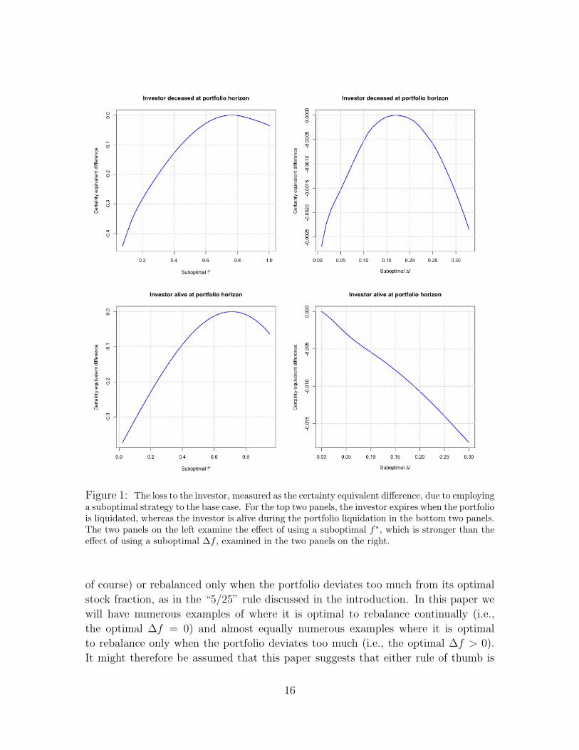
Figure 1: The loss to the investor, measured as the certainty equivalent difference, due to employinga suboptimal strategy to the base case. For the top two panels, the investor expires when the portfoliois liquidated, whereas the investor is alive during the portfolio liquidation in the bottom two panels.The two panels on the left examine the effect of using a suboptimal f∗, which is stronger than theeffect of using a suboptimal ∆f , examined in the two panels on the right.

of course) or rebalanced only when the portfolio deviates too much from its optimal

stock fraction, as in the “5/25” rule discussed in the introduction. In this paper we

will have numerous examples of where it is optimal to rebalance continually (i.e.,

the optimal ∆f = 0) and almost equally numerous examples where it is optimal

to rebalance only when the portfolio deviates too much (i.e., the optimal ∆f > 0).

It might therefore be assumed that this paper suggests that either rule of thumb is

16

equally valid. However, this is not the case. If the optimal ∆f isn’t too large, the

observation in the previous paragraph tells us that, as a rule of thumb, it is better

to continually rebalance, because the loss due to being wrong by choosing ∆f = 0

when the optimal ∆f is a small positive value will generally be less than the loss due

to being wrong by choosing a small positive value for ∆f when the optimal ∆f = 0.

That said, using the wrong rule of thumb is unlikely to have significant consequences.

After all, as we can see in the two right panels of Figure 1, there is a wide range of

suboptimal ∆f that can be used in the base case where the loss over 40 years in the

certainly equivalent difference remains under 1%.

3.2 The Effect on Varying Parameters on the Optimal Strat-egy

In the remainder of this section, f ∗ and ∆f will denote the f ∗ and ∆f of the optimal

no-rebalancing interval.

In the figures for this subsection, the parameters being varied are displayed on

the horizontal axis and stock fractions, f , are displayed on the vertical axis. Recall

that stock positions are constrained to be long only, so f ∈ [0, 1]. There are three

curves on the graphs, which represent the upper boundary, fu (red line), the lower

boundary, f l (blue line), and the midpoint, f ∗ (green line), between fu and f l. It is

reasonable to think that f ∗ and the average value of f over time are almost equal,

since, for example, they are equal to leading order as the interval width ∆f = fu−f lgets small in the related continuous time scenario considered in Goodman and Ostrov

(2010). We will sometimes refer to f ∗ as the average stock fraction for this reason

and, of course, because f ∗ is the average of the two values fu and f l.

In many of the figures, we will see that changes to our parameter values will cause

∆f to become bigger or smaller, often to the point of causing a transition between

∆f being positive and being zero. These changes in the size of ∆f are determined

by shifting balances among a number of opposing factors.

There are two factors that push ∆f to be bigger: (1) The bigger ∆f is, the more

useful deferring capital gains becomes, even when tax on the gains must be paid at

time T due to the investor being alive. (2) If the investor is deceased at time T , then

the bigger ∆f is, the more likely that larger amounts of gains will be forgiven at time

T .

In opposition to these effects are the factors that push ∆f to be smaller: (1) The

smaller ∆f is, the more useful claiming capital losses becomes, since τl > τg in current

American tax law. That is, the smaller ∆f is, the more we can take advantage of the

two tax options discussed in Constantinides (1983) and Constantinides (1984). (2)

17

The smaller ∆f is, the more control we have over keeping the portfolio near or at the

stock fraction that optimizes the investor’s expected utility.

In this subsection, we demonstrate and then explain how f ∗ and ∆f are affected

by altering our model parameters, one at a time, from their base case values. We

present the results for each parameter being varied using two graphs in each figure:

the graph on the left will correspond to the case where the investor is assumed to

expire at the portfolio horizon time T , and the graph on the right will correspond to

the case where the investor is assumed to be alive at time T .

3.2.1 Varying the Stock and Cash Growth Rates, µ and r

The stock growth rate, µ: Critical to any long-run portfolio strategy is the assumed

average growth rates of the portfolio’s financial instruments. Financial planning tools

make assumptions about this as a critical part of their process. Here, we first examine

the effect of changing the expected stock growth rate, µ, over the values 0.06, 0.07,

0.08, . . . , 0.12 per annum, while holding all the other parameters at their base case

values given above.

In Figure 2, we see, as expected, that the optimal average stock fraction, f ∗ (repre-

sented by the green line), increases as µ increases, until the investor is best off placing

the entire portfolio in stocks, so f ∗ = 1. And, of course, once this happens, the op-

timal stock fraction interval, [f l, fu], represented by the blue and red lines, collapses

to the point f l = fu = 1, so that there is no cash. Also we note, as expected from

our discussion near the beginning of Subsection 3.1, that both f ∗ and ∆f are smaller

in the graph on the right of Figure 2, where the investor is alive at the portfolio’s

liquidation time T = 40. Finally, we note that the values seen in Figure 2 for the base

case, µ = 0.07, correspond, of course, to the numerical values given in Subsection 3.1.

The risk free rate, r: Increasing r, the cash interest rate (i.e., the risk free

growth rate), essentially has the opposite effect on the optimal policy compared to

increasing µ. We examine this effect in Figure 3 as we change the interest rate, r,

over the values 0.01, 0.02, . . . , 0.06 per annum. Again, note that the base case value,

r = 0.03, in Figure 3 corresponds, as it must, to the same values in Figure 2 at the

base case value, µ = 0.07.

The stock growth rate, µ, and the risk free rate, r, while holding µ − rconstant: As a related analysis, we also examine the effect of increasing the stock

growth rate, µ, to the values 0.04, 0.05, 0.06, . . . , 0.16 per annum while equally

increasing the risk free rate so as to hold the equity risk premium constant at µ− r =

0.04.

Recall that in the absence of taxes, it is optimal to keep the stock fraction equal

18

Figure 2: The optimal stock fraction range as the expected stock growth rate, µ, varies. In thisfigure, and those below, it is optimal to rebalance only enough so that the portfolio stock fractionstays between the blue curve, f l, and the red curve, fu. The green curve, f∗, represents the center(i.e., the midpoint) of this interval. We assume the standard $3000 annual limit for claiming lossesand that all parameter values, except the varying parameter, take their base case values.

Figure 3: Optimal stock fraction range when varying the risk free rate, r.

to fMerton = µ−rασ2 at all times. If we change µ while keeping the equity risk premium,

µ − r, constant, fMerton doesn’t change. That is, as long as µ − r = 0.04, then the

optimal Merton strategy stays unchanged from the base case, namely f ∗ = 23

and

∆f = 0.

But what happens to the optimal strategy in the presence of taxes? In Figure 4,

we let µ vary while holding the equity risk premium constant at µ − r = 0.04. We

see that as µ increases, f ∗ decreases some and ∆f increases.

Because µ− r is held constant, both µ and r increase equally in value, but the tax

law’s effect on the stock is quite different from its effect on the cash. As µ increases,

there are fewer stock losses and more stock gains, which means fewer opportunities to

take advantage of the tax break created for culling losses due to τl being greater than

τg. Because culling losses is less advantageous, the stock becomes less useful relative

19

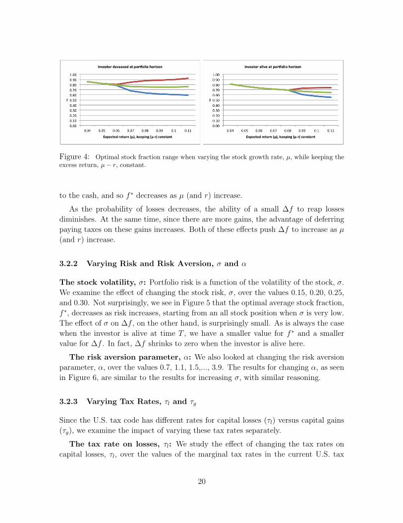
Figure 4: Optimal stock fraction range when varying the stock growth rate, µ, while keeping theexcess return, µ− r, constant.

to the cash, and so f ∗ decreases as µ (and r) increase.

As the probability of losses decreases, the ability of a small ∆f to reap losses

diminishes. At the same time, since there are more gains, the advantage of deferring

paying taxes on these gains increases. Both of these effects push ∆f to increase as µ

(and r) increase.

3.2.2 Varying Risk and Risk Aversion, σ and α

The stock volatility, σ: Portfolio risk is a function of the volatility of the stock, σ.

We examine the effect of changing the stock risk, σ, over the values 0.15, 0.20, 0.25,

and 0.30. Not surprisingly, we see in Figure 5 that the optimal average stock fraction,

f ∗, decreases as risk increases, starting from an all stock position when σ is very low.

The effect of σ on ∆f , on the other hand, is surprisingly small. As is always the case

when the investor is alive at time T , we have a smaller value for f ∗ and a smaller

value for ∆f . In fact, ∆f shrinks to zero when the investor is alive here.

The risk aversion parameter, α: We also looked at changing the risk aversion

parameter, α, over the values 0.7, 1.1, 1.5,..., 3.9. The results for changing α, as seen

in Figure 6, are similar to the results for increasing σ, with similar reasoning.

3.2.3 Varying Tax Rates, τl and τg

Since the U.S. tax code has different rates for capital losses (τl) versus capital gains

(τg), we examine the impact of varying these tax rates separately.

The tax rate on losses, τl: We study the effect of changing the tax rates on

capital losses, τl, over the values of the marginal tax rates in the current U.S. tax

20

Figure 5: Optimal stock fraction range when varying the stock volatility, σ.

Figure 6: Optimal stock fraction range when varying the risk aversion coefficient α.

code: 0.1, 0.15, 0.25, 0.28, 0.33, 0.35, and 0.396. From a tax point of view, losses are a

benefit, and the higher τl is, the greater the tax shielding experienced by the investor.

As a consequence, in Figure 7, we see that the optimal average stock fraction, f ∗,

increases with τl, since the additional tax shielding mitigates the downside risk of

holding stocks, thereby making the stock more desirable.

Also, as expected, ∆f decreases as τl increases, since the investor optimally rebal-

ances more often as the benefits from taking losses increase.

The tax rate on gains, τg: We examined the effect of changing the capital gains

tax rate, τg, over the values 0, 0.1, 0.15, 0.20, 0.25, 0.28, and 0.30. Given our analysis

for τl, it is intuitive to think that as the capital gains tax rate, τg, increases, stock

becomes less desirable, and so our desired stock fraction, f ∗, should decrease. But a

quick glance at the plot on the left in Figure 8 shows that this intuition is wrong!

Why should f ∗ increase? To provide some simple intuition, think about the case

where the stock fraction, f = 1. Whether the stock goes up or down in worth, f

continues to equal 1, so there is never a need to realize capital gains with their higher

21

Figure 7: Optimal stock fraction range when varying the tax rate on losses, τl. Note that sincethe distances between our experimental values of τl are not uniform, the grid on the horizontal axisis not uniform.

Figure 8: Optimal stock fraction range when varying the tax rate on gains, τg. Note that sincethe distances between our experimental values of τg are not uniform, the grid on the horizontal axisis not uniform.

tax rate, τg, before the liquidation time T . Therefore, in the case where capital gains

are forgiven when the investor expires at time T , this highest possible value of f is

clearly more desirable than, say, f = .9 or f = .8 etc., where capital gains will occur

every time period h. And the desirability of this higher f increases as τg increases.

We can quantify and expand this intuition with a simple calculation over a year’s

time horizon. Let f be the fraction of the portfolio we want in stock, µ be the annual

return for the stock, and r be the annual return for cash. Assume we have a portfolio

worth $1 at t = 0, so we have f dollars of stock and (1− f) dollars in cash. By t = 1,

we have (1 + µ)f dollars of stock and (1 + r)(1 − f) dollars of cash. Adding these

gives a total portfolio worth of (1 + r) + (µ− r)f dollars at t = 1. Assume we choose

∆f = 0. We then need to rebalance so that the stock fraction is f again. This means

22

we want to have ((1 + r) + (µ− r)f)f dollars of stock, and so we must sell

[(1 + µ)f ]− [((1 + r) + (µ− r)f)f ] = (µ− r)f(1− f)

dollars of stock as capital gains. This capital gains function, (µ − r)f(1 − f), is

parabolic in f . It equals 0 at f = 0, increases to its maximum value at f = 12

and

then decreases back to 0 at f = 1. This establishes that if we are in the region where

f > 12, then increasing f actually lowers capital gains.

This calculation corresponds to the case where the investor expires at the portfolio

liquidation time, T , and so capital gains are not paid at liquidation. When the

investor is alive and capital gains taxes must be paid at liquidation, there are two

opposing effects to balance: the higher deferral of capital gains that using a higher f

provides (as explained in the previous paragraph) and the higher capital gains taxes

that must be paid at liquidation when a higher f is used. We see in the plot on the

right in Figure 8 that f ∗ now slightly decreases as τg increases, so this latter effect

clearly outweighs the former effect in this case.

We also see in the plot on the right that ∆f increases as τg increases. This is

expected, since the higher τg is, the less advantageous it is to realize gains in order

to reset the cost basis and, thereby, increase the likelihood of reaping the losses,

which initially have a higher rate than the gains. Once τg surpasses τl = 0.28, the

situation is flipped, and capital gains become more destructive than capital losses

are advantageous. This makes rebalancing progressively less desirable as τg increases,

causing ∆f to increase further.

3.2.4 Varying the Initial Portfolio Worth, W0

Our power law utility function from equation (1) has the property of constant relative

risk aversion. In the absence of taxes, this implies that the optimal stock fraction

is independent of the portfolio size, as reflected by the absence of W0 in the Merton

expression given in equation (2).

If tax policy were strictly dictated by proportional factors, such as τg and τl, then

we would also expect the optimal policy with taxes to be independent of W0. However,

the $3000 limit on annual claimed losses is a constant, not proportional, factor, and

therefore, the optimal strategy will be affected by W0.

We see this effect in Figure 9. We study the effect of changing the initial size of the

portfolio, W0, over the values $10,000, $20,000, $50,000, $100,000, $200,000, $500,000,

$1,000,000, $2,000,000 and $5,000,000. As W0 increases, there is a mild decline in f ∗

due to the fact that as W0 increases, more and more losses must be carried over to

23

subsequent years, making the stock less valuable. With a small portfolio, keeping ∆f

smaller corresponds, in general, to more collectable losses, which is desirable since

the $3000 limit rarely interferes. As the portfolio becomes larger, however, the $3000

limit on losses is more easily reached, and the advantage of keeping ∆f small is

diminished. When this happens, the tax deferral provided by a larger ∆f becomes a

more dominant factor, and therefore ∆f grows as W0 increases in Figure 9.

Figure 9: Optimal stock fraction range when varying the initial wealth, W0. Note that since thedistances between our experimental values of W0 are not uniform, the grid on the horizontal axisis not uniform. In fact, the values of W0 have been chosen so that the horizontal axis is close tologarithmic.

3.2.5 Varying the Time Horizon before Portfolio Liquidation, T

We next look at the effect of the portfolio horizon, T , on the optimal strategy by

changing T over the values 5, 10, 15, . . . , 60 years.

We first consider the graph on the left in Figure 10 for the case where the investor

expires at time T . As T first begins to increase, we see that f l and fu (and therefore

f ∗) increase. This is no surprise since both the advantage of deferring capital gains

taxes and the advantage of having capital gains forgiven at liquidation grow as T

grows, which makes the stock’s worth relative to cash increase. By T = 15, fu = 1,

so the advantages of having capital gains forgiven at liquidation now completely

outweigh both the desire to position the portfolio at its optimal stock fraction and

the desire to sell stock so that more losses can be generated for tax credits.

But by T = 40, this no longer holds, and we see fu decrease. There are two effects

behind this. Effect #1: When we use an interval of the form [f l, 1], we don’t sell

stock. In this case, because µ > r, the longer the time horizon is, the more likely

the stock fraction f is to drift into the high end of the [f l, 1] interval. The closer

the stock fraction drifts towards 1, the farther it drifts from its optimal fraction, and

24

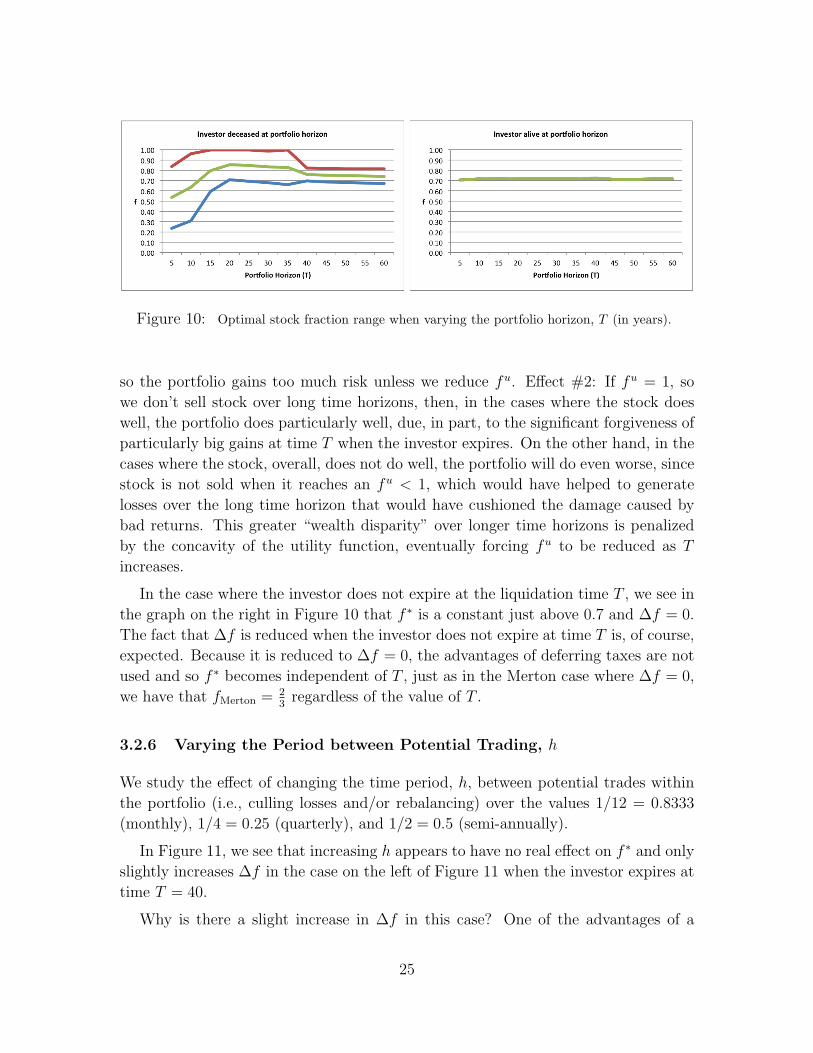
Figure 10: Optimal stock fraction range when varying the portfolio horizon, T (in years).

so the portfolio gains too much risk unless we reduce fu. Effect #2: If fu = 1, so

we don’t sell stock over long time horizons, then, in the cases where the stock does

well, the portfolio does particularly well, due, in part, to the significant forgiveness of

particularly big gains at time T when the investor expires. On the other hand, in the

cases where the stock, overall, does not do well, the portfolio will do even worse, since

stock is not sold when it reaches an fu < 1, which would have helped to generate

losses over the long time horizon that would have cushioned the damage caused by

bad returns. This greater “wealth disparity” over longer time horizons is penalized

by the concavity of the utility function, eventually forcing fu to be reduced as T

increases.

In the case where the investor does not expire at the liquidation time T , we see in

the graph on the right in Figure 10 that f ∗ is a constant just above 0.7 and ∆f = 0.

The fact that ∆f is reduced when the investor does not expire at time T is, of course,

expected. Because it is reduced to ∆f = 0, the advantages of deferring taxes are not

used and so f ∗ becomes independent of T , just as in the Merton case where ∆f = 0,

we have that fMerton = 23

regardless of the value of T .

3.2.6 Varying the Period between Potential Trading, h

We study the effect of changing the time period, h, between potential trades within

the portfolio (i.e., culling losses and/or rebalancing) over the values 1/12 = 0.8333

(monthly), 1/4 = 0.25 (quarterly), and 1/2 = 0.5 (semi-annually).

In Figure 11, we see that increasing h appears to have no real effect on f ∗ and only

slightly increases ∆f in the case on the left of Figure 11 when the investor expires at

time T = 40.

Why is there a slight increase in ∆f in this case? One of the advantages of a

25

Figure 11: Optimal stock fraction range when varying the potential trading interval h. Note thatsince the two distances between the three values of h are not uniform, the grid on the horizontalaxis is not uniform.

smaller ∆f is that it increases the likelihood of capital gains and capital losses, which

is, overall, advantageous, since τl > τg. When we increase h, however, this advantage

is reduced, since it becomes more likely that the losses will be cancelled by gains

before they can be realized. With the advantage of a smaller ∆f reduced, the factors

that push ∆f to expand become more dominant, and so ∆f increases a little as h

increases.

From a practical standpoint, however, it is more important to note that this in-

crease in ∆f is small. That is, the frequency of potential trading is not a particularly

important factor on the optimal strategy, over the reasonable range of h values con-

sidered here.

3.3 The Effect of Changing the Model on the Optimal Strat-egy

In this subsection, we consider the effect of changing the model in three ways:

• Letting the optimal stock fraction range, [f l, fu], change values when the port-

folio is halfway to liquidation (i.e., at T2

= 20 years), instead of remaining

constant.

• Using the average cost basis instead of the full cost basis to provide a quanti-

tative measure of the suboptimality generated by using the average cost basis.

• Incorporating transaction costs when we buy and sell stock to understand their

effect on the optimal stock fraction range, [f l, fu], in the presence of taxes.

26

3.3.1 Effect of a Time Dependent No-Rebalancing Region

We study the effect of allowing f l and fu to change values when we transition from

the initial 20 years, when there is a long time until liquidation, to the final 20 years,

when there is a short time until liquidation.

We must now optimize over five variables instead of three: f init (the initial stock

fraction), f l,0−20 and fu,0−20 (the values of f l and fu in the initial 20 years), and

f l,20−40 and fu,20−40 (the values of f l and fu in the final 20 years). As a typical

example of our results, in Figure 12 we show the values of f l,0−20, fu,0−20, f l,20−40 and

fu,20−40 in the context of changing τg.

Unsurprisingly, when the investor expires at the liquidation time T , the ability to

change stock proportions makes a significant difference, as shown in the left side plot

in Figure 12. Specifically, since capital gains are forgiven at time T , the stock is more

valuable in the final 20 years, so f ∗,20−40 > f ∗,0−20, and to create more capital gains

to be forgiven, we also see that ∆f 20−40 > ∆f 0−20.

Equally unsurprisingly, we find that when the investor is alive at time T , the

ability to change stock proportions makes little difference, so f l,0−20 ≈ f l,20−40 and

fu,0−20 ≈ fu,20−40, as shown in the right side plot in Figure 12. The only difference over

time is at the portfolio horizon, when there is a required liquidation and associated

capital gains tax hit. This required liquidation diminishes the advantage of having

stock, because it restricts the ability to defer capital gains taxes, and so f ∗,20−40, the

optimal stock proportion held when we are closer to liquidation, dips a little from

f ∗,0−20, the optimal proportion when we are farther from liquidation.

Figure 12: Optimal stock fraction range for the first and second half of the portfolio horizon whenvarying the tax rate on gains, τg. The entire horizon of the portfolio is 40 years. For the first 20years stock fractions are shown in bold lines, and for the last 20 years they are shown in dashedlines. As before, the upper bound on the stock fraction is shown by a red line, the lower bound isshown by a blue line, and the average of these two bounds, f∗, is given by a green line.

27

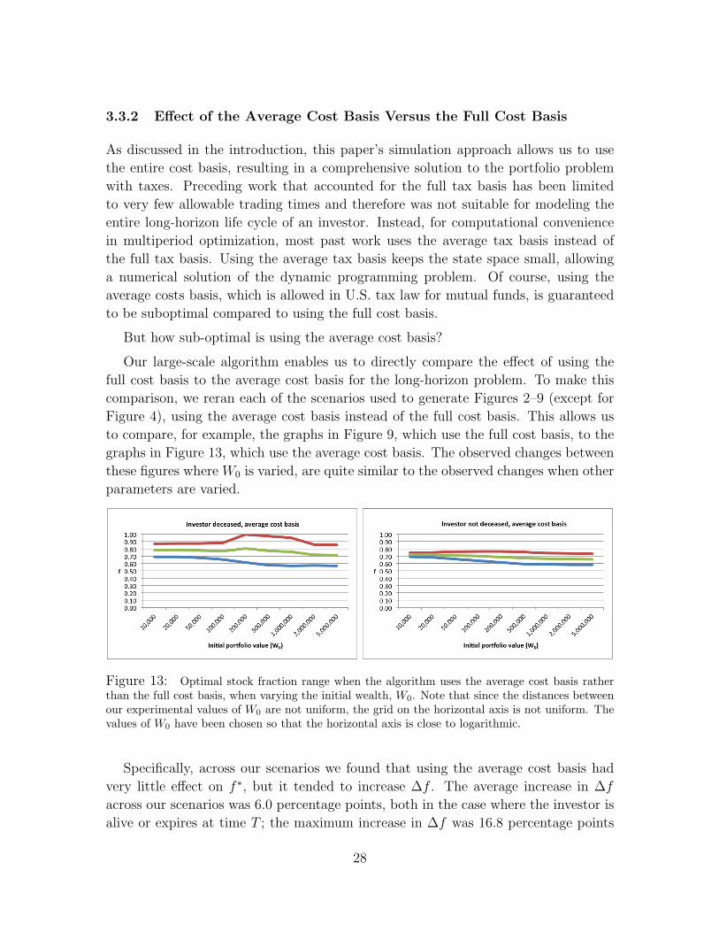
3.3.2 Effect of the Average Cost Basis Versus the Full Cost Basis

As discussed in the introduction, this paper’s simulation approach allows us to use

the entire cost basis, resulting in a comprehensive solution to the portfolio problem

with taxes. Preceding work that accounted for the full tax basis has been limited

to very few allowable trading times and therefore was not suitable for modeling the

entire long-horizon life cycle of an investor. Instead, for computational convenience

in multiperiod optimization, most past work uses the average tax basis instead of

the full tax basis. Using the average tax basis keeps the state space small, allowing

a numerical solution of the dynamic programming problem. Of course, using the

average costs basis, which is allowed in U.S. tax law for mutual funds, is guaranteed

to be suboptimal compared to using the full cost basis.

But how sub-optimal is using the average cost basis?

Our large-scale algorithm enables us to directly compare the effect of using the

full cost basis to the average cost basis for the long-horizon problem. To make this

comparison, we reran each of the scenarios used to generate Figures 2–9 (except for

Figure 4), using the average cost basis instead of the full cost basis. This allows us

to compare, for example, the graphs in Figure 9, which use the full cost basis, to the

graphs in Figure 13, which use the average cost basis. The observed changes between

these figures where W0 is varied, are quite similar to the observed changes when other

parameters are varied.

Figure 13: Optimal stock fraction range when the algorithm uses the average cost basis ratherthan the full cost basis, when varying the initial wealth, W0. Note that since the distances betweenour experimental values of W0 are not uniform, the grid on the horizontal axis is not uniform. Thevalues of W0 have been chosen so that the horizontal axis is close to logarithmic.

Specifically, across our scenarios we found that using the average cost basis had

very little effect on f ∗, but it tended to increase ∆f . The average increase in ∆f

across our scenarios was 6.0 percentage points, both in the case where the investor is

alive or expires at time T ; the maximum increase in ∆f was 16.8 percentage points

28

when the investor was alive at time T and 18.6 percentage points when the investor

expires at time T . The increase in ∆f is explained by the fact that using the average

cost basis makes losses in the portfolio less likely to occur, thereby reducing the

advantage of keeping ∆f small.

But the main concern when we switch to the average cost basis is not the change

in the optimal policy. It is the loss to the investor created by this switch. To quan-

tify this loss, we again use the certainty equivalent difference, which for our current

circumstance, is

c =

(Eavg[U(W )]

Efull[U(W )]

) 11−α

− 1. (4)

Applying equation (4) across each of our scenarios, we found that when the investor

expires at time T , the average certainty equivalent difference, c, was only −0.27%,

with a maximum certainty equivalent difference of −1.12%. When the investor is alive

at time T , the average difference increases to −0.65%, with a maximum difference of

−1.73%. For comparison, if we quantify the loss due to living at time T (no gains

forgiven) versus expiring at time T (gains forgiven) over the same set of scenarios

(using the full cost basis for both), the cost equivalent difference

c =

(Ealive[U(W )]

Edead[U(W )]

) 11−α

− 1.

averages −9.97% with a maximum difference of −23.6%.

The data in the above paragraph, by itself, gives considerable justification for past

work that employs the average cost basis to determine trading strategies in taxable

portfolios, since the loss generated by using the average cost basis in place of the full

cost basis is clearly not that great. Yet the case for justifying these average cost basis

models is even stronger: These models will generate an optimal f ∗ and ∆f for the

average cost basis, but, of course, these values for f ∗ and ∆f would always be used

with the full cost basis strategy in practice. So how much of the value of c in equation

(4) is due to the f ∗ and ∆f from the average cost basis model being suboptimal when

the investor uses the full cost basis, as they would in practice, and how much is due

to the effect of an investor actually using the average cost basis method versus using

the full cost basis?

Consider the base case again. If the investor expires at T = 40, then, for the

full cost basis optimization, we have that f ∗ = 0.764 and ∆f = 0.168, while for the

average cost basis optimization, we have that f ∗ = 0.770 and ∆f = 0.228, which,

using equation (4), corresponds to c = −0.0019. But recall from Subsection 3.1 that

small changes to f ∗ and large changes to ∆f , as we have here, usually have a small

29

impact on the certainty equivalent difference. In fact if we compute

c =

(Eafull[U(W )]

Efull[U(W )]

) 11−α

− 1,

where “Eafull” means using the full cost basis with the values f ∗ = 0.770 and ∆f =

0.228 that came from the average cost basis optimization, we get c = −0.0003. That

is, the actual loss due to using the optimal strategy for the average cost basis model is

much smaller than indicated above, specifically, it is only cc

= 319

of the loss indicated

above, as long as the full cost basis is actually employed for trading, as it would be

by any investor interested in minimizing taxes.

The base case where the investor is alive at T = 40 shows less dramatic results. In

this case, for the full cost basis optimization, we have that f ∗ = 0.711 and ∆f = 0,

while for the average cost basis optimization, we have that f ∗ = 0.701 and ∆f =

0.127, which corresponds to c = −0.0090 and c = −0.0060. Therefore, cc

= 23, where

before it was only 319

. The higher value for cc

is due to the optimal ∆f now being zero

for the full cost basis optimization, which, as seen in the right panels in Figure 1 and

explained in Subsection 3.1, leads to a higher sensitivity to changes in ∆f .

3.3.3 Effect of Incorporating Transaction Costs

Finally, we investigate the effect of incorporating transactions costs into our model.

This issue was also explored in Leland (2000), who found that transaction costs reduce

optimal portfolio churn by 50%. He also found that capital gains taxes lead to lower

investment in stock, and we find that this is not always the case.

Assume that for the current time t, the current number of shares of stock in the

portfolio is Nt, the current stock price is St, the current worth of the portfolio’s cash

position is Ct, and the number of shares to be transacted at time t is n. Let e denote

the proportion of the worth of a trade lost to transaction costs. Based on Domowitz,

Glen, and Madhavan (2001) and Pollin and Heintz (2011), we assume transaction costs

range from 0 to 50 basis points of the value of the transaction, i.e., we consider the

e values 0 (our base case), 0.0005, 0.0010, . . . , 0.0050. These proportional transaction

costs can be incurred at four places in the simulation:

1. When any stock has a capital loss, we sell it and buy back the same value of an

equivalent stock, so our cash balance must be reduced by 2(nSte), which cor-

responds to the transaction costs incurred both for selling and for repurchasing

this stock. We note that while it is always optimal to sell and buy back stock

with a capital loss when there are no transaction costs, this is no longer guar-

30

anteed to be the optimal strategy when we have transaction costs. However, for

the small transaction costs we consider here, the investor will, generally, still be

better off selling and buying back stock with a capital loss, so we continue to

implement this strategy in our transaction cost model.

2. When the stock fraction falls below fl, we buy stock so that the new stock frac-

tion equals fl after transaction costs. This must satisfy the following equation:

fl =(Nt + n)St

(Nt + n)St + Ct − nSt − nSte,

which, after rearrangement, leads to the following expression for the number of

shares that will be bought:

n =NtSt(fl − 1) + Ctfl

St(fle+ 1).

Using the subscript (t+) to denote values just after rebalancing at time t, we

then update the total number of shares of stock

N(t+) = Nt + n

and the cash balance

C(t+) = Ct − nSt − nSte.

3. When the stock fraction rises above fu, we sell stock so that the new stock frac-

tion equals fu after transaction costs. This must satisfy the following equation:

fu =(Nt − n)St

(Nt − n)St + Ct + nSt − nSte,

which, after rearrangement, leads to the following expression for the number of

shares that will be sold:

n =NtSt(fu − 1) + Ctfu

St(fue− 1).

We then update the total number of shares of stock

N(t+) = Nt − n

and the cash balance

C(t+) = Ct + nSt − nSte.

31

4. Finally, at the end of the year, if there are capital losses, then the tax break

generated by these losses is used to buy additional shares. This additional

number of shares (after transaction costs) will be

n =τl ·min[3000,max(0,−G)]

St(1 + e),

since $3, 000 is the annual limit allowed for taking tax losses and G, as before,

represents the realized gains in the portfolio. Therefore, shares are only bought

when G < 0; i.e., there are losses.

Figure 14: Optimal stock fraction range when varying transactions costs (in bps). These costsare stated in terms of the percentage of the value of each transaction lost to costs.

As expected, we see from Figure 14 that rebalancing occurs less often as transaction

costs increase. That is, ∆f increases as e increases. What is more surprising is that

the optimal average stock fraction, f ∗, is essentially unaffected by e, at least over the

range of values for e considered here.

Considerable attention has been devoted to understanding the asymptotic effect of

small proportional transaction costs in portfolios that are not subject to taxes. See for

example, Atkinson and Mokkhavesa (2002), Goodman and Ostrov (2010), Janacek

and Shreve (2004), Rogers (2004), Shreve and Soner (1994), and Whaley and Wilmott

(1997), who all conclude that the order of growth of ∆f is given by ∆f ∼ O(e13 ) when

e is small. What happens to this asymptotic expression in portfolios subject to taxes?

The expression has no relevance to the case in the left panel of Figure 14 where the

investor expires at time T , since ∆f 6= 0 when e = 0 in this case. The case in the

right panel of Figure 14, where the investor is alive at time T , has more potential to

be connected to the asymptotic expression, since ∆f = 0 when e = 0, and ∆f grows

as e grows. However, even in this case, it is clear from Figure 14 that ∆f does not

grow by order e13 , so the asymptotic formula for cases without taxes is not relevant

to cases with taxes.

32

4 Conclusions

In this paper we have modeled the optimal trading strategy of a taxable portfolio

with a stock position and a cash position in which we consider the effects of the

American tax system, including keeping track of the cost basis of stocks whenever

they are bought and sold, utilizing the tax benefits from stocks with losses, and using

the annual $3000 limit on claimable losses along with carrying over losses above this

limit. We develop a large-scale simulated optimization program that offers facile

computation on standard hardware, extending the number of trading periods into

the hundreds (∼500) from earlier models (∼20 periods).

For our model, we have determined the optimal static interval [f l, fu] within which

to maintain f , the fraction of the portfolio invested in stock. When the portfolio is

inside this interval, it is optimal to trade only to reap capital losses, not to rebalance.

When the portfolio strays outside this interval, it is optimal to rebalance the portfolio

back to the nearest endpoint, f l or fu.

Our experiments to determine this optimal interval provide a number of insights

concerning the best strategies for investors to pursue in their taxable portfolios. A

number of our conclusions differ from conventional wisdom and many investors’ in-

tuitions:

• The optimal value of f , the fraction of the portfolio in stock, is often higher for

taxable accounts than for tax-free accounts like the Roth IRA.

This is the case even if the cash position is not taxed and if we assume that

the investor is alive at liquidation, meaning that taxes on all capital gains are

paid. This is explained by the fact that τl, the refund tax rate for capital losses,

which is equal to the marginal income tax rate, is higher than τg, the (long

term) tax rate for capital gains. Therefore, the benefit of culling capital losses

from stock can, on average, outweigh the disadvantage of paying capital gains

taxes, making the stock more useful in the taxable portfolio than in the tax-

free portfolio. For example, in Subsection 3.1, we considered a base case where

the investor is alive at the time of liquidation, and we found that the optimal

value of f = f l = fu was about four percentage points higher than the value of

fMerton, the optimal constant stock fraction in a tax-free portfolio.

• If the capital gains tax rate increases, then f , the fraction of the portfolio in

stock, should be raised, not lowered.

In the previous section, we establish this both experimentally and with an

intuitive explanation. This conclusion assumes that the portfolio is designed

33

to be given to a beneficiary, so that gains are forgiven at death, and it assumes

that the stock position is larger than the cash position.

• The 5/25 rule for rebalancing taxable portfolios is less than ideal, even as a rule

of thumb.

The “5” part of the 5/25 rule corresponds to an interval width ∆f = fu− f l =

2× 0.05 = 0.10. That is, it recommends using an interval for the stock fraction

with a width of 10 percentage points. (The “25” part of the rule is irrelevant

for our stock-cash model if f ∗, the center of the optimal interval, is between

0.20 and 0.80.)

But we find that there are common circumstances where the optimal ∆f = 0

and almost equally common circumstances where the optimal ∆f > 0. More-

over, because the effect of using a suboptimal ∆f will generally be more harmful

when the optimal ∆f = 0 than when the optimal ∆f > 0 (for reasons explained

in Subsection 3.1), our analysis suggests that, for a rule of thumb, it makes more

sense to adopt ∆f = 0, in other words, adopt a strategy of continual rebalanc-

ing, if transaction costs are small.

Overall, our model shows that the optimal width, ∆f = fu − f l, of the stock

fraction interval...

• ...significantly increases when the stock’s expected return, µ, increases or the

risk free interest rate, r, decreases; when the tax rate for capital gains, τg,

increases or the tax rate for capital losses, τl, decreases; when the initial portfolio

size, W0, increases; or when the lifetime of the portfolio, T , decreases.

• ...slightly increases when the time interval between potential transactions, h,

increases or when the utility function risk aversion parameter, α, in equation

(1) decreases.

• ...and is essentially unaffected when the stock’s volatility, σ, changes.

and that the optimal portfolio stock fraction — or, more specifically, the optimal

center, f ∗ = fl+fu2

, of the stock fraction interval...

• ...significantly increases when µ increases or when r, σ, or α decrease.

• ...slightly increases when τl increases; when W0 decreases; when τg increases,

assuming the investor expires at time T ; or when τg decreases, assuming the

investor is alive at time T .

34

• ...is essentially unaffected when h changes or, in the case where the investor is

alive at time T , when T changes.

• ...and, in the case where the investor expires at time T , increases when T initially

increases, but as T increases further, it levels off, then slowly decreases, and

finally levels off again.

Finally, our model provides a number of other insights about optimal investing in

taxable portfolios:

• Using a suboptimal value for f ∗ is generally far more detrimental to the investor

than using a suboptimal value for ∆f .

• The optimal strategy is almost completely unaffected by considering potential

trading on a monthly versus quarterly versus semi-annual basis.

• When the optimal stock fraction interval, [f l, fu], is allowed to depend on time,

we see far more dynamic behavior for this interval when the investor expires

at time T than when the investor is alive at time T . Unsurprisingly, when

the investor expires at time T , both f ∗ and ∆f increase over time. When

the investor is alive at time T , f ∗ decreases slightly over time, while ∆f stays

essentially constant.

• While using the full cost basis history versus the average cost basis has a signif-

icant effect on the optimal stock fraction interval, [f l, fu], it has a surprisingly

small effect on the investor’s outcome, generally leading to a certainty equiv-

alent difference of less than 1 percent over 40 years. This justifies the use of

the average cost basis approximation, which had to be employed by many pre-

vious papers using Bellman equation approaches to investigate optimal taxable

portfolio strategies.

• As the magnitude of proportional transaction costs increases, the width, ∆f , of

the optimal stock fraction interval also, unsurprisingly, increases, however, the

center, f ∗, for this interval remains surprisingly constant.

35

References

Akian, M., Menaldi, J. L., Sulem, A., (1996). “On an Investment-Consumption Model

with Transactions Costs,” SIAM Journal of Control and Optimization 34, 329–364.

Atkinson, C., Mokkhavesa, S., (2002). “Perturbation Solution of Optimal Portfolio

Theory with Transaction Costs for any Utility Function,” IMA Journal of Man-

agement Mathematics 13, 131–151.

Atkinson, C., Ingpochai, P., (2006). “The Influence of Correlation on Multi-Asset

Portfolio Optimization with Transaction Costs,” J. of Computational Finance, 10,

no. 2, pp. 53-96.

Bichuch M., (2012). “Asymptotic Analysis for Optimal Investment in Finite Time

with Transaction Costs,” SIAM Journal on Financial Mathematics, Vol. 3, No. 1,

pp. 433-458.

Constantinides, G. Capital market equilibrium with personal taxes. Econometrica 51

(1983), 611–636.

Constantinides, G.M., (1984). “Optimal Stock Trading with Personal Taxes,” Journal

of Financial Economics 13, 65–89.

M. Dai, H. Liu, Y. Zhong (2011). “Optimal Consumption and Investment with Dif-

ferential Long-term/Short-term Capital Gain Tax Rates,” Working paper, Wash-

ington University at St. Louis.

Dammon, R.M., Dunn, K.B., Spatt, C.S., (1989). “A Reexamination of the Value of

Tax Options,” Review of Financial Studies 2(3), 341–372

Dammon, R.M., Spatt, C.S., (1996). “The Optimal Trading and Pricing of Secu-

rities with Asymmetric Capital Gains Taxes and Transactions Costs,” Review of

Financial Studies 3, 921–952.

Dammon, R.M, Spatt, C.S., Zhang, H. (2001). “Optimal consumption and investment

with capital gains taxes,” Review of Financial Studies 14, 583–616.

Dammon, R.M., Spatt, C.S., Zhang, H. (2004). “Optimal asset location and allocation

with taxable and tax-deferred investing,” Journal of Finance 59, 999–1037.

Dammon, R.M., Spatt, C.S., (2012). “Taxes and Investment Choice,” Annual Review

of Finance and Economics 4, 411–429.

Davis, M.H.A., Norman, A., (1990). “Portfolio Selection with Transaction Costs,”

SIAM Journal of Control and Optimization 31, 470–493.

36

DeMiguel, A., Uppal, R., (2005). “Portfolio investment with the exact tax basis via

nonlinear programming,” Management Science 51, 277–290.

Domowitz, I., Glen, J., Madhavan, A., (2001). “Global Equity Trading Costs,” Work-

ing paper, ITG. Inc.

Dybvig, P., Koo H., (1996). “Investment with Taxes,” Working paper, Washington

University in St. Louis.

Gallmeyer, M., Kaniel, R., Tompaidis , S., (2006). “Tax management strategies with

multiple risky assets,” Journal of Financial Economics 80, 243–291.

Gill, P., Murray, W., Saunders M., (2002). “SNOPT: An SQP algorithm for large-

scale constrained optimization,” SIAM Journal of Optimization 12, 979–1006.

Goodman, J., Ostrov, D. N., (2010). Balancing Small Transaction Costs with Loss of

Optimal Allocation in Dynamic Stock Trading Strategies. SIAM J. Appl. Math.,

70, no. 6, pp. 1977–1998.

Haugh, M., Iyengar, G., Wang. C. (2014). Tax-Aware Dynamic Asset Allocation,

Working paper, Columbia University.

Huang, J., (2008). “Taxable and Tax-Deferred Investing: A Tax-Arbitrage Ap-

proach,” Review of Financial Studies 21, 2173–2207.

Janacek, K., Shreve, S.E., (2004). “Asymptotic analysis for optimal investment and

consumption with transaction costs,” Finance and Stochastics 8, 181–206.

Leland, H., (2000). “Optimal Portfolio Implementation with Transactions Costs and

Capital Gains Taxes,” UC Berkeley, Working paper.

Liu, H., (2004). “Optimal Consumption and Investment with Transactions Costs and

Multiple Risky Assets,” Journal of Finance 59(1), 289–338.

Merton, R. Continuous-Time Finance. (1992) revised edition, Blackwell, Oxford.

Muthuraman, K. and Kumar, S., (2006). “Multidimensional Portfolio Optimization

with Proportional Transaction Costs,” Mathematical Finance, 16, pp. 301–335.

Ostrov, D.N., and Wong, T.G., (2011). “Optimal Asset Allocation for Passive Invest-

ing with Capital Loss Harvesting,” Applied Mathematical Finance 18(4), 291-329.

Pollin, R., Heintz, J., (2011). “Transaction Costs, Trading Elasticities, and the Rev-

enue Potential of Financial Transaction Taxes for the United States,” Working pa-

per, Political Economy Research Institute, University of Massachusetts, Amherst.

37

Rogers, L.C.G., (2004). “Why is the effect of proportional transaction costs O(δ2/3)?”

Mathematics of Finance, Amer. Math. Soc., Providence RI, 303–308.

Shreve, S. E. and Soner, H. M., (1994). “Optimal Investment and Consumption with

Transaction Costs,” Ann. Appl. Probab. 4(3), 609–692.

Tahar, I. B., Soner, H.M., and Touzi, N., (2010). “Merton Problem with Taxes:

Characterization, Computation, and Approximation,” SIAM J. Financial Math.,

1, 366–395

Whaley, A. E. and Wilmott, P., (1997). “An Asymptotic Analysis of an Optimal

Hedging Model for Option Pricing with Transaction Costs,” Math. Finance 7(3),

307–324.

38