Eur. Actuar. J. https://doi.org/10.1007/s13385-018-0174-6

1 3

ORIGINAL RESEARCH PAPER

Optimal management of immunized portfolios

Riccardo Cesari1,2,3 · Vieri Mosco2,3

Received: 27 April 2017 / Revised: 7 May 2018 / Accepted: 24 May 2018 © EAJ Association 2018

Abstract We generalize the contribution of Fong and Vasicek (Financ Anal J 39:73–78, 1983a; Innov Bond Portf Manag Durat Analy Immun 1983:227–238, 1983b; J Financ 39:1541–1546, 1984) by developing a risk-return optimization problem for immunized life insurance portfolios. The M2 measure of risk for arbi-trary changes of the term structure of interest rates is used for a bond portfolio with duration matched to a given liability horizon. The immunization case becomes a “passive” strategy among an entire menu of active management decisions in which a partial risk minimization is exchanged for more return potential. As in the classi-cal Markowitz (Portfolio Selection, New York, Wiley, 1959) approach, an efficient frontier at the given horizon provides the optimal tradeoff between risk and return. An empirical application to insurance companies shows that such a perspective may be proved useful to highlight which segregated funds can be re-positioned over the efficient frontier, at the chosen level of the firm’s risk appetite.

Keywords Insurance companies · Immunization · Convexity · Fong–Vasicek theorem · Efficient frontier

JEL Classification G22 · G11 · G12

* Riccardo Cesari riccardo.cesari@unibo.it

1 University of Bologna, Bologna, Italy2 IVASS, Rome, Italy3 IVASS, Research Department, Rome, Italy

R. Cesari, V. Mosco

1 3

1 Introduction

Notwithstanding the strong innovation wave which is hitting the insurance industry, a large share of its business model still relies on the good old principle of selling guarantees through a maturity matching between assets and liabilities. This match-ing and the general approach known as integrated management of assets and liabili-ties (ALM) has essentially the aim to cope with the interest rate risk, i.e. the risk of an asymmetric impact of interest rate movements (and risk factors in general) to the asset and the liability side of the balance sheet. As an alternative to the basic cash flow matching solution, the duration concept, as suggested by Redington [24], provided a feasible, more sophisticated, but more vulnerable solution. In his semi-nal work, he introduced the term of immunization to indicate a balance sheet not exposed to interest rate movements. “Hedging” would be the modern equivalent. The essential aspect is the link between duration D (or average of cash flow times) and the price sensitivity to interest rates:

so that the change in portfolio value due to a change in interest rates is proportional to portfolio duration. In a balance sheet set up, the risk capital is E = A − L and we obtain, using the duration formula:

where the interest rate sensitivity of risk capital is a function of four components: durations of asset and liability, leverage A∕L and liability level L.

If E > 0 we have the formula for the equity duration:

where DE can be regarded as the duration of liability plus the product of leverage A∕E and mismatch.1 If E ≡ 0 ( A = L . or zero equity portfolio), we obtain DA = DL and this perfect matching represents the fundamental immunization formula. How-ever, the duration is a reliable measure of risk only in case of special interest rate changes (small, additive shift of the term structure): as shown by Fong and Vasicek [11], arbitrary movements of rates have an impact which depends not only on the average of cash flow times ( D ), but also on their dispersion ( M2.). In this broader sense, immunization as a minimum (zero) risk approach must be considered only

D = −1

P

�P

�r

�E

�r=(−1

L

�L

�r

)L −

(−1

A

�A

�r

)A =

(DL − DA

A

L

)L

DE = DL +A

E⋅(DA − DL

)⋛ 0

1 See Messmore [20] who shows that if E > 0 (the present value of assets greater than the present value of liabilities) the immunization of E , i.e. DE = 0 , implies DA < DL . In the following we assume a fixed income portfolio with A = L.

1 3

Optimal management of immunized portfolios

as a special, one-dimensional case of the portfolio optimization problem, where, as in the classical Markowitz model [18], an entire risk-return frontier provides a complete menu of management decisions, according to the firm’s propensity to risk (risk appetite) and financial market opportunities. Fong and Vasicek [9, 10] intro-duced this double, risk-return dimension into the immunization literature. General-izing their approach, we shall provide an implementable model according to which an insurance company could estimate the efficient frontier facing its fixed income balance sheet and evaluate, against arbitrary interest rate movements, how distant its portfolio is from efficiency and how much risk it is bearing with the chosen asset–liability mix.

In the next paragraph we shall review a few basic results of the classical theory of immunization, particularly useful for our developments. Then we will see in prac-tice the term structure movements as suggested by recent European stress tests and financial market dynamics. In paragraphs 4 and 5 we will analyze passive and active strategies of portfolio immunization providing, in paragraph 6, an empirical exam-ple of the model. The final section concludes the paper with a recap of results and possible extensions.

2 Some results of the classical theory of immunization2

Let Aj for j = 1,… ,m be the cash flows of a bond portfolio, available at time sj , j = 1,… ,m , 0 < s1 < ⋯ < sm . Let P(0, s) be the initial (time 0 ) discount function for maturity s.

The current value of the assets is:

where

and rFW (0, �) is the initial instantaneous forward rate:

A(0) =

m∑j=1

AjP(0, sj

)

P(0, s) = exp

⎛⎜⎜⎝−

s

∫0

rFW (0, �)d�

⎞⎟⎟⎠= exp (−sR(0, s))

rFW (0, �) ≡ −� lnP(0, �)

��

2 See Appendix 1 for a proof of the theorems. Without loss of generality we assume continuous com-pounding.

R. Cesari, V. Mosco

1 3

and R(0, s) is the initial spot rate for maturity s:

Let L be the value of a single liability at the target time H , such that3:

Note that L ≡ A0(H) is the forward, time H value of the portfolio calculated at time 0:

If forward interest rates do not change, the value of the bond portfolio at the tar-get date is A(H) = L . If, instead, interest rates do change we could have A(H) ⋚ L.

In fact:

The balance sheet is said to be immunized against interest rate movements if A(H) ≥ L and it would be interesting to find the conditions (if any) under which a given balance sheet has this property. Clearly, the immunizing conditions depend on the assets and liabilities as well as the type of movements assumed for the interest rates.

Theorem 1 (constant shift) If the term structure of interest rates undergoes an additive and small constant shift from rFW (0, �). to rFW

(0+, �

)= rFW (0, �) + Δ0 then

the balance sheet with liability L at time H (or the portfolio at the target horizon H) is immunized if the duration D(A) of the portfolio is equal to H.

R(0, s) =1

s

s

∫0

rFW (0, �)d�

A(0) = L(0) = L exp

⎛⎜⎜⎝−

H

∫0

rFW (0, 𝜏)d𝜏

⎞⎟⎟⎠. (budget constraint)

L ≡ A0(H) = A(0)exp

⎛⎜⎜⎝

H

�0

rFW (0, 𝜏)d𝜏

⎞⎟⎟⎠=

m�j=1

Ajexp

⎛⎜⎜⎜⎝

H

�sj

rFW (0, 𝜏)d𝜏

⎞⎟⎟⎟⎠

A(H) =

m�j=1

AjP(H, sj) =

m�j=1

Ajexp

⎛⎜⎜⎜⎝

H

∫sj

rFW (H, �)d�

⎞⎟⎟⎟⎠= AH(H)

3 This multiple asset—single liability case is equivalent to the case of an asset only bond portfolio with

target horizon H and target value L = A(0) exp

(H∫0

rFW (0, 𝜏)d𝜏

).

1 3

Optimal management of immunized portfolios

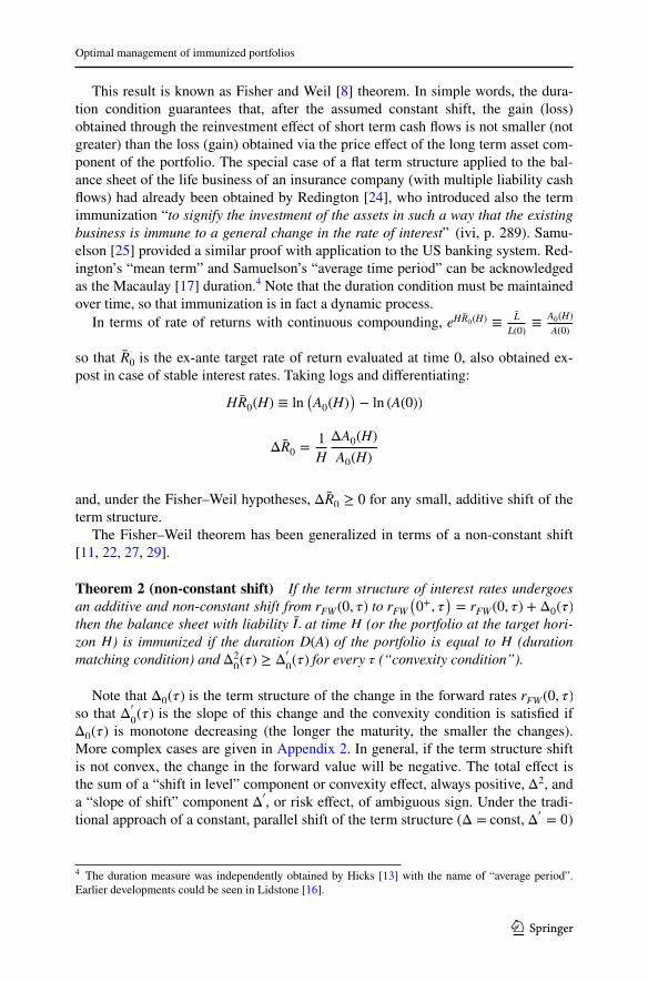
This result is known as Fisher and Weil [8] theorem. In simple words, the dura-tion condition guarantees that, after the assumed constant shift, the gain (loss) obtained through the reinvestment effect of short term cash flows is not smaller (not greater) than the loss (gain) obtained via the price effect of the long term asset com-ponent of the portfolio. The special case of a flat term structure applied to the bal-ance sheet of the life business of an insurance company (with multiple liability cash flows) had already been obtained by Redington [24], who introduced also the term immunization “to signify the investment of the assets in such a way that the existing business is immune to a general change in the rate of interest” (ivi, p. 289). Samu-elson [25] provided a similar proof with application to the US banking system. Red-ington’s “mean term” and Samuelson’s “average time period” can be acknowledged as the Macaulay [17] duration.4 Note that the duration condition must be maintained over time, so that immunization is in fact a dynamic process.

In terms of rate of returns with continuous compounding, eHR0(H) ≡ L

L(0)≡ A0(H)

A(0)

so that R0 is the ex-ante target rate of return evaluated at time 0, also obtained ex-post in case of stable interest rates. Taking logs and differentiating:

and, under the Fisher–Weil hypotheses, ΔR0 ≥ 0 for any small, additive shift of the term structure.

The Fisher–Weil theorem has been generalized in terms of a non-constant shift [11, 22, 27, 29].

Theorem 2 (non‑constant shift) If the term structure of interest rates undergoes an additive and non-constant shift from rFW (0, �) to rFW

(0+, �

)= rFW (0, �) + Δ0(�)

then the balance sheet with liability L at time H (or the portfolio at the target hori-zon H) is immunized if the duration D(A) of the portfolio is equal to H (duration matching condition) and Δ2

0(�) ≥ Δ

�

0(�) for every � (“convexity condition”).

Note that Δ0(�) is the term structure of the change in the forward rates rFW (0, �) so that Δ�

0(�) is the slope of this change and the convexity condition is satisfied if

Δ0(�) is monotone decreasing (the longer the maturity, the smaller the changes). More complex cases are given in Appendix 2. In general, if the term structure shift is not convex, the change in the forward value will be negative. The total effect is the sum of a “shift in level” component or convexity effect, always positive, Δ2 , and a “slope of shift” component Δ� , or risk effect, of ambiguous sign. Under the tradi-tional approach of a constant, parallel shift of the term structure ( Δ = const, Δ�

= 0 )

HR0(H) ≡ ln(A0(H)

)− ln (A(0))

ΔR0 =1

H

ΔA0(H)

A0(H)

4 The duration measure was independently obtained by Hicks [13] with the name of “average period”. Earlier developments could be seen in Lidstone [16].

R. Cesari, V. Mosco

1 3

the total effect is due to convexity only and it is always positive, so that a high con-vexity portfolio would gain an extra-return.5

A Corollary of Theorem 2 gives a useful approximation.

Corollary of Theorem 2 The following second-order approximation holds:

where M20(D) is a variability measure of portfolio cash-flow times measured at time

0:

A lower bound for the change in value was obtained by Fong and Vasicek [11].

Theorem  3 (lower bound for non‑constant shift) If the term structure of interest rates undergoes an additive and non-constant shift from rFW (0, �) to rFW

(0+, �

)= rFW (0, �) + Δ0(�) and if the duration D(A) of the portfolio is equal to

the maturity H of the liability L (duration matching condition), then a lower bound for the change in value of the portfolio is:

where K0 is the maximum of Δ�

0(�) and M2

0(D) is the time 0 variability of portfolio

cash-flow times.Note that M2 is a proper variance of times, given that D is the time average (dura-

tion). This impliesM2 = C − D2 where C is the asset convexity (average of times squared).6

The extension to multiple liabilities was firstly considered in Redington’s seminal paper. He expressed financial immunization by introducing (sufficient) conditions for a fixed income portfolio backing insurance commitments (spread across many

ΔA0(H)

A0(H)≡ G

(rFW + Δ0

)

L≃

1

2M2

0(D)[Δ2

0(D) − Δ

�

0(D)]

M20(D) ≡

∑m

j=1aj�sj − D

�2∑m

j=1aj

=

∑m

j=1Aj

�sj − D

�2exp

�− ∫ sj

0rFW (0, �)d�

�

∑m

j=1Aj exp

�− ∫ sj

0rFW (0, �)d�

�

ΔA0(H)

A0(H)≡ G

(rFW + Δ0

)

L≥ −

1

2K0M

20(D)

6 As duration is linked to the first derivative of the price with respect to the interest rate, convexity repre-sents the second derivative. It is easy also to show that M2 = −

�D

�r.

5 Clearly, interest rate dynamics implying constant shifts are not arbitrage-free. See Boyle [3].

1 3

Optimal management of immunized portfolios

maturities) to be immunized (i.e. protected) against parallel and small variations of a flat term structure. He proved that assets remain above liabilities in value if, sub-ject to the initial balance constraint, the duration (time average) of asset cash flows equals the duration of liabilities and the convexity (time dispersion) of asset cash flows is greater than that of liability cash flows.7

3 Some market data

Depending on their asset and liability composition, insurance companies will be dif-ferently affected by future levels and shapes of interest rates. The duration mismatch gives an approximate measure of this exposure: as shown in Fig. 1, country aver-ages in Europe are widely dispersed, often far away from the perfect matching line.8 This implies that market movements could impair the firms by different amounts, depending also on the different dynamics that will take place in real markets. How-ever, as we shall see, even well matched countries, like Italy, Great Britain, Belgium, Spain and Portugal, are not immunized against general movements in the shape of the term structure.

For example, in its 2014 stress test exercises, EIOPA, the European Supervisory Authority for Insurance and Pension Funds, paid special attention to a scenario of lowering rates, with a long-lasting flattening view of the term structure (so called Japanese scenario).9 In Fig.  2 this low yield scenario is depicted along with the

Fig. 1 Duration of assets and liabilities in the EIOPA stress test report

7 This multiple liability immunization has been generalized by Shiu [28].8 The EIOPA calculation of the liability side in Fig. 1 does not take into account all the contract option-ality available in different countries so that the country relative positions could be altered.9 For instance, see the EIOPA official presentation of the 2014 Stress Test in EIOPA [6].

R. Cesari, V. Mosco

1 3

actual market term structure at the end of 2013 (“Baseline scenario”) and that at the end of 2014, which resulted even lower than envisaged before.

One can see that the hypothetical and the actual market movements are far from being a small, constant shift of the interest rates: the term structure of the shocks {Δ(�), � = 1, 2,… , 30} is both non infinitesimal and not flat across maturities, quite far from the typical 100 basis points figure, ranging roughly from + 20 bps to − 120 bps. According to the EIOPA 2014 Stress Test Report [7], the results of the stress exercise have been evaluated with respect to “the size of duration mismatches between assets and liabilities as well as mismatches in internal rate of return of assets and liabilities” which are “considered the main drivers for the severity of an interest rate stress” .10 However, as it is well known after Redington [24] and the fol-lowing literature,11 in case of not small and not parallel shocks to the term structure, the classical “duration gap” analysis should be generalized to take into account also portfolio convexity and its effect on the balance sheet.12

Fig. 2 EIOPA 2014 stress test scenarios for European interest rates

10 See EIOPA [7], section C, “Low Yield Module Description and Results”, paragraph 2, sub-paragraph 56.11 See Martellini, Priaulet and Priaulet [19], ch. 6 and the references therein.12 Apart from EIOPA Stress Tests, convexity effects are still ignored in many empirical applications as well as popular textbooks in banking and finance (e.g. Mishkin and Apostolos [21]). Moreover, under the Basel III Capital Requirement Regulation (CRR, in force since 1 January 2014), the Standardised Approach includes a calculation for the own funds requirement for the general risk on debt instruments only based on the duration. See European Banking Authority (EBA), Interactive Single Rulebook, arti-cle 340 in https ://www.eba.europ a.eu/regul ation -and-polic y/singl e-ruleb ook. A partial justification can be found in the relevance of the first order effect (duration) as documented in Schaefer [26] and in the empirical literature on Principal Components (Martellini, Priaulet and Priaulet [19], ch. 3) where the first factor (the parallel shift of the term structure) accounts for 50% to 90% of total variability of interest rate changes, especially in the long side of the yield curve.

1 3

Optimal management of immunized portfolios

4 M2 and the passive strategy of minimizing risk

Following Fong and Vasicek [9, 11], let R0 be the guaranteed target return, fixed ex ante at time 0, for the investment horizon (holding period) H . If the portfolio dura-tion D is equal to H , the Fong–Vasicek lower bound (Theorem 3 above) shows that the ex post portfolio value has a minimum percentage change (maximum shortfall):

where M20 is a variance of times to payment and max

{Δ�

0

} is the maximum change

of the slope of the current term structure across its maturities. By definition:

where D is the duration and the weights wj are given by the present values of the cash flows at time sj . As duration represents a time average, M2

0 is a time variance

and can be expressed in terms of duration and convexity. Note that, according to the Fong and Vasicek lower bound, M2

0 is a risk measure in that it captures the exposure

to any arbitrary movement of the discount curve. It suffices, therefore, to minimize M2

0 in order to minimize such exposure, maximizing, at the same time, the lower

bound for changes in the forward value of the portfolio. If the absolute minimum of M2

0= 0 is attainable (using zero-coupon bonds of maturity H ), then ΔA0(H)

A0(H)≥ 0 and

the forward portfolio value cannot undergo capital losses. This prudential strategy of minimizing M2

0 might be regarded as a “passive” management, in the sense that it

collapses into a simple one-dimensional recipe: buy the minimum risk portfolio and stick to it.

An example could be useful: let us consider the case of two portfolios, the “bullet” and the “barbell”. A perfect “bullet” portfol with maturity D has a minimum M2

0 of

zero. In practice, it is composed by low-coupon securities with maturities close to D so that M2

0 is close to zero. Viceversa, a “barbell” portfolio is a set of very short and

very long securities with large M20 even if it has the same duration D . These two port-

folios with equal duration D are differently affected by a positive twist of interest rates (“steepening”), i.e. a decrease in short rates and an increase in long rates. In fact, this twist has effects both in terms of “reinvested income” and “capital gain” because short term rates have become lower, producing lower coupon (higher cost prices) from rein-vested income whilst long term rates are now higher, producing higher capital losses realized at the horizon. This will produce a shortfall of the portfolio value with respect to the target value (a negative twist will produce the opposite). But the two portfolios are differently (negatively) affected: the barbell portfolio (with higher M2

0 ) is penalized

ΔA0(H)

A0(H)≥ −

1

2M2

0⏟⏟⏟

endogenous

max�

{Δ

�

0(�)

}⏟⏞⏞⏞⏞⏞⏟⏞⏞⏞⏞⏞⏟

exogenous

M20=

m∑j=1

(sj − D

)2⋅ wj

R. Cesari, V. Mosco

1 3

twice, because, due to the barbell profile, i) a greater number of securities/cash flows reach sooner the maturity date with reinvestment at lower interest rates (due to the downward shock on short interest rates) and ii) a higher and longer portion of the port-folio will be outstanding after the horizon date, producing a higher capital loss, given that securities with longer maturities will depreciate more heavily. This means that both M2

0 and the risk of the barbell portfolio are greater than those of the bullet.

5 Active strategy: the risk‑return tradeoff optimization

Immunization, as a minimum (zero) risk approach, must be considered as a special case in the broader area of portfolio optimization, in which risk-return considerations pro-vide an entire menu of management decisions, depending on the firm’s risk aversion and financial market opportunities. In the following, starting from Fong and Vasicek [9, 10], we provide this generalized risk-return approach for duration matching, insurance portfolios, analogous to Markowitz’s mean–variance asset portfolio analysis.

Let R0(H) be the current annual ex-ante rate of return over the horizon H . By definition:

In case of no shift of the term structure, the ex-ante is also the ex-post rate of return.Using the Corollary of Theorem 2, after an instantaneous non-constant shift of the

term structure we have the second-order approximation:

where:

is a special function of the term structure shift from time 0 to time 0+ . and maturity H (see Appendix 2). Note that this function is the sum of a “shift in level” compo-nent (“convexity effect”), always positive, Δ2 , and a “slope of shift” component Δ� , (“risk effect”) of ambiguous sign. In case of adverse shift ( Δ2

0< Δ

�

0 , ΔS0 < 0)he

realized return will be under the target value.The portfolio risk can be measured by the volatility (standard deviation) of ΔR0(H)

and it is proportional to the dispersion measure M20 . As explained by Fong and Vasicek

[10, p. 235]: “A portfolio with half the value of M2 than another portfolio can be expected to produce half the dispersion of realized returns around the target value when submitted to a variety of interest rate scenarios than the other portfolio” .

Summing up all the shape changes between 0 . and H − 1 . we have:

eHR0(H) ≡ A0(H)

A(0)

ΔR0(H) =1

H

ΔA0(H)

A0(H)≃

1

HM2

0(H)ΔS0(H)

ΔS0(H) ≡ 1

2

[Δ2

0(H) − Δ

�

0(H)

]⋛ 0

1 3

Optimal management of immunized portfolios

where the difference, RH − R0 , between the future annual rate 1Hln(

AH (H)

A(0)

) and cur-

rent ex-ante rate is a random variable (sum of H random variables ΔSt(H) ), with mean and variance given by:

In practice, in all financial markets, cash flows can be typically bought and sold only in pre-defined “bundles” (the coupon bonds) so that optimal management must be set in terms of available bond portfolios. Given a set of K different bonds, the port-folio return can be represented as a linear combination of K random variables:

with mean �iH and covariance

Clearly:

and we link the dynamics of M2it and ΔSt to their current values M2

i0 and ΔS0 as fol-

lows (see [10]):

where, if D0i is the i-th bond duration, we have13:

RH(H) − R0(H) =

H−1∑t=0

ΔRt(H) ≃1

H

H−1∑t=0

M2t(H)ΔSt(H)

𝜇H ≡ E(RH − R0), 𝜎2H≡ Var

(RH − R0

).

K∑i=1

wi(RiH − Ri0)

𝜎ij = Cov(RiH − Ri0,RjH − Rj0)

RiH − Ri0 =1

H

H−1∑t=0

M2it(H)ΔSt(H) i = 1,… ,K

M2it(H)ΔSt(H) ≅ M2

i0(H)

(H − t

H

)3

ΔS0(Di0)

(H − t

Di0

)

M2i0(H) =

m∑j=1

(sj − H)2w0j = M20

(Di0

)+ (Di0 − H)2

13 Note that using (realistically) bonds instead of cash flows has no effect on the calculation of duration but it affects the calculation of risk. In fact, the duration of a portfolio of bonds is simply the “portfolio” (average) of bond durations; however, the M2 of a portfolio of bonds is the “portfolio” of M2 (within vari-ance) plus the variance of durations (between variance). See the Appendix 4.

R. Cesari, V. Mosco

1 3

so that14:

The active strategy is to find the portfolio wi maximizing the objective function U , in mean and variance:

where � is the vector of expected returns �iH and � ≡ [�ij

] is the covariance matrix.

As an example: U(w�

�,w��w;�) = w

�

� − �√w��w

where the confidence level parameter � (implying the maximization of the lower bound of the return confidence interval) has the same role of the risk aversion parameter in Markowitz risk-return approach: the higher the parameter, the more rel-evant the effect of portfolio variance and the more conservative the preferred portfo-lio will be. For � = 0 the optimal portfolio will maximize the ex ante rate of return; for � large, the optimal portfolio is the passive portfolio with minimum immunizing risk. As in the classical Markowitz approach, the solution procedure can be divided in steps, the first one being the minimum variance portfolio for a given ex ante dif-ferential return m and the given horizon H:

𝜇iH = E(RiH − Ri0) =1

H

H−1∑t=0

M2it(H)E

(ΔSt(H)

)=

1

HM2

i0(H)E

(ΔS0

(Di0

)) 1

Di0

H−1∑t=0

(H − t)4

H3,

𝜎ij =Cov(RiH − Ri0,RjH − Rj0) = Cov

(1

H

H−1∑t=0

M2it(H)ΔSt(H),

1

H

H−1∑v=0

M2jv(H)ΔSv(H)

)

=1

H2M2

i0(H)M2

j0(H)

(H−1∑t=0

(H − t)4

H3

)2

1

Di0

1

Dj0

Cov(ΔS0

(Di0

),ΔS0

(Dj0

))

maxwi

U(w�

�,w��w)

⎧⎪⎨⎪⎩

∑1≤i≤K

wi ⋅ Di0 = H (target duration constraint)

∑1≤i≤K

wi = 1 (budget constraint)

wi ≥ 0 (no short selling)

14 Note that Fong and Vasicek [10] assume, in the variance calculation, the asymptotic approximation: ∑H

t=0M4

t=

M40

H6

∑H

t=0(H − t)6 =

M40

H6

H(H+1)(2H+1)(3H4+6H3−3H+1)

42→

forH→ ∞

H

7M4

0

so that the variance is proportional to M40

7H . We do not use this asymptotic approximation.

1 3

Optimal management of immunized portfolios

By varying m, the efficient frontier m(�) can be traced, for a given H . More gen-erally, assuming the horizon H . as an additional control variable, an efficient surface m(�,H) could be obtained, showing the portfolio possibilities for an “active” man-agement strategy in terms of optimal return-risk-horizon tradeoff.

6 An empirical application

We provide an empirical application using a sample of Italian data. In Italy, at the end of 2014, 56 life insurance companies totalled 429 billion euros of segregated funds representing with-profit, participating policies,15 mainly invested (218 billion euros) in fixed coupon bonds.

In a sample of 10 medium-large life insurance companies (covering a market share of 54% in terms of collected premiums) the duration gap is particularly small, as required. In 5 cases the duration was about 7.5 years and in the other 5 cases it was about 10 years. For simplicity, the Government bond market was reduced into four bond benchmarks with maturity 3, 5, 10 and 20 years respectively (see Appen-dix 3), so that the results cannot measure the “selection” effect of asset management. The following frontiers (Fig.  3) have been obtained by calculating, as explained in the previous paragraph, the efficient frontiers with horizon (average duration) H = 7.5 and H = 10 respectively. The gap between each firm and the frontier is a measure of the “allocation” inefficiency of the firm’s portfolio.

A firm finding its portfolio appreciably distant from the efficiency curve could reduce the level of risk without penalty in the expected return dimension or, vice-versa, reallocate its assets to reach a higher level of expected return while keeping up its risk exposure. In the first case, it is plausible that it has to reduce the portfolio “barbellness” by increasing the share of bonds with a lower M2 and/or the share of zero-coupon bonds of the given maturity H. In the second case, it is probable that a few coupon bonds are available in the market with better return perspectives and

minwi

√w��w

⎧⎪⎪⎨⎪⎪⎩

∑1≤i≤K

wi �iH = m

∑1≤i≤K

wi ⋅ Di0 = H (target duration constraint)

∑1≤i≤K

wi = 1 (budget constraint)

wi ≥ 0 (no short selling)

15 Because of the profit participation mechanism, the liability cash-flows partly depend on the asset cash-flows, through the returns realized by the assets in the segregated funds. Usually, this effect is neg-ligible.

R. Cesari, V. Mosco

1 3

better (de-) correlation for given term structure movements. The reallocation in favor of these bonds would improve the portfolio expected return without increasing its risk.

7 Conclusions and further developments

Following the seminal work by Fong and Vasicek [9–11], it is possible to actively manage the “immunization risk” of a duration-matching portfolio, i.e. a portfolio which, notwithstanding the equality of asset and liability durations (immunized portfolio), has a risky return, being exposed to the effects of arbitrary shifts of the term structure of interest rates. This risk is proportional to a measure ( M2 ) of the dispersion of the cash flow dates around the duration average so that, in this risk-return framework, you can build a generalized optimal management of the com-pany’s bond portfolio essentially in the same way as asset managers choose the optimal asset portfolio along Markowitz’s efficient frontier. The empirical appli-cation of the model shows that it can disclose how distant the actual portfolio is

Fig. 3 Efficient frontiers for immunized portfolios at different horizons

1 3

Optimal management of immunized portfolios

from the efficient frontier, helping to select, along the frontier, the optimal bond portfolio corresponding to the firm’s risk appetite.

Extensions of the analysis are manifold. Theoretically, one can attempt to con-sider the multiple-liability framework in order to be more consistent in the mod-eling of the life insurance business. Moreover, the shocks to the forward rates can be assumed to have an explicit stochastic dynamics, to be exploited in the calcu-lation of moments. At the same time, the empirical implementation could take into account the complete set of bonds available in the financial market, in order to have more refined measures of risks, returns and the frontier. The calculation of a three-dimensional frontier (risk, return and horizon) could be implemented through this more refined modelling and it could be proved useful in generalizing the traditional profit testing activity for new insurance products.

Acknowledgements We thank Antonio De Pascalis, Lino Matarazzo, Enzo Orsingher, Stefano Pasqua-lini, Fabio Polimanti, Giovanni Rago, Arturo Valerio and the participants to a seminar of IVASS and Bank of Italy for their comments. A special thank to Oldrich Vasicek and two anonymous referees for their detailed comments and suggestions to a previous version of the paper. All remaining errors are ours.

Appendix 1: Proof of the theorems

Proof of Theorem 1 The current budget constraint expressed at the forward time H is:

Let

We have:

m�j=1

Aj exp

⎛⎜⎜⎜⎝

H

�sj

rFW (0, 𝜏)d𝜏

⎞⎟⎟⎟⎠≡

m�j=1

aj = L

G�rFW + Δ0

� ≡m�j=1

Aj exp

⎛⎜⎜⎜⎝

H

�sj

�rFW (0, 𝜏) + Δ0

�d𝜏

⎞⎟⎟⎟⎠− L ≡ ΔA0(H)

�G

�Δ0

=

m�j=1

Aj

�H − sj

�exp

⎛⎜⎜⎜⎝

H

∫sj

�rFW (0, �) + Δ0

�d�

⎞⎟⎟⎟⎠

𝜕2G

𝜕Δ20

=

m�j=1

Aj

�H − sj

�2exp

⎛⎜⎜⎜⎝

H

∫sj

�rFW (r, 𝜏) + Δ0

�d𝜏

⎞⎟⎟⎟⎠> 0

R. Cesari, V. Mosco

1 3

so that G(rFW + Δ0

)= 0 for Δ0 = 0 and G

(rFW + Δ0

) ≥ 0 for every Δ0 in a neigh-bourhood of 0 , if Δ0 = 0 is a (local) minimum i.e. if:

where the derivative is taken at Δ0 = 0. Solving for H and multiplying and dividing by P(0,H) , we have the duration condition16:

□

Proof of  Theorem  2 Using the notation introduced in the proof of Theorem  1, define:

so that: f (H) = 1 , f � (s) = −f (s)Δ0(s) , f��

(s)[Δ2

0(s) − Δ

�

0(s)

] ≥ 0 (by the “convexity condition”)

Then the change in value is:

and by Taylor (exact) formula:

�G

�Δ0 �Δ0=0

=

m�j=1

Aj

�H − sj

�exp

⎛⎜⎜⎜⎝

H

∫sj

rFW (0, �)d�

⎞⎟⎟⎟⎠= 0

D(A) =

∑m

j=1Ajsj exp

�− ∫ sj

0rFW (0, �)d�

�

∑m

j=1Aj exp

�− ∫ sj

0rFW (0, �)d�

� = H

f (s) ≡ exp

⎛⎜⎜⎝

H

�s

Δ0(�)d�

⎞⎟⎟⎠

ΔA0(H) ≡ G(rFW + Δ0

)− G

(rFW

)= G

(rFW + Δ0

)=

m∑j=1

aj(f(sj)− 1

)

f(sj)= f (H) +

(sj − H

)f�

(H) +1

2

(sj − H

)2f��(�j)

16 Note that the second order (convexity) condition is always satisfied in the single liability case.

1 3

Optimal management of immunized portfolios

so that, substituting:

where the second equality comes from the duration matching hypothesis D = H and the inequality from the “convexity condition”. □

An alternative proof is given by Montrucchio and Peccati [22].

Proof of Corollary of Theorem 2 Using Taylor’s formula around H :

so that, for H = D:

□

Proof of Theorem 3 From the first order approximation for f (s) = ex(s) ≥ 1 + x(s) we have:

By the integral formula:

so that, integrating and using the Fubini theorem to change the order of integration:

(1)

G(rFW + Δ0

)= −

m∑j=1

aj(sj − H

)Δ0(H) +

1

2

m∑j=1

aj(sj − H

)2f(�j)[Δ2

0

(�j)− Δ

�

0

(�j)]

=1

2

m∑j=1

aj(sj − D

)2f(�j)[Δ2

0

(�j)− Δ

�

0

(�j)] ≥ 0

f(sj)≃ f (H) +

(sj − H

)f�

(H) +1

2

(sj − H

)2f��

(H)

= 1 −(sj − H

)Δ

0(H) +

1

2

(sj − H

)2[Δ2

0(H) − Δ

�

0(H)

]

ΔA0(H)

A0(H)≡ G

(rFW + Δ0

)

L≃

1

2L

m∑j=1

aj(sj − D

)2[Δ2

0(D) − Δ

�

0(D)

] ≡ 1

2M2

0(D)

[Δ2

0(D) − Δ

�

0(D)

]

G(rFW + Δ0

)=

m∑j=1

aj(f(sj)− 1

) ≥m∑j=1

aj

H

�sj

Δ0(�)d�

Δ0(H) − Δ0(�) =

H

∫�

Δ�

0(u)du

R. Cesari, V. Mosco

1 3

If K0 ≡ maxu

{Δ

�

0(u)

}.,

so that, using the duration matching condition D = H:

□

Shiu [27] uses an exact Taylor formula for H∫sj

Δ0(�)d� and Nawalkha and Cham-

bers [23] use higher-order approximations for f (s).

Appendix 2: The shift function

The Fong–Vasicek [11] sufficient condition for immunization is a constraint on the shift function:

Note that the term “convexity condition” stems from the fact that under this condi-tion the function:

H

∫sj

Δ0(�)d� =(H − sj

)Δ0(H) −

H

∫sj

H

∫�

Δ�

0(u)dud� =

(H − sj

)Δ0(H) −

H

∫sj

Δ�

0

u

∫sj

d�du

=(H − sj

)Δ0(H) −

H

∫sj

Δ�

0(u)

(u − sj

)du

(2)

H

�sj

Δ0(�)d� ≥ (H − sj

)Δ0(H) − K0

H

�sj

(u − sj

)du =

(H − sj

)Δ0(H) −

1

2K0

(H − sj

)2

G(rFW + Δ0

) ≥ −1

2K0

m∑j=1

aj(D − sj

)2= −

1

2K0M

20(D)L

Δt(�) ≡ rFW (t + dt, �) − rFW (t, �) ∶

Δ2t(�) − Δ

�

t(�) = c ≥ 0,∀�

f (s) ≡ exp

⎛⎜⎜⎝

H

�s

Δt(�)d�

⎞⎟⎟⎠

1 3

Optimal management of immunized portfolios

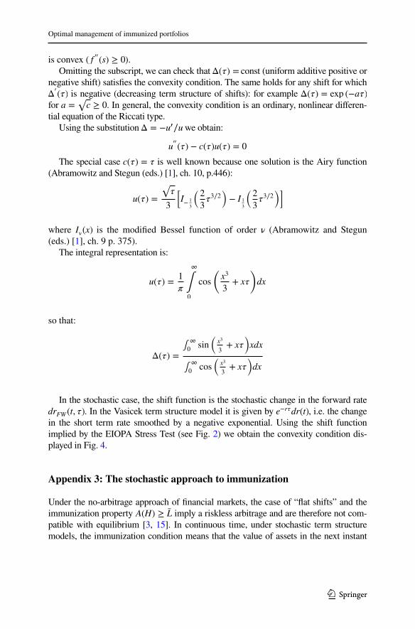
is convex ( f �� (s) ≥ 0).Omitting the subscript, we can check that Δ(�) = const (uniform additive positive or

negative shift) satisfies the convexity condition. The same holds for any shift for which Δ

�

(�) is negative (decreasing term structure of shifts): for example Δ(�) = exp (−a�) for a =

√c ≥ 0 . In general, the convexity condition is an ordinary, nonlinear differen-

tial equation of the Riccati type.Using the substitution Δ = −u�∕u we obtain:

The special case c(�) = � is well known because one solution is the Airy function (Abramowitz and Stegun (eds.) [1], ch. 10, p.446):

where I�(x) is the modified Bessel function of order ν (Abramowitz and Stegun (eds.) [1], ch. 9 p. 375).

The integral representation is:

so that:

In the stochastic case, the shift function is the stochastic change in the forward rate drFW (t, �) . In the Vasicek term structure model it is given by e−r�dr(t) , i.e. the change in the short term rate smoothed by a negative exponential. Using the shift function implied by the EIOPA Stress Test (see Fig. 2) we obtain the convexity condition dis-played in Fig. 4.

Appendix 3: The stochastic approach to immunization

Under the no-arbitrage approach of financial markets, the case of “flat shifts” and the immunization property A(H) ≥ L imply a riskless arbitrage and are therefore not com-patible with equilibrium [3, 15]. In continuous time, under stochastic term structure models, the immunization condition means that the value of assets in the next instant

u��

(�) − c(�)u(�) = 0

u(�) =

√�

3

�I− 1

3

�2

3�3∕2

�− I 1

3

�2

3�3∕2

��

u(�) =1

�

∞

∫0

cos

(x3

3+ x�

)dx

Δ(�) =∫ ∞

0sin

(x3

3+ x�

)xdx

∫ ∞

0cos

(x3

3+ x�

)dx

R. Cesari, V. Mosco

1 3

must be equal to the value of liabilities, so that, in differential terms: dA(t) = dL(t) and immunization is guaranteed if the value of assets and liabilities have the same sensitiv-ity to the state variables [2]. This has suggested the definition of a generalized or sto-chastic duration concept [4].

As an example of this stochastic approach to the asset-liability problem, let us con-sider the case of the extended-Vasicek [31], no arbitrage term structure model [14]:

where the time-dependent drift a(s) is obtained in order to guarantee a perfect fit of the theoretical term structure with the current yield curve:

The solution for r(s) is:

and the relative difference between ex post and ex ante portfolio value is:

dr(s) = [a(s) − kr(s)]ds + 𝜎dZ(s)

a(s) = krFW (t, s) +𝜕rFW (t, s)

𝜕s+

𝜎2

2k(1 − e−2k(s−t))

r(s) = rFW (t, s) +𝜎2

2G2(t, s) + 𝜎

s

∫t

e−k(s−u)dZ(u)

G(t, s) =1 − e−k(s−t)

k

Fig. 4 EIOPA shift function Δ(�) and convexity condition

1 3

Optimal management of immunized portfolios

The variable Xtj has an explicit form in this case:

with mean:

and covariance

so that a risk-return approach can be analytically developed.

A(H) − A0(H)

A0(H)=

∑m

j=1Aj exp

�∫ H

sjr(u)du

�−∑m

j=1Aj exp

�∫ H

sjrFW (0, �)d�

�

∑m

j=1Aj exp

�∫ H

sjrFW (0, �)d�

�

=

∑m

j=1Aj exp

�∫ H

sjrFW (0, �)d�

��exp

�∫ H

sjr(u)du − ∫ H

sjrFW (0, �)d�

�− 1

�

∑m

j=1Aj exp

�∫ H

sjrFW (0, �)d�

�

≈

∑m

j=1aj

�∫ H

sj

�r(u) − rFW (0, u)

�du�

∑m

j=1aj

≡m�j=1

bjX0j

Xtj =

H

∫sj

(r(u) − rFW (t, u)

)du =

𝜎2

2k2

H

∫sj

(1 − e−k(u−t)

)2du + 𝜎

H

∫sj

u

∫t

e−k(u−v)dZ(v)du

E(Xtj

)=

�2

2k2

H

∫sj

(1 − e−k(u−t)

)2du

=�2

k3

[k

2

(H − sj

)+ e−k(H−t) − e−k(sj−t) −

e−2k(H−t)

4+

e−2k(sj−t)

4

]

Cov�Xti,Xtj

�= 𝜎2E

⎡⎢⎢⎢⎣

H

∫si

u

∫t

e−k(u−v)dZ(v)du

H

∫sj

s

∫t

e−k(s−v)dZ(v)ds

⎤⎥⎥⎥⎦

= 𝜎2

H

∫si

H

∫sj

min(u,s)

∫t

e−k(u−v)−k(s−v)dvdsdu

R. Cesari, V. Mosco

1 3

Appendix 4: Practical aspects of the computations of some financial variables

In this Appendix we give some technical details of the computations involving financial variables.

The computation of term structure changes

In the empirical application we use daily data and we calculate, from the 1 year-forward rates, rFW(t,τ, τ+1) for τ = 1,…,25 the daily changes:

The analytic, closed form computation of the portfolio cash‑flow dispersion

It is possible to compute in closed-form, i.e. via an analytic formula, the cash-flow dispersion of a securities portfolio. Portfolio cash-flow dispersion turns out to be a quadratic function of portfolio duration, of its yield-to-maturity and its convexity17:

M2(D) = variance of the asset cash-flow maturities around their duration; y = portfo-lio yield-to-maturity, D = portfolio duration (average time-to-maturity), CMod. = port-folio modified convexity.

The variance with respect to horizon H is obtained as:

Yield, duration and convexity aggregation at portfolio level

• The computation of the portfolio aggregate yield-to-maturity

Traditionally one computes the average portfolio yield, weighted by the amount invested (w.r.t. either book-value or market value). This estimate represents an approximation to the yield-to-maturity as seen from the valuation date. A better alternative seems to consist of computing an estimate that takes into account the different time distance of cash-flows from the valuation date: one weights each yield by the “dollar duration” of its security. One obtains the so called WADD yield (Weighted Average Dollar Duration Yield, see Grondin [12]). The Dollar Duration is the product of duration and price of a security.

Δt(�) ≡ rFW(t + 1, �, � + 1) − rFW(t , �, � + 1)

Δ�t(�) ≡ Δt(� + 1) − Δt(�)

ΔSt(�) ≡ 1∕2[Δ2t(�) − Δ�

t(�)]

M2(D) = CMod ⋅ (1 + y)2 − D ⋅ (D + 1)

M2(H) = M2(D) + (D − H)2

17 See for example, Smith [30], p. 1670, formula (9) or de La Grandville [5], p. 163, formula (19). With continuous compounding, the formula simplifies into M2 = C – D.

1 3

Optimal management of immunized portfolios

• The computation of average portfolio Duration and Convexity

The (modified) duration was downloaded from Bloomberg, for each security in the data set (at the date 31/12/2014). Portfolio duration is the average (weighted by market value amounts) of the durations of single securities.

Convexity was also downloaded from Bloomberg, for each security (at the date 31/12/2014). Bloomberg approximated the second derivative (of price w.r.t. yield) as the “central difference” by varying yield-to-maturity by ± 1 basis point, that is18:

Convexity is a “quadratic” measure and hence it can be linearly aggregated (by summation): by weighting with the amounts (at market value) one obtains portfolio convexity.

• The bond benchmarks for maturity classes

The four bond classes used in the empirical application are represented by the fol-lowing benchmark bonds:

Bond index Bond ISIN Time-to-matu-rity (years)

Duration (years) Convexity M-squared

3 IT0004867070 2.84 2.72 10.31 0.215 IT0003644769 5.09 4.58 27.08 1.5410 IT0004513641 10.17 8.27 86.32 9.5920 IT0003535157 19.60 13.46 241.60 46.84

• M-squared for a portfolio of bonds

Let BT = B1 + B2 a portfolio of 2 bonds with cash flows c11, c12 and c21, c22 respectively at times t11, t12 and t21, t22 respectively.

Using a flat term structure:

CMod ≅1

P⋅

P+−P

Δy−

P−P−

Δy

Δy=

1

P⋅P+ − 2 ⋅ P + P−

(Δy)2

⏟⏟⏟Δy=0.01%

= 10, 000 ⋅P+ − 2 ⋅ P + P−

P.

18 Bloomberg data include in the price P accrued interest (full price = clean price + accrued interest) and assume a variation of ± 1 basis point w.r.t. the yield implicit in the price P.

R. Cesari, V. Mosco

1 3

References

1. Abramowitz M, Stegun IA (eds) (1964) Handbook of mathematical functions, with formulas, graphs, and mathematical tables, 10th edn. National Bureau of Standards, USA, p 1972

2. Albrecht P (1985) A note on immunization under a general stochastic equilibrium model of the term structure. Insur Math Econ 4:239–244

3. Boyle PP (1978) Immunization under stochastic models of the term structure. J Inst Actuaries 105:177–187

4. Cox JC, Ingersoll JE Jr, Ross SA (1979) Duration and the measurement of basis risk. J Bus 52(1):51–61

5. de La Grandville O (2001) Bond pricing and portfolio analysis. MIT Press, Cambridge 6. EIOPA (2014 a). https ://eiopa .europ a.eu/Publi catio ns/Speec hes%20and %20pre senta tions /EIOPA

_ST201 4_Suppo rting _mater ial.prese ntati on.pdf 7. EIOPA (2014 b), Document EIOPA-BOS-14-203, 28 November 2014 8. Fisher L, Weil RL (1971) Coping with the risk of interest-rate fluctuations: returns to bondholders

from naïve and optimal strategies. J Bus 44:408–431 9. Fong HG, Vasicek OA (1983a) The tradeoff between return and risk in immunized portfolios.

Financ Anal J 39:73–78 10. Fong HG, Vasicek OA (1983b) Return maximization for immunized portfolios. In: Kaufman GG,

Bierwag GO, Toevs A (eds) Innovations in bond portfolio management: duration analysis and immunization. JAI Press, London

11. Fong HG, Vasicek OA (1984) A risk minimizing strategy for portfolio immunization. J Financ 39(5):1541–1546

12. Grondin TM (1998) Portfolio Yield? Sure, but …, The society of actuaries, risk and rewards Letters, p 16

13. Hicks JR (1939) Value and capital, 2nd edn. 1946, OUP, Oxford 14. Hull JC, White A (1990) Pricing interest-rate derivative securities. Rev Financ Stud 3:573–592 15. Ingersoll JE Jr, Skelton J, Weil RL (1978) Duration forty years later. J Financ Quant Anal

13:627–650

B1 = c11 exp(−rt11

)+ c12 exp

(−rt12

)

B2 = c21 exp(−rt21

)+ c22 exp

(−rt22

)

D1 = t11c11 exp(−rt11

)∕B1 + t12c12 exp

(−rt12

)∕B1

D2 = t21c21 exp(−rt21

)∕B2 + t22c22 exp

(−rt22

)∕B2

DT = t11c11 exp(−rt11

)∕B1

(B1∕BT

)+ t12c12 exp

(−rt12

)∕B1(

B1∕BT

)+ t21c21 exp

(−rt21

)∕B2

(B2∕BT

)

+t22c22 exp(−rt22

)∕B2

(B2∕BT

)= D1B1∕BT + D2B2∕BT

M21=(t11 − D1

)2c11 exp

(−rt11

)∕B1 +

(t11 − D1

)2c12 exp

(−rt12

)∕B1

M22=(t21 − D2

)2c21 exp

(−rt21

)∕B2 +

(t22 − D2

)2c22 exp

(−rt22

)∕B2

M2T=(t11 − DT

)2c11 exp

(−rt11

)∕B1

(B1∕BT

)+(t12 − DT

)2c12 exp

(−rt12

)∕B1

(B1∕BT

)

+(t21 − DT

)2c21 exp

(−rt21

)∕B2

(B2∕BT

)+(t22 − DT

)2c22 exp

(−rt22

)∕B2

(B2∕BT

)

=[M2

1+(D1 − DT

)2](B1∕BT

)+[M2

2+(D2 − DT

)2](B2∕BT

)

1 3

Optimal management of immunized portfolios

16. Lidstone GJ (1893) On the approximate calculation of the values of increasing annuities and assur-ances. J Inst Actuaries 31:68–72

17. Macaulay FR (1938) Some theoretical problems suggested by the movements of interest rates, bond yields and stock prices in the United States since 1856. NBER, New York

18. Markowitz, H. (1959), Portfolio selection: efficient diversification of investments, Cowles Founda-tion Monograph n. 16, New York, Wiley

19. Martellini L, Priaulet P, Priaulet S (2003) Fixed-income securities. Valuation, risk management and portfolio strategies. Wiley, Chichester (UK)

20. Messmore TE (1990) The duration of surplus. J Portf Manag 16(2):19–22 21. Mishkin FS, Apostolos S (2011) The economics of money, banking and financial markets, 4th edn.

Pearson, Toronto 22. Montrucchio L, Peccati L (1991) A note on Shiu–Fisher–Weil immunization theorem. Insur Math

Econ 10:125–131 23. Nawalkha SK, Chambers DR (1997) The M-vector model: derivation and testing of extensions to

M-square. Working paper. http://ssrn.com/abstr act=97960 0 24. Redington FM (1952) Review of the principles of life-office valuations. J Inst Actuaries

78(350):286–340 25. Samuelson PA (1945) The effect of interest rate increases on the banking system. Am Econ Rev

35(1):16–27 26. Schaefer SM (1984) Immunization and duration: a review of theory, performance and applications.

Midl Corpor Financ J Fall 2(2):41–59 27. Shiu ESW (1987) On the Fisher-Weil immunization theorem. Insur Math Econ 6:259–266 28. Shiu ESW (1988) Immunization of multiple liabilities. Insur Math Econ 7:219–224 29. Shiu ESW (1990) On Redington’s theory of immunization. Insur Math Econ 9:171–175 30. Smith DJ (2010) Bond portfolio duration, cash flow dispersion and convexity. Appl Econ Lett

17(2010):1669–1672 31. Vasicek OA (1977) An equilibrium characterization of the term structure. J Financ Econ 5:177–188