Supervised classification methods for mining celldifferences as depicted by Raman spectroscopy

Petros Xanthopoulos1, Roberta De Asmundis2, Mario Rosario Guarracino2,Georgios Pyrgiotakis3, and and Panos M. Pardalos1,4

1 Center for Applied Optimization, Department of Industrial and SystemsEngineering, University of Florida, Gainesville, FL, USA.

2 High Performance Computing and Networking Institute, National Research Councilof Italy, Naples, IT.

3 Particle Engineering Research Center, University of Florida, Gainesville, FL, USA.4 McKnight Brain Institute, University of Florida, Gainesville, FL, USA.

Abstract. Discrimination of different cell types is very important inmany medical and biological applications. Existing methodologies arebased on cost inefficient technologies or tedious one-by-one empirical ex-amination of the cells. Recently, Raman spectroscopy, a inexpensive andefficient method, has been employed for cell discrimination. Nevertheless,the traditional protocols for analyzing Raman spectra require preprocess-ing and peak fitting analysis which does not allow simultaneous exam-ination of many spectra. In this paper we examine the applicability ofsupervised learning algorithms in the cell differentiation problem. Fivedifferent methods are presented and tested on two different datasets.Computational results show that machine learning algorithms can beemployed in order to automate cell discrimination tasks.abstract

Keywords: Raman spectroscopy, Cell discrimination, Supervised clas-sification

1 Introduction

The discrimination of cells has widespread use in biomedical and biological ap-plications. Cells can undergo different death types (e.g. apoptotic, necrotic), dueto the action of a toxic substance or shock. In the case of cancer cell death, thequantity of cells subject to necrotic death, compared with those going throughapoptotic death, is an indicator of the treatment effect. Another application ofcell discrimination is cell line characterization, that is to confirm the identity andthe purity of a group of cells that will be used for an experiment. The standardsolution is either to use microarray technologies, or to relay on the knowledgeof an expert. In the first case, analysis takes a long time, is subject to errors,and requires specialized equipments [1]. On the other hand, when the analysisis based only on observations, results can be highly subjective and difficult toreproduce.

Recently, Raman spectroscopy has been applied to the analysis of cells. Thismethod is based on a diffraction principle, called the Raman shift, that permits

2 Xanthopoulos et. al

Fig. 1. Pictorial view or Raman spectrometer.

to estimate the quantity and quality of enzymes, proteins and DNA present ina single cell. A microscope focuses the laser through the objective lens on thesample and the scattered photons are collected by the same objective lens andtravel to the Raman spectrometer, where they are analyzed by a grating and aCCD detector, as depicted in Figure 1.

Since low energy lasers do not deteriorate or kill cells, it is used in vitro andit can be used in vivo. Furthermore, Raman spectra are not affected by changesin water, which makes the results robust with respect to the natural changes insize and shape of cells. Finally, the spectrometer scan accomplish the experimentin less than a minute, and can even be brought outside a biological laboratory,which can make it potentially useful in many other applications, as in the caseof biological threat detection in airports or battlefields.

Raman spectrum is usually analyzed to find peaks at specific wavelengths,which reveals the presence and abundance of a specific cell component. This inturn can be used as a biomarker for cell discrimination or cell death classifica-tion [2]. This strategy is highly dependent on the experiment and spectroscopetuning, thus giving rise to questions regarding normalization of spectra and peakdetection.

In this work, we explore and compare alternative data mining algorithms thatcan analyze the whole spectrum. These techniques have been successfully appliedto other biological and biomedical problems, and and are de facto standardmethods for supervised data classification [3, 4]. Methods are tested throughnumerical experiments on real data and their efficiency with respect to theiroverall classification accuracy is reported.

In this article we use the following notation: all vectors will be column vectorsand for a vector x in the m-dimensional input space Rm, its components will be

Supervised Classification for Raman Spectroscopy 3

600 800 1000 1200 1400 1600 1800

Wavelength (cm−1)

Inte

nsity

a.u

.

A549MCF7

,800 900 1000 1100 1200 1300 1400 1500 1600 1700 1800

Wavelength (cm−1)

Inte

nsity

a.u

.

healthyapoptoticnecrotic

(a) (b)

Fig. 2. The mean Raman spectra for each class: a) cells from A459 and MCF7 cellline and b) A549 cells treated with Etoposide (apoptotic), Triton-X (necrotic) andcontrol cells. All spectra have been normalized so that they have zero mean and unitarystandard deviation and then they were shifted for clarity.

denoted as xi, for i = 1, . . . ,m. A column vector of 1s of arbitrary dimensionwill be denoted by e. Matrices are indicated with capital letters.

The rest of the paper is organized as follows. In Section 2 we discuss aboutthe data sets used to test the different algorithms, in Section 3 we present thecomputational results and in Section 4 we discuss some further extensions andchallenges.

2 Materials

2.1 Dataset

For evaluating the data mining algorithms, we used two different data sets. Thefirst contains cells from two different cell lines: 30 cells from the A549 cell lineand 60 from MCF7 cell line. The first are breast cancer cells, whereas the laterare cancer epithelia cells. All 90 cells of this class were not treated with anysubstance. The aim of this experiment is to evaluate the ability of various datamining techniques in discriminating between different cell lines.

The second dataset consists uniquely of A549 cancer epithelial cells. The first28 cells are untreated cancer cells (control), the next 27 cells were treated withEtoposide and the last 28 cells were treated with Triton-X, so that they undergoapoptotic and necrotic death correspondingly. The detailed protocols followedfor the biological experiments were standard and can be found at [5]. The meanspectrum of each class for the two datasets are shown in Fig1 (a & b).

4 Xanthopoulos et. al

2.2 Raman Spectroscope

The Raman microscope is an InVia system by Renishaw. It consists of a Leicamicroscope connected to a Renishaw 2000 spectrometer. The high power diodelaser (250 mW) produces laser light of 785 nm. Both data sets were acquired byParticle engineering Research Center (P.E.R.C.) at the University of Florida.

2.3 Data preprocessing

For peak analysis Raman spectra can be preprocessed in many ways. Once theyhave been acquired by the instrument, the first step consists in subtracting thebackground noise. This is usually done subtracting to each spectrum the value ofa spectrum obtained without the biological sample. Then spectra are normalizedsubtracting a mean spectrum obtained with a polynomial approximation of fixedorder. Other techniques are used to detect peaks and to delete spikes.

In the present work, we only normalized the data along the features of thetraining set, to obtain features with zero mean and unit variance. Those valuesof mean and variance are then used to normalize the test spectra.

2.4 Methods

2.5 Support Vector Machines

Support Vector Machines (SVM) [6] are state of the art supervised classificationmethods, widely used in many application areas. Let us consider a dataset com-posed of n pairs (xi, yi) where xi ∈ Rm is the feature vector, and yi ∈ {−1, 1}is the class label. SVM find a hyperplane wTx + b = 0 with the objective toseparate the elements belonging to the two different classes. To this extend theydetermine two parallel hyperplanes wTx+ b = ±1, of maximum distance, leav-ing all points of the two classes on different sides. Elements with the minimumdistance from both classes are called support vectors and are the only elementsneeded to train the classifier. This is equivalent to the solution of the followingmathematical program:

minw ̸=012w

Tws.t.

yi(wTxi + b) ≥ 1.

(1)

The optimal hyperplane is the solution to the above quadratic linearly con-strained problem. The advantage of this method is that a very small numberof support vectors are sufficient to define the optimal separating hyperplane.The problem has a solution if exist a line which separates all points of the twoclasses in different half spaces. When this is not the case, then we need to allowfor some errors and let some of the points to be between the two hyperplaneswTx+ b = ±1. For this purpose, we introduce a slack variable ξi for each point

Supervised Classification for Raman Spectroscopy 5

xi, and we search for the hyperplane minimizing the following problem:

minw ̸=012w

Tw + C∑N

i=1 ξis.t.

yi(wTxi + b) ≥ 1− ξi

ξi ≥ 0 i = 1, . . . , N

(2)

where C is the capacity constant, w is again the coefficient vector of the sepa-rating hyperplane, and b the intercept.

One generalization for the multiclass case is obtained with a one againstall strategy, in which a binary classifier is built for each class against all otherpoints. For each new test point, the class label is assigned voting on the labelsassigned by the single classifiers.

2.6 Regularized Generalized Eigenvalue Classifier

Mangasarian et al. [7] proposed to generalize the previous technique and toclassify these two classes of points using two non parallel hyperplanes, each theclosest to one set of points, and the furthest from the other. We indicate withA ∈ Rn×m and B ∈ Rk×m the matrices containing the points of the data set,one point of each class on each row. Let xTw − γ = 0 be a hyperplane in Rm.In order to satisfy the previous condition for all points in A, the hyperplane canbe obtained by solving the following optimization problem:

minw,γ ̸=0

∥Aw − eγ∥2

∥Bw − eγ∥2. (3)

The hyperplane for cases in B can be obtained by minimizing the inverse ofthe objective function in (3). Now, let

G = [A − e]T [A − e],

H = [B − e]T [B − e], (4)

z = [wT γ]T ,

where [A − e] is the matrix obtained from A adding the column vector −e.Using (4), equation (3) becomes:

minz∈Rm

zTGz

zTHz. (5)

The expression in (5) is the Raleigh quotient of the generalized eigenvalueproblem Gx = λHx. The stationary points occur at, and only at, the eigenvec-tors of (5), and the value of the objective function (3) are given by the respectiveeigenvalues. When H is positive definite, the Raleigh quotient is bounded and itranges over the interval determined by minimum and maximum eigenvalues [8].Matrix H is positive definite under the assumption that the columns of [B −e]

6 Xanthopoulos et. al

are linearly independent. This is actually the case, since the number of features(wavelengths) is much higher than the number of spectra. The inverse of theobjective function in (5) has the same eigenvectors and reciprocal eigenvalues.Let zmin = [wT

1 γ1]T and zmax = [wT

2 γ2]T be the eigenvectors related to the

eigenvalues of smallest and largest modulo, respectively. Then, xTw1 − γ1 = 0is the closest hyperplane to the set of points in A and the furthest from thosein B, and xTw2 − γ2 = 0 is the closest hyperplane to the set of points in B andthe furthest from those in A.

For the multiclass problem, a strategy similar to the one used for SVM isapplied. Suppose the problem is to build a classification model for a linearlyseparable data set, described by two features and divided in three classes Classi, i = 1, 2, 3. Following the ReGEC idea, to separate the Class 1 from the othertwo classes, it is possible to build two hyperplanes wT

l x− γl = 0, l = 2, 3. Theaverage of these hyperplanes is then evaluated as the average w̃ of the normalvectors of coefficients wi. The average hyperplane is obtained computing theprincipal components of the two normal vectors, and using the solution as thenormal vector of the resulting hyperplane.

2.7 k-Nearest Neighboor

The key idea of the algorithm is to assign a new point to the class that belongsto the majority of the k closest neighbors in the training set. This is a majorityvoting on the class labels for every test point. When k = 1, the point is simply as-signed to the same class of its closest neighbor. To measure the distance betweentwo points, different distance functions can be used. In our experiments, we de-cided to use an Euclidean distance, in accordance with the other classificationmethods, and a fixed value of k = 3.

2.8 Linear Discriminant Analysis

Linear Discriminant analysis (LDA) provides an elegant way for classificationusing discriminant features [9]. We first discuss about the two-class LDA.LDA’s idea is to transform multivariate observations x to univariate observationsy such that new observations derived from the two classes are separated as muchas possible. Let x1, . . . ,xp ∈ Rm be a set of p samples belonging to two differentclasses A and B. We define the scatter matrices, with respect to A and B, as

SA =∑

x∈A(x− x̄A)(x− x̄A)T ,

SB =∑

x∈B(x− x̄B)(x− x̄B)T (6)

where x̄A = 1pA

∑x∈A x and x̄B = 1

pB

∑x∈B x, and pA, pB are the number of

samples in A and B respectively. The total intra-class scatter matrix is given bythe sum of SA and SB:

S = SA + SB . (7)

Beside this, the inter-class scatter matrix is given by

SAB = (x̄A − x̄B)(x̄A − x̄B)T . (8)

Supervised Classification for Raman Spectroscopy 7

We can find the linear transformation ϕ which minimizes the following ratio,using the Fisher’s criterion

ℑ(ϕ) =∣∣ϕTSABϕ

∣∣|ϕTSϕ|

. (9)

If the matrix S is non singular then Eq. (9) can be solved as a simple eigenvalueproblem and ϕ is given by the eigenvectors of matrix S−1SAB .

Multi-class LDA is a natural extension of the previous case. Given n classes,we need to redefine the scatter matrices: the intra-class matrix becomes

S = S1 + S2 + · · ·+ Sn (10)

while the inter-class scatter matrix is given by

S1,...,n =n∑

i=1

pi(x̄i − x̄)(x̄i − x̄)T (11)

where pi is the number of samples in the i-th class, x̄i is the mean for each class,and x̄ is the total mean vector calculated with

x̄ =1

p

n∑i=1

pix̄i.

The linear transformation ϕ we wish to find can be obtained by solving thefollowing generalized eigenvalue problem:

S1,...,nϕ = λSϕ.

Once the transformation ϕ is given, the classification can be performed inthe transformed space based on some distance measures d. The class of a newpoint z is determined by

class(z) = argminn

{d(zϕ, x̄nϕ)} (12)

where x̄n is the centroid of n-th class.

2.9 Software

For the computational experiments Matlab arsenal toolbox was used for LDA,IIS, k-NN [10], whereas for SVM, libsvm was employed [11]. For ReGEC classi-fication, the author’s implementation was used [12, 13].

2.10 Improved Iterative Scaling

Given a random process which produces, at each time step, some output valuey which is a member of the set of possible outputs, IIS [14] computes the prob-ability of the event y influenced by a conditioning information x. In this way

8 Xanthopoulos et. al

we can consider, for example, in a text sequence, the probability p(y|x) of theevent that given a word x, the next word will be y. This leads to the followingexponential model:

pΛ(y|x) =1

ZΛ(x)exp(

m∑i=1

λifi(x, y)), (13)

where fi(x, y) is a binary valued function called feature function, λi ∈ R is theLagrange multiplier corresponding to fi and |λi| is a measure of the importance ofthe feature fi, ZΛ(x) is a normalizing factor and finally we put Λ = {λ1, . . . , λm}.

Given a joint empirical distribution p̄(x, y), the log-likelihood of p̄ accordingto a conditional model pΛ(y|x), is defined as

L(̄p)(Λ) =∑x,y

p̄(x, y) log pΛ(y|x). (14)

This can be regarded as a measure of the quality of the model pΛ. Clearly wehave that L(̄p)(Λ) ≤ 0 and L(̄p)(Λ) = 0 if and only if pΛ is perfect with respect

to p̄, i.e. pΛ(y|x) = 1 ⇔ p̄(x, y) > 0.

Given the set {f1, . . . , fm}, the exponential form 13 and the distribution p̄,IIS solves the maximum likelihood problem computing

Λ∗ = argmaxΛ

Lp̄(Λ) ∈ Rm.

3 Results and discussion

3.1 Classification and model selection

We applied the following supervised learning algorithms on both datasets: a)soft margin SVM b) Regularized generalized eigenvalue classification and c) knearest neighbor classification (k-NN with k = 3), d) Linear Discriminant Anal-ysis and e) Improved Iterative Scaling (IIS) classification. No kernel was appliedin the classifiers. In particular, for soft margin SVM classifier the parameter Cwas chosen to be 10 for the first dataset and 100 for the second. For ReGECthe regularization parameter δ was chosen 0.01. The tuning was done througha grid search on the on the parameter space. At every repetition 90% of thesamples were used for training and 10% for testing. The average cross validationaccuracies are reported on Table 3.1.

We can see that for both datasets only C-SVM and ReGEC achieve classi-fication higher that 95%. Nearest neighbor classification although it performsvery well for the three class problem it has poor results in the two class. Thisis related to the generic drawback of this method which makes it very sensitiveto outliers. Linear Discriminant analysis also achieves high classification results(> 90% in both cases) justifying its use in the literature [15, 16].

Supervised Classification for Raman Spectroscopy 9

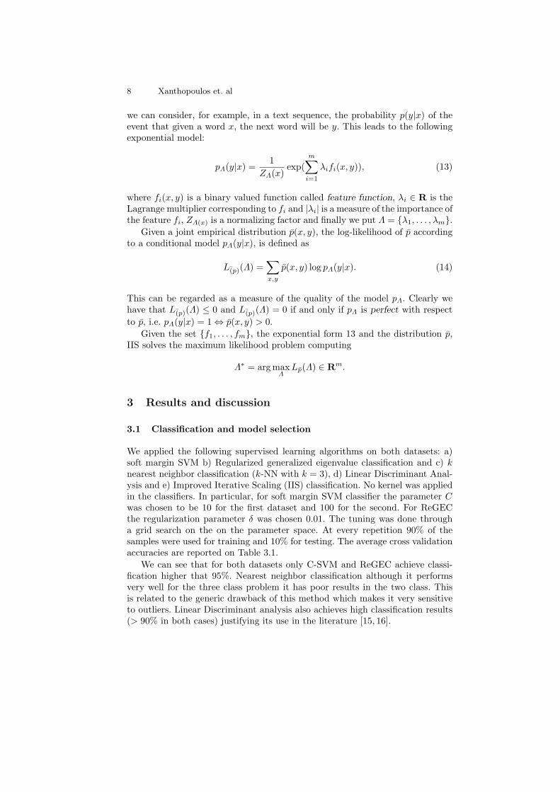
Classification accuracy (%)

Cell line discrimination Cell death discrimination(two class) (three class)

C-SVM 95.33 97.33ReGEC 96.66 98.443-NNR 79.22 95.44IIS 95.67 87.44LDA 100 91.00

Table 1. Average classification accuracy for hold out cross validation (100 repetitions).With bold is the highest accuracy achieved for each dataset.

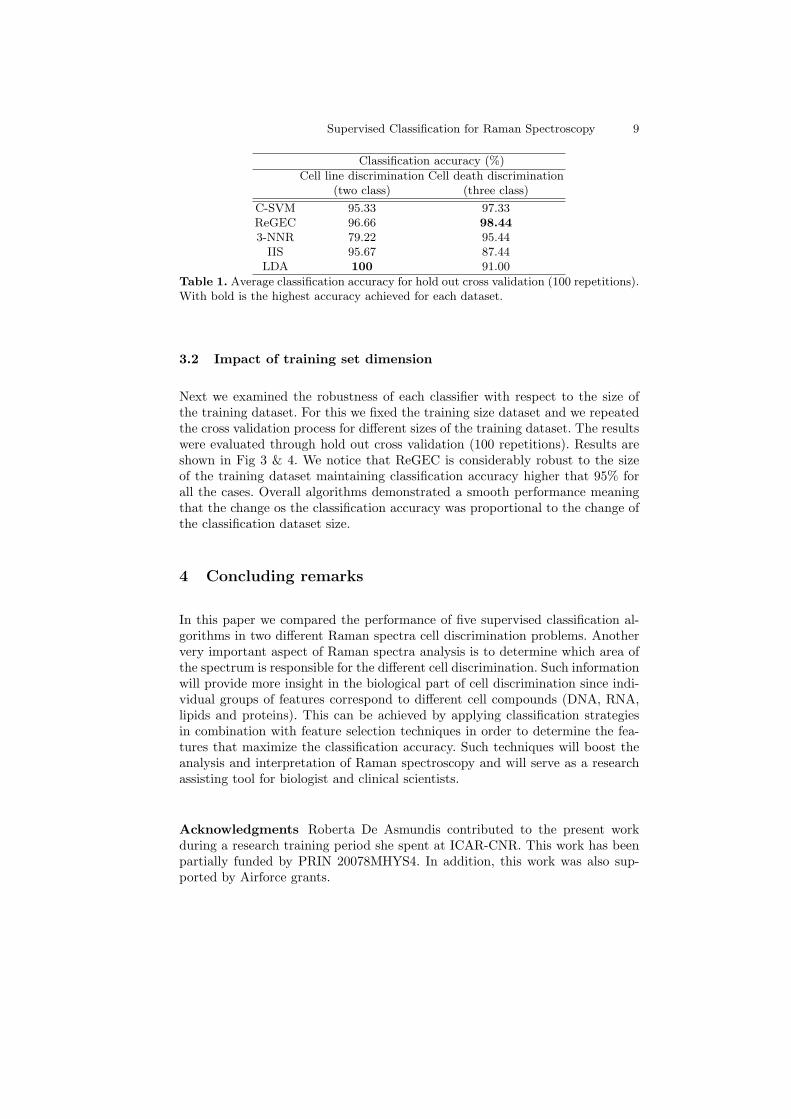
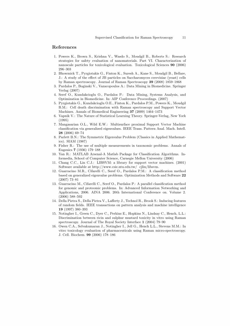
3.2 Impact of training set dimension

Next we examined the robustness of each classifier with respect to the size ofthe training dataset. For this we fixed the training size dataset and we repeatedthe cross validation process for different sizes of the training dataset. The resultswere evaluated through hold out cross validation (100 repetitions). Results areshown in Fig 3 & 4. We notice that ReGEC is considerably robust to the sizeof the training dataset maintaining classification accuracy higher that 95% forall the cases. Overall algorithms demonstrated a smooth performance meaningthat the change os the classification accuracy was proportional to the change ofthe classification dataset size.

4 Concluding remarks

In this paper we compared the performance of five supervised classification al-gorithms in two different Raman spectra cell discrimination problems. Anothervery important aspect of Raman spectra analysis is to determine which area ofthe spectrum is responsible for the different cell discrimination. Such informationwill provide more insight in the biological part of cell discrimination since indi-vidual groups of features correspond to different cell compounds (DNA, RNA,lipids and proteins). This can be achieved by applying classification strategiesin combination with feature selection techniques in order to determine the fea-tures that maximize the classification accuracy. Such techniques will boost theanalysis and interpretation of Raman spectroscopy and will serve as a researchassisting tool for biologist and clinical scientists.

Acknowledgments Roberta De Asmundis contributed to the present workduring a research training period she spent at ICAR-CNR. This work has beenpartially funded by PRIN 20078MHYS4. In addition, this work was also sup-ported by Airforce grants.

10 Xanthopoulos et. al

20 30 40 50 60 70 80 9060

65

70

75

80

85

90

95

100

Training set size (%)

Cla

ssifi

catio

n ac

cura

cy (

%)

C−SVMReGECk−NNIISLDA

Fig. 3. Classification accuracy versus size of the training set for the binary classificationtask. Accuracy is evaluated for 100 cross validation runs.

20 30 40 50 60 70 80 9070

75

80

85

90

95

100

Training set size (%)

Cla

ssifi

catio

n ac

cura

cy (

%)

C−SVMReGECk−NNIISLDA

Fig. 4. Classification accuracy versus size of the training set for the multiclass classi-fication task. Accuracy is evaluated for 100 cross validation runs.

Supervised Classification for Raman Spectroscopy 11

References

1. Powers K., Brown S., Krishna V., Wasdo S., Moudgil B., Roberts S.: Researchstrategies for safety evaluation of nanomaterials. Part VI. Characterization ofnanoscale particles for toxicological evaluation. Toxicological Sciences 90 (2006)296–303

2. Bhowmick T., Pyrgiotakis G., Finton K., Suresh A., Kane S., Moudgil B., Bellare,J.: A study of the effect of JB particles on Saccharomyces cerevisiae (yeast) cellsby Raman spectroscopy. Journal of Raman Spectroscopy 39 (2008) 1859–1868

3. Pardalos P., Boginski V., Vazacopoulos A.: Data Mining in Biomedicine. SpringerVerlag (2007)

4. Seref O., Kundakcioglu O., Pardalos P.: Data Mining, Systems Analysis, andOptimization in Biomedicine. In: AIP Conference Proceedings. (2007)

5. Pyrgiotakis G., Kundakcioglu O.E., Finton K., Pardalos P.M., Powers K., MoudgilB.M.: Cell death discrimination with Raman spectroscopy and Support VectorMachines. Annals of Biomedical Engineering 37 (2009) 1464–1473

6. Vapnik V.: The Nature of Statistical Learning Theory. Springer-Verlag, New York(1995)

7. Mangasarian O.L., Wild E.W.: Multisurface proximal Support Vector Machineclassification via generalized eigenvalues. IEEE Trans. Pattern Anal. Mach. Intell.28 (2006) 69–74

8. Parlett B.N.: The Symmetric Eigenvalue Problem (Classics in Applied Mathemat-ics). SIAM (1987)

9. Fisher R.: The use of multiple measurements in taxonomic problems. Annals ofEugenics 7 (1936) 179–188

10. Yan R.: MATLAB Arsenal-A Matlab Package for Classification Algorithms. In-formedia, School of Computer Science, Carnegie Mellon University (2006)

11. Chang C.C., Lin C.J.: LIBSVM: a library for support vector machines. (2001)Software available at http://www.csie.ntu.edu.tw/ cjlin/libsvm.

12. Guarracino M.R., Cifarelli C., Seref O., Pardalos P.M.: A classification methodbased on generalized eigenvalue problems. Optimization Methods and Software 22(2007) 73–81

13. Guarracino M., Cifarelli C., Seref O., Pardalos P.: A parallel classification methodfor genomic and proteomic problems. In: Advanced Information Networking andApplications, 2006. AINA 2006. 20th International Conference on. Volume 2.(2006) 588–592

14. Della Pietra S., Della Pietra V., Lafferty J., Technol R., Brook S.: Inducing featuresof random fields. IEEE transactions on pattern analysis and machine intelligence19 (1997) 380–393

15. Notingher I., Green C., Dyer C., Perkins E., Hopkins N., Lindsay C., Hench, L.L.:Discrimination between ricin and sulphur mustard toxicity in vitro using Ramanspectroscopy. Journal of The Royal Society Interface 1 (2004) 79–90

16. Owen C.A., Selvakumaran J., Notingher I., Jell G., Hench L.L., Stevens M.M.: Invitro toxicology evaluation of pharmaceuticals using Raman micro-spectroscopy.J. Cell. Biochem. 99 (2006) 178–186