SULFIDE STRESS CRACKING RESISTANCE OF API-X100 HIGH STRENGTHLOW ALLOY STEEL IN H2S ENVIRONMENTS

By

MANSOUR A. ALMANSOUR

B.Sc., King Fand University of Petroleum and Minerals, 2000

A THESIS SUBMITTED IN PARTIAL FULFILLMENT OFTHE REQUIRMENTS FOR THE DEGREE OF

MASTER OF APPLIED SCIENCE

In

THE FACULTY OF GRADUATE STUDIES

(Materials Engineering)

THE UNIVERSITY OF BRITISH COLUMBIA

November 2007

© Mansour A. Almansour, 2007

ABSTRACT:

Sulfide Stress Cracking (SSC) resistance of the newly developed API-X100 High

Strength Low Alloy (HSLA) steel was investigated in the NACE TM0177 "A" solution.

The NACE TM0177 "A" solution is a hydrogen sulfide (H2S) saturated solution

containing 5.0 wt.% sodium chloride (NaC1) and 0.5 wt.% acetic acid (CH 3COOH). The

aim of this thesis was to study the effect of microstructure, non-metallic inclusions and

alloying elements of the X100 on H2S corrosion and SSC susceptibility. The study was

conducted by means of electrochemical polarization techniques and constant load (proof

ring) testing. Microstructural analysis and electrochemical polarization results for X100

were compared with those for X80, an older generation HSLA steel. Uniaxial constant

load SSC testing was conducted using X100 samples and the results were compared with

those reported for older generation HSLA steels.

Addition of H2S to the NACE TM0177 "A" solution increased the corrosion rate of X100

from 51.6 to 96.7 mpy. The effect of H2S on the corrosion rate was similar for X80. The

corrosion rate for X80 increased from 45.2 to 80.2 mpy when H 2S was added to the test

solution. Addition of H2S enhanced the anodic kinetics by forming a catalyst (FeHS - 1ads,

on the metal surface and as a result, shifted the anodic polarization curve to more current

densities. Moreover, the cathodic half cell potential increased due to the decrease in pH,

from 2.9 to 2.7, which shifted the cathodic polarization curve to more current densities.

i

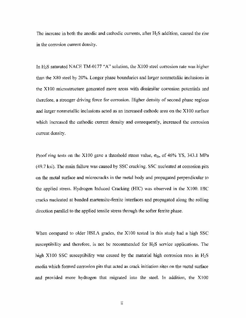
The increase in both the anodic and cathodic currents, after H2S addition, caused the rise

in the corrosion current density.

In H2S saturated NACE TM-0177 "A" solution, the X100 steel corrosion rate was higher

than the X80 steel by 20%. Longer phase boundaries and larger nonmetallic inclusions in

the X100 microstructure generated more areas with dissimilar corrosion potentials and

therefore, a stronger driving force for corrosion. Higher density of second phase regions

and larger nonmetallic inclusions acted as an increased cathode area on the X100 surface

which increased the cathodic current density and consequently, increased the corrosion

current density.

Proof ring tests on the X100 gave a threshold stress value, C5th, of 46% YS, 343.1 MPa

(49.7 ksi). The main failure was caused by SSC cracking. SSC nucleated at corrosion pits

on the metal surface and microcracks in the metal body and propagated perpendicular to

the applied stress. Hydrogen Induced Cracking (HIC) was observed in the X100. HIC

cracks nucleated at banded martensite-ferrite interfaces and propagated along the rolling

direction parallel to the applied tensile stress through the softer ferrite phase.

When compared to older HSLA grades, the X100 tested in this study had a high SSC

susceptibility and therefore, is not be recommended for H2S service applications. The

high X100 SSC susceptibility was caused by the material high corrosion rates in H2 S

media which formed corrosion pits that acted as crack initiation sites on the metal surface

and provided more hydrogen that migrated into the steel. In addition, the X100

ii

inhomogeneous microstructure provided a high density of hydrogen traps in front of the

main crack tip which promoted SSC microcrack formation inside the metal. Microcracks

in the metal body connected with the main crack tip that originated from corrosion pits

which assisted SSC propagation.

iii

TABLE OF CONTENTS:

ABSTRACT^ i

TABLE OF CONTENTS^ iv

LIST OF TABLES^ vi

LIST OF FIGURES^ vii

ACKNOWLEDGMENT^ x

1 INTRODUCTION^ 1

2 LITERATURE REVIEW^ 6

2.1 HSLA steels^ 62.1.1 Definition of HSLA steels ^ 62.1.2 Processing of HSLA steels^ 7

2.2 Electrochemical background^ 122.2.1 Corrosion in H2S environments^ 122.2.2 Electrochemical measurements^ 17

2.2.2.1 Pourbaix diagrams^ 172.2.2.2 Polarization diagrams^ 19

2.3 Sulfide Stress Cracking (SSC)^ 212.3.1 SSC definition^ 212.3.2 SSC process^ 252.3.3 Stress intensity at the SSC crack tip^ 262.3.4 Testing for SSC susceptibility^ 312.3.5 Factors influencing SSC in HSLA steels^ 33

2.3.5.1 Effect of material strength^ 332.3.5.2 Effect of microstructure^ 342.3.5.3 Effect of material homogeneity^ 38

3 EXPERIMENTAL PROCEDURES^ 40

3.1 Tested materials^ 40

3.2 Microstructure analysis^ 41

3.3 Electrochemical testing^ 42

iv

3.3.1 Specimen preparation^ 423.3.2 Test solution^ 433.3.3 Cell setup^ 433.3.4 Electrochemical techniques^ 45

3.3.4.1 Open circuit potential measurements^ 453.3.4.2 Potentiodynamic polarization tests^ 45

3.4 SSC constant load tests^ 463.4.1 Proof ring devices^ 463.4.2 Test solution^ 503.4.3 Test procedure^ 503.4.4 Failure detection^ 513.4.5 Failure analysis^ 51

4 RESULTS AND DISCUSSION^ 52

4.1 Metallurgical examination^ 524.1.1 Microstructure and strength^ 524.1.2 Nonmetallic inclusions^ 57

4.2 Electrochemical behaviour^ 624.2.1 Corrosion potential^ 624.2.2 Anodic polarization behaviour^ 64

4.2.2.1 X100^ 644.2.2.2 X80^ 66

4.2.3 Surface characterization^ 684.2.4 Mechanistic insights^ 73

4.2.4.1 Effect of H2S on corrosion rates^ 744.2.4.2 Comparison between X100 and X80^ 78

4.3 Proof ring testing^ 834.3.1 Threshold stress determination for API-X100^ 834.3.2 Crack characterization^ 854.3.3 Mechanistic insights^ 894.3.4 Comparison between X100 and other HSLA steels ^95

4.4 Implications of results on X100 susceptibility^ 97

5 SUMMARY AND CONCLUSION^ 99

6 REFERENCES^ 104

v

LIST OF TABLES

Table 2.1 Time to failure results (hours) for as receivedand quenched-tempered X60^ 39

Table 3.1 Chemical analysis with carbon equivalence (C.E.)for the X80 and X100 steels^ 40

Table 3.2 X100 proof ring specimens and applied stresses^49

Table 4.1 Average yield and tensile strength values (engineering and true)for X100 and X80^ 56

Table 4.2 Average hardness values and standard deviation inRockwell C for X80 and X100 ^ 56

Table 4.3 Summary of electrochemical test results conducted on X100and X80 in H2S-free and H2S-saturated NACE TM0177 "A" solution^73

Table 4.4 Proof ring test results tested in NACE TM-0177 "A" (23 °C)^ 83

vi

LIST OF FIGURES

Fig. 1.1 History of the development of HSLA linepipe steels^2

Fig. 2.1 Temperature-time profile for rolling of a microalloyed steel plate^ 8

Fig. 2.2 Different approaches to produce API-X100 steel^ 10

Fig. 2.3 Hydrogen migration into the steel^ 13

Fig. 2.4 Effect of added oxidizer. An increase in pH (pH line 2 < PH line 1)will result in an increase in E con. and icoff^ 15

Fig. 2.5 E-pH diagram showing the thermodynamic stability regionsfor surface sulfides^ 18

Fig. 2.6 Pourbaix diagram (E-pH) for the iron-water system^ 19

Fig. 2.7 Schematic polarization diagram for iron dissolution(anode) and hydrogen evolution (cathode)^ 20

Fig. 2.8 Polarization test set up^ 21

Fig. 2.9 Hydrogen accumulation and crackinitiation at SSC crack tip^ 22

Fig. 2.10 SSC and HIC cracks^ 24

Fig. 2.11 Stresses acting in front of a crack (mode I)^ 27

Fig. 2.12 Crack tip stress distribution^ 28

Fig. 2.13 Center crack with uniform loading^ 29

Fig. 2.14 Diagram of uniaxial tensile testing (constant load)^32

Fig. 2.15 Elongation (in NACE TM-0177 "A" solution) / Elongation (in air)for API-X70 with different microstructures^ 35

Fig 3.1 Specimens used for microstructural analysis (left)and polarization analysis (right)^ 42

vii

Fig. 3.2 Electrochemical polarization experimental setup^ 44

Fig. 3.3 Proof ring testing device^ 47

Fig. 3.4 X100 tensile specimen^ 48

Fig. 4.1 X80 optical imaging showing granular bainite(dark) and ferrite (light) microstructure^ 53

Fig. 4.2 X100 optical imaging showing martensite (dark), bainiteand ferrite (light) microstructure^ 53

Fig. 4.3 Engineering stress-stain curve for in air for (a) X100 and (b) X80 ^55

Fig. 4.4 Spherical non-metallic inclusions in (a) X80 and(b) X100 (SEM)^ 57

Fig. 4.5 EDX spectra for (a) X80 and (b) X100^ 58

Fig 4.6 Stringers found in the X100 steel, arrow indicatingrolling direction (SEM)^ 59

Fig. 4.7 Initiated cracks at the interface between an inclusion and thesteel matrix in X100 specimen, arrow indicating rolling direction (SEM)^61

Fig. 4.8 Eocp for X100 versus SCE in (H2S-saturated and H2S-free)NACE TM0177 "A" solution^ 63

Fig. 4.9 Eocp for X80 versus SCE in (H2S-saturated and H2S-free)NACE TM0177 "A" solution^ 64

Fig. 4.10 X100 polarization in H2S-saturated NACE TM0177 "A"solution (5.0% NaC1 + 0.5% CH3COOH)^ 65

Fig. 4.11 X100 polarization in H2S-free NACE TM-0177 "A" solution(5.0% NaC1 + 0.5% CH3COOH)^ 66

Fig. 4.12 X80 polarization in H2S-saturated NACE TM0177 "A"solution (5.0% NaC1 + 0.5% CH3COOH)^ 67

Fig. 4.13 X80 polarization in H2S-free NACE TM0177 "A"solution (5.0% NaC1 + 0.5% CH3COOH)^ 68

Fig. 4.14 Corrosion product EDX for X100 in (a) H2S-free, (b) H2S-saturatedNACE TM-0177 "A" solution and (c) Polished uncorroded X100 specimen^70

viii

Fig. 4.15 Corrosion product EDX for X100 in (a) H2S-free and (b) H2S-saturatedNACE TM-0177 "A" solution^ 71

Fig. 4.16 Polarization diagrams of (a) X100 and (b) X80 in NACETM0177 "A" solution (H2S-free and H2S-saturated)^ 74

Fig. 4.17 Evans diagrams for (a) X100 and (b) X80 in NACE TM0177 "A"solution (H2S-free and H2S-saturated)^ 75

Fig. 4.18 Anodic overpotential (q) vs. current density for X100 and X80in H2 S-free and H2S-saturated NACE TM-0177 "A" solution^77

Fig. 4.19 Polarization diagram of X100 and X80 in H2S-saturatedNACE TM0177 "A" solution^ 79

Fig. 4.20 Evans diagrams for X100 and X80 in NACE TM0177 "A"solution (H2S-saturated)^ 79

Fig. 4.21 Pitting in (a) X80 and (b) X100 in H2S saturatedNACE solution (SEM)^ 82

Fig. 4.22 Proof ring time to failure graph for the X100 in H2S-saturatedNACE solution^ 84

Fig. 4.23 Fracture face longitudinal section for 80%YS specimen^86

Fig. 4.24 Longitudinal section of fracture face (80%YS specimen)showing transgranular crack propagation (light)^ 87

Fig. 4.25 Longitudinal section of the fracture face of an X100 specimenloaded at 65%YS showing a HIC crack connected to the SSC crack (light)^88

Fig. 4.26 Effect of applied stress and rolling direction on HIC propagation^88

Fig. 4.27 Longitudinal section of X100 specimen loaded at 65%YS showing SSC crack and surface inclusions (dark regions) (light)^89

Fig. 4.28 Longitudinal section of an X100 specimen loaded at 65%YS showing main SSC crack (right of image) and small microcracks

(left of image) (light)^ 90

Fig. 4.29 SSC brittle regions connected by a ductile section found in thefracture face of X100 specimen loaded at 80% YS (SEM)^91

Fig. 4.30 Optical imaging of a transverse section of an X100 specimenloaded at 50% YS showing HIC cracks^ 92

ix

ACKNOWLEDGMENT

I would like to thank my supervisor, Dr. Akram Alfantazi, for his guidance throughout

the course of this project. I would also like to express my deep appreciation to Dr. Joseph

Kish for his valued assistance. This report would have not been achievable without his

contributions.

My thanks extend to CANMET labs represented by Dr. Mimoun Elboujdaini for

supplying the materials required to undertake this project and for allowing me to use their

H2S lab for the electrochemical polarization experiments. In addition, I would like to

express my appreciation to Bodycote labs represented by Heath Walker for conducting

the proof ring experiments at such a short notice and prompt delivery of the test data. I

also would like to thank the examining committee members, Dr. Steve Cockcroft, Dr.

Chad Sinclair and Dr. GOran Femlund for simulating valuable discussions and comments

that benefited the quality of this report. My acknowledgment extends to my sponsoring

company, Saudi Aramco, for the post graduate degree scholarship it granted me.

Finally, I would like to express my deepest gratitude to my wife, Jumana, and family.

Their patience, support and encouragement were the most important aid throughout the

period of my study.

x

Chapter 1

1 Introduction:

High Strength Low Alloy (HSLA) steels are extensively used in oil and gas

transportation pipelines. HSLA steels have a low price-to-yield strength ratio, pipelines

with minimum yield strength (ay) of 70 ksi (483 MPa) are readily available in the oil and

gas industry. In addition to material strength, HSLA steels provide good weldability

because of their low carbon contents. The approach to generate HSLA steels involves a

combination of lower carbon content and fine grain size by microalloying along with

thermomechanical rolling or accelerated cooling (Ref. 1). API grade HSLA steels are

designated by their minimum yield strength value. For example, API-X100 steel is

designed to have a yield strength of 100 ksi (690 MPa).

The developmental history of HSLA steels is shown schematically in Figure 1.1. In the

seventies, hot rolling and normalizing was replaced by thermomechanical rolling. The

latter process enabled materials up to X70 (ay = 70 ksi) to be produced from steels that

are microalloyed with niobium and vanadium and have a reduced carbon content. An

improved processing method, consisting of thermomechanical rolling plus subsequent

accelerated cooling, emerged in the eighties. By this method, it has become possible to

produce higher strength materials like X80 (a y = 80 ksi). The X80 has a further reduced

carbon content and thereby excellent field weldability. Additions of Mo, Cu and Ni

enable the strength to be raised to that of grade X100 (a y = 100 ksi), when the steel is

1

processed to plate by thermomechanical rolling plus modified accelerated cooling (Ref.

2005 -

2000 -

1995 -

1990 -

1985 -

1980

1975

1970

1965 -

1960

2).

Year TMtreatment

Hot rolledand normalized

(

TM and intensiveaccelerated cooling

TM treatment andaccelerated cooling

X52^X60^X70^X80^X100

APIgrade

Fig. 1.1

History of the development of HSLA linepipe steels.

The application of HSLA steels in oil and gas transportation pipelines has been

increasing in the past few years. Requirements for higher strength HSLA steels have risen

as a result of the increased global energy demand. Transportation pipelines with higher

mechanical limits have been utilized to withstand the increasing line pressures. API-X100

is a newly developed HSLA steel that was designed to fill the gap for these new

requirements. One of the important aspects to assure good performance of X100 pipeline

steels is to minimize cracking susceptibility when exposed to sour environments. The

major cracking phenomenon in sour pipelines is Sulfide Stress Cracking (SSC). There is

a need to investigate the SSC resistance of X100, considering the higher strength and

2

hardness values it has relative to older generation HSLA steels. Investigating SSC

susceptibility will open doors for future improvements on the X100 in order to generate a

more cracking and corrosion resistant material in H2 S environments.

SSC is an embrittlement phenomenon in which crack failures can occur in stresses well

below the yield strength of the material. SSC is a joint process of two factors (Ref 3):

• H2S corrosion causing metal dissolution, pit formation and production of

hydrogen atoms.

• Migration of hydrogen atoms into the steel causing metal embrittlement.

A number of experimental procedures have been developed to assess susceptibility to

SSC. Results from these tests can be used to compare SSC susceptibility of different

metals or in purchase requisitions. One of the most widely used SSC assessment methods

is the uniaxial constant load test. Constant load tests generate a threshold stress value

(Gth), which is the maximum stress at which no failure occurs during the test duration of

720 hours (1 month) (Ref. 4).

Current work on the X100 has been concentrating on generating the optimum

microstructure, welding processes, alloying elements and thermomechanical processing

methods for the material (Ref 5). So far, little attention has been made to investigate the

newly developed X100 in SSC environments. Some SSC work on the X100 was done

back in the early eighties by Borik et al. (Ref 6). These tests were conducted to

3

investigate the possibility to produce a future X100 grade steel (at that time). It should be

noted that the X100 used in these studies does not resemble current X100 steels. X100

that were tested, but not implemented, in the eighties were developed by hot forging and

hot rolling followed by quenching the tempering. No thermomechanical controlled

processing or micro alloying by Ti, V and Nb were used. This material was highly

susceptible in sour media and generated very low threshold stress values (a th), 25% of the

material yield strength. The existing X100 material is produced by controlled rolling and

accelerated cooling processes coupled with controlled addition of microalloying elements

such as Ti, V and Nb.

Therefore, SSC studies on the current generation X100 are needed to evaluate its

susceptibility in sour environments. This includes evaluating the material's corrosion

rates in H2S environments. H2S corrosion will provide hydrogen atoms that would

migrate into the steel and cause embrittlement. In addition, pits generated from the

corrosion process will act as initiation sites for SSC on the metal surface.

The aim of this study is to examine the SSC resistance of the current generation API-

X100. This includes:

• Examining the X100 microstructure and nonmetallic inclusions to observe their

effect on SSC susceptibility.

4

• Studying the material's corrosion response in sour media by developing

electrochemical polarization diagrams in H2S-saturated NACE TM-0177 "A"

solutions.

• Proof ring testing to determine the threshold stress value (oth). X100 specimens

were tested at varying fractions of the material's yield strength to generate CYth•

• Studying the generated cracks and their nucleation/propagation processes.

An older generation HSLA steel, X80, was used for comparison in microstructural and

electrochemical examinations. For proof ring testing, experiments were conducted on the

X100 and results were compared with earlier work in literature.

5

Chapter 2

2 LITERATURE REVIEW

2.1 High Strength Low Allow (HSLA) Steels:

2.1.1 Definition of HSLA steels:

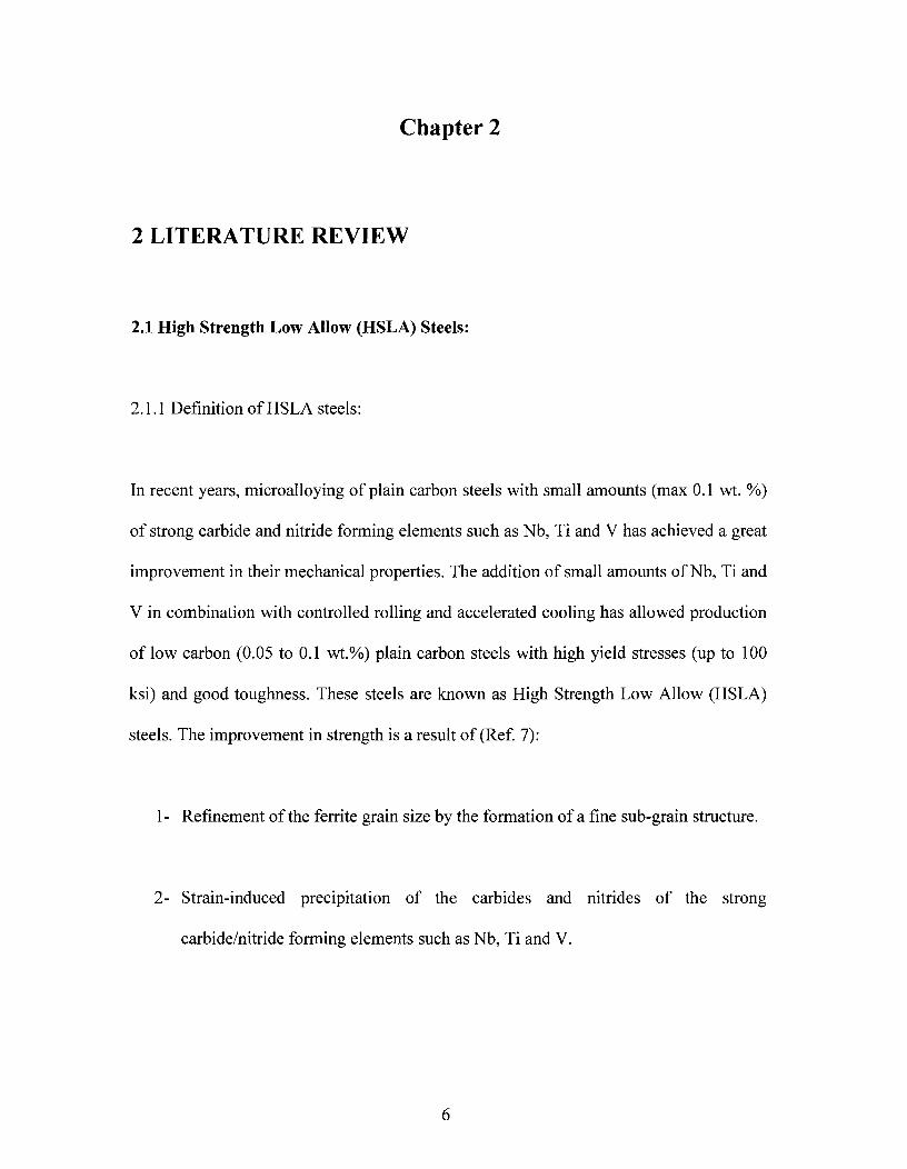
In recent years, microalloying of plain carbon steels with small amounts (max 0.1 wt. %)

of strong carbide and nitride forming elements such as Nb, Ti and V has achieved a great

improvement in their mechanical properties. The addition of small amounts of Nb, Ti and

V in combination with controlled rolling and accelerated cooling has allowed production

of low carbon (0.05 to 0.1 wt.%) plain carbon steels with high yield stresses (up to 100

ksi) and good toughness. These steels are known as High Strength Low Allow (HSLA)

steels. The improvement in strength is a result of (Ref. 7):

1- Refinement of the ferrite grain size by the formation of a fine sub-grain structure.

2- Strain-induced precipitation of the carbides and nitrides of the strong

carbide/nitride forming elements such as Nb, Ti and V.

6

Many advantages arise from the production of HSLA steels. One advantage is the price to

yield strength ratio. HSLA steel is priced from the base price of carbon steels and not

from the base price of alloy steels. This gives the opportunity to use thinner pipelines

with HSLA steels impacting material, installation and inspection costs. In addition, the

low carbon content provides low carbon equivalence values and thus, coupled with their

relative thinner wall thickness, welding of HSLA steels is much easier and less

expensive. For the reasons mentioned above, big pipeline projects have been depending

on HSLA steels as the material of choice (Ref. 8, 9).

2.1.2 Processing of HSLA steels:

A controlled rolling and accelerated cooling process is applied to produce HSLA steels.

This process will provide toughness and weldability, as well as, high strength. A

Thermomechanical Controlled Process (TMCP) schedule is an elaborate sequence of

stages interrupted by cooling periods and cooling after finish rolling either in air or water.

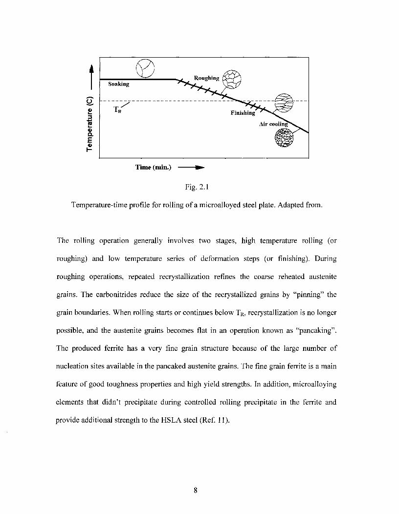
Initially, slabs are reheated to temperatures in the range of 1100 to 1250 °C (2010 to 2280

°F) and, as a result, significant amount of the carbonitrides are dissolved as shown in Fig.

2.1 for a temperature-time profile for rolling of a microalloyed steel plate. As temperature

decreases during controlled rolling, the carbonitrides become insoluble and precipitate

out in austenite (Ref. 10).

Soaking

r-r ..,./..1 R

Roughing

Finishing

Air cooling

Time (min.) -10.-

Fig. 2.1

Temperature-time profile for rolling of a microalloyed steel plate. Adapted from.

The rolling operation generally involves two stages, high temperature rolling (or

roughing) and low temperature series of deformation steps (or finishing). During

roughing operations, repeated recrystallization refines the coarse reheated austenite

grains. The carbonitrides reduce the size of the recrystallized grains by "pinning" the

grain boundaries. When rolling starts or continues below TR, recrystallization is no longer

possible, and the austenite grains becomes flat in an operation known as "pancaking".

The produced ferrite has a very fine grain structure because of the large number of

nucleation sites available in the pancaked austenite grains. The fine grain ferrite is a main

feature of good toughness properties and high yield strengths. In addition, microalloying

elements that didn't precipitate during controlled rolling precipitate in the ferrite and

provide additional strength to the HSLA steel (Ref. 11).

8

The small additions of alloying elements in HSLA steels processing have a significant

effect on the resulting mechanical and electrochemical properties. In HSLA steel

processing, C is kept at low levels to improve weldability. High content of Ni and Mo are

provided to increase hardenability. Microalloying with V and Nb is used to induce

strengthening via stable carbide and carbonitride precipitations (Ref. 12). Cu additions

are used to reduce hydrogen diffusion in the steel by forming a protective CuS layer on

the steel surface in the corrosive media of mildly sour environments (between pH 4.0 and

7.0) and decreasing the corrosion rate at open circuit potential (Ref. 13).

Further increase in strength and toughness from older generation HSLA steels, like X70,

can be attained by changing the microstructure of the steel from ferrite-pearlite to ferrite-

bainite. This has lead to the development of X80 steel which, compared to X70, has a

further reduced grain size and increased dislocation density.

After controlled rolling, accelerated cooling (15 to 20 °C/sec) with a cooling stop

temperature of about 500 °C followed by air cooling generates a microstructure of ferrite

with a certain amount of bainite. Transformation into bainite is promoted by increasing

hardenability by additions of B or Ni and Mo to the steel. It should be noted however that

these alloy additions increase the carbon equivalent value, which may affect the steel

weldability (Ref 14, 15). The term carbon equivalent (C.E.) estimates the cracking

susceptibility of steel after welding and determines whether the steel needs any heat

treatment to avoid cracking. Carbon equivalent includes the hardeability effect of the

9

A^ A

Carbon equivalent

Fig. 2.2

Cooling rate C°/Sec

alloying elements by expressing the chemical composition of the steel as a sum of

weighted alloying contents (concentration in wt.%) according to the equation below:

C.E. = C + Mn/6 + (Cr + Mo + V)/5 + (Ni + Cu)/15^(2.1)

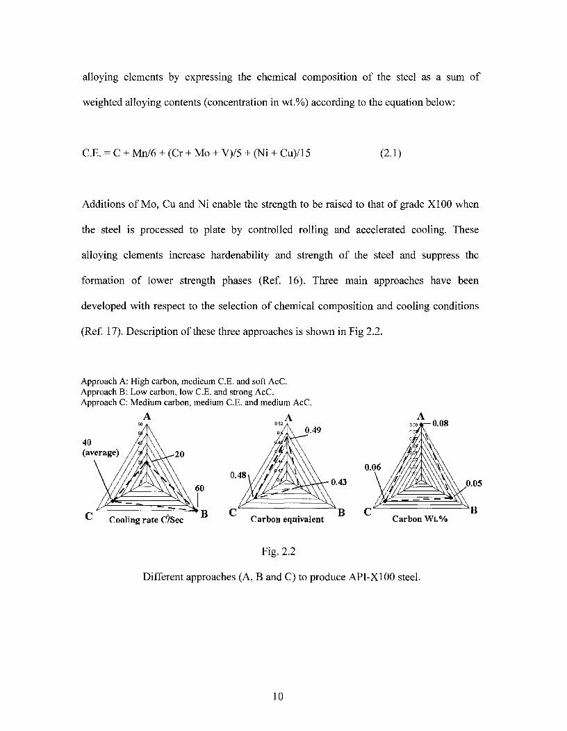
Additions of Mo, Cu and Ni enable the strength to be raised to that of grade X100 when

the steel is processed to plate by controlled rolling and accelerated cooling. These

alloying elements increase hardenability and strength of the steel and suppress the

formation of lower strength phases (Ref. 16). Three main approaches have been

developed with respect to the selection of chemical composition and cooling conditions

(Ref. 17). Description of these three approaches is shown in Fig 2.2.

Approach A: High carbon, medieum C.E. and soft AcC.Approach B: Low carbon, low C.E. and strong AcC.Approach C: Medium carbon, medium C.E. and medium AcC.

Different approaches (A, B and C) to produce API-X100 steel.

10

The first approach ("A" in Fig. 2.2) involved a relatively high carbon (about 0.08%) and

medium carbon equivalent (about 0.49). The processing was a reheating temperature

1140-1220 °C, finish rolling temperature 680-780 °C, and a cooling rate of 20 °C/sec.

This procedure had some difficulties when it came to fulfilling the requirements for

toughness to ensure crack arrest. In addition, this approach was detrimental in terms of

field weldability.

The second approach ("B" in Fig. 2.2) involved a relatively low carbon (around 0.05%)

and low carbon equivalent (about 0.43). The processing had high cooling rate of about 60

°C/sec. The result was an uncontrolled fraction of martensite in the microstructure, which

has a detrimental effect on toughness properties.

The third approach ("C" in Fig. 2.2) was the most preferred process. Approach "C"

involved a medium carbon content (about 0.06%) and medium carbon equivalent (0.48).

This process had a cooling rate range of 30-50 °C/sec. This approach has shown good

toughness and satisfactory field weldability (Ref. 18). Approach "C" is not strictly

followed and manufacturers tend to modify it in order to reach the desired X100

properties.

11

2.2 Electrochemical background:

2.2.1 Corrosion in H2S environments:

Most of the H2S in downstream oil transportation pipelines is produced by Sulfate

Reducing Bacteria (SRB). SRB enters the oil well with the make-up water. Make-up

water is usually injected to oil well to maintain the well pressure. SRB reduce sulfate to

sulfide and then converts sulfide to H 2S by oxidizing molecular hydrogen or hydrogen

released as a result of cathodic reaction during corrosion (Ref 19)

Iron corrodes in H2S environments according to the following reaction scheme:

Fe + H2S -› FeS + 2H °^(2.2)

2H° H2^ (2.3)

Sulfur acts as a poison to the second reaction and thus, promotes the migration of H ° into

the metal lattice (Fig. 2.3). The anodic and cathodic reactions are as follows:

Fe 4 Fe2+ + 2e - (Anode)^

(2.4)

2H+ + 2e - 4 2H° (Cathode)^

(2.5)

Different H2S concentrations produce different corrosion rates. For example, Radkevych

et al. (Ref 20) reported that in a natural gas well containing an H2S concentration of 0.25

12

mol% (steel grade was not identified), a corrosion rate of 20.0 mpy (mils per year) was

generated, where 1 mil = 0.001 in. Another well with higher H2S content, 16 mol %, had

a more aggressive corrosion rate of 34.6-60.0 mpy. Radkevych reported that corrosion

rates in H2 S environments can reach up to 236-314 mpy (Ref. 20). Theoretically, as

corrosion rates become higher, more hydrogen is available to migrate into the metal. Koh

et al. (Ref 21) measured the corrosion rates for different HSLA steels with yield

strengths that ranged from 431 to 539 MPa (X52 to X80). The steels were tested in the

NACE TM-0177 "A" solution at 25 °C. The tested HSLA steels exhibited close corrosion

rates that varied from 92.1-110.6 mpy.

FeSMetal

as

IT-Trap

II HH.

H It

Fig. 2.3

Hydrogen migration into the steel.

H2S can influence corrosion in three different ways:

• Increase in cathodic half cell electrode potential

• Formation of surface catalyst

• Films with low protective abilities and "sulfide-oxide" galvanic couple formation

13

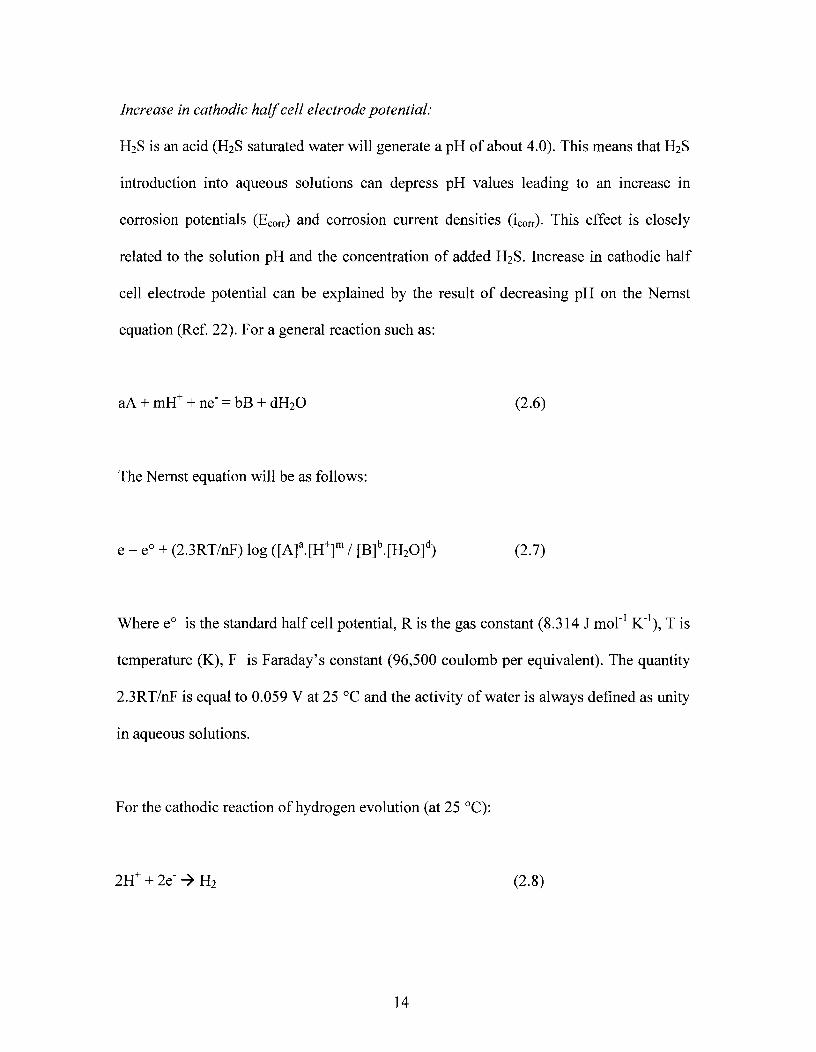
Increase in cathodic half cell electrode potential:

H2S is an acid (H2S saturated water will generate a pH of about 4.0). This means that H 2 S

introduction into aqueous solutions can depress pH values leading to an increase in

corrosion potentials (E con.) and corrosion current densities (icon). This effect is closely

related to the solution pH and the concentration of added H2S. Increase in cathodic half

cell electrode potential can be explained by the result of decreasing pH on the Nernst

equation (Ref 22). For a general reaction such as:

aA + mH+ + ne" = bB + dH2O^ (2.6)

The Nernst equation will be as follows:

e = e° + (2.3RT/nF) log ([Al a.[H+] m / [B] b [H2O] d)^(2.7)

Where e° is the standard half cell potential, R is the gas constant (8.314 J moi l 1(1 ), T is

temperature (K), F is Faraday's constant (96,500 coulomb per equivalent). The quantity

2.3RT/nF is equal to 0.059 V at 25 °C and the activity of water is always defined as unity

in aqueous solutions.

For the cathodic reaction of hydrogen evolution (at 25 °C):

2H+ + 2e - H2^ (2.8)

14

e +H TH 2

pH decreasee +H /H 2

Ecorr2

Ecorrl

Anodee Fe /Fe2+

Cathode

"A" and H2O in equation 2.6 are absent and B is replaced by H2 (PH2 assumed to be 1

atm). Since pH = -log (11 ±), Equation 2.7 becomes:

eH+/H2 = eH+/H2° - (0.059) pH^

(2.9)

As a result, as the concentration of the oxidizer, }1 ±, increases (pH decreases), the

potential, eH+,H2, increases. More importantly, the corrosion current density, i con-, will also

increase as can be seen in Fig. 2.4.

asO

con' 1^icorr2

Current density

Fig. 2.4

Effect of added oxidizer on the electrochemical behaviour. An increase in pH (pH line 2 <

pH line 1) will result in an increase in E con- and icorr•

15

Formation of surface catalyst:

Radkevych, (Ref 20), suggested that H2S effects the electrode reactions by forming an

intermediate compound, FeHS -ad„ which acts as a surface catalyst. For the anodic

reaction:

Fe + H2S 4 FeHS -ad s + H±^(2.10)

FeHS -ads^Fel-IS+ads ± 2e^ (2.11)

FeHS±ads + 11+ - Fe2+ + H2 S^ (2.12)

The complex FeHS -ads will decompose allowing H 2S to regenerate. When the complex is

formed on the metal surface, the bond of iron with sulfur decreases the metallic bonds in

the metal which facilitates ionization.

Films with low protective abilities and "sulfide-oxide" galvanic couple formation:

For the corrosion process in gas field equipments after long-term service (> 10 years),

steel parts will be covered with a thick layer corrosion products. For example, according

to Radkevych et al (Ref 20), corrosion products on pipeline metal surfaces after service

in H2S containing gas deposits can be as thick as 2 mm. For this reason, it is necessary to

consider the influence of surface sulfides on the corrosion process.

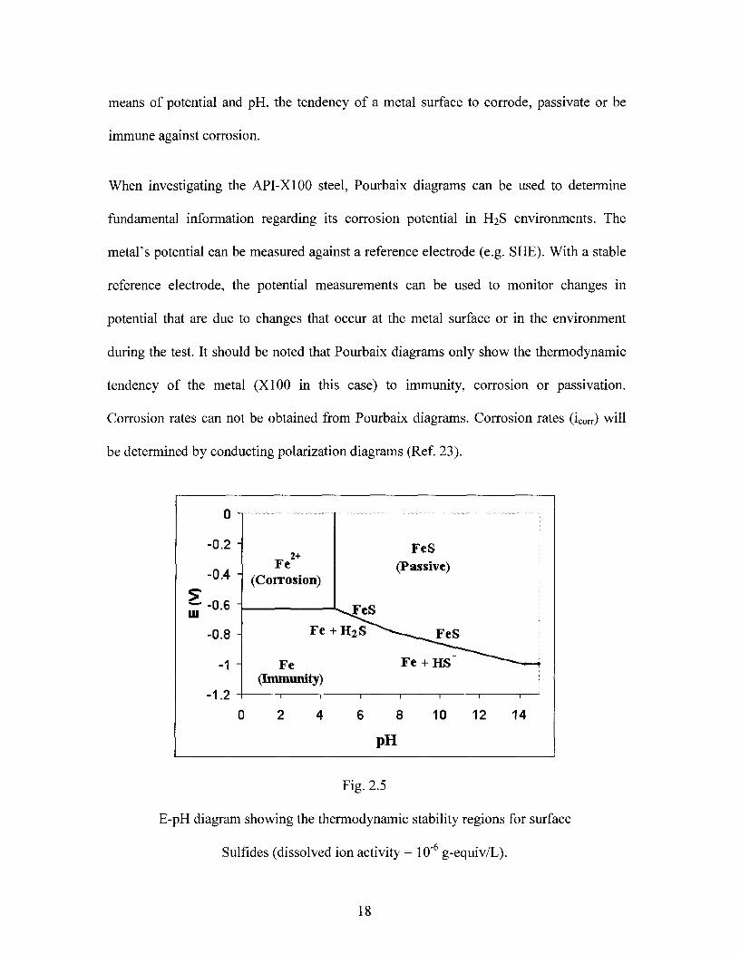
Fig. 2.5 shows the thermodynamic stability regions for the surface sulfides, Different

types of HSLA chemistry (X60/70/80/100) will produce slightly different E-pH

diagrams, but the general observation will be valid for all. It is shown that those surface

16

sulfides are stable in pH > 4.5. It is important that E-pH diagrams will only show the

thermodynamic stability of reaction species and not the rate of their formation (Ref 23).

In order to obtain quantitative data on the chemical composition of products of H 2 S

corrosion, analytical calculations of possible products of corrosion with various types of

sulfides were conducted (Ref 20). Results showed that H 2S corrosion of iron generated a

significant percentage of oxides alongside the sulfide corrosion products. The potential

difference between a steel electrode covered with sulfide and another of oxidized steel

electrode gave a difference of 0.1-0.4 V, which means that the iron sulfide will act as a

cathode relative to oxidized iron. Radkevych (Ref 20) proposes that the product of H2 S

corrosion generates a lot of "oxide-sulfide" galvanic couples. Thus, hydrogen more

intensively diffuses into the metal due to the operation of numerous galvanic couples on

the steel surface that increase the corrosion rate.

2.2.2 Electrochemical measurements:

2.2.2.1 Pourbaix (Potential-pH) Diagrams:

When investigating SSC on pipeline steels, API-X100 in this case, the use of Pourbaix

diagrams is quite useful. Through the use of thermodynamic theory (the Nernst equation),

Pourbaix diagrams can be constructed. These diagrams show the thermodynamic stability

of species as a function of potential and pH. Fig. 2.6 represents a version of the Pourbaix

diagram for the iron-water system at ambient temperature. This diagram determines, by

17

0

-0.2 -

-0.4 -2"-0.6-0.6 -in

-0.8 -

Fe2+

(Corrosion)

FeS(Passive)

^ FeSFe +112S

FeS

Fe^Fe + HS(Immunity)

-1.2 i0^2^4^6^8^10^12^14

pH

means of potential and pH, the tendency of a metal surface to corrode, passivate or be

immune against corrosion.

When investigating the API-X100 steel, Pourbaix diagrams can be used to determine

fundamental information regarding its corrosion potential in H2S environments. The

metal's potential can be measured against a reference electrode (e.g. SHE). With a stable

reference electrode, the potential measurements can be used to monitor changes in

potential that are due to changes that occur at the metal surface or in the environment

during the test. It should be noted that Pourbaix diagrams only show the thermodynamic

tendency of the metal (X100 in this case) to immunity, corrosion or passivation.

Corrosion rates can not be obtained from Pourbaix diagrams. Corrosion rates (icorr) will

be determined by conducting polarization diagrams (Ref 23).

Fig. 2.5

E-pH diagram showing the thermodynamic stability regions for surface

Sulfides (dissolved ion activity = 10 -6 g-equiv/L).

18

Fe E-pH Diagram

Fe+++

Fe(OH)3(Passivity)

Fe++(Corrosion)

Fe^Fe(OH)2(immunity)^(Passivity)im 'it

-1^1^2^3

11 0

1.1.1

1.2

-IFe02-Corrosion

4^6^6^7^8^9 10 11 12 13 14 16 16

pH

Fig. 2.6

Pourbaix diagram (E-pH) for the iron-water system

(dissolved ion activity = 10 6 g-equiv/L).

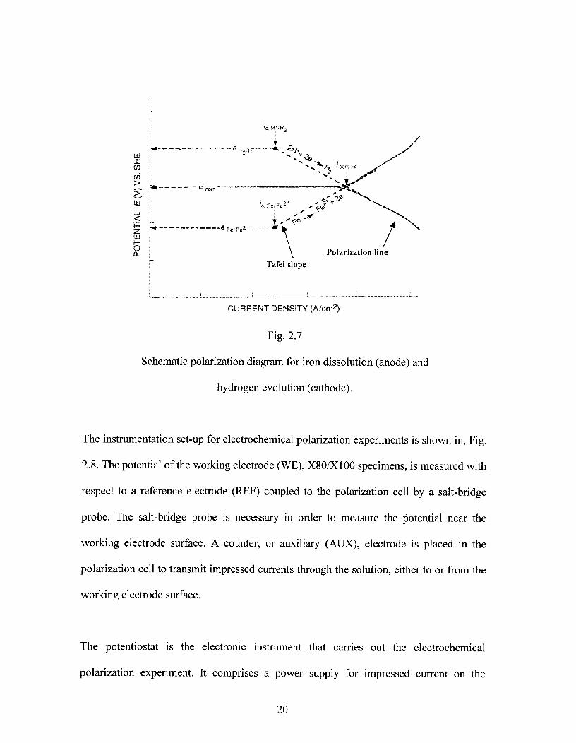
2.2.2.2 Polarization Diagrams:

As discussed in the previous section, Pourbaix diagrams show the tendency of the

material to corrode but it won't describe how fast the reaction will be, in other words, the

corrosion rate or i con. A useful method to determine the corrosion rate is by constructing a

polarization diagram for the environment of interest. When the corrosion reaction starts,

the cathodic and anodic half-cell reactions will polarize to a point of intersection, which

determines the corrosion rate (i con) and the corrosion potential (E con), as shown in Fig.

2.7.

19

JO, H:r1.•12

cri>•,tor 4.7-eLL!^ Fe2' .-• ''' C'e...1

'-'°'

a.

illi-0^

----a FefFe 2 ' — — - et \

Polarization line7

Tafel slope

CURRENT DENSITY (A/cm 2)

Fig. 2.7

Schematic polarization diagram for iron dissolution (anode) and

hydrogen evolution (cathode).

The instrumentation set-up for electrochemical polarization experiments is shown in, Fig.

2.8. The potential of the working electrode (WE), X80/X100 specimens, is measured with

respect to a reference electrode (REF) coupled to the polarization cell by a salt-bridge

probe. The salt-bridge probe is necessary in order to measure the potential near the

working electrode surface. A counter, or auxiliary (AUX), electrode is placed in the

polarization cell to transmit impressed currents through the solution, either to or from the

working electrode surface.

The potentiostat is the electronic instrument that carries out the electrochemical

polarization experiment. It comprises a power supply for impressed current on the

20

electrochemical cell and circuits that measure and control the potential to set values. A

high-impedance voltmeter measures the potential between the working electrode and the

reference electrode without affecting the potential of the working electrode. A low-

resistance ammeter measures the current flow between the counter and working electrode

without affecting current flow (Ref 24).

Referenceelectrode

Auxiliary electrode^Working electrode

Fig. 2.8

Polarization test setup.

2.3 Sulfide Stress Cracking (SSC):

2.3.1 SSC definition:

SSC is a cracking phenomenon caused by the joint effect of H 2S corrosion and hydrogen

embrittlement. During exposure of pipeline steels to sour environments, H2S corrosion

generates on the steel causing metal dissolution and corrosion pit formation. As part of

21

AP'

stress

the corrosion process, hydrogen cathodically evolves on the metal surface and migrate

into the steel leading to metal embrittlement.

The generated corrosion pits are usually the initiation site for the main SSC crack at the

metal surface. The main crack propagates by connecting with brittle microcracks in the

metal body causing crack propagation and pipeline failure at applied stresses well below

the material's yield strength. In the absence of hydrogen charging, the material can hold

stresses up to the material's yield strength before plastic deformation. In the event of

hydrogen charging, a threshold stress value is present above which SSC will propagate.

The threshold stress (6th) is a fraction of the yield strength value and its value decreases

with increasing susceptibility (Ref. 25), Fig. 2.9.

Yieldstrength

Yieldstrength

Thresholdstress

Applied^ Appliedstresses^ stresses

11==.

H H^

I

H H H stress

Without hydrogen^With hydrogencharging^ charging

Fig. 2.9

Hydrogen accumulation and crack initiation at SSC crack tip.

22

Many factors control SSC susceptibility. One of the main aspects is corrosion behaviour

because this process determines the intensity of hydrogen that migrates into the steel. In

addition, corrosion produces corrosion pits that can act as the initial site for cracking.

Another important factor is mechanical properties such as hardness and yield strength

values. HSLA microstructure and homogeneity are also essential to determine SSC

susceptibility.

A number of candidate mechanisms for hydrogen embrittlement have been proposed

(Ref. 26). One reasonable aspect of this controversy is that there are several viable

mechanisms of hydrogen related failure and that the search for a single mechanism to

explain all the observations may not be successful. It is generally accepted that hydrogen

migration into susceptible steels causes embrittlement regardless of the exact mechanism.

These theories are:

• Decohesion theory, according to which interatomic bonds in the crystal lattice

weaken due to the diffusion of hydrogen into triaxial stressed regions.

• Enhanced localized plasticity by increasing the mobility of dislocations in

hydrogen enriched regions.

• Pressure theory caused by the combination of hydrogen atoms to form molecular

hydrogen inside in steel leading to an increase in internal pressures and void

formation.

23

Another form of hydrogen damage that might form in HSLA steels, in addition to SSC, is

hydrogen induced cracking (HIC). HIC is generated by hydrogen migration into voids or

inclusions followed by combination to form hydrogen gas. The pressure caused by the

generated hydrogen gas forms blisters inside the metal that propagate parallel to the

rolling direction. In the presence of residual or applied stresses, connection of HIC cracks

might occur in a stepwise manner (through pipe thickness) (Ref. 26), Fig. 2.10. It should

be noted that in Fig. 2.10, the applied stresses are parallel to the rolling direction. As a

result, the generated HIC cracks that propagate along the rolling direction are

independent of the applied stresses. In the case where the applied stresses are

perpendicular to the rolling direction, HIC cracks are affected by the applied stress and

propagate as a result.

Corrosion pit

SSC^MC crack

crack

Microcracks

Rolling direction ■••■1111110.

41/11111^Applied stress ■=11111110.

Fig. 2.10

SSC and HIC cracks.

24

2.3.2 SSC process:

One of the principle factors that determine the hydrogen damage susceptibility of ferrous

alloys is a phenomenon referred to as "trapping". Diffusion studies of iron and steels has

shown an initial retardation in diffusion rate or lag time for hydrogen diffusion through

these alloys before a steady state diffusivity compatible with that expected theoretically is

achieved. This lag time is generally considered to be related to the filling of traps by

hydrogen. Trapping will facilitate nucleation of SSC microcracks in the metal body, these

microcracks can connect to the main crack tip thereby assisting SSC propagation (Ref.

27).

After diffusing into the metal, hydrogen collects at metal-inclusion (mainly sulfides and

oxides) voids which are usually present because of the coefficient of thermal expansion

(a) differences between the base metal and inclusions. MnS inclusions are known to be

of an elongated shape, therefore, providing a relatively large metal-inclusion void that

can trap hydrogen and, ultimately, form a microcrack in the metal body (Ref. 28).

SSC is confined to highly stressed regions where hydrogen accumulation occurs

preferentially. The combination of internal or applied stresses and a susceptible

microstructure determine the critical hydrogen build-up needed for crack initiation and

growth. The microstructural part of SSC susceptibility is controlled by the magnitude and

dispersion of Ti and Nb carbides, hard low temperature transformation phases such

untempered martensite or bainite and alloying elements such as C and Mn, which give

25

rise to segregation bands (Ref 29). Susceptibility is also affected by the presence and

shape of oxide (e.g. Al203) and sulfide (e.g. MnS) inclusions. Ume et al. (Ref 30) have

shown that nonmetallic inclusions can raise the SSC and HIC cracking susceptibility. ath

values for X70 steels dropped from 80%YS to 50%YS due to added sulfur content which

gave raise to MnS inclusions.

In general, SSC cracking propagates by bursts where the most favourable oriented

microcrack will eventually reach the main crack earlier than the rest. Thus, the exhibited

rates of crack growth can be directly related to the relative difficulty for microcracks to

reach the main crack under a given applied stress, only those cracks that successfully

meet the crack tip are able to keep on growing. SSC crack growth in the steel is mostly of

a brittle nature, but it contains some ductile crack growth segments. A ductile segment

represents the region between the main crack tip and a microcrack. This region cracks in

a ductile manner when it can no longer hold the applied stresses and, as a result, leads to

joining the microcrack to the main crack tip (Ref 31, 32).

2.3.3 Stress intensity at the SSC crack tip:

In most cases, SSC cracks initiate at surface imperfections or at pits generated from the

corrosion reaction. The stress concentrations at the base of these pits can promote SSC

crack nucleation.

26

To illustrate the stresses at the crack tip, a body with arbitrary shape with a crack of

arbitrary size subject to arbitrary tensile loading is considered, Fig. 2.11. If the material is

assumed to be elastic, following Hook's law, the theory of elasticity can be used to

calculates the stress field and the stresses G, and Gy can be obtained (Ref 33)

Fig. 2.11

Stresses acting in front of a crack (mode I).

The crack tip stresses can be biaxial or triaxial (if contraction in thickness is constrained).

As a result, there will be stresses in at least the x and y directions. Stresses in the material

in Fig. 2.11 can be described by:

G, = [K / .N1(2 it r)] cos (0/2) [1 - sin (0/2) sin (30/2)] + G,^(2.13a)

ay = [K / A2 it r)] cos (0/2) [1 + sin (0/2) sin (30/2)]^(2.13b)

27

For r = x and 0 = 0 (plane through the cracked section), eqn. 2.13a and 2.13b become:

ax = K / Ai(2 IC X)^

(2.14a)

Gy = K / Ai(2 7r X)^

(2.14b)

Here, K is the stress intensity factor. According to the above equation, crack tip stresses

will be infinite at x = 0 regardless of the value of K. This is a direct consequence of the

use of the theory of elasticity, which states a is linearly proportional to strain, E, without

any limitation. In reality, a material exhibits plastic deformation which limits the stress as

can be seen in Fig. 2.12 (Ref. 34).

Plastic k4zone

Fig. 2.12

Crack tip stress distribution.

Since the stresses everywhere in an elastic body are proportional to the applied load, the

crack tip stress is proportional to the applied stress a:

ay a [a / \I(2 a x)]^ (2.15)

28

^Mow r

For a very large (infinite) panel subjected to tensile loading with a nominal stress of a,

Fig. 2.13, the crack tip stresses also depends on the crack length, a. The stresses are

higher when "a" is longer so the crack size "a" must appear in the nominator in equation

2.15:

cry = (C a \la) / -\1(2 a x)

K = C a Ala

Where "C" is a dimensionless factor.

(2.16)

(2.17)

Fig. 2.13

Center crack with uniform loading.

In the practical use of the equations above, all "C" terms are divided by -\in and Ana) is

substituted for .Va to compensate. The function C/Jir is then renamed 13", the geometry

factor:

29

Gy = (13 6 \Ina) / -\/(2 7C X) = K / Ai(2 7E X)^(2.18)

K =13 a pia^ (2.19)

It must be noted that equations 2.18 and 2.19 represent the crack tip stresses and stress

intensity for all crack problems. The equations above are derived from the general

solution for an arbitrary crack in an arbitrary body with arbitrary mode I loading (Ref.

35). For any crack in any particular problem, only the function f3 or its functional value

needs to be derived. 13 is a function of the specimen geometry. The function 13 has already

been calculated for many configurations (Ref 36).

Fracture occurs when the stresses at the crack tip becomes too high for the material to

withstand. As the stress intensity factor, K, determines the entire crack tip stress field,

fracture occurs when K becomes too high for the material. This critical value of K is

known as the threshold stress intensity factor Kissc• "I" here refers to mode I (tensile

loading) fracture and "SSC" refers to Sulfide Stress Cracking. The unit for the threshold

stress intensity factor is ksi .Niin or MPa gym. This follows from the definition of K which

is the product between stress (ksi) and square root of crack length.

30

2.3.4 Testing for SSC susceptibility:

Standardized testing of metals for resistance to cracking failure under the combined

action of stress and corrosion in H25 environments is very important to asses the SSC

susceptibility of any material of interest and to assure safe operation. In addition, these

tests facilitate conformity in testing so that data from different sources can be compared

on a common basis. Standardized tests also aid the evaluation and selection of all type of

metals and alloys regardless of their form or application for service in H25 environments.

Most material standards include SSC testing requirements according to test methods that

are described in NACE TM-0177 "Laboratory testing of materials for resistance to

specific forms of environmental cracking in H2 S environments" (Ref 4). One of the most

popular methods in the NACE standard is the uniaxial tensile test (constant load test).

The uniaxial tensile test evaluates SSC cracking susceptibility in H2S environments under

an applied stress. Since the SSC phenomena produces cracks in materials bearing applied

stresses below their yield strengths, test specimens are loaded to stress levels below the

material's yield strength value. SSC susceptibility is determined by time-to-failure. A

specimens loaded to a particular stress level give either a pass or fail test result after a

specified test period.

When testing multiple specimens at varying stress levels, an apparent threshold stress for

SSC can be obtained, a th. The threshold stress represents the maximum stress above

which SSC occurs on a smooth surface. The NACE TM-0177 standard indicates that a th

31

is the stress value below which no SSC failure is detected after the 720 hours (1 month)

test period (Ref 4). This test is popular because the stress pattern is simple and uniform.

In addition, the magnitude of the applied stress can be accurately determined. Figure 2.14

shows a schematic arrangement of test equipment for the uniaxial tensile test.

Force

Fig. 2.14

Diagram of uniaxial tensile testing (constant load).

Proof rings are one of the most economical and effective uniaxial stress methods used to

determine SSC susceptibility of metals in H2S service (Ref. 37). Proof rings are

specifically designed to meet the NACE TM-0177 standard, and are less expensive to

purchase, maintain, and operate than dead-weight testers. Proof rings are fabricated from

precision-machined alloy steel and are available in many load ranges. Tension on the

32

Proof ring is quickly and easily adjusted using a standard wrench on the tension-adjusting

screw and lock nut. A thrust bearing distributes the load and prevents seizure. Each

individually calibrated proof ring is accompanied by a conversion chart that can

accurately determine specimen load.

2.3.5 Factors influencing SSC susceptibility in HSLA steels:

Various metallurgical variables can be controlled to maximize HSLA resistance to SSC.

The strength level (commonly measured by hardness) is a widely used criteria to predict

performance in SSC media. NACE recommends that carbon and low alloy steels used in

H2S environments should have a hardness value of 22 HRC or less (Ref. 38). This

hardness value has been challenged by many because a material susceptibility to SSC

should not be determined from its hardness value alone since microstructure is very

important and essentially controls the material's SSC properties (Ref 39).

2.3.5.1 Effect of material strength:

In general, SSC susceptibility increases with increasing strength. This can be seen very

clearly in materials with the same microstructure. Hardie et al. (Ref 40) tested three API

HSLA pipeline steels (X50, X60 and X70) from the point of view of their susceptibility

to SSC. The microstructure of the three steels consisted of ferrite-pearlite bands. In this

study, the degree of embrittlement tended to increase with strength level. The relationship

between yield strength and SSC should not be taken when comparing different

33

microstructures because, even though YS plays a major role in SSC susceptibility, other

microstructural features like banding, non-metallic inclusion and carbide distribution play

an important role in SSC susceptibility.

2.3.5.2 Effect of microstructure:

In the work of Koh et al. (Ref. 41), different microalloyed HSLA steels with different

microstructures were examined in an H2S environment. The four microstructures were

coarse ferrite-pearlite, fine ferrite-pearlite, acicular ferrite and ferrite-bainite. SSC was

evaluated by Constant Elongation Rate Test (CERT) in NACE TM-0177 "A" solution.

Elongation to failure in the test solution was measured and compared with those

measured in air, Fig. 2.15. In general, all failures in test solution occurred much sooner

than in air. Acicular ferrite was the least sensitive to cracking while ferrite-bainite was

the most sensitive.

34

F. 0.3 -

oC0.25

CO

0.2CO10.1500

^0.1 ^CO

0.050C

^

0 ^

M1^M2^M3^M4Material

Fig. 2.15

Elongation (in NACE TM-0177 "A" solution) / Elongation (in air) for API-X70 with

different microstructures (M1 = ferrite+coarse pearlite, M2 = ferrite + fine pearlite, M3 =

acicular ferrite, M4 = ferrite + bainite).

In all microstructures, cracks nucleated at Al-Ca oxide inclusions. In addition to

nonmetallic inclusions, microcracks nucleated at grain boundaries and at the needle

shaped second phases in coarse ferrite-pearlite and ferrite-bainite steels respectively.

These additional crack nucleation sites seemed to contribute to the microscopic advance

of cracks. In addition, high SSC susceptibility was observed in coarse ferrite-pearlite and

ferrite-bainite steels. Crack nucleation at grain boundaries in coarse ferrite-pearlite was

due to the grain boundary network of cementite and it was concluded that segregation of

cementite at grain boundaries must be avoided to increase SSC resistance. In ferrite-

bainite, needle shaped second phase was sensitive to crack nucleation. These needle

shaped second phases seemed to be related to the formation of interlath martensite and

35

retained austenite constituents (M/A). It was concluded that retardation of M/A

constituents formation as a second phase is desirable to increase SSC resistance. On the

other hand, fine-ferrite-pearlite and acicular ferrite steels didn't form the grain boundary

cementite or the interlath M/A constituents, so that their resistance to SSC was higher. It

has been shown, (Ref. 42), that upper bainite was more susceptible to SSC and showed

lower threshold stress intensity factor (Kissc) values when compared to acicular ferrite

and tempered martensite. The negative effect of bainite was related to the large matrix-

carbide interface where crack could nucleate, thus, providing large hydrogen trapping

sites.

Zhao et al. (Ref. 43) also investigated the role of microstructure on SSC. In a bent beam

test conducted on three HSLA microstructures (acicular ferrite, ultrafine ferrite and

ferrite-pearlite), acicular ferrite possessed the best SSC resistance by having the highest

critical stress. Ultrafine ferrite was in second position while ferrite-pearlite steel was the

most susceptible to SSC as it exhibited more cracks at even less applied stresses than the

ultrafine ferrite microstructure. Zhao noted that a ferrite-banded pearlite microstructure is

susceptible to SSC cracking. Zhao also noted that carbides and MnS inclusions

precipitate along the banded pearlite. Hydrogen easily diffuses to the interfaces between

these precipitates and banded pearlite reaching the critical hydrogen concentration.

Furthermore, SSC propagation occurs normally through the susceptible cracking path

provided by the segregated pearlite bands, because most of the microcracks formed in

crack initiation can grow along the layered pearlite, which accordingly promotes the main

cracks to propagate. On the other hand, there is no susceptible banded pearlite

36

microstructure in ultrafine ferrite or acicular ferrite so the harmful effects on SSC

resistance caused by coarsening carbides and MnS inclusions can almost be neglected.

Even if microcracks initiate due to HE, they can be retarded to further propagate by

numerous grain boundaries because of the fine grain size.

The benefit of acicular ferrite comes from its good dispersion of carbonitrides and high

dislocation density. Nb and V carbonitrides in acicular ferrite delay crack initiation

through increasing the number and distribution of hydrogen trapping sites, instead of

localized hydrogen accumulation (Ref. 44). High-angle boundaries in acicular ferrite act

as obstacles to cleavage propagation, forcing the cleavage crack to change the

microscopic plane of propagation in order to accommodate the new local crystallography

(Ref 45, 46).

In addition to acicular ferrite, tempered martensite has shown good SSC resistance when

compared to a lath martensite microstructure. Quenched and tempered martensite is a

good candidate in H2S environments because of its dispersed carbon rich regions and

carbides (dispersed hydrogen traps). Quenching is detrimental to SSC because it

generates a susceptible lath martensite microstructure. In the as quenched condition, it is

expected that carbon segregation at grain and interlath boundaries combines with

internally stressed martensite to give a more susceptible steel condition. Multiple cracks

can then appear along martensite interlath boundaries. Albarran (Ref 47) showed that

lath martensite cracks at lower stress intensity factors than tempered martensite and with

higher crack propagation rates.

37

2.3.5.3 Effect of material homogeneity:

In addition to microstructure, the distribution of different phases in the steel can

contribute to the material's susceptibility in H2S environments. A banded microstructure

provides high hydrogen trapping site density in front of the main crack tip yielding lower

threshold stresses, crth. In a banded microstructure, reaching the critical hydrogen

concentration, for microcrack formation, will be easier because more hydrogen

accumulates in these traps. A homogeneous microstructure is beneficial to steels because

it provides dispersed hydrogen traps in which, reaching the critical hydrogen

concentration for a single trap site is more difficult. Albarran and Flores (Ref. 48)

observed that an API X52 and X80 with a banded ferrite-pearlite microstructure

developed longer SSC cracks that followed the banded ferrite. Significant microcracks

ahead of the crack tips were observed. On the other hand, X65 samples with homogenous

acicular ferrite microstructure had the lowest crack propagation rate.

Carneiro et al. (Ref. 49) tested the effect of homogeneity in H 2S environments for API

X60 steels. X60 specimens were given different thermal treatments to produce different

microstructures. The as received material consisted of a banded ferrite-pearlite

microstructure while quenching and tempering produced a homogenous ferrite-pearlite

microstructure. The homogenous microstructure generated the highest a th value (70% of

YS) as seen in Table 2.1. In addition, banded microstructures were more susceptible to

HIC cracking. HIC cracks initiated at hard phase constituents and propagated in a

38

direction parallel to the stress direction. Corrosion pits and HIC cracks acted as SSC

nucleation sites.

X60 Applied stress (% of yield strength)100 85 70 60

As received 7 114 365 720

Quenched andtempered 22 28 720 ---

Table 2.1

Time to failure results (hours) for as received and quenched-tempered X60. Adapted

from (Ref. 49).

39

Chapter 3

3 EXPERIMENTAL PROCEDURES:

The aim of these experiments is to study the behaviour of the current generation X100

pipeline steel in SSC media. An older generation of HSLA steels, X80, was used for

comparison in microstructural and electrochemical examinations. For proof ring testing,

experiments were conducted for the X100 and results were compared with earlier work

on older generation HSLA steels reported in literature.

3.1 Tested materials

X100 and X80 pipeline materials were used in this study. The two materials were

supplied by CANMET Materials Laboratories. In order to determine the chemical

composition (wt.%) of the specimens to be used in the experiments, X100 and X80

samples were sent to International Plasma Labs (IPL) for chemical analysis. The

specimens were analyzed by inductive coupled plasma (ICP) and LECO carbon analysis.

Results for both materials are shown in Table 3.1.

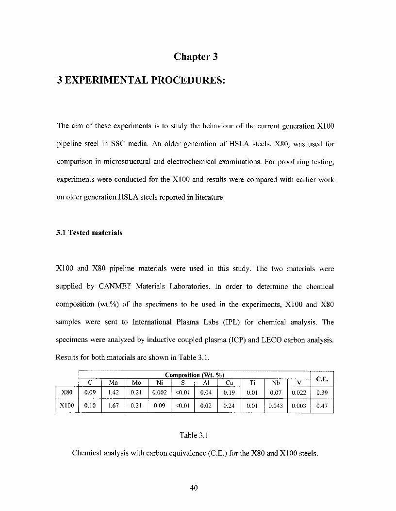
Composition (Wt. %)C.E.C Mn Mo Ni S Al Cu Ti Nb V

X80 0.09 1.42 0.21 0.002 <0.01 0.04 0.19 0.01 0.07 0.022 0.39

X100 0.10 1.67 0.21 0.09 <0.01 0.02 0.24 0.01 0.043 0.003 0.47

Table 3.1

Chemical analysis with carbon equivalence (C.E.) for the X80 and X100 steels.

40

3.2 Microstructure analysis:

After mounting, the specimens underwent the following steps before examining their

microstructures under the optical microscope:

• Wet-ground in a series of progressively finer silicon carbide papers up to 1200

grit finish.

• Polishing in 6 um diamond suspension.

• Cleaning with ethyl alcohol swabbing followed by drying in warm air.

• Polishing in 11,tm suspension.

• Repeat cleaning step with ethyl alcohol swabbing followed by drying in warm air.

• Etching in 2% nital (2 ml nitric acid + 98 ml ethyl alcohol).

• Cleaning in water followed by alcohol swabbing then air drying.

In order to examine the as-polished surface for non-metallic inclusions, the steps above

were repeated except for the etching step. Specimen etching was replaced by a final

polishing step using 0.05 i-tM colloidal silica followed by alcohol swabbing then air

drying. All surfaces were examined under light microscopy (LM). Scanning electron

microscopy (SEM) equipped with an energy dispersive X-ray spectrometer (EDX) was

used to investigate as polished specimens and non-metallic inclusions.

41

3.3 Electrochemical testing:

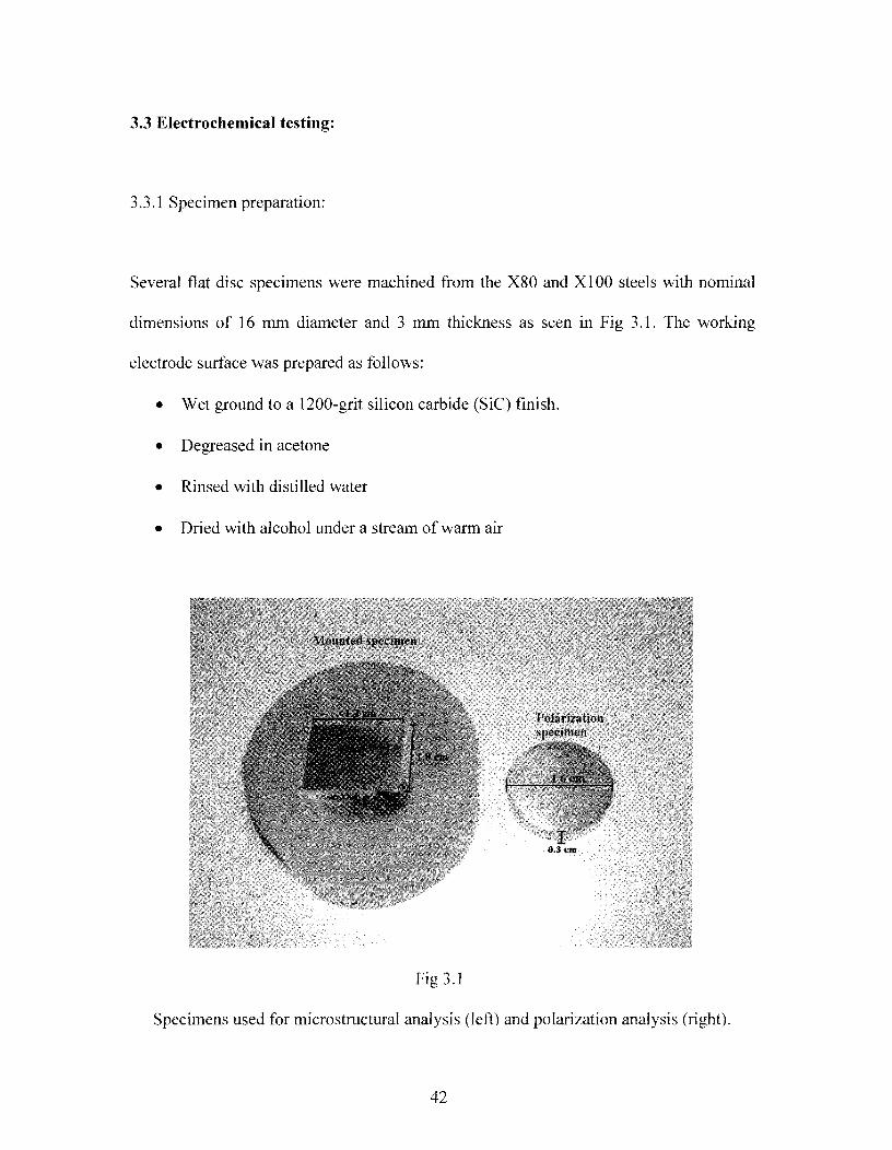
3.3.1 Specimen preparation:

Several flat disc specimens were machined from the X80 and X100 steels with nominal

dimensions of 16 mm diameter and 3 mm thickness as seen in Fig 3.1. The working

electrode surface was prepared as follows:

• Wet ground to a 1200-grit silicon carbide (SiC) finish.

• Degreased in acetone

• Rinsed with distilled water

• Dried with alcohol under a stream of warm air

Mounted specimen

Polarizationspecimen

1.6 c

83 cm

Fig 3.1

Specimens used for microstructural analysis (left) and polarization analysis (right).

42

3.3.2 Test solution:

NACE TM0177 test solution "A" (Ref. 4) was used in all electrochemical tests in this

study. Test solution "A" consisted of an acidified H2S saturated aqueous environment

containing 5.0 wt% NaC1 and 0.5 wt% CH3COOH. The solution pH after saturation was

expected to range between 2.6 and 2.8 and increase to below 4.0 as the test progresses.

pH values were measured with a combination pH electrode (glass membrane with

Ag/AgC1 reference element) calibrated with pH value of 7.0 standard buffer solution. H2S

gas, NaCl and CH3COOH were reagent-grade chemicals. For each test, 600 ml of test

solution were used. A fresh solution was used in every new test. To study the

electrochemical behaviour in the absence of H2S, the same NACE TM-0177 "A" solution

composition was used but without the addition of H2S.

3.3.3 Cell setup:

In this study, all electrochemical tests were conducted at 23 °C and atmospheric pressure.

Tests were made using a standard glass cell containing the working electrode (specimen)

and a graphite counter electrode. Potentials were measured with reference to a saturated

calomel reference electrode (SCE) interfaced to the test solution via a salt bridge that

terminated about 2 mm from the specimen, Fig. 3.2.

43

Fig. 3.2

Referenceelectrode Working

electrode

Electrochemical polarization experimental setup.

A SolatronTM potentiostat system (Model 1286) was utilized to perform and analyze the

potentiodynamic polarization curves. The system was coupled with a software package

having a combination of CorrWareTM (for hardware control and data acquisition) and

CorrViewTM (for data comparison and analysis).

After pouring the solution and sealing the cell, the cell was deaerated by argon for 1 hour

to eliminate any oxygen interference with the electrochemical reaction. After purging,

H2S was bubbled in to the cell at a flow rate of 50 cc/min for 30 minutes before starting

the test. H2S bubbling was eliminated when testing the X100 in the H 2S free NACE TM-

0177 "A" solution.

44

3.3.4 Electrochemical techniques:

3.3.4.1 Open circuit potential measurements:

After preparing and sealing the electrochemical cell, the test specimen was immersed in

the test solution for 33 minutes in order to measure the open circuit potential (E0q). Eocp

measurement was made between the working electrode (specimen) and the reference

electrode. No current was passed in this test to the working electrode. The aim of this test

was to find the potential at which the anodic and cathodic reaction currents at the

working electrode/solution interface were balanced. E ocp measurements are needed prior

to the electrochemical polarization tests to insure stability.

3.3.4.2 Potentiodynamic polarization tests:

After reaching a stable open circuit potential (E ocp), the electrode potential was swept

potentiodynamically at a scan rate of 0.66 mV/sec from an initial potential of -0.15 V to

0.5 V versus open circuit potential unless otherwise indicated. All potentials in this test

were measured with respect to the saturated calomel electrode (E = 0.241 V vs. standard

hydrogen electrode SHE). The corroded surface was examined under scanning electron

microscopy (SEM) equipped with an energy dispersive X-ray spectrometer (EDX).

The corrosion rates, in mils (0.001 inch) per year (mpy), for the tested materials were

calculated by the following equation:

45

Corrosion rate (mpy) = (0.129 x icon- x EW) / (D)^

(3.1)

Where:

icon = corrosion current density in pA/cm 2 .

EW = the equivalent weight, indicating the mass of metal in grams, which is oxidized.

For carbon steels, EW is approximately 28 grams (assuming Fe oxidation state of +2).

D = density in g/cm3 . Density for carbon steel is 7.84 g/cm3 .

3.4 SSC constant load testing:

3.4.1 Proof ring devices:

Time to failure data, by SSC constant load testing, was conducted at Bodycote labs while

crack imaging, crack analysis and threshold stress determination were conducted at UBC.

In this study, all proof ring tests were conducted at room temperature. A calibrated proof

ring was used to test X100 specimens at constant load (CL). Fig. 3.3 shows a description

of the different components of the proof ring. The used proof rings were specifically

designed to meet the NACE standards (Ref 4, 38). Standard tensile specimen dimensions

were used as seen in Fig. 3.4. Each individually calibrated proof ring was made using

precision-mechanics alloy steel and was accompanied by a calibration curve showing the

load versus deflection. The test specimens were loaded under uniaxial tension. The

46

Dial

Environment( harnber

Fig. 3.3

tensile load on the proof ring was quickly and easily adjusted using a standard wrench on

the tension-adjusting screw and lock nut. A thrust bearing distributed the load and

prevented seizure. The environmental test chamber was secured by 0-ring seals that

prevented any leakage during testing.

Proof ring testing device.

47

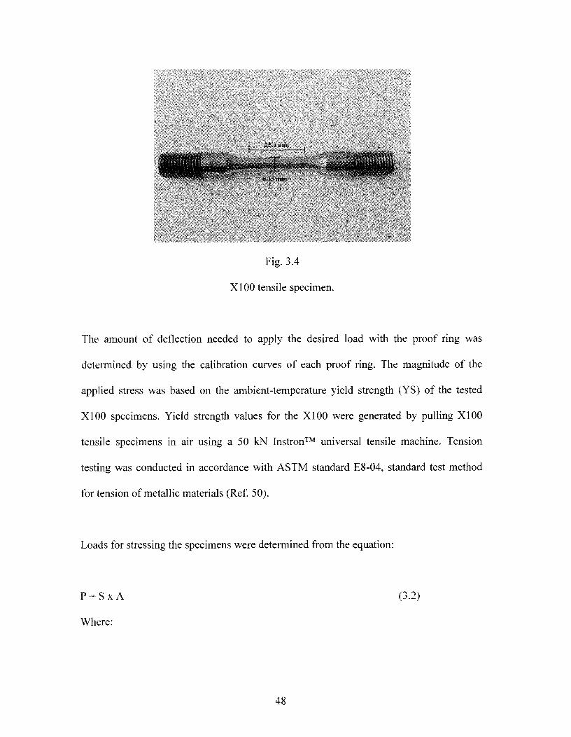
Fig. 3.4

X100 tensile specimen.

The amount of deflection needed to apply the desired load with the proof ring was

determined by using the calibration curves of each proof ring. The magnitude of the

applied stress was based on the ambient-temperature yield strength (YS) of the tested

X100 specimens. Yield strength values for the X100 were generated by pulling X100

tensile specimens in air using a 50 kN InstronTM universal tensile machine. Tension

testing was conducted in accordance with ASTM standard E8-04, standard test method

for tension of metallic materials (Ref 50).

Loads for stressing the specimens were determined from the equation:

P=SxA^ (3.2)

Where:

48

P = Load

S = applied stress

A = actual cross section area of the gauge section (31.67 mm 2)

The specimens were loaded at stress values equivalent to different percentages of the

material's YS value and the corresponding time-to-failure (TTF) was recorded. Table 3.2

lists the different stresses applied on the X100 specimens. Determination of SCC

susceptibility using this technique was based on the TTF for a maximum test duration of

720 hours (30 days). An automatic timer attached to the test specimen recorded the TTF.

The cracking susceptibility was expressed in terms of a threshold stress (a th) for SCC

below which cracking did not occur during the maximum test duration.

# specimens Applied stress (%YS)

3 80%3 65%3 50%3 40%3 30%

Total # ofspecimens : 15

Test termination: Specimen failureor after 720 hrs. (1 month), whichever occurs first.

Table 3.2

X100 proof ring specimens and applied stresses.

49

3.4.2 Test solution:

NACE TM0177 test solution "A" (Ref. 4) was used in all electrochemical tests in this

study. This is the same test solution used in the electrochemical measurements. A fresh

solution was used in each test. In addition, initial and final pH values were measured for

each test.

3.4.3 Testing procedure:

The test procedure was conducted according to the following sequence:

• The minimum gauge diameter of the test specimen was measured and the test

specimen load was calculated accordingly for the desired stress level.

• The tensile test specimen was cleaned and placed in the test vessel. The test vessel

was sealed to prevent air leaks into the vessel during the test.

• After loading and purging the test vessel, the test vessel was immediately filled with

deaerated test solution. The solution was poured to a level where solution-gas

interface didn't contact the gauge section of the test specimen. Deaerated solution

was prepared in a sealed vessel that was purged with inert gas.

• The solution, once in the test vessel, was purged with inert gas for at least 20 min to

insure that the test solution is oxygen free before introducing H 2 S.

• The test solution was then saturated with H 2S at a rate of 150 mL/min. for 30 minutes.

A continuous flow of H2S through the test vessel and outlet trap was maintained for

the duration of the test at a low flow rate (a few bubbles per minute). This maintained

50

the H2 S concentration and a slight positive pressure to prevent air from entering the

test vessel through small leaks.

• The test was terminated either after specimen failure (double ended fracture) or 720

hours (1 month), which ever occurred first.

3.4.4 Failure detection:

Following exposure, the surface of the gauge section of the non-failed test specimens

were cleaned and inspected for evidence of cracking. The specimens were cleaned by an

inhibited acid consisting of a stock solution of HC1 + 3.5 g/1 of methenamine diluted with

an equal amount of distilled water. The failure criterion was either complete separation of

the test specimen or visual observation of cracks on the gauge section of the test

specimen at 10X magnification after completing the 720 hour test duration (1 month).

3.4.5 Failure analysis:

In order to analyze the generated cracks, specimens were cut in both the longitudinal and

transverse directions to observe the generated cracks. Fracture faces were examined

under the SEM microscope to observe brittle and ductile regions. Transverse and

longitudinal cut specimens were ground to 1200 grit finish, polished with 6 and 1 micron

diamond suspension then etched in 5% nital. The specimen and generated cracks were

then examined under the light microscope.

51

Chapter 4

4 RESULTS AND DISCUSSION

4.1 Metallurgical examination:

4.1.1 Microstructure and strength:

Optical microscopy images for the X80 and X100 microstructures are shown in Fig. 4.1

and Fig. 4.2 respectively. The X80 microstructure was composed mainly of ferrite and

regions of granular bainite, which is composed of low carbon bainite and martensite. On

the other hand, the X100 steel showed a more complex microstructure consisting of

martensite, bainite and ferrite. Bainite was observed to grow from the prior austenite

grain boundaries that were elongated due to rolling.

The chemistry variation between the two steels is one of the factors affecting the

differences in microstructure between the X80 and X100 steels. It can be seen from the

chemical analysis of the two materials that the X100 possessed higher Cu, Mn, Mo and

Ni contents. These alloying elements tend to increase the metal hardenability and shift the

continuous cooling transformation (CCT) diagram line to the right. Shifting of the CCT

line in this manner increases the formation of low temperature transformation

microstructures like bainite and martensite under the same cooling rate (Ref. 51).

52

Fig. 4.1

X80 light microscopy imaging showing granular bainite (dark) and ferrite (light)

microstructure.

Fig. 4.2

X100 light microscopy imaging showing martensite (dark), bainite and ferrite (light)

microstructure.

53

In that essence, the X80 produced the ferrite-granular bainite microstructure because the

X80 CCT line promoted the formation of higher temperature transformation temperatures

due to the material's less alloying elements, compared to X100, and limited the

possibility of forming larger amounts of bainite and martensite to very high cooling rates.

The resulting differences in microstructure had its effect on the material's strength

values. The yield strength for the X100 was determined by pulling X100 tensile

specimens in air as shown in Fig. 4.3a. The engineering yield strength for the X100 was

743 MPa (107.8 ksi), Table 4.1. X80 tensile specimens were also pulled in air to verify

the material's yield strength value as shown in Fig. 4.3b and Table. 4.1. The X80 stress-

strain curve generated an engineering yield strength value of 579 MPa (84.0 ksi). The

generated yield strength values are in agreement with HSLA specifications. It should be

noted that specimen elongation during the test reduces the cross sectional area. As a

result, the true stress applied on the gauge section is higher than the engineering stress

determined from the stress-strain curve, which is based on the original cross section area.

Assuming that no volume change occurs during the test, the true stress (Gtrue), engineering

stress (aerig) and engineering strain (E eng) are related by the following equation:

true = Geng ( 1 + ceng) (4.1)

The yield strength value for X80 shows the effect of HSLA microstructure on strength.

For API grade HSLA steels, increase in strength from older generation HSLA steels, like

X70, is attained by changing the microstructure from ferrite-pearlite to ferrite-bainite.

54

0 5 10 15

Strain %

20 25 30

1000

900

800

700

O- 600M

500win 400

300

200

100

0

1000 ^

900 —

200 -

100

0^

5^10^15^

20^25^30Strain (%)

(a) Engineering stress-strain curve for X100

(b) Engineering stress strain curve for X80

Fig. 4.3

Engineering stress-stain curve for in air for (a) X100 and (b) X80.

55

Specimen Type Yield MPa (Ksi)(engineering)

Yield MPa (Ksi)(true)

UTS MPa (Ksi)(engineering)

UTS MPa (Ksi)(true)

X1006.35 mm 0 743 (107.8) 746 (108.2) 850 (123.3) 893 (129.5)

X806.35 mm 0 579 (84.0) 581 (84.3) 675 (97.9) 745 (108.1)

Table 4.1

Average yield and tensile strength values (engineering and true) for X100 and X80.

Table 4.2 shows the hardness values obtained for the two materials using the Rockwell C

scale. The higher hardness values for the X100 are attributed to the low temperature

transformation microstructures in the steel. Lower hardness values for the X80 steel are a

result of its ferrite-granular bainite microstructure which was expected to generate lower

hardness values than the X100. It should be noted that the X100 hardness values

exceeded the maximum hardness value of HRC 22 as recommended by NACE for

pipeline materials to be used in H 2S environments (Ref. 38).

Hardness (HRC)Specimen X80 X100

1 18.3 23.32 18.8 25.23 17.8 23.44 17.9 23.55 18.2 25.26 17.7 23.87 19.3 23.88 18.2 24.39 18.6 25.310 19.1 24.4

Average 18.4 24.2Standard deviation 0.54 0.78

Table 4.2

Average hardness values and standard deviation in Rockwell C for X80 and X100.

56

n

(a)

:2 I^L,^•

4.1.2 Nonmetallic inclusions

As can be seen in Fig. 4.4a and 4.5a for the X80 steel, the non metallic inclusions were

spherical Al-Ca-O-S inclusions. The spherical inclusions were randomly dispersed in the

metal and showed no signs of clustering. Inclusion diameter ranged between 2.0-4.5 pm.

The average spherical inclusion diameter was 3.5 gm. No elongated MnS inclusions were

observed in the steel.

(b)

Fig. 4.4

Spherical non-metallic inclusions in (a) X80 and (b) X100 (SEM).

57

a

Most of the examined inclusions in the X100 steel, Fig 4.4b and 4.5b, showed a similar

spherical shape to those observed in the X80 samples. Although the X100 and X80

samples had a similar inclusion shape, the size of these non-metallic inclusions was

different. Spherical inclusion diameter in the X100 ranged between 6.0-9.5 gm. The

average inclusions diameter for X100 was 8.0 gm. Therefore, the average inclusion

diameter in the X100 was higher than the X80 average inclusion diameter, 3.5 lam.

2 kee

(a)

Counts

Fe

N.,

2

(b)

Fig. 4.5

EDX spectra for (a) X80 and (b) X100.

58

In addition to spherical inclusions, the X100 steel showed some stringers which were not

observed in the X80 steel, Fig 4.6. Those stringers are most likely a result of rolling when

large oxide inclusions are broken into a line of smaller particles. The broken small

particles connecting the other larger pieces of the stringers are evidence that these

inclusions are hard and brittle. Stringers formed by softer inclusions would have

generated a smooth "line like" connection between the larger pieces of the inclusion. No

MnS inclusions were found in the X100 specimens.

nnnn 2nkV acwffl

Fig 4.6

Stringers found in the X100 steel, arrow indicating rolling direction (SEM).

EDX spectra for the X80 and X100 spherical inclusions showed that the inclusions

consisted of aluminium, calcium, oxygen and smaller amounts of sulfur. This inclusion

chemistry is typical for Al killed and Ca treated carbon steels and mainly consists of

59

calcium aluminate (CaO-Al203) and calcium sulfide (CaS) (Ref 52). As for the stringer

inclusions found in the X100 steel, the bright regions (larger parts) of the stringer

consisted of MgO-Al203 the while darker regions (smaller parts) consisted of CaO-Al203.

Nuspl et al.(Ref. 52) showed that brittle stringers found in carbon steel pipeline materials

mainly consisted of MgO, Al 203 and CaO. In addition, since both steels had a low sulfur

content, most of the sulfur is bound in calcium sulphides (Ref 53). This explains why no

elongated MnS inclusions were found in the steel as most of the sulfur reacted with

calcium to form CaS instead of MnS.

Stress localization at the inclusion/matrix interface is a preferential site for crack

initiation and hydrogen trapping. This arises from:

(1) Differential thermal contraction of inclusions and matrix during cooling

(2) Concentration of remote applied stresses.

Gaps and cracks initiate at the interface between the inclusion and the steel matrix during

hot deformation such as rolling. An example of this was observed in some of the

inclusions in the X100 material, Fig. 4.7. The effect of inclusions on the crack initiation

depends on chemistry, size, density, location, and morphology of the inclusion. Large and

brittle Al203 inclusions are more detrimental to fracture toughness than soft MnS

inclusions. However, it should be noted that elongated sulfide inclusions, such as MnS,

are very effective in promoting hydrogen embrittlement because of its planner shape

which is easier to trap hydrogen atoms (Ref 54).

60

Fig. 4.7

Initiated cracks at the interface between an inclusion and the steel matrix in X100

specimen, arrow indicating rolling direction (SEM).

The large inclusions found in the X100 steel are expected to reduce cracking resistance in

sour environments much more than the small inclusions. Dub et al. (Ref 55) stated that

CaO-Al203 inclusions have a lower thermal expansion coefficient than iron (matrix). As a

result, gaps and cracks formed at large inclusions after cooling or during rolling can act

as hydrogen accumulation sites. Finally, large surface inclusions can provide a larger

inclusion/matrix interface that can preferentially corrode and form corrosion pits on the

surface (Ref 55).

6 1

4.2 Electrochemical behaviour:

This section demonstrates the results generated from the electrochemical polarization

testing that was conducted on the X100 and X80 HSLA steels. The aim of these tests is to

study the effect of X100 and X80 microstructures on corrosion rates. The NACE

TM0177 "A" solution was used in these tests. To examine the effect of H2S, testing in

H2S free NACE solutions were conducted and compared with results generated in

saturated H2S environments.

4.2.1 Corrosion potential:

Fig. 4.8 shows the open circuit potential (Eocp) measurement for the API X100 steel over

1800 seconds (30 min.) of immersion in the (H2S-saturaded) NACE TM0177 "A"

solution. Potential readings were slightly fluctuating in the first 200 seconds. The

readings then started to decrease until a steady state open circuit potential, E ocp , reading

of -0.61 V was reached. E ocp for the X100 steel in the (H2S-free) NACE TM0177 "A"

solution yielded a similar trend with an open circuit potential value of -0.63 V (average

value).

62

Fig. 4.8

Eocp for X100 versus SCE in (H 2 S-saturated and H2S-free) NACE TM0177 "A" solution

(5.0% NaCI + 0.5% CH3COOH), T = 23 °C.

The X80 Eow measurements in the (H2S-saturaded) NACE TM0177 "A" solution showed

a similar decreasing potential trend before reaching a steady state value, Fig. 4.9. With

the X80 steel, potential values kept decreasing before reaching a steady state value of -

0.63 V. Eocp for the X80 steel in the (H2S-free) NACE TM0177 "A" solution was -0.65

V.

63

Fig. 4.9

Eocp for X100 versus SCE in H2S-saturated NACE TM0177 "A" solution (5.0% NaC1 +

0.5% CH3COOH), T = 23 °C.

4.2.2 Anodic polarization behaviour:

4.2.2.1 X100:

The polarization diagram for the X100 steel in H2S-saturated NACE TM0177 "A"

solution is shown in Fig. 4.10. The anodic curve showed linear Tafel behaviour until

about -0.5 V. At that potential, dark corrosion products formed on the surface, the

corroded surface became darker with increased applied potentials and showed a black

color appearance. After -0.5 V, current density continued to increase with increasing

potential but at a lower rate. Some of the produced corrosion product started to spall off

the specimen and mix with the test solution. The corrosion current density (i co,) was

found to be 210 RA/cm 2 by extrapolating the linear Tafel slopes. The initial pH was 2.7.

64

X100 (H2 S -saturated)

0D

-0.1-

-02 -

-0 3 -

5 -0 4

w -0 .6

-0 -

-0 .7 -

-0 2 -

-0 D ^i ^..t1.0E08^1.0E07^1.0E06^1.0E06^1.0 504^10E03

(Ak m2)

1.0E02^1.0E01^1.0E00

The pH at the end of the test was 2.9. The increase in bulk pH was due to the

consumption of hydrogen ions to form hydrogen gas (atomic or molecular) as part of the

cathodic reaction:

2H+ + 2e" H2 or 2H^

(4.2)

Fig. 4.10

X100 polarization (3 measurements) in H 2S-saturated NACE TM0177 "A" solution

(5.0% NaC1 + 0.5% CH3COOH), T = 23 °C.

To study any influence of H2S on the polarization behaviour of the X100 steel, a round of

polarization tests were conducted using H2 S-free NACE TM0177 "A" solution. The test

solution had an initial pH of 2.9. The pH value increased during the test to a 3.0 (caused

by hydrogen ion consumption). Fig. 4.11 shows the resulting polarization behaviour

65

X100 (H2S-free)

0

-0.1

-02

-03

5 -0.4

LU

-0

-0.7

-02

-OD •̂

1.0E-08 1.0E-07 1.0E-06 1,0E-05 1.0E-04 1.0E-03 1.0E02 1.0E-01 1.0E+00

i (A fo m2)

without H2S. With no H2S, the cell had a lower open circuit potential, -0.63V, than the

value obtained in the H2S saturated test. By extrapolating the linear Tafel slopes, the

corrosion current density (icon) was found to be 112 liA/cm2 . At potentials above -0.30 V,

the color of the metal surface became darker and turned black at the end of the test.

Fig. 4.11

X100 polarization (3 measurements) in H2S-free NACE TM-0177 "A" solution (5.0%

NaC1 + 0.5% CH3COOH), T = 23 °C.

4.2.2.2 X80:

Even though the X80 exhibited lower open circuit potentials than the X100, the general

structure of the polarization diagrams for the X80 steel in saturated H 2S solutions were

similar to the X100, Fig. 4.12. The anodic polarization curve started off linearly until -

0.51V where, similar the X100, current density continued to increase with increasing

66

X80 (H2 S-saturated)

D

-0.1

-0 2

-0 3

5 -04

w -0 .5

-016

-0.7

-0 2

-0 9111608^10E07^1.0E013^1.0E06^1.0 504^1.0E03^1.0E02^1.0E01^1.0E4-00

i (A fc m2)

potential but at a lower rate. The corrosion current density (i cc,n) was 174 iA/cm2 . Like

the X100, corrosion product accumulated on the surface until it reached a point where

some of it started to spall off the specimen surface and mix with the solution. The initial

pH was 2.7 and increased to 2.9 at the end of the test due to consumption of hydrogen

ions (cathodic reaction).

Fig. 4.12

X80 polarization (3 measurements) in H 2S-saturated NACE TM0177 "A" solution (5.0%

NaC1 + 0.5% CH3COOH), T = 23 °C.

Like the X100, polarization tests in H2S-free NACE TM-0177 "A" solutions were

conducted to observe the influence of H2S on the polarization behaviour of the X80 steel.

Polarization of X80 in H2S-free NACE TM-0177 "A" solution had an open circuit

potential of -0.65 V. Initial and final pH were 2.9 and 3.0 respectively. Fig. 4.13 shows

the resulting polarization behaviour of X80 without H2S. The corrosion current density

67

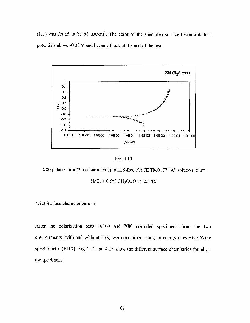
X80 (H2S-free)

^0 ^

-0.1 7-02 7-03 —

▪ -0.4 —

;7; -0 b -

-0e6 —

-0.7 -

-013

^

-0.9 ^

1.0E-09

1.0E-07 1 DE-06 16E-05 1.0E-04 1.0E-03 1.0E02 1.0E-01 1.0E+00

i (A k m2)

(icorr) was found to be 98 ttA/cm 2 . The color of the specimen surface became dark at

potentials above -0.33 V and became black at the end of the test.

Fig. 4.13

X80 polarization (3 measurements) in H2S-free NACE TM0177 "A" solution (5.0%

NaC1 + 0.5% CH3COOH), 23 °C.

4.2.3 Surface characterization:

After the polarization tests, X100 and X80 corroded specimens from the two

environments (with and without H2 S) were examined using an energy dispersive X-ray

spectrometer (EDX). Fig 4.14 and 4.15 show the different surface chemistries found on

the specimens.

68

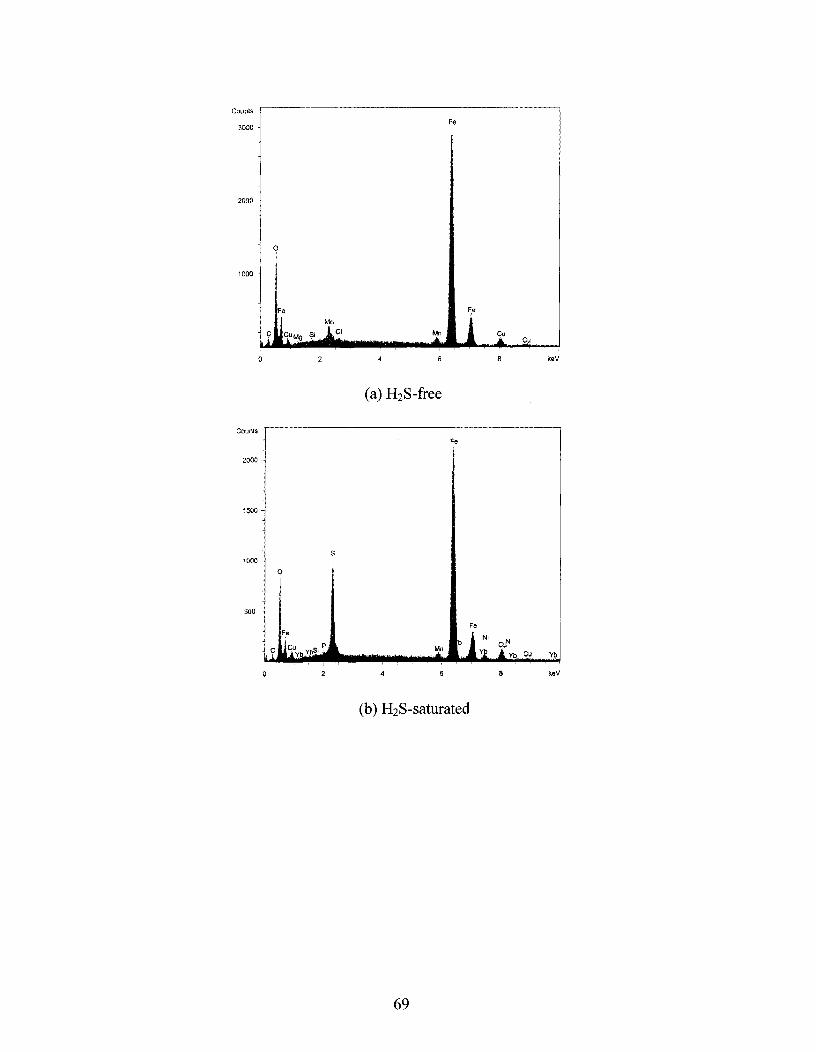
Counts

0^

2^

4^

6^

8^

keV

(a) H2 S-free

0^

2^

4^

6^

8^

keV

(b) H2 S-saturated

69

2^

4^

8^

8^

keV

(c) Polished uncorroded X100 specimen

Fig. 4.14

Corrosion product EDX for X100 in (a) H2S-free, (b) H2S-saturated NACE TM-0177

"A" solution and (c) Polished uncorroded X100 specimen was used as a reference.

Counts4000

Fe

2^

4^

a^keV

(a) H2S-free

70

Coures

3000

2000 -

1000

2^

8^

keV

(b) H2S-saturated

Fig. 4.15

Corrosion product EDX for X80 in (a) H2S-free and (b) H 2 S-saturated NACE TM-0177

"A" solution.

It can be seen that in H2S-free NACE TM-0177 "A" solution, the EDX spectra was

mainly composed of iron and oxygen. These products on the metal surface did not

promote passivity, as can be seen in the (H2S-free) polarization diagrams for the two

materials (Fig. 4.11 and 4.13). In the (H2S-free) polarization diagrams, the measured

anodic current densities kept on increasing with potential and the resulting anodic

polarization curve didn't show any sign of passivity. The presence of these products on

the metal was most likely caused by precipitation of Fe(OH)2 on the surface. Fe(OH)2

was likely produced by the reaction between Fe 2+ and H2O:

2H+ + 2e" -3 H2^(corrosion cathodic reaction)^(4.3)

Fe^Fe2+ + 2e^

(corrosion anodic reaction)^(4.4)

Fe2+ + 2H20 Fe(OH) 2 + 2H+^(4.5)

71

In H2S-saturated NACE TM0177 "A" solutions, the EDX spectra showed significant

amounts of sulfur. After the consumption of H +, produced by CH3CHOOH, has reached a

certain degree (increase in pH), FeS was likely formed by the reactions below:

Cathodic reaction:

H2S + H2O 4 H+ + HS - + H2O^

(4.6)

HS - + H2O 4 H+ + S2- + H2O^

(4.7)

2H+ + 2C 4 H2 or 2H^

(4.8)

Anodic reaction:

Fe 4 Fe2+ + 2C^ (4.9)

Overall:

Fe + H2S 4 FeS + 2H^

(4.10)

In the EDX spectra, the Mo and S peaks are very close and some times a Mo peak might

be labelled by EDX as an S peak and vice versa. In the H2S-free EDX spectra, this peak

was most representing Mo because the concentration of Mo in both steels (0.21 wt.%) is

much higher than S (<0.01 wt.%). In addition, the H2S-free environment is not expected

to promote any sulfide film formation. In H2S-saturated environment, the peak was likely

72

representative of S because the presence of H 2S generates a sulfide corrosion product,

which increases the S peak in the EDX spectra.

4.2.4 Mechanistic insights:

Table 4.3 summarizes the results obtained from the electrochemical tests on both the

X100 and X80. It can be seen from Table 4.3 that the starting pH values were lower in

H2S environments. Both E con. and icon increased when H2S was added to the test solution.

It can also be seen that anodic Tafel slopes, r3a, were close in value. Likewise, values for

the cathodic Tafel slopes, Pc , were also similar. Addition of H2S to the NACE TM0177

"A" solution increased the corrosion rate of X100 from 51.6 to 96.7 mpy. The effect of

H2S on the corrosion rate was similar for X80. The corrosion rate for X80 increased from

45.2 to 80.2 mpy.

pHInitial/final

Emil'

(V)iCOrr

(pA/cm2)fla

(V/dec.)Pc

(V/dec.)Corrosionrate (mpy)

X80(H2S-free solution) 2.9 / 3.0 -0.65 98 0.065 -0.121 45.2

X80(H2S-saturated solution) 2.7 / 2.9 -0.63 174 0.063 -0.112 80.2

X100(H2S-free solution) 2.9 / 3.0 -0.63 112 0.066 -0.123 51.6

X100(H2 S-saturated solution) 2.7 / 2.9 -0.61 210 0.065 -0.111 96.7

Table 4.3

Summary of electrochemical test results conducted on API-X100 and X80 in H2S-free

and H2S-saturated NACE TM0177 "A" solution.

73

X100 ( S -saturated )

X100 (H2S free)0D ^

-0.1 -

-0 2 -

-0 3

-0.4 -

"' -0,5-

-00-

-0.7 -

-0 2 -

-0 9 10E08^1.0E07^1.0E06^1.0E06^12E04^1.0E03^1.0E02^1.0E01

^1.0E1-00

i (Akm2)

X10 (H2 S -saturated )

----X00 (H2S-free)OD ^

-0.1 -

-0 2 -

-0.3-02 -

-0.4 -

w -0.6

-00 -

-0.7

-0.8 -

-0 9 ^12E08

1.0E07^1.0E06^1.0E06^1.0E04^1.0E03^1.0E02^1.0E01^1.0E4-00

i (Akm2)

4.2.4.1 Effect of H2S on corrosion rates:

Fig. 4.16 shows the polarization diagrams of (a) X100 and (b) X80 with and without H2S

(NACE TM0177 "A" solution). Schematic Evans diagrams for each metal (with and

without H2S) were also drawn as shown in Fig. 4.17.

(a)

(b)

Fig. 4.16

Polarization diagrams of (a) X100 and (b) X80 in NACE TM0177 "A" solution (H2S-free

and 1-12S-saturated), T = 23 °C.

74

Log i X100

u.i

(a)

(b)

Fig. 4.17

Evans diagrams for (a) X100 and (b) X80 in NACE TM0177 "A" solution (H 2 S-free and

H2S-saturated). E = potential, Log i = log value of current density.

75

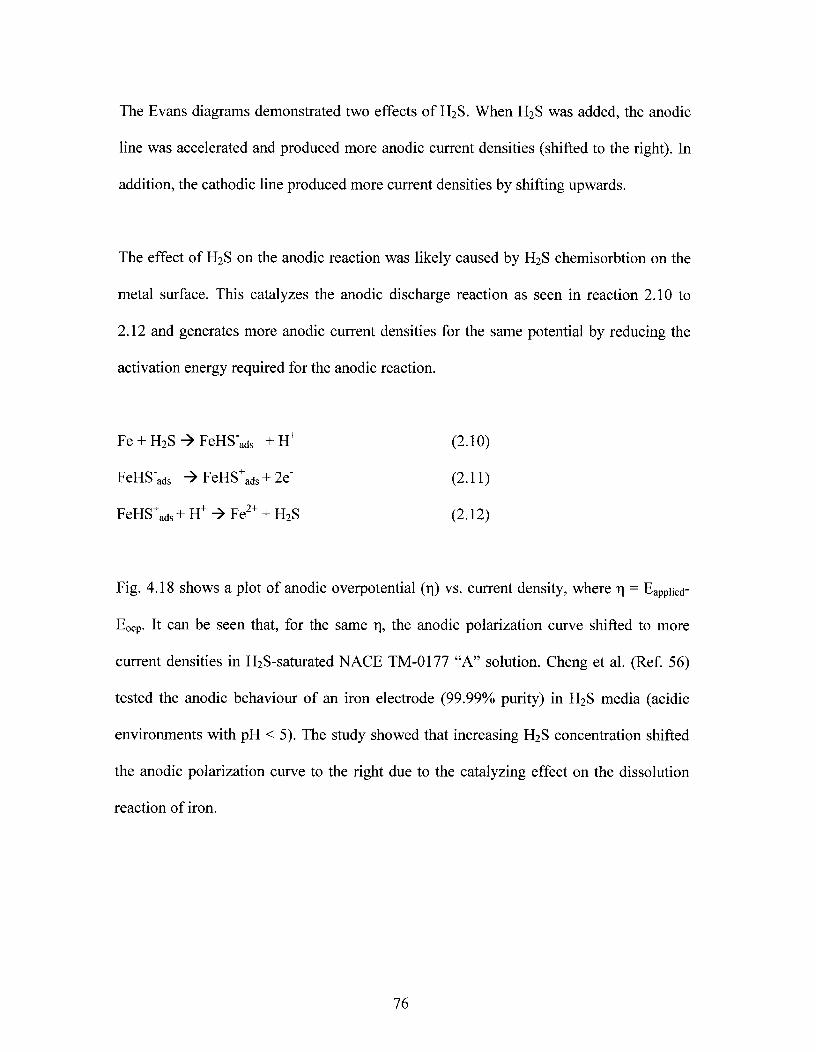
The Evans diagrams demonstrated two effects of H 2 S. When H2S was added, the anodic

line was accelerated and produced more anodic current densities (shifted to the right). In

addition, the cathodic line produced more current densities by shifting upwards.

The effect of H2S on the anodic reaction was likely caused by H2S chemisorbtion on the

metal surface. This catalyzes the anodic discharge reaction as seen in reaction 2.10 to

2.12 and generates more anodic current densities for the same potential by reducing the

activation energy required for the anodic reaction.

Fe + H2 S^FeHS -ads (2.10)

FeHS -ads^4 FeHS±ads + 2e" (2.11)

FeHS+ads +1-1± 4 Fe2+ + H2 S (2.12)

Fig. 4.18 shows a plot of anodic overpotential (i) vs. current density, where ri = Eapplted-

Eocp. It can be seen that, for the same II, the anodic polarization curve shifted to more

current densities in H2S-saturated NACE TM-0177 "A" solution. Cheng et al. (Ref. 56)

tested the anodic behaviour of an iron electrode (99.99% purity) in H2S media (acidic

environments with pH < 5). The study showed that increasing H 2S concentration shifted

the anodic polarization curve to the right due to the catalyzing effect on the dissolution

reaction of iron.

76

X100 ( H2 S -saturated )

X100 (H2S- free)0.8

5 0.5 -

? 0.4 -

0.3 -

‹Y; 0.2-0.1 -

0 ^1.0E08 1.0 6.07^1.0E08^1.0E05^1 DE04

i (Pabm2)

1.0E03^1.0E02^1.0E01^1.0B-00

(a) X100

0.6

5. 0.5 -

la. 0.4

0.3 -

0.20.1 -

0 ^1.0E08

^X80 ( H2 S -saturated )

XBO (112S - free)

1.0E07^1.0E08^1.0E1)6^1.0E04^1.0E03^1.0E02^1.0E01^1.0E00

i (Akm2)

(b) X80

Fig. 4.18

Anodic overpotential (i) vs. current density for (a) X100 and (b) X80 in H2S-free and

H2S-saturated NACE TM-0177 "A" solution, T = 23 °C.

In addition to the effect on the anodic reaction, H 2S also affected the cathodic reaction.

The Evans diagrams in Fig. 4.17 show a shift of the cathodic lines to more current

densities. This effect is due to an increase in the cathodic half cell potential, eH+/H2,

because of the decrease in pH that is observed with H2S saturation. Table 4.3 shows that

77

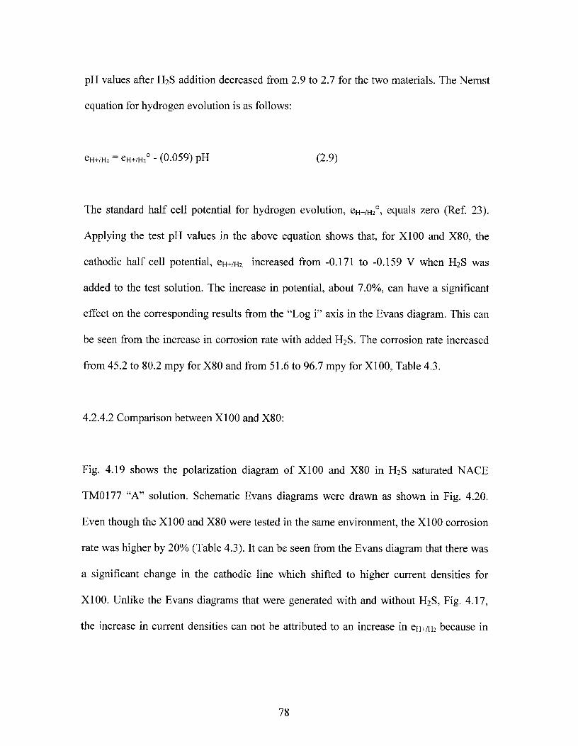
pH values after H2S addition decreased from 2.9 to 2.7 for the two materials. The Nernst

equation for hydrogen evolution is as follows:

eH+/H2 = eH+/H2 ° - (0.059) pH^

(2.9)

The standard half cell potential for hydrogen evolution, eH+/H 2°, equals zero (Ref. 23).

Applying the test pH values in the above equation shows that, for X100 and X80, the

cathodic half cell potential, eH+/H2 . increased from -0.171 to -0.159 V when H 2S was

added to the test solution. The increase in potential, about 7.0%, can have a significant

effect on the corresponding results from the "Log i" axis in the Evans diagram. This can

be seen from the increase in corrosion rate with added H2S. The corrosion rate increased

from 45.2 to 80.2 mpy for X80 and from 51.6 to 96.7 mpy for X100, Table 4.3.

4.2.4.2 Comparison between X100 and X80:

Fig. 4.19 shows the polarization diagram of X100 and X80 in H2S saturated NACE

TM0177 "A" solution. Schematic Evans diagrams were drawn as shown in Fig. 4.20.

Even though the X100 and X80 were tested in the same environment, the X100 corrosion

rate was higher by 20% (Table 4.3). It can be seen from the Evans diagram that there was

a significant change in the cathodic line which shifted to higher current densities for

X100. Unlike the Evans diagrams that were generated with and without H2S, Fig. 4.17,

the increase in current densities can not be attributed to an increase in eH+/H2 because in

78

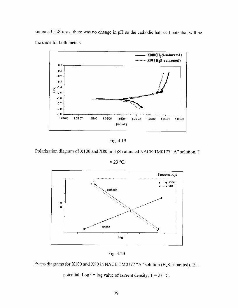
X100 (H2S -saturated )X80 (H2S-saturated)

On ^-0.1 -

-0 2 -

-013 -

-0.4 -

1.0502^1.0501 1.0E+00

w -0,5-

-0.6 -

-0.7 -

-DS -

^

-0.9 ^

^

1.0508^113507^1.0506 1.0505^1.0504^15503

i (A km2)

saturated H2S tests, there was no change in pH so the cathodic half cell potential will be

the same for both metals.

Fig. 4.19

Polarization diagram of X100 and X80 in H2S-saturated NACE TM0177 "A" solution, T

= 23 °C.

Fig. 4.20

Evans diagrams for X100 and X80 in NACE TM0177 "A" solution (H2S-saturated). E =

potential, Log i = log value of current density, T = 23 °C.

79

Microstructural differences between the X100 and X80 might have caused the shift in the

cathodic line and the resulting increase in corrosion rates. As can be seen in Fig. 4.1 and

4.2 for the microstructure of the two materials, the interfacial area between ferrite and the

other phases is higher in the X100. Phase boundaries are areas of inhomogeneous

corrosion potentials. As a result, ferrite at phase boundaries have a stronger driving force

to corrode than ferrite in the homogeneous matrix because second phases acts as a local

cathode to the surrounding ferrite. The shift of the cathodic line in the Evans diagram can

then be attributed to an increased cathodic area in the X100. An increase in cathodic areas

tends to shift the cathodic line further to the right, rather than upward, yielding higher

corrosion potentials and higher corrosion rates.

Reformatskaya et al. (Ref. 57) showed that the corrosion rate of carbon steel was affected

by corrosion potential inhomogeneity between ferrite and the other phases in the steel.

The study showed that corrosion rate increases with an increase in phase boundaries

between ferrite and second phases. These phase boundaries increase with increasing

second phase grain sizes or by a higher dispersion of these phases in the steel.

The nonmetallic inclusion diameter difference between the two steels may have also

played a role in the increased corrosion rate in the X100. Inclusion diameter in the X100

ranged between 6-9.5 pm while for the X80, inclusion diameter ranged between 2-4.5

p,m. Furthermore, the average inclusion diameter in the X100 steel, 8.0 wn, was higher

than those in the X80, 3.5 [n. The effect of surface inclusions is associated with

preferential dissolution of the surrounding metal matrix. Corrosion of ferrite at inclusion-

80

matrix interfaces develops more rapidly than ferrite in the matrix. Due to the higher

dissolution rates in that area, a narrow corroded area forms around the inclusion and the

contact between the inclusion and the matrix breaks forming a local pit at the inclusion

site (Ref. 58). Because of the larger inclusion diameter in the X100, the inclusion-matrix

interface is larger which leads to a higher corrosion rate than the X80. This is

accomplished by providing larger cathodic area (inclusion) relative to any single

nucleation site in the surrounding metal. Fig. 4.21 shows the corroded metal surface of

X100 and X80 after polarization testing in H2S-saturated NACE TM-0177 "A" solution.

For both steels, the surface consisted of randomly distributed pits. However, the

corrosion pits in the X100 were bigger than those in the X80. X100 average pit diameter,

dot, was 0.36 mm while X80 average pit diameter was 0.27 mm. Therefore, corrosion pits

in X100 were 25% larger than those in X80. In addition, X100 had a corrosion pit

density, pot, of 2.13 pit/mm2 which was 17% more that the pit density in X80, 1.82

pit/mm2 .

81

(a)

(b)

Fig. 4.21

Pitting in (a) X80 and (b) X100 in H2S saturated NACE solution (SEM).

82

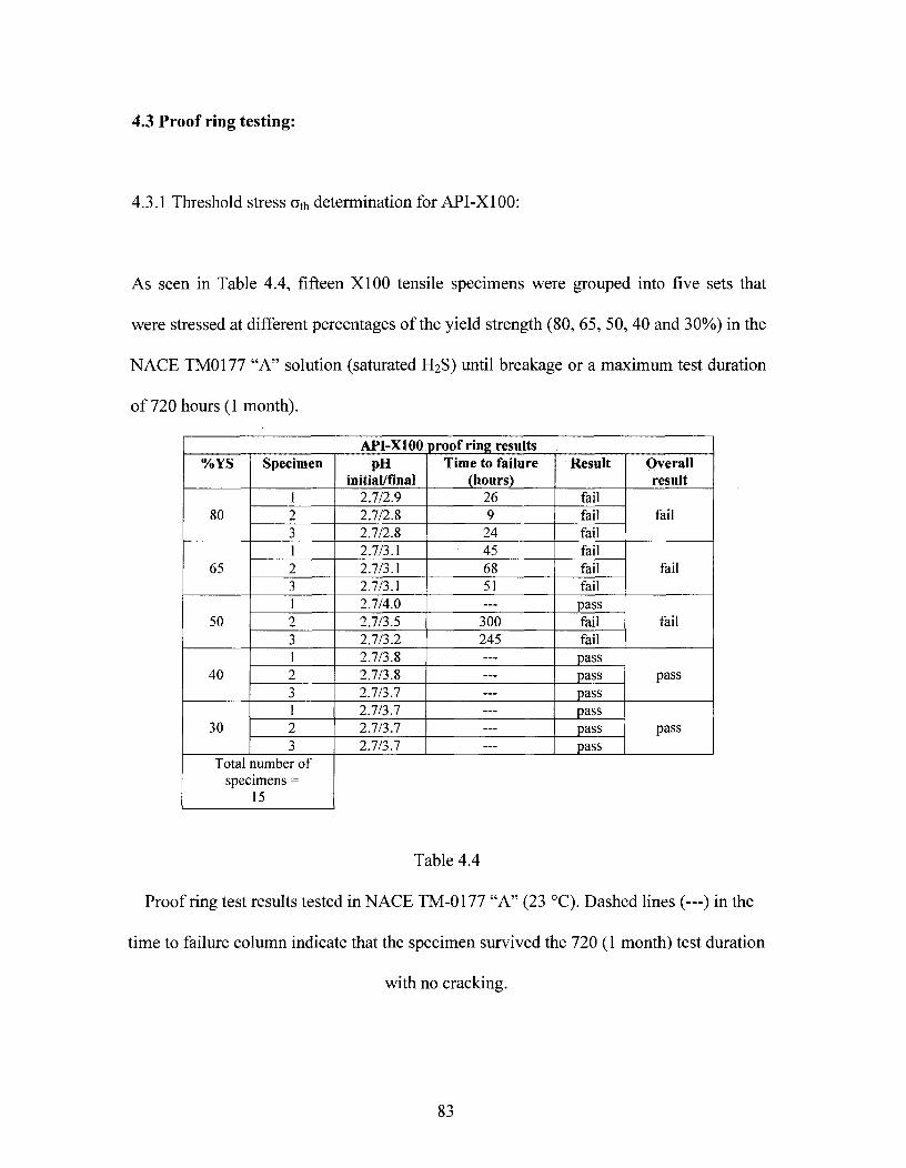
4.3 Proof ring testing:

4.3.1 Threshold stress 6 th determination for API-X100:

As seen in Table 4.4, fifteen X100 tensile specimens were grouped into five sets that

were stressed at different percentages of the yield strength (80, 65, 50, 40 and 30%) in the

NACE TM0177 "A" solution (saturated H2S) until breakage or a maximum test duration

of 720 hours (1 month).

API-X100 proof ring results%YS Specimen pH

initial/finalTime to failure

(hours)Result Overall

result

801 2.7/2.9 26 fail

fail2 2.7/2.8 9 fail3 2.7/2.8 24 fail

651 2.7/3.1 45 fail

fail2 2.7/3.1 68 fail3 2.7/3.1 51 fail

501 2.7/4.0 --- pass

fail2 2.7/3.5 300 fail3 2.7/3.2 245 fail

401 2.7/3.8 --- pass

pass2 2.7/3.8 --- pass3 2.7/3.7 pass

301 2.7/3.7 --- pass

pass2 2.7/3.7 --- pass3 2.7/3.7 --- pass

Total number ofspecimens =

15

Table 4.4

Proof ring test results tested in NACE TM-0177 "A" (23 °C). Dashed lines (---) in the

time to failure column indicate that the specimen survived the 720 (1 month) test duration

with no cracking.

83

The results from Table 4.4 are plotted in Fig. 4.22. It can be seen that the time to failure

increased with a decrease in the applied load. In addition, the change of time to failure

values between two consecutive applied stresses seemed to widen as the threshold stress

value was approached. Since an applied stress of 50%YS generated a "fail" result while

40%YS generated a "pass" result, the threshold stress will be between these two points.

Proof ring time to failure

90 ^80 -70

- 60

50

• 40cp

3co 0

20 -100 ^

^

0^

100 200 300 400 500 600 700 800 900 1000

Time (hours)

Fig. 4.22

Proof ring time to failure graph for the X100 in H 2S-saturated NACE TM-0177 "A"

solution (dark = fail, clear = pass, dashed line = 720 hrs. max. test duration). Dashed line

indicates the 720 hours (1 month) test duration).

The LOGEST function in Microsoft Exce1TM was used to generate an equation to fit the

proof ring results. The LOGEST function calculated the exponential curve that fitted the

data from the proof ring experiments and returned an array of values that described the

curve. The generated equation was:

0

0

84

Time to failure (hours) = (3.41x10 5) x (0.875 %11s)^(4.11)

Equation 4.11 predicts that time to failure, in NACE TM-0177 "A", reaches 720 hours (1

month) when the applied stress is 46% of the yield strength or 343.1 MPa (49.7 ksi).

Therefore, the threshold stress value (ath) for the X100 steel quoted here is 46% YS. As

per equation 4.11, X100 loaded below 46%YS should always pass the NACE TM-0177

test. Implication of this conclusion is seen in specimens loaded to 40%YS and 30%YS in

which all specimens passed the test.

4.3.2 Crack characterization:

Fig. 4.23 shows a longitudinal section for a failed tensile specimen. In all cracked

specimens, the main failure mechanism was SSC cracking that propagated perpendicular

to the applied stress. The SSC crack was transgranular as seen in Fig. 4.24. All samples

that fractured into two parts exhibited the same fracture morphology. SSC initiated at the

surface and propagated by brittle fracture perpendicular to the applied stress. The crack

kept on propagating until the specimen could not hold the applied load any longer. At that

stage, the specimen broke mechanically into two parts by ductile fracture.

85

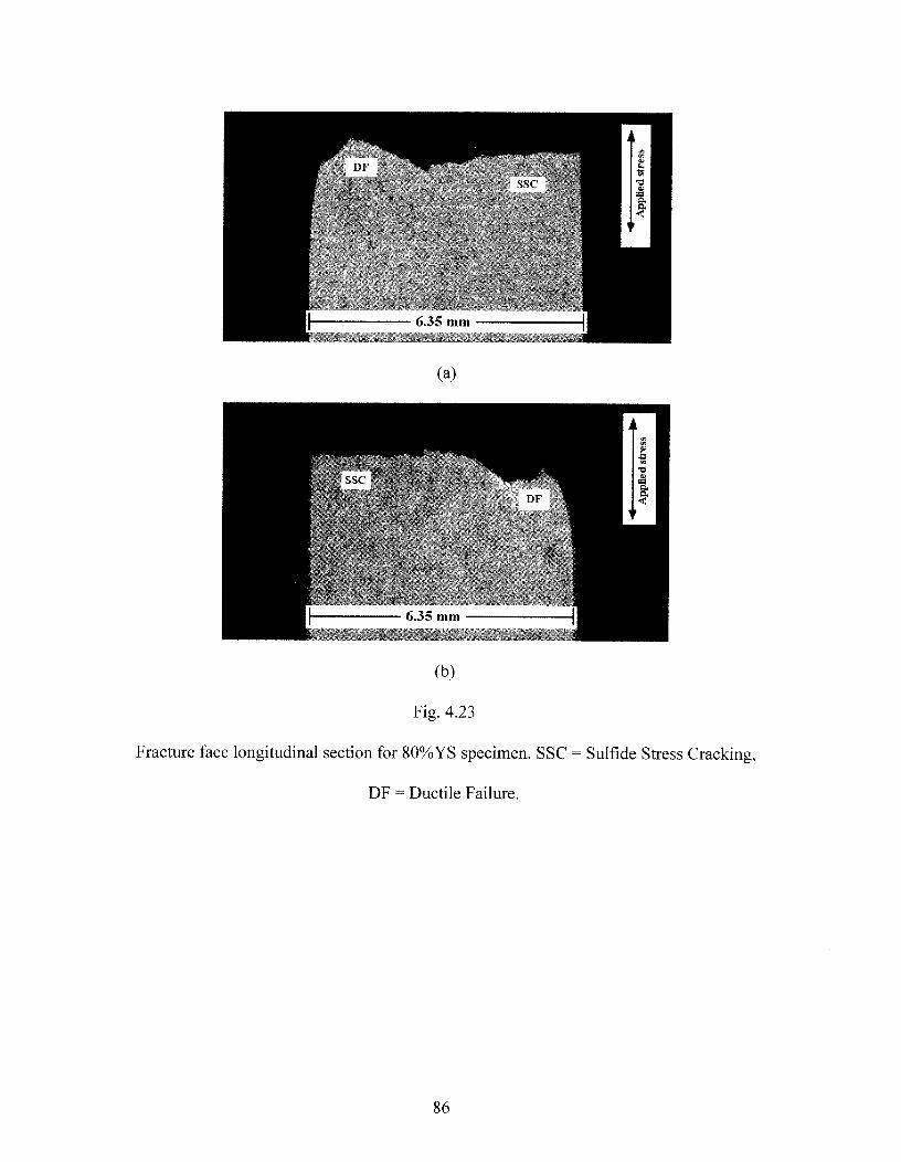
(a)

(b)

Fig. 4.23

Fracture face longitudinal section for 80%YS specimen. SSC = Sulfide Stress Cracking,

DF = Ductile Failure.

86

Fig. 4.24

Longitudinal section of fracture face (80%YS specimen) showing transgranular crack

propagation (light).

In addition to SSC, Hydrogen Induced Cracking (HIC) sites were observed as well. These

HIC cracks were observed to propagate parallel to the rolling direction of the material

and in some cases were connected to the main crack that caused failure, as seen in Fig.

4.25. In this study, the applied stresses were parallel to the rolling direction. Since HIC

cracks propagate along the rolling direction, HIC cracks in this case were not affected by

the applied stresses and its propagation was due to internal hydrogen pressure originating

from inside the HIC crack. If the applied stresses were perpendicular to the rolling

direction, applied stresses, in this case, would have an effect on HIC propagation, Fig.

4.26.

87

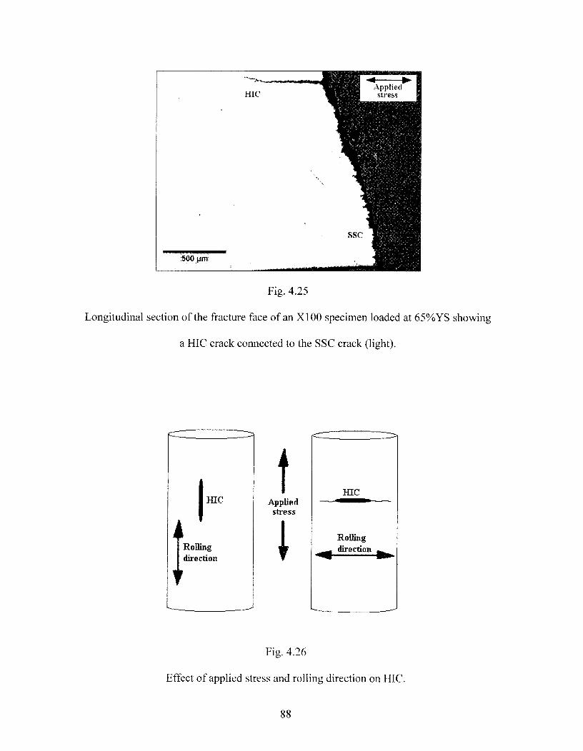
Fig. 4.25

Longitudinal section of the fracture face of an X100 specimen loaded at 65%YS showing

a HIC crack connected to the SSC crack (light).

I MC

Rollingdirection

Appliedstress

HIC--4111■1111111111m----

Rollingdirection

Fig. 4.26

Effect of applied stress and rolling direction on HIC.

88

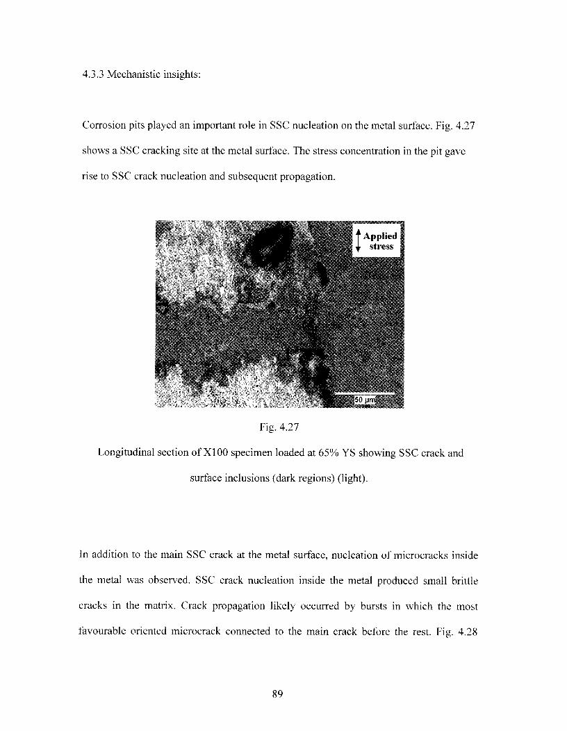
4.3.3 Mechanistic insights:

Corrosion pits played an important role in SSC nucleation on the metal surface. Fig. 4.27

shows a SSC cracking site at the metal surface. The stress concentration in the pit gave

rise to SSC crack nucleation and subsequent propagation.

Fig. 4.27

Longitudinal section of X100 specimen loaded at 65% YS showing SSC crack and

surface inclusions (dark regions) (light).

In addition to the main SSC crack at the metal surface, nucleation of microcracks inside

the metal was observed. SSC crack nucleation inside the metal produced small brittle

cracks in the matrix. Crack propagation likely occurred by bursts in which the most

favourable oriented microcrack connected to the main crack before the rest. Fig. 4.28

89

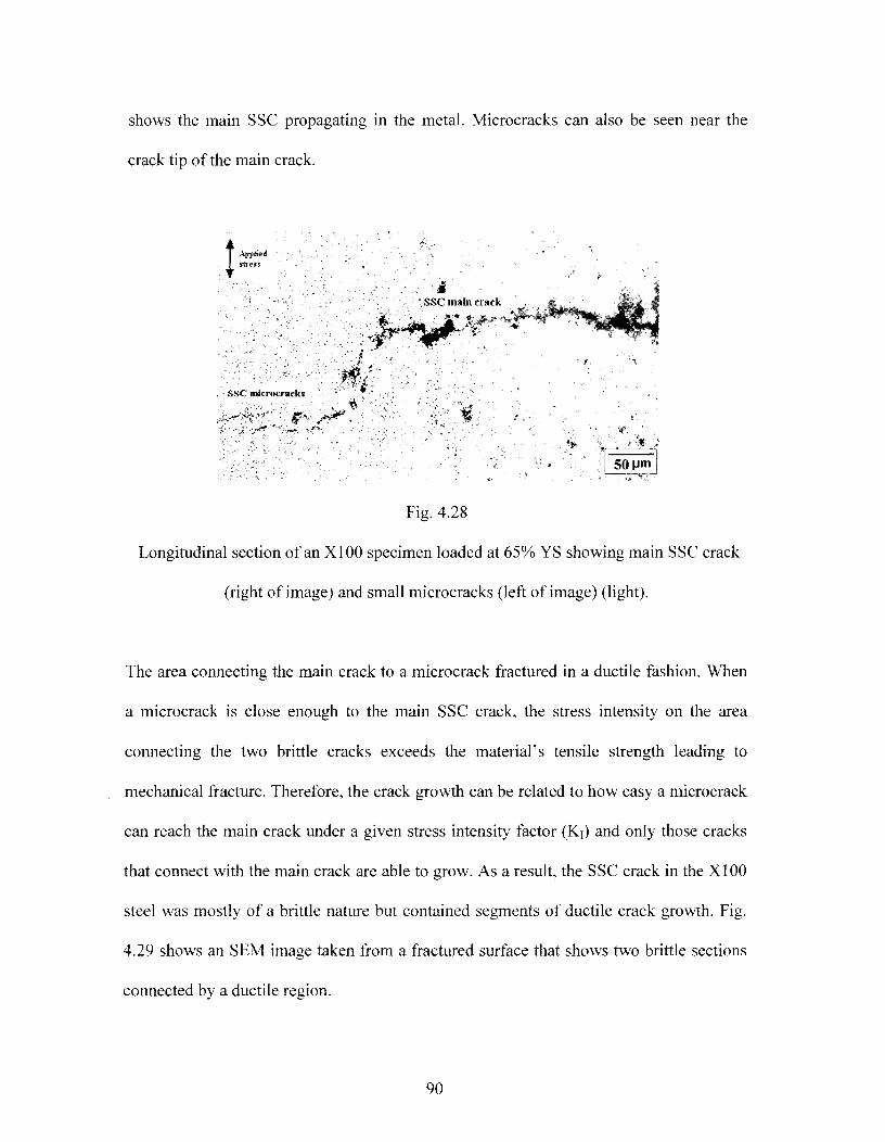
shows the main SSC propagating in the metal. Microcracks can also be seen near the

crack tip of the main crack.

Fig. 4.28

Longitudinal section of an X100 specimen loaded at 65% YS showing main SSC crack

(right of image) and small microcracks (left of image) (light).

The area connecting the main crack to a microcrack fractured in a ductile fashion. When

a microcrack is close enough to the main SSC crack, the stress intensity on the area

connecting the two brittle cracks exceeds the material's tensile strength leading to

mechanical fracture. Therefore, the crack growth can be related to how easy a microcrack

can reach the main crack under a given stress intensity factor (K 1) and only those cracks

that connect with the main crack are able to grow. As a result, the SSC crack in the X100

steel was mostly of a brittle nature but contained segments of ductile crack growth. Fig.

4.29 shows an SEM image taken from a fractured surface that shows two brittle sections

connected by a ductile region.

90

x 500 0000 20 k V 1 00.0 m

Fig. 4.29

SSC brittle regions connected by a ductile section found in the fracture face of X100

specimen loaded at 80% YS (SEM). B = brittle (SSC), D = ductile.

HIC cracks found in the tested specimens were nucleated at banded martensite-ferrite

interfaces and non-metallic inclusions and propagated along the rolling direction parallel

to the applied tensile stress through the softer ferrite phase. Fig. 4.30 shows HIC cracks

found in specimens stressed at 50% of the yield strength. After hydrogen accumulation,

internal pressure in these traps increased due to the reaction between hydrogen atoms to

form molecular hydrogen leading to HIC folination.

91

Fig. 4.30

Transverse section of an X100 specimen loaded at 50% YS showing HIC cracks (light).

The existence of HIC cracks can affect the material's cracking susceptibility in sour

environments. Residual or applied stresses can increase the stress field surrounding the

cracks. This generates localized yielding which can produce a second crack perpendicular

to the tensile stress direction.

Hydrogen can diffuse rather quickly into the steel matrix. Koh et al. (Ref. 41) measured

the diffusivity of hydrogen, at 25 °C, in several HSLA steels, X52 to X80, with varying

microstructures, ferrite-pearlite, acicular ferrite and ferrite-bainite, using the NACE

TM0177 "A" solution (the same solution used in the polarization and proof ring tests).

The study showed that the lowest hydrogen diffusivity in the tested HSLA steels was 3.5

92

x 10 -6 cm2/sec. Diffusivity of hydrogen is closely related to the trapping sites provided by

various defects such as vacancies, inclusions and precipitation in the steel.

In order to demonstrate the rate of hydrogen diffusion into the test specimen, a Gurney-

Lurie chart for a cylindrical shape was used (Ref. 59). A chart for a long cylinder was

used so the effect of the cylinder ends can be neglected. The Gurney-Lurie charts

represent solutions for unsteady state mass transfer problems for several simple shapes by

relating the relative time (XD) to the unaccomplished concentration change (Y). XD and Y

are dimensionless ratios described as follows:

Y = unaccomplished concentration change = (CH s — CH) / (CHs CH0)^

(4.12)

XD = relative time = (D • t) / x1 2^(4.13)

Where:

CHs concentration of hydrogen at the surface.

CH0 = concentration of hydrogen at the specimen center at t = O.

CH = unknown hydrogen concentration at desired t and x.

D = hydrogen diffusivity.

x i = specimen radius.

t = time.

When t = 0, CH0 = O. As a result, Equation 4.12 will be rearranged as follows:

93

CH = (1 —^CHs^ (4.14)

In the proof ring tests conducted in this study, x 1 = 0.318 cm. In addition, the earliest time

to failure was 9 hours, Table 4.4, so t = 32400 sec. (9 hrs.). It is assumed that the test

solution is well mixed. Therefore, for a hydrogen diffusivity value of 3.5 x 10 -6 cm2/sec:

XD = (D t) / x 1 2 = (3.5 x 10 -6 32400) / (0.318 2) = 1.12^ (4.15)

At the specimen center, the calculated XD will yield Y = 0.003. Therefore, after 9 hours:

CH = (1 — 0.003) CHs CH = 0.997 CHs^CH = 99.7% CHs^(4.16)

It is shown that after 9 hours, the hydrogen concentration at the specimen center was

99.7% of the hydrogen concentration at the surface. To further illustrate the fast diffusion

of hydrogen through the tested specimens, the time that hydrogen will need to reach the

center was examined by determining the value of XD at Y = 1.0 (Y value below which CH

at the center will be above 0). At Y = 1.0, XD = 0.09. Applying Equation 4.13:

XD = 0.09 = (3.5 x 10 -6 t) / (0.318 2)^t = 2592 seconds = 43.2 minutes^(4.17)

It is seen that hydrogen will reach the specimen center after 43.2 minutes. It should be

noted that the specimen radius was very small (3.18 mm). This explains why little time

was required for hydrogen to reach the specimen center line.

94

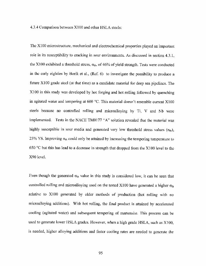
4.3.4 Comparison between X100 and other HSLA steels:

The X100 microstructure, mechanical and electrochemical properties played an important

role in its susceptibility to cracking in sour environments. As discussed in section 4.3.1,

the X100 exhibited a threshold stress, ath, of 46% of yield strength. Tests were conducted

in the early eighties by Borik et al., (Ref. 6) to investigate the possibility to produce a

future X100 grade steel (at that time) as a candidate material for deep sea pipelines. The

X100 in this study was developed by hot forging and hot rolling followed by quenching

in agitated water and tempering at 600 °C. This material doesn't resemble current X100

steels because no controlled rolling and microalloying by Ti, V and Nb were

implemented. Tests in the NACE TM0177 "A" solution revealed that the material was

highly susceptible in sour media and generated very low threshold stress values (cr th),

25% YS. Improving ath could only be attained by increasing the tempering temperature to

650 °C but this has lead to a decrease in strength that dropped from the X100 level to the

X90 level.

Even though the generated ath value in this study is considered low, it can be seen that

controlled rolling and microalloying used on the tested X100 have generated a higher ath

relative to X100 generated by older methods of production (hot rolling with no

microalloying additions). With hot rolling, the final product is attained by accelerated

cooling (agitated water) and subsequent tempering of martensite. This process can be

used to generate lower HSLA grades. However, when a high grade HSLA, such as X100,

is needed, higher alloying additions and faster cooling rates are needed to generate the

95

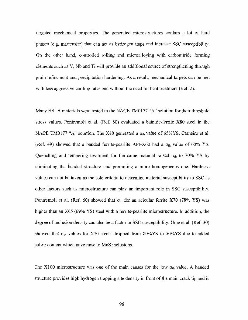
targeted mechanical properties. The generated microstructures contain a lot of hard

phases (e.g. martensite) that can act as hydrogen traps and increase SSC susceptibility.

On the other hand, controlled rolling and microalloying with carbonitride forming

elements such as V, Nb and Ti will provide an additional source of strengthening through

grain refinement and precipitation hardening. As a result, mechanical targets can be met

with less aggressive cooling rates and without the need for heat treatment (Ref. 2).

Many HSLA materials were tested in the NACE TM0177 "A" solution for their threshold

stress values. Pontremoli et al. (Ref. 60) evaluated a bainitic-ferrite X80 steel in the

NACE TM0177 "A" solution. The X80 generated a 6 th value of 65%YS. Carneiro et al.

(Ref 49) showed that a banded ferrite-pearlite API-X60 had a 6 th value of 60% YS.

Quenching and tempering treatment for the same material raised 6 th to 70% YS by

eliminating the banded structure and promoting a more homogeneous one. Hardness

values can not be taken as the sole criteria to determine material susceptibility to SSC as

other factors such as microstructure can play an important role in SSC susceptibility.

Pontremoli et al. (Ref 60) showed that 6 th for an acicular ferrite X70 (78% YS) was

higher than an X65 (69% YS) steel with a ferrite-pearlite microstructure. In addition, the

degree of inclusion density can also be a factor in SSC susceptibility. Ume et al. (Ref. 30)

showed that 6th values for X70 steels dropped from 80%YS to 50%YS due to added

sulfur content which gave raise to MnS inclusions.

The X100 microstructure was one of the main causes for the low 6 th value. A banded

structure provides high hydrogen trapping site density in front of the main crack tip and is

96

more susceptible to SSC than homogenous microstructures (Ref. 49). Homogeneous

microstructures present dispersed and relatively smaller sites for hydrogen trapping

hence, reaching the critical hydrogen concentration for SSC microcrack formation is

more difficult. In addition, bands in inhomogeneous microstructures act as nucleation

sites for HIC cracks (Ref. 48). HIC can connect with propagating SSC cracks which lead

to failure in sour environments at lower applied stresses. In addition to the susceptible

microstructure, the higher corrosion rates experienced in the X100 steel is evidence that

more hydrogen was available from the corrosion reaction. Hydrogen can migrate into the

steel and cause embrittlement after it accumulates in hydrogen traps.

4.4 Implications of results on X100 susceptibility:

The results generated in this study and comparison with older generation HSLA steels

revealed that X100 is susceptible in H2S environments. The X100 high susceptibility is

demonstrated by its high yield strength value, susceptible microstructure, high corrosion

rates and low threshold stress value in the NACE TM0177 "A" environment.

Investigating the reasons behind the low SSC susceptibility should open doors for future

improvements on the X100 in order to generate a more resistant material in H2S

environments.

Manufacturing an X100 grade steel with acceptable resistance to SSC might be possible

if the areas that lead to its high susceptibility in this study are improved. This can be

achieved by generating methods to produce a more homogeneous microstructure that will

97

minimize local hydrogen build-up that might lead to SSC nucleation. In addition,

minimizing the phase boundaries in the steel will depress corrosion rates which will

minimize pit formation and reduce the intensity of hydrogen propagation into the steel.

Another way to improve SSC resistance is to better control nonmetallic inclusions by

reducing inclusion sizes and eliminating any elongated inclusions. A material with less

nonmetallic inclusions will have less nucleation sites for corrosion pits on the surface and

less hydrogen traps in the metal body.

98

Chapter 5

5 SUMMARY AND CONCLUSION:

In this study, API-X100 HSLA steel was tested for its SSC susceptibility in H2S

environments. The application of HSLA steels in oil and gas transportation pipelines has

increased in the past few years because of an increase in global energy demand. The

X100 is a newly developed HSLA steel that was designed to meet the requirement for

pipelines with higher mechanical limits to withstand the increasing line pressures. To

assure safe and reliable performance, it is necessary to investigate the X100 SSC cracking

susceptibility in H2S environments. The need to investigate SSC susceptibility is raised

from the material's higher strength and hardness values that might make it more

susceptible to cracking than older generation HSLA steels. Investigating SSC

susceptibility will open doors for future improvements on the X100 in order to generate a

more resistant material in H 2S environments.

Electrochemical and proof ring tests were conducted on the X100 steel using the NACE

TM0177 "A" test solution. X80, an older generation HSLA steel, was used for

comparison in the microstructural and electrochemical examinations. Uniaxial (constant

load) SSC testing was conducted on the X100 to determine the material threshold stress

value (a th) in H2S environment. Test results and comparison with older generation HSLA

steels showed that the X100 displayed low resistance to SSC.

99

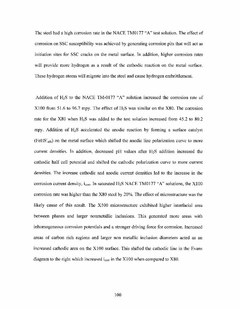
The steel had a high corrosion rate in the NACE TM0177 "A" test solution. The effect of

corrosion on SSC susceptibility was achieved by generating corrosion pits that will act as

initiation sites for SSC cracks on the metal surface. In addition, higher corrosion rates

will provide more hydrogen as a result of the cathodic reaction on the metal surface.

These hydrogen atoms will migrate into the steel and cause hydrogen embrittlement.

Addition of H2S to the NACE TM-0177 "A" solution increased the corrosion rate of

X100 from 51.6 to 96.7 mpy. The effect of H 2S was similar on the X80. The corrosion

rate for the X80 when H2S was added to the test solution increased from 45.2 to 80.2

mpy. Addition of H2S accelerated the anodic reaction by forming a surface catalyst

(FeHS -ads) on the metal surface which shifted the anodic line polarization curve to more

current densities. In addition, decreased pH values after H 2S addition increased the

cathodic half cell potential and shifted the cathodic polarization curve to more current

densities. The increase cathodic and anodic current densities led to the increase in the

corrosion current density, i cor,. In saturated H2 S NACE TM0177 "A" solutions, the X100

corrosion rate was higher than the X80 steel by 20%. The effect of microstructure was the

likely cause of this result. The X100 microstructure exhibited higher interfacial area

between phases and larger nonmetallic inclusions. This generated more areas with

inhomogeneous corrosion potentials and a stronger driving force for corrosion. Increased

areas of carbon rich regions and larger non metallic inclusion diameters acted as an

increased cathodic area on the X100 surface. This shifted the cathodic line in the Evans

diagram to the right which increased i con- in the X100 when compared to X80.

100

The X100 generated a low threshold stress value, a th, of 46% YS, 343.2 MPa (49.7 ksi).

The main failure mechanism in the proof ring specimens was SSC cracking. SSC

nucleated at corrosion pits in the metal surface. Nucleation of SSC microcracks inside the

metal was observed. SSC crack nucleation inside the metal produced small brittle cracks

in the matrix. SSC crack propagation occurred by bursts in which the most favourable

oriented microcrack connected to the main crack.

In addition to SSC, HIC was observed as well. HIC cracks were observed to propagate

parallel to the rolling direction of the material and in some cases were connected to the

main crack that caused failure. HIC cracks nucleated at banded martensite-ferrite

interfaces and propagated along the rolling direction parallel to the applied tensile stress

through the softer ferrite phase.

When compared to older HSLA grades, the X100 tested in this study had a high SSC

susceptibility. SSC susceptibility was caused by the X100 high corrosion rate in the H 2 S-

saturated TM0177 "A" test solution. The increased corrosion rate formed more corrosion

pits that acted as crack initiation sites on the metal surface and provided more hydrogen

that migrated into the steel. The X100 inhomogeneous microstructure provided a high

density of hydrogen traps in front of the main crack tip which promoted SSC microcrack

formation inside the metal. Microcracks in the metal body connected with the main crack

tip that originated from corrosion pits which assisted SSC propagation.

101

The X100 microstructure played a role in SSC susceptibility. Inhomogeneous

microstructure with bands of carbon rich phases acted as SSC and HIC initiation sites

inside the metal. Crack nucleation formed more easily in the susceptible microstructures

and linkage of microcracks inside the metal with the main crack tip was less difficult.

Manufacturing an X100 grade steel with acceptable susceptibility to SSC might be

possible if the areas that lead to its high susceptibility in this study are improved.

Methods to produce a homogeneous X100 microstructure need to be generated in order to

minimize hydrogen build-up, in front of the main crack tip, that might lead to SSC

microcrack nucleation in the metal body. In addition, microstructures with minimized

phase boundaries are needed to reduce corrosion rates which will minimize pit formation

and reduce hydrogen propagation into the steel. Finally, better control of nonmetallic

inclusions by reducing inclusion sizes and eliminating any elongated inclusions are

needed in order to produce a material with less nucleation sites for corrosion pits on the

surface and less hydrogen traps in the metal body.

For future academic research in the area of SSC and H 2S corrosion in HSLA steels, the

following is recommended:

• Effect of possible microstructures for new generation HSLA steels on SSC

susceptibility. Small differences in microstructure will produce different response

in SSC media. Factors such as non-metallic inclusions, banding, present phases

should be investigated.

102

• Effect of alloying elements on H2S corrosion and SSC cracking. Optimum

alloying additions that can minimize H 2S corrosion and inclusion morphology and

size will have a positive effect on SSC resistance.

• Threshold stress intensity factors (Kissc) for new generation HSLA steels. Kissc

examinations for new HSLA steels are needed to determine SSC susceptibility in

the presence of existing cracks or corrosion pits. Kissc determination will also

facilitate maximum stress calculations of corroded pipeline materials.

• Effect of test variables on Kissc values. Kissc determination using double

cantilever beam (DCB) testing is sensitive to various experimental factors such as

temperature, applied load, wedge thickness and even test vessel volumes.

Research should be conducted to verify the exact effect of these variables.

• Effect of temperature on H 2S corrosion for new HSLA steels. Even though SSC is

most severe at ambient temperatures, determining the effect of temperature for

new HSLA steels is practically useful in the industry. Many pipelines are operated

at temperatures below or above ambient temperatures and this will affect the

materials response in SSC environments.

103

REFERENCES:

1. ASM Handbook. Volume 1: Properties and Selection: Iron Steels and High-

Performance Alloys. ASM international, Materials Park OH, 1993.

2. H. G. Hillenbrand et al."Development and Production of High Strength Pipeline

Steels". Niobium 2001, December 02-05. Orlando Florida, 2001.

3. Alan F. Liu. Structural Life Assessment Methods. 2' nd edition. ASM international,

Materials Park OH, 1998.

4. NACE Test Method TM177-96. "Laboratory Testing of Materials for Resistance

to Specific Forms of Environmental Cracking in H2S Environments". NACE

Houston TX, USA, 1996.

5. R. Denys. Pipeline Technology: Volume I. 1 ' t edition. Elsevier Science B.V,

Amsterdam, 2000.

6. F. Borik et al. "SSC Resistance of Electron Beam Welded, Q&T, X60, X80 and

X100 Line Pipe Steels". Corrosion 82. March 22-26, Houston TX, 1982.

7. W. F. Smith. Structure and Properties of Engineering Alloys. 2' nd Edition,

McGraw Hill, New York NY, 1993.

8. A. A. Groni et al."Austenite Transformation and Age Hardnening of HSLA-80

and ULCB Steels". Journal of Materials Processing Technology, 155, 2004. pp:

1513-1518.

9. N. Ishikawa et al." High Performance UOE Linepipes". JFE Technical Report No.

7, January 2006, pp: 20-26.

104

10. Y. I. Komizo. "Progress in Structural Steels for Bridge and Linepipes".

Transactions of JWRI. vol. 35. no. 1. 2006, pp: 1-7.

11. J. Bauer et al." Microstructure and Properties of Thermomechanical Controlled

Processing Steels for Linepipe Applications". Iron Making and Steel Making, vol.

32, no. 4, 2005, pp: 325:330

12. S. K. Das et al." The Effect of Variation of Microstructure on Fracture Mechanics

Parameters of HSLA-100 steel". Materials Science and Engineering A431, 2006,

pp: 68-79.

13.F. Xiao et al." Acicular Ferrite Microstructure of a Low Carbon Mn-Mo-Nb

Microalloyed Pipeline Steel". Materials Characterization, vol. 54, 2005, pp: 305-

314.

14.M. Zhao et al." Continuous Cooling Transformation of Undeformed and

Deformed Low Carbon Pipeline Steels". Materials Science and Engineering

A355, 2003, pp: 126-136.

15. H. G. Hillenbrand et al." Development of Line Pipe in Grade Up to X100". Paper

6, 1 1 'th EPRG/PRCI Biannual Joint Technical Meeting On Pipeline Research,

Arlington, 1997.

16. M. Okatsu et al." Metallurgical and Mechanical Features of X100 Linepipe

Steel". Proceeding of OMAE 1997, Yokohama, Japan, April 13-17, 1997, pp:

119-124.

17. L. Barsanti et al." Possible Use of New Materials for High Pressure Linepipe

Construction: an Opening on X100 Grade Steel". Proceedings of IPC, 2004.

105

International Pipeline Conference, October 4-8, Calgary, Alberta, Canada, 2004,

pp: 287-298.

18. G. Demofonti et al." Evaluation of the Suitability of X100 Steel Pipes for High

pressure Gas Transportation Pipelines by Full Scale Tests". Proceedings of IPC

2004 International Pipeline Conference, October 4-8, Calgary, Alberta, Canada,

2004, pp: 1685-1692.

19. V. Yu Chernov et al. "On the Causes of Corrosion Fracture on Industrial

Pipelines", Materials Science, vol. 38, no. 6, 2002, pp: 114-147.

20.0. I. radkevych et al. "Influence of Hydrogen Sulfide on Serviceability of

Materials of Gas Field Equipment", Materials Science, vol. 37, no. 2, 2001, pp:

319-332.

21. S. U. Koh et al." Effect of Alloying Elements on the Susceptibility to Sulfide

Stress Cracking", Corrosion Science, vol. 60, no. 3, 2004, pp: 262-274.

22. A. D. Brasunas et al. Corrosion Basics: An Introduction. 1 ' st Edition. NACE,

Houston TX, 1984.

23. D. A. Jones. Principles and Prevention of Corrosion. 2' nd edition, Prentice-Hall ,

Upper Saddle River NJ, USA, 1996.

24. ASTM Standard G5-94. "Standard Reference Test Method for Making

Potentiostatic and Potentiodynamic Anodic Polarization Measurements". ASTM

International. West Conshohocken PA, USA, 1994.

25. J. L Albarran et al. "Potential Drop Measurements During Stress Corrosion of

API-X80 Pipeline Microalloyed Steel". Paper 312, Corrosion 94, Feb. 27 - March

4, Baltimore MD, 1994.

106

26. ASM Handbook. Volume 13A: Corrosion. ASM international, Materials Park

OH, 2003.

27. S. Serna et al. "Crack Growth in Microalloyed Pipeline Steels for Sour Gas

Transport". Journal of Material Engineering Performance, vol. 14, no. 2, April

2005, pp: 224-228.

28. API Recommended Practice. Damage Mechanisms Affecting Fixed Equipment in

the Refining Industry. l' st edition, American Petroleum Institute, Washington DC,

2003.

29. M. Elboujdaini et al."Studies on Inhibition of Hydrogen-Induced Cracking of

Linepipe Steels". Corrosion, vol. 62, no. 1, 2006, pp: 29-34.

30. K. Ume et al. "Initiation and Propagation Morphology of Sulfide Stress Corrosion

Cracking at Welds on Line Pipe Steels". paper 240, Corrosion 85, 25-29 March,

Boston, Massachusetts,1985.

31. H. F. Lopez et al. "Microstructural Aspects of Sulfide Stress Cracking in an API

X80 Pipeline Steel". Metallurgical and Materials Transactions A, vol. 27A,

November 1996, pp: 3601-3611.

32. M. Elboujdaini et al. "Studies on Inhibition of Hydrogen-Induced Cracking of

Linepipe Steels". Corrosion, vol. 62, no. 1, 2006, pp: 29-34.

33. W. D. Callister. Materials Science and Engineering: An Introduction. 3'rd edition,

Willey, Hoboken NJ, 1994.

34. ASM Handbook. Volume 11: Failure analysis and Prevention, ASM international,

Materials Park OH, 1992.

107

35. D. Broek. Elementary Engineering Fracture Mechanics. 4'th Edition, Kluwer

Academic Publishers, Dordrecht, The Netherlands, 1986.

36. H. Tada. The Stress Analysis of Cracks. Del Research Corp, Hellertown PA,

1973.

37. H. Asahi et al. "Sulfide Stress Cracking Resistance Evaluation Methods for Steels

Used in Oil Field Environments: Features and Problems". Paper 29, Corrosion 91,

March 11-15, Cincinnati, OH, 1991.

38. NACE Standard MR175. "Materials for Use in H2S Containing Environments in

Oil and Gas Production", NACE, Houston TX, USA 2001.

39. J. L Albarran et al. "Corrosion and Cracking Behaviour in an API X-80 Steel

Exposed to Sour Gas Environments". Corrosion, Vol. 58, no. 9, 2002, pp: 783-

792.

40. D. Hardie et al." Hydrogen Embrittlement of High Strength Pipeline Steels".

Corrosion Science, vol. 48, 2006, pp. 4378-4385.

41. S. U. Koh et al." Effect of Line Pipe Steel Microstructure on Susceptibility to

Sulfide Stress Cracking". Corrosion Science, vol. 60, no. 3, 2004, pp: 244-253.

42. G. Echanniz et al." The Effect of Microstructure on the Kissc Low Alloy Carbon

Steels". Paper 120, Corrosion 98, March 22-27, San Diego CA, 1998.

43. M. Zhao et al." Role of Microstructure on Sulfide Stress Cracking of Oil and Gas

Pipeline Steels". Metallurgical and Materials Transactions A, vol. 34A, May,

2003, pp: 1089-1096.

44. J.C. Charbonnier et al." SSC of High Strength Modified Cr-Mo Steels".

Metallurgical and Materials Transactions A, vol. 16A, no. 935, 1985, pp. 935-44.

108

45. M. Diaz-fuentes et al." Analysis of Different Acicular ferrite Microstructures in

Low Alloy-Carbon Steels by Electron Backscattered Diffraction: Study of Their

Toughness Behaviour", Metallurgical and Materials Transactions A, vol. 34A,

November, 2003, pp. 2505-2516.

46. M. Zhao et al." Investigation on the H2S-resistance behaviours of Acicular Ferrite

and Ultrafine Ferrite". Materials Letters, vol. 57, November, 2002, pp. 141-145.

47. J. L Albarran et al. "Crack Growth in a Welded Microalloyed Steel under Sulfide

Stress Cracking Conditions", Journal of Materials Engineering and Performance,

vol. 7, no. 6, December, 1998, pp: 777-783.

48. J. L. Albarran et al. "Stress Corrosion Cracking Response of Microalloyed

Pipeline Steels Exposed to Pressurized Sour Gas Environments". Paper 3447,

Corrosion 2003, March 16-20, San Diego CA, 2003.

49. R. A. Carneiro et al."The influence of Chemical Composition and Microstructure

of API Linepipe Steels on Hydrogen Induced Cracking and Sulfide Stress

Cracking". Materials Science and Engineering A357, 2003, pp: 104-110.

50. ASTM Standard E8-04, Standard Test Method for Tension Testing of Metallic

Materials, ASTM, West Conshohocken PA, USA, 2004

51. R. A. Farrar et al." Acicular Ferrite in carbon Manganese Weld Metals: An

Overview", Journal of Materials Science, vol. 22, no. 22, 1987, pp: 3812-3820.

52. M. Nuspl et al." Qualitative and Quantitative Determination of Micro-Inclusions

by Automated SEM/EDX Analysis", Annual Bional Chem., 379, 2004, pp. 640-

645.

109

53. L. E. K. Holappa et al." Inclusion Control in High Performance Steels", Journal of

materials Science Technology, vol. 53, 1995, pp. 177-186.

54. H. V. Atkinson et al. - Characterization of Inclusion in Clean Steels: A Review

Including the Statistics of Extreme Methods-, Progress in Materials Science, vol.

48, 2003, pp. 457-520.

55. A. V. Dub et al." Nonmetallic Inclusion in Low-Alloy Tube Steel", Metallurgist,

vol. 49, no. 4, 2005, pp. 138-148.

56. X. L. Cheng el al." Corrosion of Iron in Acid Solutions with Hydrogen Sulfide".

Corrosion, vol. 54, no. 5, May, 1998, pp: 369-376.

57.1. I. Reformatskaya et al." The Effect of Nonmetallic Inclusions and

Microstructure on Local Corrosion of Carbon and Low-alloyed Steels", Protection

of Metals, vol. 40, no. 5, 2004, pp: 498-504.

58. Y. Wang et al." Role of Nonmetallic Inclusions in Fatigue, Pitting and Corrosion

Fatigue", Corrosion Science, vol. 52, no. 2, 1996, pp: 92-101.

59. J. Welty et al. Fundamentals of Momentum, Heat and Mass Transfer. 3'" 1 edition.

John Willey and Sons, New York NY, 1984.

60. M. Pontremoli et al." Composition, Microstructure and Properties of Pipeline

Steels with High HIC and SSCC Resistance". XXII International Metallurgy

Congress: Innovation for Quality, 17-19 May, 1988, Bologna, Italy, pp: 1543-

1561.

110