arX

iv:q

uant

-ph/

0503

086

v2

1 M

ar 2

006

Sudden switching in two-state systems

Kh Kh Shakov1, J H McGuire1, L Kaplan1, D Uskov2‡ and A

Chalastaras1

1 Physics Dept., Tulane University, New Orleans, LA 70118, USA2 Physics Dept., Louisiana State University, Baton Rouge, LA 70803, USA

E-mail: kshakov@tulane.edu

Abstract. Analytic solutions are developed for two-state systems (e.g. qubits)

strongly perturbed by a series of rapidly changing pulses, called ‘kicks’. The evolution

matrix may be expressed as a time ordered product of evolution matrices for single

kicks. Single, double, and triple kicks are explicitly considered, and the onset of

observability of time ordering is examined. The effects of different order of kicks on

the dynamics of the system are studied and compared with effects of time ordering in

general. To determine the range of validity of this approach, the effect of using pulses

of finite widths for 2s− 2p transitions in atomic hydrogen is examined numerically.

PACS numbers: 32.80.Qk, 42.50.-p, 42.65.-k

Submitted to: J. Phys. B: At. Mol. Opt. Phys.

‡ Permanent address: Lebedev Physical Institute, Moscow, Russia

Sudden switching in two-state systems 2

1. Introduction

For many years a wide variety of physical systems have been described, often

approximately, in terms of coupled two-state systems [1, 2, 3]. In more recent years

application has been found in quantum information and quantum computing [4], where

such two-state systems have been used to describe a quantum mechanical version of

the classical computer bit. This quantum bit, or ‘qubit’, is described as a linear

superposition of two states (say ‘off’ and ‘on’), so that before a measurement the qubit

is in some sense simultaneously both off and on, unlike a classical bit which is always

either off or on.

While two-state quantum systems are widely used, their utility suffers because

there are only a limited number of known analytic solutions. For most two-state

systems numerical calculations are required. Although standard numerical methods

are both fast and reliable for these simple systems, finding how the corresponding

physical systems work is largely a numerical fishing trip in cloudy waters. Analytic

solutions, where they exist, are more transparent. One such solution that has received

widespread applications in quantum optics [1, 2, 5] is obtained using the rotating wave

approximation (RWA). In this approach, periodic transfer of the population within

the system is achieved by applying an external field (e.g. laser) that is tuned to a

narrow band of frequencies to match a particular transition between the system’s levels.

The result is well known Rabi oscillations. In this paper we wish to call attention to

another analytic solution for two-state quantum equations, namely the limit of sudden

pulses. Such a fast pulse is called a ‘kick’. Unlike a periodic field with well defined

carrier frequency used in the RWA technique, a kick is localized in time and consists

of a broad range of frequency components. Due to their ’non-periodic’ structure, kicks

are well suited for applications that require occasional modifications of the system’s

state (one kick - one transition). There are advantages in using kicks in systems where

two states of interest lie close to one another in energy (nearly degenerate systems).

And, of course, kicks would be a natural choice in cases where a pulsed source has

to be used for one reason or another. Fast pulses are an essential ingredient in the

kicked rotor or standard map, a paradigm of the transition to chaos in one-dimensional

time-dependent dynamics [6]. The kicked rotor was first realized in the laboratory by

exposing ultracold sodium atoms to a periodic sequence of sharp pulses of near-resonant

light [7]. Signatures of classical and quantum chaotic behavior, including momentum

diffusion, dynamical localization, and quantum resonances have all been observed in

such atom optics experiments. Intriguing connections have also been demonstrated

between momentum localization in the quantum kicked rotor and Anderson localization

in disordered lattices [8]. The use of short pulses for the purpose of control of quantum

systems was suggested previously for a variety of systems, including excitation of

electronic states in molecules [9], product formation in chemical reactions [10, 11], and

quantum computing [12]. Due to complexity of those systems, control pulses have to

be carefully shaped to achieve effective control, and determination of such shapes often

Sudden switching in two-state systems 3

requires one to use either numerical techniques, or genetic algorithms. The response

of quantum systems to fast pulses has also been studied extensively in the context of

pulsed nuclear magnetic resonance (NMR) [13]. In this case, the pulse width is typically

short compared with the time scales of the relaxation processes, including spin-lattice

relaxation time T1 and transverse relaxation time T ∗2 associated with line broadening. A

single pulse may be used to study free induction decay; more sophisticated multi-pulse

sequences are used in spin echo experiments and in multi-dimensional fourier transform

NMR [14]. Techniques similar to ones discussed here are therefore developed to study

the detailed evolution of a single spin or multiple spins, corresponding to multi-qubit

systems, including spin precession and relaxation effects in the time intervals between

pulses. Quantum gates necessary for computation have been constructed using such

pulse sequences [15], and realized in experiments [16]. In some systems, discussed in

this paper, one may take advantage of single or multiple external pulses of simple shape

(e.g. Gaussian) that contain many frequency components to reliably control quantum

systems. There are other limits in which analytic solutions may be obtained, including

perturbative and constant external interactions, and degenerate systems. However,

these tend to be of limited use, as we discuss below.

In this paper we develop simple analytic solutions for singly and multiply kicked

two-state quantum systems [17]. Since the kicked limit is an ideal limit of pulses very

sharp in time, we do numerical calculations for pulses of finite width to illustrate the

region of validity for fast pulses. We do this for 2s− 2p dipole transitions in hydrogen

and illustrate the limits on the band width of the signals required to sensibly access such

a region. Part of our motivation for this study is to understand reaction dynamics [18]

and coherent control [19] in the time domain. In particular we are interested in the study

of observable effects of time ordering and also in understanding the related problem of

time correlation [20] in few body dynamics [21], corresponding to a system of a few

dynamically coupled qubits. We use both analytic and numerical solutions to study

effects of time ordering in multiply kicked systems. In a simple analytic example we

illustrate the difference between time ordering and time reversal invariance. Atomic

units are used throughout the paper.

2. Dynamics of a two-state system

2.1. Basic equations

A two-state quantum system may be described by a wave function, |ψ〉 = a1

(

1

0

)

+

a2

(

0

1

)

, where

(

0

1

)

and

(

1

0

)

represent the two basis states, e.g. on and off. Here a1

and a2 are complex probability amplitudes restricted by the normalization condition,

|a1|2 + |a2|2 = 1.

The basis states

(

1

0

)

and

(

0

1

)

are eigenstates of an unperturbed Hamiltonian,

Sudden switching in two-state systems 4

H0, given here by,

H0 = −∆E

2σz , (1)

where ∆E = E2 − E1 is the energy difference of the eigenstates of H0, and σz is a

Pauli spin matrix. The average energy of ‘on’ and ‘off’ states of the unperturbed system

may always be taken as zero since a shift in overall energy of the system corresponds

to an unphysical overall phase in the wavefunction. Probability amplitudes evolve as

aj(t) = aj(0)e−iEjt, and the occupation probabilities of the basis states, Pj = |aj |2,remain constant in time.

The states of a qubit can be coupled via an external interaction V (t), so that the

occupation probabilities change in time. For simplicity, we assume that the interaction

has the following form:

V (t) = V (t)σx , (2)

i.e. all of the time dependence in the interaction operator V (t) is contained in a single

real function of t and the interaction does not contain a term proportional to H0.

Without loss of generality, in this section we only consider interactions that include

terms proportional to σx. These assumptions are often justifiable on experimental

grounds [22, 23, 24]. The Hamiltonian of the system then becomes,

H(t) = H0 + V (t) = −∆E

2σz + V (t)σx , (3)

and the probability amplitudes evolve according to

id

dt

(

a1(t)

a2(t)

)

=

(

−∆E/2 V (t)

V (t) ∆E/2

)(

a1(t)

a2(t)

)

. (4)

Formal solution to (4) may be written in terms of the time evolution operator U(t)

as(

a1(t)

a2(t)

)

= U(t)

(

a1(0)

a2(0)

)

. (5)

In general, solving (4) and (5) requires use of numerical methods.

The time evolution operator U(t) may be expressed here as

U(t) = T e−i∫ t

0H(t′)dt′ = T e−i

∫ t

0(−∆E

2σz+V (t′)σx)dt′ (6)

= T∞∑

n=0

(−i)n

n!

∫ t

0H(tn)dtn...

∫ t

0H(t2)dt2

∫ t

0H(t1)dt1 .

The only non-trivial time dependence in U(t) arises from time dependent H(t) and time

ordering T . The Dyson time ordering operator T specifies that H(ti)H(tj) is properly

ordered:

TH(ti)H(tj) = H(ti)H(tj) + θ(tj − ti)[

H(tj), H(ti)]

.

Time ordering imposes a connection between the effects of H(ti) and H(tj) and leads to

observable time ordering effects [22, 23, 24]. Since time ordering effects can be defined

as the difference between a result with time ordering and the corresponding result in the

limit of no time ordering, it is useful to specify carefully the limit without time ordering.

Removing time ordering corresponds to replacing T → 1 in (6).

Sudden switching in two-state systems 5

2.2. Analytical solutions

In this paper we emphasize the utility of having analytic solutions, i.e. as compared

to less transparent solutions obtained numerically. Unfortunately there are a limited

number of conditions under which analytic solutions may be obtained. In order of

increasing complexity these include:

(i) Perturbative interactions [25]. Here the interaction V (t) is sufficiently weak that

the system largely remains in its initial state. The solution of (4) is trivial:

U(t) ≃(

ei∆E2

t −i∫

ei∆E( t2−t′)V (t′)dt′

−i∫

e−i∆E( t2−t′)V (t′)dt′ e−i∆E

2t

)

.

The mathematical validity condition is that the action associated with the external

field is small, i.e.∫

V (t)dt << 1.

(ii) Degenerate basis states [26]. In this case the energy levels of the two unperturbed

states are nearly the same. For two-state systems the occupation probabilities are

typically cos2(∫

V (t)dt) and sin2(∫

V (t)dt). Remarkably this form holds for both

slowly and rapidly changing fields. Validity requires that the action difference

associated with free propagation of the two unperturbed states be small, i.e.

∆Et << 1.

(iii) Constant external fields. Here the interaction V (t) is a constant. The analytic

solution, found from that for slowly changing fields given immediately below, is

mathematically similar to the physically distinct RWA solution [27].

(iv) Slowly changing (adiabatic) fields [2, 28]. The analytic solution of (4) is,

U(t) ≃(

cos Θ(t) + i ∆EΩ(t)

sin Θ(t) −2iV (t)Ω(t)

sin Θ(t)

−2iV (t)Ω(t)

sin Θ(t) cos Θ(t) − i ∆EΩ(t)

sin Θ(t)

)

,

where Ω(t) =√

(∆E)2 + 4V (t)2 and Θ(t) =∫ t0 Ω(t′)dt′/2. The validity condition

V (t) << Ω2(t) is sometimes difficult to achieve.

(v) RWA solutions. V (t) oscillates with a frequency ω close to the resonant frequency

of the transition between the basis states, ω0 = ∆E. The RWA expression for U

is the same as the expression for slowly changing fields given immediately above,

except that Θ(t) = Ωt, where Ω2 = V 2 + (∆ω)2. The RWA is valid [27] when

the frequency of the external field, ω, is nearly the same as that of the transition

frequency, ω0, i.e. ∆ω = ω − ω0 << ω0.

(vi) A sudden pulse [29] or series of sudden pulses (single or multiple kicks). The

basic validity condition [30] is that the external field is sharply tuned in time,

i.e. ∆Eτ << 1, where τ is the width of the pulse. This condition is met when

τ is relatively small. We examine this in detail below. In many experimentally

accessible cases one can build an external field using a combination of kicks.

These solutions represent different scenarios, some of which can lead to a significant

or even complete transfer of the population between basis states of the qubit. The

Sudden switching in two-state systems 6

scenarios that allow complete transfer of the population are especially interesting for

possible applications in the field of quantum information. Any measurement of a

superposition state of the qubit leads to the collapse of the wavefunction and results

in finding a qubit in one of its basis states. Therefore, the only states of a qubit for

which one can predict the outcome of the measurement are the basis states themselves.

Consequently, one needs a reliable way to drive the system into one of these states. Also,

to form an arbitrary superposition state, one should be able to transfer any fraction of

the population of the system into any of the states. This cannot be achieved with the

perturbative scenario, for which the transfer of population is always incomplete, and

some superposition states can never be formed.

In the stationary or adiabatically changing field scenario, completeness of the

transfer is limited by the ratio ∆E/V . Transfer is incomplete unless the energy levels are

degenerate. In RWA, the probability amplitudes oscillate [27] with the Rabi frequency Ω,

and completeness of the transfer can be adjusted by changing the detuning parameter,

∆ω. Again, only in the limit of exact resonance, ∆ω → 0, is the transfer complete.

Another technique, which is based on RWA and, when applicable, enables one to achieve

almost complete transfer of the population, is STIRAP (stimulated Raman adiabatic

passage [31]). In this approach, a counter intuitive sequence of a pump pulse and a

Stokes pulse is used to transfer the population via an intermediate state without losing

any population due to the spontaneous decay of that state. This technique has proven

to be very effective in a number of systems. The limiting factors there, however, are:

i) it cannot be applied to degenerate or nearly degenerate systems, and ii) the pulses

have to be applied adiabatically, which prevents one from using fast and ultrafast pulses

(typical duration of pulses used in STIRAP is of the order of a nanosecond, whereas in

the kick approach, the only restriction comes from the structure of the energy levels of

the system, so picosecond and, in some cases, even femtosecond pulses can be used).

In degenerate qubits, even higher degree of controllability can be achieved [26]. And in

some systems, a natural way to achieve a complete transfer of the population in a qubit

is to apply a sudden pulse, or a kick. The focus of this paper therefore is on suddenly

changing pulses, i.e. kicks, where population transfer can in some cases be complete.

2.3. Pulses

Kicks are an ideal limit of finite pulses, or sequence of pulses, each of some finite duration

τ . Each kick causes sudden changes in the populations of the two states. It is instructive

to define phase angles for each individual pulse, namely,

α =∫

V (t)dt ,

β = τ∆E/2 . (7)

The angle α is a measure of the strength of the interaction V (t) over the duration of

a given pulse. The angle β is a measure of the influence of H0 during the interaction

interval τ .

Sudden switching in two-state systems 7

Exact analytical solutions can be obtained in the limit of kicks when the pulse

applied at the time t = tk becomes a δ-function, V (t) → αkδ(t−tk), since the integration

over time in (6) becomes trivial. For a more realistic case where the pulse has a finite

width, one may, at best, only obtain an approximate solution.

3. Sudden switching

In this section we consider single and multiple kicks, where V (t) may be described in

terms of delta functions in time, i.e. V (t) =∑n

k=1 αkδ(t − tk). We work primarily in

the interaction representation, since the solutions are relatively simple and there are

generally advantages with convergence in the interaction representation [32]. In the

interaction representation the evolution operator has the general form

UI(t) = T e−i∫ t

0VI(t′)dt′

= T exp(

−i∫ t

0e−i∆E

2t′σzV (t′)σxe

i∆E2

t′σzdt′)

. (8)

It’s straightforward (e.g. using power series expansions) to show that

e−i∆E2

tσzσxei∆E

2tσz = cos(∆Et)σx + sin(∆Et)σy.

Introducing a unit vector ~n(t) = cos(∆Et); sin(∆Et); 0, (8) can be written as

UI(t) = T exp(

−i∫ t

0V (t′)~n(t′)·~σ dt′

)

, (9)

where ~σ = σx; σy; σz.As mentioned above there are relatively few cases in which analytic solutions are

available. Considered next is one set of such cases, namely singly and multiply kicked

qubits.

3.1. A single kick

The basic building block is a two-state system subject to a single kick at time tk,

corresponding to V (t) = αkδ(t − tk). The integration over time is trivial and the time

evolution operator in (9) becomes

UkI (t) = exp [−iαk ~n(tk)·~σ ] =

(

cosαk −i sinαke−i∆Etk

−i sinαkei∆Etk cosαk

)

(10)

for t > tk. Here we used the identity eiφ~σ·~u = cosφ I + i sinφ ~σ · ~u, where ~u is an

arbitrary unit vector. Note that UkI (t) is independent of t since the ei∆Et factors, due

to free propagation, are transferred from the evolution operator to the wavefunction in

the interaction representation.

Another way to evaluate UkI (t) is to use Uk

S(t) from the Schrodinger representation

and to use the general relation, UI(t) = eiH0tUkS(t). For a single kick US(t) has been

previously evaluated [30], namely,

UkS(t) =

(

ei∆Et/2 cosαk −iei∆E(t/2−tk) sinαk

−ie−i∆E(t/2−tk) sinαk e−i∆Et/2 cosαk

)

.

Sudden switching in two-state systems 8

There is an explicit dependence on time in UkS(t). Even in this elementary example the

expression for the time evolution matrix, U , is simpler in the interaction representation

than in the Schrodinger representation.

For a kicked qubit initially found in the state

(

1

0

)

, the occupation probabilities

are simply,

P1(t) = |a1(t)|2 = |Uk11(t)|2 = cos2 αk ,

P2(t) = |a2(t)|2 = |Uk21(t)|2 = sin2 αk . (11)

When the pulse width is finite, the corrections to (11) are O(β). These corrections

result from the commutator of the free Hamiltonian H0 with the interaction V during

the time τ when the pulse is active. For example, in the case of a rectangular pulse of

width τ , the exact time evolution is given [30] by

U rectI =

(

e−iβ(

cosα′ + iβ sin α′

α′

)

−ie−i∆Etkα sinα′

α′

−iei∆Etkα sinα′

α′eiβ(

cosα′ − iβ sin α′

α′

)

)

, (12)

where α′ =√α2 + β2. To leading order in β, i.e. in the width of the pulse, the error in

the kicked approximation is given by

δUI(t) = U rectI − Uk

I = iβ(

sinα

α− cosα

)

σz . (13)

In the Schrodinger picture, time ordering effects are present even for a single ideal kick,

specifically the time ordering between the interaction and the free evolution preceding

and following the kick [30]. The time ordering effect vanishes in either the degenerate

limit ∆Et→ 0 or in the perturbative limit α→ 0.

In the interaction picture, time ordering effects disappear for a single ideal kick.

This is easily understood by considering that in the interaction picture, time ordering

is only between interactions at different times, VI(t′) and VI(t

′′), not between the

interaction V (t′) and the free Hamiltonian H0(t′′), as in the Schrodinger case. For a

single ideal kick, all the interaction occurs at one instant, and no ordering is needed. Of

course, for a finite-width pulse, i.e. β 6= 0, time-ordering effects do begin to appear even

in the interaction picture [30]. We note that the time ordering effect in the interaction

picture is independent of the measurement time t, though it does depend on the pulse

width τ through the β parameter.

3.2. Multiple kicks

Consider now a series of kicks, α1, α2, ..., αn, applied at t = t1, t2, ..., tn with t1 < t2 <

... < tn, i.e. a potential of the form V (t) = α1δ(t− t1) + α2δ(t− t2) + ...+ αnδ(t− tn).

In the interaction representation, this potential has the form:

VI(t) = (α1δ(t− t1) + α2δ(t− t2) + ... + αnδ(t− tn))~n(t)·~σ .

The evolution operator (9) becomes

UmkI = T exp

−in∑

j=1

αj~n(tj)·~σ

. (14)

Sudden switching in two-state systems 9

For a given order of pulses, the (14) can be written as

UmkI = exp[−iαn~n(tn)·~σ] × ...× exp[−iα1~n(t1)·~σ] , (15)

which is a simple product of time evolution operators for single kicks. Using (10), one

obtains:

UmkI =

(

cosαn −i sinαne−i∆Etn

−i sinαnei∆Etn cosαn

)

× ... (16)

×(

cosα1 −i sinα1e−i∆Et1

−i sinα1ei∆Et1 cosα1

)

.

This can be evaluated for an arbitrary combination of kicks, so the analytical expression

for the final occupational probabilities for the basis states can be obtained. As we shall

explicitly demonstrate later, the order in which the kicks occur can make an observable

difference.

3.2.1. Two arbitrary kicks The simplest example of a series of arbitrary kicks is a

sequence of two kicks, of strengths α1 and α2, applied at times t1 and t2. Then (16) is

easily solved, namely,

U(2)I = Uk2

I × Uk1

I = exp[−iα2~n(t2)~σ] exp[−iα1~n(t1)~σ]

=

(

U11 −U∗21

U21 U∗11

)

, (17)

where

U11 = cosα1 cosα2 − sinα1 sinα2e−i∆Et− , (18)

U21 = − iei∆E2

t+(cosα1 sinα2ei∆E

2t− + sinα1 cosα2e

−i∆E2

t−) .

Here t− = t2 − t1, and t+ = t1 + t2. In the limit t2 → t1, (17) reduces to (10) with

α → α1 + α2. Note that [Uk2

I , Uk1

I ] 6= 0 so that the time ordering of the interactions is

important. In the interaction representation the expression for the matrix elements of U

and the corresponding probability amplitudes are a little simpler than the corresponding,

physically equivalent, expressions in the Schrodinger representation, which include an

unnecessary explicit dependence on time. This reflects the idea that the interaction

representation takes advantage of the known eigensolutions of H0.

The algebra for doing a combination of two arbitrary kicks, one proportional

to σy and the other proportional to σx, is very similar to that for two arbitrary

kicks proportional to σx. For a single σy kick, similarly to (10) one quickly finds

Uky =

(

cosαk −e−i∆Etk sinαk

ei∆Etk sinαk cosαk

)

.

Then using Uk2xk1y = Uk2x × Uk1y , one finds that the matrix elements for a σy kick

at t1 followed by a σx kick at t2 are,

U11 = cosα1 cosα2 − i sinα1 sinα2e−i∆Et− , (19)

U21 = ei∆E2

t+(cosα2 sinα1e−i∆E

2t− − i sinα2 cosα1e

i∆E2

t−) .

Sudden switching in two-state systems 10

From that, the transition probability to the off state is,

Pk2xk1y

2 = |U21|2 (20)

= cos2 α1 sin2 α2 + sin2 α1 cos2 α2 +1

2sin 2α1 sin 2α2 sin ∆Et− .

If the σx and σy kicks are reversed, then t− → −t− so that Pk2xk1y

2 − Pk2yk1x

2 =

sin 2α1 sin 2α2 sin ∆Et−. This difference oscillates between ±1 when α1 = α2 = π/4.

This effect can be observed. In contrast there is no observable difference for two σx

kicks as may be easily shown from (18).

3.2.2. Two identical kicks If the pulses for two σx kicks are identical (α1 = α2 = α),

then (18) simplifies further to

U11 = cos2 α− e−i∆Et− sin2 α , (21)

U21 = − iei∆E2

t+ sin 2α cos∆E

2t− .

In the limit t2 → t1 (21) reduces to (10) with α doubled.

Similarly, for two σx kicks of equal magnitude but opposite sign (α1 = −α2 = α)

applied at times t1 and t2,

U11 = cos2 α + e−i∆Et− sin2 α , (22)

U21 = − sin 2αei∆E2

t+ sin∆E

2t− ,

which in the limit t2 → t1 reduces to the identity matrix.

3.2.3. Three arbitrary kicks For three arbitrary σx kicks of strengths α1, α2, and α3,

applied at times t1, t2, and t3,

U(3)I = Uk3

I × Uk2

I × Uk1

I

=

(

U11 −U∗21

U21 U∗11

)

, (23)

where

U11 = cosα1 cosα2 cosα3 − sinα1 sinα2 sinα3 (24)

×(ei∆E(t2−t3) cotα1 + ei∆E(t1−t3) cotα2 + ei∆E(t1−t2) cotα3) ,

U21 = i(sinα1 sinα2 sinα3ei∆E(t3−t2+t1) − cosα1 cosα2 cosα3

×(ei∆Et1 tanα1 + ei∆Et2 tanα2 + ei∆Et3 tanα3)) .

4. Calculations

In this section we present the results of numerical calculations of occupation probabilities

for transitions in a two-state system, caused by a series of narrow Gaussian pulses of

width τ . We study the effects of the order in which pulses are applied on the final

occupation probabilities. First we illustrate the results obtained in the previous section

using a model two-state system. Then we present realistic calculations for 2s → 2p

Sudden switching in two-state systems 11

transitions in atomic hydrogen. We also discuss in detail the applicability of a two-state

model to this transition.

4.1. A model two-state system

Here we present the results of numerical calculations for transitions in a model two-state

system. We directly integrate (4) using a standard fourth order Runge-Kutta method.

In our calculations we use an interaction of the form Vk(t) = (αk/√πτ)e−(

t−tkτ

)2 , i.e. we

replace an ideal kick (delta function) by a Gaussian pulse of strength αk centered at tkwith width τ . When τ is small enough for the sudden, kicked approximation to hold,

this should give the same results as the analytic expression for a kick above, i.e. as

τ → 0, Vk(t) → αkδ(t− tk).

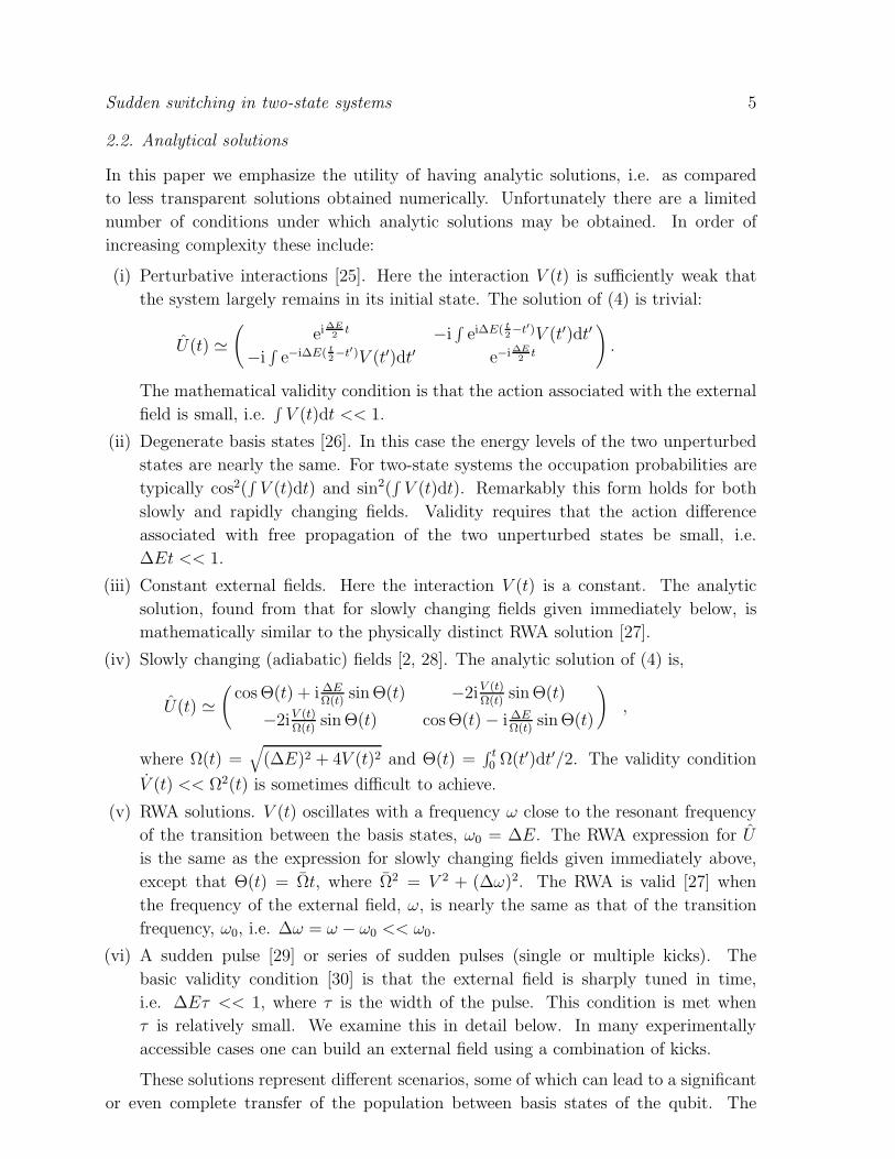
4.1.1. Two similar kicks First we calculate the probabilities for transitions caused by

two similar kicks. Both pulses are proportional to σx, but the action integral values are

different: V (t) = V1(t)·σx+V2(t)·σx (cf. (17)). In figure 1 we show results of a calculation

for the probability P2(t) that a system initially in the state

(

1

0

)

makes a transition into

the state

(

0

1

)

when perturbed by two pulses applied at t1 and t2. The ideal kick is

very nearly achieved since we choose τ to be a factor of 103 times smaller than the Rabi

time, T∆, for the population to oscillate between the two states. Peaks and dips in the

P2(t) graphs, that occur during application of a second pulse, reflect the following fact.

By the time second pulse is applied, the system already is in a superposition of the

basic states, and it’s this superposition that undergoes a precession when the pulse is

on. The final occupation probability of the target state doesn’t depend on the order in

which the kicks are applied. In figure 2, the results of a similar calculation for broader

pulses of width τ = 0.005T∆ are shown. The shape of the P (t) graph reflects the fact

that the pulses have finite width. However, the outcome of the calculation still doesn’t

depend on the order in which the kicks were applied.

4.1.2. Ordering effects As we have shown in the previous subsection, if two pulses act

on the system, then the outcome of the process is independent on the order in which they

are applied as long as the pulses are similar (e.g. two σx or two σy pulses). However, if

the two pulses that act on the system have different structure (e.g., one is a σx pulse,

and the other one is a σy pulse), then the results can be significantly different if different

sequences of pulses are used. In figure 3, the occupation probability of the target state is

calculated using two different sequences: an α1σx pulse followed by an α2σy pulse (solid

line) and an α2σy pulse followed by an α1σx pulse (dashed line). All the parameters are

identical to the ones used in the previous part (two σx pulses), except for the structure

of the pulses. The difference between two sequences is obvious. The effect of using

different order of pulses, as well as the occupation probabilities for each case, are in

very good agreement with the values calculated analytically (cf. (20)).

Sudden switching in two-state systems 12

0

0.2

0.4

0.6

0.8

1

0 100 200 300 400 500 600 700

Occ

up. p

roba

bilit

y

Time, arb. units

Figure 1. Target state probability as a function of time. Two σx kicks applied at

t1 and t2. Width of the kicks: τ = 0.001T∆. Action integral values: α1 = 0.1π,

α2 = 0.15π (chosen arbitrarily). The solid line: probability for α1 followed by α2; the

dashed line: probability for α2 followed by α1. The sharp dip due to using a pulse of

finite width is explained in the text. The final probability doesn’t depend on the order

of kicks.

0

0.2

0.4

0.6

0.8

1

0 100 200 300 400 500 600 700

Occ

up. p

roba

bilit

y

Time, arb. units

Figure 2. Target state probability as a function of time. Same as figure 1 but

broader kicks (kick width τ = 0.005T∆). The solid line: probability for α1 followed

by α2; the dashed line: probability for α2 followed by α1. The final probability still

doesn’t depend on the order of kicks.

Sudden switching in two-state systems 13

0

0.2

0.4

0.6

0.8

1

0 100 200 300 400 500 600 700

Occ

up. p

roba

bilit

y

Time, arb. units

Figure 3. Target state probability as a function of time. Two kicks, α1σx and α2σy,

applied at t1 and t2. Kick width τ = 0.001T∆. Action integral values: α1 = 0.1π,

α2 = 0.15π. The solid line: probability for α1σx followed by α2σy; the dashed line:

probability for α2σy followed by α1σx. The final probability depends on the order in

which the kicks are applied.

Even for a sequence of pulses of the same structure, the order of pulses can be

significant. To illustrate this fact, consider a series of three σx pulses. The results of

numerical calculations are shown in figure 4. As long as the time intervals between

pulses are not the same, the outcome of the process does depend on the sequence in

which the pulses are applied.

4.2. 2s− 2p transition in hydrogen

In this section we present the results of numerical calculations for 2s→ 2p transitions in

atomic hydrogen caused by a series of Gaussian pulses of width τ . Applicability of a two-

state approximation to this transition is discussed in detail in the Appendix. Specifically,

we consider the fine structure splitting of the 2p state (target state) into 2p1/2 and 2p3/2

states. As we show, the phase difference accumulated during free evolution between

pulses oscillates with the period Tr = 2π/Efs, where Efs ≈ 10956 MHz is the fine

structure splitting. Therefore, the same superposition state is formed periodically. By

choosing time intervals between kicks to be integer multiples of Tr, one can effectively

treat the superposition of 2p1/2 and 2p3/2 states as one state (2p state), that is coupled

to the initial 2s state. The occupation probabilities of the initial state 2s and the target

state 2p are evaluated by integrating two-state equations using a standard fourth order

Runge-Kutta method. This enables us to verify the validity of our analytic solutions for

Sudden switching in two-state systems 14

0

0.2

0.4

0.6

0.8

1

0 100 200 300 400 500 600 700

Occ

up. p

roba

bilit

y

Time, arb. units

Figure 4. Target state probability as a function of time. Three σx kicks applied at t1,

t2, and t3. Kick width τ = 0.001T∆. Action integral values: α1 = 0.1π, α2 = 0.15π,

α3 = 0.25π. The solid line: probability for α1 followed by α2 followed by α3; the

dashed line: probability for α3 followed by α2 followed by α1. The final probability

depends on the order of kicks.

kicked qubits in the limit as τ → 0 and also to consider the effects of time ordering.

The splitting between the 2s and 2p1/2 states in atomic hydrogen (Lamb shift) is

∆E ≈ 1057 MHz. The corresponding time scale (the Rabi time that gives the period of

oscillation between the states) is T∆ ≈ 10−9 seconds. This gives rise to the first limitation

on the duration of the pulse, τ : it has to be significantly smaller than T∆, otherwise the

pulse will not be sudden and the kicked approximation will fail. On the other hand if τ

is too small, then the interaction will have frequency components that couple the initial

state to other states. Specifically, if 1/τ is greater than (E3p −E2s) ≈ 1015 Hz, then the

interaction will induce transitions into states with n ≥ 3 and the system will not be well

approximated by a two-state model. Also there is another constraint in our case. If the

time of interaction becomes comparable to the lifetime of one of the active states (the

less stable 2p state has a lifetime of ≈ 1.6ns), then the dissipation effects (spontaneous

decay into the lower states outside two-state model) cannot be neglected.

Here we use Gaussian pulses with width τ = 1ps, and limit the time of interaction

to ≈ 600ps. Single and multiple pulses of such width (and even much shorter) are

achievable experimentally (e.g. half-cycle electromagnetic pulses, [33]). We explicitly

include in the numerical calculations both 2p1/2 and 2p3/2 states, and keep the time

separation between the pulses t2 − t1 = Tr. The loss of population from the two-state

system due to spontaneous decay (2p → 1s) is also included. The evaluation of α in

terms of the dipole matrix element for the 2s− 2p transition is discussed in a previous

Sudden switching in two-state systems 15

0

0.2

0.4

0.6

0.8

1

0 100 200 300 400 500 600 700

Occ

up. p

roba

bilit

y

Time, ps

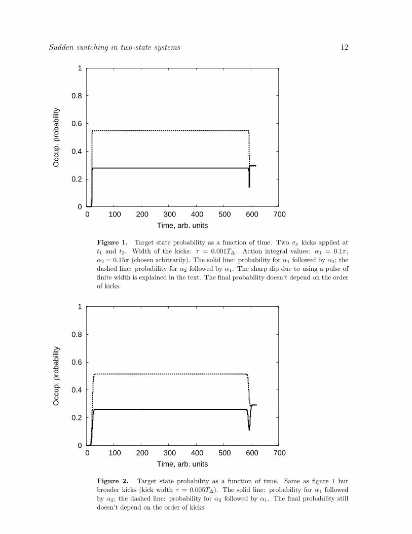
Figure 5. Target state probability as a function of time for 2s → 2p transition

in atomic hydrogen. Two σx kicks applied at t1 = 20ps and t2 = 593.5ps. Width

of the kicks: τ = 1ps. Action integral values: α1 = 0.1π, α2 = 0.15π. The solid

line: probability for α1 followed by α2; the dashed line: probability for α2 followed by

α1. The only difference in the final probability for different orders of kicks is due to

dissipation. As in figure 1, the sharp dips are real and due to the finite width of the

pulse.

paper [26]. We present results for the occupation probability of the target state, P2,

which includes both 2p1/2 and 2p3/2 states, as a function of time.

4.2.1. Two similar kicks In figure 5 we show the results of a calculation for the

probability P2(t) that a hydrogen atom initially in the 2s state makes a transition

into the 2p state when perturbed by two σx Gaussian pulses applied at t1 and t2. We

have obtained our results by numerically integrating the coupled equations,

id

dt

a1

a2

a3

=

∆E −V (t) −√

2V (t)

−V (t) −iΓ2

0

−√

2V (t) 0 (Efs − iΓ2)

·

a1

a2

a3

, (25)

where Γ ≈ 626 MHz is the decay rate for the 2p state, and we set E2p1/2= 0, so

E2p1/2= ∆E and E2p3/2

= Efs. For the calculation, we used the following parameters:

kicks applied at t1 = 20ps and t2 = 593.5ps (separation between the pulses is equal

to the revival time Tr for the superposition of 2p1/2 and 2p3/2 states); action integral

values: α1 = 0.1π, α2 = 0.15π. The final occupation probability of the target state

doesn’t depend on the order in which the kicks are applied. The small difference in the

final probabilities is entirely due to dissipation effects since the decay rates of 2s and

2p states in hydrogen differ by nine orders of magnitude. Removing dissipation yields

Sudden switching in two-state systems 16

0

0.2

0.4

0.6

0.8

1

0 100 200 300 400 500 600 700

Occ

up. p

roba

bilit

y

Time, ps

Figure 6. Target state probability as a function of time. Two kicks, α1σx and α2σy,

applied at t1 = 20ps and t2 = 593.5ps. Kick width τ = 1ps. Action integral values:

α1 = 0.1π, α2 = 0.15π. The solid line: probability for α1σx followed by α2σy ; the

dashed line: probability for α2σy followed by α1σx. The final probability depends on

the order in which the kicks are applied.

results indistinguishable from figure 3.

In figure 6, the occupation probability of the target state is calculated using two

different sequences: an α1σx pulse followed by an α2σy pulse (solid line) and an α2σy

pulse followed by an α1σx pulse (dashed line). All the parameters are identical to the

ones used in the previous part (two σx pulses), except for the structure of the pulses.

Now the difference between the effects of two sequences is obvious.

4.3. Effect of time ordering in a doubly kicked system

In this subsection we use our analytic expressions to examine the effect of the Dyson

time ordering operator, T , in a kicked two-state system. The effect of time ordering

has been considered previously in the context of atomic collisions with charged particles

[18, 20, 21, 22, 23, 24] and differs somewhat from the order in which external pulses

are applied, as illustrated below. As is intuitively evident, there is no time ordering in

a singly kicked qubit [30] since there is only one kick. The simplest kicked two-state

system that shows an effect due to time ordering is the qubit kicked by two equal and

opposite pulses separated by a time t− = t2 − t1. The evolution matrix U−kkI for this

system of (22) may be rewritten for convenience (as may be easily verified) as,(

e−i∆E2

t−(cos ∆E2t− + i cos 2α sin ∆E

2t−) e−i∆Et+ sin 2α sin ∆E

2t−

−ei∆Et+ sin 2α sin ∆E2t− ei∆E

2t−(cos ∆E

2t− − i cos 2α sin ∆E

2t−)

)

. (26)

Sudden switching in two-state systems 17

The limit of no time ordering, i.e. T → 1 in (8), may in principle be generally

obtained [30] by replacing∫ t0 VI(t

′)dt with V t, where V is an average (constant) value

of the interaction. In the case of two kicks of the same magnitude and opposite signs,

it is then straightforward to show that,

U(0)−kkI = e−iV t =

(

cos(2α sin ∆E2t−) e−i∆Et+ sin(2α sin ∆E

2t−)

−ei∆Et+ sin(2α sin ∆E2t−) cos(2α sin ∆E

2t−)

)

. (27)

In this example we now have analytic expressions for the matrix elements of both U−kkI

that contains time ordering and U(0)−kkI that does not include time ordering.

Let us now pause to examine the difference between time ordering and time reversal

in this simple, illustrative example. Reversal of time ordering means that, since αk and tkare both reversed, both t− → −t− and α→ −α. In this case one sees from the equations

above that U−kkI is not invariant, i.e. phase changes occur, while U

(0)−kkI remains the

same. Thus U−kkI changes when the time ordering is changed, but U

(0)−kkI does not

change. For time reversal [25] t± → −t± and, since the initial and final states are also

interchanged, U → U †. In this case one sees by inspection of the above equations that

both U−kkI and U

(0)−kkI are invariant under time reversal, as expected. As shown below

when the symmetry of the kicks is broken the difference between UkUk′

and Uk′

Uk can

be observed.

We have shown above both algebraically and numerically that for two kicks

proportional to σx, the order of the kicks does not change the final population transfer

probability P2. However, interestingly, this does not mean that there is no effect due

to time ordering in this case. As we show next, there is an effect due to time ordering

in this case, even though reversing the order of the kicks has no effect. The effect

of time ordering on the occupation probabilities may be examined by considering the

probability of transfer of population from the on state to the off state with and without

time ordering, namely,

P2 = |U12|2 = | sin 2α sin∆E

2t−|2 = |ǫ sinφ|2 , (28)

P(0)2 = |U (0)

12 |2 = | sin(2α sin∆E

2t−)|2 = | sin ǫφ|2 ,

where ǫ = sin ∆E2t− and φ = 2α.

The effect of time ordering is shown in figure 7, where P2 − P(0)2 is plotted as a

function of φ = 2α, corresponding to the strength of the kicks, and ǫ = sin ∆E2t−, which

varies with the time separation of the two kicks. The effect of time ordering disappears in

the example we present here in the limit that either the interaction strength or the time

separation of the pulses goes to zero. For small, but finite, values of both the interaction

strength and the time separation of the pulses, the effect of time ordering is to reduce

the probability of transition from the initially occupied state to an initially unoccupied

state. That is, in this regime time ordering reduces the maximum transfer of population

from one state to another. As either of these two parameters gets sufficiently large, the

Sudden switching in two-state systems 18

-1 -0.8 -0.6 -0.4 -0.2 0ε 0

1 2

3 4

5 6

φ

-1-0.8-0.6-0.4-0.2

0 0.2 0.4 0.6

P2 - P2(0)

Figure 7. Difference in population transfer probability, P2 − P(0)2 vs. ǫ = sin ∆E

2 t−

and φ = 2α. Here t− = t2 − t1 is the time between the pulses and α =∫

V (t′)dt′ is a

measure of the interaction strength. The two-state system is kicked by a sharp pulse

of strength α at time t1 and by an equal and opposite pulse at time t2. The difference,

P2 − P(0)2 , is due to time ordering in this qubit.

effect of time ordering oscillates with increasing values of the interaction strength or the

separation time between the two pulses. Time ordering effects are present even though

U−kk = Uk−k.

5. Discussion

Clearly one may extend this approach past two kicks or three. Since arbitrary pulses

can be built from a series of kicks, in principle one may build arbitrarily complex pulses

using kicks. While adding more kicks is straightforward, the algebra becomes more

difficult. Also, the number of natural systems in which the validity conditions apply

diminishes as the pulse becomes more complex. Hence it may be sensible to seek cases

that have sufficient symmetry so the analysis is both simple and applicable. It has been

previously noted [30], for example, that a simple expression, corresponding to Floquet

states, exists for a periodic series of narrow pulses.

Part of the motivation for this paper grew out of an effort to define correlation

in time [20], based on effects of time ordering. While in principle we have found no

fundamental problem with this effort, we have found that it is often difficult to find

expressions for the time evolution matrix in the limit of no time ordering, namely U0.

Furthermore, U0 can depend on the representation used [30]. We also note that time

ordering may occur in the degenerate limit, e.g. when H = H0σz +V1(t)σx +V2(t)σy. In

Sudden switching in two-state systems 19

recent applications in collision dynamics using perturbation theory [21], time ordering

is removed by use of degenerate states since the external interactions do not contain

more than one type of coupling. But in these calculations there is no difference between

time ordering and time correlation. The most reliable way to remove time ordering

is replacement [30] of the instantaneous interaction V (t) by its time averaged value,

V = 1t

∫ t0 V (t′)dt′.

In summary, analytic solutions for two-state systems (e.g. qubits) strongly

perturbed by a series of rapidly changing pulses, called ‘kicks’, have been developed

and discussed. Such analytic solutions provide useful physical insight, which together

with more complete numerical methods [34, 35] may be used to solve more complex

problems. For a series of kicks the evolution matrix may be expressed as a time ordered

product of single kicks. We have explicitly considered in detail single, double, and triple

kicks. While there is no difference in the population transition probability if two σx kicks

are interchanged, time ordering does have an observable effect. The effect happens to

be the same for both of these orderings. If a σx kick is interchanged with a σy kick in

a doubly kicked system, the difference can be observed in most cases. If three σx kicks

are used, different orderings can also be observably different. The effect of using pulses

of finite widths has been studied numerically for 2s−2p transitions in atomic hydrogen.

If the pulse width is much smaller than the Rabi time of the active states, then the

analytic kicked solutions are valid. Such pulses can be created experimentally using

existing microwave sources. The difference between time ordering and time reversal

has been specified. Time ordering can have observable effects. Under time reversal

the quantum amplitudes are generally invariant. Our results may be extended to an

arbitrary number of kicks. However, without simplifying symmetries, the solutions

become more complex, and the applicability of this approach becomes more limited, as

the number of kicks increases.

Appendix

Here we discuss some details concerning the use of the two-state approach for studying

the 2s – 2p transition in hydrogen. First, we note that the eight n = 2 states (two 2s1/2

states, two 2p1/2 states, and four 2p3/2 states) are nearly degenerate and well separated

in energy from states with n 6= 2. Thus, smooth external pulses may easily be chosen

long enough to prevent field-induced population transfer out of the n = 2 subspace, and

requiring us only to include the spontaneous decay rate Γ from 2p to 1s. Furthermore,

rotational invariance around the axis of the external electric field ~E leads to conservation

of total angular momentum component along that direction, allowing a given 2s1/2 state

to couple only to one 2p1/2 state and one 2p3/2 state. Specifically, starting with an initial

2s1/2 state with spin polarization at some angle χ relative to ~E, the accessible subspace

Sudden switching in two-state systems 20

is spanned by the three basis vectors

|2s〉 = |ℓ = 0, m = 0〉|χ〉|2p〉 = |ℓ = 1 , m = 0〉|χ〉 (A.1)

|2p′〉 = cosχ

2|ℓ = 1 , m = +1〉| ↓〉 + sin

χ

2|ℓ = 1 , m = −1〉| ↑〉

where the initial spin state is |χ〉 = cos χ2| ↑〉 + sin χ

2| ↓〉, and both orbital angular

momentum and spin components are measured along the direction of ~E.

Since the external pulse does not change the orbital angular momentum component

m, the external field couples only the two states |2s〉 and |2p〉 in the above basis, e.g.

V (t) = V (t)

0 1 0

1 0 0

0 0 0

(A.2)

for a σx pulse. The free Hamiltonian H0 is diagonal in the basis of good total angular

momentum j. In the basis of (A.1),

H0 =

E2s1/20 0

0 23E2p3/2

+ 13E2p1/2

− iΓ2

√2

3Efs

0√

23Efs

13E2p3/2

+ 23E2p1/2

− iΓ2

, (A.3)

where Efs = E2p3/2−E2p1/2

is the fine structure splitting, and we take the decay rate Γ

to be the same for 2p1/2 and 2p3/2.

For narrow pulses, whose inverse width 1/τ is large compared both with the splitting

∆E between the 2s1/2 and 2p1/2 energies (Lamb shift) and also Efs (fine structure), the

free propagation may be neglected during the time of the pulse. Then the full propagator

in the interaction representation may be written as a product of kick operators of the

form e+itH0tne−i∫

dtVn(t)e−iH0tn , where tn is the time of the nth kick. Now e−i∫

dtVn(t) is

block-diagonal by construction (A.2), with the 2p′ state decoupled. In between pulses,

amplitude oscillates between the 2p and 2p′ states with period Tr = 2π/Efs. However,

if we now choose all inter-pulse spacings to be integer multiples of this period,

∆tn = tn+1 − tn = mTr , (A.4)

then the free propagation between kicks also becomes diagonal:

e−iH0∆tn =

e−iE2s1/2

∆tn 0 0

0 e(−iE2p1/2

−Γ/2)∆tn 0

0 0 e(−iE2p1/2

−Γ/2)∆tn

, (A.5)

as may easily be checked explicitly by writing the above free propagator in the 2p1/2,

2p3/2 basis and noting that the two basis vectors acquire the same phase e−iE2p1/2

∆tn =

e−iE2p3/2

∆tn . Thus the 2p′ state decouples entirely and its occupation probability will

always be zero when we view the dynamics stroboscopically with period Tr starting with

the time t1 of the first kick. The three-state dynamics therefore reduces to two-state

dynamics in the 2s, 2p subspace.

Sudden switching in two-state systems 21

Finally, as long the the inter-kick spacings are all integer multiples of Tr, we may

also use the two-state formulas presented in the main body of the paper to evaluate the

occupation probabilities at an arbitrary time between kicks or after the last kick. We

need only remember that the 2p probability that we compute at these arbitrary times

is the total probability for being in either the 2p and 2p′ state, or equivalently the total

probability for being in either the 2p1/2 or 2p3/2 state.

Acknowledgments

DBU acknowledges support under NSF grant 0243473.

References

[1] Allen L and Eberly J H 1987 Optical Resonance in Two-level Atoms (New York: Dover)

[2] Shore B W 1990 Theory of Coherent Atomic Excitation (New York: Wiley)

[3] Poole C P, Farach H A and Creswick R J 1995 Superconductivity (San Diego: Academic Press);

van der Wal C H, ter Haar A C J, Wilhelm F K, Schouten R N, Harmans C J P M, Orlando T

P, Lloyd S and Mooij J E 2000 Science 290 773

[4] Nielsen M A and Chuang I L 2000 Quantum Computation and Quantum Information (Cambridge:

Cambridge University Press); Cirac J I and Zoller P 1995 Phys. Rev. Lett. 74 4091

[5] Mandel L and Wolf E 1995 Optical Coherence and Quantum Optics (Cambridge: Cambridge

University Press)

[6] Stockmann H-J 1999 Quantum Chaos: An Introduction (Cambridge: Cambridge University Press);

Reichl L E 2004 The Transition to Chaos: Conservative Classical Systems and Quantum

Manifestations (New York: Springer)

[7] Moore F L, Robinson J C, Bharucha C F, Sundaram B, and Raizen M G 1995 Phys. Rev. Lett.

75 4598

[8] Fishman S, Grempel D R, and Prange R E 1982 Phys. Rev. Lett. 49 509

[9] Kosloff R, Hammerich A D, and Tannor D 1992 Phys. Rev. Lett. 69 2172

[10] Kosloff R, Rice S A, Gaspard P, and Tannor D 1989 Chem. Phys. 139 201

[11] Shi S, Woody A, and Rabitz H 1988 J. Chem. Phys. 88 6870

[12] Palao J and Kosloff R 2002 Phys. Rev. Lett. 89 188301

[13] Slichter C P 1996 Principles of Magnetic Resonance (Berlin: Springer)

[14] Ernst R R, Bodenhausen G, and Wokaun A 1990 Principles of Nuclear Magnetic Resonance in

One and Two Dimensions (Oxford: Oxford University Press)

[15] Jones J A, Hansen R H, and Mosca M 1998 J. Magn. Reson. 138 353

[16] Vandersypen L M K, Steffen M, Breyta G, Yannoni C S, Sherwood M H, and Chuang I L 2001

Nature 414 883

[17] Expressions somewhat similar to ours have been noted by P. R. Berman and R. G. Brewer, private

communication (2004); also see Berman P R and Steel D G in Handbook of Optics vol. IV ed

M. Bass et al (New York: McGraw-Hill)

[18] McGuire J H 1987 Electron Correlation Dynamics in Atomic Scattering (Cambridge: Cambridge

University Press)

[19] 2004 Proc. Ann Arbor Conf. Building Computational Devices using Coherent Control ed V

Malinovsky; Rangan C, Bloch A M, Monroe C and Bucksbaum P H 2004 Phys. Rev. Lett.

92 113004; Wineland D J et al 1998 J. Res. Natl. Inst. Stand. Technol. 103, 259; Turinici G

and Rabitz H 2001 J. Chem. Phys. 267, 1

[20] Godunov A L and McGuire J H 2001 J. Phys. B: At. Mol. Opt. Phys. 34 L223. Time correlation is

Sudden switching in two-state systems 22

defined as a deviation from the independent time approximation (ITA), where U(t) =∏

j Uj(t),

where the Uj(t) include time ordering for each particle.

[21] Godunov A L et al 2001 J. Phys. B: At. Mol. Opt. Phys. 34 5055

[22] Zhao H Z, Lu Z H and Thomas J E 1997 Phys. Rev. Lett. 79 613

[23] Andersen L H et al 1986 Phys. Rev. Lett. 57 2147

[24] Merabet H, Bruch R, Hanni J, Godunov A L and McGuire J H 2002 Phys. Rev. A 65 010703(R)

[25] Goldberger M L and Watson K M 1964 Collision Theory (New York: Wiley)

[26] Shakov Kh Kh and McGuire J H 2003 Phys. Rev. A 67 033405

[27] Milonni P and Eberly J H 1985 Lasers (New York: Wiley)

[28] Solov’ev E A 1989 Phys. Usp. 32(3) 228; Nikitin E E 1984 Theory of Slow Atomic Collisions

(Berlin: Springer-Verlag)

[29] Demkov Yu N, Ostrovskii V N and Solov’ev E A 1978 Phys. Rev. A 18 2089

[30] Kaplan L, Shakov Kh Kh, Chalastaras A, Maggio M, Burin A L and McGuire J H 2004 Phys.

Rev. A 70 063401

[31] Bergamann K, Theuer H, and Shore B W 1998 Rev. Mod. Phys. 70 1003

[32] Tannor D 2004 Introduction to Quantum Mechanics: A Time-Dependent Perspective (Sausalito,

CA: Univ. Science Books)

[33] Jones R R, You D and Bucksbaum P H 1993 Phys. Rev. Lett. 70 1236; Matos-Abiague A and

Berakdar J 2004 Appl. Phys. Lett. 84(13) 2346

[34] Lindblad G 1976 Commun. math. Phys. 48 119

[35] Breurer H-P and Petruccione F 2002 The theory of open quantum systems (Oxford: Oxford

University Press)