Hydrobiologia 328 : 1 73 -197, 1996 .

173© 1996 Kluwer Academic Publishers. Printed in Belgium.

Subtle relationships: freshwater fishes and water chemistry in southernSouth America

Roberto C. Menni l "2 , Sergio E. Gomez 1 '3 & Fernanda Lopez Armengol l,4

1 Consejo Nacional de Investigaciones Cientificas2Museo de La Plata, Paseo del Bosque s/n, 1900 La Plata, Argentina31nstituto de Limnologia de La Plata4Facultad de Medicina, Universidad Nacional de La Plata

Received 15 December1994 ; in revised form 14 November 1995 ; accepted 22 November 1995

Key words : water chemistry, environment, ecology, fish geography, physiology, cluster and PC analysis

Abstract

We investigated the relationships between water chemistry and the occurrence, distribution, physiology, andmorphology of fish faunas. We examined 34 species (ca . 10% of the Argentinean freshwater fish fauna) from 120localities (5 areas) situated between 26°15' S (Trancas, 'lucuman) and 38°30' S (Sierra de la Ventana, BuenosAires). Fourteen chemical features are described by : conductivity, total dissolved solids, temperature, pH, CO3 2 ,CO3H- , Cl- , SO4- , Cat+, K+ , Mgt+, Na+, Mg/Ca, Mg+Ca/Na+K. Three Basic Data Matrices considering themean, maximum and minimum values of each variable for each fish species were used in a Cluster and PrincipalComponent Analysis . Groups of species clustered in similar ways to particular water chemistries . Similarity wasthe common occurrence of species in a defined area and preference for a common range of the factors considered .Groups of species so defined showed patterns of distribution related to climate, environment, trophic state andhydrographic complexity. Each cluster included some eurytopic species which appeared together at extremechemical and geographic characteristics . Twenty four species had ranges of tolerance for the 14 variables andevidence of a grouping according to these ranges. Eighteen species which occurred at maximum or minimumabsolute values for more than one factor were ordered along an eurytopy - stenotopy axis. We support the statementthat species with a larger tolerance range for most factors have a higher probability of being widely distributed .Astyanax fasciatus and A. bimaculatus tolerated the highest number of maximum and minimum values, followedby Jenynsia l. lineata, A. eigenmanniorum and Trichomycterus corduvensis . Groups of species based on chemicalfactors showed differences in the relative number of basic morphological types .

Introduction

Although many experimental studies have explored theresponse of fishes to environmental factors (Fry, 1971 ;Braga, 1975; Dunson et al ., 1977; Gomez, 1993 ;Kramer, 1987 ; Pickering, 1981; Wootton, 1991), fishbehavior in relation to complex interactions amongdiverse variables in nature is difficult to describe . Itis difficult to find strong correlations between chemi-cal factors and fish distribution patterns, except underextreme conditions (Stevenson et al ., 1974) .

* This paper was submitted at the symposium `Fish Ecology inLatin America' during the 1993 meeting of the ASIH at Austin .

Some physical - chemical characteristics are rela-tively easy to obtain, and have been considered in theevaluation of aquatic environments and their faunas(e .g . Bonetto & Lancelle,1981 for the Parana River ;Geisler et al ., 1975 for the Amazon ; Ringuelet et al.,1967b for the Pampasic lagoons) . As far as the influ-ences on fishes is concerned, the importance of naturalwater chemical composition on fish occurrence andbehavior have, in general terms, either been neglectedor considered too difficult to evaluate (Hynes, 1970 ;Whitton, 1975; Menni et al ., 1984). Though the gen-eral chemical composition of several basins is known,global values can not be related a priori to the presence

174

or absence of fishes, given the habitat variability andthe differences in spatial distribution of these organ-isms .

A synthesis of the predominant view can be seenin the following excerpts from Beadle (1974 : 51, 52,57): `The apparently insignificant ecological effects ofionic differences within the freshwater range shouldnot surprise us, because, in contrast to the sea, inlandwaters are chemically unstable and variable by nature,and could have been colonized only by organisms withionic regulating mechanisms that can function under awide range of chemical conditions . . . It seems, there-fore, that within the limits of composition of mostinland freshwater, faunal and floral differences arerarely directly explicable in terms of mineral chem-ical differences . . . In conclusion, it may be repeatedthat in tropical African freshwater (within the salinityrange 0 .02-5%°) there is so far no evidence of a directecological effect of a peculiar mineral composition' .

The opposite opinion has been briefly stated byRoberts (1972 : 123). He says, in reference to thewater conditions in the Rio Negro of Brazil that `Thecharacteristics of the basins and the water chemistryplay profound roles in determining the distribution andabundance of animals in the Amazon basin' . Moreexact statements have been given for the associationof Corydoras macropterus and Mimagoniates lateraliswith black waters and that of Corydoras barbatus withclear waters (Weitzman et al., 1988) . The limited dis-tribution of a Curimata species in the Rio Negro inBrazil appears to be primarily a consequence of thepreference of the species for acidic black waters (Vari,1988) .

We surveyed the relationship between the occur-rence of fish species and a set of fourteen physical andchemical variables usually obtained as descriptors ofthe main features of water .

The combination of Cluster Analysis and PrincipalComponent Analysis used in this paper provides newinsights in the study of the shared occurrence of fish-es, their geographical peculiarities and environmentalcharacteristics . More importantly, the analysis showsthat groups of species react in a similar way to com-binations of properties of water, and provides a newframework for the experimental study of physiologyand adaptation in freshwater fishes .

Materials and methods

Source of data

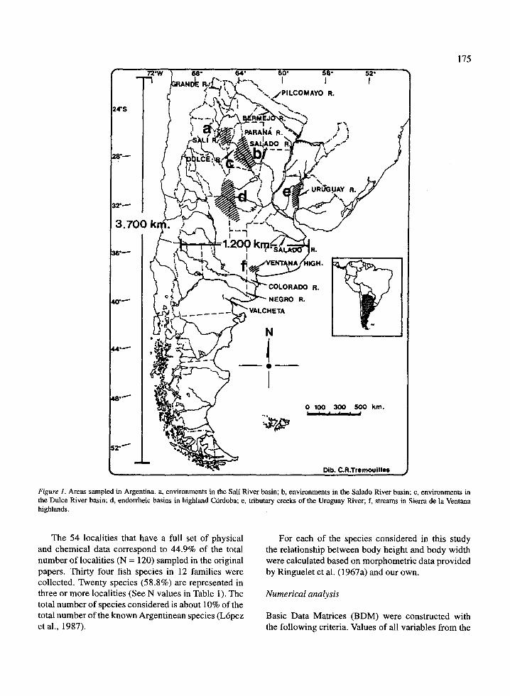
The fish composition and the physical and chemicalvariables from limnetic environments in five zonescovering a wide area of the temperate region ofArgentina (Figure 1) were used as basic data for thepresent paper, namely :

(a) Environments in the Sali River basin (Tucumdnprovince) . Presence data of 21 fish species andphysical - chemical data from 10 localities wereavailable from Miquelarena et al . (1990) .

(b) Environments in the Salado River basin (Santiagodel Estero province). Presence data of fish speciesand physical - chemical data from 3 localities wereavailable from Casciotta et al . (1989) .

(c) Environments in the Dulce River basin (Santiagodel Estero province) . Presence data of 3 speciesand physical - chemical data from 1 locality wereavailable from Casciotta et al . (1989) .

(d) Localities in the highland region of northwesternC6rdoba. Presence data of 9 fish species and phys-ical - chemical data from 29 localities were avail-able from Menni et al . (1984) .

(e) Tributary creeks of the Uruguay River . Presencedata of 19 fish species and physical - chemicaldata from 7 localities were available from L6pez etal. (1984) .

(f) Creeks in Sierra de la Ventana highlands (BuenosAires province) . Presence data of 5 fish speciesand physical - chemical data from 4 localities wereavailable from Menni et al. (1988) .

All data were gathered by the senior author duringprojects under his direction . Complete faunistic lists,environmental descriptions, and physical and chemicalsynopsis of the studied areas can be obtained from theabovementioned papers . Water samples collected forexamination of limnological variables were obtainedimmediately prior to fishing operations . The wateranalyses were made at the Chemistry Laboratory ofthe Instituto de Limnologia de La Plata using APHA(1985) techniques . Values of the following variableswere obtained (in parenthesis abbreviations, and unitsused in the text and tabels): Conductivity (COND, /sScm-1 ), Total dissolved Solids (TDS, mg 1 -1 ), temper-ature (t, °C), pH, CO3

-2, CO3- H, C1- , SOn+2 , Ca+2 ,K+, Mg+ 2 , Na+ (ions in mg l-1 ) and the ratios Mg/Caand Mg+Ca/Na+K .

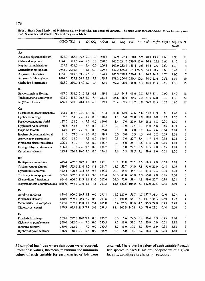
The 54 localities that have a full set of physicaland chemical data correspond to 44 .9% of the totalnumber of localities (N = 120) sampled in the originalpapers. Thirty four fish species in 12 families werecollected. Twenty species (58 .8%) are represented inthree or more localities (See N values in Table 1) . Thetotal number of species considered is about 10% of thetotal number of the known Argentinean species (Lbpezet al., 1987) .

175

Figure 1 . Areas sampled in Argentina . a, environments in the Sali River basin; b, environments in the Salado River basin ; c, environments inthe Dulce River basin ; d, endorrheic basins in highland Cordoba ; e, tributary creeks of the Uruguay River ; f, streams in Sierra de la Ventanahighlands .

For each of the species considered in this studythe relationship between body height and body widthwere calculated based on morphometric data providedby Ringuelet et al. (1967a) and our own .

Numerical analysis

Basic Data Matrices (BDM) were constructed withthe following criteria. Values of all variables from the

176

Table 1 . Basic Data Matrix 1 of 34 fish species by 14 physical and chemical variables . The mean value for each variable for each species wasused . N = number of samples . See text for groups labels.

AxAstyanax eigenmanniorumCharax stenopterusHoplias m . malabaricusSerrasalmus spilopleumAstyanax f. fasciatusAstyanax b. bimaculatusCheirodon i .interruptus

BxBryconamericus iheringiTrichomycterus corduvenseJenynsia 1 . lineata

FxPimelodella laticepsCichlasoma portalegrenseJobertina rachowiHyphessobrycon luetkeni

COND TDS t pH CO3- C031-1- Cl- SOy- Na+ K+ Ca2+ Mgt+ Mg/Ca Mg+Ca/ NNa+K

627.0 466.9 19 .6 7 .3 0 .0 230.31144.0 812 .6 -- 7.5 0 .0 270.0869 .5 621 .0 -- 7.4 0 .0 209 .2

2944 .0 2019 .6 -- 7.8 0 .0 499 .71108 .0 788.0 19 .8 7 .5 0 .0 194.81084 .0 825 .1 20 .4 7 .8 3 .9 199 .5665.0 500.0 17 .0 7.7 1 .4

183.0

417 .0 361 .0 21 .6 7 .8 6.1 179 .6502 .0 415.0 20 .5 7.9 7.4 213 .0656 .3 500.0 20.4 7 .8 6.6

189.8

CxCnesterodon decemmaculatus 363 .2 317.8 24 .0 7.3 0.0 181 .4Cyphocharax yoga 187.0 158.0 7.2 0.0 110 .0Pseudocorynopoma doriai 187.0 158 .0 7 .2 0.0 110 .0Hyphessobrycon anisitsi 166.5 153 .5 7 .3 0 .0 93.7Diapoma terofali 44.0 47.0 7.0 0 .0 26.8Hyphessobrycon meridionalis 71 .0 57.0 6.6 0.0 19 .5Aphyocharax rubropinnis 182.0 164.0 7.2 .0.0 116.8Pimelodus clarias maculatus 206.0 181 .0 7 .6 0 .0 138.7Iheringichthys westermanni 206.0 181 .0 7 .6 0 .0 138 .7Corydoras paleatus

233.4 220.7 19.0 7 .6 0.0 156 .2

DxHeptapterus mustelinus 425 .4 432 .0 20.7 8 .0 8 .2 197 .1Trichomycterus alterum 529 .0 553 .0 21 .0 8 .0 8.8 224.7Hypostomus cordovae 472.4 420.8 22.3 7 .8 9 .2 155.5Trichomycterus spegazzinii 555 .0 522 .0 21 .0 8 .2 9 .6 123 .4Characidium f. fasciatum 664.0 664.0 21 .3 8 .4 11.0 207 .0Jenynsia lineata alternimaculata 1015 .0 984 .0 23 .0 8 .2 7 .2 207 .2

ExAcrobrycon tarijaePimelodus albicansOdontostilbe microcephalaOligosarcus jenynsi

830.0 909 .0 20.5 8 .8 0 .0 291 .8830.0 909 .0 20 .5 7 .9 0 .0 291 .8577 .0 702 .0 19 .8 8 .2 2 .4 205 .0850.3 675.1 21 .3 7 .9 3 .6 239 .5

263 .0 247 .0 20.0 7 .4 0 .0 175 .7350.0 312 .0 -- 7.0 0 .0 230.5350.0 312 .0 -- 7.0 0 .0 230.5158.0 148 .0 -- 6 .8 0 .0

94.9

54 sampled localities where fish occur were recorded .From those values, the mean, maximum and minimumvalues of each variable for each species of fish were

52 .9 97.4 120.8 8 .2 40 .7 13 .8 0.60 0.90 11145 .2 281 .0 249 .9 11 .6 70 .8 25.8 0.60 1 .10 3109.0 212.1 188 .4 9 .6 54 .8 2.0 0.60 1 .30 4432.2 835.4 69 .3 27.5 164 .3 60 .5 0.60 0.43 1186.3 228.3 230.4 9 .1 74 .7 24 .3 0.70 1 .90 7171 .2 206.0 220 .3 10 .2 74.0 22 .4 0.56 1 .56 1097.2 106.0 126 .0 6 .3 45.6 14 .5 0.50

1.30

15

19.5 34.5 63.6 5 .8 35 .7 11 .1 0.60 1 .40 1825.8 36.0 80 .3 7 .2 31 .5 12 .8 0.70 1 .30 2278 .4 69.5 117 .2 5 .9 36.7 12 .5 0 .52

0.90

17

20.8 32.0 57 .6 6 .6 33 .7 11 .3 0 .60 1 .48 41 .1

5.0 20.0 3 .9 18.0 6 .8

0.62

1.50

31.4 5.0 20.0 3 .9 18 .2 6.8 0 .70 1 .70 30.3

3.0 19 .5 3 .7 14.0 5 .8

0.66

1.39

20.3

3.0

4.0 3.7

6.6 2.6 0.64

2.08

10.0

5.0

3.3 4.3

6.6 3.2 0.79

2.36

10.3

5.0 22.7 3 .4

1.7 5.4 0.52

1.24

20.3 5 .0 28 .7 3 .6 17 .5 7 .0 0 .65 1 .08 10 .3 5 .0 28 .7 3.6 17 .5 7 .0 0 .65 1 .08 15 .6

5.3 28.5 3 .1 29 .6 9.0 0 .51

1.70

5

10.3 33.8 29 .2 3 .5 68 .5 19 .0 0.50 3.60 513 .2 53 .7 34.0 3 .8 91 .0 26 .0 0 .48 4 .05 322 .3 38 .5 45 .4 3.1 51.3 12 .4 0 .30 1 .70 560 .0 49 .0 65.0 4.0 65.0 19 .0 0 .46 2 .50 335.0 75 .0 53 .4 4.3 99 .0 22 .7 0.34 2 .71 284.4 129 .5 108 .0 5 .7 142 .0 37 .4 0.44

2.80

2

15.3 121 .0 56 .7 4.7 157 .7 38 .3 0 .40 4 .27 115 .3 121 .0 56.7 4.7 157 .7 38 .3 0.40 4 .27 113 .4 75 .5 83 .0 4.5 96.3 24.0 0.43 2.40 288.4 166 .9 145 .8 9 .0 78 .6 22 .3 0.44

2.00

6

6.0 6 .6 29 .5 3 .4 36.4 10.3 0.458.7 11 .0 37 .3 5 .3 50.9 15 .9 0 .518.7 11 .0 37 .3 5 .3 50.9 15.9 0.510 .3

5.0 16.7 3.2 16 .4 3 .8 0 .38

2 .00 32.18 12 .18 11 .40

1

obtained . Therefore the values of each variable for eachfish species in each BDM are independent of a givenlocality, avoiding circularity of reasoning .

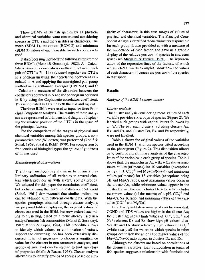
Three BDM's of 34 fish species by 14 physicaland chemical variables were constructed consideringspecies as OTU's and the variables as characters . Themean (BDM 1), maximum (BDM 2) and minimum(BDM 3) values of each variable for each species wasused .

Data processing included the following steps for thethree BDM's (Menni & Gosztonyi, 1982) : A - Calcu-late a Pearson's correlation coefficient between eachpair of OTU's ; B - Link (cluster) together the OTU'sin a phenogram using the correlation coefficient cal-culated in A and applying the unweighted pair-groupmethod using arithmetic averages (UPGMA) ; and C- Calculate a measure of the distortion between thecoefficients obtained in A and the phenogram obtainedin B by using the Cophenetic correlation coefficient .This is indicated as CCC in both the text and figures .

The three BDM's were used as input for three Prin-cipal Component Analysis . The results of these analy-ses are represented in bidimensional diagrams display-ing the relative position of the OTU's in the space ofthe principal factors .

For the comparison of the ranges of physical andchemical variables among fish species groups, a non-parametrical test (Wilcoxon) was performed (Rohlf &Sokal, 1969 ; Sokal & Rohlf, 1979) . For comparison offrequencies of biological types the x 2 test of goodnessof fit was used .

Methodological observations

The chosen methodology allows us to obtain a pre-liminary ordination of all variables in several clus-ters which provides us with several species groups .We selected for this paper the correlation coefficient,but a check using the Taxonomic distance coefficient(Sokal, 1961) demonstrated that similar ordinationscan be obtained with different coefficients . With thespecies groupings obtained through cluster analysis,we prepared tables displaying the original values ofcharacters used in the BDM, but now ordered accord-ing to clustering, based on a tactic already used in astudy of marine fish communities (Menni & Gosztonyi,1982; Menni & Lopez, 1984) . This procedure allowsto identify which values, or combination of values,support the clustering . As has been extensively dis-cussed, it is not necessary to choose a significancevalue for the clusters in non-taxonomic analyses, andgroups at any level can be studied to find any classof properties (Mello & Buzas, 1968) . Cluster analysisallowed us to identify groups of species based on sim-

177

ilarity of characters ; in this case ranges of values ofphysical and chemical variables. The Principal Com-ponent Analysis identified those characters responsiblefor each group . It also provided us with a measure ofthe importance of each factor, and gave us a graphicdisplay of the relative position of species in characterspace (see Margalef & Estrada, 1980). The represen-tation of the regression lines of the factors, of whichwe selected a few as examples, show how the valuesof each character influences the position of the speciesin that space .

Results

Analysis of the BDM I (mean values)

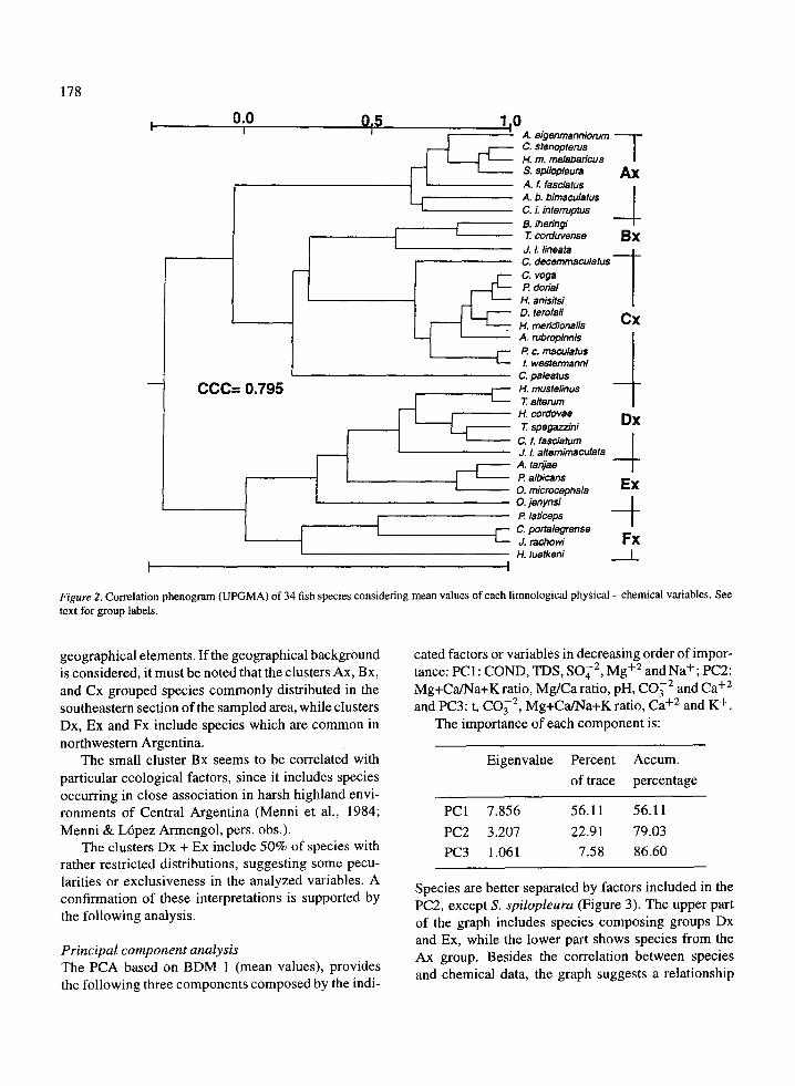
Cluster analysisThe cluster analysis considering mean values of eachvariable provides six groups of species (Figure 2) . Welabelled such groups with capital letters followed byan `x' . The two main clusters including clusters Ax,Bx, and Cx, and clusters Dx, Ex, and Fx respectively,were not labelled .

Table 1 shows the original values of the variablesused in the BDM 1, with the species listed accordingto the phenogram (Figure 2) . This disposition allowsus to perform a preliminary analysis of the character-istics of the variables in each group of species . Table 1shows that : the main cluster Ax + Bx + Cx shows max-imum values (of means) for 10 variables (exceptionsbeing t, pH, CO3 2 and Mg+Ca/Na+K) and minimumvalues (of means) for 13 variables (exceptions beingpH and Mg/Ca ratio) ; most maximum values occur inthe cluster Ax, while minimum values appear in thecluster Cx; and the main cluster Dx + Ex + Fx includesmaximum values (of the means) of t, pH, CO3 2 andMg+Ca/Na+K ratio, and minimum values of two vari-ables (CO3 2 and Mg/Ca) .

In a less quantitative manner it can be seen that :COND and TDS values are higher in the cluster Ax ;the cluster Ax shows high values of Cl - , SO42 andNa+ ; clusters Dx and Ex show high pH values ; clus-ters Bx and Dx show relatively high values of CO3 2(while nearly all the waters in which species in othergroups occur lack the anion) and higher values of theMg+Ca/Na+K ratio appear in clusters Dx and Ex .

Although the clusters are based on correlations ofthe chemical variables, their composition in terms offish species suggests a relationship with faunistic and

178

1 0.0

CCC= 0.795

0F5

geographical elements . If the geographical backgroundis considered, it must be noted that the clusters Ax, Bx,and Cx grouped species commonly distributed in thesoutheastern section of the sampled area, while clustersDx, Ex and Fx include species which are common innorthwestern Argentina .

The small cluster Bx seems to be correlated withparticular ecological factors, since it includes speciesoccurring in close association in harsh highland envi-ronments of Central Argentina (Menni et al ., 1984 ;Menni & Lopez Armengol, pers . obs .) .

The clusters Dx + Ex include 50% of species withrather restricted distributions, suggesting some pecu-larities or exclusiveness in the analyzed variables . Aconfirmation of these interpretations is supported bythe following analysis .

Principal component analysisThe PCA based on BDM 1 (mean values), providesthe following three components composed by the indi-

oA. eigenmanniorumC. stenopterusH. m. malabaricusS. spilopleura

AXA. f. fasciatusA. b. bimaculatusC. L interruptusB. iheringiTT corduvense

BxJ. l. lineataC. decemmaculatusC. yogaP doriaiH. anisitsiD. terofaliH. meridionalisA. nibropinnisP. c. maculatusl. westermanniC. paleatus

C H. mustelinusTT alterumH. cordovae7 spegazziniC. f. fasciatumJ. L altemimaculataA . tarijaeP. albicans0. microcephala0. jenynsiP laticepsC C. ponalegrenseJ. rachowiH. luetkeni

CX

Figure 2 . Correlation phenogram (UPGMA) of 34 fish species considering mean values of each limnological physical - chemical variables . Seetext for group labels.

cated factors or variables in decreasing order of impor-tance : PC 1 : COND, TDS, SO4 2 , Mg+2 and Na+ ; PC2 :Mg+Ca/Na+K ratio, Mg/Ca ratio, pH, CO3 2 and Ca+2

and PC3: t, CO3 2 , Mg+Ca/Na+K ratio, Ca +2 and K+ .The importance of each component is :

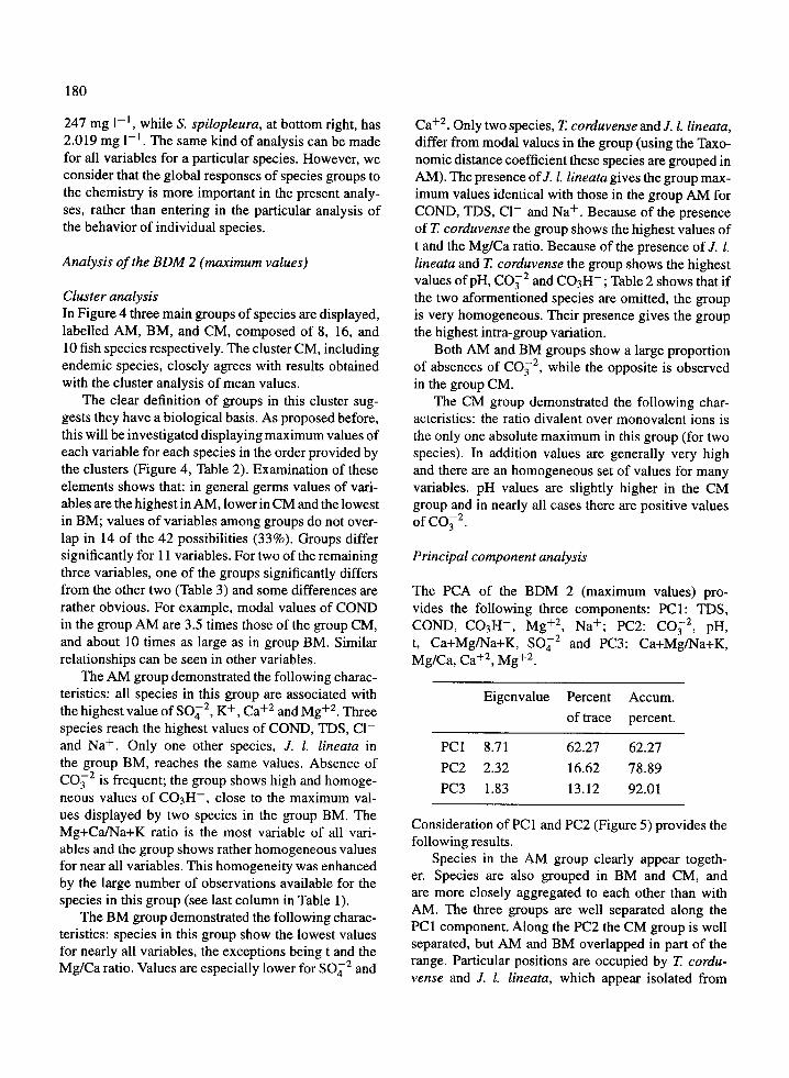
Species are better separated by factors included in thePC2, except S. spilopleura (Figure 3). The upper partof the graph includes species composing groups Dxand Ex, while the lower part shows species from theAx group. Besides the correlation between speciesand chemical data, the graph suggests a relationship

Eigenvalue Percentof trace

Accum.percentage

PC1 7.856 56.11 56.11PC2 3.207 22.91 79.03PC3 1 .061 7.58 86 .60

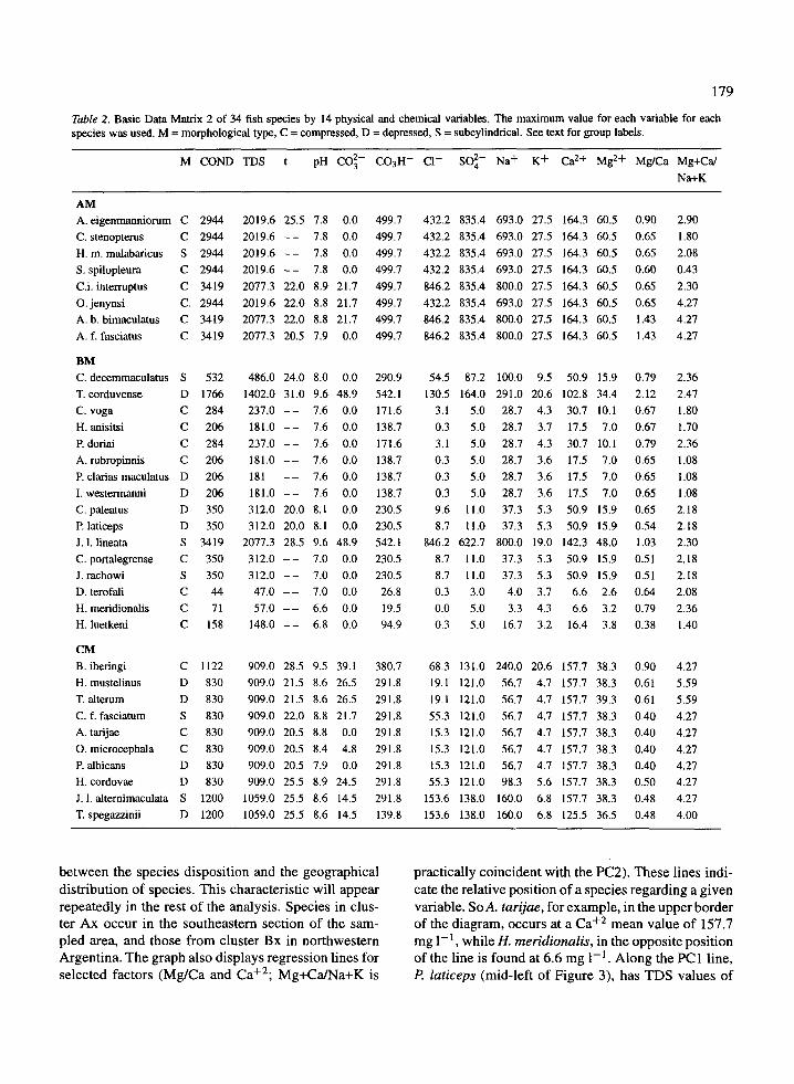
Table 2 . Basic Data Matrix 2 of 34 fish species by 14 physical and chemical variables . The maximum value for each variable for eachspecies was used. M = morphological type, C = compressed, D = depressed, S = subcylindrical . See text for group labels.

BMC. decemmaculatus S 532 486 .0T.corduvense D 1766 1402 .0C.voga C 284 237 .0H. anisitsi

C

206

181 .0P. doriai C 284 237 .0A. rubropinnis

C

206

181 .0P. clarias maculatus D 206 181I. westermanni D 206 181 .0C . paleatus

D

350

312.0P. laticeps D 350 312 .0J .1 .lineata S 3419 2077 .3C. portalegrense

C 350

312.0J . rachowi

S

350

312.0D. terofali

C

44

47.0H. meridionalis

C

71

57.0H. luetkeni

C

158

148.0

M COND TDS t

pH C03- C03H- Cl- SO4- Na+ K+ Cat+ Mgt+ Mg/Ca Mg+Ca/Na+K

AMA. eigenmanniorum C 2944 2019.6 25 .5 7 .8 0.0 499 .7C. stenopterus

C 2944

2019.6 -- 7 .8 0 .0

499.7H. m . malabaricus

S 2944

2019.6 - - 7 .8 0 .0

499.7S. spilopleura C 2944 2019.6 -- 7 .8 0 .0 499 .7C .i . interruptus

C 3419

2077.3 22 .0 8.9 21 .7

499.70. jenynsi C. 2944 2019.6 22 .0 8.8 21 .7 499 .7A . b . bimaculatus

C 3419

2077.3 22 .0 8 .8 21 .7

499.7A . f. fasciatus

C 3419

2077.3 20 .5 7 .9 0 .0

499.7

8 .0 0 .0 290.99 .6 48 .9 542.17 .6 0 .0 171 .67 .6 0 .0 138 .77.6 0.0 171 .67.6 0.0 138 .77.6 0.0 138 .7

-- 7.6 0 .0 138 .720.0 8 .1 0 .0 230 .520.0 8 .1 0 .0 230.528.5 9 .6 48 .9 542.1

7.0 0.0 230 .57.0 0.0 230 .57.0 0.0 26 .86.6 0.0 19 .56 .8 0 .0

94.9

CMB. iheringi

C 1122

909.0 28 .5 9.5 39 .1

380.7H. mustelinus

D

830

909.0 21 .5 8.6 26 .5

291 .8T. alterum

D

830

909.0 21 .5 8.6 26 .5

291 .8C. f. fasciatum

S

830

909.0 22 .0 8 .8 21 .7

291.8A. tarijae

C

830

909.0 20 .5 8 .8 0 .0

291 .80. microcephala

C

830

909.0 20 .5 8 .4 4 .8

291 .8P. albicans

D

830

909.0 20 .5 7 .9 0 .0

291 .8H. cordovae

D

830

909.0 25 .5 8.9 24 .5

291 .8J . 1 . alternimaculata S 1200 1059.0 25 .5 8.6 14.5 291 .8T. spegazzinii

D 1200

1059.0 25 .5 8.6 14 .5

139.8

between the species disposition and the geographicaldistribution of species . This characteristic will appearrepeatedly in the rest of the analysis . Species in clus-ter Ax occur in the southeastern section of the sam-pled area, and those from cluster Bx in northwesternArgentina . The graph also displays regression lines forselected factors (Mg/Ca and Ca+ 2 ; Mg+Ca/Na+K is

432 .2 835.4 693 .0432 .2 835.4 693.0432 .2 835.4 693.0432.2 835 .4 693 .0846 .2 835.4 800.0432 .2 835.4 693.0846 .2 835 .4 800.0846 .2 835.4 800.0

27 .5 164 .3 60 .5 0.90 2 .9027.5 164.3 60.5 0.65 1 .8027 .5 164 .3 60 .5 0.65 2 .0827.5 164 .3 60.5 0.60 0.4327.5 164.3 60 .5 0.65 2.3027.5 164.3 60 .5 0.65 4.2727 .5 164 .3 60.5 1 .43 4.2727.5 164.3 60 .5

1 .43

4.27

54 .5 87 .2 100.0 9.5 50 .9 15 .9 0.79 2.36130 .5 164 .0 291.0 20.6 102.8 34 .4 2 .12 2 .47

3 .1

5.0

28.7

4.3

30.7 10 .1

0.67

1.800.3

5.0

28.7

3.7

17.5

7.0

0.67

1.703.1

5.0

28 .7 4.3

30.7 10 .1

0.79

2.360.3

5.0

28.7

3.6

17.5

7.0

0.65

1.080.3

5.0

28.7

3.6

17.5

7.0

0.65

1.080.3

5.0

28.7

3 .6

17.5

7.0

0.65

1 .089.6

11 .0

37.3

5.3

50.9 15.9

0.65

2.188.7 11 .0 37 .3 5 .3 50.9 15 .9 0 .54 2.18

846 .2 622 .7 800.0 19.0 142.3 48 .0 1 .03 2.308 .7

11 .0

37.3

5.3

50.9 15 .9

0.51

2.188.7

11 .0

37.3

5.3

50.9 15.9

0.51

2.180.3

3.0

4.0 3.7

6.6 2.6

0.64

2.080.0

5.0

3.3 4.3

6.6 3 .2

0.79

2.360.3

5.0

16.7 3.2

16.4 3.8

0.38

1.40

68.3 131 .0 240.0 20.6 157.7 38 .3 0 .90 4 .2719.1 121 .0 56 .7 4 .7 157 .7 38 .3 0 .61 5 .5919 .1 121 .0 56.7 4.7 157.7 39.3 0.61 5 .5955 .3 121 .0 56.7 4.7 157.7 38 .3 0 .40 4 .2715.3 121 .0 56 .7 4 .7 157 .7 38 .3 0 .40 4 .2715.3 121 .0 56.7 4.7 157.7 38 .3 0 .40 4 .2715 .3 121 .0 56 .7 4 .7 157.7 38 .3 0 .40 4 .2755.3 121 .0 98 .3 5 .6 157.7 38 .3 0 .50 4 .27153 .6 138.0 160 .0 6 .8 157.7 38 .3 0 .48 4 .27153 .6 138 .0 160 .0 6.8 125.5 36 .5

0.48

4.00

179

practically coincident with the PC2) . These lines indi-cate the relative position of a species regarding a givenvariable . So A. tarijae, for example, in the upper borderof the diagram, occurs at a Ca+ 2 mean value of 157 .7mg 1-1 , while H. meridionalis, in the opposite positionof the line is found at 6 .6 mg 1 -1 . Along the PC 1 line,P laticeps (mid-left of Figure 3), has TDS values of

180

247 mg 1 -1 , while S. spilopleura, at bottom right, has2.019 mg I' . The same kind of analysis can be madefor all variables for a particular species . However, weconsider that the global responses of species groups tothe chemistry is more important in the present analy-ses, rather than entering in the particular analysis ofthe behavior of individual species .

Analysis of the BDM 2 (maximum values)

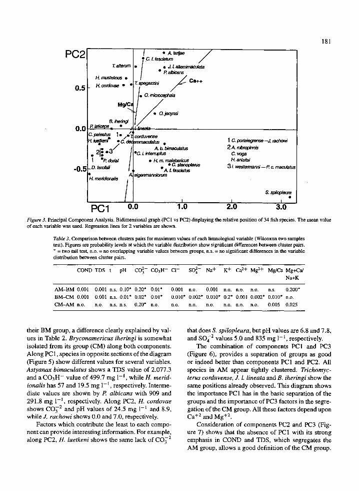
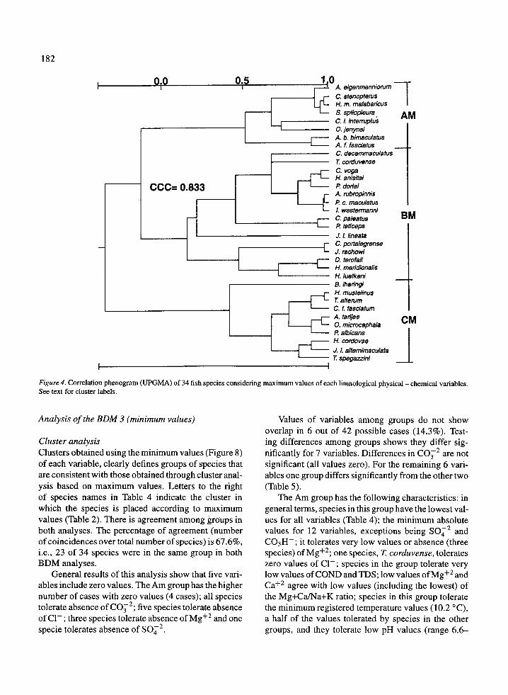
Cluster analysisIn Figure 4 three main groups of species are displayed,labelled AM, BM, and CM, composed of 8, 16, and10 fish species respectively. The cluster CM, includingendemic species, closely agrees with results obtainedwith the cluster analysis of mean values .

The clear definition of groups in this cluster sug-gests they have a biological basis. As proposed before,this will be investigated displaying maximum values ofeach variable for each species in the order provided bythe clusters (Figure 4, Table 2) . Examination of theseelements shows that: in general germs values of vari-ables are the highest in AM, lower in CM and the lowestin BM; values of variables among groups do not over-lap in 14 of the 42 possibilities (33%) . Groups differsignificantly for 11 variables. For two of the remainingthree variables, one of the groups significantly differsfrom the other two (Table 3) and some differences arerather obvious . For example, modal values of CONDin the group AM are 3 .5 times those of the group CM,and about 10 times as large as in group BM . Similarrelationships can be seen in other variables .

The AM group demonstrated the following charac-teristics : all species in this group are associated withthe highest value of So42 , K+, Ca+ 2 and Mg+ 2 . Threespecies reach the highest values of COND, TDS, Cl -and Na+ . Only one other species, J. l. lineata inthe group BM, reaches the same values . Absence ofCO32 is frequent; the group shows high and homoge-neous values of C03H - , close to the maximum val-ues displayed by two species in the group BM . TheMg+Ca/Na+K ratio is the most variable of all vari-ables and the group shows rather homogeneous valuesfor near all variables . This homogeneity was enhancedby the large number of observations available for thespecies in this group (see last column in Table 1) .

The BM group demonstrated the following charac-teristics : species in this group show the lowest valuesfor nearly all variables, the exceptions being t and theMg/Ca ratio . Values are especially lower for So42 and

Ca+2 .Only two species, T corduvense and J. L lineata,differ from modal values in the group (using the Taxo-nomic distance coefficient these species are grouped inAM). The presence ofJ. L lineata gives the group max-imum values identical with those in the group AM forCOND, TDS, Cl- and Na+. Because of the presenceof T corduvense the group shows the highest values oft and the Mg/Ca ratio . Because of the presence of J. l.lineata and T corduvense the group shows the highestvalues of pH, CO3 2 and C03H- ; Table 2 shows that ifthe two aformentioned species are omitted, the groupis very homogeneous . Their presence gives the groupthe highest intra-group variation .

Both AM and BM groups show a large proportionof absences of CO3 2 , while the opposite is observedin the group CM .

The CM group demonstrated the following char-acteristics : the ratio divalent over monovalent ions isthe only one absolute maximum in this group (for twospecies). In addition values are generally very highand there are an homogeneous set of values for manyvariables. pH values are slightly higher in the CMgroup and in nearly all cases there are positive valuesof CO3

-2 .

Principal component analysis

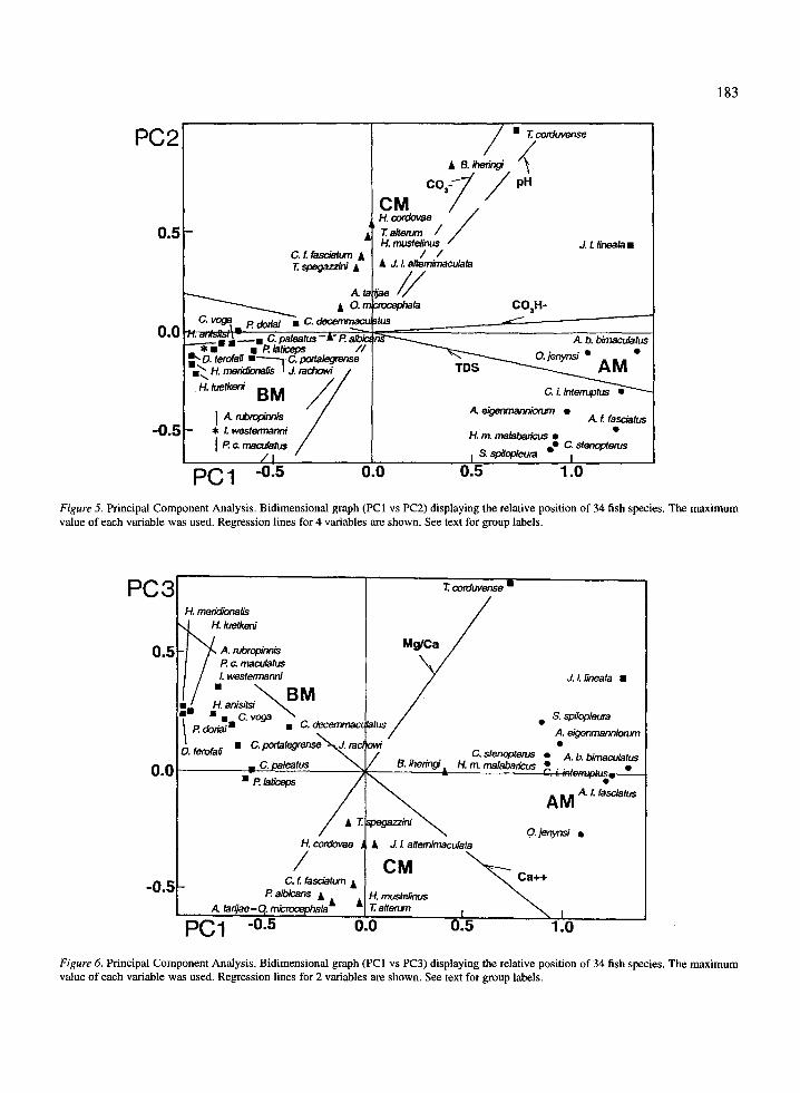
The PCA of the BDM 2 (maximum values) pro-vides the following three components : PC1 : TDS,COND, C03H-, Mg+2 , Na+; PC2: CO32 , pH,t, Ca+Mg/Na+K, SO4 2 and PC3: Ca+Mg/Na+K,Mg/Ca, Ca+2, Mg+2

Consideration of PC 1 and PC2 (Figure 5) provides thefollowing results .

Species in the AM group clearly appear togeth-er. Species are also grouped in BM and CM, andare more closely aggregated to each other than withAM. The three groups are well separated along thePC 1 component. Along the PC2 the CM group is wellseparated, but AM and BM overlapped in part of therange. Particular positions are occupied by T cordu-vense and J. L lineata, which appear isolated from

Eigenvalue Percentof trace

Accum .percent .

PC I 8.71 62.27 62.27PC2 2.32 16.62 78.89PC3 1 .83 13 .12 92.01

PC2

0.5

0.0

-0 .

PC1 0.0Figure 3 . Principal Component Analysis. Bidimensional graph (PC1 vs PC2) displaying the relative position of 34 fish species . The mean valueof each variable was used . Regression lines for 2 variables are shown .

Table 3. Comparison between clusters pairs for maximum values of each limnological variable (Wilcoxon two samplestest) . Figures are probability levels at which the variable distribution show significant differences between cluster pairs .* = two tail test, n .o . = no overlapping variable values between groups, n .s. = no significant differences in the variabledistribution between cluster pairs .

COND TDS t pH CO3- COSH- Cl- SO4- Na+ K+ Cat+ Mgt+ Mg/Ca Mg+Ca/Na+K

AM-BM 0.001 0.001 n .s . 0.10* 0 .20* 0 .01*

0.001 n .o .

0.001 n.o. n .o . n .o .

n.s.

0.200*BM-CM 0.001 0.001 n .s. 0.01* 0 .02* 0 .01*

0.010* 0 .002* 0 .010* 0 .2* 0.001 0 .002* 0.010* n .o .CM-AM n .o .

n.o. n.s . n .s .

0.20* n.o .

n.o.

n.o .

n.o .

n.o. n.o . n .o .

0.005 0.025

their BM group, a difference clearly explained by val-ues in Table 2 . Bryconamericus iheringi is somewhatisolated from its group (CM) along both components .Along PC 1, species in opposite sections of the diagram(Figure 5) show different values for several variables .Astyanax bimaculatus shows a TDS value of 2 .077 .3and a C03H- value of 499.7 mg 1-1 , while H. merid-ionalis has 57 and 19 .5 mg 1 -1 , respectively. Interme-diate values are shown by P. albicans with 909 and291 .8 mg 1 -1 , respectively. Along PC2, H. cordovaeshows CO3 2 and pH values of 24 .5 mg 1 -1 and 8.9,while J. rachowi shows 0 .0 and 7 .0, respectively .

Factors which contribute the least to each compo-nent can provide interesting information . For example,along PC2, H. luetkeni shows the same lack of CO3 2

1 .0 2.0 3.0

181

that does S. spilopleura, but pH values are 6.8 and 7 .8,and SO42 values 5.0 and 835 mg 1-1, respectively .

The combination of components PC1 and PC3(Figure 6), provides a separation of groups as goodor indeed better than components PC1 and PC2 . Allspecies in AM appear tightly clustered . Trichomyc-terus corduvense, J. L lineata and B. iheringi show thesame positions already observed. This diagram showsthe importance PC1 has in the basic separation of thegroups and the importance of PC3 factors in the segre-gation of the CM group . All these factors depend uponCa+2 and Mg+2 .

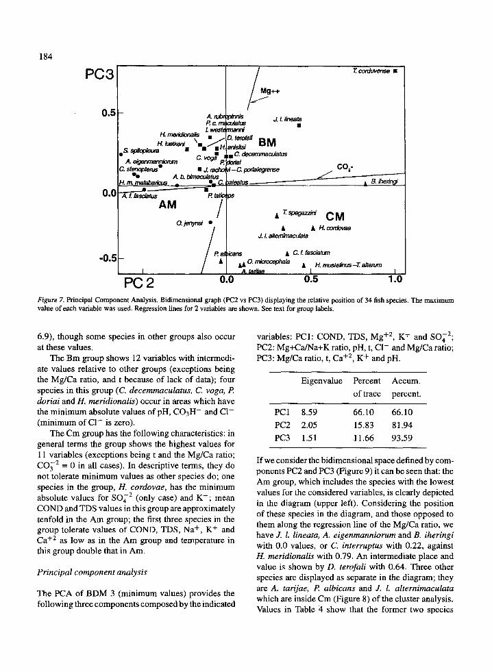
Consideration of components PC2 and PC3 (Fig-ure 7) shows that the absence of PC1 with its strongemphasis in COND and TDS, which segregates theAM group, allows a good definition of the CM group .

T altenun

•

A tanjae•

C. t fasciatum•

• J. L aiemimacuiata•

P. aibicansH.mustellnus

H. cordovae • •T Pe9 azz r ww

Ca++

•

O. miaacephala

Mg/C•

O.jenynsiB. Teringi

P lat'

C. palmsgretkeru

•c.corduvense

tus 1 C. portalegrense-,l. rachowi. / A b. bfmaculatus 2 A. n~bnavinnis2I; -3 C. L intemrp<us C. voga

I -PP doriai •

H. m, malabaricus H. arusitsi

D. terofaff •

• C stengoten's 3l. westennanni --P c. maculatusA f fasciatweigenmarwrorum•

H. mendionalis

S. spilopleura

I

Figure 4. Correlation phenogram (UPGMA) of 34 fish species considering maximum values of each limnological physical - chemical variables .See text for cluster labels .

Analysis of the BDM 3 (minimum values)

Cluster analysisClusters obtained using the minimum values (Figure 8)of each variable, clearly defines groups of species thatare consistent with those obtained through cluster anal-ysis based on maximum values . Letters to the rightof species names in Table 4 indicate the cluster inwhich the species is placed according to maximumvalues (Table 2). There is agreement among groups inboth analyses. The percentage of agreement (numberof coincidences over total number of species) is 67 .6%,i .e ., 23 of 34 species were in the same group in bothBDM analyses .

General results of this analysis show that five vari-ables include zero values . The Am group has the highernumber of cases with zero values (4 cases) ; all speciestolerate absence of CO3 2 ; five species tolerate absenceof Cl- ; three species tolerate absence of Mg+ 2 and onespecie tolerates absence of So4 2 .

Values of variables among groups do not showoverlap in 6 out of 42 possible cases (14 .3%) . Test-ing differences among groups shows they differ sig-nificantly for 7 variables . Differences in CO3 2 are notsignificant (all values zero) . For the remaining 6 vari-ables one group differs significantly from the other two(Table 5) .

The Am group has the following characteristics : ingeneral terms, species in this group have the lowest val-ues for all variables (Table 4) ; the minimum absolutevalues for 12 variables, exceptions being SO4 2 andC03H-; it tolerates very low values or absence (threespecies) of Mg+2 ; one species, T corduvense, tolerateszero values of Cl- ; species in the group tolerate verylow values of COND and TDS ; low values of Mg+ 2 andCa+ 2 agree with low values (including the lowest) ofthe Mg+Ca/Na+K ratio ; species in this group toleratethe minimum registered temperature values (10 .2 °C),a half of the values tolerated by species in the othergroups, and they tolerate low pH values (range 6 .6-

182

0 10

0 15 A. eigenmanniorumI

C. ma/astenopterusricusH.

m.mala6ari

S. spilopleuraC. L interruptus

AM0.jenynsi

bimaculatusA . b.A. f. fascaaumC. decemmaculatusT corduvenseC. Yoga

-E H. anisitsiCCC= 0.833 P dortai

A . rubropinnisP. C. maculatusE l. westermanniC. paleatus

BMC P. laticeps

J.1. fineataC. portalegrenseC J. rachowiD. ferofali

C H. meridionalisH. luetkeniB. lheringiH. mustelinusT alterumC. f fasciatumA . tarijaeO. microcephalaP. albicans

CM

H. cordovaeJ. L altemimaculataT spegazzini

PC2

0.5

0.0

-0.5

Figure 5 . Principal Component Analysis . Bidimensional graph (PC I vs PC2) displaying the relative position of 34 fish species . The maximumvalue of each variable was used . Regression lines for 4 variables are shown . See text for group labels .

PC 3

0.5

0.0

-0.5

PC 1 -0.5

1

--

0.0 0.5 1 .0

1 .0

183

Figure 6 . Principal Component Analysis . Bidimensional graph (PC I vs PC3) displaying the relative position of 34 fish species . The maximumvalue of each variable was used . Regression lines for 2 variables are shown . See text for group labels .

T co duvense

Mg/Ca

J.l.lineata ∎

usS. spr7opleura•A eigenmannionxn

C, stenoptenrs • A . b. bimaculatusB. iheringi H. m. malabancus •

t∎ PP tadceps

A MA • I fasciatus

A T

H, cordovae

C.ffsciatum A

. . .

ni

A J. L altemimaculata

C M

O. jenynsi

Ca++P albicans L A

AA. tadjae- . microcephala

H, mustefinusT altenxn

_

AC. L tasciatum AT spegazzrni A

A toA O- m

~P abriai ∎ C • .-

∎ a -∎ C. paleas s -~Ralb' •* ∎

∎ P• laticeps

//0"D. terola1 ∎~ C. portalegrense

ns

∎,H meridfonalis J. radrowfH. Iuetked B M /

TDS

C, i. intemrptus

A. efgenmannforumA• ~

- * I• westennanniA. I lasciatus

H. m. mafabarrcusPP a maculates S C. stenopterus

/ I I S. spilcp/eura

I

184

PC3

0.5

0.0

-0.5

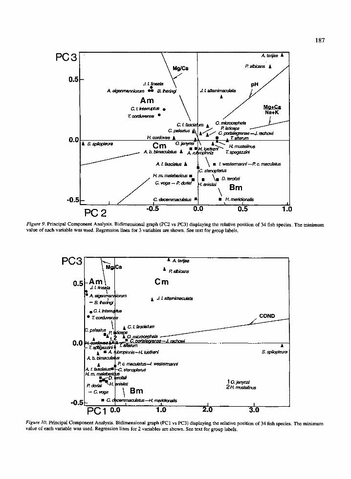
PC 2 0.0Figure 7. Principal Component Analysis . Bidimensional graph (PC2 vs PC3) displaying the relative position of 34 fish species . The maximumvalue of each variable was used . Regression lines for 2 variables are shown . See text for group labels .

6 .9), though some species in other groups also occur

variables: PC I : COND, TDS, Mg+2, K+ and SO4 2 ;

at these values .

PC2: Mg+Ca/Na+K ratio, pH, t, Cl- and Mg/Ca ratio ;The Bm group shows 12 variables with intermedi-

PC3: Mg/Ca ratio, t, Ca+ 2 , K+ and pH.ate values relative to other groups (exceptions beingthe Mg/Ca ratio, and t because of lack of data); fourspecies in this group (C. decemmaculatus, C. yoga, Pdoriai and H. meridionalis) occur in areas which havethe minimum absolute values of pH, C03H - and Cl-(minimum of Cl- is zero) .

The Cm group has the following characteristics : ingeneral terms the group shows the highest values for11 variables (exceptions being t and the Mg/Ca ratio ;

C032 = 0 in all cases) . In descriptive terms, they donot tolerate minimum values as other species do ; onespecies in the group, H. cordovae, has the minimumabsolute values for S042 (only case) and K+ ; meanCOND and TDS values in this group are approximatelytenfold in the Am group ; the first three species in thegroup tolerate values of COND, TDS, Na+, K+ andCa+2 as low as in the Am group and temperature inthis group double that in Am .

Principal component analysis

The PCA of BDM 3 (minimum values) provides thefollowing three components composed by the indicated

0.5 1 .0

If we consider the bidimensional space defined by com-ponents PC2 and PC3 (Figure 9) it can be seen that : theAm group, which includes the species with the lowestvalues for the considered variables, is clearly depictedin the diagram (upper left) . Considering the positionof these species in the diagram, and those opposed tothem along the regression line of the Mg/Ca ratio, wehave J. L lineata, A. eigenmanniorum and B. iheringiwith 0.0 values, or C. interruptus with 0.22, againstH. meridionalis with 0.79. An intermediate place andvalue is shown by D. terofali with 0.64. Three otherspecies are displayed as separate in the diagram ; theyare A . tarijae, P. albicans and J. L alternimaculatawhich are inside Cm (Figure 8) of the cluster analysis .Values in Table 4 show that the former two species

Mg++

l

T cwduvense ∎

A. n ibrPP aL west

H. mendianalis ,H. luettent~ `∎/.m

~

A. egemanniw ,n w,n

C. V09∎P,C.

cutatusm

D. ter~faliar

i

tdecemmaculatus

J. t. lineata,

BM

C93

B Then

C. Stenoptenis 0

∎ J.• A a bimaculatusH. mm malady '

• C.

'-C. patalegrense

leatus

A f fasdatus

P lat'AM

/Q

•

T. apegaz&4 C MA

A H cordovae

P tans

J. I alternimaculata

A C. t fasciatumA

LA0. miaoceptiala A H. mustelinus-T alterum

Eigenvalue Percentof trace

Accum .percent .

PC1 8.59 66.10 66.10PC2 2.05 15.83 81 .94PC3 1 .51 11 .66 93.59

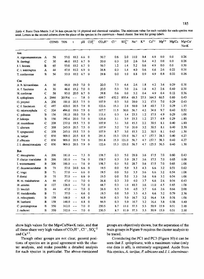
show high values for the Mg+Ca/Na+K ratio, and thatall three share very high values of C03H- , Cl- , SO42

and Ca+2 .Though other groups are not clear, general posi-

tions of species are in good agreement with the clus-ter analysis, and make possible a detailed analysisfor each species in particular. The above-mentioned

185

Table 4 . Basic Data Matrix 3 of 34 fish species by 14 physical and chemical variables . The minimum value for each variable for each species wasused. Letters in the second column show the place of the species in the maximum - based cluster. See text for group labels .

groups are objectively shown, but the separation of themain groups in Figure 9 requires the cluster analysis tobe traced .

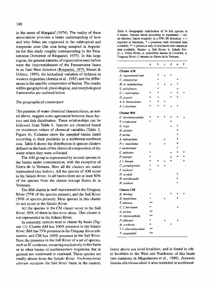
Considering the PC 1 and PC3 (Figure 10) it can beseen that S . spilopleura, with a maximum value (onlyone data in all), is extremely segregated . Aside fromthis species, A . tarijae, P. albicans and J. L alternimac-

COND TDS t pH C03- C03H- Cl- SO'- Na+ K+ Cat+ Mg2+ Mg/Ca Mg+Ca/Na+K

AmA. eigenmanniorum A 58 53 .0 10 .2 6 .6 0 30 .7 0.6 2.0 11 .0 0.4 4 .9 0 .0 0 .0 0 .26

B . iheringi C 30 46 .0 10 .2 6 .7 0 20 .0 0 .3 2 .0 2 .6 0.4 4 .2 0 .0 0 .0 0 .26

J . 1. lineata B 65 53 .0 10 .2 6.7 0 30 .7 1 .2 1 .4 5 .2 0.6 4 .9 0 .0 0 .0 0 .30

C. i . interruptus A 44 47 .0 10 .2 6 .9 0 26 .8 0 .3 1 .4 4 .0 0 .6 6 .6 2 .6 0.22 0 .31

T.corduvense B 56 53 .0 10 .2 6 .7 0 29 .8 0 .0 1 .0 8 .8 0 .9 4 .9 0 .8 0.22 0 .26

CmA. b . bimaculatus A 30 46 .0 19 .0 7 .0 0 20 .0 7 .3 6 .4 2 .6 1 .8 4 .2 3 .6 0.29 0 .31A . f . fasciatus A 30 46 .0 19 .2 7 .0 0 20 .0 0 .3 3 .0 2 .6 1 .8 4 .2 2 .6 0 .40 0 .31

H. cordovae C 58 93 .0 20 .0 6.7 0 39 .8 0 .6 0 .0 5 .2 0 .4 4 .9 0 .4 0.12 0 .36

S . spilopleura A 2944 2019.6 -- 7.8 0 499 .7 432.2 835 .4 69 .3 27 .5 164 .3 60 .5 0.60 0 .43O. jenynsi A 206 181 .0 20 .5 7.5 0 107 .9 0 .3 5 .0 20 .0 3 .2 17 .5 7 .0 0.29 0 .43C . f. fasciatum C 497 420 .0 20 .5 7 .9 0 122 .6 15 .3 2 .8 50 .0 3 .8 40 .7 7 .2 0.29 1 .150. microcephala C 324 494 .0 19 .0 7 .9 0 117 .7 11 .5 30 .0 56 .7 4 .2 34 .8 9 .7 0.40 0 .52

C. paleatus B 156 181 .0 18 .0 7 .0 0 115 .4 0 .3 1 .4 23 .3 1 .2 17 .5 4 .9 0.29 1 .08P. laticeps B 156 192 .4 20 .0 7 .0 0 125 .0 3 .1 3 .9 23 .3 1 .2 27 .7 4 .9 0 .29 1 .80H. mustelinus C 208 237 .0 19 .5 7 .3 0 107 .9 3 .1 3 .0 15 .3 2 .2 30 .5 8 .1 0.40 1 .80

T . alterum C 208 243 .0 20 .5 7 .5 0 107 .9 5 .2 7 .0 20.0 3 .2 30 .5 8 .1 0.40 2 .30T . spegazzinii C 208 243 .0 19 .5 7.5 0 107 .9 8 .7 3 .0 15 .3 2 .2 30 .5 8 .1 0.43 1 .30A . tarijae C 830 909 .0 20 .5 8.8 0 291 .8 15 .3 121 .0 56 .7 4 .7 157 .7 38 .3 0.40 4 .27P. albicans C 830 909 .0 20 .5 7.9 0 291 .8 15 .3 121 .0 56 .7 4 .7 157 .7 38 .3 0.40 4 .27J.1. altemimaculata C 830 909 .0 20 .5 7 .9 0 122 .6 15 .3 121 .0 56 .7 4 .7 125 .5 36 .5 0.40 1 .30

BmC. stenopterus A 206 181 .0 7 .3 0 138 .7 0 .3 5 .0 28 .0 3 .6 17 .5 7 .0 0.60 0 .43P. clarias maculatus B 206 181 .0 - 7.6 0 138 .7 0 .3 5 .0 28 .7 3 .6 17 .5 7 .0 0.65 1 .08I . westermanni B 206 181 .0 -- 7 .6 0 138 .7 0 .3 5 .0 28 .7 3 .6 17 .5 7 .0 0.65 1 .08C. decemmaculatus B 71 57 .0 24 .0 6 .6 0 19 .5 0 .0 5 .0 3 .3 4 .3 6 .6 3 .2 0.51 0 .62C. yoga B 71 57 .0 6 .6 0 19 .5 0 .0 5 .0 3 .3 3.6 6 .6 3 .2 0.54 1 .08P. doriai B 71 57 .0 6 .6 0 19 .5 0 .0 5 .0 3 .3 3 .6 6 .6 3 .2 0.54 1 .08H. m. malabaricus A 44 47 .0 7 .0 0 26.8 0 .3 3 .0 4.0 3 .7 6 .6 2 .6 0.54 0 .43H . anisitsi B 127 126 .0 7 .0 0 48 .7 0 .3 1 .0 10 .3 3 .6 11 .0 4 .5 0.65 1 .08D . terofali B 44 47 .0 7 .0 0 26.8 0 .3 3 .0 4.0 3 .7 6 .6 2 .6 0.64 2 .08H. meridionalis B 71 57 .0 - 6 .6 0 19.5 0 .0 5 .0 3 .3 4 .3 6 .6 3 .2 0 .79 2 .36A. rubropinnis B 158 148 .0 6 .8 0 94.9 0 .3 5 .0 16 .7 3 .2 16 .4 3 .8 0.38 1 .08H . luetkeni B 158 148 .0 - 6 .8 0 94.9 0 .3 5 .0 16 .7 3 .2 16 .4 3 .8 0 .38 1 .40C. portalegrense B 350 312 .0 7.0 0 230 .5 8 .7 11 .0 37 .3 5 .3 50 .9 15 .9 0.51 2 .18J. rachowi B 350 312 .0 7 .0 0 230.5 8 .7 11 .0 37 .3 5 .3 50 .9 15 .9 0 .51 2 .18

186

l0.00.51 t0E A. eigenmanniorumB . iheringiJ. L fineata

AmC. J. intenuptusT corduvenseA . b. bimaculatusA. f. fasaatusH. cordovaeS. spilopleura0. jenynsiC. f. fasciatum0. microcephalaC. paleatus

CmP. laticeps

r- H. mustelinusT afterumT spegazziniA . tarijaeP. albicans

CCC= 0.708

J. L altemimaculataC. stenopterus

r-- P. c. maculatesIlL westermanni

C. decemmaculatusC. yogaP. donaiH. m. malabaricusH. anisitsi

B mD. terofa!H. meridionalisA . rubropinnisH. luetkeni

E C. portalegrenseJ. rachowi

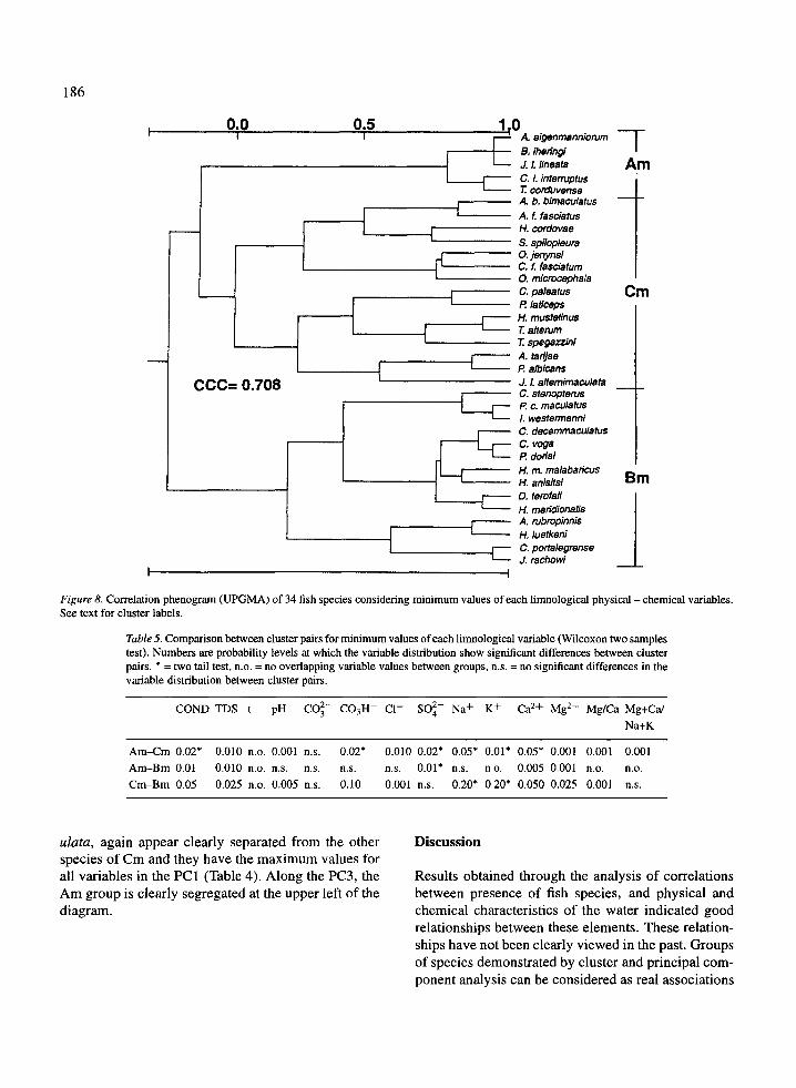
Figure 8. Correlation phenogram (UPGMA) of 34 fish species considering minimum values of each limnological physical - chemical variables .See text for cluster labels .

Table 5 . Comparison between cluster pairs for minimum values of each limnological variable (Wilcoxon two samplestest) . Numbers are probability levels at which the variable distribution show significant differences between clusterpairs . * = two tail test, n .o . = no overlapping variable values between groups, n .s. = no significant differences in thevariable distribution between cluster pairs .

ulata, again appear clearly separated from the other

Discussionspecies of Cm and they have the maximum values forall variables in the PC 1 (Table 4) . Along the PC3, the

Results obtained through the analysis of correlationsAm group is clearly segregated at the upper left of the

between presence of fish species, and physical anddiagram . chemical characteristics of the water indicated good

relationships between these elements . These relation-ships have not been clearly viewed in the past. Groupsof species demonstrated by cluster and principal com-ponent analysis can be considered as real associations

COND TDS t pH C03- CO3H- Cl- SOy- Na+ K+ Ca2+ Mgt+ Mg/Ca Mg+Ca/Na+K

Am-Cm 0.02* 0.010 n.o. 0.001 n.s . 0 .02* 0 .010 0.02* 0 .05* 0 .01* 0 .05* 0 .001 0 .001 0 .001Am-Bm 0.01 0.010 n .o. n .s. n.s. n.s . n .s . 0 .01* n .s . n .o . 0 .005 0.001 n .o . n .o .Cm-Bm 0.05 0.025 n.o . 0.005 n.s . 0 .10 0 .001 n.s.

0.20* 0.20* 0 .050 0.025 0 .001 n .s .

PC 3

0.5

0.0

-0 .

PC3

0.5

0.0

-0.5

PC 2

PC 1 0.0

-0.5

Figure 9. Principal Component Analysis . Bidimensional graph (PC2 vs PC3) displaying the relative position of 34 fish species . The minimumvalue of each variable was used. Regression lines for 3 variables are shown . See text for group labels .

1 .0

0.0 0.5

3.0

1 .0

187

Figure 10. Principal Component Analysis . Bidimensional graph (PC 1 vs PC3) displaying the relative position of 34 fish species . The minimumvalue of each variable was used . Regression lines for 2 variables are shown . See text for group labels .

Mg

-Am

•

A tanjaeCa

aP atbkans

CmJ.1. lineata

•

A eigenn annionm ~ J. l. altemimaculata- B. rneringi

•

C. L intemrpfus•

T co duvenae COND

C. palealus 1a~P

H. ooordora

A C. , fasciatum

2t O ndcrooephalalewertse-J raa>o~~~

-T. sp~gazzlnii•

AA b. bknactdats

nrbropinnis-H. luetkeni

S. spibpieura

a 0 P a maculatus-l. westermarv iA ff fasaatu•-C stenopterusH. m. malabanaus

∎ D. ierofaiH anisitsi

1 O. jenynsiP dw'ai 2H. mustelinus-CVOM 1 Bm

∎ C. c em guar , atus-H. meridionalls-

I

I

l

l

MgICa

J.1. lineataA egenmanninnmnnm N B. Tenngi

A tadfae A

P albicans A

pH

J.1. altemimaculata

AmC. L intern ptus •

T

•

C. ff fasciaC. paleatus

H. cordbvae

M +CaNa+K

0. mbucephalaA~/ ~

P faticepC portalegrense-J. rac>tiavi

∎

T. aiennnAS.

spiople(

m

C m O. !m •H am\ H. mustelinusA b. bimaadatus A A. nnis

T spegaznni

A L fasciatus A \ ∎ lL westetmanni-P. a maculatus

H. m. malabarxws iC. stenoptens

∎ \∎ D. terofaliC. vcga - PP domai anisitsi

B mC deoen naculatus • ∎ H. meridionalis

1 8 8

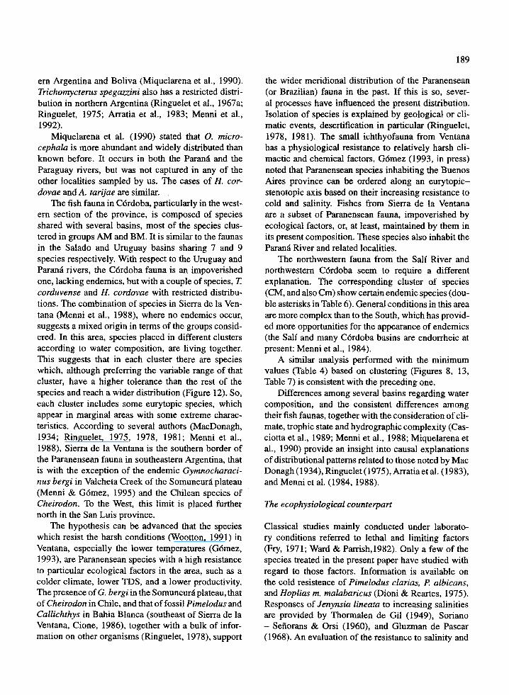
in the sense of Margalef (1974) . The reality of theseassociations provides a better understanding of howand why fishes are organized in the subtropical andtemperate zone (the area being sampled in Argenti-na for this study roughly corresponding to the Para-nensean Dominion of Ringuelet, 1975) . In this largeregion, the general patterns of organization seen beforewere the impoverishment of the Paranensean faunain an East-West direction (Ringuelet, 1975 ; Menni &Gomez, 1995), the latitudinal variation of richness inwestern Argentina (Arratia et al., 1983) and the differ-ences in the specific composition of basins . The resultswithin geographical, physiological, and morphologicalframeworks are outlined below .

The geographical counterpart

The patterns of water-chemical characteristics, as not-ed above, suggest some agreement between these fac-tors and fish distribution . These relationships can befollowed from Table 6 . Species are clustered basedon maximum values of chemical variables (Table 2,Figure 4). Columns show the sampled basins listedaccording to their positions in a northwest-southeastaxis . Table 6 shows the distribution in species clustersdefined on the basis of the chemical composition of thewater where they were collected .

The AM group is represented by several species inthe basins under consideration, with the exception ofSierra de la Ventana . Here all the clusters are underrepresented (see below) . All the species of AM occurin the Salado River. In all basins there are at least 50%of the species from the cluster (except Sierra de laVentana) .

The BM cluster is well represented in the UruguayRiver (75% of the species present), and the Sail River(50% of species present). Most species in this clusterdo not occur in the Salado River.

All the species in the CM cluster occur in the SailRiver, 50% of them in this river alone . This cluster isnot represented in the Salado River .

In summary, species tend to cluster by basin (Fig-ure 11). Cluster AM has 100% presence in the SaladoRiver, BM has 75% presence in the Uruguay River trib-utaries, and CM has 100% presence in the Sail River .Note the presence in the Sail River of a set of species,such asH. cordovae, occurring exclusively in this basinor in other basins of northewestern Argentina, but ingeneral not southward or eastward . These species aretotally absent from the Salado River . Trichomycterusalterum occupies the Sail River basin in the eastern,

Table 6 . Geographic distribution of 34 fish species in6 basins . Species listed according to maximum - val-ue clusters ; basins roughtly in a NW-SE direction . + =reported in literature, * = presence with chemical dataavailable, ** = presence only in that basin with chemicaldata available . Basins : a, Sail River; b, Salado Riv-er; c, Dulce River ; d, endorrheic basins in C6rdoba ; e,Uruguay River ; f, streams in Sierra de la Ventana.

Cluster CMB. iheringi•

mustelinusT alterumC.f.fasciatumA. tarijae0. microcephalaP. albicans•

cordovae•

1. alternimaculataT spegazzinii

a

b c

d e

f

Cluster AMA. eigenmanniorumC. stenopterusH. m. malabaricusS. spilopleura

*

+C. i. interruptus0. jenynsiA. b. bimaculatusA. t: facciatus

*

*

*

+

**

**

*

*************

*

Cluster BM•

decemmaculatusT corduvense•

yogaH. anisitsiP. doriaiA. rubropinnis

+P. c. maculatus

+

+/L westermaniC. paleatusP. laticepsJ. 1. lineata

*

+C. portalegrense

*

+ +J. rachowiD. tergfaliH. meridionalisH. leutkeni

• * * *• * * *•

* *

**

*****

***

•

** *

•

*

•

*•

*

lower above sea level localities, and is found in oth-er localities to the West and Northwest of this basin(see summary in Miquelarena et al ., 1990) . Jenynsialineata alternimaculata is also restricted to northwest-

ern Argentina and Boliva (Miquelarena et al ., 1990) .Trichomycterus spegazzini also has a restricted distri-

Argentina (Ringuelet et al., 1967a;Ringuelet, 5 ; Arratia et al ., 1983; Menni et al.,1992) .

Miquelarena et al . (1990) stated that O . micro-cephala is more abundant and widely distributed thanknown before. It occurs in both the Parana and theParaguay rivers, but was not captured in any of theother localities sampled by us . The cases of H. cor-dovae and A . tarijae are similar.

The fish fauna in C6rdoba, particularly in the west-ern section of the province, is composed of speciesshared with several basins, most of the species clus-tered in groups AM and BM . It is similar to the faunasin the Salado and Uruguay basins sharing 7 and 9species respectively. With respect to the Uruguay andParand rivers, the C6rdoba fauna is an impoverishedone, lacking endemics, but with a couple of species, Tcorduvense and H. cordovae with restricted distribu-tions. The combination of species in Sierra de la Ven-tana (Menni et al ., 1988), where no endemics occur,suggests a mixed origin in terms of the groups consid-ered. In this area, species placed in different clustersaccording to water composition, are living together .This suggests that in each cluster there are specieswhich, although preferring the variable range of thatcluster, have a higher tolerance than the rest of thespecies and reach a wider distribution (Figure 12) . So,each cluster includes some eurytopic species, whichappear in marginal areas with some extreme charac-teristics . According to several authors (MacDonagh,1934; Ringuelet, 1975, 1978, 1981 ; Menni et al .,1988), Sierra de la Ventana is the southern border ofthe Paranensean fauna in southeastern Argentina, thatis with the exception of the endemic Gymnocharaci-nus bergi in Valcheta Creek of the Somuncurd plateau(Menni & G6mez, 1995) and the Chilean species ofCheirodon . To the West, this limit is placed furthernorth in the San Luis province .

The hypothesis can be advanced that the specieswhich resist the harsh conditions (Wootton, 1991) inVentana, especially the lower temperatures (G6mez,1993), are Paranensean species with a high resistanceto particular ecological factors in the area, such as acolder climate, lower 'i'DS, and a lower productivity .The presence of G . bergiin the Somuncurd plateau, thatof Cheirodon in Chile, and that of fossil Pimelodus andCallichthys in Bahia Blanca (southeast of Sierra de laVentana, Cione, 1986), together with a bulk of infor-mation on other organisms (Ringuelet, 1978), support

the wider meridional distribution of the Paranensean(or Brazilian) fauna in the past. If this is so, sever-al processes have influenced the present distribution .Isolation of species is explained by geological or cli-matic events, desertification in particular (Ringuelet,1978, 1981) . The small ichthyofauna from Ventanahas a physiological resistance to relatively harsh cli-mactic and chemical factors. G6mez (1993, in press)noted that Paranensean species inhabiting the BuenosAires province can be ordered along an eurytopic-stenotopic axis based on their increasing resistance tocold and salinity. Fishes from Sierra de la Ventanaare a subset of Paranensean fauna, impoverished byecological factors, or, at least, maintained by them inits present composition . These species also inhabit theParana River and related localities .

The northwestern fauna from the Sail River andnorthwestern C6rdoba seem to require a differentexplanation . The corresponding cluster of species(CM, and also Cm) show certain endemic species (dou-ble asterisks in Table 6) . General conditions in this areaare more complex than to the South, which has provid-ed more opportunities for the appearance of endemics(the Sail and many C6rdoba basins are endorrheic atpresent : Menni et al., 1984) .

A similar analysis performed with the minimumvalues (Table 4) based on clustering (Figures 8, 13,Table 7) is consistent with the preceding one .

Differences among several basins regarding watercomposition, and the consistent differences amongtheir fish faunas, together with the consideration of cli-mate, trophic state and hydrographic complexity (Cas-ciotta et al ., 1989 ; Menni et al., 1988 ; Miquelarena etal., 1990) provide an insight into causal explanationsof distributional patterns related to those noted by MacDonagh (1934), Ringuelet (1975), Arratia et al . (1983),and Menni et al . (1984, 1988) .

The ecophysiological counterpart

Classical studies mainly conducted under laborato-ry conditions referred to lethal and limiting factors(Fry, 1971 ; Ward & Parrish,1982) . Only a few of thespecies treated in the present paper have studied withregard to those factors . Information is available onthe cold resistence of Pimelodus clarias, P. albicans,and Hoplias m. malabaricus (Dioni & Reartes, 1975) .Responses of Jenynsia lineata to increasing salinitiesare provided by Thormalen de Gil (1949), Soriano- Senorans & Orsi (1960), and Gluzman de Pascar(1968). An evaluation of the resistance to salinity and

1 89

1 90

pa

ta

i0

1,000

2,000

,000

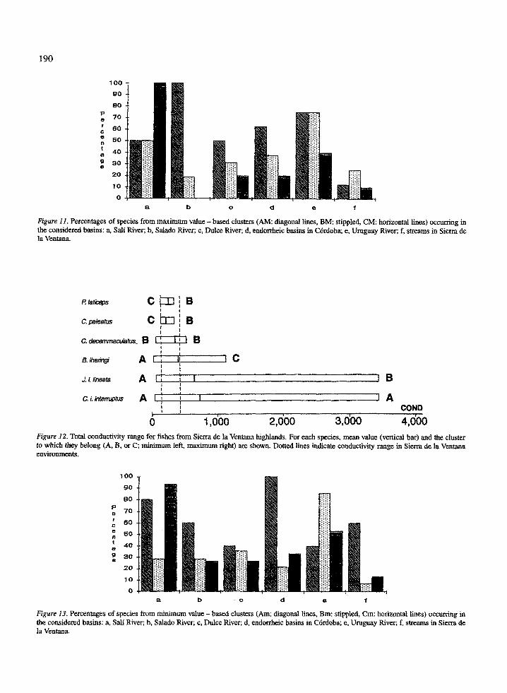
4Figure 12. Total condu range for fishes from Sierra de la Ventana highlands . For each species, mean value (vertical bar) and the clusterto which they belong (A, , or C ; minimum left, maximum right) are shown. Dotted lines indicate conductivity range in Sierra de la Ventanaenvironments .

100 -90 -so-70 -80 -50 -40 -

30 -20 -

10 -

a

b

d

e

i

Figure]] . Percentages of species from maximum value -based clusters (AM: diagon lines, BM: stippled, CM: horizontal lines) occurring inthe considered basins : a, Sail River; b, Salado River; c, Dulce River; d, endorrheic basins in Cdrdoba ; e, Uruguay River; f, streams in Sierra dela Ventana.

P laticeps

C paleatus

C. decemmaculatus-

B. ihenngi

J. I. lineata

C. i. inlemiptus

b

d

e

t

Figure 13. Percentages of species from minimum value - based clusters (Am : diagonal lines, Bm : stippled, Cm: horizontal lines) occurring inthe considered basins : a, Sali River ; b, Salado River; c, Dulce River ; d, endorrheic basins in C6rdoba ; e, Uruguay River; f, streams in Sierra dela Ventana.

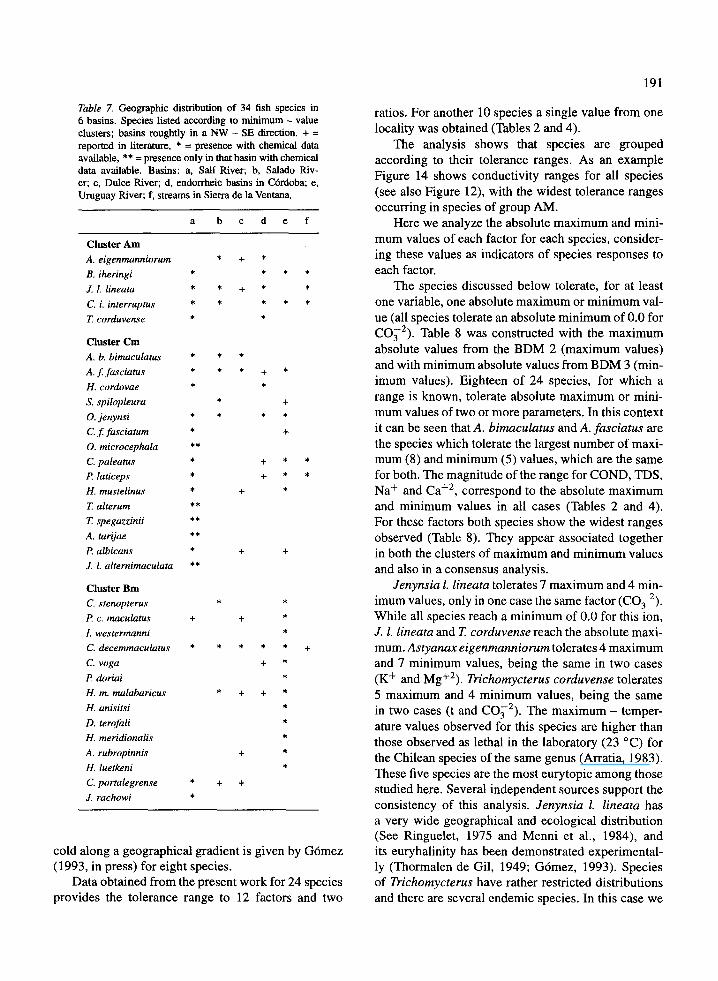
Table 7. Geographic distribution of 34 fish species in6 basins . Species listed according to minimum - valueclusters ; basins roughtly in a NW - SE direction . + =reported in literature, * = presence with chemical dataavailable, ** = presence only in that basin with chemicaldata available . Basins : a, Sali River; b, Salado Riv-er; c, Dulce River ; d, endorrheic basins in C6rdoba ; e,Uruguay River; f, streams in Sierra de la Ventana .

cold along a geographical gradient is given by G6mez(1993, in press) for eight species .

Data obtained from the present work for 24 speciesprovides the tolerance range to 12 factors and two

191

ratios. For another 10 species a single value from onelocality was obtained (Tables 2 and 4) .

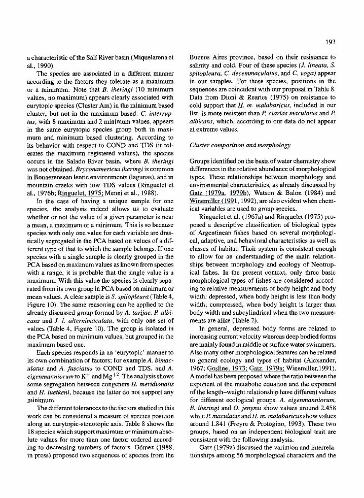
The analysis shows that species are groupedaccording to their tolerance ranges . As an exampleFigure 14 shows conductivity ranges for all species(see also Figure 12), with the widest tolerance rangesoccurring in species of group AM .

Here we analyze the absolute maximum and mini-mum values of each factor for each species, consider-ing these values as indicators of species responses toeach factor .

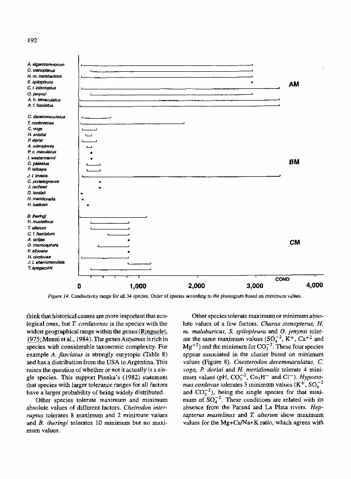
The species discussed below tolerate, for at leastone variable, one absolute maximum or minimum val-ue (all species tolerate an absolute minimum of 0 .0 forCO32 ) . Table 8 was constructed with the maximumabsolute values from the BDM 2 (maximum values)and with minimum absolute values from BDM 3 (min-imum values) . Eighteen of 24 species, for which arange is known, tolerate absolute maximum or mini-mum values of two or more parameters. In this contextit can be seen that A. bimaculatus and A. fasciatus arethe species which tolerate the largest number of maxi-mum (8) and minimum (5) values, which are the samefor both . The magnitude of the range for COND, TDS,Na+ and Ca+ 2 , correspond to the absolute maximumand minimum values in all cases (Tables 2 and 4) .For these factors both species show the widest rangesobserved (Table 8). They appear associated togetherin both the clusters of maximum and minimum valuesand also in a consensus analysis .

Jenynsia 1. lineata tolerates 7 maximum and 4 min-imum values, only in one case the same factor (CO 3 2 ) .While all species reach a minimum of 0 .0 for this ion,J. L lineata and T corduvense reach the absolute maxi-mum . Astyanax eigenmanniorum tolerates 4 maximumand 7 minimum values, being the same in two cases(K+ and Mg+ 2) . Trichomycterus corduvense tolerates5 maximum and 4 minimum values, being the samein two cases (t and CO3 2 ) . The maximum - temper-ature values observed for this species are higher thanthose observed as lethal in the laboratory (23 °C) forthe Chilean species of the same genus (Arratia, 1983) .These five species are the most eurytopic among thosestudied here. Several independent sources support theconsistency of this analysis . Jenynsia 1. lineata hasa very wide geographical and ecological distribution(See Ringuelet, 1975 and Menni et al ., 1984), andits euryhalinity has been demonstrated experimental-ly (Thormalen de Gil, 1949 ; G6mez, 1993) . Speciesof Trichomycterus have rather restricted distributionsand there are several endemic species . In this case we

a

b c d e f

Cluster AmA. eigenmanniorum *

*

*

*B. iheringiJ. l . lineataC. i . interruptusT corduvense

*

*

*

**

*

*

**

Cluster CmA. b. bimaculatusA . j: . fasciatus

*

*

**

*

*

H. cordovaeS. spilopleura0. jenynsiC. .f. fasciatum0. microcephalaC. paleatusP laticepsH. mustelinus

*

**

*

*

*****

*

**

*

**

*

T alterum ****T spegazzinii

A. tarijaeP. albicansJ. 1. alternimaculata

Cluster BinC. stenopterusP. c. maculatus

*****

**+

+I. westermanniC. decemmaculatusC. yoga

**

+P. doriaiH. m. malabaricus

*

+ + *H. anisitsi *

D. terofaliH. meridionalisA. rubropinnis

***+

H. luetkeniC. portalegrense

*

*

+ +J. rachowi *

0

1,000

think that historical causes are more important that eco-logical ones, but T corduvense is the species with thewidest geographical range within the genus (Ringuelet,1975 ; Menni et al ., 1984) . The genusAstyanax is rich inspecies with considerable taxonomic complexity. Forexample A. fasciatus is strongly eurytopic (Table 8)and has a distribution from the USA to Argentina . Thisraises the question of whether or not it actually is a sin-gle species . This support Pianka's (1982) statementthat species with larger tolerance ranges for all factorshave a larger probability of being widely distributed .

Other species tolerate maximum and minimumabsolute values of different factors . Cheirodon inter-ruptus tolerates 8 maximum and 2 minimum valuesand B. iheringi tolerates 10 minimum but no maxi-mum values .

4

i

AM

BM

CM

COND2,000

3,000

4,000

Figure 14. Conductivity range for all 34 species . Order of species according to the phenogram based on maximum values .

Other species tolerate maximum or minimum abso-lute values of a few factors . Charax stenopterus, H.m. malabaricus, S. spilopleura and O. jenynsi toler-ate the same maximum values (SO4 2 , K+, Ca+ 2 andMg+ 2 ) and the minimum for CO3 2 . These four speciesappear associated in the cluster based on minimumvalues (Figure 8) . Cnesterodon decemmaculatus, C .yoga, P doriai and H. meridionalis tolerate 4 mini-mum values (pH, CO3 2 , Co3H- and Cl- ) . Hyposto-mus cordovae tolerates 3 minimum values (K+, SO4 2

and C07 2 ), being the single species for that mini-mum of So4 2 . These conditions are related with itsabsence from the Parana and La Plata rivers . Hep-tapterus mustelinus and T alterum show maximumvalues for the Mg+Ca/Na+K ratio, which agrees with

192

A. eigenmannionrmC. stenopterusH. m. malabaricusS. spilopleuraC. i. interruptus0.JenynsiA. b. bimaculatusA . f. fasciatus

C. decemmaculatusT corduvenseC. yogaH. anlsitsiP. dorsal

I

u

A . rubropinnisP c. maculatesL westem,anniC. paleatus

u

P. latlcepsJ. L IineataC. portalegrenseJ. rachowl ∎D. terofallH. meridlonalisH. luetkeni

B. lhe,*791H. mustelinus

1T altenrmC. L fasciatumA . tadJae0. microcephalaP. alblcansH. cordovae 4

J. L altemimaculataTT spegazzini

a characteristic of the Salf River basin (Miquelarena etal., 1990) .

The species are associated in a different manneraccording to the factors they tolerate as a maximumor a minimum. Note that B. iheringi (10 minimumvalues, no maximum) appears clearly associated witheurytopic species (Cluster Am) in the minimum basedcluster, but not in the maximum based . C. interrup-tus, with 8 maximum and 2 minimum values, appearsin the same eurytopic species group both in maxi-mum and minimum based clustering . According toits behavior with respect to COND and TDS (it tol-erates the maximum registered values), the speciesoccurs in the Salado River basin, where B. iheringiwas not obtained . Bryconamericus iheringi is commonin Bonaerensean lentic environments (lagunas), and inmountain creeks with low TDS values (Ringuelet etal., 1976b; Ringuelet, 1975; Menni et al ., 1988) .

In the case of having a unique sample for onespecies, the analysis indeed allows us to evaluatewhether or not the value of a given parameter is neara mean, a maximum or a minimum . This is so becausespecies with only one value for each variable are dras-tically segregated in the PCA based on values of a dif-ferent type of that to which the sample belongs . If onespecies with a single sample is clearly grouped in thePCA based on maximum values as known from specieswith a range, it is probable that the single value is amaximum. With this value the species is clearly sepa-rated from its own group in PCA based on minimum ormean values. A clear sample is S . spilopleura (Table 4,Figure 10) . The same reasoning can be applied to thealready discussed group formed by A . tarijae, P. albi-cans and J. 1. alternimaculata, with only one set ofvalues (Table 4, Figure 10) . The group is isolated inthe PCA based on minimum values, but grouped in themaximum based one.

Each species responds in an 'eurytopic' manner toits own combination of factors ; for example A . bimac-ulatus and A . fasciatus to COND and TDS, and A .eigenmanniorumto K+ and Mg+ 2 . The analysis showssome segregation between congeners H. meridionalisand H. luetkeni, because the latter do not support anyminimum .

The different tolerances to the factors studied in thiswork can be considered a measure of species positionalong an eurytopic-stenotopic axis . Table 8 shows the18 species which support maximum or minimum abso-lute values for more than one factor ordered accord-ing to decreasing numbers of factors. Gbmez (1988,in press) proposed two sequences of species from the

193

Buenos Aires province, based on their resistance tosalinity and cold. Four of these species (J. lineata, S.spilopleura, C. decemmaculatus, and C. yoga) appearin our samples . For these species, positions in thesequences are coincident with our proposal in Table 8 .Data from Dioni & Reartes (1975) on resistance tocold support that H. m. malabaricus, included in ourlist, is more resistent than P. clarias maculatus and P.albicans, which, according to our data do not appearat extreme values .

Cluster composition and morphology

Groups identified on the basis of water chemistry showdifferences in the relative abundance of morphologicaltypes. These relationships between morphology andenvironmental characteristics, as already discussed byGatz (1979a, 1979b), Watson & Balon (1984) andWinemiller (1991, 1992), are also evident when chem-ical variables are used to group species .

Ringuelet et al . (1967a) and Ringuelet (1975) pro-posed a descriptive classification of biological typesof Argentinean fishes based on several morphologi-cal, adaptive, and behavioral characteristics as well, asclasses of habitat . Their system is consistent enoughto allow for an understanding of the main relation-ships between morphology and ecology of Neotrop-ical fishes . In the present context, only three basicmorphological types of fishes are considered accord-ing to relative measurements of body height and bodywidth: depressed, when body height is less than bodywidth ; compressed, when body height is larger thanbody width and subcylindrical when the two measure-ments are alike (Table 2) .

In general, depressed body forms are related toincreasing current velocity whereas deep bodied formsare mainly found in middle or surface water swimmers .Also many other morphological features can be relatedto general ecology and types of habitat (Alexander,1967 ; Gosline, 1973 ; Gatz, 1979a; Winemiller,1991) .A model has been proposed where the ratio between theexponent of the metabolic equation and the exponentof the length-weight relationship have different valuesfor different ecological groups . A . eigenmanniorum,B. iheringi and O. jenynsi show values around 2.458while P. maculatus andH. m. malabaricus show valuesaround 1 .841 (Freyre & Protogino, 1993) . These twogroups, based on an independent biological trait areconsistent with the following analysis .

Gatz (1979a) discussed the variation and interrela-tionships among 56 morphological characters and the

194

Table 8 . Tolerance ranges for species tolerating at least one absolute maximum or one absolute minimum value . Number under the speciesname is the total of absolute values tolerated . Last column shows the number of tolerated maximum or

or both.

general ecology of 44 species of stream fishes . Gatz(1979a) stated that there should be strong correlationbetween such a feature (a morphological one) and some

of its biological role . Also there shouldbe a correlation between this feature and others asso-ciated with the same role, so that some significanceportion of the biology of a freshwater stream fish isdetermined by its morphology.

From 34 species considered, 18 were compressed(52.95%), 10 depressed (29 .41%), and 6 subcylindri-cal (17.64%). These frequencies can be expected foreach category in any subset of those species sampled atrandom. Instead, percentages of morphological typesdiffer from those quoted above (Figures 15 and 16) .Within clusters CM and Cm, which group a majorityof endemic species or species with restricted distri-butions, the number of depressed species is 50% and

COND TDS t pH CO3- C03H- C1- SO'- Na+ K+ Ca2+ Mgt+ Mg/Ca Mg+Ca/Na+K

A. b. bimaculatus

M 3419 2077 .3 846 .2 835 .4 800.0 27 .5 164.3 60.5 8(13)

m

30 46.0 0.0

- - - - 2.6 - - 4 .2 - - 5A. f. fasciatus

M 3419 2077 .3 846 .2 835.4 800 .0 27 .5 164 .3 60.5 8(13)

m

30 46.0 0.0 -- 2.6 -- 4.2 -- 5A. eigenmanniorum M - - -- -- -- 835 .4 -- 27 .5 164.3 60.5 4(11) m - - 10 .2 6.6 0.0 -- 0 .4 -- 0.0 0.00 0 .26 7J . 1 . lineata M 3419 2077 .3 -- 9.6 48 .9

542.1

846.2 800.0 -- -- -- 7(11) m -- -- 10.2 -- 0.0

-- -- -- -- -- 0.0 0.00 4C. L interruptus M 3419 2077 .3 846 .2 835.4 800.0 27 .5 164 .3 60.5 -- 8(10) m 10 .2 0 .0 2B. iheringi M -- -- -- -- 0(10) m 30 46 .0 10 .2 -- 0 .0 -- 2 .6 0 .4 4 .2 0.0 0.00 0 .26 10T. corduvense M 31 .0 9 .6 48 .9

542.1 -- 2.12 -- 5(9) m 10.2 -- 0.0 0 .26 4

C. stenopterus M -- 835.4 -- 27 .5 164 .3 60.5 -- 4(5) m -- -- 0 .0 1H. m . malabaricus M 835 .4 -- 27 .5 164.3 60.5 -- 4--(5) m - - - - 0 .0 1S . spilopleura M -- 835 .4 -- 27 .5 164 .3 60 .5 -- 4(5) m - - - - 0.0 10.jenynsi M -- 835 .4 -- 27 .5 164.3 60.5 -- 4(5) m -- -- 0.0 1C. decemmaculatus M -- 0

(4) m 6 .6 0 .0 19.5 0 .0 4

C. voga M - 0(4) m - - 6 .6 0.0 19.5 0 .0 - - 4P doriai M --- 0(4) m -- 6.6 0.0 19.5 0 .0 - 4

H. meridionalis M -- 0(4) m - - 6.6 0.0 19 .5 0 .0 - 4H. cordovae M 0

(3) m - - - - 0 .0 0 .0 -- 0.4 -- -- 3

H. mustelinus M 5.59 1(2) m -- -- 0.0 -- 1

T. alterum M 5.59 1

(2) m - - 0.0 1

Figure 15. ercentage of species from each morphological type (Compressed : diagonal lines, Subcylindrical: stippled, Depressed: horizontallines) occurring in clusters based on maximum values (AM, BM, CM).

70 -

AM BM

46.7% respectively. This is larger than expected at ran-dom (29.4%). Within the same clusters, the numberof compressed forms is 30% and 40% respectively.The value expected at random for this type, is 52 .9%(Figures 15 and 16) .

Clusters AM and Am, containing many eurytopicspecies, show a predominance of compressed forms,and a single depressed form in Am and none in AM .

The BM cluster, where typical Paranoplatenseanspecies are grouped, show frequencies of the threetypes similar to those randomly expected (BM p <0.95; Bm p < 0.95). This suggests that the area close-ly related with the Parana and Uruguay rivers is, atpresent, the `normal' or common habitat for subtropi-cal species in Argentina. This area provides the optimalconditions for diversity and abundance, because of itssize, variety of habitats, food richness, and complexecology .

CM RAN DOM

Am

BM

Cm

RAN DO M

Figure 16 . centage of species from each morphological type (Compressed : diagonal lines, Subcylindrical : stippled, Depressed: hon ntallines) occurring in clusters based on minimum values (Am, Bm, Cm) .

195

Frequencies of the subcylindrical forms are simi-lar among clusters (12 .5-21 .4%), with values close tothose expected at random (Figures 15 and 16) .

The preceding analysis shows that there is a corre-lation between water chemistry, types of environment,distribution, and the history of particular faunas whichhas been largely underestimated in past work . We donot imply that water chemical characteristics are thecause of these differences, though we do assume thatdifferential clustering of species according to chemi-cal water traits indicates the presence of different fishcommunities. One attribute of these communities is, ofcourse, their specific composition . Ecological relation-ships can be inferred from an analysis of morpholog-ical features (Winemiller, 1991) . In the present studythe converse approach was used to show that speciesclusters derived from ecological traits show differentcomposition in term of species, distribution patterns,physiological features, and relative incidence of bio-logical types .

196

Acknowledgements

To V. Conzonno who directed the chemical analysis,K. 0. Winemiller and B . Dyer for the critical review andhelpful suggestions, A. Escalante and J. R. Casciottafor many comments, and to N . I. Toresani and M .Menni for technical help .

References

Alexander, R . McN., 1967 . Functional design in fishes . HutchinsonUniversity Library, London, 160 pp .

American Public Health Association, 1985 . Standard methods forexamination of water and wastewater. 16th edn. A .P.H.A., Wash-ington.

Arratia, G., 1983 . Preferencias de habitat de peces siluriformes deaguas continentales de Chile (Fam . Diplomystidae y Trichomyc-teridae) . Stud. Neotrop . fauna & envir. 18 : 217-237 .

Arratia, G ., M. B . Peiiafort & S . Menu-Marque, 1983 . Peces dela regi6n sureste de los Andes y sus probables relaciones bio-geograficas actuales . Deserta 7 : 48-107 .

Beadle, L . C ., 1974 . The inland waters of tropical Africa : An intro-duction tropical limnology. Longman, London, 365 pp .

Bonetto, A. A . & H . G . Lancelle, 1981 . Calidad de las aguas delrio Parana medio . Principales caracteristicas Micas y guimicas .Com. Cient . CECOAL 11 : 1-22.

Braga, R. A., 1975 . Ecologfa y etologia de piranhas no nordeste doBrasil (Pisces, Serrasalmus Lacepede, 1803). Bol. Cearense deAgronomia 15/16 : 1-268 .

Casciotta, J. R ., H. L. L6pez, R . C. Menni & A. M . Miquelare-na, 1989 . The first fish fauna from the Salado River (CentralArgentina, South America) with additions to the Dulce River andlimnological comments . Arch. Hydrobiol. 115 : 603-612 .

Cione, A . L ., 1986 . Los peces continentales del Cenozoico deArgentina. So significaci6n paleoambiental y paleogeografica .Actas IV Cong. Arg . Paleont. Bioestrat., Mendoza, Argentina, 2 :101-106 .

Dioni, W. & J. L . Reartes, 1975 . Susceptibilidad de algunos peces delParana medio expuestos a temperaturas extremas en condicionesde campo y laboratorio. Physis B 34: 129-137 .

Dunson, W., F. Swarts & M. Silvestri, 1977 . Exceptional toleranceto low pH of some tropical blackwater fish . J . Exp . Zool . 201 :157-162 .

Freyre, L . R . & L. C . Protogino, 1993 . Dos modelos de metabolismoenergetico de peces de agua dulce de Argentina . Gayana Zool .57 : 47-55.

Fry, F. E. J ., 1971 . Effects of environmental factors on the physiologyof fishes. In W. S . Hoar & D . J . Randall (eds), Fish Physiology6(1) : 1-97 . Academic Press, New York .

Gatz, A . J., 1979a . Ecological morphology of freshwater streamfishes . Tulane Stud . Zool . Bot . 21 : 91-124.

Gatz, A . J ., 1979b. Community organization in fishes as indicatedby morphological features. Ecology 60: 711-718 .

Geisler, R ., H. A . Knoppel & H . Sioli, 1975 . The ecology of freshwa-ter fishes in Amazonia. Present status and future task for research.Animal Res . Develop ., Inst. Scient. Coop. Tubingen 1 : 101-119 .

Gluzman de Pascar, C ., 1968. Variaciones de la concentraci6n desodio plasmatico en el tele6steo eurihalino Jenynsia lineata luegodel pasaje a soluciones hipertonicas . Rev. Mus . la Plata, (NS),Zool . 10: 261-270 .

G6mez, S . E ., 1993 . Susceptibilidad a diversos factores ecologicosextremos, en peces de la pampasia bonaerense, en condicionesde laboratorio . In Tesis Doctorates, Restimenes 1986-1990, Fac .Cienc. nat . y . Museo, Univ. Nac. La Plata: 165-174.

G6mez, S. E ., (in press) . Resistenza alla temperatura e salinita inpesci della provincia di Buenos Aires (Argentina), con impli-cazioni zoogeografiche . In Atti 4 Convegno Nazionale Assoc .Ital . Ittiol. Acque dolci, Trento, Italy.

Gosline, W. A ., 1973 . Functional morphology and classification ofteleostean fishes . Univ . Press Hawai, 2nd edn ., i-ix, 1-208.

Hynes, H. B . N ., 1970 . The ecology of running waters . LiverpoolUniv. Press, 555 pp .

Kramer, D. L., 1987 . Dissolved oxygen and fish behavior. Envir.biol. fish . 18 : 81-92 .

L6pez, H . L., J . R . Casciotta, A . M . Miquelarena & R . C . Menni,1984 . Nuevas localidades para peces de agua dulce de la Argenti-na. IV. Adiciones a la ictiofauna del rio Uruguay y algunos aflu-entes . Stud . Neotrop . fauna & envir. 19 : 73-87 .

L6pez, H. L., R . C . Menni & A. M . Miquelarena, 1987 . Lista de lospeces de agua dulce de la Argentina . Biol. Acuat. 12 : 1-50 .

Mac Donagh, E . J ., 1934 . Nuevos conceptos sobre la distribuci6ngeografica de los peces argentinos basados en expediciones delMuseo de La Plata. Rev. Mus . La Plata 24 : 21-170.

Margalef, R ., 1974 . Ecologia. Omega Edn, Barcelona. xv + 951 pp .Margalef, R . & M . Estrada, 1980 . Las areas oceanicas mas produc-

tivas . Inves . y . Ciencia 49 : 8-20.Mello, J . F & M . A . Buzas, 1968 . An application of cluster analysis

as method of determining biofacies . J. Pal. 42: 747-758 .Menni, R . C. & S . E. G6mez, 1995 . On the habitat and isolation of

Gymnocharacinus bergi (Osteichthyes, Characidae) . Envir. biol.fish . 42 : 15-23 .

Menni, R . C . & A. E . Gosztonyi, 1982. Benthic and semidemersalfish associations in the Argentina sea . Stud . Neotrop. fauna &envir. 17 : 1-29 .

Menni, R. C . & H . L . L6pez, 1984 . Distributional patterns of argen-tine marine fishes. Physis A 42 : 71-85 .

Menni, R. C., H . L . Lopez & R . H . Aramburu, 1988. Ictiofauna deSierra de la Ventana y Chasic6 (Pcia . de Buenos Aires, Argenti-na) . Zoogeografia y parametros ambientales . Ann. Mus . Hist . nat .Valparaiso 19 : 75-84 .

Menni, R . C., H. L . L6pez, J . R . Casciotta & A . M . Miquelare-na, 1984. Ictiologia de arenas serranas de Cordoba y San Luis(Argentina) . Biol . Acuat . 5 : 1-63 .

Menni, R . C ., A. M. Miquelarena, H . L . L6pez, J. R . Casciotta,A . E . Almir6n & L . C . Protogino, 1992 . Fish fauna and environ-ments of the Pilcomayo-Paraguay basins in Formosa, Argentina .Hydrobiologia 245 : 129-146.

Miquelarena, A . M., R . C. Menni, H . L. Lopez & J. R. Casciotta,1990. Ichthyological and limnological observations on the SaliRiver basin (Tucuman, Argentina) . Icthyol . Explor. Freshw. 1 :269-276.

Pianka, E . R ., 1982. Ecologia evolutiva. Omega Edn, Barcelona, 365PP .

Pickering, A . D., 1981 . Stress and fish . Academic Press, London,367 pp.

Ringuelet, R . A., 1975 . Zoogeografia y ecologia de los peces deaguas continentales de la Argentina y consideraciones sobre lasareas ictiol6gicas de America del Sur. Ecosur 2 : 1-122 .

Ringuelet, R . A., 1978 . Dinamismo hist6rico de la fauna brasilicaen la Argentina. Ameghiniana 15 : 255-262 .

Ringuelet, R. A ., 1981 . El ecotono faunistico subtropical -pampasico y sus cambios hist6ricgs . In Symposia, VI JornadasArg. Zoo] . La Plata, II Biogeografia: 75-80 .

Ringuelet, R . A ., R. H. Aramburu & A. S . Alonso de Aramburu,1967a . Los peces de agua dulce de la Repablica Argentina . Corn.Inv. Cient. Pcia. Buenos Aires, La Plata, 602 pp .

Ringuelet, R . A ., A. Salibian, E. Claverie & S . Ilhero, 1967b. Lim-nologia quimica de las lagunas pampasicas (Provincia de BuenosAires) . Physis 27 : 201-221 .

Roberts, T. R ., 1972 . Ecology of fishes in the Amazon and Congobasins . Bull . Mus. Comp. Zool. Harvard 143 : 117-147 .

Rohlf, F. J. & R . R. Sokal, 1969 . Statistical tables, W. H . Freeman& Co. San Francisco, 253 pp.

Sokal, R . R ., 1961 . Distance as a measure of taxonomic similarity .Syst . Zool . 10: 70-79.

Sokal, R . R . & F. J. Rohlf, 1979 . Biometria . Principios y metodosestadisticos en la investigaci6n biologia. H. Blume Edn, Madrid,832 pp .

Soriano-Senorans, J . & O . Orsi, 1960. Alteraci6n experimental delgrado de eurihalinidad en Fitzroya lineata (Jen .) . Actas y trabajosIer Congr. Sudamericano Zool ., Univ. Nac. La Plata, 1 : 159-162 .

Stevenson, M . M., G. D. Schnell & R. Black, 1974. Factor analysisof fish distribution patterns in western and central Oklahoma .Syst. Zool . 23 : 202-218 .

Thormahlen de Gil, A . L ., 1949 . Estudio bioldgico experimentalde las adaptaciones (Eurihalinidad) del pez viviparo Jenynsialineata. Rev. Mus . La Plata (NS), Zool. 5: 441-540 .

Vari, R . C ., 1988 . The Curimatidae, a lowland neotropical fish family

197

(Pisces, Characiformes) : distribution, endemism, and phyloge-netic biography. In W. R . Heyer & P. E . Vanzolini (eds .), Proc.Workshop Neotropical distribution patterns . Acad . Bras . Cienc .,Rio de Janeiro: 343-377 .

Ward, G . S . & P. R . Parrish, 1982 . Manual de metodos de investi-gacion del medio acuatico. Parte 6. Ensayos de toxicidad. FAODoc . Tec. Pesca 185 : 1-25 .

Watson, D . J. & E. K . Balon, 1984. Ecomorphological analysis offish taxocenes in rainforest streams of northern Borneo . J . Fish.Biol . 25 : 371-384 .

Weitzman, S . H ., N . A . Menezes & M . J . Weitzman, 1988 . Phyloge-netic biogeography of the Glandulocaudini (Teleostei : Characi-formes) with comments on the distribution of other freshwaterfishes in Eastern and Southeastern Brazil. In W. R . Heyer &P. E. Vanzolini, (eds), Proc . Workshop Neotropical distributionpatterns . Acad . Bras . Cienc., Rio de Janeiro : 379-427.

Whitton, R . B . (ed .) . 1975 . River ecology . Blackwell, London, 725PP .

Winemiller, K . O . (ed .), 1991 . Ecomorphological diversification inlowland freshwater fish assemblages from five biotic regions .Ecol. Monogr. 61 : 343-365 .

Winemiller, K. 0., 1992. Ecomorphology of freshwater fishes . Nat .Geog . Res . Expl . 8 : 308-327.

Wootton, R . J ., 1991 . Ecology of teleost fishes . Chapman and Hall,London, 404 pp.