Study on Model Simulation Design Based on Open CASCADE ...

Study on Model Simulation Design Based on Open CASCADE Platform

Mingxia Zhao

State Grid Jibei Electric Power Company LimitedSkills Training Center

Baoding ElectricPower VOC.& TECH.

College, Baoding

Hebei, China

E-mail: [email protected]

Abstract—CAD-based geometric design has been widely used

in various industries in the society. With the continuous

improvement of design complexity, higher requirements are

placed on the model simulation design of high-precision and

high-confidence. The paper analyzes the simulation process of

3D model and improves the feature extraction method in the

process based on the research of OpenCASCADE platform.

Firstly, the CAD platform geometry model is used to develop

the model concept map, and then the model's three-view

projection map is used to extract feature information;

meanwhile, the complex surface adjustment and description

are used to represent the model feature information. Finally,

the graph feature vector obtained by the complex facet and

transformation is calculated by using the maximum and

minimum approximations as the distance between the feature

references, so as to evaluate the similarity between the models.

the experiment have shown that the projection mapping of

complex surface adjustment can accurately identify the

fluctuations of complex surfaces in the model, and facilitate the

more precise acquisition of feature parameters. The related

functions studied in the paper will help to further improve the

development capability of 3D models based on

OpenCASCADE, which can make the faster implementation of

high-precision simulation design requirements.

Keywords-OpenCASCADE; CAD; Model Simulation

I. INTRODUCTION

Model processing and expression in the mechanical

design drawing is inseparable from CAD model. The effect

display of CAD model can be used to perform

three-dimensional rotation and perspective special effects

inspection to represent the completeness of model

establishment. However, it is much more complicated to

copy the prototype only in the case of a prototype. First,

since the precise parameters of the original object are not

grasped that require a series of measurement and

conceptualization processes, but the details of the

measurement and expression of the original object are not

accurate enough, the deviation of the retrieval precision is

easily generated, which requires and calculates the physical

object to be prototyped and a more adequate description, so

as to obtain accurate model parameters[1-3].

II. MODEL SIMULATION PROCESS AND ALGORITHM

PRINCIPLE

A. Model simulation process

The model simulation design in the paper is taken as the

research object, and a representation method for complex

surface adjustment and reconciliation is proposed. The box

screening of the surface adjustment of the original physical

model is carried out, and the model projections of different

complexity levels are applied to different packaging boxes

for feature vector extraction[4]. Firstly, the user applies the

CAD model projected in the model library to extract the

feature information according to the conceptual design

requirements and extracts the feature information, and uses

the complex facet and descriptor to represent the feature

information. Finally, the target model is returned from the

database according to the feature information similarity

measure result, and pushed to the users; the implementation

process is shown in Figure 1.

International Conference on Precision Machining, Non-Traditional Machining and Intelligent Manufacturing (PNTIM 2019)

Copyright © 2019, the Authors. Published by Atlantis Press. This is an open access article under the CC BY-NC license (http://creativecommons.org/licenses/by-nc/4.0/).

Atlantis Highlights in Engineering, volume 5

436

Figure 1. Process of model simulationdesign

B. Model geometry metric

In order to accurately identify and screen small, narrow

and irregular objects in large-scale complex CAD models, a

method in the paper is proposed to measure the size and

space occupancy of the model.

1) Model size metric based on approximate minimum

bounding box

Due to the advantages of simple calculations and small

storage space, AABB bounding boxes and bounding spheres

in computer graphics are widely used for approximating

expressions of primitive geometric models for such things as

collision/intersection calculations, occlusion queries, etc.

However, the encircled ball contains too much redundant

volume; while the faces of the AABB bounding box are

axially parallel, it is easy to be affected by the direction of

the model that have with uneven distribution in three axial

directions, which is as shown in Figure 2. Therefore, the

accuracy of the approximate calculation of the model size of

using the volume of the OBB bounding box is more

accurate .

Figure 2. Extracting model features using OBB bounding box

Based on the above analysis, the approximate minimum

bounding box (or Oriented-Bounding-Box, OBB) volume in

the paper is used as an approximate calculation of the model

size. Approximate minimum bounding box is calculated

using a method based on covariance matrix.


437

C. Algorithm principle

In mathematical statistics, for two-dimensional random

variables (X, Y), in addition to the mean, standard deviation,

and variance, the covariance is described as a linear

correlation between X and Y. The equation of calculating the

covariance cov(X,Y) is as follows.

)()(),cov( yeyxexeyx (1)

Where, E represents the expected value of the variable.

The smaller the covariance, the more independent the two

variables are, namely, the linear correlation is small.

A three-dimensional random variable (x, y, z) is

constructed by inputting the vertex coordinates , ,i i ix y z（）

of the model. The above covariance calculation formula is

used to establish a covariance matrix, which is as follows.

z)cov(z,z)cov(y,z)cov(x,

z)cov(y,y)cov(y,y)cov(x,

z)cov(x,y)cov(x,x)cov(x,

a (2)

Where, the leading diagonal element is actually the

variance of the variable, and the non-diagonal element

represents the covariance between the variables. The

elements of the covariance matrix are real and symmetric.

The covariance matrix defines the propagation (variance)

and direction (covariance) of the vertex data. The similar

transformation of the covariance matrix is as follows.

963

852

741

963

852

741

3

2

1

a

(3)

The last three matrices in the equation are that the last

one is the inverse matrix of the first one, and the middle one

is the diagonal matrix; then the three eigenvectors of A are

1 1 2 3 2 4 5 6 3 7 8 9( , , ) , ( , , ) , ( , , )a a a a a a a a a ,

respectively; these three feature vectors are approximate the

direction of the 3 axes of the minimum bounding box;

wherein the feature vector corresponding to the largest

feature value points to the direction of the maximum

variance of the data, which is the longest axis direction of the

model, and each vertex is separately projected on three axes

to easily obtain the center point of the approximate bounding

box and the length and width of the bounding box. Using the

above method to obtain an approximate minimum bounding

box result, the approximate minimum bounding box is more

compact than other bounding boxes, and its size is not

affected by the geometric model rotating in three dimensions.

Therefore, it is more accurate to describe the size of the

geometric model with the volume of the approximate

minimum bounding box[5]. As a result, the OBB bounding

box is taken as the best solution in the approximate

minimum bounding box of the complex shape object of the

model. The process is mainly to calculate the volume of each

object and approximate the bounding box and sort it, so that

different sizes of objects can be selected in the model.

III. OPTIMIZATION PROCESSING OF COMPLEX SURFACE

FEATURE VECTOR EXTRACTION

A. Three-dimensional space function representation

It needs to be spatially processed by the model after the

OBB bounding box determines the model features. The

detailed steps for converting the 2D graphics acquired by the

projection into 3D space are as follows.

Step1. For a model part, the acquired complex surface

projection image forms a 2D image, and a bounding sphere

is constructed. The center of the surrounding sphere is

located at the origin of the coordinate system xyz, which

satisfies three conditions: 1) the center of the encircled ball

corresponds to the center of the smallest bounding box of

model A; 2) the radius of the surrounding sphere is 1/2 of the

diagonal length of the minimum bounding box of model A; 3)

The model A is located on the equatorial plane surrounding

the ball S, which is located on the coordinate plane xy of the

coordinate system xyz.

Step2. A series of rays are generated from the center of

the surrounding sphere, and the intersection of these rays


438

with the model A is calculated, so that the model A can be

approximated representation by these intersection points,

which isthe A pi

, and is as shown in Fig 3. Assuming

that the angle between a certain ray ri and the coordinate axis

x isθi, and the distance between the intersection pi of the ray

ri and the model A and the center of the surrounding sphere

is di, the intersection pi can be expressed as ( , )i i ip f d in

the two-dimensional space. Another variable QQ is

introduced for converting the engineering model A into a

three-dimensional space, which is defined as:

arctan( / )i id r , where r is the radius surrounding the

sphere. Therefore, the transformation intersection point piis

in the form of a complex surface function( , , )i i i ip f d

, in

which case each intersection point pi has a unique ,i i （）

corresponding to it in the three-dimensional space. As a

result, the model A has a one-to-one correspondence with

complex surface functions.

Figure 3. ComplexSurfaceRepresentationofModelA

B. Feature Vector Extraction of Model Complex Surfaces

In order to obtain the rotation invariant of the model

projection surface, 2B Chebyshev data points are sampled on

the complex surface function with bandwidth B using the

fast complex surfaceand transformation method. The

complex surfaceand descriptor extraction steps of model A

are as follows.

Step1. Data point sampling on model A.

2B rays are extracted from the center of the minimum

bounding box of the model A, and the intersection of the ray

and the model A is: p ( , )i i if d , and the position of the

sampling point in the three-dimensional space is calculated

according to the equation(1).

)12,,2,1,0(

arctan

)5.0(i

bi

r

dB

i

ii

(4)

Step1. The Chebyshev point position of the sampling

point i , i （）is calculated.

)12,,2,1,0,(5.0

2

bjib

j

ii

i

(5)

Then model A can be represented by the Chebyshev

point position (i, j), which is

12,,2,1,0,),( bjijifdid (6)

Step2. Normalization.

In general, different graphics have different sizes. If two

shapes are the same and the sizes are different that the {di} is

different. Therefore, the graphics need to be normalized.

Unification of model A is generally normalized to the long

or short side of the minimum bounding box of its model A.

The normalization factor of the paper is the radius r of the


439

bounding sphere, and its normalization is as shown in

equation7.

12,,2,1,0,),( bjijifsdidr

vs

(7)

Where,v is a predefined constant.

Step4. Fasting and complex surface adjustment and

transformation.

The rotation invariant descriptor of model A is obtained

by using the method proposed in [16] to perform fast

complex surface adjustment and transformation. A

corresponding rotation invariant will be obtained for each

frequency. The method can avoid the one-to-many

correspondence and the instability caused by the shape

disturbance, so as to obtain the rotation invariant descriptor

of the model A.

Bandwidth B determines the density of the sampling

points. When B is small, many details will be lost. When B

is large, the model A is more accurate, but the time is

relatively large. Therefore, we need to make trade-offs.

When the bandwidth B gotten by the experiments is 64, the

accuracy is -35 10 , which can meet the graphics retrieval

requirements. As a result, the bandwidth in the paper is set to

64.

C. Feature Vector Similarity Extraction

The similarity comparison problem between the graphics

is converted into the distance metric between the feature

vectors by using complex surface adjustment and

transformation to obtain the feature vectors of the graphics.

The Euclidean distance is selected to calculate the distance

between the feature vectors. Assuming that the eigenvectors

of the two models f and g are 1, , ,sh o bf f f f

and

1, , ,sh o bg g g g , respectively, the similarity distance

between the two models is shown in Equation 8.

b

l

llshsh gfgfd0

2),( (8)

IV. MODELING SIMULATION EXPERIMENT

A. Modeling implementation

The OpenCASCADE is modeled based on the BREP

method. In the document module generated by the wizard,

the parameters of the model are placed in the label of the

data frame, and then the modeling function is used to

generate the geometric model according to the parameters in

the label. We modify the values in the label and reshape

them during the modification process. The label framework

of the parameter attributes in the data frame can be displayed

in the visualization module generated by the wizard. The

model can be displayed by associating the model generated

in the document module with the corresponding

TPrsStd_AISPresentation class. The OpenCASCADE

modelling is parameter driven and the parameters are saved

in the label of the document. Therefore, interactive

manipulation of the model can be achieved by modifying the

parameters in the label accordingly.

Handle(TDocStd_Document)D=GetOCAFDoc();//opena

newdocument

D->NewCommand();

TCollection_AsciiString

Name((Standard_CString)(LPCTSTR)"Sphere");//Namet

hemodel

L_Sphere=TDF_TagSource::NewChild(D->Main());//Cr

eatelabelsunderdocuments

Standard_Realr=50;//Assignmentofmodelparameters

TDataStd_Real::Set(L_Sphere.FindChild(1),r);//Addpara

meterstolabels

TDataStd_Name::Set(L_Sphere,Name);

staticStandard_GUIDanID

("22D22E53-D69A-11d4-8F1A-0060B0EE18E7");

Handle(TFunction_Function)myFunction=

TFunction_Function::Set(L_Sphere,anID);

BRepPrimAPI_MakeSpheremkSphere(r,h);//Establishing

asphericalmodel

ResultShape_Sphere=mkSphere.Shape();

TNaming_BuilderB(L_Sphere);

B.Generated(ResultShape_Sphere);


440

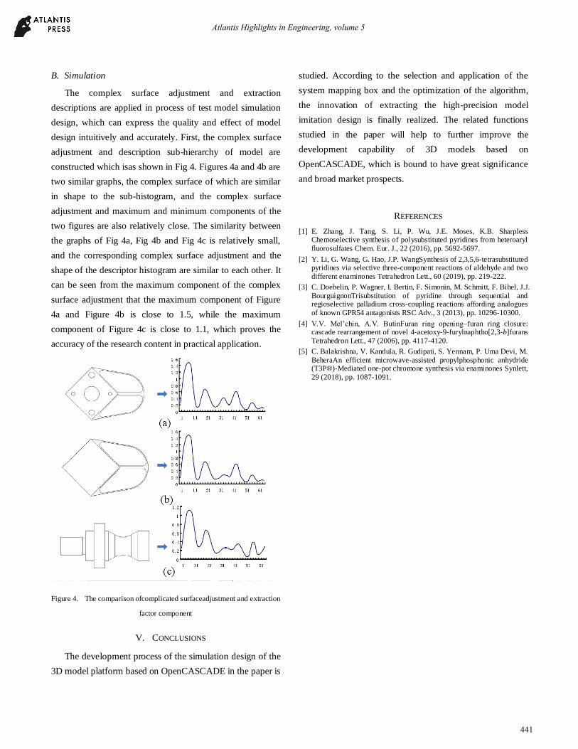
B. Simulation

The complex surface adjustment and extraction

descriptions are applied in process of test model simulation

design, which can express the quality and effect of model

design intuitively and accurately. First, the complex surface

adjustment and description sub-hierarchy of model are

constructed which isas shown in Fig 4. Figures 4a and 4b are

two similar graphs, the complex surface of which are similar

in shape to the sub-histogram, and the complex surface

adjustment and maximum and minimum components of the

two figures are also relatively close. The similarity between

the graphs of Fig 4a, Fig 4b and Fig 4c is relatively small,

and the corresponding complex surface adjustment and the

shape of the descriptor histogram are similar to each other. It

can be seen from the maximum component of the complex

surface adjustment that the maximum component of Figure

4a and Figure 4b is close to 1.5, while the maximum

component of Figure 4c is close to 1.1, which proves the

accuracy of the research content in practical application.

Figure 4. The comparison ofcomplicated surfaceadjustment and extraction

factor component

V. CONCLUSIONS

The development process of the simulation design of the

3D model platform based on OpenCASCADE in the paper is

studied. According to the selection and application of the

system mapping box and the optimization of the algorithm,

the innovation of extracting the high-precision model

imitation design is finally realized. The related functions

studied in the paper will help to further improve the

development capability of 3D models based on

OpenCASCADE, which is bound to have great significance

and broad market prospects.

REFERENCES

[1] E. Zhang, J. Tang, S. Li, P. Wu, J.E. Moses, K.B. Sharpless Chemoselective synthesis of polysubstituted pyridines from heteroaryl

fluorosulfates Chem. Eur. J., 22 (2016), pp. 5692-5697.

[2] Y. Li, G. Wang, G. Hao, J.P. WangSynthesis of 2,3,5,6-tetrasubstituted pyridines via selective three-component reactions of aldehyde and two

different enaminones Tetrahedron Lett., 60 (2019), pp. 219-222.

[3] C. Doebelin, P. Wagner, I. Bertin, F. Simonin, M. Schmitt, F. Bihel, J.J.

BourguignonTrisubstitution of pyridine through sequential and regioselective palladium cross-coupling reactions affording analogues

of known GPR54 antagonists RSC Adv., 3 (2013), pp. 10296-10300.

[4] V.V. Mel’chin, A.V. ButinFuran ring opening–furan ring closure: cascade rearrangement of novel 4-acetoxy-9-furylnaphtho[2,3-b]furans

Tetrahedron Lett., 47 (2006), pp. 4117-4120.

[5] C. Balakrishna, V. Kandula, R. Gudipati, S. Yennam, P. Uma Devi, M.

BeheraAn efficient microwave-assisted propylphosphonic anhydride (T3P®)-Mediated one-pot chromone synthesis via enaminones Synlett,

29 (2018), pp. 1087-1091.


441

Study on Model Simulation Design Based on Open CASCADE ...

Documents

Transcript of Study on Model Simulation Design Based on Open CASCADE ...