STUDY OF NOBLE GASES IN LUNAR

EXOSPHERE USING THE CHACE-MIPOBSERVATION OF CHANDRAYAAN-1

Thesis submitted toCochin University of Science and Technology

In partial fulfillment of the requirementsfor the award of

Doctor of Philosophyin

Physics

UNDER THE FACULTY OF SCIENCES

by

Tirtha Pratim Das

Space Physics LaboratoryVikram Sarabhai Space Centre

Indian Space Research OrganisationThiruvananthapuram-695 022

INDIA

December 2016

DECLARATION

This is to declare that the work presented in this thesis has been carried out at the SpacePhysics Laboratory (SPL), Vikram Sarabhai Space Centre (VSSC), Indian Space ResearchOrganisation (ISRO), Thiruvananthapuram, India, for the award of the degree of Doctor ofPhilosophy in Physics from the Cochin University of Science and Technology (CUSAT),Cochin, Kerala, India. This thesis is the outcome of the original work done by me andthe work did not form any dissertation submitted for the award of any degree, diploma,associateship or any other title or recognition from any University/Institution.

December, 2016Place: Thiruvananthapuram, India TIRTHA PRATIM DAS

CERTIFICATE

Certified that the thesis titled Study of noble gases in Lunar exosphere using theCHACE-MIP observation of Chandrayaan-1 submitted by Mr. Tirtha Pratim Das(Ph.D. registration number 4181) to Cochin University of Science and Technology,Cochin, embodies the original results of the investigations carried out by him at the SpacePhysics Laboratory, Vikram Sarabhai Space Centre, Indian Space Research Organisation,Thiruvananthapuram. To the best of my knowledge this thesis is a bonafide record ofresearch carried out by Mr. Tirtha Pratim Das, under my supervision. The work presentedin this thesis has not been submitted for the award of any other degree, diploma orassociateship to any other University or Institution.

CERTIFICATE

This is to certify that all the relevant corrections and modifications suggested by theaudience during the Pre-synopsis seminar and recommended by the Doctoral Committeeof Mr. Tirtha Pratim Das (PhD. registration number 4181) have been incorporated in thethesis.

DEDICATION

When the Guru and God both stand in front of me,who will I bow to first? Prostrations unto the Guru whobestowed me the path to God!

— Sant Kabir

This humble work is dedicated to my revered teachers, who built me with lot of loveand care.

ACKNOWLEDGEMENT

Quoting Guru Granth Sahib, “Were there to rise a hundred Moons, and a thousandSuns; without the Guru, it will still be pitch darkness.”. Despite his faith in the heritageof the Guru-disciple lineage, my Guru, Dr. Anil Bhardwaj, Director, Space PhysicsLaboratory (SPL), beleives that his disciples have to be self-sufficient, independent, andhence self-luminiscent. I am indebted to him and bow to him for showing me the way tothe truth. No word can sufficiently describe his effective mentoring and strong influence onme to pave the way of continuous refinement. As an Internationally acclaimed planetaryscientist of his own stature, mentor to numerous gems in this field, Dr. Anil Bhardwaj hasbeen exceptionally kind to have accepted a person like me, with no extra-ordinary virtue,as his doctoral student. If I do not feel the touch of the Almightly in these flow of events,how else do I realize that how blessed am I?

While my Guru has introduced me to the Almighty in the form of joy and beauty tounveil the mysteries of the Universe, I have felt the touch of Almighty throughout myjourney through various encouraging and challenging moments, shared with many peoplein an intricately weaven relationship. I am immensely grateful to all of them.

I am indebted to the Director, Vikram Sarabhai Space Centre (VSSC), ISRO, forgranting me kind permission to pursue this doctoral work as a part-time student, registeredin the Cochin University of Science and Technology (CUSAT).

My doctoral work is based on the in-situ measurement of the tenuous lunar exosphereusing the Chandra’s Altitudinal Composition Explorer (CHACE) payload housed in theMoon Impact Probe (MIP) in the Chandrayaan-1 mission (2008). The very idea of sendingthe impactor to the Moon in the maiden lunar mission of India was the brainchild of lateDr. A.P.J. Abdul Kalam, former President of India, a visionary technologist, who inspiredinnumerable souls like me. I bow to him for his great vision which facilitaed probing theMoon from close range. The CHACE experiment was the brainchild of Prof. R. Sridharan,the then Director of the SPL, who was also the principal investigator of the CHACEexperiment in Chandrayaan-1/MIP mission. I was greatly inspired by him to study thesubjects of mass spectrometry and lunar atmosphere during my initial days at SPL. It wasProf. R. Sridharan who showered his blessings on me and had strong faith on my abilitiesto carry out the project-related activities of time-bound nature leading to the realization ofthe CHACE payload. I gratefully acknowledge his deep influence on me, without whichthis thesis would not have materialized. I gratefully remember the affectionate, yet criticalmentoring by Dr. K. Krishnamoorthy, ex-Director, SPL during my doctoral journey. Dr.Krishnamoorthy, even after his superannuation from SPL, while handling other scientificand administrative responsibilities in ISRO Head Quarters and later in Indian Instituteof Science (IISc), Bangalore, have never forgotten to enquire about the progress of myresearch. I still feel his blessings in every step of my research. I thankfully recall andacknowledge numerous moments shared and discussions held with Dr. S. Maqbool Ahmed,who was the project manager of the CHACE payload, and currently the Head, CentralInstrumentation Laboratory, Central University of Hyderabad.

I am thankful to Shri S V Mohankumar, who was my division head till August 2016, forhis affectionate blessings for my doctoral journey. I have no words to express the support Ihave received from him. My present division head, Dr. K. Rajeev, who is also a member of

i

my Doctoral Committee, has made me indebted not only by his constant support, but alsothrough his strong faith on my capabilities. In the same context, I fondly remember Late BManojkumar, my first reporting officer in ISRO, whom I worked with from 2004 to 2006during my service as a launch vehicle technologist in VSSC’s Mechanisms and VehicleIntegration Testing (MVIT) entity. I remember with deep gratitude how much personalinterest he used to take to ensure that I enrolled into the doctoral programme. I am surethat his immortal soul is constantly blessing me and giving me enough strength to stand onmy own feet, just the way he used to mentor me during my tender years in ISRO. Had Inot been fortunate enough to get these God-sent people as my bosses, today this researchwould not have seen the light of the day.

I take this opportunity to acknowledge the role of the Doctoral Committee for constantmonitoring of the progress of this research work and keeping my doctoral journey in track.Gratefully acknowledged are the regular reviews conducted by the Academic Committeeof SPL, Doctoral Committee and the CUSAT Research Committee, which ensured thatthis research brings out the best possible science. I express my deep sense of gratitude toDr. Radhika Ramachandran, Chairperson, Academic Committee, SPL, for her constantsupport, blessings, valuable timely suggestions and encouragement. I am grateful to myexaminers, viz. Dean of the Facilty of Sciences, CUSAT, Head of the Department ofPhysics, CUSAT, Prof. T. Rameshbabu, Department of Physics, CUSAT, Dr. GeorgeJoseph, VSSC and Dr. A K Anilkumar, VSSC, who spent their valuable time to haveevaluated me during the process of my Ph.D. coursework examination.

I thankfully mention the important scientific discussions with Dr. Smitha Thampi,scientist, SPL, on my research topic. She has not only spared her valuable time for scientificdiscussions, but have also given many valueable suggestions to improve the thesis. Thediscussions held with Dr. Megha Upendra Bhatt, Research Associate, SPL are thankfullyacknowledged for discussions on the origin and evolution of the Moon. Insightful scientificdiscussions with all my colleagues, especially with Dr. K. Rajeev, Dr. Tarun Kumar Pant,Ms. M B Dhanya, Dr. Prabha Nair, Dr. Geetha Ramkumar, Dr. K. Kishore Kumar, Dr.Suresh Babu, Dr. C Suresh Raju, Dr. Satheesh Thampi, Dr. Vipin K Yadav, Dr. SiddharthSankar Das, Dr. Damu Bala Subrahamaniyam are gratefully acknowledged. I beg tobe condoned for not being able to mention all the names, as the list is quite big. I amalso thankful to our Research Fellows Ms. Shreedevi P R, Ms. Vrinda Mukundan, Mr.Abhinaw Alok for various supports. In fact, my each and every colleague from the scienticand engineering fields have their own contributions to enrich me through discussions,critical judgements, strong cooperation and most importantly, emotional cohesion, withoutwhich this reasearch would not have bloomed to completeness. They are the source of myinspiration and strength.

At this juncture, I would like to specially mention about Shri Madan Lal, the thenDeputy Director of the Launch Vehicle Design Entity (LVDE) of VSSC, who was thefirst team leader of the MIP project. He ensured that MIP is developed with zero-defectperfection, within the project deadline. As a task master, he used to extract the best from us.Working with him for the MIP project is a cherishable memory of my life. Later, after thesuperannuation of Shri Madan Lal, Shri Y Ashok Kumar of the Avionics entity of VSSCbecame the team leader of MIP. Under the able guidance and leadership of Shri AshokKumar, MIP was delivered to the Chandrayaan-1 project. I fondly remember both ShriMadan Lal and Shri Ashok Kumar and acknowledge their immense contributions towards

ii

the success of the MIP. It is my pleasure to recall the mathematical discussions on the MIPtrajectory with Dr. R V Ramanan, who was with the Applied Mathematics Division ofVSSC and is currently at the Indian Institute of Space Science and Technology (IIST). Ithankfully mention about my colleagues with whom I have worked for the development ofthe CHACE instrument: Shri P. Pradeepkumar, Dr. P. Sreelatha, Ms. Supriya Gogulapati,Ms. Neha Naik and Shri Dinakar Prasad Vajja. Most of them, as well as Shri Abhishek J Kare the copassangers of my current journey to explore the Martian and lunar exospheres inthe Mars Orbiter Mission (MOM) and forthcoming Chandrayaan-2 mission, respectively. Imust make special mention of Dr. Raghuram Susarla and Dr. Sonal Jain, who were thedoctoral students of my guide, and currently doing active research in the Imperial College,London and Laboratory for Atmospheric and Space Physics (LASP), USA, respectively.Both of them have helped me in many respects during my research when they were in SPL.Dr. Sonal has been helpful to me even after he went aboard for his post-doctoral research.

I am immensely thankful to Dr. Neeraj Srivastava, scientist, Physical Research Labora-tory (PRL), Ahmedabad and Ms. Indhu Varatharajan, the then project student working withDr. Neeraj at PRL, for introducing me to the field of lunar geology during the StructuredTraining Programme (STP) on planetary exploration organised by ISRO, held at PRL.I am immensely thankful to Prof. S V S Murthy and Prof. S A Haider, PRL and Dr.P. Sreekumar, Director, Indian Institute of Astrophysics (IIA), Bangalore, for scientificdiscussions in the field of planetary science and instrumentation on several occasions,which helped me to get insight to my field of research. Thanks to the PLANEX programmeat PRL, which gave me many opportunities to interact with scientists and technologists aswell as students working in the field of planetary sciences. Dr. Bhala Sivaraman, scientist,PRL is fondly acknowledged for his constant encouragement and energizing friendship,which have helped me to love my field of research more passionately.

I hereby acknowledge the insightful scientific discussions on lunar exosphere over email with Dr. Richard Hodges, LASP, Colorado, USA and Dr. Dana Hurley, AppliedPhysics Laboratory, John Hopkins University, USA. Also gratefully acknowledged are theprivate communications with Dr. Paul Mahaffy, Principal Investigator of the Neutral MassSpectrometer (NMS) experiment in NASA’s LADEE mission to the Moon and NeutralGas Ion Mass Spectrometer (NGIMS) experiment aboard the MAVEN mission to Mars,who is presently in the Goddard Space Flight Centre, NASA, USA.

I am also thankful to the Administrative Officer, Establishment section, VSSC and hisable team for helping me to complete all the formalities during the process of my gettinginducted into research. In the course of my doctoral journey, I have received completecooperation from the SPL office; especially from Ms. P R Suseela, Ms. Sisira and Ms. CGeetha. They have helped me in all administrative matters. Ms. Sisira used to meticulouslykeep all the records of my research-related matters and also used to keep in touch withCUSAT to make me less bothered about the administrative formalities. The VSSC libraryhas tremendous effect on me. The Head of the Library and Documentation Division andhis able team have been regularly sending me updates on my field of research throughoutmy doctoral journey. I also acknowledge the kind cooperation of the staff of the CUSATduring the entire process of my doctoral work.

I take this opportunity to pay homage to all my teachers who have built me with somuch love and care. It is difficult to name all of them here; yet, I choose to name a few ofthem. I would like to mention about Mr. Ananda Banerjee, who was the librarian at the St.

iii

Lawrence High School, Kolkata, where I have studied till my plus-two standard. He hasbuilt my reading habit. Today when I receive the same warmth from Shri Narayanakutty,Head Library, VSSC and Dr. Rajendran, former head of the VSSC library, I remember myquality time spent with Mr. Ananda Banerjee at school library. I was strongly influencedby the moral teachings of late Father Andre Bruylanths, late Father Adrian Wavrail, FatherK. Thottam, and many other teachers of the St. Lawrence High School. I fondly rememberthe contributions of all my teachers who tought me physics and mathematics during mygraduate studies in the St. Xavier’s College, Kolkata and post-graduate studies in theInstitute of Radiophysics and Electronics, University of Calcutta. Especially, I would liketo mention the great infleunces of late Dr. Sisir Kumar Bhanja of St. Xavier’s College,Kolkata and Dr. Kiranmoy Sengupta of Dinabandhu Andrews College, Kolkata, on me,who unraveled the beauty of Physics to me during my graduation years. I carry within meall of them in my subconscious.

I thankfully acknowledge the contributions of my parents, Shri Tushar Kanti Das andSmt. Sumita Das and my parents in-law Shri Santosh Nandi and Smt. Papia Nandi, fortheir constant encouragement and especially for having strong faith on my capabilities.My wife Megha has taken the maximum pain; I remember, just after we got married, Iwas spending days and night in office, in connection with the test and evaluation of thequalification model (QM) of CHACE. She was thousands of kilometers away from herhometown, solely counting on my support, but had to bear with my entries and exits duringodd hours of the day. Hats off to her perseverance and cooperation, without which I wouldnot have been able to contribute to the development of CHACE. My son Meghtirtha, whois four years old now, keeps me busy at home, and hence forcefully provides me breaksfrom my research-related thoughts and anxiety. Hope one day he will understand howgreatly he has helped me by doing this, once he grows up and cares to turn the pages of hispapa’s thesis.

Tirtha Pratim Das

December 2016

iv

Contents

List of Figures viii

List of Tables xiv

Journal publications xv

Presentations in conferences/workshops/symposia xvi

Acronyms xviii

Symbols xx

Preface xxi

1 Introduction 11.1 Moon: Origin and evolution . . . . . . . . . . . . . . . . . . . . . . . . 1

1.1.1 Lunar origin: a brief history . . . . . . . . . . . . . . . . . . . . 21.1.2 The Lunar Magma Ocean (LMO) . . . . . . . . . . . . . . . . . 61.1.3 Formation of basins and Lunar maria . . . . . . . . . . . . . . . 71.1.4 The ‘recent’ Moon . . . . . . . . . . . . . . . . . . . . . . . . . 8

1.2 Evolution of the lunar atmosphere . . . . . . . . . . . . . . . . . . . . . 91.2.1 Epoch I: From ∼ 4.57 Gy to ∼ 4.4 Gy . . . . . . . . . . . . . . . 101.2.2 Epoch II: From ∼ 4.4 Gy to ∼ 3.1 Gy . . . . . . . . . . . . . . . 101.2.3 Epoch III: Last ∼ 3.1 Gy . . . . . . . . . . . . . . . . . . . . . . 11

1.3 The Lunar Exosphere . . . . . . . . . . . . . . . . . . . . . . . . . . . . 121.3.1 Source processes . . . . . . . . . . . . . . . . . . . . . . . . . . 131.3.2 Sink processes . . . . . . . . . . . . . . . . . . . . . . . . . . . 18

1.4 Modelling of the Lunar exosphere . . . . . . . . . . . . . . . . . . . . . 221.5 Observations on the lunar exosphere . . . . . . . . . . . . . . . . . . . . 24

1.5.1 The Apollo observations (1969-1972) . . . . . . . . . . . . . . . 241.5.2 Observations by Lunar Prospector (1998-1999) . . . . . . . . . . 261.5.3 Observations by Kaguya (2007-2009) . . . . . . . . . . . . . . . 261.5.4 Observations by Chang’E-1 (2007-2009) . . . . . . . . . . . . . 27

v

1.5.5 Observations by Chandrayaan-1 (2008-2009) . . . . . . . . . . . 271.5.6 Observations by LAMP/LRO (2009-present) . . . . . . . . . . . 281.5.7 Observations by LCROSS (2009) . . . . . . . . . . . . . . . . . 291.5.8 Observations by NMS/LADEE . . . . . . . . . . . . . . . . . . . 321.5.9 Coordinated observations . . . . . . . . . . . . . . . . . . . . . . 33

1.6 Motivation and scope of the present work . . . . . . . . . . . . . . . . . 33

2 Moon Impact Probe and the CHACE experiment 362.1 The MIP aboard Chandrayaan-1 . . . . . . . . . . . . . . . . . . . . . . 36

2.1.1 Introduction . . . . . . . . . . . . . . . . . . . . . . . . . . . . . 362.1.2 The Moon Impact Probe Mission . . . . . . . . . . . . . . . . . 36

2.2 The CHACE instrument . . . . . . . . . . . . . . . . . . . . . . . . . . . 372.2.1 Physics of the transmission-type QMA . . . . . . . . . . . . . . 382.2.2 The CHACE sensor probe and electronics . . . . . . . . . . . . . 472.2.3 Development philosophy . . . . . . . . . . . . . . . . . . . . . . 502.2.4 Operating parameters . . . . . . . . . . . . . . . . . . . . . . . . 51

2.3 Ground calibration and testing . . . . . . . . . . . . . . . . . . . . . . . 542.3.1 Relative detection efficiencies . . . . . . . . . . . . . . . . . . . 542.3.2 Mass calibration . . . . . . . . . . . . . . . . . . . . . . . . . . 552.3.3 Pressure calibration . . . . . . . . . . . . . . . . . . . . . . . . . 572.3.4 Sensitivity test . . . . . . . . . . . . . . . . . . . . . . . . . . . 582.3.5 Test and Evaluation . . . . . . . . . . . . . . . . . . . . . . . . . 59

2.4 Mission operation of CHACE and data analysis . . . . . . . . . . . . . . 61

3 Observations on Argon 673.1 The lunar Argon . . . . . . . . . . . . . . . . . . . . . . . . . . . . . . . 67

3.1.1 Origin of 40Ar . . . . . . . . . . . . . . . . . . . . . . . . . . . 68

3.1.2 Loss processes for 40Ar . . . . . . . . . . . . . . . . . . . . . . 693.2 Previous observations . . . . . . . . . . . . . . . . . . . . . . . . . . . . 703.3 Observations and Results . . . . . . . . . . . . . . . . . . . . . . . . . . 72

3.3.1 Distribution of 40Ar . . . . . . . . . . . . . . . . . . . . . . . . . 733.3.2 The 40Ar:36Ar ratio . . . . . . . . . . . . . . . . . . . . . . . . . 75

3.4 Concluding remarks . . . . . . . . . . . . . . . . . . . . . . . . . . . . . 78

4 Observations on Neon 794.1 The lunar Neon . . . . . . . . . . . . . . . . . . . . . . . . . . . . . . . 79

4.1.1 Origin of 20Ne . . . . . . . . . . . . . . . . . . . . . . . . . . . 80

4.1.2 Loss processes for 20Ne . . . . . . . . . . . . . . . . . . . . . . 804.2 Previous observations . . . . . . . . . . . . . . . . . . . . . . . . . . . . 804.3 Observations and Results . . . . . . . . . . . . . . . . . . . . . . . . . . 82

4.3.1 Sensitivity analysis . . . . . . . . . . . . . . . . . . . . . . . . . 854.4 Concluding remarks . . . . . . . . . . . . . . . . . . . . . . . . . . . . . 88

vi

5 Observation on Helium 905.1 The lunar Helium . . . . . . . . . . . . . . . . . . . . . . . . . . . . . . 905.2 Previous observations . . . . . . . . . . . . . . . . . . . . . . . . . . . . 945.3 Observations by CHACE . . . . . . . . . . . . . . . . . . . . . . . . . . 955.4 The Peak Detection Algorithm . . . . . . . . . . . . . . . . . . . . . . . 965.5 Interpretation . . . . . . . . . . . . . . . . . . . . . . . . . . . . . . . . 995.6 Discussion . . . . . . . . . . . . . . . . . . . . . . . . . . . . . . . . . . 995.7 Conclusion . . . . . . . . . . . . . . . . . . . . . . . . . . . . . . . . . 101

6 Observations on H2 1036.1 The lunar H2 . . . . . . . . . . . . . . . . . . . . . . . . . . . . . . . . 1036.2 Previous observations . . . . . . . . . . . . . . . . . . . . . . . . . . . . 1046.3 Results of CHACE observations . . . . . . . . . . . . . . . . . . . . . . 1066.4 Concluding remarks . . . . . . . . . . . . . . . . . . . . . . . . . . . . . 109

7 Summary and Future Work 1107.1 Summary of the Work and Major Results . . . . . . . . . . . . . . . . . 1107.2 Open Questions . . . . . . . . . . . . . . . . . . . . . . . . . . . . . . . 1127.3 Future work: Detailed observation of the lunar exosphere . . . . . . . . . 113

Appendices 114

A Vertical density profile in an exosphere 115A.1 Hydrostatic equilibrium and the barometric law . . . . . . . . . . . . . . 115A.2 Exosphere: the collisionless regime . . . . . . . . . . . . . . . . . . . . 116A.3 Discussion . . . . . . . . . . . . . . . . . . . . . . . . . . . . . . . . . . 120

Bibliography 121

vii

List of Figures

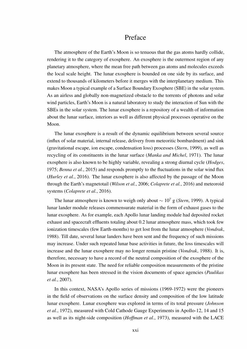
1.1 Moon, as seen from the Earth. The yellow coloured vertical and horizontallines represent the lunar prime meridian and equator respectively. Thedark regions are Mare Basalts, formed by the solidification of the moltenmagma that oozed from the interior through fissures. They are relativelyyounger (3.0 to 3.9 Ga) than the highlands (relatively brighter regions).[Taken from Marble virtual globe (http://edu.kde.org/marble)]. . . . . . . 8

1.2 A schematic of the time evolution of the Moon. The time scales are fromElkins-Tanton et al. (2011); Stern (1999); Greeley (2013) . . . . . . . . . 9

1.3 A schematic of the evolution of the lunar atmosphere since its formation(redrawn from Stern, 1999). Epoch II and III witnessed episodic increaseof the atmospheric pressure due to the release of gases as a result ofbombardment of meteorites. . . . . . . . . . . . . . . . . . . . . . . . . 10

1.4 Schematic showing the source and sink processes in the Lunar exosphere . 13

1.5 The energy distribution of sputtered Oxygen atoms, given by the Sigmunddistribution function, (equation 1.4) for proton projectiles with 1 keV en-ergy and surface binding energy of 2 eV, is plotted with open stars. TheSigmund distribution function, at higher energies, falls off with E−2

e vari-ation. The Maxwell-Boltzmann energy distribution function followed bythermal atoms, given by 2(E/π)1/2(kT )−3/2e−E/kT , with T=400 K (typi-cal value of the dayside lunar surface temperature at equator) is co-plotted(open circles) for comparison. The Maxwell-Boltzmann distribution fallsoff exponentially with energy. . . . . . . . . . . . . . . . . . . . . . . . . 16

1.6 Summary and time-line of the lunar missions that have contributed to thepresent understanding of the lunar exosphere. The only three missions thatconducted in-situ study of the lunar neutral exosphere are Apollo (LACE inApollo-17) in 1972-1973, Chandrayaan-1 (CHACE aboard MIP) in 2008and LADEE (the NMS) in 2013-2014. . . . . . . . . . . . . . . . . . . . 24

1.7 Trends of diurnal variation of the lunar He and Ar as observed by LACE.The He values are averaged over ten lunations. The Ar measurementscorrespond to 20 July to 3 August 1973. Subsolar meridian of 180◦

represents local midnight. Succesful observations by LACE were limitedto the lunar nightside. Redrawn based on the Figs. 2 and 3 from Stern(1999). Original data are from Hodges (1975). . . . . . . . . . . . . . . 25

viii

1.8 Diurnal variation of the surface density of He and Ne as derived from theNMS observations. The longitudes from the subsolar meridian 90◦, 180◦

and 270◦ represent local dusk, midnight and dawn, respectively. [Redrawnbased on the Figures 2 a and c from Benna et al. (2015)]. . . . . . . . . . 32

2.1 Schematic of Chandrayaan-1 with the MIP attached as a piggyback mi-crosatellite on the top deck. . . . . . . . . . . . . . . . . . . . . . . . . . 37

2.2 Schematic of the MIP showing the payloads. . . . . . . . . . . . . . . . . 37

2.3 Flight model of the CHACE instrument. . . . . . . . . . . . . . . . . . . 38

2.4 Cross section of the Quadrupole Mass Analyser rods with hyperbolicgeometry . . . . . . . . . . . . . . . . . . . . . . . . . . . . . . . . . . 39

2.5 Computer simulated saddle-shaped Potential Energy Surface (PES) insidethe QMA with a constant potential. A charged particle may be lookedupon as a ball resting on the saddle. It is stable along the x direction withcharacteristic frequency ωp, while unstable along the y direction. . . . . . 41

2.6 Computer simulated PES inside the QMA with the assumption of an RFcomponent. Simulations depict the PES at the RF phases of 0◦ (top panel)and 180◦ (bottom panel). The simulation is carried out for a species withm/q=28 amu and using the CHACE geometrical and RF parameters. Itshows that in one half cycle, the ion is stable along the x direction, whilein the next half cycle it is stable in the y direction. . . . . . . . . . . . . . 43

2.7 Computer simulated trajectories of two species with m/q=1 and 2 amu,computed by numerically solving the Mathieu equation. The ions aremoving from the QMA entry aperture (left) towards the detector (right).The combination of the DC and RF potentials rendered amu 1 ions stableand the amu 2 unstable. . . . . . . . . . . . . . . . . . . . . . . . . . . 45

2.8 The top panel (a) shows the time axis; Tscan represents the time requiredto complete a mass scan. Panel (b) shows that mass scanning is achievedby ramping U and V simultaneously and proportionally. Ions with a givenmass-to-charge ratio are stable and hence pass through the QMA when thebias curve intersects the triangular regions called the Paul stability regions.Panel (c) shows that how a mixture of ions pass through the mass filter andconstitute output current proportional to their relative abundances at thedetector. . . . . . . . . . . . . . . . . . . . . . . . . . . . . . . . . . . . 46

2.9 Quadrupole rods of circular geometry are easier to machine than thehyperbolic rods. The circular rods with radius 1.148 times r0 (radius of thein-circle touching the quadrupole rods) fairly reproduce the quadrupolefield as done by the ideal hyperbolic geometry rods. . . . . . . . . . . . . 47

2.10 Block diagram of the CHACE instrument. The MTU is responsible formultiplexing the data from CHACE, Moon Imaging System (MIS) andthe Radar Altimeter (RA). The data are transmitted through the UHFtransmitter and antennae to Chandrayaan-1 orbiter. . . . . . . . . . . . . 48

2.11 Schematic diagram of the sensor probe of the CHACE instrument. . . . . 49

ix

2.12 A laboratory spectrum acquired by the CHACE instrument. The signaturesof the major residual gases in the chamber are seen in the spectrum. . . . 50

2.13 Variation of the ion current for amu 28 (N2) for different focus voltages. . 52

2.14 Variation of the optimum bias voltage of the CEM detector with totalpressure. The filled squares are the experimentally obtained points and thecontinuous solid line is the exponential fit, which is extrapolated (dottedextension) to 10−10 Torr of total pressure, as expected in the sunlit sideof the Moon. At a given total pressure, the optimum CEM bias voltage isobtained by studying the variation of the SNR of amu 28 peak with CEMbias voltage, as shown in the inset for a pressure of 4 × 10−9 Torr. Basedon this experiment, the CEM bias voltage of CHACE was set at 1800 V. . 53

2.15 The continuous line represents the variation of the relative transmissionefficiency (with respect to N2 (amu 28)) with ion mass. The relativetransmission efficiency curve is obtained by comparing the experimentaland theoretical values of the fractionation ratios of water vapour (amu 1 ,amu 16, amu 17, amu 18) and the compound Per Fluoro Tri Butyl Amine(PFTBA) (which yields mass peaks at amu 31, 69 and 100 in the range of 1-100 amu) for 70 eV electron impact energy. In addition to the fractionationratios of the compounds, the experimental and theoretical values of thesingle-to-double ionization ratios of atomic species like 40Ar (i.e. ratio ofthe parent peak at amu 40 to the harmonic peak at amu 20) and N (i.e.ratio of the parent peak at amu 14 to the harmonic peak at amu 7) at 70eV electron energy are also used for obtaining the relative transmissionefficiency profile. The solid circles, drawn on the relative transmissionefficiency curve, represent the relative transmission efficiencies of 4He,20Ne, 40Ar with respect to N2 due to the Quadrupole Mass Discrimination(QMD) effect. . . . . . . . . . . . . . . . . . . . . . . . . . . . . . . . . 55

2.16 Variation of the Electron Multiplier Gain (EMG) of CHACE with the ionmass, at 1800 V bias. The EMG is calculated by comparing the signalstrengths of the residual atmospheric gases viz. amu 1 (H atom), amu16 (O atom), amu 28 (N2 molecule), amu 44 (CO2 molecule) and amu56 (which is due to the oil used in the turbomolecular pump) in electronmultiplier and Faraday cup modes. The criteria to choose these pointsare: 1) the signal strength should be high enough to detect it even in theFarady cup mode (less sensitive mode), 2) the signal strength should bestable with time (so that it doesn’t vary during the span of the experiment)and 3) signals should cover a wide mass range. . . . . . . . . . . . . . . 56

2.17 Combined relative sensitivity of the instrument due to the mass dependentperformances of the QMA and the CEM. The lighter species have greatermobility and are less affected by the fringing fields at the terminations ofthe QMA, and hence have greater transmission efficiency. Also, the CEMgain is greater for the lighter species than the heavier ones. The overalleffect is that the instrument is more sensitive to the lighter species than theheavier ones. This effect is corrected during the data analysis. . . . . . . 57

x

2.18 Signature of 4He acquired by CHACE during laboratory calibration. Whilethe parent peak is at amu 4, there is a harmonic peak due to doubleionization of 4He at amu 2, with a relative abundance of 0.08 with respectto the parent peak. . . . . . . . . . . . . . . . . . . . . . . . . . . . . . 58

2.19 Signature of 40Ar acquired by CHACE during laboratory calibration. Thedouble ionized Argon (Ar++) produces a peak at m/q = 20 amu. . . . . . 59

2.20 Signature of N2 (amu 28) acquired by CHACE during laboratory calibra-tion. The dissociated atomic N produces a peak at m/q = 14 amu. . . . . . 59

2.21 Signature of CO2 (amu 44) acquired by CHACE during laboratory cali-bration. The dissociation products are CO and O and C producing peaksat m/q = 28, 16 and 12 amu, respectively. . . . . . . . . . . . . . . . . . 60

2.22 Total pressure calibration curve of the Bayard-Alpert gauge of CHACE.The linearity of the response of the gauge is established. The deviationbetween the readings of the Bayard-Alpert gauge of CHACE and thereference pressure gauge is due to the different locations of their mountingin the vacuum chamber with respect to the turbomolecular pump. . . . . . 61

2.23 (a) A mass spectrum acquired with CHACE before the environmental test,at a total pressure of ∼ 5 × 10−7 Torr. (b) A mass spectrum acquiredafter the completion of the environmental tests were completed, undersimilar total pressure. It is observed that the quality of the mass spectrum(assessed with respect to the mass resolution, peak shape, throughput andmass shift) is retained even after the environmental tests. . . . . . . . . . 62

2.24 (a) Location of the Moon with respect to the Earth during the MIP release.The bow shock and the geomagnetic tail are shown for nominal solarconditions. (b) Ground trace of the MIP (red curve) after release from theChandrayaan-1 orbiter. . . . . . . . . . . . . . . . . . . . . . . . . . . . 63

2.25 The flow chart describing the process of data reduction. . . . . . . . . . . 64

2.26 The step-by-step processing of the raw mass spectrum during the processof data reduction. The ordinates in the first three panels are plottedin arbitrary units (a.u.). The applications of relative transmission anddetection efficiency corrections and normalization with the gas-correctedtotal pressure are demonstrated here. . . . . . . . . . . . . . . . . . . . . 64

2.27 The black line shows the latitude-altitude profile of the trajectory of theMIP. The red coloured dotted line shows the variation of the lunar surfacetemperature as a function of latitude along the ground trace of the MIP. Thesurface temperature graph is as per the Diviner radiometer observations(Paige et al., 2010a). . . . . . . . . . . . . . . . . . . . . . . . . . . . . 65

3.1 Schematic of the main processes in the lunar Argon exosphere. . . . . . . 70

3.2 Sample raw spectra covering the mass range of 36 to 40 amu showingthe presence of 40Ar and 36Ar. For panels (a) and (b), the altitude ofobservation was ∼98 km, i.e. before the separation of the MIP from thespacecraft. For panel (c), the altitude of observation was ∼80 km and forpanel (d), the observation was close to the surface of the Moon. . . . . . 72

xi

3.3 The number density of 40Ar from the in-situ measurements of CHACEalong the MIP trajectory. The measurements are convolution of altitudinaland latitudinal effects. . . . . . . . . . . . . . . . . . . . . . . . . . . . 73

3.4 The top panel shows the surface density of 40Ar derived using barometriclaw from the CHACE observations. The lower panel shows the lunarsurface topography obtained using LLRI data along the ground track ofthe MIP. The anti-correlation of the trends of the surface density and theelevation from ∼ 42◦S till the South pole is quite evident. . . . . . . . . . 74

3.5 Two dimensional (latitude versus altitude) map of lunar 40Ar along thetrajectory of the MIP. . . . . . . . . . . . . . . . . . . . . . . . . . . . . 75

3.6 Variation of the 40Ar:36Ar ratio as obtained by CHACE. The red markersare the observed ratios while the blue continuous line is a 15 point movingaverage, which is equivalent to ∼ 100 km of ground trace. . . . . . . . . 76

3.7 Redrawn antiquity estimates of the lunar samples along with their corre-sponding 40Ar:36Ar ratios using the basic data from Eugster et al. (2001)along with the present estimates for both the Northern and Southern hemi-sphere values. . . . . . . . . . . . . . . . . . . . . . . . . . . . . . . . 77

4.1 Schematic of the main processes acting on the lunar Neon exosphere. . . . 81

4.2 Number density of Neon as a function of lunar latitude and altitude in thesunlit lunar exosphere derived from CHACE measurement. . . . . . . . . 84

4.3 Variation of surface number density of Neon with latitude in Southernhemisphere of the Moon observed by CHACE (filled circles). NMS/LADEEobservations shown here were made on 25 December 2013, 18 March2014 and 21 January 2014, when the Moon was in the magnetotail of theEarth, similar to the CHACE observation. . . . . . . . . . . . . . . . . . 85

4.4 A two dimensional (latitude vs altitude) distribution of Neon generatedusing the scale heights at different latitudes for the 14◦E lunar meridian.The black continuous line depicts the locus of the MIP during the CHACEobservations. . . . . . . . . . . . . . . . . . . . . . . . . . . . . . . . . 86

4.5 (a): Temperature profiles used for the sensitivity analysis of the derivednumber densities of Neon. The graph with blue circles represents thetemperature profile from Sridharan et al. (2010b), while the one with redsquares represent the tempretaure profile inferred from the Diviner obser-vations. L represents the lunar latitude. (b): The result of the sensitivityanalysis for four cases that include the combination of two temperatureprofiles and two different ratios of the double-to-single ionization crosssection of 40Ar. The latitude binning is same as that used in Fig. 4.3 . . . 88

4.6 The variation of the Neon surface density n with respect to T−5/2 for thelunar Neon at the middle and higher lunar latitudes. . . . . . . . . . . . 89

5.1 Schematic of the main processes acting on the lunar Neon exosphere. . . . 91

5.2 A typical mass peak in CHACE, comprising nine equispaced sample points,shown by xi, where i=1,2,...9. . . . . . . . . . . . . . . . . . . . . . . . 96

xii

5.3 The flow chart of the PDA. . . . . . . . . . . . . . . . . . . . . . . . . . 98

5.4 The inferred surface density of He corresponding to the PDA-positivepoints, detected based on pattern recognition. The dark horizontal lineindicates the detection thresold of the instrument, limited by the system noise.100

5.5 Monthly averaged solar wind alpha particle flux, as derived from theSWEEPAM/ACE observations over few years, covering the observationtime of CHACE/Chandrayaan-1 and NMS/LADEE. Alpha particle numberdensity data along with the velocity data of protons are used to computethe alpha particle flux. It is observed that during the CHACE observations,the solar wind alpha particle flux was significantly less than that duringthe NMS/LADEE observations. . . . . . . . . . . . . . . . . . . . . . . . 102

6.1 Cartoon showing the major source and sink processes of the lunar H2,based on the discussions given in (Hurley et al., 2017). The major sourceof the lunar H2 is the chemical sputtering from the lunar regilith, whichowes its hydrogen inventory to the solar wind proton influx. The physicallysputtered component of the H2 from the lunar regolith usually has enoughenergy to escape the lunar gravity. In the cartoon, both the thermal escapeand physical sputtering-induced escape components of the lunar H2 areshown as gravitational escape. Another escape mechanism is the ionescape, collectively due to photoionization, charge exchange and electronimpact ionization. . . . . . . . . . . . . . . . . . . . . . . . . . . . . . . 105

6.2 Left: The observed partial pressure of H2 along the MIP trajectory. Right:The calculated number density of H2 along the MIP trajectory. . . . . . . 107

6.3 A two dimensional (latitude vs altitude) map of H2 generated using thescale heights at different latitudes. The black continuous line depicts thelocus of the MIP during the CHACE observations. . . . . . . . . . . . . . 107

6.4 Variation of the surface number density of H2 (top panel) and the surfacetopography (bottom panel) at different lunar latitudes along the MIPground trace. . . . . . . . . . . . . . . . . . . . . . . . . . . . . . . . . 108

7.1 Latitudinal variation of the surface density of 40Ar, 20Ne and H2, as derivedfrom the CHACE observations. Fourth order polynomials are plotted inorder to emphasize the latitudinal variation of the surface densities ofthese species thereby suppressing the local variations. . . . . . . . . . . . 112

xiii

List of Tables

1.1 Orbital and physical parameters of Moon. From de Pater and Lissauer(2010); Greeley (2013) . . . . . . . . . . . . . . . . . . . . . . . . . . . 2

1.2 Calculated values of thermal escape parameter λesc for few species . . . . 19

1.3 Non-thermal escape processes [Taken from de Pater and Lissauer (2010)] 21

1.5 The derived upper limits of surface densities some of the lunar speciesat day-night terminators from LAMP. Adopted from Cook et al. (2013);Feldman et al. (2012); Stern et al. (2013) . . . . . . . . . . . . . . . . . . 31

2.1 Specifications of the CHACE instrument . . . . . . . . . . . . . . . . . . 38

2.2 Mass calibration with residual gases in the vacuum chamber . . . . . . . 58

2.3 Relative ionization sensitivity factor (with respect to N2 ) (Summers, 1969;Holanda, 1972) and overall sensitivities for the noble gases covered in thisthesis . . . . . . . . . . . . . . . . . . . . . . . . . . . . . . . . . . . . 60

3.1 Loss processes of 40Ar in the lunar exosphere (from Stern (1999); Nakaiet al. (1987); Huebner et al. (1992); Grava et al. (2015b), and the refer-ences therein) . . . . . . . . . . . . . . . . . . . . . . . . . . . . . . . . 69

4.1 Loss processes of 20Ne in the lunar exosphere (from Huebner and Mukher-jee (2015); Kim and Rudd (1994)) . . . . . . . . . . . . . . . . . . . . . 80

5.1 Loss processes of He in the lunar exosphere ( from Huebner et al. (1992);Stern (1999); Benna et al. (2015)) . . . . . . . . . . . . . . . . . . . . . 91

6.1 Loss processes of H2 in the lunar exosphere (Benna et al., 2015; Huebneret al., 1992) . . . . . . . . . . . . . . . . . . . . . . . . . . . . . . . . . 104

xiv

Journal publicationsDIRECTLY RELATED TO THESIS

1. Tirtha Pratim Das, Smitha V. Thampi, M B Dhanya, Anil Bhardwaj, S M Ahmed and RSridharan, Upper limit of helium-4 in the sunlit lunar exosphere during magnetotail passageunder low solar wind condition: Result from CHACE aboard MIP in Chandrayaan-1, Icarus,297, 189 – 194, doi: 10.1016/j.icarus.2017.07.001, 2017.

2. Tirtha Pratim Das., S. V. Thampi, A. Bhardwaj, S. M. Ahmed, and R. Sridharan, Observationof Ne at mid and high latitudes in the sunlit Lunar Exosphere: Results from CHACE aboardMIP/Chandrayaan-1, Icarus, 272, 206 – 211, doi: 10.1016/j.icarus.2016.02.030, 2016.

3. Thampi, S.V., R. Sridharan, Tirtha Pratim Das, S.M. Ahmed, J.A. Kamalakar, and A.Bhardwaj, The spatial distribution of molecular Hydrogen in the lunar atmosphere Newresults, Planetary and Space Science, 106, 142 – 147, doi: 10.1016/j.pss.2014.12.018, 2015.

4. Sridharan, R., Tirtha Pratim Das, S. M. Ahmed, G. Supriya, A. Bhardwaj, and J. A. Ka-malakar, Spatial heterogeneity in the radiogenic activity of the lunar interior: Inferencesfrom CHACE and LLRI on Chandrayaan-1, Advances in Space Research, 51, 168 – 178, doi:10.1016/j.asr.2012.08.005, 2013a.

5. Sridharan, R, Tirtha Pratim Das, SM Ahmed, and Anil Bhardwaj, Indicators for localizedregions of heavier species in the lunar surface from CHACE on Chandrayaan-1, CurrentScience, 105(11), 1470 – 1472, 2013b.

6. Sridharan, R., S. M. Ahmed, Tirtha Pratim Das, P. Sreelatha, P. Pradeepkumar, N. Naik, andG. Supriya, Direct evidence for water H2O in the sunlit lunar ambience from CHACE on MIPof Chandrayaan I, Planetary and Space Science, 58, 947 – 950, doi: 10.1016/j.pss.2010.02.013,2010a

7. Sridharan, R., S. M. Ahmed, Tirtha Pratim Das, P. Sreelatha, P. Pradeepkumar, N. Naik,and G. Supriya, The sunlit lunar atmosphere: A comprehensive study by CHACE on theMoon Impact Probe of Chandrayaan-1, Planetary and Space Science, 58, 1567 – 1577, doi:10.1016/j.pss.2010.07.027, 2010b.

8. Ashok kumar, R. V. Ramanan, M. Mohan, B. Sunder, A. Varghese, R. Bagavathiappan, S.Aravamuthan, A. K. A. Samad, K. Ramaswamy, D. Muraleedharan, P. Haridasan, G. Sajitha,Padma, S. Joy, M. J. Lal, K. K. Mukundan, G. SunilKumar, S. R. Biju, B. S. SureshKumar,Rajendran, V. Murugesan, Reshmi, S. Chatterjee, M. Manohar, G. Murali, S. Raghavendran,M. Kalavathi, A. S. K. Kumar, S. A. Kuriakose, S. Paul, A. Verma, R. Sridharan, S. M. Ahmed,P. Sreelatha, Tirtha Pratim Das, P. P. Kumar, G. Supriya, and Neha Naik, The Moon ImpactProbe on Chandrayaan-I, Current Science, 96(4), 540 – 543, 2009.

OTHER PUBLICATIONS

1. Bhardwaj, A., S. V. Thampi, Tirtha Pratim Das, M. B. Dhanya, N. Naik, D. P. Vajja, P.Pradeepkumar, P. Sreelatha, J. K. Abhishek, R. S. Thampi, V. K. Yadav, B. Sundar, A. Nandi,G. P. Padmanabhan and A.V. Aliyas, Observation of suprathermal argon in the exosphere ofMars, Geophysical Research Letters, 44(5), 2088–2095, doi:10.1002/2016GL072001, 2017

2. Bhardwaj, A., S. V. Thampi, Tirtha Pratim Das, M. B. Dhanya, N. Naik, D. P. Vajja, P.Pradeepkumar, P. Sreelatha, G. Supriya, J. K. Abhishek, S.V. Mohankumar, R. S. Thampi,V. K. Yadav, B. Sundar, A. Nandi, G. P. Padmanabhan and A.V. Aliyas, On the eveningtime exosphere of Mars: Result from MENCA aboard Mars Orbiter Mission, GeophysicalResearch Letters, 43(5),1862 – 1867, doi:10.1002/2016GL067707, 2016

3. Bhardwaj, A., S. V. Mohankumar, Tirtha Pratim Das, P. Pradeepkumar, P.Sreelatha, B.Sundar, A. Nandi, D. P. Vajja, M. B. Dhanya, N. Naik, G. Supriya, R. S. Thampi, G. P.Padmanabhan, V. K. Yadav, A. V. Aliyas, MENCA Experiment aboard India’s Mars OrbiterMission, Current Science, 109 (6), 1106 – 1113, doi: 10.18520/v109/i6/1106-1113, 2015

xv

Presentations in Conferences/Workshops/Symposia

1. Tirtha Pratim Das, The lunar neutral exosphere and the CHACE-2 experimentaboard Chandrayaan-2 orbiter, Planex workshop on ”Exploration of inner solar systemobjects”, at PRL, Ahmedabad, 7-10 March, 2016, (Invited lecture)

2. Tirtha Pratim Das, MENCA data structure and analysis procedure, Mars Data Anal-ysis (MDA) workshop, organised by ISRO-NASA Mars Working Group (INMWG),at ISRO Head Quarters, 23-25 February, 2016, (Invited lecture)

3. Tirtha Pratim Das, Smitha V. Thampi, Anil Bhardwaj, S .M. Ahmed, R. Sridharan,Distribution of neutral Ne-20 in the sunlit lunar exosphere, National Space ScienceSymposium, at VSSC, Trivandrum, 9-12 February 2016

4. Anil Bhardwaj, Tirtha Pratim Das, S.V. Mohankumar, Smitha V. Thampi, P. Pradeep-kumar , P. Sreelatha, B. Sundar, Amarnath Nandi, Dinakar Prasad Vajja, M.B. Dhanya,Neha Naik, G. Supriya, R. Satheesh Thampi, G.Padma Padmanabhan, Vipin K. Yadav,A.V. Aliyas, Abhishek J K, CHACE-2 mass spectrometer aboard Chandrayaan-2orbiter to study the lunar neutral exosphere, National Space Science Symposium,atVSSC, Trivandrum, 9-12 February 2016

5. Tirtha Pratim Das, MENCA aboard Mars Orbiter Mission, MOM data analysisworkshop, at Physical Research Laboratory, Ahmedabad, 4-5 September, 2015, (In-vited lecture)

6. Tirtha Pratim Das, MENCA experiment aboard the Mars Orbiter Mission, 20thNational Conference on Atomic and Molecular Physics (NCAMP-20), at IndianInstitute of Space Science and Technology, Trivandrum, 9-12 December, 2014.

7. Tirtha Pratim Das, MENCA experiment aboard the Mars Orbiter Mission: Science,Technology and Observations, Workshop on Mars Orbiter Mission: Data analysisand science plan, at Physical Research Laboratory, Ahmedabad, 20-21 August, 2014,(Invited lecture)

8. Anil Bhardwaj, S.V. Mohankumar, P. Sreelatha, P. Pradeepkumar, B. Sunder, TirthaPratim Das,Amarnath Nandi, Neha Naik, G. Supriya, R. Satheesh Thampi, G. P.Padmanabhan, Vipin K. Yadav, M. B. Dhanya, and A.V. Aliyas, An Orbiter-based insitu Study of the Lunar Exosphere : the CHACE-2 Experiment aboard Chandrayaan-2,National Space Science Symposium, 29 January - 1 February, 2014

9. Tirtha Pratim Das, Past and Future of the planet Earth : Do our neighbour planetshave the clue ? National Seminar on Impact of Global Warming and Climate Change(at Christ University, Trivandrum Campus,22- 23 February 2013, (Invited lecture)

10. Tirtha Pratim Das, Anil Bhardwaj, R. Sridharan, S.M. Ahmed, S V Mohankumar, ”Study of Lunar Atmosphere by CHACE aboard Chandrayaan-1: A Follow-up by TheCHACE-2 onboard Chandrayaan-2, 39th COSPAR Scientific Assembly, at Mysore,India, 14-22 July 2012

11. R. Sridharan, Tirtha Pratim Das, S.M.Ahmed, Gogulapati Supriya, Anil BhardwajandJ.A. Kamalakar, Observations on possible spatial heterogeneity of lunar radiogenicactivity by CHACE and its casual relation to lunar surface topography as measuredby LLRI : Results from Chandrayaan-1; 17th National Space Science Symposium2012 (NSSS2012), at SV University, Tirupati, 14th-17th February, 2012

12. Tirtha Pratim Das, Development of instruments for space applications, delivered atChallenges in Space Science Engineering [CSSE 2012], at Manipal University, 27th -28th Jan 2012, (Invited lecture)

xvi

13. Tirtha Pratim Das, Dry Moon, Wet Moon : The story of discovery of water onMoon, delivered at Challenges in Space Science Engineering [CSSE 2012], at ManipalUniversity, 27th - 28th Jan 2012, (Invited lecture)

14. Tirtha Pratim Das, Importance of Lunar research for the benefit of mankind : Along-term perspective; delivered at the National Energy Parliament, PriyadarshiniScience and Technological Museum, Trivandrum, on 30 December, 2011, (Invitedlecture)

15. R. Sridharan, Tirtha Pratim Das, S.M.Ahmed, Gogulapati Supriya, Anil Bhardwaj,Results from the CHACE Experiment in the MIP Chandrayaan-1; PLANEX DecadalConference cum 07th Chandrayaan-1 Science Meet, at Physical Research Laboratory,Ahmedabad 12-14 December, 2011

16. Tirtha Pratim Das, Prasanna Mahavarkar, Gogulapati Supriya, Satheesh Thampi,P. Sreelatha, P. Pradeepkumar, Neha Naik, S V Mohankumar and Anil Bhardwaj,Accurate estimation of the total pressure using a mass spectrometer below the X-raylimit, International Conference on Innovative Science and Engineering Technology(ICISET 2011), at VVP Engineering college, Rajkot, 8-9 April, 2011

17. Tirtha Pratim Das, Gogulapati Supriya, Prasanna Mahavarkar, P. Sreelatha, P.Pradeepkumar, S V Mohankumar, Anil Bhardwaj and R Sridharan, Study on thewater vapour desorption rate from space-borne mass spectrometers under simulateddeep space vacuum, International Conference on Innovative Science and EngineeringTechnology (ICISET 2011), at VVP Engineering college, Rajkot, 8-9 April, 2011

18. Tirtha Pratim Das, In-situ study of the Martian upper atmosphere using neutral massspectrometer, Brainstorming session on the exploration of Mars, at Physical ResearchLaboratory, Ahmedabad, 24 March 2011

19. Tirtha Pratim Das, Planetary exploration using rovers, at PLANEX workshop on‘Exploration of Mars and Moon’, organised by Physical Research Laboratory, Ahmed-abad, 3-7 January, 2011, (Invited lecture)

20. Tirtha Pratim Das, CHACE: In search of the lunar atmosphere, National Work-shop on Atmospheric and Space Sciences (NWASS), University of Calcutta, 23-24November, 2010, (Invited lecture)

21. Tirtha Pratim Das, CHACE in Moon Impact Probe on Chandrayaan 1 Mission, atCOSPAR Capacity Building Workshop 2009: Planetary and Surface Sciences, atHarbin, China, on 17 September, 2009, (Invited lecture)

xvii

Acronyms

ALSEP Apollo Lunar Surface Experiment Packageamu Atomic Mass UnitARTEMIS Acceleration, Reconnection, Turbulence and

Electrodynamics of Moon’s Interaction with theSun

AS Active SunAU Astronomical UnitB/A Gauge Bayard-Alpert GaugeCEM Channel Electron MultiplierCENA Chandrayaan-1 Energetic Neutral AnalyzerCHACE CHandra’s Altitudinal Composition ExplorerCHACE-2 CHandra’s Atmospheric Composition ExplorerDC Direct CurrentEMC Electro Magnetic CompatibilityEMG Electron Multiplier GainEMI Electro Magnetic InterferenceENA Energetic Neutral AtomESA Electro Static AnalyserETLS Environmental Test Level SpecificationsFC Faraday CupFAT Flight Aceptance TestFWHM Full Width at Half the MaximumGRAIL Gravity Recovery and Interior LaboratoryGSE Geocentric Solar Ecliptic (Coordinate system)HK House KeepingIBEX Interstellar Boundary ExplorerIDSN Indian Deep Space NetworkIEA Ion Energy AnalyzerIMA Ion Mass AnalyzerIMF Interplanetary Magnetic FieldIPD Inter Planetary DustISRO Indian Space Research OrganisationKREEP Potassium (K), Rare Earth Elements (REE) and

Phosphorus (P)LACE Lunar Atmospheric Composition ExperimentLADEE Lunar Atmospheric and Dust Environment Ex-

plorerLAMP Lyman Alpha Mapping ProjectLCROSS Lunar Crater Observation and Sensing SatelliteLExS Lunar Exospheric Simulation (toolkit)LHB Late Heavy BombardmentLISM Local Inter Stellar MediumLLRI Lunar Laser Ranging InstrumentLMO Lunar Magma OceanLOLA Lunar Orbiter Laser Altimeter

xviii

LRO Lunar Reconnaissance OrbiterMAP MAgnetic field and Plasma experimentME Mean Earth (Coordinate system)MIP Moon Impact ProbeMTU MIP Telemetry UnitNAIF Navigation and Ancillary Information FacilityNASA National Aeronautics and Space AdministrationNIST National Institute of Standards and TechnologyNMS Neutral Mass SpectrometerPACE Plasma energy Angle and Composition Experi-

mentPAS Photon Assisted SputteringPDA Peak Detection AlgorithmPES Potential Energy SurfacePFTBA Per Fluoro Tri Butyl AminePSD Photon Stimulated DesorptionPSR Permanently Shadowed RegionQMA Quadrupole Mass AnalyzerQMD Quadrupole Mass DiscriminationQS Quiet SunRA Radar AltimeterRF Radio FrequencySARA Sub-KeV Atom Reflecting AnalyzerSBE Surface Boundary ExosphereSELENE SElenological and Engineering ExplorerSPL Space Physics LaboratorySRC Standard Room ConditionsSSDR Solid State Data RecorderSWID Solar Wind Ion DetectorSWIM Solar WInd MonitorSZA Solar Zenith AngleUBT UHF Band TransmitterUHF Ultra High FrequencyUTC Coordinated Universal Time

xix

Symbols

∆m Full Width at Half the Maximum of a mass peakΦ0 Potential applied at the quadrupole rodsΦj Thermal escape fluxΦ(x, y) Quadrupole potential energy surfaceλesc Escape parameterψ Solar Zenith Angleωp Characteristic frequency of an ionω Radio frequency applied at the quadrupole rodsθ Colatitudeφ subsolar longitudea, a Single and double time derivatives of ae− electron−→E Quadrupole electric fieldG Universal gravitational constantH Hamiltonian of an exospheric atom under the

gravitational influence of a planeti2 moleculei, j atomsi+, j+ ionsk Boltzmann’s constantLE−M Angular momentum of the Earth-Moon systemm Mass of a speciesMp Mass of a planetary bodyNex Number density at the exobase(pi, qi) Generalized coordinates in the phase spaceq Electronic charger0 Radius of the in-circle in the quadrupole mass

analyzerR Radius of a celestial bodysuperscript ∗ represents energetic atom or moleculeT Kinetic temperature of species, also lunar sur-

face temperatureTc Temperature at the exobaseTscan Time to scan a mass rangeU DC component of the quadrupole potentialV RF component of the quadrupole potentialvescape Escape velocityv Thermal velocityv0 Most probable velocityx, y Position coordinates in Cartesian systemz Arbitrary altitude

xx

Preface

The atmosphere of the Earth’s Moon is so tenuous that the gas atoms hardly collide,rendering it to the category of exosphere. An exosphere is the outermost region of anyplanetary atmosphere, where the mean free path between gas atoms and molecules exceedsthe local scale height. The lunar exosphere is bounded on one side by its surface, andextend to thousands of kilometers before it merges with the interplanetary medium. Thismakes Moon a typical example of a Surface Boundary Exosphere (SBE) in the solar system.As an airless and globally non-magnetized obstacle to the torrents of photons and solarwind particles, Earth’s Moon is a natural laboratory to study the interaction of Sun with theSBEs in the solar system. The lunar exosphere is a repository of a wealth of informationabout the lunar surface, interiors as well as different physical processes operative on theMoon.

The lunar exosphere is a result of the dynamic equilibrium between several source(influx of solar material, internal release, delivery from meteoritic bombardment) and sink(gravitational escape, ion escape, condensation loss) processes (Stern, 1999), as well asrecycling of its constituents in the lunar surface (Manka and Michel, 1971). The lunarexosphere is also known to be highly variable, revealing a strong diurnal cycle (Hodges,1975; Benna et al., 2015) and responds promptly to the fluctuations in the solar wind flux(Hurley et al., 2016). The lunar exosphere is also affected by the passage of the Moonthrough the Earth’s magnetotail (Wilson et al., 2006; Colaprete et al., 2016) and meteoroidsystems (Colaprete et al., 2016).

The lunar atmosphere is known to weigh only about ∼ 107 g (Stern, 1999). A typicallunar lander module releases commensurate material in the form of exhaust gases to thelunar exosphere. As for example, each Apollo lunar landing module had deposited rocketexhaust and spacecraft effluents totaling about 0.2 lunar atmosphere mass, which took fewionization timescales (few Earth-months) to get lost from the lunar atmosphere (Vondrak,1988). Till date, several lunar landers have been sent and the frequency of such missionsmay increase. Under such repeated lunar base activities in future, the loss timescales willincrease and the lunar exosphere may no longer remain pristine (Vondrak, 1988). It is,therefore, necessary to have a record of the neutral composition of the exosphere of theMoon in its present state. The need for reliable composition measurements of the pristinelunar exosphere has been stressed in the vision documents of space agencies (Paulikaset al., 2007).

In this context, NASA’s Apollo series of missions (1969-1972) were the pioneersin the field of observations on the surface density and composition of the low latitudelunar exosphere. Lunar exosphere was explored in terms of its total pressure (Johnsonet al., 1972), measured with Cold Cathode Gauge Experiments in Apollo-12, 14 and 15as well as its night-side composition (Hoffman et al., 1973), measured with the LACE

xxi

mass spectrometer in Apollo-17. The Chang’E-1 (Wang et al., 2011) and Kaguya (Yokotaet al., 2009) missions explored the lunar ion exosphere from orbiting platforms, throwingsome light on the neutral exosphere. India’s maiden mission to Moon, Chandrayaan-1,carried aboard the Moon Impact Probe (MIP), a microsatellite, which was released fromthe spacecraft at 13.6◦S, 14◦E lunar coordinates at an altitude of 98 km, and made to impactclose to the lunar South pole (Kumar et al., 2009). MIP carried the CHandra’s AltitudinalComposition Explorer (CHACE) mass spectrometer which conducted in-situ observationsof the sunlit lunar exosphere at different latitudes and altitudes during the descent of theMIP. In addition, the Chandrayaan-1 studied the energetic neutrals from the Moon withthe CENA instrument, which was a part of the orbiter-borne SARA instrument (Bhardwajet al., 2005; Barabash et al., 2009). More recently, several lunar exospheric species havebeen studied at the day-night terminators using UV remote sensing with the Lyman AlphaMapping Project (LAMP) instrument aboard the LRO spacecraft (Cook et al., 2013), andalso with the ejecta from the impact of the LCROSS impactor at the lunar South pole at UVwavelengths to explore the surface-bound constituents. The Neutral Mass Spectrometer(NMS) aboard the LADEE mission of NASA has concentrated on the diurnal variation ofHe, Ne and Ar in the lunar exosphere in the lower latitudes (±23◦) (Benna et al., 2015).Very recently, the influence of the Solar Wind on the lunar He exosphere was studiedthrough coordinated observations by LRO, LADEE and ARTEMIS (Hurley et al., 2016).

Our present understanding on the complex nature of the lunar exosphere is based onthe above observations, while model calculations are resorted to in order to answer thequestions in the gap areas. The state-of-the-art in the field of lunar exospheric modelling isthe Lunar Exospheric Simulation (LExS) toolkit (Hodges and Mahaffy, 2016), which hasevolved over several decades from the initial Monte Carlo model by Hodges et al. (1972).This model requires realistic boundary conditions based on observations for more accuratemodelling of the lunar exosphere.

Review of all the major observations on the noble gases in the lunar exosphere from theabove-mentioned missions highlights the fact that the lunar daytime exosphere remaineduncharacterized in terms of latitudinal and altitudinal variations. The solar forcing islatitude-dependent because of the variation of the surface obliquity. For example, thelatitudinal variation of insolation level on the Moon results in latitudinal variation of thelunar surface temperature, which, in turn, affects the velocity distribution of thermallydesorbed species in the lunar exosphere. The other solar forcings like solar wind implanta-tion, sputtering and photon-stimulated desorption also vary with the latitudes. Hence, it isof utmost importance to investigate the latitudinal variation of the sunlit lunar exosphere.This was accomplished with the CHACE experiment aboard the MIP of Chandrayaan-1.The CHACE observations were carried out during lunar day, covering a mass range of 1 to100 amu. Till date, the observations from CHACE are considered as the only informationon the latitudinal and altitudinal distribution of the daytime lunar exosphere. The results of

xxii

the investigation carried out on the sunlit lunar exosphere presented in this work are basedon the observations by CHACE.

This doctoral work addresses the latitudinal and altitudinal distribution of the majorlunar exospheric noble gases (40Ar, 20Ne and 4He) using CHACE/MIP/Chandrayaan-1data. The study of the lunar noble gases is of paramount importance, as they the arepotential tracers of the internal and surface processes. For example, on one hand, lunarNe and a major portion of He are of solar wind origin (Heiken et al., 1991; Benna et al.,2015), implanted on the lunar surface, while ∼10-40% of the He is known to be endogenic(Hodges, 1975; Hurley et al., 2016). On the other hand, Lunar Ar, which is dominantly40Ar, is a radiogenic daughter of the radioactive 40K available in the interior of the Moon(Heiken et al., 1991). He, the lightest among them, is lost mostly by thermal escape(Stern, 1999), whereas the major loss mechanisms of Ne and Ar include photoionization,electron impact ionization, charge exchange and ion-pick up by the solar wind (Johnsonet al., 1972). 40Ar is also prone to be lost through cold trap condensation in the day-nightterminators and the permanently shadowed regions on the lunar surface (Heiken et al.,1991). The above-mentioned noble gases even exhibit different behaviours with respect tothe diurnal variation of their surface density. While the surface density of Ar minimises atnight due to condensation loss, He and Ne display maximum surface density post-midnightand pre-dawn respectively, due to their non-condensable nature under lunar temperatureand pressure conditions.

In addition to these noble gases, the distribution of another non-condensable gas in thelunar exosphere, H2, is also addressed. Lunar H2 is a result of the conversion of the solarwind Hydrogen implanted in the regolith (Hodges et al., 1972). The lunar regolith is areservoir of atomic Hydrogen, which, by chemical sputtering, forms H2. The H2 moleculeis sensitive to dissociation to H and also thermal escape. Hence, the study of the lunar H2

provides clues on the lunar surface processes.

The thesis is organised into seven chapters. The first chapter briefly introduces thepresent knowledge about the lunar origin and evolution. The contributions of differentlunar missions towards the current understanding of the lunar exosphere are presented.The second chapter describes the Moon Impact Probe (MIP) mission and the CHACEinstrument. It presents the aspects of instrument calibration, characterization and parame-terization, and data analysis. The third, fouth, fifth and sixth chapters present the scientificresults on the distributions of 40Ar, 20Ne, 4He and H2, respectively. Finally, the seventhchapter summarises the scientific outcomes of the present work and discusses the questionsthat are still unresolved. These scientific results prompt the need of detailed exploration ofthe lunar exosphere using a sensitive mass spectrometer from a polar orbiting satellite.

xxiii

Chapter 1

Introduction

O Moon! We should be able to know You through our intellect; You

enlighten us through the right path.

—Rig Veda

1.1 Moon: Origin and evolution

Moon has been one of the oldest companions of the humankind through its journey oforigin and evolution. It has been a time-keeper when there was neither clock nor calender,and thus had immense influence on almanac and agriculture; and the lunar calender is stillin use. Tidally locked with Earth, it rotates in synchronism with Earth so that only a singleside of the Moon is visible from the Earth (Heiken et al., 1991). Moon has inspired ourliterature, influenced our mood and psyche, and hence has been an inseparable entity of themankind through ages. In Indian mythology, Moon is considered a deity and the ancientIndian text, the Rigveda, prays to the Moon deity to unveil his mystery to the mankindthrough intellect and wisdom.

Human knowledge has evolved through a long journey from the realm of mythologyto logical science. From the concept of a flat Earth, the concept of the spherical Earthhas evolved. From the Earth-centric solar system, humankind has adopted the conceptof the Sun-centric solar system. The invention of telescope had pushed the horizon ofobservations dramatically; the birth of astronomy helped mankind to view things in a largerperspective. Quite naturally, early astronomers found the Moon to be their first focus. Theearly studies of natural sciences bifurcated to more specialized fields of astrophysics andastrochemistry, which served as potential tools to extrapolate back to the origin of the

1

1.1. Moon: Origin and evolution Chapter 1

Table 1.1: Orbital and physical parameters of Moon. From de Pater and Lissauer (2010); Greeley(2013)

Attribute Value

Perigee 356400 to 370400 kmApogee 404000 to 406700 kmEccentricity 0.0549Orbital period 27.321 d (d=Earth day)Sidereal rotation period1 27.321 d (synchronous)Synodic period2 29.530 dInclination 5.145 ◦ to the eclipticMean radius 1737.1 km ( ∼ 27 % of Earth’s mean radius)Equatorial radius 1738.1 kmPolar radius 1736.0 kmMass 7.342 × 1022 kg (∼ 1.23 % of Earth’s mass)Moment of interia ratio3 0.393Mean density 3.344 g cm−3 (∼ 60 % of Earth’s mean density)Surface gravity 1.622 m s−2 (∼ 16.55 % of Earth’s surface gravity)Surface escape velocity 2.38 km s−1 (∼ 21.2 % of the Earth’s surface escape velocity)Bond albedo 4 0.123

1 Sidereal rotation period is the time Moon takes to orbit 360◦ around the Earth relative to the fixed stars.2 Synodic period is the periodicity of the lunar phases, i.e. the time between two consecutive full-Moons. As the Earth moves in its

own orbit, the synodic period of the Moon is greater than its sidereal period because it has to travel further in its orbit around Earth in

order to reach the next full-Moon condition.3 Moment of interia ratio is a dimensionless quantity. For a spherical body of moment of inertia I, mass M and radius R, the moment

of interia ratio is defined as I/MR2. Refer subsection 1.1.1 for more details.4 Bond albedo is the ratio of the total (integrated over frequency) radiation reflected or scattered by an object to the total (integrated

over frequency) incident radiation.

solar system and eventually the Universe. Several hypotheses were formulated and manyof them did not stand the test of time; while some of them stood firmly and formed thepillars of our current understanding of the Universe. One such hypothesis is the nebularhypothesis (Woolfson, 1993; Montmerle et al., 2006) on the origin of the solar system.

Table 1.1 summarises the physical parameters of the Moon.

1.1.1 Lunar origin: a brief history

According to the nebular hypothesis, the solar system was formed out of a rotating giantmolecular cloud and dust, called the solar nebula. The gravitational contraction of the solar

2

Chapter 1 1.1. Moon: Origin and evolution

nebula gave rise to the proto-Sun at the centre, surrounded by swirling ice, dust and rocks.The swirling ice, dust and rocks were gravitationally bound to the proto-Sun forminga proto-planetary disc. Terrestrial planet accretion in our solar system is understood tohave happened in three stages (Canup, 2004). First, the random collisions between thefragments in the proto-planetary disc led to the formation of kilometer-sized planetesimals.In the second step, the planetesimals coalesced to form planetary embryos, which wereabout 1 to 10 % of the Earth’s mass. In the third step, tens to hundreds of the planetaryembryos coalesced to form the proto-planets. The energy deposited by accretion resultedinto melting of the proto-planets. The heavier species in the melt sank more towards thecentre of the planet while the lighter ones were buoyant and floated up. This processis referred to as ‘planetary differentiation’. Thus, the crust of the terrestrial planets arecomposed of lesser dense materials than their mantles and core. The gas giants wereformed by the formation of planetary embryos bigger than a critical mass (Mizuno, 1980),which accreted large amount of gas from the protostellar disk (Stevenson, 1982; Pollacket al., 1996; Inaba et al., 2003). Regarding the formation of the ice giants Uranus andNeptune, it is currently believed that a chain of events, viz. disk instability leading to theformation of gas giant protoplanets, coagulation and settling of dust grains to form icerockcores at their centers, and photoevaporation of their gaseous envelopes, is responsible fortheir formation (Boss et al., 2002).

Thus, each proto-planet in the inner solar system (from Mercury at 0.38 AU to Mars at1.52 AU) underwent a long process of evolution through cooling of the molten magma andbombardment by the meteoroids. They are believed to have lost their primary atmospherespaving the way for the secondary atmospheres. The Moon was formed by the last giantimpact experienced by Earth. Jacobson et al. (2014) dated this impact based on theconcentration of Highly Siderophile Elements (HSE) in Earth’s mantle relative to the HSEabundances in chondritic meteorites and concluded that the Moon was formed after 95 ±32 My of the formation of the solar system.

Earth’s Moon has some interesting features, which make it unique. Unlike the othernatural satellites in the solar system, the ratio of the radius of the Moon to its host planet,the Earth, is significantly large (∼ 0.27) and the composition of the lunar crust resemblesthe composition of the Earth’s mantle (Geiss and Rossi, 2013). The moment of interiaratio is an important index that tells about the radial distribution of mass in a celestialbody. For a spherical body of moment of inertia I, mass M and radius R, the momentof interia ratio is defined as I/MR2. The ratio is 0.667 for a hollow sphere, 0.4 for ahomogeneous sphere and less than 0.4 for a centrally massive sphere. How much less isthis ratio from 0.4 is a measure of the concentration of mass in the core of the celestialbody. The moment of inertia ratio of the Moon is ∼ 0.393, only slightly less than thatof an ideal homogeneous sphere (Yoder, 1995). The moment of inertia ratio for Earth is0.33 (Yoder, 1995), which suggests that Earth has a relatively bigger core than Moon. For

3

1.1. Moon: Origin and evolution Chapter 1

Moon, the radial distribution of mass is relatively uniform as compared with the Earth,which indicates a relatively smaller higher density central core. The moment of intertaratio of the Moon, along with the lunar seismic data suggests that the average density ofthe Moon is 3.344 ± 0.003 g cm−3, with a lower density crust (density 2.85 g cm−3) ofabout few tens of kilometers thickness and an iron core (density 8 g cm−3) with a radiusless than 300-400 km (de Pater and Lissauer, 2010). Thus, any successful theory on thelunar origin must have to satisfy the constraints posed by celestial dynamics, geophysicsand geochemistry. The hypotheses on the birth of the Moon have undergone evolution overtime, from the pre-Apollo era till date, and have later been constrained by observations.

Pre-Apollo hypotheses on the lunar origin

The three hypotheses on the lunar origin that predominated prior to the Apollo era werecapture, fission and co-accretion (Wood, 1986; Boss, 1986; Canup, 2004). None of thesemodels were able to account for all the major characteristics of the Moon as well as theEarth-Moon system. The capture hypothesis (Singer, 1986; Urey, 1966) suggested that theMoon was formed independently and later gravitationally captured during the very earlyhistory of the Earth. This could explain differences in chemical compositions betweenMoon and Earth. However, the capture hypothesis could not explain Moon’s capturein its present orbit. The fission hypothesis (Darwin, 1879) suggested that the rapidlyspinning Earth became rotationally unstable while it was still molten and thus a chunkof material flung out of the equatorial region, thereby forming the Moon. The fissionhypothesis requires very high value of the angular momentum of the Earth-Moon system.The angular momentum of the Earth-Moon system (LE−M = 3.5 × 1041 g cm2 s−1) isknown to be fairly conserved for the last 4.5 Gy (also called Ga or Giga annum, meaningBillion years) (Canup and Asphaug, 2001) and therefore the above hypothesis was notplausible. The co-accretion hypothesis (Schmidt et al., 1959) suggested that the Moongrew simultaneously with the Earth by accretion of smaller material from the solar nebula.The coformation theory, however, did not explain: i) the iron depletion in Moon and ii) theEarth-Moon angular momentum. It should be noted that growth by multiple small impactstypically would result into smaller angular momentum and slow planetary rotation, unlikewhat is encountered with the Earth-Moon system.

Later, the observations from the Apollo series of missions by NASA, especially thecareful analyses of the returned lunar samples provided the first set of observationalconstraints, guiding the hypotheses on the lunar origin and evolution.

4

Chapter 1 1.1. Moon: Origin and evolution

Post-Apollo hypothesis: Giant impact

Initially, solar system is believed to have experienced chaotic dynamics of colliding debrisand the materials left-over during the formation of the solar system. Based on geophysicaland geochemical evidences, it is believed that about 4.5 Gy (Billion years) ago, while theEarth was still differentiating, it was impacted by a Mars-sized rock (Melosh and Sonett,1986; Canup and Asphaug, 2001), often referred to as Theia (Geiss and Rossi, 2013), anda part of the proto-Earth was ripped off. Computer simulations (Melosh and Kipp, 1986;Kipp and Melosh, 1986a,b) suggest that both the impactor and the Earth had metallic cores,surrounded by silicate mantles at the time of the giant impact. As a result, the metalliccores of both the bodies coalesced in the Earth while the ejected silicate material weregravitationally bound to the Earth. Accretion of these impact-generated fragments formedthe proto-Moon, rotating round the Earth. This is known as the giant impact hypothesison the origin of the Moon. Although the mantles of the Moon and Earth have similarcompositions (Geiss and Rossi, 2013), lunar samples are found to be more depleted involatiles than the terrestrial rocks, which is explained by the preferential accretion of thevolatile-rich melt by the proto-Earth rather than the growing Moon (Canup et al., 2015).In the sense of randomness of chances, the giant impact was a very fortuitous event thatmade Earth’s Moon a reality.

In the post Apollo era, with the lunar samples available for radioactive dating, it wasanticipated that all the questions about the origin of the Moon would be permanentlyanswered. This would have been the case had Moon been a perfectly homogeneous bodywith no separation of minerals by the planetary differentiation process. As we will seein the next section, Moon has undergone the differentiation process which has obscuredmany clues of its origin. The striking similarity between the Earth and the Moon interms of their Oxygen isotope composition is one of the important constraints of a Giantimpact hypothesis (Canup, 2012; Geiss and Rossi, 2013), which suggests an impactor ofcomparable size with that of the proto-Earth (at the time of the impact) with impactor tototal mass ratio of ∼ 0.45.

Recent studies (Wang and Jacobsen, 2016) based on high precision potassium isotope(41K and 39K) data indicate that the lunar rocks are enriched in 41K, by ∼ 0.4 parts perthousand, which is attributed to isotopic fractionation owing to incomplete condensationof the potassium vapour during the lunar formation. From the extent of the isotopicfractionation, Wang and Jacobsen (2016) predicted that the Moon condensed at a pressureof more than 10 bar. This study is suggestive of an extremely violent giant impact, whichled to the vapourization of the impactor as well as a substantial part of the Earth’s mantle.The resultant vapours underwent thorough mixing and its subsequent condensation causedthe formation of the Moon. This explains the idential isotopic composition of the Earthand the Moon.

5

1.1. Moon: Origin and evolution Chapter 1

In the view of the high energy involved in the giant impact, the giant impact hypothesisrequires a higher (by a factor of ∼ 2) post-impact angular momentum of the Earth-Moonsystem as compared to the present value. The subsequent shedding of this additionalangular momentum of the Earth-Moon system is attributed to the process of evectionresonance with the Sun (Canup, 2012, 2014). Evection resonance occured when theprecession period of the periapsis of the Moon matched with the orbital period of theEarth (Cuk and Stewart, 2012; Noordeh et al., 2014). As the early Moon’s orbit expandeddue to tidal interactions with the Earth, evection resonance took place. As a result, theorbital eccentricity of the Moon increased and the angular momentum of the Earth-Moonsystem decreased reaching up to the present value of the angular momentum that has beenconserved for last 4.5 Gy (Canup and Asphaug, 2001).

Thanks to the remote sensing and in-situ measurements of the lunar surface; it has nowbecome possible to characterize the Moon globally and arrive at realistic constraints forthe models. The giant impact hypothesis suggests that the Moon was completely or atleast partially molten in its early formation stage, which was known as the Lunar MagmaOcean.

1.1.2 The Lunar Magma Ocean (LMO)

During the process of solidification of the molten magma, the low density aluminium-richplagioclase rock anorthosite buoyantly floated while the heavier material sunk beneath.Due to this process of differentiation, the upper crust of the Moon is rich in lighter minerals,like plagioclase feldspar (CaAl2Si2O8), while the deeper part of the crust and the mantle arerich in heavier minerals, like (Mg, Fe)SiO3 (pyroxene) and (Mg, Fe)2SiO4 (olivine). TheLMO hypothesis suggests that the process of differentiation started through solidificationof magma and first produced mantle, rich in olivine and pyroxenes. Plagioclase began tocrystallize late when more than 75 % of the LMO was solid (Warren, 1985). The thicknessof the lunar crust is beleived to be directly proportional to the extent of melting (Warren,1985). It was suggested by Elkins-Tanton et al. (2011) that a magma ocean of ∼ 1000km depth is consistent with the creation of an anorthositic crust of 40-50 km thickness.Recently, the GRAIL spacecraft, using the gravity data, suggested that the lunar crustalthickness is ∼ 34 to 43 km (Wieczorek et al., 2013). The GRAIL data also suggested thatthe thickness of the LMO was ∼ 200 to 300 km (Andrews-Hanna et al., 2013). Elkins-Tanton et al. (2011) further suggested that in the first∼ 1000 years, about 80% (by volume)of the magma ocean was solidified, with the process of complete solidification of themagma having been gradual that took another few tens of millions of years.

The gradual solidification of the molten magma ocean gave rise to a gravitationallyunstable stratigraphy with higher density at the top, supported by lower density regionsat the bottom of mantle. This induced Rayleigh-Taylor instability, which lead to an

6

Chapter 1 1.1. Moon: Origin and evolution

‘overturn’of the mantle stratigraphy. The time of this stratigraphy-overturn is inverselyproportional to the thickness of the solidified layer. As a result of the mantle overturn, muchof the iron- and titanium-bearing material sank to greater depth with a possible exceptionof some titanium-bearing materials, which did not participate in the process of overturn,remained under the solidified lower crust, thus increasing the titanium heterogeneity in thelunar upper mantle (Elkins-Tanton et al. (2011), and the references therein).

During the gradual solidification of the molten magma, different minerals are believedto have cystallized in a sequence, within the magma, determined by the chamical com-position and pressure (Taylor, 2011). Last in the sequence of crystallization could be thecrystallographically incompatible elements that were not incorporated into most of theminerals that crystallized (Geiss and Rossi (2013), and references therein). They werePotassium (K), Rare Earth Elements (REE) and Phosphorus (P), collectively known asKREEP, which became progressively abundant in the magma as the crystallization processcontinued.

1.1.3 Formation of basins and Lunar maria

Although the Moon was cooling first radiatively and later conductively through the con-ductive plagioclase lid at the upper crust, it was still hot due to the radioactive decay ofisotopes such as 232Th and 238U and the process of accretion and differentiation. That isbelieved to be the period when impacts on the planets by the solar system debris werecommon. Such impacts created the big basins (such as Imbrium, Crisium, Serenitatis,etc.) with upturned rims on the Moon. The lunar samples returned by Apollo providedthe timing of the basin formation, which dates back to the Late Heavy Bombardment(LHB), about 3.8 to 4 Gy ago, which is considered the window in the lunar chronology thatexperienced brief pulse of impacts by large objects. Many of the impacts created fissures(cracks) on the lunar surface, through which hot mantle material rose to the surface. Theimpact basins were filled with the molten lava. It crystallized to form the basalt rock. Thecomposition of the basalt rock varied since they were a result of the magma from differentdepths of the lunar interior. Basalts are dark, fine-grained volcanic rocks, and they formedthe large, smooth and dark regions visible on the lunar surface, known as lunar maria (seeFigure 1.1). In Latin, ’maria’ means ’sea’; and the early astronomers found a resemblancebetween the smooth basaltic regions and the Earth’s sea surface. These regions are smoothas they are relatively young and hence less cratered than the lunar highlands. Radiometricdating suggested that the mare basalts are 3.0 to 3.9 Gy old (Geiss and Rossi, 2013).

7

1.1. Moon: Origin and evolution Chapter 1

1.1.4 The ‘recent’ Moon

As the interior of the Moon cooled down, volcanism decreased. Although it is believedthat Moon is geologically inactive since last ∼ 1 Gy, there have been evidences of recentlunar volcanism from remote sensing measurements, which date to about 100 Ma (Bradenet al., 2014), and sporadic occurrences of Transient Lunar Phenomena (Crotts, 2008). Thestriking of the lunar surface by meteoroids still continue which break the rocks to formdust (regolith) that cover the lunar surface.

Figure 1.1: Moon, as seen from the Earth. The yellow coloured vertical and horizontal linesrepresent the lunar prime meridian and equator respectively. The dark regions are Mare Basalts,formed by the solidification of the molten magma that oozed from the interior through fissures.They are relatively younger (3.0 to 3.9 Ga) than the highlands (relatively brighter regions). [Takenfrom Marble virtual globe (http://edu.kde.org/marble)].

To summarize, lunar history is divided into five periods, viz.: 1) the pre-Nectarianperiod, 2) Nectarian period, 3) Imbrian period, 4) Eratosthenian period, and 5) Copernicanperiod (Harland, 1990; Hiesinger et al., 2003; Greeley, 2013). The pre-Nectarian period isrepresented by the ancient heavily cratered highlands. No geologic formations have beenmapped for this era (Greeley, 2013). The Nectarian period marks its beginning with the

8

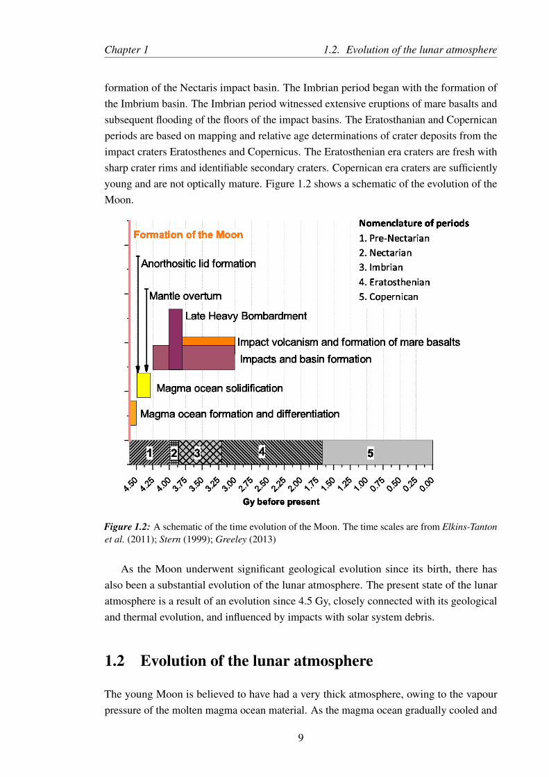
Chapter 1 1.2. Evolution of the lunar atmosphere

formation of the Nectaris impact basin. The Imbrian period began with the formation ofthe Imbrium basin. The Imbrian period witnessed extensive eruptions of mare basalts andsubsequent flooding of the floors of the impact basins. The Eratosthanian and Copernicanperiods are based on mapping and relative age determinations of crater deposits from theimpact craters Eratosthenes and Copernicus. The Eratosthenian era craters are fresh withsharp crater rims and identifiable secondary craters. Copernican era craters are sufficientlyyoung and are not optically mature. Figure 1.2 shows a schematic of the evolution of theMoon.

Figure 1.2: A schematic of the time evolution of the Moon. The time scales are from Elkins-Tantonet al. (2011); Stern (1999); Greeley (2013)

As the Moon underwent significant geological evolution since its birth, there hasalso been a substantial evolution of the lunar atmosphere. The present state of the lunaratmosphere is a result of an evolution since 4.5 Gy, closely connected with its geologicaland thermal evolution, and influenced by impacts with solar system debris.

1.2 Evolution of the lunar atmosphere

The young Moon is believed to have had a very thick atmosphere, owing to the vapourpressure of the molten magma ocean material. As the magma ocean gradually cooled and

9

1.2. Evolution of the lunar atmosphere Chapter 1

solidified, the pressure decreased. Over this background pressure, there were episodicincreases of pressure due to meteoritic bombardment. This is discussed in detail by Stern(1999), who has divided the pathway of the evolution of the lunar atmosphere in threeepochs and presented a schematic illustration of this evolution, as presented in Fig 1.3.

Figure 1.3: A schematic of the evolution of the lunar atmosphere since its formation (redrawn fromStern, 1999). Epoch II and III witnessed episodic increase of the atmospheric pressure due to therelease of gases as a result of bombardment of meteorites.

1.2.1 Epoch I: From ∼ 4.57 Gy to ∼ 4.4 Gy

Prior to the formation of the lunar crust (∼ 4.4 Gy ago), the lunar atmosphere was thick,governed by the vapour pressure of the rocks in the molten magma ocean, at temperatures1000 to 2000 K. The rock vapours primarily consisted of Silicon, Aluminium, Magnesium,Sulphur, Iron Oxides as well as volatiles like Hydrogen Sulphide. This resulted into arock vapour pressure-limited atmospheric pressure of ∼ 102 bar, much like the presentatmospheric pressure of Venus. The escape of this atmosphere must have been dominatedby the Jeans process (escape of atoms from the lunar gravity by acquiring enough thermalenergy) (Vondrak, 1974; Stern, 1999) and scavenging by the solar wind and the solar UVphotons (Stern, 1999).

1.2.2 Epoch II: From ∼ 4.4 Gy to ∼ 3.1 Gy

This era represents the window when the lunar crust is solidified (∼ 4.4 Gy ago) andvolcanism associated with occasional large crater- or basin-forming impacts predominated(∼ 3.8-3.4 Gy) (Stern (1999) and the references therein). These impacts either puncturedthe crust releasing the internal gases and/or caused ablation of the materials at the point

10

Chapter 1 1.2. Evolution of the lunar atmosphere

of impact releasing gases to the lunar atmosphere. The mare volcanism and hence theformation of mare basalts continued till ∼ 3.1 Gy. In this epoch, the initial rock vapourpressure-limited atmosphere went on declining by thermal or Jean’s loss and other non-thermal loss mechanisms, as described in details in section 1.3.2. During that era the lunaratmosphere was supported by internal releases aided by volcanism and impacts.

1.2.3 Epoch III: Last ∼ 3.1 Gy

About ∼ 3.1 Gy ago, the mare volcanism ceased (Stern, 1999). By that time, the largerimpacts also became less frequent. The mean time before successive impacts for 10 m-classof impactors, which are capable of generating a substantial transient atmosphere, became100-200 years. Model calculations suggest that these impacts generate vapours of 1-5times of the impactor mass, with characteristic vapour temperature of 2000-5000 K. This isless than the temperature (∼ 16,000 K) required by the vapours to escape the lunar gravity.Also, the ionization effects are not very effective at vapour temperatures below ∼ 20,000K. As a result, all the impact generated vapours essentially remain as neutral gases in thelunar atmosphere. As Vondrak (1974, 1988) calculated, transient lunar atmospheres withmasses∼ 1010 g decline in a few days back to normalcy. Considering the mean time beforesuch transient atmosphere-forming impacts and their characteristic loss time, the duty ratiofor significant lunar atmospheric transient above the current background environment isonly ∼ 0.1-3%. Hence, the time-averaged value of the present lunar atmospheric pressuresuggests that it is extremely tenuous and falls under the category of exosphere.

The term exosphere is the outermost part of any planetary atmosphere where the atomsrarely collide with each other. Exosphere is defined as the region where the mean free pathof the gas atoms or molecules is larger than the local scale height (Chamberlain, 1963).The term exobase refers to the bottom of the exosphere where the mean free path of thegas atoms and molecules just exceeds the local scale height. In the absence of collisions,the trajectories of the exospheric neutral particles are governed by the gravitation of theplanet and solar radiation pressure (Bishop and Chamberlain, 1989; Beth et al., 2016a,b).In the collisionless regime, the dynamics of a species is driven solely by its kinetics, whichdictates whether a species will be ballistic, satellite, or escaping (Chamberlain, 1963).Ballistic particles are the ones which are gravitationally bound to the host planet, with theirorbits intersecting the exobase. The satellite particles are also gravitationally bound to thehost planet, but they have stable orbits above the exobase. The escaping particles, as thename suggests, are the ones that escape the gravitational pull of the planet.

The exobase of Earth is located at an altitude of ∼ 550 km (Angerami and Thomas,1964), while that on Mars is at ∼ 200 km (Yagi et al., 2012). There are celestial bodieswhose exospheres are bounded on one side by their surfaces; typical examples of suchSurface Boundary Exospheres (SBE) in the solar system include Earth’s Moon, Mercury,

11

1.3. The Lunar Exosphere Chapter 1

Saturn’s satellite Enceladus, asteroids etc.. Earth’s Moon is the closest SBE to the Earthand hence a natural laboratory to study the physical processes characteristic to the SBEs inthe solar system.

1.3 The Lunar Exosphere

Initially, polarimetric studies indicated an upper limit of 10−9 to 10−10 bar for the lunarsurface pressure (Dollfus, 1956). It was generally believed that any lunar atmospherewould have been lost to space due to non-thermal processes, like the ion pick-up by thesolar wind (Herring and Licht, 1959; Hinton and Taeusch, 1964). The Apollo series ofmeasurements returned the first set of data on the lunar atmospheric composition nearthe surface. Yet, these experiments did not yield useful data from the sunlit side dueto the saturation of the cold cathode gauges and mass spectrometers presumably due tothe contamination and degassing from the space modules (Hoffman et al., 1972; Stern,1999). After the Apollo missions, the limited set of in-situ observation data available onthe lunar exosphere are from the Chandra’s Altitudinal Composition Explorer (CHACE)instrument aboard the Moon Impact Probe (MIP) in the Chandrayaan-1 mission in 2008(Kumar et al., 2009) and the Neutral Mass Spectrometer (NMS) instrument aboard theLunar Atmospheric and Dust Environment Explorer (LADEE) mission in 2013-2014 timeframe (Benna et al., 2015).

The lunar neutral exosphere is a result of a dynamic equilibrium between several sourceand sink processes. The species that constitute the lunar neutral exosphere, if classifiedon the basis of their energetics, form two classes, viz. thermal and non-thermal. Thethermal species are the ones, whose energy (and hence velocity) distribution follows theMaxwell-Boltzmann distribution. The Maxwell-Boltzmann velocity distribution of gasesis given by:

f(v)dv = N

(2

π

)1/2 ( mkT

)3/2

v2 exp

(−mv2

2kT

)dv (1.1)

Here, v is the velocity of the species, m is its mass, N is its local number density and T isthe kinetic temperature.

The Maxwell-Boltzmann distribution suggests that the most probable velocity of aparticle at a temperature T is given by

v0 =√

2kT/m (1.2)

The non-thermal species, on the other hand, are characterized by higher kinetic tem-peratures and do not follow the Maxwell-Boltzmann distribution. The energy distribution

12

Chapter 1 1.3. The Lunar Exosphere

of the species in any planetary atmosphere is, therefore, a signature of the process ithas undergone. As for example, the energy distribution of the species originated by theprocess of charged particle sputtering is different from that of the thermalized species; theformer follow the Sigmund distribution (refer subsection 1.3.1), while the latter follow theMaxwell-Boltzmann distribution.

The scematic in Figure 1.4 summarises the source and sink processes of the lunarexosphere.

Figure 1.4: Schematic showing the source and sink processes in the Lunar exosphere

1.3.1 Source processes

In the lunar exosphere, different source mechanisms are important for different species.Also, in general, there may be multiple sources and sinks of a given species (Stern,1999). The sources of the lunar exosphere include Solar wind capture and subsequentdesorption, Internal release, Impact vapourization and sputtering. Their relative importanceis dependent on the species. As for example, for lunar Helium is mostly of solar windorigin, while there is an internal release source which accounts for the rest. For 40Ar, onthe other hand, it is the internal release process that is the only substantial source, sincesolar wind contains mostly 36Ar rather than 40Ar (Wieler, 2002). When it comes to 20Ne, itis completely from the solar wind. H2 is mostly due to the chemical sputtering of solar Hatoms on the lunar surface. The sources of the lunar exosphere are briefly discussed below.

• Thermal desorption

Thermal desorption refers to the process of sublimation of the atoms from the adsorp-tion wells on grains at the uppermost layer of the surface or within the uppermost

13

1.3. The Lunar Exosphere Chapter 1

regolith, i.e. to the depth that is in thermal contact with the diurnal cycle. The ad-sorbed atoms acquire thermal energy from solar radiation, which, in turn, is convertedto their vibrational energy (phonons) under van der Waals potential at the adsorptionsite. The thermal desorption rate is the inverse of the residence time of the adsorbedatom in the potential well, which is given by (Hunten et al., 1988)

τ = τ0 exp

(D0

kT

)(1.3)

Here τ0 is the vibration period of the adsorbed atom for the van der Waals potential,D0 is the heat of adsorption, k is the Boltzmann constant, and T is the surfacetemperature. τ0 is a property of the adsorbing material and not of the species (Gravaet al., 2015b). Thus, although initiated by photons (solar radiation), thermal desorptionis fundamentally a phonon-induced process.

Armand (1977) has formulated the classical theory of thermal desorption whichsays that although the velocity distribution of the thermally desorbed particles isMaxwellian at the crystal temperature regardless of the interaction potential (betweenthe surface and the adsorbed atom, often called the adatom), the total desorption ratedepends on the vibrational frequency of the adatom and the surface-adatom interaction,which, in turn, depends on the surface binding energy. The Armand distribution ofthe thermal desorption rate is thus a Maxwellian, modified by a prefactor, accountingfor the vibrational frequency of the adatom and the surface-adatom interaction.

• Photon Stimulated Desorption (PSD)

While thermal desorption is a phonon-induced process, PSD is induced by photons.In PSD, the photon energy is absorbed by an atom on the surface and it is excited to anew electronic state, where its binding energy to the surface is reduced (Townsend,1979). If the thermal lattice energy is sufficient to overcome the new binding energy,the atom undergoes PSD (Townsend, 1979). PSD is also known as the major sourceof the lunar Na and K exosphere (Colaprete et al., 2016).

• Capture of solar wind particles

In the absence of a global magnetic field, the charged particles from the solar windare implanted onto the surface. A substantial fraction of them may be neutralized,and upon acquiring thermal energy from insolation and/or meteoroid impacts, theseare released from the surface and become a part of the lunar exosphere. Examplesinclude the lunar Hydrogen, Helium, Neon, Argon-36 (Stern, 1999), as well as heavierelements, like Krypton and Xenon, that were implanted on the surface of the Moon(Wieler, 2002). In fact, the lunar soil acts as a substrate that collects the solar windparticles, which can be used to study the abundances of different elements in the solarwind (Wieler, 2002).

14

Chapter 1 1.3. The Lunar Exosphere

• Sputtering

The term sputtering refers to the process of ejection of a species from a lattice site inthe upper few mono-layers of a surface, due to the injection of a discrete impulse ofenergy. The solar wind is known to sputter material from the regolith and to implantmaterial in and around the regolith. Effective yield obtained from the analysis of lunarsamples indicates sputtering erosion of 10-100 g s−1 for the whole Moon (Arnold,1979). Sputtering may be stimulated by different sources, like Photon AssistedSputtering (PAS), charged particle sputtering (due to incident energetic electrons,protons or alpha particles) or chemical sputtering.

In PAS, a photon bombards a surface atom and imparts energy, but no momentum(Townsend, 1979). If the lattice vibration energy (phonon energy) overcomes thebinding energy, the atom is liberated from the surface. The liberated atom has theenergy in the thermal range (Townsend, 1979).

In charge particle sputtering, the incident ion or electron imparts both energy andmomentum to the surface atom. The incident ion undergoes a series of collisions onthe surface, and atoms that recoil with sufficient energy undergo secondary collisions,thereby creating secondary recoiling atoms. Some of the atoms are backscatteredthrough the surface. If they have sufficient energy to overcome the surface bindingenergy, they are liberated as sputtered atoms. The atoms ejected by sputtering have anenergy distribution extending from thermal to high energies. The energy distributionfor particles sputtered from a solid is given as (Sigmund, 1969):

f(Ee) =6Eb

3− 8√Eb/Ec

Ee(Ee + Eb)3

(1−

√Ee + EbEc

)(1.4)

Here, Ee is the energy of the sputtered species, Eb is its surface binding energy andEc is the cut-off energy, which is the maximum energy that can be imparted to asputtered particle by a projectile particle. Ec is given by

Ec = Ei4M1M2

(M1 +M2)2(1.5)

Here, Ei is the energy of the projectile, and M1,2 represent the masses of the projectileand the target respectively (in atomic mass unit).

The cut-off energy depends on the masses of the projectile ion and the target atom aswell as on the energy of the projectile. According to the Sigmund distribution givenby equation 1.4, the most probable velocity is given by√

Eb/msputtered

15

1.3. The Lunar Exosphere Chapter 1

Here msputtered is the mass of the sputtered species in kg. As for example, for Oxygen,Eb = 2.0 eV and the most probable velocity is 3.47 km s−1, which exceeds thelunar surface escape velocity of 2.38 km s−1. Sputtered Oxygen atoms in the lunarexosphere have been reported by Vorburger et al. (2014) from the CENA/SARAobservations of Chandrayaan-1. Figure 1.5 shows a plot of the Sigmund distributionfunction along with the Maxwell-Boltzmann energy distribution function.

10−2

100

102

10−4

10−2

100

Energy (eV)

Pro

ba

bili

ty d

en

sity f

un

ction

Sigmund

Maxwell−Boltzmann

Figure 1.5: The energy distribution of sputtered Oxygen atoms, given by the Sigmund distributionfunction, (equation 1.4) for proton projectiles with 1 keV energy and surface binding energy of 2eV, is plotted with open stars. The Sigmund distribution function, at higher energies, falls off withE−2e variation. The Maxwell-Boltzmann energy distribution function followed by thermal atoms,

given by 2(E/π)1/2(kT )−3/2e−E/kT , with T=400 K (typical value of the dayside lunar surfacetemperature at equator) is co-plotted (open circles) for comparison. The Maxwell-Boltzmanndistribution falls off exponentially with energy.

Sputtering by solar wind protons of 1 keV energy causes maximum yield for the O,Si, Ca and Fe atoms in the energy range of 1 to 10 eV (Wurz et al., 2007). Due totheir larger scale height, the sputtered species dominate the exosphere at altitudesexceeding a few 1000 km (Wurz et al., 2007).

Solar wind sputtering is believed to be a minor source of the lunar exosphere, whichaccounts for ∼10−3 % of the lunar day-side total exospheric density (Wurz et al.,2007).

Chemical sputtering, on the other hand, results when a chemical reaction on thesurface is exothermic and has sufficient excess energy to desorb an atom or molecularfragment onto a ballistic trajectory.

Recently, the contribution of the self-sputtering process to the lunar exosphere hasbeen reported (Poppe et al., 2013), where the newly born ions from the exospherecause sputtering of additional neutrals from the lunar surface. The contribution ofself-sputtering, however, is an order of magnitude less than the solar wind sputtering.

16

Chapter 1 1.3. The Lunar Exosphere

• Meteoritic impacts

Meteoritic impacts onto the lunar surface at velocities above a few km s−1 (averagelunar meteorite impact velocity is about 15 km s−1 (Stern, 1999)) produce both acloud of impact-generated vapour and a source of hot or even molten surface materialthat subsequently outgasses until it cools. The yield depends on several factors,like the energetics of collision, composition of the target site and impactor, surfacetemperature, rock/soil ratio, compaction state, etc. The micrometeroid impacts onthe Moon contribute to the Na, K, Li, Si, Ca, Al, Mg and Fe exospheres (Berezhnoy,2013; Colaprete et al., 2016).

• Internal release

Gases, like 40Ar, 222Rn are released from the lunar interior by the process of volcanism,radiogenic activity, crustal diffusion or seismically induced seepage (Hodges, 1977;Stern, 1999; Killen, 2002). Evidences of recent (age few tens of My) tectonicallyinduced shallow moonquakes have been found from Lunar Reconnaissance Orbiterand Chandrayaan-1 images (Senthil Kumar et al., 2016). The impact due to volcanismin the geologically recent years (∼ 100 My) has not been found to be very significant(Braden et al., 2014). Data from the Apollo seismic network stations had reportedonly very minor (107-109 erg) tidal, stress-driven events over a period of six years(Nakamura et al., 1979). Correlation between these stress-driven seismic events andAr releases detected by the Apollo 17 LACE surface mass spectrometer have beenreported by Hodges and Hoffman (1975) and Rn production has been found to becorrelated with the mare-highland boundaries.

• Release due to dielectric breakdown

Jordan et al. (2017) recently suggested that the large solar energetic particle (SEP)events may cause charged particles penetrate the lunar regolith, cause sufficientcharging, leading to dielectric breakdown in the upper 1 mm of the lunar regolithin the Permanently Shadowed Regions (PSR). The PSRs are regions in higher lunarlatitudes where the maximum solar declination could be as low as 1.54◦ (Williamset al., 2017) so that solar radiation can never reach there. This phenomenon is believedto cause vapourization and melting in the coldest PSRs with production rates up to 1.8to 3.5 × 10−7 kg m2 y1 , which is comparable to that produced by meteoroid impacts.

The above-mentioned sources are balanced by a set of sinks, which maintain the lunarexosphere in a dynamic equilibrium.

17

1.3. The Lunar Exosphere Chapter 1

1.3.2 Sink processes

A species is able to escape the gravitational pull of a planetary body if it has energy excessto the gravitational binding energy. This excess energy may come as a result of variousthermal and non-thermal processes. The relative importance of the sink processes variesfrom species to species. For lighter non-condensable species like Helium and H2, it isthe Jeans escape (Jeans, 1923) that plays a significant role. 40Ar, on the other hand, isvulnerable to ionization loss (photoionization (Huebner et al., 1992) and charge exchange(Nakai et al., 1987)) and condensation trapping. 20Ne is vulnerable to photoionization loss(Huebner et al., 1992), but not condensation trapping.

• Thermal or Jeans escape

Jeans escape (Jeans, 1923), also known as thermal or gravitational escape, is importantfor lighter species (H and He), where the thermal energy of an atom exceeds thegravitational binding energy. At and below the exobase (for the Moon the exobaseis at its surface) the particle velocities are distributed according to the Maxwell-Boltzmann distribution (Chamberlain, 1963; Armand, 1977), given by equation 1.1.The parameter that underpins the degree of vulnerability of an atom to undergo Jeansescape is the escape parameter λesc, which is the ratio of the potential to the kineticenergy of the atom. Lesser the gravitational potential energy compared to the thermalkinetic energy, lesser is the value of the escape parameter and more vulnerable is thespecies to undergo Jeans or thermal escape.

The escape parameter λesc is given by

λesc =GMm

kT (R + z)=

(R + z)

H(z)=

(vescv0

)2

(1.6)

Here, G is the Universal gravitational constant, M is the planetary mass, m is themass of a given species (proton rest mass multiplied by the mass of the species inatomic mass unit), R is the radius of the planet and z is an arbitrary height above thesurface. H(z) represents the local scale height.

Integration of the upward flux (velocity multiplied by the number density) assumingthe Maxwell-Boltzmann velocity distribution above the exobase leads to the Jeansformula for the thermal escape flux (in m−2 s−1), given by:

ΦJ =Nexv0

2√π

(1 + λesc) exp (λesc) (1.7)

Here Nex refers to the number density of the species at the exobase. For surfaceboundary exospheres like Moon, it represents the surface number density.

18

Chapter 1 1.3. The Lunar Exosphere

The typical parameters for Moon are:

R= RM = 1735 × 103 mM = 7.342 × 1022 kgT = 390 K, the equatorial surface temperature for sunlit lunar hemispherez = 0, since moon has a surface boundary exospherevesc = 2.38 × 103 m s−1

For a surface density of Nex = 1 × 109 m−3, for Helium (amu 4) over the equatorialregion in the sunlit hemisphere of the Moon, substituting the above parameters inequations 1.6 and 1.7, λesc = 3.47 and ΦJ = 4.98 × 1010 m−2 s−1 = 4.98 × 106 cm−2

s−1. This is the thermal evaporation rate of the Helium atoms. Thermal loss is lesssignificant for the heavier species; which can be understood by comparing the valuesof the λesc for few species, calculated based on the above-mentioned lunar parameters,as shown in Table 1.2.

Table 1.2: Calculated values of thermal escape parameter λesc for few species

Species Value of λesc

Hydrogen atom (amu 1) 0.87Hydrogen molecule (amu 2) 1.74Helium (amu 4) 3.47Oxygen (amu 16) 13.90Neon (amu 20) 17.38Argon (amu 40) 34.77

The value of the escape parameter is directly proportional to the mass of the species.Lunar surface escape velocity (2.38 km s−1) corresponds to an energy requirementof 0.03 eV/amu, equivalently 226 K amu−1 for a species to escape (Stern, 1999).Exceptions to this occur even in the collisionless regime, if during the process ofescape, radiation pressure retards the velocity below the local escape speed (Bishopand Chamberlain, 1989; Beth et al., 2016a,b), or the species is ionized and recycledto the Moon (Manka and Michel, 1971).

• Non-thermal loss processes

Non-thermal loss processes include several physical and chemical processes. Some ofthem include knocking out of the atmospheric species by the solar wind particles, pick-up by the solar wind fields, etc. Like Jeans escape, these are also permanent removalprocesses of atmospheric species. Table 1.3 presents a list of different non-thermalprocesses that lead to the loss of atmospheric species.

19

1.3. The Lunar Exosphere Chapter 1

• Impact loss

Impacts by micrometeoroids may impart sufficient energy to the surface and ablatematerials from the impact zone. The temperature of the vapor escaping the impactsite follows a Maxwellian distribution with characteristic temperatures of 2000-5000K, while the vapor produced by the outgassing of the ablated material produces aweighted average Maxwellian with temperatures up to ∼ 3000 K (Stern (1999) andthe references therein). The ablated materials may escape if excess energy is availableto circumvent the gravitational barrier. This is also a permanent removal process.

• Condensation loss

Condensation occurs primarily on the lunar nightside or in the PSRs, where the solarradiation can never reach (Paige et al., 2010a). A typical example is the trappingof Hydrogen-bearing molecules in the lunar PSR (Lawrence et al., 2015) and polarregions (Sanin et al., 2017). The species are adsorbed in a shallow potential wellwith lattice residence times comparable to or in excess of the 14-day lunar night.Condensible lunar atmospheric species include Ar, Na, and K, as well as the H2O.Condensed species may undergo sublimation after sunrise and are released by theprocess of thermal desorption, and hence the condensation loss is considered atemporary sink (Stern, 1999). In contrary, if a condensible gas finds its way to apermanently shadowed polar cold trap, then it may be permanently lost until andunless it gathers sufficient energy from any external stimulus (meteoritic impact orSEP-induced dielectric breakdown) to be re-leleased.

• Chemical loss

Collisions between exospheric atoms or molecules with the surface can result inchemical reactions leading to its bonding to the surface before being ballisticallyejected again (Stern, 1999). It is believed to be an important loss mechanism for H+,He, and O from solar wind impingement on the Moon.

The relative importances of the above-mentioned source and sink processes depend onthe species as well as the environment they are exposed to, the understanding of whichculminates to the modelling of the lunar exosphere. Lunar exospheric modelling aims atthe complete understanding of the source and sink processes of the lunar exosphere, itscomposition and variability as well as dynamics.

20

Chapter 1 1.3. The Lunar Exosphere

Table 1.3: Non-thermal escape processes [Taken from de Pater and Lissauer (2010)]

Nomenclature used: i2=molecule; i, j=atoms; i+, j+=ions; e−=electron; superscript ∗

represents energetic atom or molecule

Non-thermal escape Description

Dissociation A neutral molecule may be dissociated by UV photon orenergetic electron The products may have excess energy toescape the gravity.

1. i2+hν → i∗+i∗

2. i2+e−∗→ i∗+i∗+e−

Dissociative recombina-tion

A molecular ion may be dissociated by electron impact (EI),and the product may escape the gravity.i∗2+e−→ i∗+i∗

Ion-neutral reaction When an atomic ion interacts with a neutral molecule, thereaction may produce an ionic molecule and a fast atom,which may eventually escape.i2+j+→ ij++i∗

Charge exchange When an energetic ion interacts with a heavier neutral atom,the ion loses its charge but retains its kinetic energy (Res-onant charge exchange). Thus, the former ion becomes anenergetic neutral atom, which may escape the gravity.i+ j+∗→ i++ j∗

Sputtering When a fast ion (case 1) or an atom (case 2) ‘knocks on’ anatmospheric atom, it may gain sufficient energy to escapethe gravity. In case the product does not have excess energyto escape, it remains gravitationally bound, thereby forminga corona. For surface boundary exospheres (like Moon),significant sputtering occurs at the surface.

1. i+j+∗→ i∗+j+∗

2. i+j∗→ i∗+j∗

Solar wind sweeping In the absence of a global magnetic field (similar to that inMoon), charged particles in the atmosphere may interactwith the solar wind directly. and are swept out by the solarwind fields.

21

1.4. Modelling of the Lunar exosphere Chapter 1

1.4 Modelling of the Lunar exosphere

In his classical model, Chamberlain (1963) treated the dynamics of ballistic, satelliteand escaping particles. Hartle (1971) generalized the Chamberlain model of planetaryexosphere by allowing arbitrary variations of density and temperature over the exobase.For the case of the Moon, the exobase is right at the lunar surface and hence the surfacetemperature plays an important role in determining the desorption and velocity distributionof the lunar species. In early 1970s, the exospheric transport model did not provide adetailed description of the diurnal variation of the light species on the Moon, as Hodgeset al. (1972) pointed out, which was attributed to the inherent difficulties in accounting forthe large diurnal variation of the lunar surface temperature. Hodges et al. (1972) used thethen available lunar surface temperature models, which were based on thermal propertydata acquired at the Apollo 15 and 17 landing sites. Among these two, the temperaturemodel based on Apollo-17 measurements were considered to be well suited to comparebetween theory and experiments because of the simultaneous availability of the in-situatmospheric composition data from the LACE mass spectrometer.

The Monte Carlo model used by Hodges et al. (1972) was meant to trace the paths ofa succession of individual particles since their creation, till escape. For lighter species,like H, H2, and He, the scale heights exceed the vertical scales of orographic features andhence the lunar surface was assumed to be smooth with constant gravitational potential.For the solar wind-borne species, like H+ and He++, their influx was assumed to vary asthe cosine of the lunar-centric angle from the subsolar point to the point of interest.

In the Monte Carlo model, the origin of a lunar species is chosen randomly by fixingthe co-latitude (θ0) and the longitude (φ0). Based on the temperature model, the surfacetemperature (T) at the location (θ0, φ0) is determined. The velocity v of the species israndomly chosen based on the Maxwell-Boltzmann velocity distribution with characteristictemperature T. The velocity components are randomly chosen from three Gaussian deviates.The magnitude of the velocity (v) is then compared with the lunar surface escape velocity(ve). If v ≥ ve, an escape event is recorded and a new particle is created. In case theparticle did not escape, its point of impact on the lunar surface is computed based on orbitalmechanics. The loop repeats itself by treating the point of impact as the point of origin forthe next iteration.

Since Moon’s is a Surface Boundary Exosphere, it is sensitive to the orograhic features,gravitational anomalies and surface temperature fluctuations. The lunar exospheric modelunderwent evolution with the advancement of knowledge in the field of lunar surfacescience. As a result, the Monte Carlo model by Hodges et al. (1972) evolved to the LunarExospheric Simulation (LExS) toolkit (Hodges and Mahaffy, 2016). As for example,the lunar terrain varies by ∼20 km in altitude (Hodges and Mahaffy, 2016), which iscomparable with the lunar exospheric scale heights. To accommodate this, the lunar

22

Chapter 1 1.4. Modelling of the Lunar exosphere

exospheric model has undergone refinement by adopting the lunar topographic modelderived from Lunar Orbiter Laser Altimeter (LOLA) data with lateral resolution of 500m. This makes the LExS model capable of accounting for the effects of topography oninsolation. Thus, the spatial variations of the lunar surface temperature near the terminator,the poles, in small craters and otherwise rough terrain are accounted for in the LExS. Theincorporation of topographical model has enhanced the computational accuracy of theorographical effects on the points of origin and impact as well as the extents of the ballistictrajectories of the species over the terrain.

As mentioned, another important factor that governs the density and dynamics of thelunar exospheric species is the surface temperature. The lunar exospheric model is furtherrefined by the incorporation of the surface temperature model (Hurley et al., 2015), basedon the mapping of the lunar infrared albedo by the Diviner Lunar Radiometer aboard LRO(Paige et al., 2010a,b). For a point on the lunar surface with colatitude θ and longiture φwith solar zenith angle ψ, the surface temperature is given by the following set of analyticfunctions, as proposed by Hurley et al. (2015):

T (ψ) = 392 cos1/4(ψ) for ψ < 90◦ (1.8)

T (θ, φ) =∑

(aiφi) + 35(sin(θ)− 1) for ψ > 90◦ (1.9)

Here i runs from 0 to 5 with the coefficients given by

a = [444.738,−448.937, 239.668,−63.8844, 8.34064,−0.423502]

This yields an equatorial day-side temperature as 392K. At equator, the function sug-gests 130 K surface temperature at post-dusk and 95 K at pre-dawn. More detailed resultson the lunar surface temperarture mapping based on the Diviner radiometer measurementsare also reported recently (Williams et al., 2017).

The LExS toolkit is being refined with the progress of knowledge of the lunar science(private communication with Dr. R. R. Hodges). In-situ and remote sensing observationsof the lunar exosphere play a major role in the refining of the lunar exospheric model.Figure 1.6 presents a summary and time-line of the lunar missions that have contributedto the present understanding of the lunar exosphere. The next section presents a briefdiscussion on the observations on the lunar exosphere made by several lunar missions.

23

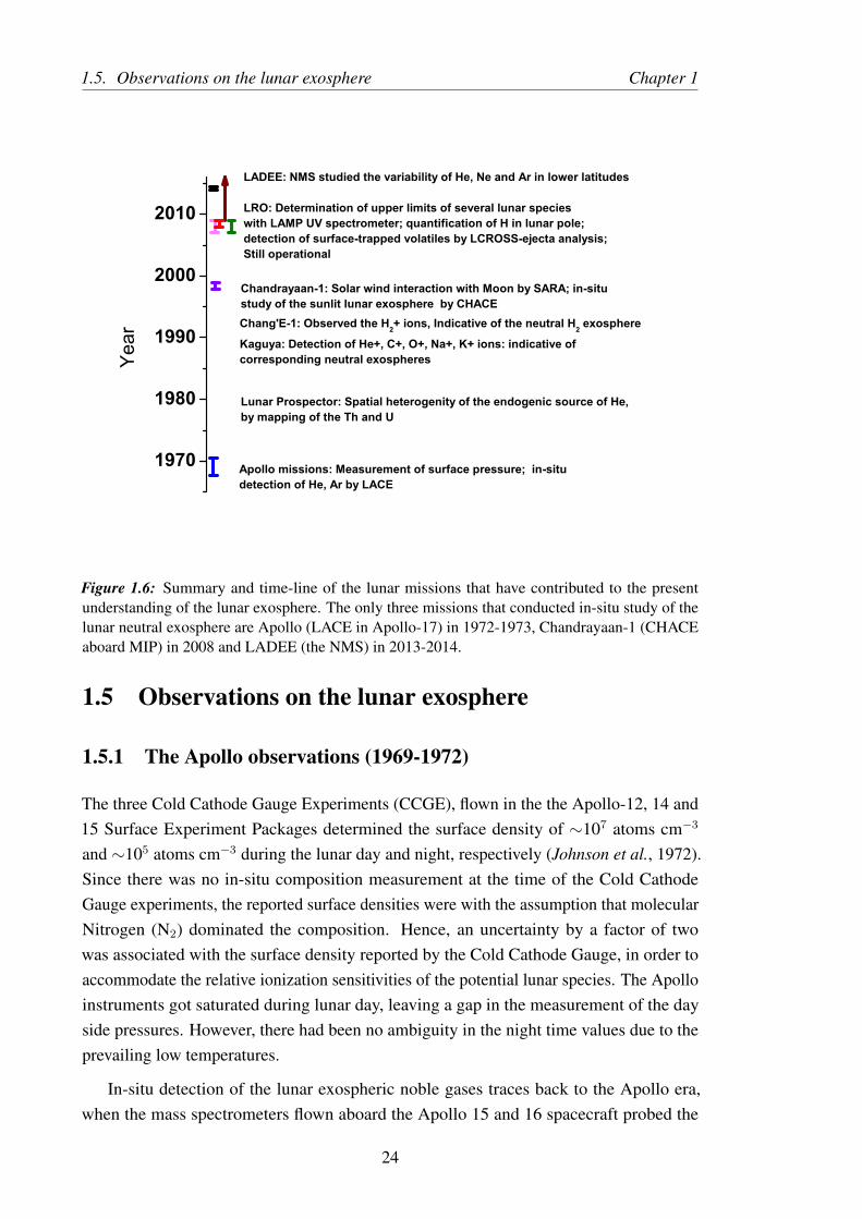
1.5. Observations on the lunar exosphere Chapter 1

1970

1980

1990

2000

2010

Apollo missions: Measurement of surface pressure; in-situdetection of He, Ar by LACE

Yea

r

Lunar Prospector: Spatial heterogenity of the endogenic source of He, by mapping of the Th and U

Kaguya: Detection of He+, C+, O+, Na+, K+ ions: indicative of corresponding neutral exospheres

Chandrayaan-1: Solar wind interaction with Moon by SARA; in-situstudy of the sunlit lunar exosphere by CHACE

LRO: Determination of upper limits of several lunar specieswith LAMP UV spectrometer; quantification of H in lunar pole; detection of surface-trapped volatiles by LCROSS-ejecta analysis;Still operational

LADEE: NMS studied the variability of He, Ne and Ar in lower latitudes

Chang'E-1: Observed the H2+ ions, Indicative of the neutral H2 exosphere

Figure 1.6: Summary and time-line of the lunar missions that have contributed to the presentunderstanding of the lunar exosphere. The only three missions that conducted in-situ study of thelunar neutral exosphere are Apollo (LACE in Apollo-17) in 1972-1973, Chandrayaan-1 (CHACEaboard MIP) in 2008 and LADEE (the NMS) in 2013-2014.

1.5 Observations on the lunar exosphere

1.5.1 The Apollo observations (1969-1972)

The three Cold Cathode Gauge Experiments (CCGE), flown in the the Apollo-12, 14 and15 Surface Experiment Packages determined the surface density of ∼107 atoms cm−3

and ∼105 atoms cm−3 during the lunar day and night, respectively (Johnson et al., 1972).Since there was no in-situ composition measurement at the time of the Cold CathodeGauge experiments, the reported surface densities were with the assumption that molecularNitrogen (N2) dominated the composition. Hence, an uncertainty by a factor of twowas associated with the surface density reported by the Cold Cathode Gauge, in order toaccommodate the relative ionization sensitivities of the potential lunar species. The Apolloinstruments got saturated during lunar day, leaving a gap in the measurement of the dayside pressures. However, there had been no ambiguity in the night time values due to theprevailing low temperatures.

In-situ detection of the lunar exospheric noble gases traces back to the Apollo era,when the mass spectrometers flown aboard the Apollo 15 and 16 spacecraft probed the

24

Chapter 1 1.5. Observations on the lunar exosphere

lunar exosphere (Hoffman et al., 1972), but with limited success. A significant step tostudy the lunar exospheric composition was accomplished by the Lunar AtmosphericComposition Experiment (LACE) (Hoffman et al., 1973), deployed on the Taurus-LittrowValley with its entrance aperture oriented upward to intercept and measure the downwardflux of the lunar exospheric gases. LACE was a magnetic sector mass spectrometer, whichwas a part of the Apollo Lunar Surface Experiment Package (ALSEP) in the Apollo-17mission. LACE analyzed the constituents of the lunar neutral exosphere at the surface. TheLACE instrument ran into saturation during lunar days and hence provided useful scientificinformation only during lunar nights. Starting from December 1972, it continued to operatefor nine lunations before it developed some anomaly in the instrument during the tenthlunation (October 1973) (Hoffman, 1975). The noble gases detected unambiguously in thelunar exosphere were Helium and Argon. Figure 1.7 shows the diurnal variation of He andAr as observed by LACE. It is observed that He and Ar have different diurnal variabilitybecause of the fact that the former is non-condensable while the latter is condensable underlunar temperature and pressure conditions. Ar density minimizes at night because of thecondensation loss, while the He density maximizes post-midnight. The 20Ne signature, onthe other hand, observed by LACE was believed to be contaminated by the signal of H18

2 Ofrom Apollo equipment (Hodges et al., 1973).

Figure 1.7: Trends of diurnal variation of the lunar He and Ar as observed by LACE. The Hevalues are averaged over ten lunations. The Ar measurements correspond to 20 July to 3 August1973. Subsolar meridian of 180◦ represents local midnight. Succesful observations by LACE werelimited to the lunar nightside. Redrawn based on the Figs. 2 and 3 from Stern (1999). Original dataare from Hodges (1975).

The absence of species, like H, C and N, in the lunar exosphere is attributed to theirconversion to H2, CH4 and NH3 (Hodges et al., 1972). Further, the usage of LACE datafor setting up an upper limit for the H2 had been supported by the ultraviolet spectrometer,which is free of contamination. Though the Apollo 17 mass spectrometer detected species

25

1.5. Observations on the lunar exosphere Chapter 1

with atomic mass 16, 18 and 44, more favorably during pre-sunrise conditions (Hodges,1975), they were considered of terrestrial origin carried along with the instrument.

On the other hand, the mass spectrometers flown in the orbiters Apollo 15 and 16 werebelieved to have been so heavily dominated by the contaminants from the orbiter module,that no detection or upper limits could be obtained (Hodges et al., 1972). Therefore, allthe in-situ measurements attempted in the past had the problem of possible contamination.The UV observations aboard Apollo-17, meant to detect resonance fluorescence emissionscharacteristic of lunar exospheric species, did not yield any significant positive results(Fastie et al., 1973). It was inferred that nearly 100 percent of the solar wind protonsshould have been converted into H2 and have arrived at upper limits for H, O, C, N, Kr, Xe,H2 and CO. No significant improvement was reported even by revisiting the Apollo-17 UVspectrometer data with improved resonance fluorescence g-factors (Feldman and Morrison,1991).

1.5.2 Observations by Lunar Prospector (1998-1999)

NASA’s Lunar Prospector mission was launched on 7 January 1998 and it continued till 31July 1999. Lunar Prospector conducted remote sensing of the Moon from a 100 km polarorbit. Two important findings of the mission as far as the lunar exosphere is concerned wasthe mapping of the radioactive materials (Lawrence et al., 1999), like Thorium, Uraniumand Potassium on the lunar surface. The radioactive decay process is an endogenic sourceof the lunar He atoms (Heiken et al., 1991; Hodges, 1975; Benna et al., 2015) with a supplyrate of ∼ (4.5± 1.2) × 106 atoms cm−2 s−1 (Grava et al., 2015a). The Lunar Prospectorneutron spectrometer conducted high resolution mapping of the polar Hydrogen in thepermanently shadowed regions in the lunar poles (Lawrence et al., 2015).

1.5.3 Observations by Kaguya (2007-2009)

The Japanese mission Kaguya (SELENE) was launched on 14 September 2007 and itcontinued to operate until 10 June 2009. Kaguya studied the Moon from a 100 km circular,and later from a 30-50 km polar orbit. The MAP (MAgnetic field and Plasma experiment)was a suit of scientifc instruments aboard Kaguya.

The Ion Mass Analyzer (IMA) of the MAP-PACE detected reflected/scattered solarwind ions with energies of ∼ 1 keV, while the IEA detected the solar wind ions (withenergy ∼ 2 keV) directly. The origin of the ions with energy ranging between 10 to 800eV detected by IMA was attributed to the lunar surface and exosphere.

The detected lunar ions were composed of He+, C+, O+, Na+ and K+ (Yokota et al.,2009). The Na and K exospheres of Moon was found earlier (Potter and Morgan, 1988),

26

Chapter 1 1.5. Observations on the lunar exosphere

using ground based spectroscopy. Model simulations have been used to understand thecorresponding neutral exospheres from these ion measurements (Hartle et al., 2009).

In addition to the detection of the lunar ions, the Gamma Ray Spectrometer aboardKaguya yielded high resolution maps of the radioactive Thorium, Uranium and Potassiumon the lunar surface (Hasebe et al., 2009; Kobayashi et al., 2010; Yamashita et al., 2010),which are localized endogenic sources of the lunar exospheric He atoms. These mapshave helped to understand the distribution of the endogenic sources of He in the lunarexosphere.

1.5.4 Observations by Chang’E-1 (2007-2009)

The Chinese lunar mission ChangE-1 was launched on 24 October 2007; it was operateduntil 01 March 2009. Chang’E-1 carried onboard Solar Wind Ion Detectors (SWID,consisting of two mutually perpendicular Electro Static Analysers (ESA), both viewing uptowards the space (Wang et al., 2011). The energy-time spectrogram of the SWID revealedparallel curve (PC) structures. In the parallel curve (PC) structures, a component is due toa flux of ions with energy ∼ 8 times greater than the solar wind proton energy (Wang et al.,2011).

Energy analysis showed that the ions had m/q = 2, indicative of either H+2 or He2+ ions.

Based on the comparison between the observed flux of the ions and the possible H+2 or

He2+ flux levels estimated based on the production rates of H+2 and He2+, it was inferred

that the observed pick-up ions were H+2 , which originated from the ionizing processes like

photoionization, charge exchange, electron impact ionization, etc. of the lunar neutral H2.This was the first observation of the lunar pick-up H+

2 ions, which served as an evidencefor the lunar neutral H2 exosphere.

1.5.5 Observations by Chandrayaan-1 (2008-2009)

The Indian mission to Moon Chandrayaan-1 was launched on 22 October 2008, it reachedthe lunar orbit on 8 November 2008 and subsequently it was operational for a period often months. Chandrayaan-1 carried a piggyback 34 kg microsatellite called the MoonImpact Probe (MIP) (Kumar et al., 2009), which was released from an altitude of 98 km tothe lunar surface on 14 November 2008. MIP carried a neutral mass spectrometer calledChandra’s Altitudinal Composition Explorer (CHACE), which conducted in-situ studies ofthe altitudinal and latitudinal distribution and composition of the sunlit lunar exospherewith 1 to 100 amu mass range. The observations made by CHACE about the distributionof the lunar exospheric Ar, Ne, He and H2 form the the basis of the research presented inthis thesis.

27

1.5. Observations on the lunar exosphere Chapter 1

In addition to CHACE, there were ten more experiments in the Chandrayaan-1 orbiterexploring the Lunar ambience and also the surface features of the Moon (Goswami andAnnadurai, 2009). Chandrayaan-1 observed the Moon to study its mineralogy at visibleand infrared wavelengths with instruments Hyper Spectral Imager (HySI) covering 400nm to 950 nm wavelength range (with 15 nm resolution); infrared spectrometer SIR-2covering 900 nm to 2400 nm wavelength (with 6 nm resolution) and the Moon MineralogyMapper (M3) covering the wavelength range of 700 nm to 3000 nm (with 10 nm resolution).The M3 instrument inferred the presence of water ice on the lunar surface in the higherlatitudes and the polar regions based on the remote sensing of the spectral signature of OH(Pieters et al., 2009). There were High Energy X ray (HEX) and Chandrayaan-1 X raySpectrometer (C1XS) experiments aboard Chandrayaan-1 for the study of transportation ofvolatiles and study of the fluorescent signatures of minerals, respectively. The RAdioationDOse Monitoring (RADOM) studied the lunar radiation environment. The Mini-SyntheticAperture Radar (Mini-SAR) instrument was used for the subsurface studies. The TerrainMapping Camera (TMC) and Lunar Laser Ranging Instrument (LLRI) were optical instru-ments for mapping of the lunar terrain and studying the surface topography. The Sub-keVAtom Reflecting Analyzer (SARA) experiment onboard Chandrayaan-1 consisted of twosensors, viz. CENA (Chandrayaan-1 Energetic Neutral Atom Analyzer) and SWIM (SolarWind Monitor) (Bhardwaj et al., 2005; Barabash et al., 2009). CENA detected energeticneutral atoms (ENAs), while the SWIM measured ions of solar wind origin. The SARAsuit of instruments provided clues to the solar wind forcing on the Moon and has providedimportant results on the lunar exosphere.

The SARA experiment discovered substantial and sustained backscattering of solarwind protons from lunar surface as energetic neutral Hydrogen atom contributing to theneutral Hydrogen exosphere of the Moon (Wieser et al., 2009; Vorburger et al., 2013;Bhardwaj et al., 2015). They also suggested the entry of solar wind protons to the lunarwake region (Futaana et al., 2010; Dhanya et al., 2013), which may cause sputteringof neutrals from the night-side lunar surface thereby contributing to the night-side exo-sphere (Vorburger et al., 2016; Dhanya et al., 2016). The CENA instrument indicated thebackscatter of a fraction of the solar wind alpha particles as energetic He atom (Vorburgeret al., 2014).

1.5.6 Observations by LAMP/LRO (2009-present)

A more recent lunar mission had been the NASA’s LRO mission, which was launchedon 18 June 2009. The Lyman Alpha Mapping Project (LAMP) far-ultraviolet (FUV)spectrograph aboard LRO (Gladstone et al., 2010a) detected several lunar exosphericspecies including the major noble gases in its limb viewing mode. It covers a wavelengthrange of 57.5 nm to 196.5 nm (Stern et al., 2012). LAMP observed the lunar exosphere by

28

Chapter 1 1.5. Observations on the lunar exosphere

viewing the sunlit part of the exosphere while the lunar surface was dark.

Lunar H2 was detected by the LAMP in the vapour plume emanated from the impactof the LCROSS into the permanently shadowed Cabeus crater (Gladstone et al., 2010b).In addition to this, the regular LAMP observations at Lyman and Werner bands detectedlunar exospheric H2 (Cook et al., 2013; Stern et al., 2013).

Helium was detetecd by LAMP in the lunar exosphere using the 58.4 nm emission(1s2p → 1s2) line (Stern et al., 2012). LAMP inferred the Helium surface density of∼ 2×104 cm−3 (Feldman et al., 2012) during local dawn. LAMP results further suggestedthat instead of all the alpha particles from the solar wind incident on the lunar surfacebeing thermalized, a significant fraction (∼50%) of them escape as suprathermal Heliumor backscattered from the lunar surface.

LAMP also studied the lunar Argon at 104.8 and 106.7 nm fluorescent emission(3s23p54s→ 3s23p6) wavelengths, corresponding to the fluorescent emission of the sunlitArgon in the lunar exosphere in the background of the dark surface. An upper limit of 2.3× 104 cm−3 is reported for Argon (Cook et al., 2013), which is ∼1.5 times lower than theupper limit given by LACE (Hodges and Hoffman, 1975).

For lunar Neon, Cook et al. (2013) reported an upper limit of 4400 cm−3 for its surfacenumber density based on the observation of 63 nm (2s22p54s → 2s22p6) and 73.5 nm(2s22p53s→ 2s22p6) spectral lines from the LAMP instrument.

The LAMP instrument also yielded the upper limits of the surface densities for someof the species (Cook et al., 2013; Feldman et al., 2012; Stern et al., 2013), a summary ofwhich is presented in Table 1.5.

Recently, Sanin et al. (2017) presented polar maps of the Moons inferred hydrogenabundance based on Lunar Exploration Neutron Detector (LEND) instrument.

1.5.7 Observations by LCROSS (2009)

The Lunar Crater Observation and Sensing Satellite (LCROSS) sent an impactor to strikethe Cabeus crater (84.675◦S, 311.281◦E ) on 9 October 2009, nearly at the local noon(LST of 11:34 hours), in order to explore the volatiles trapped in the lunar polar soil. Theplume generated by the LCROSS impact was observed with the LAMP instrument aboardthe LRO. The far-ultraviolet emissions from the fluorescence of sunlight by molecularhydrogen (H2) and carbon monoxide (CO), as well as resonantly scattered sunlight fromatomic mercury (Hg) with contributions from calcium (Ca) and magnesium (Mg) wereobserved. The observed signatures were well simulated by expansion of a vapour cloudat a temperarture of ∼ 1000 K, containing ∼570 kg of CO, ∼140 kg of H2, ∼160 kg ofCa, ∼120 kg of Hg, and ∼40 kg of Mg (Gladstone et al., 2010b). The ejecta plume also

29

1.5. Observations on the lunar exosphere Chapter 1

showed the signatures of other volatile compounds, like H2O, H2S, NH3, SO2, C2H4, CO2,CH3OH, CH4, OH (Colaprete et al., 2010) and Na (Killen et al., 2010).

30

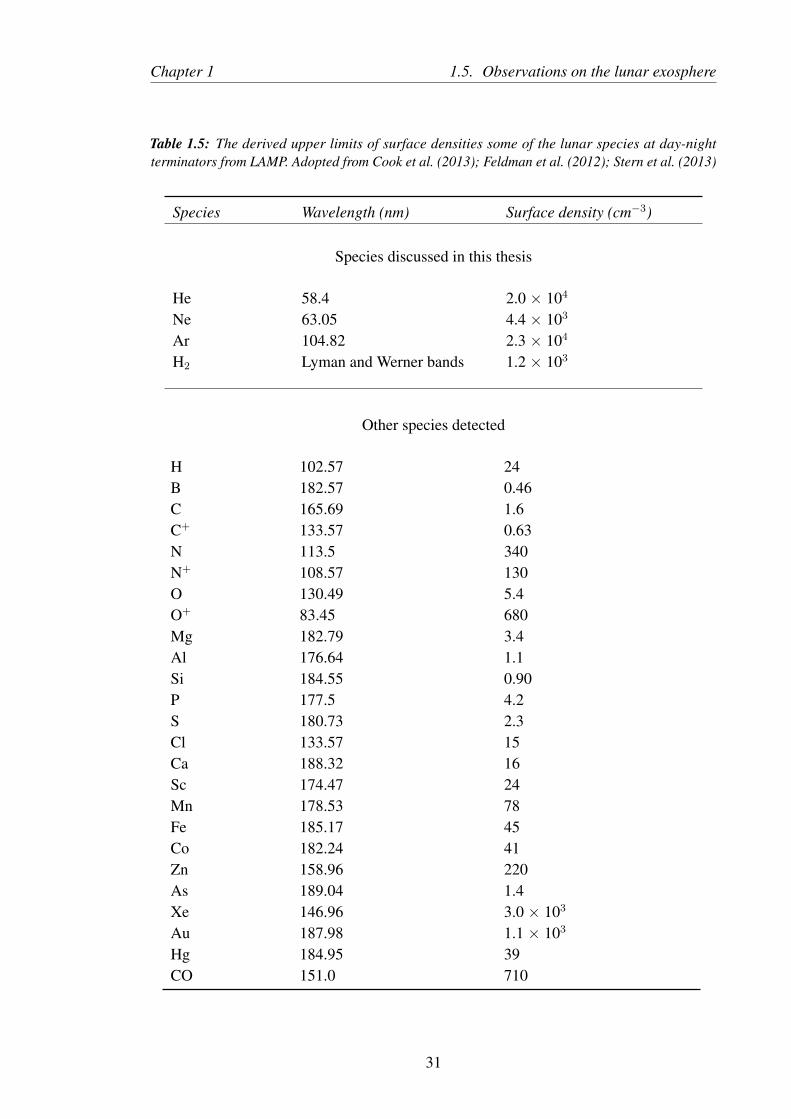
Chapter 1 1.5. Observations on the lunar exosphere

Table 1.5: The derived upper limits of surface densities some of the lunar species at day-nightterminators from LAMP. Adopted from Cook et al. (2013); Feldman et al. (2012); Stern et al. (2013)

Species Wavelength (nm) Surface density (cm−3)

Species discussed in this thesis

He 58.4 2.0 × 104

Ne 63.05 4.4 × 103

Ar 104.82 2.3 × 104

H2 Lyman and Werner bands 1.2 × 103

Other species detected

H 102.57 24B 182.57 0.46C 165.69 1.6C+ 133.57 0.63N 113.5 340N+ 108.57 130O 130.49 5.4O+ 83.45 680Mg 182.79 3.4Al 176.64 1.1Si 184.55 0.90P 177.5 4.2S 180.73 2.3Cl 133.57 15Ca 188.32 16Sc 174.47 24Mn 178.53 78Fe 185.17 45Co 182.24 41Zn 158.96 220As 189.04 1.4Xe 146.96 3.0 × 103

Au 187.98 1.1 × 103

Hg 184.95 39CO 151.0 710

31

1.5. Observations on the lunar exosphere Chapter 1

1.5.8 Observations by NMS/LADEE

The Lunar Atmospheric and Dust Environment Explorer (LADEE) (Elphic et al., 2014)conducted in-situ studies of the equatorial (limited to ±23◦ latitude) lunar exosphere fromDecember 2013 to April 2014 covering an altitude range of 61 km down to 4 km. LADEEcarried the Neutral Mass Spectrometer (NMS) instrument that studied the lunar exospherein the mass range of 2 to 150 amu. In spite of the wide mass range covered, emphasis hasbeen given only to the noble gases detected by the instrument. LADEE has discovered thepresence of Ne in the lunar exosphere and has studied the distribution and variabilities ofHe, Ne and Ar in the equatorial latitudes (Benna et al., 2015). Figure 1.8 shows the diurnalvariation of the surface density of He and Ne derived from the NMS observations. It isobserved that, since both He and Ne are non-condensable under lunar temperature andpressure conditions, the behaviour of their diurnal variations are similar. He maximizesbetween 2 and 3 AM local time while Ne maximizes just before sunrise.

Figure 1.8: Diurnal variation of the surface density of He and Ne as derived from the NMSobservations. The longitudes from the subsolar meridian 90◦, 180◦ and 270◦ represent local dusk,midnight and dawn, respectively. [Redrawn based on the Figures 2 a and c from Benna et al.(2015)].

It is also confirmed by NMS that the exospheric He is controlled by solar wind andby endogenous radiogenic sources. In spite of the significant differences in the sourcestrengths due to the higher lifetime (few months) of Ne as compared with He (few days),the nightside concentrations of Ne and He are comparable (Benna et al., 2015). Localizedenhancement of Ar is observed at the Western maria, coincident with the potassium-rich

32

Chapter 1 1.6. Motivation and scope of the present work

KREEP (Potassium, Rear Earth Elements and Phosphorus) regions, vindicating the closeinteraction between the surface and the exosphere, characteristic to the surface boundaryexospheres (Benna et al., 2015).

The NMS data have also revealed synodic and semiannual oscillations of 40Ar of thelunar exosphere (Hodges and Mahaffy, 2016). The semiannual oscillation of Ar is foundto be consistent with condensation loss in the seasonal cold traps at the poles due to theobliquity of the Moon. The results show that the exospheric morphology depends on theenergetics of desorption of atoms from soil grains. It also brought out the importance ofthe surface-exosphere interaction process.

The Ultraviolet Spectrometer (UVS) aboard LADEE brought out the variabilities ofthe lunar exosphere during the passage of the Moon through the Earth’s magnetotail andmeteoroid systems by studying the resonant scattering from exospheric Na and K. Factorof ∼ 2 enhancement of the Na and K exospheres during the passage of the Moon throughthree meteoroid systems are reported (Colaprete et al., 2016).

1.5.9 Coordinated observations

The LAMP UV spectrometer aboard LRO and the NMS aboard LADEE were simulta-neously operated during the five-month span of the LADEE mission to study the lunarHelium exosphere. The “Acceleration, Reconnection, Turbulence and Electrodynamics ofMoon’s Interaction with the Sun”(ARTEMIS) mission simultaneously monitored the solarwind alpha particle flux to the Moon (Hurley et al., 2016). The correlation between thefluctations of the solar wind alpha particle flux and the variations in the lunar exosphericHe was studied. It was found that the solar wind contributes 64 ± 5 % of the He to thelunar exosphere, while the remaining may be endogenic to Moon, arising out of radioactivedecay of 232Th and 238U. It was also suggested through these coordinated observations that63 ± 6 % of the incident solar wind alpha particles are converted to the thermalized Heatoms by surface-interactions, while the rest may be backscattered as He++ or EnergeticNeutral Atoms (ENA) (Vorburger et al., 2014; Hurley et al., 2016; Grava et al., 2016).

1.6 Motivation and scope of the present work

The noble gases are good tracers to study the different processes in the lunar exospheresince they do not react to form compounds. Reviewing all the major findings on the lunarneutral exosphere, it stands out that the day-time lunar exosphere remains uncharacterizedin terms of the latitudinal and altitudinal variations of the noble gases. Study of thelatitudinal variation of the noble gases in the day-time lunar exosphere is important, as ithighlights the variation of the lunar surface temperature due to the variation of the solar

33

1.6. Motivation and scope of the present work Chapter 1

incidence angle, thereby affecting the dynamics of the lunar species by modulating theirvelocity distributions. The latitudinal variation of the surface obliquity also brings in avariation of the flux level of the solar wind as well as EUV photons on the surface, which,in turn, influences several source and sink mechanisms in the lunar exosphere.

The present work focuses on the latitudinal and altitudinal distribution of the lunarexospheric noble gases during lunar daytime, based on the in-situ observations of thedayside lunar exosphere by CHACE aboard MIP in Chandrayaan-1. This include studieson the spatial distribution of 4He, 20Ne and 40Ar in the lunar exosphere. In addition tothe noble gases, results on the lunar H2 are also discussed. Lunar H2 is a result of theconversion of the solar wind Hydrogen implanted to the regolith (Hodges et al., 1972;Hurley et al., 2017). Hence the lunar regolith is a reservoir of the lunar H2. The H2

molecule is sensitive to dissociation to H and thermal escape. Hence, the study of the lunarH2 provides clues on the lunar surface processes.

The second chapter presents the instrumentation and operation details of the CHACEinstrument and the MIP. The working principle and the development of CHACE as wellas the critical aspects of its calibration, testing and space qualification are also discussedin this chapter. The observation and the analysis methodology are also included in thischapter.

The third chapter deals with the Lunar Argon, which is mostly 40Ar, while the solarwind Argon is rich in 36Ar (Wieler, 2002). This is because the lunar 40Ar is a result of theradioactive decay of the 40K in the lunar interior, which upon release into the exosphereremains gravitationally bound. Hence, the study of 40Ar tells about the internal releaseprocesses of gases from the Moon. 40Ar is condensable under the prevailing lunar ambienttemperature and pressure conditions in the night side and also in the permanently shadowedregions and hence it has close interaction with the regolith through the process of adsorptionand desorption. The observation of CHACE on the 40Ar is presented and the 40Ar: 36Arratio is computed along the 14◦E lunar meridian. An altitude versus latitude map of thelunar Ar along the above-mentioned meridian is also described. The new results presentedin this chapter are the spatial heterogeneity of the radiogenic activity of the lunar interiorand its possible relation to the surface topography.

The fourth chapter discusses about the observations on lunar exospheric Ne. LunarNe is derived from the solar wind and is primarily lost through photoionization. Ne isnon-condensable under the lunar temperature and pressure conditions. It is shown from theCHACE observations that Ne obeys the law of exospheric equilibrium for non-condensablegases, originally proposed by Hodges and Johnson (1968). The new results presented inthis chapter include an empirical relation between the lunar Ne surface density and surfacetemperature. The empirical relation provides a first order estimate on the surface densityof Ne using the surface temperature information.

34

Chapter 1 1.6. Motivation and scope of the present work

The fifth chapter deals with the observation of He. Lunar He, which is mostly 4He, isderived primarily from the solar wind alpha particle flux, although there is a secondaryendogenic source of the lunar He owing to the radioactive decay of 232Th and 238U (Heikenet al., 1991; Hodges, 1975; Benna et al., 2015). The abundance of the lunar He directlydepends on the solar wind alpha particle flux; decreases during the day-time due to theexpansion of the He-corona and Jeans escape; and also decreases during the passageof the Moon through Earth’s magnetotail due to the shielding of Moon from the solarwind. When CHACE conducted the in-situ study of the lunar exospheric constituents, thesolar wind alpha particle flux levels were low, the surface was sunlit and the Moon waswithin the Earth’s magnetotail. Thus, the number density of He was found to be mostlybelow the detection limit of CHACE. The outcome of this study is the proposed upperlimit of the surface density of He in the sunlit lunar exosphere, when Moon is in Earth’smagnetotail, and solar wind alpha particle flux is low. This result is expected to providerealistic constraints to the lunar He exosphere models under such an extreme condition.

The sixth chapter presents the observations of CHACE on the lunar exospheric H2. Itis known that the solar wind implants H+ on the lunar regolith, a part of which is convertedto H2 (Hodges et al., 1972; Crider and Vondrak, 2002; Hurley et al., 2017), thus makingthe lunar regolith a reservoir of the H2 gas. Hence, although not a noble gas, the lunar H2

provides valuable information on the surface processes on the Moon. This chapter presentsthe variation of the surface density of H2 with latitude. An altitude versus latitude map ofthe lunar H2 along the 14◦E meridian is also presented.

Finally, the seventh chapter summarises the major scientific findings of the presentwork. The scientific outcome of this research is expected to add value to the understandingof the composition and distribution of the noble gases in the sunlit lunar exosphere, bysetting realistic boundary conditions for the lunar exospheric models. This chapter alsodiscusses the open questions on the global characterization of the lunar exosphere and itsvariabilities. A polar orbiting satellite with a mass spectrometer aboard may address theyet-unsolved issues and advance our knowledge on the lunar exosphere.

35

Chapter 2

Moon Impact Probe and the CHACEexperiment

It is a capital mistake to theorize before one has data.

—Sherlock Holmes

2.1 The MIP aboard Chandrayaan-1

2.1.1 Introduction

In this chapter, the MIP and the CHACE instrument are described. This includes a semi-analytical description of the physics of a transmission type Quadrupole Mass Analyzer(QMA), which is followed by a description on the CHACE instrumentation, along with itscalibration, test & evaluation, mission operation and data analysis aspects.

2.1.2 The Moon Impact Probe Mission

The MIP was a 375 mm × 375 mm × 470 mm microsatellite with mass ∼ 34 kg (Kumaret al., 2009) attached as a piggyback to the Chandrayaan-1 orbiter, as shown in Figure 2.1.MIP consisted of three payloads, viz. Moon Imaging System (MIS) to take colour picturesof the Moon, a Radar Altimeter (RA) to measure the instantaneous altitude of the MIPduring its descend, and Chandra’s Altitudinal Composition Explorer (CHACE) — thequadrupole mass spectrometer to conduct in-situ measurements of the composition of thelunar neutral exosphere (Kumar et al., 2009; Goswami and Annadurai, 2009). Figure 2.2shows the location of the CHACE instrument inside the MIP.

36

Chapter 2 2.2. The CHACE instrument

Figure 2.1: Schematic of Chandrayaan-1 with the MIP attached as a piggyback microsatellite onthe top deck.

Figure 2.2: Schematic of the MIP showing the payloads.

2.2 The CHACE instrument

CHACE is developed at Space Physics Laboratory (SPL), VSSC (with the collaboration ofother entities in VSSC), around a laboratory-grade open source neutral mass spectrometerwith a transmission type Quadrupole Mass Analyzer (QMA) and a Bayard-Alpert (B/A)gauge. It consists of a cylindrical sensor probe, attached to the electronics. The aperture ofthe sensor protrudes out of the MIP top deck, while the sensor and the electronics wereinside the MIP, as shown in Figure 2.2. Figure 2.3 shows the picture of the flight model ofthe CHACE instrument. Table 2.1 presents the specifications of the CHACE instrument.

In the following subsection, a semi-analytical description of the working principle ofa transmission-type QMA will be presented. It will be followed by a description of theQMA of CHACE and an overall system-level description of the payload.

37

2.2. The CHACE instrument Chapter 2

Figure 2.3: Flight model of the CHACE instrument.

Table 2.1: Specifications of the CHACE instrument

Mass range 1 to 100 amuMass resolution 1 amuSensors QMA, B/A GaugeDetector Faraday Cup, Channel Electron Multiplier (CEM)Interfaces Power and data (RS232)Instrument mass 3.15 kgRaw power 25 W

2.2.1 Physics of the transmission-type QMA

A quadrupole mass spectrometer is a path-stability based instrument to analyze the com-position of different gas atoms and molecules. This is often referred to as a transmissionquadrupole (Young, 2002) as opposed to quadrupole traps. A quadrupole mass spectrome-ter has potential space applications because of its compact size, non-requirement of anymagnetic field and a linear mass axis (Dawson, 1976; Young, 2002). The electric field usedin the QMA varies typically from 102 V m−1 to 104 V m−1 for filtering the ions in themass range of 1 to 100 amu, and because of this electric field the force experienced by theions inside the QMA is typically 102 to 104 times greater than that experienced by themdue to the Earth’s magnetic field. Therefore, the trajectories of the ions inside the QMAare decided by the applied electric field.

Here, the basic theory of the transmission QMA (Dawson, 1976) will be introduced in asemi-analytical approach, before the specific details of the QMA of CHACE are addressed.

38

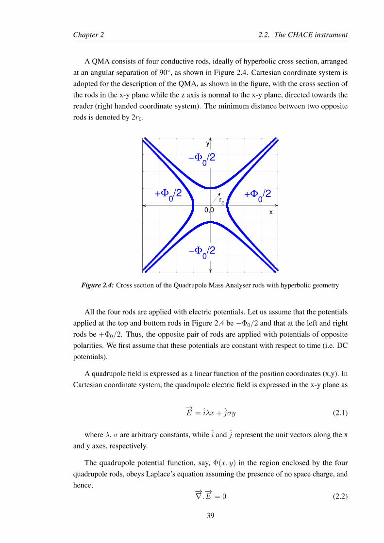
Chapter 2 2.2. The CHACE instrument

A QMA consists of four conductive rods, ideally of hyperbolic cross section, arrangedat an angular separation of 90◦, as shown in Figure 2.4. Cartesian coordinate system isadopted for the description of the QMA, as shown in the figure, with the cross section ofthe rods in the x-y plane while the z axis is normal to the x-y plane, directed towards thereader (right handed coordinate system). The minimum distance between two oppositerods is denoted by 2r0.

r0

0,0

y

x

+Φ0/2 +Φ

0/2

−Φ0/2

−Φ0/2

Figure 2.4: Cross section of the Quadrupole Mass Analyser rods with hyperbolic geometry

All the four rods are applied with electric potentials. Let us assume that the potentialsapplied at the top and bottom rods in Figure 2.4 be −Φ0/2 and that at the left and rightrods be +Φ0/2. Thus, the opposite pair of rods are applied with potentials of oppositepolarities. We first assume that these potentials are constant with respect to time (i.e. DCpotentials).

A quadrupole field is expressed as a linear function of the position coordinates (x,y). InCartesian coordinate system, the quadrupole electric field is expressed in the x-y plane as

−→E = iλx+ jσy (2.1)

where λ, σ are arbitrary constants, while i and j represent the unit vectors along the xand y axes, respectively.

The quadrupole potential function, say, Φ(x, y) in the region enclosed by the fourquadrupole rods, obeys Laplace’s equation assuming the presence of no space charge, andhence,

−→∇ .−→E = 0 (2.2)

39

2.2. The CHACE instrument Chapter 2

and since field is the negative gradient of the potential,

Φ = −1

2

(λx2 + σy2

)(2.3)

The constraint posed by the Laplace’s equation eliminates one of the two arbitraryconstants in the Equation (2.3) as

λ+ σ = 0 (2.4)

Thus, the potential energy function retains only one arbitrary constant and is expressed as

Φ =λ

2

(y2 − x2

)(2.5)

The second arbitrary constant is eliminated by imposing the following boundary conditions:

At x = 0, y = ±r0 the potential Φ = −Φ0/2. This yields λ = −Φ0

r20. Thus, Equation

(2.5) reduces to

Φ(x, y) =Φ0

2r20

(x2 − y2

)(2.6)

Let us now introduce a positive ion (hereafter will be referred to as ion) with mass m andcharge q in the space under the influence of the quadrupole field given by Equation (2.6).The force experienced by the ion in the x and y directions are given by:

mx = qEx = −q∂Φ

∂x= −q Φ0

r20x

(2.7)

my = qEy = −q∂Φ

∂y= +q

Φ0

r20x

(2.8)

The equations of motion of the ion in the x and y directions are, respectively:

x+(q/mr2

0

)Φ0x = 0 (2.9)

and

y −(q/mr2

0

)Φ0y = 0 (2.10)

Note the differences in sign in equations (2.9) and (2.10). As we have assumed Φ0

to be constant, the motion of the ion in the x direction will be simple harmonic, withcharacteristic frequency of

ωp =

√q

mr20

Φ0 (2.11)

40

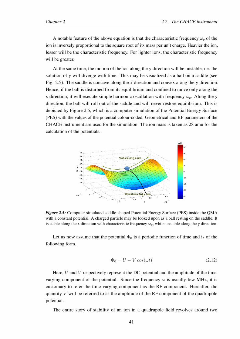
Chapter 2 2.2. The CHACE instrument

A notable feature of the above equation is that the characteristic frequency ωp of theion is inversely proportional to the square root of its mass per unit charge. Heavier the ion,lesser will be the characteristic frequency. For lighter ions, the characteristic frequencywill be greater.

At the same time, the motion of the ion along the y direction will be unstable, i.e. thesolution of y will diverge with time. This may be visualized as a ball on a saddle (seeFig. 2.5). The saddle is concave along the x direction and convex along the y direction.Hence, if the ball is disturbed from its equilibrium and confined to move only along thex direction, it will execute simple harmonic oscillation with frequency ωp. Along the ydirection, the ball will roll out of the saddle and will never restore equilibrium. This isdepicted by Figure 2.5, which is a computer simulation of the Potential Energy Surface(PES) with the values of the potential colour-coded. Geometrical and RF parameters of theCHACE instrument are used for the simulation. The ion mass is taken as 28 amu for thecalculation of the potentials.

Figure 2.5: Computer simulated saddle-shaped Potential Energy Surface (PES) inside the QMAwith a constant potential. A charged particle may be looked upon as a ball resting on the saddle. Itis stable along the x direction with characteristic frequency ωp, while unstable along the y direction.

Let us now assume that the potential Φ0 is a periodic function of time and is of thefollowing form.

Φ0 = U − V cos(ωt) (2.12)

Here, U and V respectively represent the DC potential and the amplitude of the time-varying component of the potential. Since the frequency ω is usually few MHz, it iscustomary to refer the time varying component as the RF component. Hereafter, thequantity V will be referred to as the amplitude of the RF component of the quadrupolepotential.

The entire story of stability of an ion in a quadrupole field revolves around two

41

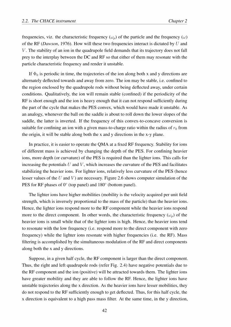
2.2. The CHACE instrument Chapter 2

frequencies, viz. the characteristic frequency (ωp) of the particle and the frequency (ω)of the RF (Dawson, 1976). How will these two frequencies interact is dictated by U andV . The stability of an ion in the quadrupole field demands that its trajectory does not fallprey to the interplay between the DC and RF so that either of them may resonate with theparticle characteristic frequency and render it unstable.

If Φ0 is periodic in time, the trajectories of the ion along both x and y directions arealternately deflected towards and away from zero. The ion may be stable, i.e. confined tothe region enclosed by the quadrupole rods without being deflected away, under certainconditions. Qualitatively, the ion will remain stable (confined) if the periodicity of theRF is short enough and the ion is heavy enough that it can not respond sufficiently duringthe part of the cycle that makes the PES convex, which would have made it unstable. Asan analogy, whenever the ball on the saddle is about to roll down the lower slopes of thesaddle, the latter is inverted. If the frequency of this convex-to-concave conversion issuitable for confining an ion with a given mass-to-charge ratio within the radius of r0 fromthe origin, it will be stable along both the x and y directions in the x-y plane.

In practice, it is easier to operate the QMA at a fixed RF frequency. Stability for ionsof different mass is achieved by changing the depth of the PES. For confining heavierions, more depth (or curvature) of the PES is required than the lighter ions. This calls forincreasing the potentials U and V , which increases the curvature of the PES and facilitatesstabilizing the heavier ions. For lighter ions, relatively less curvature of the PES (hencelesser values of the U and V ) are necessary. Figure 2.6 shows computer simulation of thePES for RF phases of 0◦ (top panel) and 180◦ (bottom panel).

The lighter ions have higher mobilities (mobility is the velocity acquired per unit fieldstrength, which is inversely proportional to the mass of the particle) than the heavier ions.Hence, the lighter ions respond more to the RF component while the heavier ions respondmore to the direct component. In other words, the characteristic frequency (ωp) of theheavier ions is small while that of the lighter ions is high. Hence, the heavier ions tendto resonate with the low frequency (i.e. respond more to the direct component with zerofrequency) while the lighter ions resonate with higher frequencies (i.e. the RF). Massfiltering is accomplished by the simultaneous modulation of the RF and direct componentsalong both the x and y directions.

Suppose, in a given half cycle, the RF component is larger than the direct component.Thus, the right and left quadrupole rods (refer Fig. 2.4) have negative potentials due tothe RF component and the ion (positive) will be attracted towards them. The lighter ionshave greater mobility and they are able to follow the RF. Hence, the lighter ions haveunstable trajectories along the x direction. As the heavier ions have lesser mobilities, theydo not respond to the RF sufficiently enough to get deflected. Thus, for this half cycle, thex direction is equivalent to a high pass mass filter. At the same time, in the y direction,

42

Chapter 2 2.2. The CHACE instrument

Figure 2.6: Computer simulated PES inside the QMA with the assumption of an RF component.Simulations depict the PES at the RF phases of 0◦ (top panel) and 180◦ (bottom panel). Thesimulation is carried out for a species with m/q=28 amu and using the CHACE geometrical and RFparameters. It shows that in one half cycle, the ion is stable along the x direction, while in the nexthalf cycle it is stable in the y direction.

heavy ions are unstable because of the defocussing effect of the direct component (thedirect component is at a lower potential and the heavier ions tend to be attracted) of thetop and bottom rods. However, some lighter ions are stabilized in the y direction by theRF component provided certain conditions are met. The conditions are that the mass (andhence the mobility) of the lighter ions are such that their trajectories are ’self-correcting’and hence, never fall prey to the combination of the amplitude and the frequency of theRF component which could have rendered them unstable. This means that the lighter ionsmust correct their trajectories whenever the amplitude of oscillation in the y directiontends to increase. Hence, the RF component acts as a high pass mass filter while the directcomponent acts as a low pass mass filter. Thus, the y direction acts as a low pass massfilter. The two directions (x and y) collectively give rise to a mass filter with a certain passband.

Substituting equation (2.12) in equations (2.9) and (2.10) , the equations of motion fora time-varying potential assume the following form.

x+(q/mr2

0

)(U − V cos(ωt))x = 0 (2.13)

and

y −(q/mr2

0

)(U − V cos(ωt)) y = 0 (2.14)

43

2.2. The CHACE instrument Chapter 2

Using the transformations given by equations 2.15, 2.16 and 2.17, the equations (2.13)and (2.14) are combined into a single equation, given by equation 2.18.

au = ax = −ay =4qU

mω2r20

(2.15)

qu = qx = −qy =2qV

mω2r20

(2.16)

ξ =ω t

2(2.17)

and u = x, y.

Equations (2.13) and (2.14) are thus reduced to the form

d2u

dξ2+ {au − 2qu cos (ξ − ξ0)}u = 0 (2.18)

Here, ξ0 accounts for the initial phase of the RF as seen by the ion when it wasintroduced to the quadrupole field.

Equation (2.18) is known as the Mathieu differential equation.

Solution of the Mathieu differential equation yields both stable and unstable trajectories.The unstable trajectories are those for which

limt→∞

u =∞ (2.19)

During the motion of an ion in the x-y plane under the influence of the quadrupole field,if a negative potential gradient is applied along the positive z direction, the ion experiencesa motion in the z direction as well. As a result, while responding to the transverse (x-y)quadrupole field, the ion also moves from the entrance of the QMA to the exit, where adetector with radius RD is placed. If the trajectory of the ion is such that

√x2 + y2 > RD

at the exit of the QMA, it does not reach the detector and hence no current is produced. Thestable trajectories are the ones for which

√x2 + y2 < RD. Figure 2.7 shows a computer

simulation of the ion trajectories with purely axial initial velocity, obtained by numericallysolving the Mathieu differential equation using Runge-Kutta method (Scarborough, 1966)under the influence of both the transverse quadrupole field and the axial electric field. Thecombination of DC and RF components of the quadrupole potential are such that an ionwith m/q=1 amu has a stable trajectory while an ion with m/q=2 amu is rendered unstable.

The condition for stability of a solution depends on the parameters au and qu. Adetailed mathematical analysis on the stability conditions of the solution of the Mathieu’sequation is given in Dawson (1976). In short, Mathieu’s equation yields stable solution

44

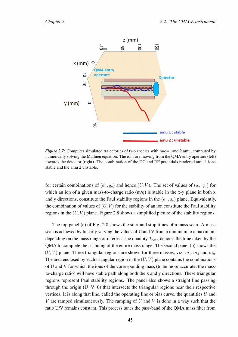
Chapter 2 2.2. The CHACE instrument

Figure 2.7: Computer simulated trajectories of two species with m/q=1 and 2 amu, computed bynumerically solving the Mathieu equation. The ions are moving from the QMA entry aperture (left)towards the detector (right). The combination of the DC and RF potentials rendered amu 1 ionsstable and the amu 2 unstable.

for certain combinations of (au, qu) and hence (U, V ). The set of values of (au, qu) forwhich an ion of a given mass-to-charge ratio (m/q) is stable in the x-y plane in both xand y directions, constitute the Paul stability regions in the (au, qu) plane. Equivalently,the combination of values of (U, V ) for the stability of an ion constitute the Paul stabilityregions in the (U, V ) plane. Figure 2.8 shows a simplified picture of the stability regions.

The top panel (a) of Fig. 2.8 shows the start and stop times of a mass scan. A massscan is achieved by linearly varying the values of U and V from a minimum to a maximumdepending on the mass range of interest. The quantity Tscan denotes the time taken by theQMA to complete the scanning of the entire mass range. The second panel (b) shows the(U, V ) plane. Three triangular regions are shown for three masses, viz. m1,m2 and mn.The area enclosed by each triangular region in the (U, V ) plane contains the combinationsof U and V for which the ions of the corresponding mass (to be more accurate, the mass-to-charge ratio) will have stable path along both the x and y directions. These triangularregions represent Paul stability regions. The panel also shows a straight line passingthrough the origin (U=V=0) that intersects the triangular regions near their respectivevertices. It is along that line, called the operating line or bias curve, the quantities U andV are ramped simultaneously. The ramping of U and V is done in a way such that theratio U/V remains constant. This process tunes the pass-band of the QMA mass filter from

45

2.2. The CHACE instrument Chapter 2

Figure 2.8: The top panel (a) shows the time axis; Tscan represents the time required to complete amass scan. Panel (b) shows that mass scanning is achieved by ramping U and V simultaneouslyand proportionally. Ions with a given mass-to-charge ratio are stable and hence pass through theQMA when the bias curve intersects the triangular regions called the Paul stability regions. Panel(c) shows that how a mixture of ions pass through the mass filter and constitute output currentproportional to their relative abundances at the detector.

lighter to the heavier ions. The segments of the operating line that pass through the Paulstability regions are shown with thicker lines.

The third panel (c) in Figure 2.8 shows the mass axis along the abscissa as mass sinceboth U and V are proportional to the mass of the stable ions. The y axis shows the currentgenerated at the detector by the incidence of the path-stable ions onto it. The currentgenerated at the detector due to the ions with a given m/q is equivalent to their relativeabundance in the medium. It is shown in the figure that during the ramping of U and Vwhenever the bias curve intersects the Paul stability regions (shown with thicker segmentsof the bias curve), it offers an opportunity to a group of ions with the correct m/q to bestable. If such ions are present in the medium, they travel to the detector through theQMA and constitute an output current. In the Figure 2.8, these regions are labeled as‘window’regions. The ‘wall’regions are those where the bias curve does not intersect thPaul stability regions and no ion is stable in the x-y plane. Hence no current is formed atthe detector by the ions. The third panel further shows that a mixture of three kinds ofions (with masses m1,m2 and mn), thus mass-filtered, constitute peaks at the respectivewindow slots; the peak amplitude is determined by their relative abundances. The shapeof the peaks, especially the Full Width at Half the Maximum (FWHM), which is oftendenoted by ∆m, depends on the width of the regions of the bias curve that intersectthe Paul stability regions. The resolution of a peak is given by R = m/∆m. For asharp peak (high resolution), the quantity ∆m should be small. This is accomplished

46

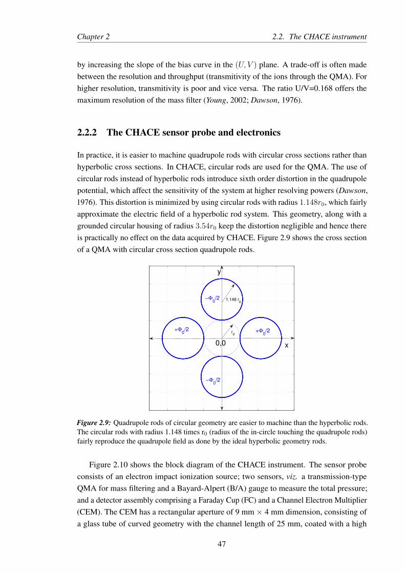
Chapter 2 2.2. The CHACE instrument

by increasing the slope of the bias curve in the (U, V ) plane. A trade-off is often madebetween the resolution and throughput (transmitivity of the ions through the QMA). Forhigher resolution, transmitivity is poor and vice versa. The ratio U/V=0.168 offers themaximum resolution of the mass filter (Young, 2002; Dawson, 1976).

2.2.2 The CHACE sensor probe and electronics

In practice, it is easier to machine quadrupole rods with circular cross sections rather thanhyperbolic cross sections. In CHACE, circular rods are used for the QMA. The use ofcircular rods instead of hyperbolic rods introduce sixth order distortion in the quadrupolepotential, which affect the sensitivity of the system at higher resolving powers (Dawson,1976). This distortion is minimized by using circular rods with radius 1.148r0, which fairlyapproximate the electric field of a hyperbolic rod system. This geometry, along with agrounded circular housing of radius 3.54r0 keep the distortion negligible and hence thereis practically no effect on the data acquired by CHACE. Figure 2.9 shows the cross sectionof a QMA with circular cross section quadrupole rods.

0,0

y

x

r0

−Φ0/2

+Φ0/2 +Φ

0/2

−Φ0/2

1.148 r0

Figure 2.9: Quadrupole rods of circular geometry are easier to machine than the hyperbolic rods.The circular rods with radius 1.148 times r0 (radius of the in-circle touching the quadrupole rods)fairly reproduce the quadrupole field as done by the ideal hyperbolic geometry rods.

Figure 2.10 shows the block diagram of the CHACE instrument. The sensor probeconsists of an electron impact ionization source; two sensors, viz. a transmission-typeQMA for mass filtering and a Bayard-Alpert (B/A) gauge to measure the total pressure;and a detector assembly comprising a Faraday Cup (FC) and a Channel Electron Multiplier(CEM). The CEM has a rectangular aperture of 9 mm × 4 mm dimension, consisting ofa glass tube of curved geometry with the channel length of 25 mm, coated with a high

47

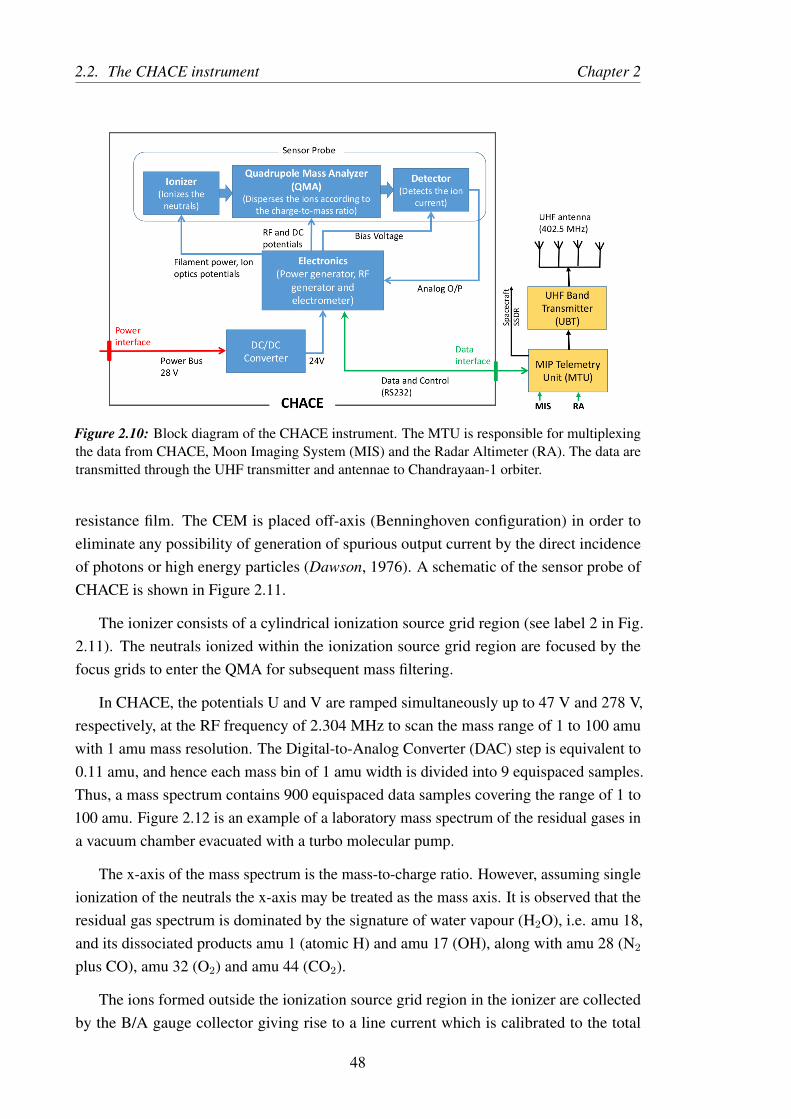
2.2. The CHACE instrument Chapter 2

Figure 2.10: Block diagram of the CHACE instrument. The MTU is responsible for multiplexingthe data from CHACE, Moon Imaging System (MIS) and the Radar Altimeter (RA). The data aretransmitted through the UHF transmitter and antennae to Chandrayaan-1 orbiter.

resistance film. The CEM is placed off-axis (Benninghoven configuration) in order toeliminate any possibility of generation of spurious output current by the direct incidenceof photons or high energy particles (Dawson, 1976). A schematic of the sensor probe ofCHACE is shown in Figure 2.11.

The ionizer consists of a cylindrical ionization source grid region (see label 2 in Fig.2.11). The neutrals ionized within the ionization source grid region are focused by thefocus grids to enter the QMA for subsequent mass filtering.

In CHACE, the potentials U and V are ramped simultaneously up to 47 V and 278 V,respectively, at the RF frequency of 2.304 MHz to scan the mass range of 1 to 100 amuwith 1 amu mass resolution. The Digital-to-Analog Converter (DAC) step is equivalent to0.11 amu, and hence each mass bin of 1 amu width is divided into 9 equispaced samples.Thus, a mass spectrum contains 900 equispaced data samples covering the range of 1 to100 amu. Figure 2.12 is an example of a laboratory mass spectrum of the residual gases ina vacuum chamber evacuated with a turbo molecular pump.

The x-axis of the mass spectrum is the mass-to-charge ratio. However, assuming singleionization of the neutrals the x-axis may be treated as the mass axis. It is observed that theresidual gas spectrum is dominated by the signature of water vapour (H2O), i.e. amu 18,and its dissociated products amu 1 (atomic H) and amu 17 (OH), along with amu 28 (N2

plus CO), amu 32 (O2) and amu 44 (CO2).

The ions formed outside the ionization source grid region in the ionizer are collectedby the B/A gauge collector giving rise to a line current which is calibrated to the total

48

Chapter 2 2.2. The CHACE instrument

Figure 2.11: Schematic diagram of the sensor probe of the CHACE instrument.

pressure in a N2 dominated medium at 300 K temperature.

The CHACE electronics caters to four important functions. First, it supplies electricalpower to the different subsystems in the sensor probe that include the electrodes, filaments,ion optics, quadrupole potentials and the detector assembly. Secondly, it generates RFof 2.304 MHz frequency for the QMA. Thirdly, it receives the ion current and does thenecessary signal conditioning, which include current to voltage conversion and digitization.Fourth, it sends the digitized data to the MIP Telemetry Unit (MTU) through the RS232interface. The MTU contains the firmware to control and command the CHACE electronics.Upon switch ON, the initialization code containing the instrument parameters stored inthe MTU is pushed to the CHACE electronics. Once initialized, the filament is turnedon gradually and the QMA operation starts. The science and the house keeping (HK)data of the CHACE instrument are sent to the MTU, which, in turn, interface to the UHFtransmitter of the MIP for subsequent transmission to the Chandrayaan-1 spacecraft. MTUalso contains a hard-line interface to write the data directly into the Solid State DataRecorder (SSDR) in the spacecraft before the MIP-separation.

Apart from the RS232 data interface, CHACE has power interface with the MIP battery.It receives 28 V through the MIP power bus and uses the regulated 24 V output.

49

2.2. The CHACE instrument Chapter 2

Figure 2.12: A laboratory spectrum acquired by the CHACE instrument. The signatures of themajor residual gases in the chamber are seen in the spectrum.

2.2.3 Development philosophy

During the development of the CHACE experiment, there was no reliable in-situ measure-ment of the sunlit side of the lunar exosphere. Based on the measurements of the lunaratmospheric pressure at the surface by the Cold Cathode gauges in Apollo 12, 14 and 15missions (Stern, 1999), total pressure of ∼ 10−10 Torr was expected in the sunlit lunarexosphere.

The challenge was to conduct in-situ measurement of the tenuous lunar exosphere andconfigure the instrument suitably to cover the expected range of pressures with adequatedynamic range, without resorting to higher integration time as that would have limitedthe spatial resolution of the measurements. In general, the major considerations for thedevelopment of the CHACE instrument included the following:

1. Sensitivity to measure the tenuous exosphere of the Moon.

2. Collection of sufficient number of mass spectra since the CHACE was a one-timeexperiment.

3. Cleanliness to minimize the effect of outgassing from the instrument.

4. Structural integrity of the payload for avoiding field imperfections and accuratemeasurement of the ion current.

50

Chapter 2 2.2. The CHACE instrument

The sensitivity of CHACE was ensured by the careful choice of the operating parame-ters, through numerous characterization experiments conducted in the ultra high vacuumcondition (pressure ∼ 10−8 to 10−9 Torr). The cleanliness of the instrument was ensuredby the careful choice of materials of low outgassing property, ultrasonic cleaning andbaking of the sensor probe prior to the assembly in the clean room and vacuum-isolationof the sensor probe while integrating with the MIP.

Ruggedization of the payload was of paramount importance in order to eliminate anypossibility of permanent deformation of the ion optics and/or the quadrupole rods dueto the mechanical distrubances during the launch phase. The structural dynamics of thesensor was studied using finite element model and the ruggedization scheme was workedout. The overall payload design was conducted based on the prescribed environmental testlevels for the lunar mission using PSLV core alone configuration. The CHACE sensor wassuitably ruggedized using ceramic material in order to protect its mechanical precision.The electronic components were protected from mechanical disturbances by using pottingcompounds. All materials that were used for the process of ruggesdization underwentnecessary tests for outgassing properties and were accepted as per quality protocols forflight.

2.2.4 Operating parameters

The major parameters that determine the performance of the CHACE instrument includethe focus voltage, electron energy, mass scan rate and the CEM bias voltage.

1. Focus voltage (FV)Focus voltage is the voltage applied at the electrode marked with label 5 with respectto the one marked with label 4 in the Figure 2.11. A negative FV attracts the positiveions from the source grid (label 2) to the entrance of the QMA. This potential focusesthe mixture of ions with different mass-to-charge ratio to the entrance aperture ofthe QMA. Figure 2.13 shows the result of the characterization of the focus voltagewith respect to the ion current corresponding to amu 28. Based on the results, theoptimized focus voltage of -30 V was used for CHACE.

2. Electron energyThe term electron energy in the present context refers to the energy imparted to thethermionic electrons emitted from the dual filament system by the application of apotential. The Coulomb interaction between the energetic electrons and the valenceelectrons of the neutrals causes ionization of the neutrals in the ionizer region. Mostof the atomic and molecular species have their electron impact ionization cross sectionmaximum in the range of ∼ 60-100 eV (Lotz, 1968; Montanari and Miraglia, 2014).CHACE used 70 eV electron energy to ionize the neutrals.

51

2.2. The CHACE instrument Chapter 2

0 - 2 0 - 4 0 - 6 0 - 8 0 - 1 0 0 - 1 2 0 - 1 4 0 - 1 6 00 . 0 1

0 . 1

1

1 0Ion

curre

nt (nA

)

F o c u s V o l t a g e ( V )

Figure 2.13: Variation of the ion current for amu 28 (N2) for different focus voltages.

3. Mass scan rateMass scan rate refers to the rate at which a mass spectrum (ranging from amu 1 to100) is scanned. Faster the scan, higher is the noise level and the spectrum acquisitiontime is less. For slower scans, on the other hand, the noise level is lower but the timerequired to acquire a spectrum is more. The spectrum acquisition time of CHACE waschosen based on the criteria: 1) the noise level should be low enough to sample thetenuous lunar exosphere, and 2) The spatial resolution, when translated to the groundtrace, should be better than 10 km, in order to study the dependence of the exosphereon the spatial variabilities of the lunar surface. Based on these considerations, a masscan rate of ∼4 s was chosen. Taking the motion of the MIP in consideration, thistranslated to a ground trace of ∼6.5 km on the lunar surface.

4. CEM bias voltageThe input of the CEM is biased with a negative voltage in the range of 103 Volt. Thepositive ions that reach the input of the CEM detector create a cascade of electrons.These electrons exit the CEM at a potential of∼ -150 V DC with respect to the groundand are attracted to the Faraday cup held at virtual ground. The current produced atthe Faraday cup is a measure of the abundance of the corresponding neutrals in themedium. An increase in the CEM bias voltage causes enhancement in the electronmultiplication at the CEM, resulting into a higher gain, thus enhancing the value ofthe current at the Faraday cup output. As a result, the sensitivity of detection of agiven species is increased.

Initially, the SNR increases because of the increase in the CEM gain with increasein the CEM bias voltage; then attains a plateau; and subsequently decreases with

52

Chapter 2 2.2. The CHACE instrument

further increase in the bias voltage (refer the inset of Fig.2.14 for the variation ofSNR of amu 28 with CEM bias voltage at a total pressure of 4 × 10−9 Torr). That isbecause of the saturation of the CEM gain and increase in the shot noise in the CEMdetector with increase in the bias voltage. Hence, there exists an optimum value ofthe CEM bias voltage, for which the SNR is maximum. The optimum bias voltageof the CEM depends on total pressure. For higher pressure, the optimal value of theCEM bias voltage is less. This is because of the ionization of neutrals within the CEMthat causes saturation of the CEM gain even at comparatively lower bias voltages.Experiments were conducted at different levels of total pressure and the optimumvalues of CEM bias voltage were obtained. Figure 2.14 shows the variation of theoptimum CEM voltage with total pressure. A detailed description of the figure isprovided in the caption. The CEM of CHACE was biased at 1800 V for the totalpressure of 10−10 Torr expected at the lunar day-side.

- 1 0 - 9 - 8 - 7 - 6 - 51 0 0 0

1 2 0 0

1 4 0 0

1 6 0 0

1 8 0 0

2 0 0 0

8 0 0 1 2 0 0 1 6 0 0 2 0 0 01 0 4

1 0 5

1 0 6

1 0 7

���������� ��� � ��������� �����

Optim

um bi

as vo

ltage

of th

e CEM

detec

tor (V

olt)

l o g 1 0 o f t o t a l p r e s s u r e

SNR

for am

u 28

C E M b i a s v o l t a g e ( V o l t )

��� �����������������������

���������� ������ �������

Figure 2.14: Variation of the optimum bias voltage of the CEM detector with total pressure. Thefilled squares are the experimentally obtained points and the continuous solid line is the exponentialfit, which is extrapolated (dotted extension) to 10−10 Torr of total pressure, as expected in the sunlitside of the Moon. At a given total pressure, the optimum CEM bias voltage is obtained by studyingthe variation of the SNR of amu 28 peak with CEM bias voltage, as shown in the inset for a pressureof 4 × 10−9 Torr. Based on this experiment, the CEM bias voltage of CHACE was set at 1800 V.

53

2.3. Ground calibration and testing Chapter 2

2.3 Ground calibration and testing

The CHACE instrument was ground calibrated from high vacuum of 10−6 Torr to ultra highvacuum of 10−9 Torr. The calibration included determination of the relative transmissionand detection efficiencies of ions with different mass-to-charge ratios. It also involvedmass calibration with residual gases and insertion of pure and mixed gases in the chamber.The B/A gauge is calibrated for the total pressure.

2.3.1 Relative detection efficiencies

Detection efficiency of an ion by a transmission-type quadrupole mass spectrometer de-pends on the transmission properties through the quadrupole mass filter and the sensitivityof the detector. The relative detection efficiencies of the lighter species are greater thanthe heavier ones. This is mostly because of the Quadrupole Mass Discrimination (QMD)effect and the mass-dependent sensitivity of the CEM detector (Dawson, 1976).

The analytical theory of an ideal QMA does not take into account the effects of thefringing electric fields on the motion of the ions at the terminations of the quadrupole rods.In practice, the fringing fields affect the entry of the ions from the ionizer to the QMA(Dawson, 1976). They tend to trap the ions and delay the process of its transmission throughthe mass filter. Because of their lesser mobility, the heavier ions are more susceptible toget delayed in the fringing fields than the lighter ones. As a result, the heavier species havelesser transmission efficiencies than the lighter ones. This results into the overestimation ofthe relative abundance of the lighter species with respect to the heavier ones. This is knownas the QMD effect (Dawson, 1976). The relative transmission efficiencies of different ionsis calibrated for different masses in order to nullify this mass discrimination effect duringanalysis. The QMD factor is the reciprocal of the relative transmission efficiencies of theions, which is a multiplicative correction factor to compensate for the QMD effect.

The variation of the relative transmission efficiency with ion mass, represented by thecontinuous curve in figure 2.15, is obtained by comparing the experimental and theoreticalvalues of the fractionation ratios of water vapour (amu 1 , amu 16, amu 17, amu 18) andthe compound Per Fluoro Tri Butyl Amine (PFTBA) (which yields mass peaks at amu 31,69 and 100 in the range of 1-100 amu) (Chapman, 1995) for 70 eV electron impact energy.Also, the experimental and theoretical values of the single-to-double ionization ratios ofAr-40 and N (amu 14) are used for obtaining the relative transmission efficiency profile.

Figure 2.16 shows the gain of the CEM detector in CHACE as a function of theion mass. The bias voltage was 1800 V. The Electron Multiplier Gain (EMG) profile ischaracterized to study the variation of the gain of the CEM detector with the ion mass. TheEMG profile is obtained by comparing the mass spectra acquired with Faraday cup and the

54

Chapter 2 2.3. Ground calibration and testing

0 20 40 60 80 100

0

5

10

15

20

25

Rel

ativ

e tra

nsm

issi

on e

ffici

ency

with

resp

ect t

o m

/q=2

8 am

u

m/q (amu)

Figure 2.15: The continuous line represents the variation of the relative transmission efficiency(with respect to N2 (amu 28)) with ion mass. The relative transmission efficiency curve is obtainedby comparing the experimental and theoretical values of the fractionation ratios of water vapour(amu 1 , amu 16, amu 17, amu 18) and the compound Per Fluoro Tri Butyl Amine (PFTBA) (whichyields mass peaks at amu 31, 69 and 100 in the range of 1-100 amu) for 70 eV electron impactenergy. In addition to the fractionation ratios of the compounds, the experimental and theoreticalvalues of the single-to-double ionization ratios of atomic species like 40Ar (i.e. ratio of the parentpeak at amu 40 to the harmonic peak at amu 20) and N (i.e. ratio of the parent peak at amu 14to the harmonic peak at amu 7) at 70 eV electron energy are also used for obtaining the relativetransmission efficiency profile. The solid circles, drawn on the relative transmission efficiencycurve, represent the relative transmission efficiencies of 4He, 20Ne, 40Ar with respect to N2 due tothe Quadrupole Mass Discrimination (QMD) effect.

CEM detector. The EMG profile is a divisive correction factor to account for the lessersensitivity of the CEM detector to the heavier ions.

Both the relative transmission efficiency and the EMG are functions of ion mass andhence, the raw spectra needs to be corrected by incorporating the QMD and EMG effects,for the accurate interpretation of the relative abundances of gases. Figure 2.17 shows therelative sensitivity profile of the instrument (normalized with respect to amu 28) for thecombined effects of mass dependent performances of the QMA and CEM.

2.3.2 Mass calibration

It is important to ensure that the gas atoms and molecules, ionized by the ionizer section ofCHACE, register peaks at the correct value of the mass-to-charge ratio bin. This is ensuredby mass calibration of CHACE, which is conducted with reference to the following:

55

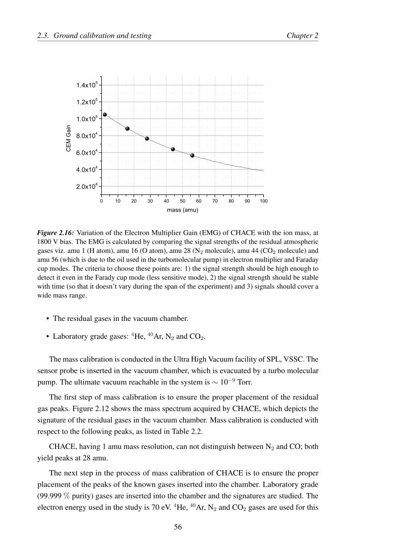
2.3. Ground calibration and testing Chapter 2

0 10 20 30 40 50 60 70 80 90 100

2.0x104

4.0x104

6.0x104

8.0x104

1.0x105

1.2x105

1.4x105

CE

M G

ain

mass (amu)

Figure 2.16: Variation of the Electron Multiplier Gain (EMG) of CHACE with the ion mass, at1800 V bias. The EMG is calculated by comparing the signal strengths of the residual atmosphericgases viz. amu 1 (H atom), amu 16 (O atom), amu 28 (N2 molecule), amu 44 (CO2 molecule) andamu 56 (which is due to the oil used in the turbomolecular pump) in electron multiplier and Faradaycup modes. The criteria to choose these points are: 1) the signal strength should be high enough todetect it even in the Farady cup mode (less sensitive mode), 2) the signal strength should be stablewith time (so that it doesn’t vary during the span of the experiment) and 3) signals should cover awide mass range.

• The residual gases in the vacuum chamber.

• Laboratory grade gases: 4He, 40Ar, N2 and CO2.

The mass calibration is conducted in the Ultra High Vacuum facility of SPL, VSSC. Thesensor probe is inserted in the vacuum chamber, which is evacuated by a turbo molecularpump. The ultimate vacuum reachable in the system is ∼ 10−9 Torr.

The first step of mass calibration is to ensure the proper placement of the residualgas peaks. Figure 2.12 shows the mass spectrum acquired by CHACE, which depicts thesignature of the residual gases in the vacuum chamber. Mass calibration is conducted withrespect to the following peaks, as listed in Table 2.2.

CHACE, having 1 amu mass resolution, can not distinguish between N2 and CO; bothyield peaks at 28 amu.

The next step in the process of mass calibration of CHACE is to ensure the properplacement of the peaks of the known gases inserted into the chamber. Laboratory grade(99.999 % purity) gases are inserted into the chamber and the signatures are studied. Theelectron energy used in the study is 70 eV. 4He, 40Ar, N2 and CO2 gases are used for this

56

Chapter 2 2.3. Ground calibration and testing

Figure 2.17: Combined relative sensitivity of the instrument due to the mass dependent perfor-mances of the QMA and the CEM. The lighter species have greater mobility and are less affected bythe fringing fields at the terminations of the QMA, and hence have greater transmission efficiency.Also, the CEM gain is greater for the lighter species than the heavier ones. The overall effect is thatthe instrument is more sensitive to the lighter species than the heavier ones. This effect is correctedduring the data analysis.

study. Figures 2.18, 2.19 , 2.20 and 2.21 show the signatures of 4He, 40Ar, N2 and CO2

respectively, as acquired by CHACE during mass calibration in the laboratory.

The mass calibration ensured not only the proper placement of the mass peaks on themass axis, but also demonstrated the detectability of the lighter species like Hydrogenand Helium and stability of the measurement. As the quadrupole potentials (U and V) areproportional to the mass of the ion whose path is stable in the QMA, higher percentagestability of the quadrupole potentials is required for the stable measurement of the lighterspecies (Dawson, 1976).

2.3.3 Pressure calibration

Pressure calibration addresses to the calibration of the B/A gauge which measures the totalpressure, which, in turn, is used to derive the partial pressures of the individual species. Thetotal pressure measured by the B/A gauge is calibrated in an N2 dominated environmentusing an external master gauge. For any other gas than N2, the relative sensitivity factorwith respect to Nitrogen is used, as shown in the second column of Table 2.3. Figure 2.22shows the calibration of the B/A gauge of CHACE in an N2 dominated environment.

57

2.3. Ground calibration and testing Chapter 2

Table 2.2: Mass calibration with residual gases in the vacuum chamber

Species Nominal mass-to-charge ratio (amu)

Hydrogen atom 1Hydrogen molecule 2Hydroxyl radical 17Water 18Nitrogen molecule and Carbon monoxide 28Oxygen molecule 32Carbon dioxide 44

0 4 8 12 16 20 24 28 32 36 40 44 48 52 56 60 64 68 72 76 80 84 88 92 96 1000

0.5

1

1.5

2

2.5

3

3.5

4

4.5

5x 10

−7

mass (amu)

Raw

part

ial pre

ssure

(T

orr

)

Figure 2.18: Signature of 4He acquired by CHACE during laboratory calibration. While the parentpeak is at amu 4, there is a harmonic peak due to double ionization of 4He at amu 2, with a relativeabundance of 0.08 with respect to the parent peak.

2.3.4 Sensitivity test

CHACE was subjected to a sensitivity test in order to study its response to He-4 and 40Ar.Laboratory grade gases were used for the test. Before the sensitivity tests were conducted,the vacuum system and the CHACE sensor were thoroughly baked in vacuum for a periodof two weeks. This was done in order to minimize the impurity level of gases due to theresidual gases. The gas insertion and pump-out rates were adjusted in a way such that therate of change of the abundance of the gas in the chamber was reasonably slow. Throughoutthe experiment, the inserted gas was dominant in the chamber, which was ensured from thespectra. The total pressure was measured with an external pressure gauge. The detectorcurrent was studied for different values of the total pressure and the sensitivities werederived from the slopes of the curves.

Table 2.3 presents the relative ionization sensitivities (with respect to N2) of the gasesaddressed in the thesis, and their overall sensitivities.

58

Chapter 2 2.3. Ground calibration and testing

10 20 30 40 50 60 70 80 90 1000

0.5

1

1.5

2

2.5

3

3.5

x 10−8

mass (amu)

Ra

w p

art

ial p

ressu

re (

To

rr)

Figure 2.19: Signature of 40Ar acquired by CHACE during laboratory calibration. The doubleionized Argon (Ar++) produces a peak at m/q = 20 amu.

0 4 8 12 16 20 24 28 32 36 40 44 48 52 56 60 64 68 72 76 80 84 88 92 96 1000

0.5

1

1.5

2

2.5

x 10−8

mass (amu)

Raw

part

ial pre

ssure

(T

orr

)

Figure 2.20: Signature of N2 (amu 28) acquired by CHACE during laboratory calibration. Thedissociated atomic N produces a peak at m/q = 14 amu.

It may be noted that the sensitivity tests were conducted in order to test the performanceof the instrument for different gases. The sensitivity values were not used in derivingthe absolute number densities of the gases reported in this thesis. Since CHACE wasequipped with a calibrated Bayard-Alpert gauge, the absolute abundances were obtainedby normalizing the sum over the peaks in a given mass spectrum with the total pressureand applying necessary calibration factors, as described in section 2.4. However, thenumber densities obtained from the absolute calibration (sensitivity test) match with thenumber densities obtained from the normalized partial pressures using Bayard-Alpertgauge measurements.

2.3.5 Test and Evaluation

CHACE has undergone all the tests as per the Chandrayaan-1 Environmental Test LevelSpecifications (ETLS) (ISRO internal report: ISRO-VSSC-MIP-TR-001/2007, 2007; Testreport on CHACE-FM: ISRO internal report, 2008; CHACE Package Assurance Re-

59

2.3. Ground calibration and testing Chapter 2

0 4 8 12 16 20 24 28 32 36 40 44 48 52 56 60 64 68 72 76 80 84 88 92 961000

0.5

1

1.5

2

2.5

x 10−8

mass (amu)

Ra

w p

art

ial p

ressu

re (

To

rr)

Figure 2.21: Signature of CO2 (amu 44) acquired by CHACE during laboratory calibration. Thedissociation products are CO and O and C producing peaks at m/q = 28, 16 and 12 amu, respectively.

Table 2.3: Relative ionization sensitivity factor (with respect to N2 ) (Summers, 1969; Holanda,1972) and overall sensitivities for the noble gases covered in this thesis

Species Relative ionization sensitivity with respect to N2 Overall sensitivity (A/Torr)

He 0.13 4.5Ar 1.11 32.5Ne 0.28 8.2H2 0.33 9.6

The overall sensitivities of Ne and H2 are estimated from the experimentally obtained overall sensitivity of Ar, using the relative

ionization sensitivity data.

port: ISRO internal report, 2008). The Flight Acceptance Tests (FAT) included pre-environmental tests at Standard Room Conditions (SRC); followed by the environmentaltests which included thermovacuum test, sine and random vibration tests, (Electro MagneticInterference/ Electro Magnetic Compatibility) EMI/EMC tests. The environmental testswere followed by the post-environmental SRC tests to confirm the functional normalcy ofCHACE.

It was found that the performance of CHACE in the post-environmental SRC tests waswithin the specification limits and conformed to the pre-enviromental SRC test results.Figure 2.23 shows a comparison between two mass spectra obtained with CHACE flightmodel, acquired before and after the environmental tests.

60

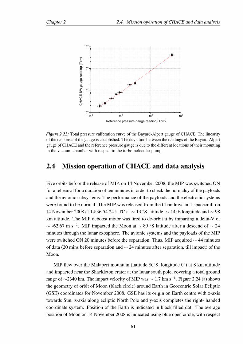
Chapter 2 2.4. Mission operation of CHACE and data analysis

10-8 10-7 10-6 10-510-8

10-7

10-6

10-5

CH

AC

E B

/A g

auge

read

ing

(Tor

r)

Reference pressure gauge reading (Torr)

Figure 2.22: Total pressure calibration curve of the Bayard-Alpert gauge of CHACE. The linearityof the response of the gauge is established. The deviation between the readings of the Bayard-Alpertgauge of CHACE and the reference pressure gauge is due to the different locations of their mountingin the vacuum chamber with respect to the turbomolecular pump.

2.4 Mission operation of CHACE and data analysis

Five orbits before the release of MIP, on 14 November 2008, the MIP was switched ONfor a rehearsal for a duration of ten minutes in order to check the normalcy of the payloadsand the avionic subsystems. The performance of the payloads and the electronic systemswere found to be normal. The MIP was released from the Chandrayaan-1 spacecraft on14 November 2008 at 14:36:54.24 UTC at ∼ 13 ◦S latitude, ∼ 14◦E longitude and ∼ 98km altitude. The MIP deboost motor was fired to de-orbit it by imparting a delta-V of∼ -62.67 m s−1. MIP impacted the Moon at ∼ 89 ◦S latitude after a descend of ∼ 24minutes through the lunar exosphere. The avionic systems and the payloads of the MIPwere switched ON 20 minutes before the separation. Thus, MIP acquired ∼ 44 minutesof data (20 mins before separation and ∼ 24 minutes after separation, till impact) of theMoon.

MIP flew over the Malapert mountain (latitude 86◦S, longitude 0◦) at 8 km altitudeand impacted near the Shackleton crater at the lunar south pole, covering a total groundrange of ∼2340 km. The impact velocity of MIP was ∼ 1.7 km s−1. Figure 2.24 (a) showsthe geometry of orbit of Moon (black circle) around Earth in Geocentric Solar Ecliptic(GSE) coordinates for November 2008. GSE has its origin on Earth centre with x-axistowards Sun, z-axis along ecliptic North Pole and y-axis completes the right- handedcoordinate system. Position of the Earth is indicated in black filled dot. The averageposition of Moon on 14 November 2008 is indicated using blue open circle, with respect

61

2.4. Mission operation of CHACE and data analysis Chapter 2

0 10 20 30 40 50 60 70 80 90 100

2

4

6

8

10

12x 10

−10

Mass (amu)

Ion c

urr

ent (A

)

0 10 20 30 40 50 60 70 80 90 100

2

4

6

8

10

12x 10

−10

Mass (amu)

Ion c

urr

ent (A

)

(b) Post−environmental test spectrum

(a) Pre−environmental test spectrum

Figure 2.23: (a) A mass spectrum acquired with CHACE before the environmental test, at atotal pressure of ∼ 5 × 10−7 Torr. (b) A mass spectrum acquired after the completion of theenvironmental tests were completed, under similar total pressure. It is observed that the quality ofthe mass spectrum (assessed with respect to the mass resolution, peak shape, throughput and massshift) is retained even after the environmental tests.

to the estimated positions of bow shock and geomagnetic tail. Figure 2.24 (b) shows theground track of Moon Impact Probe (MIP) on Moon (red curve) in the y-z plane of MeanEarth (ME) coordinate system. The ME coordinate system has its origin on Moon centrewith x-axis towards Earth, z-axis along the rotational pole of Moon and y-axis completesthe right-handed coordinate system. This projection represents the geometry as viewedfrom Earth, such that the co-ordinate (0,0) represents the center of the near-side of Moon.

During the MIP mission, CHACE was switched ON at 14:16 UTC along with the otherpayloads, twenty minutes prior to the MIP release. The instrument took ∼ 20 minutes forthe stability of its emission current from the hot cathode filament. During the MIP mission,CHACE was operated for a duration of ∼ 44 minutes, out of which for 20 minutes theMIP was attached with the Chandrayaan-1 orbiter. Each mass spectrum was acquired in ∼4.1 s, which translates to an average ground range of ∼6.5 km. During the MIP mission,CHACE acquired 650 mass spectra.

The post flight analysis of the HK parameters confirmed that CHACE was healthyduring its operation. All the major parameters, viz. filament voltage, filament resistance,emission current, temperature, etc. were within the specification limits (ISRO internalreport: ISRO-VSSC-MIP-PFA-001/2008, 2008).

62

Chapter 2 2.4. Mission operation of CHACE and data analysis

-100 -50 0 50 100XGSE (REarth)

-100

-50

0

50

100

YG

SE (

RE

art

h)

Earth

Moon

(a)

-2000 -1000 0 1000 2000YME (km)

-2000

-1000

0

1000

2000

ZM

E (

km

)

90E90W

90N

90S

(b)

Figure 2.24: (a) Location of the Moon with respect to the Earth during the MIP release. The bowshock and the geomagnetic tail are shown for nominal solar conditions. (b) Ground trace of theMIP (red curve) after release from the Chandrayaan-1 orbiter.

The science data of CHACE comprise 650 mass spectra containing raw partial pressure(relative abundances of different species) data in the mass range of 1 to 100 amu; and thetotal pressure data for each spectrum from the B/A gauge. Out of these 650 mass spectra,the first 310 spectra were acquired when the emission circuit of CHACE was undergoingstabilization, while the rest 340 spectra were acquired with the emission circuit stabilized.For calculating the absolute abundances of species, the last 340 spectra were used, whileall the 650 spectra were useful for ratiometric measurements (relative abundances).

First, the total pressure is corrected for the dominant gas with reference to the massspectrum (the N2-equivalent total pressure is divided by the gas-dependent sensitivityfactor). The mass-dependent quadrupole mass discrimination (QMD) and electron multi-plier gain (EMG) factors are incorporated to retrieve the correct relative abundances ofthe species. The resultant peaks are summed over and normalized to match the dominantgas-corrected total pressure. Finally, the corrected partial pressure of the species of interestis obtained by dividing the peak height by the corresponding relative sensitivity factorin order to account for its relative ionization efficiency with respect to N2. The overalluncertainty in the derived absolute abundances of the species is ∼ ± 40 %.

Figure 2.25 shows the flow chart of the data reduction process. Figure 2.26 showsthe step-by-step reduction of the raw science data to the calibrated data. Here, the gascorrection factor for the total pressure is 1.0 since the spectrum is dominated by watervapour and Nitrogen molecule. The QMD and EMG corrections compensate for the massdependent transmission efficiency and the detector sensitivity (panels 2 and 3 from top).The total pressure normalization helps estimating the absolute partial pressures of thespecies (bottom panel).

63

2.4. Mission operation of CHACE and data analysis Chapter 2

Raw sweep dataRaw sweep dataRaw sweep data

Raw sweep data

Relative quadrupole transmission efficiency correction(QMD and EMG)

Dominant gascorrection fortotal pressure

Normalization ofmass spectrumwith respect to thegas-corrected total pressure

Relative sensitivitycorrection (with respectto N

2) for the species

of interest

Total pressure

Figure 2.25: The flow chart describing the process of data reduction.

0 4 8 12 16 20 24 28 32 36 40 44 48 52 56 60 64 68 72 76 80 84 88 92 96 1000

1

2

x 10−4

Pe

ak s

tre

ng

th (

a.u

)

0 4 8 12 16 20 24 28 32 36 40 44 48 52 56 60 64 68 72 76 80 84 88 92 96 1000

1

2x 10

−4

Pe

ak s

tre

ng

th (

a.u

.)

0 4 8 12 16 20 24 28 32 36 40 44 48 52 56 60 64 68 72 76 80 84 88 92 96 1000

1

2

3

x 10−4

Pe

ak s

tre

ng

th (

a.u

.)

0 4 8 12 16 20 24 28 32 36 40 44 48 52 56 60 64 68 72 76 80 84 88 92 96 1000

1

2

x 10−7

Pa

rtia

l P

ressu

re (

To

rr)

Mass (amu)

(a) Raw spectrum

(b) QMD corrected

(c) QMD and EMG corrected

(d) QMD, EMG corrected and normalized to gas−correctedtotal pressure

Figure 2.26: The step-by-step processing of the raw mass spectrum during the process of datareduction. The ordinates in the first three panels are plotted in arbitrary units (a.u.). The appli-cations of relative transmission and detection efficiency corrections and normalization with thegas-corrected total pressure are demonstrated here.

The ram pressure enhancement of pressure due to the motion of the MIP through thelunar medium is accounted (Sridharan et al., 2015). The measurements made by CHACEare a convolution of both altitude and latitude variations. The latitude variation brings in thevariation of the local surface temperature, which, in turn, controls the altitude distributionof the exospheric species and is used to derive the number density. It is assumed herethat the neutrals detected by CHACE were in thermal equilibrium with the lunar surfaceand the contribution of the sputtered neutrals in the lunar exosphere, if any, is less (Wurzet al., 2007). Benna et al. (2015) has shown that the derived scale height temperaturebased on NMS/LADEE observations is in agreement with the surface temperature, which

64

Chapter 2 2.4. Mission operation of CHACE and data analysis

20 30 40 50 60 70 80 90

10

20

30

40

50

60

70

80

90

100

Sur

face

tem

pera

ture

(K)

Altitude of MIP

Alti

tude

of M

IP (k

m)

Latitude (deg S)

0

40

80

120

160

200

240

280

320

360

400 Surface temperature

Figure 2.27: The black line shows the latitude-altitude profile of the trajectory of the MIP. The redcoloured dotted line shows the variation of the lunar surface temperature as a function of latitudealong the ground trace of the MIP. The surface temperature graph is as per the Diviner radiometerobservations (Paige et al., 2010a).

substantiates this assumption.

The 2D (latitude versus altitude) maps and the surface densities of the species arecalculated by using the barometric law (Chamberlain, 1963) given by

P = P0 exp

(r − r0

kT/mg

)(2.20)

Here P is the pressure at a selenocentric distance r, r0 is the radius of the Moon, T isthe surface temperature, m is the mass of the species, P0 is the pressure at the surface, k isthe Boltzmann constant and g is the acceleration due to gravity in Moon. The equation

P = nKT

is used to convert the pressure (P ) to the number density (n).

The barometric law holds good even in the collisionless regime as long as the mean ki-netic energy per atom is constant. Barometric law has been used extensively by researchersto describe the vertical profile of the density even in planetary exospheres (Benna et al.,2015; Hurley et al., 2016). A discussion on this is presented in the Appendix. The lunarsurface temperature along the MIP ground trace is taken from the global temperature mapprovided by the Diviner Lunar Radiometer Experiment aboard the Lunar ReconnaissanceOrbiter (LRO) Paige et al. (2010a). Accordingly, an empirical model of the lunar surfacetemperature variation is adopted in the present analysis with the equatorial temperature of382 K and polar temperature of 95 K, based on the Diviner temperature map at the subsolarmeridian range relevant to the CHACE observations. Figure 2.27 shows the latitudinal and

65

2.4. Mission operation of CHACE and data analysis Chapter 2

altitudinal variation of the MIP trajectory and the variation of the lunar surface temperaturewith latitude along the ground trace of the MIP.

In the subsequent chapters, the observations of CHACE on the lunar exospheric noblegases (Ar, Ne and He) and H2 will be presented.

66

Chapter 3

Observations on Argon

The most beautiful experience we can have is the mysterious. It is the

fundamental emotion which stands at the cradle of true art and true

science.

—Albert Einstein

3.1 The lunar Argon

The Cold Cathode Gauge Experiment (CCGE) of the Apollo-12, 14 and 15 SurfaceExperiment Packages determined the surface density of∼107 cm−3 and∼105 cm−3 duringthe lunar day and night, respectively (Johnson et al., 1972). This results in the day-to-nightratio of the surface number density as ∼102.

Hodges and Johnson (1968) predicted that in hydrostatic equilibrium, one would expectlateral flow in the lunar exosphere to establish a relation between surface number density (n)distribution and surface temperature (T), given by nT 5/2 = constant for non-condensablegases, in the absence of sinks. This is known as the law of exospheric equilibrium fornon-condensable gases. The distribution of any condensable gas will deviate from this law.

For typical values of 100 K and 400 K for the lunar nightside and dayside temperatures,the law of exospheric equilibrium for non-condensable gases (Hodges and Johnson, 1968)suggests a ratio of∼30. The higher value of the day-to-night surface density ratio measuredwith CCGE in the lunar exosphere indicated the dominance of non-condensable species,which was later detected by the LACE experiment of Apollo-17 Surface ExperimentPackage as Argon. Argon is condensable under the prevailing temperature and pressure

67

3.1. The lunar Argon Chapter 3

conditions on the lunar night side and the polar regions and is one of the importantconstituents of the lunar neutral exosphere. Out of the two prominent isotopes of Argon,40Ar and 36Ar, most of the lunar Argon is 40Ar while the isotope 36Ar, which is of thesolar origin (Wieler, 2002), accounts for only ∼10% of the lunar Ar inventory (Wieler andHeber, 2003).

3.1.1 Origin of 40Ar

Lunar 40Ar is a product of the radioactive decay of 40K in the lunar interior (Hodges,1977). The radioactive isotope 40K has an abundance of 0.012 % in natural Potassiumand has a half life of 1.27 × 109 years, which decays to 40Ar by the process of electroncapture resulting into the emission of 1.46 MeV gamma ray photon and electron neutrino(Wetherill, 1957; Beckinsale and Gale, 1969; Ward, 1981). The decay equation is given by:

4019K + 0

−1e−1 −→ 40

18Ar + νe + γ (1.46 MeV)

Hodges (1977) proposed that 40Ar must be released from a depth of ∼1000 km, in themolten asthenosphere of the Moon. This depth was revised by Weber et al. (2011) to be∼1250 km. These depths were arrived at by considering the 40Ar effusion rate of 1.4 ×1021 atoms s−1 (Hodges, 1977), without attributing much importance to diffusion on thegrounds that diffusion is a slow process to explain this effusion rate and the returned lunarrock samples would show a dearth of 40Ar instead of the excess, as reported by Heymannand Yaniv (1970).

Killen (2002), using a multipath diffusion code, showed that a source of 40Ar at a depthof ∼1000 to 1250 km is not a necessity. Natural diffusion from a crustal depth of ∼25km through micropores and cracks, aided by shallow Moonquakes could account for theeffusion rate of 40Ar in the lunar exosphere.

The Ar atoms generated in the lunar interior diffuse to the surface and eventuallyundergo thermal desorption, which is indicated by the strong diurnal variation of the Argondensity (Hodges and Hoffman, 1975; Benna et al., 2015). The residence time of Ar on thelunar surface is given by (Hodges, 1982):

tres =C

T 2exp

(4.19Q

RT

)(3.1)

where Q is the heat of adsorption in Calories mole−1, 4.19 is Joule’s constant, R is thegas constant and T is the surface temperature and C is a constant expressed in s K−2. Thephysical meaning of the pre-exponential factor is the vibration period (in s) for the van derWaals potential of the adsorbed atom, which is a property of the adsorbing material and

68

Chapter 3 3.1. The lunar Argon

not of the species (Grava et al., 2015b). The best model fit to the nightside variation ofAr from the LACE observations yield C= 4 × 10−6 s K−2 and Q=6500 Cal mole−1. Thissuggests the residence time of Ar on the lunar nightside ranges between 1010 and 102 s forsurface temperatures of 80 to 120 K (Grava et al., 2015b).

Sputtering, on the other hand, is considered as a source of non-thermal Argon, capableof producing an extended Argon corona (Chaufray et al., 2009), although, with lesscontribution (Wurz et al., 2007).

3.1.2 Loss processes for 40Ar

Among the loss processes of lunar Argon, photoionization is important. The photoion-ization life-time of lunar exospheric Argon is ∼34 days for quiet Sun and ∼ 15 days foractive Sun (Huebner and Mukherjee, 2015). Equally important loss process of the lunarexospheric 40Ar is the charge exchange with solar wind protons (Grava et al., 2015b).Electron impact ionization lifetime is ∼ 550 days (Stern, 1999). In addition to thesepermanent loss processes, if Argon is transported to a Permanently Shadowed Region(PSR), it may be condensed. The process of cold trapping may be permanent unless anyexternal source supplies energy to it either by space weathering, shallow Moonquakes,meteor impacts or seasonal warming of the polar regions (Grava et al., 2015b). Table3.1 summarises the different loss processes of the lunar exospheric 40Ar and their relativeimportances.

Table 3.1: Loss processes of 40Ar in the lunar exosphere (from Stern (1999); Nakai et al. (1987);Huebner et al. (1992); Grava et al. (2015b), and the references therein)

Process Loss rate (atoms s−1) Lifetime (Earth-days)

PSR-cold trapping 3.0 × 10−7 38Photo-ionization 3.0× 10−7 (QS), 6.86× 10−7

(AS)38 (QS), 16 (AS)

Charge exchange with solarprotons

4.9 × 10−7 34

Solar radiation pressure 9 × 10−8 12731Electron impact ionization 2.1 × 10−8 5.5 × 102

Jeans escape 3.2 × 10−16 3.6 × 1010

QS = Quiet Sun, AS = Active Sun

The dominant loss mechanism for lunar Ar is photoionization, although the loss rates

69

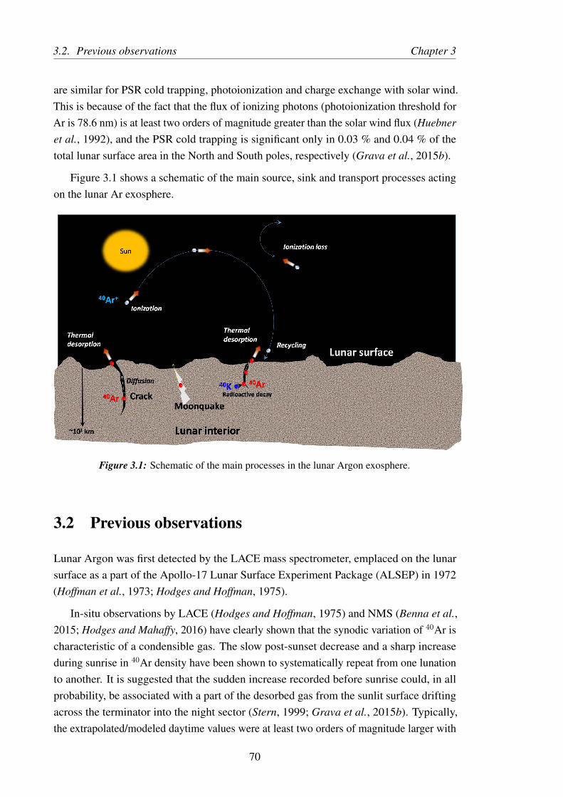
3.2. Previous observations Chapter 3

are similar for PSR cold trapping, photoionization and charge exchange with solar wind.This is because of the fact that the flux of ionizing photons (photoionization threshold forAr is 78.6 nm) is at least two orders of magnitude greater than the solar wind flux (Huebneret al., 1992), and the PSR cold trapping is significant only in 0.03 % and 0.04 % of thetotal lunar surface area in the North and South poles, respectively (Grava et al., 2015b).

Figure 3.1 shows a schematic of the main source, sink and transport processes actingon the lunar Ar exosphere.

Figure 3.1: Schematic of the main processes in the lunar Argon exosphere.

3.2 Previous observations

Lunar Argon was first detected by the LACE mass spectrometer, emplaced on the lunarsurface as a part of the Apollo-17 Lunar Surface Experiment Package (ALSEP) in 1972(Hoffman et al., 1973; Hodges and Hoffman, 1975).

In-situ observations by LACE (Hodges and Hoffman, 1975) and NMS (Benna et al.,2015; Hodges and Mahaffy, 2016) have clearly shown that the synodic variation of 40Ar ischaracteristic of a condensible gas. The slow post-sunset decrease and a sharp increaseduring sunrise in 40Ar density have been shown to systematically repeat from one lunationto another. It is suggested that the sudden increase recorded before sunrise could, in allprobability, be associated with a part of the desorbed gas from the sunlit surface driftingacross the terminator into the night sector (Stern, 1999; Grava et al., 2015b). Typically,the extrapolated/modeled daytime values were at least two orders of magnitude larger with

70

Chapter 3 3.2. Previous observations

reference to the night side measurements. Even with the spot measurement data fromLACE, Hodges (1973) could get evidence for a potentially varying source of 40Ar, i.e., fora varying release rate of 40Ar from the lunar interior, possibly associated with Moonquakes(Hodges and Hoffman, 1975). There were attempts during Apollo 15 and 16 missionswherein mass spectrometers were flown in the service modules but with limited success.One of the objectives of the studies carried out by Hodges et al. (1972) was to look forlunar volcanism. The 40Ar:36Ar ratio has been shown to be ∼3.5. No further details areavailable from the orbiter data even for the anti-sunward side, leave alone the sunlit side.Lunar Argon was also studied by the LAMP ultraviolet spectrometer aboard LRO at 104.8and 106.7 nm fluorescent emission wavelengths, and an upper limit of 2.3 × 104 cm−3

is reported (Cook et al., 2013), which is ∼1.5 times lower than the upper limit given byLACE (Hodges and Hoffman, 1975).

Recently, the NMS instrument aboard LADEE orbiter has studied the diurnal variationof the lunar exospheric Argon in the low latitudes (± 23◦) for a period of five months.NMS observations have brought out significant evidences of the lunar surface-exosphereinteraction through the spatial inhomogeneity of the lunar exospheric Argon (Benna et al.,2015). NMS has observed localized enhancement of 40Ar at the Western maria, coincidentwith the potassium-rich KREEP regions, suggesting the close interaction between thesurface and the exosphere, characteristic to the surface boundary exospheres (Benna et al.,2015).

The NMS observations have also revealed synodic and semiannual oscillations of 40Ar(Hodges and Mahaffy, 2016). The semiannual oscillation of 40Ar is found to be consistentwith condensation loss in the seasonal cold traps at the poles due to the obliquity of theMoon. The results show that the exospheric morphology depends on the energetics ofdesorption of atoms from soil grains. It also brought out the importance of the surface-exosphere interaction process.

In addition to the observations, several modelling studies on lunar Argon have beenconducted (Hodges et al., 1974; Hodges and Hoffman, 1975; Hodges, 1975; Chaufray et al.,2009; Grava et al., 2015b). These models accounted for cold trap condensation/adsorptionof Argon on the lunar surface along with the ionization loss process. Attempts were evenmade to take into account of the Argon ions produced by the solar UV and then acceleratedin the convective electric field of the solar wind towards the lunar surface and eventuallygetting implanted in the Lunar regolith and neutralized (Manka and Michel, 1971). Theimportance of the charge exchange process with the solar wind protons is also consideredin the recent model of the lunar exospheric Argon (Grava et al., 2015b).

In the present chapter, observation on the latitudinal variation of 40Ar in the sunlit lunarexosphere and the relative variation of 40Ar with respect to 36Ar, based on the CHACEobservation are reported. Since 40Ar is produced from the lunar interior, it is directly

71

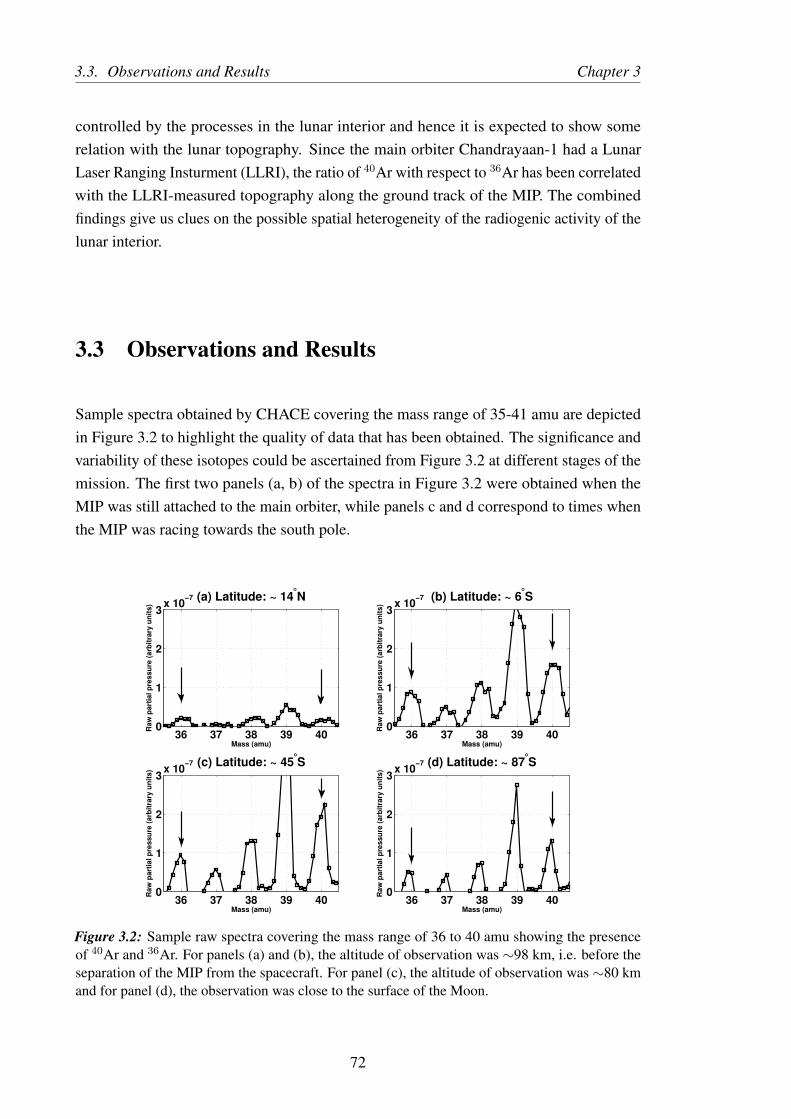
3.3. Observations and Results Chapter 3

controlled by the processes in the lunar interior and hence it is expected to show somerelation with the lunar topography. Since the main orbiter Chandrayaan-1 had a LunarLaser Ranging Insturment (LLRI), the ratio of 40Ar with respect to 36Ar has been correlatedwith the LLRI-measured topography along the ground track of the MIP. The combinedfindings give us clues on the possible spatial heterogeneity of the radiogenic activity of thelunar interior.

3.3 Observations and Results

Sample spectra obtained by CHACE covering the mass range of 35-41 amu are depictedin Figure 3.2 to highlight the quality of data that has been obtained. The significance andvariability of these isotopes could be ascertained from Figure 3.2 at different stages of themission. The first two panels (a, b) of the spectra in Figure 3.2 were obtained when theMIP was still attached to the main orbiter, while panels c and d correspond to times whenthe MIP was racing towards the south pole.

36 37 38 39 400

1

2

3x 10

−7 (a) Latitude: ~ 14°N

Ra

w p

art

ial

pre

ss

ure

(a

rbit

rary

un

its

)

Mass (amu)

36 37 38 39 400

1

2

3x 10

−7 (c) Latitude: ~ 45°S

Ra

w p

art

ial

pre

ss

ure

(a

rbit

rary

un

its

)

Mass (amu)36 37 38 39 40

0

1

2

3x 10

−7 (d) Latitude: ~ 87°S

Mass (amu)

Ra

w p

art

ial

pre

ss

ure

(a

rbit

rary

un

its

)

36 37 38 39 400

1

2

3x 10

−7 (b) Latitude: ~ 6°S

Mass (amu)

Ra

w p

art

ial

pre

ss

ure

(a

rbit

rary

un

its

)

Figure 3.2: Sample raw spectra covering the mass range of 36 to 40 amu showing the presenceof 40Ar and 36Ar. For panels (a) and (b), the altitude of observation was ∼98 km, i.e. before theseparation of the MIP from the spacecraft. For panel (c), the altitude of observation was ∼80 kmand for panel (d), the observation was close to the surface of the Moon.

72

Chapter 3 3.3. Observations and Results

3.3.1 Distribution of 40Ar

When the partial pressures or absolute number densities of different species are to bedealt with, it is essential to ensure that the instrument has stabilized, which, in the case ofCHACE, is ∼20 minutes after switch ON, during which time the MIP had crossed 20◦ S.Thus, data beyond 20◦ S are considered to calculate the absolute density of 40Ar. Figure3.3 shows the number density of 40Ar (colour coded), along the MIP trajectory in latitudeand altitude.

Figure 3.3: The number density of 40Ar from the in-situ measurements of CHACE along the MIPtrajectory. The measurements are convolution of altitudinal and latitudinal effects.

The top panel of Figure 3.4 shows the surface density of 40Ar derived from the in-situobservations of CHACE by using barometric law using the local scale heights. In theabsence of any surface heterogeneity, one would have expected to see a smooth variation inthe latitudinal distribution of 40Ar. In contrast, it is seen that, there are several undulations.To facilitate viewing the small scale undulations from the mean trend (presumably due tothe surface temperature variation with latitude), a fourth order polynomial fit representingthe mean trend has also been superposed on the plots along with the number densities.A maximum fluctuation of ∼5% is observed about the mean trend. These short scalevariations of the 40Ar surface number density are proposed to be associated with thelunar surface topography (Sridharan et al., 2013a). The bottom panel shows the surfacetopography obtained from the LLRI on Chandrayaan-1 (Kamalakar et al., 2009). TheLLRI data corresponding to the longitude zone of the MIP ground track had been strippedout of the main data base and the topological features were extracted (Sridharan et al.,2013a).

Since 40Ar is a by-product of radiogenic activity from the lunar interior, it is expectedthat its concentration would increase in the regions of deep craters and decrease along with

73

3.3. Observations and Results Chapter 3

Figure 3.4: The top panel shows the surface density of 40Ar derived using barometric law from theCHACE observations. The lower panel shows the lunar surface topography obtained using LLRIdata along the ground track of the MIP. The anti-correlation of the trends of the surface density andthe elevation from ∼ 42◦S till the South pole is quite evident.

high elevation regions. While making the comparison, the mean reference - zero elevationline - for the LLRI data had been considered. The striking observations from Figure 3.4are: from ∼42◦S to ∼80◦S the elevation registered an increasing trend from ∼-2.3 km to∼+1.6 km and there had been a corresponding decreasing trend from ∼ 4 × 104 cm−3

to ∼ 1 × 104 cm−3 in the 40Ar surface number density. Further, it could also be notedthat the undulations in the 40Ar density are nearly of the same scale lengths as revealedby the ranging instrument in the whole region under consideration. The elevation rangeof the lunar surface between 25◦ to 30◦ S along the ground trace of the MIP is 0-1 km.Similar range of elevation is observed between 60◦ to 75◦ S. However, the 40Ar surfacenumber density in these two regions differ by almost a factor of 2. This indicates spatialheterogeneity of the lunar 40Ar.

The in-situ observations by CHACE are used to generate the 2-dimensional (latitudeversus altitude) distribution map with a resolution of 1◦ in latitude and 5 km in altitude,using the barometric law, as shown in Figure 3.5.

The deviations from the mean concentration of 40Ar show that, the deeper one goesinto the lunar interior, more would be the 40Ar density (Sridharan et al., 2013a). Thesevariations point to the important role of lunar surface processes in modulating the 40Ardensities. Any long lived species, over time, would tend to get uniformly distributed.However, it may not be the case for a gas that has a source spatially distributed and source

74

Chapter 3 3.3. Observations and Results

Figure 3.5: Two dimensional (latitude versus altitude) map of lunar 40Ar along the trajectory ofthe MIP.

strength larger in comparison with the redistribution. In the absence of such a factor, asmentioned above, the variations would have been smooth (dictated only by the surfacetemperature variation with latitude). In the case of a SBE, the very fact that undulationsare present in the density indicates the possible decisive role of lunar surface.

3.3.2 The 40Ar:36Ar ratio

The summary of the important findings of LACE on lunar Argon have been succinctlyprovided by Stern (1999) and Wieler and Heber (2003). The conclusion that 40Ar is of lunarorigin is essentially based on the relative concentration of 40Ar with respect to 36Ar. Thisratio has to be ∼ 10−4 if these two isotopes are of solar wind origin (Wieler, 2002). On theother hand, the measurements from LACE in the Apollo-17 Surface Experiment Packagerevealed that, the ratio remained >1 all the times, and in fact, typically varied from 7.5 to10 over the Apollo-17 landing site. This ratio was characteristic to the LACE deploymentsite as it is believed that LACE has observed significant amount of Moonquake-releasedArgon over and above the steady state Argon inventory (Grava et al., 2015b).

On the other hand, CHACE has studied the variation of this ratio over a broad rangeof latitudes, as it was switched on at 40◦N and the measurements continued till the MIPimpacted close to the South Pole. When the ratios of the relative amplitudes are considered,stabilization of the instrument is not mandatory since within the short time span of ∼250ms taken to cover the mass range of 36 to 40 amu the instrument characteristics are notlikely to change. Therefore even when the instrument is just getting stabilized, 40Ar: 36Arratio could be studied. Results are depicted in Figure 3.6, wherein 15 point running average(equivalent to ∼100 km ground range) has been shown (continuous line) in addition toactual ratios in every sweep (red open circles). The average ratio initially registered a valueof ∼1, over the lunar latitude of 40◦N, then increased to ∼2.25 over 12◦S and remainedcentred around this value till the point of impact. There are large and small undulationsall through, which could on occasions, reach as large as 30% of the mean value. One

75

3.3. Observations and Results Chapter 3

important aspect of the above result is that the ratio was consistently larger than thatcorresponding to the solar wind, indicating the potential radiogenic activity in the lunarinterior and its possible variation along the ground track.

−40 −30 −20 −10 0 10 20 30 40 50 60 70 80 90

1

2

3

4

5

6

7

8

9

10

Lunar Latitude (+ve for degree South)

40A

r :

36A

r

Figure 3.6: Variation of the 40Ar:36Ar ratio as obtained by CHACE. The red markers are theobserved ratios while the blue continuous line is a 15 point moving average, which is equivalent to∼ 100 km of ground trace.

In this context, some of the earlier results on the 40Ar:36Ar ratio and their possiblerelation to the de-gassing history of the lunar surface under consideration become important.Wieler and Heber (2003) have exhaustively discussed about the noble gas isotopes on theMoon and have highlighted how these ‘parentless’gases could be used to constrain thedegassing history of the Moon itself. The parentless 40Ar is used as a semi-quantitativemeasure of the ‘antiquity’of a soil, i.e., the time in the past when a sample was exposedto the solar wind at the top of the regolith. 40Ar concentration needs to be normalised tothe length of time a sample had spent on the surface for which 36Ar from the solar windcould be used as proxy. It is believed that the 40Ar:36Ar ratio in any sample that had beenirradiated by the solar wind for several billion years would be higher than in the samplethat received the radiation later. This implies that higher the ratio of 40Ar:36Ar in anysample, the older the sample would be. A cross calibration has been provided by Eugsteret al. (2001), which clearly indicates that a ratio of ∼13 would correspond to an antiquityof ∼3.7 Gy while a ratio of ∼0.5 would correspond to ∼10 My. Figure 3.7 depicts there-plotted cross calibration of the basic inputs given by Eugster et al. (2001) and Wielerand Heber (2003). The 40Ar:36Ar ratio after the instrument stabilization is seen to becentred ∼2.25 in the southern hemisphere of the near side of the Moon. This would implyan antiquity of ∼1.5 Gy for the longitudinal segment corresponding to the ground track of

76

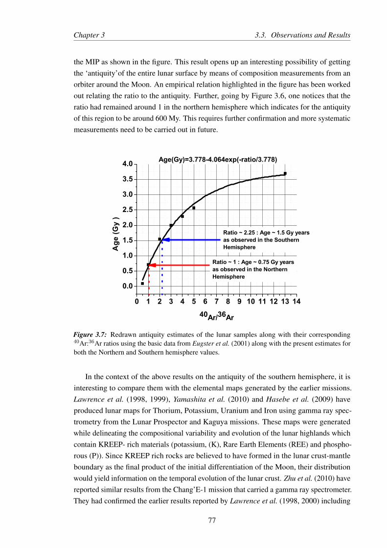
Chapter 3 3.3. Observations and Results

the MIP as shown in the figure. This result opens up an interesting possibility of gettingthe ‘antiquity’of the entire lunar surface by means of composition measurements from anorbiter around the Moon. An empirical relation highlighted in the figure has been workedout relating the ratio to the antiquity. Further, going by Figure 3.6, one notices that theratio had remained around 1 in the northern hemisphere which indicates for the antiquityof this region to be around 600 My. This requires further confirmation and more systematicmeasurements need to be carried out in future.

0 1 2 3 4 5 6 7 8 9 10 11 12 13 14

0.0

0.5

1.0

1.5

2.0

2.5

3.0

3.5

4.0

Ratio ~ 1 : Age ~ 0.75 Gy yearsas observed in the NorthernHemisphere

Age

(Gy

)

40Ar/36Ar

Ratio ~ 2.25 : Age ~ 1.5 Gy yearsas observed in the SouthernHemisphere

Age(Gy)=3.778-4.064exp(-ratio/3.778)

Figure 3.7: Redrawn antiquity estimates of the lunar samples along with their corresponding40Ar:36Ar ratios using the basic data from Eugster et al. (2001) along with the present estimates forboth the Northern and Southern hemisphere values.

In the context of the above results on the antiquity of the southern hemisphere, it isinteresting to compare them with the elemental maps generated by the earlier missions.Lawrence et al. (1998, 1999), Yamashita et al. (2010) and Hasebe et al. (2009) haveproduced lunar maps for Thorium, Potassium, Uranium and Iron using gamma ray spec-trometry from the Lunar Prospector and Kaguya missions. These maps were generatedwhile delineating the compositional variability and evolution of the lunar highlands whichcontain KREEP- rich materials (potassium, (K), Rare Earth Elements (REE) and phospho-rous (P)). Since KREEP rich rocks are believed to have formed in the lunar crust-mantleboundary as the final product of the initial differentiation of the Moon, their distributionwould yield information on the temporal evolution of the lunar crust. Zhu et al. (2010) havereported similar results from the Chang’E-1 mission that carried a gamma ray spectrometer.They had confirmed the earlier results reported by Lawrence et al. (1998, 2000) including

77

3.4. Concluding remarks Chapter 3

the correlation between the radioactivity and lunar topography. Thus, the gamma rayspectrometry could yield absolute information on large scale features. The lunar mapsshown by the earlier workers clearly demarcate the far and the near side of the Moon, thefar side showing substantially less counts than the near side. Even in the near side, largedifferences exist both along the latitude and longitude. For example maximum potassiumconcentration has been shown to be localized and centred around ± 15◦ S latitude and 0 to40◦ W longitude with an irregular structure in the periphery (Lawrence et al., 1998; Zhuet al., 2010). The ground projection of the MIP trajectory was centred around 14◦E. As theground track covered large number of small and medium craters, and in all probability, thesort of undulations revealed in the 40Ar:36Ar ratio might correspond to the surface hetero-geneity. Since there is no mixing of the atmospheric constituents in the lunar atmosphere,the concentration at any point in the atmosphere would be directly linked to the sourceregion at the surface.

3.4 Concluding remarks

The CHACE experiment on the Moon Impact Probe of Chandrayaan-1, enabled us toobtain the daytime lunar atmospheric composition with unprecedented altitude and latitudecoverage. In this chapter, the 2-D (latitude versus altitude) distribution of the lunarexospheric 40Ar is presented. The number densities presented here agree well with theprevious estimates. The remarkable feature observed in the 2D maps is the significantspatial heterogeneity. Such heterogeneity had been earlier reported by NMS aboardLADEE (Benna et al., 2015) in the distribution of 40Ar, in the low latitude region.

The in-situ measurements of the ratio 40Ar:36Ar and the laser based topography databring out the heterogeneity in the radiogenic activity of the lunar interior, with a very highspatial resolution in addition to providing semi quantitative antiquity of the region fallingunder the ground track. This opens up the interesting possibility of using the ratio of thenoble gas isotopes to establish the antiquity of the whole Moon by suitably planning thelunar atmospheric composition measurements in future missions.

The results reported here highlight the complexities of the lunar exosphere and thesignificant role of the lunar surface processes in modulating the distribution of the differentspecies and also highlighting the importance of more in-situ measurements.

78

Chapter 4

Observations on Neon

My Poet, is it thy delight to see thy creation through my eyes and to stand at

the portals of my ears silently to listen to thine own eternal harmony ?

—Rabindranath Tagore

4.1 The lunar Neon

Neon is known to be the most volatile element after Helium (Lodders, 2003). Neon inthe solar system owes its origin to the solar wind, and its isotopic composition is a proxyto the composition of the outer convective zone of the Sun (Heber, 2002). While thesolar wind is composed mostly of Hydrogen and Helium ions, Neon is a trace constituentwith abundance ∼10−4 times that of the Hydrogen ions (Lodders, 2003). The isotopiccomposition of the primordial Neon is beleived to have been preserved in the solar interior,since the large Coulumb barrier of the Neon isotopes protect these nuclides from alteration(Kallenbach et al., 1997).

Due to its volatile nature, the abundance of Neon in the planetary materials is severalorders of magnitude less than the solar abundance (Kallenbach et al., 1997; Lodders, 2003).Another reason for the depletion of Neon in the planetary bodies is beleived to be degassingfrom the interior resulting into hydrodynamical escape (Hunten et al., 1991). Neon is atrace constituent in the Earth’s atmosphere with an abundance of (10.0 ± 0.1) × 10−12

g/g (Pepin, 1997), which is about two orders of magnitude less than the solar abundance(Marty, 2012) .

Neon is yet another noble gas constituent of the lunar neutral exosphere. Lunar Neonis mostly 20Ne, which is non-condensable even in the lunar night side and the PSRs.

79

4.2. Previous observations Chapter 4

4.1.1 Origin of 20Ne

Since Moon does not have a global magnetic field, the solar wind ions are directly implantedonto the surface. A substantial fraction of them may be neutralized and become a part ofthe lunar exosphere. It is understood that the lunar Neon exosphere owes its origin to theNeon ions present in the solar wind (Wieler, 2002). The solar wind origin of the lunarNe is substantiated by the fact that both solar wind and lunar samples have shown similarvalues of the Neon isotope ratio, i.e. 20Ne: 22Ne ∼ 13.8 (Wieler, 2002; Wieler and Heber,2003). The Neon implanted on the lunar surface thermally desorbs and becomes a part ofthe lunar exosphere (Benna et al., 2015).

4.1.2 Loss processes for 20Ne

Among the loss processes of lunar Neon, photoionization is important. Electron impactionization life-time is very high compared to the photoionization life-time. Table 4.1summarises the different loss processes of the lunar exospheric 20Ne and their relativeimportances.

Table 4.1: Loss processes of 20Ne in the lunar exosphere (from Huebner and Mukherjee (2015);Kim and Rudd (1994))

Process Loss rate (atomss−1)

Lifetime (Earthdays)

Photoionization 1.84 × 10−7 (QS)and 5.87 × 10−7

(AS)

58 (QS) and 20(AS)

Electron ionization 8.2 × 10−9 1.4 × 103 (∼ 3.8Earth years)

Figure 4.1 shows a schematic of the main source, sink and transport processes actingon the lunar Neon exosphere.

4.2 Previous observations

The 20Ne signature observed by LACE in the Apollo-17 surface experiment package wasbelieved to be contaminated by the signal of H18

2 O from Apollo equipment (Hodges et al.,1973). There was an attempt to estimate the possible concentration of the neutral 20Nefrom the measurements of the fluxes of ionized Neon from the Suprathermal Ion Detector

80

Chapter 4 4.2. Previous observations

Solar wind

implantation

Thermal

desorption

Lateral

transport Sputtering

+

Ion escape

Figure 4.1: Schematic of the main processes acting on the lunar Neon exosphere.

Experiment (SIDE) emplaced by Apollo 12, 14 and 15 missions (Benson et al., 1975;Freeman and Benson, 1977). The estimated surface concentration of Neon at the terminatorcrossing was 105 cm−3. Owing to the different uncertainties involved in the estimationof the concentration of neutral Neon from its ion fluxes and also due to the lack of theobservations on neutral Neon, the inference on 20Ne from SIDE data was largely ignoredin later analyses (Stern, 1999).

Since there was no reliable observations from LACE on Neon, work resorted to modelcalculations (Hodges, 1973; Hodges et al., 1973) and the concentration of Neon duringthe lunar day was estimated as (4-7)×103 cm−3. In the decade of 1970s, concentrationsof different constituents of the lunar exosphere including 20Ne were calculated by severalresearchers (Johnson et al., 1972; Hodges, 1973; Hodges et al., 1974; Hoffman and Hodges,1975; Mukherjee, 1975) and the 20Ne concentrations of 4×103 to 104 cm−3 for lunar day-time and 105 cm−3 for lunar night-time were reported in the lunar sourcebook (Heikenet al., 1991). Wurz et al. (2007) calculated the lunar Neon based on solar wind implantationas 4900 cm−3.

Later, Cook et al. (2013) reported an upper limit of 4400 cm−3 for the surface numberdensity of Neon based on the observation of 63 nm (2s22p54s → 2s22p6) and 73.5 nm(2s22p53s→ 2s22p6) spectral lines from the LAMP instrument aboard Lunar Reconnas-saince Orbiter. Recently, the NMS instrument aboard the LADEE spacecraft has reportedthe diurnal variation of Neon at lower latitudes (Benna et al., 2015) during the observations

81

4.3. Observations and Results Chapter 4

in February 2014. It is observed that the Ne density peaks to ∼ 3.5× 104 cm−3 about10◦ prior to the lunar sunrise because of the progressive cooling of the surface, and dropssharply by more than two orders of magnitude because of the increase in the surfacetemperature.

In this context, the observations by the CHACE experiment aboard the MIP in theChandrayaan-1 mission are significant as they provide the latitudinal and altitudinalvariations of 20Ne (hereafter to be referred to as Neon) in the sunlit lunar exosphere. TheCHACE experiment studied for the first time the constituents of the sunlit lunar exospherewith broad latitudinal (45◦ North to the South pole) and altitudinal (∼98 km to the surface)coverage (Sridharan et al., 2010a,b; Sridharan et al., 2013b; Sridharan et al., 2013a, 2015;Thampi et al., 2015). The observation of Neon by CHACE is reported in this chapter. Thederived surface number densities from CHACE are compared with those obtained from theNMS/LADEE observations.

4.3 Observations and Results

The CHACE instrument used 70 eV electrons to impact-ionize the ambient neutrals. Thedoubly ionized 40Ar, i.e. Ar++, would contribute to the m/q = 20 bin of the mass spectra.NIST has listed a value of the Ar++:Ar+ ratio as 13%. The laboratory calibration dataof the CHACE instrument acquired by inserting laboratory grade Ar-40 in the vacuumchamber yielded a value of 14.5% at 70 eV electron energy. Montanari and Miraglia(2014) compiled the experimental work of several workers to determine the electron impactionization cross sections of Argon and compared the results with theoretical calculations,suggesting a value of the Ar++:Ar+ ratio as 8.7% (0.087), which is on the lower side.Since the present work aims at investigating the upper limits of the Neon density, the valueof 0.087 of the Ar++:Ar+ ratio is used to remove the Ar++ contribution from the amu 20signal to obtain the Neon number density. Also, results of the sensitivity analysis presentedin section 4.3.1 show that the number density of Neon is not very sensitive to the Ar++:Ar+

ratio at the high latitudes.

Two important instrument calibration factors are the relative gain of the CEM detectorand the relative transmission efficiency of the quadrupole mass analyser (due to quadrupolemass discrimination) at amu 20 with respect to amu 40. For the CHACE instrument, therelative gain of the CEM detector and the relative transmission efficiency of the quadrupolemass analyser at amu 20 with respect to amu 40 are 1.25 and 1.6, respectively. In additionto these calibration factors, the relative (with respect to N2) ionization sensitivity factors of40Ar and Neon (1.11 and 0.28, respectively) are also taken into account. The total numberdensity was derived by accounting for the local surface temperature on the Moon and alsoby applying the correction for the ram pressure enhancement due to the velocity of the

82

Chapter 4 4.3. Observations and Results

MIP (Sridharan et al., 2015).

Significant information on the lunar global surface temperature distribution was pro-vided by the Diviner Lunar Radiometer Experiment aboard the LRO, which brought outthe diurnal and latitudinal variabilities of the lunar surface temperatures by mapping thealbedo of the Moon at infrared wavelengths (Paige et al., 2010b). Accordingly, a cosinemodel of the lunar surface temperature variation is adopted in the present analysis withthe equatorial temperature of 382 K and polar temperature of 95 K, based on the Divinertemperature map at the Local Solar Time (LST) relevant to the CHACE observations. TheDiviner observations have revealed distinct variations of the lunar surface temperature athigher lunar latitudes including patches of very low temperature regions (from 80◦ towardspoles), ranging down to 25 K (Paige et al., 2010a) at the permanently shadowed regions(PSR) on the lunar surface. In addition, the local surface temperatures at higher lunarlatitudes have significant spatial and temporal variations due to the variations of the solarincidence angle owing to the local topography. Due to the inhomogeneity of differentsurface parameters that govern the local surface temperature, any analytical model woulddeviate from the actual values. Analytical modeling of the lunar surface temperatures forexospheric modeling using Diviner observations deviate from the measured lunar surfacetemperature near the terminators and higher lunar latitudes (Hurley et al., 2015) due to localvariations in the solar incidence angle. The local fluctuations of the surface temperatureat higher lunar latitudes translate to fluctuations in the spatial distribution of the numberdensity observed by CHACE.

Fig. 4.2 presents the number densities of Neon as a function of the lunar altitude andlatitude derived from the partial pressure measurements and accounting for the correctionsas mentioned above.

The Fig. 4.3 shows the surface number density of Neon as a function of the lunarlatitude, derived using the scale heights at different latitudes assuming a cosine model oftemperature consistent with the Diviner observations (Hurley et al., 2015). The surfacenumber density from the CHACE observations are seen to vary (1σ variation) from 7×103 to 22 × 103 cm−3 near the pole, 3× 103 to 5× 103 cm−3 in mid (50◦S) latitudes, and0.5× 103 to 1.1× 103 cm−3 in lower (20◦S) latitudes. This is due to the non-condensiblebehaviour of Neon at Moon. The filled circles in the figure represent the mean of thenumber densities derived from 10 consecutive spectra acquired by CHACE, leading toa latitudinal binning of ∼2◦. The error bars are standard deviations on the observationswithin a bin. The higher values of the standard deviations in the CHACE observations at thehigher latitudes are attributed to the high inhomogeneity in the local surface temperaturedue to the local topography.

The results are compared with the number density derived from the NMS instrumentaboard the LADEE spacecraft. The NMS observed the lunar exosphere in the mass range

83

4.3. Observations and Results Chapter 4

Figure 4.2: Number density of Neon as a function of lunar latitude and altitude in the sunlit lunarexosphere derived from CHACE measurement.

of 2 to 150 amu and observations on the variability of Neon in the lunar exosphere havebeen reported (Benna et al., 2015). The calibrated science data from the PDS webpagealong with the ephemeris information provided as the SPICE Kernels by Navigation andAncillary Information Facility (NAIF) are used to calculate the surface number densitiesof Neon on 25 December 2013, 18 March 2014, and 21 January 2014, when the Moonwas in the geomagnetic tail. The counts corresponding to amu-20 are extracted from eachmass spectrum, and converted to number densities. These values are corrected to removethe contribution from Ar++, using the number density values obtained for amu-40. Thecorrected values for Neon are converted to the surface values using the local scale height.The time information in the data is converted to Local Solar Time (LST), expressing thelocal time on a 24 hour clock. In this scale, 12:00 LST represents the sub-solar meridian,06:00 LST represents the sunrise terminator and 18:00 LST represents the sunset terminator.From the three orbits, the data corresponding to the LST between 10.00 and 11.00 hoursare used to compare with the observations of the sunlit lunar exosphere by CHACE. Theresults from NMS/LADEE observations indicate that the surface number density of Neonis ∼103 cm−3 in the lower lunar latitudes. This is consistent with the derived surfacenumber density from CHACE observations at lower latitudes.

A two dimensional (latitude and altitude) map of the number density of Neon isgenerated based on its scale height at different latitudes. The result is shown in Fig. 4.4.

84

Chapter 4 4.3. Observations and Results

Figure 4.3: Variation of surface number density of Neon with latitude in Southern hemisphere ofthe Moon observed by CHACE (filled circles). NMS/LADEE observations shown here were madeon 25 December 2013, 18 March 2014 and 21 January 2014, when the Moon was in the magnetotailof the Earth, similar to the CHACE observation.

It shows a higher concentration of the Neon at the higher lunar latitudes. The blackcontinuous line represents the MIP track during the observation made by CHACE.

4.3.1 Sensitivity analysis

The derived values of the number densities are sensitive to two parameters, viz., the locallunar surface temperature and the ratio of double to single electron impact ionizationcross section of 40Ar at 70 eV. A sensitivity analysis is conducted in order to study thevariation in the number density of Neon with respect to the lunar surface temperatureprofile and the Ar++:Ar+ electron impact ionization cross section ratio. The lunar surfacetemperature profile depends on the local surface mineralogy, emissivity, as well as thelocal topography. Heterogeneity of the lunar surface mineralogy and emissivity, as well asthe sensitivity of the solar incidence angle to the local topographical variations (especiallyin the higher latitudes), the analytical surface temperature profiles are always associatedwith uncertainties. These uncertainties are more at the higher lunar latitudes (Hurley et al.,

85

4.3. Observations and Results Chapter 4

20 30 40 50 60 70 80

10

20

30

40

50

60

70

80

90

100

Lunar latitude (°S)

Alt

itu

de

(km

)

0

2000

4000

6000

8000

10000

12000

14000

16000cm

−3

Figure 4.4: A two dimensional (latitude vs altitude) distribution of Neon generated using the scaleheights at different latitudes for the 14◦E lunar meridian. The black continuous line depicts thelocus of the MIP during the CHACE observations.

2015).

To understand the sensitivity of the derived number density to such a difference, wehave used two temperature models. One of them assumes 382 K at equator and 95 K atthe pole, which is based on the Diviner observations, and used in this analysis. However,the previous reports from CHACE (Sridharan et al., 2010b; Thampi et al., 2015) used aslightly different temperature profile, with 400 K at equator and 150 K near the pole.

The Ar++:Ar+ electron impact ionization cross section ratio of ∼0.087 at 70 eV iscalculated from the single and double electron ionization cross section results reportedby Montanari and Miraglia (2014). Several researchers have reported the experimentalvalues of single and double electron impact ionization cross sections of Ar-40 over a rangeof electron energies which show good agreement with one another in the case of singleionization but show a factor of ∼2 dispersion in the range of 70-100 eV electron energy incase of double ionization cross section measurements (see Figs.2 and 3 in Montanari andMiraglia (2014) and the references therein). Considering the dispersion factor of ∼2 inthe experimentally obtained double ionization cross section results, the ratio could be ashigh as ∼20%. Considering these dispersions, sensitivity analysis is carried out using thevalues of Ar++:Ar+ ratio as 8.7% and 20%.

The two temperature models, with two different values of the electron impact ionizationcross section ratios have been used to derive the surface number densities.

The top panel of the Fig.4.5 shows the two temperature models used for the sensitivityanalysis. The temperature variation-1 (dashed line) and the temperature variation-2 (solid

86

Chapter 4 4.3. Observations and Results

line) assume 400 K at equator and 150 K at the pole. The bottom panel presents the resultsof the sensitivity analysis, as mentioned below.

1. Case-1: Temperature model-1 (382 K at equator and 95 K at pole) and Ar++:Ar+

electron impact ionization cross section ratio 8.7:100

2. Case-2: Temperature model-1 (382 K at equator and 95 K at pole) and Ar++:Ar+

electron impact ionization cross section ratio 20:100

3. Case-3: Temperature model-2 (400 K at equator and 150 K at pole) and Ar++:Ar+

electron impact ionization cross section ratio 8.7:100

4. Case-4: Temperature model-2 (400 K at equator and 150 K at pole) and Ar++:Ar+

electron impact ionization cross section ratio 20:100

The Neon number density is found to be more sensitive to the variation in the lunarsurface temperature as it directly affects its velocity distribution. It may also be noted thatthe Ar++ contribution would be inherently high at the lower and middle lunar latitudes andhence the Neon number density is more affected by the Ar++ signature over those regions.However, near the poles, the temperature is so low that the 40Ar undergoes condensationloss while Neon remains uncondensed. Hence, the effect of Ar++ contamination to theNeon in the measurements made by CHACE is not significant at higher lunar latitudes andnear the poles.

CHACE observations have shown that the surface number density of Neon is higher atthe colder regions near the pole as compared with the lower latitudes (∼ 20◦S), consistentwith the law of exospheric equilibrium for noncondensable gases (Hodges and Johnson,1968).

Figure 4.6 shows the plot of the surface density (n) with respect to T−5/2 and the bestfit straight line has the R2 value of 0.94. The surface number density (n) is seen to berelated to the local surface temperature (T ) as

n(T ) = 2.5× 109T−5/2 + 2.1× 103 (4.1)

where n is in cm−3 and T is in Kelvin. This equation suggests that the surfacenumber density of Neon is ∼ 2.7 × 104 cm−3 at midnight in low lunar latitudes wherethe temperature is ∼ 100 K, which is consistent with the NMS/LADEE-reported Neonconcentration of ∼2× 104 cm−3 at local midnight in the low latitude region (Benna et al.,2015).

Hence equation (4.1) can be used to obtain an expected Neon surface number density ifmeasured temperature is available, like that provided by the Diviner (Paige et al., 2010b).

87

4.4. Concluding remarks Chapter 4

Figure 4.5: (a): Temperature profiles used for the sensitivity analysis of the derived numberdensities of Neon. The graph with blue circles represents the temperature profile from Sridharanet al. (2010b), while the one with red squares represent the tempretaure profile inferred from theDiviner observations. L represents the lunar latitude. (b): The result of the sensitivity analysis forfour cases that include the combination of two temperature profiles and two different ratios of thedouble-to-single ionization cross section of 40Ar. The latitude binning is same as that used in Fig.4.3

It may be noted that this estimate would be valid in the absence of sinks, and that theconstants of the equation (4.1) derived correspond to low solar activity conditions, withoutany CME events and based on the observations along a given longitude of 14◦E, along theMIP trajectory.

4.4 Concluding remarks

The distribution of neutral Neon at the mid and high latitudes in the sunlit lunar exosphereobserved by CHACE aboard the MIP of the Chandrayaan-1 is reported. The upper limitesof the surface number density is found to vary from (7–22)× 103 cm−3 at the pole, to(3–5)× 103 cm−3 in mid (50◦S) latitudes and to (0.5–1.1)× 103 cm−3 in lower (20◦S)latitudes. The two dimensional map presented in Fig. 4.4 is characteristic to the LST

88

Chapter 4 4.4. Concluding remarks

1 2 3 4 5 6

x 10−6

2000

4000

6000

8000

10000

12000

14000

16000

T −5/2

n (

cm

−3)

Observation

Linear fit : n = (2.5 × 109)T

−5/2 + (2.1 × 10

3)

Temperature (T) in K

122132144162190251

Figure 4.6: The variation of the Neon surface density n with respect to T−5/2 for the lunar Neon atthe middle and higher lunar latitudes.

of observation by CHACE (∼14◦ E) and the meridional variation of the number densityof Neon may be estimated to the first order by the law of exospheric equilibrium fornoncondensable gases. The surface number densities estimated at lower latitudes fromCHACE observations are consistent with the LADEE/NMS observations.

89

Chapter 5

Observation on Helium

Expect the best. Prepare for the worst. Capitalize on what comes.

—Zig Ziglar

5.1 The lunar Helium

Helium (He) is the lightest among the noble gases in the lunar neutral exosphere. The cur-rent understanding from the coordinated observations between NMS/LADEE, LRO/LAMPand ARTEMIS is that the source of lunar He is primarily (accounting for 64 ± 5 % of thetotal inventory) the solar wind alpha particles (He++), while the rest is from endogenicsources owing to the radioactive decay of 232Th and 238U (Hurley et al., 2016). Alphaparticles from the solar wind get neutralized upon incidence on the lunar surface and con-stitute a majority of the lunar neutral Helium inventory (Heiken et al., 1991; Benna et al.,2015). In-situ (Benna et al., 2015) and remote sensing (Hurley et al., 2016) observationsof the lunar Helium have shown a strong dependence of its abundance on the solar windflux. The radiogenic Helium, on the other hand, constitutes a constant background of thelunar Helium. The latter is not expected to be affected by the fluctuations of the solar windalpha particle flux (Hodges, 1975; Benna et al., 2015). While the lunar disc is uniformlyexposed to the He++ ions from the solar wind (except for the latitude-dependent surfaceobliquity and shielding by the minimagnetospheres, whereever present), the endogenicsource of the lunar He is expected to show spatial heterogenity, as shown by the Thoriumand Uranium maps reported from the Gamma Ray Spectrometer observations from LunarProspector (Lawrence et al., 1999) and Kaguya (Hasebe et al., 2009; Kobayashi et al.,2010; Yamashita et al., 2010) missions. The flux level of the endogenic component of the

90

Chapter 5 5.1. The lunar Helium

lunar He is estimated to be (4.5± 1.2)× 106 He atoms cm−2 s−1 (Grava et al., 2015a).Since He is non-condensable in the prevailing temperature and pressure conditions on theMoon, the Jean’s escape is its primary loss process (Hodges, 1973), with a time constant of∼ 5 days, as inferred from simultaneous multi-platform observations (Benna et al., 2015;Hurley et al., 2016).

Table 5.1 summarises the different loss processes of the lunar exospheric He andtheir relative importances. Figure 5.1 shows the schematic of different sources, sinks andprocesses in the lunar He exosphere.

Table 5.1: Loss processes of He in the lunar exosphere ( from Huebner et al. (1992); Stern (1999);Benna et al. (2015))

Process Lifetime (Earth-days)

Jeans escape ∼ 5Photo-ionization 200 (QS), 68 (AS)Electron impact ionization 2.9 × 103

QS = Quiet Sun, AS = Active Sun

Figure 5.1: Schematic of the main processes acting on the lunar Neon exosphere.

Initially, in the absence of sufficient measurements, Monte Carlo simulations (Hodges,1973), coupled with LACE results, indicated an upper limit of the daytime He abundanceof 1.6 × 103 cm−3 for a solar wind alpha particle flux of 1.3 × 107 cm−2 s−1. Modelsimulations based on exospheric model of Hartle (1971) further refined the upper limit to1.2×103 cm−3 (Hartle and Thomas, 1974), for a solar wind alpha particle flux of 1.1×107

91

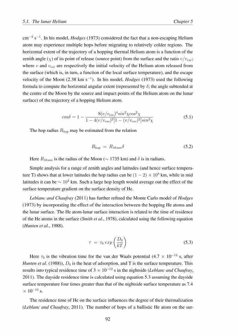
5.1. The lunar Helium Chapter 5

cm−2 s−1. In his model, Hodges (1973) considered the fact that a non-escaping Heliumatom may experience multiple hops before migrating to relatively colder regions. Thehorizontal extent of the trajectory of a hopping thermal Helium atom is a function of thezenith angle (χ) of its point of release (source point) from the surface and the ratio v/vesc;where v and vesc are respectively the initial velocity of the Helium atom released fromthe surface (which is, in turn, a function of the local surface temperature), and the escapevelocity of the Moon (2.38 km s−1). In his model, Hodges (1973) used the followingformula to compute the horizontal angular extent (represented by δ; the angle subtended atthe centre of the Moon by the source and impact points of the Helium atom on the lunarsurface) of the trajectory of a hopping Helium atom.

cosδ = 1− 8(v/vesc)4sin2χcos2χ

1− 4(v/vesc)2[1− (v/vesc)2]sin2χ(5.1)

The hop radius Rhop may be estimated from the relation

Rhop = RMoonδ (5.2)

Here RMoon is the radius of the Moon (∼ 1735 km) and δ is in radians.

Simple analysis for a range of zenith angles and latitudes (and hence surface tempera-ture T) shows that at lower latitudes the hop radius can be (1− 2)× 103 km, while in midlatitudes it can be ∼ 102 km. Such a large hop length would average out the effect of thesurface temperature gradient on the surface density of He.

Leblanc and Chaufray (2011) has further refined the Monte Carlo model of Hodges(1973) by incorporating the effect of the interaction between the hopping He atoms andthe lunar surface. The He atom-lunar surface interaction is related to the time of residenceof the He atoms in the surface (Smith et al., 1978), calculated using the following equation(Hunten et al., 1988).

τ = τ0 exp

(D0

kT

)(5.3)

Here τ0 is the vibration time for the van der Waals potential (4.7 × 10−13 s, afterHunten et al. (1988)), D0 is the heat of adsorption, and T is the surface temperature. Thisresults into typical residence time of 3 × 10−12 s in the nightside (Leblanc and Chaufray,2011). The dayside residence time is calculated using equation 5.3 assuming the daysidesurface temperature four times greater than that of the nightside surface temperature as 7.4× 10−13 s.

The residence time of He on the surface influences the degree of their thermalization(Leblanc and Chaufray, 2011). The number of hops of a ballistic He atom on the sur-

92

Chapter 5 5.1. The lunar Helium

face and its residence time determines its energetics. This is quantified with the enrgyaccommodation factor, which is defined as the ratio of energy transfer between gas andsurface to the energy which would have been transferred if the gas atoms had come intothermal equilibrium with the surface before re-emission (Trilling, 1970). It is given by α= (E2 − E0)/(E1 − E0), where E0, E1 and E2, respectively, represent the mean energiesper atom of the 1) impacting species, 2) species in thermal equilibrium with the surface,and 3) species leaving the surface (Shemansky and Broadfoot, 1977). A low value of α,such as 0.05, corresponds to a single collision of the surface, while higher values (0.25 ormore) suggest more than three collisions (Shemansky and Broadfoot, 1977; Hunten et al.,1988). The limiting condition of α→ 1 suggests complete thermalization of the atom withthe surface. Leblanc and Chaufray (2011) found the best fit of the He data of LACE withα=0.75, which suggests that neither the full energy accommodation, as assumed by Hodges(1975) in his modelling, nor the low energy accommodation as assumed by Shemanskyand Broadfoot (1977) were appropriate.

Hurley et al. (2016) has further improved the Monte Carlo model of the lunar Heliumexosphere. Photoionization rate from Huebner et al. (1992) is used in the model for quietSun conditions. The model assumes that He is re-released immediately since the lunarsurface temperature exceeds the sticking temperature and hops depending on its energetics.The model approximates the interaction of a He atom with the regolith grains leading to itsthermalization by envisaging a thermalization coefficient (ft), randomly chosen betwen 0% and 100 %. The velocity (v) at which the He atom is released from the lunar surfaceto the exosphere is computed as a combination of the velocity with which the He atomhad entered the regolith grains (ingoing velocity vb) and a velocity picked up from theMaxwell-Boltzmann distribution at the local surface temperature. Assuming conservationof energy, the velocity of release of the He atom is computed as

v2 = ftv2t + (1− ft)v2

b (5.4)

The analytical model of the lunar surface temperature (Hurley et al., 2015) obtainedusing the temperature map from the Diviner radiometer measurements (Paige et al.,2010b) has gone into the Monte Carlo model to compute the Maxwell-Boltzmann velocitydistribution function at a given point on the lunar surface.

The distribution of He on the lunar surface in the steady state is computed for a constantday-side He source of 4.7 × 1023 s−1 with the model. The model predicts that He surfacedensity would peak at around 60-70◦ subsolar longitude. This apparently deviates from thetemperature-dependent surface density predicted by the law of exospheric equilibrium fornon-condensable gases (Hodges and Johnson, 1968). However, He being very light withlarge hop lengths, a large-area-averaged surface temperature is more relevant (Benna et al.,2015).

93

5.2. Previous observations Chapter 5

The model predicts that the noon-time surface density of He to be ∼ 103 cm−3 and hasminimum latitudinal variation.

In last few decades, several missions have observed the lunar He exosphere, thoughin-situ as well as remote sensing techniques. These measurements have helped to constrainthe model calculations. In the next section, the observations on the He exosphere will bepresented.

5.2 Previous observations

Lunar He was first detected by the Lunar Atmospheric Composition Experiment (LACE)mass spectrometer (Hoffman et al., 1973), emplaced on the lunar surface at 20◦N latitudeas a part of the Apollo-17 Lunar Surface Experiment Package. The diurnal variation ofHe revealed a maximum in density about 2 to 3 hours after the local midnight, with avalue of (2–4) × 104 cm−3 (Hodges, 1975). Although LACE operated for nine lunations,the information on the daytime He was very limited, owing to low (∼ 2× 103 cm−3) Hedensity with large statistical fluctuations (Hoffman et al., 1973).

The ultraviolet imaging spectrograph LAMP (Lyman Alpha Mapping Project) aboardthe polar orbiting Lunar Reconnaissance Orbiter (LRO) detected He in the lunar exosphereusing the 58.4 nm emission (1s2p → 1s2) line (Stern et al., 2012), which is resonantlyscattered by the Sun-illuminated He in the exosphere against the dark lunar surface at thedawn terminator. The results revealed hardly any latitudinal variation of the surface densityof Helium (Grava et al., 2016). LAMP inferred the Helium surface abundance to bemaximum at local dawn with a number density of ∼ 2× 104 cm−3 (Feldman et al., 2012).It also revealed significant day-to-day variability, which was attributed to the variations inthe solar wind flux. The absolute density also decreased by a factor of ∼ 2 during eachpassage of the Moon through the Earth’s magnetotail (Feldman et al., 2012).

In addition, sporadic flares of He were observed by LAMP, which were attributedto strong bursts of alpha particles in the solar wind and this conjecture is supported byARTEMIS observations (Cook and Stern, 2014). Another possible reason behind theobserved sporadic increases of the lunar Helium is the sudden internal release from endo-genic sources triggered by Moonquakes, which could be verified by simultaneous seismicmeasurements and remote sensing observations (Cook and Stern, 2014). By maneuveringthe lateral roll and pitch of LRO towards and opposite to the direction of motion of thespacecraft, the line-of-sight illumination of LAMP was increased considerably, thus mak-ing reliable measurements possible (Grava et al., 2016). The results suggested that insteadof all the incident alpha particles getting thermalized, a significant fraction (∼50%) of theincoming flux escapes as suprathermal Helium or by backscatter from the lunar surface.These conjectures were supported by the simultaneous observations by LAMP, NMS, and

94

Chapter 5 5.3. Observations by CHACE

ARTEMIS (Hurley et al., 2016). It was inferred that about 60% of the solar wind alphaparticles are converted to thermalized exospheric Helium through interaction with the lunarsurface, while the rest may be reflected/scattered as He+ or He++, or escape as energeticneutral atoms (ENA). In fact, Helium ENA has been observed by Chandrayaan-1 Ener-getic Neutral Analyzer (CENA), a sensor of the SARA experiment aboard Chandrayaan-1(Vorburger et al., 2014; Bhardwaj et al., 2015), and has been understood as to be dueto backscattering of the alpha particles after neutralization with a backscatter ratio of(0.5− 5)× 10−3. This is considered to be a lower limit since the detection efficiency ofCENA for He was less because of the higher ionization potential of He and it is estimatedthat the actual backscatter ratio could be 10 times higher (Vorburger et al., 2014).

The NMS characterized the lunar neutral Helium over the equatorial latitudes (±23◦)and reported the variability in terms of the diurnal cycle and also during the magnetosphericpassages (Benna et al., 2015). The He density has been observed to reach its maximumaround 2 to 3 AM local time and to decrease by a factor of ∼2 during the magnetotailpassage of the Moon. As mentioned earlier, increases in the He abundance are wellcorrelated with solar particle events. NMS, however, did not report the day-side abundancesof Helium due to the lower signal level and also the higher statistical noise in the data. Inparticular, no densities were reported between 1120 and 1400 LT. (Benna et al., 2015).

The following section presents the in-situ observation of He in the sunlit lunar exosphereby CHACE.

5.3 Observations by CHACE

In most of the mass spectra acquired by CHACE, the amu-4 mass bin is found to be noisy,implying poor Signal-to-Noise Ratio (SNR). In majority of the spectra, He is not detected.

The apparent non-detection of He by CHACE could raise two concerns. Either, 1) theperformance of the instrument in the lower mass range is below the expectations, becauseof the stringent requirement of high stability of the ion optics and mass filtering potentials;or, 2) the lunar exosphere had a density of He lower than the detection threshold of theinstrument. The first possibility is ruled out by a careful check of the instrument HouseKeeping (HK) parameters, which were normal throughout the observation session. Also,the performance of CHACE was tested by inserting laboratory grade He during groundtesting. This indicates that the He density in the sunlit lunar exosphere is indeed tenuous.

In order to recognize the feeble signatures of He amidst the system noise, the amu 4mass bin in each mass spectrum has been scrutinized with a suitable pattern recognitionbased Peak Detection Algorithm (PDA).

The PDA takes 9 points in a given mass bin as input and checks for the pattern of

95

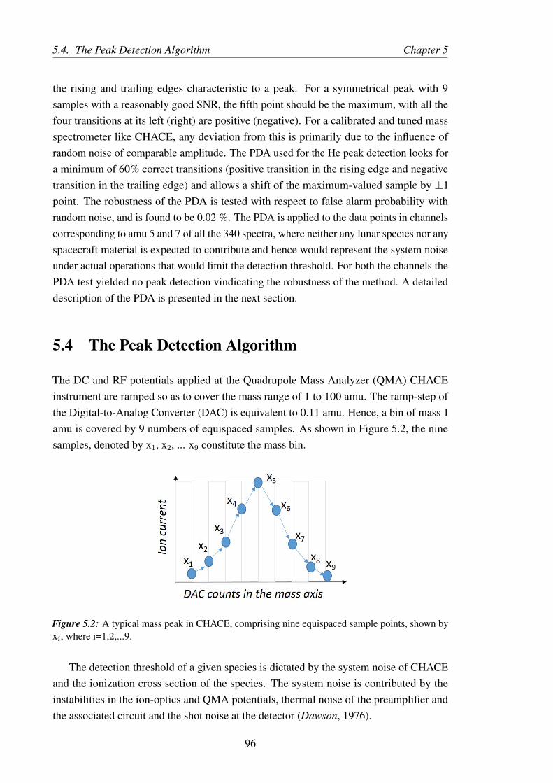
5.4. The Peak Detection Algorithm Chapter 5

the rising and trailing edges characteristic to a peak. For a symmetrical peak with 9samples with a reasonably good SNR, the fifth point should be the maximum, with all thefour transitions at its left (right) are positive (negative). For a calibrated and tuned massspectrometer like CHACE, any deviation from this is primarily due to the influence ofrandom noise of comparable amplitude. The PDA used for the He peak detection looks fora minimum of 60% correct transitions (positive transition in the rising edge and negativetransition in the trailing edge) and allows a shift of the maximum-valued sample by ±1point. The robustness of the PDA is tested with respect to false alarm probability withrandom noise, and is found to be 0.02 %. The PDA is applied to the data points in channelscorresponding to amu 5 and 7 of all the 340 spectra, where neither any lunar species nor anyspacecraft material is expected to contribute and hence would represent the system noiseunder actual operations that would limit the detection threshold. For both the channels thePDA test yielded no peak detection vindicating the robustness of the method. A detaileddescription of the PDA is presented in the next section.

5.4 The Peak Detection Algorithm

The DC and RF potentials applied at the Quadrupole Mass Analyzer (QMA) CHACEinstrument are ramped so as to cover the mass range of 1 to 100 amu. The ramp-step ofthe Digital-to-Analog Converter (DAC) is equivalent to 0.11 amu. Hence, a bin of mass 1amu is covered by 9 numbers of equispaced samples. As shown in Figure 5.2, the ninesamples, denoted by x1, x2, ... x9 constitute the mass bin.

Figure 5.2: A typical mass peak in CHACE, comprising nine equispaced sample points, shown byxi, where i=1,2,...9.

The detection threshold of a given species is dictated by the system noise of CHACEand the ionization cross section of the species. The system noise is contributed by theinstabilities in the ion-optics and QMA potentials, thermal noise of the preamplifier andthe associated circuit and the shot noise at the detector (Dawson, 1976).

96

Chapter 5 5.4. The Peak Detection Algorithm

If the number density of a given species is above the detection threshold of the massspectrometer, a peak is registered in the corresponding mass bin. For a tuned massspectrometer, the peak is ideal. That is, the peak is symmetrical, which, in turn, means thatx5 will have the maximum value and the elements in the rising edge, viz. x1, x2, x3 and x4

are in the increasing order of their respective values (i.e. positive transitions), while theelements in the falling edge, viz. x6, x7, x8 and x9 are in the decreasing order (i.e. negativetransitions).

If the Signal-to-Noise-Ratio (SNR) is small, i.e. ∼1, the signal (peak) is contaminatedwith the noise, and hence, one or more of the following effects on the peak may beobserved.

1. The maximum value of the peak may be shifted to left or right from the middle, i.e.x5 no longer remains the maximum.

2. The increasing sequence of x1, x2, x3 and x4 is lost. There may be one or more wrong(decreasing) transitions due to the noise.

3. The decreasing sequence of x6, x7, x8 and x9 is lost. There may be one or more wrong(increasing) transitions due to the noise.

The PDA searches for the pattern of the ideal peak in the vector xi = [x1 x2 x3 x4 x5 x6

x7 x8 x9], with all the possible modes of distortion of the pattern as described above. Theflow chart of the PDA is shown in Figure 5.3.

The PDA first checks the value of the index i, (say, k) for xk = max(xi). It allows formaximum one step of shift on either side, i.e. 4 ≤ k ≤ 6. If this condition is not satisfied,the vector xi is declared as ‘not-a-peak’. If passed, then the vector is subjected to two moretests, which check in how many cases the required condition of positive transitions in therising edge and negative transitions in the trailing edge are obeyed. In the PDA flow-chartshown in Figure 5.3, it is represented by the percentage of correct transitions in the left(rising) and right (trailing) edges, denoted by NL and NR, respectively. If any of these twoconditions are not satisfied, the vector xi is declared as ‘not-a-peak’. In other words, inorder to qualify as a possible peak, the maximum of the peak should not have a shift bymore than one point on either sides and the number of correct transitions in the rising andtrailing edges should be at least equal to a given percentage (NL = NR = NL,R, say ), whichcontrols the stringency of the test.

Two possible errors in the PDA are:

1. Type-I error: Rejecting a true peak

2. Type-II error: Accepting a noise pattern as a peak (false detection)

97

5.4. The Peak Detection Algorithm Chapter 5

Figure 5.3: The flow chart of the PDA.

The type-I and II errors have the same significance as in the testing of a null hypothesisin statistics (Goon et al., 1968). The PDA is tested for both kinds of errors. The probabilityof type-I error is tested by generating vectors with 9 elements by envisaging an ideal peakwith 9 points and coherently adding a Gaussian noise with 9 points with its 3-σ value equalto the peak amplitude. The test is run for 107 times where the ideal peak is kept invariantwhile the noise pattern is changed from interation to iteration. On the other hand, for thetype-II error test, Gaussian noise is generated and the PDA is run to check for any falsedetection. This test is also run for 107 times.

In the present application of the PDA to search for the pattern of the He peak with smallSNR, the type-II error is more serious, which signifies false detection. For NL,R=50%, thefalse detection probability is ∼ 2.7 %, while for NL,R=60%, it is only ∼ 0.02 %. For thepresent analysis, NL,R=60% is used.

98

Chapter 5 5.5. Interpretation

5.5 Interpretation

As a next step, the points in the amu 4 mass bin from all the 340 mass spectra weresubjected to the PDA. Out of all the trials, only 16 positive detections were encountered.Second order polynomials are fitted on the 9 points of the amu-4 mass bins that passed thePDA test and the peak amplitudes are determined. Barometric law is used to estimate thesurface number density of He from the peak amplitudes, and are presented in Figure 5.4. Itis observed that the inferred densities from the PDA-positive points are very close to thedetection thresold of the instrument. Due to very less number of positive detections andpoor SNR, in this paper we restrict ourselves to estimating the upper limit of He based onthe detection thresold of the instrument.

Taking into account the instrument calibration factor from the detector current to thenumber density conversion using the total pressure measurement by the in-built Bayard-Alpert gauge of CHACE, and also accounting for the ram enhancement effect (Sridharanet al., 2015), the detection threshold for N2 gas in CHACE is ∼ 1.0 × 102 cm−3. Ac-counting for the relative sensitivity of He to electron ionization at 70 eV with respect toN2, which is 0.13 (Summers, 1969; Holanda, 1972), the detection threshold for He is ∼8 × 102 cm−3. The uncertainty in the estimation of this value, accounting for the majorcontributors to the overall uncertainty, viz. the total pressure and relative partial pressuremeasurements, is ±50%.

5.6 Discussion

Lunar He is known to have a uniform latitudinal distribution, as reported by LAMP inthe terminator region (Feldman et al., 2012; Grava et al., 2016). This is attributed to themultiple hops undergone by the ballistic (Moon-bound) He atoms on the lunar surface(Shemansky and Broadfoot, 1977), resulting into uniform latitudinal distribution. Thenumber of hops experienced by a ballistic He atom on the lunar surface determines theextent of its interaction with the lunar surface and the degree of thermalization.

As discussed earlier, the dynamics of this hopping process is described by the energyaccommodation factor. Monte Carlo simulation by Leblanc and Chaufray (2011) broughtout the sensitivity of the night-to-dayside density ratio of He to the energy accommodationfactor. In the present work, the energy accommodation factor is estimated with the upperlimit of ∼ 8 × 102 cm−3 of the dayside He density reported here, and the nightsidemaximum density of ∼ 7 × 104 cm−3 observed by NMS when the Moon was outsidethe Earth’s magnetotail, during a coronal mass ejection (CME) (Benna et al., 2015). Themaximum night-time density reported by Benna et al. (2015) is scaled down by a factorof ∼3.6 (to normalize the state of the solar wind alpha particle flux during the reported

99

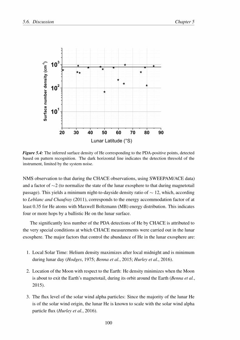
5.6. Discussion Chapter 5

20 30 40 50 60 70 80 90

101

102

103

Sur

face

num

ber

dens

ity (c

m-3

)

Lunar Latitude (°S)

Figure 5.4: The inferred surface density of He corresponding to the PDA-positive points, detectedbased on pattern recognition. The dark horizontal line indicates the detection thresold of theinstrument, limited by the system noise.

NMS observation to that during the CHACE observations, using SWEEPAM/ACE data)and a factor of ∼2 (to normalize the state of the lunar exosphere to that during magnetotailpassage). This yields a minimum night-to-dayside density ratio of ∼ 12, which, accordingto Leblanc and Chaufray (2011), corresponds to the energy accommodation factor of atleast 0.35 for He atoms with Maxwell Boltzmann (MB) energy distribution. This indicatesfour or more hops by a ballistic He on the lunar surface.

The significantly less number of the PDA detections of He by CHACE is attributed tothe very special conditions at which CHACE measurements were carried out in the lunarexosphere. The major factors that control the abundance of He in the lunar exosphere are:

1. Local Solar Time: Helium density maximizes after local midnight and is minimumduring lunar day (Hodges, 1975; Benna et al., 2015; Hurley et al., 2016).

2. Location of the Moon with respect to the Earth: He density minimizes when the Moonis about to exit the Earth’s magnetotail, during its orbit around the Earth (Benna et al.,2015).

3. The flux level of the solar wind alpha particles: Since the majority of the lunar Heis of the solar wind origin, the lunar He is known to scale with the solar wind alphaparticle flux (Hurley et al., 2016).

100

Chapter 5 5.7. Conclusion

When it comes to the loss processes, the Lunar He is sensitive to Jeans escape becauseof its small escape parameter, which is the ratio of its gravitational binding energy tothermal energy (computed as ∼3.47 at 390 K surface temperature). Because of its lowmass, it has a large scale height (∼400 km at 390 K surface temperature, which is typicalduring lunar day). Thus, during a lunar day, the insolation at lower latitudes is enough tocause thermal expansion of the He exosphere so as to reduce the surface density. Apartfrom the He atoms that undergo Jeans escape, the ballistic component of He has a largehop length, often in the order of half to one third of the lunar radius at lower latitudes inthe sunlit side (Hodges, 1973; Leblanc and Chaufray, 2011).

In addition to the diurnal variability, lunar He is also sensitive to the location of theMoon with respect to the Earth. When the Moon enters the Earth’s magnetotail where itspends ∼ 4–5 days, it is shielded from the solar wind influx. Thus, the loss of the lunar He,which is mostly by Jeans escape with a time constant of ∼4.5 days (Benna et al., 2015), isnot replenished during the passage of the Moon through the Earth’s magnetotail, resultingin the monotonic decrease of the lunar He abundance.

Since the lunar Helium owes its origin to the solar wind, the absolute values of itssurface density at any given local time depends on the prevailing solar wind alpha particleflux. The above inference is substantiated by the measurements of NMS/LADEE duringseveral lunations and it is observed that lunar He inventory hits its minimum when theMoon is about to come out of the Earth’s magnetotail (Benna et al., 2015).

Figure 5.5 shows the monthly averaged solar wind alpha particle flux from year 2008to 2015, as derived from the SWEEPAM/ACE observations. The time range covers theobservation time of CHACE/Chandrayaan-1 and NMS/LADEE. During NMS observations,there have been several occasions of solar flares, which caused increase in the level of thesolar wind alpha particle flux. On the other hand, it is observed that during the CHACEobservations, the solar wind alpha particle flux was less by a factor of ∼ 3.6 than duringFebruary 2014, when the NMS observed the maximum He density.

Further, the CHACE observations were carried out in the lunar dayside, when theMoon was on the verge of coming out of the Earth’s magnetotail, as shown in Figure 2.24.A combination of these conditions, along with the low solar wind alpha particle flux at thetime of CHACE observations present a case when the He abundance in the Moon had beenat its lowest. CHACE has thus studied the lunar exosphere in an extreme condition of thefactors that control the lunar He abundance.

5.7 Conclusion

An upper limit of ∼ 8.0 × 102 cm−3 for the surface density of the neutral He in the sunlitlunar exosphere is proposed based on the observations made by CHACE/MIP/Chandrayaan-

101

5.7. Conclusion Chapter 5

2008 2009 2010 2011 2012 2013 2014 201510

6

107

Year

So

lar

win

d a

lph

a p

art

icle

flu

x (

cm

−2s

−1)

(Mo

nth

ly a

ve

rag

e)

NMS observationCHACE observation

Figure 5.5: Monthly averaged solar wind alpha particle flux, as derived from the SWEEPAM/ACEobservations over few years, covering the observation time of CHACE/Chandrayaan-1 andNMS/LADEE. Alpha particle number density data along with the velocity data of protons are usedto compute the alpha particle flux. It is observed that during the CHACE observations, the solarwind alpha particle flux was significantly less than that during the NMS/LADEE observations.

1. However, more sensitive measurements are called for to throw more light on this aspect.The CHACE observations were carried out in the lunar dayside, when the non-escapingcomponent of the lunar He exosphere thermally expands, thereby reducing its surfacenumber density. Furthermore, during CHACE observations, the Moon was about to exitthe Earth’s magnetotail and thus had been deprived of the fresh influx of the solar windalpha particles. In addition, the then prevailing low level of the solar wind alpha particleflux present a case where the He abundance in the Moon had hit one of its lowest values.

Thus, CHACE has observed the lunar exosphere in an extreme condition, where allthe major factors controlling the lunar He inventory were unfavourable, and, therefore,provides a constraint to the lunar He exosphere models under such extreme conditions.

102

Chapter 6

Observations on H2

A scientist in his laboratory is not only a technician, he is also a child

placed before the natural phenomena which impress him like a fairy tale.

—Marie Curie

6.1 The lunar H2

Study of the distribution of H2 is considered to be an important tool to study the exosphere-surface interaction in the Moon. The major source of the Lunar exospheric H2 is the solarwind proton flux (Hodges et al., 1972). In steady state, a balance exists between the influxof the solar wind protons and the outflux of hydrogen. At energies of ∼ 1 keV amu−1,solar wind protons penetrate few 10s of nm into the rim of the regolith grain and most ofthem are neutralised (Hurley et al., 2017). The Kaguya mission has measured that a smallfraction (∼ 0.1 to 1 %) of the solar wind protons are backscattered from the surface as ions(Saito et al., 2008). This has been confirmed by the ARTEMIS spacecraft (Halekas et al.,2013). The SARA instrument of Chandrayaan-1 (Wieser et al., 2009) and the InterstellarBoundary Explorer (IBEX) (McComas et al., 2009; Funsten et al., 2013; Allegrini et al.,2013) have shown that about 10 to 20 % of the incident solar wind protons are converted toEnergetic Neutral Atoms (ENA). Thus, about 10 to 20 % of the incident solar wind protonflux is directly accounted as H+ ions and ENAs, leaving the rest 80 to 90 % unobserved(Hurley et al., 2017).

It is proposed (Crider and Vondrak, 2002) that H2 is produced from the interaction ofthe solar wind with the regolith through chemical sputtering. Further, Hurley et al. (2017)has quantified this process as 10 % of the solar wind H+ requires to be converted to H2,

103

6.2. Previous observations Chapter 6

for a density of ∼ 1200 cm−3 of the latter. The chemically sputtered H2 molecules arereleased from the surface with a lower energy and hence remain in the lunar exosphere overseveral hops. On the other hand, the process of physical sputtering is not very significantas a potential source of the lunar H2 since it releases H2 with higher energy resulting intohigher scale height and escape fraction (Hurley et al., 2017).

Apart from the chemical sputtering of the solar wind protons on the lunar regolithwhich produces a symmetrical H2 density about the subsolar point, Hurley et al. (2017) hasalso considered the role of micrometeorides as a source of the lunar H2. Micrometeroridesare likely to produce a dawn-dusk asymmetry in the H2 density, as the dawn hemisphereof the Moon experiences greater influx of the micrometeoroids than the dusk hemisphereowing to the motion of the Earth-Moon system around the Sun (Fechtig et al., 1974).This is confirmed by the Lunar Dust Experiment (LDEX) aboard the LADEE spacecraft(Horanyi et al., 2015). However, direct delivery of H2 via micrometeoroids is not a veryefficient source, even if the micrometeoroid is composed entirely of water (Hurley et al.,2017) as they are not likely to carry large amounts of hydrogen. Thus, the solar windproton flux remains as the potential source of the lunar exospheric H2.

Table 6.1 summarises the different loss processes of the lunar exospheric H2 and theirrelative importances. Figure 6.1 shows the major source and sink processes of the lunarH2.

Table 6.1: Loss processes of H2 in the lunar exosphere (Benna et al., 2015; Huebner et al., 1992)

Process Lifetime

Jeans escape 2.2 days a

Photo-ionization 214 days (QS)b and 100 days (AS)b

a Scaled down the Jeans escape time constant of He-4 (Benna et al., 2015) by a factor of 2.b Photoionization lifetimes are computed based on the photoionization rates provided by Huebner andMukherjee (2015). QS and AS refer to quiet Sun and active Sun respectively.

6.2 Previous observations

The results from the in-situ obervations made by the LACE instrument in the Apollo-17Surface Experiment Package suggested the presence of molecular Hydrogen in the lunaratmosphere, which owe its origin to the lunar surface (Hoffman et al., 1973). The LACEhad measured a H2 surface density of 6.5 × 104 cm−3 at night, which agreed with theprediction (Hodges, 1973).

104

Chapter 6 6.2. Previous observations

Solar wind implantation of H+

Lateral transport

Chemical Sputtering

+Ion escape

H2

Gravitational escape

H2

Physical Sputtering

Figure 6.1: Cartoon showing the major source and sink processes of the lunar H2, based on thediscussions given in (Hurley et al., 2017). The major source of the lunar H2 is the chemicalsputtering from the lunar regilith, which owes its hydrogen inventory to the solar wind proton influx.The physically sputtered component of the H2 from the lunar regolith usually has enough energy toescape the lunar gravity. In the cartoon, both the thermal escape and physical sputtering-inducedescape components of the lunar H2 are shown as gravitational escape. Another escape mechanism isthe ion escape, collectively due to photoionization, charge exchange and electron impact ionization.

Apart from LACE, the UV spectrometer aboard the Apollo 17 orbiter also detectedsimilar levels of H2 (∼104 cm−3 ). On the other hand, the estimated atomic Hydrogenabundance was too low, i.e., ∼10 cm−3 (Fastie et al., 1973). This was interpreted asan indication for the conversion of the majority of the solar wind protons as H2 at thelunar surface and its re–emission to the atmosphere in accordance with the lunar surfacetemperature. The upper limits of H2 at the Apollo–17 site Hodges et al. (1974) alsoqualitatively agreed with this hypothesis. Later, using the Apollo–17 UV spectrometerdata, Feldman and Morrison (1991), provided more stringent upper limits to the numberdensities of H (17 cm−3), and H2 (9000 cm−3). On the other hand, Wurz et al. (2012),based on the previously reported upper limits, arrived at H2 number density of 5× 104

cm−3 near 10 km above the lunar surface on the dayside, at a temperature of 400 K.

Lunar H2 was also detected by the LAMP UV spectrometer aboard the LRO spacecraftin the vapour plume emanated from the impact of the LCROSS into the permanentlyshadowed Cabeus crater (Gladstone et al., 2010b). A release of about 110 kg of H2 wasestimated (Hurley et al., 2012). LAMP also derived a H2 surface density of 1.7 ± 0.4 ×103 cm−3 at dusk increasing to 2.1 ± 0.3 × 103 cm−3 at dawn (Cook et al., 2013). Usingthe same dataset, averaging many different column lengths throughout the mission, Stern

105

6.3. Results of CHACE observations Chapter 6

et al. (2013) obtained an effective vertical column density of ∼ 6 × 109 cm−2, whichtranslated to a surface density of ∼ 1.2 × 103 cm−3, at 120 K.

The Chinese lunar mission Chang’E-1 flew Electro Static Analysers (ESA), whichrevealed parallel curve structures in the energy-time spectrogram with a component dueto a flux of ions with energy ∼ 8 times greater than the solaw wind proton energy (Wanget al., 2011). The ions exhibited ring-distribution in the VE-VC space, where VE andVC are respectively the velocity components parallel to the Interplanetary Magnetic Field(IMF) and perpendicular to the local IMF direction. The ring distribution, along with the∼ 90◦ pitch angle indicated their ‘pick-up’origin. The low initial velocity of these pick-upions (with m/q = 2, which could either be H+

2 or He++), derived from the velocity-spacedistribution confirmed their cold source origin, including the Local Inter Stellar Medium(LISM), Inter Planetary Dust (IPD) or the neutral exosphere of the Moon. Based on theirobserved flux level, the LISM and IPD sources of the pick-up ions were ruled out and lunarneutral exosphere was confirmed as the source. Further, based on the comparison betweenthe observed flux of the ions and the possible H+

2 or He++ flux levels estimated based onthe production rates of H+

2 and He++, it was inferred that the observed pick-up ions wereH+

2 , which originated from the ionizing processes like photoionization, charge exchange,electron impact ionization, etc. of the lunar neutral H2. This was the first observation ofthe lunar pick-up H+

2 ions, and indirect evidence for the lunar neutral H2 exosphere.

Recently, Halekas et al. (2015) has inferred the neutral H2 density from the mea-surement of H+

2 ions by the NMS instrument in its ion mode. However, the NMS ionobservations are convolution of the ionization production process and the column densityalong the electric field direction.

6.3 Results of CHACE observations

The CHACE instrument aboard the MIP conducted in-situ measurements of the lunar H2

from 100 km altitude to the surface at different latitudes along the 14◦ E meridian. Thein-situ obervations were convolution of altitude and latitude (refer Figure 6.2). Barometriclaw is used to translate the measured partial pressure of H2 to the surface density using thelocal surface temperature and scale height. A 2D (latitude versus altitude) map of the lunarH2 is generated along the 14◦ meridian, as shown in Figure 6.3.

The map clearly shows the increased abundance of H2 near the polar region. Asexpected, the H2 number density do not show any significant altitude variation due to itsscale height being larger than 100 km, even at 88◦S and even when the temperature is low.The derived values of the surface number density of H2 agree with the values reportedby Stern et al. (2013) wherein they had estimated a surface density of∼103 cm−3 for H2

corresponding to a surface with a temperature of 120 K, and the present estimates for

106

Chapter 6 6.3. Results of CHACE observations

Figure 6.2: Left: The observed partial pressure of H2 along the MIP trajectory. Right: Thecalculated number density of H2 along the MIP trajectory.

the surface density at 88◦N (∼140 K) is ∼825 cm−3. However, it should also be notedthat our estimates are significantly lower than the upper limit reported by Cook et al. (2013).

Figure 6.3: A two dimensional (latitude vs altitude) map of H2 generated using the scale heightsat different latitudes. The black continuous line depicts the locus of the MIP during the CHACEobservations.

Further, the CHACE measurements reveal significant latitudinal variation which is anindication of the spatial heterogeneity of the lunar H2. Until now no such information isavailable since all the previous estimates were based either, on single point measurementsor, on highly averaged UV spectra/calculations based on night time measurements. Ifthe latitudinal variation of H2 had been only due to surface temperature variation, then itshould have been rather smooth and the density should have monotonically increased withlatitude. On the other hand, distinct undulations are observed in the spatial variation of H2

number density despite its large scale height.

The surface number density of H2 derived from the in-situ observations by CHACEis correlated with the surface topography along the 14◦ E meridian. The surface topog-

107

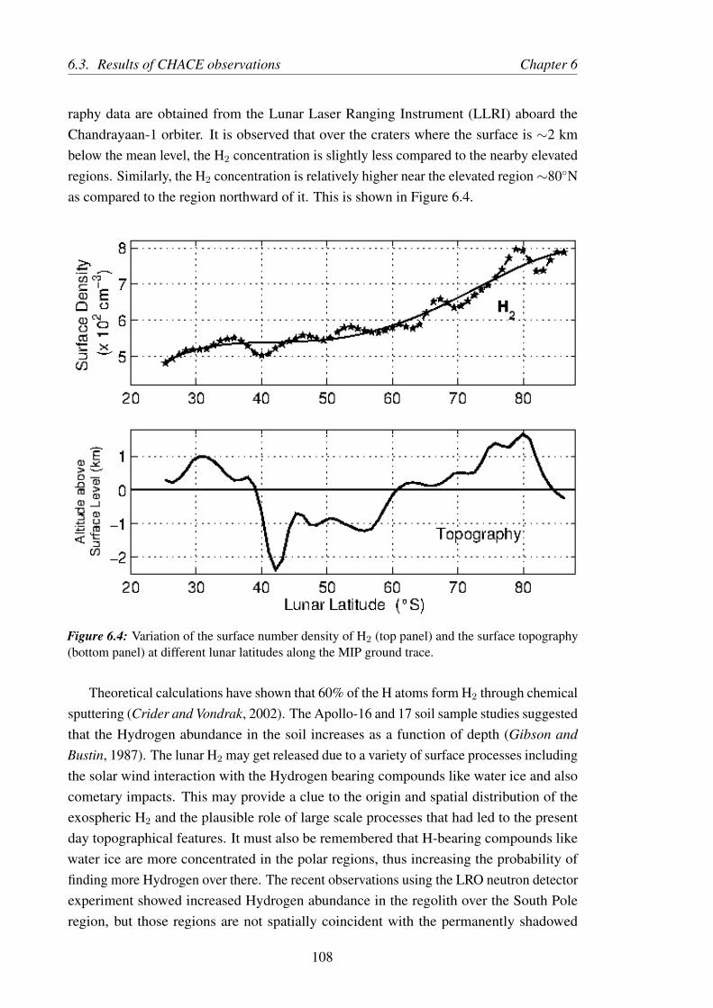
6.3. Results of CHACE observations Chapter 6

raphy data are obtained from the Lunar Laser Ranging Instrument (LLRI) aboard theChandrayaan-1 orbiter. It is observed that over the craters where the surface is ∼2 kmbelow the mean level, the H2 concentration is slightly less compared to the nearby elevatedregions. Similarly, the H2 concentration is relatively higher near the elevated region∼80◦Nas compared to the region northward of it. This is shown in Figure 6.4.

Figure 6.4: Variation of the surface number density of H2 (top panel) and the surface topography(bottom panel) at different lunar latitudes along the MIP ground trace.

Theoretical calculations have shown that 60% of the H atoms form H2 through chemicalsputtering (Crider and Vondrak, 2002). The Apollo-16 and 17 soil sample studies suggestedthat the Hydrogen abundance in the soil increases as a function of depth (Gibson andBustin, 1987). The lunar H2 may get released due to a variety of surface processes includingthe solar wind interaction with the Hydrogen bearing compounds like water ice and alsocometary impacts. This may provide a clue to the origin and spatial distribution of theexospheric H2 and the plausible role of large scale processes that had led to the presentday topographical features. It must also be remembered that H-bearing compounds likewater ice are more concentrated in the polar regions, thus increasing the probability offinding more Hydrogen over there. The recent observations using the LRO neutron detectorexperiment showed increased Hydrogen abundance in the regolith over the South Poleregion, but those regions are not spatially coincident with the permanently shadowed

108

Chapter 6 6.4. Concluding remarks

craters (Mitrofanov et al., 2010). More such measurements are needed to unravel thecomplexities of the lunar atmosphere.

6.4 Concluding remarks

The CHACE experiment on the MIP enabled us to obtain the distribution of the lunar H2

during daytime along the 14◦ E meridian. A remarkable feature observed was the spatialheterogenity of the lunar H2 number density. The H2 density showed enhancement in theelevated regions, despite the fact that the scale height of H2 is vergy large (∼ 700 km at400 K) compared to the scale of orographic variations on Moon. These results highlight thecomplexities of the lunar atmosphere and the significant role of the lunar surface processesin modulating the distribution of the different species.

109

Chapter 7

Summary and Future Work

The more you lose yourself in something bigger than yourself, the more

energy you will have.

—Norman Vincent Peale

7.1 Summary of the Work and Major Results

The present thesis is the outcome of the scientific investigation of the lunar exospheric40Ar, 20Ne, 4He and H2, based on the in-situ observations made by the CHACE payloadaboard the MIP in Chandrayaan-1 mission. This is the first, and so far the only observationon the latitudinal and altitudinal distribution of the lunar exospheric noble gases coveringmid and high latitudes and the southern polar region, under sunlit condition.

The distribution of 40Ar at the mid and high latitudes in the sunlit lunar exosphereis investigated. 40Ar density is seen to be maximum between 30◦ and 50◦S with a valueof ∼4× 104 cm−3. The upper limits of the surface number density decreases at higherlatitudes and near the polar region it is found to be ∼ 1× 104 cm−3. The 40Ar:36Ar ratioalong the 14◦E meridian is found to be ∼ 1 in the Northern hemisphere and ∼ 2.5 inthe Southern hemisphere. An altitude versus latitude map of the lunar 40Ar along theabove-mentioned meridian is also presented. The relation between the topography andthe 40Ar concentration is delineated and the indications on the spatial heterogeneity of theradiogenic processes are brought out. It is observed that the 40Ar density enhances nearthe crater regions.

For 20Ne, it is found that the upper limit of the surface number density varies from(7–22)× 103 cm−3 at the pole, to (3–5)× 103 cm−3 in mid (50◦S) latitudes and to (0.5–1.1)× 103 cm−3 in lower (20◦S) latitudes. An empirical relation between the lunar 20Ne

110

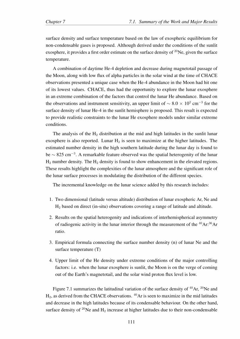
Chapter 7 7.1. Summary of the Work and Major Results

surface density and surface temperature based on the law of exospheric equilibrium fornon-condensable gases is proposed. Although derived under the conditions of the sunlitexosphere, it provides a first order estimate on the surface density of 20Ne, given the surfacetemperature.

A combination of daytime He-4 depletion and decrease during magnetotail passage ofthe Moon, along with low flux of alpha particles in the solar wind at the time of CHACEobservations presented a unique case when the He-4 abundance in the Moon had hit oneof its lowest values. CHACE, thus had the opportunity to explore the lunar exospherein an extreme combination of the factors that control the lunar He abundance. Based onthe observations and instrument sensitivity, an upper limit of ∼ 8.0 × 102 cm−3 for thesurface density of lunar He-4 in the sunlit hemisphere is proposed. This result is expectedto provide realistic constraints to the lunar He exosphere models under similar extremeconditions.

The analysis of the H2 distribution at the mid and high latitudes in the sunlit lunarexosphere is also reported. Lunar H2 is seen to maximize at the higher latitudes. Theestimated number density in the high southern latitude during the lunar day is found tobe ∼ 825 cm−3. A remarkable feature observed was the spatial heterogenity of the lunarH2 number density. The H2 density is found to show enhancement in the elevated regions.These results highlight the complexities of the lunar atmosphere and the significant role ofthe lunar surface processes in modulating the distribution of the different species.

The incremental knowledge on the lunar science added by this research includes:

1. Two dimensional (latitude versus altitude) distribution of lunar exospheric Ar, Ne andH2 based on direct (in-situ) observations covering a range of latitude and altitude.

2. Results on the spatial heterogenity and indications of interhemispherical asymmetryof radiogenic activity in the lunar interior through the measurement of the 40Ar:36Arratio.

3. Empirical formula connecting the surface number density (n) of lunar Ne and thesurface temperature (T)

4. Upper limit of the He density under extreme conditions of the major controllingfactors: i.e. when the lunar exosphere is sunlit, the Moon is on the verge of comingout of the Earth’s magnetotail, and the solar wind proton flux level is low.

Figure 7.1 summarizes the latitudinal variation of the surface density of 40Ar, 20Ne andH2, as derived from the CHACE observations. 40Ar is seen to maximize in the mid latitudesand decrease in the high latitudes because of its condensable behaviour. On the other hand,surface density of 20Ne and H2 increase at higher latitudes due to their non-condensable

111

7.2. Open Questions Chapter 7

nature. The slope of the surface density of H2 is found to be less, as it is a light speciesand has large hop lengths and hence not affected by local temperature variations.

Figure 7.1: Latitudinal variation of the surface density of 40Ar, 20Ne and H2, as derived from theCHACE observations. Fourth order polynomials are plotted in order to emphasize the latitudinalvariation of the surface densities of these species thereby suppressing the local variations.

7.2 Open Questions

The scientific outcome of this research, based on the observations by CHACE, on thelatitudinal and altitudinal variation of the noble gases on the lunar exosphere facilitated theunderstanding of the source and sink processes of the lunar exosphere, surface-exosphereinteraction and the dynamics of the exospheric species.

The polar exosphere of the Moon remain inadequately explored. For instance, TheMoon’s South Pole-Aitken Basin, one of the largest impact structures known withinthe Solar System, exposes material from deep within the crust and possibly even theupper mantle that was excavated by the impact, and may preserve melt rocks from theimpact itself. The permenantly shadowed regions of the Moon shows signatures of thepresence of Hydrogen bearing compounds (Pieters et al., 2009). All these reiterate theimportance of having a polar orbiting satellite equipped with composition measurementsof the lunar exosphere, which is directly coupled to the lunar surface. CHACE aboard MIPin Chandrayaan-1 was a one-time experiment. The spatial heterogenity observed in thevariation of several species from the CHACE results calls for more observations, both inspace and time. This can be accomplished by in situ measurements from a polar satellite

112

Chapter 7 7.3. Future work: Detailed observation of the lunar exosphere

platform. The CHACE-2 (CHandra’s Atmospheric Composition Explorer-2) experimentaboard Chandrayaan-2 mission is going to fullfil this important requirement.

7.3 Future work: Detailed observation of the lunar exo-sphere

The lunar exosphere will be studied in more details in the Chandrayaan-2 mission. TheChandrayaan-2 will consist of an orbiter, lander and a rover. The Chandra’s AtmosphericComposition Explorer (CHACE-2) will be a payload aboard the Chandrayaan-2 orbiter,which will study the lunar exosphere from 100 km circular polar orbit. The CHACE-2instrument will be fundamentally similar to CHACE aboard MIP/Chandrayaan-1, butwith important functional differences (mass range, multi-mode operation, telecommandcapability, etc.) that will facilitate detailed study of the lunar neutral exosphere.

The selection of the operating parameters and configurations of the CHACE-2 instru-ment are guided by the experiences gained in the CHACE observations. While the mandateof CHACE was to study the lunar neutral exosphere till the surface of the Moon , it was aone-time experiment and hence was operated in a given configuration of instrument param-eters. On the other hand, the CHACE-2 instrument will be housed in the Chandrayaan-2orbiter and hence, multiple operating configurations are being worked out based on scien-tific requirements. The different operating configurations and telecommand-amenabilityof CHACE-2 will allow the instrument to choose the mass range of operation, scan rate,electron energy for impact ionization, ion optics parameters, etc..

The CHACE-2 experiment will provide new insights about the lunar exosphere, espe-cially over the least explored polar and high latitude regions and may provide answers tomany questions that are open today.

113

Appendices

114

Appendix A

Vertical density profile in an exosphere

The following sections present a discussion on the applicability of the barometric law to de-rive the vertical density profile in the collisionless regime characteristic to an exosphere. Inthe first section, the barometric law will be derived from the law of hydrostatic equilibriumand the ideal gas law. In the second section, the transport of the atoms in the collisionlessregime is presented in line with the derivation reported by Chamberlain (1963), where it isassumed that below the exobase the collisions among the gas atoms maintain a Maxwellianvelocity distribution. It will be shown that the barometric law can be used in the exosphericregime as well up to the altitude where the mean kinetic energy per atom remains constant.

A.1 Hydrostatic equilibrium and the barometric law

The temperature, pressure and density in a planetary atmosphere are governed by theequilibrium between the gravitation (acting radially inwards to the planet) and buoyancy(acting radially outwards, due to the pressure gradient). If m and n, respectively, denote themass of an atom and its number density in a slab of thickness dr, kept under a gravitationalfield with acceleration due to gravity g, then the pressure (P ) at any altitude r is given by

dP

dr= −mng (A.1)

According to the kinetic theory of gases, the mean kinetic energy of an atom isproportional to its absolute temperature (T ). In a system with 3 degrees of freedom, thekinetic energy of a gas with velocity v is given by

1

2mv2 =

3

2kT (A.2)

Here, k is the Boltzmann’s constant.

The expression of pressure exerted by gas atoms in terms of their mean velocity v isgiven by

115

A.2. Exosphere: the collisionless regime Chapter 1

P =1

3mnv2 (A.3)

Substituting the expression for the mean velocity v from equation A.2 to equation A.3,the expression of pressure comes out as

P = nkT (A.4)

Equation A.4, which is referred to as the perfect gas law, is, hence, a consequence ofthe proportionality of the mean kinetic energy of the atoms to the absolute temperature.

Substituting equation A.4 in equation A.1, the hydrostatic equilibrium equation assumesthe following form:

dP

dr= −mg

kTP (A.5)

The pressure P at any arbitrary altitude r is computed by evaluating the followingintegral

∫ P

P0

dP

P= −mg

kT

∫ r

r0

dr (A.6)

Here, r0 represents the planetary radius or surface of the body and P0 the pressure atthe surface of the planet.

Equation A.6 yields

P = P0 exp

(r − r0

kT/mg

)(A.7)

Equation A.7 is known as the barometric law, which suggests that the pressure fallsexponentially with altitude with characteristic height kT/mg, which is called the scaleheight. The barometric law is derived from the hydrostatic equilibrium and the perfectgas law and is valid irrespective of any information on the distribution function of the gasatoms.

A.2 Exosphere: the collisionless regime

The theory presented here is based on Chamberlain (1963). Let us assume a planet and itsatmosphere around it in spherical symmetry. Let us further assume that the exobase is at aplanetocentric distance of rc. The evolution of the density function f(q, p) of ensemble

116

Chapter 1 A.2. Exosphere: the collisionless regime

of atoms in the 6 dimensional (3 spatial coordinates q1,2,3 and 3 momentum coordinatesp1,2,3) phase space is described by the Boltzmann transport equation, given by

∂f

∂t+∇q.(qf) + p.∇pf = Jcollision (A.8)

Below the exobase, the velocity of the atoms follow Maxwellian distribution. Onthe other hand, above the exobase, collisions are absent and the spatial and momentumdistribution of the atoms is governed by Liouville’s equation, which is equivalent to theBoltzmann transport equation without the collision term. Hence, above the exobase,equation A.8 reduces to

∂f

∂t+

3∑i=1

[∂fqi∂qi

+∂fpi∂pi

]= 0 (A.9)

The system of atoms are under the influence of the gravitation of the planet. Theirvelocities and equation of motion are given in terms of the Hamiltonial function H as

qi =∂H

∂pi(A.10)

andpi = −∂H

∂qi(A.11)

Expanding each term in the square bracket of equation A.9,

∂(f qi)

∂qi= f

∂qi∂qi

+ qi∂f

∂qi(A.12)

and∂(fpi)

∂pi= f

∂pi∂pi

+ pi∂f

∂pi(A.13)

Adding equations A.12 and A.13,

∂(f qi)

∂qi+∂(fpi)

∂pi= f

[∂qi∂qi

+∂pi∂pi

]+ qi

∂f

∂qi+ pi

∂f

∂pi(A.14)

Using equations A.10 and A.11 on the square bracketted terms in equation A.14,

f

∂(∂H∂pi

)∂qi

+∂(−∂H∂qi

)∂pi

=∂2H

∂qi∂pi− ∂2H

∂pi∂qi= 0 (A.15)

Thus, equation A.14 reduces to

117

A.2. Exosphere: the collisionless regime Chapter 1

∂(f qi)

∂qi+∂(fpi)

∂pi= qi

∂f

∂qi+ pi

∂f

∂pi(A.16)

Using equation A.16, equation A.9 reduces to

∂f

∂t+

3∑i=1

[qi∂f

∂qi+ pi

∂f

∂pi

]= 0 (A.17)

Equation A.17 signifies that the density in phase space remains constant along adynamical trajectory. Under steady state, the time-derivative of the distribution functionvanishes and equation A.17 reduces to

3∑i=1

dqidt

∂f

∂qi= −

3∑i=1

dpidt

∂f

∂pi(A.18)

Replacing q with r (the planetocentric distance) and p with pr (radial component of themomentum), equation A.18 assumes the form

dr

dt

∂f

∂r= −dpr

dt

∂f

∂pr(A.19)

The Hamiltonian of the particle in spherical polar coordinate system is given by

H =p2r

2m+

P 2χ

2mr2− GMpm

r(A.20)

Here Pχ is the angular momentum, m is the mass of the atom, Mp is the mass of theplanet and G is the Universal gravitational constant. The equation of motion is given by

pr =dprdt

= −∂H∂r

=P 2χ

mr3− GMpm

r2(A.21)

Below the exobase, the collisions between the atoms maintain their velocity distributionMaxwellian. Even in the case of Surface Boundary Exosphere, like that of the Moon,the velocities of the thermally desorbed atoms from the surface follow the Maxwelliandistribution (Armand, 1977). The Maxwellian distribution is given by

f(r, pr, Pχ) =N exp

(− p2r

2mkT

)exp

(− P 2

χ

2mkTr2

)(2πmkT )3/2

(A.22)

where N is the density of atoms at a distance of r. At the exobase, r = rc, n = Nex and T =Tc. Thus, from equation A.22,

118

Chapter 1 A.2. Exosphere: the collisionless regime

(∂f

∂pr

)r=rc

= − prmkTc

f (A.23)

d(ln f)

dr= −

(GMpm

kTcr2−

P 2χ

mkTcr3

)(A.24)

It may be noted that the equation A.24 is independent of pr. Since the functionaldependence of f on pr does not depend on r, equations A.23 and A.24 are valid for r > rc

(above the exobase) as well.

Expressing the gravitational potential energy GMpm/r in terms of thermal energy kTc,a parameter λ(r) is envisaged, given by

λ(r) =GMpm

kTcr=

v2esc

U2(A.25)

where vesc = (2GMp/r)1/2 is the escape velocity and U = (2kTc/m)1/2 is the most

probable velocity from the Maxwell distribution.

From equation A.24, we get

∫ f

fc

d(ln f) = −∫ r

rc

(GMpm

kTcr2−

P 2χ

mkTcr3

)dr (A.26)

where fc is the Maxwellian distribution at r = rc, which is calculated using equationA.22. Thus the distribution function f at any arbitrary distance r is obtained as

f(r, pr, Pχ) =Nex exp(−(λc − λ)) exp

(− p2r

2mkT

)exp

(− P 2

χ

2mkTr2

)(2πmkT )3/2

(A.27)

The number density at a given altitude r is given by

N(r) =

∫f(qi, pi)d

3pi (A.28)

If the momenta are independent and can take all values (−∞ < pr <∞ ; 0 < Pχ <

∞), as the case is at lower altitudes (and below the exobase), equation A.28 reduces to

N(r) = Nex exp(−(λc − λ)) (A.29)

Equations A.28 and A.29 are the generalized form of the vertical density profile, whichresembles the barometric law given by equation A.7.

119

A.3. Discussion Chapter 1

A.3 Discussion

In the collisionless regime (above the exobase), the vertical distribution of the density ofthe atoms depends on their energy distribution. The energy distribution of the atoms isMaxwellian below the exobase. The ballistic atoms that are found above the exobase havetheir velocities distributed as the tail of the Maxwellian, which is an exponential function.As long as the mean kinetic energy per atom is constant, the vertical density profile ofatoms display the exponential variation with altitude.

For a given ensemble of thermal atoms in the exosphere, the mean potential energy peratom increases as the particle go up, and hence the mean KE per atom reduces. This isthe ideal scenario when the ballistic particle does not undergo any other process whichcan change their energy state. As the mean kinetic energy per atom decreases at largeraltitudes, deviation from the barometric law is observed. Hurley et al. (2016), with anexample of lunar 4He, has showed that the barometric approximation of the vertical profilematches well with that obtained by Monte Carlo model of the lunar exosphere at altitudesbelow 200 km. At higher altitudes, deviations are observed from the barometric law, as themean kinetic energy per atom decreases.

The in-situ observations of the lunar exosphere by CHACE cover the altitude rangeof 98 km to ground, and hence the barometric law is applicable for the estimation of thedensity of species at any altitude in that range.

120

Bibliography

Allegrini, F, MA Dayeh, MI Desai, HO Funsten, SA Fuselier, PH Janzen, DJ McComas,E Mobius, DB Reisenfeld, N Schwadron, et al., Lunar energetic neutral atom (ENA)spectra measured by the interstellar boundary explorer (IBEX), Planetary and SpaceScience, 85, 232–242, 2013.

Andrews-Hanna, J.C., S.W. Asmar, J.W. Head, W.S. Kiefer, A.S. Konopliv, F.G. Lemoine,I Matsuyama, E Mazarico, P.J. McGovern, H.J. Melosh, and G.A Neumann, Ancientigneous intrusions and early expansion of the Moon revealed by GRAIL gravity gra-diometry, Science, 339(6120), 675–678, 2013.

Angerami, J. J., and J. O. Thomas, Studies of Planetary Atmospheres, 1, The Distributionof Electrons and Ions in the Earth’s Exosphere, Journal of Geophysical Research, 69,4537–4560, 1964.

Armand, G, Classical theory of desorption rate velocity distribution of desorbed atoms:Possibility of a compensation effect, Surface Science, 66(1), 321–345, 1977.

Arnold, J R., Ice in the polar regions, Journal of Geophysical Research, 86(810), 5659–5668, 1979.

Barabash, Stas, Anil Bhardwaj, Martin Wieser, R Sridharan, Thomas Kurian, SubhaVarier, E Vijayakumar, Veena Abhirami, KV Raghavendra, SV Mohankumar, et al.,Investigation of the solar wind-moon interaction onboard chandrayaan-1 mission withthe sara experiment, Current Science, 96(4), 2009.

Beckinsale, R.D., and N.H. Gale, A reappraisal of the decay constants and branching ratioof 40k, Earth and Planetary Science Letters, 6(4), 289 – 294, 1969.

Benna, M., P. R. Mahaffy, J. S. Halekas, R. C. Elphic, and G. T. Delory, Variabilityof helium, neon, and argon in the lunar exosphere as observed by the LADEE NMSinstrument, Geophysical Research Letters, 42, 3723–3729, 2015.

Benson, J., J. W. Freeman, and H. K. Hills, The lunar terminator ionosphere, Proc. 6thLunar. Sci. Conf, pp. 3013–3021, 1975.

121

Bibliography

Berezhnoy, A A, Chemistry of impact events on the Moon, Icarus, 226, 205–211, 2013.

Beth, A., P. Garnier, D Toublanc, I Dandouras, and C Mazelle, Theory for planetaryexospheres: I. Radiation pressure effect on dynamical trajectories, Icarus, 266, 410–422,2016a.

Beth, A., P. Garnier, D Toublanc, I Dandouras, and C Mazelle, Theory for planetaryexospheres: II. Radiation pressure effect on exospheric density profiles, Icarus, 266,423–432, 2016b.

Bhardwaj, A, S Barabash, Y Futaana, Y Kazama, K Asamura, D McCann, R Sridharan,M Holmstrom, P Wurz, and R Lundin, Low energy neutral atom imaging on the moonwith the sara instrument aboard chandrayaan-1 mission, Journal of Earth System Science,114(6), 749–760, 2005.

Bhardwaj, A., M. B. Dhanya, A. Alok, S. Barabash, M. Wieser, Y. Futaana, P. Wurz,A. Vorburger, M. Holmstrom, C. Lue, Y. Harada, and K. Asamura, A new view on thesolar wind interaction with the Moon, Geoscience Letters, 2, 10, 2015.

Bishop, J., and J.W. Chamberlain, Radiation pressure dynamics in planetary exospheres: Anatural framework, Icarus, 81, 145–163, 1989.

Boss, Alan P, The origin of the moon, Science, 231(4736), 341–345, 1986.

Boss, Alan P, George W Wetherill, and Nader Haghighipour, Rapid formation of ice giantplanets, Icarus, 156(1), 291–295, 2002.

Braden, S. E., J. D. Stopar, M. S. Robinson, S. J. Lawrence, C. H. van der Bogert, andH. Hiesinger, Evidence for basaltic volcanism on the Moon within the past 100 millionyears, Nature Geoscience, 7, 787–791, 2014.

Canup, R. M., Origin of Terrestrial Planets and the Earth-Moon System, Physics Today,57(4), 56–62, 2004.

Canup, R. M., Forming a Moon with an Earth-like composition via a giant impact, Science,338(6110), 1052–1055, 2012.

Canup, R. M., Lunar-forming impacts: processes and alternatives, Philosophical Transac-tions of the Royal Society of London Series A, 372, 20130175–20130175, 2014.

Canup, R. M., and Erik Asphaug, Origin of the Moon in a giant impact near the end of theEarth’s formation, Nature, 412(6848), 708–712, 2001.

Canup, R. M., C. Visscher, J. Salmon, and B. Fegley Jr., Lunar volatile depletion due toincomplete accretion within an impact-generated disk, Nature Geoscience, 8, 918–921,2015.

122

Bibliography

CHACE Package Assurance Report: ISRO internal report, CHACE Package AssuranceReport; ISRO internal report number QDTE/PAR/852/2008, Vikram Sarabhai SpaceCentre, ISRO, 2008.

Chamberlain, J. W., Planetary coronae and atmospheric evaporation, Planetary and SpaceScience, 11, 901–960, 1963.

Chapman, J.R., Practical organic mass spectrometry, 2nd edition, John Wiley & Sons,Chichester, UK, 1995.

Chaufray, J.-Y., K. D. Retherford, G. R. Gladstone, D. M. Hurley, and R. R. Hodges, LunarArgon Cycle Modeling, Lunar Reconnaissance Orbiter Science Targeting Meeting, vol.1483 of LPI Contributions, 22–23, 2009.

Colaprete, A, M Sarantos, D H Wooden, T J Stubbs, A M Cook, and M Shirley, Howsurface composition and meteoroid impacts mediate sodium and potassium in the lunarexosphere, Science, 351, 249–252, 2016.

Colaprete, Anthony, Peter Schultz, Jennifer Heldmann, Diane Wooden, Mark Shirley,Kimberly Ennico, Brendan Hermalyn, William Marshall, Antonio Ricco, Richard CElphic, et al., Detection of water in the lcross ejecta plume, science, 330(6003), 463–468,2010.

Cook, J. C., and S.A. Stern, Sporadic increases in lunar atmospheric helium detected byLAMP, Icarus, 236, 48–55, 2014.

Cook, Jason C, S. A. Stern, P. D. Feldman, G. R. Gladstone, K.D. Retherford, andConstantine C C Tsang, New upper limits on numerous atmospheric species in the nativelunar atmosphere, Icarus, 225, 681–687, 2013.

Crider, D. H., and R. R. Vondrak, Hydrogen migration to the lunar poles by solar windbombardment of the moon, Advances in Space Research, 30, 1869–1874, 2002.

Crotts, A. P. S., Lunar Outgassing, Transient Phenomena, and the Return to the Moon. I.Existing Data, The Astrophysical Journal, 687, 692–705, 2008.

Cuk, M., and S. T. Stewart, Making the Moon from a Fast-Spinning Earth: A Giant ImpactFollowed by Resonant Despinning, Science, 338, 1047, 2012.

Darwin, G. H., On the Precession of a Viscous Spheroid, and on the Remote History of theEarth, Philosophical Transactions of the Royal Society of London Series I, 170, 447–538,1879.

Dawson, P. H. (Ed.), Quadrupole mass spectrometry and its applications, Elsevier scientificpublishing company, Amsterdam, Oxford, New York, 1976.

123

Bibliography

de Pater, I., and J. J. Lissauer, Planetary Sciences, Cambridge University Press, Cambridge,UK, 2010.

Dhanya, M B, A Bhardwaj, Y Futaana, M Fatemi, M Holmstroem, S Barabash, M Wieser,P Wurz, A Alok, and R S Thampi, Proton entry into the near-lunar plasma wake formagnetic field aligned flow, Geophysical Research Letters, 40, 2913–2917, 2013.

Dhanya, MB, Anil Bhardwaj, Yoshifumi Futaana, Stas Barabash, Abhinaw Alok, MartinWieser, Mats Holmstrom, and Peter Wurz, Characteristics of proton velocity distributionfunctions in the near-lunar wake from chandrayaan-1/swim observations, Icarus, 271,120–130, 2016.

Dollfus, A., Polarization of light scattered by solid bodies and natural clouds , Ann.Astrophysics, 19, 83–113, 1956.

Elkins-Tanton, Linda T, Seth Burgess, and Qing-Zhu Yin, The lunar magma ocean: Rec-onciling the solidification process with lunar petrology and geochronology, Earth andPlanetary Science Letters, 304(3), 326–336, 2011.

Elphic, R. C., G. T. Delory, B. P. Hine, P. R. Mahaffy, M. Horanyi, A. Colaprete, M. Benna,and S. K. Noble, The Lunar Atmosphere and Dust Environment Explorer Mission, SpaceScience Review, 185, 3–25, 2014.

Eugster, O., D. Terribilini, E. Polnau, and J. Kramers, The antiquity indicator argon-40/argon-36 for lunar surface samples calibrated by uranium-235-xenon-136 dating,Meteoritics and Planetary Science, 36, 1097–1115, 2001.

Fastie, W G, P D Feldman, R C Henry, H W Moos, C A Barth, G E Thomas, and T MDonahue, A search for far-ultraviolet emissions from the lunar atmosphere, Science,182, 710–711, 1973.

Fechtig, H, JB Hartung, K Nagel, G Neukum, and D Storzer, Lunar microcrater studies,derived meteoroid fluxes, and comparison with satellite-borne experiments, Lunar andPlanetary Science Conference Proceedings, vol. 5, 2463–2474, 1974.

Feldman, P D, and D Morrison, The Apollo 17 ultraviolet spectrometer : Lunar atmospheremeasurements revisited, Geophysical Research Letters, 18(11), 2105–2109, 1991.

Feldman, P. D., D. M. Hurley, K. D. Retherford, G. Randall Gladstone, S. Alan Stern,Wayne Pryor, Joel Wm. Parker, David E. Kaufmann, Michael W. Davis, Maarten H.Versteeg, and LAMP Team, Temporal variability of lunar exospheric helium duringJanuary 2012 from LRO/LAMP, Icarus, 221, 854–858, 2012.

Freeman, J. W., and J. L. Benson, A search for gaseous emissions from the Moon, Phys.Earth Planet. Inter., 14, 276–281, 1977.

124

Bibliography

Funsten, HO, F Allegrini, PA Bochsler, SA Fuselier, M Gruntman, K Henderson,PH Janzen, RE Johnson, BA Larsen, DJ Lawrence, et al., Reflection of solar windhydrogen from the lunar surface, Journal of Geophysical Research: Planets, 118(2),292–305, 2013.

Futaana, Yoshifumi, Stas Barabash, Martin Wieser, M Holmstrom, Anil Bhardwaj,MB Dhanya, R Sridharan, Peter Wurz, Audrey Schaufelberger, and Kazushi Asamura,Protons in the near-lunar wake observed by the sub-kev atom reflection analyzer onboard chandrayaan-1, Journal of Geophysical Research: Space Physics, 115(A10),2010.

Geiss, Johannes, and Angelo Pio Rossi, On the chronology of lunar origin and evolution:Implications for Earth, Mars and the Solar System as a whole, Astronomy & AstrophysicsReview, 21(1), 1 – 54, 2013.

Gibson Jr., E. K., and R. Bustin, Hydrogen Abundances vs. Depth in the Lunar Regolith:Results From an Apollo 15 Double Drive Tube and Deep Drill Core, Lunar and PlanetaryScience Conference, vol. 18 of Lunar and Planetary Science Conference, 1987.

Gladstone, G. R., S. A. Stern, K. D. Retherford, R. K. Black, D. C. Slater, M. W. Davis,M. H. Versteeg, K. B. Persson, J. W. Parker, D. E. Kaufmann, A. F. Egan, T. K.Greathouse, P. D. Feldman, D. Hurley, W. R. Pryor, and A. R. Hendrix, LAMP: TheLyman Alpha Mapping Project on NASA’s Lunar Reconnaissance Orbiter Mission,Space Science Review, 150, 161–181, 2010a.

Gladstone, G Randall, Dana M Hurley, Kurt D Retherford, Paul D Feldman, Wayne RPryor, Jean-Yves Chaufray, Maarten Versteeg, Thomas K Greathouse, Andrew J Steffl,Henry Throop, et al., LRO-LAMP observations of the LCROSS impact plume, Science,330(6003), 472–476, 2010b.

Goon, A.M., M.K. Gupta, and B Dasgupta, Fundamentals of Statistics, The World pressPvt. Ltd., 1968.

Goswami, J.N., and M. Annadurai, Chandrayaan-1: India’s first planetary science missionto the Moon, Current Science, 96(4), 486 – 491, 2009.

Grava, C., K. D. Retherford, D. M. Hurley, P. D. Feldman, R. Gladstone, T. K. Greathouse,J. C. Cook, A. Stern, W. R. Pryor, J. S. Halekas, and D. E. Kaufmann, LRO-LAMPObservations of Lunar Exospheric Helium, AAS/Division for Planetary Sciences MeetingAbstracts, vol. 47 of AAS/Division for Planetary Sciences Meeting Abstracts, 107.12,2015a.

125

Bibliography

Grava, C., J.-Y. Chaufray, K. D. Retherford, G. R. Gladstone, T. K. Greathouse, D. M.Hurley, R. R. Hodges, A. J. Bayless, J. C. Cook, and S. A. Stern, Lunar exosphericargon modeling, Icarus, 255, 135–147, 2015b.

Grava, C., K. D. Retherford, D. M. Hurley, P. D. Feldman, G. R. Gladstone, T. K.Greathouse, J. C. Cook, S. A. Stern, K. E. Mandt, D. E. Kaufmann, W. R. Pryor,and J. S. Halekas, Lunar exospheric helium observations of LRO/LAMP coordinatedwith ARTEMIS , Icarus, 273, 36 – 44, 2016.

Greeley, R., Introduction to Planetary Geomorphology, Cambridge University Press, 2013.

Halekas, JS, AR Poppe, JP McFadden, and K-H Glassmeier, The effects of reflectedprotons on the plasma environment of the Moon for parallel interplanetary magneticfields, Geophysical Research Letters, 40(17), 4544–4548, 2013.

Halekas, JS, M Benna, PR Mahaffy, RC Elphic, AR Poppe, and GT Delory, Detections oflunar exospheric ions by the LADEE neutral mass spectrometer, Geophysical ResearchLetters, 42(13), 5162–5169, 2015.

Harland, W Brian, A geologic time scale 1989, Cambridge University Press, 1990.

Hartle, R. E., Model for rotating and nonuniform planetary exospheres, Physics of Fluids,14(12), 2592–2598, 1971.

Hartle, R. E., and G. E. Thomas, Neutral and ion exosphere models for lunar hydrogen andhelium, Journal of Geophysical Research, 79, 1519–1526, 1974.

Hartle, R. E., M. Sarantos, R. M. Killen, E. C. Sittler, J. S. Halekas, S. Yokota, Y. Saito,and W. Farrell, Lunar neutral exosphere properties from pickup ion analysis, AGU FallMeeting Abstracts, p. C1266, 2009.

Hasebe, N, E Shibamura, T Miyachi, T Takashima, M-N Kobayashi, O Okudaira, N Ya-mashita, S Kobayashi, Y Karouji, M Hareyama, et al., First results of high performancege gamma-ray spectrometer onboard lunar orbiter SELENE (KAGUYA), Journal ofthe Physical Society of Japan, 78(Suppl. A), 18–25, 2009.

Heber, Veronika S, Ancient solar wind noble gases in lunar and meteoritic archives andtests for modern solar wind collection with the GENESIS mission, Ph.D. dissertation,ETH Zurich, 2002.

Heiken, G. H., D. T. Vaniman, and B. M. French, Lunar Sourcebook - A user’s guide to theMoon, Cambridge University Press, 1991.

Herring, J R, and A L Licht, Effect of the solar wind on the lunar atmosphere , Science,130, 206, 1959.

126

Bibliography

Heymann, D., and A. Yaniv, Ar40 anomaly in lunar samples from Apollo 11, Geochimicaet Cosmochimica Acta Supplement, 1, 1261, 1970.

Hiesinger, H, JW Head, U Wolf, R Jaumann, and G Neukum, Ages and stratigraphy ofmare basalts in oceanus procellarum, mare nubium, mare cognitum, and mare insularum,Journal of Geophysical Research, 108(E7), 2003.

Hinton, F. L., and D. R. Taeusch, Variation of the Lunar Atmosphere with the Strength ofthe Solar Wind, Journal of Geophysical Research, 69, 1341–1347, 1964.

Hodges, R. R., Helium and hydrogen in the lunar atmosphere, Journal of GeophysicalResearch, 78(34), 8055 – 8064, 1973.

Hodges, R. R., Formation of the lunar atmosphere, Moon, 14, 139–157, 1975.

Hodges, R. R., Release of radiogenic gases from the moon, Physics of the Earth andPlanetary Interiors, 14, 282–288, 1977.

Hodges, R R, Adsorption of exospheric argon-40 in lunar regolith, Lunar and PlanetaryInstitute Science Conference Abstracts, vol. 13, 329–330, 1982.

Hodges, R. R., and F. S. Johnson, Lateral transport in planetary exosphere, Journal ofGeophysical Research, 73(23), 7307–7317, 1968.

Hodges, R R, Hoffman J H, Yeh T T J, and Chang G K, Helium and hydrogen in the lunaratmosphere , Journal of Geophysical Research, 77(22), 4079–4085, 1972.

Hodges Jr., R. R., and J. H. Hoffman, Implications of atmospheric Ar escape on the interiorstructure of the Moon, Proc. Lunar Sci. Conf., 6th, 3039–3047, 1975.

Hodges Jr., R. R., J. H. Hoffman, T. T. J. Yeh, and G. K. Chang, Orbital search for lunarvolcanism, Journal of Geophysical Research, 77, 4079, 1972.

Hodges Jr., R. R., J. H. Hoffman, F. S. Johnson, and D. E. Evans, Composition anddynamics of lunar atmosphere, Lunar and Planetary Science Conference Proceedings,vol. 4 of Lunar and Planetary Science Conference Proceedings, 2855, 1973.

Hodges, R Richards., and P. R. Mahaffy, Synodic and semiannual oscillations of argon-40in the lunar exosphere, Geophysical Research Letters, 43, 22–27, 2016.

Hodges, R.R., J.H. Hoffman, and F. S. Johnson, The lunar atmosphere, Icarus, 21, 415–426,1974.

Hoffman, J. H., R. R. Hodges Jr., and D. E. Evans, Lunar orbital mass spectrometerexperiment, Lunar and Planetary Science Conference Proceedings, vol. 3 of Lunar andPlanetary Science Conference Proceedings, 2205, 1972.

127

Bibliography

Hoffman, J. H., R. R. Hodges Jr., F. S. Johnson, and D. E. Evans, Lunar atmospheric com-position results from Apollo 17, Lunar and Planetary Science Conference Proceedings,vol. 4 of Lunar and Planetary Science Conference Proceedings, 2875–2875, 1973.

Hoffman, JH, Lunar atmospheric composition experiment. final report, 1 jun. 1971-30 sep.1975, Texas Univ., Dallas (USA). Richardson Center for Advanced Studies, 1975.

Hoffman, J.H., and R.R. Hodges, Molecular gas species in the lunar atmosphere, TheMoon, 14, 159–167, 1975.

Holanda, R., Sensitivity of hot-cathode ionization vacuum gauges in several gases; nasatechnical report, nasa-tn-d-6815 e-6759, Lewis Research Center, Cleveland, Ohio, 1972.

Horanyi, M, JR Szalay, S Kempf, J Schmidt, E Grun, R Srama, and Z Sternovsky, Apermanent, asymmetric dust cloud around the moon, Nature, 522(7556), 324–326, 2015.

Huebner, W. F., and J. Mukherjee, Photoionization and photodissociation rates in solar andblackbody radiation fields, Planetary and Space Science, 106, 11–45, 2015.

Huebner, W. F., J. J. Keady, and S. P. Lyon, Solar photo rates for planetary atmospheresand atmospheric pollutants, Astrophys. Space Sci., 195, 1–289, 1992.

Hunten, DM, TH Morgan, and DE Shemansky, The Mercury atmosphere, Mercury, pp. 562–612, 1988.

Hunten, DM, J-C Gerard, and LM Francois, The atmosphere’s response to solar irradiation,The Sun in time, vol. 1, 463–497, 1991.

Hurley, D. M, G R. Gladstone, S A. Stern, K. D Retherford, P. D Feldman, W. Pryor, A. FEgan, T. K Greathouse, D. E Kaufmann, A J Steffl, et al., Modeling of the vapor releasefrom the lcross impact: 2. observations from lamp, Journal of Geophysical Research:Planets, 117(E12), 2012.

Hurley, D. M., M. Sarantos, C. Grava, J.-P. Williams, K. D. Retherford, M. Siegler,B. Greenhagen, and D. Paige, An analytic function of lunar surface temperature forexospheric modeling, Icarus, 255, 159–163, 2015.

Hurley, D. M., J. C. Cook, M. Benna, J. S. Halekas, P. D. Feldman, K. D. Retherford,R. R. Hodges, C. Grava, P. Mahaffy, G R. Gladstone, Greathouse T., Kaufmann D. E.,Elphic R. C., and Stern S. A., Understanding temporal and spatial variability of thelunar helium atmosphere using simultaneous observations from LRO, LADEE, andARTEMIS, Icarus, 273, 45 – 52, 2016.

Hurley, D M, J C Cook, K D Retherford, T Greathouse, G R Gladstone, K Mandt, C Grava,D Kaufmann, A Hendrix, P D Feldman, Pryor W, Stickle A, Killen R M, and Stern S A,

128

Bibliography

Contributions of solar wind and micrometeoroids to molecular hydrogen in the lunarexosphere, Icarus, 283, 31–37, 2017.

Inaba, S., G. W. Wetherill, and M. Ikoma, Formation of gas giant planets: core accretionmodels with fragmentation and planetary envelope, Icarus, 166, 46–62, 2003.

ISRO internal report: ISRO-VSSC-MIP-PFA-001/2008, MIP Post Flight Analysis (PFA)Document; ISRO internal report number ISRO-VSSC-MIP-PFA-001/2008, VikramSarabhai Space Centre, ISRO, 2008.

ISRO internal report: ISRO-VSSC-MIP-TR-001/2007, Environmental Level Specificationsfor Moon Impact Probe (MIP): ISRO internal report number ISRO-VSSC-MIP-TR-001/2007, Vikram Sarabhai Space Centre, ISRO, 2007.

Jacobson, S. A., A. Morbidelli, S. N. Raymond, D. P. O’Brien, K. J. Walsh, and D. C.Rubie, Highly siderophile elements in Earth’s mantle as a clock for the Moon-formingimpact, Nature, 508, 84–87, 2014.

Jeans, J., The dynamical theory of gases, Cambridge University Press, New York, 1923.

Johnson, F. S., J. M. Carroll, and D. E. Evans, Lunar atmosphere measurements, Proc.Lunar Sci. Conf. 3rd, pp. 2231–2242, 1972.

Jordan, A P, T J Stubbs, J K Wilson, N A Schwadron, and H E Spence, The rate ofdielectric breakdown weathering of lunar regolith in permanently shadowed regions,Icarus, 283, 352–358, 2017.

Kallenbach, R, FM Ipavich, P Bochsler, S Hefti, D Hovestadt, H Grunwaldt, M Hilchen-bach, WI Axford, H Balsiger, A Burgi, et al., Isotopic composition of solar windneon measured by celias/mtof on board soho, Journal of Geophysical Research: SpacePhysics, 102(A12), 26895–26904, 1997.

Kamalakar, J.A., K.V.S. Bhaskar, A.S. Laxmi Prasad, P. Selvaraj, K.R.K. Venkateswaran,A. Goswami, and V.L.N. Sridhar Raja, Lunar Laser Ranging Instrument (LLRI): a toolfor the study of topography and gravitational field of the Moon, Current Science, 96,512–516, 2009.

Killen, R. M., Source and maintenance of the argon atmospheres of Mercury and the Moon,Meteoritics and Planetary Science, 37, 1223–1231, 2002.

Killen, RM, AE Potter, DM Hurley, C Plymate, and S Naidu, Observations of the lunarimpact plume from the lcross event, Geophysical Research Letters, 37(23), 2010.

Kim, Y.-K., and M. E. Rudd, Binary-encounter-dipole model for electron-impact ionization,Physical Review. A, 50, 3954–3967, 1994.

129

Bibliography

Kipp, M. E., and H. J. Melosh, Origin of the Moon: a Preliminary Numerical Studyof Colliding Planets, Lunar and Planetary Science Conference, vol. 17 of Lunar andPlanetary Science Conference, 420–421, 1986a.

Kipp, M. E., and H. J. Melosh, Short note: A preliminary numerical study of collidingplanets, Origin of the Moon, 643, 1986b.

Kobayashi, S., N. Hasebe, E. Shibamura, O. Okudaira, M. Kobayashi, N. Yamashita,Y. Karouji, M. Hareyama, K. Hayatsu, C. D’Uston, S. Maurice, O. Gasnault, O. Forni,B. Diez, R. C. Reedy, and K. J. Kim, Determining the Absolute Abundances of NaturalRadioactive Elements on the Lunar Surface by the Kaguya Gamma-ray Spectrometer,Space Science Review, 154, 193–218, 2010.

Kumar, Ashok, R. V. Ramanan, M. Mohan, B. Sunder, A. Varghese, R. Bagavathiappan,S. Aravamuthan, A. K. A. Samad, K. Ramaswamy, D. Muraleedharan, P. Haridasan,G. Sajitha, Padma, S. Joy, M. J. Lal, K. K. Mukundan, G. SunilKumar, S. R. Biju, B. S.SureshKumar, Rajendran, V. Murugesan, Reshmi, S. Chatterjee, M. Manohar, G. Murali,S. Raghavendran, M. Kalavathi, A. S. K. Kumar, S. A. Kuriakose, S. Paul, A. Verma,R. Sridharan, S. M. Ahmed, P. Sreelatha, T. P. Das, P. P. Kumar, G. Supriya, and NehaNaik, The Moon Impact Probe on Chandrayaan-I, Current Science, 96(4), 540 – 543,2009.

Lawrence, D. J., W. C. Feldman, B. L. Barraclough, A. B. Binder, R. C. Elphic, S. Maurice,and D. R. Thomsen, Global Elemental Maps of the Moon: The Lunar ProspectorGamma-Ray Spectrometer, Science, 281, 1484, 1998.

Lawrence, D. J., W. C. Feldman, B. L. Barraclough, A. B. Binder, R. C. Elphic, S. Maurice,M. C. Miller, and T. H. Prettyman, High resolution measurements of absolute thoriumabundances on the lunar surface, Geophysical Research Letters, 26, 2681–2684, 1999.

Lawrence, D. J., W. C. Feldman, B. L. Barraclough, A. B. Binder, R. C. Elphic, S. Maurice,M. C. Miller, and T. H. Prettyman, Thorium abundances on the lunar surface, Journal ofGeophysical Research, 105, 20307–20332, 2000.

Lawrence, David J, Richard S Miller, Martin T Ozimek, Patrick N Peplowski, and Christo-pher J Scott, High-resolution mapping of lunar polar hydrogen with a low-resourceorbital mission, Acta Astronautica, 115, 452–462, 2015.

Leblanc, F., and J.Y. Chaufray, Mercury and Moon He exospheres: Analysis and modeling,Icarus, 216(2), 551 – 559, 2011.

Lodders, Katharina, Solar system abundances and condensation temperatures of the ele-ments, The Astrophysical Journal, 591(2), 1220, 2003.

130

Bibliography

Lotz, W., Electron-impact ionization cross-sections and ionization rate coefficients foratoms and ions from hydrogen to calcium, Zeitschrift fur Physik, 216, 241–247, 1968.

Manka, R. H., and F. C. Michel, Lunar atmosphere as a source of lunar surface elements,Lunar and Planetary Science Conference Proceedings, vol. 2 of Lunar and PlanetaryScience Conference Proceedings, 1717, 1971.

Marty, B., The origins and concentrations of water, carbon, nitrogen and noble gases onEarth, Earth and Planetary Science Letters, 313, 56–66, 2012.

McComas, DJ, F Allegrini, P Bochsler, P Frisch, HO Funsten, M Gruntman, PH Janzen,H Kucharek, E Mobius, DB Reisenfeld, et al., Lunar backscatter and neutralizationof the solar wind: First observations of neutral atoms from the moon, GeophysicalResearch Letters, 36(12), 2009.

Melosh, H. J., and M. Kipp, The giant impact theory of the Moon’s origin: a computersimulation, 17th Lunar and Planetary Science Conference, vol. 592 of LPI Contributions,11, 1986.

Melosh, HJ, and CP Sonett, In origin of the moon, eds hartmann, WK, Phillips, RJ &Taylor, GJ Lunar and Planetary Institute, Houston, 1986.

Mitrofanov, I. G., A. B. Sanin, W. V. Boynton, G. Chin, J. B. Garvin, D. Golovin, L. G.Evans, K. Harshman, A. S. Kozyrev, M. L. Litvak, A. Malakhov, E. Mazarico, T. Mc-Clanahan, G. Milikh, M. Mokrousov, G. Nandikotkur, G. A. Neumann, I. Nuzhdin,R. Sagdeev, V. Shevchenko, V. Shvetsov, D. E. Smith, R. Starr, V. I. Tretyakov, J. Trom-bka, D. Usikov, A. Varenikov, A. Vostrukhin, and M. T. Zuber, Hydrogen Mapping ofthe Lunar South Pole Using the LRO Neutron Detector Experiment LEND, Science,330, 483, 2010.

Mizuno, H., Formation of the giant planets, Progress of theoretical physics, 64, 544–557,1980.

Montanari, C C, and J E Miraglia, Electron-impact multiple ionization of Ne, Ar, Kr andXe, Journal of Physics B: Atomic, Molecular and Optical Physics, 47(10), 105203,2014.

Montmerle, T., J.-C. Augereau, M. Chaussidon, M. Gounelle, B. Marty, and A. Morbidelli,From Suns to Life: A Chronological Approach to the History of Life on Earth 3. SolarSystem Formation and Early Evolution: the First 100 Million Years, Earth Moon andPlanets, 98, 39–95, 2006.

Mukherjee, N.R., Solar-wind interactions: Nature and composition of the lunar atmosphere,The Moon, 14, 169 – 186, 1975.

131

Bibliography

Nakai, Y., T. Shirai, T. Tabata, and R. Ito, Cross sections for charge transfer of hydrogenatoms and ions colliding with gaseous atoms and molecules, Atomic Data and NuclearData Tables, 37, 69, 1987.

Nakamura, Y., G. V. Latham, H. J. Dorman, A.-B. K. Ibrahim, J. Koyama, and P. Horvath,Shallow moonquakes - Depth, distribution and implications as to the present state of thelunar interior, Lunar and Planetary Science Conference Proceedings, vol. 10 of Lunarand Planetary Science Conference Proceedings, 2299–2309, 1979.

Noordeh, E., P. Hall, and M. Cuk, Simulating the Phases of the Moon Shortly After ItsFormation, The Physics Teacher, 52, 239–240, 2014.

Paige, D. A., M. A. Siegler, J. A. Zhang, P. O. Hayne, E. J. Foote, K. A. Bennett, A. R.Vasavada, B. T. Greenhagen, J. T. Schofield, D. J. McCleese, M. C. Foote, E. DeJong,B. G. Bills, W. Hartford, B. C. Murray, C. C. Allen, K. Snook, L. A. Soderblom,S. Calcutt, F. W. Taylor, N. E. Bowles, J. L. Bandfield, R. Elphic, R. Ghent, T. D. Glotch,M. B. Wyatt, and P. G. Lucey, Diviner Lunar Radiometer Observations of Cold Traps inthe Moon’s South Polar Region, Science, 330, 479–482, 2010a.

Paige, D. A., M. C. Foote, B. T. Greenhagen, J. T. Schofield, S. Calcutt, A. R. Vasavada,D. J. Preston, F. W. Taylor, C. C. Allen, K. J. Snook, B. M. Jakosky, B. C. Murray,L. A. Soderblom, B. Jau, S. Loring, J. Bulharowski, N. E. Bowles, I. R. Thomas,M. T. Sullivan, C. Avis, E. M. de Jong, W. Hartford, and D. J. McCleese, The LunarReconnaissance Orbiter Diviner Lunar Radiometer Experiment, Space Science Review,150, 125–160, 2010b.

Paulikas, George A, Carle M Pieters, WB Banerdt, JL Burch, A Chaikin, BA Cohen,M Duke, AW England, H Hiesinger, NW Hinners, et al., The scientific context for theexploration of the moon, National Research Council, Washington, 140, 2007.

Pepin, R. O., Evolution of Earth’s Noble Gases: Consequences of Assuming HydrodynamicLoss Driven by Giant Impact, Icarus, 126, 148–156, 1997.

Pieters, C. M., J. N. Goswami, R. N. Clark, M. Annadurai, J. Boardman, B. Buratti, J.-P.Combe, M. D. Dyar, R. Green, J. W. Head, C. Hibbitts, M. Hicks, P. Isaacson, R. Klima,G. Kramer, S. Kumar, E. Livo, S. Lundeen, E. Malaret, T. McCord, J. Mustard, J. Nettles,N. Petro, C. Runyon, M. Staid, J. Sunshine, L. A. Taylor, S. Tompkins, and P. Varanasi,Character and Spatial Distribution of OH/H2O on the Surface of the Moon Seen by M3

on Chandrayaan-1, Science, 326, 568, 2009.

Pollack, J. B., O. Hubickyj, P. Bodenheimer, J. J. Lissauer, M. Podolak, and Y. Greenzweig,Formation of the Giant Planets by Concurrent Accretion of Solids and Gas, Icarus, 124,62–85, 1996.

132

Bibliography

Poppe, A R, J S Halekas, M Sarantos, and G T Delroy, The self-sputtered contributionto the lunar exosphere, Journal of Geophysical Research. : Planets, 118, 1934–1944,2013.

Potter, A. E., and T. H. Morgan, Discovery of sodium and potassium vapor in the atmo-sphere of the moon, Science, 241, 675–680, 1988.

Saito, Y, S Yokota, T Tanaka, K Asamura, MN Nishino, M Fujimoto, H Tsunakawa,Hidetoshi Shibuya, M Matsushima, H Shimizu, et al., Solar wind proton reflection atthe lunar surface: Low energy ion measurement by map-pace onboard selene (kaguya),Geophysical Research Letters, 35(24), 2008.

Sanin, AB, IG Mitrofanov, ML Litvak, BN Bakhtin, JG Bodnarik, WV Boynton, G Chin,LG Evans, K Harshman, F Fedosov, D.V. Golovin, A.S. Kozyrev, T.A. Livengood, A.V.Malakhov, T.P. McClanahan, M.I. Mokrousov, R.D. Starr, R.Z. Sagdeev, V.I. Tretyakov,and A.A. Vostrukhin, Hydrogen distribution in the lunar polar regions, Icarus, pp. 20–30,2017.

Scarborough, J. B., Numerical Mathematical Analysis, The Johns Hopkins Press, Baltimore,USA, 1966.

Schmidt, Otto, George H Hanna, and A Lebedinsky, A Theory of the Origin of the Earth:4 Lectures, Lawrence & Wishart, 1959.

Senthil Kumar, P., U. Sruthi, N. Krishna, K. J. P. Lakshmi, R. Menon, Amitabh, B. GopalaKrishna, D. A. Kring, J. W. Head, J. N. Goswami, and A. S. Kiran Kumar, Recentshallow moonquake and impact-triggered boulder falls on the Moon: New insights fromthe Schrodinger basin, Journal of Geophysical Research (Planets), 121, 147–179, 2016.

Shemansky, DE, and A Lyle Broadfoot, Interaction of the surfaces of the moon and mercurywith their exospheric atmospheres, Reviews of Geophysics, 15(4), 491–499, 1977.

Sigmund, P, Theory of sputtering: I. sputtering yield of amorphous and polycrystallinetargets, Physical Review, 184(2), 383–416, 1969.

Singer, S Fred, Origin of the moon by capture, Origin of the moon, 471–485, 1986.

Smith, G R, D E Shemansky, A L Broadfoot, and L Wallace, Monte Carlo modeling ofexospheric bodies: Mercury, Journal of Geophysical Research: Space Physics, 83(A8),3783–3790, 1978.

Sridharan, R., S. M. Ahmed, T.P. Das, P. Sreelatha, P. Pradeepkumar, N. Naik, andG. Supriya, Direct evidence for water H2O in the sunlit lunar ambience from CHACEon MIP of Chandrayaan I, Planetary and Space Science, 58, 947–950, 2010a.

133

Bibliography

Sridharan, R., S. M. Ahmed, T.P. Das, P. Sreelatha, P. Pradeepkumar, N. Naik, andG. Supriya, The sunlit lunar atmosphere: A comprehensive study by CHACE on theMoon Impact Probe of Chandrayaan-1, Planetary and Space Science, 58, 1567–1577,2010b.

Sridharan, R., T. P. Das, S. M. Ahmed, G. Supriya, A. Bhardwaj, and J. A. Kamalakar,Spatial heterogeneity in the radiogenic activity of the lunar interior: Inferences fromCHACE and LLRI on Chandrayaan-1, Advances in Space Research, 51, 168–178,2013a.

Sridharan, R, T.P. Das, SM Ahmed, and A Bhardwaj, Indicators for localized regions ofheavier species in the lunar surface from CHACE on Chandrayaan-1, Current Science,105(11), 1470–1472, 2013b.

Sridharan, R., S. M. Ahmed, T. P. Das, P. Sreelatha, P. Pradeep Kumar, N. Naik, andG. Supriya, Corrigendum to ”The Sunlit lunar atmosphere: A Comprehensive study byCHACE on the Moon Impact Probe of Chandrayaan-1” [Planet. Space Sci. 58 (2010)1567-1577], Planetary and Space Science, 111, 167–168, 2015.

Stern, S. A., The Lunar atmosphere: History, status, current problems, and context, Reviewsof Geophysics, 37, 453–491, 1999.

Stern, S. A., K. D. Retherford, C. C. C. Tsang, P. D. Feldman, W. Pryor, and G. R.Gladstone, Lunar atmospheric helium detections by the LAMP UV spectrograph on theLunar Reconnaissance Orbiter, Geophysical Research Letters, 39, L12202, 2012.

Stern, S. A, J C Cook, J Y Chaufray, P D Feldman, G. R Gladstone, and K D Rether-ford, Lunar atmospheric H2 detections by the LAMP UV spectrograph on the LunarReconnaissance Orbiter, Icarus, 226, 1210–1213, 2013.

Stevenson, D. J., Formation of the giant planets, Planetary and Space Science, 30, 755–764,1982.

Summers, R.L., Empirical observations on the sensitivity of hot cathode ionization type vac-uum gauges; nasa technical report, nasa-tn-d-5285, Lewis Research Center, Cleveland,Ohio, 1969.

Taylor, GJ, Crystallizing the Lunar Magma Ocean, Planetary Science Research Discoveries,2011.

Test report on CHACE-FM: ISRO internal report, Test report on chace-fm; isro internalreport number qdte/tr/773/2008, Vikram Sarabhai Space Centre, ISRO, 2008.

134

Bibliography

Thampi, S.V., R. Sridharan, T.P. Das, S.M. Ahmed, J.A. Kamalakar, and A. Bhardwaj,The spatial distribution of molecular Hydrogen in the lunar atmosphere – New results,Planetary and Space Science, 106, 142–147, 2015.

Townsend, PD, Photon-induced sputtering, Surface Science, 90(2), 256–264, 1979.

Trilling, Leon, The interaction of monatomic inert gas molecules with a continuous elasticsolid, Surface Science, 21(2), 337–365, 1970.

Urey, Harold C, The capture hypothesis of the origin of the moon, in The Earth-MoonSystem, pp. 210–212, Springer, 1966.

Vondrak, R R., Lunar base activities and the lunar environment, paper LBS-89-098 pre-sented at Lunar Bases and Space Activities in the 21st century, NASA, Houston, Tex.,1988.

Vondrak, R.R., Creation of an artificial lunar atmosphere, Nature, 248, 657–659, 1974.

Vorburger, A., P. Wurz, S. Barabash, M. Wieser, Y. Futaana, C. Lue, M. Holmstrom,A. Bhardwaj, M. B. Dhanya, and K. Asamura, Energetic neutral atom imaging of thelunar surface, Journal of Geophysical Research (Space Physics), 118, 3937–3945, 2013.

Vorburger, A., P. Wurz, S. Barabash, M. Wieser, Y. Futaana, M. Holmstrom, A. Bhard-waj, and K. Asamura, First direct observation of sputtered lunar oxygen, Journal ofGeophysical Research: Space Physics, 119, 709–722, 2014.

Vorburger, A, P Wurz, S Barabash, Y Futaana, M Wieser, A Bhardwaj, MB Dhanya, andK Asamura, Transport of solar wind plasma onto the lunar nightside surface, GeophysicalResearch Letters, 43(20), 2016.

Wang, K, and S B Jacobsen, Potassium isotopic evidence for a high-energy giant impactorigin of the moon, Nature, 538(7626), 487–490, 2016.

Wang, X D, Q J Zong, J S Wang, J Cui, H Reme, I Dandouras, C Aoustin, X Tan, J Shen,X Ren, J J Liu, W Zuo, Y Su, W B Wen, F Wang, Q Fu, L L Mu, X Q Wang, L Geng,Z B Zhang, J Z Liu, C L Li, and Z Y Ouyang, Detection of m/q=2 pickup ions in theplasma environment of the Moon: The trace of exospheric H+

2 , Geophysical ResearchLetters, 38, 2011.

Ward, Stanley H, Gamma-ray spectrometry in geological mapping and uranium exploration,Economic Geology, 75th Anniversary Volume, pp. 840–849, 1981.

Warren, Paul H, The magma ocean concept and lunar evolution, Annual Review of Earthand Planetary Sciences, 13, 201–240, 1985.

135

Bibliography

Weber, R. C., P.-Y. Lin, E. J. Garnero, Q. Williams, and P. Lognonne, Seismic Detectionof the Lunar Core, Science, 331, 309, 2011.

Wetherill, G. W., Radioactivity of potassium and geologic time, Science, 126(3273),545–549, 1957.

Wieczorek, M.A., G.A Neumann, F Nimmo, W.S. Kiefer, G.J. Taylor, H.J. Melosh, R.J.Phillips, S.C. Solomon, J.C. Andrews-Hanna, S.W. Asmar, and A.S. Konopliv, Thecrust of the Moon as seen by GRAIL, Science, 339(6120), 671–675, 2013.

Wieler, R, Noble gases in the solar system, Reviews in Mineralogy and geochemistry,47(1), 21–70, 2002.

Wieler, R., and V. S. Heber, Noble Gas Isotopes on the Moon, Space Science Review, 106,197–210, 2003.

Wieser, M, Barabash S, Y Futaana, M Holmstrom, A Bhardwaj, R Sridharan, MB Dhanya,P Wurz, A Schaufelberger, and K Asamura, Extremely high reflection of solar windprotons as neutral hydrogen atoms from regolith in space, Planetary and Space Science,57(14), 2132–2134, 2009.

Williams, J-P, D A Paige, B T Greenhagen, and E Sefton-Nash, The global surfacetemperatures of the moon as measured by the diviner lunar radiometer experiment,Icarus, 283, 300–325, 2017.

Wilson, J. K., M. Mendillo, and H. E. Spence, Magnetospheric influence on the Moon’sexosphere, Journal of Geophysical Research, 111, A07207, 2006.

Wood, John A, Moon over mauna loa-a review of hypotheses of formation of earth’s moon,Origin of the Moon, 17–55, 1986.

Woolfson, M. M., The Solar - Origin and Evolution, Q. J. R. astr. Soc., 34, 1993.

Wurz, P., U. Rohner, J. A. Whitby, C. Kolb, H. Lammer, P. Dobnikar, and J. A. Martın-Fernandez, The lunar exosphere: The sputtering contribution, Icarus, 191, 486–496,2007.

Wurz, P., D. Abplanalp, M. Tulej, and H. Lammer, A neutral gas mass spectrometer forthe investigation of lunar volatiles, Planetary and Space Science, 74, 264–269, 2012.

Yagi, M., O. Leblanc, J.Y. Chaufray, F. Gonzalez-Galindo, S. Hess, and R. Modolo, Marsexospheric thermal and non-thermal components: Seasonal and local variations, Icarus,221, 682693, 2012.

136

Bibliography

Yamashita, N., N. Hasebe, R. C. Reedy, S. Kobayashi, Y. Karouji, M. Hareyama, E. Shiba-mura, M.-N. Kobayashi, O. Okudaira, C. d’Uston, O. Gasnault, O. Forni, and K. J.Kim, Uranium on the Moon: Global distribution and U/Th ratio, Geophysical ResearchLetters, 37, L10201, 2010.

Yoder, Charles F. (Ed.), Astrometric and geodetic properties of Earth and the Solar System,Wiley Online Library, 1995.

Yokota, S, Y Saito, A Kazushi, T Takaaki, M N Nishino, H Tsunakawa, H Shibuya,M Matsushima, H Shimizu, F Takahashi, M Fujimoto, T Mukai, and T Terasawa,First direct detection of ions originating from the Moon by MAP-PACE IMA onboardSELENE (KAGUYA), Geophysical Research Letters, 36, 2009.

Young, D T, Mass Spectrometry for Planetary Science, Atmospheres in the Solar System:Comparative Aeronomy Geophysical Monograph 130, pp. 353–365, 2002.

Zhu, M.-H., T. Ma, and J. Chang, Chang’E-1 gamma ray spectrometer and preliminaryradioactive results on the lunar surface, Planetary and Space Science, 58, 1547–1554,2010.

137