Noble gases in groundwater of the Azraq Oasis, Jordan, and ...
228
DISSERTATION submitted to the Combined Faculties for the Natural Sciences and for Mathematics of the Ruperto-Carola University of Heidelberg, Germany for the degree of Doctor of Natural Sciences Put forward by Dipl. Phys. Tillmann Kaudse born in Titisee-Neustadt Oral examination: 22.01.2014
-
Upload
khangminh22 -
Category
Documents
-
view
0 -
download
0
Transcript of Noble gases in groundwater of the Azraq Oasis, Jordan, and ...
DISSERTATIONsubmitted to the
Combined Faculties for the Natural Sciences and for Mathematicsof the Ruperto-Carola University of Heidelberg, Germany
for the degree ofDoctor of Natural Sciences
Put forward byDipl. Phys. Tillmann Kaudse
born in Titisee-Neustadt
Oral examination: 22.01.2014


Noble gases in groundwater
of the Azraq Oasis, Jordan,
and along the central
Dead Sea Transform
Two case studies
Referees:
Prof. Dr. Werner Aeschbach-HertigProf. Dr. Margot Isenbeck-Schröter

Abstract
For the first time, noble gases dissolved in groundwater were applied in Jordan on a largerscale. Two studies are presented where noble gases, especially the 3He/4He ratio, are used invery different contexts. The first project sheds light on the complex groundwater mixing inthe Azraq Oasis, where groundwater reserves are heavily exploited and where the creepingsalinization of some wells is explained. It is found that the mentioned wells also contain aconsiderable amount of mantle derived helium, which is interpreted as an upward leakageof deep groundwater into the shallow aquifer. The observed drawdown in the area lead toenhanced abstraction of water from deeper parts of the this aquifer, which is both saline andcontains mantle gases according to the presented mixing scheme.
The second study examines the mantle helium component in thermal springs and wellsalong both the Jordan and the Israeli part of the central Dead Sea Transform, which con-stitutes the tectonic boundary between the African and the Arabian plates. The collectedsamples range from almost crustal to clear mantle signature with 3He/4He ratios up to 5 RA.The presented data set contradicts the model published by Torfstein et al. [2013], who inter-preted their observed increase of mantle influence in Israeli thermal localities to be causedby a progressive decrease of crust thickness. Covering also Jordanian sites, the new data sug-gest a much more local control by single conductive fractures permitting an ascent of mantlevolatiles into shallow groundwaters.
Kurzfassung
Zum ersten Mal wurden in Jordanien gelöste Edelgase umfassend zur Grundwasseruntersu-chung eingesetzt. Es werden zwei Studien vorgestellt, in denen Edelgase, insbesondere das3He/4He-Verhältnis, in völlig verschiedenen Zusammenhängen verwendet werden. Das ers-te Teilprojekt beleuchtet die komplexen Grundwassermischungvorgänge in der Azraq Oase,einem Gebiet starker Grundwassernutzung und wo einige Brunnen einen seit Jahren stei-genden Salzgehalt zeigen. Es wird aufgezeigt, dass genau diese Brunnen einen deutlichenHeliumanteil aufweisen, welcher dem Erdmantel zuzuordnen ist und durch aufströmendesGrundwasser aus großen Tiefen in den flachen Grundwasserleiter gekommen sein muss.Durch die Absenkung des Grundwasserspiegels in der Region entnehmen die genanntenBrunnen vermehrt Wasser aus tieferen Zonen des Aquifers, in denen das Wasser nach dempräsentierten Mischmodell sowohl salzhaltig ist als auch Mantelhelium beinhaltet.
In der zweiten Studie werden Thermalquellen und -brunnen sowohl auf der jordanischen alsauch auf der israelischen Seite der zentralen Transformstörung, welche die tektonische Plat-tengrenze zwischen der afrikanischen und der arabischen Platte darstellt, untersucht. Da-bei zeigen einige Proben eine krustale, andere eine deutliche Mantelsignatur mit 3He/4He-Verhältnissen von bis zu 5 RA. Es zeigt sich, dass das nur auf Daten von israelischen Ther-malwässern beruhende Modell von Torfstein et al. [2013] nicht haltbar ist. Bei diesem wirddie Zunahme des Manteleinflusses von Süd nach Nord mit einer zunehmend dünner wer-denden Erdkruste erklärt. Die präsentierten Daten hingegen legen nahe, dass vielmehr jedesThermalwasser gesondert zu betrachten ist, wobei einzelne lokale, leitfähige Verwerfungen,welche einen Aufstrom tiefen, heißen Grundwassers ermöglichen, berücksichtigt werdenmüssen.


Contents
1 Introduction 1
2 Fundamentals 3
2.1 The basics of hydrogeology . . . . . . . . . . . . . . . . . . . . . . . . . . . . . 32.2 Physical parameters of groundwater . . . . . . . . . . . . . . . . . . . . . . . . 42.3 Environmental Tracers . . . . . . . . . . . . . . . . . . . . . . . . . . . . . . . . 6
2.3.1 Tritium . . . . . . . . . . . . . . . . . . . . . . . . . . . . . . . . . . . . . 62.3.2 Isotope fractionation . . . . . . . . . . . . . . . . . . . . . . . . . . . . . 82.3.3 Stable isotopes of water (2H and 18O) . . . . . . . . . . . . . . . . . . . 92.3.4 Carbon . . . . . . . . . . . . . . . . . . . . . . . . . . . . . . . . . . . . . 122.3.5 Water chemistry in groundwater . . . . . . . . . . . . . . . . . . . . . . 172.3.6 Noble Gases . . . . . . . . . . . . . . . . . . . . . . . . . . . . . . . . . . 22
2.3.6.1 Equilibration . . . . . . . . . . . . . . . . . . . . . . . . . . . . 262.3.6.2 Excess air . . . . . . . . . . . . . . . . . . . . . . . . . . . . . . 292.3.6.3 Component separation of helium . . . . . . . . . . . . . . . . 33
3 Methods 37
3.1 Multiparameter probe . . . . . . . . . . . . . . . . . . . . . . . . . . . . . . . . 373.2 Water chemistry . . . . . . . . . . . . . . . . . . . . . . . . . . . . . . . . . . . . 373.3 Stable isotopes . . . . . . . . . . . . . . . . . . . . . . . . . . . . . . . . . . . . . 383.4 Tritium . . . . . . . . . . . . . . . . . . . . . . . . . . . . . . . . . . . . . . . . . 383.5 Carbon . . . . . . . . . . . . . . . . . . . . . . . . . . . . . . . . . . . . . . . . . 383.6 Noble gases . . . . . . . . . . . . . . . . . . . . . . . . . . . . . . . . . . . . . . 40
3.6.1 Mass spectrometer . . . . . . . . . . . . . . . . . . . . . . . . . . . . . . 403.6.2 Data evaluation . . . . . . . . . . . . . . . . . . . . . . . . . . . . . . . . 413.6.3 Evaluation of diffusion samplers . . . . . . . . . . . . . . . . . . . . . . 463.6.4 Fitting noble gas temperatures . . . . . . . . . . . . . . . . . . . . . . . 47
3.7 Radon . . . . . . . . . . . . . . . . . . . . . . . . . . . . . . . . . . . . . . . . . . 49
4 Geographical and geological setting 51
4.1 Jordan and its water situation . . . . . . . . . . . . . . . . . . . . . . . . . . . . 514.2 Tectonic setting . . . . . . . . . . . . . . . . . . . . . . . . . . . . . . . . . . . . 534.3 Hydrogeology of Jordan . . . . . . . . . . . . . . . . . . . . . . . . . . . . . . . 60
5 Sampling 67
5.1 Sampling and measurement procedures . . . . . . . . . . . . . . . . . . . . . . 67

5.2 Diffusion samplers and deep sampler . . . . . . . . . . . . . . . . . . . . . . . 695.3 Sampling Campaigns . . . . . . . . . . . . . . . . . . . . . . . . . . . . . . . . . 71
6 Azraq 73
6.1 Hydrology and Hydrogeology of the Azraq basin . . . . . . . . . . . . . . . . 766.2 The salinization problem and previous studies . . . . . . . . . . . . . . . . . . 796.3 Description of the sampled wells in Azraq . . . . . . . . . . . . . . . . . . . . . 836.4 Results . . . . . . . . . . . . . . . . . . . . . . . . . . . . . . . . . . . . . . . . . 83
6.4.1 Physical parameters . . . . . . . . . . . . . . . . . . . . . . . . . . . . . 866.4.2 Water chemistry . . . . . . . . . . . . . . . . . . . . . . . . . . . . . . . . 906.4.3 Tritium, carbon and radon . . . . . . . . . . . . . . . . . . . . . . . . . . 966.4.4 Stable isotopes . . . . . . . . . . . . . . . . . . . . . . . . . . . . . . . . 986.4.5 Noble gases . . . . . . . . . . . . . . . . . . . . . . . . . . . . . . . . . . 101
6.5 Discussion and conclusion . . . . . . . . . . . . . . . . . . . . . . . . . . . . . . 112
7 Thermal waters along the Dead Sea Transform 119
7.1 Results . . . . . . . . . . . . . . . . . . . . . . . . . . . . . . . . . . . . . . . . . 1237.1.1 Basic observations . . . . . . . . . . . . . . . . . . . . . . . . . . . . . . 1237.1.2 Noble gases . . . . . . . . . . . . . . . . . . . . . . . . . . . . . . . . . . 1267.1.3 δ13C isotopy . . . . . . . . . . . . . . . . . . . . . . . . . . . . . . . . . . 1417.1.4 Stable isotopes . . . . . . . . . . . . . . . . . . . . . . . . . . . . . . . . 1457.1.5 Water chemistry and radon . . . . . . . . . . . . . . . . . . . . . . . . . 147
7.2 Detailed analysis of the geothermal localities . . . . . . . . . . . . . . . . . . . 1517.3 Conclusions . . . . . . . . . . . . . . . . . . . . . . . . . . . . . . . . . . . . . . 156
8 Summary 159
A Appendix 161
A.1 Solubility coefficients . . . . . . . . . . . . . . . . . . . . . . . . . . . . . . . . . 161A.2 Experiences applying diffusion samplers in the field . . . . . . . . . . . . . . . 162A.3 Description of the sampled wells and springs . . . . . . . . . . . . . . . . . . . 163A.4 Additional figures . . . . . . . . . . . . . . . . . . . . . . . . . . . . . . . . . . . 176A.5 Additional tables . . . . . . . . . . . . . . . . . . . . . . . . . . . . . . . . . . . 180A.6 Overview of the NG measurement runs . . . . . . . . . . . . . . . . . . . . . . 187A.7 Used software . . . . . . . . . . . . . . . . . . . . . . . . . . . . . . . . . . . . . 187A.8 PANGA data evaluation diagrams . . . . . . . . . . . . . . . . . . . . . . . . . . 187A.9 Abbreviations . . . . . . . . . . . . . . . . . . . . . . . . . . . . . . . . . . . . . 193
List of Figures 195
List of Tables 199
Acknowledgments – Danksagung 201
Bibliography 203

1 Introduction
In terms of water scarcity Jordan ranks, according to the Worldbank [2013], as the fourthpoorest country in the world. Wide parts are classified as semi-arid to arid, and considerablerain falls only in a rather small area in the highlands. Due to its geographic position inthe Middle East and its political stability, Jordan has been a major target for refugees fromPalestine in the 1960s and 70s, from Iraq in the last decade and today for people fleeingthe civil war in Syria. The development of new, sustainable water resources, however, lagsbehind the massive population growth. In consequence, the groundwater reserves are beingexploited far beyond the sustainable yield, and a drawdown of the groundwater table isobserved in most parts of the country.
Beside the depletion of groundwater reserves, the deterioration of water quality is a majorissue [Salameh, 2008]. Pollution by the residents, often in form of sewerage leakage, spoilslocal groundwater reservoirs, but also natural contamination is possible like the intrusionof saltwater into a high quality groundwater body in consequence of extensive abstractionrates. The latter occurs, for example, in the area around the Azraq Oasis, situated in thedesert about 100 km east of the Jordanian capital Amman. Since the 1980s the area is heavilypumped for municipal and agricultural purposes, and the groundwater table fell severaltens of meters since then. As a consequence, some wells of the AWSA well field showed arising salt content over the years. A large-scale survey in 2002 tried to figure out the reasonbehind the creeping water quality degradation [Al-Momani et al., 2006], but they could notwork out a satisfying answer.
The first part of this thesis addresses this salinization phenomenon in the Azraq Oasis by theapplication of dissolved noble gases to wells of the AWSA well field and the surroundings,which has never been done before in this area. The new data set suggests an upward leak-age from deeper layers into the shallow aquifer in combination with an altered abstractionpattern as a consequence of the drawdown.
The second part of the thesis approaches the tectonic setting of the Jordan Valley, which isthe central section of the Dead Sea Transform (DST) and constitutes the continental break-upzone of the African and the Arabian plates. Thermal springs and wells on the Jordanian partof the rift valley were sampled by myself, and in the course of the master’s thesis of Neta Tsur[2013] also the Israeli side is covered. The samples were analyzed for their noble gas content,especially for their 3He/4He ratio, which is a well established marker for mantle gases fromthe Earth’s interior. The presence of an elevated helium isotope ratio in tectonically activezones is associated with magmatic occurrences or deep, conductive faults facilitating theupstream of mantle fluids. The presented helium isotope data set is the most complete everreported for this area. It partly contradicts the explanation of mantle helium distributionalong the transform given by Torfstein et al. [2013], who just recently published 3He/4He
1

1 Introduction
data for thermal waters on the Israeli part of the Jordan Valley. Instead of a clear north–south trend found by these authors, which was interpreted to be the consequence of gradualthinning of the Earth’s crust towards the north, the new data proposes a much more localview of each geothermal manifestation including the consideration of single fractures andnearby recent volcanic activity.
This thesis is structured as follows: The basic knowledge about noble gases and other ap-plied groundwater tracers are elucidated in chapter 2, whereas the analytical aspects aretreated in chapter 3. Chapter 4 gives an introduction to the geological and hydrogeologicalbackground needed for the data interpretation of both studies. Sampling campaigns andprocedures are shortly reviewed in chapter 5. Chapter 6 examines the salinization in Azraq,whereas the tectonics of the Dead Sea Transform are dealt with in chapter 7. Chapter 8 brieflysummarizes the results of this thesis.
A short note should be made about the transcription of Arabic and Hebrew names of local-ities into Latin script. As both languages largely omit vowels and some consonants cannotbe translated into Latin letters, the writing of names is often ambiguous. For example theJordanian city Zarqa is also found to be written as Zerqa or Zarka. Therefore, the same lo-cality might be spelled differently in other publications, but voicing the name often helpsto find accordances. In Israel and Jordan, there are also different coordinate systems in use.Beside the global WGS84, the Palestine Belt and Palestine Grid systems are commonly usedin Jordan. Although the positions of sampling points in this thesis are given in WGS84 coor-dinates, maps taken from other publications often use local reference systems.
2

2 Fundamentals
All background information necessary to understand the topics treated in this thesis is com-piled in this chapter. First, the basics of hydrology are introduced, followed by a descriptionof the applied physical parameters. The introduction to all environmental tracers appliedwithin the scope of this thesis occupies the majority of this chapter. For a deeper insight, onemay consult the literature cited within each section and adequate textbooks.
2.1 The basics of hydrogeology
With respect to groundwater, the subsurface can be divided into an upper zone of aerationand a lower zone of saturation. In the first one, also called vadose zone, the soil pores containmainly soil air and only some water. This zone’s thickness can be close to zero or up toseveral hundred meters in arid regions. Groundwater resides in the zone of saturation, alsocalled phreatic zone. Almost no air is found there, the pores are saturated with water. Thetop of the saturated zone is defined as the groundwater table, which is the water level thatestablishes in an open borehole. There, the water pressure equals atmospheric pressure. Thetransition between vadose and phreatic zone is called capillary fringe. Its thickness variesfrom almost zero to up to more than one meter, depending on the pore and grain size of thesurrounding rock matrix. As the phreatic zone it is saturated, but by capillary force wateris held against gravitational force above the groundwater table. This situation is depicted infigure 2.1. Under natural conditions the groundwater table usually fluctuates due to a tem-poral variation of recharge events, i. e. one often observes an annual oscillation of the upperboundary of the saturated zone. Due to these fluctuations the uppermost layer contains tinyair bubbles in dead end pores. Hydrologists often name this boundary layer between thesaturated and the unsaturated zone the quasi-saturated zone.
A permeable layer of water bearing rock or unconsolidated material like gravel or sand iscalled an aquifer. Using a well it is possible to extract groundwater from an aquifer. In con-trast, aquicludes are rock strata with a very low permeability. Pores are usually filled with wa-ter, but no considerable water flow happens. Typically clay and silt strata are non-permeable.Aquitards are layers where water flow is possible but low compared to an aquifer.
Aquifers are subdivided into confined and unconfined ones (see figure 2.2). In unconfinedaquifers the water table equals the hydraulic head or potentiometric surface, which is essen-tially the water level in an open borehole driven by the hydraulic pressure in the aquifer.Spring discharge occurs at places where the water table of an unconfined aquifer is equal orhigher than the land surface. Confined aquifer, by contrast, are overlain by an impermeable,i. e. confining, layer. Under confined conditions the water level in an open borehole exceeds
3

2 Fundamentals
Figure 2.1: Structure of the subsurface related to groundwater. Modified from UKGroundwater Forum [2013].
the upper boundary of the aquifer rock material itself due to its high hydrostatic pressure.In cases where the hydraulic head lies above the land surface, water flows out a boreholewithout a pump. Such a well is called an artesian well.
In many cases there are several permeable and non-permeable layers above each other, hy-drologists speak of an aquifer system. Especially in areas of high tectonic activity, however,water exchange between aquifers which are separated from each other by an aquiclude oftenoccurs through fractures and faults.
The natural hydraulic conditions of an aquifer system can severely be changed by man-madepumping. Many regions around the world suffer from a decline of the water table. Suchover-exploitation eventually leads to an increase of the water production costs and depletesthe groundwater reservoir. Especially in coastal areas a lowering of the groundwater tablebelow the sea surface reverses the natural flow direction of groundwater into the sea. Aninflow of saline sea water into the aquifer deteriorates the groundwater quality and is amajor threat to the supply with good quality water. But also in inland areas over-pumpingcan induce a salinization of production wells. The case study in the Azraq Oasis dealt within the scope of this thesis is an example.
2.2 Physical parameters of groundwater
This chapter gives a short overview of the physical properties as they were recorded in thefield as well as implications for the interpretation of these parameters.
Temperature
Groundwater temperature varies with depth in the Earth’s crust. In most regions of theworld a geothermal gradient of about 30 K/km is present. Groundwater at the bottom of
4

2.2 Physical parameters of groundwater
Figure 2.2: Illustration of a simple aquifer with its potentiometric surface. Modifiedfrom UK Groundwater Forum [2013].
a 1 km deep borehole, for example, is therefore expected to have a temperature of about40 ◦C, given a mean annual air temperature of 10 ◦C. In regions of geothermal surface activ-ity, however, this gradient can be much higher. In Jordan, geothermal anomalies occur pre-dominantly east of the Dead Sea and in the lower Yarmouk Valley (compare chapter 4.2).
Electric conductivity (E.C.)
Electric conductivity is a measure for the total dissolved solids, i. e. the salinity, of water.These solids are present in ionic form and thus conduct an electric current. As groundwaterusually infiltrates with only a few solids dissolved, almost the whole mineralization comesfrom the interaction of the water with the surrounding rock material. The dissolution ofthe minerals is, in general, a function of temperature and especially the pH value [Merkeland Planer-Friedrich, 2005]. Major re-precipitation of dissolved minerals can take place onlywhen the conditions change significantly, and therefore it can usually be assumed that thesalinity increases monotonic with groundwater residence time.
pH
The pH value is a measure for the acidic or alkaline character of an aqueous solution andexpresses the hydrogen ion activity. Pure water has a neutral pH of 7. Water in contact withthe soil atmosphere dissolves CO2 and forms carbonic acid (H2CO3), therefore infiltratinggroundwater is slightly acidic [Appelo and Postma, 2005]. Dissolution of minerals, espe-cially bicarbonate, increases the pH value. In case of alkali basalt forming the aquifer matrix,the pH of the groundwater is higher as well, because the chemical weathering of the basaltconsumes a lot of H+ ions. This means, that the pH is the governing factor of groundwater–rock interaction, but in turn depends on dissolved solids (and gases, too).
5
2 Fundamentals
Dissolved oxygen (DO)
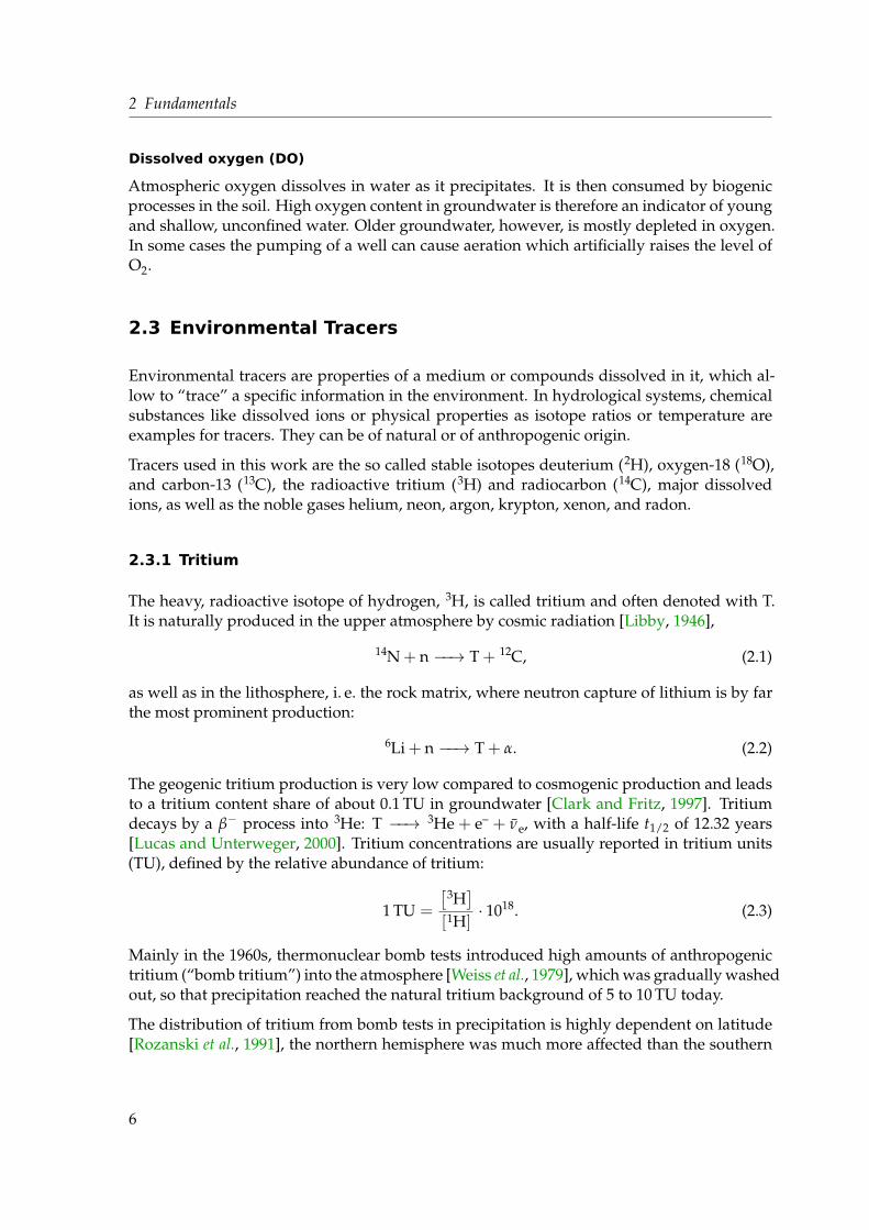
Atmospheric oxygen dissolves in water as it precipitates. It is then consumed by biogenicprocesses in the soil. High oxygen content in groundwater is therefore an indicator of youngand shallow, unconfined water. Older groundwater, however, is mostly depleted in oxygen.In some cases the pumping of a well can cause aeration which artificially raises the level ofO2.
2.3 Environmental Tracers
Environmental tracers are properties of a medium or compounds dissolved in it, which al-low to “trace” a specific information in the environment. In hydrological systems, chemicalsubstances like dissolved ions or physical properties as isotope ratios or temperature areexamples for tracers. They can be of natural or of anthropogenic origin.
Tracers used in this work are the so called stable isotopes deuterium (2H), oxygen-18 (18O),and carbon-13 (13C), the radioactive tritium (3H) and radiocarbon (14C), major dissolvedions, as well as the noble gases helium, neon, argon, krypton, xenon, and radon.
2.3.1 Tritium
The heavy, radioactive isotope of hydrogen, 3H, is called tritium and often denoted with T.It is naturally produced in the upper atmosphere by cosmic radiation [Libby, 1946],
14N + n −−→ T + 12C, (2.1)
as well as in the lithosphere, i. e. the rock matrix, where neutron capture of lithium is by farthe most prominent production:
6Li + n −−→ T + α. (2.2)
The geogenic tritium production is very low compared to cosmogenic production and leadsto a tritium content share of about 0.1 TU in groundwater [Clark and Fritz, 1997]. Tritiumdecays by a β− process into 3He: T −−→ 3He + e– + ν̄e, with a half-life t1/2 of 12.32 years[Lucas and Unterweger, 2000]. Tritium concentrations are usually reported in tritium units(TU), defined by the relative abundance of tritium:
1 TU =
[3H]
[1H]· 1018. (2.3)
Mainly in the 1960s, thermonuclear bomb tests introduced high amounts of anthropogenictritium (“bomb tritium”) into the atmosphere [Weiss et al., 1979], which was gradually washedout, so that precipitation reached the natural tritium background of 5 to 10 TU today.
The distribution of tritium from bomb tests in precipitation is highly dependent on latitude[Rozanski et al., 1991], the northern hemisphere was much more affected than the southern
6

2.3 Environmental Tracers
1 9 6 0 1 9 7 0 1 9 8 0 1 9 9 0 2 0 0 0 2 0 1 01
1 0
1 0 0
1 0 0 0
1 0 0 0 0
Tri
tium
[TU]
Y e a r
V i e n n a J o r d a n
Figure 2.3: Tritium content in precipitation in Vienna (blue) and in Jordan (red). Thebomb peak in the 1960 is clearly visible with up to 6000 TU in Vienna. The data fromJordan is compiled from all collection stations in Jordan. No data is available in the1970s and the first half of the 1980s. Tritium content in Jordan is generally lower than inVienna. All data from IAEA/WMO [2006].
one. Figure 2.3 shows the tritium content in precipitation in Vienna and in Jordan. Althoughthe available data from Jordan is sparse, the behavior at both locations is similar, but inJordan the tritium concentration is generally lower than in Vienna at higher latitudes.
Tritium can be employed to date young groundwater up to an age of about 50 years. How-ever, due to the highly seasonally variable input curve and low present day tritium con-centrations, the ages derived from tritium data are often ambiguous. The determination oftritiogenic 3He, the daughter nucleus of tritium, helps considerably to enhance the datingpotential of tritium, because the sum of tritium and 3He is conserved over time [Schlosseret al., 1988]. T–3He ages, τ, are calculated by
τ =t1/2
ln 2· ln(
1 +
[3He]
[3H]
), (2.4)
with the concentrations of 3He and tritium in the bracket given in the same unit. The 3Heamount, given in ccSTP/g, is converted into TU by the following relation (for pure water):
1 TU = 2.488× 10⁻¹⁵ ccSTP/g. (2.5)
Because 3He gets lost to the atmosphere as long as the water is in contact with the soil air,the T-3He age reflects the duration the water parcel is closed off from the atmosphere – in
7

2 Fundamentals
contrast to tritium-only ages, which express the time span between precipitation and sam-pling. The travel time in the vadose zone of infiltrating water can be up to several tens ofyears [Solomon et al., 1995; Geyh, 2000; Schwientek et al., 2009], depending on the thicknessof the unsaturated zone, the soil and rock permeability and the precipitation amount.
When mostly old groundwater is examined – as it is done in this work – tritium often acts asa marker of admixed young groundwater.
2.3.2 Isotope fractionation
The use of isotopic tracers relies on the fact that several mechanisms alter the isotopic com-position in a medium. Among these mechanisms are chemical reactions and phase changes(e.g. evaporation). The fundamental principle behind this so-called isotope fractionation isthat usually the heavier isotope is less likely to participate in a chemical reaction, rather staysin the more dense phase during a phase change compared to its lighter version, or movesslower in diffusive processes. The explanation of these phenomena comprise two points:First, heavy isotopes move slower than their lighter versions. This causes a slower diffusionvelocity as well as a lower chemical reactiveness, because the collision frequency as the pri-mary condition for chemical reactions is reduced. Second, heavier molecules generally havehigher intra-molecular binding energies. Thus, 1H2
18O has a lower vapor pressure than1H2
16O, for example, and Ca12CO3 dissolves faster in an acidic environment than Ca13CO3does. Particularly in an isotope equilibrium between two chemical compounds, the heavyisotope is, in general, enriched in the aggregate with the largest density. As the difference ofbinding energies of different isotopic compounds becomes smaller at higher temperatures,also the resulting isotope effects diminish.
Fractionating processes can occur at equilibrium (equilibrium fractionation) or at transient con-ditions (kinetic fractionation). While the first takes place at conditions which facilitate the es-tablishment of an equilibrium, kinetic fractionation results from irreversible processes likeevaporation of water with instantaneous removal of the vapor. Natural processes, however,are a mixture of equilibrium and kinetic fractionation; evaporation is neither a one-way pro-cess, because for sure there is also condensation of vapor taking place, nor is it an equilib-rium process as there is a net evaporation.
Isotope abundances are described by the isotope abundance ratio R, compare Mook [2000]:
R =abundance of rare isotope
abundance of abundant isotope. (2.6)
The isotopic composition in a chemical equilibrium (A ←→ B) or of a chemical or physicalreaction (A −→ B) is described by the isotope fractionation factor α = RB/RA. Because theisotopic variation is generally very small and α ≈ 1, the use of the fractionation ε is moreconvenient:
ε = α− 1. (2.7)
ε > 0 describes an enrichment, ε < 0 a depletion of the rare isotope in B with respect to Aand is usually reported in units of per mille.
8
2.3 Environmental Tracers
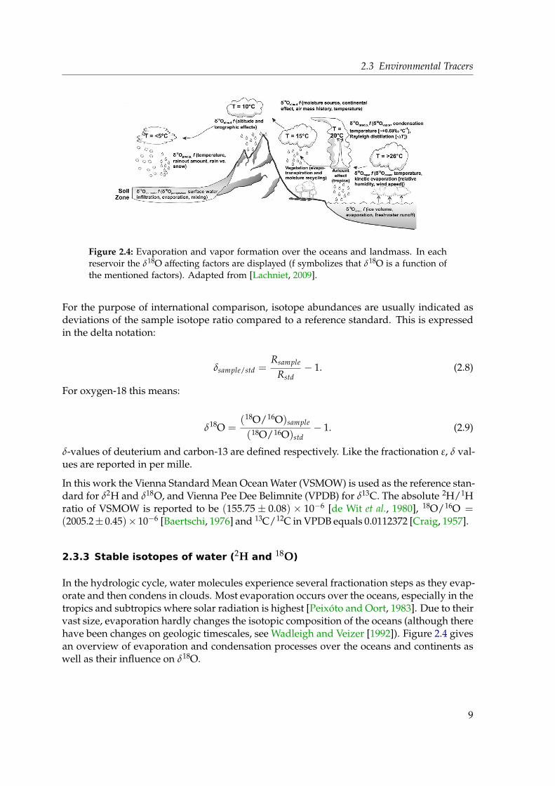
Figure 2.4: Evaporation and vapor formation over the oceans and landmass. In eachreservoir the δ18O affecting factors are displayed (f symbolizes that δ18O is a function ofthe mentioned factors). Adapted from [Lachniet, 2009].
For the purpose of international comparison, isotope abundances are usually indicated asdeviations of the sample isotope ratio compared to a reference standard. This is expressedin the delta notation:
δsample/std =Rsample
Rstd− 1. (2.8)
For oxygen-18 this means:
δ18O =(18O/16O)sample
(18O/16O)std− 1. (2.9)
δ-values of deuterium and carbon-13 are defined respectively. Like the fractionation ε, δ val-ues are reported in per mille.
In this work the Vienna Standard Mean Ocean Water (VSMOW) is used as the reference stan-dard for δ2H and δ18O, and Vienna Pee Dee Belimnite (VPDB) for δ13C. The absolute 2H/1Hratio of VSMOW is reported to be (155.75± 0.08) × 10−6 [de Wit et al., 1980], 18O/16O =(2005.2± 0.45)× 10−6 [Baertschi, 1976] and 13C/12C in VPDB equals 0.0112372 [Craig, 1957].
2.3.3 Stable isotopes of water (2H and 18O)
In the hydrologic cycle, water molecules experience several fractionation steps as they evap-orate and then condens in clouds. Most evaporation occurs over the oceans, especially in thetropics and subtropics where solar radiation is highest [Peixóto and Oort, 1983]. Due to theirvast size, evaporation hardly changes the isotopic composition of the oceans (although therehave been changes on geologic timescales, see Wadleigh and Veizer [1992]). Figure 2.4 givesan overview of evaporation and condensation processes over the oceans and continents aswell as their influence on δ18O.
9

2 Fundamentals
In the process of evaporation, equilibrium as well as kinetic fractionation contribute. In avery thin layer above the water surface 100 % humidity prevails and fractionation at equilib-rium conditions takes place. As the atmosphere usually has a lower humidity, a net transportof vapor from the water body through a transition zone into the atmosphere takes place.Thus, the different diffusivities of 1H16
2 O, 1H2H16O and 1H182 O cause kinetic fractionation
in a second step. The degree of kinetic fractionation can be estimated from the water sur-face vapor [Gonfiantini, 1986]. Due to the different fractionation processes, water moleculescontaining the heavy isotopes of hydrogen and oxygen are stronger enriched in the liquidphase and the influence of kinetic fractionation leads to an excess of deuterium (so calleddeuterium excess d) during evaporation, calculated by
d = δ2H− 8 · δ18O. (2.10)
Condensation is considered to occur at equilibrium conditions because the formation ofdroplets in clouds takes place only at 100 % humidity. Hence, the deuterium excess is notaffected by this process.
The isotopic analysis of stable isotopes in rainfall from all over the world results in the GlobalMeteoric Water Line (GMWL, see figure 2.5), first empirically delineated by Craig [1961], andlater stated more precisely by Rozanski et al. [1993], using the data of the Global Network ofIsotopes in Precipitation (GNIP) database [IAEA/WMO, 2006]:
δ2H = 8.17 · δ18O + 10.35 h VSMOW (2.11)
This equation holds for an average world-wide humidity of 85 %. 10.35 h is the averagedeuterium excess. Local Meteoric Water Lines (LMWL) can differ quite strongly from theGMWL in slope and deuterium excess. The reasons are different origins of the vapor mass,secondary evaporation during rainfall and the seasonality of precipitation.
In the Middle East often the Eastern Mediterranean Water Line (EMWL) [Gat and Carmi,1970] is applied:
δ2H = 8 · δ18O + 22 h VSMOW. (2.12)
It is the most common MWL in Israel. The high deuterium excess in precipitation in this re-gion is attributed to the favored storm path coming from the Baltics [Gat, 1987]. At continen-tal conditions, humidity is lower than over the oceans and the effect of kinetic fractionationis enhanced (see references above).
Bajjali [2012] presents a water line derived from Jordanian rainfall only with a significantlysmaller slope, the Jordanian Meteoric Water Line (JMWL):
δ2H = 6.27 · δ18O + 11.40 h VSMOW. (2.13)
The reduced slope of 6.27 can be attributed to highly evaporative conditions in Jordan, i. e.that already during precipitation the rain drops experience evaporation, rendering the dropsthat reach the surface to be enriched in the heavy isotopes.
The interpretation of stable isotopes in water requires the consideration of several environ-mental parameters that alter the isotopic composition of water. The ultimate driving force
10

2.3 Environmental Tracers
- 6 - 4 - 2 0 2
- 4 0
- 3 0
- 2 0
- 1 0
0
1 0
2 0
J M W L : � 2 H = 6 . 2 7 · � 1 8 O + 1 1 . 4 �
� 1 8 O [ � ]
�2 H [�
]
G M W L : � 2 H = 8 . 1 7 · � 1 8 O + 1 0 . 3 5 �
E q u i l i b r i u m f r a c t i o n a t i o n� 2 H = 8 · � 1 8 O �
d e u t e r i u me x c e s s : 1 0 . 3 5 �
E v a p o r a t i o n
Figure 2.5: The relation of δ2H and δ18O in global precipitation forms the GlobalMeteoric Water Line (GMWL), here depicted in green. The Jordan Meteoric WaterLine (JMWL) [Bajjali, 2012], which represents the isotopic composition in Jordanianrainfall, is characterized by a smaller slope, indicating an influence of evaporation (redline). Groundwater samples which plot along a line with smaller slope than the localmeteoric water line indicate the presence of evaporative processes before the water seepsunderground.
behind most of them is temperature. Dansgaard [1964] formulated the global relationshipbetween mean annual temperature T and the average δ18O of precipitation to be
δ18O = 0.69 · T − 13.6 h VSMOW, (2.14)
T in ◦C, but strong variances are observed on regional or local scale [Rozanski et al., 1993].Having this relation in mind, the following isotope effects can be explained. Clark and Fritz[1997] provide a good overview of these effects.
A rough correlation between latitude and local temperature explains the depletion of heavyisotopes in rainfall at higher latitudes, called latidue effect. As vapor masses travel to colderregions the relative humidity rises and finally the vapor condensates and rains out, leavingless enriched vapor behind. Analogous, vapor masses rising to high altitudes cool downadiabatically by approximately 0.5 ◦C per 100 m [Fairbridge and Oliver, 2005]. This altitudeeffect induces a depletion of heavy isotopes. For 18O in precipitation a change of −0.15 to−0.5 h per 100 m is found, but this effect strongly depends on the individual setting [Clarkand Fritz, 1997]. The further the vapor masses move inland, the relief forces progressiverainout and, hence, a depletion in heavy isotopes occurs. This effect is called continental ef-fect and is illustrated by fig 2.6. The basic principle behind all of these three isotope effects iscalled Rayleigh process or Rayleigh distillation. It describes the fact that under progressive rain-out the remaining water vapor gets less depleted with time and, hence, also the subsequentcondensation leads to isotopically “lighter” rain drops [Mook, 2000].
11
2 Fundamentals
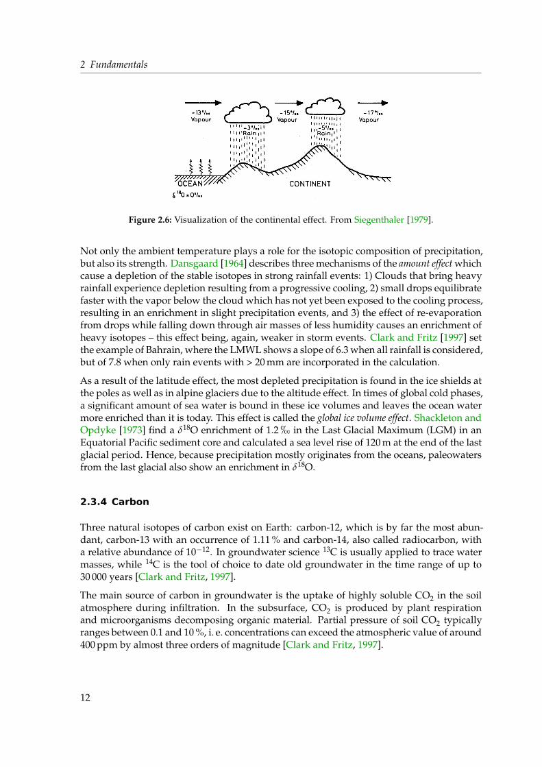
Figure 2.6: Visualization of the continental effect. From Siegenthaler [1979].
Not only the ambient temperature plays a role for the isotopic composition of precipitation,but also its strength. Dansgaard [1964] describes three mechanisms of the amount effect whichcause a depletion of the stable isotopes in strong rainfall events: 1) Clouds that bring heavyrainfall experience depletion resulting from a progressive cooling, 2) small drops equilibratefaster with the vapor below the cloud which has not yet been exposed to the cooling process,resulting in an enrichment in slight precipitation events, and 3) the effect of re-evaporationfrom drops while falling down through air masses of less humidity causes an enrichment ofheavy isotopes – this effect being, again, weaker in storm events. Clark and Fritz [1997] setthe example of Bahrain, where the LMWL shows a slope of 6.3 when all rainfall is considered,but of 7.8 when only rain events with > 20 mm are incorporated in the calculation.
As a result of the latitude effect, the most depleted precipitation is found in the ice shields atthe poles as well as in alpine glaciers due to the altitude effect. In times of global cold phases,a significant amount of sea water is bound in these ice volumes and leaves the ocean watermore enriched than it is today. This effect is called the global ice volume effect. Shackleton andOpdyke [1973] find a δ18O enrichment of 1.2 h in the Last Glacial Maximum (LGM) in anEquatorial Pacific sediment core and calculated a sea level rise of 120 m at the end of the lastglacial period. Hence, because precipitation mostly originates from the oceans, paleowatersfrom the last glacial also show an enrichment in δ18O.
2.3.4 Carbon
Three natural isotopes of carbon exist on Earth: carbon-12, which is by far the most abun-dant, carbon-13 with an occurrence of 1.11 % and carbon-14, also called radiocarbon, witha relative abundance of 10−12. In groundwater science 13C is usually applied to trace watermasses, while 14C is the tool of choice to date old groundwater in the time range of up to30 000 years [Clark and Fritz, 1997].
The main source of carbon in groundwater is the uptake of highly soluble CO2 in the soilatmosphere during infiltration. In the subsurface, CO2 is produced by plant respirationand microorganisms decomposing organic material. Partial pressure of soil CO2 typicallyranges between 0.1 and 10 %, i. e. concentrations can exceed the atmospheric value of around400 ppm by almost three orders of magnitude [Clark and Fritz, 1997].
12

2.3 Environmental Tracers
Figure 2.7: Typical variation of δ13C in several natural reservoirs [Clark and Fritz, 1997].
Carbon-13
A lot of factors influence the carbon isotopy in groundwater and give rise to wide range ofδ13C values. These effects are described below and figure 2.7 offers an overview.
While atmospheric δ13C is around −7 h, soil air carbon isotopy is more variable and de-pends mainly on the type of vegetation present on the surface. Generally, CO2 fixation pro-cesses by plants prefer the lighter 12CO2 molecule over the heavier 13CO2 to be incorporatedinto plant material. Hence, the plants are depleted in 13C. Respiration by the plant’s roots, incontrast, favors the heavy 13CO2 to be emitted to the soil air, but the resulting carbon isotopyof soil CO2 is still way below the atmospheric value (compare figure 2.7). However, so calledC3 and C4
1 plants differ from each other by their photosynthesis pathways and hence theirCO2 respiration [Peisker, 1984]. Soil air δ13C values produced by C4 plants are in the rangeof −9 to −19 h (mostly around −14 h) and therewith much less fractionated than the 13Cisotopy respirated by C3 plants, which falls in the range of −22 to −40 h (mostly around−28 h) [Peisker, 1984; Schulze et al., 2005].
C3 plants are common in temperate climate and tropical regions, where temperature andsunlight intensity are moderate and sufficient groundwater prevails [Schulze et al., 2005].They constitute most of the planet’s biomass. During photosynthesis C3 plants loose most oftheir uptaken water [Raven and Edwards, 2001] and are therefore not fitted to dry climate.
C4 plants, in contrast, are adapted to arid climate by optimizing their photosynthesis mecha-nism in respect to water transpiration. In fact, the more efficiently a C4 plant uses the scarce
1These plant types are named for the amount of carbon atoms present in the first product of the carbon fixationprocess, three in case of C3 plant, four in case of C4 plants.
13
2 Fundamentals
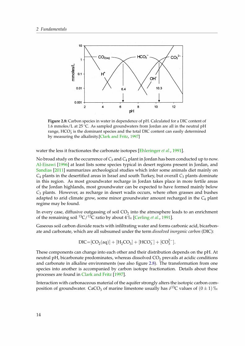
Figure 2.8: Carbon species in water in dependence of pH. Calculated for a DIC content of1.6 mmoles/L at 25 ◦C. As sampled groundwaters from Jordan are all in the neutral pHrange, HCO–
3 is the dominant species and the total DIC content can easily determinedby measuring the alkalinity.[Clark and Fritz, 1997]
water the less it fractionates the carbonate isotopes [Ehleringer et al., 1991].
No broad study on the occurrence of C3 and C4 plant in Jordan has been conducted up to now.Al-Eisawi [1996] at least lists some species typical in desert regions present in Jordan, andSandias [2011] summarizes archeological studies which infer some animals diet mainly onC4 plants in the desertified areas in Israel and south Turkey, but overall C3 plants dominatein this region. As most groundwater recharge in Jordan takes place in more fertile areasof the Jordan highlands, most groundwater can be expected to have formed mainly belowC3 plants. However, as recharge in desert wadis occurs, where often grasses and bushesadapted to arid climate grow, some minor groundwater amount recharged in the C4 plantregime may be found.
In every case, diffusive outgassing of soil CO2 into the atmosphere leads to an enrichmentof the remaining soil 13C/12C ratio by about 4 h [Cerling et al., 1991].
Gaseous soil carbon dioxide reacts with infiltrating water and forms carbonic acid, bicarbon-ate and carbonate, which are all subsumed under the term dissolved inorganic carbon (DIC):
DIC−−[CO2(aq)] + [H2CO3] + [HCO−3 ] + [CO2−3 ].
These components can change into each other and their distribution depends on the pH. Atneutral pH, bicarbonate predominates, whereas dissolved CO2 prevails at acidic conditionsand carbonate in alkaline environments (see also figure 2.8). The transformation from onespecies into another is accompanied by carbon isotope fractionation. Details about theseprocesses are found in Clark and Fritz [1997].
Interaction with carbonaceous material of the aquifer strongly alters the isotopic carbon com-position of groundwater. CaCO3 of marine limestone usually has δ13C values of (0± 1)h
14
2.3 Environmental Tracers
[Geyh, 2000]. Dissolution of it therefore enriches the δ13C of the water. The lower the ground-water pH, the more calcium carbonate goes into solution, and even when saturation isreached, δ13C may still alter due to ongoing ion exchange. Hence, the aquifer material playsan important role in coining the carbon isotope discrimination. Geyh and Michel [1982], forexample, found that groundwater in a sandstone aquifer is commonly more depleted thanwater in a limestone aquifer.
Freshwater carbonates include speleothem, travertine and calcrete formations as well as sec-ondary mineralization in soil. Due to the varying genesis conditions, CO2 degassing in con-sequence of depressurization, evaporation or freezing of bicarbonate water, the δ13C valuescover a wide range, including positive values.
In locations of seismic activity, additional geogenic carbon in form of CO2 can rise fromsources in the the deep crust or the mantle and influence the carbon isotopy of groundwater.Mantle CO2 has typical δ13C of −6 h [Geyh, 2000]. Metamorphic CO2 originates from deeplimestones, which experience a transformation in their physical and/or chemical state un-der high temperatures and pressure. This decarbonation is often related to magma bodiesinteracting with the limestone and release preferentially heavy CO2. Typical δ13C values ofmetamorphic CO2 lie in the range of +5 to +10 h[Clark and Fritz, 1997].
Carbon-14
Atmospheric carbon-14 was discovered by Willard Frank Libby in 1946 [Libby, 1946]. Hewas awarded the Noble Prize in chemistry in 1960 for developing the radiocarbon datingtechnique, which revolutionized archeology as well as environmental sciences.
Radioactive 14C is naturally produced in the upper atmosphere. Cosmic rays shower the gasparticles and generate secondary thermal neutron in spallation reactions. Hitting 14N, theseneutrons produce radiocarbon:
14N + n −−→ 14C + p, (2.15)
where n are neutrons and p protons. 14C immediately oxidizes to 14CO2 and enters thetroposphere where it is assimilated in the biosphere and hydrosphere.14C disintegrates by β− decay according to 14C −−→ 14N + e– + ν̄e. Libby determined thehalf-life of 14C to be 5568 years, which was subsequently corrected to be 5730± 40 years[Godwin, 1962], but still today the Libby half-life is often used to keep the comparability toolder data.14C is widely used in archeologic and paleoclimatic studies as an age tracer. Assuming aclosed system, which means there is no gain or loss of 14C except of radioactive decay, andthat the initial concentration is known, the age t of a sample can be derived from the ratio ofthe measured activity A(t) and the initial activity A0:
t = −τ1/2
ln 2· ln A(t)
A0, (2.16)
where τ1/2 is the half-life of carbon-14.
15

2 Fundamentals
14C activity is reported in percent modern carbon (pmC). 100 pmC are set by convention as13.56 decays per minute and gram carbon and reflect the activity in the year 1950 AD [Mook,1980]. Cosmogenic production and the radioactive decay of carbon-14 form a secular equilib-rium and the concentration of 14C can indeed be considered as constant over short periodsof decades to some centuries.
Over long time periods, however, 14C activity in the atmosphere was found to vary signifi-cantly. The examination of carbon isotopes of tree rings [Becker and Kromer, 1993; Muscheleret al., 2008], foraminifera [Hughen et al., 2004, 2006] and corals [Fairbanks et al., 2005] re-vealed a variation of the atmospheric 14C concentration over the millenia. Its activity variedby over 10 % during the Holocene and was even 40 % higher during the Last Glacial Maxi-mum [Bard et al., 1990]. Crowe [1958] and Stuiver and Quay [1980] revealed a dependencyof the 14C production rate on the number of visible sunspots, while Willson and Hudson[1988] and Hoyt et al. [1992] correlated the number of sunspots with solar activity measuredby the SSM and Nimbus 7 satellites. Beiser [1957] and Damon et al. [1989] demonstrated analteration of the production rate by the variability of the Earth’s magnetic field. The latter isthe major driving force behind the natural variation [Damon et al., 1989].
The collected 14C activity data in the Earth’s atmosphere provide a calibration curve of theatmospheric 14C content over time, summarized by Reimer et al. [2009], that is applied to getactual, calibrated sample ages.
Nowadays, 14C activity in the atmosphere has an additional, anthropogenic source. Whilethe combustion of radiocarbon free fossil fuel leads to a dilution of 14C concentration inthe atmosphere (Suess effect, see Suess [1955]), nuclear bomb tests in the 1950s and 60s re-leased not only tritium in the atmosphere but increased the carbon-14 concentration as well[Münnich and Vogel, 1958]. In 1963 the activity in the atmosphere was about twice as highcompared to 1950, but declined to about 105 pmC at the present day [Levin et al., 2010]. Thedeviation of modern 14C activity in the atmosphere from that of the year AD 1890, ∆14C(delineated from 1890 tree-rings, which define the oxalic acid 14C standard, see Stuiver andPolach [1977]), is shown in figure 2.9.
While the radiocarbon method allows dating of archeologic, i. e. biological, samples up toages of 50 000 years [Kromer, 2007], 14C dating of groundwater is accompanied by severalcomplications. First, all the fractionating effects introduced above apply also for 14C. Second,and having the strongest influence on the 14C concentration in DIC in groundwater, theeffect of artificial aging. By dissolution of carbonaceous aquifer material (which is free of14C, called carbon dead) and ion exchange of DIC dissolved in water with it, the initial 14Ccontent is reduced, which is expressed in a falsely greater groundwater age. For that reason,groundwater 14C dating is generally limited to about 30 000 years [Clark and Fritz, 1997].
Several models were developed to account for the effects altering the initial 14C content us-ing different approaches. The Vogel model takes the 14C activity in young groundwater(containing bomb tritium) to estimate the matrix effects [Vogel, 1967, 1970; Clark and Fritz,1997]. The Pearson model tries to deduce the 14C dilution by measuring the δ13C and as-suming a two component mixture of soil CO2 (depending on vegetation) and leeched calcite(usually 0 h) [Pearson Jr., 1965]. Others take into account geochemical processes (Tamers
16

2.3 Environmental Tracers
Figure 2.9: Deviation of modern atmospheric 14C concentration from tree-ring data ofAD 1890 [Stuiver and Polach, 1977] in the Northern (Vermunt, Austria) and Southern(Wellington, New Zealand) hemisphere [Levin et al., 2010]. The bomb peak in the 1960sis obvious. Negative pre-1950 ∆14C values indicate the influence of the Suess effect[Suess, 1955].
model [Tamers, 1975] and the chemical mass balance model by Clark and Fritz [1997]), or acombination of these indicators [Fontes and Garnier, 1979].
Due to the totally different approach, these models often result in differing groundwaterages [Wieser, 2011]. In this work, however, the exact water age is not so much of interest andonly a very few samples are analyzed for radiocarbon. In the Azraq study, for example, mix-ing of different groundwater sources is assumed and therefore a specific water age makesprincipally no sense. Hence, 14C data is interpreted in form of its basic analysis result, givenin pmC, and is only used as a rough age indicator to discriminate between young samples,old and very old (carbon dead) samples.
2.3.5 Water chemistry in groundwater
Many different solutes are present in groundwater, mainly inorganic ions. A minor part isalready present in precipitation [Davis and DeWiest, 1966], but most of the substances resultfrom the dissolution of the aquifer rock during the subsurface flow of the water (comparetable 2.1). Generally the most abundant cations are sodium (Na+), calcium (Ca2+), magne-sium (Mg2+) and the most frequent anions are chloride (Cl−), sulfate (SO2−
4 ) and bicarbonate(HCO−3 ). They are termed major ions and are included in every hydrochemical consideration[Freeze and Cherry, 1979]. Minor constituents include iron, strontium, potassium, carbonate,nitrate, fluoride, boron as well as other trace substances.
The concentration of solutes is usually reported in mg/L or in milligram equivalent per liter(meq/L). The latter is calculated from the first by dividing the concentration in mg/L, C∗i ,by the molar weight mi and multiplying by the specific charge zi of the ion i:
17
2 Fundamentals
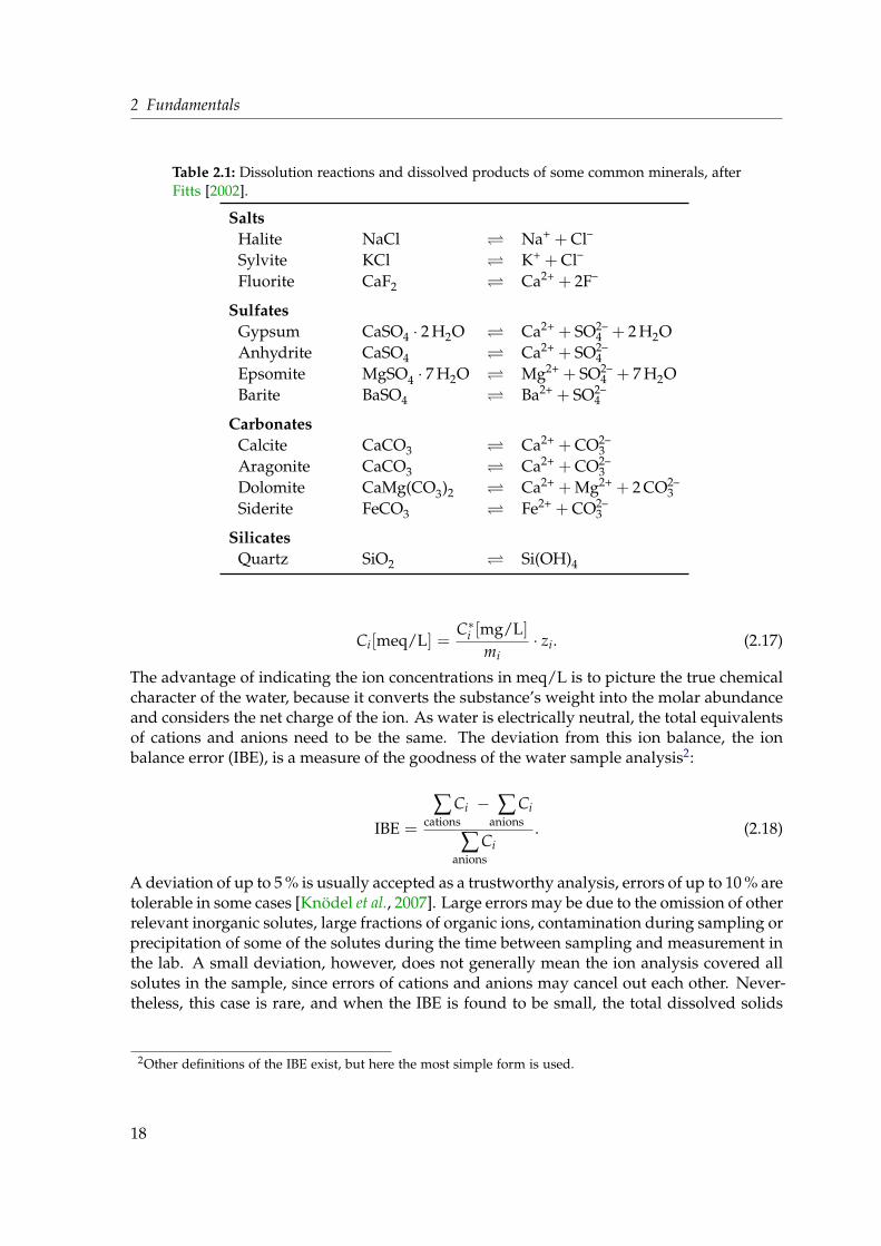
Table 2.1: Dissolution reactions and dissolved products of some common minerals, afterFitts [2002].
SaltsHalite NaCl Na+ + Cl–
Sylvite KCl K+ + Cl–
Fluorite CaF2 Ca2+ + 2F–
SulfatesGypsum CaSO4 · 2 H2O Ca2+ + SO2–
4 + 2 H2OAnhydrite CaSO4 Ca2+ + SO2–
4Epsomite MgSO4 · 7 H2O Mg2+ + SO2–
4 + 7 H2OBarite BaSO4 Ba2+ + SO2–
4
CarbonatesCalcite CaCO3 Ca2+ + CO2–
3Aragonite CaCO3 Ca2+ + CO2–
3Dolomite CaMg(CO3)2 Ca2+ + Mg2+ + 2 CO2–
3Siderite FeCO3 Fe2+ + CO2–
3
SilicatesQuartz SiO2 Si(OH)4
Ci[meq/L] =C∗i [mg/L]
mi· zi. (2.17)
The advantage of indicating the ion concentrations in meq/L is to picture the true chemicalcharacter of the water, because it converts the substance’s weight into the molar abundanceand considers the net charge of the ion. As water is electrically neutral, the total equivalentsof cations and anions need to be the same. The deviation from this ion balance, the ionbalance error (IBE), is a measure of the goodness of the water sample analysis2:
IBE =
∑cations
Ci − ∑anions
Ci
∑anions
Ci. (2.18)
A deviation of up to 5 % is usually accepted as a trustworthy analysis, errors of up to 10 % aretolerable in some cases [Knödel et al., 2007]. Large errors may be due to the omission of otherrelevant inorganic solutes, large fractions of organic ions, contamination during sampling orprecipitation of some of the solutes during the time between sampling and measurement inthe lab. A small deviation, however, does not generally mean the ion analysis covered allsolutes in the sample, since errors of cations and anions may cancel out each other. Never-theless, this case is rare, and when the IBE is found to be small, the total dissolved solids
2Other definitions of the IBE exist, but here the most simple form is used.
18

2.3 Environmental Tracers
(TDS) can usually be directly calculated with acceptable uncertainty by summing up all theindividual ion concentrations (in mg/L, of course).
Another advantage of giving the concentrations in meq/L lies in the fact that the dissolvedions from a mineral which consists of two components only are present in the same concen-tration, i. e. plotting the concentrations of these ions against each other, the result is foundto lie on the angle bisector. The dissolution of halite (NaCl), for example, leads to the sameconcentration of Na+ and Cl−, given in meq/L. Dissolution of gypsum leads to an equalamount of Ca2+ and SO2−
4 ions, and so on. Thus, the minerals that influence the consideredgroundwater can often be identified in this way (table 2.1 lists some of the most commondissolution reactions and their corresponding mineral).
Major ion data can be presented in several ways, compare Zaporozec [1972]. They all workwith ion concentrations in meq/L. The most simple graph shows the composition in cationsand anions as columns, as first proposed by Collins [1923] and depicted in figure 2.10. Theconcentration of the major ions are separately piled in two columns whose height is propor-tional to the total concentration of the cations and anions. It is therefore a graphical visual-ization of the ion balance calculation, as large IBE result in different heights of the columns.Sometimes the relative contributions of the single ions to the total cations/anions are drawn;thereby the IBE cannot be represented anymore, but the relative ionic composition of twosamples can be compared more easily, independent of their total solute content.
The semi-logarithmic Schoeller diagram ([Schoeller, 1955, 1962], cited after Freeze and Cherry[1979]) allows the comparison of several water samples (see figure 2.11). For each sample theconcentration of each observed ion is plotted and the dots are connected by a straight line,which gives kind of a footprint of each water. Samples with a similar overall compositionhave a similar footprint, independent of their total solute content.
A popular way to present major ion data is the trilinear Piper diagram [Piper, 1944; Hill,1940, both after Zaporozec [1972]], exemplary shown in figure 2.12. Each trilinear diagramcan show the composition of three ions, where the ion concentrations are given as percent-ages, those of the cations in the left triangle, those of the anion in the right triangle. Eachapex of a triangle represents water with 100 % composition of one of the three constituents.Commonly, Ca2+, Mg2+ and Na+ (+ K+) are plotted in the cations triangle, while Cl−, SO2−
4and HCO−3 (+ CO2−
3 ) form the anion triangle.
If only two of the three components are present, the water sample plots on the line betweenthe two corresponding apexes. When all ions are present the analysis falls in the interiorof the triangle. In cases of substantial potassium content, the same is added to the sodiumconcentration and the sum is drawn. The same holds for carbonate, which is grouped to thebicarbonate concentration in the anion triangle when required [Fetter, 2001].
The data point positions in the cation and the anion field are then projected into the centraldiamond. The resulting point characterizes the water type with respect to both its cationsand anions (compare figure 2.13). Data point A in figure 2.12, for example, corresponds toNa-Cl-type water, point B to Ca-Mg-Na-HCO3 water type. It is also possible to depict theabsolute solute concentration of each sample in a piper diagram by varying the size of thedata points.
19

2 Fundamentals
0
2
4
6
8
1 0
1 2
1 4
Conce
ntrati
on [m
eq/L
]
C a M g N a + K H C O 3 S O 4 C l
Figure 2.10: Column diagrams for two samples. The left one is typical for Na-Cl typewater, the right one an example of Ca-HCO3 water. Obviously, the left sample has higherTDS. The IBE is clearly visible in the visualization of the right sample. The colorationfollows the recommendation of Collins [1923].
M g C a C a + M g N a + K C l H C O 3 S O 41
1 0
1 0 0
Conce
ntrati
on [m
eq/L
]
Figure 2.11: The Schoeller diagram allows the fast distinction between different watertypes. In this example the water samples represented in red and green have a similarfootprint, i. e. they are similar in their ionic composition despite an obviously differenttotal amount of solutes, whereas the blue sample represents a different water type (moreCa compared to the Na content).
20

2.3 Environmental Tracers
Figure 2.12: The piper diagram is a smart way to illustrate the chemical compositionregarding the major ions of many water samples at once. It consists of two trilinearfields, one for cations and one for anions. In each triangle the relative shares of threeions or ion groups are plotted. The data points from the triangles are then projectedinto the central diamond shaped field, where it represents the chemical compositionwith respect to all considered ions. Taken from Freeze and Cherry [1979].
Figure 2.13: Characterization of water types in a piper diagram after Back [1966].Adopted from Freeze and Cherry [1979].
21

2 Fundamentals
Because each analysis is represented by a single point only in the diamond-shaped field,waters with very different total compositions can have the same projection in this diagram.Therefore, when investigating groundwater mixing, the two trilinear diagrams offer a muchbetter illustration since the mixture of two different water types plots on a straight line join-ing the two endmember types.
2.3.6 Noble Gases
Noble gases have proven to be valuable tracers in geosciences [Porcelli et al., 2002] andgroundwater science [Kipfer et al., 2002; Aeschbach-Hertig and Solomon, 2013]. Their chem-ical inertness and low abundance render them ideal tracers in geochemical, cosmochemicaland groundwater studies.
Three major noble gas reservoirs exist on Earth: the atmosphere, the largest storage of noblegases, the Earth’s crust and its mantle3. The different noble gas isotopic composition of thesereservoirs enables scientists to separate the influences of these reservoirs and to trace crustaland mantle fluids.
Groundwater draws its noble gas content primarily from the atmosphere, from radioactivedecay processes in the crust producing noble gases and, in regions of volcanic activity, alsofrom the mantle reservoir [Ballentine and Burnard, 2002]. In groundwater, atmospheric no-ble gases originate from the equilibration of precipitating and then infiltrating water withthe surrounding gas reservoir and an additional atmospheric component called excess air(EA) (see chapters 2.3.6.1 and 2.3.6.2). Especially within the crust, radioactive productionof noble gases takes place. Three different mechanisms are distinguished: radiogenic (α de-cay in the U/Th decay chains produces 4He), fissiogenic (direct production of Kr and Xeisotopes by spontaneous fission of heavy elements) and nucleogenic production (from theinteraction of light elements with α particles or neutrons, like in the reaction 18O (α, n)21Ne).These gases are released from the rock matrix and accumulate in groundwater. The Earth’smantle is assumed to bear primordial noble gases [Lupton and Craig, 1981] or input fromcosmic dust [Anderson, 1993]. In regions with a thin crust or tectonic activity, these gasescan ascend and mix into groundwater [Oxburgh and O’Nions, 1987].
Except for argon, all noble gases are present in the atmosphere only in traces. Table 2.2 givesan overview of atmospheric concentrations as well as relative abundances of stable noblegas isotopes used in this study.
In the following, the noble gases helium, neon, argon, krypton, xenon and radon are intro-duced. A much more detailed treatment is found in Ozima and Podosek [2002] and Porcelliet al. [2002], especially in the chapters of Ballentine and Burnard [2002] and Graham [2002]in the latter book.
3The oceans comprise dissolved noble gases as well, but those are not relevant within the scope of this thesis.
22

2.3 Environmental Tracers
Table 2.2: Atmospheric noble gas concentrations and the absolute molar abundances ofisotopes used in this study as well as the relative abundance in respect to a referenceisotope denoted with ? (i. e. the usually used isotope ratios). Data is compiled fromPorcelli et al. [2002] and references therein as well as other sources mentioned in thetext.
Noble gas Volume mixing Isotope Molar abundance Relativeratio [%] abundance
He 5.24× 10⁻⁶ 3He 1.4× 10⁻⁴ 1.384× 10⁻⁶
4He 100 ?
Ne 1.818× 10⁻⁵ 20Ne 90.50 9.8022Ne 9.23 ?
Ar 9.34× 10⁻³ 36Ar 0.3364 ?40Ar 99.60 295.5
Kr 1.14× 10⁻⁶ 84Kr 57.00
Xe 8.7× 10⁻⁸ 132Xe 26.89
Helium
Helium is produced in radiogenic and nucleogenic reactions within the Earth’s crust andmantle. Desintegration of elements in the U/Th decay chains generates one 4He in almostall α decay reactions (a small fraction induces secondary nucleogenic reactions). The pro-duction of 4He in the crust is significantly higher than in the mantle, Yatsevich and Honda[1997] indicate production rates of 4.15× 10⁻¹³ compared to 4.15× 10⁻¹⁵ ccSTP/(g·year). Inthe lithosphere 3He originates predominantly from tritium poduced by the capture of ther-mal neutrons by 6Li in the reaction 6Li (n,α) 3H (β−) 3He [Morrison and Pine, 1955; Mamyrinand Tolstikhin, 1984]. Also, atmospheric tritium is incorporated into groundwater and sub-sequently decays into 3He [Cornog and Libby, 1941; Libby, 1946]. The total atmosphericconcentration of He is 5.24 ppm [Porcelli et al., 2002] and the atmospheric 3He/4He ratio wasfound to be (1.384± 0.006)× 10−6 by Clarke et al. [1976]. This ratio is commonly named RA.Due to slightly different solubilities of 3He and 4He the 3He/4He ratio in an air equilibratedwater sample is 1.360× 10⁻⁶ [Benson and Krause Jr., 1980].
A constant flux of helium from the Earth interior to the atmosphere was observed by Craiget al. [1975] and Oxburgh and O’Nions [1987]. While the heavier noble gases from deepsources accumulate in the atmosphere, He is light enough to overcome the Earth’s escapevelocity and to vanish into the exosphere [Torgersen, 1989]. The atmospheric He concen-tration is, thus, considered to be constant due to an equilibrium between inflow from thesubsurface and an effluent into space [Torgersen, 1989].
While the atmospheric 3He/4He ratio is RA, the other reservoirs differ significantly. Sincethe neutron capture probability of 6Li is very low, the helium production in the Earth’s crustis dominated by 4He production from the U and Th decay series. This leads to a crustal3He/4He ratio of 1 to 3× 10⁻⁸ ≈ 0.015 RA [Mamyrin and Tolstikhin, 1984]. Mantle mate-
23

2 Fundamentals
rial displays a wide range of 3He/4He ratios. Mid-ocean ridge basalts (MORB) commonlyhave ratios in the range of 7 to 9 RA [Graham, 2002], i. e. 1.0 to 1.2× 10⁻⁵. Much higher3He/4He ratios of up to 50 RA [Class and Goldstein, 2005; Graham, 2002] can be associatedwith hotspot volcanism. The primordial helium composition is estimated to be in the or-der of 230 RA [Class and Goldstein, 2005]. These wide variations of 3He/4He ratios renderhelium to be a great tracer for geochemical studies of mantle fluids.
Other applications of helium in groundwater science include qualitative dating of ground-water [Solomon, 2000; Aeschbach-Hertig et al., 2002], but quantitative dating appeared to bedifficult [Torgersen and Clarke, 1985]. Torgersen [1980] revealed that the combination of 4Heand 222Rn can improve the dating potential of helium. 4He has been used to trace ground-water discharge from a deep (old, i. e. much 4He) into a shallow reservoir (less radiogenicHe) [Gascoyne and Sheppard, 1993; Stephenson et al., 1994; Deshpande and Gupta, 2013];this possibility of helium data interpretation is applied in the Azraq study of this thesis. Tri-tiogenic 3He in young groundwater is applied to considerably enhance the precision of thetritium dating method [Schlosser et al., 1988].
The interpretation of helium from different sources in groundwater is often displayed in thethree-isotope plot depicted in figure 2.14. The 3He/4He ratio is plotted against Ne/He. Neis introduced as a measure of additional atmospheric noble gases (excess air, see chapter2.3.6.2). All three possible helium sources – atmosphere, crust and mantle – are shown inform of their endmembers. Newly formed groundwater “starts” at the atmospheric compo-sition with 3He/4He = RA and Ne/He ≈ 4.2 (slightly dependent on the mean annual tem-perature). As it ages, it “moves” along the dashed line towards the radiogenic endmemberwith 3He/4He = 0.015 RA and Ne/He = 0. The mantle endmember is assumed as MORB-like with 3He/4He ≈ 8 RA and Ne/He = 0. As a result all water samples with a significantmantle influence scatter above the dashed line. The closer they are to the mantle endmember,the stronger is its influence. One exception from this rule are young groundwaters, whichpossess tritogenic 3He. These samples are found close to the atmospheric endmember, butabove the line.
If tritiogenic 3He can be neglected or determined another way, the atmospheric, crustal andmantle helium contributions to a sample can be calculated. A graphical and an analyticalmethod for that are presented in chapter 2.3.6.3.
Neon
Neon occurs in three stable isotopes, 20Ne, 21Ne and 22Ne, of which 21Ne has not been ana-lyzed in the scope of this thesis. Atmospheric neon has a ratio of 20Ne/22Ne = 9.80± 0.08,whereas the Earth’s mantle exhibits ratios of up to 20Ne/22Ne = 13.5 [Graham, 2002]. Thereare secondary nuclear reactions that produce neon isotopes [Yatsevich and Honda, 1997], butthe yield is very low (about 10−7 compared to 4He for both 20Ne and 22Ne [Yatsevich andHonda, 1997]) and affects the isotopic composition in groundwater only if residence timesare in the order of many millions of years. Because neon has a very low solubility, excessair or degassing have large effects on its concentration in water. It is often used to roughlyestimate the amount of excess air or degassing of a sample (compare chapter 2.3.6.2).
24

2.3 Environmental Tracers
0 1 2 3 4 5
0 . 0
1 . 0
2 . 0
o l d e r
c o m p o n e n t
c r u s t a l e n d m e m b e r
3 He
/ 4 He
[RA]
N e / H e
m a n t l e ~ 8 R A
a t m o s p h e r i c
w i t h t r i t i o g e n i cc o m p o n e n tw i t h m a n t l e
m i x i n g o f a t m o s p h e r i c a n dr a d i o g e n i c H e c o m p o n e n t s
y o u n g e re n d m e m b e r
Figure 2.14: Three-isotope plot indicating different sources of He. Newly formedgroundwater “starts” with atmospheric composition with 3He/4He = RA and Ne/He ≈4.2 (depending on the ambient temperature at the time of isolation from the atmosphere).In young groundwater the 3He/4He ratio is increased due to 3He from bomb tritiumdecay. When the water gets older, it “moves” towards the radiogenic endmember. Anexisting mantle component becomes apparent in data points above the atmospheric-radiogenic mixing line, in case tritiogenic origin can be ruled out.
Argon
Argon is by far the most abundant noble gas in the terrestrial atmosphere and has threestable isotopes: 36Ar, 38Ar and 40Ar. The latter is the only one with relevant productionon Earth [Sano et al., 2013]. It originates from electron capture and β− processes of 40Kand subsequently degases into the atmosphere. 40K has a half-life of 1.25× 10⁹ years, butdue to its comparatively high abundance in the crust, the 40Ar production is similar to theone of 4He (4He/40Ar ≈ 5.7 [Ballentine and Burnard, 2002]). However, because of its highconcentration in the atmosphere, radiogenic argon noticeably affects groundwater only incases of residence times of millions of years.36Ar has a very low production mainly from β− decay of 36Cl [Fontes, 1991, cited after Bal-lentine and Burnard, 2002], but the relative production of it compared to 40Ar is 6.5× 10⁻⁸.In the time range of groundwater studies, 36Ar can be assumed to be totally primordial. Theatmospheric 40Ar/36Ar ratio is found to be 295.5 [Porcelli et al., 2002].
25

2 Fundamentals
Krypton and xenon
Six stable isotopes of krypton exist. The main isotope is 84Kr with a relative abundance of57.00 % [Basford et al., 1973]. Xenon has nine stable isotopes of which 132Xe has a relativeabundance of 26.89 % [Basford et al., 1973]. Some isotopes of Kr and Xe experience produc-tion by spontaneous fission of several U and Th isotopes, but these processes play a roleonly in extremely old groundwater (Lippmann et al. [2003] dated groundwater in a deepSouth African gold mine up to 108 years by considering several Xe isotopes) or in an excep-tional site like the Oklo natural fission reactor in Gabon [Meshik et al., 2004]. In conventionalgroundwater studies krypton and xenon are assumed to be solely of atmospheric origin.
Radon
Radon has no stable isotopes. From the naturally occurring isotopes only 222Rn is commonlyapplied in groundwater science, because 219Rn and 220Rn have very short half-lifes. 222Rnis part of the 238U decay chain and, hence, is produced in the lithosphere. Its half-life of3.82 days enables scientists to estimate groundwater influx into lakes [Kluge et al., 2007] orgas diffusion in soil [Lehmann et al., 2000]. Some people employed radon as a geochemicalexploration tool [Gingrich, 1984] or to identify geological features and rock radium content[Choubey and Ramola, 1997]. Radon is also a valueable means when dating groundwaterwith 4He [Torgersen, 1980]. A good summary of the chemistry and hydrologic applicationsof radon can be found in DeWayne Cecil and Green [2000].
Due to its rapid decay, radon is not measured at the mass spectrometer in the laboratory inHeidelberg, but directly in the field by a portable radon analysis device (see chapter 3.7 fordetailed description).
Noble gases found in groundwater samples are made up of several components. Duringrecharge, the water equilibrates with the surrounding soil air (equilibrium component). Anadditional atmospheric component originates from entrapped air bubbles in the quasi-sat-urated zone (excess air component). Terrigenic noble gases, i. e. radiogenic, tritiogenic andmantle gases, are subsumed under the term non-atmospheric component. Except for he-lium the non-atmospheric component can usually be neglected. Figure 2.15 illustrates thedifferent components for each noble gas.
In order to exploit the different components as proxies for distinct effects, they have to beseparated from each other. This is done by inverse modeling as described in chapter 3.6.4.
2.3.6.1 Equilibration
When water and air are in contact with each other, gases are exchanged until an equilibriumbetween the concentration in the gas phase, Cg, and water phase, Cw, is established. Theamount of each single gas i in the water fraction is determined by its partial pressure in thegas phase, the water temperature and its dissolved ions.
26

2.3 Environmental Tracers
Figure 2.15: The composition of each noble gas in a groundwater sample normalized tothe concentration of the equilibrium component. All are affected by excess air, but theinfluence is less for the heavy noble gases. Only helium is often significantly influencedby terrigenic sources, 3He in young groundwater has a tritiogenic component. Adaptedfrom Kipfer et al. [2002].
The solubility of gas i in water is often delineated by the Henry coefficient Hi(T, S) [Henry,1803] which describes the proportionality of the gas concentrations in the gas and liquidphase in dependence of water temperature T and salinity S:
Cgi = Hi(T, S) · Cw
i . (2.19)
Often the concentration in water is correlated with the ambient partial pressure of gas i:
pi = H∗i (T, S) · Cwi . (2.20)
Partial pressures depend predominantly on the height. This relation is usually approximatedby the barometric formula for the total pressure p:
p = p0 · exp(− h
h0
). (2.21)
p0 denotes the atmospheric pressure at sea level and h0 is the scale height which can beassumed to be 8300 m [Aeschbach-Hertig et al., 1999].
Several works have been published that empirically describe the correlation between solubil-ity and temperature respectively salinity. Weiss [1970, 1971] and Weiss and Kyser [1978] listthe equilibrium concentrations of helium, neon, argon and krypton in dependence of tem-perature and salinity. Benson and Krause Jr. [1976] and Krause Jr. and Benson [1989] givesolubility-temperature relations of all noble gases except radon, Smith and Kennedy [1983]
27

2 Fundamentals
0 5 1 0 1 5 2 0 2 5 3 0 3 50 %
2 0 %
4 0 %
6 0 %
8 0 %
1 0 0 %
Relat
ive so
lubilit
y
T e m p e r a t u r e [ ° C ]
H e N e A r K r X e R n
0 1 2 3 4 5
9 7 %
9 8 %
9 9 %
1 0 0 %
Relat
ive so
lubilit
y
� � � � � � � � � �
H e N e A r K r X e R n
Figure 2.16: The relative solubility of noble gases in water in dependence of temperature(left) and salinity (right). For the temperature dependence pure water (i. e. 0 h salinity)is assumed. Salinity dependence is given for a fixed temperature of 18 ◦C. The data isplotted according to the equations in appendix A.1, citations and more details are foundthere as well. The salinity dependence of radon seems to be inaccurate at low dissolvedsalt content, because the shown solubility behavior originates from a fit on solubilities atsalinities between 12 and 362 g/kg, i. e. much higher concentration than the other gases,which in turn are optimized for the salt content range of sea water.
also determined the solubility dependence of temperature and salinity. Clever [1979a,b,1980] compiles solubility data of all noble gases, too. Figure 2.16 depicts the temperatureeffect on solubility for all noble gases, including radon.
Aeschbach-Hertig et al. [1999] and Beyerle et al. [2000] compare the different solubility datasets in the temperature range of 0 to 40 ◦C and find deviations in the order of 1 %, which is inthe range of typical measurement errors. As Aeschbach-Hertig et al. [1999] conclude, the sol-ubilities of Weiss for He to Kr are used in this work and those of Clever for Xe. For meteoricwater the salinity is usually taken to be zero, as the effect of dissolved ions is small comparedto the temperature effect and forming groundwater usually exhibits no high salinity. A moredetailed treatment of these solubilities is given in appendix A.1.
The temperature dependent solubility of noble gases was applied in paleotemperature stud-ies for 40 years [Mazor, 1972] and developed into a reliable tool to reveal a substantial tem-perature increase at the end of the last glacial 11 ka ago (for example Andrews and Lee[1979]; Stute et al. [1995]; Aeschbach-Hertig et al. [2002] and many others, compare Kipferet al. [2002] and Aeschbach-Hertig and Solomon [2013]).
Noble gas temperatures (NGTs), i. e. the temperatures reconstructed from the equilibriumcomponent of the dissolved noble gases in groundwater, reflect the mean temperature at thegroundwater table at the place of recharge. This corresponds quite well to mean annual airtemperature [Stute and Schlosser, 1993; Smith et al., 1964], unless the water table is very closeto the surface (imprint of seasonal temperature variations) or a deep (> 30 m) unsaturatedzone is prevalent, as ambient temperatures at the groundwater table in this case are higherdue to the geothermal gradient.
28

2.3 Environmental Tracers
In many areas in Jordan, the unsaturated zone is quite thick, several hundred meter in someares. An influence of the geothermal gradient can, therefore, not be neglected in general.Because wide parts of Jordan experienced volcanic activity in the recent past, the mostlyassumed gradient of 30 K per km needs to be scrutinized.
2.3.6.2 Excess air
Already the first noble gas studies on groundwater detected a gas content which exceededthe expected atmospheric equilibrium gas content. Andrews and Lee [1979] attributed thisfinding to an entrainment of air bubbles as the groundwater flows, and soon after Heatonand Vogel [1981] coined the term “excess air” (EA) for this phenomenon. During infiltrationof precipitation, the water table rises and small air bubbles are entrapped in tiny dead-endpore spaces of the quasi-saturated zone. The increasing hydrostatic pressure causes thesebubbles to dissolve, at least partly [Faybishenko, 1995; Holocher et al., 2002, 2003] and there-fore leads to an enrichment of noble gas concentrations above the equilibrium.
Some studies examined the air content of the quasi-saturated zone in different soils. Sey-mour [2000] for example found 3 to 15 % of the pore volume of a sandy soil filled withair after wetting under laboratory conditions. More studies on the air content in the quasi-saturated zone are listed in Sakaguchi et al. [2005].
To describe the additional noble gases in groundwater, several excess air models were in-troduced. The assumed processes behind those models introduced below are visualized infigure 2.17.
UA model
The Unfractionated Air (UA) model is the simplest excess air model. It assumes a totaldissolution of the entrapped air bubbles [Heaton and Vogel, 1981] and describes the noblegas concentration Ci in groundwater according to
CUAi = Ceq
i + A′xi = Ceqi (1 + AHi). (2.22)
Thereby, A′ is the fraction of entrapped air bubbles with respect to the water volume and xi isthe atmospheric mole fraction of gas i. The alternative form on the right [Aeschbach-Hertiget al., 2008] emphasizes the proportionality of the excess air to the equilibrium component.A′ and A are related by A′xi = Acair
i . Many subsequent studies found this first excess airmodel to be not satisfying, because often an enrichment of the heavy noble gases was foundcompared to atmospheric equilibrium. Thus, a couple more models were developed, ofwhich the most important are described below.
PR and PD model
Stute et al. [1995] try to explain excess air patterns in a noble gas record from Brazil assumingpartial re-equilibration (PR) with the soil air after total dissolution of the air bubbles. Due
29

2 Fundamentals
Unfractionated excess air (UA)
Partial re-equilibration (PR)
Closed-system equilibration (CE)
Oxygen depletion (OD)
AEW & air air entrapment complete dissolution
AEW & air air entrapment complete dissolution diffusive gas loss
AEW & air air entrapment partial dissolution,equilibration
water-gas separation
AEW & ox.-depleted air
air entrapment complete dissolution
0%
4%
8%
12%
He Ne Ar Kr Xe
He Ne Ar Kr Xe
He Ne Ar Kr Xe
0%
4%
8%
12%
0%
4%
8%
12%
0%
4%
8%
12%
He Ne Ar Kr Xe
Figure 2.17: Visualizations of the assumed physical processes behind the most commonexcess air models. On the right the individual excess air pattern of each model is given.Adapted from Wieser [2011], who was inspired by Kipfer et al. [2002].
30

2.3 Environmental Tracers
to the higher diffusion coefficients of He and Ne, a stronger depletion of these elements isexpected. This situation can be described by [Aeschbach-Hertig et al., 2008]:
CPRi = Ceq
i
[1 + AHi · exp
(−FPR
(Di
DNe
)β)]
. (2.23)
FPR describes the degree of excess air loss by re-equilibration processes, Di are the diffusionconstants of the noble gases in water and β is a modeling parameter from the gas transfertheory and can attain values between 0.5 and 1 [Holmén and Liss, 1984; Aeschbach-Hertiget al., 2008].
Since in the PR model only the excess component is affected by diffusive degassing, it is notable to handle cases of degassed water, i. e. cases where gas bubble formation depletes thetotal noble gas amount in groundwater. This issue is attended to by the Partial Degassing(PD) model, which is similar to the PR model, but the diffusive term applies to the total gasconcentration [Lippmann et al., 2003; Aeschbach-Hertig et al., 2008]:
CPDi = Ceq
i (1 + AHi) · exp
(−FPD
(Di
DNe
)β)
. (2.24)
Degassing in groundwater occurs when the total dissolved gas pressure is higher than thehydrostatic pressure [Fry et al., 1997], which often is the case when denitrification takes place[Blicher-Mathiesen et al., 1998] or deep thermal waters supersaturated with CO2 dischargein surface springs [Chiodini et al., 1995].
CE model
A different approach to explain the excess air is the Closed-system Equilibration (CE) model,proposed by Aeschbach-Hertig et al. [2000]. Observations of entrapped air in soils haveshown that considerable amounts of excess air is formed in the upper most meters [Fay-bishenko, 1995], where hydrostatic pressure is not sufficiently high to completely dissolvethe air bubbles. Instead, of the initial air amount A only a fraction is dissolved, resulting ina smaller amount B remaining in the gas phase. The model in the formulation of Aeschbach-Hertig et al. [2008] is reflected by
CCEi = Ceq
i1 + AHi
1 + BHi= Ceq
i
(1 +
(1− F)AHi
1 + FAHi
). (2.25)
The latter formulation introduces the fractionation factor F = B/A, which was used in thefirst formulation of the CE model. F < 1 delineates excess air in groundwater, while the CEmodel can also be applied to characterize degassing in the case of F > 1 [Aeschbach-Hertiget al., 2008; Blaser et al., 2010].
OD model
All above models start from the premise that the noble gas composition of soil air corre-sponds to atmospheric composition, which does not hold in regions with biological activity
31
2 Fundamentals
where oxygen is consumed by root respiration and the decomposition of organic material toproduce CO2. Under aerobic conditions the equimolar reactions do not change the partialpressure of the other gases. However, CO2 may be washed out due to its higher solubilityin water [Weiss, 1970, 1974] compared to oxygen. This would lead the other gases to com-pensate for the gas loss, i. e. the partial pressure of all other gases would increase. AlthoughStute and Schlosser [1993] ruled out this effect qualitatively, Hall et al. [2005] found noblegas concentrations in an aquifer in Michigan which they attributed to oxygen depletion withsubsequent CO2 wash-out and termed this excess air model OD model. The mathematicalformulation of the OD model was published by Sun et al. [2008], introducing an oxygen de-pletion factor POD which reflects the partial pressure rise of the other gases in consequenceof oxygen depletion:
CODi = Ceq
i POD + A′xi = Ceqi (POD + AHi)
4. (2.26)
Obviously the OD model resembles the UA model, but a modified soil air composition isassumed. Since a maximum of 21 % of oxygen can by replaced in soil air, POD is limitedto values between 1 and 1.26. Because increasing the partial pressure is analogues to anequilibration in lower altitudes, POD is usually considered to be constant for an aquifer toavoid high colinearities in the inverse modeling. The NGTs derived by application of the ODmodel tend to be lower than the actual ground temperatures due to the elevation of noblegas partial pressures.
The OD model and its consequences are vividly discussed recently. The effect of oxygendepletion on noble gas concentrations is investigated by Freundt et al. [2013] in boreholesunder natural and artificial precipitation conditions. While the sum of oxygen and carbondioxide is lowered to a minimum of 16.5 %, an increase of noble gas concentrations of upto 6.4 % above the atmospheric mixing ratio is observed. Whether this effect is visible rightabove the groundwater table or in groundwater itself, is subject of current research in ourgroup and data has not been published yet.
A couple of other excess air models exist and are compiled by Aeschbach-Hertig and Solomon[2013], most of them are derivations of the above listed ones. Just recently Sun et al. [2010]published a comparison of several models on synthetical and real data sets. The quintessenceis that these models produce an offset in absolute noble gas temperatures compared to thelocal mean annual air temperature, but agree remarkably well when estimating temperaturedifferences. In paleoclimate studies it is therefore essential to stick to one excess air modelfor each data set.
The decision which excess air model is chosen should depend on which one describes thephysical situation best. Since none of the current models can explain all available noble gasdata sets adequately, the processes behind those models do not seem to be fully understood.The most likely explanation is that the physical mechanisms are much more complex than
4The fact that in the model formulation of Sun et al. [2008] the POD factor acts on the equilibrium concentrationonly might be disturbing at a first glance, as formed air bubbles need to be assumed to consist of the deviatedsoil air composition as well. According to the modelling (A resp. A’ seen as model parameter) this fact canbe ignored, but one needs to have in mind, that A and A’ in the OD formulation are not the same as in theUA model formulation: A′OD = POD · A′UA and AOD = POD · AUA
32
2.3 Environmental Tracers
the lumped-parameter type models reflect. Obviously this issue needs further research. Inthe meanwhile, if no additional information is available, the accuracy of the fit is the bestpossible decision criteria. A good start is to use the UA model to distinguish between overand undersaturated samples regarding their noble gas content. In a mixed data set, thishelps to identify samples that should be fitted by the CE model in degassing mode (i. e.F > 1).
Although in most noble gas studies excess air has been considered as a disturbing or conceal-ing factor, it seems that EA itself is a paleoclimate proxy. A change in precipitation patternscan affect the water table fluctuations and, thus, the formation of excess air. Several studiesconnected the amount of excess air in groundwater to a change in local recharge patterns oramounts. A measure for the excess air amount is the so called neon excess, ∆Ne, defined asthe ratio of excess neon concentration to the calculated equilibrium Ne concentration and isusually reported in %:
∆Ne =Cexc
Ne
CeqNe
=
(Cmeas
Ne
CeqNe− 1
). (2.27)
Positive ∆Ne values indicate an excess air component, whereas negative values signal de-gassing. Especially in (semi) arid regions or regions of intermittent rainfall, water tablefluctuations can vary widely and imprint different excess air amounts [Beyerle et al., 2003;Kulongoski et al., 2004; Klump et al., 2008] but the effect can also be found in temperate cli-mate [Ingram et al., 2007]. Kulongoski et al. [2009] correlate a temporal change of excess airin California with prolonged El Niño-like conditions during the Pleistocene, Zhu and Kipfer[2010] interpret their data to reflect the passing of the southern branch of the jet stream overArizona between 14 and 17 ka BP. More studies on paleohumidity with the excess air proxyare referenced in Aeschbach-Hertig and Solomon [2013].
2.3.6.3 Component separation of helium
The endmembers of the atmospheric, crustal and mantle components in groundwater spana triangle in the 3He/4He–Ne/4He space of the isotope plot in figure 2.14, as displayed infigure 2.18. It forms a trilinear plot in which the relative abundances of 4He (which is essen-tially identical to the total He) of the three components can be graphically delineated [Pyle,1993]. Each component has its own scale on one side of the triangle, and the proportion of itcan directly be read off (an example is given in the caption of figure 2.18).
As Aeschbach-Hertig [2005] demonstrated, the crustal and the mantle share of a water sam-ple can also be separated by a simple, but more precise calculation. He realized this for thecase of old groundwater, i. e. a negligible atmospheric component. Following, I will delin-eate a similar way to calculate the fraction of crustal and mantle He in a sampled water incase of a non-negligible atmospheric component.
The helium isotope ratio, R, of a sample (S) can be expressed as a mixture of crustal (C),mantle (M) and atmospheric (A) helium:
RS =3HeS4HeS
=3HeC + 3HeM + 3HeA4HeC + 4HeM + 4HeA
. (2.28)
33

2 Fundamentals
0 2 4
0
2
4
6
8
A
C
M
S
7 5 %
7 5 %
5 0 %
5 0 %
2 5 %
2 5 %
3 He /
4 He [R
A]
N e / 4 H e
2 5 %
5 0 %
7 5 % a t m o s p h e r i c c o m p o n e n t
c r u s t a l c o m p o n e n t
mantl
e com
pone
nt
Figure 2.18: The three endmembers of the atmospheric (A), crustal (C) and mantle(M) component span a trilinear plot in the 3He/4He – Ne/4He diagram. The relativecontribution of the three reservoirs to the helium composition of a sample (S) can directlybe read off from the scale at the sides of the triangle. The helium composition of thedata point shown, for example, consists of roughly XA = 17 % atmospheric, XC = 23 %crustal and XM = 60 % mantle derived helium.
Using the 3He/4He ratios for the single components, RC, RM and RA, equation 2.28 can berewritten as:
RS =4HeCRC + 4HeMRM + 4HeARA
4HeS= XCRC + XMRM + XARA, (2.29)
with Xi being the relative share of 4Hei in the single fractions. Thus, XC + XM + XA = 1,and the crustal share, XC, can be expressed by the other 4He fractions: XC = 1− XM − XA.Equation 2.29 is then:
RS = (1− XM − XA)RC + XMRM + XARA. (2.30)
Solving equation 2.30 for the mantle derived 4He fraction XM yields:
XM =RS − RC − XA(RA − RC)
RM − RC. (2.31)
34
2.3 Environmental Tracers
The proportion of atmospheric 4He, XA, in the sample is obtained by inverse modelingusing all other noble gases (see chapter 3.6.4).5 Equation 2.31 can now be solved usingRC = 2× 10⁻⁸, RM = 1× 10⁻⁵ and RA = 1.384× 10⁻⁶. In the limiting case of a negligi-bly small atmospheric component, i. e. XA → 0, equation 2.31 reduces to the one deducedby Aeschbach-Hertig [2005] for the case of a two-component mixing between mantle andcrustal helium components.
XM characterizes the relative fraction of mantle derived 4He in the sampled water. Theobtained XA, therefore, is the fraction of atmospheric 4He, and the fraction of crustal 4He isXC = 1− XM − XA. Due to the huge difference of the helium isotope composition of thethree reservoirs, the relative contributions regarding 3He, Yi, differ from the Xi significantlyand are calculated by:
Yi =3Hei3HeS
=4HeiRi
4HeSRS= Xi ·
Ri
RS. (2.32)
5For a rough calculation, XA can also be obtained as the relative Ne/4He ratio of the sample compared tothe atmospheric one: XA = (Ne/4He)S/(Ne/4He)A. This estimation yields a correct result in case of bothmixing components having the same amount of excess air. Even when the EA amount varies greatly, thedeviation from the correct value of XA lies within a few percent.
35


3 Methods
This chapter outlines the applied measurement systems. Some parameters were recordedin the field, but most tracers were analyzed in the laboratories in Heidelberg. For a moredetailed description it is referred to the respective references in each section.
3.1 Multiparameter probe
Physical parameters are recorded with a WTW multi-parameter probe (WTW GmbH, Weil-heim, Germany), equipped with sensors for temperature, electric conductivity, pH and dis-solved oxygen. Temperature and electric conductivity are measured with a TetraConc c©325sensor. Its precision is 0.2 K for temperature and 1 µS/cm for signals below 2 mS/cm and10 µS/cm above this value. While the temperature sensor needs no calibration, the conduc-tivity sensor is calibrated once a day with a one-point calibration solution. pH is determinedby a SenTex c©41 sensor, which has an accuracy of 0.01. A two-point calibration is performedevery day with solutions of pH-values of 4.01 and 7.00. A CellOx c©325 clark cell sensor isused to determine dissolved oxygen with an accuracy of 0.01 mg/L. It is calibrated each dayin a vessel that ensures atmospheric oxygen concentration in a water saturated humidity.The maximum working temperature of this sensor is 50 ◦C, thus, there are no data of dis-solved oxygen in some thermal waters. As this sensor consumes O2 it needs to be constantlyfed with fresh water.
3.2 Water chemistry
Samples of the 2010 and 2012 field trips are analyzed for their ionic composition at the lab-oratories of the geological institute, Heidelberg University. The cations Al, Ca, Fe, K, Mg,Mn, Na and Sr are measured on a Varian Vista MPX (Agilent Technologies, California, USA),while the anions F, Cl, Br, NO3, SO4 are analyzed on a ICS 1100 (Dionex, Sunnyvale, Califor-nia, USA) using a 25 µL loop, a separating column AS23, eluent solvent containing 4.5 mmolNa2CO3 and 0.8 mmol NaHCO3.
Alkalinity, i. e. the sum of HCO–3 and CO2–
3 , is measured in the field by titration using the testkit by Salifert (Duiven, The Netherlands). In the pH range of the sampled waters almost ex-clusively HCO–
3 is present (compare figure 2.8), so only this species is incorporated in the ionbalance (see chapter 2.3.5). The alkalinity test is stated to have an accuracy of ±0.07 meq/L,
37

3 Methods
the resolution is 0.1 meq/L. Above an alkalinity of 3.9 meq/L the result may deviate by ap-proximately 0.1 meq/L. If the alkalinity exceeds 5.6 meq/L, the test was repeated with halfthe amount of water to extend the range of the test by a factor of two.
Nitrate content is also determined in the field by a titration kit by Salifert, but the resolutionof the nitrate test is quite coarse. As nitrate was only tested for to get a rough idea if thewater is of recent origin this test was sufficient.
3.3 Stable isotopes
Oxygen and hydrogen isotopy of samples from the 2009 and 2010 field trips are measured ona Finnigan MAT 252 mass spectrometer (Thermo Scientific, Waltham, Massachusetts, USA).Oxygen isotopy is determined by first equilibrating 5 ml of sample water with a CO2 atmo-sphere and then measuring the CO2 isotopy. Fractionation in the equilibrating process istaken into account [Neubert, 1998].
Hydrogen analysis requires only 2 µL of water, which is reduced to H2 gas by a reactionwith chromium at 850 ◦C [Keck, 2001] and then measured in the mass spectrometer. Since allwater molecules are reduced no fractionation between D and H occurs [Florkowski, 1985].
The absolute precision of the hydrogen analysis is 0.26 h [Keck, 2001] and 0.05 h [Neubert,1998] for the oxygen analysis.
Due to a break down of the stable isotope mass spectrometer at our institute the stable iso-tope samples from the 2012 campaign are analyzed on a Picarro L2120-i (Picarro, Sunnyvale,California, USA) in the labs of the Federal Institute for Geosciences and Natural Resources(BGR) in Hannover, Germany. Its precision is given by the manufacturer to be less than0.1 h for δ18O and less than 0.5 h for δ2H.
3.4 Tritium
Tritium content is determined by low level counting at the IUP, as described in Grothe [1992].9 ml of sample water is heated at 600 ◦C with magnesium chippings to be reduced to H2. Thisgas is measured for 48 h. The detection limit of the proportional counting chamber is 2 TUand the error is ±1 TU. This accuracy is too poor for good quantitative tritium results, butin the scope of this thesis tritium is only employed as a tracer for the presence of recentmeteoric water at the sampled sites.
3.5 Carbon
Both carbon-13 and radiocarbon analysis require the isolation of DIC from the water sample.The carbon extraction line was built by Unkel [2006] and Kreuzer [2007] and is depicted infigure 3.1. Hydrochloric acid is used to bring the carbon into gas phase. No fractionation
38
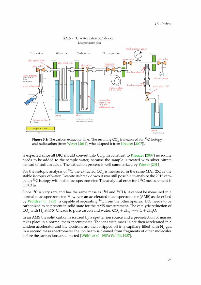
3.5 Carbon
AMS - C water extraction device14
magnetic stirrer
Erlenmeyer flask(500ml)
9 mm1/2"
Ultra-Torr adapter 1
glass valve
9 mm9 mm
20 mm 30 mm
170 mm
170 mm
9 mm
glass valveholding holding
vakuum pump
holding
90 mm
outer d. 18 mm
50 mm
glass spher. jointglass spher. joint
9 mm
Ultra-Torr adapter 21/2"
1/2"
1/2"
glass valve
Extraction
plastic capillaryi.d. 0.28 mm
3 directionglass valve
glass capillarylength 60 cmi.d. 1 mmwall thickness 3 mm
dewar(during extraction: liquid nitrogen
during transfer: acetone and dry ice)
dewar(acetone and dry ice)
dewar(liquid nitrogen)
glass capillarywith plasticinlayi.d. 0.2mm
glass valves
Pirani pressure gauge
Diagrammatic plan
Water trap Carbon trap Flux regulation
glass spher. joint glass valve 1/2“
Figure 3.1: The carbon extraction line. The resulting CO2 is measured for 13C isotopyand radiocarbon (from Wieser [2011], who adapted it from Kreuzer [2007]).
is expected since all DIC should convert into CO2. In constrast to Kreuzer [2007] no iodineneeds to be added to the sample water, because the sample is treated with silver nitrateinstead of sodium acide. The extraction process is well summarized by Wieser [2011].
For the isotopic analysis of 13C the extracted CO2 is measured in the same MAT 252 as thestable isotopes of water. Despite its break down it was still possible to analyze the 2012 cam-paign 13C isotopy with this mass spectrometer. The analytical error for δ13C measurement is±0.03 h.
Since 14C is very rare and has the same mass as 14N and 12CH2 it cannot be measured in anormal mass spectrometer. However, an accelerated mass spectrometer (AMS) as describedby Wölfli et al. [1983] is capable of separating 14C from the other species. DIC needs to becarbonized to be present in solid state for the AMS measurement. The catalytic reduction ofCO2 with H2 at 575 ◦C leads to pure carbon and water: CO2 + 2H2 −−→ C + 2H2O.
In an AMS the solid carbon is ionized by a sputter ion source and a pre-selection of massestakes place in a normal mass spectrometer. The ions with mass 14 are then accelerated in atandem accelerator and the electrons are then stripped off in a capillary filled with N2 gas.In a second mass spectrometer the ion beam is cleaned from fragments of other moleculesbefore the carbon ions are detected [Wölfli et al., 1983; Wölfli, 1987].
39

3 Methods
3.6 Noble gases
3.6.1 Mass spectrometer
Noble gas samples are analyzed on a MM 5400 mass spectrometer from GV Instruments(Manchester, UK, today Thermo Fisher, Waltham, Massachusetts) at the IUP, which is opti-mized for measuring noble gases in static mode. This sector field spectrometer is describedin detail by Friedrich [2007].
Samples are processed in several stages. First the sample water is degassed and dried fromwater vapor in a trap filled with zeolith granules with 3 Å pore diameter. Argon, kryptonand xenon as well as the permanent gases are frozen to a stainless steel trap (SST) at 25 K(compare Lott [2001]), while helium and neon are adsorbed on an activated charcoal trap(ACT) at 10 K.
Because the noble gases are analyzed one after another they are separated from each otherby exploiting their different freezing points. First, He is released by heating the ACT to 42 K.Because He concentrations in samples can differ by several orders of magnitude, the gasamount is checked in a quadrupole mass spectrometer and diluted until a concentration isreached which the detectors of the MM 5400 can handle. While measuring He, Ne is releasedat 140 K and experiences the same procedure. In the meanwhile the Kr and Xe from the SSTare being separated from Ar and the permanent gases. They are measured in the order Xe,Kr, and Ar last. Before each single analysis the detectors are tested for short-time sensitivityfluctuations by measuring a small gas amount from a (almost) pure gas reservoir. Theseso-called fastcals are analysized in exactly the same way as the samples.
The initial extraction and preparation procedure is explained in detail by Friedrich [2007],further improvements are given by Wieser [2011]. In the following I will describe only theprogress in the preparation and analysis procedures compared to Wieser [2011].
Samples up to run 62 (see appendix A.6 for an overview of all measurement runs) are ana-lyzed with the “interim procedure” described in Wieser [2011]. However, as a minor changein run 60 to reduce to measurement time span the amount of measuring points of Xe is re-duced to 15, each lasting 23 s (before it was 21 times 23 s) and of Kr from 27 times 2 s to 22times 2 s. At the same time the 4He analysis is slightly modified: Hitherto one data pointfor 4He was recorded, then the 3He measurement was done and last another seven points of4He were recorded. Due to the good reproducibility of 4He the first 4He data point is nowomitted.
In run 62 the Kr analysis procedure is optimized again to consists of 15 data points of15 s each. This prolongs the duration but reduces to measurement error significantly fromaround 1.9 % in run 60 to 1.3 % in run 62. Also the He procedure is optimized for 3He analysisto obtain better 3He-3H dating and 3He/4He ratios. While both He isotopes were analyzedat the same time before, from now on 3He is analyzed first and a small gas portion is retainedin a volume close to the inlet of the mass spectrometer and analyzed in a second inlet stepfor 4He. This eliminates the possibility to obtain 3He/4He ratios from the mass spec data
40

3.6 Noble gases
directly but facilitates to analyze bigger 3He amounts since the He splitting threshold canbe increased. This results in a slightly better 3He resolution especially for samples whichcontain a lot 4He and need to be split up.
The method described by [Stanley et al., 2009] which prevents the trapping of He and Nein the matrix of frozen gases on the SST is introduced in run 65. As in the previous routineall degassed gases are transmitted to the SST for 20 min. Before opening the ACT the SST isclosed completely and heated to 60 K and then re-cooled to 25 K. After this step the ACT isopened for 20 min to separate He and Ne from the heavy noble gases.
The Stanley procedure is modified in run 71 by opening the ACT for 5 min after the 20 minfreezing to the SST. Then the SST is closed and heated as described above. This modificationaims at hindering He and Ne to be trapped in the matrix of frozen gases in the re-coolingSST again by transporting most of the light gases into the ACT beforehand.
3.6.2 Data evaluation
The noble gas data evaluation aims at calculating the individual noble gas amounts of asample from the measured signals (a voltage in case of the faraday cup detector and countsper second in case of the electron multiplier detector). This is done by comparing the mea-sured signal of the sample with the signal of a known calibration gas standard. Due to a gasamount dependent signal strength of the detectors a nonlinearity correction has to be done.Therefore, calibration gas amounts of different sizes, usually between 0.2 and 5 cm3, are mea-sured to cover the gas amount range of all noble gases in the analyzed samples1. To accountfor short time detector sensitivity fluctuations a so-called fastcal measurement is performeddirectly before each single measurement to test the detector as well as prepare it for the com-ing measurement. The detected signal of a sample or a calibration is considered in relationof these fastcals signals. Sample and calibration signals are corrected for background sig-nal which is derived from blank analyses. An in-depth description of the measurement andanalysis process is found in [Friedrich, 2007].
The software WUCEM, written by Michael Jung from our group, simplifies the data evalu-ation in comparison to the formerly used WINCALC and CALC54002. In the first windowof the program the raw data from the spectrometer is checked and outliers are deleted. Incase of the 3He, Kr and to a minor extent also the Xe multiplier measurement occasionallyshow a sensitivity adjustment in the first few data points, before a linear decay is visible(compare figure 3.2). This usually happens at high count rates. These first points are deletedas well. A little instability of the faraday detector is observed frequently in the neon and 4Hemeasurements for which no explanation is found so far (see figure 3.3).
For each single fastcal and sample/calibration measurement a linear fit is set to the datapoints to extract the signal at the time of the gas inlet, i. e. at T = 0 s. WUCEM is also capable
1The gas pressure in the calibration gas vessel is about 1 atm in the beginning, as it is filled with atmosphericair at the air pressure present in the moment of filling. Each gas amount taken from this reservoir is regardedby the measurement software Prepline5400; therefore the gas pressure in the vessel is known at every time.From time to time the vessel has to be refilled.
2Wucem is an acronym for the German phrase Wincalc- und Calc5400-Ersatz von Michael.
41

3 Methods
Figure 3.2: Especially at higher count rates the multiplier detector needs some time toadapt to it. The first signal points are hence systematically too low and are deleted (redcircles on the left side).
of calculating isotope ratios from the raw data. Several routines are implemented in WUCEM,two of them are applied to the Jordan samples: "next neighbors" interpolates a value betweentwo data points of isotope 1 and determines the ratio to the data point, measured in between,of isotope 2 at the same position, and vice versa (used for the calculation of the 20Ne/22Neratio). "mean of isotope 1" relates all data points of isotope two to a linear fit through theisotope 1 data points. This routine is applied when the data points are not recorded in analternating way, but with a pattern like first some data points of isotope 1, then some pointsof isotope 2, again some point of isotope 1 and so on. This is the case of the 3He/4He ratio(up to run 60) and the 40Ar/36Ar. Finally one gets a ratio distribution for each isotope ratio,which is fitted by a constant fit (despite Ne ratios show a trend sometimes).
Usually each measurement is corrected with its own fastcal. If for any reasons the fastcalmeasurement has not worked, WUCEM offers several methods to handle this issue. In an-other window all fastcals are plotted against time and are fitted with different polynomials.For a specific measurement the fastcal correction can be changed. However, in the scope ofthis work all measured fastcals are suitable.
42

3.6 Noble gases
Figure 3.3: Occationally the faraday cup detector shows some instabilities, which oftenexpress in two branches. In case of the neon measurements these instabilities can usuallybe observed in both isotopes. This can sometimes help to decide which branch is morelikely to be the correct one. If this does not work all data points are considered for thefit.
Since there is no fastcal for argon, artificial fastcal are assembled in a way that the temporaltrend in the argon calibrations (due to the dilution of the calibration gas reservoir) is bal-anced out. In most measurement runs a correction with a linear trned of the artificial fastcalsis sufficient. Only Run 65 needed a second order function fitted through the artificial fastcalsto correct for the reservoir dilution effect.
In the next WUCEM window the blanks are plotted. Outstanding high blank values can usu-ally be attributed to leakage and are excluded from the further analysis. The average of allremaining blank measurements (i. e. a constant fit) is taken for the background correction.
The last step of the WUCEM analysis is to calculate the gas amounts in a sample by com-paring the measured signals to signals of aliquots of the known standard gas. The samples(vertical blue lines in figure 3.4) spread over the calibrations’ distribution and the amount ofthe respective isotope is calculated by comparing the fastcal corrected signal with a polyno-mial fit function laid through the calibrations.
43
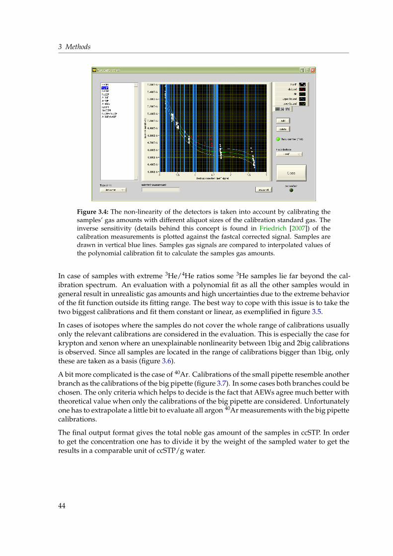
3 Methods
Figure 3.4: The non-linearity of the detectors is taken into account by calibrating thesamples’ gas amounts with different aliquot sizes of the calibration standard gas. Theinverse sensitivity (details behind this concept is found in Friedrich [2007]) of thecalibration measurements is plotted against the fastcal corrected signal. Samples aredrawn in vertical blue lines. Samples gas signals are compared to interpolated values ofthe polynomial calibration fit to calculate the samples gas amounts.
In case of samples with extreme 3He/4He ratios some 3He samples lie far beyond the cal-ibration spectrum. An evaluation with a polynomial fit as all the other samples would ingeneral result in unrealistic gas amounts and high uncertainties due to the extreme behaviorof the fit function outside its fitting range. The best way to cope with this issue is to take thetwo biggest calibrations and fit them constant or linear, as exemplified in figure 3.5.
In cases of isotopes where the samples do not cover the whole range of calibrations usuallyonly the relevant calibrations are considered in the evaluation. This is especially the case forkrypton and xenon where an unexplainable nonlinearity between 1big and 2big calibrationsis observed. Since all samples are located in the range of calibrations bigger than 1big, onlythese are taken as a basis (figure 3.6).
A bit more complicated is the case of 40Ar. Calibrations of the small pipette resemble anotherbranch as the calibrations of the big pipette (figure 3.7). In some cases both branches could bechosen. The only criteria which helps to decide is the fact that AEWs agree much better withtheoretical value when only the calibrations of the big pipette are considered. Unfortunatelyone has to extrapolate a little bit to evaluate all argon 40Ar measurements with the big pipettecalibrations.
The final output format gives the total noble gas amount of the samples in ccSTP. In orderto get the concentration one has to divide it by the weight of the sampled water to get theresults in a comparable unit of ccSTP/g water.
44

3.6 Noble gases
Figure 3.5: In cases of 3He concentration falling outside the range covered by thedifferent calibration sizes, a constant or linear fit is applied using the biggest cals.
Figure 3.6: Xenon exhibits a strongly nonlinear behavior. As all samples, except stronglydegassed ones, match calibrations bigger than 1big, only those calibrations are consid-ered in the evaluation of xenon.
45

3 Methods
Figure 3.7: Ar calibrations of small and big pipettes form two different branches. BecauseAr concentration of AEWs agree much better with theoretical values when evaluatedwith the lower branch (i. e. the calibrations from big pipettes) this one is chosen for theinterpretation of all samples.
3.6.3 Evaluation of diffusion samplers
While the WUCEM output for water samples directly gives the gas concentration in ccSTP/gwater, the gas content of diffusion samplers is only an image of the concentration in waterand, thus, needs to be converted [Wieser, 2006]. Starting from the noble gas amount in ccSTP,νi, the molar amount ni of the noble gas i is calculated:
ni =νi
Vmol, (3.1)
with Vmol = 22 414 cm3 being the molar Volume. By use of the ideal gas law the molaramount is converted into the partial pressure pi as it prevailed in the sampler at time ofsampling:
pi = ni · R · TVS
. (3.2)
The volume of the sampler, VS, is calculated from its length l: VS = 0.13583 · l − 0.12284[Wieser, 2006]. R = 83.1446 is the universal gas constant in units of cm3 atm mol−1 K−1.T denotes the ambient temperature during equilibration of the diffusion sampler. As thisquantity was not accessible at the sampling spots, a temperature of 20 ◦C is assumed forthe shallow wells in Azraq (≈ the average annual temperature). In the deep boreholes acommon geothermal gradient of 3 K per 100 m is assumed.
According to the solubility equations of Weiss [1970, 1971],Weiss and Kyser [1978] and Clever[1979b] the noble gas concentrations in ccSTP/cm3 of the water surrounding the diffusionsamplers is calculated by
CiccSTPcm3
= βi(T, S) · pi. (3.3)
46

3.6 Noble gases
The solubility of gas i is represented by the Bunsen coefficient βi(T, S), which is dependenton temperature T and salinity S and is calculated with equations A.1 and A.2 in the abovementioned publications.
The final step to compare noble gas concentrations from diffusion samplers with normalwater samples is to convert the concentrations in ccSTP/cm3 into ccSTP/g water using thedensity correlation found by Gill [1982]:
CiccSTP
g= Ci
ccSTPcm3· 1000 cm3 L−1
ρ(T, S), (3.4)
with ρ(T, S) being the density of water in dependence of temperature, T, and salinity, S.
3.6.4 Fitting noble gas temperatures
In order to compute noble gas temperatures (NGTs), first the total amount of each noble gashas to be calculated. Total Ne is received by dividing the sum of the concentrations of 20Neand 22Ne by a factor of 0.9973, which corresponds their molar abundance. Total atmosphericAr is usually calculated in the same way by taking the sum of 36Ar and 40Ar, divided by thefactor 0.999364. Only in cases of very old water, i. e. when the ratio 40Ar/36Ar deviates from295.5, atmospheric Ar is calculated from 36Ar only, using a factor of 0.003364. The latter caseis applied when the 40Ar/36Ar ratio of a sample is higher than 302. Total Kr results from 84Krby division with 0.57 and total Xe from 132Xe using a factor of 0.2689. Helium is omitted inthe NGT analysis due to its non-atmospheric component.
Noble gas temperature (NGT) fitting is performed by inverse modeling [Ballentine and Hall,1999; Aeschbach-Hertig et al., 1999], using a weighted least-square routine, with the softwarePANGA written by Michael Jung (a short description is given in Jung [2013], the correspond-ing paper is in preparation). The fitting routine uses a Levenberg-Marquardt least squarealgorithm [Levenberg, 1944; Marquardt, 1963] to inverse fit model parameters of severalexcess air models to measured data. The tool is also capable of performing Monte Carlo cal-culations. In cases of difficulties to fit the excess air model parameters to the measured noblegas concentrations the Monte Carlo method offers the chance to achieve better fit results aswell as enables one to trace the reason of fitting problems [Jung et al., 2013]. The basis ofthe Monte Carlo algorithm is to vary measured noble gas concentrations randomly withintheir error margins and perform a fit with each concentration combination. In many casesthis helps to find “reasonable” fitting results (i. e. concentration combinations) and evaluatea sample which does not deliver a sound combination of the fitting parameters temperatureT, excess air A and other parameters of the respective excess air model in the normal fittingroutine. Since inverse fitting especially of the CE model bears some risk of unreasonableconvergence, the Monte Carlo routine can be of great benefit for the analysis of groundwatersamples.
The goodness of fit is described by its χ2 value, which is defined as the sum over all input pa-rameter i (i. e. the noble gas concentrations, usually neon, argon, krypton and xenon) of the
47

3 Methods
MAS_21
T [
°C]
10
11
12
13
14
Counts
0
20
40
60
80
100
A [ccSTP/g]0.2 0.4 0.6 0.8 1
Zeeghan 14
T [
°C]
22
22.5
23
23.5
24
Counts
0
20
40
60
80
100
120
F-2,000 -1,500 -1,000 -500 0
Figure 3.8: Examples of the limiting cases of the CE model described in the text. Theleft graph shows a MC analysis, where one part of the simulations resulted in low Aand a lower NGT, and a second fraction with higher temperature, but unrealisticallyhigh excess air values. The latter block is therefore rejected in a MC analysis. Theexample on the right exhibits a small fraction of simulations with F values close to zero,and another one around F = −2000. The latter belong to MC simulations where F · Abecomes neglectible small and is considered a quasi-UA case. However, the resultingnoble gas temperatures are almost the same.
squared, error weighted deviations of the modeled to the measured noble gas concentrationsCi,
χ2 = ∑i
(Cmod
i − Cmeasi
σi
)2
(3.5)
where σi is the standard deviation of the measured noble gas concentration. In case of aGaussian error distribution and if the free model parameter (T, A and F in case of the CEmodel) are independent, the estimated value of χ2 is the same as the degrees of freedom[Aeschbach-Hertig et al., 1999], i. e. equals one in case of the CE model (four input noble gasconcentrations and three model parameters). χ2 values higher than the degrees of freedomare indicative of collinearities between the model parameters, which worsen the goodnessof fit [Oehsen von, 2008]. Very low χ2 may be a result of overestimation or correlation ofexperimental errors or of overparametrisation in the context of the small number of degreesof freedom of these calculations [Aeschbach-Hertig et al., 1999].
As Jung et al. [2013] found, the Monte Carlo simulations of the CE model sometimes exhibitstwo mathematically possible solution: Reasonable parameter combination with A < 0.1 anda solution for higher A, accompanied by higher noble gas temperatures (compare the leftdiagram in figure 3.8). The latter, unrealistic solution is attributed to the limiting case of largeA, where the CE model transforms into a pure OD model (i. e. only an excess in pressure,but no excess air). Monte Carlo simulations of this kind are discarded in the analysis of therespective samples.
Another limiting case of the CE model parametrization revealed by Monte Carlo calculationsappears for extremely small values of A, accompanied by large values of F (with positive or
48

3.7 Radon
negative sign). When the product of A and F becomes very small, the CE model transformsinto a quasi-UA model:
limFA→0
[Ceq
i
(1 +
(1− F)AHi
1 + FAHi
)]= lim
FA→0
[Ceq
i
(1 +
AHi − FAHi
1 + FAHi
)]= Ceq
i (1 + AHi). (3.6)
Despite the fact that F gains unphysical values, in combination with the tiny A values theMonte Carlo results in such cases yield reasonable solutions for the temperature T and cantherefore be trusted. An example is shown in the right panel of figure 3.8. A paper aboutthis phenomenon is in preparation by M. Jung.
3.7 Radon
Radon samples were measured in the evening or the next morning after a sampling day.The used RAD7 (Durridge, Billerica, Massachusetts, USA) radon detector is only capableof detecting alpha decays in a gas phase. Therefore, the water sample has to be degassedusing a glass frit (compare figure 3.9). The gas phase is dried by a Drierite cartridge (W.A. Hammond DRIERITE Co. LTD, Xenia, Ohio, USA) below 10 % relative humidity, theworking range of the RAD7. A detailed description of the RAD7 device is found in Durridge[2000], the extraction setup RAD-H2O is treated in Durridge [2001], Kluge et al. [2007] andReichel [2009].
Instead of counting the radon-222 decays directly the RAD7 alpha spectrometer detects thedisintegration of its daughter nucleus polonium-218. In a closed system the activities ofradon-222 and polonium-218 are in secular equilibrium after about 20 minutes. Thus, beforeeach run a 20 min equilibration cycle is performed. To account for background radiation ameasurement with an empty sample bottle is done. Due to limited time in the evenings oftenthe background determination of the first and sometimes more analyses was omitted. In caseof the first samples of a day the background is defined as the average background signal ofall other background measurements that are recorded before the first sample analysis of therespective day. As the background error the maximum of these background measurementsis assumed. The same background values are assumed for samples which are measuredafter a low-signal analysis (Zarqa Ma’in 1 and 2 and Wadi Ibn Hammat 2). In case of theAWSA 16 and the Zeeghan 15-1 sample the preceding Radon signal is significantly higherand, thus, the average of the background signals of Wadi Ibn Hammat 1 and Manshiyeh 1 isassumed as they are measured after samples of comparable background signal. The result-ing error is about twice as high as for the first-of-the-day samples but still ≈ 0 within theerror margins.
When the water temperature is higher than the surrounding temperature, small air bubblesform inside the radon sampling bottles due to contraction of the water with lower temper-atures. This causes a little loss of radon when the bottle is connected to the RAD7 instru-ment.
49

3 Methods
RAD7
drierite
filter
checkvalve
temp.sensor
glass fritwatersample
Figure 3.9: Setup of radon analysis with the RAD7 radon alpha detector. From Wieser[2011].
The background corrected activity in the gas phase, Agas, is converted into the activity in thewater sample at the time of analysis, Awater, by
Awater = Agas ·(
Vgas
Vwater+ a(T)
)· KS, (3.7)
with Vwater being the water sample volume ((242.44± 0.06)mL due to displacement of somewater by the glass frit), Vgas the volume of the gas circuit (1720.0± 5.5)mL and a(T) theOstwald solubility a(T) = 0.105+ 0.405 · exp(−0.0502 · T) [Weigel, 1978], and KS the relativesolubility correction due to salinity according to Clever [1979b], compare appendix A.1. Ex-cept of the Zeeghan samples, where the salinity correction is around 7 %, the salt influenceis negligible small.
The water temperature of the sample during measurement, T, has not been recorded and isconsidered to be (15± 5) ◦C. This temperature range implies all possible ambient temper-atures and, thus, sample temperatures at the time of analysis. The influence of the sampletemperature at the time of analysis is less than 1 % for the assumed error of ±5 ◦C and hencemuch smaller than the statistical error of the measurement. To get the radon activity at thetime of sampling, the calculated activity is finally corrected by the radioactive decay law.
50

4 Geographical and geological setting
4.1 Jordan and its water situation
Jordan, officially the Hashemite Kingdom of Jordan, is situated in the north-western part ofthe Arabian peninsula. It is bordered by Israel and the Westbank in the west, Syria in thenorth, Iraq in the east and Saudi Arabia in the south and southeast. Jordan can be dividedfrom west to east into three major landscapes: The Jordan Rift Valley, the Jordan Highlandsand the eastern deserts [Margane et al., 2002].
The Jordan Rift Valley stretches from the depression of Lake Tiberias (Sea of Galilee) in thenorth to the Gulf of Aqaba in the south. The deepest point of the rift valley is occupied bythe Dead Sea, its coast forming the deepest surface area of the world, currently about 423 mbelow sea level. The part between Lake Tiberias and the Dead Sea is called the Jordan Valley,the most fertile and, hence, most heavily tilled stripe of land in Jordan. South of the DeadSea the rift valley continues under the name Wadi Arava.
Along the rift valley’s eastern side a mountain range ascends, the Jordan Highlands. Theyelevate up to 1600 m and consist of several plateaus, separated by deeply cut wadis (valleysthat often carry water only seasonal).
Beyond the mountain range the landscape dips gently towards the east and forms the east-ern desert. Different outcropping lithology forms varying stone desert types, only in the verysouth some sand dunes are found. Large parts in the north are covered by a thick basaltshield called Harrat ash-Shaam originating from the extinct volcano Jabal ad-Druze in Syria.Just bordering the basalt desert, about 100 km east of the capital, the former oasis al-Azraqforms the center of the Azraq-Wadi Sirhan depression, which stretches in southeastern di-rection into Saudi Arabia. The picturesque landscape of the mountains of Tubeiq and WadiRam with its bizarre sandstone formations on top of the granite bedrock reaching up to600 m above the surrounding plain forms the border region to Saudi Arabia.
Jordan has three perennial rivers. The Jordan River flows from Lake Tiberias into the DeadSea, forming the border between Jordan and Israel, respectively the West Bank. The YarmoukRiver originates from Jabal ad-Druze in Syria and is the border between Syria and Jordandownstream. The Yarmouk is the main tributary to the Jordan River. The Zarqa River em-anates northeast of Amman and feeds the Jordan River as well. Some small streams in sidewadis of the Jordan Valley are fed by perennial springs, but they do not contribute signif-icantly to the Jordan water budget. A lot more rivers and streams exist throughout thecountry, but they are active only during the rainy winter season.
51

4 Geographical and geological setting
AqabaAqabaAqabaAqabaAqabaAqabaAqabaAqabaAqabaAqabaAqabaAqabaAqabaAqabaAqabaAqabaAqabaAqabaAqabaAqabaAqabaAqabaAqabaAqabaAqabaAqabaAqabaAqabaAqabaAqabaAqabaAqabaAqabaAqabaAqabaAqabaAqabaAqabaAqabaAqabaAqabaAqabaAqabaAqabaAqabaAqabaAqabaAqabaAqabaAqabaAqabaAqabaAqabaAqabaAqabaAqabaAqabaAqabaAqabaAqabaAqabaAqabaAqabaAqabaAqabaAqabaAqabaAqabaAqabaAqabaAqabaAqabaAqabaAqabaAqabaAqabaAqabaAqabaAqabaAqabaAqabaAqabaAqabaAqabaAqabaAqabaAqabaAqabaAqabaAqabaAqabaAqabaAqabaAqabaAqabaAqabaAqabaAqabaAqabaAqabaAqabaAqabaAqabaAqabaAqabaAqabaAqabaAqabaAqabaAqabaAqabaAqabaAqabaAqabaAqabaAqabaAqabaAqabaAqabaAqabaAqabaAqabaAqabaAqabaAqabaAqabaAqabaAqabaAqabaAqabaAqabaAqabaAqabaAqabaAqabaAqabaAqabaAqabaAqabaAqabaAqabaAqabaAqabaAqabaAqabaAqabaAqabaAqabaAqabaAqabaAqabaAqabaAqabaAqabaAqabaAqabaAqabaAqabaAqabaAqabaAqabaAqabaAqabaAqabaAqabaAqabaAqabaAqabaAqabaAqabaAqabaAqabaAqabaAqabaAqabaAqabaAqabaAqabaAqabaAqabaAqabaAqabaAqabaAqabaAqabaAqabaAqabaAqabaAqabaAqabaAqabaAqabaAqabaAqabaAqabaAqabaAqabaAqabaAqabaAqabaAqabaAqabaAqabaAqabaAqabaAqabaAqabaAqabaAqabaAqabaAqabaAqabaAqabaAqabaAqabaAqabaAqabaAqabaAqabaAqabaAqabaAqabaAqabaAqabaAqabaAqabaAqabaAqabaAqabaAqabaAqabaAqabaAqabaAqabaAqabaAqabaAqabaAqabaAqabaAqabaAqabaAqabaAqabaAqabaAqabaAqabaAqabaAqabaAqabaAqabaAqabaAqabaAqabaAqabaAqabaAqabaAqabaAqabaAqabaAqabaAqabaAqabaAqabaAqabaAqabaAqabaAqabaAqabaAqabaAqabaAqabaAqabaAqabaAqabaAqabaAqabaAqabaAqabaAqabaAqabaAqabaAqabaAqabaAqabaAqabaAqabaAqabaAqabaAqabaAqabaAqabaAqabaAqabaAqabaAqabaAqabaAqabaAqabaAqabaAqabaAqabaAqabaAqabaAqabaAqabaAqabaAqabaAqabaAqabaAqabaAqabaAqabaAqabaAqabaAqabaAqabaAqabaAqabaAqabaAqabaAqabaAqabaAqabaAqabaAqabaAqabaAqabaAqabaAqabaAqabaAqabaAqabaAqabaAqabaAqabaAqabaAqabaAqabaAqabaAqabaAqabaAqabaAqabaAqabaAqabaAqabaAqabaAqabaAqabaAqabaAqabaAqabaAqabaAqabaAqabaAqabaAqabaAqabaAqabaAqabaAqabaAqabaAqabaAqabaAqabaAqabaAqabaAqabaAqabaAqabaAqabaAqabaAqabaAqabaAqabaAqabaAqabaAqabaAqabaAqabaAqabaAqabaAqabaAqabaAqabaAqabaAqabaAqabaAqabaAqabaAqabaAqabaAqabaAqabaAqabaAqabaAqabaAqabaAqabaAqabaAqaba
KarakKarakKarakKarakKarakKarakKarakKarakKarakKarakKarakKarakKarakKarakKarakKarakKarakKarakKarakKarakKarakKarakKarakKarakKarakKarakKarakKarakKarakKarakKarakKarakKarakKarakKarakKarakKarakKarakKarakKarakKarakKarakKarakKarakKarakKarakKarakKarakKarakKarakKarakKarakKarakKarakKarakKarakKarakKarakKarakKarakKarakKarakKarakKarakKarakKarakKarakKarakKarakKarakKarakKarakKarakKarakKarakKarakKarakKarakKarakKarakKarakKarakKarakKarakKarakKarakKarakKarakKarakKarakKarakKarakKarakKarakKarakKarakKarakKarakKarakKarakKarakKarakKarakKarakKarakKarakKarakKarakKarakKarakKarakKarakKarakKarakKarakKarakKarakKarakKarakKarakKarakKarakKarakKarakKarakKarakKarakKarakKarakKarakKarakKarakKarakKarakKarakKarakKarakKarakKarakKarakKarakKarakKarakKarakKarakKarakKarakKarakKarakKarakKarakKarakKarakKarakKarakKarakKarakKarakKarakKarakKarakKarakKarakKarakKarakKarakKarakKarakKarakKarakKarakKarakKarakKarakKarakKarakKarakKarakKarakKarakKarakKarakKarakKarakKarakKarakKarakKarakKarakKarakKarakKarakKarakKarakKarakKarakKarakKarakKarakKarakKarakKarakKarakKarakKarakKarakKarakKarakKarakKarakKarakKarakKarakKarakKarakKarakKarakKarakKarakKarakKarakKarakKarakKarakKarakKarakKarakKarakKarakKarakKarakKarakKarakKarakKarakKarakKarakKarakKarakKarakKarakKarakKarakKarakKarakKarakKarakKarakKarakKarakKarakKarakKarakKarakKarakKarakKarakKarakKarakKarakKarakKarakKarakKarakKarakKarakKarakKarakKarakKarakKarakKarakKarakKarakKarakKarakKarakKarakKarakKarakKarakKarakKarakKarakKarakKarakKarakKarakKarakKarakKarakKarakKarakKarakKarakKarakKarakKarakKarakKarakKarakKarakKarakKarakKarakKarakKarakKarakKarakKarakKarakKarakKarakKarakKarakKarakKarakKarakKarakKarakKarakKarakKarakKarakKarakKarakKarakKarakKarakKarakKarakKarakKarakKarakKarakKarakKarakKarakKarakKarakKarakKarakKarakKarakKarakKarakKarakKarakKarakKarakKarakKarakKarakKarakKarakKarakKarakKarakKarakKarakKarakKarakKarakKarakKarakKarakKarakKarakKarakKarakKarakKarakKarakKarakKarakKarakKarakKarakKarakKarakKarakKarakKarakKarakKarakKarakKarakKarakKarakKarakKarakKarakKarakKarakKarakKarakKarakKarakKarakKarakKarak
MafraqMafraqMafraqMafraqMafraqMafraqMafraqMafraqMafraqMafraqMafraqMafraqMafraqMafraqMafraqMafraqMafraqMafraqMafraqMafraqMafraqMafraqMafraqMafraqMafraqMafraqMafraqMafraqMafraqMafraqMafraqMafraqMafraqMafraqMafraqMafraqMafraqMafraqMafraqMafraqMafraqMafraqMafraqMafraqMafraqMafraqMafraqMafraqMafraqMafraqMafraqMafraqMafraqMafraqMafraqMafraqMafraqMafraqMafraqMafraqMafraqMafraqMafraqMafraqMafraqMafraqMafraqMafraqMafraqMafraqMafraqMafraqMafraqMafraqMafraqMafraqMafraqMafraqMafraqMafraqMafraqMafraqMafraqMafraqMafraqMafraqMafraqMafraqMafraqMafraqMafraqMafraqMafraqMafraqMafraqMafraqMafraqMafraqMafraqMafraqMafraqMafraqMafraqMafraqMafraqMafraqMafraqMafraqMafraqMafraqMafraqMafraqMafraqMafraqMafraqMafraqMafraqMafraqMafraqMafraqMafraqMafraqMafraqMafraqMafraqMafraqMafraqMafraqMafraqMafraqMafraqMafraqMafraqMafraqMafraqMafraqMafraqMafraqMafraqMafraqMafraqMafraqMafraqMafraqMafraqMafraqMafraqMafraqMafraqMafraqMafraqMafraqMafraqMafraqMafraqMafraqMafraqMafraqMafraqMafraqMafraqMafraqMafraqMafraqMafraqMafraqMafraqMafraqMafraqMafraqMafraqMafraqMafraqMafraqMafraqMafraqMafraqMafraqMafraqMafraqMafraqMafraqMafraqMafraqMafraqMafraqMafraqMafraqMafraqMafraqMafraqMafraqMafraqMafraqMafraqMafraqMafraqMafraqMafraqMafraqMafraqMafraqMafraqMafraqMafraqMafraqMafraqMafraqMafraqMafraqMafraqMafraqMafraqMafraqMafraqMafraqMafraqMafraqMafraqMafraqMafraqMafraqMafraqMafraqMafraqMafraqMafraqMafraqMafraqMafraqMafraqMafraqMafraqMafraqMafraqMafraqMafraqMafraqMafraqMafraqMafraqMafraqMafraqMafraqMafraqMafraqMafraqMafraqMafraqMafraqMafraqMafraqMafraqMafraqMafraqMafraqMafraqMafraqMafraqMafraqMafraqMafraqMafraqMafraqMafraqMafraqMafraqMafraqMafraqMafraqMafraqMafraqMafraqMafraqMafraqMafraqMafraqMafraqMafraqMafraqMafraqMafraqMafraqMafraqMafraqMafraqMafraqMafraqMafraqMafraqMafraqMafraqMafraqMafraqMafraqMafraqMafraqMafraqMafraqMafraqMafraqMafraqMafraqMafraqMafraqMafraqMafraqMafraqMafraqMafraqMafraqMafraqMafraqMafraqMafraqMafraqMafraqMafraqMafraqMafraqMafraqMafraqMafraqMafraqMafraqMafraqMafraqMafraqMafraqMafraqMafraqMafraqMafraqMafraqMafraqMafraqMafraqMafraqMafraqMafraqMafraqMafraqMafraqMafraqMafraqMafraqMafraqMafraqMafraqMafraqMafraqMafraqMafraqMafraqMafraqMafraqMafraqMafraqMafraqMafraqMafraqMafraqMafraqMafraqMafraqMafraqMafraqMafraqMafraqMafraqMafraqMafraqMafraqMafraqMafraqMafraqMafraqMafraqMafraqMafraqMafraqMafraqMafraqMafraqMafraqMafraqMafraqMafraqMafraqMafraqMafraqMafraqMafraqMafraqMafraqMafraqMafraqMafraqMafraqMafraqMafraq
AmmanAmmanAmmanAmmanAmmanAmmanAmmanAmmanAmmanAmmanAmmanAmmanAmmanAmmanAmmanAmmanAmmanAmmanAmmanAmmanAmmanAmmanAmmanAmmanAmmanAmmanAmmanAmmanAmmanAmmanAmmanAmmanAmmanAmmanAmmanAmmanAmmanAmmanAmmanAmmanAmmanAmmanAmmanAmmanAmmanAmmanAmmanAmmanAmmanAmmanAmmanAmmanAmmanAmmanAmmanAmmanAmmanAmmanAmmanAmmanAmmanAmmanAmmanAmmanAmmanAmmanAmmanAmmanAmmanAmmanAmmanAmmanAmmanAmmanAmmanAmmanAmmanAmmanAmmanAmmanAmmanAmmanAmmanAmmanAmmanAmmanAmmanAmmanAmmanAmmanAmmanAmmanAmmanAmmanAmmanAmmanAmmanAmmanAmmanAmmanAmmanAmmanAmmanAmmanAmmanAmmanAmmanAmmanAmmanAmmanAmmanAmmanAmmanAmmanAmmanAmmanAmmanAmmanAmmanAmmanAmmanAmmanAmmanAmmanAmmanAmmanAmmanAmmanAmmanAmmanAmmanAmmanAmmanAmmanAmmanAmmanAmmanAmmanAmmanAmmanAmmanAmmanAmmanAmmanAmmanAmmanAmmanAmmanAmmanAmmanAmmanAmmanAmmanAmmanAmmanAmmanAmmanAmmanAmmanAmmanAmmanAmmanAmmanAmmanAmmanAmmanAmmanAmmanAmmanAmmanAmmanAmmanAmmanAmmanAmmanAmmanAmmanAmmanAmmanAmmanAmmanAmmanAmmanAmmanAmmanAmmanAmmanAmmanAmmanAmmanAmmanAmmanAmmanAmmanAmmanAmmanAmmanAmmanAmmanAmmanAmmanAmmanAmmanAmmanAmmanAmmanAmmanAmmanAmmanAmmanAmmanAmmanAmmanAmmanAmmanAmmanAmmanAmmanAmmanAmmanAmmanAmmanAmmanAmmanAmmanAmmanAmmanAmmanAmmanAmmanAmmanAmmanAmmanAmmanAmmanAmmanAmmanAmmanAmmanAmmanAmmanAmmanAmmanAmmanAmmanAmmanAmmanAmmanAmmanAmmanAmmanAmmanAmmanAmmanAmmanAmmanAmmanAmmanAmmanAmmanAmmanAmmanAmmanAmmanAmmanAmmanAmmanAmmanAmmanAmmanAmmanAmmanAmmanAmmanAmmanAmmanAmmanAmmanAmmanAmmanAmmanAmmanAmmanAmmanAmmanAmmanAmmanAmmanAmmanAmmanAmmanAmmanAmmanAmmanAmmanAmmanAmmanAmmanAmmanAmmanAmmanAmmanAmmanAmmanAmmanAmmanAmmanAmmanAmmanAmmanAmmanAmmanAmmanAmmanAmmanAmmanAmmanAmmanAmmanAmmanAmmanAmmanAmmanAmmanAmmanAmmanAmmanAmmanAmmanAmmanAmmanAmmanAmmanAmmanAmmanAmmanAmmanAmmanAmmanAmmanAmmanAmmanAmmanAmmanAmmanAmmanAmmanAmmanAmmanAmmanAmmanAmmanAmmanAmmanAmmanAmmanAmmanAmmanAmmanAmmanAmmanAmmanAmmanAmmanAmmanAmmanAmmanAmmanAmmanAmmanAmmanAmmanAmmanAmmanAmmanAmmanAmmanAmmanAmmanAmmanAmmanAmmanAmmanAmmanAmmanAmmanAmmanAmmanAmmanAmmanAmmanAmmanAmmanAmmanAmmanAmmanAmmanAmmanAmmanAmmanAmman
SafawiSafawiSafawiSafawiSafawiSafawiSafawiSafawiSafawiSafawiSafawiSafawiSafawiSafawiSafawiSafawiSafawiSafawiSafawiSafawiSafawiSafawiSafawiSafawiSafawiSafawiSafawiSafawiSafawiSafawiSafawiSafawiSafawiSafawiSafawiSafawiSafawiSafawiSafawiSafawiSafawiSafawiSafawiSafawiSafawiSafawiSafawiSafawiSafawiSafawiSafawiSafawiSafawiSafawiSafawiSafawiSafawiSafawiSafawiSafawiSafawiSafawiSafawiSafawiSafawiSafawiSafawiSafawiSafawiSafawiSafawiSafawiSafawiSafawiSafawiSafawiSafawiSafawiSafawiSafawiSafawiSafawiSafawiSafawiSafawiSafawiSafawiSafawiSafawiSafawiSafawiSafawiSafawiSafawiSafawiSafawiSafawiSafawiSafawiSafawiSafawiSafawiSafawiSafawiSafawiSafawiSafawiSafawiSafawiSafawiSafawiSafawiSafawiSafawiSafawiSafawiSafawiSafawiSafawiSafawiSafawiSafawiSafawiSafawiSafawiSafawiSafawiSafawiSafawiSafawiSafawiSafawiSafawiSafawiSafawiSafawiSafawiSafawiSafawiSafawiSafawiSafawiSafawiSafawiSafawiSafawiSafawiSafawiSafawiSafawiSafawiSafawiSafawiSafawiSafawiSafawiSafawiSafawiSafawiSafawiSafawiSafawiSafawiSafawiSafawiSafawiSafawiSafawiSafawiSafawiSafawiSafawiSafawiSafawiSafawiSafawiSafawiSafawiSafawiSafawiSafawiSafawiSafawiSafawiSafawiSafawiSafawiSafawiSafawiSafawiSafawiSafawiSafawiSafawiSafawiSafawiSafawiSafawiSafawiSafawiSafawiSafawiSafawiSafawiSafawiSafawiSafawiSafawiSafawiSafawiSafawiSafawiSafawiSafawiSafawiSafawiSafawiSafawiSafawiSafawiSafawiSafawiSafawiSafawiSafawiSafawiSafawiSafawiSafawiSafawiSafawiSafawiSafawiSafawiSafawiSafawiSafawiSafawiSafawiSafawiSafawiSafawiSafawiSafawiSafawiSafawiSafawiSafawiSafawiSafawiSafawiSafawiSafawiSafawiSafawiSafawiSafawiSafawiSafawiSafawiSafawiSafawiSafawiSafawiSafawiSafawiSafawiSafawiSafawiSafawiSafawiSafawiSafawiSafawiSafawiSafawiSafawiSafawiSafawiSafawiSafawiSafawiSafawiSafawiSafawiSafawiSafawiSafawiSafawiSafawiSafawiSafawiSafawiSafawiSafawiSafawiSafawiSafawiSafawiSafawiSafawiSafawiSafawiSafawiSafawiSafawiSafawiSafawiSafawiSafawiSafawiSafawiSafawiSafawiSafawiSafawiSafawiSafawiSafawiSafawiSafawiSafawiSafawiSafawiSafawiSafawiSafawiSafawiSafawiSafawiSafawiSafawiSafawiSafawiSafawiSafawiSafawiSafawiSafawiSafawiSafawiSafawiSafawiSafawiSafawiSafawiSafawiSafawiSafawiSafawiSafawiSafawiSafawiSafawiSafawiSafawiSafawiSafawiSafawiSafawiSafawiSafawiSafawiSafawiSafawiSafawiSafawiSafawiSafawiSafawiSafawiSafawiSafawiSafawiSafawiSafawiSafawiSafawiSafawiSafawiSafawiSafawiSafawiSafawiSafawiSafawiSafawiSafawiSafawiSafawiSafawiSafawiSafawiSafawiSafawiSafawiSafawiSafawiSafawiSafawiSafawi
SaltSaltSaltSaltSaltSaltSaltSaltSaltSaltSaltSaltSaltSaltSaltSaltSaltSaltSaltSaltSaltSaltSaltSaltSaltSaltSaltSaltSaltSaltSaltSaltSaltSaltSaltSaltSaltSaltSaltSaltSaltSaltSaltSaltSaltSaltSaltSaltSaltSaltSaltSaltSaltSaltSaltSaltSaltSaltSaltSaltSaltSaltSaltSaltSaltSaltSaltSaltSaltSaltSaltSaltSaltSaltSaltSaltSaltSaltSaltSaltSaltSaltSaltSaltSaltSaltSaltSaltSaltSaltSaltSaltSaltSaltSaltSaltSaltSaltSaltSaltSaltSaltSaltSaltSaltSaltSaltSaltSaltSaltSaltSaltSaltSaltSaltSaltSaltSaltSaltSaltSaltSaltSaltSaltSaltSaltSaltSaltSaltSaltSaltSaltSaltSaltSaltSaltSaltSaltSaltSaltSaltSaltSaltSaltSaltSaltSaltSaltSaltSaltSaltSaltSaltSaltSaltSaltSaltSaltSaltSaltSaltSaltSaltSaltSaltSaltSaltSaltSaltSaltSaltSaltSaltSaltSaltSaltSaltSaltSaltSaltSaltSaltSaltSaltSaltSaltSaltSaltSaltSaltSaltSaltSaltSaltSaltSaltSaltSaltSaltSaltSaltSaltSaltSaltSaltSaltSaltSaltSaltSaltSaltSaltSaltSaltSaltSaltSaltSaltSaltSaltSaltSaltSaltSaltSaltSaltSaltSaltSaltSaltSaltSaltSaltSaltSaltSaltSaltSaltSaltSaltSaltSaltSaltSaltSaltSaltSaltSaltSaltSaltSaltSaltSaltSaltSaltSaltSaltSaltSaltSaltSaltSaltSaltSaltSaltSaltSaltSaltSaltSaltSaltSaltSaltSaltSaltSaltSaltSaltSaltSaltSaltSaltSaltSaltSaltSaltSaltSaltSaltSaltSaltSaltSaltSaltSaltSaltSaltSaltSaltSaltSaltSaltSaltSaltSaltSaltSaltSaltSaltSaltSaltSaltSaltSaltSaltSaltSaltSaltSaltSaltSaltSaltSaltSaltSaltSaltSaltSaltSaltSaltSaltSaltSaltSaltSaltSaltSaltSaltSaltSaltSaltSaltSaltSaltSaltSaltSaltSaltSaltSaltSaltSaltSaltSaltSaltSaltSaltSaltSaltSaltSaltSaltSaltSaltSaltSaltSaltSaltSaltSaltSaltSaltSaltSaltSaltSaltSaltSaltSaltSaltSaltSaltSaltSaltSaltSaltSaltSaltSaltSaltSaltSaltSaltSaltSaltSaltSaltSaltSaltSaltSalt
TafilahTafilahTafilahTafilahTafilahTafilahTafilahTafilahTafilahTafilahTafilahTafilahTafilahTafilahTafilahTafilahTafilahTafilahTafilahTafilahTafilahTafilahTafilahTafilahTafilahTafilahTafilahTafilahTafilahTafilahTafilahTafilahTafilahTafilahTafilahTafilahTafilahTafilahTafilahTafilahTafilahTafilahTafilahTafilahTafilahTafilahTafilahTafilahTafilahTafilahTafilahTafilahTafilahTafilahTafilahTafilahTafilahTafilahTafilahTafilahTafilahTafilahTafilahTafilahTafilahTafilahTafilahTafilahTafilahTafilahTafilahTafilahTafilahTafilahTafilahTafilahTafilahTafilahTafilahTafilahTafilahTafilahTafilahTafilahTafilahTafilahTafilahTafilahTafilahTafilahTafilahTafilahTafilahTafilahTafilahTafilahTafilahTafilahTafilahTafilahTafilahTafilahTafilahTafilahTafilahTafilahTafilahTafilahTafilahTafilahTafilahTafilahTafilahTafilahTafilahTafilahTafilahTafilahTafilahTafilahTafilahTafilahTafilahTafilahTafilahTafilahTafilahTafilahTafilahTafilahTafilahTafilahTafilahTafilahTafilahTafilahTafilahTafilahTafilahTafilahTafilahTafilahTafilahTafilahTafilahTafilahTafilahTafilahTafilahTafilahTafilahTafilahTafilahTafilahTafilahTafilahTafilahTafilahTafilahTafilahTafilahTafilahTafilahTafilahTafilahTafilahTafilahTafilahTafilahTafilahTafilahTafilahTafilahTafilahTafilahTafilahTafilahTafilahTafilahTafilahTafilahTafilahTafilahTafilahTafilahTafilahTafilahTafilahTafilahTafilahTafilahTafilahTafilahTafilahTafilahTafilahTafilahTafilahTafilahTafilahTafilahTafilahTafilahTafilahTafilahTafilahTafilahTafilahTafilahTafilahTafilahTafilahTafilahTafilahTafilahTafilahTafilahTafilahTafilahTafilahTafilahTafilahTafilahTafilahTafilahTafilahTafilahTafilahTafilahTafilahTafilahTafilahTafilahTafilahTafilahTafilahTafilahTafilahTafilahTafilahTafilahTafilahTafilahTafilahTafilahTafilahTafilahTafilahTafilahTafilahTafilahTafilahTafilahTafilahTafilahTafilahTafilahTafilahTafilahTafilahTafilahTafilahTafilahTafilahTafilahTafilahTafilahTafilahTafilahTafilahTafilahTafilahTafilahTafilahTafilahTafilahTafilahTafilahTafilahTafilahTafilahTafilahTafilahTafilahTafilahTafilahTafilahTafilahTafilahTafilahTafilahTafilahTafilahTafilahTafilahTafilahTafilahTafilahTafilahTafilahTafilahTafilahTafilahTafilahTafilahTafilahTafilahTafilahTafilahTafilahTafilahTafilahTafilahTafilahTafilahTafilahTafilahTafilahTafilahTafilahTafilahTafilahTafilahTafilahTafilahTafilahTafilahTafilahTafilahTafilahTafilahTafilahTafilahTafilahTafilahTafilahTafilahTafilahTafilahTafilahTafilahTafilahTafilahTafilahTafilahTafilahTafilahTafilahTafilahTafilahTafilahTafilahTafilahTafilahTafilahTafilahTafilahTafilahTafilahTafilahTafilahTafilahTafilahTafilahTafilahTafilahTafilahTafilahTafilahTafilahTafilahTafilahTafilahTafilahTafilahTafilahTafilahTafilahTafilahTafilahTafilahTafilahTafilahTafilahTafilahTafilahTafilahTafilahTafilahTafilahTafilahTafilahTafilahTafilahTafilahTafilahTafilahTafilahTafilahTafilahTafilah
ZarqaZarqaZarqaZarqaZarqaZarqaZarqaZarqaZarqaZarqaZarqaZarqaZarqaZarqaZarqaZarqaZarqaZarqaZarqaZarqaZarqaZarqaZarqaZarqaZarqaZarqaZarqaZarqaZarqaZarqaZarqaZarqaZarqaZarqaZarqaZarqaZarqaZarqaZarqaZarqaZarqaZarqaZarqaZarqaZarqaZarqaZarqaZarqaZarqaZarqaZarqaZarqaZarqaZarqaZarqaZarqaZarqaZarqaZarqaZarqaZarqaZarqaZarqaZarqaZarqaZarqaZarqaZarqaZarqaZarqaZarqaZarqaZarqaZarqaZarqaZarqaZarqaZarqaZarqaZarqaZarqaZarqaZarqaZarqaZarqaZarqaZarqaZarqaZarqaZarqaZarqaZarqaZarqaZarqaZarqaZarqaZarqaZarqaZarqaZarqaZarqaZarqaZarqaZarqaZarqaZarqaZarqaZarqaZarqaZarqaZarqaZarqaZarqaZarqaZarqaZarqaZarqaZarqaZarqaZarqaZarqaZarqaZarqaZarqaZarqaZarqaZarqaZarqaZarqaZarqaZarqaZarqaZarqaZarqaZarqaZarqaZarqaZarqaZarqaZarqaZarqaZarqaZarqaZarqaZarqaZarqaZarqaZarqaZarqaZarqaZarqaZarqaZarqaZarqaZarqaZarqaZarqaZarqaZarqaZarqaZarqaZarqaZarqaZarqaZarqaZarqaZarqaZarqaZarqaZarqaZarqaZarqaZarqaZarqaZarqaZarqaZarqaZarqaZarqaZarqaZarqaZarqaZarqaZarqaZarqaZarqaZarqaZarqaZarqaZarqaZarqaZarqaZarqaZarqaZarqaZarqaZarqaZarqaZarqaZarqaZarqaZarqaZarqaZarqaZarqaZarqaZarqaZarqaZarqaZarqaZarqaZarqaZarqaZarqaZarqaZarqaZarqaZarqaZarqaZarqaZarqaZarqaZarqaZarqaZarqaZarqaZarqaZarqaZarqaZarqaZarqaZarqaZarqaZarqaZarqaZarqaZarqaZarqaZarqaZarqaZarqaZarqaZarqaZarqaZarqaZarqaZarqaZarqaZarqaZarqaZarqaZarqaZarqaZarqaZarqaZarqaZarqaZarqaZarqaZarqaZarqaZarqaZarqaZarqaZarqaZarqaZarqaZarqaZarqaZarqaZarqaZarqaZarqaZarqaZarqaZarqaZarqaZarqaZarqaZarqaZarqaZarqaZarqaZarqaZarqaZarqaZarqaZarqaZarqaZarqaZarqaZarqaZarqaZarqaZarqaZarqaZarqaZarqaZarqaZarqaZarqaZarqaZarqaZarqaZarqaZarqaZarqaZarqaZarqaZarqaZarqaZarqaZarqaZarqaZarqaZarqaZarqaZarqaZarqaZarqaZarqaZarqaZarqaZarqaZarqaZarqaZarqaZarqaZarqaZarqaZarqaZarqaZarqaZarqaZarqaZarqaZarqaZarqaZarqaZarqaZarqaZarqaZarqaZarqaZarqaZarqaZarqaZarqaZarqaZarqaZarqaZarqaZarqaZarqaZarqaZarqaZarqaZarqaZarqaZarqaZarqaZarqaZarqaZarqaZarqaZarqaZarqaZarqaZarqaZarqaZarqaZarqaZarqaZarqaZarqaZarqaZarqaZarqaZarqaZarqaZarqaZarqaZarqaZarqaZarqaZarqaZarqaZarqaZarqaZarqaZarqaZarqaZarqaZarqaZarqaZarqaZarqaZarqaZarqaZarqaZarqa
IrbidIrbidIrbidIrbidIrbidIrbidIrbidIrbidIrbidIrbidIrbidIrbidIrbidIrbidIrbidIrbidIrbidIrbidIrbidIrbidIrbidIrbidIrbidIrbidIrbidIrbidIrbidIrbidIrbidIrbidIrbidIrbidIrbidIrbidIrbidIrbidIrbidIrbidIrbidIrbidIrbidIrbidIrbidIrbidIrbidIrbidIrbidIrbidIrbidIrbidIrbidIrbidIrbidIrbidIrbidIrbidIrbidIrbidIrbidIrbidIrbidIrbidIrbidIrbidIrbidIrbidIrbidIrbidIrbidIrbidIrbidIrbidIrbidIrbidIrbidIrbidIrbidIrbidIrbidIrbidIrbidIrbidIrbidIrbidIrbidIrbidIrbidIrbidIrbidIrbidIrbidIrbidIrbidIrbidIrbidIrbidIrbidIrbidIrbidIrbidIrbidIrbidIrbidIrbidIrbidIrbidIrbidIrbidIrbidIrbidIrbidIrbidIrbidIrbidIrbidIrbidIrbidIrbidIrbidIrbidIrbidIrbidIrbidIrbidIrbidIrbidIrbidIrbidIrbidIrbidIrbidIrbidIrbidIrbidIrbidIrbidIrbidIrbidIrbidIrbidIrbidIrbidIrbidIrbidIrbidIrbidIrbidIrbidIrbidIrbidIrbidIrbidIrbidIrbidIrbidIrbidIrbidIrbidIrbidIrbidIrbidIrbidIrbidIrbidIrbidIrbidIrbidIrbidIrbidIrbidIrbidIrbidIrbidIrbidIrbidIrbidIrbidIrbidIrbidIrbidIrbidIrbidIrbidIrbidIrbidIrbidIrbidIrbidIrbidIrbidIrbidIrbidIrbidIrbidIrbidIrbidIrbidIrbidIrbidIrbidIrbidIrbidIrbidIrbidIrbidIrbidIrbidIrbidIrbidIrbidIrbidIrbidIrbidIrbidIrbidIrbidIrbidIrbidIrbidIrbidIrbidIrbidIrbidIrbidIrbidIrbidIrbidIrbidIrbidIrbidIrbidIrbidIrbidIrbidIrbidIrbidIrbidIrbidIrbidIrbidIrbidIrbidIrbidIrbidIrbidIrbidIrbidIrbidIrbidIrbidIrbidIrbidIrbidIrbidIrbidIrbidIrbidIrbidIrbidIrbidIrbidIrbidIrbidIrbidIrbidIrbidIrbidIrbidIrbidIrbidIrbidIrbidIrbidIrbidIrbidIrbidIrbidIrbidIrbidIrbidIrbidIrbidIrbidIrbidIrbidIrbidIrbidIrbidIrbidIrbidIrbidIrbidIrbidIrbidIrbidIrbidIrbidIrbidIrbidIrbidIrbidIrbidIrbidIrbidIrbidIrbidIrbidIrbidIrbidIrbidIrbidIrbidIrbidIrbidIrbidIrbidIrbidIrbidIrbidIrbidIrbidIrbidIrbidIrbidIrbidIrbidIrbidIrbidIrbidIrbidIrbidIrbidIrbidIrbidIrbidIrbidIrbidIrbidIrbidIrbidIrbidIrbidIrbidIrbidIrbidIrbidIrbidIrbidIrbidIrbidIrbidIrbidIrbidIrbidIrbidIrbidIrbidIrbidIrbidIrbidIrbidIrbidIrbidIrbidIrbidIrbidIrbidIrbidIrbidIrbidIrbidIrbidIrbidIrbidIrbidIrbidIrbidIrbidIrbidIrbidIrbidIrbidIrbidIrbidIrbidIrbidIrbidIrbidIrbidIrbidIrbidIrbidIrbidIrbidIrbidIrbidIrbidIrbidIrbidIrbidIrbid
Ma'anMa'anMa'anMa'anMa'anMa'anMa'anMa'anMa'anMa'anMa'anMa'anMa'anMa'anMa'anMa'anMa'anMa'anMa'anMa'anMa'anMa'anMa'anMa'anMa'anMa'anMa'anMa'anMa'anMa'anMa'anMa'anMa'anMa'anMa'anMa'anMa'anMa'anMa'anMa'anMa'anMa'anMa'anMa'anMa'anMa'anMa'anMa'anMa'anMa'anMa'anMa'anMa'anMa'anMa'anMa'anMa'anMa'anMa'anMa'anMa'anMa'anMa'anMa'anMa'anMa'anMa'anMa'anMa'anMa'anMa'anMa'anMa'anMa'anMa'anMa'anMa'anMa'anMa'anMa'anMa'anMa'anMa'anMa'anMa'anMa'anMa'anMa'anMa'anMa'anMa'anMa'anMa'anMa'anMa'anMa'anMa'anMa'anMa'anMa'anMa'anMa'anMa'anMa'anMa'anMa'anMa'anMa'anMa'anMa'anMa'anMa'anMa'anMa'anMa'anMa'anMa'anMa'anMa'anMa'anMa'anMa'anMa'anMa'anMa'anMa'anMa'anMa'anMa'anMa'anMa'anMa'anMa'anMa'anMa'anMa'anMa'anMa'anMa'anMa'anMa'anMa'anMa'anMa'anMa'anMa'anMa'anMa'anMa'anMa'anMa'anMa'anMa'anMa'anMa'anMa'anMa'anMa'anMa'anMa'anMa'anMa'anMa'anMa'anMa'anMa'anMa'anMa'anMa'anMa'anMa'anMa'anMa'anMa'anMa'anMa'anMa'anMa'anMa'anMa'anMa'anMa'anMa'anMa'anMa'anMa'anMa'anMa'anMa'anMa'anMa'anMa'anMa'anMa'anMa'anMa'anMa'anMa'anMa'anMa'anMa'anMa'anMa'anMa'anMa'anMa'anMa'anMa'anMa'anMa'anMa'anMa'anMa'anMa'anMa'anMa'anMa'anMa'anMa'anMa'anMa'anMa'anMa'anMa'anMa'anMa'anMa'anMa'anMa'anMa'anMa'anMa'anMa'anMa'anMa'anMa'anMa'anMa'anMa'anMa'anMa'anMa'anMa'anMa'anMa'anMa'anMa'anMa'anMa'anMa'anMa'anMa'anMa'anMa'anMa'anMa'anMa'anMa'anMa'anMa'anMa'anMa'anMa'anMa'anMa'anMa'anMa'anMa'anMa'anMa'anMa'anMa'anMa'anMa'anMa'anMa'anMa'anMa'anMa'anMa'anMa'anMa'anMa'anMa'anMa'anMa'anMa'anMa'anMa'anMa'anMa'anMa'anMa'anMa'anMa'anMa'anMa'anMa'anMa'anMa'anMa'anMa'anMa'anMa'anMa'anMa'anMa'anMa'anMa'anMa'anMa'anMa'anMa'anMa'anMa'anMa'anMa'anMa'anMa'anMa'anMa'anMa'anMa'anMa'anMa'anMa'anMa'anMa'anMa'anMa'anMa'anMa'anMa'anMa'anMa'anMa'anMa'anMa'anMa'anMa'anMa'anMa'anMa'anMa'anMa'anMa'anMa'anMa'anMa'anMa'anMa'anMa'anMa'anMa'anMa'anMa'anMa'anMa'anMa'anMa'anMa'anMa'anMa'anMa'anMa'anMa'anMa'anMa'anMa'anMa'anMa'anMa'anMa'anMa'anMa'anMa'anMa'anMa'anMa'anMa'anMa'anMa'anMa'anMa'anMa'anMa'anMa'anMa'anMa'anMa'anMa'anMa'anMa'anMa'anMa'anMa'anMa'anMa'anMa'anMa'anMa'an
MadabaMadabaMadabaMadabaMadabaMadabaMadabaMadabaMadabaMadabaMadabaMadabaMadabaMadabaMadabaMadabaMadabaMadabaMadabaMadabaMadabaMadabaMadabaMadabaMadabaMadabaMadabaMadabaMadabaMadabaMadabaMadabaMadabaMadabaMadabaMadabaMadabaMadabaMadabaMadabaMadabaMadabaMadabaMadabaMadabaMadabaMadabaMadabaMadabaMadabaMadabaMadabaMadabaMadabaMadabaMadabaMadabaMadabaMadabaMadabaMadabaMadabaMadabaMadabaMadabaMadabaMadabaMadabaMadabaMadabaMadabaMadabaMadabaMadabaMadabaMadabaMadabaMadabaMadabaMadabaMadabaMadabaMadabaMadabaMadabaMadabaMadabaMadabaMadabaMadabaMadabaMadabaMadabaMadabaMadabaMadabaMadabaMadabaMadabaMadabaMadabaMadabaMadabaMadabaMadabaMadabaMadabaMadabaMadabaMadabaMadabaMadabaMadabaMadabaMadabaMadabaMadabaMadabaMadabaMadabaMadabaMadabaMadabaMadabaMadabaMadabaMadabaMadabaMadabaMadabaMadabaMadabaMadabaMadabaMadabaMadabaMadabaMadabaMadabaMadabaMadabaMadabaMadabaMadabaMadabaMadabaMadabaMadabaMadabaMadabaMadabaMadabaMadabaMadabaMadabaMadabaMadabaMadabaMadabaMadabaMadabaMadabaMadabaMadabaMadabaMadabaMadabaMadabaMadabaMadabaMadabaMadabaMadabaMadabaMadabaMadabaMadabaMadabaMadabaMadabaMadabaMadabaMadabaMadabaMadabaMadabaMadabaMadabaMadabaMadabaMadabaMadabaMadabaMadabaMadabaMadabaMadabaMadabaMadabaMadabaMadabaMadabaMadabaMadabaMadabaMadabaMadabaMadabaMadabaMadabaMadabaMadabaMadabaMadabaMadabaMadabaMadabaMadabaMadabaMadabaMadabaMadabaMadabaMadabaMadabaMadabaMadabaMadabaMadabaMadabaMadabaMadabaMadabaMadabaMadabaMadabaMadabaMadabaMadabaMadabaMadabaMadabaMadabaMadabaMadabaMadabaMadabaMadabaMadabaMadabaMadabaMadabaMadabaMadabaMadabaMadabaMadabaMadabaMadabaMadabaMadabaMadabaMadabaMadabaMadabaMadabaMadabaMadabaMadabaMadabaMadabaMadabaMadabaMadabaMadabaMadabaMadabaMadabaMadabaMadabaMadabaMadabaMadabaMadabaMadabaMadabaMadabaMadabaMadabaMadabaMadabaMadabaMadabaMadabaMadabaMadabaMadabaMadabaMadabaMadabaMadabaMadabaMadabaMadabaMadabaMadabaMadabaMadabaMadabaMadabaMadabaMadabaMadabaMadabaMadabaMadabaMadabaMadabaMadabaMadabaMadabaMadabaMadabaMadabaMadabaMadabaMadabaMadabaMadabaMadabaMadabaMadabaMadabaMadabaMadabaMadabaMadabaMadabaMadabaMadabaMadabaMadabaMadabaMadabaMadabaMadabaMadabaMadabaMadabaMadabaMadabaMadabaMadabaMadabaMadabaMadabaMadabaMadabaMadabaMadabaMadabaMadabaMadabaMadabaMadabaMadabaMadabaMadabaMadabaMadabaMadabaMadabaMadabaMadabaMadabaMadabaMadabaMadabaMadabaMadabaMadabaMadabaMadabaMadabaMadabaMadabaMadabaMadabaMadabaMadabaMadabaMadabaMadabaMadabaMadabaMadabaMadabaMadabaMadabaMadabaMadaba
AzraqAzraqAzraqAzraqAzraqAzraqAzraqAzraqAzraqAzraqAzraqAzraqAzraqAzraqAzraqAzraqAzraqAzraqAzraqAzraqAzraqAzraqAzraqAzraqAzraqAzraqAzraqAzraqAzraqAzraqAzraqAzraqAzraqAzraqAzraqAzraqAzraqAzraqAzraqAzraqAzraqAzraqAzraqAzraqAzraqAzraqAzraqAzraqAzraqAzraqAzraqAzraqAzraqAzraqAzraqAzraqAzraqAzraqAzraqAzraqAzraqAzraqAzraqAzraqAzraqAzraqAzraqAzraqAzraqAzraqAzraqAzraqAzraqAzraqAzraqAzraqAzraqAzraqAzraqAzraqAzraqAzraqAzraqAzraqAzraqAzraqAzraqAzraqAzraqAzraqAzraqAzraqAzraqAzraqAzraqAzraqAzraqAzraqAzraqAzraqAzraqAzraqAzraqAzraqAzraqAzraqAzraqAzraqAzraqAzraqAzraqAzraqAzraqAzraqAzraqAzraqAzraqAzraqAzraqAzraqAzraqAzraqAzraqAzraqAzraqAzraqAzraqAzraqAzraqAzraqAzraqAzraqAzraqAzraqAzraqAzraqAzraqAzraqAzraqAzraqAzraqAzraqAzraqAzraqAzraqAzraqAzraqAzraqAzraqAzraqAzraqAzraqAzraqAzraqAzraqAzraqAzraqAzraqAzraqAzraqAzraqAzraqAzraqAzraqAzraqAzraqAzraqAzraqAzraqAzraqAzraqAzraqAzraqAzraqAzraqAzraqAzraqAzraqAzraqAzraqAzraqAzraqAzraqAzraqAzraqAzraqAzraqAzraqAzraqAzraqAzraqAzraqAzraqAzraqAzraqAzraqAzraqAzraqAzraqAzraqAzraqAzraqAzraqAzraqAzraqAzraqAzraqAzraqAzraqAzraqAzraqAzraqAzraqAzraqAzraqAzraqAzraqAzraqAzraqAzraqAzraqAzraqAzraqAzraqAzraqAzraqAzraqAzraqAzraqAzraqAzraqAzraqAzraqAzraqAzraqAzraqAzraqAzraqAzraqAzraqAzraqAzraqAzraqAzraqAzraqAzraqAzraqAzraqAzraqAzraqAzraqAzraqAzraqAzraqAzraqAzraqAzraqAzraqAzraqAzraqAzraqAzraqAzraqAzraqAzraqAzraqAzraqAzraqAzraqAzraqAzraqAzraqAzraqAzraqAzraqAzraqAzraqAzraqAzraqAzraqAzraqAzraqAzraqAzraqAzraqAzraqAzraqAzraqAzraqAzraqAzraqAzraqAzraqAzraqAzraqAzraqAzraqAzraqAzraqAzraqAzraqAzraqAzraqAzraqAzraqAzraqAzraqAzraqAzraqAzraqAzraqAzraqAzraqAzraqAzraqAzraqAzraqAzraqAzraqAzraqAzraqAzraqAzraqAzraqAzraqAzraqAzraqAzraqAzraqAzraqAzraqAzraqAzraqAzraqAzraqAzraqAzraqAzraqAzraqAzraqAzraqAzraqAzraqAzraqAzraqAzraqAzraqAzraqAzraqAzraqAzraqAzraqAzraqAzraqAzraqAzraqAzraqAzraqAzraqAzraqAzraqAzraqAzraqAzraqAzraqAzraqAzraqAzraqAzraqAzraqAzraqAzraqAzraqAzraqAzraqAzraqAzraqAzraqAzraqAzraqAzraqAzraqAzraqAzraqAzraqAzraqAzraqAzraqAzraqAzraqAzraqAzraqAzraqAzraqAzraqAzraqAzraqAzraqAzraqAzraqAzraq
Precipitation [mm/year]0 - 50
50 - 100
100 - 150
150 - 200
200 - 250
250 - 300
300 - 350
350 - 400
400 - 450
450 - 500
> 500
Figure 4.1: Precipitation distribution in Jordan. While the highlands receive considerablerain amounts, most of the country is semi-arid to arid. Also the surface water basinsare shown in this map. All data from WAJ [2010], precipitation pattern map created byThomas Bonn [2013].
The climate in Jordan is coined by Mediterranean influence and is characterized by hot, drysummers and cool winters. Temperatures in the highland occasionally fall below the freez-ing point. Practically all precipitation happens in winter. In figure 4.1 the precipitationdistribution in Jordan is shown. By far the most rain falls in the highlands, reaching morethan 500 mm per year in the North, around Ajloun, and decreases to about 300 mm per yearon the Karak plateau, southeast of the Dead Sea. Rainfall diminishes fast towards the east,with large parts of the country receiving less than 100 mm a year, rendering two thirds of thecountry to be semi-arid to arid. The aridity is also reflected by high evaporation: About 92 %of the total rainfall of 8215 MCM (Million cubic meters) evaporates, only 5 % recharges thegroundwater reserves [MWI, 2009b].
Jordan is considered as one of the most water scarce countries in the world. The annualper capita water availability in 2007 was only 145 m3/year [MWI, 2009c], far below the500 m3/year limit for absolute water scarcity according to the Falkenmark water stress in-
52

4.2 Tectonic setting
dex [Falkenmark et al., 1989]. The development of new water resources lags behind themassive population growth of about of about 2.5 % per year. This high growth rate is owedto the reduced mortality rate and the large influx of refugees from Palestine in the 1960s and70s, from Iraq in the last decade and today from people fleeing the civil war in Syria.
Agriculture in Jordan depends on irrigation in most parts of the country, only in the High-lands between Karak and Irbid rainfed farming is possible. In the Jordan Valley the waterof the Jordan and Yarmouk rivers is used for irrigation. The heavy utilization of the JordanRiver water by Israel and Jordan is the cause of the steady shrinkage of the Dead Sea. Itssurface level drops by about 1 m each year [IOLR, 2013]. Yet, the amount of surface waterdoes not satisfy the high agricultural demand in the Jordan Valley, and groundwater is usedfor irrigation purposes as well. In the desert areas, especially in Azraq and in south Jordan,agriculture depends totally on irrigation with groundwater.
To provide enough drinking water to the capital, groundwater is abstracted all around thecountry and pumped to Amman. Several well fields and pumping stations cluster aroundthe city, and a big part of the Amman drinking water originates from the AWSA well fieldin Azraq.
An estimated nation-wide annual deficit of 104 MCM in the groundwater budget is the con-sequence [MWI, 2009b], but large uncertainties come from the fact that many private wellsare run illegally [Chebaane et al., 2004; Daoud et al., 2006]. This deficit results in a depletionof the Jordanian groundwater reserves. The water table of the most employed aquifer, theB2/A7 limestone aquifer, drops between one and two meters annually, and the water tableof the B4 aquifer in the Azraq area is lowered by about 1 m per year.
The Jordan government reacts to these threats and develops new water resources. Just in2013 the Disi conveyance project finished, which draws fossil groundwater from the Disiaquifer in the very south of Jordan and pumps it more than 300 km to Amman and Zarqa.This project aims at relieving the pressure on the most heavily used groundwater basins inAmman-Zarka and Azraq [MWI, 2009a]. Another option being discussed is a connectionbetween the Red Sea and the Dead Sea, the so-called “Red-Sea-Dead-Sea” canal. Not onlycould the decent to the Dead Sea be exploited to generate electricity but also the Dead Searescued and preserved as a tourist destination. About 50 % of the water is planned to bedesalinized and used for irrigation and drinking purpose. The World Bank certifies the fea-sibility in principle [World Bank, 2013]. But due to the high investment costs the JordanGovernment recently decided to drop the project in favor of smaller, less cost intense ven-tures [Jordan Times, 2013].
4.2 Tectonic setting
This chapter covers mainly the tectonics of the Jordan Rift Valley, often considered the DeadSea Transform (DST), between Israel and Jordan. This area is treated in detail on both sidesof the transform to offer a background for the thermal waters study. Other faulting zones are
53

4 Geographical and geological setting
Figure 4.2: Sketch of the formation of a pull-apart basin. Lateral motion along offsetfaults leads to subsidence of the surface in between. From Frisch et al. [2011].
addressed only briefly, insofar as they are important for the interpretation of the mixing pro-cesses in the Azraq Oasis. The textbook of Horowitz [2001] treats the geologic and tectonicissues of the DST in very detail. This chapter bases mainly on this source.
The most prominent geotectonic feature in this area is the Dead Sea Transform. It constitutesthe plate boundary between the Arabian plate and the Sinai microplate, an appendage of theAfrican plate. The DST is part of the 6000 km large Syrian–African Rift system, which runsfrom central Africa through the Red Sea, and continues to the Taurus mountains in Turkey(compare figure 4.3). As the Arabian plate rotates couterclockwise with respect to the Sianisub-plate [Girdler, 1990; Klinger et al., 2000], the same kinematics that are responsible forthe opening of the Red Sea require a left-lateral displacement between the two plates, whichis found in the DST. Therefore, the terms rift or graben do not describe the Jordan Valleyformation correctly, as those characterize tensional spreading zones where the plates moveaway from each other [Kashai and Croker, 1987]. Transverse separation varies along the DST,but is of minor magnitude (Garfunkel and Ben-Avraham [1996] assess it to be less than 5 %of the lateral motion); however, it seems to have increased with time [Garfunkel, 1981].
In contrast, the Gulf of Aqaba/Eilat, the Dead Sea, Lake Kinneret and the Hula Lake areaform so-called pull-apart basins [Frisch et al., 2011]. This kind of depression develops whena shear system of several parallel, but offset faults moves laterally and therefore causingtranstensional structures, as illustrated in figure 4.2. The relief of the DST is depicted infigure 4.3, where also the major fault lines are shown. Obviously the Wadi Arava Fault (WAF)and the Jordan Valley Fault (JVF) are offset at the present day Dead Sea, and in combinationwith the left-lateral shear motion pull apart the Dead Sea depression. Similar processes aretaking place at the other mentioned pull-apart basins. Therefore, the term transform zoneis more adequate to describe the tectonic setting of the Jordan-Arava Valley. However, theterms rift and graben are still widely employed. The map in figure 4.4 shows the regionaltectonic activity, where the plate motion relative to Eurasia is indicated by arrows. The insetshows detail along the DST.
This horizontal shift between the two plates in the DST was determined by the comparisonof geologic units and structures to be 105 km [Quennell, 1958; Freund et al., 1970]. While thespreading of the Red Sea started in the Mid Cenozoic [Garfunkel, 1981], i. e. about 30 Ma ago,Garfunkel and Ben-Avraham [1996] found the first igneous activity along the transform to
54
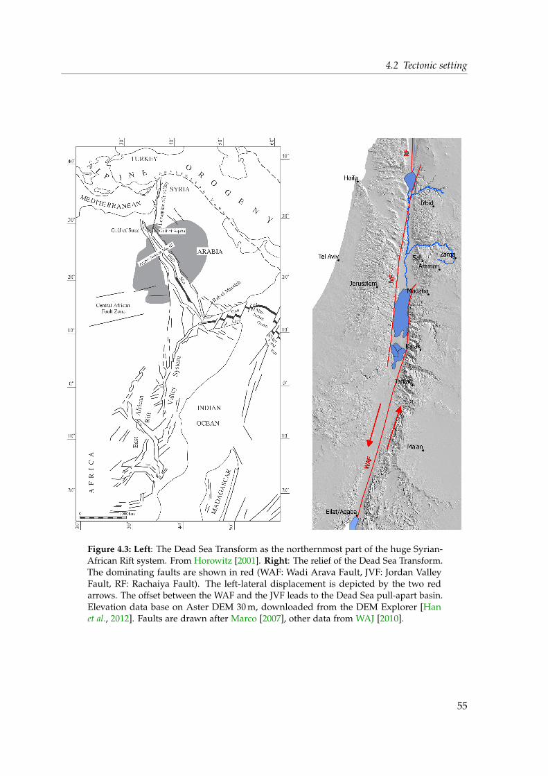
4.2 Tectonic setting
Figure 4.3: Left: The Dead Sea Transform as the northernmost part of the huge Syrian-African Rift system. From Horowitz [2001]. Right: The relief of the Dead Sea Transform.The dominating faults are shown in red (WAF: Wadi Arava Fault, JVF: Jordan ValleyFault, RF: Rachaiya Fault). The left-lateral displacement is depicted by the two redarrows. The offset between the WAF and the JVF leads to the Dead Sea pull-apart basin.Elevation data base on Aster DEM 30 m, downloaded from the DEM Explorer [Hanet al., 2012]. Faults are drawn after Marco [2007], other data from WAJ [2010].
55

4 Geographical and geological setting
Figure 4.4: The regional tectonic setting in the Middle East. The Arabian plate moveswith a counterclockwise rotation towards Eurasia. Arrows indicate the direction andvelocity relative to Eurasia. The inset zoomes to the Dead Sea Transform and showsthe major fault lines in this system as well as the speed and direction of movement ofthe Arabian plate relative to the Sinai sub-plate. Numbers indicate relative velocities inmm/year. The main map is from Reilinger et al. [2006], the inset is adapted from Gomezet al. [2007], but bases on the same data set.
56

4.2 Tectonic setting
be 18 Ma old. Yet, most basalt outpourings along the Jordan Valley, especially at the easternescarpment south of the Dead Sea and Wadi Arava, on the Golan heights and around lakeKinneret, are of Pleistocene age [Bender, 1968; Watts et al., 2004]. However, the lateral motionwas not uniform. Freund et al. [1970] recognized two phases of accelerated tectonic activity.An early one took place between 25 and 14 Ma ago and displaced the plates about 60–65 km,and a later movement took place during the last 4.5 Ma [Zak and Freund, 1981]. Recentestimates for the current relative slip velocity are (4± 2)mm/a, calculated from the offset ofPleistocene alluvial fans in the wadi Arava [Klinger et al., 2000], and more recently Gomezet al. [2007] found shear velocities of 4 to 5 mm/a, determined using GPS based monitoring(see inset of figure 4.4).
The dominating longitudinal faults, which are responsible for the pull-apart, are accompa-nied by normal faults which extend along the basin margins. The latter faults cause the slightplate separation motion and therefore are responsible for the thinning of the crust beneaththe transform and hence caused its subsidence [Garfunkel and Ben-Avraham, 1996]. Themarginal zone of normal faulting is 4 to 5 km wide on the western side, but only 2 km eastof the pull-apart. This leads to an asymmetric structure along the Dead Sea-Jordan Valleydepression in longitudinal cross-sections [Garfunkel and Ben-Avraham, 1996]. Accompany-ing the formation of the Jordan Valley Depression, the flanks experienced uplifting of about1 km, in some place considerably more [Garfunkel and Ben-Avraham, 1996].
As Galli [1999] outlines, the transform is still active along the Jordan Valley Fault and alsonorth of Lake Kinneret, and Horowitz [2001] notes, one would expect strong seismic activityalong a recently shaped rift. However, the Dead Sea Fault Zone is pretty quiet with onlyfew earthquakes in the last century, mainly distributed in the Gulf of Aqaba and north ofthe Dead Sea [Ambraseys, 2006; Grünthal and Wahlström, 2012]. Historical seismic activityover the past two millenia was considerably higher [Ambraseys, 2006].
The sedimentary fill of the rift valley is very thick in most parts. The deepest boreholein the Jordan Rift Valley fill, Sedom Deep 1, located just south of the Dead Sea, reaching6448 m below the surface, does not reach the basement [Horowitz, 2001]. Ginzburg and Ben-Avraham [1997], among others, deduce a 6 km deep sedimentation north of the Dead Sea,which increases to roughly 14 km south of it from seismic refraction. Several salt diapirsevolved especially south of the Dead Sea (Lisan and Sedom diapir), which reach thicknessesof several kilometer [Garfunkel and Ben-Avraham, 1996].
Much of this sediment fill today contains saline water bodies, which developed from leach-ing of saline lacustrine depositions arising from the evaporation of the predecessors of theDead Sea, the freshwater Lake Samra (~135 to 75 ka ago, see Waldmann et al. [2009]) andthe saline Lisan Lake (~70 to 15 ka ago, compare Bartov et al. [2002]), which both extendednorth to present day Lake Tiberias. The thickness of the resulting deposits ranges from 40 toseveral hundred meters [Salameh, 2001]. Figure 4.5 shows a geologic cross-section in W–Edirection across the DST just south of the Dead Sea.
Crustal structure is revealed by seismic refraction studies to be different on both sides of thetransform [El-Isa et al., 1987b]. The crust in southern Israel is about 35 km thick and thinstowards the north, where it is only roughly 25 km thick. The crustal basement under Jordanreaches a maximum of 40 km in the east and thins to 35 km along the rift valley [El-Isa et al.,
57
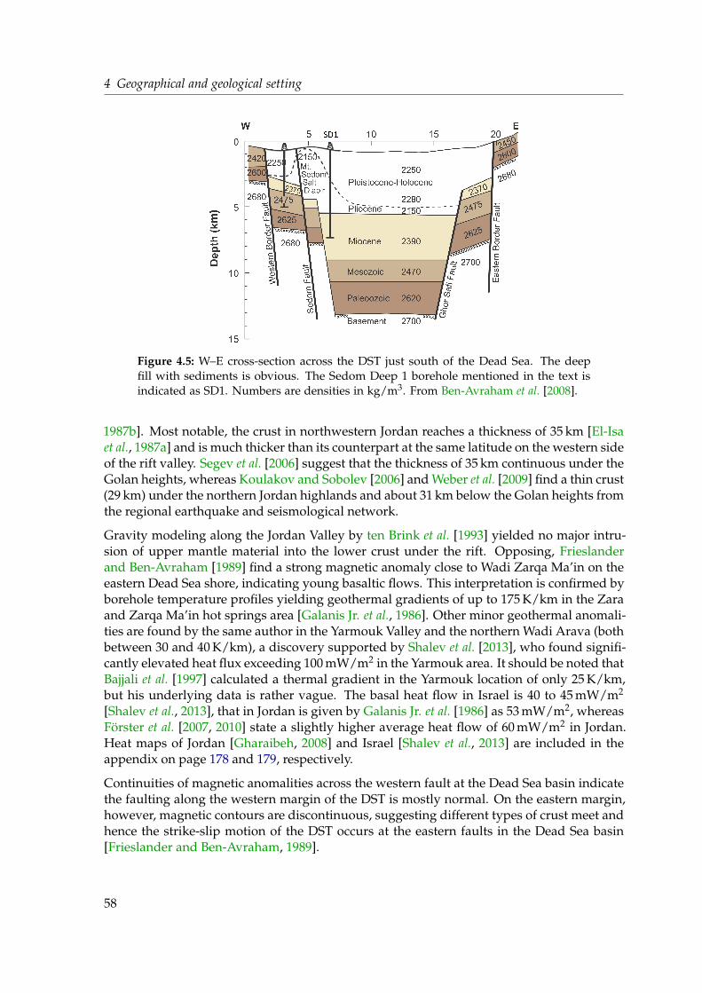
4 Geographical and geological setting
Figure 4.5: W–E cross-section across the DST just south of the Dead Sea. The deepfill with sediments is obvious. The Sedom Deep 1 borehole mentioned in the text isindicated as SD1. Numbers are densities in kg/m3. From Ben-Avraham et al. [2008].
1987b]. Most notable, the crust in northwestern Jordan reaches a thickness of 35 km [El-Isaet al., 1987a] and is much thicker than its counterpart at the same latitude on the western sideof the rift valley. Segev et al. [2006] suggest that the thickness of 35 km continuous under theGolan heights, whereas Koulakov and Sobolev [2006] and Weber et al. [2009] find a thin crust(29 km) under the northern Jordan highlands and about 31 km below the Golan heights fromthe regional earthquake and seismological network.
Gravity modeling along the Jordan Valley by ten Brink et al. [1993] yielded no major intru-sion of upper mantle material into the lower crust under the rift. Opposing, Frieslanderand Ben-Avraham [1989] find a strong magnetic anomaly close to Wadi Zarqa Ma’in on theeastern Dead Sea shore, indicating young basaltic flows. This interpretation is confirmed byborehole temperature profiles yielding geothermal gradients of up to 175 K/km in the Zaraand Zarqa Ma’in hot springs area [Galanis Jr. et al., 1986]. Other minor geothermal anomali-ties are found by the same author in the Yarmouk Valley and the northern Wadi Arava (bothbetween 30 and 40 K/km), a discovery supported by Shalev et al. [2013], who found signifi-cantly elevated heat flux exceeding 100 mW/m2 in the Yarmouk area. It should be noted thatBajjali et al. [1997] calculated a thermal gradient in the Yarmouk location of only 25 K/km,but his underlying data is rather vague. The basal heat flow in Israel is 40 to 45 mW/m2
[Shalev et al., 2013], that in Jordan is given by Galanis Jr. et al. [1986] as 53 mW/m2, whereasFörster et al. [2007, 2010] state a slightly higher average heat flow of 60 mW/m2 in Jordan.Heat maps of Jordan [Gharaibeh, 2008] and Israel [Shalev et al., 2013] are included in theappendix on page 178 and 179, respectively.
Continuities of magnetic anomalities across the western fault at the Dead Sea basin indicatethe faulting along the western margin of the DST is mostly normal. On the eastern margin,however, magnetic contours are discontinuous, suggesting different types of crust meet andhence the strike-slip motion of the DST occurs at the eastern faults in the Dead Sea basin[Frieslander and Ben-Avraham, 1989].
58

4.3 Hydrogeology of Jordan
Figure 4.6: Structural map of Jordan. The country is permeated by a lot of faults, mostnotable the Jordan Valley Fault. From Sawarieh [2005], who adapted it from Diabat[2004].
Associated with the rift formation a lot of other faults evolved. The sediments in the valleyare fractured in many places, with some of the lineaments having considerable vertical dis-placement (compare for example Horowitz [2001] or Ben-Avraham et al. [2008]). The Jordanplateau is traversed by several fracture zones, as shown in figure 4.6. The most striking oneis the Karak-Feiha Fault which extends from the Karak plateau in southeastern direction.The Sirhan Fault elongates from Wadi Sirhan in Saudi Arabia in NW-SE direction. Almostparallel to it runs the Fuluq Fault. These two faults constitute the margins of the HamzaGraben, whose formation caused the subsidence of the Azraq depression. Other prominentfaults are the Swaqa Fault, leading from the Dead Sea towards east into Saudi Arabia andthe ESE striking Zarqa Ma’in Fault, the elongation of the Wadi Zarqa Ma’in. Many morestructural elements are present and can influence the hydrodynamic patterns in Jordan.
59

4 Geographical and geological setting
Figure 4.7: Map of the major outcropping hydrogeological units. Also the groundwaterbasins in Jordan are shown. Drawn based on data from WAJ [2010].
4.3 Hydrogeology of Jordan
A lot of literature has been published about the geology and hydrogeology of Jordan. Stilltoday the book of Friedrich Bender [1968] is the reference regarding geologic aspects. Asuperb summary of hydrogeologic information in Jordan with a focus on the northern halfof the country is found in Margane et al. [2002]. The description of the hydrogeologic settingin Jordan in this thesis follows mainly this publication.
Jordan is divided into 12 groundwater basins (depicted in figure 4.7), where the Amman-Zarqa, the Azraq and the Jordan Valley basins are the most heavily exploited ones [Marganeet al., 2002; USAID, 2012]. The same map displays the outcropping major hydrogeologicunits, which are described in the following.
Over geologic timescales several sedimentary layers have deposited in Jordan. Generallyspoken, the stratigraphy in Jordan dips gently towards the east and the north (compare fig-ure 4.8). Especially along the escarpment of the Jordan Rift Valley the sequence of lithologi-
60

4.3 Hydrogeology of Jordan
Figure 4.8: A generalized cross section of the hydrogeologic pattern in central Jordan,from west to east. Aquifers are displayed in white, aquitards are shaded. From Salamehand Udluft [1985].
cal sequence is well revealed. Figure 4.9 displays the geologic classification of rock units inJordan. The Precambrian basement outcrops only in the southwest around Aqaba, whereasin the Yarmouk River area the depth to the bedrock is assumed to be more than 4000 mbsl[Margane et al., 2002].
Three aquifer systems are present in Jordan, often termed the deep, middle and shallowaquifer. Above the Precambrian bedrock lies the sandstone aquifers of the Ram group ofCambrian to Ordovician age, which underlie almost whole Jordan and extend far into SaudiArabia (where it is termed the Saq aquifer). It outcrops in wide areas of southern Jordan,where the main present-day recharge area is along the escarpment of the Wadi Araba (inmore pluvial periods recharge also took place to the Saudi part of the aquifer system [UN-ESCWA and BGR, 2013]). The flow direction is generally towards the northwest. The Ramaquifer discharges at the lower escarpments of the Jordan Valley and into the Dead Sea[Salameh and Udluft, 1985; Mallast et al., 2013]. The surface of the deep sandstone aquiferreaches a depth of more than 3500 m below surface in the Hamza oil field area southeast ofthe Azraq Oasis [HSI, 1994, cited after Ayed [1996]]. The term Disi aquifer is equivalent tothe Ram group aquifer and is widely used among hydrogeologists.
In central Jordan, the Lower Cretaceous Kurnub sandstone aquifer (K) lies directly on top ofthe Ram group, both are thus considered as one aquifer complex. However, in south Jordanthe aquitards of the Khreim group and in north Jordan those of the Zarqa group separatethese two aquiferous layers. The thickness of the Kurnub group decreases towards the eastand is 100 to 200 m in the Azraq area. The Kurnub outcrops along the slopes of the rift escarp-ment from the Zarqa River to the south and at several domal structures northwest of Amman.The Kurnub sandstone recharges on the slopes of the Sharaa mountain range between Tafi-lah and Petra, from where the water flows in northeast direction to Azraq and then turnstowards the Jordan Rift Valley again [Salameh, 1996]. UN-ESCWA and BGR [2013] suggestan additional inflow from the south and southeast and across the Iraqi border. The Kurnubaquifer in the Azraq Oasis is under artesian conditions [Ajamieh, 1998; Galanis Jr. et al., 1986].The deep aquifer system, consisting of the Ram and the Kurnub aquifer, is exploited mostly
61

4 Geographical and geological setting
Figure4.9:G
eologicand
hydrogeologicclassification
ofrock
unitsin
Jordan.FromM
arganeetal.[2002].
62

4.3 Hydrogeology of Jordan
in south Jordan due to generally great depths of the strata and often high mineralization inthe northern parts of the country.
The Kurnub aquifer is overlain by the formations of the Lower Ajloun group, A1/6. Thesemarl and limestone units are considered to act as an aquitard in most parts of the country,although the A1/2 and A4 form aquifers of local importance in some parts of the northernhighlands. These layers separate the sandstone aquifer complex from the Ammen Wadi Siraquifer (B2/A7), which is exploited most extensively for municipal and agricultural purposeof all aquifers in Jordan. Its enormous extent, relatively high permeability and good wa-ter quality makes it the primary groundwater resource in the Jordan highlands. Althoughpresent in whole northern Jordan, usage of the B2/A7 is limited to the western part, becauseunder confined conditions the water quality is mostly poor due to a high salinity. The B2/A7,often named middle aquifer in the Azraq area, consists mainly of limestone and chert of Up-per Cretaceous age. As this aquifer crops out in the Jordan highlands, it is recharged there.The difference in hydraulic head drives the groundwater to flow in eastern and northeast-ern direction towards the center of the Azraq basin (figure 4.10), except in the most westernparts, where it discharges into side wadis of the rift valley. The B2/A7 reaches a thickness ofmore than 3000 m close to the Fuluq Fault and thins rapidly to the west.
The Maastrichtian to Paleocene Muwaqqar formation (B3) confines the B2/A7 aquifer sys-tem in the eastern and northeastern area. It consists mostly of marl and bituminous marland its thickness increases to the east up to more than 400 m in the Azraq area, close to theFuluq Fault. It’s low permeability renders it to act as an aquitard.
Above the B3 formation lies the shallow aquifer system, which is made up of three subunits:the Paleocene Umm Rijam (B4) chalky limestone, the Eocene Wadi Shallala (B5) formation,and the basalt shield (B) in the north, which are all hydraulically connected. In wadis andparticularly in the central Azraq depression Quaternary sediments overlie the other mem-bers of the shallow aquifer and are accounted to it as well. The B4 and B5 are exposed widelyin the Azraq basin and increase in thickness from west towards the Fuluq Fault, where morethan 300 m is reached. In wide parts of northern Jordan the Harrat Ash-Shaam basalt shield,which extends from the Golan Heights and Jabal al-Druze in Syria into northern Saudi Ara-bia, overlies the sedimentary layers. It reaches a thickness of more than 400 m at the Syrianborder and may reach 1500 m at the mountain Jabal al-Druze [Wolfart, 1966]. The basalt cov-ers an area of 11 414 km2 [Guba and Mustafa, 1988] and is formed from Oligocene to recenttimes [Ilani et al., 2001; Krienitz et al., 2007]. Several basalt layers can be distinguished, whichare locally separated by 2 to 20 m thick clay layers [Boom, 1968]. The chemical analysis ofBoom [1968] classifies the basalt as olivine rich alkaline basalt.
The shallow aquifer system is recharged primarily at the slopes of Jabal ad-Druze, and somerecharge takes place in the wadis and the central playa of the Azraq Oasis after storm events.The flow direction of this aquifer system in the Azraq basin is generally towards the cen-tral depression (compare figure 4.11), where once several springs used to be the naturaldischarge area. About 85 % of the groundwater in the Azraq basin comes from northern tonortheastern direction [Ayed, 1996].
The B4 and the basalt are considered as generally good aquifers. Ayed [1996], citing Hum-phreys and Sons [1982], reports hydraulic transmissivities in boreholes of the AWSA well
63
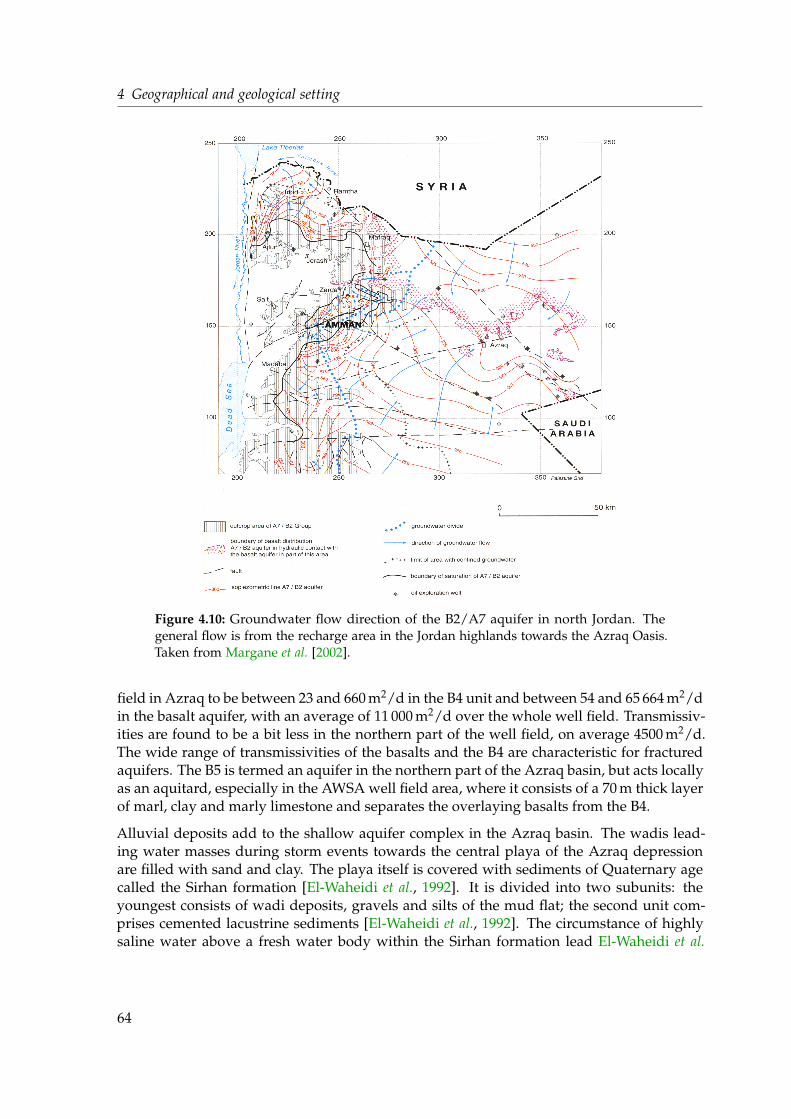
4 Geographical and geological setting
Figure 4.10: Groundwater flow direction of the B2/A7 aquifer in north Jordan. Thegeneral flow is from the recharge area in the Jordan highlands towards the Azraq Oasis.Taken from Margane et al. [2002].
field in Azraq to be between 23 and 660 m2/d in the B4 unit and between 54 and 65 664 m2/din the basalt aquifer, with an average of 11 000 m2/d over the whole well field. Transmissiv-ities are found to be a bit less in the northern part of the well field, on average 4500 m2/d.The wide range of transmissivities of the basalts and the B4 are characteristic for fracturedaquifers. The B5 is termed an aquifer in the northern part of the Azraq basin, but acts locallyas an aquitard, especially in the AWSA well field area, where it consists of a 70 m thick layerof marl, clay and marly limestone and separates the overlaying basalts from the B4.
Alluvial deposits add to the shallow aquifer complex in the Azraq basin. The wadis lead-ing water masses during storm events towards the central playa of the Azraq depressionare filled with sand and clay. The playa itself is covered with sediments of Quaternary agecalled the Sirhan formation [El-Waheidi et al., 1992]. It is divided into two subunits: theyoungest consists of wadi deposits, gravels and silts of the mud flat; the second unit com-prises cemented lacustrine sediments [El-Waheidi et al., 1992]. The circumstance of highlysaline water above a fresh water body within the Sirhan formation lead El-Waheidi et al.
64

4.3 Hydrogeology of Jordan
Figure 4.11: Groundwater contour lines and resulting flow directions of the shallowaquifer in north Jordan. Groundwater flow is from all directions towards the centralplaya in Azraq. Taken from Margane et al. [2002].
65

4 Geographical and geological setting
[1992] to the assumption of an impermeable layer in between. The presence of basaltic mate-rial below the sediments of the playa is yet unknown [Yogeshwar et al., 2013]. There are noboreholes in the Sabkha and geoelectric methods do not penetrate deeper than about 70 m.
The shallow aquifer complex is extensively pumped in Azraq for over three decades andthe groundwater reserves have significantly depleted in consequence. The issue of waterquality deterioration resulting from the exploitation is addressed in chapter 6.
66

5 Sampling
5.1 Sampling and measurement procedures
Samples for tritium and stable isotopes were collected in 50 ml glass bottles. The waterfor the anionic and cationic composition analysis were filtered with a 0.22 µm filter beforebeing bottled in 50 ml glass bottles each. The cation sample was acidified with 150 µl ofconcentrated nitric acid to a pH below 2 to prevent any precipitation of solute, because thismight affect the measurement weeks later in the laboratories in Heidelberg. Radiocarbonsamples were collected in 500 ml glass bottles and treated with 0.1 g silver nitrate to avoidany alteration of the carbonate isotopic composition by living organisms. In all samples alittle head space was left for safe transportation by air cargo.
Radon samples were collected in 250 ml glass bottles without any contact to the atmosphereto prevent any gas exchange which would alter the radon content of the sample. This wasperformed by filling the bottles under water inside a bucket, flushing the bottle with freshwater for a while and then putting the cap onto the bottle underwater with no air bubbleresiding inside the bottle. The cap has a flexible diaphragm to be able to compensate forvolume changes of the water due to temperature variation.
Radon samples were measured during the campaign between working days, mostly in theevening. As described in chapter 3.7 each measurement starts with a 20 min equilibrationphase, followed by the actual sample measurement with a duration between 40 min andmore than two hours, the last sample each day usually performing a longer analysis. The wa-ter temperature during the measurement has not been recorded. Thus, a reasonable eveningtemperature at the winter garden of the German Protestant Institute in Amman, where theradon measurements were conducted, of (15± 5) ◦C is assumed for the evaluation.
Noble gas samples were collected in copper refrigeration tubes mounted on aluminum racks,which can be sealed vacuum tight by stainless steel clamps on both sides [Beyerle et al.,2000]. In general they were connected by hoses and a fast locking coupling directly to athreaded opening at the well head. This was possible at almost all pumped wells excepttwo of the farming wells in Azraq were a rubber plug connected to a hose was used insteadto get the water through the copper tube without air contact. Since groundwater is usuallystored under high hydrostatic pressure it is important to avoid degassing during sampling.To prevent the dissolved gases to degas at the end of the copper tube a second PVC hosewas connected there to move the point of a rapid pressure decay away from the samplingcontainer. Attention was payed to a reasonably high water pressure. This was tested bychecking the distance the water sprayed after leaving the copper tube and a careful checkfor air bubbles inside the sampling hose. Before closing the container a tool was knocked
67

5 Sampling
repeatedly against it to make any bubbles that stuck in the pipe flush away. The copper tubewas closed by two steel clamps at its ends of which the one on the exit side of the coppertube was closed first to keep up the water pressure.
Sampling thermal springs sometimes needed a little variation in the sampling proceduredescribed above. In some cases where there was a little downward slope the hose feedingthe copper tube is moved as far as possible into the spring opening so that the water hasonly a minimum of atmospheric contact. The water then flows through the hose and thecopper tube,which was then closed in the same manner like at pumped wells, but with onlythe gradient as a source of pressure. This usually caused no problem as the water ran outof the rock without any pressure – if any degassing happened, it already occurred beforesampling.
In other cases there was no exploitable downward gradient, or the thermal spring dischargedbelow the surface into a pool. In these cases one of the two hoses connected to the coppertube was placed as close as possible to the spring’s discharge spot (occasionally a weighthad to be attached to the hose to lower it into the spring’s pool, see appendix A.3). On thehose at the other end of the copper tube one had to suck the water until the water surfacewas at least a little bit above the copper tube. It was then first closed at the water entry side(in contrast to the usual sampling procedure). After the first clamp was closed, the suckingstopped and the remaining water column generated a little pressure. When sampling a hotspring alone, the vertical height was at most half a meter. With the help of an assistant, morethan two meters vertical height were possible. One may argue that the sucking inducedan negative pressure, but degassing due to this should only happen above the copper tubewithin the water column in the hose. Diffusion of degassed water into the copper tube canbe neglected if one works quickly.
Some hot springs showed an obvious degassing, as bubbles of H2S (detected by its smell) orother gases ascended in the spring’s pool. These ascending bubbles strip (noble) gases fromthe water and one has to make sure this effect is kept as small as possible [Kennedy et al.,1988]. The best way of avoiding this impact is to take samples as close as possible to thebottom or the discharge opening of the pool. However, if bubble formation already occursbelow the pool’s floor, non-degassed samples are hardly possible to obtain. Sometimes alsowells are subject to degassing. In this study, the thermal wells in the Abu Zeeghan well fieldshowed a massive degassing during sampling. In both cases, springs and wells, the samplesshowed extremely low radon concentrations.
In the case of a deep pool (Himma spring) water samples in bottles were taken close to thesurface, but as deep as possible. This holds also for extremely hot springs where it was notpossible to go deep into the pool with ones hands (especially at Zerqa Ma’in spring I).
Physical parameters were analyzed on site1 with the WTW multi-parameter probe intro-duced in chapter 3.1. In cases of a water flow through the copper tube (i. e. all pumped wells
1In a few cases of extreme hurry at sampling points in Azraq electric conductivity and pH were recorded inthe evening of the same day. Due to a failure of the sensors at the NDW wells pH and electric conductivitywere measured back in Heidelberg on bottled water from these wells. No oxygen and temperature weretaken in these cases. See description of the individual sampling procedure in appendix A.3.
68
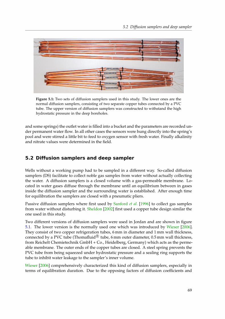
5.2 Diffusion samplers and deep sampler
Figure 5.1: Two sets of diffusion samplers used in this study. The lower ones are thenormal diffusion samplers, consisting of two separate copper tubes connected by a PVCtube. The upper version of diffusion samplers was constructed to withstand the highhydrostatic pressure in the deep boreholes.
and some springs) the outlet water is filled into a bucket and the parameters are recorded un-der permanent water flow. In all other cases the sensors were hung directly into the spring’spool and were stirred a little bit to feed to oxygen sensor with fresh water. Finally alkalinityand nitrate values were determined in the field.
5.2 Diffusion samplers and deep sampler
Wells without a working pump had to be sampled in a different way. So-called diffusionsamplers (DS) facilitate to collect noble gas samples from water without actually collectingthe water. A diffusion samplers is a closed volume with a gas-permeable membrane. Lo-cated in water gases diffuse through the membrane until an equilibrium between in gasesinside the diffusion sampler and the surrounding water is established. After enough timefor equilibration the samplers are closed with a pneumatic pliers.
Passive diffusion samplers where first used by Sanford et al. [1996] to collect gas samplesfrom water without disturbing it. Sheldon [2002] first used a copper tube design similar theone used in this study.
Two different versions of diffusion samplers were used in Jordan and are shown in figure5.1. The lower version is the normally used one which was introduced by Wieser [2006].They consist of two copper refrigeration tubes, 6 mm in diameter and 1 mm wall thickness,connected by a PVC tube (Thomafluid R© tube, 6 mm outer diameter, 0.5 mm wall thickness,from Reichelt Chemietechnik GmbH + Co., Heidelberg, Germany) which acts as the perme-able membrane. The outer ends of the copper tubes are closed. A steel spring prevents thePVC tube from being squeezed under hydrostatic pressure and a sealing ring supports thetube to inhibit water leakage to the sampler’s inner volume.
Wieser [2006] comprehensively characterized this kind of diffusion samplers, especially interms of equilibration duration. Due to the opposing factors of diffusion coefficients and
69

5 Sampling
Figure 5.2: The deep sampler used to get water samples from open borehole without apump. It is depicted in its open state. A weight is sent down along the cable enables toclose the sampler at the desired depth.
solubility in water, neon needs the longest equilibration time of all noble gases, but 75 hoursturned out to be sufficient for 99.9 h equilibration.
Because this type of diffusion sampler has never been tested under high hydrostatic pressurethe upper, a “strong” version was invented during this thesis to use it in deep boreholes. Itcomprises of one copper tube only which is perforated at one end. The same PVC tubeis pulled over this perforated part and acts as the membrane, but the total surface wheregases can diffuse to the interior is smaller, thus, equilibration time is expected to be longerthan for the normal DS. The reduction of the area where diffusion occurs is about a factorof 10, so this type of diffusion sampler needs approximately 20 days to equilibrate. Theassumed advantage of this design is that the PVC tube does not cover the edges of the coppertubes and rupture due to deformation under high pressure appears less likely. However, thenormal diffusion sampler design proved to be more sturdy. As this study is the first ofour working group where diffusion samplers are were applied under field trip conditions,especially in deep boreholes, the gained experiences are summarized in appendix A.2.
All diffusion samplers located in one borehole were fixed to a single string. In NDW 5 afishing line was used, in all other wells a stronger plastic string. Both ends were tied to thestring to prevent the samplers to get stuck in the borehole in case they can freely move. Theclosed ends were packed into duct tape because they are sharp and could cut through thestring. An additional weight was used drag the string down. The lowering of the samplerswas conducted slowly and the string finally bound fast at the well head.
Retrieval of the DS was done as fast as possible to avoid much re-equilibration with shal-lower water and the atmosphere. The copper tubes were immediately closed tight usingpneumatic pliers. Because the inner volume is changed by the first sealing-off, it is impor-tant to note the sequence in which the copper tubes were closed.
At every sampling depth at least two diffusion samplers were located to reduce the risk ofloosing the sample due to a rupture of the PVC tube (except the deepest sample from NDW7, only one normal DS was used here, as nobody exspected any sampler to survive thisdepth). The “strong” design samplers were used in depth starting from 300 m coupled witha normal sampler. The experience gained from the application of both types of diffusionsamplers is summarized in appendix A.2.
70
5.3 Sampling Campaigns
In order to collect water from the non-pumped wells, a so-called deep sampler, providedby the Water Authority, was used. This device, shown in figure 5.2, is lowered in to theborehole and fills with water. It can then be closed by a weight which is sent down alongthe cable. It has a volume of 500 ml, which means that the sampler had to be used twiceat every sampling depth. The cable provided a scale the depth could be set precisely. Thedeep sampler was also used to determine the water table in the borehole. It gave an acousticsignal when it came in contact with water.
This way samples for stable isotope, tritium, ionic composition and carbon-14 were filledinto the according bottles and treated afterwards, as explained above. Because the deepsampler could reach a maximum of 250 m no water samples from greater depths in the NDWwells in Azraq could be obtained. No radon sample was taken in these cases since the deepsampler cannot be considered gas tight and the results would have been questionable. Alsothe water temperature could not be recorded, but pH and conductivity were noted.
5.3 Sampling Campaigns
Three sampling campaigns were conducted in the scope of this thesis. In total 51 wells and9 springs were sampled, some of them several times. A detailed description of all samplingsites is given in the appendix A.3.
Campaign 2009
The first field trip took place in late September/October 2009 over three and a half weeks.Beside getting to know the general situation of Jordan regarding water issues, this fieldtrip aimed mainly to find a local partner in Jordan. With the Water Authority of Jordan(WAJ) a trustful and helpful cooperation partner was found and a cooperation agreementwas signed.
The initial plan of taking noble gas samples from the Disi aquifer in southern Jordan wasnot possible at this time due to restrictions by the Ministry of Water and Irrigation (MWI).Instead, the Azraq basin was found as a substitute and first samples were collected: Threewells (two governmental and one private farming well) in the northern part of the ground-water basin and six wells of the AWSA well field (all governmental) in the basin’s centerwere sampled.
On this campaign samples for stable isotopes of hydrogen, tritium and noble gases werecollected. In the field temperature and dissolved oxygen were measured. The limitationof recorded parameters is owed to the uncertainty of the outcome of the search for fieldpartners and, thus, only the most necessary equipment was shipped to Jordan.
Campaign 2010
The second field trip of four weeks duration took place between mid-September and mid-October 2010. Ten wells in the AWSA well field were examined to support the findings from
71

5 Sampling
the 2009 campaign. As a second study 20 governmental wells in the Karak area were sam-pled in order to estimate the local groundwater recharge rate in this agricultural dominatedregion. The wells stretched from close to Karak town along the supposed eastward ground-water flow direction to the town Swaqa. The Karak study aimed at calculating the localrecharge rate from groundwater age depth profiles and their spatial distribution. However,most waters appeared to be too old to be dated by the 3He-3H method. Therefore, this studyis not included in this thesis, but at least the measured noble gas isotope concentrations andthe most important isotope ratios are compiled in table A.8 in the appendix on page 186.
All wells were sampled for stable isotopes, tritium, radiocarbon and noble gases. Physicalparameters recorded in the field are temperature, pH, electric conductivity and dissolvedoxygen. The alkalinity and nitrate content were determined using chemical test kits at thesampling sites.
As it was decided that the ionic composition of the waters in Azraq is of importance, it wasanalyzed for it on the leftover of the tritium and stable isotope water samples. Obviously,these samples had not been filtered and treated with nitric acid and, therefore, the resultsmay show deviations from the original values. However, the ion balance confirmed that nomajor ions were precipitated in significant amounts.
Campaign 2012
In March and April 2012 the final sampling took place with a duration of about six weeks.For the Azraq study wells which penetrate the B2/A7 aquifer as well as shallow farmingwells were sampled in order to have water samples of both possible sources of salinity ofthe AWSA well field detected in the previous campaigns. There are no pumped wells ofthe B2/A7 in this area due to high salt content in this aquifer in the Azraq basin. Therefore,diffusion sampler were used in two exploration wells. In each of them they were positionedat several depth. Also some farming wells which are not in use anymore due to the saltywater were sampled with diffusion samplers.
Thermal waters in 8 springs and 7 wells along the Jordan Valley were collected. The northern-most spring was the Himma spring in the Yarmouk Valley, the southern-most spring the Afraspring in the Wadi Hasa.
Despite the information stop about the Disi project it was possible to sample four wells inthe Disi area during this campaign. Since the well drilling was still in progress it was onlypossible to take samples during the pumping test following the drilling. In the time periodof the field trip two newly drilled wells were sampled. Additionally one well from 1992 wassampled which today provides drinking water to the construction camp site. However, dueto restriction by the MWI the data of these well is not allowed to be published.
The same physical parameters were recorded as in the 2010 campaign, as well as the samechemical test have been conducted. Additionally samples for the ionic composition (majoranions and cations) were collected and treated as described in chapter 5.1. Radon was mea-sured for all samples of the thermal waters and the Disi studies as well as for some wells inAzraq.
72

6 Azraq
Azraq is situated in the northeastern desert, about 80 km east of Amman. Azraq used tobe an oasis, with an extensive system of lakes and marshland, fed by the two large springsShishan and Druze.
The first traces of habitation in the area of the Azraq Oasis date back to the Lower Paleolithic,i. e. 0.3 to 2.6 Ma BP, and people settled there during all major prehistoric periods [StanleyPrice and Garrard, 1975]. It can be assumed that this region reacted sensitive on climatevariation. Garrard et al. [1985] report a period of extreme drought during the last glacialmaximum and the total disappearance of the lakes, and the return of moist conditions about12 000 years BP, where the lake grew to cover an area of 700 km2 with 20 m depth. Duringthe Holocene the size reduced to about 7 km2. Newer studies support these findings anddetermine the driest and most inhabitable period in Azraq to last during the Bølling-Allerødwarming (14.7 – 12.8 ka BP) as there was no sediment deposition in Qa’a Azraq at this time[Jones and Richter, 2011].
The Azraq Oasis had a vivid ecosystem with a large number of species inhabitating theswamps around the pools [Nelson, 1985] and it was an important stop-over for many mi-grating birds on their journey to the south.
However, the springs dried up in 1991 in the wake of large increase of groundwater ab-straction rates (see figure 6.1, left panel), and the area of the former lake forms a waste-land now. Shallow groundwater was used for agricultural purposes for decades, and about3.3 MCM per year was pumped to Irbid since 1963 [Nelson, 1985]. In the early 1980s, how-ever, the AWSA1 well field was drilled close to the oasis to supply the urban areas of Am-man and Zarqa with good quality drinking water. This additional groundwater abstrac-tion and an increasing water demand for irrigation purposes caused the groundwater ta-ble to drop by about 1 m per year since then, as illustrated in the right panel of figure 6.1.This is due to the wide discrepancy between the estimated safe yield of the Azraq basin of24 MCM/year [USGS, 1998] to the actual abstraction rate of 59.3 MCM/year [Raddat, 2005,data from 2004].
To diminish the ecologic disaster and resettle some of the native species in Azraq (includingthe endemic Azraq Killifish Aphanius sirhani), an artificial wetland reserve was establishedby the Royal Society for the Conservation of Nature (RSCN), but it covers only a small partof the original lake area [RSCN].
Not only is overpumping a hazard for the Azraq ecosystem, but also the threat of deteri-orating groundwater quality grows. Some shallow agricultural wells already show highsalinization, rendering the groundwater useless for irrigation in some parts of the Azraq
1Amman Water and Sewage Authority
73

6 Azraq
1 9 8 0 1 9 8 2 1 9 8 4 1 9 8 6 1 9 8 8 1 9 9 0 1 9 9 2 1 9 9 4 1 9 9 6 1 9 9 8 2 0 0 0 2 0 0 20
5
1 0
1 5
2 0
2 5
Di
scharg
e resp
. Abst
ractio
n [MC
M/ye
ar]
Y e a r
S p r i n g d i s c h a r g e A W S A a b s t r a c t i o n
1 9 8 4 1 9 8 6 1 9 8 8 1 9 9 0 1 9 9 2 1 9 9 4 1 9 9 6 1 9 9 8 2 0 0 0 2 0 0 2 2 0 0 4
- 2 2
- 2 0
- 1 8
- 1 6
- 1 4
- 1 2
- 1 0
- 8
- 6
Depth
of gr
ound
water
table
[m b.
s.]
Y e a r
Figure 6.1: Left: Spring discharge (orange) of the Azraq springs and the groundwaterabstraction rates in the AWSA well field (red). Both given in million cubic meter (MCM)per year. Right: As a result of overpumping the groundwater table dropped by about1 m per year (data is shown for the AZ 12 observation well, which is situated in thecenter of the AWSA well field). Data courtesy of the WAJ.
area. While the AWSA well field produced high quality drinking water with little mineral-ization in the first years of operation, some of its wells show a rising salt content over theyears [Al-Momani et al., 2006]. It is particularly interesting that, although the wells lie closeto each other, wells in the middle of the well field are affected by saltwater intrusion ratherthan those on its edges.
The map in figure 6.2 gives an overview of the setting around the Azraq Oasis and thelocation of the sampled wells in this area. The farm land surrounds the central mud pad,which is more symbolized in this map, because the extent to the south is not known. Thebasalt cover extending north of the oasis is also shown. The boundary between salty waterin the center and fresh water in the surroundings is indicated by the orange, dotted line.The underlying data from geoelectric surveys is extracted from El-Waheidi et al. [1992, greenlines], El-Naqa [2010, brown lines] and Yogeshwar et al. [2013, blue lines]. The lines indicatethe direction of the respective georadar profiles. By far the most precise boundary locationsare those from Yogeshwar et al. who created very high resolution profiles. The locationsindicated after El-Waheidi et al. and El-Naqa are only rough positions between two distantmeasurement points. Northwest of Azraq town the AWSA well field is situated, wherewells with an elevated salt content are depicted in orange, whereas from the salt unaffectedwells are red. The observation well AZ-12 in the well field is yellow; data of depth to thegroundwater table shown in figure 6.1 originates from this well. The middle aquifer wellsNDW5 and NDW7 are printed blue, the shallow farm wells are green. Furthermore, theextensive network of faults is presented. The major ones are displayed as thick, black linesand labeled by the names stated by the geologic map prepared by Ibrahim [1993]. Manymore lineaments are known or inferred beneath superficial deposits, they are indicated bygrey lines. The wells sampled in the northern part of the basin lie 30 to 40 km north of themap section.
74

Azraq townAzraq townAzraq townAzraq townAzraq townAzraq townAzraq townAzraq townAzraq townAzraq townAzraq townAzraq townAzraq townAzraq townAzraq townAzraq townAzraq townAzraq townAzraq townAzraq townAzraq townAzraq townAzraq townAzraq townAzraq townAzraq townAzraq townAzraq townAzraq townAzraq townAzraq townAzraq townAzraq townAzraq townAzraq townAzraq townAzraq townAzraq townAzraq townAzraq townAzraq townAzraq townAzraq townAzraq townAzraq townAzraq townAzraq townAzraq townAzraq townAzraq townAzraq townAzraq townAzraq townAzraq townAzraq townAzraq townAzraq townAzraq townAzraq townAzraq townAzraq townAzraq townAzraq townAzraq townAzraq townAzraq townAzraq townAzraq townAzraq townAzraq townAzraq townAzraq townAzraq townAzraq townAzraq townAzraq townAzraq townAzraq townAzraq townAzraq townAzraq townAzraq townAzraq townAzraq townAzraq townAzraq townAzraq townAzraq townAzraq townAzraq townAzraq townAzraq townAzraq townAzraq townAzraq townAzraq townAzraq townAzraq townAzraq townAzraq townAzraq townAzraq townAzraq townAzraq townAzraq townAzraq townAzraq townAzraq townAzraq townAzraq townAzraq townAzraq townAzraq townAzraq townAzraq townAzraq townAzraq townAzraq townAzraq townAzraq townAzraq townAzraq townAzraq townAzraq townAzraq townAzraq townAzraq townAzraq townAzraq townAzraq townAzraq townAzraq townAzraq townAzraq townAzraq townAzraq townAzraq townAzraq townAzraq townAzraq townAzraq townAzraq townAzraq townAzraq townAzraq townAzraq townAzraq townAzraq townAzraq townAzraq townAzraq townAzraq townAzraq townAzraq townAzraq townAzraq townAzraq townAzraq townAzraq townAzraq townAzraq townAzraq townAzraq townAzraq townAzraq townAzraq townAzraq townAzraq townAzraq townAzraq townAzraq townAzraq townAzraq townAzraq townAzraq townAzraq townAzraq townAzraq townAzraq townAzraq townAzraq townAzraq townAzraq townAzraq townAzraq townAzraq townAzraq townAzraq townAzraq townAzraq townAzraq townAzraq townAzraq townAzraq townAzraq townAzraq townAzraq townAzraq townAzraq townAzraq townAzraq townAzraq townAzraq townAzraq townAzraq townAzraq townAzraq townAzraq townAzraq townAzraq townAzraq townAzraq townAzraq townAzraq townAzraq townAzraq townAzraq townAzraq townAzraq townAzraq townAzraq townAzraq townAzraq townAzraq townAzraq townAzraq townAzraq townAzraq townAzraq townAzraq townAzraq townAzraq townAzraq townAzraq townAzraq townAzraq townAzraq townAzraq townAzraq townAzraq townAzraq townAzraq townAzraq townAzraq townAzraq townAzraq townAzraq townAzraq townAzraq townAzraq townAzraq townAzraq townAzraq townAzraq townAzraq townAzraq townAzraq townAzraq townAzraq townAzraq townAzraq townAzraq townAzraq townAzraq townAzraq townAzraq townAzraq townAzraq townAzraq townAzraq townAzraq townAzraq townAzraq townAzraq townAzraq townAzraq townAzraq townAzraq townAzraq townAzraq townAzraq townAzraq townAzraq townAzraq townAzraq townAzraq townAzraq townAzraq townAzraq townAzraq townAzraq townAzraq townAzraq townAzraq townAzraq townAzraq townAzraq townAzraq townAzraq townAzraq townAzraq townAzraq townAzraq townAzraq townAzraq townAzraq townAzraq townAzraq townAzraq townAzraq townAzraq townAzraq townAzraq townAzraq townAzraq townAzraq townAzraq townAzraq townAzraq townAzraq townAzraq townAzraq townAzraq townAzraq townAzraq townAzraq townAzraq townAzraq townAzraq townAzraq townAzraq townAzraq townAzraq townAzraq townAzraq townAzraq townAzraq townAzraq townAzraq townAzraq townAzraq townAzraq townAzraq townAzraq townAzraq townAzraq townAzraq townAzraq townAzraq townAzraq townAzraq townAzraq townAzraq townAzraq townAzraq townAzraq townAzraq townAzraq townAzraq townAzraq townAzraq townAzraq townAzraq townAzraq townAzraq townAzraq townAzraq townAzraq townAzraq townAzraq townAzraq townAzraq townAzraq townAzraq townAzraq townAzraq townAzraq townAzraq townAzraq townAzraq townAzraq townAzraq townAzraq townAzraq townAzraq townAzraq townAzraq townAzraq townAzraq townAzraq townAzraq townAzraq townAzraq townAzraq townAzraq townAzraq townAzraq townAzraq townAzraq townAzraq townAzraq town
3740
000
3740
000
3745
000
3745
000
3750
000
3750
000
3755
000
3755
000
3760
000
3760
000
4095000
4095000
4100000
4100000
4105000
4105000
4110000
4110000
4115000
4115000
0 2 4 6 km
AWSA non affected
AWSA affected
Farm well
Middle aquifer well
Observ. well
Fresh/saltwater interface
Yogeshwar 2013
El-Naqa 2010
El-Waheidi 1992
Lineament
Major fault
Mud pan
Farm land
Basalt shield
Map key
AWSAwellfield
Figure 6.2: Overview of the vicinity of the Azraq Oasis. In brown the central mud pan(Sabkha) is displayed, the farm land in green and the basalt shield in grey. The AWSAwells are indicated by orange or red dot, whether they are affected by rising salinity ornot. Farm wells are green, the middle aquifer wells blue. The approximate boundaryof the salt water body in the center is show as an orange, dotted line, direction of thegeoradar profiles is indicated by short, colored lines (data sources El-Waheidi et al.[1992, green], El-Naqa [2010, brown] and Yogeshwar et al. [2013, blue]). The major faultsare named and thick, black lines, other lineaments are displayed as grey lines. TheSirhan and the Fuluq Faults margin the Hamza Graben structure, forming the Azraqdepression. Compiled using data of WAJ [2010], road data base on OpenStreetMaps.
75

6 Azraq
6.1 Hydrology and Hydrogeology of the Azraq basin
The Azraq Oasis is situated in the depression of the Azraq basin, a 12 800 km2 large surfacecatchment. About 94 % of this basin belongs to Jordan, 5 % is situated in Syria and about1 % in Saudi Arabia. The elevation of the central mud pan (Qa’a or Sabkha in arabic) inits deepest point is 505 m above sea level. The surface profile rises in all directions, mostprominently to the north, where the basin reaches its highest point at the mountain Jabalad-Druze (1803 m) in Syria.
Rain falls in winter only and its amount decreases from more than 300 mm per year in thenorthern part to less than 50 mm per year in the southeast of the basin [Ayed, 1996]. In Azraqtown it averages to 66 mm per year [Margane et al., 2002]. The basin has no perennial rivers,but during storm events wadis transport much water into the central playa, where most ofit evaporates.
The economy of Azraq town relies largely on agriculture. Due to the precipitation scarcity,the farmers depend almost exclusively on irrigation with groundwater, since the springsdried up.
All three aquifer systems described in chapter 4.3 are present in the Azraq basin. The prin-ciple hydrogeologic setting is sketched in figure 6.3. The Azraq oases lies in the depressionof the Hamza Graben. To the north the basalt shield forms the slopes of Jabal ad-Druze,where by far the most precipitation falls and where the major recharge area of the shallowaquifer is. The aquifers and aquitards (striped) are shown in this figure as well as the fourwell types: The northern wells, abstracting the most recently formed groundwater from thebasalt aquifer, the wells in the AWSA well field, drilled through the basalt and almost tothe bottom of the B4 aquifer, the shallow farm wells around the Sabkha and the deep wellsNDW5 and NDW7. The Fuluq Fault and the Sirhan Fault are indicated in the sketch, as isthe groundwater table, illustrated by the blue, dotted line. Its deepest point is located in thecentral depression.
The formation of the Azraq depression, where the Azraq Oasis is situated in the deepest part,is closely related to the development of the Hamza Graben system which runs in NW – SEdirection. Its eastern boundary is the Fuluq Fault, the most striking tectonic feature in Azraq,with a maximum vertical displacement of more than 3000 m [Margane et al., 2002]. TheSirhan Fault, indicated in the cross-section in figure 6.3, constitutes the western boundary ofthe graben. Plenty of other faults and minor lineaments are present, witnesses of a turbulentgeologic past. Yet, none of them has a displacement comparable to the Fuluq Fault.
The displacement at the Fuluq, however, varies largely along fault. Margane et al. [2002]published a geologic cross-section in W–E direction, which exactly runs through the AzraqOasis and crosses the Fuluq Fault, where its maximum displacement is assumed (see thetop cross-section in figure 6.4). The cross-section of Dottridge and Abu Jaber [1999], alsodisplayed on page 78, runs from the Azraq Oasis in NE direction and passes the Fuluqabout 10 km north of where the one of Margane et al. [2002] runs through it. There, thedisplacement is considerably smaller. The exact location of the two cross-sections is shownin figure A.13 on page 176.
76

6.1 Hydrology and Hydrogeology of the Azraq basin
Basalt
B4/5
B3
B2/A7
A1/6
Kurnub
B4/5
B3
B2/A7
A1/6
Kurnub
Azraq Oasis
Ram
Zarqa
NDW5NDW7
AWSAwell field
Fulu
q fa
ult
Farm wells
Sirh
an fa
ult
Northernwell
Figure 6.3: Sketch of the hydrogeologic setting around the Azraq Oasis. Aquitardsare shown as striped layers, aquifers are left white. The Fuluq Fault causes a verticaldisplacement of the strata. East of the Fuluq the thickness of the geologic units is smaller.Other faults are present, like the Sirhan Fault, but none has a displacement comparableto the Fuluq Fault. Precipitation falls mainly at the northern mountains. All four typesof wells are displayed: The northern wells, the AWSA well field, the shallow farm wellsand the deep wells NDW5 and NDW7. The groundwater table is indicated by the blue,dotted line.
This strong locality of the vertical displacement induces a very local "contact plane" betweenthe different rock layers on both sides of the fault. Whereas more south [Margane et al., 2002]the shallow aquifer to the west connects to the Kurnub on the eastern side of the fault andthe middle aquifer is connected with the Ram sandstone, some kilometers north the westernmiddle aquifer is in contact with the Kurnub on the eastern side, while the shallow aquifershave no contact at all (within the saturated zone).
In order to get an impression of the geologic settings close to the surface around the Sabkha,the detailed cross-sections found in Ibrahim [1993] are reproduced in figure A.14 on page 177.There it is evident that most of the other faults have rather small (vertical) displacements.
The data published about hydraulic heads in the three aquifer systems in the Azraq Oa-sis disperse. The upper aquifer’s head reduced from 510 masl at steady state conditions to
77
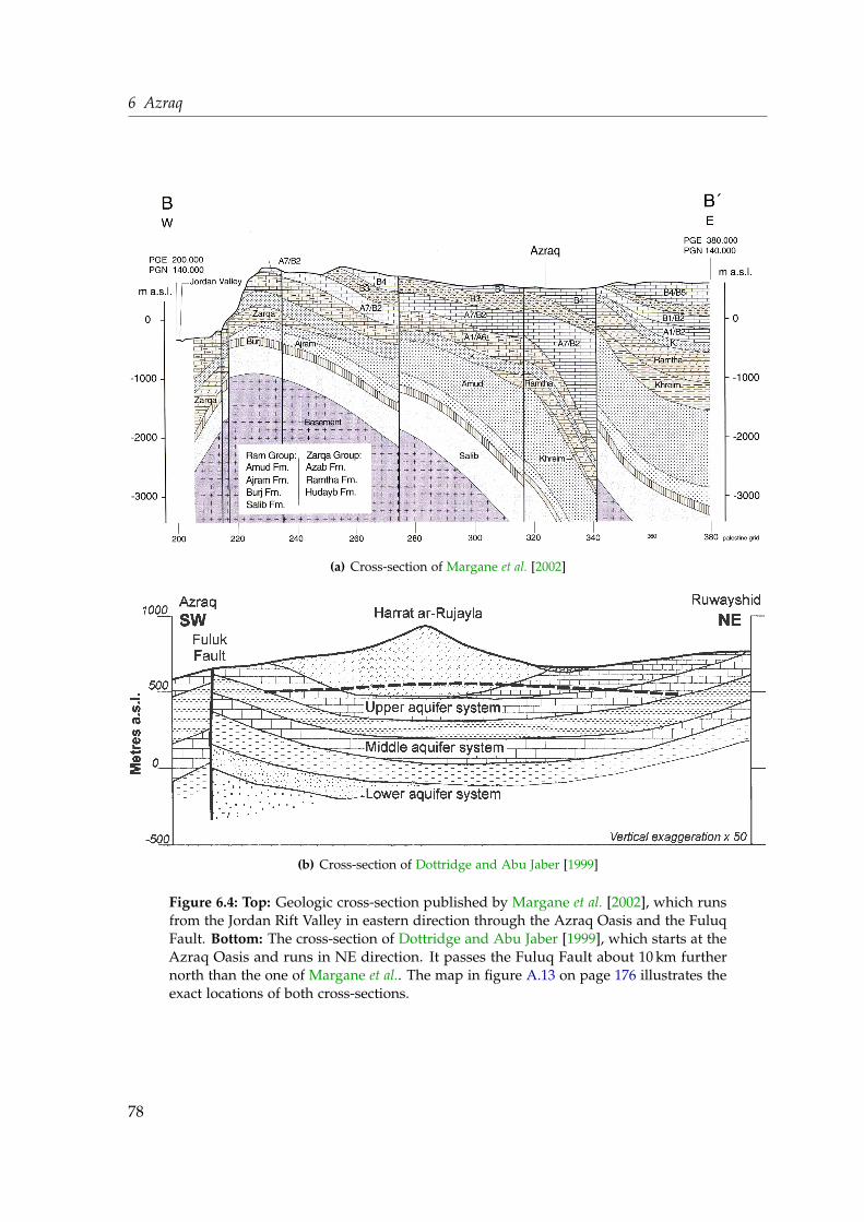
6 Azraq
(a) Cross-section of Margane et al. [2002]
(b) Cross-section of Dottridge and Abu Jaber [1999]
Figure 6.4: Top: Geologic cross-section published by Margane et al. [2002], which runsfrom the Jordan Rift Valley in eastern direction through the Azraq Oasis and the FuluqFault. Bottom: The cross-section of Dottridge and Abu Jaber [1999], which starts at theAzraq Oasis and runs in NE direction. It passes the Fuluq Fault about 10 km furthernorth than the one of Margane et al.. The map in figure A.13 on page 176 illustrates theexact locations of both cross-sections.
78

6.2 The salinization problem and previous studies
495 masl in 2002 [Al-Momani et al., 2006], and extrapolation of the almost constant ground-water level decline suggests a present day level of about 488 masl in the well field area. Ownmeasurements, comparing the depth to the water table in open boreholes to the altitudetaken from Ibrahim [1993], resulted in the farming wells F3960 and Moh in a groundwaterlevel at 493 masl. Al-Momani et al. [2006] state the piezometric head of the middle aquifer inAzraq to be 520 masl, which would promote an upward flow into the shallow aquifer; thesame information is found in Salameh and Bannayan [1993]. However, an own measure-ment at the open borehole of NDW7 resulted in much lower water level of 484 masl. Theonly borehole in the Azraq Oasis that penetrates the deep aquifer is the AZ-1 well (1299 m,taps the uppermost 40 m of the Kurnub aquifer). According to Ajamieh [1998] it has anartesian flow rate of 45 m3/h and its piezometric head is 7 m above the ground surface (i. e.519 masl). If conductive zones are present, the deep aquifer water would discharge into themiddle and the shallow aquifer.
The water of the upper aquifer is in general of good quality and, hence, largely exploitedin the basin, mostly in the northern parts and in the farm area around the central playa foragricultural, but also for domestic purposes. Only in shallow depths in the central farmingarea a groundwater body with high salinity is found. It is assumed that the dissolved min-erals originate from the S1 subunit of the Sirhan formation, which deposited in a brackishlake environment in Miocene times [Andrews, 1992, cited after Ayed [1996]]. El-Waheidiet al. [1992] find the thickness of the saline groundwater body in the Sabkha to be about 60 mand a freshwater body below. They deduce that a non-permeable layer needs to prevent themore dense saline water to descend into deeper layers.
6.2 The salinization problem and previous studies
When the AWSA well field was drilled in the early 1980s the mineralization of all wellswas low (E. C. mostly in the range of 300 to 400 µS/cm). But in the mid-90s, AWSA 12 and15 experienced an increase of salinity, AWSA 3 joined around 2005, and AWSA 13 kept ahigher mineralization level over the years, but showed a steep rise in 2012. The data suggestthat also AWSA 11 will get more saline in the coming years2. All other wells keep the lowmineralzation they had since they were drilled (figure 6.5). This difference in behavior issurprising because most wells are drilled to almost to the same depth of about 200 m andthey are located within a few kilometers from each other. In addition, the wells with a risingE. C. are not all situated at one edge of the well field, which would suggest the movement orexpansion of the salt body in the Sabkha towards the well field. However, the salty wells aretendentially located in the south of the well field, but surrounded by low-saline wells. Themap in figure 6.2 displays the well field, where the orange dots represent the salty wells andthe red dots those with a more or less constant salt content.
Three possible mechanisms of the increasing salinization of those affected wells in the AWSAwell field are discussed [Al-Momani et al., 2006; El-Naqa et al., 2007] (both publications baseon almost the same data set from 2002):
2 According to Al-Momani et al. [2006], AWSA well No 1 had a rising salt content, too, but it could not besampled in this project and is, thus, neglected.
79

6 Azraq
1 9 8 0 1 9 8 5 1 9 9 0 1 9 9 5 2 0 0 0 2 0 0 5 2 0 1 0 2 0 1 5 2 0 2 00
5 0 01 0 0 01 5 0 02 0 0 02 5 0 03 0 0 03 5 0 0
E.C. [µ
S / cm
]A W S A 1 5
A W S A 1 2A W S A 3A W S A 1 3
A W S A 4
A W S A 1 8 A W S A 6A W S A 5
A W S A 1 1
Figure 6.5: The temporal development of the salinity in most of the sampled AWSAwells; those neglected are all constant over time. Most of the wells remained below500 µS/cm, but AWSA wells No 3, 12, 13 and 15 increase in E. C. for a couple of years.Also AWSA 11 tends slightly to higher salinity for the last years. The early data iscourtesy of the WAJ, data from 2009, 2010 and 2012 is own data.
1. As a result of the continuous pumping in the AWSA well field the hydraulic gradientchanged and a back-flow of saline groundwater from the Sabkha began.
2. Due to the reduction of the groundwater table in the shallow aquifer the hydrostaticpressure is reduced and induces an upward leakage from the middle aquifer (B2/A7)and the B3 aquitard.
3. Changes in the local hydrodynamic situation lead to different hydrological and geo-chemical processes (dissolution in the aquifer matrix) which cause a different chemicalcomposition.
The first possibility is ruled out by the above mentioned studies because the hydraulic headgradient at the time of data collection (in 2002) is very low, but still drives the groundwaterto generally flow from the well field area towards the Qa’a Azraq. This fact is confirmedby El-Naqa [2010]. According to Al-Momani et al. [2006] and El-Naqa et al. [2007] the thirdexplanation seems to be the most likely where the transient condition in the upper aquiferled to a significant change in the groundwater geochemistry. This assumption is supportedby the fact that the increase of some constituents is not accompanied by a change of stableisotopes, i. e. it seems to be unlikely that water from other sources admixes into the wellfield. The possible upstream of the brackish water from the middle aquifer through faults,however, could not be ruled out by this study.
Apart from the [Al-Momani et al., 2006; El-Naqa et al., 2007] study, the complex behaviorof the groundwater in the upper aquifer system in the Azraq basin has been extensivelystudied. Several groundwater models were applied to describe the groundwater flow, thegroundwater balance and piezometric head distribution and decrease [Holden, 1998; Ab-dulla et al., 2000; Al-Kharabsheh, 2000; Aljazzar, 2003; Abu-El-Sha’r and Rihani, 2007]. The
80
6.2 The salinization problem and previous studies
Federal Institute for Geosciences and Natural Resources (BGR), Germany, established in co-operation with the Ministry of Water and Irrigation (MWI) a groundwater model of entireJordan, where the Azraq basin is incorporated [Schmidt et al., 2008]. Most of these modelsare constrained to describe only the upper aquifer or the upper and the middle aquifer (ex-cept the model of the BGR, which covers all three aquifer systems in Jordan). All mentionedmodels have in common that they describe the change of the piezometric head distributionquite well under different groundwater abstraction schemes, but none of them is capableto delineate the movement and interaction of the several groundwater species around theQa’a Azraq. This may result from the fact that mixing processes take place on a relativelysmall spacial scale, while all models employ a more or less coarse grid resolution. In addi-tion, the more complex a system is, the more input data a computational simulation needs toproperly describe it. Knowledge of the groundwater behavior in the Qa’a is still insufficient,especially regarding the deep and middle aquifer complexes and in the farm land aroundthe playa. Although there are hundreds of wells, most of them were drilled illegally andthus not much information of the subsurface geology is known. Therefore, models essen-tially lack information they would need to describe the present state and predict the futureconditions of the shallow aquifer in detail.
Geoelectric surveys shed light on the salt water/fresh water interface in the Sabkha as wellas adding information about the structure of the Sirhan formation below alluvial deposits.According to El-Waheidi et al. [1992], El-Naqa [2010] and Yogeshwar et al. [2013], the bound-ary between the highly and low conductive zone is quite sharp and was found to be severalkilometers away from the well field (compare the orange line depicting the salt water/freshwater interface in figure 6.2). El-Naqa [2010] estimated the saltwater regime to need 500 to2000 years to reach the well field at present abstraction rates.
In 1985, Rimawi and Udluft published data of 50 wells from the shallow aquifer in the Azraqbasin and clustered them in four distinct water groups according to their ionic compositionand total salinity.
Group 1 is characterized by sodium being the major cation with about 70 % and chloridethe dominant anion. Average E. C., x̄, is 1363 µS/cm with a standard deviation, s, of316 µS/cm.
Group 2 cations are also dominated by sodium (about 68 %). Regarding the anions, chlorideand bicorbonate dominate. x̄ = 676 µS/cm with s = 125 µS/cm.
Group 3 shows a sodium concentration that equals that of calcium and magnesium to-gether. Chloride is the dominating anion (46 %), but in this group the sulphate ion isthe second most abundant with 28 %. The calcium content of this water is higher thanthe bicarbonate, which is the main difference to group 1 and 2 waters. The salinity isquite high with x̄ = 2043 µS/cm and s = 564 µS/cm.
Group 4 is brine water which is dominated by sodium (91 %) and chloride (86 %). Only twowells of this type were sampled.
The Collins bar diagram and the Schoeller diagram of these groups is shown in figure 6.6.Rimawi and Udluft [1985] further conclude a progressive water genesis. Freshly rechargedrain water interacts with clayey beds in the basalt aquifer on its travel from Jebel ad-Druze
81
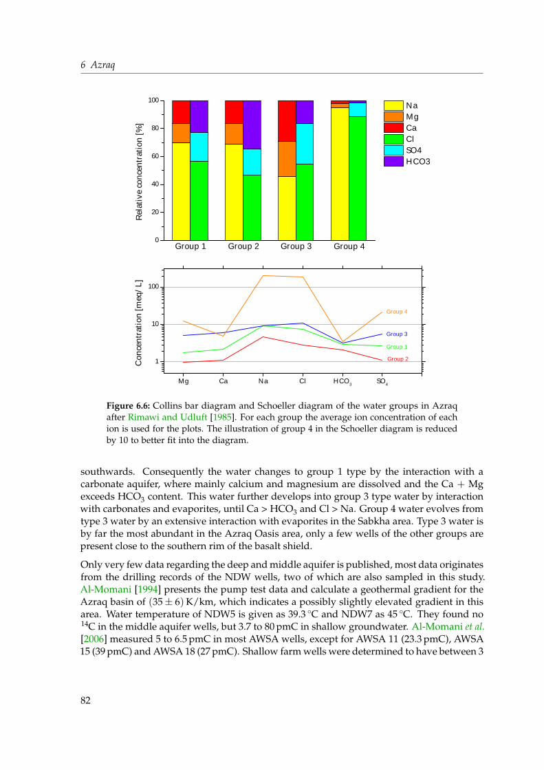
6 Azraq
0
2 0
4 0
6 0
8 0
1 0 0
Relat
ive co
ncentr
ation
[%]
N a M g C a C l S O 4 H C O 3
G r o u p 2 G r o u p 3 G r o u p 4G r o u p 1
M g C a N a C l H C O 3 S O 4
1
1 0
1 0 0
Conce
ntrati
on [m
eq/L
]
G r o u p 4
G r o u p 3G r o u p 1G r o u p 2
Figure 6.6: Collins bar diagram and Schoeller diagram of the water groups in Azraqafter Rimawi and Udluft [1985]. For each group the average ion concentration of eachion is used for the plots. The illustration of group 4 in the Schoeller diagram is reducedby 10 to better fit into the diagram.
southwards. Consequently the water changes to group 1 type by the interaction with acarbonate aquifer, where mainly calcium and magnesium are dissolved and the Ca + Mgexceeds HCO3 content. This water further develops into group 3 type water by interactionwith carbonates and evaporites, until Ca > HCO3 and Cl > Na. Group 4 water evolves fromtype 3 water by an extensive interaction with evaporites in the Sabkha area. Type 3 water isby far the most abundant in the Azraq Oasis area, only a few wells of the other groups arepresent close to the southern rim of the basalt shield.
Only very few data regarding the deep and middle aquifer is published, most data originatesfrom the drilling records of the NDW wells, two of which are also sampled in this study.Al-Momani [1994] presents the pump test data and calculate a geothermal gradient for theAzraq basin of (35± 6)K/km, which indicates a possibly slightly elevated gradient in thisarea. Water temperature of NDW5 is given as 39.3 ◦C and NDW7 as 45 ◦C. They found no14C in the middle aquifer wells, but 3.7 to 80 pmC in shallow groundwater. Al-Momani et al.[2006] measured 5 to 6.5 pmC in most AWSA wells, except for AWSA 11 (23.3 pmC), AWSA15 (39 pmC) and AWSA 18 (27 pmC). Shallow farm wells were determined to have between 3
82

6.3 Description of the sampled wells in Azraq
and 80 pmC [Al-Momani, 1994]. Tritium has not been detected in AWSA wells [Al-Momani,1994; Al-Momani et al., 2006], only in some shallow wells close to wadis tritium was detected[Al-Momani, 1994]. Salinities of the middle aquifer vary widely, with a maximum reportedfor NDW7 of about 24 mS/cm [Al-Momani, 1994].
6.3 Description of the sampled wells in Azraq
This chapter aims at presenting the basic information about the sampled wells in the Azraqbasin as well as illustrating the depth profiles of the AWSA wells regarding the hydrogeo-logic formations they penetrate. The well specific sampling conditions and procedures arenot addressed here, this information is found in appendix A.3.
The AWSA well field is located at the basalt part of the desert and has an extent of about6 x 3 km2. All wells have no casing installed, i. e. they can abstract groundwater from alldepths. Some basic information about the sampled wells is compiled in table 6.1, includingpump test results from the time the wells were drilled [Ayed, 1996]. The hydrogeologic unitsthese wells penetrate are listed in table A.2 and, more convenient, displayed in figure 6.7.
The wells tapping the middle aquifer, NDW5 and NDW7, are closed in the upper layers andthe screen opens only within the B2/A7. NDW5 also taps the deep sandstones, which ismuch closer to the surface east of the Fuluq Fault. The spudded geological units are listenin table A.2 as well.
Not much information on the farm wells is obtainable, because no drill log exist, since mostof them were drilled illegally and were later legalized. The coordinates are found in ta-ble 6.1.
Information about the northern wells is rare, but essentially not needed within this thesis.The unsaturated zone is very thick in this part of the country, in case of KM140 the waterlevel is at 275 m (statement of the well caretaker).
6.4 Results
This section summarizes the results of all wells sampled in Azraq during all three field cam-paigns. The wells are grouped according to their function in this study. In order to facili-tate an immediate recognition in the presented plots, each group is assigned a characteristiccolor:
• Group 1: wells in the northern part of the Azraq basin (purple)
• Group 2: AWSA wells affected by salt (orange)
• Group 3: not affected AWSA wells (red)
• Group 4: Farm wells (green)
• Group 5: Deep wells (blue)
83

6 AzraqTable
6.1:Basic
information
about
thesam
pled
wells
inthe
Azraq
basin.T
hed
rawd
own
andtransm
issivityinform
ationw
asrecord
edw
henthe
wells
were
drilled
.T
heobservation
wellA
Z-12,referred
toin
figure6.1,is
listed,too.
Welllocations
notedm
yself,welldepth
andinform
ationabout
thebase
ofthe
basaltshield
fromW
AJ
[2010].Pump
testdata
fromA
yed[1996].
Nam
eID
EasternN
orthernA
ltitudeD
epthInitial
InitialBase
ofbasalt
drawdow
ntransm
issivity[m
asl][m
][m
][m
2/day][m
asl]
AW
SAw
ellsA
WSA
3F1030
36 ◦49 ′8.8 ′′31 ◦55 ′53.2 ′′
521210
417539
457A
WSA
4F1031
36 ◦48 ′58.2 ′′31 ◦56 ′29.7 ′′
536206
19842
462A
WSA
5F1032
36 ◦48 ′34.4 ′′31 ◦56 ′37.3 ′′
541204
33268
444A
WSA
6F1033
36 ◦48 ′57.6 ′′31 ◦56 ′45.2 ′′
549206
36782
464A
WSA
11F1038
36 ◦49 ′18.5 ′′31 ◦55 ′30.3 ′′
51762
135165
463A
WSA
12F1039
36 ◦48 ′51.0 ′′31 ◦54 ′47.0 ′′
528209
765664
474A
WSA
13F1040
36 ◦48 ′31.5 ′′31 ◦55 ′5.2 ′′
532205
17485
473A
WSA
15F1042
36 ◦48 ′30.0 ′′31 ◦54 ′18.5 ′′
524210
26469
472A
WSA
16F4166
36 ◦48 ′25.0 ′′31 ◦55 ′38.1 ′′
539160
AW
SA18
F322236 ◦48 ′0.9 ′′
31 ◦57 ′8.4 ′′553
171494
AW
SA20
F420536 ◦48 ′2.1 ′′
31 ◦54 ′14.1 ′′533
117
Farmw
ellsF3731
F373136 ◦51 ′40.4 ′′
31 ◦52 ′57.4 ′′514
F3975F3975
36 ◦49 ′27.5 ′′31 ◦49 ′16.7 ′′
509F3741
F374136 ◦55 ′39.6 ′′
31 ◦49 ′43.8 ′′513
F3960F3960
36 ◦53 ′25.0 ′′31 ◦51 ′50.2 ′′
509M
oh?
36 ◦54 ′54.4 ′′31 ◦50 ′20.8 ′′
513
Deep
wells
ND
W5
F135436 ◦56 ′6.1 ′′
31 ◦59 ′14.8 ′′598
733N
DW
7F1350
36 ◦54 ′43.9 ′′31 ◦50 ′49.2 ′′
515970
Northern
wells
Mkeifteh
2F3524(2)
36 ◦39 ′45.4 ′′32 ◦17 ′6.1 ′′
921550
F1381F1381
36 ◦41 ′34.3 ′′32 ◦9 ′57.4 ′′
777575
KM
140F3935
36 ◦53 ′0.7 ′′32 ◦8 ′2.9 ′′
803421
Observation
well
AZ
-12F1043
36 ◦49 ′19 ′′31 ◦55 ′36 ′′
519255
462
84
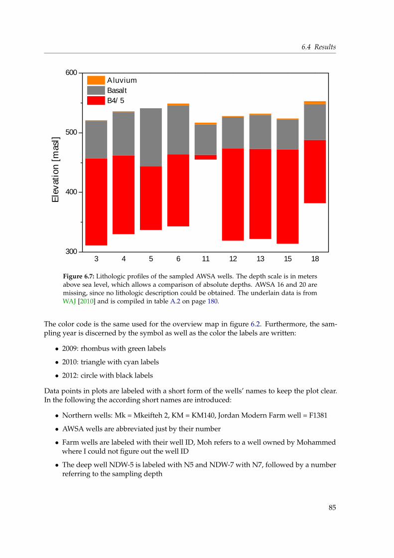
6.4 Results
3 4 5 6 1 1 1 2 1 3 1 5 1 83 0 0
4 0 0
5 0 0
6 0 0 A l u v i u m B a s a l t B 4 / 5
Eleva
tion [
masl]
Figure 6.7: Lithologic profiles of the sampled AWSA wells. The depth scale is in metersabove sea level, which allows a comparison of absolute depths. AWSA 16 and 20 aremissing, since no lithologic description could be obtained. The underlain data is fromWAJ [2010] and is compiled in table A.2 on page 180.
The color code is the same used for the overview map in figure 6.2. Furthermore, the sam-pling year is discerned by the symbol as well as the color the labels are written:
• 2009: rhombus with green labels
• 2010: triangle with cyan labels
• 2012: circle with black labels
Data points in plots are labeled with a short form of the wells’ names to keep the plot clear.In the following the according short names are introduced:
• Northern wells: Mk = Mkeifteh 2, KM = KM140, Jordan Modern Farm well = F1381
• AWSA wells are abbreviated just by their number
• Farm wells are labeled with their well ID, Moh refers to a well owned by Mohammedwhere I could not figure out the well ID
• The deep well NDW-5 is labeled with N5 and NDW-7 with N7, followed by a numberreferring to the sampling depth
85
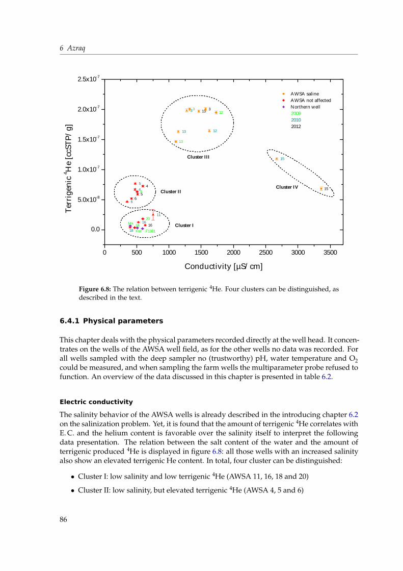
6 Azraq
0 5 0 0 1 0 0 0 1 5 0 0 2 0 0 0 2 5 0 0 3 0 0 0 3 5 0 0
0 . 0
5 . 0 x 1 0 - 8
1 . 0 x 1 0 - 7
1 . 5 x 1 0 - 7
2 . 0 x 1 0 - 7
2 . 5 x 1 0 - 7
3
45
6
1 1
1 21 3
1 5
1 61 8
3
4
1 2
1 3
1 82 0
M kK M F 1 3 8 1
3
45
6
1 3
1 5
1 6F 3 7 3 1
F 3 9 7 5
F 3 7 4 1
F 3 9 6 0
M o h
N 5
N 7 - 5 0
N 7 - 1 0 0
N 7 - 1 5 0
N 7 - 2 0 0
N 7 - 2 5 0
A W S A s a l i n e A W S A n o t a f f e c t e d N o r t h e r n w e l l
2 0 0 9 2 0 1 0 2 0 1 2
Te
rrige
nic 4 He
[ccST
P/g]
C o n d u c t i v i t y [ µ S / c m ]
C l u s t e r I
C l u s t e r I I
C l u s t e r I I I
C l u s t e r I V
Figure 6.8: The relation between terrigenic 4He. Four clusters can be distinguished, asdescribed in the text.
6.4.1 Physical parameters
This chapter deals with the physical parameters recorded directly at the well head. It concen-trates on the wells of the AWSA well field, as for the other wells no data was recorded. Forall wells sampled with the deep sampler no (trustworthy) pH, water temperature and O2could be measured, and when sampling the farm wells the multiparameter probe refused tofunction. An overview of the data discussed in this chapter is presented in table 6.2.
Electric conductivity
The salinity behavior of the AWSA wells is already described in the introducing chapter 6.2on the salinization problem. Yet, it is found that the amount of terrigenic 4He correlates withE. C. and the helium content is favorable over the salinity itself to interpret the followingdata presentation. The relation between the salt content of the water and the amount ofterrigenic produced 4He is displayed in figure 6.8: all those wells with an increased salinityalso show an elevated terrigenic He content. In total, four cluster can be distinguished:
• Cluster I: low salinity and low terrigenic 4He (AWSA 11, 16, 18 and 20)
• Cluster II: low salinity, but elevated terrigenic 4He (AWSA 4, 5 and 6)
86

6.4 Results
Table 6.2: Compilation of the recorded physical parameters of all sampled wells in theAzraq basin of all field trips alongside the corresponding content of terrigenic 4He.
Well Year E. C. O2 pH Sampling Temp. Terr. 4He Terr. 4He err[µS/cm] [mg/L] [◦C] [ccSTP/g] [ccSTP/g]
AWSA well fieldAWSA 3 2009 1320 – – 28.8 2.004E-07 2.270E-09
2010 1276 0.52 7.57 28.4 2.011E-07 4.619E-092012 1568 – 8.07 27.2 2.003E-07 8.372E-09
AWSA 4 2009 506 – – 29.1 6.319E-08 1.175E-092010 474 2.32 7.77 29.2 6.673E-08 2.180E-092012 596 – 8.20 28.2 7.227E-08 2.670E-09
AWSA 5 2010 476 0.94 7.82 28.7 7.691E-08 2.310E-092012 515 – 8.26 28.3 5.883E-08 5.882E-09
AWSA 6 2010 351 0.75 7.81 28.8 4.619E-08 1.755E-092012 419 – 8.23 28.0 5.147E-08 4.334E-09
AWSA 11 2010 755 12.00 7.90 26.2 2.436E-08 9.548E-09AWSA 12 2009 1730 – – 27.9 1.946E-07 2.226E-09
2010 1626 1.34 7.67 28.0 1.669E-07 3.957E-09AWSA 13 2009 1107 – – 27.0 1.463E-07 2.061E-09
2010 1144 0.76 7.72 27.7 1.657E-07 3.932E-092012 1463 – 8.03 26.8 1.967E-07 7.949E-09
AWSA 15 2010 2670 3.62 7.65 26.5 1.193E-07 3.070E-092012 3360 – 7.77 21.3 6.772E-08 2.798E-09
AWSA 16 2010 526 7.73 8.03 24.7 1.188E-08 1.291E-092012 631 – 8.43 23.9 7.522E-09 7.555E-09
AWSA 18 2009 467 – – 25.4 3.548E-09 6.310E-102010 397 7.43 8.20 25.3 3.372E-09 1.065E-09
AWSA 20 2009 595 – – 24.6 1.812E-08 7.972E-10
Farm wellsF3731 2012 8580 1.65 6.65 – -5.087E-10 8.363E-10F3975 2012 19750 – 7.40 – 7.070E-08 3.127E-09F3741 2012 16960 – 7.03 – 2.766E-07 6.875E-09F3960 2012 6880 – 7.10 – 2.876E-08 2.827E-09Moh 2012 50200 – 7.22 – 1.452E-07 9.601E-09
Deep wellsNDW5 684m 2012 1179 – 8.19 – 2.194E-06 4.758E-08NDW7 50m 2012 7310 – 7.20 – 4.211E-07 1.134E-08NDW7 100m 2012 7310 – 8.53 – 5.716E-07 1.572E-08NDW7 150m 2012 7300 – 8.81 – 6.827E-07 1.502E-08NDW7 200m 2012 7660 – 8.85 – 9.402E-07 2.194E-08NDW7 250m 2012 7360 – 8.00 – 1.293E-06 2.974E-08
Northern wellsMkeifteh 2 2009 400 – – 30.6 6.375E-09 6.552E-10KM 140 2009 510 – – 30.5 3.155E-09 6.218E-10JMF 2009 591 – – 35.2 1.968E-09 6.337E-10
87

6 Azraq
• Cluster III: medium salt content and high terrigenic 4He (AWSA 3, 12 and 13)
• Cluster IV: highest salinity, but only medium terrigenic 4He content (AWSA 15)
One should recall, that the terrigenic 4He content is an indicator of groundwater age. AsCluster I and II are both lowly mineralized, terrigenic 4He is a better indicator than E. C.to trace the processes taking place in the well field. Therefore, in the following the otherphysical parameters are related to the terrigenic 4He instead of E. C.
pH
The pH of the sampled water has only been noted on the 2010 and 2012 campaigns and iscompiled in table 6.2 and visualized in the terrigenic 4He-vs.-pH plot in figure 6.9. Appar-ently, the pH values of these campaigns are shifted against each other, which is likely dueto the usage of different calibration solutions. However, a general pattern is discernible: allwells affected by salinization have a significantly lower pH value than the other wells. Alsothe clusters introduced above can be differentiated. This trend may be an indicator that wa-ter from the saline wells originates from a different aquifer material. The basalt aquifer ismade up of alkaline magmas, as described in chapter 4.3. This trend in pH therefore sug-gests that those wells containing only little terrigenic He are stronger influenced by waterfrom the basaltic regime of the shallow aquifer than the wells with elevated terrigenic 4He,which implies a correlation between water age and pH.
Temperature
The water temperatures at the time of sampling show a similar pattern, as displayed infigure 6.9. All those wells with an elevated He amount are significantly warmer than thosewith almost no terrigenic 4He. Again, the clusters are clearly visible. Cluster II water isas warm as cluster III water, although it is not affected by an increased salinity, but hasan elevated He concentration. The AWSA 15 sample of 2012 is much colder than all othersamples. At the time of sampling this well showed huge air bubbled by shoves. Presumablythe pump sucked soil air, which affected the water temperature as well as the pH (and otherparameters). Higher water temperatures argue for a deeper origin of the respective water.
Dissolved oxygen
Data for dissolved oxygen in the AWSA wells is only available for the 2010 sampling trip. Asfigure 6.9 shows, all wells with a higher He content are depleted in dissolved oxygen. In thecase of AWSA 11 the notably high O2 concentration can be attributed to some air bubbles inthe measurement bucket, as the pump apparently drew some air. As a low oxygen contentis mostly found in old groundwater, this finding again supports the greater age indicated bythe elevated helium content, and older water usually exists in greater depths.
88

6.4 Results
7 . 6 7 . 8 8 . 0 8 . 2 8 . 40
1 x 1 0 - 7
2 x 1 0 - 7 3
4 56
1 3
1 5
1 6F 3 7 3 1
F 3 9 7 5
F 3 7 4 1
F 3 9 6 0
M o h
N 5
N 7 - 5 0
N 7 - 1 0 0
N 7 - 1 5 0
N 7 - 2 0 0
N 7 - 2 5 0
3
4 56
1 1
1 2 1 3
1 5
1 6 1 8
Terri
genic
4 He [cc
STP/
g]
p H
2 2 2 4 2 6 2 8 3 00
1 x 1 0 - 7
2 x 1 0 - 7 3
4 56
1 3
1 5
1 6
3
456
1 1
1 21 31 5
1 6 1 8
3
4
1 2
1 3
1 82 0 M kK M F 1 3 8 1
A W S A s a l i n e A W S A n o t a f f e c t e d
2 0 0 9 2 0 1 0 2 0 1 2
Terri
genic
4 He [cc
STP/
g]
T e m p e r a t u r e [ ° C ]
0 2 4 6 8 1 0 1 20
1 x 1 0 - 7
2 x 1 0 - 7 3
456
1 1
1 21 3
1 5
1 61 8
Terri
genic
4 He [cc
STP/
g]
O 2 [ m g / L ]Figure 6.9: The Terrigenic 4He is plotted against the physical parameters pH, watertemperature and oxygen content. Although split into two branches it is obvious thatthose wells containing an elevated amount of terrigenic helium have lower pH values.Higher pH may indicate water originating from the alkaline basalt aquifer. A similartrend is visible in the temperature diagram, where those wells with higher helium aresignificantly warmer and, hence, suggest to origin from deeper layers. The depletedoxygen content in the high-helium wells argues for older water, i. e. coming from deeperlayers, too. 89

6 Azraq
M g C a C a + M g N a + K C l H C O 3 S O 4
0 . 1
1
1 0
1 0 0
Co
ncen
tratio
n [me
q/L]
A W S A 3 A W S A 4 A W S A 5 A W S A 6 A W S A 1 3 A W S A 1 5 A W S A 1 6 F 3 7 3 1 F 3 9 7 5 F 3 7 4 1 F 3 9 6 0 M o h a m m e d N D W 5 N D W 7 - 5 0 m N D W 7 - 1 0 0 m N D W 7 - 1 5 0 m N D W 7 - 2 0 0 m N D W 7 - 2 5 0 m G r o u p 1 G r o u p 2 G r o u p 3 G r o u p 4
Figure 6.10: The Schoeller diagram of all sampled wells of 2012 in Azraq. The dataof the water groups regarding Rimawi and Udluft [1985] is plotted as well. Red arethe unaffected AWSA wells, those with elevated salt content are coded in orange. Theshallow farm wells are green, NDW5 is dark blue, while NDW7 is displayed in differentshades of blue, according to the sampling depth.
6.4.2 Water chemistry
The samples of the 2012 campaign were analyzed for their major ion content. Table A.4in the appendix on page 182 lists all data together with the total sum of the cations and theanions. The calculated ion balance error (IBE) is given in the last column. All samples exceptAWSA 4 and 16 fall into the exceptable range of the IBE of 5 %. AWSA 4 and 16 are handledlike the other samples in the further analysis, but one has to keep in mind that they mightcontain another substance not tested for, or at least experienced analytical trouble. Figure6.10 compiles all data in a Schoeller diagram. Based on this diagram the wells in Azraqare assigned to the water groups introduced by Rimawi and Udluft [1985] and which aredescribed above on page 81:
Group 1 AWSA 3 and 13
Group 2 AWSA 4, 5, 6 and 16
Group 3 AWSA 15, (F3731) and (F3960)
Group 4 F3975, Moh, NDW7 and (F3741)
90

6.4 Results
M g C a C a + M g N a + K C l H C O 3 S O 4
0 . 1
1
1 0
1 0 0
Conc
entra
tion [
meq/
L]
A W S A 3 A W S A 1 3 G r o u p 1
(a) Group 1
M g C a C a + M g N a + K C l H C O 3 S O 4
0 . 1
1
1 0
1 0 0
Conc
entra
tion [
meq/
L]
A W S A 4 A W S A 5 A W S A 6 A W S A 1 6 G r o u p 2
(b) Group 2
M g C a C a + M g N a + K C l H C O 3 S O 4
0 . 1
1
1 0
1 0 0
Conc
entra
tion [
meq/
L]
A W S A 1 5 F 3 7 3 1 F 3 9 6 0 G r o u p 3
(c) Group 3
M g C a C a + M g N a + K C l H C O 3 S O 4
0 . 1
1
1 0
1 0 0
Co
ncen
tratio
n [me
q/L]
F 3 9 7 5 F 3 7 4 1 M o h a m m e d N D W 7 - 5 0 m N D W 7 - 1 0 0 m N D W 7 - 1 5 0 m N D W 7 - 2 0 0 m N D W 7 - 2 5 0 m G r o u p 4
(d) Group 4
Figure 6.11: The Schoeller diagrams for the 2012 Azraq samples separated accordingthe four water groups of Rimawi and Udluft [1985] found in the Azraq basin.
In figure 6.11 the Schoeller diagram in figure 6.10 is split up into the individual water groupsto justify this assignment. The wells in brackets do not fit into that scheme that well andshow particular deviations from the water group definitions. F3731 is closest to group 3, butthe salinity is much higher. F3741 seems to be a mixture of groups 3 and 4, but group 4 waterdominates the pattern. F3960 is most similar to group 3 water, but has a high salinity and Mg,Ca, Na and Cl are a bit too high, whereas HCO3 and SO4 are a bit lower. However, one mayconsider that for the definition of the water groups the mean concentration of each ion isemployed, but within each group quite large deviations are accepted (compare the standarddeviations by Rimawi and Udluft [1985] given on page 81). The NDW5 sample does not fitin this scheme at all. Its ion pattern is similar to group 4 water, but the total mineralizationis far too low for Na–Cl brine water. This type of water may not be covered by the typecastof Rimawi and Udluft [1985], because they considered only water samples from the shallowaquifer in the Azraq basin.
The relative shares of cations and anions is presented in the Piper plot in figure 6.12. Regard-ing the cations the AWSA wells cluster very close to each other, with AWSA 3 and 13 lying
91

6 Azraq
Ca2+
CATIONSCl
-
ANIONS
1000
0100
100 0
0100
1000
0 100
100
100
0 0
EXPLANATIONAWSA 3AWSA 4AWSA 5AWSA 6AWSA 13AWSA 15AWSA 16F3731F3975F3741F3960MohNDW5NDW7-50mNDW7-100mNDW7-150mNDW7-200mNDW7-250m
Figure 6.12: Piper diagram of the 2012 Azraq samples. As usual, the colors indicate thewater group defined in the beginning of this chapter. A description is found in the text.
slightly more towards Na/K type water (see figure 2.13 for a description of the water typesdistinguishable in a Piper diagram); only well No 15 is a bit apart from the cluster and posi-tioned opposite the other salinity affected wells. The picture is totally different respective theanions, where the AWSA wells are widely spread from bicarbonate to chloride type water.Although the differences in salinity between the unaffected AWSA wells (red) are small, thebasic trend is also visible with AWSA 6 having the lowest salt content. All wells influencedby increasing salinity, however, are clearly shifted from the unaffected wells towards morerelative chloride content which indicates admixing with water similar to F3731 and F3975.It therefore looks like an admixing of water with a higher Cl content into these AWSA wells.Both AWSA 15 and 16 contain considerably more SO4 than the other AWSA wells.
The farm wells form two distinct clusters in the cation triangle and lie in a mixing line in-cluding the AWSA wells. In this plot it seems that AWSA 15 is influenced by water foundin the shallow wells F3731 and F3960, which, indeed, are the northernmost of the sampledfarm wells. Moreover, these two wells are the two farm wells assigned to water group 3,while the other farm wells are attributed to group 4. The anion plot locates all farm wellsin the chloride dominated corner, where F3731 and F3975 are less governed by Cl than theothers. It has to be mentioned that the grouping of farm wells in the anion triangle differsfrom that of the cation plot.
92

6.4 Results
NDW7 shows a trend with sampling depth towards more Na + K type water, which is sur-prising, because this well has a closed casing in the depth range in which water sampleswere collected using the deep sampler and water should origin from the depth where thescreen opens (upper A7 formation). Additionally, the total salinity is almost constant inall NDW7 samples. Regarding the anions, the different depths of NDW7 plot more or lessidentical, with practically no bicarbonate, but strong chloride influence. NDW5 obviously isdifferent from all other water types, as it plots rather separated in the cation as well as theanion triangle.
The results from both triangle plots unite in the central diamond shaped diagram. The trendsof both the AWSA wells and within the deep NDW7 well are transferred. Also the two farmwell groups regarding the cations are translated into the diamond. It becomes apparent thatall farm wells, both deep wells and AWSA 15 fall into the regime of Cl + SO4 type water,while the two northernmost farm wells F3731 and F3960 show considerably more Ca andMg than the other farm wells. All other AWSA wells spread in the wide field of Na + K,Ca + Mg type water, with AWSA 3 and 13 reaching almost into the Cl + SO4 regime.
In order to trace the minerals the ion composition originates from, all possible ion combina-tion were plotted against each other, but only a few yielded interesting information, whichis presented in the following. As the dominant ions are Na and Cl, the dissolution of haliteis obvious. Figure 6.13(a) shows that most wells fall onto the angle bisector which confirmsthis assumption. Dedolomitization, i. e. the weathering of dolomite (CaMg(CO3)2), is exam-ined in figure 6.13(b). The AWSA wells are well described by this process, as they all lieon the angle bisector, but one has to keep in mind that the strongest influence on most ofthese waters is still their Na and Cl content. AWSA 15 is far more influenced by dolomiteproducts than its salinity would suggest, which indicates that this well is additionally influ-enced by a source with higher dedolomitization imprint. The samples from different depthsof the NDW7 well show a trend also in this consideration, but are not so well explained bydedolomitization contributing to their ion composition. The farm wells, however, scatterquite far a round the angle bisector and cannot be well described by dedolomitization.
Gypsum dissolution results in an 1:1 ratio of sulphate and calcium ions. Similar to thedolomite dissolution plot, the AWSA wells lie on the angle bisector, with the gypsum prod-ucts disproportionately emphasized in AWSA 15 (figure 6.13(c)). This may be explained bygypsum lenses found in the very bottom of AWSA 15 during the drilling [Al-Momani et al.,2006]. Another quite strong correlation is found between SO4 and Mg, which is indicativeof epsomite dissolution (figure 6.13(d)). Even the farm wells, except for F3960, plot close tothe angel bisector, but no epsomite is reported from the Azraq basin.
A correlation of He and Cl is often applied as an indicator, that the weathering of Cl contain-ing minerals also causes the release of stored radiogenic helium. Among the Azraq wells avery rough correlation is visible, though the picture is not that clear, see figure 6.14. More-over, leaching of local minerals to explain the elevated total helium content would not ex-plain also a higher 3He content. Radiogenic production of 3He originates from the decayof 6Li (compare chapter 2.3.1). However, no elevated lithium content is reported for theAzraq basin. Generally, high lithium content is mainly found in granitic rock [James andPalmer, 2000], whereas in Azraq several kilometers of sediments have accumulated on top
93

6 Azraq
1 1 0 1 0 0
1
1 0
1 0 0
3
45
6
1 3
1 5
1 6
F 3 7 3 1
F 3 9 7 5F 3 7 4 1
F 3 9 6 0
M o h
N 5
Cl [m
eq/L
]
N a [ m e q / L ]
N D W 7
(a) Halite dissolution
1 1 0
1
1 0
3
45
6
1 3
1 5
1 6
F 3 7 3 1F 3 9 7 5 F 3 7 4 1 F 3 9 6 0
M o h
N 5
N 7 - 5 0N 7 - 1 0 0
N 7 - 1 5 0N 7 - 2 0 0
N 7 - 2 5 0
Mg [m
eq/L
]
C a [ m e q / L ]
(b) Dolomite dissolution
1 1 0
1
1 0
3
45
6
1 3
1 5
1 6
F 3 7 3 1
F 3 9 7 5
F 3 7 4 1
F 3 9 6 0
M o h
N 5
N 7 - 5 0N 7 - 1 0 0N 7 - 1 5 0
N 7 - 2 0 0 N 7 - 2 5 0
SO4 [m
eq/L
]
C a [ m e q / L ]
(c) Gypsum dissolution
1 1 0
1
1 0
3
45
6
1 3
1 5
1 6
F 3 7 3 1
F 3 9 7 5
F 3 7 4 1
F 3 9 6 0
M o h
N 5
N 7 - 5 0N 7 - 1 0 0
N 7 - 1 5 0N 7 - 2 0 0
N 7 - 2 5 0
SO4 [m
eq/L
]
M g [ m e q / L ]
(d) Epsomite dissolution
Figure 6.13: The relations of specific ion combinations indicate the dissolution of acertain mineral.
of the crystalline basement. Therefore, a matrix source of 3He is rather unlikely in the Azraqdepression.
Concluding, halite dissolution is the dominant cause of the salinity in most of the wells, butother weathering processes play a role in the ion composition as well.
In order to test the salinization scenarios introduced by Al-Momani et al. [2006], a simplethree component mixing model based on the water chemistry data is applied. Thereby, theionic patterns of AWSA 3, 13 and 15 are attempted to be characterized as mixture of middleaquifer water (D), shallow water from the Sabkha (S), and of water originating from thenorth (N). Regarding every tracer, the following equation has to be fulfilled:
cW = xD · cD + xS · cS + xN · cN , (6.1)
where cW is the concentration of ion i found in the respective AWSA well, cD, cS and cN theconcentrations of the same ion in the reservoirs D, S and N. The xS are the relative contribu-tions of the respective source to the final ion content abstracted from the well. As ∑ x ≡ 1,
94

6.4 Results
1 1 0 1 0 0
1 E - 7
1 E - 6
3
456
1 31 5
1 6 F 3 7 3 1
F 3 9 7 5
F 3 7 4 1
F 3 9 6 0
M o h
N 5
N 7 - 5 0N 7 - 1 0 0N 7 - 1 5 0
N 7 - 2 0 0N 7 - 2 5 0
4 He [cc
STP/
g]
C l [ m e q / L ]Figure 6.14: Only a very rough correlation between total He content and chloride withinthe AWSA well field is observed. Together with the high 3He content found in the salinewells it is very unlikely that matrix dissolution is the source of radiogenic helium.
one can eliminate one of the xS:
cW = xS(cS − cD) + xN(cN − cD) + cD (6.2)
A combination of two ions leads to two equations, having two variables and therefore resultsin an unambiguous result for the relative contributions.
The deep reservoir concentration, cD, is defined as the average of the 200 and 250 m depthsamples of NDW7. The unaffected AWSA water (cN) reaching the well field from the northis considered to be the water of AWSA 11 as the only member of cluster I sampled in 2012.Representative of the shallow Sabkha water ion content, cS, the average of the wells F3731and F3960 is assumed, because these two wells are closest to the well field. Besides, bothbelong to group 3 water after Rimawi and Udluft [1985], while the other farm wells arebetter described by group 4.
The result for several combinations of dissolved ions is presented in table 6.3. Combinationsincluding SO4 and HCO3 resulted generally in impossible contribution of the three reser-voirs, i. e. when some source supplies less than zero or more than 100 %. Thus, these ions areomitted.
The admixing proportions of the three basic reservoirs of the AWSA 13 ion pattern repro-duces very well with different ion combinations, as does AWSA 3 if the Ca/Mg combinationis disregarded. AWSA 15, however, is not possible to interpret as a result of mixing of thedefined water species. The resulting contributions vary strongly, and two ion combinationseven did not yield possible contributions. This reflects the position of AWSA 15 in the aniontriangle of the piper plot, where this well locates outside the range, where any mixture be-
95

6 Azraq
Table 6.3: Results of the three component mixing calculations using different combina-tion of dissolved ions. Means values and standard deviations are listed as well. Allvalue given in %. In case of AWSA 15, the ion combinations Ca/Mg and Mg/Cl yieldimpossible amounts with one reservoir having very negative values. Thus, they are leftblank. Also the presented ion combination Ca/Cl exhibits a slightly negative share ofdeep water.
Tracer AWSA 3 AWSA 13 AWSA 15combination xS xN xD xS xN xD xS xN xD
Na/Cl 1.4 88.1 10.4 -0.2 89.9 10.3 5.2 71.1 23.8Na/Mg 2.1 87.9 10.0 3.3 88.7 8.0 38.0 59.6 2.4Na/Ca 2.7 87.7 9.6 3.2 88.7 8.1 26.7 63.5 9.7Ca/Mg 5.4 94.5 0.1 2.7 87.4 9.9Ca/Cl 2.9 88.2 8.9 3.7 90.0 6.2 30.0 71.7 -1.7Mg/Cl 2.2 88.2 9.6 4.0 90.0 5.9
Mean value 2.8 89.1 8.1 2.8 89.1 8.1 25.0 66.5 8.6s. d. 1.4 2.7 4.0 1.5 1.0 1.9 14.0 5.9 11.2
tween the three water species would plot. This well seems to be influenced by an additionalmineral source which is not covered by these simple three component mixing calculations.
6.4.3 Tritium, carbon and radon
Tritium data was measured for every well and all campaigns. As shown in table 6.4 the tri-tium content is below the detection limit of 2 TU in almost all wells in 2009 and 2010. How-ever, in 2012 most of the AWSA wells have significantly higher tritium content compared tothe previous campaigns. This fact is attributed to measurement problems during the anal-ysis run of these samples. Hence the tritium data of the farm wells and the deep wells isalso questionable. Some tritium content in the shallow farm wells, however, would not besurprising due to possible local recharge of surface runoff gathering in the Sabkha duringstorm events. The wells in the northern part of the Azraq basin, where young groundwatermight be expected due to local precipitation, show no tritium content as well.
The carbon isotopy has only been analyzed for some selected AWSA wells of the 2010 sam-pling trip (see table 6.4). Although this data set is incomplete, the wells of clusters III andIV (AWSA 12, 13 and 15) are slightly less depleted than those of cluster I and II (AWSA 4, 5,11 and 18). This may be a hint that the first-mentioned wells draw water which is in contactwith different aquifer rock material than the latter ones.
The carbon-14 content has been determined on very few samples, too. AWSA 4, 5 and 12can be considered as practically 14C free, i. e. their water is several ten thousands of yearsold. AWSA 15, however, has a 14C activity of almost 28 pmC. This is in accord with thedata published by Al-Momani et al. [2006], who found elevated 14C activity only for AWSA11 (23 pmC) and AWSA 15 (38 pmC), sampled earlier than 2002. This strongly suggests that
96
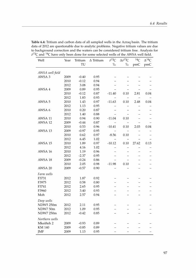
6.4 Results
Table 6.4: Tritium and carbon data of all sampled wells in the Azraq basin. The tritiumdata of 2012 are questionable due to analytic problems. Negative tritium values are dueto background correction and the waters can be considered tritium free. Analysis forδ13C and 14C have only been done for some selected wells of the AWSA well field.
Well Year Tritium ∆ Tritium δ13C ∆δ13C 14C ∆14CTU h h pmC pmC
AWSA well fieldAWSA 3 2009 -0.40 0.95 – – – –
2010 -0.12 0.94 – – – –2012 3.08 0.94 – – – –
AWSA 4 2009 0.89 0.95 – – – –2010 -0.12 0.87 -11.40 0.10 2.81 0.042012 1.83 0.93 – – – –
AWSA 5 2010 1.43 0.97 -11.63 0.10 2.48 0.042012 1.13 0.95 – – – –
AWSA 6 2010 0.20 0.87 – – – –2012 1.40 0.88 – – – –
AWSA 11 2010 0.94 0.90 -11.04 0.10 – –AWSA 12 2009 -0.44 0.87 – – – –
2010 0.53 0.96 -10.41 0.10 2.03 0.04AWSA 13 2009 -0.97 0.95 – – – –
2010 0.62 0.97 -8.56 0.10 – –2012 6.45 1.02 – – – –
AWSA 15 2010 1.89 0.97 -10.12 0.10 27.62 0.132012 4.16 1.02 – – – –
AWSA 16 2010 1.19 0.96 – – – –2012 -2.37 0.95 – – – –
AWSA 18 2009 -0.24 0.86 – – – –2010 2.05 0.98 -11.98 0.10 – –
AWSA 20 2009 -0.57 0.90 – – – –
Farm wellsF3731 2012 1.87 0.92 – – – –F3975 2012 0.58 0.80 – – – –F3741 2012 2.65 0.95 – – – –F3960 2012 3.40 0.93 – – – –Moh 2012 2.57 0.94 – – – –
Deep wellsNDW5 250m 2012 2.11 0.95 – – – –NDW7 50m 2012 1.09 0.95 – – – –NDW7 250m 2012 -0.42 0.85 – – – –
Northern wellsMkeifteh 2 2009 -0.93 0.89 – – – –KM 140 2009 -0.85 0.89 – – – –JMF 2009 1.13 0.95 – – – –
97

6 Azraq
AWSA 11 and 15 draw younger water or at least admixed young groundwater into the oldwater that mainly prevails in the AWSA well field. According to this data AWSA 15 drawsless young water today compared to > 10 years ago, which needs to be compensated by olderwater.
The radon concentration in groundwater is an indicator of the radium content of the sur-rounding rock matrix. Three AWSA wells were analyzed for their radon activity on the 2012field trip: AWSA 13 (14 801± 836)Bq/m3, AWSA 15 (41 010± 1141)Bq/m3 and AWSA 16(1589± 409)Bq/m3. The much lower activity in the unaffected well AWSA 16 is anotherhint that this well feeds from a different reservoir than the two saline wells.
6.4.4 Stable isotopes
The stable isotopes data of all sampled wells in Azraq is compiled in table 6.5 and is dis-played in the δ2H vs. δ18O plot in figure 6.15 alongside the Jordanian meteoric water line(JMWL) [Bajjali, 2012] and the global meteoric water line (GMWL). The measurements of theAWSA well field water forms three obvious groups, according to their year of sampling. It isquite unlikely that the water of the well field shifted in total over the years. Probably therewere some complications in the deuterium measurements (especially as the 2012 sampleswere analyzed in a different laboratory with another measurement principle, see chapter3.3), as the δ18O values correspond with each other over the years. For the interpretation ofadmixing in the AWSA wells, deuterium is therefore only in the 2012 samples consideredin the following analysis, which is not a big disadvantage because the farm wells and thedeep wells as possible contributors are also just analyzed in the 2012 campaign. However, apotential temporal trend in the stable isotope data between 2009 and 2012 is veiled behindthose analytical problems.
In general, all sampled wells are shifted from the local meteoric water line (JMWL) towardsthe right. This indicates a more or less strong influence of evaporation after the rainwaterreaches the land surface for all water found in the Azraq basin. The shallow farm wells inthe central mud pan are evidently most affected by evaporation processes, as they lie faraway from the local meteoric water line and on an evaporation line which also includes theAWSA groundwater. This evaporation line (drawn only for the 2012 samples) intersects theJMWL at an isotopic composition of δ18O ≈ −7.5 h and δ2H ≈ −36 h. Meteoric water inAzraq has a composition of δ18O =−5.16 h and δ2H =−24.56 h [Bajjali, 2012]. The only pre-cipitation gauge stations in Jordan, which measure a similar isotope concentration, are RasMunif (close to Irbid, 1150 masl, δ18O = −6.86 h, δ2H = −30.38 h) and Shoubak (south Jor-dan, close to Petra, 1475 masl, δ18O =−6.71 h, δ2H =−30.35 h) [Bajjali, 2012]. This indicatesthat water in the AWSA wells originates from high altitudes. More interesting, however, isthe fact that also the groundwater abstracted by the shallow farm wells originates to a greatextent from high altitudes. Recharge by local precipitation, therefore, plays a minor rolein the Azraq Oasis. Most of the local recharge comes from flash floods forming at Jabalad-Druze and rushing to the central depression, where the water needs some time to seepaway through the badly permeable mud pan surface and experiences strong evaporativeinfluences.
98

6.4 Results
Table 6.5: Stable isotope data of all sampled wells in the Azraq basin. Deuterium excess,d, is calculated according to equation 2.10.
Well Year 18O ∆18O 2H ∆2H d ∆dh h h h h h
AWSA well fieldAWSA 3 2009 -6.25 0.05 -30.75 0.26 19.25 0.66
2010 -6.28 0.05 -32.29 0.26 17.95 0.662012 -6.26 0.05 -33.52 0.07 16.60 0.48
AWSA 4 2009 -6.37 0.05 -30.58 0.26 20.38 0.662010 -6.41 0.05 -32.22 0.26 19.06 0.662012 -6.35 0.03 -33.14 0.04 17.63 0.29
AWSA 5 2010 -6.41 0.05 -32.54 0.26 18.74 0.662012 -6.35 0.05 -33.13 0.13 17.68 0.53
AWSA 6 2010 -6.33 0.05 -31.56 0.26 19.08 0.662012 -6.31 0.04 -32.83 0.27 17.65 0.60
AWSA 11 2010 -6.24 0.05 -31.11 0.26 18.81 0.66AWSA 12 2009 -6.34 0.05 -31.05 0.26 19.67 0.66
2010 -6.29 0.05 -32.50 0.26 17.82 0.66AWSA 13 2009 -6.32 0.05 -30.46 0.26 20.10 0.66
2010 -6.34 0.05 -32.18 0.26 18.54 0.662012 -6.38 0.03 -33.65 0.10 17.36 0.31
AWSA 15 2010 -6.16 0.05 -31.11 0.26 18.17 0.662012 -6.16 0.04 -32.93 0.11 16.37 0.42
AWSA 16 2010 -6.19 0.05 -30.99 0.26 18.53 0.662012 -6.16 0.02 -32.02 0.14 17.25 0.33
AWSA 18 2009 -6.17 0.05 -29.27 0.26 20.09 0.662010 -6.09 0.05 -30.57 0.26 18.15 0.66
AWSA 20 2009 -6.12 0.05 -30.51 0.26 18.45 0.66
Farm wellsF3731 2012 -5.80 0.05 -31.90 0.32 14.48 0.68F3975 2012 -5.47 0.04 -31.47 0.08 12.32 0.44F3741 2012 -3.62 0.04 -25.32 0.06 3.67 0.41F3960 2012 -5.28 0.05 -30.72 0.10 11.55 0.48Moh 2012 -3.87 0.06 -26.98 0.11 3.97 0.59
Deep wellsNDW5 684m 2012 -4.77 0.05 -31.19 0.09 6.99 0.52NDW7 50m 2012 -5.16 0.05 -31.99 0.19 9.33 0.61NDW7 100m 2012 -5.30 0.02 -32.84 0.08 9.54 0.21NDW7 150m 2012 -5.31 0.03 -33.53 0.07 8.93 0.30NDW7 200m 2012 -5.45 0.07 -34.07 0.20 9.53 0.75NDW7 250m 2012 -5.41 0.02 -33.89 0.29 9.35 0.46
Northern wellsMkeifteh 2 2009 -6.07 0.05 -27.53 0.26 21.03 0.66KM 140 2009 -6.34 0.05 -30.46 0.26 20.26 0.66JMF 2009 -6.51 0.05 -30.36 0.26 21.72 0.66
99

6 Azraq
- 7 - 6 - 5 - 4 - 3
- 3 6
- 3 4
- 3 2
- 3 0
- 2 8
- 2 6
- 2 4
345 6
1 3
1 5
1 6 F 3 7 3 1F 3 9 7 5
F 3 7 4 1
F 3 9 6 0
M o h
N 5
N 7 - 5 0
N 7 - 1 0 0N 7 - 1 5 0
N 7 - 2 0 0N 7 - 2 5 0
345
6 1 1
1 21 3
1 51 61 834
1 21 3
1 8
2 0
M k
K MF 1 3 8 1
A W S A s a l i n e A W S A n o t a f f e c t e d F a r m w e l l s D e e p w e l l s N o r t h e r n w e l l s
2 0 0 9 2 0 1 0 2 0 1 2
δ2 ����
�
δ1 8 � � � � �
J MW L : �
2 H = 6 . 2
7 · �1 8 O +
1 1. 4 �
G MW L
: �2 H =
8 . 17 · �
1 8 O + 1 0
. 3 5 �
E v a p o r a t i o n l i n e
Figure 6.15: Stable isotope data of all sampled wells in the Azraq basin. All wells inAzraq show signals of evaporation. The shallow farm wells and the AWSA wells fallon the same evaporation line. The AWSA wells are shifted in their deuterium isotopyaccording to the year of sampling (see text for explanation). The shallow farm wells areobviously strongly influenced by evaporation. Samples from different depth of NDW-7scatter along the GMWL and indicate leakage of shallow groundwater from the Sabkhainto the deep well. NDW-5 plots a little bit off the GMWL. Error bars are omitted formore clarity.
- 6 . 5 - 6 . 4 - 6 . 3 - 6 . 2 - 6 . 1 - 6 . 0
0 . 0
5 . 0 x 1 0 - 8
1 . 0 x 1 0 - 7
1 . 5 x 1 0 - 7
2 . 0 x 1 0 - 7
2 . 5 x 1 0 - 7
3
4
1 2
1 3
1 82 0
M kK MF 1 3 8 1
3
45
6
1 1
1 21 3
1 5
1 61 8
3
45
6
1 3
1 5
1 6F 3 7 3 1
F 3 9 7 5
F 3 7 4 1
F 3 9 6 0
M o h
N 5
N 7 - 5 0
N 7 - 1 0 0
N 7 - 1 5 0
N 7 - 2 0 0
N 7 - 2 5 0
A W S A s a l i n e A W S A u n a f f e c t e d N o r t h e r n w e l l s
2 0 0 9 2 0 1 0 2 0 1 2
Terri
genic
4 He [cc
STP/
g]
δ1 8 � � � � �
C l u s t e r I
C l u s t e r I I
C l u s t e r I I I
C l u s t e r I V
Figure 6.16: Those wells which have an elevated 4He content (cluster II and III) areslightly more depleted than the unaffected wells (cluster I). Although affected bysalinization, well No 15 plots a bit away from the other saline wells. Error bars areomitted for clearity reasons.
100
6.4 Results
The samples collected from different depth of the NDW-7 borehole line up along the GMWL.The deeper the water sample is from, the more depleted it is in stable isotopes. This trendmay indicate leakage of shallow groundwater into the deep well, where the infiltrating waterhas an isotopy of about δ18O ≈ −4.8 h and δ2H ≈ 29.5 h, i. e. where the GMWL and theevaporation line intersect. This might explain the trend with depth observed in other tracersas well. The NDW-5 sample is a bit less depleted than all NDW-7 samples, especially in δ18Owhich shifts it a bit to the right. Corresponding to the position of the NDW-7 samples closeto the GMWL, the δ2H excess is close to 10 h.
Two of the northern wells (F1381 and especially KM140) have a very similar isotopic signa-ture to the unaffected AWSA wells. This describes the fact that the groundwater found in theAWSA well field originates from the slopes of Jabal ad-Druze in the north. Only Mkeifteh 2is distinctly enriched in deuterium compared to the AWSA wells.
Despite the analytical problems, within all groups of AWSA data it can be recognized, thatthose wells influenced by rising salinity and as well as those wells of cluster II are a bit moredepleted in deuterium compared to the wells of cluster I. This suggests that the terrigenic4He carrying water is slightly more depleted in deuterium. AWSA 15 may be an exception.
It can also be seen, that within each sampling year those AWSA wells which have an in-creased He content are a little bit more depleted in δ18O than the unaffected wells. Thiscorrelation is well recognizable in figure 6.16, where the terrigenic 4He is plotted against theoxygen isotopy. Clusters I wells plot less depleted than cluster II and III. However, AWSA 15as the only member in cluster IV is enriched as well although it exhibits a high mineraliza-tion.
6.4.5 Noble gases
In 2009 and 2010, for each sampled well two copper tube samples were collected and ana-lyzed. The 2009 samples were measured in Run 53 and Run 55 (compare the overview ofmeasurement runs in appendix A.6). Run 55, however, suffered from several incidents andthe obtained data is partly questionable. Therefore, only the data of Run 53 is consideredfor the analysis of the 2009 samples. Similarly, the 2010 samples were measured in Run60 and Run 65, but the first one was interrupted several times and the properness of theresults is doubtful, i. e. only the Run 65 data is used for the further analysis. The sole excep-tion is AWSA well No 11, which was measured in Run 60 only because the double samplebroke. But, to make it clear, the results of two measurement runs deviate only little. The2012 samples were measured only once, in Run 72 (and a few samples in Run 71, whichwas terminated accidentally), and only in cases the data looked fishy a double sample wasanalyzed.
Noble gas raw data is treated like described in chapter 3.6.2 using the group’s own softwareWUCEM. The final noble gas isotope concentrations are given in table 6.6.
Noticeable are two samples with distinctly high noble gas content: AWSA 11 from 2010 andthe 2012 sample of AWSA 15. Both show a typical, but very strongly pronounced, excessair pattern in their heavy noble gases, i. e. the relative excess is highest in neon and lowest
101

6 Azraq
Table6.6:C
oncentrationof
allmeasured
noblegas
isotopesof
thesam
plesfrom
theA
zraqbasin
includingtheir
analyticalerrors,given
inccST
P/g.3H
e∆
3He
4He
∆4H
e20N
e∆
20Ne
22Ne
∆22N
e36A
r∆
36Ar
40Ar
∆40A
r84K
r∆
84Kr
132Xe
∆132X
e
2009
AW
SA3
2.742E-131.115E-14
2.422E-071.979E-09
1.544E-077.361E-10
1.578E-087.872E-11
8.466E-072.796E-08
2.582E-048.479E-07
3.238E-085.853E-10
2.020E-093.455E-11
AW
SA4
8.548E-143.673E-15
1.061E-079.250E-10
1.544E-077.154E-10
1.575E-087.748E-11
8.824E-072.938E-08
2.618E-048.760E-07
3.210E-085.718E-10
2.014E-093.501E-11
AW
SA12
2.592E-131.009E-14
2.367E-071.936E-09
1.555E-077.686E-10
1.584E-088.641E-11
8.793E-072.800E-08
2.604E-048.558E-07
3.236E-085.848E-10
2.075E-093.596E-11
AW
SA13
1.409E-135.662E-15
1.908E-071.807E-09
1.577E-077.325E-10
1.613E-088.089E-11
8.946E-072.892E-08
2.701E-049.114E-07
3.465E-085.855E-10
2.118E-093.532E-11
AW
SA18
6.371E-142.934E-15
4.563E-083.755E-10
1.547E-077.047E-10
1.579E-088.675E-11
9.279E-072.932E-08
2.757E-049.177E-07
3.435E-086.166E-10
2.139E-093.736E-11
AW
SA20
6.080E-142.786E-15
6.141E-085.134E-10
1.583E-077.660E-10
1.623E-089.449E-11
9.655E-072.871E-08
2.837E-049.827E-07
3.580E-086.103E-10
2.233E-093.879E-11
Mkeifteh
26.656E-14
2.700E-154.792E-08
3.952E-101.524E-07
6.897E-101.553E-08
8.023E-118.976E-07
2.795E-082.644E-04
8.520E-073.456E-08
6.017E-102.122E-09
3.633E-11K
M140
6.327E-142.698E-15
4.468E-083.674E-10
1.477E-076.848E-10
1.518E-088.040E-11
7.876E-072.963E-08
2.382E-047.796E-07
2.935E-085.474E-10
1.851E-093.204E-11
F13816.528E-14
2.858E-154.492E-08
3.698E-101.550E-07
7.108E-101.581E-08
7.923E-118.832E-07
2.876E-082.572E-04
8.482E-073.211E-08
5.772E-102.067E-09
3.529E-11
2010
AW
SA3
2.840E-131.077E-14
2.398E-072.087E-09
1.524E-078.997E-10
1.555E-081.055E-10
9.013E-072.118E-08
2.553E-047.873E-07
3.191E-088.299E-10
1.844E-097.234E-11
AW
SA4
9.168E-143.781E-15
1.082E-078.690E-10
1.509E-079.388E-10
1.501E-081.777E-10
8.242E-072.541E-08
2.560E-048.963E-07
3.168E-088.470E-10
1.868E-097.388E-11
AW
SA5
7.836E-142.938E-15
1.192E-079.606E-10
1.539E-078.663E-10
1.573E-081.024E-10
8.925E-072.123E-08
2.589E-047.662E-07
3.266E-088.888E-10
2.008E-097.977E-11
AW
SA6
6.377E-142.756E-15
8.729E-086.994E-10
1.472E-078.807E-10
1.501E-089.892E-11
8.305E-071.941E-08
2.485E-047.799E-07
3.121E-087.799E-10
1.934E-097.490E-11
AW
SA11
8.648E-135.356E-14
5.537E-074.214E-09
1.719E-066.480E-09
1.758E-077.613E-10
4.368E-062.272E-07
1.295E-033.429E-06
1.055E-071.501E-09
4.356E-091.223E-10
AW
SA12
2.145E-137.961E-15
2.065E-071.791E-09
1.532E-078.865E-10
1.546E-081.086E-10
8.877E-072.560E-08
2.582E-047.587E-07
3.178E-088.395E-10
2.081E-098.454E-11
AW
SA13
1.543E-135.933E-15
2.054E-071.755E-09
1.541E-079.090E-10
1.574E-081.116E-10
8.647E-072.017E-08
2.630E-049.113E-07
3.332E-088.198E-10
2.213E-098.931E-11
AW
SA15
9.598E-143.562E-15
1.602E-071.327E-09
1.545E-079.124E-10
1.586E-081.088E-10
9.142E-072.473E-08
2.686E-049.391E-07
3.412E-088.052E-10
1.962E-098.018E-11
AW
SA16
6.243E-142.467E-15
5.772E-084.613E-10
1.642E-079.034E-10
1.678E-081.071E-10
9.620E-072.231E-08
2.765E-049.589E-07
3.523E-088.771E-10
2.288E-099.116E-11
AW
SA18
5.545E-142.039E-15
4.506E-083.517E-10
1.508E-078.709E-10
1.541E-081.089E-10
8.786E-072.240E-08
2.658E-049.727E-07
3.436E-088.965E-10
2.115E-098.331E-11
2012
AW
SA3
2.906E-131.097E-14
2.435E-072.342E-09
1.554E-076.190E-10
1.586E-086.979E-11
8.702E-071.226E-08
2.553E-048.225E-07
3.224E-084.335E-10
2.037E-094.388E-11
AW
SA4
1.026E-133.647E-15
1.152E-071.028E-09
1.544E-076.184E-10
1.576E-086.835E-11
8.616E-071.026E-08
2.545E-048.196E-07
3.191E-084.281E-10
1.976E-093.995E-11
AW
SA5
7.459E-142.836E-15
1.018E-078.994E-10
1.543E-076.164E-10
1.575E-086.905E-11
8.607E-071.007E-08
2.544E-048.228E-07
3.187E-084.525E-10
1.975E-094.351E-11
AW
SA6
7.565E-142.715E-15
9.373E-088.247E-10
1.519E-075.961E-10
1.548E-086.545E-11
8.416E-071.279E-08
2.547E-048.317E-07
3.201E-084.726E-10
2.051E-094.248E-11
AW
SA13
1.839E-136.690E-15
2.402E-072.302E-09
1.569E-076.130E-10
1.602E-086.794E-11
8.631E-071.348E-08
2.589E-048.700E-07
3.244E-084.128E-10
2.099E-094.125E-11
AW
SA15
1.616E-135.834E-15
1.676E-071.560E-09
3.221E-071.283E-09
3.290E-081.391E-10
1.183E-061.338E-08
3.491E-041.130E-06
3.930E-085.402E-10
2.402E-094.947E-11
AW
SA16
6.149E-142.305E-15
5.040E-084.336E-10
1.565E-076.418E-10
1.593E-087.073E-11
9.152E-071.056E-08
2.692E-048.791E-07
3.450E-084.769E-10
2.141E-094.724E-11
F37316.484E-14
2.456E-155.020E-08
4.309E-101.841E-07
7.542E-101.879E-08
8.319E-111.043E-06
1.148E-083.022E-04
9.749E-073.792E-08
5.145E-102.314E-09
4.812E-11F3975
7.285E-142.692E-15
1.135E-071.021E-09
1.568E-076.248E-10
1.598E-086.987E-11
9.088E-071.335E-08
2.723E-048.877E-07
3.457E-084.608E-10
2.201E-094.514E-11
F37411.273E-13
4.659E-153.211E-07
3.165E-091.639E-07
6.440E-101.674E-08
7.204E-119.658E-07
1.134E-082.883E-04
9.398E-073.726E-08
4.874E-102.345E-09
4.943E-11F3960
8.511E-143.626E-15
7.215E-088.924E-10
1.607E-071.279E-09
1.635E-081.328E-10
9.857E-071.210E-08
2.914E-042.220E-06
3.669E-085.476E-10
2.306E-095.250E-11
Moham
med
1.079E-133.947E-15
1.865E-072.176E-09
1.557E-071.242E-09
1.588E-081.294E-10
9.793E-071.186E-08
2.893E-042.205E-06
3.689E-085.665E-10
2.363E-094.932E-11
ND
W5
684m2.239E-12
9.090E-142.230E-06
4.154E-081.268E-07
2.084E-091.294E-08
2.146E-107.119E-07
1.344E-082.119E-04
3.449E-062.623E-08
5.461E-101.602E-09
4.343E-11N
DW
750m
1.469E-135.740E-15
4.654E-079.185E-09
1.634E-072.067E-09
1.671E-082.043E-10
9.945E-071.907E-08
2.947E-043.283E-06
3.723E-086.127E-10
2.289E-095.842E-11
ND
W7
100m1.673E-13
6.612E-156.162E-07
1.325E-081.640E-07
2.416E-091.674E-08
2.400E-109.968E-07
2.012E-082.950E-04
3.963E-063.730E-08
6.701E-102.269E-09
5.759E-11N
DW
7150m
1.785E-131.399E-14
7.268E-071.382E-08
1.635E-072.403E-09
1.663E-082.388E-10
1.001E-062.035E-08
2.933E-043.934E-06
3.727E-086.732E-10
2.336E-096.331E-11
ND
W7
200m1.790E-13
1.381E-149.872E-07
2.095E-081.735E-07
2.971E-091.768E-08
2.973E-101.037E-06
2.285E-083.084E-04
4.948E-063.789E-08
7.524E-102.395E-09
6.628E-11N
DW
7250m
1.572E-131.414E-14
1.339E-062.878E-08
1.698E-072.905E-09
1.731E-082.905E-10
1.041E-062.288E-08
3.070E-044.906E-06
3.756E-087.492E-10
2.505E-097.316E-11
ND
W7
300m1.568E-13
1.461E-143.070E-06
6.921E-081.592E-07
2.754E-091.598E-08
2.681E-101.102E-06
2.406E-083.237E-04
5.153E-064.090E-08
8.331E-102.530E-09
6.722E-11N
DW
7544m
1.671E-136.941E-15
2.889E-065.454E-08
1.373E-072.276E-09
1.400E-082.333E-10
1.023E-061.966E-08
3.005E-044.933E-06
3.917E-088.127E-10
2.394E-096.526E-11
ND
W7
569m1.344E-13
5.964E-152.793E-06
5.198E-081.386E-07
2.260E-091.411E-08
2.313E-109.208E-07
1.709E-082.731E-04
4.403E-063.470E-08
7.263E-102.076E-09
5.296E-11N
DW
7ca450m
7.458E-143.630E-15
1.438E-062.691E-08
7.491E-081.254E-09
7.638E-091.291E-10
4.707E-079.134E-09
1.398E-042.321E-06
1.761E-083.837E-10
1.159E-093.035E-11
102

6.4 Results
in xenon (compare figure 2.17). This expresses also in the extremely high neon excess valuesof AWSA 11 and 15 (2012), which are listed in table 6.7. Such high ∆Ne values, defined inequation 2.27, can not be attributed to the normal excess air formation described in chapter2.3.6.2, but are credited to air bubble formation during sampling. Indeed, AWSA 11 showedair bubbles in the sampling tubes, which mostly vanished under increased water pressure,but possibly still influenced the water. At the time of sampling AWSA 15 (2012) often hadshort interruptions with almost no water running anymore, where the pump seemed to rundry (it possibly did not hang deep enough in the water). Getting a sample without disturbingair bubbles was virtually impossible. KM 140, F3731 and NDW5-684m have rather low noblegas concentrations and consequently negative ∆Ne values, which indicate degassing (withinthe aquifer or during sampling).
Table 6.7 lists the basic noble gas isotope ratios relevant for this study. The 3He/4He ratio ofthe 2009 samples is calculated by WUCEM using the “mean of isotope 1” routine, whereasit is determined by the division of the final 3He and 4He concentrations for the 2010 and2012 samples, as those two isotopes are analyzed in separate steps since then (compare thedescription of different measurement procedures in chapter 3.6.1). 20Ne/22Ne is calculatedby the “next neighbors” routine of WUCEM, while for 40Ar/36Ar the “mean of isotope 1”routine is applied.
The 20Ne/22Ne ratio of almost all samples matches the atmospheric value of 9.80. Onlyfour samples differ from that. While NDW7-300m was measured, a leak occurred in thepreparation line, which explains the high 20Ne/22Ne ratio. KM 140 and F3731 have a slightlylower 20Ne/22Ne ratio, which is associated with a lower total noble gas concentration (asdescribed above). AWSA 15 (2010) has a lower 20Ne/22Ne ratio as well, but is inconspicuousapart from that.
A high 40Ar/36Ar ratio is generally a sign of very old groundwater, i. e. the presence of asubstantial radiogenic 40Ar amount. In those cases the total Ar concentration (needed for theinverse modeling) is calculated from 36Ar only, as mentioned in chapter 3.6.4. The chosenthreshold is an argon ratio of 302, which exceeds the atmospheric ratio of 295.5 by about 2 %.Only two samples exhibit 40Ar/36Ar ratios above this threshold: the 2010 samples of AWSA4 and 18. However, these samples are obviously not old groundwater, as radiogenic 40Arproduction is always accompanied by distinct radiogenic 4He production, which is not thecase here. The high argon ratio, therefore, needs to be ascribed to measurement inaccuracies,although the data preparation with WUCEM did not exhibit any abnormity. Nevertheless,total Ar is calculated from 36Ar for those two samples.
The final noble gas concentrations are compiled in table A.5 on page 183 and are used to de-termine the noble gas temperatures (NGTs) by inverse modeling using the software PANGA,as introduced in chapter 3.6.4. In the course of the calculation, each noble gas content isseparated into its equilibrium and excess air component, and, in case of helium, the non-atmospheric amount.
The applied excess air model is the CE model, as it is the most versatile of all excess airmodels and can handle also cases of degassing. Because the Azraq samples prove to notallow a straight-forward modeling, all samples are analyzed using Monte Carlo simulations.A modeling run with 100 000 Monte Carlo simulations is performed for each sample. In
103

6 Azraq
Table6.7:The
noblegas
isotoperatios
ofallm
easuredA
zraqsam
ples.The3H
e/4H
eratio
isgiven
inabsolute
valueand
relativeto
theatm
osphericratio
RA ,indicated
bythe
indexatm
.The∆
Ne
valuesare
listed,too.3H
e/ 4He
∆3H
e/4H
e(
3He/ 4H
e)atm∆( 3H
e/4H
e)atm20N
e/ 22Ne
∆20N
e/22N
e40A
r/ 36Ar
∆40A
r/36A
rN
e/He
∆N
e/He
∆N
e∆(∆
Ne)
2009
AW
SA3
1.148E-063.643E-08
0.8300.026
9.8020.004
299.784.66
0.7010.007
5.35%0.54%
AW
SA4
7.945E-072.496E-08
0.5740.018
9.8030.004
290.424.99
1.6000.016
4.36%0.58%
AW
SA12
1.089E-063.375E-08
0.7870.024
9.7960.005
296.234.45
0.7220.007
5.67%0.55%
AW
SA13
6.998E-072.375E-08
0.5060.017
9.7930.005
297.634.50
0.9080.010
4.86%0.54%
AW
SA18
1.347E-064.257E-08
0.9740.031
9.7860.005
291.804.67
3.7270.035
1.85%0.53%
AW
SA20
9.320E-072.960E-08
0.6730.021
9.8220.005
294.554.40
2.8350.028
3.00%0.58%
Mkeifteh
21.408E-06
4.298E-081.017
0.0319.794
0.004295.12
4.363.494
0.0332.92%
0.50%K
M140
1.355E-064.265E-08
0.9790.031
9.7560.004
297.095.28
3.6360.034
3.80%0.51%
F13811.404E-06
4.374E-081.014
0.0329.792
0.004294.25
4.743.791
0.0365.79%
0.52%
2010
AW
SA3
1.184E-064.606E-08
0.8560.033
9.7710.005
284.184.23
0.7020.007
4.21%0.69%
AW
SA4
8.474E-073.560E-08
0.6120.026
9.8100.012
302.394.57
1.5370.016
3.39%0.94%
AW
SA5
6.573E-072.521E-08
0.4750.018
9.7870.006
291.814.49
1.4270.014
4.64%0.65%
AW
SA6
7.306E-073.211E-08
0.5280.023
9.8030.006
299.514.44
1.8630.019
1.20%0.64%
AW
SA11
1.562E-069.746E-08
1.1290.070
9.8080.006
290.447.19
3.4310.029
1178.93%58.07%
AW
SA12
1.039E-063.959E-08
0.7500.029
9.7990.006
287.334.96
0.8190.009
4.03%0.65%
AW
SA13
7.513E-072.959E-08
0.5430.021
9.8010.006
300.254.50
0.8290.009
3.94%0.66%
AW
SA15
5.992E-072.279E-08
0.4330.016
9.7460.006
293.255.18
1.0660.011
3.47%0.67%
AW
SA16
1.082E-064.360E-08
0.7820.032
9.7960.006
289.944.43
3.1430.031
9.18%0.64%
AW
SA18
1.231E-064.626E-08
0.8890.033
9.8060.006
304.474.81
3.6990.036
0.69%0.84%
2012
AW
SA3
1.188E-064.541E-08
0.8580.033
9.7950.004
295.852.32
0.7040.007
6.11%0.40%
AW
SA4
8.921E-073.190E-08
0.6450.023
9.7930.004
295.222.08
1.4800.014
5.57%0.41%
AW
SA5
7.370E-072.816E-08
0.5330.020
9.7920.004
300.922.93
1.6740.016
5.54%0.41%
AW
SA6
8.116E-072.928E-08
0.5860.021
9.7970.004
298.622.83
1.7890.017
3.63%0.39%
AW
SA13
7.614E-072.812E-08
0.5500.020
9.7940.004
293.662.12
0.7200.007
6.60%0.40%
AW
SA15
9.605E-073.510E-08
0.6940.025
9.8020.004
297.512.09
2.1250.021
113.24%1.46%
AW
SA16
1.230E-064.628E-08
0.8880.033
9.7890.004
294.982.03
3.4310.032
4.51%0.41%
F37311.301E-06
4.947E-080.940
0.0369.772
0.004294.45
2.024.054
0.03720.41%
0.87%F3975
6.452E-072.399E-08
0.4660.017
9.7880.004
300.922.39
1.5250.015
4.23%0.40%
F37413.957E-07
1.467E-080.286
0.0119.791
0.004295.83
2.190.563
0.0066.83%
0.42%F3960
1.202E-065.182E-08
0.8690.037
9.8190.004
296.082.03
2.4580.036
4.61%0.91%
Moham
med
5.788E-072.174E-08
0.4180.016
9.8100.004
294.842.09
0.9210.013
0.74%0.83%
ND
W5
684m9.982E-07
4.403E-080.721
0.0329.811
0.004298.20
2.050.063
0.002-9.18%
1.54%N
DW
750m
3.157E-071.382E-08
0.2280.010
9.8090.012
293.874.49
0.3880.009
7.56%1.61%
ND
W7
100m2.715E-07
1.222E-080.196
0.0099.796
0.012295.88
4.520.294
0.0087.05%
1.68%N
DW
7150m
2.455E-071.981E-08
0.1770.014
9.8000.012
291.024.43
0.2480.006
6.26%1.64%
ND
W7
200m1.813E-07
1.451E-080.131
0.0109.812
0.012297.91
4.500.194
0.00512.78%
2.08%N
DW
7250m
1.174E-071.086E-08
0.0850.008
9.7930.012
292.714.41
0.1400.004
9.60%2.00%
ND
W7
300m5.106E-08
4.895E-090.037
0.0049.976
0.012293.88
4.430.057
0.002-0.39%
1.76%N
DW
7544m
5.861E-082.626E-09
0.0420.002
9.8100.004
295.582.03
0.0520.001
-13.01%1.48%
ND
W7
569m4.879E-08
2.310E-090.035
0.0029.823
0.004296.47
2.010.055
0.001-8.53%
1.53%
104

6.4 Results
most cases the Monte Carlo analysis results in a smaller error for the NGTs and the otheroutput parameters. Above all, Monte Carlo analysis reveals samples where the traditionalnoble gas fitting routine results in bad NGTs, accompanied by unrealistic values for theparameters A and F. The details of the Monte Carlo evaluation is given in appendix A.8,including information about which part of the simulations is considered in the analysis andwhich ones are discarded.
A check using the UA excess air model revealed no cases of degassing among the Azraqsamples from all campaigns. Hence, as initial parameters for the fitting routine the followingvalues are chosen for all samples: Excess air factor A = 0.01, temperature T = 19 ◦C, salinityS = 0 mg/L and the fractionation factor F = 0.5. The air pressure at the groundwater tablein the infiltration area is quite tricky to guess for the Azraq basin. The shallow aquifer ismainly recharged at the slopes of 1500 m high Jabal ad-Druze. No information about thedepth to the water table could be obtained for this mountain. However, thicknesses of theunsaturated zone of over 400 m are reported from close to the Jordan/Syrian border [Mar-gane et al., 2002], which would correspond to a groundwater table at about 700 masl. It istherefore assumed that the average altitude of the water table is 800 masl, which correspondsto an air pressure p = 920 mbar at the water table. The middle aquifer is recharged in theJordan highlands, mainly in altitudes between 700 and 1100 masl. The static water level inwells in the highlands varies between a few 10 meters and more than 100 m below the sur-face [WAJ, 2010]. Hence, due to the lack of more information about exact groundwater flowlines, an assumed groundwater table altitude of 800 masl, too, seems to be acceptable. Even-tually, the assumed groundwater table altitude in the recharge area influences the resultingnoble gas temperature (i. e. if a too high altitude is assumed, the NGTs are calculated to becolder). However, since the main results in this chapter concern the non-atmospheric heliumcontent of the samples and the fact that the helium solubility depends only slightly on therecharge temperature, a biased NGT determination would only have a very little effect onthe amount of non-atmospheric helium.
Table 6.8 lists the resulting NGTs and the corresponding values of the fit parameters A andF. The values presented are means of all selected Monte Carlo simulations, the respective er-rors are the standard deviations of the same set of simulations. Also the mean and standarddeviation of the distribution of χ2 values is given. The new fitting routine implementedin PANGA reveals that many samples are described as quasi-UA type, identifiable by theextreme values of the fit parameter |F|. Although these numbers do not have a physicalexplanation, they lead to reasonable NGT and, hence, F is only seen as a fit parameter. Moredetails about this issue is given in chapter 3.6.4. χ2 as a measure of goodness of the fit isin an acceptable range for all analyses. In addition, table 6.8 presents the modeled atmo-spheric 3He and total helium concentrations beside the non-atmospheric components (i. e.atmospheric component subtracted from the total measured signal).
The noble gas temperatures found in the Azraq basin seem to be quite reasonable. ElevatedNGTs found in the AWSA well field reflect the deep unsaturated zone, where the ambi-ent temperature at the groundwater table, where equilibration between water and soil airtakes place, is considerably higher than the mean annual air temperature. The farm wellshave NGTs between 20 and 23 ◦C, suggesting local recharge in the Sabkha. Recharge tem-peratures from the NDW7 well range from around 21 ◦C in the uppermost 250 m, around
105

6 Azraq
Table6.8:T
hem
odeled
parameters
NG
T,Aand
Ftogether
with
theresulting
mod
eledatm
osphericcontent
(i.e.equilibrationplus
excessair
component),
3He
mod
andH
em
od,thecalculated
non-atmospheric
components,∆
3He
non-atmand
∆H
eterr,and
theχ
2values.H
ighvalues
of|F|indicatethe
quasi-UA
limiting
case,asexplained
inchapter
3.6.4.
Sample
NG
T∆
NG
TA
∆A
F∆
F3H
e mod
∆3H
e mod
He m
od∆
He m
od3H
e non-atm∆
3He non-atm
He terr
∆H
e terrχ
2∆
χ2
[ ◦C]
[ ◦C]
[ccSTP/g]
[ccSTP/g][ccST
P/g][ccSTP/g]
[ccSTP/g]
[ccSTP/g][ccST
P/g][ccSTP/g]
[ccSTP/g]
[ccSTP/g]
2009
AW
SA3
25.810.25
4.72E-042.46E-03
-1223.02373.95
5.844E-143.631E-16
4.287E-082.609E-10
2.158E-131.152E-14
2.005E-072.250E-09
4.093.53
AW
SA4
25.760.42
7.37E-031.08E-02
-478.85560.16
5.775E-143.435E-16
4.237E-082.471E-10
2.773E-144.016E-15
6.322E-081.168E-09
1.471.80
AW
SA12
25.370.22
6.02E-054.79E-04
-1352.70243.99
5.872E-143.827E-16
4.307E-082.752E-10
2.005E-131.048E-14
1.946E-072.219E-09
5.804.37
AW
SA13
24.000.28
1.44E-034.70E-03
-986.87509.59
5.844E-143.599E-16
4.288E-082.585E-10
8.247E-146.022E-15
1.464E-072.051E-09
4.914.04
AW
SA18
22.740.30
8.40E-031.20E-02
-73.73400.94
5.669E-143.505E-16
4.163E-082.544E-10
7.019E-153.284E-15
3.604E-096.266E-10
1.541.92
AW
SA20
21.770.36
1.08E-021.30E-02
-268.56417.38
5.762E-143.563E-16
4.230E-082.577E-10
3.186E-153.142E-15
1.827E-087.642E-10
1.251.67
Mkeifteh
223.73
0.208.71E-05
1.07E-03-854.26
180.235.719E-14
3.430E-164.197E-08
2.470E-109.370E-15
3.043E-156.422E-09
6.460E-109.33
5.77K
M140
30.060.23
2.76E-053.13E-03
-1028.37113.39
5.669E-143.431E-16
4.158E-082.469E-10
6.575E-153.041E-15
3.258E-096.157E-10
10.736.23
F138126.03
0.221.60E-05
1.49E-03-1371.69
114.165.866E-14
3.559E-164.302E-08
2.560E-106.617E-15
3.214E-152.062E-09
6.271E-1010.26
6.08
2010
AW
SA3
26.770.40
3.52E-036.93E-03
-493.73457.65
5.759E-144.392E-16
4.225E-083.170E-10
2.264E-131.121E-14
1.976E-072.404E-09
2.853.02
AW
SA4
27.400.88
2.93E-042.57E-03
-548.40292.61
5.695E-145.443E-16
4.178E-083.903E-10
3.473E-144.325E-15
6.641E-081.259E-09
4.383.70
AW
SA5
25.920.33
1.66E-035.72E-03
-827.05392.29
5.798E-144.301E-16
4.253E-083.096E-10
2.038E-143.368E-15
7.668E-081.270E-09
2.712.69
AW
SA6
27.530.25
3.89E-042.67E-03
-317.10247.40
5.549E-144.389E-16
4.073E-083.163E-10
8.282E-153.195E-15
4.656E-081.016E-09
3.192.92
AW
SA11
39.506.97
1.38E-017.48E-03
0.020.00
7.298E-135.804E-15
5.301E-074.251E-09
1.351E-135.937E-14
2.362E-088.464E-09
1.662.15
AW
SA12
25.950.30
1.62E-035.22E-03
-742.78368.90
5.757E-144.413E-16
4.224E-083.177E-10
1.569E-138.402E-15
1.643E-072.108E-09
3.323.07
AW
SA13
24.820.28
8.09E-041.15E-02
-898.99200.42
5.768E-144.560E-16
4.232E-083.282E-10
9.662E-146.389E-15
1.631E-072.083E-09
6.234.57
AW
SA15
23.810.34
2.40E-035.90E-03
-432.27396.36
5.763E-144.513E-16
4.230E-083.259E-10
3.835E-144.014E-15
1.179E-071.653E-09
4.013.78
AW
SA16
22.930.24
7.75E-055.24E-04
-1528.27303.28
6.159E-144.592E-16
4.515E-083.296E-10
8.387E-162.926E-15
1.257E-087.909E-10
4.623.79
AW
SA18
23.460.79
6.32E-061.06E-04
-151.41174.69
5.580E-144.928E-16
4.097E-083.535E-10
-3.553E-162.532E-15
4.085E-097.052E-10
4.183.52
2012
AW
SA3
26.690.21
6.63E-067.01E-04
-1351.6083.09
5.884E-143.106E-16
4.315E-082.233E-10
2.307E-131.103E-14
2.005E-072.544E-09
11.386.44
AW
SA4
26.860.24
5.52E-041.21E-02
-1254.73249.11
5.848E-143.105E-16
4.288E-082.231E-10
4.431E-143.872E-15
7.233E-081.242E-09
5.814.41
AW
SA5
26.910.22
1.76E-041.23E-03
-1216.12262.97
5.846E-143.090E-16
4.287E-082.221E-10
1.654E-143.098E-15
5.888E-081.114E-09
5.334.18
AW
SA6
26.610.21
2.30E-052.51E-03
-961.2691.16
5.723E-142.982E-16
4.199E-082.146E-10
1.882E-142.960E-15
5.171E-081.032E-09
11.176.39
AW
SA13
25.980.21
2.20E-069.27E-05
-1441.0778.24
5.929E-143.070E-16
4.347E-082.207E-10
1.238E-136.840E-15
1.969E-072.502E-09
12.466.78
AW
SA15
22.210.78
4.79E-031.02E-03
-0.600.26
1.376E-131.850E-15
9.960E-081.200E-09
2.340E-147.545E-15
6.806E-082.746E-09
1.562.06
AW
SA16
23.620.22
3.24E-042.22E-03
-1066.98269.06
5.835E-143.197E-16
4.281E-082.299E-10
3.577E-152.590E-15
7.554E-096.599E-10
5.894.43
F373120.81
0.826.46E-03
8.30E-03-210.38
723.816.903E-14
5.333E-165.058E-08
3.605E-10-3.771E-15
2.952E-15-4.203E-10
7.878E-102.99
3.13F3975
23.000.22
5.30E-042.99E-03
-1016.81297.35
5.828E-143.104E-16
4.276E-082.231E-10
1.496E-142.954E-15
7.075E-081.235E-09
4.123.57
F374120.41
0.256.64E-04
2.94E-03-1295.29
484.556.055E-14
3.279E-164.441E-08
2.345E-106.666E-14
4.879E-152.770E-07
3.368E-094.64
3.87F3960
20.320.52
1.34E-021.43E-02
-321.19562.50
5.903E-145.739E-16
4.334E-084.147E-10
2.773E-144.158E-15
2.882E-081.302E-09
1.121.55
Moham
med
19.540.37
2.95E-038.48E-03
-147.96379.11
5.655E-146.388E-16
4.154E-084.615E-10
5.146E-144.498E-15
1.451E-072.625E-09
1.761.92
ND
W5
684m33.80
0.68-2.14E-07
1.91E-04-1667.17
1852.644.820E-14
9.514E-163.542E-08
6.881E-102.179E-12
9.005E-142.196E-06
4.215E-083.00
2.83N
DW
750m
21.561.04
-7.83E+002.52E+03
-94.70394.06
6.025E-148.958E-16
4.424E-086.524E-10
8.668E-146.636E-15
4.212E-079.837E-09
2.642.71
ND
W7
100m20.49
0.701.20E-02
1.39E-02-444.35
787.506.079E-14
1.042E-154.462E-08
7.536E-101.065E-13
7.654E-155.716E-07
1.401E-081.69
2.28N
DW
7150m
20.000.63
7.65E-031.22E-02
-788.59859.66
6.024E-141.077E-15
4.421E-087.769E-10
1.182E-131.507E-14
6.826E-071.459E-08
1.441.83
ND
W7
200m19.97
0.891.90E-02
1.41E-02-231.10
740.766.420E-14
1.289E-154.711E-08
9.289E-101.148E-13
1.510E-149.401E-07
2.188E-081.33
1.79N
DW
7250m
19.070.79
1.35E-021.36E-02
-461.71883.30
6.243E-141.292E-15
4.581E-089.302E-10
9.478E-141.543E-14
1.293E-062.971E-08
3.543.40
ND
W7
300m15.51
0.468.81E-06
4.78E-04698.14
349.075.591E-14
8.917E-164.109E-08
6.437E-101.008E-13
1.550E-143.029E-06
6.986E-0812.16
6.98N
DW
7544m
16.970.51
1.58E-064.20E-05
3187.47417.73
4.831E-149.823E-16
3.558E-087.120E-10
1.212E-137.876E-15
2.857E-065.515E-08
11.976.66
ND
W7
569m22.16
0.543.39E-07
2.65E-082259.14
361.955.051E-14
9.997E-163.715E-08
7.233E-108.592E-14
6.941E-152.759E-06
5.260E-089.38
5.65
106

6.4 Results
16 ◦C in depth of 300 and 544 m, and again reaching 22 ◦C at 569 m. This may indicate thegroundwater recharge took place at different climatic conditions, the two colder samplesbeing recharged during a cold stage. A NGT of 33.8 ◦C found in NDW5 is quite unlikely toreflect real recharge conditions, but as this sample seems to be degassed, the high tempera-ture may also be caused by a bad fitting of the CE model.
As mentioned before, the samples AWSA 11 and AWSA 15 (2012) exhibit extremely high∆Ne values. In cases of such high additional air it is difficult for excess air models to reliablyseparate the excess from the equilibrium component. In fact, the NGT modeled for AWSA11 is unrealistically high (39.5 ◦C), indicating the CE model attributed too much gas to theexcess air component, leaving too less for the equilibrated share, which results in such ahigh temperature. On the calculated non-atmospheric helium components, however, thishas only a minor influence, because the solubility of helium is only slightly dependent onthe ambient temperature and the sample can nevertheless be used in this study. The NGTyielded for AWSA 15 (2012), in contrast, is within the range of the other wells of the wellfield and therefore trustworthy.
Many samples show a significant non-atmospheric 3He content. As outlined in chapter 2.3.6,this non-atmospheric 3He may origin from the decay of tritium and/or from deep mantlesources. As much of the Azraq groundwater is from shallow depth, above all the farm wellsaround the Sabkha, tritiogenic 3He is likely to be found. In order to exclude a pure tritiogenicsource, the samples are dated by the 3H-3He method and the results checked for plausibility.To be reasonable, the resulting apparent age needs to fall in the range of the bomb tritium inthe atmosphere, and the calculated initial tritium content needs to be in harmony with thetritium input concentration at the time of recharge (the tritium input curve is displayed infigure 2.3). At times where not data for tritium in precipitation in Jordan is available, theconcentration is estimated from the Vienna input curve, as both curves suggest to run moreor less parallel. The results are presented in table 6.9, the numbers which contradict the men-tioned requirements are colored red. For the interpretation one has to keep in mind severalconstraints. First of all, most of the tritium data is below the detection limit. Nevertheless, a3H-3He age is calculated, although the tritium concentrations should be considered as zeroin this case. Second, there may be several years between the rainfall and the water reach-ing the groundwater table (the 3H-3He ages state the time span between closure from thesoil atmosphere and the moment of sampling. And, third, mixing of different groundwatertypes in this area is expected, which would render a single water age meaningless. Yet, theresults clearly reveal that the 3He content of almost all samples cannot be explained by tritio-genic production alone. Exceptions are the 2012 samples of AWSA 13 and 15 and farm wellF3960. The two first mentioned samples have considerably higher tritium content comparedto samples from the previous year, which is attributed to analytical problems (compare chap-ter 6.4.3). The farm well F3960 possibly received young groundwater from local recharge inthe Sabkha, so it is not clear if its 3He is from tritium decay only or mantle derived, or ifboth sources contribute. In the following, however, the 3He content of all wells is beingconsidered as purely mantle derived.
Figure 6.17 presents the 3He/4He vs. Ne/He plot, which is elucidated in the caption offigure 2.14. The 3He/4He ratio is given in multiples of RA. The samples that plot close to the
107

6 Azraq
Table 6.9: 3H-3He ages of all Azraq wells as a test, if the 3He content is explainableby tritium decay only, with the resulting year of recharge and the calculated tritiumconcentration of the water at the time of recharge. Inconsistencies are marked red.The employed tritium concentration is found in table 6.4 and the non-atmospheric 3Hecontent in table 6.8. n. c. means "not calculable", which is the case when the measuredtritium concentration is below zero, or if the modeled atmospheric 3He component isnegative, as in the 2012 sample of AWSA 16.
3H-3He age ∆3H-3He age year of recharge 3H at recharge[years] [years] [TU]
AWSA 3 61.18 1.26 1951 96.25AWSA 4 42.12 1.97 1970 19.57AWSA 5 33.91 3.10 1978 7.62AWSA 6 32.68 2.30 1979 8.80AWSA 13 38.58 0.63 1973 56.52AWSA 15 21.30 1.19 1991 13.79AWSA 16 n. c.F3731 n. c.F3975 42.78 5.35 1969 6.44F3741 42.82 1.41 1969 29.48F3960 25.03 1.01 1987 13.90Mohammed 39.08 1.41 1973 23.16NDW5 250m 107.29 1.90 1905 882.80NDW7 50m 62.13 3.58 1950 35.93NDW7 250m n. c.
atmospheric endmember can be divided into a set of wells with a slightly higher 3He/4Heratio than the atmospheric ratio, which could be explained by bomb tritium (the northernwells, AWSA 11 and AWSA 18 (but only from 2009)). Other samples close to the atmosphericendmember lie on or close to the crustal mixing line (AWSA 16 and 20, Farm well F3731),but show no significant tritiogenic 3He component. All other AWSA wells, however, showa clear mantle helium component, with AWSA 3, 12 and 13 having the most distinct ones.Also the remaining farm wells exhibit some mantle helium. The samples of the middleaquifer well NDW7 show a trend: the deeper, the more crustal the helium signature. NDW5,however, situated east of the Fuluq Fault, has a strong mantle imprint and proves that ingeneral mantle helium is present in the vicinity of the Azraq Oasis.
Interestingly, the clusters of AWSA wells (compare the beginning of this chapter and figure6.8) are mirrored in this isotope plot, signaling that the distinct clusters are also differentlyinfluenced by mantle helium.
While it is quite simple to visually identify samples with a mantle helium influenced noblegas signature from this isotope plot, the absolute amount of 3He and 4He originating fromthe Earth’s mantle is only vaguely possible to determine using the triangular extension ofthis plot introduced in figure 2.18 [Pyle, 1993]. A calculation after the approach describedin chapter 2.3.6.3 yields much more precise results. Table 6.10 presents the relative fractionsof 4He and of 3He originating from the reservoirs atmosphere (A), mantle (M) and crust(C). The underlying 3He and 4He concentations and their respective atmospheric amount
108

6.4 Results
0 1 2 3 4
0 . 0 0
0 . 2 5
0 . 5 0
0 . 7 5
1 . 0 03
4
561 3
1 5
1 6F 3 7 3 1
F 3 9 7 5
F 3 7 4 1
F 3 9 6 0
M o h
N 5
N 7 - 5 0N 7 - 1 0 0N 7 - 1 5 0
N 7 - 2 0 0N 7 - 2 5 0
N 7 - 3 0 0N 7 - 6 0 0N 7 - 8 0 0
3
4
5 6
1 1
1 2
1 3
1 5
1 6
1 83
4
1 2
1 3
1 8
2 0
M k
K MF 1 3 8 1
A W S A s a l i n e A W S A u n a f f e c t e d F a r m w e l l D e e p w e l l N o r t h e r n w e l l
2 0 0 9 s a m p l e 2 0 1 0 s a m p l e 2 0 1 2 s a m p l e
3 He
/4 He [R
A]
N e / H e
C l u s t e r I
C l u s t e r I I
C l u s t e r I I IC l u s t e r I V
C r u s t
A i r
Figure 6.17: The 3He/4He vs. Ne/He plot of the Azraq samples. Again, the differentwater groups regarding the AWSA wells, defined in the beginning of this chapter (seefigure 2.14), are found. This plot bases on the data given in table 6.7.
from inverse modeling, which are needed for the calculations, are listed in table A.3 on page181.
A better overview of the total helium concentrations allows the 3He vs.4He plot in figure6.18. The three straight lines indicate isotopic helium concentrations of either atmospheric,crustal or mantle signature. An air equilibrated water sample in a pure crustal environ-ment, i. e. no mantle or tritiogenic influences, “starts” at equilibrium concentrations of 3He= 5.44× 10⁻¹⁴ ccSTP/g and 4He = 3.99× 10⁻⁸ ccSTP/g (at T = 25 ◦C, 920 mbar pressure andno salinity) and then “moves” along the curve, here called crustal evolution curve, that “con-verges” to the straight line corresponding to crustal helium isotopy. This curve is describedby the equation f (x) = 2× 10⁻⁸ · (x− 3.99× 10⁻⁸) + 5.44× 10⁻¹⁴, i. e. a straight line goingthrough the start point with a slope of 2× 10⁻⁸ indicating the ratio of crustal 3He and 4Heproduction; the curved character is due to the logarithmic scale used in the plot, in reality itis parallel to the line indicating the crustal helium ratio. Samples locating above this crustalevolution line exhibit 4He components from other sources, i. e. tritium or mantle (whereastritiogenic 3He has been excluded for the Azraq wells above).
The unaffected AWSA wells scatter quite close to the origin of the crustal evolution curve,as do the northern wells. The fact that they lie a bit above the curve can be attributed to
109

6 Azraq
Table6.10:T
herelative
fractionsof
heliumisotopes
fromthe
reservoirsatm
osphere(A
),mantle
(M)
andcrust
(C)
forthe
2012sam
ples.Allvalues
arecalculated
bythe
proceduredem
onstratedin
chapter2.3.6.3.R
esultsfor
the2009
and2010
samples
arevery
similar.
4He
A∆
4He
A4H
eM
∆4H
eM
4He
C∆
4He
C3H
eA
∆3H
eA
3He
M∆
3He
M3H
eC
∆3H
eC
AW
SA3
17.71%0.19%
8.49%0.40%
73.80%0.59%
20.53%0.83%
78.23%4.78%
1.24%0.05%
AW
SA4
37.19%0.38%
3.31%0.25%
59.50%0.63%
57.80%2.20%
40.87%3.43%
1.34%0.05%
AW
SA5
42.08%0.43%
1.26%0.21%
56.65%0.64%
79.48%3.21%
18.98%3.19%
1.55%0.06%
AW
SA6
44.96%0.46%
1.58%0.21%
53.46%0.67%
77.10%2.95%
21.58%3.03%
1.32%0.05%
AW
SA13
18.09%0.20%
4.54%0.24%
77.37%0.43%
32.70%1.28%
65.27%4.21%
2.02%0.08%
AW
SA15
59.33%0.89%
1.23%0.22%
39.45%1.10%
85.17%3.42%
14.01%2.53%
0.82%0.04%
AW
SA16
84.89%0.86%
0.38%0.32%
14.73%1.18%
96.30%3.83%
3.46%2.89%
0.24%0.02%
F3731100.61%
1.12%-0.92%
0.32%0.30%
1.44%107.81%
4.36%-7.82%
-2.72%0.00%
0.02%F3975
37.64%0.39%
0.99%0.17%
61.37%0.57%
81.19%3.20%
16.90%3.04%
1.91%0.07%
F374113.83%
0.16%1.71%
0.12%84.46%
0.27%48.27%
1.91%47.47%
3.73%4.26%
0.16%F3960
59.98%0.96%
3.11%0.36%
36.91%1.32%
70.37%3.32%
29.01%3.57%
0.63%0.04%
Moham
med
53m22.29%
0.35%2.32%
0.16%75.39%
0.51%53.32%
2.21%44.07%
3.47%2.61%
0.10%N
DW
5684m
1.59%0.04%
8.77%0.40%
89.64%0.45%
2.19%0.11%
96.02%6.16%
1.79%0.08%
ND
W7
0m97.97%
1.54%0.24%
0.36%1.79%
1.90%98.08%
4.54%1.89%
2.84%0.03%
0.03%N
DW
750m
9.48%0.24%
1.52%0.10%
89.01%0.34%
41.56%2.10%
52.80%4.07%
5.64%0.25%
ND
W7
100m7.19%
0.20%1.40%
0.09%91.42%
0.29%36.63%
1.94%56.64%
4.33%6.73%
0.30%N
DW
7150m
6.07%0.16%
1.30%0.16%
92.63%0.32%
34.21%2.90%
58.24%8.60%
7.55%0.61%
ND
W7
200m4.76%
0.14%0.88%
0.11%94.36%
0.25%36.36%
3.10%53.24%
8.18%10.41%
0.83%N
DW
7250m
3.42%0.10%
0.46%0.09%
96.12%0.19%
40.26%3.91%
43.37%9.04%
16.37%1.51%
ND
W7
300m1.37%
0.04%0.11%
0.04%98.52%
0.08%37.20%
3.75%24.21%
8.78%38.59%
3.70%N
DW
7600m
1.23%0.04%
0.19%0.02%
98.58%0.05%
29.44%1.58%
36.48%4.09%
34.07%1.55%
ND
W7
800m1.33%
0.04%0.09%
0.02%98.58%
0.05%38.22%
2.11%20.82%
3.93%40.96%
1.97%N
DW
7ca500m
1.48%0.04%
0.11%0.02%
98.41%0.06%
39.52%2.31%
22.54%4.36%
37.94%1.98%
110
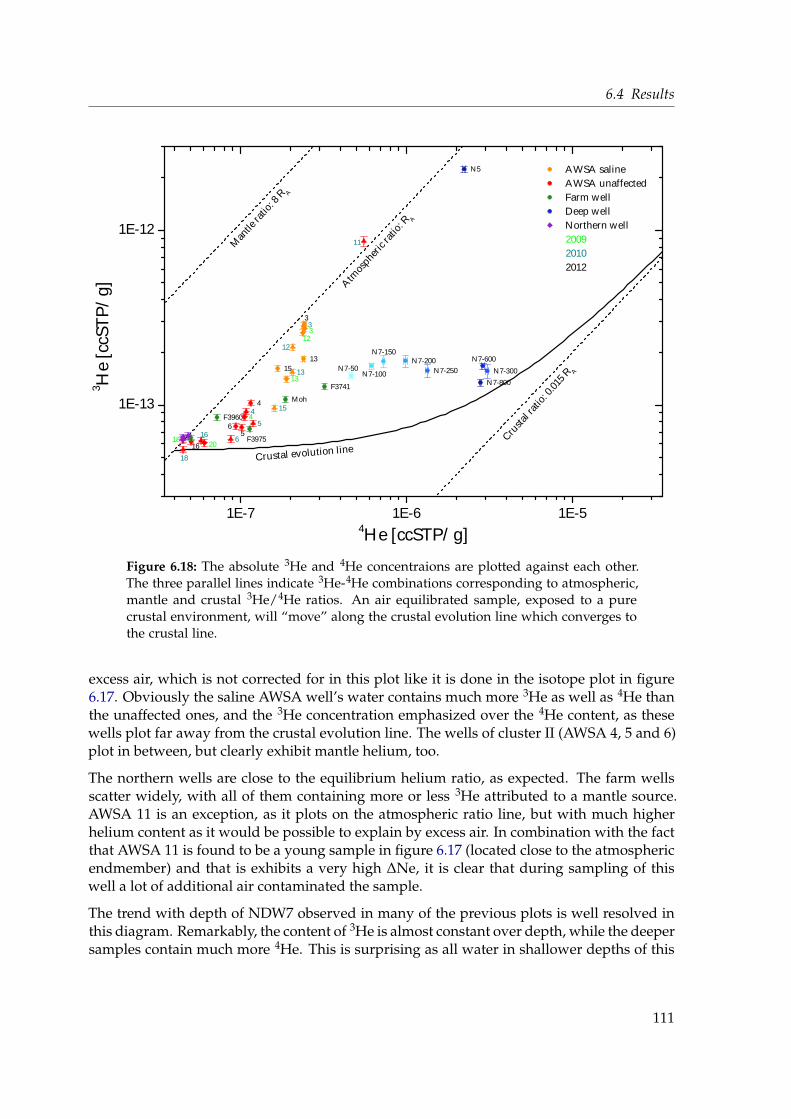
6.4 Results
1 E - 7 1 E - 6 1 E - 5
1 E - 1 3
1 E - 1 2
3
4
56
1 31 5
1 6 F 3 9 7 5
F 3 7 4 1
F 3 9 6 0M o h
N 5
N 7 - 5 0 N 7 - 1 0 0
N 7 - 1 5 0N 7 - 2 0 0
N 7 - 2 5 0 N 7 - 3 0 0N 7 - 6 0 0
N 7 - 8 0 0
3
45
6
1 1
1 2
1 3
1 5
1 6
1 8
3
4
1 2
1 3
1 8 2 0
A W S A s a l i n e A W S A u n a f f e c t e d F a r m w e l l D e e p w e l l N o r t h e r n w e l l
2 0 0 9 2 0 1 0 2 0 1 2
3 He [c
cSTP/
g]
4 H e [ c c S T P / g ]
A t m o s ph e r
i c r at i o :
R A
M a n tl e r
a t i o: 8 R
A
C r u st a l r
a t i o: 0 . 0
1 5 RA
C r u s t a l e v o l u t i o n l i n e
Figure 6.18: The absolute 3He and 4He concentraions are plotted against each other.The three parallel lines indicate 3He-4He combinations corresponding to atmospheric,mantle and crustal 3He/4He ratios. An air equilibrated sample, exposed to a purecrustal environment, will “move” along the crustal evolution line which converges tothe crustal line.
excess air, which is not corrected for in this plot like it is done in the isotope plot in figure6.17. Obviously the saline AWSA well’s water contains much more 3He as well as 4He thanthe unaffected ones, and the 3He concentration emphasized over the 4He content, as thesewells plot far away from the crustal evolution line. The wells of cluster II (AWSA 4, 5 and 6)plot in between, but clearly exhibit mantle helium, too.
The northern wells are close to the equilibrium helium ratio, as expected. The farm wellsscatter widely, with all of them containing more or less 3He attributed to a mantle source.AWSA 11 is an exception, as it plots on the atmospheric ratio line, but with much higherhelium content as it would be possible to explain by excess air. In combination with the factthat AWSA 11 is found to be a young sample in figure 6.17 (located close to the atmosphericendmember) and that is exhibits a very high ∆Ne, it is clear that during sampling of thiswell a lot of additional air contaminated the sample.
The trend with depth of NDW7 observed in many of the previous plots is well resolved inthis diagram. Remarkably, the content of 3He is almost constant over depth, while the deepersamples contain much more 4He. This is surprising as all water in shallower depths of this
111
6 Azraq
borehole originates from the top A7 formation, where the casing is screened. This trend in4He concentration could be attributed to progressive degassing, as warmer water from thedepth rises within the borehole and therefore eventually exchanges with the atmosphere.But this effect would affect all other noble gases, notably 3He. This trend, which is visible inmost other tracers as well, is not fully understood. The most likely explanation is that thewell casing, though quite sturdily constructed, corroded over the past 20 years and otherwater leaks into the borehole.
Deep well NDW5 behaves totally different from NDW7. It locates far off the evolution line,having the highest 3He content of all sampled wells in the Azraq basin. Together with itshigh 4He concentration this well is obviously mantle influenced.
6.5 Discussion and conclusion
The three salinization scenarios investigated by Al-Momani et al. [2006] and which are intro-duced in chapter 6.2 are reviewed with respect to the new data presented in this work.
The first scenario, where the change of the hydraulic gradient causes a reverse flow ofgroundwater towards the AWSA well field, is already rejected by these authors, as, at thetime of the study (2002), the affected wells already had a rising salinity, although the gra-dient still drove the groundwater from the well field area towards the Sabkha. The heliumpattern of the shallow farm wells support the discard of this salinization scheme, as admix-ing of Sabkha water can not explain the high 3He concentrations of AWSA 3, 12, 13 and 15(compare figure 6.18).
The second scenario, i. e. the upward leakage from the middle aquifer into the shallow one,which could not be excluded in the study of Al-Momani et al. [2006], is also disproved by no-ble gases. The amount of 3He in NDW7, being constant over the total depth, is considerablylower than that found in AWSA 3 and 12. The same results from the 3He/4He ratio (figure6.17). A mixture of middle aquifer water, which is very close to the crustal endmember, andwater found in the unaffected AWSA wells (which locate near the atmospheric endmember)would result in a noble gas signature plotting along the dashed crustal-atmospheric mixingline in the plot in figure 6.17. Cluster II, III and IV water can, therefore, not be explained byupstreaming B2/A7 water in the well field area.
A new mineral leaching scheme as a result of a changed groundwater flow pattern in conse-quence of the intense groundwater abstraction in Azraq, as proposed by the third scenarioand which is the favored salinization explanation of Al-Momani et al. [2006], could onlyexplain the observations, if the minerals at the bottom of the B4 aquifer (or the underly-ing B3 aquitard) would also contain high amounts of lithium. As 6Li is the parent of tri-tium, significant concentrations of it could be a geogenic source of 3He, which is not relatedto a mantle source. However, no extraordinary lithium content is reported for the Azraqbasin. In general, mainly granitic rock types contain high lithium concentrations [James andPalmer, 2000], but the proposed location of saline water is within a several kilometer thicksequence of sedimentary rock, so an unusual high lithium content is unlikely to be foundin Azraq. Therefore, a changed rock weathering scheme can not explain the presence of
112

6.5 Discussion and conclusion
high 3He/4He ratios found in the saline wells, too. Regarding the dissolved noble gases, thewater would essentially be the same independent from any change in mineral dissolutionprocesses.
As a consequence, a new hypothesis of hydrogeologic circumstances is proposed, which canexplain all findings presented in the previous chapter.
Mantle helium distribution
The finding of mantle helium in the shallow aquifer, while at the same time the underlyingaquifer exhibits crustal character, is, indeed, surprising. The fact that exactly those wellsaffected by salt are the deepest of all AWSA wells could lead to the assumption that the3He originates from high Li content in that depth, but, as outlined above, this possibility isvery unlikely. Therefore, the most probable explanation is that the mantle helium originatesfrom even deeper layers, but somehow circumvents the middle aquifer. The Azraq Oasisand its surrounding are crossed by many fault lines, some of which might go deep and behydraulically conductive. The map in figure 6.2 gives an overview of the most prominentfaults in the area. Most striking of all are the Fuluq Fault with its up to 3000 m verticaldisplacement, running about 10 km NE of the AWSA well field in NW-SE direction, and theparallel Sirhan Fault, about 10 km SW of the well field. These two faults form the easternand western boundary of the Hamza Graben system, in which Azraq is located. The findingof an obvious mantle helium signature in NDW5 generally supports the assumption of thedeep, conductive faults in the area of the central Azraq depression.
The fact that the middle aquifer well NDW7 is not affected by an upstream of mantle influ-enced water can only be read as that groundwater flow in this aquifer is towards the conduc-tive fault(s). On the other hand, the presence of mantle helium in the shallow Sabkha waterand the well field speaks for a flow towards the central area. This groundwater flow schemeis sketched in figure 6.19. As outlined in this drawing the deep water ascends most likelythrough the Fuluq Fault, because of two reasons. First, groundwater in the middle aquiferflows in eastern to northeastern direction beneath the oasis. Hence, if one of the other mainfaults is strongly conductive, mantle helium would be found in NDW7. Second, the fact thatthe Fuluq Fault experienced very strong tectonic forces over a long period of time (considerthe distinct dip of the layers west of the fault, as depicted in the geologic cross-section ofMargane et al. [2002] in figure 6.4) renders it in all probability a well conductive zone, atleast at some places.
As the upwelling deep water distributes preferably in the deeper part of the conductiveaquifer rock, it can be assumed that a gradient of mantle helium concentration establisheswithin the shallow aquifer, i. e. the deep part of the aquifer contains a larger amount ofmantle influenced water than the more shallow regime, which is compatible with only thedeepest wells are being affected by salt as well as 3He.
113

6 Azraq
Groundwater mixing pattern in the AWSA well field
In order to explain the groundwater mixing mechanisms within the AWSA well field, onehas to take a detailed look at the local hydrogeology setting, as it is sketched in figure 6.19.Most AWSA wells, like described in chapter 6.3, are drilled to roughly 200 m deep into the B4aquifer, piercing the basalt shield completely. Because they are open over the whole depth, itcan be expected they draw water from all depths of the lithologic profile. However, the trans-missivities vary widely along the depth profile. As described in chapter 4.3, the hydraulicconductivity is much better within the fractured basalt aquifer than in the underlying B5(considered an aquitard in the well field area) and the B4 formations. This means, that byfar most water is abstracted from the basaltic part of the aquifer – as long as there is waterin this layer.
The transmissivity, which, under steady state conditions, is governed by the water flow in-side the basalt shield, however, decreases the more the groundwater table is lowered, sim-ply because there are less well permeable fractures available for water transport the less thebasalt is saturated. Additionally, the pumping creates a cone of depression around a well,where the water table can locally be lowered by several meters, depending on the dischargerate and the hydraulic transmissivity of the surrounding rock. This initially small cone ofdepression in the borehole itself will surely increase the more the basalt is being depleted.
The transmissivity reduction does not necessarily need to be uniform, it strongly dependson the individual environment in a well. If, for example, the groundwater table falls belowa very conductive fracture, transmissivitiy steeply drops. Values for drawdown and trans-missivity of the AWSA wells listed in table 6.1, therefore, need to be considered to be validonly at the time of well drilling. Today, however, the conditions have certainly changed.
As soon as the groundwater surface in the well field area falls below the basalt, the transmis-sivity decreases rapidly due to the lower conductivities of the B4/5 unit, and, following, thecone of depression get much deeper. In this case, much more water is abstracted from thedeeper layers of the aquifer than it has been the case before.
This situation is depicted in figure 6.20. As long as the water table within the borehole is inthe basalt aquifer, the water is abstracted almost exclusively from there. As the water tablefalls, the basalt gets less conductive and more water is drawn from the deeper layers of theshallow aquifer.
As the groundwater table in the (unpumped) observation well AZ-12 is only roughly 15 mabove the basalt base in AWSA 12, 13 and 15, it is easily conceivable that the basalt aquiferalready fell dry at those locations and a substantial amount of water is today abstracted fromthe deeper part of the aquifer system, i. e. mainly from the B4.
Assuming, that the deeper layers of the shallow aquifer contain distinct amounts of terri-genic helium, as proposed before, and that they are considerably higher mineralized thanthe water in the basalt aquifer, then, in combination with the groundwater level drop pro-cess just exemplified, one could indeed explain the very local occurrence of salinization aswell as mantle helium in the AWSA field. As one can see in figure 6.7, the base of the basaltshield in wells No 12, 13 and 15 is at around 473 masl, while No 4, 5, 6 and 11 have the base
114

6.5 Discussion and conclusion
Basalt
B4/5
B3
B2/A7
A1/6
Kurnub
B4/5
B3
B2/A7
A1/6
Kurnub
Azraq Oasis
Ram
Zarqa
NDW5NDW7
AWSAwell field
Fulu
q fa
ult
Farm wells
Sirh
an fa
ult
Northernwell
Figure 6.19: This sketch shows the proposed groundwater flow scheme in the AzraqOasis. Water from the deep aquifer system, loaded with mantle helium, ascends alongthe Fuluq Fault. Because groundwater flow in the B2/A7 west of the fault is towards it,NDW7 is not affected by mantle gases. At some parts of the Fuluq Fault mantle gasesmay be transported into the Kurnub east of the fault. In the shallow aquifer the flowdirection is reverse and mantle helium containing water stratifies mainly into the deeppart of the shallow aquifer. The AWSA wells potentially abstract low lying, saline waterfrom the basalt aquifer and deep, saline and mantle helium containing water from theB4 unit.
115

6 Azraq
Figure 6.20: Proposed temporal development of the water abstraction in the AWSAwells. The left sketch shows the initial condition, where all water is drawn from thebasalt aquifer. When the water table within the borehole decreases and eventually fallsinto less conductive material below the basalt, the cone of depression gets deeper andmore water is abstracted from the B4/5.
10 to 30 m deeper. It is therefore clear, that under the same conditions the basaltic materialfalls dry earlier in the first mentioned wells than in the latter ones.
However, one exception has to be noted. In AWSA 3, the well containing most mantle he-lium, the base of the basalt is considerably lower than in the other saline wells. The initialAWSA 3 transmissivity of 17 539 m2/day was among the highest of all AWSA wells andsuggests merely a small cone of depression. But this situation may be owed to a highlypermeable fracture in the upper part of the basalt. As AWSA 3 is located very close to theAl-Bayda Fault, an impact to the initially good transmissivity is likely. The assumed massivedrawdown, however, may be attributed to the situation that groundwater conducted by thisfracture is no longer available and a massive local cone may have established as a conse-quence. Unfortunately, no information about the true water level in the pumped boreholesis available.
The wells of cluster II, AWSA 4, 5 and 6, are not affected by a rising salt content, but showa slightly elevated 4He concentration as well as a notably mantle helium influence. As thebottom of the basalt aquifer in these wells is located deeper than in the affected wells, onecan assume there is still a saturated zone within the basalt. As these wells locate quite closeto each other (they are all within 500 m from each other), and are not far from the Al-BaydaFault, they possibly draw groundwater from a deeper layer connected by the fault. Thiswould, however, mean, there is a water body between the basalt and the deep, saline watersource, which is impacted by terrigenic helium, but at the same time has a low mineral-ization. Admittedly, the explanation that these three wells draw water from an additionalreservoir is somewhat far-fetched, but the behavior of the wells is not easily interpreted.
AWSA 15 plays a special role. It is the only well classified as cluster IV due to its helium andsalinity pattern being different from all other wells. Following the aforementioned reason-ing, from the high mineralization one would also expect a high terrigenic helium content.AWSA 15 shows, indeed, signs of mantle influence, i. e. some water from the deep layer of
116
6.5 Discussion and conclusion
the shallow aquifer is incorporated to the final mixture, but compared to the other salinewells it is much higher mineralized. The high salt content suggests that this well feeds froman additional source, which is even more saline than the deep part of the shallow aquifer.However, the mixing calculation performed using the water chemistry data revealed thatAWSA 15 is at least not well described by a mixture of B2/A7, Sabkha and unaffected water.But one has to consider, that especially the water type of the farm area may falsely be definedby the mere two wells selected as prototype of the Sabkha water. Although Al-Momani et al.[2006] reported the hydraulic gradient to be towards the playa, strong pumping in connec-tion with conductive fractures might lead to a very local flow from the central saltwater bodytoward well AWSA 15. Another possiblity regards the observation of gypsum dissolutionsigns in AWSA 15 found by Al-Momani et al. [2006] which is confirmed by the new data.Therefore, the possibility that AWSA 15 taps an additional, highly mineralized water sourcecan not be ruled out.
The wells unaffected by rising salinity, AWSA 11, 16, 18 and 20, have in common that theydo not go as deep as the other AWSA wells. AWSA 11 is the shallowest AWSA well (62 m)and penetrates the B5 just a few meters. It is therefore comprehensible that this well doesnot abstract deep water. AWSA 18 is 171 m deep and, moreover, has the highest level of thebasalt base. It therefore seems to be a good candidate for salinization. The fact this wellstill shows no signs of it may be explained by the presence of a highly conductive fractureat the bottom of the basalt layer which still feeds AWSA 18 and prevents it from drawingdetectable mounts from deeper layers. Unfortunately no lithologic data could be obtainedfor AWSA 16 (160 m) and 20 (117 m).
Small variations of salt content over time against the general trend of increasing salt content,as shown figure 6.5, can be attributed in the presented salinization scenario to variationsof the groundwater table due to strong recharge events, or to temporarily lower abstractionrates of the well field wells. Such variations occur, like the water table development in figure6.1 displays.
The presence of different groundwater reservoirs, as concluded from the noble gases, is sup-ported by all other measured tracers. δ13C isotopy, 14C and radon activities suggest thepresence of more than one groundwater reservoir feeding the AWSA well field. The waterchemistry data shown in the Piper plot suggest an admixing of a different source into theaffected AWSA wells, too. Most notable, the hypothesis of a saline, mantle helium contain-ing reservoir in the deep part of the shallow aquifer is supported by the recorded physicalparameters (compare figure 6.9). The lower pH values of the salinization affected wells andalso those with only an elevated terrigenic helium content (cluster II) suggest they at leastincorporate water which does not originate from the alkaline basalt aquifer. The higher wa-ter temperatures of these wells are a sign of a deeper source as well. Last but not least, themuch lower oxygen content of these samples point to older, and hence deeper water.
The deep well NDW5 differs from all other wells sampled in Azraq. It contains the mostsignificant mantle helium content of all sampled well in the Azraq basin, but at the sametime has only a small content of dissolved minerals. It is located east of the Fuluq Fault,where the lithologic structure is not affected by the formation of the Hamza Graben system,i. e. the depth to the geologic units is much smaller than on the other side of the fault. NDW5
117
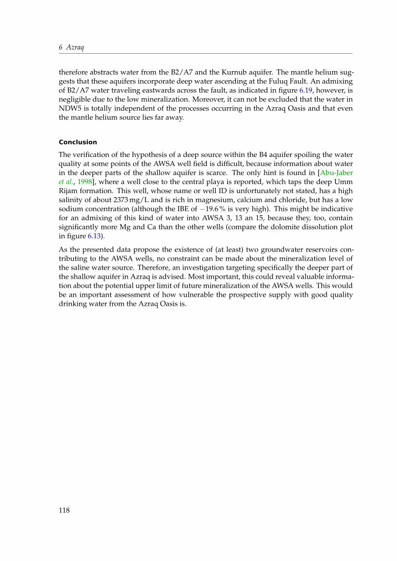
6 Azraq
therefore abstracts water from the B2/A7 and the Kurnub aquifer. The mantle helium sug-gests that these aquifers incorporate deep water ascending at the Fuluq Fault. An admixingof B2/A7 water traveling eastwards across the fault, as indicated in figure 6.19, however, isnegligible due to the low mineralization. Moreover, it can not be excluded that the water inNDW5 is totally independent of the processes occurring in the Azraq Oasis and that eventhe mantle helium source lies far away.
Conclusion
The verification of the hypothesis of a deep source within the B4 aquifer spoiling the waterquality at some points of the AWSA well field is difficult, because information about waterin the deeper parts of the shallow aquifer is scarce. The only hint is found in [Abu-Jaberet al., 1998], where a well close to the central playa is reported, which taps the deep UmmRijam formation. This well, whose name or well ID is unfortunately not stated, has a highsalinity of about 2373 mg/L and is rich in magnesium, calcium and chloride, but has a lowsodium concentration (although the IBE of −19.6 % is very high). This might be indicativefor an admixing of this kind of water into AWSA 3, 13 an 15, because they, too, containsignificantly more Mg and Ca than the other wells (compare the dolomite dissolution plotin figure 6.13).
As the presented data propose the existence of (at least) two groundwater reservoirs con-tributing to the AWSA wells, no constraint can be made about the mineralization level ofthe saline water source. Therefore, an investigation targeting specifically the deeper part ofthe shallow aquifer in Azraq is advised. Most important, this could reveal valuable informa-tion about the potential upper limit of future mineralization of the AWSA wells. This wouldbe an important assessment of how vulnerable the prospective supply with good qualitydrinking water from the Azraq Oasis is.
118

7 Thermal waters along the Dead Sea
Transform
Thermal water, especially in springs, is often associated with recent magmatic or tectonicactivity, where hot magma bodies reach close to the Earth’s surface and warm up the sur-rounding rock and thereby the contained groundwater. Another mechanism of hot springsis the heating of deeply circulating groundwater as a consequence of the local geothermalgradient. If this water rises quickly, usually in a well conductive fracture, it partly preservesits gained temperature and discharges as a hot spring.
The temperature of a thermal spring, which is essentially the surface manifestation of geother-mal heat, is controlled by several factors. In case of heating by a recently formed volcanicsource, the distance to the magma body determines the temperature of the rock and, thus,also the groundwater temperature. In case of deep circulation, several aspects govern thefinal discharge temperature of the spring. First, of course, the temperature of the originalreservoir, i. e. the depth from where the water ascends to the surface in combination withthe local geothermal gradient. Second, the upstream velocity, determined by the conduc-tivity of the fracture and the hydrostatic pressure. And, finally, ascending hot water canbe diluted by addition of cold, ambient groundwater. An overview of these controlling fac-tors is depicted in figure 7.1. Warm water discharging from a deep borehole is essentiallywarmed the same way, but the borehole replaces the conductive fracture. In both cases, heat-ing by magmatic activity or deep circulation, it can be assumed that gases from the mantleare incorporated into the ambient groundwater.
Thermal waters are found in several locations in Jordan and Israel. Most of them emergeas springs along the Dead Sea Transform Valley. In the presented study, 29 thermal springsand also wells between Wadi Arava in the south and the Hermon Mountains in the north areanalyzed. In Israel, some samples were collected in Wadi Arava, at the coast of the Dead Sea,the Yarmouk Gorge and around Lake Kinneret, including boreholes in the Golan heightsand the adjacent Hula basin. Thermal waters in Jordan are found mostly along the deeplycut side wadis of the rift escarpment. They distribute from south of the Dead Sea all the waynorth to the Yarmouk River. Figure 7.2 gives a summary of all sampled locations, wheregreen dots indicate thermal springs and red ones wells discharging hot water. These twocolors are used in all presented diagrams and maps to differentiate between springs andwells.
The data presented in this work are combined from two field trips. Wells and springs onthe Jordanian side of the rift valley were sampled on my own field trip in March and April2012, while the Israeli side was covered within the scope of the master’s thesis of Neta Tsur[2013], where sampling took place in December 2012. The focus of the analysis lies on the
119
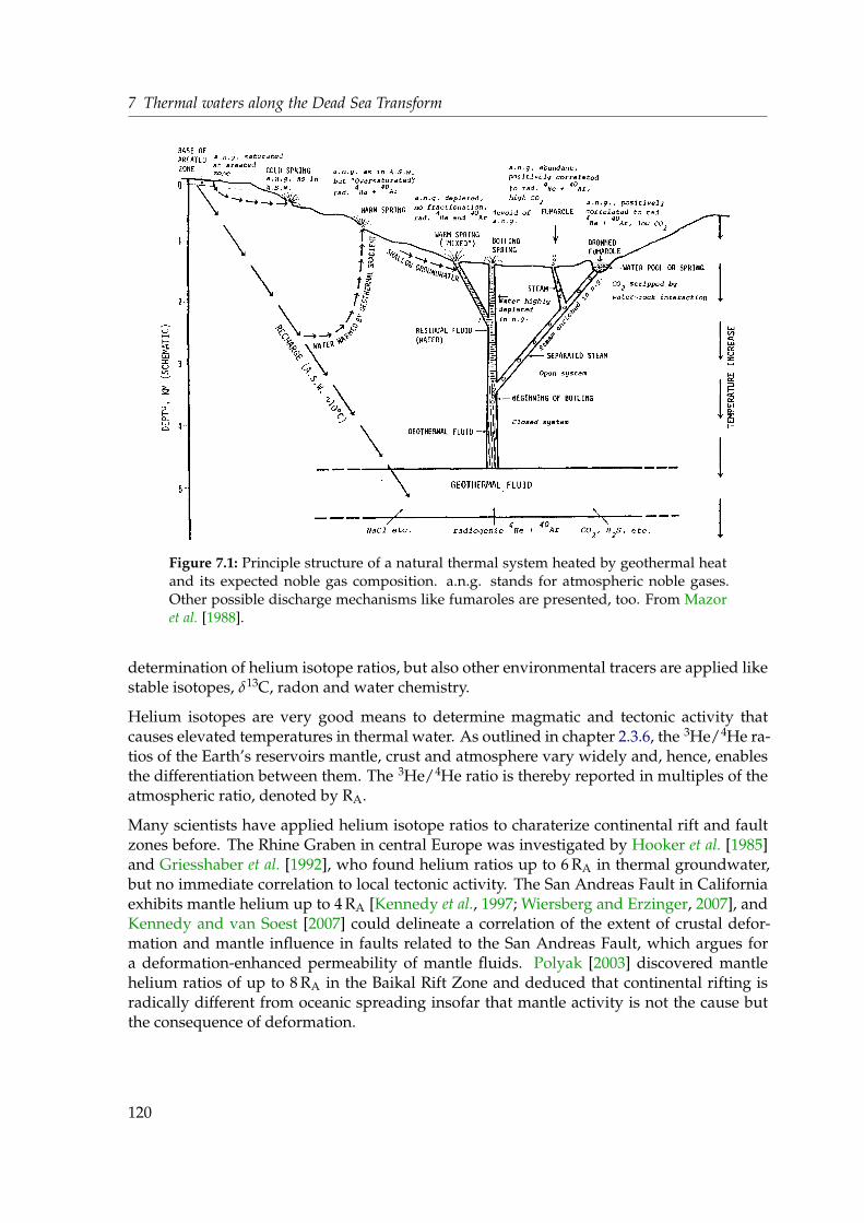
7 Thermal waters along the Dead Sea Transform
Figure 7.1: Principle structure of a natural thermal system heated by geothermal heatand its expected noble gas composition. a.n.g. stands for atmospheric noble gases.Other possible discharge mechanisms like fumaroles are presented, too. From Mazoret al. [1988].
determination of helium isotope ratios, but also other environmental tracers are applied likestable isotopes, δ13C, radon and water chemistry.
Helium isotopes are very good means to determine magmatic and tectonic activity thatcauses elevated temperatures in thermal water. As outlined in chapter 2.3.6, the 3He/4He ra-tios of the Earth’s reservoirs mantle, crust and atmosphere vary widely and, hence, enablesthe differentiation between them. The 3He/4He ratio is thereby reported in multiples of theatmospheric ratio, denoted by RA.
Many scientists have applied helium isotope ratios to charaterize continental rift and faultzones before. The Rhine Graben in central Europe was investigated by Hooker et al. [1985]and Griesshaber et al. [1992], who found helium ratios up to 6 RA in thermal groundwater,but no immediate correlation to local tectonic activity. The San Andreas Fault in Californiaexhibits mantle helium up to 4 RA [Kennedy et al., 1997; Wiersberg and Erzinger, 2007], andKennedy and van Soest [2007] could delineate a correlation of the extent of crustal defor-mation and mantle influence in faults related to the San Andreas Fault, which argues fora deformation-enhanced permeability of mantle fluids. Polyak [2003] discovered mantlehelium ratios of up to 8 RA in the Baikal Rift Zone and deduced that continental rifting isradically different from oceanic spreading insofar that mantle activity is not the cause butthe consequence of deformation.
120

Zarqa
Meitzar
Ein QedemMineral
Ein Yahav
Tzofar
Tveria
Zeeghan
Afra
Shamir
N. Shuna
Abu Ziad
Ibn Hammat
KD1
Zara
Manshiyeh
HimmaBalzamMakla
Thra'a
Gofra
De
ad
Se
a
LakeKinneret
Yarmouk R.
Zarqa R.
Jord
an
Riv
er
100
km
Figure 7.2: Locations of the sampled thermal springs (green) and wells (red). Moredetailed maps of the Lake Kinneret and the Dead Sea areas are shown on the right. Theleft-lateral motion of the main faults of the DST is indicated by arrows. WAF: WadiArava Fault, JVF: Jordan Valley Fault, RF: Rachaiya Fault. 121

7 Thermal waters along the Dead Sea Transform
The southern extension of the DST, the Syrian-African Rift Zone, exhibit mantle helium in-fluence over wide distance as well. Darling et al. [1995] found values of up to 8 RA in Kenya,while Pik et al. [2006] published helium ratios of up to 16 RA along the Rift Zone and con-clude an additional mantle plume impact. The spreading ridge of the Red Sea is also stronglyimprinted by mantle helium, including a mantle hotspot [Lupton et al., 1977; Moreira et al.,1996]. To the north, the DST joins the vast Anatolian Rift system, where also high heliumratios are found, especially in East Turkey [Güleç et al., 2002; Kipfer et al., 1994, among oth-ers].
In can be concluded that mantle volatiles are presumably found in all continental, tectoni-cally young features as is the Dead Sea Transform examined in this study.
Several scientists analyzed groundwater from the Jordan Rift Valley for noble gases before.Notably, the overall first study that obtained paleotemperatures from noble gases in ground-water was carried out by Mazor [1972] on geothermal springs in Israel. However, they mea-sured only the total noble gas amounts, but no 3He/4He ratios. The same holds for Herzbergand Mazor [1979], who determined the recharge origin of cold springs in Israel by NGTs.The Kinneret-10 borehole at the western shore of Lake Kinneret was analyzed by Bergelsonet al. [1999], who found high total helium concentration and a 3He/4He ratio of 1.45 RA. Thereason of salinization of springs in the Jericho area in the Jordan Valley was addressed byLange et al. [2008] applying helium and neon isotopes. They found the highest total 4He andmantle helium (up to 1.01 RA) in springs in the vicinity of faults.
Just recently, Torfstein et al. [2013] published an extensive data set of 3He/4He ratios in ther-mal springs and wells, which covers the Israeli part of the DST. They collected samplesaround Lake Kinneret and the Yarmouk Gorge, at the Dead Sea, and in Wadi Arava. Theyfound a gradient from high helium isotope ratios of about 2 RA in the north to more crustalsignatures at the Dead Sea (0.5 RA to 1 RA) and in the south (below 0.4 RA) and conclude thatthere is no correlation between tectonic activity, which is essentially similar around Lake Kin-neret and the Dead Sea. Torfstein et al. attribute the higher mantle component in the northto the northward thinning of the crust and hence a shallower depth of the Moho bound-ary. In addition, they propose an intermediate, ubiquitous reservoir with a mantle signatureof about 2 RA, and lower helium ratios are attributed to a certain degree of admixed waterhaving a crustal, radiogenic imprint.
The Jordanian side of the rift is much less covered by noble gas data. The only data publishedis from Eraifej [2006], who analyzed the thermal wells Mokhybeh in the Yarmouk Valley(1.91 RA), Waqas (1.62 RA, located between North Shuna hot well and Abu Ziad) and twoboreholes on the Lisan peninsula between the northern and southern part of the Dead Sea(TA1 and TA2, both found to have 0.11 RA).
Subsequently, at first the analytical results are presented, followed by a detailed view atthe local hydrogeologic conditions at each sampling location, and conclusive remark at theend.
122

7.1 Results
7.1 Results
The analysis of the presented samples is performed as described in chapter 3. The samplingprocedure, especially of the thermal springs, was quite individual and needed adaption tothe local setting. General aspects of sampling are treated in chapter 5.1, while appendixA.3 offers a description of the particular sampling procedure of each Jordanian spring andwell. Information about the localities in Israel is found in the master’s thesis of Neta Tsur[2013]. Basic information about all springs and wells is compiled in table 7.1. Because manylocalities have rather long names which would collide in the presented graphs, they arelabeled by short forms, also listed in the table.
7.1.1 Basic observations
The sampled thermal waters exhibit a wide range of temperatures and salt contents. Espe-cially in case of springs, water temperature is either an evidence of a heat source close to theground surface (which induces an elevated geothermal gradient), or points to highly con-ductive fractures which facilitate a rapid upstream of water heated in a great depth. Highsalinity, on the other hand, is often an indicator of old water, which had enough time to in-teract with the surrounding rock. The presence of salt bodies may be another possibility tofind brines.
The distribution of discharge temperatures and salinities along the DST is visualized in fig-ure 7.3, the underlying data is listed in table 7.1. Higher temperatures and salt contents,respectively, are illustrated as bigger dots, as categorized in the given legend. The highesttemperatures are found in the Meitzar 2 well in the Yarmouk Gorge and the Zarqa Ma’in 1spring, the hottest one of the Zarqa Ma’in spring field. However, no general trend regard-ing the geographic location is obvious. As the discharge temperature of wells depends ingeneral on the well depth (or more specifically, the depth from where the majority of thewater is abstracted due to the highest aquifer transmissivitiy), one should not ascribe toomuch importance to the temperature pattern of the wells. Nevertheless, the overall hottestwater temperature of well Meitzar 2, which is by far not the deepest of all wells, indicates anelevated thermal gradient in the Yarmouk Valley. More interesting with respect to geother-mal activity is the distribution of spring temperatures, with Zarqa Ma’in 1 being the mostprominent example. The high discharge temperature of this spring is in good accord withan extraordinary high heat flow exceeding 400 mW/m2 in the area [Galanis Jr. et al., 1986]and the finding of magnetic anomalies, indicating rather recent magma intrusion in the area[Frieslander and Ben-Avraham, 1989]. But also around Lake Kinneret and especially in theYarmouk Gorge thermal anomalies are found [Shalev et al., 2013] which can explain the highMeitzar 2 and Hamat Trevia temperatures.
Salinity is also distributed heterogeneously along the valley. Most notable, Ein Qedem andMineral, located just off the shore of the Dead Sea, exhibit an extreme degree of mineral-ization and an E. C. of almost 150 mS/cm. Most likely, both discharge hypersaline Dead Seawater which has intruded the subsurface beyond the shoreline, where a transition zone frombrine to fresh water exists. The highest E. C. in Dead Sea water measured by Akkawi [2006]
123

7 Thermal waters along the Dead Sea Transform
Zarqa
Meitzar
Ein QedemMineral
Ein Yahav
Tzofar
Tveria
Zeeghan
Afra
Shamir
N. Shuna
Abu Ziad
Ibn Hammat
> 60°C
50 - 60°C
40 - 50°C30 - 40°C
KD1
Zara
Manshiyeh
HimmaBalzamMakla
Thra'a
Gofra
De
ad
Se
a
LakeKinneret
Yarmouk R.
Zarqa R.
Jord
an
Riv
er
De
ad
Se
a
Lake Kinneret
Yarmouk R.
Zarqa R.
Jord
an
Riv
er
100
km
(a) Temperature distribution
Zarqa
Meitzar
Ein QedemMineral
Ein Yahav
Tzofar
Tveria
Zeeghan
Afra
Shamir
N. Shuna
Abu Ziad
Ibn Hammat
> 140 mS/cm
10 – 40 mS/cm
5 – 10 mS/cm
2 – 5 mS/cm
1 – 2 mS/cm0.5 – 1 mS/cm
Thra'a
Zara
Gofra
Himma
Manshiyeh
BalzamMakla
KD1
De
ad
Se
a
LakeKinneret
Yarmouk R.
Zarqa R.
Jord
an
Riv
er
100
km
(b) Salinity distribution
Figure 7.3: Temperature and Salinity distribution along the DST. Red dots denote wells,green dots thermal springs. The hottest water is found in the Meitzar 2 well and theZarqa Ma’in 1 spring. No general trend regarding the discharge temperatures is visible.Salinity is highest on the western Dead Sea coast, but other centers of high mineralizationare present. However, as noted for the temperature, no trend is recognizable.
124
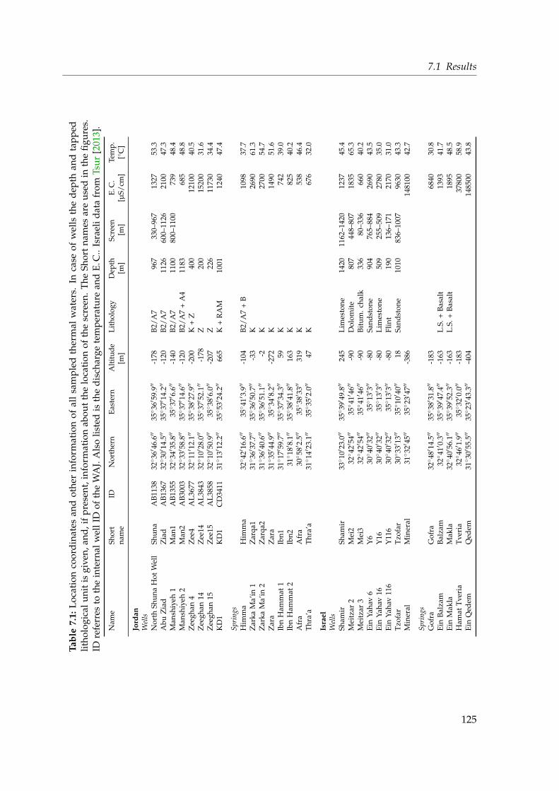
7.1 ResultsTa
ble
7.1:
Loc
atio
nco
ord
inat
esan
dot
her
info
rmat
ion
ofal
lsa
mp
led
ther
mal
wat
ers.
Inca
seof
wel
lsth
ed
epth
and
tap
ped
litho
logi
calu
nit
isgi
ven,
and
,if
pres
ent,
info
rmat
ion
abou
tth
elo
cati
onof
the
scre
en.T
heSh
ort
nam
esar
eus
edin
the
figur
es.
IDre
ferr
esto
the
inte
rnal
wel
lID
ofth
eW
AJ.
Als
olis
ted
isth
edi
scha
rge
tem
pera
ture
and
E.C
..Is
rael
idat
afr
omTs
ur[2
013]
.
Nam
eSh
ort
IDN
orth
ern
East
ern
Alt
itud
eLi
thol
ogy
Dep
thSc
reen
E.C
.Te
mp.
nam
e[m
][m
][m
][µ
S/cm
][◦
C]
Jord
anW
ells
Nor
thSh
una
Hot
Wel
lSh
una
AB1
138
32◦ 3
6′46
.6′′
35◦ 3
6′59
.9′′
-178
B2/A
796
733
0–96
713
2753
.3A
buZ
iad
Zia
dA
B136
732◦ 3
0′14
.5′′
35◦ 3
7′14
.2′′
-120
B2/A
711
2660
0–11
2621
0047
.3M
ansh
iyeh
1M
an1
AB1
355
32◦ 3
4′35
.8′′
35◦ 3
7′6.
6′′
-140
B2/A
711
0080
0–11
0073
948
.4M
ansh
iyeh
2M
an2
AB3
003
32◦ 3
3′58
.8′′
35◦ 3
7′14
.6′′
-120
B2/A
7+
A4
1183
685
48.8
Zee
ghan
4Z
ee4
AL3
677
32◦ 1
1′12
.1′′
35◦ 3
8′27
.9′′
-200
K+
Z40
012
100
40.5
Zee
ghan
14Z
ee14
AL3
843
32◦ 1
0′28
.0′′
35◦ 3
7′52
.1′′
-178
Z20
015
200
31.6
Zee
ghan
15Z
ee15
AL3
858
32◦ 1
0′50
.9′′
35◦ 3
8′6.
0′′
-207
Z22
611
730
34.4
KD
1K
D1
CD
3411
31◦ 1
3′12
.2′′
35◦ 5
3′24
.2′′
665
K+
RA
M10
0112
4047
.4
Spri
ngs
Him
ma
Him
ma
32◦ 4
2′16
.6′′
35◦ 4
1′3.
9′′
-104
B2/A
7+
B10
9837
.7Z
arka
Ma’
in1
Zar
qa1
31◦ 3
6′37
.7′′
35◦ 3
6′50
.7′′
-33
K26
9061
.3Z
arka
Ma’
in2
Zar
qa2
31◦ 3
6′40
.6′′
35◦ 3
6′51
.1′′
-2K
2700
54.7
Zar
aZ
ara
31◦ 3
5′44
.9′′
35◦ 3
4′8.
2′′
-272
K14
9051
.6Ib
nH
amm
at1
Ibn1
31◦ 1
7′59
.7′′
35◦ 3
7′34
.3′′
59K
742
39.0
Ibn
Ham
mat
2Ib
n231◦ 1
8′8.
1′′
35◦ 3
8′41
.8′′
163
K82
540
.2A
fra
Afr
a30◦ 5
8′2.
5′′
35◦ 3
8′33′′
319
K53
846
.4Th
ra’a
Thra
’a31◦ 1
4′23
.1′′
35◦ 3
5′2.
0′′
47K
676
32.0
Isra
elW
ells
Sham
irSh
amir
33◦ 1
0′23
.0′′
35◦ 3
9′49
.8′′
245
Lim
esto
ne14
2011
62–1
420
1237
45.4
Mei
tzar
2M
ei2
32◦ 4
2′54′′
35◦ 4
1′46′′
-90
Dol
omit
e80
744
8–80
718
3565
.3M
eitz
ar3
Mei
332◦ 4
2′54′′
35◦ 4
1′46′′
-90
Bitu
m.c
halk
336
80–3
3666
040
.2Ei
nYa
hav
6Y
630◦ 4
0′32′′
35◦ 1
3′3′′
-80
Sand
ston
e90
476
5–88
426
9043
.5Ei
nYa
hav
16Y
1630◦ 4
0′32′′
35◦ 1
3′3′′
-80
Lim
esto
ne50
925
5–50
927
8035
.0Ei
nYa
hav
116
Y11
630◦ 4
0′32′′
35◦ 1
3′3′′
-80
Flin
t19
013
6–17
121
7031
.0Tz
ofar
Tzof
ar30◦ 3
3′13′′
35◦ 1
0′40′′
18Sa
ndst
one
1010
836–
1007
9630
43.3
Min
eral
Min
eral
31◦ 3
2′45′′
35◦ 2
3′47′′
-386
1481
0042
.7
Spri
ngs
Gof
raG
ofra
32◦ 4
8′14
.5′′
35◦ 3
8′31
.8′′
-183
6840
30.8
Ein
Balz
amBa
lzam
32◦ 4
1′0.
3′′
35◦ 3
9′47
.4′′
-163
L.S.
+Ba
salt
1393
41.7
Ein
Mak
laM
akla
32◦ 4
0′56
.1′′
35◦ 3
9′52
.3′′
-163
L.S.
+Ba
salt
1895
48.5
Ham
atTv
eria
Tver
ia32◦ 4
6′1.
9′′
35◦ 3
2′0.
0′′
-183
3780
058
.9Ei
nQ
edem
Qed
em31◦ 3
0′55
.5′′
35◦ 2
3′43
.3′′
-404
1485
0043
.8
125

7 Thermal waters along the Dead Sea Transform
along depth profiles is 202 mS/cm at a salinity of 267 g/L, although he discovered that evenhigher mineralization resulted in lower E. C., which makes it impossible to calculate the freshwater fraction admixed in the discharged water from the E. C. alone. The saline springs onthe western coast of Lake Kinneret are thought to feed on brines evolved from the remnantof evoparation of Pliocene and Pleistoncene lakes [Rosenthal et al., 2008]. The saline wells ofthe Abu Zeeghan well field pump water which originates mainly from lateral groundwaterflow towards the rift valley in the Zarka aquifers. Thereby, evaporites and gypsum presentin the aquifer matrix are dissolved [Salameh, 2001]. All other thermal waters are only low tomedium saline.
7.1.2 Noble gases
Data preparation
The Jordanian samples’ raw data are analyzed in WUCEM together with the Azraq samples,collected at the same sampling campaign. The only exception from the normal routine arethe 3He measurements of Abu Ziad and Zeeghan 15, because in these cases the 3He signallies outside the range of calibration measurements. As described in chapter 3.6.2, a linearfit using only the two biggest calibration sizes is taken. In case of the Israeli Ein Balzam istreated the same way, but using a constant fit. The results of all noble gas isotope concentra-tions is found in table 7.2.
The total element concentrations used for the noble gas temperature fitting routine are listedin table A.6 on page 184. Some samples show an elevated 40Ar/36Ar (Zeeghan 4, 14, 15,Zarqa Ma’in 2, Ein Makla, Hamat Tveria and Ein Qedem), in these cases the total atmo-spheric argon content is calculated from 36Ar only, as mentioned in chapter 3.6.4.
Inverse NGT fitting proves to be complicated in some cases. Initial application of the UAexcess air model reveals the Jordanian samples Abu Ziad, Zarqa Ma’in 1 and 2, Zara and IbnHammat 2 to be degassed. Therefore, they are fitted by the CE model in degassing mode,initialized by F = 2, while for all other samples the initial F is 0.5. Due to default of goodknowledge about the recharge altitude, it is assumed that all waters equilibrated at 800 m,i. e. at p = 0.92 atm. This is reasonable since Bajjali et al. [1997] estimated the thermal waterfound in north Jordan to be recharged in the Jordan highlands. The springs east of the DeadSea discharge from the Kurnub Sandstone which is assumed to be recharged mainly at itsoutcrop along the southern escarpment, where an altitude of 800 m is reasonable as well,though less constrained. The initial fitting temperature is 18 ◦C for all samples.
In case of the Israeli samples, the UA model indicated degassing at Gofra, Ein Balzam, EinMakla, Meitzar 2, Tzofar, Hamat Tveria, Mineral and Ein Qedem; fitting of all these samplesis therefore initialized by F = 2, the others by F = 0.5. Infiltration altitudes are estimatedfrom the outcrop of the discharging hydrological units. Gofra, Meitzar 3, Tzofar and allEin Yahav wells: 400 m, Shamir: 650 m, Ein Balzam and Ein Makla: 800 m, Meitzar 3: 1500 m,Hamat Tveria: 220 m, and Mineral and Ein Qedem are assumed to be former Dead Sea water(see discussion below) and therefore an equilibration altitude of −400 m is assumed. 18 ◦Cis chosen as initial value of the fitting parameter T.
126

7.1 Results
Tabl
e7.
2:N
oble
gas
isot
ope
resu
ltsof
alls
ampl
edth
erm
allo
calit
ies.
All
data
are
give
nin
ccST
P/g
wat
er.I
srae
lida
tafr
omTs
ur[2
013]
.3 H
e∆
3 He
4 He
∆4 H
e20
Ne
∆20
Ne
22N
e∆
22N
e36
Ar
∆36
Ar
40A
r∆
40A
r84
Kr
∆84
Kr
132 X
e∆
132 X
e
Jord
anH
imm
a5.
842E
-12
2.35
0E-1
31.
984E
-06
1.87
4E-0
81.
861E
-07
6.75
9E-1
01.
902E
-08
7.18
2E-1
11.
084E
-06
1.75
3E-0
83.
119E
-04
1.01
4E-0
63.
935E
-08
3.37
7E-1
02.
479E
-09
4.65
1E-1
1N
orth
Shun
a5.
746E
-12
2.26
1E-1
31.
636E
-06
1.53
3E-0
82.
177E
-07
7.44
6E-1
02.
229E
-08
8.39
7E-1
11.
221E
-06
1.96
2E-0
83.
565E
-04
1.15
6E-0
64.
659E
-08
4.18
4E-1
03.
180E
-09
5.57
9E-1
1A
buZ
iad
9.03
1E-1
13.
096E
-12
3.17
5E-0
53.
150E
-07
1.43
0E-0
75.
203E
-10
1.46
2E-0
85.
618E
-11
9.74
4E-0
71.
505E
-08
2.80
3E-0
49.
282E
-07
3.67
2E-0
83.
716E
-10
2.50
6E-0
94.
177E
-11
Man
shiy
eh1
1.62
1E-1
35.
886E
-15
1.84
3E-0
71.
710E
-09
2.01
8E-0
77.
765E
-10
2.07
1E-0
88.
526E
-11
1.15
3E-0
61.
754E
-08
3.39
2E-0
41.
123E
-06
4.29
2E-0
83.
796E
-10
2.88
2E-0
95.
010E
-11
Man
shiy
eh2
1.34
1E-1
34.
758E
-15
1.65
9E-0
71.
522E
-09
2.12
7E-0
77.
299E
-10
2.17
5E-0
88.
073E
-11
1.17
2E-0
61.
780E
-08
3.47
8E-0
41.
128E
-06
4.41
9E-0
83.
741E
-10
2.86
9E-0
95.
188E
-11
Zee
ghan
42.
667E
-09
6.49
8E-1
13.
948E
-04
3.89
9E-0
62.
809E
-07
9.65
3E-1
02.
853E
-08
1.00
9E-1
01.
423E
-06
2.17
2E-0
84.
790E
-04
1.54
7E-0
65.
006E
-08
4.53
0E-1
03.
100E
-09
6.00
9E-1
1Z
eegh
an14
4.43
0E-1
01.
844E
-11
1.28
5E-0
41.
212E
-06
1.67
0E-0
75.
650E
-10
1.69
8E-0
86.
056E
-11
9.40
7E-0
71.
459E
-08
2.99
7E-0
49.
639E
-07
3.56
3E-0
83.
635E
-10
2.21
6E-0
94.
566E
-11
Zee
ghan
158.
513E
-10
2.98
2E-1
12.
457E
-04
2.43
6E-0
61.
888E
-07
6.71
8E-1
01.
920E
-08
7.11
2E-1
11.
039E
-06
1.72
4E-0
83.
551E
-04
1.14
4E-0
63.
849E
-08
3.07
4E-1
02.
427E
-09
4.04
9E-1
1Z
arka
Ma’
in1
2.88
9E-1
11.
172E
-12
1.42
1E-0
51.
325E
-07
7.21
1E-0
82.
472E
-10
7.37
8E-0
92.
890E
-11
5.61
4E-0
79.
919E
-09
1.71
1E-0
45.
580E
-07
2.41
3E-0
82.
218E
-10
1.67
4E-0
92.
578E
-11
Zar
kaM
a’in
21.
642E
-11
6.10
0E-1
39.
277E
-06
8.29
2E-0
87.
973E
-08
2.70
2E-1
08.
145E
-09
3.32
9E-1
15.
756E
-07
1.02
7E-0
81.
648E
-04
5.33
1E-0
72.
290E
-08
2.36
1E-1
01.
523E
-09
2.72
7E-1
1Z
ara
6.00
4E-1
22.
146E
-13
1.43
9E-0
51.
349E
-07
1.40
6E-0
74.
934E
-10
1.43
2E-0
85.
361E
-11
7.38
9E-0
71.
438E
-08
2.34
8E-0
47.
541E
-07
2.95
7E-0
82.
822E
-10
1.89
6E-0
93.
172E
-11
Ibn
Ham
mat
11.
652E
-13
5.84
9E-1
56.
132E
-07
6.30
1E-0
91.
554E
-07
5.43
0E-1
01.
586E
-08
5.64
7E-1
18.
254E
-07
1.31
0E-0
82.
381E
-04
7.76
2E-0
73.
132E
-08
2.99
4E-1
02.
030E
-09
3.90
5E-1
1Ib
nH
amm
at2
1.23
2E-1
24.
718E
-14
6.79
1E-0
65.
926E
-08
2.40
5E-0
78.
176E
-10
2.46
3E-0
88.
841E
-11
1.16
3E-0
61.
759E
-08
3.41
1E-0
41.
106E
-06
4.33
5E-0
84.
101E
-10
2.78
6E-0
95.
715E
-11
Afr
a1.
518E
-13
5.55
2E-1
55.
785E
-07
5.79
9E-0
91.
627E
-07
5.75
4E-1
01.
664E
-08
6.20
7E-1
19.
402E
-07
1.46
6E-0
82.
738E
-04
8.89
8E-0
73.
604E
-08
3.53
3E-1
02.
315E
-09
4.42
0E-1
1T
hra’
a1.
621E
-12
6.08
5E-1
45.
795E
-06
5.00
4E-0
81.
906E
-07
6.74
2E-1
01.
945E
-08
7.18
7E-1
11.
010E
-06
1.55
7E-0
83.
012E
-04
9.81
2E-0
73.
907E
-08
3.56
5E-1
02.
454E
-09
4.47
3E-1
1K
D1
1.49
4E-1
25.
630E
-14
7.56
2E-0
67.
151E
-08
2.14
7E-0
71.
200E
-09
2.19
7E-0
81.
432E
-10
1.06
0E-0
62.
686E
-08
3.17
5E-0
49.
855E
-07
4.08
5E-0
89.
175E
-10
2.65
7E-0
91.
040E
-10
Isra
elG
ofra
3.37
8E-1
21.
426E
-13
1.42
4E-0
68.
651E
-09
1.25
6E-0
75.
044E
-10
1.28
2E-0
86.
023E
-11
9.68
1E-0
72.
384E
-08
2.74
2E-0
46.
667E
-07
3.67
5E-0
87.
037E
-10
2.35
0E-0
94.
715E
-11
Sham
ir7.
963E
-12
3.45
7E-1
32.
046E
-06
1.05
4E-0
82.
218E
-07
8.90
2E-1
02.
268E
-08
9.48
7E-1
11.
254E
-06
2.68
0E-0
83.
704E
-04
8.52
8E-0
74.
950E
-08
8.28
1E-1
03.
227E
-09
7.23
0E-1
1M
eitz
ar3
1.10
5E-1
24.
920E
-14
4.61
4E-0
72.
464E
-09
1.97
6E-0
78.
184E
-10
2.01
8E-0
89.
710E
-11
1.11
6E-0
62.
430E
-08
3.33
9E-0
47.
869E
-07
4.24
3E-0
87.
537E
-10
2.58
7E-0
94.
770E
-11
Mei
tzar
24.
328E
-11
1.88
9E-1
21.
515E
-05
8.90
4E-0
81.
680E
-07
6.89
0E-1
01.
720E
-08
7.92
4E-1
11.
303E
-06
2.97
7E-0
83.
881E
-04
8.64
6E-0
75.
016E
-08
8.36
9E-1
03.
132E
-09
6.52
0E-1
1Ei
nBa
lzam
1.52
5E-1
17.
721E
-13
5.06
8E-0
63.
596E
-08
1.61
2E-0
77.
135E
-10
1.65
4E-0
87.
656E
-11
1.01
4E-0
62.
464E
-08
2.98
2E-0
47.
565E
-07
3.89
7E-0
87.
143E
-10
2.46
3E-0
94.
941E
-11
Ein
Mak
la2.
501E
-11
1.03
6E-1
29.
880E
-06
5.96
3E-0
81.
483E
-07
6.22
2E-1
01.
520E
-08
6.81
6E-1
11.
030E
-06
2.31
4E-0
83.
074E
-04
7.32
5E-0
74.
026E
-08
7.32
5E-1
02.
506E
-09
4.99
6E-1
1Ei
nYa
hav
116
1.24
1E-1
24.
728E
-14
2.37
6E-0
61.
234E
-08
2.36
0E-0
79.
945E
-10
2.41
2E-0
81.
109E
-10
1.11
1E-0
62.
443E
-08
3.29
9E-0
47.
554E
-07
4.02
4E-0
87.
207E
-10
2.51
1E-0
96.
149E
-11
Ein
Yaha
v6
6.20
4E-1
22.
430E
-13
9.23
5E-0
65.
569E
-08
2.21
2E-0
79.
280E
-10
2.26
6E-0
89.
742E
-11
1.17
2E-0
62.
541E
-08
3.49
4E-0
47.
975E
-07
4.07
9E-0
87.
648E
-10
2.44
4E-0
94.
898E
-11
Ein
Yaha
v16
3.67
0E-1
21.
457E
-13
6.77
2E-0
64.
224E
-08
2.06
7E-0
78.
481E
-10
2.11
1E-0
89.
041E
-11
1.08
2E-0
62.
394E
-08
3.11
2E-0
47.
217E
-07
3.74
4E-0
87.
231E
-10
2.35
4E-0
95.
355E
-11
Tzo
far
9.17
4E-1
23.
564E
-13
1.56
7E-0
58.
123E
-08
1.52
1E-0
76.
079E
-10
1.56
0E-0
87.
080E
-11
8.08
8E-0
71.
987E
-08
2.44
9E-0
46.
108E
-07
2.84
9E-0
86.
293E
-10
1.75
3E-0
93.
418E
-11
Ham
atT
veri
a4.
120E
-11
1.83
9E-1
22.
826E
-05
1.49
4E-0
79.
213E
-08
3.78
9E-1
09.
439E
-09
5.13
6E-1
16.
494E
-07
1.75
8E-0
82.
087E
-04
5.66
3E-0
72.
871E
-08
6.12
0E-1
01.
868E
-09
3.78
3E-1
1Ei
nQ
edem
7.72
9E-1
22.
918E
-13
9.13
2E-0
65.
518E
-08
3.96
1E-0
81.
756E
-10
4.02
7E-0
93.
546E
-11
2.05
4E-0
72.
048E
-08
1.06
0E-0
43.
730E
-07
1.36
6E-0
84.
590E
-10
8.73
7E-1
02.
156E
-11
Min
eral
3.32
2E-1
41.
339E
-15
2.78
6E-0
82.
840E
-10
6.76
7E-0
82.
832E
-10
6.91
8E-0
93.
962E
-11
3.00
9E-0
71.
162E
-08
8.42
4E-0
53.
489E
-07
9.61
4E-0
94.
526E
-10
5.14
2E-1
01.
465E
-11
127

7 Thermal waters along the Dead Sea Transform
For some samples it was not possible to obtain a good fit. Zara, Ibn Hammat 1, Meitzar 2,and to a lesser extent Afra, Thra’a, Ein Makla and Ein Qedem exhibit a bad χ2, indicating ageneral problem with the noble gas concentrations. Nevertheless, their resulting noble gastemperature seem to be more or less reasonable.
Many samples exhibit the limiting case, where |F| becomes very high and the CE modelbecomes a quasi-UA model (see chapter 3.6.2). All samples are therefore further processedby Monte Carlo simulations; for each sample 100 000 simulations are done. The final resultsof the calculated NGTs, the CE model parameters A and F, the modeled atmospheric 3He and4He concentrations and the distribution of χ2 from the Monte Carlo analyses are presentedin table 7.3. In case only a subset of Monte Carlo simulations was regarded, the respectiveselection is shown on page 192.
Analysis
Most resulting NGTs are more or less reasonable and lie between 12 and 23 ◦C. Cool NGTsmay reflect recharge at high altitudes (Shamir, Ein Makla) or during the last Glacial (NorthShuna, both Manshiyeh wells, Zeeghan 4, Ein Makla), whereas temperatures above 20 ◦C inthe springs discharging from the Kurnub indicate recharge in the warmer south of Jordan.However, the NGTs of Zarqa Ma’in 2 (27.4 ◦C), Zara (32.6 ◦C), Ibn Hammat 1 (30.4 ◦C), Tzo-far (31.2 ◦C) and Hamat Tveria (26.4 ◦C) exceed the local temperature regime. Most likely thehigh calculated temperatures are owed to degassing effects which are badly quantified bythe CE model, and therefore the model assumes a too low equilibrated noble gas concentra-tion, which is equivalent to a higher temperature. The difficulty to fit the noble gas data isalso reflected in bad χ2 values of the latter two samples. Meitzar 2 exhibits a very low NGTof only 2.6 ◦C, which might be reasonable at the peak of Mount Hermon, but the bad χ2 sug-gests a fitting problem. The same holds for Ein Qedem (calculated NGT 21.5 ◦C). However,as the solubility of helium is only weakly dependent on temperature, these fitting problemsdo not significantly affect the determination of the terrigenic 3He and 4He content as well asthe 3He/4He ratio. Summarizing, the NGT analysis reveals that all thermal waters along therift valley have a meteoric background and none of them has a direct mantle origin.
The consideration of the neon excess (∆Ne, defined in equation 2.27), listed in table 7.4,reveals that some samples are obviously degassed, most of them are springs (Zarqa Ma’in1 and 2, Gofra, Ein Makla, Hamat Tveria and Ein Qedem). Abu Ziad is the only well thatshows signs of degassing. Several other localities exhibit high ∆Ne values, indicating adistinct excess air contribution to the total noble gas concentrations.
Most of the sampled thermal waters along the rift valley exhibit a significant mantle heliumcomponent, as shown in figure 7.4 (explanation of this plot is found in figure 2.14). Theunderlying data is compiled in table 7.4. Almost all samples plot on or close to the verti-cal mixing line of crustal and mantle helium isotopic composition, indicating only minoratmospheric contamination. The strongest mantle signal is found in the well Zeeghan No 4,which contains a helium isotope ratio almost five times the atmospheric value (4.9 RA). Theother two samples from this well field have high ratios as well, as do the springs and wellsin or near to the Yarmouk Valley (springs: Himma, Ein Balzam and Makla, wells: Meitzar 2,North Shuna, Abu Ziad, all exhibit helium ratios between 2 and 3 RA). Also Shamir, situated
128
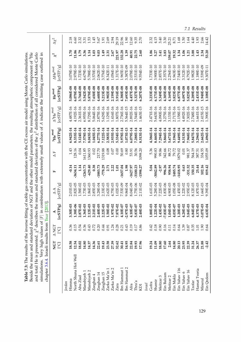
7.1 ResultsTa
ble
7.3:
The
resu
ltsof
the
inve
rse
fittin
gof
nobl
ega
sco
ncen
trat
ion
with
the
CE
exce
ssai
rm
odel
usin
gM
onte
Car
losi
mul
atio
ns.
Besi
deth
em
ean
and
stan
dard
devi
atio
nof
NG
Tan
dth
eot
her
mod
elpa
ram
eter
s,th
ere
sult
ing
atm
osph
eric
com
pone
ntof
3 He
and
tota
lHe
ispr
esen
ted
.χ
2d
escr
ibes
the
mea
nan
dst
and
ard
dev
iati
onof
the
χ2
dis
trib
uti
onof
allc
onsi
der
edM
onte
Car
losi
mu
lati
ons.
Ver
yhi
ghva
lues
of|F|i
nco
mbi
nati
onw
ith
extr
emel
ysm
all
valu
esof
Ain
dic
ate
the
limit
ing
case
outl
ined
inch
apte
r3.
6.4.
Isra
elir
esul
tsfr
omTs
ur[2
013]
.
NG
T∆
NG
TA
∆A
F∆
F3 H
emod
∆3 H
emod
Hem
od∆
Hem
odχ
2∆
χ2
[◦C
][◦
C]
[ccS
TP/
g][c
cSTP
/g]
[ccS
TP/
g][c
cSTP
/g]
[ccS
TP/
g][c
cSTP
/g]
Jord
anH
imm
a18
.58
0.36
3.30
E-03
2.01
E-03
-0.1
41.
436.
942E
-14
4.48
7E-1
65.
086E
-08
3.07
8E-1
01.
702.
18N
orth
Shun
aH
otW
ell
12.5
40.
151.
38E-
062.
82E-
05-3
634.
1112
8.16
8.33
3E-1
44.
192E
-16
6.07
8E-0
82.
978E
-10
11.8
66.
60A
buZ
iad
18.0
20.
542.
87E-
021.
58E-
021.
140.
045.
124E
-14
2.36
1E-1
63.
766E
-08
1.72
3E-1
01.
792.
32M
ansh
iyeh
114
.80
0.36
1.36
E-03
1.73
E-03
-126
3.73
1611
.85
7.57
8E-1
46.
955E
-16
5.54
2E-0
84.
679E
-10
3.36
3.31
Man
shiy
eh2
14.3
70.
432.
12E-
031.
86E-
03-6
29.4
013
60.9
38.
043E
-14
8.72
9E-1
65.
878E
-08
5.78
8E-1
01.
141.
53Z
eegh
an4
14.3
60.
722.
21E-
022.
85E-
030.
380.
021.
045E
-13
5.06
4E-1
67.
650E
-08
3.57
0E-1
01.
031.
45Z
eegh
an14
22.6
10.
202.
40E-
053.
28E-
04-1
883.
7321
7.70
6.27
7E-1
42.
875E
-16
4.60
0E-0
82.
062E
-10
9.03
5.67
Zee
ghan
1519
.43
0.44
2.22
E-03
2.33
E-03
-778
.29
1319
.88
7.12
2E-1
45.
629E
-16
5.21
3E-0
83.
776E
-10
1.49
1.91
Zar
kaM
a’in
123
.58
0.91
1.58
E-02
2.62
E-03
2.71
0.08
2.58
3E-1
41.
129E
-16
1.90
2E-0
88.
342E
-11
2.31
2.69
Zar
kaM
a’in
227
.39
1.24
1.97
E-02
4.75
E-03
2.22
0.07
2.93
5E-1
41.
416E
-16
2.15
9E-0
81.
056E
-10
2.67
2.94
Zar
a32
.62
0.28
7.87
E-02
1.02
E-03
1.01
0.00
5.33
4E-1
41.
807E
-16
3.91
4E-0
81.
317E
-10
221.
9729
.19
Ibn
Ham
mat
130
.41
0.21
4.10
E-07
7.53
E-09
-165
7.04
50.6
95.
978E
-14
2.73
6E-1
64.
380E
-08
1.96
5E-1
013
2.28
22.9
6Ib
nH
amm
at2
14.9
50.
43-2
.97E
-03
9.86
E-04
1.98
0.80
1.07
3E-1
35.
564E
-15
7.69
3E-0
83.
387E
-09
1.39
1.90
Afr
a22
.84
0.19
4.10
E-07
8.04
E-09
-162
7.97
53.9
16.
079E
-14
2.89
2E-1
64.
457E
-08
2.07
8E-1
040
.91
12.6
0Th
ra’a
19.9
30.
175.
83E-
071.
75E-
06-3
100.
2330
.56
7.28
8E-1
43.
544E
-16
5.32
7E-0
82.
531E
-10
22.7
59.
35K
D1
17.9
60.
862.
48E-
032.
11E-
02-1
598.
2710
98.2
08.
513E
-14
1.46
3E-1
56.
207E
-08
9.55
4E-1
02.
602.
70
Isra
elG
ofra
19.2
40.
421.
88E-
031.
61E-
035.
045.
364.
386E
-14
2.47
1E-1
63.
233E
-08
1.73
3E-1
01.
862.
32Sh
amir
11.0
90.
181.
22E-
045.
28E-
04-3
042.
8999
0.83
8.46
0E-1
45.
643E
-16
6.17
1E-0
83.
900E
-10
5.27
4.15
Mei
tzar
318
.80
0.90
1.43
E-02
7.22
E-03
-2.9
799
.86
7.29
4E-1
44.
090E
-16
5.34
9E-0
82.
857E
-10
3.41
3.40
Ein
Balz
am17
.60
0.16
-7.8
3E-0
71.
83E-
0699
6.26
342.
665.
866E
-14
3.27
5E-1
64.
305E
-08
2.35
7E-1
03.
833.
30M
eitz
ar2
2.64
0.11
1.04
E-04
4.90
E-03
958.
9488
.72
5.67
1E-1
43.
133E
-16
4.16
9E-0
82.
256E
-10
159.
0725
.21
Ein
Mak
la14
.80
0.14
4.03
E-07
1.05
E-08
1485
.74
79.7
25.
196E
-14
2.71
7E-1
63.
823E
-08
1.96
3E-1
019
.32
8.71
Ein
Yaha
v11
620
.13
0.64
1.20
E-03
1.45
E-03
-141
8.95
1879
.02
9.44
9E-1
41.
158E
-15
6.87
7E-0
87.
540E
-10
1.34
1.68
Ein
Yaha
v6
23.9
51.
394.
28E-
021.
22E-
020.
630.
018.
313E
-14
4.49
2E-1
66.
097E
-08
3.31
2E-1
01.
061.
50Ei
nYa
hav
1622
.39
0.87
3.84
E-03
2.95
E-03
-331
.52
981.
377.
968E
-14
7.30
2E-1
65.
825E
-08
4.79
2E-1
01.
211.
64Tz
ofar
31.2
40.
356.
84E-
038.
12E-
0315
0.35
564.
195.
847E
-14
2.74
8E-1
64.
289E
-08
1.98
2E-1
03.
884.
40H
amat
Tver
ia26
.37
1.01
4.37
E-03
1.87
E-03
25.4
438
7.51
3.29
6E-1
41.
661E
-16
2.43
1E-0
81.
188E
-10
1.43
1.93
Min
eral
21.8
81.
90-3
.07E
-03
1.66
E-03
102.
1633
4.55
2.66
2E-1
42.
415E
-15
1.94
8E-0
81.
539E
-09
2.34
2.66
Ein
Qed
em-2
.42
0.64
6.63
E-04
9.39
E-04
819.
4210
55.0
91.
496E
-14
1.39
0E-1
61.
108E
-08
9.30
7E-1
153
.20
14.4
2
129

7 Thermal waters along the Dead Sea TransformTable
7.4:Helium
isotoperatios
ofallsam
pledtherm
alspringsand
wells.
The
absolute3H
e/4H
eratios
isgiven
first,thenthe
ratiorelative
tothe
atmospheric
value,RA ,follow
edby
theextrapolated,corrected
heliumratio,as
explainedin
thetext
andin
figure7.5.The
Ne/
4He
ratioused
infigure
7.4is
listedand
finallythe
neonexcess
values,∆N
e.Israelidatafrom
Tsur[2013].
3He/ 4H
e∆
( 3He/
4He)
3He/ 4H
e∆
( 3He/
4He)
(3H
e/ 4He)corr
∆( 3H
e/4H
e)corrN
e/He
∆(N
e/He)
∆N
e∆(∆
Ne)
[RA
][R
A]
[RA
][R
A]
[%]
[%]
JordanH
imm
a2.883E-06
1.193E-072.083
0.0862.110
0.0880.104
0.00119.65%
0.56%N
orthShuna
3.512E-061.421E-07
2.5380.103
2.5940.106
0.1470.001
32.92%0.49%
Abu
Ziad
3.049E-061.201E-07
2.2030.087
2.2040.087
0.0050.000
-8.46%0.52%
Manshiyeh
18.798E-07
3.297E-080.636
0.0240.488
0.0331.210
0.01225.77%
0.62%M
anshiyeh2
8.085E-072.963E-08
0.5840.021
0.3720.032
1.4170.014
31.99%0.68%
Zeeghan
46.755E-06
2.678E-074.881
0.1944.882
0.1940.001
0.00074.23%
1.25%Z
eeghan14
3.448E-061.472E-07
2.4920.106
2.4920.106
0.0010.000
10.78%0.41%
Zeeghan
153.802E-06
1.497E-072.747
0.1082.747
0.1080.001
0.00022.14%
0.61%Z
arkaM
a’in1
2.033E-068.461E-08
1.4690.061
1.4700.061
0.0060.000
-51.80%0.37%
Zarka
Ma’in
21.770E-06
6.763E-081.279
0.0491.279
0.0490.009
0.000-45.23%
0.52%Z
ara4.172E-07
1.542E-080.301
0.0110.300
0.0110.011
0.0000.07%
0.40%Ibn
Ham
mat
12.672E-07
9.863E-090.193
0.0070.136
0.0080.278
0.0038.97%
0.41%Ibn
Ham
mat
21.814E-07
7.126E-090.131
0.0050.123
0.0050.039
0.00050.02%
0.76%A
fra2.632E-07
1.000E-080.190
0.0070.125
0.0080.312
0.0038.12%
0.41%Thra’a
2.798E-071.077E-08
0.2020.008
0.1950.008
0.0360.000
23.86%0.47%
KD
12.035E-07
1.134E-080.147
0.0080.141
0.0080.032
0.00039.35%
1.06%
IsraelG
ofra2.371E-06
1.011E-071.713
0.0731.730
0.0750.097
0.001-21.55%
0.39%Sham
ir3.893E-06
1.702E-072.813
0.1232.866
0.1270.120
0.00133.34%
0.55%M
eitzar2
2.856E-061.258E-07
2.0630.091
2.0670.091
0.0120.000
23.03%1.00%
Meitzar
32.394E-06
1.074E-071.730
0.0781.823
0.0870.473
0.0032.98%
0.42%Ein
Balzam3.008E-06
1.538E-072.173
0.1112.183
0.1120.035
0.0004.64%
0.45%Ein
Makla
2.531E-061.059E-07
1.8290.077
1.8320.077
0.0170.000
-6.02%0.38%
EinYahav
66.718E-07
2.661E-080.485
0.0190.482
0.0190.026
0.00048.45%
0.94%Ein
Yahav16
5.419E-072.177E-08
0.3920.016
0.3870.016
0.0340.000
43.26%1.56%
EinYahav
1165.224E-07
2.008E-080.377
0.0150.361
0.0150.110
0.00132.28%
1.00%Tzofar
5.853E-072.293E-08
0.4230.017
0.4210.017
0.0110.000
3.63%0.46%
Ham
atT
veria1.458E-06
6.553E-081.053
0.0471.053
0.0470.004
0.000-40.69%
0.48%Ein
Qedem
8.463E-073.236E-08
0.6110.023
0.6110.023
0.0050.000
-25.70%0.41%
Mineral
1.192E-064.959E-08
0.8620.036
0.6160.100
2.6840.030
19.17%0.70%
130

7.1 Results
0 1 2 3 40
1
2
3
4
5
H i m m aS h u n a
Z i a d
M a n 1 M a n 2
Z e e 4
Z e e 1 4Z e e 1 5
Z a r q a 1Z a r q a 2
Z a r aI b n 1I b n 2 A f r aT h r a ' aK D 1
G o f r a
S h a m i r
M e i 3M e i 2 B a l z a m
M a k l a
Y 1 1 6Y 6
Y 1 6T z o f a r
T v e r i aQ e d e m M i n e r a l
3 He/4 He
[RA]
N e / H eC r u s t
A i r
crust-
mantl
e mixi
ng lin
e
c r u s t - a t m o s p h e r e m i x i n g l i n e
Figure 7.4: Helium isotope ratio plot as explained in figure 2.14. Most thermal watersamples exhibit a significant mantle helium component.
at the eastern flanks of the Hula Basin has 2.8 RA. The samples from the shore of Lake Kin-neret, Hamat Tveria and Gofra, are a bit less influenced by mantle helium, but still aboveatmospheric 3He/4He ratio. Also in the same range are the samples from the hot springsin Zarqa Ma’in. All thermal waters in the south of the Dead Sea exhibit only a pretty smallmantle helium amount. Overall, the helium isotope ratios are well consistent with thosepublished by Torfstein et al. [2013].
Some of the samples, however, plot away from the crust–mantle mixing line, they are shiftedtowards more atmospheric composition. This indicates either admixing of young, almost at-mospherically coined groundwater to the mantle influenced water, or air contamination dur-ing sampling. This holds especially for Mineral, both Manshiyeh wells and Meitzar 3. Thewater of Mineral definitely experienced gas exchange with the atmosphere during sampling,as the water was collected from the outlet of a vessel in which an air phase was present.Therefore, the noble gas analysis for this sample has to be treated with caution. The caseis not so clear regarding the Manshiyeh wells. Both are deep, artesian wells and it is un-likely that they incorporate shallow groundwater. Sampling of both wells happened with-out any visible air bubbles, so direct contamination during sampling is not likely as well.∆Ne, also listed in table 7.4, is a little bit high, but not conspicuous in comparison with theother samples. What also speaks against contamination during sampling is the fact that both
131

7 Thermal waters along the Dead Sea Transform
Manshiyeh wells plot close to each other, indicating the atmospheric component is alreadypresent within the reservoir. The presence of little tritium content (see table 7.7) in bothManshiyeh wells argues for relatively young water contributing to the discharge despite thedepth of these wells. In case of Meitzar 3 bubble formation was observed during samplingand could not totally be inhibited. However, as this well is artesian, the bubbles are morelikely due to degassing instead of being air contamination. The atmospheric contaminationof Afra and Wadi Ibn Hammat 1 springs is easy to explain. In both cases the water is uti-lized in a spa center and the spring itself is cased. The samples were collected as close aspossible to the spring’s discharge opening, but the water is channeled a few meters throughpipes where the gases in the water certainly exchange with the atmosphere. Himma springforms a deep pool, where the water resides for a while, before it flows away. Although carewas taken to sample the water as deep as possible, it cannot be excluded that atmosphericgases influenced also the deeper layers of the pool, especially as cooling at the pool’s sur-face leads to a descent of water which exchanged its gases with the atmosphere. Becausethe discharge rate is high (up to 1000 L/s) not too much atmospheric influence is expected.However, Himma contains a considerable tritium content (11 TU), an indication of admixingof young groundwater. Ein Yahav 6, although being the deepest of the well field, containssome tritium as well, but shows no significant atmospheric contribution in its noble gases.
However, the original helium ratio can be determined in these cases by the assumption thatthe measured data point falls on a mixing line in the 3He/4He vs. Ne/He isotope plot be-tween atmospheric and the original composition. Hence, where this line meets the crust–mantle mixing line (i. e. where Ne/He = 0), the original 3He/4He ratio is found. The ac-cording error is calculated using the theorem of intersecting lines, which results in a multi-plication of the measurement error with the factor [1− (Ne/4He)sample/(Ne/4He)air]
−1. Fig-ure 7.5 visualizes this procedure and the corrected helium ratios are listed as (3He/4He)corrin table 7.4. An additional correction for the Ne/He error is omitted since this error is minus-cule for all samples. In the further discussion it is always referred to the corrected 3He/4Heratios.
The spatial distribution of the corrected 3He/4He ratios is shown in figure 7.6. Generally,the samples in the north of the DST are more enriched in mantle helium than the southernsamples. However, it also reveals the clear north–south trend found by Torfstein et al. [2013]considering only the Israeli part of the DST is not that evident on the eastern side.
The 3He against 4He plot in figure 7.7 (which is elucidated in the Azraq chapter on page 111)exhibits the wide range of absolute helium isotope concentrations in groundwater alongthe rift valley. Those samples obviously contaminated by air have the least isotope amountdue to degassing. Notably, Mineral shows helium concentrations even below atmosphericvalues. The highest concentration in both helium isotopes is found in Zeeghan 4, in which4He exceeds atmospheric concentration by almost four orders of magnitude, and 3He byeven 5× 10⁴. Also the other two samples from the Zeeghan well field contain a lot of bothhelium isotopes. None of the samples experienced pure radiogenic development, whichwould locate them on the crustal evolution line. Even those samples classified as almostcrustal in the helium ratio plot above contain 3He contents which are several times abovethe crustal evolution line.
132

7.1 Results
0 1 2 3 4
0 . 0
0 . 5
1 . 0
1 . 5
2 . 0
2 . 5
3 He/4 He
[RA]
N e / H e
R S
c o r r . R S
A i r
C r u s t
crust-
mantl
e mixi
ng lin
e
c r u s t - a t m o s p h e r e m i x i n g l i n e
Figure 7.5: Illustration of the reconstruction of the original 3He/4He isotope ratio, heredenoted “corr. RS”, of a sample with measured 3He/4He = RS and a Ne/He ratio of 1,indicating atmospheric contamination. The according error of the corrected ratio resultsfrom the theorem of intersecting lines.
Starting from the helium isotope data, the relative contributions of the three endmembersatmosphere, crust and mantle are calculated according to the scheme introduced in chapter2.3.6.3. The result is presented in table 7.5 and visualized in figure 7.8 (which is essentially anequilateral form of the triangle drawn into the isotope ratio plot in figure 2.18). The relativeshares are calculated using the “canonical” ratios for the three endmembers crust (2× 10⁻⁸),mantle (1.1× 10⁻⁵) and atmosphere (1.384× 10⁻⁶). The mantle ratio of RM = 8 RA is con-sidered despite Torfstein et al. [2013] published a local mantle ratio of (6.6± 0.7)RA derivedfrom basalt rock samples from the Golan Heights. However, they measured only very fewrock samples from a very spatially limited area, which might lead to an overinterpretationif one applies this mantle endmember for the whole DST. Moreover, the highest value ob-tained by these authors is (7.83± 0.19)RA, which suggests an upper mantle source with8 RA is present in the region and basalt samples containing lower helium ratios are possiblycontaminated. Independently, when using 6.6 RA as the mantle endmember composition,the relative mantle helium contribution of Zeeghan 4, the most mantle impacted of all sam-ples and therefore the one with the most distinct shift by a variation of RM, changes to 74 %instead of 61 %, which results from the assumption of 8 RA being the mantle endmember. Al-together, assuming a different mantle helium composition leads to slightly different relativecontributions of the distinct reservoirs, but the basic statement stays the same.
As said, the highest relative mantle helium contribution of 61 % is found in Zeeghan 4, whileit is 20 % to 40 % at several localities, and negligible in others. As shown in figure 7.8,
133

7 Thermal waters along the Dead Sea Transform
Zarqa
Meitzar
Ein QedemMineral
Ein Yahav
Tzofar
Tveria
Zeeghan
Afra
Shamir
N. Shuna
Abu Ziad
Ibn Hammat
5 RA
2 – 3 RA
1 – 2 RA
0.25 – 1 RA
< 0.25 RA
KD1
Gofra
Thra'a
Manshiyeh
HimmaBalzamMakla
Zara
De
ad
Se
a
LakeKinneret
Yarmouk R.
Zarqa R.
Jord
an
Riv
er
100
km
(a) Mantle helium distribution
Zarqa
Meitzar
Ein QedemMineral
Ein Yahav
Tzofar
Tveria
Zeeghan
Afra
Shamir
N. Shuna
Abu Ziad
Ibn Hammat
> +1‰
-2 – +1‰
-5 – -2‰
-8 – -5‰
< -8‰
KD1
Gofra
Thra'a
Manshiyeh
Zara
HimmaBalzamMakla
De
ad
Se
a
LakeKinneret
Yarmouk R.
Zarqa R.
Jord
an
Riv
er
100
km
(b) δ13C distribution
Figure 7.6: Distribution of mantle helium influence and δ13C on springs (green) andwells (red) along the Dead Sea Transform. The size of the dots represents the 3He/4Heratio and 13C isotopy, respectively, as declared in the legend.
134

7.1 ResultsTa
ble
7.5:
The
rela
tive
cont
ribu
tion
sof
3 He
and
4 He
toth
eto
talm
easu
red
conc
entr
atio
nof
the
DST
sam
ple
s.N
ote
the
huge
diff
eren
cere
gard
ing
the
man
tlesh
ares
of3 H
ean
d4 H
e,re
sulti
ngfr
omw
idel
ydi
ffer
ing
isot
ope
ratio
sin
the
endm
embe
rre
serv
oirs
.A
llva
lues
in%
.Isr
aeli
data
from
Tsur
[201
3].
4 He A
∆4 H
e A4 H
e M∆
4 He M
4 He C
∆4 H
e C3 H
e A∆
3 He A
3 He M
∆3 H
e M3 H
e C∆
3 He C
Jord
anH
imm
a2.
560.
0326
.32
1.10
71.1
21.
131.
200.
0598
.31
5.79
0.48
0.02
Nor
thSh
una
3.72
0.04
31.3
51.
2964
.94
1.33
1.46
0.06
98.1
75.
660.
370.
02A
buZ
iad
0.12
0.00
25.7
10.
9274
.17
0.93
0.06
0.00
99.4
25.
040.
520.
02M
ansh
iyeh
130
.07
0.38
4.09
0.25
65.8
30.
6347
.31
1.87
51.1
93.
701.
500.
06M
ansh
iyeh
235
.44
0.48
2.78
0.21
61.7
90.
6960
.66
2.37
37.8
13.
181.
530.
06Z
eegh
an4
0.02
0.00
61.3
41.
6238
.64
1.62
0.00
0.00
99.8
83.
720.
110.
01Z
eegh
an14
0.04
0.00
31.2
21.
3468
.75
1.34
0.01
0.00
99.5
96.
030.
400.
02Z
eegh
an15
0.02
0.00
31.3
81.
1568
.60
1.15
0.01
0.00
99.6
05.
140.
400.
02Z
arka
Ma’
in1
0.13
0.00
18.3
20.
7781
.55
0.77
0.09
0.00
99.1
15.
860.
800.
03Z
arka
Ma’
in2
0.23
0.00
15.9
10.
6283
.86
0.62
0.18
0.01
98.8
75.
380.
950.
04Z
ara
0.27
0.00
3.58
0.14
96.1
40.
140.
900.
0394
.49
5.08
4.61
0.17
Ibn
Ham
mat
17.
140.
081.
380.
0891
.47
0.16
36.7
01.
4156
.51
3.89
6.79
0.25
Ibn
Ham
mat
21.
130.
051.
330.
0697
.54
0.11
8.64
0.52
80.6
14.
7610
.75
0.42
Afr
a7.
700.
091.
250.
0891
.05
0.17
40.6
41.
6152
.42
3.90
6.94
0.26
Thra
’a0.
920.
012.
250.
1096
.83
0.11
4.55
0.18
88.5
35.
126.
920.
27K
D1
0.82
0.01
1.57
0.10
97.6
10.
115.
550.
3284
.85
7.25
9.59
0.53
Isra
elG
ofra
2.27
0.02
21.1
30.
9276
.60
0.94
1.32
0.06
98.0
35.
980.
650.
03Sh
amir
3.02
0.02
34.9
01.
5562
.09
1.58
1.07
0.05
98.6
16.
150.
320.
02M
eitz
ar3
11.5
90.
0920
.18
0.99
68.2
21.
086.
700.
3092
.73
6.16
0.57
0.03
Mei
tzar
20.
280.
0025
.79
1.15
73.9
21.
150.
140.
0199
.34
6.22
0.52
0.02
Ein
Balz
am0.
820.
0127
.11
1.40
72.0
71.
410.
380.
0299
.14
7.21
0.48
0.03
Ein
Mak
la0.
390.
0022
.82
0.97
76.7
90.
970.
210.
0199
.18
5.90
0.61
0.03
Ein
Yaha
v11
62.
890.
044.
220.
1992
.89
0.22
7.67
0.31
88.7
85.
213.
560.
14Ei
nYa
hav
60.
660.
015.
850.
2493
.49
0.25
1.36
0.06
95.8
65.
502.
780.
11Ei
nYa
hav
160.
860.
014.
650.
2094
.49
0.21
2.20
0.09
94.3
25.
543.
490.
14Tz
ofar
0.27
0.00
5.11
0.21
94.6
10.
210.
650.
0396
.12
5.44
3.23
0.13
Ham
atTv
eria
0.09
0.00
13.0
80.
6086
.83
0.60
0.08
0.00
98.7
36.
321.
190.
05Ei
nQ
edem
0.20
0.02
7.50
0.30
92.3
00.
320.
320.
0497
.49
5.37
2.18
0.08
Min
eral
39.7
90.
535.
730.
5254
.48
1.04
46.1
82.
0152
.90
5.25
0.91
0.04
135
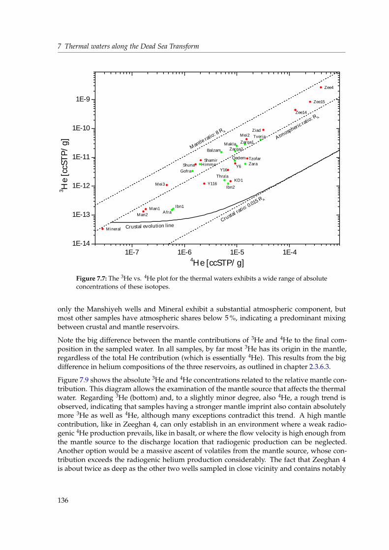
7 Thermal waters along the Dead Sea Transform
1 E - 7 1 E - 6 1 E - 5 1 E - 41 E - 1 4
1 E - 1 3
1 E - 1 2
1 E - 1 1
1 E - 1 0
1 E - 9
H i m m aS h u n a
Z i a d
M a n 1M a n 2
Z e e 4
Z e e 1 4Z e e 1 5
Z a r q a 1Z a r q a 2
Z a r a
I b n 1
I b n 2
A f r a
T h r a ' a K D 1G o f r a
S h a m i r
M e i 3
M e i 2
B a l z a mM a k l a
Y 1 1 6
Y 6Y 1 6
T z o f a r
T v e r i a
Q e d e m
M i n e r a l
3 He [c
cSTP/
g]
4 H e [ c c S T P / g ]
A t m o s p h e r i c ra t i o : R A
M a n t l e r at i o : 8 R A
C r u s t a l r a t i o : 0 . 0 1 5 R A
C r u s t a l e v o l u t i o n l i n e
Figure 7.7: The 3He vs. 4He plot for the thermal waters exhibits a wide range of absoluteconcentrations of these isotopes.
only the Manshiyeh wells and Mineral exhibit a substantial atmospheric component, butmost other samples have atmospheric shares below 5 %, indicating a predominant mixingbetween crustal and mantle reservoirs.
Note the big difference between the mantle contributions of 3He and 4He to the final com-position in the sampled water. In all samples, by far most 3He has its origin in the mantle,regardless of the total He contribution (which is essentially 4He). This results from the bigdifference in helium compositions of the three reservoirs, as outlined in chapter 2.3.6.3.
Figure 7.9 shows the absolute 3He and 4He concentrations related to the relative mantle con-tribution. This diagram allows the examination of the mantle source that affects the thermalwater. Regarding 3He (bottom) and, to a slightly minor degree, also 4He, a rough trend isobserved, indicating that samples having a stronger mantle imprint also contain absolutelymore 3He as well as 4He, although many exceptions contradict this trend. A high mantlecontribution, like in Zeeghan 4, can only establish in an environment where a weak radio-genic 4He production prevails, like in basalt, or where the flow velocity is high enough fromthe mantle source to the discharge location that radiogenic production can be neglected.Another option would be a massive ascent of volatiles from the mantle source, whose con-tribution exceeds the radiogenic helium production considerably. The fact that Zeeghan 4is about twice as deep as the other two wells sampled in close vicinity and contains notably
136
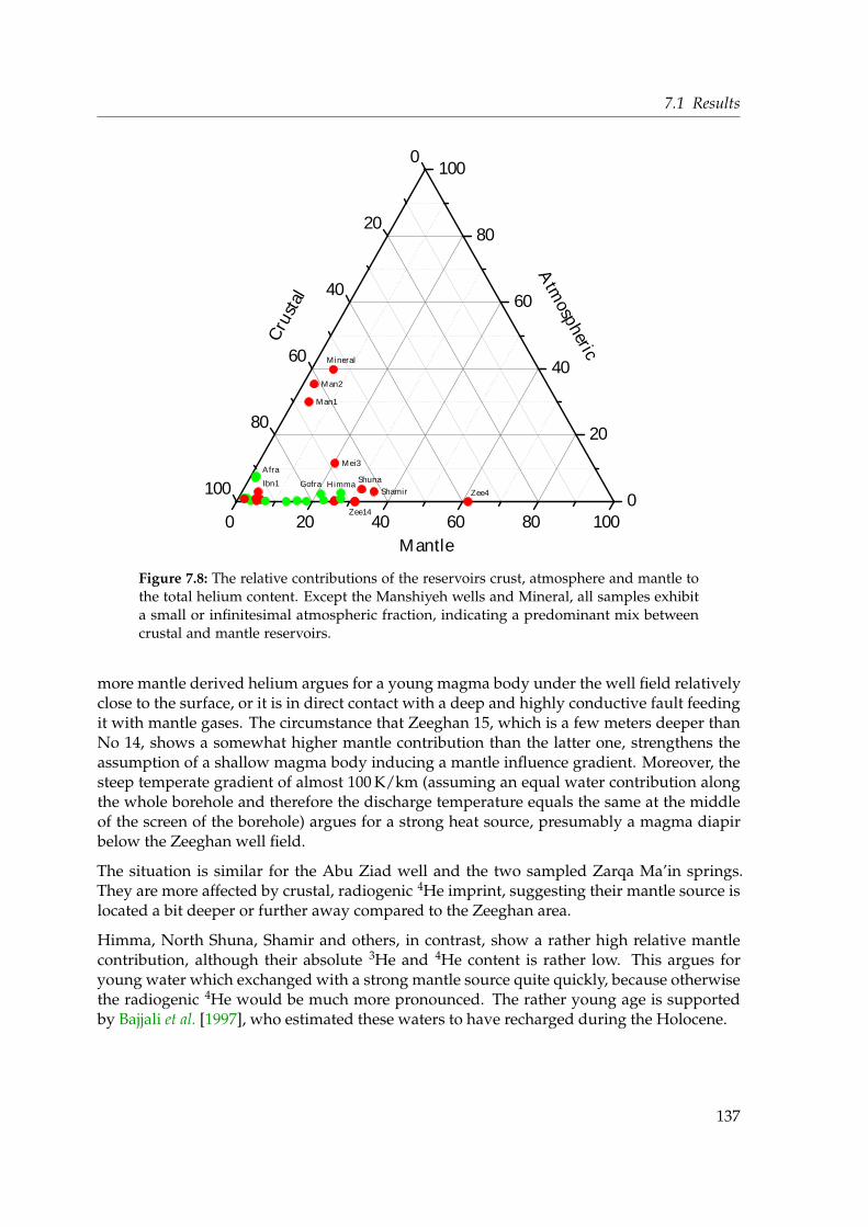
7.1 Results
0 2 0 4 0 6 0 8 0 1 0 0
0
2 0
4 0
6 0
8 0
1 0 0 0
2 0
4 0
6 0
8 0
1 0 0
H i m m a S h u n a
M a n 1M a n 2
Z e e 4Z e e 1 4
I b n 1A f r a
G o f r a S h a m i r
M e i 3
M i n e r a l
A t m o s p h e r i cC r us t a
l
M a n t l eFigure 7.8: The relative contributions of the reservoirs crust, atmosphere and mantle tothe total helium content. Except the Manshiyeh wells and Mineral, all samples exhibita small or infinitesimal atmospheric fraction, indicating a predominant mix betweencrustal and mantle reservoirs.
more mantle derived helium argues for a young magma body under the well field relativelyclose to the surface, or it is in direct contact with a deep and highly conductive fault feedingit with mantle gases. The circumstance that Zeeghan 15, which is a few meters deeper thanNo 14, shows a somewhat higher mantle contribution than the latter one, strengthens theassumption of a shallow magma body inducing a mantle influence gradient. Moreover, thesteep temperate gradient of almost 100 K/km (assuming an equal water contribution alongthe whole borehole and therefore the discharge temperature equals the same at the middleof the screen of the borehole) argues for a strong heat source, presumably a magma diapirbelow the Zeeghan well field.
The situation is similar for the Abu Ziad well and the two sampled Zarqa Ma’in springs.They are more affected by crustal, radiogenic 4He imprint, suggesting their mantle source islocated a bit deeper or further away compared to the Zeeghan area.
Himma, North Shuna, Shamir and others, in contrast, show a rather high relative mantlecontribution, although their absolute 3He and 4He content is rather low. This argues foryoung water which exchanged with a strong mantle source quite quickly, because otherwisethe radiogenic 4He would be much more pronounced. The rather young age is supportedby Bajjali et al. [1997], who estimated these waters to have recharged during the Holocene.
137

7 Thermal waters along the Dead Sea Transform
0 5 1 0 1 5 2 0 2 5 3 0 3 5 4 0 4 5 5 0 5 5 6 0 6 51 E - 1 31 E - 1 21 E - 1 11 E - 1 01 E - 91 E - 81 E - 71 E - 61 E - 51 E - 4
H i m m a S h u n a
Z i a d
M a n 1M a n 2
Z e e 4Z e e 1 4Z e e 1 5
Z a r q a 1Z a r q a 2Z a r a
I b n 1
I b n 2
A f r a
T h r a ' aK D 1
G o f r a S h a m i r
M e i 3
M e i 2B a l z a m
M a k l a
Y 1 1 6
Y 6Y 1 6
T z o f a rT v e r i a
Q e d e m
M i n e r a l
H i m m a S h u n a
Z i a d
M a n 1M a n 2
Z e e 4
Z e e 1 4Z e e 1 5
Z a r q a 1Z a r q a 2
Z a r a
I b n 1I b n 2
A f r a
T h r a ' aK D 1 G o f r aS h a m i r
M e i 3
M e i 2B a l z a mM a k l a
Y 1 1 6
Y 6Y 1 6
T z o f a rT v e r i a
Q e d e m
M i n e r a l
Isotop
e con
centra
tion [
ccSTP
/g]
M a n t l e c o n t r i b u t i o n [ % ]
4 H e
3 H e
Figure 7.9: The relation of total 3He and 4He concentrations to the relative mantlecontribution gives evidence for the distance between mantle source and dischargelocation as well as for the mantle imprint history. See text for details.
On the other hand there are samples with considerable 3He content, but in total a smallamount of mantle helium contributing to the total helium content. This indicates either aweak or distant mantle source, where crustal helium production dominates, or, more likely,the water once passed a strong and locally limited mantle source, but is exposed to crustalconditions before and/or afterwards. This seems to be the case for Ibn Hammat 2, Thra’a,KD1, Zara and the wells in Wadi Arava, which contain even as much 3He as Himma orNorth Shuna.
One may infer from these observations that the link between a geothermal heat source andthe mantle helium ratio would result in a correlation of discharge temperature and the (cor-rected) 3He/4He ratio. This relation is displayed in figure 7.10. However, no overall ten-dency is discernible, indicating the discharge temperature and the magnitude of mantlehelium imprint are independent. This observation coincides with the data published byTorfstein et al. [2013], who likewise found no correlation between 3He/4He ratio and dis-charge temperature. This notice disagrees with the interpretation above, that mantle heliumcontent is related to the distance from a magmatic heat source, but rather argues either formantle volatile ascending independently from groundwater movement (i. e. in form of gasbubbles), or for a differently mantle imprinted, local reservoir. The latter would contrast theconcept of an uniform reservoir suggested by Torfstein et al. [2013].
138

7.1 Results
3 0 3 5 4 0 4 5 5 0 5 5 6 0 6 5 7 00
1
2
3
4
5
H i m m aS h u n a
Z i a d
M a n 1M a n 2
Z e e 4
Z e e 1 4Z e e 1 5
Z a r q a 1Z a r q a 2
Z a r aI b n 1 I b n 2 A f r aT h r a ' a K D 1
G o f r a
S h a m i r
M e i 3M e i 2B a l z a m
M a k l a
Y 1 1 6 Y 6Y 1 6 T z o f a r
T v e r i aQ e d e mM i n e r a l
3 He /
4 He [R
A]
T e m p e r a t u r e [ ° C ]Figure 7.10: No overall tendency is recognizable in the 3He/4He ratio against dischargetemperature plot. The trend within the Zeeghan well field (data points labeled Zee4,14 and 15) suggests a strong mantle source beneath the well field which establishes agradient of heat and mantle influence. The thermal gradient in this locality can roughlybe determined to about 100 K/km.
Other noble gas isotope ratios were found to vary in the reservoirs air and mantle. Some ofthese isotope ratios are determined in this study. The according endmember composition islisted in table 7.6 and figure 7.11 presents the ratios 20Ne/22Ne, 3He/22Ne and 3He/36Ar, inevery plot relative to the 40Ar/36Ar ratio. The dashed lines indicate the mixing line betweenthe atmospheric and the MORB-like mantle reservoir. No clear trend is discernible in all dia-grams, which may partly be due to large inaccuracies of the data. But more important is thatthe noble gas isotope data of the sampled thermal waters all plot very close to atmosphericvalues compared to MORB-mantle ratios. Even if OIB-mantle values would be considered,the image would not change considerably. Therefore, scattering seems to be predominantover real mixing trends.
It is, however, not so obvious, why the mantle signature is that more pronounced in heliumisotopes than in the other mentioned ratios. Since helium has a better solubility in mag-matic melts than the heavier noble gases [Carroll and Webster, 1994], partitioning duringdegassing of the melt under decreased pressure would favor the heavy noble gases to befound in mantle affected groundwater, especially as the heavy noble gases in turn have bet-ter solubilities in water. The strongest effect of the other isotope ratios should, hence, beseen in the argon ratio, since it varies most notably among the two reservoirs. The fact thatthe mantle signature is by far best pronounced in helium isotopes may result from muchhigher diffusivity of helium compared to the other noble gases. Burnard [2004] modeledthe fractionation between argon and helium ascending in fractures up to one order of mag-nitude, while Torgersen and O’Donnell [1991] calculated the (crustal) noble gas release fluxfrom immediate rock fracturing to be fractionated between He and Ar up several orders of
139

7 Thermal waters along the Dead Sea Transform
9 . 7 5 9 . 8 0 9 . 8 52 8 0
2 9 0
3 0 0
3 1 0
3 2 0
3 3 0
3 4 0
40 Ar/36 Ar
2 0 N e / 2 2 N e
Z e e 1 5
Z e e 4
T v e r i a
Z e e 1 4Z a r a Q e d e m
0 . 0 0 0 . 0 2 0 . 0 43 H e / 2 2 N e
Z e e 1 5
Z e e 4
Z e e 1 4
T v e r i aZ a r a
Q e d e m
Z i a d
0 5 x 1 0 - 4 1 x 1 0 - 32 8 0
2 9 0
3 0 0
3 1 0
3 2 0
3 3 0
3 4 0
3 H e / 3 6 A r
Z e e 1 5Z e e 4
Z e e 1 4
T v e r i a
Z a r aQ e d e m
Figure 7.11: Other noble gas isotope ratio plots indicating possible mantle influence.The dashed lines are mixing lines between atmospheric and MORB composition, ascompiled in table 7.6. No clear tendency is visible in all plots.
magnitude. However, whether these effects can solely explain the observed effects remainsuncertain.
In case of argon another explanation is possible. Since this noble gas is by far the most abun-dant in the atmosphere, a mantle argon signature would be masked by the atmosphericcomponent if the absolute argon concentration within the mantle is considerably lower thanin the atmosphere. Unfortunately, only argon isotope ratios, but no absolute argon contentsin magmatic minerals are published, but Nakai et al. [1997] measured absolute argon con-centrations in CO2-CH4 rich gas samples from Etna, Italy, to be about 15 times smaller thanatmospheric ones. As neon occurs at roughly the same concentration in the atmosphereas helium, such a masking effect can not explain the absence of mantle neon signatures insamples with high helium isotope ratios typical for mantle sources. Possibly this resultssimply from the merely small difference regarding the neon isotope composition in air andMORB.
Table 7.6: Other noble gas isotope ratios in air, MORB and different OIBs [Moreira andKurz, 2013, and references therein].
Reservoir 3He/4He [RA] 40Ar/36Ar 20Ne/22Ne 3He/22Ne 3He/36Ar
Air 1 295.5 9.8 ~0 ~0MORB 8 ~30 000 12.6 5.1 0.45OIB (Galapagos) 23 ~3000 12.6 2.3± 0.5 0.35OIB (Iceland) 17.5 ~5000 12.6 2.5± 0.3 0.4
140
7.1 Results
However, 40Ar/36Ar ratios in other hydrothermal systems, compiled by Sano and Fischer[2013], reveal that in most cases the ratio is close to the atmospheric value of 295.5, as it isfound in the presented study. In samples from Vulcano, Italy, elevated argon ratios above1000 are found [Magro and Pennisi, 1991], but a crustal neon systematic revealed by Tedescoand Nagao [1996] suggests the high argon ratios result from crustal 40Ar production ratherthan from a mantle source at this locality. On the other hand, in case of samples from Etna,Italy [Nakai et al., 1997], as well as from the continental rift zone in the Eiffel, Germany[Aeschbach-Hertig et al., 1996], high argon ratios are associated with stronger mantle influ-enced neon signatures and, therefore, are interpreted to be an evidence for a mantle source.
Overall, the mantle influence is much less expressed in noble gas isotope ratios other thanthe 3He/4He ratio in most hydrothermal occurrences and their relative intensity comparedto the helium isotope ratio seems to vary widely. Therefore, the 3He/4He ratio is by far themost sensitive mantle impact indicator among the noble gases.
Following, the other tracers determined in this study are compared to the helium ratio datain order to reveal any correlation between them and the mantle helium signals.
7.1.3 δ13C isotopy
The carbon isotopy of the sampled thermal waters is listed in table 7.7 and varies widelyfrom −12 h to +5 h. Most samples show a rather enriched δ13C level compared to valuestypically found in groundwater (compare figure 2.7). The most 13C depleted thermal wateris tendentially found in the springs and wells in and around the Yarmouk Gorge, namelyHimma, North Shuna, Meitzar 2, both Manhiyeh wells, Gofra and, a little bit more enriched,Ein Balzam and Ein Makla, with δ13C values between −7 and −11 h. However, in thesame area the more shallow well Meitzar 3 is obviously enriched (−3.40 h), as is Shamir(−1.54 h), located north of Lake Kinneret, and Hamat Tveria (−1.85 h), west of the lake.Unfortunately, no δ13C value for Zeeghan 4, the sample with the highest 3He/4He ratio, isavailable, because the sample bottle broke during shipment.
The wells and springs along the eastern side of the central Jordan Valley, from Abu Ziadsouth to the Zarqa Ma’in spring cluster, are highly enriched, the Zeeghan wells reachingpositive δ13C values. Further south, the δ13C isotopy tendentially attains medium depletedvalues of −7 h to −4 h. The map in figure 7.6 visualizes the δ13C distribution along theDST, with bigger circles representing samples more enriched in 13C.
The outstanding high δ13C value of +5.5 h found in the Mineral well at the Dead Sea, incombination with its very high salinity, suggests that this well feeds on inland intrudingDead Sea water, which is reported to have δ13C up to +4 h in the uppermost 20 m (althoughthis value fluctuates between +0.5 h and the mentioned +4 h) [Barkan et al., 2001]. Thesame explanation is reasonable for the sampled spring at the Dead Sea shore, Ein Qedem,which has a δ13C value of −1.1 h. The indication of Dead Sea water found at these localitiesis supported by the stable isotopes of the water molecules, as shown below. The high δ13Cvalues of the Zarqa Ma’in springs, located about 400 m above the Dead Sea, however, areunlikely explained by an upstream of Dead Sea derived water, because highly mineralized
141

7 Thermal waters along the Dead Sea TransformTable
7.7:Com
piledanalysis
results
forδ
2H,
δ18O
,δ
13C,tritiu
m,rad
onand
alkalinityfor
allthermalw
atersam
plesalong
theD
ST.Israelidatafrom
Tsur[2013].
Localityδ
2H∆
δ2H
δ18O
∆δ
18Oδ
13C∆
δ13C
Tritium∆
TritiumR
n∆
Rn
Alkalinity
hh
hh
hh
TUTU
Bq/m3
Bq/m3
meq/L
JordanW
ellsN
orthShuna
-5.680.01
-27.530.09
-10.02–
–2693
3966.84
Abu
Ziad
-5.740.04
-28.090.21
-3.082.27
0.9717228
6724.72
Manshiyeh
1-5.50
0.12-26.05
0.40-10.45
4.030.93
25865870
6.26M
anshiyeh2
-5.360.26
-25.740.68
-10.712.70
0.9816352
8216.38
Zeeghan
4-6.58
0.06-41.34
0.090.00
––
2873281
23.00Z
eeghan14
-5.810.04
-35.770.09
1.19–
–27174
59018.24
Zeeghan
15-6.82
0.04-43.20
0.342.05
––
1896418
23.00K
D1
-7.010.05
-39.210.26
b.d.3.85
SpringsH
imm
a-5.86
0.03-29.55
0.32-9.75
11.141.04
414871212
6.24Z
arkaM
a’in1
-4.110.01
-32.780.05
-3.46–
–5340
3464.90
Zarka
Ma’in
2-4.09
0.05-32.30
0.20-0.92
b.d.34277
14585.02
Zara
-5.350.08
-39.730.06
0.00b.d.
782111952
3.08Ibn
Ham
mat
1-6.91
0.17-43.83
0.56-4.85
––
1760953144
3.53Ibn
Ham
mat
2-6.99
0.06-40.18
0.10-6.50
––
6461408
3.30A
fra-6.50
0.05-36.27
0.21-6.55
––
9604555
2.50Thra’a
-6.700.05
-38.850.19
0.00–
–5944
3732.62
IsraelW
ellsSham
ir-7.03
0.07-36.02
0.11-1.54
b.d.M
eitzar2
-5.690.10
-28.680.41
-11.79b.d.
Meitzar
3-7.02
0.15-36.63
0.90-3.40
b.d.Ein
Yahav6
-7.510.11
-47.830.66
-5.716.52
1.1Ein
Yahav16
-6.910.10
-42.380.54
-3.40b.d.
EinYahav
116-6.60
0.06-39.56
0.45-6.20
b.d.Tzofar
-8.380.05
-57.580.13
-7.15b.d.
Mineral
1.080.06
-4.240.40
5.543.34
1.09SpringsG
ofra-4.60
0.07-21.84
0.12-8.38
b.d.Ein
Balzam-5.93
0.09-30.74
0.56-8.45
b.d.Ein
Makla
-6.040.12
-31.410.53
-7.63b.d.
Ham
atTveria
-3.570.10
-16.000.50
-1.85b.d.
EinQ
edem0.92
0.10-4.49
0.57-1.10
b.d.
142

7.1 Results
water contributing to these springs is not in accord with the rather low salinity found in bothsampled Zarqa Ma’in springs.
As summarized in figure 2.7, the enriched carbon-13 found along the DST may in principleresult from mantle CO2, freshwater carbonates and metamorphic CO2. A significant mantlesource of CO2 can be excluded due to two reasons: First, it is unlikely that it can explain δ13Cvalues above −3 h. Second, a correlation between mantle helium and δ13C isotopy wouldbe expected. Griesshaber et al. [1992], for example, found clear positive correlations betweenthe helium isotope ratios and δ13C of CO2 degassing from thermal waters from the severallocalities in the Rhine Graben and concluded a mantle source of the carbon dioxide.
As shown in figure 7.12, δ13C of the DST water samples does not correlate with the 3He/4Heratios. Therefore, a substantial mantle CO2 contribution to the thermal waters along theJordan Rift Valley can be excluded. However, a slight correlation of δ13C and the absolutemeasured 3He and 4He concentration is discernible. Mineral, which seems to represent a spe-cial case (see above), can be omitted in this consideration. Also the wells of the Zeeghan wellfield may need a separate treatment. They are strongly degassing, and the extremely highalkalinity and the absence of any smell (H2S) suggest that mostly CO2 gas escapes. There-fore, these wells might be affected by additional Rayleigh-like fractionation further enrichingthe 13C isotopy of the water phase, as Evans et al. [2008] suggest to explain extraordinarilyhigh δ13C values of up to +13 h in Himalayan hot springs. This would imply the Zeeghansamples would plot further left in the diagrams in figure 7.12 if no additional carbon frac-tionation would take place. Therefore, if the Zeeghan wells and Mineral are excluded fromthis analysis, no trend in the plots δ13C versus 3He or 4He, respectively, is visible anymore.
Freshwater carbonates are not found in the DST, as most of the sedimentation occurred un-der saline conditions, when the precursors of the Dead Sea evaporated. However, Katz et al.[1977] report δ13C of −7.7 up to +3.4 h for aragonites of the Lisan formation, the sedimen-tary remnant of the former saline, Pleistocene Lake Lisan. Generally, groundwater bodiesleaching evaporites from this formation have a high salinity, but are found only in the valleydepression itself, as for example reported by Salameh [2001]. Sources of salinity in watersentering the Jordan Valley from its eastern escarpment, however, are the Jurassic and Trias-sic sandstone rocks (Kurnub and Ram aquifers). This means carbon isotopy of the springsin the side-wadis of the Jordan Valley is unlikely to be affected by carbonates from the Lisanformation. Deeply drilled wells and the springs at Lake Kinneret, in contrast, cannot beruled out to incorporate Lisan formation carbonate.
In case the dissolution of Lisan evaporites would influence the tested thermal waters, theprocess takes place within in the crust and therefore no correlation between the 3He/4Heratio and δ13C should be observed, as is the case for the presented localities. However, if dis-solution of carbon from the Lisan formation is the governing process, a correlation betweensalinity and δ13C should be discernible, at least among the wells (because most springs aresomewhat elevated above the bottom of the Jordan Valley, yet an upstream is not principallyimpossible). This relation is depicted in figure 7.13. Only a very rough trend is observed, butespecially those locations with E. C. below 3000 µS/cm are widely scattered with no pattern.Even more, no general difference between springs and wells can be recognized.
143

7 Thermal waters along the Dead Sea Transform
- 1 2 - 1 0 - 8 - 6 - 4 - 2 0 2 4 6
1 E - 1 3
1 E - 1 2
1 E - 1 1
1 E - 1 0
1 E - 9
H i m m aS h u n a
Z i a d
M a n 1M a n 2
Z e e 1 4Z e e 1 5
Z a r q a 1Z a r q a 2
I b n 1
I b n 2
A f r a
G o f r aS h a m i r
M e i 3
M e i 2B a l z a mM a k l a
Y 1 1 6
Y 6Y 1 6
T z o f a r
T v e r i a
Q e d e m
M i n e r a l
3 He [c
cSTP/
g]
δ 1 3 � � � � �- 1 2 - 1 0 - 8 - 6 - 4 - 2 0 2 4 6
1 E - 7
1 E - 6
1 E - 5
1 E - 4
1 E - 3
H i m m aS h u n a
Z i a d
M a n 1M a n 2
Z e e 1 4Z e e 1 5
Z a r q a 1 Z a r q a 2
I b n 1
I b n 2
A f r aG o f r a S h a m i r
M e i 3
M e i 2B a l z a m
M a k l a
Y 1 1 6
Y 6 Y 1 6T z o f a r
T v e r i a
Q e d e m
M i n e r a l
4 He [c
cSTP/
g]
δ 1 3 � � � � �
- 1 2 - 1 0 - 8 - 6 - 4 - 2 0 2 4 60
1
2
3
H i m m a
S h u n a
Z i a d
M a n 1M a n 2
Z e e 1 4Z e e 1 5
Z a r q a 1Z a r q a 2
I b n 1I b n 2A f r a
G o f r a
S h a m i r
M e i 3M e i 2 B a l z a m
M a k l a
Y 1 1 6Y 6 Y 1 6
T z o f a r
T v e r i a
Q e d e m M i n e r a l
3 He /
4 He [R
A]
δ1 3 � � � � �
Figure 7.12: No correlation between the corrected 3He/4He ratio and δ13C can berecognized, excluding a mantle source of carbon in the DST groundwater samples. Theslight trends visible in 3He, respectively 4He, against δ13C disappear, when the Zeeghanand Mineral samples are discarded (see text for details).
These findings suggest that neither mantle CO2 nor dissolution of evaporites are the reasonfor the distinctly enriched δ13C isotopy along the Jordan Rift Valley. The incorporation ofascending CO2 from metamorphic decarbonation is therefore the most likely explanationfor it.
In general, however, the δ13C isotopy is no good indicator of mantle induced processes, be-cause the signatures of the different carbon sources can not easily be distinguished from eachother and ambiguity remains. A better differentiation between a mantle and a crustal carbonsource can be obtained by considering the CO2/3He ratio in addition to the 3He/4He ratio[Sano and Fischer, 2013]. However, no CO2 concentration in thermal waters and volatilesescaping from them was determined during this study. Torfstein et al. [2013], on the contrary,published CO2/3He ratios for many thermal waters in Israel and concluded that crustal car-bon dissolution and precipitation are the controlling factors regarding the carbon contentalong the DST.
144
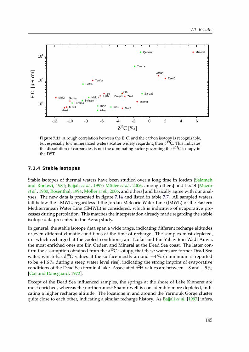
7.1 Results
- 1 2 - 1 0 - 8 - 6 - 4 - 2 0 2 4 6
1 0 3
1 0 4
1 0 5
H i m m aS h u n a Z i a d
M a n 1M a n 2
Z e e 1 4Z e e 1 5
Z a r q a 1 Z a r q a 2
I b n 1I b n 2A f r a
G o f r a
S h a m i rM e i 3
M e i 2B a l z a m
M a k l a Y 1 1 6Y 6 Y 1 6
T z o f a r
T v e r i a
Q e d e m M i n e r a l
E.C. [µ
S/cm
]
δ1 3 � � � � �
Figure 7.13: A rough correlation between the E. C. and the carbon isotopy is recognizable,but especially low mineralized waters scatter widely regarding their δ13C. This indicatesthe dissolution of carbonates is not the dominating factor governing the δ13C isotopy inthe DST.
7.1.4 Stable isotopes
Stable isotopes of thermal waters have been studied over a long time in Jordan [Salamehand Rimawi, 1984; Bajjali et al., 1997; Möller et al., 2006, among others] and Israel [Mazoret al., 1980; Rosenthal, 1994; Möller et al., 2006, and others] and basically agree with our anal-yses. The new data is presented in figure 7.14 and listed in table 7.7. All sampled watersfall below the LMWL, regardless if the Jordan Meteoric Water Line (JMWL) or the EasternMediterranean Water Line (EMWL) is considered, which is indicative of evaporative pro-cesses during percolation. This matches the interpretation already made regarding the stableisotope data presented in the Azraq study.
In general, the stable isotope data span a wide range, indicating different recharge altitudesor even different climatic conditions at the time of recharge. The samples most depleted,i. e. which recharged at the coolest conditions, are Tzofar and Ein Yahav 6 in Wadi Arava,the most enriched ones are Ein Qedem and Mineral at the Dead Sea coast. The latter con-firm the assumption obtained from the δ13C isotopy, that these waters are former Dead Seawater, which has δ18O values at the surface mostly around +4 h (a minimum is reportedto be +1.6 h during a steep water level rise), indicating the strong imprint of evaporativeconditions of the Dead Sea terminal lake. Associated δ2H values are between −8 and +5 h[Gat and Dansgaard, 1972].
Except of the Dead Sea influenced samples, the springs at the shore of Lake Kinneret aremost enriched, whereas the northernmost Shamir well is considerably more depleted, indi-cating a higher recharge altitude. The locations in and around the Yarmouk Gorge clusterquite close to each other, indicating a similar recharge history. As Bajjali et al. [1997] infers,
145

7 Thermal waters along the Dead Sea Transform
- 9 - 8 - 7 - 6 - 5 - 4 - 3 - 2 - 1 0 1 2- 6 0
- 5 0
- 4 0
- 3 0
- 2 0
- 1 0
0
H i m m aS h u n aZ i a d
M a n 1 M a n 2
Z e e 4
Z e e 1 4
Z e e 1 5
Z a r q a 1Z a r q a 2
Z a r a
I b n 1
I b n 2
A f r aT h r a ' aK D 1
G o f r a
S h a m i rM e i 3
M e i 2B a l z a mM a k l a
Y 1 1 6
Y 6
Y 1 6
T z o f a r
T v e r i a
Q e d e m M i n e r a l
E MW L : �
2 H = 8· �
1 8 O + 22 �
δ2 ����
�
δ1 8 � � � � �
J M W L : �2 H = 6 . 2 7
· �1 8 O + 1 1 . 4
�
G M W L : �2 H = 8
. 1 7 · �1
8 O + 10 . 3 5
�
Figure 7.14: Stable isotope plot of all sampled thermal waters. All samples fall belowthe local meteoric water lines, indicating evaporative processes in the top soil. Thesprings of the Zarqa Ma’in/Zara cluster are significantly shifted towards less depleted18O, signaling the original hot water reservoir exceeded temperatures of 100 ◦C, whereoxygen exchange reactions with the surrounding aquifer matrix occur.
recharge of this cluster of waters took place in the Jordan highlands and the opposing GolanHeights, except Ein Maqla whose water originates from higher altitudes, presumably fromMount Hermon at the Syrian-Libanese border. Ein Balzam is, according to the mentionedpublication, assumed to be a mixture of the water body feeding Ein Maqla with water foundin the other springs in the area, an interpretation that can be confirmed by the presentedstable isotope data. Also the 800 m deep Meitzar 2 well fits into this cluster, whereas themore shallow Meitzar 3 well plots closer to the water found more to the south of the JordanValley.
The stable isotope pattern changes south of the Abu Ziad well, where the Zeeghan wells andthe springs in the side-wadis southeast of the Dead Sea cluster loosely together and are moredepleted than the northern water types. Also the Ein Yahav wells 16 and 116 and the moreinland located KD1 well belong to this cluster. It is actually not surprising that KD1 has asimilar isotopic imprint than Afra, Thra’a and the two Ibn Hamat springs, because they alldischarge from the Lower Cretaceous Kurnub sandstone aquifer. In total, a general trendis observable since waters in the north of the study area are less depleted in stable isotopesthan those found in the south.
146

7.1 Results
An exception of the water group of the eastern Dead Sea escarpment are the springs ofZarqa Ma’in and Zara. These are distinctly more enriched in δ18O, expressed also in a verylow deuterium excess, which plots them far away from the meteoric water lines. This pointsto interaction of the oxygen in the water molecules with oxygen incorporated in the rockmaterial. According to Clark and Fritz [1997], oxygen containing minerals have positiveδ18O values (carbonate rock ~+29 h, granitic rock ~+10 h, basalt ~+8 h). As exchangerates at low temperatures are much too slow to considerably influence the oxygen isotopy ofgroundwater within typical residence times, the case is different in geothermal systems. Theexchange rate is notably increased at temperatures above 100 ◦C and therefore water perco-lating through the rock at such high temperatures gets enriched in δ18O. At the same timeδ2H stays virtually the same, simply because most minerals do not contain any hydrogen[Clark and Fritz, 1997]. The right-shift in the δ2H–δ18O diagram of groundwater interact-ing with the rock matrix at high temperatures is found in many geothermal systems aroundthe world [Truesdell and Hulston, 1980] and can explain the δ2H–δ18O composition of theZarqa and Zara springs. Moreover, it shows that no juvenile or magmatic water, which isestimated to have δ18O between +6 and +9 h, but δ2H between −40 and −80 h [White,1974], contributes to the sampled thermal waters. The thermal anomality with very highgeothermal gradients found in the Zarqa Ma’in/Zara area (compare chapter 4.2) is in goodaccordance with the finding of temperature induced oxygen exchange between rock andwater molecules.
A slight influence of the temperature effect on δ18O can not principally be excluded for theother waters, but the effect of a hot reservoir would be much less compared to the Zara andZarqa springs.
The question of a relation between mantle helium influence and stable isotopes is answeredby the graphs in figure 7.15: there is no relation recognizable between 3He/4He ratio, 3He or4He and δ18O. Therefore, δ18O cannot be taken as an additional tracer for mantle influencedfluids.
7.1.5 Water chemistry and radon
Water chemistry
The major ion analysis of the thermal waters of Jordan is presented in a Piper plot in figure7.16 and the underlying data is compiled in table A.7 on page 185. The samples from Israelilocalities were not analyzed for water chemistry. Some water groups can be distinguished.First, the two Manshiyeh wells form a solitary group, where bicarbonate and Ca/Mg domi-nate. Second, the water from the Zeeghan wells and the spring field of Zarqa Ma’in and Zaraare similar in their mineralization pattern, with Cl being the dominant anion and Na themost abundant cation. Most notable, however, the wells and springs around the YarmoukValley, carrying much mantle helium, and those springs furthest south with predominantcrustal signature exhibit a very similar ionic composition and cannot be distinguished fromeach other. Therefore, the ionic pattern of the thermal waters in Jordan is not suitable todifferentiate the tectonic behavior and the mantle gas input along the DST.
147

7 Thermal waters along the Dead Sea Transform
- 8 - 6 - 4 - 2 0 2
1 E - 1 31 E - 1 21 E - 1 11 E - 1 01 E - 9
H i m m a S h u n a
Z i a d
M a n 1M a n 2
Z e e 4
Z e e 1 4Z e e 1 5
Z a r q a 1Z a r q a 2
Z a r a
I b n 1
I b n 2
A f r a
T h r a ' aK D 1 G o f r aS h a m i r
M e i 3
M e i 2B a l z a m
M a k l a
Y 1 1 6
Y 6Y 1 6
T z o f a r
T v e r i a
Q e d e m
M i n e r a l
3 He [c
cSTP/
g]
δ 1 8 � � � � �- 8 - 6 - 4 - 2 0 2
1 E - 7
1 E - 6
1 E - 5
1 E - 4
1 E - 3
H i m m aS h u n a
Z i a d
M a n 1 M a n 2
Z e e 4Z e e 1 4
Z e e 1 5
Z a r q a 1Z a r q a 2Z a r a
I b n 1
I b n 2
A f r a
T h r a ' aK D 1
G o f r aS h a m i r
M e i 3
M e i 2
B a l z a mM a k l a
Y 1 1 6
Y 6Y 1 6
T z o f a r T v e r i aQ e d e m
M i n e r a l
4 He [c
cSTP/
g]
δ 1 8 � � � � �
- 9 - 8 - 7 - 6 - 5 - 4 - 3 - 2 - 1 0 1 20
1
2
3
4
5
H i m m a
S h u n aZ i a d
M a n 1M a n 2
Z e e 4
Z e e 1 4Z e e 1 5
Z a r q a 1Z a r q a 2
Z a r aI b n 1I b n 2 A f r a
T h r a ' aK D 1
G o f r a
S h a m i r
M e i 3 M e i 2B a l z a m
M a k l a
Y 1 1 6Y 6 Y 1 6T z o f a r
T v e r i aQ e d e m M i n e r a l
3 He /
4 He [R
A]
δ1 8 � � � � �
Figure 7.15: No correlation between the corrected 3He/4He ratio, 3He or 4He and δ18Ocan be recognized.
The origin of thermal waters can be studied with a ternary diagram of relative Cl, SO4 andHCO3 content, as shown in figure 7.17, and which is in principle the anion triangle of thePiper diagram, but uses the ion concentrations in mg/L instead of in meq/L (after Giggen-bach and Goguel [1989], cited according to Powell and Cumming [2010]). According to thisplot, water can be classified into four types: 1) HCO3 rich, peripheral, i. e. meteoric waterwith no or only little geothermal influence, 2) steam heated, SO4 rich water, 3) volcanic wa-ter which is rich in SO4 and Cl, originating from absorption of H2S carrying volcanic gases,and 4) mature or geothermal water, dominated by Cl.
The samples from north Jordan plot all more or less in the bicarbonate dominated corner,while the samples from the Zarqa Ma’in/Zara spring cluster and the Zeeghan well field arelocated tendentially towards the mature water vertex. All samples contain sulphate to acertain extent. Abu Ziad, where H2S smell was perceptible at sampling, contains most SO4,followed by Zeeghan 4 and 15. The latter wells showed extreme degassing, but H2S was notnoticeable at the sites. On the other hand, North Shuna well has a quite low SO4 content,but exhibited obvious H2S smell. In total, however, none of the samples can be referred toas real volcanic water.
148
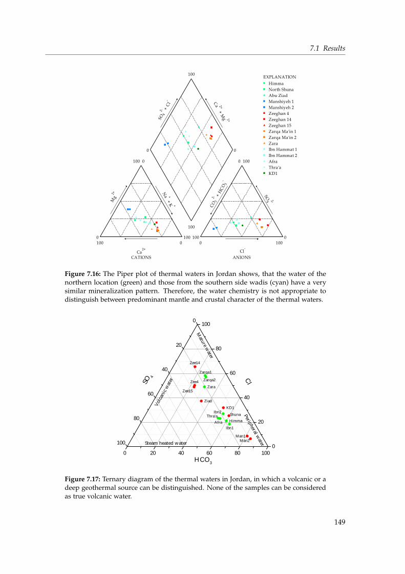
7.1 Results
Ca2+
CATIONSCl
-
ANIONS
1000
0100
100 0
0100
1000
0 100
100
100
0 0
EXPLANATIONHimmaNorth ShunaAbu ZiadManshiyeh 1Manshiyeh 2Zeeghan 4Zeeghan 14Zeeghan 15Zarqa Ma'in 1Zarqa Ma'in 2ZaraIbn Hammat 1Ibn Hammat 2AfraThra'aKD1
Figure 7.16: The Piper plot of thermal waters in Jordan shows, that the water of thenorthern location (green) and those from the southern side wadis (cyan) have a verysimilar mineralization pattern. Therefore, the water chemistry is not appropriate todistinguish between predominant mantle and crustal character of the thermal waters.
Z a r a
S h u n a
Z a r q a 1Z a r q a 2
H i m m a
Z e e 1 5
Z e e 1 4
Z e e 4
A f r aI b n 1
M a n 1M a n 2
Z i a d
I b n 2T h r a ' a
K D 1
0 2 0 4 0 6 0 8 0 1 0 0
0
2 0
4 0
6 0
8 0
1 0 0 0
2 0
4 0
6 0
8 0
1 0 0
P e r i p h e r a l w a t e r
C lS O 4
H C O 3
M a t u r e w a t e r
V ol c a
n i c w a t e
r
S t e a m h e a t e d w a t e r
Figure 7.17: Ternary diagram of the thermal waters in Jordan, in which a volcanic or adeep geothermal source can be distinguished. None of the samples can be consideredas true volcanic water.
149
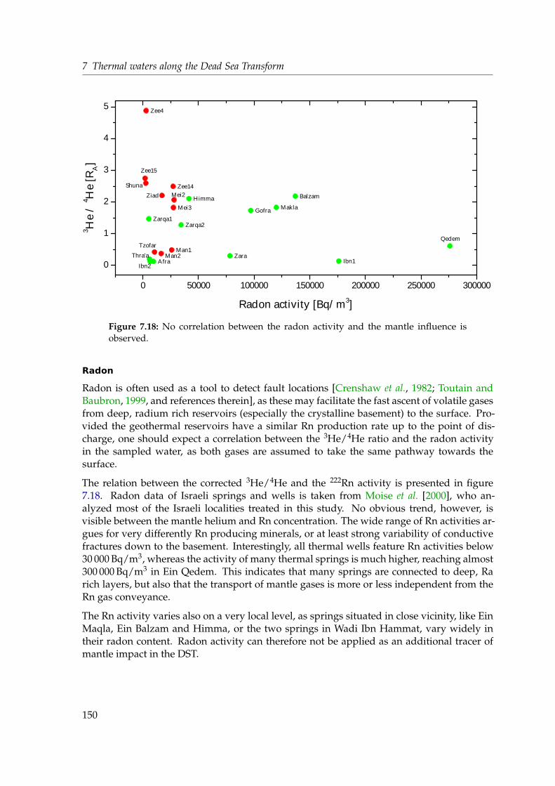
7 Thermal waters along the Dead Sea Transform
0 5 0 0 0 0 1 0 0 0 0 0 1 5 0 0 0 0 2 0 0 0 0 0 2 5 0 0 0 0 3 0 0 0 0 00
1
2
3
4
5
H i m m aS h u n a
Z i a d
M a n 1M a n 2
Z e e 4
Z e e 1 4
Z e e 1 5
Z a r q a 1 Z a r q a 2
Z a r a I b n 1I b n 2 A f r aT h r a ' a
G o f r aM e i 3M e i 2 B a l z a m
M a k l a
T z o f a rQ e d e m
3 He /
4 He [R
A]
R a d o n a c t i v i t y [ B q / m 3 ]Figure 7.18: No correlation between the radon activity and the mantle influence isobserved.
Radon
Radon is often used as a tool to detect fault locations [Crenshaw et al., 1982; Toutain andBaubron, 1999, and references therein], as these may facilitate the fast ascent of volatile gasesfrom deep, radium rich reservoirs (especially the crystalline basement) to the surface. Pro-vided the geothermal reservoirs have a similar Rn production rate up to the point of dis-charge, one should expect a correlation between the 3He/4He ratio and the radon activityin the sampled water, as both gases are assumed to take the same pathway towards thesurface.
The relation between the corrected 3He/4He and the 222Rn activity is presented in figure7.18. Radon data of Israeli springs and wells is taken from Moise et al. [2000], who an-alyzed most of the Israeli localities treated in this study. No obvious trend, however, isvisible between the mantle helium and Rn concentration. The wide range of Rn activities ar-gues for very differently Rn producing minerals, or at least strong variability of conductivefractures down to the basement. Interestingly, all thermal wells feature Rn activities below30 000 Bq/m3, whereas the activity of many thermal springs is much higher, reaching almost300 000 Bq/m3 in Ein Qedem. This indicates that many springs are connected to deep, Rarich layers, but also that the transport of mantle gases is more or less independent from theRn gas conveyance.
The Rn activity varies also on a very local level, as springs situated in close vicinity, like EinMaqla, Ein Balzam and Himma, or the two springs in Wadi Ibn Hammat, vary widely intheir radon content. Radon activity can therefore not be applied as an additional tracer ofmantle impact in the DST.
150

7.2 Detailed analysis of the geothermal localities
7.2 Detailed analysis of the geothermal localities
Following, the different localities of thermal water occurrence are considered in detail andthe individual conditions leading to elevated water temperatures are tried to deduce in viewof the new data and other sources.
In and around the Yarmouk Gorge
The thermal waters in the Yarmouk Gorge were intensively studied. They are situated be-tween the structural depression of the Golan Heights and the anticline of the Ajloun Dome.Most of the groundwater originates from the Ajloun ridge [Bajjali et al., 1997; Margane et al.,2002], but stable isotopes in some sources indicate also a fraction being recharged at theslopes of Mount Hermon in the north [Arad and Bein, 1986; Bajjali et al., 1997]. Figure 7.19shows a hydrogeologic cross-section along a north–south line from the Hermon MountainRidge in Lebanon across the Golan Heights and the Ajloun dome to the Zarqa River Valleyin the south, including assumed hot and cold groundwater flow and its ascent through asupposed zone of enhanced conductivity in the Yarmouk Gorge.
Both, Galanis Jr. et al. [1986] and Shalev et al. [2013] report an elevated heat flow in thearea of the lower Yarmouk Gorge, where the springs are located. This heat flow anomalyseems to be a very local phenomenon, as Dafny et al. [2006] found no heat anomaly beneaththe Golan Heights, and Galanis Jr. et al. [1986] and Bajjali [1994] reported no evidence fora deviation from the normal Jordanian heat flow at the Ajloun Ridge. This would be anindication of a fast upstream of deep, hot groundwater. However, no evidence for majorfractures is reported in the Yarmouk Valley [Roded et al., 2013], only the presence of hotsprings in the valley is interpreted as an indication of deep faulting beneath the YarmoukGorge [Levitte and Eckstein, 1978]. Additionally, no significant volcanic activity has beenreported for the Ajloun Dome, but the Golan area is covered by basalts originating form theHarrat ash-Shaam volcanic field which has its center several hundred kilometer eastwards atJabal ad-Druze. The youngest basalts on the Golan are dated to ages of 0.5 Ma and younger[Horowitz, 2001].
The approximately uniform distribution of helium isotope ratios of around 2 RA to 2.5 RA inthe Yarmouk Gorge and the wells nearby along the Jordan Rift escarpment southward arguefor a source of mantle volatiles not directly related to recent Harrat ash-Shaam volcanic activ-ity. This would imply a groundwater flow from the north crossing the Yarmouk Gorge in thesubsurface towards the wells at the flanks of the Ajloun Ridge, which is rather unlikely dueto the updoming of the strata south of the gorge, as depicted in figure 7.19. Instead, Rodedet al. [2013] assume two separated deep reservoirs which are recharged at the Hermon andthe Ajloun Mountains, respectively, and which are heated under a normal geothermal gra-dient. The water of these reservoirs, as it percolates, interacts with mantle fluids or volatilesrising through permeable fractures opened by the deformation leading to the syncline of theGolan Heights and the updoming of the Ajloun Ridge. As hot springs can always be consid-ered to be a mixture of thermal water with cool, shallow water, the original reservoir can beexpected to have a higher helium isotope ratio than observed at the surface.
151
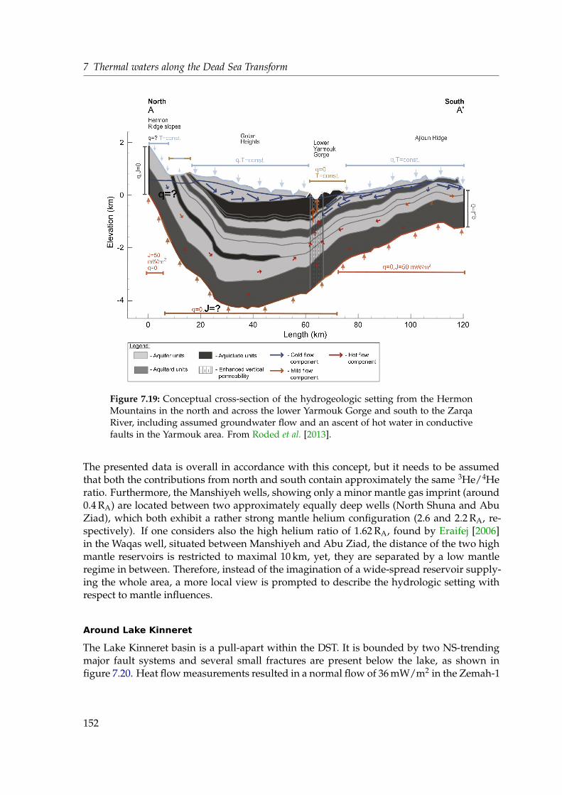
7 Thermal waters along the Dead Sea Transform
Figure 7.19: Conceptual cross-section of the hydrogeologic setting from the HermonMountains in the north and across the lower Yarmouk Gorge and south to the ZarqaRiver, including assumed groundwater flow and an ascent of hot water in conductivefaults in the Yarmouk area. From Roded et al. [2013].
The presented data is overall in accordance with this concept, but it needs to be assumedthat both the contributions from north and south contain approximately the same 3He/4Heratio. Furthermore, the Manshiyeh wells, showing only a minor mantle gas imprint (around0.4 RA) are located between two approximately equally deep wells (North Shuna and AbuZiad), which both exhibit a rather strong mantle helium configuration (2.6 and 2.2 RA, re-spectively). If one considers also the high helium ratio of 1.62 RA, found by Eraifej [2006]in the Waqas well, situated between Manshiyeh and Abu Ziad, the distance of the two highmantle reservoirs is restricted to maximal 10 km, yet, they are separated by a low mantleregime in between. Therefore, instead of the imagination of a wide-spread reservoir supply-ing the whole area, a more local view is prompted to describe the hydrologic setting withrespect to mantle influences.
Around Lake Kinneret
The Lake Kinneret basin is a pull-apart within the DST. It is bounded by two NS-trendingmajor fault systems and several small fractures are present below the lake, as shown infigure 7.20. Heat flow measurements resulted in a normal flow of 36 mW/m2 in the Zemah-1
152

7.2 Detailed analysis of the geothermal localities
Figure 7.20: Structural map of Lake Kinneret. The lake is bounded by two main faultsand several structural features are present below the lake. The two sampled springs,Gofra and Hamat Tveria, are drawn in. Adapted from Ben-Avraham et al. [2008].
borehole (4249 m) at the southern tip of the lake [Eckstein and Maurath, 1995, cited afterRoded et al. [2013]], but Ben-Avraham et al. [1978] obtained an elevated average heat flowthrough Lake Kinneret itself of 75 mW/m2. Local basalt outcrops are dated to ages of 3.5 Mato 5 Ma [Mor, 1993], and dating of deep occurrences observed in boreholes drilled around thelake resulted in ages of around 9 Ma [Heimann and Steinitz, 1989, after Horowitz [2001]].
Hamat Tveria on the west coast of Lake Kinneret discharges hydrochemically different wa-ter from Gofra, located on the eastern side [Möller et al., 2012, and references therein] andpresumably not much exchange takes place between the two reservoirs. Although HamatTveria is distinctly warmer than Gofra (59 ◦C versus 31 ◦C), the latter spring has a signif-icantly higher helium isotope ratio (1.56 RA, whereas Hamat Tveria has only 1.13 RA). Amagmatic heat source, however, would increase both the temperature and the 3He/4He ra-tio. Such a heat source at Lake Kinneret can be excluded due to the high ages of the basaltbodies around and beneath the lake. Therefore, deep circulation and ascent through conduc-tive fractures is most likely to be the reason of thermal waters at Lake Kinneret. This would,however, imply that the reservoir feeding Gofra is considerably more enriched in mantle he-lium than the one supplying Hamat Tveria, as the higher temperature of the latter indicateseither a faster ascent or less admixed shallow groundwater. Both possibilities would resultin a higher helium ratio in Hamat Tveria, if the helium composition of the reservoirs wouldbe the same. This finding, again, contradicts the common reservoir proposed by Torfsteinet al. [2013].
153

7 Thermal waters along the Dead Sea Transform
Shamir well
Shamir well, 1420 m deep and located on the eastern margin of the Hula basin, the north-ernmost pull-apart in Israel, has a high helium ratio of 2.83 RA, yet, the water temperatureindicates a normal thermal gradient at the well location, although an elevated gradient of40 K/km was detected within the basin [Bein and Feinstein, 1988]. In this case the observa-tion of mantle helium is apparently not connected to a geothermal anomaly as found in thesystems explained above.
Western Dead Sea coast
The noble gas interpretation of Mineral is problematic. The well did not facilitate goodsampling conditions and atmospheric contamination occurred, which needed profound cor-rection. The extremely low 3He and 4He content below atmospheric values indicates evenmore strong degassing prior to sampling. Ein Qedem seems to be reasonable, although theNGT fit had bad χ2 values. Its proximity to the crust–mantle mixing line in plot 7.4 indicatesno major atmospheric contamination.
Despite sampling difficulties, both samples show very similar 3He/4He ratios of 0.6 RA,which agree with data published by Torfstein et al. [2013] and Lange et al. [2008], the lat-ter found samples with up to 1 RA a few kilometers further north. Although located close tothe western fault comprising the Dead Sea pull-apart, the mantle influence in these localitiesis rather low.
Zeeghan well field
Not much detailed information is available on the structural geology of the Zeeghan area.The Zeeghan wells are drilled where the Zarqa River Gorge enters the Jordan Valley. Thisgorge is cut into the uplifted rock of the Ajloun dome. Information on deep faults in thisanticline is inconsistent. Salameh and Rimawi [1984] show a N–S cross-section throughhighlands, where no relevant faults are present at the site, whereas Bajjali [1994] displaysextensive faulting at the Ajloun ridge. The database of WAJ [2010] contains only a few lin-eaments and faults in the well field area, but no information about displacement is given.The closest basalt occurrence, dated to around 3 Ma, is found somewhat further away fromthe rift, at the headwaters of Zarqa River [Baubron et al., 1985, after Horowitz [2001]]. Themagnetic survey of Frieslander and Ben-Avraham [1989] did not suggest a magma body atshallow depth in the well field area, whereas Ben-Avraham and Ginzburg [1990] indicate aslight magnetic anomaly a little bit further east, but their presented map has a large scaleand details are hard to figure out.
The presence of the very high geothermal gradient discovered by a very rough estimation inthis study has not been reported before and indicates the influence of a strong heat source,either being quite close to the surface, or an upstream of huge amounts of deep, mantleimpacted groundwater over an area of several km2 occupied by the Zeeghan well field. Theobservation of a high helium isotope ratio of up to 5 RA supports the discovery a strongmantle reservoir. A favored transport of mantle gases by metamorphic CO2 bubbles seemsvery likely.
154

7.2 Detailed analysis of the geothermal localities
Zarqa Ma’in/Zara spring cluster
The area around the spring fields of Zarqa Ma’in and Zara are considered to have the mostfavorable geothermal potential in Jordan and are therefore studied most extensively of allthermal spring systems in the country. Extensive surface volcanism is found in the area andmagmas are dated to ages between 0.6 and 3.4 Ma [Duffield et al., 1988]. Moreover, the areais traversed by deep faults, most prominent the shearing Zarqa Ma’in Fault which extendsmore than 200 km eastwards to Saudi Arabia (compare figure 4.6). Heat flow in the areais found to be very high. Galanis Jr. et al. [1986] reports heat flows of up to 472 mW/m2
and a temperature gradient of 175 K/km for the Zara springs area and an almost as highgeothermal gradient of 165 K/km in the Zarqa Ma’in spring cluster, where the heat flow is255 mW/m2. That this enhanced heat flow is a local phenomenon and not directly relatedto the pull-apart of the Dead Sea basin is documented by Ben-Avraham et al. [1978], whodetermined a rather low heat flow of only 29 mW/m2 on average through the Dead Sea (al-though it should be noted they did not measure off the Jordanian coast). However, Sawarieh[2005] assumes this heat reservoir also supplies the shallow, hot wells in Jiza, located furtherinland, about 30 km south of Amman.
Duffield et al. [1988] state that the magma bodies found in the area are too old to considerablycontribute to the heat anomaly in Zarqa Ma’in and Zara, as they should have already cooleddown. The discharge of hot water in these springs is therefore attributed to deep circulatingwater in an environment of an enhanced geothermal gradient. Hakki and Teimeh [1981,cited after Sawarieh [2005]] related the hottest springs to the highest shearing intensity inthe area. This means the high temperature gradient is owned to quickly rising hot waterfrom great depths instead of a shallow heat source being responsible for warming up thewater. An initial reservoir temperature of > 100 ◦C is indicated by δ18O.
The presented helium isotope data support the assumption of deep water being in con-tact with mantle fluids rising through permeable fault segments. However, this mantleimprint is very local and not related to the heat flow, because Zara spring, located wherethe highest heat flow was recorded, has a much more crustal signature than the Zarqa Ma’insprings. The deep reservoir discharging at the Zara springs is hence less affected by mantlevolatiles.
Other localities along the eastern side of the Dead Sea and in Wadi Arava
The same explanation as for the Zara spring can be assumed to apply to the springs in theother side-wadis at the Dead Sea, i. e. the springs in Wadi Ibn Hammat, Afra, and Thra’a.They feed on deep reservoirs heated under a possibly elevated geothermal gradient (no heatflow data in this area is available), but these reservoirs are only very weakly affected by man-tle fluids. The same holds for the wells in Wadi Arava, where Eckstein and Simmonsi [1977]report a temperature gradient of about 16 K/km and a heat flow of 45 mW/m2 at shallowdepths of the Ein Yahav well nest. There, the discharged water temperature correspondsto the wells’ screen interval depth and almost no mantle impact is present. The only mag-matic occurrence in Wadi Arava is found close to Ein Yahav and yielded ages around 6 Ma[Horowitz, 2001], which is obviously too old to significantly influence the groundwater inEin Yahav wells today. The observation that the thermal groundwater south of the Dead Sea
155

7 Thermal waters along the Dead Sea Transform
is only weakly impacted by mantle volatiles is supported by Eraifej [2006], who reportedhelium isotope ratios of 0.11 RA in two wells located at the southern end of the Dead Sea.It should, however, be noted that the sampled wells at the margins of Wadi Arava have ahigher helium ratio than those localities in the southern side-wadis. The general low inter-action with mantle gases corresponds to the inferior seismic and tectonic activity in WadiArava [Ambraseys, 2006].
7.3 Conclusions
An extensive data set of helium isotopes in thermal waters along the Dead Sea Transform,covering both the Jordanian and the Israeli part of the valley, is presented, accompaniedby other hydrological tracers. A wide range of 3He/4He ratios from crustal signature tohigh mantle influence is found in hot springs and wells along the margins of the JordanValley. Helium isotope ratios prove to be the only reliable tracer of interaction of thermalgroundwaters with a mantle reservoir, as no other tracer shows a credible relation to themantle helium content. Only in a few cases the stable isotopes of carbon and oxygen revealdeeper insight in the mantle gas origin or the heat history of the thermal water.
The samples collected along the Jordanian part of the DST yield a significantly higher spatialresolution than the Torfstein et al. [2013] data set, where mantle helium information is gath-ered in three locations only, namely the Lake Kinneret/Yarmouk area, the western Dead Seaand the central Wadi Arava, with no data available in between. In contrast, thermal watersin Jordan are distributed more widely and therefore give a more detailed and finer resolvedpicture of mantle gas impact along the valley.
The general north–south trend of mantle gas influence reported by Torfstein et al. [2013] isnot reproduced in the clarity claimed by those authors when the thermal waters along theJordanian part of the rift escarpment are considered, too. In figure 7.21 the north–southdistribution of the 3He/4He ratio, 4He and 3He is illustrated versus the distance from theGulf of Aqaba (GOA). It is the same configuration Torfstein et al. [2013] used in their figure 8.As already mentioned by the same authors, the 3He/4He distribution pattern is not reflectedif only 3He or 4He is considered, rendering the 3He/4He ratio a unique marker for mantleinfluence.
The illustration shows that, indeed, the samples coined most strongly by a crustal environ-ment are collected south of the Dead Sea and most of the locations in the north exhibit atypical mantle signature, but two exceptions exist: 1) the Zeeghan wells, located midway be-tween Lake Kinneret and the Dead Sea, and especially Zeeghan 4, exhibit the highest mantlecomponent of all tested waters (4.9 RA), exceeding the highest ratio found by Torfstein et al.by a factor of 2.5; and 2) the Manshiyeh wells which show a minor mantle gas imprint only(around 0.4 RA), yet, they are closely neighbored by two approximately equally deep wellsthat exhibit a rather strong mantle helium configuration.
The presented observations, therefore, do not permit the straightforward explanation of themantle influence distribution given by Torfstein et al. [2013], where the gradual thinningof the crust from south to north is responsible for a more developed fracture system there
156

7.3 Conclusions
Zarqa
Meitzar
Ein QedemMineral
Ein Yahav
Tzofar
Tveria
Zeeghan
Afra
Shamir
N. Shuna
Abu Ziad
Ibn Hammat
5 RA
2 – 3 RA
1 – 2 RA
0.25 – 1 RA
< 0.25 RA
KD1
Gofra
Thra'a
Manshiyeh
HimmaBalzamMakla
Zara
0 1 2 3 4 50
1 0 0
2 0 0
3 0 0
4 0 0
H i m m aS h u n a
Z i a dM a n 1
M a n 2
Z e e 4Z e e 1 4Z e e 1 5
Z a r q a 1Z a r q a 2Z a r a
I b n 1I b n 2
A f r aT h r a ' a
G o f r a
S h a m i r
M e i 3M e i 2
B a l z a mM a k l a
Y 1 1 6Y 6Y 1 6
T z o f a r
T v e r i a
Q e d e mM i n e r a l
3 H e / 4 H e [ R A ]
Dista
nce f
rom GO
A [km
]
1 0 - 7 1 0 - 6 1 0 - 5 1 0 - 4
H i m m aS h u n a Z i a dM a n 1
M a n 2
Z e e 4Z e e 1 4Z e e 1 5
Z a r q a 1Z a r q a 2 Z a r a
I b n 1 I b n 2
A f r a
T h r a ' a
G o f r a
S h a m i r
M e i 3 M e i 2B a l z a m M a k l a
Y 1 1 6 Y 6Y 1 6
T z o f a r
T v e r i a
Q e d e mM i n e r a l
4 H e [ c c S T P / g ]1 0 - 1 3 1 0 - 1 2 1 0 - 1 1 1 0 - 1 0 1 0 - 9 1 0 - 8
H i m m a
S h u n a Z i a dM a n 1
M a n 2
Z e e 4Z e e 1 4Z e e 1 5
Z a r q a 1Z a r q a 2
Z a r a
I b n 1 I b n 2
A f r a
T h r a ' a
G o f r a
S h a m i r
M e i 3 M e i 2B a l z a m M a k l a
Y 1 1 6 Y 6Y 1 6
T z o f a r
T v e r i a
Q e d e mM i n e r a l
3 H e [ c c S T P / g ]
Figure 7.21: Spacial pattern of the 3He/4He ratio as well as 4He and 3He concentrationsas functions of the distance from the Gulf of Aqaba (GOA). The clear north–south trendinferred by Torfstein et al. [2013] is not reproduced when samples of the Jordanian partof the DST are considered, too. The distribution pattern found for the 3He/4He ratio isnot reproduced by 3He or 4He alone.
and, hence, the elevated mantle influence around Lake Kinneret and the Yarmouk Gorge.To the contrary, a much more localized view needs to be inferred, including single fractureswhich affect the groundwater often in close vicinity only. This becomes especially apparentalong the rift flanks south of where the Yarmouk Gorge meets the Jordan Valley. The caseof the Manshiyeh wells, having only a slight mantle influence, but being enclosed by twosignificantly mantle coined wells, indicate the localities north and south of Manshiyeh aresupplied by (at least) two different mantle helium containing reservoirs which are separatedby groundwater masses less affected.
Instead of a north–south tendency of mantle gas influence the present data set rather sug-gests a difference between the eastern and the western margin of the Dead Sea Transform.This might be an indicator that recent shearing took place predominantly along the easternbounding fault system, creating more or better conductive fractures. However, helium iso-tope data density is only low on the western rift side, and more samples should be collectedto confirm or disprove this hypothesis.
Furthermore, the existence of a sub-continental, wide-spread, intermediate mixing reservoir,where mantle and crustal endmembers mix to a local endmember of ≈ 2 RA, probably atthe base of the crust, and which is then further diluted by shallow groundwater on its wayto the surface [Torfstein et al., 2013], is not supported by the new data. If this would bethe case, a correlation between water temperature and mantle component should be visible,because, in general, it can be assumed that slowly ascending groundwater, which has further
157

7 Thermal waters along the Dead Sea Transform
cooled down when reaching the discharge location, is also stronger admixed by shallow,crust-impacted water. Moreover, this deep uniform reservoir, from which all thermal watersources are supplied, would need to have a helium isotope ratio of at least 4.9 RA to becapable to explain the helium data of Zeeghan 4.
Present-day knowledge of heat flow pattern beneath Jordan and Israel, as displayed in theheat maps on pages 178 and 179, meets very well with the presented observation of mantlehelium amount in case of the Yarmouk/Kinneret and the Zarqa Ma’in areas, but due to thelack of high resolution temperature–depth data in Jordan, the observed heat anomaly at theZeeghan well field is not yet captured. Borehole logging should be undertaken in this areato complete the knowledge about geothermal heat distribution in this location. A first, veryrough estimation of the local geothermal gradient of 100 K/km in the Zeeghan well fieldarea is found from discharge temperature in this thesis, which is comparable to the gradientfound in the Zarqa Ma’in locality [Galanis Jr. et al., 1986]. Together with the remarkably high3He/4He ratios found in the Zeeghan wells this area is probably the most promising localityfor geothermal energy usage, maybe even including electric power generation.
158
8 Summary
Two case studies are presented in this work where noble gases and especially the heliumisotope ratio in Jordanian groundwaters are applied in very diverse contexts and for totallydifferent purposes.
In the Azraq study dissolved noble gases are used to uncover a complex groundwater mix-ing scheme, which has not been understood before and which causes creeping salinizationof groundwater reserves in the Azraq Oasis. The new approach includes the determinationof noble gas contents in three well types found in Azraq: The AWSA well field wells, mostlyaround 200 m deep, abstract water from the uppermost of three aquifer systems, which lieon top of each other and are separated by poorly permeable layers, shallow agriculturalwells, and two deep wells tapping the middle aquifer. It is found that those wells which areaffected by a rising salt content feature the presence of mantle helium, expressed as elevated3He/4He ratios, which indicate an upstream of deep groundwater. However, the middleaquifer is virtually free of mantle helium, so the ascent needs to occur from even deeperaquifers through deep and permeable fractures. To my knowledge, such a hydrological set-ting has not been reported before and is interpreted as groundwater in the middle aquiferflowing towards the deep reaching, conductive fault, whereas it is directed opposed towardsthe sampled wells in the shallow aquifer.
The observation that those wells of the well field containing a considerable amount of mantlehelium are the same affected by rising salinity is interpreted in terms of an increasing share ofgroundwater from deeper parts of the shallow aquifer contributing to the discharged water.It is made plausible that water at the bottom part of this aquifer seems to be both saline andto contain some mantle imprint, although several assumptions are made to infer this. Dueto the continuous drawdown the water table in some wells left the highly conductive regimeof the basalt rock lying on top and therefore the deeper aquifer layers are considerably moreinvolved, resulting in both increased salinity and mantle helium content.
The second study investigates geothermal systems along the central Dead Sea Transformsystem, the continental break-up zone of the African and the Arabian plates, where the3He/4He ratio proved to be a valuable tracer for tectonic activity. For the first time a com-prehensive data set, covering both the Jordanian and the Israeli part of the transform valley,is presented. 3He/4He ratios observed lie in the range from clear crustal signature to almost5 RA, RA being the atmospheric ratio. The new data contradict the interpretation of Torf-stein et al. [2013] who examined thermal localities on the Israeli side only for mantle helium.While they inferred a general north–south trend in the distribution of mantle influence andattributed this to the gradual thinning of the crust northwards, the new data suggest thateach thermal manifestation needs to be looked at on a very local scale. Instead of a universalintermediate reservoir with about 2 RA, which is diluted in different degrees to generate the
159

8 Summary
observed 3He/4He ratio, as proposed by Torfstein et al. [2013], the thermal springs dischargewater which circulated deep in the crust under a local geothermal gradient. Whether thiswater is affected by mantle gases, however, depends on the presence or absence of deep, con-ductive fractures in the close vicinity. Therefore, the simple model of Torfstein et al. [2013]needs to be replaced by a concept regarding more the individual tectonic surroundings ofthe thermal localities.
160
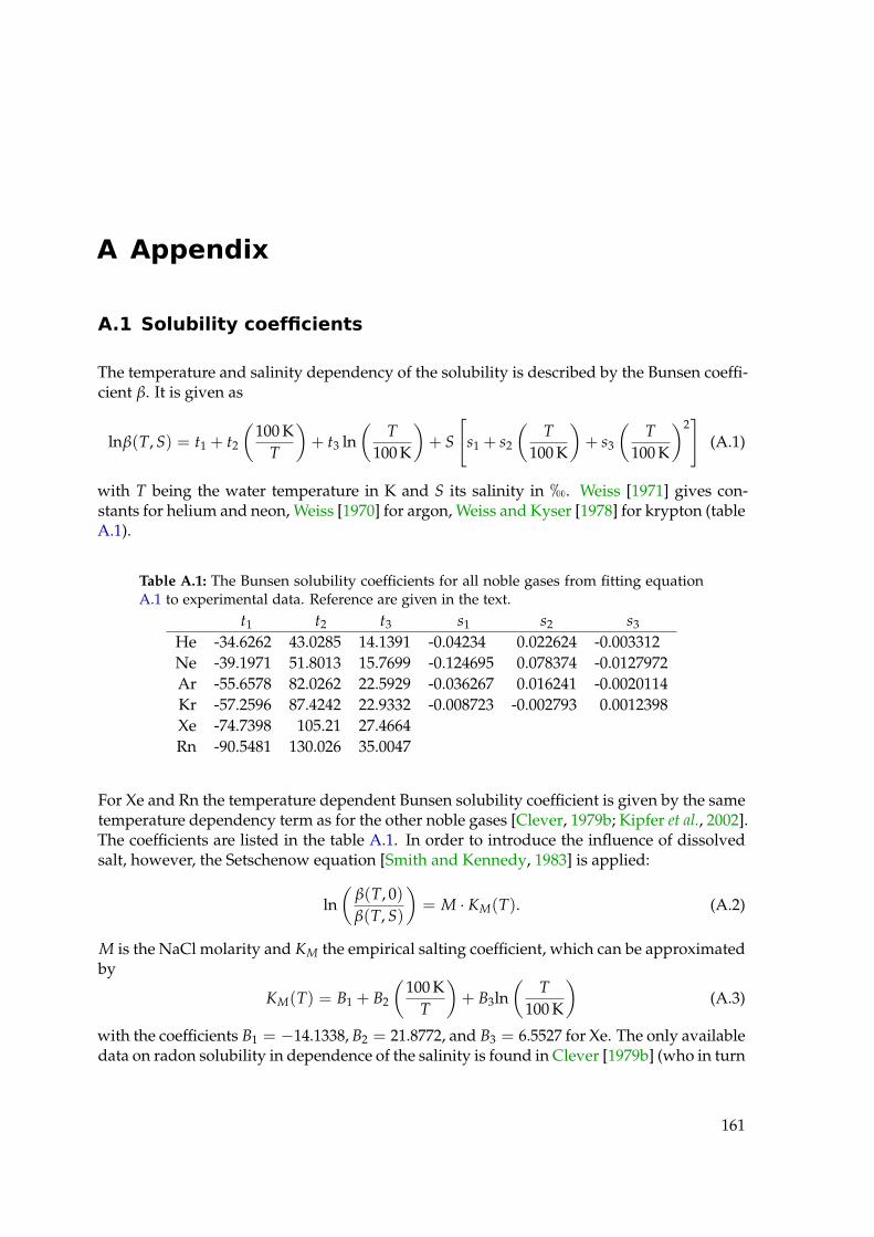
A Appendix
A.1 Solubility coefficients
The temperature and salinity dependency of the solubility is described by the Bunsen coeffi-cient β. It is given as
lnβ(T, S) = t1 + t2
(100 K
T
)+ t3 ln
(T
100 K
)+ S
[s1 + s2
(T
100 K
)+ s3
(T
100 K
)2]
(A.1)
with T being the water temperature in K and S its salinity in h. Weiss [1971] gives con-stants for helium and neon, Weiss [1970] for argon, Weiss and Kyser [1978] for krypton (tableA.1).
Table A.1: The Bunsen solubility coefficients for all noble gases from fitting equationA.1 to experimental data. Reference are given in the text.
t1 t2 t3 s1 s2 s3
He -34.6262 43.0285 14.1391 -0.04234 0.022624 -0.003312Ne -39.1971 51.8013 15.7699 -0.124695 0.078374 -0.0127972Ar -55.6578 82.0262 22.5929 -0.036267 0.016241 -0.0020114Kr -57.2596 87.4242 22.9332 -0.008723 -0.002793 0.0012398Xe -74.7398 105.21 27.4664Rn -90.5481 130.026 35.0047
For Xe and Rn the temperature dependent Bunsen solubility coefficient is given by the sametemperature dependency term as for the other noble gases [Clever, 1979b; Kipfer et al., 2002].The coefficients are listed in the table A.1. In order to introduce the influence of dissolvedsalt, however, the Setschenow equation [Smith and Kennedy, 1983] is applied:
ln(
β(T, 0)β(T, S)
)= M · KM(T). (A.2)
M is the NaCl molarity and KM the empirical salting coefficient, which can be approximatedby
KM(T) = B1 + B2
(100 K
T
)+ B3ln
(T
100 K
)(A.3)
with the coefficients B1 = −14.1338, B2 = 21.8772, and B3 = 6.5527 for Xe. The only availabledata on radon solubility in dependence of the salinity is found in Clever [1979b] (who in turn
161

A Appendix
0 5 0 1 0 0 1 5 0 2 0 0 2 5 0 3 0 0 3 5 0 4 0 04 0 %
5 0 %
6 0 %
7 0 %
8 0 %
9 0 %
1 0 0 %
Relat
ive so
lubilit
y
� � � � � � � � � �
H e N e A r K r X e R n
Figure A.1: The radon solubility in dependence of salt content is shown. Since thecalculated solubility is derived from data between 12 and 362 g/kg salt concentration[Kofler, 1913], the fit is questionable at low concentrations. The other noble gasesare shown as well in the same salinity range, but their fits are optimized for low saltconcentration in the range of seawater.
cites Kofler [1913]) for a fixed temperature of 18 ◦C. The Rn curve in the right plot of figures2.16 and A.1 is created by performing an exponential fit KM(S) = C1 + C2 · exp(−S/C3) tothe data for KM(18) given in Clever [1979b]. The resulting coefficients are C1 = 0.14116, C2 =0.18364, and C3 = 76.7217.
Since the radon solubility dependence on salinity is derived from data between 12 and362 g/kg salt concentration – contrary to the other noble gases which are optimized for saltcontents in the range of seawater – the fit is questionable at a low salinity. Figure A.1 givesthe relative solubilities of Rn in a much wides range. The plots for the other noble gases areincluded as well, but are in turn questionable at higher salt concentrations.
A.2 Experiences applying diffusion samplers in the field
Since diffusion samplers of the kind developed in our group [Wieser, 2006] had never beenapplied in a field campaign, I summarize the experiences gained during my field trip in 2012in Jordan.
• The first apprehension that this design does not withstand the high hydrostatic pres-sure in deep wells lead to a construction where the PVC tube was not spanned betweentwo copper tubes, but tightly covered a perforated part of one longer copper tube(compare figure 5.1 on page 69). This promised a more stable built as the squeezedPVC tube cannot be incised by the rims of the copper tubes. However, the normaldiffusion sampler design proved to be very sturdy under high pressure and even the
162

A.3 Description of the sampled wells and springs
deepest sampler at 569 m was retrieved obviously undamaged. The newly constructedsamples with the perforated copper tube, in contrast, leaked much more often, whichleads to the recommendation to use the normal diffusion sampler design but to locateseveral samplers, at least two, at the same depth to raise the chance of getting at leastone undamaged sample.
• A considerable amount of (normal) diffusion samplers broke during transport. As theyare fast and easy to assemble they should be put together in the field just right beforeusage.
• We first tried to use a fishing line to lower the diffusion samplers into the boreholes,as it is light and easy to transport. However, the fishing line we used formed knotsvery easily, in the first attempt a big clutter swam upon the groundwater surface andthe samplers not even submerged into the water. A stronger, more heavy string incombination with an additional weight at the bottom proved to be much more reliable.However, even with this string knots occurred, presumably because the samplers werelowered too fast. Thus, it should be taken care of a permanent tension in the string thatthe string with the samplers can not get caught somewhere on its way down.
• To prevent the diffusion samplers from moving much and being stuck in the borehole,both ends were fixed to the string. As the closed outer ends of the copper tubes arequite sharp they were wrapped with duct tape that they cannot cut the string.
• Afterwards, I think the approach of putting all diffusion samplers on one single stringis the right strategy when sampling a depth profile. The use of separate strings for eachsampler would in all likelihood lead to knotting together of the strings. Especiallywhen retrieving the samples as a pair, the retrieving speed is not significantly lowerwhen one person closes the copper tubes while the other continues pulling up thesamples.
• The usage of the simple diffusion sampler design applied during this thesis in coldwater gives rise to the assumption that the closing with the pneumatic pliers is unreli-able under these circumstances. During a test of the samplers in the water of a frozenlake nearly all samplers appeared to leak. Maybe the copper is not as smooth at wintrytemperatures as it usually is and the galling does not work.
A.3 Description of the sampled wells and springs
In this chapter a detailed description of the sampled springs and wells is given.
Azraq project
AWSA well field
All wells of the AWSA well field are productive wells which operate day and night. Thewater is pumped to Amman for drinking water purposes. Some wells where visited more
163

A Appendix
than once in the different campaigns. In every case it was possible to connect the samplinghoses via a hose coupling. For the connection itself the pump was stopped for some minutesby an employee of the WAJ. The pressure was high at all wells. All wells have a casing andthe screen covers the whole length.
Figure A.2: Well AWSA 3 as a typical example for wells in the AWSA well field.
Farming wells
Private wells of farmers in the Azraq Oasis are simpler constructions compared to the gov-ernmental production wells. Beside drilled wells also dug wells exist with depths of aroundten meters. The bottom of these holes with diameters of several meters is filled with ground-water, which is supplied to the fields by a pump. Contact with the atmosphere is evident inthese cases.
F3975
The accompanying employee of the WAJ had to manipulate the well’s flow meter since theowner did not want to pay for the “wasted” water during sampling. No flushing of the bore-hole before sampling was possible since the owner offered only five minutes of samplingtime. Pressure was usable, equipment connected at a tap.
F3731
A dug well, about eight meters deep. The pump was started for the sampling procedure.I connected the equipment with a rubber plug to the installed plastic tubing system. Justbefore I took the second noble gas sample the well ran dry and I waited for about 20 minutesfor the water to return to the well hole, killing the time with a tea offered by the farmer.Sampling pressure was poor, but usable.
164

A.3 Description of the sampled wells and springs
Figure A.3: Well head with flow meter and sampled tap of F3975
F3960
The pump of this drilled well was not working anymore, though it still hung in the borehole.It was damaged by the saline water, they told me. The depth of the well is 35 m, the watertable at 16 m below surface. Diffusion samplers were placed at 27 m below surface on 8 April2012 at 5pm and collect the following day at 6pm. I dared to only collect water with the deepsampler once, because it almost stuck at the pump.
F3741
A drilled well. The pump was started for the time of sampling, but no long flushing waspossible. Connection with a rubber plug, the pressure was usable.
Mohammeds well
This well was drilled just recently and no pump was installed yet. The well was quite dis-turbed since the owner let down a rock on a rope down the borehole beforehand. Water levelwas about 20 m. Samples were collected from a depth of 53 m below surface and diffusionsamplers installed at the same depth on 7 April 2012, 4:15pm. Retrieval on 9 April 2012,7pm.
B2/A7 wells
Since the B2/A7 aquifer in the Azraq area consists of saline water, no production wells exist.The only two wells which enabled me to sample water from this aquifer were abandonedmonitoring wells. The NDW 5 (733 m deep) and NDW7 (970 m deep, according to WAJ database) were drilled in 1992 as geological exploration wells, are constructed in the same way
165

A Appendix
Figure A.4: The 8 m deep dug well F3731.
and haven’t been used since then. Thus, noble gas samples were collected at different depthwith diffusion samplers, while anion, cation, tritium, carbon and stable isotope samples wereobtained using a deep sampler provided by the WAJ (description in chapter 5.2). Detailedinformation about the construction was not available. A farmer who participated in thedrilling of NDW 7 remembered that this wells had a full length casing and the screen startsat 400 m below surface (he remembered the depth of 973 m correctly so I assume the otherfacts are right as well). The piezometric head was at 101 m below surface in NDW 5 and at26 m below surface in NDW 7.
Because the lack of experience of the physical stability of the classical diffusion samplers[Wieser, 2006] another type, which was thought of being more robust against high pressure(see chapter 5.2 for details), was applied at depth below about 300 m in addition to the clas-sical ones.
Diffusion samplers were positioned in NDW 5 in depths of 310, 444 and 684 m on 9 March2012 at around 2pm using a fishing line and retrieved on 30 March 2012 at 11:30am. Unfor-tunately only one (classical) DS from 684 m was undamaged, all others leaked. Possibly the684 m was not at that depth because for the last about 200 m the thread tension was lowerthan before and the sampler might have lain at the bottom (this would imply a wrong depthinformation or a partial collapse of the borehole). Water samples were collected from 250 mbelow surface. Chemical treatment took place at 10:30am the following day.
Noble gas samples from NDW 7 were planned to be collected in depths of 50, 100, 150, 200,250, 300, 450, 600, and 800 m. A strong PVC thread with a weight at the bottom end was usedand all diffusion samplers were lined up according to their depth. Due to the formation ofknots between the 250 and 300 m samples (a loss of about 6 m), between 300 and 450 m (a lossof about 50 m) and another one between the two deepest samples (a loss of about 175 m) thedepths correct to 50, 100, 150, 200, 250, 294, 394, 544 and 569 m. These depths hold provided
166

A.3 Description of the sampled wells and springs
Figure A.5: Mohammeds well. There was no pump installed yet. Well F3960 was of thesame type as this one.
the rope was straight except the knotty sections. Diffusion samplers were positioned inthe borehole on 13 March 2012 at 1:30pm and retrieved on 30 March 2012. All DS except theclassical DS at 394 m were undamaged, and the 569 m sampler was inflated from the high gaspressure in that depth. Anyway some samplers displayed some fogging inside the PVC tube.Water samples were collected at depth of 50, 100, 150, 200 and 250 m, the maximum depthachievable with the deep sampler. Due to problems with the deep sampler at 250 m only onevolume of 500 ml was pulled up and distributed to the small bottles, the ion samples beingfiltered. The remaining 250 ml was treated with only 0.5 ml AgNO3 solution to produce thesame concentration as the other 14C samples. Like the NDW 5 samples, chemical treatmentwas conducted the following morning.
Wells in Northern Azraq
Three wells in the Northern Part of the Azraq basin were sampled, two governmental (KM140 and Mukefteh 2) and one private farming well (Jordan Modern Farm). Sampling pres-sure was good and the connection of the tubing was easy. Thickness of the unsaturated zoneis more than 100 m in this part of the country (275 m at the KM 140 well).
167

A Appendix
(a) My College Florian Freundt sampling NDW7 using a deepsampler.
(b) Lowering the deepest diffusion sam-pler, an additional weight is attached.
(c) The 569 m diffusion sampler was inflated after being retrieved to the surface.
Figure A.6: Sampling NDW7
Thermal waters project
Thermal waters were sampled from thermal springs and wells. They distribute along theJordan Valley and its side wadis from the Syrian border in the North and Wadi al-KarakSouth of the Dead Sea.
Thermal springs
Zara Ma’in spring
This spring complex is situated at the Dead Sea. Several springs discharge within aboutone kilometer. The sampled spring forms a small cave with a little pool in it. A hose wasmoved as deep as possible into the cave and weighted down with a small rock to collectwater for noble gas analysis from as far away from atmospheric influences as possible. Asmall downhill gradient was exploited to let the water flow into the copper tubes. Bottledsamples were filled from the pool.
168

A.3 Description of the sampled wells and springs
Figure A.7: The cave pool of Zara Ma’in spring close to the Dead Sea shore.
Zarqa Ma’in springs
The Zarqa Ma’in spring complex is situated in a deeply cut side wadi of the Dead Sea closeto the Zara Ma’in springs and nowadays feeds a famous public spa center. Water sampleswere collected at two discharge spots. The first, labeled Zarqa Ma’in I, forms a small pool ofvery hot water (61 ◦C) and gloves had to be filled with cool water to prevent skin burningto fill the sample bottles, especially the radon sample, underwater. Heavy degassing wasobvious as gas bubbles ascended; it smelled of H2S. Because no downward gradient couldbe utilized, NG samples needed to be collected with the suction technique introduced inchapter 5.1. For this my partner stood about 1.5 m above the spring pool. Oxygen contentcould not be recorded since the CellOx 325 sensor refuses to work at temperatures above50 ◦C.
The second sampled discharge point, labeled Zarka Ma’in II, is located about 100 m fromthe first one and some meters higher. The discharge rate is very low. The inlet tubing waslocated in the tiny pond using the weight of small rocks and a small gradient made the waterflow through the copper tubes. Water samples were taken from the exit of the tubing system.No degassing could be observed here. Again no oxygen could be measured due to the watertemperature above 50 ◦C.
169

A Appendix
(a) Heavy degassing of the Zarka Ma’in I hot spring. (b) Hauling of the hose in Zarka Ma’in II.
(c) A hot waterfalls feeds the spa center of Zarka Ma’in.
Hemme spring
Hemme spring, located in the lower Yarmouk Valley, was used as a public swimming poolyears ago. It discharges into an 18 m deep pool with a rate of around 1000 m3/h. Influx intothe pool takes place from the Western side. In order to take NG samples from as deep aspossible from the influx location the end of the sampling hose was weighted with a rockwhich allowed to draw samples from a depth of about 3 to 4 m. The several NG sampleswere taken from different spots. The suction technique was applied. Samples in bottle were
170

A.3 Description of the sampled wells and springs
taken from about 40 cm below the water surface. A couple of ascending gas bubbles indicatedegassing accompanied by a H2S smell.
Figure A.8: Hemme spring
Afra spring
Afra spring in Wadi Hasa south of the Dead Sea is used as a spa retreat as well. The springitself is cased, and samples were drawn from the discharging pipe. The sampling hose wastelescoped about 60 cm into it. No H2S smell was recognized.
Figure A.9: The sampling tube was telescoped into the discharge pipe at Afra spring.
Springs in Wadi Ibn Hammat
In Wadi Ibn Hammat there are two thermal springs. Water from the first one, named IbnHammat I, is used in a spa facility. The spring itself is cased and, like at Afra spring, accesswas only possible through a pipe. This pipe was inside a manhole. The sampling hose wastelescoped 60 cm into the pipe and blocked with a rock. This setup dammed up the water
171

A Appendix
and minimal contact to the atmosphere guaranteed. NG samples were taken by the suctiontechnique.
The second spring, Ibn Hammat 2, is located about two kilometers upstream of the firstone. It discharges into a pond and is used for relaxation by people who do not like to orcannot afford the entrance fee of the spa downstream. The hose was telescoped as far aspossible into the discharging opening, but a little exchange with the atmosphere can not beexcluded. NG samples were taken by suction, bottles were filled from the pool water closeto the discharge hole. Emerging gas bubbles indicate some degassing, but no H2S could besmelled. The sampling took about two hours because it was Friday (puplic holiday in theArab world). A lot of families enjoyed their leisure time and invited me for lunch and drinksseveral times.
(a) The manhole of Ibn Hammat I (b) Discharge pipe of Ibn Hammat I
(c) Pool of Ibn Hammat II. The spring is under the rock inthe upper right corner.
(d) Jordanian hospitality
172

A.3 Description of the sampled wells and springs
Thra’a
Thra’a spring is situated in Wadi al-Thra’a, a side wadi of Wadi al-Karak. The discharge islocated at the sandy floor of a 1 m deep artificial pool. I collected NG samples with suctionwhile I hold the hose end at the ground with my foot. Bottles were filled at the pool’s bottomas well.
Thermal wells
North Shuna Hot Well
North Shuna Hot Well at the mouth of Wadi al-Arab is an artesian well and is utilized ina spa facility. It was easy to connect the sampling equipment to this 967 m deep well. H2Swas present. The cation sample changed color to yellow upon acidification with nitric acid,while the carbon sample changed color to brown instead of the usual purple upon additionof silver nitrate solution. Oxygen content could not be recorded due to water temperatureof 53.3 ◦C. Sampling pressure was high.
Figure A.10: Sampling the thermal well in North Shuna.
Abu Zeeghan well field
Highly saline thermal water from the Abu Zeeghan well field is being desalinized andtreated and contributes to the water supply of Irbid. The brine is dumped into the JordanRiver. Three wells were sampled.
All sampled wells showed a heavy degassing, No 14 the least (but still more than any othersampled spring or well in Jordan), No 4 degassed extremely. However, there was no smellof H2S. All waters tasted of iron which was also visible at leaks. At well No 15 there wereno bubbles visible inside the sampling hose after closing the NG copper tubes, however,
173

A Appendix
Figure A.11: Precipitated iron oxide on the ground at well Abu Zeeghan No 4
after removal of the hoses foamily water dripped out. Chemical treatment of the carbon andcation sample was done after all the samples had been collected.
Alkalinity was far beyond the working range of the alkalinity test kit at all Abu Zeeghanwell. Even at quadruplicated concentration, which is not supported by this test kit officially,the exact alkalinity could not be determined for wells No 4 and 15. No further dilution wasdone, but as it was obvious that the threshold was almost reached and a value of 23 meq/Lis assumed for these wells. The good result in the ion balance justify this assumption. Thewell No 14 alkalinity value was within range of the quadruplicated test, thus providing apossibly arguable value.
During the Radon measurement the Abu Zeeghan samples exhibited a foamy behavior. Thebubbles at the surface even ascended into the tubing system and a little bit into the Driritecartridge of the first radon analysis (Zeeghan No 4). The bottle was detached from the closedsystem and a small gulp was discarded, thus additional contact to the ambient air was es-tablished and also part of the radon which was already degassed into the tubing system gotlost. In the case of the other two samples I poured out a gulp of about 5 to 10 mL before Iconnected them to the closed system.
Figure A.12: Heavy degassing occurred during sampling and foam formation at theradon measurement of the Zeeghan wells
174

A.3 Description of the sampled wells and springs
Mashiyeh 1 and 2
Both Manshiyeh wells used to be pumped wells, but the pumps do not work anymore. Any-way, together they yield about 50 m3/h as they are artesian wells. The water was iron bear-ing and was said to contain H2S but this was not smellable. In both cases the sampling tubecould be telescoped a few centimeter into small openings. At Manshiyeh 1 no bubbles werevisible, at Manshiyeh 2 some were in the sampling bucket but not in the sampling hoseswhile the copper tube were being closed.
(a) Sampling hose connection at Manshiyeh 1 (b) Making new friends
Abu Ziad
This thermal well in the Wadi Abu Ziad is an artesian well, too and used for irrigation pur-poses. The sampling hose was telescoped about 4 m deep into the borehole, thus contami-nation with atmospheric gases can be ruled out. H2S was present, but no strong degassingwas noticeable. The hoses revealed no air bubbles, only inside the carbon bottle a few verysmall ones were visible.
(c) Abu Ziad Thermal Well (d) I can’t complain about a lackof courtesy during sampling
175

A Appendix
Lajjun KD1
This well was sampled in the scope of the attempted groundwater recharge study in theKarak area in 2010 and is now included into the thermal waters study due to its character-istics. Sampling was problem-free. Pressure was low, but no bubble formation was observ-able.
A.4 Additional figures
Azraq townAzraq townAzraq townAzraq townAzraq townAzraq townAzraq townAzraq townAzraq townAzraq townAzraq townAzraq townAzraq townAzraq townAzraq townAzraq townAzraq townAzraq townAzraq townAzraq townAzraq townAzraq townAzraq townAzraq townAzraq townAzraq townAzraq townAzraq townAzraq townAzraq townAzraq townAzraq townAzraq townAzraq townAzraq townAzraq townAzraq townAzraq townAzraq townAzraq townAzraq townAzraq townAzraq townAzraq townAzraq townAzraq townAzraq townAzraq townAzraq townAzraq townAzraq townAzraq townAzraq townAzraq townAzraq townAzraq townAzraq townAzraq townAzraq townAzraq townAzraq townAzraq townAzraq townAzraq townAzraq townAzraq townAzraq townAzraq townAzraq townAzraq townAzraq townAzraq townAzraq townAzraq townAzraq townAzraq townAzraq townAzraq townAzraq townAzraq townAzraq townAzraq townAzraq townAzraq townAzraq townAzraq townAzraq townAzraq townAzraq townAzraq townAzraq townAzraq townAzraq townAzraq townAzraq townAzraq townAzraq townAzraq townAzraq townAzraq townAzraq townAzraq townAzraq townAzraq townAzraq townAzraq townAzraq townAzraq townAzraq townAzraq townAzraq townAzraq townAzraq townAzraq townAzraq townAzraq townAzraq townAzraq townAzraq townAzraq townAzraq townAzraq townAzraq townAzraq townAzraq townAzraq townAzraq townAzraq townAzraq townAzraq townAzraq townAzraq townAzraq townAzraq townAzraq townAzraq townAzraq townAzraq townAzraq townAzraq townAzraq townAzraq townAzraq townAzraq townAzraq townAzraq townAzraq townAzraq townAzraq townAzraq townAzraq townAzraq townAzraq townAzraq townAzraq townAzraq townAzraq townAzraq townAzraq townAzraq townAzraq townAzraq townAzraq townAzraq townAzraq townAzraq townAzraq townAzraq townAzraq townAzraq townAzraq townAzraq townAzraq townAzraq townAzraq townAzraq townAzraq townAzraq townAzraq townAzraq townAzraq townAzraq townAzraq townAzraq townAzraq townAzraq townAzraq townAzraq townAzraq townAzraq townAzraq townAzraq townAzraq townAzraq townAzraq townAzraq townAzraq townAzraq townAzraq townAzraq townAzraq townAzraq townAzraq townAzraq townAzraq townAzraq townAzraq townAzraq townAzraq townAzraq townAzraq townAzraq townAzraq townAzraq townAzraq townAzraq townAzraq townAzraq townAzraq townAzraq townAzraq townAzraq townAzraq townAzraq townAzraq townAzraq townAzraq townAzraq townAzraq townAzraq townAzraq townAzraq townAzraq townAzraq townAzraq townAzraq townAzraq townAzraq townAzraq townAzraq townAzraq townAzraq townAzraq townAzraq townAzraq townAzraq townAzraq townAzraq townAzraq townAzraq townAzraq townAzraq townAzraq townAzraq townAzraq townAzraq townAzraq townAzraq townAzraq townAzraq townAzraq townAzraq townAzraq townAzraq townAzraq townAzraq townAzraq townAzraq townAzraq townAzraq townAzraq townAzraq townAzraq townAzraq townAzraq townAzraq townAzraq townAzraq townAzraq townAzraq townAzraq townAzraq townAzraq townAzraq townAzraq townAzraq townAzraq townAzraq townAzraq townAzraq townAzraq townAzraq townAzraq townAzraq townAzraq townAzraq townAzraq townAzraq townAzraq townAzraq townAzraq townAzraq townAzraq townAzraq townAzraq townAzraq townAzraq townAzraq townAzraq townAzraq townAzraq townAzraq townAzraq townAzraq townAzraq townAzraq townAzraq townAzraq townAzraq townAzraq townAzraq townAzraq townAzraq townAzraq townAzraq townAzraq townAzraq townAzraq townAzraq townAzraq townAzraq townAzraq townAzraq townAzraq townAzraq townAzraq townAzraq townAzraq townAzraq townAzraq townAzraq townAzraq townAzraq townAzraq townAzraq townAzraq townAzraq townAzraq townAzraq townAzraq townAzraq townAzraq townAzraq townAzraq townAzraq townAzraq townAzraq townAzraq townAzraq townAzraq townAzraq townAzraq townAzraq townAzraq townAzraq townAzraq townAzraq townAzraq townAzraq townAzraq townAzraq townAzraq townAzraq townAzraq townAzraq townAzraq townAzraq townAzraq townAzraq townAzraq townAzraq townAzraq townAzraq townAzraq townAzraq townAzraq townAzraq townAzraq townAzraq townAzraq townAzraq townAzraq townAzraq townAzraq townAzraq townAzraq townAzraq townAzraq townAzraq townAzraq townAzraq town
Figure A.13: The location of the cross-sections published by Margane et al. [2002] (W–Edirection) and Dottridge and Abu Jaber [1999] (NE direction, starting from the AzraqOasis).
176
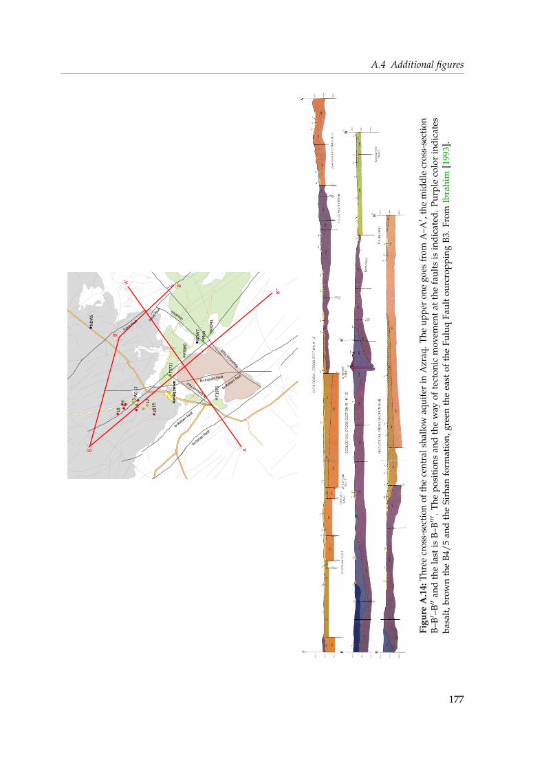
A.4 Additional figures
Azr
aq t
own
Azr
aq t
own
Azr
aq t
own
Azr
aq t
own
Azr
aq t
own
Azr
aq t
own
Azr
aq t
own
Azr
aq t
own
Azr
aq t
own
Azr
aq t
own
Azr
aq t
own
Azr
aq t
own
Azr
aq t
own
Azr
aq t
own
Azr
aq t
own
Azr
aq t
own
Azr
aq t
own
Azr
aq t
own
Azr
aq t
own
Azr
aq t
own
Azr
aq t
own
Azr
aq t
own
Azr
aq t
own
Azr
aq t
own
Azr
aq t
own
Azr
aq t
own
Azr
aq t
own
Azr
aq t
own
Azr
aq t
own
Azr
aq t
own
Azr
aq t
own
Azr
aq t
own
Azr
aq t
own
Azr
aq t
own
Azr
aq t
own
Azr
aq t
own
Azr
aq t
own
Azr
aq t
own
Azr
aq t
own
Azr
aq t
own
Azr
aq t
own
Azr
aq t
own
Azr
aq t
own
Azr
aq t
own
Azr
aq t
own
Azr
aq t
own
Azr
aq t
own
Azr
aq t
own
Azr
aq t
own
Azr
aq t
own
Azr
aq t
own
Azr
aq t
own
Azr
aq t
own
Azr
aq t
own
Azr
aq t
own
Azr
aq t
own
Azr
aq t
own
Azr
aq t
own
Azr
aq t
own
Azr
aq t
own
Azr
aq t
own
Azr
aq t
own
Azr
aq t
own
Azr
aq t
own
Azr
aq t
own
Azr
aq t
own
Azr
aq t
own
Azr
aq t
own
Azr
aq t
own
Azr
aq t
own
Azr
aq t
own
Azr
aq t
own
Azr
aq t
own
Azr
aq t
own
Azr
aq t
own
Azr
aq t
own
Azr
aq t
own
Azr
aq t
own
Azr
aq t
own
Azr
aq t
own
Azr
aq t
own
Azr
aq t
own
Azr
aq t
own
Azr
aq t
own
Azr
aq t
own
Azr
aq t
own
Azr
aq t
own
Azr
aq t
own
Azr
aq t
own
Azr
aq t
own
Azr
aq t
own
Azr
aq t
own
Azr
aq t
own
Azr
aq t
own
Azr
aq t
own
Azr
aq t
own
Azr
aq t
own
Azr
aq t
own
Azr
aq t
own
Azr
aq t
own
Azr
aq t
own
Azr
aq t
own
Azr
aq t
own
Azr
aq t
own
Azr
aq t
own
Azr
aq t
own
Azr
aq t
own
Azr
aq t
own
Azr
aq t
own
Azr
aq t
own
Azr
aq t
own
Azr
aq t
own
Azr
aq t
own
Azr
aq t
own
Azr
aq t
own
Azr
aq t
own
Azr
aq t
own
Azr
aq t
own
Azr
aq t
own
Azr
aq t
own
Azr
aq t
own
Azr
aq t
own
Azr
aq t
own
Azr
aq t
own
Azr
aq t
own
Azr
aq t
own
Azr
aq t
own
Azr
aq t
own
Azr
aq t
own
Azr
aq t
own
Azr
aq t
own
Azr
aq t
own
Azr
aq t
own
Azr
aq t
own
Azr
aq t
own
Azr
aq t
own
Azr
aq t
own
Azr
aq t
own
Azr
aq t
own
Azr
aq t
own
Azr
aq t
own
Azr
aq t
own
Azr
aq t
own
Azr
aq t
own
Azr
aq t
own
Azr
aq t
own
Azr
aq t
own
Azr
aq t
own
Azr
aq t
own
Azr
aq t
own
Azr
aq t
own
Azr
aq t
own
Azr
aq t
own
Azr
aq t
own
Azr
aq t
own
Azr
aq t
own
Azr
aq t
own
Azr
aq t
own
Azr
aq t
own
Azr
aq t
own
Azr
aq t
own
Azr
aq t
own
Azr
aq t
own
Azr
aq t
own
Azr
aq t
own
Azr
aq t
own
Azr
aq t
own
Azr
aq t
own
Azr
aq t
own
Azr
aq t
own
Azr
aq t
own
Azr
aq t
own
Azr
aq t
own
Azr
aq t
own
Azr
aq t
own
Azr
aq t
own
Azr
aq t
own
Azr
aq t
own
Azr
aq t
own
Azr
aq t
own
Azr
aq t
own
Azr
aq t
own
Azr
aq t
own
Azr
aq t
own
Azr
aq t
own
Azr
aq t
own
Azr
aq t
own
Azr
aq t
own
Azr
aq t
own
Azr
aq t
own
Azr
aq t
own
Azr
aq t
own
Azr
aq t
own
Azr
aq t
own
Azr
aq t
own
Azr
aq t
own
Azr
aq t
own
Azr
aq t
own
Azr
aq t
own
Azr
aq t
own
Azr
aq t
own
Azr
aq t
own
Azr
aq t
own
Azr
aq t
own
Azr
aq t
own
Azr
aq t
own
Azr
aq t
own
Azr
aq t
own
Azr
aq t
own
Azr
aq t
own
Azr
aq t
own
Azr
aq t
own
Azr
aq t
own
Azr
aq t
own
Azr
aq t
own
Azr
aq t
own
Azr
aq t
own
Azr
aq t
own
Azr
aq t
own
Azr
aq t
own
Azr
aq t
own
Azr
aq t
own
Azr
aq t
own
Azr
aq t
own
Azr
aq t
own
Azr
aq t
own
Azr
aq t
own
Azr
aq t
own
Azr
aq t
own
Azr
aq t
own
Azr
aq t
own
Azr
aq t
own
Azr
aq t
own
Azr
aq t
own
Azr
aq t
own
Azr
aq t
own
Azr
aq t
own
Azr
aq t
own
Azr
aq t
own
Azr
aq t
own
Azr
aq t
own
Azr
aq t
own
Azr
aq t
own
Azr
aq t
own
Azr
aq t
own
Azr
aq t
own
Azr
aq t
own
Azr
aq t
own
Azr
aq t
own
Azr
aq t
own
Azr
aq t
own
Azr
aq t
own
Azr
aq t
own
Azr
aq t
own
Azr
aq t
own
Azr
aq t
own
Azr
aq t
own
Azr
aq t
own
Azr
aq t
own
Azr
aq t
own
Azr
aq t
own
Azr
aq t
own
Azr
aq t
own
Azr
aq t
own
Azr
aq t
own
Azr
aq t
own
Azr
aq t
own
Azr
aq t
own
Azr
aq t
own
Azr
aq t
own
Azr
aq t
own
Azr
aq t
own
Azr
aq t
own
Azr
aq t
own
Azr
aq t
own
Azr
aq t
own
Azr
aq t
own
Azr
aq t
own
Azr
aq t
own
Azr
aq t
own
Azr
aq t
own
Azr
aq t
own
Azr
aq t
own
Azr
aq t
own
Azr
aq t
own
Azr
aq t
own
Azr
aq t
own
Azr
aq t
own
Azr
aq t
own
Azr
aq t
own
Azr
aq t
own
Azr
aq t
own
Azr
aq t
own
Azr
aq t
own
Azr
aq t
own
Azr
aq t
own
Azr
aq t
own
Azr
aq t
own
Azr
aq t
own
Azr
aq t
own
Azr
aq t
own
Azr
aq t
own
Azr
aq t
own
Azr
aq t
own
Azr
aq t
own
Azr
aq t
own
Azr
aq t
own
Azr
aq t
own
Azr
aq t
own
Azr
aq t
own
Azr
aq t
own
Azr
aq t
own
Azr
aq t
own
Azr
aq t
own
Azr
aq t
own
Azr
aq t
own
Azr
aq t
own
Azr
aq t
own
Azr
aq t
own
Azr
aq t
own
Azr
aq t
own
Azr
aq t
own
Azr
aq t
own
Azr
aq t
own
Azr
aq t
own
Azr
aq t
own
Azr
aq t
own
Azr
aq t
own
Azr
aq t
own
Azr
aq t
own
Azr
aq t
own
Azr
aq t
own
Azr
aq t
own
Azr
aq t
own
Azr
aq t
own
Azr
aq t
own
Azr
aq t
own
Azr
aq t
own
Azr
aq t
own
Azr
aq t
own
Azr
aq t
own
Azr
aq t
own
Azr
aq t
own
Azr
aq t
own
Azr
aq t
own
Azr
aq t
own
Azr
aq t
own
Azr
aq t
own
Azr
aq t
own
Azr
aq t
own
Azr
aq t
own
Azr
aq t
own
Azr
aq t
own
Azr
aq t
own
Azr
aq t
own
Azr
aq t
own
Azr
aq t
own
Azr
aq t
own
Azr
aq t
own
Azr
aq t
own
Azr
aq t
own
Azr
aq t
own
Azr
aq t
own
Azr
aq t
own
Azr
aq t
own
Azr
aq t
own
Azr
aq t
own
Azr
aq t
own
Azr
aq t
own
Azr
aq t
own
Azr
aq t
own
Azr
aq t
own
Azr
aq t
own
Azr
aq t
own
Azr
aq t
own
Azr
aq t
own
Azr
aq t
own
Azr
aq t
own
Azr
aq t
own
Azr
aq t
own
Azr
aq t
own
Azr
aq t
own
Azr
aq t
own
Azr
aq t
own
Azr
aq t
own
Azr
aq t
own
Azr
aq t
own
Azr
aq t
own
Azr
aq t
own
Azr
aq t
own
Azr
aq t
own
Azr
aq t
own
Azr
aq t
own
Azr
aq t
own
Azr
aq t
own
Azr
aq t
own
Azr
aq t
own
Azr
aq t
own
Azr
aq t
own
Azr
aq t
own
Azr
aq t
own
B A
A'
B'
B''
B'''
Figu
reA
.14:
Thre
ecr
oss-
sect
ion
ofth
ece
ntra
lsha
llow
aqui
fer
inA
zraq
.The
uppe
ron
ego
esfr
omA
–A′ ,
the
mid
dle
cros
s-se
ctio
nB–
B′ –
B′′
and
the
last
isB–
B′′′
.The
posi
tion
san
dth
ew
ayof
tect
onic
mov
emen
tat
the
faul
tsis
indi
cate
d.Pu
rple
colo
rin
dica
tes
basa
lt,b
row
nth
eB4
/5an
dth
eSi
rhan
form
atio
n,gr
een
the
east
ofth
eFu
luq
Faul
tou
rcro
ppin
gB3
.Fro
mIb
rahi
m[1
993]
.
177
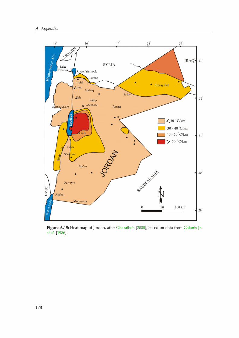
A Appendix
Figure A.15: Heat map of Jordan, after Gharaibeh [2008], based on data from Galanis Jr.et al. [1986].
178

A.4 Additional figures
Figure A.16: Heat map of Israel, from Shalev et al. [2013].
179

A Appendix
A.5 Additional tables
Table A.2: The lithologic data for all sampled well in the Azraq basin where thisinformation could be obtained. All numbers indicate the bottom of the respective layer.All heights are given in meters above sea level. Data from WAJ [2010].
Altitude Aluvium Basalt B4/5 B3 B2/A7 A1/6 Kurnub
AWSA 3 521 520 457 311AWSA 4 536 535 462 330AWSA 5 541 541 444 337AWSA 6 549 546 464 343AWSA 11 517 514 463 455AWSA 12 528 526 474 319AWSA 13 532 530 473 322AWSA 15 524 522 472 314AWSA 18 553 548 488 382
NDW5 598 598 523 not present 445 308 -6 -135NDW7 515 513 401 200 -195 -455
180

A.5 Additional tables
Tabl
eA
.3:H
eliu
mco
mpo
nent
sof
Azr
aqw
ells
sam
pled
in20
12.A
llco
ncen
trat
ions
incc
STP/
g.3 H
e mea
s∆
3 He m
eas
4 He m
eas
∆4 H
e mea
s3 H
e mod
∆3 H
e mod
4 He m
od∆
4 He m
odR
S∆
RS
AW
SA3
2.89
5E-1
31.
072E
-14
2.43
7E-0
72.
321E
-09
5.88
4E-1
43.
106E
-16
4.31
5E-0
82.
233E
-10
1.18
8E-0
64.
541E
-08
AW
SA4
1.02
8E-1
33.
562E
-15
1.15
2E-0
71.
019E
-09
5.84
8E-1
43.
105E
-16
4.28
8E-0
82.
231E
-10
8.92
1E-0
73.
190E
-08
AW
SA5
7.49
9E-1
42.
789E
-15
1.01
8E-0
78.
915E
-10
5.84
6E-1
43.
090E
-16
4.28
7E-0
82.
221E
-10
7.37
0E-0
72.
816E
-08
AW
SA6
7.60
5E-1
42.
662E
-15
9.37
0E-0
88.
175E
-10
5.72
3E-1
42.
982E
-16
4.19
9E-0
82.
146E
-10
8.11
6E-0
72.
928E
-08
AW
SA13
1.83
0E-1
36.
533E
-15
2.40
4E-0
72.
281E
-09
5.92
9E-1
43.
070E
-16
4.34
7E-0
82.
207E
-10
7.61
4E-0
72.
812E
-08
AW
SA15
1.61
0E-1
35.
695E
-15
1.67
7E-0
71.
547E
-09
1.37
6E-1
31.
850E
-15
9.96
0E-0
81.
200E
-09
9.60
5E-0
73.
510E
-08
AW
SA16
6.19
3E-1
42.
270E
-15
5.03
7E-0
84.
300E
-10
5.83
5E-1
43.
197E
-16
4.28
1E-0
82.
299E
-10
1.23
0E-0
64.
628E
-08
F373
16.
526E
-14
2.41
8E-1
55.
016E
-08
4.27
4E-1
06.
903E
-14
5.33
3E-1
65.
058E
-08
3.60
5E-1
01.
301E
-06
4.94
7E-0
8F3
975
7.32
3E-1
42.
643E
-15
1.13
5E-0
71.
012E
-09
5.82
8E-1
43.
104E
-16
4.27
6E-0
82.
231E
-10
6.45
2E-0
72.
399E
-08
F374
11.
272E
-13
4.55
1E-1
53.
215E
-07
3.13
3E-0
96.
055E
-14
3.27
9E-1
64.
441E
-08
2.34
5E-1
03.
957E
-07
1.46
7E-0
8F3
960
8.67
6E-1
43.
584E
-15
7.21
5E-0
88.
869E
-10
5.90
3E-1
45.
739E
-16
4.33
4E-0
84.
147E
-10
1.20
2E-0
65.
182E
-08
Moh
amm
ed1.
080E
-13
3.85
9E-1
51.
866E
-07
2.16
4E-0
95.
655E
-14
6.38
8E-1
64.
154E
-08
4.61
5E-1
05.
788E
-07
2.17
4E-0
8N
DW
568
4m2.
227E
-12
8.91
0E-1
42.
231E
-06
4.14
6E-0
84.
820E
-14
9.51
4E-1
63.
542E
-08
6.88
1E-1
09.
982E
-07
4.40
3E-0
8N
DW
750
m1.
469E
-13
5.74
0E-1
54.
654E
-07
9.18
5E-0
96.
025E
-14
8.95
8E-1
64.
424E
-08
6.52
4E-1
03.
157E
-07
1.38
2E-0
8N
DW
710
0m1.
673E
-13
6.61
2E-1
56.
162E
-07
1.32
5E-0
86.
079E
-14
1.04
2E-1
54.
462E
-08
7.53
6E-1
02.
715E
-07
1.22
2E-0
8N
DW
715
0m1.
785E
-13
1.39
9E-1
47.
268E
-07
1.38
2E-0
86.
024E
-14
1.07
7E-1
54.
421E
-08
7.76
9E-1
02.
455E
-07
1.98
1E-0
8N
DW
720
0m1.
790E
-13
1.38
1E-1
49.
872E
-07
2.09
5E-0
86.
420E
-14
1.28
9E-1
54.
711E
-08
9.28
9E-1
01.
813E
-07
1.45
1E-0
8N
DW
725
0m1.
572E
-13
1.41
4E-1
41.
339E
-06
2.87
8E-0
86.
243E
-14
1.29
2E-1
54.
581E
-08
9.30
2E-1
01.
174E
-07
1.08
6E-0
8N
DW
730
0m1.
568E
-13
1.46
1E-1
43.
070E
-06
6.92
1E-0
85.
591E
-14
8.91
7E-1
64.
109E
-08
6.43
7E-1
05.
106E
-08
4.89
5E-0
9N
DW
754
4m1.
695E
-13
6.89
3E-1
52.
892E
-06
5.44
4E-0
84.
831E
-14
9.82
3E-1
63.
558E
-08
7.12
0E-1
05.
861E
-08
2.62
6E-0
9N
DW
756
9m1.
364E
-13
5.94
1E-1
52.
796E
-06
5.18
8E-0
85.
051E
-14
9.99
7E-1
63.
715E
-08
7.23
3E-1
04.
879E
-08
2.31
0E-0
9
181

A Appendix
TableA
.4:The
results
ofthe
ionanalysis
ofthe
2012A
zraqsam
ples.
The
totalcationand
anionconcentration
isfou
ndto
theright,together
with
theion
balanceerror
(IBE)after
equation2.18.b.d.m
eansbelow
detectionlim
it.
Ca
FeK
Mg
Mn
Na
SrF
Cl
BrN
O3
SO4
HC
O3
∑C
ations∑
Anions
IBEm
eq/Lµeq
/Lm
eq/Lm
eq/Lµeq
/Lm
eq/Lµeq
/Lµeq
/Lm
eq/Lµeq
/Lµeq
/Lm
eq/Lm
eq/Lm
eq/Lm
eq/L
AW
SA3
2.031.53
0.251.70
b.d.9.20
11.0511.52
9.596.15
67.331.42
2.1613.18
13.26-0.53%
AW
SA4
0.930.32
0.220.73
b.d.3.45
4.6115.22
2.453.03
71.530.84
2.285.34
5.65-5.53%
AW
SA5
0.900.39
0.130.72
b.d.2.98
4.7617.36
1.912.33
52.040.73
2.114.74
4.81-1.62%
AW
SA6
0.800.49
0.100.61
b.d.2.26
3.7413.87
1.121.61
60.340.56
2.163.78
3.92-3.57%
AW
SA13
2.051.22
0.461.79
0.158.54
14.6137.55
8.416.43
9.082.00
2.1612.86
12.621.94%
AW
SA15
7.241.54
0.577.57
0.9317.75
48.859.87
20.685.22
403.9910.06
2.0533.17
33.21-0.10%
AW
SA16
0.800.23
0.130.91
b.d.3.49
5.487.94
2.172.45
192.261.62
1.785.33
5.77-7.51%
F373126.20
b.d.0.38
17.94b.d.
46.76129.65
5.9271.46
34.6451.52
15.337.64
91.4194.52
-3.29%F3975
8.81b.d.
4.3917.40
b.d.171.81
162.0653.88
164.1172.70
70.0334.42
5.02202.57
203.75-0.57%
F374110.78
2.396.39
19.261.50
138.54151.11
61.30161.36
34.1450.16
9.723.46
175.12174.69
0.25%F3960
18.76b.d.
1.0118.76
6.2229.84
204.0619.93
65.0021.74
68.781.63
1.3268.59
68.050.79%
Moham
med
29.19132.51
11.3454.31
58.43486.30
249.94b.d.
527.48143.42
349.3548.44
2.85581.59
579.260.40%
ND
W5
684m1.06
0.490.44
3.407.79
5.709.94
59.155.94
4.500.17
3.841.13
10.6110.97
-3.24%N
DW
750m
8.780.79
2.219.87
12.5648.89
122.8036.42
64.7329.27
b.d.7.62
0.3369.89
72.74-3.92%
ND
W7
100m8.04
b.d.2.14
8.419.25
49.93118.69
58.0163.97
33.10b.d.
7.300.33
68.6671.69
-4.23%N
DW
7150m
7.47b.d.
2.367.13
7.7253.15
115.9666.33
62.5632.78
2.486.95
0.3370.23
69.940.42%
ND
W7
200m6.81
0.902.50
6.308.23
57.76109.56
48.1966.82
31.61b.d.
7.120.37
73.4974.39
-1.20%N
DW
7250m
7.14b.d.
2.416.83
6.7456.72
111.3951.56
66.0635.76
b.d.7.19
0.3373.22
73.66-0.60%
182
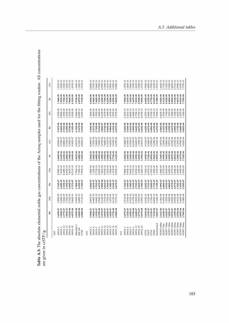
A.5 Additional tables
Tabl
eA
.5:T
heab
solu
teel
emen
taln
oble
gas
conc
entr
atio
nsof
the
Azr
aqsa
mpl
esus
edfo
rth
efit
ting
rout
ine.
All
conc
entr
atio
nsar
egi
ven
incc
STP/
g.H
e∆
He
Ne
∆N
eA
r∆
Ar
Kr
∆K
rX
e∆
Xe
2009
AW
SA3
2.43
3E-0
71.
989E
-09
1.71
4E-0
78.
208E
-10
2.60
4E-0
48.
804E
-07
5.70
7E-0
81.
032E
-09
7.54
8E-0
91.
291E
-10
AW
SA4
1.05
6E-0
79.
208E
-10
1.69
8E-0
77.
914E
-10
2.61
6E-0
49.
018E
-07
5.60
6E-0
89.
986E
-10
7.45
5E-0
91.
296E
-10
AW
SA12
2.37
7E-0
71.
944E
-09
1.72
5E-0
78.
608E
-10
2.62
5E-0
48.
880E
-07
5.70
1E-0
81.
030E
-09
7.75
0E-0
91.
343E
-10
AW
SA13
1.89
3E-0
71.
793E
-09
1.72
9E-0
78.
090E
-10
2.69
0E-0
49.
332E
-07
6.03
0E-0
81.
019E
-09
7.81
1E-0
91.
303E
-10
AW
SA18
4.52
3E-0
83.
722E
-10
1.69
5E-0
77.
867E
-10
2.74
4E-0
49.
393E
-07
5.97
4E-0
81.
072E
-09
7.88
4E-0
91.
377E
-10
AW
SA20
6.05
7E-0
85.
064E
-10
1.72
7E-0
78.
511E
-10
2.81
0E-0
49.
982E
-07
6.19
5E-0
81.
056E
-09
8.19
1E-0
91.
423E
-10
Mke
ifte
h2
4.83
9E-0
83.
990E
-10
1.70
0E-0
77.
796E
-10
2.68
1E-0
48.
891E
-07
6.12
2E-0
81.
066E
-09
7.97
0E-0
91.
364E
-10
KM
140
4.48
4E-0
83.
688E
-10
1.63
9E-0
77.
700E
-10
2.40
0E-0
48.
126E
-07
5.16
7E-0
89.
638E
-10
6.90
7E-0
91.
196E
-10
F138
14.
508E
-08
3.71
1E-1
01.
718E
-07
7.95
0E-1
02.
592E
-04
8.80
6E-0
75.
653E
-08
1.01
6E-0
97.
715E
-09
1.31
7E-1
0
2010
AW
SA3
2.39
8E-0
72.
087E
-09
1.68
4E-0
71.
008E
-09
2.56
4E-0
48.
090E
-07
5.59
9E-0
81.
456E
-09
6.85
6E-0
92.
690E
-10
AW
SA4
1.08
2E-0
78.
690E
-10
1.66
3E-0
71.
120E
-09
2.45
0E-0
47.
555E
-06
5.55
7E-0
81.
486E
-09
6.94
6E-0
92.
747E
-10
AW
SA5
1.19
2E-0
79.
606E
-10
1.70
1E-0
79.
713E
-10
2.60
0E-0
47.
880E
-07
5.73
0E-0
81.
559E
-09
7.46
8E-0
92.
966E
-10
AW
SA6
8.72
9E-0
86.
994E
-10
1.62
7E-0
79.
822E
-10
2.49
5E-0
47.
998E
-07
5.47
6E-0
81.
368E
-09
7.19
3E-0
92.
785E
-10
AW
SA11
5.53
7E-0
74.
214E
-09
1.90
0E-0
67.
261E
-09
1.30
0E-0
33.
659E
-06
1.85
0E-0
72.
633E
-09
1.62
0E-0
84.
549E
-10
AW
SA12
2.06
5E-0
71.
791E
-09
1.69
1E-0
79.
979E
-10
2.59
3E-0
47.
848E
-07
5.57
6E-0
81.
473E
-09
7.73
9E-0
93.
144E
-10
AW
SA13
2.05
4E-0
71.
755E
-09
1.70
3E-0
71.
023E
-09
2.64
0E-0
49.
321E
-07
5.84
5E-0
81.
438E
-09
8.22
9E-0
93.
321E
-10
AW
SA15
1.60
2E-0
71.
327E
-09
1.70
8E-0
71.
024E
-09
2.69
7E-0
49.
645E
-07
5.98
6E-0
81.
413E
-09
7.29
8E-0
92.
982E
-10
AW
SA16
5.77
2E-0
84.
613E
-10
1.81
4E-0
71.
013E
-09
2.77
6E-0
49.
818E
-07
6.18
1E-0
81.
539E
-09
8.50
9E-0
93.
390E
-10
AW
SA18
4.50
6E-0
83.
517E
-10
1.66
7E-0
79.
825E
-10
2.61
2E-0
46.
659E
-06
6.02
7E-0
81.
573E
-09
7.86
5E-0
93.
098E
-10
2012
AW
SA3
2.43
7E-0
72.
321E
-09
1.71
6E-0
75.
986E
-10
2.56
4E-0
48.
384E
-07
5.62
6E-0
85.
341E
-10
7.59
6E-0
91.
397E
-10
AW
SA4
1.15
2E-0
71.
019E
-09
1.70
5E-0
75.
975E
-10
2.55
6E-0
48.
339E
-07
5.56
9E-0
85.
261E
-10
7.36
7E-0
91.
240E
-10
AW
SA5
1.01
8E-0
78.
915E
-10
1.70
4E-0
75.
962E
-10
2.55
4E-0
48.
370E
-07
5.56
1E-0
85.
860E
-10
7.35
5E-0
91.
396E
-10
AW
SA6
9.37
0E-0
88.
175E
-10
1.67
6E-0
75.
717E
-10
2.54
9E-0
48.
479E
-07
5.58
5E-0
86.
304E
-10
7.64
7E-0
91.
332E
-10
AW
SA13
2.40
4E-0
72.
281E
-09
1.73
2E-0
75.
876E
-10
2.59
9E-0
48.
869E
-07
5.66
2E-0
84.
776E
-10
7.83
3E-0
91.
263E
-10
AW
SA15
1.67
7E-0
71.
547E
-09
3.56
3E-0
71.
235E
-09
3.50
5E-0
41.
149E
-06
6.86
7E-0
86.
751E
-10
8.99
4E-0
91.
538E
-10
AW
SA16
5.03
7E-0
84.
300E
-10
1.72
8E-0
76.
245E
-10
2.70
3E-0
48.
941E
-07
6.02
3E-0
86.
019E
-10
7.99
5E-0
91.
517E
-10
F373
15.
016E
-08
4.27
4E-1
02.
034E
-07
7.33
6E-1
03.
035E
-04
9.91
6E-0
76.
625E
-08
6.35
7E-1
08.
658E
-09
1.50
6E-1
0F3
975
1.13
5E-0
71.
012E
-09
1.73
1E-0
76.
037E
-10
2.73
4E-0
49.
048E
-07
6.03
7E-0
85.
604E
-10
8.23
2E-0
91.
406E
-10
F374
13.
215E
-07
3.13
3E-0
91.
810E
-07
6.19
2E-1
02.
895E
-04
9.55
8E-0
76.
509E
-08
5.79
3E-1
08.
775E
-09
1.55
5E-1
0F3
960
7.21
5E-0
88.
869E
-10
1.77
3E-0
71.
369E
-09
2.92
6E-0
42.
238E
-06
6.41
5E-0
87.
312E
-10
8.51
9E-0
91.
693E
-10
Moh
amm
ed1.
866E
-07
2.16
4E-0
91.
718E
-07
1.33
1E-0
92.
905E
-04
2.22
2E-0
66.
451E
-08
7.70
6E-1
08.
748E
-09
1.54
1E-1
0
ND
W5
684m
2.23
1E-0
64.
146E
-08
1.39
9E-0
72.
284E
-09
2.12
8E-0
43.
467E
-06
4.58
6E-0
88.
463E
-10
5.92
8E-0
91.
464E
-10
ND
W7
50m
4.65
4E-0
79.
185E
-09
1.80
6E-0
72.
277E
-09
2.95
9E-0
43.
304E
-06
6.53
1E-0
81.
075E
-09
8.51
1E-0
92.
173E
-10
ND
W7
100m
6.16
2E-0
71.
325E
-08
1.81
2E-0
72.
663E
-09
2.96
2E-0
43.
986E
-06
6.54
4E-0
81.
176E
-09
8.43
8E-0
92.
142E
-10
ND
W7
150m
7.26
8E-0
71.
382E
-08
1.80
6E-0
72.
649E
-09
2.94
5E-0
43.
957E
-06
6.53
9E-0
81.
181E
-09
8.68
6E-0
92.
354E
-10
ND
W7
200m
9.87
2E-0
72.
095E
-08
1.91
7E-0
73.
277E
-09
3.09
7E-0
44.
974E
-06
6.64
7E-0
81.
320E
-09
8.90
6E-0
92.
465E
-10
ND
W7
250m
1.33
9E-0
62.
878E
-08
1.87
7E-0
73.
204E
-09
3.08
3E-0
44.
932E
-06
6.58
9E-0
81.
314E
-09
9.31
4E-0
92.
721E
-10
ND
W7
300m
3.07
0E-0
66.
921E
-08
1.75
6E-0
73.
030E
-09
3.25
0E-0
45.
181E
-06
7.17
5E-0
81.
462E
-09
9.40
7E-0
92.
500E
-10
ND
W7
544m
2.89
2E-0
65.
444E
-08
1.51
5E-0
72.
495E
-09
3.01
7E-0
44.
959E
-06
6.86
8E-0
81.
257E
-09
8.95
1E-0
92.
219E
-10
ND
W7
569m
2.79
6E-0
65.
188E
-08
1.52
9E-0
72.
476E
-09
2.74
2E-0
44.
426E
-06
6.08
1E-0
81.
126E
-09
7.75
5E-0
91.
775E
-10
183
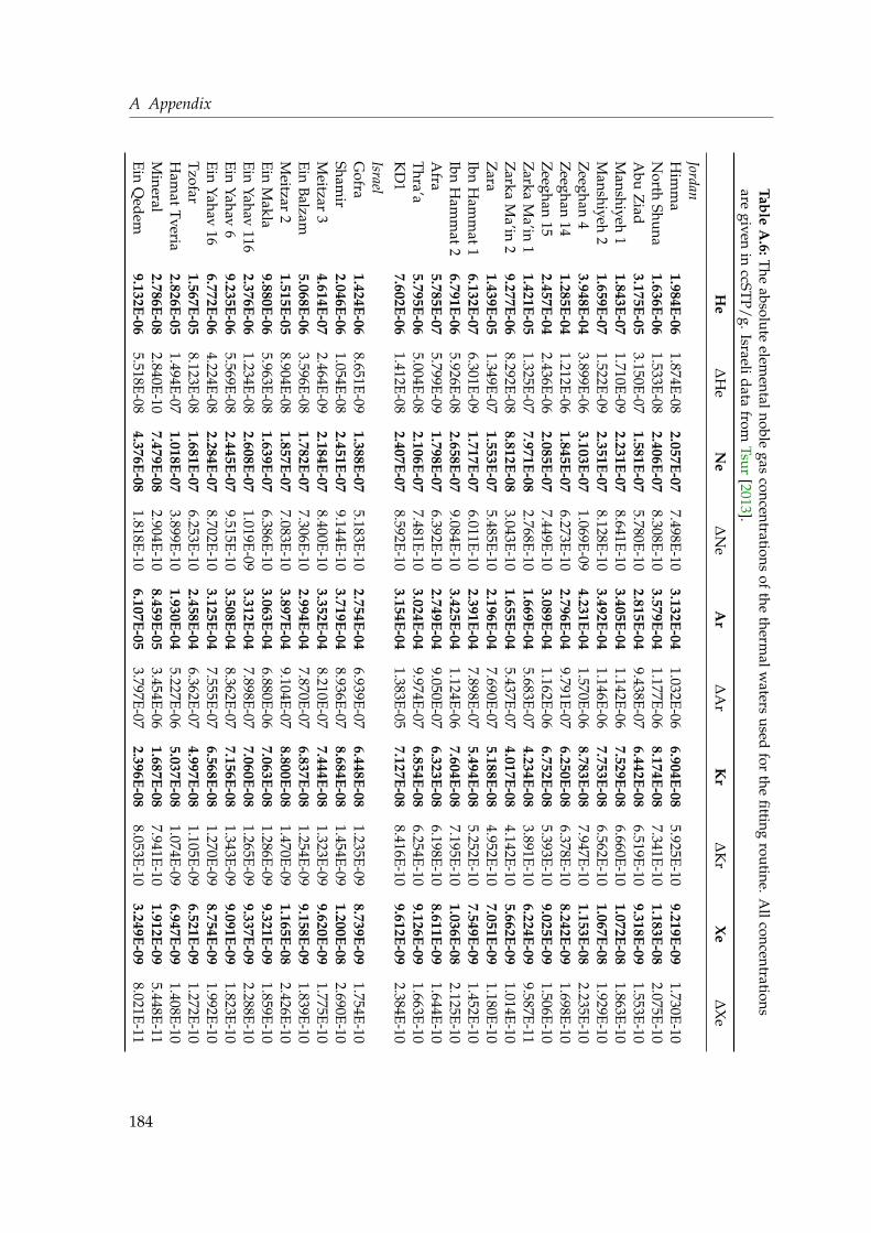
A AppendixTable
A.6:The
absoluteelem
entalnoblegas
concentrationsof
thetherm
alwaters
usedfor
thefitting
routine.Allconcentrations
aregiven
inccSTP/g.Israelidata
fromTsur
[2013].
He
∆H
eN
e∆
Ne
Ar
∆A
rK
r∆
Kr
Xe
∆X
e
JordanH
imm
a1.984E-06
1.874E-082.057E-07
7.498E-103.132E-04
1.032E-066.904E-08
5.925E-109.219E-09
1.730E-10N
orthShuna
1.636E-061.533E-08
2.406E-078.308E-10
3.579E-041.177E-06
8.174E-087.341E-10
1.183E-082.075E-10
Abu
Ziad
3.175E-053.150E-07
1.581E-075.780E-10
2.815E-049.438E-07
6.442E-086.519E-10
9.318E-091.553E-10
Manshiyeh
11.843E-07
1.710E-092.231E-07
8.641E-103.405E-04
1.142E-067.529E-08
6.660E-101.072E-08
1.863E-10M
anshiyeh2
1.659E-071.522E-09
2.351E-078.128E-10
3.492E-041.146E-06
7.753E-086.562E-10
1.067E-081.929E-10
Zeeghan
43.948E-04
3.899E-063.103E-07
1.069E-094.231E-04
1.570E-068.783E-08
7.947E-101.153E-08
2.235E-10Z
eeghan14
1.285E-041.212E-06
1.845E-076.273E-10
2.796E-049.791E-07
6.250E-086.378E-10
8.242E-091.698E-10
Zeeghan
152.457E-04
2.436E-062.085E-07
7.449E-103.089E-04
1.162E-066.752E-08
5.393E-109.025E-09
1.506E-10Z
arkaM
a’in1
1.421E-051.325E-07
7.971E-082.768E-10
1.669E-045.683E-07
4.234E-083.891E-10
6.224E-099.587E-11
Zarka
Ma’in
29.277E-06
8.292E-088.812E-08
3.043E-101.655E-04
5.437E-074.017E-08
4.142E-105.662E-09
1.014E-10Z
ara1.439E-05
1.349E-071.553E-07
5.485E-102.196E-04
7.690E-075.188E-08
4.952E-107.051E-09
1.180E-10Ibn
Ham
mat
16.132E-07
6.301E-091.717E-07
6.011E-102.391E-04
7.898E-075.494E-08
5.252E-107.549E-09
1.452E-10Ibn
Ham
mat
26.791E-06
5.926E-082.658E-07
9.084E-103.425E-04
1.124E-067.604E-08
7.195E-101.036E-08
2.125E-10A
fra5.785E-07
5.799E-091.798E-07
6.392E-102.749E-04
9.050E-076.323E-08
6.198E-108.611E-09
1.644E-10T
hra’a5.795E-06
5.004E-082.106E-07
7.481E-103.024E-04
9.974E-076.854E-08
6.254E-109.126E-09
1.663E-10K
D1
7.602E-061.412E-08
2.407E-078.592E-10
3.154E-041.383E-05
7.127E-088.416E-10
9.612E-092.384E-10
IsraelG
ofra1.424E-06
8.651E-091.388E-07
5.183E-102.754E-04
6.939E-076.448E-08
1.235E-098.739E-09
1.754E-10Sham
ir2.046E-06
1.054E-082.451E-07
9.144E-103.719E-04
8.936E-078.684E-08
1.454E-091.200E-08
2.690E-10M
eitzar3
4.614E-072.464E-09
2.184E-078.400E-10
3.352E-048.210E-07
7.444E-081.323E-09
9.620E-091.775E-10
EinBalzam
5.068E-063.596E-08
1.782E-077.306E-10
2.994E-047.870E-07
6.837E-081.254E-09
9.158E-091.839E-10
Meitzar
21.515E-05
8.904E-081.857E-07
7.083E-103.897E-04
9.104E-078.800E-08
1.470E-091.165E-08
2.426E-10Ein
Makla
9.880E-065.963E-08
1.639E-076.386E-10
3.063E-046.880E-06
7.063E-081.286E-09
9.321E-091.859E-10
EinYahav
1162.376E-06
1.234E-082.608E-07
1.019E-093.312E-04
7.898E-077.060E-08
1.265E-099.337E-09
2.288E-10Ein
Yahav6
9.235E-065.569E-08
2.445E-079.515E-10
3.508E-048.362E-07
7.156E-081.343E-09
9.091E-091.823E-10
EinYahav
166.772E-06
4.224E-082.284E-07
8.702E-103.125E-04
7.555E-076.568E-08
1.270E-098.754E-09
1.992E-10Tzofar
1.567E-058.123E-08
1.681E-076.253E-10
2.458E-046.362E-07
4.997E-081.105E-09
6.521E-091.272E-10
Ham
atTveria
2.826E-051.494E-07
1.018E-073.899E-10
1.930E-045.227E-06
5.037E-081.074E-09
6.947E-091.408E-10
Mineral
2.786E-082.840E-10
7.479E-082.904E-10
8.459E-053.454E-06
1.687E-087.941E-10
1.912E-095.448E-11
EinQ
edem9.132E-06
5.518E-084.376E-08
1.818E-106.107E-05
3.797E-072.396E-08
8.053E-103.249E-09
8.021E-11
184

A.5 Additional tables
Tabl
eA
.7:T
here
sult
sof
the
ion
anal
ysis
ofth
eJo
rdan
ian
ther
mal
wat
ers
sam
ples
.T
heto
talc
atio
nan
dan
ion
conc
entr
atio
nis
foun
dto
the
righ
t,to
geth
erw
ith
the
ion
bala
nce
erro
r(I
BE
)af
ter
equa
tion
2.18
.N
ow
ater
chem
istr
yan
alys
isw
asd
one
for
the
Isra
elis
ampl
es.b
.d.m
eans
belo
wde
tect
ion
limit
.
Ca
FeK
Mg
Mn
Na
SrF
Cl
BrN
O3
SO4
HC
O3
∑C
atio
ns∑
Ani
ons
IBE
meq
/Lµe
q/L
meq
/Lm
eq/L
µeq
/Lm
eq/L
µeq
/Lµe
q/L
meq
/Lµe
q/L
µeq
/Lm
eq/L
meq
/Lm
eq/L
Him
ma
5.44
0.21
0.22
2.72
b.d.
3.48
41.2
051
.81
3.82
16.5
4b.
d.2.
496.
2411
.91
12.6
1-5
.61%
Nor
thSh
una
4.29
1.55
0.14
3.77
0.18
5.57
27.3
937
.81
5.00
11.9
54.
542.
186.
8413
.80
14.0
8-1
.99%
Abu
Zia
d8.
138.
270.
654.
710.
439.
1873
.27
37.2
78.
9413
.99
b.d.
5.04
4.72
22.7
518
.74
21.3
6%M
ansh
iyeh
13.
7470
.91
0.05
3.21
1.58
1.41
14.2
728
.06
1.16
2.14
b.d.
1.03
6.26
8.50
8.48
0.34
%M
ansh
iyeh
23.
7434
.56
0.05
3.07
0.78
1.12
11.8
726
.20
0.85
1.60
b.d.
0.88
6.38
8.03
8.13
-1.3
0%Z
eegh
an4
37.1
810
7.80
4.32
10.7
82.
5187
.21
336.
6815
5.99
86.8
011
1.98
32.5
534
.25
23.0
013
9.94
144.
35-3
.05%
Zee
ghan
1435
.93
b.d.
5.47
33.4
91.
9593
.30
261.
3697
.54
132.
7564
9.43
275.
5528
.40
18.2
416
8.46
180.
42-6
.63%
Zee
ghan
1532
.19
99.2
04.
7717
.82
2.89
82.8
626
3.64
141.
7783
.31
156.
86b.
d.35
.23
23.0
013
8.00
141.
83-2
.70%
Zar
kaM
a’in
16.
39b.
d.1.
142.
1626
.47
16.3
179
.89
31.0
218
.67
32.0
42.
743.
654.
9026
.11
27.2
8-4
.30%
Zar
kaM
a’in
26.
646.
951.
132.
3127
.70
15.7
078
.75
35.3
217
.94
32.5
9b.
d.3.
575.
0225
.89
26.6
0-2
.66%
Zar
a4.
42b.
d.0.
631.
4222
.02
7.33
62.8
918
.56
8.51
18.1
68.
062.
653.
0813
.88
14.2
8-2
.81%
Ibn
Ham
mat
12.
590.
420.
191.
52b.
d.3.
3116
.43
14.5
91.
772.
60b.
d.1.
283.
537.
636.
5915
.70%
Ibn
Ham
mat
22.
3312
.82
0.16
1.51
3.02
3.89
11.5
326
.17
2.79
5.05
b.d.
1.40
3.30
7.91
7.52
5.22
%A
fra
2.39
21.4
90.
061.
542.
021.
649.
3415
.04
1.82
3.04
b.d.
1.32
2.50
5.67
5.66
0.28
%Th
ra’a
2.57
43.6
90.
141.
515.
752.
3513
.24
7.79
1.97
3.69
b.d.
1.48
2.62
6.63
6.08
9.08
%K
D1
2.24
0.73
0.19
1.56
1.58
5.02
10.4
421
.15
4.05
5.13
11.6
41.
453.
859.
029.
38-3
.88%
185

A Appendix
TableA
.8:Noble
gasisotope
concentrationsof
samples
collectedon
theK
arakplateau.A
lldatain
ccSTP/g.Inthe
bottomtable
thedeterm
inedisotope
ratiosare
listed.3H
e∆
3He
4He
∆4H
e20N
e∆
20Ne
22Ne
∆22N
e36A
r∆
36Ar
40Ar
∆40A
r84K
r∆
84Kr
132Xe
∆132X
e
Swaqa
17.415E-14
2.946E-157.175E-08
5.639E-101.941E-07
1.123E-091.981E-08
1.244E-101.054E-06
2.217E-083.098E-04
9.246E-073.824E-08
9.106E-102.356E-09
8.824E-11Sw
aqa5A
7.247E-142.810E-15
5.546E-084.400E-10
1.851E-071.026E-09
1.888E-081.213E-10
1.233E-062.644E-08
3.222E-049.478E-07
4.041E-089.505E-10
2.469E-099.073E-11
Swaqa
236.645E-14
2.650E-155.766E-08
4.533E-101.625E-07
9.448E-101.664E-08
1.112E-109.430E-07
2.403E-082.821E-04
8.456E-073.636E-08
8.994E-102.119E-09
8.023E-11Sw
aqa24
6.499E-142.513E-15
1.360E-071.111E-09
1.617E-078.817E-10
1.645E-081.073E-10
9.444E-072.177E-08
2.831E-048.400E-07
3.674E-088.831E-10
2.343E-098.872E-11
Swaqa
257.223E-14
2.683E-156.233E-08
4.886E-101.615E-07
9.377E-101.645E-08
1.055E-109.665E-07
2.127E-082.835E-04
8.223E-073.572E-08
8.732E-102.355E-09
9.232E-11Sw
aqa27
7.788E-143.071E-15
6.810E-085.355E-10
1.979E-071.139E-09
2.025E-081.299E-10
1.019E-062.106E-08
3.201E-041.096E-06
3.970E-088.945E-10
2.455E-099.281E-11
Swaqa
288.192E-14
3.169E-157.556E-08
5.976E-102.174E-07
1.250E-092.217E-08
1.779E-101.020E-06
3.190E-083.376E-04
1.118E-064.246E-08
9.152E-102.578E-09
1.001E-10Sw
aqa29
5.683E-142.181E-15
7.257E-085.716E-10
1.556E-078.716E-10
1.591E-081.122E-10
7.236E-073.362E-08
2.749E-049.756E-07
3.661E-088.688E-10
2.374E-099.296E-11
Qatraneh
83.724E-13
1.379E-142.951E-07
2.637E-098.513E-07
5.293E-098.666E-08
5.914E-102.263E-06
3.822E-086.631E-04
1.995E-066.128E-08
1.324E-093.151E-09
1.201E-10Q
atraneh12
7.170E-142.982E-15
8.009E-086.355E-10
1.661E-071.050E-09
1.709E-081.127E-10
9.682E-072.668E-08
2.931E-049.029E-07
3.889E-088.928E-10
2.424E-098.980E-11
Qatraneh
265.973E-14
2.376E-156.487E-08
5.129E-101.563E-07
9.506E-101.601E-08
1.019E-109.489E-07
2.153E-082.778E-04
8.261E-073.703E-08
9.470E-102.055E-09
7.933E-11K
SH1
2.221E-138.245E-15
1.900E-071.600E-09
6.644E-073.769E-09
6.778E-084.350E-10
2.198E-064.008E-08
6.597E-041.979E-06
6.842E-081.413E-09
4.297E-091.725E-10
KSH
85.654E-13
2.179E-145.116E-07
4.741E-091.445E-06
8.695E-091.486E-07
1.108E-093.843E-06
6.406E-081.157E-03
3.374E-061.001E-07
1.966E-094.428E-09
1.798E-10K
D1
1.494E-125.630E-14
7.562E-067.151E-08
2.147E-071.200E-09
2.197E-081.432E-10
1.060E-062.686E-08
3.175E-049.855E-07
4.085E-089.175E-10
2.657E-091.040E-10
KD
57.071E-14
2.727E-156.588E-08
5.155E-101.595E-07
9.395E-101.636E-08
1.101E-109.648E-07
2.675E-082.849E-04
8.431E-073.705E-08
8.904E-102.450E-09
9.633E-11Lajjun
7A6.408E-13
2.476E-144.943E-07
4.569E-091.551E-06
8.803E-091.594E-07
1.116E-094.767E-06
7.977E-081.424E-03
4.259E-061.241E-07
2.588E-095.473E-09
2.578E-10G
huwair
35.808E-13
2.216E-144.207E-07
3.844E-091.323E-06
7.488E-091.354E-07
8.910E-103.217E-06
5.266E-089.656E-04
2.792E-068.450E-08
1.672E-093.620E-09
1.418E-10Shihan
7.316E-143.116E-15
1.107E-078.850E-10
1.743E-079.699E-10
1.785E-081.152E-10
1.101E-062.321E-08
3.249E-041.087E-06
4.224E-081.022E-09
3.005E-091.129E-10
3He/ 4H
e∆
3He/
4He
20Ne/ 22N
e∆
20Ne/
22Ne
40Ar/ 36A
r∆
40Ar/
36Ar
Swaqa
11.033E-06
4.185E-089.799
0.006292.20
4.40Sw
aqa5A
1.307E-065.171E-08
9.7830.005
258.363.99
Swaqa
231.153E-06
4.685E-089.764
0.006277.32
4.45Sw
aqa24
4.777E-071.888E-08
9.7990.006
303.894.61
Swaqa
251.159E-06
4.400E-089.793
0.006288.68
5.26Sw
aqa27
1.144E-064.598E-08
9.7810.006
315.184.76
Swaqa
281.084E-06
4.280E-089.823
0.007305.50
5.38Sw
aqa29
7.832E-073.068E-08
9.7760.006
338.576.80
Qatraneh
81.262E-06
4.808E-089.804
0.006293.59
4.32Q
atraneh12
8.952E-073.791E-08
9.7360.006
291.054.95
Qatraneh
269.208E-07
3.735E-089.773
0.006298.30
4.52K
SH1
1.169E-064.451E-08
9.7770.006
301.984.52
KSH
81.105E-06
4.380E-089.758
0.007299.47
4.43K
D1
1.976E-077.676E-09
9.7680.005
295.324.72
KD
51.073E-06
4.224E-089.779
0.006305.85
4.94Lajjun
7A1.296E-06
5.151E-089.748
0.008295.09
4.38G
huwair
31.381E-06
5.417E-089.800
0.006300.63
4.43Shihan
6.610E-072.865E-08
9.7930.005
295.924.38
186
A.6 Overview of the NG measurement runs
A.6 Overview of the NG measurement runs
Noble gas measurements are always executed in so-called runs, i. e. several samples aremeasured together with several calibrations of each size. Data evaluation takes place for awhole run at once.
Run 53: Samples of 2009 campaignRun 55: Double-samples of 2009 campaignRun 60: Azraq samples 2010Run 62: Karak samples 2010Run 65: Double-sample of the 2010 campaignRun 71: Samples of 2012 campaignRun 72: continuance of run 71, most of the 2012 samples were measured in run 72
A.7 Used software
• This document is prepared using LATEX with the MikTeX 2.9 distribution. The develop-ment environment is Texmaker.
• Plots are created using OriginPro 9.0.
• Geographical maps are prepared using Quantum GIS, most of the georeferenced datais from WAJ [2010].
• Piper diagrams are plotted using the freeware GW_Chart, published by the USGS(http://water.usgs.gov/nrp/gwsoftware/GW_Chart/GW_Chart.html).
• Microsoft Excel is in charge of the data management.
• Data preparation was done with the group-own programs introduced in the text, WUCEM
and PANGA.
A.8 Panga data evaluation diagrams
Following, the relevant Monte Carlo plots used in the analysis. The simulations withinthe white array are the selected one, all others are omitted in the analysis. This approachis justified in chapter 3.6.4. In case no Panga plots are shown there were not made anyselections of Monte Carlo simulations.
187
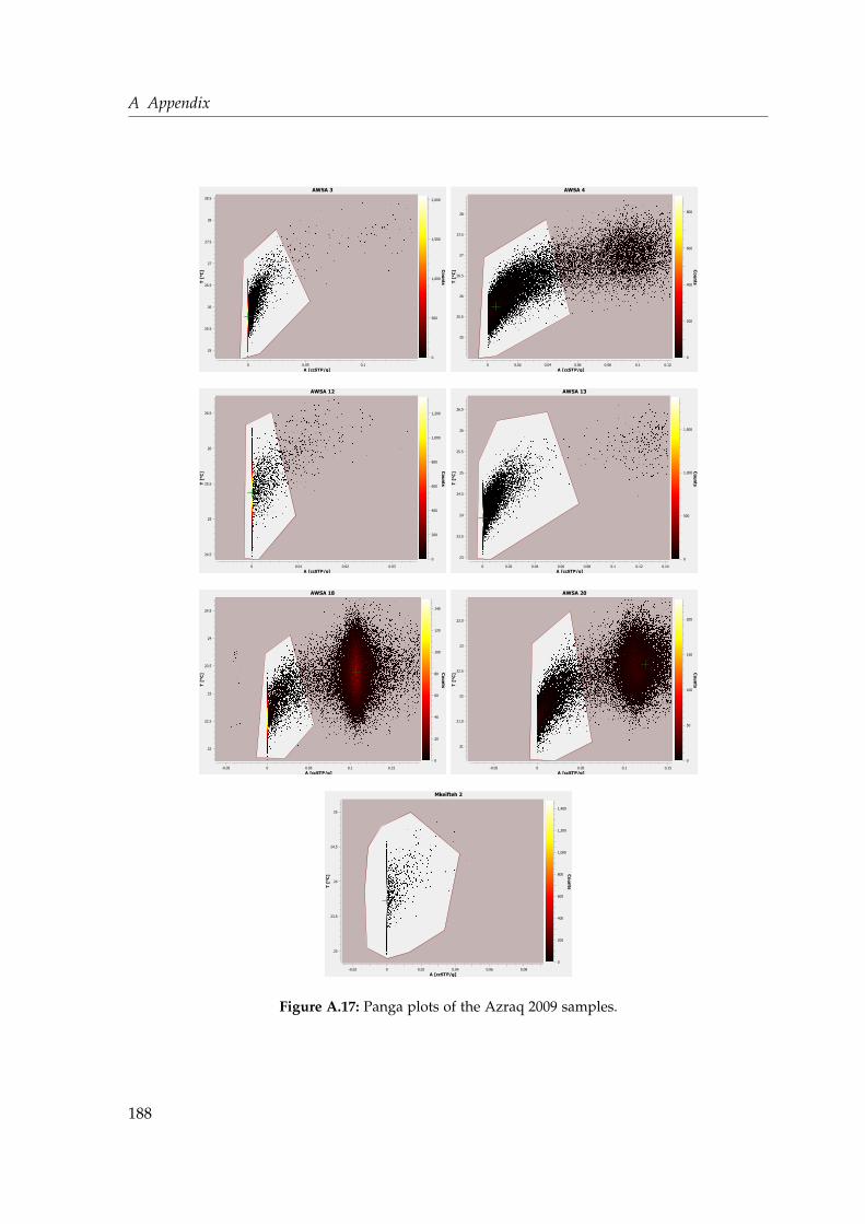
A Appendix
AWSA 3
T [
°C]
25
25.5
26
26.5
27
27.5
28
28.5
Counts
0
500
1,000
1,500
2,000
A [ccSTP/g]0 0.05 0.1
AWSA 4
T [
°C]
25
25.5
26
26.5
27
27.5
28
Counts
0
200
400
600
800
A [ccSTP/g]0 0.02 0.04 0.06 0.08 0.1 0.12
AWSA 12
T [
°C]
24.5
25
25.5
26
26.5
Counts
0
200
400
600
800
1,000
1,200
A [ccSTP/g]0 0.01 0.02 0.03
AWSA 13
T [
°C]
23
23.5
24
24.5
25
25.5
26
26.5
Counts
0
500
1,000
1,500
A [ccSTP/g]0 0.02 0.04 0.06 0.08 0.1 0.12 0.14
AWSA 18
T [
°C]
22
22.5
23
23.5
24
24.5
Counts
0
20
40
60
80
100
120
140
A [ccSTP/g]-0.05 0 0.05 0.1 0.15
AWSA 20
T [
°C]
21
21.5
22
22.5
23
23.5
Counts
0
50
100
150
200
A [ccSTP/g]-0.05 0 0.05 0.1 0.15
Mkeifteh 2
T [
°C]
23
23.5
24
24.5
25
Counts
0
200
400
600
800
1,000
1,200
1,400
A [ccSTP/g]-0.02 0 0.02 0.04 0.06 0.08
Figure A.17: Panga plots of the Azraq 2009 samples.
188

A.8 Panga data evaluation diagrams
AWSA 3
T [
°C]
26
27
28
29
30
Counts
0
100
200
300
400
500
A [ccSTP/g]0 0.05 0.1 0.15
AWSA 4
T [
°C]
24
26
28
30
32C
ounts
0
200
400
600
800
A [ccSTP/g]0 0.02 0.04 0.06 0.08 0.1 0.12 0.14
AWSA 5
T [
°C]
25
26
27
28
Counts
0
500
1,000
1,500
A [ccSTP/g]0 0.02 0.04 0.06 0.08 0.1
AWSA 6
T [
°C]
26.5
27
27.5
28
28.5
Counts
0
200
400
600
800
1,000
A [ccSTP/g]0 0.05 0.1 0.15 0.2 0.25
AWSA 12
T [
°C]
25
25.5
26
26.5
27
27.5
28
28.5
Counts
0
500
1,000
1,500
A [ccSTP/g]0 0.05 0.1 0.15
AWSA 15
T [
°C]
23
24
25
26
Counts
0
100
200
300
400
A [ccSTP/g]0 0.05 0.1 0.15 0.2
AWSA 16
T [
°C]
22
23
24
25
Counts
0
500
1,000
1,500
2,000
A [ccSTP/g]0 0.02 0.04 0.06 0.08
AWSA 18
T [
°C]
21
22
23
24
25
26
Counts
0
200
400
600
800
1,000
A [ccSTP/g]-0.01 0 0.01 0.02 0.03 0.04
Figure A.18: Panga plots of the Azraq 2010 samples.
189

A Appendix
AWSA 5
T [
°C]
26
26.5
27
27.5
28
28.5
29
Counts
0
500
1,000
1,500
2,000
A [ccSTP/g]0 0.02 0.04 0.06 0.08 0.1 0.12
AWSA 16
T [
°C]
22
23
24
25
Counts
0
500
1,000
1,500
2,000
A [ccSTP/g]0 0.02 0.04 0.06 0.08
F3975
T [
°C]
22.5
23
23.5
24
24.5
25
25.5
Counts
0
500
1,000
1,500
2,000
A [ccSTP/g]0 0.02 0.04 0.06 0.08 0.1 0.12 0.14
F3741
T [
°C]
20
21
22
23
Counts
0
500
1,000
1,500
2,000
2,500
A [ccSTP/g]0 0.05 0.1 0.15
F3960
T [
°C]
19
20
21
22
23
Counts
0
50
100
150
A [ccSTP/g]-0.02 0 0.02 0.04 0.06 0.08 0.1 0.12
Mohammed
T [
°C]
18.5
19
19.5
20
20.5
21
Counts
0
100
200
300
400
500
A [ccSTP/g]0 0.02 0.04 0.06 0.08
Figure A.19: Panga plots of the AWSA and Farm well 2012 samples.
190
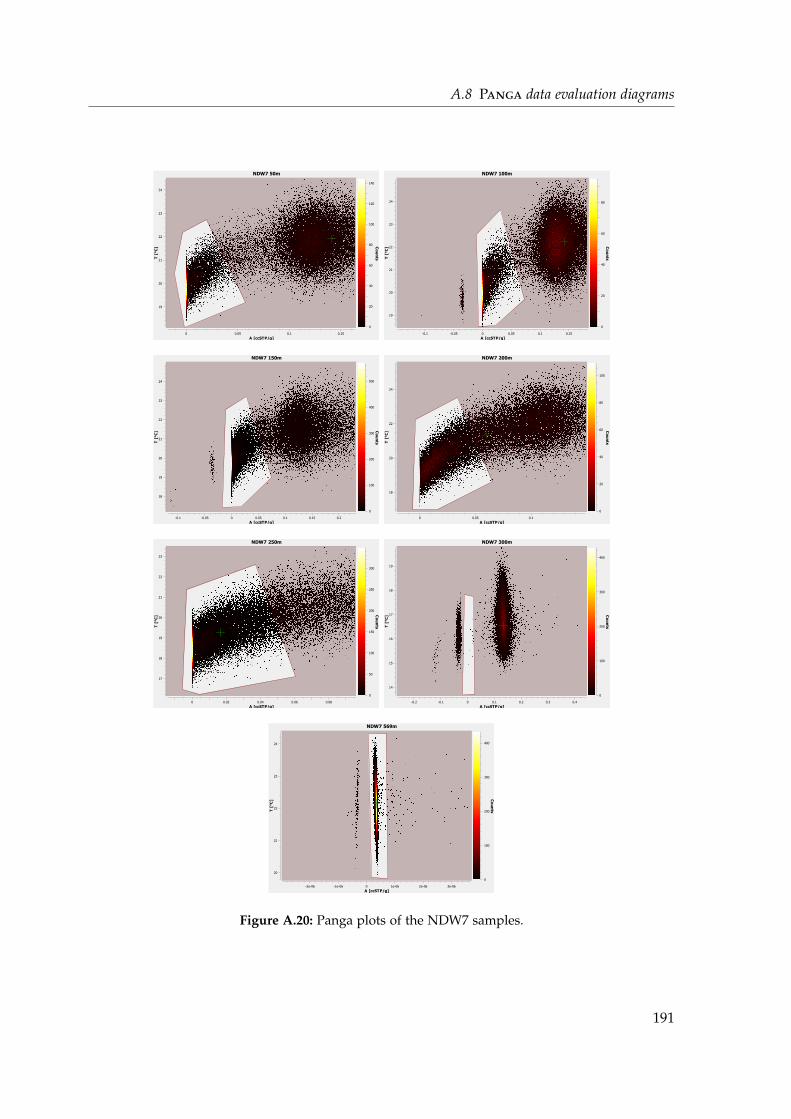
A.8 Panga data evaluation diagrams
NDW7 50m
T [
°C]
19
20
21
22
23
24
Counts
0
20
40
60
80
100
120
140
A [ccSTP/g]0 0.05 0.1 0.15
NDW7 100m
T [
°C]
19
20
21
22
23
24
Counts
0
20
40
60
80
A [ccSTP/g]-0.1 -0.05 0 0.05 0.1 0.15
NDW7 150m
T [
°C]
18
19
20
21
22
23
24
Counts
0
100
200
300
400
500
A [ccSTP/g]-0.1 -0.05 0 0.05 0.1 0.15 0.2
NDW7 200m
T [
°C]
18
20
22
24
Counts
0
20
40
60
80
100
A [ccSTP/g]0 0.05 0.1
NDW7 250m
T [
°C]
17
18
19
20
21
22
23
Counts
0
50
100
150
200
250
300
A [ccSTP/g]0 0.02 0.04 0.06 0.08
NDW7 300m
T [
°C]
14
15
16
17
18
19
Counts
0
100
200
300
400
A [ccSTP/g]-0.2 -0.1 0 0.1 0.2 0.3 0.4
NDW7 569m
T [
°C]
20
21
22
23
24
Counts
0
100
200
300
400
A [ccSTP/g]-2e-06 -1e-06 0 1e-06 2e-06 3e-06
Figure A.20: Panga plots of the NDW7 samples.
191

A Appendix
Himma
F
-100
-80
-60
-40
-20
0
20
40
Counts
0
100
200
300
400
A [ccSTP/g]0 0.002 0.004 0.006 0.008
Abu Ziad
F
0.5
1
1.5
2C
ounts
0
50
100
150
200
250
300
A [ccSTP/g]0 0.05 0.1 0.15 0.2
Zara
T [
°C]
29
30
31
32
33
34
Counts
0
200
400
600
800
1,000
A [ccSTP/g]-0.02 0 0.02 0.04 0.06 0.08
6545_GOFRA_121210_1
T [
°C]
17
17.5
18
18.5
19
19.5
20
Counts
0
20
40
60
80
F0 20 40 60 80
6551_MEITZAR3_2
T [
°C]
16
18
20
22
24
Counts
0
50
100
150
A [ccSTP/g]0 0.02 0.04 0.06 0.08 0.1
6555_EIN_BALZAM_1
T [
°C]
17
17.5
18
Counts
0
50
100
150
200
250
300
350
A [ccSTP/g]-0.005 0 0.005 0.01 0.015
6571_EIN_MAKLA_4
T [
°C]
14.5
15
15.5
16
16.5
17
17.5
18
Counts
0
200
400
600
800
1,000
A [ccSTP/g]0 0.05 0.1
6577_EIN_YAHAV_6_2
T [
°C]
20
22
24
26
28
30
Counts
0
10
20
30
40
50
60
70
A [ccSTP/g]0.02 0.04 0.06 0.08 0.1
6585_TZOFAR_20_1
T [
°C]
30.5
31
31.5
32
32.5
33
33.5
Counts
0
50
100
150
200
250
A [ccSTP/g]-0.02 0 0.02 0.04 0.06 0.08 0.1 0.12
6591_MINERAL_2
T [
°C]
16
18
20
22
24
26
28
Counts
0
100
200
300
400
500
600
700
A [ccSTP/g]-0.025 -0.02 -0.015 -0.01 -0.005 0 0.005
Figure A.21: Panga plots of Thermal waters.
192

A.9 Abbreviations
A.9 Abbreviations
AWSA Amman Water and Sewage Authoriy
CE Closed-system equilibration excess air model
DS Diffusion sampler
DST Dead Sea Transform
EA Excess air
EMWL Eastern Mediterranean Water Line
GMWL Global Meteoric Water Line
JMWL Jordanian Meteoric Water Line
LMWL Local Meteoric Water Line
masl Meters above sea level
mbsl Meters below sea level
MORB Mid-Ocean Ridge Basalt
NGT Noble Gas Temperature
OIB Ocean Island Basalt
UA Unfractionated Air excess air model
193

List of Figures
2.1 Structure of the subsurface related to groundwater . . . . . . . . . . . . . . . . 42.2 Illustration of a simple aquifer . . . . . . . . . . . . . . . . . . . . . . . . . . . . 52.3 Tritium in precipitation . . . . . . . . . . . . . . . . . . . . . . . . . . . . . . . . 72.4 Evaporation and condensation over oceans and landmass . . . . . . . . . . . . 92.5 Jordan Meteoric Water Line . . . . . . . . . . . . . . . . . . . . . . . . . . . . . 112.6 Continental Effect . . . . . . . . . . . . . . . . . . . . . . . . . . . . . . . . . . . 122.7 δ13C variations in nature . . . . . . . . . . . . . . . . . . . . . . . . . . . . . . . 132.8 DIC components vs. pH . . . . . . . . . . . . . . . . . . . . . . . . . . . . . . . 142.9 Modern 14C . . . . . . . . . . . . . . . . . . . . . . . . . . . . . . . . . . . . . . 172.10 Collins diagram . . . . . . . . . . . . . . . . . . . . . . . . . . . . . . . . . . . . 202.11 Schoeller diagram . . . . . . . . . . . . . . . . . . . . . . . . . . . . . . . . . . . 202.12 Piper diagram . . . . . . . . . . . . . . . . . . . . . . . . . . . . . . . . . . . . . 212.13 Characterization of water types in a piper diagram . . . . . . . . . . . . . . . . 212.14 Three-isotope plot of He . . . . . . . . . . . . . . . . . . . . . . . . . . . . . . . 252.15 Noble gas components in a groundwater sample . . . . . . . . . . . . . . . . . 272.16 Noble gas solubility in dependence of temperature and salinity . . . . . . . . 282.17 Excess air models . . . . . . . . . . . . . . . . . . . . . . . . . . . . . . . . . . . 302.18 Graphical separation of the atmospheric, crustal and mantle component . . . 34
3.1 Carbon extraction line . . . . . . . . . . . . . . . . . . . . . . . . . . . . . . . . 393.2 Data analysis with Wucem . . . . . . . . . . . . . . . . . . . . . . . . . . . . . . 423.3 Instability of the faraday cup detector . . . . . . . . . . . . . . . . . . . . . . . 433.4 Evaluation with WUCEM . . . . . . . . . . . . . . . . . . . . . . . . . . . . . . . 443.5 Wucem evaluation of samples containing very high 3He concentration . . . . 453.6 Nonlinearity of Xe . . . . . . . . . . . . . . . . . . . . . . . . . . . . . . . . . . . 453.7 Nonlinearity of argon . . . . . . . . . . . . . . . . . . . . . . . . . . . . . . . . . 463.8 Examples of limiting cases of the CE model . . . . . . . . . . . . . . . . . . . . 483.9 Setup Radon analysis . . . . . . . . . . . . . . . . . . . . . . . . . . . . . . . . . 50
4.1 Precipitation distribution in Jordan . . . . . . . . . . . . . . . . . . . . . . . . . 524.2 Sketch of a pull-apart . . . . . . . . . . . . . . . . . . . . . . . . . . . . . . . . . 544.3 Relief of the DST . . . . . . . . . . . . . . . . . . . . . . . . . . . . . . . . . . . 554.4 Regional tectonic setting . . . . . . . . . . . . . . . . . . . . . . . . . . . . . . . 564.5 W–E cross-section across the DST . . . . . . . . . . . . . . . . . . . . . . . . . . 584.6 Structural map of Jordan . . . . . . . . . . . . . . . . . . . . . . . . . . . . . . . 594.7 Hydrological units at the surface . . . . . . . . . . . . . . . . . . . . . . . . . . 60
195
List of Figures
4.8 Hydrogeologic pattern of Jordan . . . . . . . . . . . . . . . . . . . . . . . . . . 614.9 Rock units in Jordan . . . . . . . . . . . . . . . . . . . . . . . . . . . . . . . . . 624.10 Groundwater flow pattern of the B2/A7 aquifer . . . . . . . . . . . . . . . . . 644.11 Groundwater flow pattern of the B4 aquifer . . . . . . . . . . . . . . . . . . . . 65
5.1 Diffusion samplers . . . . . . . . . . . . . . . . . . . . . . . . . . . . . . . . . . 695.2 Deep sampler . . . . . . . . . . . . . . . . . . . . . . . . . . . . . . . . . . . . . 70
6.1 Azraq groundwater situation . . . . . . . . . . . . . . . . . . . . . . . . . . . . 746.2 Overview Map of Azraq . . . . . . . . . . . . . . . . . . . . . . . . . . . . . . . 756.3 Sketch of the hydrogeology in Azraq . . . . . . . . . . . . . . . . . . . . . . . . 776.4 Geologic cross sections Azraq . . . . . . . . . . . . . . . . . . . . . . . . . . . . 786.5 Temporal development of the Salinity in AWSA . . . . . . . . . . . . . . . . . 806.6 Collins and Schoeller diagram of the water groups in Azraq . . . . . . . . . . 826.7 Depth profiles of AWSA wells . . . . . . . . . . . . . . . . . . . . . . . . . . . . 856.8 Terrigenic 4He vs. E. C. . . . . . . . . . . . . . . . . . . . . . . . . . . . . . . . . 866.9 Terrigenic 4He vs. Physical parameters . . . . . . . . . . . . . . . . . . . . . . . 896.10 Schoeller diagram of all sampled Azraq wells . . . . . . . . . . . . . . . . . . . 906.11 Azraq Schoeller diagram splitted into water groups . . . . . . . . . . . . . . . 916.12 Piper diagram of Azraq samples . . . . . . . . . . . . . . . . . . . . . . . . . . 926.13 Ion relations in Azraq . . . . . . . . . . . . . . . . . . . . . . . . . . . . . . . . . 946.14 Relation of He and Cl . . . . . . . . . . . . . . . . . . . . . . . . . . . . . . . . . 956.15 Stable isotope data in Azraq . . . . . . . . . . . . . . . . . . . . . . . . . . . . . 1006.16 Terrigenic 4He vs. δ18O in Azraq . . . . . . . . . . . . . . . . . . . . . . . . . . 1006.17 3He/4He vs. Ne/He plot of the Azraq samples . . . . . . . . . . . . . . . . . . 1096.18 3He vs. 4He plot of Azraq samples . . . . . . . . . . . . . . . . . . . . . . . . . 1116.19 Explanation for mantle helium in the shallow aquifer in Azraq . . . . . . . . . 1156.20 Depiction of a cone of depression at the AWSA wells . . . . . . . . . . . . . . 116
7.1 Principle structure of a thermal system . . . . . . . . . . . . . . . . . . . . . . . 1207.2 Thermal springs and wells location along the DST . . . . . . . . . . . . . . . . 1217.3 Temperature and Salinity distribution along the DST . . . . . . . . . . . . . . 1247.4 Helium isotope plot of thermal waters . . . . . . . . . . . . . . . . . . . . . . . 1317.5 Graphical mantle correction . . . . . . . . . . . . . . . . . . . . . . . . . . . . . 1337.6 Mantle helium and δ13C distribution along the DST . . . . . . . . . . . . . . . 1347.7 3He vs. 4He plot for the thermal waters . . . . . . . . . . . . . . . . . . . . . . 1367.8 Helium components of crust, atmosphere and mantle . . . . . . . . . . . . . . 1377.9 Total 3He and 4He concentrations vs. relative mantle contribution . . . . . . . 1387.10 3He/4He ratio vs. discharge temperature . . . . . . . . . . . . . . . . . . . . . 1397.11 Other noble gas isotope ratio plot indicating mantle influence . . . . . . . . . 1407.12 Mantle helium vs. δ13C . . . . . . . . . . . . . . . . . . . . . . . . . . . . . . . . 1447.13 E. C. vs. δ13C in thermal waters . . . . . . . . . . . . . . . . . . . . . . . . . . . 1457.14 Stable isotopes of thermal waters . . . . . . . . . . . . . . . . . . . . . . . . . . 1467.15 Mantle helium vs. δ18O . . . . . . . . . . . . . . . . . . . . . . . . . . . . . . . . 148
196
List of Figures
7.16 Piper plot of thermal waters in Jordan . . . . . . . . . . . . . . . . . . . . . . . 1497.17 Ternary plot of thermal waters in Jordan . . . . . . . . . . . . . . . . . . . . . . 1497.18 Mantle helium vs. radon activity . . . . . . . . . . . . . . . . . . . . . . . . . . 1507.19 Cross-section across the Yarmouk Gorge . . . . . . . . . . . . . . . . . . . . . . 1527.20 Structural map of Lake Kinneret . . . . . . . . . . . . . . . . . . . . . . . . . . 1537.21 North–south distribution of mantle helium . . . . . . . . . . . . . . . . . . . . 157
A.1 Salinity dependent radon solubility (full range) . . . . . . . . . . . . . . . . . . 162A.15 Heat map of Jordan . . . . . . . . . . . . . . . . . . . . . . . . . . . . . . . . . . 178A.16 Heat map of Israel . . . . . . . . . . . . . . . . . . . . . . . . . . . . . . . . . . . 179A.17 Panga plots Azraq 2009 . . . . . . . . . . . . . . . . . . . . . . . . . . . . . . . . 188A.18 Panga plots Azraq 2010 . . . . . . . . . . . . . . . . . . . . . . . . . . . . . . . . 189A.19 Panga plots Azraq 2012, part 1 . . . . . . . . . . . . . . . . . . . . . . . . . . . 190A.20 Panga plots Azraq 2012, part 2 . . . . . . . . . . . . . . . . . . . . . . . . . . . 191A.21 Panga plots of Thermal waters . . . . . . . . . . . . . . . . . . . . . . . . . . . 192
197


List of Tables
2.1 Mineral dissolution reactions . . . . . . . . . . . . . . . . . . . . . . . . . . . . 182.2 Atmospheric noble gas composition . . . . . . . . . . . . . . . . . . . . . . . . 23
6.1 Basic information of Azraq wells . . . . . . . . . . . . . . . . . . . . . . . . . . 846.2 Physical parameters of the Azraq wells . . . . . . . . . . . . . . . . . . . . . . 876.3 Results three component mixing model . . . . . . . . . . . . . . . . . . . . . . 966.4 Tritium and carbon in Azraq . . . . . . . . . . . . . . . . . . . . . . . . . . . . . 976.5 Stable Isotope data in Azraq . . . . . . . . . . . . . . . . . . . . . . . . . . . . . 996.6 Noble gas isotope concentrations in Azraq wells . . . . . . . . . . . . . . . . . 1026.7 Noble gas isotope ratios of Azraq samples . . . . . . . . . . . . . . . . . . . . . 1046.8 Results from inverse modeling Azraq . . . . . . . . . . . . . . . . . . . . . . . 1066.9 3H-3He ages of Azraq wells . . . . . . . . . . . . . . . . . . . . . . . . . . . . . 1086.10 Relative mantle, crust and atmospheric share of Azraq samples . . . . . . . . 110
7.1 Basic information of the thermal water sample locations . . . . . . . . . . . . . 1257.2 Noble gas isotope results of thermal waters . . . . . . . . . . . . . . . . . . . . 1277.3 Results of inverse fitting of noble gas concentration of the thermal waters . . 1297.4 Helium ratios in thermal waters . . . . . . . . . . . . . . . . . . . . . . . . . . . 1307.5 Relative 3He and 4He contributions . . . . . . . . . . . . . . . . . . . . . . . . . 1357.6 Other noble gas isotope ratios in the atmosphere and the mantle . . . . . . . . 1407.7 δ2H, δ18O, δ13C, tritium, radon and alkalinity of thermal waters . . . . . . . . 142
A.1 Solubility coefficients . . . . . . . . . . . . . . . . . . . . . . . . . . . . . . . . . 161A.2 Lithologic data of Azraq wells . . . . . . . . . . . . . . . . . . . . . . . . . . . . 180A.3 Helium components of Azraq wells . . . . . . . . . . . . . . . . . . . . . . . . 181A.4 Water chemistry data for the 2012 Azraq samples . . . . . . . . . . . . . . . . . 182A.5 Noble gas element concentration of the Azraq samples . . . . . . . . . . . . . 183A.6 Noble gas element concentration of the thermal waters . . . . . . . . . . . . . 184A.7 Water chemistry data of thermal waters . . . . . . . . . . . . . . . . . . . . . . 185A.8 Noble gas isotope concentrations of samples from the Karak plateau . . . . . 186
199


Acknowledgments – Danksagung
Many people have, directly or indirectly, contributed that I could finalize this theses success-fully.
First of all, I thank my supervisor, Prof. Dr. Werner Aeschbach-Hertig for the possibilityto spend the last four years in a very inspiring, interdisciplinary environment and for thedeep insight to noble gas geochemistry in groundwater. He gave me the opportunity toexperiment a lot with the noble gas mass spectrometer setup and I learned a lot about thetechnical background of rare gas analysis.
Gratitude is owed to Prof. Dr. Margot Isenbeck-Schröter for taking over the task of being mysecond referee.
I thank all workers at the Water Authority of Jordan for the intensive and very successful co-operation. Suzan Kilani was responsible in the beginning of this project in that she agreed ona collaboration. Also her successor, Prof. Dr. Muna Hindiyeh, kindly supported the mutualproject. Most joint work, however, was done by the workers of the water authority, in par-ticular Randa Tuffaha and Refaat Bani-Khalaf. They had an open ear all time and managedrelentlessly all planning of the field trips and were irreplaceable regarding communicationwith the Ministry of Water and Irrigation and other institutions. Refaat introduced me toArcGIS data analysis and supported me several times on the sampling excursions. Honestly,without both of you I would not stand where I am now, and I’m really glad that you man-aged to visit us in Heidelberg. I hope you always keep pleasant memories of this journey. Iam definitely sure we’ll meet again one day.
Yet, many more people supported me in the field, most notable Ismail Abdeldin, who facili-tated two exciting trips to the southern desert, as well as Zeyad Qawasmeh, Omar Alqudahand Zak for assistance and nice conversations on sampling trips and in the office. A lotmore people at the laboratories of the Water Authority and in several pumping stationscontributed their share. Uncountable people in Jordan comforted us with their stunninghospitality, making us often think we can learn a lot from the Arabian mentality. And fi-nally, I’d like to thank all Jordanian car drivers, as they taught us to deeply relax and keep aeverlasting smile on our lips.
Florian Freundt was my ever-reliable assistant and friend on the field trips in 2010 and 2012.He always kept a cool head when things went too fast or I was too sleepy after short nightsof radon measurements. Furthermore, he is responsible for most photos in this thesis andgenerally the best documented time period of my life. Special thanks to you, Florian!
Neta Tsur deserves my gratitude for sampling the Israeli localities and the accurate datapreparation. Her samples complete the data set of thermal waters along the Dead Sea Trans-form.
201

Acknowledgments – Danksagung
I furthermore thank the Water Gang, i. e. Thomas Bonn, Barbara Brilmayer-Bakti, FranziskaFörster, Silvan Eppinger and Florian Freundt, for a wonderful and inspiring time, the weeklygathering in the canteen, and mutual easement and fun factor during our common fieldtrips.
Thank is owned also to Prof. Dr. Mustafa Al-Kuisi, Prof. Nasim Barham and Taiseer HarbAljazzar for introductions to the Jordan water sector. Prof. Kamal Dahab and Sebnem ArslanI thank for introductory lessons to water chemistry.
I also thank the Federal State of Baden-Württemberg and the Heidelberg University for finan-cial support within the framework of the Global Change and Globalization research cluster.Nicole Vollweiler is thanked for her relentless administration.
Dann gebührt natürlich großer Dank an meine ganze Arbeitsgruppe, welche die vier Jah-re am Institut wie im Flug vergehen ließ, beim alltäglichen Gang in die Mensa, den regel-mäßigen Grillabenden, aber auch die Arbeit im Labor und am Schreibtisch habt ihr allemir versüßt. Insbesondere danke ich meinen Bürokollegen Thomas, Neta und Lisa, die im-mer ein offenes Ohr hatten und für so manchen Spaß zu haben waren. Auch allen emsigenKorrekturlesern (insbesondere Flo, Simon und Thomas) danke ich selbstverständlich, dennohne euch wäre diese Arbeit nie so toll geworden. Außerdem danke ich meinen drei Paper-Beschaffern Lisa, Christoph und Kira, ohne die so manche Information nicht überprüfbargewesen wäre.
Einige Leute haben für mich Proben analysiert: Michael Sabasch für the Stabilen Isotope2009, 2010 sowie alle 13C-Messungen, Christian Scholz und Stefan Rheinberger für die Io-nenanalyse, sowie unseren wechselnden HiWis, die die Tritiummessungen sowie die Koh-lenstoffextraktion geschmissen haben. Ein besonderer Dank geht an Dr. Paul Königer vomBGR in Hannover, der sich freundlicherweise bereit erklärt hat, die Stabilen Isotope meiner2012er sowie Netas Proben aus Israel zu bestimmen. Ich hoffe, dass ich mich eines Tagesdafür revanchieren kann.
Gerhard Schmidt und Klaus Schelkes vom BGR danke ich für die Einführung in Grundwas-serfließmodelle in Jordanien. Ein großer Dank geht auch Pritam Yogeshwar für aufschluss-reiche Diskussionen über die geologische Struktur der Azraq Oase.
Doch wo wäre ich ohne die Unterstützung im privaten Umfeld. Ganz besonderer Dank ge-bührt meiner wunderbaren Freundin Eva, die zusammen mit mir Hochs und Tiefs ertragenhat und es stets verstanden hat mich wieder aufzubauen, wenn es mal nicht so lief wie ge-wünscht. Dein Anteil an dieser Arbeit ist kaum zu überschätzen .
Meine Familie hat mich über all die Jahre des Studiums unterstützt und in meinen Entschei-dungen bekräftigt. Hierfür und für die Aufmunterung danke ich euch.
Zuletzt gilt mein Dank auch all meinen Freunden in und außerhalb Heidelbergs, die mirwährend des Studiums und der Doktorarbeit eine unvergessliche Zeit beschert haben. Washaben wir gefeiert und gelacht!
202

Bibliography
ABDULLA FA, AL-KHATIB MA, AL-GHAZZAWI ZD (2000) Development of groundwater modeling for theAzraq basin, Jordan. Environmental Geology 40(1-2)
ABU-EL-SHA’R WY, RIHANI JF (2007) Application of the high performance computing techniques of parflowsimulator to model groundwater flow at Azraq basin. Water Resource Management 21: 409–425
ABU-JABER NS, ALI AJ, AL-QUDAH K (1998) Use of solute and isotopic composition of ground water to con-strain the ground water flow system of the Azraq area, Jordan. Groundwater 36(2): 361–365
AESCHBACH-HERTIG W (2005) A comment on “Helium sources in passive margin aquifers – new evidence for asignificant mantle 3He source in aquifers with unexpectedly low in situ 3He/4He production” by M. C. Castro[Earth Planet. Sci. Lett. 222 (2004) 897-913]. Earth Planetary Science Letters 240: 827–829
AESCHBACH-HERTIG W, SOLOMON DK (2013) Noble gas thermometry in groundwater hydrology. In:BURNARD P (Ed.), The noble gases as geochemical tracers, Advances in isotope geochemistry, 81–122.Springer, Berlin, Heidelberg
AESCHBACH-HERTIG W, KIPFER R, HOFER M, IMBODEN DM, WIELER R, SIGNER P (1996) Quantification ofgas fluxes from the subcontinental mantle: The example of Laacher See, a maar lake in Germany. Geochimicaet Cosmochimica Acta 60(1): 31–41
AESCHBACH-HERTIG W, PEETERS F, BEYERLE U, KIPFER R (1999) Interpretation of dissolved atmospheric noblegases in natural waters. Water Resourse Research 35(9): 2779–2792
AESCHBACH-HERTIG W, PEETERS F, BEYERLE U, KIPFER R (2000) Palaeotemperature reconstruction from noblegases in ground water taking into account equilibration with entrapped air. Nature 405: 1040–1044
AESCHBACH-HERTIG W, STUTE M, CLARK J, REUTER R, SCHLOSSER P (2002) A paleotemperature record de-rived from dissolved noble gases in groundwater of the Aquia Aquifer (Maryland, USA). Geochimica et Cos-mochimica Acta 66(5): 797–817
AESCHBACH-HERTIG W, EL-GAMAL H, WIESER M, PALCSU L (2008) Modeling excess air and degassing ingroundwater by equilibrium partitioning with a gas phase. Water Resourse Research 44: W08449
AJAMIEH M (1998) Water Quality Improvement and Conservation Project – Assessment of Brackish Groundwa-ter in Jordan. Tech. rep., USAID
AKKAWI EJ (2006) Locating Zones and Quantify the Submarine Groundwater Discharge into the Eastern Shoresof the Dead Sea-Jordan. PhD Thesis, University of Göttingen
AL-EISAWI D (1996) Vegetation in Jordan. Tech. rep., UNESCO - Cairo Office, Regional Office for Science andTechnology for the Arab States
AL-KHARABSHEH A (2000) Ground-water modelling and long-term management of the Azraq basin as an ex-ample of arid area conditions (Jordan). Journal of Arid Environments 44: 143–153
AL-MOMANI MR (1994) Environmental isotope and hydrochemical study of the shallow and deep groundwaterin the Azraq basin, Jordan. In: IAEA TecDoc 890, 75–101
203

AL-MOMANI MR, AMRO H, KILANI S, EL-NAQA A, RIMAWI O, KATBEH H, TUFFAHA R (2006) Isotope re-sponse to hydrological systems for long term exploitation, case of Azraq basin, Jordan. In: IAEA TecDoc 1507,177–211
ALJAZZAR TH (2003) Groundwater recharge modeling in the Azraq basin considering the unsaturated flowcomponents. Master’s Thesis, Jordan University of Science and Technology, Irbid
AMBRASEYS NN (2006) Comparison of frequency of occurrence of earthquakes with slip rates from long-termseismicity data: the cases of Gulf of Corinth, Sea of Marmara and Dead Sea Fault Zone. Geophysical JournalInternational 165(2): 516–526
ANDERSON DL (1993) Helium-3 from the mantle: Primordial signal or cosmic dust? Science 261: 170–176
ANDREWS J I (1992) Cretaceous and Paleogene Lithostratigraphy in the subsurface of Jordan, vol. 5 of SubsurfaceGeology Bulletin. Subsurface Geoloy Division, NRA, Amman, Jordan
ANDREWS JN, LEE DJ (1979) Inert gases in groundwater from the Bunter Sandstone of England as indicators ofage and palaeoclimatic trends. Journal of Hydrology 41: 233–252
APPELO CAJ, POSTMA D (2005) Geochemistry, groundwater and pollution. A. A. Balkema Publishers, Leiden,London, New York, Philadelphia, Singapore
ARAD A, BEIN A (1986) Saline- versus freshwater contribution to the thermal waters of the northern Jordan RiftValley, Israel. Journal of Hydrology 83(1-2): 49–66
AYED R (1996) Hydrological and Hydrogeological study of the Azraq Basin, Jordan. PhD Thesis, University ofBaghdad, Iraq
BACK W (1966) Hydrochemical facies and ground-water flow patterns in northern part of Atlantic Coastal Plain.USGS Prof Paper 498-A
BAERTSCHI P (1976) Absolute 18O content of standard mean ocean water. Earth and Planetary Science Letters 31:341–344
BAJJALI W (1994) Recharge and regional circulation of thermal groundwater in northern Jordan using isotopegeochemistry. PhD Thesis, University of Ottawa
BAJJALI W (2012) Spatial variability of environmental isotope and chemical content of precipitation in Jordanand evidence of slight change in climate. Applied Water Science 2: 271–283
BAJJALI W, CLARK ID, FRITZ P (1997) The artesian thermal groundwaters of northern Jordan: insights into theirrecharge history and age. Journal of Hydrology 192(1-4): 355–382
BALLENTINE CJ, BURNARD PG (2002) Production, release and transport of noble gases in the continental crust.In: PORCELLI D, BALLENTINE C, WIELER R (Eds.), Noble gases in geochemistry and cosmochemistry, vol. 47of Reviews in Mineralalogy and Geochemistry, 481–538. Mineralogical Society of America, Geochemical Society,Washington, DC
BALLENTINE CJ, HALL CM (1999) Determining paleotemperature and other variables by using an error-weighted, nonlinear inversion of noble gas concentrations in water. Geochimica et Cosmochimica Acta 63(16):2315–2336
BARD E, HAMELIN B, FAIRBANKS RG, ZINDLER A (1990) Calibration of the 14C timescale over the past 30,000years using mass spectrometric U-Th ages from Barbados corals. Nature 345: 405–410
BARKAN E, LUZ B, LAZAR B (2001) Dynamics of the carbon dioxide system in the Dead Sea. Geochimica etCosmochimica Acta 65(3): 355 – 368
BARTOV Y, STEIN M, ENZEL Y, AGNON A, RECHES Z (2002) Lake Levels and Sequence Stratigraphy of LakeLisan, the Late Pleistocene Precursor of the Dead Sea. Quarternary Research 57: 9–21
204

BASFORD JR, DRAGON JC, PEPIN RO, COSCIO JR MR, MURTHY VR (1973) Krypton and xenon in lunar fines.Proc 4th Lunar Sci Conf 2: 1915–1955
BAUBRON JC, BESANÇON J, COPELAND L, HOURS F, MACAIRE JJ, SANLAVILLE P (1985) Évolution de la moyenvallée du Zarqa (Jordanie) au Néogène et au Quaternaire. Rév Géol Dyn Géog Phys 26(5): 273–283
BECKER B, KROMER B (1993) The continental tree-ring record – absolute chronology, 14C calibration and climaticchange at 11 ka. Palaeogeography, Palaeoclimatology, Palaeoecology 103(1-2): 67–71
BEIN A, FEINSTEIN S (1988) Late Cenozoic thermal gradients in Dead Sea Transform system basins. Journal ofPetroleum Geology 11(2): 185–192
BEISER A (1957) Variations in the Geomagnetic Dipole in the past 15,000 Years. Journal of Geophysical Research62(2): 235–239
BEN-AVRAHAM Z, GINZBURG A (1990) Displaced terranes and crustal evolution of the Levant and the easternMediterranean. Tectonics 9(4): 613–622
BEN-AVRAHAM Z, HÄNEL R, VILLINGER H (1978) Heat flow through the Dead Sea rift. Marine Geology 28(3-4):253–269
BEN-AVRAHAM Z, GARFUNKEL Z, LAZAR M (2008) Geology and evolution of the southern Dead Sea Fault withemphasis on subsurface structure. Annual Review of Earth and Planetary Science 36: 357–387
BENDER F (1968) Geologie von Jordanien. Beiträge zur regionalen Geologie der Erde. Gebrüder Borntraeger,Berlin, Stuttgart. An English translation was released by the same publisher in 1974 under the title “Geologyof Jordan”
BENSON BB, KRAUSE JR D (1976) Empirical laws for dilute aqueous solutions of nonpolar gases. Journal ofChemical Physics 64(2): 689–709
BENSON BB, KRAUSE JR D (1980) Isotopic fractionation of helium during solution: A probe for the liquid state.Journal of Solution Chemistry 9(12): 895–909
BERGELSON G, NATIV R, BEIN A (1999) Salinization and dilution history of ground water discharging into theSea of Galilee, the Dead Sea Transform, Israel. Applied Geochemistry 14(1): 91–118
BEYERLE U, AESCHBACH-HERTIG W, IMBODEN DM, BAUR H, GRAF T, KIPFER R (2000) A mass spectrometricsystem for the analysis of noble gases and tritium from water samples. Environtal Science & Technology 34(10):2042–2050
BEYERLE U, RUEEDI J, LEUENBERGER M, AESCHBACH-HERTIG W, PEETERS F, KIPFER R, DODO A (2003) Evi-dence for periods of wetter and cooler climate in the Sahel between 6 and 40 kyr BP derived from groundwater.Geophysical Research Letters 30(4): 1173
BLASER PC, KIPFER R, LOOSLI HH, WALRAEVENS K, VAN CAMP M, AESCHBACH-HERTIG W (2010) A 40 karecord of temperature and permafrost conditions in northwestern Europe from noble gases in the Ledo-Paniselian Aquifer (Belgium). Journal Quaternary Science 25(6): 1038–1044
BLICHER-MATHIESEN G, MCCARTY GW, NIELSEN LP (1998) Denitrification and degassing in groundwaterestimated from dissolved dinitrogen and argon. Journal of Hydrology 208: 16–24
BONN T (2013) Strategische Ressourcenwahrheiten – Interaktion zwischen Behörden und Geberorganisationenin der jordanischen Wasserpolitik. PhD Thesis, Heidelberg University
BOOM G (1968) Zur Petrogenese der Plateaubasalte Nordostjordaniens. In: Geologisches Jahrbuch, vol. 85, 489–496. Bundesamt für Bodenforschung und Geologische Landesämter der Bundesrepublik Deutschland
BURNARD P (2004) Diffusive fractionation of noble gases and helium isotopes during mantle melting. Earth andPlanetary Science Letters 220(3-4): 287–295
205

CARROLL MR, WEBSTER JD (1994) Solubilities of sulphur, noble gases, nitrogen, chlorine, and fluorine in mag-mas. In: CARROLL MR (Ed.), Volatiles in magmas, vol. 30 of Reviews in Mineralogy and Geochemistry, 231–279.Mineralogical Society of America
CERLING TE, SOLOMON DK, QUADE J, BOWMAN JR (1991) On the isotopic composition of carbon in soil carbondioxide. Geochimica et Cosmochimica Acta 3403–3405
CHEBAANE M, EL-NASER H, FITCH J, HIJAZI A, JABBARIN A (2004) Participatory groundwater managementin Jordan: Development and analysis of options. Hydrogeology Journal 12: 14–32
CHIODINI G, FRONDINI F, PONZIANI F (1995) Deep structures and carbon dioxide degassing in Central Italy.Geothermics 24(1): 81–94
CHOUBEY VW, RAMOLA RC (1997) Correlation between geology and radon levels in groundwater, soil andindoor air in Bhilangana Valley, Garhwal Himalaya, India. Environmental Geology 32(4): 258–262
CLARK ID, FRITZ P (1997) Environmental Isotopes in Hydrogeology. CRC Press, Boca Raton, New York
CLARKE WB, JENKINS WJ, TOP Z (1976) Determination of tritium by mass spectrometric measurement of 3He.International Journal of Applied Radiation and Isotopes 27: 515–522
CLASS C, GOLDSTEIN SL (2005) Evolution of helium isotopes in the Earth’s mantle. Nature 436: 1107–1112
CLEVER HL (1979a) Helium and neon – gas solubilities, vol. 1 of Solubility data series. Pergamon Press, Oxford
CLEVER HL (1979b) Krypton, xenon and radon – gas solubilities, vol. 2 of Solubility data series. Pergamon Press,Oxford
CLEVER HL (1980) Argon, vol. 4 of Solubility data series. Pergamon Press, Oxford
COLLINS WD (1923) Graphic representation of water analyses. Industrial and Engineering Chemistry 15(4): 394
CORNOG R, LIBBY WF (1941) Production of Radioactive Hydrogen by Neutron Bombardment of Boron andNitrogen. Physical Review 59: 12
CRAIG H (1957) Isotopic standards for carbon and oxygen and correction factors for massspectrometric analysisof carbon dioxide. Geochimica et Cosmochimica Acta 12: 133–149
CRAIG H (1961) Isotopic variations in meteoric water. Science 133: 1702–1703
CRAIG H, CLARKE WB, BEG MA (1975) Excess 3He in deep water on the East Pacific Rise. Earth and PlanetaryScience Letters 26: 125–132
CRENSHAW WB, WILLIAMS SN, STOIBER RE (1982) Fault location by radon and mercury detection at an activevolcano in Nicaragua. Nature 300: 345–346
CROWE C (1958) Carbon-14 Activity during the past 5,000 Years. Nature 182: 470–471
DAFNY E, BURG A, GVIRTZMAN H (2006) Deduction of groundwater flow regime in a basaltic aquifer usinggeochemical and isotopic data: The Golan Heights, Israel case study. Journal of Hydrology 330(3-4): 506–524
DAMON PE, CHENG SL, LINICK TW (1989) Fine and Hyperfine Structure in the Spectrum of Secular Variationsof Atmospheric 14C. Radiocarbon 31(3): 704–718
DANSGAARD W (1964) Stable isotopes in precipitation. Tellus 16(4): 436–468
DAOUD R, NABER H, ABU TARBUSH M, QUOSSOUS R, SALMAN A, KARABLIEH E (2006) Environmental Issuesof Water Resources. In: HADDADIN MJ (Ed.), Water resources in Jordan – Evolving policies for development,the environment, and conflict resolution, 88–115. Resources for the Future, Washington
DARLING WG, GRIESSHABER E, ANDREWS JN, ARMANNSSON H, O’NIONS RK (1995) The origin of hydrother-mal and other gases in the Kenya Rift Valley. Geochimica et Cosmochimica Acta 59(12): 2501–2512
206
DAVIS SN, DEWIEST RJM (1966) Hydrogeology. John Wiley & Sons, New York, London, Sydney
DE WIT JC, VAN DER STRAATEN CM, MOOK WG (1980) Determination of the absolute hydrogen isotopic ratioof V-SMOW and SLAP. Geostandards Newsletter 4(1): 33–36
DESHPANDE RD, GUPTA SK (2013) Groundwater helium: An indicator of active tectonic regions along NarmadaRiver, central India. Chemical Geology 344: 42–49
DEWAYNE CECIL L, GREEN JR (2000) Radon-222. In: COOK P, HERCZEG AL (Eds.), Environmental tracers insubsurface hydrology, 175–194. Kluwer Academic Publishers, Boston
DIABAT A (2004) Structural map of Jordan. Unpublished report, Natural Resources Authority, Amman, Jordan
DOTTRIDGE J, ABU JABER N (1999) Groundwater resources and quality in northeastern Jordan: safe yield andsustainability. Applied Geography 19: 313–323
DUFFIELD WA, MCKEE EH, EL SALEM F, TEIMEH M (1988) K-Ar ages, chemical composition and geothermalsignificance of cenozoic basalt near the Jordan rift. Geothermics 17(4): 635–644
DURRIDGE (2000) RAD7 radon detector – Owner’s manual. http://www.durridge.com/product_manuals.shtml
DURRIDGE (2001) RAD7 RAD-H2O – Radon in water accessory – Owner’s manual.http://www.durridge.com/product_manuals.shtml
ECKSTEIN Y, MAURATH G (1995) Heat flow and the hydrologic cycle: examples from Israel. In: GUPTA ML,YAMANO M (Eds.), Terrestrial heat flow and geothermic energy in Asia, 1–21. Oxford & IBH Publishing, NewDelhi, Bombay, Calcutta
ECKSTEIN Y, SIMMONSI G (1977) Measurement and interpretation of terrestrial heat flow in Israel. Geothermics6(3-4): 117–142
EHLERINGER JR, PHILIPS SL, SCHUSTER WSF, SANDQUIST DR (1991) Differential utilization of summer rainsby desert plants. Oecologia 88: 430–434
EL-ISA Z, MECHIE J, PRODEHL C (1987a) Shear velocity structure of Jordan from explosion seismic data. Geo-physical Journal of the Royal Astronomical Society 90(1): 265–281
EL-ISA Z, MECHIE J, PRODEHL C, MAKRIS J, RIHM R (1987b) A crustal structure study of Jordan derived fromseismic refraction data. Tectonophysics 138(2-4): 235–253
EL-NAQA A (2010) Study of saltwater intrusion in the upper aquifer in Azraq basin. Tech. rep., IUCN
EL-NAQA A, AL-MOMANI M, KILANI S, HAMMOURI N (2007) Groundwater deterioration of shallow ground-water aquifers due to overexploitation in northeast Jordan. Clean 35(2): 156–166
EL-WAHEIDI MM, MERLANTI F, PAVAN M (1992) Geoelectrical resistivity survey of the central part of the Azraqbasin (Jordan) for identifying saltwater/freshwater interface. Journal Applied Geophysics 29: 125–133
ERAIFEJ N (2006) Gas geochemistry and isotopic signatures in the deep thermal waters in Jordan. Freiberg OnlineGeology 16
EVANS MJ, DERRY LA, FRANCE-LANORD C (2008) Degassing of metamorphic carbon dioxide from the NepalHimalaya. Geochemistry, Geophysics, Geosystems 9(4): Q04021
FAIRBANKS RG, MORTLOCK RA, CHIU TC, CAO L, KAPLAN A, GUILDERSON TP, FAIRBANKS TW, BLOOM AL,GROOTES PM, NADEAU MJ (2005) Radiocarbon calibration curve spanning 0 to 50,000 years BP based onpaired 230Th/ 234U/ 238U and 14C dates on pristine corals. Quaternary Science Reviews 24: 1781–1796
FAIRBRIDGE RW, OLIVER JE (2005) Lapse rate. In: OLIVER JE (Ed.), Encyclopedia of world climatology, 448–450.Springer, Dordrecht, Berlin, Heidelberg
207
FALKENMARK M, LUNDQVIST J, WIDSTRAND C (1989) Macro-scale water scarcity requires micro-scale ap-proaches: Aspects of vulnerability in semi-arid development. Natural Resources Forum 13(4): 258–267
FAYBISHENKO BA (1995) Hydraulic behavior of quasi-saturated soils in the presence of entrapped air: Labora-tory experiments. Water Resourse Research 31(10): 2421–2435
FETTER CW (2001) Applied Hydrogeology. Prentice-Hall, New Jersey, 4 edn.
FITTS CR (2002) Groundwater science. Academic Press, London
FLORKOWSKI T (1985) Sample preparation for hydrogen isotope analysis by mass spectrometry. InternationalJournal of Applied Radiation and Isotopes 36(12): 991–992
FONTES JC (1991) Évaluation de la production naturelle in situ d’argon-36 via le chlore-36 : implicationsgéochimiques et géochronologiques. Comptes rendus de l’Académie des sciences Série 2 313(6): 649–654
FONTES JC, GARNIER JM (1979) Determination of the initial 14C activity of the total dissolved carbon: A reviewof the existing models and a new approach. Water Resource Research 15(2): 399–413
FREEZE RA, CHERRY JA (1979) Groundwater. Prentice-Hall, New Jersey, USA
FREUND R, GARFUNKEL Z, ZAK I, GOLDBERG M, WEISSBROD T, DERIN B, BENDER F, WELLINGS FE, GIRDLER
RW (1970) The Shear along the Dead Sea Rift [and Discussion]. Philosophical Transactions of the Royal Society ofLondon A 267(1181): 107–130
FREUNDT F, SCHNEIDER T, AESCHBACH-HERTIG W (2013) Response of noble gas partial pressures in soil air tooxygen depletion. Chemical Geology 339: 283 – 290
FRIEDRICH R (2007) Grundwassercharakterisierung mit Umwelttracern: Erkundung des Grundwassers derOdenwald-Region sowie Implementierung eines neuen Edelgas-Massenspektrometersystems. PhD Thesis,Heidelberg University
FRIESLANDER U, BEN-AVRAHAM Z (1989) Magnetic field over the Dead Sea and vicinity. Marine and PetroleumGeology 6(2): 148–160
FRISCH W, MESCHEDE M, BLAKEY R (2011) Plate tectonics – Continental drift and mountain building. Springer,Berlin, Heidelberg
FÖRSTER A, FÖRSTER HJ, MASARWEH R, MASRI A, TARAWNEH K (2007) The surface heat flow of the ArabianShield in Jordan. Journal of Asian Earth Sciences 30(2): 271–284
FÖRSTER HJ, FÖRSTER A, OBERHÄNSLI R, STROMEYER D (2010) Lithospheric composition and thermal structureof the Arabian Shield in Jordan. Tectonophysics 481(1-4): 29–37
FRY VA, SELKER JS, GORELICK SM (1997) Experimental investigations for trapping oxygen gas in saturatedporous media for in situ bioremedation. Water Resource Research 33(12): 2687–2696
GALANIS JR SP, SASS JH, MUNROE RJ, ABU-AJAMIEH M (1986) Heat flow at Zerqa Ma’in and Zara and ageothermal reconnaissance of Jordan. USGS Open File Report 86(631)
GALLI P (1999) Active tectonics along the Wadi Araba-Jordan Valley transform fault. Journal of GeophysicalResearch: Solid Earth 104(B2): 2777–2796
GARFUNKEL Z (1981) Internal structure of the Dead Sea leaky transform (rift) in relation to plate kinematics.Tectonophysics 80: 81–108
GARFUNKEL Z, BEN-AVRAHAM Z (1996) The structure of the Dead Sea basin. Tectonophysics 266: 155–176
GARRARD AN, HARVEY P, HIVERNEL F, BYRD B (1985) The environmental history of the Azraq Basin. Studiesin the History and Archaeology of Jordan 2: 109–115
208
GASCOYNE M, SHEPPARD MI (1993) Evidence of terrestrial discharge of deep groundwater of the CanadianShield from helium in soil gases. Environtal Science & Technology 27: 2420–2426
GAT JR (1987) Effect of climate changes on the precipitation patterns and isotopic composition of water in aclimate transition zone: Case of the Eastern Mediterranean Sea area. In: Proceedings of the Vancouver Sym-posium, August 1987: The influence of climate change and climatic variability on the hydrologic regime andwater resources, 168, 513–523. IAHS
GAT JR, CARMI I (1970) Evolution of the Isotopic Composition of Atmospheric Waters in the Mediterranean SeaArea. Journal of Geophysical Research 75(15): 3039–3048
GAT JR, DANSGAARD W (1972) Stable isotope survey of the fresh water occurrences in Israel and the NorthernJordan Rift Valley. Journal of Hydrology 16(3): 177 – 211
GEYH M (2000) Groundwater – Saturated and unsaturated zone. In: MOOK WG (Ed.), Environmental Isotopesin the hydrological cycle; principles and applications, vol. 4. UNESCO, Paris
GEYH MA, MICHEL G (1982) Isotopical differentiation of groundwater of different hydrogeologic origin. Journalof Hydrology 59(1–2): 161–171
GHARAIBEH AAJ (2008) Heat source study and geothermal reservoir assessment for the Zarqa Ma’in – Dab’aarea, central Jordan. In: United Nations University, Geothermal Trainng Programm, 221–246
GIGGENBACH WF, GOGUEL RL (1989) Collection and analysis of geothermal and volcanic water and gas dis-charges. DSIR report CD 2401, 4. edition. Department of Scientific and Industrial Research, Pentone, NewZealand
GILL AE (1982) Atmosphere-Ocean Dynamics. International Geophysics Series. Academic Press
GINGRICH JE (1984) Radon as a geochemical exploration tool. Journal of Geochemical Exploration 21(1-3): 19–39
GINZBURG A, BEN-AVRAHAM Z (1997) A seismic refraction study of the north basin of the Dead Sea, Israel.Geophysical Research Letters 24(16): 2063–2066
GIRDLER RW (1990) The Dead Sea transform fault system. Tectonophysics 180: 1–13
GÜLEÇ N, HILTON DR, MUTLU H (2002) Helium isotope variations in Turkey: relationship to tectonics, volcan-ism and recent seismic activities. Chemical Geology 187(1?2): 129–142
GODWIN H (1962) Half-life of Radiocarbon. Nature 195: 984
GOMEZ F, KARAM G, KHAWLIE M, MCCLUSKY S, VERNANT P, REILINGER R, JAAFAR R, TABET C, KHAIR
K, BARAZANGI M (2007) Global Positioning System measurements of strain accumulation and slip transferthrough the restraining bend along the Dead Sea fault system in Lebanon. Geophysical Journal International168(3): 1021–1028
GONFIANTINI R (1986) Environmental isotopes in lake studies. In: FRITZ P, FONTES JC (Eds.), Handbook ofEnvironmental Isotope Geochemistry, vol. 2, 113–168. Elsevier, Amsterdam
GRAHAM DW (2002) Noble gas isotope geochemistry of mid-ocean ridge and ocean island basalts: Characteri-zation of mantle source reservoirs. In: PORCELLI D, BALLENTINE C, WIELER R (Eds.), Noble Gases in Geo-chemistry and Cosmochemistry, vol. 47 of Rev. Mineral. Geochem., 247–317. Mineralogical Society of America,Geochemical Society, Washington, DC
GRIESSHABER E, O’NIONS RK, OXBURGH ER (1992) Helium and carbon isotope systematics in crustal fluidsfrom the Eifel, the Rhine Graben and Black Forest, F.R.G. Chemical Geology 99(4): 213–235
GRÜNTHAL G, WAHLSTRÖM R (2012) The European-Mediterranean Earthquake Catalogue (EMEC) for the lastmillennium. Journal of Seismology 16(3): 535–570
209

GROTHE J (1992) Datenerfassung und Datenauswertung am Heidelberger Low-Level-Tritium-Messsystem.Diploma Thesis, Heidelberg University
GUBA I, MUSTAFA H (1988) Structural control of young basaltic fissure eruptions in the plateau basalt area ofthe Arabian plate, northeastern Jordan. Journal of Volcanology and Geothermal Research 35: 319–334
HAKKI W, TEIMEH M (1981) The geology of Zarqa Ma’in and Zara areas. Tech. rep., NRA, Amman
HALL CM, CASTRO MC, LOHMANN KC, MA L (2005) Noble gases and stable isotopes in a shallow aquifer insouthern Michigan: Implications for noble gas paleotemperature reconstructions for cool climates. GeophysicalResearch Letters 32: L18404
HAN W, DI L, ZHAO P, SHAO Y (2012) DEM Explorer: An online interoperable DEM data sharing and analysissystem. Environmental Modelling & Software 38: 101–107
HEATON THE, VOGEL JC (1981) “Excess air” in groundwater. Journal of Hydrology 50: 201–216
HEIMANN A, STEINITZ G (1989) 40Ar/39Ar total gas ages of basalts from Notera #3 well, Hula Valley, Dead SeaRift: stratigraphic and tectonic implications. Israel Journal of Earth Sciences 38: 173–184
HENRY W (1803) Experiments on the quantity of gases absorbed by water, at different temperatures, and underdifferent pressures. Philosophical Transactions of the Royal Society of London 93: 29–42+274–276
HERZBERG O, MAZOR E (1979) Hydrological applications of noble gases and temperature measurements inunderground water systems: Examples from Israel. Journal of Hydrology 41: 217–231
HILL RA (1940) Geochemical patterns in Coachella Valley. Transactions American Geophysical Union 21: 46–53
HOLDEN W (1998) Modelling and isotope study of the Azraq basin. In: DUTTON RW, CLARKE JI, BATTICKI A(Eds.), Arid land resources and their management: Jordan’s desert margin, 87–93. Kegan Paul International,London
HOLMÉN K, LISS P (1984) Models for air-water gas transfer: An experimental investigation. Tellus 36B(2): 92–100
HOLOCHER J, PEETERS F, AESCHBACH-HERTIG W, HOFER M, BRENNWALD M, KINZELBACH W, KIPFER R(2002) Experimental investigations on the formation of excess air in quasi-saturated porous media. Geochimicaet Cosmochimica Acta 66(23): 4103–4117
HOLOCHER J, PEETERS F, AESCHBACH-HERTIG W, KINZELBACH W, KIPFER R (2003) Kinetic model of gasbubble dissolution in groundwater and its implications for the dissolved gas composition. Environtal Science& Technology 37: 1337–1343
HOOKER PJ, O’NIONS RK, OXBURGH ER (1985) Helium isotopes in North Sea gas fields and the Rhine rift.Nature 318: 273–275
HOROWITZ A (2001) The Jordan Rift Valley. A. A. Balkema Publishers, Lisse, Abingdon, Exton (PA), Tokyo
HOYT DV, KYLE HL, HICKEY JR, MASCHHOFF RH (1992) The Nimbus 7 solar total irradiance – A new algorithmfor its derivation. Journal of Geophysical Research 97(A1): 51–63
HSI (1994) Groundwater Investigations in the Hammad and Sirhan Basin, Vol. 1. Unpublished Report, Ministryof Water and Irrigation, Amman, Jordan
HUGHEN K, LEHMAN S, SOUTHON J, OVERPECK J, MARCHAL O, HERRING C, TURNBULL J (2004) 14C activityand global carbon cycle changes over the past 50,000 years. Science 303: 202–207
HUGHEN K, SOUTHON J, LEHMAN S, BERTRAND C, TURNBULL J (2006) Marine-derived 14C calibration andactivity record for the past 50,000 years updated from the Cariaco Basin. Quaternary Science Reviews 25: 3216–3227
HUMPHREYS AND SONS (1982) Azraq well-field evaluation, Hydrochemistry and monitoring. Tech. rep., Am-man Water and Sewerage Authority, Amman, Jordan
210

IAEA/WMO (2006) Global Network of Isotopes in Precipitation database. Accessible at: www.iaea.org/water
IBRAHIM KM (1993) Geologic map, sheet Al-Azraq, by the Geologic Mapping Division, NRA, Jordan
ILANI S, HARLAVAN Y, TARAWNEH K, RABBA I, WEINBERGER R, IBRAHIM K, PELTZ S, STEINITZ G (2001)New K-Ar ages of basalts from the Harrat Ash Shaam volcanic field in Jordan: Implications for the span andduration of the upper-mantle upwelling beneath the western Arabian plate. Geology 29(2): 171–174
INGRAM RGS, HISCOCK KM, DENNIS PF (2007) Noble gas excess air applied to distinguish groundwaterrecharge conditions. Environtal Science & Technology 41: 1949–1955
IOLR (2013) Monitoring the Dead Sea. Israel Oceanographic & Limnological Research.http://isramar.ocean.org.il. Viewed 30/09/2013
JAMES RH, PALMER RP (2000) The lithium isotope composition of international rock standards. Chemical Geology166(3-4): 319–326
JONES MD, RICHTER T (2011) Paleoclimatic and archeological implications of Pleistocene and Holocene envi-ronments in Azraq, Jordan. Quaternary Research 363–372
JORDAN TIMES (2013) Red Sea project dropped, gov’t ready with alternatives. http://jordantimes.com/red-sea-project-dropped-govt-ready-with-alternatives. Viewed 30/09/2013
JUNG M (2013) PANGA: A new tool for the evaluation of noble gas data. Goldschmidt Conference Abstract.http://goldschmidt.info/2013/abstracts/finalPDFs/1412.pdf
JUNG M, WIESER M, VON OEHSEN A, AESCHBACH-HERTIG W (2013) Properties of the closed-system equilibra-tion model for dissolved noble gases in groundwater. Chemical Geology 339: 291–300
KASHAI EL, CROKER PF (1987) Structural geometry and evolution of the Dead Sea-Jordan rift system as deducedfrom new subsurface data. Tectonophysics 141: 33–60
KATZ A, KOLODNY Y, NISSENBAUM A (1977) The geochemical evolution of the Pleistocene Lake Lisan-DeadSea system. Geochimica et Cosmochimica Acta 41(11): 1609–1626
KECK L (2001) Climate significance of stable isotope records from Alpine ice cores. PhD Thesis, HeidelbergUniversity
KENNEDY BM, VAN SOEST MC (2007) Flow of mantle fluids through the ductile lower crust: Helium isotopetrends. Science 318: 1433–1436
KENNEDY BM, REYNOLDS JH, SMITH SP (1988) Noble gas geochemistry in thermal springs. Geochimica et Cos-mochimica Acta 52(7): 1919–1928
KENNEDY BM, KHARAKA YK, EVANS WC, ELLWOOD A, DEPAOLO DJ, THORDSEN J, AMBATS G, MARINER
RH (1997) Mantle fluids in the San Andreas Fault System, California. Science 278(5341): 1278–1281
KIPFER R, AESCHBACH-HERTIG W, BAUR H, HOFER M, IMBODEN DM, SIGNER P (1994) Injection of mantletype helium into Lake Van (Turkey): The clue for quantifying deep water renewal. Earth and Planetary ScienceLetters 125: 357–370
KIPFER R, AESCHBACH-HERTIG W, PEETERS F, STUTE M (2002) Noble gases in lakes and ground waters. In:PORCELLI D, BALLENTINE C, WIELER R (Eds.), Noble gases in geochemistry and cosmochemistry, vol. 47 ofRev. Mineral. Geochem., 615–700. Mineralogical Society of America, Geochemical Society, Washington, DC
KLINGER Y, AVOUAC JP, ABOU KARAKI N, DORBATH L, BOURLES D, REYSS JL (2000) Slip rate on the Dead Seatransform fault in the northern Araba Valley (Jordan). Geophysical Journal International 142: 755–768
KLUGE T, ILMBERGER J, VON ROHDEN C, AESCHBACH-HERTIG W (2007) Tracing and quantifying groundwaterinflow into lakes using a simple method for radon-222 analysis. Hydrology and Earth System Sciences 11: 1621–1631
211

KLUMP S, GRUNDL T, PURTSCHERT R, KIPFER R (2008) Groundwater and climate dynamics derived from noblegas, 14C, and stable isotope data. Geology 36(5): 395–398
KNÖDEL K, LANGE G, VOIGT HJ (2007) Environmental Geology – Handbook of field methods and case studies.Springer, Berlin, Heidelberg, New York
KOFLER M (1913) Mitteilungen aus dem Institut für Radiumforschung. XXXIII. Monatshefte für Chemie und ver-wandte Teile anderer Wissenschaften 34(2): 389–400
KOULAKOV I, SOBOLEV SV (2006) Moho depth and three-dimensional P and S structure of the crust and upper-most mantle in the Eastern Mediterranean and Middle East derived from tomographic inversion of local ISCdata. Geophysical Journal International 164(1): 218–235
KRAUSE JR D, BENSON BB (1989) The solubility and isotopic fractionation of gases in dilute aqueous solution.IIa. Solubilities of the noble gases. Journal of Solution Chemistry 18(9): 823–873
KREUZER A (2007) Paläotemperaturstudie mit Edelgasen im Grundwasser der Nordchinesischen Tiefebene. PhDThesis, Heidelberg University
KRIENITZ MS, HAASE KM, MEZGER K, SHAIKH-MASHAIL MA (2007) Magma Genesis and Mantle Dynamicsat the Harrat Ash Shamah Volcanic Field (Southern Syria). Journal of Petrology 48(8): 1513–1542
KROMER B (2007) Radiokohlenstoffdatierung. In: WAGNER GA (Ed.), Einführung in die Archäometrie, 3–10.Springer, Berlin/Heidelberg
KULONGOSKI JT, HILTON DR, SELAOLO ET (2004) Climate variability in the Botswana Kalahari from the latePleistocene to the present day. Geophysical Research Letters 31: L10204
KULONGOSKI JT, HILTON DR, IZBICKI JA, BELITZ K (2009) Evidence for prolonged El Nino-like conditions inthe Pacific during the Late Pleistocene: A 43 ka noble gas record from California groundwaters. QuaternaryScience Reviews 28: 2465–2473
LACHNIET MS (2009) Climatic and environmental controls on speleothem oxygen-isotope values. QuaternaryScience Reviews 28: 412–432
LANGE T, HAMMERSCHMIDT K, FRIEDRICHSEN H, MAREI A, WEISE SM (2008) Groundwater in the shallowaquifer of the Jericho area, Jordan Valley – Noble gas evidence for different sources of salinization. In: ZEREINI
F, HÖTZL H (Eds.), Climatic changes and water resources in the Middle East and North Africa, 469–495.Springer, Berlin, Heidelberg
LEHMANN BE, LEHMANN M, NEFTEL A, TARAKANOV SV (2000) Radon-222 monitoring of soil diffusivity. Geo-physical Research Letters 27(23): 3917–3920
LEVENBERG K (1944) A method for the solution of certain problems in least squares. Quarterly of Applied Mathe-matics 2: 164–168
LEVIN I, NAEGLER T, KROMER B, DIEHL M, FRANCEY RJ, GOMEZ-PELAEZ AJ, STEELE LP, WAGENBACH D,WELLER R, WORTHY DE (2010) Observations and modelling of the global distribution and long-term trendof atmospheric 14CO2. Tellus 62B: 26–46
LEVITTE D, ECKSTEIN Y (1978) Correlation between the silica concentration and the orifice temperature in thewarm springs along the Jordan–Dead Sea Rift Valley. Geothermics 7(1): 1–8
LIBBY W (1946) Atmospheric Helium Three and Radiocarbon from Cosmic Radiations. Physical Review 69: 11–12
LIPPMANN J, STUTE M, TORGERSEN T, MOSER DP, HALL JA, LIN L, BORCSIK M, BELLAMY RES, ONSTOTT TC(2003) Dating ultra-deep mine waters with noble gases and 36Cl, Witwatersrand Basin, South Africa. Geochim-ica et Cosmochimica Acta 67(23): 4597–4619
LOTT DE (2001) Improvements in noble gas separation methodology: A nude cryogenic trap. GeochemistryGeophysics Geosystems 2: 2001GC000202
212

LUCAS LL, UNTERWEGER MP (2000) Comprehensive review and critical evaluation of the half-life of Tritium.Journal of Research of NIST 105(4): 541–549
LUPTON JE, CRAIG H (1981) A major helium-3 source at 15◦S on the East Pacific Rise. Science 214(4516): 13–18
LUPTON JE, WEISS RF, CRAIG H (1977) mantle helium in the Red Sea brines. Nature 266: 244–246
MAGRO G, PENNISI M (1991) Noble gases and nitrogen: mixing and temporal evolution in the fumarolic fluidsof Vulcano, Italy. Journal of Volcanology and Geothermal Research 47(3–4): 237–247
MALLAST U, SIEBERT C, WAGNER B, SAUTER M, GLOAGUEN R, GEYER S, MERZ R (2013) Localisation andtemporal variability of groundwater discharge into the Dead Sea using thermal satellite data. EnvironmentalEarth Sciences 69(2): 587–603
MAMYRIN BA, TOLSTIKHIN IN (1984) Helium isotopes in nature. Elsevier, Amsterdam
MARCO S (2007) Temporal variation in the geometry of a strike-slip fault zone: Examples from the Dead SeaTransform. Tectonophysics 445(3?4): 186–199
MARGANE A, HOBLER M, AL-MOMANI M, SUBAH A (2002) Contributions to the hydrogeology of northern andcentral Jordan. Geologisches Jahrbuch C 68: 3–52
MARQUARDT DW (1963) An algorithm for least-squares estimation of nonlinear parameters. Journal of the Societyfor Industrial and Applied Mathematics 11(2): 431–441
MAZOR E (1972) Paleotemperatures and other hydrological parameters deduced from gases dissolved in ground-waters, Jordan Rift Valley, Israel. Geochimica et Cosmochimica Acta 36: 1321–1336
MAZOR E, LEVITTE D, TRUESDELL AH, HEALY J, NISSENBAUM A (1980) Mixing models and ionic geother-mometers applied to warm (up to 60◦C) springs: Jordan Rift Valley, Israel. Journal of Hydrology 45(1-2): 1–19
MAZOR E, DUBOIS J, FLUCK J, JAFFÉ F (1988) Noble gases as tracers identifying geothermal components inregions devoid of surface geothermal manifestations: A case study in the Baden springs area, Switzerland.Chemical Geology: Isotope Geoscience Section 72(1): 47 – 61
MERKEL BJ, PLANER-FRIEDRICH B (2005) Groundwater geochemistry. Springer, Berlin, Heidelberg
MESHIK AP, HOHENBERG CM, PRAVDIVTSEVA OV (2004) Record of Cycling Operation of the Natural NuclearReactor in the Oklo/Okelobondo Area in Gabon. Physical Review Letters 93(18): 182302
MÖLLER P, DULSKI P, SALAMEH E, GEYER S (2006) Characterization of the sources of thermal spring- and wellwater in Jordan by rare earth element and yttrium distribution and stable isotopes of H2O. Acta Hydrochimicaet Hydrobiologica 34(1-2): 101–116
MÖLLER P, SIEBERT C, GEYER S, INBAR N, ROSENTHAL E, FLEXER A, ZILBERBRAND M (2012) Relationship ofbrines in the Kinnarot Basin, Jordan-Dead Sea Rift Valley. Geofluids 12(2): 166–181
MOISE T, STARINSKY A, KATZ A, KOLODNY Y (2000) Ra isotopes and Rn in brines and ground waters of theJordan-Dead Sea Rift Valley: enrichment, retardation, and mixing. Geochimica et Cosmochimica Acta 64(14):2371–2388
MOOK WG (1980) Carbon-14 in hydrogeological Studies. In: FRITZ P, FONTES JC (Eds.), Handbook of Environ-mental Isotope Geochemistry, vol. 1, 49–74. Elsevier, New York
MOOK WG (2000) Environmental Isotopes in the hydrological cycle; principles and applications, vol. 1: Intro-duction: Theory, Methods, Review. UNESCO, Paris
MOR D (1993) A time-table for the Levant Volcanic Province, according to K-Ar dating in the Golan Heights,Israel. Journal of African Earth Sciences (and the Middle East) 16(3): 223–234
MOREIRA M, VALBRACHT PJ, STAUDACHER T, ALLÈGRE C (1996) Rare gas systematics in Red Sea ridge basalts.Geophysical Research Letters 23(18): 2453–2456
213

MOREIRA MA, KURZ MD (2013) Noble gases as tracers of mantle processes and magmatic degassing. In:BURNARD P (Ed.), The noble gases as geochemical tracers, Advances in isotope geochemistry, 371–391.Springer, Heidelberg, New York
MORRISON P, PINE J (1955) Radiogenic origin of the helium isotopes in rock. Annals of the New York Acadamy ofSciences 62(3): 71–92
MÜNNICH KO, VOGEL JC (1958) Durch Atomexplosionen erzeugter Radiokohlenstoff in der Atmosphäre.Naturwissenschaften 45(7): 327–329
MUSCHELER R, KROMER B, BJÖRCK S, SVENSSON A, FRIEDRICH M, KAISER KF, SOUTHON J (2008) Tree ringsand ice cores reveal 14C calibration uncertainties during the Younger Dryas. Nature Geoscience 1: 263–267
MWI (2009a) Disi-Mudawarra to Amman water conveyance system – environmental & social management planpart 2 (ESMP 2). Tech. rep., Ministry of Water and Irrigation
MWI (2009b) National Water Master Plan 2: Water resources in Jordan. Tech. rep., Ministry of Water an Irrigation.2nd edition
MWI (2009c) Water for life: Jordan’s water strategy 2008–2022. Tech. rep., Ministry of Water and Irrigation
NAKAI S, WAKITA H, NUCCIO MP, ITALIANO F (1997) MORB-type neon in an enriched mantle beneath Etna,Sicily. Earth and Planetary Science Letters 153(1–2): 57–66
NELSON JB (1985) Azraq – A case study. In: HADIDI A (Ed.), Studies in the history and archaeology of Jordan,vol. 2, 39–44. Routledge, London
NEUBERT R (1998) Messung der stabilen Isotopomere des atmosphärischen Kohlendioxids. PhD Thesis, Heidel-berg University
OEHSEN VON A (2008) Parameter estimation and model validation for models of dissolved noble gas conentra-tions in groundwater. Diploma Thesis, Heidelberg University
OPENSTREETMAP FOUNDATION (2013) http://www.openstreetmap.org. Downloaded 02/10/2013
OXBURGH ER, O’NIONS RK (1987) Helium loss, tectonics, and the terrestrial heat budget. Science 237(4822):1583–1588
OZIMA M, PODOSEK FA (2002) Noble gas geochemistry. Cambridge University Press, Cambridge, 2. edn.
PEARSON JR FJ (1965) Use of C-13/C-12 ratios to correct radiocarbon ages of material initially diluted by lime-stone. In: Radiocarbon and Tritium Dating, Proceedings of Sixth International Conference on Radiocarbon,357–366. Pullman, Washington
PEISKER M (1984) Modellvorstellungen zur Kohlenstoff-Isotopendiskriminierung bei der Photosynthese von C3-und C4-Pflanzen. Kulturpflanze 32: 35–65
PEIXÓTO JP, OORT AH (1983) The atmospheric branch of the hydrological cycle and climate. In: STREET-PERROTT A, BERAN M, RATCLIFFE R (Eds.), Variations in the global water budget, 5–65. Reidel PublishingCompany, Dordrecht
PIK R, MARTY B, HILTON DR (2006) How many mantle plumes in Africa? The geochemical point of view.Chemical Geology 226(3?4): 100–114
PIPER AM (1944) A graphic procedure in the geochemical interpretation of water analyses. Transactions AmericanGeophysical Union 25: 914–928
POLYAK BG (2003) Helium Isotopes in the ground fluids of the Baikal Rift and its surrounding, contribution tocontinental rifting geodynamics. Russian Journal of Earth Sciences 5(1): 45–66
PORCELLI D, BALLENTINE CJ, WIELER R (Eds.) (2002) Noble gases in geochemistry and cosmochemistry, vol. 47of Reviews in mineralogy & geochemistry. Mineralogical Society of America, Geochemical Society
214
POWELL T, CUMMING W (2010) Spreadsheets for geothermal water and gas geochemistry. In: 35. Workshop ongeothermal reservoir engineering. Stanford University. Proceedings
PYLE DM (1993) Graphical analysis of rare gas mixing systematics in geothermal systems. Geochemical Journal27: 125–129
QUENNELL AM (1958) The structural and geomorphic evolution of the Dead Sea rift. Quarterly Journal of theGeological Society of London 114: 1–24
RADDAT K (2005) Water supply and water use statistics in Jordan. In: IWG-Env, International Work Session onWater Statistics. Vienna
RAVEN JA, EDWARDS D (2001) Roots: evolutionary origins and biogeochemical significance. Journal of Experi-mental Botany 52: 381–401
REICHEL T (2009) Optimierung eines Verfahrens zur Radonmessung in Wasser. Diploma Thesis, HeidelbergUniversity
REILINGER R, MCCLUSKY S, VERNANT P, LAWRENCE S, ERGINTAV S, CAKMAK R, OZENER H, KADIROV F,GULIEV I, STEPANYAN R, NADARIYA M, HAHUBIA G, MAHMOUD S, SAKR K, ARRAJEHI A, PARADISSIS
D, AL-AYDRUS A, PRILEPIN M, GUSEVA T, EVREN E, DMITROTSA A, FILIKOV SV, GOMEZ F, AL-GHAZZI
R, KARAM G (2006) GPS constraints on continental deformation in the Africa-Arabia-Eurasia continentalcollision zone and implications for the dynamics of plate interactions. Journal of Geophysical Research: SolidEarth 111(B5): 26
REIMER PJ, BAILLIE MGL, BARD E, BAYLIS A, BECK JW, BLACKWELL PG, BRONK RAMSEY C, BUCK CE, BURR
GS, EDWARDS RL, FRIEDRICH M, GROOTES PM, KROMER B, MCCORMAC FG, MANNING SW, REIMER RW,RICHARDS DA, SOUTHON JR, TALAMO S, TURNEY CSM, PLICHT JVD, WEYHENMEYER CE (2009) Intcal09and Marine09 radiocarbon age calibration curves 0 – 50,000 years cal BP. Radiocarbon 51(4): 1111–1150
RIMAWI O, UDLUFT P (1985) Natural water groups and their origin of the shallow aquifers complex in Azraq-depression/Jordan. Geologisches Jahrbuch C 38: 17–38
RODED R, SHALEV E, KATOSHEVSKI D (2013) Basal heat-flow and hydrothermal regime at the Golan-Ajlounhydrological basins. Journal of Hydrology 476: 200–211
ROSENTHAL E (1994) The hydrogeothermal provinces of Israel. In: RISLER JJ, SIMMERS I (Eds.), Hydrogeother-mics (International contributions to hydrogeology), 113–135. A A Balkema Publishers, Leiden, London, NewYork, Philadelphia, Singapore
ROSENTHAL E, FLEXER A, MÖLLER P (2008) The hydrochemical history of the Rift. In: HÖTZL H, MÖLLER
P, ROSENTHAL E (Eds.), The Water of the Jordan Valley – Scarcity and deterioration of groundwater and itsimpact on the regional development, 75–82. Springer, Berlin
ROZANSKI K, GONFIANTINI R, ARAGUÁS-ARAGUÁS L (1991) Tritium in the global atmosphere: Distributionpatterns and recent trends. Journal of Physics G: Nuclear and Partical Physics 17: S523–S536
ROZANSKI K, ARAGUÁS-ARAGUÁS L, GONFIANTINI R (1993) Isotopic patterns in modern global precipitation.Geophysical Monograph 78: 1–36
RSCN – ROYAL SOCIETY FOR THE CONSERVATION OF NATURE (2013) http://www.rscn.org.jo/. Sighted07/03/13
SAKAGUCHI A, NISHIMURA T, KATO M (2005) The Effect of entrapped air on the quasi-saturated soil hydraulicconductivity and comparison with the unsaturated hydraulic conductivity. Vadose Zone Journal 4: 139–144
SALAMEH E (1996) Water quality degradation in Jordan (Impacts on environment, economy and future genera-tions resources base). Friedrich Ebert Stiftung, Amman
215

SALAMEH E (2001) Sources of water salinities in the Jordan Valley Area/Jordan. Acta hydrochimica et hydrobiolog-ica 29(6-7): 329–362
SALAMEH E (2008) Over-exploitation of groundwater resources and their environmental and socio-economicimplications: the case of Jordan. Water International 33(1): 55–68
SALAMEH E, BANNAYAN H (1993) Water resources of Jordan – Present status and future potentials. FriedrichEbert Stiftung, Amman
SALAMEH E, RIMAWI O (1984) Isotopic analyses and hydrochemistry of the thermal springs along the easternside of the Jordan Dead Sea–Wadi Araba Rift Valley. Journal of Hydrology 73(1-2): 129–145
SALAMEH E, UDLUFT P (1985) The hydrodynamic pattern of the central part of Jordan. Geologisches Jahrbuch C38: 40–53
SANDIAS M (2011) The reconstruction of diet and environment in ancient Jordan by carbon and nitrogen stableisotope analysis of human and animal remains. International Hydrology Series. Cambridge University Press
SANFORD WE, SHROPSHIRE RG, SOLOMON DK (1996) Dissolved gas tracers in groundwater: Simplified injec-tion, sampling, and analysis. Water Resource Research 32(6): 1635–1642
SANO Y, FISCHER TP (2013) The analysis and interpretation of noble gases in modern hydrothermal systems.In: BURNARD P (Ed.), The noble gases as geochemical tracers, Advances in isotope geochemistry, 249–317.Springer, Berlin, Heidelberg
SANO Y, MARTY M, BURNARD P (2013) Noble gases in the atmosphere. In: BURNARD P (Ed.), The noble gasesas geochemical tracers, Advances in isotope geochemistry, 17–31. Springer, Berlin, Heidelberg
SAWARIEH AK (2005) Heat sources of the groundwater in the Zara-Zarqa Ma’in-Jiza area, Central Jordan. PhDThesis, University of Karlsruhe, Germany
SCHLOSSER P, STUTE M, DÖRR C, SONNTAG C, MÜNNICH KO (1988) Tritium/3He-dating of shallow ground-water. Earth and Planetary Science Letters 89: 353–362
SCHMIDT G, SUBAH A, KHALIF N (2008) Model investigations on the groundwater system in Jordan – A contri-bution to the resources management (National Water Master Plan). In: ZEREINI F, HÖTZL H (Eds.), Climaticchanges and water resources in the Middle East and North Africa. Springer, Berlin, Heidelberg
SCHOELLER H (1955) Géochimie des eaux souterraines: application aux eaux des gisements de pétrole. InstitutFrançais du Pétrole
SCHOELLER H (1962) Les eaux souterraines. Mason et Cie
SCHULZE ED, BECK E, MÜLLER-HOHENSTEIN K (2005) Plant ecology. Springer, Berlin, Heidelberg
SCHWIENTEK M, MALOSZEWSKI P, EINSIEDL F (2009) Effect of the unsaturated zone thickness on the distribu-tion of water mean transit times in a porous aquifer. Journal of Hydrology 373: 516–526
SEGEV A, RYBAKOV M, LYAKHOVSKY V, HOFSTETTER A, TIBOR G, GOLDSHMIDT V, BEN-AVRAHAM Z (2006)The structure, isostasy and gravity field of the Levant continental margin and the southeast Mediterraneanarea. Tectonophysics 425(1-4): 137–157
SEYMOUR RM (2000) Air entrapment and consolidation occuring with saturated hydraulic conductivity changeswith intermittent wetting. Irrigation Science 20: 9–14
SHACKLETON NJ, OPDYKE ND (1973) Oxygen isotope and palaeomagnetic stratigraphy of Equatorial Pacificcore V28-238: Oxygen isotope temperatures and ice volumes on a 105 year and 106 year scale. QuaternaryResearch 3(1): 39–55
SHALEV E, LYAKHOVSKY V, WEINSTEIN Y, BEN-AVRAHAM Z (2013) The thermal structure of Israel and theDead Sea Fault. Tectonophysics 602: 69–77
216

SHELDON AL (2002) Diffusion of radiogenic helium in shallow groundwater: Implications for crustal degassing.PhD Thesis, University of Utah
SIEGENTHALER U (1979) Stable hydrogen and oxygen isotopes in the water cycle. In: JÄGER E, HUNZIKER JC(Eds.), Lectures in isotope geology, 264–274. Springer, Berlin, Heidelberg, New York
SMITH GD, NEWHALL F, ROBINSON LH, SWANSON D (1964) Soil temperature regimes: Their characteristicsand predictability. Tech. Rep. SCS-TP-144, USDA, Soil Conservation Service
SMITH SP, KENNEDY BM (1983) The solubility of noble gases in water and in NaCl brine. Geochimica et Cos-mochimica Acta 47: 503–515
SOLOMON DK (2000) 4He in groundwater. In: COOK P, HERCZEG AL (Eds.), Environmental tracers in subsur-face hydrology, 425–439. Kluwer Academic Publisher, Boston
SOLOMON DK, POREDA RJ, COOK PG, HUNT A (1995) Site characterization using 3H/3He ground-water ages,Cape Cod, MA. Ground Water 33(6): 988–996
STANLEY RHR, BASCHEK B, LOTT III DE, JENKINS WJ (2009) A new automated method for measuring noblegases and their isotopic ratios in water samples. Geochemistry Geophysics Geosystems 10(5)
STANLEY PRICE NP, GARRARD AN (1975) A survey of prehistoric sites in the Azraq Basin, eastern Jordan.Paléorient 3: 109–126
STEPHENSON M, SCHWARTZ WJ, MELNYK TW, MOTYCKA MF (1994) Measurement of advective water velocityin lake sediment using natural helium gradients. Journal of Hydrology 154(1-4): 63–84
STUIVER M, POLACH H (1977) Discussion: reporting of 14C data. Radiocarbon 19: 355–363
STUIVER M, QUAY PD (1980) Changes in atmospheric carbon-14 attributed to a variable sun. Science 207(4426):11–19
STUTE M, SCHLOSSER P (1993) Principles and applications of the noble gas paleothermometer. In: SWART PK,LOHMANN KC, MCKENZIE J, SAVIN S (Eds.), Climate change in continental isotopic records, vol. 78 of AGUGeophysical Monograph Series, 89–100. American Geophysical Union, Washington, DC
STUTE M, CLARK J, SCHLOSSER P, BROECKER W (1995) A 30,000 yr continental paleotemperature record derivedfrom noble gases dissolved in groundwater from the San Juan Basin, New Mexico. Quaternary Research 43:209–220
SUESS H (1955) Radiocarbon concentration in modern wood. Science 122: 415
SUN T, HALL CM, CASTRO MC, LOHMANN KC, GOBLET P (2008) Excess air in the noble gas groundwaterpaleothermometer: A new model based on diffusion in the gas phase. Geophysical Research Letters 35: L19401
SUN T, HALL CM, CASTRO MC (2010) Statistical properties of groundwater noble gas paleoclimate models: Arethey robust and unbiased estimators? Geochemistry Geophysics Geosystems 11(2): Q02002
TAMERS MA (1975) Validity of Radiocarbon Dates on Ground Water. Geophysical Surveys 2 217–239
TEDESCO D, NAGAO K (1996) Radiogenic 4He, 21Ne and 40Ar in fumarolic gases on Vulcano: implication for thepresence of continental crust beneath the island. Earth and Planetary Science Letters 144(3–4): 517–528
TEN BRINK US, BEN-AVRAHAM Z, BELL RE, HASSOUNEH M, COLEMAN DF, ANDREASEN G, TIBOR G, COAK-LEY B (1993) Structure of the Dead Sea pull-apart basin from gravity analyses. Journal of Geophysical Research98(B12): 21877–21894
TORFSTEIN A, HAMMERSCHMIDT K, FRIEDRICHSEN H, STARINSKY A, GARFUNKEL Z, KOLODNY Y (2013) He-lium isotopes in Dead Sea Transform waters. Chemical Geology 352: 188–201
TORGERSEN T (1980) Controls on pore-fluid concentration of 4He and 222Rn and the calculation of 4He/222Rnages. Journal of Geochemical Exploration 13: 57–75
217

TORGERSEN T (1989) Terrestrial degassing fluxes and the atmospheric helium budget: Implications with respectto the degassing processes of continental crust. Chemical Geology 79: 1–14
TORGERSEN T, CLARKE WB (1985) Helium accumulation in groundwater, I: An evaluation of sources and thecontinental flux of crustal 4He in the Great Artesian Basin, Australia. Geochimica et Cosmochimica Acta 49:1211–1218
TORGERSEN T, O’DONNELL J (1991) The degassing flux from the solid earth: Release by fracturing. GeophysicalResearch Letters 18(5): 951–954
TOUTAIN JP, BAUBRON JC (1999) Gas geochemistry and seismotectonics: a review. Tectonophysics 304: 1–27
TRUESDELL AH, HULSTON JR (1980) Isotopic evidence on environments of geothermal systems. In: FRITZ P,FONTES JC (Eds.), Handbook of environmental isotope geochemistry, Vol 1: The terrestrial environment, A,chap. 5, 179–226. Elsevier, Amsterdam, Oxford, New York
TSUR N (2013) Noble gas isotopic signatures in thermal waters of the Dead Sea Transform, Israel. Master’s Thesis,Heidelberg University
UK GROUNDWATER FORUM (2013) http://www.groundwateruk.org. Downloaded 04/10/2013
UN-ESCWA, BGR (2013) Inventory of Shared Water Resources in Western Asia. Tech. Rep. 10, United NationsEconomic and Social Commission for Western Asia and Bundesanstalt für Geowissenschaften und Rohstoffe,Beirut
UNKEL I (2006) AMS-14C-Analysen zur Rekonstruktion der Landschafts- und Kulturgeschichte in der RegionPalpa (S-Peru). PhD Thesis, Heidelberg University
USAID (2012) A review of water policies in Jordan and recommendations for strategic priorities. Tech. rep.,USAID
USGS (1998) EXACT – Overview of Middle East water resources. Tech. rep., U.S. Geological Survey
VOGEL JC (1967) Investigation of groundwater flow with radiocarbon. In: IAEA-SM-83 (Ed.), Isotopes inHydrology, 355–369. IAEA, Vienna
VOGEL JC (1970) Carbon-14 dating of groundwater. In: Isotope Hydrology, 225–240. Vienna
WADLEIGH MA, VEIZER J (1992) 18O/16O and 13C/12C in lower Paleozoic articulate brachiopods: Implicationsfor the isotopic composition of seawater. Geochimica et Cosmochimica Acta 56: 431–443
WAJ (2010) GIS database of the Water Authority of Jordan
WALDMANN N, STEIN M, ARIZTEGUI D, STARINSKY A (2009) Stratigraphy, depositional environments and levelreconstruction of the last interglacial Lake Samra in the Dead Sea basin. Quarternary Research 72: 1–15
WATTS BG, BENNETT ME, KOPP OC, MATTINGLY GL (2004) Geochemistry and petrography of basalt grind-stones from the Karak Plateau, central Jordan. Geoarchaeology 19(1): 47–69
WEBER M, ABU-AYYASH K, ABUELADAS A, AGNON A, ALASONATI-TAŠÁROVÁ Z, AL-ZUBI H, BABEYKO A,BARTOV Y, BAUER K, BECKEN M, BEDROSIAN PA, BEN-AVRAHAM Z, BOCK G, BOHNHOFF M, BRIBACH
J, DULSKI P, EBBING J, EL-KELANI R, FÖRSTER A, FÖRSTER HJ, FRIESLANDER U, GARFUNKEL Z, GOETZE
HJ, HAAK V, HABERLAND C, HASSOUNEH M, HELWIG S, HOFSTETTER A, HOFFMANN-ROTHE A, JÄCKEL
KH, JANSSEN C, JASER D, KESTEN D, KHATIB M, KIND R, KOCH O, KOULAKOV I, LASKE G, MAERCKLIN
N, MASARWEH R, MASRI A, MATAR A, MECHIE J, MEQBEL N, PLESSEN B, MÖLLER P, MOHSEN A, OBER-HÄNSLI R, ORESHIN S, PETRUNIN A, QABBANI I, RABBA I, RITTER O, ROMER RL, RÜMPKER G, RYBAKOV
M, RYBERG T, SAUL J, SCHERBAUM F, SCHMIDT S, SCHULZE A, SOBOLEV SV, STILLER M, STROMEYER D,TARAWNEH K, TRELA C, WECKMANN U, WETZEL U, WYLEGALLA K (2009) Anatomy of the Dead Sea Trans-form from lithospheric to microscopic scale. Reviews of Geophysics 47(2): 44
WEIGEL F (1978) Radon. Chemiker-Zeitung 102: 287–299
218
WEISS RF (1970) The solubility of nitrogen, oxygen and argon in water and seawater. Deep-Sea Research 17:721–735
WEISS RF (1971) Solubility of helium and neon in water and seawater. Journal of Chemical Engineering Data 16(2):235–241
WEISS RF (1974) Carbon dioxide in water and seawater: The solubility of a non-ideal gas. Marine Chemistry 2:203–215
WEISS RF, KYSER TK (1978) Solubility of krypton in water and seawater. Journal of Chemical Engineering Data23(1): 69–72
WEISS W, BULLACHER J, ROETHER W (1979) Evidence of pulsed discharges of tritium from nuclear energyinstallations in Central European precipitation. In: IAEA (Ed.), Behaviour of tritium in the environment,Proceedings Series, 17–30. IAEA, San Francisco, 16-20 Oct. 1978
WHITE DE (1974) Diverse origins of hydrotehermal ore fluids. Economic Geology 69: 954–973
WIERSBERG T, ERZINGER J (2007) A helium isotope cross-section study through the San Andreas Fault at seis-mogenic depths. Geochemistry Geophysics Geosystems 8(1): Q01002
WIESER M (2006) Entwicklung und Anwendung von Diffusionssamplern zur Beprobung gelöster Edelgase inWasser. Diploma Thesis, Heidelberg University
WIESER M (2011) Imprints of climatic and environmental change in a regional aquifer system in an arid part ofIndia using noble gases and other environmental tracers. PhD Thesis, Heidelberg University
WILLSON RC, HUDSON HS (1988) Solar luminosity variations in Solar Cycle-21. Nature 332(6167): 810–812
WOLFART R (1966) Zur Geologie und Hydrogeologie von Syrien – unter besonderer Berücksichtigung der süd-und nordwestlichen Landesteile. Beiheft Geologisches Jahrbuch 68
WÖLFLI W (1987) Advances in accelerator mass spectrometry. Nuclear Instruments and Methods in Physics Research29: 1–13
WÖLFLI W, BONANI G, SUTER M, BALZER R, NESSI M, STOLTER C (1983) Radioisotope dating with the ETHZ-EN-Tandem accelerator. Radiocarbon 25(2): 745–753
WORLD BANK (2013) Red Sea – Dead Sea water conveyance study program: Feasibility study. Tech. rep., Coyne-et Bellier in association with Tractebel Engineering and Kema
WORLDBANK (2013) Jordan country overview. http://www.worldbank.org/en/country/jordan/overview.Checked 05/11/2013
YATSEVICH I, HONDA M (1997) Production of nucleogenic neon in the Earth from natural radioactive decay.Journal of Geophysical Research 102(B5): 10291–10298
YOGESHWAR P, TEZKAN B, HAROON A (2013) Investigation of the Azraq sedimentary basin, Jordan using inte-grated geoelectrical and electromagnetic techniques. Near Surface Geophysics 11: 283–291
ZAK I, FREUND R (1981) Asymmetry and basin migration in the Dead Sea rift. Tectonophysics 80: 27–38
ZAPOROZEC A (1972) Graphical interpretation of water-quality data. Groundwater 10(2): 32–43
ZHU C, KIPFER R (2010) Noble gas signatures of high recharge pulses and migrating jet stream in the latePleistocene over Black Mesa, Arizona, United States. Geology 38: 83–86
219