study of flow and heat transfer features of nanofluids using ...
134
STUDY OF FLOW AND HEAT TRANSFER FEATURES OF NANOFLUIDS USING MULTIPHASE MODELS: EULERIAN MULTIPHASE AND DISCRETE LAGRANGIAN APPROACHES by MOSTAFA MAHDAVI Submitted in partial fulfilment of the requirements for the degree Philosophiae Doctor (Mechanical Engineering) in the Department of Mechanical and Aeronautical Engineering Faculty of Engineering, Built Environment and Information Technology University of Pretoria Pretoria 2016 © University of Pretoria
-
Upload
khangminh22 -
Category
Documents
-
view
0 -
download
0
Transcript of study of flow and heat transfer features of nanofluids using ...
i
STUDY OF FLOW AND HEAT TRANSFER FEATURES OF
NANOFLUIDS USING MULTIPHASE MODELS: EULERIAN
MULTIPHASE AND DISCRETE LAGRANGIAN APPROACHES
by
MOSTAFA MAHDAVI
Submitted in partial fulfilment of the requirements for the degree
Philosophiae Doctor (Mechanical Engineering)
in the
Department of Mechanical and Aeronautical Engineering
Faculty of Engineering, Built Environment and Information Technology
University of Pretoria
Pretoria
2016
© University of Pretoria
ii
DECLARATION
I, Mostafa Mahdavi, hereby declare that the matter embodied in this thesis, Study of flow
and heat transfer features of nanofluids by CFD models: Eulerian multiphase and
discrete Lagrangian approaches, is the result of investigations carried out under the
supervision of Dr M Sharifpur and Prof JP Meyer in the Department of Mechanical and
Aeronautical Engineering, University of Pretoria, South Africa, towards the awarding of
the degree Philosophiae Doctor. I also declare that this thesis has not been submitted
elsewhere for any degree or diploma. In keeping with the general practice in reporting
scientific observations, due acknowledgment was made whenever the work described was
based on the findings of other researchers.
Signature.............................................. Date…………………………………………
© University of Pretoria
iii
ACKNOWLEDGEMENTS
I would like to express my gratitude to my supervisor, Prof. Mohsen Sharifpur, for his
guidance throughout this study, for creating a good supervisor-student relationship and
for creating time for all my challenges.
My thanks and appreciation also go to my co-supervisor and Head of the Department of
Mechanical and Aeronautical Engineering at the University of Pretoria, Prof. Josua P
Meyer, for his technical and financial support, which allowed me to successfully
complete this study.
I would also like to thank Ms Tersia Evans (Departmental Postgraduate Administrator).
She provided a warm friendly atmosphere in the department, which was important in the
completion of my PhD degree.
© University of Pretoria
iv
ABSTRACT
Title: Study of flow and heat transfer features of nanofluids by CFD models:
Eulerian multiphase and discrete Lagrangian approaches
Author: Mostafa Mahdavi
Supervisors: Prof. Mohsen Sharifpur and Prof. Josua P Meyer
Department: Mechanical and Aeronautical Engineering
University: University of Pretoria
Degree: Philosophiae Doctor (Mechanical Engineering)
Choosing correct boundary conditions, flow field characteristics and employing right
thermal fluid properties can affect the simulation of convection heat transfer using
nanofluids. Nanofluids have shown higher heat transfer performance in comparison with
conventional heat transfer fluids. The suspension of the nanoparticles in nanofluids
creates a larger interaction surface to the volume ratio. Therefore, they can be
distributed uniformly to bring about the most effective enhancement of heat transfer
without causing a considerable pressure drop. These advantages introduce nanofluids as
a desirable heat transfer fluid in the cooling and heating industries. The thermal effects of
nanofluids in both forced and free convection flows have interested researchers to a great
extent in the last decade.
Investigating the interaction mechanisms happening between nanoparticles and base
fluid is the main goal of the study. These mechanisms can be explained via different
approaches through some theoretical and numerical methods. Two common approaches
regarding particle-fluid interactions are Eulerian-Eulerian and Eulerian-Lagrangian.
The dominant conceptions in each of them are slip velocity and interaction forces
respectively. The mixture multiphase model as part of the Eulerian-Eulerian approach
deals with slip mechanisms and somehow mass diffusion from the nanoparticle phase to
the fluid phase. The slip velocity can be induced by a pressure gradient, buoyancy, virtual
mass, attraction and repulsion between particles. Some of the diffusion processes can be
caused by the gradient of temperature and concentration.
© University of Pretoria
Abstract
v
The discrete phase model (DPM) is a part of the Eulerian-Lagrangian approach. The
interactions between solid and liquid phase were presented as forces such as drag,
pressure gradient force, virtual mass force, gravity, electrostatic forces, thermophoretic
and Brownian forces. The energy transfer from particle to continuous phase can be
introduced through both convective and conduction terms on the surface of the particles.
A study of both approaches was conducted in the case of laminar and turbulent forced
convections as well as cavity flow natural convection. The cases included horizontal and
vertical pipes and a rectangular cavity. An experimental study was conducted for cavity
flow to be compared with the simulation results. The results of the forced convections
were evaluated with data from literature. Alumina and zinc oxide nanoparticles with
different sizes were used in cavity experiments and the same for simulations. All the
equations, slip mechanisms and forces were implemented in ANSYS-Fluent through some
user-defined functions.
The comparison showed good agreement between experiments and numerical results.
Nusselt number and pressure drops were the heat transfer and flow features of nanofluid
and were found in the ranges of the accuracy of experimental measurements. The findings
of the two approaches were somehow different, especially regarding the concentration
distribution. The mixture model provided more uniform distribution in the domain than
the DPM. Due to the Lagrangian frame of the DPM, the simulation time of this model
was much longer. The method proposed in this research could also be a useful tool for
other areas of particulate systems.
Keywords: Nanofluid, Eulerian-Eulerian, Eulerian-Lagrangian, mixture model,
discrete phase model, slip velocity, interaction forces, ANSYS-Fluent, user-defined
functions
© University of Pretoria
vi
DECLARATION................................................................................................................ ii
ACKNOWLEDGEMENTS ............................................................................................ iii
ABSTRACT ................................................................................................................. iv
LIST OF FIGURES ....................................................................................................... viii
LIST OF TABLES ............................................................................................................ xi
NOMENCLATURE ......................................................................................................... xii
PUBLICATIONS IN JOURNALS AND CONFERENCE PROCEEDINGS ........... xvi
CHAPTER 1: INTRODUCTION.................................................................................. 1
1.1 BACKGROUND ..................................................................................................... 1
1.2 AIM OF THE RESEARCH ..................................................................................... 2
1.3 RESEARCH OBJECTIVES .................................................................................... 2
1.4 SCOPE OF THE STUDY ........................................................................................ 3
1.5 ORGANISATION OF THE THESIS ...................................................................... 3
CHAPTER 2: LITERATURE REVIEW ..................................................................... 4
2.1 INTRODUCTION ................................................................................................... 4
2.2 EXPERIMENTAL STUDIES OF NANOFLUID ................................................... 4
2.2.1 Nanofluid laminar forced convective flow .............................................................. 4
2.2.2 Nanofluid turbulent forced convective flow ............................................................ 7
2.2.3 Nanofluid natural convective flow ......................................................................... 11
2.3 THEORETICAL STUDIES OF NANOFLUID .................................................... 15
2.4 CONCLUSION ...................................................................................................... 21
CHAPTER 3: METHODOLOGY .............................................................................. 23
3.1 INTRODUCTION ................................................................................................. 23
3.2 MULTIPHASE MIXTURE MODEL .................................................................... 23
3.2.1 Two-phase model equations .................................................................................. 23
3.2.2 Mixture model governing equations ...................................................................... 24
3.2.3 Constitutive equations of mixture .......................................................................... 30
3.2.4 Slip mechanisms in the mixture model .................................................................. 30
3.2.5 Development of a new slip velocity: slip velocity approach ................................. 31
3.2.6 Development of a new slip velocity: diffusion approach ...................................... 35
3.2.7 Mixture thermophysical properties ........................................................................ 36
3.3 DISCRETE PHASE MODELLING (DPM) .......................................................... 38
3.3.1 Forces between particles ........................................................................................ 39
© University of Pretoria
Table of contents
vii
3.3.2 Forces induced by the presence of fluid ................................................................ 40
3.3.3 Energy equation of the nanoparticles ..................................................................... 46
3.3.4 Coupling between continuous phase and discrete nanoparticles ........................... 48
3.3.5 Numerical considerations of discrete phase modelling ......................................... 48
3.4 CONCLUSION ...................................................................................................... 51
CHAPTER 4: SIMULATION RESULTS AND DISCUSSION ............................... 52
4.1 INTRODUCTION ................................................................................................. 52
4.2 SIMULATIONS OF NANOFLUID USING MIXTURE AND DPM
APPROACHES IN FORCED CONVECTION .................................................... 52
4.2.1 Case study of heat transfer features ....................................................................... 58
4.2.2 Study of hydrodynamic features ............................................................................ 59
4.3 SIMULATION OF NATURAL CONVECTION USING THE MODIFIED
MIXTURE MODEL IN THE STUDY .................................................................. 69
4.4 SIMULATION STUDY OF LAMINAR NANOFLUID FLOW IN A
HORIZONTAL CIRCULAR MICROCHANNEL USING DISCRETE PHASE
MODELLING ........................................................................................................ 78
4.5 CONCLUSION ...................................................................................................... 90
CHAPTER 5: CONCLUSIONS AND RECOMMENDATIONS ............................. 93
5.1 SUMMARY ........................................................................................................... 93
5.2 CONCLUSIONS.................................................................................................... 93
5.3 RECOMMENDATIONS ....................................................................................... 95
REFERENCES ................................................................................................................ 97
APPENDIX A:User-Defined Functions ....................................................................... 109
APPENDIX A.1: UDFs for the developed mixture model, slip velocity approach ........ 109
APPENDIX A.2: UDFs for the developed mixture model, diffusion approach ........ 114115
© University of Pretoria

viii
LIST OF FIGURES
Figure 4.1: Generated mesh for CFD study with Y as vertical direction ........................... 54
Figure 4.2: Effect of parameter a in Gaussian function on concentration distribution of
alumina nanofluid with α = 2.76% at the outlet of the tube at Re = 1 131, qʺ = 18.7
kW/m2. ................................................................................................................................ 55
Figure 4.3: Effect of presence of gravity in DPM simulations for alumina and zirconia
nanofluids, Left and bottom axis for alumina and right and top axis for zirconia. ............ 56
Figure 4.4: Distribution of nanoparticle volume fraction at the outlet for alumina and
zirconia nanofluids. a) 0.65% alumina nanofluid, Re = 1 797, qʺ = 18.6 kW/m2 b) 2.76%
alumina nanofluid, Re = 1 666, qʺ = 25.3 kW/m2 c) 0.32% zirconia nanofluid, Re = 356,
qʺ = 19.4 kW/m2 d) 1.32% zirconia nanofluid, Re = 293, qʺ = 16.4 kW/m2 ..................... 57
Figure 4.5: Heat transfer coefficient predicted by numerical solution and experimentally
measured for laminar flow in vertical tubes ...................................................................... 59
Figure 4.6: Comparison of experimental data and numerical predictions for heat transfer
coefficient by the mixture model and DPM for a) alumina b) zirconia nanofluid. ........... 62
Figure 4.7: Nu number estimated by the mixture model and DPM in comparison with
measured values for silica nanofluid .................................................................................. 62
Figure 4.8: Prediction of pressure drops for alumina nanofluid by the mixture model and
DPM in comparison with the correlation ........................................................................... 63
Figure 4.9: Prediction of pressure drops for zirconia nanofluid by the mixture model and
DPM in comparison with the correlation, zirconia nanofluid a) 0.32% vol. b) 0.64% vol.
c) 1.32% vol. ...................................................................................................................... 64
Figure 4.10: Prediction of pressure drops for silica nanofluid by the mixture model and
DPM in comparison with the correlation for silica nanofluid a) 0.2% vol. b) 1% vol. ..... 65
© University of Pretoria

List of figures
ix
Figure 4.11: Changes in the number of nanoparticles in each parcel from inlet to outlet at
the centre of the tube .......................................................................................................... 66
Figure 4.12: Non-dimensional temperature distribution of base fluid and alumina
nanofluid predicted by DPM, a) alumina nanoparticle, α = 0.65%, Re = 1 797 qʺ = 18.6
kW/m2. b) base flow, Re = 1 797, qʺ = 18.6 kW/m2. c) alumina nanoparticle, α = 2.76%,
Re = 1 666, qʺ = 25.3 kW/m2. d) base flow Re = 1 666, qʺ = 25.3 kW/m2. ...................... 67
Figure 4.13: Non-dimensional temperature distribution of base fluid and nanofluid
predicted by DPM. a) zirconia nanoparticle, α = 1.32%, Re = 293, qʺ = 16.3 kW/m2, b)
base flow, Re = 293, qʺ = 16.3 kW/m2, c) silica nanoparticle, α = 0.2%, Re = 843,
qʺ = 15.7 kW/m2, d) base flow, Re = 843, qʺ = 15.7 kW/m2 ............................................. 68
Figure 4.14: Velocity profile on the symmetry line at the outlet of tubes for alumina and
zirconia nanofluids. a) alumina nanofluid, Re = 1 680, α = 2.76%, b) zirconia nanofluid,
Re = 1 060, α = 1.32%. ..................................................................................................... 69
Figure 4.15: Schematic of the cavity with heat exchangers ............................................... 71
Figure 4.16: The generated mesh for a) tube of heat exchanger (unstructured) b) cavity
(structured) ......................................................................................................................... 72
Figure 4.17: Comparison of Nusselt number measured during the experiments and
calculated by the numerical model for alumina and zinc oxide nanofluids ....................... 74
Figure 4.18: The profile of temperature in the Y-direction at the mid-vertical line of the
cavity .................................................................................................................................. 75
Figure 4.19: Concentration profile of alumina and zinc oxide nanoparticles at the vicinity
of the hot wall (horizontal) and from the bottom of the cavity (vertical), a) alumina
nanofluid 0.5%, Ra = 9.3E8, b) zinc oxide 1%, Ra = 7.7E8. ........................................... 77
Figure 4.20: Three-dimensional distribution of nanoparticle concentration in a cavity, a)
alumina 0.5%, Ra = 9.3E8, conventional method, b) alumina 0.5%, Ra = 9.3E8, proposed
© University of Pretoria
List of figures
x
method, c) zinc oxide 1%, Ra = 7.7E8, conventional method, d) zinc oxide 1%,
Ra = 7.7E8, proposed method ........................................................................................... 78
Figure 4.21: Non-dimensional Y velocity (Vy) at the vicinity of the cold wall ................. 79
Figure 4.22: Flow, heat and mass boundary layers of nanofluids in natural convection
near to the cold wall, a) alumina 0.5%, Ra = 9.3E8, b) zinc oxide 1%, Ra = 7.7E8. ....... 79
Figure 4.23: Nusselt number vs Reynolds number predicted by DPM compared with
experimental measurements with 5% error bar ................................................................. 80
Figure 4.24: Comparative study of interaction forces between fluid and nanoparticles in a)
X- b) Y- and c) Z-direction for alumina nanofluid 0.77% vol. Z-axis is flow direction ... 82
Figure 4.25: Concentration distribution of alumina nanoparticles 0.77% vol. at different
cross-sections in flow direction in a horizontal microchannel at a) Z = 0.5 mm b) Z = 1
mm c) Z = 10 mm d) Z = 100 mm. .................................................................................... 84
Figure 4.26: Angular movement of the nanoparticles from inlet to outlet at different radial
positions. r is the initial radial position of the nanoparticle at the inlet or injection
position. a) r = 0.028 mm b) r = 0.045 mm c) r = 0.061 mm d) r = 0.24 mm e) Polar
coordinate system at a cross-section of the microchannel. ................................................ 86
Figure 4.27: Radial displacement of nanoparticles from inlet to outlet ............................. 88
Figure 4.28: Evolution of relative velocity between nanoparticles and fluid in the
microchannel at different injected radial positions ............................................................ 88
Figure 4.29: Nanoparticles and flow angular velocity a) near to the wall and b) centre of
the microchannel. ............................................................................................................... 90
© University of Pretoria

xi
LIST OF TABLES
Table 2-1 Summary of some experimental studies of turbulent nanofluid flow ................. 9
Table 2-2 Summary of some experimental studies of natural convective nanofluid flow 13
Table 2-3 Summary of some theoretical studies of nanofluid flow ................................... 17
Table 2-4 Summary of theoretical studies of discrete phase modelling of nanofluid flows
............................................................................................................................................ 19
Table 3-1 Hamaker constant for some particles in different media ................................... 33
Table 4-1 Thermophysical properties of water and nanoparticles ..................................... 53
Table 4-2 Grid study of the numerical simulation ............................................................. 72
© University of Pretoria

xii
NOMENCLATURE
A Hamaker constant (J)
pA particle surface area (m2)
Cc Cunningham slip correction factor (-)
CD drag coefficient (-)
ci concentration (mol/L)
CL lift coefficient (-)
CML rotational lift coefficient (-)
pC specific heat (J/kg.K)
C rotational drag coefficient (-)
D, d diameter (m)
dc molecule diameter (m) DB diffusion coefficient (-)
DT thermophoresis coefficient (-)
E energy source term (W/m3)
f force per mass vector (N/kg)
F Faraday constant (C/mol) F force vector (N)
F non-dimensional force ratio (-)
df drag function (-)
g gravity vector (m/s2)
wG Gaussian weight function (-)
h enthalpy (J/kg), with subscripts
h heat transfer coefficient (W/m2.K)
0I ionic strength (mol/L)
pI moment of inertia (kg.m2)
J mass flux diffusion ( kg/m2.s)
k thermal conductivity (W/m.oK)
KB Boltzmann constant (m2.kg/oK.s2)
© University of Pretoria

Nomenclature
xiii
K n Knudsen number (-)
L length (m)
m mass (kg)
M momentum source term vector ( kg/m2.s2)
m mass flow rate (kg/s)
Nu Nusselt number (-)
particleN number of particles in a parcel (-)
p pressure (N/m2)
Pr Prandtl number (-)
q heat flux vector (W/m2)
qʺ heat flux (W/m2)
Qs heat transfer (W)
r radial direction (m)
R gas universal constant (J/mol.K)
Ra Rayleigh number (-)
Re Reynolds number (-)
wRe vorticity Reynolds number (-)
T temperature (K)
Tref freezing temperature (K)
*T non-dimensional temperature
u velocity magnitude (m/s)
v velocity vector (m/s)
V volume (m3)
kmV , cmV , p mV drift velocity vector (m/s)
RV potential energy (J)
s l ipv slip velocity vector (m/s)
.x x mean square displacement (m)
X, Y, Z coordinate directions (m)
zi charge (-)
© University of Pretoria

Nomenclature
xiv
Greek symbols
volume fraction (-)
thermal expansion coefficient (K-1)
particle-to-particle distance (m)
t particle time step (s)
0 vacuum permittivity (C/V.m)
r relative permittivity (-)
mass source term ( kg/m3.s)
shear rate (1/s)
Debye-Huckel parameter (1/m)
mean free path of the liquid phase (m)
viscosity (Pa.s)
kinematic viscosity (m2/s)
pω particle angular velocity vector (rad/s)
Ω relative angular velocity of the fluid and particle (rad/s)
density (kg/m3)
surface potential (V)
τ shear stress vector (Pa)
particle relaxation time (s)
shape factor (-)
parcel particle variables
i Gaussian white noise function (-)
Subscripts
b bulk
B Brownian
c continuous phase
c-ave average on the cold wall drag drag force
© University of Pretoria
Nomenclature
xv
EDL electric double layer
fr freezing h-ave average on the hot wall
in inlet to a cell
k a phase of mixture
lift lift force
m mixture
nf nanofluid
out outlet of a cell
p particle
pressure pressure gradient force
virtual-mass virtual mass force
VDW Van der Waals
w wall
© University of Pretoria
xvi
PUBLICATIONS IN JOURNALS AND CONFERENCE PROCEEDINGS
The following articles and conference papers were published while this study was in
progress. It provided independent peer reviews, and very valuable feedback from
reviewers was implemented.
Published articles in international journals
1. M. Mahdavi, M. Sharifpur and J.P. Meyer, CFD modelling of heat transfer and
pressure drops for nanofluids through vertical tubes in laminar flow by DPM and
mixture model, International Journal of Heat and Mass Transfer, vol. 88, 803-813,
2015.
2. M. Mahdavi, M. Sharifpur, H. Ghodsinezhad and J.P. Meyer, Experimental and
numerical study on thermal and hydro-dynamic characteristics of laminar natural
convective flow inside a rectangular cavity with water, EG-water and air,
Experimental Thermal and Fluid Science, vol. 78, 50-64, 2016.
3. M. Mahdavi, M. Sharifpur and J.P. Meyer, Simulation study of convective and
hydrodynamic turbulent nanofluids by turbulence models, International Journal of
Thermal Sciences, vol. 110, 36-51, 2016.
4. Mostafa Mahdavi, M. Sharifpur and J.P. Meyer, Implementation of diffusion and
electrostatic forces to produce a new slip velocity in multiphase approach of
nanofluids, Powder Technology, Vol. 307, 1 February 2017, pp. 153-162.
5. Mostafa Mahdavi, M. Sharifpur and J.P. Meyer, A new combination of
nanoparticles mass diffusion flux and slip mechanism approaches with electrostatic
forces in a natural convective cavity flow, International Journal of Heat and Mass
Transfer, Vol. 106, March 2017, pp. 980–988.
Manuscripts accepted
6. M. Mahdavi, M. Sharifpur, H. Ghodsinezhad and J.P. Meyer, Experimental and
numerical investigation on a water-filled cavity natural convection to find proper
© University of Pretoria
Publications in journals and conference proceedings
xvii
thermal boundary conditions for simulation, Journal of Heat Transfer Engineering.
Accepted, 2016.
Manuscripts submitted
7. Mostafa Mahdavi, M. Sharifpur and J.P. Meyer, Aggregation study of Brownian
nanoparticles in convective phenomena, submitted to International Journal Heat and
Mass Transfer, manuscript number: HMT_2017_438.
Published refereed conference papers
8. M. Mahdavi, M. Sharifpur and J.P. Meyer, Comparative study on simulation of
convective Al2O3-water nanofluid by using ANSYS-Fluent, The 15th International
Heat Transfer Conference (IHTC-15), August 10-15, 2014, Kyoto, Japan.
9. M. Mahdavi, H. Ghodsinezhad, M. Sharifpur and J.P. Meyer, Boundary condition
investigation for cavity flow natural convection, 11th International Conference on
Heat Transfer, Fluid Mechanics and Thermodynamics (HEFAT 2015), July 20-23,
2015, Kruger National Park, South Africa.
10. M. Mahdavi, M. Sharifpur and J.P. Meyer, Natural convection study of Brownian
nano-size particles inside a water-filled cavity by Lagrangian-Eulerian tracking
approach, 12th International Conference on Heat Transfer, Fluid Mechanics and
Thermodynamics (HEFAT 2016), July 10-14, 2016, Malaga, Spain.
11. Mostafa Mahdavi, M. Sharifpur and J.P. Meyer, Development of a novel method for
slip velocity of fluid structure interactions by employing effects of electrostatic
attraction on the surface of nano-scale particles, The Sixth International Conference
on Structural Engineering, Mechanics and Computation (SEMC 2016), September 5-
7, 2016, Cape Town, South Africa.
© University of Pretoria
1
1 CHAPTER 1: INTRODUCTION
BACKGROUND
Enhancement of heat transfer and improvement of performance are some of the most
important issues in industrial equipment. Some of the applications can be found in heat
exchangers, solar collectors, boilers, etc.
Due to the low thermal conductivity of the liquid phase compared with that of metallic
solids, heat transfer improvement via mixing nanoparticles with liquid has caught much
attention in recent years. This mixture is commonly called nanofluid. The order of
magnitude of particle sizes can be 102 nm. High uniformity of distribution of
nanoparticles inside the liquid can provide a new fluid with higher conductivity, density
and viscosity. In spite of the increase in thermal conductivity, the negative side of the rise
in viscosity cannot be ignored.
There are two main approaches to model particulate systems. In the multiphase mixture
model, both solid and liquid phases are assumed continuum and the relative velocity
between two phases is small. Nonetheless, it might have a considerable impact on the
particle phase’s final distribution. The conventional slip velocity in ANSYS-Fluent is the
acceleration due to gravitational and centrifugal forces. The essential part of the mixture
model is the thermophysical properties of the nanofluid mixture. There are a large number
of empirical and theoretical correlations for nanofluid mixture properties in literature. The
reliability of those correlations for a wide range of nanofluids is still in doubt. In addition,
the phenomena of aggregation and sedimentation can be considered the unknown and
unexplained parts in the mixture model due to nature of this model to the solid-liquid
mixture.
In the Lagrangian discrete phase model, only the liquid phase is the continuum and all the
nanoparticles are tracked separately. The effect of the particles on each other is expressed
in terms of the interaction forces. The exchange of momentum and energy between solid
and liquid is established through the source terms. The important forces on the
© University of Pretoria
Chapter 1: Introduction
2
nanoparticles can be different depending on the particle size. Other phenomena such as
collision, clustering and sedimentation are still not fully explained for this size of
particles. One of the main advantages of this approach is to provide a more realistic
distribution of nanoparticles inside the liquid phase.
AIM OF THE RESEARCH
The aim of this research is to fully investigate the affecting parameters in governing
equations for both the mixture and DPM approaches when the heat transfer fluid is a
nanofluid. Due to the incomplete built-in models in CFD software packages, further
development will be implemented through user-defined functions using ANSYS-Fluent.
RESEARCH OBJECTIVES
The specific objectives of this research are as follows:
The flow in horizontal and vertical pipes is modelled by ANSYS-Fluent. Because this
research has been going on for three years as a PhD work, three versions of ANSYS-
Fluent, namely 15.0, 16.0 and 17.0 are used. Forced convection flow is investigated
with the presence of nanoparticles. The results are compared with experimental data
from literature. The experimental work is particularly borrowed from previous
studies. The capabilities and weaknesses of both the mixture model and DPM are also
evaluated.
A two- and a three-dimensional analysis of natural convective flow in a water-filled
cavity are presented and compared with experimental measurements to find the actual
boundary conditions.
New mathematical approaches are implemented into the ANSYS-Fluent through
some UDFs for both the mixture model and DPM.
The results of new approaches are compared with the measurements of nanofluid-
filled cavity taken in this research. The capabilities of these are explained compared
with the conventional methods.
© University of Pretoria
Chapter 1: Introduction
3
SCOPE OF THE STUDY
In this research, the application of both Eulerian and Lagrangian approaches for
nanofluids modelling are studied. The interactions between solid and liquid phases are
explained and the available parameters and correlations are implemented into the models.
The simulations cover laminar and turbulent forced convections as well as natural
convection in cavities. The findings of forced convections are compared with
experimental measurements from literature. Some experiments are conducted for the case
of cavity flow natural convection with nanofluids.
.
ORGANISATION OF THE THESIS
A brief study of other researches is presented in Chapter 2. The literature review mainly
covers the experimental and theoretical investigations of nanofluid flows. Both the
mixture model and discrete phase modelling are extensively explained and the new
modifications in both are proposed in Chapter 3. The results of some simulations
conducted in terms of these proposed approaches are discussed in Chapter 4. The final
conclusions and some recommendations for future work are provided in Chapter 5.
© University of Pretoria
4
2 CHAPTER 2: LITERATURE REVIEW
INTRODUCTION
Nanotechnology can be involved in many sections of technology and industry, for
instance, energy management, medicine, information technology, environmental science,
thermal storage and food safety. Nanofluids have shown higher heat transfer performance
in comparison with conventional heat transfer fluids, therefore, they have captured the
interest of many researchers in recent years. Nanoparticles are suspended in conventional
heat transfer fluids (base fluids) to produce stable nanofluids. On the other hand, the
advantage of nanoparticles compared with microparticles is a higher surface area per
volume, which clearly enhances heat transfer rate. In addition, the random movement of
ultrafine particles can be another reason for the heat transfer enhancement. Experimental
findings explain that the heat transfer improvement by nanofluids can vary from a small
percentage [1] to a few times higher than the case for pure base fluid (without particles)
[2]. All the studies can be categorised into three sections, namely experimental, numerical
and theoretical studies. In each section, different types of flows are briefly explained.
EXPERIMENTAL STUDIES OF NANOFLUID
Both force and natural convection have been experimentally investigated in the literature.
A large number of these are associated with pipe flow, either laminar or turbulence. Also,
there are some reports about the increase of heat performance in heat exchangers.
2.1.1 Nanofluid laminar forced convective flow
Experimental studies of nanofluid laminar flow in pipes (both of horizontal and vertical
cases) have been conducted by different researchers [3–15]. Wen and Ding [3] studied the
enhancement of heat transfer for alumina nanofluid in a horizontal pipe with Reynolds
number up to 1950. The nanoparticle concentration was kept below 2% vol., but the
enhancement was measured up to 50% in some tests. This is contrary to Rea et al. [7],
who showed that the conventional correlations failed to correctly predict heat transfer
© University of Pretoria

Chapter 2: Literature review
5
coefficient. The main reasons were pointed out, namely the particle migration, disturbed
hydrodynamic and thermal boundary layers.
Yang et al. [4] used two different base fluids from water, mixed with graphite
nanoparticles with an aspect ratio of 0.02. The nanofluid mixture was reported stable and
no settling was observed. Because the result of heat transfer for the nanofluid was
different from the one calculated based on static thermophysical properties for single-
phase flow, the homogeneous behaviour of the nanofluid mixture was questioned. They
suggested that new correlations were essential for nanofluid heat transfer features.
He et al. [5] investigated the hydrodynamic and heat transfer characteristics of TiO2
nanofluid in a vertical pipe under both laminar and turbulent conditions. The volume
fraction was less than 1.2% vol. They observed a slight effect of particle size on heat
transfer coefficient. Even though the enhancement of heat transfer was reported up to
40%, the impacts on pressure drops were found almost negligible compared with pure
water. The traditional correlations for heat transfer in pipe flows underpredicted the
results.
Kim et al. [6] investigated alumina and carbonic nanofluid in a laminar and turbulent
horizontal pipe flow with constant heat flux. The volume fraction for both was chosen
about 3% vol. The increase in heat transfer coefficient was found higher in the case of
alumina nanofluid. The particle migration was stated as the main cause of enhancement in
heat transfer at the entrance.
Anoop et al. [8] proposed a new correlation for the local Nusselt number for alumina
nanofluid up to 8 wt% in terms of particle size and volume fraction. The measurements
were conducted in the developing region of a laminar pipe flow with constant heat flux
and were found to be higher than those for the fully developed part of the pipe. They also
reported the enhancement in local heat transfer coefficient to be more than 30% compared
with pure water.
Improvement of heat transfer and increased nanofluid thermal conductivity in a horizontal
pipe were measured by Kolade et al. [9]. The Reynolds number was up to 1600 for
© University of Pretoria
Chapter 2: Literature review
6
alumina nanoparticles in DI water up to 2% vol. and carbon nanotubes in silicone oil up
to 0.2% vol. It was shown that the dynamic nanofluid thermal conductivity in the pipe can
somehow differ from the static measurements. Also, the structure of carbon nanotube was
the contributing factor to higher enhancement compared with alumina nanofluid.
Zhang [11] and Rea et al. [7] conducted experimental studies of silica, alumina and
zirconia nanofluid in two vertical pipes in the laminar regime. One of the pipes was used
to measure pressure loss and the other one for heat transfer coefficient. The highest value
of performance was reported for alumina 6% vol. with 27% in heat transfer coefficient
compared with pure water. On the other hand, the increase in heat transfer was measured
3% for zirconia at 1.32% vol. Rea et al. [7] state that the traditional correlations for the
calculating of pressure loss and heat transfer coefficient in pipes are valid for nanofluid
by using the thermophysical properties of the mixture. Zhang [11] observed only a small
increase in heat transfer performance for silica nanofluid up to 5% vol. In most of the
cases, the increase was reported at the order of the uncertainty of the experiment, i.e.
10%.
Liu and Yu [16] conducted some experiments for alumina nanofluid up to 5% vol. in a
horizontal minichannel tube with Reynolds number from 600 to 4500. They explain that
the enhancement of heat transfer with nanofluid can only happen either in laminar or fully
developed turbulent flow. The reason for this is the size distribution of the particles
especially in the turbulent section. The interactions between nanoparticles and base fluid
are presented as the main cause of changes in fluid flow features. They state that the
turbulence intensity and instability reduce under the effect of particle-fluid interactions.
They also state that the presence of the particle distribution gradient is unavoidable, being
maximum at the centre line of the tube and decreasing towards the wall. Consequently,
the velocity profile will be affected by this non-homogeneity.
The friction factor of alumina nanofluid at 6% vol. in a laminar pipe flow was
experimentally measured by Tang et al. [14]. The study of shear rate proved the
Newtonian behaviour of the mixture for a wide range of temperatures. The measured
friction factor was found close to the calculations from conventional correlations for
© University of Pretoria

Chapter 2: Literature review
7
single phase in pipe flows. Nonetheless, the transition Reynolds number was observed to
be 1500, which was different from single-phase liquids, previously mentioned as being
2300.
Utomo et al. [15] studied the impacts of the presence of alumina, titania and carbon
nanotube in a horizontal pipe. The results of the local Nusselt number, heat transfer
coefficient and pressure drops were found in the range of 10% error of traditional
correlations for straight pipes. The SEM images showed the presence of diameter
distribution from 120 nm to 200 nm in average in the case of alumina nanoparticles,
which was different from the nanoparticle size reported by the manufacturer. They state
that the nanofluid mixture is highly homogeneous and the influences of Brownian
diffusion, thermophoresis, viscosity gradient and non-uniform shear rate can be negligible
in heat transfer.
In summary, literature review in this section shows that there is no full agreement on the
impacts of nanoparticles on heat transfer and pressure losses in laminar flow and further
theoretical exploration is necessary.
2.1.2 Nanofluid turbulent forced convective flow
Due to the presence of a higher order of velocity in turbulent flow, it is expected that the
nanoparticles mainly follow the streamlines. But the reciprocal interactions between
particles and turbulent eddies during the lifetime of the eddies can be important. There are
also a large number of experimental studies for nanofluid in turbulent flows and
commonly in pipes [17-32].
One of the earliest experimental reports comes from the study by Pak and Cho [17]. Two
nanoparticles were employed in the tests, alumina with 13 nm and titania with 27 nm in
size. The mixture viscosity of alumina nanofluid was found much higher than that of
titania nanofluid. Viscosity of the nanofluid is the most significant parameter in flow
pressure drops; 30% pressure drops was reported for 3% volume fraction. A new
correlation for the Nusselt number was proposed in terms of the Reynolds and Prandtl
numbers based on mixture properties. It was found that the heat transfer showed a
© University of Pretoria
Chapter 2: Literature review
8
decrease in nanofluid compared with pure water under similar inlet average velocity. This
was attributed to the decrease of the Reynolds number in nanofluid.
Xuan and Li [18] proposed a correlation for Cu-water nanofluid Nusselt number in terms
of the Reynolds, Prandtl and Peclet numbers and volume fraction up to 2% vol. The
results of friction factor showed almost no impact by the presence of nanoparticles
compared with pure water, while the heat transfer was highly influenced by changes in
the nanoparticle volume fraction.
Williams et al. [19] reported that the conventional correlations for pressure drops and heat
transfer features for turbulent pipe flow were sufficiently enough to predict the nanofluid
behaviour in a horizontal pipe with constant heat flux. In other words, the appropriate
correlations for nanofluid mixture properties had to be measured in each case. Alumina
and zirconia nanofluid were used in the tests up to 3.6% vol. and 0.9% vol. respectively.
Yu et al. [20] studied the heat transfer and pressure loss of silicon cardide-water nanofluid
in a horizontal pipe for Reynolds number from 3 300 to 13 000. They explained that the
traditional correlations for heat transfer coefficient in turbulent flows provided 14% to
32% underprediction compared with the measurements. The pumping power of SiC-water
was also compared with that of alumina nanofluid and it was found less for SiC-water.
Under constant average inlet velocity, the nanofluid heat transfer coefficient was found
less than for pure water.
Duangthongsuk and Wongwises [21] investigated the effect of the presence of titania
nanofluid in a double-tube counterflow heat exchanger with turbulent flow. The growth in
heat transfer coefficient was only observed for volume fraction up to 1% vol. The heat
transfer coefficient improvement was 26% compared with that of pure water at 1% vol.,
while heat transfer was found to be 14% smaller than for pure water for 2% vol. The
correlation of Nusselt number suggested by Pak and Cho [17] was only proper for volume
fraction less than 0.2%. New correlations were proposed for Nusselt number and pressure
drops in terms of Reynolds and Prandtl numbers and volume fraction.
© University of Pretoria

Chapter 2: Literature review
9
The flow characteristics of alumina nanofluid inside a horizontal tube with twisted tape
insert were studied by Sundar and Sharma [22] under turbulent flow Reynolds number
between 10 000 and 22 000. The positive effect of nanofluid on heat transfer was
observed higher than the negative effect on pressure loss. The presence of nanoparticles
on heat transfer was found to be effective in all the ranges of volume fraction. The
conventional correlations underestimated the Nusselt number for turbulent pipe single-
phase flow. Two correlations were proposed for Nusselt number and friction coefficient
in terms of Reynolds and Prandtl numbers, volume fraction and twist ratio. Some other
experimental studies of nanofluid are described in Table 2-1.
Table 2-1 Summary of some experimental studies of turbulent nanofluid flow
Authors Geometry Nanoparticles Remarks
Torii et al. [23] Horizontal pipe flow with constant heat flux
Diamond, Al2O3, CuO, base fluid is water
Deterioration of heat transfer due to nanoparticle aggregation, slight increase in pressure loss, the aggregated size of the particles is much higher than the one reported by manufacturer.
Ferrouillat et al. [24]
Counterflow shell-and-tube heat exchanger, fixed temperature on the wall of the tube
SiO2-water Particle stability problem at high temperature, only the measured thermal conductivity and viscosity are introduced as the main criteria of the benefits of nanoparticles. Accordingly, a dimensionless number based on heat transfer and pressure drops is defined.
Sajadi and Kazemi [25]
Horizontal tube with wall temperature condition
TiO2-water Even small amount of nanoparticles enhanced heat transfer, the increase in volume fraction makes not many changes in heat transfer, previous correlations fail to predict Nusselt number properly, a new correlation is proposed.
© University of Pretoria
Chapter 2: Literature review
10
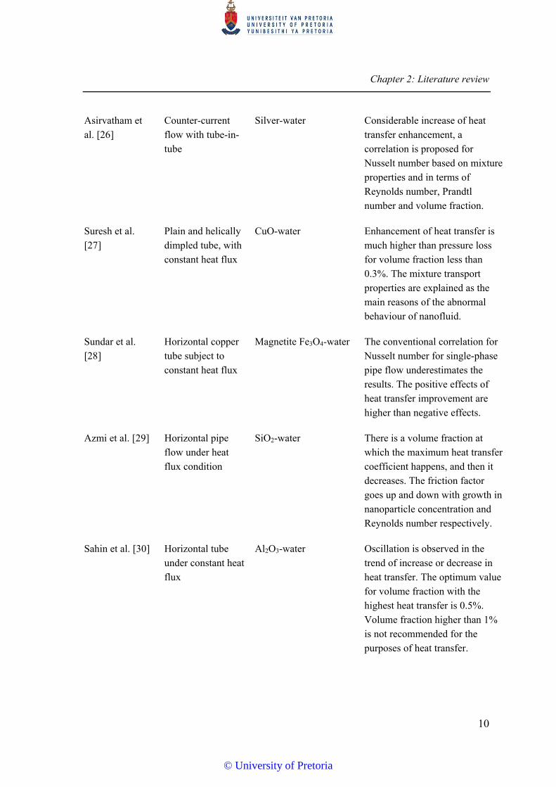
Asirvatham et al. [26]
Counter-current flow with tube-in-tube
Silver-water Considerable increase of heat transfer enhancement, a correlation is proposed for Nusselt number based on mixture properties and in terms of Reynolds number, Prandtl number and volume fraction.
Suresh et al. [27]
Plain and helically dimpled tube, with constant heat flux
CuO-water Enhancement of heat transfer is much higher than pressure loss for volume fraction less than 0.3%. The mixture transport properties are explained as the main reasons of the abnormal behaviour of nanofluid.
Sundar et al. [28]
Horizontal copper tube subject to constant heat flux
Magnetite Fe3O4-water The conventional correlation for Nusselt number for single-phase pipe flow underestimates the results. The positive effects of heat transfer improvement are higher than negative effects.
Azmi et al. [29] Horizontal pipe flow under heat flux condition
SiO2-water There is a volume fraction at which the maximum heat transfer coefficient happens, and then it decreases. The friction factor goes up and down with growth in nanoparticle concentration and Reynolds number respectively.
Sahin et al. [30] Horizontal tube under constant heat flux
Al2O3-water Oscillation is observed in the trend of increase or decrease in heat transfer. The optimum value for volume fraction with the highest heat transfer is 0.5%. Volume fraction higher than 1% is not recommended for the purposes of heat transfer.
© University of Pretoria
Chapter 2: Literature review
11
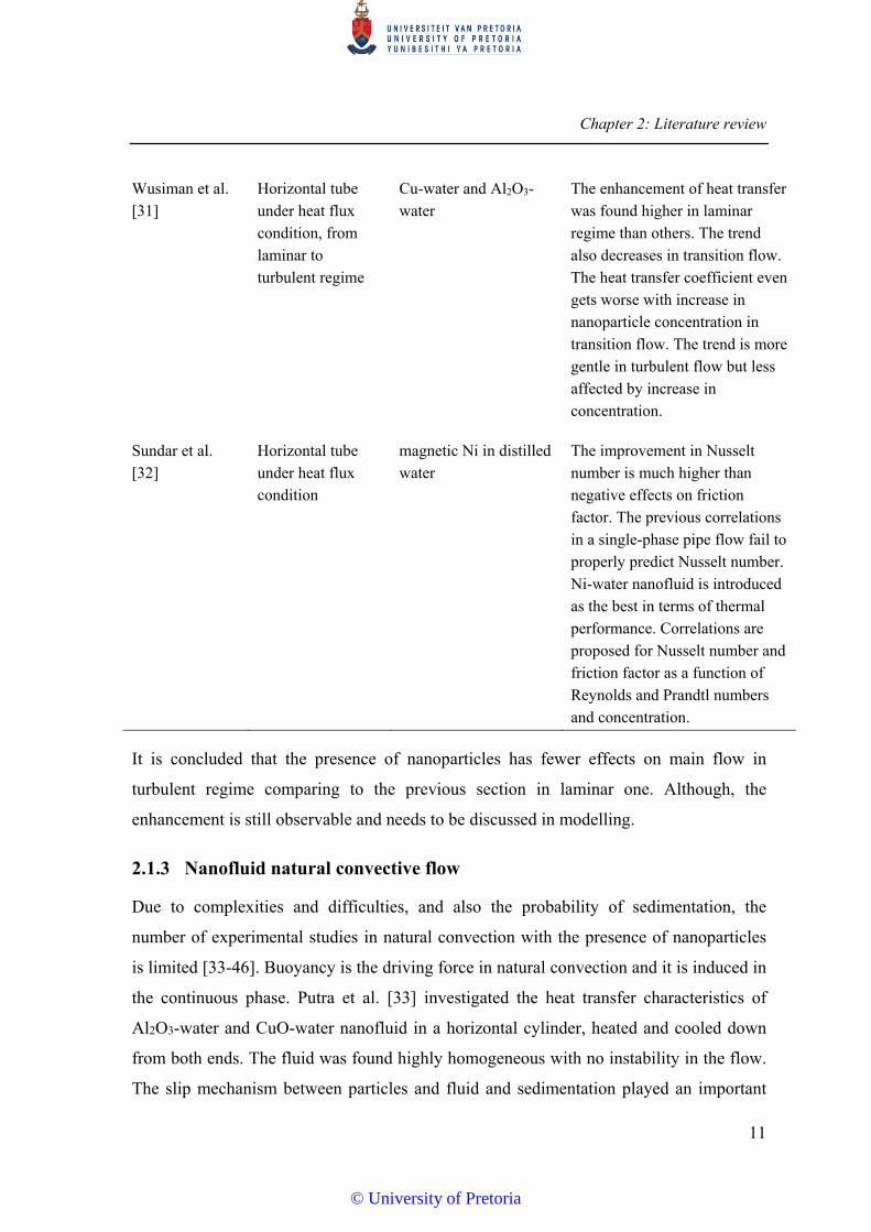
Wusiman et al. [31]
Horizontal tube under heat flux condition, from laminar to turbulent regime
Cu-water and Al2O3-water
The enhancement of heat transfer was found higher in laminar regime than others. The trend also decreases in transition flow. The heat transfer coefficient even gets worse with increase in nanoparticle concentration in transition flow. The trend is more gentle in turbulent flow but less affected by increase in concentration.
Sundar et al. [32]
Horizontal tube under heat flux condition
magnetic Ni in distilled water
The improvement in Nusselt number is much higher than negative effects on friction factor. The previous correlations in a single-phase pipe flow fail to properly predict Nusselt number. Ni-water nanofluid is introduced as the best in terms of thermal performance. Correlations are proposed for Nusselt number and friction factor as a function of Reynolds and Prandtl numbers and concentration.
It is concluded that the presence of nanoparticles has fewer effects on main flow in
turbulent regime comparing to the previous section in laminar one. Although, the
enhancement is still observable and needs to be discussed in modelling.
2.1.3 Nanofluid natural convective flow
Due to complexities and difficulties, and also the probability of sedimentation, the
number of experimental studies in natural convection with the presence of nanoparticles
is limited [33-46]. Buoyancy is the driving force in natural convection and it is induced in
the continuous phase. Putra et al. [33] investigated the heat transfer characteristics of
Al2O3-water and CuO-water nanofluid in a horizontal cylinder, heated and cooled down
from both ends. The fluid was found highly homogeneous with no instability in the flow.
The slip mechanism between particles and fluid and sedimentation played an important
© University of Pretoria

Chapter 2: Literature review
12
role. Deterioration in heat transfer was observed in all the cases, depending on the
density, concentration and aspect ratio of the cylinder.
Nanofluid natural convective flow between two circular disks was experimentally studied
by Wen and Ding [34]. Titanium dioxide nanoparticles with the nominal size of 34 nm
were mixed with water. After providing the nanofluid at a given concentration and size
measurement, the average size was observed to be 170 nm, which was much higher than
the nominal size. To stabilise the nanoparticles inside the liquid, the pH was set around 3
with zeta potential from 25 to 50 mV. The negative impacts of nanoparticles on heat
transfer were seen in any concentration compared with those for pure water. Also, the
Nusselt number dropped with an increase in concentration, even as small as 0.19% vol.
Nnanna [35] conducted an experimental study in a vertically heated cavity with
isothermal walls and alumina nanofluid up to 8% vol. in the laminar regime. The
enhancement of the Nusselt number was reported for volume fraction up to 2%, and then
it decreased. The trend for the Nusselt number indicated that it highly depended on
volume fraction, even at small changes of concentration. A correlation for the Nusselt
number was proposed in terms of Rayleigh number and volume fraction.
Alumina nanofluid with 250 nm in size was used in two cavities with an aspect ratio of
10.9 and 50.7 under the laminar regime at different inclination angles by Chang et al.
[36]. In a vertical situation, no dependency on nanoparticle concentration was observed
by the Nusselt and Rayleigh numbers, while the Nusselt number decreased with changes
in inclination angle and increase in particle concentration compared with the conditions
for pure water. The abnormal behaviour of heat transfer in the cavity was due to the size
of the nanoparticles and the possibility of sedimentation at higher volume fraction.
Thermophoresis was also mentioned as being important only for particle size less than
100 nm.
Li and Peterson [37] explained some of the main phenomena causing deterioration in heat
transfer in the natural convective regime. They used alumina nanofluid up to 6% vol. in a
rectangular enclosure. On the other hand, the visualisation of the flow and thermal
patterns was conducted by polystyrene-water with 850 nm in size. Some of the reasons
© University of Pretoria
Chapter 2: Literature review
13
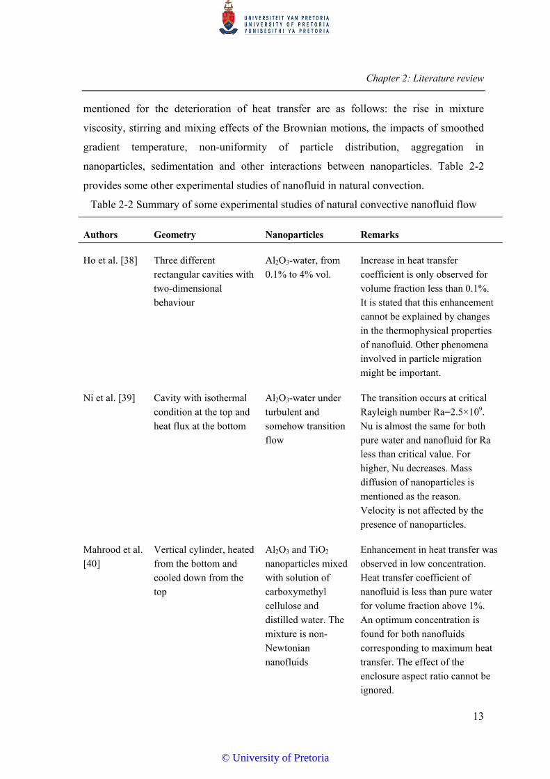
mentioned for the deterioration of heat transfer are as follows: the rise in mixture
viscosity, stirring and mixing effects of the Brownian motions, the impacts of smoothed
gradient temperature, non-uniformity of particle distribution, aggregation in
nanoparticles, sedimentation and other interactions between nanoparticles. Table 2-2
provides some other experimental studies of nanofluid in natural convection.
Table 2-2 Summary of some experimental studies of natural convective nanofluid flow
Authors Geometry Nanoparticles Remarks
Ho et al. [38] Three different rectangular cavities with two-dimensional behaviour
Al2O3-water, from 0.1% to 4% vol.
Increase in heat transfer coefficient is only observed for volume fraction less than 0.1%. It is stated that this enhancement cannot be explained by changes in the thermophysical properties of nanofluid. Other phenomena involved in particle migration might be important.
Ni et al. [39] Cavity with isothermal condition at the top and heat flux at the bottom
Al2O3-water under turbulent and somehow transition flow
The transition occurs at critical Rayleigh number Ra=2.5×10⁹. Nu is almost the same for both pure water and nanofluid for Ra less than critical value. For higher, Nu decreases. Mass diffusion of nanoparticles is mentioned as the reason. Velocity is not affected by the presence of nanoparticles.
Mahrood et al. [40]
Vertical cylinder, heated from the bottom and cooled down from the top
Al2O3 and TiO2 nanoparticles mixed with solution of carboxymethyl cellulose and distilled water. The mixture is non-Newtonian nanofluids
Enhancement in heat transfer was observed in low concentration. Heat transfer coefficient of nanofluid is less than pure water for volume fraction above 1%. An optimum concentration is found for both nanofluids corresponding to maximum heat transfer. The effect of the enclosure aspect ratio cannot be ignored.
© University of Pretoria
Chapter 2: Literature review
14
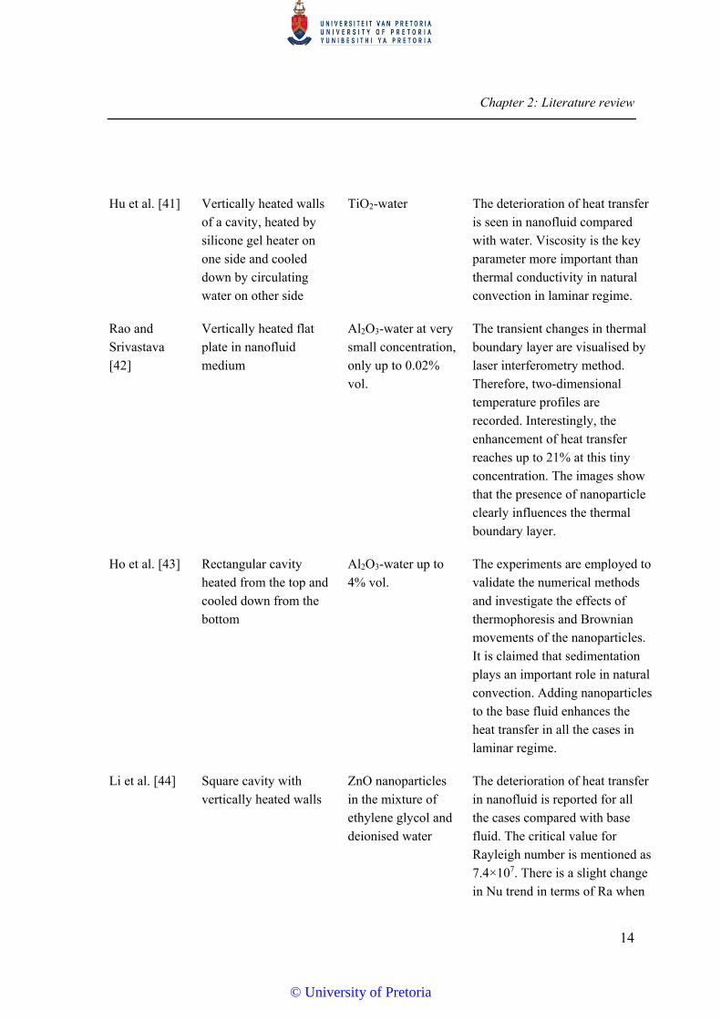
Hu et al. [41] Vertically heated walls of a cavity, heated by silicone gel heater on one side and cooled down by circulating water on other side
TiO2-water The deterioration of heat transfer is seen in nanofluid compared with water. Viscosity is the key parameter more important than thermal conductivity in natural convection in laminar regime.
Rao and Srivastava [42]
Vertically heated flat plate in nanofluid medium
Al2O3-water at very small concentration, only up to 0.02% vol.
The transient changes in thermal boundary layer are visualised by laser interferometry method. Therefore, two-dimensional temperature profiles are recorded. Interestingly, the enhancement of heat transfer reaches up to 21% at this tiny concentration. The images show that the presence of nanoparticle clearly influences the thermal boundary layer.
Ho et al. [43] Rectangular cavity heated from the top and cooled down from the bottom
Al2O3-water up to 4% vol.
The experiments are employed to validate the numerical methods and investigate the effects of thermophoresis and Brownian movements of the nanoparticles. It is claimed that sedimentation plays an important role in natural convection. Adding nanoparticles to the base fluid enhances the heat transfer in all the cases in laminar regime.
Li et al. [44] Square cavity with vertically heated walls
ZnO nanoparticles in the mixture of ethylene glycol and deionised water
The deterioration of heat transfer in nanofluid is reported for all the cases compared with base fluid. The critical value for Rayleigh number is mentioned as 7.4×10⁷. There is a slight change in Nu trend in terms of Ra when
© University of Pretoria
Chapter 2: Literature review
15
it is below or above critical value.
Moradi et al. [45]
Vertical cylindrical enclosure heated from the bottom and cooled down from the top
Al2O3 and TiO2 nanopartilces in water
The effects of nanoparticles in water on heat transfer are small or deteriorated. The enhancement may only be seen in low Ra. The impacts of changes in inclination angle are noticeable.
Rao and Srivastava [46]
Vertically heated wall cavity, hot and cold walls at the bottom and top respectively.
Al2O3-water up to 0.04% vol.
The presence of nanoparticles has considerable positive effects on heat transfer. Nanoparticles clearly change thermal field of the fluid. Roll-like structures appear or break into smaller structures with changes in concentration. This eventually enhances the heat transfer.
In conclusion, even though the negative impacts of nanoparticles in base fluid was observed in some experiments, it is worthwhile to make an attempt to find the areas that enhancement can be achieved regarding to particles type and size. Theoretical modelling can be recommended in this matter.
THEORETICAL STUDIES OF NANOFLUID
A large part of the theoretical analysis of nanofluid is associated with numerical
simulations. Other theoretical works are concerned with the modelling of transport
properties of nanofluid to be employed for numerical purposes. Therefore, two main
approaches should be studied. First, both nanoparticles and base fluid are assumed
continuous phase and the conventional Navier-Stokes is valid for both of them. The only
interaction between them is the slip mechanism. This approach is the most common
numerical approach in terms of numerical simulations of nanofluid. Second, the base fluid
is considered the only continuous phase and nanoparticle is assumed to be a discrete
phase. The second approach is still undeveloped and needs many phenomena involved.
Hence, only a few studies are available and more are definitely needed.
© University of Pretoria
Chapter 2: Literature review
16
One of the most applicable models based on the first approach mentioned above is the
mixture model from multiphase models. This model will be extensively explained in the
next chapter. Also, some reports are available which consider only the single-phase
equations with nanofluid mixture properties. Many researchers have used the mixture and
single phase models to simulate nanofluid in different flow regimes [47-61].
Xuan and Roetzel [47] explain that many phenomena are involved in particle-fluid
interactions such as gravity, friction force between the fluid and solid particles, Brownian
force and Brownian diffusion, sedimentation, aggregation, collision, clustering and
dispersion. They used single-phase equations in their model, considering nanofluid
mixture properties from some previous analytical models. They introduced a new
parameter in energy equation as the total thermal dispersion coefficient. It included both
effects of thermal diffusivity of the flow or conduction and thermal dispersion or
diffusion of the nanoparticles in both laminar and turbulent flow. They stated that their
proposed approach was not complete and further development was needed in the special
case of ultrafine particles.
Maiga et al. [48] considered nanofluid as a highly homogeneous single-phase fluid in a
laminar pipe flow and only used mixture thermophysical properties from previous
classical correlations in their equations. Alumina nanofluid was mixed in two different
base fluids, water and ethylene glycol. They assumed that there was no concentration
gradient in the nanofluid and that nanoparticles were uniformly distributed. This
assumption is, however, contrary to some experimental observations and theoretical
analyses [42, 46, 47].
Buongiorno [49] used scale analysis to show that the slip velocity between nanoparticle
and fluid was negligible and only the mass diffusion of the particles was important in
thermal transport. He states that, firstly, the nanoparticles can be treated as continuum
because of the small Knudsen number. Secondly, the slip mechanisms due to the inertia
of the nanoparticles, diffusiophoresis, Magnus effect, wall lubrication and gravity can be
neglected. Only diffusion due to thermophoresis and Brownian was mentioned scalable in
nanofluid. Therefore, the momentum equation was written similar to the single-phase
© University of Pretoria
Chapter 2: Literature review
17
flow and the energy equation contained the effects of the particle thermal diffusion into
the base fluid. Also, the mass equation for the nanofluid was solved similar to the
continuty for the fluid considering the influences of the diffusion terms. Buongiorno [49]
shows that the turbulent diffusivity is stronger than Brownian concentration diffusion in
turbulent flow and should be considered in equations. Some other theoretical and
numerical analyses of nanofluid are explained in Table 2-3.
Table 2-3 Summary of some theoretical studies of nanofluid flows
Authors Geometry and model Nanoparticles Remarks
Akbarinia and Laur [50]
A circular curved tube with laminar regime. The default
mixture model in ANSYS-Fluent was employed. The slip
velocity was the default function, only considering the effects of gravity and centrifugal force.
Alumina nanofluid up to 1% vol.
The impact of nanoparticle diameter was investigated, from 10 nm to 30 μm. Nanoparticle distribution was reported uniform at small diameter, while it was non-uniform at higher size and concentrated to the outer bend of the tube. They concluded that nanofluid was completely homogeneous.
Bianco et al. [51]
Turbulent flow in a tube with constant heat flux. Both single- and mixture phase models were used. The mixture model
was the default from ANSYS-Fluent and no contribution to
the model. The thermophysical properties were borrowed from literature.
Alumina nanofluid
The numerical simulation was validated by the previous studies of heat transfer in a pipe flow without particles. The concentration distribution was observed close to the wall.
Moghari et al. [52]
Laminar conjugate convective flow in an annulus. The default
mixture model from ANSYS-Fluent was employed. More
complicated nanofluid properties from literature were used. No contribution to the model.
Alumina nanofluid
Heat transfer enhancement was observed with increase in concentration and not much negative effects on pressure loss.
© University of Pretoria

Chapter 2: Literature review
18
Haddad et al. [53]
A cavity with heated and cooled walls at the bottom and top respectively. Concentration and thermophoretic diffusion terms were implemented in energy and mass equations. No-slip velocity was considered in momentum equation. The validation was done by comparing with other numerical studies of nanofluid.
Alumina nanofluid
The effects of nanoparticle concentration and temperature gradients on simulation results of heat transfer were found surprisingly noticeable.
Pakravan and Yaghoubi [54]
Laminar cavity flow. Mixture model was used considering the concentration and thermophoretic diffusion terms as slip mechanisms. High resolution in grid generation was necessary.
Alumina nanofluid
Distribution of nanoparticles in the cavity was observed. The drops in Nusselt number due to increase in volume fraction were considerable. Thermophoretic coefficient was the key parameter in simulations.
Di Schio et al. [55]
Laminar channel flow. Concentration and thermophoretic diffusion terms were implemented in energy and mass equations. No-slip mechanisms in equations.
Alumina nanofluid
There was a noticeable distribution of nanoparticle concentration. The thermophoresis and the Brownian diffusion were found important terms in simulations of nanofluid.
Shariat et al. [56]
Laminar mixed convection in an elliptic duct. The default
mixture model from ANSYS-Fluent was employed. The
simulation results were validated by previous studies for duct flow without particles. No contribution to the model.
Alumina nanofluid
Brownian motions were considered through thermal conductivity of the nanofluid. A weak concentration gradient was seen in the duct cross-sections. The effect of particle size was studied.
Goodarzi et al. [57]
A cavity with heated and cooled walls at the bottom and top respectively. The default
mixture model from ANSYS-
Cu-water nanofluid
Validated by previous studies without nanoparticles. Different turbulent models were investigated.
© University of Pretoria
Chapter 2: Literature review
19
Fluent was employed. No
contribution to the model.
Hejazian et al. [58]
Turbulent mixed convection tube flow. Both Euler and mixture models from multi-phase approach were employed. The default models
from ANSYS-Fluent were
used. No contribution to the models.
Alumina nanofluid
Not much difference was found between the prediction of both models. Mixture model was recommended for the case of nanofluid simulations.
Abbassi et al. [59]
Vertical annulus with cosine heat flux at inner-tube wall. The default mixture model
from ANSYS-Fluent was
employed. No contribution to the models.
Alumina nanofluid
Increase in concentration led to increase in heat transfer coefficient and decrease in Nusselt number.
Garoosi et al. [60]
Mixed convection of nanofluids in a square cavity with internal and external heating. The default mixture
model from ANSYS-Fluent was employed. No contribution to the models.
Cu- and TiO2-water nanofluid
It was found that in each case, a volume fraction corresponded to the maximum amount of Nusselt number. The drag and gravity forces can be important in some cases.
Kakaç and Pramuanjaroe-nkij [61]
Single-phase and two-phase models. Review paper.
The most recent review of nanofluid simulations.
Due to many solid-liquid interactions involved in nanofluid medium, there are a few studies of discrete phase model in literature, explained in Table 2-4.
Table 2-4 Summary of theoretical studies of discrete phase modelling of nanofluid flows
Authors Geometry and model Particles Remarks
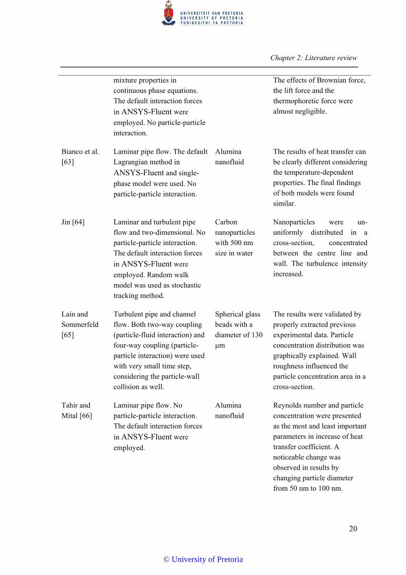
He et al. [62] Laminar tube flow. The Lagrangian method was used considering the nanofluid
TiO2-water nanofluid
Heat transfer coefficient was more affected by thermal conductivity than viscosity.
© University of Pretoria
Chapter 2: Literature review
20
mixture properties in continuous phase equations. The default interaction forces
in ANSYS-Fluent were
employed. No particle-particle interaction.
The effects of Brownian force, the lift force and the thermophoretic force were almost negligible.
Bianco et al. [63]
Laminar pipe flow. The default Lagrangian method in
ANSYS-Fluent and single-
phase model were used. No particle-particle interaction.
Alumina nanofluid
The results of heat transfer can be clearly different considering the temperature-dependent properties. The final findings of both models were found similar.
Jin [64] Laminar and turbulent pipe flow and two-dimensional. No particle-particle interaction. The default interaction forces
in ANSYS-Fluent were
employed. Random walk model was used as stochastic tracking method.
Carbon nanoparticles with 500 nm size in water
Nanoparticles were un-uniformly distributed in a cross-section, concentrated between the centre line and wall. The turbulence intensity increased.
Laín and Sommerfeld [65]
Turbulent pipe and channel flow. Both two-way coupling (particle-fluid interaction) and four-way coupling (particle-particle interaction) were used with very small time step, considering the particle-wall collision as well.
Spherical glass beads with a diameter of 130 μm
The results were validated by properly extracted previous experimental data. Particle concentration distribution was graphically explained. Wall roughness influenced the particle concentration area in a cross-section.
Tahir and Mital [66]
Laminar pipe flow. No particle-particle interaction. The default interaction forces
in ANSYS-Fluent were
employed.
Alumina nanofluid
Reynolds number and particle concentration were presented as the most and least important parameters in increase of heat transfer coefficient. A noticeable change was observed in results by changing particle diameter from 50 nm to 100 nm.
© University of Pretoria

Chapter 2: Literature review
21
Bahremand et al. [67]
Turbulent flow in a helical coiled tube. CFX-Solver was used for simulation with adding a subroutine using FORTRAN to add Brownian motion.
Water-silver nanofluid
It was found that the single-phase approach underestimated the heat transfer results compared with the experiments, while the results of discrete phase model were almost accurate. The impacts of nanoparticle migration on flow velocity and kinetic energy were small.
In conclusion, literature review in this section shows that there are many other
phenomena involved in nanoparticles interactions and theoretical studies are still in
developing parts. Thus, further investigations are essentially needed concerning to solid-
liquid interactions in nanoscale.
CONCLUSION
An extensive review of nanofluid flow in literature was presented in this section. Broad
ranges of experimental studies on various geometries with different nanoparticles were
explained. Most of the works in forced convection reported enhancement in heat transfer,
while both enhancement and deterioration in heat transfer were observed in natural
convection.
The literature showed that most studies used the multiphase approach and the mixture
model. The available mixture model properly works for liquid-liquid or liquid-gas flows
with high connectivity at the interface. But it seems that due to many phenomena
involved in nanoscale between particles and fluid, it is essential to consider other aspects
of this field. Some examples of these aspects are diffusion due to concentration and
gradient of temperature or slip mechanisms caused by some forces. However, the role of
other forces such as attractive Van der Waals and repulsive electrostatic double-layer
forces and also the substitution of these in mixture equations should be investigated.
Discrete phase modelling or DPM can be the other appropriate approach for nanofluid
simulations. This model was developed for particles in sizes larger than nanoscale. Hence
© University of Pretoria
Chapter 2: Literature review
22
many of the interactions involved in micro-sizes might be negligible in nano-sizes and
other phenomena should be implemented. It was shown that only a few studies were
conducted for nanofluid using this model and not much manipulation of the model in
CFD software. Clustering and sedimentation must also be present in CFD code.
From an experimental aspect, only a few exact measurements of nanofluids are available
in the literature of experimental works showing the precise amount of heat transfer and
hydrodynamic feature enhancement. No studies providing the concentration distribution
during convective heat transfer have been found. Also, the experimental study borrowed
from literature was carefully chosen to cover at least both heat transfer and hydrodynamic
features of the flow with high accuracy. Further experimental studies are recommended.
© University of Pretoria
23
3 CHAPTER 3: METHODOLOGY
INTRODUCTION
The extensive details of the mixture model and discrete phase modelling are explained in
this chapter. As a first step, the governing equations for the multiphase mixture model are
expressed in proper forms. Then, the proposed modifications in the model are added to
the equations. The discrete phase model is subsequently presented considering the
interactions between the particles and liquid.
MULTIPHASE MIXTURE MODEL
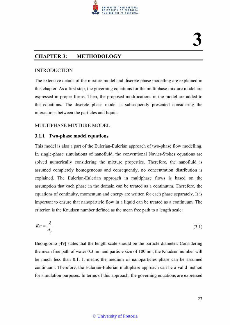
3.1.1 Two-phase model equations
This model is also a part of the Eulerian-Eulerian approach of two-phase flow modelling.
In single-phase simulations of nanofluid, the conventional Navier-Stokes equations are
solved numerically considering the mixture properties. Therefore, the nanofluid is
assumed completely homogeneous and consequently, no concentration distribution is
explained. The Eulerian-Eulerian approach in multiphase flows is based on the
assumption that each phase in the domain can be treated as a continuum. Therefore, the
equations of continuity, momentum and energy are written for each phase separately. It is
important to ensure that nanoparticle flow in a liquid can be treated as a continuum. The
criterion is the Knudsen number defined as the mean free path to a length scale:
p
Knd
(3.1)
Buongiorno [49] states that the length scale should be the particle diameter. Considering
the mean free path of water 0.3 nm and particle size of 100 nm, the Knudsen number will
be much less than 0.1. It means the medium of nanoparticles phase can be assumed
continuum. Therefore, the Eulerian-Eulerian multiphase approach can be a valid method
for simulation purposes. In terms of this approach, the governing equations are expressed
© University of Pretoria

Chapter 3: Methodology
24
for each phase separately and only some source terms and interactions are present in the
equation.
Mass equation for each phase:
( )( )k k
k k k kt
v (3.2)
Because no mass transfer occurs between nanoparticles and fluid (neither produced nor
destroyed), k is zero.
Momentum equation for each phase:
( ) ( ) ( ) ( )k k k k k k k k k k k k kpt
kv v v g Mτ (3.3)
Energy equation:
( ) :kk k k k k k k k k k k k k k k
Dh h p E
t Dt
v q vτ (3.4)
As can be seen, kM and kE are the source terms due to interactions between the two
phases. The details of the derivation of the mentioned equations can be found in a book
by Ishii and Hibiki [68].
3.1.2 Mixture model governing equations
The mixture model is a part of the two-phase model approach in multiphase flows. Strong
coupling between two phases is assumed in this model, which can be the case in
nanofluid flows. It was shown in the previous chapter that most of the studies in
nanofluids were concerned with the mixture model, even though not many developments
have been presented in the model in recent years. Therefore, some ideas and methods are
developed into this model in this research.
The governing equations for each phase are combined with others and new sets of
equations are defined based on mixture variables and properties. The strong coupling can
© University of Pretoria
Chapter 3: Methodology
25
be presented through slip or drift velocity. The mixture model is properly presented as
follows:
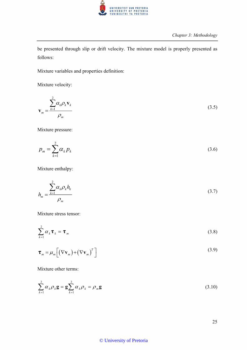
Mixture variables and properties definition:
Mixture velocity:
2
1k k k
km
m
v
v (3.5)
Mixture pressure:
2
1m k k
k
p p
(3.6)
Mixture enthalpy:
2
1k k k
km
m
hh
(3.7)
Mixture stress tensor:
2
1k k m
k
τ τ (3.8)
T
m m m m v vτ
(3.9)
Mixture other terms:
2 2
1 1k k k k m
k k
g g g (3.10)
© University of Pretoria
Chapter 3: Methodology
26
2
1m
k
kM M (3.11)
Mixture continuity equation:
2 2
1 1
( )( ) 0k k
k k kk kt
v (3.12)
( ) 0mm mt
v
(3.13)
The drift and slip velocity are defined as the relative velocity between one phase to the
mixture and two phases respectively:
km k m V v v (3.14)
slip p c v v v (3.15)
Momentum equation of the mixture:
2 2 2
1 1 1
2 2 2
1 1 1
( ) ( ) ( )
( )
k k k k k k k k kk k k
k k k kk k k
pt
k
v v v
g Mτ (3.16)
With manipulation of the terms, the equation should be rearranged based on mixture
variables and properties:
© University of Pretoria
Chapter 3: Methodology
27
2 2
1 1
2 2
1 1
2 2
1 1
2 2 2
1 1 1
( )
( )
k k k k k k k m kmk k
k k k m k k k kmk k
m m m m k k k m k k km kmk k
m m m m k k k m k k m k k km kmk k k
v v v v V
v v v V
v v v v v V V
v v v v v v V V
(3.17)
2 2
1 1k k k k m m m k k km km
k k
v v v v V V (3.18)
Hence a form of the mixture momentum equation is:
2
1
m mm m m m m m m k k km km
k
pt
v
v v g M V Vτ (3.19)
A similar way of derivation was also presented by Ishii and Hibiki [68] and Manninen et
al. [69]. There is only one difference between this version of momentum equation and the
one presented in the ANSYS-Fluent 17.0 Theory guide. The sign of the drift flux on the
right-hand side is positive in the ANSYS-Fluent 17.0 Theory guide (the reason is
unknown to the author). The same problem was found in previous versions and also 16.0
and 17.0, recently released. It was reported to the company anyway.
Because only mixture variables and properties along with the special form of slip velocity
should be present in the momentum equation, further manipulation is needed to replace
the drift flux term.
Relation between two drift velocities:
p pcm pm
c c
V V (3.20)
© University of Pretoria

Chapter 3: Methodology
28
The subscripts p and c represent particle and continuous phase with the definition of drift
mass flux for nanoparticles:
p p p p m J V (3.21)
Thus:
2
(1 )
k k km km c c cm cm p p pm pm
p pc c pm pm p p pm pm
c c
mp p
p p c p
V V V V V V
V V V V
J J
(3.22)
The final form of the momentum equation reaches to:
(1 )
m mm m m m m m m
mp p
p p c p
pt
vv v g M
J J
τ
(3.23)
The drift flux can be rewritten in terms of slip velocity as:
c cpm slip
m
V v (3.24)
The energy equation of the mixture obtains from the combination of the energy equation
for each phase:
2 2 2 2
1 1 1 1
2 2
1 1
( )
:
kk k k k k k k k k k k
k k k k
k k k kk k
Dh h p
t Dt
E
v q
vτ (3.25)
© University of Pretoria
Chapter 3: Methodology
29
The second and third terms on the right-hand side are the net mechanical works and the
fourth term is the net energy transfer between two phases.
The mixture variables are:
2
1k k k m m
k
h h
(3.26)
2
1k k m
k
q q (3.27)
2
1k m
k
E E
(3.28)
Then, based on drift flux model:
2 2
1 1
2
1
( )k k k k k k m km kk k
m m m k k km kk
h h
h h
v v V
v V
(3.29)
k k km k c c cm c p p pm p
p pc c pm c p p pm p
c c
p p c
h h h
h h
h h
V V V
V V
J
(3.30)
The general form reaches to:
2
1
2
1
( )
:
km m m m m m k k
k
k k k m p p ck
Dh h p
t Dt
E h h
v q
v Jτ
(3.31)
© University of Pretoria
Chapter 3: Methodology
30
Some simplification can be mentioned here: due to the ranges of velocity and shear
stresses, the mechanical works can be ignored; the net heat transfer between nanoparticles
and fluid can be zero; the thermodynamic equilibrium can be applied, i.e. ph C T and
p c mT T T [69].
3.1.3 Constitutive equations of mixture
Due to newly defined variables in mixture equations, some closure relations are needed to
reach the adequate number of equations.
Equation of volume fraction:
2
1
1k p ck
(3.32)
Mass balance for nanoparticles with constant density:
( ) 0pp pt
v
(3.33)
1
pp m p pm
pp
t
v V
J
(3.34)
The other forms of this equation can be found in [69]. The key parameter in the mixture
model is slip velocity, which is explained in the following section.
3.1.4 Slip mechanisms in the mixture model
Slip velocity is the relative velocity between the nanoparticles and the fluid in which they
are immersed. Typically, the slip velocity should include all the slip mechanisms involved
in the phase interface. The algebraic form of the slip velocity used in ANSYS-Fluent only
covers gravitational and centrifugal effects. Therefore, other phenomena in nanoscale
ranges should be implemented. The slip velocity used in ANSYS-Fluent:
© University of Pretoria
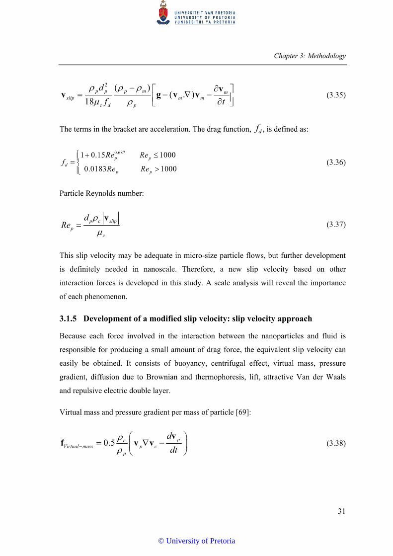
Chapter 3: Methodology
31
2 ( )( . )
18p p p m m
slip m mc d p
d
f t
vv g v v (3.35)
The terms in the bracket are acceleration. The drag function, df , is defined as:
0.6871 0.15 1000
0.0183 1000
p p
d
p p
Re Ref
Re Re
(3.36)
Particle Reynolds number:
p c slip
pc
dRe
v
(3.37)
This slip velocity may be adequate in micro-size particle flows, but further development
is definitely needed in nanoscale. Therefore, a new slip velocity based on other
interaction forces is developed in this study. A scale analysis will reveal the importance
of each phenomenon.
3.1.5 Development of a modified slip velocity: slip velocity approach
Because each force involved in the interaction between the nanoparticles and fluid is
responsible for producing a small amount of drag force, the equivalent slip velocity can
easily be obtained. It consists of buoyancy, centrifugal effect, virtual mass, pressure
gradient, diffusion due to Brownian and thermophoresis, lift, attractive Van der Waals
and repulsive electric double layer.
Virtual mass and pressure gradient per mass of particle [69]:
0.5 pcVirtual mass p c
p
d
dt
vf v v (3.38)
© University of Pretoria
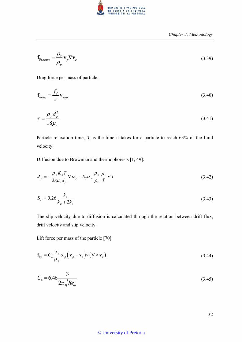
Chapter 3: Methodology
32
Prc
essure p cp
f v v (3.39)
Drag force per mass of particle:
ddrag slip
f
f v (3.40)
c
ppd
18
2
(3.41)
Particle relaxation time, , is the time it takes for a particle to reach 63% of the fluid
velocity.
Diffusion due to Brownian and thermophoresis [1, 49]:
3p B p c
p p T pc p c
K TS T
d T
J (3.42)
cp
cT kk
kS
226.0
(3.43)
The slip velocity due to diffusion is calculated through the relation between drift flux,
drift velocity and slip velocity.
Lift force per mass of the particle [70]:
clift L p p c c
p
C
f v v v (3.44)
36 46
2LC .
Re (3.45)
© University of Pretoria
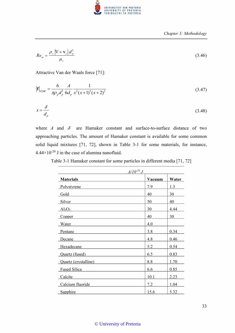
Chapter 3: Methodology
33
2c c p
c
dRe
v (3.46)
Attractive Van der Waals force [71]:
3 2 3 2
6 1
6 ( 1) ( 2)VDWp p p
A
d d x x x
f (3.47)
p
xd
(3.48)
where A and are Hamaker constant and surface-to-surface distance of two
approaching particles. The amount of Hamaker constant is available for some common
solid liquid mixtures [71, 72], shown in Table 3-1 for some materials, for instance,
4.44×10⁻²⁰ J in the case of alumina nanofluid.
Table 3-1 Hamaker constant for some particles in different media [71, 72]
A/10-20 J
Materials Vacuum Water
Polystyrene 7.9 1.3
Gold 40 30
Silver 50 40
Al2O3 30 4.44
Copper 40 30
Water 4.0
Pentane 3.8 0.34
Decane 4.8 0.46
Hexadecane 5.2 0.54
Quartz (fused) 6.5 0.83
Quartz (crystalline) 8.8 1.70
Fused Silica 6.6 0.85
Calcite 10.1 2.23
Calcium fluoride 7.2 1.04
Sapphire 15.6 5.32
© University of Pretoria

Chapter 3: Methodology
34
Poly (methyl methacrylate) 7.1 1.05
Poly (vinyl chloride) 7.8 1.30
Polyisoprene 6.0 0.74
Poly (tetrafluoroethylene) 3.8 0.33
Electrical double-layer repulsion force:
20 exp( )R p rV d 10pd (3.49)
20 1 ( )R p rV d Ln exp 10pd (3.50)
3
6 REDL
p p
dV
d d f (3.51)
where RV is the repulsion energy on the surface of a particle. The amount of vacuum and
relative permittivity of the medium is 1 1
0-128.854×10 CV m and r=80 for water
respectively. is the potential on the surface of the electrical double layer over charged
surface group, which can be approximated by zeta potential on the surface of the diffuse
layer. Because the small zeta potential means fewer repulsion barriers and consequently
produces stronger agglomeration inside the nanofluid, the approaching potential to zero is
avoided in all the simulations. is Debye-Huckel parameter and defined as:
RT
IF
r
0
022000
(3.52)
1 1 1,F 96485 Cmol R 8.31 Jmol K
where F and R are Faraday and gas universal constants. The ionic strength is simply
calculated by knowing the concentration (ci) and the charge (zi) of the species. With the
assumption of the presence of only two ions (H+ and OH-) in the mixture, it gives:
© University of Pretoria
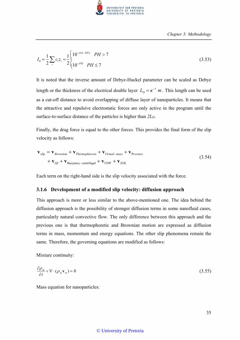
Chapter 3: Methodology
35
710
710
2
1
2
1)14(
0
PH
PHzcI
PH
PH
iii (3.53)
It is noted that the inverse amount of Debye-Huckel parameter can be scaled as Debye
length or the thickness of the electrical double layer mLD1 . This length can be used
as a cut-off distance to avoid overlapping of diffuse layer of nanoparticles. It means that
the attractive and repulsive electrostatic forces are only active in the program until the
surface-to-surface distance of the particles is higher than 2LD.
Finally, the drag force is equal to the other forces. This provides the final form of the slip
velocity as follows:
Pr
Buoyancy centrifugal
slip Brownian Thermophoresis Virtual mass essure
lift VDW EDL
v v v v v
v v v v (3.54)
Each term on the right-hand side is the slip velocity associated with the force.
3.1.6 Development of a modified slip velocity: diffusion approach
This approach is more or less similar to the above-mentioned one. The idea behind the
diffusion approach is the possibility of stronger diffusion terms in some nanofluid cases,
particularly natural convective flow. The only difference between this approach and the
previous one is that thermophoretic and Brownian motion are expressed as diffusion
terms in mass, momentum and energy equations. The other slip phenomena remain the
same. Therefore, the governing equations are modified as follows:
Mixture continuity:
( ) 0mm mt
v (3.55)
Mass equation for nanoparticles:
© University of Pretoria

Chapter 3: Methodology
36
22.( ) .( )p
p p m p p pm p B p T
TD D
t T
v V (3.56)
0.262
c cT p
p c c
kD
k k
(3.57)
pc
BB d
TKD
3 (3.58)
Momentum equation of the mixture:
.( ) . .
(1 )p p mm m
m m m m m m pm pmp c
P gt
vv v V V (3.59)
Energy equation of the mixture:
.( ) . . ( )
..
m p c
p
m p m m m p p pm m p p
p p B T
C T T C C
T TC D T D
T
v q V
(3.60)
The source terms in all the equations are implemented through some UDFs in ANSYS-
Fluent.
3.1.7 Mixture thermophysical properties
Due to buoyancy effects of the base fluid in natural convection, a high accurate density
correlation by curve fitting from Kröger [73] for water was employed in all the equations:
3 2c 0.0000152322T - 0.0183891979T + 6.6564073561T
+ 243.4039040229
(3.61)
The linear combination of density for nanoparticles and base fluid is the most common
and highly valid assumption in the mixture properties.
© University of Pretoria
Chapter 3: Methodology
37
2
1kkkm (3.62)
m
kPkk
P
k
m
CC
2
1
(3.63)
Michaelides [74] shows that the thermal expansion coefficient of the nanofluid mixture
must be calculated in the same way as the density. Considering the element changes of
temperature and volume under constant pressure leads to:
1
P
V
V T
(3.64)
(1 )p p p c c pV V T and V V T (3.65)
and a linear summation of the element volume:
(1 )p p c pV V T (3.66)
1(1 )m p p c p
P
V
V T
(3.67)
The transport properties of the nanofluid viscosity and thermal conductivity are borrowed
from reference [75]:
10
0 .4 0 .66 0 .661+ 4 .4 pmp
c fr c
kk TR e P r
k T k
(3.68)
c B pB
c
u dRe
(3.69)
© University of Pretoria
Chapter 3: Methodology
38
2
2
pc
BB d
TKu
(3.70)
0.3 1.03
1
1 34.87
m
c p c pd d
(3.71)
where frT and cd are water freezing temperature and molecule diameter as 0.3nm. These
correlations were presented to be valid for different types of nanoparticles, such as
alumina, copper, TiO2, SiO2, etc. Also, the size can go up to more than 200 nm and
volume fraction up to 7% vol.
ANSYS-Fluent is employed to simulate the nanofluid. All the above-mentioned slip
mechanisms are implemented as a new slip velocity equation into the mixture model
through the user-defined function (UDF). The UDF is divided into three sections: adjust
function to define gradient of concentration, slip velocity function and mixture
thermophysical properties. The mixture model UDF is presented in Appendix A.
DISCRETE PHASE MODELLING (DPM)
The basic difference between this model and the mixture model is that DPM assumes
there is only base fluid as the continuous phase and the nanoparticles are non-continuous
suspended in the fluid. In DPM, nanoparticles are tracked as a large number of particles
and all the energy or force interactions are introduced as momentum or energy source
terms in the governing equations. The rest of the Navier-Stokes equations are treated as
usual for the base fluid. A differential form of force balance equation is applied to a
particle suspended in the flow to calculate the trajectory of the particle. Here, the focus is
only on the interaction forces and particle equation because the flow equations are similar
to those of the single-phase model.
The forces on a particle in a fluid can be categorised into three sections: the forces
between particles such as electrostatic forces, the interaction forces between nanoparticles
and fluid such as drag, the interaction forces between nanoparticles and walls.
© University of Pretoria

Chapter 3: Methodology
39
Due to the small size, it can be expected that the nanoparticles mostly follow the base
flow regime and two situations can be presumed for the particles at the vicinity of the
walls. They can either stick on or fully rebound from the walls. The sticking situation can
happen when clustering occurs in the main flow, otherwise the rebound situation would
apply.
There are many interactions between fluid and nanoparticles. All the forces along with
particle-particle forces are solved in Newton’s equation of the motion for a single particle
and the results are extended to the rest of the particles. The possible affecting forces are
explained here. Newton’s equation of force balance in Lagrangian frame for nanoparticles
is written as:
( )p p nfp drag p lift virtua l M agnus
p p
therm o B V D W E D L
d gm m
dt
vF F F F
F F F F
(3.72)
tp is the travelling time of a nanoparticle from the point of injection until it reaches its
final fate in the domain (sticking on a wall or leaving the domain).
3.1.8 Forces between particles
The main attraction forces between particles can be divided into a short range due to
chemical reactions and a long range by Van der Waals forces. The long range forces are
only present for particle-particle distance much more than 1 °A. This force is caused by
the fluctuating of negative electrons around a positive nucleus in an atom, which induces
constant changing dipole moments and electric fields. Eventually, the interactions
between magnetic fields will lead to the Van der Waals attraction forces. The impact
distances of Van der Waals force can be much higher than the London and Lifshitz theory
of distances, from 1 nm to 100 nm [76]. Three types of Van der Waals forces are found in
literature [76]: Keesom-orientation force from interactions of randomly orienting dipole-
dipole, Debeye-induction force between dipoles and induced dipoles, London-dispersion
force from fluctuating dipole-induced dipole. Among all, the first two are the result of
molecules with permanent dipole movements. Because the last force is bigger than the
© University of Pretoria
Chapter 3: Methodology
40
others, it will be taken into account in simulations. The Van der Waals force can be
expressed in terms of Lifshitz Van der Waals constant. This constant is linearly connected
to the Hamaker constant, which will be used in this study. The attraction force is similar
to equation (3.47) for two-sphere particles. At the limit as the particles approach each
other, it can be rewritten as:
224VDWp
A
d xF (3.73)
and for a particle approaching a flat wall:
212VDWp
A
d xF (3.74)
The other particle-to-particle force is the repulsive electrical double-layer force, as
presented in equations (3.49) (3.50) and (3.51).
The combination of the mentioned forces is a part of DLVO theory as explained by [77].
Because one of the forces is attractive and the other one is repulsive, the net of them will
be applied.
3.1.9 Forces induced by the presence of fluid
Drag force:
The correlation of drag force should be the same everywhere in the domain because of the
small size of the nanoparticles.
24
p D pdrag c p
c
m C Re
C F v v (3.75)
c p c p
pc
dRe
v v (3.76)
Drag coefficient for a smooth spherical particle is introduced as:
© University of Pretoria
Chapter 3: Methodology
41
321D 2
p p
aaC a
Re Re (3.77)
The constant values ia are available for a wide range of Reynolds numbers [78]. Because
the nanoparticles are ultrafine, Rep<<1 and a1=a3=0 and a2=24 give Dp
24C =
Re. The
Cunningham slip correction factor, Cc, is used when the no-slip boundary condition for a
continuum cannot be preserved over a particle or solid wall. Since the Knudsen number in
this study is much less than 0.1 and highly continuum, it gives Cc=1:
0.55- KncC = 1 + K n 2.514 + 0.8e
(3.78)
For non-spherical particles with the sphericity, θ, smaller than unity, the following
expression is used by Haider and Levenspiel [79]:
31
4
24(1 )2 pb
D pp p
b ReC b Re
Re b Re
(3.79)
A
a (3.80)
)4486.24581.63288.2exp( 21 b (3.81)
5565.00964.02 b (3.82)
)2599.104222.188944.13905.4exp( 323 b (3.83)
)8855.157322.20258.124681.1exp( 324 b
(3.84)
where a and Ap are the surface of a spherical particle with the same volume as the actual
particle and surface area of the particle respectively. Basically, the drag force at the
vicinity of a wall would be different from the core region of the fluid, but due to
© University of Pretoria
Chapter 3: Methodology
42
nanoscale size, this can be neglected and only sticking on and rebounding from the wall
would be the case.
Because the centrifugal force (force due to rotating of a particle on a circle) is mainly
caused by the presence of other forces in the flow field, it can be safely ignored in
calculations. On the other hand, the lift induced by the rotation of the particle around its
axis in uniform flow or Magnus force can also be negligible in terms of the nanosize of
the particles. However, it can be important if the flow is highly rotational and the inertia
of the particles is noticeable.
Magnus force. Similar to the force balance equation, the particle angular velocity, pω ,
can be obtained from particle conservation of angular momentum equation as follows
[80]:
5
2 2p pc
p
d dI C
dt
ωΩ (3.85)
As can be seen, similar to Newton’s law of motion, the acceleration of the particle torque
(left-hand side of equation (3.71)) is damped by the rotational drag coefficient, C, and
relative angular velocity of the fluid and particle, Ω :
1
2 c p Ω v ω (3.86)
The moment of inertia for a spherical particle is expressed as:
5
60p p pI d (3.87)
The rotational drag coefficient [81]:
pp
6.45 32.1C
ReRe
(3.88)
© University of Pretoria
Chapter 3: Methodology
43
2
4p
c p
c
dRe
Ω
(3.89)
Therefore, the rotational flow condition is important for the presence of Magnus force in
the solution ( 0p
Re ). The general form of Magnus lift force can be written as:
1
2c p
Magnus p ML c c pA C
v v
F v v ΩΩ
(3.90)
where Ap and CML are projected particle surface area and rotational lift coefficient
respectively. This coefficient is calculated from the following correlation [80]:
0.4 0.30.45 0.45 0.05684 ,10 140p
pML p p
p
ReC exp Re Re Re
Re
(3.91)
c p c p
pc
dRe
v v (3.92)
Another correlation for Magnus force is presented by Varaksin et al. [82]:
3 2
, 12 p
p c pMagnus M c c p p
c
d dk Re
ωF v v ω (3.93)
For the lower limit of Reynolds numbers, it gives Mk . The other general form of the
coefficient:
0.64 0.7150.534pM pk Re Re
(3.94)
Saffman lift force. Due to induced pressure difference on both sides of a particle in a
shear flow, a force known as the Saffman lift force acts on the particle. Because strong
shear stress is mainly found close to walls, the lift force will be perpendicular to the walls,
presented as [70, 83]:
© University of Pretoria

Chapter 3: Methodology
44
220.3 ( ) sgn( )clift c p c p
c
d
F v v (3.95)
where is the shear rate mainly important at the vicinity of the walls.
Pressure gradient force. It comes from any static pressure gradient field in the flow on a
particle [84]:
nfpressure p p c
p
m
F v v (3.96)
Virtual mass force. Changes in the velocity of a mass of the fluid due to acceleration of
particle movement will lead to virtual mass force. This force is available only when the
interactions between particle and fluid are present [84]:
0.5 ( )nfvirtual p c p
p
dm
dt
F v v (3.97)
Thermophoretic force. It is caused by higher kinetic energy of a particle with higher
temperature. It produces stronger movement in one region and finally, the gradient of
temperature will be the driving diffusion force for particles with higher temperature. The
following equation can be the thermophoresis force for particles with lower thermal
conductivity [85]:
thermo T
TD
T
F (3.98)
2c p c
Tc c p
d kD 0 .7 8
2 k k
(3.99)
There is no conclusive agreement on the thermophoretic coefficient in literature,
especially for nanofluids. This coefficient can depend on base fluid, nanoparticles,
thermal conductivity of the particles and temperature. The factor in equation (3.86) was
found to be 0.017 for water-based nanofluid by Ahmed and Eslamian [86], rather than
© University of Pretoria

Chapter 3: Methodology
45
0.78. Michaelides [87] proposes a new form of thermophoresis force based on molecular
dynamic simulation:
2
10
C
p cthermo c p thermo c p
c
d T3 d 3 d C
d T
F v (3.100)
The Ci constants vary depending on the type of nanofluid.
Brownian motion or diffusion force? It is the random motion of particles suspended in a
fluid. It may result in collision among other particles or molecules. Brownian movement
is induced by the kinetic energy or temperature of the particles. There are two approaches
in the literature for this force: Brownian diffusion force [49] and Brownian random force
in the base fluid [88]. The diffusion force approach is expressed as:
Brownian c p diffusion3 dF v (3.101)
p pdiffusion B
p p p
JD
v (3.102)
where D is particle mass diffusivity or diffusion coefficient:
3B
Bc p
K TD
d (3.103)
The other time-averaged Brownian velocity for nanofluids with no effects of random
movement can be written as:
Koo and Kleinstreuer [89]:
3
18 BB
p p
K T
dv (3.104)
Patel et al. [90]:
© University of Pretoria
Chapter 3: Methodology
46
2
2 BB
c p
K T
dv (3.105)
One possibility of modelling the Brownian force can be adding unit-variance Gaussian
random numbers to the Brownian velocity mentioned above.
The other approach to the Brownian force is to consider any motions by a small time step
regarding the acting of the force in arbitrary directions. It is presented as:
6 p c BB i
p
d K T
t
F (3.106)
where i is the unit-variance random number produced by a Gaussian white noise
process. Michaelides [74] obtained a new form of random motion force by solving the
Langevin equation as follows:
33
21
6 3B
B p p ip c p
K Td
d t
F (3.107)
and mean square displacement of the particle:
2.
3B
pp c
K Tt
d x x (3.108)
3.1.10 Energy equation of the nanoparticles
The basic form of the heat transfer equation for a particle in a flow can easily be referred
to as the balance of changes in temperature in the travelling path, known as transient or
Lagrangian frame, and convection on the particles:
( )p
pp p p c p
dTm C hA T T
dt (3.109)
© University of Pretoria

Chapter 3: Methodology
47
Because radiation heat transfer was not investigated in this research, the associated term
was ignored from the equation. This ordinary differential equation can easily be solved to
reach final form of temperature in each time step. Then, it gives:
p
p p p
A ht
m Ct t tp c p cT T T T e
(3.110)
The important parameter is heat transfer coefficient for flow over a spherical particle
[91]:
0.5 1/32.0 0.6pp
c
hdNu Re Pr
k (3.111)
cp c
c
CPr
k
(3.112)
The other less mentioned form of particle heat transfer equation is proposed by
Michaelides and Feng [92]:
2 ( )p c
p cp p c p p c p c
d T D Tm C m C d k T T
d t D t (3.113)
where 31
6c c pm d mc is the mass of the fluid occupying the particle place. The first
term on the right-hand side (material derivative) is the heat transferred by the fluid being
in place of the particle. This term is similar to the virtual mass term in force balance
equation of the particles. The second term is obviously due to heat conduction from the
surface of the nanoparticle. The significance of this term can mainly be seen in the case of
nanosize with small particle Reynolds number and density ratio close to unity. The
solution of this ODE will lead to:
43 3
c tt t tp pT c T c e (3.114)
3 2cc p c
cp c
m C DTc T
d k Dt (3.115)
© University of Pretoria
Chapter 3: Methodology
48
4 2cc p
p c
m Cc
d k (3.116)
3.1.11 Coupling between continuous phase and discrete nanoparticles
It is important to consider the impacts of nanoparticles on the base fluid. In the case of
ignoring this coupling, the nanoparticles will be tracked under the effects of the
mentioned forces during the given time in the domain. Otherwise, the effects of
nanoparticle momentum and energy should be seen in fluid equations as some source
terms. The exchanges of momentum and energy are:
2
18( ( ) )
24D pc
s p c other pp p
C Rem t
d
F v v F (3.117)
)(celloutcellinp pppps TTcmQ
(3.118)
These source terms are presented on the right-hand side of fluid momentum and energy
equations. Because there is no mass exchange, particle flow rate pm in each cell will be
conserved. inpT and
outpT are particle temperature at the inlet and outlet of a cell
respectively. They are calculated according to the time of tracking of the nanoparticles.
3.1.12 Numerical considerations of discrete phase modelling
Both 2D and 3D models were employed in this study for the cases and the results showed
that it was important to use a 3D model in nanofluid flow in some geometries, especially
with the presence of gravity in the Lagrangian approach. It could be argued that 2D
axisymmetric could only capture radial migration of nanoparticles inside the fluid, while
the difference between a 3D model and 2D axisymmetric simulation results proved that
nanoparticles migrated from the wall both radially and tangentially. Also, the simulations
showed that gravity could not be neglected when DPM was used and the absence of
gravity force underestimated pressure drops in, for example, vertical tubes. The CFD
software employed in this research to solve the governing equations was Fluent 15.0,
© University of Pretoria
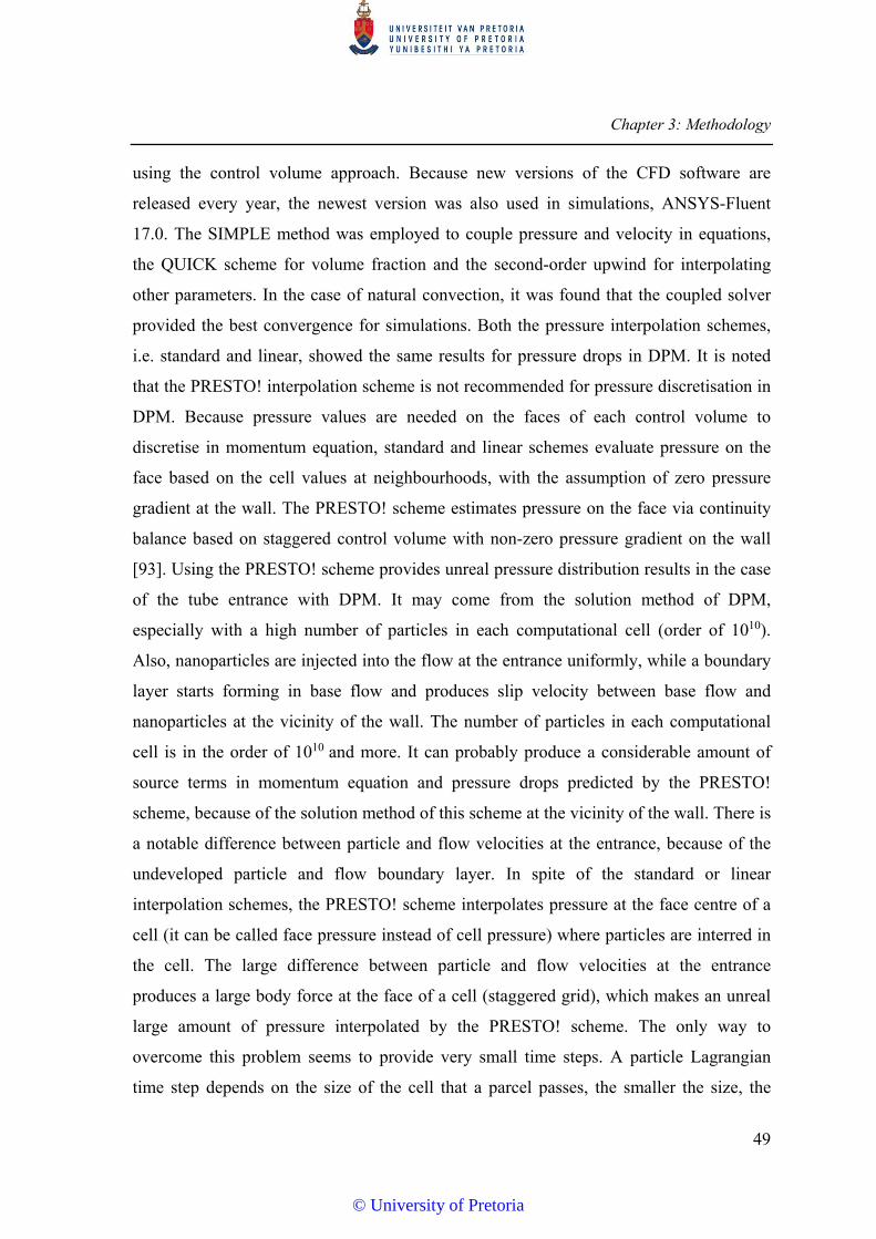
Chapter 3: Methodology
49
using the control volume approach. Because new versions of the CFD software are
released every year, the newest version was also used in simulations, ANSYS-Fluent
17.0. The SIMPLE method was employed to couple pressure and velocity in equations,
the QUICK scheme for volume fraction and the second-order upwind for interpolating
other parameters. In the case of natural convection, it was found that the coupled solver
provided the best convergence for simulations. Both the pressure interpolation schemes,
i.e. standard and linear, showed the same results for pressure drops in DPM. It is noted
that the PRESTO! interpolation scheme is not recommended for pressure discretisation in
DPM. Because pressure values are needed on the faces of each control volume to
discretise in momentum equation, standard and linear schemes evaluate pressure on the
face based on the cell values at neighbourhoods, with the assumption of zero pressure
gradient at the wall. The PRESTO! scheme estimates pressure on the face via continuity
balance based on staggered control volume with non-zero pressure gradient on the wall
[93]. Using the PRESTO! scheme provides unreal pressure distribution results in the case
of the tube entrance with DPM. It may come from the solution method of DPM,
especially with a high number of particles in each computational cell (order of 1010).
Also, nanoparticles are injected into the flow at the entrance uniformly, while a boundary
layer starts forming in base flow and produces slip velocity between base flow and
nanoparticles at the vicinity of the wall. The number of particles in each computational
cell is in the order of 1010 and more. It can probably produce a considerable amount of
source terms in momentum equation and pressure drops predicted by the PRESTO!
scheme, because of the solution method of this scheme at the vicinity of the wall. There is
a notable difference between particle and flow velocities at the entrance, because of the
undeveloped particle and flow boundary layer. In spite of the standard or linear
interpolation schemes, the PRESTO! scheme interpolates pressure at the face centre of a
cell (it can be called face pressure instead of cell pressure) where particles are interred in
the cell. The large difference between particle and flow velocities at the entrance
produces a large body force at the face of a cell (staggered grid), which makes an unreal
large amount of pressure interpolated by the PRESTO! scheme. The only way to
overcome this problem seems to provide very small time steps. A particle Lagrangian
time step depends on the size of the cell that a parcel passes, the smaller the size, the
© University of Pretoria

Chapter 3: Methodology
50
shorter the time step. Simulation showed some improvement with very fine mesh at the
entrance with the PRESTO! scheme, but the geometry required grids with the same size
as DNS to overcome this issue completely, which was not the main goal of this study.
One of the most important rules of the Lagrangian tracking method is that a particle never
skips a computational cell. Hence each computational cell is divided into a number of
sub-cells, known as parcels, based on time steps and the number of steps that a particle
should pass in each cell. A nanoparticle in each parcel is representative of the entire
nanoparticles on that parcel and heat transfer and motion equations are solved only for
this nanoparticle and extended to others. Therefore, the distribution effects of these
nanoparticles on parcels in the neighbourhood are not usually applied to the equations,
which can be called a point-particle approach. For this aim, the node-based averaging
method is employed to consider those influences from the Lagrangian frame onto the
Eulerian field. The Gaussian distribution function is used to interpolate the neighbouring
parcel’s impact on the centroid parcel, as the following [94]:
particlewparticleparcel GN (3.119)
2
22/3
expx
xxa
aG
particleparcel
w (3.120)
where parcel , particleN , wG , particl , x , parcelx and particlex are particle variables affected by
nodes in the neighbourhood (which are 26 cells for the structured quad mesh in three-
dimensional structure meshes), number of particles in the parcel, Gaussian weight
function, particle variable in the node, characteristic length of the cell, parcel location in
the neighbourhood and particle location respectively. a is a constant which changes the
width of Gaussian function. The number of particles in each parcel can be calculated as:
ppparticle m
tmN
(3.121)
© University of Pretoria
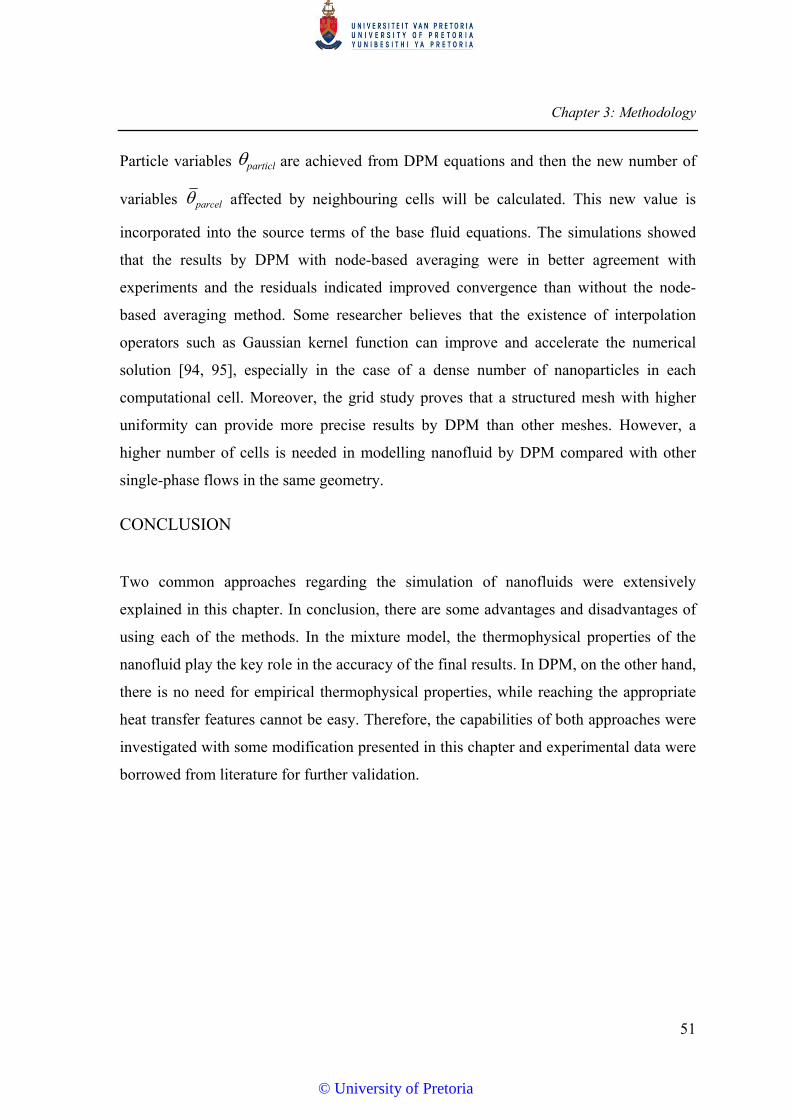
Chapter 3: Methodology
51
Particle variables particl are achieved from DPM equations and then the new number of
variables parcel affected by neighbouring cells will be calculated. This new value is
incorporated into the source terms of the base fluid equations. The simulations showed
that the results by DPM with node-based averaging were in better agreement with
experiments and the residuals indicated improved convergence than without the node-
based averaging method. Some researcher believes that the existence of interpolation
operators such as Gaussian kernel function can improve and accelerate the numerical
solution [94, 95], especially in the case of a dense number of nanoparticles in each
computational cell. Moreover, the grid study proves that a structured mesh with higher
uniformity can provide more precise results by DPM than other meshes. However, a
higher number of cells is needed in modelling nanofluid by DPM compared with other
single-phase flows in the same geometry.
CONCLUSION
Two common approaches regarding the simulation of nanofluids were extensively
explained in this chapter. In conclusion, there are some advantages and disadvantages of
using each of the methods. In the mixture model, the thermophysical properties of the
nanofluid play the key role in the accuracy of the final results. In DPM, on the other hand,
there is no need for empirical thermophysical properties, while reaching the appropriate
heat transfer features cannot be easy. Therefore, the capabilities of both approaches were
investigated with some modification presented in this chapter and experimental data were
borrowed from literature for further validation.
© University of Pretoria

52
4 CHAPTER 4: SIMULATION RESULTS AND DISCUSSION
INTRODUCTION
The presence of nanoparticles in a liquid points to two important aspects of fluid
mechanics, namely pressure drops and heat transfer enhancement. A large part of this
study focuses on these two features, which are compared with measured values in
experiments. Most of the experimental studies in literature are concerned with forced
convection, both laminar and turbulence, only a few works deal with mixed and natural
convection. The common geometry for nanofluid tests is a circular tube for forced and a
cavity for natural convection. A few reports for both of these are explained and compared
with the simulation results of the present study for validation purposes. Due to the
different nature of the flow in forced and natural convection, the interaction between flow
and particles can vary depending on the geometry and intensity of the flow field. In other
words, the important interactions in natural convective flow might not be the same as for
the forced one. The other significant aspect of nanofluid simulations is to understand and
explain the particle distribution inside the domain. All the above-mentioned are presented
in this chapter. Firstly, simulations are conducted for forced tube convective flow via both
conventional DPM and mixture models. Secondly, natural convective cavity flow is
modelled via the developed mixture model proposed in this study. Finally, laminar
nanofluid flow is simulated in a circular microchannel using DPM regarding some
considerations in the present work.
SIMULATIONS OF NANOFLUID USING MIXTURE AND DPM APPROACHES IN FORCED CONVECTION
To understand some drawbacks of both approaches, a few early simulations are
conducted and compared with the experimental results in literature. As explained in
Chapter 3, the default version of the mixture model only assumes gravitational and
centrifugal forces as the dominant slip mechanisms between particles and fluid. The
default forces for the DPM model are drag, Saffman’s lift, gravity, virtual mass, pressure
© University of Pretoria

Chapter 4: Simulation results and discussion
53
gradient, thermophoretic and Brownian motion. Because the comparison between
experiments and simulations are made for a few geometries, the grid study and settings
for each case are separately explained. The first case is a vertical pipe with laminar
nanofluid conducted by Zhang [11] and Rea et al. [7]. Based on experimental works, two
different diameter sizes of vertical tubes are simulated in this study, with the same length
of 1 m. Rea et al. [7] used a stainless steel tube with ID 4.5 mm, and Zhang [11] with
5.537 mm. Both the tubes encountered constant heat flux on the outside of the tubes.
Three types of nanoparticles as nanofluids were injected into the tubes consisting of
Al2O3 and ZrO2 by Rea et al. [7] and SiO2 by Zhang [11]. In all the tests, the Reynolds
number was below 2 000 and therefore the flow was laminar. They are described in Table
4-1 with the thermophysical properties of nanoparticles.
Table 4-1 Thermophysical properties of water and nanoparticles [96]
)/( 3mkg ( / . )pC J k g K ( / . )k W m K )./( smkg )( nmd p
water 2T0.0035-
T1.8142+765.33
1000)T9-1.857e+
T6-2.48e-
T0.00125+
T0.2817-(28.07
4
3
2
2T6-8.151e-
T0.006397+0.5752-
3
2
T9-2.244e-
T6-2.344e+
T4-8.207e-0.0967
-
Al2O3 3920 880 36 - 50
ZrO2 5600 418 2 - 50
SiO2 2200 745 1.38 - 20
Temperature is in terms of Kelvin.
Both 2D axisymmetric and 3D models were examined at the beginning of this study and
the results showed that it was crucial to use a 3D model in laminar nanofluid flow,
especially with the presence of gravity in the Lagrangian approach. It can be argued that
2D axisymmetric can only capture the radial migration of nanoparticles inside the fluid,
while the difference between a 3D model and 2D axisymmetric simulation results proves
that nanoparticles migrate from the wall both radially and tangentially.
© University of Pretoria

Chapter 4: Simulation results and discussion
54
The grid dependence study proves that a structured mesh with higher uniformity can
provide more precise results by DPM than other meshes. However, a higher number of
cells is needed in modelling nanofluid by DPM compared with other laminar single-phase
flow in the same geometry. The final number of grids for this geometry is chosen to be 16
radially, 58 tangentially and 600 longitudinally (16×58×600), which are shown in Figure
4.1. The closest node to the wall is almost 1×10⁻⁴m, which is less than 5% of tube radius.
It is noted that the simulation results achieved by this mesh and even many times more
than this without node-based averaging method are not in agreement with
experimentations. Boundary conditions for DPM consist of the following: similar uniform
velocity and temperature at the inlet for both particles and base flow, particle mass flow
rate at the inlet based on particle volume fraction (it is important to make sure particles
are uniformly distributed at the inlet), constant heat flux over the external surface of the
tube, fully developed condition at the outlet and no-slip condition at the wall of the tube.
The inlet conditions for particles are equivalent boundary and initial conditions for
particles in the Lagrangian frame. Also, wall boundary conditions differ for the particles
from base flow. Two main possibilities are that they can either rebound off the wall or
stick to the wall. The simulation results showed that none of the mentioned conditions
happened for particles. It means that particles never reached the wall or met the wall
conditions. Mixture model B.C. is similar to base flow conditions in DPM.
Figure 4.1: Generated mesh for CFD study with Y as vertical direction
© University of Pretoria

Chapter 4: Simulation results and discussion
55
As a first step, the extent of parameter a in the Gaussian distribution function in equation
(3.109) needs to be chosen. Kaufmann et al. [97] successfully used a=6 in their study.
Simulation results proved that any changes in a influenced mostly the particle
concentration field and it had small impacts on pressure drops and heat transfer
coefficient. The effects of a on alumina nanofluid with volume fraction 2.76% at the
outlet of the tube can be seen in Figure 4.2. It can be seen that the larger amount of a=6
provides higher uniformity than the smaller one, but still the presence of the concentration
gradient is obvious in all of them. Also, the same pattern of distribution can be observed
for different ranges of a. However, a=6 was chosen for all the simulations here similar to
Kaufmann et al. [97].
a) a = 0.5 b) a = 3.0 c) a = 6.0
Figure 4.2: Effect of parameter a in Gaussian function on concentration distribution of
alumina nanofluid with α = 2.76% at the outlet of the tube at Re = 1 131, qʺ = 18.7
kW/m2.
© University of Pretoria

Chapter 4: Simulation results and discussion
56
Figure 4.3: Effect of presence of gravity in DPM simulations for alumina and zirconia
nanofluids, Left and bottom axis for alumina and right and top axis for zirconia.
The importance of gravity can be seen in Figure 4.3. When gravity is excluded from
DPM, the pressure drops predicted by simulations are close to pressure drops with pure
water, while DPM predicts more than twice the pressure loss with pure water. Hence
considering no gravity in DPM may produce errors up to 200% in vertical laminar flow.
The dispersion of alumina and zirconia nanoparticles at the outlet section of the tube is
illustrated in Figure 4.4, which shows the similar pattern of distribution for both alumina
and zirconia nanofluids in different volume fractions. The percentage range of volume
fraction in both nanoparticles with various particle loadings demonstrates that
nanoparticles follow almost uniformly the base flow in lower volume fractions rather than
in higher concentrations, notwithstanding the types of nanoparticles.
© University of Pretoria
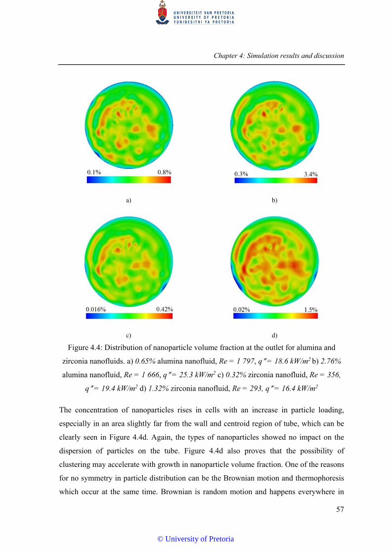
Chapter 4: Simulation results and discussion
57
a)
b)
c)
d)
Figure 4.4: Distribution of nanoparticle volume fraction at the outlet for alumina and
zirconia nanofluids. a) 0.65% alumina nanofluid, Re = 1 797, qʺ = 18.6 kW/m2 b) 2.76%
alumina nanofluid, Re = 1 666, qʺ = 25.3 kW/m2 c) 0.32% zirconia nanofluid, Re = 356,
qʺ = 19.4 kW/m2 d) 1.32% zirconia nanofluid, Re = 293, qʺ = 16.4 kW/m2
The concentration of nanoparticles rises in cells with an increase in particle loading,
especially in an area slightly far from the wall and centroid region of tube, which can be
clearly seen in Figure 4.4d. Again, the types of nanoparticles showed no impact on the
dispersion of particles on the tube. Figure 4.4d also proves that the possibility of
clustering may accelerate with growth in nanoparticle volume fraction. One of the reasons
for no symmetry in particle distribution can be the Brownian motion and thermophoresis
which occur at the same time. Brownian is random motion and happens everywhere in
© University of Pretoria

Chapter 4: Simulation results and discussion
58
cross-section and thermophoresis is strong close to the wall. The combination of both
may disturb the cross-sectional concentration distribution. On the other hand, the mixture
model results provided more uniform distribution of concentration than those of DPM for
any types of nanoparticles and particle loadings. It means that the slip velocity assumed
by the mixture model in the simulations is almost negligible. The nanofluid is treated as a
homogeneous mixture with no relative velocity between solid and liquid parts.
4.1.1 Case study of heat transfer features
Heat transfer and hydrodynamic characteristics of laminar nanofluid in two vertical tubes
are presented in this section. Figure 4.5 shows the good agreement between experiments
and numerical solutions for heat transfer coefficient in base flow without nanoparticles
for different Reynolds numbers. The heat transfer coefficient is simply calculated from
/ ( )w bq T T . The important parameter is the bulk temperature Tb, which can be defined
as:
dAVc
VTdAcT
p
p
b
(4.1)
The heat transfer coefficient and Nu number estimated by the mixture model and DPM
compared with experimental results for three types of nanofluids are illustrated in Figure
4.6 and Figure 4.7. A wide range of Reynolds numbers from 290 to 1 800 and particle
volume fraction from 0.2% to 2.76% was simulated for three common nanofluids, i.e.
alumina, zirconia and silica nanofluid, with different diameters of nanoparticles.
© University of Pretoria
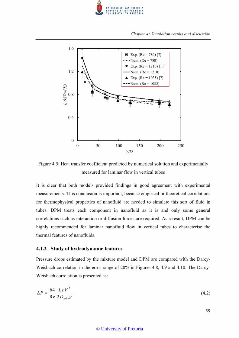
Chapter 4: Simulation results and discussion
59
Figure 4.5: Heat transfer coefficient predicted by numerical solution and experimentally
measured for laminar flow in vertical tubes
It is clear that both models provided findings in good agreement with experimental
measurements. This conclusion is important, because empirical or theoretical correlations
for thermophysical properties of nanofluid are needed to simulate this sort of fluid in
tubes. DPM treats each component in nanofluid as it is and only some general
correlations such as interaction or diffusion forces are required. As a result, DPM can be
highly recommended for laminar nanofluid flow in vertical tubes to characterise the
thermal features of nanofluids.
4.1.2 Study of hydrodynamic features
Pressure drops estimated by the mixture model and DPM are compared with the Darcy-
Weisbach correlation in the error range of 20% in Figures 4.8, 4.9 and 4.10. The Darcy-
Weisbach correlation is presented as:
264
Re 2 tube
L VP
D g
(4.2)
© University of Pretoria

Chapter 4: Simulation results and discussion
60
All the properties for the Darcy-Weisbach correlation were borrowed from mixture
properties presented in literature. The simulations were carried out for volume fraction
below 3% and a good agreement was observed between modelling and the correlation.
DPM showed a better trend for pressure loss prediction compared with the mixture
model. The simulations were also conducted for higher 3% volume fractions. The DPM
results were sometimes 100% different from the correlation, especially in the case of the
higher velocity shown notwithstanding the type of nanofluid. The main differences
between lower and higher volume fraction can be introduced as: firstly, rising the number
of nanoparticles in each computational cell. One of the problems can come from
inaccurate weight or Gaussian function to distribute the effects of particle variables to
neighbouring cells. Secondly, the possibility of clustering and collision among
nanoparticles will expand with an increase in volume fraction.
Due to a higher number of silica nanoparticles in each parcel compared with the other two
nanoparticles with the same conditions, as shown in Figure 4.11, the percentage of
difference for pressure drops in higher volume fraction was found much appreciable. It is
noted that the number of particles is conserved in the entire domain when the particles are
solved in Lagrangian frame. It means that it is important to assign the proper number of
time steps for nanoparticles to make sure all the injected particles will leave the geometry
domain. Moreover, the average difference between simulations and Darcy equation for
pressure drops was found to be near 12% by the mixture model and 10% by DPM.
Non-dimensional temperature distribution of fluid and nanoparticles at the outlet is
illustrated in Figures 4.12 and 4.13 for three nanofluids. With heat transfer parameters in
this study consisting of heat flux, temperature, thermal conductivity and characteristic
length, non-dimensional temperature can easily be defined as:
* 2 ( )in c
tu b e
T T kT
q D
(4.3)
© University of Pretoria
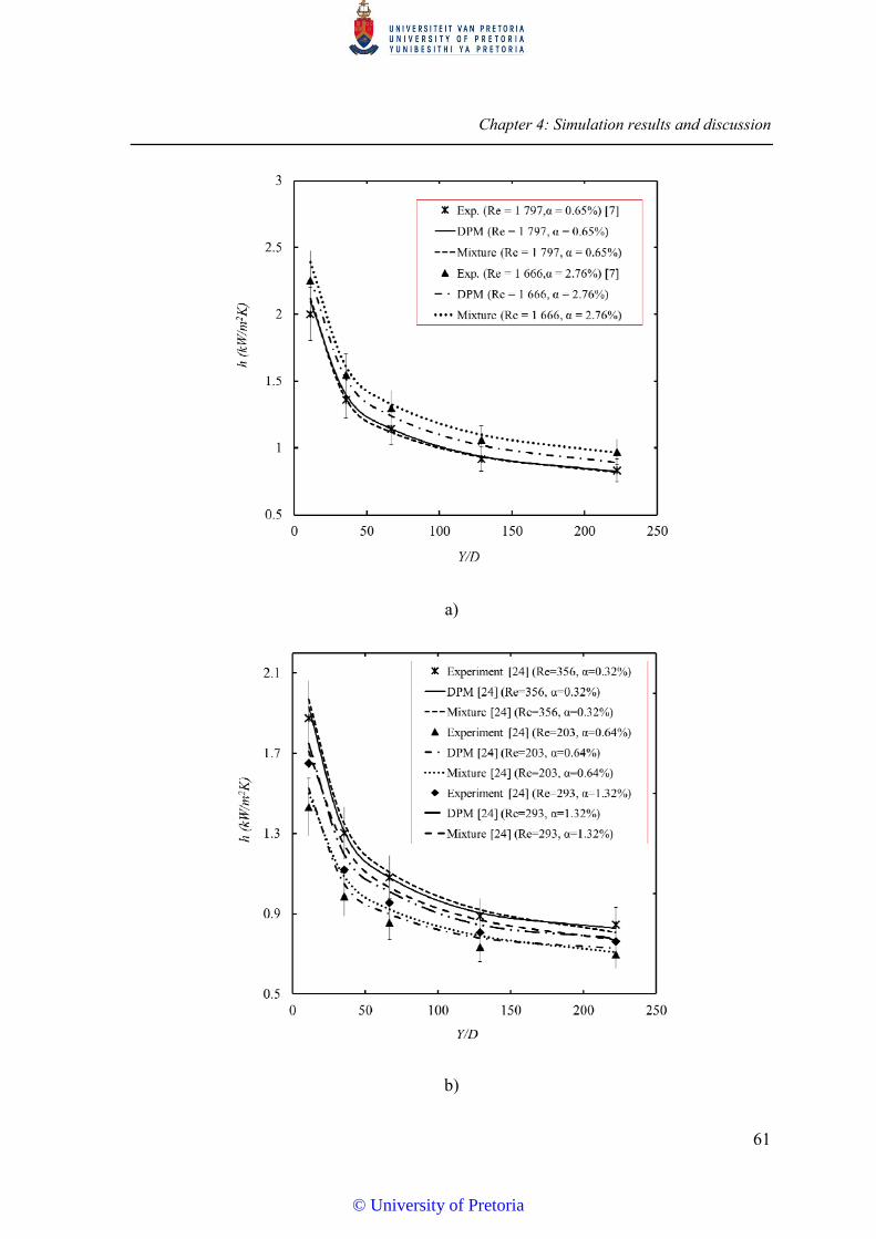
Chapter 4: Simulation results and discussion
61
a)
b)
© University of Pretoria
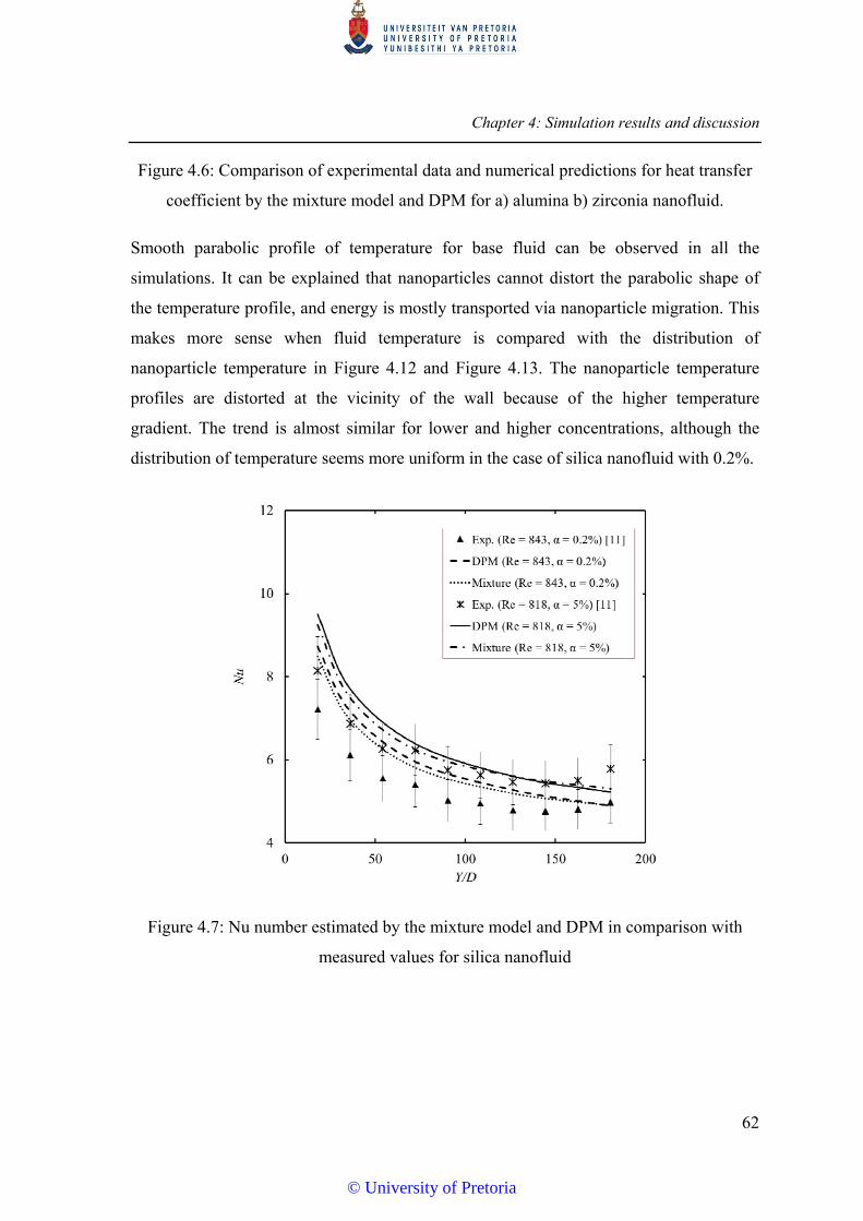
Chapter 4: Simulation results and discussion
62
Figure 4.6: Comparison of experimental data and numerical predictions for heat transfer
coefficient by the mixture model and DPM for a) alumina b) zirconia nanofluid.
Smooth parabolic profile of temperature for base fluid can be observed in all the
simulations. It can be explained that nanoparticles cannot distort the parabolic shape of
the temperature profile, and energy is mostly transported via nanoparticle migration. This
makes more sense when fluid temperature is compared with the distribution of
nanoparticle temperature in Figure 4.12 and Figure 4.13. The nanoparticle temperature
profiles are distorted at the vicinity of the wall because of the higher temperature
gradient. The trend is almost similar for lower and higher concentrations, although the
distribution of temperature seems more uniform in the case of silica nanofluid with 0.2%.
Figure 4.7: Nu number estimated by the mixture model and DPM in comparison with
measured values for silica nanofluid
© University of Pretoria
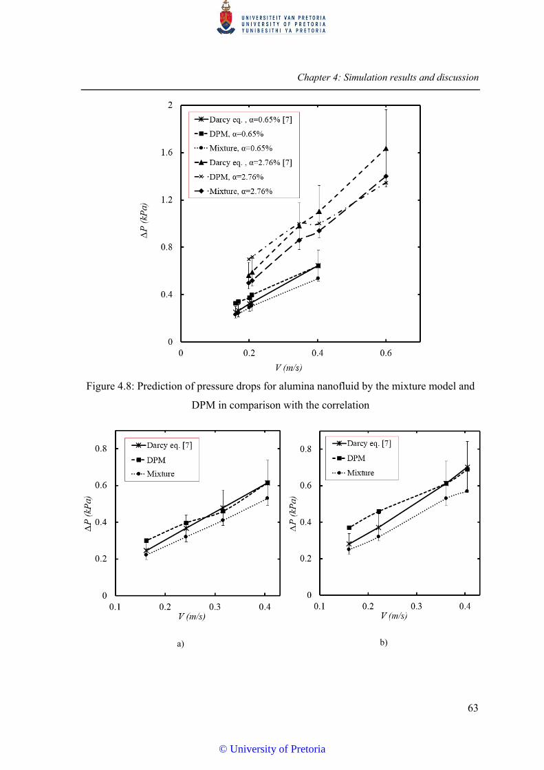
Chapter 4: Simulation results and discussion
63
Figure 4.8: Prediction of pressure drops for alumina nanofluid by the mixture model and
DPM in comparison with the correlation
a)
b)
© University of Pretoria
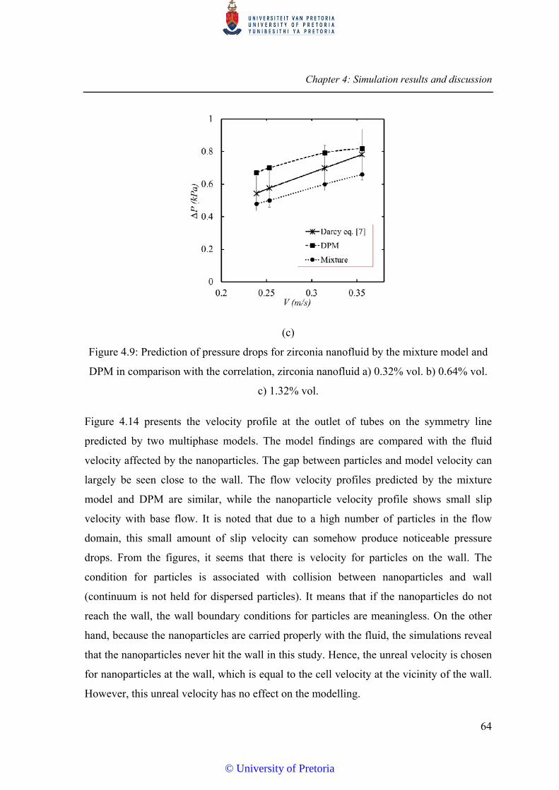
Chapter 4: Simulation results and discussion
64
(c)
Figure 4.9: Prediction of pressure drops for zirconia nanofluid by the mixture model and
DPM in comparison with the correlation, zirconia nanofluid a) 0.32% vol. b) 0.64% vol.
c) 1.32% vol.
Figure 4.14 presents the velocity profile at the outlet of tubes on the symmetry line
predicted by two multiphase models. The model findings are compared with the fluid
velocity affected by the nanoparticles. The gap between particles and model velocity can
largely be seen close to the wall. The flow velocity profiles predicted by the mixture
model and DPM are similar, while the nanoparticle velocity profile shows small slip
velocity with base flow. It is noted that due to a high number of particles in the flow
domain, this small amount of slip velocity can somehow produce noticeable pressure
drops. From the figures, it seems that there is velocity for particles on the wall. The
condition for particles is associated with collision between nanoparticles and wall
(continuum is not held for dispersed particles). It means that if the nanoparticles do not
reach the wall, the wall boundary conditions for particles are meaningless. On the other
hand, because the nanoparticles are carried properly with the fluid, the simulations reveal
that the nanoparticles never hit the wall in this study. Hence, the unreal velocity is chosen
for nanoparticles at the wall, which is equal to the cell velocity at the vicinity of the wall.
However, this unreal velocity has no effect on the modelling.
© University of Pretoria

Chapter 4: Simulation results and discussion
65
a) b)
Figure 4.10: Prediction of pressure drops for silica nanofluid by the mixture model and
DPM in comparison with the correlation for silica nanofluid a) 0.2% vol. b) 1% vol.
In summary, the two approaches can be compared as follows: the mixture model results
highly depend on transport properties coming from experimentation. There is no need for
the mixture properties for DPM, which only needs appropriate interaction or diffusion
forces, empirical or analytical. The mixture model considers nanofluid as two phases.
DPM treats the nanofluid as base fluid and solid separately, as it is in reality.
© University of Pretoria
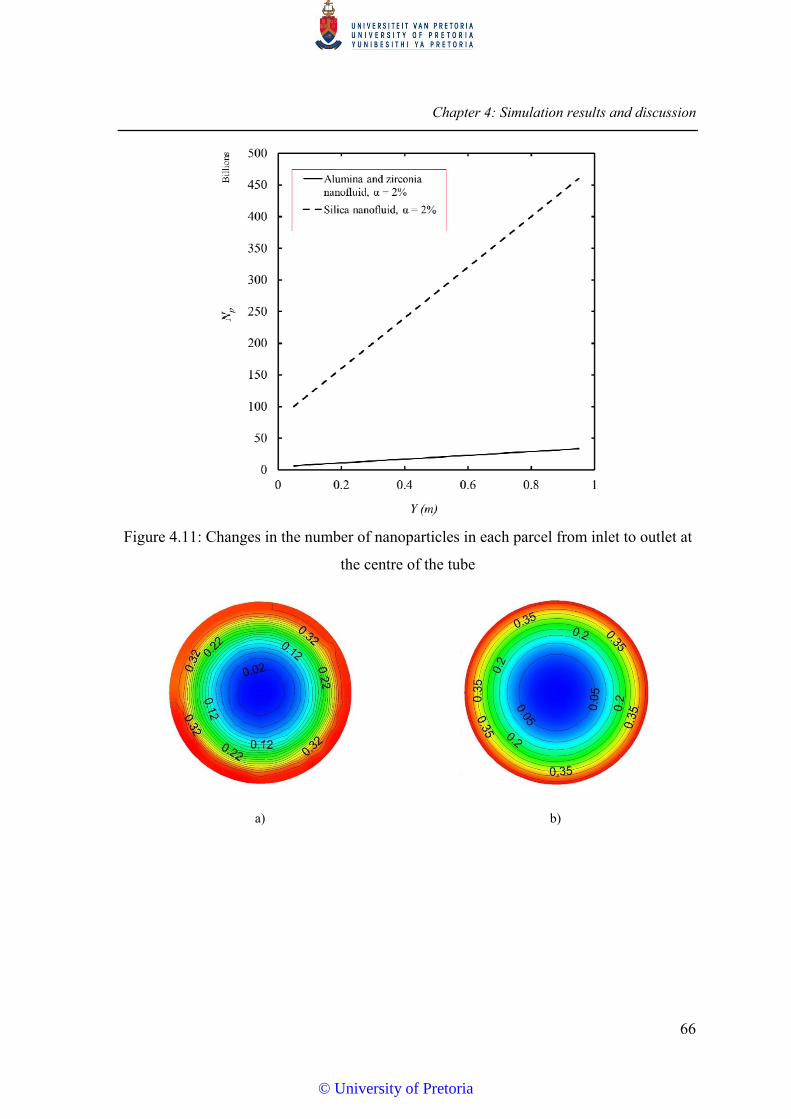
Chapter 4: Simulation results and discussion
66
Figure 4.11: Changes in the number of nanoparticles in each parcel from inlet to outlet at
the centre of the tube
a)
b)
© University of Pretoria
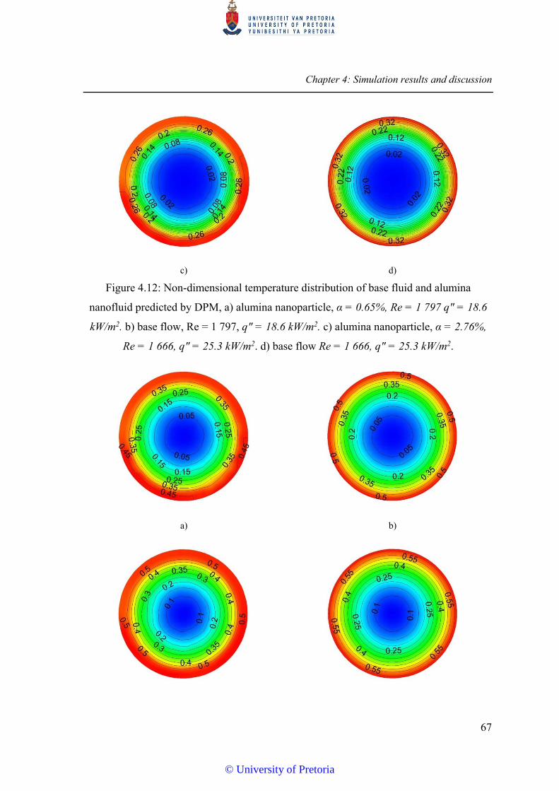
Chapter 4: Simulation results and discussion
67
c)
d)
Figure 4.12: Non-dimensional temperature distribution of base fluid and alumina
nanofluid predicted by DPM, a) alumina nanoparticle, α = 0.65%, Re = 1 797 qʺ = 18.6
kW/m2. b) base flow, Re = 1 797, qʺ = 18.6 kW/m2. c) alumina nanoparticle, α = 2.76%,
Re = 1 666, qʺ = 25.3 kW/m2. d) base flow Re = 1 666, qʺ = 25.3 kW/m2.
a)
b)
© University of Pretoria
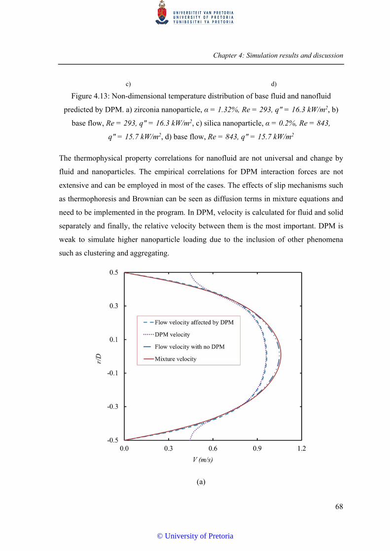
Chapter 4: Simulation results and discussion
68
c) d)
Figure 4.13: Non-dimensional temperature distribution of base fluid and nanofluid
predicted by DPM. a) zirconia nanoparticle, α = 1.32%, Re = 293, qʺ = 16.3 kW/m2, b)
base flow, Re = 293, qʺ = 16.3 kW/m2, c) silica nanoparticle, α = 0.2%, Re = 843,
qʺ = 15.7 kW/m2, d) base flow, Re = 843, qʺ = 15.7 kW/m2
The thermophysical property correlations for nanofluid are not universal and change by
fluid and nanoparticles. The empirical correlations for DPM interaction forces are not
extensive and can be employed in most of the cases. The effects of slip mechanisms such
as thermophoresis and Brownian can be seen as diffusion terms in mixture equations and
need to be implemented in the program. In DPM, velocity is calculated for fluid and solid
separately and finally, the relative velocity between them is the most important. DPM is
weak to simulate higher nanoparticle loading due to the inclusion of other phenomena
such as clustering and aggregating.
(a)
© University of Pretoria
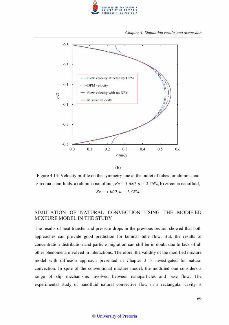
Chapter 4: Simulation results and discussion
69
(b)
Figure 4.14: Velocity profile on the symmetry line at the outlet of tubes for alumina and
zirconia nanofluids. a) alumina nanofluid, Re = 1 680, α = 2.76%, b) zirconia nanofluid,
Re = 1 060, α = 1.32%.
SIMULATION OF NATURAL CONVECTION USING THE MODIFIED MIXTURE MODEL IN THE STUDY
The results of heat transfer and pressure drops in the previous section showed that both
approaches can provide good prediction for laminar tube flow. But, the results of
concentration distribution and particle migration can still be in doubt due to lack of all
other phenomena involved in interactions. Therefore, the validity of the modified mixture
model with diffusion approach presented in Chapter 3 is investigated for natural
convection. In spite of the conventional mixture model, the modified one considers a
range of slip mechanisms involved between nanoparticles and base flow. The
experimental study of nanofluid natural convective flow in a rectangular cavity is
© University of Pretoria
Chapter 4: Simulation results and discussion
70
borrowed from the recently published paper by Ghodsinezhad et al. [98], conducted at the
University of Pretoria.
The size of the cavity used was 96mm×120mm for cold and hot walls and the space
between the walls was 102mm, therefore, the aspect ratio about unity. The entire
schematic of the test section is shown in Figure 4.15. The hot and cold wall sides of the
cavity are heated and cooled by two shell-and-tube heat exchangers with counterflow
inside. All the materials of the heat exchangers were made from copper, including 4mm
copper plates in each side of the cavity. The dimensions of the shell part of the heat
exchanger were 96mm×120mm×18mm. To improve the heat transfer and uniformity of
temperature inside the heat exchanger, the mass flow from and to the heat exchanger was
split between shell and tube parts equally. The diameter of the tube was chosen to be
10.7mm ID and 1mm wall thickness. The hydraulic diameter of the shell part was
calculated almost similar to the tube diameter to achieve the best distribution of mass and
heat transfer inside heat exchangers. Also, three plates made of copper were installed
inside heat exchangers as buffers to make the channel for the shell side.
With the calculation of Reynolds number in heat exchangers and Rayleigh number
defined as
)(3avecaveh TTLg
Ra , three separate types of flow regimes are
recognised in the experiment: turbulent flow in hot heat exchanger, laminar flow in the
cold heat exchanger and laminar natural convection flow in the cavity.
All the thermophysical and transport properties of the fluid were expressed in terms of
temperature. Density in momentum equation was the non-Boussinesq term used in the
cavity. Instead of the linear function of temperature for density by Boussinesq
approximation as β∆T, a third-order polynomial function of temperature in Chapter 3 was
employed. Also, the turbulence terms were ignored for laminar flow inside the cold heat
exchanger and cavity. The realisable k-ɛ model was employed to simulate the fluctuating
velocity and turbulent viscosity, which was successfully used by Bacharoudis et al. [99]
and Teodosiu et al. [100].
© University of Pretoria

Chapter 4: Simulation results and discussion
71
Figure 4.15: Schematic of the cavity with heat exchangers
Both structured and unstructured meshes were required for this kind of geometry,
unstructured mesh for heat exchangers and the structured one for cavity and copper
layers. Also, boundary layer meshes were added in heat exchangers due to the small size
of the tube and existence of turbulent flow inside the hot section. Some interfaces were
needed for the sections between heat exchangers and copper layers due to different types
of meshes. The realisable k-ɛ model was operated with enhanced wall function as wall
treatment in shell and tubes. The initial results exhibited the amount of y+ at the vicinity
of all walls less than 5, which was an acceptable amount for this method. On the other
hand, the natural convection simulations inside the cavity proved that the mesh had to be
fine enough in the vicinity of the walls to capture the entire influences of the small
boundary layer due to natural convection. As a result, the closest node to the shell-and-
tube walls was chosen as 0.3mm for the cavity. Three kinds of flow regimes existed in the
model, namely turbulent forced convection, laminar forced convection and laminar
natural convective flow. Therefore, it could be expected that a large number of iterations
would be required to reach heat transfer balance in the cavity, which was the most
important criteria for convergence. Various meshes were tried to find the optimum and
best grid for each section in the model concerning the grid study (up to 2 million nodes in
total). The criteria for comparison among different grids were chosen as heat flux in
walls, temperature and velocity profile at the centre line of the cavity. Finally, the proper
mesh was chosen as 912 081 unstructured cells for each heat exchanger, 226 981
© University of Pretoria
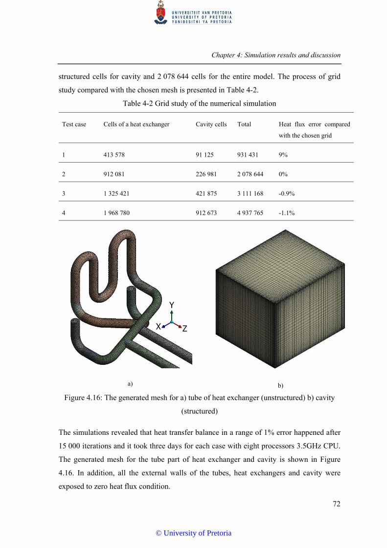
Chapter 4: Simulation results and discussion
72
structured cells for cavity and 2 078 644 cells for the entire model. The process of grid
study compared with the chosen mesh is presented in Table 4-2.
Table 4-2 Grid study of the numerical simulation
Test case Cells of a heat exchanger Cavity cells Total Heat flux error compared
with the chosen grid
1 413 578 91 125 931 431 9%
2 912 081 226 981 2 078 644 0%
3 1 325 421 421 875 3 111 168 -0.9%
4 1 968 780 912 673 4 937 765 -1.1%
a)
b)
Figure 4.16: The generated mesh for a) tube of heat exchanger (unstructured) b) cavity
(structured)
The simulations revealed that heat transfer balance in a range of 1% error happened after
15 000 iterations and it took three days for each case with eight processors 3.5GHz CPU.
The generated mesh for the tube part of heat exchanger and cavity is shown in Figure
4.16. In addition, all the external walls of the tubes, heat exchangers and cavity were
exposed to zero heat flux condition.
© University of Pretoria
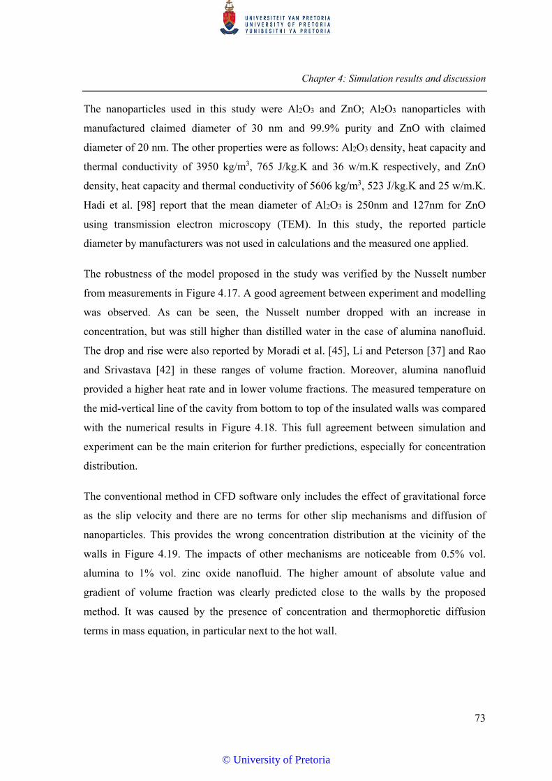
Chapter 4: Simulation results and discussion
73
The nanoparticles used in this study were Al2O3 and ZnO; Al2O3 nanoparticles with
manufactured claimed diameter of 30 nm and 99.9% purity and ZnO with claimed
diameter of 20 nm. The other properties were as follows: Al2O3 density, heat capacity and
thermal conductivity of 3950 kg/m3, 765 J/kg.K and 36 w/m.K respectively, and ZnO
density, heat capacity and thermal conductivity of 5606 kg/m3, 523 J/kg.K and 25 w/m.K.
Hadi et al. [98] report that the mean diameter of Al2O3 is 250nm and 127nm for ZnO
using transmission electron microscopy (TEM). In this study, the reported particle
diameter by manufacturers was not used in calculations and the measured one applied.
The robustness of the model proposed in the study was verified by the Nusselt number
from measurements in Figure 4.17. A good agreement between experiment and modelling
was observed. As can be seen, the Nusselt number dropped with an increase in
concentration, but was still higher than distilled water in the case of alumina nanofluid.
The drop and rise were also reported by Moradi et al. [45], Li and Peterson [37] and Rao
and Srivastava [42] in these ranges of volume fraction. Moreover, alumina nanofluid
provided a higher heat rate and in lower volume fractions. The measured temperature on
the mid-vertical line of the cavity from bottom to top of the insulated walls was compared
with the numerical results in Figure 4.18. This full agreement between simulation and
experiment can be the main criterion for further predictions, especially for concentration
distribution.
The conventional method in CFD software only includes the effect of gravitational force
as the slip velocity and there are no terms for other slip mechanisms and diffusion of
nanoparticles. This provides the wrong concentration distribution at the vicinity of the
walls in Figure 4.19. The impacts of other mechanisms are noticeable from 0.5% vol.
alumina to 1% vol. zinc oxide nanofluid. The higher amount of absolute value and
gradient of volume fraction was clearly predicted close to the walls by the proposed
method. It was caused by the presence of concentration and thermophoretic diffusion
terms in mass equation, in particular next to the hot wall.
© University of Pretoria

Chapter 4: Simulation results and discussion
74
(a)
(b)
Figure 4.17: Comparison of Nusselt number measured during the experiments and
calculated by the numerical model for alumina and zinc oxide nanofluids
© University of Pretoria
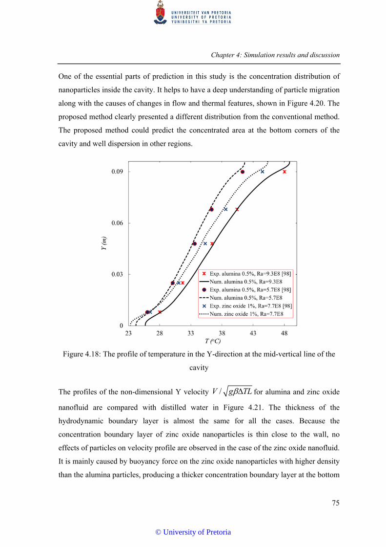
Chapter 4: Simulation results and discussion
75
One of the essential parts of prediction in this study is the concentration distribution of
nanoparticles inside the cavity. It helps to have a deep understanding of particle migration
along with the causes of changes in flow and thermal features, shown in Figure 4.20. The
proposed method clearly presented a different distribution from the conventional method.
The proposed method could predict the concentrated area at the bottom corners of the
cavity and well dispersion in other regions.
Figure 4.18: The profile of temperature in the Y-direction at the mid-vertical line of the
cavity
The profiles of the non-dimensional Y velocity /V g TL for alumina and zinc oxide
nanofluid are compared with distilled water in Figure 4.21. The thickness of the
hydrodynamic boundary layer is almost the same for all the cases. Because the
concentration boundary layer of zinc oxide nanoparticles is thin close to the wall, no
effects of particles on velocity profile are observed in the case of the zinc oxide nanofluid.
It is mainly caused by buoyancy force on the zinc oxide nanoparticles with higher density
than the alumina particles, producing a thicker concentration boundary layer at the bottom
© University of Pretoria
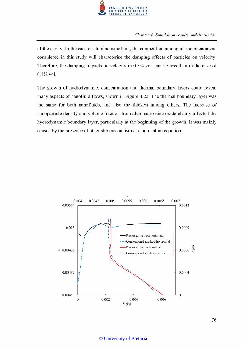
Chapter 4: Simulation results and discussion
76
of the cavity. In the case of alumina nanofluid, the competition among all the phenomena
considered in this study will characterise the damping effects of particles on velocity.
Therefore, the damping impacts on velocity in 0.5% vol. can be less than in the case of
0.1% vol.
The growth of hydrodynamic, concentration and thermal boundary layers could reveal
many aspects of nanofluid flows, shown in Figure 4.22. The thermal boundary layer was
the same for both nanofluids, and also the thickest among others. The increase of
nanoparticle density and volume fraction from alumina to zinc oxide clearly affected the
hydrodynamic boundary layer, particularly at the beginning of the growth. It was mainly
caused by the presence of other slip mechanisms in momentum equation.
© University of Pretoria
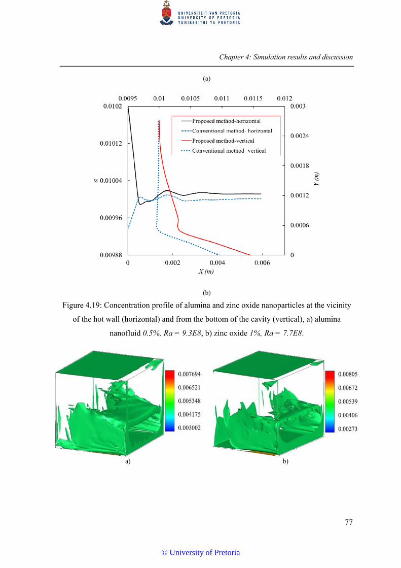
Chapter 4: Simulation results and discussion
77
(a)
(b)
Figure 4.19: Concentration profile of alumina and zinc oxide nanoparticles at the vicinity
of the hot wall (horizontal) and from the bottom of the cavity (vertical), a) alumina
nanofluid 0.5%, Ra = 9.3E8, b) zinc oxide 1%, Ra = 7.7E8.
a) b)
© University of Pretoria
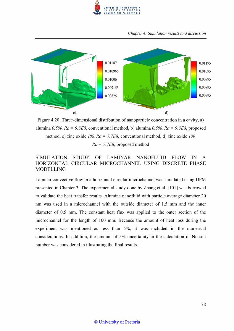
Chapter 4: Simulation results and discussion
78
c) d)
Figure 4.20: Three-dimensional distribution of nanoparticle concentration in a cavity, a)
alumina 0.5%, Ra = 9.3E8, conventional method, b) alumina 0.5%, Ra = 9.3E8, proposed
method, c) zinc oxide 1%, Ra = 7.7E8, conventional method, d) zinc oxide 1%,
Ra = 7.7E8, proposed method
SIMULATION STUDY OF LAMINAR NANOFLUID FLOW IN A HORIZONTAL CIRCULAR MICROCHANNEL USING DISCRETE PHASE MODELLING
Laminar convective flow in a horizontal circular microchannel was simulated using DPM
presented in Chapter 3. The experimental study done by Zhang et al. [101] was borrowed
to validate the heat transfer results. Alumina nanofluid with particle average diameter 20
nm was used in a microchannel with the outside diameter of 1.5 mm and the inner
diameter of 0.5 mm. The constant heat flux was applied to the outer section of the
microchannel for the length of 100 mm. Because the amount of heat loss during the
experiment was mentioned as less than 5%, it was included in the numerical
considerations. In addition, the amount of 5% uncertainty in the calculation of Nusselt
number was considered in illustrating the final results.
© University of Pretoria
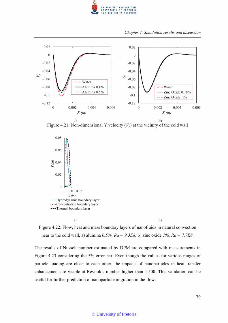
Chapter 4: Simulation results and discussion
79
a) b) Figure 4.21: Non-dimensional Y velocity (Vy) at the vicinity of the cold wall
a)
b)
Figure 4.22: Flow, heat and mass boundary layers of nanofluids in natural convection
near to the cold wall, a) alumina 0.5%, Ra = 9.3E8, b) zinc oxide 1%, Ra = 7.7E8.
The results of Nusselt number estimated by DPM are compared with measurements in
Figure 4.23 considering the 5% error bar. Even though the values for various ranges of
particle loading are close to each other, the impacts of nanoparticles in heat transfer
enhancement are visible at Reynolds number higher than 1 500. This validation can be
useful for further prediction of nanoparticle migration in the flow.
© University of Pretoria

Chapter 4: Simulation results and discussion
80
Figure 4.23: Nusselt number vs Reynolds number predicted by DPM compared with
experimental measurements with 5% error bar
One of the most important issues in interactions between fluid and solid is to understand
the significance of forces involved. The drag force can be considered the final result of all
other forces. The importance of each force acting on the nanoparticles compared with the
drag force is shown in Figure 4.24. Because some forces only interact in some specific
directions, for example, gravity only in the Y-direction, the comparison is therefore
presented in X-, Y- and Z-directions separately. The following conclusion can be made:
The gravitational force can be safely neglected in laminar force flow for nanoparticles.
The pressure gradient and virtual mass forces due to acceleration of the particle almost
contain the minimum impacts on the particle in all directions. Due to lower ranges of
particle concentration (<1% vol.), the long range attraction force of Van der Waals has a
small effect on particle migration. It is noted that this force highly depends on particle-to-
particle distance. The electric double-layer force can play a key role in particle-to-particle
© University of Pretoria

Chapter 4: Simulation results and discussion
81
interactions, but it depends on the final nanofluid solution and pH value. The pH is
assumed 3 in this simulation.
(a)
(b)
© University of Pretoria

Chapter 4: Simulation results and discussion
82
(c)
Figure 4.24: Comparative study of interaction forces between fluid and nanoparticles in a)
X- b) Y- and c) Z-direction for alumina nanofluid 0.77% vol. Z-axis is flow direction
Because the main flow occurs in the Z-direction, the magnitude of the repulsive electric
double-layer force decreases compared with drag force in this direction. The other
important force is lift force due to shear stresses near to the wall towards the centre of the
tube. This force can be strong in laminar nanofluid flow and mainly in the radial
direction. Thermophoretic force only acts in radial direction due to temperature gradient.
Thus, it can influence the particle migration near to the wall and it decreases towards the
centre of the tube. Because the straight flow inside a circular tube can somehow be a
rotational flow, the lift force due to rotation of the particle in the flow is taken into
account, called Magnus force. The magnitude analysis indicates that this force can
influence the particle migration in the radial direction, but not as much as Saffman’s lift
force. Brownian random force is the only effective force in all three directions and cannot
be neglected, although the strong flow field and drag force in the Z-direction can even
suppress those effects.
The distribution of nanoparticle concentration at different cross-sections of the
microchannel is illustrated in Figure 4.25. The concentration boundary layer immediately
© University of Pretoria
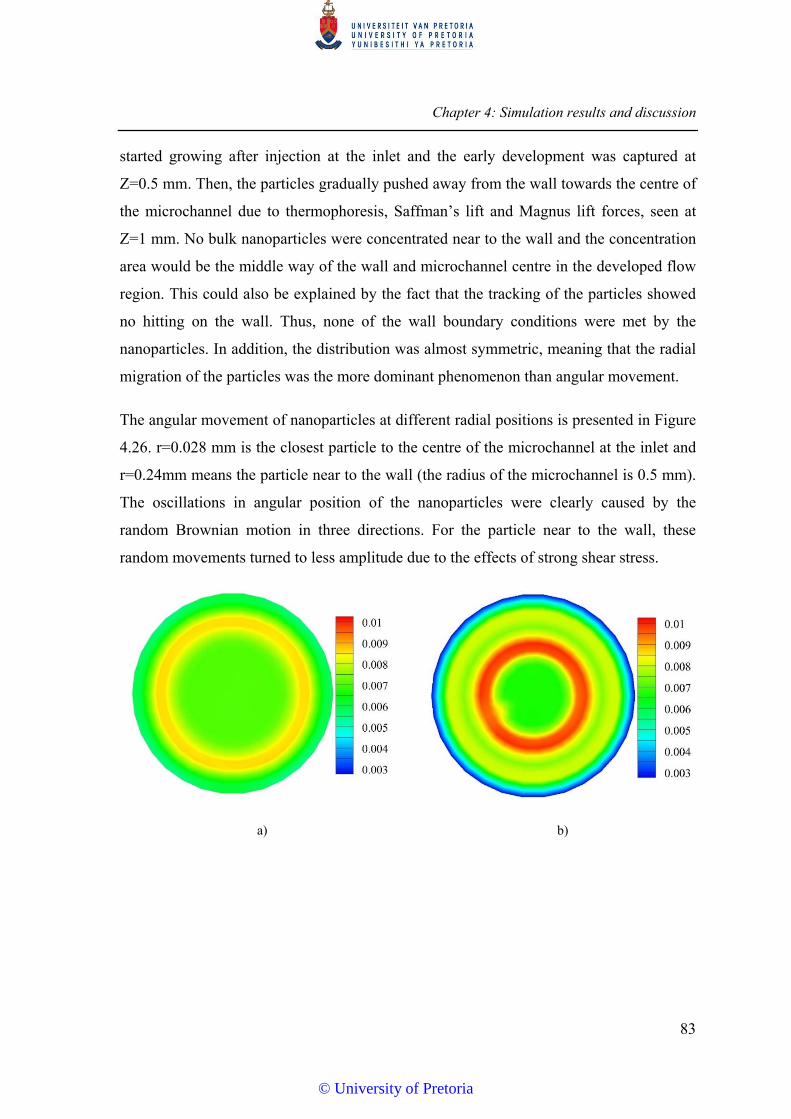
Chapter 4: Simulation results and discussion
83
started growing after injection at the inlet and the early development was captured at
Z=0.5 mm. Then, the particles gradually pushed away from the wall towards the centre of
the microchannel due to thermophoresis, Saffman’s lift and Magnus lift forces, seen at
Z=1 mm. No bulk nanoparticles were concentrated near to the wall and the concentration
area would be the middle way of the wall and microchannel centre in the developed flow
region. This could also be explained by the fact that the tracking of the particles showed
no hitting on the wall. Thus, none of the wall boundary conditions were met by the
nanoparticles. In addition, the distribution was almost symmetric, meaning that the radial
migration of the particles was the more dominant phenomenon than angular movement.
The angular movement of nanoparticles at different radial positions is presented in Figure
4.26. r=0.028 mm is the closest particle to the centre of the microchannel at the inlet and
r=0.24mm means the particle near to the wall (the radius of the microchannel is 0.5 mm).
The oscillations in angular position of the nanoparticles were clearly caused by the
random Brownian motion in three directions. For the particle near to the wall, these
random movements turned to less amplitude due to the effects of strong shear stress.
a)
b)
© University of Pretoria
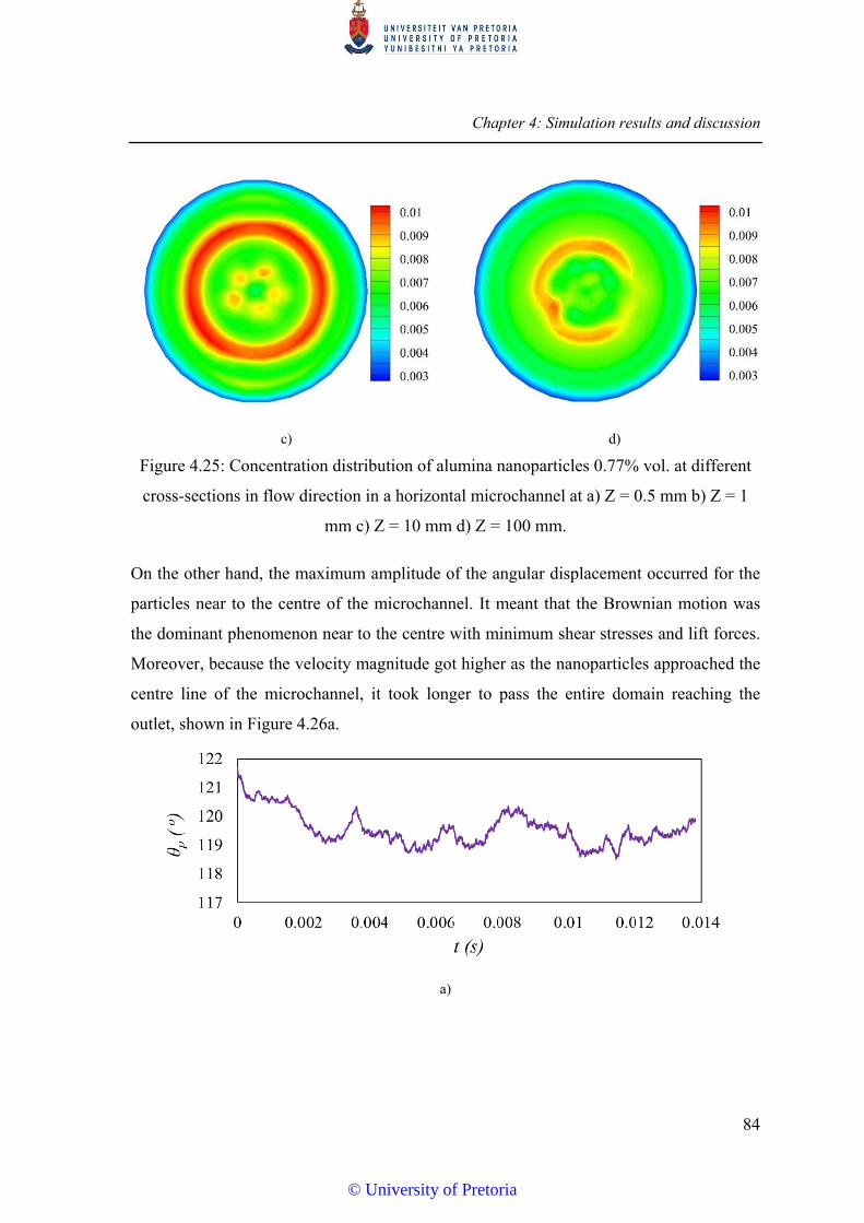
Chapter 4: Simulation results and discussion
84
c)
d)
Figure 4.25: Concentration distribution of alumina nanoparticles 0.77% vol. at different
cross-sections in flow direction in a horizontal microchannel at a) Z = 0.5 mm b) Z = 1
mm c) Z = 10 mm d) Z = 100 mm.
On the other hand, the maximum amplitude of the angular displacement occurred for the
particles near to the centre of the microchannel. It meant that the Brownian motion was
the dominant phenomenon near to the centre with minimum shear stresses and lift forces.
Moreover, because the velocity magnitude got higher as the nanoparticles approached the
centre line of the microchannel, it took longer to pass the entire domain reaching the
outlet, shown in Figure 4.26a.
a)
© University of Pretoria
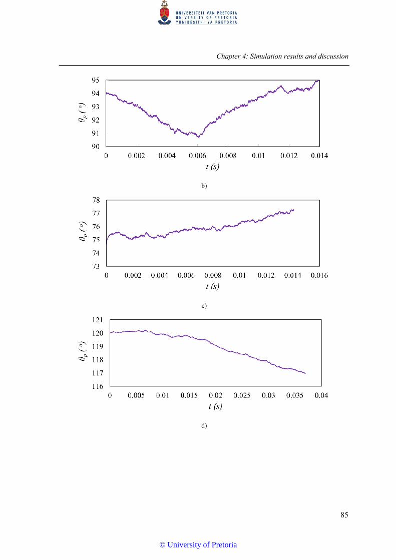
Chapter 4: Simulation results and discussion
85
b)
c)
d)
© University of Pretoria

Chapter 4: Simulation results and discussion
86
e)
Figure 4.26: Angular movement of the nanoparticles from inlet to outlet at different radial
positions. r is the initial radial position of the nanoparticle at the inlet or injection
position. a) r = 0.028 mm b) r = 0.045 mm c) r = 0.061 mm d) r = 0.24 mm e) Polar
coordinate system at a cross-section of the microchannel.
The radial migration of nanoparticles from the injection plane to the outlet is shown in
Figure 4.26. The particles near to the wall took the highest displacement in radial
direction due to all the forces caused by the temperature gradient and lift forces. Because
most of the important interaction forces acted in the radial direction, such as
thermophoresis, Saffman’s and Magnus forces, the oscillations in displacement from one
frame to another would be small due to fewer impacts of random Brownian motion. The
trend of radial migration was more or less similar in all the nanoparticles. They took the
path towards the centre of the microchannel while the concentration boundary layer grew.
Then, the displacement grew up to reach the asymptotic value in the developed flow
region.
© University of Pretoria
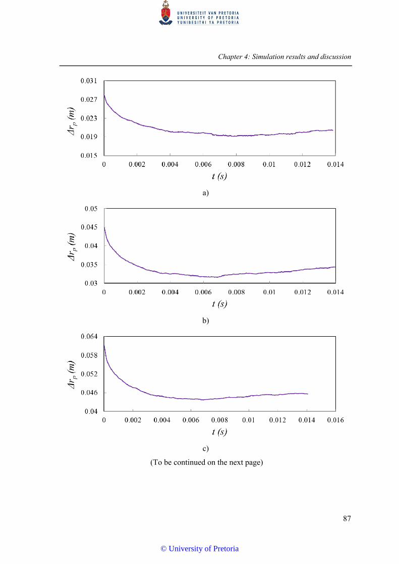
Chapter 4: Simulation results and discussion
87
a)
b)
c)
(To be continued on the next page)
© University of Pretoria

Chapter 4: Simulation results and discussion
88
d)
Figure 4.27: Radial displacement of nanoparticles from inlet to outlet
Figure 4.28: Evolution of relative velocity between nanoparticles and fluid in the
microchannel at different injected radial positions
One of the most important parameters in solid-liquid flows is the slip velocity between
particles and base fluid, shown in Figure 4.28. Due to migration of the nanoparticles in
© University of Pretoria
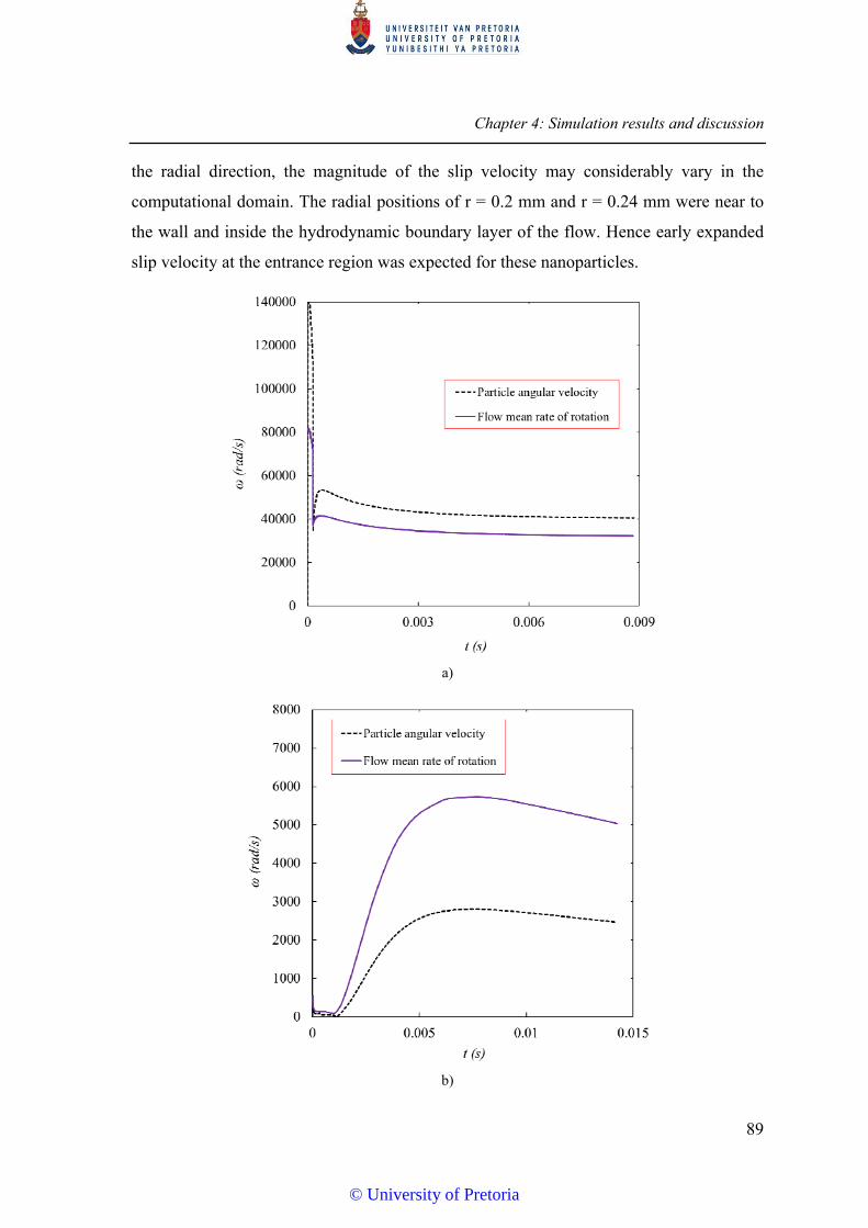
Chapter 4: Simulation results and discussion
89
the radial direction, the magnitude of the slip velocity may considerably vary in the
computational domain. The radial positions of r = 0.2 mm and r = 0.24 mm were near to
the wall and inside the hydrodynamic boundary layer of the flow. Hence early expanded
slip velocity at the entrance region was expected for these nanoparticles.
a)
b)
© University of Pretoria
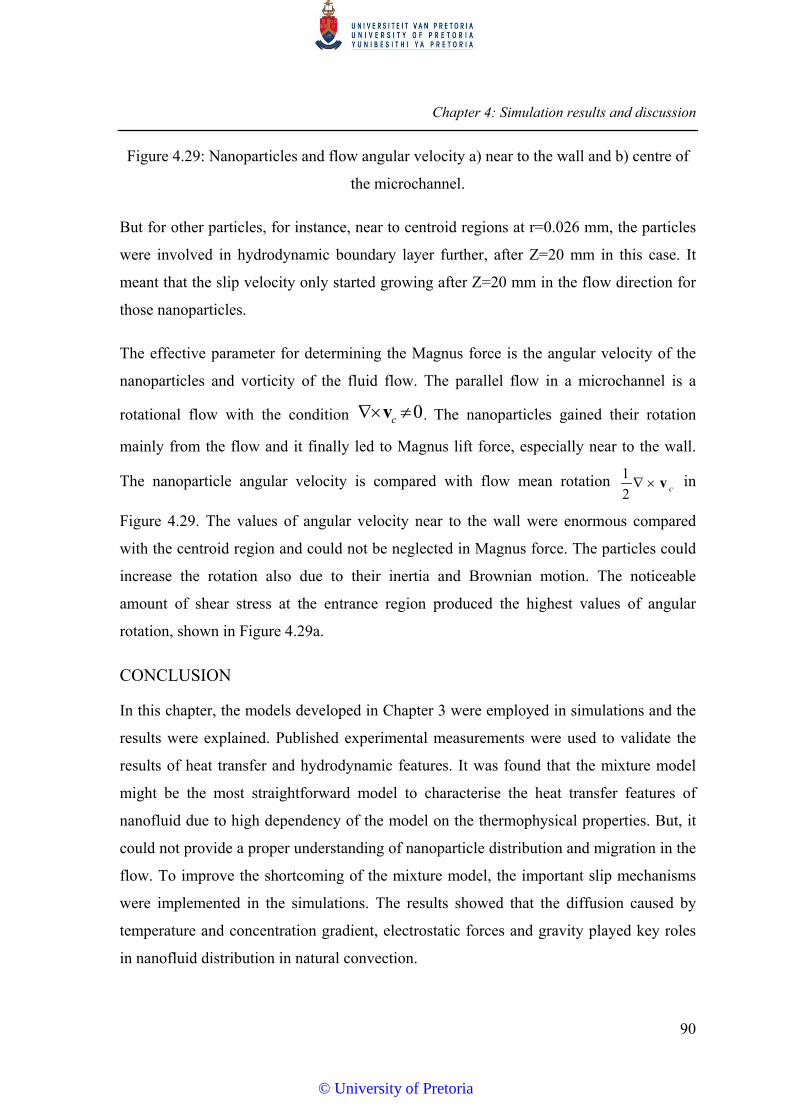
Chapter 4: Simulation results and discussion
90
Figure 4.29: Nanoparticles and flow angular velocity a) near to the wall and b) centre of
the microchannel.
But for other particles, for instance, near to centroid regions at r=0.026 mm, the particles
were involved in hydrodynamic boundary layer further, after Z=20 mm in this case. It
meant that the slip velocity only started growing after Z=20 mm in the flow direction for
those nanoparticles.
The effective parameter for determining the Magnus force is the angular velocity of the
nanoparticles and vorticity of the fluid flow. The parallel flow in a microchannel is a
rotational flow with the condition 0c v . The nanoparticles gained their rotation
mainly from the flow and it finally led to Magnus lift force, especially near to the wall.
The nanoparticle angular velocity is compared with flow mean rotation 1
2 c v in
Figure 4.29. The values of angular velocity near to the wall were enormous compared
with the centroid region and could not be neglected in Magnus force. The particles could
increase the rotation also due to their inertia and Brownian motion. The noticeable
amount of shear stress at the entrance region produced the highest values of angular
rotation, shown in Figure 4.29a.
CONCLUSION
In this chapter, the models developed in Chapter 3 were employed in simulations and the
results were explained. Published experimental measurements were used to validate the
results of heat transfer and hydrodynamic features. It was found that the mixture model
might be the most straightforward model to characterise the heat transfer features of
nanofluid due to high dependency of the model on the thermophysical properties. But, it
could not provide a proper understanding of nanoparticle distribution and migration in the
flow. To improve the shortcoming of the mixture model, the important slip mechanisms
were implemented in the simulations. The results showed that the diffusion caused by
temperature and concentration gradient, electrostatic forces and gravity played key roles
in nanofluid distribution in natural convection.
© University of Pretoria

Chapter 4: Simulation results and discussion
91
Discrete phase modelling was used to simulate nanoparticle flow in a microchannel. The
advantage of this model has concerned the real physical model of the simulations where
there was no need for extra thermophysical properties. The results for DPM were found in
good agreement for laminar flow in a horizontal microchannel. Most of the possible
phenomena involved in nanoparticle interactions were included. Brownian random
motion and electrostatic forces were found to be present in all the domains, but others
were effective only near to the wall.
The other forces including Saffman’s lift, Magnus lift and thermophoresis were scalable
only in the radial direction. Virtual mass, pressure gradient and gravity can be safely
neglected in nanofluid laminar flow. The impacts of the lift due to rotation of
nanoparticles in rotational flow or Magnus force could be observed on particle radial
distribution. Brownian motion was found the essential reason of particle migration,
especially angular displacement, but the impacts deteriorated when the nanoparticles
approached the wall. Higher amplitude of the angular displacement occurred near to the
centre of the microchannel. Van der Waals attraction force highly depended on particle-
to-particle distance and could be weak for volume fractions of less than 1%. On the other
hand, the electric double-layer force could play an important role in particle distribution.
The abilities and weaknesses of the mixture model for nanofluid are summarised as
follows:
The mixture model results highly depend on transport properties coming from
experimentation. It considers nanofluid as two phases. The thermophysical property
correlations for nanofluid are not universal and change by base fluid and nanoparticles.
The effects of slip mechanisms such as thermophoresis and Brownian can be presented as
diffusion terms in mixture equations and need to be implemented in the program.
The abilities and weaknesses of DPM for nanofluid are summarised as follows:
For the DPM model, there is no need for the nanofluids’ properties, but appropriate
interaction or diffusion forces, empirically or analytically. It treats the nanofluid as base
fluid and solid separately, as it is in reality. The empirical correlations for DPM
© University of Pretoria

Chapter 4: Simulation results and discussion
92
interaction forces are not extensive and can be employed in most of the cases. The
velocity is calculated for fluid and solid separately and eventually, the relative velocity
between them is the most important parameter.
There are some aspects of nanofluid simulations which are recommended here: possibility
of clustering and agglomeration inside the flow, and somehow sedimentation, size
distribution of the nanoparticles in the computational domain for the mixture model,
finding a way to combine both the mixture model and DPM, further development of
modelling the electric double layer around the particle.
.
© University of Pretoria
93
5 CHAPTER 5: CONCLUSIONS AND RECOMMENDATIONS
SUMMARY
The effect of the heat transfer enhancement of nanofluid has been the focus of many
researchers in recent years. A large number of experimental studies proved the
effectiveness of the presence of nanoparticles in a base fluid. Because of the complexity
of the interactions between solid and liquid, only a few methods have been developed in
recent years regarding the simulations. Most of the studies in this field of science were
briefly presented in Chapter 2 of this thesis.
The aim of this investigation is to develop new ideas in nanofluid flow regarding the
solid-liquid interaction phenomena. The mixture model as a common model in
simulations of nanofluid flow was presented and developed in Chapter 3. New slip
velocity was developed and implemented through some UDFs in ANSYS-Fluent. Only
thermophoresis and concentration diffusions were implemented in mass and energy
equations separately. The other interactions such as pressure gradient, virtual mass, lift,
gravity and electrostatic slip mechanisms were implemented in momentum equation as a
separate UDF.
Due to many restrictions in DPM, only a few studies were found in literature. In this
study, an attempt was made to consider most of the phenomena involved in nanofluid
mixtures in DPM. The validity of the final results was compared with other experimental
measurements. The findings covered the heat transfer and hydrodynamic features of the
flow, nanoparticle migration and concentration distribution. Electrostatic forces were
implemented in ANSYS-Fluent through some UDFs. Also, the new heat transfer equation
of particles was implemented as a new heat law with small predefined time steps in a
separate UDF.
CONCLUSIONS
Two different flow regimes were investigated in this study consisting of forced and
natural convective flows. Natural convection was studied in a rectangular cavity with
© University of Pretoria

Chapter 5: Conclusions and recommendations
94
nanofluid suspended and simulated with the developed mixture model. The results of heat
transfer were found in good agreement with experimental data. The conventional mixture
model in CFD software only considered the effect of the gravitational force as the slip
velocity. This provided the wrong concentration distribution at the vicinity of the walls.
Higher absolute value and gradient of volume fraction was predicted close to the walls by
the proposed method. The results showed that the diffusion caused by temperature and
concentration gradient, electrostatic forces and gravity played key roles in nanofluid
distribution in natural convection. The hydrodynamic boundary layer was the same for
most of the cases. The concentration boundary layer of zinc oxide nanoparticles was
found thin close to the wall and it had no effect on the velocity profile. It was mainly
caused by buoyancy force on zinc oxide nanoparticles with higher density than alumina
particles. The thermal boundary layer was the same for both alumina and zinc oxide
nanofluids. The increase of nanoparticle density and volume fraction from alumina to
zinc oxide clearly influenced the hydrodynamic boundary layer, particularly at the
beginning of the growth.
The discrete phase modelling was used to simulate nanoparticle flow in a horizontal
microchannel with laminar flow. This model was developed for particles in sizes larger
than nanoscale. Hence many of the interactions involved in micro-sizes might be
negligible in nano-sizes and other phenomena should be implemented. The heat transfer
results of DPM were found in good agreement with experimental data. Most of the
possible phenomena involved in nanoparticle interactions were included. Brownian
random motion and electrostatic forces were found to be present in all the domains, but
other parameters were effective only near to the wall. The other forces including
Saffman’s lift, Magnus lift and thermophoresis were scalable only in the radial direction
and mainly near to the wall. Virtual mass, pressure gradient and gravity could be safely
neglected in nanofluid laminar flow. The lift due to rotation of nanoparticles in rotational
flow or Magnus force could have an impact on particle radial distribution. Brownian
motion was found to be the most significant cause of particle migration, especially
angular displacement. However, the effect deteriorated when the particle approached the
wall because of the presence of other forces. Higher amplitude of the angular
© University of Pretoria
Chapter 5: Conclusions and recommendations
95
displacement occurred for the particles near to the centre of the microchannel. It meant
that Brownian motion was the phenomenon near to the centre with minimum shear
stresses and lift forces. Van der Waals attraction force highly depended on the particle-to-
particle distance and could be weak for volume fraction less than 1%. On the other hand,
the electric double-layer force could play a key role in particle distribution, depending on
the pH of the solution and zeta potential on the particles. The analysis of slip velocity
between nanoparticles and base fluid showed that, firstly, a stronger shear flow region
produced higher values of slip velocity. Secondly, the magnitude of the slip velocity was
found one order less than the fluid velocity, or even less.
In summary, the abilities of both the developed mixture model and DPM were studied in
this research. The following differences between these models were indicated:
1. The mixture model considered nanofluid as two phases. DPM treated the nanofluid as
base fluid and solid separately, as in reality.
2. The effect of slip mechanisms such as thermophoresis and Brownian could be
presented as diffusion terms in mixture equations and needed to be implemented in the
program. In DPM, velocity was calculated for fluid and solid separately and eventually,
the relative velocity between them was the most important parameter.
RECOMMENDATIONS
There are many untouched aspects of nanofluid in terms of both experimentations and
simulations. The following recommendations are provided for further investigation:
1. Only a few experimental measurements are available in literature for nanofluids to
show the precise amount of heat transfer and hydrodynamic feature enhancement.
Therefore, further experimental studies are recommended to provide the concentration
distribution during convective heat transfer
2. One of the important aspects of nanofluid is the possibility of clustering and
agglomeration inside the flow, and somehow sedimentation. This phenomenon are too
complicated and should be considered in future simulation
© University of Pretoria
Chapter 5: Conclusions and recommendations
96
3. The mixture model cannot consider the size distribution of the nanoparticles in the
computational domain, as DPM does. Further development for this case is needed.
4. Finding a way to combine both the mixture model and DPM can be one of the new
approaches in this field of study.
5. Because the liquid electrons are rearranged around a particle, called double layer, it can
be assumed that a new type of phase is added to the system. The surface tension between
this new phase and base fluid can be one of the phenomena involved. Further
investigation is needed.
© University of Pretoria
97
REFERENCES
[1] K.S. Hwang, S.P. Jang, S.U.S. Choi, Flow and convective heat transfer
characteristics of water-based Al2O3 nanofluids in fully developed laminar flow
regime, Int. J. Heat Mass Transf. 52 (2009) 193–199.
doi:10.1016/j.ijheatmasstransfer.2008.06.032.
[2] Y. Ding, H. Alias, D. Wen, R.A. Williams, Heat transfer of aqueous suspensions of
carbon nanotubes (CNT nanofluids), Int. J. Heat Mass Transf. 49 (2006) 240–250.
doi:10.1016/j.ijheatmasstransfer.2005.07.009.
[3] D. Wen, Y. Ding, Experimental investigation into convective heat transfer of
nanofluids at the entrance region under laminar flow conditions, Int. J. Heat Mass
Transf. 47 (2004) 5181–5188. doi:10.1016/j.ijheatmasstransfer.2004.07.012.
[4] Y. Yang, Z.G. Zhang, E.A. Grulke, W.B. Anderson, G. Wu, Heat transfer
properties of nanoparticle-in-fluid dispersions (nanofluids) in laminar flow, Int. J.
Heat Mass Transf. 48 (2005) 1107–1116.
doi:10.1016/j.ijheatmasstransfer.2004.09.038.
[5] Y. He, Y. Jin, H. Chen, Y. Ding, D. Cang, H. Lu, Heat transfer and flow behaviour
of aqueous suspensions of TiO 2 nanoparticles (nanofluids) flowing upward
through a vertical pipe, Int. J. Heat Mass Transf. 50 (2007) 2272–2281.
[6] D. Kim, Y. Kwon, Y. Cho, C. Li, S. Cheong, Y. Hwang, J. Lee, D. Hong, S. Moon,
Convective heat transfer characteristics of nanofluids under laminar and turbulent
flow conditions, Curr. Appl. Phys. 9 (2009) 119–123.
doi:10.1016/j.cap.2008.12.047.
[7] U. Rea, T. McKrell, L. wen Hu, J. Buongiorno, Laminar convective heat transfer
and viscous pressure loss of alumina-water and zirconia-water nanofluids, Int. J.
Heat Mass Transf. 52 (2009) 2042–2048.
doi:10.1016/j.ijheatmasstransfer.2008.10.025.
[8] K.B. Anoop, T. Sundararajan, S.K. Das, Effect of particle size on the convective
heat transfer in nanofluid in the developing region, Int. J. Heat Mass Transf. 52
© University of Pretoria
References
98
(2009) 2189–2195. doi:10.1016/j.ijheatmasstransfer.2007.11.063.
[9] B. Kolade, K.E. Goodson, J.K. Eaton, Convective Performance of Nanofluids in a
Laminar Thermally Developing Tube Flow, J. Heat Transfer. 131 (2009) 52402.
doi:10.1115/1.3013831.
[10] W.-Y. Lai, Experiments on Laminar Convective Heat Transfer with gamma-Al
2O3 Nanofluids, Arizona State University, 2010.
[11] Z. Zhang, Experimental evaluation of heat transfer characteristics of silica
nanofluid, Massachusetts Institute of Technology, 2010.
[12] M.M. Derakhshan, M.A. Akhavan-Behabadi, S.G. Mohseni, Experiments on
mixed convection heat transfer and performance evaluation of MWCNT-Oil
nanofluid flow in horizontal and vertical microfin tubes, Exp. Therm. Fluid Sci. 61
(2015) 241–248. doi:10.1016/j.expthermflusci.2014.11.005.
[13] Y.L. Zhai, G.D. Xia, X.F. Liu, Y.F. Li, Heat transfer enhancement of Al2O3-H2O
nanofluids flowing through a micro heat sink with complex structure, Int.
Commun. Heat Mass Transf. 66 (2015) 158–166.
doi:10.1016/j.icheatmasstransfer.2015.05.025.
[14] C.. Tang, S. Tiwari, M.W. Cox, Viscosity and friction factor of aluminum oxide--
water nanofluid flow in circular tubes, J. Nanotechnol. Eng. Med. 4 (2013) 21004.
[15] A.T. Utomo, E.B. Haghighi, A.I.T. Zavareh, M. Ghanbarpourgeravi, H. Poth, R.
Khodabandeh, B. Palm, A.W. Pacek, The effect of nanoparticles on laminar heat
transfer in a horizontal tube, Int. J. Heat Mass Transf. 69 (2014) 77–91.
doi:10.1016/j.ijheatmasstransfer.2013.10.003.
[16] D. Liu, L. Yu, Single-phase thermal transport of nanofluids in a minichannel, J.
Heat Transfer. 133 (2011) 31009. doi:10.1115/1.4002462.
[17] B.C. Pak, Y.I. Cho, Hydrodynamic and heat transfer study of dispersed fluids with
submicron metallic oxide particles, Exp. Heat Transf. 11 (1998) 151–170.
© University of Pretoria

References
99
doi:10.1080/08916159808946559.
[18] Y. Xuan, Q. Li, Investigation on convective heat transfer and flow features of
nanofluids, J. Heat Transfer. 125 (2003) 151. doi:10.1115/1.1532008.
[19] W. Williams, J. Buongiorno, L.-W. Hu, Experimental investigation of turbulent
convective heat transfer and pressure loss of alumina/water and zirconia/water
nanoparticle colloids (nanofluids) in horizontal tubes, J. Heat Transfer. 130 (2008)
42412. doi:10.1115/1.2818775.
[20] W. Yu, D.M. France, D.S. Smith, D. Singh, E. V. Timofeeva, J.L. Routbort, Heat
transfer to a silicon carbide/water nanofluid, Int. J. Heat Mass Transf. 52 (2009)
3606–3612. doi:10.1016/j.ijheatmasstransfer.2009.02.036.
[21] W. Duangthongsuk, S. Wongwises, An experimental study on the heat transfer
performance and pressure drop of TiO2-water nanofluids flowing under a turbulent
flow regime, Int. J. Heat Mass Transf. 53 (2010) 334–344.
doi:10.1016/j.ijheatmasstransfer.2009.09.024.
[22] L.S. Sundar, K. V. Sharma, Turbulent heat transfer and friction factor of Al2O3
Nanofluid in circular tube with twisted tape inserts, Int. J. Heat Mass Transf. 53
(2010) 1409–1416. doi:10.1016/j.ijheatmasstransfer.2009.12.016.
[23] S. Torii, Y. Satou, Y. Koito, Experimental study on convective thermal-fluid flow
transport phenomena in circular tube using nanofluids, Int. J. Green Energy. 7
(2010) 289–299. doi:10.1080/15435071003796061.
[24] S.S. Ferrouillat, A.A. Bontemps, J.-P.J.P. Ribeiro, J.-A.A. Gruss, O. Soriano,
Hydraulic and heat transfer study of SiO 2/water nanofluids in horizontal tubes
with imposed wall temperature boundary conditions, Int. J. Heat Fluid Flow. 32
(2011) 424–439. doi:10.1016/j.ijheatfluidflow.2011.01.003.
[25] A.R. Sajadi, M.H. Kazemi, Investigation of turbulent convective heat transfer and
pressure drop of TiO2/water nanofluid in circular tube, Int. Commun. Heat Mass
© University of Pretoria
References
100
Transf. 38 (2011) 1474–1478. doi:10.1016/j.icheatmasstransfer.2011.07.007.
[26] L.G. Asirvatham, B. Raja, D. Mohan Lal, S. Wongwises, Convective heat transfer
of nanofluids with correlations, Particuology. 9 (2011) 626–631.
doi:10.1016/j.partic.2011.03.014.
[27] S. Suresh, M. Chandrasekar, P. Selvakumar, Experimental studies on heat transfer
and friction factor characteristics of CuO/water nanofluid under laminar flow in a
helically dimpled tube, Heat Mass Transf. Und Stoffuebertragung. 48 (2012) 683–
694. doi:10.1007/s00231-011-0917-2.
[28] L.S. Sundar, M.T. Naik, K.V. Sharma, M.K. Singh, T.C. Siva Reddy, Experimental
investigation of forced convection heat transfer and friction factor in a tube with
Fe3O4 magnetic nanofluid, Exp. Therm. Fluid Sci. 37 (2012) 65–71.
doi:10.1016/j.expthermflusci.2011.10.004.
[29] W.H. Azmi, K. V. Sharma, P.K. Sarma, R. Mamat, S. Anuar, V. Dharma Rao,
Experimental determination of turbulent forced convection heat transfer and
friction factor with SiO2 nanofluid, Exp. Therm. Fluid Sci. 51 (2013) 103–111.
doi:10.1016/j.expthermflusci.2013.07.006.
[30] B. Sahin, G.G. Gültekin, E. Manay, S. Karagoz, Experimental investigation of heat
transfer and pressure drop characteristics of Al2O3-water nanofluid, Exp. Therm.
Fluid Sci. 50 (2013) 21–28. doi:10.1016/j.expthermflusci.2013.04.020.
[31] K. Wusiman, H. Chung, J.N. Md, A. Handry, Y. Eom, J. Kim, H. Jeong, Heat
transfer characteristics of nanofluid through circular tube, J. Cent. South Univ. 20
(2013) 142–148. doi:10.1007/s11771-013-1469-z.
[32] L.S. Sundar, M.K. Singh, I. Bidkin, A.C.M. Sousa, Experimental investigations in
heat transfer and friction factor of magnetic Ni nanofluid flowing in a tube, Int. J.
Heat Mass Transf. 70 (2014) 224–234.
doi:10.1016/j.ijheatmasstransfer.2013.11.004.
© University of Pretoria
References
101
[33] N. Putra, W. Roetzel, S.K. Das, Natural convection of nano-fluids, Heat Mass
Transf. Und Stoffuebertragung. 39 (2003) 775–784. doi:10.1007/s00231-002-
0382-z.
[34] D. Wen, Y. Ding, Formulation of nanofluids for natural convective heat transfer
applications, Int. J. Heat Fluid Flow. 26 (2005) 855–864.
doi:10.1016/j.ijheatfluidflow.2005.10.005.
[35] A.G.A. Nnanna, Experimental Model of Temperature-Driven Nanofluid, J. Heat
Transfer. 129 (2007) 697. doi:10.1115/1.2717239.
[36] B.H. Chang, A.F. Mills, E. Hernandez, Natural convection of microparticle
suspensions in thin enclosures, Int. J. Heat Mass Transf. 51 (2008) 1332–1341.
doi:10.1016/j.ijheatmasstransfer.2007.11.030.
[37] C.H. Li, G.P. Peterson, Experimental studies of natural convection heat transfer of
Al2O3/DI water nanoparticle suspensions (Nanofluids), Adv. Mech. Eng. 2010
(2009). doi:10.1155/2010/742739.
[38] C.J. Ho, W.K. Liu, Y.S. Chang, C.C. Lin, Natural convection heat transfer of
alumina-water nanofluid in vertical square enclosures: An experimental study, Int.
J. Therm. Sci. 49 (2010) 1345–1353. doi:10.1016/j.ijthermalsci.2010.02.013.
[39] R. Ni, S.Q. Zhou, K.Q. Xia, An experimental investigation of turbulent thermal
convection in water-based alumina nanofluid, Phys. Fluids. 23 (2011).
doi:10.1063/1.3553281.
[40] M.R. Khadangi Mahrood, S.G. Etemad, R. Bagheri, Free convection heat transfer
of non Newtonian nanofluids under constant heat flux condition, Int. Commun.
Heat Mass Transf. 38 (2011) 1449–1454.
doi:10.1016/j.icheatmasstransfer.2011.08.012.
[41] Y. Hu, Y. He, S. Wang, Q. Wang, H. Inaki Schlaberg, Experimental and
Numerical Investigation on Natural Convection Heat Transfer of TiO2–Water
© University of Pretoria
References
102
Nanofluids in a Square Enclosure, J. Heat Transfer. 136 (2013) 22502.
doi:10.1115/1.4025499.
[42] S.S. Rao, A. Srivastava, Interferometry-based whole field investigation of heat
transfer characteristics of dilute nanofluids, Int. J. Heat Mass Transf. 79 (2014)
166–175. doi:10.1016/j.ijheatmasstransfer.2014.07.097.
[43] C.J. Ho, D. Chen, W. Yan, O. Mahian, Buoyancy-driven flow of nanofluids in a
cavity considering the Ludwig – Soret effect and sedimentation : Numerical study
and experimental validation, 77 (2014) 684–694.
doi:10.1016/j.ijheatmasstransfer.2014.05.059.
[44] H. Li, Y. He, Y. Hu, B. Jiang, Y. Huang, Thermophysical and natural convection
characteristics of ethylene glycol and water mixture based ZnO nanofluids, Int. J.
Heat Mass Transf. 91 (2015) 385–389.
doi:10.1016/j.ijheatmasstransfer.2015.07.126.
[45] H. Moradi, B. Bazooyar, A. Moheb, S.G. Etemad, Optimization of natural
convection heat transfer of Newtonian nanofluids in a cylindrical enclosure,
Chinese J. Chem. Eng. 23 (2015) 1266–1274. doi:10.1016/j.cjche.2015.04.002.
[46] S.S. Rao, A. Srivastava, Interferometric study of natural convection in a
differentially-heated cavity with Al2O3-water based dilute nanofluids, Int. J. Heat
Mass Transf. 92 (2016) 1128–1142. doi:10.1016/j.ijheatmasstransfer.2015.09.074.
[47] Y. Xuan, W. Roetzel, Conceptions for heat transfer correlation of nanofuids, Int. J.
Heat Mass Transf. 43 (2000) 3701–3707.
[48] S. Sidi El Becaye Maiga, S.J. Palm, C.T. Nguyen, G. Roy, N. Galanis, Heat
transfer enhancement by using nanofluids in forced convection flows, Int. J. Heat
Fluid Flow. 26 (2005) 530–546. doi:10.1016/j.ijheatfluidflow.2005.02.004.
[49] J. Buongiorno, Convective Transport in Nanofluids, J. Heat Transfer. 128 (2006)
240. doi:10.1115/1.2150834.
© University of Pretoria

References
103
[50] A. Akbarinia, R. Laur, Investigating the diameter of solid particles effects on a
laminar nanofluid flow in a curved tube using a two phase approach, Int. J. Heat
Fluid Flow. 30 (2009) 706–714. doi:10.1016/j.ijheatfluidflow.2009.03.002.
[51] V. Bianco, O. Manca, S. Nardini, Numerical investigation on nanofluids turbulent
convection heat transfer inside a circular tube, Int. J. Therm. Sci. 50 (2011) 341–
349. doi:10.1016/j.ijthermalsci.2010.03.008.
[52] R. Mokhtari Moghari, A. Akbarinia, M. Shariat, F. Talebi, R. Laur, Two phase
mixed convection Al2O3-water nanofluid flow in an annulus, Int. J. Multiph. Flow.
37 (2011) 585–595. doi:10.1016/j.ijmultiphaseflow.2011.03.008.
[53] Z. Haddad, E. Abu-Nada, H.F. Oztop, A. Mataoui, Natural convection in
nanofluids: Are the thermophoresis and Brownian motion effects significant in
nanofluid heat transfer enhancement?, Int. J. Therm. Sci. 57 (2012) 152–162.
doi:10.1016/j.ijthermalsci.2012.01.016.
[54] H.A. Pakravan, M. Yaghoubi, Analysis of nanoparticles migration on natural
convective heat transfer of nanofluids, Int. J. Therm. Sci. 68 (2013) 79–93.
doi:10.1016/j.ijthermalsci.2013.04.007.
[55] E. Rossi di Schio, M. Celli, A. Barletta, Effects of Brownian Diffusion and
Thermophoresis on the Laminar Forced Convection of a Nanofluid in a Channel, J.
Heat Transfer. 136 (2013) 22401. doi:10.1115/1.4025376.
[56] M. Shariat, R.M. Moghari, A. Akbarinia, R. Rafee, S.M. Sajjadi, Impact of
nanoparticle mean diameter and the buoyancy force on laminar mixed convection
nanofluid flow in an elliptic duct employing two phase mixture model, Int.
Commun. Heat Mass Transf. 50 (2014) 15–24.
doi:10.1016/j.icheatmasstransfer.2013.11.003.
[57] M. Goodarzi, M.R. Safaei, K. Vafai, G. Ahmadi, M. Dahari, S.N. Kazi, N.
Jomhari, Investigation of nanofluid mixed convection in a shallow cavity using a
two-phase mixture model, Int. J. Therm. Sci. 75 (2014) 204–220.
© University of Pretoria

References
104
doi:10.1016/j.ijthermalsci.2013.08.003.
[58] M. Hejazian, M.K. Moraveji, A. Beheshti, Comparative study of Euler and mixture
models for turbulent flow of Al2O3 nanofluid inside a horizontal tube, Int.
Commun. Heat Mass Transf. 52 (2014) 152–158.
doi:10.1016/j.icheatmasstransfer.2014.01.022.
[59] Y. Abbassi, A.S. Shirani, S. Asgarian, Two-phase mixture simulation of
Al2O3/water nanofluid heat transfer in a non-uniform heat addition test section,
Prog. Nucl. Energy. 83 (2015) 356–364. doi:10.1016/j.pnucene.2015.04.009.
[60] F. Garoosi, B. Rohani, M.M. Rashidi, Two-phase mixture modeling of mixed
convection of nanofluids in a square cavity with internal and external heating,
Powder Technol. 275 (2015) 304–321. doi:10.1016/j.powtec.2015.02.015.
[61] S. Kakac, A. Pramuanjaroenkij, Single-phase and two-phase treatments of
convective heat transfer enhancement with nanofluids - A state-of-the-art review,
Int. J. Therm. Sci. 100 (2016) 75–97. doi:10.1016/j.ijthermalsci.2015.09.021.
[62] Y. He, Y. Men, Y. Zhao, H. Lu, Y. Ding, Numerical investigation into the
convective heat transfer of TiO2 nanofluids flowing through a straight tube under
the laminar flow conditions, Appl. Therm. Eng. 29 (2009) 1965–1972.
doi:10.1016/j.applthermaleng.2008.09.020.
[63] V. Bianco, F. Chiacchio, O. Manca, S. Nardini, Numerical investigation of
nanofluids forced convection in circular tubes, Appl. Therm. Eng. 29 (2009) 3632–
3642. doi:10.1016/j.applthermaleng.2009.06.019.
[64] K. Jin, Modeling Nano-Particle Migration in Pipe Flow through Eulerian-
Lagrangian Approach, Lehigh University, 2011.
http://preserve.lehigh.edu/cgi/viewcontent.cgi?article=2253&context=etd.
[65] S. Laín, M. Sommerfeld, Numerical calculation of pneumatic conveying in
horizontal channels and pipes: Detailed analysis of conveying behaviour, Int. J.
© University of Pretoria
References
105
Multiph. Flow. 39 (2012) 105–120. doi:10.1016/j.ijmultiphaseflow.2011.09.006.
[66] S. Tahir, M. Mital, Numerical investigation of laminar nanofluid developing flow
and heat transfer in a circular channel, Appl. Therm. Eng. 39 (2012) 8–14.
doi:10.1016/j.applthermaleng.2012.01.035.
[67] H. Bahremand, A. Abbassi, M. Saffar-Avval, Experimental and numerical
investigation of turbulent nanofluid flow in helically coiled tubes under constant
wall heat flux using Eulerian-Lagrangian approach, Powder Technol. 269 (2014)
93–100. doi:10.1016/j.powtec.2014.08.066.
[68] M. Ishii, T. Hibiki, Thermo-fluid dynamics of two-phase flow, Springer Science &
Business Media, 2010.
[69] M. Manninen, V. Taivassalo, S. Kallio, On the mixture model for multiphase flow,
Technical Research Centre of Finland Finland, VTT publications 288, 1996.
[70] P.G.T. Saffman, The lift on a small sphere in a slow shear flow, J. Fluid Mech. 22
(1965) 385–400.
[71] J.S. Marshall, S. Li, Adhesive particle flow, Cambridge University Press, 2014.
[72] A.R. Petosa, Transport , deposition and aggregation of metal oxide nanoparticles in
saturated granular porous media : role of water chemistry , collector surface and
particle coating, McGill University, Canada, 2013.
[73] D.G. Kröger, Air-cooled heat exchangers and cooling towers. Appendix A:
Properties of Biological Fluids, PennWell Books, 2004. doi:10.1016/B978-0-08-
087780-8.00143-1.
[74] E.E.S. Michaelides, Heat and mass transfer in particulate suspensions, Springer
Science & Business Media, 2013.
[75] M. Corcione, Empirical correlating equations for predicting the effective thermal
conductivity and dynamic viscosity of nanofluids, Energy Convers. Manag. 52
© University of Pretoria
References
106
(2011) 789–793. doi:10.1016/j.enconman.2010.06.072.
[76] F. Podczeck, Particle-particle adhesion in pharmaceutical powder handling, World
Scientific, 1998.
[77] R.J. Hunter, Foundations of colloid science, Oxford University Press, 2001.
[78] Sa. Morsi, A.J. Alexander, An investigation of particle trajectories in two-phase
flow systems, J. Fluid Mech. 55 (1972) 193–208.
[79] A. Haider, O. Levenspiel, Drag coefficient and terminal velocity of spherical and
nonspherical particles, Powder Technol. 58 (1989) 63–70.
[80] B. Oesterle, T.B. Dinh, Experiments on the lift of a spinning sphere in a range of
intermediate Reynolds numbers, Exp. Fluids. 25 (1998) 16–22.
doi:10.1007/s003480050203.
[81] S.C.R. Dennis, S.N. Singh, S.B. Ingham, The steady flow due to a rotating sphere
at low and moderate Reynolds numbers, J. Fluid Mech. 101 (1980) 257–279.
doi:10.1017/S0022112080001656.
[82] A.Y. Varaksin, J. Melorose, R. Perroy, S. Careas, Turbulent particle-laden gas
flows, Springer, 2007. doi:10.1017/CBO9781107415324.004.
[83] X. Zheng, Z. Silber-Li, The influence of Saffman lift force on nanoparticle
concentration distribution near a wall, Appl. Phys. Lett. 95 (2009) 24–27.
doi:10.1063/1.3237159.
[84] W. Kraipech, A. Nowakowski, T. Dyakowski, A. Suksangpanomrung, An
investigation of the effect of the particle-fluid and particle-particle interactions on
the flow within a hydrocyclone, Chem. Eng. J. 111 (2005) 189–197.
doi:10.1016/j.cej.2005.02.022.
[85] G.S. McNab, A. Meisen, Thermophoresis in liquids, J. Colloid Interface Sci. 44
(1973) 339–346. doi:10.1016/0021-9797(73)90225-7.
© University of Pretoria
References
107
[86] M. Ahmed, M. Eslamian, Numerical Simulation of Natural Convection of a
Nanofluid in an Inclined Heated Enclosure Using Two-Phase Lattice Boltzmann
Method: Accurate Effects of Thermophoresis and Brownian Forces, Nanoscale
Res. Lett. 10 (2015) 296. doi:10.1186/s11671-015-1006-0.
[87] E.E. Michaelides, Brownian movement and thermophoresis of nanoparticles in
liquids, Int. J. Heat Mass Transf. 81 (2015) 179–187.
doi:10.1016/j.ijheatmasstransfer.2014.10.019.
[88] A. Li, G. Ahmadi, Dispersion and Deposition of Spherical Particles from Point
Sources in a Turbulent Channel Flow, Aerosol Sci. Technol. 16 (1992) 209–226.
doi:10.1080/02786829208959550.
[89] J. Koo, C. Kleinstreuer, A new thermal conductivity model for nanofluids, J.
Nanoparticle Res. 6 (2004) 577–588. doi:10.1007/s11051-004-3170-5.
[90] H.E. Patel, T. Sundararajan, T. Pradeep, A. Dasgupta, N. Dasgupta, S.K. Das, A
micro-convection model for thermal conductivity of nanofluids, Pramana - J. Phys.
65 (2005) 863–869. doi:10.1007/BF02704086.
[91] W.E. Ranz, Evaporation from drops: Part II, Chem. Engng. Prog. 48 (1952) 173–
180.
[92] E.E. Michaelides, Z. Feng, Heat transfer from a rigid sphere in a nonuniform flow
and temperature field, Int. J. Heat Mass Transf. 37 (1994) 2069–2076.
doi:10.1016/0017-9310(94)90308-5.
[93] J.H. Ferziger, M. Peric, Computational methods for fluid dynamics, Springer
Science & Business Media, 2012.
[94] S. V Apte, K. Mahesh, T. Lundgren, Accounting for finite-size effects in
simulations of disperse particle-laden flows, Int. J. Multiph. Flow. 34 (2008) 260–
271.
[95] D.M. Snider, An incompressible three-dimensional multiphase particle-in-cell
© University of Pretoria
References
108
model for dense particle flows, J. Comput. Phys. 170 (2001) 523–549.
[96] ASHRAE, American society of heating, refrigerating and air-conditioning
engineers, Fundamentals. Appendix A, 2009.
[97] A. Kaufmann, M. Moreau, O. Simonin, J. Helie, Comparison between Lagrangian
and mesoscopic Eulerian modelling approaches for inertial particles suspended in
decaying isotropic turbulence, J. Comput. Phys. 227 (2008) 6448–6472.
doi:10.1016/j.jcp.2008.03.004.
[98] H. Ghodsinezhad, M. Sharifpur, J.P. Meyer, Experimental investigation on cavity
flow natural convection of Al2O3–water nanofluids, Int. Commun. Heat Mass
Transf. 76 (2016) 316–324. doi:10.1016/j.icheatmasstransfer.2016.06.005.
[99] E. Bacharoudis, M.G. Vrachopoulos, M.K. Koukou, D. Margaris, A.E. Filios, S.A.
Mavrommatis, Study of the natural convection phenomena inside a wall solar
chimney with one wall adiabatic and one wall under a heat flux, Appl. Therm. Eng.
27 (2007) 2266–2275. doi:10.1016/j.applthermaleng.2007.01.021.
[100] C. Teodosiu, F. Kuznik, R. Teodosiu, CFD modeling of buoyancy driven cavities
with internal heat source - Application to heated rooms, Energy Build. 68 (2014)
403–411. doi:10.1016/j.enbuild.2013.09.041.
[101] H. Zhang, S. Shao, H. Xu, C. Tian, Heat transfer and flow features of Al2O3-water
nanofluids flowing through a circular microchannel - Experimental results and
correlations, Appl. Therm. Eng. 61 (2013) 86–92.
doi:10.1016/j.applthermaleng.2013.07.026.
© University of Pretoria

109
A APPENDIX A: User-Defined Functions
APPENDIX A.1: UDFs for the developed mixture model, slip velocity approach /*********************************************************************** This UDF is to define a new slip velocity due to diffusion in mixture model equation This code needs to be either interpreted or compiled and all DEFINE_ADJUST functions are needed to be hooked up. ***********************************************************************/ /*Hint for temp gradianet from Help: Note that gradient variables are available only when the equation for that variable is being solved. */ #define diam 137.e-9 //particle diameter # define kB 1.3806e-23 //Boltzmann constant # define pi 3.1415 # define PH 3 //PH of the nanofluid # define e0 8.854e-12 //vaccum permitivity # define er 80 //relative permitivity (in this case for water # define Fa 96485 //Faraday constant # define Rg 8.31 # define zetap 30e-3 # define Ham 4e-20 //Hamaker constant(in this case for alumina nanofluid # define kp 36 //particle thermal conductivity DEFINE_ADJUST(adjust_T, domain) //new scalar for Temp int n = 0; Thread *t; cell_t c; face_t f; domain = Get_Domain(1); thread_loop_c(t, domain) begin_c_loop(c, t) C_UDSI(c, t, 0) = C_T(c, t); end_c_loop(c, t) thread_loop_f(t, domain) if (NULL != THREAD_STORAGE(t, SV_UDS_I(0)))
© University of Pretoria
Appendix A
110
begin_f_loop(f, t) real T1 = 0.; if (NULL != THREAD_STORAGE(t, SV_T)) T1 = F_T(f, t); else if (NULL != THREAD_STORAGE(t->t0, SV_T)) T1 = C_T(F_C0(f, t), t->t0); F_UDSI(f, t, 0) = T1; end_f_loop(f, t) DEFINE_ADJUST(adjust_vof, domain) Thread *t; cell_t c; face_t f; domain = Get_Domain(2); // Fill UDS with the vof. thread_loop_c(t, domain) begin_c_loop(c, t) C_UDSI(c, t, 1) = 1 - C_VOF(c, t); end_c_loop(c, t) thread_loop_f(t, domain) if (THREAD_STORAGE(t, SV_UDS_I(1)) != NULL) begin_f_loop(f, t) F_UDSI(f, t, 1) = 1 - F_VOF(f, t); end_f_loop(f, t) //slip velocity will be added DEFINE_VECTOR_EXCHANGE_PROPERTY(custom_slip, c, mixture_thread, primary_phase, secondary_phase, vector_result)
© University of Pretoria

Appendix A
111
real gravity[2] = 0., -9.81 ; real phi, T, rho_c, rho_m, mu_c, rhop;
real taup; real C_Brownian, kf, ST; real C_thermophes; real D_B; real Vp_x, Vp_y, Vp; real CB;
real Umgrad_x, Umgrad_y; real Vmgrad_x, Vmgrad_y; real Vm, Um; real a_x, a_y;
real Vs_x_BTGC, Vs_y_BTGC; real fvm_x, fvm_y; real fp_x, fp_y; real Vs_x_vm, Vs_y_vm; real xx; real Vs_x_p, Vs_y_p;
real Io, kk; real Fvdw, Fedl; real Fdlvo_x, Fdlvo_y;
real Vs_x_dlvo=0; real Vs_y_dlvo=0; real curlu;
real Rew; real CL; real fL_x, fL_y; real Vs_x_L, Vs_y_L;
Thread *pt; // thread pointers for primary phases Thread *st; // thread pointers for secondary phases pt = THREAD_SUB_THREAD(mixture_thread, primary_phase); st = THREAD_SUB_THREAD(mixture_thread, secondary_phase); phi = C_VOF(c, st); //vof second phase (or particle) // at this point the phase threads are known for primary (0) and secondary(1) phases T = C_T(c, pt); rho_c = 765.33 + 1.8142*T - 0.0035*pow(T, 2); //fluid density rho_m = C_R(c, mixture_thread); //mixture density kf = -0.00000718*pow(T, 2) + 0.00575419*T - 0.46662403; //water thermal conductivity
mu_c = 0.000000000029885*pow(T, 4) - 0.000000040781184*pow(T, 3) + 0.000020927097596*pow(T, 2) - 0.004792184560427*T + 0.414092804247831; //laminar fluid (water) viscosity
rhop = C_R(c, st); //secondary (particle) density taup = rhop*diam*diam / 18. / mu_c; //particle relaxation time D_B = kB*T / 3.0 / pi / mu_c / diam;
© University of Pretoria
Appendix A
112
C_Brownian = rho_m *D_B / (phi*(1 - phi)*rho_c); ST = 0.26*kf / (2.0 * kf + kp); C_thermophes = rho_m*ST*mu_c / ((1 - phi)*rho_c*rho_c); Um = C_U(c, mixture_thread); Vm = C_V(c, mixture_thread); Umgrad_x = C_U_G(c, mixture_thread)[0]; //U mixture velocity gradianet in x-direction Umgrad_y = C_U_G(c, mixture_thread)[1]; //U mixture velocity gradianet in y-direction Vmgrad_x = C_V_G(c, mixture_thread)[0]; //V mixture velocity gradianet in x-direction Vmgrad_y = C_V_G(c, mixture_thread)[1]; //V mixture velocity gradianet in y-direction a_x = gravity[0] - Um*Umgrad_x - Vm*Umgrad_y; //acceleration in x-direction a_y = gravity[1] - Um*Vmgrad_x - Vm*Vmgrad_y; //acceleration in y-direction
Vs_x_BTGC = taup*(rhop - rho_m)*a_x / rhop - C_thermophes*C_UDSI_G(c, pt, 0)[0] / T - C_Brownian*C_UDSI_G(c, st, 1)[0]; Vs_y_BTGC = taup*(rhop - rho_m)*a_y / rhop - C_thermophes*C_UDSI_G(c, pt, 0)[1] / T - C_Brownian*C_UDSI_G(c, st, 1)[1]; fvm_x = rho_c*0.5*(C_U(c, pt)*C_U_G(c, pt)[0] + C_V(c, pt)*C_U_G(c, pt)[1]);
fvm_y = rho_c*0.5*(C_U(c, pt)*C_V_G(c, pt)[0] + C_V(c, pt)*C_V_G(c, pt)[1]); Vs_x_vm = taup*fvm_x / rhop; //slip velocity due to virtual mass force in x-axis Vs_y_vm = taup*fvm_y / rhop; //////////////////////////pressure gradient slip velocity fp_x = rho_c*(C_U(c, pt)*C_U_G(c, pt)[0] + C_V(c, pt)*C_U_G(c, pt)[1]); fp_y = rho_c*(C_U(c, pt)*C_V_G(c, pt)[0] + C_V(c, pt)*C_V_G(c, pt)[1]); Vs_x_p = taup*fp_x / rhop; Vs_y_p = taup*fp_y / rhop; /////////////////////////// Saffman lift force curlu = C_V_G(c, pt)[0] - C_U_G(c, pt)[1]; Rew = rho_c*fabs(curlu)*diam*diam / mu_c; if (Rew == 0) CL = 0.076; else CL = 3.*6.46 / (2. * pi*sqrt(Rew)); fL_x = CL*rho_c*phi*curlu*vector_result[1]; fL_y = CL*rho_c*phi*curlu*vector_result[0]; Vs_x_L = taup*fL_x / rhop; Vs_y_L = taup*fL_y / rhop;
© University of Pretoria

Appendix A
113
//////////////////////////// van der waals attraction and repulsion (electrical double layer) forces xx =pow((pi / 6 / phi), 0.333333333333333)-1; //xx is h/d, surface distance to diameter of particle if (PH > 7) Io = 0.5*pow(10, (PH - 14)); //ionic strength else Io = 0.5*pow(10, -PH); kk = sqrt(2000 * pow(Fa, 2)*Io / e0 / er / Rg / T); //Debye parameter, 1/kk is Debye lenght if (xx > 1 / kk / diam) Fvdw = Ham / 6.0 / diam / (pow(xx, 2.0)*pow((xx + 1), 3)*pow((xx + 2), 2.0)); Fedl = pi*diam*kk*e0*er*zetap*zetap*exp(-kk*xx*diam); if (C_U(c, pt) > 0) Fdlvo_x = Fvdw - Fedl; else Fdlvo_x = Fedl - Fvdw; if (C_V(c, pt) > 0) Fdlvo_y = Fvdw - Fedl; else Fdlvo_y = Fedl - Fvdw; Vs_x_dlvo = Fdlvo_x / (3 * pi*mu_c*diam); Vs_y_dlvo = Fdlvo_y / (3 * pi*mu_c*diam); vector_result[0] = Vs_x_BTGC + Vs_x_vm + Vs_x_p - Vs_x_dlvo + Vs_x_L; vector_result[1] = Vs_y_BTGC + Vs_y_vm + Vs_y_p - Vs_y_dlvo + Vs_y_L; C_UDMI(c, pt, 0) = Fvdw / Fedl; C_UDMI(c, pt, 1) = Vs_x_dlvo / Vs_x_BTGC; C_UDMI(c, pt, 2) = Vs_x_L / Vs_x_BTGC; C_UDMI(c, pt, 3) = Vs_y_dlvo / Vs_y_BTGC; C_UDMI(c, pt, 4) = Vs_y_L / Vs_y_BTGC; //////////////////////////////////////////////////////////////////////////////////////////////////////////////////////////////////////// DEFINE_PROPERTY(airviscosity, c, t) real T = C_T(c, t); real alfa = C_VOF(c, t); real muair, muwater;
real mumixture;
© University of Pretoria
Appendix A
114
muwater = 0.000000000029885*pow(T, 4) - 0.000000040781184*pow(T, 3) + 0.000020927097596*pow(T, 2) - 0.004792184560427*T + 0.414092804247831;
mumixture = muwater / (1-34.87*pow(diam/3e-10,-0.3)*pow(alfa,1.03)); if (alfa == 0) muair = .0008; else muair = (mumixture - (1 - alfa)*muwater) / alfa; return muair; DEFINE_PROPERTY(airconductivity, c, t) real T = C_T(c, t); real alfa = C_VOF(c, t); real kbf, kair;
real knf; real mu_c = 0.000000000029885*pow(T, 4) - 0.000000040781184*pow(T, 3) + 0.000020927097596*pow(T, 2) - 0.004792184560427*T + 0.414092804247831; //laminar fluid (water) viscosity
real rho_c = 765.33 + 1.8142*T - 0.0035*pow(T, 2); //fluid density real cp_c = -0.00014301*pow(T, 3) + 0.15359377*pow(T, 2) - 54.08920728*T + 10444.58656104; real ub, Re, Pr_f; ub = 2 * kB*T / (pi*mu_c*diam*diam); Re = rho_c*ub*diam / mu_c;
kbf = -0.00000718*pow(T, 2) + 0.00575419*T - 0.46662403; Pr_f = cp_c*mu_c / kbf; knf = kbf*(1 + 4.4*pow(Re, 0.4)*pow(Pr_f, 0.66)*pow(T / 273.15, 10.)*pow(kp / kbf,0.03)*pow(alfa, 0.66)); if (alfa == 0) kair = .6; else kair = (knf - (1 - alfa)*kbf) / alfa; return kair;
APPENDIX A.2: UDFs for the developed mixture model, diffusion approach
© University of Pretoria
Appendix A
115
/*********************************************************************** Only the following code is added to the above mentioned code and diffusion of thermophoresis and Brownian is removed in slip velocity section. it is avoided mentioning it here (with some modifications) ***********************************************************************/ //source term in mass equation of second phase DEFINE_SOURCE(mass_source, c, t, dS, eqn) real source;
real T, Cp_c, DB; real kf, mu_c, rho_c; real ST, DT; real Gphi_GT; real GT_GT; real G2phi; real G2T;
T = C_T(c, t); Cp_c = -0.00014301*pow(T, 3) + 0.15359377*pow(T, 2) - 54.08920728*T + 10444.58656104; kf = -0.00000718*pow(T, 2) + 0.00575419*T - 0.46662403;
mu_c = 0.000000000029885*pow(T, 4) - 0.000000040781184*pow(T, 3) + 0.000020927097596*pow(T, 2) - 0.004792184560427*T + 0.414092804247831; //laminar fluid (water) viscosity
rho_c = 765.33 + 1.8142*T - 0.0035*pow(T, 2); DB = kB*T / 3.0 / pi / mu_c / diam; //for laminar ST = 0.26*kf / (2.0 * kf + kp); DT = ST*mu_c*C_UDSI(c, t, 4) / rho_c; Gphi_GT = C_UDSI(c, t, 5) * C_UDSI(c, t, 1) + C_UDSI(c, t, 6) * C_UDSI(c, t, 2) + C_UDSI(c, t, 7) * C_UDSI(c, t, 3); G2phi = C_UDSI_G(c, t, 5)[0] + C_UDSI_G(c, t, 6)[1] + C_UDSI_G(c, t, 7)[2]; G2T = C_UDSI_G(c, t, 1)[0] + C_UDSI_G(c, t, 2)[1] + C_UDSI_G(c, t, 3)[2]; source = rhop*((DB / T + ST*mu_c / rho_c / T)*Gphi_GT + DB*G2phi + DT*G2T / T); dS[eqn] = rhop* ST*mu_c *G2T / rho_c / T; return source; /////////////////////////////////////////////////////////////////////////////////////////////////////////////////////////////////////////////////////////////////////////////////// //source term in mixture enrgy equation DEFINE_SOURCE(Heat_source, c, t, dS, eqn)
© University of Pretoria
Appendix A
116
real source; real T, Cp_c, DB; real kf, mu_c, rho_c; real ST, DT; real Gphi_GT; real GT_GT; real G2phi; real G2T;
T = C_T(c, t); Cp_c = 28070 - 281.7*T + 1.25*pow(T, 2) - 0.00248*pow(T, 3) + 1.857e-06*pow(T, 4); kf = -.5752 + 6.397*.001*T - 8.151*.001*.001*pow(T, 2); //water thermal conductivity mu_c = .0967 - .0008207*T + 2.344*pow(10., -6)*pow(T, 2) - 2.244*pow(10., -9)*pow(T, 3); rho_c = 765.33 + 1.8142*T - 0.0035*pow(T, 2); DB = kB*T / 3.0 / pi / mu_c / diam; ST = 0.26*kf / (2.0 * kf + kp); DT = ST*mu_c*C_UDSI(c, t, 3) / rho_c; //thermophesis coefficient
Gphi_GT = C_UDSI_G(c, t, 3)[0] * C_UDSI_G(c, t, 0)[0] + C_UDSI_G(c, t, 3)[1] * C_UDSI_G(c, t, 0)[1] + C_UDSI_G(c, t, 3)[2] * C_UDSI_G(c, t, 0)[2];
GT_GT = C_UDSI_G(c, t, 1)[0] + C_UDSI_G(c, t, 2)[1] + C_UDSI_G(c, t, 3)[2]; source = rhop*Cp_p*(DB*Gphi_GT + DT*GT_GT/T); dS[eqn] = rhop*Cp_p *(kB*Gphi_GT / 3.0 / pi / mu_c / diam); return source; //the following boundary conditions are applied in the case of cavity DEFINE_PROFILE(temp_hot, t, i) real x[ND_ND]; /* this will hold the position vector */ real y; face_t f; begin_f_loop(f, t) F_CENTROID(x, f, t); y = x[1]; F_PROFILE(f, t, i) = -363.56*pow(y, 2.) + 74.527*y + 313.39; end_f_loop(f, t) DEFINE_PROFILE(temp_cold, t, i)
© University of Pretoria

Appendix A
117
real x[ND_ND]; /* this will hold the position vector */ real y; face_t f; begin_f_loop(f, t) F_CENTROID(x, f, t); y = x[1]; F_PROFILE(f, t, i) = 32.941*y + 294.17; end_f_loop(f, t)
© University of Pretoria