
Seasonal Variations in Water Quality of the Ganges and Brahmaputra River, Bangladesh
Upload
khangminh22Category
view
0download
0
FINAL REPORT
ON
STUDY OF BRAHMAPUTRA RIVER EROSION AND ITS CONTROL
Study Conducted
By
Department of Water Resources Development and Management Indian Institute of Technology Roorkee
For
National Disaster Management Authority of India

1
PHASE – I

2
TEAM OF INVESTIGATORS
1. Prof. Dr. Nayan Sharma
2. Dr. R. D. Garg
3. Ms. Archana Sarkar
4. Md. Parwez Akhtar
5. Mr. Neeraj Kumar

3
TABLE OF MAJOR CONTENTS
Sl. No. Subject Page No.
CHAPTER –I:
SATELLITE DATA BASED ANALYSIS OF
CHANNEL MORPHO-DYNAMIC STUDY FOR EROSION CONTROL OF BRAHMAPUTRA
RIVER SYSTEM
[A] BRAHMAPUTRA RIVER MAIN STEM
[B] MAJOR TRIBUTARIES OF
BRAHMAPUTRA RIVER SYSTEM
3
46
CHAPTER – II
SATELLITE DATA BASED ANALYSIS FOR
MORIGAON SITE ON BRAHMAPUTRA RIVER
60
CHAPTER – III
FINDINGS OF PHASE – I STUDY 71
REFERENCES 75

4
CHAPTER - I
SATELLITE DATA BASED
ANALYSIS OF CHANNEL MORPHO-
DYNAMIC STUDY FOR EROSION
CONTROL OF BRAHMAPUTRA
RIVER SYSTEM
[A] BRAHMAPUTRA MAIN STEM

5
CHAPTER – I [A]
BRAHMAPUTRA MAIN STEM SATELLITE DATA BASED ANALYSIS OF CHANNEL MORPHO-DYNAMIC STUDY FOR EROSION CONTROL OF BRAHMAPUTRA RIVER SYSTEM INTRODUCTION
The river Brahmaputra has been the lifeline of northeastern India since ages. This mighty river runs for 2880 kms through China, India and Bangladesh. Any alluvial river of such magnitude has problems of sediment erosion-deposition attached with it; the Brahmaputra is no exception. The problems of flood, erosion and drainage congestion in the Brahmaputra basin are gigantic. The Brahmaputra river is characterized by its exceedingly large flow, enormous volume of sediment load, continuous changes in channel morphology, rapid bed aggradations and bank line recession and erosion. The river has braided channel in most of its course in the alluvial plains of Assam. The lateral changes in channels cause severe erosion along the banks leading to a considerable loss of good fertile land each year. Bank oscillation also causes shifting of outfalls of its tributaries bringing newer areas under waters. Thousands of hectares of agricultural land is suffering from severe erosion continuously in the Brahmaputra basin covering parts of states like Assam, Arunachal Pradesh, Meghalaya, Nagaland and Manipur.
In order to tackle the problem of floods and erosion various agencies including state, central government and autonomous institutions are engaged in planning and execution of flood management programs in the north eastern region. To achieve effective flood management programs a variety of structural and non structural measures are adopted. These result in reasonable degree of protection to the flood prone areas in the Brahamaputra valley. However, due to the inherent widening characteristic of the Brahmaputra river they do not sustain and adversely affect the benefits anticipated while implementing the flood control and anti-erosion works. High floods cause large scale breaches in the existing embankments bringing vast areas under flood inundation.
Stream-bank erosion and its effects on channel evolution are essential geomorphic research problems with relevance to many scientific and engineering fields. Stream-bank erosion can damage infrastructure such as highway and bridges, can cause significant problems in adjusting water-discharge rating curves, and may represent up to 80 to 90% of the sediment load in streams and rivers (Simon and Rinaldi, 2000). It contributes to total maximum daily loads (TMDLs), can be a significant source of nonpoint-source sediment and nutrient pollution, and can have adverse effects on water quality and fish spawning habitat. However, bank erosion also is beneficial and an integral part of many river ecosystem processes (Florsheim et al., 2008). For example, coarse sediment from bank erosion can provide substrate for fish spawning (Flosi et al., 1998) and sediment for crane roosting habitat (Johnson 1994; U.S. Geological Survey, 2005). Irregular banks provide habitat for invertebrates, fish, and birds (Florsheim et al., 2008), and areas disturbed by erosion and deposition provide substrate for the establishment of riparian vegetation (Miller and Friedman, 2009). Moreover, knowledge of the dynamics of bank erosion is essential for planning dam removal projects and for designing river restoration

6
projects that accommodate the natural river migration processes that erode banks and build floodplains (Moody and Meade, 2008) on various time scales (Couper, 2004). Therefore, a better understanding on river channel changes is of great importance for river engineering and environmental management. LITERATURE REVIEW
Several investigators have used remotely sensed data for ascertaining channel changes of Brahmaputra River and its tributaries. NRSA (1980) has done the river migration study of the Brahmaputra using airborne scanner survey and to carry out repetitive survey to monitor changes in landuse, river channels and banks to provide a base for estimating the response of the rivers to flood events. Sarma and Basumallick (1980) studied the bankline migration of the Burhi Dihing River (southern tributary of Brahmaputra river) using topographic maps and field survey. Bardhan (1993) studied the channel behavior of the Barak river using satellite imagery and other data to identify the river stretches, if any, which remained reasonably stable during the period 1910-1988. SAC (Space Application Centre), Ahmedabad and Brahmaputra Board (1996) jointly took up a study to access the extent of river erosion in Majuli island in order to identify and delineate the areas of the island which have undergone changes along the bankline due to dynamic behaviour of the river. Based on this report and other collateral data, Brahmaputra Board (1997) has prepared a status report on the erosion problem of Majuli Island. Naik et al. (1999) studied the erosion at Kaziranga National Park using remote sensing data. Goswami et al. (1999) carried out a study on river channel changes of the Subansiri (northern tributary of Brahmaputra River) in Assam, India using information of topographic sheet and satellite data. Mani et al. (2003) studied the erosion in Majuli island using remote sensing data. Bhakal et al. (2005) have quantified the extent of bank erosion in Brahmaputra River near Agyathuri in Assam, India over a period of thirty years (1973-2003) using remote sensing data integrated with GIS. Kotoky et al (2005) studied selected reach of Brahamputra with two sets of Survey of India toposheets (1914 and 1975) and a set of IRS satellite images (1998, IRS-1B, LISS II B/W geocoded data by dividing the 270 km channel configuration from Panidihing Reserve Forest to Holoukonda Bil of the Brahmaputra River into ten segments. Sarma et al. (2007) studied the nature of bankline migration as well as made a quantitative assessment of the total amount of bank area subjected to erosion at different parts of Burhi Dihing River (southern tributary of Brahmaputra river) course during a period of time from 1934 to 2004 using Survey of India (SOI) toposheets, aerial photographs and IRS satellite data. Das and Saraf (2007) made a study in respect to a trend in river course changes of Brahmaputra river and influence of various surrounding geotectonic features for varying period between 1970-2002 for different sections of the river using Landsat-MSS, TM and ETM images. However, a comprehensive study of the bank erosion and channel migration of the entire Brahmaputra in India including its major tributaries with most recent satellite data has not yet been reported in the literature.
Fluvial landforms are produced by the action of flowing water in the terrestrial environment, whereas fluvial geomorphic processes are those natural processes that produce, maintain and change fluvial landforms. The channel pattern or landform of a reach of an alluvial river reflects the hydrodynamics of flow within the channel and the associated processes of sediment transfer and energy dissipation. Channel
7
patterns form a continuum in response to varying energy conditions ranging from straight and meandering to braided forms. Generally, braiding is favoured by high energy fluvial environments with steeper gradients, large and variable discharges, dominant bed load transport and non-cohesive banks lacking stabilization by vegetation (Richards, 1982). The secondary flow component also contributes to the growth of channel deformations (Bathurst et al., 1979).
Kotoky et al (2005) studied selected reach of Brahamputra with two sets of Survey of India toposheets (1914 and 1975) and a set of IRS satellite images covering the cloud-free period. For assessing rate of erosion, the channel configuration was divided for a distance of 270 km from Panidihing Reserve Forest to Holoukonda Bil of the Brahmaputra River into ten segments (I to X) at an interval of 15 minute east longitude in downstream direction. The bank-lines were superimposed upon each other and the areas subjected to erosion and deposition were measured with the help of a digital planimeter. Kotoky et al (2005) reported that the activity of erosion/deposition processes that operated was not similar for the periods 1914–75 and 1975–98.
However, Kotoky’s(2005) work was restricted to some of the limited stretches of river Brahmaputra and lacks a representative braiding tendency of the river in Assam flood plains, moreover braiding phenomenon which has been the major stakeholder of causative erosion and deposition was not dealt with. The remote sensing data used for study pertained to previous IRS sensor namely LISS I with coarse resolution resulting in possibilities of enhanced discrepancy while conducting analysis for studying bank shifting trend of River Brahmaputra. Existing Braiding Indicators
Several past studies had presented discrimination between the straight, meandering, and braided streams on the basis of discharge and channel slope. Lane (1957) suggested the following criterion for the occurrence of braiding. S > 0.004 (Qm)-0.25 (1) Where, Qm = mean annual discharge; and S = channel slope.
Using bank full discharge Qb, Leopold and Wolman in 1957 (Richards, 1982) proposed the relationship for braiding to occur, which also predicts braids at higher slopes and discharges: S > 0.013 Qb -0.44 (2) Where, Qb = bank full discharge.
Antropovskiy (1972) developed the following criterion for the occurrence of braiding S > 1.4Qb -1
(3) Leopold and Wolman (1957) also indicated that braided and meandering
streams can be separated by the relationship: S = 0.06 Q 0. 44 (4) Where, S = channel; and Q = water discharge.
However, these indicators have been criticized by Schumm and Khan (1972) as none of these recognizes the importance of sediment transport. These results imply a higher power expenditure rate in braided streams, a conclusion reinforced by Schumm and Khan’s (1972) flume experiments. However, none of these investigators recognizes the control of channel pattern by sedimentology. Since, bed material transport and bar formation are necessary in both meander and braid development processes, the threshold between the patterns should relate to bed load.
8
Henderson (1961) re-analyzed Leopold and Wolman's data to derive an expression including d50, median grain size (mm): S > 0.002 d50
1.15 Qb -0.46 (5)
Where, d50 = median grain size According to equation (5), a higher threshold slope is necessary for braiding in
coarse bed materials. Bank material resistance affects rate of channel migration and should also influence the threshold, although its effect may be difficult to quantify and also be non-linear since greater stream power is required to erode clays and cobbles than sands.
Parker's stability analysis (1976) indirectly illustrates the effects of bank material resistance by defining the meander - braid threshold as: S/Fr = D/B (6)
Where, D = mean depth of the flow; B = width of the stream, and Fr = Froude number. However, depth, width and Froude number may be expressed in terms of discharge and bank silt-clay percentage, as suggested by Schumm (Richards, 1982). Meandering occurs when S/Fr ≤ D/B, braiding occurs when S/Fr ≥ D/B, and transition occurs in between S/Fr ~ D/B.
Ferguson (1981) suggested for braiding to occur, which predicts steeper threshold slopes for braiding in channels with resistant silty banks. S > 0.0028 (Qb)-0.34 Bc
0.90 (7) Where, Bc = percentage of silty clay content in the bank material. Measures of the degree of braiding generally fall into two categories: (i) the
mean number of active channels or braid bars per transect across the channel belt; and (ii) the ratio of sum of channel lengths in a reach to a measure of reach length (total sinuosity). The sinuosity, P is thalweg length / valley length.
Smith (1970) illustrated the measurement of cross - section bed relief, measured by the index.
(8)
Where, Ti = height maxima between hollows; ti = minima between peaks; BL= transect length; and Te = end heights.
Sharma (2004) developed Plan Form Index (PFI), Flow Geometry Index (FGI), and Cross-Slope ratio for identifying the degree of braiding of highly braided river. The PFI, FGI and Cross- Slope formulae have been given below:
Plan Form Index =N
xBT 100
(9)
Flow Geometry Index = NxWxD
xd ii ][∑
(10)
Cross-Slope =).(
2levelbedAvlevelBank
BL
− (11)
where, T = flow top width; B= overall width of the channel; BL = Transect length across river width; N = number of braided channel; di and xi are depth and top lateral distance of submerged sub-channel; and D = hydraulic mean depth.
LBBRI Te,Te.tn)]t3t2(t1-..Tn)T22[(T1 21±……+++……+
=

9
Fig. 1 Definition sketch of PFI
Plan Form Index (PFI) in Equation 9 (Definition sketch as shown in Fig. 1)
reflects the fluvial landform disposition with respect to a given water level and its lower value is indicative of higher degree of braiding. For providing a broad range of classification of the braiding phenomenon, the following threshold values for PFI are proposed by Sharma (2004). Highly Braided: PFI < 4 Moderately Braided: 19 > PFI > 4 Low Braided: PFI > 19 STUDY OBJECTIVE
The present paper briefly describes a study of the Brahmaputra river - its entire course in Assam from upstream of Dibrugarh up to the town Dhubri near Bangladesh border for a stretch of around 620 kms and i ts major tributaries (13 northern and 10 southern) for a period of recent 18 years (1990-2008) using an integrated approach of Remote Sensing and Geographical Information System (GIS). The satellite data has provided the information on the channel configuration of the river system on repetitive basis revealing much needed data on the changes in river morphology, erosion pattern and its influence on the land, stable and unstable reaches of the river banks, changes in the main channel of the Brahmaputra river, changes in the major tributaries of the Brahmaputra river, etc
In this study, it is endeavored to assess the channel morphological changes actuated by stream bank erosion process. The newer braiding indicator PFI for Brahmaputra River formulated by Sharma (2004) has been adopted in the study to analyze the braiding behavior. Attempt has been made to assess the temporal and spatial variation of braiding intensities along the whole stretch of Brahmaputra in Assam plains of Indian Territory based on the remote sensing image analyses, which is the forcing function of erosion and thereby causing severe yearly land loss. THE STUDY AREA The Brahmaputra river, termed a moving ocean, is an antecedent snow fed river which flows across the rising young Himalayan Range. Geologically, the Brahmaputra is the youngest of the major rivers of the world. It originates at an altitude of 5,300 m about 63 Km south-east of the Mansarowar lake in Tibet. The river is known as Psangpo in Tibet. Flowing eastward for 1,625 km. over the Tibetan plateau, the Tsangpo enters a deep narrow gorge at Pe (3,500 m.) and continues southward across the east-west trending ranges of the Himalayas, viz. the Greater
T = T1 + T2 Water Level
B
T1 T2

10
Himalayas, Middle Himalayas and sub-Himalayas. After crossing the Indo-China border near Pasighat the river is called as the Siang or the Dihang. Two major rivers namely the Dibang and the Lohit join the Dihang at a short distance upstream of Kobo to form the river Brahmaputra. The river flows westward through Assam for about 700 Km distance from Dhola until dowmstream of the town Dhubri, where it abruptly turns south and enters Bangladesh. The gradient of the Brahmaputra river is as steep as 4.3 to 16.8 m./km. in the gorge section upstream of Pasighat, but near Guwahati it is as flat as 0.1m./km. The dramatic reduction in the slope of the Brahmaputra as it cascades through one of the world’s deepest gorges in the Himalayas before flowing in to the Assam plains explains the sudden dissipation of the enormous energy locked in it and the resultant unloading of large amounts of sediments in the valley downstream. In the course of its 2,880 km. journey, the Brahmaputra receives as many as 22 major tributaries in Tibet, 33 in India and three in Bangladesh. The northern and southern tributaries differ considerably in their hydro-geomorphological characteristics owing to different geological, physiographic and climatic conditions. The north bank tributaries generally flow in shallow braided channels, have steep slopes, carry a heavy silt charge and are flashy in character, whereas the south bank tributaries have a flatter gradient, deep meandering channels with beds and banks composed of fine alluvial soils, marked by a relatively low sediment load. Due to the colliding Eurasian (Chinese) and Indian tectonic plates, the Brahmaputra valley and its adjoining hill ranges are seismically very unstable. The earthquakes of 1897 and 1950, both of Richter magnitude 8.7, are among the most severe in recorded history. These earthquakes caused extensive landslides and rock falls on hill slopes, subsidence and fissuring in the valley and changes in the course and configuration of several tributary rivers as well as the main course The drainage basin of the Brahmaputra extends to an area of about 580,000 km2, from 82°E to 97° 50' E longitudes and 25° 10' to 31° 30' N latitudes. The basin spans over an area of 293,000 km2 (50.51%) in Tibet (China), 45,000 km2 (7.75%) in Bhutan, 194,413 km2 (33.52%) in India and 47,000 km2 (8.1%) in Bangladesh. Its basin in India is shared by six states namely, Arunachal Pradesh (41.88%), Assam (36.33%), Nagaland (5.57%), Meghalaya (6.10%), Sikkim (3.75%) and West Bengal (6.47%) (59).
For the present study, a reach of 620 Km on the main stem of Brahmaputra River, i.e., its entire course in Assam from upstream of Dibrugarh up to the town Dhubri near Bangladesh border has been considered. Twenty three major tributaries (13 northern and 10 southern) with in India have also been considered.

11
Fig. 2: Study Area
DATA USED
The basic data used in this study are digital satellite images of Indian Remote Sensing (IRS) LISS-I and LISS-III sensor, comprising of scenes for the years 1990, 1997, and 2008. In order to bring all the images under one geometric co-ordinate system, these are geo-referenced with respect to Survey of India (1:50,000 scale) topo-sheets using second order polynomial. IRS P6 LISS images of 1990, 1997 and 2008 years are geometrically rectified with reference to the Landsat images of the same area. The UTM projection and WGS 84 datum has been taken for geo-referencing. Rectification of the images was done with a residual RMS (root mean square error) of less than 1. Subsequently the re-sampling was performed at 23.5 m resolution using Nearest Neighborhood technique.
The entire river from Dhubri to upper Assam beyond Dibrugarh has been divided into 12 reaches. Each reach comprised of 10 cross sections. The bank line of the Brahmaputra River is demarcated from each set of imageries and the channel patterns are digitized using Arc GIS software. Cross sections are shown Fig. 2.
The spatial resolution of LISS-III is 23.5 m. The data used in the analysis have been presented in Table 1. ERDAS IMAGINE 8.6 image processing software has been used to perform the image processing works. Then satellite images of the other years were co-registered using image-to-image registration technique.

12
TABLE 1: CHARACTERISTICS OF THE REMOTE SENSING DATA USED
Satellite /sensor
Path/row Acquisition Spatial resolution
Spectral bands and channels
IRS 1C and D/ LISS-III (Standard Product)
112/52 1990, 1997, 2007-08
23.5m Visible band- (Green channel) (0.52 -0.59µm) Visible band- Red channel (0.62-0.68µm) Near infrared (NIR) (0.77 - 0.86µm)
IRS 1C and D/ LISS-III (Standard Product)
112/53 1990, 1997,2007-08
23.5m
For convenience in computing, the study area of around 622.73 km from Dhubri to Kobo beyond Dibrugarh in Upper Assam is considered as shown in Figs 2. METHODOLOGY
Appropriate GIS applications are done to precisely extract bank line information. Segment wise satellite-derived plan-form maps have been developed for the discrete years i.e. 1990, 1997 and 2007-08. Data Geo Referencing and Image Processing
One set of Survey of India topo-sheets (1965) and digital satellite images of IRS LISS-I and LISS-III sensors, comprising scenes for the years 1990, 1997 and 2007-08 are used for the present study. In order to assess the rate of erosion, maps and imagery are registered and geo-referenced with respect to Survey of India (1:50,000 scale) toposheets using second order polynomial. Using ERDAS imagine software, the satellite data have been geo-referenced with respect to 1:50,000 Survey of India topo-sheets.
The geo-referencing was done by the hardcopy map on digitizing table using second order equation with root mean square error less than 1.0 and nearest neighborhood re-sampling technique to create a geo-referenced image of pixel size 23.5m x 23.5m. Subsequently other images were also registered with the geo-referenced image using image-to-image registration technique. The registered images for different dates pertaining to study area were used for further analysis. Delineation of River Bank Line
For convenience, the main river has been divided into 120 strips, and reference cross sections were drawn at the boundary of each strip. Each ten cross sections are grouped as a reach with numbering from downstream to upstream of the river (of equal base length (Fig. 3; Table -2). Base line of Latitude 25.966o and Longitude 90o E has been taken as permanent reference line. The derived data for each cross section from satellite images of years 1990, 1997, 2008 have been analyzed and the bank lines are also digitized for all the years. The length of arcs of both the left and right banks for all the above years are found out using GIS software. The years 1990 , 1997 and 2008 have been taken for analyzing erosion and deposition along the river left bank as well as right bank.

13
Fig.3: 120 strips of left bank Intermediate channel widths, and total widths of channel at each predefined
cross sections are measured using GIS software tools for computing Plan Form Indices for each cross sections for further analysis.
Erosion in north and south banks of the river area during the study period (that is 1990-2007-08 and 1997-2007-08) is estimated by GIS software tools through delineating the river bank lines and drawing polygons within bank line variations within the study period
Remote sensing satellite data having ability to provide comprehensive, synoptic view of fairly large area at regular interval with quick turn around time integrated with GIS techniques makes it appropriate and ideal for studying and monitoring river erosion and its bank line shifting. Various studies in this regard have been carried out for some major rivers all over the world. Surian (1999) reported the channel changes of the Piave River in the Eastern Alps, Italy, which occurred in response to human interventions in the fluvial system through a historical analysis using maps and aerial photographs. A typical study of channel migration by Yang et al. (1999) in Yellow river (China) made use both analog and digital data with a time sequential imageries of 19 dates from 1976 to 1994. Rinaldi (2003) presented changes in channel width of the main alluvial rivers of Tuscany (central Italy) during the 20th century by comparing available aerial photographs (1954 and 1993-98). Surian and Rinaldi (2003) reviewed all existing published studies and available data on most Italian rivers that experienced considerable channel adjustment during the last centuries due to various types of human disturbance. Fuller et al (2003) quantified three-dimensional morphological adjustment in a chute cutoff (breach) alluvial channel using Digital Elevation Model (DEM) analysis for a 0.7 km reach of the River Coquet, Northumberland, UK. Li et al (2007) examined human impact on channel change in Jianli reach of the middle Yangtze River of China employing 1:100,000 channel distribution maps from 1951, 1961 and 1975 and 1:25,000 navigation charts from 1981 and 1997 to reconstruct channel change in the study reach. Kummu et al (2008) assessed bank erosion problems in the Vientiane–Nong Khai section of the Mekong River, where the Mekong borders Thailand and Lao PDR using two Hydrographic Atlases dated 1961 and 1992, and SPOT5 satellite images of 2004 and 2005 with a resolution of 2.5m in natural colours.
Base line

14
PLAN FORM INDEX (PFI) Plan Form Index (PFI) reflects the fluvial landform disposition with respect to a
given water level and its lower value is indicative of higher degree of braiding. The computed Plan Form Index for each reference cross-section totalling 120
in numbers across the study reaches are plotted against reach cross-section number in Fig. 7 for three discrete years. From the plot, it can be readily inferred that from 1990 to 2007-08, the PFI values by and large decreases significantly indicating the increase in braiding intensities in majority of cross sections considering the fixed threshold values of PFI given for measuring braiding intensity mentioned in Sec. 2 (Sharma, 2004) of this paper.
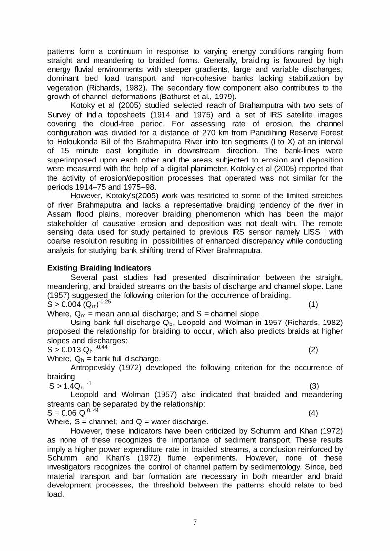
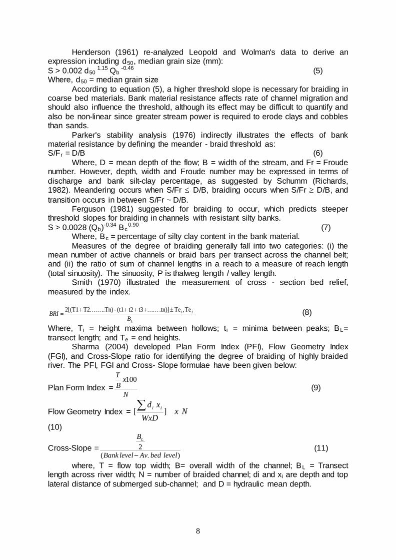
The analysis can further be extended by computing mean PFI values for reach-1 to reach 12 comprising of ten cross-sections each, shown in tables 3, 4, 5 for the discrete years. Similarly, extreme values that are maximum PFI (indicating least braiding within the reach) and minimum PFI (indicating highest braiding within the reach) for each reach are computed and shown in Table-6. The corresponding plot for Mean, Minimum and Maximum PFI against reach numbers are plotted and shown in Fig. 4, 5 and 6 respectively. Mean PFI enveloping with maximum and minimum cross-sectional PFI suggest the ranges of variation in braiding intensities within a reach. It can be easily figured out that maximum values are predominant in the year 1990, whereas in 2007-08 minimum values are predominant. All three statistically measured PFIs are registering little changes or similar trend in three to four identified reaches with rock-outcrops numbered 2, 4 ,6-7 and 9, which are in the vicinity of Jogighopa, Guwahati, Tezpur and Bessamora in Majuli.
It strongly suggests that irrespective of the time, the aforementioned four discrete reaches show little changes in braiding intensity and pattern. It confirms the existence of the aforesaid four geological control points which hold the river, and in between there are intermittent fanning out of the river with time. Other than these river control points, more braiding is expected where bank line configurations and characteristics are conducive for braiding to occur in other reaches.
As discussed, the graphical plots of Plan Form Index for the Brahmaputra River shows increasing trend thereby registering an increasing level of braiding, as can be seen from the threshold limits as described in Sec. 2 of this paper. Plots for all reference cross sections for the years 1990, 1997 and 2007-08 between PFI’s and cross section numbers shows the increasing trend of braiding with time. These plots clearly demonstrate the rationality of using the Plan Form Index as a measure of braiding and closely conform to the actual physical situation of the occurrence of braiding vividly depicted in satellite images. In light of the threshold values of Plan Form Index, it can be readily inferred from graphical plots showing maximum, minimum and mean values of PFIs of cross sections that have heavy with moderate and low braiding characteristics resulting in a very complex channel hydrodynamics.

15
TABLE 2: IDENTIFICATION OF REACHES IN RESPECT OF THE LOCATION IN THE VICINITY
Reach Locations in Vicinity
1 Dhubri 2 Goalpara 3 Palasbari 4 Guwahati 5 Morigaon (Near Mangaldai) 6 Morigaon (Near Dhing) 7 Tezpur 8 U/s of Tezpur (Near Gohpur) 9 Majuli 10 U/s of Majuli (Near Sibsagar) 11 Dibrugarh 12 U/s of Dibrugarh
TABLE 3: PLAN FORM INDEX (PFI) ESTIMATION OF BRAHMAPUTRA RIVER FOR 1990 YEAR
Reach Plan Form Index Threshold Indicator
1 22.69 Low Braided 2 15.39 Moderately Braided 3 10.55 Moderately Braided 4 55.97 Low Braided 5 14.19 Moderately Braided 6 28.34 Low Braided 7 31.94 Low Braided 8 19.12 Low Braided 9 10.14 Moderately Braided
10 13.61 Moderately Braided 11 12.38 Moderately Braided 12 20.95 Low Braided

16
TABLE 4: PLAN FORM INDEX (PFI) ESTIMATION OF BRAHMAPUTRA RIVER FOR 1997 YEAR
Reach Plan Form Index Threshold Indicator
1 8.94 Moderately Braided 2 8.60 Moderately Braided 3 7.71 Moderately Braided 4 33.62 Low Braided 5 13.55 Moderately Braided 6 14.74 Moderately Braided 7 17.21 Moderately Braided 8 10.77 Moderately Braided 9 10.69 Moderately Braided
10 7.87 Moderately Braided 11 6.81 Moderately Braided 12 4.89 Moderately Braided
TABLE 5: PLAN FORM INDEX (PFI) ESTIMATION OF BRAHMAPUTRA RIVER FOR 2008 YEAR
Reach Plan Form Index Threshold
Indicator 1 15.66 Moderately Braided 2 20.30 Low Braided 3 9.99 Moderately Braided 4 73.64 Low Braided 5 8.08 Moderately Braided 6 7.78 Moderately Braided 7 18.50 Moderately Braided 8 6.89 Moderately Braided 9 6.34 Moderately Braided 10 6.54 Moderately Braided 11 5.41 Moderately Braided 12 2.61 Heavily Braided

16
TABLE 6: COMPARISON OF PLAN FORM INDEX (PFI) FOR THE YEAR 1990, 1997 AND 2008 FOR THE RIVER BRAHMAPUTRA
Reach
No. PFI(1990) PFI(1997) PFI(2008) Remarks
Mean Minimum Maximum Mean Minimum Maximum Mean Minimum Maximum 1 22.69 9.90 45.16 8.94 13.22 4.37 15.66 5.74 38.65 Highly
Braided: PFI < 4 Moderately Braided: 19 > PFI > 4 Low Braided: PFI > 19
2 15.39 5.23 48.67 8.60 3.50 21.09 20.30 4.42 98.05 3 10.55 3.50 31.15 7.71 2.83 16.22 9.99 3.75 24.79 4 55.97 8.46 113.89 33.62 8.94 124.48 73.64 16.47 136.85 5 14.19 6.18 20.92 13.55 4.52 38.39 8.08 4.88 19.67 6 28.34 9.98 108.61 14.74 7.73 30.46 7.78 3.40 31.30 7 31.94 18.23 82.47 17.21 7.48 37.27 18.50 4.37 100.00 8 19.12 3.28 83.19 10.77 4.39 32.43 6.89 3.84 14.95 9 10.14 5.25 22.71 10.69 3.64 48.37 6.34 2.00 17.55
10 13.61 6.09 34.31 7.87 5.25 10.65 6.54 3.77 12.57 11 12.38 7.65 27.93 6.81 3.36 12.23 5.41 3.52 10.91 12 20.95 4.27 87.05 4.89 2.76 7.57 2.61 1.63 3.70
Note: There is considerable increase in braiding intensity during the period 1990-2008 as can be seen from Table -5
17
Fig. 4: Change in the Reach wise MEAN Plan Form Index (PFI) Values in different reaches of the Brahmaputra River in 1990, 1997 and 2008 year
Fig. 5: Change in the Reach wise MINIMUM Plan Form Index (PFI) Values in different reaches of the Brahmaputra River in 1990, 1997 and 2008 year
Comparison of reachwise Mean PFI
0.00
10.00
20.00
30.00
40.00
50.00
60.00
70.00
80.00
1 2 3 4 5 6 7 8 9 10 11 12
Reach Number
Mea
n re
achw
ise
PFI
199019972008
Comparison of reachwise Min. PFI
0.00
2.00
4.00
6.00
8.00
10.00
12.00
14.00
16.00
18.00
20.00
1 2 3 4 5 6 7 8 9 10 11 12
Reach Number
Reac
hwis
e M
in. P
FI
199019972008
Highly Braided
PFI =4
Highly Braided

18
Fig. 6: Change in the Reach wise MAXIMUM Plan Form Index (PFI) Values in different reaches of the Brahmaputra River in 1990, 1997 and 2008 year
Fig. 7: Cross-section wise Plan Form Index (PFI) Values in different
reaches of the Brahmaputra River in 1990, 1997 and 2008 year
Comparison of Reachwise Max. PFI
0.00
20.00
40.00
60.00
80.00
100.00
120.00
140.00
160.00
1 2 3 4 5 6 7 8 9 10 11 12
Reach Number
Reac
hwis
e M
ax. P
FI199019972008
0.0
20.0
40.0
60.0
80.0
100.0
120.0
140.0
160.0
1.1
1.5
1.9
2.4
2.8
3.3
3.7
4.2
4.6
4.10 5.1
5.5
5.9
6.4
6.8
7.3
7.7
8.2
8.6
8.10 9.1
9.5
9.9
10.4
10.8
11.3
11.7
12.2
12.6
12.1
0
Reachwise Cross sections
PFI V
alue
s
199019972008

19
Fig. 8: The Moderately Braided Channels (Reach 1 - Near Dhubri) in IRS 1C LISS - III image of 1997 year with Plan Form Index value 11.2
Fig. 9: The Highly Braided Channels (Reach 1 - Near Dhubri) in IRS P6 LISS - III image of 2008 year with Plan Form Index value 3.7
20
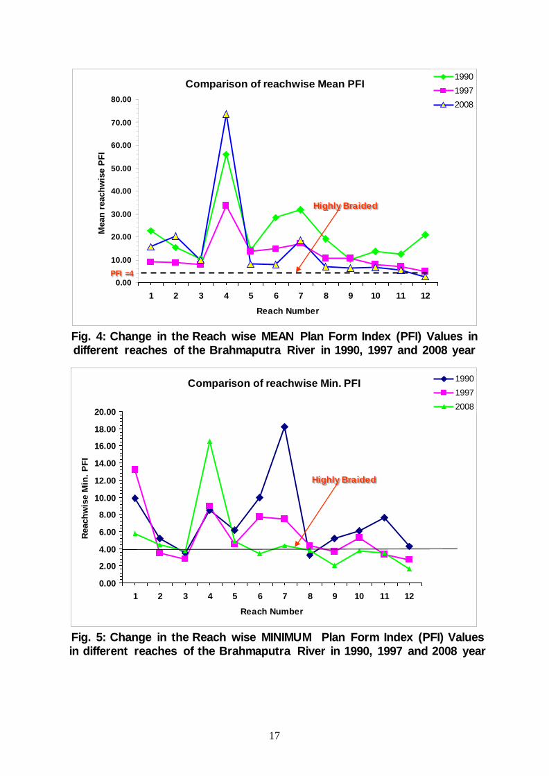
Fig. 10: The Moderately Braided Channels (Reach 2 – Near Barpeta) in IRS 1C LISS - III image of 1997 year with Plan Form Index value 4.1
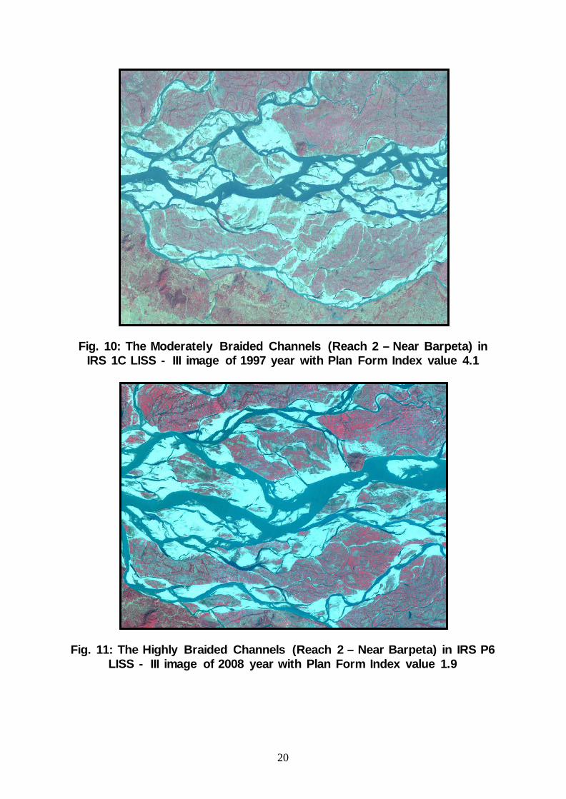
Fig. 11: The Highly Braided Channels (Reach 2 – Near Barpeta) in IRS P6 LISS - III image of 2008 year with Plan Form Index value 1.9

21
Fig. 12: The Moderately Braided Channels (Reach 3 - Palashbari Gumi) in IRS 1C LISS - III image of 1997 year with Plan Form Index value 2.4
Fig. 13: The Highly Braided Channels (Reach 3 - Palashbari Gumi) in IRS P6 LISS - III image of 2008 year with Plan Form Index value 1.6

22
Fig. 14: The Highly Braided Channels (Reach 5 – Near Mangaldai) in IRS 1C LISS - III image of 1997 year with Plan Form Index value 2.1
Fig. 15: The Highly Braided Channels (Reach 5 – Near Mangaldai) in IRS P6 LISS - III image of 2008 year with Plan Form Index value 2.7

23
Fig. 16: The Moderately Braided Channels (Reach 7 – Upstream Silghat) in IRS 1C LISS - III image of 1997 year with Plan Form Index value 5.5
Fig. 17: The Highly Braided Channels (Reach 7 – Upstream Silghat) in IRS P6 LISS - III image of 2008 year with Plan Form Index value 3.7
24
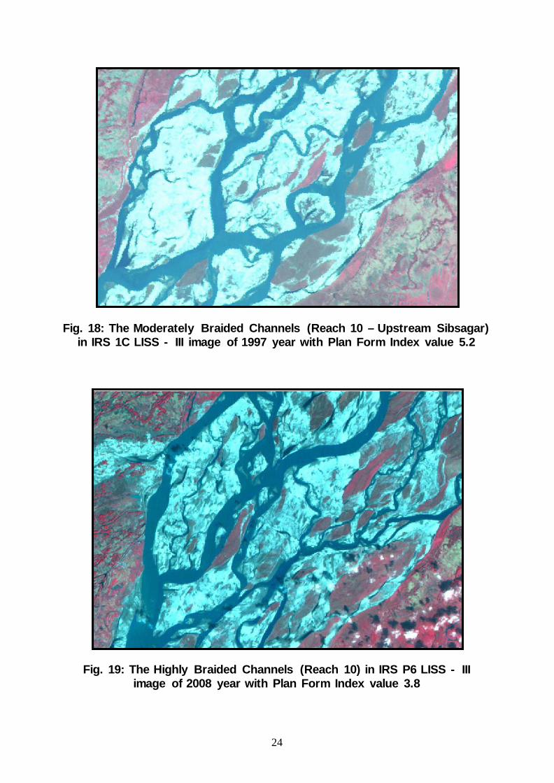
Fig. 18: The Moderately Braided Channels (Reach 10 – Upstream Sibsagar) in IRS 1C LISS - III image of 1997 year with Plan Form Index value 5.2
Fig. 19: The Highly Braided Channels (Reach 10) in IRS P6 LISS - III image of 2008 year with Plan Form Index value 3.8

25
RIVER BANK EROSION / MIGRATION
The bank lines of the river were demarcated from the Satellite Imageries of 1990, 1997 and 2008 year using ERDAS and ArcMap Software Tools. Mosaic images of year 1990, 1997 and 2007-08 with digitized bank lines and reference cross-sections are presented in Fig. 20, 21 and 22 respectively.
The satellite image based estimation of area eroded in Brahmaputra during periods 1990 to 2007-08 and 1997 to 2007-08 is presented in tabular form (Table 7), which shows the eroding tendency along the river banks of Brahmaputra in the entire study area. For the period of 17 years, the total land loss per year excluding forest area is found out to be 62km2/year. For more recent period of 1997 to 2007-08 the total land loss per year (excluding avulsion) is found out to be 72.5km2/year which is registering sharp increase in land lost due to river erosion in recent years. This calls for a robust and efficient river management action plan to arrest huge valuable land losses to erosion.
TABLE 7 SATELLITE BASED ESTIMATION AND COMPARISON OF AREA
ERODED IN BRAHMAPUTRA DURING THE PERIOD 1990 TO 2007-08 AND 1997 TO 2007-08
Reach Number
North Bank South Bank
Minimum PFI
Values
Total Erosion Length (Km)
1990 to 2007-08 (in Sq.Km)
1997 to
2007-08 (in
Sq. Km)
Total Erosion Length (Km)
1990 to
2007-08
(Sq. Km)
1997 to
2007-08 (in
Sq. Km)
1997
2007
-08
1(Dhubri) 40.19 124.461 94.129 7.05 194.983 10.791 13.22 5.74 2(Goalpara) 39.5 79.046 40.902 4.85 17.816 5.052 3.50 4.42 3(Palasbari) 54.87 48.668 42.914 14.02 23.006 15.859 2.83 3.75 4(Guwahati) 21.02 7.92 1.654 24.38 5.385 12.079 8.94 16.4 5(Morigaon-Mangaldai ) 6 35.606 2.138 47.91 96.979 103.7 4.52 4.88 6(Morigaon-Dhing) 24.86 29.057 7.275 47.8 10.795 56.72 7.73 3.40 7(Tezpur) 8.58 38.758 4.733 52.95 16.628 44.774 7.48 4.37 8( Tezpur-Gohpur) 8.85 31.187 5.794 44.16 26.098 71.227 4.39 3.84 9(Majuli-Bessamora) 24.69 25.562 12.327 47.17 32.788 28.998 3.64 2.00 10( Majuli-Sibsagar) 16.93 60.657 16.878 54.95 44.018 42.118 5.25 3.77 11(Dibrugarh) 37.86 37.506 43.529 43.89 46.595 6.066 3.36 3.52 12(U/s Dibrugarh)
70.5 20.376 55.454 57.54 399.529 333.416 Forest Area Excluded southern
side TOTAL 353.85 538.805 327.726 389.13 914.62 730.8

26
Moreover, vulnerability of the stream bank erosion is significant as evident
from Table 7. Almost 750 km of bank line in both side of the river has potential erosion tendency. The table also shows that downstream of Guwahati (Reach Number 4), erosion tendency is considerably high in north bank line whereas in the upstream of Guwahati erosion tendency is considerably high in south bank-line, indicating that river geological control point at Guwahati in respect to other control points has significant causative impact on the morphological behavior of River Brahmaputra as a whole in Assam flood plains. It urgently warrants attention for undertaking the integrated river management planning of Brahmaputra on holistic approach.
Fig. 20: Brahmaputra River Cross-Sections Year 1990

27
Fig. 21: Mosaic of IRS 1C LISS – III Satellite Image of
Brahmaputra River Year 1997
Fig. 22: Mosaic of IRS P6 LISS – III Satellite Image of
Brahmaputra River Cross-Sections Year 2007-08
P6
28
Nort
Dhubri
Barpeta
Goalpara Guwahati
Lahorighat Dhing
Dibrugarh
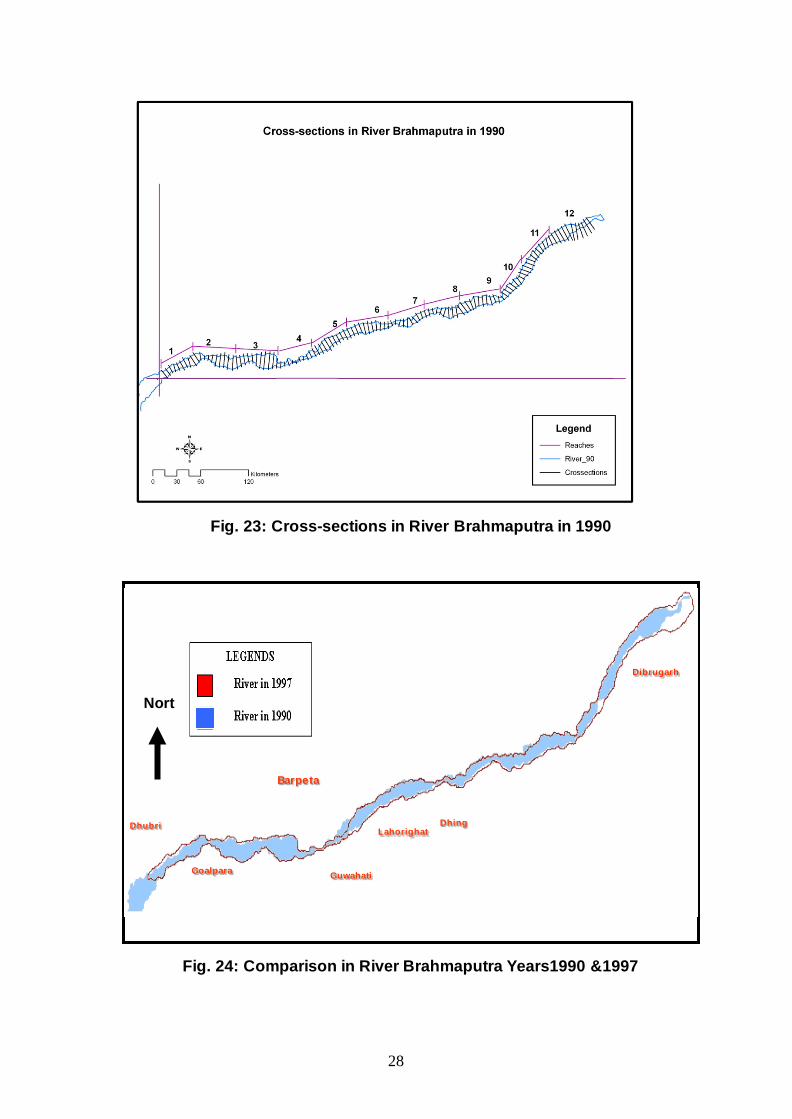
Fig. 23: Cross-sections in River Brahmaputra in 1990
Fig. 24: Comparison in River Brahmaputra Years1990 &1997
29
1
2 3 4
5
6 7
9
10
11
8
North
East
Dhubri
Barpeta
Goalpara Guwahati
Lahorighat Dhing
Dibrugarh
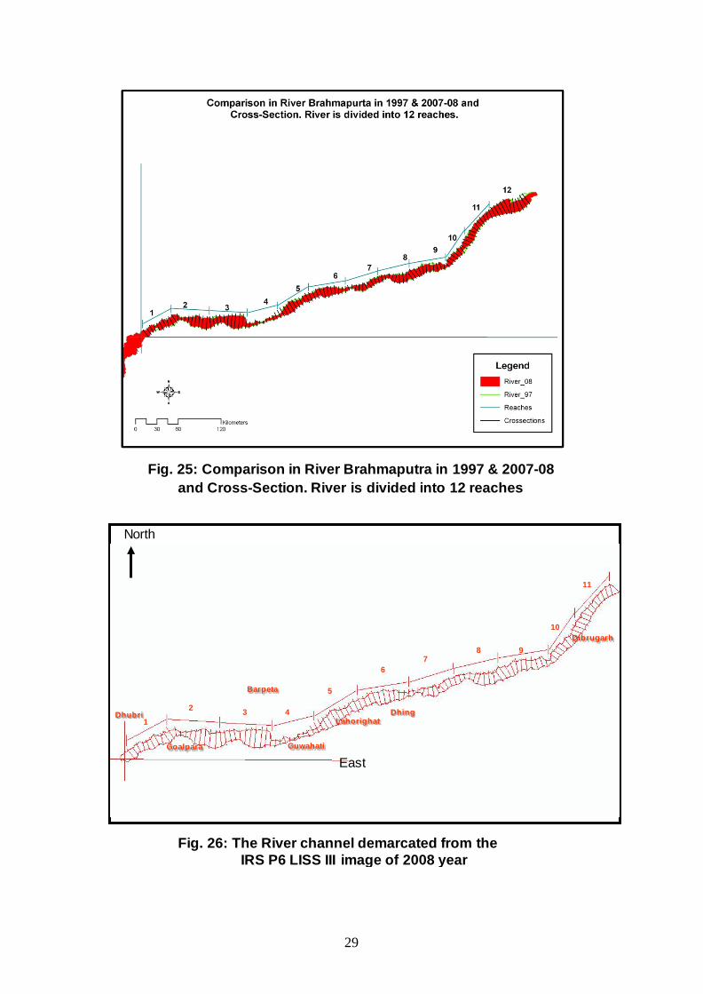
Fig. 25: Comparison in River Brahmaputra in 1997 & 2007-08 and Cross-Section. River is divided into 12 reaches
Fig. 26: The River channel demarcated from the IRS P6 LISS III image of 2008 year

30
Fig. 27: Comparison in River Brahmaputra in 1990 & 2008 and Cross-Section. River is divided into 12 reaches
Fig. 28: Bank Line of Year 2007-08 compared with year 1990 in reaches 5-11

31
Fig. 29: The River channel in Reach 1 demarcated from the IRS P6 LISS III image of 2008 year
Fig. 30: The River channel in Reach 2 demarcated from the IRS P6 LISS III image of 2008 year.
Dhubri
Gupigaon
Chapar
Goalpara
Barpeta
32
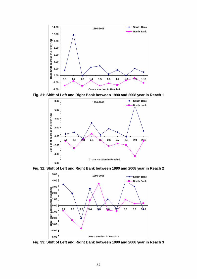
Fig. 31: Shift of Left and Right Bank between 1990 and 2008 year in Reach 1
Fig. 32: Shift of Left and Right Bank between 1990 and 2008 year in Reach 2
Fig. 33: Shift of Left and Right Bank between 1990 and 2008 year in Reach 3
1990-2008
-4.00
-2.00
0.00
2.00
4.00
6.00
8.00
10.00
12.00
14.00
1.1 1.2 1.3 1.4 1.5 1.6 1.7 1.8 1.9 1.10
Cross section in Reach-1
Ban
k Sh
ift a
ccro
ss th
e riv
er(K
m)
South BankNorth Bank
1990-2008
-6.00
-4.00
-2.00
0.00
2.00
4.00
6.00
8.00
2.1 2.2 2.3 2.4 2.5 2.6 2.7 2.8 2.9 2.10
Cross section in Reach-2
Ban
k sh
ift a
ccro
ss th
e riv
er(K
m)
South BankNorth bank
1990-2008
-5.00
-4.00
-3.00
-2.00
-1.00
0.00
1.00
2.00
3.00
4.00
5.00
3.1 3.2 3.3 3.4 3.5 3.6 3.7 3.8 3.9 3.10
cross section in Reach-3
Ban
k sh
ift a
ccro
ss th
e riv
er(k
m)
South BankNorth Bank

33
Fig. 34: Shift of Left and Right Bank between 1990 and 2008 year in Reach 4
Fig. 35: Shift of Left and Right Bank between 1990 and 2008 year in Reach 5
Fig. 36: Shift of Left and Right Bank between 1990 and 2008 year in Reach 6
1990-2008
-2.00
-1.00
0.00
1.00
2.00
3.00
4.00
5.00
6.00
7.00
4.1 4.2 4.3 4.4 4.5 4.6 4.7 4.8 4.9 4.10
cross section in Reach-4
Ban
k sh
ift a
ccro
ss th
e riv
er
South Bank
North Bank
1990-2008
-4.00
-3.00
-2.00
-1.00
0.00
1.00
2.00
3.00
4.00
5.00
6.00
5.1 5.2 5.3 5.4 5.5 5.6 5.7 5.8 5.9 5.10
Cross section in Reach-5
Ban
k sh
ift a
ccro
ss th
e riv
er(K
m)
South Bank
North Bank
1990-2008
-4.00
-3.00
-2.00
-1.00
0.00
1.00
2.00
3.00
4.00
6.1 6.2 6.3 6.4 6.5 6.6 6.7 6.8 6.9 6.10
Cross section in Reach-6
Ban
k sh
ift a
ccro
ss th
e riv
er(k
m)
South Bank
North Bank

34
Fig. 37: Shift of Left and Right Bank between 1990 and 2008 year in Reach 7
Fig. 38: Shift of Left and Right Bank between 1990 and 2008 year in Reach 8
Fig. 39: Shift of Left and Right Bank between 1990 and 2008 year in Reach 9
1990-2008
-15.00
-10.00
-5.00
0.00
5.00
10.00
15.00
7.1 7.2 7.3 7.4 7.5 7.6 7.7 7.8 7.9 7.10
Cross section in Reach-7
Ban
k sh
ift a
ccro
ss th
e riv
er(K
m)
South BankNorth Bank
1990-2008
-20.00
-15.00
-10.00
-5.00
0.00
5.00
10.00
15.00
8.1 8.2 8.3 8.4 8.5 8.6 8.7 8.8 8.9 8.10
Cross section in Reach-8
Ban
k sh
ift a
ccro
ss th
e riv
er(K
m)
South BankNorth Bank
1990-2008
-20.00
-15.00
-10.00
-5.00
0.00
5.00
10.00
15.00
9.1 9.2 9.3 9.4 9.5 9.6 9.7 9.8 9.9 9.10
Cross section in Reach-9
Ban
k sh
ift a
ccro
ss th
e R
iver
(Km
)
South BankNorth Bank

35
Fig. 40: Shift of Left and Right Bank between 1990 and 2008 year in Reach 10
Fig. 41: Shift of Left and Right Bank between 1990 and 2008 year in Reach 11
Fig. 42: Shift of Left and Right Bank between 1990 and 2008 year in Reach 12
1990-2008
-25.00
-20.00
-15.00
-10.00
-5.00
0.00
5.00
10.00
15.00
10.1 10.2 10.3 10.4 10.5 10.6 10.7 10.8 10.9 10.10
Cross section in Reach-10
Ban
k Sh
ift a
ccro
ss th
e riv
er(K
m)
South BankNorth Bank
1990-2008
-20.00
-15.00
-10.00
-5.00
0.00
5.00
10.00
15.00
11.1 11.2 11.3 11.4 11.5 11.6 11.7 11.8 11.9 11.10
Cross section in Reach-11
Ban
k sh
ift a
ccro
ss th
e riv
er(K
m)
South BankNorth Bank
!990-2008
-25.00
-20.00
-15.00
-10.00
-5.00
0.00
5.00
10.00
15.00
12.1 12.2 12.3 12.4 12.5 12.6 12.7 12.8 12.9 12.10
Cross section in Reach-12
Ban
k Sh
ift a
ccro
ss th
e R
iver
(Km
)
South BankNorth Bank

36
Fig. 43: Comparison in River Brahmaputra in (Reach- 1) (Year 1990 &2008)
Fig. 44: Comparison of Bank Line Reach -2 near Goalpara for the Year 1990 & 2007-08

37
Fig. 45: Reach 5-6 Near Morigaon comparing the bank shift from 1990 to 2007-08 showing heavy braiding in 2007 (Dhing)
Fig. 46: Bank Line of year 1990 with year 2007-08

38
Fig. 47: Bank Line of Year 1990 with Year 2007-08 in Upstream Reaches
Fig. 48: Area eroded in Main Brahmaputra during the period 1990- 2007-08

39
Fig. 49: Area eroded in Main Brahmaputra during the period 1997- 2007-08
Fig. 50: Area eroded in Main Brahmaputra near Dhubri & Goalpara during the period 1990- 2007-08

40
Fig. 51: Land Loss in Brahmaputra River Year 1990- 2007-08
Fig. 52: Area eroded in Main Brahmaputra near Guwahati during the period 1990- 2007-08

41
Fig. 53: Comparison of Braiding Channel (1997) with Bankline of 1990 near Morigaon
Fig. 54: Area eroded in Main Brahmaputra near Tezpur during the period 1990- 2007-08
42
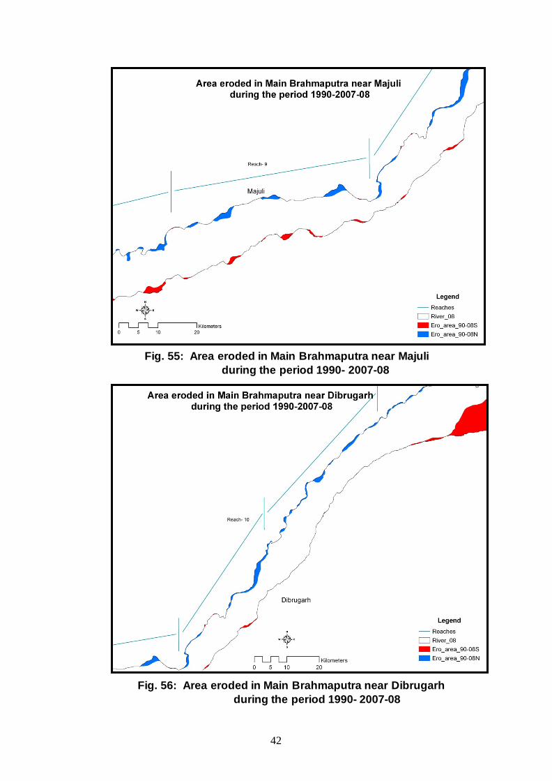
Fig. 55: Area eroded in Main Brahmaputra near Majuli during the period 1990- 2007-08
Fig. 56: Area eroded in Main Brahmaputra near Dibrugarh during the period 1990- 2007-08

43
TABLE 8: PRIORITIZATION WITH RESPECT TO LAND AREA LOST
PRIORITIZATION WITH RESPECT TO LAND AREA LOST Satellite based estimation of area eroded in Brahmaputra River for the period 1997 to 2007-08
Reach No.
South Bank
Reach No.
North Bank
Remarks
Total Erosion Length
Km
Area Eroded
Km²
Total Erosion Length
Km
Area Eroded
Km² 5(Morigaon) 47.91 103.700 1(Dhubri) 40.19 94.129
8(U/s Tezpur) 44.16 71.227 11(Dibrugarh) 37.86 43.529 6(Morigaon) 47.8 56.720 3(Palasbari) 54.87 42.914 7(Tezpur) 52.95 44.774 2(Goalpara) 39.5 40.902 10(U/s Majuli) 54.95 42.118 10(U/s Majuli) 16.93 16.878 9(Majuli) 47.17 28.998 9(Majuli) 24.69 12.327 3(Palasbari) 14.02 15.859 6(Morigaon) 24.86 7.275 4(Guwahati) 24.38 12.079 8(U/s Tezpur) 8.85 5.794 1(Dhubri) 7.05 10.791 7(Tezpur) 8.58 4.733 11(Dibrugarh) 43.89 6.066 5(Morigaon) 6 2.138 2(Goalpara) 4.85 5.052 4(Guwahati) 21.02 1.654 12(U/s Dibrugarh) 57.54 333.416 12(U/s Dibrugarh) 70.5 55.454 Forest Area
excluded in Northern side

44
TABLE 9: PRIORITIZATION WITH RESPECT TO MAXIMUM BANK SHIFT OF THE LEFT BANK OF BRAHMAPUTRA
S.No.
South Bank
Reach No. Erosion Length (Km)
Maximum erosion in tranverse
Direction (Km) 1 5(Morigaon) 47.909 4.125 2 11(Dibrugarh) 28.297 3.716 3 10 (U/s Majuli) 54.95 3.432 4 8(U/s Tezpur) 16.402 2.935 5 8(U/s Tezpur) 9.384 2.709 6 9(Majuli) 9.012 2.653 7 8(U/s Tezpur) 18.372 2.567 8 2(Goalpara) 2.71 2.412 9 7(Tezpur) 30.715 2.237
10 1(Dhubri) 5.423 2.159 11 6(Morigaon) 12.049 1.775 12 9(Majuli) 18.805 1.624 13 6(Morigaon) 4.062 1.601 14 7(Tezpur) 13.073 1.528 15 7(Tezpur) 9.164 1.486 16 11(Dibrugarh) 15.588 1.464 17 6(Morigaon) 31.686 1.392 18 9(Majuli) 3.698 1.226 19 9(Majuli) 5.053 1.216 20 3(Palasbari) 3.518 1.207 21 9(Majuli) 3.996 1.056 22 4(Guwahati) 6.702 0.953 23 4(Guwahati) 17.68 0.847 24 3(Palasbari) 4.89 0.766 25 3(Palasbari) 3.975 0.741 26 9(Majuli) 2.209 0.735 27 9(Majuli) 4.399 0.634 28 1(Dhubri) 1.624 0.553 29 3(Palasbari) 1.634 0.307 30 2(Goalpara) 2.139 0.204
45
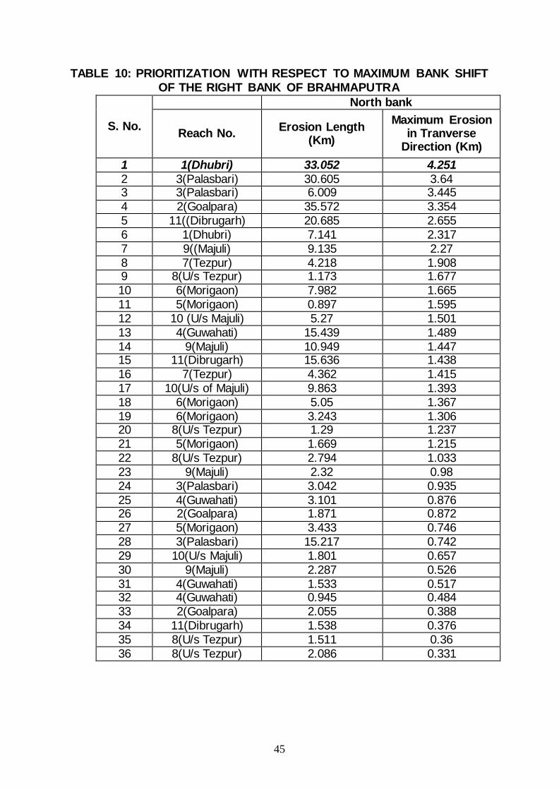
TABLE 10: PRIORITIZATION WITH RESPECT TO MAXIMUM BANK SHIFT OF THE RIGHT BANK OF BRAHMAPUTRA
S. No.
North bank
Reach No. Erosion Length (Km)
Maximum Erosion in Tranverse
Direction (Km) 1 1(Dhubri) 33.052 4.251 2 3(Palasbari) 30.605 3.64 3 3(Palasbari) 6.009 3.445 4 2(Goalpara) 35.572 3.354 5 11((Dibrugarh) 20.685 2.655 6 1(Dhubri) 7.141 2.317 7 9((Majuli) 9.135 2.27 8 7(Tezpur) 4.218 1.908 9 8(U/s Tezpur) 1.173 1.677 10 6(Morigaon) 7.982 1.665 11 5(Morigaon) 0.897 1.595 12 10 (U/s Majuli) 5.27 1.501 13 4(Guwahati) 15.439 1.489 14 9(Majuli) 10.949 1.447 15 11(Dibrugarh) 15.636 1.438 16 7(Tezpur) 4.362 1.415 17 10(U/s of Majuli) 9.863 1.393 18 6(Morigaon) 5.05 1.367 19 6(Morigaon) 3.243 1.306 20 8(U/s Tezpur) 1.29 1.237 21 5(Morigaon) 1.669 1.215 22 8(U/s Tezpur) 2.794 1.033 23 9(Majuli) 2.32 0.98 24 3(Palasbari) 3.042 0.935 25 4(Guwahati) 3.101 0.876 26 2(Goalpara) 1.871 0.872 27 5(Morigaon) 3.433 0.746 28 3(Palasbari) 15.217 0.742 29 10(U/s Majuli) 1.801 0.657 30 9(Majuli) 2.287 0.526 31 4(Guwahati) 1.533 0.517 32 4(Guwahati) 0.945 0.484 33 2(Goalpara) 2.055 0.388 34 11(Dibrugarh) 1.538 0.376 35 8(U/s Tezpur) 1.511 0.36 36 8(U/s Tezpur) 2.086 0.331
46
CHAPTER - I
SATELLITE DATA BASED
ANALYSIS OF CHANNEL MORPHO-
DYNAMIC STUDY FOR EROSION
CONTROL OF BRAHMAPUTRA
RIVER SYSTEM
[B] MAJOR TRIBUTARIES OF BRAHMAPUTRA RIVER
SYSTEM
47
Chapter – I (B)
MAJOR TRIBUTARIES OF BRAHMAPUTRA RIVER SYSTEM
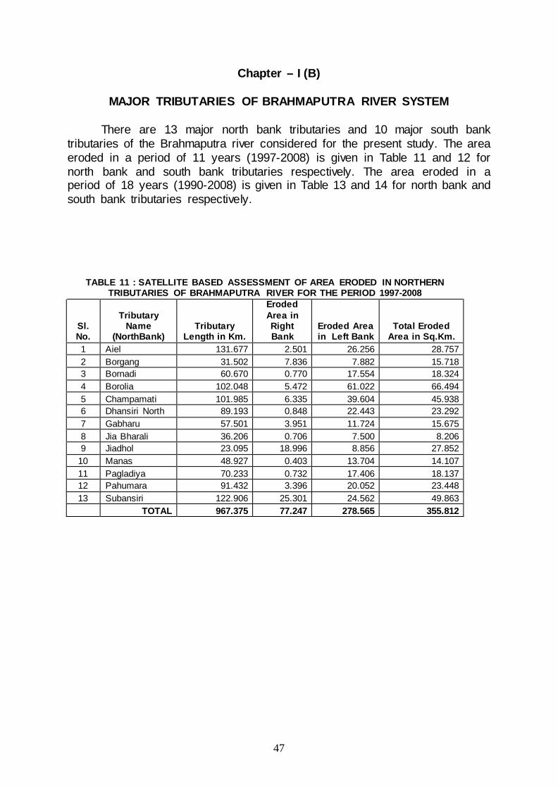
There are 13 major north bank tributaries and 10 major south bank tributaries of the Brahmaputra river considered for the present study. The area eroded in a period of 11 years (1997-2008) is given in Table 11 and 12 for north bank and south bank tributaries respectively. The area eroded in a period of 18 years (1990-2008) is given in Table 13 and 14 for north bank and south bank tributaries respectively.
TABLE 11 : SATELLITE BASED ASSESSMENT OF AREA ERODED IN NORTHERN
TRIBUTARIES OF BRAHMAPUTRA RIVER FOR THE PERIOD 1997-2008
Sl. No.
Tributary Name
(NorthBank) Tributary
Length in Km.
Eroded Area in Right Bank
Eroded Area in Left Bank
Total Eroded Area in Sq.Km.
1 Aiel 131.677 2.501 26.256 28.757 2 Borgang 31.502 7.836 7.882 15.718 3 Bornadi 60.670 0.770 17.554 18.324 4 Borolia 102.048 5.472 61.022 66.494 5 Champamati 101.985 6.335 39.604 45.938 6 Dhansiri North 89.193 0.848 22.443 23.292 7 Gabharu 57.501 3.951 11.724 15.675 8 Jia Bharali 36.206 0.706 7.500 8.206 9 Jiadhol 23.095 18.996 8.856 27.852
10 Manas 48.927 0.403 13.704 14.107 11 Pagladiya 70.233 0.732 17.406 18.137 12 Pahumara 91.432 3.396 20.052 23.448 13 Subansiri 122.906 25.301 24.562 49.863 TOTAL 967.375 77.247 278.565 355.812

48
TABLE 12 : SATELLITE BASED ASSESSMENT OF AREA ERODED IN SOUTHERN TRIBUTARIES OF BRAHMAPUTRA RIVER FOR THE PERIOD 1997-2008
Sl. No.
Tributary Name (South
Bank) Tributary
Length in Km.
Eroded Area in Right Bank
Eroded Area in Left Bank
Total Eroded Area in Sq.Km.
1 Buri Dihing 120.406 15.386 13.329 28.716 2 Dhansiri South 163.025 29.240 5.291 34.531 3 Dikhow 93.292 14.104 6.726 20.830 4 Disang 197.585 10.113 10.979 21.092 5 Dudhnoi 34.354 8.362 0.091 8.453 6 Jhanji 56.428 7.740 2.806 10.546 7 Jinari 28.790 5.581 0.409 5.991 8 Kolong /Kapili 192.511 21.840 10.346 32.186 9 Krishnai 106.792 12.523 0.610 13.133
10 Kulsi 80.140 8.332 3.308 11.640 TOTAL 1073.323 133.221 53.897 187.118
Total Eroded Area in Major Tributaries during 1997 to 2008 = 355.812+187.118 = 542.930 Sq.Km
542.930 km²
Eroded Area per year 54.293 Km²/year

49
TABLE 13 : SATELLITE BASED ESTIMATION OF AREA ERODED IN NORTHERN TRIBUTARIES OF BRAHMAPUTRA RIVER FOR THE PERIOD 1990-2008
Sl. No.
Tributary Name (North Bank)
Tributary Length in
Km. Eroded Area in
Right Bank Eroded Area in Left Bank
Total Eroded Area in Sq.Km.
1 Aiel 131.677 8.549 27.118 35.667 2 Borgang 31.502 9.462 8.300 17.762 3 Bornadi 60.670 2.250 18.814 21.064 4 Borolia 102.048 7.089 66.410 73.499 5 Champamati 101.985 9.194 42.852 52.046 6 Dhansiri North 89.193 1.500 30.509 32.009 7 Gabharu 57.501 7.405 13.671 21.076 8 Jia Bhareli 36.206 1.974 8.956 10.930 9 Jiadhol 23.095 19.554 10.297 29.851
10 Manas 48.927 1.476 15.496 16.972 11 Pagladiya 70.233 1.839 19.717 21.556 12 Pahumara 91.432 4.792 23.204 27.996 13 Subansiri 122.906 29.925 26.144 56.069 TOTAL 967.375 105.009 311.488 416.497
TABLE 14 : SATELLITE BASED ESTIMATION OF AREA ERODED IN SOUTHERN TRIBUTARIES OF BRAHMAPUTRA RIVER FOR THE PERIOD 1990-2008
Sl. No.
Tributary Name (South Bank)
Tributary Length in Km.
Eroded Area in Right
Bank Eroded Area in Left Bank
Total Eroded Area in Sq.Km.
1 Buri Dihing 120.406 17.711 15.008 32.719 2 Dhansiri South 163.025 31.557 7.899 39.456 3 Dikhow 93.292 15.734 9.201 24.935 4 Disang 197.585 11.581 12.306 23.887 5 Dudhnoi 34.354 9.492 1.306 10.798 6 Jhanji 56.428 9.667 4.085 13.752 7 Jinari 28.790 6.091 1.539 7.630 8 Kolong Kapili 192.511 23.943 12.884 36.827 9 Krishnai 106.792 15.579 1.314 16.893
10 Kulsi 80.140 11.397 4.390 15.787 TOTAL 1073.323 152.752 69.932 222.684
Total Eroded Area in Major Tributaries during 1990- 2008 = 416.497+222.684 = 639.181 Sq.Km
639.181
km² Eroded Area per year 37.60 Km²/year

50
Fig. 57: Brahmaputra River and its major tributaries of the Year 1990

51
Fig. 58: Brahmaputra River and its major tributaries of the Year 1990
Fig. 59: Mosaic of IRS P6 LISS – III Satellite Images of Brahmaputra River and its major tributaries of the Year 2007-08
P6

52
Fig. 60: Brahmaputra River and its major tributaries of the Year 2007-08
Fig. 61: Brahmaputra River and its North Bank Tributaries Year 2007-08
53
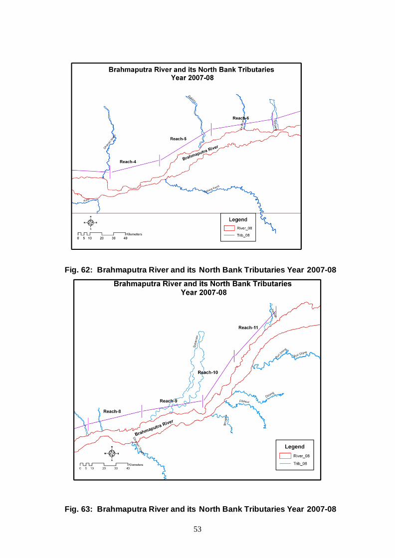
Fig. 62: Brahmaputra River and its North Bank Tributaries Year 2007-08
Fig. 63: Brahmaputra River and its North Bank Tributaries Year 2007-08

54
Fig. 64: Brahmaputra River and its South Bank Tributaries Year 2007-08
Fig. 65: Brahmaputra River and its South Bank Tributaries Year 2007-08
55
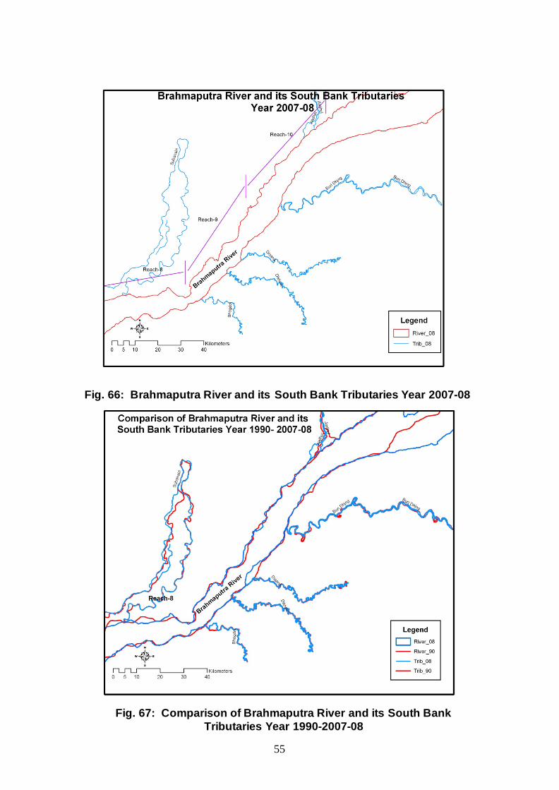
Fig. 66: Brahmaputra River and its South Bank Tributaries Year 2007-08
Fig. 67: Comparison of Brahmaputra River and its South Bank Tributaries Year 1990-2007-08

56
Fig. 68: Comparison of Brahmaputra River and its South Bank Tributaries Year 1990-2007-08
Fig. 69: Comparison of Brahmaputra River and its South Bank Tributaries Year 1990-2007-08

57
Fig. 70: Comparison of Brahmaputra River and its North Bank Tributaries Year 1990-2007-08
Fig. 71: Comparison of Brahmaputra River and its North Bank Tributaries Year 1990-2007-08

58
Fig. 72: Comparison of Brahmaputra River and its North Bank Tributaries Year 1990-2007-08
Fig. 73: Comparison of Brahmaputra River and its North Bank Tributaries Year 1990-2007-08

59
Fig. 74: Comparison of Brahmaputra River and its South Bank Tributaries Year 1990-2007-08

60
CHAPTER – II
SATELLITE DATA BASED
ANALYSIS FOR MORIGAON SITE
ON BRAHMAPUTRA RIVER

61
CHAPTER – II
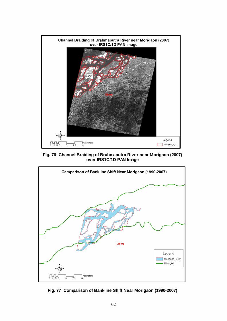
SATELLITE DATA BASED ANALYSIS FOR MORIGAON SITE ON BRAHMAPUTRA RIVER As decided in the monitoring committee meeting held in the office of Chief Secretary Assam on 17th November 2008, in depth satellite based analysis of the fluvial land-form changes of the Brahmaputra near Morigaon have been conducted and a scheme for pilot study for erosion control has been evolved for this site. For the above purpose, satellite imageries of IRS 1C/1D for Panchromatic sensor have been processed with the help of ERDAS and Arc-Gis software. The interpretation of these imageries and maps has yielded the quantitative measure of various aspects related to bank erosion. The processed version of these imageries and maps have been placed below.
Fig. 75: Channel Braiding of Brahmaputra River near Morigaon (1997) over IRS1C/1D PAN Image
62
Fig. 76 Channel Braiding of Brahmaputra River near Morigaon (2007) over IRS1C/1D PAN Image
Fig. 77 Comparison of Bankline Shift Near Morigaon (1990-2007)

63
Fig. 78 Comparison of Braiding of Brahmaputra Near Morigaon 2007 laid over Braiding of 1997
Fig. 79 Comparison of Braiding of Brahmaputra Near Morigaon in Year 1997 laid over Braiding of Year 2007
64
River in 1990
Dhing
Lahorighat
Reach-5
Reach-6
River in 1990
Reach-5
Reach-6
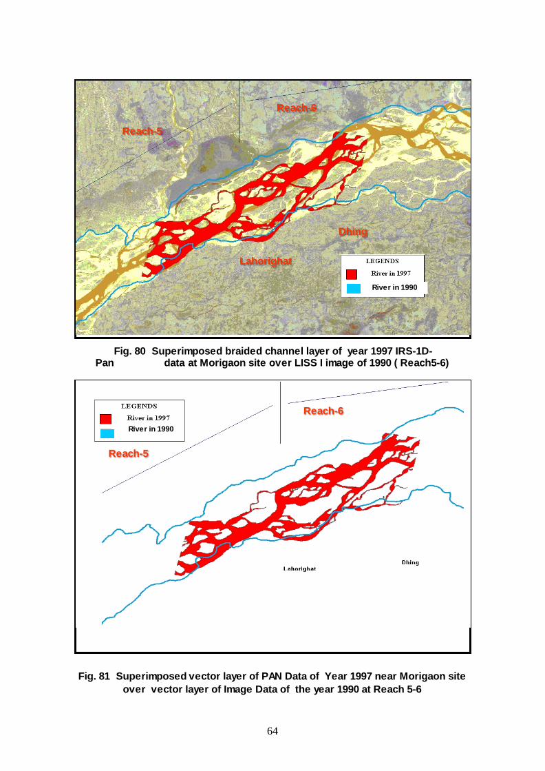
Fig. 80 Superimposed braided channel layer of year 1997 IRS-1D-Pan data at Morigaon site over LISS I image of 1990 ( Reach5-6)
Fig. 81 Superimposed vector layer of PAN Data of Year 1997 near Morigaon site over vector layer of Image Data of the year 1990 at Reach 5-6

65
Dhing
Fig. 82 Comparison of Bank Line Shift near Morigaon site (1990-2007)
Fig. 83 Comparison of Braiding of Brahmaputra near Morigaon in 1997 with layed over braiding of 2007

66
Dhing
Fig. 84 Comparison of Braiding of Brahmaputra near Morigaon in 2007 with layed over braiding of 1997
67
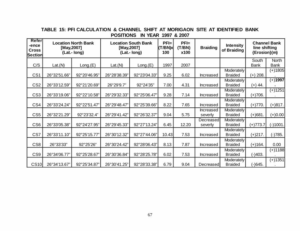
TABLE 15: PFI CALCULATION & CHANNEL SHIFT AT MORIGAON SITE AT IDENTIFIED BANK POSITIONS IN YEAR 1997 & 2007
Refer-ence Cross
Section
Location North Bank [May,2007] (Lat.- long)
Location South Bank [May,2007] (Lat.- long)
PFI= (T/BN)x
100
PFI= (T/BN)
x100 Braiding Intensity
of Braiding
Channel Bank line shifting {Erosion}(m)
C/S Lat.(N) Long.(E) Lat.(N) Long.(E) 1997 2007 South Bank
North Bank
CS1 26°32’51.66” 92°20’46.95” 26°28’38.39” 92°23’04.33” 9.25 6.02 Increased Moderately Braided (+) 208.
(+)1805.
CS2 26°33’12.59” 92°21’20.69” 26°29’9.7” 92°24’35” 7.00 4.31 Increased Moderately Braided (+) 44.
(+)1997.
CS3 26°33’19.06” 92°22’10.58” 26°29’32.33” 92°25’06.47” 9.28 7.14 Increased Moderately Braided (+)706.
(+)1251.
CS4 26°33’24.24” 92°22’51.47” 26°29’48.47” 92°25’39.66” 8.22 7.65 Increased Moderately Braided (+)770. (+)817.
CS5 26°32’21.29” 92°23’32.4” 26°29’41.42” 92°26’32.37” 9.04 5.75 Increased severly
Moderately Braided (+)681. (+)0.00
CS6 26°33’05.38” 92°24’27.95” 26°29’45.33” 92°27’13.24” 6.45 12.20 Decreased severly
Moderately Braided (+)773.7 (-)1001.
CS7 26°33’11.10” 92°25’15.77” 26°30’12.32” 92°27’44.06” 10.43 7.53 Increased Moderately Braided (+)217. (-)785.
CS8 26°33’33” 92°25’26” 26°30’24.42” 92°28’06.43” 8.13 7.87 Increased Moderately Braided (+)164. 0.00
CS9 26°34’06.77” 92°25’28.67” 26°30’36.84” 92°28’25.78” 6.02 7.53 Increased Moderately Braided (-)403.
(+)1188.
CS10 26°34’13.67” 92°25’34.87” 26°30’41.25” 92°28’33.38” 6.79 9.04 Decreased Moderately Braided (-)645.
(+)1351.
68
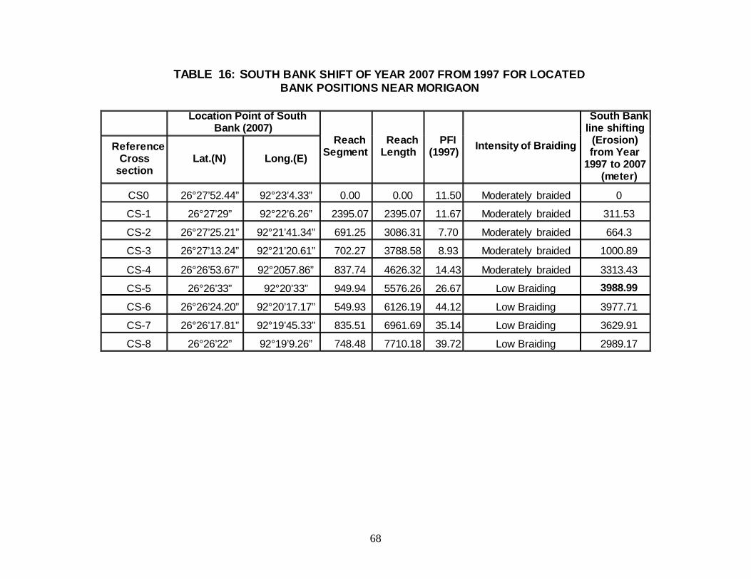
TABLE 16: SOUTH BANK SHIFT OF YEAR 2007 FROM 1997 FOR LOCATED BANK POSITIONS NEAR MORIGAON
Location Point of South
Bank (2007) Reach
Segment Reach
Length PFI
(1997) Intensity of Braiding
South Bank line shifting
(Erosion) from Year
1997 to 2007 (meter)
Reference Cross
section Lat.(N) Long.(E)
CS0 26°27’52.44” 92°23’4.33” 0.00 0.00 11.50 Moderately braided 0
CS-1 26°27’29” 92°22’6.26” 2395.07 2395.07 11.67 Moderately braided 311.53
CS-2 26°27’25.21” 92°21’41.34” 691.25 3086.31 7.70 Moderately braided 664.3
CS-3 26°27’13.24” 92°21’20.61” 702.27 3788.58 8.93 Moderately braided 1000.89
CS-4 26°26’53.67” 92°2057.86” 837.74 4626.32 14.43 Moderately braided 3313.43
CS-5 26°26’33” 92°20’33” 949.94 5576.26 26.67 Low Braiding 3988.99
CS-6 26°26’24.20” 92°20’17.17” 549.93 6126.19 44.12 Low Braiding 3977.71
CS-7 26°26’17.81” 92°19’45.33” 835.51 6961.69 35.14 Low Braiding 3629.91
CS-8 26°26’22” 92°19’9.26” 748.48 7710.18 39.72 Low Braiding 2989.17

69
Fig. 85 Plan Form Index Comparison of year 1997 and 2007
for Morigaon Site
Fig. 86 Bank Line Shift Comparison of Left and Right Bank
for 1997 -2007 for Morigaon Site
0.00
2.00
4.00
6.00
8.00
10.00
12.00
14.00
CS1 CS2 CS3 CS4 CS5 CS6 CS7 CS8 CS9 CS10
Cross sections in Morigaon Erosion Area
PFI(P
lan
Form
Inde
x)
Year 1997Year2007
-2000
-1000
0
1000
2000
3000
4000
5000
CS-
8
CS-
7
CS-
6
CS-
5
CS-
4
CS-
3
CS-
2
CS-
1
CS0
CS1
CS2
CS3
CS4
CS5
CS6
CS7
CS8
CS9
CS1
0
Cross section in Morigaon Erosion Reach
Eros
ion
accr
oss
the
cros
s se
ctio
n (m
eter
s)
Left Bank
Right Bank
Erosion → Positive

70
From the above analysis, the following major findings have emerged
i) Braiding intensity has registered a significant rise during the course of 1997 – 2007 as evident from the Table No.10 due to unabated stream bank erosion.
ii) The maximum length of bank retreat due to erosion in the south bank approximately 4 Km.
iii) The maximum length of bank retreat due to erosion in the North bank approximately 1.99 Km.

71
Chapter -III
FINDINGS OF PHASE – I STUDY

72
Chapter – III
FINDING OF PHASE – I STUDY
Table 17: SUMMARY OF LAND LOSS DUE TO EROSION IN MAIN STEM AND MAJOR TRIBUTARIES OF BRAHMAPUTRA RIVER SYSTEM
From the preceding analyses, the following findings have emerged.
[A] Brahmaputra Main Stem:-
i) Braiding intensity has registered a sharp rise during the course of 1990 – 2008 as evident from the Table No.5 due to unabated stream bank erosion.
ii) The total land area lost during 1990 – 2008 in main stem Brahmaputra is assessed through GIS data base of satellite derive maps to be 1054 Sq. Km (without considering the isolation of forest area of Dibru-Saikhowa reserved forest due to avulsion).
iii) The total land area lost during 1997 – 2008 in main stem Brahmaputra is assessed through GIS data base of satellite derive maps to be 725 Sq. Km (without considering the isolation of forest area of Dibru-Saikhowa reserved forest due to avulsion).
iv) The total land area lost during 1990 – 2008 is assessed to be 515 Sq. Km in the south bank.
v) The total land area lost during 1990 – 2008 is assessed to be 539 Sq. Km in the north bank.
S. No. Item
Period of Study
Remarks 1997 to 2007-08 1990 to 2007-08
Annual land loss
Sq.km/ year
Total Land Lost
Sq.km
Annual land loss
Sq.km/ year
Total Land Lost
Sq.km 1 Main stem 73 725 62 1054 During the shorter period
of 1997-2008 Brahmaputra river system has exhibited considerable increase in annual land lost in comparison to prolong period of 1990 to 2007-08
2. Major Tributaries
54 543 38 639
Total 127 1268 100 1693

73
vi) The total land area lost during 1997 – 2008 is assessed to be 397 Sq. Km in the south bank.
vii) The total land area lost during 1997 – 2008 is assessed to be 328 Sq. Km in the north bank
viii) Thus, during 1990-2007-08 approximately 1054 Sq. Km. of land area has been lost, giving an annual area loss of 62 Sq.Km/Year.
ix) During the period of 1997 to 2007-08 the annual rate of erosion has considerably increase to 73 sq.km /year in comparison to 62 sq Km/year for the prolong period of 1990 to 2007-08.
x) During the recent period of 1997-2007-08, South Bank of Main Brahmaputra stem has exhibited considerably higher erosion in comparison to north Bank in contrast to the prolonged period of 1990-2007-08.
xi) The maximum length of bank retreat due to erosion in the south bank approximately 4.125 Km at near Morigaon.
xii) The maximum length of bank retreat due to erosion in the North bank approximately 4.251 Km at near Dhubri.
xiii) The total length of erosion-affected bank line approximately 743 Km out of which south bank 389 Km and 354 Km in North bank.
[B] Major Tributaries of Brahmaputra River System:-
i) The total land area lost during 1990 – 2008 in major tributaries of Brahmaputra river system is worked out through GIS data base of satellite derive maps to be 639 Sq. Km .
ii) The total land area lost during 1997 – 2008 in major tributaries of Brahmaputra river system is assessed through GIS data base of satellite derive maps to be 543 Sq. Km.
iii) The total land area lost during 1990 – 2008 is assessed to be 223 Sq. Km in the southern tributaries.
iv) The total land area lost during 1990 – 2008 is assessed to be 416 Sq. Km in the northern tributaries.
v) The total land area lost during 1997 – 2008 is assessed to be 187 Sq. Km in the southern tributaries.
vi) The total land area lost during 1997 – 2008 is assessed to be 356 Sq. Km in the northern tributaries.

74
vii) Thus, during 1990-2007-08 approximately 639 Sq. Km. of land area has been lost, giving an annual area loss of 38 Sq.Km/Year for major tributaries.
viii) During the period of 1997 to 2007-08 the annual rate of erosion has considerably increase to 54 sq.km /year in comparison to 38 sq Km/year for the prolong period of 1990 to 2007-08 for major tributaries.
ix) During the study periods Northern tributaries of Brahmaputra River have exhibited higher erosion in comparison to Southern tributaries.

75
REFERENCES

76
REFERENCES
1. Bardhan, M. (1993). Channel stability of Barak river and its tributaries between Manipur-Assam and Assam- Bangladesh borders as seen from satellite imagery, Proc. Nat. Syrup. on Remote Sensing Applications for resource Management with special emphasis on N.E. region, held in Guwahati, Nov. 25-27, 481-485.
2. Bhakal, L., Dubey, B., and Sarma, A.K. 2005. Estimation of bank erosion
in the river Brahmaputra near Agyathuri by using geographic information system. Photonirvachak, J. of the Indian Society of Remote Sensing, Vol. 33, No.1, 81-84.
3. Brahmaputra Board (1997). Report on erosion Problem of Majuli Island,
Brahmaputra Board, Guwahati.
4. Couper, P.R., 2004, Space and time in river bank erosion research: A review: Area,v.36,no.4,p.387–403.
5. Das, J.D. and Saraf, A.K. 2007. Remote sensing in the mapping of the
Brahmaputra/Jamuna River channel patterns and its relation to various landforms and tectonic environment. Intl J of remote sensing, 28, pp3619-3631.
6. Florsheim, J.L., Mount, J.F., and Chin, A., 2008, Bank erosion as a
desirable attribute of rivers, BioScience, v. 58, no. 6, p. 519–529. 7. Flosi, G., Downie, S., Hopelain, J., Bird, M., Coey, R., and Collins, B.,
1998, California salmonid stream habitat restoration manual: Sacramento, California Department of Fish and Game.
8. Fuller, I.C., Large, A.R.G., Milan, D.J., 2003. Quantifying channel
development and sediment transfer following chute-off in a wandering gravel-bed river. Geomorphology 54, 307–323.
9. Goswami, U., Sarma, J.N. and Patgiri, A.D. (1999). River channel
changes of Subansiri in Assam. India. Geomorphology, 30: 227-244.
10. Johnson, W.C., 1994, Woodland expansion in the Platte River, Nebraska:
Patterns and causes: Ecological Monographs, no. 64, p. 45–84. 11. Kotoky P., Bezbaruah D., Baruah J. and J. N. Sarma J. N., “Nature of
bank erosion along the Brahmaputra river channel, Assam, India” CURRENT SCIENCE, VOL. 88, NO. 4, 25 FEBRUARY 2005,pp 634-640

77
12. Kummu, M., Lub, X.X., Rasphonec, A., Sarkkulad, J.,and Koponen, J. 2008. Quaternary International 186, 100–112.
13. Li, L.Q., Lu, X.X., Chen, Z., 2007. River channel change during the last 50
years in the middle Yangtze River: an example of the Jianli reach. Geomorphology 85, 185-196.
14. Mani, P., Kumar, R., and Chatterjee, C. (2003). Erosion Study of a Part of
Majuli River-Island Using Remote Sensing Data. Journal of the Indian Society of Remote Sensing, Vol. 31, No. 1, pp11-18.
15. Miller, J.R., and Friedman, J.M., 2009, Influence of flow variability on
floodplain formation and destruction, Little Missouri River, North Dakota: Geological Society of America Bulletin, v. 121, p. 752–759.
16. Moody, J.A., and Meade, R.H., 2008, Terrace aggradation during the 1978
flood on Powder River, Montana, USA: Geomorphology, v. 99, p. 387–403.
17. Naik, S.D., Chakravorty, S.K., Bora, T. and Hussain, (1999). Erosion at
Kaziranga National Park, Assam, a study based on multitemporal satellite data. Project Report. Space Application Centre (ISRO) Ahmedabad and Brahmaputra Board, Guwahati.
18. NRSA (1980). Brahmaputra flood mapping and river migration studies-
airborne scanner survey. National Remote Sensing Agency, Hyderabad, India
19. Rinaldi, M., 2003. Recent channel adjustments in alluvial rivers of
Tuscany, central Italy. Earth Surface Processes and Landforms 28, 587–608.
20. SAC and Brahmaputra Board (1996). Report on bank erosion on Majuli
Island, Assam: a study based on multi temporal satellite data. Space Application Centre, Ahmedabad and Brahmaputra Board, Guwahati.
21. Sarma, J.N. and Basumallick, S. (1980). Bankline migration of Burhi
Dihing River, Assam. Ind. J. Ear. Sci., 11(3&4): 199-206.
22. Sarma, J.N., Borah, D., and Goswami, U. 2007 , Change of River Channel and Bank Erosion of the Burhi Dihing River (Assam), Assessed Using Remote Sensing Data and GIS. Journal of the Indian Society of Remote Sensing, Vol. 35, No. 1, pp 94-100.

78
23. Simon, A., and Rinaldi, M., 2000, Channel instability in the loess area of the midwestern United States: Journal of the American Water Resources Association, v. 36, no. 1, p. 133–150.
24. Surian, N., 1999. Channel changes due to river regulation: the case of the
Piave River, Italy. Earth Surface Processes and Landforms 24, 1135–1151.
25. Surian, N., Rinaldi, M., 2003. Morphological response to river engineering
and management in alluvial channels in Italy. Geomorphology 50, 307–326.
26. U.S. Geological Survey, 2005, Assessing sandhill crane roosting habitat
along the Platte River, Nebraska:. Fact Sheet 2005–3029, 2 p. [http://pubs.usgs.gov/fs/2005/3029/]
27. Yang, X., Damen M.C.J. and Zuidam R.A.van: Satellite remote sensing and GIS for the analysis of chanel migration changes in the active Yellow river Delta, China, Int 'l. J. of Applied Earth Observation and Geoinformation, Vol. 1, Issue 2, pp. 146-157, 1999.

PPHHAASSEE –– IIII

1
TTEEAAMM OOFF IINNVVEESSTTIIGGAATTOORRSS
1. Prof. Dr. Nayan Sharma
2. Ms. Archana Sarkar
3. Mr. Neeraj Kumar

2
TABLE OF MAJOR CONTENTS
Sl. No. Subject Page No. CHAPTER –I INTRODUCTION
3
CHAPTER – II
BACKGROUND OF ARTIFICIAL NEURAL NETWORKS
11
CHAPTER – III
REVIEW OF LITERATURE 40
CHAPTER – IV
STUDY AREA AND DATA AVAILABILITY
61
CHAPTER – V
METHODOLOGY 77
CHAPTER – VI
RESULTS AND DISCUSSION 98
CHAPTER – VII
SUMMARY 116
CHAPTER – VIII
REFERENCES & BIBLIOGRAPHY 119

3
Chapter – 1
II nn tt rr oo dd uu cc tt ii oo nn

4
Introduction
1.1 GENERAL
Management of Water resources requires input from hydrological studies. This is
mainly in the form of estimation or forecasting of the magnitude of a hydrological variable
like rainfall, runoff and sediment concentrations using past experience. Such forecasts are
useful in many ways. They provide a warning of the extreme flood or drought conditions in
case of rainfall-runoff modeling and assessment of volume of sediments being transported by
a river in case of runoff-sediment modeling. This helps to optimize the design and
maintenance of systems like reservoirs and power plants. The contract negotiation and
hydropower sales also call for forecasted values of river flows and sediment loads.
1.2 RAINFALL-RUNOFF PROCESS
The rainfall - runoff process is believed to be highly nonlinear, time-varying, spatially
distributed, and not easily described by simple models. In addition to rainfall, runoff is
dependent on numerous factors such as initial soil moisture, land use, watershed
geomorphology, evaporation, infiltration, distribution, duration of the rainfall, and so on.
Although many watersheds have been gauged to provide continuous records of stream flow,
engineers are often faced with situations where little or no information is available. A number
of models have been developed to simulate this process. Depending on the complexities
involved, these models are categorized as empirical, black-box, conceptual or physically-
based distribution models. In operational hydrology, the system-theoretic black-box and
conceptual models are usually employed for rainfall-runoff modeling because the physically-
based distributed models are too complex, data intensive and cumbersome to use.
Conceptual rainfall-runoff (CRR) models are designed to approximate with in their
structures (in some physically realistic manner) the general internal sub processes and
physical mechanics, which govern the hydrologic cycle. CRR models usually incorporate
simplified forms of physical laws and are generally nonlinear, time-invariant, and
deterministic, with parameters that are representative of watershed characteristic. Until
recently, for practical reasons (data availability, calibration problems, etc.) most conceptual
1

5
watershed models assumed lumped representations of the parameters. Among the more
widely used and reported lumped parameter watershed models are the Sacramento soil
moisture accounting (SAC-SMA) model of the U.S. National Weather Service (Burnash et al.
1973. Brazil and Hudlow, 1980) HEC-1 (U.S. Army corps of engineers, 1990) and the
Stanford watershed model (SWM) Crawford and Linsley, 1966). While such models ignore
the rainfall runoff process, they attempt to incorporate realistic representations of the major
nonlinearities inherent in the R-R relationships. Conceptual watershed models are generally
reported to be reliable in forecasting the most important features of the hydrograph, such as
the beginning of the rising limb, the time and the height of the peak and volume of flow
(Kitanidis and Bras, 1980 a;b;Sorooshian, 1983), However, the implementation and
calibration of such a model can typically present various difficulties (Duan et al.. 1992)
requiring sophisticated mathematical tools (Duan et al.. 1992.1993.1994; Sorooshain et al..,
1993) significant amounts of calibration data (Yapo et al.., 1995) and some degree of
expertise and experience with the model.
While conceptual models are of importance in the under standing of hydrologic
processes, there are may practical situations such as streamflow forecasting where the main
concern is with making accurate predictions at specific watershed locations. In such a
situation, a hydrologist may prefer not to expend the time and effort required to develop and
implement a conceptual model and instead implement a simpler system theoretic model. In
the system theoretic approach, difference equation or differential equation models are used to
identify a direct mapping between the inputs and outputs without detailed consideration of
the internal structure of the physical processes. The linear time series models such as
ARMAX (auto regressive moving average with exogenous inputs) models developed by Box
and Jenkins (1976) have been most commonly used in such situations because they are
relatively easy to develop and implement; they have been found to provide satisfactory
predictions in may applications (Bras and Rodriguez-Iturbe, 1985; Salas et al.., 1980; wood,
1980) How-ever, such models do not attempt to represent the nonlinear dynamics inherent in
the transformation of rainfall to runoff and therefore may not always perform well.
Owing to the difficulties associated with nonlinear model structure identification and
parameter estimation, very few truly nonlinear system theoretic watershed models have been
reported (Jacoby, 21966; Amorocho and Brandstetter, 1971; Ikeda et al., 1976). In most
cases, linearity or piecewise linearity ahs been assumed (Natale and Todini, 1976a,b). The

6
model structural errors that arise from such assumptions can, to some extent, be compensated
for by allowing the model parameters to very with time (Young, 1982; Young and Wallis,
1985) For example, real time identification techniques, such as recursive least squares and
state space Kalman filtering models have been applied for adaptive estimation of model
parameters (Chiu, 1978; Kitanidis and Bras, 1980a,b; Bras and Rodriguez-Iturbe, 1985) with
generally acceptable results.
Recently, significant progress in the fields of nonlinear pattern recognition and system
control theory have been made possible through advances in a branch of nonlinear system
theoretic modeling called artificial neural networks (ANN). An ANN is a nonlinear
mathematical structure, which is capable of representing arbitrarily complex nonlinear
processes that relate the inputs and outputs of any system. A number of papers have discussed
the capability of three-layer feed forward ANNs to approximate any continuous input-output
mapping and its derivatives to arbitrary accuracy (Funahashi, 1989; White, 1990; Hornik et
al., 1990; Blum and Li. 1991; Ito, 1992; Gallant and White, 1992; Cardaliaguet and Euvrard,
1992; Takahashi, 1993). ANN models have been used successfully to model complex
nonlinear input-output time series relationship in a wide variety of fields (Vemuri and
Rogers, 1994).
1.3 RUNOFF – SEDIMENT PROCESS
The magnitude of sediment transported by rivers has become a serious concern for the
water resources planning and management. The assessment of the volume of sediments
being transported by a river is required in a wide spectrum of problems such as the design of
reservoirs and dams; hydroelectric power generation and water supply; transport of sediment
and pollutants in rivers, lakes and estuaries; determination of the effects of watershed
management; and environmental impact assessment. The sediment outflow the watershed is
induced by processes of detachment, transportation and deposition of soil materials by
rainfall and runoff.
Sediment rating curves are widely used to estimate the sediment load being
transported by a river. A sediment-rating curve is a relation between the sediment and river

7
discharges. Such a relationship is usually established by a regression analysis, and the curves
are generally expressed in the form of a power equation.
A number of attempts have been made to relate the amount of sediment transported by
river with flow conditions such as discharge, velocity, and shear stress. However, none of
these equations have received universal acceptance. Usually, either the weight of the
sediments or the sediment concentration is related to the discharge. Many times, these two
forms are used interchangeably. McBeab and Al-Nassri (1988) examined this issue and
concluded that the practice of using sediment load versus discharge is misleading because the
goodness of fit implied by this relation is spurious. They have instead recommended that the
regression be established between sediment concentration and discharge. Karim and
Kennedy (1990) attempted to establish relations among the velocity, sediment discharge, bed-
form geometry, and friction factor of alluvial rivers. Loped and Ffolliott (1993) point out that
an additional complexity is introduced to the sediment concentration and streamflow relation
due to a hysteresis effect. The sediment concentrations for a given level of streamflow
discharge in rising stage of a streamflow hydrograph are greater than on the falling stage. The
conventional regression approach is not able to account for this hysteresis effect. A power
equation is normally used to represent sediment rating and its transformation. Usually, the
power equation is log transformed and linear regression with least squares is applied to
estimate the parameters. While applying the equation, the data are transformed to the original
domain. The entire process introduces a bias in the estimates. This aspect has been examined
by Ferguson (1986) and Jansson (1996).Jansson (19960 proposed a correction factor that is
based on the variance of the data and claimed that the use of this factor leads to improvement
in the results.
As the sediment-discharge relationship is not linear, conventional statistical tools used
in such situations such as regression and curve fitting methods are unable to model the non-
linearity in the relationship. On the other hand, the application of physics-based distributed
process computer simulation offers another possible method of sediment prediction. But the
application of these complex software programs is often problematic, due to the use of
idealized sedimentation components, or the need for massive amounts of detailed spatial and
temporal environmental data, which are not available. Simpler approaches are therefore
required in the form of 'conceptual' solutions or 'black-box' modelling techniques.

8
Neurocomputing, in the form of artificial neural networks provide one possible answer to the
problematic task of sediment transfer prediction.
1.4 POTENTIAL OF ANN TECHNIQUES FOR HYDROLOGICAL MODELING IN BRAHMAPUTRA RIVER BASIN
An Artificial Neural Network (ANN) is a computational method inspired by the
studies of the brain and nervous system in biological organisms. ANN represent highly
idealized mathematical models of our present understanding of such complex systems. One
of the characteristics of the neural networks is their ability to learn. A neural network is not
programmed like a conventional computer program, but is presented with examples of the
patterns, observations and concepts, or any type of data, which it is supposed to learn.
Through the process of learning (also called training) the neural network organizes itself to
develop an internal set of features, that it uses to classify information or data. Due to its
massively parallel processing architecture the ANN is capable of efficiently handling
complex computations, thus making it the most preferred technique today for high speed
processing of huge data. ANNs have been in existence since the 1940s, but since current
algorithms have overcome the limitations of those early networks great interest in the
practical applications of ANNs has arisen in recent decades (Wasserman 1989; Muller and
Reinhardt 1990). Various ANN algorithms have an objective to map a set of inputs to a set of
outputs. ANNs have been proven to provide better solutions when applied to (1) complex
systems that may be poorly described or understood; (2) problems that deal with noise or
involve pattern recognition, diagnosis, abstraction, and generalization; and (3) situations
where input is incomplete or ambiguous by nature. It has been reported that an ANN has the
ability to extract patterns in phenomena, which avoids the selection of a model form such as
linear, power, or polynomial. In addition, there are many advantageous characteristics of
ANN approach to problem solving viz.: (1) application of a neural network does not require a
priori knowledge of the underlying process; (2) one may not recognize all the existing
complex relationships between various aspects of the process under investigation; (3) a
standard optimization approach or statistical model provides a solution only when allowed to
run to completion whereas a neural network always converges to an optimal (sub-optimal)
solution condition and; (4) neither constraints nor an a priori solution structure is necessarily
assumed or strictly enforced in the ANN development. These characteristics render ANNs to
be very suitable tools for handling various hydrological modeling problems.

9
1.5 OBJECTIVES OF THE STUDY
The assessment of the runoff in a river as well as volume of sediments being trans-
ported by a river is required in a wide spectrum of problems such as the design of reservoirs
and dams; hydroelectric power generation and water supply; transport of sediment and
pollutants in rivers, lakes and estuaries; determination of the effects of watershed
management; and environmental impact assessment. The soil erosion and sediment yield is
one of the major problems in Himalayan region. The fragile ecosystem of Himalayas has
been an increasing cause of concern to environmentalists and water resources planners.
Accelerated erosion has occurred in this region due to intensive deforestation, large-scale
road construction, mining and cultivation on steep slopes. Keeping this in view, a part of
Brahmaputra River, which flows through the eastern Himalayan region of India has been
selected for this study.
The main objective of the present study is the application of the emerging technique,
namely, artificial neural networks (ANNs) for modeling the rainfall-runoff process as well as
the runoff-sediment process for a part of the Brahmaputra River in eastern Himalayan region
of India. The principle objective of the study has been achieved through the following
milestones:
i. Development of stage-discharge and runoff-sediment rating curves using
artificial neural network (ANN) models and conventional techniques for the
important gauging sites in the Brahmaputra River basin.
ii. Development of rainfall-runoff and sediment-runoff models using artificial
neural network (ANN technique for Subansiri River basin.
iii. Validation of the formulated models.
iv. Performance evaluation of the formulated models for the Pranhita sub-
basin.
1.6 ORGANIZATION OF THE THESIS
The remainder of the thesis is divided into seven chapters.
CHAPTER TWO gives a brief background on Artificial Neural Networks. This
includes the basic definitions of various terminologies used in the applied technique, various

10
ANN architectures as well as training algorithms. This chapter also addresses various issues
of ANN application.
CHAPTER THREE presents the literature review pertaining to some conventional
rainfall-runoff-sediment modeling and ANN applications in rainfall-runoff modeling as well
as runoff-sediment modeling.
CHAPTER FOUR gives a summary of information on the Brahmaputra river basin
and Subansiri River basin, a sub-basin of Brahmaputra river basin, India, which is considered
for the present study along with data availability and location of various hydro-
meteorological stations in the basin.
CHAPTER FIVE deals with the methodology of ANN model development. It gives
the details of selection procedure of input and output variables for various ANN model
structures along with some selected performance evaluation criteria for training, testing and
validation of the models. It also presents some features of the software, namely, Neural
Power used for the model development.
CHAPTER SIX presents the results of the analysis using various developed ANN
models.
CHAPTER SEVEN summarises the present work and gives suggestions for future
extensions of the work.
At last, attempts were made to compile the useful earlier works in the field of study
and are listed at the end in the reference section.

11
Chapter – 2
BB aa cc kk gg rr oo uu nn dd oo ff AA rr tt ii ff ii cc ii aa ll NN ee uu rr aa ll NN ee tt ww oo rr kk ss

12
Background of
Artificial Neural Networks
Artificial Neural Networks provide a unique computing architecture whose potential
has only begun to be tapped. Used to address problems that are intractable or cumbersome
with traditional methods these new computing architectures are inspired by the structure of
the brain and are radically different from the currently dominant architecture of programmed
computing.
ANNs are massively parallel systems that rely on dense arrangement of
interconnections and surprisingly simple processors and in these learning replaces a priori
program development method. Emerging ANN technology is a broad body of often loosely
related knowledge and techniques that provide practical alternatives to conventional
computing solutions and offers some potential for approaching many currently unsolved
problems.
ANN is defined as a structure (network) composed of a number of interconnecting
units (artificial neurons). Each unit has an input/output (I/O) and implements a local
computation or function. The output of any unit is determined by its I/O characteristics; it’s
interconnection to other units and possibly external inputs. Although "hand crafting" of the
network is possible, the network usually develops an overall functionality through one or
more forms of training.
2.1 CHRONOLOGY AND APPLICATION
The development of artificial neural networks began approximately 50 years ago
(McCulloch and Pitts 1943), inspired by a desire to understand the human brain and emulate
its functioning. Within the last two decades, it has experienced a huge resurgence due to the
development of more sophisticated algorithms and the emergence of powerful computation
tools. The human brain always stores the information as a pattern. Any capability of the
brain may be viewed as a pattern recognition task. The high efficiency and speed with which
the human brain processes the patterns inspired the development of ANN and its application
in field of pattern recognition. ANN is a computing model that tries to mimic the human
brain and the nervous system in a very primitive way to emulate the capabilities of the human
being in a very limited sense. ANNs have been developed as a generalization of
mathematical models of human cognition or neural biology. Their development is based on
the following rules:
2

13
1. Information processing occurs at many single elements called nodes, also referred
to as units, cells, or neurons.
2. Signals are passed between nodes through connection links.
3. Each connection link has an associated weight that represents its connection
strength.
4. Each node typically applies a nonlinear transformation called an activation
function to its net input to determine its output signal.
Fig. 2.1 Basic Principle Of Artificial Neural Networks
An ANN is network of parallel, distributed information processing system that relates
an input vector to an output vector. It consists of a number of information processing
elements called neurons or nodes, which are grouped in layers. The input layer processing
elements receive the input vector and transmit the values to the next layer of processing
elements across connections where this process is continued. This type of network, where
data flow one way (forward), is known as a feed-forward network. A feed-forward ANN has
an input layer, an output layer, and one or more hidden layers between the input and output
layers. Each of the neurons in a layer is connected to all the neurons of the next layer, and
the neurons in one layer are connected only to the neurons of the immediate next layer. The
strength of the signal passing from one neuron to the other depends on the weight of the
interconnections. The hidden layers enhance the network’s ability to model complex
functions.
2.2 BIOLOGICAL BASIS OF ANNS
The fundamental unit of a network is neuron, consists of nucleus in its cell body of
soma. Neuron or nerve cell is the complex biochemical and electrical signal processing
factory. Tree like nerve fibers called dendrites are associated with cell body, which receives

14
signals from other neurons. Soma is the main body of the nerve cell. The outer boundary is
cell membrane and the interior and outside of the cell is filled with intracellular and extra
cellular fluid. When some are excited above a certain level, the neuron fires, which it
transmits an electrical signal, and that signal passes through the axon. The long fiber, axon
extending from the cell body, eventually branches into stands and sub-stands connecting to
many other neurons at the synaptic junction, or synapses. The receiving ends of these
junctions on other cells can be found both on the dendrites and on the cell bodies. The axon
of a typical neuron leads to a new thousand synapses associated with other neurons.
The transmission of a signal from one cell to another at a synapse is a complex
chemical process in which specific transmitter substances are released from the sending side
of the junction. The effect is to raise or lower the electrical potential inside the body of the
receiving cell. If this potential reaches the threshold an electrical activity in the form of short
pulses, is generated. When this happens, the cell is said to have fired. These electrical
signals of fixed strength and durations are not down the axon. Generally the electrical
activity is confined to the interior of a neuron, as the chemical mechanism operates at the
synapses.
Fig. 2.2 Schematic Diagram Of A Typical Biological Neuron
Information enters nerve cell at the synaptic site on the dendrite
axon terminal
Information carried to other cells
axon branches
synapse 2
synapse 1
Propagated action potentials leave the soma-dendrite complex to travel to the axon terminals
soma
dendrite
nucleus
axon
15
The dendrites serve as receptors for signals from other neurons, where as the purpose
of axon is transmission of the generated activity to other cells (inter-neuron). A third type of
neuron, which receives information from muscles or sensory organs such as eye or ear, is
called a receptor neuron.
2.3 THE NEURAL NETWORK TOPOLOGY
The topology of a network describes the connection infrastructure of an ANN.
Connections link the neurons together and transport the data through the network and
different types of connections produce different performance characteristics. Connections
between neurons can be classified as being either inhibitory or excitatory. Inhibitory
connections tend to prevent a neuron from reacting (negative term in a sum); while excitatory
connections cause firing of the neuron (positive sum). At times, ANNs involve inhibitory
connections from one neuron to all the others and this is referred to as lateral inhibition.
Other types of connections are delay connections (Fig. 2.3). They introduce a time lag
into the data flow, which can be useful for time related phenomena (Day and Davenport,
1993) like the prediction of the flood routing through a sewer system or the control of an
overflow weir.
The definition of so called layers and clusters is another frequently applied
representation of the topology of an ANN. A layer can be seen as a group of neurons, which
share the same input and output connections, but do not interconnect with themselves:
Connections occur only between layers and not within a layer (Fig. 2.4). Layers are often
classified as being input, output or hidden; whereby an input layer receives data from the
outside world, an output layer returns data to the outside world; and hidden layers perform
unknown operations between the input and output layers.
As soon as connections exist within a layer, then reference is made to a cluster of
neurons. If within a cluster, lateral inhibition is executed for each individual neuron
competition is created (Fig. 2.5). Competition occurs, when all the neurons in a cluster are
connected to each other through inhibitory connections (Rumelhart and Zipser, 1986).
Consequently, neurons in each cluster compete with each other for the right to recognize
some feature in the input. The neuron that resembles the input vector the most, wins and
yields an output vector, while the other neurons in the cluster are denied any response at all.
Eventually, each type of vector presented to the cluster, will cause the response of a different
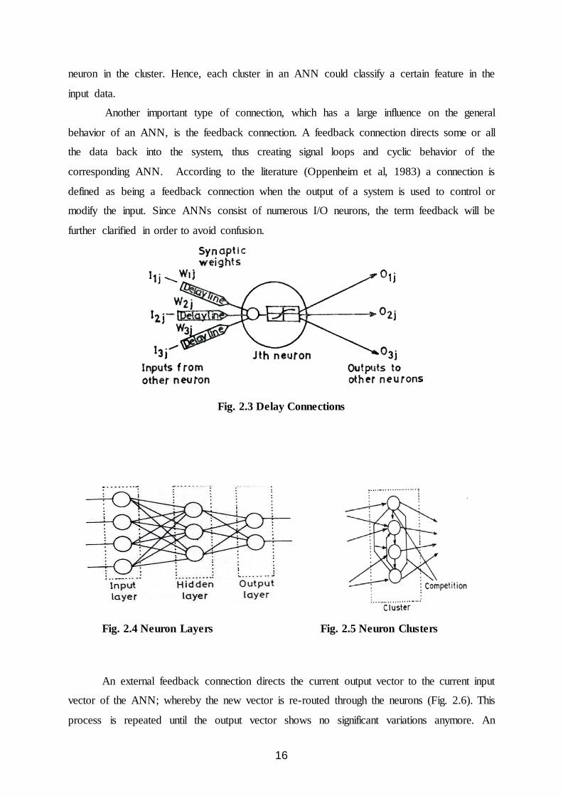
16
neuron in the cluster. Hence, each cluster in an ANN could classify a certain feature in the
input data.
Another important type of connection, which has a large influence on the general
behavior of an ANN, is the feedback connection. A feedback connection directs some or all
the data back into the system, thus creating signal loops and cyclic behavior of the
corresponding ANN. According to the literature (Oppenheim et al, 1983) a connection is
defined as being a feedback connection when the output of a system is used to control or
modify the input. Since ANNs consist of numerous I/O neurons, the term feedback will be
further clarified in order to avoid confusion.
Fig. 2.3 Delay Connections
Fig. 2.4 Neuron Layers Fig. 2.5 Neuron Clusters
An external feedback connection directs the current output vector to the current input
vector of the ANN; whereby the new vector is re-routed through the neurons (Fig. 2.6). This
process is repeated until the output vector shows no significant variations anymore. An

17
internal feedback connection directs the output signal of one neuron to the input of another
neuron (Fig. 2.7). Often multiple feedback loops are used between neurons in the same
cluster or between different layers.
Fig. 2.6 External Feedback Connections Fig. 2.7 Internal Feedback Connections
In general, Feedback networks (also referred to as recurrent networks) are defined as
being systems that settle or relax into an output vector. The data will pass through some or all
of the neurons more than once. Because the actual state of a network is dependent on its
previous states, the same input vector can produce different output vectors. Stability and
convergence characterize the performance of a feedback network. Feedback networks are
also referred to as dynamic non-linear systems.
When there is a total lack of feedback connections, one generally speaks of feed-
forward networks. This means that a given input vector will always produce one output
vector. Once trained (fixed weights), this input vector will always produce the same output
vector. Often feed-forward networks are referred to as instantaneous static non-linear
mapping systems.
2.4 LEARNING ALGORITHMS
The weight distribution in every ANN is unique and will determine the specific
response of the network to any given input vector. In order to perform a required process
task, these weights must be determined in advance through a learning process. The learning
process for ANNs encompasses the adjustment of weights and this process makes use of a
learning algorithm and a training set of examples.
The learning process in an ANN can be seen as teaching the network to yield a
particular response to a specific input. This often consists of an iterative process; whereby the
network tries to match output vectors to desired ones and uses any deviations to adjust some
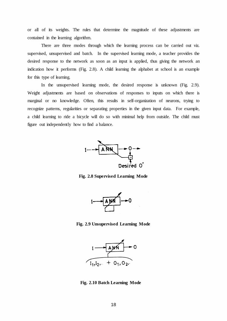
18
or all of its weights. The rules that determine the magnitude of these adjustments are
contained in the learning algorithm.
There are three modes through which the learning process can be carried out viz.
supervised, unsupervised and batch. In the supervised learning mode, a teacher provides the
desired response to the network as soon as an input is applied, thus giving the network an
indication how it performs (Fig. 2.8). A child learning the alphabet at school is an example
for this type of learning.
In the unsupervised learning mode, the desired response is unknown (Fig. 2.9).
Weight adjustments are based on observations of responses to inputs on which there is
marginal or no knowledge. Often, this results in self-organization of neurons, trying to
recognize patterns, regularities or separating properties in the given input data. For example,
a child learning to ride a bicycle will do so with minimal help from outside. The child must
figure out independently how to find a balance.
Fig. 2.8 Supervised Learning Mode
Fig. 2.9 Unsupervised Learning Mode
Fig. 2.10 Batch Learning Mode
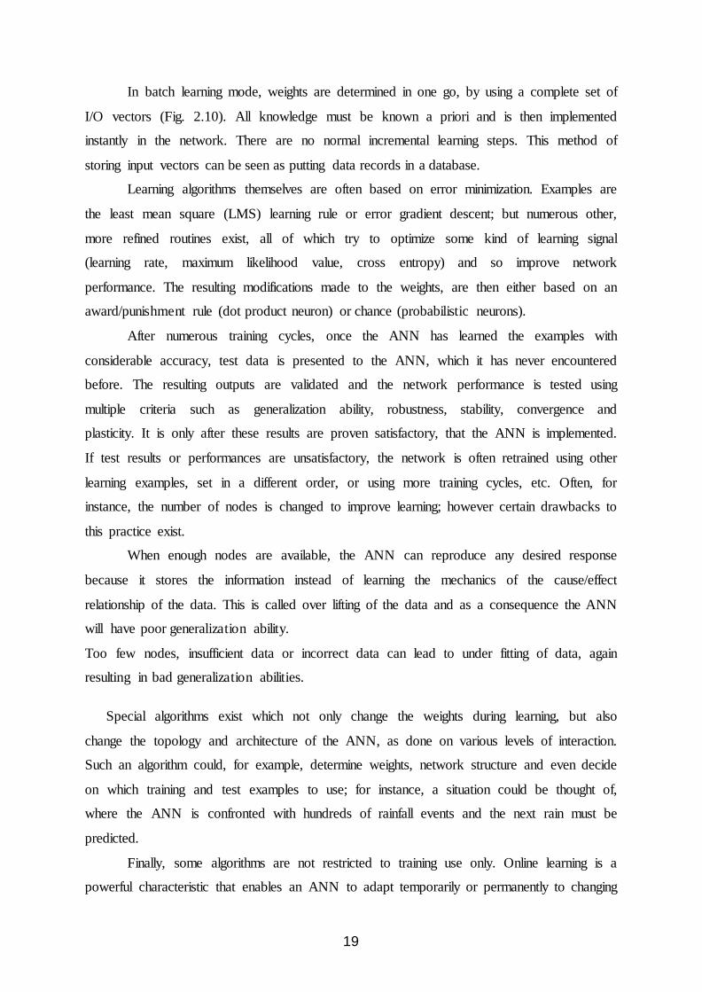
19
In batch learning mode, weights are determined in one go, by using a complete set of
I/O vectors (Fig. 2.10). All knowledge must be known a priori and is then implemented
instantly in the network. There are no normal incremental learning steps. This method of
storing input vectors can be seen as putting data records in a database.
Learning algorithms themselves are often based on error minimization. Examples are
the least mean square (LMS) learning rule or error gradient descent; but numerous other,
more refined routines exist, all of which try to optimize some kind of learning signal
(learning rate, maximum likelihood value, cross entropy) and so improve network
performance. The resulting modifications made to the weights, are then either based on an
award/punishment rule (dot product neuron) or chance (probabilistic neurons).
After numerous training cycles, once the ANN has learned the examples with
considerable accuracy, test data is presented to the ANN, which it has never encountered
before. The resulting outputs are validated and the network performance is tested using
multiple criteria such as generalization ability, robustness, stability, convergence and
plasticity. It is only after these results are proven satisfactory, that the ANN is implemented.
If test results or performances are unsatisfactory, the network is often retrained using other
learning examples, set in a different order, or using more training cycles, etc. Often, for
instance, the number of nodes is changed to improve learning; however certain drawbacks to
this practice exist.
When enough nodes are available, the ANN can reproduce any desired response
because it stores the information instead of learning the mechanics of the cause/effect
relationship of the data. This is called over lifting of the data and as a consequence the ANN
will have poor generalization ability.
Too few nodes, insufficient data or incorrect data can lead to under fitting of data, again
resulting in bad generalization abilities.
Special algorithms exist which not only change the weights during learning, but also
change the topology and architecture of the ANN, as done on various levels of interaction.
Such an algorithm could, for example, determine weights, network structure and even decide
on which training and test examples to use; for instance, a situation could be thought of,
where the ANN is confronted with hundreds of rainfall events and the next rain must be
predicted.
Finally, some algorithms are not restricted to training use only. Online learning is a
powerful characteristic that enables an ANN to adapt temporarily or permanently to changing

20
conditions. Self organizing maps, for example, can continue learning with each new input
vector they receive. An ANN could be created, for example, which simulates flow through a
sewer pipe and adapts its parameters when the resistance of a sewer pipe becomes higher;
independent of any intervention from an external source.
2.5 STRUCTURE
In order for an ANN to learn a certain response, it must be provided with numerous
examples. The data contained in these examples is crucial for the performance to the network.
Incorrect input data will certainly result in slow learning, unstable or unreliable networks.
Therefore, the training and test examples should be chosen with care and (pre-) processed
accordingly.
The term input vector will be used to refer to the input data needed for one training,
test or on-line example (Fig. 2.11). Consecutively output vector refers to the final calculated
result of the ANN. Each input/output vector has a certain dimension R, representing different
features of the data, e.g. 1(1) represents the catchment size, 1(4) is the type of vegetation, etc.
When Q different vectors are presented to the ANN randomly or in ordered fashion, we can
Fig. 2.11 Input Vectors and their Dimensions
define a matrix P, which defines a set of Q I/O vectors of dimension R (P = Q x R). In the
training of an ANN, which should, for example, determine the runoff coefficient of an urban
catchment area, the input matrix P could consist of 100 catchments (Q=100), each
representing specified catchment characteristics. The output vectors would then consist of
single values, representing the runoff coefficients.
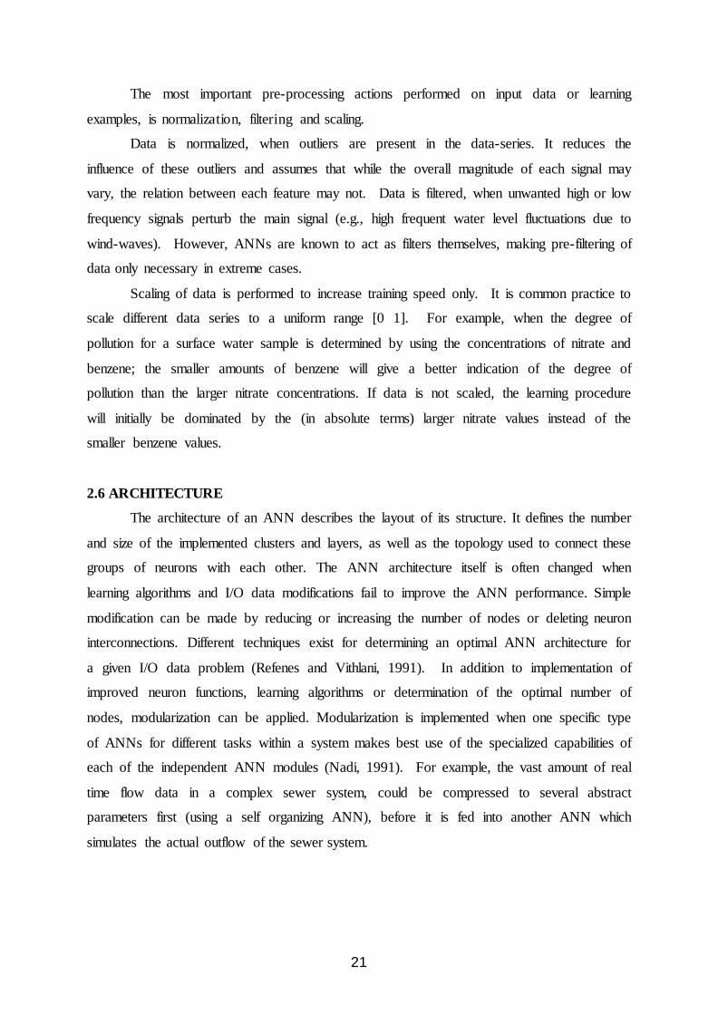
21
The most important pre-processing actions performed on input data or learning
examples, is normalization, filtering and scaling.
Data is normalized, when outliers are present in the data-series. It reduces the
influence of these outliers and assumes that while the overall magnitude of each signal may
vary, the relation between each feature may not. Data is filtered, when unwanted high or low
frequency signals perturb the main signal (e.g., high frequent water level fluctuations due to
wind-waves). However, ANNs are known to act as filters themselves, making pre-filtering of
data only necessary in extreme cases.
Scaling of data is performed to increase training speed only. It is common practice to
scale different data series to a uniform range [0 1]. For example, when the degree of
pollution for a surface water sample is determined by using the concentrations of nitrate and
benzene; the smaller amounts of benzene will give a better indication of the degree of
pollution than the larger nitrate concentrations. If data is not scaled, the learning procedure
will initially be dominated by the (in absolute terms) larger nitrate values instead of the
smaller benzene values.
2.6 ARCHITECTURE
The architecture of an ANN describes the layout of its structure. It defines the number
and size of the implemented clusters and layers, as well as the topology used to connect these
groups of neurons with each other. The ANN architecture itself is often changed when
learning algorithms and I/O data modifications fail to improve the ANN performance. Simple
modification can be made by reducing or increasing the number of nodes or deleting neuron
interconnections. Different techniques exist for determining an optimal ANN architecture for
a given I/O data problem (Refenes and Vithlani, 1991). In addition to implementation of
improved neuron functions, learning algorithms or determination of the optimal number of
nodes, modularization can be applied. Modularization is implemented when one specific type
of ANNs for different tasks within a system makes best use of the specialized capabilities of
each of the independent ANN modules (Nadi, 1991). For example, the vast amount of real
time flow data in a complex sewer system, could be compressed to several abstract
parameters first (using a self organizing ANN), before it is fed into another ANN which
simulates the actual outflow of the sewer system.

22
2.7 PERFORMANCE INDICATORS
During learning or network optimization, it is often necessary to monitor the effects of
a certain intervention or system alteration. Numerous performance indicators exist to quantify
progression or drawbacks of certain methods:
Generalization is the ability of the ANN to formulate an answer to a problem it has
never seen before (predict a future flow rate using on-line data).
Fault tolerance is the ability to keep processing, albeit with reduced accuracy and/or
speed, even though data is missing or neurons have been disabled/destroyed (A water
level meter fails).
Convergence speed is the rate at which the network state changes as it moves to a
stable state.
The states of an ANN can be mathematically expressed in a function, representing a 3
dimensional surface of the computational energy of the ANN. Computational energy
describes the stable states or solutions of an ANN and the paths leading to them.
These stable states are represented as valleys (energy minima) in the 3 dimensional
surfaces, also called basins of attraction. By changing the weights, this energy surface
is changed and the valleys get larger and deeper, increasing the convergence speed of
an ANN.
Adaptability is the ability of an ANN to modify its response to changing conditions.
Four characteristics govern this ability: learning, self organization, generalization and
training.
Reliability is the ability to produce the same result, when the same input vector is
repeatedly presented to a network. Reliability is mostly used to describe the
performance of feedback networks, since feed-forward networks always produce the
same result.
Robustness is the ability to produce the same result, even though input data is noisy,
contains data gaps and contradictory data.
Sensitivity is closely related to robustness, it shows the extent to which a network
response will change, due to variations in the features of the input vector.

23
Three other less obvious indicators that can also be used are:
Memory requirements: Some ANNs need less (hardware) memory to perform their
task, than others. This can be decisive for data base related problems that use pattern
storage for instance (Hopfield network).
Amount of training data needed: for some problems, lack of data poses a constant
hindrance to efficient modeling. Thus an ANN requiring less training data to learn a
specific response is better suited for these kinds of problems.
Learning speed: The speed at which new data is learned, can be crucial for on-line
applications in fast changing environments. This performance indicator is often used
to evaluate new learning algorithms.
With these performance indicators, it is possible to make an evaluation table, showing
the different ANN types and their relative performances.
2.8 MODEL OF AN ARTIFICIAL NEURAL NETWORK
The main function of the ANN paradigms is to map a set of inputs to a set of outputs.
A single processing unit or neuron is shown in Fig.2.12. The incoming signals are multiplied
by respective weights through which they are propagated toward the neurons or node, where
they are aggregated (summed up) and the net input is passed through the activation function
to produce the output.
Fig. 2.12 A Single Artificial Neuron (Perceptron)
Output
x1
x2
xn
.
.
.
.
w1
w2
wn
Weights Inputs
∑ ƒ y
Neuron (Summation of weighted inputs and
thresholding output)
Aggregation (SUMMATIO N UNIT)
Activation (THRESHO LDING UNIT)

24
Let x i (i = 1,2, ... n) are inputs and wi (i = 1,2, … n) are respective weights. The net input
to the node can be expressed as
i
n
ii wxnet ∑
=
=1 …(2.1)
The net input is then passed through an activation function ƒ(.) and the output y of the node is
computed as
y = ƒ(net) …(2.2)
To ensure that the neurons response is bounded that is the actual response of the neuron is
conditioned, or damped, as a result of large or small activating stimuli and thus is
controllable.
Sigmoid function is the most commonly used nonlinear activation function for solving
ANN Problems which is given by y = ƒ(net) = nete−+11 .
This activation function is shown in Fig. 2.13.
-4 -2 0 2 4 0
0.2
0.4
0.6
0.8
1
net
y=f(n
et)
Fig. 2.13 The Sigmoid Function

25
2.9 MULTILAYER FEED-FORWARD NETWORK
The most important attribute of a multilayer feed-forward network is that it can learn
a mapping of any complexity (Zurada. 1992). This network is made up of multiple layers of
neurons. In this architecture, besides the input layer and the output layer, the network also
has one or more than one intermediate layer(s) called hidden layer(s). Each layer is fully
connected to the preceding layer by interconnection strengths or weights. Fig.2.14 illustrates
this type of network consisting of a single hidden layer. As can be seen, the generic feed-
forward network is characterized by the lack of feedback. Even though this network has no
explicit feedback connection when the input is mapped into the output, the output values are
often compared with the desired output values, and also an error signal can be employed for
adapting the network’s weights during the learning process.
Fig. 2.14 Multilayer Feed – Forward Artificial Neural Network Configuration
2.10 OTHER ANN NETWORKS
Some of the most important networks are explained below:
2.10.1 Back Propagation Network (BP)
Back Propagation network (BP) are the most widely used ANNs. The name comes
from the fact that an error term is back propagated through the network during learning and
used to change the weights (Fig. 2.15). However, no feedback links are actually incorporated
Input
Input layer Hidden layer
Output
Output layer
i =1, 2, 3……ni j=1, 2, 3 …….nh k=1, 2, 3…….no
.
.
.
.
.
.
y1
y2
yno
x1
x2
xni
h4
h1
hnh
wh11 wo11
whnh,ni wono,ni
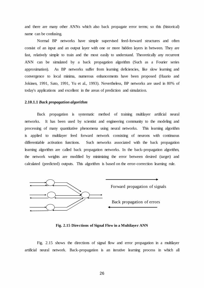
26
and there are many other ANNs which also back propagate error terms; so this (historical)
name can be confusing.
Normal BP networks have simple supervised feed-forward structures and often
consist of an input and an output layer with one or more hidden layers in between. They are
fast, relatively simple to train and the most easily to understand. Theoretically any recurrent
ANN can be simulated by a back propagation algorithm (Such as a Fourier series
approximation). As BP networks suffer from learning deficiencies, like slow learning and
convergence to local minima, numerous enhancements have been proposed (Haario and
Jokinen, 1991, Sato, 1991, Yu et al., 1993). Nevertheless, BP networks are used in 80% of
today's applications and excellent in the areas of prediction and simulation.
2.10.1.1 Back propagation algorithm
Back propagation is systematic method of training multilayer artificial neural
networks. It has been used by scientist and engineering community to the modeling and
processing of many quantitative phenomena using neural networks. This learning algorithm
is applied to multilayer feed forward network consisting of neurons with continuous
differentiable activation functions. Such networks associated with the back propagation
learning algorithm are called back propagation networks. In the back-propagation algorithm,
the network weights are modified by minimizing the error between desired (target) and
calculated (predicted) outputs. This algorithm is based on the error-correction learning rule.
Fig. 2.15 Directions of Signal Flow in a Multilayer ANN
Fig. 2.15 shows the directions of signal flow and error propagation in a multilayer
artificial neural network. Back-propagation is an iterative learning process in which all
Forward propagation of signals
Back propagation of errors

27
weight parameters are randomly initialized and then updated (in each iteration) through feed-
forward calculations and back-propagation of errors.
2.10.1.2 Learning factors of back propagation
One of the major issues concerning back propagation algorithm is its convergence.
The convergence of back propagation is based on some important learning factors such as the
initial weights, the learning rate, the nature of training set and the architecture of the network.
(a) Initial weights
The initial weights of a multilayer feed forward network strongly affect the ultimate
solution. They are typically initialized by small random values (between -1.0 and 1.0 or -0.5
to +0.5). Equal weights values cannot train the network properly if the solution requires
unequal weights to be developed. The initial weights cannot be large, otherwise the sigmoid
will saturate, from the beginning and the system will stock at a local minimum. The
saturation is avoided by choosing the initial values of the synoptic weights to be uniformly
distributed inside a small range of values. The range should not be too small as it can cause
the learning to be very small.
(b) Frequency of weight updates
There are two approaches to learning
1. In “per-pattern” learning, used, in the algorithm, weights are changed after every
sample presentation.
2. In “per-epoch” (or “batch-mode”) learning, weights are updated only after all samples
are presented to the network. An epoch consists of such a presentation of the entire
set of training samples. Weight changes suggested by different training samples are
accumulated together into a single change to occur at the end of each epoch.
(c) Learning rate (η)
A control parameter used by several learning algorithms, which affects the changing
of weights. The bigger learning rates cause bigger weight changes during each iteration.
Weight vector changes in backpropagation are proportional to the negative gradient of the
error; this guideline determines the relative changes that must occur in different weights
when a training sample (or a set of samples) is presented, but does not fix the exact

28
magnitudes of the desired weight changes. The magnitude change depends on the
appropriate choice of learning rate, η. A large value of η will lead to rapid learning but the
weight may oscillate, while low values imply slow learning. This is typical of all gradient
descent methods. The right value of η will depend on the application. Values between 0.1
and 0.9 have been used in many applications in the literature.
(d) Momentum (α )
A simple method of increasing the rate of learning and yet avoiding the danger of
instability is to include a momentum term to the normal gradient descent method. To give
each weight some inertia or momentum so that it tends to change the direction of average
downhill force that it feels. The scheme is implemented by giving a contribution from the
previous step to each weight change. The range of momentum is and a value of 0.9 is
generally used for momentum factor.
(e) Data normalization
The variables fall in the range of a 0 to 1, because it smoothens the solution space and
averages out some of the noise effects. Such process is called normalization or
standardization.
(f) Number of hidden nodes
The size of a hidden layer is usually determined experimentally. In practice, the
number of hidden layer is relatively smaller than the number of nodes in the input layer. If the
network fails to converge, more neurons are added gradually to the hidden layer till a good
performance is achieved.
(g) Data training and generalization
The training data submitted to the network for it to learn and generalized the relation
between input and output should be sufficient and proper. There is no rule for choosing the
training data. Networks with too many trainable parameters for a given amount of training
data learn well but do not generalize well. This phenomena is called over fitting with too few
trainable parameter, the network fails to learn the training data.
The available data is divided into two parts one for training another for testing. The
purpose of training is to determine the set of connection weights that cause the neural

29
network to estimate outputs that are sufficiently close to target values. The training data
should contain sufficient patterns.
The training set is further divided into two subsets:
A subset used for estimation of the model ( i.e. training the networks)
A subset used for evaluation of the performance of the model. The validation subset
is usually 10 to 20 of the training set.
(h) Strength of Feed-forward Neural Network
They are able to recognize the relation between the input and output variables without
knowing physical consideration.
They work well even when the training set contains noise and measurement errors.
There is no need to make assumption about the mathematical form the relationship
between input and output.
2.10.1.3 Feed-forward calculation
In the feed-forward calculation, the nodes in the input layer receive the input signals
which are passed to the hidden layer and then to the output layer. The signals are multiplied
by the current values of weights, and then the weighted inputs are added to yield the net input
to each neuron of the next layer. The net input of a neuron is passed through an activation or
transfer function to produce the output of the neuron. Considering the ANN shown in Fig.2.14, the procedure for feed-forward calculations in different layers is as follows
The net input to jth node of the hidden layer is given by
i
ni
ijij xwhneth ∑
=
=1
…(2.3)
where ni is the number of neurons in the input layer and jiwh is the connection weight
between ith node of the input layer and jth node of the hidden layer. The output of jth node of
the hidden layer hj is
hj=f(nethj) …(2.4)
where f(.) is the activation function, e.g. a sigmoid activation function. Thus

30
( )jj neth
h−+
=exp1
1 …(2.5)
Similarly, the net input to kth node of the output layer is given by
∑=
=nh
jjkjk hwonety
1 …(2.6)
where, nh is the number of neurons in the hidden layer and kjwo is the connection weight
between jth node of the hidden layer and kth node of the output layer.
The output of kth node of the output layer is
yk=f(netyk) …(2.7)
Now operating through the sigmoid activation function
( )kk nety
y−+
=exp1
1 …(2.8)
After calculation of these outputs the error between desired and calculated output is
computed which is propagated in the backward direction, as explained below.
2.10.1.4 Error back-propagation
The error calculated at the output layer is propagated back to the hidden layers and
then to the input layer, in order to determine the updates for the weights. This method is
derived from the well-known gradient descent method in which the weights updatation is
performed by moving in the direction of negative gradient along the multidimensional
surface of the error function. The sum square error E for a single input-output pair data set is
given by
E = ( )2
121∑
=
−no
kkk ty …(2.9)

31
Where, t k is the desired output or target at the kth node and yk is the calculated output at the
same node. In order to minimize the above error function, weights are updated by subtracting
incremental changes in the weights from their old values.
That is,
kjoldkj
newkj wowowo ∆−= …(2.10)
(j=1, 2, 3.. . nh, and k=1,2,3.. no)
jioldji
newji whwhwh ∆−= … (2.11)
(i=1, 2, 3.ni, and j=1,2,3.. nh)
Where, kjwo∆ and jiwh∆ are incremental changes in the weights for output layer and hidden
layer respectively.
The incremental changes in the weights for output layer are given by
∂∂
=∆kj
kj woEwo η …(2.12)
where, η is the learning rate.
By using chain rule, kjwo
E∂∂ can be written as
kj
k
k
k
kkj wonety
netyy
yE
woE
∂∂
∂∂
∂∂
=∂∂ …(2.13)
Now, differentiating Eqn (2.6) with respect to kjwo ,
jkj
k hwonety
=∂∂ …(2.14)
Differentiating Eqn (2.8) with respect to knety ,
( )kkk
k yynety
y−=
∂∂
1 …(2.15)
Also differentiating Eqn (2.9) with respect to ky yields
( )kkk
tyyE
−=∂∂
kyδ= …(2.16)

32
where kyδ is the error at the output side of kth output node. Substituting Eqn 2.14 and Eqn.
2.16 in Eqn 2.13, the Eqn 2.12 may be represented as,
( ) jkkkkj hyyywo .1. −=∆ ηδ …(2.17)
or
jkkj hywo ∆=∆ η …(2.18)
where, )1(. kkkk yyyy −=∆ δ …(2.19)
ky∆ is the error at the input side of the kth output node. Similarly the incremental changes in
the weights for the hidden layer are given by
∂∂
=∆ji
ji whEwh η …(2.20)
By using chain rule
ji
j
j
j
j
k
k
kno
k kji whneth
nethh
hnety
netyy
yE
whE
∂
∂
∂
∂
∂∂
∂∂
∂∂
=∂∂ ∑
=
...1
…(2.21)
Now, differentiating Eq. (2.8) with respect to knety∂ ,
( )kkk
k yynety
y−=
∂∂
1 …(2.22)
Differentiating Eq. (2.6) with respect to jh∂ ,
kjj
k woh
nety=
∂∂ …(2.23)
Differentiating Eq. (2.5) with respect to jneth∂ ,
( )jjj
j hhneth
h−=
∂
∂1 …(2.24)
Also differentiating Eq. (2.3) with respect to jiwh∂ ,
iji
j xwhneth
=∂
∂ …(2.25)

33
Substituting Eqs. (2.16), (2.22) and (2.25) in Eq. (2.21), then the Eq. 2.20 may be
represented as,
ijjkjkk
no
kk
jiji xhhwoyyy
whEwh )1()1(
1−−=
∂∂
=∆ ∑=
δηη
ijjkjkk
no
kkji xhhwoyyywh )1()1(
1−−=∆ ∑
=
δη …(2.26)
Using Eq. (2.19)
ijjkj
no
kkji xhhwoywh )1(
1−∆=∆ ∑
=
η …(2.27)
where,
kj
no
kkj woyh ∑
=
∆=1
δ …(2.28)
Here, jhδ is the error at the output side of the jth hidden node.
( )jjjj hhhh −=∆ 1δ …(2.29)
Here, jh∆ is the error at the input side of the jth hidden node.
Substituting Eq. (2.29) in Eq. (2.27)
ijji xhwh ∆=∆ η …(2.30)
The learning process starts with a random set of weights. During the training process,
weights are updated through error back-propagation using Eq. (2.17) or (2.18) and Eq. (2.30)
respectively for output and hidden layers. The flowcharts for training of ANN using back-
propagation algorithm and that for testing of the trained ANN are shown in Fig. 2.16 and Fig.
2.17 respectively.
2.10.2 Adaline Network
Adaline networks were one of the earliest ANNs. They consist of single neuron
elements employing only linear functions and a simple Least Mean Square (LMS) learning.
This makes them suited for simple classifications and restricted non-linear system simulation.

34
START
Read training d
Normalize the training data
Define the structure of ANN, i.e. no. of layers and nodes in each layer
Assign the random weights for each i
Assign maxm no. of iterations and tolerance for MSE
Assign iteration count = 0
Calculate networks outputs and errors between desired and calculated outputs
using feed-forward calculation
Output the weight parameters
STOP
No Is RMSE > tolerance
?
Is Iteration count
<maxm iterations ?
A
Back-propagate the errors between desired and calculated outputs and update the
weights Calculate mean square error (RMSE)
Increment the iteration count by one
STOP
A
Yes
Convergence could not be achieved; redefine the structure
and learning rate etc. and try again
Yes
No
Fig. 2.16 Flowchart for training using back-propagation algorithm
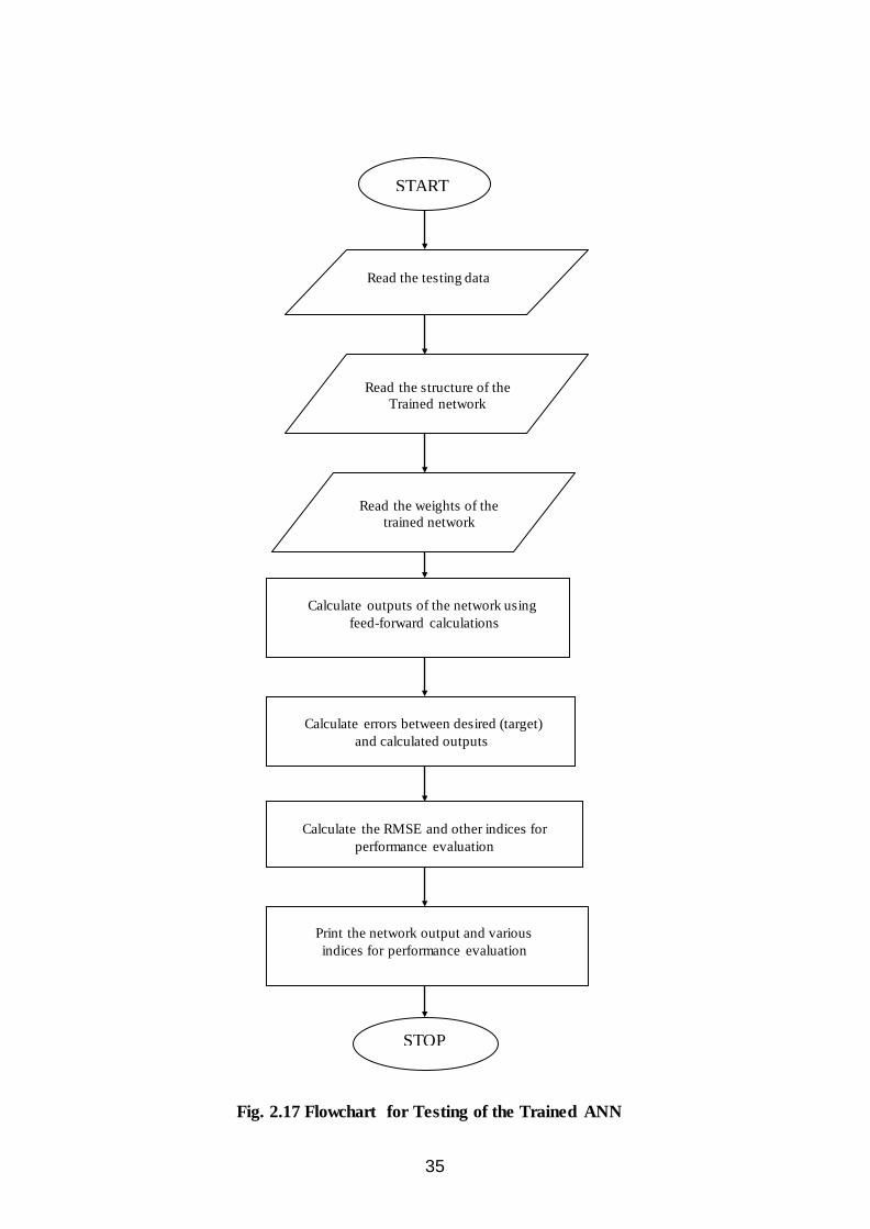
35
Fig. 2.17 Flowchart for Testing of the Trained ANN
START
Read the testing data
Read the structure of the Trained network
Read the weights of the trained network
Calculate outputs of the network using feed-forward calculations
Calculate errors between desired (target) and calculated outputs
Calculate the RMSE and other indices for performance evaluation
Print the network output and various indices for performance evaluation
STOP
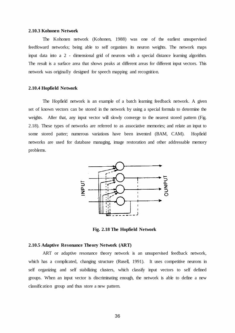
36
2.10.3 Kohonen Network
The Kohonen network (Kohonen, 1988) was one of the earliest unsupervised
feedfoward networks; being able to self organizes its neuron weights. The network maps
input data into a 2 - dimensional grid of neurons with a special distance learning algorithm.
The result is a surface area that shows peaks at different areas for different input vectors. This
network was originally designed for speech mapping and recognition.
2.10.4 Hopfield Network
The Hopfield network is an example of a batch learning feedback network. A given
set of known vectors can be stored in the network by using a special formula to determine the
weights. After that, any input vector will slowly converge to the nearest stored pattern (Fig.
2.18). These types of networks are referred to as associative memories; and relate an input to
some stored patter; numerous variations have been invented (BAM, CAM). Hopfield
networks are used for database managing, image restoration and other addressable memory
problems.
Fig. 2.18 The Hopfield Network
2.10.5 Adaptive Resonance Theory Network (ART)
ART or adaptive resonance theory network is an unsupervised feedback network,
which has a complicated, changing structure (Rusell, 1991). It uses competitive neurons in
self organizing and self stabilizing clusters, which classify input vectors to self defined
groups. When an input vector is discriminating enough, the network is able to define a new
classification group and thus store a new pattern.

37
2.10.6 Linear Vector Quantization Network (LVQ)
Linear Vector Quantization (LVQ) network is a supervised feedback network. It is a
method whereby supervision and competitive layers are combined. The competitive layer
finds subclasses among then input data; and these are then classified into user defined target
classes. In contrast to back propagation classification networks, LVQ can also classify non-
linearly separable sets of vectors.
2.10.7 Elman Network
It has two hidden layer back propagation network, with the addition of a feedback
connection from the output of the first hidden layer to its input. This feedback path allows
Elman networks to learn to recognize and generate temporal patterns as well as spatial
patterns (Elman, 1990).
2.11 SELECTION OF NETWORK ARCHITECTURE
One of the most important attributes of a layered neural network design is choosing
the architecture. The number of input nodes is simply determined by the dimension of the
input vector to be generalized or associated with a certain output quality. The dimension of
the input vector corresponds to the number of distinct feature of the input pattern. Similarly
the number of neurons in the output layer can be made equal to the dimension of vectors to be
associated. The size of the hidden layer(s) is the most important consideration when solving
the actual problems using multilayer feed-forward neural networks. The most popular and
effective strategy for selecting the appropriate number and size(s) of the hidden layer(s) is
trial-and-error procedure. A number of networks with one or two hidden- layer(s) are trained
with different combination of hidden neurons and a network is selected that yields the
minimum root mean square error (MSE). It is also important that the size of the network
should be as small as possible. An effective criterion for selecting the best network from
these two points of view, i.e. minimum RMSE and smallest size, is Akaike’s Information
Criterion (AIC). The AIC is an operational way of trading off the size of the network against
how well the network fits the data (Akaike, 1974). It is given by
+=
nEnkAIC 2ln2 …(3.31)

38
Where, E is the sum-square-error; k is the number of parameters; and n is the number
of observations. The network with minimum value of AIC is considered to be the best
network.
2.12 ISSUES IN ANN APPLICATION
By now, ANNs are firmly established as a viable black–box modeling tool. However,
along with numerous advantages, ANNs have some disadvantages too. The first and foremost
is the requirement of adequate data of desirable quality and quantity. To be fair to ANNs, this
is a crucial requirement with all modeling techniques and ANN cannot be an exception.
Presently clear guidelines are not available except that the entire range of likely inputs should
be covered. Guidelines to select network architecture for a given type
of problems are also badly missing. In this context, ASCE (2000b) has raised the following
very pertinent questions, which need to be resolved.
Can ANNs make to reveal any physics? The application of ANNs can get a boost if
some physical explanation of their functioning is available. This will also help in
selecting the appropriate type of network and learning algorithm for a given problem.
Some neural networks can provide statistical interpretations in terms of conditional
probabilities. For instance, a feed forward network can learn the posterior probability
of a classification. This problem is receiving attention of many researchers.
Can an optimal training set be identified? ANNs cannot learn without data –they are
data intensive and poor training data will result in poor learning. An optimal data set
should fully represent the modeling domain, have minimum required data points and
there should not be repetition of data. So far, there are no guidelines about these.
Can ANNs improve time series analysis? The time series models are based on
extracting the correlation and dependence structure of the data. While ANNs have
been not given any insight into the process, it would be welcome if ANNs can bring
out the relationships among the variables and highlight those features of input data are
not revealed by other techniques.
Can training of ANNs be made adaptive? The most time-consuming part of ANN
application is training. As new data become available, the previously trained ANN has
to be re-training. Since the catchment properties change with time, it is important to
incorporate the new information in the model. The ANN applications will be

39
immensely benefited if the training can be made adaptive, i.e., the new information is
incorporated into the models without the necessity of complete re-training.
Are ANNs good extrapolators? Many studies have shown that ANNs work well in the
range of input data that were used for training and their performance deteriorates if
during application, the input data are of this range. This aspect is receiving attention
of hydrologists. Imrie et al. (2000) have presented a methodology for training ANNs
to produce models that generalize well on new data and can extrapolate beyond the
range of values included in the calibration range. They claimed good results the data
from the catchment or the River Trent and a modified cascade- correlation algorithm.
A think and solution to the above issues will certainly help in better understanding of
the artificial neural networks. Of course ANNs cannot be considered as a panacea for all
types of problems of water resources or an alternative to other modeling approaches. Gupta et
al. (2000) have aptly comment: “ We do not advocate that the ANN approach be generally
used in place of that the ANN approach does not- in particular, the conceptual approach has
potential to be applied to ungaged watersheds or to simulate the potential behavior of a
watershed under land use changes… Further, implementation of the ANN approach does not
require the considerable amount of expertise and data required to calibrate a conceptual
watershed model.” Logically then, ANN should be viewed as alternative to computing
techniques.

40
Chapter – 3
RR ee vv ii ee ww oo ff LL ii tt ee rr aa tt uu rr ee

41
Review of Literature
In recent years ANNs have shown exceptional performance as regression tools,
especially when used for pattern recognition and function estimation. They are highly non-
linear, and can capture complex interactions among the input variables in a system without
any prior knowledge about the nature of this interactions (Hammerstrom, 1993). The main
advantage of ANNs is that one does not have to explicitly assume a model form, which is a
prerequisite in conventional modelling approaches. Indeed, in ANNs the data points
themselves generate a relationship of possibly complicated or orthodox shape. In comparison
to the conventional methods, ANNs tolerate imprecise or incomplete data, approximate
results, and are less vulnerable to outliers (Haykin, 1994). They are highly parallel, i.e.; their
numerous independent operations can be executed simultaneously. Although application of
ANN approach in hydrological modeling is recent and limited, it has already produced very
encouraging results. A number of researchers have investigated the potential of artificial
neural networks in modeling the rainfall runoff process as well as the runoff sediment
process. The review is given separately in the following sections.
3.1 ANN APPLICATIONS IN RAINFALL-RUNOFF MODELING
In a preliminary study, Halff et al. (1993) designed a three-layer feedforward ANN
using the observed rainfall hyetographs as inputs and hydrographs recorded by the U.S.
Geological Survey (USGS) at Bellvue, Washington, as outputs. The authors decided to use
five nodes in the hidden layer. A total of five storm events were considered. On a rotation
basis, data from four storms were used for training, while data from the fifth storm were used
for testing network performance. A sequence of 25 normalized 5 min rainfalls was applied as
inputs to predict the runoff. This study opened up several possibilities for rainfall-runoff
application using neural networks.
In an application using two neural networks, Zhu et al. (1994) predicted upper and
lower bounds on the flood hydrograph in Butter Creek, New York. Off-line predictions were
made when present flood data were not available and estimates had to be based on rainfall
data alone. On-line predictions were based on both rainfall and previous flood data. Data for
ANN testing and validation were generated from a nonlinear storage model. Model
3

42
performance was strongly influenced by the training data set. The authors found that, while
the ANN did well during interpolation, predictions made by ANNs outside the range of the
training data set were not encouraging. The process of trying to make ANNs adaptive was
computationally very demanding, because the entire training process needed to be repeated
with each new data pair. As the lead time for forecasting increased, ANN performance
deteriorated. By comparison, ANNs were found to be marginally better than fuzzy inference-
based techniques.
In a more detailed study along similar lines, Karunanithi et al. (1994) were interested
in estimating streamflows at an ungauged site on the Huron River in Michigan, based on data
from USGS stream gauging stations located 30 km upstream and 20 km downstream of the
sampling site. They compared ANN performance to an empirical two-station power law
relationship that is based on log-transformation of the actual streamflow values. Fig. 3 shows
a comparison of observed versus predicted daily flows for a testing period of two years. Daily
data were found to exhibit rapid fluctuations, and the authors worked with five-day non-
overlapping averages and five-day moving averages to obtain a smoother representation
when using regression. However, the raw data were utilized as ANN inputs. They used the
cascade-correlation algorithm so that the network architecture could be determined during
training. When using empirical regression equations, the largest errors were associated with
the highest stream flows. Neural networks were found to better predict these high events,
while both methods predicted low streamflows fairly well. These authors stated that ANNs
are capable of adapting their complexity to accommodate temporal changes in historical
streamflow records. They also found that including another gauging station that supposedly
had little or no effect on streamflows at the gauging site caused the performance of the,
regression technique to deteriorate, while the ANN performance was not affected. The
authors claimed that ANNs are likely to be more robust when noisy data is present in the,
inputs. Karunanithi et al. (1994) found lag time to be important in predicting streamflows.
This reflects the longer memory associated with streamflows. The authors did not use any
statistical techniques to evaluate the lag time and include it in the network architecture.
Lorrai and Sechi (1995) developed and applied neural networks to rainfall – runoff
transformation. The network architecture was developed with two hidden layers and sigmoid
response function by using back propagation algorithm. Monthly rainfall, runoff, and
temperature were used to develop the model by dividing the data into three ten year period
and verified in rest two ten years’ block. They found that artificial neural networks
provide higher efficiency during model development and were superior to simple

43
multivariate auto-regressive model. However, the verification of results of the developed
models was not so promising.
Smith and Eli (1995) applied a back-propagation neural network model to predict
peak discharge and time to peak over a hypothetical watershed. Data sets for training and
validation were generated by either a linear or a nonlinear reservoir model. By representing
the watershed as a grid of cells, it was possible for the authors to incorporate the spatial and
temporal distribution information of rainfall into the ANN model. As an example, the authors
chose a synthetic watershed that was composed of 5 X 5 cells. A tree-type drainage pattern
was superimposed on the grid to concentrate runoff towards a single watershed outlet. Each
cell was treated as a reservoir and water was routed in a cascading fashion. A rainfall depth of
one unit was applied instantaneously at several cells on a random basis. Each rainfall pattern
in the training set was presented to the network as an input image consisting of Boolean
values with 1 representing a wet cell and O a dry cell. The peak discharge and the time to
peak corresponding to each rainfall pattern were computed using a linear and nonlinear
reservoir model and served as target outputs for the ANN model. Many such patterns formed
the training set. These cases represented single-storm events for which the number of input
units was the same as the number of cells. To simulate the occurrence of several storms in a
sequence, three stochastically generated rainfall patterns were imposed consecutively over
the synthetic watershed. In this case, the input layer had 75 units, corresponding to three
rainfall patterns requiring 25 cells each. The output was either the watershed runoff alone or
the runoff and the time to peak. The number of nodes in the hidden layer was determined by
trial and error for each case. For single-storm events, the peak discharge and the time to peak
were predicted well by the neural network, both during training and testing. The authors were
less successful for multiple-storm events. One reason for this may have been insufficient
number of nodes in the output layer. In a separate application dealing with multiple storms,
Smith and Eli (1995) represented the entire hydrograph by a Fourier series with 21
coefficients, rather than just two attributes as in single-storm events. The ANN output layer
now consisted of 21 nodes corresponding to the Fourier coefficients. Using this method, the
authors found the prediction of the entire hydrograph to be very accurate for multiple storm
events.
The issue of enhancing the training speed using a three-layer network was addressed
by Hsu et al. (1995) and Gupta et al. (1997). These studies advocated the linear least squares

44
simplex (LLSSIM) algorithm, which partitions the weight space to implement a synthesis of
two training strategies. The input-hidden layer weights were estimated using a multistart
down-hill simplex nonlinear optimization algorithm, while the hidden-output layer weights
were estimated using optimal linear least square estimation. The nonlinear portion of the
search was thereby confined to a smaller dimension space, resulting in acceleration of the
training process. The simplex search involves multiple starts that are initiated randomly in the
search space, and the probability of finding local minima is virtually eliminated. The authors
applied this technique to daily rainfall-runoff modeling of the Leaf River Beam near Collins,
Mississippi. The performance of neural networks was compared with the linear ARMAX
time series model and the conceptual SAC-SMA model. Even though all the models seemed
to underestimate low flows in general, the ANN performance was found to be superior to the
other models. Gupta et al. (1997) concluded that the LLSSIM is likely to be a better training
algorithm than back-propagation or conjugate gradient techniques, especially in the absence
of a good initial guess of weights.
In another related study over the Leaf River Basin, Hsu et al. (1997) used a three-
layer feedforward ANN and a recurrent ANN to model daily rainfall-runoff. They concluded
that the feedforward ANN needed a trial-and-error procedure to find the appropriate number
of time-delayed input variables to the model and also was not suitable to distributed
watershed modeling. On the other hand, the recurrent ANN was able to provide a
representation of the dynamic internal feedback loops in the system, eliminating the need for
lagged inputs and resulting in a compact weight space. However, both ANNs performed
equally well at runoff prediction.
In a study by Minns and Hall (1996), data for network training consisted of model
results from one storm sequence, and two such sequences were generated for testing. Each
storm sequence was generated using a Monte Carlo procedure that preserved predetermined
storm characteristics. For each such storm sequence, the corresponding runoff sequence was
constructed using a simple nonlinear model for flood estimation (called RORB) that allowed
for different levels of nonlinearly in the response. A three-layer network with back-
propagation was used. Network inputs consisted of concurrent and 14 antecedent rainfall
depths and 3 antecedent runoff values, and the network output was current runoff. It was
found that ANN performance was hardly influenced by level of nonlinearity, with
performance deteriorating only slightly for high levels of nonlinearity. Using 2 hidden layers

45
1 and the associated extra cost on network training could rectify this. Minns and Hall (1996)
point out the importance of standardization based j on maximum and minimum values of
inputs and outputs. Whenever the network was required to predict,. out of range' , of the
standardized values, the performance dropped significantly, suggesting that ANNs are not
very good extrapolators.
Jayawardena and Fernando (1995, 1996) and Fernando and Jayawardena (1998) also
used RBF methods for flood forecasting. They illustrated the application of (REF) artificial
neural networks using an orthogonal least squares algorithm (OLS) to model the rainfall-
runoff process. Hourly rainfall and runoff data from a 3.12 km2 watershed were collected and
used in developing the ANN. The autocorrelation of runoff, and the cross correlation between
rainfall and runoff indicated that the discharges at a certain time were influenced by
antecedent rainfall from up to three previous hours. Therefore, the input nodes contained
three antecedent discharges ~d two rainfall values-that is, Q(t-1), Q(t-2), Q(t-3), R(t-2), and
R(t-3). The output was the discharge at the current hour, Q(t). Both a multiple layer
perceptron (MLP) neural network and a REF network were developed and compared with the
statistical ARMAX model. Even though both the REF and MLP networks performed well, it
was found that RBF networks could be trained much faster than MLP networks using back
propagation. Both networks performed better than the ARMAX model.
Shamseldin (1997) compared ANNs with a simple linear model, a season-based linear
perturbation model, and a nearest neighbor linear perturbation model. Daily average values of
rainfall and runoff from six different watersheds around the world were collected for this
study. Three different types of input information were compiled from this data. These were
weighted averages of recent rainfall measurements, seasonal information on <I>-index and
average discharges, and nearest neighbor information. Four different scenarios based on
combinations of some or all of these types of input information were examined. The author
adopted a three-layer neural network, and the conjugate gradient method was used for
training. A two-parameter gamma function representation was chosen as the impulse
response of the rainfall series. The parameters were also estimated as part of the training
procedure. The network output consisted of the runoff time series. The results suggested that
the neural networks generally performed better than the other models during training and
testing.

46
Yang et al. (1997) described the development of an ANN model to simulate
fluctuations is midspan water-table depths and drain outflows as influenced by daily rainfall
and potential evapotranspiration rates. The model was developed using field observations of
water-table depths from 1991 to 1993 and drain outflows from 1991 to 1994 made at an
agricultural field in Ottawa, Canada. The root mean squared error and standard deviation of
errors of simulated results were found to range from 46.5 to 161.1 mm and 46.6 to 139.2 mm,
respectively, thus showing potential applications of ANNs in land drainage engineering.
Dawson and Wilby (1998) used a three-layer back-propagation network to determine
runoff over the catchments of the Rivers Amber and Mole. The two catchments are about 140
km2 in size, and are prone to floods. ANN inputs were past flows and averages of past
rainfall and flow values. The ANN output consisted of predicting future flows at 15 rnin
intervals up to a lead time of six hours. Their results show that ANNs performed about as
well as an existing forecasting system that required more information. When compared with
actual flows, the ANNs appeared to overestimate low flows for the Mole River.
Thirumalaiah and Deo (1998) highlighted the use of neural networks in real- time
forecasting of water levels at given site (Jagdalpur on river Indravathi, a major tributary of
the river Godavari) with a lead time of 1 and 2 day of daily stream levels continuously
throughout the year based on the same levels at some upstream gauging station and/or using
the stage time history recorded at the same site. The network was trained by using three
algorithms, namely, error back propagation, cascade correlation, and conjugate gradient. The
training results were compared with each other. The network was verified with untrained
data.
Tokar and Johnson (1999) reported that ANN models provided higher training and
testing accuracy when compared with regression and simple conceptual models. Their goal
was to forecast daily runoff for the Little Patuxent River, Maryland, with daily precipitation,
temperature, and snowmelt equivalent serving as inputs. It was found that the selection of
training data has a large impact on accuracy of prediction. The authors trained and tested the
ANN with wet, dry, and average-year data, respectively, as well as combinations of these, in
order to illustrate the impact of the training series on network performance. The ANN that
was trained on wet and dry data had the highest prediction accuracy. The length of training
record had a much smaller impact on network performance than the types of training data.

47
Jain and Srivastava (1999) studied the application of ANNs for reservoir inflow
forecasting and further development of reservoir operation policy. An auto-regressive
integrated moving average time series model and an ANN based model were fitted to the
monthly inflow data series and their performances were compared. The ANN was found to
model the high flow better, whereas, the low flows were better predicted through the auto-
regressive integrated moving average model. Reservoir operation policies were formulated
through dynamic programming.
Zealand et al. (1999) investigated the utility of artificial neural networks approach for
short term forecasting of stream flows to a portion of the Winnipeg River system in North-
West Ontario, Canada. Forecasting was conducted on a catchment area of approximately
20,000 km2 using quarter monthly time intervals. A very close fit was obtained during the
calibration phase and the ANNs developed consistently outperformed a conventional model
during the verification phase for all four forecasts lead-time.
Thirumalaiah and Deo (2000) demonstrated the application of neural networks to real-
time forecasting of hourly flood runoff with a warning time of a few hours (i.e with a lead
time of 1, 2, and 3 hour) and daily river stage with a warning time of a few days (with a lead
time of 1day and 2 day) at given sites in Godavari river basin, as well as to the prediction of
rainfall sufficiency for India. The study showed the capability of neural networks in all of
these applications and they performed better than the statistical models.
ASCE Task Committee (2000 a) investigated the preliminary application and role of
artificial neural networks (ANNs) in hydrology. The study offers a brief comparison of the
nature ANNs and other modeling philosophies in hydrology. A discussion on the strengths
and limitations of ANNs brought out the similarities they had with other modeling
approaches, such as the physical model.
ASCE Task Committee (2000 b) examined the hydrologic applications and role of
ANNs in various branches of hydrology. It was found that ANNs are robust tools for
modeling many of the nonlinear hydrologic processes such as rainfall- runoff, stream flow,
ground-water management, water quality simulation and precipitation. A good physical
understanding of the hydrologic process being modeled can help in selecting the input vector
and designing a more efficient network. However, artificial neural networks tend to be very
data intensive, and there appears to be no established methodology for design and successful
implementation. The merits and limitations of ANNs were discussed and potential research
avenues were explored briefly.

48
Anmala et al. (2000) used ANNs for predicting runoff over three medium- sized
watersheds in Kansas. The performance of ANNs possessing different architectures and
recurrent neural networks were evaluated by comparisons with other empirical approaches.
Monthly precipitation and temperature formed the inputs and monthly average runoff was
chosen as the output. The issues of overtraining and influence of derived inputs were
addressed and it appeared that a direct use of feed-forward neural networks without time-
delayed input may not provide a significant improvement over other regression techniques.
Thandaveswara and Sajikumar (2000) investigated rational procedure for clustering
or grouping of river basins based on the hydrological homogeneity by applying artificial
neural network. First, an attempt was carried out to check whether the classifications in the
data hyperspace have any physical meaning or not. Subsequently, it was attempted to check
whether the clustering with factors that affect runoff has any effect in runoff values of each
cluster. The statistics presented indicates that there was congregation about the cluster
center. Finally, they investigated the use of clustering of basins based on homogeneity in
data hyperspace.
In an another study Tokar and Markus (2000) have compared the ANN models with
traditional conceptual models in predicting watershed runoff as a function of rainfall, snow
water equivalent, and temperature. The ANN technique was applied to model watershed
runoff in three basins with different climatic and physiographic characteristics – the Fraser
River in Colorado, Raccoon Creek in Iowa, and Little Patuxent River in Maryland. In the
Fraser River watershed, the ANN technique was applied to model monthly streamflow and
was compared with a conceptual water balance (watbal) model. In the Raccoon River
watershed, the ANN technique was applied to model the daily rainfall-runoff process and was
compared to the Sacramento soil moisture accounting (SAC-SMA) model. The daily
rainfall-runoff process was also modeled using the ANN technique in the Little Patuxent
River basin and the training and testing results were compared to those of a simple
conceptual rainfall-runoff (SCRR) model. In all cases, the ANN models provided higher
accuracy, a more systematic approach, and shortened the time spent in training of the models.
Coulibaly et al (2001) also agree that various ANN-based models tend to outperform
the conventional models on forecasting peak hydrologic events. In their study, the authors
have addressed the issue of selection of appropriate model input using a peak and low flow
criteria (PLC). The optimal artificial neural network (ANN) models selected using the PLC
significantly outperform those identified with the classical root-mean-square error (RMSE) or
49
the conventional Nash-Sutcliffe coefficient (NSC) statistics. The comparative forecast results
indicate that the PLC can help to design an appropriate ANN model to improve extreme
hydrologic events (peak and low flow) forecast accuracy.
Birkundavyi et. al. (2002) investigated the performance of ANNs as potential models
capable of forecasting daily streamflows in the Mistassibi River basin, located in the
northeastern Quebec. The results based on mean square errors and Nash coefficients show
that ANNs outperform the deterministic model PREVIS for up to 5-day-ahead forecasts.
Moreover, the results obtained with the ANN are also superior to the ones obtained with a
classic autoregressive model coupled with a Kalman filter.
Chibanga et al (2003) have modeled the derived flow series( by simple reservoir
routing) and the time series of historic flow measured at the Kafue Hook Bridge (KHB),
Kafue River basin in Vietnam, separately using artificial neural networks (ANNs). For each
of these two series, relevant inputs were given to a host of three layer feedforward back
propagation (FF-BP), ANNs to predict the current, derived flow or KHB flow. A couple of
ANN models selected on the basis of defined criteria were then used to forecast the flows at
in time steps ahead. To evaluate the forecasting performance of the best ANN models,
comparison with best autoregressive moving average models with exogenous inputs ARMAX
were made. In both cases the ANNs gave more robust forecasts over long terms than
ARMAX models thereby making ANNs a viable alternative in flow forecasting
Chiang et al (2004) have presented a system comparison of two basic types of neural
networks, static and dynamic, their study. Two back-propagation learning algorithms, the
standard BP and conjugate gradient (CG) method, were used for the static network and the
real- time recurrent learning (RTRL) algorithm was used for the dynamic–feedback network.
In comparison of searching algorithms for a static network, the results show that CG method
was superior to the standard BP method in terms of the efficiency and effectiveness of the
constructed network’s performance. For a comparison of the static neural network using the
CG algorithm with the dynamic neural network using RTRL, the authors concluded that: (i)
the static-feedforward neural network could produce satisfactory results only when there
were a sufficient and adequate training data set, (ii) the dynamic neural network generally
could produce better and more stable flow forecasting than the static network, and (iii) the
RTRL algorithm helps to continually update the dynamic network for learning- this feature is

50
especially important for the extraordinary time-varying characteristics of rainfall-runoff
process.
Sarkar (2005) has presented the application of artificial neural network (ANN)
methodology for real time flood forecasting in a medium size catchment of the Ajay River in
Jharkhand state of India. The author has designed and developed back propagation ANN
models for 1-hour ahead to 6-h ahead runoff predictions at the Sarath gauging site of the Ajay
River basin. Various combinations of the flood events have been used for the training of
ANN models. The performance of each model structure has been evaluated using common
performance criteria, i.e., root mean square error (RMSE), coefficient of correlation (r), and
coefficient of determination (R2). The criteria selected by the author to avoid over training
was generalization of ANN through cross validation. Fairly accurate hourly runoff
predictions have been obtained using the data of six flood events suggesting that the ANN
models are particularly suited for flood forecasting purposes. The two important parameters,
when predicting a flood hydrograph, are the magnitude of peak discharge and the time to
peak discharge. The author has found that the ANN flood forecasting models have been able
to predict this information with great accuracy. However, the forecasting efficiency goes
down with increasing lead time.
Jy S. Wu et al. (2005) demonstrated the application of ANNs for watershed-runoff
and stream-flow forecasts. A watershed runoff prediction model was developed to predict
stormwater runoff at a gauged location near the watershed outlet. Another stream flow
forecasting model was formulated to forecast river flow at downstream locations along the
same channel. Input data for both models include the current and preceding records of
rainfall and stream flow gathered at the watershed outlet and downstream locations.
Computational algorithms for both models were based on commercially available software.
A case study was conducted on a small urban watershed in Greensboro, North Carolina.
These two ANN - hydrologic forecasting models were successfully applied to provide near-
real-time and near-term -flow predictions with lead times starting from the present time and
advancing to a few hours late on 15-min increments. An important aspect of this research
was the development of methodology for input data organization, model performance
evaluation, and ANN processing techniques. Encouraging results obtained indicate that ANN
- hydrologic forecasting models can be considered an alternate and practical tool for stream-
flow forecast, which is particularly useful for assisting small urban watersheds to issue timely
and early flood warnings.

51
Sarkar et al. (2006) developed back propagation ANN runoff models to simulate and
forecast daily runoff for a part of the Satluj river basin of India and observed that only
rainfall and temperature considered as input are not adequate to develop a model for the
simulation as well as forecasting of the catchment runoff, resulting from rainfall and
snowmelt contribution. In order to improve upon the performance of the models, it was
suggested that to consider the runoff of the upstream site as an additional input to the model.
Thomas et al. (2006) developed ANN model and trained using the daily rainfall and
stream flow for the Sindh river up to Madhikhera dam site for a period of seven years from
1992 to 1999 and then tested for 2000 and 2001 and the results were compared with the
observed daily discharges of the corresponding period. The efficiency of the ANN model
varied between 70.36% and 94.57% during calibration and between 63.02% and 92.76%
during validation. The results suggested that a three layer feed forward ANN having a single
hidden layer with five neurons in the hidden layer can effectively be used to relate the
Rainfall-Runoff process.
Kumar and Viswanadh (2006) established relationship between rainfall and runoff
using feed forward multi layer neural networks and investigated the performance of neural
networks as potential models capable of forecasting annual runoff. The study was taken up
for Osmansagar catchment, Hyderabad, Andhra Pradesh, India. The best fit model (1-10-1)
was trained using data for 38 years (1941 – 1979) and validated on 14 years (1980 – 1993).
Based on the evaluation of the performance criteria such as root mean square error and the
correlation coefficient, the study revealed that ANNs perform well in estimating the runoff.
Kisi (2007) presented a comparison of different artificial neural network algorithms
for short term daily streamflow forecasting. Four different ANN algorithms, namely,
backpropagation, conjugate gradient, cascade correlation, and Levenberg – Marquardt were
applied to continuous flow data of the North Platte river in the United States. The models
were verified with untrained data. The results from the different algorithms were compared
with each other. The correlation analysis was used in the study and found to be useful for
determining appropriate input vectors to the ANNs.
Kumar (2007) developed an ANN model for the prediction of runoff from Nagwan
watershed of Damoder Valley Corporation (DVC), Hazaribagh, Jharkhand, India. He used
the back propagation algorithm in the training of feed-forward multilayer neural networks
with fixed iteration 15000 and 17000 for single and two hidden layer(s) respectively. The
daily rainfall and runoff data of active monsoon period i.e. 1st June to 30th September were

52
used in the development of the model. The data of the years 1993 – 1999 were used for the
training; years 2000 – 2002 were used for testing of the trained ANN. Six selected
performance evaluation criterion, viz. correlation coefficient, coefficient of efficiency, root
mean square error, integral square error, coefficient of variation and volumetric error were
employed for the performance evaluation of model. He found that network architecture
with five number of inputs (rainfall of current day, rainfall of two previous days and runoff of
two previous days), six neurons in the single hidden layer, and one neuron in output layer
yielded the good results for the runoff prediction.
Kalteh (2008) developed a rainfall-runoff model using an ANN approach in a
watershed in northern Iran,, and described different approaches including Neural
Interpretation Diagram, Garson’s algorithm, and randomization approach to understand the
relationship learned by the ANN model. The results indicated that ANNs are promising tools
not only in accurate modelling of complex processes but also in providing insight from the
learned relationship, which would assist the modeller in understanding of the process under
investigation as well as in evaluation of the model.
Modarres (2009) developed an effective ANN model for studying the rainfall-runoff
relationship in the main upstream basin of the Zayandehrud watershed in the western region
of Isfahan Province in the center of Iran and verified the models by the global statistics such
as root mean square error (RMSE), coefficient of correlation and coefficient of efficiency. In
the second step, the non-parametric test for the equality of the mean, variance and probability
distribution of the observed and simulated runoff were used to validate rainfall-runoff models
and to compare them with global statistics. The study illustrated that the modelers should
select appropriate and relevant evaluation measures from the set of existing metrics based on
the particular requirements of each individual applications.
3.2 ANN APPLICATIONS IN RUNOFF-SEDIMENT MODELING
There are numerous studies related to the application of ANN’s to rainfall-runoff
modeling (ASCE Task Committee, 2000). But the application of ANN approach for modeling
runoff-sediment process is very recent and few, but has already produced very encouraging
results.
In a research project by Rosenbaum (2000), ANN technique has been used to predict
sediment distribution in Swedish harbors. The authors have chosen factored wave energy,
sedimentation potential and discharge as input to three layer back propagation ANN models
53
for the prediction of sediment quantity. Seven years data has been used for training and two
years for verification. The authors foun that though the ANN model had sunstantial error in
prediction, particularly for the high peaks still the general trend of sedimentation could be
predicted. Considering the uncertainties associated with the assessment of sedimentation, the
predictive accuracy of the ANN was reasonable.
Baruah et. al. (2001) developed neural network models of Lake surface chlorophyll
and sediment content from LandsatTM imagery in order to assess the water quality of the
lake Kasumigaura in Japan. In this study, back propagation neural network has been used to
model the transfer function between chlorophyll concentration and suspended solid, and
sensor received radiances at the first four bands of LandsatTM. The authors found that back
propagation neural network with only one hidden layer could model both the parameters
better than conventional regression techniques.
Jain (2001) used the ANN approach to establish an integrated stage-discharge-
sediment concentration relation for two sites on the Mississipi River. Based on the
comparison of results for two gauging sites, the author has shown that the results are much
closer to the observed values than the conventional technique and that a network whose
inputs are the current and previous stage, discharge, and sediment concentration of two
previous periods can adequately map the current discharge and sediment concentration.
In a study by Nagy et al. (2002), an ANN is used to estimate the natural sediment
discharge in rivers in terms of sediment concentration. The selection of water and sediment
variables used in the model is based on the prior knowledge of the conventional analysis,
based on the dynamic lows of flow and sediment. The model parameters as well as fluvial
variables are extensively investigated in order to get the most accurate results. In verification
the estimated sediment concentration values agree well with the measured ones. The model is
evaluated by applying it to other groups of data from different rivers. The authors have
addressed the importance of choosing an appropriate neural network structure and providing
field data to that network for training purpose. It is found in general that the ANN approach
gives better results compared to several commonly used formulas of sediment discharge.
Tayfur (2002) used ANNs for sheet sediment transport modeling. A three-layer feed-
forward artificial neural network structure was constructed and a back propagation algorithm
was used for the training of ANNs. Even based runoff driven experiment sediment data were
used for the training and testing of the ANNs. In training, data on slope and rainfall intensity

54
were fed into the network as inputs and data on sediment discharge were used as target
outputs. The performance of the ANNs was tested against that of the most commonly used
physically based models, whose transport capacity was based on one of the dominant
variables- flow velocity, shear stress, stream power and unit stream power. The comparison
results revealed that the ANNs performed as well as the physically-based models for
simulating nonsteady-state sediment loads from different slopes.
Cigizoglu (2002) made a comparison between ANNs and sediment rating curves for
two rivers with very similar catchment areas and characteristics in the north of England. Data
from one river are used to estimate sediment concentrations and flux in the other for both
estimation techniques. The author has highlighted the potential advantages of ANNs in
sediment concentration and flux estimation. In particular, an ANN approach can give
information about the structure of events (hysteresis) which is impossible to achieve with
sediment rating curves.
Agarwal (2002) studied the simulation and forecasting of runoff and sediment yield
for Vamsadhara river catchment for different time units (viz. daily, weekly, ten-daily, and
monthly) using a new improved ANN modeling technique and the results so obtained were
compared with the single - input linear transfer function and multi-input linear transfer
function models. Two computer algorithms in FORTRAN language (viz. ANN.FOR and
LTF.FOR) were developed respectively for ANN, linear transfer function simulation and
forecasting models. The multi-input linear transfer function runoff simulation models for
different time base were found superior to respective single-input linear transfer function
models in model development but not in model verification. However, the pattern learned
ANN runoff simulation models for different time units were found superior to both single-
input and multi-input linear transfer function models only in model development. The ANN
sediment yield simulation models were superior to single-input and multi-input linear transfer
function models both in calibration and verification.
Yitian and Gu (2003) developed a model for prediction flow and sediment transport in
a river system by incorporating flow and sediment mass conservation equations into an
artificial neural network (ANN), using actual river network to design the ANN architecture,
and expanding hydrological applications of the ANN modeling technique to sediment yield
predictions. The ANN river system model is applied to modeling daily discharges and annual
sediment discharges in the Jingjiang reach of the Yangtze River and Dongting Lake, China.
55
By the comparison of calculated and observed data, it was demonstrated that the ANN
technique is a powerful tool for real-time prediction of flow and sediment transport in a
complex network of rivers. A significant advantage of applying the ANN technique to model
flow and sediment phenomena was the minimum data requirements for topographical and
morphometric information without significant loss of model accurachy. The methodology
and results presented show that it is possible to integrate fundamental physical principles into
a data-driven modeling technique and to use a natural system for ANN construction. This
approach may increase model performance and interpretability while at the same time making
the model more understandable to the engineering community.
In a study by Sarkar et al (2004), ANN technique has been applied to model the
sediment-discharge relationship of an Indian river. Daily data of sediment load and discharge
of Kosi River of Bihar in India have been used. The authors have made a comparison
between the results obtained using ANNs and sediment rating curves. The sediment load
estimations in the river obtained by ANNs have been found to be significantly superior to the
corresponding classical sediment rating curve ones. A significant advantage of using the
ANN approach is that it can successfully model the hysteresis effect that is associated with
unsteady flow in open channels.
Singh (2004) has done a case study for the Satluj basin to demonstrate the
applicability of ANN in model development. Rainfall-runoff and runoff-sediment models
have been developed for the Sutluj River basin upto Kasol gauge site. The results of ANN
modeling have been compared with those of the conventional techniques, viz. linear multiple
regression approach for rainfall-runoff modeling and sediment rating curve analysis for
runoff-sediment modeling. A back propagation ANN with the generalized delta rule as the
training algorithm has been employed in this study. The structure of all ANN models was
three layered back propagation ANN with non-linear sigmoid as activation function
uniformly applied between the layers with constant 0.15 and 0.5 learning rate and momentum
respectively. The statistical and hydrological evaluation criteria used were root mean square
error (RMSE), correlation coefficient (r), coefficient of efficiency (CE) and volumetric error
(EV).
Kisi (2005) investigated the abilities of neuro-fuzzy (NF) and neural network (NN)
approaches to model the streamflow-suspended sediment relationship by using the daily
streamflow and suspended sediment data for two stations - Quebrada Blanca station and Rio
Valenciano station - operated by the US Geological Survey as case studies. The NF and NN

56
models were established for estimating current suspended sediment values using the
streamflow and antecedent sediment data. The sediment rating curve and multi-linear
regression were also applied to the same data. Statistic measures were used to evaluate the
performance of the models. Based on comparison of the results, it was found that the NF
model gives better estimates than the other techniques.
Schnabel and Maneta (2005) tested the performance of a feed-forward back
propagation artificial neural network (ANN) and a multiple quadratic regression (MQR)
model using data from the Parapunos Catchment, a wooded rangeland located in SW Spain.
Both models were calibrated using rainfall and discharge time series and derived variables
such as rainfall intensity, runoff coefficient and rate of change of discharge. The final set of
variables used in the analysis was done based on sensitivity analysis for the ANN model and
based on an analysis of statistical significance of parameters in the MQR model. The
performance of ANN and MQR were similar but better than rating curves of a single variable.
In addition, ANN and MQR were similar but better than rating curves of a single variable. In
addition, ANN and MQR can reproduce the hysteretic loop of sediment-discharge
relationship.
Sinha (2005) used a multilayered feed forward neural network to establish an
integrated stage-discharge-sediment concentration relation for Thebes site for the Mississippi
river and found excellent reproducing ability of ANNs for the observed values and also found
that a network whose inputs are the current and previous stage, discharge and sediment
concentration of two previous periods, can adequately map the current discharge and
sediment concentration. The performance of input training set based on only stage data was
observed very poor.
Agarwal et al. (2006) simulated the daily, weekly, ten-daily, and monthly monsoon
runoff and sediment yield from an Indian catchment using back propagation artificial neural
network (BPANN) technique, and the results compared with the observed and with those due
to single and multi-input linear transfer function models. Normalizing the input by its
maximum for the pattern and batch learning algorithms in BPANN, the model parsimony was
achieved through network pruning utilizing error sensitivity to weight a criterion, and it was
generalized through cross validation. The performance based on correlation coefficient and
coefficient of efficiency suggested the pattern-learned artificial neural network (ANN) based
on runoff simulation to be superior to both single- and multi-input models in calibration. The
single input models were however superior in verification. The ANN based sediment-yield
57
models performed better than both single- and multi-input models in calibration as well as
cross-validation/verification.
Kerem et al. (2006) estimated the river suspended sediment using another ANN
algorithm, generalized regression neural network, GRNN, as the majority of the ANN
applications in water resources involve the employment of feed forward back propagation
(FFBP) method. They opted the present methodology, because the Generalized regression
neural network does not require an iterative training procedure as in back propagation method
and the GRNN simulations do not face the frequently encountered local minima problem in
FFBP applications, as GRNN does not generate estimates physically not plausible. The neural
networks were trained using daily river flow and suspended sediment data belonging to
Juniata Catchment in USA. The suspended sediment estimations provided by two ANN
algorithms are compared with conventional sediment rating curve and multi linear regression
method results. The mean squared error and the determination coefficient were used as
comparison criteria. Also the estimated and observed sediment sums are examined in addition
to two previously mentioned performance criteria. The ANN estimations were found
significantly superior to conventional method results.
Raghuvanshi et al. (2006) developed five ANN models to predict daily and weekly
runoff and sediment yield for Nagwan watershed, Damodar Valley Corporation (DVC),
Hazaribagh, Jharkhand, India. All five models were developed both with one and two hidden
layers. Each model was developed with five different network architectures by selecting a
different number of hidden neurons. The models were trained using monsoon season (June to
October) data of five years (1991– 1995) for different sizes of architecture, and then tested
with respective rainfall and temperature data of monsoon season (June to October) of two
years (1996 – 1997). Training was conducted using the Levenberg – Marquardt
backpropagation where the input and output were presented to the neural network as a series
of learning sets. Simulated surface runoff and sediment yield were compared with observed
values and the minimum root-mean-square error and Nash Sutcliff efficiency (coefficient of
efficiency) criteria were used for selecting the best performing model. Regression models for
predicting daily and weekly runoff and sediment yield were also developed using the above
training datasets, whereas these models were tested using the testing datasets. In all cases, the
ANN models performed better than the linear regression based models. The ANN models
with a double hidden layer were observed to be better than those with single hidden layer.
Further, the ANN model prediction performance improved with increased number of hidden
neurons and input variables. As a result, models considering both rainfall and temperature as

58
input performed better than those considering rainfall alone as input. Training and testing
results revealed that the models were predicting the daily and weekly runoff and sediment
yield satisfactorily. Therefore, these ANN models based on simple input can be used for
estimation of runoff and sediment yield, missing data, and testing the accuracy of other
models.
Tayfur and Guldal (2006) developed an artificial neural network (ANN) model to
predict daily total suspended sediment (TSS) in rivers. The model is constructed as a three-
layer feedforward network using the back-propagation algorithm as training tool. The model
predicts TSS rates using precipitation (P) data as input. For network training and testing 240
sets of data sets were used. The model successfully predicted daily TSS loads using the
present and past 4 days precipitation data in the input vector with R2 = 0.91 and MAE = 34.22
mg/L. The performance of the model was also tested against the most recently developed
non-linear black box model based upon two-dimensional unit sediment graph theory (2D-
USGT). The comparison of results revealed that the ANN model requires a period of more
than 75d of measured P-TSS data for training the model for satisfactory TSS estimation. The
statistical parameter range (xmin-xmax) plays a major role for optimal partitioning of data into
training and testing sets. Both sets had comparable values for the range parameter.
Kisi (2007) investigated the abilities of range-dependent neural networks (RDNN) to
improve the accuracy of streamflow-suspended sediment rating curve in daily suspended
sediment estimation. A comparison was made between the estimates provided by the RDNN
and those of the following models: Artificial neural networks (ANN), linear regression (LR),
range-dependent linear regression (RDLR), sediment rating curve (SRC) and range-
dependent sediment rating curve (RDSRC). The daily streamflow and suspended sediment
data belonging to two stations – Calleguas Station and Santa Clara Station – operated by the
US Geological Survey were used as case studies. Based on comparison of the results, it was
found that the RDNN model gives better estimates than the other techniques. RDLR
technique was also found to perform better than the single ANN model.
Lohani et al. (2007) applied a fuzzy logic technique to model the stage-discharge-
sediment concentration relationship. The technique has been applied to two gauging sites in
the Narmada basin in India. Performance of the conventional sediment
rating curves, neural networks and fuzzy rule-based models was evaluated using the
coefficient of correlation, root mean square error and pooled average relative
(underestimation and overestimation) errors (PARE) of sediment concentration. Comparison

59
of results showed that the fuzzy rule-based model could be successfully applied for sediment
concentration prediction as it significantly improves the magnitude of prediction accuracy.
Jain (2008) investigated the abilities of compound neural networks (CNNs) to model
integrated stage-discharge-suspended sediment rating relationship. Using the data of two
stations on the Mississippi River and one station on Conococheague Creek, CNNs were
trained. A comparison of the results of applying a single ANN and a CNN shows that the
estimates of CNN are closer to the observed values than those of single ANN.
Rai and Mathur (2008) developed a back propagation feed-forward artificial neural
network (ANN) model for the computation of event-based temporal variation of sediment
yield from the watersheds. The training of the network was performed by using the gradient
descent algorithm with automated Bayesian regularization, and different ANN structures
were tried with different input patterns. The model was developed from the storm event data
(i.e. rainfall intensity, runoff and sediment flow) registered over the two small watersheds and
the responses were computed in terms of runoff hydrographs and sedimentographs. Selection
of input variables was made by using the autocorrelation and cross-correlation analysis of the
data as well as by using the concept of travel time of the watershed. Finally, the best fit ANN
model with suitable combination of input variables was selected using the statistical criteria
such as root mean square error (RMSE), correlation coefficient (CC) and Nash efficiency
(CE), and used for the computation of runoff hydrographs and sedimentographs. Further, the
relative performance of the ANN model was also evaluated by comparing the results obtained
from the linear transfer function model. The error criteria viz. Nash efficiency (CE), error in
peak sediment flow rate (EPS), error in time to peak (ETP) and error in total sediment yield
(ESY) for the storm events were estimated for the performance evaluation of the models.
Based on these criteria, ANN based model results better agreement than the linear transfer
function model for the computation of runoff hydrographs and sedimentographs for both the
watersheds.
In a study by Rajaee et al. (2009), artificial neural networks (ANNs), neuro-fuzzy
(NF), multi linear regression (MLR) and conventional sediment rating curve (SRC) models
were considered for time series modeling of suspended sediment concentration (SSC) in
rivers. As for the artificial intelligence systems, feed forward back propagation (FFBP)
method and Sugeno inference system were used for ANNs and NF models, respectively. The
models were trained using daily river discharge and SSC data belonging to Little Black River
and Salt River gauging stations in the USA. Obtained results demonstrated that ANN and NF

60
models were in good agreement with the observed SSC values; while they depicted better
results than MLR and SRC methods. The values of cumulative suspended sediment load
estimated by ANN and NF models were closer to the observed data than the other models.
Based on the above review it seems that more work on ANN based studies is required
to be done on different river basins of India using the latest software to get better prediction
accuracy. The ANN studies available in the field of hydrology provide enough evidence that
the ANNs are highly capable in learning and extracting the behavior of a system, when
sufficient data is available for the training of the ANN model. ANNs have proven application
efficiency especially in the hydrological processes like rainfall, runoff, sediment yield etc.
The performance of the developed ANN model has frequently been compared with other
empirical, conceptual and statistical models. The comparison is normally input dependent
and the ANNs have been resulted with the superior performance. The use of artificial neural
networks for runoff and sediment yield simulation and forecasting is an advancing area of
research that is yet be fully explored.

61
Chapter – 4
SS tt uu dd yy AA rr ee aa AA nn dd DD aa tt aa AA vv aa ii ll aa bb ii ll ii tt yy

62
Study Area and Data Availability
4.1 THE BRAHMAPUTRA RIVER
The Brahmaputra is a major international river covering a drainage basin of 580,000
km2, extending from 82°E to 97° 50' E longitudes and 25° 10' to 31° 30' N latitudes. The
basin spans over an area of 293,000 km2 (50.51%) in Tibet (China), 45,000 km2 (7.75%) in
Bhutan, 194,413 km2 (33.52%) in India and 47,000 km2 (8.1%) in Bangladesh. Its basin in
India is shared by Arunachal Pradesh (41.88%), Assam (36.33%), Nagaland (5.57%),
Meghalaya (6.10%), Sikkim (3.75%) and West Bengal (6.47%) (59). Originating in a great
glacier mass at an altitude of 5,300 m just south of the lake Konggyu Tso in the Kailas range,
about 63 km southeast of Mansarovar lake in southern Tibet at an elevation of 5300m, the
Brahmaputra flows through China (Tibet), India and Bangladesh for a total distance of 2880
km, before emptying itself into the Bay of Bengal through a joint channel with the Ganga. It
is known as the Tsangpo in Tibet (China), the Siang or Dihang in Arunachal Pradesh (India),
the Brahmaputra in Assam (India) and the Jamuna, Padma, and Meghana in Bangladesh.
Before entering India, the river flows in a series of big cascades as it rounds the
Namcha-Barwa peak. The river forms almost trough receiving the flows of its tributaries both
from North and South. The river, with its Tibetan name Tsangpo in the uppermost reach,
flows through southern Tibet for about 1,625 km eastward and parallel to tributaries, viz., the
Nau Chhu, the Tsa Chhu, the Men Chhu, the Charta Tsangpo, the Raga Tsangpo, the Tong
Chhu, the Shang Chhu, the Gya Chhu, the Giamda Chhu, the Po Tsangpo and the Chindru
Chhu and the right bank tributaries, viz. the Kubi, the Kyang, the Sakya Trom Chhu, the Rhe
Chhu, the Rang Chhu, the Nyang Chhu, the Yarlang Chhu, and the Trulung Chhu join the
river along its uppermost reach. At the extreme eastern end of its course in Tibet the Tsangpo
suddenly enters a deep narrow gorge at Pe, where in the gorge section the river has a gradient
ranging from about 4.3 to 16.8 m/km (Fig. 3.1).
The river enters in India near Tuning in Arunachal Pradesh. After travelling for a
distance of 278 km up to Kobo, it meets with two rivers the Dibang and the Lohit in Assam
near Kobo. Below this confluence point, the river is known by the name of the Brahmaputra.
It passes through Assam into Bangladesh and at last it meets with the Ganga near Goalundo
4

63
in Bangladesh before joining the Bay of Bengal. Its total length is 2,880 km comprising of
1,625 km in Tibet, 918 km in India and 337 km in Bangladesh. It is also one of the most
braided rivers in the world with width variation from 1.2 km at Pandu near Guwahati to about
18.13 km near Gumi few km distances downstream to this point.
Traversing through deep narrow gorges of the Himalayan terrain the Tsangpo takes a
southward turn and enters Indian territory at an elevation of 660 m. The river then enters the
State of Assam (India) taking two important tributaries the Dibang and the Lohit. At the exit
of the gorge the slope of the river is only 0.27 m/km. At the head of the valley near Dibrugarh
the river has a gradient of 0.09-0.17 m/km, which is further reduced to about 0.1 m/km near
Pandu (Fig. 3.1). The mighty Brahmaputra rolls down the Assam valley from east to west for
a distance of 640 km up to Bangladesh border (Table 4.1).
Table 4.1 The Brahmaputra river: Country and Indian state-wise break-up of basin area and channel length
Country Basin area
(Km2)
Channel Length
(Km)
I. Tibet (China) 293,000 1,625
2. Bhutan 45,000 -
3. India 194,413 918
(a) Arunachal Pradesh 81,424 278
(b) Assam 70,634 640
(c) Nagaland 10,803 -
(d) Meghalaya 11,667 -
(e) Sikkim 7,300 -
(f) West Bengal 12,585 -
4. Bangladesh 47,000 337
4.2 LONGITUDINAL SECTION OF THE BRAHMAPUTRA RIVER
The longitudinal section of the Brahmaputra river from its origin to the outfall
point is depicted in Fig. 4.1.

64
4.3 THE BRAHMAPUTRA BASIN
The Brahmaputra basin is confined by the great Himalayan ranges in the North and
Northeast, Naga-Patkai hills in the East, and Mikir hills and Shillong plateau in the South.
The Assam valley is the eastern continuation of the Indo-Gangetic plains of the Indian
subcontinent valley. It is very narrow in the east and gradually expands to the west to nearly
80 km width, covering an area of about 5,62,704 km2. In this valley, the river itself occupies a
width of 6 to 12 km in most places. The basin of the river extends from parts of Tibet, Nepal,
Bangladesh, Northeast India and Bhutan. The state wise distribution within India and the
country wise distribution of the basin are presented in Table 4.2.
The Indian part of the basin has a maximum east-west length of about 1,540 km and a
maximum north-south width of about 682 km along 93° east longitude. The basin is
characterized by large variations in relief slope, landforms, climate, vegetation and land use.
The upper basin lying in Tibet (China) and in the eastern Himalayas of Arunachal Pradesh,
Sikkim and Nagaland comprise mostly mountain ranges and narrow valleys and the channels
are restricted within steep and narrow valleys in the mountains. In Assam and Meghalaya, the
basin consists of hills, plateaus and plains covered by forests, tea gardens, agricultural lands
and built-up areas. In West Bengal also, the basin covers hills and valleys dominated by
forests, tea gardens, agricultural lands and built-up areas. The lower portion of the basin in
Bangladesh consists largely of fertile plains and delta regions.
Fig. 4.1 Longitudinal Profile of the Brahmaputra River (Modified After WAPCOS, 1993)
Kanglung Kang Mansoravar

65
The Brahmaputra basin in India is most generously gifted with a fabulous water
wealth that accounts for nearly 30% of the total water resources and about 40% of the total
hydropower potential of the country. However, so far the utilisation of this enormous water
resources potential of the region is limited. For example, less than 5% of the existing
hydropower potential, 10% of the irrigation potential and about 4% of the ground water
potential have so far been harnessed.
The Brahmaputra river is characterized by high intensity flood which flows during the
monsoon season, June through September, with an average annual flood discharge of 48,160
m3/sec (August, 1998 at Pancharatna). The highest flood discharge recorded in the
Brahmaputra at Pandu (Assam) was of the order of 72,148 m3/sec (in year 1962), which had a
recurrence interval of 100 years (173). The daily hydrograph of the river at Pandu exhibits
drastic fluctuations in discharge during the monsoon season, whereas the time series of
annual maximum flood events for the period 1955-2000 do not indicate any perceptible trend
(59).
Analysis of 100-year rainfall records at Guwahati also does not show any distinct long
term trend (59). However, there is a considerable variation in the spatio-temporal distribution
of rainfall with marked seasonality. For example, precipitation varies from as low as 120 cm
in parts of Nagaland to above 600 cm in the southern slopes of the Himalayas. A gradual
increase in rainfall from the valley bottom towards the lower ranges of the Himalayas,
followed by a decrease towards the higher ranges is evident from the observed records at
Dibrugarh (285 cm) in the eastern part of the valley through Pasighat (507 cm) in the foothills
to Tuting (274 cm) further up in the Himalayas. Monsoon rains from June to September
accounts for 60-70% of the annual rainfall. These rains that contribute a large portion of the
runoff in the Brahmaputra and its tributaries are primarily controlled by the position of a belt
of depressions, called the monsoon trough, extending from northwest India to the head of the
Bay of Bengal. In the course of the north-south oscillations in summer, when this axis moves
closer to the foothills of the Himalayas, heavy precipitation occurs in Assam and adjoining
highlands. The severity of rainstorms occasionally reaches as high as 40 cm per day. The
years 1998 and 2004 which saw extremely high floods in the region also recorded excessively
high rainfall, especially in the upper basin areas. Rainfall recorded at Guwahati during the
monsoon months in 1998, June through September, is 922 mm, while at Dibrugarh it is 2002
mm and Pasighat in Arunachal Pradesh 4,573 mm accounting for 60%, 67% and 75% of the
annual rainfall respectively (59). During the flood season, all the districts in Arunachal

66
Pradesh receive rainfall much above the normal rainfall. The intensity of rainfall recorded at
Dibrugarh on June 28, 1998 is of the order of 17 mm/hr.
The Brahmaputra basin, especially its monsoon dominated wetter parts, is enormously
rich in biotic resources with a great diversity of flora and fauna types marked by significant
variations, both in vertical and horizontal distributions. The forest cover of the basin in India,
as indicated by recent satellite surveys, is 144,922 km2, which accounts for 59% of the total
geographical area (Myint and Hofer, 1997). In contrast to this, the total basin forest cover
including the portion outside India accounts for only 14.07% of the total geographical area of
the basin. The distribution of forest cover in different states lying within the basin in India is
estimated as: Arunachal Pradesh (82.8%), Nagaland (68.9%), Meghalaya (63.53%), Sikkim
(39.52%), West Bengal (21.4%) and Assam (20.56%) (Myint and Hofer, 1997). In fact,
Arunachal Pradesh accounts for about 60% of the forest cover in the Indian part of the basin.
The vegetation changes from tropical evergreen and mixed deciduous forest in the
Assam valley and the foothills, through temperate coniferous belts in the middle Himalayas
to alpine meadows and steppes in the still higher ranges. There has been considerable decline
in the forest cover due to deforestation, land use conversion and land degradation in the
basin. Shifting cultivation, involving traditional slash and burn technique of agriculture which
is widely being practiced in the hills of northeast India, is a major cause of environmental
degradation leading to deterioration of forest cover, loss of biodiversity, soil erosion, loss of
soil fertility and crop yield, reduction in ground water recharge, increase in surface runoff,
lowering of water table and acceleration in the rates of sedimentation in rivers and reservoirs
downstream.
The Brahmaputra basin in northeast India provides a unique habitat for an exquisite
variety of fauna, some of which belong to the most rare and endangered species. The
floodplain of the Brahmaputra river in Assam is dotted with a large number of wetlands,
numbering more than 3,500, which have great significance as unique habitats for exquisite
varieties of flora and fauna and also as natural flood water retention basins. Degradation and
destruction of these wetlands have considerable impact on the deteriorating flood hazard
scenario in the state.
4.4 THE BRAHMAPUTRA RIVER SYSTEM
The Brahmaputra river, termed as a moving ocean (173), is an antecedent snow-fed
large Trans-Himalayan river which flows across the rising young Himalayan range.

67
Considerable variations in width, gradient, discharge and channel pattern occur throughout its
course. Geologically, the Brahmaputra is the youngest of the major rivers of the world and
unique in many respects. It happens to be a major river for three countries, viz., China, India
and Bangladesh. The river basin of the Brahmaputra is bounded on the north by the Kailas
and Nyen- Chen-TanghIa ranges of mountains; on the east by the Salween river basin and the
Patkai range running along the Indo-Myanmar border; on the south by the Nepal Himalayas,
the Naga and Barail ranges and the Meghalaya Plateau; and on the west by the Ganga river
basin.
The maximum meridional extent of the basin is 1,540 km along 29°30' N latitude and
maximum latitudinal extent is 780 km along 90° E longitude. The total length of the river is
2,880 km (Table 3.1). Several tributaries join the river all along its length. The average
annual runoff of the Brahmaputra at Pasighat, Pandu and Bahadurabad in Bangladesh is
186,290,494,357 and 589,000 million cubic metre respectively. The monsoon flow of the
Brahmaputra at Tesla Dzong in Tibet is 36.27% of the flow at Pasighat (173).
Throughout its course within India, the Brahmaputra is braided with some well
defined nodal points where the river width is narrow and restricted within stable banks. All
along its course in the valley, abandoned wetlands and back swamps are common. The river
carries about 735 million metric tons of suspended sediment loads annually.
The Indian section of the Brahmaputra river receives innumerable tributaries flowing
down the northern, north-eastern and southern hill ranges. The mighty Brahmaputra along
with the well-knit network of its tributaries controls the geomorphic regime of the entire
region, especially the Brahmaputra valley. In the north, the principal tributaries are the
Subansiri, the Jia Bhareli, the Dhansiri, the Puthimari, the Pagladiya, the Manas and the
Champamati. Amongst these, the Subansiri, the Jia Bhareli and the Manas are the Trans-
Himalayan rivers. The principal south bank tributaries are the Burhi Dehing, the Disang, the
Dikhow, the Dhansiri (south), the Kopili and the Krishnai. Hydrological characteristics of 18
important north bank tributaries and 10 important south bank tributaries are presented in
Table 4.2.
It is observed that three Trans-Himalayan tributaries, the Subansiri, the Jia Bhareli
and the Manas on the north have a basin more than 10,000 km2, i.e., only two south bank
tributaries namely the Dhansiri and the Kopili form a basin area more than 10,000 km2. The
Manas river combined with the Aie and the Beki rivers drains biggest area of 41, 350 km2.

68
The 442 km long Subansiri river and the 360 km long Burhi Dehing river are considered
longest, respectively, among the north-bank and south bank tributaries (Water Year book,
CWC, 2002). In terms of the average annual discharge, the Subansiri carries a discharge of
755,771 m3/sec, which ranks first among all the important tributaries. The Jia Bhareli and the
Manas in the north carrying an average annual suspended sediment load of 2,013 ha.m and
2,166 ha.m, respectively, are the leading rivers in the case of sediment discharge (59). Of all
the north and south bank tributaries, as many as fourteen have sediment yields in excess of
500 tons/ km2/year, the highest being 4,721 tons/km2 /year.
4.5 THE TRIBUTARIES OF THE BRAHMAPUTRA RIVER
In the past, the Dibang and the Lohit, two major rivers joined the Dihang a short
distance upstream of Kobo to form the Brahmaputra. Now, the situation has undergone a
radical change. Dibang and Lohit joined Dihang through another channel Dibru, developed
through phenomenon river avulsion. Dibru is receiving major part of the discharge of Lohit
for the last few years. The river receives numerous tributaries from both sides all along its
course, thereby progressively growing in its size. Some of the tributaries are trans-Himalayan
rivers with considerable discharges. In the north, the principal tributaries are the Subansiri,
the Jia Bhareli, the Dhansiri (north), the Puthimari, the Pagladiya, the Manas, the
Champamati. On the south bank the main tributaries are the Burhi Dehing, the Disang, the
Dikhow, the Dhansiri (south) and the Kopili. The Brahmaputra also has some important
tributaries, like the Teesta, the Jaldhaka, the Torsa, the Kaljani and the Raidak flowing
through North Bengal.
The important tributaries on both the north and the south bank of Brahmaputra are
listed in Table 4.3 along with chainage in km of their present outfalls from Indo Bangladesh
border. The position of the outfall changes whenever bank erosion takes place there. Besides
these tributaries, there are many other small streams which drain directly into the river.
Certain fluvio-geomorphic features which are found in the Brahmaputra basin have a
significant bearing on the characteristics of the north and south bank tributaries. The
variations in environmental settings, including geology, geomorphology, physiography,
relief, precipitation and soils of the two regions belonging to the north bank and south bank
river basins bring about notable differences between these two groups of rivers. On the north,
the rainfall is heavier and the hills are less stable and more liable to soil erosion and
landslides. In consequence, the north bank tributaries carry larger silt charge. The

69
characteristics of north bank and south bank tributaries (173) reveal the following points of
differences -
4.5.1 The North Bank Tributaries
(i) The north bank tributaries have higher rainfall and pass through the Himalayan
reaches with steep channel gradient.
(ii) In case of northern tributaries, the long section of river course is in the hilly terrain
while the small section is in the plains.
(iii) The northern tributaries carry an enormous sediment load as compared to the
southern tributaries. On an average, the sediment yield of the north-bank
tributaries is three times higher than that of the south bank tributaries coming out
of the Naga, Mikir hills and the Meghalaya plateau (173).
(iv) Due to steep slope and heavy sediment load, these streams are braided over major
portion of their travel. These have shallow braided channels for a considerable
distance from the foot of the hill and in some cases right up to the outfall.
(v) The northern tributaries have generally coarse sandy beds with occasional gravel
beds up to some distance from the foothills.
(vi) These tributaries generally have flashy floods.
(vii) The basins of all the north bank tributaries have hypsometric curves with a
plateau indicating a relatively youthful stage in their development.
(viii) The north bank tributaries show a general parallel drainage pattern.
(ix) The northern tributaries have shallow braided channels.
(x) The northern tributaries are characterized by frequent shifting of their channels
during floods. As revealed by the study, the northern tributaries have peculiar
channel shifting patterns. The Subansiri and all other eastern rivers shift their
channels westward, while the rivers between the Pagladiya and Subansiri shift
eastwards. Again from the Manas up to the river Sonkosh in the west, all the
rivers migrate westward.
4.5.2 The South Bank Tributaries
(i) These tributaries have comparatively flatter gradient and deep meandering
channels almost from the foot hills.
(ii) The southern tributaries have beds & banks composed of fine alluvial soils.
(iii) The southern tributaries have their long courses over the plains.
(iv) These tributaries have comparatively less silt charge with finer fractions.

70
(v) In contrary to the north bank basins, the basins of the tributaries from the south
bank indicate much mature stage with hypsometric curves showing a continuously
decreasing profile.
(vi) The south bank tributaries while keeping the parallel drainage pattern, show signs
of dendritic configuration.
(vii) The southern tributaries change their courses less frequently.
(viii) The southern ones have their meandering channels over the plains.
4.6 HYDROLOGICAL CHARACTERISTICS OF SOME MAJOR TRIBUTARIES
The hydrological characteristics such as basin area, length, average annual discharge,
average annual suspended load and the sediment yield of some major tributaries are outlined
in Table 3.2 (173).
Table 4.2 Hydrological characteristics of some major tributaries
Tributaries Basin Area (Km2)
Length (Km)
Average annual
discharge (m3/sec)
Average annual
suspended load
(ha. m)
Sediment yield
(ton/ Km2 /year)
Northern Tributaries
1. Subansiri 28,000 442 755,771 992 959
2. Ranganadi 2,941 150 74,309 186 1,598
3. Burai 791 64 20,800 16 529
4. Bargang 550 42 16,000 27 1,749
5. Jia Bhareli 11,716 247 349,487 2013 4721
6. Gabhru 577 61 8450 11 520
7. Belsiri 751 110 9300 9 477
8. Dhansiri (North) 1,657 123 26,577 29 463
9. Noa Nadi 907 75 4450 6 166
10. Nanoi 860 105 10,281 5 228
11. Bamadi 739 112 5756 9 323
12. Puthimari 1,787 190 26,324 195 2,887

71
13. Pagladiya 1674 197 15201 27 1,883
14. Manas-Aie-Beki 41,350 215 307,947 2,166 1,581
15. Champamati 1,038 135 32,548 13 386
16. Gaurang 1379 98 22,263 26 506
17. Tipkai 1,364 108 61,786 31 598
18. Gadadhar 610 50 7,000 0.21 272
Southern Tributaries
I. Burhi Dehing 8,730 360 1411,539 210 1,129
2. Disang 3,950 230 55,101 93 622
3. Dikhow 3,610 200 41,892 34 252
4. Jhanzi 1,130 108 8,797 16 366
5. Bhogdoi 920 160. 6072 15 639
6. Dhansiri (South) 10,242 352 68,746 147 379
7. Kopili 13,556 297 90,046 118 230
8. Kulsi 400 93 11,643 0.6 135
9. Krishnai 1,615 81 22,452 10 131
10. Jinari 594 60 7,783 3 96
Table 4.3 Tributary distances measured from Indo-Bangladesh border
(Along the upstream) (WAPCOS, 1993)
Sl. No North Bank Tributaries Chainage in km.
1. Simen 580
2. Jiyadhol 540
3. Subansiri 430
4. Burai 392
5. Bargang 382
6. Jia Bhareli 338
7. Gabhru 300
8. Belsiri 280
9. Dhansiri 270
10. Noa Nadi 230
11. Nanai Nadi 215
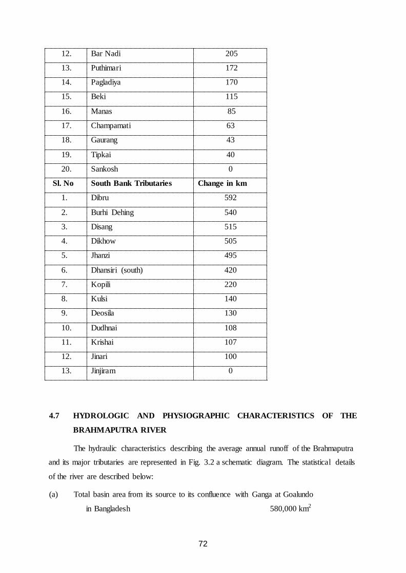
72
12. Bar Nadi 205
13. Puthimari 172
14. Pagladiya 170
15. Beki 115
16. Manas 85
17. Champamati 63
18. Gaurang 43
19. Tipkai 40
20. Sankosh 0
Sl. No South Bank Tributaries Change in km
1. Dibru 592
2. Burhi Dehing 540
3. Disang 515
4. Dikhow 505
5. Jhanzi 495
6. Dhansiri (south) 420
7. Kopili 220
8. Kulsi 140
9. Deosila 130
10. Dudhnai 108
11. Krishai 107
12. Jinari 100
13. Jinjiram 0
4.7 HYDROLOGIC AND PHYSIOGRAPHIC CHARACTERISTICS OF THE
BRAHMAPUTRA RIVER
The hydraulic characteristics describing the average annual runoff of the Brahmaputra
and its major tributaries are represented in Fig. 3.2 a schematic diagram. The statistical details
of the river are described below:
(a) Total basin area from its source to its confluence with Ganga at Goalundo
in Bangladesh 580,000 km2

73
(i) Basin area within Tibet 293,000 km2
(ii) Basin area in Bhutan and India 240,000 km2
(iii) Basin area in Bangladesh 47,000 km2
(b) Length from its source to outfall in Bay of Bengal 2,880 km
(i) Length within Tibet 1,625 km
(ii) Length within India 918 km
(iii) Length within Bangladesh 337 km
(c) Gradient
(i) Reach within Tibet 1 in 385
(ii) Reach between Indo-China border and Kobo in India 1 in 515
(iii) Reach between Kobo and Dhubri 1 in 6,990
(iv) Reach within Bangladesh First 60 km from Indian Border
1 in 11,340
Next 100 km stretch 1 in 12,360
Next 90 km stretch 1 in 37,700
(d) Observed discharge
(i) Maximum observed discharge at Pandu (on 23.8.1962) 72,727 m3/sec
(ii) Minimum observed discharge at Pandu (on 20.2.1968) 1,757 m3/sec
Average dry season discharge at Pandu 4,420 m3/sec
(e) Normal annual rainfall within basin ranges between 2,125 mm in Kamrup
district of Assam and 4,142 mm in Tirap district of Arunachal Pradesh.

74
Fig. 4.2 Average Annual Runoff of the Brahmaputra and its Tributaries
High variability in discharge of the river is mainly caused by seasonal rhythm of the
monsoon and the freeze-thaw cycle of the Himalayan snow. As regards the pattern of
sediment transport, the river has the record of carrying excessive sediment load which is
believed to be one of the important factors responsible for braiding.
4.8 THE STUDY AREA
In the present study, For the rating curve modelling, three gauging sites, two on the
main stem of the brahmaputra River, namely Pandu and Panchratna and one at the outlet of
the biggest northern tributary (Subansiri River), namely, Choulduaghat have been considered.
For rainfall-runoff and sediment runoff modelling in a sub basin, the Subansiri River basin
has been taken up a the study area (Fig. 4.3).
7.9%
6 64
5,89,000MCM
Pancharatna Guwahati (Pandu)
4,94,357 MCM
Subansiri (57,298)
Puthimari & Pagaldiya
(3364) Jia Bhareli (27574)
Lohit (4656
Dibang (39085)
Kobo C/S-65
Dihang
Disang (4803)
Buri Dehing (11906)
Gabhru (927)
Dhansiri (2003)
Dhubri (C/S-2)
5,10,450 MCM
Dhansiri(S)
Main Manas (32258)
Dikhow (4230)
Kopili (9022)
Brahmaputra
Tezpur
Tipkai and Champamati
(in MCM)
31.63% 7.92%
5.48%
1.5% 1.15% 0.7% 0.85% 1.9%
4.6%
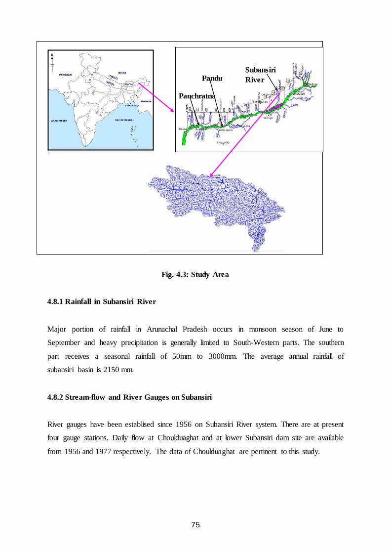
75
Fig. 4.3: Study Area
4.8.1 Rainfall in Subansiri River
Major portion of rainfall in Arunachal Pradesh occurs in monsoon season of June to
September and heavy precipitation is generally limited to South-Western parts. The southern
part receives a seasonal rainfall of 50mm to 3000mm. The average annual rainfall of
subansiri basin is 2150 mm.
4.8.2 Stream-flow and River Gauges on Subansiri
River gauges have been establised since 1956 on Subansiri River system. There are at present
four gauge stations. Daily flow at Choulduaghat and at lower Subansiri dam site are available
from 1956 and 1977 respectively. The data of Choulduaghat are pertinent to this study.
Subansiri River Pandu
Panchratna
76
4.8.3 Sediment Load in Subansiri Basin
The sub-Himalayan range of Subansisri generally consists of soft sandstones and
weathered rocks. Land formation of the catchment having steep slope and shallow braided
channels, therefore, carries heavy charge of coarse sediment particles of sizes 0.2 mm dia
upto 2 mm dia in suspension.
Due to granulometric characteristics of the soils present in this river basin, their
density of deposition and coverage is guided by the energy potentialities of the flood volume
based on the runoff. As the precipitation is intensive during the period May to October and
the grade of flowing surface being a steep one, sediment deposits at areas nearer to and along
the foot hills are heavier materials and debris such as boulders and shingles and towards the
lower portions of the catchment they are of porous detritus materials such as fine sands and
silt.
Daily suspended sediment load data at Choulduaghat site is available from 1974
onwards.
4.9 DATA USED
• Hydrological data: Daily stage, discharge and sediment concentration at Pandu,
Panchratna and Choulduaghat for 10 years from 1997 to 2006
• Meteorologcal data: Daily rainfall at Daporizo, Ziro, Bomdilla, Bhalukpong,
Choulduaghat, Badatighat, North Lakhimpur for three years from 2003-2005. Daily
average temperature at one grid point within the Subaasiri basin for three years from
2003-2005.

77
Chapter – 5
MM ee tt hh oo dd oo ll oo gg yy

78
Methodology
In recent years ANNs have shown exceptional performance as regression tools,
especially when used for pattern recognition and function estimation. They are highly non-
linear, and can capture complex interactions among the input variables in a system without
any prior knowledge about the nature of these interactions (Hammerstrom, 1993). The main
advantage of ANNs is that one does not have to explicitly assume a model form, which is a
prerequisite in conventional modeling approaches. Indeed, in ANNs the data points
themselves generate a relationship of possibly complicated or orthodox shape. In comparison
to the conventional methods, ANNs tolerate imprecise or incomplete data, approximate
results, and are less vulnerable to outliers (Haykin, 1994). They are highly parallel i.e. their
numerous independent operations can be executed simultaneously. Although application of
ANN approach in water resources is recent and limited, it has already produced very
encouraging results.
In the present study, various ANN models have been developed for simulating the
sediment concentration of the Pranhita sub-basin at six gauging sites. In this chapter, the
methodology of ANN models development has been described. First various aspects of ANN
modeling are discussed. Then some salient features of the software used are described and
then the steps followed for the implementation of the ANN sediment concentration models
using the software are given.
5.1. VARIOUS ASPECTS OF ANN MODELING
There are no fixed rules for developing an ANN, even though a general framework
can be followed based on previous successful applications in engineering.
Some issues that typically arise while developing an ANN are briefly described in this
section.
5.1.1. Selection of Input and Output Variables
The goal of an ANN is to generalize a relationship of the form
Ym = f(Xn) …(5.1)
5
79
Where Xn is an n-dimensional input vector consisting of variables x1,…........ xi, ............. xn ; and
Ym is an m-dimensional output vector consisting of resulting variables of interest y1 ,
…..….. yi, ……....ym. We use the term “generalize” to imply that the functional form of f(.)
in Eq. 6.1 to Eq.6.6 will not be revealed explicitly, but will be represented by the network
parameters. In hydrology, the values of xi can be causal variables such as rainfall,
temperature, previous flows, water levels, spatial locations, evaporation, basin area,
elevation, slopes, pump operating status, contaminant loads, meteorological data, and so on.
The values of yi can be hydrological responses such as runoff, streamflow, ordinates of a
hydrograph, optimal pumping patterns, rain fields, hydraulic conductivities, contaminant
concentrations, and others.
The selection of an appropriate input vector that will allow an ANN to successfully
map to the desired output vector is not a trivial task. Unlike physically based models, the sets
of variables that influence the system are not known a priori. In this sense of nonlinear
process identification, an ANN should not be considered as a mere black box. A firm
understanding of the hydrologic system under consideration is an important prerequisite for
successful application of ANNs. For instance physical insight into the problem being studied
can lead to better choice of input variables for proper mapping. This will help in avoid loss of
information that may result if key input variables are omitted, and also prevent inclusion of
spurious inputs that tend to confuse the training process. A sensitivity analysis can be used to
determine the relative importance of a variable (Maier and Dandy 1996) when sufficient data
is available. The input variables that do not have a significant effect on the performance of an
ANN can be trimmed from the input vector, resulting in a more compact network.
5.1.2. Collecting and Preprocessing Data
Most hydrologic data are obtained from gauges that are placed on site or through
remote sensing instruments. Also, either an existing or laboratory experiments can be used to
generate the data patterns for specific applications (French et al. 1992; Ranjithan et al. 1993;
Rogers and Dowla 1994; Smith and Eli 1995; Minns and Hall 1996). Again, there appears to
be no fixed method for determining the number of input-output data pairs that will be
required. To ensure a good approximation, Carpenter and Barthelemy (1994) stated that the
number of data pairs used for training should be equal to or greater than the number of data
parameters (weights) in the network. An optimal data set should be representative of the
probable occurrence of an input vector and should facilitate the mapping of the underlying

80
nonlinear process. Inclusion of unnecessary patterns could slow network learning. In contrast,
an insufficient data set could lead to poor learning. This makes it useful to analyze and
preprocess the data before it is used for ANN application. Routine procedures such as
plotting and examining the statistics are sometimes effective in judging the reliability of the
data and possibly to remove outliers. In many cases, the data needs to be encoded,
normalized, or transformed before being applied to an ANN.
5.1.3. Designing the ANN
This is important step, involves the determination of the ANN architecture and
selection of a training algorithm. An optimal architecture may be considered the one, yielding
the best performance in terms of error minimization, while retaining a simple and compact
structure. No unified theory exists for determination of such an optimal ANN architecture.
Often, more than one ANN can generate similar results. The numbers of input and output
nodes are problems dependent. They are equal to n and m in Eq. 5.1, the flexibility lies in
selecting the number of hidden layers and in assigning the number of nodes to each of these
layers. A trail-and-error procedure is generally applied to decide on the optimal architecture.
As discussed earlier, the cascade-correlation-training algorithm is an efficient method to find
the optimal architecture.
The potential of feed-forward neural networks can be attributed to three main factors
(Kothari and Agyepong 1996): (1) multilayered feedforward neural networks do not need an
explicit mathematical equation relating inputs and outputs; (2) a feedforward network with a
single hidden layer with an arbitrary number of sigmoidal hidden nodes can approximate any
continuous function; and (3) a feedforward network with a single hidden layer of ‘m’
sigmoidal nodes achieves an integrated squared error of O(1/m) while a linear combination of
a set of ‘m’ fixed basis functions achieves an integrated squared error of O(1/m2/d), where ‘d’
is the dimension of the input (Barron 1993). Points 1 and 3 above refer to computational
superiority of feedforward ANN, while 2 hints to an existence theorem that establishes the
capabilities of a feedforward ANN. It does not, however, allow for a systematic
determination of the number of hidden nodes to use in a given situation. The number of
hidden layer neurons significantly influences the performance of a network; with too few
nodes the network will approximate poorly, while with too many nodes it will overfit the
training data.
The influence of the size of a neural network on its generalization performance is
well known (Baum and Haussler 1989; Kothari and 1997 Agyepong). Bishop (1995) provides

81
an excellent review of proposed approaches that allow the determination of network
architecture with acceptable performance on the training and generalization data. Some of the
popular techniques include network growing (e.g., Gallant 1986; Nadal 1989; Fahlman and
Lebiere 1991; Bose and Garga 1993; Kwok and Yeung 1995) and network pruning (e.g.,
Mozer and Smolensky 1989; Karnin 1990; LeCun et al. 1990; Hassibi and Stork 1993; Reed
1993). These algorithms treat the network structure as an optimization parameter along with
the weights. Pruning algorithms generally start with a large network and proceed by
removing weights to which sensitivity of the error is minimal. Growing methods, on the other
hand, typically start with a small network and add nodes with full connectivity to nodes in the
existing network when a suitably chosen measure (e.g., entropy, covariance, etc.) stops
decreasing. An alternative to these methods is called soft weight sharing (Nowlan and
Hinton, 1992), where groups of weights are encouraged to have equal values, allowing for a
reduction in the effective number of free parameters in the network. Soft weight sharing can
train a large network with a small amount of training data (Agyepong and Kothari 1997);
however, to ensure convergence to good solutions, proper initialization of the weights is
necessary.
5.1.4. Training and Cross Training
This is similar to the idea of calibration that is an integral part of most hydrologic
modeling studies. The available data set is generally partitioned into three parts for training,
cross training, and validation. The purpose of training is to determine the set of connection
weights and nodal thresholds that cause the ANN to estimate outputs that are sufficiently
close to target values. The dataset reserved for training is used to achieve this goal. This
fraction of the complete data to be employed for training should contain sufficient patterns so
that the network can mimic the underlying relationship between input and output variables
adequately. The weights and threshold values are assigned small random values initially
(usually, -0.3 ~ 0.3). During training, these are adjusted based on the error, or the difference
between ANN output and the target responses. This adjustment can be continued recursively
until a weight pace is found, which results in the smallest overall prediction error. However,
there is the danger of overtraining a network in this fashion, also referred as over fitting. This
happens when the network parameters are too fine-tuned to the training data set.
It is as if the network, in the process of trying to “learn” the underlying rule, has
started trying to fit the noise component of the data as well. In other words, overtraining
results in a network that memorizes the individual examples, rather than trends in the data set

82
as a whole. When this happens, the network performs very well over the data set used for
training, but shows poor predictive capabilities when supplied with data other than the
training patterns. To prevent this kind of over fitting, a cross training procedure is usually
recommended. The goal of this procedure is to stop training when the network begins to
overtrain. The second portion of the data is reserved for this purpose. After the adjustment of
network parameters with each epoch, the network is used to find the error for this data set.
Initially, errors for both the training and cross training data sets go down. After
an optimal amount of training has been achieved, the errors for training set continue to
decrease, but those associated with the cross training data set begin to rise. This is indication
that furthers training will likely result in the network over fitting the training data. The
process of training is stopped at this time, and the current set of weights and thresholds are
assumed to be the optimal values. The network is ready for use as a predictive tool. If
the available data set is too small for partitioning, the simplest way to prevent overtraining is
to stop training when the mean square error ceases to decrease significantly.
5.1.5. Model Validation
Similar to other modeling approaches in hydrology, the performance of a trained
ANN can be fairly evaluated by subjecting it to new patterns that it has not seen during
training. The performance of the network can be determined by computing the percentage
error between predicted and desired values. In addition, plotting the model output versus
desired response could also be used to assess ANN performance. Since finding optimal
network parameters is essentially a minimization process, it is advisable to repeat the training
and validation processes several times to ensure that satisfactory results have been obtained.
5.2. FEATURES OF ANN SOFTWARE - NEURAL POWER
The ANN software used in this study is Neural Power. Neural Power is an easy-to-use
powerful Artificial Neural Network (ANN) program. With its user friendly interface, simple
operation and highly efficient performance, most of general ANN problems can be handled
with great results. Neural Power can be applied in following fields: multi-nonlinear
regression, forecasting, curve fitting, pattern recognition, classification, decision making,
problem optimization and time series analysis.

83
5.2.1. Neural Power is Suitable for:
♦ People who have to work or analyze data in any form.
♦ People working on problems that are complexes, laborious, ‘fuzzy’ or simply un-
resolvable using present methods.
♦ People who simply want to improve on their current techniques and gain competitive
advantage.
5.2.2. Features of Neural Power
♦ Multi-learning data files supported: almost all other similar software only one data file for
the learning process. Sometimes, this is a not enough for a real problem.
♦ Normal and grid data types supported: no other software supports “grid” data type
learning.
♦ Visual and real time monitoring of learning process. Almost all aspects of network can be
controlled in graphical mode, i.e. use any connection weight, and variations of RMSE.
♦ Visual design of network structures.
♦ Step-by-step learning.
♦ Support interrupting/suspending and resuming of learning process. Learning can start
from a set of random weights specified by a user.
♦ Genetic Algorithms can be used as one of the learning algorithms.
♦ No limitation on hidden layer numbers and node number for each layer. Each layer can
have different transfer functions.
♦ Includes six types of the most-often used transfer functions, in addition, customers can
define functions of their own.
♦ Fast convergence of learning.
♦ Easy settlement for time series analysis.
♦ Abilities for optimal study and 2D-3D graphical analysis.
♦ Excel-like, multi-window data file editor enhanced by VB, Java and Delphi/Pascal script
languages.
♦ Many very useful data analysis tools beyond neural network: create data chart, 2-D, 3-
D function chart, curve fit with over 30 pre-defined functions, function/equation fit and
equation solve.

84
5.2.3. System Requirements
Running the 32-bit version of Neural Power requires a minimum 486 processor and
Window 95/98/2000/ME/XP or NT 4.0. A complete installation requires about 10 MB of
hard disk space. 64 MB or high RAM is recommended.
There are three main procedures: “Data Files”, “Learning/Training” and
“Applications” for being selected. The Data file editor provides a spreadsheet-like tool for
easy pre-and post-processing of data. In addition, many extra jobs can be performed here
also, i.e. charting, regression.
The Excel-style data file editor is mainly used for creating new or viewing/editing
existed data files. Such data files will be used for either the learning/training process or for
applications later. “InputSheet” is especially for input data entry of learning data; while
“OutputSheet” is for output data corresponded. “ChartStore” is for chart store, view and edit.
The chart can be created with the data either from input data or output data, or copy from
result charts of Learning or Application procedures.
5.2.4. File Format
♦ Neural Power data file (.ogy): any numerical data or strings may be contained. However,
if this file to be used for learning later, be sure no string data is contained within the file
except for the column title. For string data, represent them by real values, for example,
“1” for “True” and “0” for “False”.
♦ Excel file (.xls): Read/save MS Excel data file directly, without OLE linker. Data values
only, all other information will be ignored. If there are more than two worksheets in “xls”
file, only first two will be inputted.
♦ Lotus 1-2-3 file (.wks, .wk1) and Quattro Pro file (.wq1): Direct read without OLE.
♦ Comma-delimited text file (.csv, .txt): Save and load most general data file format.
Reading data with separate of tab space, space, “.”, and “,” automatically; while saving
data with separate of “,”.
♦ Dbase file (.dbf): Save and load popular desktop database directly.
♦ MS Access file (.mdb): Save and load another popular desktop database files through
DAO.
♦ Neural Power network file (.par): Load Neural Power network file for viewing connection
weight.

85
5.2.5. Learning/Training
The learning/training process shows that the free parameters of a neural network are
adapted through observed data (data file). The objective is to obtain “Network Weights File”
which will be used for “Application” later.
To start “learning”, one needs to load one or more data files (.ogy) initially. Multi-
files are allowed in the meantime, if they are all for the same problem and have similar data
structures. The files with “checked” will be used for learning; while, “Not checked” files are
for testing/verification.
Data types are classified into two catalogs: “Normal Type” and “Grid Type”:
♦ Normal type: one pattern consists of the data placed in any row of the output sheet that
correspond to the data in some row of input sheet. Within a data file, the pattern number
is the same as the row number, and the row number in the output sheet must be identical
with that in input sheet. If using a different data file and the same question, however, the
row number can be various.
♦ Grid Type: all input data and output data in one file are considered as one pattern. Row
numbers are not necessary identical between input and output. However the row and
column number should be matched for different data file correspondence within the same
problem, e.g. in input and output, respectively.
5.2.6. Learning Algorithm
There are five learning algorithm supported in Neural Power currently:
1. Incremental Back Propagation (IBP): the network weights are updated after presenting
each pattern from the learning data set, rather than once per iteration. This is referred to as
Standard Back Propagation, and is the most preferred algorithm for large data sets.
2. Batch Back Propagation (BBP): the network weights update takes place once per
iteration, while all learning data pattern are processed through the network.
3. Quick Propagation (QP): Quick propagation is a heuristic modification of the back
propagation algorithm. It’s proved to be much faster than standard back-propagation for
many problems.
4. Genetic Algorithm (GA): Genetic algorithm is employed to find optimal connections
weights.
5. Levenberg-Marquardt Algorithm.

86
5.2.7. Connection Types
Two kinds of connections are in existence:
Multilayer normal feed-forward: A Multilayer Feed forward network consists of one or
more layers. Each layer receives an input vector, which is either the external input vector or
the output vector of the prior layer. The layers are placed in a linear order, so that the input to
the first layer is the external input, the input to the second layer, if it exists, is the output of
the first layer, and so on, with layers 2,3,…, receiving their inputs from the previous layer.
The last layer in the sequence is the output layer; its output vector represents the network
output. Every other layer besides the output layer is referred to as a “hidden” layer, because
their activation is not externally visible. This is most commonly used and is generally
recommended for most of the applications.
Multilayer full feed-forward: The Multilayer Full Feed Forward architecture is similar to
Multilayer Normal Feed forward, expect for two differences. First, each layer is provided
with the external input. Second, each layer receives input from every layer below it in the
linear ordering. For example, if the network has 3 layers, the first one receives the input
vector, as usual. The second one receives an input vector that is the concatenation of the input
vector and the output of the first layer. The third layer receives inputs from the input vector,
and the output vectors of both prior layers.
5.2.8. Transfer Functions
The transfer function denoted by ξ (µk), defines the output of a neuron in terms of the
activity level at its input. Six commonly used functions are predefined as below:
♦ The Sigmoid function, ranged from 0 to 1, is defined as:
ξ (µk) = 1/[1+exp(-aµk)]
♦ The Hyberbolic Tanh function, ranged from –1 to 1, is defined by:
ξ (µk) = [1-exp(-aµk)]/[1+exp(-aµk)]
♦ The Gaussian function, ranged from 0 to 1, defined as:
ξ (µk) = e(-a.µ2)2
♦ The Linear function: ranged from -α to +α:
ξ (µk) = a.µk
♦ The Threshold Linear function: ranged from 0 to +1:

87
ξ (µk) = 0 if µk < 0
ξ (µk) = 1 if µk > 1
ξ (µk) = aµk if 0 <= µk <=1
♦ The Bipolar Linear function: ranged from –1 to +1:
ξ (µk) = -1 if µk < -1
ξ (µk) = 1 if µk > 1
ξ (µk) = α 'µk if -1 <= µk <=1
where, α ' is a parameter called “slope” of transfer functions.
5.2.9. Weight Editor
Default, connection weights will be started from random values. However, may be
started learning with specified weight values by utilizing the weights editor.
5.2.10. Learning Parameters
In the “settlements” section, one can set parameters such as learning rate, momentum,
screen update rate and stop criteria. All of those parameters may be modified at any time
during learning.
5.2.11. Applications
In the application module, the network file (.par) obtained through the learning
progress will be used for further analysis:
♦ Query/Forecasting
♦ Optimize analysis
♦ 2-D and 3-D analysis
♦ Error surface analysis
♦ Importance analysis
Before carrying out above analysis, a network file (.par) must be loaded firstly.
Forecasting or verification can easily be done here. The data values can be either inputted
directly or loaded from a data file. In the situation where the time series items are included in
the output data series (recorded in Network file), and if you have input data values directly,
the initial data must be inputted corresponding to the output items that contain the time series.
During the learning process, will be seen the observed data (red line) vs. calculated
data (green line) for all output variables as the learning progresses.

88
5.3. DEVELOPMENT OF REGRESSION AND ANN MODELS FOR STAGE-DISCHARGE AND SEDIMENT-DISCHARGE CURVES IN BRAHMAPUTRA BASIN
5.3.1. Input Variables
The selection of training data that represents the characteristics of a catchment and
meteorological patterns is extremely important in modeling. The training data should be large
enough to contain the characteristics of the watershed and to accommodate the requirements
of the ANN architecture. If the information included in the training data set is insufficient, an
increase in the complexity of a network (i.e., an increase in the number of neurons or layers
in a network) will not enable the network to generalize the patterns in the physical
phenomena. To the contrary, an increase in the complexity of the models might mislead the
modeler to overfit the training data and lead to poor forecasts (Tokar and Johnson, 1999).
The error back propagation ANN models used in the present study are basically static-
feedforward ANNs, the most widely used ANN structures, but they lack feedback
connections to effectively remember and handle the previous states of information. One way
that information can be introduced in static-feedforward ANNs is to input a time delay
pattern that constitutes the tapped delay line information. Therefore, this network must
determine the input variables, output variables and the lag time of the basin before
constructing rainfall-runoff-sediment processes in order to increase its accuracy. In general,
the selection of input variables and output variables is problem dependent. The appropriate
input variables will allow the network to successfully map to the desired output and avoid
loss of important information. In the present study, the input dimensions are determined by
the input variables and the lag time.
5.3.1.1 Input variables for stage-discharge regression and ANN models
The daily data of stage and discharge were available at the sites, namely Pandu (main
Brahmaputra River), Panchratna (main Brahmaputra River) and Choulduaghat (Subansiri
River) for ten years from January 1997 to December 2006. Out of this, six years data were
used for training, two years data for testing and two years data for validation.
The output from the model is the discharge at time step t, Qt. It has been shown by
many authors that the current discharge can be mapped better by considering, in addition to
the current value of stage, the discharge and stage at the previous times. Therefore, in
addition to Ht, i.e., stage at time step t, other variables such as Ht, Ht-1 , Ht-2 , Qt-1 , Qt-2 were

89
also considered in the input. Various combinations of input data considered for training of
ANN in the present study are given in Table 5.1. However, the input-output variables of
ANNH-1 have been used for the conventional sediment rating curve analysis.
Table 5.1 Various ANN stage-discharge Models
ANN
Model
Input
Variables
Output Variables
ANNH-1 Ht Qt ANNH-2 Ht, Ht-1, Qt-1 Qt ANNH-3 Ht, Ht-1, Ht-2, Qt-1, Qt-2 Qt ANNH-4 Ht, Ht-1, Ht-2, Ht-3, Qt-1, Qt-2, Qt-3 Qt ANNH-5 Ht, Ht-1, Ht-2, Ht-3, Ht-4,
Qt-1, Qt-2, Qt-3, Qt-4 Qt
Where Q=Discharge, H=Stage
5.3.1.2 Input variables for runoff-sediment regression and ANN models
The daily data of discharge and sediment concentration were available at the sites
namely, Pandu (main Brahmaputra River), Panchratna (main Brahmaputra River) and
Choulduaghat (Subansiri River) for ten years from January 1997 to December 2006. Out of
this, six years data were used for training, two years data for testing and two years data for
validation.
The output from the model is the sediment concentration at time step t, St . It has been
shown by many authors that the current sediment concentration can bemapped better by
considering, in addition to the current value of discharge, the sediment and discharge at the
previous times. Therefore, in addition to Qt , i.e., discharge at time step t, other variables such
as Qt-1 , Qt-2 , and St-1 , St-2 , were also considered in the input. Various combinations of input
data considered for training of ANN in the present study are given in Table 5.2. However, the
input-output variables of ANNS-1 have been used for the conventional sediment rating curve
analysis.

90
Table 5.2 Various ANN Runoff-Sediment Models
ANN
Model
Input
Variables
Output Variables
ANNS-1 Qt St
ANNS-2 Qt, Qt-1, St-1 St
ANNS-3 Qt, Qt-1, Qt-2, St-1, St-2 St
ANNS-4 Qt, Qt-1, Qt-2, Qt-3, St-1 St-2, St-3 St
ANNS-5 Qt, Qt-1, Qt-2, Qt-3, Qt-4 St-1, St-2,
St-3, St-4
St
Where Q=Discharge, S=Sediment Concentration
5.3.2. Regression Models Using Conventional Techniques
Regression models have been developed for runoff-sediment modeling. Sediment
rating curve analysis has been carried out for the six sites. These models have been
calibrated, using six years data and then validated with two year data and again cross
validated with remaining two+86 year data.
5.3.2.1 Rating curves for stage-discharge and runoff-sediment modeling
Rating curves are widely used to estimate the discharge vis-à-vis sediment load being
transported by a river. A rating curve is a relation between the sediment and river discharge.
Rating curves may be plotted showing average discharge/sediment concentration or load as a
function of stage/discharge averaged over daily, monthly, or other time periods. Rating
curves are developed on the premise that a stable relationship between discharge/sediment
concentration and stage/discharge can be developed which, although exhibiting scatter, will
allow the mean discharge/sediment yield to be determined on the basis of the stage/discharge
history. A problem inherent in the rating curve technique is the high degree of scatter, which
may be reduced but not eliminated. Discharge/Sediment Concentration does not necessarily
increase as a function of satge/discharge.
Mathematically, a rating curve may be constructed by log-transforming all data and
using a linear least square regression to determine the line of best fit. The log-log relationship

91
between Discharge(Q)/Sediment load (S) and Stage(H)/Discharge(Q) is of the form:
Q= a Hb …(5.2)
S = c Qd … (5.3)
where , ‘a’, ‘b’, ‘c’ and ‘d’ are constants
5.4 DEVELOPMENT OF RAINFALL-RUNOFF AND SEDIMENT-RUNOFF ANN
MODELS FOR SUBANSIRI RIVER BASIN
5.4.1 Input data and ANN model development for Rainfall-Runoff models
The daily data of discharge for ten years (1997-2006) were available at the
Choulduaghat site which has been considered as the outlet of the basin for the present study.
Daily rainfall data were available for three years (2003-2005) at Daporizo, Ziro, Bomdilla,
Bhalukpong, Choulduaghat, Badatighat and North Lakhimpur. Daily average temperature at
one grid point within the Subansiri basin for three years from 2003-2005 has been used.
Similarly, three years of daily discharge data has also been used for ANN models
development.
The output from the model is the runoff at time step t, Qt . It has been shown by many
authors that the current runoff can be mapped better by considering, in addition to the current
value of rainfall and temperature, the rainfall, temperature and runoff at the previous times.
Therefore, in addition to Rt , and Tt i.e., rainfall and temperature at time step t, other variables
such as Rt-1 , Rt-2 , Tt-1 , Tt-2 , and Qt-1 were also considered in the input. Various combinations
of input data were considered based upon a cross correlation of the data at various stations
with varying lag time as given in Table 5.3. Based on the cross correlation, various ANN
models considered for ANN training are given in Table 5.4.
5.4.2 Input data and ANN model development for Runoff-sediment models
The daily data of discharge and suspended sediment concentration for ten years
(1997-2006) were available at the Choulduaghat site which has been considered as the outlet
of the basin for the present study. Daily rainfall data were available for three years (2003-
2005) at Daporizo, Ziro, Bomdilla, Bhalukpong, Choulduaghat, Badatighat and North

92
Lakhimpur. Daily average temperature at one grid point within the Subansiri basin for three
years from 2003-2005 has been used. Similarly, three years of daily discharge and suspended
sediment concentration data has also been used for ANN models development.
The output from the model is the sediment concentration at time step t, St . It has been
shown by many authors that the current sediment concentration can be mapped better by
considering, in addition to the current value of rainfall, temperature, runoff and the rainfall,
temperature, runoff and sediment concentration at the previous times. Therefore, in addition
to Rt , Tt and Qt , i.e., rainfall, temperature and runoff at time step t, other variables such as Rt-
1 , Rt-2 , Tt-1 , Tt-2 , Qt-1 Qt-2, and St-1 were also considered in the input. Various combinations of
input data were considered based upon a cross correlation of the data at various stations with
varying lag time as given in Table 5.3. Based on the cross correlation, various ANN models
considered for ANN training are given in Table 5.5.

93
Table 5.3: Cross Correlation of Data

94
Table 5.4: Various ANN rainfall-runoff models
Table 5.5: Various ANN sediment-runoff models
ANN Model
Input Variables
Output Variables
ANNS-1 Rt(Ziro, Daporizo, Bhalukpong, Bomdilla, Badatighat, Choulduaght), Qt(Choulduaghat)
St
ANNS-2 Rt(Ziro, Daporizo, Bhalukpong, Bomdilla, Badatighat, Choulduaght), Tt(G1), Qt(Choulduaghat)
St
ANNS-3 Rt(Ziro, Daporizo, Bhalukpong, Bomdilla, Badatighat, Choulduaght), Rt-1(Ziro), Tt(G1), Qt(Choulduaghat)
St
ANNS-4 Rt(Ziro, Daporizo, Bhalukpong, Bomdilla, Badatighat, Choulduaght), Rt-1(Ziro), Tt(G1), Qt(Choulduaghat), St-1(Choulduaghat)
St
ANN
Model
Input Variables
Output Variables
ANNR-1 Rt(Ziro, Daporizo, Bhalukpong, Bomdilla, Badatighat, Choulduaght)
Qt
ANNR-2 Rt(Ziro, Daporizo, Bhalukpong, Bomdilla, Badatighat, Choulduaght), Tt(G1)
Qt
ANNR-3 Rt(Ziro, Daporizo, Bhalukpong, Bomdilla, Badatighat, Choulduaght), Rt-1(Ziro), Tt(G1)
Qt
ANNR-4 Rt(Ziro, Daporizo, Bhalukpong, Bomdilla, Badatighat, Choulduaght), Rt-1(Ziro), Tt(G1), Tt-1(G1)
Qt
ANNR-5 Rt(Ziro, Daporizo, Bhalukpong, Bomdilla, Badatighat, Choulduaght), Rt-1(Ziro), Tt(G1), Tt-1(G1), Tt-2(G1)
Qt
ANNR-6 Rt(Ziro, Daporizo, Bhalukpong, Bomdilla, Badatighat, Choulduaght), Rt-1(Ziro), Tt(G1), Qt-1(choulduaghat)
Qt
95
5.5 ANN MODELS
5.5.1 TRAINING OF ANN MODELS
The training of various ANN models has been accomplished through the ANN
software, namely, Neural Power (NPP 2.5, 2004). A back-propagation ANN with the
generalized delta rule as the training algorithm has been employed in this study. The structure
of the ANN models were three and four layer BPANN developed with non-linear sigmoid as
activation function uniformly between the layers. Nodes in the input layer were equal to
number of input variables, nodes in hidden layer were varied from the number of input nodes
to approximately double of input nodes (Hipel, et al., 1994) and the nodes in the output layer
was one as the models provide single output. Therefore, various ANN models were trained
considering different hidden node numbers on a trial and error fashion and the best
performing model has been reported in the results.
The learning of ANN initiates with the normalization (re-scaling) of all data with the
maximum value of respective variable thus reducing the data domain in the range 0 to 1. This
was accomplished through the software. All interconnecting links between nodes of
successive layers were assigned random values called weight between +0.5 to –0.5 and a
constant value of 0.15 and 0.8 was considered for learning rate ‘η’ and momentum term ‘α’
respectively. The quick propagation (QP) learning algorithm has been adopted for the
training of all the ANN models. QP is a heuristic modification of the standard back
propagation and is very fast (Neural Power, 2003). The network weights were updated after
presenting each pattern from the learning data set, rather than once per iteration.
The criteria selected to avoid over training was generalization of ANN through cross-
validation (Haykin, 1994). For this purpose, the data were divided into training, testing and
validation sets. Training data (730/731 patterns) were used for estimation of weights of the
ANN model and testing data (365/366 patterns) for evaluation of the performance of ANN
model during training. Training was stopped when the error for the testing dataset started
increasing. In this way, the training and testing datasets have been used to assess the
performance of various candidate model structures, and thereby choose the best one. The
particular ANN model with the best performing parameter values was chosen and the
generalized performance of the resulting network has been measured on the validation data
set (two years data) to which it has never before been exposed. The performance of the model
was tested through the statistical criterion discussed in the following section.
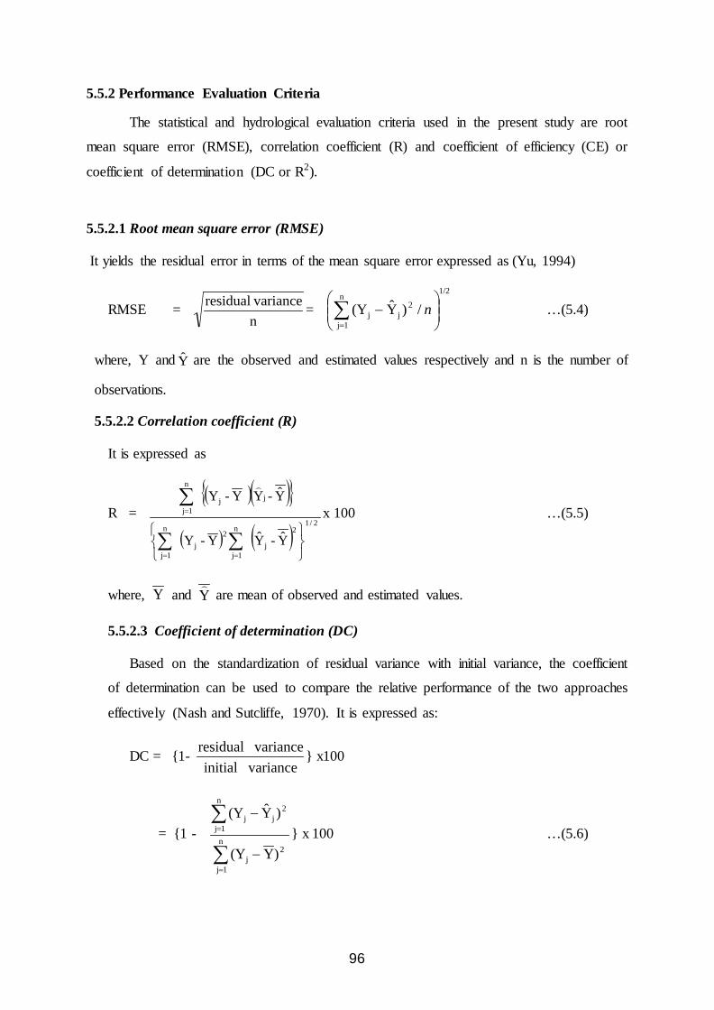
96
5.5.2 Performance Evaluation Criteria
The statistical and hydrological evaluation criteria used in the present study are root
mean square error (RMSE), correlation coefficient (R) and coefficient of efficiency (CE) or
coefficient of determination (DC or R2).
5.5.2.1 Root mean square error (RMSE)
It yields the residual error in terms of the mean square error expressed as (Yu, 1994)
RMSE = n varianceresidual =
1/2n
1j
2jj /)Y(Y
−∑
=
n …(5.4)
where, Y and Y are the observed and estimated values respectively and n is the number of
observations.
5.5.2.2 Correlation coefficient (R)
It is expressed as
R = ( )( ){ }
( ) ( )2/1
2
j
n
1j
2j
n
1j
jj
n
1j
Y-YY-Y
Y-YY-Y
∑∑
∑
==
=
x 100 …(5.5)
where, Y and Y
are mean of observed and estimated values.
5.5.2.3 Coefficient of determination (DC)
Based on the standardization of residual variance with initial variance, the coefficient
of determination can be used to compare the relative performance of the two approaches
effectively (Nash and Sutcliffe, 1970). It is expressed as:
DC = {1- varianceinitialvarianceresidual } x100
= {1 - 2
n
1jj
n
1j
2jj
)Y(Y
)Y(Y
−
−
∑
∑
=
= } x 100 …(5.6)

97
The coefficient of determination is also commonly known as the coefficient of
efficiency which may be written in a number of ways and represents the fraction of
variance that is explained by regression. The closer this ratio is to unity, the better is
the regression relation.

98
Chapter – 6
RR ee ss uu ll tt ss aa nn dd DD ii ss cc uu ss ss ii oo nn

99
Results and Discussion
6.1 RUNOFF AND SEDIMENT MODELING BASED ON RATING CURVE
TECHNIQUE
Based on the rating curve technique (Eq. 5.2) the equations for the three sites are
given below:
1. Stage discharge Rating Curve for Pandu site on Brahmaputra River
C=1.0 E-22Q16.781 …(6.1)
2. Stage discharge Rating Curve for Panchratna site on Brahmaputra River
C=8.0 E-14Q11.484 …(6.2)
6
y = 1E-22x15.781
R2 = 0.9538
0
10000
20000
30000
40000
50000
60000
70000
40 41 42 43 44 45 46 47 48 49 50
Water level
Disc
harg
e
y = 8E-14x11.434
R2 = 0.9454
0
10000
20000
30000
40000
50000
60000
70000
25 27 29 31 33 35 37 39
Water level
Disc
harg
e

100
3. Sediment dischage Rating Curve for Panchratna site on Brahmaputra River
C=0.002Q0.6888 …(6.3)
4. Stage discharge Rating Curve for Chouldhuaghat site on Subansiri River
C=1.0 E-93Q48.48 …(6.4)
y = 1E-93x48.49
R2 = 0.7526
0.00
2000.00
4000.00
6000.00
8000.00
10000.00
12000.00
14000.00
92.00 93.00 94.00 95.00 96.00 97.00 98.00 99.00 100.00 101.00
Water level
Disc
harg
e
y = 0.002x0.5888
R2 = 0.6706
0
0.5
1
1.5
2
2.5
0 10000 20000 30000 40000 50000 60000 70000
Discharge
Sedi
men
t

101
5. Sediment discharge Rating Curve for Chouldhuaghat site on Subansiri River
C=1.0 E-06Q1.2823 …(6.5)
where, H = River stage in m.
S = Sediment Concentration in g/l
Q = Discharge in the river in Cumec
6.2 RATING CURVE MODELING BASED ON ANN TECHNIQUE
The statistical performances of various ANN models for all the three study gauging
sites are summarized in Table 6.1 to Table 6.5. The tables show the comparative performance
of all the models during training, testing and validation.
6.2.1 Stage discharge ANN Modeling for Pandu site on Brahmaputra River
The results are summarized in Table 6.1.
Table 6.1 Comparative performance of various stage discharge ANN models for Pandu
site (Brahmaputra River)
ANN model Training Testing Validation
RMSE R DC R DC R DC
ANNPH-1 (1-2-1)
2468.6 0.974 0.949 0.998 0.974 0.987 0.749
ANNPH-2 (3-2-1)
745.2 0.995 0.995 0.999 0.999 0.998 0.995
ANNPH-3 710.46 0.998 0.996 0.999 0.999 0.998 0.994
y = 7E-06x1.2923
R2 = 0.8337
0.0000
0.5000
1.0000
1.5000
2.0000
2.5000
3.0000
0.00 2000.00 4000.00 6000.00 8000.00 10000.00 12000.00 14000.00
Discharge
Sedi
men
t

102
(5-4-1) ANNPH-4 (7-6-1)
676.85 0.998 0.996 0.999 0.999 0.997 0.995
ANNPH-5 (9-7-1)
654.29 0.998 0.996 0.999 0.999 0.997 0.995
It is observed from Table 6.1 that the RMSE values are generally low for all the ANN
models. There are two candidate models in RMSE criteria, ANNPH2, i.e, ANN model with
two hidden nodes and ANNPH4 model with three hidden nodes. In ANNPH2 model, the
RMSE value is 745.2 during training. In ANN3 model, the RMSE value is 710.46 during
training.
It can be seen from Table 6.1 that the correlation coefficient (R) values are very high
(more than 0.90, i.e., 90%) for all the ANN models, during all the three phases, i.e., training,
testing as well as validation. It is also observed that there is not much decrease in the R
values during validation as compared to the training phase. The performance of ANNPH3
model is the best in R statistic. The R values for ANN are 0.998, 0.999 and 0.998 during
training, testing and validation respectively. The increase in R values of ANNPH3 during
validation indicates good generalization capability of the ANN model.
In the determination coefficient (DC) statistic, all the ANN models perform well. The
DC values are fairly high (more than 0.90) for all models during all the three phases. In DC
statistic also, ANNPH2 model performs the best. The DC values for ANN2 are 0.995, 0.999,
and 0.995 during training, testing and validation respectively. There is not much decrease in
the DC values during validation which indicate good generalization capability of the ANN
models.
Therefore, ANN2 is the best performing model in all the three statistical and
hydrological criteria. Fig. 6.1 presents the plots of observed and estimated discharge for
ANN2 mdel during training (a), testing (b) and validation (c). It is observed from Fig 6.1 that
there is very little mismatch between the observed and estimated discharge series for ANN2
model during all the three phases.
6.2.2 Stage Discharge Modeling for Panchratna site on Brahmaputra River
The results are summarized in Table 6.2.

103
Table 6.2 Comparative performance of various stage discharge ANN models for Panchratna site (Brahmaputra River)
ANN model Training Testing Validation
RMSE R DC R DC R DC
ANNPRH-1 (1-2-1)
2285.6 0.984 0.968 0.975 0.893 0.991 0.977
ANNPRH-2 (3-5-1)
1189.7 0.999 0.999 0.993 0.986 0.991 0.982
ANNPRH-3 (5-4-1)
853.71 0.998 0.998 0.997 0.992 0.996 0.991
ANNPRH-4 (7-6-1)
856.66 0.998 0.996 0.997 0.992 0.996 0.991
ANNPRH-5 (9-7-1)
857.52 0.998 0.996 0.997 0.991 0.996 0.991
(a) Training
(b) Testing
0
10000
20000
30000
40000
50000
60000
1 366 731 1096 1461
Days
Wat
er le
vel (
m)
Observed water level Estimated water level (ANN)
0
5000
10000
15000
20000
25000
30000
35000
40000
45000
1 366
Days
Wat
er le
vel (
m)
Observed water level Estimated water level (ANN)

104
(c)Validation
Fig. 6.1 Comparative Performance of Observed Discharge with Estimated Discharge using
ANNPH-2 at Pandu
It is observed from Table 6.2 that the RMSE values are generally low for all the ANN
models. There are two candidate models in RMSE criteria, ANNPRH3, i.e, ANN model with
four hidden nodes and ANNPRH4 model with six hidden nodes. In ANN3 model, the RMSE
value is 853.71 during training. In ANN4 model, the RMSE value is 856.66 during training.
It can be seen from Table 6.1 that the correlation coefficient (R) values are very high
(more than 0.90, i.e., 90%) for all the ANN models, during all the three phases, i.e., training,
testing as well as validation. It is also observed that there is not much decrease in the R
values during validation as compared to the training phase. The performance of ANNPRH3
model is the best in R statistic, the R values are 0.998, 0.997 and 0.996 during training,
testing and validation respectively.
In the determination coefficient (DC) statistic, all the ANN models perform well. The
DC values are fairly high (more than 0.90) for all models during all the three phases. In DC
statistic also, ANNPRH3 model performs the best. The DC values for ANN2 are 0.998,
0.992, and 0.991 during training, testing and validation respectively. There is not much
decrease in the DC values during validation which indicate good generalization capability of
the ANN models.
Therefore, ANNPRH3 is the best performing model in all the three statistical and
hydrological criteria. Fig. 6.2 presents the plots of observed and estimated discharge for
ANN3 model during training (a), testing (b) and validation (c). It is observed from Fig 6.2
0
5000
10000
15000
20000
25000
30000
35000
40000
1 366
Days
Wat
er le
vel (
m)
Observed water level Estimated water level (ANN)

105
that there is very little mismatch between the observed and estimated discharge series for
ANNPRH3 model during all the three phases.
6.2.3 Sediment discharge Modeling for Panchratna site on Brahmaputra River
The results are summarized in Table 6.3.
Table 6.3 Comparative performance of various sediment-discharge ANN models for
Panchratna site (Brahmaputra River)
ANN model Training Testing Validation
RMSE R DC R DC R DC
ANNPRS-1 (1-2-1)
0.1788 0.878 0.771 0.417 0.468 0.996 0.628
ANNPRS-2 (3-3-1)
0.0378 0.995 0.989 0.996 0.991 0.770 0.990
ANNPRS-3 (5-4-1)
0.0348 0.996 0.991 0.995 0.990 0.996 0.993
ANNPRS-4 (7-10-1)
0.0379 0.995 0.989 0.994 0.988 0.996 0.990
ANNPRS-5 (9-12-1)
0.0347 0.996 0.991 0.992 0.983 0.995 0.989
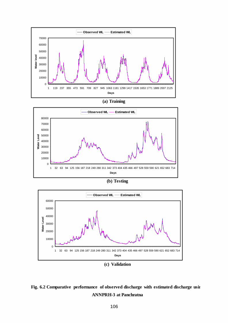
106
(a) Training
(a) Training
(b) Testing
(c) Validation
0
10000
20000
30000
40000
50000
60000
70000
1 119 237 355 473 591 709 827 945 1063 1181 1299 1417 1535 1653 1771 1889 2007 2125
Days
Wat
er le
vel
Observed WL Estimated WL
0
10000
20000
30000
40000
50000
60000
70000
80000
1 32 63 94 125 156 187 218 249 280 311 342 373 404 435 466 497 528 559 590 621 652 683 714
Days
Wat
er L
evel
Observed WL Estimated WL
0
10000
20000
30000
40000
50000
60000
1 32 63 94 125 156 187 218 249 280 311 342 373 404 435 466 497 528 559 590 621 652 683 714
Days
Wat
er L
evel
Observed WL Estimated WL
Fig. 6.2 Comparative performance of observed discharge with estimated discharge usin
ANNPRH-3 at Panchratna

107
It is observed from Table 6.3 that the RMSE values are generally low for all the ANN models. There are two candidate models in RMSE criteria, ANNPRS3, i.e, ANN model with four hidden nodes and ANNPRS5 model with six hidden nodes. In ANNPRS3 model, the RMSE value is 0.0348 during training. In ANNPRS5 model, the RMSE value is 0.0347 during training.
It can be seen from Table 6.3 that the correlation coefficient (R) values are very high (more than 0.90, i.e., 90%) for all the ANN models, during all the three phases, i.e., training, testing as well as validation. It is also observed that there is not much decrease in the R values during validation as compared to the training phase. The performance of ANNPRS3 model is the best in R statistic. The R values for ANN are 0.996, 0.995 and 0.996 during training, testing and validation respectively.
In the determination coefficient (DC) statistic, all the ANN models perform well. The DC values are fairly high (more than 0.90) for all models during all the three phases. In DC statistic also, ANNPRS3 model performs the best. The DC values for ANNPRS3 are 0.991, 0.990, and 0.993 during training, testing and validation respectively. There is increase in the DC values during validation which indicate good generalization capability of the ANN models.
Therefore, ANNPRS3 is the best performing model in all the three statistical and hydrological criteria. Fig. 6.3 presents the plots of observed and estimated discharge for ANN3 model during training (a), testing (b) and validation (c). It is observed from Fig. 6.3 that there is very little mismatch between the observed and estimated discharge series for ANN2 model during all the three phases.
6.2.4 Stage discharge Modeling for Chouldhuaghat site on Subansiri River
The results are summarized in Table 6.4.
Table 6.4 Comparative performance of various stage-discharge ANN models for Choudhuaghat site (Subansiri River)
ANN model Training Testing Validation
RMSE R DC R DC R DC ANNCH-1 (1-2-1)
957.89 0.903 0.813 0.955 0.097 0.969 0.047
ANNCH-2 (3-5-1)
384.71 0.985 0.970 0.986 0.966 0.983 0.948
ANNCH-3 (5-4-1)
363.78 0.986 0.973 0.986 0.969 0.986 0.961
ANNCH-4 (7-6-1)
356.01 0.987 0.974 0.986 0.971 0.986 0.968
ANNCH-5 (9-7-1)
340.63 0.988 0.976 0.987 0.970 0.988 0.971
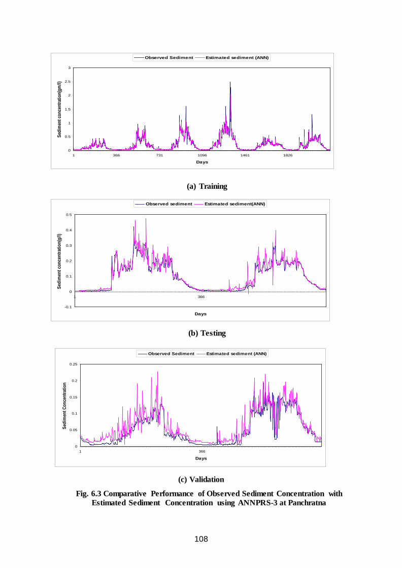
108
(a) Training
(b) Testing
(c) Validation
Fig. 6.3 Comparative Performance of Observed Sediment Concentration with Estimated Sediment Concentration using ANNPRS-3 at Panchratna
0
0.5
1
1.5
2
2.5
3
1 366 731 1096 1461 1826
Days
Sedi
men
t con
cent
ratio
n(gm
/l)Observed Sediment Estimated sediment (ANN)
-0.1
0
0.1
0.2
0.3
0.4
0.5
1 366
Days
Sedi
men
t con
cent
ratio
n(g/
l)
Observed sediment Estimated sediment(ANN)
0
0.05
0.1
0.15
0.2
0.25
1 366
Days
Sedi
men
t Con
cent
ratio
n
Observed Sediment Estimated sediment (ANN)

109
It is observed from Table 6.4 that the RMSE values are generally low for all the ANN models. The performance of ANNCH5 model is the best in RMSE statistic.. In ANNCH5 model, the RMSE value is 340.63 during training.
It can be seen from Table 6.4 that the correlation coefficient (R) values are very high (more than 0.90, i.e., 90%) for all the ANN models, during all the three phases, i.e., training, testing as well as validation. It is also observed that there is not much decrease in the R values during validation as compared to the training phase. The performance of ANNCH5 model is the best in R statistic. The R values for ANN are 0.988, 0.987 and 0.988 during training, testing and validation respectively.
In the determination coefficient (DC) statistic, all the ANN models perform well. The DC values are fairly high (more than 0.90) for all models during all the three phases. In DC statistic also, ANNCH5 model performs the best. The DC values for ANNCH5 are 0.976, 0.970, and 0.971 during training, testing and validation respectively. There is increase in the DC values during validation which indicate good generalization capability of the ANN models.
Therefore, ANNCH5 is the best performing model in all the three statistical and hydrological criteria. Fig. 6.4 presents the plots of observed and estimated discharge for ANN3 model during training (a), testing (b) and validation (c). It is observed from Fig. 6.4 that there is very little mismatch between the observed and estimated discharge series for ANN2 model during all the three phases. 6.2.5 Sediment discharge Modeling for Chouldhuaghat site on Subansiri River
The results are summarized in Table 6.5.
Table. 6.5. Comparative performance of various runoff-sediment ANN models for Chouldhuaghat site on Subansiri River
ANN model Training Testing Validation
RMSE R DC R DC R DC
ANNCS-1 (1-2-1)
0.154 0.780 0.606 0.787 0.025 0.708 0.089
ANNCS-2 (3-3-1)
0.0822 0.942 0.888 0.940 0.845 0.879 0.587
ANNCS-3 (5-4-1)
0.084 0.939 0.881 0.940 0.836 0.887 0.583
ANNCS-4 (7-10-1)
0.077 0.950 0.902 0.948 0.861 0.900 0.627
ANNCS-5 (9-12-1)
0.076 0.950 0.904 0.942 0.860 0.889 0.672

110
(a) Training
(b) Testing
(c) Validation
Fig. 6.4 Comparative Performance of Observed Sediment Concentration with Estimated Sediment Concentration Using ANNCH-5 at Choulduaghat
0
2000
4000
6000
8000
10000
12000
14000
1 366 731 1096 1461 1826
Days
Wat
er L
evel
(m)
Observed WL Estimated wL(ANN)
0
1000
2000
3000
4000
5000
6000
7000
8000
9000
10000
1 366
Days
Wat
er le
vel (
m)
Observed WL Estimated WL(ANN)
0
2000
4000
6000
8000
10000
12000
1 26 51 76 101 126 151 176 201 226 251 276 301 326 351 376 401 426 451 476 501 526 551 576 601 626 651 676 701 726
Days
Wat
er le
vel(m
)
Observed Water level Estimated Water level (ANN)

111
It is observed from Table 6.5 that the RMSE values are generally low for all the ANN models. The performance of ANNCH5 model is the best in RMSE statistic.. In ANNCS5 model, the RMSE value is 0.076 during training.
It can be seen from Table 6.4 that the correlation coefficient (R) values are very high (more than 0.90, i.e., 90%) for all the ANN models, during all the three phases, i.e., training, testing as well as validation. It is also observed that there is not much decrease in the R values during validation as compared to the training phase. The performance of ANNCS5 model is the best in R statistic. The R values are 0.995, 0.942 and 0.889 during training, testing and validation respectively.
In the determination coefficient (DC) statistic, all the ANN models perform well. The DC values are fairly high (more than 0.90) for all models during all the three phases. In DC statistic also, ANNCS5 model performs the best. The DC values for ANNCS5 are 0.904, 0.860, and 0.672 during training, testing and validation respectively. There is not much decrease in the DC values during validation which indicate good generalization capability of the ANN models.
Therefore, ANNCS5 is the best performing model in all the three statistical and hydrological criteria. Fig. 6.5 presents the plots of observed and estimated discharge for ANNCS5 model during training (a), testing (b) and validation (c). It is observed from Fig. 6.5 that there is very little mismatch between the observed and estimated discharge series for ANN2 model during all the three phases.
6.3 ANN BASED RAINFALL RUNOFF MODELLING
6.3.1 Rainfall- Runoff in Subansiri Basin using ANN
The results are summarized in Table 6.6.
Table 6.6 Comparative performance of various rainfall-runoff ANN models for Subansiri Basin
ANN model Training Testing
RMSE R DC R DC
ANNR-1 (6-6-1)
1345.0 0.74 0.55 0.61 0.37
ANNR-2 (7-7-1)
1062.5 0.85 0.72 0.80 0.62
ANNR-3 (8-8-1)
1044.9 0.86 0.73 0.81 0.64
ANNR-4 (9-9-1)
1049.6 0.87 0.76 0.78 0.60
ANNR-5 (10-10-1)
1053.8 0.85 0.72 0.81 0.64
ANNR-6 (9-9-1)
450.26 0.9748 0.9502 0.9721 0.9448

112
(a) Training
(b) Testing
(c) Validation
Fig. 6.5 Comparative performance of observed sediment concentration with estimated sediment concentration using ANNCS-5 at Chouldhuaghat
0
0.5
1
1.5
2
2.5
3
1 366 731 1096 1461 1826
Days
Sedi
men
t con
cent
ratio
n(gm
/l)Observed Sediment Estimated sediment (ANN)
-0.1
0
0.1
0.2
0.3
0.4
0.5
1 366
Days
Sedi
men
t con
cent
ratio
n(g/
l)
Observed sediment Estimated sediment(ANN)
0
0.05
0.1
0.15
0.2
0.25
1 366
Days
Sedi
men
t Con
cent
ratio
n
Observed Sediment Estimated sediment (ANN)

113
It is observed from Table 6.6 that the performance of ANNR-3 model without previous discharge as input and ANNR-6 model with previous discharge as input are the best among the two types of ANN models developed for rainfall-runoff modeling. However, the performance of ANNR-6 is much higher than the ANNR-3 model in all the three statistical criterion and in both the phases, i.e., training as well as testing/validation. The RMSE value is 450.26 for ANNR-6 compared to the RMSE value of 1044.9 for ANNR-6 which is less than 50%. Similarly, the R and DC values for ANNR-3 are much higher han hose of ANNR-3.
Therefore, ANNR-6 is the best performing model in all the three statistical and hydrological criteria. Fig. 6.6 presents the plots of observed and estimated discharge for ANNR-6 model during training (a), and validation (b).
(a) Training
(b) Testing
Fig. 6.6 Comparative Performance of Observed Discharge with Estimated Discharge using ANNR-6 for Subansiri Basin
0
2000
4000
6000
8000
10000
12000
1 23 45 67 89 111 133 155 177 199 221 243 265 287 309 331 353 375 397 419 441 463 485 507 529 551 573 595 617 639 661 683 705 727
Time (Days)
Disc
harg
e (Cu
mec
)
Observed Discharge Estimated Discharge
0
1000
2000
3000
4000
5000
6000
7000
8000
9000
10000
1 12 23 34 45 56 67 78 89 100 111 122 133 144 155 166 177 188 199 210 221 232 243 254 265 276 287 298 309 320 331 342 353
Time (Days)
Disc
harg
e (cu
mec
)
Observed Discharge Estimated Discharge
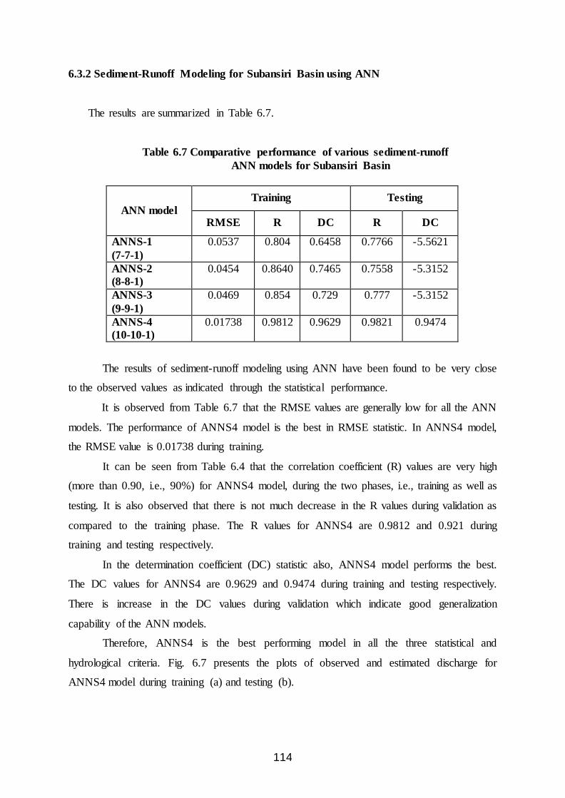
114
6.3.2 Sediment-Runoff Modeling for Subansiri Basin using ANN
The results are summarized in Table 6.7.
Table 6.7 Comparative performance of various sediment-runoff ANN models for Subansiri Basin
ANN model Training Testing
RMSE R DC R DC
ANNS-1 (7-7-1)
0.0537 0.804 0.6458 0.7766 -5.5621
ANNS-2 (8-8-1)
0.0454 0.8640 0.7465 0.7558 -5.3152
ANNS-3 (9-9-1)
0.0469 0.854 0.729 0.777 -5.3152
ANNS-4 (10-10-1)
0.01738 0.9812 0.9629 0.9821 0.9474
The results of sediment-runoff modeling using ANN have been found to be very close
to the observed values as indicated through the statistical performance.
It is observed from Table 6.7 that the RMSE values are generally low for all the ANN
models. The performance of ANNS4 model is the best in RMSE statistic. In ANNS4 model,
the RMSE value is 0.01738 during training.
It can be seen from Table 6.4 that the correlation coefficient (R) values are very high
(more than 0.90, i.e., 90%) for ANNS4 model, during the two phases, i.e., training as well as
testing. It is also observed that there is not much decrease in the R values during validation as
compared to the training phase. The R values for ANNS4 are 0.9812 and 0.921 during
training and testing respectively.
In the determination coefficient (DC) statistic also, ANNS4 model performs the best.
The DC values for ANNS4 are 0.9629 and 0.9474 during training and testing respectively.
There is increase in the DC values during validation which indicate good generalization
capability of the ANN models.
Therefore, ANNS4 is the best performing model in all the three statistical and
hydrological criteria. Fig. 6.7 presents the plots of observed and estimated discharge for
ANNS4 model during training (a) and testing (b).

115
0
0.05
0.1
0.15
0.2
0.25
0.3
0.35
0.4
0.45
1 23 45 67 89 111 133 155 177 199 221 243 265 287 309 331 353 375 397 419 441 463 485 507 529 551 573 595 617 639 661 683 705 727
Time (Days)
Sedi
men
t Con
cent
ratio
n
Observed Sediment Estimated sediment
(a) Training
(b) Testing
Fig. 6.7 Comparative Performance of Observed Sediment Concentration with Estimated Sediment Concentration using ANNS-4 for Subansiri Basin
-0.02
0
0.02
0.04
0.06
0.08
0.1
0.12
0.14
0.16
1 12 23 34 45 56 67 78 89 100 111 122 133 144 155 166 177 188 199 210 221 232 243 254 265 276 287 298 309 320 331 342 353
Time (Days)
Sedi
men
t Con
cent
ratio
n
Observed Sediment Estimated Sediment

116
Chapter – 7
SS uu mm mm aa rr yy
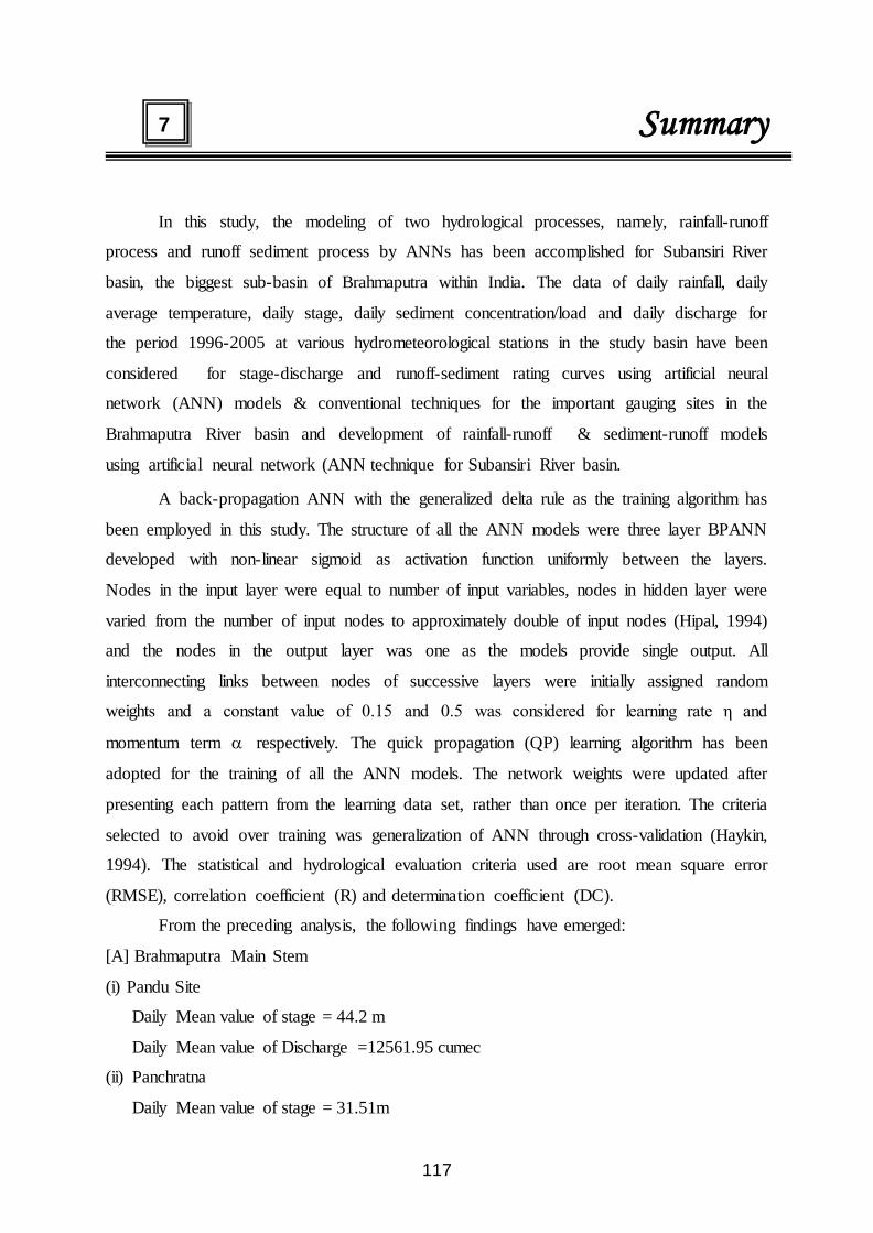
117
Summary
In this study, the modeling of two hydrological processes, namely, rainfall-runoff
process and runoff sediment process by ANNs has been accomplished for Subansiri River
basin, the biggest sub-basin of Brahmaputra within India. The data of daily rainfall, daily
average temperature, daily stage, daily sediment concentration/load and daily discharge for
the period 1996-2005 at various hydrometeorological stations in the study basin have been
considered for stage-discharge and runoff-sediment rating curves using artificial neural
network (ANN) models & conventional techniques for the important gauging sites in the
Brahmaputra River basin and development of rainfall-runoff & sediment-runoff models
using artificial neural network (ANN technique for Subansiri River basin.
A back-propagation ANN with the generalized delta rule as the training algorithm has
been employed in this study. The structure of all the ANN models were three layer BPANN
developed with non-linear sigmoid as activation function uniformly between the layers.
Nodes in the input layer were equal to number of input variables, nodes in hidden layer were
varied from the number of input nodes to approximately double of input nodes (Hipal, 1994)
and the nodes in the output layer was one as the models provide single output. All
interconnecting links between nodes of successive layers were initially assigned random
weights and a constant value of 0.15 and 0.5 was considered for learning rate η and
momentum term α respectively. The quick propagation (QP) learning algorithm has been
adopted for the training of all the ANN models. The network weights were updated after
presenting each pattern from the learning data set, rather than once per iteration. The criteria
selected to avoid over training was generalization of ANN through cross-validation (Haykin,
1994). The statistical and hydrological evaluation criteria used are root mean square error
(RMSE), correlation coefficient (R) and determination coefficient (DC).
From the preceding analysis, the following findings have emerged:
[A] Brahmaputra Main Stem
(i) Pandu Site
Daily Mean value of stage = 44.2 m
Daily Mean value of Discharge =12561.95 cumec
(ii) Panchratna
Daily Mean value of stage = 31.51m
7

118
Daily Mean value of Discharge = 15492.42 cumec
Daily Mean value of sediment conc = 0.4911 g/l
= 491.1 ppm
[B] Subansiri Basin
Basin area (upto Chouldughat site) = 28,000 Sq. Km
River Length = 442 Km
Av annual rainfall = 2150 mm
Daily Mean value of stage = 94.38m
Daily Mean value of Discharge = 2410.27 cumec
Daily Mean value of sediment conc = 0.1137 g/l
= 113.7 ppm
The results of modeling using ANN approach obtained in this study indicate the
capability of back propagation ANN models in simulation of daily river flows using daily
discharge, rainfall and temperature data (correlation more than 90%). Because the ANN
approach presented here does not provide models that have physically realistic components
and parameters, it is by no means a substitute for conceptual modeling. However, the results
suggest that the ANN approach may provide a superior alternative to the regression approach
for developing input-output simulation and forecasting models in situations that do not
require modeling of the internal structure of the basin.
The results of sediment-runoff modeling using ANN have been found to be much
closer to the observed values (correlation more than 99%) than the conventional sediment
rating curve technique. The study shows that the ANN technique can be successfully applied
for the development of reliable relationships between sediment and discharge in a river when
other approaches cannot succeed due to the uncertainty and the stochastic nature of the
sediment movement.
Moreover, the ANN technique has preference over the conventional methods as
ANNs can accept any number of effective variables as input parameters without omission or
simplification as commonly done in the conventional methods. The presented ANN models
were constructed by using only field river data, and it has no boundary conditions in
application. The only restriction is that the model cannot estimate accurately the discharge or
sediment load for data out of the range of the training pattern data. Such a problem can easily
be overcome by feeding the training patterns with wide range data.

119
RR ee ff ee rr ee nn cc ee ss aa nn dd BB ii bb ll ii oo gg rr aa pp hh yy

120
References and Bibliography
Agarwal, A., Mishra, S. K., and Ram, S., and Singh, J. K. 2006. Simulation of runoff and sediment yield using artificial neural networks. Biosystems Engineering, 94(4): 597 – 613.
Akaike, H. 1974. A new look at the statistical model identification. IEEE Trans. Autom.
Control. AC – 19, 716 – 723. Anmala, J., Zhang, B., and Govindaraju, R. S. 2000 Comparison of ANNs and empirical
approaches for predicting watershed runoff. Journal of Water Resources Planning and Management, ASCE, 126 (3): 156 – 166.
ASCE Task Committee. on Application of Artificial Neural Networks in hydrology
(2000 a). Artificial neural networks in hydrology. I: Preliminary concepts. Journal of Hydrologic Engineering, ASCE, 5(2): 115 – 123.
ASCE, Task committee on Application of Artificial Neural Networks in Hydrology
(2000 b). Artificial neural networks in hydrology. II: Hydrologic applications. Journal of Hydrologic Engineering, ASCE, 5(2): 124 – 137.
Barron, A. R. 1993. Universal approximation bounds for superposition of a sigmoid
function. IEEE Trans. Information Theory, 39, 930 – 945. Baum, E., and Haussler, D. 1989. What sized net goves valid generalization. Neural
Information Processing Sys. 1, 81 – 90. Bishoop, C. M. 1995. Neural Networks for pattern recognition. Oxford University Press,
New York. Bose, N. K., and Garga, A. K. 1993. Neural Network design using Voronoi diagrams.
IEEE Transactions on Neural Networks, 45(5): 778-787. Caamaño. D., Goodwin, P., and Milos, M. 2006. Derivation of a bedload sediment transport
formula using artificial neural networks, 7th International Conference on Hydroinformatics HIC 2006, Nice, FRANCE.
Christopher S. H., Ran, Q., Joel E. V., and Keith, L. 2006. Adding sediment transport to
the integrated hydrology model (InHM) : Development and testing. Advances in Water Resources Vol. 29(6): 930 – 943.

121
Cigizoglu, H. K. 2002. Suspended sediment estimation and forecasting using artificial
neural networks. Turkish J. Eng. Env. Sci. 26(2002), 15 – 25. Corpenter, W. C., and Barhelemy, J. 1994. Common misconcepts about neural networks
as approximators. Journal of Computing in Civil Engineering, ASCE. 8(3): 345 – 358.
CWC 2002 . Water and Related studies. Central Water Commission, New Delhi.
David, W. P., and Beer, C. E. 1975a. Simulation of soil erosion. I: Development of a mathematical erosion model. Transactions of the American Society of Agricultural Engineers, 18(1): 126–129.
David, W. P., and Beer, C. E. 1975b. Simulation of soil erosion. II: Stream flow and
suspended sediment simulation results. Transactions of the American Society Agricultural Engineers, 18(1): 130–133.
Day, S. P., and Davenport, M. R. 1993. Continuous time temporal back-propagation with
adaptable time delays. IEEE Transactions on Neural Networks. 4(2): 348 – 354. Elman, J. L. 1990. Finding structure in time. Cognitive Science, Vol. 4, No.2, pp 348 – 354. Elwell, H. A. 1978. Modelling of soil losses in southern Africa. Journal of Agricultural
Engineering Research, 23: 117-127. Fahlman, S. E., and Lebiere, C. 1991. The cascade-correlation learning architecture. CMU
Tech. Rep. CMU-CS-90-100. Carnegie Mellon University, Pittsburgh, Pa. Ferguson, R. I. 1986. River loads underestimated by rating curves. Water Resources
Research, 22(1): 74 – 76. Foster, G. R., and Meyer, L. D. 1972a. A closed form soil erosion equation for upland
areas. Sedimentation (Einstein), H. W. Shen, ed., Colorado State University Press, Fort Collins, Colorado.
Foster, G. R., and Meyer, L. D. 1972b. Transport of soil particles by shallow flow.
Transactions of the American Society of Agricultural Engineers, 15(1): 99 -102. Foster, G. R. 1982. “Modelling the erosion processes.” Hydrological modelling of small
watersheds, ASAE Monograph No. 5, C. T. Haan, H. Johnson, and D. L. Brakensiek, eds., American Society of Agricultural Engineers, St. Joseph, Mich., 297–380.
French, M. N., Krajewski, W. F., and Cuykendal, R. R. 1992. Rainfall forecasting in
space and time using a neural network. Journal of Hydrology, Amsterdam, 137: 1-31. Gallant, S. I. 1986. Three constructive algorithms for network learning. Proc. 8th ANN
Conf. of the Cognitive Sci. Soc., Cognitive Science Society, ANN Arbor, 652-660.

122
Govindaraju, R. S., and Kavvas, M. L. 1991. Modeling the erosion process over steep slopes: Approximate analytical solutions. Journal of Hydrology, 127(1–4): 279–305.
Gupta, H. V., Ksu, K., and Sorooshian, S. 1997. Superior training of artificial neural
networks using weight-space partitioning. Proc. IEEE Int. Con. on Neural Networks, Institute of Electrical and Electronics Engineers, New York.
Hammerstrom, D. 1993. Neural Networks at Work. IEEE spectrum, 30, 46 -53. Hario, H., and Jokinen, P., 1991. Increasing the learning speed of back-propagation
algorithm by linearization. Artificial Neural Networks, T. Kohonen et al., pp 629 – 634.
Hassibi, B., and Stork, D. G. 1993. Second order derivatives for networks pruning; optimal
brain surgeon. Proc., Neural Information Processing Sys. 4, MIT Press, Cambridge, Mass., 164 – 171.
Haykin, S., 1994. Neural Networks - A Comprehensive Foundation McMillan, New York. Hipel, K. W., Ian, A., Panu, U. S., and Singh, V. P. 1994. Stochastic and Statistical
Methods in Hydrology and Environmental Engineering, Vol. 3. The series analysis in Hydrology and Environmental Engineering, Kluwer Academic Publishers, The Netherlands.
Hsu, Kuo-lin., Gupta, H. V. and Soroosh, Sorooshian. 1995. Artificial Neural Network
modeling of the rainfall-runoff process. Water Resources Research, 31 (10): 2517 – 2530.
Imrie, C. E., Durucan, S., and Korre, A. 2000. River flow prediction using Artificial
Neural Networks. Generlization Beyond the calibration Range. Journal of Hydrology, Vol. 233, 138 – 153.
Jain, S. K. and Srivastava, D. K. 1999. Application of ANN for reservoir inflow prediction
and operation. Journal of Water Resources Planning and Management, ASCE, 125 (5): 263 – 271.
Jain, S. K. 2001. Development of integrated sediment rating curves using ANNs. Journal of
Hydraulic Engineering, ASCE, 127(1): 30 -37. Jain, S. K. 2008. Development of integrated discharge and sediment rating relation using a
compound neural network. Journal of Hydrologic Engineering, ASCE, 13(3): 124 – 131.

123
Jansson, M. B. 1996. Estimating a sediment rating curve of the Reventazon river at Palomo
using mean loads within discharge classes. Journal of Hydrology, Amsterdam, 183(3-4): 227 – 241.
Jy. S. Wu, P. E., Han, J., Annambhotla, S., and Bryant, S. 2005. Artificial neural
networks for forecasting watershed runoff and stream flows. Journal of Hydrologic Engineering, ASCE. 10(3): 216 – 222.
Kalin, L., Govidaraju, R. S., and Hantush, M. M. 2003. Effect of geomorphologic
resolution on modeling of runoff hydrograph and sedimentograph over small watersheds. Journal of Hydrology, 276(1–4): 89–111.
Kalin, L., Govidaraju, R. S., and Hantush, M. M. 2004. Development and application of a
methodology for sediment source identification. I: Modified unit sedimentograph approach.” Journal of Hydrologic Engineering, ASCE, 9(3):184–193.
Karim, M. F., and and Kennedy, J. F. 1990. Menu of coupled velocity and sediment-
discharge relations for rivers. Journal of Hydrologic Engineering, ASCE, 116(8): 978 – 996.
Karnin, E. D. 1990. A simple procedure for pruning back propagation trained neural
netoworks. IEEE Tran. Neural Networks, 1, 239 -242. Karunanithi, N., Grenney, W. J., Whitley, D., and Bovee, K. 1994. Neural networks for
river flow prediction. Journal of Computing in Civil Engineering, ASCE. 8(2): 201 - 220.
Kerem, H., Cigizoglu, and Alp, M. 2006. Generalized regression neural network in
modelling river sediment yield. Advances in Engineering Software archive, 37(2): 63 - 68.
Kisi, O. 2005. Suspended sediment estimation using neuro-fuzzy and neural network
approaches. Hydrological Sciences Journal, 50(4): 683 – 689. Kisi, O. 2007. Streamflow forecasting using different artificial neural network algorithms.
Journal of Hydrologic Engineering, ASCE., 12(5): 532 – 539. Kisi, O. 2007. Development of streamflow-suspended sediment rating curve using a range
dependent neural network. International Journal of Science & Technology, 2(1): 49 – 61.
Kohonen, T. 1998. Self organization and associative memory. 2nd Ed., Springer Verlag,
New York. Kothari, R., and Agyepong, K. 1996. On lateral connections in feedforward neural
networks. Proc., IEEE Int. Conf. on Neural Networks, Institute of Electrical and Electronics Engineers, New York, 13 – 18.

124
Kothari, R., and Agyepong, K. 1997. Induction specialization of context units for temporal pattern recognition and reproduction. Proc. IEEE Neural Networks for signal processing V11, J. Principle, L. Gile, N. Morgan, and E. Wilson, Eds., Institute of Electrical and Electronics Engineers, New York, 131 -140.
Kothyari, U. C., Tiwari, A. K., and Singh, R. 1997. Estimation of temporal variation of
sediment yield from small catchment through the kinematic method. Journal of Hydrology, 203(1–4): 39–57.
Kumar, A. 1993. Dynamic models of daily rainfall-runoff-sediment yield for sub-
catchment of Ramganga river. Ph.D. Thesis, Department of Soil and Water Conservation Engineering, G. B. Pant University of Agriculture and Technology, Pantnagar – 263 145, Uttarakhand, India.
Kumar, D. 2007. Hydrological response prediction of a watershed using artificial neural
networks. M. Tech. Thesis, Department of Soil and Water Conservation Engineering, G. B. Pant University of Agriculture and Technology, Pantnagar – 263 145, Uttarakhand, India.
Kumar, C. S. V. S. and Viswanadh, G. K. 2006. Performance of artificial neural networks
in rainfall-runoff modeling. Proc. 2nd International Conference on Hydrology and Watershed Management, Centre for Water Resources, Jawaharlal Nehru Technological University, Hyderabad – 500 072, Andhra Pradesh, India.
Kwowk, T., and Yeung, D. 1995. Constructive feedforward neural networks for regression
problems, A survey Tech. Rep., Hong Kong University of Science and Technology, Hong Kong.
Laguna, A., and Giraldez, J. V. 1993. The description of soil erosion through a kinematic
wave model. Journal of Hydrology, 145(1–2): 65–82. LeCun, Y., Denkar, J. S., and Solla, S. A. 1990. Optimal brain damage. Proc., Neural
Information Processing Sys. 2, MIT Press, Cambridge, Mass., 598 – 605. Lohani, A. K., Goel, N. K., and Bhatia, K. K. S. 2007. Deriving stage-discharge-sediment
concentration relationships using fuzzy logic. Hydrological Sciences Journal, 52(4): 793 – 807.
Lopes, V. L., and Ffolliott, P. F. 1993. Sediment rating curves for a clearcut Ponderosa
Pine watershed in Northern Arizona. Water Resour. Bull., 29(3): 369 – 382. Lorrai, M. and Sechi, G. M. 1995. Neural nets for modeling rainfall-runoff
transformations. Water Resources Management, 9: 299 – 313. Maier, H. R., and Dandy, G. C. 1996. Use of artificial neural networks for prediction of
water quality parameters. Water Resources Research, Vol. 32, No. 4, pp. 1013 – 1022.

125
Maier, H. R., and Dandy, G. C. 2000. Neural network for the prediction and forecasting of water resources variables: a review of modeling issues and applications. Environ. Modelling and Software, 15, 101 – 124.
McBean, E. A., and Al-Nassri, S. 1998. Uncertainity in suspended sediment transport
curves. Journal of Hydrologic Engineering, ASCE, 114(1): 63 – 74. McCulloch, W. S., and Pitts, W. 1943 A logic Calculus of the ideas immanent in nervous
activity. Bull. of Math. Biophys., 5, 115 – 133.
Mingguo, Z., Qiangguo, C., and Qinjuan, C. 2008. Modelling the runoff-sediment yield relationship using a proportional function in hilly areas of the Loess Plateau, North China. Geomorphology, 93(3 – 4): 288 – 301.
Minns, A.W., and Hall, M.J. 1996. Artificial neural networks as rainfall-runoff models. Hydrological Sciences Journal, 41(3): 399-417.
Mishra, S. K., Tyagi, J. V., Singh, V. P., and Singh, R. 2006. SCS-CN-based modeling of
sediment yield. Journal of Hydrology, Vol. 324(1 – 4): 301 – 322. Mozer, M. C., and Smolensky, P. 1989. Skeletonization: A technique for trimming the fat
form a network via relevance assessment. Advances in neural information processing systems 1, D. Touretzky, ed., Morgan Kaufmann, San Monteo, Calif., 107 -115.
Nadal, J. P. 1989. Study of a growth algorithm for neural networks. Int. J. Neural Sys., 55 -
59 Nadi, F. 1991. Topological design of modular neural networks. Artificial Neural Networks,
T. Kohonen et al., pp 213 – 217. Nagy, H. M., Watanabe, K., and Hirano, M. 2003. Prediction of sediment load
concentration in rivers using artificial neural network model. Journal of Hydraulic Engineering, ASCE, 128(6): 588 – 595.
Narayana, D. V. V. and Babu, R. 1983. Estimation of soil erosion in India. Journal of
Irrigation and Drainage Engineering, ASCE, 109(4): 419 – 434. Nash, J. E., and Sutcliffe, J. V. 1970. River flow forecasting through conceptual models,
Part 1 – A: Discussion principles. Journal of Hydrology, Vol. 10, 282 – 290. Nearing, M. A., Foster, G. R., Lane, L. J., and Finkner, S. C. 1989. A process-based soil
erosion model for USDA-Water erosion prediction project technology. Transactions of the American Society of Agricultural Engineers, 32(5): 1587–1593.

126
Neural Power. 2003. Neural Networks Professional Version 2.5, CPC - X Software,
Copyright: 1997-2003, Demoversion, http://www.geocities.com/neural power. Nowlan, S. J., and Hinton, G. E. 1992. Simplifying neural networks by soft weight sharing.
Neural Computation, 4, 473 – 493. Onstad, C. A. and Foster, G. R. 1975. Erosion modeling simulation for the process of soil
erosion by water. Transaction of the ASCE, 18(2): 288 – 292. Oppenheim Alan, V. “Signals and systems”. Prentice-Hall Editions, p 685. Ozturk, F., Yurekli, K., and Apaydin, H. (2008). Stochastic Modeling of Suspended
Sediment from Yesilirmak Basin, Turkey, International Journal of Natural and Engineering Sciences 2 (1): 21-27. (ISSN: 1307 – 1149)
Pyasi, S. K. 1997. Memory based input – output runoff and sediment yield models for the
upper Ramganga Himalayan Catchment, Ph.D. Thesis, Department of Soil and Water Conservation Engineering, G. B. Pant University of Agriculture and Technology, Pantnagar – 263 145, Uttarakhand, India.
Raghuvanshi, N. S., Singh, R. and Reddy, L. S. 2006. Runoff and sediment yield
modeling using artificial neural networks: Upper Siwane River, India. Journal of Hydrologic Engineering, ASCE, 11(1): 71 – 79.
Rai, R. K., and Mathur, B. S. 2008. Event - based sediment yield modeling using artificial
neural network. Water Resources Management, 22(4): 423 – 441. Ramchandrarao, P. 2003 Godavari daily discharge report, Godavari Circle Hyderabad,
Central Water Commission, Govt. of India. Ranjithan, S., Eheart, J. W., and Rarret, jr., J. H. 1993. Neural network - screening for
groundwater reclamation under certainty. Water Resources Research, 29(30): 563 – 574.
Reed, R. 1993. Pruning algorithm - A survey. IEEE Trans. Neural Networks 4, 740 – 744. Refenes, A. N., and Vithlani, S. 1991. Constructive learning by specialization. Artificial
Neural Networks, T. Kohonen et al., pp 923 – 929. Rogers, L. L., and Dowla, F. U. 1994. Optimization of groundwater remediation using
artificial neural networks with parallel solute transport modeling. Water Resources Research, 30920, 457 – 481.
Rumelhart, D. E., Hinton, G. E. and Williams, R. J. 1986. Learning internal
representations by error propagation. Parallel Distributed Processing, Vol. I MIT Press, Cambridge, Mass: 318 – 362.

127
Rumelhart, D. E., and Zipser 1986. Feature discovery by competitive learning. Parallel distribution processing, Explorations in the microstructure of cognition, Vol. 1, pp 318 – 364.
Rusell, I. F. 1991. Self organizing competitive learning and adaptive resonance networks.
Int. Jour. of Neural Networks, Vol. 2, No. 2/3/4. Sadeghi, S. H., Mizuyama, T., and Vangah, B. G. 2007. Conformity of MUSLE estimates
and erosion plot data for storm-wise sediment yield estimation. Terr. Atmos. Ocean. Sci., Vol. 18 (1): 117-128.
Sarkar, A., Kumar, R., Singh, R. D., Thakur, G., and Jain, S. K. (2004). Sediment-
discharge modeling in a river using artificial neural networks. Proc. International Conference ICON – HERP, Oct 26 – 28, 2004, IIT Roorkee, India.
Sarkar, A. 2005. Real time flood forcasting using artificial neural networks in an Indian
river. Proc. International Conference on Monitoring, Prediction and Mitigation of Water Related Disasters (MPMD-2005), January 12-15, 2005, Kyoto, Japan.
Sarkar, A., Agarwal, A. and Singh, R. D. 2006. Artificial Neural Network models for
rainfall-runoff forecasting in a hilly catchment. Journal of Indian Water Resources Society, 26(3-4): 1 – 4.
Sato, A., 1991. An analytical study of the momentum term in a back-propagation algorithm.
Artificial Neural Networks, T. Kohonen et al., pp 617 – 622. Schnabel, S., and Maneta, M. 2005. Comparison of a neural network and a regression
model to estimate suspended sediment in a semiarid basin. Geomorphological Process and Human Impacts in River Basins, Proceedings of the International Conference held at Solsona, Catalonia, Spain, May 2004, Publ. 299, 2005, 91 – 100.
Shamseldin, A. Y., O ‘ Connor, K. M. and Liang, G. C. 1997. Methods for combining the
outputs of different rainfall-runoff models. Journal of Hydrology, 197: 203 – 229. Sharma, T. C. and Dickinson, W. T. 1980. System model for daily sediment yield. Water
Resources Research, 16(3): 501 – 506. Shieh, C. L., and Lee, S. Y. 2005. Sediment yield model for a watershed: a case study of
Choushui River, Taiwan. Geophysical Research Abstracts, Vol. (7): 05931, 2005, European Geosciences Union.
Singh, P. V. 1999. Linear time invariant rainfall-runoff and storage-runoff forecasting
models using transfer function approach for Himalayan Watershed. M.Tech. Thesis, Department of Soil and Water Conservation Engineering, G. B. Pant University of Agriculture and Technology, Pantnagar – 263 145, Uttarakhand, India.
Singh, R. P. 2000. Genetic Algorithm approach in development and optimization of
memory based transfer function models for runoff and sediment prediction – A case study. M. .Tech. Thesis, Department of Soil and Water Conservation Engineering, G. B. Pant University of Agriculture and Technology, Pantnagar – 263 145, Uttarakhand, India.

128
Singh, U. P. 2004. Hydrology modeling using artificial neural networks. M. Tech (Water
Resources Engineering) dissertation, Department of Civil Engineering, Malaviya National Institute of Technology, Jaipur – 302 017 (Rajasthan), India.
Sinha, A. 2005. Stage-Discharge-Sediment analysis using Artificial Neural Networks. M.
Tech (Water Resources Engineering) dissertation, Department of Civil Engineering, Indian Institute of Technology, Delhi, India.
Smith, J. and Eli, R. N. 1995. Neural Network models of rainfall-runoff process. Journal
of Water Resources Planning and Management, ASCE, 121(6): 499 – 508. Srivastava, P. K., Rastogi, R. A. and Chauhan, H. S. 1984. Prediction of storm sediment
yield from a small watershed. Journal of Agricultural Engineering, ISAE, 21(1 - 2): 121 – 126.
Tayfur, G. 2001. Modeling two-dimensional erosion process over infiltrating surfaces.
Journal of Hydrologic Engineering, ASCE, 6(3): 259–262. Tayfur, G. 2002. Applicability of sediment transport capacity models for nonsteady state
erosion from steep slopes. Journal of Hydrologic Engineering, ASCE, 7(3): 252–259. Tayfur, G., and Sing, V. P. 2004. Numerical model for sediment transport over nonplanar,
nonhomogeneous surfaces. Journal of Hydrologic Engineering, ASCE, Vol. 9(1): 35 – 41.
Tayfur, G., and Guldal, V. 2005. Artificial neural networks for estimating daily total
suspended sediment in natural streams. Nordic Hydrology, 37(1): 69 – 79. Thandaveswara, B. S. and Sajikumar, N. 2000. Classification of river basins using
artificial neural networks. Journal of Hydrologic Engineering, ASCE, 5(3): 290 – 298.
Thirumalaiah, K. and Deo, M. C. 1998. River stage forecasting using artificial neural
networks. Journal of Hydrologic Engineering, ASCE, 3(1): 26 – 32. Thirumalaiah, K. and Deo, M. C. 2000. Hydrological forecasting using neural networks.
Journal of Hydrologic Engineering, ASCE, 5(2): 180 - 189. Thomas, T., Jaiswal, R. K. and Singh, S. 2006. Hydrological modeling of streamflows
using artificial neural networks. Proc. 2nd International Conference on Hydrology and Watershed Management, Centre for Water Resources, Jawaharlal Nehru Technological University, Hyderabad – 500 072, Andhra Pradesh, India.
Tokar, A. S. and Johnson, P. A. 1999. Rainfall – Runoff modeling using artificial neural
networks. Journal of Hydrologic Engineering, ASCE, 4(3): 232 – 239.

129
Tokar, A. S. and Markus, M. 2000. Precipitation – Runoff modeling using artificial neural
networks and conceptual models. Journal of Hydrologic Engineering, ASCE, 5(2): 156 – 161.
Wasserman, P. D. 1989. Neural computing: theory and practice. Van Nostrand Reinhold,
New York. Webros, P. J. 1974. Beyond Regression: new tools for prediction and analysis in behavior
scienes. Ph.D Thesis, Harward University, Cambridge, Mass. Wischmeir, W. H. and Smith, D. D. 1958. Rainfall energy and its relationship to soil loss.
Transactions of American Geophysics Union, 39: 285 – 291. Woolhiser, D. A., Smith, R. E., and Goodrich, D. C. 1990. KINEROS: A kinematic runoff
and erosion model: Documentation and user’s manual, USDA Agriculture Research Service ARS-77, Washington, D.C. United States.
Wu, T. H., Hall, J. A. and Bonta, J. V. 1993. Evaluation of runoff and erosion models.
Journal of Irrigation and Drainage Engineering, ASCE, 119(4): 364 – 382. Yang, C. C., Prasher, S. O., Lacroix, R., Sreekanth, S., Patni, N. K. and Masse, L. 1997.
Artificial neural network model for subsurface drained farm lands. Journal of Irrigation and Drainage Engineering, ASCE, 123(4): 285 – 292.
Yitian, L., and Gu RR. 2003. Modeling flow and sediment transport in a river system using
an artificial neural network. Environmental Management, 31(1): 122 – 134. Yu, X., Loh, N. K. and Miller, W.C., 1993. A new acceleration method for the back-
propagation algorithm. IEEE Transactions on Neural Networks., pp 1157 -1161. Yu, P.S., Liu, C. L., and Lee T. Y. 1994. Application of a transfer function model to a
storage runoff process. Stochastic and statistical methods in Hydrology and Environmental Engineering, Vol. 3, 87 – 97.
Zealand, C. M., Burn, D. H. and Simonovic, S. P. 1999. Short term steam flow
forecasting using Artificial Neural Networks. Journal of Hydrology, 214: 32 – 48. Zurada, M. Zacek. 1992. Introduction to artificial neural system, St. Paul, New York: West
publishing company.

PPHHAASSEE –– IIIIII

1
TTEEAAMM OOFF IINNVVEESSTTIIGGAATTOORRSS
1. Prof. Dr. Nayan Sharma
2. Mr. Belay Zeleke
3. Ms Anupama Nayak
4. Md. Parwez Akhtar
5. Mr. Neeraj Kumar
2
TABLE OF MAJOR CONTENTS
Sl. No. Subject Page No.
CHAPTER –1 INTRODUCTION 3
CHAPTER – 2 LITERATURE REVIEW
9
CHAPTER – 3 DESCRIPTION OF STUDY AREA 44
CHAPTER – 4
FORMULATION AND DEVELOPMENT OF FLOW SIMULATION MODEL
59
CHAPTER – 5
RESULTS AND DISCUSSIONS 79
CHAPTER – 6
PILOT STUDY SCHEMES FOR EROSION CONTROL ON THE BRAHMAPUTRA RIVER FOR MORIGAON SITE; AND NEAR GUWAHATI AIRPORT OF BRAHMAPUTRA RIVER
94
CHAPTER – 7
SUMMARY
116
CHAPTER – 8
REFERENCES
118

3
CHAPTER -1 INTRODUCTION

4
CHAPTER-1
INTRODUCTION
1.1 INTRODUCTION
The flow resistance characteristics of an alluvial stream are highly complex which warrant
considerable research efforts. Due to this reason water surface level, velocity and discharge
computations in alluvial streams have great deal of uncertainties. The art of modelling an
alluvial river is still in developing stage and lot of ground yet remain to be uncovered. The
dynamics of flow is further complicated in a natural stream due to wide differences in
hydraulic properties and resistances of flow in the main channel and the subsidiary channels.
The position of the free surface is likely to change with respect to time and space and also by
the fact that the depth of flow, the discharge and the slopes of the channel bottom and of the
free surface are interdependent. To add to the intensity of parameters, a more profound
problem defines the flow behavior and attributes i.e., the fact that rivers and other
watercourses, in most cases, run through loose material and the water carries/transport some
of this material along with it. Generally the loose non-cohesive material through which a
river flows is generally termed as “sediment”.
An integrated study in Fluvial Hydraulics and Sediments Transport involves the analysis of
the capacity of the river or channel to carry water and sediment, and the corresponding
morphological changes in both the main channel and floodplain. Sediment transport in
concise, replicates the various aspects of the dynamics of solid particle movement, properties
of the transported materials, and characteristics of the transporting medium, which in turn,
may be affected by the solids transported.
The morphological changes of rivers are deeply interrelated with bed deformation and bank
erosion because of the mutual relationship between water flow and sediment transport. A
better understanding of these processes is very important in river engineering to prevent
disasters due to flooding, to design and manage hydraulic structures, like bridges and water
intake towers, and to maintain river ecosystems and the landscape for environmental
Engineering purposes.
Reliable and quantitative estimate of the bed aggradation or degradation are very important in
river engineering and management projects as well as accurately predicting the water surface
elevations during floods in estimating flood related damage. Thus, engineers are greatly
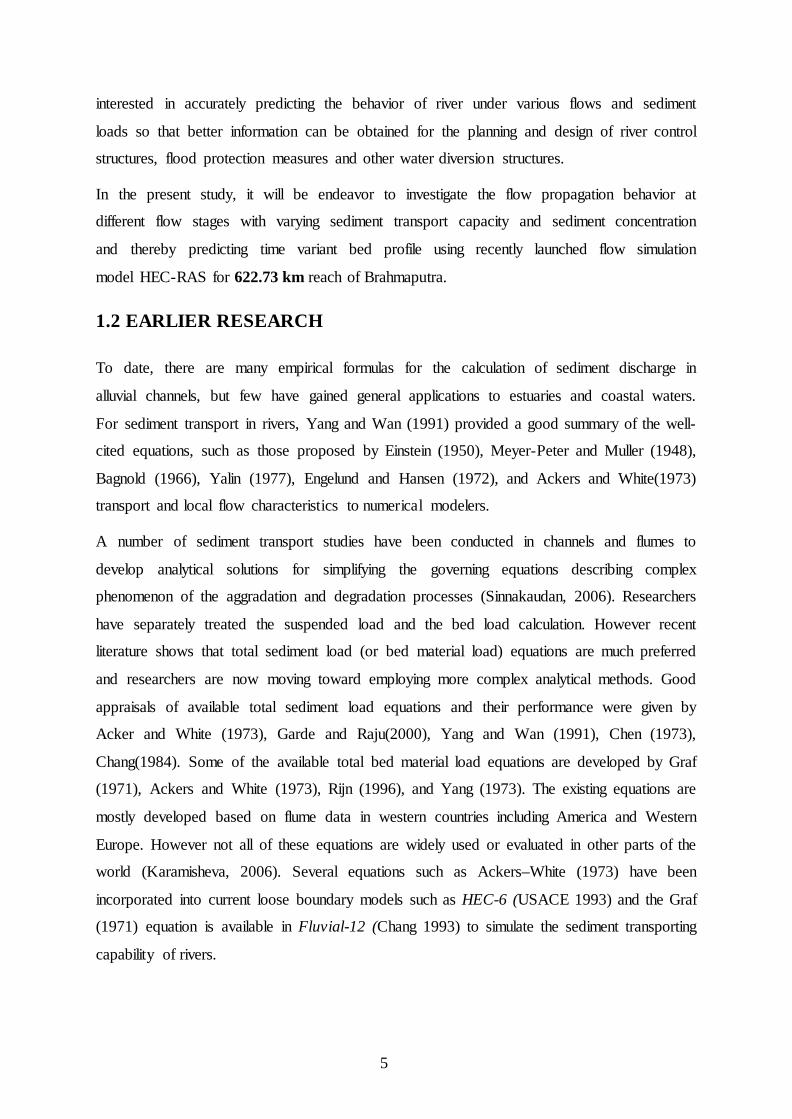
5
interested in accurately predicting the behavior of river under various flows and sediment
loads so that better information can be obtained for the planning and design of river control
structures, flood protection measures and other water diversion structures.
In the present study, it will be endeavor to investigate the flow propagation behavior at
different flow stages with varying sediment transport capacity and sediment concentration
and thereby predicting time variant bed profile using recently launched flow simulation
model HEC-RAS for 622.73 km reach of Brahmaputra.
1.2 EARLIER RESEARCH
To date, there are many empirical formulas for the calculation of sediment discharge in
alluvial channels, but few have gained general applications to estuaries and coastal waters.
For sediment transport in rivers, Yang and Wan (1991) provided a good summary of the well-
cited equations, such as those proposed by Einstein (1950), Meyer-Peter and Muller (1948),
Bagnold (1966), Yalin (1977), Engelund and Hansen (1972), and Ackers and White(1973)
transport and local flow characteristics to numerical modelers.
A number of sediment transport studies have been conducted in channels and flumes to
develop analytical solutions for simplifying the governing equations describing complex
phenomenon of the aggradation and degradation processes (Sinnakaudan, 2006). Researchers
have separately treated the suspended load and the bed load calculation. However recent
literature shows that total sediment load (or bed material load) equations are much preferred
and researchers are now moving toward employing more complex analytical methods. Good
appraisals of available total sediment load equations and their performance were given by
Acker and White (1973), Garde and Raju(2000), Yang and Wan (1991), Chen (1973),
Chang(1984). Some of the available total bed material load equations are developed by Graf
(1971), Ackers and White (1973), Rijn (1996), and Yang (1973). The existing equations are
mostly developed based on flume data in western countries including America and Western
Europe. However not all of these equations are widely used or evaluated in other parts of the
world (Karamisheva, 2006). Several equations such as Ackers–White (1973) have been
incorporated into current loose boundary models such as HEC-6 (USACE 1993) and the Graf
(1971) equation is available in Fluvial-12 (Chang 1993) to simulate the sediment transporting
capability of rivers.

6
The prediction of open channel flows using numerical models is of great interest to hydraulic
researchers and engineers. Most open channel flows are well described by the Saint Venant
equations. Although the Saint Venant equations are derived based on the shallow water
hypothesis, many studies have revealed that the equations are also applicable to the rapidly
varied flows such as dam-break flows. So far, many numerical schemes for the Saint Venant
equations have been developed. However, most conventional schemes are incapable of
encompassing the diverse and complex open channel flows. For example, the four-point
implicit scheme was found to have numerical stability problems with Tran critical flow (Cao
and Carling 2002).
One-dimensional (1-D) modelling of sediment transport in streams has seen extensive
development over the past decades. Chen (1973), for the first time formulated a model that
included sediment transport for generalized use. Dass (1975) developed multi-stream flow
and compound stream flow models by adopting the uncoupled solution procedure to route
water and sediment in non uniform channels. Steady and step wise quasi-unsteady 1-D
models, such as HEC-6 (HEC 1990a) model, Chang’s(1984) model, and others, have been
widely tested and applied to sedimentation studies in reservoirs and rivers in which the long
wave assumption is valid and the long-term results are mainly considered. Many unsteady
flow models (Cunge et al. 1980) have been developed and applied to river estuaries and other
situations where the unsteadiness of flow prevails. With a lot of enhancement and refinement,
1-D models continue to have their place in engineering applications. The majority of the early
1-D sediment transport models decoupled the flow and sediment calculations, which resulted
in simpler computer codes. This strategy was justified because of the different time scales of
flow and sediment transport and the inherent inaccuracies introduced by the use of empirical
formulas for bed roughness and sediment transport capacity. Recently, much effort has been
made toward relaxing the limit in time and space steps and extending the applicability of the
fully decoupled model. One effective approach is to couple the equations of flow and
sediment movement, which was done by Cao et al. (2002), who compared the numerical
stability of coupled and decoupled models and found out that the coupled model is more
stable. However, the implementation of a coupled model for non uniform sediment transport
is rather complicated, which is one of the reasons the decoupled models are still used by
many scientists. Another approach, which has substantially improved sediment transport
modeling, is the non equilibrium (also referred as non saturated) sediment transport model
(Cao and Carling, 2002). In the traditional equilibrium (or saturated) transport model, the

7
actual sediment transport rate is assumed equal to the sediment transport capacity at every
cross section (i.e., locally at equilibrium state, and the bed change is calculated by the
sediment continuity equation (Cao and Carling, 2002). However, in many cases, such as
sediment strongly overloading or under loading, the inflow sediment discharge imposed at
the inlet is significantly different from the transport capacity, which might lead to difficulties
in the calculation of bed changes near the inlet, thus requiring a small time step. The non
equilibrium transport model adopts the mass transport equation to determine the actual
sediment transport rate, which should be more suitable for the simulation of sediment
transport in natural rivers that are mostly in non equilibrium state.
1.3 OBJECTIVE
The study is aimed to:
• Application of flow simulation model HEC-RAS to investigate flow characteristics
and behavior at different flow stages with varying sediment inflows and prediction of
longitudinal bed profile.
• Investigation of the suitability of available sediment predictor for assessing the
sediment transport capacity for the study reach.
• Estimation of stream power for justifying aggradation and degradation in the study
reach.
1.4 STUDY AREA
The area under the consideration for the present study encloses a 622.73 km river stretch of
Brahmaputra encompassing 65 no. of different cross-sections, 7 reaches with Kobo on the
northern most (65 no.) to Dhubri on the south (2 no.). The prime data, the study utilizes is the
survey data of the cross sections taken in the years 1993 and 1997. The other hydrologic data
of the river at different locations (Pandu, Jogighopa etc,) for the years 1993 to 2002 sourced
from Central Water Commission and Brahmaputra Board). Photographic images derived
from different digital satellites imageries processing in the earlier works are incorporated to
draw the idea of the area at a glance.

8
1.5 THE METHODOLOGY
The methodology for this work is to first assess Manning’s n in all segments( all 7 reaches) of
the whole study area (622.73 K.M.) through simulating the flow and comparing the
computed water surface profiles at down stream with observed water surface profiles using 1-
D hydraulic model namely HEC-RAS 4.0. Secondly, the sediment transport module in HEC-
RAS 4.0 proposed to be performed for the study reach to estimate long term aggradation and
degradation to predict the longitudinal bed profile through appropriately feeding inflowing
sediment concentration, sediment inflow from tributaries, bed material sampling and
selection of appropriate sediment transport function along with flow data and calibrated
resistance parameter. For the model constituted in this work, several available sediment
discharge predictors will be experimented and to adopt the method which yield best possible
results.

9
CHAPTER -2
LITERATURE REVIEW

10
CHAPTER-2
LITERATURE REVIEW
2.1 INTRODUCTION
Sediment transport problems related to the identification and mitigation of flood hazard on
alluvial fans in arid and semiarid environments is a current and critical concern of the
engineering profession. In particular, estimating the length and maximum depth of deposition
or erosion that occurs during a flow event when there is a change in the longitudinal slope of
the channel is an important problem. Deposition occurs when the slope changes from steep to
mild and erosion occurs when the slope changes from mild to steep. Once, a flood is over, or
in a gradual time span, large changes on the river bed are observed with banks or piers
eroded, while other locations get covered or aggraded. It might be impacted that when
extremely large floods with limited sediment supplies and high sediment carrying capacities
occur in rivers with erodible bed and bank materials, scour will continue to take place within
the erosive capacity of the stream till it approaches the minimum/optimum value required to
transport the available material.
Traditional approaches have investigated the ways in which stream flows, sediment loads and
channel forms vary along a river from headwaters to mouth and with time over periods
ranging from hours to years. Represented in their most simple form, rivers have been viewed
a unidirectional systems that change progressively from headwaters to mouth. The river
continuum concept takes the physical structure of a stream, coupled with the hydrological
regime and energy inputs to produce a series of responses (in form as stream flow
hydrographs, etc.)
2.2 HISTORY
An exemplary representation of history of river channel evolution may be envisioned through
Fig: 2.1 (Schumm 2000).
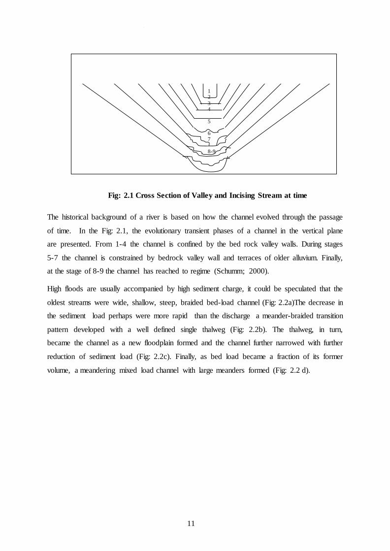
11
The historical background of a river is based on how the channel evolved through the passage
of time. In the Fig: 2.1, the evolutionary transient phases of a channel in the vertical plane
are presented. From 1-4 the channel is confined by the bed rock valley walls. During stages
5-7 the channel is constrained by bedrock valley wall and terraces of older alluvium. Finally,
at the stage of 8-9 the channel has reached to regime (Schumm; 2000).
High floods are usually accompanied by high sediment charge, it could be speculated that the
oldest streams were wide, shallow, steep, braided bed-load channel (Fig: 2.2a)The decrease in
the sediment load perhaps were more rapid than the discharge a meander-braided transition
pattern developed with a well defined single thalweg (Fig: 2.2b). The thalweg, in turn,
became the channel as a new floodplain formed and the channel further narrowed with further
reduction of sediment load (Fig: 2.2c). Finally, as bed load became a fraction of its former
volume, a meandering mixed load channel with large meanders formed (Fig: 2.2 d).
1 2 3 4 5 6 7 8-9
Fig: 2.1 Cross Section of Valley and Incising Stream at time

12
Primarily concerning to the Longitudinal bed profile it is found customary to mention the
hydraulic characteristics of river flow dynamics with sediment discharge which constitutes
and imparts dynamism to river streambed and other river morphological parameters. It is
spontaneous to understand that a river originates from its watershed at higher altitudes of
mountainous slopes which relatively receive high intensity rainfalls. Mainly, large river
streams all around the world starts its voyages from higher mountainous elevation towards
the sea. In the beginning the path of the flow is so steep that it has enormous potential to
erode the bed in the vertical direction by virtue of which it develops V-shaped river section
deep gorge or canyons. It has no flood plains and covers full width of its valley at all stages.
A river at its young stage is characterized by presence of rapids, water falls, steep and
varying gradients and presence of lakes.
At this stage the river is said to become mature after its youth stage. The slope at this stage is
so reduced that it can no more cut the bed but starts widening. The sediment transportation
capacity is just adequate to transport the sediments in the flow from upstream and the
sediment material is derived from bank widening.
If the sediment content in the flow is above the transporting capacity heavier sediments are
settled on the bed upstream the profile slope. Conversely, if the transporting rate capacity is
yet to be satisfied, the bed material picked up and the stream slope is reduced. Hence,
matured streams adjust its profile slope delicately. It is in the stage of maturity that the stream
flows sinusoidal or meandering path in plan.
(a)
(b)
(c) (e)
(d)
Fig: 2.2 Sequence of Channel Changes with Decrease in Discharge and Sediment

13
2.3 STREAM SLOPE
In general the longitudinal slope of a stream shows a continual decrease along its length.
Examination of stream profiles would show that the slope is greatest near the source,
decreasing more or less regularly as the river follows its course. Such reduction in slopes
corresponds to a longitudinal profile which is concave upwards (Garde and Raju 2000).
Several factors are responsible for this. The reasons put forward by different scientists and
engineers have been summarized in the following lines.
Firstly, size of bed material being transported decreases in downstream direction due to
abrasion (Garde and Raju 2000). Hack (1962) found slope varied as d0.60 for stream in
Verginia and Meryland (USA). Shulits (1941) assumed that the stream slope is proportional
to the size of the bed material and accordingly proposed a slope reduction equation (Eq: 2.1)
(2.1)
So and S are the slopes at x=0 and at any distance x being measured in downstream direction
and α a slope reduction coefficient. Brush (1961) and Hack (1962) have shown that the
stream slope is proportional to a negative power of the length of the stream up to that point
indicating there by a decrease in slope along the length in conformity with the equation.
Low water profiles of the river Mississippi between Fort Jackson and Cairo of the Ohio
between Cairo- Pittsburg (USA) and of several rivers in Europe are found to confirm the Eq:
(2.1) (Garde and Raju 2000).
Secondly, in humid regions, the discharge in a stream increases in the downstream direction
due to inflow from the tributaries. Unless there is a corresponding increase in the sediment
inflow, the stream would necessarily flatten to the extent required by the increased sediment
and water discharge (Garde and Raju 2000).
Thirdly, the sediment contribution of the upper region of a drainage basin is large compared
to the run-off contribution to the stream flow. Which mean higher sediment contribution
necessitating higher slope. While the lower region of the same drainage basin contributes
smaller sediment quantity compared to its run-off discharge contribution signifying flatter
slope requirement (Garde and Raju 2000).
xoeSS α−=
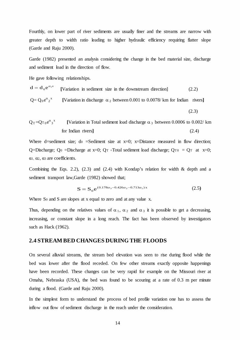
14
Fourthly, on lower part of river sediments are usually finer and the streams are narrow with
greater depth to width ratio leading to higher hydraulic efficiency requiring flatter slope
(Garde and Raju 2000).
Garde (1982) presented an analysis considering the change in the bed material size, discharge
and sediment load in the direction of flow.
He gave following relationships.
[Variation in sediment size in the downstream direction] (2.2)
Q= Q0eα2
x [Variation in discharge α 2 between 0.001 to 0.0078/ km for Indian rivers]
(2.3)
QT =QT 0eα3
x [Variation in Total sediment load discharge α 3 between 0.0006 to 0.002/ km
for Indian rivers] (2.4)
Where d=sediment size; d0 =Sediment size at x=0; x=Distance measured in flow direction;
Q=Discharge; Q0 =Discharge at x=0; QT =Total sediment load discharge; QT0 = QT at x=0;
α1, α2, α3 are coefficients.
Combining the Eqs. 2.2), (2.3) and (2.4) with Kondap’s relation for width & depth and a
sediment transport law,Garde (1982) showed that;
(2.5)
Where S0 and S are slopes at x equal to zero and at any value x.
Thus, depending on the relatives values of α 1 , α 2 and α 3 it is possible to get a decreasing,
increasing, or constant slope in a long reach. The fact has been observed by investigators
such as Hack (1962).
2.4 STREAM BED CHANGES DURING THE FLOODS
On several alluvial streams, the stream bed elevation was seen to rise during flood while the
bed was lower after the flood receded. On few other streams exactly opposite happenings
have been recorded. These changes can be very rapid for example on the Missouri river at
Omaha, Nebraska (USA), the bed was found to be scouring at a rate of 0.3 m per minute
during a flood. (Garde and Raju 2000).
In the simplest form to understand the process of bed profile variation one has to assess the
inflow out flow of sediment discharge in the reach under the consideration.
x1edd 0α=
x)713.0426.0178.0(0
123eSS ααα −−=

15
a) If the incoming amount or the rate of the sediment upstream of the reach is higher than
outgoing from the reach downstream it is obvious that the difference of the two quantities
must have been dropped within the length of the reach. This process of rising of the bed
level is called Aggradation.
b) Conversely, if the incoming amount or the rate of the sediment upstream of the reach is
lower than outgoing from the reach downstream then the difference of the two quantities
must have been fulfilled by picking up the bed materials from within the length of the
reach. This process of lowering of the bed level is called Degradation.
2.5 OCCURRENCES OF AGGERADATIONS AND DEGRADATION
2.5.1 AGGRADATION
2.5.1.1 Occurrence of Aggradation
Occurrence of aggradation is the most often observed phenomena on the upstream side of
Dams, Barrages and any other disturbances caused by man made features or natural activities
like barricade due to land slide. Because of disturbance in the equilibrium state of sediment
flow in the stream causing reduction in the bed profile slope the sediment carrying capacity
of the flow is weakened, which leads to settling of the sediment contained in the flow
(Basically bed load) is retained in the zone upstream to such features.
Other instance of aggradation of river bed is rising of the water level in the Lake or the sea
which causes to reduce the slope of the water surface of river leading to a drop in the
sediment transporting capacity and the result is aggradation.The situation of aggradation
involves lower rate of sediment outflow than the inflow so that temporal gradient of bed level
is positive.
In the sediment continuity equation
(2.6)
Where λ = Porosity of the bed; qt= Rate of sediment inflow per unit width; z= Bed elevation.
The consequences of aggradation more often reduce the conveyance capacity of the channel
due to reduction in the flow area.
0xq
)1(1
tz
=∂∂
−+
∂∂ t
λ

16
Fig: 2.3 Aggradation and Equilibrium L-Profile
Fig.: 2.3 shows how the process of aggradation reaches to final equilibrium condition. Where
the aggradation takes place because of increase in the sediment load in the flow above its
transport capacity part of the sediment of the bed load is disposed on the bed of the channel
which gradually extends upstream and downstream (as shown in the figure continues) till
new profile is attained. This new profile is the equilibrium state of the profile adequate to
transport the incoming sediment discharge.
2.5.1.2 Effects of Aggradation
a) Firstly, aggradation shrinks the active flow area of the river. Consequently, the flow is
pushed to spread to wider coverage extending the flood affected area.
b) In the reservoirs behind the storage dams, the filling up of the reservoir leads to decrease
in the depth of the usable water. This necessitates fixing a dead level in the design of
such structures.
c) Bank erosion and river migration problems are more pronounced in the aggrading rivers
like lower reaches of the river Brahmaputra.
d) Aggradation of the river bed restricts the navigational opportunities of the river courses.
e) The effect of aggradation extends the flood detention period over the flood plain during
wet season causing water table to raise causing water logging (Garde and Raju 2000).
2.5.2 DEGRADATION
2.5.2.1 Occurrence of Degradation
Most often degradation of streambed is observed to be lowered downstream of Large
Capacity Reservoirs and Pools. Such degradation was observed in Cherry Creek USA where

17
the extent of lowering being measured was 4.9m. But wherever sound rock exposures are
encountered the process of degradation have found retarded (Garde and Raju 2000).
Another prominent location of occurrence of degradation is confluence of two or more rivers.
Tributaries, generally steeper than the main stream but carry less run-off cause to lower the
bed. At the instances, where the water discharges in the stream increases due to mixing of
tributaries with relatively sediment free water discharge enhances the sediment transport
capacity degradation occurs subsequently. And one another cause of degradation is because
of increase in water surface profile slope as the result of fall in level of a lake. This type of
degradation was noted in White river in California USA (Garde and Raju 2000).
Another location of degradation is where river has been started to flow along the cut-off
developed in the meandered river (Fig: 2.4). The cut-off shortens the length of the river. In
the beginning the cut-off has narrow width which gradually opens to accommodate the
discharge through the channel.
In the meandered rivers, the meandering
process advances to a stage that the river
no more can negotiate a long serpentine
path which impose more resistance and take
a shortest channel route at an incidence of
high flow.
2.5.2.2 Effect of Degradation
Followings are some of the much pronounced effects both harmful as well as beneficial in the
study of River Engineering.
a) Formation of Hydraulic Jump is apparently pushed downstream in spillways and
Barrages due to downstream bed level lowering jeopardizing the stability of the
structure. This situation was faced in the Wisconsin River at downstream of Praire Du
San Dam (USA).
b) Dams constructed in pervious strata exhibit increase seepage head due to increase in
level difference between upstream and downstream water. The effect of this could be
more uplift and seepage.
Cut-off
Fig: 2.4 Shortening of the River Flow Path
due to Cut-off Development

18
c) While in case of lowering of tail water level downstream of a Power Generation point
due to degradation leads to increase in available effective heads for more power
generation. This has occurred at Paraire Du Sac Dam in the Wisconsin river USA.
And also at Upperborn power house at Munich on the Saalach River.
d) Lowering of river bed by degradation process increases the capacity of the river
channel to carry the flood flow, by lowering the high flood level of the river. Creating
an artificial degradation by construction of a big reservoir was a method that had been
suggested as a possible solution to the flood problem of the Yellow river in China and
Kosi River in the Indian Territory. Lowering of water level due to degradation
reduces the height of the ground water table in the adjoining areas.
e) Lowering of water level may expose pile foundation of bridges abutments and other
structures to air and this may lead to deterioration of piling & stability endangering
the whole structure. This problem has also been observed in many of the river bridges
around on their downstream due to increased flow intensities aggravated by the
construction of the bridges.
f) Degradation also causes lowering of water level at the existing irrigation intakes and
thus makes the diversion of water for irrigation more difficult.
g) Degradation may cause substantial lowering of bed in navigable rivers and in extreme
cases locks may become inoperative. Such difficulties have been encountered on a
lock at the Wisconsin River (USA) and on the Mausa River (Holland) (Garde and
Raju 2000).
2.6 MATHEMATICAL MODELLING OF ALLUVIAL RIVERS
Mathematical modelling of fluvial flow, sediment transport and morphological evolution
started half a century ago and, to date, a variety of mathematical models have been developed
and are in widespread use. However, the quality of mathematical river modelling remains
uncertain because of: (a) poor assumptions in model formulations; (b) simplified numerical
solution procedure; (c) the implementation of sediment relationships of questionable validity;
and (d) the problematic use of model calibration and verification as assertions of model
veracity.
The ability to make accurate calculations of fluvial flow, sediment transport, the associated
morphological evolution processes and water quality is vital in a period when the concern

19
over the river environment and the influence of human intervention is increasing. The
interaction between sediment and turbulent flow is of fundamental interest in the field of two-
phase flow, and modelling the strongly coupled flow– sediment–morphology system provides
a problem of considerable interest in computational fluid dynamics. Fluvial sediment
transport process has been an increasingly important subject in the fields of water resources
engineering, hydrology, geographical, geological, and environmental sciences, and more
fundamentally fluid dynamics.
Fluvial sediment transport poses great challenges for river scientists and engineers. The
essence of the discipline is the interaction between the fluid (water) and the solid (dispersed
sediment particles) phases. The exposure of the fluvial systems to the natural and variable
environment (climatic, geological, ecological and social, etc.) adds to the complexity of the
process of sediment transport and the resulting morphological evolution of rivers.
The earlier efforts in mathematical river modelling were almost exclusively built on
traditional fluvial hydraulics—that is, one-dimensional (1D) and two-dimensional (2D) Saint-
Venant equations. The 1D and 2D models are at present widely used in engineering practice;
yet the future of mathematical river modelling will undoubtedly be the more advanced full
3D computational fluid dynamics (Cao and Carling 2002).
2.6.1 MAJOR ISSUES OF MATHEMATICAL MODELS FORALLUVIAL RIVERS
Mathematical models of alluvial rivers can be categorized into two types: academic and
applied. Academic models often deal with ‘how and why’ problems, being devoted to the
conceptualization, mathematical formulation, solution (analytical or numerical) and
interpretation of the flow, sediment transport, and morphological reaction. Improving the
understanding of the mechanism of interaction among water, sediment and morphology is the
major purpose of academic models. On the other hand, applied models are entirely concerned
with quantitative modelling of the river systems in response to natural changes and human
activities (e.g. construction of dams, bridges and flood control works). Currently, the most
extensively used fluvial models are either 1D or depth-averaged (shallow) 2D, which are built
upon traditional hydraulics principles—that is, Saint-Venant equations (Cao and Carling
2002).

20
2.6.2 1D AND 2D COMPUTATIONAL HYDRAULICS MODELS
This section mainly focuses on 1D hydraulic model, while most aspects examined here are
pertinent to depth-averaged 2D cases. Based on cross-section-averaged variables, 1D
numerical modelling of alluvial rivers has been most widely used in the fields of river
training, hydropower generation, flood control and disaster alleviation, water supply,
navigation improvement, as well as environment enhancement. HEC-6, ISIS-Sediment,
GSTAR3D, CCHED, HEC-RAS and Mike11 are examples of a number of mathematical
river models developed for fluvial water–sediment–morphology systems. The outputs of
these models usually include sediment transport rates, changes in bed elevation and amounts
of erosion and deposition throughout the river system considered. It has been recognized that
1D models are appropriate primarily for long-term and long-reach situations, whereas these
models have been less successful for local flow–sediment–morphology problems as can be
anticipated. Prior studies in this connection have focused on such aspects as flow resistance
relations (including parameter identification and optimization), grain sorting, non-equilibrium
modules, numerical techniques, and effects of vertical distributions. In the present state of the
art, it is a common practice to tune the friction factor and sediment transport formulae to
reconcile the computational results with measurements. In this section the fundamental
components of 1D model are examined. In particular the effects of simplified continuity
equations and the asynchronous solution procedure are addressed, which have rarely been
studied before except for a formative comparison by Krishnappan (Cao and Carling 2002).
2.6.3 SIMPLIFIED CONTINUITY EQUATION FOR WATER-SEDIMENT MIXURE
Alluvial flows over erodible beds can be distinguished from those over fixed beds in that the
flow may entrain sediment from the bed or in contrast render the sediment carried by the flow
to be deposited on the bed, which usually causes riverbed degradation or aggradation. This
aspect is referred to as the bottom mobile (free) boundary problem. At the same time, the
water–sediment mixture may have properties (density, etc.) different from clear water. In
spite of these apparently known features of erodible-bed alluvial flows, it is often assumed
that the rate of bed morphological evolution is of a lower order of magnitude than flow
changes with adequately low sediment concentration. Accordingly, in existing 1D and 2D
models, the water–sediment mixture continuity equation is almost exclusively assumed to be
identical to that for a clear-water flow over a fixed bed without considering the alluvial
riverbed mobility. This simplified mixture continuity equation is, in its form, the same as that

21
in the traditional Saint-Venant equations. The effect of this treatment appears to have been
quantitatively addressed only by Correia et al(1992) and discussed by Rahuel(1993)
Stevens(1988) claimed that bed mobility is important for complete coupling of water and
sediment in discussing Lyn’s(1987) analysis. Worm leaton and Ghumman(1994) compared
the performance of several simplified models, but exclusive of a fully coupled model on a
rigorous basis. Therefore the effect of bed mobility on model performance has not been
apparent (Cao and Carling 2002).
2.6.4 SIMPLIFIED EQUATIONS IN ANALYTICAL MODELS
It is interesting to note that there have been several analytical models for channel aggradation
and degradation. Whereas providing an easy-to-use approach to evaluating the response of
channels to the changing of a simple water and sediment hydrograph or base lowering, these
models are based heavily on assumptions. First, the flow is assumed to be quasi-steady,
leading to the elimination of local derivatives in the water–sediment mixture continuity and
momentum equations. Second, in the momentum equation the nonlinear convective
acceleration term is ignored, yielding a diffusion model for bed elevation evolution. A
slightly modified type of models, namely hyperbolic models have been developed by partly
including the non-linear convective effect using a perturbation technique. Finally in the
sediment continuity equation the temporal concentration term is almost exclusively not taken
into account in order to make the analytical solution tractable. One of the major difficulties in
using these analytical models is the determination of the model coefficients involved.
Additionally, it appears not encouraging to use these analytical models with highly variable
hydrographs (complicated boundary conditions). More comments on these analytical models
can be found in Zanre and Needham (1996). It is necessary to recognize that the momentum
equation for the mixture flow over erodible bed differs from that of fixed-bed clear water
flow. However, it seems a common practice to reduce it to a clear water flow momentum
equation, recognizing the uncertainty inherent in the resistance relationship that must be
incorporated to close the momentum equation (Cao and Carling, 2002).
2.6.5 SEDIMENT TRANSPORT FUNCTIONS
A function is necessary to determine sediment transport rate and, for heterogeneous
sediments, the size distribution of bed material being transported. A large number of
functions have been developed. However, most, if not all, of these functions have been

22
confirmed using specific laboratory and/or field measurement datasets, and none has been
proved to be universally correct. Also it cannot be stated which function is the ‘best’ to use
for a given situation. Distinct sediment transport functions will yield different answers, and
normally the sediment rates/discharges are more sensitive to the choice of sediment function
than the changes of river morphology. The latter concurs with the known feature that the
time-scale of changes in flow variables (velocity, depth and sediment discharge, etc.) is
normally significantly less than that of bed evolution. This aspect will be recalled later with
respect to the asynchronous solution procedure commonly used in current mathematical river
modeling practice. Therefore model developers and end-users have to judge the
computational results based on their experience and their understanding of the basis on which
existing sediment transport functions were derived and validated. Undoubtedly the modelling
output is still subject to model developers and end-users—the lack of objectiveness is
apparent. Using both laboratory and river datasets, Yang and Wan(1991) compared the
performance of several sediment transport functions that are popularly used, and showed that,
for river datasets considered, the accuracy in ascending order was Engelund–Hansen(1967),
Laursen(1958), Colby(1964), Ackers–White(1973), Einstein(1950), Toffaletti(1969), and
Yang(1973). At the same time Yang and Wan (1991) claimed that the rating does not
guarantee that any specific function is better than others under all hydraulic and sediment
cases. For gravel-bed rivers, the formulae of Einstein, Parker, and Ackers– White were
shown to perform reasonably well(Gomez and Church,1989).To measure the applicability of
sand transport functions, an ‘applicability index’ was proposed by Williams and Julien(1989)
on the basis of river characteristics. These authors argue that developing a universal (at least
to a certain extent) procedure to help choose the ‘optimum’ sediment transport function
among the large pool of candidates will be one of the most realistic strategies to cope with the
uncertainty due to sediment transport functions (Cao and Carling ,2002).
2.6.6 MODEL CALIBRATION AND VERIFICATION/VALIDATION
2.6.6.1 Model calibration
A mathematical river model encompasses a number of parameters to be determined. One
primary question is whether there is a unique combination of these parameters. From time to
time the same (or similar) results are produced using different sets or combinations of model
parameters. Usually there is no way to choose between these sets of parameters, other than to
invoke extra-evidential considerations such as symmetry, simplicity, flexibility, personal,

23
political or metaphysical preferences as well as prejudices and financial considerations. A
secondary question arises as to how the overall performance of modeling can be objectively
judged in comparison with measurement. This is especially critical for 3D modeling as
normally there are many megabytes of numbers (typically with over 50 000 nodes for a real
river problem), and it is almost impossible for model developers and end-users to view,
assimilate, interpret and present even a small fraction of the output. That way, the judgment
of acceptable agreement with measured data is virtually on a basis of a limited portion of
information, for example some selected verticals and cross-sections, etc. Known too many
model developers and end-users is the fact that it is fairly feasible to reconcile the computed
results to measurements within a local area by tuning the various parameters. Thirdly, it is
hard to specify the initial conditions, whereas the computation can be sensitively influenced
by the initial status in the non-linear systems; therefore the agreement between computed and
measured results in general is largely not unbiased but subjective (Cao and Carling, 2002).
2.6.6.2 Model verification and validation
A verified model is useful as a prediction tool because of its demonstrated truth, and implies
its reliability as a basis for decision-making. Equally correct is the term ‘validation’, which
usually connotes legitimacy. It can, but does not necessarily denote an establishment of truth.
Instead, it indicates the establishment of legitimacy, generally in terms of contracts,
arguments, and methods. Validation means making legally valid, granting official sanction to
or confirming the validity of something. A valid model contains no known errors or
detectable flaws and is internally consistent. Verification is only possible in closed, rather
than open systems, in which all components of the system are established independently, and
are correct. Its application to natural systems is misleading. Alluvial river models are never
closed systems, and therefore it is incorrect to use the term ‘verification’ for such models.
Below are two specific reasons that make alluvial river models open. First, the model requires
a number of input parameters that are not completely known. These input parameters are
often embedded in turbulent closure modules, boundary conditions, sediment transport and
entrainment functions as well as numerical discretization schemes, etc. Second, the
observation and measurement of both independent and dependent quantities are laden with
inferences and assumptions. Although many inferences and assumptions can, in some cases,
be justified with experience, the degree to which the assumptions hold in new and
complicated studies can never be established a priori. Alluvial river systems are complicated

24
in that turbulence is one of the last problems in classic physics, which remains to be solved,
and this is further aggravated due to the presence of sediments. It is essential to recognize the
restricted sense of the term ‘validation’. Legitimacy, official sanction, or being free of
apparent errors and inconsistency does not necessarily mean truth or correctness, although
truth or correctness is not precluded. It is misleading if the term validation is used to refer to
actual modeling results in any particular realization. It is fairly popular for river modelers to
use interchangeably the terms verification and validation. Thus they misleadingly imply that
validation establishes model veracity. Even more critically, the term validation is used to
suggest that the physical river phenomenon is accurately represented by numerical models.
As stated above, there exist a lot of critical problems with the model calibration–
verification/validation phases, both logically and practically. The most significant problem
comes with the verification/validation phase, where the model is claimed a success. This is,
as a matter of fact, committing the basic logic error of affirming the model output. Oreskes et
al.describe this as follows ‘To claim that a proposition (or model) is verified because
empirical data match a predicted outcome is to commit the fallacy of affirming the
consequent. If a model fails to reproduce observed data, then we know that the model is
faulty in some way, but the reverse is never the case. Confirming observations do not
demonstrate the veracity of a model or a hypothesis, they only support its probability.’ The
misuse of the terms verification and validation in mathematical river modeling can be risky
with respect to public interests. Often the decision-makers may not be experts in river
hydraulics. It is the responsibility of model developers and end-users to correctly inform the
decision-makers of what mathematical Models can realistically reflect, and more essentially
the degree to which the modeling results can be relied upon (Cao and Carling, 2002).
2.7 REVIEW OF THE EXISTING MODELS PERTAINING TO
ALLUVIAL STREAMS
2.7.1 DELFT HYDRAULIC LABORATORY MODEL
DE Varies (1973) developed a mathematical model combining continuity and momentum
equations along with Chezy’s equations for alluvial streams. In this model, the two dependent
variables U(x, t) and Z(x, t) are computed in two separate steps. In this model, Cunge et al
(1980) commented that computational time step cannot be chosen arbitrarily. This model is
true for coarse sediment only.

25
2.7.2 CHEN’S MODEL
Chen (1973) formulated a model based on Saint Venant’s continuity and momentum
equations of unsteady flow of sediment-laden water. This model is capable of flood and
sediment routing in a gradually varied flow channel. He used sediment load functions from
Einstein’s Bed load function as well as Toffaleti’s function. Chen for the first time
formulated a mathematical model that included sediment transport for generalized use. His
works have proved to be a landmark in the field of open channel modeling for sediment-laden
flow (Chen, 1973).
2.7.3 DASS MODEL
Dass (1975) developed multi-stream flow and compound stream flow models by adopting the
uncoupled solution procedure to rout water and sediment in non-uniform channels with the
capability to simulate bed level changes. The governing equations adopted by Dass are:
Where; x=Horizontal distance along the channel; t= Time; Q=Total discharge of sediment
laden water; A= Area of available flow; Ad = Area of deposit; ql = lateral inflow; As =Volume
of sediment concentration in flow; ρ = Density of sediment laden water; p= Porosity of bed
material; qs = Lateral inflow of sediment; Qs = Sediment Discharge. Sf = Energy slope;
Mc=Factor dependent on bed slope; V= Mean velocity of flow;
However, the validation of the model has been done in a hypothetical channel case (Dass,
1975).
0qt
At
Ap
xQ
ssds =−
∂∂
+∂
∂+
∂∂
0MgASxygA
xQV)(
tQ
cf =−+∂∂
+∂
∂+
∂∂ ρ
(2.7)
(2.8)
(2.9)
0qt
AtA
xQ d =−
∂∂
+∂∂
+∂∂
l

26
2.7.4 FLUVIAL MODELS (1978 and 1984)
Chang and Hill (1976) developed this model in 1976.The same equations of St. Venant are
solved. In the case of aggradation, the deposition is made starting from the lowest point in
horizontal layers. A four point implicit finite difference schemes with uncoupled solution
procedure is used to solve the equations. Channel width adjustments are used to reflect
lateral migration. Manning’s equation is used to represent resistance to flow.
He also developed FLUVIAL 11 Model in 1984 which employs a space-time domain in
which space domain is represented by the discrete cross-sections along the river reach and the
time domain is represented by discrete time steps. The model uses the concept enunciated by
Langbein and Leopold that the equilibrium channel represents a state of balance with a
minimum rate of energy expenditure along the channel. Chang has considered the bank
erodibility or coefficient of bank erosion to predict the bank changes. Fluvial 11 is
undoubtedly a promising model for channel changes prediction. However the adoption of
empirical bank erodibility factor appears to have constrained its universal applicability and
may require considerable calibration efforts. This model cannot be applicable for a river of
multi-channel configuration.
2.7.5 HEC-6 MODEL
This model has been developed by W.A.Thomas at Hydrologic Engineering Centre, U.S.A. in
1977. There are five different options provided for the transport of sediment, viz Lausen’s
equation, Toffaleti’s equation, Yang’s stream power function, Duboy’s equation and Qt =
f(Q,S). The flow equation is the Manning’s equation. For numerical solution, uncoupled
explicit finite difference scheme is used. Simulation of reservoir sedimentation using HEC-6
was reported to be successful (HEC 2004).
2.7.6 WATER RESOURCES MODELLING FROM DHI WATER AND ENVIRONMENT
MIKE 11 - River and Channel Hydraulics
MIKE 11 is a one-dimensional hydrodynamic software package including a full solution of
the St. Venant equations, plus many process modules for advection-dispersion, water quality
and ecology, sediment transport, rainfall-runoff, flood forecasting, real-time operations, and
dam break modelling.
The software can simulate flow and water level, water quality and sediment transport in
rivers, irrigation canals, reservoirs and other inland water bodies. It is an engineering tool

27
with capabilities provided in a modular framework. It can be applied on numerous
applications - from simple design tasks to large forecasting projects including complex
structure operation policies. It allows you to integrate your river and floodplain modelling
with watershed processes, detailed floodplain representation, sewer systems and coastal
processes. MIKE 11 offers links to groundwater codes (Mike 11 User Guide, 1993).
2.7.7 HEC-RAS - (Version-4.0, 2006)
This is the latest version developed by US Army Corps of Engineers at Hydrologic
Engineering Center. This is Next Generation of hydrologic engineering software which
encompasses several aspects of hydrologic engineering including; river hydraulics; reservoir
system simulation; flood damage analysis; and real time river forecasting for reservoir
operations. The system is comprised of a graphical user interface (GUI), separate hydraulic
analysis components, data storage and management capabilities, graphics and reporting
facilities. The HEC-RAS system will ultimately contain three one dimensional hydraulic
analysis components (i) Steady flow water surface profile (ii) Unsteady flow simulations (iii)
movable boundary sediment transport computations. Apart from this software contains
several hydraulic design features. This is capable of importing GIS data or HEC-2 data
(Brunner, 2002; HEC-RAS Manual, 2006).
It is an integrated system of software, designed for interactive use in a multi-tasking
environment. The system is comprised of a graphical user interface, separate hydraulic
analysis components, data storage and management capabilities, graphics and reporting
facilities.
The HEC-RAS system will ultimately contain three one-dimensional hydraulic analysis
components for:
• Steady flow water surface profile computations
• Unsteady flow simulation
• Movable boundary sediment transport computations
A key element is that all three components will use a common geometric data representation
and common geometric and hydraulic computation routines. In addition to the three hydraulic
analysis components, the system contains several hydraulic design features that can be
invoked once the basic water surface profiles are computed (HEC-RAS Manual, 2006).

28
The review of existing models indicates that several models are available with different
features. All the models use St. Venant’s equations and have different sediment predictors,
energy slope relations and distribution of aggradation/degradation equations. A natural river
has many complexities due to its size, flow variations, concentration of sediment and its
properties, engineering works carried out on the river and other geographical, meteorological,
social factors. Due to these reasons, no model can claim to have considered all the factors.
Therefore, the models cannot have universal applicability. Hence, for modelling a particular
river one should be very careful to choose a model, which is applicable according to the
characteristics of that river.
Hec-Ras (version 4.0) is latest in the family of the existing models for sediment transport &
mobile bed modeling, so in this dissertation it has been envisaged to initiate work on this
model to figure out the suitability for the specific purpose as well for specific applicability.
2.8 GENERAL PHILOSOPHY OF THE MODELLING SYSTEMS IN HEC-RAS
HEC-RAS is an integrated system of software, designed for interactive use in a multi-tasking,
multi-user network environment. The system is comprised of a graphical user interface
(GUI), separate hydraulic analysis components, data storage and management capabilities,
graphics and reporting facilities. The system contains three one-dimensional hydraulic
analysis components for: (1) steady flow water surface profile computations; (2) unsteady
flow simulation; and (3) movable boundary sediment transport computations. A key element
is that all three components use a common geometric data representation and common
geometric and hydraulic computation routines. In addition to the three hydraulic analysis
components, the system contains several hydraulic design features that can be invoked once
the basic water surface profiles are computed (Brunner, 2002; Warner, 2002).
2.8.1 OVERVIEW OF HYDRAULIC CAPABILITIES
HEC-RAS is designed to perform one-dimensional hydraulic calculations for a full network
of natural and constructed channels. The following is a description of the major hydraulic
capabilities of HEC-RAS.
Steady Flow Water Surface Profiles: This component of the modeling system is intended for
calculating water surface profiles for steady gradually varied flow. The system can handle a
single river reach, a dendritic system, or a full network of channels. The steady flow

29
component is capable of modeling subcritical, supercritical, and mixed flow regime water
surface profiles.
The basic computational procedure is based on the solution of the one-dimensional energy
equation. Energy losses are evaluated by friction (Manning's equation) and
contraction/expansion (coefficient multiplied by the change in velocity head). The
momentum equation is utilized in situations where the water surface profile is rapidly varied.
These situations include mixed flow regime calculations (i.e., hydraulic jumps), hydraulics of
bridges, and evaluating profiles at river confluences (stream junctions).
The effects of various obstructions such as bridges, culverts, weirs, spillways and other
structures in the flood plain may be considered in the computations. The steady flow system
is designed for application in flood plain management and flood insurance studies to evaluate
floodway encroachments. Also, capabilities are available for assessing the change in water
surface profiles due to channel improvements, and levees.
Unsteady Flow Simulation: This component of the HEC-RAS modelling system is capable of
simulating one-dimensional unsteady flow through a full network of open channels. The
unsteady flow equation solver was adapted from Dr. Robert L. Barkau's UNET model (HEC,
2004). This unsteady flow component was developed primarily for subcritical flow regime
calculations.
The hydraulic calculations for cross-sections, bridges, culverts, and other hydraulic structures
that were developed for the steady flow component were incorporated into the unsteady flow
module. Additionally, the unsteady flow component has the ability to model storage areas
and hydraulic connections between storage areas, as well as between stream reaches.
Sediment Transport/Movable Boundary Computations: This component of the modeling
system is intended for the simulation of one-dimensional sediment transport/movable
boundary calculations resulting from scour and deposition over moderate time periods
(typically years, although applications to single flood events will be possible).
The sediment transport potential is computed by grain size fraction, thereby allowing the
simulation of hydraulic sorting and armoring. Major features include the ability to model a
full network of streams, channel dredging, various levee and encroachment alternatives, and
the use of several different equations for the computation of sediment transport.
The model will be designed to simulate long-term trends of scour and deposition in a stream
channel that might result from modifying the frequency and duration of the water discharge

30
and stage, or modifying the channel geometry. This system can be used to evaluate deposition
in reservoirs, design channel contractions required to maintain navigation depths, predict the
influence of dredging on the rate of deposition, estimate maximum possible scour during
large flood events, and evaluate sedimentation in fixed channels (Brunner, 2002 ; Warner
2002; Manual HEC-RAS,2006).
2.8.2 THEORETICAL BASIS FOR ONE- DIMENSIONAL FLOW CALCULATION
HEC-RAS is currently capable of performing one-dimensional water surface profile
calculations for steady gradually varied flow in natural or constructed channels. Subcritical,
supercritical, and mixed flow regime water surface profiles can be calculated.
Equations for Basic Profile Calculations
Water surface profiles are computed from one cross section to the next by solving the
Energy equation with an iterative procedure called the standard step method. The Energy
equation is written as follows:
Where: Y1, Y2 = depth of water at cross sections; Z1, Z2 = elevation of the main channel
inverts; V1, V2 = average velocities (total discharge/ total flow area); α1, α2 = velocity
weighting coefficients; g = gravitational acceleration; he = energy head loss; a diagram
showing the terms of the energy equation is shown in Fig: 2.5.
(2.10) e
211
11
222
22 hg2VZY
g2VZY +++=++
αα

31
Fig: 2.5 Representations of Terms in the Energy Equation The energy head loss (he) between two cross sections is comprised of friction losses and
contraction or expansion losses. The equation for the energy head loss is as follows:
The distance weighted reach length, L, is calculated as:
Where: Llob, Lch, Lrob = cross section reach lengths specified for flow in the left overbank,
main channel, and right overbank, respectively ; Qlob ,Qch ,Qrob = arithmetic average of the
flows between sections for the left overbank, main channel, and right overbank,
respectively
Cross Section Subdivision for Conveyance Calculations
The determination of total conveyance and the velocity coefficient for a cross section requires
that flow be subdivided into units for which the velocity is uniformly distributed. The
approach used in HEC-RAS is to subdivide flow in the overbank areas using the input cross
section n-value break points (locations where n-values change) as the basis for subdivision.
Conveyance is calculated within each subdivision from the following form of Manning’s
equation (based on English units):
(2.12)
(2.11) g2V
g2VCSLh
211
222
feαα
−+=
robchlob
robrobchchloblob
QQQQLQLQL
L++
++=

32
Where: K = conveyance for subdivision; n = Manning's roughness coefficient for subdivision
A = flow area for subdivision; R = hydraulic radius for subdivision (area / wetted perimeter)
The program sums up all the incremental conveyances in the overbanks to obtain a
conveyance for the left overbank and the right overbank. The main channel conveyance is
normally computed as a single conveyance element. The total conveyance for the cross
section is obtained by summing the three subdivision conveyances (left, channel, and right).
In general, it is felt that the HECRAS default method is more commensurate with the
Manning equation and the concept of separate flow elements (Brunner, 2002).
Composite Manning's n for the Main Channel
Flow in the main channel is not subdivided, except when the roughness coefficient is changed
within the channel area. HEC-RAS tests the applicability of subdivision of roughness within
the main channel portion of a cross section, and if it is not applicable, the program will
compute a single composite n value for the entire main channel. The program determines if
the main channel portion of the cross section can be subdivided or if a composite main
channel n value is utilized.
The computed composite nc should be checked for reasonableness. The computed value is
the composite main channel n value in the output and summary tables.
Evaluation of the Mean Kinetic Energy Head
Because the HEC-RAS software is a one-dimensional water surface profiles program, only a
single water surface and therefore a single mean energy are computed at each cross section.
For a given water surface elevation, the mean energy is obtained by computing a flow
weighted energy from the three subsections of a cross section (left overbank, main channel,
(2.13)
(2.14)
21fKSQ =
32
ARn486.1K =

33
and right overbank). Figure 2.6 below shows how the mean energy would be obtained for a
cross section with a main channel and a right overbank (no left overbank area).
V1 = mean velocity for sub area 1, V2 = mean velocity for sub area 2
Fig: 2.6 Example of How Mean Energy is Obtained
To compute the mean kinetic energy it is necessary to obtain the velocity head weighting
coefficient alpha. Alpha is calculated as follows:
Mean Kinetic Energy Head = Discharge-Weighted Velocity Head
═
In general:
The velocity coefficient, α, is computed based on the conveyance in the three flow elements:
left overbank, right overbank, and channel. It can also be written in terms of conveyance and
area as in the following equation:
(2.15)
21
22
2
21
12
QQg2
VQg2
VQ
g2V
+
+=α
221
22
2
21
1
V)Q(Q
g2VQ
g2VQg2
+
+
=α
[ ]2
21
222
211
V)Q(Q
VQVQ
+
+=α
[ ]2
2NN
222
211
VQ
VQ........VQVQ +++=α

34
Where: At = total flow area of cross section; Alob, Ach, Arob = flow areas of left overbank,
main channel and right overbank, respectively; Kt = total conveyance of cross section; Klob,
Kch, Krob = conveyances of left overbank, main channel and right overbank, respectively.
Friction Loss Evaluation
Friction loss is evaluated in HEC-RAS as the product of Sf and L (Eq: 2.11), where Sf is the
representative friction slope for a reach and L is defined by Eq: (2.12). The friction slope
(Slope of the energy grade line) at each cross section is computed from Manning’s equation
as follows:
Alternative expressions for the representative reach friction slope (Sf) in HEC-RAS are as follows:
Average Conveyance Equation
Average Friction Slope Equation
Geometric Mean Friction Slope Equation
Harmonic Mean Friction Slope Equation
(2.16)
(2.17)
(2.18)
(2.19)
(2.20)
(2.21)
3t
2rob
3rob
2ch
3ch
2lob
3lob2
t
KAK
AK
AK
)(A
++
=α
2
f KQS
=
2
21
21f KK
QQS
++
=
2SSS 2f1f
f+
=
2f1ff SSS ×=
2f1f
2f1ff SS
)S(S2S+×
=

35
Equation (2.21) is the “default” equation used by the program; that is, it is used automatically
unless a different equation is requested by input. The program also contains an option to
select equations, depending on flow regime and profile type (e.g., S1, M1, etc)
Contraction and Expansion Loss Evaluation
Contraction and expansion losses in HEC-RAS are evaluated by the following equation:
Where: C = the contraction or expansion coefficient
The program assumes that a contraction is occurring whenever the velocity head downstream
is greater than the velocity head upstream. Likewise, when the velocity head upstream is
greater than the velocity head downstream, the program assumes that a flow expansion is
occurring.
Steady Flow Program Limitations
The following assumptions are implicit in the analytical expressions used in the current
version of the program:
1. Flow is steady.
2. Flow is gradually varied. (Except at hydraulic structures such as: bridges; culverts;
and weirs. At these locations, where the flow can be rapidly varied, the momentum
equation or other empirical equations are used.)
3. Flow is one dimensional (i.e., velocity components in directions other than the
direction of flow are not accounted for).
4. River channels have “small” slopes; say less than 1:10.
Flow is assumed to be steady because time-dependent terms are not included in the energy
equation (Eq: 2.10). Flow is assumed to be gradually varied because Eq: (2.10) is based on
the premise that a hydrostatic pressure distribution exists at each cross section. At locations
where the flow is rapidly varied, the program switches to the momentum equation or other
empirical equations. Flow is assumed to be one-dimensional because Eq: (2.11) is based on
the premise that the total energy head is the same for all points in a cross section. Small
(2.22) g2V
g2VCh
222
211
ceαα
+=
36
channel slopes are assumed because the pressure head, which is a component of Y in Eq:
(2.10), is represented by the water depth measured vertically.
The program has the capability to deal with movable boundaries (i.e., sediment transport) and
requires that energy losses be definable with the terms contained in Eq: (2.11).
Uniform Flow Computations
For preliminary channel sizing and analysis for a given cross section, a uniform flow editor is
available in HEC-RAS. The uniform flow editor solves the steady-state, Manning’s equation
for uniform flow. The five parameters that make up the Manning’s equation are channel
depth, width, slope, discharge, and roughness.
Q = f (A, R, S, n)
Where: Q = Discharge; A = Cross sectional area; R = Hydraulic radius; S = Energy slope
n = Manning’s n value
When an irregularly shaped cross section is subdivided into a number of sub areas, a unique
solution for depth can be found. And further, when a regular trapezoidal shaped section is
used, a unique solution for the bottom width of the channel can be found if the channel side
slopes are provided. The dependant variables A, and R, can then be expressed in the Manning
equation in terms of depth, width and side slope as follows:
Q = f(Y, W, z, S, n)
Where: Y = Depth; W= Bottom width; z = Channel side slope
By providing four of the five parameters, HEC-RAS will solve the fifth for a given cross
section. When solving for width, some normalization must be applied to a cross section to
obtain a unique solution, therefore a trapezoidal or compound trapezoidal section with up to
three templates must be used for this situation.
Cross Section Subdivision for Conveyance Calculations
In the uniform flow computations, the HEC-RAS default Conveyance Subdivision Method is
used to determine total conveyance. Sub areas are broken up by roughness value break points
and then each sub area’s conveyance is calculated using Manning’s equation. Conveyances
are then combined for the left overbank, the right overbank, and the main channel and then
further summed to obtain the total cross section conveyance.
(2.23)
(2.24)

37
Bed Roughness Functions
Because Manning’s n values are typically used in HEC-RAS, the uniform flow feature allows
for the use of a number of different roughness equations to solve for n. HEC-RAS allows the
user to apply any of these equations at any area within a cross section; however, the
applicability of each equation should be noted prior to selection. Manning equation method,
one n value or a range of n values is prescribed across the cross section and then the
Manning’s equation is used to solve for the desired parameter.
Sediment Transport Capacity
The sediment transport capacity function in HEC-RAS has the capability of predicting
transport capacity for non-cohesive sediment at one or more cross sections based on existing
hydraulic parameters and known bed sediment properties. It does not take into account
sediment inflow, erosion, or deposition in the computations. Classically, the sediment
transport capacity is comprised of both bed load and suspended load, both of which can be
accounted for in the various sediment transport predictors available in HEC-RAS. Results
can be used to develop sediment discharge rating curves, which help to understand and
predict the fluvial processes found in natural rivers and streams.
Sediment Gradation
Sediment transport rates are computed for the prescribed hydraulic and sediment parameters
for each representative grain size. Transport capacity is determined for each grain size as if
that particular grain size made up 100% of the bed material. The transport capacity for that
size group is then multiplied by the fraction of the total sediment that that size represents.
The fractional transport capacities for all sizes are summed for the total sediment transport
capacity.
Where: gs = Total sediment transport; gsi = Sediment transport for size class i; Pi = Fraction
of size class i in the sediment; n = Number of size classes represented in the gradation.
Because different sediment transport functions were developed differently with a wide range
of independent variables, HEC-RAS gives the user the option to select how depth and width
(2.25) ∑=
=n
1iisis pgg

38
are to be computed. The HEC-6 method converts everything to an effective depth and width.
However, many of the sediment transport functions were developed using hydraulic radius
and top width, or an average depth and top width. For this reason, HEC-RAS allows the user
to designate which depth/width method to use. If the default selection is chosen, then the
method consistent with the development of the chosen function will be used. For irregular
cross section shapes, HEC-RAS uses the effective depth/effective width or hydraulic
radius/top width as the default. Also available for use is the hydraulic depth, which is used to
represent the average depth and is simply the total area of the section divided by the top
width.
Sediment Transport Functions
Because different sediment transport functions were developed under different conditions, a
wide range of results can be expected from one function to the other. Therefore it is
important to verify the accuracy of sediment prediction to an appreciable amount of measured
data from either the study stream or a stream with similar characteristics. It is very important
to understand the processes used in the development of the functions in order to be confident
of its applicability to a given stream.
Typically, sediment transport functions predict rates of sediment transport from a given set of
steady-state hydraulic parameters and sediment properties. Some functions compute bed-load
transport, and some compute bed-material load, which is the total load minus the wash load
(total transport of particles found in the bed). In sand-bed streams with high transport rates, it
is common for the suspended load to be orders of magnitude higher than that found in gravel-
bed or cobbled streams. It is therefore important to use a transport predictor that includes
suspended sediment for such a case.
The following sediment transport functions which are also available in HEC-RAS:
• Ackers-White (1973)
• Engelund-Hansen (1967)
• Laursen (1958)
• Meyer-Peter Müller (1948)
• Toffaleti (1969)
• Yang (1973)

39
These functions were selected based on their validity and collective range of applicability.
All of these functions, except for Meyer-Peter Müller(1948), are compared extensively by
Yang and Wan (1991) over a wide range of sediment and hydraulic conditions. Results
varied, depending on the conditions applied. The Meyer-Peter Müller(1948) and the bed-load
portion of the Toffaleti(1969) function were compared with each other by Amin and Murphy
(1981). They concluded that Toffaleti(1969) bed-load procedure was sufficiently accurate for
their test stream, whereby, Meyer-Peter Müller(1948) was not useful for sand-bed channels at
or near incipient. A short description three main sediment predictors is summarized below.
(Brunner, 2002; Karamisheva(2006).
Ackers-White(1973): The Ackers-White transport function is a total load function
developed under the assumption that fine sediment transport is best related to the turbulent
fluctuations in the water column and coarse sediment transport is best related to the net grain
shear with the mean velocity used as the representative variable. The transport function was
developed in terms of particle size, mobility, and transport.
A dimensionless size parameter is used to distinguish between the fine, transitionary, and
coarse sediment sizes. Under typical conditions, fine sediments are silts less than 0.04 mm,
and coarse sediments are sands greater than 2.5 mm. Since the relationships developed by
Ackers-White are applicable only to non-cohesive sands greater than 0.04 mm, only
transitionary and coarse sediments apply. Original experiments were conducted with coarse
grains up to 4 mm; however the applicability range was extended to 7 mm.
This function is based on over 1000 flume experiments using uniform or near-uniform
sediments with flume depths up to 0.4 m. A range of bed configurations was used, including
plane, rippled, and dune forms, however the equations do not apply to upper phase transport
(e.g. anti-dunes) with Froude numbers in excess of 0.8. The general transport equation for
the Ackers-White function for a single grain size is represented by:
Where: X = Sediment concentration, in parts per part; Ggr = Sediment transport parameter ; s
= Specific gravity of sediments ; ds = Mean particle diameter ; D = Effective depth ; u* =
Shear velocity ; V = Average channel velocity ; n = Transition exponent, depending on
(2.26) n*
sgr
VuD
sdGX
=
−= 1
AF
CG grgrand

40
sediment size ; C = Coefficient ; Fgr = Sediment mobility parameter ; A = Critical sediment
mobility parameter
A hiding adjustment factor was developed for the Ackers-White method by Profitt and
Sutherland (1983), and is included in RAS as an option. The hiding factor is an adjustment to
include the effects of a masking of the fluid properties felt by smaller particles due to
shielding by larger particles. This is typically a factor when the gradation has a relatively
large range of particle sizes and would tend to reduce the rate of sediment transport in the
smaller grade classes (Brunner, 2002).
Engelund-Hansen(1967): The Engelund-Hansen function is a total load predictor which
gives adequate results for sandy rivers with substantial suspended load. It is based on flume
data with sediment sizes between 0.19 and 0.93 mm. It has been extensively tested, and
found to be fairly consistent with field data.
The general transport equation for the Engelund-Hansen function is represented by:
Where: gs = Unit sediment transport; γ = Unit wt of water; γs = Unit wt of solid particles; V =
Average channel velocity; τo = Bed level shear stress; d50 = Particle size of which 50% is
smaller
Yang(1973): Yang’s method (1973) is developed under the premise that unit stream power is
the dominant factor in the determination of total sediment concentration. The research is
supported by data obtained in both flume experiments and field data under a wide range
conditions found in alluvial channels. Principally, the sediment size range is between 0.062
and 7.0 mm with total sediment concentration ranging from 10 ppm to 585,000 ppm.
Channel widths range from 0.44 to1746 ft, depths from 0.037 to 49.4 ft, water temperature
from 0o to 34.3°Celsius, average channel velocity from 0.75 to 6.45 fps, and slopes from
0.000043 to 0.029 (Yang and Wan ,1991).
Yang (1984) expanded the applicability of his function to include gravel-sized sediments.
The general transport equations for sand and gravel using the Yang function for a single grain
size is represented by: (Garde and Raju, 2000; Brunner, 2002)
(2.27) 2
3
50s
0
s
502ss d)(
1g
dV05.0g
−
−
=γγ
τ
γγ
γ

41
For sand d
For gravel d
Where: Ct = Total sediment concentration, ω = Particle fall velocity, dm =Med. particle
diameter ν = Kinematic viscosity, u* = Shear velocity, V = Average channel velocity,
S = Energy gradient
2.8.3 THEORETICAL BASIS FOR SEDIMENT CALCULATIONS (HEC, 1981)
Sediment transport rates are calculated for each flow in the hydrograph for each grain size.
The transport potential is calculated for each grain size class in the bed as though that size
comprised 100% of the bed material. Transport potential is then multiplied by the fraction of
each size class present in the bed at that time to yield the transport capacity for that size class.
These fractions often change significantly during a time step; therefore an iteration technique
is used to permit these changes to affect the transport capacity. The basis for adjusting bed
elevations for scour or deposition is the Exner equation.
2.8.3.1 Equation for Continuity of Sediment Material Control Volume
Each cross section represents a control volume. The control volume width is usually equal to
the movable bed width and its depth extends from the water surface to the top of bedrock or
other geological control beneath the bed surface. In areas where no bedrock exists, an
arbitrary limit (called the "model bottom") is assigned (Fig: 2.7). The control volume for
cross section 2 is represented by the heavy dashed lines. The control volumes for cross
sections 1 and 3 join that for cross section 2, etc.
(2.28)
−
−−
+−−=
ωωωνω
ωνω
cr*
m
*m
t
VVSlogulog314.0dlog409.0799.1
ulog457.0dlog286.0435.5logC
−
−−
+−−=
ωωωνω
ωνω
Scr*
m
*m
t
VVSlogulog282.0dlog305.0784.2
ulog816.4dlog633.0681.6logC (2.29)

42
Fig: 2.7 Control Volume for Bed Material
2.8.3.2 Exner Equation
The above description of the processes of scour and deposition must be converted into
numerical algorithms for computer simulation. The basis for simulating vertical movement of
the bed is the continuity equation for sediment material (Eq: 2.30)
Where: Bo = width of movable bed; t = time; G = average sediment discharge rate during
time step Δt; x = distance along the channel; Ys = depth of sediment in control volume
Fig: 2.8 Computation Grid
Equations (2.31) and (2.32) represent the Exner Equation expressed in finite difference form
for point P using the terms shown in Fig: 2.8.
0t
YB
xG s
0 =∂
∂+
∂∂ (2.30)
43
Where: Bsp = width of movable bed at point P; Gu, Gd = sediment loads at the upstream and
downstream cross sections, respectively; Lu, Ld = upstream and downstream reach lengths,
respectively, between; cross sections Ysp, Y′sp = depth of sediment before and after time step,
respectively, at point P; 0.5 = the "volume shape factor" which weights the upstream and
downstream reach lengths; Δt = computational time step.
The initial depth of bed material at point P defines the initial value of Ysp. The sediment load,
Gu, is the amount of sediment, by grain size, entering the control volume from the upstream
control volume. For the upstream-most reach, this is the inflowing load boundary condition
provided by the user. The sediment leaving the control volume, Gd, becomes the Gu for the
next downstream control volume. The sediment load, Gd, is calculated by considering the
transport capacity at point P, the sediment inflow, availability of material in the bed, and
armoring. The difference between Gd and Gu is the amount of material deposited or scoured
in the reach labeled as "computational region" on Fig: 2.8, and is converted to a change in
bed elevation using Eq: 2.32.
The transport potential of each grain size is calculated for the hydraulic conditions at the
beginning of the time interval and is not recalculated during that interval. Therefore, it is
important that each time interval be short enough so that changes in bed elevation due to
scour or deposition during that time interval do not significantly influence the transport
potential by the end of the time interval. Fractions of a day are typical time steps for large
water discharges and several days or even months may be satisfactory for low flows. The
amount of change in bed elevation that is acceptable in one time step is a matter of judgment.
Good results have been achieved by using 10% of the water depth, whichever is less, as the
allowable bed change in a computational time interval. The gradation of the bed material,
however, is recalculated during the time interval because the amount of material transported
is very sensitive to the gradation of bed material. If transport capacity is greater than the load
entering the control volume, available sediment is removed from the bed to satisfy continuity
(HEC, 1981).
ud
ud
spspsp LL
GGB)5.0(tYY
+−
⋅∆
−=′
0t
)YY(B)L(L5.0
GG spspsp
ud
ud =∆
−′+
−− (2.31)
(2.32)

44
CHAPTER -3
DESCRIPTION OF STUDY AREA

45
CHAPTER-3
DESCRIPTION OF STUDY AREA
3.1 INTRODUCTION
Stretching within the basin periphery of 82°E to 97° 50' E longitudes and 25° 10' to 31° 30'
N latitudes the river Brahmaputra envelopes a drainage area of 580,000 sq.km and
recognized to be one of the most braided channel river. The hugeness of the river system in
terms of the drainage area and the lengths it encompasses may be realised from its aerial
extent as under.
Table: 3.1 The Aerial Distribution of the Total Drainage Basin.
Originating in a great glacier mass at an altitude of 5,300 m just south of the lake Konggyu
Tso in the Kailas range, about 63 km southeast of Mansarovar lake in southern Tibet at an
elevation of 5300m, the Brahmaputra flows through China (Tibet), India and Bangladesh for
a total distance of 2880 km, before emptying itself into the Bay of Bengal through a joint
channel with the Ganga. It is known as the Tsangpo in Tibet (China), the Siang or Dihang in
Arunachal Pradesh (India), the Brahmaputra in Assam (India) and the Jamuna, Padma, and
Meghana in Bangladesh.
Before entering India, the river flows in a series of big cascades as it rounds the Namcha-
Barwa peak. The river forms almost trough receiving the flows of its tributaries both from
North and South. The river, with its Tibetan name Tsangpo in the uppermost reach, flows
through
Country Basin area
Channel Length
(Km2) (Km) I. Tibet (China) 293,000 1,625 2. Bhutan 45,000 - 3. India 194,413 918 (a) Arunachal Pradesh 81,424 278 (b) Assam 70,634 640 (c) Nagaland 10,803 - (d) Meghalaya 11,667 - (e) Sikkim 7,300 - (f) West Bengal 12,585 - 4. Bangladesh 47,000 337

46
southern Tibet for about 1,625 km eastward and parallel to tributaries, viz., the Nau Chhu, the
Tsa Chhu, the Men Chhu, the Charta Tsangpo, the Raga Tsangpo, the Tong Chhu, the Shang
Chhu, the Gya Chhu, the Giamda Chhu, the Po Tsangpo and the Chindru Chhu and the right
bank tributaries, viz. the Kubi, the Kyang, the Sakya Trom Chhu, the Rhe Chhu, the Rang
Chhu, the Nyang Chhu, the Yarlang Chhu, and the Trulung Chhu join the river along its
uppermost reach. At the extreme eastern end of its course in Tibet the Tsangpo suddenly
enters a deep narrow gorge at Pe, where in the gorge section the river has a gradient ranging
from about 4.3 to 16.8 m/km (Fig. 3.2).
The river enters in India near Tuning in Arunachal Pradesh. After travelling for a distance of
278 km up to Kobo, it meets with two rivers the Dibang and the Lohit in Assam near Kobo.
Below this confluence point, the river is known by the name of the Brahmaputra. It passes
through Assam into Bangladesh and at last it meets with the Ganga near Goalundo in
Bangladesh before joining the Bay of Bengal. Its total length is 2,880 km comprising of 1,625
km in Tibet, 918 km in India and 337 km in Bangladesh. It is also one of the most braided
rivers in the world with width variation from 1.2 km at Pandu near Guwahati to about 18.13
km near Gumi few km distances downstream to this point.
Fig: 3.1 Location Map of the Brahmaputra River in Assam, India (Sarma, 2005)

47
Traversing through deep narrow gorges of the Himalayan terrain the Tsangpo takes a
southward turn and enters Indian Territory at an elevation of 660 m. The river then enters the
State of Assam (India) taking two important tributaries the Dibang and the Lohit. At the exit
of the gorge the slope of the river is only 0.27 m/km. At the head of the valley near Dibrugarh
the river has a gradient of 0.09-0.17 m/km, which is further reduced to about 0.1 m/km near
Pandu (Fig: 3.1). The mighty Brahmaputra rolls down the Assam valley from east to west for
a distance of 640 km up to Bangladesh border (Table 3.1).
3.2 LONGITUDINAL SECTION OF THE BRAHMAPUTRA RIVER
The longitudinal section of the Brahmaputra River from its origin to the outfall point is
depicted in Fig: 3.2.
Fig: 3.2 longitudinal profile of the Brahmaputra River (Sarma, 2005)
3.3 THE BRAHMAPUTRA RIVER SYSTEM
The Brahmaputra River, termed as a moving ocean (Wapcos, 1993), is an antecedent snow-
fed large Trans-Himalayan river which flows across the rising young Himalayan range.
Considerable variations in width, gradient, discharge and channel pattern occur throughout its
course. Geologically, the Brahmaputra is the youngest of the major rivers of the world and
unique in many respects. It happens to be a major river for three countries, viz., China, India
and Bangladesh. The river basin of the Brahmaputra is bounded on the north by the Kailas
and Nyen- Chen-TanghIa ranges of mountains; on the east by the Salween river basin and the
Patkai range running along the Indo-Myanmar border; on the south by the Nepal Himalayas,

48
the Naga and Barail ranges and the Meghalaya Plateau; and on the west by the Ganga river
basin (Sarma, 2005).
The maximum meridional extent of the basin is 1,540 km along 29°30' N latitude and
maximum latitudinal extent is 780 km along 90° E longitude. The total length of the river is
2,880 km (Table 3.1). Several tributaries join the river all along its length. The average
annual runoff of the Brahmaputra at Pasighat, Pandu and Bahadurabad in Bangladesh is
186,290,494,357 and 589,000 million cubic metre respectively. The monsoon flow of the
Brahmaputra at Tesla Dzong in Tibet is 36.27% of the flow at Pasighat (Wapcos, 1993).
Throughout its course within India, the Brahmaputra is braided with some well defined nodal
points where the river width is narrow and restricted within stable banks. All along its course
in the valley, abandoned wetlands and back swamps are common. The river carries about 735
million metric tons of suspended sediment loads annually.
The Indian section of the Brahmaputra River receives innumerable tributaries flowing down
the northern, north-eastern and southern hill ranges. The mighty Brahmaputra along with the
well-knit network of its tributaries controls the geomorphic regime of the entire region,
especially the Brahmaputra valley. In the north, the principal tributaries are the Subansiri, the
Jia Bhareli, the Dhansiri, the Puthimari, the Pagladiya, the Manas and the Champamati.
Amongst these, the Subansiri, the Jia Bhareli and the Manas are the Trans-Himalayan Rivers.
The principal south bank tributaries are the Burhi Dehing, the Disang, the Dikhow, the
Dhansiri (south), the Kopili and the Krishnai.
It is observed that three Trans-Himalayan tributaries, the Subansiri, the Jia Bhareli and the
Manas on the north have a basin more than 10,000 km2, i.e., only two south bank tributaries
namely the Dhansiri and the Kopili form a basin area more than 10,000 km2. The Manas
River combined with the Aie and the Beki rivers drains biggest area of 41, 350 km2. The 442
km long Subansiri River and the 360 km long Burhi Dehing River are considered longest,
respectively, among the north-bank and south bank tributaries (Water Year book, CWC,
2002). In terms of the average annual discharge, the Subansiri carries a discharge of 755-771
m3/sec, which ranks first among all the important tributaries. The Jia Bhareli and the Manas
in the north carrying an average annual suspended sediment load of 2,013 ha.m and 2,166
ha.m, respectively, are the leading rivers in the case of sediment discharge (11). Of all the
north and south bank tributaries, as many as fourteen have sediment yields in excess of 500
tons/ km2/year, the highest being 4,721 tons/km2 /year (Sankhua,2006).

49
3.4 HYDROLOGIC AND PHYSIOGRAPHIC CHARACTERISTICS OF THE BRAHMAPUTRA RIVER
The statistical details of the river are described below (Sankhua, 2006):
(a) Total basin area from its source to its confluence with Ganga at Goalundo in Bangladesh
580,000 km2
(i) Basin area within Tibet 293,000 km2 (ii) Basin area in Bhutan and India 240,000 km2 (iii) Basin area in Bangladesh 47,000 km2
(b) Length from its source to outfall in Bay of Bengal 2,880 km
(c) Gradient
(i) Reach within Tibet 1 in 385 (ii) Reach between Indo-China border and Kobo in India 1 in 515 (iii) Reach between Kobo and Dhubri 1 in 6,990 (iv) Reach within Bangladesh
First 60 km from Indian Border 1 in 11,340 Next 100 km stretch 1 in 12,360
Next 90 km stretch 1 in 37,700 (d) Observed discharge
(i) Maximum observed discharge at Pandu (on 23.8.1962) 72,727 m3/sec (ii) Minimum observed discharge at Pandu (on 20.2.1968) 1,757 m3/sec (iii) Average dry season discharge at Pandu 4,420 m3/sec (iv) Normal annual rainfall within basin ranges between 2,125 mm in Kamrup District of Assam and 4,142 mm in Tirap district of Arunachal Pradesh.
3.5 GEOLOGY AND GEOMORPHOLOGY
The Brahmaputra basin in India, comprising of varying geologic and geomorphic
characteristics, represents its peculiar physiographic make-up. The basin is bounded by the
eastern Himalayas on the north and east, the Naga-Patkai ranges on the northeast and
Meghalaya Plateau and Mikir hills on the south. The region can be geologically and
tectonically divided into four major zones, viz. the Himalayan folded and Tertiary hills and
mountains, the Naga-Patkai ranges, the Meghalaya Plateau and Mikir hills and the
Brahmaputra valley in Assam.
The Himalayan zone comprises of three topographic units that rise progressively to the north.
The lowermost ranges, called sub-Himalayas with an average elevation of 1,000 m, consist
mainly of Tertiary sand stones, and are conspicuous by the presence of many raised,
relatively young terraces (Goswami and Das, 2000). The middle Himalayas, having an

50
average elevation of 4,000 m are underlain by lower Gondwana (Palaeozoic) deposits
comprising shales, slates, and phyllites overlain by a thick horizon of basaltic rocks. The
greater Himalayas with an average elevation of 6,000 m consist primarily of granites and
gneisses (Goswami and Das, 2000). The Himalayan Mountains with their syntaxial N-E
bends originated out of the Tethyan Geo-synclin) and are essentially composed of loose
sedimentary rocks. The sub Himalayas and the lower Himalayas are characterized by
piedmont zones, low discontinuous ridges, low linear ridges, high rugged hills and upland
valley depressions.
The Patkai-Naga ranges stand on the eastern and south-eastern border of the Brahmaputra
valley in Assam. These ranges, with an average elevation of 1,000 m, are composed of
Tertiary sediments and characterized by the presence of a large number of active faults. This
zone consists of piedmont plains, anticlinal ridges and synclinal valleys with terraced alluvial
fills, undifferentiated sharp ridges and narrow valleys, upland valley depressions and plateau
remnants. The Meghalaya plateau and the Mikir hills attaining an elevation ranging from 600
m to 1,800 m are made up primarily of gneisses and schist. This part, being a rigid mass,
belongs to the Deccan plateau of the stable Indian peninsular block of Pre-Cambrian age. It is
characterized by plateau remnants, inselbergs, deeply dissected uplands with faulted
monoclines of Tertiary cover, denuded hills, basement controlled structural ridges covered
with Tertiary rocks and upland valley depressions (Sankhua, 2000).
The Brahmaputra valley in Assam, on the other hand, is underlain by recent alluvium
approximately 200-300 m thick, consisting of clay, silt, sand, and pebbles. The valley is
developed over the fore deep in between the peninsular mass and the Tethyan geosynclines.
The fore deep is characterized by some complicated tectonic features represents a series of
faults and thrust extending in the NE-SW direction from the eastern margin of the Meghalaya
plateau across the North Cachar Hills to Tirap District of Arunachal Pradesh. These thrusts
are originated at the time of the late Himalayan-Patkai-Naga Hills orogeny and pushed the
tertiary deposits into folds and faults. The fore deep is believed to be under the sea till the
sub-recent period received deposits during all the periods of the tertiary and quaternary ages.
The tertiary deposits consist mainly of sand stones, shale, grit, conglomerate and lime stones
(Sankhua, 2000).
Towards the close of the Pleistocene period, alluvium began to be deposited in the form of
sand, pebbles and gravels especially along the northern foothills of the Brahmaputra valley.
These valley deposits of reddish brown sandy clay with some pockets of unasserted pebble,

51
cobble, sand and silt have been identified as older alluvium. The tertiary beds of the valley
are overlain by a thick layer of newer alluvium composed of sand, silt and clay, which are
being brought down from the rising Himalayas in the north, the Patkai Naga ranges in the
east and south-east and the Meghalaya plateau in the south by numerous tributaries of the
Brahmaputra. The characteristic geological and tectonic framework coupled with structural
complexities has rendered the Brahmaputra basin geo-morphologically a most complicated
one. A variety of landform under varied climatic conditions has formed over the geologic and
tectonic base of the region. The peri-glacial, glacio-fluvial, and fluvial processes are
dominantly operative in the basin at varying altitudes (Sankhua, 2006).
The higher elevations of the Himalayas experience peri-glacial and glacio-fluvial erosion and
deposition. The bare relief of the sub-Himalayas and greater Himalayas suffer from immense
sheet erosion owing to peri-glacial solifluction. The low hill ranges with hot and humid
climate and heavy rainfall concentrated to a few months of the year experience solifluction,
sheet erosion and landsides.
The incidence of landslides is high in the Himalayan foothills, where heavy rainfall, high
seismicity and toe cutting of hill slopes by the streams are most frequent. Heavy rains often
loosen soil and the soft rocks of the young Himalayan ranges. Rainwater percolates through
joints, fractures, foliations, and pores of rocks and soils and finally makes them loose and
heavy, which cause heavy slope failure. Fluvial processes are, on the other hand, significantly
dominant on the valley bottoms and plains where alluvial deposition takes place due to
erosion of the higher surface by rivers and flooding in the valleys. The Eros ional and
depositional processes conspicuously intensified by copious rainfall and frequent seismic
movements, however, play a dominant role in creating various fluvial-geomorphic
environments in the basin (Sankhua, 2006).
3.6 CHANNEL PROCESS
The Brahmaputra River in India forms a complex river system characterized by the most
dynamic and unique water and sediment transport pattern. The Brahmaputra is the fourth
largest river in the world (Goswami and Das, 2000). The water yield from per unit basin area
is among the highest of the major rivers of the world. The Jia Bhareli, a major tributary,
carries a mean annual water discharge in the order of 0.0891 m3/sec/km2. As estimated by
Goswami (1982), the Brahmaputra yields 0.0306 m3/sec/km2 at Pandu. As regards sediment
transport, the river has also set records in carrying large volumes of sediment. The high

52
intensity of monsoon rains, easily erodible rocks, steep slopes, and high seismicity contribute
a lot by rendering the river a heavily sediment-laden one. Thus, the Brahmaputra becomes
one of the leading sediment carrying rivers of the world. Amongst the large rivers of the
world, it is second only to the Yellow river in China in the amount of sediment transport per
unit of basin area (Goswami and Das, 2000).
The Brahmaputra is a uniquely braided river of the world. Although braiding seems to be best
developed in rivers flowing over glacier outwash plains or alluvial fans, perfect braiding is
also found to occur in large alluvial rivers having low slope, such as the Brahmaputra in
Assam (India) and Bangladesh or the Yellow River in China. The Assam section of the
Brahmaputra River is in fact, highly braided and characterized by the presence of numerous
lateral as well as mid channel bars and islands (Goswami and Das, 2000).
The high degree of braiding of the Brahmaputra channel near Dibrugarh and downstream of
Guwahati is indicated by the calculated braiding indices of 5.3 and 6.7 respectively for the
two reaches, following the method suggested by Brice (1964). A braiding Index of 4.8 for the
entire Assam section of the river calculated on the basis of satellite data of 1993 also suggests
a high degree of braiding of the Brahmaputra River (Sankhua, 2006).
The basin with varied terrain characteristics and being an integral part of the monsoonal
regime of south-east Asia shows a marked spatial variation in the distribution of precipitation.
The rainfall in the Teesta valley varies from 164 cm in the south to 395 cm in the north. The
average annual rainfall in the lower Brahmaputra valley is 213 cm while the same in the
north-eastern foothill belt is 414 cm. The basin as a whole has the average annual rainfall of
230 cm with a variability of 15-20%. The Himalayan sector receives 500 cm of rainfall per
year, the lower ranges receiving more than the higher areas (Goswami and Das, 2000).
During the monsoon, months of May to October receive about 12% of the annual total.
In the sub-Himalayan belt soils with little depth developed over the Tertiary sand stones
generally belong to red loam, laterite, and brown hill soil type with admixtures of cobbles and
boulders. The greater part of the Brahmaputra valley is made up of new alluvium of recent
deposition overlying Tertiary, Mesozoic and Archaean bedrocks. Along the piedmont zone,
there occur some patches of older alluvium extending along the interfluves of the tributaries
flowing from the Himalayan foothills. The soils of the Meghalaya plateau and the Mikir Hills
in the south are of laterite and loamy silt and fine silt types.
In general, braiding in the Brahmaputra follows the mechanism of central bar type of braid

53
formation. During high flow, a central bar is deposited in the channel and gradually the bar
accretes vertically to the level of the floodplain. It also builds on the downstream end through
deposition of bed load material due to the slack water occurring behind the bar. The bar
growth causes a decrease in total cross-sectional area leading, thereby, to the instability of the
channel. Lateral erosion then follows on one or both the banks. Through repetition of this
process in the divided reach, a well developed braided reach with multiple sandbars and
islands is produced (Sankhua, 2006).
In the Assam section of the river, the presence of such nodes of stable banks is found to effect
the formation and location of the bars. There are nine nodal reaches of narrow constriction at
various locations along the Brahmaputra, which are at Murkongselek (4.8 km), Disangmukh
(5.10 km), downstream of Jhanjimukh (3.75), upstream of Dhansiri north (4.0 km),
downstream of Dhansirimukh (4.4 km), upstream of Tezpur (3.6 km), Pandu, Guwahati (1.2
km), Sualkuchi (2.4 km) and Pancharatna (2.4 km). Since banks are relatively stable in these
reaches, the river scours deeper to accommodate the flood discharge. The scoured debris is
then deposited in the channel immediately downstream from the narrow section. As a result,
the channel becomes wider and bars and islands are produced. Formation of bars causes
reduction in cross sectional area and the river, therefore, cuts its banks laterally to
accommodate the discharge. Thus, the downstream of the nodes intense braiding develops
resulting in channel widening through continuous migration of both banks of the
Brahmaputra (Sankhua, 2006).
As reported from the studies carried out on braided rivers of the world, the major factors
thought to be responsible for braiding and bar formation are steep channel gradient, high
erodibility of bank materials, great variability in discharge, overabundance of load, and
aggradation of the channel bed. In case of the Brahmaputra River in Assam bar formation and
channel division are owing to a combination of factors like high variability in discharge,
excessive sediment transport, easily erodible bank materials and aggradation of the channel.
Being the fourth largest river in the world with an average discharge of 19,830 m3/sec at its
mouth, the Brahmaputra carries 82% of its annual flow at Pandu (Assam) only during the
rainy season from May to October. The maximum and minimum mean monthly flows in the
river during 1990-2002 are 48,160 m3/sec and 3,072 m3/sec, respectively. On an average,
therefore, the maximum flow is more than fifteen times the minimum (Goswami and Das,
2000).
High variability in discharge of the river is mainly caused by seasonal rhythm of the monsoon
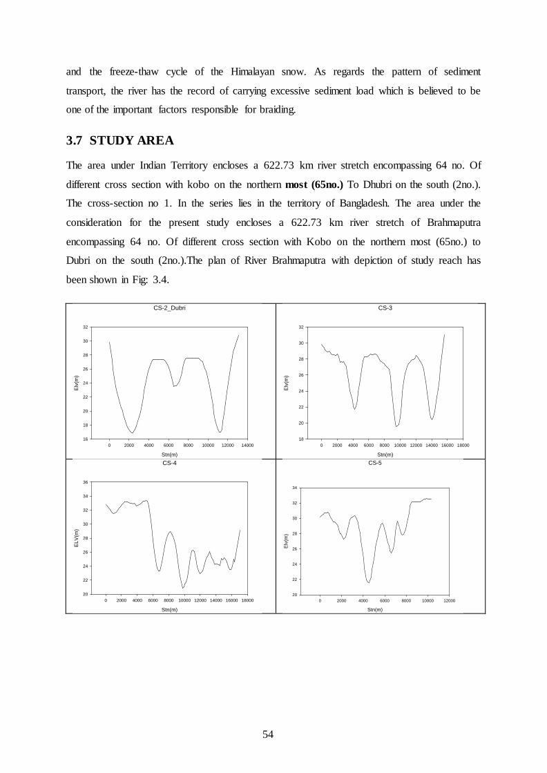
54
and the freeze-thaw cycle of the Himalayan snow. As regards the pattern of sediment
transport, the river has the record of carrying excessive sediment load which is believed to be
one of the important factors responsible for braiding.
3.7 STUDY AREA
The area under Indian Territory encloses a 622.73 km river stretch encompassing 64 no. Of
different cross section with kobo on the northern most (65no.) To Dhubri on the south (2no.).
The cross-section no 1. In the series lies in the territory of Bangladesh. The area under the
consideration for the present study encloses a 622.73 km river stretch of Brahmaputra
encompassing 64 no. Of different cross section with Kobo on the northern most (65no.) to
Dubri on the south (2no.).The plan of River Brahmaputra with depiction of study reach has
been shown in Fig: 3.4.
CS-2_Dubri
Stn(m)
0 2000 4000 6000 8000 10000 12000 14000
Elv
(m)
16
18
20
22
24
26
28
30
32
CS-3
Stn(m)
0 2000 4000 6000 8000 10000 12000 14000 16000 18000
Elv
(m)
18
20
22
24
26
28
30
32
CS-4
Stn(m)
0 2000 4000 6000 8000 10000 12000 14000 16000 18000
ELV
(m)
20
22
24
26
28
30
32
34
36
CS-5
Stn(m)
0 2000 4000 6000 8000 10000 12000
Elv
(m)
20
22
24
26
28
30
32
34

55
CS-6
Stn(m)
0 2000 4000 6000 8000 10000 12000 14000 16000
Elv
(m)
22
24
26
28
30
32
34
36
CS-7
Stn(m)
0 2000 4000 6000 8000 10000 12000 14000 16000 18000
Elv
(m)
22
24
26
28
30
32
34
CS-8
Stn(m)
0 2000 4000 6000 8000 10000
Elv
(m)
24
26
28
30
32
34
36
CS-9_Jogighopa
Stn(m)
0 500 1000 1500 2000 2500 3000
Elv
(m)
15
20
25
30
35
40
CS-10
Stn(m)
0 2000 4000 6000 8000
Elv
(m)
20
22
24
26
28
30
32
34
36
CS-15
Stn(m)
0 2000 4000 6000 8000 10000 12000 14000 16000
Elv
(m)
32
34
36
38
40
42
CS-17
Stn(m)
0 2000 4000 6000 8000 10000 12000 14000 16000
Elv
(m)
39
40
41
42
43
44
45
CS-22_Pandu
Stn(m)
0 500 1000 1500 2000 2500 3000 3500
Elv
(m)
34
36
38
40
42
44
46
48
50
52

56
Fig: 3.3. Measured cross section for different cross sections along the 622 km river reach taken between the year 1982 to 1997
CS-30
Stn(m)
0 2000 4000 6000 8000 10000 12000 14000
Elv
(m)
44
46
48
50
52
54
56
58
CS-35
Stn(m)
0 2000 4000 6000 8000 10000
Elv
(m)
45
50
55
60
65
70
CS-40
Stn(m)
0 2000 4000 6000 8000 10000 12000
Elv
(m)
64
66
68
70
72
74
76
78
CS-45
Stn(m)
0 5000 10000 15000 20000 25000
Elv
(m)
70
72
74
76
78
80
82
84
86
88
90
CS-50
Stn(m)
0 2000 4000 6000 8000
Elv
(m)
70
72
74
76
78
80
82
84
86
88
CS-55
Stn(m)
0 2000 4000 6000 8000 10000 12000 14000 16000
Elv
(m)
88
90
92
94
96
98
CS-60
Stn(m)
0 2000 4000 6000 8000 10000 12000 14000 16000
Elv
(m)
98
100
102
104
106
108
110
CS-65_Kobo
Stn(m)
0 2000 4000 6000 8000
Elv
(m)
108
110
112
114
116
118

57
One can easily figure out the significant variations in width as well as bed configuration in
general. Widths of the channel vary ranging from 3 km to 20 km. In an average width is
around 6 km in the study reach. Visualizing the cross-sections in Fig: 3.3 , it is evident that
some cross-sections are exhibiting incised channel forms whereas some showing wide
shallow river pattern indicating that bed configurations of the study reach are highly irregular
ranging from rock outcrops to fine alluvial bed. The hydraulic geometry data of 64 number
of cross section were plotted to view the general tendencies of variation of the cross section
profile in the temporal increments. The plotting reveal a very drastic changes in the cross
profiles for some of the sections. Since, the successive stations along a cross section are very
widely apart compared to the vertical variation of the ground levels the non submergible
banks are not easily discernible. The longitudinal profile (Thalweg) for the study reach gives
the idea that the reach is by a large aggrading in nature. The bed level variations from Year-
1993 to Year -1997 are highly irregular which suggests that 1 D hydraulic modelling should
be applied only for relatively long stretch of the river. In this case it should be at least above
100 km to predict longitudinal thalweg profiles.
At Pandu, the river carries an average suspended load of 402 million metric tons. A river with
such gigantic water and sediment discharge magnitudes represents its most dynamic fluvial
regime. Its large alluvial channel having a width of 6 to 17 km is, therefore, marked by
braiding, rapid aggradation and bank line changes (Sankhua, 2006). The longitudinal slope of
reach Pandu to Jogighopa is 0.11m/km (Sarma, 2006)

58
Fig: 3.4 Study Area
59
CHAPTER -4 FORMULATION AND DEVELOPMENT
OF FLOW SIMULATION MODEL

60
CHAPTER-4
FORMULATION AND DEVELOPMENT OF FLOW SIMULATION MODEL
4.1 INTRODUCTION
The global hierarchal rank of the river Brahmaputra is recognized to be third in sediment
discharge, fifth in fluvial discharge and eleventh in size of the total drainage area (Sarma,
2005). Being one of the youngest river system with varied nature of drainage areas from
snow peak mountains to lower flood valley of the Assam and the complexity exuberated by
high sediment yielding geological surfaces it has been a very formidable task to quantify all
the embodied “fluvial-river-morphological characteristics” to explain the ever changing
characteristics of the river. The high degree of braiding(Goswami and Das, 2000) of the
parent channel, more emphatically, when it open to the Assam valley because of still a steep
valley gradient the fall in the hydraulic competency due to braiding is reflected to sediment
transportation and downstream aggradation. Very unstable hydraulic geometry and hence the
river channel morphology in the spatial and temporal space hinders the formulation of an
idealised hydraulic models. Moreover, the researches and the literatures on braided channels
are less compared to single channel in alluvium region. Due to high non linearity involved in
the interdependencies of the hydrological – morphological and hydraulic parameters,
majority of relationships developed relating hydrological and hydraulic parameters are
empirical.
The river Brahmaputra is one of the rivers which are well under the observation of different
stake holders. The sediment discharges and flood discharges at certain locations have been
continuingly recorded and the river cross sections surveyed. Still, the limitation in the human
capacity, instrumentation, the ambience of the measurement and the risk involved, the actual
data acquisition often remain off-set by errors. The importance of the information that could
be derived from the analysis of the data is very high in the design, management and future
risk and hazard strategies.
Taking in to account the situation as described above, the present study is a formative attempt
to implement a flow simulation model HEC-RAS for the study reach. The algorithms
established by the researchers /modellers in the various literatures advocate success of flow
simulation model application depends on the size of the data covering wide patterns of

61
phenomena .More the data sets better is the results’ reliability. In the assessment of the
available data, data sorting, data generation supporting further analysis, modelling and
deriving inferences HEC-RAS has been known to be robust. As the technique is a data driven
model requiring gamut of data patterns representing the actual phenomena to accommodate
all the possibilities within the patterns of independent and dependent variables.
In the near future, more work with more expertise on this line would be enhancing the
dependability on the strength of the technique in the more complex analysis.
The study has been carried out on the following data sets and the area.
a) Study Stretch of the river channel (from Kobo to Dhubri) 622.73 km
b) No. of the river cross sections ( year 1988, 1992, 1993 and 1997) 65.no
c) Hydrological Data( Jogighopa-Pandu) 2003 to 2007
4.2 DATA SOURCES AND DATA TYPES
4.2.1 HYDROGRAPHIC DATA
Morpho-metric data: the reduced levels of the river cross-sections of post-monsoon period of
64 stations have been collected from the Brahmaputra Board, Government of India. The
surveying time varies from 1957 to 1997. But for the present modeling, the most current
available cross sectional data for the year 1988, 1992, 1993 and 1997 has been adopted. This
data assumed to represent the most recent cross section configuration.
4.2.2 DISCHARGE AND STAGE DATA
Discharge and stage data of the river Brahmaputra collected for two along the main river
channel cross-sections from Central Water Commission (CWC), Assam Flood Control
Department and Brahmaputra Board have constituted main data resource to the model
implementation. The length of data record used was from year 2003 to 2007.
4.2.3 SEDIMENT DATA
Sediment data obtained from the monthly suspended sediment data in respect of Jogighopa
and Pandu for the years from 2003 to 2007 and average monthly discharge (cumecs) and
monthly average suspended sediment yield of major tributaries processed for all the years
from 1993 to 1997 have been used in the study. Characteristic sediment particle size
distribution at the cross-sections was collected from CWC.

62
4.3 PRE- PROCESSING OF HYDRO GRAPHIC DATA
As a certain degree of uncertainty is associated with hydrologic frequency distributions on
relative time scales, the sensitive response function of the river / stream as Stage - Discharge
(G-Q) relationships , Sediment discharge Rating (Qt
–Q) curves, Stream flow Hydrographs,
etc needs to adequately represented from the observed field data. The Brahmaputra River
Basin in terms of its complexity calls for well-defined response models. In the study, some of
the significant steps followed are outlined as:
(i) The first step is the abstraction of outliers and errors in the data sets.
Conceptual or statistical tools as regression and curve fitting were implemented
on the variables pertaining to specific river / stream to identify the irrational
points; they were either discarded or rectified based on the earlier trends or
pattern of the data.
(ii) The datasets are then sorted strictly on a base time scale. Monthly average
record data sets pertaining to the main river are chosen for the study, the period
between November 2003 and October 2007 has been adopted as the base time
scale for the framing of the channel response parameters and the model
formulation.
4.4 DATA GENERATION
In numerical river modelling one of the most important parameter is upstream river boundary
condition. For the Brahmaputra River the only available flow data are located in the middle
reach of the main river (Pandu, at river cross section 22 and Jogigopa cross section 9).
The upstream river location is located at a river cross section 65 place called Kobo.
Therefore, using the drainage-area ratio method, flow measured at Pandu site was transferred
to Kobo site. The remaining flow at Pandu was used as internal boundary in the numerical
model.
In this process, with the help of ARCHYDRO 9 extension of ARCGIS 9.3, the drainage area
of the two gauging sites has been delineated; i.e. drainage area which is contributing for
gauging station at Pandu and drainage areas contributing for gauging site at Kobo. See Fig.
For both station the contributing drainage area has been calculated and used for generation of
upstream boundary condition. The drainage area contributing for station at Kobo has been
found to be 175862 km2 and for Pandu 345667 km2.

63
Figure showing the contributing area for Pandu and Kobo gauging stations; Developed from
90m resolution SRTM DEM.
4.5 DEVELOPMENT OF FLOW SIMULATION MODEL IN ‘HEC-RAS’
The system contains three one-dimensional hydraulic analysis components for: (1) steady
flow water surface profile computations; (2) unsteady flow simulation; and (3) movable
boundary sediment transport computations. A key element is that all three components will
use a common geometric data representation and common geometric and hydraulic
computation routines. In addition to the three hydraulic analysis components, the system
contains several hydraulic design features that can be invoked once the basic water surface
profiles are computed.
HEC-RAS is designed to perform one-dimensional hydraulic calculations for a full network
of natural and constructed channels. Theoretical basis for one-dimensional calculation in
HECRAS is briefed in chapter-2.
4.5.1 DATA REQUIREMENTS AND INPUT
The basic input data required for sedimentation analysis by HEC-RAS model can be grouped
into four categories as below.

64
4.5.1.1 Geometric Data
Geometry of the physical system is represented by cross sections, specified by coordinate
points (stations and elevations), and the distance between cross sections. Hydraulic roughness
is measured by Manning’s n-values and can vary from cross section to cross section. At each
cross section n-values may vary vertically and horizontally. The program raises or lowers
cross-section elevations to reflect deposition or scour and thus generates data during the
course of its execution.
The River System Schematic
The river system schematic is required for any geometric data set within the HEC-RAS
system. The schematic defines how the various river reaches are connected, as well as
establishing a naming convention for referencing all the other data. The river system
schematic is developed by drawing and connecting the various reaches of the system within
the geometric data editor (Fig: 4.1). It is required to develop the river system schematic
before any other data can be entered.
Each river reach on the schematic is given a unique identifier. As other data are entered, the
data are referenced to a specific reach of the schematic. For example, each cross section must
have a “River”, “Reach” and “River Station” identifier. The river and reach identifiers
defines which reach the cross section lives in, while the river station identifier defines where
that cross section is located within the reach, with respect to the other cross sections for that
reach.
Fig: 4.1 Schematic Plot of the Study Reach of Brahmaputra
River in the Program Module.
reachlength620km
6563.33
62.4444*61.625*
61605958
57.125*56.5833*
56.0833*55.2857*
54.2857*53.5714*
5352515049484746
454443
424139.375*
38373635343332
3130
29.2857*282726252322212019
1817
1615141312
11109
8765
4.16666*32
Brhamaputra
Brahamputra River Schematic plot(c/s2-c/s65)

65
The connectivity of reaches is very important in order for the model to understand how the
computations should proceed from one reach to the next. It is required to draw each reach
from upstream to downstream, in what is considered to be the positive flow direction.
Cross Section Geometry
Boundary geometry for the analysis of flow in natural streams is specified in terms of ground
surface profiles (cross sections) and the measured distances between them (reach lengths).
Cross sections are located at intervals along a stream to characterize the flow carrying
capability of the stream and its adjacent floodplain. They should extend across the entire
floodplain and should be perpendicular to the anticipated flow lines. Occasionally it is
necessary to layout cross-sections in a curved or dog-leg alignment to meet this requirement.
Every effort should be made to obtain cross sections that accurately represent the stream and
floodplain geometry.
Cross sections are required at representative locations throughout a stream reach and at
locations where changes occur in discharge, slope, shape, or roughness, at locations where
levees begin or end and at bridges or control structures such as weirs. Where abrupt changes
occur, several cross sections should be used to describe the change regardless of the distance.
Cross section spacing is also a function of stream size, slope, and the uniformity of cross
section shape. In general, large uniform rivers of flat slope normally require the fewest
number of cross sections per km. The purpose of the study also affects spacing of cross
sections. For instance, navigation studies on large relatively flat streams may require closely
spaced (e.g., 200 feet) cross sections to analyze the effect of local conditions on low flow
depths, whereas cross sections for sedimentation studies, to determine deposition in
reservoirs, may be spaced at intervals on the order of km.
The choice of friction loss equation may also influence the spacing of cross sections. For
instance, cross section spacing may be maximized when calculating an M1 profile (backwater
profile) with the average friction slope equation or when the harmonic mean friction slope
equation is used to compute M2 profiles (draw down profile). The HEC-RAS software
provides the option to let the program select the averaging equation.
Each cross section in an HEC-RAS data set is identified by a River, Reach, and River Station
label. The cross section is described by entering the station and elevation (X-Y data) from
left to right, with respect to looking in the downstream direction. The River Station identifier
may correspond to stationing along the channel, mile points, or any fictitious numbering

66
system. The numbering system must be consistent, in that the program assumes that higher
numbers are upstream and lower numbers are downstream.
Each data point in the cross section is given a station number corresponding to the horizontal
distance from a starting point on the left. Up to 500 data points may be used to describe each
cross section. Cross section data are traditionally defined looking in the downstream
direction. The program considers the left side of the stream to have the lowest station
numbers and the right side to have the highest. Cross section data are allowed to have
negative stationing values. Stationing must be entered from left to right in increasing order.
However, more than one point can have the same stationing value. The left and right stations
separating the main channel from the over bank areas must be specified on the cross section
data editor. End points of a cross section that are too low (below the computed water surface
elevation) will automatically be extended vertically and a note indicating that the cross
section had to be extended will show up in the output for that section. The program adds
additional wetted perimeter for any water that comes into contact with the extended walls.
Other data that are required for each cross section consist of: downstream reach lengths;
roughness coefficients; and contraction and expansion coefficients. These data will be
discussed in detail later in this chapter. Numerous program options are available to allow
easily adding or modifying cross section data.
Reach Lengths
The measured distances between cross sections are referred to as reach lengths. The reach
lengths for the left over bank, right over bank and channel are specified on the cross section
data editor. Channel reach lengths are typically measured along the thalweg. Over bank
reach lengths should be measured along the anticipated path of the center of mass of the over
bank flow. Often, these three lengths will be of similar value. There are, however,
conditions where they will differ significantly, such as at river bends, or where the channel
meanders and the over banks are straight. Where the distances between cross sections for
channel and over banks are different, a discharge-weighted reach length is determined based
on the discharges in the main channel and left and right over bank segments of the reach. In
the selected reach of Brahmaputra, all three lengths were taken similar values. Downstream
reach lengths as well as reach length with respect to extreme downstream station (Jogighopa)
are given in Table: 4.1
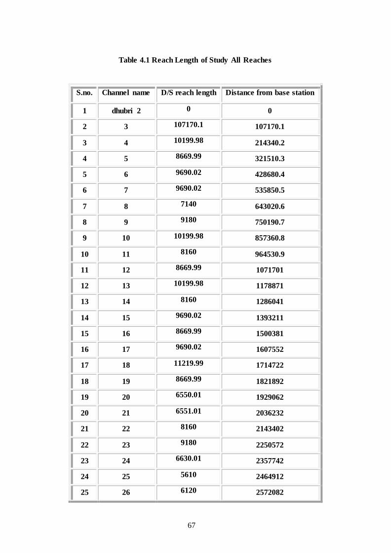
67
Table 4.1 Reach Length of Study All Reaches
S.no. Channel name D/S reach length Distance from base station
1 dhubri 2 0 0
2 3 107170.1 107170.1
3 4 10199.98 214340.2
4 5 8669.99 321510.3
5 6 9690.02 428680.4
6 7 9690.02 535850.5
7 8 7140 643020.6
8 9 9180 750190.7
9 10 10199.98 857360.8
10 11 8160 964530.9
11 12 8669.99 1071701
12 13 10199.98 1178871
13 14 8160 1286041
14 15 9690.02 1393211
15 16 8669.99 1500381
16 17 9690.02 1607552
17 18 11219.99 1714722
18 19 8669.99 1821892
19 20 6550.01 1929062
20 21 6551.01 2036232
21 22 8160 2143402
22 23 9180 2250572
23 24 6630.01 2357742
24 25 5610 2464912
25 26 6120 2572082

68
26 27 9690.02 2679253
27 28 6630.01 2786423
28 29 10719.98 2893593
29 30 10199.98 3000763
30 31 10199.98 3107933
31 32 11729.99 3215103
32 33 12750 3322273
33 34 13270 3429443
34 35 15800 3536613
35 36 15309.96 3643783
36 37 11729 3750954
37 38 12240 3858124
38 39 6630 3965294
39 40 11219.99 4072464
40 41 11219.99 4179634
41 42 8669.99 4286804
42 43 13759.99 4393974
43 44 11219.99 4501144
44 45 16320.09 4608314
45 46 14280 4715484
46 47 11219.99 4822655
47 48 9690.02 4929825
48 49 8669.99 5036995
49 50 7140 5144165
50 51 7140 5251335
51 52 7140 5358505
52 53 7140 5465675
53 54 9690 5572845

69
54 55 9180 5680015
55 56 9180 5787185
56 57 17850 5894356
57 58 11219.99 6001526
58 59 9690.02 6108696
59 60 9690.02 6215866
60 61 12750 6323036
61 62 11219.99 6430206
62 63 13260.01 6537376
63 64 8160 6644546
64 Kobo 65 5610 6751716
Energy Loss Coefficients
Several types of loss coefficients are utilized by the program to evaluate energy losses: (1)
Manning’s n values or equivalent roughness “k” values for friction loss, (2) contraction and
expansion coefficients to evaluate transition (shock) losses.
Manning’s n: Selection of an appropriate value for Manning’s n is very significant to the
accuracy of the computed water surface profiles. The value of Manning’s n is highly variable
and depends on a number of factors including: surface roughness; vegetation; channel
irregularities; channel alignment; scour and deposition; obstructions; size and shape of the
channel; stage and discharge; seasonal changes; temperature; and suspended material and bed
load.
In general, Manning’s n values should be calibrated whenever observed water surface profile
information (gage data, as well as high water marks) is available. As water surface profile
information is adequately available for the study reach, so Manning’s n values were
calibrated in fixed bed module with spatial as well as based on discharge variation and values
fed into sediment module of flow simulation for further analysis.
There is a difference in Manning's n between fixed and movable bed situations. Fixed bed n's
are values which do not depend on the characteristics of the movable boundary, movable bed

70
n's are values which may depend on the rate of sediment transport and, hence, the discharge.
Appropriate values for Manning's n were initially determined by executing HEC-RAS in
fixed bed mode, i.e., as a step-backwater program. This is necessary to properly compare
calculated water surface elevations with observed water surface profiles, with established
rating curves, during the analysis of geometric data and calibration of n values, many
program executions were required. Study reach has been subdivided into separate segments,
cross-section were interpolated to appropriate numbers and program is executed for different
value of n until computed water surface profiles at approximately matched with observed
ones. Finally, calibrated n with discharge variation and spatial variation obtained.
Changing n values with distance should be justified based on changes in vegetation, channel
form, structures, or sediment size. The technique assumes that the entire bed of the river is
stationary and does not move or change roughness during a flood event. Before focusing on
sediment transport, however, Manning’s n value for the channel is appropriate for a movable
boundary analyzed and whatever required minor adjustments, were made to ensure that the n
value for the movable portion of the cross section is in reasonable agreement with that
obtained from bed roughness predictors.
Selection of Contraction and Expansion Coefficients
Information for contraction and expansion losses is sparser than that for n values. King and
Brater (1963) give values of 0.5 and 1.0 respectively for a sudden change in area
accompanied by sharp corners, and values of 0.05 and 0.10 for the most efficient transitions.
Design values of 0.1 and 0.2 are suggested. They cite Hinds (1928) as their reference. Values
often cited by the Corps of Engineers (HEC, 1990a) are 0.1 and 0.3, contraction and
expansion respectively, for gradual transitions .So in the present study, contraction and
expansion coefficient are by default taken as 0.1 and 0.30.
4.4.1.2 Hydrologic Data
The hydrologic data consist of water discharges, temperatures and flow durations. The
discharge hydrograph is approximated by a sequence of steady inflow discharges each of
which occurs for a specified numbers of days. Water surface profiles are calculated by using
the standard step method to solve the energy equation. Friction loss is calculated by
Manning’s equation, and expansion and contraction losses will be included if the
representative loss coefficients are specified.

71
The monthly discharges at the site for the period Nov. 1993 to Nov. 1997 are used to obtain a
discharge frequency hydrographs and the gauges respective.
Steady Flow Data
Steady flow data were required in order to perform a steady water surface profile calculation
and consequently calibration of ‘n’ worked out. Steady flow data consist of flow regime,
boundary conditions and discharge information.
Boundary conditions are necessary to establish the water surface at the ends of the river
system (upstream and downstream). A starting water surface is necessary in order for the
program to begin the calculations. In a sub critical flow regime, boundary conditions are
only necessary at the downstream ends of the river system. If a supercritical flow regime is
going to be calculated, boundary conditions are only necessary at the upstream ends of the
river system. If a mixed flow regime calculation is going to be made, then boundary
conditions must be entered at all ends of the river system. Observed monthly flow profile
were fed as input in different cross-section segmental reach and program were run separately
to compute water surface elevation at d/s and compared with observed one to estimate n .
Quasi-unsteady Flow Data
Current sediment capabilities in HEC-RAS are based on quasi-unsteady hydraulics. The
quasi-unsteady approach approximates a flow hydrograph by a series of steady flow profiles
associated with corresponding flow durations. Boundary conditions were flow series (flow
hydrograph) at upstream boundary(c/s-65 Kobo). At downstream boundary(c/s-2 at Dubri
site), stage time series /rating curve applied. The stage -time series boundary condition allows
inputting a time series of stages at the downstream boundary.
As sensitive inputs to the Model boundary values, the Stage-Discharge relations, the G-Q
relations of the major rivers/ streams under consideration needs to sufficiently dictate the
hydraulic behavior,.

72
Fig 4.2 Simulation Hydrograph generated at c/s-65 (Kobo Site)
Stage-Discharge Relation at extreme d/s boundary of reach is plotted in Fig: 4.4, similarly
Discharge hydrograph at extreme u/s boundary is also plotted in Fig 4.3 which has also been
taken as inputs for simulating flow for specific period. Lateral flow series at Jogighopa site
shown in Fig 4.4.
Fig: 4.3 Stage – Discharge Relation at c/s-9(Jogighopa site)
May Nov May Nov May Nov May Nov2004 2005 2006 2007
0
5000
10000
15000
20000
25000
30000Hydrograph Data
Date
Flow
Legend
Flow Duration

73
Fig 4.4 Stage Series at c/s-9(Jogighopa site)
4.4.1.3 Sediment Data
The sediment data consist of inflowing sediment load data, gradation of material in the
stream bed and information about sediment properties. The inflowing sediment load is related
to water discharge by a rating table at the upstream end of the model.
Sediment mixtures are classified by grain size using the American Geophysical union scale.
The program accommodates clay (up to 0.004 mm), four classes of silt (0.004 – 0.0625 mm),
five classes of sand (very fine sand 0.0625 mm to very course sand 0.2 mm) and five classes
of gravel (very fine gravel 0.2mm to very coarse gravel 0.64mm).Sediment transport capacity
is calculated at each cross section by using hydraulic data obtained during the calculation of
water surface profiles and the gradation of bed material for that cross section.
The variations in the sediment load discharge with the flow is calibrated from the Sediment
Discharge Rating Curves and entered to the model input.
Each cross-section must have an associated bed gradation. Possession of data in regard to bed
material for all cross section couldn’t be done. But character of bed material within the study
reach can presumed to be similar in nature so far sediment transport is concerned. Bed
material gradation at cross section -2 (Dhubri) is taken as representative bed gradation (Fig:
4.5) through out the alluvial study reach except where outcrops were present.
26
28
30
32
34
36No
v-93
Mar
-94
Jun-
94
Sep-
94
Jan-
95
Apr-9
5
Jul-9
5
Oct
-95
Feb-
96
May
-96
Aug-
96
Dec-
96
Mar
-97
Jun-
97
Sep-
97
Jan-
98
Simulation Period
Stag
e(m
)
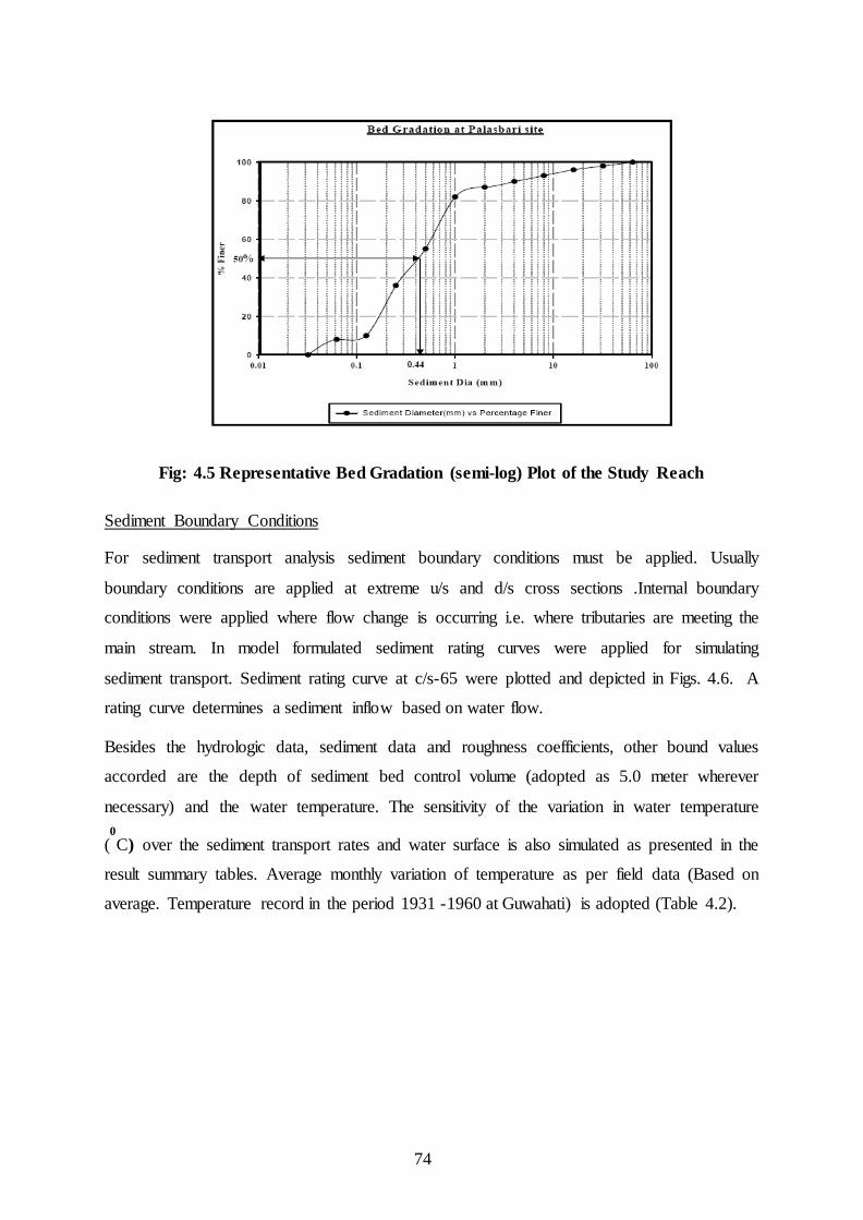
74
Fig: 4.5 Representative Bed Gradation (semi-log) Plot of the Study Reach
Sediment Boundary Conditions
For sediment transport analysis sediment boundary conditions must be applied. Usually
boundary conditions are applied at extreme u/s and d/s cross sections .Internal boundary
conditions were applied where flow change is occurring i.e. where tributaries are meeting the
main stream. In model formulated sediment rating curves were applied for simulating
sediment transport. Sediment rating curve at c/s-65 were plotted and depicted in Figs. 4.6. A
rating curve determines a sediment inflow based on water flow.
Besides the hydrologic data, sediment data and roughness coefficients, other bound values
accorded are the depth of sediment bed control volume (adopted as 5.0 meter wherever
necessary) and the water temperature. The sensitivity of the variation in water temperature
(0C) over the sediment transport rates and water surface is also simulated as presented in the
result summary tables. Average monthly variation of temperature as per field data (Based on
average. Temperature record in the period 1931 -1960 at Guwahati) is adopted (Table 4.2).

75
Fig: 4.6 Sediment Rating Curve at c/s-22 (Pandu Site)
Table: 4.2 Average Monthly Temperature Variations
S.N. Month Average Temperature(°C)
1 January 17.5 2 February 19.55 3 March 23.35 4 April 25.95 5 May 26.9 6 June 28.1 7 July 28.95 8 August 29 9 September 28.65 10 October 26.25 11 November 22.3 12 December 18.7
4.4.2 PROGRAM ORGANISATION
The HEC-RAS program in its present form has been organized into two major modules.
Modules run with various sub-programs where data have been transferred for specific output
generation. The functional flowchart of the program is shown in Fig. 4.8
1 10 100 1000 10000 1000001
10
100
1000
10000
100000
1000000Sediment Load Series
Flow
Load
Legend
Load Duration

76
4.4.2.1 Hydrodynamic modeling and calibration of ‘n’. (Steady flow analysis)[First
Module]
Roughness Coefficients
Roughness coefficients are one of the main variables used in calibrating a hydraulic model.
Generally, for a free flowing river, roughness decreases with increased stage and flow
However, if the banks of a river are rougher than the channel bottom (due to trees and
brushes), then the composite n value will increase with increased stage. Sediment and debris
can also play an important role in changing the roughness. More sediment and debris in a
river will require the modeler to use higher n values in order to match observed water
surfaces.
4.4.2.2 Sediment Transport Analysis (Quasi-unsteady flow analysis) [Second Module]
The outputs obtained from first module were to be applied in this module for calibration and
testing of the model. Calibrated value of roughness parameter n from first module gave the
idea of n and its relation with discharge and also its variation with distance. With slight
processing the calibrated set of Manning’s n were fed into sediment module. In this module
the whole study reach were taken as geometric data i.e. Cross-section-65 (Kobo) to cross-
section -2 (Dhubri). Some intermediate cross-sections were linearly interpolated to assure
stability to running of the module.
Other sediment data like representative bed gradation at each cross-section /sediment inflow
at u/s locations as well as flow change locations were fed into the module. Flow series at u/s
boundary and lateral flow series at internal boundaries as well as stage series at d/s is fed into
the module. Simulation plans for varying sediment predictors as well as different time series
were designated and executed and outputs were obtained. A detailed discussion on outputs
will be done in the consecutive chapter.

77
Fig 4.7 Sediment Transport Analysis and Prediction of water surface profile for
Nov2003 and July2004 (C/s-2 to C/s-65)
0 100000 200000 300000 400000 500000 600000 7000000
20
40
60
80
100
120
Rev3_1D_Sedmod_Brahmaputra Plan: 1) kobo3 16-03-2011
Main Channel Distance (m)
Ele
vatio
n (
m)
Legend
EG 23Jul2004 0000
WS 23Jul2004 0000
EG 28Nov2003 0000
WS 28Nov2003 0000
Crit 23Jul2004 0000
Crit 28Nov2003 0000
Ground
Brhamaputra reachlength620km
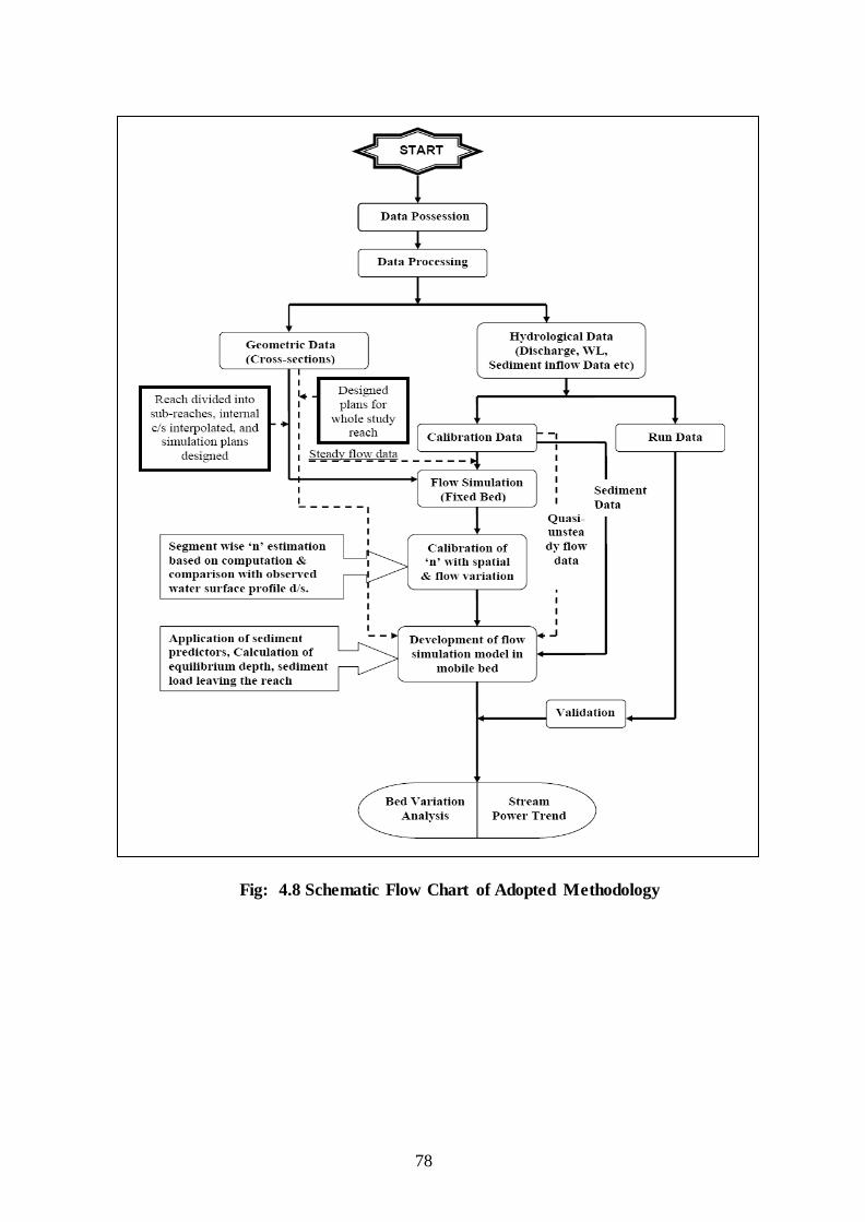
78
Fig: 4.8 Schematic Flow Chart of Adopted Methodology

79
CHAPTER -5 RESULTS AND DISCUSSIONS
80
CHAPTER-5
RESULTS AND DISCUSSIONS 5.1 INTRODUCTION Flow simulation is done on the 1D mathematical model HEC-RAS in the study reach of
Brahmaputra Rive. The manning’s roughness coefficient is calibrated and assessment of
stream power, rating curves and consequently sediment transport analysis is done with
application of various available sediment predictors to assess aggradations/degradations
within the reach. Temporal unit stream power variations with correlation to slope variation
are also dealt. The results obtained are discussed in detail herein after.
5.2 BED ROUGHNESS CALIBRATION
Observed flow series of year 2004 at Jogighpa and Pandu is used to calibrate manning’s
roughness coefficient. The calibration is done for range of flows for each month. And hence
roughness variation for high and low flows is accounted for (Fig. 5.1). For this process steady
flow condition is used and observed water surface is matched with calculated one.
It can be observed that, the seasonal variation of manning’s roughness is higher in non
monsoon period (low flow) and lower monsoon period (high flow). This trend is in
agreement with observed results in major alluvial rivers (Fig. 5.2.).
It is also observed that roughness varies within the same month; but since the seasonal
variation is more pronounced, seasonal value is adopted for qausi-unsteady sediment
transport analysis in HEC-RAS model.
The capability of HEC-RAS to accommodate seasonal roughness variation within a one full
year cycle is applied. The subsequent sediment transport analysis will be discussed in the
coming topics.

81
Fig.5.1. Seasonal roughness variation after model calibration
Fig.5.2. Seasonal roughness variation vs. high flow used for calibration.
5.3 SEDIMENT TRANSPORT ANALYSIS, HEC-RAS
Using the calibrated Manning’s roughness value, mobile bed sediment transport is done for
the year Nov28, 2003 to Sept30, 2007. The analysis is preformed using Ackers – White,
Engelund-Hansen and Yang’s sediment transport function. The reason this functions are
Seasonal RoughnessVariation
Year 2004
Dec Jan Feb Mar Apr May Jun Jul Aug Sep Oct Nov Dec Jan
Man
ning's
'n'
0.01
0.02
0.03
0.04
0.05
0.06
time vs 'n' for high flow time vs 'n' for low flow
Flow vs Roughness Seasonal Sariation
Year 2004
Dec Jan Feb Mar Apr May Jun Jul Aug Sep Oct Nov Dec Jan
Q(m^
3/s) a
nd n/
1000
000
0
20000
40000
60000
80000
Time vs HighFlow (Q)Time vs 'n' for corresponding Q

82
selected is that the range of input values they used in developing their equations encompass
the situation in Brahmaputra River and also due to their wide range of applicability. Ackers –
White is developed in flume for overall particle diameter of 0.04-7mm and Yang developed
his equation based on filed observation of overall particle diameter of 0.15-1.7mm, which
bases transport on Stream Power, the product of velocity and shear stress. Engelund-Hansen
is developed based on flume data for particle mean diameter of 0.19mm to 0.93mm. It has
been extensively tested and found to be fairly consistent with field data (HEC-RAS, manual,
2010). To see the comparison for this study average mean particle diameter of 0.44mm is
used. The Ackers-White transport function is a total load function developed under the
assumption that fine sediment transport is best related to the turbulent fluctuations in the
water column and coarse sediment transport is best related to the net grain shear with the
mean velocity used as the representative variable. The transport function was developed in
terms of particle size, mobility, and transport. See Chapter 2 for further discussion.
It should be noted that the value adopted here is based on sediment gradation data collected in
the middle reach of the river (Plasibari). Hence it is assumed that it represents the whole
reach.
The analysis is performed using upstream boundary condition of Equilibrium Load option;
this is due to lack of verified rating curve at Cross Section 65. HEC-RAS computes sediment
transport capacity, for each time step, at this cross section and this will be used as the
sediment inflow. Since load is set equal to capacity for each grain size, there will no be
aggradation or degradation at this cross section.
The output from the above three sediment transport function will be discussed here under.
The discussion will focus on the overall sediment deposition or erosion and hence the
aggradation and degradation of bed level over the analysis period of 2003 to 2007.
Bed level change of + 5cm will be considered as fairly stable cross section in this analysis.
5.3.1 ACKERS – WHITE SEDIMENT TRANSPORT ANALYSIS OUTPUT As can be seen in the figure below, the river bed is exhibiting variation in time in the pattern
of aggradation or degradation. The output of this analysis clearly shows that aggradation and
degradation occurring simultaneously in different portion of the river reach. And also it can
be observed that in some cross sections there is pure aggradation or degradation trend over
the year 2003 to 2007; where as in some there is occurrence of both aggradation(e.g. CS62)
and degradation(e.g. CS63) over the simulation period (e.g. CS 60, 58, 53, 46) for example.

83
FebMayAug Nov FebMayAugNov FebMayAug Nov FebMayAug2004 2005 2006 2007
104.92
104.94
104.96
104.98
105.00
105.02
i:\Dissertation material\NDMA Report\NDMA_RAS_MODEL\S.Transport_model\Acker-whi_equlb\RAS_Brahmaputra.sed04
Time
Ch
Inve
rt E
l (m
)
Legend
Ch Invert El (m)
Simulation
FebMayAug Nov FebMayAugNov FebMayAug Nov FebMayAug2004 2005 2006 2007
101.4
101.6
101.8
102.0
102.2
102.4
i:\Dissertation material\NDMA Report\NDMA_RAS_MODEL\S.Transport_model\Acker-whi_equlb\RAS_Brahmaputra.sed04
Time
Ch
Inve
rt E
l (m
)
Legend
Ch Invert El (m)
Simulation
FebMayAug Nov FebMayAugNov FebMayAug Nov FebMayAug2004 2005 2006 2007
98.8
98.9
99.0
99.1
99.2
99.3
i:\Dissertation material\NDMA Report\NDMA_RAS_MODEL\S.Transport_model\Acker-whi_equlb\RAS_Brahmaputra.sed04
Time
Ch
Inve
rt E
l (m
)
Legend
Ch Invert El (m)
Simulation
FebMayAug Nov FebMayAugNov FebMayAug Nov FebMayAug2004 2005 2006 2007
93.4
93.5
93.6
93.7
93.8
93.9
i:\Dissertation material\NDMA Report\NDMA_RAS_MODEL\S.Transport_model\Acker-whi_equlb\RAS_Brahmaputra.sed04
Time
Ch
Inve
rt E
l (m
)
Legend
Ch Invert El (m)
Simulation
FebMayAug Nov FebMayAugNov FebMayAug Nov FebMayAug2004 2005 2006 2007
84.68
84.70
84.72
84.74
84.76
84.78
84.80
i:\Dissertation material\NDMA Report\NDMA_RAS_MODEL\S.Transport_model\Acker-whi_equlb\RAS_Brahmaputra.sed04
Time
Ch
Inve
rt E
l (m
)
Legend
Ch Invert El (m)
Simulation
FebMayAug Nov FebMayAugNov FebMayAug Nov FebMayAug2004 2005 2006 2007
81.2
81.4
81.6
81.8
82.0
82.2
82.4
82.6
i:\Dissertation material\NDMA Report\NDMA_RAS_MODEL\S.Transport_model\Acker-whi_equlb\RAS_Brahmaputra.sed04
Time
Ch
Inve
rt E
l (m
)
Legend
Ch Invert El (m)
Simulation
FebMayAug Nov FebMayAugNov FebMayAug Nov FebMayAug2004 2005 2006 2007
79.96
79.98
80.00
80.02
80.04
80.06
80.08
80.10
i:\Dissertation material\NDMA Report\NDMA_RAS_MODEL\S.Transport_model\Acker-whi_equlb\RAS_Brahmaputra.sed04
Time
Ch
Inve
rt E
l (m
)
Legend
Ch Invert El (m)
Simulation
FebMayAug Nov FebMayAugNov FebMayAug Nov FebMayAug2004 2005 2006 2007
68.6
68.7
68.8
68.9
69.0
i:\Dissertation material\NDMA Report\NDMA_RAS_MODEL\S.Transport_model\Acker-whi_equlb\RAS_Brahmaputra.sed04
Time
Ch
Inve
rt E
l (m
)
Legend
Ch Invert El (m)
Simulation
FebMayAug Nov FebMayAugNov FebMayAug Nov FebMayAug2004 2005 2006 2007
71.90
71.92
71.94
71.96
71.98
72.00
72.02
72.04
i:\Dissertation material\NDMA Report\NDMA_RAS_MODEL\S.Transport_model\Acker-whi_equlb\RAS_Brahmaputra.sed04
Time
Ch
Inve
rt E
l (m
)
Legend
Ch Invert El (m)
Simulation
FebMayAug Nov FebMayAugNov FebMayAug Nov FebMayAug2004 2005 2006 2007
73.96
73.98
74.00
74.02
74.04
74.06
74.08
i:\Dissertation material\NDMA Report\NDMA_RAS_MODEL\S.Transport_model\Acker-whi_equlb\RAS_Brahmaputra.sed04
Time
Ch
Inve
rt E
l (m
)
Legend
Ch Invert El (m)
Simulation
FebMayAug Nov FebMayAugNov FebMayAug Nov FebMayAug2004 2005 2006 2007
70.5
71.0
71.5
72.0
72.5
73.0
73.5
i:\Dissertation material\NDMA Report\NDMA_RAS_MODEL\S.Transport_model\Acker-whi_equlb\RAS_Brahmaputra.sed04
Time
Ch
Inve
rt E
l (m
)
Legend
Ch Invert El (m)
Simulation
FebMayAug Nov FebMayAugNov FebMayAug Nov FebMayAug2004 2005 2006 2007
66.5
67.0
67.5
68.0
68.5
69.0
i:\Dissertation material\NDMA Report\NDMA_RAS_MODEL\S.Transport_model\Acker-whi_equlb\RAS_Brahmaputra.sed04
Time
Ch
Inve
rt E
l (m
)
Legend
Ch Invert El (m)
Simulation
FebMayAug Nov FebMayAugNov FebMayAug Nov FebMayAug2004 2005 2006 2007
67.2
67.3
67.4
67.5
67.6
67.7
67.8
67.9
i:\Dissertation material\NDMA Report\NDMA_RAS_MODEL\S.Transport_model\Acker-whi_equlb\RAS_Brahmaputra.sed04
Time
Ch
Inve
rt E
l (m
)
Legend
Ch Invert El (m)
Simulation
FebMayAug Nov FebMayAugNov FebMayAug Nov FebMayAug2004 2005 2006 2007
65.2
65.4
65.6
65.8
66.0
66.2
66.4
i:\Dissertation material\NDMA Report\NDMA_RAS_MODEL\S.Transport_model\Acker-whi_equlb\RAS_Brahmaputra.sed04
Time
Ch
Inve
rt E
l (m
)
Legend
Ch Invert El (m)
Simulation
FebMayAug Nov FebMayAugNov FebMayAug Nov FebMayAug2004 2005 2006 2007
64.0
64.2
64.4
64.6
64.8
i:\Dissertation material\NDMA Report\NDMA_RAS_MODEL\S.Transport_model\Acker-whi_equlb\RAS_Brahmaputra.sed04
Time
Ch
Inve
rt E
l (m
)
Legend
Ch Invert El (m)
Simulation
CS 44 CS 43 CS 42
CS 45 CS 46 CS 48
CS 52 CS 50 CS 49
CS 58 CS 54 CS 53
CS 63 CS 62 CS 60

84
FebMayAug Nov FebMayAugNov FebMayAug Nov FebMayAug2004 2005 2006 2007
61.8
62.0
62.2
62.4
62.6
62.8
63.0
i:\Dissertation material\NDMA Report\NDMA_RAS_MODEL\S.Transport_model\Acker-whi_equlb\RAS_Brahmaputra.sed04
Time
Ch
Inve
rt E
l (m
)
Legend
Ch Invert El (m)
Simulation
FebMayAug Nov FebMayAugNov FebMayAug Nov FebMayAug2004 2005 2006 2007
60.02
60.04
60.06
60.08
60.10
i:\Dissertation material\NDMA Report\NDMA_RAS_MODEL\S.Transport_model\Acker-whi_equlb\RAS_Brahmaputra.sed04
Time
Ch
Inve
rt E
l (m
)
Legend
Ch Invert El (m)
Simulation
FebMayAug Nov FebMayAugNov FebMayAug Nov FebMayAug2004 2005 2006 2007
50.24
50.25
50.26
50.27
50.28
50.29
50.30
50.31
50.32
50.33
i:\Dissertation material\NDMA Report\NDMA_RAS_MODEL\S.Transport_model\Acker-whi_equlb\RAS_Brahmaputra.sed04
Time
Ch
Inve
rt E
l (m
)
Legend
Ch Invert El (m)
Simulation
FebMayAug Nov FebMayAugNov FebMayAug Nov FebMayAug2004 2005 2006 2007
53.50
53.55
53.60
53.65
53.70
i:\Dissertation material\NDMA Report\NDMA_RAS_MODEL\S.Transport_model\Acker-whi_equlb\RAS_Brahmaputra.sed04
Time
Ch
Inve
rt E
l (m
)
Legend
Ch Invert El (m)
Simulation
FebMayAug Nov FebMayAugNov FebMayAug Nov FebMayAug2004 2005 2006 2007
37.0
37.2
37.4
37.6
37.8
38.0
i:\Dissertation material\NDMA Report\NDMA_RAS_MODEL\S.Transport_model\Acker-whi_equlb\RAS_Brahmaputra.sed04
Time
Ch
Inve
rt E
l (m
)
Legend
Ch Invert El (m)
Simulation
FebMayAug Nov FebMayAugNov FebMayAug Nov FebMayAug2004 2005 2006 2007
49.4
49.5
49.6
49.7
49.8
49.9
i:\Dissertation material\NDMA Report\NDMA_RAS_MODEL\S.Transport_model\Acker-whi_equlb\RAS_Brahmaputra.sed04
Time
Ch
Inve
rt E
l (m
)
Legend
Ch Invert El (m)
Simulation
FebMayAug Nov FebMayAugNov FebMayAug Nov FebMayAug2004 2005 2006 2007
45.24
45.26
45.28
45.30
45.32
45.34
45.36
45.38
i:\Dissertation material\NDMA Report\NDMA_RAS_MODEL\S.Transport_model\Acker-whi_equlb\RAS_Brahmaputra.sed04
Time
Ch
Inve
rt E
l (m
)
Legend
Ch Invert El (m)
Simulation
FebMayAug Nov FebMayAugNov FebMayAug Nov FebMayAug2004 2005 2006 2007
42.2
42.3
42.4
42.5
42.6
42.7
42.8
42.9
43.0
i:\Dissertation material\NDMA Report\NDMA_RAS_MODEL\S.Transport_model\Acker-whi_equlb\RAS_Brahmaputra.sed04
Time
Ch
Inve
rt E
l (m
)
Legend
Ch Invert El (m)
Simulation
FebMayAug Nov FebMayAugNov FebMayAug Nov FebMayAug2004 2005 2006 2007
42.3
42.4
42.5
42.6
42.7
42.8
42.9
43.0
i:\Dissertation material\NDMA Report\NDMA_RAS_MODEL\S.Transport_model\Acker-whi_equlb\RAS_Brahmaputra.sed04
Time
Ch
Inve
rt E
l (m
)
Legend
Ch Invert El (m)
Simulation
FebMayAug Nov FebMayAugNov FebMayAug Nov FebMayAug2004 2005 2006 2007
38.0
38.5
39.0
39.5
40.0
40.5
41.0
41.5
i:\Dissertation material\NDMA Report\NDMA_RAS_MODEL\S.Transport_model\Acker-whi_equlb\RAS_Brahmaputra.sed04
Time
Ch
Inve
rt E
l (m
)
Legend
Ch Invert El (m)
Simulation
FebMayAug Nov FebMayAugNov FebMayAug Nov FebMayAug2004 2005 2006 2007
35.98
35.99
36.00
36.01
36.02
36.03
36.04
i:\Dissertation material\NDMA Report\NDMA_RAS_MODEL\S.Transport_model\Acker-whi_equlb\RAS_Brahmaputra.sed04
Time
Ch
Inve
rt E
l (m
)
Legend
Ch Invert El (m)
Simulation
FebMayAug Nov FebMayAugNov FebMayAug Nov FebMayAug2004 2005 2006 2007
35.2
35.3
35.4
35.5
35.6
35.7
35.8
i:\Dissertation material\NDMA Report\NDMA_RAS_MODEL\S.Transport_model\Acker-whi_equlb\RAS_Brahmaputra.sed04
Time
Ch
Inve
rt E
l (m
)
Legend
Ch Invert El (m)
Simulation
FebMayAug Nov FebMayAugNov FebMayAug Nov FebMayAug2004 2005 2006 2007
28.4
28.6
28.8
29.0
29.2
29.4
29.6
29.8
30.0
i:\Dissertation material\NDMA Report\NDMA_RAS_MODEL\S.Transport_model\Acker-whi_equlb\RAS_Brahmaputra.sed04
Time
Ch
Inve
rt E
l (m
)
Legend
Ch Invert El (m)
Simulation
FebMayAug Nov FebMayAugNov FebMayAug Nov FebMayAug2004 2005 2006 2007
33.34
33.35
33.36
33.37
33.38
33.39
i:\Dissertation material\NDMA Report\NDMA_RAS_MODEL\S.Transport_model\Acker-whi_equlb\RAS_Brahmaputra.sed04
Time
Ch
Inve
rt E
l (m
)
Legend
Ch Invert El (m)
Simulation
FebMayAug Nov FebMayAugNov FebMayAug Nov FebMayAug2004 2005 2006 2007
33.10
33.15
33.20
33.25
33.30
i:\Dissertation material\NDMA Report\NDMA_RAS_MODEL\S.Transport_model\Acker-whi_equlb\RAS_Brahmaputra.sed04
Time
Ch
Inve
rt E
l (m
)
Legend
Ch Invert El (m)
Simulation
CS 20 CS 19 CS 18
CS 29 CS 25 CS 22
CS 32 CS 31 CS 30
CS 36 CS 34 CS 37
CS 41 CS 39 CS 38

85
Fig.5.3. variation of bed change for individual cross section over the simulation period based on
Acker-White sediment transport function
Sediment transport function is directly dependent on parameters like mean sediment particle
size, velocity, shear stress and flow pattern in the channel. Figure 5.4 shows that bed change
over high flow and low flow. It is observed that the bed is eroding in high flow period and
deposition is taking place over low flow periods.
Fig. 5.4 bed level change vs water surface elevation
FebMayAug Nov FebMayAugNov FebMayAug Nov FebMayAug2004 2005 2006 2007
17.15
17.20
17.25
17.30
17.35
17.40
17.45
17.50
i:\Dissertation material\NDMA Report\NDMA_RAS_MODEL\S.Transport_model\Acker-whi_equlb\RAS_Brahmaputra.sed04
Time
Ch
Inve
rt E
l (m
)
Legend
Ch Invert El (m)
Simulation
FebMayAug Nov FebMayAugNov FebMayAug Nov FebMayAug2004 2005 2006 2007
18.96
18.97
18.98
18.99
19.00
19.01
19.02
19.03
i:\Dissertation material\NDMA Report\NDMA_RAS_MODEL\S.Transport_model\Acker-whi_equlb\RAS_Brahmaputra.sed04
Time
Ch
Inve
rt E
l (m
)
Legend
Ch Invert El (m)
Simulation
FebMayAug Nov FebMayAugNov FebMayAug Nov FebMayAug2004 2005 2006 2007
100
102
104
106
108
110
112
114
i:\Dissertation material\NDMA Report\NDMA_RAS_MODEL\S.Transport_model\Acker-whi_equlb\RAS_Brahmaputra.sed04
Time
Ch
Inve
rt E
l (m
),Wse
l (m
)
Legend
Wsel (m)
Ch Invert El (m)
Simulation
FebMayAug Nov FebMayAugNov FebMayAug Nov FebMayAug2004 2005 2006 2007
92
94
96
98
100
102
104
106
i:\Dissertation material\NDMA Report\NDMA_RAS_MODEL\S.Transport_model\Acker-whi_equlb\RAS_Brahmaputra.sed04
Time
Ch
Inve
rt E
l (m
),Wse
l (m
)
Legend
Wsel (m)
Ch Invert El (m)
Simulation
FebMayAug Nov FebMayAugNov FebMayAug Nov FebMayAug2004 2005 2006 2007
66
68
70
72
74
76
78
80
82
i:\Dissertation material\NDMA Report\NDMA_RAS_MODEL\S.Transport_model\Acker-whi_equlb\RAS_Brahmaputra.sed04
Time
Ch
Inve
rt E
l (m
),Wse
l (m
)
Legend
Wsel (m)
Ch Invert El (m)
Simulation
FebMayAug Nov FebMayAugNov FebMayAug Nov FebMayAug2004 2005 2006 2007
64
66
68
70
72
74
76
78
i:\Dissertation material\NDMA Report\NDMA_RAS_MODEL\S.Transport_model\Acker-whi_equlb\RAS_Brahmaputra.sed04
Time
Ch
Inve
rt E
l (m
),Wse
l (m
)
Legend
Wsel (m)
Ch Invert El (m)
Simulation
FebMayAug Nov FebMayAugNov FebMayAug Nov FebMayAug2004 2005 2006 2007
35
40
45
50
55
60
65
i:\Dissertation material\NDMA Report\NDMA_RAS_MODEL\S.Transport_model\Acker-whi_equlb\RAS_Brahmaputra.sed04
Time
Ch
Inve
rt E
l (m
),Wse
l (m
)
Legend
Wsel (m)
Ch Invert El (m)
Simulation
FebMayAug Nov FebMayAugNov FebMayAug Nov FebMayAug2004 2005 2006 2007
34
36
38
40
42
44
46
48
50
52
i:\Dissertation material\NDMA Report\NDMA_RAS_MODEL\S.Transport_model\Acker-whi_equlb\RAS_Brahmaputra.sed04
Time
Ch
Inve
rt E
l (m
),Wse
l (m
)
Legend
Wsel (m)
Ch Invert El (m)
Simulation
FebMayAug Nov FebMayAugNov FebMayAug Nov FebMayAug2004 2005 2006 2007
25
30
35
40
45
50
55
i:\Dissertation material\NDMA Report\NDMA_RAS_MODEL\S.Transport_model\Acker-whi_equlb\RAS_Brahmaputra.sed04
Time
Ch
Inve
rt E
l (m
),Wse
l (m
)
Legend
Wsel (m)
Ch Invert El (m)
Simulation
FebMayAug Nov FebMayAugNov FebMayAug Nov FebMayAug2004 2005 2006 2007
32
34
36
38
40
42
44
46
48
i:\Dissertation material\NDMA Report\NDMA_RAS_MODEL\S.Transport_model\Acker-whi_equlb\RAS_Brahmaputra.sed04
Time
Ch
Inve
rt E
l (m
),Wse
l (m
)
Legend
Wsel (m)
Ch Invert El (m)
Simulation
FebMayAug Nov FebMayAugNov FebMayAug Nov FebMayAug2004 2005 2006 2007
15
20
25
30
35
40
i:\Dissertation material\NDMA Report\NDMA_RAS_MODEL\S.Transport_model\Acker-whi_equlb\RAS_Brahmaputra.sed04
Time
Ch
Inve
rt E
l (m
),Wse
l (m
)
Legend
Wsel (m)
Ch Invert El (m)
Simulation
CS 9
CS 20 CS 18 CS 9
CS 43 CS 36 CS 22
CS 62 CS 58 CS 45
CS 8

86
And it is also observed that when the discharge increases, velocity and shear stress in the
channel increase and hence bed level change is the result (Fig. 5.5). In figure 5.5, velocity,
flow and shear stress pattern changing in tandem is shown.
Fig. 5.5 bed level change vs channel shear stress and velocity
5.3.2 YANG TRANSPORT ANALYSIS OUTPUT
Similarly the sediment analysis is performed using Yang’s sediment transport function. Here
also the general trend is more or less the same as that of result obtained from Acker-White
sediment transport function. But the major difference is observed in the extent of aggradation
and degradation observed.
In Yang’ sediment transport function the observed bed change variation is minimal compared
to the above method. As can be observed in figure 5.6, the number of cross section which
shows bed change variation in the range of ±5cm has greatly decreased. 12 compared to 32
observed in Acker-White sediment transport predictor.
61 56 54
FebMayAugNovFebMayAugNovFebMayAugNovFebMayAug2004 2005 2006 2007
0
5
10
15
20
25
30
i:\Dissertation material\NDMA Report\NDMA_RAS_MODEL\S.Transport_model\Acker-whi_equlb\RAS_Brahmaputra.sed04
Time
Ch
Inve
rt E
l (m
),Vel
ocity
(m/s
),She
ar S
tress
(pa)
Legend
Ch Invert El (m)
Velocity (m/s)
Shear Stress (pa)
Simulation
FebMayAugNovFebMayAugNovFebMayAugNovFebMayAug2004 2005 2006 2007
0
5
10
15
20
25
30
35
40
i:\Dissertation material\NDMA Report\NDMA_RAS_MODEL\S.Transport_model\Acker-whi_equlb\RAS_Brahmaputra.sed04
Time
Ch
Inve
rt E
l (m
),Vel
ocity
(m/s
),She
ar S
tress
(pa)
Legend
Ch Invert El (m)
Velocity (m/s)
Shear Stress (pa)
Simulation
FebMayAugNovFebMayAugNovFebMayAugNovFebMayAug2004 2005 2006 2007
0
10
20
30
40
50
60
70
i:\Dissertation material\NDMA Report\NDMA_RAS_MODEL\S.Transport_model\Acker-whi_equlb\RAS_Brahmaputra.sed04
Time
Ch
Inve
rt E
l (m
),Vel
ocity
(m/s
),She
ar S
tress
(pa)
Legend
Ch Invert El (m)
Velocity (m/s)
Shear Stress (pa)
Simulation
FebMayAug Nov FebMayAugNov FebMayAug Nov FebMayAug2004 2005 2006 2007
101.90
101.92
101.94
101.96
101.98
102.00
102.02
i:\Dissertation material\NDMA Report\NDMA_RAS_MODEL\S.Transport_model\Yang_Equlb\RAS_Brahmaputra.sed04
Time
Ch
Inve
rt E
l (m
)
Legend
Ch Invert El (m)
Simulation
FebMayAug Nov FebMayAugNov FebMayAug Nov FebMayAug2004 2005 2006 2007
91.93
91.94
91.95
91.96
91.97
91.98
91.99
i:\Dissertation material\NDMA Report\NDMA_RAS_MODEL\S.Transport_model\Yang_Equlb\RAS_Brahmaputra.sed04
Time
Ch
Inve
rt E
l (m
)
Legend
Ch Invert El (m)
Simulation
FebMayAug Nov FebMayAugNov FebMayAug Nov FebMayAug2004 2005 2006 2007
84.72
84.73
84.74
84.75
84.76
84.77
84.78
84.79
i:\Dissertation material\NDMA Report\NDMA_RAS_MODEL\S.Transport_model\Yang_Equlb\RAS_Brahmaputra.sed04
Time
Ch
Inve
rt E
l (m
)
Legend
Ch Invert El (m)
Simulation
CS 43 CS 22 CS 20
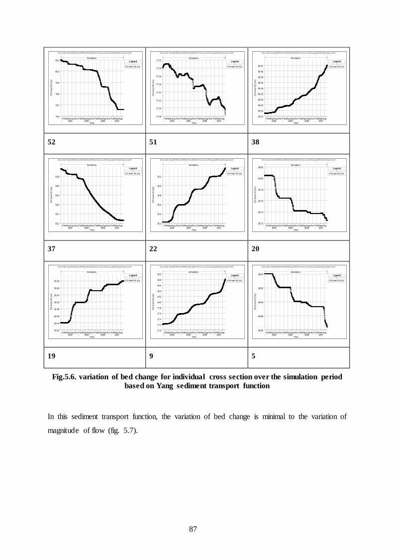
87
52 51 38
37 22 20
19 9 5
Fig.5.6. variation of bed change for individual cross section over the simulation period based on Yang sediment transport function
In this sediment transport function, the variation of bed change is minimal to the variation of
magnitude of flow (fig. 5.7).
FebMayAug Nov FebMayAugNov FebMayAug Nov FebMayAug2004 2005 2006 2007
79.6
79.7
79.8
79.9
80.0
80.1
i:\Dissertation material\NDMA Report\NDMA_RAS_MODEL\S.Transport_model\Yang_Equlb\RAS_Brahmaputra.sed04
Time
Ch
Inve
rt E
l (m
)
Legend
Ch Invert El (m)
Simulation
FebMayAug Nov FebMayAugNov FebMayAug Nov FebMayAug2004 2005 2006 2007
77.08
77.10
77.12
77.14
77.16
77.18
77.20
77.22
i:\Dissertation material\NDMA Report\NDMA_RAS_MODEL\S.Transport_model\Yang_Equlb\RAS_Brahmaputra.sed04
Time
Ch
Inve
rt E
l (m
)
Legend
Ch Invert El (m)
Simulation
FebMayAug Nov FebMayAugNov FebMayAug Nov FebMayAug2004 2005 2006 2007
50.24
50.26
50.28
50.30
50.32
50.34
50.36
50.38
50.40
50.42
i:\Dissertation material\NDMA Report\NDMA_RAS_MODEL\S.Transport_model\Yang_Equlb\RAS_Brahmaputra.sed04
Time
Ch
Inve
rt E
l (m
)
Legend
Ch Invert El (m)
Simulation
FebMayAug Nov FebMayAugNov FebMayAug Nov FebMayAug2004 2005 2006 2007
53.1
53.2
53.3
53.4
53.5
53.6
i:\Dissertation material\NDMA Report\NDMA_RAS_MODEL\S.Transport_model\Yang_Equlb\RAS_Brahmaputra.sed04
Time
Ch
Inve
rt E
l (m
)
Legend
Ch Invert El (m)
Simulation
FebMayAug Nov FebMayAugNov FebMayAug Nov FebMayAug2004 2005 2006 2007
35.2
35.4
35.6
35.8
36.0
36.2
i:\Dissertation material\NDMA Report\NDMA_RAS_MODEL\S.Transport_model\Yang_Equlb\RAS_Brahmaputra.sed04
Time
Ch
Inve
rt E
l (m
)
Legend
Ch Invert El (m)
Simulation
FebMayAug Nov FebMayAugNov FebMayAug Nov FebMayAug2004 2005 2006 2007
29.72
29.74
29.76
29.78
29.80
29.82
i:\Dissertation material\NDMA Report\NDMA_RAS_MODEL\S.Transport_model\Yang_Equlb\RAS_Brahmaputra.sed04
Time
Ch
Inve
rt E
l (m
)
Legend
Ch Invert El (m)
Simulation
FebMayAug Nov FebMayAugNov FebMayAug Nov FebMayAug2004 2005 2006 2007
33.32
33.34
33.36
33.38
33.40
33.42
33.44
33.46
i:\Dissertation material\NDMA Report\NDMA_RAS_MODEL\S.Transport_model\Yang_Equlb\RAS_Brahmaputra.sed04
Time
Ch
Inve
rt E
l (m
)
Legend
Ch Invert El (m)
Simulation
FebMayAug Nov FebMayAugNov FebMayAug Nov FebMayAug2004 2005 2006 2007
17.0
17.2
17.4
17.6
17.8
18.0
18.2
18.4
18.6
18.8
19.0
i:\Dissertation material\NDMA Report\NDMA_RAS_MODEL\S.Transport_model\Yang_Equlb\RAS_Brahmaputra.sed04
Time
Ch
Inve
rt E
l (m
)
Legend
Ch Invert El (m)
Simulation
FebMayAug Nov FebMayAugNov FebMayAug Nov FebMayAug2004 2005 2006 2007
18.86
18.88
18.90
18.92
18.94
i:\Dissertation material\NDMA Report\NDMA_RAS_MODEL\S.Transport_model\Yang_Equlb\RAS_Brahmaputra.sed04
Time
Ch
Inve
rt E
l (m
)
Legend
Ch Invert El (m)
Simulation
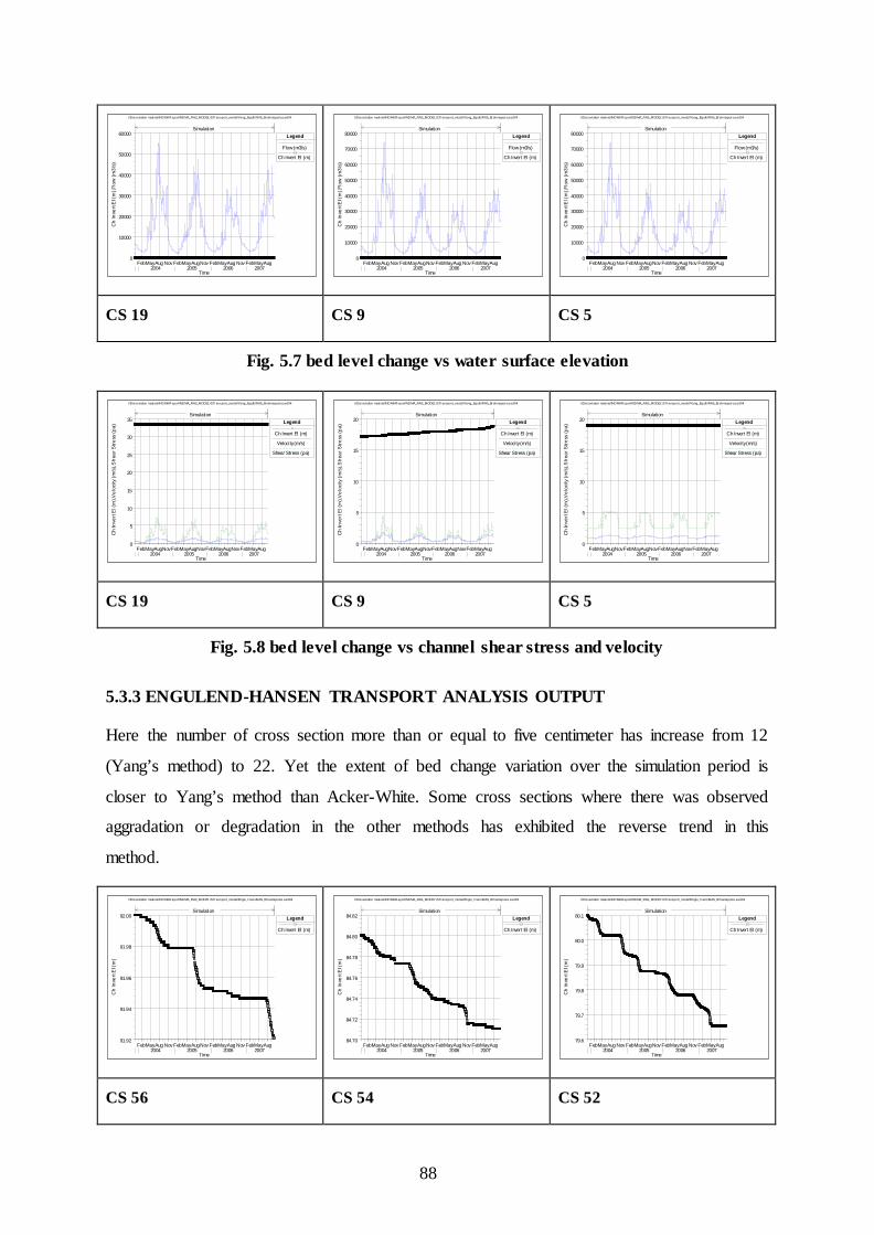
88
CS 19 CS 9 CS 5
Fig. 5.7 bed level change vs water surface elevation
CS 19 CS 9 CS 5
Fig. 5.8 bed level change vs channel shear stress and velocity
5.3.3 ENGULEND-HANSEN TRANSPORT ANALYSIS OUTPUT
Here the number of cross section more than or equal to five centimeter has increase from 12
(Yang’s method) to 22. Yet the extent of bed change variation over the simulation period is
closer to Yang’s method than Acker-White. Some cross sections where there was observed
aggradation or degradation in the other methods has exhibited the reverse trend in this
method.
CS 56 CS 54 CS 52
FebMayAug Nov FebMayAugNov FebMayAug Nov FebMayAug2004 2005 2006 2007
0
10000
20000
30000
40000
50000
60000
i:\Dissertation material\NDMA Report\NDMA_RAS_MODEL\S.Transport_model\Yang_Equlb\RAS_Brahmaputra.sed04
Time
Ch
Inve
rt E
l (m
),Flo
w (m
3/s)
Legend
Flow (m3/s)
Ch Invert El (m)
Simulation
FebMayAug Nov FebMayAugNov FebMayAug Nov FebMayAug2004 2005 2006 2007
0
10000
20000
30000
40000
50000
60000
70000
80000
i:\Dissertation material\NDMA Report\NDMA_RAS_MODEL\S.Transport_model\Yang_Equlb\RAS_Brahmaputra.sed04
Time
Ch
Inve
rt E
l (m
),Flo
w (m
3/s)
Legend
Flow (m3/s)
Ch Invert El (m)
Simulation
FebMayAugNovFebMayAugNovFebMayAugNovFebMayAug2004 2005 2006 2007
0
5
10
15
20
25
30
35
i:\Dissertation material\NDMA Report\NDMA_RAS_MODEL\S.Transport_model\Yang_Equlb\RAS_Brahmaputra.sed04
Time
Ch
Inve
rt E
l (m
),Vel
ocity
(m/s
),She
ar S
tress
(pa)
Legend
Ch Invert El (m)
Velocity (m/s)
Shear Stress (pa)
Simulation
FebMayAugNovFebMayAugNovFebMayAugNovFebMayAug2004 2005 2006 2007
0
5
10
15
20
i:\Dissertation material\NDMA Report\NDMA_RAS_MODEL\S.Transport_model\Yang_Equlb\RAS_Brahmaputra.sed04
TimeC
h In
vert
El (
m),V
eloc
ity (m
/s),S
hear
Stre
ss (p
a)
Legend
Ch Invert El (m)
Velocity (m/s)
Shear Stress (pa)
Simulation
FebMayAug Nov FebMayAugNov FebMayAug Nov FebMayAug2004 2005 2006 2007
91.92
91.94
91.96
91.98
92.00
i:\Dissertation material\NDMA Report\NDMA_RAS_MODEL\S.Transport_model\Englu_Hans\RAS_Brhamaputra.sed04
Time
Ch
Inve
rt E
l (m
)
Legend
Ch Invert El (m)
Simulation
FebMayAug Nov FebMayAugNov FebMayAug Nov FebMayAug2004 2005 2006 2007
84.70
84.72
84.74
84.76
84.78
84.80
84.82
i:\Dissertation material\NDMA Report\NDMA_RAS_MODEL\S.Transport_model\Englu_Hans\RAS_Brhamaputra.sed04
Time
Ch
Inve
rt E
l (m
)
Legend
Ch Invert El (m)
Simulation
FebMayAug Nov FebMayAugNov FebMayAug Nov FebMayAug2004 2005 2006 2007
79.6
79.7
79.8
79.9
80.0
80.1
i:\Dissertation material\NDMA Report\NDMA_RAS_MODEL\S.Transport_model\Englu_Hans\RAS_Brhamaputra.sed04
Time
Ch
Inve
rt E
l (m
)
Legend
Ch Invert El (m)
Simulation

89
CS 51 CS 50 CS 41
CS 39 CS 38 CS 37
CS 28 CS 26 CS 23
CS 22 CS 20 CS 19
FebMayAug Nov FebMayAugNov FebMayAug Nov FebMayAug2004 2005 2006 2007
77.05
77.10
77.15
77.20
77.25
i:\Dissertation material\NDMA Report\NDMA_RAS_MODEL\S.Transport_model\Englu_Hans\RAS_Brhamaputra.sed04
Time
Ch
Inve
rt E
l (m
)
Legend
Ch Invert El (m)
Simulation
FebMayAug Nov FebMayAugNov FebMayAug Nov FebMayAug2004 2005 2006 2007
68.85
68.86
68.87
68.88
68.89
68.90
68.91
68.92
i:\Dissertation material\NDMA Report\NDMA_RAS_MODEL\S.Transport_model\Englu_Hans\RAS_Brhamaputra.sed04
Time
Ch
Inve
rt E
l (m
)
Legend
Ch Invert El (m)
Simulation
FebMayAug Nov FebMayAugNov FebMayAug Nov FebMayAug2004 2005 2006 2007
62.90
62.95
63.00
63.05
63.10
63.15
63.20
i:\Dissertation material\NDMA Report\NDMA_RAS_MODEL\S.Transport_model\Englu_Hans\RAS_Brhamaputra.sed04
Time
Ch
Inve
rt E
l (m
)
Legend
Ch Invert El (m)
Simulation
FebMayAug Nov FebMayAugNov FebMayAug Nov FebMayAug2004 2005 2006 2007
60.00
60.02
60.04
60.06
60.08
60.10
i:\Dissertation material\NDMA Report\NDMA_RAS_MODEL\S.Transport_model\Englu_Hans\RAS_Brhamaputra.sed04
Time
Ch
Inve
rt E
l (m
)
Legend
Ch Invert El (m)
Simulation
FebMayAug Nov FebMayAugNov FebMayAug Nov FebMayAug2004 2005 2006 2007
50.20
50.25
50.30
50.35
50.40
50.45
50.50
i:\Dissertation material\NDMA Report\NDMA_RAS_MODEL\S.Transport_model\Englu_Hans\RAS_Brhamaputra.sed04
Time
Ch
Inve
rt E
l (m
)
Legend
Ch Invert El (m)
Simulation
FebMayAug Nov FebMayAugNov FebMayAug Nov FebMayAug2004 2005 2006 2007
53.2
53.3
53.4
53.5
53.6
i:\Dissertation material\NDMA Report\NDMA_RAS_MODEL\S.Transport_model\Englu_Hans\RAS_Brhamaputra.sed04
Time
Ch
Inve
rt E
l (m
)
Legend
Ch Invert El (m)
Simulation
FebMayAug Nov FebMayAugNov FebMayAug Nov FebMayAug2004 2005 2006 2007
41.25
41.26
41.27
41.28
41.29
41.30
41.31
i:\Dissertation material\NDMA Report\NDMA_RAS_MODEL\S.Transport_model\Englu_Hans\RAS_Brhamaputra.sed04
Time
Ch
Inve
rt E
l (m
)
Legend
Ch Invert El (m)
Simulation
FebMayAug Nov FebMayAugNov FebMayAug Nov FebMayAug2004 2005 2006 2007
37.14
37.15
37.16
37.17
37.18
37.19
37.20
37.21
i:\Dissertation material\NDMA Report\NDMA_RAS_MODEL\S.Transport_model\Englu_Hans\RAS_Brhamaputra.sed04
Time
Ch
Inve
rt E
l (m
)
Legend
Ch Invert El (m)
Simulation
FebMayAug Nov FebMayAugNov FebMayAug Nov FebMayAug2004 2005 2006 2007
36.48
36.49
36.50
36.51
36.52
36.53
36.54
i:\Dissertation material\NDMA Report\NDMA_RAS_MODEL\S.Transport_model\Englu_Hans\RAS_Brhamaputra.sed04
Time
Ch
Inve
rt E
l (m
)
Legend
Ch Invert El (m)
Simulation
FebMayAug Nov FebMayAugNov FebMayAug Nov FebMayAug2004 2005 2006 2007
35.2
35.4
35.6
35.8
36.0
36.2
i:\Dissertation material\NDMA Report\NDMA_RAS_MODEL\S.Transport_model\Englu_Hans\RAS_Brhamaputra.sed04
Time
Ch
Inve
rt E
l (m
)
Legend
Ch Invert El (m)
Simulation
FebMayAug Nov FebMayAugNov FebMayAug Nov FebMayAug2004 2005 2006 2007
29.3
29.4
29.5
29.6
29.7
29.8
i:\Dissertation material\NDMA Report\NDMA_RAS_MODEL\S.Transport_model\Englu_Hans\RAS_Brhamaputra.sed04
Time
Ch
Inve
rt E
l (m
)
Legend
Ch Invert El (m)
Simulation
FebMayAug Nov FebMayAugNov FebMayAug Nov FebMayAug2004 2005 2006 2007
33.3
33.4
33.5
33.6
33.7
i:\Dissertation material\NDMA Report\NDMA_RAS_MODEL\S.Transport_model\Englu_Hans\RAS_Brhamaputra.sed04
Time
Ch
Inve
rt E
l (m
)
Legend
Ch Invert El (m)
Simulation

90
CS 17 CS 16 CS 13
CS 9 CS 8 CS 5
CS 4
Fig.5.9. variation of bed change for individual cross section over the simulation period based on sediment transport function Engulend-Hansen
FebMayAug Nov FebMayAugNov FebMayAug Nov FebMayAug2004 2005 2006 2007
36.28
36.30
36.32
36.34
36.36
36.38
i:\Dissertation material\NDMA Report\NDMA_RAS_MODEL\S.Transport_model\Englu_Hans\RAS_Brhamaputra.sed04
Time
Ch
Inve
rt E
l (m
)
Legend
Ch Invert El (m)
Simulation
FebMayAug Nov FebMayAugNov FebMayAug Nov FebMayAug2004 2005 2006 2007
30.72
30.74
30.76
30.78
30.80
30.82
i:\Dissertation material\NDMA Report\NDMA_RAS_MODEL\S.Transport_model\Englu_Hans\RAS_Brhamaputra.sed04
Time
Ch
Inve
rt E
l (m
)
Legend
Ch Invert El (m)
Simulation
FebMayAug Nov FebMayAugNov FebMayAug Nov FebMayAug2004 2005 2006 2007
27.908
27.910
27.912
27.914
27.916
27.918
27.920
i:\Dissertation material\NDMA Report\NDMA_RAS_MODEL\S.Transport_model\Englu_Hans\RAS_Brhamaputra.sed04
Time
Ch
Inve
rt E
l (m
)
Legend
Ch Invert El (m)
Simulation
FebMayAug Nov FebMayAugNov FebMayAug Nov FebMayAug2004 2005 2006 2007
17.0
17.2
17.4
17.6
17.8
18.0
18.2
18.4
18.6
i:\Dissertation material\NDMA Report\NDMA_RAS_MODEL\S.Transport_model\Englu_Hans\RAS_Brhamaputra.sed04
Time
Ch
Inve
rt E
l (m
)
Legend
Ch Invert El (m)
Simulation
FebMayAug Nov FebMayAugNov FebMayAug Nov FebMayAug2004 2005 2006 2007
18.75
18.80
18.85
18.90
18.95
19.00
i:\Dissertation material\NDMA Report\NDMA_RAS_MODEL\S.Transport_model\Englu_Hans\RAS_Brhamaputra.sed04
Time
Ch
Inve
rt E
l (m
)
Legend
Ch Invert El (m)
Simulation
FebMayAug Nov FebMayAugNov FebMayAug Nov FebMayAug2004 2005 2006 2007
18.55
18.60
18.65
18.70
18.75
18.80
18.85
18.90
i:\Dissertation material\NDMA Report\NDMA_RAS_MODEL\S.Transport_model\Englu_Hans\RAS_Brhamaputra.sed04
Time
Ch
Inve
rt E
l (m
)
Legend
Ch Invert El (m)
Simulation
FebMayAug Nov FebMayAugNov FebMayAug Nov FebMayAug2004 2005 2006 2007
13.07
13.08
13.09
13.10
13.11
13.12
13.13
13.14
i:\Dissertation material\NDMA Report\NDMA_RAS_MODEL\S.Transport_model\Englu_Hans\RAS_Brhamaputra.sed04
Time
Ch
Inve
rt E
l (m
)
Legend
Ch Invert El (m)
Simulation

91
Mass capacity vs flow CS8 Mass capacity vs flow CS9
Fig. 5.10 Mass capacity vs flow
In the above figure it can be seen that, at cross sections where there is low mass capacity
(transport capacity in total mass at computational step) (CS9) there is a tendency for
deposition. Where there is high mass capacity (CS8) erosion is occurring. Therefore this
clearly shows the correlation between sediment transport capacity and bed level change.
4 9 22
Fig. 5.11 bed level change vs water surface elevation
9 8 4
Fig. 5.12 bed level change vs channel shear stress and velocity
Feb May Aug Nov Feb May Aug Nov Feb May Aug Nov Feb May Aug2004 2005 2006 2007
0
500000
1000000
1500000
2000000
2500000
3000000
3500000
i:\Dissertation mater ial\NDMA Report\NDMA_RAS_MODEL\S.Transport_model\Englu_Hans\RAS_Brhamaputra.sed04
Time
Ch I
nver
t El
(m
),Fl
ow (m
3/s)
,Mas
s Ca
paci
ty:
All (
tons
/day
)
Legend
Flow (m3/s)
Ch Invert El (m)
Mass Capacity: All (tons/day)
Simulation
Feb May Aug Nov Feb May Aug Nov Feb May Aug Nov Feb May Aug2004 2005 2006 2007
0
2000000
4000000
6000000
8000000
10000000
i:\Dissertation material\NDMA Report\NDMA_RAS_MODEL\S.Transport_model\Englu_Hans\RAS_Brhamaputra.sed04
Time
Ch I
nver
t El
(m
),Fl
ow (m
3/s)
,Mas
s Ca
paci
ty:
All (
tons
/day
)
Legend
Flow (m3/s)
Ch Invert El (m)
Mass Capacity: All (tons/day)
Simulation
FebMayAug Nov FebMayAugNov FebMayAug Nov FebMayAug2004 2005 2006 2007
0
10000
20000
30000
40000
50000
60000
70000
80000
i:\Dissertation material\NDMA Report\NDMA_RAS_MODEL\S.Transport_model\Englu_Hans\RAS_Brhamaputra.sed04
Time
Ch
Inve
rt E
l (m
),Flo
w (m
3/s)
Legend
Flow (m3/s)
Ch Invert El (m)
Simulation
FebMayAug Nov FebMayAugNov FebMayAug Nov FebMayAug2004 2005 2006 2007
0
10000
20000
30000
40000
50000
60000
i:\Dissertation material\NDMA Report\NDMA_RAS_MODEL\S.Transport_model\Englu_Hans\RAS_Brhamaputra.sed04
Time
Ch
Inve
rt E
l (m
),Flo
w (m
3/s)
Legend
Flow (m3/s)
Ch Invert El (m)
Simulation
FebMayAugNovFebMayAugNovFebMayAugNovFebMayAug2004 2005 2006 2007
0
5
10
15
20
i:\Dissertation material\NDMA Report\NDMA_RAS_MODEL\S.Transport_model\Englu_Hans\RAS_Brhamaputra.sed04
Time
Ch
Inve
rt E
l (m
),Vel
ocity
(m/s
),She
ar S
tress
(pa)
Legend
Ch Invert El (m)
Velocity (m/s)
Shear Stress (pa)
Simulation
FebMayAugNovFebMayAugNovFebMayAugNovFebMayAug2004 2005 2006 2007
0
5
10
15
20
i:\Dissertation material\NDMA Report\NDMA_RAS_MODEL\S.Transport_model\Englu_Hans\RAS_Brhamaputra.sed04
Time
Ch
Inve
rt E
l (m
),Vel
ocity
(m/s
),She
ar S
tress
(pa)
Legend
Ch Invert El (m)
Velocity (m/s)
Shear Stress (pa)
Simulation
FebMayAugNovFebMayAugNovFebMayAugNovFebMayAug2004 2005 2006 2007
0
2
4
6
8
10
12
14
i:\Dissertation material\NDMA Report\NDMA_RAS_MODEL\S.Transport_model\Englu_Hans\RAS_Brhamaputra.sed04
Time
Ch
Inve
rt E
l (m
),Vel
ocity
(m/s
),She
ar S
tress
(pa)
Legend
Ch Invert El (m)
Velocity (m/s)
Shear Stress (pa)
Simulation

92
The above figure (5.11 and 5.12) also shows the same trend that is explained in the above
topics.
Figure 5.13 shows that the average bed variation comparing the three methods used in this
study. All of the methods have their own bed level prediction, Acker-White methods gives
very high bed level variation compared to the other two methods.
In terms of the magnitude of bed level change, Yang and Engulend-Hansen functions are in
agreement.
From this figure, it can be concluded that generally the pattern of aggradation and
degradation is distributed throughout the 620km of the reach. The localities that aggradation
is predominant are in the vicinity of Cross Section 62,58,50,47,43,28,22,18,and 9.
It should be bear in mind that in some cross sections one function is predicting and the other
degradation or relatively stable bed level condition. And the use of any particular method is
very much dependent on the applicability of the function for the given river. To suggest any
one of the above method for sediment transport predication, it requires the use of intensive
data for model verification; which in this case could not be available for the simulation
period.

93
Fig. 5.13 Average bed level variation for the three transport functions over the
simulation period The sediment transport functions are, to varying degrees, the results of theoretical and
empirical science. Even the most theoretically detailed was fit to data using empirical
coefficients. These coefficients represent the central tendencies of the data considered but
will not likely reflect the transport of the specific site precisely, even if an appropriate
transport function is selected. Hence at the end of the day field verification is a must.
Average river bed level change over the simulation period
Cross Section Number
5101520253035404550556065
Bed
Lev
el C
hang
e (c
m)
-300
-200
-100
0
100
200
300
400
Cross Section number vs bed level change(A-W)Cross Section number vs bed level change(Yang) Cross Section number vs bed level change(E-H)

94
CHAPTER – 6
PILOT STUDY SCHEMES FOR EROSION
CONTROL ON THE BRAHMAPUTRA
RIVER FOR MORIGAON SITE;
AND NEAR GUWAHATI AIRPORT OF
BRAHMAPUTRA RIVER

95
CHAPTER-6
PILOT STUDY SCHEMES FOR EROSION CONTROL ON THE BRAHMAPUTRA RIVER FOR MORIGAON SITE;
AND NEAR GUWAHATI AIRPORT OF BRAHMAPUTRA RIVER
6.1 PILOT STUDY SCHEME FOR EROSION CONTROL ON THE BRAHMAPUTRA RIVER FOR MORIGAON SITE The Water Resources Department of Assam communicated to IIT Roorkee the partial cross-sectional data survey data of the left bank side of the Brahmaputra in the study area in Morigaon site at the vicinity of 61th KM of the left Dyke, along with stage data. In addition the latest satellite data (2007) of the pilot study area has been procured by IIT Roorkee. Making use of the above data, a scheme for pilot study has been formulated. A schematic diagram of the arrangement of erosion control structures is depicted in Fig. 62. The underlying concept behind the pilot scheme is centred on breaking-up the incoming erosion vortex current by using framed structures like RCC Kellner Jetty, and reversal of the erosion secondary flow towards the away from the bank through use of emerging technique of submerged vane to induce sedimentation. Furthermore, to afford protection to the critical toe of the bank line. Polymer Rope Gabions filled with Geo-Synthetic bags has been proposed along with and additional protection by RCC Kellner Jetty. The rationale of using the above new techniques for the Brahmaputra is based on the fact that the RCC Kellner Jetty field is expected to trap sediment and debris and thereby effectively weaken the eroding flow vortices. The RCC Kellner Jetty field technique in due course will create sediment deposits as the heavy sediment laden flow will be adequately slowed down the part with bed material load. The detailed estimate of the pilot study scheme is given in the following pages along with the layout of the river training structures their structural details. Total estimated cost of the scheme stands of Rs. 1.644 crores for the one Kilometer bank length of the pilot study area.

96
6.1.1 ABSTRACT OF TOTAL APPROXIMATE COST AT MORIGAON SITE
1. Cost of Polymer Rope Gabion Submerged Vane Total No. of submerged vane = 3 no. x 7 array = 21 no. Cost of one submerged vane = 93650 Total Cost of Submerged vane = 21 x 93650 = Rs.1966650
Cost of Polymer Rope Gabion along the bank Total length = 500m Cost of Polymer Rope Gabion 9365/m Cost Polymer Rope Gabion along the bank = 500 x 9365
= Rs.4682500 2. No. RCC Kellner Jetty along the bank = (500/2.5) x 3 rows = 600 no. No. of RCC Kellner Jetty in retards along the bank = (10/2.5)x3 rows x 7 lines = 84 no.
No. of RCC Kellner Jetty in diversion line = (510/2.5)x5 line = 1020 no. No. of RCC Kellner Jetty in retard line (50/2.5)x5 line + (50/2.5)x 3line + (45/2.5)x 3line x 2 no. +(40/2.5)x 3line x 2 no.+ (35/2.5)x 3line + (30/2.5)x 3line + (20/2.5)x 3line +(20/2.5)x 5line =506 Total No. of RCC Kellner Jetty in retard and diversion
= 600 + 84 + 1020 + 506= 2210 no. Cost of one RCC Kellner Jetty Rs. 4040 Total cost of RCC Kellner Jetty = 2210 x 4040 = Rs.8928400
3. Cost of 26mm PP Rope Total length = 510 x 5rows + 50 x 5 + 50 x 3 + 45 x 3 + 45 x 3+ 40 x 5 + 35 x 3 + 30 x 3+ 20 x 3 + 20 x 5 + 500 x 3 + 7 x 10 x 3 = 5485m Add 5% extra for tie, anchorage and wastage = 1.05 x 5485 = 5760m Cost of pp rope = Rs.150/m Total cost of pp rope = 5760 x 150 = Rs.864000
Total cost of Submerged Vane + RCC Kellner Jetty + PP Rope = Rs.1966650 + Rs.4682500 + Rs.8928400+ Rs.864000
= Rs.16441550/- = Rs.1.644 Crore

97
6.1.2 APPROXIMATE ESTIMATE FOR R.C.C. KELLNER JETTY
Size of RCC Kellner Jetty = 3.0 m Section – 15 cm x 15 cm 6.1.2.1 Quantity of Concrete for one No. RCC Kellner Jetty
(a) Volume of Concrete = 0.15 m x 0.15 m x 3.0 m x 3 nos. = 0.2025 m3 (b) Providing haunch at the junction of RCC Kellner jetty of size = 0.15 m x 0.15 m No. of haunch = 12 Nos. Quantity of Concrete for haunch
= 1215.015.015.021
××××
= 0.02025 m3 Total volume of concrete (a+b) =(0.2025 + 0.02025) m3 = 0.22275 m3 = 7.867 cft = 0.223m3 6.1.2.2 Quantity of steel for one RCC Kellner Jetty (a) For longitudinal bars No of bars = 4 nos Dia of bars = 8 mm Volume of longitudinal bas
= 4 nos x 4π x 82 x 3000 = 602880 mm3
= 6.0288 x 10⁻⁴ m3 Density of steel = 7.85 t/m3 Wt. of longitudinal bars = 7.85 x 6.0288 x 10-4 x 3 nos. = 0.01420 t = 14.20 kg (b) For stirrups Length of one strimps rod = (120 mm x 4 + 50 mm) = 530 mm = 0.53 m
No of stirrup =
+1
1503000 =21 nos
Total length of stirrup rod = 21 x 0.53 x 3
= 33.39 m
Volume of stirrup rod = π/4 x 62 x 33.39 x 103
=943601.4 mm3
= 9.4360x 10⁻⁴ m3
Wt of stirrup rod = 7.85 x 9.4360 x 10-4 t =7.4072 x 10⁻³ t =7.40 kg

98
Total wt (a+b) = (14.20 +7.40 ) = 21.60 kg Add 5% extra for wastage = 21.60 x 1.05 = 22.68 kg = 0.02268MT 6.1.2.3 Quantity of G. I.wire of dia 4 mm Providing hole at the spacing of 30 cm c/c No of hole for one member
( )
+
− 130
60300 =9 nos
Provide 10 nos hole, 5 nos of each side Then spacing of hole = 25 cm c/c
Length of wire
=15525255050
75751001001251252222
222222
×+++++
+++++
= 176.77 + 141.42 + 106.06 + 70.71 + 35.355 + 75 = 605.315 CM
Total no of force = 12 nos Total length = 12 x 605.315 = 7263.75 cm = 72.64 m Add 5% extra for wastage = 3.64 --------------- = 76.28 m Using 4 mm G. I wire Volume of total wire = π/4 x 42 x 76.28 x 103 =958076.8 mm3 =9.58x 10⁻⁴ m3 Wt of wire = 7.85 x 9.58 x 10-4 = 7.52 x 10⁻³ t = 7.52 kg 6.1.2.4 Quantity of Shuttering Total length of shuttering = (0.15+0.15+0.15)x 3 + 0.15 x 0.15 x 2
= 1.395 m2 for 1 no. For 3 no. = 1.395 x 3 = 4.185 m2
1.5
1.5m
15cm
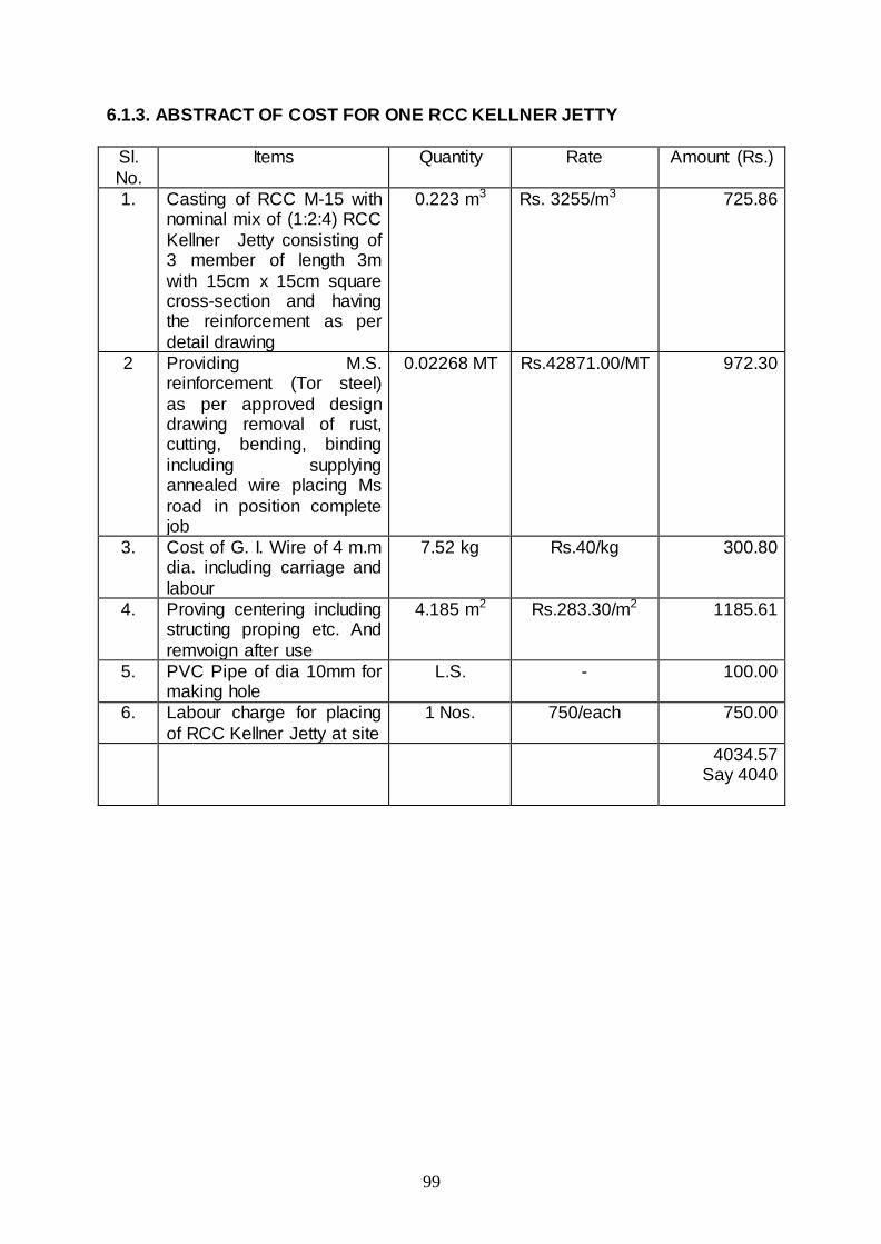
99
6.1.3. ABSTRACT OF COST FOR ONE RCC KELLNER JETTY
Sl. No.
Items Quantity Rate
Amount (Rs.)
1. Casting of RCC M-15 with nominal mix of (1:2:4) RCC Kellner Jetty consisting of 3 member of length 3m with 15cm x 15cm square cross-section and having the reinforcement as per detail drawing
0.223 m3 Rs. 3255/m3 725.86
2 Providing M.S. reinforcement (Tor steel) as per approved design drawing removal of rust, cutting, bending, binding including supplying annealed wire placing Ms road in position complete job
0.02268 MT Rs.42871.00/MT 972.30
3. Cost of G. I. Wire of 4 m.m dia. including carriage and labour
7.52 kg Rs.40/kg 300.80
4. Proving centering including structing proping etc. And remvoign after use
4.185 m2 Rs.283.30/m2 1185.61
5. PVC Pipe of dia 10mm for making hole
L.S. - 100.00
6. Labour charge for placing of RCC Kellner Jetty at site
1 Nos. 750/each 750.00
4034.57 Say 4040
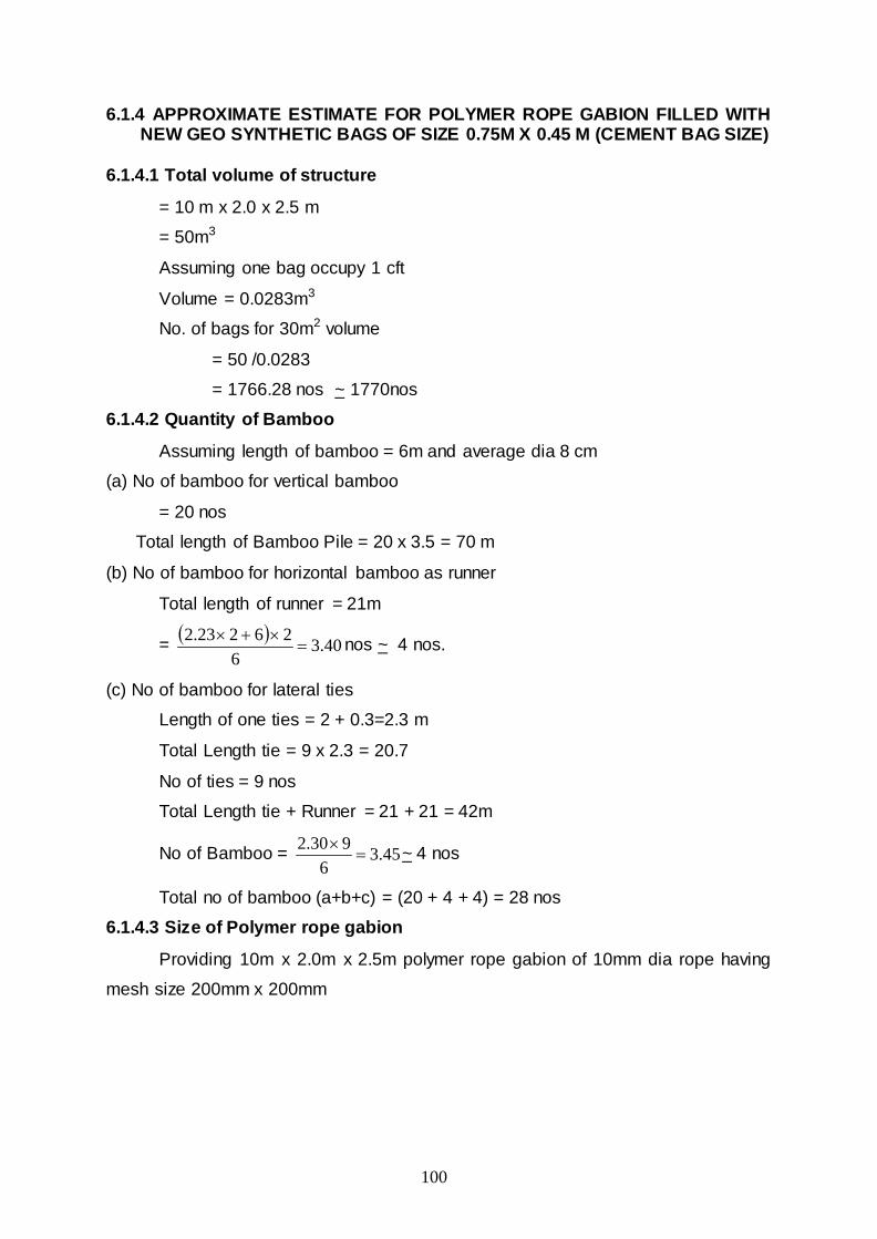
100
6.1.4 APPROXIMATE ESTIMATE FOR POLYMER ROPE GABION FILLED WITH NEW GEO SYNTHETIC BAGS OF SIZE 0.75M X 0.45 M (CEMENT BAG SIZE) 6.1.4.1 Total volume of structure
= 10 m x 2.0 x 2.5 m
= 50m3
Assuming one bag occupy 1 cft
Volume = 0.0283m3
No. of bags for 30m2 volume
= 50 /0.0283
= 1766.28 nos ~ 1770nos
6.1.4.2 Quantity of Bamboo
Assuming length of bamboo = 6m and average dia 8 cm
(a) No of bamboo for vertical bamboo
= 20 nos
Total length of Bamboo Pile = 20 x 3.5 = 70 m
(b) No of bamboo for horizontal bamboo as runner
Total length of runner = 21m
= ( ) 40.36
26223.2=
×+× nos ~ 4 nos.
(c) No of bamboo for lateral ties
Length of one ties = 2 + 0.3=2.3 m
Total Length tie = 9 x 2.3 = 20.7
No of ties = 9 nos
Total Length tie + Runner = 21 + 21 = 42m
No of Bamboo = 45.36
930.2=
× ~ 4 nos
Total no of bamboo (a+b+c) = (20 + 4 + 4) = 28 nos
6.1.4.3 Size of Polymer rope gabion
Providing 10m x 2.0m x 2.5m polymer rope gabion of 10mm dia rope having
mesh size 200mm x 200mm

101
6.1.5 ABSTRACT OF COST OF ONE POLYMER ROPE GABION FILLED WITH NEW GEO SYNTHETIC BAG GABION
Sl. No.
Items Quantity Rate
Amount (Rs.)
1. Supply of new Geo synthetic bags of size 0.75 m x 0.45 m
1770 nos Rs.15 each 26,550
2 Supply of Bamboo of average dia of 8 cm
28 nos Rs.80 each 2240
3. Labour charge of piling of Bamboo
70 m Rs.8.9/m 623
4. Labour charges for fitting and fixing of horizontal Bamboo as runner and lateral ties
42 m Rs.1.90/m 79.80
5. Labur charge for filling empty new synthetic bag with local sand, stiching the bags and placing polymer rope gabion in water with a carrage of filled bag by boat including loading unloading and stacking with lead of ½ km all complete job as per approve design specification and direction of E/I
1770 Rs. 8.0/each 14160
6 Supply of polymer rope gabion of size 10m x 2.0m x 1.5 m of 10mm dia rope and having mesh size of 200mm x 200mm
1 nos. 50000 50000
93,652.80 Say 93,650 for 10 m length
9365 m for 1 m length

102
6m 2m 2m
2m 450
1m Bamboo
Fig. 6.1 Plan of Polymer Rope Gabion
X X
New Geo-synthetic bags filling
River bed 2.5m
3.5m Bamboo
10m
Section X – X
Fig. 6.2 Typical Drawing of Polymer Rope Gabion Submerged Vane
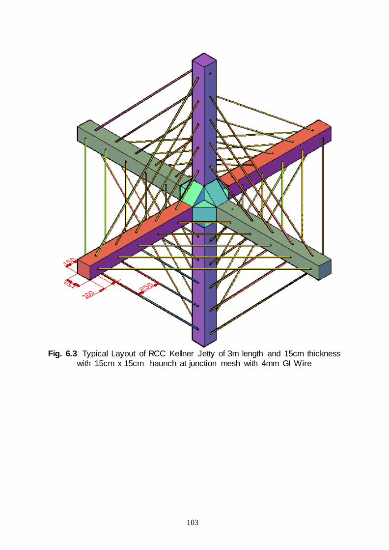
103
Fig. 6.3 Typical Layout of RCC Kellner Jetty of 3m length and 15cm thickness
with 15cm x 15cm haunch at junction mesh with 4mm GI Wire
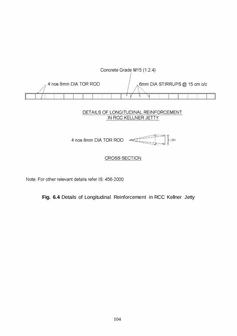
104
Fig. 6.4 Details of Longitudinal Reinforcement in RCC Kellner Jetty

105
Fig. 6.5 Detail Layout of Erosion Control Structures at Morigaon Site in the vicinity of 61st Km of the left Dyke

106
6.2 DESIGN PHILOSOPHY TO EVOLVE COST EFFECTIVE RIVER TRAINING MEASURES IN SITE OF THE BRAHMAPUTRA NEAR GAUWAHATI AIRPORT
6.2.1 PREAMBLE
For the purpose of experimental field study a drifting subsidiary channel of the
Brahmaputra river hugging the Gauwahati airport( shown in the enclosed satellite
imagery) has been adopted to test the river response as well as to effect required
fine tuning to achieve efficacious results.
6.2.2 OBJECTIVES
The basic goal of the proposed field experimental study with very limited intervention
is broadly spelt out below
1. To simulate the Brahmaputra river reach based on one dimensional numerical
model developed by United States Hydrologic Engineering Center (USHEC)
called HEC- RAS 4.1. The reach length span from Dubri, (Cross section 2)
and Kobo, (Cross-section 65). Simulation of flow includes the analysis of
stream bed aggradation and degradation behavior of the critical reach of the
Brahmaputra River. Based on this flow simulation findings and experimental
study, training measure are given below
2. to observe the effect of Jack Jetty Screen for effecting limited siltation and
partial channel closure.
3. to test and evaluate the combined action of the package of measures
comprising bamboo submerged vanes, RCC Jack Jetty field and bamboo
board fencing on bank protection / near bank modification of fluvial parameter
and near bank sedimentation. Obviously any limited achievement of near
bank sedimentation is expected to facilitate & contribute towards land
reclamation with the help of subsequent consolidation of sediment deposits.
6.2.3 HYDRAULICS OF PROPOSED TRAINING MEASURES
1. The submerged vane systems made of Jati bamboo is expected to generate
desired secondary circulation in the stream flow to deflect the heavy sediment

107
laden bottom flow filaments towards the stream bank side resulting in
sedimentation. The upper flow layers deficient in requisite sediment load are
forced by the vane generated swirling vortices to move towards the channel
centerline, thereby causing deepening of the streambed away from the bank.
This radical modification of stream flow characteristics due to presence of
submerged vanes acts as a catalyst in desired reshaping of channel
topography. It may be highlighted here that the above radical transformation
involving reversal of flow vortex direction cannot possibly be achieved through
the conventional spur/ groyne system or any other flow retarding devices such
as porcupine screens or permeable spur.
2. The deflected heavy sediment laden flow layers coming from the submerged
vanes will be intercepted by the jack jetty field comprising the diversion lines &
the retards to further assist in the dissipation of residual flow energy.
Obviously the slowed down sediment carrying flow will be induced to deposit
its sediment load within the compartments of the jack jetty field.
4. To further help in the desired aim of sedimentation within the jetty field,
improvised board fencing method will be put in plane behind the jack jetty
system & these improvised board fencing is proposed to be made of Jati
bamboo which is locally available in abundance in Assam.
The above new river training structures presented through the attached four
numbers of typical drawings which may be further modified appropriately at the time
of implementation. The layout of the above river training systems can also be seen
from the attached satellite imageries which also depict the channel changes
occurring in the study area covering a period from 2005 – 2011.

108
Fig. 6.6 Detail Layout Of River Erosion Control Structures At Proposed Site Of The Brahmaputra Near Gauwahati Airport

109
α = 150
Flow
Diversion Line of RCC Jack Jetty
Retard of RCC Jack Jetty
50Μ
20Μ
44Μ
Fig. 6.7 Typical Drawings Of Submerged Vanes Board Fencing And RCC Jack Jetty For Brahmaputra River Near Guwahati Bridge
50Μ
7.7Μ
50Μ
Two rows of Board Fencing
5 Rows of Rcc Jack Jetty screen

110
15cm
0.03m
0.03m Plan
River bed 2.2
3m
A
Section A-A
2 Nos. horizontal bamboo both face
A
Bank Line 7.7m
150
6.6m
Fig. 6.8 Typical Layout of Bamboo Submerged Vane
FLOW

111
Fig. 6.9 Typical Layout of RCC Kellner Jetty of 3m length and 15cm
thickness with 4mm GI Wire
DETAILS OF LONGITUDINAL REINFORCEMENT IN RCC JACK JETTY

112
Fig. 6.10 Typical Layout of Board Fencing
Board made of 3cm dia 5 Jati Bamboo
Deep River Channel Bed
Sectional Elevation
Anchor Row Front Row
Tie
3m 1.5 m
1.5m
3m
Bamboo Tie 5m
Boards comprising of each 5 Jati Bamboos
Plan

113
6.2.4 COST ESTIMATE OF PROPOSED SITE OF THE BRAHMAPUTRA NEAR GAUWAHATI AIRPORT 6.2.4.1 Approximate Estimate of Jack Jetty
Width of river at left channel = 350 m Size of one jack jetty = 3 m
No of jetties required in one row to cover the whole width of the river = 117 No of jetties required in 5 row to cover the whole width of the river = 585
No of jetties required in 4 rows in the second tier = 468 Total no of jetties required to cover the whole width of the river = 1053
Length of the river that is being protected by jetty field = 1000 m
No of jetties required in one row to cover the1000m length of the river = 333 No of jetties required in 5 row to cover the1000m length of the river = 1665
No of jetties required in one row on the second tier to cover the1000m length of the river = 333
No of jetties required in 4 row on the second tier to cover the1000m length of the river = 1332
Length of retard = 50 m
No of jetties required in one row of retard = 17 No of jetties required in 5 rows of retards = 85
No of jetties required in one row of retard on the second tier = 17 No of jetties required in 4 rows of retards on the second tier = 68
No of jetties required in one retard = 153 Spacing of retards = 33 m
No of retards required to cover 1000m width of the river = 31 Totals no of jetties required for the retards = 4743
Total number of jack jetties required for jetty screen and jetty field = 8793
Length of rope required for jetty screens in front = 3150 m 10%= 315 m
Length of rope required to tie each jack unit in diversion line jetty fields = 9000 m 10%= 900 m
Length of rope required to tie each jack unit in retard jetty fields = 13950 m 10%= 1395 m
Total length of rope to tie jack jetties = 28710 m 10% for dead man acnchor = 2871 m
Total length of rope = 31581 m
Cost of one prestressed member = 950 RS Cost of three prestressed members = 2850 RS
Apprx. Cost of one jack jetty is = 2850 RS Cost of jack jetties is = 25060050 RS
Cost of rope per metre = 140 RS
Total Cost of rope = 4421340 RS
Total cost of jack jetties = 29481390 RS
6.2.4.2 Approximate Cost Estimate of Submerged Vane
Width of river covered by vanes = 35 m
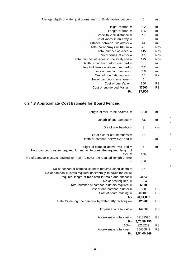
114
Average depth of water just downstream of Brahmapitra bridge = 5 m
Height of vane = 2.2 m
Length of vane = 6.6 m Vane to vane distance = 7.7 m
No of vanes in an array = 5 m Distance between two arrays = 44 m
Total no of arrays in 1000m = 23 Nos Total number of vanes = 115 Nos
No of vanes at entry = 10 Nos Total number of vanes in the study site = 125 Nos
Depth of bamboo below river bed = 3 m Height of bamboo above river bed = 2.2 m
size of one Jati bamboo = 7.6 m Cost of one Jati bamboo = 60 Rs
No of bamboo in one vane = 5 Cost of one Vane = 300 RS
Cost of submerged Vanes = 37500 RS Rs 37,500
6.2.4.3 Approximate Cost Estimate for Board Fencing
Length of river to be covered = 1000 m
Length of one bamboo = 7.6 m
Dia of one bamboo= 3 cm
Dia of cluster of 5 bamboos = 15
Depth of bamboo below river bed = 3 m
Height of bamboo above river bed = 5 m
Noof bamboo clusters required for anchor to cover the required length of river = 466
No of bamboo clusters required for main to cover the required length of river = 466
No of horizontal bamboo clusters required along depth = 17
No of bamboo clusters required horizontally to cover the entire required length of river both for main and anchor = 4474
No of ties required = 1564 Total number of bamboo clusters required = 6970 Cost of one bamboo cluster = 300 RS
Cost of board fencing = 2091000 RS Rs 20,91,000
Rate for driving the bamboo by water jetty technique= 425700 RS
Expense for site visit = 147000 RS
Approximate total cost = 32182590 RS Rs 2,70,59,790
10%= 3218259 RS Approximate total cost = 35400849 RS
Rs 3,54,00,849
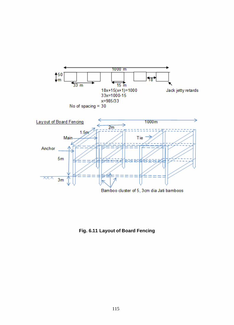
115
Fig. 6.11 Layout of Board Fencing

116
CHAPTER – 7
SUMMARY

117
Chapter – 7
SUMMARY
Using HEC-RAS 4.1 latest version of ‘River Analysis System’ whole reach of Brahmaputra
River from Dhubri( Cross section 2) to Kobo( Cross section 65)extending a length of 622km
is modeled and flow in simulation is done. The model is calibrated for seasonal variation of
roughness coefficient. Based on the output of this one dimensional numerical model,
analysis of stream bed aggradation and degradation behavior of critical reach of the
Brahmaputra River is performed. Model output is used as supplementary information for
river training work for erosion studies. This model can also be used for flood propagation
study with unsteady flow analysis option and for specific bed configuration.
River training works is proposed for two pilot areas on Brahmaputra River. Those pilot areas
are, near Airport of Guwahati Bridge and Morigaon site. The proposed river training work
includes observing the effect of Jack Jetty Screen for effecting limited siltation and partial
channel closure and to test and evaluate the combined action of the package of measures
comprising bamboo submerged vanes, RCC Jack Jetty field and bamboo board fencing on the
bank protection/ near bank modification of fluvial parameter and near bank sedimentation.
Obviously any limited achievement of near bank sedimentation is expected to facilitate and
contribute towards land reclamation with the help of subsequent consolidation of sediment
deposits.
The submerged vane systems made of Jati bamboo is expected to generate desired secondary
circulation in the stream flow to deflect the heavy sediment laden bottom flow filaments
towards the stream bank side resulting in sedimentation. The deflected heavy sediment laden
flow layers coming from the submerged vanes will be intercepted by the jack jetty field
comprising the diversion lines and the retards to further assist in the dissipation of residual
flow energy.
To further help in the desired aim of sedimentation within the jetty field, improvised board
fencing method will be put in plane behind the jack jetty system and these improvised board
fencing is proposed to be made of Jati bamboo which is locally available in abundance in
Assam.

118
REFERENCES

119
REFERENCES
120
121
122

FINAL
RECOMMENDATIONS

1. Data analysis and computer simulation studies conducted in the present study have
succinctly brought out that the prime causative factor of stream bank erosion vis-à-vis
channel instability processes of the Brahmaputra can be attributed to inherent “sediment
overloading” of the river fluvial system. In the light of aforesaid observation, it is
recommended to effectively control sediment ingress into the Brahmaputra river system
through comprehensive watershed management as well as development programme.
2. In view of the fact that extensive extent of stream bank-line is under grip of unabated
erosion process, it is recommended to deploy cost-effective erosion control measures,
namely single or multiple tier Jack Jetty system along with submerged vanes as per site
condition feasibility. The required layout of Jack Jetty field may be appropriately devised
by carefully considering the suitable Jack Jetty Density Index (JJDI) and Jack Jetty
Submergence Index (JJSI)at the time of implementation of field pilot schemes after duly
accounting for the prevailing river configuration.
3. The braiding phenomenon of the Brahmaputra has displayed a sharply increasing trend in
the recent decades giving rise to highly disturbing incidence of channel instability in the
wake of stream bank erosion process. It is recommended to urgently undertake measures
to control the rise of braiding intensity through effective closures of subsidiary channels
with the help of Jack Jetty Screen and submerged vanes protected by Reno Mattress.
4. To start with, field pilot studies may be undertaken at two sites – one near Morigaon
(Bhuragaon) and the other near Guwahati Airport for which preliminary designs have
been evolved. The preliminary design may be fine tuned at the time of implementation as
mentioned at para 2 above, as well as after critically reviewing their performance in the
post flood season.
5. The R&D endeavour of the present study to evolve ANN models for simulating watershed
hydrologic response for runoff and sediment is found to be quite encouraging. It is
recommended to use and periodically improve these models with availability of more
field data in future.
6. The mathematical model developed with the help of HEC-RAS 4.1 may be used on trial
basis to start with for flood forecasting and preliminary channel improvement purposes.
However, an exclusive comprehensive study is recommended to develop a fully moveable

bed and bank erosion model which duly accounts for complex flow phenomena such as
secondary flow, vortex formation, turbulence & mass dispersion, fluvial transients of
water and sediment, and morphodynamic fluxes as per state-of-the-art.
7. On account of the prevalent inadequacy of reliable and consistent field data, modelling in
relation to erosion, sediment inflow and flood forecasting may have certain elements of
inconsistencies and discrepancies, resulting in fallacious prediction of future scenario. It
urgently warrants strengthening and upgrading of existing data acquisition and processing
infrastructure at the ground level of the concerned agencies. Following equipment/data
should urgently be procured for the existing or proposed data acquisition establishments
of the field agencies / organizations.
(i) Data acquisition instruments –
a. Acoustic Doppler Current Profilers (ADCPs)
b. Ultrasonic Flow Meter / Fluorometer
c. Latest Sediment Sampler
d. Portable Suspended Sediment Analyzer
e. Laser Particle Size Analyzer
f. Total Station and GPS
g. Automatic Gauge Level Recorder
(ii) Upgrading of Surveyed Hydrographic Data
a. Survey of cross sectional data interval should be of the order of 500m at least
between two given sections for good quality mathematical model development and
analysis.
b. The cross-sections survey should be updated regularly (at say every five years
interval) depending on observed hydrological events
c. Flow measurements for high flood events
(iii) Optical and Microwave Satellite Data Procurement
a. For monitoring and change detection of spatial and temporal features in the river
and in the basin including flood plain.
(iv) Improving the spatial density of hydro-meteorological data acquisition network

a. Hydrological data (Stage, Discharge & Sediment) observation stations may be
increased by including / restoring sites near Tezpur (Koliabhomora Bridge) ,
Bessamara (Majuli), Bogibeel (New Bridge near Dibrugarh), in addition to the
existing sites at Pandu & Jogighopa
b. The spatial density of Meteorological stations requires to be significantly
upgraded along with installation of the latest data acquisition and data logging
systems.
(v) Development of Management Information System (MIS) for main stem
Brahmaputra along with the flood plain / catchments, tributaries
8. Capacity building of the technical manpower associated at various levels of river
management is recommended through periodic professional training on latest advances in
the technology
9. Creation of a comprehensive data base comprising all pertinent data & information using
latest data management system.
10. Establishment of an autonomous well-equipped R&D Centre to be manned by highly
competent manpower for conducting applied research at state-of-the-art level.
*************
Copyright © 2022 FDOKUMEN